/
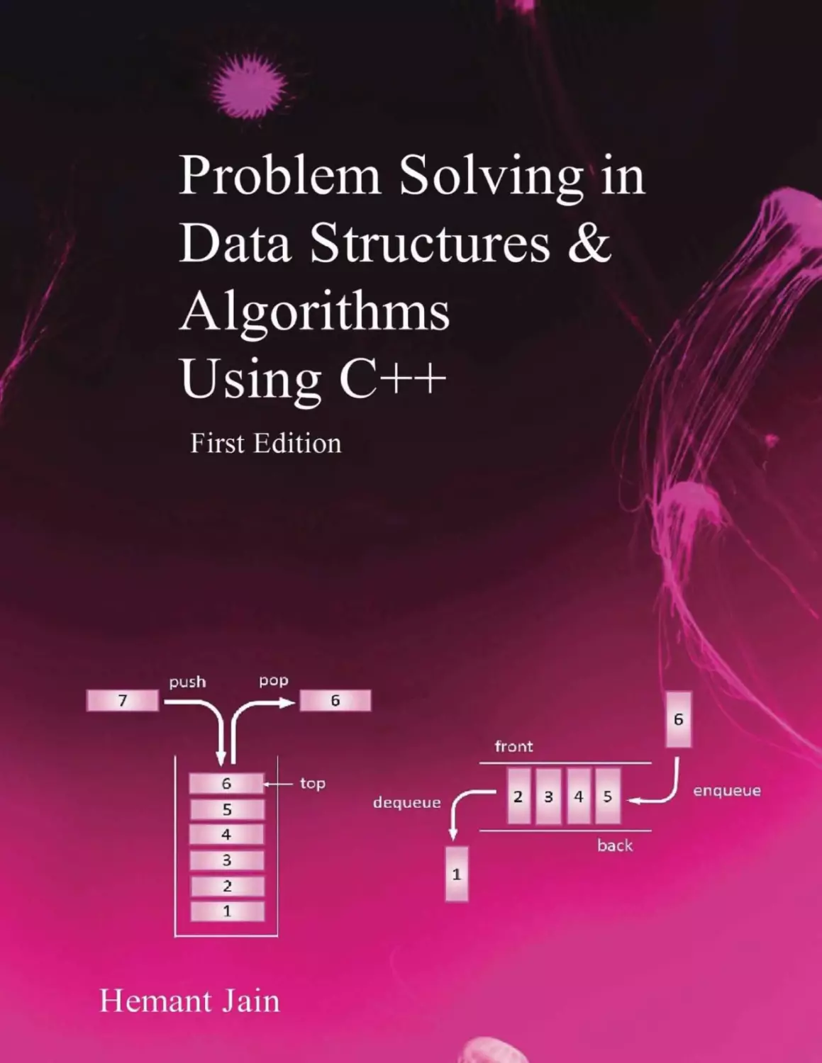


Автор: Jain H.
Теги: algorithms information technology c++ programming language data structures
Год: 2016




Текст
                    Problem Solving in
Data Structures &
Algorithms Using
C++
First Edition

By Hemant Jain

Problems Solving in Data Structures & Algorithms Using C++
HEMANT JAIN
Copyright © 2016 by HEMANT JAIN. All Right Reserved.
No part of this publication may be reproduced, distributed, or transmitted in any
form or by any means, including photocopying, recording, or other electronic or
mechanical methods, or by any information storage and retrieval system without
the prior written permission of the author, except in the case of very brief
quotations embodied in critical reviews and certain other non-commercial uses
permitted by copyright law.

ACKNOWLEDGEMENT
The author is very grateful to GOD ALMIGHTY for his grace and blessing.
Deepest gratitude for the help and support of my brother Dr. Sumant Jain. This
book would not have been possible without the support and encouragement he
provided.
I would like to express profound gratitude to my guide/ my friend Naveen
Kaushik for his invaluable encouragement, supervision and useful suggestion
throughout this book writing work. His support and continuous guidance enable
me to complete my work successfully.
Last but not least, I am thankful to Anil Berry and Others who helped me
directly or indirectly in completing this book.
Hemant Jain

TABLE OF CONTENTS
TABLE OF CONTENTS
TABLE OF CONTENTS
CHAPTER 0: HOW TO USE THIS BOOK
WHAT THIS BOOK IS ABOUT
PREPARATION PLANS
SUMMARY
CHAPTER 1: INTRODUCTION - PROGRAMMING OVERVIEW
INTRODUCTION
FIRST C++ PROGRAM
OBJECT
VARIABLE
PARAMETER PASSING, CALL BY VALUE
PARAMETER PASSING, CALL BY REFERENCE
PARAMETER PASSING, CALL BY POINTER
KINDS OF VARIABLES
METHODS
ACCESS MODIFIERS
ABSTRACT CLASS
RELATIONSHIP
GENERAL PROTOTYPE OF A CLASS
NESTED CLASS
ENUMS
CONSTANTS
CONDITIONS AND LOOPS
ARRAY
VECTOR
ARRAY INTERVIEW QUESTIONS
CONCEPT OF STACK
SYSTEM STACK AND METHOD CALLS
RECURSIVE FUNCTION
EXERCISES

CHAPTER 2: ALGORITHMS ANALYSIS
INTRODUCTION
ASYMPTOTIC ANALYSIS
BIG-O NOTATION
OMEGA-Ω NOTATION
THETA-Θ NOTATION
COMPLEXITY ANALYSIS OF ALGORITHMS
TIME COMPLEXITY ORDER
DERIVING THE RUNTIME FUNCTION OF AN ALGORITHM
TIME COMPLEXITY EXAMPLES
MASTER THEOREM
MODIFIED MASTER THEOREM
EXERCISE
CHAPTER 3: APPROACH TO SOLVE ALGORITHM DESIGN
PROBLEMS
INTRODUCTION
CONSTRAINTS
IDEA GENERATION
COMPLEXITIES
CODING
TESTING
EXAMPLE
SUMMARY
CHAPTER 4: ABSTRACT DATA TYPE & C++ COLLECTIONS
ABSTRACT DATA TYPE (ADT)
DATA-STRUCTURE
C++ COLLECTION FRAMEWORK
ARRAY
LINKED LIST
STACK
QUEUE
TREES
BINARY TREE
BINARY SEARCH TREES (BST)
PRIORITY QUEUE (HEAP)

HASH-TABLE
DICTIONARY / SYMBOL TABLE
GRAPHS
GRAPH ALGORITHMS
SORTING ALGORITHMS
COUNTING SORT
END NOTE
CHAPTER 5: SEARCHING
INTRODUCTION
WHY SEARCHING?
DIFFERENT SEARCHING ALGORITHMS
LINEAR SEARCH – UNSORTED INPUT
LINEAR SEARCH – SORTED
BINARY SEARCH
STRING SEARCHING ALGORITHMS
HASHING AND SYMBOL TABLES
HOW SORTING IS USEFUL IN SELECTION ALGORITHM?
PROBLEMS IN SEARCHING
EXERCISE
CHAPTER 6: SORTING
INTRODUCTION
TYPE OF SORTING
BUBBLE-SORT
MODIFIED (IMPROVED) BUBBLE-SORT
INSERTION-SORT
SELECTION-SORT
MERGE-SORT
QUICK-SORT
QUICK SELECT
BUCKET SORT
GENERALIZED BUCKET SORT
HEAP-SORT
TREE SORTING
EXTERNAL SORT (EXTERNAL MERGE-SORT)
COMPARISONS OF THE VARIOUS SORTING ALGORITHMS.
SELECTION OF BEST SORTING ALGORITHM

EXERCISE
CHAPTER 7: LINKED LIST
INTRODUCTION
LINKED LIST
TYPES OF LINKED LIST
SINGLY LINKED LIST
DOUBLY LINKED LIST
CIRCULAR LINKED LIST
DOUBLY CIRCULAR LIST
EXERCISE
CHAPTER 8: STACK
INTRODUCTION
THE STACK ABSTRACT DATA TYPE
STACK USING ARRAY
STACK USING ARRAY (GROWING-REDUCING CAPACITY
IMPLEMENTATION)
STACK USING LINKED LIST
PROBLEMS IN STACK
PROS AND CONS OF ARRAY AND LINKED LIST IMPLEMENTATION
OF STACK.
USES OF STACK
EXERCISE
CHAPTER 9: QUEUE
INTRODUCTION
THE QUEUE ABSTRACT DATA TYPE
QUEUE USING ARRAY
QUEUE USING LINKED LIST
PROBLEMS IN QUEUE
EXERCISE
CHAPTER 10: TREE
INTRODUCTION
TERMINOLOGY IN TREE
BINARY TREE
TYPES OF BINARY TREES

PROBLEMS IN BINARY TREE
BINARY SEARCH TREE (BST)
PROBLEMS IN BINARY SEARCH TREE (BST)
EXERCISE
CHAPTER 11: PRIORITY QUEUE
INTRODUCTION
TYPES OF HEAP
HEAP ADT OPERATIONS
OPERATION ON HEAP
HEAP-SORT
USES OF HEAP
PROBLEMS IN HEAP
EXERCISE
CHAPTER 12: HASH-TABLE
INTRODUCTION
HASH-TABLE
HASHING WITH OPEN ADDRESSING
HASHING WITH SEPARATE CHAINING
COUNT MAP
PROBLEMS IN HASHING
EXERCISE
CHAPTER 13: GRAPHS
INTRODUCTION
GRAPH REPRESENTATION
ADJACENCY MATRIX
ADJACENCY LIST
GRAPH TRAVERSALS
DEPTH FIRST TRAVERSAL
BREADTH FIRST TRAVERSAL
PROBLEMS IN GRAPH
DIRECTED ACYCLIC GRAPH
TOPOLOGICAL SORT
MINIMUM SPANNING TREES (MST)
SHORTEST PATH ALGORITHMS IN GRAPH
EXERCISE

CHAPTER 14: STRING ALGORITHMS
INTRODUCTION
STRING MATCHING
DICTIONARY / SYMBOL TABLE
PROBLEMS IN STRING
EXERCISE
CHAPTER 15: ALGORITHM DESIGN TECHNIQUES
INTRODUCTION
BRUTE FORCE ALGORITHM
GREEDY ALGORITHM
DIVIDE-AND-CONQUER, DECREASE-AND-CONQUER
DYNAMIC PROGRAMMING
REDUCTION / TRANSFORM-AND-CONQUER
BACKTRACKING
BRANCH-AND-BOUND
A* ALGORITHM
CONCLUSION
CHAPTER 16: BRUTE FORCE ALGORITHM
INTRODUCTION
PROBLEMS IN BRUTE FORCE ALGORITHM
CONCLUSION
CHAPTER 17: GREEDY ALGORITHM
INTRODUCTION
PROBLEMS ON GREEDY ALGORITHM
CHAPTER 18: DIVIDE-AND-CONQUER, DECREASE-AND-CONQUER
INTRODUCTION
GENERAL DIVIDE-AND-CONQUER RECURRENCE
MASTER THEOREM
PROBLEMS ON DIVIDE-AND-CONQUER ALGORITHM
CHAPTER 19: DYNAMIC PROGRAMMING
INTRODUCTION
PROBLEMS ON DYNAMIC PROGRAMMING ALGORITHM
CHAPTER 20: BACKTRACKING AND BRANCH-AND-BOUND

INTRODUCTION
PROBLEMS ON BACKTRACKING ALGORITHM
CHAPTER 21: COMPLEXITY THEORY AND NP COMPLETENESS
INTRODUCTION
DECISION PROBLEM
COMPLEXITY CLASSES
CLASS P PROBLEMS
CLASS NP PROBLEMS
CLASS CO-NP
NP–HARD:
NP–COMPLETE PROBLEMS
REDUCTION
END NOTE
CHAPTER 22: INTERVIEW STRATEGY
INTRODUCTION
RESUME
NONTECHNICAL QUESTIONS
TECHNICAL QUESTIONS
CHAPTER 23: SYSTEM DESIGN
SYSTEM DESIGN
SYSTEM DESIGN PROCESS
SCALABILITY THEORY
DESIGN SIMPLIFIED FACEBOOK
DESIGN A SHORTENING SERVICE LIKE BITLY
STOCK QUERY SERVER
DESIGN A BASIC SEARCH ENGINE DATABASE
DUPLICATE INTEGER IN MILLIONS OF DOCUMENTS
ZOMATO
YOUTUBE
DESIGN IRCTC
ALARM CLOCK
DESIGN FOR ELEVATOR OF A BUILDING
VALET PARKING SYSTEM
OO DESIGN FOR A MCDONALDS SHOP
OBJECT ORIENTED DESIGN FOR A RESTAURANT

OBJECT ORIENTED DESIGN FOR A LIBRARY SYSTEM
SUGGEST A SHORTEST PATH
EXERCISE
APPENDIX
APPENDIX A
INDEX

CHAPTER 0: HOW TO USE THIS
BOOK

What this book is about
This book is about usage of data structures and algorithms in computer
programming. Data structures are the ways in which data is arranged in
computers memory. Algorithms are set of instructions to solve some problem by
manipulating these data structures.
Designing an efficient algorithm to solve a computer science problem is a skill
of Computer programmer. This is the skill which tech companies like Google,
Amazon, Microsoft, Facebook and many others are looking for in an interview.
Once we are comfortable with a programming language, the next step is to learn
how to write efficient algorithms.
This book assumes that you are a C++ language developer. You are not an expert
in C++ language, but you are well familiar with concepts of pointers, references,
functions, arrays and recursion. At the start of this book, we will be revising the
C++ language fundamentals that will be used throughout this book. In the
chapter 1 we will be looking into some of the problems in arrays and recursion
too.
Then in the coming chapter we will be looking into Complexity Analysis.
Followed by the various data structures and their algorithms. Will look into a
Linked-List, Stack, Queue, Trees, Heap, Hash-Table and Graphs. We will also be
looking into Sorting, Searching techniques.
And we will be looking into algorithm analysis of various algorithm techniques,
such as Brute-Force algorithms, Greedy algorithms, Divide and Conquer
algorithms, Dynamic Programming, Reduction and Back-Tracking.
In the end, we will be looking into System Design that will give a systematic
approach to solve the design problems in an Interview.

Preparation Plans
Given the limited time you have before your next interview, it is important to
have a solid preparation plan. The preparation plan depends upon the time and
which companies you are planning to target. Below are the three-preparation
plan for 1 Month, 3 Month and 5 Month durations.

1 Month Preparation Plans
Below is a list of topics and approximate time user need to take to finish these
topics. These are the most important chapters that must to be prepared before
appearing for an interview.
This plan should be used when you have a small time before an interview. These
chapters cover 90% of data structures and algorithm interview questions. In this
plan since we are reading about the various ADT and C++ collections in chapter
4 so we can use these datatype easily without knowing the internal details how
they are implemented.
Chapter 24 is for system design, you must read this chapter if you are three or
more years of experienced. Anyway, reading this chapter will give the reader a
broader perspective of various designs.
Time
Week 1

Week 2

Week 3

Week 4

Chapters
Chapter 1: Introduction Programming Overview
Chapter 2: Algorithms Analysis
Chapter 3: Approach To Solve
Algorithm Design Problems
Chapter 4: Abstract Data Type &
C++ Collections
Chapter 5: Searching
Chapter 6: Sorting
Chapter 14: String Algorithms
Chapter 7: Linked List
Chapter 8: Stack
Chapter 9: Queue
Chapter 10: Tree
Chapter 23: Interview Strategy

Explanation
You will get a basic understanding of
how to find complexity of a solution.
You will know how to handle new
problems. You will read about a variety
of datatypes and their uses.

Searching, Sorting and String algorithm
consists of a major portion of the
interviews.
Linked list, Stack and Queue are one of
the favorites in an interview.
This portion you will read about Trees
and System Design. You are good to go

Chapter 24: System Design

for interviews. Best of luck.

3 Month Preparation Plan
This plan should be used when you have some time to prepare for an interview.
This preparation plan includes nearly everything in this book except various
algorithm techniques. Algorithm problems that are based on dynamic
programming divide & conquer etc. Which are asked in vary specific companies
like Google, Facebook, etc. Therefore, until you are planning to face interview
with them you can park these topics for some time and focus on the rest of the
topics.
Again, same thing here with system design problems, the more experience you
are, the more important this chapter becomes. However, if you are a fresher from
college, then also you should read this chapter.
Time
Week 1

Week 2
& Week
3
Week 4
& Week
5
Week 6
& Week
7
Week 8
& Week
9

Chapters
Chapter 1: Introduction Programming Overview
Chapter 2: Algorithms
Analysis
Chapter 3: Approach To Solve
Algorithm Design Problems
Chapter 4: Abstract Data Type &
C++ Collections
Chapter 5: Searching
Chapter 6: Sorting
Chapter 14: String Algorithms
Chapter 7: Linked List
Chapter 8: Stack
Chapter 9: Queue
Chapter 10: Tree
Chapter 11: Heap

Explanation
You will get a basic understanding of
how to find complexity of a solution.
You will know how to handle new
problems. You will read about a
variety of datatypes and their uses.

Chapter 12: Hash-Table
Chapter 13: Graphs

Hash-Table is used throughout this
book in various places, but now it’s
time to understand how Hash-Table
are actually implemented.
Graphs are used to propose a solution
many real life problems.

Searching, sorting and string algorithm
consists of a major portion of the
interviews.
Linked list, Stack and Queue are one
of the favorites in an interview.
This portion you will read about trees
and heap data structures.

Week 10

Chapter 23: Interview Strategy
Chapter 24: System Design

Week 11
& Week
12

Revision of the chapters listed
above.

Interview strategy and system design
chapter are the final chapters of this
course.
At this time, you need to revise all the
chapters that we have seen in this
book. Whatever is left needs to be
completed and the exercise that may
be left needing to be solved in this
period of time.

5 Month Preparation Plan
In this preparation plan is made on top of 3-month plan. In this plan, the students
should look for algorithm design chapters. In addition, in the rest of the time
they need to practice more and more from www.topcoder.com and other
resources. If you are targeting google, Facebook, etc., Then it is highly
recommended to join topcoder and practice as much as possible.
Time
Week 1
Week 2

Chapters
Chapter 1: Introduction Programming Overview
Chapter 2: Algorithms
Analysis
Chapter 3: Approach To
Solve Algorithm Design
Problems
Chapter 4: Abstract Data
Type & C++ Collections
Week 3 Chapter 5: Searching
Week 4 Chapter 6: Sorting
Week 5 Chapter 14: String
Algorithms
Week 6 Chapter 7: Linked List
Week 7 Chapter 8: Stack
Week 8 Chapter 9: Queue
Week 9 Chapter 10: Tree
Week 10 Chapter 11: Heap
Week 11 Chapter 12: Hash-Table
Week 12 Chapter 13: Graphs

Explanation
You will get a basic understanding of how to
find complexity of a solution. You will know
how to handle new problems. You will read
about a variety of datatypes and their uses.

Searching, sorting and string algorithm
consists of a major portion of the interviews

Linked list, Stack and Queue are one of the
favorites in an interview
This portion you will read about trees and
priority queue
Hash-Table is used throughout this book in
various places, but now it’s time to
understand how Hash-Table are actually
implemented.

Week 13
Week 14
Week 15
Week 16

Week 17
Week 18
Week 19
Week 20

Chapter 15: Algorithm
Design Techniques
Chapter 16: Brute Force
Chapter 17: Greedy
Algorithm
Chapter 18: Divide-AndConquer, Decrease-AndConquer
Chapter 19: Dynamic
Programming
Chapter 20: Backtracking
And Branch-And-Bound
Chapter 21: Complexity
Theory And Np
Completeness
Chapter 22: Interview
Strategy
Chapter 23: System Design
Revision of the chapters
listed above

Graphs are used to propose a solution many
real life problems
These chapters contain various algorithms
types and their usage. Once the user is
familiar with most of this algorithm. Then
the next step is to start solving topcoder
problems from topcode

Interview strategy and system design chapter
are the final chapters of this course
At this time, you need to revise all the
chapters that we have seen in this book.
Whatever is left needs to be completed and
the exercise that may be left needing to be
solved in this period

Summary
These are few preparation plans that can be followed to complete this book there
by preparing for the interview. It is highly recommended that the user should
read the problem statement first, then he should try to solve the problems by
himself and then only he should look into the solution to find the approach of the
book. Practicing more and more problems will increase your thinking capacity
and you will be able to handle new problems in an interview. System design is a
topic that is not asked much from a fresher from college, but as you gain
experience its importance increase. We will recommend practicing all the
problems given in this book, then solve more and more problems from online
resources like www.topcoder.com, www.careercup.com, www.geekforgeek.com
etc.

CHAPTER 1: INTRODUCTION PROGRAMMING OVERVIEW

Introduction
This chapter emphasizes on brush up of the fundamentals of the C++
Programming language. It will talk about variables, pointers, references, classes,
loops, recursion, arrays etc. We assume that the reader is familiar with the syntax
of the C++ programming language and knows the basics of Object-Orientation.

First C++ Program
Example 1.1:
#include <iostream>
int main(int argc, char* argv[])
{
//Single Line comment.
/*
Multiple line comments.
*/
std::cout << "Hello, World!" << std::endl;
return 0;
}

It is tradition to discuss a HelloWorld program in the start which will print the
phrase “Hello, World!” to the output screen. So let us start discussing it. This is a
small program but it contains many common features of all the C++ programs.
1. This program begins with “#include <iostream>”:
a. This tells the compiler that we are going to use the functions defined
in iostream file. Cpp language provide a number of predefined files,
which contain functions that are commonly used by programmer.
For example std::cout is defined inside iostream file which will be
used to print “Hello, World!” to the output screen.
2. Next comes the method “int main(int argc, char* argv[])”:
a. A method is a set of statements that are executed to give desire
result.
b. main() is a special method of a class this is the entry point of the
application.
c. The int keyword means that this method is going to return an integer
value in our case it is 0.
3. Next are the comments, which are for readability of the program and are
ignored by the compiler.
a. A single line comment begins with two forward slash //
b. A multiline comment begins with /* and ends with */.
4. “std::cout << "Hello, World!" << std::endl;”, is a system provided

operator(object) which will print “Hello, World! ” to the standard output
and will print next line char in the end.
5. In the end there is a “return 0;” which will give return value to the caller
of the main function. Return statement is a way to pass the return value to
the caller of the function.

Object
An Object is an entity with state and behavior. A cat, a dog, a bulb etc are all
examples of objects. For example a bulb have two states (on, off) and the two
behaviors (turn on, turn off).
Software objects are just like real world objects. They have state in the form of
member variables called fields (isOn) and they expose behavior in the form of
member functions called methods (turn on, turn off).
Hiding internal details (state) of the object and allowing all the actions to be
performed over the objects using methods is known has data-encapsulation.
A Class is a prototype (blueprint) of objects. An object is an instance of a class.
Human is a class of living being and a person named John is an instance of
human class.
Example 1.2:
class Bulb
{
private:
// Instance Variables
bool isOn;
public:
// Constructor
Bulb();
// Instance Method
virtual void turnOn();
// Instance Method
virtual void turnOff();
// Instance Method
virtual bool isOnFun();
};

In this example, we have a class name Bulb. It has a member variable isOn,
which indicates its state that the bulb is on or off. It has two methods turnOn()
and turnoff() which will change the state of the object from off to on and vice
versa.

Variable
"Variables" are simply storage locations for data. For every variable, some
memory is allocated. The size of this memory depends on the type of the
variable.
Example 1.3:
void variableExample()
{
int var1, var2, var3;
var1 = 100;
var2 = 200;
var3 = var1 + var2;
std::cout << "Adding " << var1 << " and " << var2 << " will give " << var3 << std::endl;
}

Analysis:
· Memory is allocated for variables var1, var2 and var3. Whenever we
declare a variable, then memory is allocated for storing the value in the
variable. In our example, 4 bytes are allocated for each of the variable.
· Value 100 is stored in variable var1 and value 200 is stored in variable
var2.
· Value of var1 and var2 is added and stored in var3.
· Finally, the value of var1, var2 and var3 is printed to screen using
std::cout.

Parameter passing, Call by value
Arguments can be passed from one method to other using parameters. By default
all, the variables, which are passed as parameters, are passed-by-value. That
means a separate copy is created inside the called method and no changes done
inside called method will reflect in calling method.
Example 1.4:
void incrementPassByValue(int var)
{
var++;
}
int main()
{
int i = 10;
std::cout << "Value of i before increment is : " << i << std::endl;
incrementPassByValue(i);
std::cout << "Value of i after increment is : " << i << std::endl;
}

Output:
Value of i before increment is : 10
Value of i after increment is : 10

Analysis:
· Variable ”i” is declared and the value 10 is initialized to it.
· Value of ”i” is printed.
· Increment method is called. When a method is called the value of the
parameter is copied into another variable of the called method. Flow of
control goes to increase() function.
· Value of var is incremented by 1. However, remember, it is just a copy
inside the increment method.
· When the method exits, the value of ”i” is still 10.
Points to remember:
1. Pass by value just creates a copy of variable.
2. Pass by value, value before and after the method call remain same.

Parameter passing, Call by Reference
If you need to change the value of the parameter inside the method, then you
should use call by reference. C++ language by default passes by value.
Therefore, to make it happen, you need to pass by reference by using “&”
operator. The variable inside the called function also refer to the same variable
inside the calling function. When the value of reference variable is changed then
the original variable value also change.
Example 1.5:
void incrementPassByReference(int& var)
{
var++;
}
int main()
{
int i = 10;
std::cout << "Value of i before increment is : " << i << std::endl;
incrementPassByReference(i);
std::cout << "Value of i after increment is : " << i << std::endl;
}

Output:
Value of i before increment is : 10
Value of i after increment is : 11

Analysis: Variable “i” is passed as pass by reference, so variable “i” inside
calling function and variable “var” inside called function are the same. So value
of var changed inside called function will also be reflected into the variable “i”
inside calling function.

Parameter passing, Call by Pointer
When we pass address of variable inside calling function to the called function
then the changes done inside called function is also reflected inside calling
function.
Example 1.6:
void incrementPassByPointer(int* ptr)
{
(*ptr)++;
}
int main()
{
int i = 10;
std::cout << "Value of i before increment is : " << i << std::endl;
incrementPassByPointer(&i);
std::cout << "Value of i after increment is : " << i << std::endl;
}

Output:
Value of i before increment is : 10
Value of i after increment is : 11

Analysis: We are passing address of a variable inside calling function to the
called function. Moreover, modifying the value at that address so the change
done is reflected to the calling function variable too.

Kinds of Variables
The C++ programming language defines three kinds of variables:
1. Instance Variables (Non-Static): They are instance variables so they are
unique to each instance/object of a class.
2. Class Variables (Static): A class variable is any field with
the static modifier. These variables are linked with the class not with the
objects of the class. There is exactly one copy of these variables regardless of
how many instances of the class are created.
3. Local Variables: the temporary variables in a method are called local
variables. The local variables are only visible to the method in which they are
declared. The parameters that are passed to the methods are also local
variables of the called method.
Example 1.7:
class Bulb
{
private:
// Class Variables
static int TotalBulbCount;
// Instance Variables
bool isOn;
public:
// Constructor
Bulb();
// Class Method
static int getBulbCount();
// Instance Method
virtual void turnOn();
// Instance Method
virtual void turnOff();
// Instance Method
virtual bool isOnFun();
};
Bulb::Bulb()
{
isOn = false;
TotalBulbCount++;

}
int Bulb::getBulbCount()
{
return TotalBulbCount;
}
void Bulb::turnOn()
{
isOn = true;
}
void Bulb::turnOff()
{
isOn = false;
}
bool Bulb::isOnFun()
{
return isOn;
}

Analysis: isOn is an instance variable that is separate for each object. Each bulb
has its state of on or off. However, the total number of bulb is property of the
whole class, which is the total number of objects of type bulb created. The
TotalBulbCount is a class variable and getBulbCount is class method.

Methods
There are four types of methods. Class Methods, Instance Methods and
Constructors. By default, all the methods are instance methods.
Class Methods (Static): The static modifier is used to create class methods.
Class methods with static modifier with them should be invoked with the class
name without the need of creating even a single instance of the class
Instance Methods (Non-Static): These methods can only be invoked over an
instance of the class.
Some points regarding Instance methods and Class methods:
1. Instance methods can access other instance methods and instance variables
directly.
2. Instance methods can access class methods and variables directly.
3. Class methods can access other class methods and class variables directly.
4. Class methods cannot access instance methods and instance variables
directly. To access instance variable and methods they need to create and
instance (object) of class.
5. The special keyword “this” is valid only inside instance methods (and invalid
inside class methods) as “this“ refers to the current instance.
Constructor: It is a special kind of method, which is invoked over objects when
they are created. Constructor methods have the same name as the class.
Constructor method is used to initialize the various fields of the object. For the
class that does not have constructors, C++ language provides default
constructors for them.
Distructor: It is a special kind of method, which is invoked over object when
they are destroyed. Distructor method are named “~” added by the name of the
class. Distructor method is used to do the clean-up of the memory contained in
the object. For the class that does not have Distructor C++ language provide
default Distructor for it.

Access Modifiers
Access modifiers are used to set the visibility level to the class, variables and
methods. C++ provide four types access modifiers: default, public, protected,
private.
1. Private modifier has visibility only within its own class.
2. Public modifier has visibility to all the classes in the package.
3. Protected modifier has visibility within its own class and the subclasses its
own class.

Abstract class
Objects define their interface as the interaction with the outside world. For
example, in the bulb case switch is the interface between you and the bulb. You
press the button turn on and the bulb start glowing. C++ does not have any
interface keyword, it just define some functions as abstract function by making it
“= 0” thereby making the whole class abstract.
Example 1.8:
class BulbInterface
{
public:
virtual void turnOn() = 0;
virtual void turnOff() = 0;
virtual bool isOnFun() = 0;
};
// implements BulbInterface
class Bulb : public BulbInterface
{
private:
// Instance Variables
bool isOn;
public:
// Constructor
Bulb();
// Instance Method
virtual void turnOn();
// Instance Method
virtual void turnOff();
// Instance Method
virtual bool isOnFun();
};
int main()
{
Bulb b;
std::cout << "bulb is on return : " << b.isOnFun() << std::endl;
b.turnOn();
std::cout << "bulb is on return : " << b.isOnFun() << std::endl;
return 0;
}

Analysis:
In this example, BulbInterface is the interface of Bulb class. Bulb class needs to
implement all the methods of BulbInterface to make itself a concrete class. A
concrete class is a class whole object or instance can be created.
An abstract method is a method which does not have a definition. Such methods
are declared with abstract keyword.
A class which has at least one abstract method need to be declared as abstract.
We cannot create objects of an abstract class. (A class which does not have any
abstract method can also be declared as abstract to prevent its object creation.).

Example 1.9:
//Abstract Class
class Shape
{
public:
// Abstract Method
virtual double area() = 0;
// Abstract Method
virtual double perimeter() = 0;
};

Shape is an abstract class. And its instance cannot be created. Those classes,
which extend it, need to implement these two functions to become concrete class
whose instances can be created.
class Circle : public Shape
{
private:
double radius = 0;

public:
Circle();
Circle(double r);
virtual void setRadius(double r);
virtual double area() override;
virtual double perimeter() override;
};
Circle::Circle() :
Circle(1)
{
}
Circle::Circle(double r)
{
radius = r;
}
void Circle::setRadius(double r)
{
radius = r;
}
double Circle::area()
{
return M_PI * std::pow(radius, 2);
}
double Circle::perimeter()
{
return 2 * M_PI * radius;
}

Circle is a class which extends shape class and implement area() and perimeter()
methods.
class Rectangle : public Shape
{
private:
double width = 0, length = 0;
public:
Rectangle();
Rectangle(double w, double l);

virtual void setWidth(double w);
virtual void setLength(double l);
virtual double area() override;
virtual double perimeter() override;
};
Rectangle::Rectangle() :
Rectangle(1, 1)
{}
Rectangle::Rectangle(double w, double l)
{
width = w;
length = l;
}
void Rectangle::setWidth(double w)
{
width = w;
}
void Rectangle::setLength(double l)
{
length = l;
}
double Rectangle::area()
{
return width * length; // Area = width * length
}
double Rectangle::perimeter()
{
return 2 * (width + length); // Perimeter = 2(width + length)
}

Same as Circle class, Rectangle class also extends Shape class and implements
its abstract functions.
#include "Shape.h"
#include "Rectangle.h"
#include "Circle.h"
int main()
{
double width = 2, length = 3;
Shape *rectangle = new Rectangle(width, length);
std::cout << "Rectangle width: " << width << " and length: " << length << " Area: " << rectangle>area() << " Perimeter: " << rectangle->perimeter() << std::endl;

double radius = 10;
Shape *circle = new Circle(radius);
std::cout << "Circle radius: " << radius << " Area: " << circle->area() << " Perimeter: " << circle>perimeter() << std::endl;
return 0;
}

Analysis: Shape demo creates an instance of the Rectangle and the Circle class
and assign it to a pointer of type Shape. Finally area() and perimeter() functions
are called over instances

Relationship

These various relationships exist between two classes:
1. Dependency: Objects of one-class use objects of another class
temporarily. When a class creates an instance of another class inside its
member method and use it and when the method exits, then the instance of
the other class is deleted.
2. Association: Objects of one class work with objects of another class for
some amount of time. The association is of two kinds - Aggregation and
Composition.
3. Aggregation: One class object share a pointer to objects of another class.
When a class stores the pointer of another class inside it. Just a pointer is
kept inside the class.
4. Composition: One class contains objects of another class. In
Composition, the containing object is responsible for the creation and
deletion of the contained object.
5. Inheritance: One class is a sub-type of another class. Inheritance is a
straightforward relationship to explain the parent-child relationship.
Example 1.10: AdvanceBulb is sub-class of Bulb class. Demonstrating
Inheritance.
class AdvanceBulb : public Bulb
{
private:

// Instance Variables
int intensity;
public:
AdvanceBulb();
// Instance Method
virtual void setIntersity(int i);
// Instance Method
virtual int getIntersity();
};
AdvanceBulb::AdvanceBulb()
{
intensity = 0;
}
void AdvanceBulb::setIntersity(int i)
{
intensity = i;
}
int AdvanceBulb::getIntersity()
{
return intensity;
}

Analysis: In our example, AdvanceBulb is a sub-class of Bulb. When an object
of AdvanceBulb is created, all public and protected methods of Bulb class are
also accessible to it.

General Prototype of a Class
Example 1.11:
class ChildClass : [public/protected/private] ParentClass
{
private:
// private fields and methods.
protected:
// private fields and methods.
public:
// private fields and methods.
};

A ChildClass inherited from ParentClass and implements SomeInterface.

Nested Class
A class within another class is called a nested class.
Compelling reasons for using nested classes include the following:
1. It is a way of logically grouping classes that are only used in one place: If
a class is useful to only one other class, then it is logical to embed it in that
class and keep the two together. Nesting such "helper classes" makes their
package more streamlined.
2. It increases encapsulation: Consider two top-level classes, A and B, where
B needs access to members of A that would otherwise be declared private. By
hiding class B within class A, A's members can be declared private and B can
access them. In addition, B itself can be hidden from the outside world.
3. It can lead to more readable and maintainable code: Nesting small classes
within top-level classes places the code closer to where it is used.
A nested class has an independent set of modifiers from the outer class. Visibility
modifiers (public, private and protected) effect whether the nested class
definition is accessible beyond the outer class definition. For example, a private
nested class can be used by the outer class, but by no other classes.
Example 1.12: Demonstrating Nested Class
class OuterClass
{
private:
class NestedClass
{
// NestedClass fields and methods.
};
// OuterClass fields and methods.
};

Let us take example of LinkedList and Tree class. Both the linked list and tree
have nodes to store new element. Both the linked list and tree have their nodes
different, so it is best to declare their corresponding nodes class inside their own
class to prevent name conflict and increase encapsulation.
Example 1.13:
class LinkedList

{
private:
class Node
{
private:
int value;
Node *next;
// Nested Class Node other fields and methods.
};
Node *head;
int size;
// LinkedList Class other fields and methods.
};
class Tree
{
private:
class Node
{
private:
int value = 0;
Node *lChild;
Node *rChild;
// Nested Class Node other fields and methods.
};
Node *root;
// Tree Class other fields and methods.
};

Enums
Enums restrict a variable to have one of the few predefined values.
Example 1.14:
enum class BulbSize
{
SMALL,
MEDIUM,
LARGE
};
class Bulb
{
private:
// Instance Variables
BulbSize size;
public:
// Instance Method
BulbSize getBulfSize()
{
return size;
}
// Instance Method
void setBulbSize(BulbSize s)
{
size = s;
}
//Other bulb class fields and methods.
};
int main()
{
Bulb b;
b.setBulbSize(BulbSize::MEDIUM);
std::cout << "Bulb Size :" << (int)b.getBulfSize() << std::endl;
return 0;
}

Analysis: In the above code, we made some change to Bulb class. It has one
more field size and size is of type enum BulbSize. And the allowed values of the
size are SMALL, MEDIUM and LARGE.

Constants
Constants are defined by using const modifier. The const modifier indicates that
the value of this field cannot be changed.
For example, the following variable declaration defines a constant named PI,
whose value approximates pi.
const double PI = 3.141592653589793;

Another example, in this we had created a constant of string type.
const std::string text = "Hello, World!";

Conditions and Loops
IF Condition
If condition consists of a Boolean condition followed by one or more statements.
It allows you to take different paths of logic, depending on a given Boolean
condition.

if (boolean_expression)
{
// statements
}

If statement can be followed by else statements and an optional else statement
which is executed when the Boolean condition is false.

if(boolean_expression)
{
// if condition statements boolean condition true
}
else
{
// else condition statements, boolean condition false
}

While Loop
A while-loop is used to repeatedly execute some block of code as long as a given
condition is true.

Example 1.15:
int main()
{
std::vector<int> numbers = {1, 2, 3, 4, 5, 6, 7, 8, 9, 10};
int sum = 0;
int i = 0;
while (i < numbers.size())
{
sum += numbers[i];
i++;
}
std::cout << "Sum is :: " << sum << std::endl;
return 0;
}

Analysis:
All the variables stored in array are added to the sum variable one by one in a
while loop.

Do..While Loop
A do..while-loop is similar to while-loop, but the only difference is that the
conditional code is executed before the test condition. do..while-loop is used
where you want to execute some conditional code at least once.

Example 1.16:
int main()
{
std::vector<int> numbers = { 1, 2, 3, 4, 5, 6, 7, 8, 9, 10 };
int sum = 0;
int i = 0;
do {
sum += numbers[i];
i++;
} while (i < numbers.size());
std::cout << "Sum is :: " << sum << std::endl;
return 0;
}

For Loop
For loop is just another loop in which initialization, condition check and
increment are bundled together.
for ( initialization; condition; increment )
{
statements
}

Example 1.17:
int main()
{
std::vector<int> numbers = {1, 2, 3, 4, 5, 6, 7, 8, 9, 10};
int sum = 0;
for (int i = 0; i < numbers.size(); i++)
{
sum += numbers[i];
}
std::cout << "Sum is :: " << sum << std::endl;
return 0;
}

ForEach Loop
For loop works well with basic types, but it does not handle collections objects
well. For this, an alternate syntax foreach loop is provided. C++ does not have
keyword foreach it uses for keyword.
for ( declaration : collection / array )
{
statements
}

Example 1.18:

int main()
{
std::vector<int> numbers = {1, 2, 3, 4, 5, 6, 7, 8, 9, 10};
int sum = 0;
for (auto n : numbers)
{
sum += n;
}
std::cout << "Sum is :: " << sum << std::endl;
return 0;
}

Array
Arrays are the most basic data structures used to store information. An array is a
data structure used to store multiple data elements of the same data type. All the
data is stored sequentially. The value stored at any index can be accessed in
constant time.
Example 1.19:
void arrayExample()
{
int arr[10];
for (int i = 0; i < 10; i++)
{
arr[i] = i;
}
printArray(arr, 10);
}

Analysis: Defines an array of integer arr. The array is of size 10 - which means
that it can store 10 integers inside it. Array elements are accessed using the
subscript operator []. Lowest subscript is 0 and highest subscript is (size of array
– 1). Value 0 to 9 is stored in the array at index 0 to 9.
Array and its size are passed to printArray() method.
Example 1.20:
void printArray(int arr[], int count)
{
std::cout << "Values stored in vector are : " << std::endl;
for (int i = 0; i < count; i++)
{
std::cout << " " << arr[i] << std::endl;
}
}

Analysis:
· Array variable arr and its variable count are passed as arguments to
printArray() method.
· Finally array values are printed to screen using std::cout in a for loop.
Point to Remember:
1. Array index always starts from 0 index and highest index is size -1.

2. The subscript operator has highest precedence if you write arr[2]++. Then
the value of arr[2] will be incremented.

Vector
Vectors store multiple data elements of same data types in contiguous storage
location just like arrays. There elements can also be accessed using offsets and
are as efficient as arrays. But unlike arrays the size of vectors can change
dynamically. The data storage is handled automatically by the vector.
Example 1.21:
void vectorExample()
{
std::vector<int> vec;
for (int i = 0; i < 10; i++)
{
vec.push_back(i);
}
printVector(vec);
}

Analysis: Defines a vector of integer vec. Value 0 to 9 is added to the vector by
calling push_back() method. Vector is passed to printVector() method. No need
to pass size of vector it keep track of its size too.
Example 1.22:
void printVector(std::vector<int> &data)
{
int count = data.size();
std::cout << "Values stored are : ";
for (int i = 0; i < count; i++)
{
std::cout << " " << data[i];
}
}

Analysis:
· Size of the vector is stored inside count variable.
· For loop is executed for all the elements of the vector. .
· Finally vector values are printed to screen using the std::cout in a for
loop.
Point to Remember:
1. Vector index always starts from 0 index and highest index is size -1.

2. The subscript operator has highest precedence if you write vec[2]++. Then
the value of vec[2] will be incremented.
Note:- Vector has mental model same as array so we will use vector and array as
interchangeably. We will prefer vectors over array in most of the cases.

Array Interview Questions
The following section will discuss the various algorithms that are applicable to
arrays/vectors and will follow by list of practice problems with similar
approaches.

Sum Array
Write a method that will return the sum of all the elements of the integer array
given array and its size as an argument.
Example 1.23:
int SumArray(std::vector<int> &arr)
{
int size = arr.size();
int total = 0;
int index = 0;
for (index = 0; index < size; index++)
{
total = total + arr[index];
}
return total;
}
int main()
{
std::vector<int> arr = { 1,2,3,4,5,6,7,8,9 };
std::cout << "sum of all the values in array:" << SumArray(arr) << std::endl;
return 0;
}

Sequential Search
Write a method, which will search an array for some given value.
Example 1.24:
int SequentialSearch(std::vector<int> &arr, int value)
{
int size = arr.size();
for (int i = 0; i < size; i++)
{
if (value == arr[i])
return i;

}
return -1;
}

Analysis:
· Since we have no idea about the data stored in the array, or if the data is
not sorted then we have to search the array in sequential manner one by
one.
· If we find the value, we are looking for we return that index.
· Else, we return -1 index, as we did not found the value we are looking
for.
In the above example, the data are not sorted. If the data is sorted, a binary
search may be done. We examine the middle position at each step. Depending
upon the data that we are searching is greater or smaller than the middle value.
We will search either the left or the right portion of the array. At each step, we
are eliminating half of the search space there by making this algorithm very
efficient the linear search.

Binary Search
Binary search is sued to search in a sorted array. Each iteration search space is
divided into half.
Example 1.25:
int BinarySearch(std::vector<int> &arr, int value)
{
int size = arr.size();
int mid;
int low = 0;
int high = size - 1;
while (low <= high)
{
mid = low + (high - low) / 2; // To avoid the overflow
if (arr[mid] == value)
{
return mid;
}
else
{
if (arr[mid] < value)
low = mid + 1;
else
high = mid - 1;
}

}
return -1;
}

Analysis:
· Since we have data sorted in increasing / decreasing order, we can apply
more efficient binary search. At each step, we reduce our search space by
half.
· At each step, we compare the middle value with the value we are
searching. If mid value is equal to the value we are searching for then we
return the middle index.
· If the value is smaller than the middle value, we search the left half of the
array.
· If the value is grater then the middle value then we search the right half of
the array.
· If we find the value we are looking for then its index is returned or -1 is
returned otherwise.

Rotating an Array by K positions.
For example, an array [10,20,30,40,50,60] rotate by 2 positions to
[30,40,50,60,10,20]
Example 1.26:
void rotateArray(std::vector<int> &arr, int k)
{
int n = arr.size();
reverseArray(arr, 0, k - 1);
reverseArray(arr, k, n - 1);
reverseArray(arr, 0, n - 1);
}
void rotateArray(std::vector<int> &arr, int k)
{
int n = arr.size();
reverseArray(arr, 0, k - 1);
reverseArray(arr, k, n - 1);
reverseArray(arr, 0, n - 1);
}
void reverseArray(std::vector<int> &a, int start, int end)
{
for (int i = start, j = end; i < j; i++, j--)

{
int temp = a[i];
a[i] = a[j];
a[j] = temp;
}
}

1,2,3,4,5,6,7,8,9,10
=>
5,6,7,8,9,10,1,2,3,4
1,2,3,4,5,6,7,8,9,10
=> 4,3,2,1,10,9,8,7,6,5
=> 5,6,7,8,9,10,1,2,3,4
Analysis:
· Rotating array is done in two parts trick. In the first part, we first reverse
elements of array first half and then second half.
· Then we reverse the whole array there by completing the whole rotation.

Find the largest sum contiguous subarray.
Given an array of positive and negative integer s, find a contiguous subarray
whose sum (sum of elements) is maximized.
Example 1.27:
int maxSubArraySum(std::vector<int> &a)
{
int size = a.size();
int maxSoFar = 0, maxEndingHere = 0;
for (int i = 0; i < size; i++)
{
maxEndingHere = maxEndingHere + a[i];
if (maxEndingHere < 0)
maxEndingHere = 0;
if (maxSoFar < maxEndingHere)
maxSoFar = maxEndingHere;
}
return maxSoFar;
}
int main() {
std::vector<int> arr = { 1,-2,3,4,-4,6,-14,8,2 };
std::cout << "Max sub array sum :" << maxSubArraySum(arr);
}

Analysis:
· Maximum subarray in an array is found in a single scan. We keep track of
global maximum sum so far and the maximum sum, which include the

current element.
· When we find global maximum value so far is less than the maximum
value containing current value we update the global maximum value.
· Finally return the global maximum value.

Concept of Stack
A stack is a memory in which values are stored and retrieved in “last in first out”
manner. Data is added to stack using push operation and data is taken out of
stack using pop operation.

1. Initially the stack was empty. Then we have added value 1 to stack using
push(1) operator.
2. Similarly, push(2) and push(3)
3. Pop operation take the top of the stack. In Stack, data is added and deleted
in “last in, first out” manner.
4. First pop() operation will take 3 out of the stack.
5. Similarly, other pop operation will take 2 then 1 out of the stack
6. In the end, the stack is empty when all the elements are taken out of the
stack.

System stack and Method Calls
When the method is called, the current execution is stopped and the control goes
to the called method. After the called method exits / returns, the execution
resumes from the point at which the execution was stopped.
To get the exact point at which execution should be resumed, the address of the
next instruction is stored in the stack. When the method call completes, the
address at the top of the stack is taken out.
Example 1.28:
void function2()
{
std::cout << "fun2 line 1" << std::endl;
}
void function1()
{
std::cout << "fun1 line 1" << std::endl;
function2();
std::cout << "fun1 line 2" << std::endl;
}
void main()
{
std::cout << "main line 1" << std::endl;
function1();
std::cout << "main line 2" << std::endl;
}

Output:
main line 1
fun1 line 1
fun2 line 1
fun1 line 2
main line 2

Analysis:
· Every program starts with main() method.
· The first statement of main() will be executed. And we will print “main
line 1” as output.

·
·
·
·

·
·
·

·

function1() is called. Before control goes to function1() then next
instruction that is address of next line is stored in the system stack.
Control goes to function1() method.
The first statement inside function1() is executed, this will print “fun1
line 1” to output.
function2() is called from function1(). Before control goes to function2()
address of the next instruction that is address of next line is added to the
system stack.
Control goes to function2() method.
“fun2 line 1” is printed to screen.
When function2() exits, control come back to function1(). And the
program reads the next instruction from the stack, and the next line is
executed. And print “fun1 line 2” to screen.
When fun1 exits, control comes back to the main method. And program
reads the next instruction from the stack and executed it and finally “main
line 2” is printed to screen.

Points to remember:
1. Methods are implemented using a stack.
2. When a method is called the address of the next instruction is pushed into
the stack.
3. When a method is finished the address of the execution is taken out of the
stack.

Recursive Function
A recursive function is a function that calls itself, directly or indirectly. A
recursive method consists of two parts: Termination Condition and Body (which
include recursive expansion).
1. Termination Condition: A recursive method always contains one or more
terminating condition. A condition in which recursive method is
processing a simple case and will not call itself.
2. Body (including recursive expansion): The main logic of the recursive
method contained in the body of the method. It also contains the recursion
expansion statement that in turn calls the method itself.
Three important properties of recursive algorithm are:
1) A recursive algorithm must have a termination condition.
2) A recursive algorithm must change its state, and move towards the
termination condition.
3) A recursive algorithm must call itself.
Note: The speed of a recursive program is slower because of stack overheads. If
the same task can be done using an iterative solution (loops), then we should
prefer an iterative solution (loops) in place of recursion to avoid stack overhead.
Note: Without termination condition, the recursive method may run forever and
will finally consume all the stack memory.

Factorial
Factorial Calculation. N! = N* (N-1)…. 2*1. Find the factorial of the given
value.
Example 1.29:
int factorial(int i)
{
// Termination Condition
if (i <= 1)
{
return 1;
}
// Body, Recursive Expansion

return i * factorial(i - 1);
}

Analysis: Each time method fn is calling fn-1. Time Complexity is O(N)

Print Base 10 Integer s
Example 1.30:
void printInt1(int number)
{
char digit = static_cast<char>(number % 10 + '0');
number = number / 10;
if (number != 0)
printInt1(number);
std::cout << digit;
}

Analysis:
· Each time remainder is calculated and stored its char equivalent in digit.
· If the number is greater than 10 then the number divided by 10 is passed
to printInt() method.
· Number will be printed with higher order first than the lower order digits.
Time Complexity is O(N)

Print Base 16 Integer s
Example 1.31: Generic print to some specific base method.
void printInt2(int number, int const base)
{
std::string conversion = "0123456789ABCDEF";
char digit = static_cast<char>(number % base);
number = number / base;
if (number != 0)
{
printInt2(number, base);
}
std::cout << " " << conversion[digit];
}

Analysis:

·
·
·

Base value is provided along with the number in the function parameter.
Remainder of the number is calculated and stored in digit.
If the number is greater than base then, number divided by base is passed
as an argument to the printInt() method recursively.
· Number will be printed with higher order first than the lower order digits.
Time Complexity is O(N)

Tower of Hanoi
The Tower of Hanoi (also called the Tower of Brahma) We are given three
rods and N number of disks, initially all the disks are added to first rod (the
leftmost one) in decreasing size order. The objective is to transfer the entire stack
of disks from first tower to third tower (the rightmost one), moving only one
disk at a time and never a larger one onto a smaller.

Example 1.32:
void towerOfHanoi(int num, char src, char dst, char temp)
{
if (num < 1)
{
return;
}

towerOfHanoi(num - 1, src, temp, dst);
std::cout << "Move " << num << " disk from peg " << src << " to peg " << dst << std::endl;
towerOfHanoi(num - 1, temp, dst, src);
}
int main()
{
int num = 4;
std::cout << "The sequence of moves involved in the Tower of Hanoi are :" << std::endl;
towerOfHanoi(num, 'A', 'C', 'B');
return 0;
}

Analysis: TowerOfHanoi problem if we want to move N disks from source to
destination, then we first move N-1 disks from source to temp, then move the
lowest Nth disk from source to destination. Then will move N-1 disks from temp
to destination.

Greatest common divisor (GCD)
Example 1.33:
int GCD(int m, int n)
{
if (m < n)
{
return (GCD(n, m));
}
if (m % n == 0)
{
return (n);
}
return (GCD(n, m % n));
}

Analysis: Euclid’s algorithm is used to find gcd. GCD(n, m) == GCD(m, n mod
m)

Fibonacci number
Example 1.34:
int fibonacci(int n)
{

if (n <= 1)
{
return n;
}
return fibonacci(n - 1) + fibonacci(n - 2);
}

Analysis: Fibonacci number are calculated by adding sum of the previous two
number.
There is an inefficiency in the solution we will look better solution in coming
chapters.

All permutations of an integer array
Example 1.35:
void permutation(std::vector<int> &data, int i, int length)
{
if (length == i)
{
printArray(data, length);
return;
}
int j = i;
for (j = i; j < length; j++)
{
swap(data, i, j);
permutation(data, i + 1, length);
swap(data, i, j);
}
return;
}
void swap(std::vector<int> &data, int x, int y)
{
int temp = data[x];
data[x] = data[y];
data[y] = temp;
return;
}
void printArray(std::vector<int> &data, int count)
{
std::cout << "Values stored are : ";
for (int i = 0; i < count; i++)
{
std::cout << " " << data[i];

}
}
void main()
{
std::vector<int> data(5);
for (int i = 0; i < 5; i++)
{
data[i] = i;
}
permutation(data, 0, 5);
}

Analysis: In permutation method at each recursive call number at index, “i” is
swapped with all the numbers that are right of it. Since the number is swapped
with all the numbers in its right one by one it will produce all the permutation
possible.

Binary search using recursion
Example 1.36:
int BinarySearchRecursive(std::vector<int> &data, int low, int high, int value)
{
int mid = low + (high - low) / 2; // To avoid the overflow
if (data[mid] == value)
{
return mid;
}
else if (data[mid] < value)
{
return BinarySearchRecursive(data, mid + 1, high, value);
}
else
{
return BinarySearchRecursive(data, low, mid - 1, value);
}
}

Analysis: Similar iterative solution we had already seen. Now let us look into
the recursive solution of the same problem in this solution also, we are diving
the search space into half and doing the same what we had done in the iterative
solution.

Exercises
1. Find average of all the elements in an array.
2. Find the sum of all the elements of a two dimensional array.
3. Find the largest element in the array.
4. Find the smallest element in the array.
5. Find the second largest number in the array.
6. Print all the maxima’s in an array. (A value is a maximum if the value
before and after its index are smaller than it is or does not exist.)
Hint:
a) Start traversing array from the end and keep track of the max element.
b) If we encounter an element > max, print the element and update max.
7. Print alternate elements in an array.
8. Given an array with value 0 or 1, write a program to segregate 0 on the
left side and 1 on the right side.
9. Given a list of intervals, merge all overlapping intervals.
Input: {[1, 4], [3, 6], [8, 10]}
Output: {[1, 6], [8, 10]}
10. Write a method that will take intervals as input and takes care of
overlapping intervals.
11. Reverse an array in-place. (You cannot use any additional array in other
wards Space Complexity should be O(1).)
Hint: Use two variable, start and end. Start set to 0 and end set to (n-1).
Increment start and decrement end. Swap the values stored at arr[start]
and arr[end]. Stop when start is equal to end or start is greater than end.
12. Given an array of 0s and 1s. We need to sort it so that all the 0s are
before all the 1s.
Hint: Use two variable, start and end. Start set to 0 and end set to (n-1).
Increment start and decrement end. Swap the values stored at arr[start]

and arr[end] only when arr[start] == 1 and arr[end]==0. Stop when start
is equal to end or start is greater than end.
13. Given an array of 0s, 1s and 2s. We need to sort it so that all the 0s are
before all the 1s. And all the 1s are before 2s.
Hint: Same as above first think 0s and 1s as one group and move all the
2s on the right side. Then do a second pass over the array to sort 0s and
1s.
14. Find the duplicate elements in an array of size n where each element is
in the range 0 to n-1
Hint:
Approach 1: Compare each element with all the elements of the array
(using two loops) O(n2) solution
Approach 2: Maintain a Hash-Table. Set the hash value to 1 if we
encounter the element for the first time. When we same value again we
can see that the hash value is already 1 so we can print that
value. O(n) solution, but additional space is required.
Approach 3: We will exploit the constraint "every element is in the range
0 to n-1".
We can take an array arr[] of size n and set all the elements to 0.
Whenever we get a value say val1. We will increment the value at
arr[var1] index by 1. In the end, we can traverse the array arr and print
the repeated values. Additional Space Complexity will be O(n) which
will be less then Hash-Table approach.
15. Find the maximum element in a sorted and rotated array.
Complexity: O(logn)
Hint: Use binary search algorithm.
16. Given an array with 'n' elements & a value 'x', find two elements in the
array that sums to 'x'.
Hint:
Approach 1: Sort the array.
Approach 2: Using a Hash-Table.
17. Write a method to find the sum of every number in an int number.

Example: input= 1984, output should be 32 (1+9+8+4).
18. Write a method to compute Sum(N) = 1+2+3+…+N.

CHAPTER 2: ALGORITHMS
ANALYSIS

Introduction
Computer programmer learn by experience. We learn by seeing solved problems
and solving new problems by ourselves. Studying various problem-solving
techniques and by understanding how different algorithms are designed helps us
to solve the next problem that is given to us. By considering a number of
different algorithms, we can begin to develop pattern so that the next time a
similar problem arises, we are better able to solve it.
When an interviewer asks to develop a program in an interviewer, what are the
steps that an interviewee should follow? We will be taking a systematic approach
to handle the problem and finally reaching to the solution.

Algorithm
An algorithm is a set of steps to accomplish a task.
An algorithm in a computer program is a set of steps applied over a set of input
to produce a set of output.
Knowledge of algorithm helps us to get our desired result faster by applying the
right algorithm.
The most important properties of an algorithm are:
1. Correctness: The algorithm should be correct. It should be able to process all
the given inputs and provide correct output.
2. Efficiency: The algorithm should be efficient in solving problems.
Algorithmic complexity is defined as how fast a particular algorithm performs.
Complexity is represented by function T (n) - time versus the input size n.

Asymptotic analysis
Asymptotic analysis is used to compare the efficiency of algorithm
independently of any particular data set or programming language.
We are generally interested in the order of growth of some algorithm and not
interested in the exact time required for running an algorithm. This time is also
called Asymptotic-running time.

Big-O Notation
Definition: “f(n) is big-O of g(n)” or f(n) = O(g(n)), if there are two +ve
constants c and n0 such that
f(n) ≤ c g(n) for all n ≥ n0,
In other words, c g(n) is an upper bound for f(n) for all n ≥ n0
The function f(n) growth is slower than c g(n)

Example:

Omega-Ω Notation
Definition: “f(n) is omega of g(n).” or f(n) = Ω(g(n)) if there are two +ve
constants c and n0 such that
c g(n) ≤ f(n) for all n ≥ n0
In other words, c g(n) is lower bound for f(n)
Function f(n) growth is faster than c g(n)

Find relationship of

and

Theta-Θ Notation
Definition: “f(n) is theta of g(n).” or f(n) = Θ(g(n)) if there are three +ve
constants c1, c2 and n0 such that c1 g(n) ≤ f(n) ≤ c2 g(n) for all n ≥ n0
g(n) is an asymptotically tight bound on f(n).
Function f(n) grows at the same rate as g(n).

Example:
Example:
Find relationship of

and

Note:- Asymptotic Analysis is not perfect, but that is the best way available for
analyzing algorithms.
For example, say there are two sorting algorithms first take
and
time. The asymptotic analysis says that the first algorithm is better (as it
ignores constants) but actually for a small set of data when n is small then
10000, the second algorithm will perform better. To consider this drawback of
asymptotic analysis case analysis of the algorithm is introduced.

Complexity analysis of algorithms
1) Worst Case complexity: It is the complexity of solving the problem for the
worst input of size n. It provides the upper bound for the algorithm. This is the
most common analysis done.
2) Average Case complexity: It is the complexity of solving the problem on an
average. We calculate the time for all the possible inputs and then take an
average of it.
3) Best Case complexity: It is the complexity of solving the problem for the best
input of size n.

Time Complexity Order
A list of commonly occurring algorithm Time Complexity in increasing order:
Name
Constant
Logarithmic
Linear
N-LogN
Quadratic
Polynomial
Exponential
Factorial or N-power-N

Notation

c is a constant & c>1
c is a constant & c>1
or

Constant Time: O(1)
An algorithm is said to run in constant time regardless of the input size.
Examples:
1. Accessing
element of an array
2. Push and pop of a stack.
3. Enqueue and remove of a queue.
4. Accessing an element of Hash-Table.
5. Bucket sort

Linear Time: O(n)
An algorithm is said to run in linear time if the execution time of the algorithm is
directly proportional to the input size.
Examples:
1. Array operations like search element, find min, find max etc.
2. Linked list operations like traversal, find min, find max etc.
Note: when we need to see/ traverse all the nodes of a data-structure for some
task then complexity is no less than O(n)

Logarithmic Time: O(logn)
An algorithm is said to run in logarithmic time if the execution time of the
algorithm is proportional to the logarithm of the input size. Each step of an
algorithm, a significant portion of the input is pruned out without traversing it.
Example:
1. Binary search
Note: We will read about these algorithms in this book.

N-LogN Time: O(nlog(n))
An algorithm is said to run in logarithmic time if the execution time of an
algorithm is proportional to the product of input size and logarithm of the input
size.
Example:
1. Merge-Sort
2. Quick-Sort (Average case)
3. Heap-Sort
Note: Quicksort is a special kind of algorithm to sort a list of numbers. Its worstcase complexity is
and average case complexity is
.

Quadratic Time: O( )
An algorithm is said to run in logarithmic time if the execution time of an
algorithm is proportional to the square of the input size.
Examples:
1. Bubble-Sort
2. Selection-Sort
3. Insertion-Sort

Deriving the Runtime Function of an Algorithm
Constants
Each statement takes a constant time to run. Time Complexity is

Loops
The running time of a loop is a product of running time of the statement inside a
loop and number of iterations in the loop. Time Complexity is

Nested Loop
The running time of a nested loop is a product of running time of the statements
inside loop multiplied by a product of the size of all the loops. Time Complexity
is
Where c is a number of loops. For two loops, it will be

Consecutive Statements
Just add the running times of all the consecutive statements

If-Else Statement
Consider the running time of the larger of if block or else block. And ignore the
other one.

Logarithmic statement
If each iteration the input size is decreases by a constant factors.
.

Time Complexity Examples
Example 1
int fun1(int n)
{
int m = 0;
for (int i = 0; i<n; i++)
m += 1;
return m;
}

Time Complexity: O(n)
Example 2
int fun2(int n)
{
int i=0, j=0, m = 0;
for (i = 0; i<n; i++)
for (j = 0; j<n; j++)
m += 1;
return m;
}

Time Complexity:
Example 3
int fun3(int n)
{
int i=0, j=0, m = 0;
for (i = 0; i<n; i++)
for (j = 0; j<i; j++)
m += 1;
return m;
}

Time Complexity: O(N+(N-1)+(N-2)+...) == O(N(N+1)/2) ==
Example 4
int fun4(int n)
{
int i = 0, m = 0;
i = 1;
while (i < n) {

m += 1;
i = i * 2;
}
return m;
}

Each time problem space is divided into half. Time Complexity: O(log(n))
Example 5
int fun5(int n)
{
int i = 0, m = 0;
i = n;
while (i > 0) {
m += 1;
i = i / 2;
}
return m;
}

Same as above each time problem space is divided into half.
Time Complexity: O(log(n))
Example 6
int fun6(int n)
{
int i = 0, j = 0, k = 0, m = 0;
i = n;
for (i = 0; i<n; i++)
for (j = 0; j<n; j++)
for (k = 0; k<n; k++)
m += 1;
return m;
}

Outer loop will run for n number of iterations. In each iteration of the outer loop,
inner loop will run for n iterations of their own. Final complexity will be n*n*n.
Time Complexity:
Example 7
int fun7(int n)
{
int i = 0, j = 0, k = 0, m = 0;
i = n;
for (i = 0; i<n; i++)
for (j = 0; j<n; j++)

m += 1;
for (i = 0; i<n; i++)
for (k = 0; k<n; k++)
m += 1;
return m;
}

These two groups of for loop are in consecutive so their complexity will add up
to form the final complexity of the program.
Time Complexity: T(n) =
=
Example 8
int fun8(int n)
{
int i = 0, j = 0, m = 0;
for (i = 0; i<n; i++)
for (j = 0; j< Math.sqrt(n); j++)
m += 1;
return m;
}

Time Complexity:
Example 9
int fun9(int n)
{
int i = 0, j = 0, m = 0;
for ( i = n; i > 0; i /= 2)
for ( j = 0; j < i; j++)
m += 1;
return m;
}

Each time problem space is divided into half.
Time Complexity: O(log(n))
Example 10
int fun10(int n)
{
int i = 0, j = 0, m = 0;
for ( i = 0; i < n; i++)
for ( j = i; j > 0; j--)
m += 1;
return m;
}

O(N+(N-1)+(N-2)+...) = O(N(N+1)/2) // arithmetic progression.
Time Complexity:
Example 11
int fun11(int n)
{
int i = 0, j = 0, k = 0, m = 0;
for (i = 0; i<n; i++)
for (j = i; j<n; j++)
for (k = j+1; k<n; k++)
m += 1;
return m;
}

Time Complexity:
Example 12
int fun12(int n)
{
int i = 0, j = 0, m = 0;
for (i = 0; i<n; i++)
for (; j<n; j++)
m += 1;
return m;
}

Think carefully once again before finding a solution, j value is not reset at each
iteration.
Time Complexity: O(n)
Example 13
int fun13(int n)
{
int i = 1, j = 0, m = 0;
for (i = 1; i<=n; i *= 2)
for (j = 0; j<=i; j++)
m += 1;
return m;
}

The inner loop will run for 1, 2, 4, 8,… n times in successive iteration of the
outer loop.
Time Complexity: T(n) = O(1+ 2+ 4+ ….+n/2+n) = O(n)

Example 14: Calling all the function fun1() to fun13() above and try to find the
number of instructions.
int main()
{
std::cout << "N = 100, Number of instructions O(n):: " << fun1(100);
std::cout << "N = 100, Number of instructions O(n^2):: " << fun2(100);
std::cout << "N = 100, Number of instructions O(n^2):: " << fun3(100) ;
std::cout << "N = 100, Number of instructions O(log(n)):: " << fun4(100;
std::cout << "N = 100, Number of instructions O(log(n)):: " << fun5(100;
std::cout << "N = 100, Number of instructions O(n^3):: " << fun6(100;
std::cout << "N = 100, Number of instructions O(n^2):: " << fun7(100;
std::cout << "N = 100, Number of instructions O(n^(3/2)):: " << fun8(100;
std::cout << "N = 100, Number of instructions O(log(n)):: " << fun9(100;
std::cout << "N = 100, Number of instructions O(n^2):: " << fun10(100);
std::cout << "N = 100, Number of instructions O(n^3):: " << fun11(100;
std::cout << "N = 100, Number of instructions O(n):: " << fun12(100);
std::cout << "N = 100, Number of instructions O(n):: " << fun13(100);
return 0;
}

Output:
N = 100, Number of instructions O(n):: 100
N = 100, Number of instructions O(n^2):: 10000
N = 100, Number of instructions O(n^2):: 4950
N = 100, Number of instructions O(log(n)):: 7
N = 100, Number of instructions O(log(n)):: 7
N = 100, Number of instructions O(n^3):: 1000000
N = 100, Number of instructions O(n^2):: 20000
N = 100, Number of instructions O(n^(3/2)):: 1000
N = 100, Number of instructions O(log(n)):: 197
N = 100, Number of instructions O(n^2):: 4950
N = 100, Number of instructions O(n^3):: 166650
N = 100, Number of instructions O(n):: 100
N = 100, Number of instructions O(n):: 134

Analysis: The total number of instructions in the various functions clearly gives
us the idea that the BigO notation is not perfect and does not given us the exact
number of instructions. Also it shows that it gives us a good picture of the
approximate overall complexity.

Master Theorem
The master theorem solves recurrence relations of the form:
Where a ≥ 1 and b > 1.
"n" is the size of the problem.
"a" is a number of sub problem in the recursion.
“n/b” is the size of each sub-problem.
"f(n)" is the cost of the division of the problem into sub problem or merge of
results of sub problems to get the final result.
It is possible to determine an asymptotic tight bound in these three cases:
Case 1: when
) and constant
, than the final Time Complexity
will be:

) and constant k ≥ 0, than the final Time

Case 2: when
Complexity will be:
)
Case 3: when
will be:

and constant

, Then the final Time Complexity

Example 15: Take an example of Merge-Sort,
Sol:=
=1
)
Case 2 applies and
)

Example 16: Binary Search
Sol:=
=0
)
Case 2 applies and

)

Example 17: Binary tree traversal
Sol:=
=1
)
Case 1 applies and

Example 18: Take an example
Sol:=
=1
Case 3 applies and

)

Example 19: Take an example
Sol:=
=2
)
Case 2 applies and

)

Modified Master theorem
This is a shortcut to solving the same problem easily and fast. If the recurrence
relation is in the form of T(n)

Example 20:
Sol:s=2
Case 3:
=
Example 21: T (n) = T (n/2) + 2n
Sol:s=1
Case 3
T(n)=
Example 22: T (n) = 16T (n/4) + n
Sol:- r = 2
s=1
Case 1
T(n)=
Example 23: T (n) = 2T (n/2) + n log n

Sol:- There is logn in f(n) so use master theorem shortcut will not word.
)
)=
))
Example 24:
Sol:Case 2:

0.5 = s
)=

)

Example 25:
Sol:- Case 1:
=
Example 26: T (n) = 3T (n/3) + √ n
Sol:s=½
Case 1
Example 27:T (n) = 3T (n/4) + n log n
Sol:- There is logn in f(n) so see if master theorem.
f(n) = n log n =
)
Case 3:
Example 28: T (n) = 3T (n/3) + n/2
Sol:- r=1=s
Case 2:

Exercise
1. True or false
a. 5 n + 10 n2= O(n2)
b. n log n + 4 n = O(n)
c. log(n2) + 4 log(log n) = O(logn)
d. 12 n1/2+ 3 = O(n2)
e. 3n+ 11 n2+ n20= O(2n)
2. What is the best-case runtime complexity of searching an array?
3. What is the average-case runtime complexity of searching an array?

CHAPTER 3: APPROACH TO SOLVE
ALGORITHM DESIGN PROBLEMS

Introduction
Know the theoretical knowledge of the algorithm is essential, but it is not
sufficient. You need to have a systematic approach to solve a problem. Our
approach is fundamentally different to solve any algorithm design question. We
will follow a systematic five-step approach to reach to our solution. Master this
approach and you will be better than most of the candidates in interviews.
Five steps for solving algorithm design questions are:
1. Constraints
2. Ideas Generation
3. Complexities
4. Coding
5. Testing

Constraints
Solving a technical question is not just about knowing the algorithms and
designing a good software system. The interviewer wants to know you approach
towards any given problem. May people make mistakes, as they do not ask
clarifying questions about a given problem? They assume many things and begin
working with that. There are a lot of data that is missing that you need to collect
from your interviewer before beginning to solve a problem.
In this step, you will capture all the constraints about the problem. We should
never try to solve a problem that is not completely defined. Interview questions
are not like exam paper where all the details about a problem are well defined. In
the interview, the interviewer actually expects you to ask questions and clarify
the problem.
For example: When the problem statement says that write an algorithm to sort
numbers.
The first information you need to capture is what king of data. Let us suppose
interviewer respond with the answer Integer.
The second information that you need to know what is the size of data. Your
algorithm differs if the input data size if 100 integers or 1 billion integers.
Basic guideline for the Constraints for an array of numbers:
1. How many numbers of elements in the array?
2. What is the range of value in each element? What is the min and max value?
3. What is the kind of data in each element is it an integer or a floating point?
4. Does the array contain unique data or not?
Basic guideline for the Constraints for an array of string:
1. How many numbers of elements in the array?
2. What is the length of each string? What is the min and max length?
3. Does the array contain unique data or not?
Basic guideline for the Constraints for a Graph
1. How many nodes are there in the graph?

2.
3.
4.
5.
6.
7.

How many edges are there in the graph?
Is it a weighted graph? What is the range of weights?
Is the graph directed or undirected?
Is there is a loop in the graph?
Is there negative sum loop in the graph?
Does the graph have self-loops?

We have already seen this in graph chapter that depending upon the constraints
the algorithm applied changes and so is the complexity of the solution.

Idea Generation
We have covered a lot of theoretical knowledge in this book. It is impossible to
cover all the questions as new ones are created every day. Therefore, we should
know how to handle new problems. Even if you know the solution of a problem
asked by the interviewer then also you need to have a discussion with the
interviewer and reach to the solution. You need to analyze the problem also
because the interviewer may modify a question a little bit and the approach to
solve it will vary.
Well, how to solve a new problem? The solution to this problem is that you need
to do a lot of practice and the more you practice the more you will be able to
solve any new question, which come in front of you. When you have solved
enough problems, you will be able to see a pattern in the questions and able to
solve new problems easily.
Following is the strategy that you need to follow to solve an unknown problem:
1. Try to simplify the task in hand.
2. Try a few examples
3. Think of a suitable data-structure.
4. Think about similar problems you have already solved.

Try to simplify the task in hand
Let us look into the following problem: Husbands and their wives are standing in
random in a line. They have been numbered for husbands H1, H2, H3 and so on.
And their corresponding wives have number W1, W2, W3 and so on. You need
to arrange them so that H1 will stand first, followed by W1, then H2 followed by
W2 and so on.
At the first look, it looks difficult, but it is a simple problem. Try to find a
relation of the final position.
P(Hi) = i*2 – 1, P(Wi) = i*2
The rest of the algorithm we are leaving you to do something like Insertion-Sort
and you are done.

Try a few examples
In the same above problem if you have tried it with some example for 3 husband
and wife pair then you may have reached to the same formula that we have
shown in the previous section. Some time thinking some more examples try to
solve the problem at hand.

Think of a suitable data-structure
For some problems, it is straight forward which data structure will be most
suitable for. For example, if we have a problem finding min/max of some given
value, then probably heap is the data structure we are looking for. We have seen
a number of data structure throughout this book. And we have to figure out
which data-structure will suite our need.
Let us look into a problem: We are given a stream of data at any time we can be
asked to tell the median value of the data and maybe we can be asked to pop
median data.
We can think about some sort of tree, may be balanced tree where the root is the
median. Wait but it is not so easy to make sure the tree root to be a median.
A heap can give us minimum or maximum so we cannot get the desired result
from it too. However, what if we use two heap one max heap and one min heap.
The smaller values will go to min heap and the bigger values will go to max
heap. In addition, we can keep the count of how many elements are there in the
heap. The rest of the algorithm you can think yourself.
For every new problem think about the data structure, you know and may be one
of them or some combination of them will solve your problem.
Think about similar problems you have already solved. Let us suppose you are
given, two linked list head pointers and they meet at some point and need to find
the point of intersection. However, in place of the end of both the linked list to
be a null pointer there is a loop.
You know how to find intersection point of two intersecting linked list, you
know how to find if a linked list have a loop (three-pointer solution). Therefore,

you can apply both of these solutions to find the solution of the problem in hand.

Complexities
Solving a problem is not just finding a correct solution. The solution should be
fast and should have reasonable memory requirement. You have already read
about Big-O notation in the previous chapters. You should be able to do Big-O
analysis. In case you think the solution you have provided is not that optimal and
there is some more efficient solution, then think again and try to figure out this
information.
Most interviewers expect that you should be able to find the time and Space
Complexity of the algorithms. You should be able to compute the time and Space
Complexity instantly. Whenever you are solving some problem, you should find
the complexity associated with it from this you would be able to choose the best
solutions. In some problems there is some trade-offs between space and Time
Complexity, so you should know these trade-offs. Sometime taking some bit
more space saves a lot of time and make your algorithm much faster.

Coding
At this point, you have already captured all the constraints of the problem,
proposed few solutions, evaluated the complexities of the various solutions and
picked the one solution to do final coding. Never ever, jump into coding before
discussing constraints, Idea generation and complexity with the interviewer.
We are accustomed to coding in an IDE like visual studio. So many people
struggle when asked to write code on a whiteboard or some blank sheet.
Therefore, we should have a little practice to the coding on a sheet of paper. You
should think before coding because there is no back button in sheet of paper.
Always try to write modular code. Small functions need to be created so that the
code is clean and managed. If there is a swap function so just use this function
and tell the interviewer that you will write it later. Everybody knows that you
can write swap code.

Testing
Once the code is written, you are not done. It is most important that you test your
code with several small test cases. It shows that you understand the importance
of testing. It also gives confidence to your interviewer that you are not going to
write a buggy code. Once you are done with, your coding it is a good practice
that you go through your code line by line with some small test case. This is just
to make sure your code is working as it is supposed to work.
You should test few test cases.
Normal test cases: These are the positive test cases, which contain the most
common scenario, and focus is on the working of the base logic of the code. For
example, if we` are going to write some algorithm for linked list, then this may
contain what will happen when a linked list with 3 or 4 nodes is given as input.
These test cases you should always run in your head before saying the code is
done.
Edge cases: These are the test cases, which are going to test the boundaries of
the code. For the same linked list algorithm, edge cases may be how the code
behaves when an empty list is passed or just one node is passed. These test cases
you should always run in your head before saying the code is done. Edge cases
may help to make your code more robust. Just few checks need to be added to
the code to take care of the condition.
Load testing: In this kind of test, your code will be tested with a huge data. This
will allow us to test if your code is slow or too much memory intensive.
Always follow these five steps never jump to coding before doing constraint
analysis, idea generation, and Complexity Analysis: At least never, miss the
testing phase.

Example
Let us suppose the interviewer ask you to give a best sorting algorithm.
Some interviewee will directly jump to Quick-Sort O(nlogn). Oops, mistake you
need to ask many questions before beginning to solve this problem.
Questions 1: What kind of data we are talking about? Are they integer s?
Answer: Yes, they are integer s.
Questions 2: How much data are we going to sort?
Answer: May be thousands.
Questions 3: What exactly is this data about?
Answer: They store a person’s age
Questions 4: What kind of data-structure used to hold this data?
Answer: Data are given in the form of some array
Questions 5: Can we modify the given data-structure? In addition, many, many
more…?
Answer: No, you cannot modify the data structure provided
Ok from the first answer, we will deduce that the data is integer. The data is not
so big it just contains a few thousand entries. The third answer is interesting
from this we deduce that the range of data is 1-150. Data is provided in an array.
From fifths answer we deduce that we have to create our own data structure and
we cannot modify the array provided. So finally, we conclude, we can just use
bucket sort to sort the data. The range is just 1-150 so we need just 151-capacity
integral array. Data is under thousands so we do not have to worry about data
overflow and we get the solution in linear time O(N).
Note: We will read sorting in the coming chapters.

Summary
At this point, you know the process of handling new problems very well. In the
coming chapter we will be looking into a lot of various data structure and the
problems they solve. A huge number of problems are solved in this book.
However, it is recommended to first try to solve them by yourself, and then look
for the solution. Always think about the complexity of the problem. In the
interview interaction is the key to get problem described completely and discuss
your approach with the interviewer.

CHAPTER 4: ABSTRACT DATA
TYPE & C++ COLLECTIONS

Abstract data type (ADT)
An abstract data type (ADT) is a logical description of how we view the data and
the operations that are allowed on it. ADT is defined as a user point of view of a
data type. ADT concerns about the possible values of the data and what are
interface exposed by it.
ADT does not concern about the actual implementation of the data structure.
For example, a user wants to store some integers and find a mean of it. Does not
talk about how exactly it will be implemented.

Data-Structure
Data structures are concrete representations of data and are defined as a
programmer point of view. Data-structure represents how data will be stored in
memory. All data-structures have their own pros and cons. And depending upon
the problem at hand, we pick a data-structure that is best suited for it.
For example, we can store data in an array, a linked-list, stack, queue, tree, etc.

C++ Collection Framework
C++ programming language provides a C++ Collection Framework, which is a
set of high quality, high performance & reusable data-structures and algorithms.
The following advantages of using a C++ collection framework:
1. Programmers do not have to implement basic data structures and
algorithms repeatedly. Thereby it prevents the reinvention the wheel. Thus,
the programmer can devote more effort in business logic.
2. The C++ Collection Framework code is well-tested, high quality, high
performance code there by increasing the quality of the programs.
3. Development cost is reduced as basic data structures and algorithms are
implemented in Collections framework.
4. Easy for the review and understanding others programs as other
developers also use the Collection framework. In addition, collection
framework is well documented.

Array

Array represents a collection of multiple elements of the same datatype. Arrays
are fixed size data structure, the size of this data structure is fixed at the time of
its creation. Arrays are the most common data structure used to store data.
As we cannot change the size of an array, we generally declare a large size array
to handle any future data expansion. This ends up in creating a large size array,
where most of the space is unused.
Note: - Arrays can store a fixed number of elements, whereas a collection stores
object dynamically so there is no size restrictions it grows and shrinks
automatically.

Array ADT Operations
Below is the API of array:
1. Adds an element at kth position
Value can be stored in array at Kth position in O(1) constant time. We just
need to store value at arr[k].
2. Reading the value stored at kth position.
Accessing value stored a some location in array is also O(1) constant time.
We just need to read value stored at arr[k].
C++ standard arrays are of fixed length. Sometime we do not know how much
memory we need so we create a bigger size array. There by wasting space to
avoid this situation C++ Collection framework had implemented ArrayList to
solve this problem.

Vector implementation in C++ Collections
Vector<E> in by C++ Collections is a collection of similar type of variables.

Vector is an implementation as dynamic array that can grow or shrink as needed.
(Internally array is used when it is full a bigger array is allocated and the old
array values are copied to it.)
Example 4.1:
void vectorExample()
{
std::vector<int> vec;
for (int i = 0; i < 10; i++)
{
vec.push_back(i);
}
int count = vec.size();
std::cout << "Values stored are : ";
for (int i = 0; i < count; i++)
{
std::cout << " " << vec[i];
}
}

Output
Values stored are : 0 1 2 3 4 5 6 7 8 9

Linked List

Linked lists are dynamic data structure and memory is allocated at run time. The
concept of linked list is not to store data contiguously. Uses links that point to
the next elements.
Performance wise linked lists are slower than arrays because there is no direct
access to linked list elements.
The linked list is a useful data structure when we do not know the number of
elements to be stored ahead of time.
There are many flavors of linked list that you will see: linear, circular, doubly,
and doubly circular.

Linked List ADT Operations
Below is the API of Linked list.
Insert(k): adds k to the start of the list.
Insert an element at the start of the list. Just create a new element and move
pointers. So that this new element becomes the head element of the list. This
operation will take O(1) constant time.
Delete(): delete element at the start of the list
Delete an element at the start of the list. We just need to move one pointer and
free the old head node. This operation will also take O(1) constant time.
PrintList(): display all the elements of the list.
Start with the first element and then follow the pointers. This operation will take
O(N) time.

Find(k): find the position of element with value k
Start with the first element and follow the pointers until we get the value we are
looking for or reach the end of the list. This operation will take O(N) time.
Note: binary search does not work on linked lists.
FindKth(k): find element at position k
Start from the first element and follow the links until you reach the kth element.
This operation will take O(N) time.
IsEmpty(): check if the number of elements in the list are zero.
Just check the head pointer of the list it should be nullptr. Which means list is
empty. This operation will take O(1) time.

Linked List implementation in C++ Collections
list<E> in by C++ Collections is a data structure which implements linked list.
When we have insertion and deletion from both the front and back, we use
linked list.
Example 4.2
#include <list>
int main()
{
std::list<int> ll;
ll.push_front(1);
ll.push_back(11);
ll.push_front(2);
ll.push_back(21);
ll.push_front(3);
ll.push_back(31);
std::cout << "Contents of Linked List: ";
for (auto var : ll)
std::cout << var << " ";
std::cout << std::endl;
ll.pop_front();
ll.pop_back();
std::cout << "Contents of Linked List: “;
for (auto var : ll)
std::cout << var << " ";
return 0;
}

Output
Contents of Linked List: 3 2 1 11 21 31
Contents of Linked List: 2 1 11 21

Analysis: Values are added to the back and front of the linked list. Then the
value stored in linked list are printed. Then values are removed from linked list
from front and back and again linked list content is printed to screen.

Stack

Stack is a special kind of data structure that follows Last-In-First-Out (LIFO)
strategy. This means that the element that is added to stack last will be the first to
be removed.
The various applications of stack are:
1. Recursion: recursive calls are preformed using system stack.
2. Postfix evaluation of expression.
3. Backtracking
4. Depth-first search of trees and graphs.
5. Converting a decimal number into a binary number etc.

Stack ADT Operations
Push(k): Adds a new item to the top of the stack
Pop(): Remove an element from the top of the stack and return its value.
Top(): Returns the value of the element at the top of the stack
Size(): Returns the number of elements in the stack
IsEmpty(): determines whether the stack is empty. It returns 1 if the stack is
empty or return 0.
Note: All the above Stack operations are implemented in O(1) Time Complexity.

Stack implementation in C++ Collection
Stack is implemented by calling push and pop methods of ArrayDeque<T> class.
JDK also provides Stack<T>, but we should not use this class and prefer Deque
which implement collection interface.
1. First reason is that Stack<T> does not drive from Collection interface.
2. Second Stack<T> drives from Vector<T> so random access is possible so
it brakes abstraction of a stack.
3. Third ArrayDeque is more efficient as compared to Stack<T>.
Example 4.3
#include <stack>
int main()
{
std::stack<int> stk;
std::vector<int> arr = { 1, 2, 3, 4, 5, 6, 7, 8, 9, 10 };
for (auto i : arr)
{
stk.push(i);
}
for (unsigned int i = 0; i < arr.size(); i++)
{
std::cout << stk.top() << " ";
stk.pop();
}
std::cout << std::endl;
return 0;
}

Analysis: Values are added to the stack and are taken out of the stack since stack
is last-in-first-out, the values that are added last are the first to come out of the
stack.

Queue

A queue is a First-In-First-Out (FIFO) kind of data structure. The element that is
added to the queue first will be the first to be removed from the queue and so on.
Queue has the following application uses:
1. Access to shared resources (e.g., printer)
2. Multiprogramming
3. Message queue

Queue ADT Operations:
Add(): Add a new element to the back of the queue.
Remove(): remove an element from the front of the queue and return its value.
Front(): return the value of the element at the front of the queue.
Size(): returns the number of elements inside the queue.
IsEmpty(): returns 1 if the queue is empty otherwise return 0
Note:- All the above Queue operations are implemented in O(1) Time
Complexity.

Queue implementation in C++ Collection
Queue<T> is the class implementation of queue.
Example 4.4
#include <queue>
int main()

{
std::queue<int> que;
std::vector<int> arr = { 1, 2, 3, 4, 5, 6, 7, 8, 9, 10 };
for (auto i : arr)
que.push(i);
for (unsigned int i = 0; i < arr.size(); i++)
{
std::cout << que.front() << " ";
que.pop();
}
return 0;
}

Analysis: Values are added to the queue and are taken out of the queue. Since
stack is first-in-first-out, the values that are added first are the first to come out
of the queue.

Trees

Tree is a hierarchical data structure. The top element of a tree is called the root
of the tree. Except the root element, every element in a tree has a parent element,
and zero or more child elements. The tree is the most useful data structure when
you have hierarchical information to store.
There are many types of trees, for example, binary-tree, Red-black tree, AVL
tree, etc.

Binary Tree
A binary tree is a type of tree in which each node has at most two children (0, 1
or 2) which are referred as left child and right child.

Binary Search Trees (BST)

A binary search tree (BST) is a binary tree on which nodes are ordered in the
following way:
1. The key in the left subtree is less than the key in its parent node.
2. The key in the right subtree is greater or equal the key in its parent node.

Binary Search Tree ADT Operations
Insert(k): Insert an element k into the tree.
Delete(k): Delete an element k from the tree.
Search(k): Search a particular value k into the tree if it is present or not.
FindMax(): Find the maximum value stored in the tree.
FindMin(): Find the minimum value stored in the tree.
The average Time Complexity of all the above operations on a binary search tree
is O(log n), the case when the tree is balanced.
The worst-case Time Complexity will be O(n) when the tree is skewed. A binary
tree is skewed when tree is not balanced.
There are two types of skewed tree.
1. Right Skewed binary tree: A binary tree in which each node is having
either only a right child or no child at all.
2. Left Skewed binary tree: A binary tree in which each node is having either
only a left child or no child at all.

Balanced Binary search tree
There are few binary search tree, which always keeps themselves balanced. Most
important among them are Red-Black Tree (RB-Tree) and AVL tree. The
standard template library (STL) is implemented using this Red-Black Tree (RBTree).

Set implementation in C++ Collections
Set<> is a class which implements Set which means that it store only unique
elements. Set<> is implemented using a red-black balanced binary search tree in
C++ Collections. Since Set<> is implemented using a binary search tree its
elements are stored in sequential order.
Example 4.5
#include <set>
int main()
{
// Create a hash set.
std::set<std::string> ts;
// Add elements to the hash set.
ts.insert("India");
ts.insert("USA");
ts.insert("Brazile");
ts.insert("Canada");
ts.insert("UK");
ts.insert("China");
ts.insert("France");
ts.insert("Spain");
ts.insert("Italy");
for each (auto var in ts)
{
std::cout << var << " ";
}
std::cout << std::endl;
std::cout << "Hash Table contains USA : " << (std::find(ts.begin(), ts.end(), "USA") != ts.end()) <<
std::endl;
std::cout << "Hash Table contains Russia : " << (std::find(ts.begin(), ts.end(), "Russia") != ts.end())
<< std::endl;

ts.erase("USA");
for each (auto var in ts)
{
std::cout << var << " ";
}
std::cout << std::endl;
std::cout << "Hash Table contains USA : " << (std::find(ts.begin(), ts.end(), "USA") != ts.end()) <<
std::endl;
return 0;
}

Output
Brazile Canada China France India Italy Spain UK USA
Hash Table contains USA : 1
Hash Table contains Russia : 0
Brazile Canada China France India Italy Spain UK
Hash Table contains USA : 0

Note:- TreeSet is implemented using a binary search tree so add, remove, and
contains methods have logarithmic time complexity O(log (n)), where n is the
number of elements in the set.

Map implementation in C++ Collection
A Map<> is an interface that maps keys to values. Also called a dictionary. A
Map<> is implemented using red-black balanced binary tree so the key value
pairs are stored in sorted order.
Example 4.6
#include <map>
int main()
{
// Create a hash map.
std::map<std::string, int> tm;
// Put elements into the map
tm["Mason"] = 55;
tm["Jacob"] = 77;
tm["Jacob"] = 77;
tm["William"] = 99;
tm["Alexander"] = 80;
tm["Michael"] = 50;
tm["Emma"] = 65;
tm["Olivia"] = 77;
tm["Sophia"] = 88;

tm["Emily"] = 99;
tm["Isabella"] = 100;
std::cout << "Total number of students in class :: " << tm.size() << std::endl;
for (auto key : tm)
{
std::cout << key.first << " score marks :" << tm[key.first] << std::endl;
}
auto temp = tm.find("Emma") != tm.end();
std::cout << "Emma present in class :: " << temp << std::endl;
auto result = tm.find("John") != tm.end();
std::cout << "John present in class :: " << result << std::endl;
return 0;
}

Output
Total number of students in class :: 10
Alexander score marks :80
Emily score marks :99
Emma score marks :65
Isabella score marks :100
Jacob score marks :77
Mason score marks :55
Michael score marks :50
Olivia score marks :77
Sophia score marks :88
William score marks :99
Emma present in class :: 1
John present in class :: 0

Priority Queue (Heap)

Priority queue is implemented using a binary heap data structure. In a heap, the
records are stored in an array so that each key is larger than its two children
keys. Each node in the heap follows the same rule that the parent value is greater
than its two children.
There are two types of the heap data structure:
1. Max heap: each node should be greater than or equal to each of its
children.
2. Min heap: each node should be smaller than or equal to each of its
children.
A heap is a useful data structure when you want to get max/min one by one from
data. Heap-Sort uses max heap to sort data in increasing/decreasing order.

Heap ADT Operations

Insert() - Adding a new element to the heap. The Time Complexity of this
operation is O(log(n))
remove() - Extracting max for max heap case (or min for min heap case). The
Time Complexity of this operation is O(log(n))
Heapify() – To convert a list of numbers in an array into a heap. This operation
has a Time Complexity O(n)

PriorityQueue implementation in C++ Collection
Min heap implementation of Priority Queue
Example 4.7
#include <queue>
void minheapdemo()
{
std::priority_queue<int, std::vector<int>, std::greater<int>> minHeap;
std::vector<int> arr = { 1, 2, 10, 8, 7, 3, 4, 6, 5, 9 };
for (auto i : arr)
minHeap.push(i);
for (unsigned int i = 0; i < arr.size(); i++)
{
std::cout << minHeap.top() << " ";
minHeap.pop();
}
}

Output
1 2 3 4 5 6 7 8 9 10

Max heap implementation of Priority Queue
We just need to change collection order to make max heap from
PriorityQueue<> collection.
Example 4.9
std::priority_queue<int, std::vector<int>, std::less<int>> maxHeap;

Output
10 9 8 7 6 5 4 3 2 1

Hash-Table
A Hash-Table is a data structure that maps keys to values. Each position of the
Hash-Table is called a slot. The Hash-Table uses a hash function to calculate an
index of an array of slots. We use the Hash-Table when the number of keys
actually stored is small relatively to the number of possible keys.
The process of storing objects using a hash function is as follows:
1. Create an array of size M to store objects, this array is called Hash-Table.
2. Find a hash code of an object by passing it through the hash function.
3. Take module of hash code by the size of Hash-Table to get the index of the
table where objects will be stored.
4. Finally store these objects in the designated index.

The process of searching objects in Hash-Table using a hash function is as
follows:
1. Find a hash code of the object we are searching for by passing it through the
hash function.
2. Take module of hash code by the size of Hash-Table to get the index of the
table where objects are stored.
3. Finally, retrieve the object from the designated index.

Hash-Table Abstract Data Type (ADT)
ADT of Hash-Table contains the following functions:
Insert(x): Add object x to the data set.
Delete(x): Delete object x from the data set.
Search(x): Search object x in data set.
The Hash-Table is a useful data structure for implementing dictionary. The
average time to search for an element in a Hash-Table is O(1). A Hash Table
generalizes the notion of an array.

HashSet implementation of C++ Collections
unordered_set<> is a class which implements set which means that it store only
unique elements. unordered_set<> is implemented using a hash table. Since
unordered_set<> is implemented using a hash table its elements are not stored in
sequential order.
Example 4.8
int main()
{
// Create a hash set.
std::unordered_set<std::string> hs;
// Add elements to the hash set.
hs.insert("India");
hs.insert("USA");
hs.insert("Brazile");
hs.insert("Canada");
hs.insert("UK");
hs.insert("China");

hs.insert("France");
hs.insert("Spain");
hs.insert("Italy");
for each (auto var in hs)
{
std::cout << var<< " ";
}
std::cout << std::endl;
std::cout << "Hash Table contains USA : " << (std::find(hs.begin(), hs.end(), "USA") != hs.end()) <<
std::endl;
std::cout << "Hash Table contains Russia : "<< (std::find(hs.begin(), hs.end(), "Russia") != hs.end())
<< std::endl;
hs.erase("USA");
for each (auto var in hs)
{
std::cout << var<<" ";
}
std::cout << std::endl;
std::cout << "Hash Table contains USA : " << (std::find(hs.begin(), hs.end(), "USA") != hs.end() )<<
std::endl;
return 0;
}

Output
Italy India China USA Spain Brazile Canada UK France
Hash Table contains USA : 1
Hash Table contains Russia : 0
Italy India China Spain Brazile Canada UK France
Hash Table contains USA : 0

Comparison of various Set classes.
Storage
Performance
Order of Iteration

std::set
Red-Black Tree
Slower than unordered_set,
O(log(N))
Increasing Order

std::unordered_set
Hash Table
Fastest, constant time
No order guarantee

Map implementation in C++ Collection
A Map<> is a data structure that maps keys to values. Also called a dictionary. A
Map<> is implemented using a hash table so the key value pairs are not stored in
sorted order. Map<> does not allow duplicate keys buts values can be duplicate.

Example 4.9
#include <unordered_map>
int main()
{
// Create a hash map.
std::unordered_map<std::string, int> hm;
// Put elements into the map
hm["Mason"] = 55;
hm["Jacob"] = 77;
hm["William"] = 99;
hm["Alexander"] = 80;
hm["Michael"] = 50;
hm["Emma"] = 65;
hm["Olivia"] = 77;
hm["Sophia"] = 88;
hm["Emily"] = 99;
hm["Isabella"] = 100;
std::cout << "Total number of students in class :: " << hm.size() << std::endl;
for (auto key : hm)
{
std::cout << key.first << (" score marks :") << hm[key.first] << std::endl;
}
auto temp = hm.find("Emma") != hm.end();
std::cout << "Emma present in class :: " << temp << std::endl;
auto result = hm.find("John") != hm.end();
std::cout <<"John present in class :: " << result << std::endl;
return 0;
}

Output
Total number of students in class :: 10
Mason score marks :55
Sophia score marks :88
Emily score marks :99
Alexander score marks :80
Jacob score marks :77
William score marks :99
Michael score marks :50
Emma score marks :65
Olivia score marks :77
Isabella score marks :100
Emma present in class :: 1
John present in class :: 0

Comparison of various map classes.
Storage
Performance

std::map
Red-Black Tree
Slower than unordered_map,
O(log(N))

std::unordered_map
Hash Table
Fastest, constant time

Order of Iteration

Increasing Order of keys

No order guarantee

Dictionary / Symbol Table
A symbol table is a mapping between a string (key) and a value, which can be of
any data type. A value can be an integer such as occurrence count, dictionary
meaning of a word and so on.

Binary Search Tree (BST) for Strings
Binary Search Tree (BST) is the simplest way to implement symbol table.
Simple string compare function can be used to compare two strings. If all the
keys are random, and the tree is balanced. Then on an average key lookup can be
done in logarithmic time.

Hash-Table
The Hash-Table is another data structure, which can be used for symbol table
implementation. Below Hash-Table diagram, we can see the name of that person
is taken as the key, and their meaning is the value of the search. The first key is
converted into a hash code by passing it to appropriate hash function. Inside hash
function the size of Hash-Table is also passed, which is used to find the actual
index where values will be stored. Finally, the value that is meaning of name is
stored in the Hash-Table, or you can store a pointer to the string which store
meaning can be stored into the Hash-Table.

Hash-Table has an excellent lookup of constant time.
Let us suppose we want to implement autocomplete the box feature of Google
search. When you type some string to search in google search, it proposes some
complete string even before you have done typing. BST cannot solve this
problem as related strings can be in both right and left subtree.
The Hash-Table is also not suited for this job. One cannot perform a partial
match or range query on a Hash-Table. Hash function transforms string to a
number. Moreover, a good hash function will give a distributed hash bode even
for partial string and there is no way to relate two strings in a Hash-Table.
Trie and Ternary Search tree are a special kind of tree, which solves partial
match, and range query problem well.

Trie
Trie is a tree, in which we store only one character at each node. This final key
value pair is stored in the leaves. Each node has K children, one for each
possible character. For simplicity purpose, let us consider that the character set is
26, corresponds to different characters of English alphabets.
Trie is an efficient data structure. Using Trie, we can search the key in O(M)
time. Where M is the maximum string length. Trie is also suitable for solving
partial match and range query problems.

Ternary Search Trie/ Ternary Search Tree
Tries having a very good search performance of O(M) where M is the maximum
size of the search string. However, tries having very high space requirement.
Every node Trie contain pointers to multiple nodes, each pointer corresponds to
possible characters of the key. To avoid this high space requirement Ternary
Search Trie (TST) is used.
A TST avoid the heavy space requirement of the traditional Trie while still
keeping many of its advantages. In a TST, each node contains a character, an end
of key indicator, and three pointers. The three pointers are corresponding to
current char hold by the node (equal), characters less than and character greater
than.
The Time Complexity of ternary search tree operation is proportional to the
height of the ternary search tree. In the worst case, we need to traverse up to 3
times that many links. However, this case is rare.

Therefore, TST is a very good solution for implementing Symbol Table, Partial
match and range query.

Graphs

A graph is a data structure that represents a network that connects a collection of
nodes called vertices, and their connections, called edges. An edge can be seen
as a path between two nodes. These edges can be either directed or undirected. If
a path is directed then you can move only in one direction, while in an
undirected path you can move in both the directions.

Graph Algorithms

Depth-First Search (DFS)
The DFS algorithm we start from starting point and go into depth of graph until
we reach a dead end and then move up to parent node (Backtrack). In DFS, we
use stack to get the next vertex to start a search. Alternatively, we can use
recursion (system stack) to do the same.

Breadth-First Search (BFS)
In BFS algorithm, a graph is traversed in layer-by-layer fashion. The graph is
traversed closer to the starting point. The queue is used to implement BFS.

Sorting Algorithms

Sorting is the process of placing elements from a collection into ascending or
descending order.
Sorting arranges data elements in order so that searching become easier.
There are good sorting functions available which does sorting in O(nlogn) time,
so in this book when we need sorting we will use sort() function and will assume
that the sorting is done in O(nlogn) time.

Counting Sort
Counting sort is the simplest and most efficient type of sorting. Counting sort
has a strict requirement of a predefined range of data.
Like, sort how many people are in which age group. We know that the age of
people can vary between 1 and 130.

If we know the range of input, then sorting can be done using counting in
O(n+k).

End note
This chapter has provided a brief introduction of the various data structures,
algorithms and their complexities. In the coming chapters we will look into all
these data structure in details. If you know the interface of the various data
structures, then you can use them while solving other problems without knowing
the internal details how they are implemented.

CHAPTER 5: SEARCHING

Introduction
In Computer Science, Searching is the algorithmic process of finding a particular
item in a collection of items. The item may be a keyword in a file, a record in a
database, a node in a tree or a value in an array etc.

Why Searching?
Imagine you are in a library with millions of books. You want to get a specific
book with specific title. How will you find? You will just start searching by
initial letter of the book title. Then you continue matching with a whole book
title until you find your desired book. (By doing this small heuristic you have
reduced the search space by a factor of 26, consider we have an equal number of
books whose title begin with particular char.)
Similarly, computer stores lots of information and to retrieve this information
efficiently, we need very efficient searching algorithms. To make searching
efficient, we keep the data in some proper order. There are certain ways of
organizing the data. If you keep the data in proper order, it is easy to search
required element. For example, Sorting is one of the process for making data
organized.

Different Searching Algorithms
·
·
·
·
·

Linear Search – Unsorted Input
Linear Search – Sorted Input
Binary Search (Sorted Input)
String Search: Tries, Suffix Trees, Ternary Search.
Hashing and Symbol Tables

Linear Search – Unsorted Input
When elements of an array are not ordered or sorted and we want to search for a
particular value, we need to scan the full array unless we find the desired value.
This kind of algorithm known as unordered linear search. The major problem
with this algorithm is less performance or high Time Complexity in worst case.
Example 5.1
bool linearSearchUnsorted(std::vector<int> &data, int value)
{
int size = data.size();
for (int i = 0; i < size; i++)
{
if (value == data[i])
{
return true;
}
}
return false;
}

Time Complexity: O(n). As we need to traverse the complete array in worst
case. Worst case is when your desired element is at the last position of the array.
Here, ‘n’ is the size of the array.
Space Complexity: O(1). No extra memory is used to allocate the array.

Linear Search – Sorted
If elements of the array are sorted either in increasing order or in decreasing
order, searching for a desired element will be much more efficient than
unordered linear search. In many cases, we do not need to traverse the complete
array. Following example explains when you encounter a greater element from
the increasing sorted array, you stop searching further. This is how this algorithm
saves the time and improves the performance.
Example 5.2
bool linearSearchSorted(std::vector<int> &data, int value)
{
int size = data.size();
for (int i = 0; i < size; i++)
{
if (value == data[i])
{
return true;
}
else if (value < data[i])
{
return false;
}
}
return false;
}

Time Complexity: O(n). As we need to traverse the complete array in worst
case. Worst case is when your desired element is at the last position of the sorted
array. However, in the average case this algorithm is more efficient even though
the growth rate is same as unsorted.
Space Complexity: O(1). No extra memory is used to allocate the array.

Binary Search
How do we search a word in a dictionary? In general, we go to some
approximate page (mostly middle) and start searching from that point. If we see
the word that we are searching is same then we are done with the search. Else, if
we see the page is before the selected pages, then apply the same procedure for
the first half otherwise to the second half. Binary Search also works in the same
way. We get the middle point from the sorted array and start comparing with the
desired value.
Note: Binary search requires the array to be sorted otherwise binary search
cannot be applied.
Example 5.3
bool Binarysearch(std::vector<int> &data, int value)
{
int size = data.size();
int low = 0;
int high = size - 1;
int mid;
while (low <= high)
{
mid = low + (high - low) / 2; // To avoid the overflow
if (data[mid] == value)
{
return true;
}
else if (data[mid] < value)
{
low = mid + 1;
}
else
{
high = mid - 1;
}
}
return false;
}

Time Complexity: O(logn). We always take half input and throwing out the
other half. So the recurrence relation for binary search is T(n) = T(n/2) + c.
Using master theorem (divide and conquer), we get T(n) = O(logn)

Space Complexity: O(1)
Example 5.4
bool BinarySearchRecursive(std::vector<int> &data, int low, int high, int value)
{
if (low > high)
{
return false;
}
int mid = low + (high - low) / 2; // To avoid the overflow
if (data[mid] == value)
{
return true;
}
else if (data[mid] < value)
{
return BinarySearchRecursive(data, mid + 1, high, value);
}
else
{
return BinarySearchRecursive(data, low, mid - 1, value);
}
}

Time Complexity: O(logn). Space Complexity: O(logn) For system stack in
recursion

String Searching Algorithms
Refer String chapter.

Hashing and Symbol Tables
Refer Hash-Table chapter.

How sorting is useful in Selection Algorithm?
Selection problems can be converted to sorting problems. Once the array is
sorted, it is easy to find the minimum/maximum (or desired element) from the
sorted array. The method ‘Sorting and then Selecting’ is inefficient for selecting
a single element, but it is efficient when many selections need to be made from
the array. It is because only one initial expensive sort is needed, followed by
many cheap selection operations.
For example, if we want to get the maximum element from an array. After
sorting the array, we can simply return the last element from the array. What if
we want to get second maximum. Now, we do not have to sort the array again
and we can return the second last element from the sorted array. Similarly, we
can return the kth maximum element by just one scan of the sorted list.
So with the above discussion, sorting is used to improve the performance. In
general this method requires O(nlogn) (for sorting) time. With the initial sorting,
we can answer any query in one scan, O(n).

Problems in Searching
Print Duplicates in Array
Given an array of n numbers, print the duplicate elements in the array.
First approach: Exhaustive search or Brute force, for each element in array find
if there is some other element with the same value. This is done using two for
loop, first loop to select the element and second loop to find its duplicate entry.
Example 5.5
void printRepeating(std::vector<int> &data)
{
int size = data.size();
std::cout << " Repeating elements are ";
for (int i = 0; i < size; i++)
{
for (int j = i + 1; j < size; j++)
{
if (data[i] == data[j])
std::cout << " " << data[i];
}
}
}

The Time Complexity is

and Space Complexity is

Second approach: Sorting, Sort all the elements in the array and after this in a
single scan, we can find the duplicates.
Example 5.6
void printRepeating2(std::vector<int> &data)
{
int size = data.size();
sort(data.begin(), data.end()); // Sort(data,size);
std::cout << " Repeating elements are : " ;
for (int i = 1; i < size; i++)
{
if (data[i] == data[i - 1])
std::cout << " " << data[i] ;
}

}

Sorting algorithms take
time and single scan take
time.
The Time Complexity of an algorithm is
and Space Complexity is
Third approach: Hash-Table, using Hash-Table, we can keep track of the
elements we have already seen and we can find the duplicates in just one scan.
Example 5.7
void printRepeating3(std::vector<int> &data)
{
std::unordered_set<int> hs;
int size = data.size();
std::cout << " Repeating elements are : " ;
for (int i = 0; i < size; i++)
{
if (std::find(hs.begin(), hs.end(), data[i]) != hs.end())
std::cout << " " << data[i];
else
hs.insert(data[i]);
}
}

Hash-Table insert and find take constant time
so the total Time Complexity
of the algorithm is
time. Space Complexity is also
Forth approach: Counting, this approach is only possible if we know the range
of the input. If we know that, the elements in the array are in the range 0 to n-1.
We can reserve and array of length n and when we see an element we can
increase its count. In just one single scan, we know the duplicates. If we know
the range of the elements, then this is the fastest way to find the duplicates.
Example 5.8
void printRepeating4(std::vector<int> &data)
{
int size = data.size();
std::vector<int> count(size);
for (int i = 0; i < size; i++)
{
count[i] = 0;
}
std::cout << " Repeating elements are : ";
for (int i = 0; i < size; i++)
{

if (count[data[i]] == 1)
std::cout << " " << data[i];
else
count[data[i]]++;
}
}

Counting approach just uses an array so insert and find take constant time
so
the total Time Complexity of the algorithm is
time. Space Complexity for
creating count array is also

Find max, appearing element in an array
Given an array of n numbers, find the element, which appears maximum number
of times.
First approach: Exhaustive search or Brute force, for each element in array find
how many times this particular value appears in array. Keep track of the
maxCount and when some element count is greater than it then update the
maxCount. This is done using two for loop, first loop to select the element and
second loop to count the occurrence of that element.
The Time Complexity is
and Space Complexity is
Example 5.9
int getMax(std::vector<int> &data)
{
int size = data.size();
int max = data[0], count = 1, maxCount = 1;
for (int i = 0; i < size; i++)
{
count = 1;
for (int j = i + 1; j < size; j++)
{
if (data[i] == data[j])
count++;
}
if (count > maxCount)
{
max = data[i];
maxCount = count;
}
}
return max;
}

Second approach: Sorting, Sort all the elements in the array and after this in a
single scan, we can find the counts. Sorting algorithms take
time and
single scan take
time. The Time Complexity of an algorithm is
and
Space Complexity is
Example 5.10
int getMax2(std::vector<int> &data)
{
int size = data.size();
int max = data[0], maxCount = 1;
int curr = data[0], currCount = 1;
sort(data.begin(), data.end()); // Sort(data,size);
for (int i = 1; i < size; i++)
{
if (data[i] == data[i - 1])
currCount++;
else
{
currCount = 1;
curr = data[i];
}
if (currCount > maxCount)
{
maxCount = currCount;
max = curr;
}
}
return max;
}

Third approach: Counting, This approach is only possible if we know the range
of the input. If we know that, the elements in the array are in the range 0 to n-1.
We can reserve and array of length n and when we see an element we can
increase its count. In just one single scan, we know the duplicates. If we know
the range of the elements, then this is the fastest way to find the max count.
Counting approach just uses array so to increase count take constant time
so
the total Time Complexity of the algorithm is
time. Space Complexity for
creating count array is also
Example 5.11
int getMax3(std::vector<int> &data, int range)
{

int max = data[0], maxCount = 1;
int size = data.size();
std::vector<int> count(range);
for (int i = 0; i < size; i++)
{
count[data[i]]++;
if (count[data[i]] > maxCount)
{
maxCount = count[data[i]];
max = data[i];
}
}
return max;
}

Majority element in an Array
Given an array of n elements. Find the majority element, which appears more
than n/2 times. Return 0 in case there is no majority element.
First approach: Exhaustive search or Brute force, for each element in array find
how many times this particular value appears in array. Keep track of the
maxCount and when some element count is greater than it then update the
maxCount. This is done using two for loop, first loop to select the element and
second loop to count the occurrence of that element.
Once we have the final, maxCount we can see if it is greater than n/2, if it is
greater than we have a majority if not we do not have any majority.
The Time Complexity is
and Space Complexity is
Example 5.12
int getMajority(std::vector<int> &data)
{
int size = data.size();
int max = 0, count = 0, maxCount = 0;
for (int i = 0; i < size; i++)
{
for (int j = i + 1; j < size; j++)
{
if (data[i] == data[j])
count++;
}
if (count > maxCount)
{
max = data[i];

maxCount = count;
}
}
if (maxCount > size / 2)
return max;
else
throw std::exception("MajorityDoesNotExist");
}

Second approach: Sorting, Sort all the elements in the array. If there is a majority
than the middle element at the index n/2 must be the majority number. So just
single scan can be used to find its count and see if the majority is there or not.
Sorting algorithms take
time and single scan take
time.
The Time Complexity of an algorithm is
and Space Complexity is
Example 5.13
int getMajority2(std::vector<int> &data)
{
int size = data.size();
int majIndex = size / 2, count = 1;
int candidate;
sort(data.begin(), data.end()); // Sort(data,size);
candidate = data[majIndex];
count = 0;
for (int i = 0; i < size; i++)
{
if (data[i] == candidate)
count++;
}
if (count > size / 2)
return data[majIndex];
else
throw std::exception("MajorityDoesNotExist");
}

Third approach: This is a cancelation approach (Moore’s Voting Algorithm), if
all the elements stand against the majority and each element is cancelled with
one element of majority if there is majority then majority prevails.
· Set the first element of the array as majority candidate and initialize the
count to be 1.
· Start scanning the array.
o If we get some element whose value same as a majority candidate, then
we increase the count.

o If we get an element whose value is different from the majority
candidate, then we decrement the count.
o If count become 0, that means we have a new majority candidate. Make
the current candidate as majority candidate and reset count to 1.
o At the end, we will have the only probable majority candidate.
· Now scan through the array once again to see if that candidate we found
above have appeared more than n/2 times.
Counting approach just scans throw array two times. The Time Complexity of the
algorithm is
time. Space Complexity for creating count array is also
Example 5.14
int getMajority3(std::vector<int> &data)
{
int majIndex = 0, count = 1;
int candidate;
int size = data.size();
for (int i = 1; i < size; i++)
{
if (data[majIndex] == data[i])
count++;
else
count--;
if (count == 0)
{
majIndex = i;
count = 1;
}
}
candidate = data[majIndex];
count = 0;
for (int i = 0; i < size; i++)
{
if (data[i] == candidate)
{
count++;
}
}
if (count > size / 2)
return data[majIndex];
else
throw std::exception("MajorityDoesNotExist");
}

Find the missing number in an Array
Given an array of n-1 elements, which are in the range of 1 to n. There are no
duplicates in the array. One of the integer is missing. Find the missing element.
First approach: Exhaustive search or Brute force, for each value in the range 1
to n, find if there is some element in array which have the same value. This is
done using two for loop, first loop to select value in the range 1 to n and the
second loop to find if this element is in the array or not.
The Time Complexity is

and Space Complexity is

Example 5.15
int findMissingNumber(std::vector<int> &data)
{
int found;
int size = data.size();
for (int i = 1; i <= size; i++)
{
found = 0;
for (int j = 0; j < size; j++)
{
if (data[j] == i)
{
found = 1;
break;
}
}
if (found == 0)
{
return i;
}
}
throw std::exception("NoNumberMissing");
}

Second approach: Sorting, Sort all the elements in the array and after this in a
single scan, we can find the duplicates.
Sorting algorithms take
time and single scan take
time.
The Time Complexity of an algorithm is
and Space Complexity is
Third approach: Hash-Table, using Hash-Table, we can keep track of the

elements we have already seen and we can find the missing element in just one
scan.
Hash-Table insert and find take constant time
so the total Time Complexity
of the algorithm is
time. Space Complexity is also
Forth approach: Counting, we know the range of the input so counting will
work. As we know that, the elements in the array are in the range 0 to n-1. We
can reserve and array of length n and when we see an element we can increase
its count. In just one single scan, we know the missing element.
Counting approach just uses an array so insert and find take constant time
so
the total Time Complexity of the algorithm is
time. Space Complexity for
creating count array is also
Fifth approach: You are allowed to modify the given input array. Modify the
given input array in such a way that in the next scan you can find the missing
element.
When you scan through the array. When at index “index”, the value stored in the
array will be arr[index] so add the number “n + 1” to arr[ arr[ index]]. Always
read the value from the array using a reminder operator “%”. When you scan the
array for the first time and modified all the values, then one single scan you can
see if there is some value in the array which is smaller than “n+1” that index is
the missing number.
In this approach, the array is scanned two times and the Time Complexity of this
algorithm is
. Space Complexity is
Sixth approach: Summation formula to find the sum of n numbers from 1 to n.
Subtract the values stored in the array and you will have your missing number.
The Time Complexity of this algorithm is
. Space Complexity is
Seventh approach: XOR approach to find the sum of n numbers from 1 to n.
XOR the values stored in the array and you will have your missing number.
The Time Complexity of this algorithm is
. Space Complexity is
Example 5.16

int findMissingNumber(std::vector<int> &data, int range)
{
int size = data.size();
int xorSum = 0;
// get the XOR of all the numbers from 1 to range
for (int i = 1; i <= range; i++)
{
xorSum ^= i;
}
// loop through the array and get the XOR of elements
for (int i = 0; i < size; i++)
{
xorSum ^= data[i];
}
return xorSum;
}

Note: Same problem can be asked in many forms (sometimes you have to do the
xor of the range sometime you do not):
1. There are numbers in the range of 1-n out of which all appears single time
but one that appear two times.
2. All the elements in the range 1-n are appearing 16 times and one element
appear 17 times. Find the element that appears 17 times.
3.

Find Pair in an Array
Given an array of n numbers, find two elements such that their sum is equal to
“value”
First approach: Exhaustive search or Brute force, for each element in array find
if there is some other element, which sum up to the desired value. This is done
using two for loop, first loop to select the element and second loop to find
another element.
The Time Complexity is
and Space Complexity is
Example 5.17
bool FindPair(std::vector<int> &data, int value)
{
int size = data.size();
for (int i = 0; i < size; i++)
{
for (int j = i + 1; j < size; j++)
{
if ((data[i] + data[j]) == value)

{
std::cout << "The pair is : " << data[i] << "," << data[j] << std::endl;
return true;
}
}
}
return false;
}

Second approach: Sorting, Steps are as follows:
1. Sort all the elements in the array.
2. Take two variable first and second. Variable first= 0 and second = size -1
3. Compute sum = arr[first]+arr[second]
4. If the sum is equal to the desired value, then we have the solution
5. If the sum is less than the desired value, then we will increase first
6. If the sum is greater than the desired value, then we will decrease the
second
7. We repeat the above process till we get the desired pair or we get first >=
second (don’t have a pair)
Sorting algorithms take
time and single scan take
time.
The Time Complexity of an algorithm is
and Space Complexity is
Example 5.18
bool FindPair2(std::vector<int> &data, int value)
{
int size = data.size();
int first = 0, second = size - 1;
int curr;
sort(data.begin(), data.end()); // Sort(data, size);
while (first < second)
{
curr = data[first] + data[second];
if (curr == value)
{
std::cout << "The pair is " << data[first] << "," << data[second] << std::endl;
return true;
}
else if (curr < value)
first++;
else
second--;
}
return false;
}

Third approach: Hash-Table, using Hash-Table, we can keep track of the
elements we have already seen and we can find the pair in just one scan.
1. For each element, insert the value in Hashtable. Let say current value is
arr[index]
2. And see if the value - arr[index] is already in a Hashtable.
3. If value - arr[index] is in the Hashtable then we have the desired pair.
4. Else, proceed to the next entry in the array.
Hash-Table insert and find take constant time
so the total Time Complexity
of the algorithm is
time. Space Complexity is also
Example 5.19
bool FindPair3(std::vector<int> &data, int value)
{
std::unordered_set<int> hs;
int i;
int size = data.size();
for (i = 0; i < size; i++)
{
if (std::find(hs.begin(), hs.end(), value - data[i]) != hs.end())
{
std::cout << "The pair is : " << data[i] << " , " << (value - data[i]) << std::endl;
return true;
}
hs.insert(data[i]);
}
return false;
}

Forth approach: Counting, This approach is only possible if we know the range
of the input. If we know that, the elements in the array are in the range 0 to n-1.
We can reserve and array of length n and when we see an element we can
increase its count. In place of the Hashtable in the above approach, we will use
this array and will find out the pair.
Counting approach just uses an array so insert and find take constant time
so
the total Time Complexity of the algorithm is
time. Space Complexity for
creating count array is also

Find the Pair in two Arrays

Given two array X and Y. Find a pair of elements (xi, yi) such
that xi∈X and yi∈Y where xi+yi=value.
First approach: Exhaustive search or Brute force, loop through element xi of X
and see if you can find (value – xi) in Y. Two for loop.
The Time Complexity is
and Space Complexity is
Second approach: Sorting, Sort all the elements in the second array Y. For each
element if X you can see if that element is there in Y by using binary search.
Sorting algorithms take
and searching will take
The Time Complexity of an algorithm is
Complexity is

time.
and Space

Third approach: Sorting, Steps are as follows:
1. Sort the elements of both X and Y in increasing order.
2. Take the sum of the smallest element of X and the largest element of Y.
3. If the sum is equal to value, we got our pair.
4. If the sum is smaller than value, take next element of X
5. If the sum is greater than value, take the previous element of Y
Sorting algorithms take
take
time.
The Time Complexity of an algorithm is

for sorting and searching will
Space Complexity is

Forth approach: Hash-Table, Steps are as follows:
1. Scan through all the elements in the array Y and insert them into
Hashtable.
2. Now scan through all the elements of array X, let us suppose the current
element is xi see if you can find (value - xi) in the Hashtable.
3. If you find the value, you got your pair.
4. If not, then go to the next value in the array X.
Hash-Table insert and find take constant time
so the total Time Complexity
of the algorithm is
time. Space Complexity is also

Fifth approach: Counting, This approach is only possible if we know the range
of the input. Same as Hashtable implementation just use a simple array in place
of Hashtable and you are done.
Counting approach just uses an array so insert and find take constant time
so
the total Time Complexity of the algorithm is
time. Space Complexity for
creating count array is also

Two elements whose sum is closest to zero
Given an Array of integer s, both +ve and -ve. You need to find the two
elements such that their sum is closest to zero.
First approach: Exhaustive search or Brute force, for each element in array find
the other element whose value when added will give minimum absolute value.
This is done using two for loop, first loop to select the element and second loop
to find the element that should be added to it so that the absolute of the sum will
be minimum or close to zero.
The Time Complexity is

and Space Complexity is

Example 5.20
void minabsSumPair(std::vector<int> &data)
{
int minSum, sum, minFirst, minSecond;
int size = data.size();
// Array should have at least two elements
if (size < 2)
{
throw std::exception("InvalidInput");
}
// Initialization of values
minFirst = 0;
minSecond = 1;
minSum = std::abs(data[0] + data[1]);
for (int l = 0; l < size - 1; l++)
{
for (int r = l + 1; r < size; r++)
{
sum = std::abs(data[l] + data[r]);
if (sum < minSum)
{
minSum = sum;

minFirst = l;
minSecond = r;
}
}
}
std::cout << " The two elements with minimum sum are : " << data[minFirst] << " , " <<
data[minSecond] << std::endl;
}

Second approach: Sorting
Steps are as follows:
1. Sort all the elements in the array.
2. Take two variable firstIndex = 0 and secondIndex = size -1
3. Compute sum = arr[firstIndex]+arr[secondIndex]
4. If the sum is equal to the 0 then we have the solution
5. If the sum is less than the 0 then we will increase first
6. If the sum is greater than the 0 then we will decrease the second
7. We repeat the above process 3 to 6, till we get the desired pair or we get
first >= second
Example 5.21
void minabsSumPair2(std::vector<int> &data)
{
int minSum, sum, minFirst, minSecond;
int size = data.size();
if (size < 2)
// Array should have at least two elements
{
throw std::exception("InvalidInput");
}
sort(data.begin(), data.end()); // Sort(data, size);
// Initialization of values
minFirst = 0;
minSecond = size - 1;
minSum = std::abs(data[minFirst] + data[minSecond]);
for (int l = 0, r = size - 1; l < r;)
{
sum = (data[l] + data[r]);
if (std::abs(sum) < minSum)
{
minSum = std::abs(sum); /// just corrected......hemant
minFirst = l;
minSecond = r;
}
if (sum < 0)
l++;

else if (sum > 0)
r--;
else
break;
}
std::cout << " The two elements with minimum sum are : " << data[minFirst] << " , " <<
data[minSecond] << std::endl;
}

Find maxima in a bitonic array
A bitonic array comprises of an increasing sequence of integers immediately
followed by a decreasing sequence of integer s. Since the elements are sorted in
some order, we should go for algorithm similar to binary search. The steps are as
follows:
1. Take two variable for storing start and end index. Variable start=0 and
end=size-1
2. Find the middle element of the array.
3. See if the middle element is the maxima. If yes, return the middle element.
4. Alternatively, If the middle element in increasing part, then we need to
look for in mid+1 and end.
5. Alternatively, if the middle element is in the decreasing part, then we need
to look in the start and mid-1.
6. Repeat step 2 to 5 until we get the maxima.
Example 5.22
int SearchBotinicArrayMax(std::vector<int> &data)
{
int size = data.size();
int start = 0, end = size - 1;
int mid = (start + end) / 2;
int maximaFound = 0;
if (size < 3)
{
throw std::exception("InvalidInput");
}
while (start <= end)
{
mid = (start + end) / 2;
if (data[mid - 1] < data[mid] && data[mid + 1] < data[mid]) // maxima
{
maximaFound = 1;
break;
}
else if (data[mid - 1] < data[mid] && data[mid] < data[mid + 1]) // increasing

start = mid + 1;
else if (data[mid - 1] > data[mid] && data[mid] > data[mid + 1]) // decreasing
end = mid - 1;
else
break;
}
if (maximaFound == 0)
throw std::exception("NoMaximaFound");
return data[mid];
}

Search element in a bitonic array
A bitonic array comprises of an increasing sequence of integers immediately
followed by a decreasing sequence of integer s. To search an element in a bitonic
array:
1. Find the index or maximum element in the array. By finding the end of
increasing part of the array, using modified binary search.
2. Once we have the maximum element, search the given value in increasing
part of the array using binary search.
3. If the value is not found in increasing part, search the same value in
decreasing part of the array using binary search.
Example 5.23
int SearchBitonicArray(std::vector<int> &data, int key)
{
int size = data.size();
int max = FindMaxBitonicArray(data);
int k = BinarySearch(data, 0, max, key, true);
if (k != -1)
{
return k;
}
else
{
return BinarySearch(data, max + 1, size - 1, key, false);
}
}
int FindMaxBitonicArray(std::vector<int> &data)
{
int size = data.size();
int start = 0, end = size - 1, mid;
if (size < 3)
{

throw std::exception("InvalidInput");
}
while (start <= end)
{
mid = (start + end) / 2;
if (data[mid - 1] < data[mid] && data[mid + 1] < data[mid]) // maxima
{
return mid;
}
else if (data[mid - 1] < data[mid] && data[mid] < data[mid + 1]) // increasing
{
start = mid + 1;
}
else if (data[mid - 1] > data[mid] && data[mid] > data[mid + 1]) // decreasing
{
end = mid - 1;
}
else
{
break;
}
}
std::cout << "error" << std::endl;
return -1;
}
int BinarySearch(std::vector<int> &data, int start, int end, int key, bool isInc)
{
int mid;
if (end < start)
return -1;
mid = (start + end) / 2;
if (key == data[mid])
{
return mid;
}
if (isInc != false && key < data[mid] || isInc == false && key > data[mid])
{
return BinarySearch(data, start, mid - 1, key, isInc);
}
else
{
return BinarySearch(data, mid + 1, end, key, isInc);
}
}

Occurrence counts in sorted Array
Given a sorted array arr[] find the number of occurrences of a number.

First approach: Brute force, Traverse the array and in linear time we will get the
occurrence count of the number. This is done using one loop.
The Time Complexity is
and Space Complexity is
Example 5.24
int findKeyCount(std::vector<int> &data, int key)
{
int count = 0;
int size = data.size();
for (int i = 0; i < size; i++)
{
if (data[i] == key)
count++;
}
return count;
}

Second approach: Since we have sorted array, we should think about some
binary search.
1. First, we should find the first occurrence of the key.
2. Then we should find the last occurrence of the key.
3. Take the difference of these two values and you will have the solution.
Example 5.25
int findKeyCount2(std::vector<int> &data, int key)
{
int firstIndex, lastIndex;
int size = data.size();
firstIndex = findFirstIndex(data, 0, size - 1, key);
lastIndex = findLastIndex(data, 0, size - 1, key);
return (lastIndex - firstIndex + 1);
}
int findFirstIndex(std::vector<int> &data, int start, int end, int key)
{
int mid;
if (end < start)
return -1;
mid = (start + end) / 2;
if (key == data[mid] && (mid == start || data[mid - 1] != key))
return mid;
if (key <= data[mid]) // <= is us the number.t in sorted array.
return findFirstIndex(data, start, mid - 1, key);

else
return findFirstIndex(data, mid + 1, end, key);
}
int findLastIndex(std::vector<int> &data, int start, int end, int key)
{
int mid;
if (end < start)
return -1;
mid = (start + end) / 2;
if (key == data[mid] && (mid == end || data[mid + 1] != key))
return mid;
if (key < data[mid]) // <
return findLastIndex(data, start, mid - 1, key);
else
return findLastIndex(data, mid + 1, end, key);
}

Separate even and odd numbers in Array
Given an array of even and odd numbers, write a program to separate even
numbers from the odd numbers.
First approach: allocate a separate array, then scan through the given array, and
fill even numbers from the start and odd numbers from the end.
Second approach: Algorithm is as follows.
1. Initialize the two variable left and right. Variable left=0 and right= size-1.
2. Keep increasing the left index until the element at that index is even.
3. Keep decreasing the right index until the element at that index is odd.
4. Swap the number at left and right index.
5. Repeat steps 2 to 4 until left is less than right.
Example 5.26
void seperateEvenAndOdd(std::vector<int> &data)
{
int size = data.size();
int left = 0, right = size - 1;
while (left < right)
{
if (data[left] % 2 == 0)
left++;
else if (data[right] % 2 == 1)

right--;
else
{
swap(data, left, right);
left++;
right--;
}
}
}
void swap(std::vector<int> &data, int first, int second)
{
int temp = data[first];
data[first] = data[second];
data[second] = temp;
}

Stock purchase-sell problem
Given an array, whose nth element is the price of the stock on nth day. You are
asked to buy once and sell once, on what date you will be buying and at what
date you will be selling to get maximum profit.
Or
Given an array of numbers, you need to maximize the difference between two
numbers, such that you can subtract the number, which appear before form the
number that appear after it.
First approach: Brute force, for each element in array find if there is some other
element whose difference is maximum. This is done using two for loop, first
loop to select, buy date index and the second loop to find its selling date entry.
The Time Complexity is
and Space Complexity is
Second approach: Another clever solution is to keep track of the smallest value
seen so far from the start. At each point, we can find the difference and keep
track of the maximum profit. This is a linear solution.
The Time Complexity of the algorithm is
time. Space Complexity for
creating count array is also
Example 5.27
void maxProfit(std::vector<int> &stocks)
{
int size = stocks.size();

int buy = 0, sell = 0;
int curMin = 0;
int currProfit = 0;
int maxProfit = 0;
for (int i = 0; i < size; i++)
{
if (stocks[i] < stocks[curMin])
curMin = i;
currProfit = stocks[i] - stocks[curMin];
if (currProfit > maxProfit)
{
buy = curMin;
sell = i;
maxProfit = currProfit;
}
}
std::cout << "Purchase day is- " << buy << " at price " << stocks[buy] << std::endl;
std::cout << "Sell day is- " << sell << " at price " << stocks[sell] << std::endl;
}

Find a median of an array
Given an array of numbers of size n, if all the elements of the array are sorted
then find the element, which lie at the index n/2.
First approach: Sort the array and return the element in the middle.
Sorting algorithms take
.
The Time Complexity of an algorithm is
and Space Complexity is
Example 5.28
int getMedian(std::vector<int> &data)
{
int size = data.size();
sort(data.begin(), data.end()); // Sort(data, size);
return data[size / 2];
}

Second approach: Use QuickSelect algorithm. This algorithm we will look into
the next chapter. In QuickSort algorithm just skip the recursive call that we do
not need.
The average Time Complexity of this algorithm will be

Find median of two sorted arrays.
First approach: Keep track of the index of both the array, say the index are i and
j. keep increasing the index of the array which ever have a smaller value. Use a
counter to keep track of the elements that we have already traced.
The Time Complexity of an algorithm is
and Space Complexity is
Example 5.29
int findMedian(std::vector<int> &dataFirst, int sizeFirst, std::vector<int> &dataSecond, int sizeSecond)
{
int medianIndex = ((sizeFirst + sizeSecond) + (sizeFirst + sizeSecond) % 2) / 2;
int i = 0, j = 0;
int count = 0;
while (count < medianIndex - 1)
{
if (i < sizeFirst - 1 && dataFirst[i] < dataSecond[j])
i++;
else
j++;
count++;
}
if (dataFirst[i] < dataSecond[j])
{
return dataFirst[i];
}
else
{
return dataSecond[j];
}
}

Search 01 Array
Given an array of 0’s and 1’s. All the 0’s come before 1’s. Write an algorithm to
find the index of the first 1.
Or You are given an array which contains either 0 or 1, and they are in sorted
order Ex. a [] = { 1,1,1,1,0,0,0} How will you count no of 1`s and 0's?
First approach: Binary Search, since the array is sorted using binary search to
find the desired index.
The Time Complexity of an algorithm is
and Space Complexity is

Example 5.30
int BinarySearch01(std::vector<int> &data)
{
int size = data.size();
if (size == 1 && data[0] == 1)
{
return 0;
}
return BinarySearch01Util(data, 0, size - 1);
}
int BinarySearch01Util(std::vector<int> &data, int start, int end)
{
int mid;
if (end < start)
return -1;
mid = (start + end) / 2;
if (1 == data[mid] && 0 == data[mid - 1])
{
return mid;
}
if (0 == data[mid])
{
return BinarySearch01Util(data, mid + 1, end);
}
else
{
return BinarySearch01Util(data, start, mid - 1);
}
}

Search in sorted rotated Array
Given a sorted array s of n integer. s is rotated an unknown number of times.
Find an element in the array.
First approach: Since the array is sorted, we can use modified binary search to
find the element.
The Time Complexity of an algorithm is
and Space Complexity is
Example 5.31
int BinarySearchRotateArray(std::vector<int> &data, int key)
{
int size = data.size();
return BinarySearchRotateArrayUtil(data, 0, size - 1, key);

}
int BinarySearchRotateArrayUtil(std::vector<int> &data, int start, int end, int key)
{
int mid;
if (end < start)
{
return -1;
}
mid = (start + end) / 2;
if (key == data[mid])
{
return mid;
}
if (data[mid] > data[start])
{
if (data[start] <= key && key < data[mid])
{
return BinarySearchRotateArrayUtil(data, start, mid - 1, key);
}
else
{
return BinarySearchRotateArrayUtil(data, mid + 1, end, key);
}
}
else
{
if (data[mid] < key && key <= data[end])
{
return BinarySearchRotateArrayUtil(data, mid + 1, end, key);
}
else
{
return BinarySearchRotateArrayUtil(data, start, mid - 1, key);
}
}
}

First Repeated element in the array
Given an unsorted array of n elements, find the first element, which is repeated.
First approach: Exhaustive search or Brute force, for each element in array find
if there is some other element with the same value. This is done using two for
loop, first loop to select the element and second loop to find its duplicate entry.
The Time Complexity is

and Space Complexity is

Example 5.32
int FirstRepeated(std::vector<int> &data)
{
int size = data.size();
for (int i = 0; i < size; i++)
{
for (int j = i + 1; j < size; j++)
{
if (data[i] == data[j])
return data[i];
}
}
return 0;
}

Second approach: Hash-Table, using Hash-Table, we can keep track of the
number of times a particular element came in the array. First scan just populate
the Hashtable. In the second, scan just look the occurrence of the elements in the
Hashtable. If occurrence is more for some element, then we have our solution
and the first repeated element.
Hash-Table insert and find take constant time
so the total Time Complexity
of the algorithm is
time. Space Complexity is also
for maintaining hash.

Transform Array
How would you swap elements of an array like [a1 a2 a3 a4 b1 b2 b3 b4] to
convert it into [a1 b1 a2 b2 a3 b3 a4 b4]?
Approach:
· First swap elements in the middle pair
· Next swap elements in the middle two pairs
· Next swap elements in the middle three pairs
· Iterate n-1 steps.
Ex: with n = 4.
a1 a2 a3 a4 b1 b2 b3 b4
a1 a2 a3 b1 a4 b2 b3 b4
a1 a2 b1 a3 b2 a4 b3 b4
a1 b1 a2 b2 a3 b3 a4 b4

Example 5.33
void transformArrayAB1(std::vector<int> &data)
{
int size = data.size();
int N = size / 2;
for (int i = 1; i < N; i++)
{
for (int j = 0; j < i; j++)
swap(data, N - i + 2 * j, N - i + 2 * j + 1);
}
}

Find 2nd largest number in an array with minimum
comparisons
Suppose you are given an unsorted array of n distinct elements. How will you
identify the second largest element with minimum number of comparisons?
First approach: Find the largest element in the array. Then replace the last
element with the largest element. Then search the second largest element int the
remaining n-1 elements.
The total number of comparisons is: (n-1) + (n-2)
Second approach: Sort the array and then give the (n-1) element. This approach
is still more inefficient.
Third approach: Using priority queue / Heap. This approach we will look into
heap chapter. Use buildHeap() function to build heap from the array. This is done
in n comparisons. Arr[0] is the largest number, and the grater among arr[1] and
arr[2] is the second largest.
The total number of comparisons are: (n-1) + 1 = n

Check if two arrays are permutation of each other
Given two integer arrays. You have to check whether they are permutation of
each other.
First approach: Sorting, Sort all the elements of both the arrays and Compare
each element of both the arrays from beginning to end. If there is no mismatch,

return true. Otherwise, false.
Sorting algorithms take
time and comparison take
time.
The Time Complexity of an algorithm is
and Space Complexity is
Example 5.34
bool checkPermutation(std::vector<int> &data1, std::vector<int> &data2)
{
int size1 = data1.size();
int size2 = data2.size();
if (size1 != size2)
return false;
sort(data1.begin(), data1.end());
sort(data2.begin(), data2.end());
for (int i = 0; i < size1; i++)
{
if (data1[i] != data2[i])
return false;
}
return true;
}

Second approach: Hash-Table (Assumption: No duplicates).
1. Create a Hash-Table for all the elements of the first array.
2. Traverse the other array from beginning to the end and search for each
element in the Hash-Table.
3. If all the elements are found in, the Hash-Table return true, otherwise return
false.
Hash-Table insert and find take constant time
so the total Time Complexity
of the algorithm is
time. Space Complexity is also
Time Complexity = O(n) (For creation of Hash-Table and look-up), Space
Complexity = O(n) (For creation of Hash-Table).
Example 5.35
bool checkPermutation2(std::vector<int> &data1, std::vector<int> &data2)
{
int size1 = data1.size();
int size2 = data2.size();
if (size1 != size2)
return false;
std::vector<int> al;

for (int i = 0; i < size1; i++)
al.push_back(data1[i]);
for (int i = 0; i < size2; i++)
{
if (std::find(al.begin(), al.end(), data2[i]) != al.end() == false)
return false;
al.erase(al.begin() + data2[i]);
}
return true;
}

Remove duplicates in an integer array
First approach: Sorting, Steps are as follows:
1. Sort the array.
2. Take two pointers. A subarray will be created with all unique elements
starting from 0 to the first pointer (The first pointer points to the last index
of the subarray). The second pointer iterates through the array from 1 to
the end. Unique numbers will be copied from the second pointer location
to first pointer location and the same elements are ignored.
Time Complexity calculation:
Time to sort the array = O(nlogn).
Time to remove duplicates = O(n). Overall Time Complexity = O(nlogn).
No additional space is required so Space Complexity is O(1).
Example 5.36
int removeDuplicates(std::vector<int> &data)
{
int j = 0;
int size = data.size();
if (size == 0)
return 0;
sort(data.begin(), data.end());// Sort(array,size);
for (int i = 1; i < size; i++)
{
if (data[i] != data[j])
{
j++;
data[j] = data[i];
}
}
return j + 1;
}

Searching for an element in a 2-d sorted array
Given a 2 dimensional array. Each row and column are sorted in ascending order.
How would you find an element in it?
The algorithm works as:
1. Start with element at last column and first row
2. If the element is the value we are looking for, return true.
3. If the element is greater than the value we are looking for, go to the
element at previous column but same row.
4. If the element is less than the value we are looking for, go to the element
at next row but same column.
5. Return false, if the element is not found after reaching the element of the
last row of the first column. Condition (row < r && column >= 0 ) is false.
Running time = O(N).
Example 5.37
bool FindElementIn2DArray(int** data, int r, int c, int value)
{
int row = 0;
int column = c - 1;
while (row < r && column >= 0)
{
if (data[row][column] == value)
{
return true;
}
else if (data[row][column] > value)
{
column--;
}
else
{
row++;
}
}
return false;
}

Exercise
1. Given an array of n elements, find the first repeated element. Which of the
following methods will work for us. And which, if the method will not
work for us. If a method work, then implements it.
· Brute force exhaustive search.
· Use Hash-Table to keep an index of the elements and use the second
scan to find the element.
· Sorting the elements.
· If we know the range of the element then we can use counting
technique.
Hint: When order in which elements appear in input is important, we
cannot use sorting.
2. Given an array of n elements, write an algorithm to find three elements in
an array whose sum is a given value.
Hint: Try to do this problem using a brute force approach. Then try to
apply the sorting approach along with a brute force approach. The Time
Complexity will be
3. Given an array of –ve and +ve numbers, write a program to separate –ve
numbers from the +ve numbers.
4. Given an array of 1’s and 0’s, write a program to separate 0’s from 1’s.
Hint: QuickSelect, counting
5. Given an array of 0’s, 1’s and 2’s, write a program to separate 0’s , 1’s and
2’s.
6. Given an array whose elements is monotonically increasing with both
negative and positive numbers. Write an algorithm to find the point at
which list becomes positive.
7. Given a sorted array, find a given number. If found return the index if not,
find the index of that number if it is inserted into the array.

8. Find max in sorted rotated array.
9. Find min in the sorted rotated array.
10. Find kth Smallest Element in the Union of Two Sorted Arrays

CHAPTER 6: SORTING

Introduction
Sorting is the process of placing elements from a collection into ascending or
descending order. For example, when we play cards, sort cards, according to
their value so that we can find the required card easily.
When we go to some library, the books are arranged according to streams
(Algorithm, Operating systems, Networking etc.). Sorting arranges data elements
in order so that searching become easier. When books are arranged in proper
indexing order, then it is easy to find a book we are looking for.
This chapter discusses algorithms for sorting a set of N items. Understanding
sorting algorithms are the first step towards understanding algorithm analysis.
Many sorting algorithms are developed and analyzed.
A sorting algorithm like Bubble-Sort, Insertion-Sort and Selection-Sort are easy
to implement and are suitable for the small input set. However, for large dataset
they are slow.
A sorting algorithm like Merge-Sort, Quick-Sort and Heap-Sort are some of the
algorithms that are suitable for sorting large dataset. However, they are overkill
if we want to sort the small dataset.
Some algorithm, which is suitable when we have some range information on
input data.
Some other algorithm is there to sort a huge data set that cannot be stored in
memory completely, for which external sorting technique is developed.
Before we start a discussion of the various algorithms one by one. First, we
should look at comparison function that is used to compare two values.
Less function will return 1 if value1 is less than value2 otherwise, it will return
0.
bool less(int value1, int value2)
{
return value1 < value2;

}

More function will return 1 if value1 is more than value2 otherwise it will
return 0.
bool more(int value1, int value2)
{
return value1 > value2;
}

The value in various sorting algorithms is compared using one of the above
functions and it will be swapped depending upon the return value of these
functions. If more() comparison function is used, then sorted output will be
increasing in order and if less() is used than resulting output will be in
descending order.

Type of Sorting
Internal Sorting: All the elements can be read into memory at the same time and
sorting is performed in memory.
1. Selection-Sort
2. Insertion-Sort
3. Bubble-Sort
4. Quick-Sort
External Sorting: In this, the dataset is so big that it is impossible to load the
whole dataset into memory so sorting is done in chunks.
1. Merge-Sort
Three things to consider in choosing, sorting algorithms for application:
1. Number of elements in list
2. A number of different orders of list required
3. The amount of time required to move the data or not move the data

Bubble-Sort
Bubble-Sort is the slowest algorithm for sorting, but it is heavily used, as it is
easy to implement.
In Bubble-Sort, we compare each pair of adjacent values. We want to sort values
in increasing order so if the second value is less than the first value then we swap
these two values. Otherwise, we will go to the next pair.
Thus, smaller values bubble to the start of the array.
We will have N number of passes to get the array completely sorted.
After the first pass, the largest value will be in the rightmost position.

Example 6.1
class BubbleSort
{
private:
std::vector<int>& arr;
bool less(int value1, int value2);
bool more(int value1, int value2);
public:
BubbleSort(std::vector<int> &data);
virtual void sort();
};
BubbleSort::BubbleSort(std::vector<int> &data):
arr(data)
{
}

bool BubbleSort::less(int value1, int value2)
{
return value1 < value2;
}
bool BubbleSort::more(int value1, int value2)
{
return value1 > value2;
}
void BubbleSort::sort()
{
int size = arr.size();
int i, j, temp;
for (i = 0; i < (size - 1); i++)
{
for (j = 0; j < size - i - 1; j++)
{
if (more(arr[j], arr[j + 1]))
{
/* Swapping */
temp = arr[j];
arr[j] = arr[j + 1];
arr[j + 1] = temp;
}
}
}
}
int main()
{
std::vector<int> data = { 9, 1, 8, 2, 7, 3, 6, 4, 5 };
BubbleSort *bs = new BubbleSort(data);
bs->sort2();
for (int i = 0; i < data.size(); i++)
std::cout << data[i] << " ";
return 0;
}

Analysis:
· The outer for loops represents the number of swaps that are done for
comparison of data.
· The inner loop is actually used to do the comparison of data. At the end
of each inner loop iteration, the largest value is moved to the end of the
array. In the first iteration the largest value, in the second iteration the
second largest and so on.
· more() function is used for comparison which means when the value of

the first argument is greater than the value of the second argument then
perform a swap. By this we are sorting in increasing order if we have, the
less() function in place of more() than we will get decreasing order sorting.
Complexity Analysis:
Each time the inner loop execute for (n-1), (n-2), (n-3)…
(n-1) + (n-2) + (n-3) + ..... + 3 + 2 + 1 = n(n-1)/2
Worst case performance

O( )

Average case performance

O( )

Space Complexity

O(1) as we need only one temp variable

Stable Sorting

Yes

Modified (improved) Bubble-Sort
When there is no more swap in one pass of the outer loop. It indicates that all the
elements are already in order so we should stop sorting. This sorting
improvement in Bubble-Sort is extremely useful when we know that, except few
elements rest of the array is already sorted.
Example 6.2
void BubbleSort::sort()
{
int size = arr.size();
int i, j, temp, swapped = 1;
for (i = 0; i < (size - 1) && swapped == 1; i++)
{
swapped = 0;
for (j = 0; j < size - i - 1; j++)
{
if (more(arr[j], arr[j + 1]))
{
temp = arr[j];
arr[j] = arr[j + 1];
arr[j + 1] = temp;
swapped = 1;
}
}
}
}

By applying this improvement, best case of this algorithm, when an array is
nearly sorted, is improved.
Best case is O(n)
Complexity Analysis:
Worst case performance

O( )

Average case performance

O( )

Space Complexity

O(1)

Adaptive: When array is nearly sorted

O(n)

Stable Sorting

Yes

Insertion-Sort
Insertion-Sort Time Complexity is O( ) which is same as Bubble-Sort but
perform a bit better than it. It is the way we arrange our playing cards. We keep a
sorted subarray. Each value is inserted into its proper position in the sorted subarray in the left of it.

Example 6.3
class InsertionSort
{
private:
std::vector<int>& arr;
bool more(int value1, int value2);

public:
InsertionSort(std::vector<int> &data);
virtual void sort();
};
InsertionSort::InsertionSort(std::vector<int> &data):
arr(data)
{ }
bool InsertionSort::more(int value1, int value2)
{
return value1 > value2;
}
void InsertionSort::sort()
{
int size = arr.size();
int temp, j;
for (int i = 1; i < size; i++)
{
temp = arr[i];
for (j = i; j > 0 && more(arr[j - 1], temp); j--)
{
arr[j] = arr[j - 1];
}
arr[j] = temp;
}
}
int main()
{
std::vector<int> data = { 9, 1, 8, 2, 7, 3, 6, 4, 5 };
InsertionSort *bs = new InsertionSort(data);
bs->sort();
for (int i = 0; i < data.size(); i++)
std::cout << data[i] << " ";
return 0;
}

Analysis:
· The outer loop is used to pick the value we want to insert into the sorted
left array.
· The value we want to insert we have picked and saved in a temp variable.
· The inner loop is doing the comparison using the more() function. The
values are shifted to the right until we find the proper position of the temp
value for which we are doing this iteration.
· Finally, the value is placed into the proper position. In each iteration of
the outer loop, the length of the sorted array increase by one. When we exit

the outer loop, the whole array is sorted.
Complexity Analysis:
Worst case Time Complexity

O( )

Best case Time Complexity

O(n)

Average case Time Complexity

O( )

Space Complexity

O(1)

Stable sorting

Yes

Selection-Sort
Selection-Sort searches the whole unsorted array and put the largest value at the
end of it. This algorithm is having the same Time Complexity, but performs
better than both bubble and Insertion-Sort as less number of comparisons
required. The sorted array is created backward in Selection-Sort.

Example 6.4:
class SelectionSort
{
private:
std::vector<int>& arr;
bool less(int value1, int value2);
bool more(int value1, int value2);
public:
SelectionSort(std::vector<int> &data);
virtual void sort(); // back array
virtual void sort2(); // front array
};
SelectionSort::SelectionSort(std::vector<int> &data):
arr(data)
{
}
bool SelectionSort::less(int value1, int value2)
{
return value1 < value2;
}
bool SelectionSort::more(int value1, int value2)

{
return value1 > value2;
}
void SelectionSort::sort()
{
int size = arr.size();
int i, j, max, temp;
for (i = 0; i < size - 1; i++)
{
max = 0;
for (j = 1; j < size - 1 - i; j++)
{
if (arr[j] > arr[max])
{
max = j;
}
}
temp = arr[size - 1 - i];
arr[size - 1 - i] = arr[max];
arr[max] = temp;
}
}

Analysis:
· The outer loop decide the number of times the inner loop will iterate. For
a input of N elements the inner loop will iterate N number of times.
· In each iteration of the inner loop the largest value is calculated and is
placed at the end of the array.
· This is the final replacement of the maximum value to the proper
location. The sorted array is created backward.
Complexity Analysis:
Worst Case Time Complexity

O(n2)

Best Case Time Complexity

O(n2)

Average case Time Complexity

O(n2)

Space Complexity

O(1)

Stable Sorting

No

The same algorithm can be implemented by creating the sorted array in the front
of the array.

Example 6.5:
void SelectionSort::sort2()
{
int size = arr.size();
int i, j, min, temp;
for (i = 0; i < size - 1; i++)
{
min = i;
for (j = i + 1; j < size; j++)
{
if (arr[j] < arr[min])
{
min = j;
}
}
temp = arr[i];
arr[i] = arr[min];
arr[min] = temp;
}
}

Merge-Sort

Merge sort divide the input into half recursive in each step. It sort the two parts
separately recursively and finally combine the result into final sorted output.
Example 6.6:
class MergeSort
{
private:
std::vector<int>& arr;
void merge(std::vector<int> &arr, std::vector<int> &tempArray, int lowerIndex, int middleIndex, int
upperIndex);
void mergeSrt(std::vector<int> &arr, std::vector<int> &tempArray, int lowerIndex, int upperIndex);
public:
MergeSort(std::vector<int> &data);
virtual void sort();
};
MergeSort::MergeSort(std::vector<int> &data):
arr(data)
{
}
void MergeSort::sort()
{
int size = arr.size();
std::vector<int> tempArray(size);
mergeSrt(arr, tempArray, 0, size - 1);
}
void MergeSort::mergeSrt(std::vector<int> &arr, std::vector<int> &tempArray, int lowerIndex, int
upperIndex)

{
if (lowerIndex >= upperIndex)
{
return;
}
int middleIndex = (lowerIndex + upperIndex) / 2;
mergeSrt(arr, tempArray, lowerIndex, middleIndex);
mergeSrt(arr, tempArray, middleIndex + 1, upperIndex);
merge(arr, tempArray, lowerIndex, middleIndex, upperIndex);
}
void MergeSort::merge(std::vector<int> &arr, std::vector<int> &tempArray, int lowerIndex, int
middleIndex, int upperIndex)
{
int lowerStart = lowerIndex;
int lowerStop = middleIndex;
int upperStart = middleIndex + 1;
int upperStop = upperIndex;
int count = lowerIndex;
while (lowerStart <= lowerStop && upperStart <= upperStop)
{
if (arr[lowerStart] < arr[upperStart])
{
tempArray[count++] = arr[lowerStart++];
}
else
{
tempArray[count++] = arr[upperStart++];
}
}
while (lowerStart <= lowerStop)
{
tempArray[count++] = arr[lowerStart++];
}
while (upperStart <= upperStop)
{
tempArray[count++] = arr[upperStart++];
}
for (int i = lowerIndex; i <= upperIndex; i++)
{
arr[i] = tempArray[i];
}
}
·

·
·

The Time Complexity of Merge-Sort is O(nlogn) in all 3 cases (best, average
and worst) as Merge-Sort always divides the array into two halves and take
linear time to merge two halves.
It requires the equal amount of additional space as the unsorted list. Hence, it
is not at all recommended for searching large unsorted lists.
It is the best Sorting technique for sorting Linked Lists.

Complexity Analysis:
Worst Case Time Complexity

O(nlogn)

Best Case Time Complexity

O(nlogn)

Average Time Complexity

O(nlogn)

Space Complexity

O(n)

Stable Sorting

Yes

Quick-Sort

Quick sort is also a recursive algorithm.
· In each step we select a pivot (let us say first element of array).
·
Then we traverse the rest of the array and copy all the elements of the array
which are smaller than the pivot to the left side of array
·
We copy all the elements of the array that are grater then pivot to the right
side of the array. Obviously, the pivot is at its sorted position.
· Then we sort the left and right subarray separately.
· When the algorithm returns the whole array is sorted.

Example 6.7:
class QuickSort
{
private:
std::vector<int>& arr;
void swap(std::vector<int> &arr, int first, int second);
void quickSortUtil(std::vector<int> &arr, int lower, int upper);
public:
QuickSort(std::vector<int> &data);
virtual void sort();
};
QuickSort::QuickSort(std::vector<int> &data):
arr(data)
{
}
void QuickSort::sort()
{
int size = arr.size();
quickSortUtil(arr, 0, size - 1);
}
void QuickSort::quickSortUtil(std::vector<int> &arr, int lower, int upper)
{
if (upper <= lower)
{
return;
}
int pivot = arr[lower];
int start = lower;
int stop = upper;
while (lower < upper)
{
while (arr[lower] <= pivot && lower < upper)
{
lower++;
}
while (arr[upper] > pivot && lower <= upper)
{
upper--;
}
if (lower < upper)
{
swap(arr, upper, lower);
}
}
swap(arr, upper, start); // upper is the pivot position

quickSortUtil(arr, start, upper - 1); // pivot -1 is the upper for left sub array.
quickSortUtil(arr, upper + 1, stop); // pivot + 1 is the lower for right sub array.
}
void QuickSort::swap(std::vector<int> &arr, int first, int second)
{
int temp = arr[first];
arr[first] = arr[second];
arr[second] = temp;
}
int main6()
{
std::vector<int> data = { 3, 4, 2, 1, 6, 5, 7, 8, 1, 1 };
QuickSort *qs = new QuickSort(data);
qs->sort();
for (int i = 0; i < data.size(); i++)
{
std::cout << data[i] << " ";
}
return 0;
}
·
·

The space required by Quick-Sort is very less, only O(nlogn) additional
space is required.
Quicksort is not a stable sorting technique, so it might change the occurrence
of two similar elements in the list while sorting.

Complexity Analysis:
Worst Case Time Complexity

O(n2)

Best Case Time Complexity

O(nlogn)

Average Time Complexity

O(nlogn)

Space Complexity

O(nlogn)

Stable Sorting

No

Quick Select
Quick select is very similar to Quick-Sort in place of sorting the whole array we
just ignore the one-half of the array at each step of Quick-Sort and just focus on
the region of array on which we are interested.
Example 6.8:
class QuickSelect
{
private:
static void swap(std::vector<int> &arr, int first, int second);
static void quickSelect(std::vector<int> &arr, int lower, int upper, int k);
public:
static void quickSelect(std::vector<int> &arr, int k);
};
void QuickSelect::quickSelect(std::vector<int> &arr, int lower, int upper, int k)
{
if (upper <= lower)
return
int pivot = arr[lower];
int start = lower;
int stop = upper;
while (lower < upper)
{
while (arr[lower] <= pivot && lower < upper)
lower++;
while (arr[upper] > pivot && lower <= upper)
upper--;
if (lower < upper)
{
swap(arr, upper, lower);
}
}
swap(arr, upper, start); // upper is the pivot position
if (k < upper)
{
quickSelect(arr, start, upper - 1, k); // pivot -1 is the upper for left sub array.
}
if (k > upper)
{
quickSelect(arr, upper + 1, stop, k); // pivot + 1 is the lower for right sub array.

}
}
void QuickSelect::quickSelect(std::vector<int> &arr, int k)
{
quickSelect(arr, 0, arr.size() - 1, k);
}
int main()
{
std::vector<int> data = { 3, 4, 2, 1, 6, 5, 7, 8, 10, 9 };
QuickSelect::quickSelect(data, 5);
std::cout << "value at index 5 is : " << data[4];
return 0;
}

Complexity Analysis:
Worst Case Time Complexity

O(n2)

Best Case Time Complexity

O(logn)

Average Time Complexity

O(logn)

Space Complexity

O(nlogn)

Bucket Sort
Bucket sort is the simplest and most efficient type of sorting. Bucket sort has a
strict requirement of a predefined range of data.
Like, sort how many people are in which age group. We know that the age of
people can vary between 1 and 130.

Example 6.9:
class BucketSort
{
private:
std::vector<int>& data;
int range = 0;
int lowerRange = 0;
public:
BucketSort(std::vector<int> &arr, int lowerRange, int upperRange);
virtual void sort();
};
BucketSort::BucketSort(std::vector<int> &arr, int lowerRange, int upperRange):
data(arr)
{
range = upperRange - lowerRange;
this->lowerRange = lowerRange;
}
void BucketSort::sort()
{
int i, j;
int size = data.size();
std::vector<int> count(range);

for (i = 0; i < range; i++)
count[i] = 0;
for (i = 0; i < size; i++)
count[data[i] - lowerRange]++;
j = 0;
for (i = 0; i < range; i++)
{
for (; count[i] > 0; count[i]--)
data[j++] = i + lowerRange;
}
}
int main()
{
std::vector<int> data = { 23, 24, 22, 21, 26, 25, 27, 28, 21, 21 };
BucketSort *m = new BucketSort(data, 20, 30);
m->sort();
for (int i = 0; i < data.size(); i++)
{
std::cout << data[i] << " ";
}
return 0;
}

Analysis:
· We have created a count array to store counts.
· Count array elements are initialized to zero.
· Index corresponding to input array is incremented.
· Finally, the information stored in count array is saved in the array.
Complexity Analysis:
Data structure

Array

Worst case performance

O(n+k)

Average case performance

O(n+k)

Worst case Space Complexity

O(k)

Where k - is number of distinct elements.
n – is the total number of elements in array.

Generalized Bucket Sort
There are cases when the element falling into a bucket are not unique but are in
the same range. When we want to sort an index of a name, we can use the
pointer bucket to store names.

The buckets are already sorted and the elements inside each bucket can be kept
sorted by using an Insertion-Sort algorithm. We are leaving this generalized
bucket sort implementation to the reader of this book. The similar data structure
will be defined in the coming chapter of Hash-Table using separate chaining.

Heap-Sort
Heap-Sort we have already studied in the Heap chapter.
Complexity Analysis:
Data structure

Array

Worst case performance

O(nlogn)

Average case performance

O(nlogn)

Worst case Space Complexity

O(1)

Tree Sorting
In-order traversal of the binary search tree can also be seen as a sorting
algorithm. We will see this in binary search tree section of tree chapter.
Complexity Analysis:
Worst Case Time Complexity

O( )

Best Case Time Complexity

O(nlogn)

Average Time Complexity

O(nlogn)

Space Complexity

O(n)

Stable Sorting

Yes

External Sort (External Merge-Sort)
When data need to be sorted is huge. Moreover, it is not possible to load it
completely in memory (RAM) for such a dataset we use external sorting.
Specific data is sorted using external Merge-Sort algorithm. First data are picked
in chunks and it is sorted in memory. Then this sorted data is written back to
disk. Whole data are sorted in chunks using Merge-Sort. Now we need to
combine these sorted chunks into final sorted data.
Then we create queues for the data, which will read from the sorted chunks.
Each chunk will have its own queue. We will pop from this queue and these
queues are responsible for reading from the sorted chunks. Let us suppose we
have K different chunks of sorted data each of length M.
The third step is using a Min-Heap, which will take input data from each of this
queue. It will take one element from each queue. The minimum value is taken
from the Heap and added to the final sorted element output. Then queue from
which this min element is inserted in the heap will again popped and one more
element from that queue is added to the Heap. Finally, when the data is
exhausted from some queue that queue is removed from the input list. Finally,
we will get a sorted data came out from the heap.
We can optimize this process further by adding an output buffer, which will store
data coming out of Heap and will do a limited number of the write operation in
the final Disk space.

Note: No one will be asking to implement external sorting in an interview, but it
is good to know about it.

Comparisons of the various sorting algorithms.
Sort

Space

Stable

O(n2)

Worst
Time
O(n2)

O(1)

yes

O(n2)

O(n)

O(n2)

O(1)

yes

O(n2)

O(n2)

O(n2)

O(1)

No

O(n2)

O(n)

O(n2)

O(1)

Yes

O(n *
log(n))
O(n *
log(n))

O(n *
log(n))
O(n *
log(n))

O(n *
log(n))
O(n *
log(n))

O(1)

No

O(n)

Yes

Quick-Sort

O(n *
log(n))

O(n *
log(n))

O(n2)

O(n) worst case
O(log(n))
average case

No

Bucket Sort

O(n k)

O(n k)

O(n k)

O(n k)

Yes

Bubble-Sort
Modified
Bubble-Sort
SelectionSort
InsertionSort
Heap-Sort
Merge-Sort

Average
Time
O(n2)

Best Time

Selection of Best Sorting Algorithm
No sorting algorithm is perfect. Each of them has their own pros and cons. Let
us read one by one:
Quick-Sort: When you do not need a stable sort and average case performance
matters more than worst-case performance. When data is random, we prefer the
Quick-Sort. Average case Time Complexity of Quick-Sort is O(nlogn) and worstcase Time Complexity is O(n2). Space Complexity of Quick-Sort is O(logn)
auxiliary storage, which is stack space used in recursion.
Merge-Sort: When you need a stable sort and Time Complexity of O(nlogn),
Merge-Sort is used. In general, Merge-Sort is slower than Quick-Sort because of
lot of copy happening in the merge phase. There are two uses of Merge-Sort
when we want to merge two sorted linked lists and Merge-Sort is used in
external sorting.
Heap-Sort: When you do not need a stable sort and you care more about worstcase performance than average case performance. It has guaranteed to be
O(nlogn), and uses O(1) auxiliary space, meaning that you will not unexpectedly
run out of memory on very large inputs.
Insertion-Sort: When we need a stable sort, When N is guaranteed to be small,
including as the base case of a Quick-Sort or Merge-Sort. Worst-case Time
Complexity is O(n2), it has a very small constant, so for smaller input size it
performs better than Merge-Sort or Quick-Sort. It is also useful when the data is
already pre-sorted in this case its best case running time is O(N).
Bubble-Sort: Where we know the data is very nearly sorted. Say only two
elements are out of place. Then in one pass, Bubble Sort will make the data
sorted and in the second pass, it will see everything is sorted and then exit. Only
takes 2 passes of the array.
Selection-Sort: Best Worst Average Case running time all O(n2). It is only
useful when you want to do something quick. They can be used when you are
just doing some prototyping.

Counting-Sort: When you are sorting data within a limited range.
Radix-Sort: When log(N) is significantly larger than K, where K is the number
of radix digits.
Bucket-Sort: When your input is more or less uniformly distributed.
Note: A stable sort is one that has guaranteed not to reorder elements with
identical keys.

Exercise
1. Given a text file, print the words with their frequency. Now print the kth
word in term of frequency.
Hint:
a. First approach may be you can use the sorting and return the kth
element.
b. Second approach: You can use the kth element quick select algorithm.
c. Third approach You can use Hashtable or Trie to keep track of the
frequency. Use Heap to get the Kth element.
2. Given K input streams of number in sorted order. You need to make a single
output stream, which contains all the elements of the K streams in sorted
order. The input streams support ReadNumber() operation and output stream
support WriteNumber() operation.
Hint:
a. Read the first number from all the K input streams and add them to a
Priority Queue. (Nodes should keep track of the input stream)
b. Dequeue one element at a time from PQ, Put this element value to the
output stream, Read the input stream number and from the same input
stream add another element to PQ.
c. If the stream is empty, just continue
d. Repeat till PQ is empty.
3. Given K sorted arrays of fixed length M. Also, given a final output array of
length M*K. Give an efficient algorithm to merge all the arrays into the
final array, without using any extra space.
Hint: you can use the end of the final array to make PQ.
4. How will you sort 1 PB numbers? 1 PB = 1000 TB.
5. What will be the complexity of the above solution?
6. Any other improvement on question 3 solution if the number of cores is
eight.

7. Given an integer array that support three function findMin, findMax,
findMedian. Sort the array.
8. Given a pile of patient files of High, mid and low priority. Sort these files
such that higher priority comes first, then mid and last low priority.
Hint: Bucket sort.
9. Write pros and cons of Heap-Sort, Merge-Sort and Quick-Sort.
10. Given a rotated - sorted array of N integer s. (The array was sorted then it
was rotated some arbitrary number of times.) If all the elements in the array
were unique the find the index of some value.
Hint: Modified binary search
11. In the problem 9, what if there are repetitions allowed and you need to find
the index of the first occurrence of the element in the rotated-sorted array.
12. Merge two sorted arrays into a single sorted array.
Hint: Use merge method of Merge-Sort.
13. Given an array contain 0’s and 1’s, sort the array such that all the 0’s come
before 1’s.
14. Given an array of English characters, sort the array in linear time.
15. Write a method to sort an array of strings so that all the anagrams are next
to each other.
Hint:
a. Loop through the array.
b. For each word, sort the characters and add it to the hash map with keys
as sorted word and value as the original word. At the end of the loop,
you will get all anagrams as the value to a key (which is sorted by its
constituent chars).
c. Iterate over the hashmap, print all values of a key together and then
move to the next key.
Space Complexity: O(n), Time Complexity: O(n)

CHAPTER 7: LINKED LIST

Introduction
Let us suppose we have an array that contains following five elements 1, 2, 4, 5,
6. We want to insert a new element with value “3” in between “2” and “4”. In the
array, we cannot do so easily. We need to create another array that is long
enough to store the current values and one more space for “3”. Then we need to
copy these elements in the new space. This copy operation is inefficient. To
remove this fixed length constraint linked list is used.

Linked List
The linked list is a list of items, called nodes. Nodes have two parts, value part
and link part. Value part is used to stores the data. The value part of the node can
be either a basic data-type like an integer or it can be some other data-type like
an object of some class.
The link part is a pointer, which is used to store addresses of the next element in
the list.

Types of Linked list
There are different types of linked lists. The main difference among them is how
their nodes refer to each other.

Singly Linked List
Each node (Except the last node) has a pointer to the next node in the linked list.
The link portion of node contains the address of the next node. The link portion
of the last node contains the value null.

Doubly Linked list
The node in this type of linked list has pointer to both previous and the next node
in the list.

Circular Linked List
This type is similar to the singly linked list except that the last element have
pointer to the first node of the list. The link portion of the last node contains the
address of the first node.

The various parts of linked list
1. Head: Head is a pointer that holds the address of the first node in the linked
list.
2. Nodes: Items in the linked list are called nodes.
3. Value: The data that is stored in each node of the linked list.
4. Link: Link part of the node is used to store the pointer of other node.
a. We will use “next” and “prev” to store address of next or previous
node.

Singly Linked List

Let us look an example of Node, in this example, the value is of type int, but it
can be of some other data-type. The link is named as next in the below class
definition.

Note: For a singly linked, we should always test these three test cases before
saying that the code is good to go. This one node and zero node case is used to
catch boundary cases. It is always to take care of these cases before submitting
code to the reviewer.
· Zero element / Empty linked list.
· One element / Just single node case.
· General case.
The various basic operations that we can perform on linked lists, many of these
operations require list traversal:
· Insert an element in the list, this operation is used to create a linked list.
· Print various elements of the list.
· Search an element in the list.
· Delete an element from the list.
· Reverse a linked list.
You cannot use Head to traverse a linked list because if we use the head, then we
lose the nodes of the list. We have to use another pointer variable of same datatype as the head.

Example 7.1
class LinkedList
{
private:
struct Node
{
int value;
Node *next;
Node(int v, Node *n);
Node(int v);
};
Node *head;
int list_size;
public:
virtual int size();
virtual bool isEmpty();
virtual int peek();
virtual void addHead(int value);
virtual int removeHead();
// Other linked list methods.
};
LinkedList::Node::Node(int v, Node *n)
{
value = v;
next = n;
}
LinkedList::Node::Node(int v)
{
value = v;
next = nullptr;
}

Size of List
Example 7.2
int LinkedList::size()
{
return list_size;
}

IsEmpty function
Example 7.3
bool LinkedList::isEmpty()

{
return list_size == 0;
}

Insert element in linked list
An element can be inserted into a linked list in various orders. Some of the
example cases are mentioned below:
1. Insertion of an element at the start of linked list
2. Insertion of an element at the end of linked list
3. Insertion of an element at the Nth position in linked list
4. Insert element in sorted order in linked list

Insert element at the Head

Example 7.4
void LinkedList::addHead(int value)
{
head = new Node(value, head);
list_size++;
}

Analysis:
· We need to create a new node with the value passed to the function as
argument.
· While creating the new node the pointer stored in head is passed as
argument to Node() constructor so that the next pointer will start pointing
to the node or null which is pointed by the head node.
· The newly created node will become head of the linked list.
· Size of the list is increased by one.

Insertion of an element at the end
Example 7.5: Insertion of an element at the end of linked list
void LinkedList::addTail(int value)
{
Node *newNode = new Node(value, nullptr);
Node *curr = head;
if (head == nullptr)
head = newNode;
while (curr->next != nullptr)
curr = curr->next;
curr->next = newNode;
}

Analysis:
· New node is created and the value is stored inside it. If the list is empty.
Next of new node is null.
· If list is empty then head will store the pointer to the newly created node.
· If list is not empty then we will traverse until the end of the list.
· Finally, new node is added to the end of the list.
Note: This operation is un-efficient as each time you want to insert an element

you have to traverse to the end of the list. Therefore, the complexity of creation
of the list is n2. So how to make it efficient we have to keep track of the last
element by keeping a tail pointer. Therefore, if it is required to always insert
element at the end of linked list, then we will keep track of the tail pointer also.

Traversing Linked List
Example 7.6: Print various elements of a linked list
void LinkedList::print()
{
Node *temp = head;
while (temp != nullptr)
{
std::cout << temp->value << " ";
temp = temp->next;
}
std::cout << std::endl;
}

Analysis:
We will store the pointer of head in a temporary variable temp.
We will traverse the list by printing the content of list and always incrementing
the temp by pointing to its next node.

Complete code for list creation and printing the list.
Example 7.7:
int main()
{
LinkedList ll = LinkedList();
ll.addHead(1);
ll.addHead(2);
ll.addHead(3);
ll.addHead(3);
ll.print();
}

Analysis:
New instance of linked list is created.
Various elements are added to list by calling addHead() method.

Finally all the content of list is printed to screen by calling print() method.

Sorted Insert
Insert an element in sorted order in linked list given Head pointer

Example 7.8:
void LinkedList::sortedInsert(int value)
{
Node *newNode = new Node(value, nullptr);
Node *curr = head;
if (curr == nullptr || curr->value > value)
{
newNode->next = head;
head = newNode;
return;
}
while (curr->next != nullptr && curr->next->value < value)
{
curr = curr->next;

}
newNode->next = curr->next;
curr->next = newNode;
}

Analysis:
· Head of the list is stored in curr.
· A new empty node of the linked list is created. And initialized by storing
an argument value into its value. Next of the node will point to null.
· It checks if the list was empty or if the value stored in the first node is
greater than the current value. Then this new created node will be added to
the start of the list. And head need to be modified.
· We iterate through the list to find the proper position to insert the node.
· Finally, the node will be added to the list.

Search Element in a Linked-List
Search element in linked list. Given a head pointer and value. Returns true if
value found in list else returns false.
Note: Search in a single linked list can be only done in one direction. Since all
elements in the list have pointer to the next item in the list. Therefore, traversal
of linked list is linear in nature.
Example 7.9:
bool LinkedList::isPresent(int data)
{
Node *temp = head;
while (temp != nullptr)
{
if (temp->value == data)
{
return true;
}
temp = temp->next;
}
return false;
}

Analysis:
· We create a temp variable which will point to head of the list.

·
·

Using a while loop we will iterate through the list.
Value of each element of list is compared with the given value. If value is
found, then the function will return true.
· If the value is not found, then false will be returned from the function in
the end.

Delete element from the linked list

Delete First element in a linked list.
Example 7.10:
int LinkedList::removeHead()
{
if (isEmpty())
{
throw std::exception("EmptyListException");
}
Node* deleteMe = head;
int value = head->value;
head = head->next;
list_size--;
delete deleteMe;

return value;
}

Analysis:
· First, we need to check if the list is already empty. If list is already empty
then throw EmptyListException.
· If list is not empty then store the value of head node in a temporary
variable value.
· Store the address of head inside deleteMe variable.
· We need to find the second element of the list and assign it as head of the
linked list.
· Since the first node is no longer part of the list we need to free it.
· Decrease the size of list. And return the value stored in temporary
variable value.

Delete node from the linked list given its value.

Example 7.11:
bool LinkedList::deleteNode(int delValue)
{
Node *temp = head;
Node *deleteMe;
if (isEmpty())
throw std::exception("EmptyListException");
if (delValue == head->value)
{
deleteMe = head;
head = head->next;
list_size--;
delete deleteMe;
return true;
}
while (temp->next != nullptr)

{
if (temp->next->value == delValue)
{
deleteMe = temp->next;
temp->next = temp->next->next;
list_size--;
delete deleteMe;
return true;
}
temp = temp->next;
}
return false;
}

Analysis:
· If the list is empty then we will return false from the function which
indicate that the deleteNode() method executed with error.
· If the node that need to be deleted is head node than head pointer need to
be modified and point to the next node.
· In a while loop we will traverse the link list and try to find the node that
need to be deleted. If the node is found that we will point its pointer to the
node next to it. And return true.
· If the node is not found then we will return false.

Delete all the occurrence of particular value in linked list.
Example 7.12:
void LinkedList::deleteNodes(int delValue)
{
Node *currNode = head;
Node *nextNode;
Node *deleteMe;
while (currNode != nullptr && currNode->value == delValue) // first node
{
deleteMe = head;
head = currNode->next;
currNode = head;
delete deleteMe;
}
while (currNode != nullptr)
{
nextNode = currNode->next;
if (nextNode != nullptr && nextNode->value == delValue)
{
deleteMe = currNode->next;

currNode->next = nextNode->next;
delete deleteMe;
}
else
currNode = nextNode;
}
}

Analysis:
· In the first while loop will delete all the nodes that are at the front of the
list, which have valued equal to delValue. In this, we need to update head
of the list.
· In the second while loop, we will be deleting all the nodes that are having
value equal to the delValue. Remember that we are not returning even
though we have the node that we are looking for.

Delete a single linked list
Delete all the elements of a linked list.
Example 7.13:
void LinkedList::freeList()
{
Node* curr = head;
Node* next;
while (curr != nullptr)
{
next = curr->next;
delete curr;
curr = next;
}
head = nullptr;
list_size = 0;
}

Analysis:
Traverse the list and delete all the nodes one by one. Then point head to nullptr.

Reverse a linked list.
Reverse a singly linked List iteratively using three Pointers
Example 7.14:

void LinkedList::reverse()
{
Node *curr = head;
Node *prev = nullptr;
Node *next = nullptr;
while (curr != nullptr)
{
next = curr->next;
curr->next = prev;
prev = curr;
curr = next;
}
head = prev;
}

Analysis: The list is iterated. Make next equal to the next node of the curr node.
Make curr node’s next point to prev node. Then iterate the list by making prev
point to curr and curr point to next.

Recursively Reverse a singly linked List
Example 7.15: Recursively Reverse a singly linked list arguments are current
node and its next value.
LinkedList::Node *LinkedList::reverseRecurseUtil(Node *currentNode, Node *nextNode)
{
Node *ret;
if (currentNode == nullptr)
return nullptr;
if (currentNode->next == nullptr)
{
currentNode->next = nextNode;
return currentNode;
}
ret = reverseRecurseUtil(currentNode->next, currentNode);
currentNode->next = nextNode;
return ret;
}
void LinkedList::reverseRecurse()
{
head = reverseRecurseUtil(head, nullptr);
}

Analysis:
· ReverseRecurse function will call a reverseRecurseUtil function to

reverse the list and the pointer returned by the reverseRecurseUtil will be
the head of the reversed list.
· The current node will point to the nextNode that is previous node of the
old list.
Note: A linked list can be reversed using two approaches the one approach is by
using three pointers. The Second approach is using recursion both are linear
solution, but three-pointer solution is more efficient.

Remove duplicates from the linked list
Remove duplicate values from the linked list. The linked list is sorted and it
contains some duplicate values, you need to remove those duplicate values. (You
can create the required linked list using SortedInsert() function)
Example 7.16:
void LinkedList::removeDuplicate()
{
Node *curr = head;
Node *deleteMe;
while (curr != nullptr)
{
if (curr->next != nullptr && curr->value == curr->next->value)
{
deleteMe = curr->next;
curr->next = curr->next->next;
delete deleteMe;
}
else
{
curr = curr->next;
}
}
}

Analysis: While loop is used to traverse the list. Whenever there is a node
whose value is equal to the next node’s value, that current node next will point to
the next of next node. Which will remove the next node from the list.

Copy List Reversed
Copy the content of linked list in another linked list in reverse order. If the

original linked list contains elements in order 1,2,3,4, the new list should contain
the elements in order 4,3,2,1.
Example 7.17:
LinkedList* LinkedList::CopyListReversed()
{
Node *tempNode = nullptr;
Node *tempNode2 = nullptr;
Node *curr = head;
while (curr != nullptr)
{
tempNode2 = new Node(curr->value, tempNode);
curr = curr->next;
tempNode = tempNode2;
}
LinkedList* ll2 = new LinkedList();
ll2->head = tempNode;
return ll2;
}

Analysis: Traverse the list and add the node’s value to the new list. Since the
list is traversed in the forward direction and each node’s value is added to
another list so the formed list is reverse of the given list.

Copy the content of given linked list into another linked list
Copy the content of given linked list into another linked list. If the original
linked list contains elements in order 1,2,3,4, the new list should contain the
elements in order 1,2,3,4.
Example 7.18:
LinkedList* LinkedList::CopyList()
{
Node *headNode = nullptr;
Node *tailNode = nullptr;
Node *tempNode = nullptr;
Node *curr = head;
if (curr == nullptr)
{
LinkedList* ll2 = new LinkedList();
ll2->head = nullptr;
return ll2;
}
headNode = new Node(curr->value, nullptr);
tailNode = headNode;

curr = curr->next;
while (curr != nullptr)
{
tempNode = new Node(curr->value, nullptr);
tailNode->next = tempNode;
tailNode = tempNode;
curr = curr->next;
}
LinkedList* ll2 = new LinkedList();
ll2->head = headNode;
return ll2;
}

Analysis: Traverse the list and add the node’s value to new list, but this time
always at the end of the list. Since the list is traversed in the forward direction
and each node’s value is added to the end of another list. Therefore, the formed
list is same as the given list.

Compare List
Example 7.19: Compare two list given
bool LinkedList::compareList(LinkedList* ll)
{
return compareList(head, ll->head);
}
bool LinkedList::compareList(Node *head1, Node *head2)
{
if (head1 == nullptr && head2 == nullptr)
{
return true;
}
else if ((head1 == nullptr) || (head2 == nullptr) || (head1->value != head2->value))
{
return false;
}
else
{
return compareList(head1->next, head2->next);
}
}

Analysis:
· List is compared recursively. Moreover, if we reach the end of the list and
both the lists are null. Then both the lists are equal and so return true.

·

List is compared recursively. If either one of the list is empty or the value
of corresponding nodes is unequal, then this function will return false.
· Recursively calls compare list function for the next node of the current
nodes.

Find Length
Example 7.20: Find the length of given linked list.
int LinkedList::findLength()
{
Node *curr = head;
int count = 0;
while (curr != nullptr)
{
count++;
curr = curr->next;
}
return count;
}

Analysis: Length of linked list is found by traversing the list till we reach the
end of list

Nth Node from Beginning
Example 7.21: : Find Nth node from beginning
int LinkedList::nthNodeFromBegining(int index)
{
if (index > size() || index < 1)
{
throw std::exception("TooFewNodes");
}
int count = 0;
Node *curr = head;
while (curr != nullptr && count < index - 1)
{
count++;
curr = curr->next;
}
return curr->value;
}

Analysis: Nth node can be found by traversing the list N-1 number of time and
then return the node. If list does not have N elements method return null.

Nth Node from End
Example 7.22: Find Nth node from end
int LinkedList::nthNodeFromEnd(int index)
{
int size = findLength();
int startIndex;
if (size != 0 && size < index)
{
throw std::exception("TooFewNodes");
}
startIndex = size - index + 1;
return nthNodeFromBegining(startIndex);
}

Analysis: First find the length of list, then nth node from end will be (length –
nth +1) node from the beginning.
Example 7.23:
int LinkedList::nthNodeFromEnd2(int index)
{
int count = 1;
Node *forward = head;
Node *curr = head;
while (forward != nullptr && count <= index)
{
count++;
forward = forward->next;
}
if (forward == nullptr)
{
throw std::exception("TooFewNodes");
}
while (forward != nullptr)
{
forward = forward->next;
curr = curr->next;
}
return curr->value;
}

Analysis: Second approach is to use two pointers one is N steps / nodes ahead of
the other when forward pointer reach the end of the list then the backward
pointer will point to the desired node.

Loop Detect
Find if there is a loop in a linked list.
Hash table solution:
1. Traverse through the list.
2. If the current node is, not there in the Hash-Table then insert it into the
Hash-Table.
3. If the current node is already in the Hashtable then we have a loop.

Loop Detect
We have to find if there is a loop in the linked list. There are two ways to find if
there is a loop in a linked list. One way is called “Slow pointer and fast pointer
approach (SPFP)” the other is called “Reverse list approach”. Both approaches
are linear in nature, but still in SPFP approach, we do not require to modify the
linked list so it is preferred.

Find if there is a loop in a linked list. If there is a loop, then return 1 if not, then
return 0. Use slow pointer fast pointer approach.

Example 7.24: Find if there is a loop in a linked list. If there is a loop, then
return true if not, then return false.
bool LinkedList::loopDetect()
{
Node *slowPtr;
Node *fastPtr;
slowPtr = fastPtr = head;
while (fastPtr->next != nullptr && fastPtr->next->next != nullptr)
{
slowPtr = slowPtr->next;
fastPtr = fastPtr->next->next;
if (slowPtr == fastPtr)
{
std::cout << "loop found" << std::endl;
return true;
}
}
std::cout << "loop not found" << std::endl;
return false;
}

Analysis:
· The list is traversed with two pointers, one is slow pointer and another is
fast pointer. Slow pointer always moves one-step. Fast pointer always
moves two steps. If there is no loop, then control will come out of while

loop. So return false.
· If there is a loop, then there came a point in a loop where the fast pointer
will come and try to pass slow pointer and they will meet at a point. When
this point arrives, we come to know that there is a loop in the list. So return
true.

Reverse List Loop Detect
Example 7.25: Find if there is a loop in a linked list. Use reverse list approach.
bool LinkedList::reverseListLoopDetect()
{
Node *tempHead = head;
reverse();
if (tempHead == head)
{
reverse();
std::cout << "loop found" << std::endl;
return true;
}
else
{
reverse();
std::cout << "loop not found" << std::endl;
return false;
}
}

Analysis:
· Store pointer of the head of list in a temp variable.
· Reverse the list
· Compare the reversed list head pointer to the current list head pointer.
· If the head of reversed list and the original list are same then reverse the
list back and return true.
· If the head of the reversed list and the original list are not same, then
reverse the list back and return false. Which means there is no loop.

Loop Type Detect
Find if there is a loop in a linked list. If there is no loop, then return 0, if there is
loop return 1, if the list is circular then 2. Use slow pointer fast pointer approach.
Example 7.26:

int LinkedList::loopTypeDetect()
{
Node *slowPtr;
Node *fastPtr;
slowPtr = fastPtr = head;
while (fastPtr->next != nullptr && fastPtr->next->next != nullptr)
{
if (head == fastPtr->next || head == fastPtr->next->next)
{
std::cout << "circular list loop found" << std::endl;
return 2;
}
slowPtr = slowPtr->next;
fastPtr = fastPtr->next->next;
if (slowPtr == fastPtr)
{
std::cout << "loop found" << std::endl;
return 1;
}
}
std::cout << "loop not found" << std::endl;
return 0;
}

Analysis: This program is same as the loop detect program only if it is a circular
list than the fast pointer reach the slow pointer at the head of the list this means
that there is a loop at the beginning of the list.

Remove Loop
Example 7.27: Given there is a loop in linked list remove the loop.
void LinkedList::removeLoop()
{
Node *loopPoint = loopPointDetect();
if (loopPoint == nullptr)
{
return;
}
Node *firstPtr = head;
if (loopPoint == head)
{
while (firstPtr->next != head)
{
firstPtr = firstPtr->next;
}
firstPtr->next = nullptr;
return;

}
Node *secondPtr = loopPoint;
while (firstPtr->next != secondPtr->next)
{
firstPtr = firstPtr->next;
secondPtr = secondPtr->next;
}
secondPtr->next = nullptr;
}
LinkedList::Node *LinkedList::loopPointDetect()
{
Node *slowPtr;
Node *fastPtr;
slowPtr = fastPtr = head;
while (fastPtr->next != nullptr && fastPtr->next->next != nullptr)
{
slowPtr = slowPtr->next;
fastPtr = fastPtr->next->next;
if (slowPtr == fastPtr)
{
return slowPtr;
}
}
return nullptr;
}

Analysis:
· Loop through the list by two pointer, one fast pointer and one slow
pointer. Fast pointer jumps two nodes at a time and slow pointer jump one
node at a time. The point where these two pointer intersect is a point in the
loop.
· If that intersection point is head of the list, this is a circular list case and
you need to again traverse through the list and make the node before head
point to null.
· In the other case you need to use two pointer variable one start from head
and another start form loop point. They both will meet at the point of loop.
(You can mathematically prove it ;) )

Find Intersection

Example 7.28:
LinkedList::Node *LinkedList::findIntersection(Node *head, Node *head2)
{
int l1 = 0;
int l2 = 0;
Node *tempHead = head;
Node *tempHead2 = head2;
while (tempHead != nullptr)
{
l1++;
tempHead = tempHead->next;
}
while (tempHead2 != nullptr)
{
l2++;
tempHead2 = tempHead2->next;
}
int diff;
if (l1 < 12)
{
Node *temp = head;
head = head2;
head2 = temp;
diff = l2 - l1;
}
else
{
diff = l1 - l2;
}
for (; diff > 0; diff--)
{
head = head->next;
}
while (head != head2)
{
head = head->next;
head2 = head2->next;
}
return head;

}

Analysis: Find length of both the lists. Find the difference of length of both the
lists. Increment the longer list by diff steps, and then increment both the lists and
get the intersection point.

Doubly Linked List
In a Doubly Linked list, there are two pointers in each node. These pointers are
called prev and next. The prev pointer of the node will point to the node before it
and the next pointer will point to the node next to the given node.

Let us look an example of Node, in this example, the value is of type int, but it
can be of some other data-type. The two link pointers are prev and next.

Search in a single linked list can be only done in one direction. Since all
elements in the list has pointer to the next item in the list. Therefore, traversal of
linked list is linear in nature.
In a doubly linked list, we keep track of both head of the linked list and tail of
linked list.
For a doubly linked list linked list, there are few cases that we need to keep in
mind while coding:
· Zero element case (head and tail both can be modified)
· Only element case (head and tail both can be modified)
· First element (head can be modified)
· General case
· The last element (tail can be modified)
Note: Any program which is likely to change head pointer or tail pointer is to be
passed as a double pointer, which is pointing to head or tail pointer.

Basic operations of Linked List
Basic operation of a linked list requires traversing a linked list. The various
operations that we can perform on linked lists, many of these operations require
list traversal:
· Insert an element in the list, this operation is used to create a linked list.
· Print various elements of the list.
· Search an element in the list.
· Delete an element from the list.
· Reverse a linked list.
For any linked list there are only three cases zero element, one element, and
generally
For doubly linked list, we have a few more things
1. null values (head and tail both can be modified)
2. Only element (head and tail both can be modified)
3. First element (head can be modified)
4. General case
5. Last element (tail can be modified)
Example 7.29:
class DoublyLinkedList
{
private:
struct Node
{
int value;
Node *next;
Node *prev;
Node(int v, Node *nxt, Node *prv);
Node(int v);
};
Node *head;
Node *tail;
int list_size;
public:
DoublyLinkedList();
virtual int size();
virtual bool isEmpty();
virtual int peek();
virtual void addHead(int value);
virtual int removeHead();

// Other methods.
};
DoublyLinkedList::Node::Node(int v, Node *nxt, Node *prv)
{
value = v;
next = nxt;
prev = prv;
}
DoublyLinkedList::Node::Node(int v)
{
value = v;
next = nullptr;
prev = nullptr;
}

Example 7.30:
DoublyLinkedList::DoublyLinkedList()
{
list_size = 0;
}

Example 7.31:
int DoublyLinkedList::size()
{
return list_size;
}

Example 7.32:
bool DoublyLinkedList::isEmpty()
{
return list_size == 0;
}

Example 7.33:
int DoublyLinkedList::peek()
{
if (isEmpty())
throw std::exception("EmptyListException");
return head->value;
}

Insert at Head

Example 7.34:
void DoublyLinkedList::addHead(int value)
{
Node *newNode = new Node(value, nullptr, nullptr);
if (list_size == 0)
{
tail = head = newNode;
}
else
{
head->prev = newNode;
newNode->next = head;
head = newNode;
}
list_size++;
}

Analysis: Insert in double linked list is same as insert in a singly linked list.
· Create a node assign null to prev pointer of the node.
· If the list is empty then tail and head will point to the new node.
· If the list is not empty then prev of head will point to newNode and next
of newNode will point to head. Then head will be modified to point to
newNode.

Insert at Tail
Example 7.35: Insert an element at the end of the list.
void DoublyLinkedList::addTail(int value)
{
Node *newNode = new Node(value, nullptr, nullptr);
if (list_size == 0)
{
head = tail = newNode;
}
else
{
newNode->prev = tail;
tail->next = newNode;
tail = newNode;
}
list_size++;
}

Analysis: Find the proper location of the node and add it to the list. Manage next
and prev pointer of the node so that list always remain double linked list.

Remove Head of doubly linked list
Example 7.36:
int DoublyLinkedList::removeHead()
{
if (isEmpty())
throw std::exception("EmptyListException");
Node* deleteMe;
int value = head->value;
deleteMe = head;
head = head->next;
if (head == nullptr)
{
tail = nullptr;
}
else
{
head->prev = nullptr;
}
delete deleteMe;
list_size--;
return value;
}

Analysis:
· If the list is empty then EmptyListException will be raised.
· Now head will point to its next.
· If head is null then this was single node list case tail also need to be made
null.
· In all the general case head. Prev will be set to null.
· Size of list will be reduced by one and value of node is returned.

Delete a node given its value

Example 7.37: Delete node in linked list
bool DoublyLinkedList::removeNode(int key)
{
Node *curr = head;
Node *deleteMe;
if (curr == nullptr) // empty list
return false;
if (curr->value == key) // head is the node with value key.
{
deleteMe = curr;
curr = curr->next;
delete deleteMe;
list_size--;
if (curr != nullptr)
{
head = curr;
head->prev = nullptr;
}
else
tail = nullptr; // only one element in list.
return true;
}
while (curr->next != nullptr)
{
if (curr->next->value == key)
{
deleteMe = curr->next;
curr->next = curr->next->next;
if (curr->next == nullptr) // last element case.
tail = curr;
else
curr->next->prev = curr;
delete deleteMe;
list_size--;
return true;
}
curr = curr->next;
}
return false;
}

Analysis: Traverse the list find the node which need to be deleted. Then remove
it and adjust next pointer of the node previous to it and prev pointer of the node
next to it.

Search list
Example 7.38:
bool DoublyLinkedList::isPresent(int key)
{
Node *temp = head;
while (temp != nullptr)
{
if (temp->value == key)
return true;
temp = temp->next;
}
return false;
}

Analysis: Traverse the list and find if some value is resent or not.

Free List
Example 7.39:
void DoublyLinkedList::freeList()
{
Node* curr = head;
Node* next;
while (curr != nullptr)
{
next = curr->next;
delete curr;
curr = next;
}
tail = head = nullptr;
list_size = 0;
}

Analysis: We need to traverse the list and free each node one by one. Finally
head and tail pointers point to nullptr.

Print list

Example 7.40:
void DoublyLinkedList::print()
{
Node *temp = head;
while (temp != nullptr)
{
std::cout << temp->value << std::string(" ");
temp = temp->next;
}
}

Analysis: Traverse the list and print the value of each node.

Reverse a doubly linked List iteratively
Example 7.41:
void DoublyLinkedList::reverseList()
{
Node *curr = head;
Node *tempNode;
while (curr != nullptr)
{
tempNode = curr->next;
curr->next = curr->prev;
curr->prev = tempNode;
if (curr->prev == nullptr)
{
tail = head;
head = curr;
return;
}
curr = curr->prev;
}
return;
}

Analysis: Traverse the list. Swap the next and prev. then traverse to the direction
curr->prev that was next before swap. If you reach the end of the list then set
head and tail.

Copy List Reversed
Example 7.42: Copy the content of the list into another list in reverse order.

void DoublyLinkedList::copyListReversed(DoublyLinkedList& dll)
{
Node *curr = head;
while (curr != nullptr)
{
dll.addHead(curr->value);
curr = curr->next;
}
}

Analysis:
· Create a DoublyLinkedList class object dll.
· Traverse through the list and copy the value of the nodes into another list
by calling addHead() method.
· Since the new nodes are added to the head of the list, the new list formed
have nodes order reverse there by making reverse list.

Copy List
Example 7.43:
void DoublyLinkedList::copyList(DoublyLinkedList& dll)
{
Node *curr = head;
while (curr != nullptr)
{
dll.addTail(curr->value);
curr = curr->next;
}
}

Analysis:
· Create a DoublyLinkedList class object dll.
· Traverse through the list and copy the value of the nodes into another list
by calling addTail() method.
· Since the new nodes are added to the tail of the list, the new list formed
have nodes order same as the original list.

Sorted Insert

Example 7.44:
void DoublyLinkedList::sortedInsert(int value)
{
Node *temp = new Node(value);
Node *curr = head;
if (curr == nullptr) // first element
{
head = temp;
tail = temp;
}
if (head->value <= value) // at the begining

{
temp->next = head;
head->prev = temp;
head = temp;
}
while (curr->next != nullptr && curr->next->value > value) // treversal
{
curr = curr->next;
}
if (curr->next == nullptr) // at the end
{
tail = temp;
temp->prev = curr;
curr->next = temp;
}
else /// all other
{
temp->next = curr->next;
temp->prev = curr;
curr->next = temp;
temp->next->prev = temp;
}
}

Analysis:
· We need to consider only element case first. In this case, both head and
tail will modify.
· Then we need to consider the case when head will be modified when new
node is added to the beginning of the list.
· Then we need to consider general cases
· Finally, we need to consider the case when tail will be modified.

Remove Duplicate
Example 7.45: Consider the list as sorted remove the repeated value nodes of
the list.
void DoublyLinkedList::removeDuplicate()
{
Node *curr = head;
Node *deleteMe;
while (curr != nullptr)
{
if ((curr->next != nullptr) && curr->value == curr->next->value)

{
deleteMe = curr->next;
curr->next = deleteMe->next;
curr->next->prev = curr;
if (deleteMe == tail)
{
tail = curr;
}
delete deleteMe;
}
else
{
curr = curr->next;
}
}
}

Analysis:
· Remove duplicate is same as single linked list case.
· Head can never modify only the tail can modify when the last node is
removed.

Circular Linked List
This type is similar to the singly linked list except that the last element points to
the first node of the list. The link portion of the last node contains the address of
the first node.

Example 7.46:
class CircularLinkedList
{
private:
struct Node
{
int value;
Node *next;
Node(int v, Node *n);
Node(int v);
};
private:
Node *tail;
int list_size;
public:
CircularLinkedList();
virtual int size();
virtual bool isEmpty();
virtual int peek();
virtual void addHead(int value);
virtual int removeHead();
// Other methods.
};
CircularLinkedList::Node::Node(int v, Node *n)
{
value = v;
next = n;
}
CircularLinkedList::Node::Node(int v)
{

value = v;
next = nullptr;
}
CircularLinkedList::CircularLinkedList()
{
list_size = 0;
}
int CircularLinkedList::size()
{
return list_size;
}
bool CircularLinkedList::isEmpty()
{
return list_size == 0;
}
int CircularLinkedList::peek()
{
if (isEmpty())
throw std::exception("EmptyListException");
return tail->next->value;
}

Analysis: In the circular linked list, we just need the pointer to the tail node. As
head node can be easily reached from tail node. Size(), isEmpty() and peek()
functions remains the same.

Insert element in front

Example 7.47:
`void CircularLinkedList::addHead(int value)
{
Node *temp = new Node(value, nullptr);
if (isEmpty())
{
tail = temp;
temp->next = temp;
}
else
{
temp->next = tail->next;
tail->next = temp;

}
list_size++;
}
int main()
{
CircularLinkedList *ll = new CircularLinkedList();
ll->addHead(1);
ll->addHead(2);
ll->addHead(3);
ll->addHead(1);
ll->addHead(2);
ll->addHead(3);
ll->print();
return 0;
}

Analysis:
· First, we create node with given value and its next pointing to null.
· If the list is empty then tail of the list will point to it. And the next of
node will point to itself.
· If the list is not empty then the next of the new node will be next of the
tail. And tail next will start pointing to the new node.
· Thus, the new node is added to the head of the list.
· The demo program create an instance of CircularLinkedList class. Then
add some value to it and finally print the content of the list.

Insert element at the end
Example 7.48:
void CircularLinkedList::addTail(int value)
{
Node *temp = new Node(value, nullptr);
if (isEmpty())
{
tail = temp;
temp->next = temp;
}
else
{
temp->next = tail->next;
tail->next = temp;
tail = temp;
}
list_size++;

}

Analysis: Adding node at the end is same as adding at the beginning. Just need
to modify tail pointer in place of the head pointer.

Remove element in the front
Example 7.49:
int CircularLinkedList::removeHead()
{
if (isEmpty())
{
throw std::exception("EmptyListException");
}
int value = tail->next->value;
Node* delMe = tail->next;
if (tail == tail->next)
{
tail = nullptr;
}
else
{
tail->next = tail->next->next;
}
delete delMe;
list_size--;
return value;
}

Analysis:
· If the list is empty then exception will be thrown. Then the value stored
in head is stored in local variable value.
· If tail is equal to its next node that means there is only one node in the list
so the tail will become null.
· In all the other cases, the next of tail will point to next element of the
head.
· Finally, the value is returned.

Search element in the list
Example 7.50:

bool CircularLinkedList::isPresent(int data)
{
Node *temp = tail;
for (int i = 0; i < list_size; i++)
{
if (temp->value == data)
return true;
temp = temp->next;
}
return false;
}

Analysis: Iterate through the list to find if particular value is there or not.

Print the content of list
Example 7.51:
void CircularLinkedList::print()
{
if (isEmpty())
return;
Node *temp = tail->next;
while (temp != tail)
{
std::cout << temp->value << " ";
temp = temp->next;
}
std::cout << temp->value;
}

Analysis: In circular list, end of list is not there so we cannot check with null. In
place of null, tail is used to check end of the list.

Delete List
Example 7.52:
void CircularLinkedList::freeList()
{
if (tail == nullptr)
return;
Node* curr = tail->next;
Node* next;
while (curr != tail)
{
next = curr->next;

delete curr;
curr = next;
}
delete tail;
tail = nullptr;
list_size = 0;
}

Analysis: The pointer to the list is tail. By making tail null, the whole list is
deleted.

Delete a node given its value

Example 7.53:
bool CircularLinkedList::removeNode(int key)
{
if (isEmpty())
return false;
Node *prev = tail;
Node *curr = tail->next;
Node *head = tail->next;
if (curr->value == key) // head and single node case.
{
if (curr == curr->next) // single node case
{
tail = nullptr;
}
else // head case
{
tail->next = tail->next->next;
}
delete curr;
return true;
}
prev = curr;
curr = curr->next;
while (curr != head)
{
if (curr->value == key)
{
if (curr == tail)
{
tail = prev;
}
prev->next = curr->next;
delete curr;
return true;
}
prev = curr;

curr = curr->next;
}
return false;
}

Analysis: Find the node that need to free. Only difference is that while
traversing the list end of list is tracked by the head pointer in place of null.

Copy List Reversed
Example 7.54:
CircularLinkedList* CircularLinkedList::copyListReversed()
{
CircularLinkedList *cl = new CircularLinkedList();
Node *curr = tail->next;
Node *head = curr;
if (curr != nullptr)
{
cl->addHead(curr->value);
curr = curr->next;
}
while (curr != head)
{
cl->addHead(curr->value);
curr = curr->next;
}
return cl;
}

Analysis: The list is traversed and nodes are added to new list at the beginning.
There by making the new list reverse of the given list.

Copy List
Example 7.55:
CircularLinkedList* CircularLinkedList::copyList()
{
CircularLinkedList *cl = new CircularLinkedList();
Node *curr = tail->next;
Node *head = curr;
if (curr != nullptr)
{
cl->addTail(curr->value);

curr = curr->next;
}
while (curr != head)
{
cl->addTail(curr->value);
curr = curr->next;
}
return cl;
}

Analysis:
List is traversed and nodes are added to the new list at the end. There by making
the list whose value are same as the input list.

Doubly Circular list
1. For any linked list there are only three cases zero element, one element,
general case
2. To doubly linked list we have a few more things
a) null values
b) Only element (it generally introduces an if statement with null)
c) Always an “if” before “while”. Which will check from this head.
d) General case (check with the initial head kept)
e) Avoid using recursion solutions it makes life harder

Example 7.56:
class DoublyCircularLinkedList
{
private:
struct Node
{
int value;
Node *next;
Node *prev;
Node(int v, Node *nxt, Node *prv);
Node(int v);
};
Node *head = nullptr;
Node *tail = nullptr;
int list_size = 0;
public:
DoublyCircularLinkedList();
virtual int size();
virtual bool isEmpty();
virtual int peekHead();
virtual void addHead(int value);
virtual int removeHead();
// Other Methods.
};

DoublyCircularLinkedList::Node::Node(int v, Node *nxt, Node *prv)
{
value = v;
next = nxt;
prev = prv;
}
DoublyCircularLinkedList::Node::Node(int v)
{
value = v;
next = this;
prev = this;
}
DoublyCircularLinkedList::DoublyCircularLinkedList()
{
list_size = 0;
}
int DoublyCircularLinkedList::size()
{
return list_size;
}
bool DoublyCircularLinkedList::isEmpty()
{
return list_size == 0;
}
int DoublyCircularLinkedList::peekHead()
{
if (isEmpty())
{
throw std::exception("EmptyListException");
}
return head->value;
}

Search value
Example 7.57:
bool DoublyCircularLinkedList::isPresent(int key)
{
Node *temp = head;
if (head == nullptr)
return false;
do
{
if (temp->value == key)

{
return true;
}
temp = temp->next;
} while (temp != head);
return false;
}

Analysis: Traverse through the list and see if given key is present or not. We use
do..while loop as initial state is our termination state too.

Delete list
Example 7.58:
void DoublyCircularLinkedList::freeList()
{
if (head == nullptr)
return;
Node* curr = head->next;
Node* next;
while (curr != head)
{
next = curr->next;
delete curr;
curr = next;
}
delete head;
head = nullptr;
tail = nullptr;
list_size = 0;
}

Analysis: Traverse through the list and free each node one by one and finally
assign the head and tail to nullptr.

Print List
Example 7.59:
void DoublyCircularLinkedList::print()
{
if (isEmpty())
return;
Node *temp = head;
do
{

std::cout << temp->value << " ";
temp = temp->next;
} while (temp != nullptr);
}

Analysis: Traverse the list and print its content. Do..while is used as we want to
terminate when temp is head. And want to process head node once.

Insert Node at head
Example 7.60: Insert value at the front of the list.
void DoublyCircularLinkedList::addHead(int value)
{
Node *newNode = new Node(value);
if (list_size == 0)
{
tail = head = newNode;
newNode->next = newNode;
newNode->prev = newNode;
}
else
{
newNode->next = head;
newNode->prev = head->prev;
head->prev = newNode;
newNode->prev->next = newNode;
head = newNode;
}
list_size++;
}

Analysis:
· A new node is created and if the list is empty then head and tail will point
to it. The newly created newNode’s next and prev also point to newNode.
· If the list is not empty then the pointers are adjusted and a new node is
added to the front of the list. Only head need to be changed in this case.
· Size of the list is increased by one.

Insert Node at tail
Example 7.61:
void DoublyCircularLinkedList::addTail(int value)
{
Node *newNode = new Node(value, nullptr, nullptr);
if (list_size == 0)

{
head = tail = newNode;
newNode->next = newNode;
newNode->prev = newNode;
}
else
{
newNode->next = tail->next;
newNode->prev = tail;
tail->next = newNode;
newNode->next->prev = newNode;
tail = newNode;
}
list_size++;
}

Analysis:
· A new node is created and if the list is empty then head and tail will point
to it. The newly created newNode’s next and prev also point to newNode.
· If the list is not empty then the pointers are adjusted and a new node is
added to the end of the list. Only tail need to be changed in this case.
· Size of the list is increased by one.

Delete head node
Example 7.62:
int DoublyCircularLinkedList::removeHead()
{
if (list_size == 0)
throw std::exception("EmptyListException");
int value = head->value;
list_size--;
if (list_size == 0)
{
delete head;
head = nullptr;
tail = nullptr;
return value;
}
Node *next = head->next;
next->prev = tail;
tail->next = next;
delete head;
head = next;
return value;
}

Analysis: Delete node in a doubly circular linked list is just same as delete node
in a circular linked list. Just few extra next pointer need to be adjusted.

Delete tail node
Example 7.63:
int DoublyCircularLinkedList::removeTail()
{
if (list_size == 0)
throw std::exception("EmptyListException");
int value = tail->value;
list_size--;
if (list_size == 0)
{
delete tail;
head = tail = nullptr;
return value;
}
Node *prev = tail->prev;
prev->next = head;
head->prev = prev;
delete tail;
tail = prev;
return value;
}

Analysis: Delete node in a doubly circular linked list is just same as delete node
in a circular linked list. Just few extra prev pointer need to be adjusted.

Exercise
1) Insert an element kth position from the start of linked list. Return 1 if
success and if list is not long enough, then return -1.
Hint: Take a pointer advance it K steps forward, and then inserts the node.
2) Insert an element kth position from the end of linked list. Return 1 if
success and if list is not long enough, then return -1.
Hint: Take a pointer advance it K steps forward, then take another pointer
and advance both of them simultaneously, so that when the first pointer
reach the end of a linked list that is the point where you need to insert the
node.
3) Consider there is a loop in a linked list, Write a program to remove loop if
there is a loop in this linked list.
4) In the above SearchList program return, the count of how many instances
of same value found else if value not found then return 0. For example, if
the value passed is “4”. The elements in the list are 1,2,4,3 & 4. The
program should return 2.
Hint: In place of return 1 in the above program increment a counter and
then return counter at the end.

5) If linked list having a loop is given. Count the number of nodes in the
linked list

6) We were supposed to write the complete code for the addition of
polynomials using Linked Lists. This takes time if you do not have it by
heart, so revise it well.
7) Given two linked lists. We have to find that whether the data in one is

reverse that of data in another. No extra space should be used and traverse
the linked lists only once.
8) Find the middle element in a singly linked list. Tell the complexity of your
solution.
Hint:· Approach 1: find the length of linked list. Then find the middle
element and return it.
· Approach 2: use two pointer one will move fast and one will move
slow make sure you handle border case properly. (Even length and
odd length linked list cases.)
9) Print list in reverse order.
Hint: Use recursion.

CHAPTER 8: STACK

Introduction
A stack is a basic data structure that organized items in last-in-first-out (LIFO)
manner. Last element inserted in a stack will be the first to be removed from it.
The real-life analogy of the stack is "chapattis in hotpot", "stack of plates".
Imagine a stack of plates in a dining area everybody takes a plate at the top of
the stack, thereby uncovering the next plate for the next person.
Stack allow to only access the top element. The elements that are at the bottom
of the stack are the one that is going to stay in the stack for the longest time.

Computer science also has the common example of a stack. Function call stack
is a good example of a stack. Function main() calls function foo() and then foo()
calls bar(). These function calls are implemented using stack first bar() exists,
then go() and then finally main().
As we navigate from web page to web page, the URL of web pages are kept in a
stack, with the current page URL at the top. If we click back button, then each
URL entry is popped one by one.

The Stack Abstract Data Type
Stack abstract data type is defined as a class, which follows LIFO or last-in-firstout for the elements, added to it.
The stack should support the following operation:
1. Push(): which add a single element at the top of the stack
2. Pop(): which remove a single element from the top of a stack.
3. Top(): Reads the value of the top element of the stack (does not remove it)
4. isEmpty(): Returns 1 if stack is empty
5. Size(): returns the number of elements in a stack.

Add n to the top of a stack
void push(int value);.
Remove the top element of the stack and return it to the caller function.
int pop();
The stack can be implemented using an array or a linked list.
In array case, there are two types of implementations

·
·

One in which array size is fixed, so it the capacity of the stack.
Another approach is variable size array in which memory of the array is
allocated using malloc and when the array is filled the size if doubled
using realloc (when the stack size decreases below half the capacity is
again reduced).
In case of a linked list, there is no such limit on the number of elements it can
contain.
When a stack is implemented, using an array top of the stack is managed using
an index variable called top.
When a stack is implemented using a linked list, push() and pop() is
implemented using insert at the head of the linked list and remove from the head
of the linked list.

Stack using Array
Implement a stack using a fixed length array.
Example 8.1:
class Stack
{
private:
static const int MIN_CAPACITY = 10;
int* data;
int stack_top = -1;
int capacity;
public:
Stack();
Stack(int capacity);
~Stack();
virtual int size();
virtual bool isEmpty();
virtual int top();
virtual void push(int value);
virtual int pop();
virtual void print();
};
Stack::Stack() : Stack(MIN_CAPACITY)
{
}
Stack::Stack(int MaxCapacity)
{
data = new int[MaxCapacity];
capacity = MaxCapacity;
}
Stack::~Stack()
{
delete[] data;
}

If user does not provide the max capacity of the array. Then an array of 1000
elements is created.
The top is the index to the top of the stack.
Number of elements in the stack is governed by the “top” index and top is
initialized to -1 when a stack is initialized. Top index value of -1 indicates that
the stack is empty in the beginning.

bool Stack::isEmpty()
{
return (stack_top == -1);
}

isEmpty() function returns 1 if stack is empty or 0 in all other cases. By
comparing the top index value with -1.
int Stack::size()
{
return (stack_top + 1);
}

size() function returns the number of elements in the stack. It just returns
"top+1". As the top is referring the array index of the stack top variable so we
need to add one to it.
void Stack::print()
{
for (int i = stack_top; i > -1; i--)
{
std::cout << " " << data[i];
}
}

The print function will print the elements of the array.
void Stack::push(int value)
{
if (size() == data.size())
{
throw std::exception("StackOvarflowException");
}
stack_top++;
data[stack_top] = value;
}

push() function checks whether the stack has enough space to store one more
element, then it increases the "top" by one. Finally sort the data in the stack
"data" array. In case, stack is full then "stack overflow" message is printed and
that value will not be added to the stack and will be ignored.
int Stack::pop()
{

if (isEmpty())
{
throw std::exception("StackEmptyException");
}
int topVal = data[stack_top];
stack_top--;
return topVal;
}

The pop() function is implemented, first it will check that there are some
elements in the stack by checking its top index. If some element is there in the
stack, then it will store the top most element value in a variable "value". The top
index is reduced by one. Finally, that value is returned.
int Stack::top()
{
if (isEmpty())
throw std::exception("StackEmptyException");
return data[stack_top];
}

top()function returns the value of stored in the top element of stack (does not
remove it)
int main()
{
Stack s(1000);
for (int i = 1; i <= 100; i++)
s.push(i);
for (int i = 1; i <= 50; i++)
s.pop();
s.print();
return 0;
}

Analysis:
· The user of the stack will create a stack local variable.
· Use push() and pop() functions to add / remove variables to the stack.
· Read the top element using the top() function call.
· Query regarding size of the stack using size() function call
· Query if stack is empty using isEmpty() function call

Stack using Array (Growing-Reducing capacity
implementation)
In the above dynamic array implementation of a stack. Make the capacity of
stack variable so that when it is nearly filled, then double the capacity of the
stack.
Example 8.2:
void Stack::Push(int value)
{
if (size() == capacity)
{
int *delMe = data;
capacity = 2 * capacity;
data = new int[capacity];
for (int i = stack_top; i > -1; i--)
data[i] = delMe[i];
delete[] delMe;
std::cout << "stack size doubled" << std::endl;
}
stack_top++;
data[stack_top] = value;
}
int Stack::Pop()
{
if (isEmpty())
{
throw std::exception("StackEmptyException");
}
int topVal = data[stack_top];
stack_top--;
if (stack_top < capacity / 2 && stack_top > MIN_CAPACITY)
{
capacity = capacity / 2;
int *delMe = data;
data = new int[capacity];
for (int i = stack_top; i > -1; i--)
{
data[i] = delMe[i];
}
std::cout << "stack size reduced" << std::endl;
}
return topVal;
}

Analysis:
· In the push() function we double the size of the stack when stack is full.
First, an array of double capacity is created. All the data of the old array is
copied to the new array. Finally the pointer to the array of the stack is
changed to the newly array.
· In the pop() function when size of the stack is half the max capacity of
the stack and is grater then the minimum threshold then the array of half
size is created and the value of the old bigger array is copied to the newly
created array.
· Apart from push() and pop() all the other functions are same as the
before fixed size implementation of stack.

Stack using linked list
Example 8.3: Implement stack using a linked list.
class Stack
{
private:
struct Node
{
int value = 0;
Node *next;
Node(int v, Node *n);
};
Node *head = nullptr;
int stack_size = 0;
public:
// Stack class API-methods .
};
Stack::Node::Node(int v, Node *n)
{
value = v;
next = n;
}
int Stack::size() {
return stack_size;
}
bool Stack::isEmpty()
{
return stack_size == 0;
}
int Stack::peek()
{
if (isEmpty())
throw std::exception("StackEmptyException");
return head->value;
}
void Stack::push(int value)
{
head = new Node(value, head);
stack_size++;
}
int Stack::pop()
{
if (isEmpty())
throw std::exception("StackEmptyException");

int value = head->value;
Node* delMe = head;
head = head->next;
delete delMe;
stack_size--;
return value;
}
void Stack::print()
{
Node *temp = head;
while (temp != nullptr)
{
std::cout << temp->value << " ";
temp = temp->next;
}
}
int main()
{
Stack s;
for (int i = 1; i <= 100; i++)
s.push(i);
for (int i = 1; i <= 50; i++)
s.pop();
s.print();
}

Analysis:
· Stack implemented using a linked list is simply insertion and deletion at
the head of a singly linked list.
· In push() function, memory is created for one node. Then the value is
stored into that node. Finally, the node is inserted at the beginning of the
list.
· In pop() function, the head of the linked list starts pointing to the second
node there by releasing the memory allocated to the first node (Garbage
collection.).

Problems in Stack
Balanced Parenthesis
Example 8.4: Stacks can be used to check a program for balanced symbols (such
as {}, (), []). The closing symbol should be matched with the most recently seen
opening symbol.
Example: {()} is legal, {() ({})} is legal, but {((} and {(}) are not legal
bool isBalancedParenthesis(const std::string &expn)
{
std::stack<char> stk;
char val;
for (auto ch : expn)
{
switch (ch)
{
case '{':
case '[':
case '(':
stk.push(ch);
break;
case '}':
val = stk.top();
stk.pop();
if (val != '{')
{
return false;
}
break;
case ']':
val = stk.top();
stk.pop();
if (val != '[')
{
return false;
}
break;
case ')':
val = stk.top();
stk.pop();
if (val != '(')
{
return false;
}
break;
}

}
return stk.empty();
}
int main()
{
std::string expn = "{()}[]";
bool value = isBalancedParenthesis(expn);
std::cout << "Given Expn:" << expn << std::endl;
std::cout << "Result aft1er isParenthesisMatched:" << value << std::endl;
return 0;
}

Analysis:
· Traverse the input string when we get an opening parenthesis we push it
into stack. And when we get a closing parenthesis then we pop a
parenthesis from the stack and compare if it is the corresponding to the one
on the closing parenthesis.
· We return false if there is a mismatch of parenthesis.
· If at the end of the whole staring traversal, we reached to the end of the
string and the stack is empty then we have balanced parenthesis.

Infix, Prefix and Postfix Expressions
When we have an algebraic expression like A + B then we know that the
variable is being added to variable B. This type of expression is called infix
expression because the operator “+” is between operands A and operand B.
Now consider another infix expression A + B * C. In the expression there is a
problem that in which order + and * works. Does A and B are added first and
then the result is multiplied. Alternatively, B and C are multiplied first and then
the result is added to A. This makes the expression ambiguous. To deal with this
ambiguity we define the precedence rule or use parentheses to remove
ambiguity.
So if we want to multiply B and C first and then add the result to A. Then the
same expression can be written unambiguously using parentheses as A + (B *
C). On the other hand, if we want to add A and B first and then the sum will be
multiplied by C we will write it as (A + B) * C. Therefore, in the infix
expression to make the expression unambiguous, we need parenthesis.

Infix expression: In this notation, we place operator in the middle of the
operands.
< Operand > < operator > < operand >
Prefix expressions: In this notation, we place operator at the beginning of the
operands.
< Operator > < operand > < operand >
Postfix expression: In this notation, we place operator at the end of the
operands.
< Operand > < operand > < operator >
Infix Expression

Prefix Expression

Postfix Expression

A+B

+AB

AB+

A + (B * C)

+A*BC

ABC*+

(A + B) * C

* + ABC

AB+C*

Now comes the most obvious question why we need so unnatural Prefix or
Postfix expressions when we already have infix expressions which words just
fine for us.
The answer to this is that infix expressions are ambiguous and they need
parenthesis to make them unambiguous. While postfix and prefix notations do
not need any parenthesis.

Infix-to-Postfix Conversion
Example 8.5:
std::string infixToPostfix(std::string &expn)
{
std::stack<char> stk;
std::string output = "";
char out;
for (auto ch : expn)
{

if (ch <= '9' && ch >= '0')
{
output = output + ch;
}
else
{
switch (ch)
{
case '+':
case '-':
case '*':
case '/':
case '%':
case '^':
while (stk.empty() == false && precedence(ch) <= precedence(stk.top()))
{
out = stk.top(); stk.pop();
output = output + " " + out;
}
stk.push(ch);
output = output + " ";
break;
case '(':
stk.push(ch);
break;
case ')':
while (stk.empty() == false && (out = stk.top()) != '(')
{
stk.pop();
output = output + " " + out + " ";
}
if(stk.empty() == false && (out = stk.top()) == '(')
stk.pop();
break;
}
}
}
while (stk.empty() == false)
{
out = stk.top(); stk.pop();
output = output + out + " ";
}
return output;
}
int main()
{
std::string expn = "10+((3))*5/(16-4)";
std::string value = infixToPostfix(expn);
std::cout << "Infix Expn: " << expn << std::endl;
std::cout << "Postfix Expn: " << value << std::endl;

return 0;
}

Analysis:
· Print operands in the same order as they arrive.
· If the stack is empty or contains a left parenthesis “(” on top, we should push
the incoming operator in the stack.
· If the incoming symbol is a left parenthesis ”(”, push left parenthesis in the
stack.
· If the incoming symbol is a right parenthesis “)”, pop from the stack and
print the operators till you see a left parenthesis “)”. Discard the pair of
parentheses.
· If the precedence of incoming symbol is higher than the operator at the top
of the stack, then push it to the stack.
· If the incoming symbol has, an equal precedence compared to the top of the
stack, use association. If the association is left to right, then pop and print the
symbol at the top of the stack and then push the incoming operator. If the
association is right to left, then push the incoming operator.
· If the precedence of incoming symbol is lower than the operator on the top
of the stack, then pop and print the top operator. Then compare the incoming
operator against the new operator at the top of the stack.
· At the end of the expression, pop and print all operators on the stack.

Infix-to-Prefix Conversion
Example 8.6:
std::string infixToPrefix( std::string expn)
{
reverseString(expn);
replaceParanthesis(expn);
expn = infixToPostfix(expn);
reverseString(expn);
return expn;
}
void replaceParanthesis(std::string &a)
{
int lower = 0;
int upper = a.size() - 1;
while (lower <= upper)
{
if (a[lower] == '(')

{
a[lower] = ')';
}
else if (a[lower] == ')')
{
a[lower] = '(';
}
lower++;
}
}
void reverseString(std::string &expn)
{
int lower = 0;
int upper = expn.size() - 1;
char tempChar;
while (lower < upper)
{
tempChar = expn[lower];
expn[lower] = expn[upper];
expn[upper] = tempChar;
lower++;
upper--;
}
}
int main()
{
std::string expn = "10+((3))*5/(16-4)";
std::string value = infixToPrefix(expn);
std::cout << "Infix Expn: " << expn << std::endl;
std::cout << "Prefix Expn: " << value << std::endl;
return 0;
}

Analysis:
1. Reverse the given infix expression.
2. Replace '(' with ')' and ')' with '(' in the reversed expression.
3. Now apply infix to postfix subroutine that we had already discussed.
4. Reverse the generated postfix expression and this will give required prefix
expression.

Postfix Evaluate
Write a postfixEvaluate() function to evaluate a postfix expression. Such as: 1 2
+34+*
Example 8.7:

int postfixEvaluate(const std::string &expn)
{
std::stack<int> stk;
int digit = 0;
int value = 0;
for (auto ch : expn)
{
if (isdigit(ch))
{
digit = 1;
value = value * 10 + (ch - '0');
}
else if (ch == ' ')
{
if (digit == 1)
{
stk.push(value); /* Push the operand */
digit = 0;
value = 0;
}
}
else
{
int num1 = stk.top();
stk.pop();
int num2 = stk.top();
stk.pop();
switch (ch)
{
case '+':
stk.push(num1 + num2);
break;
case '-':
stk.push(num1 - num2);
break;
case '*':
stk.push(num1 * num2);
break;
case '/':
stk.push(num1 / num2);
break;
}
}
}
int val = stk.top(); stk.pop();
return val;
}
int main2()

{
std::string expn = "6 5 2 3 + 8 * + 3 + *";
int value = postfixEvaluate(expn);
std::cout << "Given Postfix Expn: " << expn << std::endl;
std::cout << "Result after Evaluation: " << value << std::endl;
return 0;
}

Analysis:
1) Create a stack to store values or operands.
2) Scan through the given expression and do following for each element:
a) If the element is a number, then push it into the stack.
b) If the element is an operator, then pop values from the stack. Evaluate
the operator over the values and push the result into the stack.
3) When the expression is scanned completely, the number in the stack is the
result.

Min stack
Design a stack in which get minimum value in stack should also work in O(1)
Time Complexity.
Hint: Keep two stack one will be general stack, which will just keep the
elements. The second will keep the min value.
1. Push: Push an element to the top of stack1. Compare the new value with
the value at the top of the stack2. If the new value is smaller, then push the
new value into stack2. Or push the value at the top of the stack2 to itself
once more.
2. Pop: Pop an element from top of stack1 and return. Pop an element from
top of stack2 too.
3. Min: Read from the top of the stack2 this value will be the min.

Palindrome string
Find if given string is a palindrome or not using a stack.
Definition of palindrome: A palindrome is a sequence of characters that is same
backward or forward.
Eg. “AAABBBCCCBBBAAA”, “ABA” & “ABBA”
Hint: Push characters to the stack until the half-length of the string. Then pop

these characters and then compare. Make sure you take care of the odd length
and even length.

Reverse Stack
Given a stack how to reverse the elements of the stack without using any other
data-structure. You cannot use another stack too.
Hint: Use recursion (system stack.) When you go inside the stack pop elements
from stack in each subsequent call until stack is empty. Then push these
elements one by one when coming out of the recursion. The elements will be
reversed.
Example 8.8:
template<typename T>
void reverseStack(stack<T>& stk)
{
if (stk.empty())
return;
else
{
T value = stk.pop();
reverseStack(stk);
insertAtBottom(stk, value);
}
}

Insert At Bottom
Example 8.9:
template<typename T>
void insertAtBottom(stack<T>& stk, T value)
{
if (stk.empty())
stk.push(value);
else
{
T out = stk.pop();
insertAtBottom(stk, value);
stk.push(out);
}
}

Depth-First Search with a Stack

In a depth-first search, we traverse down a path until we get a dead end; then
we backtrack by popping a stack to get an alternative path.
· Create a stack
· Create a start point
· Push the start point onto the stack
· While (value searching not found and the stack is not empty)
o Pop the stack
o Find all possible points after the one which we just tried
o Push these points onto the stack

Stack using a queue
How to implement a stack using a queue. Analyze the running time of the stack
operations.
See queue chapter for this.

Stock Span Problem
Given a list of daily stock price in an array A[i]. Find the span of the stocks for
each day. A span of stock is the maximum number of days for which the price of
stock was lower than that day.

Example 8.10: Approach 1
std::vector<int> StockSpanRange(std::vector<int> &arr)
{
std::vector<int> SR(arr.size());
SR[0] = 1;
for (int i = 1; i < arr.size(); i++)
{

SR[i] = 1;
for (int j = i - 1; (j >= 0) && (arr[i] >= arr[j]); j--)
{
SR[i]++;
}
}
return SR;
}

Example 8.11: Approach 2:
std::vector<int> StockSpanRange2(std::vector<int> &arr)
{
std::stack<int> stk;
std::vector<int> SR(arr.size());
stk.push(0);
SR[0] = 1;
for (int i = 1; i < arr.size(); i++)
{
while (!stk.empty() && arr[stk.top()] <= arr[i])
{
stk.pop();
}
SR[i] = (stk.empty()) ? (i + 1) : (i - stk.top());
stk.push(i);
}
return SR;
}

Get Max Rectangular Area in a Histogram
Given a histogram of rectangle bars of each one unit wide. Find the maximum
area rectangle in the histogram.

Example 8.12: Approach 1
int GetMaxArea(std::vector<int> &arr)
{
int size = arr.size();
int maxArea = -1;
int currArea;
int minHeight = 0;
for (int i = 1; i < size; i++)
{
minHeight = arr[i];
for (int j = i - 1; j >= 0; j--)
{
if (minHeight > arr[j])
{
minHeight = arr[j];
}
currArea = minHeight * (i - j + 1);
if (maxArea < currArea)
{
maxArea = currArea;
}
}
}
return maxArea;
}

Approach 2: Divide and conquer
Example 8.13: Approach 3
int GetMaxArea2(std::vector<int> &arr)
{
int size = arr.size();

std::stack<int> stk;
int maxArea = 0;
int top;
int topArea;
int i = 0;
while (i < size)
{
while ((i < size) && (stk.empty() || arr[stk.top()] <= arr[i]))
{
stk.push(i);
i++;
}
while (!stk.empty() && (i == size || arr[stk.top()] > arr[i]))
{
top = stk.top();
stk.pop();
topArea = arr[top] * (stk.empty() ? i : i - stk.top() - 1);
if (maxArea < topArea)
{
maxArea = topArea;
}
}
}
return maxArea;
}

Two stacks using single array
Example 8.14: How to implement two stacks using one single array.
class TwoStack
{
private:
const static int MAX_SIZE = 5000;
int top1 = 0;
int top2 = 0;
std::array<int, MAX_SIZE> data;// We can also use c stype array int data[MAX_SIZE];
public:
TwoStack();
virtual void StackPush1(int value);
virtual void StackPush2(int value);
virtual int StackPop1();
virtual int StackPop2();
};
TwoStack::TwoStack()
{
top1 = -1;
top2 = MAX_SIZE;

}
void TwoStack::StackPush1(int value)
{
if (top1 < top2 - 1)
{
data[++top1] = value;
}
else
{
throw std::exception("StackFullException");
}
}
void TwoStack::StackPush2(int value)
{
if (top1 < top2 - 1)
{
data[--top2] = value;
}
else
{
throw std::exception("StackFullException");
}
}
int TwoStack::StackPop1()
{
if (top1 >= 0)
{
int value = data[top1--];
return value;
}
else
{
throw std::exception("StackEmptyException");
}
}
int TwoStack::StackPop2()
{
if (top2 < MAX_SIZE)
{
int value = data[top2++];
return value;
}
else
{
throw std::exception("StackEmptyException");
}
}

int main()
{
TwoStack st;
for (int i = 0; i < 10; i++)
st.StackPush1(i);
for (int j = 0; j < 10; j++)
st.StackPush2(j + 10);
for (int i = 0; i < 10; i++)
{
std::cout << "stack one pop value is : " << st.StackPop1() << std::endl;
std::cout << "stack two pop value is : " << st.StackPop2() << std::endl;
}
return 0;
}

Analysis: Same array is used to implement two stack. First stack is filled from
the beginning of the array and second stack is filled from the end of the array.
Overflow and underflow conditions need to be taken care of carefully.

Pros and cons of array and linked list
implementation of stack.
Linked lists: List implementation uses 1 pointer extra memory per item. There is
no size restriction.
Arrays: Allocated a constant amount of space, when the stack is nearly empty,
then lost of space is waste, as it is not used. Maximum size is determined when
the stack is created.

Uses of Stack
·
·
·

Recursion can also be done using stack. (In place of the system stack)
The function call is implemented using stack.
Some problems when we want to reverse a sequence, we just push
everything in stack and pop from it.
· Grammar checking, balance parenthesis, infix to postfix conversion,
postfix evaluation of expression etc.

Exercise
Ex 1: Converting Decimal Numbers to Binary Numbers using stack data
structure.
Hint: store reminders into the stack and then print the stack.
Ex 2: Convert an infix expression to prefix expression.
Hint: Reverse given expression, Apply infix to postfix, and then reverse the
expression again.
Step 1. Reverse the infix expression.
5^E+D*) C^B+A (
Step 2. Make Every '(' as ')' and every ')' as '('
5^E+D*(C^B+A)
Step 3. Convert an expression to postfix form.
Step 4. Reverse the expression.
+*+A^BCD^E5
Ex 3: Write an HTML opening tag and closing tag-matching program.
Hint: parenthesis matching.
Ex 4: Write a function that will do Postfix to Infix Conversion
Ex 5:: Write a function that will do Prefix to Infix Conversion
Ex 6: Write a palindrome matching function, which ignore characters other than
English alphabet and digits. String "Madam, I'm Adam." should return true.
Ex 7: In the Growing-Reducing Stack implementation using array. Try to figure
out a better algorithm which will work similar to Vector<> or ArrayDeque<>.

CHAPTER 9: QUEUE

Introduction
A queue is a basic data structure that organized items in first-in-first-out (FIFO)
manner. First element inserted into a queue will be the first to be removed. It is
also known as "first-come-first-served".
The real life analogy of queue is typical lines in which we all participate time to
time.
· We wait in a line of railway reservation counter.
· We wait in the cafeteria line (to pop a plate from “stack of plates”).
· We wait in a queue when we call to some customer case.
The elements, which are at the front of the queue, are the one that stayed in the
queue for the longest time.

Computer science also has common examples of queues. We issue a print
command from our office to a single printer per floor, print task gets lined up in
a printer queue. The print command that was issued first will be printed before
the next commands in line.
In addition to printing queues, operating system is also using different queues to
control process scheduling. Processes are added to processing queue, which is
used by an operating system for various scheduling algorithms. Soon we will be
reading about graphs and will come to know about breadth-first traversal, which
uses a queue.

The Queue Abstract Data Type
Queue abstract data type is defined as a class whose object follows FIFO or firstin-first-out for the elements, added to it.
Queue should support the following operation:
1. add(): Which add a single element at the back of a queue
2. remove(): Which remove a single element from the front of a queue.
3. isEmpty(): Returns 1 if the queue is empty

Queue Using Array

Example 9.1:
class Queue
{
private:
int queue_size = 0;
int Capacity = 100;
int* data;
int front = 0;
int back = 0;
public:
Queue();
virtual bool add(int value);
virtual int remove();
virtual bool isEmpty();
virtual int size();
};
Queue::Queue()
{
queue_size = 0;
data = new int[100];
}
bool Queue::isEmpty()
{
return queue_size == 0;
}
int Queue::size()
{
return queue_size;
}

bool Queue::add(int value)
{
if (queue_size >= Capacity)
{
throw std::exception("QueueFullException");
return false;
}
else
{
queue_size++;
data[back] = value;
back = (++back) % (Capacity - 1);
}
return true;
}
int Queue::remove()
{
int value;
if (queue_size <= 0)
{
throw std::exception("QueueEmptyException");
}
else
{
queue_size--;
value = data[front];
front = (++front) % (Capacity - 1);
}
return value;
}
int main()
{
Queue que;
for (int i = 0; i < 20; i++)
que.add(i);
for (int i = 0; i < 20; i++)
std::cout << que.remove() << std::endl;
return 0;
}

Analysis:
1. Hear queue is created from an array of size 100.
2. The number of element in queue to zero. By assigning front, back and size
of queue to zero.

3. Add() insert one element at the back of the queue.
4. Remove() delete one element from the front of the queue.

Queue Using linked list
Example 9.2:
class Queue
{
private:
struct Node
{
int value = 0;
Node *next;
Node(int v, Node *n);
};
Node *head = nullptr;
Node *tail = nullptr;
int queue_size = 0;
public:
virtual int size();
virtual bool isEmpty();
virtual int peek();
virtual void push(int value);
virtual int pop();
virtual void print();
};
Queue::Node::Node(int v, Node *n)
{
value = v;
next = n;
}
int Queue::size()
{
return queue_size;
}
bool Queue::isEmpty()
{
return queue_size == 0;
}
int Queue::peek()
{
if (isEmpty())
throw std::exception("QueueEmptyException");
return head->value;

}
void Queue::print()
{
Node *temp = head;
while (temp != nullptr)
{
std::wcout << temp->value << std::wstring(L" ");
temp = temp->next;
}
}

Add
Enqueue into a queue using linked list. Nodes are added to the end of the linked
list. Below diagram indicates how a new node is added to the list. The tail is
modified every time when a new value is added to the queue. However, the head
is also updated in the case when there is no element in the queue and when that
first element is added to the queue both head and tail will be pointing to it.

Example 9.3:
void Queue::push(int value)
{
Node *temp = new Node(value, nullptr);
if (head == nullptr)
{
head = tail = temp;
}
else
{
tail->next = temp;
tail = temp;
}
queue_size++;
}

Analysis: add operation add one element at the end of the Queue (linked list).

Remove

In this we need the tail pointer as it may be the case there was only one element
in the list and the tail pointer will also be modified in case of the remove.
Example 9.4:
int Queue::pop()
{
if (isEmpty())
throw std::exception("QueueEmptyException");
int value = head->value;
Node* delMe = head;
head = head->next;
delete delMe;
queue_size--;
return value;
}
int main()
{
Queue q;
for (int i = 1; i <= 100; i++)
q.push(i);

for (int i = 1; i <= 50; i++)
q.pop();
q.print();
return 0;
}

Analysis: Remove operation removes first node from the start of the queue
(linked list).

Problems in Queue
Queue using a stack
How to implement a queue using a stack. You can use more than one stack.
Solution: We can use two stack to implement queue. We need to simulate first in
first our using stack.
a) Enqueue Operation: new elements are added to the top of first stack.
b) Dequeue Operation: elements are popped from the second stack and when
second stack is empty then all the elements of first stack are popped one by
one and pushed to second stack.
Example 9.5:
class QueueUsingStack
{
private:
std::stack<int> stk1;
std::stack<int> stk2;
public:
virtual void add(int value);
virtual int remove();
};
void QueueUsingStack::add(int value)
{
stk1.push(value);
}
int QueueUsingStack::remove()
{
int value;
if (stk2.empty() == false)
{
value = stk2.top();
stk2.pop();
return value;
}
while (stk1.empty() == false)
{
value = stk1.top();
stk1.pop();

stk2.push(value);
}
value = stk2.top();
stk2.pop();
return value;
}

Analysis: All add() happens to stack 1. When remove() is called remove
happens from stack 2. When the stack 2 is empty then stack 1 is popped and
pushed into stack 2. This popping from stack 1 and pushing into stack 2 revert
the order of retrieval there by making queue behavior out of two stacks.

Stack using a Queue
Implement stack using a queue.
Solution 1: use two queue
Push: add new elements to queue1.
Pop: while size of queue1 is bigger than 1. Push all items from queue 1 to queue
2 except the last item. Switch the name of queue 1 and queue 2. And return the
last item.
Push operation is O(1) and Pop operation is O(n)
Solution 2: This same can be done using just one queue.
Push: add the element to queue.
Pop: find the size of queue. If size is zero then return error. Else, if size is
positive then remove size- 1 elements from the queue and again add to the same
queue. At last, remove the next element and return it.
Push operation is O(1) and Pop operation is O(n)
Solution 3: In the above solutions the push is efficient and pop is un efficient
can we make pop efficient O(1) and push inefficient O(n)
Push: add new elements to queue2. Then add all the elements of queue 1 to
queue 2. Then switch names of queue1 and queue 2.
Pop: remove from queue1
Push operation is O(n) and Pop operation is O(1)

Reverse a stack
Reverse a stack using queue
Solution:
a) Pop all the elements of stack and add them into a queue.
b) Then remove all the elements of the queue into stack
c) We have the elements of the stack reversed.

Reverse a queue
Reverse a queue using stack
Solution:
a) Dequeue all the elements of the queue into stack
b) Then pop all the elements of stack and add them into a queue.
c) We have the elements of the queue reversed.

Breadth-First Search with a Queue
In breadth-first search, we explore all the nearest nodes first by finding all
possible successors and add them to a queue.
a) Create a queue
b) Create a start point
c) Enqueue the start point onto the queue
d) while (value searching not found and the queue is not empty)
o Dequeue from the queue
o Find all possible points after the last one tried
o Enqueue these points onto the queue

Josephus problem
There are n people standing in a queue waiting to be executed. The counting
begins at the front of the queue. In each step, k number of people are removed
and again add one by one from the queue. Then the next person is executed. The
execution proceeds around the circle until only the last person remains, who is
given freedom.

Find that position where you want to stand and gain your freedom.
Solution:
1) Just insert integer for 1 to k in a queue. (corresponds to k people)
2) Define a Kpop() function such that it will remove and add the queue k-1
times and then remove one more time. (This man is dead.)
3) Repeat second step until size of queue is 1.
4) Print the value in the last element. This is the solution.

Exercise
1) Implement queue using dynamic memory allocation. Such that the
implementation should follow the following constraints.
a) The user should use memory allocation from the heap using new operator.
In this, you need to take care of the max value in the queue.
b) Once you are done with the above exercise and you are able to test your
queue. Then you can add some more complexity to your code. In add()
function when the queue is full in place of printing “Queue is full” you
should allocate more space using new operator.
c) Once you are done with the above exercise. Now in remove function once
you are below half of the capacity of the queue, you need to decrease the
size of the queue by half. You should add one more variable "min" to
queue so that you can track what is the original value capacity passed at
init() function. And the capacity of the queue will not go below the value
passed in the initialization.
(If you are not able to solve the above exercise, and then have a look into stack
chapter, where we have done similar for stack)
2) Implement the below function for the queue:
a. IsEmpty: This is left as an exercise for the user. Take a variable, which
will take care of the size of a queue if the value of that variable is zero,
isEmpty should return 1 (true). If the queue is not empty, then it should
return 0 (false).
b. Size: Use the size variable to be used under size function call. Size()
function should return the number of elements in the queue.
3) Implement stack using a queue. Write a program for this problem. You can
use just one queue.
4) Write a program to Reverse a stack using queue

5) Write a program to Reverse a queue using stack
6) Write a program to solve Josephus problem (algo already discussed.). There
are n people standing in a queue waiting to be executed. The counting begins
at the front of the queue. In each step, k number of people are removed and
again added one by one from the queue. Then the next person is executed.
The elimination proceeds around the circle until only the last person remains,
who is given freedom. Find that position where you want to stand and gain
your freedom.
7) Write a CompStack() function which takes pointer to two stack as an
argument and return true or false depending upon whether all the elements of
the stack are equal or not. You are given isEqual(int, int ) which will compare
and return 1 if both values are equal and 0 if they are different.

CHAPTER 10: TREE

Introduction
We have already read about various linear data structures like an array, linked
list, stack, queue etc.
Both array and linked list have a drawback of linear time required for searching
an element.
A tree is a nonlinear data structure, which is used to represent hierarchical
relationships (parent-child relationship). Each node is connected by another node
by directed edges.
Example 1: Tree in organization

Example 2: Tree in a file system

Terminology in tree

Root: The root of the tree is the only node in the tree that has no incoming
edges. It is the top node of a tree.
Node: It is a fundamental element of a tree. Each node has data and two pointers
that may point to null or its child’s.
Edge: It is also a fundamental part of a tree, which is used to connect two nodes.
Path: A path is an ordered list of nodes that are connected by edges.
Leaf: A leaf node is a node that has no children.
Height of the tree: The height of a tree is the number of edges on the longest
path between the root and a leaf.
The level of node: The level of a node is the number of edges on the path from

the root node to that node.

Children: Nodes that have incoming edges from the same node to be said to be
the children of that node.
Parent: Node is a parent of all the child nodes that are linked by outgoing edges.
Sibling: Nodes in the tree that are children of the same parent are said to be
siblings’
Ancestor: A node reachable by repeated moving from child to parent.

Binary Tree
A binary tree is a type tree in which each node has at most two children (0, 1 or
2), which are referred to as the left child and the right child.
Below is a node of the binary tree with "a" stored as data and whose left child
(lChild) and whose right child (rchild) both pointing towards null.

Below is a class definition used to define node.
Example 10.1:
class Tree
{
private:
struct Node
{
int value;
Node *lChild;
Node *rChild;
Node(int v, Node *l, Node *r);
Node(int v);
};
Node *root;
public:
Tree();
// Other Tree methods.
};
Tree::Node::Node(int v, Node *l, Node *r)
{
value = v;
lChild = l;
rChild = r;
}
Tree::Node::Node(int v)
{

value = v;
lChild = nullptr;
rChild = nullptr;
}
Tree::Tree()
{
root = nullptr;
}

Below is a binary tree whose nodes contains data from 1 to 10

In the rest of the book, binary tree will be represented as below:

Properties of Binary tree are:
1. The maximum number of nodes on level i of a binary tree is , where i
>= 1
2. The maximum number of nodes in a binary tree of depth k is
, where k
>= 1
3. There is exactly one path from the root to any nodes in a tree.
4. A tree with N nodes have exactly N-1 edges connecting these nodes.
5. The height of a complete binary tree of N nodes is
.

Types of Binary trees
Complete binary tree
In a complete binary tree, every level except the last one is completely filled. All
nodes in the left are filled first, then the right one.
A binary heap is an example of a complete binary tree.

Full/ Strictly binary tree
The full binary tree is a binary tree in which each node has exactly zero or two
children.

Perfect binary tree
The perfect binary tree is a type of full binary tree in which each non-leaf node
has exactly two child nodes. All leaf nodes have identical path length and all
possible node slots are occupied

Right skewed binary tree
A binary tree in which either each node is having only a right child or no child
(leaf) is called as right skewed binary tree

Left skewed binary tree
A binary tree in which either each node is having only a left child or no child
(leaf) is called as Left skewed binary tree

Height-balanced Binary Tree
A height-balanced binary tree is a binary tree such that the left & right subtrees
for any given node differ in height by max one.
Note: Each complete binary tree is a height-balanced binary tree

AVL tree and RB tree are an example of height balanced tree we will discuss
these trees in advance tree topic.

Problems in Binary Tree
Create a Complete binary tree
Create a binary tree given a list of values in an array.
Solution: Since there is no order defined in a binary tree, so nodes can be
inserted in any order so it can be a skewed binary tree. But it is inefficient to do
anything in a skewed binary tree so we will create a Complete binary tree. At
each node, the middle value stored in the array is assigned to node and left of
array is passed to the left child of the node to create left sub-tree. And right
portion of array is passed to right child of the node to crate right sub-tree.
Example 10.2:
void Tree::levelOrderBinaryTree(int arr[],int size)
{
root = levelOrderBinaryTree(arr, 0,size);
}
Tree::Node *Tree::levelOrderBinaryTree(int arr[], int start, int size)
{
Node *curr = new Node(arr[start]);
int left = 2 * start + 1;
int right = 2 * start + 2;
if (left < size)
curr->lChild = levelOrderBinaryTree(arr, left, size);
if (right < size)
curr->rChild = levelOrderBinaryTree(arr, right, size);
return curr;
}
int main()
{
Tree t;
int arr[] = {1, 2, 3, 4, 5, 6, 7, 8, 9, 10};
t.levelOrderBinaryTree(arr,10);
t. PrintInOrder();
return 0;
}

Complexity Analysis:

This is an efficient algorithm for creating a complete binary tree.
Time Complexity:
Space Complexity:

Pre-Order Traversal
Traversal is a process of visiting each node of a tree. In Pre-Order Traversal
parent is visited/traversed first, then left child and right child. Pre-Order traversal
is a type of depth-first traversal.

Solution:
Preorder traversal is done using recursion. At each node, first the value stored in
it is printed and then followed by the value of left child and right child. At each
node its value is printed followed by calling printTree() function to its left and
right child to print left and right sub-tree.
Example 10.3:
void Tree::PrintPreOrder()
{
PrintPreOrder(root);
}
void Tree::PrintPreOrder(Node *node)
{
if (node != nullptr)
{
std::cout << " " << node->value;
PrintPreOrder(node->lChild);
PrintPreOrder(node->rChild);
}
}

Output:
6 4 2 1 3 5 8 7 9 10

Complexity Analysis: Time Complexity:

Space Complexity:

Note: When there is an algorithm in which all nodes are traversed, then
complexity cannot be less then
. When there is a large portion of the tree,
which is not traversed, then complexity reduces.

Post-Order Traversal
In Post-Order Traversal left child is visited/traversed first, then right child and
last parent
Post-Order traversal is a type of depth-first traversal.

Solution: In post order traversal, first, the left child is traversed then right child
and in the end, current node value is printed to the screen.
Example 10.4:
void Tree::PrintPostOrder()
{
PrintPostOrder(root);
}
void Tree::PrintPostOrder(Node *node)
{
if (node != nullptr)
{
PrintPostOrder(node->lChild);

PrintPostOrder(node->rChild);
std::cout << " " << node->value;
}
}

Output:
1 3 2 5 4 7 10 9 8 6

Complexity Analysis: Time Complexity:

Space Complexity:

In-Order Traversal
In In-Order Traversal left child is visited/traversed first, then the parent and last
right child
In-Order traversal is a type of depth-first traversal. The output of In-Order
traversal of BST is a sorted list.
Solution:
In In-Order traversal first, the value of left child is traversed, then the value of
node is printed to the screen and then the value of right child is traversed.

Example 10.5:
void Tree::PrintInOrder()
{
PrintInOrder(root);
}
void Tree::PrintInOrder(Node *node)
{

if (node != nullptr)
{
PrintInOrder(node->lChild);
std::cout << " " << node->value;
PrintInOrder(node->rChild);
}
}

Output:
1 2 3 4 5 6 7 8 9 10

Complexity Analysis: Time Complexity:

Space Complexity:

Note: Pre-Order, Post-Order, and In-Order traversal are for all binary trees. They
can be used to traverse any kind of a binary tree.

Level order traversal / Breadth First traversal
Write code to implement level order traversal of a tree. Such that nodes at depth
k is printed before nodes at depth k+1.

Solution:
Level order traversal or Breadth First traversal of a tree is done using a queue. At
the start, the root node pointer is added to queue. The traversal of tree happens
until its queue is empty. When we traverse the tree, we first remove an element
from the queue, print the value stored in that node and then its left child and
right child will be added to the queue.

Example 10.6:
void Tree::PrintBredthFirst()
{
std::queue<Node*> que;
Node *temp;
if (root != nullptr)
{
que.push(root);
}
while (que.empty() == false)
{
temp = que.front();
que.pop();
std::cout << temp->value << std::endl;
if (temp->lChild != nullptr)
{
que.push(temp->lChild);
}
if (temp->rChild != nullptr)
{
que.push(temp->rChild);
}
}
}

Complexity Analysis: Time Complexity:

Space Complexity:

Print Depth First without using the recursion / system stack.
Solution: Depth first traversal of the tree is done using recursion by using
system stack. The same can be done using stack. In the start root node pointer is
added to the stack. The whole tree is traversed until the stack is empty. In each
iteration, an element is popped from the stack its value is printed to screen. Then
right child and then left child of the node is added to stack.
Example 10.7:
void Tree::PrintDepthFirst()
{
std::stack<Node*> stk;
Node *temp;
if (root != nullptr)
{
stk.push(root);

}
while (stk.empty() == false)
{
temp = stk.top();
stk.pop();
std::cout << temp->value << std::endl;
if (temp->lChild != nullptr)
{
stk.push(temp->lChild);
}
if (temp->rChild != nullptr)
{
stk.push(temp->rChild);
}
}
}

Complexity Analysis: Time Complexity:

Space Complexity:

Tree Depth
Solution: Depth is tree is calculated recursively by traversing left and right child
of the root. At each level of traversal depth of left child is calculated and depth
of right child is calculated. The greater depth among the left and right child is
added by one (which is the depth of the current node) and this value is returned.
Example 10.8:
int Tree::TreeDepth(Node *root)
{
if (root == nullptr)
return 0;
int lDepth = TreeDepth(root->lChild);
int rDepth = TreeDepth(root->rChild);
if (lDepth > rDepth)
return lDepth + 1;
else
return rDepth + 1;
}
int Tree::TreeDepth()
{
return TreeDepth(root);

}

Complexity Analysis: Time Complexity:

Space Complexity:

Nth Pre-Order
Solution: We want to print the node that will be at the nth index when we print
the tree in Preorder traversal. So we keep a counter to keep track of the index.
When the counter is equal to index, then we print the value and return the Nth
preorder index node.
Example 10.9:
void Tree::NthPreOrder(int index)
{
int counter = 0;
NthPreOrder(root, index, counter);
}
void Tree::NthPreOrder(Node *node, int index, int& counter)
{
if (node != nullptr)
{
counter++;
if (counter == index)
{
std::cout << " " << node->value;
}
NthPreOrder(node->lChild, index, counter);
NthPreOrder(node->rChild, index, counter);
}
}

Complexity Analysis: Time Complexity:

Space Complexity:

Nth Post Order
Solution: We want to print the node that will be at the nth index when we print
the tree in post order traversal. Therefore, we keep a counter to keep track of the
index, but at this time, we will increment the counter after left child and right
child traversal. When the counter is equal to index, then we print the value and
return the nth post order index node.

Example 10.10
void Tree::NthPostOrder(int index)
{
int counter = 0;
NthPostOrder(root, index, counter);
}
void Tree::NthPostOrder(Node *node, int index, int& counter)
{
if (node != nullptr)
{
NthPostOrder(node->lChild, index, counter);
NthPostOrder(node->rChild, index, counter);
counter++;
if (counter == index)
{
std::cout << " " << node->value;
}
}
}

Complexity Analysis:
Time Complexity:

Space Complexity:

Nth In Order
Solution:
We want to print the node that will be at the nth index when we print the tree in
in-order traversal. Therefore, we keep a counter to keep track of the index, but at
this time, we will increment the counter after left child traversal but before the
right child traversal. When the counter is equal to index, then we print the value
and return the nth in-order index node.
Example 10.11:
void Tree::NthInOrder(int index)
{
int counter = 0;
NthInOrder(root, index, counter);
}
void Tree::NthInOrder(Node *node, int index, int& counter)
{
if (node != nullptr)
{
NthInOrder(node->lChild, index, counter);

counter++;
if (counter == index)
{
std::cout << " " << node->value;
}
NthInOrder(node->rChild, index, counter);
}
}

Complexity Analysis:
Time Complexity:

Space Complexity:

Copy Tree
Solution: Copy tree is done by copy nodes of the input tree at each level of the
traversal of the tree. At each level of the traversal of nodes of tree, a new node is
created and the value of the input tree node is copied to it. The left child tree is
copied recursively and then pointer to new subtree is returned will be assigned to
the left child of the current new node. Similarly for the right child too. Finally,
the tree is copied.
Example 10.12:
Tree::Node *Tree::CopyTree(Node *curr)
{
Node *temp;
if (curr != nullptr)
{
temp = new Node(curr->value);
temp->lChild = CopyTree(curr->lChild);
temp->rChild = CopyTree(curr->rChild);
return temp;
}
else
{
return nullptr;
}
}
Tree *Tree::CopyTree()
{
Tree *tree2 = new Tree();
tree2->root = CopyTree(root);
return tree2;
}

Complexity Analysis: Time Complexity:

Space Complexity:

Copy Mirror Tree
Solution: Copy, mirror image of the tree is done same as copy tree, but in place
of left child pointing to the tree formed by left child traversal of input tree, this
time left child points to the tree formed by right child traversal. Similarly right
child point to the traversal of the left child of the input tree.
Example 10.13:
Tree *Tree::CopyMirrorTree()
{
Tree *tree2 = new Tree();
tree2->root = CopyMirrorTree(root);
return tree2;
}
Tree::Node *Tree::CopyMirrorTree(Node *curr)
{
Node *temp;
if (curr != nullptr)
{
temp = new Node(curr->value);
temp->rChild = CopyMirrorTree(curr->lChild);
temp->lChild = CopyMirrorTree(curr->rChild);
return temp;
}
else
{
return nullptr;
}
}

Complexity Analysis: Time Complexity:
Space Complexity:

Number of Element
Solution: Number of nodes at the right child and the number of nodes at the left
child is added by one and we get the total number of nodes in any tree/sub-tree.
Example 10.14:
int Tree::numNodes()

{
return numNodes(root);
}
int Tree::numNodes(Node *curr)
{
if (curr == nullptr)
{
return 0;
}
else
{
return (1 + numNodes(curr->rChild) + numNodes(curr->lChild));
}
}

Complexity Analysis: Time Complexity:

Space Complexity:

Number of Leaf nodes
Solution: If we add the number of leaf node in the right child with the number of
leaf nodes in the left child, we will get the total number of leaf node in any tree
or subtree.
Example 10.15:
int Tree::numLeafNodes()
{
return numLeafNodes(root);
}
int Tree::numLeafNodes(Node *curr)
{
if (curr == nullptr)
{
return 0;
}
if (curr->lChild == nullptr && curr->rChild == nullptr)
{
return 1;
}
else
{
return (numLeafNodes(curr->rChild) + numLeafNodes(curr->lChild));
}
}

Complexity Analysis: Time Complexity:

Space Complexity:

Identical
Solution: Two trees have identical values if at each level the value is equal.
Example 10.16:
bool Tree::isEqual(Tree *T2)
{
return Identical(root, T2->root);
}
bool Tree::Identical(Node *node1, Node *node2)
{
if (node1 == nullptr && node2 == nullptr)
{
return true;
}
else if (node1 == nullptr || node2 == nullptr)
{
return false;
}
else
{
return (Identical(node1->lChild, node2->lChild) && Identical(node1->rChild, node2->rChild)
&& (node1->value == node2->value));
}
}

Complexity Analysis: Time Complexity:

Space Complexity:

Free Tree
Solution: The tree is traversed and nodes of tree are freed in such a manner such
that all child nodes are freed before it.
Example 10.17:
void Tree::Free()
{
FreeTree(root);
root = nullptr;
}

void Tree::FreeTree(Node* node)
{
if (node)
{
FreeTree(node->lChild);
FreeTree(node->rChild);
delete(node);
}
}

Complexity Analysis: Time Complexity:

Space Complexity:

System will do garbage collection so for user action the time complexity is 0.

Tree to List Rec
Solution: Tree to the list is done recursively. At each node we will suppose that
the tree to list function will do its job for the left child and right child. Then we
will combine the result of the left child and right child traversal. We need a head
and tail pointer of the left list and right list to combine them with the current
node. In the process of integration the current node will be added to the tail of
the left list and current node will be added to the head to the right list. Head of
the left list will become the head of the newly formed list and tail of the right list
will become the tail of the newly created list.
Example 10.18:
Tree::Node *Tree::treeToListRec()
{
Node *head = treeToListRec(root);
Node *temp = head;
return temp;
}
Tree::Node *Tree::treeToListRec(Node *curr)
{
Node *Head = nullptr, *Tail = nullptr;
if (curr == nullptr)
{
return nullptr;
}
if (curr->lChild == nullptr && curr->rChild == nullptr)
{
curr->lChild = curr;
curr->rChild = curr;
return curr;

}
if (curr->lChild != nullptr)
{
Head = treeToListRec(curr->lChild);
Tail = Head->lChild;
curr->lChild = Tail;
Tail->rChild = curr;
}
else
{
Head = curr;
}
if (curr->rChild != nullptr)
{
Node *tempHead = treeToListRec(curr->rChild);
Tail = tempHead->lChild;
curr->rChild = tempHead;
tempHead->lChild = curr;
}
else
Tail = curr;
Head->lChild = Tail;
Tail->rChild = Head;
return Head;
}

Complexity Analysis: Time Complexity:

Space Complexity:

Print all the paths
Print all the paths from the roots to the leaf
Solution: Whenever we traverse a node we add that node to the list. When we
reach a leaf we print the whole list. When we return from a function, then we
remove the element that was added to the list when we entered this function.
Example 10.19:
void Tree::printAllPath()
{
std::vector<int> stk;
printAllPath(root, stk);
}

void Tree::printAllPath(Node *curr, std::vector<int> &stk)
{
if (curr == nullptr)
{
return;
}
stk.push_back(curr->value);
if (curr->lChild == nullptr && curr->rChild == nullptr)
{
for (int i = 0; i < stk.size(); i++)
std::cout << stk[i] << " ";
stk.pop_back();
std::cout << std::endl;
return;
}
printAllPath(curr->rChild, stk);
printAllPath(curr->lChild, stk);
stk.pop_back();
}

Complexity Analysis:
Time Complexity:
, Space Complexity:

Least Common Ancestor
Solution: We recursively traverse the nodes of a binary tree. And we find any
one of the node we are searching for then we return that node. And when we get
both the left and right as some valid pointer location other than null we will
return that node as the common ancestor.
Example 10.20:
int Tree::LCA(int first, int second)
{
Node *ans = LCA(root, first, second);
if (ans != nullptr)
{
return ans->value;
}
else
{
throw std::exception("NotFoundException");
}
}

Tree::Node *Tree::LCA(Node *curr, int first, int second)
{
Node *left, *right;
if (curr == nullptr)
{
return nullptr;
}
if (curr->value == first || curr->value == second)
{
return curr;
}
left = LCA(curr->lChild, first, second);
right = LCA(curr->rChild, first, second);
if (left != nullptr && right != nullptr)
{
return curr;
}
else if (left != nullptr)
{
return left;
}
else
{
return right;
}
}

Complexity Analysis:
Time Complexity:

Space Complexity:

Find Max in Binary Tree
Solution: We recursively traverse the nodes of a binary tree. We will find the
maximum value in the left and right subtree of any node then will compare the
value with the value of the current node and finally return the largest of the three
values.
Example 10.21:
int Tree::findMaxBT()
{
int ans = findMaxBT(root);
return ans;

}
int Tree::findMaxBT(Node *curr)
{
int left, right;
if (curr == nullptr)
{
return std::numeric_limits<int>::min();
}
int max = curr->value;
left = findMaxBT(curr->lChild);
right = findMaxBT(curr->rChild);
if (left > max)
{
max = left;
}
if (right > max)
{
max = right;
}
return max;
}

Search value in a Binary Tree
Solution: To find if some value is there in a binary tree or not is done using
exhaustive search of the binary tree. First, the value of current node is compared
with the value which we are looking for. Then it is compared recursively inside
the left child and right child.
Example 10.22:
bool Tree::searchBT(Node *root, int value)
{
bool left, right;
if (root == nullptr)
return false;
if (root->value == value)
return true;
left = searchBT(root->lChild, value);
if (left)
return true;
right = searchBT(root->rChild, value);

if (right)
return true;
return false;
}

Maximum Depth in a Binary Tree
Solution: To find the maximum depth of a binary tree we need to find the depth
of the left tree and depth of right tree then we need to store the value and
increment it by one so that we get depth of the given node.
Example 10.23:
int Tree::TreeDepth()
{
return TreeDepth(root);
}
int Tree::TreeDepth(Node *root)
{
if (root == nullptr)
return 0;
int lDepth = TreeDepth(root->lChild);
int rDepth = TreeDepth(root->rChild);
if (lDepth > rDepth)
return lDepth + 1;
else
return rDepth + 1;
}

Number of Full Nodes in a BT
Solution: A full node is a node which have both left and right child. We will
recursively travers the whole tree and will increase the count of full node as we
find them.
Example 10.24:
int Tree::numFullNodesBT()
{
return numNodes(root);
}
int Tree::numFullNodesBT(Node *curr)

{
int count;
if (curr == nullptr)
return 0;
count = numFullNodesBT(curr->rChild) + numFullNodesBT(curr->lChild);
if (curr->rChild != nullptr && curr->lChild != nullptr)
count++;
return count;
}

Maximum Length Path in a BT/ Diameter of BT
Solution: To find the diameter of BT we need to find the depth of left child and
right child then will add these two values and increment it by one so that we will
get the maximum length path (diameter candidate) which contains the current
node. Then we will find max length path in the left child sub-tree. And will also
find the max length path in the right child sub-tree. Finally, we will compare the
three values and return the maximum value out of these this will be the diameter
of the Binary tree.
Example 10.25:
int Tree::maxLengthPathBT()
{
return maxLengthPathBT(root);
}
int Tree::maxLengthPathBT(Node *curr)
{
int max;
int leftPath, rightPath;
int leftMax, rightMax;
if (curr == nullptr)
return 0;
leftPath = TreeDepth(curr->lChild);
rightPath = TreeDepth(curr->rChild);
max = leftPath + rightPath + 1;
leftMax = maxLengthPathBT(curr->lChild);
rightMax = maxLengthPathBT(curr->rChild);
if (leftMax > max)

max = leftMax;
if (rightMax > max)
max = rightMax;
return max;
}

Sum of All nodes in a BT
Solution: We will find the sum of all the nodes recursively. sumAllBT() will
return the sum of all the node of left and right subtree then will add the value of
current node and will return the final sum.
Example 10.26:
int Tree::sumAllBT()
{
return sumAllBT(root);
}
int Tree::sumAllBT(Node *curr)
{
int sum, leftSum, rightSum;
if (curr == nullptr)
return 0;
rightSum = sumAllBT(curr->rChild);
leftSum = sumAllBT(curr->lChild);
sum = rightSum + leftSum + curr->value;
return sum;
}

Iterative Pre-order
Solution: In place of using system stack in recursion, we can traverse the tree
using stack data structure.
Example 10.27:
void Tree::iterativePreOrder()
{
std::stack<Node*> stk;
Node *curr;
if (root != nullptr)
stk.push(root);

while (stk.empty() == false)
{
curr = stk.top();
stk.pop();
std::cout << curr->value << " ";
if (curr->rChild != nullptr)
stk.push(curr->rChild);
if (curr->lChild != nullptr)
stk.push(curr->lChild);
}
}

Complexity Analysis:
Time Complexity:

Space Complexity:

Iterative Post-order
Solution: In place of using system stack in recursion, we can traverse the tree
using stack data structure.
Example 10.28:
void Tree::iterativePostOrder()
{
std::stack<Node*> stk;
std::stack<int> visited;
Node *curr;
int vtd;
if (root != nullptr)
{
stk.push(root);
visited.push(0);
}
while (stk.empty() == false)
{
curr = stk.top();
stk.pop();
vtd = visited.top();
visited.pop();
if (vtd == 1)
{
std::cout << curr->value << " ";
}
else
{
stk.push(curr);

visited.push(1);
if (curr->rChild != nullptr)
{
stk.push(curr->rChild);
visited.push(0);
}
if (curr->lChild != nullptr)
{
stk.push(curr->lChild);
visited.push(0);
}
}
}
}

Complexity Analysis: Time Complexity:

Space Complexity:

Iterative In-order
Solution: In place of using system stack in recursion, we can traverse the tree
using stack data structure.
Example 10.29:
void Tree::iterativeInOrder()
{
std::stack<Node*> stk;
std::stack<int> visited;
Node *curr;
int vtd;
if (root != nullptr)
{
stk.push(root);
visited.push(0);
}
while (stk.empty() == false)
{
curr = stk.top();
stk.pop();
vtd = visited.top();
visited.pop();
if (vtd == 1)
std::cout << curr->value;
else
{
if (curr->rChild != nullptr)

{
stk.push(curr->rChild);
visited.push(0);
}
stk.push(curr);
visited.push(1);
if (curr->lChild != nullptr)
{
stk.push(curr->lChild);
visited.push(0);
}
}
}
}

Complexity Analysis: Time Complexity:

Space Complexity:

Binary Search Tree (BST)
A binary search tree (BST) is a binary tree on which nodes are ordered in the
following way:
· The key in the left subtree is less than the key in its parent node.
· The key in the right subtree is greater the key in its parent node.
· No duplicate key allowed.
Note: there can be two separate key and value fields in the tree node. But for
simplicity, we are considering value as the key. All problems in the binary search
tree are solved using this supposition that the value in the node is key for the
tree.
Note: Since binary search tree is a binary tree to all the above algorithm of a
binary tree are applicable to a binary search tree.

Problems in Binary Search Tree (BST)
All binary tree algorithms are valid for binary search tree too.

Create a binary search tree from sorted array
Create a binary tree given list of values in an array in sorted order.
Solution:
Since the elements in the array are in sorted order and we want to create a binary
search tree in which left subtree nodes are having values less than the current
node and right subtree nodes have value greater than the value of the current
node.
We have to find the middle node to create a current node and send the rest of the
array to construct left and right subtree.
Example 10.30:
void Tree::CreateBinaryTree(int arr[], int size)
{
root = CreateBinaryTree(arr, 0, size - 1);
}
Tree::Node *Tree::CreateBinaryTree(int arr[], int start, int end)
{
Node *curr = nullptr;
if (start > end)
return nullptr;
int mid = (start + end) / 2;
curr = new Node(arr[mid]);
curr->lChild = CreateBinaryTree(arr, start, mid - 1);
curr->rChild = CreateBinaryTree(arr, mid + 1, end);
return curr;
}
void main()
{
Tree t = new Tree();
int arr[] = {1,2,3,4,5,6,7,8,9,10};
t.CreateBinaryTree(arr);
t.PrintInOrder();
}

Insertion

Nodes with key 6,4,2,5,1,3,8,7,9,10 are inserted in a tree. Below is step by step
tree after inserting nodes in the order.

Solution: Smaller values will be added to the left child sub-tree of a node and
greater value will be added to the right child sub-tree of the current node.
Example 10.31:
void Tree::InsertNode(int value)

{
root = InsertNode(value, root);
}
Tree::Node *Tree::InsertNode(int value, Node *node)
{
if (node == nullptr)
{
node = new Node(value, nullptr, nullptr);
}
else
{
if (node->value > value)
{
node->lChild = InsertNode(value, node->lChild);
}
else
{
node->rChild = InsertNode(value, node->rChild);
}
}
return node;
}

Complexity Analysis: Time Complexity:

Space Complexity:

Find Node
Solution: The value grater then the current node value will be in the right child
sub-tree and the value smaller than the current node is in the left child sub-tree.
We can find a value by traversing the left or right subtree iteratively.
Example 10.32: Find the node with the value given.
bool Tree::Find(int value)
{
Node *curr = root;
while (curr != nullptr)
{
if (curr->value == value)
{
return true;
}
else if (curr->value > value)
{
curr = curr->lChild;
}
else

{
curr = curr->rChild;
}
}
return false;
}

Complexity Analysis: Time Complexity:

Space Complexity:

Example 10.33: Operators are generally read from left to right
bool Tree::Find2(int value)
{
Node *curr = root;
while (curr != nullptr && curr->value != value)
{
curr = (curr->value > value) ? curr->lChild : curr->rChild;
}
return curr != nullptr;
}

Complexity Analysis:
Time Complexity:

Space Complexity:

Find Min
Find the node with the minimum value.

Solution: left most child of the tree will be the node with the minimum value.
Example 10.34:
int Tree::FindMin()
{

Node *node = root;
if (node == nullptr)
{
throw std::exception("EmptyTreeException");
}
while (node->lChild != nullptr)
{
node = node->lChild;
}
return node->value;
}

Complexity Analysis:
Time Complexity:

Space Complexity:

Find Max
Find the node in the tree with the maximum value.

Solution: Right most node of the tree will be the node with the maximum value.
Example 10.35:
int Tree::FindMax()
{
Node *node = root;
if (node == nullptr)
{
throw std::exception("EmptyTreeException");
}
while (node->rChild != nullptr)
{
node = node->rChild;
}
return node->value;
}

Complexity Analysis: Time Complexity:

Space Complexity:

Is tree a BST
Solution: At each node we check, max value of left subtree is smaller than the
value of current node and min value of right subtree is grater then the current
node.
Example 10.36:
bool Tree::isBST3(Node *root)
{
if (root == nullptr)
{
return true;
}
if (root->lChild != nullptr && FindMax(root->lChild)->value > root->value)
{
return false;
}
if (root->rChild != nullptr && FindMin(root->rChild)->value <= root->value)
{
return false;
}
return (isBST3(root->lChild) && isBST3(root->rChild));
}

Complexity Analysis:
Time Complexity:

Space Complexity:

The above solution is correct but it is not efficient as same tree nodes are
traversed many times.
Solution: A better solution will be the one in which we will look into each node
only once. This is done by narrowing the range. We will be using a isBSTUtil()
function which will take the max and min range of the values of the nodes. The
initial value of min and max will be INT_MIN and INT_MAX.
Example 10.37:
bool Tree::isBST()
{
return isBST(root, std::numeric_limits<int>::min(), std::numeric_limits<int>::max());
}

bool Tree::isBST(Node *curr, int min, int max)
{
if (curr == nullptr)
return true;
if (curr->value < min || curr->value > max)
return false;
return isBST(curr->lChild, min, curr->value) && isBST(curr->rChild, curr->value, max);
}

Complexity Analysis:
Time Complexity:

Space Complexity:

for stack

Solution: Above method is correct and efficient but there is an easy method to
do the same. We can do in-order traversal of nodes and see if we are getting a
strictly increasing sequence
Example 10.38:
bool Tree::isBST2()
{
int c;
return isBST2(root, c);
}
bool Tree::isBST2(Node *root, int& count)
{
bool ret;
if (root != nullptr)
{
ret = isBST2(root->lChild, count);
if (!ret)
return false;
if (count > root->value)
return false;
count = root->value;
ret = isBST2(root->rChild, count);
if (!ret)
return false;
}
return true;
}

Complexity Analysis:
Time Complexity:

Space Complexity:

for stack

Delete Node
Description: Remove the node x from the binary search tree, making the
necessary, reorganize nodes of binary search tree to maintain its properties.
There are three cases in delete node, let’s call the node that need to be deleted as
x.
Case 1: node x has no children. Just delete it (i.e. Change parent node so that it
does not point to x)
Case 2: node x has one child. Splice out x by linking x’s parent to x’s child
Case 3: node x has two children. Splice out the x’s successor and replace x with
x’s successor
When the node to be deleted have no children
This is a trivial case in this case we directly delete the node and return null.
When the node to be deleted have only one child.
In this case we save the child in a temp variable, then delete current node, and
finally return the child.

We want to remove node
with value 9. The node has
only one child.

Right child of the parent of
node with value 9 that is
node with value 8 will point
to the node with value 10.

Finally, node with value 9 is
removed from the tree.

When the node to be deleted has two children.
We want to delete node with
value 6. Which have two
children.

We had found minimum value

node of the right child of node
with value 6.

Minimum value node value is
copied to the node with value
6.

Delete node with minimum
value 7 is called over the right
child tree of the node.
Finally the tree with both the
children is created.

Example 10.39:
void Tree::DeleteNode(int value)
{
root = DeleteNode(root, value);
}
Tree::Node *Tree::DeleteNode(Node *node, int value)
{
Node *temp = nullptr;

if (node != nullptr)
{
if (node->value == value)
{
if (node->lChild == nullptr && node->rChild == nullptr)
{
delete node;
return nullptr;
}
else
{
if (node->lChild == nullptr)
{
temp = node->rChild;
delete node;
return temp;
}
if (node->rChild == nullptr)
{
temp = node->lChild;
delete node;
return temp;
}
Node *maxNode = FindMax(node->lChild);
int maxValue = maxNode->value;
node->value = maxValue;
node->lChild = DeleteNode(node->lChild, maxValue);
}
}
else
{
if (node->value > value)
{
node->lChild = DeleteNode(node->lChild, value);
}
else
{
node->rChild = DeleteNode(node->rChild, value);
}
}
}
return node;
}

Analysis: Time Complexity:

Least Common Ancestor

Space Complexity:

In a tree T. The least common ancestor between two nodes n1 and n2 is defined
as the lowest node in T that has both n1 and n2 as descendants.
Example 10.40:
int Tree::LcaBST(int first, int second)
{
return LcaBST(root, first, second);
}
int Tree::LcaBST(Node *curr, int first, int second)
{
if (curr == nullptr)
{
throw std::exception("NotFoundException");
}
if (curr->value > first && curr->value > second)
{
return LcaBST(curr->lChild, first, second);
}
if (curr->value < first && curr->value < second)
{
return LcaBST(curr->rChild, first, second);
}
return curr->value;
}

Trim the Tree nodes which are Outside Range
Given a range as min, max. We need to delete all the nodes of the tree that are
out of this range.
Solution: Traverse the tree and each node that is having value outside the range
will delete itself. All the deletion will happen from inside out so we do not have
to care about the children of a node as if they are out of range then they already
had deleted themselves.
Example 10.41:
Tree::Node *Tree::trimOutsideRange(Node *curr, int min, int max)
{
if (curr == nullptr)
return nullptr;
curr->lChild = trimOutsideRange(curr->lChild, min, max);
curr->rChild = trimOutsideRange(curr->rChild, min, max);

if (curr->value < min)
return curr->rChild;
if (curr->value > max)
return curr->lChild;
return curr;
}
void Tree::trimOutsideRange(int min, int max)
{
trimOutsideRange(root, min, max);
}

Print Tree nodes which are in Range
Print only those nodes of the tree whose value is in the range given.
Solution: Just normal inorder traversal and at the time of printing we will check
if the value is inside the range provided.
Example 10.42:
void Tree::printInRange(int min, int max)
{
printInRange(root, min, max);
}
void Tree::printInRange(Node *root, int min, int max)
{
if (root == nullptr)
return;
printInRange(root->lChild, min, max);
if (root->value >= min && root->value <= max)
std::cout << root->value << " ";
printInRange(root->rChild, min, max);
}

Find Ceil and Floor value inside BST given key
Given a tree and a value we need to find the ceil value of node in tree which is
smaller than the given value and need to find the floor value of node in tree
which is bigger. Our aim is to find ceil and floor value as close as possible then

the given value.
Example 10.43:
int Tree::FloorBST(int val)
{
Node *curr = root;
int floor = std::numeric_limits<int>::max();
while (curr != nullptr)
{
if (curr->value == val)
{
floor = curr->value;
break;
}
else if (curr->value > val)
{
curr = curr->lChild;
}
else
{
floor = curr->value;
curr = curr->rChild;
}
}
return floor;
}
int Tree::CeilBST(int val)
{
Node *curr = root;
int ceil = std::numeric_limits<int>::min();
while (curr != nullptr)
{
if (curr->value == val)
{
ceil = curr->value;
break;
}
else if (curr->value > val)
{
ceil = curr->value;
curr = curr->lChild;
}
else
{
curr = curr->rChild;
}
}
return ceil;

}

Exercise
1. Construct a tree given its in-order and pre-order traversal strings.
o inorder: 1 2 3 4 5 6 7 8 9 10
o pre-order: 6 4 2 1 3 5 8 7 9 10
2. Construct a tree given its in-order and post-order traversal strings.
o inorder: 1 2 3 4 5 6 7 8 9 10
o post-order: 1 3 2 5 4 7 10 9 8 6
3. Write a delete node function in Binary tree.
4. Write a function print depth first in a binary tree without using system
stack (use STL queue or stack etc.)
Hint: you may want to keep another element to tree node like visited flag.
5. Check whether a given Binary Tree is Complete or not
o In a complete binary tree, every level except the last one is
completely filled. All nodes in the left are filled first, then the right
one.

6. Check whether a given Binary Tree is Full/ Strictly binary tree or not
o The full binary tree is a binary tree in which each node has zero or
two children.

7. Check whether a given Binary Tree is a Perfect binary tree or not
o The perfect binary tree- is a type of full binary trees in which each
non-leaf node has exactly two child nodes.
8. Check whether a given Binary Tree is Height-balanced Binary Tree or not
o A height-balanced binary tree is a binary tree such that the left &
right subtrees for any given node differ in height by no more than
one

9. Isomorphic: two trees are isomorphic if they have the same shape, it does
not matter what the value is. Write a program to find if two given tree are
isomorphic or not.
10. The worst-case runtime Complexity of building a BST with n nodes
o O(n2)
o O(n * log n)
o O(n)

o O(logn)
11. The worst-case runtime Complexity of insertion into a BST with n nodes
is
o O(n2)
o O(n * log n)
o O(n)
o O(logn)
12. The worst-case runtime Complexity of a search of a value in a BST with n
nodes.
o O(n2)
o O(n * log n)
o O(n)
o O(logn)
13. Which of the following traversals always gives the sorted sequence of the
elements in a BST?
o Preorder
o Ignored
o Postorder
o Undefined
14. The height of a Binary Search Tree with n nodes in the worst case?
o O(n * log n)
o O(n)
o O(logn)
o O(1)
15. Try to optimize the above solution to give a DFS traversal without using
recursion use some stack or queue.
16. This is an open exercise for the readers. Every algorithm that is solved
using recursion (system stack) can also be solved using user defined or
library defined (STL) stack. So try to figure out what all algorithms that
are using recursion and try to figure out how you will do this same issue
using user layer stack.

17. In a binary tree, print the nodes in zigzag order. In the first level, nodes
are printed in the left to right order. In the second level, nodes are printed
in right to left and in the third level again in the order left to right.
o Hint: Use two stacks. Pop from first stack and push into another
stack. Swap the stacks alternatively.
18. Find nth smallest element in a binary search tree.
o Hint: Nth inorder in a binary tree.
19. Find the floor value of key that is inside a BST.
20. Find the Ceil value of key, which is inside a BST.
21. What is Time Complexity of the below code:
void DFS(Node head) {
Node curr = head, prev;
int count = 0;
while (curr && ! curr.visited) {
count++;
if (curr.lChild && ! curr.lChild.visited) {
curr= curr.lChild;
}
else if (curr.rChild && ! curr.rChild.visited) {
curr= curr.rChild;
}
else {
std::cout << curr.value);
curr.visited = 1;
curr = head;
}
}
std::cout<< “count is : " << count;
}

CHAPTER 11: PRIORITY QUEUE

Introduction
A Priority-Queue also knows as Binary-Heap, is a variant of queue. Items are
removed from the start of the queue. However, in a Priority-Queue the logical
ordering of objects is determined by their priority. The highest priority item are
at the front of the Priority-Queue. When you add an item to Priority-Queue the
new item can more to the front of the queue. A Priority-Queue is a very
important data structure. Priority-Queue is used in various Graph algorithms
like Prim’s Algorithm and Dijkstra’s algorithm. Priority-Queue is also used in
the timer implementation etc.
A Priority-Queue is implemented using a Heap (Binary Heap). A Heap data
structure is an array of elements that can be observed as a complete binary tree.
The tree is completely filled on all levels except possibly the lowest. And heap
satisfies the heap ordering property. A heap is a complete binary tree so the
height of tree with N nodes is always O(logn).

A heap is not a sorted data structure and can be regarded as partially ordered. As
you see from the picture, there is no relationship among nodes at any given level,
even among the siblings.
Heap is implemented using an array. And because heap is a complete binary tree,
the left child of a parent (at position x) is the node that is found in position 2x in

the array. Similarly, the right child of the parent is at position 2x+1 in the array.
To find the parent of any node in the heap, we can simply division. Given the
index y of a node, the parent index will by y/2.

Types of Heap
There are two types of heap and the type depends on the ordering of the
elements. The ordering can be done in two ways: Min-Heap and Max-Heap

Max Heap
Max-Heap: the value of each node is less than or equal to the value of its parent,
with the largest-value element at the root.

Max Heap Operations
Insert

O(logn)

DeleteMax

O(logn)

Remove

O(logn)

FindMax

O(1)

Min Heap
Min-Heap: the value of each node is greater than or equal to the value of its
parent, with the minimum-value element at the root.

Use it whenever you need quick access to the smallest item, because that item
will always be at the root of the tree or the first element in the array. However,
the remainder of the array is kept partially sorted. Thus, instant access is only
possible for the smallest item.
Min Heap Operations
Insert

O(logn)

DeleteMin

O(logn)

Remove

O(logn)

FindMin

O(1)

Throughout this chapter, the word "heap" will always refer to a max-heap. The
implementation of min-heap is left for the user to do it as an exercise.

Heap ADT Operations
The basic operations of binary heap are as follows:
Binary Heap

Create a new empty binary heap

O(1)

Insert

Adding a new element to the heap

O(logn)

DeleteMax

Delete the maximum element form the heap.

O(logn)

FindMax

Find the maximum element in the heap.

O(1)

isEmpty

return true if the heap is empty else return false

O(1)

Size

Return the number of elements in the heap.

O(1)

BuildHeap

Build a new heap from the array of elements

O(logn)

Operation on Heap
Create Heap from an array
1.
2.

3.

Starts by putting the elements to an array.
Starting from the middle of the array move downward towards the start of
the array. At each step, compare parent value with its left child and right
child. And restore the heap property by shifting the parent value with its
greatest-value child. Such that the parent value will always be greater than
or equal to left child and right child.
For all elements from middle of the array to the start of the array. We are
doing comparisons and shift till we reach the leaf nodes of the heap. The
Time Complexity of build heap is O(N).

Given an array as input to create
heap function. Value of index i is
compared with value of its
children nodes that is at index (
i*2 + 1 ) and ( i*2 + 2 ). Middle
of array N/2 that is index 3 is
comapred with index 7. If the
children node value is grater then
parent node then the value will be
swapped.

Similarly, value of index 2 is
compared with index 5 and 6. The
largest of the value is 7 which
will be swapped with the value at
the index 2.

Similarly, value of index 1 is
compared with index 3 and 4 The
largest of the value is 8 which
will be swapped with the value at
the index 1.

Percolate down function is used
to subsequently adjest the value
replased in the previous step by
comparing it with its children
nodes.

Now value at index 0 is comared
with index 1 and 2. 8 is the
largest value so it swapped with
the value at index 0.

Percolate down function is used
to further compare the value at
index 1 with its children nodes at
index 3 and 4.

In the end max heap is created.

Example 11.1:
class Heap
{

private:
static const int CAPACITY = 16;
int size; // Number of elements in heap
std::vector<int> arr; // The heap array
void proclateDown(int position);
void proclateUp(int position);
public:
Heap();
Heap(std::vector<int> &array_in);
virtual void add(int value);
virtual int remove();
virtual bool isEmpty();
virtual int peek();
static void heapSort(std::vector<int> &array_in);
};
Heap::Heap(std::vector<int> &array_in)
{
size = array_in.size();
arr = std::vector<int>(array_in.size() + 1);
auto it = arr.begin();
copy(array_in.begin(), array_in.end(), ++it); // we do not use 0 index
// Build Heap operation over array
for (int i = (size / 2); i > 0; i--)
{
proclateDown(i);
}
}
void Heap::proclateDown(int position)
{
int lChild = 2 * position;
int rChild = lChild + 1;
int small = -1;
int temp;
if (lChild <= size)
{
small = lChild;
}
if (rChild <= size && (arr[rChild] - arr[lChild]) < 0)
{
small = rChild;
}
if (small != -1 && (arr[small] - arr[position]) < 0)
{
temp = arr[position];

arr[position] = arr[small];
arr[small] = temp;
proclateDown(small);
}
}
bool Heap::isEmpty()
{
return (size == 0);
}
int Heap::peek()
{
if (isEmpty())
throw std::exception("Heap empty exception.");
return arr[1];
}

Initializing an empty Heap
Example 11.2:
Heap::Heap()
{
arr = std::vector<int>(CAPACITY);
size = 0;
}

Enqueue / Insert
1. Add the new element at the end of the array. This keeps the structure as a
complete binary tree, but it might no longer be a heap since the new
element might have a value greater than its parent.
2. Swap the new element with its parent until it has value greater than its
parents.
3. Step 2 will terminate when the new element reaches the root or when the
new element's parent have a value greater than or equal to the new
element's value.
Let’s take an example of the Max heap created in the above example.

Let’s take an example by inserting element with value 9 to the heap. The element
is added to the end of the heap array. Now the value will be percolate up by
comparing it with the parent. The value is added to index 8 and its parent will be
(N-1)/2 = index 3.

Since the value 9 is grater then 4 it
will be swapped with it.

Percolate up is used and the value is
moved up till heap property is
satisfied.

Now the value at index 1 is compared
with index 0 and to satisfy heap
property it is further swapped.

Now finally max heap is created by
inserting new node.

Example 11.3:
void Heap::add(int value)
{

arr[++size] = value;
proclateUp(size);
}
void Heap::proclateUp(int position)
{
int parent = position / 2;
int temp;
if (parent == 0)
return;
if ((arr[parent] - arr[position]) < 0)
{
temp = arr[position];
arr[position] = arr[parent];
arr[parent] = temp;
proclateUp(parent);
}
}

Dequeue / Delete
1. Copy the value at the root of the heap to the variable used to return a
value.
2. Copy the last element of the heap to the root, and then reduce the size of
heap by 1. This element is called the "out-of-place" element.
3. Restore heap property by swapping the out-of-place element with its
greatest-value child. Repeat this process until the out-of-place element
reaches a leaf or it has a value that is greater or equal to all its children.
4. Return the answer that was saved in Step 1.
To remove an element from heap its top value is swapped to the end of the heap
array and size fo heap is reduced by 1.
Since end of the heap value is
copied to head of heap. Heap
property is disturbed so we
need to again percolate down
by comparing node with its
children nodes to restore
heap property.

Percolate down continued by
comparing with its children
nodes.

Percolate down

Percolate down Complete

Example 11.4:
int Heap::remove()
{
if (isEmpty())
throw std::exception("HeapEmptyException.");
int value = arr[1];
arr[1] = arr[size];
size--;
proclateDown(1);
return value;
}

Heap-Sort
1. Use create heap function to build a max heap from the given array of
elements. This operation will take O(N) time.
2. Dequeue the max value from the heap and store this value to the end of
the array at location arr[size-1]
a) Copy the value at the root of the heap to end of the array.
b) Copy the last element of the heap to the root, and then reduce the
size of heap by 1. This element is called the "out-of-place" element.
c) Restore heap property by swapping the out-of-place element with its
greatest-value child. Repeat this process until the out-of-place
element reaches a leaf or it has a value that is greater or equal to all
its children
3. Repeat this operation till there is just one element in the heap.
Let’s take example of the heap which we had created at the start of the chapter.
Heap sort is algorithm starts by creating a heap of the given array which is done
in linear time. Then at each step head of the heap is swapped with the end of the
heap and the heap size is reduced by 1. Then percolate down is used to restore
the heap property. And this same is done multiple times till the heap contain just
one element.

We had started with max heap.
The maximum value as the first
element of the Heap array is
swapped with the last element of
the array. Now the largest value is
at the end of the array. Then we
will reduce the size of the heap by
one.

Since 1 is at the top of the heap.
And heap property is lost we will
use Percolate down method to

regain the heap property.

Percolate down cont.

Since heap property is regained.
Then we will copy the first
element of the heap array to the
second last position.

Heap size is further reduced and
percolate down cont.

Percolate down cont.

Again swap.

Size of heap reduced and

percolate down.

Again swap.

Size of heap reduced and
percolate down.

Again swap.

Size of heap reduced and
percolate down.

Again swap.

Again swap.

End.

Final array which is sorted in
increasing order.

Example 11.5:
void Heap::heapSort(std::vector<int> &array_in)
{
Heap *hp = new Heap(array_in);
for (int i = 0; i < array_in.size(); i++)
{
array_in[i] = hp->remove();
}
}
int main()
{
std::vector<int> a = { 1, 9, 6, 7, 8, -1, 2, 4, 5, 3 };
Heap *hp = new Heap(a);
hp->print();
std::cout << "value pop from heap::" << std::endl;
for (int i = 0; i < a.size(); i++) {
std::cout << "pop value :: " << hp->remove() << std::endl;

}
Heap::heapSort(a);
std::cout << "value after heap sort::" << std::endl;
for (int i = 0; i < a.size(); i++) {
std::cout << " " << a[i];
}
return 0;
}

Data structure

Array

Worst Case Time Complexity

O(nlogn)

Best Case Time Complexity

O(nlogn)

Average Time Complexity

O(nlogn)

Space Complexity

O(1)

Note: Heap-Sort is not a Stable sort and do not require any extra space for
sorting a list.

Uses of Heap
1. Heapsort: One of the best sorting methods being in-place and log(N) time
complexity in all scenarios.
2. Selection algorithms: Finding the min, max, both the min and max,
median, or even the kth largest element can be done in linear time (often
constant time) using heaps.
3. Priority Queues: Heap Implemented priority queues are used in Graph
algorithms like Prim’s Algorithm and Dijkstra’s algorithm. A heap is a
useful data structure when you need to remove the object with the highest
(or lowest) priority. Schedulers, timers
4. Graph algorithms: By using heaps as internal traversal data structures,
run time will be reduced by polynomial order. Examples of such problems
are Prim's minimal
5. Because of the lack of pointers, the operations are faster than a binary tree.
Also, some more complicated heaps (such as binomial) can be merged
efficiently, which isn't easy to do for a binary tree.

Problems in Heap
Kth Smallest in a Min Heap
Just call DeleteMin() operation K-1 times and then again call DeleteMin() this
last operation will give Kth smallest value. Time Complexity O(KlogN)

Kth Largest in a Max Heap
Just call DeleteMax() operation K-1 times and then again call DeleteMax () this
last operation will give Kth smallest value. Time Complexity O(KlogN)

100 Largest in a Stream
There are billions of integers coming out of a stream some getInt() function is
providing integers one by one. How would you determine the largest 100
numbers?
Solution: Large hundred (or smallest hundred etc.) such problems are solved
very easily using a Heap. In our case, we will create a min heap.
1. First from 100 first integers builds a min heap.
2. Then for each coming integer compare if it is greater than the top of the min
heap.
3. If not, then look for next integer. If yes, then remove the top min value from
the min heap, insert the new value at the top of the heap, use procolateDown,
and move it to its proper position down the heap.
4. Every time you have largest 100 values stored in your head

Merge two Heap
How can we merge two heaps?
Solution: There is no single solution for this. Let us suppose the size of the
bigger heap is N and the size of the smaller heap is M.
1. If both heaps are comparable size, then put both heap arrays in same bigger

arrays. Or in one of the arrays if they are big enough. Then apply
CreateHeap() function which will take theta(N+M) time.
2. If M is much smaller then N then add() each element of M array one by one
to N heap. This will take O(MlogN) the worst case or O(M) best case.

Get Median function
Give a data structure that will provide median of given values in constant time.
Solution: We will be using two heap one min heap and other max heap. First,
there will be a max heap which will contain the first half of data and there will
be an min heap which will contain the second half of the data. Max heap will
contain the smaller half of the data and its max value that is at the top of the heap
will be the median contender. Similarly, the Min heap will contain the larger
values of the data and its min value that is at its top will contain the median
contender. We will keep track of the size of heaps. Whenever we insert a value to
heap, we will make sure that the size of two heaps differs by max one element,
otherwise we will pop one element from one and insert into another to keep them
balanced.
Example 11.6:
class MedianHeap
{
private:
std::priority_queue<int, std::vector<int>, std::greater<int>> minHeap;
std::priority_queue<int, std::vector<int>, std::less<int>> maxHeap;
public:
virtual void insert(int value);
virtual int getMedian();
};
void MedianHeap::insert(int value)
{
if (maxHeap.size() == 0 || maxHeap.top() >= value)
maxHeap.push(value);
else
minHeap.push(value);
// size balancing
if (maxHeap.size() > minHeap.size() + 1)
{
value = maxHeap.top();
maxHeap.pop();
minHeap.push(value);

}
if (minHeap.size() > maxHeap.size() + 1)
{
value = minHeap.top();
minHeap.pop();
maxHeap.push(value);
}
}
int MedianHeap::getMedian()
{
if (maxHeap.size() == 0 && minHeap.size() == 0)
throw std::exception("HeapEmptyException");
if (maxHeap.size() == minHeap.size())
return (maxHeap.top() + minHeap.top()) / 2;
else if (maxHeap.size() > minHeap.size())
return maxHeap.top();
else
return minHeap.top();
}
int main()
{
std::vector<int> arr = { 1,9,2,8,3,7,4,6,5,1,9,2,8,3,7,4,6,5,10,10};
MedianHeap hp;
for (int i = 0; i < 20; i++)
{
hp.insert(arr[i]);
std::cout << "Median after insertion of " << arr[i] << " is " << hp.getMedian() << std::endl;
}
}

Is Min Heap
Example 11.7: Given an array, find if it is a binary Heap is Min Heap
bool IsMinHeap(std::vector<int> &arr, int size)
{
for (int i = 0; i <= (size - 2) / 2; i++)
{
if (2 * i + 1 < size)
{
if (arr[i] > arr[2 * i + 1])
{
return false;
}
}
if (2 * i + 2 < size)
{

if (arr[i] > arr[2 * i + 2])
{
return false;
}
}
}
return true;
}

Is Max Heap
Example 11.8: Given an array find if it is a binary Heap Max heap
bool IsMaxHeap(std::vector<int> &arr, int size)
{
for (int i = 0; i <= (size - 2) / 2; i++)
{
if (2 * i + 1 < size)
{
if (arr[i] < arr[2 * i + 1])
{
return false;
}
}
if (2 * i + 2 < size)
{
if (arr[i] < arr[2 * i + 2])
{
return false;
}
}
}
return true;
}

Analysis: If each parent is grater then its children then heap property is true. We
will start from half of the array and will reduce the size one by one thereby
comparing the value of index node with its left child and right child node.

Traversal in Heap
Heaps are not designed to traverse to find some element they are made to get
min or max element fast. Still if you want to traverse a heap just traverse the
array sequentially. This traversal will be level order traversal. This traversal will
have linear Time Complexity.

Deleting Arbiter element from Min Heap
Again, heap is not designed to delete an arbitrary element, but still if you want to
do so. Find the element by linear search in the heap array. Replace it with the
value stored at the end of the Heap value. Reduce the size of the heap by one.
Compare the new inserted value with its parent. If its value is smaller than the
parent value, then percolate up. Else if its value is greater than its left and right
child then percolate down. Time Complexity is O(logn)

Deleting Kth element from Min Heap
Again, heap is not designed to delete an arbitrary element, but still if you want to
do so. Replace the kth value with the value stored at the end of the Heap value.
Reduce the size of the heap by one. Compare the new inserted value with its
parent. If its value is smaller than the parent value, then percolate up. Else if its
value is greater than its left and right child then percolate down. Time
Complexity is O(logn)

Print value in Range in Min Heap
Linearly traverse through the heap and print the value that are in the given range.

Exercise
1. What is the worst-case runtime Complexity of finding the smallest item in a
min-heap?
2. Find max in a min heap.
Hint: normal search in the complete array. There is one more optimization
you can search from the mid of the array at index N/2
3. What is the worst-case time Complexity of finding the largest item in a minheap?
4. What is the worst-case time Complexity of deleteMin in a min-heap?
5. What is the worst-case time Complexity of building a heap by insertion?
6. Is a heap full or complete binary tree?
7. What is the worst time runtime Complexity of sorting an array of N elements
using heapsort?
8. Given a sequence of numbers: 1, 2, 3, 4, 5, 6, 7, 8, 9
a. Draw a binary Min-heap by inserting the above numbers one by one
b. Also draw the tree that will be formed after calling Dequeue() on this
heap
9. Given a sequence of numbers: 1, 2, 3, 4, 5, 6, 7, 8, 9
a. Draw a binary Max-heap by inserting the above numbers one by one
b. Also draw the tree that will be formed after calling Dequeue() on this
heap
10. Given a sequence of numbers: 3, 9, 5, 4, 8, 1, 5, 2, 7, 6. Construct a Minheap by calling CreateHeap function.
11. Show an array that would be the result after the call to deleteMin() on this
heap

12. Given an array: [3, 9, 5, 4, 8, 1, 5, 2, 7, 6]. Apply heapify over this to make a
min heap and sort the elements in decreasing order?
13. In Heap-Sort once a root element has been put in its final position, how
much time, does it take to re-heapify the structure so that the next removal
can take place? In other words, what is the Time Complexity of a single
element removal from the heap of size N?
14. What do you think the overall Time Complexity for heapsort is? Why do you
feel this way?

CHAPTER 12: HASH-TABLE

Introduction
In the previous chapter, we have looked into various searching techniques.
Consider a problem of searching a value in an array. If the array is not sorted
then we have no other option but to look into each and every element one by one
so the searching Time Complexity will be O(n). If the array is sorted then we can
search the value we are looking for in O(logn) logarithmic time using binary
search.
What if we have a function that can tell us the location/index of the value we are
looking for in the array? We can directly go into that location and tell whether
our object we are searching for is present or not in just O(1) constant time. Such
a function is called a Hash function.
In real life when a letter is handed over to a postman, by looking at the address
on the letter, postman precisely knows to which house this letter needs to be
delivered. He is not going to ask for a person door to door.

The process of storing objects using a hash function is as follows:
1. Create an array of size M to store objects; this array is called Hash-Table.
2. Find a hash code of an object by passing it through the hash function.

3. Take module of hash code by the size of Hashtable to get the index of the
table where objects will be stored.
4. Finally store these objects in the designated index.
The process of searching objects in Hash-Table using a hash function is as
follows:
1. Find a hash code of the object we are searching for by passing it through the
hash function.
2. Take module of hash code by the size of Hashtable to get the index of the
table where objects are stored.
3. Finally, retrieve the object from the designated index.

Hash-Table
A Hash-Table is a data structure that maps keys to values. Each position of the
Hash-Table is called a slot. The Hash-Table uses a hash function to calculate an
index of an array of slots. We use the Hash-Table when the number of keys
actually stored is small relatively to the number of possible keys.

Hash-Table Abstract Data Type (ADT)
ADT of Hash-Table contains the following functions:
1. Insert(x), add object x to the data set.
2. Delete(x), delete object x from the data set.
3. Search(x), search object x in data set.

Hash Function
A hash function is a function that generates an index in a table for a given object.
An ideal hash function should generate a unique index for each and every object
is called the perfect hash function.
Example 12.1: Most simple hash function
int HashTable::ComputeHash(int key)
{
return key % tableSize;
}

There are many hash functions, but this is the minimum that a hash function
should do. Various hash generation logics will be added to this function to
generate a better hash.

Properties of good hash function:
1. It should provide a uniform distribution of hash values. A non-uniform
distribution increased the number of collisions and the cost of resolving
them.
2. Choose a hash function which can be computed quickly and returns values
within the range of the Hash-Table.

3. Chose a hash function with a good collision resolution algorithm which
can be used to compute alternative index if the collision occurs.
4. Choose a hash function which uses the necessary information provided in
the key.
5. It should have high load factor for a given set of keys.

Load Factor
Load factor = Number of elements in Hash-Table / Hash-Table size
Based on the above definition, Load factor tells whether the hash function is
distributing the keys uniformly or not. So it helps in determining the efficiency
of the hashing function. It also works as decision parameter when we want to
expand or rehash the existing Hash-Table entries.

Collisions
When a hash function generates the same index for the two or more different
objects, the problem known as the collision. Ideally, hash function should return
a unique address for each key, but practically it is not possible.

Collision Resolution Techniques
Hash collisions are practically unavoidable when hashing large number of
objects. Techniques that are used to find the alternate location in the Hash-Table
is called collision resolution. There are a number of collision resolution
techniques to handle the collision in hashing.
Most common and widely used techniques are:
· Open addressing
· Separate chaining

Hashing with Open Addressing
When using linear open addressing, the Hash-Table is represented by a onedimensional array with indices that range from 0 to the desired table size-1.
One method of resolving collision is the look into a Hash-Table and find another
free slot the hold the object that have caused the collision. A simple way is to
move from one slot to another in some sequential order until we find a free
space. This collision resolution process is called Open Addressing.

Linear Probing
In Linear Probing, we try to resolve the collision of an index of a Hash-Table by
sequentially searching the Hash-Table free location. Let us suppose, if k is the
index retrieved from the hash function. If the kth index is already filled then we
will look for (k+1) %M, then (k+2) %M and so on. When we get a free slot, we
will insert the object into that free slot.
Example 12.2: The resolver function of linear probing
int HashTable::ResolverFun(int index)
{
return index;
}

Quadratic Probing
In Quadratic Probing, we try to resolve the collision of the index of a Hash-Table
by quadratic ally increasing the search index free location. Let us suppose, if k is
the index retrieved from the hash function. If the kth index is already filled then
we will look for (k+1^2) %M, then (k+2^2) %M and so on. When we get a free
slot, we will insert the object into that free slot.
Example 12.3: The resolver function of quadratic probing
int HashTable::ResolverFun(int index)
{
return index*index;
}

Note:- Table size should be a prime number to prevent early looping should not
be too close to 2powN

Linear Probing implementation
Example 12.4: Below is a linear probing collision resolution Hash-Table
implementation.
class HashTable
{
private:
static int EMPTY_NODE;
static int LAZY_DELETED;
static int FILLED_NODE;
std::vector<int> Arr;
std::vector<int> Flag;
int tableSize = 0;
virtual int ComputeHash(int key);
virtual int ResolverFun(int index);
public:
HashTable(int tSize);
virtual bool Add(int value);
virtual bool Find(int value);
virtual bool Remove(int value);
virtual void Print();
};

Table array size will be 50 and we have defined two constant values
EMPTY_NODE and LAZY_DELETED.
int HashTable::ComputeHash(int key)
{
return key % tableSize;
}

This is the most simple hash generation function which does nothing but just
take the modulus of the key.
int HashTable::ResolverFun(int index)
{
return index;
}

When the hash index is already occupied by some element the value will be
placed in some other location to find that new location resolver function is used.
Hash-Table has two component one is table size and other is pointer to array.

Example 12.5:
bool HashTable::Add(int value)
{
int hashValue = ComputeHash(value);
for (int i = 0; i < tableSize; i++)
{
if (Flag[hashValue] == EMPTY_NODE || Flag[hashValue] == LAZY_DELETED)
{
Arr[hashValue] = value;
Flag[hashValue] = FILLED_NODE;
return true;
}
hashValue += ResolverFun(i);
hashValue %= tableSize;
}
return false;
}

An insert node function is used to add values to the array. First hash is
calculated. Then we try to place that value in the Hash-Table. We look for empty
node or lazy deleted node to insert value. In case insert did not success, we try
new location using a resolver function.
Example 12.6:
bool HashTable::Find(int value)
{
int hashValue = ComputeHash(value);
for (int i = 0; i < tableSize; i++)
{
if (Flag[hashValue] == EMPTY_NODE)
return false;
if (Flag[hashValue] == FILLED_NODE && Arr[hashValue] == value)
return true;
hashValue += ResolverFun(i);
hashValue %= tableSize;
}
return false;
}

Find node function is used to search values in the array. First hash is calculated.
Then we try to find that value in the Hash-Table. We look for over desired value
or empty node. In case we find the value we are looking for then we return that
value or in case we don’t we return -1. We use a resolver function to find the
next probable index to search.

Example 12.7:
bool HashTable::Remove(int value)
{
int hashValue = ComputeHash(value);
for (int i = 0; i < tableSize; i++)
{
if (Flag[hashValue] == EMPTY_NODE)
return false;
if (Flag[hashValue] == FILLED_NODE && Arr[hashValue] == value)
{
Flag[hashValue] = LAZY_DELETED;
return true;
}
hashValue += ResolverFun(i);
hashValue %= tableSize;
}
return false;
}

Delete node function is used to delete values from a Hashtable. We do not
actually delete the value we just mark that value as LAZY_DELETED. Same as
the insert and search we use resolverFun to find the next probable location of the
key.
Example 12.8:
void HashTable::Print()
{
std::cout << "\nValues Stored in HashTable are::" << std::endl;
for (int i = 0; i < tableSize; i++)
{
if (Flag[i] == FILLED_NODE)
std::cout << "Node at index [" << i << " ] :: " << Arr[i] << std::endl;
}
}

Print method print the content of hash table.
int main()
{
HashTable *ht = new HashTable(1000);
ht->Add(89); ht->Add(18); ht->Add(49); ht->Add(58); ht->Add(69);
ht->Add(89); ht->Add(18); ht->Add(49); ht->Add(58); ht->Add(69);
ht->Print();
ht->Remove(89);ht->Remove(18);ht->Remove(49);ht->Remove(58);
ht->Remove(69);
ht->Print();

return 0;
}

Output:
Values Stored in HashTable are::
Node at index [18 ] :: 18
Node at index [19 ] :: 18
Node at index [49 ] :: 49
Node at index [50 ] :: 49
Node at index [58 ] :: 58
Node at index [59 ] :: 58
Node at index [69 ] :: 69
Node at index [70 ] :: 69
Node at index [89 ] :: 89
Node at index [90 ] :: 89
Values Stored in HashTable are::
Node at index [19 ] :: 18
Node at index [50 ] :: 49
Node at index [59 ] :: 58
Node at index [70 ] :: 69
Node at index [90 ] :: 89

Main function demonstrating how to use hash table.

Quadratic Probing implementation.
Everything will be same as linear probing implementation only resolver function
will be changed.
int resolverFun(int index)
{
return index * index;
}

Hashing with separate chaining
Another method for collision resolution is based on an idea of putting the keys
that collide in a linked list. This method is called separate chaining. To speed up
search we use Insertion-Sort or keeping the linked list sorted.

Separate Chaining implementation
‘Example 12.9: Below is separate chaining implementation of hash tables.
class HashTableSC
{
private:
struct Node
{
int value;
Node *next;
Node(int v, Node *n);
};
int tableSize;
std::vector<Node*> listArray;
int ComputeHash(int key); // division method
public:
HashTableSC();
virtual void Add(int value);
virtual bool Remove(int value);

virtual void Print();
virtual bool Find(int value);
};
HashTableSC::Node::Node(int v, Node *n)
{
value = v;
next = n;
}
HashTableSC::HashTableSC()
{
tableSize = PRIME_NUMBER;
listArray = std::vector<Node*>(tableSize);
for (int i = 0; i < tableSize; i++)
{
listArray[i] = nullptr;
}
}
void HashTableSC::Add(int value)
{
int index = ComputeHash(value);
listArray[index] = new Node(value, listArray[index]);
}
ool HashTableSC::Remove(int value)
{
int index = ComputeHash(value);
Node *nextNode, *head = listArray[index];
Node *delMe;
if (head != nullptr && head->value == value)
{
delMe = head;
listArray[index] = head->next;
delete(delMe);
return true;
}
while (head != nullptr)
{
nextNode = head->next;
if (nextNode != nullptr && nextNode->value == value)
{
delMe = head->next;
head->next = nextNode->next;
delete(delMe);
return true;
}
else
{
head = nextNode;
}

}
return false;
}
void HashTableSC::Print()
{
for (int i = 0; i < tableSize; i++)
{
Node *head = listArray[i];
if (head)
std::cout << "Index:: " << i << "Value :: " << std::endl;
while (head != nullptr)
{
std::cout << head->value << std::endl;
head = head->next;
}
}
}
bool HashTableSC::Find(int value)
{
int index = ComputeHash(value);
Node *head = listArray[index];
while (head != nullptr)
{
if (head->value == value)
return true;
head = head->next;
}
return false;
}

Note: It is important to note that the size of the “skip” must be such that all the
slots in the table will eventually be occupied. Otherwise, part of the table will be
unused. To ensure this, it is often suggested that the table size being a prime
number. This is the reason we have been using 11 in our examples.

Count Map
Below is CountMap<T> implementation over C++ collection HashMap<T>, this
interface is important if you have repeted values can come and you want to keep
track of there count. CountMap<T> is our implementation that we will use to
solve many problems.
Example 12.10:
template<typename T>
class CountMap
{
public:
std::unordered_map<T, int> hm;
virtual void add(T key)
{
if (hm.find(key) != hm.end())
hm[key] = hm[key]+ 1;
else
hm[key] = 1;
}
virtual void remove(T key)
{
if (hm.find(key) != hm.end())
{
if (hm[key] == 1)
hm.erase(key);
else
hm[key] = hm[key]- 1;
}
}
virtual int get(T key)
{
if (hm.find(key) != hm.end())
return hm[key];
return 0;
}
virtual bool containsKey(T key)
{
return hm.find(key) != hm.end();
}
virtual int size()
{
return hm.size();
}

};
int main()
{
CountMap<int> *cm = new CountMap<int>();
cm->add(2);
cm->add(2);
cm->remove(2);
std::cout << "count is : " << cm->get(2) << std::endl;
std::cout << "count is : " << cm->get(3) << std::endl;
return 0;
}

Output:
count is : 1
count is : 0

Problems in Hashing
Anagram solver
An anagram is a word or phrase formed by reordering the letters of another word
or phrase.
Example 12.11: Two words are anagram if they are of same size and there
chracters are same.
bool isAnagram(std::string &str1, std::string &str2)
{
int size1 = str1.size();
int size2 = str2.size();
if (size1 != size2)
return false;
CountMap<char> *cm = new CountMap<char>();
for (auto ch : str1)
cm->add(ch);
for (auto ch : str2)
cm->remove(ch);
return (cm->size() == 0);
}

Remove Duplicate
Remove duplicates in an array of numbers.
Solution: We can use a second array or the same array, as the output array. In the
below example Hash-Table is used to solve this problem.
Example 12.12:
void removeDuplicate(std::string &str)
{
int index = 0;
std::unordered_set<char> hs;
for (auto ch : str)
{

if (hs.find(ch) == hs.end())
{
str[index++] = ch;
hs.insert(ch);
}
}
str[index] = '\0';
}

Find Missing
Example 12.13: There is a list of integers we need to find the missing number in
the list.
int findMissing(std::vector<int> &arr, int start, int end)
{
std::unordered_set<int> hs;
for (auto i : arr)
{
hs.insert(i);
}
for (int curr = start; curr <= end; curr++)
{
if (hs.find(curr) == hs.end())
{
return curr;
}
}
return std::numeric_limits<int>::max();
}

All the element in the list is added to hashtable and then the missing element is
found by searching into hashtable and final missing value is returned.

Print Repeating
Example 12.14: Print the repeating integer in a list of integers.
void printRepeating(std::vector<int> &arr)
{
std::unordered_set<int> hs;
std::cout << "Repeating elements are:";
for (auto val : arr)
{

if (hs.find(val) != hs.end())
{
std::cout << val << " ";
}
else
{
hs.insert(val);
}
}
}

All the values to the hash table when some value came which is already in the
hash table then that is the repeted value.

Print First Repeating
Same as the above problem in this we need to print the first repeating number.
Caution should be taken to find the first repeating number. It should be the one
number that is repeating. For example, 1, 2, 3, 2,1. The answer should be 1 as it
is the first number which is repeating.
Example 12.15:
void printFirstRepeating(std::vector<int> &arr)
{
int i;
int size = arr.size();
CountMap<int> *hs = new CountMap<int>();
for (i = 0; i < size; i++)
{
hs->add(arr[i]);
}
for (i = 0; i < size; i++)
{
hs->remove(arr[i]);
if (hs->containsKey(arr[i]))
{
std::cout << "First Repeating number is : " << arr[i] << std::endl;
return;
}
}
}

Add values to the count map the one that is repeting will have multiple
count. Now traverse the array again and see if the count is more then

one. So that is the first repeting.

Exercise
1. Design a number (ID) generator system that generate numbers between 099999999 (8-digits).
The system should support two functions:
a. int getNumber();
b. int requestNumber();
getNumber() function should find out a number that is not assigned, than
marks it as assigned and return that number.
requestNumber() function checks the number is assigned or not. If it is
assigned returns 0, else marks it as assigned and return 1.
Hint: You can keep a counter for assigning numbers. Whenever there is a
getNumber() call you will check if that number is already assigned in a
Hash-Table. If it is already assigned, then increase the counter and check
again. If you find a number not in the Hash-Table then add it to Hashtable
and increase the counter.
requestNumber() will look in the Hash-Table if the number is already
taken, then it will return 0 else it will return 1 and mark that number as
taken inside the Hash-Table.
2. Given a large string, find the most occurring words in the string. What is the
Time Complexity of the above solution?
Hint:a. Create a Hashtable which will keep track of <word, frequency>
b. Iterate through the string and keep track of word frequency by inserting
into Hash-Table.
c. When we have a new word, we will insert it into the Hashtable with
frequency 1. For all repetition of the word, we will increase the
frequency.
d. We can keep track of the most occurring words whenever we are
increasing the frequency we can see if this is the most occurring word
or not.
e. The Time Complexity is O(n) where n is the number of words in the
string and Space Complexity is the O(m) where m is the unique words

in the string.
3. In the above question, What if you are given whole work of OSCAR
WILDE, most popular playwrights in the early 1890s.
Hint:a. Who knows how many books are there, let’s assume there is a lot and
we can’t put everything in memory. First, we need a Streaming Library
so that we can read section by section in each document. Then we need
a tokenizer that will give words to our program. And we need some sort
of dictionary let’s say we will use HashTable.
b. What you need is - 1. A streaming library tokenizer, 2. A tokenizer 3. A
hashmap
Method:
1. Use streamers to find a stream of the given words
2. Tokenize the input text
3. If the stemmed word is in hash map, increment its frequency count else adds a
word to hash map with frequency 1
c. We can improve the performance by looking into parallel computing.
We can use the map-reduce to solve this problem. Multiple nodes will
read and process multiple documents. Once they are done with their
processing, then we can use reduce to merge them.
4. In the above question, What if we wanted to find the most common PHRASE
in his writings.
Hint:- We can keep <phrase, frequency> Hash-Table and do the same process of
the 2nd and 3rd problems.
5. Write a hashing algorithm for strings.
Hint: Use Horner's method
int hornerHash(std::vector<char> &key, int tableSize)
{
int size = key.size();
int h = 0;
int i;
for (i = 0; i < size; i++)
{
h = (32 * h + key[i]) % tableSize;
}
return h;
}

6. Pick two data structures to use in implementing a Map. Describe lookup,
insert, & delete operations. Give time & Space Complexity for each. Give
pros & cons for each.
Hint:a) Linked List
I. Insert is O(1)
II. Delete is O(1)
III. Lookup is O(1) auxiliary and O(N) worst case.
IV. Pros: Fast inserts and deletes, can use for any data type.
V. Cons: Slow lookups.
b) Balanced Search Tree (RB Tree)
I. Insert is O(logn)
II. Delete is O(logn)
III. Lookup is O(logn)
IV. Pros: Reasonably fast inserts/deletes and lookups.
V. Cons: Data needs to have order defined on it.

CHAPTER 13: GRAPHS

Introduction
In this chapter, we will study about Graphs. Graphs can be used to represent
many interesting things in the real world. Flights from cities to cities, rods
connecting various town and cities. Even the sequence of steps that we take to
become ready for jobs daily, or even a sequence of classes that we take to
become a graduate in computer science. Once we have a good representation of
the map, then we use a standard graph algorithms to solve many interesting
problems of real life.
The flight connection between major cities of India can also be represented by
the below graph. Each node is a city and each edge is a straight flight path from
one city to another. You may want to go from Delhi to Chennai, if given this data
in good representation to a computer, through graph algorithms the computer
may propose shortest, quickest or cheapest path from soured to destination.

Google map that we use is also a big graph of lots of nodes and edges. And
suggest shortest and quickest path to the user.
Graph Definitions
A Graph is represented by G where G = (V, E), where V is a finite set of points
called Vertices and E is a finite set of Edges.
Each edge is a tuple (u, v) where u, v ∈ V. There can be a third component

weight to the tuple. Weight is cost to go from one vertex to another.
Edge in a graph can be directed or undirected. If the edges of graph are one way,
it is called Directed graph or Digraph. The graph whose edges are two ways
are called Undirected graph or just graph.
A Path is a sequence of edges between two vertices. The length of a path is
defined as the sum of the weight of all the edges in the path.
Two vertices u and v are adjacent if there is an edge whose endpoints are u and
v.
In the below graph:
V = { V1, V2, V3, V4, V5, V6, V7, V8, V9 } ,
E=

The in-degree of a vertex v, denoted by indeg(v) is the number of incoming
edges to the vertex v. The out-degree of a vertex v, denoted by outdeg(v) is the
number of outgoing edges of a vertex v. The degree of a vertex v, denoted by
deg(v) is the total number of edges whose one endpoint is v.
deg(v) = Indeg (v) + outdeg (v)

In the above graph
deg(V4)=3, indeg(V4)=2 and outdeg(V4)=1
A Cycle is a path that starts and ends at the same vertex and include at least one
vertex.
An edge is a Self-Loop if two if its two endpoints coincide. This is a form of a
cycle.
A vertex v is Reachable from vertex u or “u reaches v” if there is a path from u
to v. In an undirected graph if v is reachable from u then u is reachable from v.
But in a directed graph it is possible that u reaches v but there is no path from v
to u.
A graph is Connected if for any two vertices there is a path between them.
A Forest is a graph without cycles.
A Sub-Graph of a graph G is a graph whose vertices and edges are a subset of
the vertices and edges of G.
A Spanning Sub-Graph of G is a graph that connects all the vertices of G.
A tree is an acyclic connected graph.
A Spanning tree of a graph is a spanning sub-graph that is also a tree that
means, a connected graph which connects all the vertices of graph and that does
not have a cycle.

Graph Representation
In this section, we introduce the data structure for representing a graph. In the
below representations we maintain a collection to store edges and vertices of the
graph.

Adjacency Matrix
One of the ways to represent a graph is to use two-dimensional matrix. Each
combination of row and column represent a vertex in the graph. The value stored
at the location row v and column w is the edge from vertex v to vertex w. The
nodes that are connected by an edge are called adjacent nodes. This matrix is
used to store adjacent relation so it is called the Adjacency Matrix. In the below
diagram, we have a graph and its Adjacency matrix.

In the above graph, each node has weight 1 so the adjacency matrix has just 1s
or 0s. If the edges are of different, weights that that weight will be filled in the
matrix.
Pros: Adjacency matrix implementation is simple. Adding/Removing an edge
between two vertices is just O(1). Query if there is an edge between two vertices
is also O(1)
Cons: It always consumes O(V^2) space, which is an inefficient way to store
when a graph is a sparse.
Sparse Matrix: In a huge graph, each node is connected with fewer nodes. So
most of the places in adjacency matrix are empty. Such matrix is called sparse
matrix. In most of the real world problems adjacency matrix is not a good choice
for sore graph data.

Adjacency List
A more space efficient way of storing graph is adjacency list. In adjacency list of
pointers to a linked list node. Each pointer corresponds to vertices in a graph.
Each pointer will then point to the vertices that are connected to it and store this
as a list.
In the below diagram node 2 is connected to 1, 3 and 4. So the pointer at location
2 is pointing to a list which contain 1, 3 and 4.

The adjacency list helps us to compactly represent a sparse graph. An adjacency
list representation also allows us to find all the vertices that are directly
connected to any vertices by just one link list scan. In all our programs, we are
going to use the adjacency list to store the graph.
Below is the code for adjacency list representation of an undirected graph:
Example 13.1:
class Graph
{
private:
struct Edge
{
int source;
int destination;
int cost;
Edge *next;
Edge(int src, int dst, int cst);
};

struct AdjList
{
Edge *head;
};
int count;
std::vector<AdjList*> ListVector;
class EdgeComparator
{
public:
bool operator()(Edge *x, Edge *y);
};
public:
Graph(int cnt);
virtual void AddEdge(int source, int destination, int cost);
virtual void AddEdge(int source, int destination);
virtual void AddBiEdge(int source, int destination, int cost); // bi
virtual void AddBiEdge(int source, int destination); // bi directional edge
virtual void Print();
// Other Methods of graph.
};
Graph::Edge::Edge(int src, int dst, int cst = 1)
{
source = src;
destination = dst;
cost = cst;
next = nullptr;
}
Graph::Graph(int cnt)
{
count = cnt;
ListVector = std::vector<AdjList*>(cnt);
for (int i = 0; i < cnt; i++)
{
ListVector[i] = new AdjList();
ListVector[i]->head = nullptr;
}
}
void Graph::AddEdge(int source, int destination, int cost)
{
Edge *edge = new Edge(source, destination, cost);
edge->next = ListVector[source]->head;
ListVector[source]->head = edge;
}

void Graph::AddEdge(int source, int destination)
{
AddEdge(source, destination, 1);
}
void Graph::AddBiEdge(int source, int destination, int cost)
{
AddEdge(source, destination, cost);
AddEdge(destination, source, cost);
}
void Graph::AddBiEdge(int source, int destination)
{
AddBiEdge(source, destination, 1);
}
void Graph::Print()
{
Edge *ad;
for (int i = 0; i < count; i++)
{
ad = ListVector[i]->head;
if (ad != nullptr)
{
std::cout << "Vertex " << i << " is connected to : ";
while (ad != nullptr)
{
std::cout << ad->destination << " ";
ad = ad->next;
}
std::cout << std::endl;
}
}
}
bool Graph::EdgeComparator::operator()(Edge *x, Edge *y)
{
if (x->cost <= y->cost)
{
return false;
}
return true;
}

Graph traversals
The Depth first search (DFS) and Breadth first search (BFS) are the two
algorithms used to traverse a graph. These same algorithms can also be used to
find some node in the graph, find if a node is reachable etc.
Traversal is the process of exploring a graph by examining all its edges and
vertices.
A list of some of the problems that are solved using graph traversal are:
1. Determining a path from vertex u to vertex v, or report an error if there is
no such path.
2. Given a starting vertex s, finding the minimum number of edges from
vertex s to all the other vertices of the graph.
3. Testing of a graph G is connected.
4. Finding a spanning tree of a Graph.
5. Finding if there is some cycle in the graph.

Depth First Traversal
The DFS algorithm we start from starting point and go into depth of graph until
we reach a dead end and then move up to parent node (Backtrack). In DFS we
use stack to get the next vertex to start a search. Or we can use recursion (system
stack) to do the same.

Algorithm steps for DFS
1. Push the starting node in the stack.
2. Loop until the stack is empty.
3. Pop the node from the stack inside loop call this node current.
4. Process the current node. //Print, etc.
5. Traverse all the child nodes of the current node and push them into stack.
6. Repeat steps 3 to 5 until the stack is empty.

Stack based implementation of DFS
Example 13.2:
void Graph::DFSStack()
{
std::vector<int> visited(count);
int curr;
std::stack<int> stk;

for (int i = 0; i < count; i++)
visited[i] = 0;
visited[0] = 1;
stk.push(0);
while (stk.empty() == false)
{
curr = stk.top();
stk.pop();
Edge *head = ListVector[curr]->head;
while (head != nullptr)
{
if (visited[head->destination] == 0)
{
visited[head->destination] = 1;
stk.push(head->destination);
}
head = head->next;
}
}
}

Recursion based implementation of DFS
Example 13.3:
void Graph::DFS()
{
std::vector<int> visited(count);
for (int i = 0; i < count; i++)
{
visited[i] = 0;
}
for (int i = 0; i < count; i++)
{
if (visited[i] == 0)
{
visited[i] = 1;
DFSRec(i, visited);
}
}
}
void Graph::DFSRec(int index, std::vector<int> &visited)
{
Edge *head = ListVector[index]->head;
while (head != nullptr)
{

if (visited[head->destination] == 0)
{
visited[head->destination] = 1;
DFSRec(head->destination, visited);
}
head = head->next;
}
}

Breadth First Traversal
In BFS algorithm, a graph is traversed in layer-by-layer fashion. The graph is
traversed closer to the starting point. The queue is used to implement BFS.

Algorithm steps for BFS
1. Push the starting node into the Queue.
2. Loop until the Queue is empty.
3. Remove a node from the Queue inside loop, call this node current.
4. Process the current node.//print etc.
5. Traverse all the child nodes of the current node and push them into Queue.
6. Repeat steps 3 to 5 until Queue is empty.
Example 13.4:
void Graph::BFS()
{
std::vector<int> visited(count);
for (int i = 0; i < count; i++)
{
visited[i] = 0;
}
for (int i = 0; i < count; i++)
{
if (visited[i] == 0)
{
BFSQueue(i, visited);

}
}
}
void Graph::BFSQueue(int index, std::vector<int> &visited)
{
int curr;
std::queue<int> que;
visited[index] = 1;
que.push(index);
while (que.empty() == false)
{
curr = que.front();
que.pop();
Edge *head = ListVector[curr]->head;
while (head != nullptr)
{
if (visited[head->destination] == 0)
{
visited[head->destination] = 1;
que.push(head->destination);
}
head = head->next;
}
}
}

A runtime analysis of DFS and BFS traversal is O(n+m) time, where n is the
number of edges reachable from source node and m is the number of edges
incident on s.
The following problems have O(m+n) time performance:
1. Determining a path from vertex u to vertex v, or report an error if there is
no such path.
2. Given a starting vertex s, finding the minimum number of edges from
vertex s to all the other vertices of the graph.
3. Testing of a graph G is connected.
4. Finding a spanning tree of a Graph.
5. Finding if there is some cycle in the graph.

Problems in Graph
Determining a path from vertex u to vertex v
IF there is a path from u to v and we are doing DFS from u then v must be
visited. And if there is no path them report an error.
Example 13.5:
int Graph::PathExist(int source, int destination)
{
std::vector<int> visited(count);
for (int i = 0; i < count; i++)
visited[i] = 0;
visited[source] = 1;
DFSRec(source, visited);
return visited[destination];
}

Given a starting vertex s, finding the minimum number of
edges from vertex s to all the other vertices of the graph
Look for single source shortest path algorithm for each edge cost as 1 unit.

Testing of a graph G is connected.
We simply start from any arbitrary vertex and do DFS search and should see if
there is some vertex which is not visited. If all the vertices are visited then it is a
connected graph.
Example 13.6:
bool Graph::isConnected()
{
std::vector<int> visited(count);
for (int i = 0; i < count; i++)
{
visited[i] = 0;
}
visited[0] = 1;
DFSRec(0, visited);
for (int i = 0; i < count; i++)
{

if (visited[i] == 0)
{
return false;
}
}
return true;
}

Finding if there is some cycle in the graph.
Modify DFS problem and get this done.

Directed Acyclic Graph
A Directed Acyclic Graph (DAG) is a directed graph with no cycle. A DAG
represent relationship which is more general than a tree. Below is an example of
DAG, this is how someone becomes ready for work. There are N other real life
examples of DAG such as coerces selection to being graduated from college

Topological Sort
A topological sort is a method of ordering the nodes of a directed graph in which
nodes represent activities and the edges represent dependency among those
tasks. For topological sorting to work it is required that the graph should be a
DAG which means it should not have any cycle. Just use DFS to get topological
sorting.
Example 13.7:
void Graph::TopologicalSort()
{
std::stack<int> stk;
std::vector<int> visited(count);
for (int i = 0; i < count; i++)
{
visited[i] = 0;
}
for (int i = 0; i < count; i++)
{
if (visited[i] == 0)
{
visited[i] = 1;
TopologicalSortDFS(i, visited, stk);
}
}
while (stk.empty() != true)
{
std::cout << stk.top() << " ";
stk.pop();
}
}
void Graph::TopologicalSortDFS(int index, std::vector<int> &visited, std::stack<int> &stk)
{
Edge *head = ListVector[index]->head;
while (head != nullptr)
{
if (visited[head->destination] == 0)
{
visited[head->destination] = 1;
TopologicalSortDFS(head->destination, visited, stk);
}
head = head->next;
}
stk.push(index);
}

Topology sort is DFS traversal of topology graph. First the children of node are
added to the stack then only the current node is added. So the sorting order is
maintained. Reader is requested to run some examples to fully understand this
algo.

Minimum Spanning Trees (MST)
A Spanning Tree of a graph G is a tree which contains all the edges of the Graph
G.
A Minimum Spanning Tree is a tree whose sum of length/weight of edges is
minimum as possible.
For example, if you want to setup communication between a set of cities, then
you may want to use the least amount of wire as possible. MST can be used to
find the network path and wire cost estimate.

Prim’s Algorithm for MST
Prim’s algorithm grows a single tree T, one edge at a time, until it becomes a
spanning tree.
We initialize T with zero edges. And U with single node. Where T is spanning
tree edges set and U is spanning tree vertex set.
At each step, Prim’s algorithm adds the smallest value edge with one endpoint in
U and other not in us. Since each edge adds one new vertex to U, after n − 1
additions, U contain all the vertices of the spanning tree and T becomes a
spanning tree.
Example 13.8:
// Returns the MST by Prim’s Algorithm
// Input: A weighted connected graph G = (V, E)
// Output: Set of edges comprising a MST
Algorithm Prim(G)
T = {}

Let r be any vertex in G
U = {r}
for i = 1 to |V| - 1 do
e = minimum-weight edge (u, v)
With u in U and v in V-U
U = U + {v}
T = T + {e}
return T

Prim’s Algorithm using a priority queue (min heap) to get the closest fringe
vertex
Time Complexity will be O(m log n) where n vertices and m edges of the MST.
Example 13.9:
void Graph::Prims()
{
std::vector<int> previous(count);
std::vector<int> dist(count);
int source = 1;
for (int i = 0; i < count; i++)
{
previous[i] = -1;
dist[i] = std::numeric_limits<int>::max();
}
dist[source] = 0;
std::priority_queue<Edge*, std::vector<Edge*>, EdgeComparator> que;
Edge *edge = new Edge(source, source, 0);
que.push(edge);
while (que.empty() != true)
{
edge = que.top();
que.pop();
if (dist[edge->destination] < edge->cost)
continue;
dist[edge->destination] = edge->cost;
previous[edge->destination] = edge->source;
AdjList *adl = ListVector[edge->destination];
Edge *adn = adl->head;
while (adn != nullptr)
{
if (previous[adn->destination] == -1)
{
edge = new Edge(adn->source, adn->destination, adn->cost);

que.push(edge);
}
adn = adn->next;
}
}
// Printing result.
for (int i = 0; i < count; i++)
{
if (dist[i] == std::numeric_limits<int>::max())
{
std::cout << " edge id " << i << " prev " << previous[i] << " distance : Unreachable" <<
std::endl;
}
else
{
std::cout << " edge id " << i << " prev " << previous[i] << " distance : " << dist[i] <<
std::endl;
}
}
}
void main()
{
Graph* g = new Graph(9);
g->AddBiEdge(0, 2, 1);
g->AddBiEdge(1, 2, 5);
g->AddBiEdge(1, 3, 7);
g->AddBiEdge(1, 4, 9);
g->AddBiEdge(3, 2, 2);
g->AddBiEdge(3, 5, 4);
g->AddBiEdge(4, 5, 6);
g->AddBiEdge(4, 6, 3);
g->AddBiEdge(5, 7, 1);
g->AddBiEdge(6, 7, 7);
g->AddBiEdge(7, 8, 17);
g->Prims();
}

Output:
edge id 0
edge id 1
edge id 2
edge id 3
edge id 4
edge id 5
edge id 6
edge id 7
edge id 8

prev 2 distance : 1
prev 1 distance : 0
prev 1 distance : 5
prev 2 distance : 2
prev 5 distance : 6
prev 3 distance : 4
prev 4 distance : 3
prev 5 distance : 1
prev 7 distance : 17

Kruskal’s Algorithm
Kruskal’s Algorithm repeatedly chooses the smallest-weight edge that does not
form a cycle.
Sort the edges in non-decreasing order of cost: c (e1) ≤ c (e2) ≤ · · · ≤ c (em).
Set T to be the empty tree. Add edges to tree one by one if it does not create a
cycle.
Example 13.10:
// Returns the MST by Kruskal’s Algorithm
// Input: A weighted connected graph G = (V, E)
// Output: Set of edges comprising a MST
Algorithm Kruskal(G)
Sort the edges E by their weights
T = {}
while |T | + 1 < |V | do
e = next edge in E
if T + {e} does not have a cycle then
T = T + {e}
return T

Kruskal’s Algorithm is O(E log V) using efficient cycle detection.

Shortest Path Algorithms in Graph
Single Source Shortest Path
For a graph G= (V, E), the single source shortest path problem is to find the
shortest path from a given source vertex s to all the vertices of V.

Single Source Shortest Path for unweighted Graph.
Find single source shortest path for unweighted graph or a graph whose all the
vertices have same weight.
Example 13.11:
void Graph::ShortestPath(int source)
{
int curr;
std::vector<int> distance(count);
std::vector<int> path(count);
std::list<int> que;
for (int i = 0; i < count; i++)
{
distance[i] = -1;
}
que.push_back(source);
distance[source] = 0;
while (que.empty() == false)
{
curr = que.front();
que.pop_front();
Edge *head = ListVector[curr]->head;
while (head != nullptr)
{
if (distance[head->destination] == -1)
{
distance[head->destination] = distance[curr] + 1;
path[head->destination] = curr;
que.push_back(head->destination);
}
head = head->next;
}

}
for (int i = 0; i < count; i++)
{
std::cout << path[i] << " to " << i << " weight " << distance[i] << std::endl;
}
}

Dijkstra’s algorithm
Dijkstra’s algorithm for single-source shortest path problem for weighted edges
with no negative weight. Given a weighted connected graph G, find shortest
paths from the source vertex s to each of the other vertices. Dijkstra’s algorithm
is similar to prims algorithm. It maintains a set of nodes for which shortest path
is known.

The algorithm starts by keeping track of the distance of each node and its
parents. All the distance is set to infinite in the beginning as we don’t know the
actual path to the nodes and parents of all the vertices are set to null. All the
vertices are added to a priority queue (min heap implementation)
At each step algorithm takes one vertex from the priority queue (which will be
the source vertex in the beginning). Then update the distance array
corresponding to all the adjacent vertices. When the queue is empty, then we will
have the distance and parent array fully populated.
Example 13.12:
// Solves SSSP by Dijkstra’s Algorithm
// Input: A weighted connected graph G = (V, E)
// with no negative weights, and source vertex v
// Output: The length and path from s to every v

Algorithm Dijkstra(G, s)
for each v in V do
D[v] = infinite // Unknown distance
P[v] = null //unknown previous node
add v to PQ //adding all nodes to priority queue
D[source] = 0 // Distance from source to source
while (PQ is not empty)
u = vertex from PQ with smallest D[u]
remove u from PQ
for each v adjacent from u do
alt = D[u] + length ( u , v)
if alt < D[v] then
D[v] = alt
P[v] = u
Return D[] , P[]

Time Complexity will be O(|E|log|V|)
Note: Dijkstra’s algorithm does not work for graphs with negative edges weight.
Note: Dijkstra’s algorithm is applicable to both undirected and directed graphs.
Example 13.13:
void Graph::Dijkstra(int source)
{
std::vector<int> previous(count);
std::vector<int> dist(count);
for (int i = 0; i < count; i++)
{
previous[i] = -1;
dist[i] = std::numeric_limits<int>::max(); // infinite
}
dist[source] = 0;
std::priority_queue<Edge*, std::vector<Edge*>, EdgeComparator> que;
Edge *edge = new Edge(source, source, 0);
que.push(edge);
while (que.empty() != true)
{
edge = que.top();
que.pop();
if (dist[edge->destination] < edge->cost)
continue;
dist[edge->destination] = edge->cost;

previous[edge->destination] = edge->source;
AdjList *adl = ListVector[edge->destination];
Edge *adn = adl->head;
while (adn != nullptr)
{
if (previous[adn->destination] == -1)
{
edge = new Edge(adn->source, adn->destination, adn->cost + dist[adn->source]);
que.push(edge);
}
adn = adn->next;
}
}
for (int i = 0; i < count; i++)
{
if (dist[i] == std::numeric_limits<int>::max())
{
std::cout << " edge id " << i << " prev " << previous[i] << " distance : Unreachable" <<
std::endl;
}
else
{
std::cout << " edge id " << i << " prev " << previous[i] << " distance : " << dist[i] <<
std::endl;
}
}
}

Output:
edge id 0
edge id 1
edge id 2
edge id 3
edge id 4
edge id 5
edge id 6
edge id 7
edge id 8

prev 2 distance : 6
prev 1 distance : 0
prev 1 distance : 5
prev 1 distance : 7
prev 1 distance : 9
prev 3 distance : 11
prev 4 distance : 12
prev 5 distance : 12
prev 7 distance : 29

Bellman Ford Shortest Path
The bellman ford algorithm works even when there are negative weight edges in
the graph. It does not work if there is some cycle in the graph whose total weight
is negative.
Example 13.14:

void Graph::BellmanFordShortestPath(int source)
{
std::vector<int> distance(count);
std::vector<int> path(count);
for (int i = 0; i < count; i++)
{
distance[i] = std::numeric_limits<int>::max();
}
distance[source] = 0;
for (int i = 0; i < count - 1; i++)
{
for (int j = 0; j < count; j++)
{
Edge *head = ListVector[j]->head;
while (head != nullptr)
{
int newDistance = distance[j] + head->cost;
if (distance[head->destination] > newDistance)
{
distance[head->destination] = newDistance;
path[head->destination] = j;
}
head = head->next;
}
}
}
for (int i = 0; i < count; i++)
{
std::cout << path[i] << " to " << i << " weight " << distance[i] << std::endl;
}
}

All Pairs Shortest Paths
Given a weighted graph G(V, E), the all pair shortest path problem is to find the
shortest path between all pairs of vertices u, v є V.
Execute n instances of single source shortest path algorithm for each vertex of
the graph.
The complexity of this algorithm will be

Exercise
1. In all the path finding algorithm we have created a path array which just
store immediate parent of a node, print the complete path for it.
2. All the functions are implemented considering as if the graph is
represented by adjacency list. To write all those functions for graph
representation as adjacency matrix.
3. Given a start string, end string and a set of strings, find if there exists a
path between the start string and end string via the set of strings.
A path exists if we can get from start string to end the string by changing
(no addition/removal) only one character at a time. The restriction is that
the new string generated after changing one character has to be in the set.
start: "cog"
end: "bad"
set: ["bag", "cag", "cat", "fag", "con", "rat", "sat", "fog"]
one of the paths: "cog" -> "fog" -> "fag" -> "bag" -> "bad"

CHAPTER 14: STRING
ALGORITHMS

Introduction
String in C++ programming is a sequence of character. String is so widely used
in C++ that they have their own class, which contains a number of methods to
create and manipulate strings. A String is a object and if it is not initialized then
it will point to null. We can initialize string by using a string literal, which is a
text inside two double inverted commas. Or we can initialize string using one of
many constructors provided by String class.
In this chapter, we will look into implementation of some of the constructors and
methods of String class that are most frequently used and which are used in this
chapter.
If string is just declared and not initialized then it will point to null. Just like any
other object variable in C++.
std::string str;

The most easiest way to create a String is by string literal under double interted
commas.
std::string text = "Hello, World!";

Another important method of creating String is by using String constructor that
takes an array of characters as argument.
char arr[] = { 'H','e','l','l','o', ',' ,' ','W','o','r','l','d','!','\0' };
std::string hello(arr);

A length() function is there to find the length of string.
int len = hello.length();

Concatination of string is done by concat() function provided in String class or
just using ‘+’ operator.
std::string first = "Hello, ";
std::string second = "World!";
std::string helloworld = first + second;

Below fragment of code also does the same job.
first.append(second);

A single character at specific index in string can be extracted by calling charAt()

method.
Below code will print ‘W’ to the output screen.
std::string text = "Hello, World!";
text[7];
std::cout << first.compare(first);
std::cout << (first == first);

Remember that string is a object so if we call “==” to compare two string it will
compare the memory location of the strings and if both the string objects are not
pointing to same memory location / same string then it will fail. But many time
we want to compare if the content of the two is same so string class had provided
equals() method, which will compare if the given string content is same as the
string object on whose equals() method is called.
Method equals() is case sensitive, it will consider upper case and lower case
characters different. The below code will give true when str1 is compared with
str2. But at the same time it will return false when str1 is compared with str3.
void main()
{
std::string str1 = "hello";
std::string str2 = "hello";
std::string str3 = "Hello";
std::cout << "str1 equals str2 :" << (str1 == str2) << std::endl;
std::cout << "str1 equals str3 :" << (str1 == str3) << std::endl;
}

Output:
str1 equals str2 :1
str1 equals str3 :0

String Matching
Every word processing program has a search function in which you can search
all occurrences of any particular word in a long text file. For this, we need
string-matching algorithms.

Brute Force Search
We have a pattern that we want to search in the text. The pattern is of length m
and the text is of length n. Where m < n. The brute force search algorithm will
check the pattern at all possible value of “i” in the text where the value of “i”
range from 0 to n-m. The pattern is compared with the text, character by
character from left to right. When a mismatch is detected, then pattern is
compared by shifting the compare window by one character.
Example 14.1:
int BruteForceSearch(const std::string &text, const std::string &pattern)
{
std::vector<char> txt(text.begin(), text.end());
std::vector<char> ptn(pattern.begin(), pattern.end());
return BruteForceSearch(txt, ptn);
}
int BruteForceSearch(std::vector<char> &text, std::vector<char> &pattern)
{
int i = 0, j = 0;
const int n = text.size();
const int m = pattern.size();
while (i <= n - m)
{
j = 0;
while (j < m && pattern[j] == text[i + j])
{
j++;
}
if (j == m)
{
return (i);
}
i++;
}
return -1;
}

Worst case Time Complexity of the algorithm is O(m*n), we got the pattern at the
end of the text or we didn’t get the pattern at all.
Best case Time Complexity of this algorithm is O(m)
The average Time Complexity of this algorithm is O(n)

Robin-Karp algorithm
Robin-Karp algorithm is somewhat similar to the brute force algorithm. Because
the pattern is compared to each textbox. Instead of pattern at each position a
hash code is compared, only one comparison is performed. The hash code of the
pattern is compared with the hash code of the text window. We try to keep the
hash code as unique as possible.
The two features of good hash code are:
· The collision should be excluded as much as possible.
· The hash code of text must be calculated in constant time.
A collision occurs when hash code matches, but the pattern does not.
Calculation in constant time, one member leaves the window and a new number
enters a window.
Multiplication by 2 is same as left shift operation. Multiplication by
is same
as left shift m-1 times. We want this multiple times so just store it in variable
pow(m) =
We do not want to do big multiplication operations so modular operation with a
prime number is used.
Example 14.2:
int RobinKarp(const std::string &text, const std::string &pattern)
{
std::vector<char> txt(text.begin(), text.end());
std::vector<char> ptn(pattern.begin(), pattern.end());
return RobinKarp(txt, ptn);
}
int RobinKarp(std::vector<char> &text, std::vector<char> &pattern)
{
int n = text.size();
int m = pattern.size();
int i, j;

int prime = 101;
int powm = 1;
int TextHash = 0, PatternHash = 0;
if (m == 0 || m > n)
return -1;
for (i = 0; i < m - 1; i++)
{
powm = (powm << 1) % prime;
}
for (i = 0; i < m; i++)
{
PatternHash = ((PatternHash << 1) + pattern[i]) % prime;
TextHash = ((TextHash << 1) + text[i]) % prime;
}
for (i = 0; i <= (n - m); i++)
{
if (TextHash == PatternHash)
{
for (j = 0; j < m; j++)
{
if (text[i + j] != pattern[j])
break;
}
if (j == m)
{
return i;
}
}
TextHash = (((TextHash - text[i] * powm) << 1) + text[i + m]) % prime;
if (TextHash < 0)
{
TextHash = (TextHash + prime);
}
}
return -1;
}

Knuth-Morris-Pratt algorithm
After a shift of the pattern, the brute force algorithm forgotten all the information
about the previous matched symbols. This is because of which its worst case
Time Complexity is O(mn).
The Knuth-Morris-Pratt algorithm make use of this information that is computed
in the previous comparison. It never re compares the whole text.

It uses preprocessing of the pattern. The preprocessing takes O(m) time and
whole algorithm is O(n)
Preprocessing step: we try to find the border of the pattern at a different prefix of
the pattern.
A prefix is a string that comes at the start of a string.
A proper prefix is a prefix that is not the complete string. Its length is less than
the length of the string.
A suffix is a string that comes at the end of a string.
A proper suffix is a suffix that is not the complete string. Its length is less than
the length of the string.
A border is a string that is both proper prefix and a proper suffix.

Example 14.3:
void KMPPreprocess(std::vector<char> &pattern, std::vector<int> &ShiftArr)
{
const int m = pattern.size();
int i = 0, j = -1;
ShiftArr[i] = -1;
while (i < m)
{
while (j >= 0 && pattern[i] != pattern[j])
{
j = ShiftArr[j];
}
i++;
j++;
ShiftArr[i] = j;
}
}

We have to loop outer loop for the text and inner loop for the pattern when we
have matched the text and pattern mismatch, we shift the text such that the
widest border is considered and then the rest of the pattern matching is resumed
after this shift. If again a mismatch happens then the next mismatch is taken.

Example 14.4:
int KMP(const std::string &text, const std::string &pattern)
{
std::vector<char> txt(text.begin(), text.end());
std::vector<char> ptn(pattern.begin(), pattern.end());
return KMP(txt, ptn);
}
int KMP(std::vector<char> &text, std::vector<char> &pattern)
{
int i = 0, j = 0;
const int n = text.size();
const int m = pattern.size();
std::vector<int> ShiftArr(m + 1);
KMPPreprocess(pattern, ShiftArr);
while (i < n)
{
while (j >= 0 && text[i] != pattern[j])
{
j = ShiftArr[j];
}
i++;
j++;
if (j == m)
{
return (i - m);
}
}
return -1;
}

Example 14.5: Use the same KMP algorithm to find the number of occurrences
of the pattern in a text.
int KMPFindCount(std::vector<char> &text, std::vector<char> &pattern)
{
int i = 0, j = 0, count = 0;
const int n = text.size();
const int m = pattern.size();

std::vector<int> ShiftArr(m + 1);
KMPPreprocess(pattern, ShiftArr);
while (i < n)
{
while (j >= 0 && text[i] != pattern[j])
{
j = ShiftArr[j];
}
i++;
j++;
if (j == m)
{
count++;
j = ShiftArr[j];
}
}
return count;
}

Dictionary / Symbol Table
A symbol table is a mapping between a string (key) and a value that can be of
any type. A value can be an integer such as occurrence count, dictionary
meaning of a word and so on.

Binary Search Tree (BST) for Strings
Binary Search Tree (BST) is the simplest way to implement symbol table.
Simple strcmp() function can be used to compare two strings. If all the keys are
random, and the tree is balanced. Then on an average key lookup can be done in
O(logn) time.

Below is an implementation of binary search tree to store string as key. This will
keep track of the occurrence count of words in a text.
Example 14.6:
class StringTree
{
private:
struct Node
{
Node(std::string);
std::string value;
int count = 0;
Node *lChild;
Node *rChild;
};
Node *root = nullptr;

virtual void print(Node *curr); // pre order
virtual Node *insert(const std::string &value, Node *curr);
virtual void freeTree(Node *curr);
virtual bool find(Node *curr, const std::string &value);
virtual int frequency(Node *curr, const std::string &value);
public:
virtual void print();
virtual void insert(const std::string &value);
virtual void freeTree();
virtual bool find(const std::string &value);
virtual int frequency(const std::string &value);
};
StringTree::Node::Node(std::string val)
{
value = val;
lChild = rChild = nullptr;
count = 1;
}
void StringTree::print()
{
print(root);
}
void StringTree::print(Node *curr)
{
if (curr != nullptr)
{
std::cout << " value is ::" << curr->value;
std::cout << " count is :: " << curr->count << std::endl;
print(curr->lChild);
print(curr->rChild);
}
}
void StringTree::insert(const std::string &value)
{
root = insert(value, root);
}
StringTree::Node *StringTree::insert(const std::string &value, Node *curr)
{
int compare;
if (curr == nullptr)
{
curr = new Node(value);
}
else
{
compare = curr->value.compare(value);
if (compare == 0)

{
curr->count++;
}
else if (compare == 1)
{
curr->lChild = insert(value, curr->lChild);
}
else
{
curr->rChild = insert(value, curr->rChild);
}
}
return curr;
}
void StringTree::freeTree()
{
freeTree(root);
root = nullptr;
}
void StringTree::freeTree(Node* node)
{
if (node)
{
freeTree(node->lChild);
freeTree(node->rChild);
delete(node);
}
}
bool StringTree::find(const std::string &value)
{
bool ret = find(root, value);
std::cout << "Find " << value << " Return " << ret << std::endl;
return ret;
}
bool StringTree::find(Node *curr, const std::string &value)
{
int compare;
if (curr == nullptr)
{
return false;
}
compare = curr->value.compare(value);
if (compare == 0)
{
return true;
}
else
{

if (compare == 1)
{
return find(curr->lChild, value);
}
else
{
return find(curr->rChild, value);
}
}
}
int StringTree::frequency(const std::string &value)
{
return frequency(root, value);
}
int StringTree::frequency(Node *curr, const std::string &value)
{
int compare;
if (curr == nullptr)
return 0;
compare = curr->value.compare(value);
if (compare == 0)
{
return curr->count;
}
else
{
if (compare > 0)
{
return frequency(curr->lChild, value);
}
else
{
return frequency(curr->rChild, value);
}
}
}

Hash-Table
The Hash-Table is another data structure that can be used for symbol table
implementation. Below Hash-Table diagram, we can see the name of that person
is taken as the key, and their meaning is the value of the search. The first key is
converted into a hash code by passing it to appropriate hash function. Inside hash

function the size of Hash-Table is also passed, which is used to find the actual
index where values will be stored. Finally, the value which is meaning of name
is stored in the Hash-Table, or you can store a pointer to the string which store
meaning can be stored into the Hash-Table.

Hash-Table has an excellent lookup of O(1).
Let us suppose we want to implement autocomplete the box feature of Google
search. When you type some string to search in google search, it propose some
complete string even before you have done typing. BST cannot solve this
problem as related strings can be in both right and left subtree.
The Hash-Table is also not suited for this job. One cannot perform a partial
match or range query on a Hash-Table. Hash function transforms string to a
number. And a good hash function will give a fairly distributed hash bode even
for partial string and there is no way to relate two strings in a Hash-Table.
Trie and Ternary Search tree are a special kind of tree that solves partial match
and range query problem well.

Trie

Trie is a tree, in which we store only one character at each node. This final key
value pair is stored in the leaves. Each node has R children, one for each
possible character. For simplicity purpose, let’s consider that the character set is
26, corresponds to different characters of English alphabets.
Trie is an efficient data structure. Using Trie we can search the key in O(M)
time. Where M is the maximum string length. Trie is also suitable for solving
partial match and range query problems.

Example 14.7:
class Trie
{
private:
struct Node
{
bool isLastChar = false;
std::vector<Node*> child;
Node();
};
static const int CharCount = 26;

Node *root = nullptr;
virtual Node *Insert(Node *curr, const std::string &str, int index);
virtual void Remove(Node *curr, const std::string &str, int index);
virtual bool Find(Node *curr, const std::string &str, int index);
public:
Trie();
virtual void Insert(const std::string &str);
virtual void Remove(const std::string &str);
virtual bool Find(const std::string &str);
};
Trie::Node::Node()
{
for (int i = 0; i < CharCount; i++)
child.push_back(nullptr);
isLastChar = false;
}
Trie::Trie()
{
root = new Node(); // first node with dummy value.
}
void Trie::Insert(const std::string &s)
{
if (s == "")
return;
std::string str = s;
transform(str.begin(), str.end(), str.begin(), ::tolower);
Insert(root, str, 0);
}
Trie::Node *Trie::Insert(Node *curr, const std::string &str, int index)
{
if (curr == nullptr)
{
curr = new Node();
}
if (str.length() == index)
{
curr->isLastChar = true;
}
else
{
curr->child[str[index] - 'a'] = Insert(curr->child[str[index] - 'a'], str, index + 1);
}
return curr;
}

void Trie::Remove(const std::string &s)
{
if (s == "")
return;
std::string str = s;
transform(str.begin(), str.end(), str.begin(), ::tolower);
Remove(root, str, 0);
}
void Trie::Remove(Node *curr, const std::string &str, int index)
{
if (curr == nullptr)
{
return;
}
if (str.length() == index)
{
if (curr->isLastChar)
{
curr->isLastChar = false;
}
return;
}
Remove(curr->child[str[index] - 'a'], str, index + 1);
}
bool Trie::Find(const std::string &s)
{
if (s == "")
{
return false;
}
std::string str = s;
transform(str.begin(), str.end(), str.begin(), ::tolower);
return Find(root, str, 0);
}
bool Trie::Find(Node *curr, const std::string &str, int index)
{
if (curr == nullptr)
{
return false;
}
if (str.length() == index)
{
return curr->isLastChar;
}
return Find(curr->child[str[index] - 'a'], str, index + 1);

}

Ternary Search Trie/ Ternary Search Tree
Tries have a very good search performance of O(M) where M is the maximum
size of the search string. But tries have a very high space requirement. Every
node Trie contains pointers to multiple nodes, each pointer corresponds to
possible characters of the key. To avoid this high space requirement Ternary
Search Trie (TST) is used.
A TST avoid the heavy space requirement of the traditional Trie while still
keeping many of its advantages. In a TST each node contains a character, an end
of key indicator, and three pointers. The three pointers are corresponding to
current char hold by the node (equal), characters less than and character greater
than.
The Time Complexity of ternary search tree operation is proportional to the
height of the ternary search tree. In the worst case, we need to traverse up to 3
times that many links. However, this case is rare. Therefore, TST is a very good
solution for implementing Symbol Table, Partial match and range query.

Example 14.8:
class TST
{
private:
struct Node
{
char data = '\0';
bool isLastChar = false;
Node *left, *equal, *right;
Node(TST *outerInstance, char d);
};
Node *root;
Node *insert(Node *curr, const std::string &word, int wordIndex);
public:
virtual void insert(const std::string &word);
bool find(Node *curr, const std::string &word, int wordIndex);
virtual bool find(const std::string &word);
};
TST::Node::Node(TST *outerInstance, char d)
{
data = d;
isLastChar = false;
left = equal = right = nullptr;
}
void TST::insert(const std::string &word)
{
root = insert(root, word, 0);
}
TST::Node *TST::insert(Node *curr, const std::string &word, int wordIndex)
{
if (curr == nullptr)
{
curr = new Node(this, word[wordIndex]);
}
if (word[wordIndex] < curr->data)
{
curr->left = insert(curr->left, word, wordIndex);
}
else if (word[wordIndex] > curr->data)
{
curr->right = insert(curr->right, word, wordIndex);
}
else
{
if (wordIndex < word.length() - 1)
{
curr->equal = insert(curr->equal, word, wordIndex + 1);
}
else

{
curr->isLastChar = true;
}
}
return curr;
}
bool TST::find(Node *curr, const std::string &word, int wordIndex)
{
if (curr == nullptr)
{
return false;
}
if (word[wordIndex] < curr->data)
{
return find(curr->left, word, wordIndex);
}
else if (word[wordIndex] > curr->data)
{
return find(curr->right, word, wordIndex);
}
else
{
if (wordIndex == word.length() - 1)
{
return curr->isLastChar;
}
return find(curr->equal, word, wordIndex + 1);
}
}
bool TST::find(const std::string &word)
{
bool ret = find(root, word, 0);
std::cout << word << " :: ";
if (ret)
{
std::cout << " Found " << std::endl;
}
else
{
std::cout << "Not Found " << std::endl;
}
return ret;
}

Problems in String
Regular Expression Matching
Implement regular expression matching with the support of ‘?’ and ‘*’ special
character.
‘?’ Matches any single character.
‘*’ Matches zero or more of the preceding element.
Example 14.9:
bool matchExp(std::string &exp, std::string &str)
{
return matchExpUtil(exp, str, 0, 0);
}
bool matchExpUtil(std::string &exp, std::string &str, int i, int j)
{
if (i == exp.size() && j == str.size())
{
return true;
}
if ((i == exp.size() && j != str.size()) || (i != exp.size() && j == str.size()))
{
return false;
}
if (exp[i] == '?' || exp[i] == str[j])
{
return matchExpUtil(exp, str, i + 1, j + 1);
}
if (exp[i] == '*')
{
return matchExpUtil(exp, str, i + 1, j) || matchExpUtil(exp, str, i, j + 1) || matchExpUtil(exp, str,
i + 1, j + 1);
}
return false;
}

Order Matching
Given a long text string and a pattern string. Find if the characters of pattern
string are in the same order in text string. Eg. Text String:
ABCDEFGHIJKLMNOPQRSTUVWXYZ

Pattern string: JOST
Example 14.10:
int match(std::string &source, std::string &pattern)
{
int iSource = 0;
int iPattern = 0;
int sourceLen = source.size();
int patternLen = pattern.size();
for (iSource = 0; iSource < sourceLen; iSource++)
{
if (source[iSource] == pattern[iPattern])
{
iPattern++;
}
if (iPattern == patternLen)
{
return 1;
}
}
return 0;
}

ASCII to Integer Conversion
Write a function that take integer as a char array and convert it into an int.
Example 14.11:
int myAtoi(const std::string &str)
{
int value = 0;
int size = str.length();
for (int i = 0; i < size; i++)
{
char ch = str[i];
value = (value << 3) + (value << 1) + (ch - '0');
}
return value;
}

To Upper Case
Write a function that will convert all lower case letters in a string to upper case.
Example 14.12: ToUpper
char ToUpper(char s)
{
if (s >= 97 && s <= (97 + 25))

{
s = static_cast<char>(s - 32);
}
return s;
}

To Lower Case
Write a function that will convert upper case letter in a string to lower case
Example 14.13: ToLower
char ToLower(char s)
{
if (s >= 65 && s <= (65 + 25))
{
s = static_cast<char>(s + 32);
}
return s;
}

Unique Characters
Write a function that will take a string as input and return 1 if it contain all
unique characters else return 0.
Example 14.14:
bool isUniqueChar(const std::string &str)
{
std::vector<int> bitarr(26);
for (int i = 0; i < 26; i++)
{
bitarr[i] = 0;
}
int size = str.length();
for (int i = 0; i < size; i++)
{
char c = str[i];
if ('A' <= c && 'Z' >= c)
{
c = static_cast<char>(c - 'A');
}
else if ('a' <= c && 'z' >= c)
{
c = static_cast<char>(c - 'a');
}
else
{
std::cout << "Unknown Char!" << std::endl;
return false;

}
if (bitarr[c] != 0)
{
std::cout << "Duplicate detected!" << std::endl;
return false;
}
}
std::cout << "No duplicate detected!" << std::endl;
return true;
}

Permutation Check
Write a function to check if two strings are permutation of each other.
Example 14.15:
bool isPermutation(const std::string &s1, const std::string &s2)
{
std::vector<int> count(256);
int length = s1.length();
if (s2.length() != length)
{
std::cout << "is permutation return false" << std::endl;
return false;
}
for (int i = 0; i < 256; i++)
{
count[i] = 0;
}
for (int i = 0; i < length; i++)
{
char ch = s1[i];
count[ch]++;
ch = s2[i];
count[ch]--;
}
for (int i = 0; i < length; i++)
{
if (count[i] != 0)
{
std::cout << "is permutation return false" << std::endl;
return false;
}
}
std::cout << "is permutation return true" << std::endl;
return true;
}

Palindrome Check

Given a string as an array of characters find if the string is a palindrome or not?
Example 14.16:
bool isPalindrome(const std::string &str)
{
int i = 0, j = str.length() - 1;
while (i < j && str[i] == str[j])
{
i++;
j--;
}
if (i < j)
{
std::cout << "String is not a Palindrome" << std::endl;
return false;
}
else
{
std::cout << "String is a Palindrome" << std::endl;
return true;
}
}

Time Complexity is O(n) and Space Complexity is O(1)

Reverse Case function
Write a function that will convert Lower case letter in a string to upper case and
upper case letter to lower case.
Example 14.17:
char LowerUpper(char s)
{
if (s >= 97 && s <= (97 + 25))
{
s = static_cast<char>(s - 32);
}
else if (s >= 65 && s <= (65 + 25))
{
s = static_cast<char>(s + 32);
}
return s;
}

Power function
Write a function which will calculate , Taking x and n as argument.
Example 14.18: Power function

int pow(int x, int n)
{
int value;
if (n == 0)
{
return (1);
}
else if (n % 2 == 0)
{
value = pow(x, n / 2);
return (value * value);
}
else
{
value = pow(x, n / 2);
return (x * value * value);
}
}

String Compare function
Write a function strcmp() to compare two strings. The function return values
should be:
The return value is 0 indicates that both first and second strings are equal.
The return value is negative indicates the first string is less than the second
string.
The return value is positive indicates that the first string is greater than the
second string.
Example 14.19:
int myStrcmp(const std::string &a, const std::string &b)
{
int index = 0;
int len1 = a.length();
int len2 = b.length();
int minlen = len1;
if (len1 > len2)
{
minlen = len2;
}
while (index < minlen && a[index] == b[index])
{
index++;
}
if (index == len1 && index == len2)
return 0;
else if (len1 == index)

return -1;
else if (len2 == index)
return 1;
else
return a[index] - b[index];
}

Reverse String
Example 14.20: Reverse all the characters of a string.
void reverseString(std::string &a)
{
int lower = 0;
int upper = a.size() - 1;
char tempChar;
while (lower < upper)
{
tempChar = a[lower];
a[lower] = a[upper];
a[upper] = tempChar;
lower++;
upper--;
}
}
void reverseString(std::string &a, int lower, int upper)
{
char tempChar;
while (lower < upper)
{
tempChar = a[lower];
a[lower] = a[upper];
a[upper] = tempChar;
lower++;
upper--;
}
}

Reverse Words
Example 14.21: Reverse order of words in a string sentence.
void reverseWords(std::string &a)
{
int length = a.size();
int lower, upper = -1;
lower = 0;
for (int i = 0; i <= length; i++)
{
if (a[i] == ' ' || a[i] == '\0')

{
reverseString(a, lower, upper);
lower = i + 1;
upper = i;
}
else
{
upper++;
}
}
reverseString(a, 0, length - 1);
}

Print Anagram
Example 14.22: Given a string as character array, print all the anagram of the
string.
void printAnagram(std::string &a)
{
int n = a.size();
printAnagram(a, n, n);
}
void printAnagram(std::string &a, int max, int n)
{
if (max == 1)
{
for(auto ch : a)
std::cout << ch;
}
for (int i = -1; i < max - 1; i++)
{
if (i != -1)
{
a[i] ^= a[max - 1] ^= a[i] ^= a[max - 1];
}
printAnagram(a, max - 1, n);
if (i != -1)
{
a[i] ^= a[max - 1] ^= a[i] ^= a[max - 1];
}
}
}

Shuffle String
Example 14.23: Write a program to convert array ABCDE12345 to
A1B2C3D4E5

void shuffle(std::string &ar)
{
int n = ar.size() / 2;
int count = 0;
int k = 1;
char temp = '\0';
for (int i = 1; i < n; i = i + 2)
{
temp = ar[i];
k = i;
do
{
k = (2 * k) % (2 * n - 1);
temp ^= ar[k] ^= temp ^= ar[k];
count++;
} while (i != k);
if (count == (2 * n - 2))
{
break;
}
}
}

Binary Addition
Example 14.24: Given two binary string, find the sum of these two binary
strings.
std::string addBinary(std::string &first, std::string &second)
{
int size1 = first.size();
int size2 = second.size();
int totalIndex;
std::string total;
if (size1 > size2)
{
total = std::string('0',size1 + 2);
totalIndex = size1;
}
else
{
total = std::string('0', size2 + 2);
totalIndex = size2;
}
total[totalIndex + 1] = '\0';
int carry = 0;
size1--;
size2--;
while (size1 >= 0 || size2 >= 0)
{
int firstValue = (size1 < 0) ? 0 : first[size1] - '0';

int secondValue = (size2 < 0) ? 0 : second[size2] - '0';
int sum = firstValue + secondValue + carry;
carry = sum >> 1;
sum = sum & 1;
total[totalIndex] = (sum == 0) ? '0' : '1';
totalIndex--;
size1--;
size2--;
}
total[totalIndex] = (carry == 0) ? '0' : '1';
return total;
}

Exercise
1. Given a string, find the longest substring without reputed characters.
2. The function memset() copies ch into the first 'n' characters of the string
3. Serialize a collection of string into a single string and de serializes the
string into that collection of strings.
4. Write a smart input function, which take 20 characters as input from the
user. Without cutting some word.
User input: “Harry Potter must not go”
First 20 chars: “Harry Potter must no”
Smart input: “Harry Potter must”
5. Write a code that returns if a string is palindrome and it should return true
for below inputs too.
Stella won no wallets.
No, it is open on one position.
Rise to vote, Sir.
Won't lovers revolt now?
6. Write an ASCII to integer function which ignore the non-integral
character and give the integer . For example, if the input is “12AS5” it
should return 125.
7. Write code that would parse a Bash brace expansion.
Example: the expression "(a, b, c) d, e" and would output all the possible
strings: ad, bd, cd, e
8. Given a string write a function to return the length of the longest substring
with only unique characters
9. Replace all occurrences of "a" with "the"

10. Replace all occurrences of %20 with ' '.
E.g. Input: www.Hello%20World.com
Output: www.Hello World. com
11. Write an expansion function that will take an input string like
"1..5,8,11..14,18,20,26..30" and will print
"1,2,3,4,5,8,11,12,13,14,18,20,26,27,28,29,30"
12. Suppose you have a string like "Thisisasentence". Write a function that
would separate these words. And will print whole sentence with spaces.
13. Given three string str1, str2 and str3. Write a complement function to find
the smallest sub-sequence in str1 which contains all the characters in str2
and but not those in str3.
14. Given two strings A and B, find whether any anagram of string A is a sub
string of string B.
For eg: If A = xyz and B = afdgzyxksldfm then the program should return
true.
15. Given a string, find whether it contains any permutation of another string.
For example, given "abcdefgh" and "ba", the function should return true,
because "abcdefgh" has substring "ab", which is a permutation of the given
string "ba".
16. Give an algorithm which removes the occurrence of “a” by “bc” from a
string? The algorithm must be in-place.
17. Given a string "1010101010" in base2 convert it into string with base4.
Do not use an extra space.
18. In Binary Search tree to store strings, delete() function is not implemented
implement the same.
19. If you implement delete() function, then you need to make changes in
find() function. Do the needful.

CHAPTER 15: ALGORITHM DESIGN
TECHNIQUES

Introduction
In real life when we are asked to do some work, we try to correlate it with our
experience and then try to solve it. Similarly, when we get a new problem to
solve. We first try to find the similarity of the current problem with some
problems for which we already know the solution. Then solve the current
problem and get our desired result.
This method provides following benefits:
1) It provides a template for solving a wide range of problems.
2) It provides us the idea of the suitable data structure for the problem.
3) It helps us in analyzing, space and Time Complexity of algorithms.
In the previous chapters, we have used various algorithms to solve different kind
of problems. In this chapter, we will read about various techniques of solving
algorithmic problems.
Various Algorithm design techniques are:
1) Brute Force
2) Greedy Algorithms
3) Divide-and-Conquer, Decrease-and-Conquer
4) Dynamic Programming
5) Reduction / Transform-and-Conquer
6) Backtracking and Branch-and-Bound

Brute Force Algorithm
Brute Force is a straightforward approach of solving a problem based on the
problem statement. It is one of the easiest approaches to solve a particular
problem. It is useful for solving small size dataset problem.
Some examples of brute force algorithms are:
· Bubble-Sort
· Selection-Sort
· Sequential search in an array
· Computing pow(a, n) by multiplying a, n times.
· Convex hull problem
· String matching
· Exhaustive search: Traveling salesman, Knapsack, and Assignment
problems

Greedy Algorithm
In greedy algorithm, solution is constructed through a sequence of steps. At each
step, choice is made which is locally optimal. Greedy algorithms are generally
used to solve optimization problems. We always take the next data to be
processed depending upon the dataset which we have already processed and then
choose the next optimum data to be processed. Greedy algorithms does not
always give optimum solution.
Some examples of brute force algorithms are:
· Minimal spanning tree: Prim’s algorithm, Kruskal’s algorithm
· Dijkstra’s algorithm for single-source shortest path problem
· Greedy algorithm for the Knapsack problem
· The coin exchange problem
· Huffman trees for optimal encoding

Divide-and-Conquer, Decrease-and-Conquer
Divide-and-Conquer algorithms involve basic three steps, first split the problem
into several smaller sub-problems, second solve each sub problem and then
finally combine the sub problems results so as to produce the final result.
In divide-and-conquer the size of the problem is reduced by a factor (half, onethird, etc.), While in decrease-and-conquer the size of the problem is reduced by
a constant.
Examples of divide-and-conquer algorithms:
· Merge-Sort algorithm (using recursion)
· Quicksort algorithm (using recursion)
· Computing the length of the longest path in a binary tree (using
recursion)
· Computing Fibonacci numbers (using recursion)
· Quick-hull
Examples of decrease-and-conquer algorithms:
· Computing pow(a, n) by calculating pow(a, n/2) using recursion.
· Binary search in a sorted array (using recursion)
· Searching in BST
· Insertion-Sort
· Graph traversal algorithms (DFS and BFS)
· Topological sort
· Warshall’s algorithm (using recursion)
· Permutations (Minimal change approach, Johnson-Trotter algorithm)
· Computing a median, Topological sorting, Fake-coin problem (Ternary
search)
Consider the problem of exponentiation Compute
Brute Force:
Divide and conquer:
Decrease by one:

n-1 multiplications
T(n) = 2*T(n/2) + 1 = n-1
T (n) = T (n-1) + 1 = n-1

Decrease by constant factor:

T (n) = T (n/a) + a-1
= (a-1) n
= n when a = 2

Dynamic Programming
While solving problems using Divide-and-Conquer method, there may be a case
when recursively sub-problems can result in the same computation being
performed multiple times. This problem arises when there are identical subproblems arise repeatedly in a recursion.
Dynamic programming is used to avoid the requirement of repeated calculation
of same sub-problem. In this method, we usually store the result of sub problems in a table and refer that table to find if we have already calculated the
solution of sub - problems before calculating it again.
Dynamic programming is a bottom up technique in which the smaller subproblems are solved first and the result of these are sued to find the solution of
the larger sub-problems.
Examples:
· Fibonacci numbers computed by iteration.
· Warshall’s algorithm for transitive closure implemented by iterations
· Floyd’s algorithms for all-pairs shortest paths
int fibonacci(int n)
{
if (n <= 1)
{
return n;
}
return fibonacci(n - 1) + fibonacci(n - 2);
}

Using divide and conquer the same sub problem is solved again and again,
which reduce the performance of the algorithm. This algorithm has an
exponential Time Complexity. And linear Space Complexity.
int fibo(int n)
{
int first = 0, second = 1;
int temp = 0, i;
if (n == 0)
return first;
else if (n == 1)
return second;
for (i = 2; i <= n; i++)
{
temp = first + second;
first = second;
second = temp;
}
return temp;
}

Using this algorithm, we will get Fibonacci in linear Time Complexity and
constant Space Complexity.

Reduction / Transform-and-Conquer
These methods works as two-stage procedure. First, the problem is transformed
into a known problem for which we know optimal solution. In the second stage,
the problem is solved. The most common types of transformation are sort of an
array.
For example: Given an array of numbers finds the two closest number.
The brute force solution for this problem will take distance between each
element in the array and will try to keep the minimum distance pair; this
approach will have a Time Complexity of
Transform and conquer solution, will be first sort the array in O(nlogn) time and
then find the closest number by scanning the array in another O(n). Which will
give the total Time Complexity of O(nlogn).
Examples:
· Gaussian elimination
· Heaps and Heapsort

Backtracking
In real life, let us suppose someone gave you a lock with a number (three digit
lock, number range from 1 to 9). And you don’t have the exact password key for
the lock. You need to test each and every combination till you got the right one.
Obviously, you need to test starting from something like “111”, then “112” and
so on. And you will get your key before you reach “999”. So what you are doing
is backtracking.
Suppose the lock produce some sound “click” correct digit is selected for any
level. If we can listen to this sound such intelligence/ heuristics will help you to
reach your goal much faster. These functions are called Pruning function or
bounding functions.
Backtracking is a method by which solution is found by exhaustively searching
through large but finite number of states, with some pruning or bounding
function which will narrow down our search. For all the problems like (NP hard
problems) for which there does not exist any other method we use backtracking.
Backtracking problems have the following components:
1. Initial state
2. Target / Goal state
3. Intermediate states
4. Path from the initial state to the target / goal state
5. Operators to get from one state to another
6. Pruning function (optional)
The solving process of backtracking algorithm starts with the construction of
state’s tree, whose nodes represents the states. The root node is the initial state
and one or more leaf node will be our target state. Each edge of the tree
represents some operation. The solution is obtained by searching the tree until a
Target state is found.
Backtracking uses depth-first search:
1) Store the initial state in a stack
2) While the stack is not empty, repeat:

3) Read a node from the stack.
4) While there are available operators, do:
a. Apply an operator to generate a child
b. If the child is a goal state – return solution
c. If it is a new state, and pruning function does not discard it push the
child into the stack.
There are three monks and three demons at one side of a river. We want to move
all of them to the other side using a small boat. The boat can carry only two
persons at a time. Given if on any shore the number of demons will be more than
monks then they will eat the monks. How can we move all of these people to the
other side of the river safely?
Same as the above problem there is a farmer who has a goat, a cabbage and a
wolf. If the farmer leaves, goat with cabbage, goat will eat the cabbage. If the
farmer leaves wolf alone with goat, wolf will kill the goat. How can the farmer
move all his belongings to the other side of the river?
You are given two jugs, a 4-gallon one and a 3-gallon one. There are no
measuring markers on jugs. There is a tap that can be used to fill the jugs with
water. How can you get 2 gallons of water in the 4-gallon jug?

Branch-and-bound
Branch and bound method is used when we can evaluate cost of visiting each
node by a utility functions. At each step we choose the node with lowest cost to
proceed further. Branch-and bound algorithms are implemented using a priority
queue. In branch and bound we traverse the nodes in breadth-first manner.

A* Algorithm
A* is sort of an elaboration on branch-and-bound. In branch-and-bound, at each
iteration we expand the shortest path that we have found so far. In A*, instead of
just picking the path with the shortest length so far, we pick the path with the
shortest estimated total length from start to goal, where the total length is
estimated as length traversed so far plus a heuristic estimate of the remaining
distance from the goal.
Branch-and-bound will always find an optimal solution which is shortest path.
A* will always find an optimal solution if the heuristic is correct. Choosing a
good heuristic is the the most important part of A* algorithm.

Conclusion
Usually a given problem can be solved using a number of methods, however it is
not wise to settle for the first method that comes to our mind. Some methods
result in a much more efficient solutions than others.
For example, the Fibonacci numbers calculated recursively (decrease-andconquer approach), and computed by iterations (dynamic programming). In the
first case the complexity is O( ), and in the other case the complexity is O(n).
Another example, consider sorting based on the Insertion-Sort and basic bubble
sort. For almost sorted files Insertion-Sort will give almost linear complexity,
while bubble sort sorting algorithms have quadratic complexity.
So the most important question is, how to choose the best method?
First, you should understand the problem statement.
Second by knowing various problems and there solutions.

CHAPTER 16: BRUTE FORCE
ALGORITHM

Introduction
Brute Force is a straightforward approach of solving a problem based on the
problem statement. It is one of the easiest approaches to solve a particular
problem. It is useful for solving small size dataset problem.
Many times, there are other algorithm techniques that can be used to get a better
solution of the same problem.
Some examples of brute force algorithms are:
· Bubble-Sort
· Selection-Sort
· Sequential search in an array
· Computing pow (a, n) by multiplying a, n times.
· Convex hull problem
· String matching
· Exhaustive search
· Traveling salesman
· Knapsack
· Assignment problems

Problems in Brute Force Algorithm
Bubble-Sort
In Bubble-Sort, adjacent elements of the list are compared and are exchanged if
they are out of order.
// Sorts a given array by Bubble Sort
// Input: An array A of orderable elements
// Output: Array A[0..n - 1] sorted in ascending order
Algorithm BubbleSort(A[0..n - 1])
sorted = false
while !sorted do
sorted = true
for j = 0 to n - 2 do
if A[j] > A[j + 1] then
swap A[j] and A[j + 1]
sorted = false

The Time Complexity of the algorithm is

Selection-Sort
The entire given list of N elements is traversed to find its smallest element and
exchange it with the first element. Then, the list is traversed again to find the
second element and exchanged it with the second element. After N-1 passes, the
list will be fully sorted.
//Sorts a given array by selection sort
//Input: An array A[0..n-1] of orderable elements
//Output: Array A[0..n-1] sorted in ascending order
Algorithm SelectionSort (A[0..n-1])
for i = 0 to n - 2 do
min = i
for j = i + 1 to n - 1 do
if A[j] < A[min]
min = j
swap A[i] and A[min]

The Time Complexity of the algorithm is

Sequential Search
The algorithm compares consecutive elements of a given list with a given search
keyword until either a match is found or the list is exhausted.
Algorithm SequentialSearch (A[0..n], K)
i=0
While A [i] ≠ K do
i=i+1
if i < n
return i
else
return -1

Worst case Time Complexity is Θ (n).

Computing pow (a, n)
Computing (a > 0, and n is a nonnegative integer ) based on the definition of
exponentiation.
N-1 multiplications are required in brute force method.
// Input: A real number a and an integer n = 0
// Output: a power n
Algorithm Power(a, n)
result = 1
for i = 1 to n do
result = result * a
return result

The algorithm requires Θ (n)

String matching
A brute force string matching algorithm takes two inputs, first text consists of n
characters and a pattern consist of m character (m<=n). The algorithm starts by
comparing the pattern with the beginning of the text. Each character of the
patters is compared to the corresponding character of the text. Comparison starts
from left to right until all the characters are matched or a mismatch is found. The

same process is repeated until a match is found. Each time the comparison starts
one position to the right.
//Input: An array T[0..n - 1] of n characters representing a text
// an array P[0..m - 1] of m characters representing a pattern
//Output: The position of the first character in the text that starts the first
// matching substring if the search is successful and -1 otherwise.
Algorithm BruteForceStringMatch (T[0..n - 1], P[0..m - 1])
for i = 0 to n - m do
j=0
while j < m and P[j] = T[i + j] do
j=j+1
if j = m then
return i
return -1

In the worst case, the algorithm is O(mn).

Closest-Pair Brute-Force Algorithm
The closest-pair problem is to find the two closest points in a set of n points in a
2-dimensional space.
A brute force implementation of this problem computes the distance between
each pair of distinct points and find the smallest distance pair.
// Finds two closest points by brute force
// Input: A list P of n >= 2 points
// Output: The closest pair
Algorithm BruteForceClosestPair(P)
dmin = infinite
for i = 1 to n - 1 do
for j = i + 1 to n do
d=
+
if d < dmin then
dmin = d
imin = i
jmin = j
return imin, jmin

In the Time Complexity of the algorithm is

Convex-Hull Problem

Convex-hull of a set of points is the smallest convex polygon containing all the
points. All the points of the set will lie on the convex hull or inside the convex
hull. Illustrate the rubber-band interpretation of the convex hull. The convex-hull
of a set of points is a subset of points in the given sets.
How to find this subset?
Answer: The rest of the points of the set are all on one side.

Two points (x1, y1), (x2, y2) make the line ax + by = c
Where a = y2-y1, b = x1-x2, and c = x1y2 - y1x2
And divides the plane by ax + by - c < 0 and ax + by - c > 0
So we need to only check ax + by - c for the rest of the points
If we find all the points in the set lies one side of the line with either all have ax
+ by - c < 0 or all the points have ax + by - c > 0 then we will add these points to
the desired convex hull point set.
For each of n (n -1) /2 pairs of distinct points, one needs to find the sign of ax +
by - c in each of the other n - 2 points.
What is the worst case cost of the algorithm? O(n3)
Algorithm ConvexHull
for i=0 to n-1
for j=0 to n-1
if (xi,yi) !=(xj,yj)
draw a line from (xi,yi) to (xj,yj)

for k=0 to n-1
if(i!=k and j!=k)
if ( all other points lie on the same side of the line (xi,yi) and (xj,yj))
add (xi,yi) to (xj,yj) to the convex hull set

Exhaustive Search
Exhaustive search is a brute force approach applies to combinatorial problems.
In exhaustive search we generate all the possible combinations. See if the
combinations satisfy the problem constraints and then finding the desired
solution.
Examples of exhaustive search are:
· Traveling salesman problem
· Knapsack problem
· Assignment problem

Traveling Salesman Problem (TSP)
In the traveling salesman problem we need to find the shortest tour through a
given set of N cities that salesman visits each city exactly once before returning
to the city where he started.
Alternatively: Finding the shortest Hamiltonian circuit in a weighted connected
graph. A cycle that passes through all the vertices of the graph exactly once.

Tours where A is starting city:
Tour
A→B→C→D→A

Cost
1+3+6+5 = 15

A→B→D→C→A
A→C→B→D→A
A→C→D→B→A
A→D→B→C→A
A→D→C→B→A

1+4+6+8 = 19
8+3+4+5 = 20
8+6+4+1 = 19
5+4+3+8 = 20
5+6+3+1 = 15

Algorithm TSP
Select a city
MinTourCost = infinite
For ( All permutations of cities ) do
If( LengthOfPathSinglePermutation < MinTourCost )
MinTourCost = LengthOfPath

Total number of possible combinations = (n-1)!
Cost for calculating the path? Θ(n)
So the total cost for finding the shortest path? Θ(n!)

Knapsack Problem
Given an item with cost C1, C2,..., Cn, and volume V1, V2,..., Vn and knapsack
of capacity Vmax, find the most valuable (max ∑Cj) that fit in the knapsack
(∑Vj ≤ Vmax).
The solution is one of all the subset of the set of object taking 1 to n objects at a
time, so the Time Complexity will be O( )
Algorithm KnapsackBruteForce
MaxProfit = 0
For ( All permutations of objects ) do
CurrProfit = sum of objects selected
If( MaxProfit < CurrProfit )
MaxProfit = CurrProfit
Store the current set of objects selected

Conclusion
Brute force is the first algorithm that comes into mind when we see some
problem. They are the simplest algorithms which are very easy to understand.
But these algorithms rarely provide an optimum solution. Many cases we will
find other effective algorithm which is more efficient than the brute force
method.
This is the most simple to understand the kind of problem solving technique.

CHAPTER 17: GREEDY
ALGORITHM

Introduction
Greedy algorithms are generally used to solve optimization problems. To find
the solution that minimizes or maximizes some value (cost/profit/count etc.).
In greedy algorithm solution is constructed through a sequence of steps. At each
step choice is made which is locally optimal. We always take the next data to be
processed depending upon the dataset which we have already processed and then
choose the next optimum data to be processed.
Greedy algorithms does not always give optimum solution. For some problems,
greedy algorithm gives an optimal solution. For most, they don’t, but can be
useful for fast approximations.
Greedy is a strategy that works well on optimization problems with the
following characteristics:
1. Greedy choice: A global optimum can be arrived at by selecting a local
optimum.
2. Optimal substructure: An optimal solution to the problem is made from
optimal solutions of sub problems.
Some examples of brute force algorithms are:
Optimal solutions:
· Minimal spanning tree:
o Prim’s algorithm,
o Kruskal’s algorithm
· Dijkstra’s algorithm for single-source shortest path
· Huffman trees for optimal encoding
· Scheduling problems
Approximate solutions:
· Greedy algorithm for the Knapsack problem
· Coin exchange problem

Problems on Greedy Algorithm
Coin exchange problem
How can a given amount of money N be made with the least number of coins of
given denominations D= {d1… dn}?
The Indian coin system {5, 10, 20, 25, 50,100}
Suppose we want to give change of a certain amount of 40 paisa.
We can make a solution by repeatedly choosing a coin ≤ to the current amount,
resulting in a new amount. The greedy solution is to always choose the largest
coin value possible without exceeding the total amount.
For 40 paisa: {25, 10, and 5}
The optimal solution will be {20, 20}
The greedy algorithm did not give us optimal solution, but it gave a fair
approximation.
Algorithm MAKE-CHANGE (N)
C = {5, 20, 25, 50, 100} // constant.
S = {}
// set that will hold the solution set.
Value = N
WHILE Value != 0
x = largest item in set C such that x < Value
IF no such item THEN
RETURN "No Solution"
S=S+x
Value = Value - x
RETURN S

Minimum Spanning Tree
A spanning tree of a connected graph is a tree containing all the vertices.
A minimum spanning tree of a weighted graph is a spanning tree with the
smallest sum of the edge weights.

Prim’s Algorithm
Prim’s algorithm grows a single tree T, one edge at a time, until it becomes a
spanning tree.
We initialize T with zero edges. And U with single node. Where T is spanning
tree edges set and U is spanning tree vertex set.
At each step, Prim’s algorithm adds the smallest value edge with one endpoint in
U and other not in us.
Since each edge adds one new vertex to U, after n − 1 additions, U contain all
the vertices of the spanning tree and T becomes a spanning tree.
// Returns the MST by Prim’s Algorithm
// Input: A weighted connected graph G = (V, E)
// Output: Set of edges comprising a MST
Algorithm Prim(G)
T = {}
Let r be any vertex in G
U = {r}
for i = 1 to |V| - 1 do
e = minimum-weight edge (u, v)
With u in U and v in V-U
U = U + {v}
T = T + {e}
return T

Prim’s Algorithm using a priority queue (min heap) to get the closest fringe
vertex
Time Complexity will be O(m log n) where n vertices and m edges of the MST.

Kruskal’s Algorithm
Kruskal’s Algorithm is used to create minimum spanning tree. Spanning tree is
created by choosing smallest weight edge that does not form a cycle. And
repeating this process till all the edges from the original set is exhausted.
Sort the edges in non-decreasing order of cost: c (e1) ≤ c (e2) ≤ · · · ≤ c (em).
Set T to be the empty tree. Add edges to tree one by one if it does not create a
cycle. ( If the new edge form cycle then ignore that edge.)
// Returns the MST by Kruskal’s Algorithm
// Input: A weighted connected graph G = (V, E)
// Output: Set of edges comprising a MST
Algorithm Kruskal(G)
Sort the edges E by their weights
T = {}
while |T | + 1 < |V | do
e = next edge in E
if T + {e} does not have a cycle then
T = T + {e}
return T

Kruskal’s Algorithm is O(E log V) using efficient cycle detection.

Dijkstra’s algorithm for single-source shortest path problem
Dijkstra’s algorithm for single-source shortest path problem for weighted edges
with no negative weight. It
determine the length of the shortest path from the source to each of the other
nodes of the graph.
Given a weighted graph G, we need to find shortest paths from the source vertex
s to each of the other vertices.

The algorithm starts by keeping track of the distance of each node and its
parents. All the distance is set to infinite in the beginning as we don’t know the
actual path to the nodes and parents of all the vertices are set to null. All the
vertices are added to a priority queue (min heap implementation)
At each step algorithm takes one vertex from the priority queue (which will be
the source vertex in the beginning). Then update the distance array
corresponding to all the adjacent vertices. When the queue is empty, then we will
have the distance and parent array fully populated.
// Solves SSSP by Dijkstra’s Algorithm
// Input: A weighted connected graph G = (V, E)
// with no negative weights, and source vertex v
// Output: The length and path from s to every v
Algorithm Dijkstra(G, s)
for each v in V do
D[v] = infinite // Unknown distance
P[v] = null //unknown previous node
add v to PQ //adding all nodes to priority queue
D[source] = 0 // Distance from source to source
while (Q is not empty)
u = vertex from PQ with smallest D[u]
remove u from PQ
for each v adjacent from u do
alt = D[u] + length ( u , v)
if alt < D[v] then
D[v] = alt
P[v] = u
Return D[] , P[]

Time Complexity will be O(|E|log|V|).

Note: Dijkstra’s algorithm does not work for graphs with negative edges weight.
Note: Dijkstra’s algorithm is applicable to both undirected and directed graphs.

Huffman trees for optimal encoding
Coding is basically an assignment of bit strings of alphabet characters.
There are two types of encoding:
· Fixed-length encoding (eg., ASCII)
· Variable-length encoding (eg., Huffman code)
Variable length encoding can only work on prefix free encoding. Which means
that no code word is a prefix of another code word.
Huffman codes are the best prefix free code. Any binary tree with edges labeled
as 0 and 1 will produce a prefix free code of characters assigned to its leaf nodes.
Huffman’s algorithm is used to construct a binary tree whose leaf value is
assigned a code which is optimal for the compression of the whole text need to
be processed. For example, the most frequently occurring words will get the
smallest code so that the final encoded text is compressed.
Initialize n one-node trees with words and the tree weights with their
frequencies. Join the two binary tree with smallest weight into one and the
weight of the new formed tree as the sum of weight of the two small trees.
Repeat the above process N-1 times and when there is just one big tree left you
are done.
Mark edges leading to left and right subtrees with 0’s and 1’s, respectively.
Word
Apple
Banana
Mango
Orange
Pineapple

Frequency
30
25
21
14
10

Word
Apple
Banana
Mango
Orange
Pineapple

Value
30
25
21
14
10

Code
11
10
01
001
000

It is clear that more frequency words gets smaller Huffman’s code.
// Computes optimal prefix code.
// Input: Array W of character probabilities
// Output: The Huffman tree.
Algorithm Huffman(C[0..n - 1], W[0..n - 1])
PQ = {} // priority queue
for i = 0 to n - 1 do
T.char = C[i]
T.weight = W[i]
add T to priority queue PQ
for i = 0 to n - 2 do
L = remove min from PQ
R = remove min from PQ
T = node with children L and R
T.weight = L.weight + R.weight
add T to priority queue PQ
return T

The Time Complexity is O(nlogn).

Activity Selection Problem
Suppose that activities require exclusive use of common resources, and you want
to schedule as many activities as possible.
Let S = {a1,..., an} be a set of n activities.
Each activity ai needs the resource during a time period starting at si and
finishing before fi, i.e., during [si, fi).
The optimization problem is to select the non-overlapping largest set of activities
from S.
We assume that activities S = {a1,..., an} are sorted in finish time f1 ≤ f2 ≤ ... fn1 ≤ fn (this can be done in Θ(n lg n)).
Example
Consider these activities:
i

1

2

3

4

5

6

7

8

9

10

11

S[i]

1

3

0

5

3

5

6

8

8

2

11

F[i]

4

5

6

7

8

9

10

11

12

13

14

Here is a graphic representation:

We chose an activities that start first, and then look for the next activity that
starts after it is finished. This could result in {a4, a7, a8}, but this solution is not
optimal.
An optimal solution is {a1, a3, a6, a8}. (It maximizes the objective function of a
number of activities scheduled.)
Another one is {a2, a5, a7, a9}. (Optimal solutions are not necessarily unique.)
How do we find (one of) these optimal solutions? Let's consider it as a dynamic
programming problem...
We are trying to optimize the number of activities. Let's be greedy!
·
The more time left after running an activity, the more subsequent
activities we can fit in.
·
If we choose the first activity to finish, the more time will be left.
·
Since activities are sorted by finish time, we will always start with a1.
·
Then we can solve the single sub problem of activity scheduling in this
remaining time.
Algorithm ActivitySelection(S[], F[], N)
Sort S[] and F [] in increasing order of finishing time
A = {a1}
K=1
For m = 2 to N do

If S[m] >= F[k]
A = A + {am}
K=m
Return A

Knapsack Problem
A thief enters a store and sees a number of items with their cost and weight
mentioned. His Knapsack can hold a max weight. What should he steal to
maximize profit?

Fractional Knapsack problem
A thief can take a fraction of an item (they are divisible substances, like gold
powder).

The fractional knapsack problem has a greedy solution one should first sort the
items in term of cost density against weight. Then fill up as much of the most
valuable substance by weight as one can hold, then as much of the next most
valuable substance, etc. Until W is reached.
Item
Cost
Weight
Cost/weight

A
300
3
100

For a knapsack of capacity of 4 kg.

B
190
2
95

C
180
2
90

The optimum solution of the above will take 3kg of A and 1 kg of B.
Algorithm FractionalKnapsack(W[], C[], Wk)
For i = 1 to n do
X[i] = 0
Weight = 0
//Use Max heap
H = BuildMaxHeap(C/W)
While Weight < Wk do
i = H.GetMax()
If(Weight + W[i] <= Wk) do
X[i] = 1
Weight = Weight + W[i]
Else
X[i] = (Wk – Weight)/W[i]
Weight = Wk
Return X

0/1 Knapsack Problem
A thief can only take or leave the item. He can’t take a fraction.
A greedy strategy same as above could result in empty space, reducing the
overall cost density of the knapsack.
In the above example, after choosing object A there is no place for B or C so
there leaves empty space of 1kg. And the result of the greedy solution is not
optimal.
The optimal solution will be when we take object B and C. This problem can be
solved by dynamic programming which we will see in the coming chapter.

CHAPTER 18: DIVIDE-ANDCONQUER, DECREASE-ANDCONQUER

Introduction
Divide-and-Conquer algorithms works by recursively breaking down a problem
into two or more sub-problems (divide), until these sub problems become simple
enough so that can be solved directly (conquer). The solution of these sub
problems is then combined to give a solution of the original problem.
Divide-and-Conquer algorithms involve basic three steps
1. Divide the problem into smaller problems.
2. Conquer by solving these problems.
3. Combine these results together.
In divide-and-conquer the size of the problem is reduced by a factor (half, onethird etc.), While in decrease-and-conquer the size of the problem is reduced by
a constant.

Examples of divide-and-conquer algorithms:
· Merge-Sort algorithm (recursion)
· Quicksort algorithm (recursion)
· Computing the length of the longest path in a binary tree (recursion)

·
·

Computing Fibonacci numbers (recursion)
Convex Hull

Examples of decrease-and-conquer algorithms:
· Computing POW (a, n) by calculating POW (a, n/2) using recursion
· Binary search in a sorted array (recursion)
· Searching in BST
· Insertion-Sort
· Graph traversal algorithms (DFS and BFS)
· Topological sort
· Warshall’s algorithm (recursion)
· Permutations (Minimal change approach, Johnson-Trotter algorithm)
· Fake-coin problem (Ternary search)
· Computing a median

General Divide-and-Conquer Recurrence
T(n) = aT(n/b) + f (n)
· Where a ≥ 1 and b > 1.
· "n" is the size of a problem.
· "a" is a number of sub-problem in the recursion.
· “n/b” is the size of each sub-problem.
· "f(n)" is the cost of the division of the problem into sub problem or merge
of the results of sub-problem to get the final result.

Master Theorem
The master theorem solves recurrence relations of the form:
It is possible to determine an asymptotic tight bound in these three cases:
Case 1: when
) and constant
, than the final Time Complexity
will be:

) and constant k ≥ 0, than the final Time

Case 2: when
Complexity will be:
)
Case 3: when
will be:

and constant

, Then the final Time Complexity

Modified Master theorem: This is a shortcut to solving the same problem easily
and fast. If the recurrence relation is in the form of T(n)

Example 1: Take an example of Merge-Sort,
Sol:=
=1
)
Case 2 applies and
)

Example 2: Binary Search
=
=0
)
Case 2 applies and

Example 3: Binary tree traversal
=
=1
)
Case 1 applies and

)

Problems on Divide-and-Conquer Algorithm
Merge-Sort algorithm

// Sorts a given array by mergesort
// Input: An array A of orderable elements
// Output: Array A[0..n − 1] in ascending order
Algorithm Mergesort(A[0..n − 1])
if n ≤ 1 then
return;
copy A[0..⌊n/2⌋ − 1] to B[0..⌊n/2⌋ − 1]
copy A[⌊n/2⌋..n − 1] to C[0..⌈n/2⌉ − 1]
Mergesort(B)
Mergesort(C)
Merge(B, C, A)
// Merges two sorted arrays into one array
// Input: Sorted arrays B and C
// Output: Sorted array A
Algorithm Merge(B[0..p − 1], C[0..q − 1], A[0..p + q − 1])
i=0
j=0
for k = 0 to p + q − 1 do
if i < p and (j = q or B[i] ≤ C[j]) then
A[k] = B[i]
i=i+1
else
A[k] = C[j]
j=j+1

Time Complexity: O(nlogn)
Space Complexity: O(n)
The Time Complexity of Merge-Sort is O(nlogn) in all 3 cases (worst, average
and best) as Merge-Sort always divides the array into two halves and take linear
time to merge two halves.
It requires the equal amount of additional space as the unsorted list. Hence, it's
not at all recommended for searching large unsorted lists.

Quick-Sort

// Sorts a subarray by quicksort
// Input: An subarray of A
// Output: Array A[l..r] in ascending order
Algorithm Quicksort(A[l..r])
if l < r then
p ← Partition(A[l..r]) // p is index of pivot
Quicksort(A[l..p − 1])
Quicksort(A[p + 1..r])
// Partitions a subarray using A[..] as pivot
// Input: Subarray of A
// Output: Final position of pivot
Algorithm Partition(A[], left, right)
pivot = A[left]
lower = left
upper= right
while lower < upper
while A[lower] <= pivot
lower = lower + 1
while A[upper] > pivot
upper = upper – 1
if lower < upper then
swap A[lower] and A[upper]
swap A[lower] and A[upper] //upper is the pivot position
return upper

Worst Case Time Complexity: O(n2)
Best Case Time Complexity: O(nlogn)
Average Time Complexity: O(nlogn)
Space Complexity: O(nlogn)
The space required by Quick-Sort is very less, only O(nlogn) additional space is
required.
Quicksort is not a stable sorting technique, so it might change the occurrence of
two similar elements in the list while sorting.

External Sorting
External sorting is also done using divide and conquer algorithm.

Binary Search
We get the middle point from the sorted array and start comparing with the
desired value.
Note: Binary search requires the array to be sorted otherwise binary search
cannot be applied.
// Searches a value in a sorted array using binary search
// Input: An sorted array A and a key K
// Output: The index of K or −1
Algorithm BinarySearch(A[0..N − 1], N, K) // iterative solution
low = 0
high = N-1
while low <= high do
mid = ⌊ (low + high)/2⌋
if K = A[mid] then
return mid
else if A[mid] < K
low = mid + 1
else
high = mid - 1
return −1
Time // Searches a value in a sorted array using binary search
// Input: An sorted array A and a key K
// Output: The index of K or −1
Algorithm BinarySearch(A[], low, high, K) //Recursive solution

If low > high
return -1
mid = ⌊ (low + high)/2⌋
if K = A[mid] then
return mid
else if A[mid] < K
return BinarySearch(A[],mid + 1, high, K)
else
return BinarySearch(A[],low, mid - 1, K)

Complexity: O(logn). If you notice the above programs, you see that we always
take half input and throwing out the other half. So the recurrence relation for
binary search is T (n) = T (n/2) + c. Using a divide and conquer master theorem,
we get T (n) = O(logn).
Space Complexity: O(1)

Power function
// Compute Nth power of X using divode and conquer using recursion
// Input: Value X and power N
// Output: Power( X, N)
Algorithm Power( X, N)
If N = 0
Return 1
Else if N % 2 == 0
Value = Power(X, N/2)
Return Value * Value
Else
Value = Power(X, N/2)
Return Value * Value * X

Convex Hull
Sort points by X-coordinates
Divide points into equal halves A and B
Recursively compute HA and HB
Merge HA and HB to obtain CH

LowerTangent(HA, HB)
A = rightmost point of HA
B = leftmost point of HB
While ab is not a lower tangent for HA and HB do
While ab is not a lower tangent to HA do
a = a − 1 (move a clockwise)
While ab is not a lower tangent to HB do
b = b + 1 (move b counterclockwise)
Return ab

Similarly find upper tangent and combine the two hulls.

Initial sorting takes O(nlogn) time
Recurrence relation T (N) = 2T (N/2) + O(N)
Where, O(N) time for tangent computation inside merging
Final Time Complexity will be T (N) = O(nlogn).

Closest Pair
Given N points in 2-dimensional plane, find two points whose mutual distance is
smallest.

A brute force algorithm takes each and every point and find its distance with all
the other points in the plane. And keep track of the minimum distance points and
minimum distance. The closest pair will be found in O( ) time.
Let us suppose there is a vertical line which divide the graph into two separate
parts (let’s call it left and right part). The brute force algorithm, we will notice
that we are comparing all the points in the left half with the points in the right
half. This is the point where we are doing some extra work.

To find the minimum we need to consider only three cases:

1) Closest pair in the right half
2) Closest pair in the left half.
3) Closest pair in the boundary region of the two halves. (Gray)
Every time we will divide the space S into two parts S1 and S2 by a vertical line.
Recursively we will compute the closest pair in both S1 and S2. Let's call
minimum distance in space S1 as δ1 and minimum distance in space S2 as δ2.
We will find δ = min (δ1, δ2)
Now we will find the closest pair in the boundary region. By taking one point
each from S1 and S2 in the boundary range of δ width on both sides.
The candidate pair of point (p, q) where p Є S1 and q Є S2.

We can find the points which lie in this region in linear time O(N) by just
scanning through all the points and finding which all points lie in this region.
Now we can sort them in increasing order in Y axis in just O(nlogn) time. And
then scan through them and get the minimum in just one more linear pass.
Closest pair can't be far apart from each other.
Let's look into the next figure.

Then the question is how many points we need to compare. We need to compare
the points sorted in Y axis only in the range of δ. So the number of points will
come down to only 6 points.

By doing this we are getting equation.
T(N) = 2T(N/2) + N + NlogN + 6N = O(
Can we optimize this further?
Yes
Initially, when we are sorting the points in X coordinate we are sorting them in Y
coordinate too.
When we divide the problem, then we traverse through the Y coordinate list too,
and construct the corresponding Y coordinate list for both S1 and S2. And pass
that list to them.
Since we have the Y coordinate list passed to a function the δ region points can
be found sorted in the Y coordinates in just one single pass in just O(N) time.
T(N) = 2T(N/2) + N + N + 6N = O(nlogn)
// Finds closest pair of points
// Input: A set of n points sorted by coordinates

// Output: Distance between closest pair
Algorithm ClosestPair(P)
if n < 2 then
return ∞
else if n = 2 then
return distance between pair
else
m = median value for x coordinate
δ 1 = ClosestPair(points with x < m)
δ 2 = ClosestPair(points with x > m)
δ = min(δ 1, δ 2)
δ 3 = process points with m −δ < x < m + δ
return min(δ, δ 3)

First pre-process the points by sorting them in X and Y coordinates. Use two
separate lists to keep this sorted points.
Before recursively solving sub-problem pass the sorted list for that sub-problem.

CHAPTER 19: DYNAMIC
PROGRAMMING

Introduction
While solving problems using Divide-and-Conquer method, there may be a case
when recursively sub-problems can result in the same computation being
performed multiple times. This problem arises when there are identical subproblems arise repeatedly in a recursion.
Dynamic programming is used to avoid the requirement of repeated calculation
of same sub-problem. In this method we usually store the result of sub problems in some data structure (like a table) and refer it to find if we have
already calculated the solution of sub - problems before calculating it again.
Dynamic programming is applied to solve problems with the following
properties:
1. Optimal Substructure: An optimal solution constructed from the optimal
solutions of its sub-problems.
2. Overlapping Sub problems: While calculating the optimal solution of sub
problems same computation is repeated again and again.
Examples:
· Fibonacci numbers computed by iteration.
· Assembly-line Scheduling
· Matrix-chain Multiplication
· 0/1 Knapsack Problem
· Longest Common Subsequence
· Optimal Binary Tree
· Warshall’s algorithm for transitive closure implemented by iterations
· Floyd’s algorithms for all-pairs shortest paths
· Optimal Polygon Triangulation
· Floyd-Warshall’s Algorithm
Steps for solving / recognizing if DP applies.
1) Optimal Substructure: Try to find if there is a recursive relation between
problem and sub-problem.
2) Write recursive relation of the problem. (Observe Overlapping Sub
problems at this step.)

3) Compute the value of sub problems in a bottom up fashion and store this
value in some table.
4) Construct the optimal solution from the value stored in step 3.
5) Repeat step 3 and 4 till you get your solution.

Problems on Dynamic programming Algorithm
Fibonacci numbers
int fibonacci(int n)
{
if (n <= 1)
return n;
return fibonacci(n - 1) + fibonacci(n - 2);
}

Using divide and conquer same sub-problem is solved again and again, which
reduce the performance of the algorithm. This algorithm has an exponential Time
Complexity.
Same problem of Fibonacci can be solved in linear time if we sort the results of
sub problems.
int fibo(int n)
{
int first = 0, second = 1;
int temp = 0, i;
if (n == 0)
return first;
else if (n == 1)
return second;
for (i = 2; i <= n; i++)
{

temp = first + second;
first = second;
second = temp;
}
return temp;
}

Using this algorithm we will get Fibonacci in linear Time Complexity and
constant Space Complexity.

Assembly-line Scheduling

We consider the problem of calculating the least amount of time necessary to
build a car when using a manufacturing chain with two assembling lines, as
shown in the figure
The problem variables:
· e[i]: entry time in assembly line i
· x[i]: exit time from assembly line i
· a[i,j]: Time required at station S[i,j] (assembly line i, stage j)
· t[i,j]: Time required to transit from station S[i,j] to the other assembly line
Your program must calculate:
· The least amount of time needed to build a car
· The list of stations to traverse in order to assemble a car as fast as
possible.
The manufacturing chain will have no more than 50 stations.
If we want to solve this problem in the brute force approach, there will be in
total Different combinations so the Time Complexity will be O( )

Step 1: Characterizing the structure of the optimal solution
To calculate the fastest assembly time, we only need to know the fastest time to
S1;n and the fastest time to S2;n, including the assembly time for the nth part.
Then we choose between the two exiting points by taking into consideration the
extra time required, x1 and x2. To compute the fastest time to S1;n we only need
to know the fastest time to S1;n1 and to S2;n1. Then there are only two
choices...
Step 2: A recursive definition of the values to be computed

Step 3: Computing the fastest time finally, compute f* as
Step 4: Computing the fastest path compute as li[j] as the choice made for fi[j]
(whether the first or the second term gives the minimum). Also, compute the
choice for f* as l*.
FASTEST-WAY(a, t, e, x, n)
f1[1] ← e1 + a1,1
f2[1] ←e2 + a2,1
for j ← 2 to n
do if f1[j - 1] + a1,j ≤ f2[j - 1] + t2,j-1 + a1,j
then f1[j] ← f1[j - 1] + a1, j
l1[j] ← 1
else f1[j] ← f2[j - 1] + t2,j-1 + a1,j
l1[j] ← 2
if f2[j - 1] + a2,j ≤ f1[j - 1] + t1,j-1 + a2,j
then f2[j] ← f2[j - 1] + a2,j
l2[j] ← 2
else f2[j] ∞ f1[j - 1] + t1,j-1 + a2,j
l2[j] ← 1
if f1[n] + x1 ≤ f2[n] + x2
then f* = f1[n] + x1
l* = 1
else f* = f2[n] + x2
l* = 2

Matrix chain multiplication

Same problem is also known as Matrix Chain Ordering Problem or Optimalparenthesization of matrix problem.
Given a sequence of matrices, M = M1,…, Mn. The goal of this problem is to
find the most efficient way to multiply these matrices. The guild is not to
perform the actual multiplication, but to decide the sequence of the matrix
multiplications, so that the result will be calculated in minimal operations.
To compute the product of two matrices of dimensions pXq and qXr, pqr number
of operations will be required. Matrix multiplication operations are associative in
nature. So matrix multiplication can be done in many ways.
For example, M1, M2, M3 and M4, can be fully parenthesized as:
( M1· (M2· (M3·M4)))
( M1· (( M2·M3)· M4))
(( M1·M2)· (M3·M4))
((( M1·M2)· M3)· M4)
(( M1· (M2·M3))· M4)
For example,
Let M1 dimensions are 10 × 100, M2 dimensions are 100 × 10, and M3
dimensions are 10 × 50.
((M1·M2)· M3) = (10*100*10) + (10*10*50) = 15000
(M1· (M2·M3) = (100*10*50) + (10*100*50) = 100000
So in this problem we need to parenthesize the matrix chain so that total
multiplication cost is minimized.
Given a sequence of n matrices M1, M2,… Mn. And their dimensions are p0,
p1, p2,…, pn.
Where matrix Ai has dimension pi − 1 × pi for 1 ≤ i ≤ n. Determine the order of
multiplication that minimizes the total number of multiplications.
If you try to solve this problem using the brute - force method, then you will find
all possible parenthesization. Then will compute the cost of multiplication. Then
will pick the best solution. This approach will be exponential in nature.
There is an insufficiency in the brute force approach. Take an example of M1,
M2,…, Mn. When you have calculated that ((M1·M2) · M3) is better than (M1·

(M2·M3) so there is no point of calculating then combinations of (M1· (M2·M3)
with (M4, M5…. Mn).
Optimal substructure:
Assume that M (1, N) is the optimum cost of production of the M1,…, Mn.
An array p [] to record the dimensions of the matrices.
P [0] = row of the M1
p[i] = col of Mi 1<=i<=N
For some k
M(1,N) = M(1,K) + M(K+1,N) + p0*pk*pn
If M (1, N) is minimal then both M (1, K) & M (K+1, N) are minimal.
Otherwise, if there is some M’(1, K) is there whose cost is less than M (1.. K),
then M (1.. N) can't be minimal and there is a more optimal solution possible.
For some general i and j.
M(i,j) = M(i,K) + M(K+1,j) + pi-1*pk*pj
Recurrence relation:
M(i,j) =

Overlapping Sub problems:

Directly calling recursive function will lead to calculation of same sub-problem
multiple times. This will lead to exponential solution.
Algorithm MatrixChainMultiplication(p[])
for i := 1 to n
M[i, i] := 0;
for l = 2 to n // l is the moving line
for i = 1 to n − l +1
j = i + l − 1;
M[i, j] =

Time Complexity will O(
Constructing optimal parenthesis Solution
Use another table s[1..n, 1..n]. Each entry s[i, j] records the value of k such that
the optimal parenthesization of Mi Mi+1...Mj splits the product between Mk and
Mk+1.
Algorithm MatrixChainMultiplication(p[])
for i := 1 to n
M[i, i] := 0;
for l = 2 to n // l is the moving line
for i = 1 to n − l +1
j = i + l − 1;
M[i, j] =
S[i, j] =

Algorithm MatrixChainMultiplication(p[])
for i := 1 to n
M[i, i] := 0;
for l = 2 to n // l is the moving line
for i = 1 to n − l +1
j = i + l − 1;
for k = i to j
if( (
M[i, j] = (
S[i, j] = k
Algorithm PrintOptimalParenthesis(s[], i, j)
If i = j
Print Ai
Else
Print “(”
PrintOptimalParenthesis(s[], i,s[i, j])
PrintOptimalParenthesis(s[], s[i, j],j)
Print “)”

Longest Common Subsequence
Let X = {x1, x2,…., xm} is a sequence of characters. And Y = {y1, y2,…, yn} is
another sequence.
Z is a subsequence of X if it can be driven by deleting some elements of X. Z is
a subsequence of Y if it can be driven by deleting some elements form Y. Z is
LCS of it is subsequence to both X and Y, and there is no subsequence whose
length is greater than Z.
Optimal Substructure:
Let X = < x1, x2, ..., xm > and Y = < y1, y2, ..., yn > be two sequences, and let Z
= < z1, z2, ..., zk > be a LCS of X and Y.
·
·

If xm = yn, then zk = xm = yn ⇒ Zk−1 is a LCS of Xm−1 and Yn−1
If xm != yn, then:
o zk != xm ⇒ Z is an LCS of Xm−1 and Y.
o zk != yn ⇒ Z is an LCS of X and Yn−1.

Recurrence relation
Let c[i, j] be the length of the longest common subsequence between X = {x1,

x2,…., xi} and Y = {y1, y2,…, yj}.
Then c[n, m] contains the length of an LCS of X and Y

Algorithm LCS(X[], m, Y[], n)
for i = 1 to m
c[i,0] = 0
for j = 1 to n
c[0,j] = 0;
for i = 1 to m
for j = 1 to n
if X[i] == Y[j]
c[i,j] = c[i-1,j-1] + 1
b[i,j] = ↖
else
if c[i-1,j] ≥ c[i,j-1]
c[i,j] = c[i-1,j]
b[i,j] = ↑
else
c[i,j] = c[i,j-1]
b[i,j] = ←
Algorithm PrintLCS(b[],X[], i, j)
if i = 0
return
if j = 0
return
if b[i, j] = ↖
PrintLCS (b[],X[], i − 1, j − 1)
print X[i]
else if b[i, j] = ↑
PrintLCS (b[],X[], i − 1, j)
else
PrintLCS (b[],X[], i, j − 1)

Coin Exchanging problem
How can a given amount of money N be made with the least number of coins of
given denominations D= {d1… dn}?
For example, Indian coin system {5, 10, 20, 25, 50,100}. Suppose we want to
give change of a certain amount of 40 paisa.

We can make a solution by repeatedly choosing a coin ≤ to the current amount,
resulting in a new amount. The greedy solution is to always choose the largest
coin value possible.
For 40 paisa: {25, 10, and 5}
This is how billions of people around the globe do change every day. That is an
approximate solution of the problem. But this is not the optimal way, the optimal
solution for the above problem is {20, 20}
Step (I): Characterize the structure of a coin-change solution.
Define C [j] to be the minimum number of coins we need to make a change for j
cents.
If we knew that an optimal solution for the problem of making change for j cents
used a coin of denomination di, we would have:
C[j] = 1+C[j − di]
Strep (II): Recursively defines the value of an optimal solution.

Step (III): Compute values in a bottom-up fashion.
Algorithm CoinExchange(n, d[], k)
C[0] = 0
for j = 1 to n do
C[j] = infinite
for i = 1 to k do
if j < di and 1+C[j − di] < C[j] then
C[j] = 1+C[j − di]
return C

Complexity: O(nk)
Step (iv): Construct an optimal solution
We use an additional array Deno[1.. n], where Deno[j] is the denomination of a
coin used in an optimal solution.
Algorithm CoinExchange(n, d[], k)
C[0] = 0
for j = 1 to n do

C[j] = infinite
for i = 1 to k do
if j < di and 1+C[j − di] < C[j] then
C[j] = 1+C[j − di]
Deno[j] = di
return C
Algorithm PrintCoins( Deno[], j)
if j > 0
PrintCoins (Deno, j −Deno[j])
print Deno[j]

CHAPTER 20:
BACKTRACKING AND BRANCHAND-BOUND

Introduction
Suppose the lock produce some sound “click” correct digit is selected for any
level. You just will find the first digit, then find the second digit, then find the
third digit and done. This will be a greedy algorithm and you will find the
solution very quickly.
But let us suppose the lock is some old one and it creates same sound not only at
the correct digit but at some other digits also. So when you are trying to find the
digit of the first ring, then it may product sound at multiple instances. So at this
point you are not directly going straight to the solution, but you need to test
various states and in case those states are not the solution you are looking for,
then you need to backtrack one step at a time and find the next solution. But sure
this intelligence/ heuristics of click sound will help you to reach your goal much
faster. These functions are called Pruning function or bounding functions.

Problems on Backtracking Algorithm
N Queens Problem
There are N queens given, you need to arrange them in a chess board on NxN
such that no queen should attach each other.
void NQueens(std::vector<int> &Q, int k, int n)
{
if (k == n)
{
print(Q, n);
return;
}
for (int i = 0; i < n; i++)
{
Q[k] = i;
if (Feasible(Q, k))
{
NQueens(Q, k + 1, n);
}
}
}
bool Feasible(std::vector<int> &Q, int k)
{
for (int i = 0; i < k; i++)
{
if (Q[k] == Q[i] || std::abs(Q[i] - Q[k]) == std::abs(i - k))
{
return false;
}
}
return true;
}
void print(std::vector<int> &Q, int n)
{
for (int i = 0; i < n; i++)
{
std::cout << " " << Q[i];
}
std::cout << " " << std::endl;
}
int main()
{
std::vector<int> Q(8);

NQueens(Q,0,8);
return 0;
}

Tower of Hanoi
The Tower of Hanoi puzzle, disks need to be moved from one pillar to another
such that any large disk cannot rest above any small disk.
This is a famous puzzle in the programming world, its origins can be tracked
back to India.
"There is a story about an Indian temple in Kashi Viswanathan which contains a
large room with three timeworn posts in it surrounded by 64 golden disks.
Brahmin priests, acting out the command of an ancient Hindu prophecy, have
been moving these disks, in accordance with the immutable rules of the Brahma
the creator of universe, since the beginning of time. The puzzle is therefore also
known as the Tower of Brahma puzzle. According to the prophecy, when the last
move of the puzzle will be completed, the world will end." ;) ;) ;)

void TowersOfHanoi(int num)
{
std::cout << "The sequence of moves involved in the Tower of Hanoi are :" << std::endl;
TOHUtil(num, 'A', 'C', 'B');

}
void TOHUtil(int num, char from, char to, char temp)
{
if (num < 1)
return;
TOHUtil(num - 1, from, temp, to);
std::cout << "Move disk " << num << " from peg " << from << " to peg " << to << std::endl;
TOHUtil(num - 1, temp, to, from);
}
int main()
{
std::vector<int> Q(8);
TowersOfHanoi(3);
return 0;
}

CHAPTER 21: COMPLEXITY
THEORY AND NP COMPLETENESS

Introduction
Computational complexity is the measurement of how much resources are
required to solve some problem.
There are two types of resources:
1. Time: how many steps it takes to solve a problem
2. Space: how much memory it takes to solve a problem.

Decision problem
Much of Complexity theory deals with decision problems. A decision problem
always has a yes or no answer.
Many problems can be converted to a decision problem which have answered as
yes or no. For example:
1. Searching: The problem of searching element can be a decision problem if
we ask to find if a particular number is there in the list?
2. Sorting of list and to find if the list is sorted you can make a decision
problem is the list is sorted in increasing order or not?
3. Graph coloring algorithms: this is also can be converted to a decision
problem. Can we do the graph coloring by using X number of colors?
4. Hamiltonian cycle: Is there is a path from all the nodes, each node is
visited exactly once and come back to the starting node without breaking?

Complexity Classes
Problems are divided into many classes such that how difficult to solve them or
how difficult to find if the given solution is correct or not.

Class P problems
The class P consists of a set of problems that can be solved in polynomial time.
The complexity of a P problem is O( Where n is input size and k is some
constant (it can’t depend on n).
Class P Definition: The class P contains all decision problems for which there
exists a Turing machine algorithm that leads to the “yes/no” answer in a definite
number of steps bounded by a polynomial function.
For example:
Given a sequence a1, a2, a3…. an. Find if a number X is in this array.
We can search, the number X in this array in linear time (polynomial time)
Another example:
Given a sequence a1, a2, a3…. an. If we are asked to sort the sequence.
We can sort and array in polynomial time using Bubble-Sort, this is also linear
time.
Note: O(logn) is also polynomial. Any algorithm which has complexity less than
some O( is also polynomial.
Some problem of P class is:
1. Shortest path
2. Minimum spanning tree
3. Maximum problem.
4. Max flow graph problem.
5. Convex hull

Class NP problems
Set of problems for which there is a polynomial time checking algorithm. Given
a solution if we can check in a polynomial time if that solution is correct or not
then, the problem is NP problem.
Class NP Definition: The class NP contains all decision problems for which,
given a solution, there exists a polynomial time “proof” or “certificate” that can
verify if the solution is the right “yes/no” answer

Note: There is no guarantee that you will be able to solve this problem in
polynomial time. But if a problem is an NP problem, then you can verify an
answer in polynomial time.
NP does not mean non polynomial. Actually, it is Non-Deterministic polynomial
type of problem. They are the kind of problems which can be solved in
polynomial time by a Non-Deterministic Turing machine. At each point all the
possibilities are executed in parallel. If there are n possible choices, then all n
cases will be executed in parallel. We don’t have non deterministic computers.
Don’t confuse it with parallel computing because the number of CPU is limited
in parallel computing it may be 16 core or 32 core but it can’t be N-Core.
In short NP problems are those problems for which, if a solution is given. We
can verify that solution (if it is correct or not) in polynomial time.

Boolean Satisfiability problem
A Boolean formula is satisfied if there exist some assignment of the values 0 and

1 to its variables that causes it to evaluate to 1.

There are in total N Different Boolean Variables A1, A2… AN. There are an M
number of brackets. Each bracket has K variables.
There is N variable so the number of solutions will be
And to verify if the solutions really evaluate the equation to 1 will take total
steps
Given solution of this problem you can find if the formula satisfies or not in KM
steps.

Hamiltonian cycle
Hamiltonian cycle is a path from all the nodes of a graph, each node is visited
exactly once and come back to the starting node without breaking.
Is an NP problem, if you have a solution to it, then you just need to see if all the
nodes are there in the path and you came back to where you started and you are
done? The checking is done in linear time and you are done.
Determining whether a directed graph has a Hamiltonian cycle doesn’t have a
polynomial time algorithm. O(n!)
However, if someone have given you a sequence of vertices, determining
whether or not that sequence forms a Hamiltonian cycle can be done in
polynomial time (Linear time).
Hamiltonian cycles are in NP

Clique Problem
In a graph given is there is a clique of size K or more. A clique is a subset of
nodes which are fully connected to each other.
This problem is NP problem. Given a set of nodes you can very easily find out
whether it is a clique or not.
For example:

Prime Number
Finding Prime number is NP. Given a solution, it is easy to find if it is a Prime or
not in polynomial time. Finding prime numbers is important as cryptography
heavily uses prime numbers.
boolean isPrime(int n){
boolean answer = (n>1)? true: false;
for(int i = 2; i*i <= n; ++i)
{
if(n%i == 0)
{
answer = true;
break;
}
}
return answer;
}

Checking will happen till the square root of number so the Time Complexity will
be O( ). Hence prime number finding is an NP problem as we can verify the
solution in polynomial time.
Graph theory have wonderful set of problems

•
•
•
•

Shortest path algorithms?
Longest path is NP complete.
Eulerian tours is a polynomial time problem.
Hamiltonian tours is a NP complete

Class co-NP
Set of problems for which there is a polynomial time checking algorithm. Given
a solution if we can check in a polynomial time if that solution is incorrect the
problem is co-NP problem.
Class co-NP Definition: The class co-NP contains all decision problems such
that there exists a polynomial time proof that can verify if the problem does not
have the right “yes/no” answer.

Class P is Subset of Class NP
All problems which are P also are NP (
). Problem set P is a subset of
problem set NP.
Searching
If we have some number sequence a1, a2, a3…. an. We already know that
searching a number X inside this array is of type P.
If it is given that number X is inside this sequence, then we can verify by
looking into each and every entry again and find if the answer is correct in
polynomial time (linear time.)
Sorting
Another example of sorting a number sequence, if it is given that the array b1,
b2, b3.. bn is a sorted then we can loop through this given array and find if the
list is really sorted in polynomial time (linear time again.)

NP–Hard:
A problem is NP-Hard if all the problems in NP can be reduced to it in
polynomial time.

NP–Complete Problems
Set of problem is NP-Complete if it is an NP problem and also an NP-Hard
problem.
It should follow both the properties:
1) Its solutions can be verified in a polynomial time.
2) All problems of NP are reduced to NP complete problems in polynomial
time.
You can always reduce any NP problem into an NP-Complete in polynomial
time. And when you get the answer to the problem, then you can verify this
solution in polynomial time.

Any NP problem is polynomial reduced to NP-Complete problem, if we can find
a solution to a single NP-Complete problem in polynomial time, then we can
solve all the NP problems in polynomial time. But so far no one is able to find
any solution of NP-Complete problem in polynomial time.
P ≠ NP

Reduction
It is a process of transformation of one problem into another problem. The
transformation time should be polynomial. If a problem A is transformed into B
and we know the solution of B in polynomial time, then A can also be solved in
polynomial time.
For example,
Quadratic Equation Solver: We have a Quadratic Equation Solver, which solves
equation of the form a bx+c = 0. It takes Input a, b, c and generate output r1,
r2.
Now try to solve a linear equation 2x+4=0. Using reduction second equation can
be transformed to the first equation.
2x+4 = 0

2x+4 = 0

ATLAS: We have an atlas and we need to color maps so that no two countries
have the same color. Let us suppose below is the various countries. And different
pattern represents different color.

We can see that same problem of atlas coloring can be reduced to graph coloring
and if we know the solution of graph coloring then same solution can work for
atlas coloring too. Where each node of the graph represents one country and the

adjacent country relation is represented by the edges between nodes.

The sorting problem reduces (≤) to Convex Hull problem.
SAT reduces (≤) to 3SAT

Traveling Salesman Problem (TSP)
The traveling salesman problem tries to find the shortest tour through a given set
of n cities that visits each city exactly once before returning to the city where it
started.
Alternatively: Finding the shortest Hamiltonian circuit in a weighted connected
graph. A cycle that passes through all the vertices of the graph exactly once.
Algorithm TSP
Select a city
MinTourCost = infinite
For ( All permutations of cities ) do
If( LengthOfPathSinglePermutation < MinTourCost )
MinTourCost = LengthOfPath

Total number of possible combinations = (n-1)!
Cost for calculating the path? Θ(n)
So the total cost for finding the shortest path? Θ(n!)

It is an NP-Hard problem there is no efficient algorithm to find its solution. Even
if some solution is given, it is equally hard to verify that this is a correct solution
or not. But there are some approximate algorithms which can be used to find a
fairly good solution. We will not always get the best solution but will get a fairly
good solution.
Our approximate algorithm is based on the minimum spanning tree problem. In
which we have to construct a tree from a graph such that every node is
connected by edges of the graph and the total sum of the cost of all the edges it
minimum.

In the above diagram, we have a group of cities (each city is represented by a
circle.) Which are located in the grid and the distance between the cities is same
as per the actual distance. And there is a path from each city to another city
which is a straight path from one to another.

We have made a minimum spanning tree for the above city graph.
What we want to prove that the shortest path in a TSP will always be greater
than the length of MST. Since all nodes are connected to the next node which is
the minimum distance from the group of node so some node is removed and new
nodes will be added to make it a path so TSP path will always be greater than
MST.

Now let’s take a path from starting node and traverse each node on the way
given above and then come back to the starting node. The total cost of the path is

2MST. The only difference is that we are visiting many nodes multiple times.

Now let’s change our traversal algorithm so that it will become TSP in our
traversal, we didn’t visit an already visited node we will skip them and will visit
the next unvisited node. In this way we will reach the next node by as shorter
path. (The sum of the length of all the edges of a polygon is always greater than
a single edge.) Ultimately we will get the TSP and its path length is no more than
twice the optimal solution. So the proposed algorithm gives fairly good results.

End Note
Nobody has come up with such a polynomial-time algorithm to solve a NPComplete problem. Many important algorithms depends upon it. But at the same
time nobody has proven that no polynomial time algorithm is possible. There's a
million US dollars for anyone who can do either solve any NP Complete
problem in polynomial time. The whole economy of the world will fall as most
of the banks depends on public key encryption will be easy to break if P=NP
solution is found.

CHAPTER 22: INTERVIEW
STRATEGY

Introduction
Success in tech interview depends on so many factors, your non-technical skills,
your technical skills, etc. But above all the interviewers should be convinced that
they would enjoy working with you.

Resume
The best resumes are those that communicate your skills and accomplishments
in a clear and effective way.
A good resume format has the following attributes:
1. Multiple Columns: Multiple columns make it easier for someone to quickly
skim your company name, positions, collage, and other key facts.
2. Short and Sweet: Interviewer is going to spend about 30 Sec reading your
resume. You should just focus on the highlights. One page is all you need, but
if you are 10+ years of experience, then you can justify two pages.
3. No Junk: No objective, No oath, Summary section/Key skills section may be
fine, if your resume is short and concise then you don’t need a summary
section.
4. Use Tables: You can use tables, but it should not waste space.
5. Highlights: highlights should be short. Keep your highlights to one liner.
6. Neat: Keep your resume neat and clean. Use appropriate Fonts and
Formatting. Bold to represent highlights and maybe italics in some places.

Nontechnical questions
Prepare for various non-technical questions. The first thing to do is to prepare
answers of any question that is related to your resume. The interviewer is going
to look into it and ask a few questions to get an idea about you. So go through all
the past/current job and projects and make sure you know what they were about
and your role.
These questions may be like:
1. What was the most challenging activity you have done in project ABC?
2. What did you learn from project ABC?
3. What are your responsibilities in the current job?
4. What was the most interesting thing you have done in your current job?
5. Which course in university did you like most and why?

Technical questions
Solving a technical question is not just about knowing the algorithms and
designing a good software system. The interviewer wants to know you approach
towards any given problem.
Many people make mistakes like they don’t ask clarifying questions about a
given problem? They assume a lot of things and begin working with that. Well
the truth is the interviewer to actually expect you to ask constraints questions.
There are a lot of data that is missing that you need to collect from your
interviewer before beginning to solve a problem.
For example: Let us suppose the interviewer ask you to give a best sorting
algorithm.
Some interviewee will directly jump to Quick-Sort O(nlogn). Oops, mistake you
need to ask many questions before beginning to solve this problem.
Questions:
1. What kind of data we are talking about? Are they integer s?
2. How much data are we going to sort?
3. What exactly is this data about?
4. What kind of data-structure used to hold this data?
5. Can we modify the given data-structure? And many, many more…?
Answer:
1. Yes, they are integer s.
2. May be thousands.
3. They store a person’s age.
4. Data are given in the form of some array.
5. No you can’t modify the data structure provided.
Ok from the first answer we will deduce that the data is integer . The data is not
so big it just contains a few thousand entries. The third answer is interesting
from this we deduce that the range of data is 1-150. Data is provided in an array.
From fifths answer we deduce that we have to create our own data structure and
we cannot modify the array provided. So finally we conclude, we can just use

bucket sort to sort the data. The range is just 1-150 so we need just 151 capacity
integral array. Data is under thousands so we don’t have to worry about data
overflow and we get the solution in linear time O(N).

CHAPTER 23: SYSTEM DESIGN

System Design
The section we will look into questions in which interviewer asks to design a
high-level architecture of any software system.
Note: - This is an advance chapter It may be that the user is not able to
understand it completely. I would suggest that give it some time read the chapter
and try to read online. The more time you give to this chapter the better
understanding you will get. It may also help if you give multiple rounds of
reading.
There are two kinds of questions in this and which will be asked depends on the
type of companies. The first kind of questions is to design some kind of elevator
system, valet parking system, etc. In this, the interviewer just wants to test how
well you are able to design a system, especially how well your classes are
interacting.
The Second kind of system design problems is more interesting, in which the
interviewer asks you to design some kind of website or some kind of service or
some API interface. For example, design google search engine or design some
feature of Facebook like how friends mapping is done on Facebook, design a
web-based game that allows 4 people play poker etc. They are interesting one
and in this, the interviewer can ask about scalability aspect.
Now comes a question to our mind, how would you design google search engine
in 10-15 minutes? Well, the answer is you can’t. It took many days if not years
by a group of a smart engineer to design google search engine. The interviewer
is expecting a Higher-level architecture of the system that can address the given
Use-Cases and Constraints of the problem in hand. There is no single right
solution. The same problem can be solved in a number of ways. The most
important thing is that you should be able to justify your solution.

System Design Process
Let’s look into a 5 Steps approach for solving system design problems:
1. Use Cases Generation
2. Constraints and Analysis
3. Basic Design
4. Bottlenecks
5. Scalability

Use Cases
Just like algorithm design problems, the system design questions are also most
likely weakly defined. There is so much information that is missing and without
them the design is impossible. So first thing in the design process is that you
should gather all the possible use cases. You should ask questions to the
interviewer to find the use case of the system. The interviewer wants to see your
requirement gathering capability. Same as algorithm questions never assume
things, which are not stated.

Constraints and Analysis
This is the step in which you will define various constraints of the system and
then analyse them. Your system design will depend on the analysis that you do in
this step. In this step, you need to find answers to questions like. How many
users will be using the system? What kind of data that we are going to store?
Etc.

Basic Design
In this step, you will design the most basic design of the system. Draw your
main components and make connections between them. In this step, you need to
design a system with the supposition that there is no memory limitation and all
data can fit in one single machine. You should be able to justify your idea. In this
step, you need to handle all the use-cases.

Bottlenecks Analysis
In this step, you will find the one or more bottlenecks on the basic design you
had proposed. The “Scalability Theory” given below will help to identify the
bottlenecks. You need to know the below theory which experts had developed
over time. In this step, you will consider how much data your proposed system
can handle, memory limitations etc.

Scalability
In this step, you will remove all the bottlenecks of the system and you are done.
There may be multiple iterations between “Bottlenecks analysis” and
“Scalability” until we reach our final solution. We will be reading various
concepts like Vertical scaling, Horizontal scaling, Load-Balancer, Redundancy
and Caching in this chapter. “Scalability Theory” given below will help you to
understand these concepts.

Scalability Theory
In this section, we will be designing a generic web server, which will be
handling a large number of requests. You can imagine it as some sort of website
like Facebook in which large number of users are accessing it.

Vertical scaling
Vertical scaling means that you scale by adding more resources (Higher speed
CPU, More RAM etc.) To your existing machine.
Vertical scaling has its own limit it can help you to handle more load, but until
its limit is reached, then we have to go for horizontal scaling.

Horizontal scaling
Horizontal scaling means that you scale by adding more machines to your pool
of resources.
Distribute the request by distributing the request among more than one web
server. In doing this we need to have a load balancer, which will distribute the
request among the servers.

Load Balancer (Application layer)
Load balancer has to decide which server should serve the next request. So
distributing the load can be made using different strategies:
1) Round Robbin: Round robin is the way of distributing requests in a
sequential fashion. The request is sent to the server 1 then the next request is sent
to server 2 and so on till we reach the end of the server list. Then when we reach
the end, it is sent again to server 1. Round robin has a problem that a server,
which is already busy, may get another request. Round robin also has a problem
with sticky sessions. We want that a request to be sent to the same server the
next time.
2) Another approach is to select server corresponds to the hash value of the data.
Find the hash value of the data, mod the hash value by the number of servers.
Assign the job to a machine whose value we got after mod. Stick session
problem is already solved in hash value approach. However, the problem of
uneven load distribution is there, there is possible to have a more load sent to a
server, which is already busy.
3) May be the load balancer know, how much load each server has or how busy
each the server is. Moreover, will send the next request to the least busy server.
4) The server can be a specialized one serving image some serving video and
some serving other data.

Problems of load Balancing
Consider a customer who had selected some items in his buy cart on Amazon.
When he selects another item then it should be added to the same cart so it

should be sent to the same server. Also, the user profile which is saved to one
server and if the user request reaches the other server his profile will be empty
this is also not a good idea.
This problem can be solved by making the load balancer decide that a particular
user request would always go to the same server. The user profile and cart details
should be saved in some database.
Stick session: same sessions should lend to the same server. How to get this
done. The first approach is that we store the IP address returned by load
balancing into a cookie and then use this IP address in the subsequent requests.
However, this reveals the IP address of the server to the world that we do not
want. Therefore, another solution is that we use some session id that is a number
that the load balancer knows that belongs to which server. By this, we are
preventing our servers being exposed to the outer world and prevent it from
being attacked.

Load Balancer (Database layer)
1. The most basic approach is Round Robin. Data is distributed in a circular
fashion. First, data go to the first database, the second will go to the second
database and so one. Each database server had an equal load. However, it
has a disadvantage that the data lookup is complex. And need a large
lookup table.
2. Another approach is to divide the data in such a way that all the data will
go to the first machine until it reaches its maximum capacity. When
maximum capacity is reached, then data goes to the second machine and
so on. This approach has an advantage that only the required number of
machines is used. However, it has a disadvantage that the data lookup is
complex. And need a large lookup table.
3. Another approach is to select database corresponds to the hash value of
the data. Find the hash value of the data. Mod the hash value by the
number of databases. The data are then stored in the database value we got
after modulus. For has a value approach we do not require any lookup
table. We can find the database, which is storing the data, by finding the

hash value. However, the problem of uneven distribution of data is there,
there is possible to have a more data sent to a database, which has already
reached its maximum capacity. In this case, we need to find a better loadbalancing key or split the data from the database into a number of
databases.
4. In the hash value, based distribution of data there is no relation between
the data that is stored in a particular database. Information about the data
can be used to make the database accessible faster. For example, in social
networking like Facebook, if someone who lives in India is more likely to
have friends from India. And someone who lives in the USA is more likely
to have friends in the USA.
5. Perhaps location aware (approach 4) and the hash value based (approach
3) distribution of data may be the best approach to keep the data so that it
can take advantage of both the approaches. Country code and user ID can
be used to get the location of the database.

Redundancy
There is one problem in our system, there is a redundancy in the servers but our
load balancer is now our single point of failure. We add a secondary load
balancer in case the primary load balancer dies, then secondary load balancer
becomes primary and then all the requests will be handled by it.

Raid (Redundant Array of Inexpensive Disk): Raid is a technology to create
redundancy in the databases. Multiple hard drives are used to replicate data,
thereby proving redundancy.

Caching
A cache is a simple key-value store and it should reside as a buffering layer
between your application and your data storage. Whenever your application
wants to read, it first tries to retrieve the data from your cache. Only if data is not
present in the cache, then only it tries to get the data from the main database.
Caching improves application performance by storing portion of data in memory
for low-latency access. We need databases and access to the database is slow, so
we use multiple types of caching to make our system faster. Database servers
itself does caching so do the other entities in between the user and the database.
Memcached: It is a server software, what it does is it kept whatever you access
in memory. It can run on the same server as the webserver or it can run on a
separate machine all together.
Redis: It is a data structure server based on "NoSQL" which is a key-value data
store. Data is stored as the value with respect to corresponding key. This data is
later retrieved by the use of the key. Redis is used for caching it is best to store
the whole object as one instance so that the data can be accessed in parallel and
data expiration will flush out the whole object.
There is a problem since ram is finite, then the cache will get full. The expired
object will be removed so everything that is accessed then its expiry will be reset
and if there is an object that is not used for some time then it was deleted. Cache
is more important when the website that we are designing is more read heavier
than a write.

A complete web server implementation
The summary of the above system.
1. The Web-Servers of scalable web service is hidden behind a load balancer.
The load balancer evenly distributes load across all the servers.
2. The user should get the same result from web-server regardless which server
is actually serving the request. Therefore, every server should be identical to
each other. Servers should not contain any data like session information or user
profile.
3. Session need to be stored in a centralized data store (DB) which is accessible
to all the servers. Data can be stored in some external database. Redundancy in
the database is provided by raid technology.
4. The database is slow, so we need a cache. In-memory based cache like Redis
or Memcached.
5. However, the cache has a problem of expiring. When a table changes, then
the cache is outdated.
6. For Memcached there are two options:
a. We can save queries to the DB
b. We can save the whole object that will keep us close to web-server.
7. CDN (Content delivery networks) can be used to provide a pre-processed
web page.
Below diagram will give you a complete picture of the whole system.

Design simplified Facebook
Design simplified Facebook where people can add other people as friends. In
addition, where people can post messages and that messages are visible on their
friend’s page. The design should be such that it can handle 10 million of people.
There may be, on an average 100 friends each person has. Every day each person
posts some 10 messages on an average.

Use Case
1.
2.
3.
4.
5.
6.

A user can create their own profile.
A user can add other users to his friend list.
Users can post messages to their timeline.
The system should display posts of friends to the display board/timeline.
People can like a post.
People can share their friends post to their own display board/timeline.

Constraints
1. Consider a whole network of people as represented by a graph. Each
person is a node and each friend relationship is an edge of the graph.
2. Total number of distinct users / nodes: 10 million
3. Total number of distinct friend’s relationship / edges in the graph: 100 *
10 million
4. Number of messages posted by a single user per day: 10
5. Total number of messages posted by the whole network per day: 10 * 10
million

Basic Design
Our system architecture is divided into two parts:
1. First, the web server which will handle all the incoming requests.
2. The second database, which will store the entire person's profile, their friend
relations and posts.

First, three requirements creating a profile, adding friends, posting messages are
written some information to the database. While the last operation is reading
data from the database.
The system will look like this:
1. Each user will have a profile.
2. There will be a list of friends in each user profile.
3. Each user will have their own homepage where his posts will be visible.
A user can like any post of their friend and that likes will reflect on the actual
message shared by his friend.
If a user shares some post, then this post will be added to the user home page and
all the other friends of the user will see this post as a new post.

Bottleneck
A number of requests posted per day is 100 million. Approximate some 1000
request are posted per second. There will be an uneven distribution of load so the
system that we will design should be able to handle a few thousand requests per
seconds.

Scalability
Since there is, a heavy load we need horizontal scaling many web servers will be
handling the requests. In doing this we need to have a load balancer, which will
distribute the request among the servers.

This approach gives us a flexibility that when the load increases, we can add
more web servers to handle the increased load.
These web servers are responsible for handling new post added by the user. They
are responsible for generating various user homepage and timeline pages. In our
diagram, the client is the web browser, which is rendering the page for the user.
We need to store data about user profile, Users friend list, User-generated posts,
User like statues to the posts.
Let us find out how much storage we need to store all this data. The total number
of users 10 million. Let us suppose each user is using Facebook for 5 to 6 years,
so the total number of posts that a user had produced in this whole time is
approximately 20,000 million or 20 billion. Let us suppose each message
consists of 100 words or 500 characters. Let us assume each character take 2
bytes.
Total memory required
=
=
=

= 20 * 500 * 2 billion bytes.
20,000 billion bytes
20, 000 GB
20 TB

1 gigabyte (GB) = 1 billion bytes
1000 gigabytes (GB) = 1 Terabytes

Most of the memory is taken from the posts and the user profile and friend list
will take nominal as compared with the posts. We can use a relational database
like SQL to store this data. Facebook and twitter are using a relational database
to store their data.

Responsiveness is key for social networking site. Databases have their own
cache to increase their performance. Still database access is slow as databases
are stored on hard drives and they are slower than RAM. Database performance
can be increased by replication of the database. Requests can be distributed
between the various copies of the databases.
Also, there will be more reads then writes in the database so there can be
multiple slave DB which are used for reading and there can be few master DB
for writing. Still database access is slow to we will use some caching mechanism
like Memcached in between application server and database. Highly popular
users and their home page will always remain in the cache.
There may be the case when the replication no longer solves the performance
problem. In addition, we need to do some Geo-location based optimization in
our solution.
Again, look for a complete diagram in the scalability theory section.
If it were asked in the interview how you would store the data in the database.
The schema of the database can look like:

Table Users
· User Id
· First Name
· Last Name
· Email
· Password
· Gender
· Birthday
· Relationship
Table Friends
· Relation Id
· First Friend Id
· Second Friend Id

Table Posts
· Post Id
· Author Id
· Date of Creation
· Content

Table Likes
· Id
· Post Id
· User Id

Design Facebook Friends suggestion function
Design a system to implement a friend suggestion functionality of Facebook,
with millions of users. The algorithm should suggest all the friends of the
immediate friends as a proposed list to add as friends.

Use Case
The system should suggest friends of the friends as suggested new friends.

Constraint
Millions of user’s lot of data with billions of relations.

Basic Design
Forget about millions of users. Just consider there are only a few persons and
they are connected with each other as friends.
Consider that people are represented by vertices of graphs and their friendship
relation is represented by edges.
Since there are only a few people, then we can keep everything in memory and
find the friend suggestion using Breadth First Traversal.
We just need to find the nodes, which are just 2 degrees apart from the starting
node.

Bottleneck
Since there are millions of users, we cannot have everything in memory. Since
there are millions of users, we cannot keep the data on one machine. One
friends’ profiles may lie on many different machines.

Scalability
Since there are millions of users, their user profile is distributed among many
different database servers. User profiles can be distributed depending upon GeoLocation. The Indian users profile will lie in a server located in India and US
citizen's profile lie in the server located in the US.
Each user will have corresponding User Id associated with them. Some portion
of ID can be used to get Geo location of the user. Another portion of user id can
find the user profile on that server.
The user profile is not that frequently updated so there is more read than write.

So single master writer - multiple slave reader architecture is most suitable for
this application.
The application server can process the data; it can do the optimization to query
less from the database by accumulating user list to be processed.
class system
{
private:
map<int, int> *personIdToMachineIdMap;
map<int, Machine*> *machineIdToMachineMap;
Machine getMachine(int machineId);
public:
virtual Person *getPerson(int personId);
};
Person *system::getPerson(int personId)
{
int machienId = personIdToMachienIdMap[personId];
Machine *m = machineIdToMachineMap[machienId];
return m->getPersonWithId(personId);
}

Optimization: Reduced the number of jumps by first finding the list of friends
whose profile is on the same machine. Then send the find next degree friends
query which will return the list of next level friends. By doing, this work is
distributed among various machines. Finally, the result of the various queries
will be merged and then suggested the friends list.
Better result: You can calculate the degree of the friends with the friend list. The
person who is a friend of many of my friends is more likely to be my friend than
the person who is just a friend of one of my friends. We need to keep track of the
friend reference counts by keeping Hash-Table for the friend list and make the
count 1 whenever we find a new person otherwise increase the count by 1.
If we want to take advantage of caching, then we need to add some database
cache in between.

There can be multiple web servers, which will be querying the databases, and
there will be multiple users who are accessing their Facebook profile and each
one of them is proposed with new friends list so the final architecture is again
same as the one proposed in the complete web server implemented in scalability
theory.

Design a shortening service like Bitly
Use Case
Basic use case:
1. Shortening takes a URL and returns a short URL.
2. Redirection takes a short URL and redirects to the original URL.
3. Custom URL.
4. High availability of the system.
Additional use cases:
1. Analytics
2. Automatic link expiration.
3. Manual link removal.
4. Specific company URL.
5. UI or just API
Requirement Analysis/ Math
Firs we need to find the usage pattern.
You can directly ask this data from the interviewer or you can derive it using
some data that the interviewer provides. Let us suppose that the interviewer tells
that there will be 1 billion requests per month. In addition, out of these 10%
times, it is a new request and 90% of the time, it is a redirection of the already
shortened URL. Let us write down the data that we get.
1. 1BN requests per month
2. 10% are for new URL/shortening and 90% are for redirection.
3. New URLs per month is 100MLN
4. Requests per second 1BN/ (30*24*3600) = 385. Roughly, you can assume it
400 requests per seconds.
5. Total number of URLs stored in 5 years.
5* 12* 100 MLN = 6BN URLs in 5 years.
6. Let us suppose the space required by each URL is 500bytes.
7. Let us suppose the space required by each Hash code for corresponding
URLs is 6byte long.
8. Total data we need to store in five years. 3TBs for all the URLs and 36gb for
hashes

6,000,000,000 * 500 bytes = 3 terabytes
6,000,000,000 * 6 bytes = 36 gigabytes
9. New data write requests per second: 40 * (500+6): 20k

Basic design
Web server: provide the website for the Bitly service where users can generate
the short URL.
Application Server: provides the following services:
1. Shortening service
2. Redirection service
3. Key = Hash Function (URL)
Database Server:
1. Keep track of hash to URL mapping.
2. Works like a huge Hash-Table stores the new mapping and retrieves old
mapping given key.
Bottleneck
1. Traffic is not much
2. Data storage can be a problem.

Scalability
Application Server:
1. Start with the single machine.
2. Test how far it takes up.
3. Do a vertical scaling for some time?
4. Add load balancer and a cluster of machines to handle spikes and to increase
availability.
Data Storage:
1. Billions of objects
2. Each object is fairly small
3. There is no relationship between objects
4. Reads are more than write.
5. 3TBs of URLs and 36GB of hash.
MySQL:

1.
2.
3.
4.
5.

Widely used
A mature technology
Clean scaling paradigms (master/slave, master/ master)
Used by Facebook, google, twitter etc.
Index lookup is very fast.

Mappings: <Hash, URL>
1. Use only MySQL table with two fields.
2. Create a unique index on the hash we want to hold it in memory to speed up
lookups.
3. Vertical scaling of MySQL for a while
4. Partition of data into many partitions
5. Master-slave (read from slave and write to master.)
6. Eventually, partition the data by taking the first character of the hash mod the
number of partitions.

Stock Query Server
Implement a stock query service that can provide an interface to get stock price
information like open price, close price, highest price, lowest price etc. You
should provide an interface that will be used to enter these data and interface to
read this data.

Use Case
There will be two interfaces to this system.
1) First interface to add daily stock price information to the system.
2) Second interface to read stock price information giving the date and stock
id as input.

Constraints
Let us suppose the system will be used by thousands of users.
For each stock, there will be only one write operation per day. However, there
will be any number of read operations that can happen per stock so the
application is more read heavy then write heavy.
The solution should be flexible enough so that if new data fields need to be
added to the stock they can easily be added to the system.
The solution provided should be secure.

Basic Design
We can use a database like SQL to store stock data. Client can access the
database using the web server interface. Below diagram will show the basic
architecture.

In the above architecture, the user can access the database using web service.
Any number of flexibility can be provided for the use. For example, what is the
max price of some stock in 6 months etc. At the same time, the user does not
have access to the data they should not have. We can provide different access of
read and write depending on the normal users or administrator. Well-defined
rolling back, backing up data and security features are provided by the SQL
database. The above architecture is easily extendable to use with a website or
some mobile application.

Scalability
Since we have 1000’s of users, then having a single web server and a single
database is not extendable. We need to distribute data among N number of
Databases, which sit behind some load balancer. In addition, multiple N number
of web server which will sit behind some load balancer. Each of the load
balancers needs to be provided with some redundancy as they will be a single
point of failure. Finally, the solution will look like below diagram. (For details,
see scalability theory explained earlier in this chapter)

Design a basic search engine Database
You are given millions of URLs; how would you create your database. So that
given a query string of words, how to find the URLs, which contain all the
words of the query string. The words can come in any order.

Use Case
1) We are given a list of millions of URLs.
2) The user of the system will provide query string. And we need to return
the URLs, which contain all the words of the query string.
3) It is some kind of search engine so we can pre-process the data and make
our database.

Requirement Analysis
In the requirement step, you need to find out how many users are going to use
this search engine. In our case, let us suppose there are not many users who are
going to use our system so the sour main concern is a database.
Maybe we have N number of machines that can be used to fast our data preprocessing.

Basic Design
In this step, we will make the basic design so let us make a working system with
just a few URLs. How would you find the required URL from the given URLs,
which contains all the words of the input query string?
We can make a Hash-Table in which words are the keys and document ids are
values.
“Hello” -> {url1, url2, url3}
“World” -> {url2, url4, url5}
To search the document, which contains “hello world”, we can find the
intersection of the two lists. In addition, url2 is the result.

Bottleneck

In this step, we will look back to our original problem in which there are
millions of URLs that we need to pre-process. There may be a number of
different words so it may not be possible to keep the whole Hash-Table on a
single machine. Therefore, we need to divide the Hash-Table and keep it on a
separate machine.
We need to retrieve the URLs that match a given word efficiently. So that we can
find the intersection.
Pre-processing all the millions, URLs by single machine will be slow. We need
to find a way to parallel process pre-processing step.

Scalability
Let us look into the problem of keeping the Hash-Table in different databases.
One solution is to divide the words alphabetically. We can make tables
corresponding to each word. Each database contains tables of words under some
range. For example, DB1 contains all the words, which start with alphabet “a”,
and DB2 contains all the words, which starts with the alphabets “b” and so on.
Data is stored in the database and when a database reaches its maximum
capacity, then the data is stored to next machine and a tree kind of structure can
be made. Finding the list of URLs corresponding to some word is easy, we can
go to the corresponding database and find the table and get all the data of that
table. Finally, we can take the intersection of the result of various words. In
addition, the result will be given as output.
Processing of the millions of URLs with a single machine is slow. Therefore, we
can divide a bunch of URL processing among an N number of machines, each
URL processing is independent of each other and the final Hash-Table of the
URLs can be finally combined. This approach of processing independent data
and finally combining their result is used in MapReduce.
MapReduce: A MapReduce divides the input dataset into independent chunks,
which are processed in parallel. Then their output is combined to get the result.

Duplicate integer in millions of documents
Given millions of documents with all distinct numbers, find the number, which
occurs multiple times.

Basic Design
Consider there are just a few numbers, and we want to find the duplicate
numbers.
The first approach is to find keep a sorted list of the numbers and see if the next
read number matches with some number in the list.
Another better approach is to find a hash value corresponding to number and add
that the number to a Hash-Table.

Constraint
Millions of documents and there is no range of number so we cannot keep
everything in memory.

Scalability
We can find the hash value for all the integers and then add that integer to its
corresponding hash value file or database. If there is some duplicate, then they
will fall in the same file. In the first pass, various files are created and integers
are distributed.
In the second pass all, the data of the individual files can be loaded into memory
and sorted to find if there is some duplicate value.
We can use the same technique explained above to process the various
documents of integer in parallel by different machines and then combine their
output to get our result faster.

Design a basic search engine Caching
Given a search engine database implementation which supports QuerySearch()
function which will return the best list of URLs based on the words of the query.
This time you need to design the web server implementation of this such that
there are N number of the web servers which are responding to the user queries.
Any web server can be picked at random. QuerySearch() is a heavy operation so
you need to design, caching for this system so that database access is reduced.

Use Case
1) The user of the system will provide query string and system will respond
with the proper list of URLs corresponding to his request.
2) Given that, the database operations are very heavy we need to minimize them
by caching the queries at the web server.
3) We need to keep the frequent queries in the cache and stale queries need to be
removed from the cache.
4) We need to have some proper refresh mechanism for each query.

Basic Design
Let us lust forget about an N number of machines and assume that
QuerySearch() operation happens on a single machine. Now we would like to
cache queries. Each query will consist of some string. And the result of a query
is a list of URLs.
We need to have a quick cache lookup so that we can get the result of the Query
from the cache if it is present there. Also, need to have some proper refresh
mechanism for each query.
The Hash-Table is most effective to keep the cache. By using a hash, a table
lookup is fast. However, if the cache is filled how you would remove the least
used data from the cache.
A linked list can be used to remove the old data. You can keep a double linked
list to manage the old data removal. Whenever a data is accessed, it can be
moved to the front of the linked list and the removal can happen from the end of
the linked list.

Taking advantage of both the solutions, we can keep the cache in a linked list
and add its reference to the Hash-Table.
Now the last problem of how to remove the data upon the expiry of it. For
example, most frequently accessed query result will always remain in the linked
list even though that result is changed and if it is accessed again from the
database then it will give some updated result. For this, we need to have some
TTL (time to live) associated with each query depending upon the result of
URLs we get from each query. For example, some weather or current news
related queries should have a TTL of days, on the other hand, some historic data
should have a long TTL. The TTL can be derived from how frequently the URLs
are changing in the query result.

Bottleneck
There are N different web servers. And any particular query can be served by
any server.
Data access should be fast.

Scalability
The various solutions that we can think about are:
Approach 1:
Servers can have their own cache. If some query is sent to Machine1 it will catch
it in its cache when the same query is sent to it again it will return it from its
cache. However, if some query is sent to Machine1 first, it will cache it and if
the same query is sent to Machine2, it will again do a database lookup and cache
it to its own cache. This implementation is suboptimal as it is doing more
number of database lookups than what is actually required.
Approach 2:
Another approach is that each machine stores identical cache. Whenever some
database access happened then the same cache is updated by all the web server.
This approach has a drawback that whenever a data is updated in cache same
cache update is fired to all the N web servers. Another disadvantage is that all

the cache stores the same data so we are wasting precious cache space.
Approach 3:
In this approach, we will divide our cache such that each web server holds a
different part of the cache. When a query reach to some web server it knows
which webserver actually holds the cache for this query or at least knows that
which server is supposed to keep a cache of the particular query.
To do this we need a hash-based approach. We find the server, which serves the
query, by just finding the hash (query) percentage N.
When a query request come to some web server, it will find the webserver
corresponding to this query by applying the formula. It will ask the
QuerySearch() function to that particular server. That server will in turn will
query the database if required or provide the result from its own cache.
Now, regarding the cache expiration and old cache removal. We are keeping the
TTL corresponding to each query so there can be a thread running which looks
for the expired data and remove it from the cache.
In addition, combination of linked list and Hash-Table is used to keep the cache
to get rid of less accessed data when the cache is almost full.
As a further improvement, we can think of some sort of Geo location aware
webserver selection and cache policy so that query related to India is more
supposed to be done in India and query related to china is supposed to come
more from china.

Zomato
Use Case
1.
2.
3.
4.
5.
6.
7.
8.

Given a location, the list of hotels in that locality needs to be displayed.
Given a hotel name that hotel’s rating, review, and menu need to be displayed
There should be some option to find if a delivery option is there in the hotel.
There should be some option to select a hotel on veg/non-veg category.
There should be some option to select hotels, which serve alcohol.
The user should be able to add reviews, add personal ratings to the hotels.
The user has some account or can access as guest.
Users/Admin should be able to add a new hotel to the system.

Constraints
1. A number of queries per second, suppose 100 queries per second.
2. There are more reads than writes.
3. 90% of the time there is read operation and only 10% of the time there is a
write operation.
4. 100 * 60 * 60 * 24 = 8,640,000

Basic Design

The scalability will be same as that of the examples explained above in the case
of basic Facebook. Same concept of redundancy, load balancing, scalability etc.

Abstract Design
Each hotel has some hotel id associated with it.
1. Data of the hotel can be Name, Address, Rating, Review List, VegNonveg, and Alcohol etc.
2. The region is a field in the address.
3. Search: When a user does a region based query all the entries of the hotels
in that region need to be displayed to the user.
4. Search: User should be able to search specific hotel.
5. Add Review/ Rating: When users assess a hotel, then he should be able to
add reviews and rating for the hotel.
6. Obviously the images are stored in CDN
Application Service layer
1. Start with fewer machines
2. All load balancer + a cluster of machines over time.
3. Traffic spike handling.
4. High availability.
Data Storage Layer:
1. Thousands of hotels.
2. There are no relationships between the object.
3. Reads are more than writing.
4. Relational database option is MySQL
5. Widely used.
6. Clear scaling paradigms. (Master-Master replication, Master-Slave
replication)
7. Index lookups are very fast.
One optimization that we can assign an id to hotels the id can be derived from
the locality so that it would be easy to find hotels in that locality.

YouTube
Scenarios
1. Users have some profile according to which content is shown.
2. Content thumbnails are shown when the user opens the YouTube web page.
3. When the user clicks on some thumbnail, then that video is played on flash
player.

Constraints
1. Millions of users are going to use this service.
2. 200 million video requests served per day.
3. More reads than writes.

Design
1. YouTube is supposed to serve huge number of videos for which it has video
serving clusters. A single video can be served from multiple servers in clusters
and from multiple clusters thereby distributing the disk read which increases the
performance of the system.
2. The most popular videos are served from CDN, CDN is more close to the
user which reduce the response time. And reduce the load to the video serving
clusters.
3. The rest of the metadata of the video is served from other servers as the user
is not much interested in the metadata.
4. The rest of the application will be same as it will have an application server,
database servers, load balancer, caching etc.
5. There is more read than write so the master server topology will be used.
Therefore, there can be a single master for writing and multiple slaves for
reading.
6. Master data is replicated to slaves. Since slaves are same as master then the
master is down, then slaves can be promoted to make as master.
7. Page to be displayed to the user depends on his subscribed pages, History etc.
8. Information can be cached in the Memcached implemented near the database

load balancer.

Design IRCTC
Scenario
1. The user should be able to query trains between two stations.
2. The query should be based on the date, quota, from and to the station.
3. The user should be able to see the availability in the train list retrieved from
the above query.
4. The user should be able to book tickets for the available seats.

Constraints
1. There will be a huge number of people requesting the service. Let us suppose
0.01 percent of the population use the service daily once.
2. Geo-Redundancy should be provided.
3. More read query/ request then writes requests.

Design
1. The basic architecture from the scalability theory topic can be used here too.
2. There should be a huge number of servers which are serving the users.
3. There should be multiple servers at multiple geo locations to provide georedundancy. The database should be replicated at these multiple geo locations.
There may be multiple servers in one particular zone too.
4. There is a huge number of read query, the user generally does a large number
of query to find the seat he wants to book. There will be more reads then write so
master-slave.
5. Queries can be cached; little old data is ok.
6. All the search will be served by slave servers.
7. When we book a ticket then transaction goes directly to the master server.
Locks on train number can be taken to prevent race conditions. Once a lock is
acquired then only you can book a ticket. Some counts can be used to avoid
unnecessary locking and some counter can be used for this.
8. Each station has a quota in train and seats are allocated from that quota.
9. Each physical train will have two train ids one when trans go from source to

destination station and one when it comes back. So in the system, there will be
two train ids. Keeping these two separate ids will make the query easier to
implement.
10. When final charting is done then each seat is swapped for the empty slots
and we try to find the request from source station whose destination is also in
that slot. The first fit is allotted that seat.
11. A load balancer is used to distribute traffic.
12. There may be multiple booking servers which ask for a booking token to the
master server. Master server allocate a token for that server and reserve it for
some time. When all the user information is filled and payment is done then only
it allocates real seat depending upon user preference.
13. Slave server will handle user request till the end. Final booking request with
the user payment and his complete information will go to the master server and
the corresponding ticket will be booked.

Alarm Clock
How would you design an alarm clock?

Use Case
Alarm clock should have all the functions of clock. Should be able to show time.
The User can set the alarm time
The User can reset the alarm.
The User can set the alarm.

Constrains
The Granularity of alarm can be 15 min.

Test Case
Set the alarm at some time 6:00AM and set it.
The Alarm should work at 6:00AM
Stop the alarm, then alarm should stop ringing.

Design
There can be a clock class, which manages time and shoe time to the screen.
It has functions getTime() and setTime()
Alarm Clock extends Clock, and have some more function like startAlarm(),
stopAlarm(), setAlarmTime(), ring()

Implementation
A timer entry will run for granularity of 15 min. Or one min depends on
customer requirement.
It will check if current time == alarm time if true then ring. And the alarm is on,
If start Alarm is called, it will set alarm on
If stop alarm is called, it will set alarm off.

Design for Elevator of a building
Scenarios
A typical lift has buttons (Elevator buttons) inside the cabin to let the user who
got the lift to select his/her desired floor. Similarly, each floor has buttons (Floor
buttons) to call the lift to go floors above and a floor below respectively. The
buttons illuminate indicating the request is accepted. In addition, the button stops
illuminating when the lift reaches the requested floor.
Use cases:
User
• Presses the floor button to call the lift
• Presses the elevator button to move to the desired floor
Floor Button & Elevator Button
• Illuminates when pressed by user
• Places an elevator request when pressed
Elevator
• Moves up/down as per instruction
• Opens/closes the door

Design
Each button press results in an elevator request which has to be served. Each of
these requests is tracked at a centralized place. Elevator Requests, the class that
stores, elevator requests can use different algo to schedule the elevator requests.
The elevator is managed by a controller class, which we call Elevator Controller.
Elevator controller class provide instructions to the elevator. Elevator controller
reads the next elevator request to be processed and served.

The button is an abstract class defining common behavior like illuminate,
doNotIlluminate. FloorButton, Elevator Button extends Button type and define
placeRequest () method which is invoked when a button is pressed. When a floor
button or elevator button is presses a requests is added to a common queue.
ElevatorController reads the next request and instruct next action to the elevator.
How can we extend this to multiple elevators?
In the single elevator scenario, there is a single elevator and an elevator
controller and a common server where the floor requests and the elevator button
request are stored. Which are processed as per the scheduling algorithm.
To extend this to multiple elevator scenarios there will still be single elevator
controller. Floor based requests can be served by any elevator whereas elevator
button requests will be served only by the elevator to whom the button belongs.
FloorButton's placeRequest() adds a request to the common queue, which is
accessed by the elevator controller thereby assigning the request to one of the
elevators. ElevatorButton's placeRequest adds a request to the elevator directly
as it is supposed to serve it. Elevator controller will be running various

algorithms like shortest seek etc. to decide which lift is supposed to handle
which request.

Valet parking system
Design a valet parking system.

Use Case
The requirements of the valet parking system should be:
1. Given a Parking lot having a fixed number of slots
2. Where a car can enter the slot if there is a free slot and then it will be given
the direction
of the free slot.
3. When exiting the car has to pay the fees for the duration of the time the car is
in the slot.

Constraints
1.
2.
3.
4.
5.

Parking slots come in multiple sizes- small, mid and large
Three types of vehicles, small, mid, large
A small vehicle can park in a small, medium, or large spot
A medium vehicle can park in a medium or large spot
A large vehicle can park only in a large spot

Design & Implementation
The parking lot will have the following interface
class parkingLot
{
private:
std::unordered_map<int, Space*> unreservedMap;
std::unordered_map<int, Space*> reservedMap;
public:
//It will find if there is space in the
//unreserved map
//If yes, then we will pick that element and
//put into the reserved map with the current time value.
virtual bool reserveSpace(Space);
// It will find the entry in reserve map
// if yes then we will pick that

// Element and put into the unreserved map.
// And return the charge units with the current time value.
virtual int unreserveSpace(Space);
};

OO design for a McDonalds shop
Let’s start with the description of how the McDonalds shop works.
1. In a McDonalds shop, the Customer selects the burger and directly
places the order with the cashier.
2. In a McDonalds shop, the Customer waits for the order ready
notification. Customer upon being notified that the order is ready collects
the burger himself.
There are three different actors in our scenario and below is the list of actions
they do.
Customer
1. Pays the cash to the cashier and places his order, get a token number
and receipt
2. Waits for the intimation that order for his token is ready
3. Upon intimation/ notification, he collects the burger and enjoys his
drink
Cashier
1. Takes an order and payment from the customer
2. Upon payment, creates an order and places it into the order queue
3. Provide token and receipt to the customer
Cook
1.
2.
3.
4.

Gets the next order from the queue
Prepares the burger
Places the burger in the completed order queue
Places a notification that order for token is ready

Object oriented design for a Restaurant
Let’s describe how the restaurant works.
1. In a restaurant, the waiter takes order from the customer.
2. The waiter waits for the order to be ready and once ready serves the
dishes to the customer.
These are the different actors in the model and I have listed the different actions
against each actor
Customer
1. Selects the dish from the menu and call upon a waiter
2. Places the order
3. Enjoys his meal once the dish is served on his plate
4. Ask for the bill
5. Pays for the services
Waiter
1. Responds to the customers call on the tables he is waiting
2. Takes the customer's order
3. Places the order in the pending order queue
4. Waits for the order ready notifications
5. Once notification is received, collects the dish and serves the dish to the
corresponding customer
6. Receives the bill request from customer
7. Asks the Cashier to prepare the bill
8. Gives the bill to the customer and accepts the payment
Cashier
1. Accepts the prepared bill request from the waiter for the given order
details
2. Prepares the bills and hands it over to the waiter
3. Accepts the cash from the waiter towards the order
Cook
1. Gets the next order from the pending order queue
2. Prepares the dish and push the order to finished order queue

3. Sends a notification that the order is ready

Class diagram for the Restaurant.

Object oriented design for a Library system
A library has a set of books, which the users can borrow for a certain period of
time and return back. Users may choose to renew the return date if they feel they
need more time to read the book.
The typical user actions with this online library would be
· Sign in/register
· Search books
· Borrow books
· Renew books
· Return books
· View his profile
The online library must keep track of the different books in the library currently
available for users to borrow and the books already borrowed by users. Put it
simply the inventory should be managed.
The various components of the system:
1. User
2. Librarian
3. Library
4. Book
5. Transection
6. Event Manager
The below class diagram, which depicts how these components inter-operates.

The User interacts with the Librarian, the user either request, return or renews a
book. The Librarian will search for the book if the book is available in the
Library then issue it to the user. A Transection will be created and added to the
Event Manager. Event Manager will support add transaction and send return
request interface. Once the book is overdue then the event manager will send an
indication to the student that the book needs to be returned. When the book is
renewed then the library state is not changed but the Transection detail is
renewed at the Event Manager.

Suggest a shortest path
Use Case
The user had some coordinate by searching the coordinate from the name.
Show the whole map considering the coordinate as its centre.
Suggest the shortest path between two points.

Constraints
All paths are positive in cost.
For simplicity, I am considering all paths are for vehicle only, no pedestrian
(pedestrian can walk in either direction even in one-way road.)

Design
The whole city map is stored as a graph in google.
We need to find the map by looking into the objects, which are in the distance
shown by the browser.
The same path is stored as directed graph. And the graph that needs to be
rendered depends on the zoom level. The preferred algorithm is a* for this
application to get the shortest path.
Weight = h(x, y) + g(x, y)

Exercise
1. Design a system to implement social networking like Facebook, with millions
of users? How would you find the connection between two people?
2. Autocomplete in www.booking.com. Design autocomplete feature for
www.booking.com.
3. Instagram, Instagram is an online mobile-based photo sharing, video sharing
service, which enables users to take pictures, and video upload them to the
server and share them on social networking sites like Facebook or Twitter.
Note: - CDN is used to store active images.
4. Monolithic Website, assume you have a monolithic website and you are asked
to rearchitect the website
Hint: - Discuss whole scalability theory section here.
5. Trip Advisor
URL's are parsed; content is collected from various services, and then applied to
a template.
6. Cinchcast
Live audio streaming for business to do conferences.
7. BlogTalkRadio
Audio social network
8. Client based recommendation feature
How would you design a client based recommendation feature (based on
customer history) on the product detail page? Design Customers who viewed
item A also view item B and item C in an online shopping portal.
9. Car renting system
Design a car renting system, including reserving a car, checking in and checking
out. Consider all the cases: reserve a car, then check out successfully; reserve a
car, but the car is sold out before you check out...

Test Cases:
1. Try to reserve a car for more than one person
2. Try to reserve a car that is sold out
3. Verify the checkout process. After checking out a particular, you should
be able to reserve it for another customer.
4. Try to reserve the same car for different customers in different dates
10. Online cab booking system ( like Uber )
Admin Module
1. Admin should be able to add new driver / taxi details.
2. Should be able to calculate the amount that needs to be paid to
the drivers. Monthly, weekly or daily.
User Module
1. Should be able to choose from and to location.
2. Available Taxies type, along with fare details.
3. Select a Taxi type
4. Book the taxi.
5. A confirmation message for the booking.
Driver Module
1. A driver should be able to register as a driver to Uber.
2. When a job is displayed to the driver he should be able to accept
the job.
3. When the driver reaches to the customer then he should be able to
start a trip.
4. When the driver had taken the customer to the desired location
then he should stop the trip.
5. The driver should collect the fare based on the amount displayed
in the app.
6. The driver should be able to give customer feedback.
Note: Just assume 2 minutes is equal to 1 KM.
11. Online teaching system
· In an online teaching system, there are n number of teachers and each one
teaches only one subject to any number of students.
· And a student can join to any number of teachers to learn those subjects.

·

And each student can give one preference through which he can get
updates about the subject or class timings etc.
· Those preferences can be through SMS or Twitter/Facebook or Email etc.
· Design above system and draw the diagram for above.
12. Customer Order Booking System
Admin Module
1. Should be able to add/edit/delete item, along with quantity, price,
and unit.
2. Should be able to see all orders.
Customer Module
1. Should be able to enter his/her details for shipping, along will
basic information like name, email, contact etc.
2. Can choose item, quantity
3. automatically payable price should be generated as per selected
item and quantity.
4. Should be able to confirm the order.
5. After confirmation can see order confirmation report along with
order number, which will be, system generated.
13. Online Movie Booking System
Admin Module
1. Should be able to enter all movies, which have been released, and
about to release in next week with all possible details like theatre
location, price, show timings and seats.
2. Should be able to delete movies, which are no longer in the
theatre.
3. Can see a number of booked tickets and remaining tickets for
single theatre or for all theatre.
User Module
1. User should be able to check all ongoing movies in theatre along
with locations, availability of seats, price, and show timings
2. The user should be able to check all upcoming movies for next
week too.
3. All movies those are running on theatre should be available for
booking (one ticket or more than one ticket can be booked).
4. After booking user should see the confirmation message of

booking.
14. Design an online Auction system (similar to e-bay)
Functionalities include enlisting a product for auction by bid owner, placing the
bid for a product by bidders, Bid winner selection, Notification of bid winner
etc.).

APPENDIX

Appendix A
Algorithms
Binary Search in a sorted array of N elements
Reversing a string of N elements
Linear search in an unsorted array of N elements
Compare two strings with lengths L1 and L2
Computing the Nth Fibonacci number using dynamic
programming
Checking if a string of N characters is a palindrome
Finding a string in another string using the Aho-Corasick
algorithm
Sorting an array of N elements using Merge-Sort/QuickSort/Heap-Sort
Sorting an array of N elements using Bubble-Sort
Two nested loops from 1 to N
The Knapsack problem of N elements with capacity M
Finding a string in another string – the naive approach
Three nested loops from 1 to N
Twenty-eight nested loops … you get the idea
Stack
Adding a value to the top of a stack
Removing the value at the top of a stack
Reversing a stack
Queue
Adding a value to end of the queue
Removing the value at the front of the queue
Reversing a queue
Heap
Adding a value to the heap
Removing the value at the top of the heap
Hash
Adding a value to a hash
Checking if a value is in a hash

Time Complexity
(log)
()
()
(
(1, 2))
()
()
()
( ∗ log)
(!)
(!)
(∗)
(1 ∗ 2)
( )
( )
(1)
(1)
()
(1)
(1)
()
log
(log)
(1)
(1)