I I I
i
I
h
TM
n
ADNAN AZIZ
TSUNG-HSIEN LEE
AMIT PRAKASH

Elements of
Programming
Interviews in Python
The Insiders' Guide
Adnan Aziz
Tsung-Hsien Lee
Amit Prakash
ElementsOfProgramminglnterviews.com

Adnan Aziz is a Research Scientist at Facebook, where his team develops the technology that powers
everything from check-ins to Facebook Pages. Formerly, he was a professor at the Department of
Electrical and Computer Engineering at The University of Texas at Austin, where he conducted
research and taught classes in applied algorithms. He received his Ph.D. from The University of
California at Berkeley; his undergraduate degree is from Indian Institutes of Technology Kanpur.
He has worked at Google, Qualcomm, IBM, and several software startups. When not designing
algorithms, he plays with his children, Laila, Imran, and Omar.
Tsung-Hsien Lee is a Senior Software Engineer at Uber working on self-driving cars. Previously,
he worked as a Software Engineer at Google and as Software Engineer Intern at Facebook. He
received both his M.S. and undergraduate degrees from National Tsing Hua University. He has a
passion for designing and implementing algorithms. He likes to apply algorithms to every aspect
of his life. He takes special pride in helping to organize Google Code Jam 2014 and 2015.
Amit Prakash is a co-founder and CTO of ThoughtSpot, a Silicon Valley startup. Previously, he was a
Member of the Technical Staff at Google, where he worked primarily on machine learning problems
that arise in the context of online advertising. Before that he worked at Microsoft in the web search
team. He received his Ph.D. from The University of Texas at Austin; his undergraduate degree is
from Indian Institutes of Technology Kanpur. When he is not improving business intelligence, he
indulges in his passion for puzzles, movies, travel, and adventures with Nidhi and Aanya.
Elements of Programming Interviews in Python: The Insiders' Guide
by Adnan Aziz, Tsung-Hsien Lee, and Amit Prakash
Copyright © 2017 Adnan Aziz, Tsung-Hsien Lee, and Amit Prakash. All rights reserved.
No part of this publication may be reproduced, stored in a retrieval system, or transmitted, in any
form, or by any means, electronic, mechanical, photocopying, recording, or otherwise, without the
prior consent of the authors.
The views and opinions expressed in this work are those of the authors and do not necessarily
reflect the official policy or position of their employers.
We typeset this book using ET^X and the Memoir class. We used TikZ to draw figures. Allan Ytac
created the cover, based on a design brief we provided.
The companion website for the book includes contact information and a list of known errors for
each version of the book. If you come across an error or an improvement, please let us know.
Website: http://elementsofprogrammingintervJews.com

To my father, Ishrat Aziz,
for giving me my lifelong love of learning
Adrian Aziz
To my parents, Hsien-Kuo Lee and Tseng-Hsia Li,
for the everlasting support and love they give me
Tsung-Hsien Lee
To my parents, Manju Shree and Arun Prakash,
the most loving parents I can imagine
Amit Prakash

Table of Contents
Introduction 1
I The Interview 5
1 Getting Ready 6
2 Strategies For A Great Interview 13
3 Conducting An Interview 19
II Data Structures and Algorithms 22
4 Primitive Types 23
4.1 Computing the parity of a word 24
4.2 Swap bits 27
4.3 Reverse bits 28
4.4 Find a closest integer with the same weight 28
4.5 Compute x x y without arithmetical operators 29
4.6 Compute x/y 31
4.7 Computed 32
4.8 Reverse digits 32
4.9 Check if a decimal integer is a palindrome 33
4.10 Generate uniform random numbers 34
4.11 Rectangle intersection 35
5 Arrays 37
5.1 The Dutch national flag problem 39
5.2 Increment an arbitrary-precision integer 43
5.3 Multiply two arbitrary-precision integers 43
5.4 Advancing through an array 44
5.5 Delete duplicates from a sorted array 45
5.6 Buy and sell a stock once 46
5.7 Buy and sell a stock twice 47
i

5.8 Computing an alternation 48
5.9 Enumerate all primes to n 49
5.10 Permute the elements of an array 50
5.11 Compute the next permutation 52
5.12 Sample offline data 54
5.13 Sample online data 55
5.14 Compute a random permutation 56
5.15 Compute a random subset 57
5.16 Generate nonuniform random numbers 58
5.17 The Sudoku checker problem 60
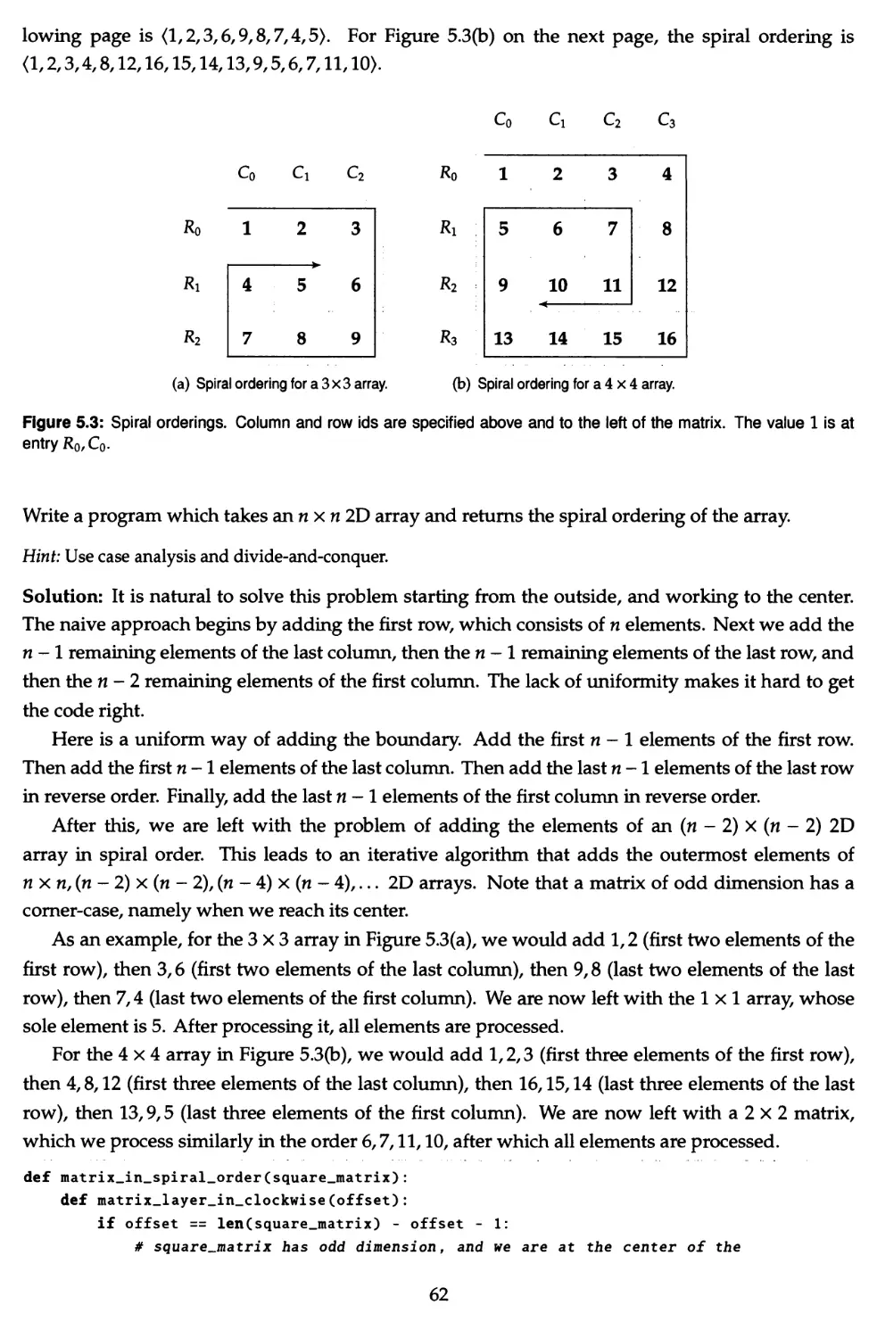
5.18 Compute the spiral ordering of a 2D array 61
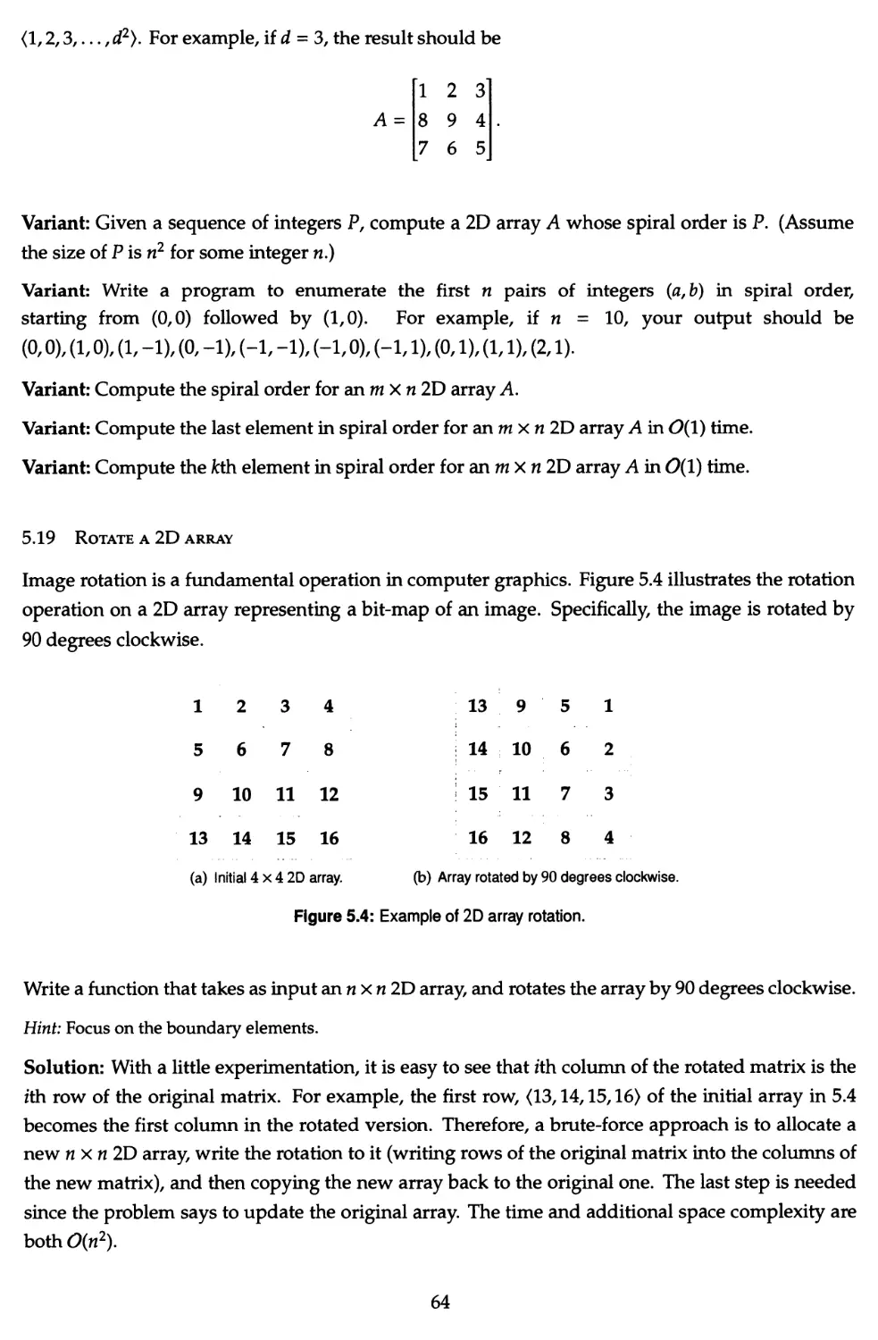
5.19 Rotate a 2D array 64
5.20 Compute rows in Pascal's Triangle 65
6 Strings 67
6.1 Interconvert strings and integers 68
6.2 Base conversion 69
6.3 Compute the spreadsheet column encoding 70
6.4 Replace and remove 71
6.5 Test palindromicity 72
6.6 Reverse all the words in a sentence 73
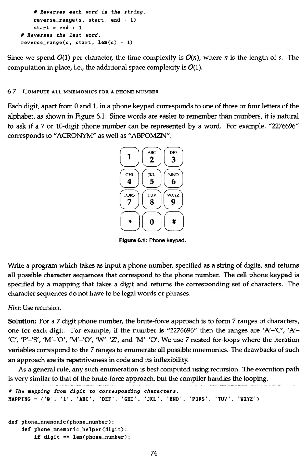
6.7 Compute all mnemonics for a phone number 74
6.8 The look-and-say problem 75
6.9 Convert from Roman to decimal 76
6.10 Compute all valid IP addresses 77
6.11 Write a string sinusoidally 78
6.12 Implement run-length encoding 79
6.13 Find the first occurrence of a substring 79
7 Linked Lists 82
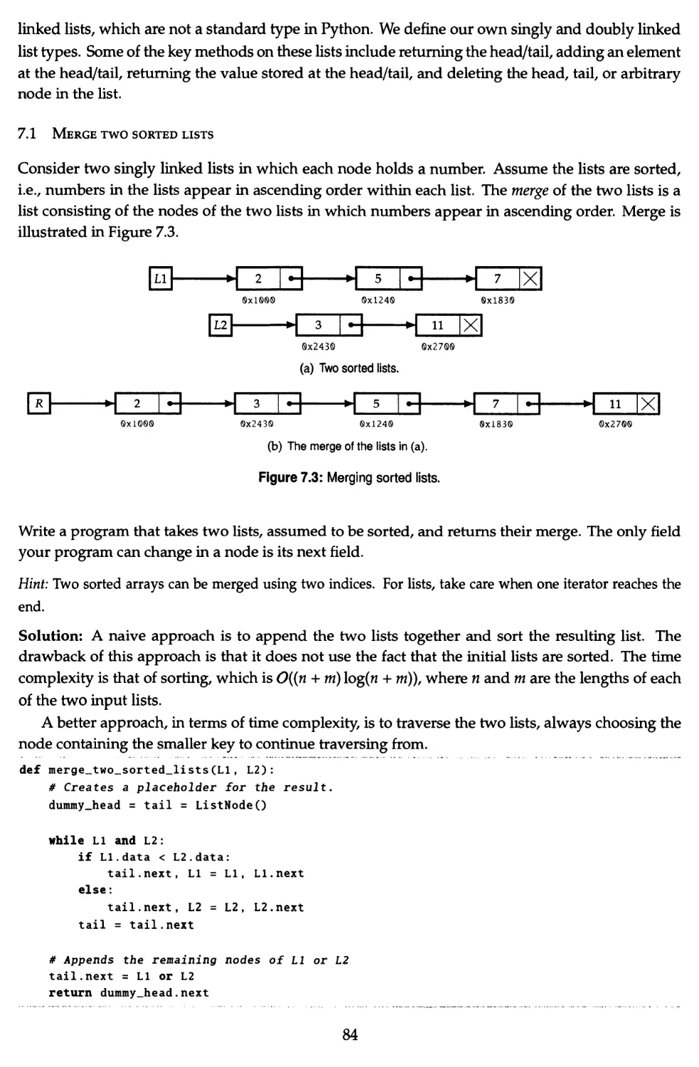
7.1 Merge two sorted lists 84
7.2 Reverse a single sublist 85
7.3 Test for cyclicity 86
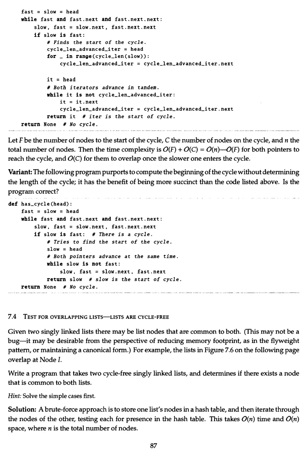
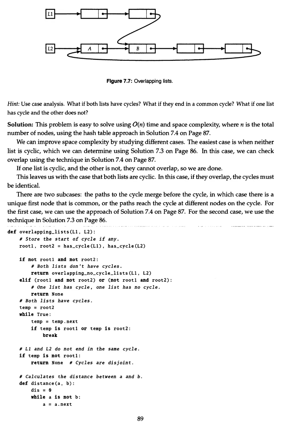
7.4 Test for overlapping lists—lists are cycle-free 87
7.5 Test for overlapping lists—lists may have cycles 88
7.6 Delete a node from a singly linked list 90
7.7 Remove the fcth last element from a list 90
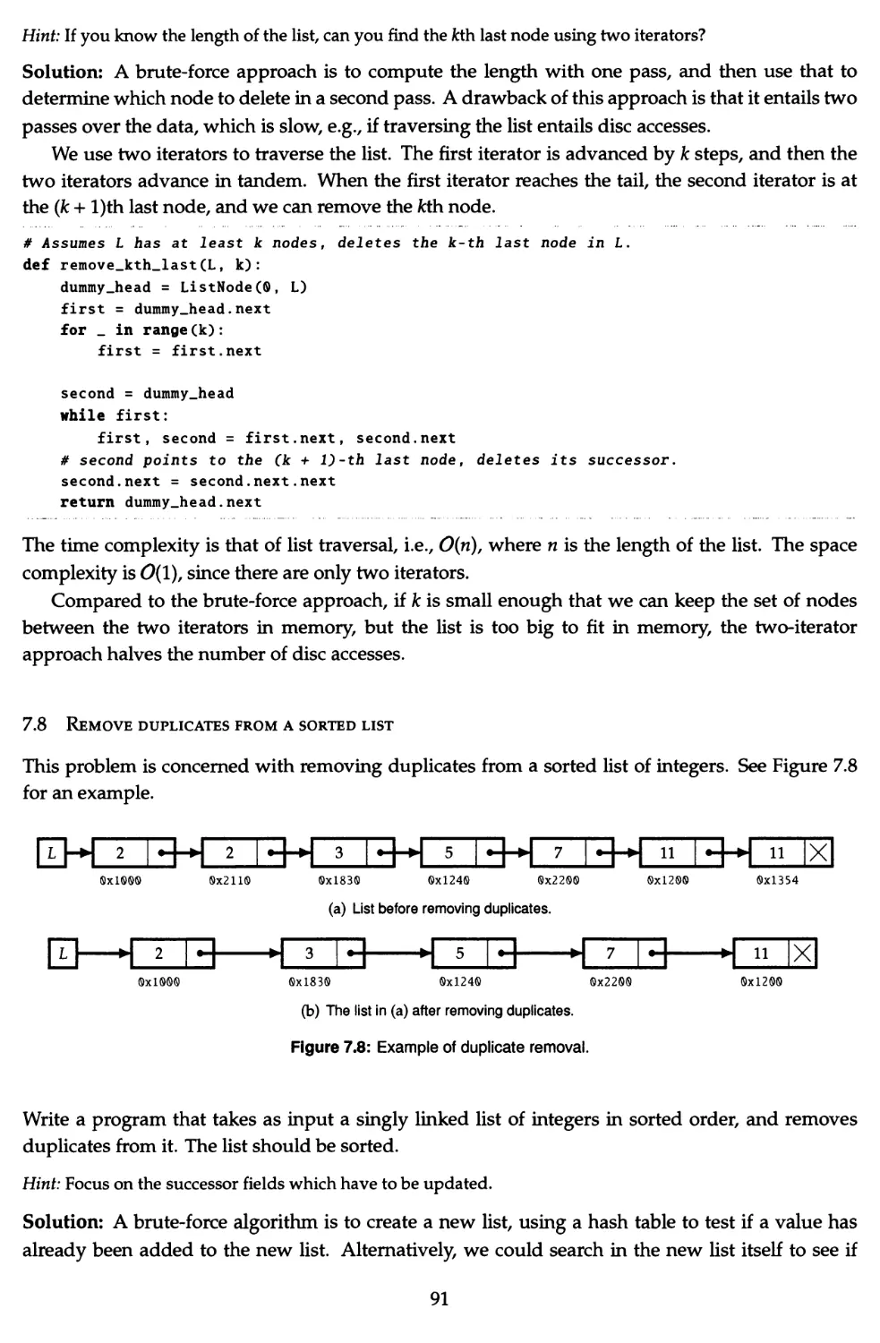
7.8 Remove duplicates from a sorted list 91
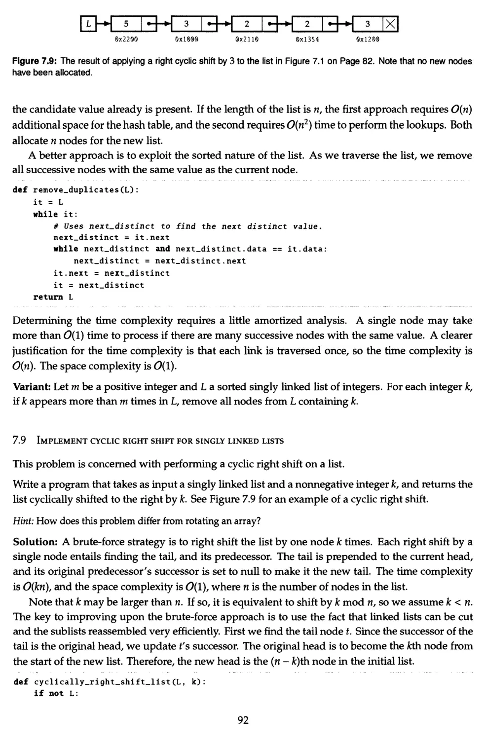
7.9 Implement cyclic right shift for singly linked lists 92
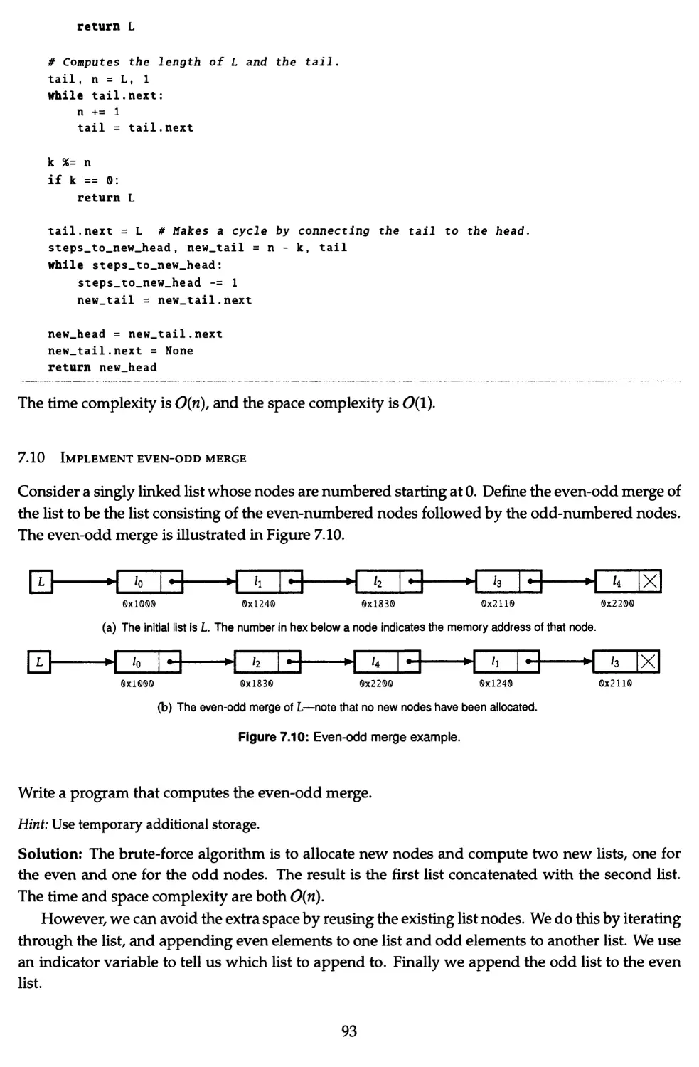
7.10 Implement even-odd merge 93
7.11 Test whether a singly linked list is palindromic 94
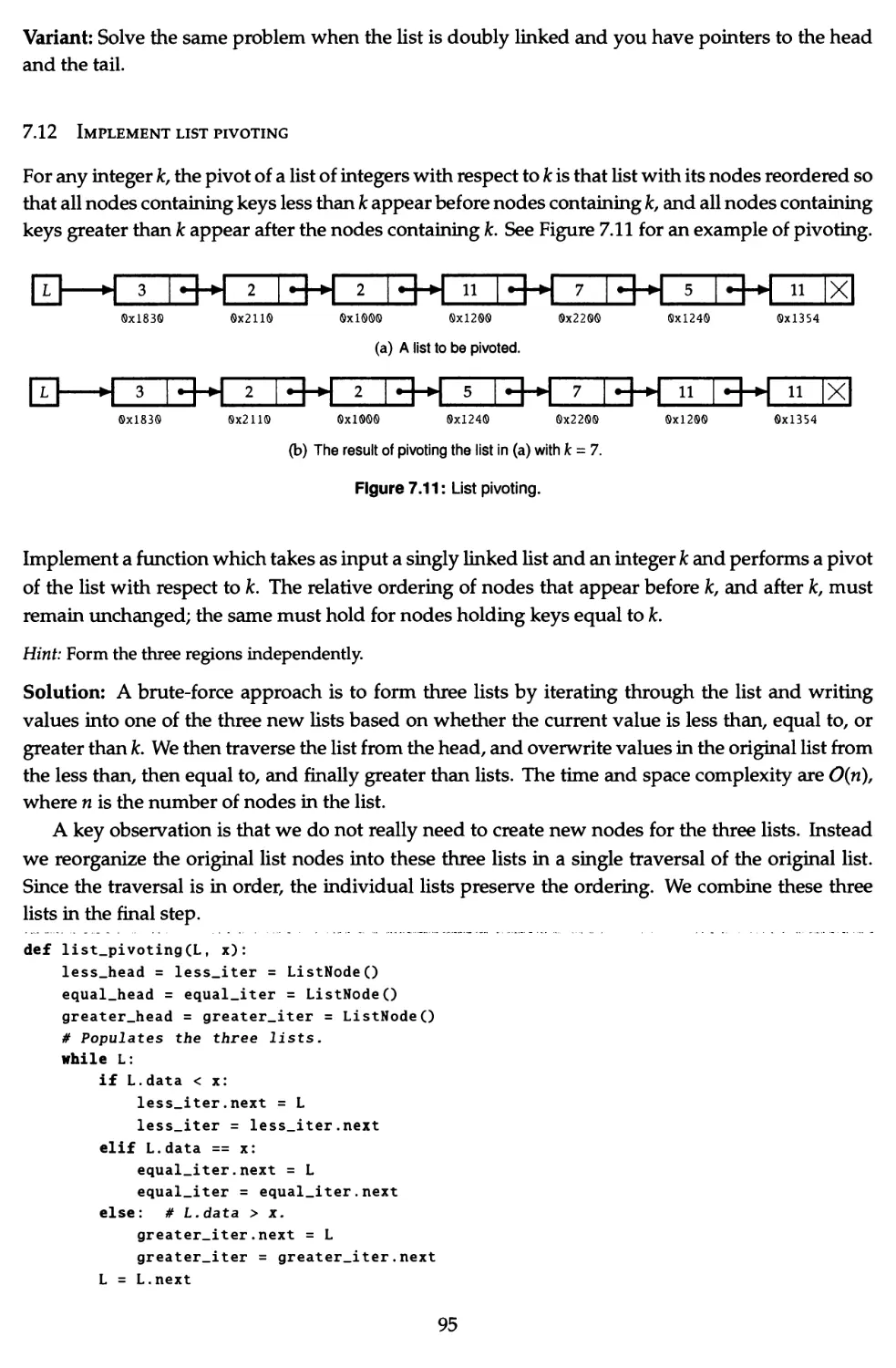
7.12 Implement list pivoting 95
7.13 Add list-based integers 96
8 Stacks and Queues 97
8.1 Implement a stack with max API 98
8.2 Evaluate RPN expressions 101
ii

8.3 Test a string over "{,},(,),[,]" for well-formedness 102
8.4 Normalize pathnames 102
8.5 Compute buildings with a sunset view 103
8.6 Compute binary tree nodes in order of increasing depth 106
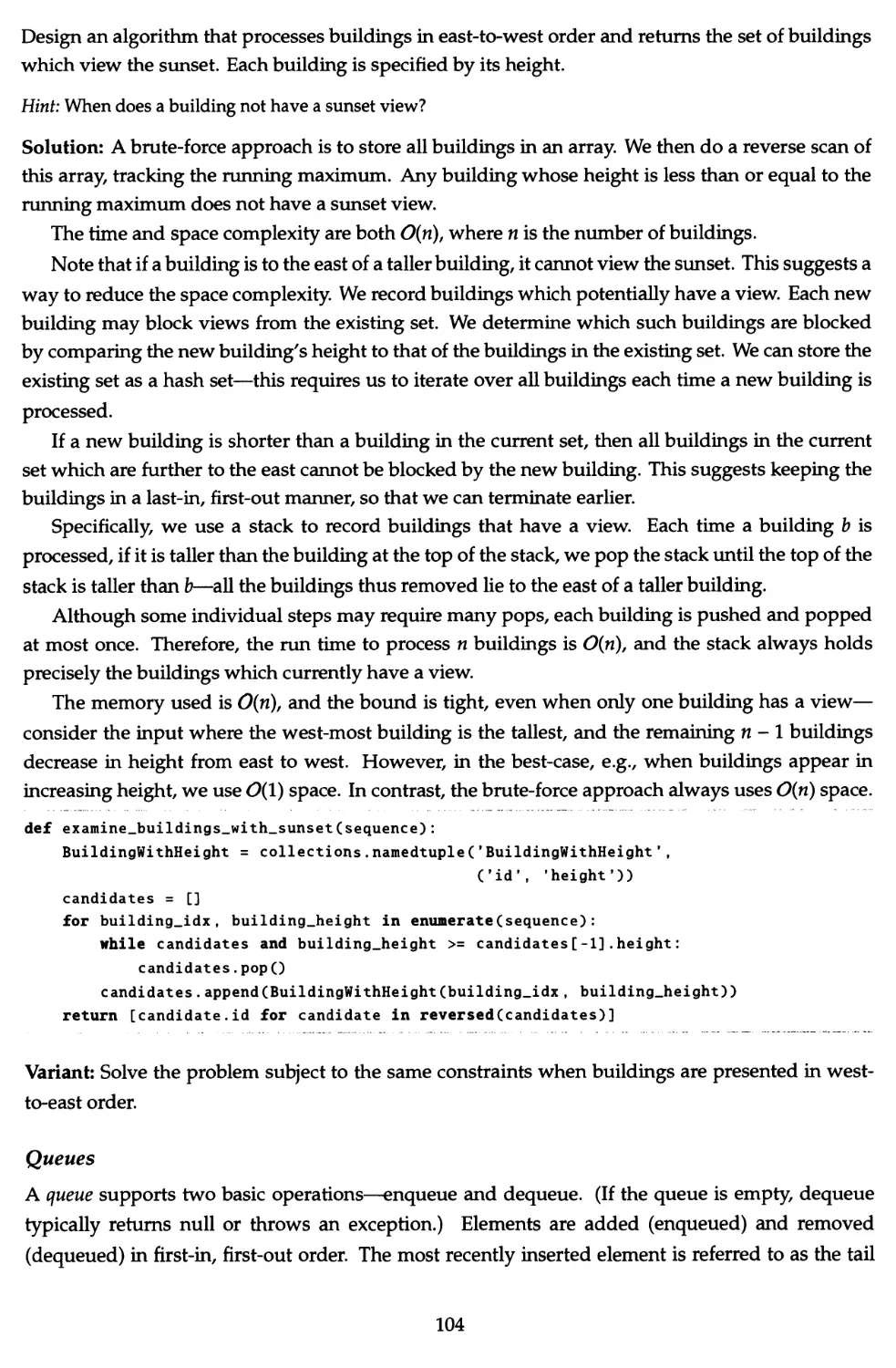
8.7 Implement a circular queue 107
8.8 Implement a queue using stacks 108
8.9 Implement a queue with max API 109
9 Binary Trees 112
9.1 Test if a binary tree is height-balanced 114
9.2 Test if a binary tree is symmetric 116
9.3 Compute the lowest common ancestor in a binary tree 117
9.4 Compute the LCA when nodes have parent pointers 118
9.5 Sum the root-to-leaf paths in a binary tree 119
9.6 Find a root to leaf path with specified sum 120
9.7 Implement an inorder traversal without recursion 121
9.8 Implement a preorder traversal without recursion 121
9.9 Compute the fcth node in an inorder traversal 122
9.10 Compute the successor 123
9.11 Implement an inorder traversal with (9(1) space 124
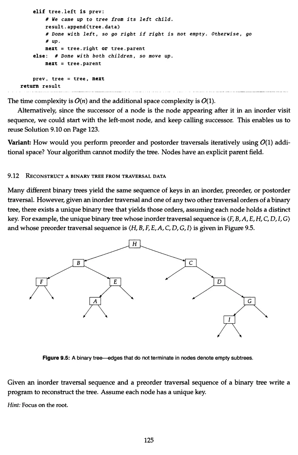
9.12 Reconstruct a binary tree from traversal data 125
9.13 Reconstruct a binary tree from a preorder traversal with markers 127
9.14 Form a linked list from the leaves of a binary tree 128
9.15 Compute the exterior of a binary tree 128
9.16 Compute the right sibling tree 129
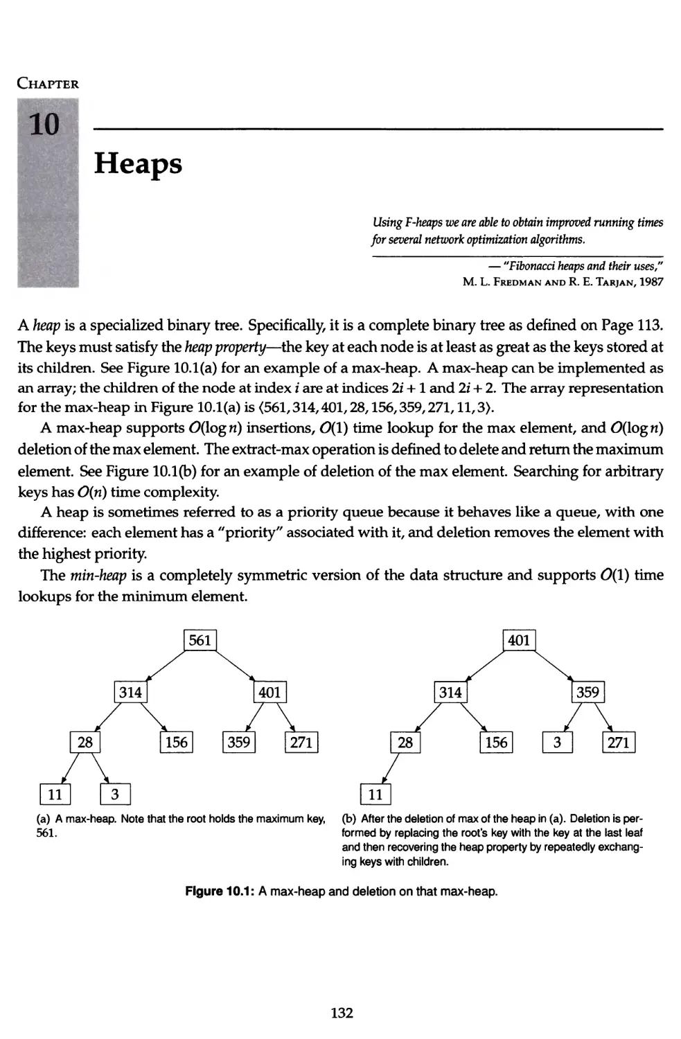
10 Heaps 132
10.1 Merge sorted files 134
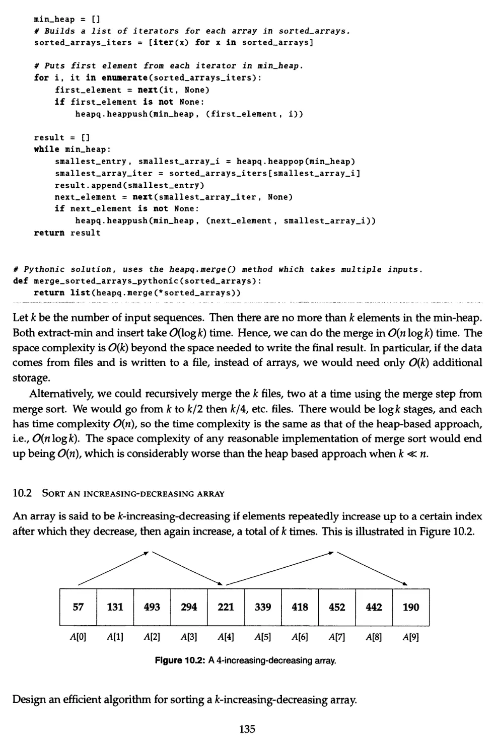
10.2 Sort an increasing-decreasing array 135
10.3 Sort an almost-sorted array 136
10.4 Compute the k closest stars 137
10.5 Compute the median of online data 139
10.6 Compute the k largest elements in a max-heap 140
11 Searching 142
11.1 Search a sorted array for first occurrence of k 145
11.2 Search a sorted array for entry equal to its index 146
11.3 Search a cyclically sorted array 147
11.4 Compute the integer square root 148
11.5 Compute the real square root 149
11.6 Search in a 2D sorted array 150
11.7 Find the min and max simultaneously 152
11.8 Find the fcth largest element 153
11.9 Find the missing IP address 155
11.10 Find the duplicate and missing elements 157
12 Hash Tables 159
iii

12.1 Test for palindromic permutations 163
12.2 Is an anonymous letter constructive? 164
12.3 Implement an ISBN cache 165
12.4 Compute the LCA, optimizing for close ancestors 166
12.5 Find the nearest repeated entries in an array 167
12.6 Find the smallest subarray covering all values 168
12.7 Find smallest subarray sequentially covering all values 171
12.8 Find the longest subarray with distinct entries 173
12.9 Find the length of a longest contained interval 174
12.10 Compute all string decompositions 175
12.11 Test the Collatz conjecture 176
12.12 Implement a hash function for chess 177
13 Sorting 180
13.1 Compute the intersection of two sorted arrays 182
13.2 Merge two sorted arrays 183
13.3 Remove first-name duplicates 184
13.4 Smallest nonconstructible value 185
13.5 Render a calendar 186
13.6 Merging intervals 188
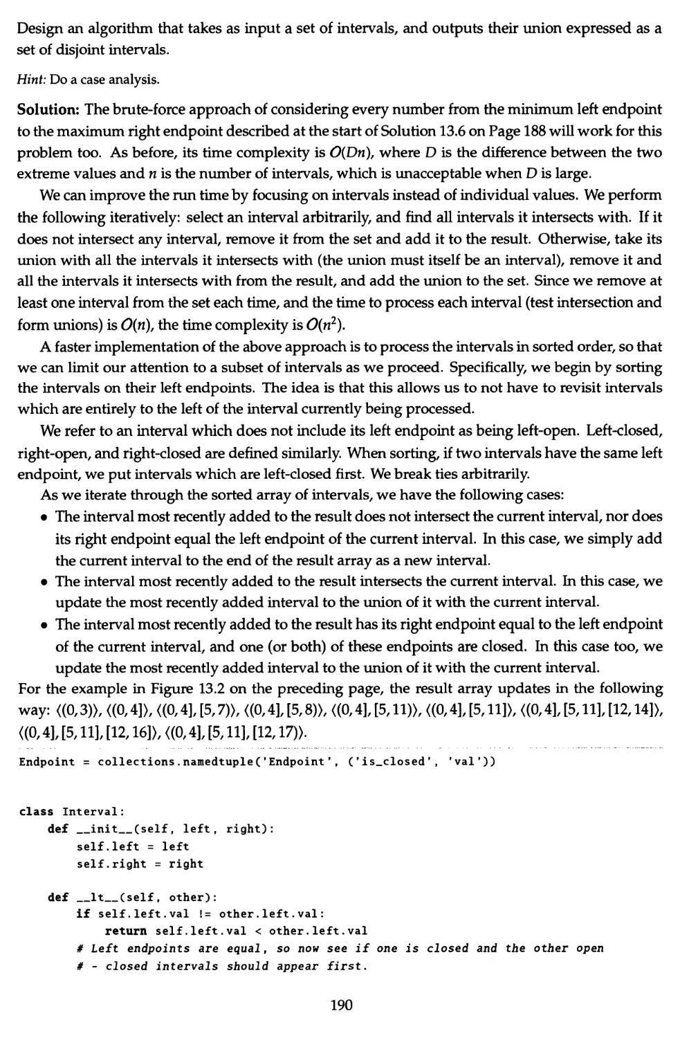
13.7 Compute the union of intervals 189
13.8 Partitioning and sorting an array with many repeated entries 191
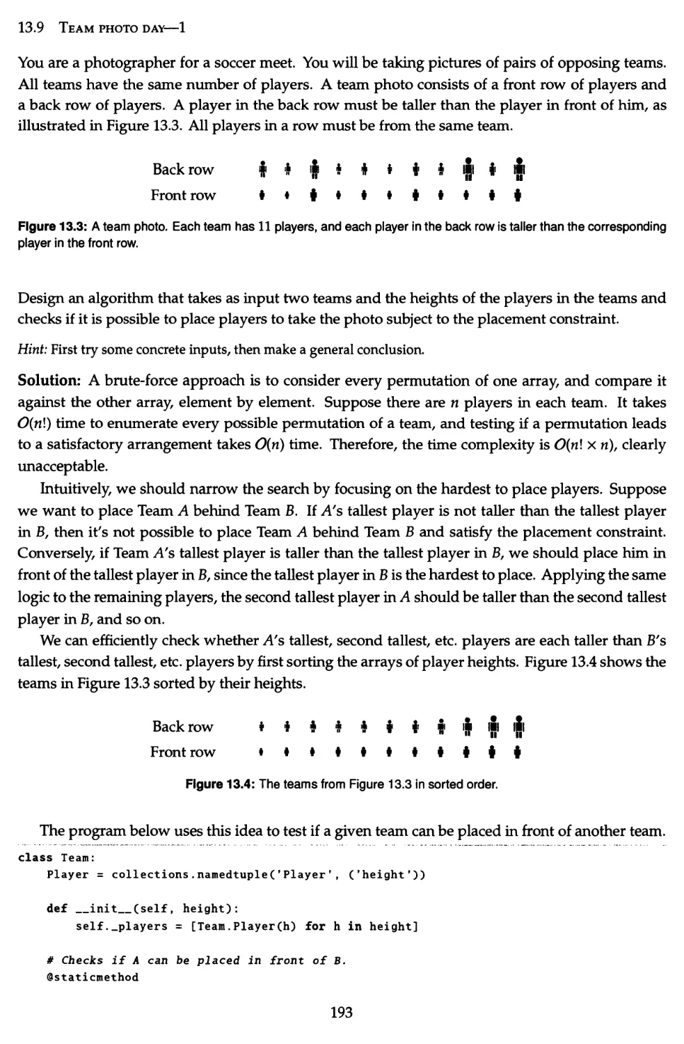
13.9 Team photo day—1 193
13.10 Implement a fast sorting algorithm for lists 194
13.11 Compute a salary threshold 195
14 Binary Search Trees 197
14.1 Test if a binary tree satisfies the BST property 199
14.2 Find the first key greater than a given value in a BST 201
14.3 Find the k largest elements in a BST 202
14.4 Compute the LCA in a BST 203
14.5 Reconstruct a BST from traversal data 204
14.6 Find the closest entries in three sorted arrays 206
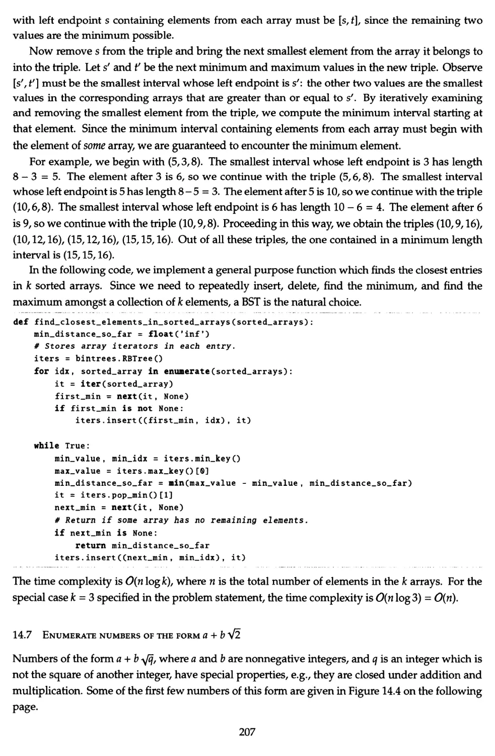
14.7 Enumerate numbers of the form a + by/l 207
14.8 Build a minimum height BST from a sorted array 210
14.9 Test if three BST nodes are totally ordered 211
14.10 The range lookup problem 212
14.11 Add credits 215
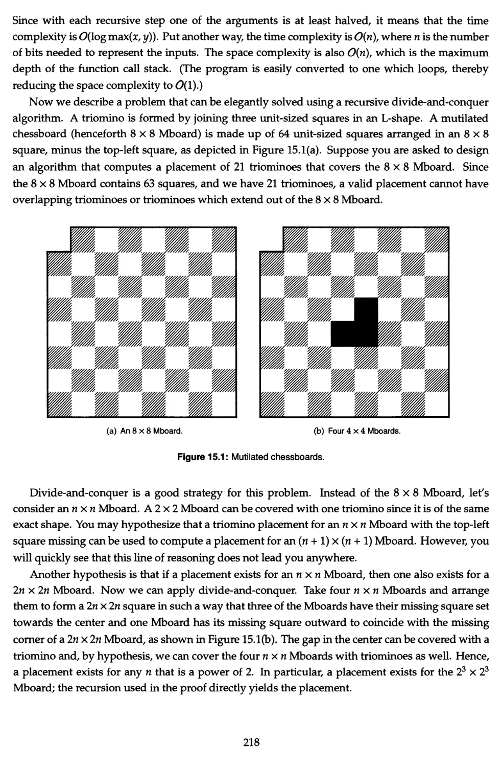
15 Recursion 217
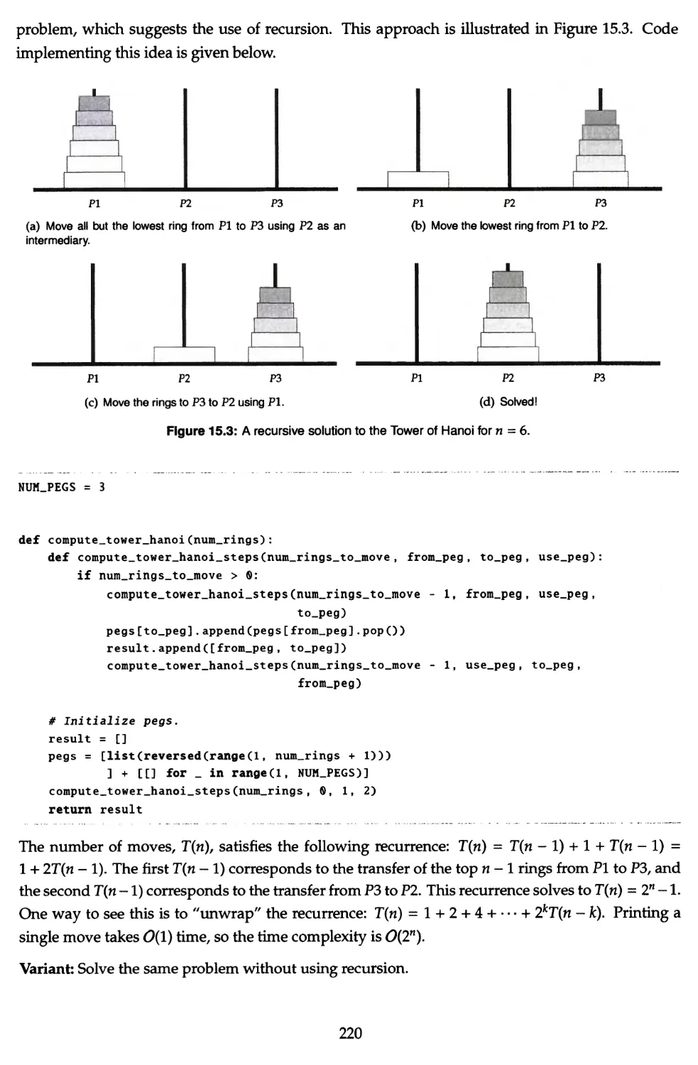
15.1 The Towers of Hanoi problem 219
15.2 Generate all nonattacking placements of n-Queens 221
15.3 Generate permutations 222
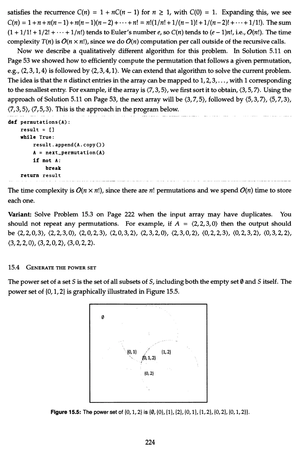
15.4 Generate the power set 224
15.5 Generate all subsets of size k 226
15.6 Generate strings of matched parens 227
15.7 Generate palindromic decompositions 228
IV

15.8 Generate binary trees 229
15.9 Implement a Sudoku solver 230
15.10 Compute a Gray code 232
16 Dynamic Programming 234
16.1 Count the number of score combinations 236
16.2 Compute the Levenshtein distance 239
16.3 Count the number of ways to traverse a 2D array 242
16.4 Compute the binomial coefficients 244
16.5 Search for a sequence in a 2D array 245
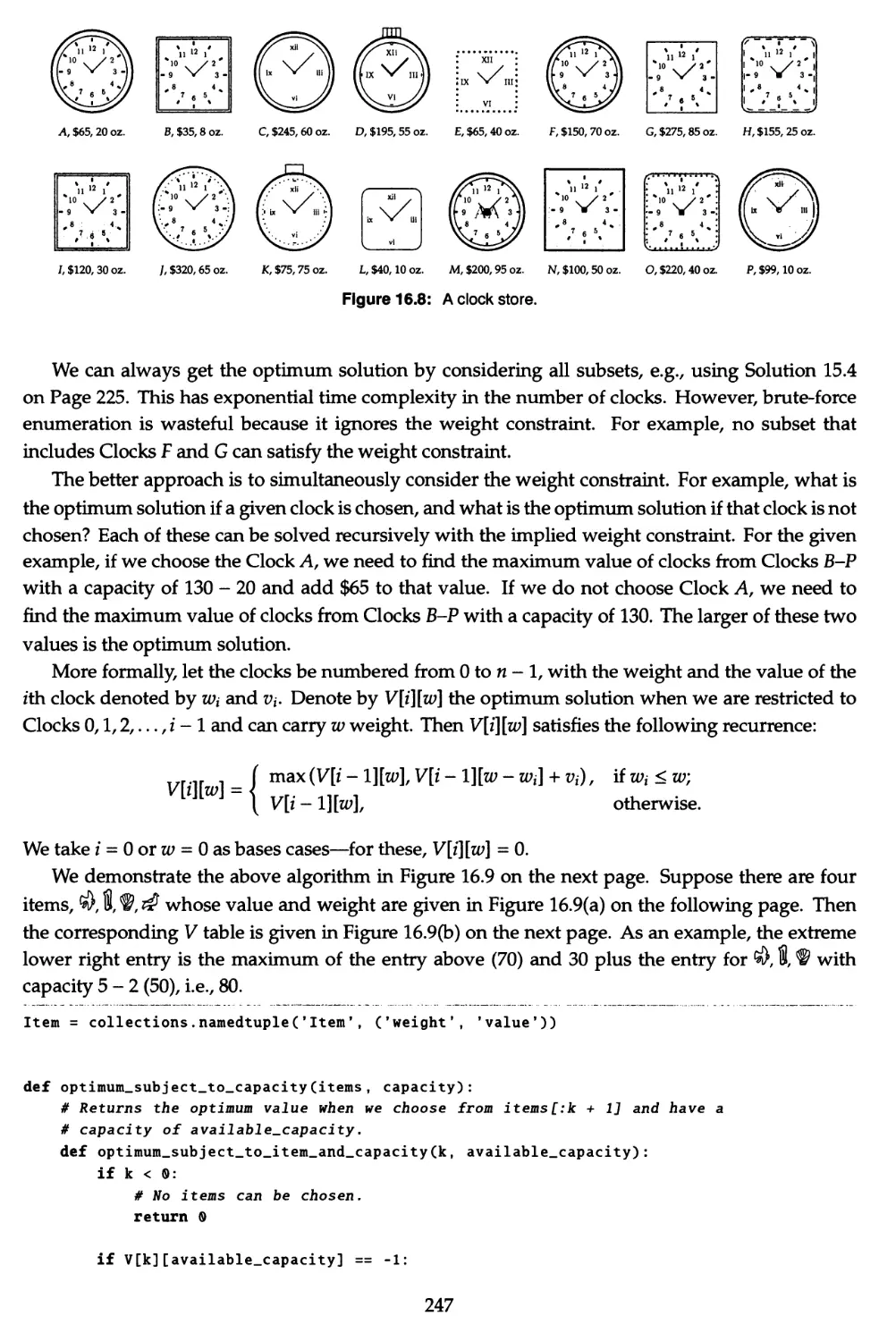
16.6 The knapsack problem 246
16.7 The bedbathandbeyond.com problem 249
16.8 Find the minimum weight path in a triangle 251
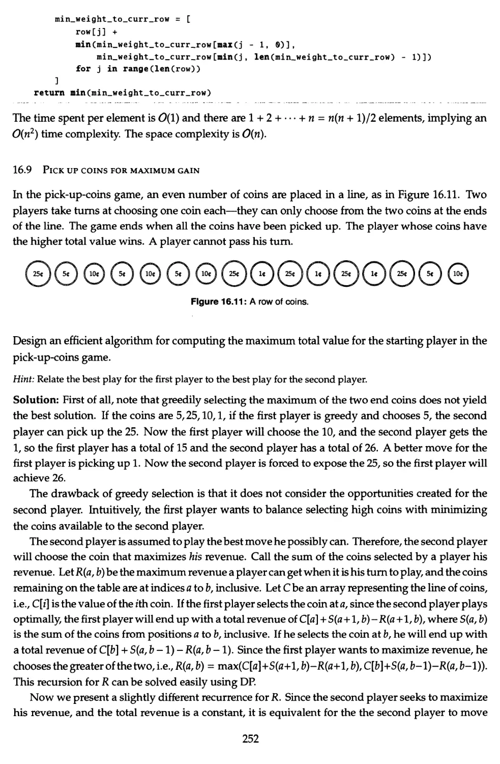
16.9 Pick up coins for maximum gain 252
16.10 Count the number of moves to climb stairs 253
16.11 The pretty printing problem 254
16.12 Find the longest nondecreasing subsequence 257
17 Greedy Algorithms and Invariants 259
17.1 Compute an optimum assignment of tasks 260
17.2 Schedule to minimize waiting time 261
17.3 The interval covering problem 262
17.4 The 3-sum problem 264
17.5 Find the majority element 266
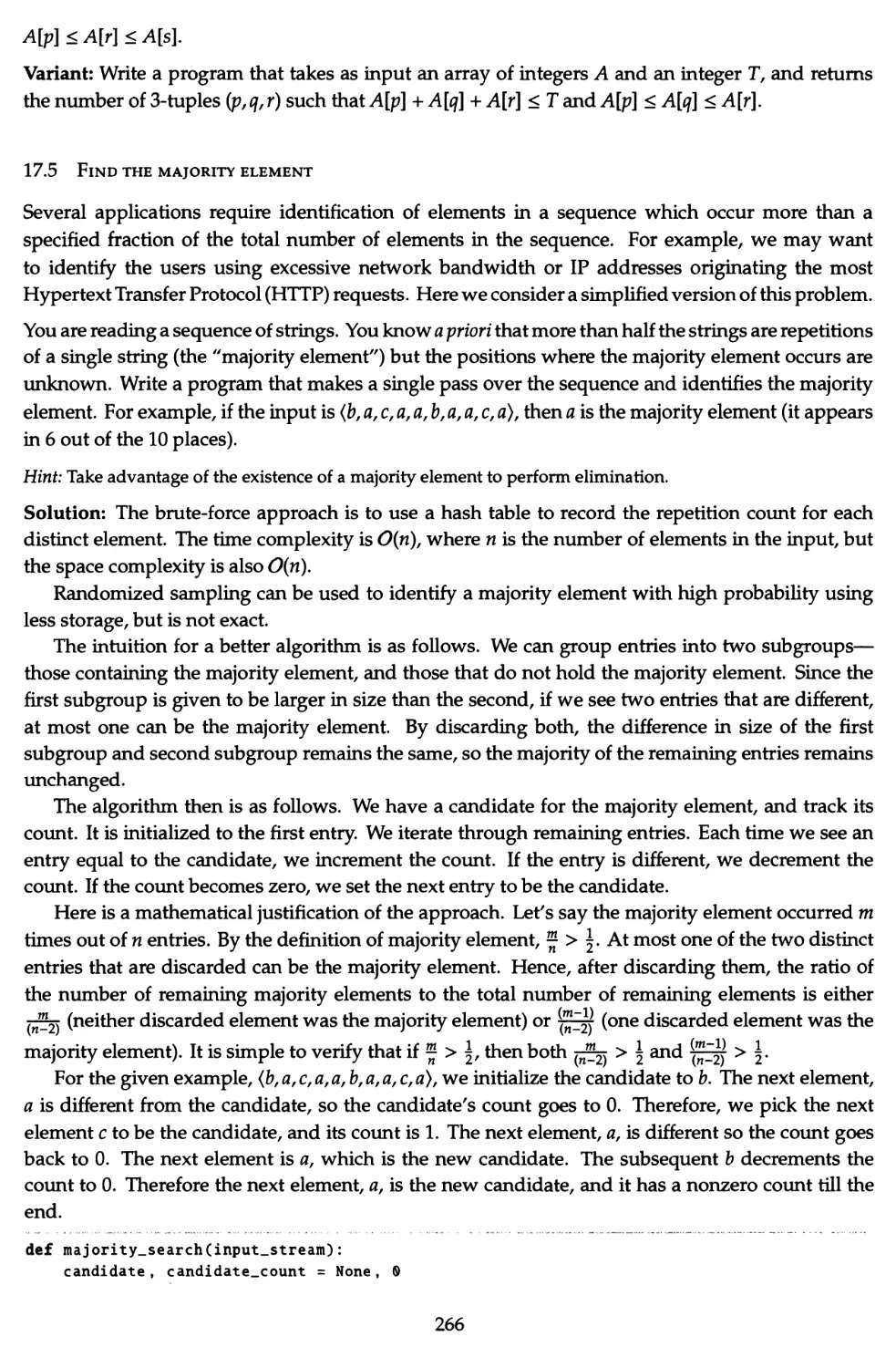
17.6 The gasup problem 267
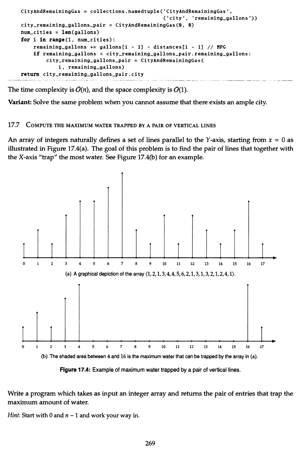
17.7 Compute the maximum water trapped by a pair of vertical lines 269
17.8 Compute the largest rectangle under the skyline 270
18 Graphs 273
18.1 Search a maze 276
18.2 Paint a Boolean matrix 278
18.3 Compute enclosed regions 280
18.4 Deadlock detection 281
18.5 Clone a graph 282
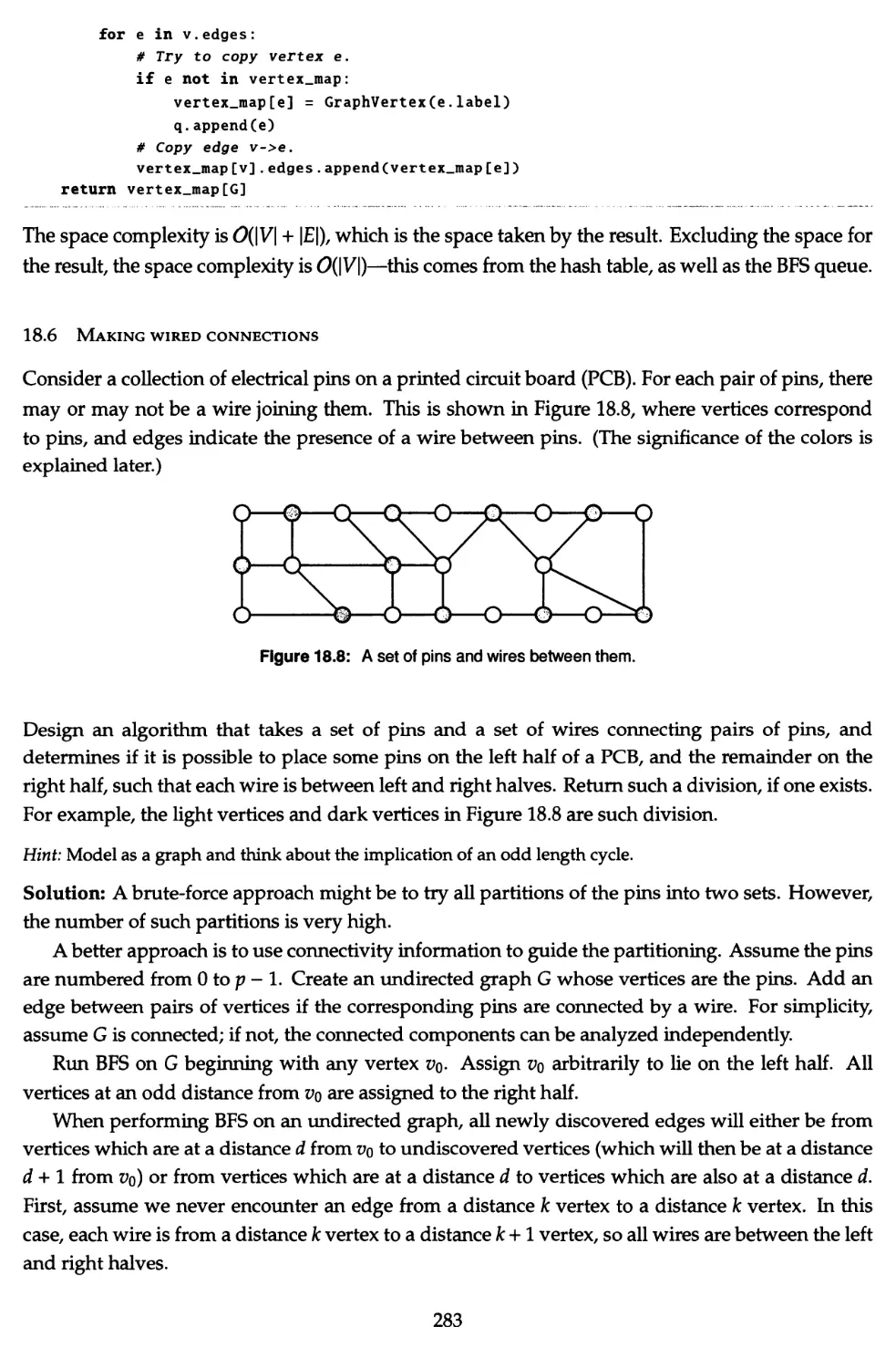
18.6 Making wired connections 283
18.7 Transform one string to another 284
18.8 Team photo day—2 286
19 Parallel Computing 289
19.1 Implement caching for a multithreaded dictionary 291
19.2 Analyze two unsynchronized interleaved threads 292
19.3 Implement synchronization for two interleaving threads 293
19.4 Implement a thread pool 294
19.5 Deadlock 295
19.6 The readers-writers problem 296
19.7 The readers-writers problem with write preference 297
19.8 Implement a Timer class 298
v

19.9 Test the Collatz conjecture in parallel
298
III Domain Specific Problems 300
20 Design Problems 301
20.1 Design a spell checker 302
20.2 Design a solution to the stemming problem 303
20.3 Plagiarism detector 304
20.4 Pair users by attributes 305
20.5 Design a system for detecting copyright infringement 306
20.6 Design TeX 307
20.7 Design a search engine 307
20.8 Implement PageRank 308
20.9 Design TeraSort and PetaSort 310
20.10 Implement distributed throttling 310
20.11 Design a scalable priority system 311
20.12 Create photomosaics 312
20.13 Implement Mileage Run 312
20.14 Implement Connexus 314
20.15 Design an online advertising system 315
20.16 Design a recommendation system 316
20.17 Design an optimized way of distributing large files 316
20.18 Design the World Wide Web 317
20.19 Estimate the hardware cost of a photo sharing app 318
21 Language Questions 319
21.1 Garbage Collection 319
21.2 Closure 319
21.3 Shallow and deep copy 320
21.4 Iterators and Generators 321
21.5 ©decorator 321
21.6 List vs tuple 323
21.7 *args and *kwargs 324
21.8 Python code 325
21.9 Exception Handling 326
21.10 Scoping 328
21.11 Function arguments 330
22 Object-Oriented Design 333
22.1 Template Method vs. Strategy 333
22.2 Observer pattern 334
22.3 Push vs. pull observer pattern 334
22.4 Singletons and Flyweights 335
22.5 Adapters 336
22.6 Creational Patterns 337
22.7 Libraries and design patterns 338
vi

23 Common Tools 339
23.1 Merging in a version control system 339
23.2 Hooks 341
23.3 Is scripting more efficient? 342
23.4 Polymorphism with a scripting language 343
23.5 Dependency analysis 343
23.6 ANT vs. Maven 344
23.7 SQLvs.NoSQL 345
23.8 Normalization 345
23.9 SQL design 346
23.10 IP, TCP, and HTTP 346
23.11 HTTPS 347
23.12 DNS 348
IV The Honors Class 349
24 Honors Class 350
24.1 Compute the greatest common divisor ©^ 351
24.2 Find the first missing positive entry Q" 352
24.3 Buy and sell a stock k times Q< 353
24.4 Compute the maximum product of all entries but one ©* 354
24.5 Compute the longest contiguous increasing subarray ©* 356
24.6 Rotate an array Q' 357
24.7 Identify positions attacked by rooks Qr 359
24.8 Justify text ©* 360
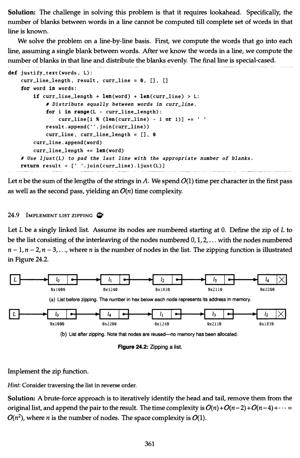
24.9 Implement list zipping Qr 361
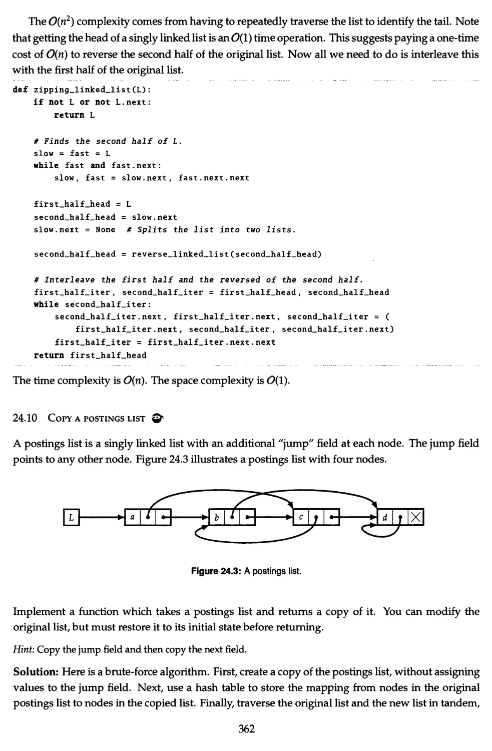
24.10 Copy a postings list ©< 362
24.11 Compute the longest substring with matching parens Q* 364
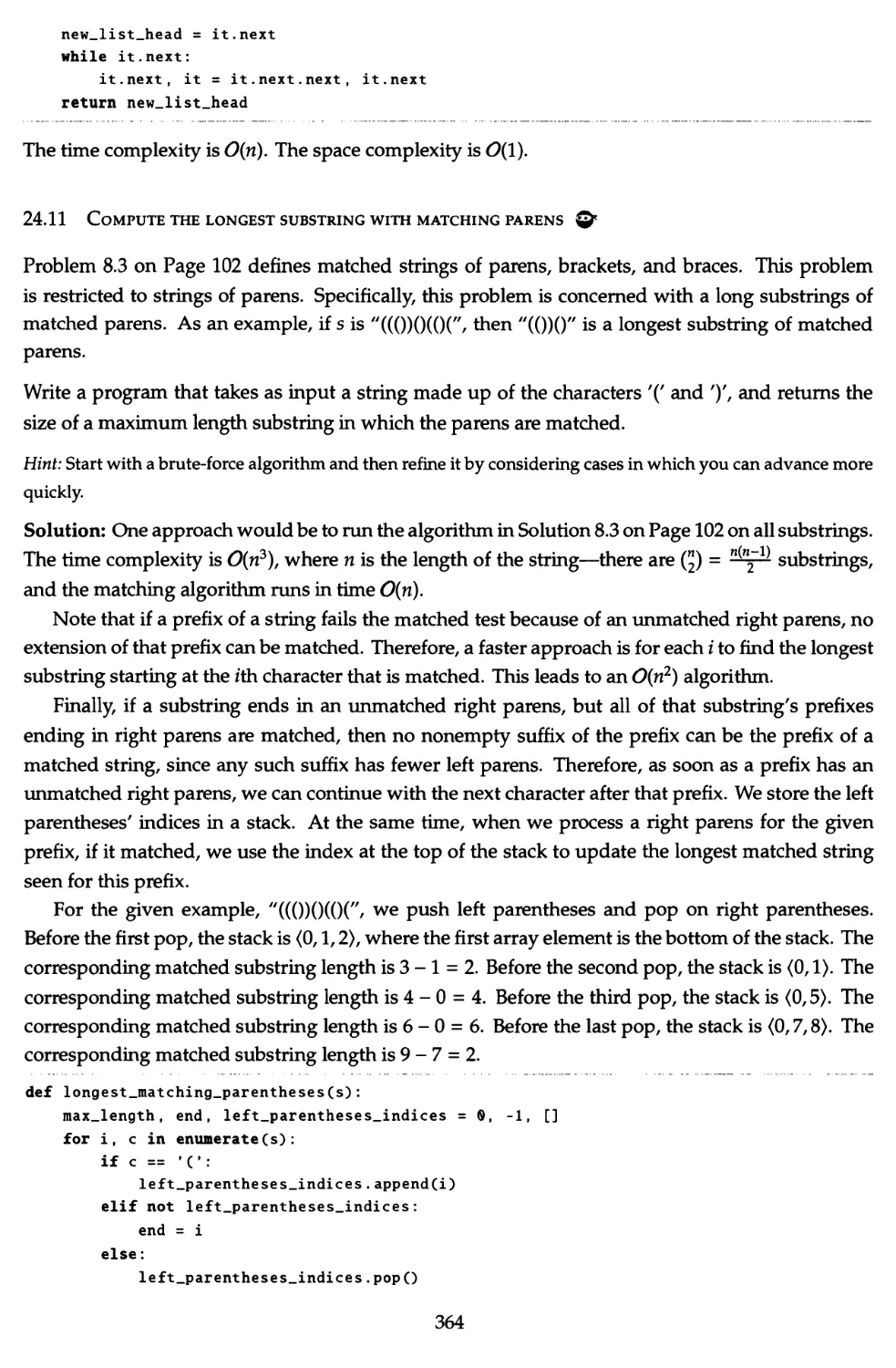
24.12 Compute the maximum of a sliding window ©* 365
24.13 Implement a postorder traversal without recursion ©* 366
24.14 Compute fair bonuses ©< 368
24.15 Search a sorted array of unknown length ©* 370
24.16 Search in two sorted arrays Q< 372
24.17 Find the fcth largest element—large n, small k Q< 373
24.18 Find an element that appears only once Q* 374
24.19 Find the line through the most points Qr- 375
24.20 Convert a sorted doubly linked list into a BST Q< 376
24.21 Convert a BST to a sorted doubly linked list Qr 378
24.22 Merge two BSTs Q< 379
24.23 Implement regular expression matching ©< 380
24.24 Synthesize an expression Qr 383
24.25 Count inversions ©* 385
24.26 Draw the skyline ©< 386
24.27 Measure with defective jugs Qr 388
24.28 Compute the maximum subarray sum in a circular array Qr- 390
vii

24.29 Determine the critical height & 391
24.30 Find the maximum 2D subarray Q< 393
24.31 Implement Huffman coding Q" 395
24.32 Trapping water ©* 398
24.33 The heavy hitter problem Qr 399
24.34 Find the longest subarray whose sum < fc ©* 400
24.35 Road network ^ 402
24.36 Test if arbitrage is possible © 403
V Notation and Index 406
Notation 407
Index of Terms 409

Introduction
It's not that I'm so smart, it's just that I stay with problems longer.
— A. Einstein
Elements of Programming Interviews (EPI) aims to help engineers interviewing for software
development positions. The primary focus of EPI is data structures, algorithms, system design, and
problem solving. The material is largely presented through questions.
An interview problem
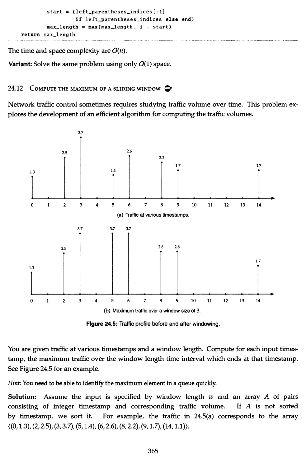
Let's begin with Figure 1 below. It depicts movements in the share price of a company over 40 days.
Specifically, for each day, the chart shows the daily high and low, and the price at the opening bell
(denoted by the white square). Suppose you were asked in an interview to design an algorithm
that determines the maximum profit that could have been made by buying and then selling a single
share over a given day range, subject to the constraint that the buy and the sell have to take place
at the start of the day. (This algorithm may be needed to backtest a trading strategy.)
You may want to stop reading now, and attempt this problem on your own.
First clarify the problem. For example, you should ask for the input format. Let's say the input
consists of three arrays L, H, and S, of nonnegative floating point numbers, representing the low,
high, and starting prices for each day. The constraint that the purchase and sale have to take place
at the start of the day means that it suffices to consider S. You may be tempted to simply return
the difference of the minimum and maximum elements in S. If you try a few test cases, you will
see that the minimum can occur after the maximum, which violates the requirement in the problem
statement—you have to buy before you can sell.
At this point, a brute-force algorithm would be appropriate. For each pair of indices i and
j > i, if S[j] - S[i] is greater than the largest difference seen so far, update the largest difference
to S[j] - S[i\. You should be able to code this algorithm using a pair of nested for-loops and test
i,, .iff iM'tll'
1111!!!'"" I,
DayO Day 5 Day 10 Day 15 Day 20 Day 25 Day 30 Day 35 Day 40
Figure 1: Share price as a function of time.
1

it in a matter of a few minutes. You should also derive its time complexity as a function of the
length n of the input array. The outer loop is invoked n - 1 times, and the zth iteration processes
n-l-i elements. Processing an element entails computing a difference, performing a compare, and
possibly updating a variable, all of which take constant time. Hence, the run time is proportional to
Tu1=o(n - 1 - 0 = (w~2)(w)/ i-e., the time complexity of the brute-force algorithm is 0(n2). You should
also consider the space complexity, i.e., how much memory your algorithm uses. The array itself
takes memory proportional to n, and the additional memory used by the brute-force algorithm is a
constant independent of n—a couple of iterators and one floating point variable.
Once you have a working algorithm, try to improve upon it. Specifically, an 0(n2) algorithm
is usually not acceptable when faced with large arrays. You may have heard of an algorithm
design pattern called divide-and-conquer. It yields the following algorithm for this problem. Split
S into two subarrays, S[0, |_§ J] and S[|_§ J + 1, n - 1]; compute the best result for the first and second
subarrays; and combine these results. In the combine step we take the better of the results for the
two subarrays. However, we also need to consider the case where the optimum buy and sell take
place in separate subarrays. When this is the case, the buy must be in the first subarray, and the sell
in the second subarray, since the buy must happen before the sell. If the optimum buy and sell are
in different subarrays, the optimum buy price is the minimum price in the first subarray, and the
optimum sell price is in the maximum price in the second subarray. We can compute these prices
in 0(n) time with a single pass over each subarray. Therefore, the time complexity T(n) for the
divide-and-conquer algorithm satisfies the recurrence relation T(n) = 2T(|) + 0(n), which solves to
<9(nlogn).
The divide-and-conquer algorithm is elegant and fast. Its implementation entails some corner
cases, e.g., an empty subarray, subarrays of length one, and an array in which the price decreases
monotonically, but it can still be written and tested by a good developer in 20-30 minutes.
Looking carefully at the combine step of the divide-and-conquer algorithm, you may have a
flash of insight. Specifically, you may notice that the maximum profit that can be made by selling
on a specific day is determined by the minimum of the stock prices over the previous days. Since
the maximum profit corresponds to selling on some day, the following algorithm correctly computes
the maximum profit. Iterate through S, keeping track of the minimum element m seen thus far.
If the difference of the current element and m is greater than the maximum profit recorded so far,
update the maximum profit. This algorithm performs a constant amount of work per array element,
leading to an 0(n) time complexity. It uses two float-valued variables (the minimum element and
the maximum profit recorded so far) and an iterator, i.e., 0(1) additional space. It is considerably
simpler to implement than the divide-and-conquer algorithm—a few minutes should suffice to
write and test it. Working code is presented in Solution 5.6 on Page 47.
If in a 45-60 minutes interview, you can develop the algorithm described above, implement and
test it, and analyze its complexity, you would have had a very successful interview. In particular,
you would have demonstrated to your interviewer that you possess several key skills:
- The ability to rigorously formulate real-world problems.
- The skills to solve problems and design algorithms.
- The tools to go from an algorithm to a tested program.
- The analytical techniques required to determine the computational complexity of your
solution.
Book organization
Interviewing successfully is about more than being able to intelligently select data structures and
design algorithms quickly. For example, you also need to know how to identify suitable compa-
2

nies, pitch yourself, ask for help when you are stuck on an interview problem, and convey your
enthusiasm. These aspects of interviewing are the subject of Chapters 1-3, and are summarized in
Table 1.1 on Page 7.
Chapter 1 is specifically concerned with preparation. Chapter 2 discusses how you should
conduct yourself at the interview itself. Chapter 3 describes interviewing from the interviewer's
perspective. The latter is important for candidates too, because of the insights it offers into the
decision making process.
Since not everyone will have the time to work through EPI in its entirety, we have prepared a
study guide (Table 1.2 on Page 8) to problems you should solve, based on the amount of time you
have available.
The problem chapters are organized as follows. Chapters 4-14 are concerned with basic data
structures, such as arrays and binary search trees, and basic algorithms, such as binary search
and quicksort. In our experience, this is the material that most interview questions are based on.
Chapters 15-18 cover advanced algorithm design principles, such as dynamic programming and
heuristics, as well as graphs. Chapter 19 focuses on parallel programming.
Each chapter begins with an introduction followed by problems. The introduction itself consists
of a brief review of basic concepts and terminology, followed by a boot camp. Each boot camp is (1.) a
straightforward, illustrative example that illustrates the essence of the chapter without being too
challenging; and (2.) top tips for the subject matter, presented in tabular format. For chapters where
the programming language includes features that are relevant, we present these features in list form.
This list is ordered with basic usage coming first, followed by subtler aspects. Basic usage is
demonstrated using methods calls with concrete arguments, e.g., D = collections.OrderedDictCCl,2),
(3,4)). Subtler aspects of the library, such as ways to reduce code length, underappreciated
features, and potential pitfalls, appear later in the list. Broadly speaking, the problems are ordered by
subtopic, with more commonly asked problems appearing first. Chapter 24 consists of a collection
of more challenging problems.
Domain-specific knowledge is covered in Chapters 20,21,22, and 23, which are concerned with
system design, programming language concepts, object-oriented programming, and commonly
used tools. Keep in mind that some companies do not ask these questions—you should investigate
the topics asked by companies you are interviewing at before investing too much time in them.
These problems are more likely to be asked of architects, senior developers and specialists.
The notation, specifically the symbols we use for describing algorithms, e.g.,
Li=o *2/ k b), (2,3,5,7), A[i, /*], \x\ (1011)2/ n\, {x | r2 > 2}, etc., is summarized starting on Page 407. It
should be familiar to anyone with a technical undergraduate degree, but we still request you to
review it carefully before getting into the book, and whenever you have doubts about the meaning
of a symbol. Terms, e.g., BFS and dequeue, are indexed starting on Page 409.
The EPI editorial style
Solutions are based on basic concepts, such as arrays, hash tables, and binary search, used in clever
ways. Some solutions use relatively advanced machinery, e.g., Dijkstra's shortest path algorithm.
You will encounter such problems in an interview only if you have a graduate degree or claim
specialized knowledge.
Most solutions include code snippets. Please read Section 1 on Page 11 to familiarize yourself
with the Python constructs and practices used in this book. Source code, which includes randomized
and directed test cases, can be found at the book website. Domain specific problems are conceptual
and not meant to be coded; a few algorithm design problems are also in this spirit.
3

One of our key design goals for EPI was to make learning easier by establishing a uniform way
in which to describe problems and solutions. We refer to our exposition style as the EPI Editorial
Style.
Problems are specified as follows:
(1.) We establish context, e.g., a real-world scenario, an example, etc.
(2.) We state the problem to be solved. Unlike a textbook, but as is true for an interview, we do
not give formal specifications, e.g., we do not specify the detailed input format or say what to
do on illegal inputs. As a general rule, avoid writing code that parses input. See Page 14 for
an elaboration.
(3.) We give a short hint—you should read this only if you get stuck. (The hint is similar to what
an interviewer will give you if you do not make progress.)
Solutions are developed as follows:
(1.) We begin a simple brute-force solution.
(2.) We then analyze the brute-force approach and try to get intuition for why it is inefficient and
where we can improve upon it, possibly by looking at concrete examples, related algorithms,
etc.
(3.) Based on these insights, we develop a more efficient algorithm, and describe it in prose.
(4.) We apply the program to a concrete input.
(5.) We give code for the key steps.
(6.) We analyze time and space complexity.
(7.) We outline variants—problems whose formulation or solution is similar to the solved problem.
Use variants for practice, and to test your understanding of the solution.
Note that exceptions exists to this style—for example a brute-force solution may not be
meaningful, e.g., if it entails enumerating all double-precision floating point numbers in some range. For
the chapters at the end of the book, which correspond to more advanced topics, such as Dynamic
Programming, and Graph Algorithms, we use more parsimonious presentations, e.g., we forgo
examples of applying the derived algorithm to a concrete example.
Level and prerequisites
We expect readers to be familiar with data structures and algorithms taught at the undergraduate
level. The chapters on concurrency and system design require knowledge of locks, distributed
systems, operating systems (OS), and insight into commonly used applications. Some of the
material in the later chapters, specifically dynamic programming, graphs, and greedy algorithms,
is more advanced and geared towards candidates with graduate degrees or specialized knowledge.
The review at the start of each chapter is not meant to be comprehensive and if you are not
familiar with the material, you should first study it in an algorithms textbook. There are dozens of
such texts and our preference is to master one or two good books rather than superficially sample
many Algorithms by Dasgupta, et ah is succinct and beautifully written; Introduction to Algorithms
by Cormen, et al. is an amazing reference.
Reader engagement
Many of the best ideas in EPI came from readers like you. The study guide, ninja notation, and hints,
are a few examples of many improvements that were brought about by our readers. The companion
website, elementsofprogrammingintervJews.com, includes a Stack Overflow-style discussion forum,
and links to our social media presence. It also has links blog postings, code, and bug reports. You
can always communicate with us directly—our contact information is on the website.
4

Parti
The Interview

Chapter
;i':
Getting Ready
t Before everything else, getting ready is the secret of success.
— H. Ford
The most important part of interview preparation is knowing the material and practicing problem
solving. However, the nontechnical aspects of interviewing are also very important, and often
overlooked. Chapters 1-3 are concerned with the nontechnical aspects of interviewing, ranging
from resume preparation to how hiring decisions are made. These aspects of interviewing are
summarized in Table 1.1 on the facing page
Study guide
Ideally, you would prepare for an interview by solving all the problems in EPI. This is doable over
12 months if you solve a problem a day, where solving entails writing a program and getting it to
work on some test cases.
Since different candidates have different time constraints, we have outlined several study
scenarios, and recommended a subset of problems for each scenario. This information is summarized
in Table 1.2 on Page 8. The preparation scenarios we consider are Hackathon (a weekend entirely
devoted to preparation), finals cram (one week, 3-4 hours per day), term project (four weeks, 1.5-2.5
hours per day), and algorithms class (3-4 months, 1 hour per day).
A large majority of the interview questions at Google, Amazon, Microsoft, and similar companies
are drawn from the topics in Chapters 4-14. Exercise common sense when using Table 1.2, e.g., if
you are interviewing for a position with a financial firm, do more problems related to probability.
Although an interviewer may occasionally ask a question directly from EPI, you should not base
your preparation on memorizing solutions. Rote learning will likely lead to your giving a perfect
solution to the wrong problem.
Chapter 24 contains a diverse collection of challenging questions. Use them to hone your
problem solving skills, but go to them only after you have made major inroads into the earlier
chapters. If you have a graduate degree, or claim specialized knowledge, you should definitely
solve some problems from Chapter 24.
The interview lifecycle
Generally speaking, interviewing takes place in the following steps:
(1.) Identify companies that you are interested in, and, ideally, find people you know at these
companies.
(2.) Prepare your resume using the guidelines on Page 8, and submit it via a personal contact
(preferred), or through an online submission process or a campus career fair.
6

Table 1.1: A summary of nontechnical aspects of interviewing
The Interview Lif ecycle, on the preceding page
• Identify companies, contacts
• R£sum£ preparation
o Basic principles
o Website with links to projects
o Linkedln profile & recommendations
• R£sum£ submission
• Mock interview practice
• Phone/campus screening
• On-site interview
• Negotiating an offer
General Advice, on Page 16
• Know the company & interviewers
• Communicate clearly
• Be passionate
• Be honest
• Stay positive
• Don't apologize
• Leave perks and money out
• Be well-groomed
• Mind your body language
• Be ready for a stress interview
• Learn from bad outcomes
• Negotiate the best offer
At the Interview, on Page 13
• Don't solve the wrong problem
• Get specs & requirements
• Construct sample input/output
• Work on concrete examples first
• Spell out the brute-force solution
• Think out loud
• Apply patterns
• Assume valid inputs
• Test for corner-cases
• Use proper syntax
• Manage the whiteboard
• Be aware of memory management
• Get function signatures right
Conducting an Interview, on Page 19
• Don't be indecisive
• Create a brand ambassador
• Coordinate with other interviewers
o know what to test on
o look for patterns of mistakes
• Characteristics of a good problem:
o no single point of failure
o has multiple solutions
o covers multiple areas
o is calibrated on colleagues
o does not require unnecessary domain
knowledge
• Control the conversation
o draw out quiet candidates
o manage verbose/overconfident candidates
• Use a process for recording & scoring
• Determine what training is needed
• Apply the litmus test
(3.) Perform an initial phone screening, which often consists of a question-answer session over
the phone or video chat with an engineer. You may be asked to submit code via a shared
document or an online coding site such as ideone.com, collabedit.com, or coderpad.io. Don't
take the screening casually—it can be extremely challenging.
(4.) Go for an on-site interview—this consists of a series of one-on-one interviews with engineers
and managers, and a conversation with your Human Resources (HR) contact.
(5.) Receive offers—these are usually a starting point for negotiations.
Note that there may be variations—e.g., a company may contact you, or you may submit via
your college's career placement center. The screening may involve a homework assignment to be
done before or after the conversation. The on-site interview may be conducted over a video chat
session. Most on-sites are half a day, but others may last the entire day. For anything involving
interaction over a network, be absolutely sure to work out logistics (a quiet place to talk with a
landline rather than a mobile, familiarity with the coding website and chat software, etc.) well in
advance.
7

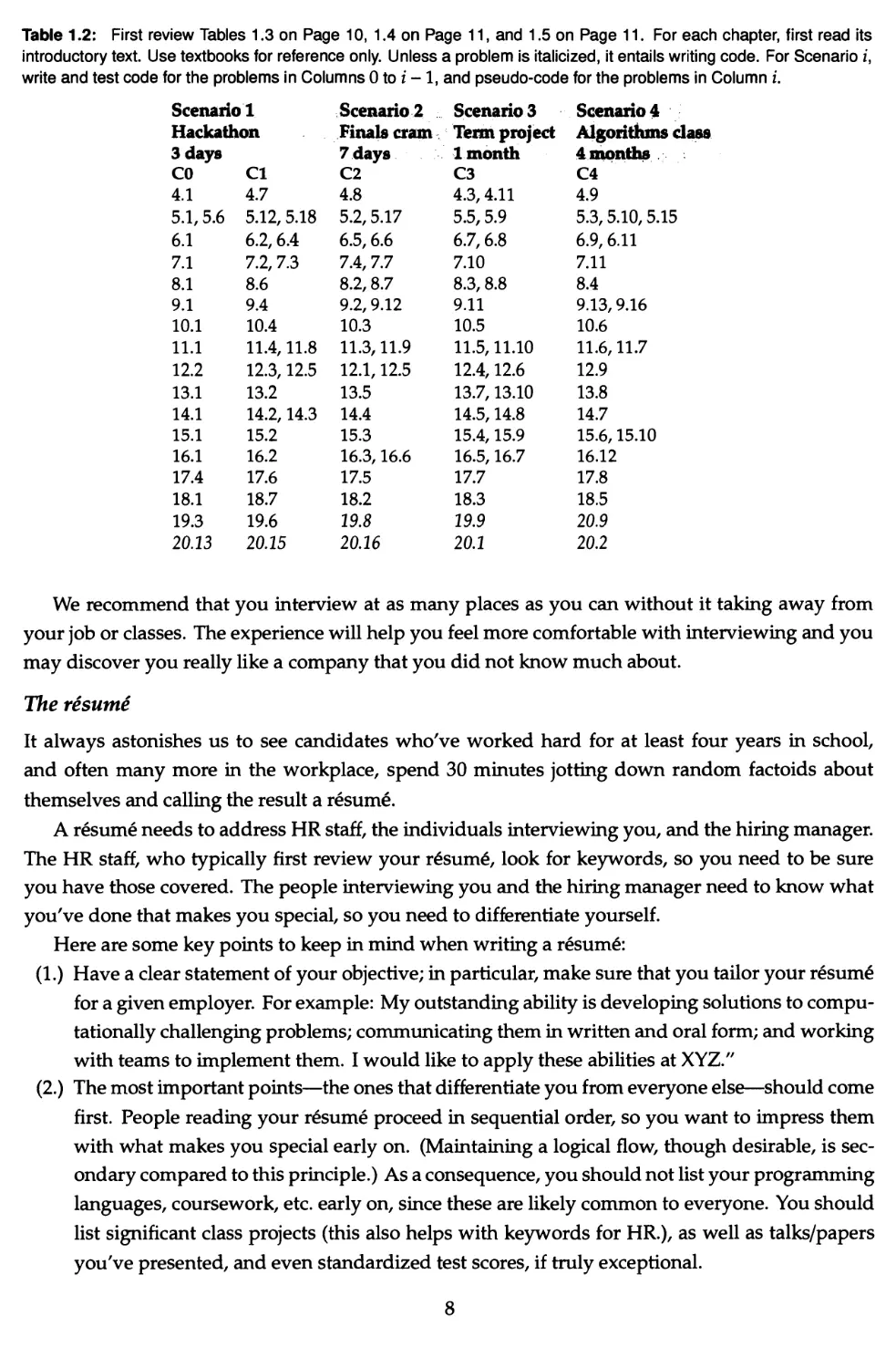
Table 1.2: First review Tables 1.3 on Page 10, 1.4 on Page 11, and 1.5 on Page 11. For each chapter, first read its
introductory text. Use textbooks for reference only. Unless a problem is italicized, it entails writing code. For Scenario z,
write and test code for the problems in Columns 0 to i -1, and pseudo-code for the problems in Column i.
Scenario!
Hackathon
3 days
CO
4.1
5.1, 5.6
6.1
7.1
8.1
9.1
10.1
11.1
12.2
13.1
14.1
15.1
16.1
17.4
18.1
19.3
20.13
CI
4.7
5.12,5.18
6.2,6.4
7.2, 7.3
8.6
9.4
10.4
11.4,11.8
12.3,12.5
13.2
14.2,14.3
15.2
16.2
17.6
18.7
19.6
20.15
Scenario 2
Finals cram
7 days
C2
4.8
5.2,5.17
6.5,6.6
7.4, 7.7
8.2,8.7
9.2,9.12
10.3
11.3,11.9
12.1,12.5
13.5
14.4
15.3
16.3,16.6
17.5
18.2
19.8
20.16
Scenario 3
Term project
1 month
C3
4.3,4.11
5.5,5.9
6.7,6.8
7.10
8.3,8.8
9.11
10.5
11.5,11.10
12.4,12.6
13.7,13.10
14.5,14.8
15.4,15.9
16.5,16.7
17.7
18.3
19.9
20.1
Scenario 4
Algorithms class
4 months
C4
4.9
5.3,5.10,5.15
6.9,6.11
7.11
8.4
9.13,9.16
10.6
11.6,11.7
12.9
13.8
14.7
15.6,15.10
16.12
17.8
18.5
20.9
20.2
We recommend that you interview at as many places as you can without it taking away from
your job or classes. The experience will help you feel more comfortable with interviewing and you
may discover you really like a company that you did not know much about.
The resume
It always astonishes us to see candidates who've worked hard for at least four years in school,
and often many more in the workplace, spend 30 minutes jotting down random factoids about
themselves and calling the result a resume.
A resume needs to address HR staff, the individuals interviewing you, and the hiring manager.
The HR staff, who typically first review your r£sum£, look for keywords, so you need to be sure
you have those covered. The people interviewing you and the hiring manager need to know what
you've done that makes you special, so you need to differentiate yourself.
Here are some key points to keep in mind when writing a resum£:
(1.) Have a clear statement of your objective; in particular, make sure that you tailor your resume
for a given employer. For example: My outstanding ability is developing solutions to
computationally challenging problems; communicating them in written and oral form; and working
with teams to implement them. I would like to apply these abilities at XYZ."
(2.) The most important points—the ones that differentiate you from everyone else—should come
first. People reading your resume proceed in sequential order, so you want to impress them
with what makes you special early on. (Maintaining a logical flow, though desirable, is
secondary compared to this principle.) As a consequence, you should not list your programming
languages, coursework, etc. early on, since these are likely common to everyone. You should
list significant class projects (this also helps with keywords for HR.), as well as talks/papers
you've presented, and even standardized test scores, if truly exceptional.
8

(3.) The r£sum£ should be of a high-quality: no spelling mistakes; consistent spacings,
capitalizations, numberings; and correct grammar and punctuation. Use few fonts. Portable Document
Format (PDF) is preferred, since it renders well across platforms.
(4.) Include contact information, a Linkedln profile, and, ideally, a URL to a personal homepage
with examples of your work. These samples may be class projects, a thesis, and links to
companies and products you've worked on. Include design documents as well as a link to
your version control repository.
(5.) If you can work at the company without requiring any special processing (e.g., if you have a
Green Card, and are applying for a job in the US), make a note of that.
(6.) Have friends review your resum£; they are certain to find problems with it that you missed.
It is better to get something written up quickly, and then refine it based on feedback.
(7.) A r£sum£ does not have to be one page long—two pages are perfectly appropriate. (Over two
pages is probably not a good idea.)
(8.) As a rule, we prefer not to see a list of hobbies/extracurricular activities (e.g., "reading
books", "watching TV", "organizing tea party activities") unless they are really different
(e.g., "Olympic rower") and not controversial.
Whenever possible, have a friend or professional acquaintance at the company route your r£sum£
to the appropriate manager/HR contact—the odds of it reaching the right hands are much higher.
At one company whose practices we are familiar with, a resume submitted through a contact is 50
times more likely to result in a hire than one submitted online. Don't worry about wasting your
contact's time—employees often receive a referral bonus, and being responsible for bringing in stars
is also viewed positively.
Mock interviews
Mock interviews are a great way of preparing for an interview. Get a friend to ask you questions
(from EPI or any other source) and solve them on a whiteboard, with pen and paper, or on a shared
document. Have your friend take notes and give you feedback, both positive and negative. Make
a video recording of the interview. You will cringe as you watch it, but it is better to learn of
your mannerisms beforehand. Ask your friend to give hints when you get stuck. In addition to
sharpening your problem solving and presentation skills, the experience will help reduce anxiety at
the actual interview setting. If you cannot find a friend, you can still go through the same process,
recording yourself.
Data structures, algorithms, and logic
We summarize the data structures, algorithms, and logical principles used in this book in Tables 1.3
on the next page, 1.4 on Page 11, and 1.5 on Page 11, and highly encourage you to review them.
Don't be overly concerned if some of the concepts are new to you, as we will do a bootcamp review
for data structures and algorithms at the start of the corresponding chapters. Logical principles are
applied throughout the book, and we explain a principle in detail when we first use it. You can also
look for the highlighted page in the index to learn more about a term.
Complexity
The run time of an algorithm depends on the size of its input. A common approach to capture the
run time dependency is by expressing asymptotic bounds on the worst-case run time as a function
9

Table 1.3: Data structures
Data structure
Primitive types
Arrays
Strings
Lists
Stacks and queues
Binary trees
Heaps
Hash tables
Binary search trees
Key points
Know how int, char, double, etc. are represented in memory
and the primitive operations on them.
Fast access for element at an index, slow lookups (unless sorted)
and insertions. Be comfortable with notions of iteration,
resizing, partitioning, merging, etc.
Know how strings are represented in memory. Understand
basic operators such as comparison, copying, matching, joining,
splitting, etc.
Understand trade-offs with respect to arrays. Be comfortable
with iteration, insertion, and deletion within singly and
doubly linked lists. Know how to implement a list with dynamic
allocation, and with arrays.
Recognize where last-in first-out (stack) and first-in first-out
(queue) semantics are applicable. Know array and linked list
implementations.
Use for representing hierarchical data. Know about depth,
height, leaves, search path, traversal sequences,
successor/predecessor operations.
Key benefit: 0(1) lookup find-max, 0(logn) insertion, and
0(logri) deletion of max. Node and array representations. Min-
heap variant.
Key benefit: 0(1) insertions, deletions and lookups. Key
disadvantages: not suitable for order-related queries; need for
resizing; poor worst-case performance. Understand implementation
using array of buckets and collision chains. Know hash
functions for integers, strings, objects.
Key benefit: (9(logn) insertions, deletions, lookups, find-min,
find-max, successor, predecessor when tree is height-balanced.
Understand node fields, pointer implementation. Be familiar
with notion of balance, and operations maintaining balance.
of the input size. Specifically, the run time of an algorithm on an input of size n is O (f(n)) if, for
sufficiently large n, the run time is not more than f(n) times a constant.
As an example, searching for a given integer in an unsorted array of integers of length n via
iteration has an asymptotic complexity of 0(n) since in the worst-case, the given integer may not be
present.
Complexity theory is applied in a similar manner when analyzing the space requirements of
an algorithm. The space needed to read in an instance is not included; otherwise, every
algorithm would have 0(n) space complexity. An algorithm that uses 0(1) space should not perform
dynamic memory allocation (explicitly, or indirectly, e.g., through library routines). Furthermore,
the maximum depth of the function call stack should also be a constant, independent of the input.
The standard algorithm for depth-first search of a graph is an example of an algorithm that does
10

Table 1.4: Algorithms
Algorithm type
Sorting
Recursion
Divide-and-conquer
Dynamic programming
Greedy algorithms
Invariants
Graph modeling
Key points
Uncover some structure by sorting the input.
If the structure of the input is defined in a recursive manner,
design a recursive algorithm that follows the input definition.
Divide the problem into two or more smaller independent sub-
problems and solve the original problem using solutions to the
subproblems.
Compute solutions for smaller instances of a given problem and
use these solutions to construct a solution to the problem. Cache
for performance.
Compute a solution in stages, making choices that are locally
optimum at each step; these choices are never undone.
Identify an invariant and use it to rule out potential solutions
that are suboptimal/dominated by other solutions.
Describe the problem using a graph and solve it using an
existing graph algorithm.
Principle
Concrete examples
Case analysis
Iterative refinement
Reduction
Table 1.5: Logical principles
Key points
Manually solve concrete instances and then build a general
solution. Try small inputs, e.g., a BST containing 5-7 elements,
and extremal inputs, e.g., sorted arrays.
Split the input/execution into a number of cases and solve each
case in isolation.
Most problems can be solved using a brute-force approach. Find
such a solution and improve upon it.
Use a known solution to some other problem as a subroutine.
not perform any dynamic allocation, but uses the function call stack for implicit storage—its space
complexity is not 0{\).
A streaming algorithm is one in which the input is presented as a sequence of items and
the algorithm makes a small number of passes over it (typically just one), using a limited amount
memory (much less than the input size) and a limited processing time per item. The best algorithms
for performing aggregation queries on log file data are often streaming algorithms.
Language review
Programs are written and tested in Python 3.6. Most of them will work with earlier versions of
Python as well. Some of the newer language features we use are concurrent. futures for thread
pools, and the ABC for abstract base classes. The only external dependency we have is on bintrees,
which implements a balanced binary search tree (Chapter 14).
11

We review data structures in Python in the corresponding chapters. Here we describe some
Python language features that go beyond the basics that we find broadly applicable. Be sure
you are comfortable with the ideas behind these features, as well as their basic syntax and time
complexity.
• We use inner functions and lambdas, e.g., the sorting code on Page 181. You should be
especially be comfortable with lambda syntax, as well as the variable scoping rules for inner
functions and lambdas.
• We use collections.namedtuples extensively for structured data—these are more readable
than dictionaries, lists, and tuples, and less verbose than classes.
• We use the following constructs to write simpler code: all () and any (), list comprehension,
mapO, functools. reduce() and zipO, and enumerate().
• The following functions from the itertools module are very useful in diverse contexts:
groupbyO, accumulateO, product(), and combinations().
For a handful of problems, when presenting their solution, we also include a Pythonic solution. This
is indicated by the use of _pythonic for the suffix of the function name. These Pythonic programs
are not solutions that interviewers would expect of you—they are supposed to fill you with a sense
of joy and wonder. (If you find Pythonic solutions to problems, please share them with us!)
Best practices for interview code
Now we describe practices we use in EPI that are not suitable for production code. They are
necessitated by the finite time constraints of an interview. See Section 2 on Page 14 for more
insights.
• We make fields public, rather than use getters and setters.
• We do not protect against invalid inputs, e.g., null references, negative entries in an array
that's supposed to be all nonnegative, input streams that contain objects that are not of the
expected type, etc.
Now we describe practices we follow in EPI which are industry-standard, but we would not
recommend for an interview.
• We follow the PEP 8 style guide, which you should review before diving into EPI. The guide is
fairly straightforward—it mostly addresses naming and spacing conventions, which should
not be a high priority when presenting your solution.
An industry best practice that we use in EPI and recommend you use in an interview is explicitly
creating classes for data clumps, i.e., groups of values that do not have any methods on them. Many
programmers would use a generic Pair or Tuple class, but we have found that this leads to confusing
and buggy programs.
Books
Our favorite introduction to Python is Severance's "Python for Informatics: Exploring Information",
which does a great job of covering the language constructs with examples. It is available for free
online.
Brett Slatkin's "Effective Python" is one of the best all-round programming books we have come
across, addressing everything from the pitfalls of default arguments to concurrency patterns.
For design patterns, we like "Head First Design Patterns" by Freeman et ah. Its primary drawback
is its bulk. Note that programs for interviews are too short to take advantage of design patterns.
12

Chapter
2
Strategies For A Great Interview
The essence of strategy is choosing what not to do.
— M. E. Porter
The technical component of an onsite interview usually consists of three to five one-on-one
interviews with engineers. A typical one hour interview with a single interviewer consists of five
minutes of introductions and questions about the candidate's r£sum£. This is followed by five to
fifteen minutes of questioning on basic programming concepts. The core of the interview is one
or two problems where the candidate is expected to present a detailed solution on a whiteboard,
paper, or integrated development environments (IDEs). Depending on the interviewer and the
question, the solution may be required to include syntactically correct code and tests. Junior
candidates should expect more emphasis on coding, and less on system design and architecture. Senior
candidates should expect more emphasis on system design and architecture, though at least one
interviewer will ask a problem that entails writing detailed code.
Approaching the problem
No matter how clever and well prepared you are, the solution to an interview problem may not
occur to you immediately. Here are some things to keep in mind when this happens.
Clarify the question: This may seem obvious but it is amazing how many interviews go badly
because the candidate spends most of his time trying to solve the wrong problem. If a question
seems exceptionally hard, you may have misunderstood it.
A good way of clarifying the question is to state a concrete instance of the problem. For example,
if the question is "find the first occurrence of a number greater than k in a sorted array", you could
ask "if the input array is (2,20,30) and k is 3, then are you supposed to return 1, the index of 20?"
These questions can be formalized as unit tests.
Feel free to ask the interviewer what time and space complexity he would like in your solution. If
you are told to implement an 0(n) algorithm or use (9(1) space, it can simplify your life considerably.
It is possible that he will refuse to specify these, or be vague about complexity requirements, but
there is no harm in asking. Even if they are evasive, you may get some clues.
Work on concrete examples: Consider the problem of determining the smallest amount of
change that you cannot make with a given set of coins, as described on Page 186. This problem
may seem difficult at first. However, if you try out the smallest amount that cannot be made with
some small examples, e.g., {1,2}, {1,3}, {1,2,4}, {1,2,5}, you will get the key insights: examine coins
in sorted order, and look for a large "jump"—a coin which is larger than the sum of the preceding
coins.
13

Spell out the brute-force solution: Problems that are put to you in an interview tend to have
an obvious brute-force solution that has a high time complexity compared to more sophisticated
solutions. For example, instead of trying to work out a DP solution for a problem (e.g., for
Problem 16.7 on Page 249), try all the possible configurations. Advantages to this approach include:
(1.) it helps you explore opportunities for optimization and hence reach a better solution, (2.) it gives
you an opportunity to demonstrate some problem solving and coding skills, and (3.) it establishes
that both you and the interviewer are thinking about the same problem. Be warned that this strategy
can sometimes be detrimental if it takes a long time to describe the brute-force approach.
Think out loud: One of the worst things you can do in an interview is to freeze up when solving
the problem. It is always a good idea to think out loud and stay engaged. On the one hand, this
increases your chances of finding the right solution because it forces you to put your thoughts in
a coherent manner. On the other hand, this helps the interviewer guide your thought process in
the right direction. Even if you are not able to reach the solution, the interviewer will form some
impression of your intellectual ability.
Apply patterns: Patterns—general reusable solutions to commonly occurring problems—can
be a good way to approach a baffling problem. Examples include finding a good data structure,
seeing if your problem is a good fit for a general algorithmic technique, e.g., divide-and-conquer,
recursion, or dynamic programming, and mapping the problem to a graph.
Presenting the solution
Once you have an algorithm, it is important to present it in a clear manner. Your solution will
be much simpler if you take advantage of libraries such as Java Collections, C++ STL, or Python
collections. However, it is far more important that you use the language you are most comfortable
with. Here are some things to keep in mind when presenting a solution.
Libraries: Do not reinvent the wheel (unless asked to invent it). In particular, master the
libraries, especially the data structures. For example, do not waste time and lose credibility trying
to remember how to pass an explicit comparator to a BST constructor. Remember that a hash
function should use exactly those fields which are used in the equality check. A comparison
function should be transitive.
Focus on the top-level algorithm: It's OK to use functions that you will implement later. This
will let you focus on the main part of the algorithm, will penalize you less if you don't complete the
algorithm. (Hash, equals, and compare functions are good candidates for deferred implementation.)
Specify that you will handle main algorithm first, then corner cases. Add TODO comments for
portions that you want to come back to.
Manage the whiteboard: You will likely use more of the board than you expect, so start at the
top-left corner. Make use of functions—skip implementing anything that's trivial (e.g., finding the
maximum of an array) or standard (e.g., a thread pool). Best practices for coding on a whiteboard
are very different from best practices for coding on a production project. For example, don't worry
about skipping documentation, or using the right indentation. Writing on a whiteboard is much
slower than on a keyboard, so keeping your identifiers short (our recommendation is no more than
7 characters) but recognizable is a best practice. Have a convention for identifiers, e.g., i, j , k for
array indices, A, B, C for arrays, s for string, d for diet, etc.
14

Assume valid inputs: In a production environment, it is good practice to check if inputs are
valid, e.g., that a string purporting to represent a nonnegative integer actually consists solely of
numeric characters, no flight in a timetable arrives before it departs, etc. Unless they are part of the
problem statement, in an interview setting, such checks are inappropriate: they take time to code,
and distract from the core problem. (You should clarify this assumption with the interviewer.)
Test for corner cases: For many problems, your general idea may work for most valid inputs
but there may be pathological valid inputs where your algorithm (or your implementation of it)
fails. For example, your binary search code may crash if the input is an empty array; or you may
do arithmetic without considering the possibility of overflow. It is important to systematically
consider these possibilities. If there is time, write unit tests. Small, extreme, or random inputs
make for good stimuli. Don't forget to add code for checking the result. Occasionally, the code to
handle obscure corner cases may be too complicated to implement in an interview setting. If so,
you should mention to the interviewer that you are aware of these problems, and could address
them if required.
Syntax: Interviewers rarely penalize you for small syntax errors since modern IDE excel at
handling these details. However, lots of bad syntax may result in the impression that you have
limited coding experience. Once you are done writing your program, make a pass through it to fix
any obvious syntax errors before claiming you are done.
Candidates often tend to get function signatures wrong and it reflects poorly on them. For
example, it would be an error to write a function in C that returns an array but not its size.
Memory management: Generally speaking, it is best to avoid memory management operations
altogether. See if you can reuse space. For example, some linked list problems can be solved with
(9(1) additional space by reusing existing nodes.
Your Interviewer Is Not Alan Turing: Interviewers are not capable of analyzing long programs,
particularly on a whiteboard or paper. Therefore, they ask questions whose solutions use short
programs. A good tip is that if your solution takes more than 50 lines to code in Python, it's a sign
that you are on the wrong track, and you should reconsider your approach.
Know your interviewers & the company
It can help you a great deal if the company can share with you the background of your interviewers
in advance. You should use search and social networks to learn more about the people interviewing
you. Letting your interviewers know that you have researched them helps break the ice and forms
the impression that you are enthusiastic and will go the extra mile. For fresh graduates, it is also
important to think from the perspective of the interviewers as described in Chapter 3.
Once you ace your interviews and have an offer, you have an important decision to make—is this
the organization where you want to work? Interviews are a great time to collect this information.
Interviews usually end with the interviewers letting the candidates ask questions. You should
make the best use of this time by getting the information you would need and communicating to
the interviewer that you are genuinely interested in the job. Based on your interaction with the
interviewers, you may get a good idea of their intellect, passion, and fairness. This extends to the
team and company.
In addition to knowing your interviewers, you should know about the company vision, history,
organization, products, and technology. You should be ready to talk about what specifically appeals
15

to you, and to ask intelligent questions about the company and the job. Prepare a list of questions
in advance; it gets you helpful information as well as shows your knowledge and enthusiasm for
the organization. You may also want to think of some concrete ideas around things you could do
for the company; be careful not to come across as a pushy know-it-all.
All companies want bright and motivated engineers. However, companies differ greatly in their
culture and organization. Here is a brief classification.
Mature consumer-facing company, e.g., Google: wants candidates who understand emerging
technologies from the user's perspective. Such companies have a deeper technology stack, much
of which is developed in-house. They have the resources and the time to train a new hire.
Enterprise-oriented company, e.g., Oracle: looks for developers familiar with how large projects
are organized, e.g., engineers who are familiar with reviews, documentation, and rigorous testing.
Government contractor, e.g., Lockheed-Martin: values knowledge of specifications and testing,
and looks for engineers who are familiar with government-mandated processes.
Startup, e.g., Uber: values engineers who take initiative and develop products on their own.
Such companies do not have time to train new hires, and tend to hire candidates who are very fast
learners or are already familiar with their technology stack, e.g., their web application framework,
machine learning system, etc.
Embedded systems/chip design company, e.g., National Instruments: wants software
engineers who know enough about hardware to interface with the hardware engineers. The tool chain
and development practices at such companies tend to be very mature.
General conversation
Often interviewers will ask you questions about your past projects, such as a senior design project
or an internship. The point of this conversation is to answer the following questions:
Can the candidate clearly communicate a complex idea? This is one of the most important
skills for working in an engineering team. If you have a grand idea to redesign a big system, can
you communicate it to your colleagues and bring them on board? It is crucial to practice how you
will present your best work. Being precise, clear, and having concrete examples can go a long way
here. Candidates communicating in a language that is not their first language, should take extra
care to speak slowly and make more use of the whiteboard to augment their words.
Is the candidate passionate about his work? We always want our colleagues to be excited,
energetic, and inspiring to work with. If you feel passionately about your work, and your eyes light
up when describing what you've done, it goes a long way in establishing you as a great colleague.
Hence, when you are asked to describe a project from the past, it is best to pick something that you
are passionate about rather than a project that was complex but did not interest you.
Is there a potential interest match with some project? The interviewer may gauge areas of
strengths for a potential project match. If you know the requirements of the job, you may want
to steer the conversation in that direction. Keep in mind that because technology changes so fast
many teams prefer a strong generalist, so don't pigeonhole yourself.
Other advice
A bad mental and physical attitude can lead to a negative outcome. Don't let these simple mistakes
lead to your years of preparation going to waste.
16

Be honest: Nobody wants a colleague who falsely claims to have tested code or done a code
review Dishonesty in an interview is a fast pass to an early exit.
Remember, nothing breaks the truth more than stretching it—you should be ready to defend
anything you claim on your r£sum£. If your knowledge of Python extends only as far as having
cut-and-paste sample code, do not add Python to your r£sum£.
Similarly, if you have seen a problem before, you should say so. (Be sure that it really is the
same problem, and bear in mind you should describe a correct solution quickly if you claim to have
solved it before.) Interviewers have been known to collude to ask the same question of a candidate
to see if he tells the second interviewer about the first instance. An interviewer may feign ignorance
on a topic he knows in depth to see if a candidate pretends to know it.
Keep a positive spirit: A cheerful and optimistic attitude can go a long way. Absolutely nothing
is to be gained, and much can be lost, by complaining how difficult your journey was, how you are
not a morning person, how inconsiderate the airline/hotel/HR staff were, etc.
Don't apologize: Candidates sometimes apologize in advance for a weak GPA, rusty coding
skills, or not knowing the technology stack. Their logic is that by being proactive they will somehow
benefit from lowered expectations. Nothing can be further from the truth. It focuses attention on
shortcomings. More generally, if you do not believe in yourself, you cannot expect others to believe
in you.
Keep money and perks out of the interview: Money is a big element in any job but it is best
left discussed with the HR division after an offer is made. The same is true for vacation time, day
care support, and funding for conference travel.
Appearance: Most software companies have a relaxed dress-code, and new graduates may
wonder if they will look foolish by overdressing. The damage done when you are too casual is
greater than the minor embarrassment you may feel at being overdressed. It is always a good idea
to err on the side of caution and dress formally for your interviews. At the minimum, be clean and
well-groomed.
Be aware of your body language: Think of a friend or coworker slouched all the time or
absentmindedly doing things that may offend others. Work on your posture, eye contact and
handshake, and remember to smile.
Stress interviews
Some companies, primarily in the finance industry, make a practice of having one of the interviewers
create a stressful situation for the candidate. The stress may be injected technically, e.g., via a ninja
problem, or through behavioral means, e.g., the interviewer rejecting a correct answer or ridiculing
the candidate. The goal is to see how a candidate reacts to such situations—does he fall apart,
become belligerent, or get swayed easily. The guidelines in the previous section should help you
through a stress interview. (Bear in mind you will not know a priori if a particular interviewer will
be conducting a stress interview.)
Learning from bad outcomes
The reality is that not every interview results in a job offer. There are many reasons for not getting
a particular job. Some are technical: you may have missed that key flash of insight, e.g., the key
17

to solving the maximum-profit on Page 1 in linear time. If this is the case, go back and solve that
problem, as well as related problems.
Often, your interviewer may have spent a few minutes looking at your r£sum£—this is a
depressingly common practice. This can lead to your being asked questions on topics outside of the
area of expertise you claimed on your r£sum£, e.g., routing protocols or Structured Query Language
(SQL). If so, make sure your resume is accurate, and brush up on that topic for the future.
You can fail an interview for nontechnical reasons, e.g., you came across as uninterested, or you
did not communicate clearly. The company may have decided not to hire in your area, or another
candidate with similar ability but more relevant experience was hired.
You will not get any feedback from a bad outcome, so it is your responsibility to try and piece
together the causes. Remember the only mistakes are the ones you don't learn from.
Negotiating an offer
An offer is not an offer till it is on paper, with all the details filled in. All offers are negotiable.
We have seen compensation packages bargained up to twice the initial offer, but 10-20% is more
typical. When negotiating, remember there is nothing to be gained, and much to lose, by being
rude. (Being firm is not the same as being rude.)
To get the best possible offer, get multiple offers, and be flexible about the form of your
compensation. For example, base salary is less flexible than stock options, sign-on bonus, relocation
expenses, and Immigration and Naturalization Service (INS) filing costs. Be concrete—instead of
just asking for more money, ask for a P% higher salary. Otherwise the recruiter will simply come
back with a small increase in the sign-on bonus and claim to have met your request.
Your HR contact is a professional negotiator, whose fiduciary duty is to the company. He will
know and use negotiating techniques such as reciprocity, getting consensus, putting words in your
mouth ("don't you think that's reasonable?"), as well as threats, to get the best possible deal for the
company. (This is what recruiters themselves are evaluated on internally.) The Wikipedia article on
negotiation lays bare many tricks we have seen recruiters employ.
One suggestion: stick to email, where it is harder for someone to paint you into a corner. If you
are asked for something (such as a copy of a competing offer), get something in return. Often it is
better to bypass the HR contact and speak directly with the hiring manager.
At the end of the day, remember your long term career is what counts, and joining a company
that has a brighter future (social-mobile vs. legacy enterprise), or offers a position that has more
opportunities to rise (developer vs. tester) is much more important than a 10-20% difference in
compensation.
18

Chapter
3
Conducting An Interview
Translated—"If you know both yourself and your
enemy, you can win numerous battles without jeopardy."
— "The Art of War/'
Sun Tzu, 515 B.C.
In this chapter we review practices that help interviewers identify a top hire. We strongly
recommend interviewees read it—knowing what an interviewer is looking for will help you present
yourself better and increase the likelihood of a successful outcome.
For someone at the beginning of their career, interviewing may feel like a huge responsibility.
Hiring a bad candidate is expensive for the organization, not just because the hire is unproductive,
but also because he is a drain on the productivity of his mentors and managers, and sets a bad
example. Firing someone is extremely painful as well as bad for to the morale of the team. On
the other hand, discarding good candidates is problematic for a rapidly growing organization.
Interviewers also have a moral responsibility not to unfairly crush the interviewee's dreams and
aspirations.
Objective
The ultimate goal of any interview is to determine the odds that a candidate will be a successful
employee of the company. The ideal candidate is smart, dedicated, articulate, collegial, and gets
things done quickly, both as an individual and in a team. Ideally, your interviews should be
designed such that a good candidate scores 1.0 and a bad candidate scores 0.0.
One mistake, frequently made by novice interviewers, is to be indecisive. Unless the candidate
walks on water or completely disappoints, the interviewer tries not to make a decision and scores
the candidate somewhere in the middle. This means that the interview was a wasted effort.
A secondary objective of the interview process is to turn the candidate into a brand ambassador
for the recruiting organization. Even if a candidate is not a good fit for the organization, he may
know others who would be. It is important for the candidate to have an overall positive experience
during the process. It seems obvious that it is a bad idea for an interviewer to check email while
the candidate is talking or insult the candidate over a mistake he made, but such behavior is
depressingly common. Outside of a stress interview, the interviewer should work on making the
candidate feel positively about the experience, and, by extension, the position and the company.
19

One important question you should ask yourself as an interviewer is how much training time your
work environment allows. For a startup it is important that a new hire is productive from the first
week, whereas a larger organization can budget for several months of training. Consequently, in a
startup it is important to test the candidate on the specific technologies that he will use, in addition
to his general abilities.
For a larger organization, it is reasonable not to emphasize domain knowledge and instead test
candidates on data structures, algorithms, system design skills, and problem solving techniques.
The justification for this is as follows. Algorithms, data structures, and system design underlie all
software. Algorithms and data structure code is usually a small component of a system dominated
by the user interface (UI), input/output (I/O), and format conversion. It is often hidden in library
calls. However, such code is usually the crucial component in terms of performance and correctness,
and often serves to differentiate products. Furthermore, platforms and programming languages
change quickly but a firm grasp of data structures, algorithms, and system design principles, will
always be a foundational part of any successful software endeavor. Finally, many of the most
successful software companies have hired based on ability and potential rather than experience or
knowledge of specifics, underlying the effectiveness of this approach to selecting candidates.
Most big organizations have a structured interview process where designated interviewers are
responsible for probing specific areas. For example, you may be asked to evaluate the candidate on
their coding skills, algorithm knowledge, critical thinking, or the ability to design complex systems.
This book gives interviewers access to a fairly large collection of problems to choose from. When
selecting a problem keep the following in mind:
No single point of failure—if you are going to ask just one question, you should not pick a
problem where the candidate passes the interview if and only if he gets one particular insight. The
best candidate may miss a simple insight, and a mediocre candidate may stumble across the right
idea. There should be at least two or three opportunities for the candidates to redeem themselves.
For example, problems that can be solved by dynamic programming can almost always be solved
through a greedy algorithm that is fast but suboptimum or a brute-force algorithm that is slow but
optimum. In such cases, even if the candidate cannot get the key insight, he can still demonstrate
some problem solving abilities. Problem 5.6 on Page 46 exemplifies this type of question.
Multiple possible solutions—if a given problem has multiple solutions, the chances of a good
candidate coming up with a solution increases. It also gives the interviewer more freedom to steer
the candidate. A great candidate may finish with one solution quickly enough to discuss other
approaches and the trade-offs between them. For example, Problem 11.9 on Page 155 can be solved
using a hash table or a bit array; the best solution makes use of binary search.
Cover multiple areas—even if you are responsible for testing the candidate on algorithms, you
could easily pick a problem that also exposes some aspects of design and software development.
For example, Problem 19.8 on Page 298 tests candidates on concurrency as well as data structures.
Problem 5.16 on Page 58 requires knowledge of both probability and binary search.
Calibrate on colleagues—interviewers often have an incorrect notion of how difficult a problem
is for a thirty minute or one hour interview. It is a good idea to check the appropriateness of a
problem by asking one of your colleagues to solve it and seeing how much difficulty they have with
20

it.
No unnecessary domain knowledge—it is not a good idea to quiz a candidate on advanced
graph algorithms if the job does not require it and the candidate does not claim any special
knowledge of the field. (The exception to this rule is if you want to test the candidate's response to
stress.)
Conducting the interview
Conducting a good interview is akin to juggling. At a high level, you want to ask your questions
and evaluate the candidate's responses. Many things can happen in an interview that could help
you reach a decision, so it is important to take notes. At the same time, it is important to keep a
conversation going with the candidate and help him out if he gets stuck. Ideally, have a series of
hints worked out beforehand, which can then be provided progressively as needed. Coming up
with the right set of hints may require some thinking. You do not want to give away the problem,
yet find a way for the candidate to make progress. Here are situations that may throw you off:
A candidate that gets stuck and shuts up: Some candidates get intimidated by the problem, the
process, or the interviewer, and just shut up. In such situations, a candidate's performance does
not reflect his true caliber. It is important to put the candidate at ease, e.g., by beginning with a
straightforward question, mentioning that a problem is tough, or asking them to think out loud.
A verbose candidate: Candidates who go off on tangents and keep on talking without making
progress render an interview ineffective. Again, it is important to take control of the conversation.
For example you could assert that a particular path will not make progress.
An overconfident candidate: It is common to meet candidates who weaken their case by
defending an incorrect answer. To give the candidate a fair chance, it is important to demonstrate
to him that he is making a mistake, and allow him to correct it. Often the best way of doing this is
to construct a test case where the candidate's solution breaks down.
Scoring and reporting
At the end of an interview, the interviewers usually have a good idea of how the candidate scored.
However, it is important to keep notes and revisit them before making a final decision. Whiteboard
snapshots and samples of any code that the candidate wrote should also be recorded. You should
standardize scoring based on which hints were given, how many questions the candidate was able
to get to, etc. Although isolated minor mistakes can be ignored, sometimes when you look at all the
mistakes together, clear signs of weakness in certain areas may emerge, such as a lack of attention
to detail and unfamiliarity with a language.
When the right choice is not clear, wait for the next candidate instead of possibly making a bad
hiring decision. The litmus test is to see if you would react positively to the candidate replacing a
valuable member of your team.
21

Part II
Data Structures and Algorithms

Chapter
s4
Primitive Types
Representation is the essence of programming.
— "The Mythical Man Month"
F. P. Brooks, 1975
A program updates variables in memory according to its instructions. Variables come in types—a
type is a classification of data that spells out possible values for that type and the operations that
can be performed on it. A type can be provided by the language or defined by the programmer. In
Python everything is an object—this includes Booleans, integers, characters, etc.
Primitive types boot camp
Writing a program to count the number of bits that are set to 1 in a positive integer is a good way to
get up to speed with primitive types. The following program tests bits one-at-a-time starting with
the least-significant bit. It illustrates shifting and masking; it also shows how to avoid hard-coding
the size of the integer word.
def count_bits(x):
num_bits = 0
while x:
num_bits += x & 1
x »= 1
return num_bits
Since we perform 0(1) computation per bit, the time complexity is 0(n), where n is the number of
bits needed to represent the integer, e.g., 4 bits are needed to represent 12, which is (1100)2 in binary.
The techniques in Solution 4.1 on the next page, which is concerned with counting the number of
bits mod 2, i.e., the parity, can be used to improve the performance of the program given above.
Know your primitive types
Python has a number of built-in types: numerics (e.g., integer), sequences (e.g., list), mappings (e.g.,
diet), as well as classes, instances and exceptions. All instances of these types are objects.
Integers in Python3 are unbounded—the maximum integer representable is a function of the
available memory. The constant sys.maxsize can be used to find the word-size; specifically, it's
the maximum value integer that can be stored in the word, e.g., 2**63 - 1 on a 64-bit machine.
Bounds on floats are specified in sys. f loat_info.
• Be very familiar with the bit-wise operators such as 6&4,112, 8»1, -16»2, 1«10, "0, 15~x.
Negative numbers are treated as their 2's complement value. (There is no concept of an
unsigned shift in Python, since integers have infinite precision.)
23

Be very comfortable with the bitwise operators, particularly XOR.
Understand how to use masks and create them in an machine independent way.
Know fast ways to clear the lowermost set bit (and by extension, set the lowermost 0, get its
index, etc.)
Understand signedness and its implications to shifting.
Consider using a cache to accelerate operations by using it to brute-force small inputs.
Be aware that commutativity and associativity can be used to perform operations in parallel
and reorder operations.
Table 4.1: Top Tips for Primitive Types
• The key methods for numeric types are abs(-34.5), math.ceil(2.17), math.floor(3.14),
min(xf-4), max(3.14, y), pow(2.71, 3.14) (alternately, 2.71 ** 3.14), and
math.sqrt(225).
• Know how to interconvert integers and strings, e.g., str (42) , int ('42'), floats and strings,
e.g., str(3.14), float('3.14').
• Unlike integers, floats are not infinite precision, and it's convenient to refer to infinity as
f loat (' inf') and f loat (' -inf'). These values are comparable to integers, and can be used
to create psuedo max-int and pseudo min-int.
• When comparing floating point values consider using math.iscloseO—it is robust, e.g.,
when comparing very large values, and can handle both absolute and relative differences.
• The key methods in random are random.randrange(28), random.randint(8,16),
random. random(), random. shuffle(A), and random, choice (A).
4.1 Computing the parity of a word
The parity of a binary word is 1 if the number of Is in the word is odd; otherwise, it is 0. For
example, the parity of 1011 is 1, and the parity of 10001000 is 0. Parity checks are used to detect
single bit errors in data storage and communication. It is fairly straightforward to write code that
computes the parity of a single 64-bit word.
How would you compute the parity of a very large number of 64-bit words?
Hint: Use a lookup table, but don't use 2M entries!
Solution: The brute-force algorithm iteratively tests the value of each bit while tracking the number
of Is seen so far. Since we only care if the number of Is is even or odd, we can store the number
mod 2.
def parity(x):
result = 0
while x:
result A= x & 1
24

X »= 1
return result
The time complexity is 0(n), where n is the word size.
We will now describe several algorithms for parity computation that are superior to the brute-
force algorithm.
The first improvement is based on erasing the lowest set bit in a word in a single operation,
thereby improving performance in the best- and average-cases. Here is a great bit-fiddling trick
which you should commit to memory: x &c(x - 1) equals x with its lowest set bit erased. (Here
& is the bitwise-AND operator.) ! For example, if x = (00101100)2, then x - 1 = (00101011)2/
so x &(x - 1) = (00101100)2&(00101011)2 = (00101000)2. This fact can be used to reduce the time
complexity. Let k be the number of bits set to 1 in a particular word. (For example, for 10001010,
k = 3.) Then time complexity of the algorithm below is 0(k).
def parity(x):
result = ®
while x:
result A= 1
x &= x - 1 # Drops the lowest set bit of x.
return result
We now consider a qualitatively different approach. The problem statement refers to computing
the parity for a very large number of words. When you have to perform a large number of parity
computations, and, more generally, any kind of bit fiddling computations, two keys to performance
are processing multiple bits at a time and caching results in an array-based lookup table.
First we demonstrate caching. Clearly, we cannot cache the parity of every 64-bit integer—we
would need 2^ bits of storage, which is of the order of two exabytes. However, when computing
the parity of a collection of bits, it does not matter how we group those bits, i.e., the computation is
associative. Therefore, we can compute the parity of a 64-bit integer by grouping its bits into four
nonoverlapping 16 bit subwords, computing the parity of each subwords, and then computing the
parity of these four subresults. We choose 16 since 216 = 65536 is relatively small, which makes it
feasible to cache the parity of all 16-bit words using an array. Furthermore, since 16 evenly divides
64, the code is simpler than if we were, for example, to use 10 bit subwords.
We illustrate the approach with a lookup table for 2-bit words. The cache is (0,1,1,0)—these
are the parities of (00), (01), (10), (11), respectively. To compute the parity of (11001010) we would
compute the parities of (11), (00), (10), (10). By table lookup we see these are 0,0,1,1, respectively,
so the final result is the parity of 0,0,1,1 which is 0.
To lookup the parity of the first two bits in (11101010), we right shift by 6, to get (00000011), and
use this as an index into the cache. To lookup the parity of the next two bits, i.e., (10), we right shift
by 4, to get (10) in the two least-significant bit places. The right shift does not remove the leading
(11)—it results in (00001110). We cannot index the cache with this, it leads to an out-of-bounds
access. To get the last two bits after the right shift by 4, we bitwise-AND (00001110) with (00000011)
(this is the "mask" used to extract the last 2 bits). The result is (00000010). Similar masking is
needed for the two other 2-bit lookups.
Another key bit-fiddling trick: x & ~(x - 1) isolates the lowest bit that is 1 in x; here ~ is the bitwise complement
operator.
25

def parity(x):
MASK_SIZE = 16
BIT.MASK = SxFFFF
return (PRECOMPUTED_PARITY[x » (3 * MASK.SIZE)] A
PRECOMPUTED_PARITY[(x » (2 * MASK.SIZE)) & BIT.MASK] A
PRECOMPUTED_PARITY[(x » MASK.SIZE)
& BIT.MASK] A PRECOMPUTED_PARlTY[x & BIT.MASK])
The time complexity is a function of the size of the keys used to index the lookup table. Let L be
the width of the words for which we cache the results, and n the word size. Since there are n/L
terms, the time complexity is <9(n/L), assuming word-level operations, such as shifting, take 0(1)
time. (This does not include the time for initialization of the lookup table.)
We can improve on the 0(n) worst-case time complexity of the previous algorithms by exploiting
some simple properties of parity. Specifically, the XOR of two bits is defined to be 0 if both bits are
0 or both bits are 1; otherwise it is 1. XOR has the property of being associative, i.e., it does not
matter how we group bits, as well as commutative, i.e., the order in which we perform the XORs
does not change the result. The XOR of a group of bits is its parity. We can exploit this fact to use
the CPU's word-level XOR instruction to process multiple bits at a time.
For example, the parity of (bes, b^i,..., b^, &2/ b\, bo) equals the parity of the XOR of
(^63/ ^62/ • • • / ^32) and ({?3i, {?3o,..., bo). The XOR of these two 32-bit values can be computed with a
single shift and a single 32-bit XOR instruction. We repeat the same operation on 32-, 16-, 8-, 4-,
2-, and 1-bit operands to get the final result. Note that the leading bits are not meaningful, and we
have to explicitly extract the result from the least-significant bit.
We illustrate the approach with an 8-bit word. The parity of (11010111) is the same as the parity
of (1101) XORed with (0111), i.e., of (1010). This in turn is the same as the parity of (10) XORed with
(10), i.e., of (00). The final result is the XOR of (0) with (0), i.e., 0. Note that the first XOR yields
(11011010), and only the last 4 bits are relevant going forward. The second XOR yields (11101100),
and only the last 2 bits are relevant. The third XOR yields (10011010). The last bit is the result, and
to extract it we have to bitwise-AND with (00000001).
def parity(x):
x A= x » 32
x A= x » 16
x A= x » 8
x A= x » 4
x A= x » 2
x A= x » 1
return x & 0x1
The time complexity is O(logn), where n is the word size.
Note that we can combine caching with word-level operations, e.g., by doing a lookup in the
XOR-based approach once we get to 16 bits.
The actual runtimes depend on the input data, e.g., the refinement of the brute-force algorithm
is very fast on sparse inputs. However, for random inputs, the refinement of the brute-force is
roughly 20% faster than the brute-force algorithm. The table-based approach is four times faster
still, and using associativity reduces run time by another factor of two.
26

Variant: Write expressions that use bitwise operators, equality checks, and Boolean operators to do
the following in 0(1) time.
• Right propagate the rightmost set bit in x, e.g., turns (01010000)2 to (01011111)2.
• Compute x mod a power of two, e.g., returns 13 for 77 mod 64.
• Test if x is a power of 2, i.e., evaluates to true for x = 1,2,4,8,..., false for all other values.
4.2 Swap bits
There are a number of ways in which bit manipulations can be accelerated. For example, as
described on Page 23, the expression x & (x -1) clears the lowest set bit in x, and x & ~(x -1) extracts
the lowest set bit of x. Here are a few examples: 16&(16 -1) = 0,11&(11 -1) = 10,20&(20 -1) = 16,
16&~(16 - 1) = 16,11&~(11 - 1) = 1, and 20&~(20 - 1) = 4.
0
1
0
0
1
0
0
1
0
0
0
0
1
0
1
1
MSB LSB MSB LSB
(a) The 8-bit integer 73 can be viewed as array of bits, (b) The result of swapping the bits at indices 1 and 6, with
with the LSB being at index 0. the LSB being at index 0. The corresponding integer is 11.
Figure 4.1: Example of swapping a pair of bits.
A 64-bit integer can be viewed as an array of 64 bits, with the bit at index 0 corresponding to the
least significant bit (LSB), and the bit at index 63 corresponding to the most significant bit (MSB).
Implement code that takes as input a 64-bit integer and swaps the bits at indices i and ;. Figure 4.1
illustrates bit swapping for an 8-bit integer.
Hint: When is the swap necessary?
Solution: A brute-force approach would be to use bitmasks to extract the zth and ;th bits, saving
them to local variables. Consequently, write the saved ;th bit to index i and the saved ith bit to
index j, using a combination of bitmasks and bitwise operations.
The brute-force approach works generally, e.g., if we were swapping objects stored in an array.
However, since a bit can only take two values, we can do a little better. Specifically, we first test if
the bits to be swapped differ. If they do not, the swap does not change the integer. If the bits are
different, swapping them is the same as flipping their individual values. For example in Figure 4.1,
since the bits at Index 1 and Index 6 differ, flipping each bit has the effect of a swap.
In the code below we use standard bit-fiddling idioms for testing and flipping bits. Overall, the
resulting code is slightly more succinct and efficient than the brute force approach.
def swap_bits(x, i, j):
# Extract the i-th and j-th bits, and see if they differ.
if (x » i) & 1 != (x » j) & 1:
# i-th and j-th bits differ. We will swap them by flipping their values.
# Select the bits to flip with bit_mask. Since xAl = 0 when x = 1 and 1
# when x = 0, we can perform the flip XOR.
bit_mask = (1 « i) I (1 « j)
x A= bit.mask
return x
27

The time complexity is 0{\), independent of the word size.
4.3 Reverse bits
Write a program that takes a 64-bit unsigned integer and returns the 64-bit unsigned integer
consisting of the bits of the input in reverse order. For example, if the input is (1110000000000001), the
output should be (1000000000000111).
Hint: Use a lookup table.
Solution: If we need to perform this operation just once, there is a simple brute-force algorithm:
iterate through the 32 least significant bits of the input, and swap each with the corresponding most
significant bit, using, for example, the approach in Solution 4.2 on the preceding page.
To implement reverse when the operation is to be performed repeatedly, we look more carefully
at the structure of the input, with an eye towards using a cache. Let the input consist of the four 16-
bit integers y3,1/2, i/i, yo, with y3 holding the most significant bits. Then the 16 least significant bits
in the reverse come from y3. To be precise, these bits appear in the reverse order in which they do in
y3. For example, if y3 is (1110000000000001), then the 16 LSBs of the result are (1000000000000111).
Similar to computing parity (Problem 4.1 on Page 24), a very fast way to reverse bits for 16-bit
integer when we are performing many reverses is to build an array-based lookup-table A such that
for every 16-bit integer y, A[y] holds the bit-reversal of y. We can then form the reverse of x with
the reverse of yo in the most significant bit positions, followed by the reverse of y\, followed by the
reverse of y2, followed by the reverse of y3.
We illustrate the approach with 8-bit integers and 2-bit lookup table keys. The table is rev =
<(00),(10),(01),(11)). If the input is (10010011), its reverse is rev(ll),rev(00),rev(01),rev(10), i.e.,
(11001001).
def reverse_bits(x):
MASK_SIZE = 16
BIT.MASK = OxFFFF
return (PREC0MPUTED_REVERSE[x & BIT_MASK] « (3 * MASK_SIZE)
I PREC0MPUTED_REVERSE[(x » MASK.SIZE) & BIT.MASK] «
(2 * MASK.SIZE) I
PRECOMPUTED_REVERSE[(x » (2 * MASK_SIZE)) & BIT_MASK] « MASK_SIZE
| PRECOMPUTED_REVERSE[(x » (3 * MASK_SIZE)) & BIT_MASK])
The time complexity is identical to that for Solution 4.1 on Page 24, i.e., 0(n/L), for n-bit integers
and L-bit cache keys.
4.4 Find a closest integer with the same weight
Define the weight of a nonnegative integer x to be the number of bits that are set to 1 in its binary
representation. For example, since 92 in base-2 equals (1011100)2, the weight of 92 is 4.
Write a program which takes as input a nonnegative integer x and returns a number y which is not
equal to x, but has the same weight as x and their difference, \y - x\, is as small as possible. You can
assume x is not 0, or all Is. For example, if x = 6, you should return 5. You can assume the integer
fits in 64 bits.
28

Hint: Start with the least significant bit.
Solution: A brute-force approach might be to try all integers x - 1, x + 1, x - 2, x + 2,..., stopping
as soon as we encounter one with the same weight at x. This performs very poorly on some inputs.
One way to see this is to consider the case where x = 23 = 8. The only numbers with a weight of
1 are powers of 2. Thus, the algorithm will try the following sequence: 7,9,6,10,5,11,4, stopping
at 4 (since its weight is the same as 8's weight). The algorithm tries 23"1 numbers smaller than 8,
namely, 7,6,5,4, and 23"1 - 1 numbers greater than 8, namely, 9,10,11. This example generalizes.
Suppose x - 230. The power of 2 nearest to 230 is 229. Therefore this computation will evaluate the
weight of all integers between 230 and 229 and between 230 and 230 + 229 - 1, i.e., over one billion
integers.
Heuristically, it is natural to focus on the LSB of the input, specifically, to swap the LSB with
rightmost bit that differs from it. This yields the correct result for some inputs, e.g., for (10)2 it
returns (01)2, which is the closest possible. However, more experimentation shows this heuristic
does not work generally. For example, for (111)2 (7 in decimal) it returns (1110)2 which is 14 in
decimal; however, (1011)2 (11 in decimal) has the same weight, and is closer to (111)2-
A little math leads to the correct approach. Suppose we flip the bit at index fcl and flip the bit
at index fc2, kl > kl. Then the absolute value of the difference between the original integer and the
new one is 2kl - 2k2. To minimize this, we should make fcl as small as possible and fc2 as close to fcl.
Since we must preserve the weight, the bit at index fcl has to be different from the bit in fc2,
otherwise the flips lead to an integer with different weight. This means the smallest fcl is the
rightmost bit that's different from the LSB, and fc2 must be the very next bit. In summary, the correct
approach is to swap the two rightmost consecutive bits that differ.
def closest_int_same_bit_count(x):
NUM_UNSIGNED_BITS = 64
for i in range(NUM_UNSIGNED_BITS - 1):
if (x » i) & 1 != (x » (i + 1)) & 1:
x A= (1 « i) | (1 « (i + 1)) # Swaps bit-i and bit-(i + 1).
return x
# Raise error if all bits of x are 0 or 1.
raise ValueErrorC'All bits are 0 or 1')
The time complexity is 0(ri), where n is the integer width.
Variant: Solve the same problem in 0(1) time and space.
4.5 Compute xxy without arithmetical operators
Sometimes the processors used in ultra low-power devices such as hearing aids do not have
dedicated hardware for performing multiplication. A program that needs to perform multiplication
must do so explicitly using lower-level primitives.
Write a program that multiplies two nonnegative integers. The only operators you are allowed to
use are
• assignment,
• the bitwise operators », «, |, &, ~, * and
29

• equality checks and Boolean combinations thereof.
You may use loops and functions that you write yourself. These constraints imply, for example,
that you cannot use increment or decrement, or test if x < y.
Hint: Add using bitwise operations; multiply using shift-and-add.
Solution: A brute-force approach would be to perform repeated addition, i.e., initialize the result
to 0 and then add x to it y times. For example, to form 5 x 3, we would start with 0 and repeatedly
add 5, i.e., form 0 + 5,5 + 5,10 + 5. The time complexity is very high—as much as 0(2n), where n is
the number of bits in the input, and it still leaves open the problem of adding numbers without the
presence of an add instruction.
The algorithm taught in grade-school for decimal multiplication does not use repeated
addition—it uses shift and add to achieve a much better time complexity. We can do the same
with binary numbers—to multiply x and y we initialize the result to 0 and iterate through the bits
of x, adding 2ky to the result if the fcth bit of x is 1.
The value 2ky can be computed by left-shifting y by k. Since we cannot use add directly, we must
implement it. We apply the grade-school algorithm for addition to the binary case, i.e., compute
the sum bit-by-bit, and "rippling" the carry along.
As an example, we show how to multiply 13 = (1101)2 and 9 = (1001)2 using the algorithm
described above. In the first iteration, since the LSB of 13 is 1, we set the result to (1001)2- The
second bit of (1101)2 is 0, so we move on to the third bit. This bit is 1, so we shift (1001)2 to the
left by 2 to obtain (100100)2, which we add to (1001 )2 to get (101101 )2. The fourth and final bit of
(1101)2 is 1, so we shift (1001)2 to the left by 3 to obtain (1001000)2, which we add to (101101)2 to get
(1110101)2 = 117.
Each addition is itself performed bit-by-bit. For example, when adding (101101)2 and (1001000)2,
the LSB of the result is 1 (since exactly one of the two LSBs of the operands is 1). The next bit is 0
(since both the next bits of the operands are 0). The next bit is 1 (since exactly one of the next bits of
the operands is 1). The next bit is 0 (since both the next bits of the operands are 1). We also "carry" a
1 to the next position. The next bit is 1 (since the carry-in is 1 and both the next bits of the operands
are 0). The remaining bits are assigned similarly.
def multiply(x, y):
def add(a, b):
running_sum, carryin, k, temp_a, temp_b = 0, 0, 1, a, b
while temp_a or temp_b:
ak, bk=a&k, b&k
carryout = (ak & bk) | (ak & carryin) | (bk & carryin)
running_sum |= ak A bk A carryin
carryin, k, temp_a, temp_b = (carryout « 1, k « 1, temp_a » 1,
temp_b » 1)
return running_sum | carryin
running_sum = ®
while x: # Examines each bit of x.
if x & 1:
running_sum = add(running_sum, y)
x, y=x»l,y«l
return running_sum
30

The time complexity of addition is 0(n), where n is the number of bits needed to represent the
operands. Since we do n additions to perform a single multiplication, the total time complexity is
0(n2).
4.6 Compute x/y
Given two positive integers, compute their quotient, using only the addition, subtraction, and
shifting operators.
Hint: Relate x/y to (x - y)/y.
Solution: A brute-force approach is to iteratively subtract y from x until what remains is less than
y. The number of such subtractions is exactly the quotient, x/y, and the remainder is the term that's
less than y. The complexity of the brute-force approach is very high, e.g., when y = 1 and x = 231 -1,
it will take 231 - 1 iterations.
A better approach is to try and get more work done in each iteration. For example, we can
compute the largest fc such that 2ky < x, subtract 2ky from x, and add 2k to the quotient. For
example, if x = (1011)2 and y = (10)2/ then fc = 2, since 2 x 22 < 11 and 2 x 23 > 11. We subtract
(1000)2 from (1011)2 to get (11)2/ add 2fc = 22 = (100)2 to the quotient, and continue by updating x to
(11)2.
The advantage of using 2*y is that it can be computed very efficiently using shifting, and x is
at least halved in each iteration. If it takes n bits to represent x/y, there are 0(n) iterations. If the
largest fc such that 2ky < x is computed by iterating through fc, each iteration has time complexity
0(n). This leads to an 0(n2) algorithm.
A better way to find the largest fc in each iteration is to recognize that it keeps decreasing.
Therefore, instead of testing in each iteration whether 2°y, 2ly, 22y,... is less than or equal to x, after
we initially find the largest fc such that 2ky < x, in subsequent iterations we test 2k~1y, 2k~2y, 2k~3y,...
with x.
For the example given earlier, after setting the quotient to (100)2 we continue with (11)2- Now
the largest fc such that 2*y < (11)2 is 0, so we add 2° = (1)2 to the quotient, which is now (101)2.
We continue with (11)2 - (10)2 = (1)2- Since (1)2 < y, we are done—the quotient is (101)2 and the
remainder is (1)2.
def divide(x, y):
result, power =0, 32
y_power = y << power
while x >= y:
while y_power > x:
y_power »= 1
power -= 1
result += 1 « power
x -= y_power
return result
In essence, the program applies the grade-school division algorithm to binary numbers. With each
iteration, we process an additional bit. Therefore, assuming individual shift and add operations
take 0(1) time, the time complexity is 0(n).
31

4.7 Compute xy
Write a program that takes a double x and an integer y and returns xy. You can ignore overflow and
underflow.
Hint: Exploit mathematical properties of exponentiation.
Solution: First, assume y is nonnegative. The brute-force algorithm is to form x2 = x x x, then
x3 = x2 x x, and so on. This approach takes y -1 multiplications, which is 0(2n), where n is number
of bits needed to represent y.
The key to efficiency is to try and get more work done with each multiplication, thereby using
fewer multiplications to accomplish the same result. For example, to compute l.l21, instead of
starting with 1.1 and multiplying by 1.1 20 times, we could multiply 1.1 by l.l2 = 1.2110 times for
a total of 11 multiplications (one to compute l.l2, and 10 additional multiplications by 1.21). We
can do still better by computing l.l3, l.l4, etc.
When y is a power of 2, the approach that uses fewest multiplications is iterated squaring,
i.e., forming x, x2, (x2)2 = x4, (x4)2 = x8, — To develop an algorithm that works for general y,
it is instructive to look at the binary representation of y, as well as properties of exponentiation,
specifically x^0+^ = x*0 • x^.
We begin with some small concrete instances, first assuming that y is nonnegative. For example,
^(loiok = ^(loih+uoih = x(ioi)2 x^(101)2. Similarly,x(101)2 = x{100h+{lh = x(ioo)2 Xx = ^(io)2 x^10)2 xx
Generalizing, if the least significant bit of y is 0, the result is (x^2)2; otherwise, it is x x (x^2)2.
This gives us a recursive algorithm for computing xy when y is nonnegative.
The only change when y is negative is replacing x by 1/x and y by -y. In the implementation
below we replace the recursion with a while loop to avoid the overhead of function calls.
def power(x, y):
result, power = 1.0, y
if y < 0:
power, x = -power, 1.0 / x
while power:
if power & 1:
result *= x
x, power = x * x, power » 1
return result
The number of multiplications is at most twice the index of y's MSB, implying an 0(n) time
complexity.
4.8 Reverse digits
Write a program which takes an integer and returns the integer corresponding to the digits of the
input written in reverse order. For example, the reverse of 42 is 24, and the reverse of -314 is -413.
Hint: How would you solve the same problem if the input is presented as a string?
Solution: The brute-force approach is to convert the input to a string, and then compute the reverse
from the string by traversing it from back to front. For example, (1100)2 is the decimal number 12,
and the answer for (1100)2 can be computed by traversing the string "12" in reverse order.
32

Closer analysis shows that we can avoid having to form a string. Consider the input 1132. The
first digit of the result is 2, which we can obtain by taking the input mod 10. The remaining digits of
the result are the reverse of 1132/10 = 113. Generalizing, let the input be k. If k > 0, then k mod 10
is the most significant digit of the result and the subsequent digits are the reverse of y^. Continuing
with the example, we iteratively update the result and the input as 2 and 113, then 23 and 11, then
231 and 1, then 2311.
For general k, we record its sign, solve the problem for |fc|, and apply the sign to the result.
def reverse(x):
result, x_remaining = Q, abs(x)
while x.remaining:
result = result * 1® + x_remaining % 1®
x_remaining //= 10
return -result if x < 0 else result
The time complexity is 0(n), where n is the number of digits in fc.
4.9 Check if a decimal integer is a palindrome
A palindromic string is one which reads the same forwards and backwards, e.g., "redivider". In this
problem, you are to write a program which determines if the decimal representation of an integer is a
palindromic string. For example, your program should return true for the inputs 0,1,7,11,121,333,
and 2147447412, and false for the inputs -1,12,100, and 2147483647.
Write a program that takes an integer and determines if that integer's representation as a decimal
string is a palindrome.
Hint: It's easy to come up with a simple expression that extracts the least significant digit. Can you find a
simple expression for the most significant digit?
Solution: First note that if the input is negative, then its representation as a decimal string cannot
be palindromic, since it begins with a -.
A brute-force approach would be to convert the input to a string and then iterate through the
string, pairwise comparing digits starting from the least significant digit and the most significant
digit, and working inwards, stopping if there is a mismatch. The time and space complexity are
0(n), where n is the number of digits in the input.
We can avoid the 0(n) space complexity used by the string representation by directly extracting
the digits from the input. The number of digits, n, in the input's string representation is the log
(base 10) of the input value, x. To be precise, n = Uog10 x\ + 1. Therefore, the least significant digit
is x mod 10, and the most significant digit is x/10n_1. In the program below, we iteratively compare
the most and least significant digits, and then remove them from the input. For example, if the
input is 151751, we would compare the leading and trailing digits, 1 and 1. Since these are equal,
we update the value to 5175. The leading and trailing digits are equal, so we update to 17. Now
the leading and trailing are unequal, so we return false. If instead the number was 157751, the final
compare would be of 7 with 7, so we would return true.
def is_palindrome_number(x):
if x <= Q:
33

return x == Q
num_digits = math.floor(math.loglQ(x)) + 1
msd_mask = lQ**(num_digits - 1)
for i in range(num_digits // 2):
if x // msd.mask != x % 10:
return False
x %= msd_mask # Kejnove the most significant digit of x.
x //= 1® # Remove the least significant digit of x.
msd_mask //= 100
return True
The time complexity is 0(ri), and the space complexity is 0(1). Alternatively, we could use
Solution 4.8 on Page 32 to reverse the digits in the number and see if it is unchanged.
4.10 Generate uniform random numbers
This problem is motivated by the following scenario. Six friends have to select a designated driver
using a single unbiased coin. The process should be fair to everyone.
How would you implement a random number generator that generates a random integer i between a
and b, inclusive, given a random number generator that produces zero or one with equal probability?
All values in [a, b] should be equally likely.
Hint: How would you mimic a three-sided coin with a two-sided coin?
Solution: Note that it is easy to produce a random integer between 0 and 2l -1, inclusive: concatenate
i bits produced by the random number generator. For example, two calls to the random number
generator will produce one of (00)2, (01)2/ (10)2/ (H)2- These four possible outcomes encode the four
integers 0,1,2,3, and all of them are equally likely.
For the general case, first note that it is equivalent to produce a random integer between 0 and
b - a, inclusive, since we can simply add a to the result. If b - a is equal to 21 -1, for some i, then we
can use the approach in the previous paragraph.
If b - a is not of the form 2l - 1, we find the smallest number of the form 2l - 1 that is greater
than b - a. We generate an /-bit number as before. This i-bit number may or may not lie between 0
and b - a, inclusive. If it is within the range, we return it—all such numbers are equally likely. If it
is not within the range, we try again with i new random bits. We keep trying until we get a number
within the range.
For example, to generate a random number corresponding to a dice roll, i.e., a number between 1
and 6, we begin by making three calls to the random number generator (since 22-l < (6-1) < 23-l).
If this yields one of (000)2,(001)2,(010)2,(011)2,(100)2,(101)2, we return 1 plus the corresponding
value. Observe that all six values between 1 and 6, inclusive, are equally likely to be returned. If the
three calls yields one of (110)2, (111)2/ we make three more calls. Note that the probability of having
to try again is 2/8, which is less than half. Since successive calls are independent, the probability
that we require many attempts diminishes very rapidly, e.g., the probability of not getting a result
in 10 attempts is (2/8)10 which is less than one-in-a-million.
def uniform_random(lower_bound, upper_bound):
34

number_of.outcomes = upper_bound - lower_bound + 1
while True:
result, i = Q, Q
while (1 « i) < number_of_outcomes:
# zero_one_random() is the provided random number generator.
result = (result « 1) | zero_one_random()
i += 1
if result < number_of_outcomes:
break
return result + lower_bound
To analyze the time complexity, let t = b - a +1. The probability that we succeed in the first try is t/2l.
Since 2l is the smallest power of 2 greater than or equal to t, it must be less than 2t. (An easy way
to see this is to consider the binary representation of t and It.) This implies that t/2l > t/2t = (1/2).
Hence the probability that we do not succeed on the first try is 1 - t/2l < 1/2. Since successive
tries are independent, the probability that more than k tries are needed is less than or equal to
1/2*. Hence, the expected number of tries is not more than 1 + 2(1/2)1 + 3(1/2)2 + The series
converges, so the number of tries is 0(1). Each try makes \log(b - a + 1)] calls to the 0/1-valued
random number generator. Assuming the 0/1-valued random number generator takes (9(1) time,
the time complexity is <9(log(b - a + 1)).
4.11 Rectangle intersection
This problem is concerned with rectangles whose sides are parallel to the X-axis and Y-axis. See
Figure 4.2 for examples.
r— ji i r -tjzzzir'3 h N
Figure 4.2: Examples of XY-aligned rectangles.
Write a program which tests if two rectangles have a nonempty intersection. If the intersection is
nonempty, return the rectangle formed by their intersection.
Hint: Think of the X and Y dimensions independently.
Solution: Since the problem leaves it unspecified, we will treat the boundary as part of the rectangle.
This implies, for example, rectangles A and B in Figure 4.2 intersect.
There are many qualitatively different ways in which rectangles can intersect, e.g., they have
partial overlap (D and F), one contains the other (F and G), they share a common side (D and E),
they share a common corner (A and B), they form a cross (B and C), they form a tee (F and H), etc.
The case analysis is quite tricky.
A better approach is to focus on conditions under which it can be guaranteed that the rectangles
do not intersect. For example, the rectangle with left-most lower point (1,2), width 3, and height 4
35

cannot possibly intersect with the rectangle with left-most lower point (5,3), width 2, and height 4,
since the X-values of the first rectangle range from 1 to 1 + 3 = 4, inclusive, and the X-values of the
second rectangle range from 5 to 5 + 2 = 7, inclusive.
Similarly, if the Y-values of the first rectangle do not intersect with the Y-values of the second
rectangle, the two rectangles cannot intersect.
Equivalently, if the set of X-values for the rectangles intersect and the set of Y-values for the
rectangles intersect, then all points with those X- and Y-values are common to the two rectangles,
so there is a nonempty intersection.
Rectangle = collections.namedtuple('Rectangle', ('x', 'y', 'width', 'height'))
def intersect_rectangle(Rl, R2):
def is_intersect(Rl, R2):
return (Rl.x <= R2.x + R2.width and Rl.x + Rl.width >= R2.x
and Rl.y <= R2.y + R2. height and Rl.y + Rl. height >= R2.y)
if not is_intersect(Rl, R2):
return Rectangle(0, 0, -1, -1) # No intersection.
return Rectangle(
max(Rl.x, R2.x),
max(Rl.y, R2.y),
min(Rl.x + Rl.width, R2.x + R2.width) - max(Rl.x, R2.x),
min(Rl.y + Rl.height, R2.y + R2.height) - max(Rl.y, R2.y))
The time complexity is 0(1), since the number of operations is constant.
Variant: Given four points in the plane, how would you check if they are the vertices of a rectangle?
Variant: How would you check if two rectangles, not necessarily aligned with the X and Y axes,
intersect?
36

Chapter
5
Arrays
The machine can alter the scanned symbol and its behavior
is in part determined by that symbol, but the symbols on
the tape elsewhere do not affect the behavior of the machine.
— "Intelligent Machinery,"
A. M. Turing, 1948
The simplest data structure is the array, which is a contiguous block of memory. It is usually
used to represent sequences. Given an array A, A[i] denotes the (i + l)th object stored in the
array. Retrieving and updating A[i] takes 0(1) time. Insertion into a full array can be handled by
resizing, i.e., allocating a new array with additional memory and copying over the entries from the
original array. This increases the worst-case time of insertion, but if the new array has, for example,
a constant factor larger than the original array, the average time for insertion is constant since
resizing is infrequent. Deleting an element from an array entails moving all successive elements
one over to the left to fill the vacated space. For example, if the array is (2,3,5,7,9,11,13,17), then
deleting the element at index 4 results in the array <2,3,5,7,11,13,17,0). (We do not care about the
last value.) The time complexity to delete the element at index i from an array of length n is 0(n - i).
The same is true for inserting a new element (as opposed to updating an existing entry).
Array boot camp
The following problem gives good insight into working with arrays: Your input is an array of
integers, and you have to reorder its entries so that the even entries appear first. This is easy if you
use 0(n) space, where n is the length of the array. However, you are required to solve it without
allocating additional storage.
When working with arrays you should take advantage of the fact that you can operate efficiently
on both ends. For this problem, we can partition the array into three subarrays: Even, Unclassified,
and Odd, appearing in that order. Initially Even and Odd are empty, and Unclassified is the entire
array. We iterate through Unclassified, moving its elements to the boundaries of the Even and Odd
subarrays via swaps, thereby expanding Even and Odd, and shrinking Unclassified.
def even_odd(A):
next_even, next_odd = Q, len(A) - 1
while next_even < next_odd:
if A[next_even] % 2 == ®:
next_even += 1
else:
A[next_even], A[next_odd] = A[next_odd], A[next_even]
next_odd -= 1
37

The additional space complexity is clearly 0(1)—a couple of variables that hold indices, and a
temporary variable for performing the swap. We do a constant amount of processing per entry, so
the time complexity is 0(n).
Array problems often have simple brute-force solutions that use 0(n) space, but there are subtler
solutions that use the array itself to reduce space complexity to (9(1).
Filling an array from the front is slow, so see if it's possible to write values from the back.
Instead of deleting an entry (which requires moving all entries to its left), consider overwriting
it.
When dealing with integers encoded by an array consider processing the digits from the back
of the array. Alternately, reverse the array so the least-significant digit is the first entry.
Be comfortable with writing code that operates on subarrays.
It's incredibly easy to make off-by-1 errors when operating on arrays—reading past the last
element of an array is a common error which has catastrophic consequences.
Don't worry about preserving the integrity of the array (sortedness, keeping equal entries
together, etc.) until it is time to return.
An array can serve as a good data structure when you know the distribution of the elements in
advance. For example, a Boolean array of length W is a good choice for representing a subset
of {0,1,..., W - 1}. (When using a Boolean array to represent a subset of {1,2,3,..., n), allocate
an array of size n + 1 to simplify indexing.) .
When operating on 2D arrays, use parallel logic for rows and for columns.
Sometimes it's easier to simulate the specification, than to analytically solve for the result. For
example, rather than writing a formula for the z-th entry in the spiral order for an n X n matrix,
just compute the output from the beginning.
Table 5.1: Top Tips for Arrays
Know your array libraries
Arrays in Python are provided by the list type. (The tuple type is very similar to the list type,
with the constraint that it is immutable.) The key property of a list is that it is dynamically-resized,
i.e., there's no bound as to how many values can be added to it. In the same way, values can be
deleted and inserted at arbitrary locations.
• Know the syntax for instantiating a list, e.g., [3, 5, 7, 11], [1] + [0] * 10,
list (range (100)). (List comprehension, described later, is also a powerful tool for
instantiating arrays.)
• The basic operations are len(A), A. append(42), A.remove(2), and A.insert(3, 28).
• Know how to instantiate a 2D array, e.g., [[1, 2, 4], [3, 5, 7, 9], [13]].
38

• Checking if a value is present in an array is as simple as a in A. (This operation has 0(n) time
complexity, where n is the length of the array.)
• Understand how copy works, i.e., the difference between B = AandB = list (A). Understand
what a deep copy is, and how it differs from a shallow copy, i.e., how copy, copy (A) differs
from copy. deepcopy (A).
• Key methods for list include min(A), max (A), binary search for sorted lists
(bisect.bisect(A, 6), bisect.bisect_left(A, 6), and bisect.bisect_right(A, 6)),
A.reverse() (in-place), reversed(A) (returns an iterator), A.sortC) (in-place), sorted(A)
(returns a copy), del A[i] (deletes the z-th element), and del A[i: j] (removes the slice).
• Slicing is a very succinct way of manipulating arrays. It can be viewed as a generalization of
indexing: the most general form of slice is A [i: j : k], with all of i, j, and k being optional. Let
A= [1, 6, 3, 4, 5, 2, 7]. Here are some examples of slicing: A [2:4] is [3, 4],A[2:] is
[3, 4, 5, 2, 7],A[:4]is[l, 6, 3, 4],A[:-1] is [1, 6, 3, 4, 5, 2],A[-3:] is [5, 2,
7],A[-3:-l] is [5, 2], A[l:5:2] is [6, 4], A[5:l:-2] is [2, 4], and A[: :-l] is [7, 2, 5,
4, 3, 6, 1] (reverses list). Slicing can also be used to rotate a list: A [k: ] + A [: k] rotates A
by k to the left. It can also be used to create a copy: B = A[: ] does a (shallow) copy of A into
B.
• Python provides a feature called list comprehension that is a succinct way to create lists. A
list comprehension consists of (1.) an input sequence, (2.) an iterator over the input sequence,
(3.) a logical condition over the iterator (this is optional), and (4.) an expression that yields
the elements of the derived list. For example, [x**2 for x in range(6)] yields [Q, 1, 4,
9, 16, 25], and [x**2 for x in range(6) if x % 2 == Q] yields [Q, 4, 16].
Although list comprehensions can always be rewritten using map(), f ilter (), and
lambdas, they are clearer to read, in large part because they do not need lambdas.
List comprehension supports multiple levels of looping. This can be used to create the
productofsets,e.g.,ifA = [1, 3, 5]andB = ['a', 'b'],then [(x, y) for x in A for y
in B] creates [(1, 'a'), (1, 'b'), (3, 'a'), (3, 'b'), (5, 'a'), (5, 'b')]. Itcan
also be used to convert a 2D list to a ID list, e.g., if M = [['a', 'b\ 'c'], [»d\ 'e\
'f']],x for row in M for x in rowcreates ['a', 'b\ 'c\ 'd\ 'e\ 'f'].Twolev-
els of looping also allow for iterating over each entry in a 2D list, e.g., if A = [[1,
2, 3], [4, 5, 6]] then [[x**2 for x in row] for row in M] yields [[1, 4, 9], [16,
25, 36]].
As a general rule, it is best to avoid more than two nested comprehensions, and use
conventional nested for loops—the indentation makes it easier to read the program.
Finally, sets and dictionaries also support list comprehensions, with the same benefits.
5.1 The Dutch national flag problem
The quicksort algorithm for sorting arrays proceeds recursively—it selects an element (the "pivot"),
reorders the array to make all the elements less than or equal to the pivot appear first, followed by
all the elements greater than the pivot. The two subarrays are then sorted recursively.
Implemented naively, quicksort has large run times and deep function call stacks on arrays with
many duplicates because the subarrays may differ greatly in size. One solution is to reorder the
array so that all elements less than the pivot appear first, followed by elements equal to the pivot,
39

followed by elements greater than the pivot. This is known as Dutch national flag partitioning,
because the Dutch national flag consists of three horizontal bands, each in a different color.
As an example, assuming that black precedes white and white precedes gray, Figure 5.1(b) is a
valid partitioning for Figure 5.1(a). If gray precedes black and black precedes white, Figure 5.1(c)
is a valid partitioning for Figure 5.1(a).
Generalizing, suppose A = (0,1,2,0,2,1,1), and the pivot index is 3. Then A[3] = 0, so
(0,0,1,2,2,1,1) is a valid partitioning. For the same array, if the pivot index is 2, then A[2] = 2, so
the arrays (0,1,0,1,1,2,2) as well as (0,0,1,1,1,2,2) are valid partitionings.
(a) Before partitioning. (b) A three-way partitioning resembling (c) Another three-way partitioning: the
the Dutch national flag. Russian national flag.
Figure 5.1: Illustrating the Dutch national flag problem.
Write a program that takes an array A and an index i into A, and rearranges the elements such
that all elements less than A[i] (the "pivot") appear first, followed by elements equal to the pivot,
followed by elements greater than the pivot.
Hint: Think about the partition step in quicksort.
Solution: The problem is trivial to solve with 0(n) additional space, where n is the length of A.
We form three lists, namely, elements less than the pivot, elements equal to the pivot, and elements
greater than the pivot. Consequently, we write these values into A. The time complexity is 0(n).
We can avoid using 0(n) additional space at the cost of increased time complexity as follows. In
the first stage, we iterate through A starting from index 0, then index 1, etc. In each iteration, we
seek an element smaller than the pivot—as soon as we find it, we move it to the subarray of smaller
elements via an exchange. This moves all the elements less than the pivot to the start of the array.
The second stage is similar to the first one, the difference being that we move elements greater than
the pivot to the end of the array. Code illustrating this approach is shown below.
RED, WHITE, BLUE = range(3)
def dutch_flag_partition(pivot_index, A):
pivot = A[pivot_index]
# First pass: group elements smaller than pivot.
for i in range(len(A)):
# Look for a smaller element.
for j in range(i + 1, len(A)):
if A[j] < pivot:
A[i], A[j] = A[j], A[i]
break
40

# Second pass: group elements larger than pivot.
for i in reversed(range(len(A))):
if A[i] < pivot:
break
# Look for a larger element. Stop when we reach an element less than
# pivot, since first pass has moved them to the start of A.
for j in reversed(range(i)):
if A[j] > pivot:
A[i], A[j] = A[j], A[i]
break
The additional space complexity is now (9(1), but the time complexity is 0(n2), e.g., if i = n/2
and all elements before i are greater than A[i], and all elements after i are less than A[i]. Intuitively,
this approach has bad time complexity because in the first pass when searching for each additional
element smaller than the pivot we start from the beginning. However, there is no reason to start
from so far back—we can begin from the last location we advanced to. (Similar comments hold for
the second pass.)
To improve time complexity, we make a single pass and move all the elements less than the pivot
to the beginning. In the second pass we move the larger elements to the end. It is easy to perform
each pass in a single iteration, moving out-of-place elements as soon as they are discovered.
RED, WHITE, BLUE = range(3)
def dutch_flag_partition(pivot_index, A):
pivot = A[pivot_index]
# First pass: group elements smaller than pivot.
smaller = 0
for i in range(len(A)):
if A[i] < pivot:
A[i], A[smaller] = A[smaller], A[i]
smaller += 1
# Second pass: group elements larger than pivot.
larger = len(A) - 1
for i in reversed(range(len(A))):
if A[i] < pivot:
break
elif A[i] > pivot:
A[i], A[larger] = A[larger], A[i]
larger -= 1
The time complexity is 0(n) and the space complexity is 0(1).
The algorithm we now present is similar to the one sketched above. The main difference is that
it performs classification into elements less than, equal to, and greater than the pivot in a single
pass. This reduces runtime, at the cost of a trickier implementation. We do this by maintaining four
subarrays: bottom (elements less than pivot), middle (elements equal to pivot), unclassified, and top
(elements greater than pivot). Initially, all elements are in unclassified. We iterate through elements
in unclassified, and move elements into one of bottom, middle, and top groups according to the relative
order between the incoming unclassified element and the pivot.
41

As a concrete example, suppose the array is currently A = <-3,0, -1,1,1, ?, ?, ?, 4,2), where the
pivot is 1 and ? denotes unclassified elements. There are three possibilities for the first unclassified
element, A [5].
• A[5] is less than the pivot, e.g., A[5] = -5. We exchange it with the first 1, i.e., the new array
is (-3,0,-1,-5,1,1,?,?, 4,2).
• A[5] is equal to the pivot, i.e., A[5] = 1. We do not need to move it, we just advance to the next
unclassified element, i.e., the array is (-3,0, -1,1,1,1, ?, ?, 4,2).
• A[5] is greater than the pivot, e.g., A[5] = 3. We exchange it with the last unclassified element,
i.e., the new array is (-3,0, -1,1,1, ?, ?, 3,4,2).
Note how the number of unclassified elements reduces by one in each case.
RED, WHITE, BLUE = range(3)
def dutch_flag_partition(pivot_index, A):
pivot = A[pivot_index]
# Keep the following invariants during partitioning:
# bottom group: A[:smaller].
# middle group: A[smaller:equal].
# unclassified group: A[equal:larger].
# top group: A[larger:].
smaller, equal, larger = ®, ®, len(A)
# Keep iterating as long as there is an unclassified element.,
while equal < larger:
# A[equal] is the incoming unclassified element.
if A[equal] < pivot:
A[smaller], A[equal] = A[equal], A[smaller]
smaller, equal = smaller + 1, equal + 1
elif A[equal] == pivot:
equal += 1
else: # A[equal] > pivot.
larger -= 1
A[equal], A[larger] = A[larger], A[equal]
Each iteration decreases the size of unclassified by 1, and the time spent within each iteration is (9(1),
implying the time complexity is 0(n). The space complexity is clearly 0(1).
Variant: Assuming that keys take one of three values, reorder the array so that all objects with the
same key appear together. The order of the subarrays is not important. For example, both Figures
5.1(b) and 5.1(c) on Page 40 are valid answers for Figure 5.1(a) on Page 40. Use 0(1) additional
space and 0(n) time.
Variant: Given an array A of n objects with keys that takes one of four values, reorder the array so
that all objects that have the same key appear together. Use 0(1) additional space and 0(n) time.
Variant: Given an array A of n objects with Boolean-valued keys, reorder the array so that objects
that have the key false appear first. Use 0(1) additional space and 0(n) time.
Variant: Given an array A of n objects with Boolean-valued keys, reorder the array so that objects
that have the key false appear first. The relative ordering of objects with key true should not change.
Use 0(1) additional space and 0(n) time.
42

5.2 Increment an arbitrary-precision integer
Write a program which takes as input an array of digits encoding a nonnegative decimal integer
D and updates the array to represent the integer D + 1. For example, if the input is (1,2,9) then
you should update the array to (1,3,0). Your algorithm should work even if it is implemented in a
language that has finite-precision arithmetic.
Hint: Experiment with concrete examples.
Solution: A brute-force approach might be to convert the array of digits to the equivalent integer,
increment that, and then convert the resulting value back to an array of digits. For example, if the
array is (1,2,9), we would derive the integer 129, add one to get 130, then extract its digits to form
(1,3,0). When implemented in a language that imposes a limit on the range of values an integer
type can take, this approach will fail on inputs that encode integers outside of that range.
We can avoid overflow issues by operating directly on the array of digits. Specifically, we mimic
the grade-school algorithm for adding integers, which entails adding digits starting from the least
significant digit, and propagate carries. If the result has an additional digit, e.g., 99 + 1 = 100, there
is not enough storage in the array for the result—we need three digits to represent 100, but the input
has only two digits.
For the given example, we would update 9 to 0 with a carry-out of 1. We update 2 to 3 (because
of the carry-in). There is no carry-out, so we stop—the result is (1,3,0).
def plus_one(A):
A[-l] += 1
for i in reversed(range(1, len(A))):
if A[i] != 1®:
break
A[i] = 0
A[i - 1] += 1
if A[®] == 1®:
# There is a carry -out, so we need one more digit to store the result.
# A slick way to do this is to append a 0 at the end of the array,
# and update the first entry to 1.
A[0] = 1
A.append(Q)
return A
The time complexity is 0(n), where n is the length of A.
Variant: Write a program which takes as input two strings s and t of bits encoding binary numbers
Bs and Bt, respectively, and returns a new string of bits representing the number Bs + Bt.
5.3 Multiply two arbitrary-precision integers
Certain applications require arbitrary precision arithmetic. One way to achieve this is to use arrays
to represent integers, e.g., with one digit per array entry, with the most significant digit appearing
first, and a negative leading digit denoting a negative integer. For example, (1,9,3,7,0,7,7,2,1)
represents 193707721 and (-7,6,1,8,3,8,2,5,7,2,8,7) represents -761838257287.
43

Write a program that takes two arrays representing integers, and returns an integer
representing their product. For example, since 193707721 x -761838257287 = -147573952589676412927, if
the inputs are (1,9,3,7,0,7,7,2,1) and (-7,6,1,8,3,8,2,5,7,2,8,7), your function should return
(-1,4,7,5,7,3,9,5,2,5,8,9,6,7,6,4,1,2,9,2,7).
Hmf: Use arrays to simulate the grade-school multiplication algorithm.
Solution: As in Solution 5.2 on the preceding page, the possibility of overflow precludes us from
converting to the integer type.
Instead we can use the grade-school algorithm for multiplication which consists of multiplying
the first number by each digit of the second, and then adding all the resulting terms.
From a space perspective, it is better to incrementally add the terms rather than compute all of
them individually and then add them up. The number of digits required for the product is at most
n + miorn and m digit operands, so we use an array of size n + m for the result.
For example, when multiplying 123 with 987, we would form 7 x 123 = 861, then we would form
8 x 123 x 10 = 9840, which we would add to 861 to get 10701. Then we would form 9 x 123 x 100 =
110700, which we would add to 10701 to get the final result 121401. (All numbers shown are
represented using arrays of digits.)
def multiply(numl, num2):
sign = -1 if (numl[Q] < ®) A (num2[®] < ®) else 1
numl[Q], num2[Q] = abs(numl [0]) , abs(num2[®])
result = [®] * (len(numl) + len(num2))
for i in reversed(range(len(numl))):
for j in reversed(range(len(num2))):
result[i + j + 1] += numl[i] * num2[j]
result[i + j] += result[i + j + 1] // 1®
result [i + j + 1] %= 10
# Remove the leading zeroes.
result = result[next((i for i, x in enumerate(result)
if x != 0), len(result)):] or [0]
return [sign * result[0]] + result [1:]
There are m partial products, each with at most n + 1 digits. We perform (9(1) operations on each
digit in each partial product, so the time complexity is 0(nm).
5.4 Advancing through an array
In a particular board game, a player has to try to advance through a sequence of positions. Each
position has a nonnegative integer associated with it, representing the maximum you can advance
from that position in one move. You begin at the first position, and win by getting to the last
position. For example, let A = (3,3,1,0,2,0,1) represent the board game, i.e., the fth entry in A is
the maximum we can advance from i. Then the game can be won by the following sequence of
advances through A: take 1 step from A[0] to A[l], then 3 steps from A[l] to A[4], then 2 steps from
A[A] to A[6], which is the last position. Note that A[0] = 3 > 1, A[l] = 3 > 3, and A[4] = 2 > 2, so all
moves are valid. If A instead was (3,2,0,0,2,0,1), it would not possible to advance past position 3,
so the game cannot be won.
44

Write a program which takes an array of n integers, where A[i] denotes the maximum you can
advance from index i, and returns whether it is possible to advance to the last index starting from
the beginning of the array.
Hint: Analyze each location, starting from the beginning.
Solution: It is natural to try advancing as far as possible in each step. This approach does not
always work, because it potentially skips indices containing large entries. For example, if A =
(2,4,1,1,0,2,3), then it advances to index 2, which contains a 1, which leads to index 3, after which
it cannot progress. However, advancing to index 1, which contains a 4 lets us proceed to index 5,
from which we can advance to index 6.
The above example suggests iterating through all entries in A. As we iterate through the array,
we track the furthest index we know we can advance to. The furthest we can advance from index i
is i + A[i\. If, for some i before the end of the array, i is the furthest index that we have demonstrated
that we can advance to, we cannot reach the last index. Otherwise, we reach the end.
For example, if A = (3,3,1,0,2,0,1), we iteratively compute the furthest we can advance to as
0,3,4,4,4,6,6,7, which reaches the last index, 6. If A = <3,2,0,0,2,0,1), we iteratively update the
furthest we can advance to as 0,3,3,3,3, after which we cannot advance, so it is not possible to
reach the last index.
The code below implements this algorithm. Note that it is robust with respect to negative entries,
since we track the maximum of how far we proved we can advance to and i + A[i\.
def can_reach_end(A):
furthest_reach_so_far, last_index = 0, len(A) - 1
i = 0
while i <= furthest_reach_so_far and furthest_reach_so_far < last_index:
furthest_reach_so_far = max(furthest_reach_so_far, A[i] + i)
i += 1
return furthest_reach_so_far >= last_index
The time complexity is 0(ri), and the additional space complexity (beyond what is used for A) is
three integer variables, i.e., 0{\).
Variant: Write a program to compute the minimum number of steps needed to advance to the last
location.
5.5 Delete duplicates from a sorted array
This problem is concerned with deleting repeated elements from a sorted array. For example, for
the array (2,3,5,5,7,11,11,11,13), then after deletion, the array is (2,3,5,7,11,13,0,0,0). After
deleting repeated elements, there are 6 valid entries. There are no requirements as to the values
stored beyond the last valid element.
Write a program which takes as input a sorted array and updates it so that all duplicates have been
removed and the remaining elements have been shifted left to fill the emptied indices. Return the
number of valid elements. Many languages have library functions for performing this operation—
you cannot use these functions.
Hint: There is an 0(n) time and 0(1) space solution.
45

Solution: Let A be the array and n its length. If we allow ourselves 0(n) additional space, we can
solve the problem by iterating through A and recording values that have not appeared previously
into a hash table. (The hash table is used to determine if a value is new.) New values are also
written to a list. The list is then copied back into A.
Here is a brute-force algorithm that uses 0(1) additional space—iterate through A, testing if A[i]
equals A[i + 1], and, if so, shift all elements at and after i + 2 to the left by one. When all entries are
equal, the number of shifts is (n - 1) + (n - 2) + • • • + 2 + 1, i.e., 0{n2), where n is the length of the
array.
The intuition behind achieving a better time complexity is to reduce the amount of shifting.
Since the array is sorted, repeated elements must appear one-after-another, so we do not need an
auxiliary data structure to check if an element has appeared already. We move just one element,
rather than an entire subarray, and ensure that we move it just once.
For the given example, {2,3,5,5,7,11,11,11,13), when processing the A[3], since we already
have a 5 (which we know by comparing A [3] with A [2]), we advance to A [4]. Since this is a new
value, we move it to the first vacant entry, namely A[3]. Now the array is (2,3,5,7,7,11,11,11,13),
and the first vacant entry is A [4]. We continue from A [5].
# Returns the number of valid entries after deletion.
def delete_duplicates(A):
if not A:
return 0
write_index = 1
for i in range(1, len(A)):
if A[write_index - 1] != A[i]:
A[write_index] = A[i]
write_index += 1
return write_index
The time complexity is 0(n), and the space complexity is 0(1), since all that is needed is the two
additional variables.
Variant: Implement a function which takes as input an array and a key, and updates the array so
that all occurrences of the input key have been removed and the remaining elements have been
shifted left to fill the emptied indices. Return the number of remaining elements. There are no
requirements as to the values stored beyond the last valid element.
Variant: Write a program which takes as input a sorted array A of integers and a positive integer m,
and updates A so that if x appears m times in A it appears exactly min(2, m) times in A. The update
to A should be performed in one pass, and no additional storage may be allocated.
5.6 Buy and sell a stock once
This problem is concerned with the problem of optimally buying and selling a stock once,
as described on Page 2. As an example, consider the following sequence of stock prices:
(310,315,275,295,260,270,290,230,255,250). The maximum profit that can be made with one buy
and one sell is 30—buy at 260 and sell at 290. Note that 260 is not the lowest price, nor 290 the
highest price.
46

Write a program that takes an array denoting the daily stock price, and returns the maximum profit
that could be made by buying and then selling one share of that stock. There is no need to buy if
no profit is possible.
Hint: Identifying the minimum and maximum is not enough since the minimum may appear after the maximum
height. Focus on valid differences.
Solution: We developed several algorithms for this problem in the introduction. Specifically, on
Page 2 we showed how to compute the maximum profit by computing the difference of the current
entry with the minimum value seen so far as we iterate through the array.
For example, the array of minimum values seen so far for the given example is
(310,310,275,275,260,260,260,230,230,230). The maximum profit that can be made by selling
on each specific day is the difference of the current price and the minimum seen so far, i.e.,
(0,5,0,20,0,10,30,0,25,20). The maximum profit overall is 30, corresponding to buying 260 and
selling for 290.
def buy_and_sell_stock_once(prices):
min_price_so_far , max_profit = float ('inf) , 0.0
for price in prices:
max_profit_sell_today = price - min_price_so_far
max_profit = max(max_profit, max_profit_sell_today)
min_price_so_far = min(min_price_so_far, price)
return max_profit
The time complexity is 0(n) and the space complexity is (9(1), where n is the length of the array.
Variant: Write a program that takes an array of integers and finds the length of a longest subarray
all of whose entries are equal.
5.7 Buy and sell a stock twice
The max difference problem, introduced on Page 1, formalizes the maximum profit that can be
made by buying and then selling a single share over a given day range.
Write a program that computes the maximum profit that can be made by buying and selling a share
at most twice. The second buy must be made on another date after the first sale.
Hint: What do you need to know about the first i elements when processing the (i + l)th element?
Solution: The brute-force algorithm which examines all possible combinations of buy-sell-buy-
sell days has complexity 0(n4). The complexity can be improved to 0(n2) by applying the 0(n)
algorithm to each pair of subarrays formed by splitting A.
The inefficiency in the above approaches comes from not taking advantage of previous
computations. Suppose we record the best solution for A[0,;], ; between 1 and n - 1, inclusive. Now
we can do a reverse iteration, computing the best solution for a single buy-and-sell for A[j, n - 1], ;
between 1 and n -1, inclusive. For each day, we combine this result with the result from the forward
iteration for the previous day—this yields the maximum profit if we buy and sell once before the
current day and once at or after the current day.
For example, suppose the input array is (12,11,13,9,12,8,14,13,15). Then the most profit that
can be made with a single buy and sell by Day i (inclusive) is F = (0,0,2,2,3,3,6,6,7). Working
47

backwards, the most profit that can be made with a single buy and sell on or after Day i is
B = (7,7,7,7,7,7,2,2,0). To combine these two, we compute M[i\ = F[i - 1] + B[i\, where F[-l]
is taken to be 0 (since the second buy must happen strictly after the first sell). This yields M =
(7,7,7,9,9,10,5,8,6), i.e., the maximum profit is 10.
def buy_and_sell_stock_twice(prices):
max_total_profit, min_price_so_far = Q.Q, float('inf')
first_buy_sell_profits = [Q] * len(prices)
# Forward phase. For each day, we record maximum profit if we sell on that
# day.
for i, price in enumerate(prices):
min_price_so_far = min(min_price_so_far, price)
max_total_profit = max(max_total_profit, price - min_price_so_far)
first_buy_sell_profits[i] = max_total_profit
# Backward phase. For each day, find the maximum profit if we make the
# second buy on that day.
max_price_so_far = float('-inf')
for i, price in reversed(list(enumerate(prices[1:] , 1))):
max_price_so_far = max(max_price_so_far , price)
max_total_profit = max(
max_total_profit,
max_price_so_far - price + first_buy_sell_profits[i - 1])
return max_total_profit
The time complexity is 0(ri), and the additional space complexity is 0(n), which is the space used
to store the best solutions for the subarrays.
Variant: Solve the same problem in 0(n) time and 0(1) space.
5.8 Computing an alternation
Write a program that takes an array A of n numbers, and rearranges A's elements to get a new array
B having the property that B[0] < B[l] > B[2] < B[3] > B[4] < B[5] > • • •.
Hint: Can you solve the problem by making local changes to A?
Solution: One straightforward solution is to sort A and interleave the bottom and top halves
of the sorted array Alternatively, we could sort A and then swap the elements at the pairs
(A[1],A[2]),(A[3],A[4]),— Both these approaches have the same time complexity as sorting,
namely 0(n log n).
You will soon realize that it is not necessary to sort A to achieve the desired configuration—
you could simply rearrange the elements around the median, and then perform the interleaving.
Median finding can be performed in time 0(n), as per Solution 11.8 on Page 153, which is the overall
time complexity of this approach.
Finally, you may notice that the desired ordering is very local, and realize that it is not necessary
to find the median. Iterating through the array and swapping A[i] and A[i + 1] when i is even and
A[i] > A[i + 1] or i is odd and A[i] < A[i + 1] achieves the desired configuration. In code:
def rearrange(A):
48

for i in range(len(A)):
A[i:i + 2] = sorted(A[i:i + 2], reverse=i % 2)
This approach has time complexity 0(n), which is the same as the approach based on median
finding. However, it is much easier to implement and operates in an online fashion, i.e., it never
needs to store more than two elements in memory or read a previous element. It nicely illustrates
algorithm design by iterative refinement of a brute-force solution.
5.9 Enumerate all primes to n
A natural number is called a prime if it is bigger than 1 and has no divisors other than 1 and itself.
Write a program that takes an integer argument and returns all the primes between 1 and that
integer. For example, if the input is 18, you should return <2,3,5,7,11,13,17).
Hint: Exclude the multiples of primes.
Solution: The natural brute-force algorithm is to iterate over all i from 2 to n, where n is the input to
the program. For each i, we test if i is prime; if so we add it to the result. We can use "trial-division"
to test if i is prime, i.e., by dividing / by each integer from 2 to the square root of i, and checking
if the remainder is 0. (There is no need to test beyond the square root of i, since if i has a divisor
other than 1 and itself, it must also have a divisor that is no greater than its square root.) Since each
test has time complexity 0{ yfn), the time complexity of the entire computation is upper bounded
by 0(n x yfh), i.e., <9(n3/2).
Intuitively, the brute-force algorithm tests each number from 1 to n independently, and does not
exploit the fact that we need to compute all primes from 1 to n. Heuristically, a better approach is
to compute the primes and when a number is identified as a prime, to "sieve" it, i.e., remove all its
multiples from future consideration.
We use a Boolean array to encode the candidates, i.e., if the ith entry in the array is true, then i
is potentially a prime. Initially, every number greater than or equal to 2 is a candidate. Whenever
we determine a number is a prime, we will add it to the result, which is an array. The first prime
is 2. We add it to the result. None of its multiples can be primes, so remove all its multiples from
the candidate set by writing false in the corresponding locations. The next location set to true is 3.
It must be a prime since nothing smaller than it and greater than 1 is a divisor of it. As before, we
add it to result and remove its multiples from the candidate array. We continue till we get to the
end of the array of candidates.
As an example, if n = 10, the candidate array is initialized to (F, F, T, T, T, T, T, T, T, T, T), where T
is true and F is false. (Entries 0 and 1 are false, since 0 and 1 are not primes.) We begin with index 2.
Since the corresponding entry is one, we add 2 to the list of primes, and sieve out its multiples. The
array is now <F, F, T, T, F, T, F, T, F, T, F). The next nonzero entry is 3, so we add it to the list of primes,
and sieve out its multiples. The array is now (F, F, T, T, F, T, F, T, F, F, F). The next nonzero entries are
5 and 7, and neither of them can be used to sieve out more entries.
# Given n, return all primes up to and including n.
def generate_primes(n):
primes = []
# is_prime[p] represents if p is prime or not. Initially, set each to
# true, expecting Q and 1. Then use sieving to eliminate nonprimes.
49

is_prime = [False, False] + [True] * (n - 1)
for p in range(2, n + 1):
if is_prime[p]:
primes.append(p)
# Sieve p's multiples.
for i in range(p, n + 1, p):
is_prime[i] = False
return primes
We justified the sifting approach over the trial-division algorithm on heuristic grounds. The
time to sift out the multiples of p is proportional to n/p, so the overall time complexity is 0(n/2 +
ft/3 + ft/5 + ft/7 + ft/11 + ...). Although not obvious, this sum asymptotically tends to ft log log ft,
yielding an 0(n log log ft) time bound. The space complexity is dominated by the storage for P, i.e.,
0(n).
The bound we gave for the trial-division approach, namely 0(n3/2), is based on an 0( yfn) bound
for each individual test. Since most numbers are not prime, the actual time complexity of trial-
division is actually lower on average, since the test frequently early-returns false. It is known that
the time complexity of the trial-division approach is 0(ft3/2/(logft)2), so sieving is in fact superior
to trial-division.
We can improve runtime by sieving p's multiples from p2 instead of p, since all numbers of the
form kp, where k < p have already been sieved out. The storage can be reduced by ignoring even
numbers. The code below reflects these optimizations.
# Given n, return all primes up to and including n.
def generate_primes(n):
if n < 2:
return []
size = (n - 3) // 2 + 1
primes = [2] # Stores the primes from 1 to n.
# is_prime[i] represents (2i + 3) is prime or not.
# Initially set each to true. Then use sieving to eliminate nonprimes.
is_prime = [True] * size
for i in range(size):
if is_prime[i]:
p = i * 2 + 3
primes.append(p)
# Sieving from pA2, where pA2 = (4iA2 + 12i + 9). The index in is_prime
# is (2iA2 + 6i + 3) because is_prime[i] represents 2i + 3.
#
# Note that we need to use long for j because pA2 might overflow.
for j in range(2 * i**2 + 6 * i + 3, size, p):
is_prime[j] = False
return primes
The asymptotic time and space complexity are the same as that for the basic sieving approach.
5.10 Permute the elements of an array
A permutation is a rearrangement of members of a sequence into a new sequence. For example,
there are 24 permutations of (a, b, c, d); some of these are (b, a, d, c), (d, a, b, c), and (a, d, b, c).
50

A permutation can be specified by an array P, where P[i] represents the location of the element
at i in the permutation. For example, the array (2,0,1,3) represents the permutation that maps the
element at location 0 to location 2, the element at location 1 to location 0, the element at location 2
to location 1, and keep the element at location 3 unchanged. A permutation can be applied to an
array to reorder the array. For example, the permutation <2,0,1,3) applied to A = (a, b, c, d) yields
the array {b,c,a,d).
Given an array A of n elements and a permutation P, apply P to A.
Hint: Any permutation can be viewed as a set of cyclic permutations. For an element in a cycle, how would
you identify if it has been permuted?
Solution: It is simple to apply a permutation-array to a given array if additional storage is available
to write the resulting array We allocate a new array B of the same length, set B[P[z]] = A[i] for each
i, and then copy B to A. The time complexity is 0(ri), and the additional space complexity is 0(n).
A key insight to improving space complexity is to decompose permutations into simpler
structures which can be processed incrementally. For example, consider the permutation (3,2,1,0). To
apply it to an array A = (a, b, c, 6), we move the element at index 0 (a) to index 3 and the element
already at index 3 (6) to index 0. Continuing, we move the element at index 1 (b) to index 2 and
the element already at index 2 (c) to index 1. Now all elements have been moved according to the
permutation, and the result is (6, c, b, a).
This example generalizes: every permutation can be represented by a collection of independent
permutations, each of which is cyclic, that is, it moves all elements by a fixed offset, wrapping
around.
This is significant, because a single cyclic permutation can be performed one element at a time,
i.e., with constant additional storage. Consequently, if the permutation is described as a set of
cyclic permutations, it can easily be applied using a constant amount of additional storage by
applying each cyclic permutation one-at-a-time. Therefore, we want to identify the disjoint cycles
that constitute the permutation.
To find and apply the cycle that includes entry i we just keep going forward (from i to P[i]) till
we get back to i. After we are done with that cycle, we need to find another cycle that has not yet
been applied. It is trivial to do this by storing a Boolean for each array element.
One way to perform this without explicitly using additional 0(n) storage is to use the sign bit
in the entries in the permutation-array. Specifically, we subtract n from P[i] after applying it. This
means that if an entry in P[i] is negative, we have performed the corresponding move.
For example, to apply (3,1,2,0), we begin with the first entry, 3. We move A[0] to A[3], first
saving the original A[3\. We update the permutation to (-1,1,2,0). We move A[3] to A[0]. Since
P[0] is negative we know we are done with the cycle starting at 0. We also update the permutation
to (-1,1,2,-4). Now we examine P[l]. Since it is not negative, it means the cycle it belongs to
cannot have been applied. We continue as before.
def apply_permutation(perm, A):
for i in range(len(A)):
# Check if the element at index i has not been moved by checking if
# perm[i] is nonnegative.
next = i
while perm [next] >= ®:
51

A[i], A[perm[next]] = A[perm[next]], A[i]
temp = perm [next]
# Subtracts len(perm) from an entry in perm to make it negative,
# which indicates the corresponding move has been performed.
perm[next] -= len(perm)
next = temp
# Restore perm.
perm[:] = [a + len(perm) for a in perm]
The program above will apply the permutation in 0(n) time. The space complexity is 0{\), assuming
we can temporarily modify the sign bit from entries in the permutation array
If we cannot use the sign bit, we can allocate an array of n Booleans indicating whether the
element at index i has been processed. Alternatively, we can avoid using 0(n) additional storage by
going from left-to-right and applying the cycle only if the current position is the leftmost position
in the cycle.
def apply_permutation(perm, A):
def cyclic_permutation(start, perm, A):
i, temp = start, A[start]
while True:
next_i = perm[i]
next_temp = A[next_i]
A[next_i] = temp
i, temp = next_i, next_temp
if i == start:
break
for i in range(len(A)):
# Traverses the cycle to see if i is the minimum element.
j = perm[i]
while j != i:
if j < i:
break
j = perm[j]
else:
cyclic_permutation(i, perm, A)
Testing whether the current position is the leftmost position entails traversing the cycle once more,
which increases the run time to 0(n2).
Variant: Given an array A of integers representing a permutation, update A to represent the inverse
permutation using only constant additional storage.
5.11 Compute the next permutation
There exist exactly n\ permutations of n elements. These can be totally ordered using the dictionary
ordering—define permutation p to appear before permutation q if in the first place where p and
q differ in their array representations, starting from index 0, the corresponding entry for p is less
than that for q. For example, <2,0,1) < <2,1,0). Note that the permutation <0,1,2) is the smallest
permutation under dictionary ordering, and <2,1,0) is the largest permutation under dictionary
ordering.
52

Write a program that takes as input a permutation, and returns the next permutation under
dictionary ordering. If the permutation is the last permutation, return the empty array. For example, if
the input is <1,0,3,2) your function should return <1,2,0,3). If the input is <3,2,1,0), return <).
Hint: Study concrete examples.
Solution: A brute-force approach might be to find all permutations whose length equals that of
the input array, sort them according to the dictionary order, then find the successor of the input
permutation in that ordering. Apart from the enormous space and time complexity this entails,
simply computing all permutations of length n is a nontrivial problem; see Problem 15.3 on Page 222
for details.
The key insight is that we want to increase the permutation by as little as possible. The loose
analogy is how a car's odometer increments; the difference is that we cannot change values, only
reorder them. We will use the permutation <6,2,1,5,4,3,0) to develop this approach.
Specifically, we start from the right, and look at the longest decreasing suffix, which is <5,4,3,0)
for our example. We cannot get the next permutation just by modifying this suffix, since it is already
the maximum it can be.
Instead we look at the entry e that appears just before the longest decreasing suffix, which is 1
in this case. (If there's no such element, i.e., the longest decreasing suffix is the entire permutation,
the permutation must be (n - 1, n - 2,..., 2,1,0), for which there is no next permutation.)
Observe that e must be less than some entries in the suffix (since the entry immediately after e is
greater than e). Intuitively, we should swap e with the smallest entry s in the suffix which is larger
than e so as to minimize the change to the prefix (which is defined to be the part of the sequence
that appears before the suffix).
For our example, e is 1 and s is 3. Swapping s and e results in (6,2,3,5,4,1,0).
We are not done yet—the new prefix is the smallest possible for all permutations greater than
the initial permutation, but the new suffix may not be the smallest. We can get the smallest suffix
by sorting the entries in the suffix from smallest to largest. For our working example, this yields
the suffix (0,1,4,5).
As an optimization, it is not necessary to call a full blown sorting algorithm on suffix. Since the
suffix was initially decreasing, and after replacing s by e it remains decreasing, reversing the suffix
has the effect of sorting it from smallest to largest.
The general algorithm for computing the next permutation is as follows:
(1.) Find k such that p[k] < p[k + 1] and entries after index k appear in decreasing order.
(2.) Find the smallest p[l] such that p[l] > p[k] (such an / must exist since p[k] < p[k + 1]).
(3.) Swap p[l] and p[k] (note that the sequence after position k remains in decreasing order).
(4.) Reverse the sequence after position k.
def next_permutation(perm):
# Find the first entry from the right that is smaller than the entry
# immediately after it.
inversion_point = len(perm) - 2
while (inversion_point >= 0
and perm[inversion_point] >= perm[inversion_point + 1]):
inversion_point -= 1
if inversion_point == -1:
return [] # perm is the last permutation.
53

# Swap the smallest entry after index inversion_point that is greater than
# perm[inversion_point]. Since entries in perm are decreasing after
# inversion_point, if we search in reverse order, the first entry that is
# greater than perm[inversion_point] is the entry to swap with.
for i in reversed(range(inversion_point + 1, len(perm))):
if perm[i] > perm[inversion_point]:
perm[inversion_point], perm[i] = perm[i], perm[inversion_point]
break
# Entries in perm must appear in decreasing order after inversion_point ,
# so we simply reverse these entries to get the smallest dictionary order.
perm[inversion_point + 1:] = reversed(perm[inversion_point + 1:])
return perm
Each step is an iteration through an array, so the time complexity is 0(n). All that we use are a few
local variables, so the additional space complexity is 0(1).
Variant: Compute the /cth permutation under dictionary ordering, starting from the identity
permutation (which is the first permutation in dictionary ordering).
Variant: Given a permutation p, return the permutation corresponding to the previous permutation
of p under dictionary ordering.
5.12 Sample offline data
This problem is motivated by the need for a company to select a random subset of its customers to
roll out a new feature to. For example, a social networking company may want to see the effect of
a new UI on page visit duration without taking the chance of alienating all its users if the rollout is
unsuccessful.
Implement an algorithm that takes as input an array of distinct elements and a size, and returns
a subset of the given size of the array elements. All subsets should be equally likely. Return the
result in input array itself.
Hint: How would you construct a random subset of size k + 1 given a random subset of size kl
Solution: Let the input array be A, its length n, and the specified size k. A naive approach is to
iterate through the input array, selecting entries with probability k/n. Although the average number
of selected entries is k, we may select more or less than k entries in this way.
Another approach is to enumerate all subsets of size k and then select one at random from
these. Since there are (£) subsets of size k, the time and space complexity are huge. Furthermore,
enumerating all subsets of size k is nontrivial (Problem 15.5 on Page 226).
The key to efficiently building a random subset of size exactly k is to first build one of size k - 1
and then adding one more element, selected randomly from the rest. The problem is trivial when
k - 1. We make one call to the random number generator, take the returned value mod n (call it r),
and swap A[0] with A[r]. The entry A[0] now holds the result.
For k > 1, we begin by choosing one element at random as above and we now repeat the same
process with the n - 1 element subarray A[l,n - 1]. Eventually, the random subset occupies the
slots A[0, k - 1] and the remaining elements are in the last n-k slots.
54

Intuitively, if all subsets of size k are equally likely, then the construction process ensures that
the subsets of size k + 1 are also equally likely. A formal proof, which we do not present, uses
mathematical induction—the induction hypothesis is that every permutation of every size k subset
of A is equally likely to be in A[0, k - 1].
As a concrete example, let the input be A = <3,7,5,11) and the size be 3. In the first iteration, we
use the random number generator to pick a random integer in the interval [0,3]. Let the returned
random number be 2. We swap A[0] with A[2]—now the array is <5,7,3,11>. Now we pick a
random integer in the interval [1,3]. Let the returned random number be 3. We swap A[l] with
A[3]—now the resulting array is (5,11,3,7). Now we pick a random integer in the interval [2,3]. Let
the returned random number be 2. When we swap A[2] with itself the resulting array is unchanged.
The random subset consists of the first three entries, i.e., {5,11,3}.
def random_sampling(k, A):
for i in range (k):
# Generate a random index in [i, len(A) - 1].
r = random.randint(i, len(A) - 1)
A[i], A[r] = A[r], A[i]
The algorithm clearly runs in additional 0(1) space. The time complexity is 0(k) to select the
elements.
The algorithm makes k calls to the random number generator. When k is bigger than |, we
can optimize by computing a subset oin — k elements to remove from the set. For example, when
k-n-\, this replaces n - 1 calls to the random number generator with a single call.
Variant: The rand() function in the standard C library returns a uniformly random number in
[0, RAND_MAX - 1]. Does rand() mod n generate a number uniformly distributed in [0, n - 1]?
5.13 Sample online data
This problem is motivated by the design of a packet sniffer that provides a uniform sample of
packets for a network session.
Design a program that takes as input a size k, and reads packets, continuously maintaining a
uniform random subset of size k of the read packets.
Hint: Suppose you have a procedure which selects k packets from the first n > k packets as specified. How
would you deal with the (n + l)th packet?
Solution: A brute force approach would be to store all the packets read so far. After reading in each
packet, we apply Solution 5.12 on the preceding page to compute a random subset of k packets.
The space complexity is high—0(n), after n packets have been read. The time complexity is also
high—0(nk), since each packet read is followed by a call to Solution 5.12 on the facing page.
At first glance it may seem that it is impossible to do better than the brute-force approach,
since after reading the nth packet, we need to choose k packets uniformly from this set. However,
suppose we have read the first n packets, and have a random subset of k of them. When we read
the (n + l)th packet, it should belong to the new subset with probability k/(n + 1). If we choose one
of the packets in the existing subset uniformly randomly to remove, the resulting collection will be
a random subset of the n + 1 packets.
55

The formal proof that the algorithm works correctly, uses induction on the number of packets
that have been read. Specifically, the induction hypothesis is that all fc-sized subsets are equally
likely after n > k packets have been read.
As an example, suppose k = 2, and the packets are read in the order p, q, r, t, u, v. We keep the
first two packets in the subset, which is {p,q}. We select the next packet, r, with probability 2/3.
Suppose it is not selected. Then the subset after reading the first three packets is still [p,q]. We
select the next packet, t, with probability 2/4. Suppose it is selected. Then we choose one of the
packets in {p, q\ uniformly, and replace it with t. Let q be the selected packet—now the subset is
(p, t}. We select the next packet u with probability 2/5. Suppose it is selected. Then we choose one
of the packets in {p, t} uniformly, and replace it with u. Let t be the selected packet—now the subset
is {p, u). We select the next packet v with probability 2/6. Suppose it is not selected. The random
subset remains {p, u}.
# Assumption: there are at least k elements in the stream.
def online_random_sample(it, k):
# Stores the first k elements.
sampling.results = list(itertools.islice(it, k))
# Have read the first k elements.
num_seen_so_far = k
for x in it:
num_seen_so_far += 1
# Generate a random number in [0, num_seen_so_far - 1], and if this
# number is in [Q, k - 1], we replace that element from the sample with
# x.
idx_to_replace = random.randrange(num_seen_so_far)
if idx_to_replace < k:
sampling_results[idx_to_replace] = x
return sampling.results
The time complexity is proportional to the number of elements in the stream, since we spend 0(1)
time per element. The space complexity is 0(k).
Note that at each iteration, every subset is equally likely. However, the subsets are not
independent from iteration to iteration—successive subsets differ in at most one element. In contrast, the
subsets computed by brute-force algorithm are independent from iteration to iteration.
5.14 Compute a random permutation
Generating random permutations is not as straightforward as it seems. For example, iterating
through <0,1,..., n - 1) and swapping each element with another randomly selected element does
not generate all permutations with equal probability. One way to see this is to consider the case
n = 3. The number of permutations is 3! = 6. The total number of ways in which we can choose
the elements to swap is 33 = 27 and all are equally likely. Since 27 is not divisible by 6, some
permutations correspond to more ways than others, so not all permutations are equally likely.
Design an algorithm that creates uniformly random permutations of (0,1,..., n - 1}. You are given
a random number generator that returns integers in the set {0,1,..., n - 1} with equal probability;
use as few calls to it as possible.
56

Hint: If the result is stored in A, how would you proceed once A[n - 1] is assigned correctly?
Solution: A brute-force approach might be to iteratively pick random numbers between 0 and n -1,
inclusive. If number repeats, we discard it, and try again. A hash table is a good way to store and
test values that have already been picked.
For example, if n = 4, we might have the sequence 1, 2, 1 (repeats), 3,1 (repeats), 2 (repeat), 0
(done, all numbers from 0 to 3 are present). The corresponding permutation is <1,2,3,0).
It is fairly clear that all permutations are equally likely with this approach. The space complexity
beyond that of the result array is 0(n) for the hash table. The time complexity is slightly challenging
to analyze. Early on, it takes very few iterations to get more new values, but it takes a long time
to collect the last few values. Computing the average number of tries to complete the permutation
in this way is known as the Coupon Collector's Problem. It is known that the number of tries on
average (and hence the average time complexity) is 0(n log ft).
Clearly, the way to improve time complexity is to avoid repeats. We can do this by restricting
the set we randomly choose the remaining values from. If we apply Solution 5.12 on Page 54 to
(0,1,2,...,n - 1) with k = n, at each iteration the array is partitioned into the partial permutation
and remaining values. Although the subset that is returned is unique (it will be {0,1,..., n - 1}), all
n! possible orderings of the elements in the set occur with equal probability. For example, let n = 4.
We begin with <0,1,2,3). The first random number is chosen between 0 and 3, inclusive. Suppose
it is 1. We update the array to (1,0,2,3). The second random number is chosen between 1 and 3,
inclusive. Suppose it is 3. We update the array to (1,3,0,2). The third random number is chosen
between 2 and 3, inclusive. Suppose it is 3. We update the array to (1,3,2,0). This is the returned
result.
def compute_random_permutation(n):
permutation = list(range(n))
random_sampling(n, permutation)
return permutation
The time complexity is 0(ri), and, as an added bonus, no storage outside of that needed for the
permutation array itself is needed.
5.15 Compute a random subset
The set (0,1,2,..., n - 1} has Q) = ft!/((ft - fc)!fc!) subsets of size k. We seek to design an algorithm
that returns any one of these subsets with equal probability.
Write a program that takes as input a positive integer n and a size k < ft, and returns a size-fc subset
of {0,1,2,..., ft - 1}. The subset should be represented as an array. All subsets should be equally
likely and, in addition, all permutations of elements of the array should be equally likely. You may
assume you have a function which takes as input a nonnegative integer t and returns an integer in
the set {0,1,..., t - 1} with uniform probability.
Hint: Simulate Solution 5.12 on Page 54, using an appropriate data structure to reduce space.
Solution: Similar to the brute-force algorithm presented in Solution 5.14 on the preceding page, we
could iteratively choose random numbers between 0 and ft - 1 until we get k distinct values. This
57

approach suffers from the same performance degradation when k is close to n, and it also requires
0(k) additional space.
We could mimic the offline sampling algorithm described in Solution 5.12 on Page 54, with
A[i] = i initially, stopping after k iterations. This requires 0(n) space and 0(n) time to create the
array. After creating <0,1,2,..., n - 1), we need 0(k) time to produce the subset.
Note that when t«n, most of the array is untouched, i.e., A[i] = i. The key to reducing the
space complexity to 0(k) is simulating A with a hash table. We do this by only tracking entries
whose values are modified by the algorithm—the remainder have the default value, i.e., the value
of an entry is its index.
Specifically, we maintain a hash table H whose keys and values are from {0,1,..., n -1}.
Conceptually, H tracks entries of the array which have been touched in the process of randomization—these
are entries A[i] which may not equal i. The hash table H is updated as the algorithm advances.
• If i is in H, then its value in H is the value stored at A[i] in the brute-force algorithm.
• If i is not in H, then this implicitly implies A[i] = L
Since we track no more than k entries, when k is small compared to n, we save time and space over
the brute-force approach, which has to initialize and update an array of length n.
Initially, H is empty. We do k iterations of the following. Choose a random integer r in [0, n -1 - i],
where i is the current iteration count, starting at 0. There are four possibilities, corresponding to
whether the two entries in A that are being swapped are already present or not present in H. The
desired result is in A[0, k - 1], which can be determined from H.
For example, suppose n = 100 and k = 4. In the first iteration, suppose we get the random
number 28. We update H to (0,28), (28,0). This means that A[0] is 28 and A[2S] is 0—for all other
i, A[i] = i. In the second iteration, suppose we get the random number 42. We update H to
(0,28), (28,0), (1,42), (42,1). In the third iteration, suppose we get the random number 28 again. We
update H to (0,28), (28,2), (1,42), (42,1), (2,0). In the third iteration, suppose we get the random
number 64. We update H to (0,28), (28,2), (1,42), (42,1), (2,0), (3,64), (64,3). The random subset is
the 4 elements corresponding to indices 0,1,2,3, i.e., (28,42,0,64).
def random_subset(n, k):
changed_elements = {}
for i in range(k):
# Generate a random index between i and n - 1, inclusive.
rand_idx = random.randrange(i, n)
rand_idx_mapped = changed_elements.get(rand_idx, rand_idx)
i_mapped = changed_elements.get(i, i)
changed_elements[rand_idx] = i_mapped
changed_elements[i] = rand_idx_mapped
return [changed.elements[i] for i in range(k)]
The time complexity is 0(k), since we perform a bounded number of operations per iteration. The
space complexity is also 0(k), since H and the result array never contain more than k entries.
5.16 Generate nonuniform random numbers
Suppose you need to write a load test for a server. You have studied the inter-arrival time of
requests to the server over a period of one year. From this data you have computed a histogram
58

of the distribution of the inter-arrival time of requests. In the load test you would like to generate
requests for the server such that the inter-arrival times come from the same distribution that was
observed in the historical data. The following problem formalizes the generation of inter-arrival
times.
You are given n numbers as well as probabilities po/ pi,. •., Pn-i, which sum up to 1. Given a random
number generator that produces values in [0,1) uniformly, how would you generate one of the n
numbers according to the specified probabilities? For example, if the numbers are 3,5,7,11, and
the probabilities are 9/18,6/18,2/18,1/18, then in 1000000 calls to your program, 3 should appear
roughly 500000 times, 5 should appear roughly 333333 times, 7 should appear roughly 111111 times,
and 11 should appear roughly 55555 times.
Hint: Look at the graph of the probability that the selected number is less than or equal to a. What do the
jumps correspond to?
Solution: First note that actual values of the numbers is immaterial—we want to choose from one
of n outcomes with probabilities po, Pi, • • •, Pn-i- If all probabilities were the same, i.e., 1/n, we could
make a single call to the random number generator, and choose outcome i if the number falls lies
between i/n and (i + l)/n.
For the case where the probabilities are not the same, we can solve the problem by partitioning
the unit interval [0,1] into n disjoint segments, in a way so that the length of the ;th interval is
proportional to p;. Then we select a number uniformly at random in the unit interval, [0,1], and
return the number corresponding to the interval the randomly generated number falls in.
An easy way to create these intervals is to use po,po + Pi,Po + Pi + Pi, • • • ,Po + Pi + Pi + * * * +
pn-i as the endpoints. Using the example given in the problem statement, the four intervals are
[0.0,0.5), [0.5,0.833), [0.833,0.944), [0.944,1.0]. Now, for example, if the random number generated
uniformly in [0.0,1.0] is 0.873, since 0.873 lies in [0.833,0.944), which is the third interval, we return
the third number, which is 7.
In general, searching an array of n disjoint intervals for the interval containing a number takes
0(n) time. However, we can do better. Since the array (po, po+pi, po+Pi +P2, • • •, Po+Pi +P2+* * * +Pn-i)
is sorted, we can use binary search to find the interval in <9(log n) time.
def nonuniform_random_number_generation(values, probabilities):
prefix_sum_of_probabilities = list(itertools.accumulate(probabilities))
interval_idx = bisect.bisect(prefix_sum_of_probabilities, random.random())
return values[interval_idx]
The time complexity to compute a single value is 0(n), which is the time to create the array of
intervals. This array also implies an 0(n) space complexity.
Once the array is constructed, computing each additional result entails one call to the uniform
random number generator, followed by a binary search, i.e., 0(\ogn).
Variant: Given a random number generator that produces values in [0,1] uniformly, how would
you generate a value X from T according to a continuous probability distribution, such as the
exponential distribution?
59

Multidimensional arrays
Thus far we have focused our attention in this chapter on one-dimensional arrays. We now turn our
attention to multidimensional arrays. A 2D array in an array whose entries are themselves arrays;
the concept generalizes naturally to k dimensional arrays.
Multidimensional arrays arise in image processing, board games, graphs, modeling spatial
phenomenon, etc. Often, but not always, the arrays that constitute the entries of a 2D array A have
the same length, in which case we refer to A as being an m X n rectangular array (or sometimes
just anmxn array), where m is the number of entries in A, and n the number of entries in A[0].
The elements within a 2D array A are often referred to by their row and column indices i and /, and
written as A[i][j].
5.17 The Sudoku checker problem
Sudoku is a popular logic-based combinatorial number placement puzzle. The objective is to fill
a 9 x 9 grid with digits subject to the constraint that each column, each row, and each of the nine
3x3 sub-grids that compose the grid contains unique integers in [1,9]. The grid is initialized with
a partial assignment as shown in Figure 5.2(a); a complete solution is shown in Figure 5.2(b).
[~i~
6
8
4
7
3
9
6
8
1
8
4
7
9
6
2
1
8
5
3
9
2
6
8
7
3
1
6
5
9
rr
6
1
[8
4
7
9
2
| 3
3
7
9
5
2
1
6
8
4
4
2
8
9
6
3
1
7
5
6
1
3
7
8
9
5
4
2
7
9
4
6
5
2
3
1
8
8
5
2
1
3
4
7
9
6
9
3
5
4
7
8
2
6
1
1
4
6
2
9
5
8
3
7
2|
8
7
3
1
6
4
5
9
(a) Partial assignment. (b) A complete solution.
Figure 5.2: Sudoku configurations.
Check whether a 9 x 9 2D array representing a partially completed Sudoku is valid. Specifically,
check that no row, column, or 3 x 3 2D subarray contains duplicates. A 0-value in the 2D array
indicates that entry is blank; every other entry is in [1,9].
Hint: Directly test the constraints. Use an array to encode sets.
Solution: There is no real scope for algorithm optimization in this problem—it's all about writing
clean code.
We need to check nine row constraints, nine column constraints, and nine sub-grid constraints.
It is convenient to use bit arrays to test for constraint violations, that is to ensure no number in [1,9]
appears more than once.
# Check if a partially filled matrix has any conflicts.
60

def is_valid_sudoku(partial_assignment):
# Return True if subarray
# partial_assignment[start_row:end_row][start_col:end_col] contains any
# duplicates in {1, 2, ..., len(partial_assignment)}; otherwise return
# False.
def has.duplicate(block):
block = list(filter(lambda x: x != 0, block))
return len(block) != len(set(block))
n = len(partial_assignment)
# Check row and column constraints.
if any(
has_duplicate([partial_assignment[i][j] for j in range(n)])
or has_duplicate([partial_assignment[j][i] for j in range(n)])
for i in range (n)):
return False
# Check region constraints.
region_size = int(math.sqrt(n))
return all(not has_duplicate([
partial_assignment[a][b]
for a in range(region_size * I, region_size * (I + 1))
for b in range(region_size * J, region_size * O + 1))
]) for I in range(region.size) for 3 in range(region.size))
# Pythonic solution that exploits the power of list comprehension.
def is_valid_sudoku_pythonic(partial_assignment):
region_size = int(math.sqrt(len(partial_assignment)))
return maz(
collections.Counter(k
for i, row in enumerate(partial_assignment)
for j, c in enumerate(row)
if c != 0
for k in ((i, str(c)), (str(c), j),
(i / region.size, j / region_size,
str(c)))).values(),
default=0) <= 1
The time complexity of this algorithm for an n x n Sudoku grid with y/nx y/n subgrids is 0(n2) +
0(n2) + 0(n2/( Vn)2 x (y/n)2) = 0(n2); the terms correspond to the complexity to check n row
constraints, the n column constraints, and the n subgrid constraints, respectively The memory
usage is dominated by the bit array used to check the constraints, so the space complexity is 0(n).
Solution 15.9 on Page 230 describes how to solve Sudoku instances.
5.18 Compute the spiral ordering of a 2D array
A 2D array can be written as a sequence in several orders—the most natural ones being row-
by-row or column-by-column. In this problem we explore the problem of writing the 2D array
in spiral order. For example, the spiral ordering for the 2D array in Figure 5.3(a) on the fol-
61

lowing page is (1,2,3,6,9,8,7,4,5). For Figure 5.3(b) on the next page, the spiral ordering is
<1,2,3,4,8,12,16,15,14,13,9,5,6,7,11,10).
Co C\ C2 C3
Ro
Ri
«2
Co
1
4
7
Q
2
5
8
c2
3
6
9
Ro
Ri :
R2 ,
R3
1
5
9
13
2
6
10
14
3
7
11
15
4
8
12
16
(a) Spiral ordering for a 3 x 3 array.
(b) Spiral ordering for a 4 x 4 array.
Figure 5.3: Spiral orderings. Column and row ids are specified above and to the left of the matrix. The value 1 is at
entry R0, C0.
Write a program which takes an n x n 2D array and returns the spiral ordering of the array.
Hint: Use case analysis and divide-and-conquer.
Solution: It is natural to solve this problem starting from the outside, and working to the center.
The naive approach begins by adding the first row, which consists of n elements. Next we add the
n-1 remaining elements of the last column, then the n-1 remaining elements of the last row, and
then the n - 2 remaining elements of the first column. The lack of uniformity makes it hard to get
the code right.
Here is a uniform way of adding the boundary. Add the first n-1 elements of the first row.
Then add the first n-1 elements of the last column. Then add the last n-1 elements of the last row
in reverse order. Finally, add the last n-1 elements of the first column in reverse order.
After this, we are left with the problem of adding the elements of an (n - 2) X (n - 2) 2D
array in spiral order. This leads to an iterative algorithm that adds the outermost elements of
n x n, (n - 2) x (n - 2), (n - 4) x (n - 4),... 2D arrays. Note that a matrix of odd dimension has a
corner-case, namely when we reach its center.
As an example, for the 3x3 array in Figure 5.3(a), we would add 1,2 (first two elements of the
first row), then 3,6 (first two elements of the last column), then 9,8 (last two elements of the last
row), then 7,4 (last two elements of the first column). We are now left with the lxl array, whose
sole element is 5. After processing it, all elements are processed.
For the 4x4 array in Figure 5.3(b), we would add 1,2,3 (first three elements of the first row),
then 4,8,12 (first three elements of the last column), then 16,15,14 (last three elements of the last
row), then 13,9,5 (last three elements of the first column). We are now left with a 2 X 2 matrix,
which we process similarly in the order 6,7,11,10, after which all elements are processed.
def matrix_in_spiral_order(square_matrix):
def matrix_layer_in_clockwise(offset):
if offset == len(square_matrix) - offset - 1:
# square_matrix has odd dimension, and we are at the center of the
62

# matrix square_matrix.
spiral_ordering.append(square_matrix[offset][offset])
return
spiral_ordering.extend(square_matrix[offset][offset:-1 - offset])
spiral_ordering.extendC
list(zip(*square_matrix))[-1 - offset][offset:-1 - offset])
spiral_ordering.extendC
square_matrix[-l - offset][-1 - offset:offset:-1])
spiral_ordering.extend(
list(zip(*square_matrix))[offset][-1 - offset:offset:-1])
spiral_ordering = []
for offset in range((len(square_matrix) + 1) // 2):
matrix_layer_in_clockwise(offset)
return spiral_ordering
The time complexity is 0(n2).
The above solution uses four iterations which are almost identical. Now we present a
solution that uses a single iteration. We start at the entry at Ko/Q)- We process entries
in the sequence Ro,Co,Ro,Ci,...,Ro,Cn-2, i-ev we are moving to the right. Then we
process entries Ro,Cn-i,Ri,Cn-i,... ,Rn-2,Cn-i, i-ev we are moving down. Then we process
entries Rn-i/Cn-i/Rn-i/Cn-2/.../Rn-i/Ci, he'' we are movmS to me kft- Then we process entries
Rn-i, Co, Rn-2, Co,..., R\, Co, i.e., we are moving up. We record that an element has already been
processed by setting it to 0, which is assumed to be a value that is not already present in the
array. (Any value not in the array works too.) After processing the entry R\,Cq we start the same
process from Ri,C\. This method is applied until all elements are processed. Conceptually, we are
processing the array in "shells" from the outside moving to the center.
def matrix_in_spiral_order(square_matrix):
SHIFT = ((0, 1), (1, 0), (0, -1), (-1, 0))
direction = x = y = 0
spiral_ordering = []
for _ in range(len(square_matrix)**2):
spiral_ordering.append(square_matrix[x][y])
square_matrix[x][y] = 0
next_x , next_y = x + SHIFT[direction][0], y + SHIFT[direction][1]
if (next_x not in range(len(square_matrix))
or next_y not in range(len(square_matrix))
or square_matrix[next_x][next_y] == 0):
direction = (direction + 1) & 3
next_x , next_y = x + SHIFT[direction][0], y + SHIFT[direction][1]
x, y = next_x, next_y
return spiral_ordering
The time complexity is 0(n2) and the space complexity is 0{\).
Variant: Given a dimension d, write a program to generate a dxd 2D array which in spiral order is
63

<1,2,3,..., d1). For example, if d = 3, the result should be
A =
1 2 3
8 9 4
7 6 5
Variant: Given a sequence of integers P, compute a 2D array A whose spiral order is P. (Assume
the size of P is n1 for some integer n)
Variant: Write a program to enumerate the first n pairs of integers (a,b) in spiral order,
starting from (0,0) followed by (1,0). For example, if n = 10, your output should be
(0,0), (1,0), (1, -1), (0, -1), (-1, -1), (-1,0), (-1,1), (0,1), (1,1), (2,1).
Variant: Compute the spiral order for an m X n 2D array A.
Variant: Compute the last element in spiral order for an m x n 2D array A in (9(1) time.
Variant: Compute the fcth element in spiral order for an m X n 2D array A in 0(1) time.
5.19 Rotate a 2D array
Image rotation is a fundamental operation in computer graphics. Figure 5.4 illustrates the rotation
operation on a 2D array representing a bit-map of an image. Specifically, the image is rotated by
90 degrees clockwise.
12 3 4 13 9 5 1
5 6 7 8 ; 14 10 6 2
9 10 11 12 15 11 7 3
13 14 15 16 16 12 8 4
(a) Initial 4 x 4 2D array. (b) Array rotated by 90 degrees clockwise.
Figure 5.4: Example of 2D array rotation.
Write a function that takes as input an n x n 2D array, and rotates the array by 90 degrees clockwise.
Hint: Focus on the boundary elements.
Solution: With a little experimentation, it is easy to see that fth column of the rotated matrix is the
ith row of the original matrix. For example, the first row, (13,14,15,16) of the initial array in 5.4
becomes the first column in the rotated version. Therefore, a brute-force approach is to allocate a
new nxn 2D array, write the rotation to it (writing rows of the original matrix into the columns of
the new matrix), and then copying the new array back to the original one. The last step is needed
since the problem says to update the original array. The time and additional space complexity are
both 0(n2).
64

Since we are not explicitly required to allocate a new array, it is natural to ask if we can perform
the rotation in-place, i.e., with 0(1) additional storage. The first insight is that we can perform the
rotation in a layer-by-layer fashion—different layers can be processed independently. Furthermore,
within a layer, we can exchange groups of four elements at a time to perform the rotation, e.g.,
send 1 to 4's location, 4 to 16's location, 16 to 13's location, and 13 to l's location, then send 2 to 8's
location, 8 to 15's location, 15 to 9's location, and 9 to 2's location, etc. The program below works
its way into the center of the array from the outermost layers, performing exchanges within a layer
iteratively using the four-way swap just described.
def rotate_matrix(square_matrix):
matrix_size = len(square_matrix) - 1
for i in range(len(square_matrix) // 2):
for j in ranged, matrix_size - i):
# Perform a 4-way exchange. Note that A[~i] for i in [9, len(A) - 1]
# is A[-(i + 1)].
(square_matrix[i][j], square_matrix[~j][i], square_matrix[~i][~j],
square_matrix[j][~i]) = (square_matrix[~j][i],
square_matrix[~i][~j],
square_matrix[j][~i], square_matrix[i][j])
The time complexity is 0(n2) and the additional space complexity is 0(1).
Interestingly, we can get the effect of a rotation with 0(1) space and time complexity, albeit with
some limitations. Specifically, we return an object r that composes the original matrix A. A read
of the element at indices i and / in r is converted into a read from A at index [n - 1 - j][i]. Writes
are handled similarly. The time to create r is constant, since it simply consists of a reference to A.
The time to perform reads and writes is unchanged. This approach breaks when there are clients
of the original A object, since writes to r change A. Even if A is not written to, if methods on the
stored objects change their state, the system gets corrupted. Copy-on-write can be used to solve
these issues.
class RotatedNatrix:
def init (self, square_matrix):
self._square_matrix = square_matrix
def read_entry(self, i, j):
# Note that A[~i] for i in [0, len(A) - 1] is A[~(i + 1)].
return self._square_matrix[~j][i]
def write_entry(self, i, j, v):
self._square_matrix[~j][i] = v
Variant: Implement an algorithm to reflect A, assumed to be an n x n 2D array, about the horizontal
axis of symmetry. Repeat the same for reflections about the vertical axis, the diagonal from top-left
to bottom-right, and the diagonal from top-right to bottom-left.
5.20 Compute rows in Pascal's Triangle
Figure 5.5 on the following page shows the first five rows of a graphic that is known as Pascal's
triangle. Each row contains one more entry than the previous one. Except for entries in the last
65

1
1
1
1
1
1
2
3
4
1
3
6
1
4
1 j
Figure 5.5: A Pascal triangle.
row, each entry is adjacent to one or two numbers in the row below it. The first row holds 1. Each
entry holds the sum of the numbers in the adjacent entries above it.
Write a program which takes as input a nonnegative integer n and returns the first n rows of Pascal's
triangle.
Hint: Write the given fact as an equation.
Solution: A brute-force approach might be to organize the arrays in memory similar to how they
appear in the figure. The challenge is to determine the correct indices to range over and to read
from.
A better approach is to keep the arrays left-aligned, that is the first entry is at location 0. Now it
is simple: the ;th entry in the ith row is 1 if ; = 0 or ; = i, otherwise it is the sum of the (; - l)th and
;th entries in the (i - l)th row. The first row Ro is <1>. The second row R\ is <1,1). The third row R2
is <l,Ri[0] + Ri[l] = 2,1). The fourth row R3 is U,R2[0] + R2[l] = 3,R2[l] + R2[2] = 3,1).
def generate_pascal_triangle(n):
result = [[1] * (i + 1) for i in range(n)]
for i in range (n):
for j in range(1, i):
# Sets this entry to the sum of the two above adjacent entries.
result[i][j] = result[i - l][j - 1] + result[i - l][j]
return result
Since each element takes 0(1) time to compute, the time complexity is 0(1 + 2 + • • • + n) = 0(n(n +
l)/2) = 0(n2). Similarly, the space complexity is 0(n2).
It is a fact that the zth entry in the nth row of Pascal's triangle is ("). This in itself does not
trivialize the problem, since computing (") itself is tricky. (In fact, Pascal's triangle can be used to
compute Q.)
Variant: Compute the nth row of Pascal's triangle using 0(n) space.
66

Chapter
6
Strings
String pattern matching is an important problem that occurs in
many areas of science and information processing. In
computing, it occurs naturally as part of data processing, text editing,
term rewriting, lexical analysis, and information retrieval
— "Algorithms For Finding Patterns in Strings"
A. V. Aho, 1990
Strings are ubiquitous in programming today—scripting, web development, and bioinf ormatics all
make extensive use of strings.
A string can be viewed as a special kind of array, namely one made out of characters. We
treat strings separately from arrays because certain operations which are commonly applied to
strings—for example, comparison, joining, splitting, searching for substrings, replacing one string
by another, parsing, etc.—do not make sense for general arrays.
You should know how strings are represented in memory, and understand basic operations on
strings such as comparison, copying, joining, splitting, matching, etc. Advanced string processing
algorithms often use hash tables (Chapter 12) and dynamic programming (Page 234). In this chapter
we present problems on strings which can be solved using basic techniques.
Strings boot camp
A palindromic string is one which reads the same when it is reversed. The program below checks
whether a string is palindromic. Rather than creating a new string for the reverse of the input
string, it traverses the input string forwards and backwards, thereby saving space. Notice how it
uniformly handles even and odd length strings.
def is_palindromic(s):
# Note that s[~i] for i in ffl>, len(s) - 1] is s[-(i + 1)].
return all(s[i] == s[~i] for i in range(len(s) // 2))
The time complexity is 0(n) and the space complexity is 0(1), where n is the length of the string.
Know your string libraries
The key operators and functions on strings are s[3], len(s), s + t, s[2:4] (and
all the other variants of slicing for lists described on Page 39), s in t, s. strip(),
s.startswith(prefix), s.endswithC suffix), 'Euclid,Axiom 5,Parallel Lines'.split(','),
3 * '01', \ '.join(('Gauss', 'Prince of Mathematicians', '1777-1855')), s.tolowerO,
and'Name {name}, Rank {rank}'.format(name='Archimedes', rank=3).
It's important to remember that strings are immutable—operations like s = s[l:] or s +=
' 123' imply creating a new array of characters that is then assigned back to s. This implies that
concatenating a single character n times to a string in a for loop has 0(n2) time complexity. (Some
67

I Similar to arrays, string problems often have simple brute-force solutions that use 0(n) space I
solution, but subtler solutions that use the string itself to reduce space complexity to 0(1).
Understand the implications of a string type which is immutable, e.g., the need to allocate a
new string when concatenating immutable strings. Know alternatives to immutable strings,
e.g., a list in Python.
Updating a mutable string from the front is slow, so see if it's possible to write values from the
| back. J
Table 6.1: Top Tips for Strings
implementations of Python use tricks under-the-hood to avoid having to do this allocation, reducing
the complexity to 0(n).)
6.1 Interconvert strings and integers
A string is a sequence of characters. A string may encode an integer, e.g., "123" encodes 123. In
this problem, you are to implement methods that take a string representing an integer and return
the corresponding integer, and vice versa. Your code should handle negative integers. You cannot
use library functions like int in Python.
Implement an integer to string conversion function, and a string to integer conversison function.
For example, if the input to the first function is the integer 314, it should return the string "314" and
if the input to the second function is the string "314" it should return the integer 314.
Hint: Build the result one digit at a time.
Solution: Let's consider the integer to string problem first. If the number to convert is a single
digit, i.e., it is between 0 and 9, the result is easy to compute: it is the string consisting of the single
character encoding that digit.
If the number has more than one digit, it is natural to perform the conversion digit-by-digit. The
key insight is that for any positive integer x, the least significant digit in the decimal representation
of x is x mod 10, and the remaining digits are x/10. This approach computes the digits in reverse
order, e.g., if we begin with 423, we get 3 and are left with 42 to convert. Then we get 2, and are left
with 4 to convert. Finally, we get 4 and there are no digits to convert. The natural algorithm would
be to prepend digits to the partial result. However, adding a digit to the beginning of a string is
expensive, since all remaining digit have to be moved. A more time efficient approach is to add
each computed digit to the end, and then reverse the computed sequence.
If x is negative, we record that, negate x, and then add a '-' before reversing. If x is 0, our code
breaks out of the iteration without writing any digits, in which case we need to explicitly set a 0.
To convert from a string to an integer we recall the basic working of a positional number system.
A base-10 number ^dido encodes the number 102 x d2 + 101 x d\ + do- A brute-force algorithm then
is to begin with the rightmost digit, and iteratively add 101 X d, to a cumulative sum. The efficient
way to compute 10I+1 is to use the existing value 101 and multiply that by 10.
A more elegant solution is to begin from the leftmost digit and with each succeeding digit,
multiply the partial result by 10 and add that digit. For example, to convert "314" to an integer, we
68

initial the partial result r to 0. In the first iteration, r = 3, in the second iteration r = 3 X 10 + 1 = 31,
and in the third iteration r = 31 x 10 + 4 = 314, which is the final result.
Negative numbers are handled by recording the sign and negating the result.
def int_to_string(x):
is_negative = False
if x < 0:
x, is_negative = -x, True
s = []
while True:
s.append(chr(ord('0') + x % 10))
x //= 10
if x == 0:
break
# Adds the negative sign back if is_negative
return ('-' if is_negative else '') + ''.join(reversed(s))
def string_to_int(s):
return functools.reduce(
lambda running_sum, c: running_sum * 10 + string.digits.index(c),
s[s[0] == '-':], 0) * (-1 if s[0] == '-' else 1)
6.2 Base conversion
In the decimal number system, the position of a digit is used to signify the power of 10 that digit
is to be multiplied with. For example, "314" denotes the number 3 X 100 + 1 X 10 + 4 X 1. The
base b number system generalizes the decimal number system: the string "fljfc-ifljfc-2... fli^o", where
0 < U{ < b, denotes in base-b the integer a0 x b° + a\ x b1 + a2 x fr2 + • • • + a*-i x b*"1.
Write a program that performs base conversion. The input is a string, an integer b\, and another
integer b2. The string represents an integer in base b\. The output should be the string representing
the integer in base b2. Assume 2 < bx, b2 < 16. Use "A" to represent 10, "B" for 11,..., and "F" for
15. (For example, if the string is "615", b\ is 7 and b2 is 13, then the result should be "1A7", since
6 x 72 + 1 x 7 + 5 = 1 x 132 + 10 x 13 + 7.)
Hint: What base can you easily convert to and from?
Solution: A brute-force approach might be to convert the input to a unary representation, and then
group the Is as multiples of b2, b\, b\, etc. For example, (102)3 = (lllllllllll)i. To convert to
base 4, there are two groups of 4 and with three Is remaining, so the result is (23)4. This approach
is hard to implement, and has terrible time and space complexity.
The insight to a good algorithm is the fact that all languages have an integer type, which
supports arithmetical operations like multiply, add, divide, modulus, etc. These operations make
the conversion much easier. Specifically, we can convert a string in base b\ to integer type using
a sequence of multiply and adds. Then we convert that integer type to a string in base b2 using
a sequence of modulus and division operations. For example, for the string is "615", b\ - 7 and
b2 = 13, then the integer value, expressed in decimal, is 306. The least significant digit of the result
is 306 mod 13 = 7, and we continue with 306/13 = 23. The next digit is 23 mod 13 = 10, which we
69

denote by 'A'. We continue with 23/13 = 1. Since 1 mod 13 = 1 and 1/13 = 0, the final digit is 1,
and the overall result is "1A7". The design of the algorithm nicely illustrates the use of reduction.
Since the conversion algorithm is naturally expressed in terms of smaller similar subproblems,
it is natural to implement it using recursion.
def convert_base(num_as_string, bl, b2):
def construct_from_base(num_as_int, base):
return ('' if num_as_int == 0 else
construct_from_base(num_as_int // base, base) +
string.hexdigits[num_as_int % base].upper())
is_negative = num_as_string[0] == '-'
num_as_int = functools.reduce(
lambda x, c: x * bl + string.hexdigits.index(c.lower()),
num_as_string[is_negative:], 0)
return ('-' if is_negative else '') + ('0' if num_as_int == 0 else
construct_from_base(num_as_int, b2))
The time complexity is 0(n(l + logb2 b\)), where n is the length of s. The reasoning is as follows.
First, we perform n multiply-and-adds to get x from s. Then we perform logb x multiply and adds
to get the result. The value x is upper-bounded by b", and log^b") = n log^ b\.
6.3 Compute the spreadsheet column encoding
Spreadsheets often use an alphabetical encoding of the successive columns. Specifically, columns
are identified by "A", "B", "C",..., "X", "Y", "Z", "AA", "AB",..., "ZZ", "AAA", "AAB",....
Implement a function that converts a spreadsheet column id to the corresponding integer, with "A"
corresponding to 1. For example, you should return 4 for "D", 27 for "AA", 702 for "ZZ", etc. How
would you test your code?
Hint: There are 26 characters in ["A", "Z"], and each can be mapped to an integer.
Solution: A brute-force approach could be to enumerate the column ids, stopping when the id
equals the input. The logic for getting the successor of "Z", "AZ", etc. is slightly involved. The
bigger issue is the time-complexity—it takes 266 steps to get to "ZZZZZZ". In general, the time
complexity is 0(26"), where n is the length of the string.
We can do better by taking larger jumps. Specifically, this problem is basically the problem of
converting a string representing a base-26 number to the corresponding integer, except that "A"
corresponds to 1 not 0. We can use the string to integer conversion approach given in Solution 6.1
on Page 68.
For example to convert "ZZ", we initialize result to 0. We add 26, multiply by 26, then add 26
again, i.e., the id is 262 + 26 = 702.
Good test cases are around boundaries, e.g., "A", "B", "Y", "Z", "AA", "AB", "ZY", "ZZ", and
some random strings, e.g., "M", "BZ", "CCC".
def ss_decode_col_id(col):
return functools.reduce(
lambda result, c: result * 26 + ord(c) - ord(fA') + 1, col, 0)
The time complexity is 0(n).
70

Variant: Solve the same problem with "A" corresponding to 0.
Variant: Implement a function that converts an integer to the spreadsheet column id. For example,
you should return "D" for 4, "AA" for 27, and "ZZ" for 702.
6.4 Replace and remove
Consider the following two rules that are to be applied to an array of characters.
• Replace each 'a' by two 'd's.
• Delete each entry containing a rb\
For example, applying these rules to the array {a, c, d, b, b, c, a) results in the array {d, d, c, d, c, d, d).
Write a program which takes as input an array of characters, and removes each V and replaces
each 'a' by two 'd's. Specifically, along with the array, you are provided an integer-valued size. Size
denotes the number of entries of the array that the operation is to be applied to. You do not have
to worry about preserving subsequent entries. For example, if the array is (a, b,a, c, ~) and the size
is 4, then you can return (d, d, d, d, c). You can assume there is enough space in the array to hold the
final result.
Hint: Consider performing multiples passes on s.
Solution: Library array implementations often have methods for inserting into a specific location
(all later entries are shifted right, and the array is resized) and deleting from a specific location
(all later entries are shifted left, and the size of the array is decremented). If the input array had
such methods, we could apply them—however, the time complexity would be 0(n2), where n is the
array's length. The reason is that each insertion and deletion from the array would have 0(n) time
complexity.
This problem is trivial to solve in 0(n) time if we write result to a new array—we skip Vs,
replace 'a's by two 'd's, and copy over all other characters. However, this entails 0(n) additional
space.
If there are no 'a's, we can implement the function without allocating additional space with one
forward iteration by skipping Vs and copying over the other characters.
If there are no T?'s, we can implement the function without additional space as follows. First, we
compute the final length of the resulting string, which is the length of the array plus the number of
'a's. We can then write the result, character by character, starting from the last character, working
our way backwards.
For example, suppose the array is (a,c,a,a, u/ u/ J), and the specified size is 4. Our algorithm
updates the array to {a, c, a, a, _, d, d). (Boldface denotes characters that are part of the final result.)
The next update is {a, c, a, d, d, d, d), followed by (a, c, c, d, d, d, d), and finally (d, d, c, d, d, d, d).
We can combine these two approaches to get a complete algorithm. First, we delete Vs and
compute the final number of valid characters of the string, with a forward iteration through the
string. Then we replace each 'a' by two 'd's, iterating backwards from the end of the resulting
string. If there are more Vs than 'a's, the number of valid entries will decrease, and if there are
more 'a's than Id's the number will increase. In the program below we return the number of valid
entries in the final result.
def replace_and_remove(size, s):
# Forward iteration: remove 'b's and count the number of 'a's.
71

write_idx, a_count = 0, 0
for i in range(size):
if s[i] != 'b':
s[write_idx] = s[i]
write_idx += 1
if s[i] == 'a':
a_count += 1
# Backward iteration: replace 'a's with 'dd's starting from the end.
cur_idx = write_idx - 1
write_idx += a_count - 1
final_size = write_idx + 1
while cur_idx >= 0:
if s[cur_idx] == 'a':
s[write_idx - l:write_idx + 1] = 'dd'
write_idx -= 2
else:
s[write_idx] = s[cur_idx]
write_idx -= 1
cur_idx -= 1
return final_size
The forward and backward iterations each take 0(n) time, so the total time complexity is 0(n). No
additional space is allocated.
Variant: You have an array C of characters. The characters may be letters, digits, blanks, and
punctuation. The telex-encoding of the array C is an array T of characters in which letters, digits,
and blanks appear as before, but punctuation marks are spelled out. For example, telex-encoding
entails replacing the character "." by the string "DOT", the character "," by "COMMA", the
character "?" by "QUESTION MARK", and the character "!" by "EXCLAMATION MARK".
Design an algorithm to perform telex-encoding with 0(1) space.
Variant: Write a program which merges two sorted arrays of integers, A and B. Specifically, the
final result should be a sorted array of length m + n, where n and m are the lengths of A and B,
respectively. Use (9(1) additional storage—assume the result is stored in A, which has sufficient
space. These arrays are C-style arrays, i.e., contiguous preallocated blocks of memory.
6.5 Test palindromicity
For the purpose of this problem, define a palindromic string to be a string which when all the
nonalphanumeric are removed it reads the same front to back ignoring case. For example, "A man,
a plan, a canal, Panama." and "Able was I, ere I saw Elba!" are palindromic, but "Ray a Ray" is not.
Implement a function which takes as input a string s and returns true if s is a palindromic string.
Hint: Use two indices.
Solution: The naive approach is to create a reversed version of s, and compare it with s, skipping
nonalphanumeric characters. This requires additional space proportional to the length of s.
We do not need to create the reverse—rather, we can get the effect of the reverse of s by traversing
s from right to left. Specifically, we use two indices to traverse the string, one forwards, the other
backwards, skipping nonalphanumeric characters, performing case-insensitive comparison on the
72

alphanumeric characters. We return false as soon as there is a mismatch. If the indices cross, we
have verified palindromicity.
def is_palindrome(s):
# i moves forward, and j moves backward.
i, j = 0, len(s) - 1
while i < j:
# i and j both skip non-alphanumeric characters.
while not s[i]. isalnumO and i < j:
i += 1
while not s[j]. isalnumO and i < j:
j -= 1
if s[i].lower() != s[ j] . lowerO :
return False
i, j = i + 1, j-1
return True
We spend 0(1) per character, so the time complexity is 0(n), where n is the length of s.
6.6 Reverse all the words in a sentence
Given a string containing a set of words separated by whitespace, we would like to transform it to
a string in which the words appear in the reverse order. For example, "Alice likes Bob" transforms
to "Bob likes Alice". We do not need to keep the original string.
Implement a function for reversing the words in a string s.
Hint: It's difficult to solve this with one pass.
Solution: The code for computing the position for each character in the final result in a single pass
is intricate.
However, for the special case where each word is a single character, the desired result is simply
the reverse of s.
For the general case, reversing s gets the words to their correct relative positions. However, for
words that are longer than one character, their letters appear in reverse order. This situation can be
corrected by reversing the individual words.
For example, "ram is costly" reversed yields "yltsoc si mar". We obtain the final result by
reversing each word to obtain "costly is ram".
# Assume s is a string encoded as bytearray.
def reverse_words(s):
# First, reverse the whole string.
s .reverseO
def reverse_range(s, start, end):
while start < end:
s[start], s[end] = s[end], s[start]
start, end = start + 1, end - 1
start = 0
while True:
end = s.find(b' ', start)
if end < 0:
break
73

# Reverses each word in the string.
reverse_range(s, start, end - 1)
start = end + 1
# Reverses the last word.
reverse_range(s, start, len(s) - 1)
Since we spend 0(1) per character, the time complexity is 0(n), where n is the length of s. The
computation in place, i.e., the additional space complexity is 0(1).
6.7 Compute all mnemonics for a phone number
Each digit, apart from 0 and 1, in a phone keypad corresponds to one of three or four letters of the
alphabet, as shown in Figure 6.1. Since words are easier to remember than numbers, it is natural
to ask if a 7 or 10-digit phone number can be represented by a word. For example, "2276696"
corresponds to "ACRONYM" as well as "ABPOMZN".
Figure 6.1: Phone keypad.
Write a program which takes as input a phone number, specified as a string of digits, and returns
all possible character sequences that correspond to the phone number. The cell phone keypad is
specified by a mapping that takes a digit and returns the corresponding set of characters. The
character sequences do not have to be legal words or phrases.
Hint: Use recursion.
Solution: For a 7 digit phone number, the brute-force approach is to form 7 ranges of characters,
one for each digit. For example, if the number is "2276696" then the ranges are 'A'-'C, 'A'-
'C, 'P'-'S', 'M'-'O', 'M'-'O', 'W'-'Z', and 'M'-'O'. We use 7 nested for-loops where the iteration
variables correspond to the 7 ranges to enumerate all possible mnemonics. The drawbacks of such
an approach are its repetitiveness in code and its inflexibility.
As a general rule, any such enumeration is best computed using recursion. The execution path
is very similar to that of the brute-force approach, but the compiler handles the looping.
# The mapping from digit to corresponding characters.
MAPPING = C®', »1\ 'ABC, 'DEF', 'GHI', ' JKL' , 'MNO', 'PQRS', 'TUV, 'WXYZ')
def phone_mnemonic(phone_number):
def phone_mnemonic_helper(digit):
if digit == len(phone_number):
74

# All digits are processed, so add partial_mnemonic to mnemonics.
# (We add a copy since subsequent calls modify partial_mnemonic.)
mnemonics.append(''.join(partial_mnemonic))
else:
# Try all possible characters for this digit.
for c in MAPPING[int(phone_number[digit])]:
partial_mnemonic[digit] = c
phone_mnemonic_helper(digit + 1)
mnemonics, partial_mnemonic = [], [G] * len(phone_number)
phone_mnemonic_helper(0)
return mnemonics
Since there are no more than 4 possible characters for each digit, the number of recursive calls, T(n),
satisfies T(n) < AT(n -1), where n is the number of digits in the number. This solves to T(n) = <9(4n).
For the function calls that entail recursion, the time spent within the function, not including the
recursive calls, is 0{\). Each base case entails making a copy of a string and adding it to the result.
Since each such string has length n, each base case takes time 0(n). Therefore, the time complexity
is0(4Mn).
Variant: Solve the same problem without using recursion.
6.8 The look-and-say problem
The look-and-say sequence starts with 1. Subsequent numbers are derived by describing the
previous number in terms of consecutive digits. Specifically, to generate an entry of the sequence
from the previous entry, read off the digits of the previous entry, counting the number of digits in
groups of the same digit. For example, 1; one 1; two Is; one 2 then one 1; one 1, then one 2, then
two Is; three Is, then two 2s, then one 1. The first eight numbers in the look-and-say sequence are
<1,11,21,1211,111221,312211,13112221,1113213211).
Write a program that takes as input an integer n and returns the nth integer in the look-and-say
sequence. Return the result as a string.
Hint: You need to return the result as a string.
Solution: We compute the nth number by iteratively applying this rule n - 1 times. Since we are
counting digits, it is natural to use strings to represent the integers in the sequence. Specifically,
going from the zth number to the (i + l)th number entails scanning the digits from most significant
to least significant, counting the number of consecutive equal digits, and writing these counts.
def look_and_say(n):
def next_number(s):
result, i = [], 0
while i < len(s):
count = 1
while i + 1 < len(s) and s[i] == s[i + 1]:
i += 1
count += 1
result.append(str(count) + s[i])
i += 1
return ''.join(result)
75

s = '1'
for _ in ranged, n):
s = next_number(s)
return s
# Pythonic solution uses the power of itertools. groupbyO.
def look_and_say_pythonic(n):
s = '1'
for _ in range(n - 1):
s = ''.join(
str(len(list(group))) + key for key, group in itertools.groupby(s))
return s
The precise time complexity is a function of the lengths of the terms, which is extremely hard to
analyze. Each successive number can have at most twice as many digits as the previous number—
this happens when all digits are different. This means the maximum length number has length no
more than 2". Since there are n iterations and the work in each iteration is proportional to the length
of the number computed in the iteration, a simple bound on the time complexity is 0(n2n).
6.9 Convert from Roman to decimal
The Roman numeral representation of positive integers uses the symbols I, V,X,L,C,D,M. Each
symbol represents a value, with I being 1, V being 5, X being 10, L being 50, C being 100, D being
500, and M being 1000.
In this problem we give simplified rules for representing numbers in this system. Specifically,
define a string over the Roman number symbols to be a valid Roman number string if symbols
appear in nonincreasing order, with the following exceptions allowed:
• I can immediately precede V and X.
• X can immediately precede L and C.
• C can immediately precede D and M.
Back-to-back exceptions are not allowed, e.g., IXC is invalid, as is CDM.
A valid complex Roman number string represents the integer which is the sum of the symbols
that do not correspond to exceptions; for the exceptions, add the difference of the larger symbol
and the smaller symbol.
For example, the strings "XXXXXIIIIIIIir', "LVHH" and "LIX" are valid Roman number strings
representing 59. The shortest valid complex Roman number string corresponding to the integer 59
is "LIX".
Write a program which takes as input a valid Roman number string s and returns the integer it
corresponds to.
Hint: Start by solving the problem assuming no exception cases.
Solution: The brute-force approach is to scan s from left to right, adding the value for the
corresponding symbol unless the symbol subsequent to the one being considered has a higher value, in
which case the pair is one of the six exception cases and the value of the pair is added.
A slightly easier-to-code solution is to start from the right, and if the symbol after the current
one is greater than it, we subtract the current symbol. The code below performs the right-to-left
76

iteration. It does not check that when a smaller symbol appears to the left of a larger one that it is
one of the six allowed exceptions, so it will, for example, return 99 for "IC".
def roman_to_integer(s):
T = {'I': 1, 'V: 5, 'X': 10, 'L': 50, 'C: 100, 'D': 500, 'M': 1000}
return functools.reduce(
lambda val, i: val + C-T[s[i]] if T[s[i]] < T[s[i + 1]] else T[s[i]]),
reversed(range(len(s) - 1)), T[s[-1]])
Each character of s is processed in 0(1) time, yielding an 0(n) overall time complexity, where n is
the length of s.
Variant: Write a program that takes as input a string of Roman number symbols and checks whether
that string is valid.
Variant: Write a program that takes as input a positive integer n and returns a shortest valid simple
Roman number string representing n.
6.10 Compute all valid IP addresses
A decimal string is a string consisting of digits between 0 and 9. Internet Protocol (IP) addresses can
be written as four decimal strings separated by periods, e.g., 192.168.1.201. A careless programmer
mangles a string representing an IP address in such a way that all the periods vanish.
Write a program that determines where to add periods to a decimal string so that the resulting
string is a valid IP address. There may be more than one valid IP address corresponding to a string,
in which case you should print all possibilities.
For example, if the mangled string is "19216811" then two corresponding IP addresses are
192.168.1.1 and 19.216.81.1. (There are seven other possible IP addresses for this string.)
Hint: Use nested loops.
Solution: There are three periods in a valid IP address, so we can enumerate all possible placements
of these periods, and check whether all four corresponding substrings are between 0 and 255. We
can reduce the number of placements considered by spacing the periods 1 to 3 characters apart. We
can also prune by stopping as soon as a substring is not valid.
For example, if the string is "19216811", we could put the first period after "1", "19", and "192".
If the first part is "1", the second part could be "9", "92", and "921". Of these, "921" is illegal so we
do not continue with it.
def get_valid_ip_address(s):
def is_valid_part(s):
# '(9(9', '(9(9(9', '(91', etc. are not valid, but '(9' is valid.
return len(s) == l or (s[0] != '0' and int(s) <= 255)
result , parts = [], [None] * 4
for i in range(1, min(4, len(s))):
parts[0] = s[:i]
if is_valid_part(parts[0]):
for j in ranged, min(len(s) - i, 4)):
parts[l] = s[i:i + j]
if is_valid_part(parts[1]):
77

for k in ranged, min(len(s) - i - j, 4)):
parts[2], parts[3] = s[i + j:i + j + k], s[i + j + k:]
if is_valid_part(parts[2]) and is__valid_part (parts [3]) :
result.append('.'.join(parts))
return result
The total number of IP addresses is a constant (232), implying an (9(1) time complexity for the above
algorithm.
Variant: Solve the analogous problem when the number of periods is a parameter k and the string
length is unbounded.
6.11 Write a string sinusoidally
We illustrate what it means to write a string in sinusoidal fashion by means of an example. The string
e u 1
"Hello^World!" written in sinusoidal fashion is H 1 o W r d
1 o !
(Here ^ denotes a blank.)
Define the snakestring of s to be the left-right top-to-bottom sequence in which characters appear
when s is written in sinusoidal fashion. For example, the snakestring string for "Hello^, World!" is
"eJHloWrdlo!".
Write a program which takes as input a string s and returns the snakestring of s.
Hint: Try concrete examples, and look for periodicity.
Solution: The brute-force approach is to populate a 3 x n 2D array of characters, initialized to null
entries. We then write the string in sinusoidal manner in this array. Finally, we read out the non-null
characters in row-major manner.
However, observe that the result begins with the characters s[l],s[5],s[9],..., followed by
s[0],s[2],s[4],..., and then s[3],s[7],s[ll], Therefore, we can create the snakestring directly,
with three iterations through s.
def snake_string(s):
result = []
# Outputs the first row, i.e., s[l], s[5], s[9], ...
for i in range(1, len(s), 4):
result.append(s[i])
# Outputs the second row, i.e., s[G], s[2], s[4], ...
for i in range(0, len(s), 2):
result.append(s[i])
# Outputs the third row, i.e., s[3], s[7], sill], ...
for i in range(3, len(s), 4):
result.append(s[i])
return ''.join(result)
# Python solution uses slicing with right steps.
def snake_string_pythonic(s):
return s[l::4] + s[::2] + s[3::4]
78

Let n be the length of s. Each of the three iterations takes 0(n) time, implying an 0(n) time complexity.
6.12 Implement run-length encoding
Run-length encoding (RLE) compression offers a fast way to do efficient on-the-fly compression
and decompression of strings. The idea is simple—encode successive repeated characters by the
repetition count and the character. For example, the RLE of "aaaabcccaa" is "4alb3c2a". The
decoding of "3e4f2e" returns "eeeffffee".
Implement run-length encoding and decoding functions. Assume the string to be encoded consists
of letters of the alphabet, with no digits, and the string to be decoded is a valid encoding.
Hint: This is similar to converting between binary and string representations.
Solution: First we consider the decoding function. Every encoded string is a repetition of a string of
digits followed by a single character. The string of digits is the decimal representation of a positive
integer. To generate the decoded string, we need to convert this sequence of digits into its integer
equivalent and then write the character that many times. We do this for each character.
The encoding function requires an integer (the repetition count) to string conversion.
def decoding(s):
count, result =0, []
for c in s:
if c.isdigit():
count = count * 10 + int(c)
else: # c is a letter of alphabet.
result.append(c * count) # Appends count copies of c to result.
count = 0
return ''.join(result)
def encoding(s):
result, count = [], 1
for i in ranged, len(s) + 1):
if i == len(s) or s[i] != s[i - 1]:
# Found new character so write the count of previous character.
result.append(str(count) + s[i - 1])
count = 1
else: # s[i] == s[i - 1].
count += 1
return ' '.join(result)
The time complexity is 0(n), where n is the length of the string.
6.13 Find the first occurrence of a substring
A good string search algorithm is fundamental to the performance of many applications. Several
clever algorithms have been proposed for string search, each with its own trade-offs. As a result,
there is no single perfect answer. If someone asks you this question in an interview, the best way
to approach this problem would be to work through one good algorithm in detail and discuss at a
high level other algorithms.
79

Given two strings s (the "search string") and t (the "text"), find the first occurrence of s in t.
Hint: Form a signature from a string.
Solution: The brute-force algorithm uses two nested loops, the first iterates through t, the second
tests if s occurs starting at the current index in t. The worst-case complexity is high. If t consists of
n 'a's and s is n/2 'a's followed by a V, it will perform n/2 unsuccessful string compares, each of
which entails n/2 + 1 character compares, so the brute-force algorithm's time complexity is 0(n2).
Intuitively, the brute-force algorithm is slow because it advances through t one character at a
time, and potentially does 0(m) computation with each advance, where m is the length of s.
There are three linear time string matching algorithms: KMP, Boyer-Moore, and Rabin-Karp. Of
these, Rabin-Karp is by far the simplest to understand and implement.
The Rabin-Karp algorithm is very similar to the brute-force algorithm, but it does not require
the second loop. Instead it uses the concept of a "fingerprint". Specifically, let m be the length of
s. It computes hash codes of each substring whose length is m—these are the fingerprints. The key
to efficiency is using an incremental hash function, such as a function with the property that the
hash code of a string is an additive function of each individual character. (Such a hash function
is sometimes referred to as a rolling hash.) For such a function, getting the hash code of a sliding
window of characters is very fast for each shift.
For example, let the strings consist of letters from {A,C,G,T). Suppose t is "GACGCCA" and
s is "CGC". Define the code for "A" to be 0, the code for "C" to be 1, etc. Let the hash function
be the decimal number formed by the integer codes for the letters. The hash code of s is 121. The
hash code of the first three characters of t, "GAC", is 201, so s cannot be the first three characters
of t. Continuing, the next substring of t is "ACG", whose hash code can be computed from 201 by
subtracting 200, then multiplying by 10, and finally adding 2. This yields 12, so there no match
yet. We then reach "CGC" whose hash code, 121, is derived in a similar manner. We are not done
yet—there may be a collision. We check explicitly if the substring matches s, which in this case it
does.
For the Rabin-Karp algorithm to run in linear time, we need a good hash function, to reduce the
likelihood of collisions, which entail potentially time consuming string equality checks.
def rabin_karp(t, s):
if len(s) > len(t):
return -1 # s is not a substring of t.
BASE = 26
# Hash codes for the substring of t and s.
t_hash = functools.reduce(lambda h, c: h * BASE + ord(c), t[:len(s)]f 0)
s_hash = functools.reduce(lambda h, c: h * BASE + ord(c), s, 0)
power_s = BASE**max(len(s) -1,0) # BASEAls-ll.
for i in range(len(s), len(t)):
# Checks the two substrings are actually equal or not, to protect
# against hash collision.
if t_hash == s_hash and t[i - len(s):i] == s:
return i - len(s) # Found a match.
# Uses rolling hash to compute the hash code.
t_hash -= ord(t[i - len(s)]) * power_s
t_hash = t_hash * BASE + ord(t[i])
80

# Tries to match s and t[-len(s):].
if t_hash == s_hash and t[-len(s):] == s:
return len(t) - len(s)
return -1 # s is not a substring of t.
For a good hash function, the time complexity is 0(m + n), independent of the inputs s and t, where
m is the length of s and n is the length of t.
81

Chapter
Linked Lists
The S-expressions are formed according to the following recursive rules.
1. The atomic symbols p\, pi, etc., are S-expressions.
\ 2. A null expression A is also admitted.
3. Ife is an S-expression so is (e).
4. lfe\ and ei are S-expressions so is (e\,e2).
— "Recursive Functions Of Symbolic Expressions,"
■ J. McCarthy, 1959
A list implements an ordered collection of values, which may include repetitions. Sepcifically, a
singly linked list is a data structure that contains a sequence of nodes such that each node contains
an object and a reference to the next node in the list. The first node is referred to as the head and the
last node is referred to as the tail; the tail's next field is null. The structure of a singly linked list is
given in Figure 7.1. There are many variants of linked lists, e.g., in a doubly linked list, each node has
a link to its predecessor; similarly, a sentinel node or a self-loop can be used instead of null to mark
the end of the list. The structure of a doubly linked list is given in Figure 7.2.
A list is similar to an array in that it contains objects in a linear order. The key differences are that
inserting and deleting elements in a list has time complexity (9(1). On the other hand, obtaining the
fcth element in a list is expensive, having 0(n) time complexity. Lists are usually building blocks of
more complex data structures. However, as we will see in this chapter, they can be the subject of
tricky problems in their own right.
0-
CZH—<
X
0x1354
0x1200
0x2200
0x1000
0x2110
Figure 7.1: Example of a singly linked list. The number in hex below a node indicates the memory address of that node.
m-
hx|2|■ u—tuun. •i.imm. 'mrrn. *r
Figure 7.2: Example of a doubly linked list.
X
For all problems in this chapter, unless otherwise stated, each node has two entries—a data field,
and a next field, which points to the next node in the list, with the next field of the last node being
null. Its prototype is as follows:
class ListNode:
def init (self, data=®, next_node=None):
self.data = data
self.next = next_node
82

Linked lists boot camp
There are two types of list-related problems—those where you have to implement your own list,
and those where you have to exploit the standard list library. We will review both these aspects
here, starting with implementation, then moving on to list libraries.
Implementing a basic list API—search, insert, delete—for singly linked lists is an excellent way
to become comfortable with lists.
Search for a key:
def search_list(L, key):
while L and L.data != key:
L = L.next
# If key was not present in the list, L will have become null.
return L
Insert a new node after a specified node:
# Insert new_node after node.
def insert_after(node, new_node):
new_node.next = node.next
node.next = new.node
Delete a node:
# Delete the node past this one. Assume node is not a tail.
def delete_after(node):
node.next = node.next.next
Insert and delete are local operations and have 0(1) time complexity. Search requires traversing the
entire list, e.g., if the key is at the last node or is absent, so its time complexity is 0(n), where n is
the number of nodes.
I List problems often have a simple brute-force solution that uses 0(n) space, but a subtler solution I
that uses the existing list nodes to reduce space complexity to 0{\).
Very often, a problem on lists is conceptually simple, and is more about cleanly coding whafs
specified, rather than designing an algorithm.
Consider using a dummy head (sometimes referred to as a sentinel) to avoid having to check
for empty lists. This simplifies code, and makes bugs less likely.
It's easy to forget to update next (and previous for double linked list) for the head and tail.
Algorithms operating on singly linked lists often benefit from using two iterators, one ahead of
I the other, or one advancing quicker than the other. |
Table 7.1: Top Tips for Linked Lists
Know your linked list libraries
We now review the standard linked list library, with the reminder that many interview problems
that are directly concerned with lists require you to write your own list class.
Under the hood, the Python list type is typically implemented as a dynamically resized array,
and the key methods on it are described on Page 38. This chapter is concerned specifically with
83

linked lists, which are not a standard type in Python. We define our own singly and doubly linked
list types. Some of the key methods on these lists include returning the head/tail, adding an element
at the head/tail, returning the value stored at the head/tail, and deleting the head, tail, or arbitrary
node in the list.
7.1 Merge two sorted lists
Consider two singly linked lists in which each node holds a number. Assume the lists are sorted,
i.e., numbers in the lists appear in ascending order within each list. The merge of the two lists is a
list consisting of the nodes of the two lists in which numbers appear in ascending order. Merge is
illustrated in Figure 7.3.
ED-
f
x
0x124(9
8x1830
11
a
0x2430
(a) Two sorted lists.
0x2700
0-
]—-CZI3
]—*
li
X
0x1000 0x2430 0x1240
(b) The merge of the lists in (a).
0x1830
Figure 7.3: Merging sorted lists.
Write a program that takes two lists, assumed to be sorted, and returns their merge. The only field
your program can change in a node is its next field.
Hint: Two sorted arrays can be merged using two indices. For lists, take care when one iterator reaches the
end.
Solution: A naive approach is to append the two lists together and sort the resulting list. The
drawback of this approach is that it does not use the fact that the initial lists are sorted. The time
complexity is that of sorting, which is 0((n + m) log(w + m)), where n and m are the lengths of each
of the two input lists.
A better approach, in terms of time complexity, is to traverse the two lists, always choosing the
node containing the smaller key to continue traversing from.
def merge_two_sorted_lists(Ll, L2):
# Creates a placeholder for the result.
dummy_head = tail = ListNodeO
while LI and L2:
if LI.data < L2.data:
tail.next, LI = LI, LI.next
else:
tail.next, L2 = L2, L2.next
tail = tail.next
# Appends the remaining nodes of LI or L2
tail.next = LI or L2
return dummy_head.next
84

The worst-case, from a runtime perspective, corresponds to the case when the lists are of comparable
length, so the time complexity is 0(n + m). (In the best-case, one list is much shorter than the other
and all its entries appear at the beginning of the merged list.) Since we reuse the existing nodes, the
space complexity is (9(1).
Variant: Solve the same problem when the lists are doubly linked.
7.2 Reverse a single sublist
This problem is concerned with reversing a sublist within a list. See Figure 7.4 for an example of
sublist reversal.
11
X
0x27QQ 0x2430 0x1240 0x1830 0x1000
Figure 7.4: The result of reversing the sublist consisting of the second to the fourth nodes, inclusive, in the list in
Figure 7.5 on the following page.
Write a program which takes a singly linked list L and two integers s and / as arguments, and
reverses the order of the nodes from the sth node to /th node, inclusive. The numbering begins at
1, i.e., the head node is the first node. Do not allocate additional nodes.
Hint: Focus on the successor fields which have to be updated.
Solution: The direct approach is to extract the sublist, reverse it, and splice it back in. The drawback
for this approach is that it requires two passes over the sublist.
The update can be performed with a single pass by combining the identification of the sublist
with its reversal. We identify the start of sublist by using an iteration to get the sth node and
its predecessor. Once we reach the sth node, we start the reversing process and keep counting.
When we reach the /th node, we stop the reversion process and link the reverted section with the
unreverted sections.
def reverse_sublist(L, start, finish):
dummy_head = sublist.head = ListNode(G), L)
for _ in range(1, start):
sublist_head = sublist_head.next
# Reverses sublist.
sublist_iter = sublist_head.next
for _ in range(finish - start):
temp = sublist_iter.next
sublist_iter.next, temp.next, sublist_head.next = (temp.next,
sublist_head.next,
temp)
return dummy.head.next
The time complexity is dominated by the search for the /th node, i.e., 0{f).
Variant: Write a function that reverses a singly linked list. The function should use no more than
constant storage beyond that needed for the list itself. The desired transformation is illustrated in
Figure 7.5 on the next page.
85

Variant: Write a program which takes as input a singly linked list L and a nonnegative integer k,
and reverses the list k nodes at a time. If the number of nodes n in the list is not a multiple of fc,
leave the last n mod k nodes unchanged. Do not change the data stored within a node.
11
X
0x2700 0x183® 0x1240 0x2430 0x1000
Figure 7.5: The reversed list for the list in Figure 7.3(b) on Page 84. Note that no new nodes have been allocated.
7.3 Test for cyclicity
Although a linked list is supposed to be a sequence of nodes ending in null, it is possible to create
a cycle in a linked list by making the next field of an element reference to one of the earlier nodes.
Write a program that takes the head of a singly linked list and returns null if there does not exist a
cycle, and the node at the start of the cycle, if a cycle is present. (You do not know the length of the
list in advance.)
Hint: Consider using two iterators, one fast and one slow.
Solution: This problem has several solutions. If space is not an issue, the simplest approach is to
explore nodes via the next field starting from the head and storing visited nodes in a hash table—a
cycle exists if and only if we visit a node already in the hash table. If no cycle exists, the search ends
at the tail (often represented by having the next field set to null). This solution requires 0(n) space,
where n is the number of nodes in the list.
A brute-force approach that does not use additional storage and does not modify the list is to
traverse the list in two loops—the outer loop traverses the nodes one-by-one, and the inner loop
starts from the head, and traverses as many nodes as the outer loop has gone through so far. If the
node being visited by the outer loop is visited twice, a loop has been detected. (If the outer loop
encounters the end of the list, no cycle exists.) This approach has 0(n2) time complexity.
This idea can be made to work in linear time—use a slow iterator and a fast iterator to traverse
the list. In each iteration, advance the slow iterator by one and the fast iterator by two. The list has
a cycle if and only if the two iterators meet. The reasoning is as follows: if the fast iterator jumps
over the slow iterator, the slow iterator will equal the fast iterator in the next step.
Now, assuming that we have detected a cycle using the above method, we can find the start
of the cycle, by first calculating the cycle length C. Once we know there is a cycle, and we have a
node on it, it is trivial to compute the cycle length. To find the first node on the cycle, we use two
iterators, one of which is C ahead of the other. We advance them in tandem, and when they meet,
that node must be the first node on the cycle.
The code to do this traversal is quite simple:
def has_cycle(head):
def cycle_len(end):
start, step = end, 0
while True:
step += 1
start = start.next
if start is end:
return step
86

fast = slow = head
while fast and fast.next and fast.next.next:
slow, fast = slow.next, fast.next.next
if slow is fast:
# Finds the start of the cycle.
cycle_len_advanced_iter = head
for _ in range(cycle_len(slow)):
cycle_len_advanced_iter = cycle_len_advanced_iter.next
it = head
# Both iterators advance in tandem.
while it is not cycle_len_advanced_iter:
it = it.next
cycle_len_advanced_iter = cycle_len_advanced_iter.next
return it # iter is the start of cycle.
return None # No cycle.
Let F be the number of nodes to the start of the cycle, C the number of nodes on the cycle, and n the
total number of nodes. Then the time complexity is (9(F) + (9(C) = 0(n)—0(F) for both pointers to
reach the cycle, and (9(C) for them to overlap once the slower one enters the cycle.
Variant: The following program purports to compute the beginning of the cycle without determining
the length of the cycle; it has the benefit of being more succinct than the code listed above. Is the
program correct?
def has_cycle(head):
fast = slow = head
while fast and fast.next and fast.next.next:
slow, fast = slow.next, fast.next.next
if slow is fast: # There is a cycle.
# Tries to find the start of the cycle.
slow = head
# Both pointers advance at the same time.
while slow is not fast:
slow, fast = slow.next, fast.next
return slow # slow is the start of cycle.
return None # No cycle.
7A Test for overlapping lists—lists are cycle-free
Given two singly linked lists there may be list nodes that are common to both. (This may not be a
bug—it may be desirable from the perspective of reducing memory footprint, as in the flyweight
pattern, or maintaining a canonical form.) For example, the lists in Figure 7.6 on the following page
overlap at Node I.
Write a program that takes two cycle-free singly linked lists, and determines if there exists a node
that is common to both lists.
Hint: Solve the simple cases first.
Solution: A brute-force approach is to store one list's nodes in a hash table, and then iterate through
the nodes of the other, testing each for presence in the hash table. This takes 0(n) time and 0(n)
space, where n is the total number of nodes.
87

Figure 7.6: Example of overlapping lists.
We can avoid the extra space by using two nested loops, one iterating through the first list, and
the other to search the second for the node being processed in the first list. However, the time
complexity is 0(n2).
The lists overlap if and only if both have the same tail node: once the lists converge at a node,
they cannot diverge at a later node. Therefore, checking for overlap amounts to finding the tail
nodes for each list.
To find the first overlapping node, we first compute the length of each list. The first overlapping
node is determined by advancing through the longer list by the difference in lengths, and then
advancing through both lists in tandem, stopping at the first common node. If we reach the end of
a list without finding a common node, the lists do not overlap.
def overlapping_no_cycle_lists(Ll, L2):
def length(L):
length = Q
while L:
length += 1
L = L.next
return length
Ll.len, L2_len = length(Ll) , length(L2)
if Ll.len > L2_len:
LI, L2 = L2, LI # L2 is the longer list
# Advances the longer list to get equal length lists.
for _ in range(abs(Ll_len - L2_len)):
L2 = L2.next
while LI and L2 and LI is not L2:
LI, L2 = LI.next, L2.next
return LI # None implies there is no overlap between LI and L2.
The time complexity is 0(n) and the space complexity is (9(1).
7.5 Test for overlapping lists—lists may have cycles
Solve Problem 7.4 on the previous page for the case where the lists may each or both have a cycle.
If such a node exists, return a node that appears first when traversing the lists. This node may not
be unique—if one node ends in a cycle, the first cycle node encountered when traversing it may
be different from the first cycle node encountered when traversing the second list, even though the
cycle is the same. In such cases, you may return either of the two nodes.
For example, Figure 7.7 on the facing page shows an example of lists which overlap and have
cycles. For this example, both A and B are acceptable answers.
88

ED HUB
E—^sCZIB
Figure 7.7: Overlapping lists.
Hint: Use case analysis. What if both lists have cycles? What if they end in a common cycle? What if one list
has cycle and the other does not?
Solution: This problem is easy to solve using 0(ri) time and space complexity, where n is the total
number of nodes, using the hash table approach in Solution 7.4 on Page 87.
We can improve space complexity by studying different cases. The easiest case is when neither
list is cyclic, which we can determine using Solution 7.3 on Page 86. In this case, we can check
overlap using the technique in Solution 7.4 on Page 87.
If one list is cyclic, and the other is not, they cannot overlap, so we are done.
This leaves us with the case that both lists are cyclic. In this case, if they overlap, the cycles must
be identical.
There are two subcases: the paths to the cycle merge before the cycle, in which case there is a
unique first node that is common, or the paths reach the cycle at different nodes on the cycle. For
the first case, we can use the approach of Solution 7.4 on Page 87. For the second case, we use the
technique in Solution 7.3 on Page 86.
def overlapping_lists(Ll, L2):
# Store the start of cycle if any.
rootl, root2 = has_cycle(LI) , has_cycle(L2)
if not rootl and not root2:
# Both lists don't have cycles.
return overlapping_no_cycle_lists(Ll, L2)
elif (rootl and not root2) or (not rootl and root2):
# One list has cycle, one list has no cycle.
return None
# Both lists have cycles.
temp = root2
while True:
temp = temp . next
if temp is rootl or temp is root2:
break
# LI and L2 do not end in the same cycle.
if temp is not rootl:
return None # Cycles are disjoint.
# Calculates the distance between a and b.
def distance(a, b):
dis = 0
while a is not b:
a = a.next
89

dis += 1
return dis
# LI and L2 end in the same cycle, locate the overlapping node if they
# first overlap before cycle starts.
steml_length, stem2_length = distance(Ll, rootl) , distance(L2, root2)
if steml_length > stem2_length:
L2, LI = LI, L2
rootl, root2 = root2, rootl
for _ in range(abs(steml_length - stem2_length)):
L2 = L2.next
while LI is not L2 and LI is not rootl and L2 is not root2:
LI, L2 = LI.next, L2.next
# If LI == L2 before reaching rootl, it means the overlap first occurs
# before the cycle starts; otherwise, the first overlapping node is not
# unique, we can return any node on the cycle.
return LI if LI is L2 else rootl
The algorithm has time complexity 0(n + m), where n and m are the lengths of the input lists, and
space complexity 0(1).
7.6 Delete a node from a singly linked list
Given a node in a singly linked list, deleting it in (9(1) time appears impossible because its
predecessor's next field has to be updated. Surprisingly, it can be done with one small caveat—the node
to delete cannot be the last one in the list and it is easy to copy the value part of a node.
Write a program which deletes a node in a singly linked list. The input node is guaranteed not to
be the tail node.
Hint: Instead of deleting the node, can you delete its successor and still achieve the desired configuration?
Solution: Given the pointer to a node, it is impossible to delete it from the list without modifying
its predecessor's next pointer and the only way to get to the predecessor is to traverse the list from
head, which requires 0(n) time, where n is the number of nodes in the list.
Given a node, it is easy to delete its successor, since this just requires updating the next pointer
of the current node. If we copy the value part of the next node to the current node, and then delete
the next node, we have effectively deleted the current node. The time complexity is 0(1).
# Assumes node_to_delete is not tail.
def deletion_from_list(node_to_delete):
node_to_delete.data = node_to_delete.next.data
node_to_delete.next = node_to_delete.next.next
7.7 Remove the fcro last element from a list
Without knowing the length of a linked list, it is not trivial to delete the fcth last element in a singly
linked list.
Given a singly linked list and an integer fc, write a program to remove the fcth last element from the
list. Your algorithm cannot use more than a few words of storage, regardless of the length of the
list. In particular, you cannot assume that it is possible to record the length of the list.
90

Hint: If you know the length of the list, can you find the fcth last node using two iterators?
Solution: A brute-force approach is to compute the length with one pass, and then use that to
determine which node to delete in a second pass. A drawback of this approach is that it entails two
passes over the data, which is slow, e.g., if traversing the list entails disc accesses.
We use two iterators to traverse the list. The first iterator is advanced by k steps, and then the
two iterators advance in tandem. When the first iterator reaches the tail, the second iterator is at
the (k + l)th last node, and we can remove the fcth node.
# Assumes L has at least k nodes, deletes the k-th last node in L.
def remove_kth_last(L, k):
dummy_head = ListNode(0, L)
first = dummy_head.next
for _ in range (k):
first = first.next
second = dummy.head
while first:
first, second = first.next, second.next
# second points to the (k + l)-th last node, deletes its successor.
second.next = second.next.next
return dummy_head.next
The time complexity is that of list traversal, i.e., 0(n), where n is the length of the list. The space
complexity is 0(1), since there are only two iterators.
Compared to the brute-force approach, if A: is small enough that we can keep the set of nodes
between the two iterators in memory, but the list is too big to fit in memory, the two-iterator
approach halves the number of disc accesses.
7.8 Remove duplicates from a sorted list
This problem is concerned with removing duplicates from a sorted list of integers. See Figure 7.S
for an example.
EH
H-»-
B—4
H-»-
H-*
B4
•-+-*
11
^-H ii lx
0x1000 0x2110 (5x1830 0x1240 0x2200
(a) List before removing duplicates.
0x1200
11
X
0x1000 0x1830 0x1240 0x2200
(b) The list in (a) after removing duplicates.
Figure 7.8: Example of duplicate removal.
0x1200
Write a program that takes as input a singly linked list of integers in sorted order, and removes
duplicates from it. The list should be sorted.
Hint: Focus on the successor fields which have to be updated.
Solution: A brute-force algorithm is to create a new list, using a hash table to test if a value has
already been added to the new list. Alternatively, we could search in the new list itself to see if
91

H"hH 5 I H~H 3 I -h+T 2 1 H"H 2 I H~H 3 lx
0x2200 0x1000 0x2110 0x1354 0x1200
Figure 7.9: The result of applying a right cyclic shift by 3 to the list in Figure 7.1 on Page 82. Note that no new nodes
have been allocated.
the candidate value already is present. If the length of the list is n, the first approach requires 0(n)
additional space for the hash table, and the second requires 0(n2) time to perform the lookups. Both
allocate n nodes for the new list.
A better approach is to exploit the sorted nature of the list. As we traverse the list, we remove
all successive nodes with the same value as the current node.
def remove_duplicates(L):
it = L
while it:
# Uses next_distinct to find the next distinct value.
next_distinct = it.next
while next_distinct and next_distinct.data == it.data:
next_distinct = next.distinct.next
it.next = next_distinct
it = next_distinct
return L
Determining the time complexity requires a little amortized analysis. A single node may take
more than 0(1) time to process if there are many successive nodes with the same value. A clearer
justification for the time complexity is that each link is traversed once, so the time complexity is
0(n). The space complexity is 0(1).
Variant: Let m be a positive integer and L a sorted singly linked list of integers. For each integer fc,
if k appears more than m times in L, remove all nodes from L containing k.
7.9 Implement cyclic right shift for singly linked lists
This problem is concerned with performing a cyclic right shift on a list.
Write a program that takes as input a singly linked list and a nonnegative integer k, and returns the
list cyclically shifted to the right by k. See Figure 7.9 for an example of a cyclic right shift.
Hint: How does this problem differ from rotating an array?
Solution: A brute-force strategy is to right shift the list by one node k times. Each right shift by a
single node entails finding the tail, and its predecessor. The tail is prepended to the current head,
and its original predecessor's successor is set to null to make it the new tail. The time complexity
is 0(kn), and the space complexity is (9(1), where n is the number of nodes in the list.
Note that k may be larger than n. If so, it is equivalent to shift by k mod n, so we assume k < n.
The key to improving upon the brute-force approach is to use the fact that linked lists can be cut
and the sublists reassembled very efficiently. First we find the tail node t. Since the successor of the
tail is the original head, we update t's successor. The original head is to become the fcth node from
the start of the new list. Therefore, the new head is the (n - fc)th node in the initial list.
def cyclically_right_shift_list(L, k):
if not L:
92

return L
# Computes the length of L and the tail.
tail, n = L, 1
while tail.next:
n += 1
tail = tail.next
k %= n
if k == 0:
return L
tail.next = L # Makes a cycle by connecting the tail to the head.
steps_to_new_head, new_tail = n - k, tail
while steps_to_new_head:
steps_to_new_head -= 1
new_tail = new_tail.next
new.head = new_tail.next
new_tail.next = None
return new.head
The time complexity is 0(n), and the space complexity is (9(1).
7.10 Implement even-odd merge
Consider a singly linked list whose nodes are numbered starting at 0. Define the even-odd merge of
the list to be the list consisting of the even-numbered nodes followed by the odd-numbered nodes.
The even-odd merge is illustrated in Figure 7.10.
0-
13 HjH3—h h i4
h
h
U
X
8x1888 8x1248 8x1838 8x2118 8x2288
(a) The initial list is L. The number in hex below a node indicates the memory address of that node.
k
1 H fi H H f3 lx
0x1000 0x183® 0x2200 0x1240 0x2110
(b) The even-odd merge of L—note that no new nodes have been allocated.
Figure 7.10: Even-odd merge example.
Write a program that computes the even-odd merge.
Hint: Use temporary additional storage.
Solution: The brute-force algorithm is to allocate new nodes and compute two new lists, one for
the even and one for the odd nodes. The result is the first list concatenated with the second list.
The time and space complexity are both 0(n).
However, we can avoid the extra space by reusing the existing list nodes. We do this by iterating
through the list, and appending even elements to one list and odd elements to another list. We use
an indicator variable to tell us which list to append to. Finally we append the odd list to the even
list.
93

def even_odd_merge(L):
if not L:
return L
even_dummy_head, odd_dummy_head = ListNode(O), ListNode(Q)
tails, turn = [even_dummy_head, odd_dummy_head], 0
while L:
tails[turn].next = L
L = L.next
tails[turn] = tails[turn].next
turn A= 1 # Alternate between even and odd.
tails[1].next = None
tails[0].next = odd_dummy_head.next
return even_dummy_head.next
The time complexity is 0(n) and the space complexity is 0(1).
7.11 Test whether a singly linked list is palindromic
It is straightforward to check whether the sequence stored in an array is a palindrome. However,
if this sequence is stored as a singly linked list, the problem of detecting palindromicity becomes
more challenging. See Figure 7.1 on Page 82 for an example of a palindromic singly linked list.
Write a program that tests whether a singly linked list is palindromic.
Hint: It's easy if you can traverse the list forwards and backwards simultaneously.
Solution: A brute-force algorithm is to compare the first and last nodes, then the second and
second-to-last nodes, etc. The time complexity is 0(n2), where n is the number of nodes in the list.
The space complexity is 0(1).
The 0(n2) complexity comes from having to repeatedly traverse the list to identify the last,
second-to-last, etc. Getting the first node in a singly linked list is an (9(1) time operation. This
suggests paying a one-time cost of 0(n) time complexity to get the reverse of the second half of the
original list, after which testing palindromicity of the original list reduces to testing if the first half
and the reversed second half are equal. This approach changes the list passed in, but the reversed
sublist can be reversed again to restore the original list.
def is_linked_list_a_palindrome(L):
# Finds the second half of L.
slow = fast = L
while fast and fast.next:
fast, slow = fast.next.next, slow.next
# Compares the first half and the reversed second half lists.
first_half_iter, second_half_iter = L, reverse_linked_list(slow)
while second_half_iter and first_half_iter:
if second_half_iter.data != first_half_iter.data:
return False
second_half_iter , first_half_iter = (second_half_iter.next,
first_half_iter.next)
return True
The time complexity is 0(n). The space complexity is 0(1).
94

Variant: Solve the same problem when the list is doubly linked and you have pointers to the head
and the tail.
7.12 Implement list pivoting
For any integer fc, the pivot of a list of integers with respect to k is that list with its nodes reordered so
that all nodes containing keys less than k appear before nodes containing fc, and all nodes containing
keys greater than k appear after the nodes containing k. See Figure 7.11 for an example of pivoting.
m-
^-►| 2 | —1-*| 11 | »-["H 7 1 —1-*| 5 | -f~H" 11 [X
0x1830 0x2110 0x1000 0x1200
(a) A list to be pivoted.
0x2200
0x1240
0x1354
B—CTH-H
^hH 5 1 *-hH 7 1 <++\ " 1 *++\ " IX
0x1830 0x2110 0x1000 0x1240 0x2200
(b) The result of pivoting the list in (a) with k = 7.
Figure 7.11: List pivoting.
0x1200
0x1354
Implement a function which takes as input a singly linked list and an integer k and performs a pivot
of the list with respect to k. The relative ordering of nodes that appear before k, and after fc, must
remain unchanged; the same must hold for nodes holding keys equal to k.
Hint: Form the three regions independently.
Solution: A brute-force approach is to form three lists by iterating through the list and writing
values into one of the three new lists based on whether the current value is less than, equal to, or
greater than fc. We then traverse the list from the head, and overwrite values in the original list from
the less than, then equal to, and finally greater than lists. The time and space complexity are 0(n),
where n is the number of nodes in the list.
A key observation is that we do not really need to create new nodes for the three lists. Instead
we reorganize the original list nodes into these three lists in a single traversal of the original list.
Since the traversal is in order, the individual lists preserve the ordering. We combine these three
lists in the final step.
def list_pivoting(L, x):
less_head = less_iter = ListNodeO
equal_head = equal_iter = ListNodeO
greater_head = greater_iter = ListNodeO
# Populates the three lists.
while L:
if L.data < x:
less_iter.next = L
less_iter = less_iter.next
elif L.data == x:
equal_iter.next = L
equal_iter = equal_iter.next
else: # L.data > x.
greater_iter.next = L
greater_iter = greater_iter.next
L = L.next
95

# Combines the three lists.
greater_iter.next = None
equal_iter.next = greater_head.next
less_iter.next = equal_head.next
return less.head.next
The time to compute the three lists is 0(n). Combining the lists takes (9(1) time, yielding an overall
0(n) time complexity. The space complexity is 0(1).
7.13 Add list-based integers
A singly linked list whose nodes contain digits can be viewed as an integer, with the least significant
digit coming first. Such a representation can be used to represent unbounded integers. This problem
is concerned with adding integers represented in this fashion. See Figure 7.12 for an example.
ED—*njB—►nrn—►thrii^i—*ttt^—>CUB—►rnxi
(a) Two lists.
m—*Hig—►cna—hxh—»tn<i
(b) The sum of the two lists in (a).
Figure 7.12: List-based interpretation of 413 + 907 = 1320.
Write a program which takes two singly linked lists of digits, and returns the list corresponding to
the sum of the integers they represent. The least significant digit comes first.
Hint: First, solve the problem assuming no pair of corresponding digits sum to more than 9.
Solution: Note that we cannot simply convert the lists to integers, since the integer word length is
fixed by the machine architecture, and the lists can be arbitrarily long.
Instead we mimic the grade-school algorithm, i.e., we compute the sum of the digits in
corresponding nodes in the two lists. A key nuance of the computation is handling the carry-out. The
algorithm continues processing input until both lists are exhausted and there is no remaining carry.
def add_two_numbers(Ll, L2):
place_iter = dummy _head = ListNodeO
carry = 0
while LI or L2 or carry:
val = carry + (LI.data if LI else 0) + (L2.data if L2 else 0)
LI = LI.next if LI else None
L2 = L2.next if L2 else None
place_iter.next = ListNode(val % 10)
carry, place_iter = val // 10, place_iter.next
return dummy_head.next
The time complexity is 0(n + m) and the space complexity is (9(max(n, m)), where n and m are the
lengths of the two lists.
Variant: Solve the same problem when integers are represented as lists of digits with the most
significant digit comes first.
96

Chapter
8
Stacks and Queues
Linear lists in which insertions, deletions, and accesses to
values occur almost always at the first or the last node are very
frequently encountered, and we give them special names...
— "The Art of Computer Programming, Volume 1,"
D. E. Knuth, 1997
Stacks support last-in, first-out semantics for inserts and deletes, whereas queues are first-in,
first-out. Stacks and queues are usually building blocks in a solution to a complex problem. As we
will soon see, they can also make for stand-alone problems.
Stacks
A stack supports two basic operations—push and pop. Elements are added (pushed) and removed
(popped) in last-in, first-out order, as shown in Figure 8.1. If the stack is empty, pop typically
returns null or throws an exception.
When the stack is implemented using a linked list these operations have 0(1) time complexity.
If it is implemented using an array, there is maximum number of entries it can have—push and pop
are still 0(1). If the array is dynamically resized, the amortized time for both push and pop is 0(1).
A stack can support additional operations such as peek, which returns the top of the stack without
popping it.
pop
(a) Initial configuration.
push 3
(b) Popping (a).
Figure 8.1: Operations on a stack.
(c) Pushing 3 on to (b).
Stacks boot camp
The last-in, first-out semantics of a stack make it very useful for creating reverse iterators for
sequences which are stored in a way that would make it difficult or impossible to step back from
a given element. This a program uses a stack to print the entries of a singly-linked list in reverse
order.
97

def print_linked_list_in_reverse(head):
nodes = []
while head:
nodes.append(head.data)
head = head.next
while nodes:
print(nodes.pop())
The time and space complexity are 0(n), where n is the number of nodes in the list.
As an alternative, we could form the reverse of the list using Solution 7.2 on Page 85, iterate
through the list printing entries, then perform another reverse to recover the list—this would have
0(n) time complexity and 0(1) space complexity.
I Learn to recognize when the stack LIFO property is applicable. For example, parsing typically I
benefits from a stack.
Consider augmenting the basic stack or queue data structure to support additional operations,
| such as finding the maximum element. J
Table 8.1: Top Tips for Stacks
Know your stack libraries
Some of the problems require you to implement your own stack class; for others, use the built-in
list-type.
• s. append(e) pushes an element onto the stack. Not much can go wrong with a call to push.
• s [-1] will retrieve, but does not remove, the element at the top of the stack.
• s. pop () will remove and return the element at the top of the stack.
• len(s) == 0 tests if the stack is empty.
When called on an empty list s, both s [-1] and s .pop() raise an IndexError exception.
8.1 Implement a stack with max API
Design a stack that includes a max operation, in addition to push and pop. The max method should
return the maximum value stored in the stack.
Hint: Use additional storage to track the maximum value.
Solution: The simplest way to implement a max operation is to consider each element in the stack,
e.g., by iterating through the underlying array for an array-based stack. The time complexity is
0(n) and the space complexity is 0(1), where n is the number of elements currently in the stack.
The time complexity can be reduced to <9(logn) using auxiliary data structures, specifically, a
heap or a BST, and a hash table. The space complexity increases to 0(n) and the code is quite
complex.
Suppose we use a single auxiliary variable, M, to record the element that is maximum in the
stack. Updating M on pushes is easy: M = max(M, e), where e is the element being pushed.
However, updating M on pop is very time consuming. If M is the element being popped, we have
98

no way of knowing what the maximum remaining element is, and are forced to consider all the
remaining elements.
We can dramatically improve on the time complexity of popping by caching, in essence, trading
time for space. Specifically, for each entry in the stack, we cache the maximum stored at or below
that entry. Now when we pop, we evict the corresponding cached value.
class Stack:
ElementWithCachedMax = collections.namedtuple('ElementWithCachedMax',
('element', 'max'))
def __init__(self):
self._element_with_cached_max = []
def empty(self):
return len(self._element_with_cached_max) == 0
def max(self):
if self.empty():
raise IndexError('max(): empty stack')
return self._element_with_cached_max[-l].max
def pop(self):
if self. emptyO :
raise IndexError( 'popO: empty stack')
return self._element_with_cached_max.pop().element
def push(self, x):
self._element_with_cached_max.append(
self.ElementWithCachedMax(x, x if self.empty() else max(
x, self.maxO)))
Each of the specified methods has time complexity 0(1). The additional space complexity is 0(n),
regardless of the stored keys.
We can improve on the best-case space needed by observing that if an element e being pushed
is smaller than the maximum element already in the stack, then e can never be the maximum, so
we do not need to record it. We cannot store the sequence of maximum values in a separate stack
because of the possibility of duplicates. We resolve this by additionally recording the number of
occurrences of each maximum value. See Figure 8.2 on the following page for an example.
class Stack:
class MaxWithCount:
def init (self, max, count):
self.max, self.count = max, count
def __init__(self):
self..element = []
self._cached_max_with_count = []
def empty(self):
return len(self..element) == 0
def max(self):
if self.empty():
99

raise IndexError('max(): empty stack')
return self._cached_max_with_count[-1].max
def pop(self):
if self.empty():
raise IndexErrorC 'popO: empty stack')
pop_element = self..element.pop()
current_max = self._cachecLmax_with_count[-1].max
if pop_element == current_max:
self._cached_max_with_count[-1].count -= 1
if self._cached_max_with_count[-1].count == 0:
self._cached_max_with_count.pop()
return pop_element
def push(self, x):
self._element.append(x)
if len(self._cached_max_with_count) == 0:
self._cached_max_with_count.append(self.MaxWithCount(x, 1))
else:
current_max = self._cached_max_with_count[-1].max
if x == current_max:
self._cached_max_with_count[-1].count += 1
elif x > current_max:
self._cached_max_with_count.append(self.MaxWithCount(x, 1))
The worst-case additional space complexity is 0{n), which occurs when each key pushed is greater
than all keys in the primary stack. However, when the number of distinct keys is small, or the
maximum changes infrequently, the additional space complexity is less, 0(1) in the best-case. The
time complexity for each specified method is still (9(1).
LlI lid]
Lij i*
iHl
iHl
,4
[l
CMI
2
44
2,2
5
4
1
2
2
54
4,1
2,2
5
5
4
1
2
2
5,2|
A1]
"2,2"!
L5!2.
[44
[2,2
5
5
4
1
2
2
A2.
4,1
2,2
5
4
1
2
2
54
4,1
2,2
4
1
2
2
44
2,2
1 J
2 J
2 1
ImJ
q
1
CMI
2
M
3
q
1
CMI
2
34
2,2
Figure 8.2: The primary and auxiliary stacks for the following operations: push 2, push 2, push 1, push 4, push 5,
push 5, push 3, pop, pop, pop, pop, push 0, push 3. Both stacks are initially empty, and their progression is shown from
left-to-right, then top-to-bottom. The top of the auxiliary stack holds the maximum element in the stack, and the number
of times that element occurs in the stack. The auxiliary stack is denoted by aux.
100

8.2 Evaluate RPN expressions
A string is said to be an arithmetical expression in Reverse Polish notation (RPN) if:
(1.) It is a single digit or a sequence of digits, prefixed with an option -, e.g., "6", "123", "-42".
(2.) It is of the form "A, B, o" where A and B are RPN expressions and o is one of +, -, x, /.
For example, the following strings satisfy these rules: "1729", "3,4,+,2,x,l,+", "l,l,+,-2,x",
"-641,6,/, 28,/".
An RPN expression can be evaluated uniquely to an integer, which is determined recursively.
The base case corresponds to Rule (1.), which is an integer expressed in base-10 positional system.
Rule (2.)corresponds to the recursive case, and the RPNs are evaluated in the natural way, e.g., if A
evaluates to 2 and B evaluates to 3, then "A, B, x" evaluates to 6.
Write a program that takes an arithmetical expression in RPN and returns the number that the
expression evaluates to.
Hint: Process subexpressions, keeping values in a stack. How should operators be handled?
Solution: Let's begin with the RPN example "3,4,+,2,x,l,+". The ordinary form for this is
(3 + 4) X 2 + 1. To evaluate this by hand, we would scan from left to right. We record 3, then 4, then
applying the + to 3 and 4, and record the result, 7. Note that we never need to examine the 3 and 4
again. Next we multiply by 2, and record the result, 14. Finally, we add 1 to obtain the final result,
15.
Observe that we need to record partial results, and as we encounter operators, we apply them
to the partial results. The partial results are added and removed in last-in, first-out order, which
makes a stack the natural data structure for evaluating RPN expressions.
def evaluate(RPN_expression):
intermediate_results = []
DELIMITER = ','
OPERATORS = {
'+': lambda y, x: x+y, '-': lambda y, x: x - y, '*':
lambda y, x: x * y, '/': lambda y, x: int(x / y)
}
for token in RPN_expression.split(DELIMITER):
if token in OPERATORS:
intermediate_results.append(OPERATORS[token](
intermediate_results.pop(), intermediate_results.pop()))
else: # token is a number.
intermediate_results.append(int(token))
return intermediate_results[-l]
Since we perform 0(1) computation per character of the string, the time complexity is 0(n), where
n is the length of the string.
Variant: Solve the same problem for expressions in Polish notation, i.e., when A, B, o is replaced by
o,A,BinRule(2.).
101

8.3 Test a string over "{,},(/),[,]" for well-formedness
A string over the characters "{,},(/),[,]" is said to be well-formed if the different types of brackets
match in the correct order.
For example, "([]){()}" is well-formed, as is "[()[]{()()}]". However, "{)", "()", and "[()[]{()()" are
not well-formed,
Write a program that tests if a string made up of the characters'(',')', '['/ T/T and"}' is well-formed.
Hint: Which left parenthesis does a right parenthesis match with?
Solution: Let's begin with well-formed strings consisting solely of left and right parentheses, e.g.,
"()(())"• W such a string is well-formed, each right parenthesis must match the closest left parenthesis
to its left. Therefore, starting from the left, every time we see a left parenthesis, we store it. Each
time we see a right parenthesis, we match it with a stored left parenthesis. Since there are not
brackets or braces, we can simply keep a count of the number of unmatched left parentheses.
For the general case, we do the same, except that we need to explicitly store the unmatched left
characters, i.e., left parenthesis, left brackets, and left braces. We cannot use three counters, because
that will not tell us the last unmatched one. A stack is a perfect option for this application: we use
it to record the unmatched left characters, with the most recent one at the top.
If we encounter a right character and the stack is empty or the top of the stack is a different
type of left character, the right character is not matched, implying the string is not matched. For
example, if the input string is "(()][)", when we encounter the first']', the character at the top of
the stack is '(', so the string is not matched. Conversely, if the input string is "(OH)"/ when we
encounter the first']', the character at the top of the stack is '[', so we continue on. If all characters
have been processed and the stack is nonempty, there are unmatched left characters so the string is
not matched.
def is_well_formed(s):
left.chars, lookup = [], {'(': ')', '{': '}', '[': ']'}
for c in s:
if c in lookup:
left_chars.append(c)
elif not left_chars or lookup[left_chars.pop()] != c:
# Unmatched right char or mismatched chars.
return False
return not left.chars
The time complexity is 0(n) since for each character we perform 0(1) operations.
8.4 Normalize pathnames
A file or directory can be specified via a string called the pathname. This string may specify an
absolute path, starting from the root, e.g., /usr/bin/gcc, or a path relative to the current working
directory, e.g., scripts/awkscripts.
The same directory may be specified by multiple directory paths. For example,
/usr/lib/. ./bin/gcc and scripts//./, ./scripts/awkscripts/./-/ specify equivalent
absolute and relative pathnames.
102

Write a program which takes a pathname, and returns the shortest equivalent pathname. Assume
individual directories and files have names that use only alphanumeric characters. Subdirectory
names may be combined using forward slashes (/), the current directory (.), and parent directory
(..).
Hint: Trace the cases. How should . and .. be handled? Watch for invalid paths.
Solution: It is natural to process the string from left-to-right, splitting on forward slashes (/s). We
record directory and file names. Each time we encounter a .., we delete the most recent name,
which corresponds to going up directory hierarchy. Since names are processed in a last-in, first-out
order, it is natural to store them in a stack. Individual periods (. s) are skipped.
If the string begins with /, then we cannot go up from it. We record this in the stack. If the stack
does not begin with /, we may encounter an empty stack when processing .., which indicates a
path that begins with an ancestor of the current working path. We need to record this in order to
give the shortest equivalent path. The final state of the stack directly corresponds to the shortest
equivalent directory path.
For example, if the string is sc//. /.. /tc/awk/. /. /, the stack progression is as follows: <sc), <),
<tc), <tc, awk). Note that we skip three .s and the / after sc/.
def shortest_equivalent_path(path):
if not path:
raise ValueErrorCEmpty string is not a valid path.')
path_names = [] # Uses list as a stack.
# Special case: starts with '/', which is an absolute path.
if path[0] == '/':
path_names.append('/')
for token in (token for token in path.split('/') if token not in ['. ', '']):
if token == '..':
if not path.names or path.names[-1] == '..':
path_names.append(token)
else:
if path_names[-l] == '/':
raise ValueError('Path error')
path_name s.pop()
else: # Must be a name.
path_names.append(token)
result = '/'.join(path_names)
return result[result.startswith('//'):] # Avoid starting '//'.
The time complexity is 0(n), where n is the length of the pathname.
8.5 Compute buildings with a sunset view
You are given a series of buildings that have windows facing west. The buildings are in a straight
line, and any building which is to the east of a building of equal or greater height cannot view the
sunset.
103

Design an algorithm that processes buildings in east-to-west order and returns the set of buildings
which view the sunset. Each building is specified by its height.
Hint: When does a building not have a sunset view?
Solution: A brute-force approach is to store all buildings in an array. We then do a reverse scan of
this array, tracking the running maximum. Any building whose height is less than or equal to the
running maximum does not have a sunset view.
The time and space complexity are both 0{n), where n is the number of buildings.
Note that if a building is to the east of a taller building, it cannot view the sunset. This suggests a
way to reduce the space complexity. We record buildings which potentially have a view. Each new
building may block views from the existing set. We determine which such buildings are blocked
by comparing the new building's height to that of the buildings in the existing set. We can store the
existing set as a hash set—this requires us to iterate over all buildings each time a new building is
processed.
If a new building is shorter than a building in the current set, then all buildings in the current
set which are further to the east cannot be blocked by the new building. This suggests keeping the
buildings in a last-in, first-out manner, so that we can terminate earlier.
Specifically, we use a stack to record buildings that have a view. Each time a building b is
processed, if it is taller than the building at the top of the stack, we pop the stack until the top of the
stack is taller than b—all the buildings thus removed lie to the east of a taller building.
Although some individual steps may require many pops, each building is pushed and popped
at most once. Therefore, the run time to process n buildings is 0(n), and the stack always holds
precisely the buildings which currently have a view.
The memory used is 0(n), and the bound is tight, even when only one building has a view—
consider the input where the west-most building is the tallest, and the remaining n - 1 buildings
decrease in height from east to west. However, in the best-case, e.g., when buildings appear in
increasing height, we use (9(1) space. In contrast, the brute-force approach always uses 0(n) space.
def examine_buildings_with_sunset(sequence):
BuildingWithHeight = collections.namedtuple('BuildingWithHeight',
('id', 'height'))
candidates = []
for building.idx, building.height in enumerate(sequence):
while candidates and building_height >= candidates[-1].height:
candidates.pop()
candidates.append(BuildingWithHeight(building_idx, building_height))
return [candidate.id for candidate in reversed(candidates)]
Variant: Solve the problem subject to the same constraints when buildings are presented in west-
to-east order.
Queues
A queue supports two basic operations—enqueue and dequeue. (If the queue is empty, dequeue
typically returns null or throws an exception.) Elements are added (enqueued) and removed
(dequeued) in first-in, first-out order. The most recently inserted element is referred to as the tail
104

or back element, and the item that was inserted least recently is referred to as the head or front
element.
A queue can be implemented using a linked list, in which case these operations have (9(1) time
complexity. The queue API often includes other operations, e.g., a method that returns the item at
the head of the queue without removing it, a method that returns the item at the tail of the queue
without removing it, etc. A queue can also be implemented using an array; see Problem 8.7 on
Page 107 for details.
, 1 1 dequeued , , , , , J
3 i 2 i 0 ' ^-2 ' 0 ' 2 i 0 ' 4 ' ^enqueue 4
■ ■ i i i i i i
(a) Initial configuration. (b) Queue (a) after dequeue. (c) Queue (b) after enqueuing 4.
Figure 8.3: Examples of enqueuing and dequeuing.
A deque, also sometimes called a double-ended queue, is a doubly linked list in which all
insertions and deletions are from one of the two ends of the list, i.e., at the head or the tail. An
insertion to the front is commonly called a push, and an insertion to the back is commonly called
an inject. A deletion from the front is commonly called a pop, and a deletion from the back is
commonly called an eject. (Different languages and libraries may have different nomenclature.)
Queues boot camp
In the following program, we implement the basic queue API—enqueue and dequeue—as well
as a max-method, which returns the maximum element stored in the queue. The basic idea is to
use composition: add a private field that references a library queue object, and forward existing
methods (enqueue and dequeue in this case) to that object.
class Queue:
def init (self):
self._data = collections.deque()
def enqueue(self, x):
self._data.append(x)
def dequeue(self):
return self._data.popleft()
def max(self):
return max(self._data)
The time complexity of enqueue and dequeue are the same as that of the library queue, namely,
(9(1). The time complexity of finding the maximum is 0(n), where n is the number of entries. In
Solution 8.9 on Page 109 we show how to improve the time complexity of maximum to 0(1) with a
more customized approach.
Learn to recognize when the queue FIFO property is applicable. For example, queues are ideal
when order needs to be preserved.
Table 8.2: Top Tips for Queues
105

Know your queue libraries
Some of the problems require you to implement your own queue class; for others, use the
collections. deque class.
• q. append(e) pushes an element onto the queue. Not much can go wrong with a call to push.
• q W will retrieve, but not remove, the element at the front of the queue. Similarly, q [-1] will
retrieve, but not remove, the element at the back of the queue.
• q. popleft O will remove and return the element at the front of the queue.
Dequeing or accessing the head/tail of an empty collection results in an IndexError exception being
raised.
8.6 Compute binary tree nodes in order of increasing depth
Binary trees are formally defined in Chapter 9. In particular, each node in a binary tree has a depth,
which is its distance from the root.
Given a binary tree, return an array consisting of the keys at the same level. Keys should appear
in the order of the corresponding nodes' depths, breaking ties from left to right. For example, you
should return «314>, <6,6>, <271,561,2,271), <28,0,3,1,28), {17,401,257), <641» for the binary tree
in Figure 9.1 on Page 112.
Hint: First think about solving this problem with a pair of queues.
Solution: A brute force approach might be to write the nodes into an array while simultaneously
computing their depth. We can use preorder traversal to compute this array—by traversing a node's
left child first we can ensure that nodes at the same depth are sorted from left to right. Now we
can sort this array using a stable sorting algorithm with node depth being the sort key. The time
complexity is dominated by the time taken to sort, i.e., 0(n logn), and the space complexity is 0(n),
which is the space to store the node depths.
Intuitively, since nodes are already presented in a somewhat ordered fashion in the tree, it
should be possible to avoid a full-blow sort, thereby reducing time complexity. Furthermore, by
processing nodes in order of depth, we do not need to label every node with its depth.
In the following, we use a queue of nodes to store nodes at depth i and a queue of nodes at
depth i + 1. After all nodes at depth i are processed, we are done with that queue, and can start
processing the queue with nodes at depth i + 1, putting the depth i + 2 nodes in a new queue.
def binary_tree_depth_order(tree):
result = []
if not tree:
return result
curr_depth_nodes = [tree]
while curr_depth_nodes:
result.append([curr.data for curr in curr_depth_nodes])
curr_depth_nodes = [
child
for curr in curr_depth_nodes for child in (curr.left, curr.right)
if child
]
return result
106

Since each node is enqueued and dequeued exactly once, the time complexity is 0(n). The space
complexity is 0(m), where m is the maximum number of nodes at any single depth.
Variant: Write a program which takes as input a binary tree and returns the keys in top
down, alternating left-to-right and right-to-left order, starting from left-to-right. For
example, if the input is the tree in Figure 9.1 on Page 112, your program should return
«314), <6,6), <271,561,2,271), <28,1,3,0,28), <17,401,257), <641».
Variant: Write a program which takes as input a binary tree and returns the keys in a bottom up,
left-to-right order. For example, if the input is the tree in Figure 9.1 on Page 112, your program
should return «641), <17,401,257), <28,0,3,1,28), <271,561,2,271), <6,6), <314)).
Variant: Write a program which takes as input a binary tree with integer keys, and returns the
average of the keys at each level. For example, if the input is the tree in Figure 9.1 on Page 112, your
program should return (314,6,276.25,12,225,641).
S.7 Implement a circular queue
A queue can be implemented using an array and two additional fields, the beginning and the end
indices. This structure is sometimes referred to as a circular queue. Both enqueue and dequeue
have 0{\) time complexity. If the array is fixed, there is a maximum number of entries that can be
stored. If the array is dynamically resized, the total time for m combined enqueue and dequeue
operations is 0(m).
Implement a queue API using an array for storing elements. Your API should include a constructor
function, which takes as argument the initial capacity of the queue, enqueue and dequeue functions,
and a function which returns the number of elements stored. Implement dynamic resizing to
support storing an arbitrarily large number of elements.
Hint: Track the head and tail. How can you differentiate a full queue from an empty one?
Solution: A brute-force approach is to use an array, with the head always at index 0. An additional
variable tracks the index of the tail element. Enqueue has 0(1) time complexity. However dequeue's
time complexity is 0(n), where n is the number of elements in the queue, since every element has
to be left-shifted to fill up the space created at index 0.
A better approach is to keep one more variable to track the head. This way, dequeue can also
be performed in 0{\) time. When performing an enqueue into a full array, we need to resize the
array. We cannot only resize, because this results in queue elements not appearing contiguously.
For example, if the array is (e,b,c,d), with e being the tail and b the head, if we resize to get
(e, b, c, d,,_,,_,,_, J), we cannot enqueue without overwriting or moving elements.
class Queue:
SCALE.FACTOR = 2
def init (self, capacity):
self..entries = [None] * capacity
self._head = self._tail = self._num_queue_elements = 0
def enqueue(self, x):
107

if self._num_queue_elements == len(self..entries): # Needs to resize.
# Makes the queue elements appear consecutively.
self..entries = (
self._entries[self._head:] + self..entries[:self._head])
# Resets head and tail.
self._head, self._tail = 0, self._num_queue_elements
self..entries += [None] * (
len(self..entries) * Queue.SCALE_FACT0R - len(self..entries))
self._entries[self._tail] = x
self._tail = (self._tail + 1) % len(self..entries)
self._num_queue_elements += 1
def dequeue(self):
if not self._num_queue_elements:
raise IndexError('empty queue')
self._num_queue_elements -= 1
ret = self..entries[self._head]
self._head = (self._head + 1) % len(self..entries)
return ret
def size(self):
return self._num_queue_elements
The time complexity of dequeue is 0(1), and the amortized time complexity of enqueue is 0(1).
8.8 Implement a queue using stacks
Queue insertion and deletion follows first-in, first-out semantics; stack insertion and deletion is
last-in, first-out.
How would you implement a queue given a library implementing stacks?
Hint: It is impossible to solve this problem with a single stack.
Solution: A straightforward implementation is to enqueue by pushing the element to be enqueued
onto one stack. The element to be dequeued is then the element at the bottom of this stack, which
can be achieved by first popping all its elements and pushing them to another stack, then popping
the top of the second stack (which was the bottom-most element of the first stack), and finally
popping the remaining elements back to the first stack.
The primary problem with this approach is that every dequeue takes two pushes and two pops
of every element, i.e., dequeue has 0(n) time complexity, where n is the number of stored elements.
(Enqueue takes 0(1) time.)
The intuition for improving the time complexity of dequeue is that after we move elements
from the first stack to the second stack, any further dequeues are trivial, until the second stack is
empty. This is true even if we need to enqueue, as long as we enqueue onto the first stack. When
the second stack becomes empty, and we need to perform a dequeue, we simply repeat the process
of transferring from the first stack to the second stack. In essence, we are using the first stack for
enqueue and the second for dequeue.
class Queue:
108

def __init__(self):
self._enq, self._deq = [], []
def enqueue(self, x):
self._enq.append(x)
def dequeue(self):
if not self._deq:
# Transfers the elements in _enq to _deq.
while self._enq:
self._deq.append(self._enq.pop())
if not self._deq: # _deq is still empty!
raise IndexErrorC'empty queue')
return self._deq.pop()
This approach takes 0(m) time for m operations, which can be seen from the fact that each element
is pushed no more than twice and popped no more than twice.
8.9 Implement a queue with max API
Implement a queue with enqueue, dequeue, and max operations. The max operation returns the
maximum element currently stored in the queue.
Hint: When can an element never be returned by max, regardless of future updates?
Solution: A brute-force approach is to track the current maximum. The current maximum has to
be updated on both enqueue and dequeue. Updating the current maximum on enqueue is trivial
and fast—just compare the enqueued value with the current maximum. However, updating the
current maximum on dequeue is slow—we must examine every single remaining element, which
takes 0(n) time, where n is the size of the queue.
Consider an element s in the queue that has the property that it entered the queue before a later
element, b, which is greater than s. Since s will be dequeued before b, s can never in the future
become the maximum element stored in the queue, regardless of the subsequent enqueues and
dequeues.
The key to a faster implementation of a queue-with-max is to eliminate elements like s from
consideration. We do this by maintaining the set of entries in the queue that have no later entry in
the queue greater than them in a separate deque. Elements in the deque will be ordered by their
position in the queue, with the candidate closest to the head of the queue appearing first. Since
each entry in the deque is greater than or equal to its successors, the largest element in the queue is
at the head of the deque.
We now briefly describe how to update the deque on queue updates. If the queue is dequeued,
and if the element just dequeued is at the deque's head, we pop the deque from its head; otherwise
the deque remains unchanged. When we add an entry to the queue, we iteratively evict from the
deque's tail until the element at the tail is greater than or equal to the entry being enqueued, and
then add the new entry to the deque's tail. These operations are illustrated in Figure 8.4 on the
following page.
109

q |3 ; i; 3;2 ; o
d I 3;3|2; 0
q 13; 2; 0; lfi
d 13 ■ 2! 2
3' 1' 3' 2
111
0! 1
I3!3!2!1
Q [3]
2 0 12 4
q 11; 3; 2; 0; 1
d 13; 2 ; 1
q 12! 0! 1! 2' 4
3 ■ 2' 0' 1
111
3!2I1
Q |3[2;0|i;2;4|4
D [T
4 4
Figure 8.4: The queue with max for the following operations: enqueue 1, dequeue, dequeue, enqueue 2, enqueue 4,
dequeue, enqueue 4. The queue initially contains 3,1,3,2, and 0 in that order. The deque D corresponding to queue Q
is immediately below Q. The progression is shown from left-to-right, then top-to-bottom. The head of each queue and
deque is on the left. Observe how the head of the deque holds the maximum element in the queue.
class QueueWithMax:
def init (self):
self..entries = collections.deque()
self._candidates_for_max = collections.deque()
def enqueue(self, x) :
self..entries.append(x)
# Eliminate dominated elements in _candidates_for_max.
while self._candidates_for_max and self._candidates_for_max[-1] < x:
self._candidates_for_max.pop()
self._candidates_for_max.append(x)
def dequeue(self):
if self._entries:
result = self ..entries .popleftO
if result == self._candidates_for_max[0]:
self._candidates_for_max.popleft()
return result
raise IndexError('empty queue')
def max(self):
if self._candidates_for_max:
return self._candidates_for_max[0]
raise IndexError('empty queue')
Each dequeue operation has time (9(1) complexity. A single enqueue operation may entail many
ejections from the deque. However, the amortized time complexity of n enqueues and dequeues
is 0(n), since an element can be added and removed from the deque no more than once. The max
operation is 0(1) since it consists of returning the element at the head of the deque.
An alternate solution that is often presented is to use reduction. Specifically, we know how to
solve the stack-with-max problem efficiently (Solution 8.1 on Page 98) and we also know how to
efficiently model a queue with two stacks (Solution 8.8 on Page 108), so we can solve the queue-
with-max design by modeling a queue with two stacks-with-max. This approach feels unnatural
compared to the one presented above.
class QueueWithMax:
def init (self):
110

self ..enqueue = StackO
self ..dequeue = StackO
def enqueue(self, x):
self..enqueue.push(x)
def dequeue(self):
if self ..dequeue . emptyO :
while not self..enqueue.empty():
self ..dequeue .push (self ..enqueue .popO)
if not self..dequeue.empty():
return self..dequeue.pop()
raise IndexError('empty queue')
def raax(self):
if not self..enqueue.empty():
return self..enqueue.max() if self..dequeue.empty() else max(
self..enqueue.max(), self..dequeue.max())
if not self..dequeue.empty():
return self..dequeue.max()
raise IndexError('empty queue')
Since the stack-with-max has 0{\) amortized time complexity for push, pop, and max, and the queue
from two stacks has 0(1) amortized time complexity for enqueue and dequeue, this approach has
0(1) amortized time complexity for enqueue, dequeue, and max.
Ill

Chapter
Binary Trees
The method of solution involves the development of a theory of finite automata
operating on infinite trees.
— "Decidability of Second Order Theories and Automata on Trees/'
M. O. Rabin, 1969
Formally, a binary tree is either empty, or a root node r together with a left binary tree and a right
binary tree. The subtrees themselves are binary trees. The left binary tree is sometimes referred to
as the left subtree of the root, and the right binary tree is referred to as the right subtree of the root.
Binary trees most commonly occur in the context of binary search trees, wherein keys are stored
in a sorted fashion (Chapter 14 on Page 197). However, there are many other applications of binary
trees: at a high level, binary tree are appropriate when dealing with hierarchies.
Figure 9.1 gives a graphical representation of a binary tree. Node A is the root. Nodes B and J
are the left and right children of A.
depth 0
«r~6i
rY
C 271
rTL
[ 28J 1 0 | /;
3
I
17
jl~6~]/
r"2~[
x^
1 1 Ik
J\^
£401 257
V,
1641] At
depth 1
] 271 \o depth 2
\n
P 1 28 |depth 3
,\ depth 4
depth 5
Figure 9.1: Example of a binary tree. The node depths range from 0 to 5. Node M has the highest depth (5) of any
node in the tree, implying the height of the tree is 5.
Often the node stores additional data. Its prototype is listed as follows:
class BinaryTreeNode:
def init (self, data=None, left=None, right=None):
self.data = data
self.left = left
self.right = right
Each node, except the root, is itself the root of a left subtree or a right subtree. If Z is the root of
p's left subtree, we will say Z is the left child of p, and p is the parent of Z; the notion of right child is
112

similar. If a node is a left or a right child of p, we say it is a child of p. Note that with the exception
of the root, every node has a unique parent. Usually, but not universally, the node object definition
includes a parent field (which is null for the root). Observe that for any node there exists a unique
sequence of nodes from the root to that node with each node in the sequence being a child of the
previous node. This sequence is sometimes referred to as the search path from the root to the node.
The parent-child relationship defines an ancestor-descendant relationship on nodes in a binary
tree. Specifically, a node is an ancestor of d if it lies on the search path from the root to d. If a node is
an ancestor of d, we say d is a descendant of that node. Our convention is that a node is an ancestor
and descendant of itself. A node that has no descendants except for itself is called a leaf.
The depth of a node n is the number of nodes on the search path from the root to n, not including
n itself. The height of a binary tree is the maximum depth of any node in that tree. A level of a tree is
all nodes at the same depth. See Figure 9.1 on the preceding page for an example of the depth and
height concepts.
As concrete examples of these concepts, consider the binary tree in Figure 9.1 on the facing page.
Node I is the parent of / and O. Node G is a descendant of B. The search path to L is (A, I, J, K, L).
The depth of N is 4. Node M is the node of maximum depth, and hence the height of the tree is
5. The height of the subtree rooted at B is 3. The height of the subtree rooted at H is 0. Nodes
D, E, H, M, N, and P are the leaves of the tree.
A full binary tree is a binary tree in which every node other than the leaves has two children.
A perfect binary tree is a full binary tree in which all leaves are at the same depth, and in which
every parent has two children. A complete binary tree is a binary tree in which every level, except
possibly the last, is completely filled, and all nodes are as far left as possible. (This terminology is
not universal, e.g., some authors use complete binary tree where we write perfect binary tree.) It is
straightforward to prove using induction that the number of nonleaf nodes in a full binary tree is
one less than the number of leaves. A perfect binary tree of height h contains exactly 2h+l -1 nodes,
of which 2h are leaves. A complete binary tree on n nodes has height UogflJ. A left-skewed tree is
a tree in which no node has a right child; a right-skewed tree is a tree in which no node has a left
child. In either case, we refer to the binary tree as being skewed.
A key computation on a binary tree is traversing all the nodes in the tree. (Traversing is also
sometimes called walking.) Here are some ways in which this visit can be done.
• Traverse the left subtree, visit the root, then traverse the right subtree (an inorder traversal).
An inorder traversal of the binary tree in Figure 9.1 on the preceding page visits the nodes in
the following order: <D, C, E, B, F, H, G, A, /, L, M, K, N, J, O, P>.
• Visit the root, traverse the left subtree, then traverse the right subtree (a preorder traversal). A
preorder traversal of the binary tree in Figure 9.1 on the facing page visits the nodes in the
following order: (A, B, C, D, E, F, G, H, I, /, K, L, M, N, O, P>.
• Traverse the left subtree, traverse the right subtree, and then visit the root (a postorder traversal).
A postorder traversal of the binary tree in Figure 9.1 on the preceding page visits the nodes
in the following order: <D, E, C, H, G, F, B, M, L, N, K, J, P, O, I, A).
Let T be a binary tree of n nodes, with height h. Implemented recursively, these traversals have
0(n) time complexity and OQi) additional space complexity. (The space complexity is dictated by
the maximum depth of the function call stack.) If each node has a parent field, the traversals can be
done with 0(1) additional space complexity.
The term tree is overloaded, which can lead to confusion; see Page 275 for an overview of the
common variants.
113

Binary trees boot camp
A good way to get up to speed with binary trees is to implement the three basic traversals—inorder,
preorder, and postorder.
def tree_traversal(root):
if root:
# Preorder: Processes the root before the traversals of left and right
# children.
print('Preorder: %d' % root.data)
tree_traversal(root.left)
# Inorder: Processes the root after the traversal of left child and
# before the traversal of right child.
print('Inorder: Xd' % root.data)
tree_traversal(root.right)
# Postorder: Processes the root after the traversals of left and right
# children.
print('Postorder: %d' % root.data)
The time complexity of each approach is 0(n), where n is the number of nodes in the tree. Although
no memory is explicitly allocated, the function call stack reaches a maximum depth of h, the height
of the tree. Therefore, the space complexity is OQi). The minimum value for h is logn (complete
binary tree) and the maximum value for h is n (skewed tree).
I Recursive algorithms are well-suited to problems on trees. Remember to include space implic- I
itly allocated on the function call stack when doing space complexity analysis. Please read the
introduction to Chapter 15 if you need a refresher on recursion.
Some tree problems have simple brute-force solutions that use 0(n) space, but subtler solutions
that use the existing tree nodes to reduce space complexity to (9(1).
Consider left- and right-skewed trees when doing complexity analysis. Note that OQi)
complexity, where h is the tree height, translates into OQogri) complexity for balanced trees, but
0(n) complexity for skewed trees.
If each node has a parent field, use it to make your code simpler, and to reduce time and space
complexity.
| It's easy to make the mistake of treating a node that has a single child as a leaf. |
Table 9.1: Top Tips for Binary Trees
9.1 Test if a binary tree is height-balanced
A binary tree is said to be height-balanced if for each node in the tree, the difference in the height of
its left and right subtrees is at most one. A perfect binary tree is height-balanced, as is a complete
binary tree. A height-balanced binary tree does not have to be perfect or complete—see Figure 9.2
on the next page for an example.
Write a program that takes as input the root of a binary tree and checks whether the tree is height-
balanced.
Hint: Think of a classic binary tree algorithm.
114

Figure 9.2: A height-balanced binary tree of height 4.
Solution: Here is a brute-force algorithm. Compute the height for the tree rooted at each node x
recursively. The basic computation is to compute the height for each node starting from the leaves,
and proceeding upwards. For each node, we check if the difference in heights of the left and right
children is greater than one. We can store the heights in a hash table, or in a new field in the nodes.
This entails 0(n) storage and 0(n) time, where n is the number of nodes of the tree.
We can solve this problem using less storage by observing that we do not need to store the
heights of all nodes at the same time. Once we are done with a subtree, all we need to know is
whether it is height-balanced, and if so, what its height is—we do not need any information about
descendants of the subtree's root.
def is_balanced_binary_tree(tree):
BalancedStatusWithHeight = collections.namedtuple(
'BalancedStatusWithHeight', ('balanced', 'height'))
# First value of the return value indicates if tree is balanced, and if
# balanced the second value of the return value is the height of tree.
def check_balanced(tree):
if not tree:
return BalancedStatusWithHeight(True, -1) # Base case.
left_result = check_balanced(tree.left)
if not left_result.balanced:
# Left subtree is not balanced.
return BalancedStatusWithHeight(False, ®)
right_result = check_balanced(tree.right)
if not right_result.balanced:
# Right subtree is not balanced.
return BalancedStatusWithHeight(False, 0)
is_balanced = abs(left_result.height - right_result.height) <= 1
height = max(left_resuit.height, right_result.height) + 1
return BalancedStatusWithHeight(is_balanced, height)
return check.balanced(tree).balanced
The program implements a postorder traversal with some calls possibly being eliminated because
of early termination. Specifically, if any left subtree is not height-balanced we do not need to visit
115

the corresponding right subtree. The function call stack corresponds to a sequence of calls from the
root through the unique path to the current node, and the stack height is therefore boimded by the
height of the tree, leading to an 0(h) space bound. The time complexity is the same as that for a
postorder traversal, namely 0(n).
Variant: Write a program that returns the size of the largest subtree that is complete.
Variant: Define a node in a binary tree to be fc-balanced if the difference in the number of nodes in
its left and right subtrees is no more than fc. Design an algorithm that takes as input a binary tree
and positive integer fc, and returns a node in the binary tree such that the node is not fc-balanced,
but all of its descendants are fc-balanced. For example, when applied to the binary tree in Figure 9.1
on Page 112, if fc = 3, your algorithm should return Node /.
9.2 Test if a binary tree is symmetric
A binary tree is symmetric if you can draw a vertical line through the root and then the left subtree
is the mirror image of the right subtree. The concept of a symmetric binary tree is illustrated in
Figure 9.3.
(a) A symmetric binary tree. (b) An asymmetric binary tree. (c) An asymmetric binary tree.
Figure 9.3: Symmetric and asymmetric binary trees. The tree in (a) is symmetric. The tree in (b) is structurally
symmetric, but not symmetric, because symmetry requires that corresponding nodes have the same keys; here C and
F as well as D and G break symmetry. The tree in (c) is asymmetric because there is no node corresponding to D.
Write a program that checks whether a binary tree is symmetric.
Hint: The definition of symmetry is recursive.
Solution: We can test if a tree is symmetric by computing its mirror image and seeing if the mirror
image is equal to the original tree. Computing the mirror image of a tree is as simple as swapping
the left and right subtrees, and recursively continuing. The time and space complexity are both
0(n), where n is the number of nodes in the tree.
The insight to a better algorithm is that we do not need to construct the mirrored subtrees. All
that is important is whether a pair of subtrees are mirror images. As soon as a pair fails the test, we
can short circuit the check to false. This is shown in the code below.
def is_symmetric(tree):
def check_symmetric(subtree.®, subtree_l):
if not subtree.® and not subtree_l:
return True
elif subtree.® and subtree_l:
return (subtree.®.data == subtree_l.data
116

and check_symmetric(subtree_8.left, subtree_l.right)
and check_symmetric(subtree.®.right, subtree_l.left))
# One subtree is empty, and the other is not.
return False
return not tree or check_symmetric(tree.left, tree.right)
The time complexity and space complexity are 0(n) and 0(h), respectively, where n is the number
of nodes in the tree and h is the height of the tree.
9.3 Compute the lowest common ancestor in a binary tree
Any two nodes in a binary tree have a common ancestor, namely the root. The lowest common
ancestor (LCA) of any two nodes in a binary tree is the node furthest from the root that is an ancestor
of both nodes. For example, the LCA of M and N in Figure 9.1 on Page 112 is K.
Computing the LCA has important applications. For example, it is an essential calculation
when rendering web pages, specifically when computing the Cascading Style Sheet (CSS) that is
applicable to a particular Document Object Model (DOM) element.
Design an algorithm for computing the LCA of two nodes in a binary tree in which nodes do not
have a parent field.
Hint: When is the root the LCA?
Solution: A brute-force approach is to see if the nodes are in different immediate subtrees of the
root, or if one of the nodes is the root. In this case, the root must be the LCA. If both nodes are in
the left subtree of the root, or the right subtree of the root, we recurse on that subtree. The time
complexity is 0(n2), where n is the number of nodes. The worst-case is a skewed tree with the two
nodes at the bottom of the tree.
The insight to a better time complexity is that we do not need to perform multiple passes. If the
two nodes are in a subtree, we can compute the LCA directly, instead of simply returning a Boolean
indicating that both nodes are in that subtree. The program below returns an object with two
fields—the first is an integer indicating how many of the two nodes were present in that subtree,
and the second is their LCA, if both nodes were present.
def lca(tree, node®, nodel):
Status = collections.namedtuple('Status', ('num_target_nodes', 'ancestor'))
# Returns an object consisting of an int and a node. The int field is G,
# 1, or 2 depending on how many of {nodeG, nodel} are present in tree. If
# both are present in tree, when ancestor is assigned to a non-null value,
# it is the LCA.
def lca_helper(tree, node®, nodel):
if not tree:
return Status(0, None)
left_result = lca_helper(tree.left, node®, nodel)
if left_result.num_target_nodes == 2:
# Found both nodes in the left subtree.
return left_result
right_result = lca_helper(tree.right, node®, nodel)
if right_result.num_target_nodes == 2:
117

# Found both nodes in the right subtree.
return right_result
num_target_nodes = (
left_result.num_target_nodes + right_result.num_target_nodes + int(
tree is node®) + int(tree is nodel))
return Status(num_target_nodes, tree if num_target_nodes == 2 else None)
return lca_helper(tree, node®, nodel).ancestor
The algorithm is structurally similar to a recursive postorder traversal, and the complexities are the
same. Specifically, the time complexity and space complexity are 0(n) and 0(h), respectively, where
h is the height of the tree.
9.4 Compute the LCA when nodes have parent pointers
Given two nodes in a binary tree, design an algorithm that computes their LCA. Assume that each
node has a parent pointer.
Hint: The problem is easy if both nodes are the same distance from the root.
Solution: A brute-force approach is to store the nodes on the search path from the root to one of the
nodes in a hash table. This is easily done since we can use the parent field. Then we go up from the
second node, stopping as soon as we hit a node in the hash table. The time and space complexity
are both 0(h), where h is the height of the tree.
We know the two nodes have a common ancestor, namely the root. If the nodes are at the same
depth, we can move up the tree in tandem from both nodes, stopping at the first common node,
which is the LCA. However, if they are not the same depth, we need to keep the set of traversed
nodes to know when we find the first common node. We can circumvent having to store these
nodes by ascending from the deeper node to get the same depth as the shallower node, and then
performing the tandem upward movement.
For example, for the tree in Figure 9.1 on Page 112, nodes M and P are depths 5 and 3, respectively.
Their search paths are (A, I, J, K, L, M) and (A, I, O, P). If we ascend to depth 3 from M, we get to K.
Now when we move upwards in tandem, the first common node is I, which is the LCA of M and P.
Computing the depth is straightforward since we have the parent field—the time complexity is
0(h) and the space complexity is 0(1). Once we have the depths we can perform the tandem move
to get the LCA.
def lca(node_0, node_l):
def get_depth(node):
depth = 6)
while node:
depth += 1
node = node.parent
return depth
depth_0, depth_l = get_depth(node_0), get_depth(node_l)
# Makes node_G as the deeper node in order to simplify the code.
if depth_l > depth_Q:
node.®, node_l = node_l, node_0
# Ascends from the deeper node.
118

depth.diff = abs(depth.® - depth.l)
while depth.diff:
node_8 = node_8.parent
depth.diff -= 1
# Now ascends both nodes until we reach the LCA.
while node.Q is not node.l:
node_0, node_l = node_0.parent, node_l.parent
return node_®
The time and space complexity are that of computing the depth, namely 0(h) and 0(1), respectively.
9.5 Sum the root-to-leaf paths in a binary tree
Consider a binary tree in which each node contains a binary digit. A root-to-leaf path can be
associated with a binary number—the MSB is at the root. As an example, the binary tree in
Figure 9.4 represents the numbers (1000)2, (1001)2, (10110)2, (110011)2, (11000)2, and (1100)2.
b Ho
7
c ro|
r/\n
\ 0 | 1 1 1 E
T"""^
V
lj
//
n r
\_
^
0 |
^TT~i /
\~o\
^x
\0\ K
r/\^
i. \l\ 0 i
Vn
1 1 | M
|0~| c.)
V,
( 0 J
V
Figure 9.4: Binary tree encoding integers.
Design an algorithm to compute the sum of the binary numbers represented by the root-to-leaf
paths.
Hint: Think of an appropriate way of traversing the tree.
Solution: Here is a brute-force algorithm. We compute the leaves, and store the child-parent
mapping in a hash table, e.g., via an inorder walk. Afterwards, we traverse from each of the leaves
to the root using the child-parent map. Each leaf-to-root path yields a binary integer, with the leaf's
bit being the LSB. We sum these integers to obtain the result. The time complexity is 0(Lh), where
L is the number of root-to-leaf paths (which equals the number of leaves), and h is the tree height.
The space complexity is dominated by the hash table, namely 0(n), where n is the number of nodes.
The insight to improving complexity is to recognize that paths share nodes and that it is not
necessary to repeat computations across the shared nodes. To compute the integer for the path from
the root to any node, we take the integer for the node's parent, double it, and add the bit at that
node. For example, the integer for the path from A to L is 2 x (1100)2 + 1 = (11001 )2.
119

Therefore, we can compute the sum of all root to leaf node as follows. Each time we visit a node,
we compute the integer it encodes using the number for its parent. If the node is a leaf we return
its integer. If it is not a leaf, we return the sum of the results from its left and right children.
def sum_root_to_leaf(tree, partial_path_sum=®):
if not tree:
return G
partial_path_sum = partial_path_sum * 2 + tree.data
if not tree.left and not tree.right: # Leaf.
return partial_path_sum
# Non-leaf.
return (sum_root_to_leaf(tree.left, partial_path_sum) + sum_root_to_leaf(
tree.right, partial_path_sum))
The time complexity and space complexity are 0(n) and 0(h), respectively.
9.6 Find a root to leaf path with specified sum
You are given a binary tree where each node is labeled with an integer. The path weight of a node in
such a tree is the sum of the integers on the unique path from the root to that node. For the example
shown in Figure 9.1 on Page 112, the path weight of E is 591.
Write a program which takes as input an integer and a binary tree with integer node weights, and
checks if there exists a leaf whose path weight equals the given integer.
Hint: What do you need to know about the rest of the tree when checking a specific subtree?
Solution: The brute-force algorithm in Solution 9.5 on the preceding page can be directly applied
to this problem, and it has the same time complexity, namely, 0(Lh), where L is the number of root-
to-leaf paths (which equals the number of leaves), and h is the tree height. The space complexity is
dominated by the hash table, namely 0(n), where n is the number of nodes.
The inefficiency in the brute-force algorithm stems from the fact that we have overlapping paths,
and we do not share the summation computation across those overlaps.
A better approach is to traverse the tree, keeping track of difference of the root-to-node path
sum and the target value—call this the remaining weight. As soon as we encounter a leaf and the
remaining weight is equal to the leaf's weight, we return true. Short circuit evaluation of the check
ensures that we do not process additional leaves.
def has_path_sum(tree, remaining_weight):
if not tree:
return False
if not tree.left and not tree.right: # Leaf.
return remaining_weight == tree.data
# Non-leaf.
return (has_path_sum(tree.left, remaining_weight - tree.data)
or has_path_sum(tree.right, remaining_weight - tree.data))
The time complexity and space complexity are 0(n) and OQi), respectively.
Variant: Write a program which takes the same inputs as in Problem 9.6 and returns all the paths to
leaves whose weight equals s. For example, if s = 619, you should return ((A, B, C, D), (A, I, O, P)).
120

9.7 Implement an inorder traversal without recursion
This problem is concerned with traversing nodes in a binary tree in an inorder fashion. See Page 113
for details and examples of these traversals. Generally speaking, a traversal computation is easy to
implement if recursion is allowed.
Write a program which takes as input a binary tree and performs an inorder traversal of the tree.
Do not use recursion. Nodes do not contain parent references.
Hint: Simulate the function call stack.
Solution: The recursive solution is trivial—first traverse the left subtree, then visit the root, and
finally traverse the right subtree. This algorithm can be converted into a iterative algorithm by
using an explicit stack. Several implementations are possible; the one below is noteworthy in that
it pushes the current node, and not its right child. Furthermore, it does not use a visited field.
def inorder_traversal(tree):
s, result = [] , []
while s or tree:
if tree:
s.append(tree)
# Goingf left.
tree = tree.left
else:
# Going up.
tree = s.popO
result.append(tree.data)
# Going right.
tree = tree.right
return result
For the binary tree in Figure 9.1 on Page 112, the first few stack states are (A), (A,B), {A,B,C),
(A, B, C, D>, <A, B, C>, <A, B, D>, <A, B>, <A>, <A, F>.
The time complexity is 0{n), since the total time spent on each node is 0(1). The space complexity
is 0(h), where h is the height of the tree. This space is allocated dynamically, specifically it is the
maximum depth of the function call stack for the recursive implementation. See Page 113 for a
definition of tree height.
9.8 Implement a preorder traversal without recursion
This problem is concerned with traversing nodes in a binary tree in preorder fashion. See Page 113
for details and examples of these traversals. Generally speaking, a traversal computation is easy to
implement if recursion is allowed.
Write a program which takes as input a binary tree and performs a preorder traversal of the tree.
Do not use recursion. Nodes do not contain parent references.
Solution:
We can get intuition as to the best way to perform a preorder traversal without recursion by
noting that a preorder traversal visits nodes in a last in, first out order. We can perform the preorder
traversal using a stack of tree nodes. The stack is initialized to contain the root. We visit a node by
121

popping it, adding first its right child, and then its left child to the stack. (We add the left child after
the right child, since we want to continue with the left child.)
For the binary tree in Figure 9.1 on Page 112, the first few stack states are (A), (I,B), (l,F,C),
(I,F,E,D), (I,F,E), (IF), (I,G), (I,H), and (I). (The top of the stack is the rightmost node in the
sequences.)
def preorder_traversal(tree):
path, result = [tree], []
while path:
curr = path.pop()
if curr:
result.append(curr.data)
path += [curr.right, curr.left]
return result
Since we push and pop each node exactly once, the time complexity is 0(n), where n is the number
of nodes. The space complexity is 0(h), where h is the height of the tree, since, with the possible
exception of the top of the stack, the nodes in the stack correspond to the right children of the nodes
on a path beginning at the root.
9.9 Compute the fcro node in an inorder traversal
It is trivial to find the fcth node that appears in an inorder traversal with 0(n) time complexity, where
n is the number of nodes. However, with additional information on each node, you can do better.
Write a program that efficiently computes the fcth node appearing in an inorder traversal. Assume
that each node stores the number of nodes in the subtree rooted at that node.
Hint: Use the divide and conquer principle.
Solution: The brute-force approach is to perform an inorder walk, keeping track of the number of
visited nodes, stopping when the node being visited is the fcth one. The time complexity is 0(n).
(Consider for example, a left-skewed tree—to get the first node (fc = 1) we have to pass through all
the nodes.)
Looking carefully at the brute-force algorithm, observe that it does not take advantage of the
information present in the node. For example, if fc is greater than the number of nodes in the left
subtree, the fcth node cannot lie in the left subtree. More precisely, if the left subtree has L nodes,
then the fcth node in the original tree is the (fc - L)th node when we skip the left subtree. Conversely,
if fc < L, the desired node lies in the left subtree. For example, the left subtree in Figure 9.1 on
Page 112 has seven nodes, so the tenth node cannot be in the left subtree. Instead it is the third node
if we skip the left subtree. This observation leads to the following program.
def find_kth_node_binary_tree(tree, k):
while tree:
left_size = tree.left.size if tree.left else 0
if left_size + 1 < k: # k-th node must be in right subtree of tree.
k -= left_size + 1
tree = tree.right
elif left.size == k - 1: # k-th is iter itself.
return tree
else: # k-th node must be in left subtree of iter.
tree = tree.left
122

return None # If k is between 1 and the tree size, this is unreachable.
Since we descend the tree in each iteration, the time complexity is 0(h), where h is the height of the
tree.
9.10 Compute the successor
The successor of a node in a binary tree is the node that appears immediately after the given node
in an inorder traversal. For example, in Figure 9.1 on Page 112, the successor of G is A, and the
successor of A is /.
Design an algorithm that computes the successor of a node in a binary tree. Assume that each node
stores its parent.
Hint: Study the node's right subtree. What if the node does not have a right subtree?
Solution: The brute-force algorithm is to perform the inorder walk, stopping immediately at the
first node to be visited after the given node. The time complexity is that of an inorder walk, namely
0(n), where n is the number of nodes.
Looking more carefully at the structure of the tree, observe that if the given node has a nonempty
right subtree, its successor must lie in that subtree, and the rest of the nodes are immaterial. For
example, in Figure 9.1 on Page 112, regardless of the structure of A's left subtree, A's successor must
lie in the subtree rooted at /. Similarly, B's successor must lie in the subtree rooted at F. Furthermore,
when a node has a nonempty right subtree, its successor is the first node visited when performing
an inorder traversal on that subtree. This node is the "left-most" node in that subtree, and can be
computed by following left children exclusively, stopping when there is no left child to continue
from.
The challenge comes when the given node does not have a right subtree, e.g., H in Figure 9.1 on
Page 112. If the node is its parent's left child, the parent will be the next node we visit, and hence
is its successor, e.g., G is H's successor. If the node is its parent's right child, e.g., G, then we have
already visited the parent. We can determine the next visited node by iteratively following parents,
stopping when we move up from a left child. For example, from G we traverse F, then B, then A.
We stop at A, since B is the left child of A—the successor of G is A.
Note that we may reach the root without ever moving up from a left child. This happens when
the given node is the last node visited in an inorder traversal, and hence has no successor. Node P
in Figure 9.1 on Page 112 illustrates this scenario.
def find_successor(node):
if node.right:
# Successor is the leftmost element in node's right subtree.
node = node.right
while node.left:
node = node.left
return node
# Find the closest ancestor whose left subtree contains node.
while node.parent and node.parent.right is node:
node = node.parent
# A return value of None means node does not have successor, i.e., node is
123

# the rightmost node in the tree.
return node.parent
Since the number of edges followed cannot be more than the tree height, the time complexity is
0(h), where h is the height of the tree.
9.11 Implement an inorder traversal with 0(\) space
The direct implementation of an inorder traversal using recursion has OQi) space complexity, where
h is the height of the tree. Recursion can be removed with an explicit stack, but the space complexity
remains 0(h).
Write a nonrecursive program for computing the inorder traversal sequence for a binary tree.
Assume nodes have parent fields.
Hint: How can you tell whether a node is a left child or right child of its parent?
Solution: The standard idiom for an inorder traversal is traverse-left, visit-root, traverse-right.
When we complete traversing a subtree we need to return to its parent. What we do after that
depends on whether the subtree we returned from was the left subtree or right subtree of the
parent. In the former, we visit the parent, and then its right subtree; in the latter, we return from
the parent itself.
One way to do this traversal without recursion is to record the parent node for each node
we begin a traversal from. This can be done with a hash table, and entails 0(n) time and space
complexity for the hash table, where n is the number of nodes, and h the height of the tree. The
space complexity can be reduced to 0(h) by evicting a node from the hash table when we complete
traversing the subtree rooted at it.
For the given problem, since each node stores its parent, we do not need the hash table, which
improves the space complexity to 0(1).
To complete this algorithm, we need to know when we return to a parent if the just completed
subtree was the parent's left child (in which case we need to visit the parent and then traverse
its right subtree) or a right subtree (in which case we have completed traversing the parent). We
achieve this by recording the subtree's root before we move to the parent. We can then compare the
subtree's root with the parent's left child. For example, for the tree in Figure 9.1 on Page 112, after
traversing the subtree rooted at C, when we return to B, we record C. Since C is B's left child, we
still need to traverse B's right child. When we return from F to B, we record F. Since F is not B's left
child, it must be B's right child, and we are done traversing B.
def inorder_traversal(tree):
prev, result = None, []
while tree:
if prev is tree.parent:
# We came down to tree from prev.
if tree.left: # Keep going left.
next = tree.left
else:
result.append(tree.data)
# Done with left, so go right if right is not empty. Otherwise,
# go up.
next = tree.right or tree.parent
124

elif tree.left is prev:
# Ate came up to tree from its left child.
result.append(tree.data)
# Done with left, so go right if right is not empty. Otherwise, go
# up.
next = tree.right or tree.parent
else: # Done with both children, so move up.
next = tree.parent
prev, tree = tree, next
return result
The time complexity is 0(n) and the additional space complexity is 0(1).
Alternatively, since the successor of a node is the node appearing after it in an inorder visit
sequence, we could start with the left-most node, and keep calling successor. This enables us to
reuse Solution 9.10 on Page 123.
Variant: How would you perform preorder and postorder traversals iteratively using 0(1)
additional space? Your algorithm cannot modify the tree. Nodes have an explicit parent field.
9.12 Reconstruct a binary tree from traversal data
Many different binary trees yield the same sequence of keys in an inorder, preorder, or postorder
traversal. However, given an inorder traversal and one of any two other traversal orders of a binary
tree, there exists a unique binary tree that yields those orders, assuming each node holds a distinct
key. For example, the unique binary tree whose inorder traversal sequence is (F, B, A, E, H, C, D, J, G)
and whose preorder traversal sequence is (H, B, F, E,A, C, D, G, J) is given in Figure 9.5.
1
A
Figure 9.5: A binary tree—edges that do not terminate in nodes denote empty subtrees.
Given an inorder traversal sequence and a preorder traversal sequence of a binary tree write a
program to reconstruct the tree. Assume each node has a unique key.
Hint: Focus on the root.
125

Solution: A truly brute-force approach is to enumerate every binary tree on the inorder traversal
sequence, and check if the preorder sequence from that tree is the given one. The complexity is
enormous.
Looking more carefully at the example, the preorder sequence gives us the key of the root
node—it is the first node in the sequence. This in turn allows us to split the inorder sequence into
an inorder sequence for the left subtree, followed by the root, followed by the right subtree.
The next insight is that we can use the left subtree inorder sequence to compute the preorder
sequence for the left subtree from the preorder sequence for the entire tree. A preorder traversal
sequence consists of the root, followed by the preorder traversal sequence of the left subtree,
followed by the preorder traversal sequence of the right subtree. We know the number k of nodes
in the left subtree from the location of the root in the inorder traversal sequence. Therefore, the
subsequence of k nodes after the root in the preorder traversal sequence is the preorder traversal
sequence for the left subtree.
As a concrete example, for the inorder traversal sequence {F,B,A,E,H,C,D,l,G) and preorder
traversal sequence {H,B,F,E,A,C,D,G,l) (in Figure 9.5 on the preceding page) the root is the
first node in the preorder traversal sequence, namely H. From the inorder traversal sequence,
we know the inorder traversal sequence for the root's left subtree is (F,B,A,E). Therefore the
sequence (B,F,E,A), which is the four nodes after the root, H, in the preorder traversal sequence
(H,B,F,E,A,C,D,G,I) is the preorder traversal sequence for the root's left subtree. A similar
construction applies to the root's right subtree. This construction is continued recursively till we
get to the leaves.
Implemented naively, the above algorithm has a time complexity of 0(n2). The worst-case
corresponds to a skewed tree. Finding the root within the inorder sequences takes time 0(n). We
can improve the time complexity by initially building a hash table from keys to their positions in
the inorder sequence. This is the approach described below.
def binary_tree_from_preorder_inorder(preorder, inorder):
node_to_inorder_idx = {data: i for i, data in enumerate(inorder)}
# Builds the subtree with preorder[preorder_start:preorder_end] and
# inorder[inorder_start:inorder_end].
def binary_tree_from_preorder_inorder_helper(preorder_start, preorder_end,
inorder_start, inorder_end):
if preorder_end <= preorder_start or inorder_end <= inorder_start:
return None
root_inorder_idx = node_to_inorder_idx[preorder[preorder_start]]
left_subtree_size = root_inorder_idx - inorder_start
return BinaryTreeNode(
preorder[preorder_start],
# Recursively builds the left subtree.
binary_tree_from_preorder_inorder_helper(
preorder_start + 1, preorder_start + 1 + left_subtree_size,
inorder_start, root_inorder_idx),
# Recursively builds the right subtree.
binary_tree_from_preorder_inorder_helper(
preorder_start + 1 + left_subtree_size, preorder_end,
root_inorder_idx + 1, inorder_end))
return binary_tree_from_preorder_inorder_helper(0,
126

len(preorder), 0,
len(inorder))
The time complexity is 0(n)—building the hash table takes 0(n) time and the recursive
reconstruction spends 0(1) time per node. The space complexity is 0(n + h) = 0(n)—the size of the hash table
plus the maximum depth of the function call stack.
Variant: Solve the same problem with an inorder traversal sequence and a postorder traversal
sequence.
Variant: Let A be an array of n distinct integers. Let the index of the maximum element of A be
m. Define the max-tree on A to be the binary tree on the entries of A in which the root contains
the maximum element of A, the left child is the max-tree on A[0, m - 1] and the right child is the
max-tree on A[m + 1, n - 1]. Design an 0(n) algorithm for building the max-tree of A.
9.13 Reconstruct a binary tree from a preorder traversal with markers
Many different binary trees have the same preorder traversal sequence.
In this problem, the preorder traversal computation is modified to mark where a left or right
child is empty. For example, the binary tree in Figure 9.5 on Page 125 yields the following preorder
traversal sequence:
<H, B, F, null, null, E, A, null, null, null, C, null, D, null, G, J, null, null, null)
Design an algorithm for reconstructing a binary tree from a preorder traversal visit sequence that
uses null to mark empty children.
Hint: It's difficult to solve this problem by examining the preorder traversal visit sequence from left-to-right.
Solution: One brute-force approach is to enumerate all binary trees and compare the resulting
preorder sequence with the given one. This approach will have unacceptable time complexity.
The intuition for a better algorithm is the recognition that the first node in the sequence is the
root, and the sequence for the root's left subtree appears before all the nodes in the root's right
subtree. It is not easy to see where the left subtree sequence ends. However, if we solve the problem
recursively, we can assume that the routine correctly computes the left subtree, which will also tell
us where the right subtree begins.
def reconstruct_preorder(preorder):
def reconstruct_preorder_helper(preorder_iter):
subtree_key = next(preorder_iter)
if subtree_key is None:
return None
# Note that reconstruct_preorder_helper updates preorder_iter. So the
# order of following two calls are critical.
left_subtree = reconstruct_preorder_helper(preorder_iter)
right_subtree = reconstruct_preorder_helper(preorder_iter)
return BinaryTreeNode(subtree_key, left_subtree, right_subtree)
return reconstruct_preorder_helper(iter(preorder))
127

The time complexity is 0(n), where n is the number of nodes in the tree.
Variant: Solve the same problem when the sequence corresponds to a postorder traversal sequence.
Is this problem solvable when the sequence corresponds to an inorder traversal sequence?
9.14 Form a linked list from the leaves of a binary tree
In some applications of a binary tree, only the leaf nodes contain actual information. For example,
the outcomes of matches in a tennis tournament can be represented by a binary tree where leaves
are players. The internal nodes correspond to matches, with a single winner advancing. For such a
tree, we can link the leaves to get a list of participants.
Given a binary tree, compute a linked list from the leaves of the binary tree. The leaves should
appear in left-to-right order. For example, when applied to the binary tree in Figure 9.1 on Page 112,
your function should return (D, E, H, M, N, P).
Hint: Build the list incrementally—it's easy if the partial list is a global.
Solution: A fairly direct approach is to use two passes—one to compute the leaves, and the other
to assign ranks to the leaves, with the left-most leaf getting the lowest rank. The final result is the
leaves sorted by ascending order of rank.
In fact, it is not necessary to make two passes—if we process the tree from left to right, the leaves
occur in the desired order, so we can incrementally add them to the result. This idea is shown
below.
def create_list_of_leaves(tree):
if not tree:
return []
if not tree.left and not tree.right:
return [tree]
# First do the left subtree, and then do the right subtree.
return create_list_of_leaves(tree.left) + create_list_of_leaves(tree.right)
The time complexity is 0(n), where n is the number of nodes.
9.15 Compute the exterior of a binary tree
The exterior of a binary tree is the following sequence of nodes: the nodes from the root to
the leftmost leaf, followed by the leaves in left-to-right order, followed by the nodes from the
rightmost leaf to the root. (By leftmost (rightmost) leaf, we mean the leaf that appears first (last)
in an inorder traversal.) For example, the exterior of the binary tree in Figure 9.1 on Page 112 is
{A,B,C,D,E,H,M,N,P,0,I).
Write a program that computes the exterior of a binary tree.
Hint: Handle the root's left child and right child in mirror fashion.
Solution: A brute-force approach is to use a case analysis. We need the nodes on the path from the
root to the leftmost leaf, the nodes on the path from the root to the rightmost leaf, and the leaves in
left-to-right order.
128

We already know how to compute the leaves in left-to-right order (Solution 9.14 on the facing
page). The path from root to leftmost leaf is computed by going left if a left child exists, and otherwise
going right. When we reach a leaf, it must be the leftmost leaf. A similar computation yields the
nodes on the path from the root to the rightmost leaf. The time complexity is 0(h + n + h) = 0(n),
where n and h are the number of nodes and the height of the tree, respectively. The implementation
is a little tricky, because some nodes appear in multiple sequences. For example, in Figure 9.1 on
Page 112, the path from the root to the leftmost leaf is (A, B, C, D), the leaves in left-to-right order are
(D,E,H,M,N,P), and the path from the root to the rightmost leaf is {A,I,0,P). Note the leftmost
leaf, D, the rightmost leaf, P, and the root, A, appear in two sequences.
We can simplify the above approach by computing the nodes on the path from the root to the
leftmost leaf and the leaves in the left subtree in one traversal. After that, we find the leaves in
the right subtree followed by the nodes from the rightmost leaf to the root with another traversal.
This is the program shown below. For the tree in Figure 9.1 on Page 112, the first traversal returns
{B,C,D,E,H), and the second traversal returns (M,N,P,0,l). We append the first and then the
second sequences to (A).
def exterior_binary_tree(tree):
def is_leaf(node):
return not node.left and not node.right
# Computes the nodes from the root to the leftmost leaf followed by all
# the leaves in subtree.
def left_boundary_and_leaves(subtree, is_boundary):
if not subtree:
return []
return (([subtree] if is_boundary
or is_leaf(subtree) else []) + left_boundary_and_leaves(
subtree.left, is_boundary) + left_boundary_and_leaves(
subtree.right, is_boundary and not subtree.left))
# Computes the leaves in left-to-right order followed by the rightmost
# leaf to the root path in subtree.
def right_boundary_and_leaves(subtree, is_boundary):
if not subtree:
return []
return (right_boundary_and_leaves(subtree.left, is_boundary
and not subtree.right) +
right_boundary_and_leaves(subtree.right, is_boundary) +
([subtree] if is_boundary or is_leaf(subtree) else []))
return ([tree] + left_boundary_and_leaves(tree.left, is_boundary=True) +
right_boundary_and_leaves(tree.right, is_boundary=True)
if tree else [])
The time complexity is 0(n).
9.16 Compute the right sibling tree
For this problem, assume that each binary tree node has a extra field, call it level-next, that holds a
binary tree node (this field is distinct from the fields for the left and right children). The level-next
129

h - -c=h - -k_> - -cr> - ->cz> - -crz> - -cm- - -tzi o
Figure 9.6: Assigning each node's level-next field to its right sibling in a perfect binary tree. A dashed arrow indicates
the value held by the level-next field after the update. No dashed arrow is shown for the nodes on the path from the root
to the rightmost leaf, i.e., A,I,M, and O, since these nodes have no right siblings.
field will be used to compute a map from nodes to their right siblings. The input is assumed to be
perfect binary tree. See Figure 9.6 for an example.
Write a program that takes a perfect binary tree, and sets each node's level-next field to the node on
its right, if one exists.
Hint: Think of an appropriate traversal order.
Solution: A brute-force approach is to compute the depth of each node, which is stored in a hash
table. Next we order nodes at the same depth using inorder visit times. Then we set each node's
level-next field according to this order. The time and space complexity are 0(n), where n is the
number of nodes.
The key insight into solving this problem with better space complexity is to use the structure of
the tree. Since it is a perfect binary tree, for a node which is a left child, its right sibling is just its
parent's right child. For a node which is a right child, its right sibling is its parent's right sibling's
left child. For example in Figure 9.6, since C is B's left child, C's right sibling is B's right child, i.e.,
F. Since Node F is B's right child, F's right sibling is B's right sibling's left child, i.e., /.
For this approach to work, we need to ensure that we process nodes level-by-level, left-to-right.
Traversing a level in which the level-next field is set is trivial. As we do the traversal, we set the
level-next fields for the nodes on the level below using the principle outlined above. To get to the
next level, we record the starting node for each level. When we complete that level, the next level
is the starting node's left child.
def construct_right_sibling(tree):
def populate_children_next_field(start_node):
while start_node and start_node.left:
# Populate left child's next field.
start_node.left.next = start_node.right
# Populate right child's next field if iter is not the last node of
# level.
start_node.right.next = start_node.next and start_node.next.left
start_node = start_node.next
while tree and tree.left:
populate_children_next_field(tree)
tree = tree.left
130

c EZD-
c=h - -tz: /
Figure 9.7: Assigning each node's level-next field to its right sibling in a general binary tree. A dashed arrow indicates
the value held by the level-next field after the update.
Since we perform 0(1) computation per node, the time complexity is 0(n). The space complexity is
0(1).
Variant: Solve the same problem when there is no level-next field. Your result should be stored in
the right child field.
Variant: Solve the same problem for a general binary tree. See Figure 9.7 for an example.
131

Chapter
10
Heaps
Using F-heaps we are able to obtain improved running times
for several network optimization algorithms.
— "Fibonacci heaps and their uses,"
M. L. Fredman and R. E. Tarjan, 1987
A heap is a specialized binary tree. Specifically, it is a complete binary tree as defined on Page 113.
The keys must satisfy the heap property—the key at each node is at least as great as the keys stored at
its children. See Figure 10.1(a) for an example of a max-heap. A max-heap can be implemented as
an array; the children of the node at index i are at indices 2i +1 and 2i + 2. The array representation
for the max-heap in Figure 10.1(a) is <561,314,401,28,156,359,271,11,3>.
A max-heap supports O(logn) insertions, 0(1) time lookup for the max element, and 0(logn)
deletion of the max element. The extract-max operation is defined to delete and return the maximum
element. See Figure 10.1(b) for an example of deletion of the max element. Searching for arbitrary
keys has 0(n) time complexity.
A heap is sometimes referred to as a priority queue because it behaves like a queue, with one
difference: each element has a "priority" associated with it, and deletion removes the element with
the highest priority.
The min-heap is a completely symmetric version of the data structure and supports 0(1) time
lookups for the minimum element.
\t
s
314
^Vn
28 156
r/V,
["1 nn
56ll
"V_,
401
rTU
|359| |271|
|401
^^^
314 359
rYVn rTU
28 156l |_3_J 12711
A
L11
(a) A max-heap. Note that the root holds the maximum key,
561.
(b) After the deletion of max of the heap in (a). Deletion is
performed by replacing the root's key with the key at the last leaf
and then recovering the heap property by repeatedly
exchanging keys with children.
Figure 10.1: A max-heap and deletion on that max-heap.
132

Heaps boot camp
Suppose you were asked to write a program which takes a sequence of strings presented in
"streaming" fashion: you cannot back up to read an earlier value. Your program must compute the k longest
strings in the sequence. All that is required is the k longest strings—it is not required to order these
strings.
As we process the input, we want to track the k longest strings seen so far. Out of these k strings,
the string to be evicted when a longer string is to be added is the shortest one. A min-heap (not
a max-heap!) is the right data structure for this application, since it supports efficient find-min,
remove-min, and insert. In the program below we use a heap with a custom compare function,
wherein strings are ordered by length.
def top_k(k, stream):
# Entries are compared by their lengths.
min_heap = [(len(s), s) for s in itertools.islice(stream, k)]
heapq.heapify(min_heap)
for next_string in stream:
# Push next_string and pop the shortest string in min_heap.
heapq.heappushpop(min_heap, (len(next_string), next_string))
return [p[l] for p in heapq.nsmallest(k, min.heap)]
Each string is processed in 0(logk) time, which is the time to add and to remove the minimum
element from the heap. Therefore, if there are n strings in the input, the time complexity to process
all of them is 0(n log/c).
We could improve best-case time complexity by first comparing the new string's length with
the length of the string at the top of the heap (getting this string takes 0(1) time) and skipping the
insert if the new string is too short to be in the set.
I Use a heap when all you care about is the largest or smallest elements, and you do not need to I
support fast lookup, delete, or search operations for arbitrary elements.
A heap is a good choice when you need to compute the k largest or k smallest elements in a
[ collection. For the former, use a min-heap, for the latter, use a max-heap. j
Table 10.1: Top Tips for Heaps
Know your heap libraries
Heap functionality in Python is provided by the heapq module. The operations and functions we
will use are
• heapq.heapify(L), which transforms the elements in L into a heap in-place,
• heapq.nlargest(k, L) (heapq.nsmallest(k, L)) returns the k largest (smallest) elements in
L,
• heapq. heappush(h, e), which pushes a new element on the heap,
• heapq.heappop(h), which pops the smallest element from the heap,
• heapq.heappushpop(h, a), which pushes a on the heap and then pops and returns the
smallest element, and
• e = h [0], which returns the smallest element on the heap without popping it.
•
It's very important to remember that heapq only provides min-heap functionality. If you need to
build a max-heap on integers or floats, insert their negative to get the effect of a max-heap using
133

heapq. For objects, implement lt() appropriately. Problem 10.4 on Page 137 illustrates how
use a max-heap.
10.1 Merge sorted files
This problem is motivated by the following scenario. You are given 500 files, each containing stock
trade information for an S&P 500 company. Each trade is encoded by a line in the following format:
1232111fAAPLf3Qf456.12.
The first number is the time of the trade expressed as the number of milliseconds since the start
of the day's trading. Lines within each file are sorted in increasing order of time. The remaining
values are the stock symbol, number of shares, and price. You are to create a single file containing
all the trades from the 500 files, sorted in order of increasing trade times. The individual files are
of the order of 5-100 megabytes; the combined file will be of the order of five gigabytes. In the
abstract, we are trying to solve the following problem.
Write a program that takes as input a set of sorted sequences and computes the union of these
sequences as a sorted sequence. For example, if the input is (3,5,7), (0,6), and (0,6,28), then the
output is <0,0,3,5,6,6,7,28).
Hint: Which part of each sequence is significant as the algorithm executes?
Solution: A brute-force approach is to concatenate these sequences into a single array and then sort
it. The time complexity is 0(n log n), assuming there are n elements in total.
The brute-force approach does not use the fact that the individual sequences are sorted. We
can take advantage of this fact by restricting our attention to the first remaining element in each
sequence. Specifically, we repeatedly pick the smallest element amongst the first element of each of
the remaining part of each of the sequences.
A min-heap is ideal for maintaining a collection of elements when we need to add arbitrary
values and extract the smallest element.
For ease of exposition, we show how to merge sorted arrays, rather than files. As a concrete
example, suppose there are three sorted arrays to be merged: <3,5,7), <0,6), and <0,6,28). For
simplicity, we show the min-heap as containing entries from these three arrays. In practice, we
need additional information for each entry, namely the array it is from, and its index in that array.
(In the file case we do not need to explicitly maintain an index for next unprocessed element in each
sequence—the file I/O library tracks the first unread entry in the file.)
The min-heap is initialized to the first entry of each array, i.e., it is {3,0,0}. We extract the smallest
entry, 0, and add it to the output which is (0). Then we add 6 to the min-heap which is {3,0,6} now.
(We chose the 0 entry corresponding to the third array arbitrarily, it would be perfectly acceptable
to choose from the second array.) Next, extract 0, and add it to the output which is (0,0); then add
6 to the min-heap which is {3,6,6}. Next, extract 3, and add it to the output which is <0,0,3); then
add 5 to the min-heap which is {5,6,6}. Next, extract 5, and add it to the output which is <0,0,3,5);
then add 7 to the min-heap which is {7,6,6}. Next, extract 6, and add it to the output which is
(0,0,3,5,6); assuming 6 is selected from the second array, which has no remaining elements, the
min-heap is {7,6}. Next, extract 6, and add it to the output which is (0,0,3,5,6,6); then add 28 to
the min-heap which is {7,28}. Next, extract 7, and add it to the output which is (0,0,3,5,6,6,7); the
min-heap is {28}. Next, extract 28, and add it to the output which is (0,0,3,5,6,6,7,28); now, all
elements are processed and the output stores the sorted elements.
def merge_sorted_arrays(sorted_arrays):
134

min_heap = []
# Builds a list of iterators for each array in sorted_arrays.
sorted_arrays_iters = [iter(x) for x in sorted_arrays]
# Puts first element from each iterator in min_heap.
for i, it in enumerate(sorted_arrays_iters):
first_element = next(it, None)
if first_element is not None:
heapq.heappush(min_heap, (first_element, i))
result = []
while min_heap:
smallest_entry, smallest_array_i = heapq.heappop(min_heap)
smallest_array_iter = sorted_arrays_iters[smallest_array_i]
result.append(smallest_entry)
next_element = next(smallest_array_iter, None)
if next_element is not None:
heapq.heappush(min_heap, (next_element, smallest_array_i))
return result
# Pythonic solution, uses the heapq.merge() method which takes multiple inputs.
def merge_sorted_arrays_pythonic(sorted_arrays):
return list(heapq.merge(*sorted_arrays))
Let k be the number of input sequences. Then there are no more than k elements in the min-heap.
Both extract-min and insert take 0(log k) time. Hence, we can do the merge in 0(n log A:) time. The
space complexity is 0(k) beyond the space needed to write the final result. In particular, if the data
comes from files and is written to a file, instead of arrays, we would need only 0(k) additional
storage.
Alternatively, we could recursively merge the k files, two at a time using the merge step from
merge sort. We would go from k to k/2 then fc/4, etc. files. There would be log A: stages, and each
has time complexity 0(n), so the time complexity is the same as that of the heap-based approach,
i.e., O(nlogfc). The space complexity of any reasonable implementation of merge sort would end
up being 0(n), which is considerably worse than the heap based approach when k «: n.
10.2 Sort an increasing-decreasing array
An array is said to be /c-increasing-decreasing if elements repeatedly increase up to a certain index
after which they decrease, then again increase, a total of k times. This is illustrated in Figure 10.2.
57
131
493
294
221
339
418
452
442
190
A[0] A[l] A[2] A[3] A[4] A[5] A[6] A[7] A[8] A[9]
Figure 10.2: A 4-increasing-decreasing array.
Design an efficient algorithm for sorting a fc-increasing-decreasing array.
135

Hint: Can you cast this in terms of combining k sorted arrays?
Solution: The brute-force approach is to sort the array, without taking advantage of the fc-increasing-
decreasing property. Sorting algorithms run in time 0(n logn), where n is the length of the array.
If k is significantly smaller than n we can do better. For example, if k = 2, the input array consists
of two subarrays, one increasing, the other decreasing. Reversing the second subarray yields two
sorted arrays, and the result is their merge. It is fairly easy to merge two sorted arrays in 0(n) time.
Generalizing, we could first reverse the order of each of the decreasing subarrays. For the
example in Figure 10.2 on the preceding page, we would decompose A into four sorted arrays—
(57,131,493), (221,294), (339,418,452), and (190,442). Now we can use the techniques in
Solution 10.1 on Page 134 to merge these.
def sort_k_increasing_decreasing_array(A):
# Decomposes A into a set of sorted arrays.
sorted_subarrays = []
INCREASING, DECREASING = range(2)
subarray_type = INCREASING
start_idx = 0
for i in range(1, len(A) + 1):
if (i == len(A) or # A is ended. Adds the last subarray.
(A[i - 1] < A[i] and subarray.type == DECREASING) or
(A[i - 1] >= A[i] and subarray.type == INCREASING)):
sorted_subarrays.append(A[start_idx:i] if subarray_type ==
INCREASING else A[i - l:start_idx - 1:-1])
start_idx = i
subarray_type = (DECREASING
if subarray.type == INCREASING else INCREASING)
return merge_sorted_arrays(sorted_subarrays)
# Pythonic solution, uses a stateful object to trace the monotonic subarrays.
def sort_k_increasing_decreasing_array_pythonic(A):
class Monotonic:
def init (self):
self._last = float('-inf')
def call (self, curr):
res = curr < self._last
self._last = curr
return res
return merge_sorted_arrays([
list(group)[::-1 if is_decreasing else 1]
for is_decreasing, group in itertools.groupby(A, Monotonic())
])
Just as in Solution 10.1 on Page 134, the time complexity is 0(n logfc) time.
10.3 Sort an almost-sorted array
Often data is almost-sorted—for example, a server receives timestamped stock quotes and earlier
quotes may arrive slightly after later quotes because of differences in server loads and network
routes. In this problem we address efficient ways to sort such data.
136

Write a program which takes as input a very long sequence of numbers and prints the numbers in
sorted order. Each number is at most k away from its correctly sorted position. (Such an array is
sometimes referred to as being fc-sorted.) For example, no number in the sequence (3, -1,2,6,4,5,8)
is more than 2 away from its final sorted position.
Hint: How many numbers must you read after reading the ith. number to be sure you can place it in the correct
location?
Solution: The brute-force approach is to put the sequence in an array sort it, and then print it. The
time complexity is 0(n log n), where n is the length of the input sequence. The space complexity is
0(n).
We can do better by taking advantage of the almost-sorted property. Specifically, after we have
read k +1 numbers, the smallest number in that group must be smaller than all following numbers.
For the given example, after we have read the first 3 numbers, 3,-1,2, the smallest, -1, must be
globally the smallest. This is because the sequence was specified to have the property that every
number is at most 2 away from its final sorted location and the smallest number is at index 0 in
sorted order. After we read in the 4, the second smallest number must be the minimum of 3,2,4,
i.e., 2.
To solve this problem in the general setting, we need to store k + 1 numbers and want to be
able to efficiently extract the minimum number and add a new number. A min-heap is exactly
what we need. We add the first k numbers to a min-heap. Now, we add additional numbers to the
min-heap and extract the minimum from the heap. (When the numbers run out, we just perform
the extraction.)
def sort_approximately_sorted_array(sequence, k):
result = []
min_heap = []
# Adds the first k elements into min_heap. Stop if there are fewer than k
# elements.
for x in itertools.islice(sequence, k):
heapq.heappush(min_heap, x)
# For every new element, add it to min_heap and extract the smallest.
for x in sequence:
smallest = heapq.heappushpop(min_heap, x)
result.append(smallest)
# sequence is exhausted, iteratively extracts the remaining elements.
while min.heap:
smallest = heapq.heappop(min_heap)
result.append(smallest)
return result
The time complexity is 0(n log A:). The space complexity is 0(k).
10.4 Compute the k closest stars
Consider a coordinate system for the Milky Way, in which Earth is at (0,0,0). Model stars as points,
and assume distances are in light years. The Milky Way consists of approximately 1012 stars, and
their coordinates are stored in a file.
How would you compute the k stars which are closest to Earth?
137

Hint: Suppose you know the k closest stars in the first n stars. If the (n + l)th star is to be added to the set of k
closest stars, which element in that set should be evicted?
Solution: If RAM was not a limitation, we could read the data into an array, and compute the
k smallest elements using sorting. Alternatively, we could use Solution 11.8 on Page 153 to find
the fcth smallest element, after which it is easy to find the k smallest elements. For both, the space
complexity is 0(n), which, for the given dataset, cannot be stored in RAM.
Intuitively, we only care about stars close to Earth. Therefore, we can keep a set of candidates,
and iteratively update the candidate set. The candidates are the k closest stars we have seen so
far. When we examine a new star, we want to see if it should be added to the candidates. This
entails comparing the candidate that is furthest from Earth with the new star. To find this candidate
efficiently, we should store the candidates in a container that supports efficiently extracting the
maximum and adding a new member.
A max-heap is perfect for this application. Conceptually, we start by adding the first k stars
to the max-heap. As we process the stars, each time we encounter a new star that is closer to
Earth than the star which is the furthest from Earth among the stars in the max-heap, we delete
from the max-heap, and add the new one. Otherwise, we discard the new star and continue. We
can simplify the code somewhat by simply adding each star to the max-heap, and discarding the
maximum element from the max-heap once it contains k + 1 elements.
class Star:
def init (self, x, y, z):
self.x, self.y, self.z = x, y, z
©property
def distance(self):
return math.sqrt(self.x**2 + self.y**2 + self.z**2)
def __lt__(self, rhs):
return self.distance < rhs.distance
def find_closest_k_stars(stars, k):
# max_heap to store the closest k stars seen so far.
max.heap = []
for star in stars:
# Add each star to the max-heap. If the max-heap size exceeds k, remove
# the maximum element from the max-heap.
# As python has only min-heap, insert tuple (negative of distance, star)
# to sort in reversed distance order.
heapq.heappush(max_heap, (-star.distance, star))
if len(max_heap) == k + 1:
heapq.heappop(max.heap)
# Iteratively extract from the max-heap, which yields the stars sorted
# according from furthest to closest.
return [s[l] for s in heapq.nlargest(k, max_heap)]
The time complexity is 0(n log A:) and the space complexity is 0(k).
Variant: Design an 0(nlogk) time algorithm that reads a sequence of n elements and for each
element, starting from the fcth element, prints the fcth largest element read up to that point. The
138

length of the sequence is not known in advance. Your algorithm cannot use more than 0(k)
additional storage. What are the worst-case inputs for your algorithm?
10.5 Compute the median of online data
You want to compute the running median of a sequence of numbers. The sequence is presented to
you in a streaming fashion—you cannot back up to read an earlier value, and you need to output
the median after reading in each new element. For example, if the input is 1,0,3,5,2,0,1 the output
is 1,0.5,1,2,2,1.5,1.
Design an algorithm for computing the itinning median of a sequence.
Hint: Avoid looking at all values each time you read a new value.
Solution: The brute-force approach is to store all the elements seen so far in an array and compute
the median using, for example Solution 11.8 on Page 153 for finding the kth smallest entry in an
array. This has time complexity 0(n2) for computing the running median for the first n elements.
The shortcoming of the brute-force approach is that it is not incremental, i.e., it does not take
advantage of the previous computation. Note that the median of a collection divides the collection
into two equal parts. When a new element is added to the collection, the parts can change by at
most one element, and the element to be moved is the largest of the smaller half or the smallest of
the larger half.
We can use two heaps, a max-heap for the smaller half and a min-heap for the larger half. We
will keep these heaps balanced in size. The max-heap has the property that we can efficiently extract
the largest element in the smaller part; the min-heap is similar.
For example, let the input values be 1,0,3,5,2,0,1. Let L and H be the contents of the min-heap
and the max-heap, respectively. Here is how they progress:
(1.) Read in 1: L = [1],H = [], median is 1.
(2.) Read in 0: L = [1],H = [0], median is (1 + 0)/2 = 0.5.
(3.) Read in 3: L = [1,3],H = [0], median is 1.
(4.) Read in 5: L = [3,5], H = [1,0], median is (3 + l)/2 = 2.
(5.) Read in 2: L = [2,3,5], H = [1,0], median is 2.
(6.) Read in 0: L = [2,3,5], H = [1,0,0], median is (2 + l)/2 = 1.5.
(7.) Read in 1: L = [1,2,3,5], H = [1,0,0], median is 1.
def online_median(sequence):
# min_heap stores the larger half seen so far.
min_heap = []
# max_heap stores the smaller half seen so far.
# values in max_heap are negative
max_heap = []
result = []
for x in sequence:
heapq.heappush(max_heap, -heapq.heappushpop(min_heap, x))
# Ensure min_heap and maxjueap have equal number of elements if an even
# number of elements is read; otherwise, min_heap must have one more
# element than max_heap.
if len(max_heap) > len(min_heap):
heapq.heappush(min.heap, -heapq.heappop(max.heap))
result. append(0. 5 * (min_heap[(S>] + (-max_heap[(S>]))
139

if len(min_heap) == len(max_heap) else min_heap[®])
return result
The time complexity per entry is 0(logn), corresponding to insertion and extraction from a heap.
10.6 Compute the k largest elements in a max-heap
A heap contains limited information about the ordering of elements, so unlike a sorted array or a
balanced BST, naive algorithms for computing the k largest elements have a time complexity that
depends linearly on the number of elements in the collection.
Given a max-heap, represented as an array A, design an algorithm that computes the k
largest elements stored in the max-heap. You cannot modify the heap. For example, if
the heap is the one shown in Figure 10.1(a) on Page 132, then the array representation is
<561,314,401,28,156,359,271,11,3), the four largest elements are 561,314,401, and 359.
Solution: The brute-force algorithm is to perform k extract-max operations. The time complexity is
0(k log n), where n is the number of elements in the heap. Note that this algorithm entails modifying
the heap.
Another approach is to use an algorithm for finding the fcth smallest element in an array, such
as the one described in Solution 11.8 on Page 153. That has time complexity almost certain 0(n),
and it too modifies the heap.
The following algorithm is based on the insight that the heap has partial order information,
specifically, a parent node always stores value greater than or equal to the values stored at its
children. Therefore, the root, which is stored in A[0], must be one of the k largest elements—in fact,
it is the largest element. The second largest element must be the larger of the root's children, which
are A[l] and A[2]—this is the index we continue processing from.
The ideal data structure for tracking the index to process next is a data structure which support
fast insertions, and fast extract-max, i.e., in a max-heap. So our algorithm is to create a max-heap
of candidates, initialized to hold the index 0, which serves as a reference to A[Q]. The indices in
the max-heap are ordered according to corresponding value in A. We then iteratively perform k
extract-max operations from the max-heap. Each extraction of an index i is followed by inserting
the indices of i's left child, 2i + 1, and right child, 2i + 2, to the max-heap, assuming these children
exist.
def k_largest_in_binary_heap(A, k):
if k <= 0:
return []
# Stores the (-value, index)-pair in candidate_max_heap. This heap is
# ordered by value field. Uses the negative of value to get the effect of
# a max heap.
candidate_max_heap = []
# The largest element in A is at index Q.
candidate_max_heap.append((-A[Q] , Q))
result = []
for _ in range (k) :
candidate_idx = candidate_max_heap[0][1]
result.append(-heapq.heappop(candidate_max_heap)[0])
left_child_idx = 2 * candidate_idx + 1
if left_child_idx < len(A):
140

heapq.heappush(candidate_max_heap, (-A[left_child_idx],
left_child_idx))
right_child_idx = 2 * candidate_idx + 2
if right_child_idx < len(A):
heapq.heappush(candidate_max_heap, (-A[right_child_idx],
right_child_idx))
return result
The total number of insertion and extract-max operations is 0(k), yielding an 0(klogk) time
complexity, and an 0(k) additional space complexity. This algorithm does not modify the original
heap.
141

Chapter
11
Searching
Lexicon
pa9erank / Searcher
— "The Anatomy of A Large-Scale Hypertextual Web Search Engine/'
S. M. Brin and L. Page, 1998
Search algorithms can be classified in a number of ways. Is the underlying collection static or
dynamic, i.e., inserts and deletes are interleaved with searching? Is it worth spending the
computational cost to preprocess the data so as to speed up subsequent queries? Are there statistical
properties of the data that can be exploited? Should we operate directly on the data or transform
it?
In this chapter, our focus is on static data stored in sorted order in an array. Data structures
appropriate for dynamic updates are the subject of Chapters 10,12, and 14.
The first collection of problems in this chapter are related to binary search. The second collection
pertains to general search.
142

Binary search
Given an arbitrary collection of n keys, the only way to determine if a search key is present is by
examining each element. This has 0(n) time complexity. Fundamentally, binary search is a natural
elimination-based strategy for searching a sorted array. The idea is to eliminate half the keys from
consideration by keeping the keys in sorted order. If the search key is not equal to the middle
element of the array, one of the two sets of keys to the left and to the right of the middle element
can be eliminated from further consideration.
Questions based on binary search are ideal from the interviewers perspective: it is a basic
technique that every reasonable candidate is supposed to know and it can be implemented in a
few lines of code. On the other hand, binary search is much trickier to implement correctly than it
appears—you should implement it as well as write corner case tests to ensure you understand it
properly.
Many published implementations are incorrect in subtle and not-so-subtle ways—a study
reported that it is correctly implemented in only five out of twenty textbooks. Jon Bentley, in his book
"Programming Pearls" reported that he assigned binary search in a course for professional
programmers and found that 90% failed to code it correctly despite having ample time. (Bentley's students
would have been gratified to know that his own published implementation of binary search, in
a column titled "Writing Correct Programs", contained a bug that remained undetected for over
twenty years.)
Binary search can be written in many ways—recursive, iterative, different idioms for
conditionals, etc. Here is an iterative implementation adapted from Bentley's book, which includes his
bug.
def bsearch(t, A):
L, U = 0, len(A) - 1
while L <= U:
M = (L + U) // 2
if A[M] < t:
L = M + 1
elif A[M] == t:
return M
else:
U = M - 1
return -1
The error is in the assignment M = (L + U) / 2 in Line 4, which can potentially lead to overflow.
This overflow can be avoided by using M = L + (U - L) / 2.
The time complexity of binary search is given by T(n) = T(n/2) + c, where c is a constant. This
solves to T(n) = O(logn), which is far superior to the 0(n) approach needed when the keys are
unsorted. A disadvantage of binary search is that it requires a sorted array and sorting an array
takes 0(n logn) time. However, if there are many searches to perform, the time taken to sort is not
an issue.
Many variants of searching a sorted array require a little more thinking and create opportunities
for missing corner cases.
143

Searching boot camp
When objects are comparable, they can be sorted and searched for using library search functions.
Typically, the language knows how to compare built-in types, e.g., integers, strings, library classes
for date, URLs, SQL timestamps, etc. However, user-defined types used in sorted collections
must explicitly implement comparison, and ensure this comparison has basic properties such as
transitivity. (If the comparison is implemented incorrectly, you may find a lookup into a sorted
collection fails, even when the item is present.)
Suppose we are given as input an array of students, sorted by descending GPA, with ties broken
on name. In the program below, we show how to use the library binary search routine to perform
fast searches in this array. In particular, we pass binary search a custom comparator which compares
students on GPA (higher GPA comes first), with ties broken on name.
Student = collections.namedtuple('Student', ('name', 'grade_point_average'))
def comp_gpa(student):
return (-student.grade_point_average, student.name)
def search_student(students, target, comp_gpa):
i = bisect.bisect_left([comp_gpa(s) for s in students], comp_gpa(target))
return 0 <= i < len(students) and students[i] == target
Assuming the i-th element in the sequence can be accessed in 0(\) time, the time complexity of the
program is O(logn).
I Binary search is an effective search tool. It is applicable to more than just searching in sorted I
arrays, e.g., it can be used to search an interval of real numbers or integers.
If your solution uses sorting, and the computation performed after sorting is faster than sorting,
e.g., 0(n) or O(logn), look for solutions that do not perform a complete sort.
I Consider time/space tradeoffs, such as making multiple passes through the data. |
Table 11.1: Top Tips for Searching
Know your searching libraries
The bisect module provides binary search functions for sorted list. Specifically, assuming a is a
sorted list.
• To find the first element that is not less than a targeted value, use bisect. bisect_lef t (a, x).
This call returns the index of the first entry that is greater than or equal to the targeted value.
If all elements in the list are less than x, the returned value is 1 en (a).
• To find the first element that is greater than a targeted value, use bisect. bisect_right (a, x).
This call returns the index of the first entry that is greater than the targeted value. If all elements
in the list are less than or equal to x, the returned value is len(a).
In an interview, if it is allowed, use the above functions, instead of implementing your own binary
search.
144

11.1 Search a sorted array for first occurrence of k
Binary search commonly asks for the index of any element of a sorted array that is equal to a
specified element. The following problem has a slight twist on this.
-14
-10
2
108
108
243
285
285
285
401
A[0] A[l] A[2] A[3] A[4] A[5] A[6] A[7] A[S] A[9]
Figure 11.1: A sorted array with repeated elements.
Write a method that takes a sorted array and a key and returns the index of the first occurrence of
that key in the array. Return -1 if the key does not appear in the array. For example, when applied
to the array in Figure 11.1 your algorithm should return 3 if the given key is 108; if it is 285, your
algorithm should return 6.
Hint: What happens when every entry equals k? Don't stop when you first see k.
Solution: A naive approach is to use binary search to find the index of any element equal to the key,
k. (If k is not present, we simply return -1.) After finding such an element, we traverse backwards
from it to find the first occurrence of that element. The binary search takes time 0(logn), where n is
the number of entries in the array. Traversing backwards takes 0(n) time in the worst-case—consider
the case where entries are equal to k.
The fundamental idea of binary search is to maintain a set of candidate solutions. For the current
problem, if we see the element at index i equals k, although we do not know whether i is the first
element equal to k, we do know that no subsequent elements can be the first one. Therefore we
remove all elements with index i + 1 or more from the candidates.
Let's apply the above logic to the given example, with k = 108. We start with all indices as
candidates, i.e., with [0,9]. The midpoint index, 4 contains k. Therefore we can now update the
candidate set to [0,3], and record 4 as an occurrence of k. The next midpoint is 1, and this index
contains -10. We update the candidate set to [2,3]. The value at the midpoint 2 is 2, so we update
the candidate set to [3,3]. Since the value at this midpoint is 108, we update the first seen occurrence
of k to 3. Now the interval is [3,2], which is empty, terminating the search—the result is 3.
def search_first_of_k(A, k):
left, right, result = 0, len(A) -1,-1
# A[left:right + 1] is the candidate set.
while left <= right:
mid = (left + right) // 2
if A[mid] > k:
right = mid - 1
elif A[mid] == k:
result = mid
right = mid - 1 # Nothing to the right of mid can be solution.
else: # A[mid] < k.
left = mid + 1
return result
145

The complexity bound is still 0(log n)—this is because each iteration reduces the size of the candidate
set by half.
Variant: Design an efficient algorithm that takes a sorted array and a key, and finds the index of
the first occurrence of an element greater than that key. For example, when applied to the array in
Figure 11.1 on the preceding page your algorithm should return 9 if the key is 285; if it is -13, your
algorithm should return 1.
Variant: Let A be an unsorted array of n integers, with A[0] > A[l] and A[n - 2] < A[n - 1]. Call an
index i a local minimum if A[i] is less than or equal to its neighbors. How would you efficiently find
a local minimum, if one exists?
Variant: Write a program which takes a sorted array A of integers, and an integer k, and returns
the interval enclosing k, i.e., the pair of integers L and U such that L is the first occurrence of k in
A and U is the last occurrence of A: in A If /c does not appear in A, return [-1, -1]. For example if
A = <1,2,2,4,4,4,7,11,11,13) and k = 11, you should return [7,8].
Variant: Write a program which tests if p is a prefix of a string in an array of sorted strings.
11.2 Search a sorted array for entry equal to its index
Design an efficient algorithm that takes a sorted array of distinct integers, and returns an index i
such that the element at index i equals i. For example, when the input is (-2,0,2,3,6,7,9) your
algorithm should return 2 or 3.
Hint: Reduce this problem to ordinary binary search.
Solution: A brute-force approach is to iterate through the array, testing whether the ith entry equals
i. The time complexity is 0(n), where n is the length of the array.
The brute-force approach does not take advantage of the fact that the array (call it A) is sorted
and consists of distinct elements. In particular, note that the difference between an entry and its
index increases by at least 1 as we iterate through A. Observe that if A[j] > /', then no entry after /'
can satisfy the given criterion. This is because each element in the array is at least 1 greater than the
previous element. For the same reason, if A[j] < j, no entry before / can satisfy the given criterion.
The above observations can be directly used to create a binary search type algorithm for finding
an i such that A[i] = i. A slightly simpler approach is to search the secondary array B whose ith
entry is A[i] - i for 0, which is just ordinary binary search. We do not need to actually create the
secondary array, we can simply use A[i] - i wherever B[i] is referenced.
For the given example, the secondary array B is (-2, -1,0,0,2,2,3). Binary search for 0 returns
the desired result, i.e., either of index 2 or 3.
def search_entry_equal_to_its_index(A):
left, right = 0, len(A) - 1
while left <= right:
mid = (left + right) // 2
difference = A[mid] - mid
# A[mid] == mid if and only if difference == 0.
if difference == 0:
return mid
elif difference > 0:
146

right = mid - 1
else: # difference < 0.
left = mid + 1
return -1
The time complexity is the same as that for binary search, i.e., 0(log n), where n is the length of A.
Variant: Solve the same problem when A is sorted but may contain duplicates.
11.3 Search a cyclically sorted array
An array is said to be cyclically sorted if it is possible to cyclically shift its entries so that it becomes
sorted. For example, the array in Figure 11.2 is cyclically sorted—a cyclic left shift by 4 leads to a
sorted array.
378
478
550
631
103
203
220
234
279
368
A[0] A[l] A[2] A[3] A[4] A[5] A[6] A[7] A[S] A[9]
Figure 11.2: A cyclically sorted array.
Design an O(logn) algorithm for finding the position of the smallest element in a cyclically sorted
array. Assume all elements are distinct. For example, for the array in Figure 11.2, your algorithm
should return 4.
Hint: Use the divide and conquer principle.
Solution: A brute-force approach is to iterate through the array, comparing the running minimum
with the current entry. The time complexity is 0(n), where n is the length of the array.
The brute-force approach does not take advantage of the special properties of the array, A. For
example, for any m, if A[m] > A[n - 1], then the minimum value must be an index in the range
[m + \,n - 1]. Conversely, if A[m] < A[n - 1], then no index in the range [m + \,n - 1] can be the
index of the minimum value. (The minimum value may be at A[m].) Note that it is not possible for
A[m] = A[n -1], since it is given that all elements are distinct. These two observations are the basis
for a binary search algorithm, described below.
def search_smallest(A):
left, right = G, len(A) - 1
while left < right:
mid = (left + right) // 2
if A[mid] > A[right]:
# Minimum must be in A[mid + 1:right + 1].
left = mid + 1
else: # A[mid] < A[right].
# Minimum cannot be in A[mid + 1:right + 1] so it must be in A[left:mid + 1].
right = mid
# Loop ends when left == right.
return left
The time complexity is the same as that of binary search, namely O(logn).
147

Note that this problem cannot, in general, be solved in less than linear time when elements may
be repeated. For example, if A consists of n - 1 Is and a single 0, that 0 cannot be detected in the
worst-case without inspecting every element.
Variant: A sequence is strictly ascending if each element is greater than its predecessor. Suppose it
is known that an array A consists of a strictly ascending sequence followed by a strictly descending
sequence. Design an algorithm for finding the maximum element in A.
Variant: Design an O(logn) algorithm for finding the position of an element k in a cyclically sorted
array of distinct elements.
11.4 Compute the integer square root
Write a program which takes a nonnegative integer and returns the largest integer whose square is
less than or equal to the given integer. For example, if the input is 16, return 4; if the input is 300,
return 17, since 172 = 289 < 300 and 182 = 324 > 300.
Hint: Look out for a corner-case.
Solution: A brute-force approach is to square each number from 1 to the key, k, stopping as soon
as we exceed k. The time complexity is 0(k). For a 32 bit integer, this algorithm may take over one
billion iterations.
Looking more carefully at the problem, it should be clear that it is wasteful to take unit-sized
increments. For example, if x2 < k, then no number smaller than x can be the result, and if x2 > k,
then no number greater than or equal to x can be the result.
This ability to eliminate large sets of possibilities is suggestive of binary search. Specifically, we
can maintain an interval consisting of values whose squares are unclassified with respect to k, i.e.,
might be less than or greater than k.
We initialize the interval to [0,/c]. We compare the square of m = 1(1 + r)/2J with k, and use the
elimination rule to update the interval. If m2 < k, we know all integers less than or equal to m have
a square less than or equal to k. Therefore, we update the interval to [m + 1, r]. If m2 > k, we know
all numbers greater than or equal to m have a square greater than k, so we update the candidate
interval to [l,m - 1]. The algorithm terminates when the interval is empty, in which case every
number less than / has a square less than or equal to k and Z's square is greater than k, so the result
is / -1.
For example, if k = 21, we initialize the interval to [0,21]. The midpoint m = |_(0 + 21)/2J = 10;
since 102 > 21, we update the interval to [0,9]. Now m = L(0 + 9)/2J = 4; since 42 < 21, we update
the interval to [5,9]. Now m = [(5 + 8)/2J = 7; since 72 > 21, we update the interval to [5,6]. Now
m = 1(5 + 6)/2J = 5; since 52 > 21, we update the interval to [5,4]. Now the right endpoint is less
than the left endpoint, i.e., the interval is empty, so the result is 5 -1 =4, which is the value returned.
For k = 25, the sequence of intervals is [0,25], [0,11], [6,11], [6,7], [6,5]. The returned value is
6-1 = 5.
def square_root(k):
left, right = G, k
# Candidate interval [left, right] where everything before left has square
# <= k, everything after right has square > k.
while left <= right:
148

mid = (left + right) // 2
mid.squared = mid * mid
if mid_squared <= k:
left = mid + 1
else:
right = mid - 1
return left - 1
The time complexity is that of binary search over the interval [0, k], i.e., <9(log k).
11.5 Compute the real square root
Square root computations can be implemented using sophisticated numerical techniques involving
iterative methods and logarithms. However, if you were asked to implement a square root function,
you would not be expected to know these techniques.
Implement a function which takes as input a floating point value and returns its square root.
Hint: Iteratively compute a sequence of intervals, each contained in the previous interval, that contain the
result.
Solution: Let x be the input. One approach is to find an integer n such that n2 < x and (n + l)2 > x,
using, for example, the approach in Solution 11.4 on the preceding page. We can then search within
[n, n + 1] to find the square root of x to any specified tolerance.
We can avoid decomposing the computation into an integer computation followed by a floating
point computation by directly performing binary search. The reason is that if a number is too big
to be the square root of x, then any number bigger than that number can be eliminated. Similarly,
if a number is too small to be the square root of x, then any number smaller than that number can
be eliminated.
Trivial choices for the initial lower bound and upper bound are 0 and the largest floating point
number that is representable. The problem with this is that it does not play well with finite precision
arithmetic—the first midpoint itself will overflow on squaring.
We cannot start with [0,x] because the square root may be larger than x, e.g., VT/4 = 1/2.
However, if x > 1.0, we can tighten the lower and upper bounds to 1.0 and x, respectively, since
if 1.0 < x then x < x2. On the other hand, if x < 1.0, we can use x and 1.0 as the lower and upper
bounds respectively, since then the square root of x is greater than x but less than 1.0. Note that
the floating point square root problem differs in a fundamental way from the integer square root
(Problem 11.4 on the facing page). In that problem, the initial interval containing the solution is
always [0,*].
def square_root(x):
# Decides the search range according to x's value relative to 1.0.
left, right = (x, 1.8) if x < 1.0 else (1.®, x)
# Keeps searching as long as left != right.
while not math.isclose(left, right):
mid = 0.5 * (left + right)
mid_squared = mid * mid
if mid_squared > x:
right = mid
149

else:
left = mid
return left
The time complexity is 0(log f), where s is the tolerance.
Variant: Given two positive floating point numbers x and y, how would you compute * to within a
specified tolerance e if the division operator cannot be used? You cannot use any library functions,
such as log and exp; addition and multiplication are acceptable.
Generalized search
Now we consider a number of search problems that do not use the binary search principle. For
example, they focus on tradeoffs between RAM and computation time, avoid wasted comparisons
when searching for the minimum and maximum simultaneously, use randomization to perform
elimination efficiently, use bit-level manipulations to identify missing elements, etc.
11.6 Search in a 2D sorted array
Call a 2D array sorted if its rows and its columns are nondecreasing. See Figure 11.3 for an example
of a 2D sorted array.
CO
RO -1
Rl 1
R2 3
R3 3
R4 6
R5 8
CI
2
5
6
6
8
10
C2
4
5
6
8
9
12
C3 C4
4 6
9 21
9 22
10 24
12 25
13 40
Figure 11.3: A 2D sorted array.
Design an algorithm that takes a 2D sorted array and a number and checks whether that number
appears in the array. For example, if the input is the 2D sorted array in Figure 11.3, and the number
is 7, your algorithm should return false; if the number is 8, your algorithm should return true.
Hint: Can you eliminate a row or a column per comparison?
Solution: Let the 2D array be A and the input number be x. We can perform binary search on each
row independently, which has a time complexity 0(m logn), where m is the number of rows and n
is the number of columns. (If searching on columns, the time complexity is 0(n logra).)
Note that the above approach fails to take advantage of the fact that both rows and columns are
sorted—it treats separate rows independently of each other. For example, if x < A[0][0] then no row
or column can contain x—the sortedness property guarantees that A[0][0] is the smallest element
in A.
150

However, if x > A[0][0], we cannot eliminate the first row or the first column of A. Searching
along both rows and columns will lead to a 0(mn) solution, which is far worse than the previous
solution. The same problem arises if x < A[m - l][n - 1].
A good rule of design is to look at extremal cases. We have already seen that there is nothing to
be gained by comparing with A[0][0] and A[m — l][n — 1]. However, there are some more extremal
cases. For example, suppose we compare x with A[0][n - 1]. If x = A[0][n - 1], we have found the
desired value. Otherwise:
• x > A[0][n - 1], in which case x is greater than all elements in Row 0.
• x < A[0][n - 1], in which case x is less than all elements in Column n - 1.
In either case, we have a 2D array with one fewer row or column to search. The other extremal case,
namely comparing with A[m - 1][0] yields a very similar algorithm.
R0
Rl
R2
R3
R4
R5
CO
CI
C2
-12 4
15 5
3 6 6
3 6
6
8
<L
10
8
9
12
C3
4
9
9
10
12
13
C4
6
( 21
22
24
25
40
R0
, Rl
R2
R3
R4
R5
CO
-1
1
3
3
6
8
CI
2
5
6
6
8
10
CI
C3
4 4
5 9
6
8
9
10
9 12
12 13
C4
6
,21,
22
24
25
40
(a) Search for 7 (not present)
(b) Search for 8 (present)
Figure 11.4: Sample searches in a 2D array.
In Figure 11.4(a), we show how the algorithm proceeds when the input number is 7. It compares
the top-right entry, A[0][4] = 6 with 7. Since 7 > 6, we know 7 cannot be present in Row 0. Now
we compare with A[l][4] = 21. Since 7 < 21, we know 7 cannot be present in Column 4. Now
we compare with A[l][3] = 9. Since 7 < 9, we know 7 cannot be present in Column 3. Now we
compare with A[l][2] = 5. Since 7 > 5, we know 7 cannot be present in Row 1. Now we compare
with A [2] [2] = 6. Since 7 > 6, we know 7 cannot be present in Row 2. Now we compare with
^[3][2] = 8. Since 7 < 8, we know 7 cannot be present in Column 2. Now we compare with
^[3][1] = 6. Since 7 > 6, we know 7 cannot be present in Row 3. Now we compare with A[4][l] = 8.
Since 7 < 8, we know 7 cannot be present in Column 1. Now we compare with A[4][0] = 6. Since
7 > 6, we know 7 cannot be present in Row 4. Now we compare with A[5][0] = 8. Since 7 < 8, we
know 7 cannot be present in Column 0. There are no remaining entries, so we return false.
In Figure 11.4(b), we show how the algorithm proceeds when the input number is 8. We
eliminate Row 0, then Column 4, then Column 3, then Row 1, then Row 2. When we compare with
A [3] [2] we have a match so we return true.
def matrix_search(A, x):
row, col = G, len(A[0]) - 1 # Start from the top-right corner.
# Keeps searching while there are unclassified rows and columns.
while row < len(A) and col >= 0:
if A[row][col] == x:
151

return True
elif A[row][col] < x:
row += 1 # Eliminate this row.
else: # A[row][col] > x.
col -= 1 # Eliminate this column.
return False
In each iteration, we remove a row or a column, which means we inspect at most m + n -1 elements,
yielding an 0(m + n) time complexity.
11.7 Find the min and max simultaneously
Given an array of comparable objects, you can find either the min or the max of the elements in the
array with n — 1 comparisons, where n is the length of the array.
Comparing elements may be expensive, e.g., a comparison may involve a number of nested
calls or the elements being compared may be long strings. Therefore, it is natural to ask if both the
min and the max can be computed with less than the 2(n -1) comparisons required to compute the
min and the max independently
Design an algorithm to find the min and max elements in an array. For example, if A = <3,2,5,1,2,4),
you should return 1 for the min and 5 for the max.
Hint: Use the fact that a < b and b < c implies a < c to reduce the number of compares used by the brute-force
approach.
Solution: The brute-force approach is to compute the min and the max independently, i.e., with
2(n - 1) comparisons. We can reduce the number of comparisons by 1 by first computing the min
and then skipping the comparison with it when computing the max.
One way to think of this problem is that we are searching for the strongest and weakest players
in a group of players, assuming players are totally ordered. There is no point in looking at any
player who won a game when we want to find the weakest player. The better approach is to play
n/2 matches between disjoint pairs of players. The strongest player will come from the n/2 winners
and the weakest player will come from the n/2 losers.
Following the above analogy, we partition the array into min candidates and max candidates
by comparing successive pairs—this will give us n/2 candidates for min and n/2 candidates for
max at the cost of n/2 comparisons. It takes n/2 - 1 comparisons to find the min from the min
candidates and n/2 - 1 comparisons to find the max from the max candidates, yielding a total of
3n/2 - 2 comparisons.
Naively implemented, the above algorithm need 0(n) storage. However, we can implement it
in streaming fashion, by maintaining candidate min and max as we process successive pairs. Note
that this entails three comparisons for each pair.
For the given example, we begin by comparing 3 and 2. Since 3 > 2, we set min to 2 and max to
3. Next we compare 5 and 1. Since 5 > 1, we compare 5 with the current max, namely 3, and update
max to 5. We compare 1 with the current min, namely 2, and update min to 1. Then we compare 2
and 4. Since 4 > 2, we compare 4 with the current max, namely 5. Since 4 < 5, we do not update
max. We compare 2 with the current min, namely 1 Since 2 > 1, we do not update min.
MinMax = collections.namedtuple('MinMax', ('smallest', 'largest'))
152

def find_min_max(A):
def min_max(a, b):
return MinMax(a, b) if a < b else MinMax(b, a)
if len(A) <= 1:
return MinMax(A[8], A [8])
global_min_max = min_max(A[0], A[l])
# Process two elements at a time.
for i in range(2, len(A) - 1, 2):
local_min_max = min_max(A[i], A[i + 1])
global_min_max = MinMax(
min(global_min_max.smallest, local_min_max.smallest),
max(global_min_max.largest, local_min_max.largest))
# If there is odd number of elements in the array, we still need to
# compare the last element with the existing answer.
if len(A) % 2:
global_min_max = MinMax(
min(global_min_max.smallest, A[-l]),
max(global_min_max.largest, A[-l]))
return global_min_max
The time complexity is 0(n) and the space complexity is 0(1).
Variant: What is the least number of comparisons required to find the min and the max in the
worst-case?
11.8 Find the km largest element
Many algorithms require as a subroutine the computation of the fcth largest element of an array. The
first largest element is simply the largest element. The nth largest element is the smallest element,
where n is the length of the array.
For example, if the input array A = (3,2,1,5,4), then A[3] is the first largest element in A, A[0]
is the third largest element in A, and A[2] is the fifth largest element in A.
Design an algorithm for computing the fcth largest element in an array.
Hint: Use divide and conquer in conjunction with randomization.
Solution: The brute-force approach is to sort the input array A in descending order and return the
element at index k - 1. The time complexity is 0{n log n), where n is the length of A.
Sorting is wasteful, since it does more than what is required. For example, if we want the first
largest element, we can compute that with a single iteration, which is 0(n).
For general k, we can store a candidate set of k elements in a min-heap, in a fashion analogous to
Solution 10.4 on Page 138, which will yield a 0{n log A:) time complexity and 0(k) space complexity.
This approach is faster than sorting but is not in-place. Additionally, it does more than what's
required—it computes the k largest elements in sorted order, but all that's asked for is the fcth largest
element.
Conceptually, to focus on the fcth largest element in-place without completely sorting the array
we can select an element at random (the "pivot"), and partition the remaining entries into those
153

greater than the pivot and those less than the pivot. (Since the problem states all elements are
distinct, there cannot be any other elements equal to the pivot.) If there are exactly fc -1 elements
greater than the pivot, the pivot must be the fcth largest element. If there are more than fc -1 elements
greater than the pivot, we can discard elements less than or equal to the pivot—the fc-largest element
must be greater than the pivot. If there are less than fc - 1 elements greater than the pivot, we can
discard elements greater than or equal to the pivot.
Intuitively, this is a good approach because on average we reduce by half the number of entries
to be considered.
Implemented naively, this approach requires 0(n) additional memory. However, we can avoid
the additional storage by using the array itself to record the partitioning.
# The numbering starts from one, i.e., if A = [3, 1, -1, 2]
# find_kth_largest(l, A) returns 3, find_kth_largest(2, A) returns 2,
# find_kth_largest(3, A) returns 1, and find_kth_largest(4, A) returns -1.
def find_kth_largest(k, A):
def find_kth(comp):
# Partition A[left:right + 1] around pivot_idx, returns the new index of
# the pivot, new_pivot_idx, after partition. After partitioning,
# A[left:new_pivot_idx] contains elements that are greater than the
# pivot, and A[new_pivot_idx + 1:right + 1] contains elements that are
# less than the pivot.
#
# Note: "less than" is defined by the comp object.
#
# Returns the new index of the pivot element after partition.
def partition_around_pivot(left, right, pivot_idx):
pivot_value = A[pivot_idx]
new_pivot_idx = left
A[pivot_idx], A[right] = A[right], A[pivot_idx]
for i in range(left, right):
if comp(A[i], pivot_value):
A[i], A[new_pivot_idx] = A[new_pivot_idx], A[i]
new_pivot_idx += 1
A[right], A[new_pivot_idx] = A[new_pivot_idx], A[right]
return new_pivot_idx
left, right = 0, len(A) - 1
while left <= right:
# Generates a random integer in [left, right].
pivot_idx = random.randint(left, right)
new_pivot_idx = partition_around_pivot(left, right, pivot_idx)
if new_pivot_idx == k - 1:
return A[new_pivot_idx]
elif new_pivot_idx > k - 1:
right = new_pivot_idx - 1
else: # new_pivot_idx < k - 1.
left = new_pivot_idx + 1
return find_kth(operator.gt)
Since we expect to reduce the number of elements to process by roughly half, the average time
complexity T(n) satisfies T(n) = 0(n) + T(n/2). This solves to T(n) = 0(n). The space complexity is
0(1). The worst-case time complexity is 0(n2), which occurs when the randomly selected pivot is
154

the smallest or largest element in the current subarray. The probability of the worst-case reduces
exponentially with the length of the input array, and the worst-case is a nonissue in practice. For
this reason, the randomize selection algorithm is sometimes said to have almost certain 0(n) time
complexity.
Variant: Design an algorithm for finding the median of an array.
Valiant: Design an algorithm for finding the fcth largest element of A in the presence of duplicates.
The fcth largest element is defined to be A[k - 1] after A has been sorted in a stable manner, i.e., if
A[i] = A[j] and i < j then A[i] must appear before A[j] after stable sorting.
Variant: A number of apartment buildings are coming up on a new street. The postal service
wants to place a single mailbox on the street. Their objective is to minimize the total distance
that residents have to walk to collect their mail each day. (Different buildings may have different
numbers of residents.)
Devise an algorithm that computes where to place the mailbox so as to minimize the total
distance, that residents travel to get to the mailbox. Assume the input is specified as an array of
building objects, where each building object has a field indicating the number of residents in that
building, and a field indicating the building's distance from the start of the street.
11.9 Find the missing IP address
The storage capacity of hard drives dwarfs that of RAM. This can lead to interesting space-time
trade-offs.
Suppose you were given a file containing roughly one billion IP addresses, each of which is a 32-bit
quantity. How would you programmatically find an IP address that is not in the file? Assume you
have unlimited drive space but only a few megabytes of RAM at your disposal.
Hint: Can you be sure there is an address which is not in the file?
Solution: Since the file can be treated as consisting of 32-bit integers, we can sort the input file
and then iterate through it, searching for a gap between values. The time complexity is 0{n log n),
where n is number of entries. Furthermore, to keep the RAM usage low, the sort will have to use
disk as storage, which in practice is very slow.
Note that we cannot just compute the largest entry and add one to it, since if the largest entry
is 255.255.255.255 (the highest possible IP address), adding one to it leads to overflow. The same
holds for the smallest entry. (In practice this would be a good heuristic.)
We could add all the IP addresses in the file to a hash table, and then enumerate IP addresses,
starting with 0.0.0.0, until we find one not in the hash table. This requires a minimum of 4 gigabytes
of RAM to store the data.1
We can reduce the storage requirement by an order of magnitude by using a bit array
representation for the set of all possible IP addresses. Specifically, we allocate an array of 232 bits, initialized
to 0, and write a 1 at each index that corresponds to an IP address in the file. Then we iterate
through the bit array, looking for an entry set to 0. There are 232 « 4 x 109 possible IP addresses, so
*A hash table has additional memory overhead, e.g., the table itself, as well as the next-fields in the collision chains,
which amounts to roughly 6 gigabytes on a 32-bit machine.
155

not all IP addresses appear in the file. The storage is 232/8 bytes, is half a gigabyte. This is still well
in excess of the storage limit.
Since the input is in a file, we can make multiple passes through it. We can use this to narrow
the search down to subsets of the space of all IP addresses as follows. We make a pass through
the file to count the number of IP addresses present whose leading bit is a 1, and the number of IP
addresses whose leading bit is a 0. At least one IP address must exist which is not present in the
file, so at least one of these two counts is below 231. For example, suppose we have determined
using counting that there must be an IP address which begins with 0 and is absent from the file.
We can focus our attention on IP addresses in the file that begin with 0, and continue the process of
elimination based on the second bit. This entails 32 passes, and uses only two integer-valued count
variables as storage.
Since we have more storage, we can count on groups of bits. Specifically, we can count the
number of IP addresses in the file that begin with 0,1,2,..., 216 -1 using an array of 216 integers that
can be represented with 32 bits. For every IP address in the file, we take its 16 MSBs to index into
this array and increment the count of that number. Since the file contains fewer than 232 numbers,
there must be one entry in the array that is less than 216. This tells us that there is at least one IP
address which has those upper bits and is not in the file. In the second pass, we can focus only on
the addresses whose leading 16 bits match the one we have found, and use a bit array of size 216 to
identify a missing address.
def find_missing_element(stream):
NUM.BUCKET = 1 « 16
counter = [0] * NUM.BUCKET
stream, stream_copy = itertools.tee(stream)
for x in stream:
upper_part_x = x » 16
counter[upper_part_x] += 1
# Look for a bucket that contains less than (1 « 16) elements.
BUCKET.CAPACITY = 1 « 16
candidate.bucket = nezt(i for i, c in enumerate(counter)
if c < BUCKET.CAPACITY)
# Finds all IP addresses in the stream whose first 16 bits are equal to
# candidate_bucket.
candidates = [0] * BUCKET.CAPACITY
stream = stream_copy
for x in stream_copy:
upper_part_x = x » 16
if candidate_bucket == upper_part_x:
# Records the presence of 16 LSB of x.
lower_part_x = ((1 « 16) - 1) & x
candidates[lower_part_x] = 1
# At least one of the LSB combinations is absent, find it.
for i, v in enumerate(candidates):
if v == S:
return (candidate_bucket « 16) I i
The storage requirement is dominated by the count array, i.e., 216 integer entries.
156

11.10 Find the duplicate and missing elements
If an array contains n -1 integers, each between 0 and n-l, inclusive, and all numbers in the array
are distinct, then it must be the case that exactly one number between 0 and n - 1 is absent.
We can determine the missing number in 0(n) time and 0(1) space by computing the sum of the
elements in the array. Since the sum of all the numbers from 0 to n - 1, inclusive, is ^, we can
subtract the sum of the numbers in the array from ^y^ to get the missing number.
For example, if the array is <5,3,0,1,2), then n = 6. We subtract (5+ 3 + 0 + 1 +2) = 11 from
~Y~ = 15, and the result, 4, is the missing number.
Similarly, if the array contains n + 1 integers, each between 0 and n-l, inclusive, with exactly
one element appearing twice, the duplicated integer will be equal to the sum of the elements of the
array minus ^y^.
Alternatively, for the first problem, we can compute the missing number by computing the XOR
of all the integers from 0 to n -1, inclusive, and XORing that with the XOR of all the elements in the
array. Every element in the array, except for the missing element, cancels out with an integer from
the first set. Therefore, the resulting XOR equals the missing element. The same approach works
for the problem of finding the duplicated element. For example, the array (5,3,0,1,2) represented
in binary is <(101)2, (011)2, (000)2, (001)2, (010)2). The XOR of these entries is (101)2. The XOR of all
numbers from 0 to 5, inclusive, is (001)2. The XOR of (101 )2 and (001)2 is (100)2 = 4, which is the
missing number.
We now turn to a related, though harder, problem.
You are given an array of n integers, each between 0 and n-l, inclusive. Exactly one element
appears twice, implying that exactly one number between 0 and n - 1 is missing from the array.
How would you compute the duplicate and missing numbers?
Hint: Consider performing multiple passes through the array.
Solution: A brute-force approach is to use a hash table to store the entries in the array. The number
added twice is the duplicate. After having built the hash table, we can test for the missing element
by iterating through the numbers from 0 to n - 1, inclusive, stopping when a number is not present
in the hash table. The time complexity and space complexity are 0(n). We can improve the space
complexity to 0{\) by sorting the array, subsequent to which finding duplicate and missing values
is trivial. However, the time complexity increases to 0(n logn).
We can improve on the space complexity by focusing on a collective property of the numbers in
the array, rather than the individual numbers. For example, let t be the element appearing twice,
and m be the missing number. The sum of the numbers from 0 to n - 1, inclusive, is g1 , so the
sum of the elements in the array is exactly ^y^ + t-m. This gives us an equation in t and m, but
we need one more independent equation to solve for them.
We could use an equation for the product of the elements in the array, or for the sum of the
squares of the elements in the array. This is not a good idea in practice because it results in very
large integers.
The introduction to this problem showed how to find a missing number from an array of n - 2
distinct numbers between 0 and n-l using XOR. Applying the same idea to the current problem,
i.e., computing the XOR of all the numbers from 0 to n - 1, inclusive, and the entries in the array,
yields m 01. This does not seem very helpful at first glance, since we want m and t. However, since
157

m±t, there must be some bit in m 01 that is set to 1, i.e., m and t differ in that bit. For example, the
XOR of (01101)2 and (11100)2 is (10001 )2- The Is in the XOR are exactly the bits where (01101)2 and
(11100)2 differ.
This fact allows us to focus on a subset of numbers from 0 to n - 1 where we can guarantee
exactly one of m and t is present. Suppose we know m and t differ in the fcth bit. We compute the
XOR of the numbers from 0 to n -1 in which the fcth bit is 1, and the entries in the array in which the
fcth bit is 1. Let this XOR be h—by the logic described in the problem statement, h must be one of m
or t. We can make another pass through A to determine if h is the duplicate or the missing element.
For example, for the array (5,3,0,3,1,2), the duplicate entry t is 3 and the missing entry m is
4. Represented in binary the array is <(101)2, (011)2, (000)2/ (011)2, (001 )2/ (010)2). The XOR of these
entries is (110)2. The XOR of the numbers from 0 to 5, inclusive, is (001)2. The XOR of (110)2 and
(001)2 is (111)2- This tells we can focus our attention on entries where the least significant bit is
1. We compute the XOR of all numbers between 0 and 5 in which this bit is 1, i.e., (001)2,(011)2,
and (101)2, and all entries in the array in which this bit is 1, i.e., (101)2,(011)2,(011)2, and (001)2.
The XOR of these seven values is (011)2- This implies that (011)2 = 3 is either the missing or the
duplicate entry. Another pass through the array shows that it is the duplicate entry. We can then
find the missing entry by forming the XOR of (011)2 with all entries in the array, and XORing that
result with the XOR of all numbers from 0 to 5, which yields (100)2, i.e., 4.
DuplicateAndMissing = collections.namedtuple('DuplicateAndMissing',
('duplicate', 'missing'))
def find_duplicate_missing(A):
# Compute the XOR of all numbers from 0 to \A\ - 1 and all entries in A.
miss_X0R_dup = functools.reduce(lambda v, i: v A i[0] A i[l],
enumerate (A) , 6>)
# We need to find a bit that's set to 1 in miss_XOR_dup. Such a bit must
# exist if there is a single missing number and a single duplicated number
# in A.
#
# The bit-fiddling assignment below sets all of bits in differ_bit
# to Q except for the least significant bit in miss_XOR_dup that's 1.
differ_bit, miss_or_dup = miss_XOR_dup & (~(miss_XOR_dup - 1)), 0
for i, a in enumerate(A):
# Focus on entries and numbers in which the differ_bit-th bit is 1.
if i & differ.bit:
miss_or_dup A= i
if a & differ.bit:
miss_or_dup A= a
# miss_or_dup is either the missing value or the duplicated entry.
if miss_or_dup in A:
# miss_or_dup is the duplicate.
return DuplicateAndMissing(miss_or_dup, miss_or_dup A miss_XOR_dup)
# miss_or_dup is the missing value.
return DuplicateAndMissing(miss_or_dup A miss_XOR_dup, miss_or_dup)
The time complexity is 0(n) and the space complexity is 0(1).
158

Chapter
12
Hash Tables
The new methods are intended to reduce the amount of space required to
contain the hash-coded information from that associated with conventional
methods. The reduction in space is accomplished by exploiting the
possibility that a small fraction of errors of commission may be tolerable in some
applications.
* — "Space/time trade-offs in hash coding with allowable errors,"
B. H. Bloom, 1970
A hash table is a data structure used to store keys, optionally, with corresponding values. Inserts,
deletes and lookups run in 0{\) time on average.
The underlying idea is to store keys in an array. A key is stored in the array locations ("slots")
based on its "hash code". The hash code is an integer computed from the key by a hash function.
If the hash function is chosen well, the objects are distributed uniformly across the array locations.
If two keys map to the same location, a "collision" is said to occur. The standard mechanism to
deal with collisions is to maintain a linked list of objects at each array location. If the hash function
does a good job of spreading objects across the underlying array and take 0(1) time to compute, on
average, lookups, insertions, and deletions have 0(1 + n/m) time complexity, where n is the number
of objects and m is the length of the array. If the "load" n/m grows large, rehashing can be applied
to the hash table. A new array with a larger number of locations is allocated, and the objects are
moved to the new array. Rehashing is expensive (0(n + m) time) but if it is done infrequently (for
example, whenever the number of entries doubles), its amortized cost is low.
A hash table is qualitatively different from a sorted array—keys do not have to appear in order,
and randomization (specifically, the hash function) plays a central role. Compared to binary search
trees (discussed in Chapter 14), inserting and deleting in a hash table is more efficient (assuming
rehashing is infrequent). One disadvantage of hash tables is the need for a good hash function but
this is rarely an issue in practice. Similarly, rehashing is not a problem outside of realtime systems
and even for such systems, a separate thread can do the rehashing.
A hash function has one hard requirement—equal keys should have equal hash codes. This may
seem obvious, but is easy to get wrong, e.g., by writing a hash function that is based on address
rather than contents, or by including profiling data.
A softer requirement is that the hash function should "spread" keys, i.e., the hash codes for a
subset of objects should be uniformly distributed across the underlying array. In addition, a hash
function should be efficient to compute.
A common mistake with hash tables is that a key that's present in a hash table will be updated.
The consequence is that a lookup for that key will now fail, even though it's still in the hash table.
If you have to update a key, first remove it, then update it, and finally, add it back—this ensures it's
moved to the correct array location. As a rule, you should avoid using mutable objects as keys.
159

Now we illustrate the steps for designing a hash function suitable for strings. First, the hash
function should examine all the characters in the string. It should give a large range of values, and
should not let one character dominate (e.g., if we simply cast characters to integers and multiplied
them, a single 0 would result in a hash code of 0). We would also like a rolling hash function, one in
which if a character is deleted from the front of the string, and another added to the end, the new
hash code can be computed in 0(1) time (see Solution 6.13 on Page 80). The following function has
these properties:
def string_hash(s, modulus):
MULT =997
return functools.reduce(lambda v, c: (v * MULT + ord(c)) % modulus, s, 0)
A hash table is a good data structure to represent a dictionary, i.e., a set of strings. In some
applications, a trie, which is a tree data structure that is used to store a dynamic set of strings, has
computational advantages. Unlike a BST, nodes in the tree do not store a key. Instead, the node's
position in the tree defines the key which it is associated with.
Hash tables boot camp
We introduce hash tables with two examples—one is an application that benefits from the
algorithmic advantages of hash tables, and the other illustrates the design of a class that can be used in a
hash table.
An application of hash tables
Anagrams are popular word play puzzles, whereby rearranging letters of one set of words, you
get another set of words. For example, "eleven plus two" is an anagram for "twelve plus one".
Crossword puzzle enthusiasts and Scrabble players benefit from the ability to view all possible
anagrams of a given set of letters.
Suppose you were asked to write a program that takes as input a set of words and returns groups
of anagrams for those words. Each group must contain at least two words.
For example, if the input is "debitcard", "elvis", "silent", "badcredit", "lives", "freedom",
"listen", "levis", "money" then there are three groups of anagrams: (1.) "debitcard", "badcredit";
(2.) "elvis", "lives", "levis"; (3.) "silent", "listen". (Note that "money" does not appear in any group,
since it has no anagrams in the set.)
Let's begin by considering the problem of testing whether one word is an anagram of another.
Since anagrams do not depend on the ordering of characters in the strings, we can perform the
test by sorting the characters in the string. Two words are anagrams if and only if they result
in equal strings after sorting. For example, sort("logarithmic") and sort("algorithmic") are both
"acghiilmort", so "logarithmic" and "algorithmic" are anagrams.
We can form the described grouping of strings by iterating through all strings, and comparing
each string with all other remaining strings. If two strings are anagrams, we do not consider the
second string again. This leads to an 0(n2m logra) algorithm, where n is the number of strings and
m is the maximum string length.
Looking more carefully at the above computation, note that the key idea is to map strings to
a representative. Given any string, its sorted version can be used as a unique identifier for the
anagram group it belongs to. What we want is a map from a sorted string to the anagrams it
160

corresponds to. Anytime you need to store a set of strings, a hash table is an excellent choice. Our
final algorithm proceeds by adding sort(s) for each string s in the dictionary to a hash table. The
sorted strings are keys, and the values are arrays of the corresponding strings from the original
input.
def find_anagrams(dictionary):
sorted_string_to_anagrams = collections.defaultdict(list)
for s in dictionary:
# Sorts the string, uses it as a key, and then appends the original
# string as another value into hash table.
sorted_string_to_anagrams[''.join(sorted(s))].append(s)
return [
group for group in sorted_string_to_anagrams.values() if len(group) >= 2
]
The computation consists of n calls to sort and n insertions into the hash table. Sorting all the
keys has time complexity O(nralogra). The insertions add a time complexity of 0(nm), yielding
0(nm log m) time complexity in total.
Variant: Design an 0(ntn) algorithm for the same problem, assuming strings are made up of lower
case English characters.
Design of a hashable class
Consider a class that represents contacts. For simplicity, assume each contact is a string. Suppose
it is a hard requirement that the individual contacts are to be stored in a list and it's possible that
the list contains duplicates. Two contacts should be equal if they contain the same set of strings,
regardless of the ordering of the strings within the underlying list. Multiplicity is not important,
i.e., three repetitions of the same contact is the same as a single instance of that contact. In order to
be able to store contacts in a hash table, we first need to explicitly define equality, which we can do
by forming sets from the lists and comparing the sets.
In our context, this implies that the hash function should depend on the strings present, but not
their ordering; it should also consider only one copy if a string appears in duplicate form. It should
be pointed out that the hash function and equals methods below are very inefficient. In practice,
it would be advisable to cache the underlying set and the hash code, remembering to void these
values on updates.
class ContactList:
def init (self, names):
names is a list of strings.
self.names = names
def __hash__(self):
# Conceptually we want to hash the set of names. Since the set type is
# mutable, it cannot be hashed. Therefore we use frozenset.
return hash(frozenset(self.names))
def eq (self, other):
return set(self.names) == set(other.names)
161

def merge_contact_lists(contacts):
contacts is a list of ContactList.
return list(set(contacts))
The time complexity of computing the hash is 0{n), where n is the number of strings in the
contact list. Hash codes are often cached for performance, with the caveat that the cache must be
cleared if object fields that are referenced by the hash function are updated.
I Hash tables have the best theoretical and real-world performance for lookup, insert and delete. I
Each of these operations has (9(1) time complexity. The (9(1) time complexity for insertion is for
the average case—a single insert can take 0(n) if the hash table has to be resized.
Consider using a hash code as a signature to enhance performance, e.g., to filter out candidates.
Consider using a precomputed lookup table instead of boilerplate if-then code for mappings,
e.g., from character to value, or character to character.
When defining your own type that will be put in a hash table, be sure you understand the
relationship between logical equality and the fields the hash function must inspect.
Specifically, anytime equality is implemented, it is imperative that the correct hash function is also
implemented, otherwise when objects are placed in hash tables, logically equivalent objects may
appear in different buckets, leading to lookups returning false, even when the searched item is
present.
Sometimes you'll need a multimap, i.e., a map that contains multiple values for a single key, or
a bi-directional map. If the language's standard libraries do not provide the functionality you
need, learn how to implement a multimap using lists as values, or find a third party library
I that has a multimap. |
Table 12.1: Top Tips for Hash Tables
Know your hash table libraries
There are multiple hash table-based data structures commonly used in Python—set, diet,
collections. defaultdict, and collections. Counter. The difference between set and the other
three is that is set simply stores keys, whereas the others store key-value pairs. All have the
property that they do not allow for duplicate keys, unlike, for example, list.
In a diet, accessing value associated with a key that is not present leads to a KeyError exception.
However, a collections. def aultdict returns the default value of the type that was specified when
the collection was instantiated, e.g., if d = collections .defaultdict(list), then if k not in d
then d[k] is []. A collections. Counter is used for counting the number of occurrences of keys,
with a number of set-like operations, as illustrated below.
c = collections.Counter(a=3, b=l)
d = collections.Counter(a=l, b=2)
# add two counters together: c[x] + d[x], collections.Counter({'a': 4, 'b': 3})
c + d
162

# subtract (keeping only positive counts), collections.Counter({'a': 2})
c - d
# intersection: min(c[x], d[x]), collections.Counter({ ' a': 1, 'b': 1})
c & d
# union: max(c[x], d[x]), collections.Counter({'a': 3, 'b': 2})
c | d
The most important operations for set are s. add(42), s. remove(42), s. discard(123), x in s,
as well as s <= t (is s a subset of t), and s - t (elements in s that are not in t).
The basic operations on the three key-value collections are similar to those on set. One difference
is with iterators—iteration over a key-value collection yields the keys. To iterate over the key-value
pairs, iterate over items 0; to iterate over values, use values (). (The keysO method returns an
iterator to the keys.)
Not every type is "hashable", i.e., can be added to a set or used as a key in a diet. In particular,
mutable containers are not hashable—this is to prevent a client from modifying an object after
adding it to the container, since the lookup will then fail to find it if the slot that the modified object
hashes to is different.
Note that the built-in hash() function can greatly simplify the implementation of a hash function
for a user-defined class, i.e., implementing hash(self) .
12.1 Test for palindromic permutations
A palindrome is a string that reads the same forwards and backwards, e.g., "level", "rotator", and
"foobaraboof".
Write a program to test whether the letters forming a string can be permuted to form a palindrome.
For example, "edified" can be permuted to form "deified".
Hint: Find a simple characterization of strings that can be permuted to form a palindrome.
Solution: A brute-force approach is to compute all permutations of the string, and test each one for
palindromicity. This has a very high time complexity. Examining the approach in more detail, one
thing to note is that if a string begins with say 'a', then we only need consider permutations that
end with 'a'. This observation can be used to prune the permutation-based algorithm. However,
a more powerful conclusion is that all characters must occur in pairs for a string to be permutable
into a palindrome, with one exception, if the string is of odd length. For example, for the string
"edified", which is of odd length (7) there are two 'e', two 'd's, two 'i's, and one 'P—this is enough
to guarantee that "edified" can be permuted into a palindrome.
More formally, if the string is of even length, a necessary and sufficient condition for it to be a
palindrome is that each character in the string appears an even number of times. If the length is
odd, all but one character should appear an even number of times. Both these cases are covered by
testing that at most one character appears an odd number of times, which can be checked using a
hash table mapping characters to frequencies.
def can_form_palindrome(s):
# A string can be permuted to form a palindrome if and only if the number
# of chars whose frequencies is odd is at most 1.
return sum(v % 2 for v in collections.Counter(s).values()) <= 1
163

The time complexity is 0(n), where n is the length of the string. The space complexity is 0(c), where
c is the number of distinct characters appearing in the string.
12.2 IS AN ANONYMOUS LETTER CONSTRUCTIBLE?
Write a program which takes text for an anonymous letter and text for a magazine and determines
if it is possible to write the anonymous letter using the magazine. The anonymous letter can be
written using the magazine if for each character in the anonymous letter, the number of times it
appears in the anonymous letter is no more than the number of times it appears in the magazine.
Hint: Count the number of distinct characters appearing in the letter.
Solution: A brute force approach is to count for each character in the character set the number of
times it appears in the letter and in the magazine. If any character occurs more often in the letter
than the magazine we return false, otherwise we return true. This approach is potentially slow
because it iterates over all characters, including those that do not occur in the letter or magazine.
It also makes multiple passes over both the letter and the magazine—as many passes as there are
characters in the character set.
A better approach is to make a single pass over the letter, storing the character counts for the
letter in a single hash table—keys are characters, and values are the number of times that character
appears. Next, we make a pass over the magazine. When processing a character c, if c appears in
the hash table, we reduce its count by 1; we remove it from the hash when its count goes to zero. If
the hash becomes empty, we return true. If we reach the end of the letter and the hash is nonempty,
we return false—each of the characters remaining in the hash occurs more times in the letter than
the magazine.
def is_letter_constructible_from_magazine(letter_text, magazine_text):
# Compute the frequencies for all chars in letter_text.
char_frequency_for_letter = collections.Counter(letter_text)
# Checks if characters in magazine_text can cover characters in
# char_frequency_for_letter.
for c in magazine_text:
if c in char_frequency_for_letter:
char_frequency_for_letter[c] -= 1
if char_frequency_for_letter[c] == 0:
del char_frequency_for_letter[c]
if not char_frequency_for_letter:
# All characters for letter_text are matched.
return True
# Empty char_frequency_for_letter means every char in letter_text can be
# covered by a character in magazine_text.
return not char_frequency_for_letter
# Pythonic solution that exploits collections.Counter. Note that the
# subtraction only keeps keys with positive counts.
def is_letter_constructible_from_magazine_pythonic(letter_text, magazine_text):
return (not collections.Counter(letter_text) -
164

collections.Counter(magazine_text))
In the worst-case, the letter is not constructive or the last character of the magazine is essentially
required. Therefore, the time complexity is 0(m + n) where m and n are the number of characters in
the letter and magazine, respectively. The space complexity is the size of the hash table constructed
in the pass over the letter, i.e., 0(L), where L is the number of distinct characters appearing in the
letter.
If the characters are coded in ASCII, we could do away with the hash table and use a 256 entry
integer array A, with A[i] being set to the number of times the character i appears in the letter.
12.3 Implement an ISBN cache
The International Standard Book Number (ISBN) is a unique commercial book identifier. It is a
string of length 10. The first 9 characters are digits; the last character is a check character. The check
character is the sum of the first 9 digits, mod 11, with 10 represented by 'X'. (Modern ISBNs use
13 digits, and the check digit is taken mod 10; this problem is concerned with 10-digit ISBNs.)
Create a cache for looking up prices of books identified by their ISBN. You implement lookup,
insert, and remove methods. Use the Least Recently Used (LRU) policy for cache eviction. If an
ISBN is already present, insert should not change the price, but it should update that entry to be the
most recently used entry. Lookup should also update that entry to be the most recently used entry.
Hint: Amortize the cost of deletion. Alternatively, use an auxiliary data structure.
Solution: Hash tables are ideally suited for fast lookups. We can use a hash table to quickly lookup
price by using ISBNs as keys. Along with each key, we store a value, which is the price and the
most recent time a lookup was done on that key.
This yields 0(1) lookup times on cache hits. Inserts into the cache are also 0(1) time, until the
cache is full. Once the cache fills up, to add a new entry we have to find the LRU entry, which will
be evicted to make place for the new entry. Finding this entry takes 0(n) time, where n is the cache
size.
One way to improve performance is to use lazy garbage collection. Specifically, let's say we
want the cache to be of size n. We do not delete any entries from the hash table until it grows to
2n entries. At this point we iterate through the entire hash table, and find the median age of items.
Subsequently we discard everything below the median. The worst-case time to delete becomes
0(n) but it will happen at most once every n operations. Therefore, the amortized time to delete is
0(1). The drawback of this approach is the 0(n) time needed for some lookups that miss on a full
cache, and the 0(n) increase in memory.
An alternative is to maintain a separate queue of keys. In the hash table we store for each key
a reference to its location in the queue. Each time an ISBN is looked up and is found in the hash
table, it is moved to the front of the queue. (This requires us to use a linked list implementation of
the queue, so that items in the middle of the queue can be moved to the head.) When the length of
the queue exceeds n, when a new element is added to the cache, the item at the tail of the queue is
deleted from the cache, i.e., from the queue and the hash table.
class LRUCache:
def init (self, capacity):
165

self ._isbn_price_table = collections. OrderedDictO
self..capacity = capacity
def lookup(selff isbn):
if isbn not in self._isbn_price_table:
return -1
price = self._isbn_price_table.pop(isbn)
self._isbn_price_table[isbn] = price
return price
def insert(self, isbn, price):
# We add the value for key only if key is not present - we don't update
# existing values.
if isbn in self._isbn_price_table:
price = self._isbn_price_table.pop(isbn)
elif self..capacity <= len(self._isbn_price_table):
self._isbn_price_table.popitem(last=False)
self._isbn_price_table[isbn] = price
def erase(self, isbn):
return self._isbn_price_table.pop(isbn, None) is not None
The time complexity for each lookup is (9(1) for the hash table lookup and (9(1) for updating the
queue, i.e., 0(1) overall.
12.4 Compute the LCA, optimizing for close ancestors
Problem 9.4 on Page 118 is concerned with computing the LCA in a binary tree with parent pointers
in time proportional to the height of the tree. The algorithm presented in Solution 9.4 on Page 118
entails traversing all the way to the root even if the nodes whose LCA is being computed are very
close to their LCA.
Design an algorithm for computing the LCA of two nodes in a binary tree. The algorithm's time
complexity should depend only on the distance from the nodes to the LCA.
Hint: Focus on the extreme case described in the problem introduction.
Solution: The brute-force approach is to traverse upwards from the one node to the root, recording
the nodes on the search path, and then traversing upwards from the other node, stopping as soon
as we see a node on the path from the first node. The problem with this approach is that if the two
nodes are far from the root, we end up traversing all the way to the root, even if the LCA is the
parent of the two nodes, i.e., they are siblings. This is illustrated in by L and N in Figure 9.1 on
Page 112.
Intuitively, the brute-force approach is suboptimal because it potentially processes nodes well
above the LCA. We can avoid this by alternating moving upwards from the two nodes and storing
the nodes visited as we move up in a hash table. Each time we visit a node we check to see if it has
been visited before.
def lca(node_®, node_l):
iter_0, iter_l = node_Q, node_l
nodes_on_path_to_root = set()
166

while iter_® or iter_l:
# Ascend tree in tandem for these two nodes.
if iter_(S>:
if iter_® in nodes_on_path_to_root:
return iter_®
nodes_on_path_to_root.add(iter_Q)
iter_(S> = iter_®.parent
if iter_l:
if iter_l in nodes_on_path_to_root:
return iter_l
nodes_on_path_to_root.add(iter_l)
iter_l = iter_l.parent
raise ValueError( 'node_(S> and node_l are not in the same tree')
Note that we are trading space for time. The algorithm for Solution 9.4 on Page 118 used 0{\) space
and 0(h) time, whereas the algorithm presented above uses O(D0 + Dl) space and time, where DO
is the distance from the LCA to the first node, and Dl is the distance from the LCA to the second
node. In the worst-case, the nodes are leaves whose LCA is the root, and we end up using 0(h)
space and time, where h is the height of the tree.
12.5 Find the nearest repeated entries in an array
People do not like reading text in which a word is used multiple times in a short paragraph. You
are to write a program which helps identify such a problem.
Write a program which takes as input an array and finds the distance between a closest pair of equal
entries. For example, if s = ("All", "work", "and", "no", "play", "makes", "for", "no", "work",
"no", "fun", "and", "no", "results"), then the second and third occurrences of "no" is the closest
pair.
Hint: Each entry in the array is a candidate.
Solution: The brute-force approach is to iterate over all pairs of entries, check if they are the same,
and if so, if the distance between them is less than the smallest such distance seen so far. The time
complexity is 0(n2), where n is the array length.
We can improve upon the brute-force algorithm by noting that when examining an entry, we
do not need to look at every other entry—we only care about entries which are the same. We can
store the set of indices corresponding to a given value using a hash table and iterate over all such
sets. However, there is a better approach—when processing an entry, all we care about is the closest
previous equal entry. Specifically, as we scan through the array, for each value seen so far, we store
in a hash table the latest index at which it appears. When processing the element, we use the hash
table to see the latest index less than the current index holding the same value.
For the given example, when processing the element at index 9, which is "no", the hash table
tells us the most recent previous occurrence of "no" is at index 7, so we update the distance of the
closest pair of equal entries seen so far to 2.
def find_nearest_repetition(paragraph):
word_to_latest_index, nearest_repeated_distance = {}, float('inf')
for i, word in enumerate(paragraph):
if word in word_to_latest_index:
167

latest_equal_word = word_to_latest_index[word]
nearest_repeated_distance = min(nearest_repeated_distance,
i - latest_equal_word)
word_to_latest_index[word] = i
return nearest_repeated_distance if nearest_repeated_distance != float(
'inf') else -1
The time complexity is 0{n), since we perform a constant amount of work per entry. The space
complexity is 0(d), where d is the number of distinct entries in the array.
12.6 Find the smallest subarray covering all values
When you type keywords in a search engine, the search engine will return results, and each result
contains a digest of the web page, i.e., a highlighting within that page of the keywords that you
searched for. For example, a search for the keywords "Union" and "save" on a page with the text
of the Emancipation Proclamation should return the result shown in Figure 12.1.
My paramount object in this struggle is to save the Union, and is not either to save or to
destroy slavery. If I could save the Union without freeing any slave I would do it, and if I
could save it by freeing all the slaves I would do it; and if I could save it by freeing some and
leaving others alone I would also do that.
Figure 12.1: Search result with digest in boldface and search keywords underlined.
The digest for this page is the text in boldface, with the keywords underlined for emphasis. It
is the shortest substring of the page which contains all the keywords in the search. The problem of
computing the digest is abstracted as follows.
Write a program which takes an array of strings and a set of strings, and return the indices of
the starting and ending index of a shortest subarray of the given array that "covers" the set, i.e.,
contains all strings in the set.
Hint: What is the maximum number of minimal subarrays that can cover the query?
Solution: The brute force approach is to iterate over all subarrays, testing if the subarray contains
all strings in the set. If the array length is n, there are 0(n2) subarrays. Testing whether the subarray
contains each string in the set is an 0(n) operation using a hash table to record which strings are
present in the subarray. The overall time complexity is 0(n3).
We can improve the time complexity to 0(n2) by growing the subarrays incrementally.
Specifically, we can consider all subarrays starting at i in order of increasing length, stopping as soon as
the set is covered. We use a hash table to record which strings in the set remain to be covered. Each
time we increment the subarray length, we need 0(1) time to update the set of remaining strings.
We can further improve the algorithm by noting that when we move from i to i +1 we can reuse
the work performed from i. Specifically, let's say the smallest subarray starting at i covering the set
ends at /. There is no point in considering subarrays starting at i + 1 and ending before /, since we
know they cannot cover the set. When we advance to / + 1, either we still cover the set, or we have
to advance / to cover the set. We continuously advance one of i or ;, which implies an 0(n) time
complexity.
168

As a concrete example, consider the array (apple, banana, apple, apple, dog, cat, apple, dog, banana,
apple, cat, dog) and the set {banana, cat}. The smallest subarray covering the set starting at 0 ends at
5. Next, we advance to 1. Since the element at 0 is not in the set, the smallest subarray covering the
set still ends at 5. Next, we advance to 2. Now we do not cover the set, so we advance from 5 to
8—now the subarray from 2 to 8 covers the set. We update the start index from 2 to 3 to 4 to 5 and
continue to cover the set. When we advance to 6, we no longer cover the set, so we advance the end
index till we get to 10. We can advance the start index to 8 and still cover the set. After we move
past 8, we cannot cover the set. The shortest subarray covering the set is from 8 to 10.
Subarray = collections.namedtuple('Subarray', ('start', 'end'))
def find_smallest_subarray_covering_set(paragraph, keywords):
keywords_to_cover = collections.Counter(keywords)
result = Subarray(-1, -1)
remaining_to_cover = len(keywords)
left = 0
for right, p in enumerate(paragraph):
if p in keywords:
keywords_to_cover[p] -= 1
if keywords_to_cover[p] >= 0:
remaining_to_cover -= 1
# Keeps advancing left until keywords_to_cover does not contain all
# keywords.
while remaining_to_cover == Q:
if result == (-1, -1) or right - left < result[1] - result[Q]:
result = (left, right)
pi = paragraph[left]
if pi in keywords:
keywords_to_cover[pi] += 1
if keywords_to_cover[pl] > 0:
remaining_to_cover += 1
left += 1
return result
The complexity is 0(n), where n is the length of the array, since for each of the two indices we spend
0(1) time per advance, and each is advanced at most n - 1 times.
The disadvantage of this approach is that we need to keep the subarrays in memory. We can
achieve a streaming algorithm by keeping track of latest occurrences of query keywords as we
process A. We use a doubly linked list L to store the last occurrence (index) of each keyword in Q,
and hash table H to map each keyword in Q to the corresponding node in L. Each time a word
in Q is encountered, we remove its node from L (which we find by using H), create a new node
which records the current index in A, and append the new node to the end of L. We also update
H. By doing this, each keyword in L is ordered by its order in A; therefore, if L has mq words (i.e.,
all keywords are shown) and the current index minus the index stored in the first node in L is less
than current best, we update current best. The complexity is still 0(n).
def find_smallest_subarray_covering_subset(stream, query_strings):
class DoublyLinkedListNode:
def init (self, data=None):
169

self.data = data
self.next = self.prev = None
class LinkedList:
def init (self):
self.head = self.tail = None
self._size = 0
def __len__(self):
return self._size
def insert_after(self, value):
node = DoublyLinkedListNode(value)
node.prev = self.tail
if self.tail:
self.tail.next = node
else:
self.head = node
self.tail = node
self._size += 1
def remove(self, node):
if node.next:
node.next.prev = node.prev
else:
self.tail = node.prev
if node.prev:
node.prev.next = node.next
else:
self.head = node.next
node.next = node.prev = None
self._size -= 1
# Tracks the last occurrence (index) of each string in query_strings.
loc = LinkedList()
d = {s: None for s in query_strings}
result = Subarray(-1, -1)
for idx, s in enumerate(stream):
if s in d: # s is in query_strings.
it = d[s]
if it is not None:
# Explicitly remove s so that when we add it, it's the string most
# recently added to loc.
loc.remove(it)
loc.insert_after(idx)
d[s] = loc.tail
if len(loc) == len(query_strings):
# We have seen all strings in query_strings, let's get to work.
if (result == (-1, -1)
or idx - loc.head.data < result[l] - result[0]):
result = (loc.head.data, idx)
return result
170

Variant: Given an array A, find a shortest subarray A[i, j] such that each distinct value present in A
is also present in the subarray.
Variant: Given an array A, rearrange the elements so that the shortest subarray containing all the
distinct values in A has maximum possible length.
Variant: Given an array A and a positive integer k, rearrange the elements so that no two equal
elements are k or less apart.
12.7 Find smallest subarray sequentially covering all values
In Problem 12.6 on Page 168 we did not differentiate between the order in which keywords appeared.
If the digest has to include the keywords in the order in which they appear in the search textbox,
we may get a different digest. For example, for the search keywords "Union" and "save", in that
order, the digest would be "Union, and is not either to save".
Write a program that takes two arrays of strings, and return the indices of the starting and ending
index of a shortest subarray of the first array (the "paragraph" array) that "sequentially covers",
i.e., contains all the strings in the second array (the "keywords" array), in the order in which they
appear in the keywords array. You can assume all keywords are distinct. For example, let the
paragraph array be (apple, banana, cat, apple), and the keywords array be (banana, apple). The
paragraph subarray starting at index 0 and ending at index 1 does not fulfill the specification, even
though it contains all the keywords, since they do not appear in the specified order. On the other
hand, the subarray starting at index 1 and ending at index 3 does fulfill the specification.
Hint: For each index in the paragraph array, compute the shortest subarray ending at that index which fulfills
the specification.
Solution: The brute-force approach is to iterate over all subarrays of the paragraph array. To
check whether a subarray of the paragraph array sequentially covers the keyword array, we search
for the first occurrence of the first keyword. We never need to consider a later occurrence of the
first keyword, since subsequent occurrences do not give us any additional power to cover the
keywords. Next we search for the first occurrence of the second keyword that appears after the first
occurrence of the first keyword. No earlier occurrence of the second keyword is relevant, since those
occurrences can never appear in the correct order. This observation leads to an 0(n) time algorithm
for testing whether a subarray fulfills the specification, where n is the length of the paragraph array
Since there are Oin1) subarrays of the paragraph array, the overall time complexity is 0(n3).
The brute-force algorithm repeats work. We can improve the time complexity to 0(n2) by
computing for each index, the shortest subarray starting at that index which sequentially covers
the keyword array. The idea is that we can compute the desired subarray by advancing from the
start index and marking off the keywords in order.
The improved algorithm still repeats work—as we advance through the paragraph array, we
can reuse our computation of the earliest occurrences of keywords. To do this, we need auxiliary
data structures to record previous results.
Specifically, we use a hash table to map keywords to their most recent occurrences in the
paragraph array as we iterate through it, and a hash table mapping each keyword to the length of
the shortest subarray ending at the most recent occurrence of that keyword.
171

These two hash tables give us is the ability to determine the shortest subarray sequentially
covering the first k keywords given the shortest subarray sequentially covering the first k - 1
keywords.
When processing the fth string in the paragraph array, if that string is the ;th keyword, we
update the most recent occurrence of that keyword to i. The shortest subarray ending at i which
sequentially covers the first/ keywords consists of the shortest subarray ending at the most recent
occurrence of the first ; - 1 keywords plus the elements from the most recent occurrence of the
(; - l)th keyword to i. This computation is implemented below.
Subarray = collections.namedtuple('Subarray', ('start', 'end'))
def find_smallest_sequentially_covering_subset(paragraph, keywords):
# Maps each keyword to its index in the keywords array.
keyword_to_idx = {k: i for i, k in enumerate(keywords)}
# Since keywords are uniquely identified by their indices in keywords
# array, we can use those indices as keys to lookup in an array.
latest_occurrence = [-1] * len(keywords)
# For each keyword (identified by its index in keywords array), the length
# of the shortest subarray ending at the most recent occurrence of that
# keyword that sequentially cover all keywords up to that keyword.
shortest_subarray_length = [float('inf')] * len(keywords)
shortest_distance = float('inf')
result = Subarray(-1, -1)
for i, p in enumerate(paragraph):
if p in keyword_to_idx:
keyword_idx = keyword_to_idx[p]
if keyword_idx == Q: # First keyword.
shortest_subarray_length[keyword_idx] = 1
elif shortest_subarray_length[keyword_idx - 1] != float('inf'):
distance_to_previous_keyword = (
i - latest_occurrence[keyword_idx - 1])
shortest_subarray_length[keyword_idx] = (
distance_to_previous_keyword +
shortest_subarray_length[keyword_idx - 1])
latest_occurrence[keyword_idx] = i
# Last keyword, for improved subarray.
if (keyword_idx == len(keywords) - 1
and shortest_subarray_length[-l] < shortest_distance):
shortest_distance = shortest_subarray_length[-1]
result = Subarray(i - shortest_distance + 1, i)
return result
Processing each entry of the paragraph array entails a constant number of lookups and updates,
leading to an 0(n) time complexity, where n is the length of the paragraph array. The additional
space complexity is dominated by the three hash tables, i.e., 0(m), where m is the number of
keywords.
172

12.8 Find the longest subarray with distinct entries
Write a program that takes an array and returns the length of a longest subarray with the property
that all its elements are distinct. For example, if the array is {f,s,f,e,t,w,e,n,w,e) then a longest
subarray all of whose elements are distinct is <s, /, e, t, w).
Hint: What should you do if the subarray from indices i to ; satisfies the property, but the subarray from i to
; + l does not?
Solution: We begin with a brute-force approach. For each subarray, we test if all its elements are
distinct using a hash table. The time complexity is 0(n3), where n is the array length since there are
0(n2) subarrays, and their average length is 0(n).
We can improve on the brute-force algorithm by noting that if a subarray contains duplicates,
every array containing that subarray will also contain duplicates. Therefore, for any given starting
index, we can compute the longest subarray starting at that index containing no duplicates in time
0{n), since we can incrementally add elements to the hash table of elements from the starting index.
This leads to an 0(n2) algorithm. As soon as we get a duplicate, we cannot find a longer beginning
at the same initial index that is duplicate-free.
We can improve the time complexity by reusing previous computation as we iterate through the
array. Suppose we know the longest duplicate-free subarray ending at a given index. The longest
duplicate-free subarray ending at the next index is either the previous subarray appended with the
element at the next index, if that element does not appear in the longest duplicate-free subarray
at the current index. Otherwise it is the subarray beginning at the most recent occurrence of the
element at the next index to the next index. To perform this case analysis as we iterate, all we need
is a hash table storing the most recent occurrence of each element, and the longest duplicate-free
subarray ending at the current element.
For the given example, (f,s,f,e,t,w,e,n,w,e), when we process the element at index 2, the
longest duplicate-free subarray ending at index 1 is from 0 to 1. The hash table tells us that the
element at index 2, namely /, appears in that subarray, so we update the longest subarray ending at
index 2 to being from index 1 to 2. Indices 3-5 introduce fresh elements. Index 6 holds a repeated
value, e, which appears within the longest subarray ending at index 5; specifically, it appears at
index 3. Therefore, the longest subarray ending at index 6 to start at index 4.
def longest_subarray_with_distinct_entries(A):
# Records the most recent occurrences of each entry.
most_recent_occurrence = {}
longest_dup_free_subarray_start_idx = result = ®
for i, a in enumerate(A):
# Defer updating dup_idx until we see a duplicate.
if a in most_recent_occurrence:
dup_idx = most_recent_occurrence[a]
# A[i] appeared before. Did it appear in the longest current
# subarray?
if dup_idx >= longest_dup_free_subarray_start_idx:
result = max(result, i - longest_dup_free_subarray_start_idx)
longest_dup_free_subarray_start_idx = dup_idx + 1
most_recent_occurrence[a] = i
return max(result, len(A) - longest_dup_free_subarray_start_idx)
173

The time complexity is 0(n), since we perform a constant number of operations per element.
12.9 Find the length of a longest contained interval
Write a program which takes as input a set of integers represented by an array, and returns the size
of a largest subset of integers in the array having the property that if two integers are in the subset,
then so are all integers between them. For example, if the input is <3, -2,7,9,8,1,2,0, -1,5,8), the
largest such subset is {-2, -1,0,1,2,3}, so you should return 6.
Hint: Do you really need a total ordering on the input?
Solution: The brute-force algorithm is to sort the array and then iterate through it, recording for
each entry the largest subset with the desired property ending at that entry.
On closer inspection we see that sorting is not essential to the functioning of the algorithm. We
do not need the total ordering—all we care are about is whether the integers adjacent to a given value
are present. This suggests using a hash table to store the entries. Now we iterate over the entries in
the array. If an entry e is present in the hash table, we compute the largest interval including e such
that all values in the interval are contained in the hash table. We do this by iteratively searching
entries in the hash table of the form e + l,e + 2,..., and e - 1, e - 2, When we are done, to avoid
doing duplicated computation we remove all the entries in the computed interval from the hash
table, since all these entries are in the same largest contained interval.
As a concrete example, consider A = (10,5,3,11,6,100,4). We initialize the hash table to
{6,10,3,11,5,100,4}. The first entry in A is 10, and we find the largest interval contained in A
including 10 by expanding from 10 in each direction by doing lookups in the hash table. The largest
set is {10,11} and is of size 2. This computation updates the hash table to {6,3,5,100,4}. The next
entry in A is 5. Since it is contained in the hash table, we know that the largest interval contained in
A including 5 has not been computed yet. Expanding from 5, we see that 3,4,6 are all in the hash
table, and 2 and 7 are not in the hash table, so the largest set containing 5 is {3,4,5,6}, which is of
size 4. We update the hash table to {100}. The three entries after 5, namely 3,11,6 are not present in
the hash table, so we know we have already computed the longest intervals in A containing each of
these. Then we get to 100, which cannot be extended, so the largest set containing it is {100}, which
is of size 1. We update the hash table to {}. Since 4 is not in the hash table, we can skip it. The largest
of the three sets is {3,4,5,6}, i.e., the size of the largest contained interval is 4.
def longest_contained_range(A):
# unprocessed_entries records the existence of each entry in A.
unprocessed_entries = set(A)
max_interval_size = (S>
while unprocessed_entries:
a = unprocessed_entries.pop()
# Finds the lower bound of the largest range containing a.
lower_bound = a - 1
while lower.bound in unprocessed_entries:
unprocessed_entries.remove(lower_bound)
lower_bound -= 1
174

# Finds the upper bound of the largest range containing a.
upper_bound = a + 1
while upper_bound in unprocessed_entries:
unprocessed_entries.remove(upper_bound)
upper_bound += 1
max_interval_size = max(max_interval_size,
upper_bound - lower_bound - 1)
return max_interval_size
The time complexity of this approach is 0{ri), where n is the array length, since we add and remove
array elements in the hash table no more than once.
12.10 Compute all string decompositions
This problem is concerned with taking a string (the "sentence" string) and a set of strings (the
"words"), and finding the substrings of the sentence which are the concatenation of all the words
(in any order). For example, if the sentence string is "amanaplanacanal" and the set of words
is {"can","apr,"ana"}, "aplanacan" is a substring of the sentence that is the concatenation of all
words.
Write a program which takes as input a string (the "sentence") and an array of strings (the "words"),
and returns the starting indices of substrings of the sentence string which are the concatenation
of all the strings in the words array. Each string must appear exactly once, and their ordering is
immaterial. Assume all strings in the words array have equal length. It is possible for the words
array to contain duplicates.
Hint: Exploit the fact that the words have the same length.
Solution: Let's begin by considering the problem of checking whether a string is the concatenation
strings in words. We can solve this problem recursively—we find a string from words that is a
prefix of the given string, and recurse with the remaining words and the remaining suffix.
When all strings in words have equal length, say n, only one distinct string in words can be a
prefix of the given string. So we can directly check the first n characters of the string to see if they
are in words. If not, the string cannot be the concatenation of words. If it is, we remove that string
from words and continue with the remainder of the string and the remaining words.
To find substrings in the sentence string that are the concatenation of the strings in words, we
can use the above process for each index in the sentence as the starting index.
def find_all_substrings(s, words):
def match_all_words_in_dict(start):
curr_string_to_freq = collections.Counter()
for i in range(start, start + len(words) * unit_size, unit_size):
curr_word = s[i:i + unit_size]
it = word_to_freq[curr_word]
if it == 0:
return False
curr_string_to_freq[curr_word] += 1
if curr_string_to_freq[curr_word] > it:
# curr^word occurs too many times for a match to be possible.
175

return False
return True
word_to_freq = collections.Counter(words)
unit_size = len(words[0])
return [
i for i in range(1en(s) - unit_size * len(words) + 1)
if match_all_words_in_dict(i)
]
We analyze the time complexity as follows. Let m be the number of words and n the length of
each word. Let N be the length of the sentence. For any fixed i, to check if the string of length nm
starting at an offset of i in the sentence is the concatenation of all words has time complexity 0(nm),
assuming a hash table is used to store the set of words. This implies the overall time complexity is
0(Nnm). In practice, the individual checks are likely to be much faster because we can stop as soon
as a mismatch is detected.
The problem is made easier, complexity-wise and implementation-wise, by the fact that the
words are all the same length—it makes testing if a substring equals the concatenation of words
straightforward.
12.11 Test the Collatz conjecture
The Collatz conjecture is the following: Take any natural number. If it is odd, triple it and add one;
if it is even, halve it. Repeat the process indefinitely. No matter what number you begin with, you
will eventually arrive at 1.
As an example, if we start with 11 we get the sequence 11,34,17,52,26,13,40,20,10,5,16,8,4,2,1.
Despite intense efforts, the Collatz conjecture has not been proved or disproved.
Suppose you were given the task of checking the Collatz conjecture for the first billion integers.
A direct approach would be to compute the convergence sequence for each number in this set.
Test the Collatz conjecture for the first n positive integers.
Hint: How would you efficiently check the conjecture for n assuming it holds for all m <n?
Solution: Often interview questions are open-ended with no definite good solution—all you can
do is provide a good heuristic and code it well.
The Collatz hypothesis can fail in two ways—a sequence returns to a previous number in the
sequence, which implies it will loop forever, or a sequence goes to infinity. The latter cannot be
tested with a fixed integer word length, so we simply flag overflows.
The general idea is to iterate through all numbers and for each number repeatedly apply the
rules till you reach 1. Here are some of the ideas that you can try to accelerate the check:
• Reuse computation by storing all the numbers you have already proved to converge to 1; that
way, as soon as you reach such a number, you can assume it would reach 1.
• To save time, skip even numbers (since they are immediately halved, and the resulting number
must have already been checked).
• If you have tested every number up to k, you can stop the chain as soon as you reach a number
that is less than or equal to k. You do not need to store the numbers below k in the hash table.
176

• If multiplication and division are expensive, use bit shifting and addition.
• Partition the search set and use many computers in parallel to explore the subsets, as show in
Solution 19.9 on Page 299.
Since the numbers in a sequence may grow beyond 32 bits, you should use 64-bit integer and keep
testing for overflow; alternately, you can use arbitrary precision integers.
def test_collatz_conjecture(n):
# Stores odd numbers already tested to converge to 1.
verifiecLnumbers = set()
# Starts from 3, hypothesis holds trivially for 1.
for i in range(3, n + 1):
sequence = set()
test_i = i
while test_i >= i:
if test_i in sequence:
# We previously encountered test_i , so the Collatz sequence has
# fallen into a loop. This disproves the hypothesis, so we
# short-circuit, returning False.
return False
sequence.add(test_i)
if test_i % 2: # Odd number.
if test_i in verified_numbers:
break # test_i has already been verified to converge to 1.
verified_numbers.add(test_i)
test_i = 3 * test_i + 1 # Multiply by 3 and add 1.
else:
test_i //= 2 # Even number, halve it.
return True
We cannot say much about time complexity beyond the obvious, namely that it is at least
proportional to n.
12.12 Implement a hash function for chess
The state of a game of chess is determined by what piece is present on each square, as illustrated in
Figure 12.2 on the following page. Each square may be empty, or have one of six classes of pieces;
each piece may be black or white. Thus riog(l + 6 x 2)1 = 4 bits suffice per square, which means that
a total of 64 x 4 = 256 bits can represent the state of the chessboard. (The actual state of the game is
slightly more complex, as it needs to capture which side is to move, castling rights, en passant, etc.,
but we will use the simpler model for this question.)
Chess playing computers need to store sets of states, e.g., to determine if a particular state has
been evaluated before, or is known to be a winning state. To reduce storage, it is natural to apply
a hash function to the 256 bits of state, and ignore collisions. The hash code can be computed by
a conventional hash function for strings. However, since the computer repeatedly explores nearby
states, it is advantageous to consider hash functions that can be efficiently computed based on
incremental changes to the board.
Design a hash function for chess game states. Your function should take a state and the hash code
for that state, and a move, and efficiently compute the hash code for the updated state.
177

8
7
6
5
4
3
2
1. £3^5 2. g4,tth4 1
a b c d e f g h
Figure 12.2: Chessboard corresponding to the fastest checkmate, Fool's Mate.
Hint: XOR is associative, commutative, and fast to compute. Additionally, a © a = 0.
Solution: A straightforward hash function is to treat the board as a sequence of 64 base 13 digits.
There is one digit per square, with the squares numbered from 0 to 63. Each digit encodes the state
of a square: blank, white pawn, white rook,... ,white king, black pawn,..., black king. We use the
hash function £^0 c(p\ where c, is the digit in location i, and p is a prime (see on Page 159 for more
details).
Note that this hash function has some ability to be updated incrementally. If, for example, a
black knight taken by a white bishop the new hash code can be computed by subtracting the terms
corresponding to the initial location of the knight and bishop, and adding a term for a blank at the
initial location of the bishop and a term for the bishop at the knight's original position.
Now we describe a hash function which is much faster to update. It is based on creating a
random 64-bit integer code for each of the 13 states that each of the 64 squares can be in. These
13 x 64 = 832 random codes are constants in the program. The hash code for the state of the
chessboard is the XOR of the code for each location. Updates are very fast—for the example above,
we XOR the code for black knight on i\, white bishop on i2, white bishop on i\, and blank on i2.
Incremental updates to the first hash function entail computing terms like pl which is more
expensive than computing an XOR, which is why the second hash function is preferable. The
maximum number of word-level XORs performed is 4, for a capture or a castling.
As an example, consider a simpler game played on a 2 x 2 board, with at most two pieces, P
and Q present on the board. At most one piece can be present at a board position. Denote the
board positions by (0,0), (0,1), (1,0), and (1,1). We use the following random 7-bit codes for each
individual position:
• For (0,0): (1100111)2 for blank, (1011000)2 for P, (1100010)2 for Q.
• For (0,1): (1111100)2 for blank, (1000001)2 for P, (0001111)2 for Q.
• For (1,0): (1100101)2 for blank, (1101101)2 for P, (0011101)2 for Q.
• For (1,1): (0100001)2 for blank, (0101100)2 for P, (1001011)2 for Q.
178

Consider the following state: P is present at (0,0) and Q at (1,1), with the remaining positions blank.
The hash code for this state is (1011000)2 0 (1111100)2 e (1100101)2 e (1001011)2 = (0001010)2. Now
to compute the code for the state where Q moves to (0,1), we XOR the code for the current state
with (1001011)2 (removes Q from (1,1)), (0100001)2 (adds blank at (1,1)), (1111100)2 (removes blank
from (0,1)), and (0001111)2 (adds Q at (0,1)). Note that, regardless of the size of the board and the
number of pieces, this approach uses four XORs to get the updated state.
Variant: How can you include castling rights and en passant information in the state?
179

Chapter
13
Sorting
PROBLEM 14 (Meshing). Two monotone sequences S, T, of lengths n, m, respectively, are stored
in two systems ofn(p + 1), m(p + 1) consecutive memory locations, respectively: s, s +1,..., s +
n(p +1) -1 and t,t + l,...,t + m{p +1) -1. ...It is desired to find a monotone permutation R
of the sum [S, T], and place it at the locations r, r +1,..., r + (n + m)(p + 1) - 1.
— "Planning And Coding Of Problems For An Electronic Computing Instrument,"
H. H. GOLDSTINE AND J. VON NEUMANN, 1948
Sorting—rearranging a collection of items into increasing or decreasing order—is a common
problem in computing. Sorting is used to preprocess the collection to make searching faster (as we saw
with binary search through an array), as well as identify items that are similar (e.g., students are
sorted on test scores).
Naive sorting algorithms run in 0(n2) time. A number of sorting algorithms run in O(nlogn)
time—heapsort, merge sort, and quicksort are examples. Each has its advantages and
disadvantages: for example, heapsort is in-place but not stable; merge sort is stable but not in-place; quicksort
runs 0(n2) time in worst-case. (An in-place sort is one which uses (9(1) space; a stable sort is one
where entries which are equal appear in their original order.)
A well-implemented quicksort is usually the best choice for sorting. We briefly outline
alternatives that are better in specific circumstances.
For short arrays, e.g., 10 or fewer elements, insertion sort is easier to code and faster than
asymptotically superior sorting algorithms. If every element is known to be at most k places from
its final location, a min-heap can be used to get an 0(n log k) algorithm (Solution 10.3 on Page 137).
If there are a small number of distinct keys, e.g., integers in the range [0..255], counting sort, which
records for each element, the number of elements less than it, works well. This count can be kept in
an array (if the largest number is comparable in value to the size of the set being sorted) or a BST,
where the keys are the numbers and the values are their frequencies. If there are many duplicate
keys we can add the keys to a BST, with linked lists for elements which have the same key; the
sorted result can be derived from an in-order traversal of the BST.
Most sorting algorithms are not stable. Merge sort, carefully implemented, can be made stable.
Another solution is to add the index as an integer rank to the keys to break ties.
Most sorting routines are based on a compare function. However, it is also possible to use
numerical attributes directly, e.g., in radix sort.
The heap data structure is discussed in detail in Chapter 10. Briefly, a max-heap (min-heap)
stores keys drawn from an ordered set. It supports O(logn) inserts and 0(1) time lookup for the
maximum (minimum) element; the maximum (minimum) key can be deleted in 0(log n) time.
Heaps can be helpful in sorting problems, as illustrated by Problems 10.1 on Page 134, 10.2 on
Page 135, and 10.3 on Page 136.
180

Sorting boot camp
It's important to know how to use effectively the sort functionality provided by your language's
library. Let's say we are given a student class that implements a compare method that compares
students by name. Then by default, the array sort library routine will sort by name. To sort an array
of students by GPA, we have to explicitly specify the compare function to the sort routine.
class Student(object):
def init (self, name, grade_point_average):
self.name = name
self.grade_point_average = grade_point_average
def __lt (self, other):
return self.name < other.name
students = [
Student('A', 4.®),
Student('C , 3.®) ,
Student('B', 2.®) ,
Student('D', 3.2)
]
# Sort according to It defined in Student, students remained unchanged.
students_sort_by_name = sorted(students)
# Sort students in-place by grade_point_average.
students.sort(key=lambda student: student.grade_point_average)
The time complexity of any reasonable library sort is 0(n logn) for an array with n entries. Most
library sorting functions are based on quicksort, which has 0(1) space complexity.
I Sorting problems come in two flavors: (1.) use sorting to make subsequent steps in an algo- I
rithm simpler, and (2.) design a custom sorting routine. For the former, it's fine to use a library
sort function, possibly with a custom comparator. For the latter, use a data structure like a BST,
heap, or array indexed by values.
Certain problems become easier to understand, as well as solve, when the input is sorted. The
most natural reason to sort is if the inputs have a natural ordering, and sorting can be used as
a preprocessing step to speed up searching.
For specialized input, e.g., a very small range of values, or a small number of values, it's
possible to sort in 0(n) time rather than 0(n log n) time.
It's often the case that sorting can be implemented in less space than required by a brute-force
approach.
Sometimes it is not obvious what to sort on, e.g., should a collection of intervals be sorted on
I starting points or endpoints? (Problem 13.5 on Page 186) J
Table 13.1: Top Tips for Sorting
Know your sorting libraries
To sort a list in-place, use the sortQ method; to sort an iterable, use the function sorted().
181

• The sort() method implements a stable in-place sort for list objects. It returns None—
the calling list itself is updated. It takes two arguments, both optional: key=None, and
reverse=False If key is not None, it is assumed to be a function which takes list elements
and maps them to objects which are comparable—this function defines the sort order. For
example, if a=[l, 2, 4, 3, 5, 0, 11, 21, 100] then a.sort(key=lambda x: str(x))
maps integers to strings, and a is updated to [0, 1, 100, 11, 2, 21, 3, 4, 5], i.e., the
entries are sorted according to the lexicographical ordering of their string representation. If
reverse is set to True, the sort is in descending order; otherwise it is in ascending order.
• The sorted function takes an iterable and return a new list containing all items from the
iterable in ascending order. The original list is unchanged. For example, b = sorted (a,
key=lambda x: str(x)) leaves a unchanged, and assigns b to [0, 1, 100, 11, 2, 21,
3, 4, 5]. The optional arguments key and reverse work identically to sort.
13.1 Compute the intersection of two sorted arrays
A natural implementation for a search engine is to retrieve documents that match the set of words in
a query by maintaining an inverted index. Each page is assigned an integer identifier, its document-
ID. An inverted index is a mapping that takes a word w and returns a sorted array of page-ids which
contain w—the sort order could be, for example, the page rank in descending order. When a query
contains multiple words, the search engine finds the sorted array for each word and then computes
the intersection of these arrays—these are the pages containing all the words in the query. The most
computationally intensive step of doing this is finding the intersection of the sorted arrays.
Write a program which takes as input two sorted arrays, and returns a new array containing
elements that are present in both of the input arrays. The input arrays may have duplicate entries,
but the returned array should be free of duplicates. For example, the input is (2,3,3,5,5,6,7,7,8,12)
and (5,5,6,8,8,9,10,10), your output should be (5,6,8).
Hint: Solve the problem if the input array lengths differ by orders of magnitude. What if they are approximately
equal?
Solution: The brute-force algorithm is a "loop join", i.e., traversing through all the elements of one
array and comparing them to the elements of the other array. Let m and n be the lengths of the two
input arrays.
def intersect_two_sorted_arrays(A, B):
return [a for i, a in enumerate(A) if (i == G or a != A[i - 1]) and a in B]
The brute-force algorithm has 0(mn) time complexity.
Since both the arrays are sorted, we can make some optimizations. First, we can iterate through
the first array and use binary search in array to test if the element is present in the second array.
def intersect_two_sorted_arrays(A, B):
def is_present(k):
i = bisect.bisect_left(B, k)
return i < len(B) and B[i] == k
return [
a for i, a in enumerate (A)
if (i == Q or a != A[i - 1]) and is_present(a)
]
182

The time complexity is 0(m logn), where m is the length of the array being iterated over. We can
further improve our run time by choosing the shorter array for the outer loop since if n is much
smaller than m, then n log(ra) is much smaller than m log(n).
This is the best solution if one set is much smaller than the other. However, it is not the best when
the array lengths are similar because we are not exploiting the fact that both arrays are sorted. We
can achieve linear runtime by simultaneously advancing through the two input arrays in increasing
order. At each iteration, if the array elements differ, the smaller one can be eliminated. If they are
equal, we add that value to the intersection and advance both. (We handle duplicates by comparing
the current element with the previous one.) For example, if the arrays are A = (2,3,3,5,7,11) and
B = (3,3,7,15,31), then we know by inspecting the first element of each that 2 cannot belong to the
intersection, so we advance to the second element of A. Now we have a common element, 3, which
we add to the result, and then we advance in both arrays. Now we are at 3 in both arrays, but we
know 3 has already been added to the result since the previous element in A is also 3. We advance
in both again without adding to the intersection. Comparing 5 to 7, we can eliminate 5 and advance
to the fourth element in A, which is 7, and equal to the element that B's iterator holds, so it is added
to the result. We then eliminate 11, and since no elements remain in A, we return <3,7).
def intersect_two_sorted_arrays(A, B):
i, j, intersection_A_B = 0, 0, []
while i < len(A) and j < len(B):
if A[i] == B[j]:
if i == fi or A[i] != A[i - 1]:
intersection_A_B.append(A[i])
i,j=i+l, j+1
elif A[i] < B[j]:
i += 1
else: # A[i] > B[j].
j += 1
return intersection_A_B
Since we spend 0{\) time per input array element, the time complexity for the entire algorithm is
0(m + n).
13.2 Merge two sorted arrays
Suppose you are given two sorted arrays of integers. If one array has enough empty entries at its
end, it can be used to store the combined entries of the two arrays in sorted order. For example,
consider (5,13,17, ~, ~, ~, ^, ~) and (3,7,11,19), where ~ denotes an empty entry. Then the combined
sorted entries can be stored in the first array as (3,5,7,11,13,17,19, ^).
Write a program which takes as input two sorted arrays of integers, and updates the first to the
combined entries of the two arrays in sorted order. Assume the first array has enough empty entries
at its end to hold the result.
Hint: Avoid repeatedly moving entries.
Solution: The challenge in this problem lies in writing the result back into the first array—if we
had a third array to store the result it, we could solve by iterating through the two input arrays in
tandem, writing the smaller of the entries into the result. The time complexity is 0(m + n), where m
and n are the number of entries initially in the first and second arrays.
183

We cannot use the above approach with the first array playing the role of the result and still
keep the time complexity 0(tn + n). The reason is that if an entry in the second array is smaller than
some entry in the first array, we will have to shift that and all subsequent entries in the first array
to the right by 1. In the worst-case, each entry in the second array is smaller than every entry in the
first array, and the time complexity is 0(tnn).
We do have spare space at the end of the first array. We take advantage of this by filling the
first array from its end. The last element in the result will be written to index m + n - 1. For
example, if A = (5,13,17, ~, ~, ~, ~, J) and B = (3,7,11,19), then A is updated in the following
manner: (5,13,17,.,.,., 19,.), (5,13,17,.,., 17,19,.), (5,13,17,., 13,17,19,.), (5,13,17,11,13,17,19,.),
(5,13,7,11,13,17,19,.), (5,5,7,11,13,17,19,.), <3,5,7,11,13,17,19,.).
Note that we will never overwrite an entry in the first array that has not already been processed.
The reason is that even if every entry of the second array is larger than each element of the first
array, all elements of the second array will fill up indices m to m + n - 1 inclusive, which does not
conflict with entries stored in the first array. This idea is implemented in the program below. Note
the resemblance to Solution 6.4 on Page 71, where we also filled values from the end.
def merge_two_sorted_arrays(A, m, B, n):
a, b, write_idx =m-l, n-1, m+n-1
while a >= 0 and b >= 0:
if A[a] > B[b]:
A[write_idx] = A[a]
a -= 1
else:
A[write_idx] = B[b]
b -= 1
write_idx -= 1
while b >= Q:
A[write_idx] = B[b]
write_idx, b = write_idx - 1, b - 1
The time complexity is 0(m + n). It uses 0(1) additional space.
13.3 Remove first-name duplicates
Design an efficient algorithm for removing all first-name duplicates from an array. For
example, if the input is ((Ian, Botham), (David, Gower), (Ian, Bell), (Ian, Chappell)), one result could be
((Ian, Bell), (David, Gower)); ((David, Gower), (Ian, Botham)) would also be acceptable.
Hint: Bring equal items close together.
Solution: A brute-force approach is to use a hash table. For the names example, we would need a
hash function and an equals function which use the first name only. We first create the hash table
and then iterate over it to write entries to the result array. The time complexity is 0(n), where n is
the number of items. The hash table has a worst-case space complexity of 0(n).
We can avoid the additional space complexity if we can reuse the input array for storing the
final result. First we sort the array, which brings equal elements together. Sorting can be done in
O(nlogtt) time. The subsequent elimination of duplicates takes 0(n) time. Note that sorting an
array requires that its elements are comparable.
class Name:
184

def init (self, first_name , last_name):
self. first_name , self.last_name = first_name , last_name
def eq (self, other):
return self.first_name == other.first_name
def It (self, other):
return (self.first_name < other.first_name
if self.first_name != other. first_name else
self.last_name < other.last_name)
def eliminate_duplicate(A):
A.sortO # /fakes identical elements become neighbors.
write_idx = 1
for cand in A[l:]:
if cand != A[write_idx - 1]:
A[write_idx] = cand
write_idx += 1
del A[write_idx:]
The time complexity is 0(n logn) and the space complexity is 0{\).
13.4 Smallest nonconstructible value
Given a set of coins, there are some amounts of change that you may not be able to make with them,
e.g., you cannot create a change amount greater than the sum of the your coins. For example, if
your coins are 1,1,1,1,1,5,10,25, then the smallest value of change which cannot be made is 21.
Write a program which takes an array of positive integers and returns the smallest number which
is not to the sum of a subset of elements of the array.
Hint: Manually solve for a few short arrays.
Solution: A brute-force approach would be to enumerate all possible values, starting from 1, testing
each value to see if it is the sum of array elements. However, there is no simple efficient algorithm
for checking if a given number is the sum of a subset of entries in the array. Heuristics may be
employed, but the program will be unwieldy.
We can get a great deal of insight from some small concrete examples. Observe that (1,2)
produces 1,2,3, and (1,3) produces 1,3,4. A trivial observation is that the smallest element in the
array sets a lower bound on the change amount that can be constructed from that array, so if the
array does not contain a 1, it cannot produce 1. However, it may be possible to produce 2 without
a 2 being present, since there can be 2 or more Is present.
Continuing with a larger example, (1,2,4) produces 1,2,3,4,5,6,7, and (1,2,5) produces
1,2,3,5,6,7,8. Generalizing, suppose a collection of numbers can produce every value up to
and including V, but not V +1. Now consider the effect of adding a new element u to the collection.
If u < V + 1, we can still produce every value up to and including V + u and we cannot produce
V + u +1. On the other hand, if u > V +1, then even by adding u to the collection we cannot produce
y + i.
185

Another observation is that the order of the elements within the array makes no difference to
the amounts that are constructible. However, by sorting the array allows us to stop when we reach
a value that is too large to help, since all subsequent values are at least as large as that value.
Specifically, let M[i -1] be the maximum constructible amount from the first i elements of the sorted
array. If the next array element x is greater than M[i-1] +1, M[i-1] is still the maximum constructible
amount, so we stop and return M[i - 1] + 1 as the result. Otherwise, we set M[i] = M[i - 1] + x and
continue with element (i + 1).
To illustrate, suppose we are given (12,2,1,15,2,4). This sorts to (1,2,2,4,12,15). The maximum
constructible amount we can make with the first element is 1. The second element, 2, is less than
or equal to 1 + 1, so we can produce all values up to and including 3 now. The third element, 2,
allows us to produce all values up to and including 5. The fourth element, 4, allows us to produce
all values up to 9. The fifth element, 12 is greater than 9 +1, so we cannot produce 10. We stop—10
is the smallest number that cannot be constructed.
The code implementing this approach is shown below.
def smallest_nonconstructible_value(A):
max_constructible_value = Q
for a in sorted (A) :
if a > max_constructible_value + 1:
break
max_constructible_value += a
return max_constructible_value + 1
The time complexity as a function of n, the length of the array, is 0(n log n) to sort and 0(n) to iterate,
i.e.,<9(nlogn).
13.5 Render a calendar
Consider the problem of designing an online calendaring application. One component of the design
is to render the calendar, i.e., display it visually.
Suppose each day consists of a number of events, where an event is specified as a start time and
a finish time. Individual events for a day are to be rendered as nonoverlapping rectangular regions
whose sides are parallel to the X- and Y-axes. Let the X-axis correspond to time. If an event starts
at time b and ends at time e, the upper and lower sides of its corresponding rectangle must be at b
and e, respectively. Figure 13.1 on the facing page represents a set of events.
Suppose the Y-coordinates for each day's events must lie between 0 and L (a pre-specified
constant), and each event's rectangle must have the same "height" (distance between the sides
parallel to the X-axis). Your task is to compute the maximum height an event rectangle can have.
In essence, this is equivalent to the following problem.
Write a program that takes a set of events, and determines the maximum number of events that
take place concurrently.
Hint: Focus on endpoints.
Solution: The number of events scheduled for a given time changes only at times that are start or
end times of an event. This leads the following brute-force algorithm. For each endpoint, compute
the number of events that contain it. The maximum number of concurrent events is the maximum
of this quantity over all endpoints. If there are n intervals, the total number of endpoints is In.
186

PH E - 3
E 3 HH E—-—3
E - 3 E 3 hJH PH
0 1 2 3 4 5 6 7 8 9 10 11 12 13 14 15 16 17
Figure 13.1: A set of nine events. The earliest starting event begins at time 1; the latest ending event ends at time 17.
The maximum number of concurrent events is 3, e.g., {£1, £5, £8} as well as others.
Computing the number of events containing an endpoint takes 0(n) time, since checking whether an
interval contains a point takes 0{\) time. Therefore, the overall time complexity is 0(2n x n) = 0(n2).
The inefficiency in the brute-force algorithm lies in the fact that it does not take advantage of
locality, i.e., as we move from one endpoint to another. Intuitively, we can improve the run time by
sorting the set of all the endpoints in ascending order. (If two endpoints have equal times, and one
is a start time and the other is an end time, the one corresponding to a start time comes first. If both
are start or finish times, we break ties arbitrarily.)
Now as we proceed through endpoints we can incrementally track the number of events taking
place at that endpoint using a counter. For each endpoint that is the start of an interval, we increment
the counter by 1, and for each endpoint that is the end of an interval, we decrement the counter by
1. The maximum value attained by the counter is maximum number of overlapping intervals.
For the example in Figure 13.1, the first seven endpoints are l(start), 2(start), 4(start), 5(end),
5(end), 6(start), 7(end). The counter values are updated to 1,2,3,2,1,2,1.
# Event is a tuple (start_time, end_time)
Event = collections.namedtuple('Event', ('start', 'finish'))
# Endpoint is a tuple (start_time, 9) or (end_time, 1) so that if times
# are equal, start_time comes first
Endpoint = collections.namedtuple('Endpoint', ('time', 'is_start'))
def find_max_simultaneous_events(A):
# Builds an array of all endpoints.
E = ([Endpoint(event.start, True)
for event in A] + [Endpoint(event .finish, False) for event in A])
# Sorts the endpoint array according to the time, breaking ties by putting
# start times before end times.
E.sort(key=lambda e: (e.time, not e.is_start))
# Track the number of simultaneous events, record the maximum number of
# simultaneous events.
max_num_simultaneous_events, num_simultaneous_events = (S>, 0
for e in E:
if e.is_start:
num_simultaneous_events += 1
max_num_simultaneous_events = max(num_simultaneous_events,
max_num_simultaneous_events)
else:
num_simultaneous_events -= 1
return max_num_simultaneous_events
187

Sorting the endpoint array takes 0(n log n) time; iterating through the sorted array takes 0(n) time,
yielding an O(nlogn) time complexity. The space complexity is 0(n), which is the size of the
endpoint array.
Valiant: Users 1,2,...,n share an Internet connection. User i uses b\bandwidth from time s, to fif
inclusive. What is the peak bandwidth usage?
13.6 Merging intervals
Suppose the time during the day that a person is busy is stored as a set of disjoint time intervals. If
an event is added to the person's calendar, the set of busy times may need to be updated.
In the abstract, we want a way to add an interval to a set of disjoint intervals and
represent the new set as a set of disjoint intervals. For example, if the initial set of
intervals is [-4,-1], [0,2], [3,6], [7,9], [11,12], [14,17], and the added interval is [1,8], the result is
[-4,-1], [0,9], [11,12], [14,17].
Write a program which takes as input an array of disjoint closed intervals with integer endpoints,
sorted by increasing order of left endpoint, and an interval to be added, and returns the union of
the intervals in the array and the added interval. Your result should be expressed as a union of
disjoint intervals sorted by left endpoint.
Hint: What is the union of two closed intervals?
Solution: A brute-force approach is to find the smallest left endpoint and the largest right endpoint
in the set of intervals in the array and the added interval. We then form the result by testing every
integer between these two values for membership in an interval. The time complexity is 0{Dn),
where D is the difference between the two extreme values and n is the number of intervals. Note
that D may be much larger than n. For example, the brute-force approach will iterate over all
integers from 0 to 1000000 if the array is ([0,1], [999999,1000000]) and the added interval is [10,20].
The brute-force approach examines values that are not endpoints, which is wasteful, since if an
integer point p is not an endpoint, it must lie in the same interval as p - 1 does. A better approach
is to focus on endpoints, and use the sorted property to quickly process intervals in the array.
Specifically, processing an interval in the array takes place in three stages:
(1.) First, we iterate through intervals which appear completely before the interval to be added—
all these intervals are added directly to the result.
(2.) As soon as we encounter an interval that intersects the interval to be added, we compute
its union with the interval to be added. This union is itself an interval. We iterate through
subsequent intervals, as long as they intersect with the union we are forming. This single
union is added to the result.
(3.) Finally, we iterate through the remaining intervals. Because the array was originally sorted,
none of these can intersect with the interval to be added, so we add these intervals to the
result.
Suppose the sorted array of intervals is [-4, -1], [0,2], [3,6], [7,9], [11,12], [14,17], and the added
interval is [1,8]. We begin in Stage 1. Interval [-4, -1] does not intersect [1,8], so we add it directly
to the result. Next we proceed to [0,2]. Since [0,2] intersects [1,8], we are now in Stage 2 of the
algorithm. We add the union of the two, [0,8], to the result. Now we process [3,6]—it lies completely
188

in [0,8], so we proceed to [7,9]. It intersects [1,8] but is not completely contained in it, so we update
the most recently added interval to the result, [1,8] to [0,9]. Next we proceed to [11,12]. It does
not intersect the most recently added interval to the result, [0,9], so we are in Stage 3. We add it
and all subsequent intervals to the result, which is now [-4, -1], [0,9], [11,12], [14,17]. Note how
the algorithm operates "locally"—sortedness guarantees that we do not miss any combinations of
intervals.
The program implementing this idea is given below.
Interval = collections.namedtuple('Interval', ('left', 'right'))
def add_interval(disjoint_intervals, new_interval):
i, result = 0, []
# Processes intervals in disjoint_intervals which come before new_interval.
while (i < len(disjoint_intervals)
and new_interval.left > disjoint_intervals[i].right):
result.append(disjoint_intervals[i])
i += 1
# Processes intervals in disjoint_intervals which overlap with new_interval.
while (i < len(disjoint_intervals)
and new_interval.right >= disjoint_intervals[i].left):
# If [a, b] and [c, d] overlap, union is [min(a, c), max(b, d)].
new_interval = Interval(
min(new_interval.left, disjoint_intervals[i].left),
max(new_interval.right, disjoint_intervals[i].right))
i += 1
# Processes intervals in disjoint_intervals which come after new_interval.
return result + [new_interval] + disjoint_intervals[i:]
Since the program spends 0(1) time per entry, its time complexity is 0(n).
13.7 Compute the union of intervals
In this problem we consider sets of intervals with integer endpoints; the intervals may be open
or closed at either end. We want to compute the union of the intervals in such sets. A concrete
example is given in Figure 13.2.
[2,4] [8,11) (13,15) (16,17)
• • • o o o o o
[1,1] [3,4) [7,8) (12,16]
(0,3) [5,7) (9,11] [12,14]
O • O O • • •
1 2 3 4 5 6 7 8 9 10 11 12 13 14 15 16 17
(0,41 [5,11] 112,17)
V_
Union of intervals
Figure 13.2: A set of intervals and their union.
189

Design an algorithm that takes as input a set of intervals, and outputs their union expressed as a
set of disjoint intervals.
Hint: Do a case analysis.
Solution: The brute-force approach of considering every number from the minimum left endpoint
to the maximum right endpoint described at the start of Solution 13.6 on Page 188 will work for this
problem too. As before, its time complexity is 0(Dn), where D is the difference between the two
extreme values and n is the number of intervals, which is unacceptable when D is large.
We can improve the run time by focusing on intervals instead of individual values. We perform
the following iteratively: select an interval arbitrarily, and find all intervals it intersects with. If it
does not intersect any interval, remove it from the set and add it to the result. Otherwise, take its
union with all the intervals it intersects with (the union must itself be an interval), remove it and
all the intervals it intersects with from the result, and add the union to the set. Since we remove at
least one interval from the set each time, and the time to process each interval (test intersection and
form unions) is 0{n), the time complexity is 0(n2).
A faster implementation of the above approach is to process the intervals in sorted order, so that
we can limit our attention to a subset of intervals as we proceed. Specifically, we begin by sorting
the intervals on their left endpoints. The idea is that this allows us to not have to revisit intervals
which are entirely to the left of the interval currently being processed.
We refer to an interval which does not include its left endpoint as being left-open. Left-closed,
right-open, and right-closed are defined similarly. When sorting, if two intervals have the same left
endpoint, we put intervals which are left-closed first. We break ties arbitrarily.
As we iterate through the sorted array of intervals, we have the following cases:
• The interval most recently added to the result does not intersect the current interval, nor does
its right endpoint equal the left endpoint of the current interval. In this case, we simply add
the current interval to the end of the result array as a new interval.
• The interval most recently added to the result intersects the current interval. In this case, we
update the most recently added interval to the union of it with the current interval.
• The interval most recently added to the result has its right endpoint equal to the left endpoint
of the current interval, and one (or both) of these endpoints are closed. In this case too, we
update the most recently added interval to the union of it with the current interval.
For the example in Figure 13.2 on the preceding page, the result array updates in the following
way: ((0,3)>, <(0,4]>, <(0,4], [5,7)>, <(0,4], [5,8)>, ((0,4], [5,11)), ((0,4], [5,11]), <(0,4], [5,11], [12,14]),
<(0,4], [5,11], [12,16]), <(0,4], [5,11], [12,17)).
Endpoint = collections.namedtuple('Endpoint', ('is_closed', 'val'))
class Interval:
def init (self, left, right):
self.left = left
self.right = right
def It (self, other):
if self.left.val != other.left.val:
return self.left.val < other.left.val
# Left endpoints are equal, so now see if one is closed and the other open
# - closed intervals should appear first.
190

return self.left.is_closed and not other.left.is_closed
def union_of_intervals(intervals):
# Empty input.
if not intervals:
return []
# Sort intervals according to left endpoints of intervals.
intervals.sort()
result = [intervals[Q]]
for i in intervals:
if intervals and (i.left.val < result[-1].right.val or
(i.left.val == result[-1].right.val and
(i.left.is_closed or result[-1].right.is_closed))):
if (i.right.val > result[-1].right.val or
(i.right.val == result[-1].right.val and i.right.is_closed)):
result[-1].right = i.right
else:
result.append(i)
return result
The time complexity is dominated by the sort step, i.e., 0(n log n).
13.8 Partitioning and sorting an array with many repeated entries
Suppose you need to reorder the elements of a very large array so that equal elements appear
together. For example, if the array is (b,a,c,b,d,a,b,d) then {a,a,b,b,b,c,d,d) is an acceptable
reordering, as is (d, d, c, a, a, b, b, b).
If the entries are integers, this reordering can be achieved by sorting the array. If the number
of distinct integers is very small relative to the size of the array, an efficient approach to sorting
the array is to count the number of occurrences of each distinct integer and write the appropriate
number of each integer, in sorted order, to the array. When array entries are objects, with multiple
fields, only one of which is to be used as a key, the problem is harder to solve.
You are given an array of student objects. Each student has an integer-valued age field that is to be
treated as a key. Rearrange the elements of the array so that students of equal age appear together.
The order in which different ages appear is not important. How would your solution change if ages
have to appear in sorted order?
Hint: Count the number of students for each age.
Solution: The brute-force approach is to sort the array, comparing on age. If the array length is n,
the time complexity is 0(nlogn) and space complexity is (9(1). The inefficiency in this approach
stems from the fact that it does more than is required—the specification simply asks for students of
equal age to be adjacent.
We use the approach described in the introduction to the problem. However, we cannot apply
it directly, since we need to write objects, not integers—two students may have the same age but
still be different.
For example, consider the array ((Greg, 14), (John, 12), (Andy, 11), (Jim, 13), (Phil, 12), (Bob, 13),
(Chip, 13), (Tim, 14)). We can iterate through the array and record the number of students of each
191

age in a hash. Specifically, keys are ages, and values are the corresponding counts. For the given
example, on completion of the iteration, the hash is (14,2), (12,2), (11,1), (13,3). This tells us that
we need to write two students of age 14, two students of age 12, one student of age 11 and three
students of age 13. We can write these students in any order, as long as we keep students of equal
age adjacent.
If we had a new array to write to, we can write the two students of age 14 starting at index 0,
the two students of age 12 starting at index 0 + 2 = 2, the one student of age 11 at index 2 + 2 = 4,
and the three students of age 13 starting at index 4 + 1 = 5. We would iterate through the original
array, and write each entry into the new array according to these offsets. For example, after the first
four iterations, the new array would be ((Greg, 14), ^, (John, 12), ~, (Andy, 11), (Jim, 13), ~, ~).
The time complexity of this approach is 0(n), but it entails 0(n) additional space for the result
array. We can avoid having to allocate a new array by performing the updates in-place. The idea is
to maintain a subarray for each of the different types of elements. Each subarray marks out entries
which have not yet been assigned elements of that type. We swap elements across these subarrays
to move them to their correct position.
In the program below, we use two hash tables to track the subarrays. One is the starting offset
of the subarray, the other its size. As soon as the subarray becomes empty, we remove it.
Person = collections.namedtuple('Person', ('age', 'name'))
def group_by_age(people):
age_to_count = collections.Counter([person.age for person in people])
age_to_offset, offset = {}, 0
for age, count in age_to_count.items():
age_to_offset[age] = offset
offset += count
while age_to_offset:
from_age = next(iter(age_to_offset))
from_idx = age_to_offset[from_age]
to_age = people[from_idx].age
to_idx = age_to_offset[people[from_idx].age]
people[from_idx], people[to_idx] = people[to_idx], people[from_idx]
# Use age_to_count to see when we are finished with a particular age.
age_to_count[to_age] -= 1
if age_to_count[to_age]:
age_to_offset[to_age] = to_idx + 1
else:
del age_to_offset[to_age]
The time complexity is 0(n), since the first pass entails n hash table inserts, and the second pass
spends 0(1) time to move one element to its proper location. The additional space complexity is
dictated by the hash table, i.e., 0(m), where m is the number of distinct ages.
If the entries are additionally required to appear sorted by age, we can use a BST-based map
(Chapter 14) to map ages to counts, since the BST-based map keeps ages in sorted order. For
our example, the age-count pairs would appear in the order (11,1), (12,2), (13,3), (14,2). The time
complexity becomes 0(n + ralogm), since BST insertion takes time 0(logm). Such a sort is often
referred to as a counting sort.
192

13.9 Team photo day—1
You are a photographer for a soccer meet. You will be taking pictures of pairs of opposing teams.
All teams have the same number of players. A team photo consists of a front row of players and
a back row of players. A player in the back row must be taller than the player in front of him, as
illustrated in Figure 13.3. All players in a row must be from the same team.
Back row ft 4 1$ * 4 ♦ i 4 ijjl I ijjl
Front row ♦ ♦ 4 * * * 4 ♦ ♦ ♦ 4
Figure 13.3: A team photo. Each team has 11 players, and each player in the back row is taller than the corresponding
player in the front row.
Design an algorithm that takes as input two teams and the heights of the players in the teams and
checks if it is possible to place players to take the photo subject to the placement constraint.
Hint: First try some concrete inputs, then make a general conclusion.
Solution: A brute-force approach is to consider every permutation of one array, and compare it
against the other array, element by element. Suppose there are n players in each team. It takes
0(n\) time to enumerate every possible permutation of a team, and testing if a permutation leads
to a satisfactory arrangement takes 0(n) time. Therefore, the time complexity is 0(n\ x n), clearly
unacceptable.
Intuitively, we should narrow the search by focusing on the hardest to place players. Suppose
we want to place Team A behind Team B. If A's tallest player is not taller than the tallest player
in B, then it's not possible to place Team A behind Team B and satisfy the placement constraint.
Conversely, if Team A's tallest player is taller than the tallest player in B, we should place him in
front of the tallest player in B, since the tallest player in B is the hardest to place. Applying the same
logic to the remaining players, the second tallest player in A should be taller than the second tallest
player in B, and so on.
We can efficiently check whether A's tallest, second tallest, etc. players are each taller than B's
tallest, second tallest, etc. players by first sorting the arrays of player heights. Figure 13.4 shows the
teams in Figure 13.3 sorted by their heights.
Back row * * 4 4 4 4 I f ijji 111 ijjl
Front row ♦ ♦♦♦♦♦♦* 4 4 4
Figure 13.4: The teams from Figure 13.3 in sorted order.
The program below uses this idea to test if a given team can be placed in front of another team.
class Team:
Player = collections.namedtuple('Player', ('height'))
def init (self, height):
self..players = [Team.Player(h) for h in height]
# Checks if A can be placed in front of B.
Gstaticmethod
193

def valid_placement_exists(A, B):
return all(a < b
for a, b in zip(sorted(A..players) , sorted(B..players)))
The time complexity is that of sorting, i.e., 0(n logn).
13.10 Implement a fast sorting algorithm for lists
Implement a routine which sorts lists efficiently. It should be a stable sort, i.e., the relative positions
of equal elements must remain unchanged.
Hint: In what respects are lists superior to arrays?
Solution: The brute-force approach is to repeatedly delete the smallest element in the list and add
it to the end of a new list. The time complexity is 0(n2) and the additional space complexity is 0(n),
where n is the number of nodes in the list. We can refine the simple algorithm to rim in 0(1) space
by reordering the nodes, instead of creating new ones.
def insertion_sort(L):
dummy_head = ListNode(®, L)
# The sublist consisting of nodes up to and including iter is sorted in
# increasing order. We need to ensure that after we move to L.next this
# property continues to hold. We do this by swapping L.next with its
# predecessors in the list till it's in the right place.
while L and L.next:
if L.data > L.next.data:
target, pre = L.next, dummy.head
while pre.next.data < target.data:
pre = pre.next
temp, pre.next, L.next = pre.next, target, target.next
target.next = temp
else:
L = L.next
return dummy_head.next
The time complexity is 0(n2), which corresponds to the case where the list is reverse-sorted to begin
with. The space complexity is 0(\).
To improve on runtime, we can gain intuition from considering arrays. Quicksort is the best
all round sorting algorithm for arrays—it runs in time O(nlogn), and is in-place. However, it is
not stable. Mergesort applied to arrays is a stable 0(n logn) algorithm. However, it is not in-place,
since there is no way to merge two sorted halves of an array in-place in linear time.
Unlike arrays, lists can be merged in-place—conceptually, this is because insertion into the
middle of a list is an 0(1) operation. The following program implements a mergesort on lists. We
decompose the list into two equal-sized sublists around the node in the middle of the list. We find
this node by advancing two iterators through the list, one twice as fast as the other. When the fast
iterator reaches the end of the list, the slow iterator is at the middle of the list. We recurse on the
sublists, and use Solution 7.1 on Page 84 (merge two sorted lists) to combine the sorted sublists.
def stable_sort_list(L):
# Base cases: L is empty or a single node, nothing to do.
if not L or not L.next:
return L
194

# Find the midpoint of L using a slow and a fast pointer.
pre_slow, slow, fast = None, L, L
while fast and fast.next:
pre_slow = slow
fast, slow = fast.next.next, slow.next
pre_slow.next = None # Splits the list into two equal-sized lists.
return merge_two_sorted_lists(stable_sort_list(L), stable_sort_list(slow))
The time complexity is the same as that of mergesort, i.e., 0(n log n). Though no memory is explicitly
allocated, the space complexity is 0(logn). This is the maximum function call stack depth, since
each recursive call is with an argument that is half as long.
13.11 Compute a salary threshold
You are working in the finance office for ABC corporation. ABC needs to cut payroll expenses to a
specified target. The chief executive officer wants to do this by putting a cap on last year's salaries.
Every employee who earned more than the cap last year will be paid the cap this year; employees
who earned no more than the cap will see no change in their salary.
For example, if there were five employees with salaries last year were $90, $30, $100, $40, and $20,
and the target payroll this year is $210, then 60 is a suitable salary cap, since 60+30+60+40+20 = 210.
Design an algorithm for computing the salary cap, given existing salaries and the target payroll.
Hint: How does the payroll vary with the cap?
Solution: Brute-force is not much use—there are an infinite number of possibilities for the cap.
The cap lies between 0 and the maximum current salary. The payroll increases with the cap,
which suggests using binary search in this range—if a cap is too high, no higher cap will work; the
same is true if the cap is too low.
Suppose there are n employees. Let the array holding salary data be A. The payroll, P(c), implied
by a cap of c is YJi=o min(A[i\,c). Each step of the binary search evaluating P(c) which takes time
0(n). As in Solution 11.5 on Page 149, the number of binary search steps depends on the largest
salary and the desired accuracy.
We can use a slightly more analytical method to avoid the need for a specified tolerance. The
intuition is that as we increase the cap, as long as it does not exceed someone's salary, the payroll
increases linearly. This suggests iterating through the salaries in increasing order. Assume the
salaries are given by an array A, which is sorted. Suppose the cap for a total payroll of T is known
to lie between the fcth and (k + l)th salaries. We want YJl=o Mi\ + (n- k)c to equal = T, which solves
toc = {T-l*ZlA[i\)l{n-k).
For the given example, A = (20,30,40,90,100), and T = 210. The payrolls for caps equal to
the salaries in A are (100,140,170,270,280). Since T = 210 lies between 170 and 270, the cap lies
between the 40 and 90. For any cap c between 40 and 90, the implied payroll is 20 + 30 + 40 + 2c.
We want this to be 210, so we solve 20 + 30 + 40 + 2c = 210 for c, yielding c = 60.
def find_salary_cap(target_payroll, current_salaries):
current_salaries.sort()
unadjusted_salary_sum = 0.0
for i, current_salary in enumerate(current_salaries):
adjusted_people = len(current_salaries) - i
195

adjusted_salary_sum = current_salary * adjusted_people
if unadjusted_salary_sum + adjusted_salary_sum >= target_payroll:
return (target_payroll - unadjusted_salary_sum) / adjusted_people
unadjusted_salary_sum += current_salary
# No solution, since target_payroll > existing payroll.
return -1.0
The most expensive operation for this entire solution is sorting A, hence the run time is 0(n log n).
Once we have A sorted, we simply iterate through its entries looking for the first entry which implies
a payroll that exceeds the target, and then solve for the cap using an arithmetical expression.
If we are given the salary array sorted in advance as well as its prefix sums, then for a given
value of T, we can use binary search to get the cap in O(logn) time.
Variant: Solve the same problem using only 0(1) space.
196

Chapter
14
Binary Search Trees
The number of trees which can be formed with n + 1
given knots a,p,y,... = (n + l)n_1.
— "A Theorem on Trees,"
A. Cayley, 1889
BSTs are a workhorse of data structures and can be used to solve almost every data structures
problem reasonably efficiently. They offer the ability to efficiently search for a key as well as find
the min and max elements, look for the successor or predecessor of a search key (which itself need
not be present in the BST), and enumerate the keys in a range in sorted order.
BSTs are similar to arrays in that the stored values (the "keys") are stored in a sorted order.
However, unlike with a sorted array, keys can be added to and deleted from a BST efficiently.
Specifically, a BST is a binary tree as defined in Chapter 9 in which the nodes store keys that are
comparable, e.g., integers or strings. The keys stored at nodes have to respect the BST property—the
key stored at a node is greater than or equal to the keys stored at the nodes of its left subtree and
less than or equal to the keys stored in the nodes of its right subtree. Figure 14.1 on the following
page shows a BST whose keys are the first 16 prime numbers.
Key lookup, insertion, and deletion take time proportional to the height of the tree, which can
in worst-case be 0{n), if insertions and deletions are naively implemented. However, there are
implementations of insert and delete which guarantee that the tree has height O(logn). These
require storing and updating additional data at the tree nodes. Red-black trees are an example of
height-balanced BSTs and are widely used in data structure libraries.
A common mistake with BSTs is that an object that's present in a BST is not updated. The
consequence is that a lookup for that object returns false, even though it's still in the BST As a rule,
avoid putting mutable objects in a BST. Otherwise, when a mutable object that's in a BST is to be
updated, always first remove it from the tree, then update it, then add it back.
The BST prototype is as follows:
class BSTNode:
def init (self, data=None, left=None, right=None):
self.data, self.left, self.right = data, left, right
Binary search trees boot camp
Searching is the single most fundamental application of BSTs. Unlike a hash table, a BST offers the
ability to find the min and max elements, and find the next largest/next smallest element. These
operations, along with lookup, delete and find, take time 0(logn) for library implementations of
BSTs. Both BSTs and hash tables use 0(n) space—in practice, a BST uses slightly more space.
197

,!Q
.T-/"
\_L\
nrT^r
' Ul PH
r p"
V
[ill '
(/
v,
|17|
13]
Figure 14.1: An example of a BST.
The following program demonstrates how to check if a given value is present in a BST. It is a
nice illustration of the power of recursion when operating on BSTs.
def search_bst(tree, key):
return (tree
if not tree or tree.data == key else search_bst(tree.left, key)
if key < tree.data else search_bst(tree.right, key))
Since the program descends tree with in each step, and spends 0{\) time per level, the time
complexity is 0(h), where h is the height of the tree.
With a BST you can iterate through elements in sorted order in time 0(n) (regardless of whether
it is balanced).
Some problems need a combination of a BST and a hashtable. For example, if you insert
student objects into a BST and entries are ordered by GPA, and then a student's GPA needs to
be updated and all we have is the student's name and new GPA, we cannot find the student by
name without a full traversal. However, with an additional hash table, we can directly go to
the corresponding entry in the tree.
Sometimes, it's necessary to augment a BST to make it possible to manipulate more complicated
data, e.g., intervals, and efficiently support more complex queries, e.g., the number of elements
in a range (on Page 214).
The BST property is a global property—a binary tree may have the property that each node's
key is greater than the key at its left child and smaller than the key at its right child, but it may
not be a BST.
Table 14.1: Top Tips for Binary Search Trees
Know your binary search tree libraries
Some of the problems in this chapter entail writing a BST class; for others, you can use a BST library.
Python does not come with a built-in BST library.
198

The sortedcontainers module the best-in-class module for sorted sets and sorted dictionaries—
it is performant, has a clean API that is well documented, with a responsive community. The
underlying data structure is a sorted list of sorted lists. Its asymptotic time complexity for inserts
and deletes is 0( yfn)) since these operations entail insertion into a list of length roughly ^n, rather
than the (9(log n)) of balanced BSTs. In practice, this is not an issue, since CPUs are highly optimized
for block data movements.
In the interests of pedagogy, we have elected to use the bintrees module which implements
sorted sets and sorted dictionaries using balanced BSTs. However, any reasonable interviewer
should accept sortedcontainers wherever we use bintrees.
Below, we describe the functionalities added by bintrees.
• insert (e) inserts new element e in the BST.
• discard(e) removes e in the BST if present.
• min_itemO/max_itemO yield the smallest and largest key-value pair in the BST.
• min_key()/max_keyO yield the smallest and largest key in the BST.
• pop_min()/pop_max() remove the return the smallest and largest key-value pair in the BST.
It's particularly important to note that these operations take (9(log n), since they are backed by the
underlying tree.
The following program illustrates the use of bintrees.
t = bintrees.RBTree([(5, 'Alfa'), (2, 'Bravo'), (7, 'Charlie'), (3, 'Delta'),
(6, 'Echo')])
print(t[2]) # 'Bravo'
print (t. min_item () , t.max_item()) # (2, 'Bravo'), (7, 'Charlie')
# {2: 'Bravo', 3: 'Delta', 5: 'Alfa', 6: 'Echo', 7: 'Charlie', 9: 'Golf'}
t.insert(9, 'Golf')
print(t)
print(t.min_key() , t.max_key()) #2, 9
t.discard(3)
print(t) # {2: 'Bravo', 5: 'Alfa', 6: 'Echo', 7: 'Charlie', 9: 'Golf'}
# a = (2: 'Bravo ')
a = t.pop_min()
print(t) # {5: 'Alfa', 6: 'Echo', 7: 'Charlie', 9: 'Golf'}
# b = (9, 'Golf')
b = t.pop_max()
print(t) # {5: 'Alfa', 6: 'Echo', 7: 'Charlie'}
14.1 Test if a binary tree satisfies the BST property
Write a program that takes as input a binary tree and checks if the tree satisfies the BST property.
Hint: Is it correct to check for each node that its key is greater than or equal to the key at its left child and less
than or equal to the key at its right child?
199

Solution: A direct approach, based on the definition of a BST, is to begin with the root, and compute
the maximum key stored in the root's left subtree, and the minimum key in the root's right subtree.
We check that the key at the root is greater than or equal to the maximum from the left subtree and
less than or equal to the minimum from the right subtree. If both these checks pass, we recursively
check the root's left and right subtrees. If either check fails, we return false.
Computing the minimum key in a binary tree is straightforward: we take the minimum of the
key stored at its root, the minimum key of the left subtree, and the minimum key of the right subtree.
The maximum key is computed similarly. Note that the minimum can be in either subtree, since a
general binary tree may not satisfy the BST property.
The problem with this approach is that it will repeatedly traverse subtrees. In the worst-case,
when the tree is a BST and each node's left child is empty, the complexity is 0(n2), where n is the
number of nodes. The complexity can be improved to 0(n) by caching the largest and smallest keys
at each node; this requires 0(n) additional storage for the cache.
We now present two approaches which have 0(n) time complexity.
The first approach is to check constraints on the values for each subtree. The initial constraint
comes from the root. Every node in its left (right) subtree must have a key less than or equal (greater
than or equal) to the key at the root. This idea generalizes: if all nodes in a tree must have keys
in the range [/, u], and the key at the root is w (which itself must be between [/, u], otherwise the
requirement is violated at the root itself), then all keys in the left subtree must be in the range [/, w],
and all keys stored in the right subtree must be in the range [w, u].
As a concrete example, when applied to the BST in Figure 14.1 on Page 198, the initial range is
[-oo, oo]. For the recursive call on the subtree rooted at B, the constraint is [-oo, 19]; the 19 is the
upper bound required by A on its left subtree. For the recursive call starting at the subtree rooted at
F, the constraint is [7,19]. For the recursive call starting at the subtree rooted at K, the constraint is
[23,43]. The binary tree in Figure 9.1 on Page 112 is identified as not being a BST when the recursive
call reaches C—the constraint is [-co, 6], but the key at F is 271, so the tree cannot satisfy the BST
property.
def is_binary_tree_bst(tree, low_range=float('-inf'), high_range=float('inf')):
if not tree:
return True
elif not low_range <= tree.data <= high_range:
return False
return (is_binary_tree_bst(tree.left, low_range, tree.data)
and is_binary_tree_bst(tree.right, tree.data, high_range))
The time complexity is 0(n), and the additional space complexity is OQi), where h is the height of
the tree.
Alternatively, we can use the fact that an inorder traversal visits keys in sorted order.
Furthermore, if an inorder traversal of a binary tree visits keys in sorted order, then that binary tree must
be a BST. (This follows directly from the definition of a BST and the definition of an inorder walk.)
Thus we can check the BST property by performing an inorder traversal, recording the key stored
at the last visited node. Each time a new node is visited, its key is compared with the key of the
previously visited node. If at any step in the walk, the key at the previously visited node is greater
than the node currently being visited, we have a violation of the BST property.
All these approaches explore the left subtree first. Therefore, even if the BST property does not
hold at a node which is close to the root (e.g., the key stored at the right child is less than the key
200

stored at the root), their time complexity is still 0{n).
We can search for violations of the BST property in a BFS manner, thereby reducing the time
complexity when the property is violated at a node whose depth is small.
Specifically, we use a queue, where each queue entry contains a node, as well as an upper and
a lower bound on the keys stored at the subtree rooted at that node. The queue is initialized to the
root, with lower bound -oo and upper bound oo. We iteratively check the constraint on each node.
If it violates the constraint we stop—the BST property has been violated. Otherwise, we add its
children along with the corresponding constraint.
For the example in Figure 14.1 on Page 198, we initialize the queue with (A, [-00,00]). Each
time we pop a node, we first check the constraint. We pop the first entry, (A, [-oo, oo]), and add
its children, with the corresponding constraints, i.e., (B,[-oo,19]) and (J, [19,00]). Next we pop
(B, [-00,19]), and add its children, i.e., (C, [-00,7]) and (D, [7,19]). Continuing through the nodes,
we check that all nodes satisfy their constraints, and thus verify the tree is a BST.
If the BST property is violated in a subtree consisting of nodes within a particular depth, the
violation will be discovered without visiting any nodes at a greater depth. This is because each
time we enqueue an entry, the lower and upper bounds on the node's key are the tightest possible.
def is_binary_tree_bst(tree):
QueueEntry = collections.namedtuple('QueueEntry', ('node', 'lower',
'upper'))
bfs_queue = collections.deque(
[QueueEntry(tree, float('-inf'), float('inf'))])
while bfs_queue:
front = bfs_queue.popleft()
if front.node:
if not front.lower <= front.node.data <= front.upper:
return False
bfs_queue += [
QueueEntry(front.node.left, front.lower, front.node.data),
QueueEntry(front.node.right, front.node.data, front.upper)
]
return True
The time complexity is 0(n), and the additional space complexity is 0(n).
14.2 Find the first key greater than a given value in a BST
Write a program that takes as input a BST and a value, and returns the first key that would appear
in an inorder traversal which is greater than the input value. For example, when applied to the BST
in Figure 14.1 on Page 198 you should return 29 for input 23.
Hint: Perform binary search, keeping some additional state.
Solution: We can find the desired node in 0(n) time, where n is the number of nodes in the BST, by
doing an inorder walk. This approach does not use the BST property.
A better approach is to use the BST search idiom. We store the best candidate for the result and
update that candidate as we iteratively descend the tree, eliminating subtrees by comparing the
keys stored at nodes with the input value. Specifically, if the current subtree's root holds a value
less than or equal to the input value, we search the right subtree. If the current subtree's root stores
201

a key that is greater than the input value, we search in the left subtree, updating the candidate to
the current root. Correctness follows from the fact that whenever we first set the candidate, the
desired result must be within the tree rooted at that node.
For example, when searching for the first node whose key is greater than 23 in the BST in
Figure 14.1 on Page 198, the node sequence is A, I, /, K, L. Since L has no left child, its key, 29, is the
result.
def find_first_greater_than_k(tree, k):
subtree, first_so_far = tree, None
while subtree:
if subtree.data > k:
first_so_far, subtree = subtree, subtree.left
else: # Root and all keys in left subtree are <= k, so skip them.
subtree = subtree.right
return first_so_far
The time complexity is OQi), where h is the height of the tree. The space complexity is (9(1).
Variant: Write a program that takes as input a BST and a value, and returns the node whose key
equals the input value and appears first in an inorder traversal of the BST. For example, when
applied to the BST in Figure 14.2, your program should return Node B for 108, Node G for 285, and
null for 143.
B fiosf
c-r"
Fun
■r/V,.
|44] [Y]
"X
1108 |
/ //
285
TV,
243] |285]
Uoi
Figure 14.2: A BST with duplicate keys.
14.3 Find the k largest elements in a BST
A BST is a sorted data structure, which suggests that it should be possible to find the k largest keys
easily.
Write a program that takes as input a BST and an integer k, and returns the k largest elements in the
BST in decreasing order. For example, if the input is the BST in Figure 14.1 on Page 198 and k = 3,
your program should return (53,47,43).
Hint: What does an inorder traversal yield?
Solution: The brute-force approach is to do an inorder traversal, which enumerates keys in
ascending order, and return the last k visited nodes. A queue is ideal for storing visited nodes, since it
makes it easy to evict nodes visited more than k steps previously. A drawback of this approach is
202

that it potentially processes many nodes that cannot possibly be in the result, e.g., if k is small and
the left subtree is large.
A better approach is to begin with the desired nodes, and work backwards. We do this by
recursing first on the right subtree and then on the left subtree. This amounts to a reverse-
inorder traversal. For the BST in Figure 14.1 on Page 198, the reverse inorder visit sequence is
{P,0,I,N,K,M,L,],A,G,H,F,B,E,C,D).
As soon as we visit k nodes, we can halt. The code below uses a dynamic array to store the
desired keys. As soon as the array has k elements, we return. We store newer nodes at the end of
the array, as per the problem specification.
To find the five biggest keys in the tree in Figure 14.1 on Page 198, we would recurse on A, I, O, P,
in that order. Returning from recursive calls, we would visit P, O, J, in that order, and add their keys
to the result. Then we would recurse on J, K, N, in that order. Finally, we would visit N and then K,
adding their keys to the result. Then we would stop, since we have five keys in the array.
def find_k_largest_in_bst(tree, k):
def find_k_largest_in_bst_helper(tree):
# Perform reverse inorder traversal.
if tree and len(k_largest_elements) < k:
find_k_largest_in_bst_helper(tree.right)
if len(k_largest_elements) < k:
k_largest_elements.append(tree.data)
find_k_largest_in_bst_helper(tree.left)
k_largest_elements = []
find_k_largest_in_bst_helper(tree)
return k_largest_elements
The time complexity is 0(h + fc), which can be much better than performing a conventional inorder
walk, e.g., when the tree is balanced and k is small. The complexity bound comes from the
observation that the number of times the program descends in the tree can be at most h more than
the number of times it ascends the tree, and each ascent happens after we visit a node in the result.
After k nodes have been added to the result, the program stops.
14.4 Compute the LCA in a BST
Since a BST is a specialized binary tree, the notion of lowest common ancestor, as expressed in
Problem 9.4 on Page 118, holds for BSTs too.
In general, computing the LCA of two nodes in a BST is no easier than computing the LCA in
a binary tree, since structurally a binary tree can be viewed as a BST where all the keys are equal.
However, when the keys are distinct, it is possible to improve on the LCA algorithms for binary
trees.
Design an algorithm that takes as input a BST and two nodes, and returns the LCA of the two
nodes. For example, for the BST in Figure 14.1 on Page 198, and nodes C and G, your algorithm
should return B. Assume all keys are distinct. Nodes do not have references to their parents.
Hint: Take advantage of the BST property.
Solution: In Solution 9.3 on Page 117 we presented an algorithm for this problem in the context of
binary trees. The idea underlying that algorithm was to do a postorder traversal—the LCA is the
203

first node visited after the two nodes whose LCA we are to compute have been visited. The time
complexity was 0(n), where n is the number of nodes in the tree.
This approach can be improved upon when operating on BSTs with distinct keys. Consider the
BST in Figure 14.1 on Page 198 and nodes C and G. Since both C and G hold keys that are smaller
than A's key, their LCA must lie in A's left subtree. Examining B, since C's key is less than B's key,
and B's key is less than G's key. B must be the LCA of C and G.
Let s and b be the two nodes whose LCA we are to compute, and without loss of generality
assume the key at s is smaller. (Since the problem specified keys are distinct, it cannot be that s and
b hold equal keys.) Consider the key stored at the root of the BST. There are four possibilities:
• If the root's key is the same as that stored at s or at b, we are done—the root is the LCA.
• If the key at s is smaller than the key at the root, and the key at b is greater than the key at the
root, the root is the LCA.
• If the keys at s and b are both smaller than that at the root, the LCA must lie in the left subtree
of the root.
• If both keys are larger than that at the root, then the LCA must lie in the right subtree of the
root.
# Input nodes are nonempty and the key at s is less than or equal to that at b.
def find_LCA(tree, s, b):
while tree.data < s.data or tree.data > b.data:
# Keep searching since tree is outside of [s, b].
while tree.data < s.data:
tree = tree.right # LCA must be in tree's right child.
while tree.data > b.data:
tree = tree.left # LCA must be in tree's left child.
# Now, s.data <= tree.data && tree.data <= b.data.
return tree
Since we descend one level with each iteration, the time complexity is OQi), where h is the height of
the tree.
14.5 Reconstruct a BST from traversal data
As discussed in Problem 9.12 on Page 125 there are many different binary trees that yield the same
sequence of visited nodes in an inorder traversal. This is also true for preorder and postorder
traversals. Given the sequence of nodes that an inorder traversal sequence visits and either of the
other two traversal sequences, there exists a unique binary tree that yields those sequences. Here
we study if it is possible to reconstruct the tree with less traversal information when the tree is
known to be a BST.
It is critical that the elements stored in the tree be unique. If the root contains key v and the
tree contains more occurrences of v, we cannot always identify from the sequence whether the
subsequent vs are in the left subtree or the right subtree. For example, for the tree rooted at G in
Figure 14.2 on Page 202 the preorder traversal sequence is 285,243,285,401. The same preorder
traversal sequence is seen if 285 appears in the left subtree as the right child of the node with key
243 and 401 is at the root's right child.
Suppose you are given the sequence in which keys are visited in an inorder traversal of a BST, and
all keys are distinct. Can you reconstruct the BST from the sequence? If so, write a program to do
so. Solve the same problem for preorder and postorder traversal sequences.
204

Hint: Draw the five BSTs on the keys 1,2,3, and the corresponding traversal orders.
Solution: First, with some experimentation, we see the sequence of keys generated by an inorder
traversal is not enough to reconstruct the tree. For example, the key sequence (1,2,3) corresponds
to five distinct BSTs as shown in Figure 14.3.
rn
t
2~|
V,
1 3J
rn
\n
|3|
A
1 2 1
rri
AY-,
| 1 | \J>\
rri
y
i
a_,
121
|~2
y
L * 1
rri
/
Figure 14.3: Five distinct BSTs for the traversal sequence <1,2,3>.
However, the story for a preorder sequence is different. As an example, consider the preorder
key sequence (43,23,37,29,31,41,47,53). The root must hold 43, since it's the first visited node.
The left subtree contains keys less than 43, i.e., 23,37,29,31,41, and the right subtree contains keys
greater than 43, i.e., 47,53. Furthermore, (23,37,29,31,41) is exactly the preorder sequence for the
left subtree and (47,53) is exactly the preorder sequence for the right subtree. We can recursively
reason that 23 and 47 are the roots of the left and right subtree, and continue to build the entire tree,
which is exactly the subtree rooted at Node 7 in Figure 14.1 on Page 198.
Generalizing, in any preorder traversal sequence, the first key corresponds to the root. The
subsequence which begins at the second element and ends at the last key less than the root,
corresponds to the preorder traversal of the root's left subtree. The final subsequence, consisting
of keys greater than the root corresponds to the preorder traversal of the root's right subtree. We
recursively reconstruct the BST by recursively reconstructing the left and right subtrees from the
two subsequences then adding them to the root.
def rebuild_bst_from_preorder(preorder_sequence):
if not preorder_sequence:
return None
transition_point = next((i for i, a in enumerate(preorder_sequence)
if a > preorder_sequence[®]),
len(preorder_sequence))
return BSTNode(
preorder_sequence[0],
rebuild_bst_from_preorder(preorder_sequence[1:transition_point]),
rebuild_bst_from_preorder(preorder_sequence[transition_point:]))
The worst-case input for this algorithm is the pre-order sequence corresponding to a left-skewed
tree. The worst-case time complexity satisfies the recurrence W(n) = W(n - 1) + 0(ri), which
solves to 0(n2). The best-case input is a sequence corresponding to a right-skewed tree, and the
corresponding time complexity is 0(n). When the sequence corresponds to a balanced BST, the time
complexity is given by B(n) = 2B(n/2) + 0(n), which solves to 0(n logn).
The implementation above potentially iterates over nodes multiple times, which is wasteful.
A better approach is to reconstruct the left subtree in the same iteration as identifying the nodes
which lie in it. The code shown below takes this approach. The intuition is that we do not want
to iterate from first entry after the root to the last entry smaller than the root, only to go back and
205

partially repeat this process for the root's left subtree. We can avoid repeated passes over nodes
by including the range of keys we want to reconstruct the subtrees over. For example, looking
at the preorder key sequence (43,23,37,29,31,41,47,53), instead of recursing on (23,37,29,31,41)
(which would involve an iteration to get the last element in this sequence). We can directly recur on
(23,37,29,31,41,47,53), with the constraint that we are building the subtree on nodes whose keys
are less than 43.
def rebuild_bst_from_preorder(preorder_sequence):
def rebuild_bst_from_preorder_on_value_range(lower_bound, upper_bound):
if root_idx[®] == len(preorder_sequence):
return None
root = preorder_sequence[root_idx [0]]
if not lower_bound <= root <= upper_bound:
return None
root_idx [<S>] += 1
# Note that rebuild_bst_from_preorder_on_value_range updates root_idx[G].
# So the order of following two calls are critical.
left_subtree = rebuild_bst_from_preorder_on_value_range(
lower_bound, root)
right_subtree = rebuild_bst_from_preorder_on_value_range(
root, upper_bound)
return BSTNode(root, left_subtree, right_subtree)
root_idx = [0] # Tracks current subtree.
return rebuild_bst_from_preorder_on_value_range(float('-inf'), float('inf'))
The worst-case time complexity is 0(n), since it performs a constant amount of work per node.
Note the similarity to Solution 24.20 on Page 377.
A postorder traversal sequence also uniquely specifies the BST, and the algorithm for
reconstructing the BST is very similar to that for the preorder case.
14.6 Find the closest entries in three sorted arrays
Design an algorithm that takes three sorted arrays and returns one entry from each such that the
minimum interval containing these three entries is as small as possible. For example, if the three
arrays are (5,10,15), (3,6,9,12,15), and (8,16,24), then 15,15,16 lie in the smallest possible interval.
Hint: How would you proceed if you needed to pick three entries in a single sorted array?
Solution: The brute-force approach is to try all possible triples, e.g., with three nested for loops.
The length of the minimum interval containing a set of numbers is simply the difference of the
maximum and the minimum values in the triple. The time complexity is 0(lmn), where /, m, n are
the lengths of each of the three arrays.
The brute-force approach does not take advantage of the sortedness of the input arrays. For
the example in the problem description, the smallest intervals containing (5,3,16) and (5,3,24)
must be larger than the smallest interval containing (5,3,8) (since 8 is the maximum of 5,3,8, and
8 < 16 < 24).
Let's suppose we begin with the triple consisting of the smallest entries in each array Let s be
the minimum value in the triple and t the maximum value in the triple. Then the smallest interval
206

with left endpoint s containing elements from each array must be [s, t], since the remaining two
values are the minimum possible.
Now remove s from the triple and bring the next smallest element from the array it belongs to
into the triple. Let s' and ? be the next minimum and maximum values in the new triple. Observe
[s', t'] must be the smallest interval whose left endpoint is s': the other two values are the smallest
values in the corresponding arrays that are greater than or equal to s'. By iteratively examining
and removing the smallest element from the triple, we compute the minimum interval starting at
that element. Since the minimum interval containing elements from each array must begin with
the element of some array, we are guaranteed to encounter the minimum element.
For example, we begin with (5,3,8). The smallest interval whose left endpoint is 3 has length
8-3 = 5. The element after 3 is 6, so we continue with the triple (5,6,8). The smallest interval
whose left endpoint is 5 has length 8-5 = 3. The element after 5 is 10, so we continue with the triple
(10,6,8). The smallest interval whose left endpoint is 6 has length 10 - 6 = 4. The element after 6
is 9, so we continue with the triple (10,9,8). Proceeding in this way, we obtain the triples (10,9,16),
(10,12,16), (15,12,16), (15,15,16). Out of all these triples, the one contained in a minimum length
interval is (15,15,16).
In the following code, we implement a general purpose function which finds the closest entries
in k sorted arrays. Since we need to repeatedly insert, delete, find the minimum, and find the
maximum amongst a collection of k elements, a BST is the natural choice.
def find_closest_elements_in_sorted_arrays(sorted_arrays):
min_distance_so_far = float('inf')
# Stores array iterators in each entry.
iters = bintrees.RBTreeO
for idx, sorted.array in enumerate(sorted_arrays):
it = iter(sorted_array)
first_min = next(it, None)
if first_min is not None:
iters.insert((first_min, idx), it)
while True:
min_value, min_idx = iters.min_key()
max_value = iters.max_key()[0]
min_distance_so_far = min(max_value - min_value, min_distance_so_far)
it = iters.pop_min()[1]
next_min = neztCit, None)
# Return if some array has no remaining elements.
if next_min is None:
return min_distance_so_far
iters.insert((next_min, min_idx), it)
The time complexity is 0(n logfc), where n is the total number of elements in the k arrays. For the
special case k = 3 specified in the problem statement, the time complexity is 0(n log 3) = 0(n).
14.7 Enumerate numbers of the form a + by/2
Numbers of the form a + b yjq, where a and b are nonnegative integers, and q is an integer which is
not the square of another integer, have special properties, e.g., they are closed under addition and
multiplication. Some of the first few numbers of this form are given in Figure 14.4 on the following
page.
207

(0+0 V2) (1+0 V2) (0+1V2) (2+0 V2) (1+1V2) (0+2 V2) (2+1V2) (1+2 V2) (2+2 V2)
0.0 1.0 1.414 2.0 2.414 2.828 3.414 3.828 4.828
Figure 14.4: Some points of the form a + byfl. (For typographical reasons, this figure does not include all numbers of
the form a + byjl between 0 and 2 + 2 V2, e.g., 3 + 0 V2,4 + 0 V2, 0 + 3 V2, 3 + 1 V2 lie in the interval but are not
included.)
Design an algorithm for efficiently computing the k smallest numbers of the form a + b y/l for
nonnegative integers a and b.
Hint: Systematically enumerate points.
Solution: A key fact about V2 is that it is irrational, i.e., it cannot equal to | for any integers a, b.
This implies that if x + y V2 = x' + y' V2, where x and y are integers, then x = x' and y -y' (since
otherwise V2 = fzfr)-
Here is a brute-force solution. Generate all numbers of the form a + b V2 where a and b are
integers, 0 < a,b < k-l. This yields exactly k2 numbers and the k smallest numbers must lie in
this collection. We can sort these numbers and return the k smallest ones. The time complexity is
0(fc2 log(fc2)) = OCfc2 logfc).
Intuitively, it is wasteful to generate k2 numbers, since we only care about a small fraction of
them.
We know the smallest number is 0 + 0 y/l. The candidates for next smallest number are 1 + 0V2
and 0 + 1V2. From this, we can deduce the following algorithm. We want to maintain a collection
of real numbers, initialized to 0 + 0 y/l. We perform k extractions of the smallest element, call it
a + b V2, followed by insertion of (a + 1) + b V2 and a + (b + 1) V2 to the collection.
The operations on this collection are extract the minimum and insert. Since it is possible that
the same number may be inserted more than once, we need to ensure the collection does not create
duplicates when the same item is inserted twice. A BST satisfies these operations efficiently, and
is used in the implementation below. It is initialized to contain 0 + 0 y/l. We extract the minimum
from the BST, which is 0 + 0 V2, and insert 1 + 0 V2 and 0 +1 V2 to the BST. We extract the minimum
from the BST, which is 1 + 0 V2, and insert 2 + 0 V2 and 1 + 1 V2 to the BST, which now consists of
0 + 1V2 = 1.414,2 + 0V2 = 2,l + lV2 = 2.414. We extract the minimum from the BST, which is
0 + 1 V2, and insert 1 + 1 V2 and 0 + 2 V2. The first value is already present, so the BST updates to
2 + 0V2 = 2,l + lV2 = 2.414,0 + 2 V2 = 2.828. (Although it's not apparent from this small example,
the values we add back to the BST may be smaller than values already present in it, so we really
need the BST to hold values.)
class ABSqrt2:
def init (self, a, b):
self.a, self.b = a, b
self.val = a + b * math.sqrt(2)
def It (self, other):
return self.val < other.val
def eq (self, other):
return self.val == other.val
208

def generate_first_k_a_b_sqrt2(k):
# Initial for 0 + Q * sqrt(2).
candidates = bintrees.RBTree([(ABSqrt2(8, 8), None)])
result = []
while len(result) < k:
next_smallest = candidates.pop_min()[0]
result.append(next_smallest.val)
# Adds the next two numbers derived from next_smallest.
candidates[ABSqrt2(next.smallest.a + 1, next_smallest.b)]
candidates[ABSqrt2(next.smallest.a, next_smallest.b +1)]
return result
In each iteration we perform a deletion and two insertions. There are k such insertions, so the time
complexity is 0(k log k). The space complexity is 0(k), since there are not more than Ik insertions.
Now we describe an 0(n) time solution. It is simple to implement, but is less easy to understand
than the one based on BST. The idea is that the (n + l)th value will be the sum of 1 or y/l with a
previous value. We could iterate through all the entries in the result and track the smallest such
value which is greater than nth value. However, this takes time 0(h) to compute the (n + l)th
element.
Intuitively, there is no need to examine all prior values entries when computing (n + l)th value.
Let's say we are storing the result in an array A. Then we need to track just two entries—i, the
smallest index such that A[i] + 1 > A[n - 1], and ;', smallest index such that A[j] + V2 > A[n - 1].
Clearly, the (n + l)th entry will be the smaller of A[i] + 1 and A[j] + V2. After obtaining the (n + l)th
entry, if it is A[i] + 1, we increment i. If it is A[j] + V2, we increment/'. If A[i] + 1 equals A[j] + V2,
we increment both i and /.
To illustrate, suppose A is initialized to (0), and i and /' are 0. The computation proceeds as
follows:
(1.) Since A[0] + 1 = 1 < A[0] + V2 = 1.414, we push 1 into A and increment i. Now A = <0,1),
1 = 1,7 = 0.
(2.) Since ^4[1] + 1 = 2 > ^4[0] + V2 = 1.414, we push 1.414 into A and increment ;. Now
A = (0,l,1.414>,/=1,; = 1.
(3.) Since A[l] + 1 = 2 < A[l] + yfl = 2.414, we push 2 into A and increment I Now A =
(0,1,1.414,2), i = 2,; = 1.
(4.) Since A[2] + 1 = 2.414 = A[l] + V2 = 2.414, we push 2.414 into A and increment both i and 7.
Now A = <0,1,1.414,2,2.414), i = 3,7 = 2.
(5.) Since A[3] + 1 = 3 > A[2] + yfl = 2.828, we push 2.828 into A and increment 7. Now
A = (0,1,1.414,2,2.828), i = 3,7 = 3.
(6.) Since A[3] + 1 = 3 < A[3] + V2 = 3.414, we push 3 into A and increment 1. Now A =
<0,1,1.414,2,2.828,3), i = 4,7 = 3.
def generate_first_k_a_b_sqrt2(k):
# Will store the first k numbers of the form a + b sqrt(2).
cand = [ABSqrt2(0, 0)]
i = j = 0
for _ in range(1, k):
cand_i_plus_l = ABSqrt2(cand[i].a + 1, cand[i].b)
cand_j_plus_sqrt2 = ABSqrt2(cand[j].a, cand[j].b + 1)
cand.append(min(cand_i_plus_l, cand_j_plus_sqrt2))
if cand_i_plus_l.val == cand[-1].val:
= None
= None
209

i += 1
if cand_j_plus_sqrt2.val
J += 1
return [a.val for a in cand]
Each additional element takes 0(1) time to compute, implying an 0(n) time complexity to compute
the first n values of the form a + b V2.
14.8 Build a minimum height BST from a sorted array
Given a sorted array, the number of BSTs that can be built on the entries in the array grows
enormously with its size. Some of these trees are skewed, and are closer to lists; others are more
balanced. See Figure 14.3 on Page 205 for an example.
How would you build a BST of minimum possible height from a sorted array?
Hint: Which element should be the root?
Solution: Brute-force is not much help here—enumerating all possible BSTs for the given array in
search of the minimum height one requires a nontrivial recursion, not to mention enormous time
complexity.
Intuitively, to make a minimum height BST, we want the subtrees to be as balanced as possible—
there's no point in one subtree being shorter than the other, since the height is determined by the
taller one. More formally, balance can be achieved by keeping the number of nodes in both subtrees
as close as possible.
Let n be the length of the array. To achieve optimum balance we can make the element in the
middle of the array, i.e., the |_§ Jth entry, the root, and recursively compute minimum height BSTs
for the subarrays on either side of this entry.
As a concrete example, if the array is (2,3,5,7,11,13,17,19,23), the root's key will be the middle
element, i.e., 11. This implies the left subtree is to be built from (2,3,5,7), and the right subtree
is to be built from (13,17,19,23). To make both of these minimum height, we call the procedure
recursively
def build_min_height_bst_from_sorted_array(A):
def build_min_height_bst_from_sorted_subarray(start, end):
if start >= end:
return None
mid = (start + end) // 2
return BSTNode(A[mid],
build_min_height_bst_from_sorted_subarray(start, mid),
build_min_height_bst_from_sorted_subarray(mid + 1, end))
return build_min_height_bst_from_sorted_subarray(®, len(A))
The time complexity T(n) satisfies the recurrence T(n) = 2T(n/2) + 0(l), which solves to T(n) = 0(n).
Another explanation for the time complexity is that we make exactly n calls to the recursive function
and spend 0(1) within each call.
== cand[-l] .val:
210

14.9 Test if three BST nodes are totally ordered
Write a program which takes two nodes in a BST and a third node, the "middle" node, and
determines if one of the two nodes is a proper ancestor and the other a proper descendant of the
middle. (A proper ancestor of a node is an ancestor that is not equal to the node; a proper descendant
is defined similarly.) For example, in Figure 14.1 on Page 198, if the middle is Node J, your function
should return true if the two nodes are {A, K] or {J,MJ. It should return false if the two nodes are
{I, P] or {/, K}. You can assume that all keys are unique. Nodes do not have pointers to their parents
Hint: For what specific arrangements of the three nodes does the check pass?
Solution: A brute-force approach would be to check if the first node is a proper ancestor of the
middle and the second node is a proper descendant of the middle. If this check returns true, we
return true. Otherwise, we return the result of the same check, swapping the roles of the first and
second nodes. For the BST in Figure 14.1 on Page 198, with the two nodes being [L, 1} and middle
K, searching for K from L would be unsuccessful, but searching for K from I would succeed. We
would then search for L from K, which would succeed, so we would return true.
Searching has time complexity 0(h), where h is the height of the tree, since we can use the BST
property to prune one of the two children at each node. Since we perform a maximum of three
searches, the total time complexity is 0(h).
One disadvantage of trying the two input nodes for being the middle's ancestor one-after-
another is that even when the three nodes are very close, e.g., if the two nodes are [A, J] and middle
node is I in Figure 14.1 on Page 198, if we begin the search for the middle from the lower of the two
nodes, e.g., from /, we incur the full 0(h) time complexity.
We can prevent this by performing the searches for the middle from both alternatives in an
interleaved fashion. If we encounter the middle from one node, we subsequently search for the
second node from the middle. This way we avoid performing an unsuccessful search on a large
subtree. For the example of [A, J] and middle I in Figure 14.1 on Page 198, we would search for I
from both A and /, stopping as soon as we get to I from A, thereby avoiding a wasteful search from
J. (We would still have to search for J from I to complete the computation.)
def pair_includes_ancestor_and_descendant_of_m(possible_anc_or_desc_®,
possible_anc_or_desc_l, middle):
search.®, search_l = possible_anc_or_desc_®, possible_anc_or_desc_l
# Perform interleaved searching from possible_anc_or_desc_0 and
# possible_anc_or_desc_l for middle.
while (search.® is not possible_anc_or_desc_l and search.® is not middle
and search_l is not possible_anc_or_desc_® and search_l is not middle
and (search_® or search_l)):
if search.®:
search.® = (search.®.left
if search.®.data > middle.data else search.®.right)
if search.l:
search.l = (search.l.left
if search.l.data > middle.data else search.l.right)
# If both searches were unsuccessful, or we got from
# possible_anc_or_desc_0 to possible_anc_or_desc_l without seeing middle,
# or from possible„anc_or_desc_l to possible_anc_or_desc_0 without seeing
# middle, middle cannot lie between possible_anc_or_desc_0 and
211

# possible_anc_or_desc_l.
if ((search.® is not middle and search.l is not middle)
or search.® is possible_anc_or_desc_l
or search_l is possible_anc_or_desc_0):
return False
def search_target(source, target):
while source and source is not target:
source = source.left if source.data > target.data else source.right
return source is target
# If we get here, we already know one of possible_anc_or_desc_0 or
# possible_anc_or_desc_l has a path to middle. Check if middle has a path
# to possible_anc_or_desc_l or to possible_anc_or_desc_G.
return search_target(middle, possible_anc_or_desc_l
if search.® is middle else possible_anc_or_desc_0)
When the middle node does have an ancestor and descendant in the pair, the time complexity is
0(d), where d is the difference between the depths of the ancestor and descendant. The reason is
that the interleaved search will stop when the ancestor reaches the middle node, i.e., after 0(d)
iterations. The search from the middle node to the descendant then takes 0(d) steps to succeed.
When the middle node does not have an ancestor and descendant in the pair, the time complexity
is OQi), which corresponds to a worst-case search in a BST.
14.10 The range lookup problem
Consider the problem of developing a web-service that takes a geographical location, and returns
the nearest restaurant. The service starts with a set of restaurant locations—each location includes
X and Y-coordinates. A query consists of a location, and should return the nearest restaurant (ties
can be broken arbitrarily).
One approach is to build two BSTs on the restaurant locations: Tx sorted on the X coordinates,
and Ty sorted on the Y coordinates. A query on location (p, q) can be performed by finding all the
restaurants whose X coordinate is in the interval [p - D,p + D], and all the restaurants whose Y
coordinate is in the interval [q - D, q + D], taking the intersection of these two sets, and finding the
restaurant in the intersection which is closest to (p, q). Heuristically, if D is chosen correctly, the
subsets are small and a brute-force search for the closest point is fast. One approach is to start with
a small value for D and keep doubling it until the final intersection is nonempty.
There are other data structures which are more robust, e.g., Quadtrees and fc-d trees, but the
approach outlined above works well in practice.
Write a program that takes as input a BST and an interval and returns the BST keys that lie in the
interval. For example, for the tree in Figure 14.1 on Page 198, and interval [16,31], you should
return 17,19,23,29,31.
Hint: How many edges are traversed when the successor function is repeatedly called m times?
Solution: A brute-force approach would be to perform a traversal (inorder, postorder, or preorder)
of the BST and record the keys in the specified interval. The time complexity is that of the traversal,
i.e., 0(n), where n is the number of nodes in the tree.
212

The brute-force approach does not exploit the BST property—it would work unchanged for an
arbitrary binary tree.
We can use the BST property to prune the traversal as follows:
• If the root of the tree holds a key that is less than the left endpoint of the interval, the left
subtree cannot contain any node whose key lies in the interval.
• If the root of the tree holds a key that is greater than the right endpoint of the interval, the
right subtree cannot contain any node whose key lies in the interval.
• Otherwise, the root of the tree holds a key that lies within the interval, and it is possible for
both the left and right subtrees to contain nodes whose keys lie in the interval.
For example, for the tree in Figure 14.1 on Page 198, and interval [16,42], we begin the traversal
at A, which contains 19. Since 19 lies in [16,42], we explore both of A's children, namely B and I
Continuing with B, we see B's key 7 is less than 16, so no nodes in B's left subtree can lie in the
interval [16,42]. Similarly, when we get to I, since 43 > 42, we need not explore J's right subtree.
Interval = collections.namedtuple('Interval', ('left', 'right'))
def range_lookup_in_bst(tree, interval):
def range_lookup_in_bst_helper(tree):
■i -f -t-roo "l c Hnrifl •
if tree is None:
return
if interval.left <= tree.data <= interval.right:
# tree.data lies in the interval.
range_lookup_in_bst_helper(tree.left)
result.append(tree.data)
range_lookup_in_bst_helper(tree.right)
elif interval.left > tree.data:
range_lookup_in_bst_helper(tree.right)
else: # interval.right > tree.data
range_lookup_in_bst_helper(tree.left)
result = []
range_lookup_in_bst_helper(tree)
return result
The time complexity is tricky to analyze. It makes sense to reason about time complexity
in terms of the number of keys m that lie in the specified interval. We partition the nodes into
two categories—those that the program recurses on and those that it does not. For our working
example, the program recurses on A,B,F,G,H,I,J,K,L,M,N. Not all of these have keys in the
specified interval, but no nodes outside of this set can have keys in the interval. Looking more
carefully at the nodes we recurse on, we see these nodes can be partitioned into three subsets—
nodes on the search path to 16, nodes on the search path to 42, and the rest. All nodes in the third
subset must lie in the result, but some of the nodes in the first two subsets may or may not lie in
the result. The traversal spends 0(h) time visiting the first two subsets, and 0(m) time traversing
the third subset—each edge is visited twice, once downwards, once upwards. Therefore the total
time complexity is 0(m + h), which is much better than 0(n) brute-force approach when the tree is
balanced, and very few keys lie in the specified range.
213

Augmented BSTs
Thus far we have considered BSTs in which each node stores a key, a left child, a right child, and,
possibly, the parent. Adding fields to the nodes can speed up certain queries. As an example,
consider the following problem.
Suppose you needed a data structure that supports efficient insertion, deletion, lookup of integer
keys, as well as range queries, i.e., determining the number of keys that lie in an interval.
We could use a BST, which has efficient insertion, deletion and lookup. To find the number of
keys that lie in the interval [U, V\, we could search for the first node with a key greater than or equal
to U, and then call the successor operation ( 9.10 on Page 123) until we reach a node whose key is
greater than V (or we run out of nodes). This has OQi + m) time complexity, where h is the height of
the tree and m is the number of nodes with keys within the interval. When m is large, this become
slow.
We can do much better by augmenting the BST. Specifically, we add a size field to each node,
which is the number of nodes in the BST rooted at that node.
For simplicity, suppose we want to find the number of entries that are less than a specified value.
As an example, say we want to count the number of keys less than 40 in the BST in Figure 14.1 on
Page 198, and that each node has a size field. Since the root A's key, 19, is less than 40, the BST
property tells us that all keys in .A's left subtree are less than 40. Therefore we can add 7 (which
we get from the left child's size field) and 1 (for A itself) to the running count, and recurse with .A's
right child.
Generalizing, let's say we want to count all entries less than v. We initialize count to 0. Since
there can be duplicate keys in the tree, we search for the first occurrence of v in an inorder traversal
using Solution 14.2 on Page 201. (If v is not present, we stop when we have determined this.) Each
time we take a left child, we leave count unchanged; each time we take a right child, we add one
plus the size of the corresponding left child. If v is present, when we reach the first occurrence of v,
we add the size of v's left child, The same approach can be used to find the number of entries that
are greater than v, less than or equal to v, and greater than or equal to v.
For example, to count the number of less than 40 in the BST in Figure 14.1 on Page 198 we would
search for 40. Since A's key, 19 is less than 40, we update count to 7 + 1 = 8 and continue from
I. Since J's key, 43 is greater than 40, we move to J's left child, /. Since /'s key, 23 is less than 40,
update count to 8 + 1 = 9, and continue from K. Since K's key, 37 is less than 40, we update count
to 9 + 2 + 1 = 12, and continue from N. Since N's key, 41, is greater than 40, we move to N's left
child, which is empty. No other keys can be less than 40, so we return count, i.e., 12. Note how we
avoided exploring A and K's left subtrees.
The time bound for these computations is OQi), since the search always descends the tree. When
m is large, e.g., comparable to the total number of nodes in the tree, this approach is much faster
than repeated calling successor.
To compute the number of nodes with keys in the interval [L, U], first compute the number of
nodes with keys less than L and the number of nodes with keys greater than U, and subtract that
from the total number of nodes (which is the size stored at the root).
The size field can be updated on insert and delete without changing the OQi) time complexity
of both. Essentially, the only nodes whose size field change are those on the search path to the
added/deleted node. Some conditional checks are needed for each such node, but these add
constant time per node, leaving the OQi) time complexity unchanged.
214

14.11 Add credits
Consider a server that a large number of clients connect to. Each client is identified by a string.
Each client has a "credit", which is a nonnegative integer value. The server needs to maintain a
data structure to which clients can be added, removed, queried, or updated. In addition, the server
needs to be able to add a specified number of credits to all clients simultaneously.
Design a data structure that implements the following methods:
• Insert: add a client with specified credit, replacing any existing entry for the client.
• Remove: delete the specified client.
• Lookup: return the number of credits associated with the specified client.
• Add-to-all: increment the credit count for all current clients by the specified amount.
• Max: return a client with the highest number of credits.
Hint: Use additional global state.
Solution: A hash table is a natural data structure for this application. However, it does not support
efficient max operations, nor is there an obvious way to perform the simultaneous increment, short
traversing all entries. A BST does have efficient max operation, but it too does not natively support
the global increment.
A general principle when adding behaviors to an object is to wrap the object, and add functions
in the wrapper, which add behaviors before or after delegating to the object. In our context, this
suggests storing the clients in a BST, and having the wrapper track the total increment amount.
For example, if we have clients A, B, C, with credits 1,2,3, respectively, and want to add 5 credits
to each, the wrapper sets the total increment amount to 5. A lookup on B then is performed by
looking up in the BST, which returns 2, and then adding 5 before returning. If we want to add 4
more credits to each, we simply update the total increment amount to 9.
One issue to watch out for is what happens to clients inserted after a call to the add-to-all
function. Continuing with the given example, if we were to now add D with a credit of 6, the
lookup would return 6 + 9, which is an error.
The solution is simple—subtract the increment from the credit, i.e., add D with a credit of
6 - 9 = -3 to the BST. Now a lookup for D will return -3 + 9, which is the correct amount.
More specifically, the BST keys are credits, and the corresponding values are the clients with
that credit. This makes for fast max-queries. However, to perform lookups and removes by client
quickly, the BST by itself is not enough (since it is ordered by credit, not client id). We can solve this
by maintaining an additional hash table in which keys are clients, and values are credits. Lookup
is trivial. Removes entails a lookup in the hash to get the credit, and then a search into the BST to
get the set of clients with that credit, and finally a delete on that set.
class ClientsCreditsInfo:
def init (self):
self..offset = 0
self._client_to_credit = {}
self._credit_to_clients = bintrees.RBTreeO
def insert(self, client_id, c):
self.remove(client_id)
self._client_to_credit[client_id] = c - self..offset
self._credit_to_clients.setdefault(c - self..offset,
setQ) .add(client_id)
215

def remove(self, client_id):
credit = self._client_to_credit.get(client_id)
if credit is not None:
self._credit_to_clients[credit].remove(client_id)
if not self._credit_to_clients[credit]:
del self._credit_to_clients[credit]
del self._client_to_credit[client_id]
return True
return False
def lookup(self, client_id):
credit = self._client_to_credit.get(client_id)
return -1 if credit is None else credit + self..offset
def add_all(self, C):
self..offset += C
def max(self):
if not self._credit_to_clients:
return ''
clients = self._credit_to_clients.max_item()[1]
return ** if not clients else next(iter(clients))
The time complexity to insert and remove is dominated by the BST, i.e., 0(logn), where n is the
number of clients in the data structure. Lookup and add-to-all operate only on the hash table, and
have 0(1) time complexity. Library BST implementations uses caching to perform max in 0(1) time.
216

Chapter
15
Recursion
The power of recursion evidently lies in the possibility of defining an infinite
set of objects by a finite statement. In the same manner, an infinite number
of computations can be described by a finite recursive program, even if this
program contains no explicit repetitions.
— "Algorithms + Data Structures = Programs,"
N. E. Wirth, 1976
Recursion is an approach to problem solving where the solution depends partially on solutions to
smaller instances of related problems. It is often appropriate when the input is expressed using
recursive rules, such as a computer grammar. More generally, searching, enumeration, divide-
and-conquer, and decomposing a complex problem into a set of similar smaller instances are all
scenarios where recursion may be suitable.
A recursive function consists of base cases and calls to the same function with different
arguments. Two key ingredients to a successful use of recursion are identifying the base cases, which
are to be solved directly, and ensuring progress, that is the recursion converges to the solution.
A divide-and-conquer algorithm works by repeatedly decomposing a problem into two or more
smaller independent subproblems of the same kind, until it gets to instances that are simple enough
to be solved directly. The solutions to the subproblems are then combined to give a solution to the
original problem. Merge sort and quicksort are classical examples of divide-and-conquer.
Divide-and-conquer is not synonymous with recursion. In divide-and-conquer, the problem is
divided into two or more independent smaller problems that are of the same type as the original
problem. Recursion is more general—there may be a single subproblem, e.g., binary search, the
subproblems may not be independent, e.g., dynamic programming, and they may not be of the same
type as the original, e.g., regular expression matching. In addition, sometimes to improve runtime,
and occasionally to reduce space complexity, a divide-and-conquer algorithm is implemented using
iteration instead of recursion.
Recursion boot camp
The Euclidean algorithm for calculating the greatest common divisor (GCD) of two numbers is a
classic example of recursion. The central idea is that if y > x, the GCD of x and y is the GCD of x
and y-x. For example, GCD(156,36) = GCD((156 - 36) = 120,36). By extension, this implies that
the GCD of x and y is the GCD of x and y mod x, i.e., GCD(156,36) = GCD((156 mod 36) = 12,36) =
GCD(12,36 mod 12 = 0) = 12.
def gcd(x, y):
return x if y == 0 else gcd(y, x % y)
217

Since with each recursive step one of the arguments is at least halved, it means that the time
complexity is 0(logmax(x, y)). Put another way, the time complexity is 0(n), where n is the number
of bits needed to represent the inputs. The space complexity is also 0(ri), which is the maximum
depth of the function call stack. (The program is easily converted to one which loops, thereby
reducing the space complexity to 0(1).)
Now we describe a problem that can be elegantly solved using a recursive divide-and-conquer
algorithm. A triomino is formed by joining three unit-sized squares in an L-shape. A mutilated
chessboard (henceforth 8x8 Mboard) is made up of 64 unit-sized squares arranged in an 8 x 8
square, minus the top-left square, as depicted in Figure 15.1(a). Suppose you are asked to design
an algorithm that computes a placement of 21 triominoes that covers the 8x8 Mboard. Since
the 8x8 Mboard contains 63 squares, and we have 21 triominoes, a valid placement cannot have
overlapping triominoes or triominoes which extend out of the 8x8 Mboard.
(a) An 8 x 8 Mboard. (b) Four 4x4 Mboards.
Figure 15.1: Mutilated chessboards.
Divide-and-conquer is a good strategy for this problem. Instead of the 8 X 8 Mboard, let's
consider an n x n Mboard. A 2 x 2 Mboard can be covered with one triomino since it is of the same
exact shape. You may hypothesize that a triomino placement for an n x n Mboard with the top-left
square missing can be used to compute a placement for an (n + 1) X (n + 1) Mboard. However, you
will quickly see that this line of reasoning does not lead you anywhere.
Another hypothesis is that if a placement exists for an n x n Mboard, then one also exists for a
2n x 2n Mboard. Now we can apply divide-and-conquer. Take four nxn Mboards and arrange
them to form a 2n x 2n square in such a way that three of the Mboards have their missing square set
towards the center and one Mboard has its missing square outward to coincide with the missing
corner of a 2n x 2n Mboard, as shown in Figure 15.1(b). The gap in the center can be covered with a
triomino and, by hypothesis, we can cover the four nxn Mboards with triominoes as well. Hence,
a placement exists for any n that is a power of 2. In particular, a placement exists for the 23 x 23
Mboard; the recursion used in the proof directly yields the placement.
218

I Recursion is especially suitable when the input is expressed using recursive rules such as a I
computer grammar.
Recursion is a good choice for search, enumeration, and divide-and-conquer.
Use recursion as alternative to deeply nested iteration loops. For example, recursion is much
better when you have an undefined number of levels, such as the IP address problem generalized
to k substrings.
If you are asked to remove recursion from a program, consider mimicking call stack with the
stack data structure.
Recursion can be easily removed from a tail-recursive program by using a while-loop—no stack
is needed. (Optimizing compilers do this.)
If a recursive function may end up being called with the same arguments more than once, cache
I the results—this is the idea behind Dynamic Programming (Chapter 16). |
Table 15.1: Top Tips for Recursion
15.1 The Towers of Hanoi problem
A peg contains rings in sorted order, with the largest ring being the lowest. You are to transfer these
rings to another peg, which is initially empty. This is illustrated in Figure 15.2.
II I _i I
PI P2 P3 PI P2 P3
(a) Initial configuration. (b) Desired configuration.
Figure 15.2: Tower of Hanoi with 6 pegs.
Write a program which prints a sequence of operations that transfers n rings from one peg to
another. You have a third peg, which is initially empty. The only operation you can perform is
taking a single ring from the top of one peg and placing it on the top of another peg. You must
never place a larger ring above a smaller ring.
Hint: If you know how to transfer the top n - 1 rings, how does that help move the nth ring?
Solution: The insight to solving this problem can be gained by trying examples. The three ring
transfer can be achieved by moving the top two rings to the third peg, then moving the lowest ring
(which is the largest) to the second peg, and then transferring the two rings on the third peg to the
second peg, using the first peg as the intermediary. To transfer four rings, move the top three rings
to the third peg, then moving the lowest ring (which is the largest) to the second peg, and then
transfer the three rings on the third peg to the second peg, using the first peg as an intermediary.
For both the three ring and four ring transfers, the first and third steps are instances of the same
219

problem, which suggests the use of recursion. This approach is illustrated in Figure 15.3. Code
implementing this idea is given below.
i
pi
Fl
P3
(a) Move all but the lowest ring from PI to P3 using P2 as an
intermediary.
PI P2 P3
(b) Move the lowest ring from PI to P2.
I
PI P2 P3 PI P2
(c) Move the rings to P3 to P2 using PI. (d) Solved!
Figure 15.3: A recursive solution to the Tower of Hanoi for n = 6.
P3
NUM.PEGS
def compute_tower_hanoi(num_rings):
def compute_tower_hanoi_steps(num_rings_to_move, from_peg, to_peg, use_peg):
if num_rings_to_move > Q:
compute_tower_hanoi_steps(num_rings_to_move - 1, from_peg, use_peg,
to.peg)
pegs[to_peg].append(pegs[from_peg].pop())
result.append([from_peg, to_peg])
compute_tower_hanoi_steps(num_rings_to_move - 1, use_peg, to_peg,
from_peg)
# Initialize pegs.
result = []
pegs = [list(reversed(range(1, num_rings + 1)))
] + [[] for _ in ranged, NUM.PEGS)]
compute_tower_hanoi_steps(num_rings, 0, 1, 2)
return result
The number of moves, T(n), satisfies the following recurrence: T(n) = T(n - 1) + 1 + T(n - 1) =
1 + 2T(n - 1). The first T(n - 1) corresponds to the transfer of the top n - 1 rings from PI to P3, and
the second T(n -1) corresponds to the transfer from P3 to P2. This recurrence solves to T(n) = 2n -1.
One way to see this is to "unwrap" the recurrence: T(n) = 1 + 2 + 4 + --- + 2kT(n - k). Printing a
single move takes 0(1) time, so the time complexity is 0(2n).
Variant: Solve the same problem without using recursion.
220

Variant: Find the minimum number of operations subject to the constraint that each operation must
involve P3.
Variant: Find the minimum number of operations subject to the constraint that each transfer must
be from PI to P2, P2 to P3, or P3 to PI.
Variant: Find the minimum number of operations subject to the constraint that a ring can never be
transferred directly from PI to P2 (transfers from P2 to PI are allowed).
Variant: Find the minimum number of operations when the stacking constraint is relaxed to the
following—the largest ring on a peg must be the lowest ring on the peg. (The remaining rings on
the peg can be in any order, e.g., it is fine to have the second-largest ring above the third-largest
ring.)
Variant: You have In disks of n different sizes, two of each size. You cannot place a larger disk on a
smaller disk, but can place a disk of equal size on top of the other. Compute the minimum number
of moves to transfer the 2n disks from PI to P2.
Variant: You have 2n disks which are colored black or white. You cannot place a white disk directly
on top of a black disk. Compute the minimum number of moves to transfer the In disks from PI to
P2.
Variant: Find the minimum number of operations if you have a fourth peg, P4.
15.2 Generate all nonattacking placements of tz-Queens
A nonattacking placement of queens is one in which no two queens are in the same row, column,
or diagonal. See Figure 15.4 for an example.
(a) Solution 1. (b) Solution 2.
Figure 15.4: The only two ways in which four queens can be placed on a 4 x 4 chessboard.
Write a program which returns all distinct nonattacking placements of n queens on an n x n
chessboard, where n is an input to the program.
Hint: If the first queen is placed at (i,;), where can the remaining queens definitely not be placed?
Solution: A brute-force approach is to consider all possible placements of the n queens—there are
(n) possible placements which grows very large with n.
Since we never would place two queens on the same row, a much faster solution is to enumerate
placements that use distinct rows. Such a placement cannot lead to conflicts on rows, but it may
221

lead to conflicts on columns and diagonals. It can be represented by an array of length n, where the
ith entry is the location of the queen on Row i.
As an example, if n = 4, begin by placing the first row's queen at Column 0. Now we enumerate
all placements of the form (0, ~, ~, J). Placing the second row's queen at Column 0 leads to a
column conflict, so we skip all placements of the form (0,0,^,.,). Placing the second row's queen
at Column 1 leads to a diagonal conflict, so we skip all placements of the form (0,1, ^, J). Now we
turn to placements of the form (0,2,0, ~). Such placements are conflicting because of the conflict on
Column 0. Now we turn to placements of the form (0,2,1, J) and (0,2,2, ~). Such placements are
conflicting because of the diagonal conflict between the queens at Row 1 and Column 2 and Row 2
and Column 1, and the column conflict between the queens at Row 1 and Column 2 and Row 2
and Column 2, respectively, so we move on to (0,2,3, J), which also violates a diagonal constraint.
Now we advance to placements of the form (0,3, ~, J). Both (0,3,1, J) and (0,3,2, ~) lead to conflicts,
implying there is no nonattacking placement possible with a queen placed at Row 0 and Column 0.
The first nonattacking placement is (1,3,0,2); the only other nonattacking placement is (2,0,3,1).
def n_queens(n):
def solve_n_queens(row):
if row == n:
# All queens are legally placed.
result.append(list(col_placement))
return
for col in range (n) :
# Test if a newly placed queen will conflict any earlier queens
# placed before.
if all(
abs(c - col) not in «S>, row - i)
for i, c in enumerate(col_placement[:row])):
col_placement[row] = col
solve_n_queens(row + 1)
result, col_placement = [] , [6>] * n
solve_n_queens(0)
return result
The time complexity is lower bounded by the number of nonattacking placements. No exact form
is known for this quantity as a function of n, but it is conjectured to tend to n\lcn, where c « 2.54,
which is super-exponential.
Variant: Compute the number of nonattacking placements of n queens on an n x n chessboard.
Variant: Compute the smallest number of queens that can be placed to attack each uncovered
square.
Variant: Compute a placement of 32 knights, or 14 bishops, 16 kings or 8 rooks on an 8 X 8 chessboard
in which no two pieces attack each other.
15.3 Generate permutations
This problem is concerned with computing all permutations of an array. For example, if the array
is <2,3,5,7> one output could be <2,3,5,7>, <2,3,7,5>, <2,5,3,7>, <2,5,7,3>, <2,7,3,5>, <2,7,5,3>,
222

<3,2,5,7>, <3,2,7,5>, (3,5,2,7), (3,5,7,2), (3,7,2,5), (3,7,5,2), (5,2,3,7), (5,2,7,3), (5,3,2,7),
(5,3,7,2), (5,7,2,3), (5,7,2,3), (7,2,3,5), (7,2,5,3), (7,3,2,5), (7,3,5,2), (7,5,2,3), (7,5,3,2). (Any
other ordering is acceptable too.)
Write a program which takes as input an array of distinct integers and generates all permutations
of that array. No permutation of the array may appear more than once.
Hint: How many possible values are there for the first element?
Solution: Let the input array be A. Suppose its length is n. A truly brute-force approach would be
to enumerate all arrays of length n whose entries are from A, and check each such array for being a
permutation. This enumeration can be performed recursively, e.g., enumerate all arrays of length
n - 1 whose entries are from A, and then for each array, consider the n arrays of length n which is
formed by adding a single entry to the end of that array. Since the number of possible arrays is nn,
the time and space complexity are staggering.
A better approach is to recognize that once a value has been chosen for an entry, we do not want
to repeat it. Specifically, every permutation of A begins with one of A[0], A[l],..., A[n - 1]. The
idea is to generate all permutations that begin with A[0], then all permutations that begin with A[l],
and so on. Computing all permutations beginning with ^4[0] entails computing all permutations of
A[l, n - 1], which suggests the use of recursion. To compute all permutations beginning with A[l]
we swap A[0] with A[l] and compute all permutations of the updated A[l,n - 1]. We then restore
the original state before embarking on computing all permutations beginning with A[2], and so on.
For example, for the array (7,3,5), we would first generate all permutations starting with 7.
This entails generating all permutations of (3,5), which we do by finding all permutations of (3,5)
beginning with 3. Since (5) is an array of length 1, it has a single permutation. This implies (3,5)
has a single permutation beginning with 3. Next we look for permutations of (3,5) beginning with
5. To do this, we swap 3 and 5, and find, as before, there is a single permutation of (3,5) beginning
with 5, namely, (5,3). Hence, there are two permutations of A beginning with 7, namely (7,3,5) and
(7,5,3). We swap 7 with 3 to find all permutations beginning with 3, namely (3,7,5) and (3,5,7).
The last two permutations we add are (5,3,7) and (5,7,3). In all there are six permutations.
def permutations(A):
def directed_permutations(i):
if i == len(A) - 1:
result.append(A.copy())
return
# Try every possibility for A[i],
for j in range(i, len(A)):
A[i], A[j] = A[j], A[i]
# Generate all permutations for A[i + J: J.
directed_permutations(i + 1)
A[i], A[j] = A[j], A[i]
result = []
directed_permutations(0)
return result
The time complexity is determined by the number of recursive calls, since within each function
the time spent is 0(1), not including the time in the subcalls. The number of function calls, C(n)
223

satisfies the recurrence C(n) = 1 + nC(n - 1) for n > 1, with C(0) = 1. Expanding this, we see
C(n) = l+n + n{n-l) + n(n-l)(n-2) + --- + n\ = n\{l/n\ + l/(n-
(1 + 1/1! + 1/2! + • • • + 1/n!) tends to Euler's number e, so C(n) tends to (e - l)n!, i.e., 0(n\). The time
complexity T(n) is 0(n x n!), since we do 0(n) computation per call outside of the recursive calls.
Now we describe a qualitatively different algorithm for this problem. In Solution 5.11 on
Page 53 we showed how to efficiently compute the permutation that follows a given permutation,
e.g., (2,3,1,4) is followed by (2,3,4,1). We can extend that algorithm to solve the current problem.
The idea is that the n distinct entries in the array can be mapped to 1,2,3,..., with 1 corresponding
to the smallest entry. For example, if the array is (7,3,5), we first sort it to obtain, <3,5,7). Using the
approach of Solution 5.11 on Page 53, the next array will be <3,7,5>, followed by <5,3,7>, <5,7,3),
(7,3,5), (7,5,3). This is the approach in the program below.
def permutations(A):
result = []
while True:
result. append(A. copyO)
A = next_permutation(A)
if not A:
break
return result
The time complexity is 0(n x n\), since there are n\ permutations and we spend 0(n) time to store
each one.
Variant: Solve Problem 15.3 on Page 222 when the input array may have duplicates. You
should not repeat any permutations. For example, if A = (2,2,3,0) then the output should
be (2,2,0,3), (2,2,3,0), (2,0,2,3), (2,0,3,2), (2,3,2,0), (2,3,0,2), (0,2,2,3), (0,2,3,2), (0,3,2,2),
(3,2,2,0), (3,2,0,2), (3,0,2,2).
15.4 Generate the power set
The power set of a set S is the set of all subsets of S, including both the empty set 0 and S itself. The
power set of {0,1,2} is graphically illustrated in Figure 15.5.
0
{(U) / {1,2}
Aw)
■ {0,2}
Figure 15.5: The power set of (0,1,2| is (0, (0), (1), (2), (0,1}, (1,2), (0,2}, (0,1,2}|.
224

Write a function that takes as input a set and returns its power set.
Hint: There are 2n subsets for a given set S of size n. There are 2k k-bit words.
Solution: A brute-force way is to compute all subsets U that do not include a particular element
(which could be any single element). Then we compute all subsets V which do include that element.
Each subset set must appear in U or in V, so the final result is just UU V. The construction is recursive,
and the base case is when the input set is empty, in which case we return {{}}.
As an example, let S = {0,1,2}. Pick any element, e.g., 0. First, we recursively compute all
subsets of {1,2}. To do this, we select 1. This leaves us with {2}. Now we pick 2, and get to a
base case. So the set of subsets of {2} is {} union with {2}, i.e., {{}, {2}}. The set of subsets of {1,2}
then is {{},{2}} union with {{1},{1,2}}, i.e., {{},{2},{1},{1,2}}. The set of subsets of {0,1,2} then is
{{}, {2}, {1}, {1,2}} union with {{0}, {0,2}, {0,1}, {0,1,2}}, i.e., {{}, {2}, {1}, {1,2}, {0}, {0,2}, {0,1}, {0,1,2}},
def generate_power_set(input_set):
# Generate all subsets whose intersection with input_set[0], . ..,
# input_set[to_be_selected - 1] is exactly selected_so_far.
def directed_power_set(to_be_selected, selected_so_far):
if to_be_selected == len(input_set):
power_set.append(list(selected_so_far))
return
directed_power_set(to_be_selected + 1, selected_so_far)
# Generate all subsets that contain input_set[to_be_selected].
directed_power_set(to_be_selected + 1,
selected_so_far + [input_set[to_be_selected]])
power_set = []
directed_power_set(0, [])
return power_set
The number of recursive calls, C(n) satisfies the recurrence C(n) = 2C(n - 1), which solves to
C(n) = 0(2n). Since we spend 0(n) time within a call, the time complexity is 0(n2n). The space
complexity is 0(n2n), since there are 2n subsets, and the average subset size is n/2. If we just want
to print the subsets, rather than returning all of them, we simply perform a print instead of adding
the subset to the result, which reduces the space complexity to 0(n)—the time complexity remains
the same.
For a given ordering of the elements of S, there exists a one-to-one correspondence between the
2n bit arrays of length n and the set of all subsets of S—the Is in the n-length bit array v indicate the
elements of S in the subset corresponding to v. For example, if S = {a, b, c, d], the bit array (1,0,1,1)
denotes the subset {a,c,d}. This observation can be used to derive a nonrecursive algorithm for
enumerating subsets.
In particular, when n is less than or equal to the width of an integer on the architecture (or
language) we are working on, we can enumerate bit arrays by enumerating integers in [0,2n - 1]
and examining the indices of bits set in these integers. These indices are determined by first isolating
the lowest set bit by computing y = *&-(* - 1), which is described on Page 23, and then getting the
index by computing log y.
def generate_power_set(S):
power_set = []
225

for int_for_subset in range(1 « len(S)):
bit_array = int_for_subset
subset = []
while bit_array:
subset.append(int(math.log2(bit_array & ~(bit_array - 1))))
bit_array &= bit_array - 1
power_set.append(subset)
return power_set
Since each set takes 0(n) time to compute, the time complexity is 0(n2n). In practice, this approach
is very fast. Furthermore, its space complexity is 0(n) when we want to just enumerate subsets,
e.g., to print them, rather that to return all the subsets.
Variant: Solve this problem when the input array may have duplicates, i.e., denotes a
multiset. You should not repeat any multiset. For example, if A = (1,2,3,2), then you should return
((>, <1>, <2>, <3>,(1,2>, (1,3>, (2,2>, (2,3>,(1,2,2>, (1,2,3>, (2,2,3>, (1,2,2,3>).
15.5 Generate all subsets of size k
There are a number of testing applications in which it is required to compute all subsets of a given
size for a specified set.
Write a program which computes all size k subsets of {l,2,...,n}, where k and n are
program inputs. For example, if k = 2 and n = 5, then the result is the following:
{{1,2}, {1,3}, {1,4}, {1,5}, {2,3}, {2,4}, {2,5}, {3,4}, {3,5}, {4,5}}
Hint: Think of the right function signature.
Solution: One brute-force approach is to compute all subsets of {1,2,..., n}, and then restrict the
result to subsets of size k. A convenient aspect of this approach is that we can use Solution 15.4 on
the preceding page to compute all subsets. The time complexity is 0(n2n), regardless of k. When
k is much smaller than n, or nearly equal to n, it ends up computing many subsets which cannot
possibly be of the right size.
To gain efficiency, we use a more focused approach. In particular, we can make nice use of case
analysis. There are two possibilities for a subset—it does not contain 1, or it does contain 1. In the
first case, we return all subsets of size k of {2,3,..., n}; in the second case, we compute all k -1 sized
subsets of (2,3,..., n] and add 1 to each of them.
For example, if n = 4 and k = 2, then we compute all subsets of size 2 from {2,3,4}, and all
subsets of size 1 from {2,3,4}. We add 1 to each of the latter, and the result is the union of the two
sets of subsets, i.e., {{2,3}, {2,4}, {3,4}} U {{1,2}, {1,3}, {1,4}}.
def combinations(n, k):
def directed_combinations(offset, partial_combination):
if len(partial_combination) == k:
result.append(list(partial_combination))
return
# Generate remaining combinations over {offset, ..., n - 1} of size
# num_remaining.
num_remaining = k - len(partial_combination)
226

i = offset
while i <= n and num_remaining <= n - i + 1:
directed_combinations(i + 1, partial_combination + [i])
i += 1
result = []
directed_combinations(l, [])
return result
The time complexity is O(ttQ); the reasoning is analogous to that for the recursive solution
enumerating the powerset (Page 225).
15.6 Generate strings of matched parens
Strings in which parens are matched are defined by the following three rules:
• The empty string, "", is a string in which parens are matched.
• The addition of a leading left parens and a trailing right parens to a string in which parens
are matched results in a string in which parens are matched. For example, since "(())()" is a
string with matched parens, so is "((OX))".
• The concatenation of two strings in which parens are matched is itself a string in which
parens are matched. For example, since "(())()" and "()" are strings with matched parens, so
is "(())()()".
For example, the set of strings containing two pairs of matched parens is {(()), ()()}, and the set
of strings with three pairs of matched parens is {((())), (()()), (())(), ()(()), ()()()}.
Write a program that takes as input a number and returns all the strings with that number of
matched pairs of parens.
Hint: Think about what the prefix of a string of matched parens must look like.
Solution: A brute-force approach would be to enumerate all strings on 2k parentheses. To test
if the parens in a string are matched, we use Solution 8.3 on Page 102, specialized to one type of
parentheses. There are 2^ possible strings, which is a lower bound on the time complexity. Even if
we restrict the enumeration to strings with an equal number of left and right parens, there are (^)
strings to consider.
We can greatly improve upon the time complexity by enumerating in a more directed fashion.
For example, some strings can never be completed to a string with k pairs of matched parens, e.g.,
if a string begins with ). Therefore, one way to be more directed is to build strings incrementally.
We will ensure that as each additional character is added, the resulting string has the potential to
be completed to a string with k pairs of matched parens.
Suppose we have a string whose length is less than 2k, and we know that string can be completed
to a string with k pairs of matched parens. How can we extend that string with an additional
character so that the resulting string can still be completed to a string with k pairs of matched
parens?
There are two possibilities: we add a left parens, or we add a right parens.
• If we add a left parens, and still want to complete the string to a string with k pairs of matched
parens, it must be that the number of left parens we need is greater than 0.
227

• If we add a right parens, and still want to complete the string to a string with k pairs of
matched parens, it must be that the number of left parens we need is less than the number of
right parens (i.e., there are unmatched left parens in the string).
As a concrete example, if k = 2, we would go through the following sequence of strings: "", "(",
"(("/ "(()"/ "(())"/ "()"/ "()(", "00". Of these, "(())" and "()()" are complete, and we would add them
to the result.
def generate_balanced_parentheses(num_pairs):
def directed_generate_balanced_parentheses(num_left_parens_needed ,
num_right_parens_needed,
valid_prefix,
result=[]):
if num_left_parens_needed > 0: # .Able to insert '('.
directed_generate_balanced_parentheses(num_left_parens_needed - 1,
num_right_parens_needed,
valid_prefix + '(')
if num_left_parens_needed < num_right_parens_needed:
# Able to insert ') '.
directed_generate_balanced_parentheses(num_left_parens_needed,
num_right_parens_needed - 1,
valid_prefix + ')')
if not num_right_parens_needed:
result.append(valid_prefix)
return result
return directed_generate_balanced_parentheses(num_pairs, num_pairs, '')
The number C(k) of strings with k pairs of matched parens grows very rapidly with k. Specifically,
it can be shown that C(k + 1) = L*L0 tf)/(* + *)/which solves to (2Jt)!/((Jt!(Jt + 1)!).
15.7 Generate palindromic decompositions
A string is said to be palindromic if it reads the same backwards and forwards. A decomposition of
a string is a set of strings whose concatenation is the string. For example, "611116" is palindromic,
and "611", "11", "6" is one decomposition for it.
Compute all palindromic decompositions of a given string. For example, if the string is
"0204451881", then the decomposition "020", "44", "5", "1881" is palindromic, as is "020", "44",
"5", "1", "88", "1". However, "02044, "5", "1881" is not a palindromic decomposition.
Hint: Focus on the first palindromic string in a palindromic decomposition.
Solution: We can brute-force compute all palindromic decompositions by first computing all
decompositions, and then checking which ones are palindromic. To compute all decompositions,
we use prefixes of length 1,2... for the first string in the decomposition, and recursively compute
the decomposition of the corresponding suffix. The number of such decompositions is 2n_1, where
n is the length of the string. (One way to understand this is from the fact that every n-bit vector
corresponds to a unique decomposition—the Is in the bit vector denote the starting point of a
substring.)
Clearly, the brute-force approach is inefficient because it continues with decompositions that
cannot possibly be palindromic, e.g., it will recursively compute decompositions that begin with
228

"02" for "0204451881". We need a more directed approach—specifically, we should enumerate
decompositions that begin with a palindrome.
For the given example, "0204451881", we would recursively compute palindromic sequences for
"204451881" (since "0" is a palindrome), and for "4451881" (since "020" is a palindrome). To
compute palindromic decompositions for "204451881", we would recursively compute palindromic
sequences for "04451881" (since "2" is the only prefix that is a palindrome). To compute
palindromic decompositions for "04451881", we would recursively compute palindromic sequences for
"4451991" (since "0" is the only prefix that is a palindrome). To compute palindromic
decompositions for "4451991", we would recursively compute palindromic sequences for "451991" (since "4"
is a palindrome) and for "51991" (since "44' is a palindrome).
def palindrome_decompositions(input):
def directed_palindrome_decompositions(offset, partial_partition):
if offset == len(input):
result.append(list(partial_partition))
return
for i in range(offset + 1, len(input) + 1):
prefix = input[offset:i]
if prefix == prefix[::-1]:
directed_palindrome_decompositions(i,
partial_partition + [prefix])
result = []
directed_palindrome_decompositions(0, [])
return result
# Pythonic solution uses bottom-up construction.
def palindrome_decompositions_pythonic(text):
return ([[text[:i]] + right for i in ranged, len(text) + 1)
if text[:i] == text[:i][::-1]
for right in palindrome_decompositions_pythonic(text[i:])] or [[]])
The worst-case time complexity is still 0(n x 2n), e.g., if the input string consists of n repetitions
of a single character. However, our program has much better best-case time complexity than the
brute-force approach, e.g., when there are very few palindromic decompositions.
15.8 Generate binary trees
Write a program which returns all distinct binary trees with a specified number of nodes. For
example, if the number of nodes is specified to be three, return the trees in Figure 15.6 on the
following page.
Hint: Can two binary trees whose left subtrees differ in size be the same?
Solution: A brute-force approach to generate all binary trees on n nodes would be to generate all
binary trees on n - 1 or fewer nodes. Afterwards, form all binary trees with a root and a left child
with n - 1 or fewer nodes, and a right child with n - 1 or fewer nodes. The resulting trees would all
229

Figure 15.6: The five binary trees on three nodes.
be distinct, since no two would have the same left and right child. However, some will have fewer
than n - 1 nodes, and some will have more.
The key to efficiency is to direct the search. If the left child has k nodes, we should only use right
children with n-l-k nodes, to get binary trees with n nodes that have that left child. Specifically,
we get all binary trees on n nodes by getting all left subtrees on i nodes, and right subtrees on n -1 - i
nodes, for i between 0 and n - 1.
Looking carefully at Figure 15.6, you will see the first two trees correspond to the trees on three
nodes which have a left subtree of size 0 and a right subtree of size 2. The third tree is the only tree
on three nodes which has a left subtree of size 1 and a right subtree of size 1. The last two trees
correspond to the trees on three nodes which have a left subtree of size 2 and a right subtree of size
0. The set of two trees on two nodes is itself computed recursively: there is a single binary tree on
one node, and it may be on either side of the root.
def generate_all_binary_trees(num_nodes):
if num_nodes == G>: # Empty tree, add as a None.
return [None]
result = []
for num_left_tree_nodes in range(num_nodes):
num_right_tree_nodes = num_nodes - 1 - num_left_tree_nodes
left_subtrees = generate_all_binary_trees(num_left_tree_nodes)
right_subtrees = generate_all_binary_trees(num_right_tree_nodes)
# Generates all combinations of left_subtrees and right_subtrees.
result += [
BinaryTreeNode«S>, left, right)
for left in left_subtrees for right in right_subtrees
]
return result
The number of calls C(n) to the recursive function satisfies the recurrence C(n) = £"=i C(n - i)C{i-\).
The quantity C(n) is called the nth Catalan number. It is known to be equal to w!(w^1),. Comparing
Solution 15.6 on Page 227 to this solution, you will see considerable similarity—the Catalan numbers
appear in numerous types of combinatorial problems.
15.9 Implement a Sudoku solver
Implement a Sudoku solver. See Problem 5.17 on Page 60 for a definition of Sudoku.
Hint: Apply the constraints to speed up a brute-force algorithm.
Solution: A brute-force approach would be to try every possible assignment to empty entries,
and then check if that assignment leads to a valid solution using Solution 5.17 on Page 60. This
230

is wasteful, since if setting a value early on leads to a constraint violation, there is no point in
continuing. Therefore, we should apply the backtracking principle.
Specifically, we traverse the 2D array entries one at a time. If the entry is empty, we try each
value for the entry, and see if the updated 2D array is still valid; if it is, we recurse. If all the
entries have been filled, the search is successful. The naive approach to testing validity is calling
Solution 5.17 on Page 60. However, we can reduce runtime considerably by making use of the fact
that we are adding a value to an array that already satisfies the constraints. This means that we
need to check just the row, column, and subgrid of the added entry.
For example, suppose we begin with the lower-left entry for the configuration in Figure 5.2(a) on
Page 60. Adding a 1 to entry does not violate any row, column, or subgrid constraint, so we move
on to the next entry in that row. We cannot put a 1, since that would now violate a row constraint;
however, a 2 is acceptable.
def solve_sudoku(partial_assignment):
def solve_partial_sudoku(i, j):
if i == len(partial_assignment):
i = 0 # Starts a row.
3 += 1
if j == len(partial_assignment[i]):
return True # Entire matrix has been filled without conflict.
# Skips nonempty entries.
if partial_assignment[i][j] != EMPTY.ENTRY:
return solve_partial_sudoku(i + 1, j)
def valid_to_add(i, j, val):
# Check row constraints.
if any(val == partial.assignment[k][j]
for k in range(len(partial_assignment))):
return False
# Check column constraints.
if val in partial_assignment[i]:
return False
# Check region constraints.
region_size = int(math.sqrt(len(partial_assignment)))
I = i // region_size
J = j // region_size
return not any(
val == partial_assignment[region_size * I + a][region_size * J
+ b]
for a, b in itertools.product(range(region_size), repeat=2))
for val in ranged, len(partial_assignment) + 1):
# It's substantially quicker to check if entry val with any of the
# constraints if we add it at (i,j) adding it, rather than adding it and
# then checking all constraints. The reason is that we know we are
# starting with a valid configuration, and the only entry which can
# cause a problem is entry val at (i,j).
if valid_to_add(i, j, val):
partial_assignment[i][j] = val
231

if solve_partial_sudoku(i + 1, j):
return True
partial_assignment[i][j] = EMPTY_ENTRY # Undo assignment.
return False
EMPTY.ENTRY = 0
return solve_partial_sudoku(Q, 0)
Because the program is specialized to 9 x 9 grids, it does not make sense to speak of its time
complexity, since there is no notion of scaling with a size parameter. However, since the problem
of solving Sudoku generalized to nxn grids is NP-complete, it should not be difficult to prove that
the generalization of this algorithm to n x n grids has exponential time complexity.
15.10 Compute a Gray code
An n-bit Gray code is a permutation of {0,l,2,...,2n - 1} such that the binary representations
of successive integers in the sequence differ in only one place. (This is with wraparound,
i.e., the last and first elements must also differ in only one place.) For example, both
<(000)2, (100)2, (101)2, (111)2,(110)2,(010)2, (011)2, (001)2> = (0,4,5,7,6,2,3,1) and (0,1,3,2,6,7,5,4)
are Gray codes for n = 3.
Write a program which takes n as input and returns an n-bit Gray code.
Hint: Write out Gray codes for n = 2,3,4.
Solution: A brute-force approach would be to enumerate sequences of length 2" whose entries
are n bit integers. We would test if the sequence is a Gray code, and stop as soon as we find
one. The complexity is astronomical—there are 2"x2" sequences. We can improve complexity by
enumerating permutations of 0,1,2,..., 2n - 1, since we want distinct entries, but this is still a very
high complexity.
We can do much better by directing the enumeration. Specifically, we build the sequence
incrementally, adding a value only if it is distinct from all values currently in the sequence, and
differs in exactly one place with the previous value. (For the last value, we have to check that
it differs in one place from the first value.) This is the approach shown below. For n = 4, we
begin with (0000)2. Next we try changing bits in (0000)2, one-at-a-time to get a value not currently
present in the sequence, which yields (0001 )2, which we append to the sequence. Changing bits
in (0001)2, one-at-a-time, we get (0000)2 (which is already present), and then (0011)2, which is not,
so we append it to the sequence, which is now <(0000)2, (0001)2, (0011)2). The next few values are
(0010)2, (0011)2, (0111)2.
def gray_code(num_bits):
def directed_gray_code(history):
def differs_by_one_bit(x, y):
bit_difference = x A y
return bit_difference and not (bit_difference &
(bit_difference - 1))
if len(result) == 1 « num_bits:
# Check if the first and last codes differ by one bit.
return differs_by_one_bit(result[0] , result[-l])
232

for i in range(num_bits):
previous_code = result[-1]
candidate_next_code = previous_code A (1 << i)
if candidate_next_code not in history:
history.add(candidate_next_code)
result.append(candidate_next_code)
if directed_gray_code(history):
return True
history.remove(candidate_next_code)
del result[-l]
return False
result = [0]
directed_gray_code(set ( [0]))
return result
Now we present a more analytical solution. The inspiration comes from small case analysis.
The sequence ((00)2, (01)2, (11)2/ (10)2> is a 2-bit Gray code. To get to n = 3, we cannot just prepend
0 to each elements of <(00)2, (01)2, (11)2, (10)2>, 1 to <(00)2, (01)2, (11)2, (10)2) and concatenate the two
sequences—that leads to the Gray code property being violated from (010)2 to (100)2. However, it
is preserved everywhere else.
Since Gray codes differ in one place on wrapping around, prepending 1 to the reverse of
((00)2,(01)2,(11)2/(10)2) solves the problem when transitioning from a leading 0 to a leading 1.
For n = 3 this leads to the sequence <(000)2,(001)2,(011)2,(010)2,(110)2,(111)2,(101)2,(100)2). The
general solution uses recursion in conjunction with this reversing, and is presented below.
def gray_code(num_bits):
if num_bits == 0:
return [0]
# These implicitly begin with 0 at bit-index (num_bits - 1).
gray_code_num_bits_minus_l = gray_code(num_bits - 1)
# Now, add a 1 at bit-index (num_bits - 1) to all entries in
# gray_code_num_bits_minus_l.
leading_bit_one = 1 « (num_bits - 1)
# Process in reverse order to achieve reflection of
# gray_code_num_bits_minus_l.
return gray_code_num_bits_minus_l + [
leading_bit_one | i for i in reversed(gray_code_num_bits_minus_l)
]
# Pythonic solution uses list comprehension.
def gray_code_pythonic(num_bits):
result = [0]
for i in range(num_bits):
result += [x + 2**i for x in reversed(result)]
return result
Assuming we operate on integers that fit within the size of the integer word, the time complexity
T(n) satisfies T(n) = T(n - 1) + 0(2n"1). The time complexity is <9(2n).
233

Chapter
16
Dynamic Programming
The importantfact to observe is that we have attempted to solve a maximization
problem involving a particular value of x and a particular value ofN by first
solving the general problem involving an arbitrary value ofx and an arbitrary
value ofN.
— "Dynamic Programming,"
R. E. Bellman, 1957
DP is a general technique for solving optimization, search, and counting problems that can be
decomposed into subproblems. You should consider using DP whenever you have to make choices
to arrive at the solution, specifically, when the solution relates to subproblems.
Like divide-and-conquer, DP solves the problem by combining the solutions of multiple smaller
problems, but what makes DP different is that the same subproblem may reoccur. Therefore, a
key to making DP efficient is caching the results of intermediate computations. Problems whose
solutions use DP are a popular choice for hard interview questions.
To illustrate the idea underlying DP, consider the problem of computing Fibonacci numbers.
The first two Fibonacci numbers are 0 and 1. Successive numbers are the sums of the two previous
numbers. The first few Fibonacci numbers are 0,1,1,2,3,5,8,13,21, The Fibonacci numbers
arise in many diverse applications—biology, data structure analysis, and parallel computing are
some examples.
Mathematically, the nth Fibonacci number F(n) is given by the equation F(n) = F(n -1)+F(n - 2),
with F(0) = 0 and F(l) = 1. A function to compute F(n) that recursively invokes itself has a time
complexity that is exponential in n. This is because the recursive function computes some F(i)s
repeatedly. Figure 16.1 on the next page graphically illustrates how the function is repeatedly
called with the same arguments.
Caching intermediate results makes the time complexity for computing the nth Fibonacci number
linear in n, albeit at the expense of 0(n) storage.
def fibonacci(n, cache={}):
if n <= 1:
return n
elif n not in cache:
cache[n] = fibonacci(n - 1) + fibonacci(n - 2)
return cache[n]
Minimizing cache space is a recurring theme in DP. Now we show a program that computes
F(n) in 0(n) time and 0(1) space. Conceptually, in contrast to the above program, this program
iteratively fills in the cache in a bottom-up fashion, which allows it to reuse cache storage to reduce
the space complexity of the cache.
def fibonacci(n):
234

Cm^) ^miT) (^f(2u^) (^au?)
(^O Qm^) Cm^) Q^^) Cm^) QSuT)
Figure 16.1: Tree of recursive calls when naively computing the 5th Fibonacci number, F(5). Each node is a call: F(x)
indicates a call with argument x, and the italicized numbers on the right are the sequence in which calls take place. The
children of a node are the subcalls made by that call. Note how there are 2 calls to F(3), and 3 calls to each of F(2),
F(l), and F(0).
if n <= 1:
return n
f_minus_2, f_minus_l = 0,1
for _ in range(1, n):
f = f_minus_2 + f_minus_l
f_minus_2, f_minus_l = f_minus_l, f
return f_minus_l
The key to solving a DP problem efficiently is finding a way to break the problem into subprob-
lems such that
• the original problem can be solved relatively easily once solutions to the subproblems are
available, and
• these subproblem solutions are cached.
Usually, but not always, the subproblems are easy to identify.
Here is a more sophisticated application of DP. Consider the following problem: find the
maximum sum over all subarrays of a given array of integer. As a concrete example, the maximum
subarray for the array in Figure 16.2 starts at index 0 and ends at index 3.
904
40
523
12
-335
-385
-124
481
-31
A[0] A[l] A[2] A[3] A[4] A[5] A[6] A[7] A[S]
Figure 16.2: An array with a maximum subarray sum of 1479.
The brute-force algorithm, which computes each subarray sum, has 0{n3) time complexity—
there are ^j^ subarrays, and each subarray sum takes 0(n) time to compute. The brute-force
algorithm can be improved to 0(n2), at the cost of 0(n) additional storage, by first computing
S[k] = L ^[0, k] for all k. The sum for A[i, j] is then S[j] - S[i - 1], where S[-l] is taken to be 0.
Here is a natural divide-and-conquer algorithm. Take m = LfJ to be the middle index of A. Solve
the problem for the subarrays L = ^4[0,m] and R = A[m + l,n- 1]. In addition to the answers for
each, we also return the maximum subarray sum / for a subarray ending at the last entry in L, and
the maximum subarray sum r for a subarray starting at the first entry of R. The maximum subarray
235

sum for A is the maximum of Z + r, the answer for L, and the answer for R. The time complexity
analysis is similar to that for quicksort, and the time complexity is 0(n logn). Because of off-by-one
errors, it takes some time to get the program just right.
Now we will solve this problem by using DP. A natural thought is to assume we have the
solution for the subarray A[0,n - 2]. However, even if we knew the largest sum subarray for
subarray A[0, n - 2], it does not help us solve the problem for A[0, n - 1]. Instead we need to know
the subarray amongst all subarrays A[0, i], i < n - 1, with the smallest subarray sum. The desired
value is S[n - 1] minus this subarray's sum. We compute this value by iterating through the array.
For each index ;', the maximum subarray sum ending at; is equal to S[j] - min/t<; S[k]. During the
iteration, we track the minimum S[k] we have seen so far and compute the maximum subarray
sum for each index. The time spent per index is constant, leading to an 0(n) time and 0(1) space
solution. It is legal for all array entries to be negative, or the array to be empty. The algorithm
handles these input cases correctly.
def find_maximum_subarray(A):
min_sum = max_sum = 0
for running_sum in itertools.accumulate(A):
min_sum = min(min_sum, running_sum)
max_sum = max(max_sum, running_sum - min_sum)
return max.sum
Dynamic programming boot camp
The programs presented in the introduction for computing the Fibonacci numbers and the maximum
subarray sum are good illustrations of DP.
16.1 Count the number of score combinations
In an American football game, a play can lead to 2 points (safety), 3 points (field goal), or 7 points
(touchdown, assuming the extra point). Many different combinations of 2,3, and 7 point plays can
make up a final score. For example, four combinations of plays yield a score of 12:
• 6 safeties (2x6 = 12),
• 3 safeties and 2 field goals (2x3 + 3x2 = 12),
• 1 safety, 1 field goal and 1 touchdown (2x1 + 3x1 + 7x1 = 12), and
• 4 field goals (3x4 = 12).
Write a program that takes a final score and scores for individual plays, and returns the number of
combinations of plays that result in the final score.
Hint: Count the number of combinations in which there are 0 Wq plays, then 1 wq plays, etc.
Solution: We can gain some intuition by considering small scores. For example, a 9 point score can
be achieved in the following ways:
• scoring 7 points, followed by a 2 point play,
• scoring 6 points, followed by a 3 point play, and
• scoring 2 points, followed by a 7 point play.
Generalizing, an s point score can be achieved by an s - 2 point score, followed by a 2 point play, an
s - 3 point score, followed by a 3 point play, or an s - 7 point score, followed by a 7 point play. This
gives us a mechanism for recursively enumerating all possible scoring sequences which lead to a
given score. Note that different sequences may lead to the same score combination, e.g., a 2 point
236

I Consider using DP whenever you have to make choices to arrive at the solution. Specifically, I
DP is applicable when you can construct a solution to the given instance from solutions to
subinstances of smaller problems of the same kind.
In addition to optimization problems, DP is also applicable to counting and decision
problems—any problem where you can express a solution recursively in terms of the same
computation on smaller instances.
Although conceptually DP involves recursion, often for efficiency the cache is built "bottom-
up", i.e., iteratively. .
When DP is implemented recursively the cache is typically a dynamic data structure such
as a hash table or a BST; when it is implemented iteratively the cache is usually a one- or
multi-dimensional array.
To save space, cache space may be recycled once it is known that a set of entries will not be
looked up again.
Sometimes, recursion may out-perform a bottom-up DP solution, e.g., when the solution is
found early or subproblems can be pruned through bounding.
A common mistake in solving DP problems is trying to think of the recursive case by splitting the
problem into two equal halves, a la quicksort, i.e., solve the subproblems for subarrays A[0, [| J]
and A[[jJ + 1, n] and combine the results. However, in most cases, these two subproblems are
not sufficient to solve the original problem.
DP is based on combining solutions to subproblems to yield a solution to the original problem.
However, for some problems DP will not work. For example, if you need to compute the longest
path from City 1 to City 2 without repeating an intermediate city, and this longest path passes
through City 3, then the subpaths from City 1 to City 3 and City 3 to City 2 may not be
I individually longest paths without repeated cities. J
Table 16.1: Top Tips for Dynamic Programming
play followed by a 7 point play and a 7 point play followed by a 2 point play both lead to a final
score of 9. A brute-force approach might be to enumerate these sequences, and count the distinct
combinations within these sequences, e.g., by sorting each sequence and inserting into a hash table.
The time complexity is very high, since there may be a very large number of scoring sequences.
Since all we care about are the combinations, a better approach is to focus on the number of
combinations for each possible number of plays of a single type.
For example, if the final score is 12 and we are only allowed 2 point plays, there is exactly one
way to get 12. Now suppose we are allowed both 2 and 3 point plays. Since all we care about
are combinations, assume the 2 point plays come before the 3 point plays. We could have zero 2
point plays, for which there is one combination of 3 point plays, one 2 point play, for which there
no combination of 3 point plays (since 3 does not evenly divide 12 - 2, two 2 point plays, for which
there no combination of 3 point plays (since 3 does not evenly 12 - 2 x 2), three 2 point plays, for
which there is one combination of 3 point plays (since 3 evenly divides 12 - 2 x 3), etc. To count
combinations when we add 7 point plays to the mix, we add the number of combinations of 2 and
3 that lead to 12 and to 5—these are the only scores from which 7 point plays can lead to 12.
Naively implemented, for the general case, i.e., individual play scores are W[0], W[l],..., W[n -
1], and s the final score, the approach outlined above has exponential complexity because it repeat-
237

edly solves the same problems. We can use DP to reduce its complexity. Let the 2D array -A[f][;]
store the number of score combinations that result in a total of ], using individual plays of scores
W[0], W[l],..., W[i - 1]. For example, ^4[1][12] is the number of ways in which we can achieve a
total of 12 points, using 2 and/or 3 point plays. Then A[i + l][j] is simply A[i][j] (no W[i + 1] point
plays used to get to ;), plus A[i][j - W[i + 1]] (one W[i + 1] point play), plus A[i\[j - 2W[i + 1]] (two
W[i + 1] point plays), etc.
The algorithm directly based on the above discussion consists of three nested loops. The first
loop is over the total range of scores, and the second loop is over scores for individual plays. For a
given i and ;, the third loop iterates over at most j/W[i\ + 1 values. (For example, if ; = 10, i = 1,
and W[i] = 3, then the third loop examines A[0][10], A[0][7], A[0][4], A[0][1].) Therefore number of
iterations for the third loop is bounded by s. Hence, the overall time complexity is 0(sns) = 0(s2n)
(first loop is to n, second is to s, third is bounded by s).
Looking more carefully at the computation for the row A[i + 1], it becomes apparent that it is
not as efficient as it could be. As an example, suppose we are working with 2 and 3 point plays.
Suppose we are done with 2 point plays. Let A[0] be the row holding the result for just 2 point
plays, i.e., A[0][;] is the number of combinations of 2 point plays that result in a final score of
;. The number of score combinations to get a final score of 12 when we include 3 point plays in
addition to 2 point plays is ^4[0][0] + A[0][3] + ^4[0][6] + ^4[0][9] + ;4[0][12]. The number of score
combinations to get a final score of 15 when we include 3 point plays in addition to 2 point plays
is A[0][0] + A[0][3] + ^4[0][6] + A[0][9] + ;4[0][12] + ;4[0][15]. Clearly this repeats computation—
A[0][0] + A[0][3] + A[0][6] + A[0][9] + ^4[0][12] was computed when considering the final score of
12.
Note that ;4[1][15] = ^4[0][15] + ;4[1][12]. Therefore a better way to fill in ^4[1] is as follows:
A[1][0] =il[0][0M[l][l] = il[0][lM[l][2] = il[0][2M[l][3] =il[0][3] +il[l][0]/il[l][4] =il[0][4] +
A[1][1],A[1][5] = A[0][5] + A[l][2],.... Observe that A[l][i] takes 0(1) time to compute—it's just
A[0][i] + A[l][i - 3]. See Figure 16.3 for an example table.
3 4 5 6 7 8 9 10 11 12
o i o io i o : i i o . i
1 1 1 2 12 2 2 2 3;
1112 2 2 3 3 3 4
Figure 16.3: DP table for 2,3,7 point plays (rows) and final scores from 0 to 12 (columns). As an example, for 2,3,7
point plays and a total of 9, the entry is the sum of the entry for 2,3 point plays and a total of 9 (no 7 point plays) and
the entry for 2,3,7 point plays and a total of 2 (one additional 7 point play).
The code below implements the generalization of this approach.
def num_combinations_for_final_score(final_score, individual_play_scores):
# One way to reach 0.
num_combinations_for_score = [[1] + [0] * final_score
for _ in individual_play_scores]
for i in range(len(individual_play_scores)):
for j in ranged, final_score + 1):
without_this_play = (num_combinations_for_score[i - l][j]
if i >= 1 else 0)
with_this_play = (
2
2,3
2,3,7
0
i 1
1
1
1
0
0
0
2
1
1
1
238

num_combinations_for_score[i][j - individual_play_scores[i]]
if j >= individual_play_scores[i] else 0)
num_combinations_for_score[i][j] = (
without_this_play + with_this_play)
return num_combinations_for_score[-1][-1]
The time complexity is 0(sn) (two loops, one to s, the other to n) and the space complexity is 0(sn)
(the size of the 2D array).
Variant: Solve the same problem using 0(s) space.
Variant: Write a program that takes a final score and scores for individual plays, and returns the
number of sequences of plays that result in the final score. For example, 18 sequences of plays yield
a score of 12. Some examples are <2,2,2,3,3), <2,3,2,2,3), <2,3,7), <7,3,2).
Variant: Suppose the final score is given in the form (s,s'), i.e., Team 1 scored s points and Team 2
scored s' points. How would you compute the number of distinct scoring sequences which result
in this score? For example, if the final score is (6,3) then Team 1 scores 3, Team 2 scores 3, Team 1
scores 3 is a scoring sequence which results in this score.
Variant: Suppose the final score is (s,s'). How would you compute the maximum number of times
the team that lead could have changed? For example, if s = 10 and s' = 6, the lead could have
changed 4 times: Team 1 scores 2, then Team 2 scores 3 (lead change), then Team 1 scores 2 (lead
change), then Team 2 scores 3 (lead change), then Team 1 scores 3 (lead change) followed by 3.
Variant: You are climbing stairs. You can advance 1 to k steps at a time. Your destination is exactly
n steps up. Write a program which takes as inputs n and k and returns the number of ways in which
you can get to your destination. For example, if n = 4 and k = 2, there are five ways in which to get
to the destination:
• four single stair advances,
• two single stair advances followed by a double stair advance,
• a single stair advance followed by a double stair advance followed by a single stair advance,
• a double stair advance followed by two single stairs advances, and
• two double stair advances.
16.2 Compute the Levenshtein distance
Spell checkers make suggestions for misspelled words. Given a misspelled string, a spell checker
should return words in the dictionary which are close to the misspelled string.
In 1965, Vladimir Levenshtein defined the distance between two words as the minimum number
of "edits" it would take to transform the misspelled word into a correct word, where a single edit
is the insertion, deletion, or substitution of a single character. For example, the Levenshtein distance
between "Saturday" and "Sundays" is 4—delete the first 'a' and 'f, substitute Y by 'n' and insert
the trailing V.
Write a program that takes two strings and computes the minimum number of edits needed to
transform the first string into the second string.
Hint: Consider the same problem for prefixes of the two strings.
Solution: A brute-force approach would be to enumerate all strings that are distance 1,2,3,...
from the first string, stopping when we reach the second string. The number of strings may grow
239

enormously, e.g., if the first string is n Os and the second is n Is we will visit all of the 2n possible bit
strings from the first string before we reach the second string.
A better approach is to "prune" the search. For example, if the last character of the first string
equals the last character of the second string, we can ignore this character. If they are different, we
can focus on the initial portion of each string and perform a final edit step. (As we will soon see,
this final edit step may be an insertion, deletion, or substitution.)
Let a and b be the length of strings A and B, respectively. Let E(A[0,a - 1],B[0, b - 1]) be the
Levenshtein distance between the strings A and B. (Note that A[0,a - 1] is just A, but we prefer to
write A using the subarray notation for exposition; we do the same for B.)
We now make some observations:
If the last character of A equals the last character of B, then E(A[0, a -1], B[0, b -1]) = E(A[0, a -
2],B[0,fc-2]).
If the last character of A is not equal to the last character of B then
•
E(A[0,a - 1], B[0, b -1]) = 1 + min
( E(A[0,a-2],B[0,b-2]), \
E(A[0,fl-l],B[0,&-2]),
U(A[0,«-2],B[0,&-1]) J
The three terms correspond to transforming A to B by the following three ways:
- Transforming A[0,a - 1] to B[0,b - 1] by transforming A[0,a - 2] to B[0,b - 2] and then
substituting A's last character with B's last character.
- Transforming A[0,a - 1] to B[0, b - 1] by transforming A[0,a - l] to B[0, b - 2] and then
adding B's last character at the end.
- Transforming A[0, a - 1] to B[0, b - 1] by transforming A[0, a - 2] to B[0, b - 1] and then
deleting A's last character.
These observations are quite intuitive. Their rigorous proof, which we do not give, is based on
reordering steps in an arbitrary optimum solution for the original problem.
DP is a great way to solve this recurrence relation: cache intermediate results on the way to
computing E(A[0,a - l],B[0,b - 1]).
We illustrate the approach in Figure 16.4 on the facing page. This shows the £ values for
"Carthorse" and "Orchestra". Uppercase and lowercase characters are treated as being different.
The Levenshtein distance for these two strings is 8.
def levenshtein_distance(A, B):
def compute_distance_between_prefixes(A_idx, B_idx):
if A_idx < 0:
# A is empty so add all of B's characters.
return B_idx + 1
elif B_idx < 0:
# B is empty so delete all of A's characters.
return A_idx + 1
if distance_between_prefixes[A_idx][B_idx] == -1:
if A[A_idx] == B[B_idx]:
distance_between_prefixes[A_idx][B_idx] = (
compute_distance_between_prefixes(A_idx - 1, B_idx - 1))
else:
substitute_last = compute_distance_between_prefixes(
A_idx - 1, B_idx - 1)
add_last = compute_distance_between_prefixes(A_idx - 1, B_idx)
delete_last = compute_distance_between_prefixes(
240

A_idx, B_idx - 1)
distance_between_prefixes[A_idx][B_idx] = (
1 + min(substitute_last, add_last, delete_last))
return distance_between_prefixes[A_idx][B_idx]
distance_between_prefixes = [[-1] * len(B) for _ in A]
return compute_distance_between_prefixes(len(A) - 1, len(B) - 1)
The value E(A[0, a -1], B[0, b -1]) takes time 0(1) to compute once E(A[0, Jfc], B[0, /]) is known for all
k < a and / < b. This implies 0(ab) time complexity for the algorithm. Our implementation uses
O(ob) space.
c
0 . 1
^
1 1-
2 2
3 3
4 4
5 5
6 6
7 7
8 8
9 9
a
2
ins
—*2
r
3
3
\
2
3
4
5
6
7
8
8
2
t
4
4
. 3
^
3
4
5
6
7
7
8
3
h
5
5
4
4
\
4
5
6
6
7
8
3
o
6
6
5
5
. 4
^
4
5
6
7
8
4-
5
6
7
8
r
7
7
6
6
5
ins
—5
s
8
8
7
7
6
6
\
5
6
6
7
5
e
9
9
8
8
7
6
. 6
^
6
7
7
6
It
7
It
8
Figure 16.4: The E table for "Carthorse" and "Orchestra".
Variant: Compute the Levenshtein distance using 0(min(fl, b)) space and 0(ab) time.
Variant: Given A and B as above, compute a longest sequence of characters that is a subsequence
of A and of B. For example, the longest subsequence which is present in both strings in Figure 16.4
is(r,/z,s>.
Variant: Given a string A, compute the minimum number of characters you need to delete from A
to make the resulting string a palindrome.
Variant: Given a string A and a regular expression r, what is the string in the language of the regular
expression r that is closest to A? The distance between strings is the Levenshtein distance specified
above.
Variant: Define a string t to be an interleaving of strings S\ and S2 if there is a way to interleave
the characters of S\ and S2, keeping the left-to-right order of each, to obtain t. For example, if S\
241

is "gtaa" and S2 is "ate", then "gattaca" and "gtataac" can be formed by interleaving S\ and S2 but
"gatacta" cannot. Design an algorithm that takes as input strings s\, S2 and t, and determines if t is
an interleaving of S\ and S2.
16.3 Count the number of ways to traverse a 2D array
In this problem you are to count the number of ways of starting at the top-left corner of a 2D array
and getting to the bottom-right corner. All moves must either go right or down. For example, we
show three ways in a 5 x 5 2D array in Figure 16.5. (As we will see, there are a total of 70 possible
ways for this example.)
*t *—* * *
Figure 16.5: Paths through a 2D array.
Write a program that counts how many ways you can go from the top-left to the bottom-right in a
2D array.
Hint: If i > 0 and; > 0, you can get to (i, j) from (i -1,;) or (i, j - 1).
Solution: A brute-force approach is to enumerate all possible paths. This can be done using
recursion. However, there is a combinatorial explosion in the number of paths, which leads to huge
time complexity.
The problem statement asks for the number of paths, so we focus our attention on that. A
key observation is that because paths must advance down or right, the number of ways to get to
the bottom-right entry is the number of ways to get to the entry immediately above it, plus the
number of ways to get to the entry immediately to its left. Let's treat the origin (0,0) as the top-left
entry. Generalizing, the number of ways to get to (i, j) is the number of ways to get to (i - 1,;)
plus the number of ways to get to (i,j - 1). (If i = 0 or ; = 0, there is only one way to get to
(i,j) from the origin.) This is the basis for a recursive algorithm to count the number of paths.
Implemented naively, the algorithm has exponential time complexity—it repeatedly recurses on
the same locations. The solution is to cache results. For example, the number of ways to get to (f,;)
for the configuration in Figure 16.5 is cached in a matrix as shown in Figure 16.6 on the facing page.
def number_of_ways(n, m):
def compute_number_of_ways_to_xy(x, y):
if x == y == 0:
return 1
if number_of_ways[x][y] == 0:
ways_top = 0 if x == 8 else compute_number_of_ways_to_xy(x - 1, y)
ways_left = (SI if y == (SI else compute_number_of_ways_to_xy(x, y - 1)
number_of_ways[x][y] = ways_top + ways_left
242

return number_of_ways[x][y]
number_of_ways = [[0] * m for _ in range(n)]
return compute_number_of_ways_to_xy(n - 1, m - 1)
The time complexity is 0(nm), and the space complexity is 0(nm), where n is the number of rows
and m is the number of columns.
1
1
1
1
2
3
4
5
3
6
10
15
4
10
20
35
5
15
35
70
Figure 16.6: The number of ways to get from (0,0) to (i, f) for 0 < i, j < 4.
A more analytical way of solving this problem is to use the fact that each path from (0,0) to
(n - \,m - 1) is a sequence of m - 1 horizontal steps and n - 1 vertical steps. There are (n+^2) =
(T-I2)=(^%I such paths.
Variant: Solve the same problem using 0(min(n, m)) space.
Variant: Solve the same problem in the presence of obstacles, specified by a Boolean 2D array, where
the presence of a true value represents an obstacle.
Variant: A fisherman is in a rectangular sea. The value of the fish at point (i, j) in the sea is specified
by an n X m 2D array A. Write a program that computes the maximum value of fish a fisherman
can catch on a path from the upper leftmost point to the lower rightmost point. The fisherman can
only move down or right, as illustrated in Figure 16.7.
CD* ^
\ ^
1
CD*
»*>
1'. '.
i «b
• }
CD*
V
t
cc*
tt>
B>
«S>
1 >
;
A
CD*
i
CD*
ie>
;
«>
K>
t»
*Bb
CD*
B>
CD*
ie>
is*
«a>
'l
X
r\
Figure 16.7: Alternate paths for a fisherman. Different types of fish have different values, which are known to the
fisherman.
Variant: Solve the same problem when the fisherman can begin and end at any point. He must still
move down or right. (Note that the value at (i, j) may be negative.)
Variant: A decimal number is a sequence of digits, i.e., a sequence over {0,1,2,..., 9}. The sequence
has to be of length 1 or more, and the first element in the sequence cannot be 0. Call a decimal
243

number D monotone if D[i] < D[i + 1], 0 < i < \D\. Write a program which takes as input a positive
integer k and computes the number of decimal numbers of length k that are monotone.
Variant: Call a decimal number D, as defined above, strictly monotone if D[i] < D[i + 1],0 < i < \D\.
Write a program which takes as input a positive integer /c and computes the number of decimal
numbers of length k that are strictly monotone.
16.4 Compute the binomial coefficients
The symbol (£) is the short form for the expression nj^Zly'^2){l)• ** *s t^ie number of ways to choose
a /c-element subset from an n-element set. It is not obvious that the expression defining Q always
yields an integer. Furthermore, direct computation of (£) from this expression quickly results in the
numerator or denominator overflowing if integer types are used, even if the final result fits in a
32-bit integer. If floats are used, the expression may not yield a 32-bit integer.
Design an efficient algorithm for computing (£) which has the property that it never overflows if
the final result fits in the integer word size.
Hint: Write an equation.
Solution: A brute-force approach would be to compute n(n -1) • • • (n -/c+1), then k(k-1) • • • (3)(2)(1),
and finally divide the former by the latter. As pointed out in the problem introduction, this can
lead to overflows, even when the final result fits in the integer word size.
It is tempting to proceed by pairing terms in the numerator and denominator that have common
factors and cancel them out. This approach is unsatisfactory because of the need to factor numbers,
which itself is challenging.
A better approach is to avoid multiplications and divisions entirely. Fundamentally, the binomial
coefficient counts the number of subsets of size k in a set of size n. We could enumerate fc-sized
subsets of {0,1,2,...,n - 1} sets using recursion, as in Solution 15.5 on Page 226. The idea is as
follows. Consider the nth element in the initial set. A subset of size k will either contain this element,
or not contain it. This is the basis for a recursive enumeration—find all subsets of size k -1 amongst
the first n - 1 elements and add the nth element into these sets, and then find all subsets of size k
amongst the first n - 1 elements. The union of these two subsets is all subsets of size k.
However, since all we care about is the number of such subsets, we can do much better complexity-
wise. The recursive enumeration also implies that the binomial coefficient must satisfy the following
formula:
This identity yields a straightforward recursion for Q. The base cases are Q and (jj), both of
which are 1. The individual results from the subcalls are 32-bit integers and if Q) can be represented
by a 32-bit integer, they can too, so it is not possible for intermediate results to overflow.
For example, $ = (*)+(}). Expanding (*), we get (*) = (23)+(?). Expanding ®, we get ® = (*)+(?).
Note that (2) is a base case, returning 1. Continuing this way, we get (2), which is 6 and (*), which is
4, so (I) = 6 + 4 = 10.
Naively implemented, the above recursion will have repeated subcalls with identical arguments
and exponential time complexity. This can be avoided by caching intermediate results.
def compute_binomial_coefficient(nf k):
244

def compute_x_choose_y(x, y):
if y in (0, x):
return 1
if x_choose_y[x] [y] == (S>:
without_y = compute_x_choose_y(x - 1, y)
with_y = compute_x_choose_y(x - 1, y - 1)
x_choose_y[x][y] = without_y + with_y
return x_choose_y[x][y]
x_choose_y = [[0] * (k + 1) for _ in range(n +1)]
return compute_x_choose_y(n, k)
The number of subproblems is 0(nk) and once (n^a) and (£~J) are known, (£) can be computed in
0(1) time, yielding an 0(nk) time complexity. The space complexity is also 0(nk); it can easily be
reduced to 0(k).
16.5 Search for a sequence in a 2D array
Suppose you are given a 2D array of integers (the "grid"), and a ID array of integers (the "pattern").
We say the pattern occurs in the grid if it is possible to start from some entry in the grid and traverse
adjacent entries in the order specified by the pattern till all entries in the pattern have been visited.
The entries adjacent to an entry are the ones directly above, below, to the left, and to the right,
assuming they exist. For example, the entries adjacent to (3,4) are (3,3), (3,5), (2,4) and (4,4). It is
acceptable to visit an entry in the grid more than once.
As an example, if the grid is
[1 2 3]
3 4 5
[5 6 7\
and the pattern is (1,3,4,6), then the pattern occurs in the grid—consider the entries
<(0,0), (1,0), (1,1), (2,1)>. However, (1,2,3,4> does not occur in the grid.
Write a program that takes as arguments a 2D array and a ID array, and checks whether the ID
array occurs in the 2D array.
Hint: Start with length 1 prefixes of the ID array, then move on to length 2,3,... prefixes.
Solution: A brute-force approach might be to enumerate all ID subarrays of the 2D subarray This
has very high time complexity, since there are many possible subarrays. Its inefficiency stems from
not using the target ID subarray to guide the search.
Let the 2D array be A, and the ID array be S. Here is a guided way to search for matches. Let's
say we have a suffix of S to match, and a starting point to match from. If the suffix is empty, we
are done. Otherwise, for the suffix to occur from the starting point, the first entry of the suffix must
equal the entry at the starting point, and the remainder of the suffix must occur starting at a point
adjacent to the starting point.
For example, when searching for (1,3,4,6) starting at (0,0), since we match 1 with A[0][0], we
would continue searching for (3,4,6) from (0,1) (which fails immediately, since ^4[0][1] =£ 3) and
from (1,0). Since A[0][1] = 3, we would continue searching for (4,6) from (0,l)'s neighbors, i.e.,
from (0,0) (which fails immediately), then from (1,1) (which eventually leads to success).
245

In the program below, we cache intermediate results to avoid repeated calls to the recursion
with identical arguments.
def is_pattern_contained_in_grid(grid, S):
def is_pattern_suffix_contained_starting_at_xy(x, y, offset):
if len(S) == offset:
# Nothing left to complete.
return True
# Check if (x, y) lies outside the grid.
if (0 <= x < len(grid) and 0 <= y < len(grid[x])
and grid[x][y] == S[offset]
and (x, y, offset) not in previous_attempts and any(
is_pattern_suffix_contained_starting_at_xy(
x + a, y + b, offset + 1)
for a, b in ((-1, <S» , (1, <S» , «S>, -1), «S>, 1)))):
return True
previous_attempts.add((x, y, offset))
return False
# Each entry in previous_attempts is a point in the grid and suffix of
# pattern (identified by its offset). Presence in previous_attempts
# indicates the suffix is not contained in the grid starting from that
# point.
previous_attempts = set()
return any(
is_pattern_suffix_contained_starting_at_xy(i, j, G>)
for i in range(len(grid)) for j in range(len(grid[i])))
The complexity is 0(nm\S\), where n and m are the dimensions of A—we do a constant amount of
work within each call to the match function, except for the recursive calls, and the number of calls
is not more than the number of entries in the ID array.
Variant: Solve the same problem when you cannot visit an entry in A more than once.
Variant: Enumerate all solutions when you cannot visit an entry in A more than once.
16.6 The knapsack problem
A thief breaks into a clock store. Each clock has a weight and a value, which are known to the thief.
His knapsack cannot hold more than a specified combined weight. His intention is to take clocks
whose total value is maximum subject to the knapsack's weight constraint.
His problem is illustrated in Figure 16.8 on the next page. If the knapsack can hold at most
130 ounces, he cannot take all the clocks. If he greedily chooses clocks, in decreasing order of value-
to-weight ratio, he will choose P, H, O, B, I, and L in that order for a total value of $669. However,
{H, /, O} is the optimum selection, yielding a total value of $695.
Write a program for the knapsack problem that selects a subset of items that has maximum value
and satisfies the weight constraint. All items have integer weights and values. Return the value of
the subset.
Hint: Greedy approaches are doomed.
Solution: Greedy strategies such as picking the most valuable clock, or picking the clock with
maximum value-to-weight ratio, do not always give the optimum solution.
246

J, $120,30 oz. /, $320,65 02. K,$75,75oz. L,$40,10oz. M,$200,95oz. N,$100,50oz. O,$220,40oz. P,$99,10oz.
Figure 16.8: A clock store.
We can always get the optimum solution by considering all subsets, e.g., using Solution 15.4
on Page 225. This has exponential time complexity in the number of clocks. However, brute-force
enumeration is wasteful because it ignores the weight constraint. For example, no subset that
includes Clocks F and G can satisfy the weight constraint.
The better approach is to simultaneously consider the weight constraint. For example, what is
the optimum solution if a given clock is chosen, and what is the optimum solution if that clock is not
chosen? Each of these can be solved recursively with the implied weight constraint. For the given
example, if we choose the Clock A, we need to find the maximum value of clocks from Clocks B-P
with a capacity of 130 - 20 and add $65 to that value. If we do not choose Clock A, we need to
find the maximum value of clocks from Clocks B-P with a capacity of 130. The larger of these two
values is the optimum solution.
More formally, let the clocks be numbered from 0 to n - 1, with the weight and the value of the
fth clock denoted by W{ and v%. Denote by V[i][ip] the optimum solution when we are restricted to
Clocks 0,1,2, ...,*'- 1 and can carry w weight. Then V^w] satisfies the following recurrence:
= / maX (VV " 1^^/ V^ ~1^w~ WA + *«)' if Wi ^ w'
\ V[i-l][w], otherwise.
We take i = 0 or w = 0 as bases cases—for these, V[i][ip] = 0.
We demonstrate the above algorithm in Figure 16.9 on the next page. Suppose there are four
items, whose value and weight are given in Figure 16.9(a) on the following page. Then
the corresponding V table is given in Figure 16.9(b) on the next page. As an example, the extreme
lower right entry is the maximum of the entry above (70) and 30 plus the entry for $, S, ® with
capacity 5-2 (50), i.e., 80.
Item = collections.namedtuple('Item', ('weight', 'value'))
def optimum_subject_to_capacity(items, capacity):
# Returns the optimum value when we choose from items[:k + 1] and have a
# capacity of available_capacity.
def optimum_subject_to_item_and_capacity(k, available_capacity):
if k < 0:
# No items can be chosen.
return 0
if V[k][available_capacity] == -1:
247

Item
5D
I
<^
4
Value
$60
$50
$70
$30
Weight
5oz.
3oz.
4oz.
2oz.
(a) Value-weight table.
0 12 3 4 5
$ 0 0 0 0 0 60
#8 : 0 ; 0 , 0 50 50 60
o o o ; so i 70 ; 70
0 0 30 50 70 ; 80
(b) Knapsack table for the items in (a). The columns
correspond to capacities from 0 to 5.
Figure 16.9: A small example of the knapsack problem. The knapsackcapacity is 5 oz.
without_curr_item = optimum_subject_to_item_and_capacity(
k - 1, available_capacity)
with_curr_item = (0 if available_capacity < items[k].weight else (
items[k].value + optimum_subject_to_item_and_capacity(
k - 1, available_capacity - items[k].weight)))
V[k][available_capacity] = max(without_curr_item, with_curr_item)
return V[k][available_capacity]
# V[i][j] holds the optimum value when we choose from items[:i + 1] and have
# a capacity of j.
V = [[-1] * (capacity + 1) for _ in items]
return optimum_subject_to_item_and_capacity(len(items) - 1, capacity)
The algorithm computes V[n - l][w] in O(nio) time, and uses O(nio) space.
Variant: Solve the same problem using 0(w) space.
Variant: Solve the same problem using 0(C) space, where C is the number of weights between 0
and w that can be achieved. For example, if the weights are 100, 200, 200, 500, and w = 853, then
C = 9, corresponding to the weights 0,100,200,300,400,500,600,700,800.
Variant: Solve the fractional knapsack problem. In this formulation, the thief can take a fractional
part of an item, e.g., by breaking it. Assume the value of a fraction of an item is that fraction times
the value of the item.
Variant: In the "divide-the-spoils-fairly" problem, two thieves who have successfully completed
a burglary want to know how to divide the stolen items into two groups such that the difference
between the value of these two groups is minimized. For example, they may have stolen the clocks
in Figure 16.8 on the preceding page, and would like to divide the clocks between them so that the
difference of the dollar value of the two sets is minimized. For this instance, an optimum split is
[A, G, /, M, O, P} to one thief and the remaining to the other thief. The first set has value $1179, and
the second has value $1180. An equal split is impossible, since the sum of the values of all the clocks
is odd. Write a program to solve the divide-the-spoils-fairly problem.
Variant: Solve the divide-the-spoils-fairly problem with the additional constraint that the thieves
have the same number of items.
Variant: The US President is elected by the members of the Electoral College. The number of electors
per state and Washington, D.C., are given in Table 16.2 on the next page. All electors from each state
248

as well as Washington, D.C., cast their vote for the same candidate. Write a program to determine
if a tie is possible in a presidential election with two candidates.
Table 16.2: Electoral college votes.
State
Alabama
Alaska
Arizona
Arkansas
California
Colorado
Connecticut
Delaware
Florida
Georgia
Hawaii
Idaho
Illinois
Indiana
Iowa
Kansas
Kentucky
Electors
9
3
11
6
55
9
7
3
29
16
4
4
20
11
6
6
8
State
Louisiana
Maine
Maryland
Massachusetts
Michigan
Minnesota
Mississippi
Missouri
Montana
Nebraska
Nevada
New Hampshire
New Jersey
New Mexico
New York
North Carolina
North Dakota
Electors
8
4
10
11
16
10
6
10
3
5
6
4
14
5
29
15
3
State
Ohio
Oklahoma
Oregon
Pennsylvania
Rhode Island
South Carolina
South Dakota
Tennessee
Texas
Utah
Vermont
Virginia
Washington
West Virginia
Wisconsin
Wyoming
Washington, D.C.
Electors
18
7
7
20
4
9
3
11
38
6
3
13
12
5
10
3
3
16.7 The bedbathandbeyond.com problem
Suppose you are designing a search engine. In addition to getting keywords from a page's
content, you would like to get keywords from Uniform Resource Locators (URLs). For example,
bedbathandbeyond.com yields the keywords "bed, bath, beyond, bat, hand": the first two coming
from the decomposition "bed bath beyond" and the latter two coming from the decomposition "bed
bat hand beyond".
Given a dictionary, i.e., a set of strings, and a name, design an efficient algorithm that checks
whether the name is the concatenation of a sequence of dictionary words. If such a concatenation
exists, return it. A dictionary word may appear more than once in the sequence. For example, "a",
"man", "a", "plan", "a", "canal" is a valid sequence for "amanaplanacanal".
Hint: Solve the generalized problem, i.e., determine for each prefix of the name whether it is the concatenation
of dictionary words.
Solution: The natural approach is to use recursion, i.e., find dictionary words that begin the
name, and solve the problem recursively on the remainder of the name. Implemented naively, this
approach has very high time complexity on some input cases, e.g., if the name is N repetitions of
"AB" followed by "C" and the dictionary words are "A", "B", and "AB" the time complexity is
exponential in N. For example, for the string "ABABC", then we recurse on the substring "ABC"
twice (once from the sequence "A", "B" and once from "AB").
The solution is straightforward—cache intermediate results. The cache keys are prefixes of the
string. The corresponding value is a Boolean denoting whether the prefix can be decomposed into
a sequence of valid words.
It's easy to determine if a string is a valid word—we simply store the dictionary in a hash table.
A prefix of the given string can be decomposed into a sequence of dictionary words exactly if it
is a dictionary word, or there exists a shorter prefix which can be decomposed into a sequence of
dictionary words and the difference of the shorter prefix and the current prefix is a dictionary word.
249

For example, for "amanaplanacanal":
(1.) the prefix "a" has a valid decomposition (since "a" is a dictionary word),
(2.) the prefix "am" has a valid decomposition (since "am" is a dictionary word),
(3.) the prefix "ama" has a valid decomposition (since "a" has a valid decomposition, and "am"
is a dictionary word), and
(4.) "aman" has a valid decomposition (since "am" has a valid decomposition and "an" is a
dictionary word).
Skipping ahead,
5. "amanapl" does not have a valid decomposition (since none of "1", "pi", apl", etc. are
dictionary words), and
6. "amanapla" does not have a valid decomposition (since the only dictionary word ending the
string is "a" and "amanapl" does not have a valid decomposition).
The algorithm tells us if we can break a given string into dictionary words, but does not yield the
words themselves. We can obtain the words with a little more book-keeping. Specifically, if a prefix
has a valid decomposition, we record the length of the last dictionary word in the decomposition.
def decompose_into_dictionary_words(domain, dictionary):
# When the algorithm finishes, last_length[i] != -1 indicates domain[:i +
# 1] has a valid decomposition, and the length of the last string in the
# decomposition is last_length[i].
last_length = [-1] * len(domain)
for i in range(len(domain)):
# If domain[:i + 1] is a dictionary word, set last_length[i] to the
# length of that word.
if domain[:i + 1] in dictionary:
last_length[i] = i + 1
# If last_length[i] = -1 look for j < i such that domain[: j + 1] has a
# valid decomposition and domain[j + l:i + 1] is a dictionary word. If
# so, record the length of that word in last_length[i].
if last_length[i] == -1:
for j in range (i) :
if last_length[j] != -1 and domain[j + l:i + 1] in dictionary:
last_length[i] = i - j
break
decompositions = []
if last_length[-l] != -1:
# domain can be assembled by dictionary words.
idx = len(domain) - 1
while idx >= ®:
decompositions.append(domain[idx + 1 - last_length[idx]:idx +1])
idx -= last_length[idx]
decompositions = decompositions[::-1]
return decompositions
Let n be the length of the input string s. For each k < n we check for each j < k whether the
substring s[j + l,fc] is a dictionary word, and each such check requires 0(k - j) time. This implies
the time complexity is 0(n3). We can improve the time complexity as follows. Let W be the length
of the longest dictionary word. We can restrict ; to range from k - W to k - 1 without losing any
decompositions, so the time complexity improves to 0(n2 W).
250

If we want all possible decompositions, we can store all possible values of / that gives us a correct
break with each position. Note that the number of possible decompositions can be exponential here.
This is illustrated by the string "itsitsitsits... ".
Variant: Palindromic decompositions were described in Problem 15.7 on Page 228. Observe every
string s has at least one palindromic decomposition, which is the trivial one consisting of the
individual characters. For example, if s is "0204451881" then "0", "T', "0", "4", "4", "5", "1", "8",
"8", "1" is such a trivial decomposition. The minimum decomposition of s is "020", "44", "5",
"1881". How would you compute a palindromic decomposition of a string s that uses a minimum
number of substrings?
16.8 Find the minimum weight path in a triangle
A sequence of integer arrays in which the nth array consists of n entries naturally corresponds to a
triangle of numbers. See Figure 16.10 for an example.
2
4
8
4
1
4
5
2
5
6
6
2
2
3
4
Figure 16.10: A number triangle.
Define a path in the triangle to be a sequence of entries in the triangle in which adjacent entries
in the sequence correspond to entries that are adjacent in the triangle. The path must start at the
top, descend the triangle continuously, and end with an entry on the bottom row. The weight of a
path is the sum of the entries.
Write a program that takes as input a triangle of numbers and returns the weight of a minimum
weight path. For example, the minimum weight path for the number triangle in Figure 16.10 is
shown in bold face, and its weight is 15.
Hint: What property does the prefix of a minimum weight path have?
Solution: A brute-force approach is to enumerate all possible paths. Although these paths are quite
easy to enumerate, there are 2n_1 such paths in a number triangle with n rows.
A far better way is to consider entries in the fth row. For any such entry, if you look at the
minimum weight path ending at it, the part of the path that ends at the previous row must also be a
minimum weight path. This gives us a DP solution. We iteratively compute the minimum weight
of a path ending at each entry in Row i. Since after we complete processing Row i, we do not need
the results for Row i - 1 to process Row i + 1, we can reuse storage.
def minimum_path_weight(triangle):
min_weight_to_curr_row = [0]
for row in triangle:
251

min_weight_to_curr_row = [
row[j] +
min(min_weight_to_curr_row[max(j - 1, 0)],
min_weight_to_curr_row[min(j, len(min_weight_to_curr_row) - 1)])
for j in range(len(row))
]
return min(min_weight_to_curr_row)
The time spent per element is 0(1) and there are 1 + 2 + • • • + n = n(n + l)/2 elements, implying an
0(n2) time complexity. The space complexity is 0(n).
16.9 Pick up coins for maximum gain
In the pick-up-coins game, an even number of coins are placed in a line, as in Figure 16.11. Two
players take turns at choosing one coin each—they can only choose from the two coins at the ends
of the line. The game ends when all the coins have been picked up. The player whose coins have
the higher total value wins. A player cannot pass his turn.
00©00©©000000000
Figure 16.11: A row of coins.
Design an efficient algorithm for computing the maximum total value for the starting player in the
pick-up-coins game.
Hint: Relate the best play for the first player to the best play for the second player.
Solution: First of all, note that greedily selecting the maximum of the two end coins does not yield
the best solution. If the coins are 5,25,10,1, if the first player is greedy and chooses 5, the second
player can pick up the 25. Now the first player will choose the 10, and the second player gets the
1, so the first player has a total of 15 and the second player has a total of 26. A better move for the
first player is picking up 1. Now the second player is forced to expose the 25, so the first player will
achieve 26.
The drawback of greedy selection is that it does not consider the opportunities created for the
second player. Intuitively, the first player wants to balance selecting high coins with minimizing
the coins available to the second player.
The second player is assumed to play the best move he possibly can. Therefore, the second player
will choose the coin that maximizes his revenue. Call the sum of the coins selected by a player his
revenue. Let R(a, b) be the maximum revenue a player can get when it is his turn to play, and the coins
remaining on the table are at indices a to b, inclusive. Let C be an array representing the line of coins,
i.e., C[i\ is the value of the ith coin. If the first player selects the coin at a, since the second player plays
optimally, the first player will end up with a total revenue of C[a] + S(a+l,b)- R(a +1, b), where S(a, b)
is the sum of the coins from positions a to b, inclusive. If he selects the coin at b, he will end up with
a total revenue of C[b] + S(a,b-1)- R(a, b-1). Since the first player wants to maximize revenue, he
chooses the greater of the two, i.e., R(a, b) = max(C[a]+S(a+l, b)-R(a+l, b), C[b]+S(a, b-l)-R(a, b-1)).
This recursion for R can be solved easily using DP.
Now we present a slightly different recurrence for R. Since the second player seeks to maximize
his revenue, and the total revenue is a constant, it is equivalent for the the second player to move
252

so as to minimize the first player's revenue. Therefore, R(a, b) satisfies the following equations:
R(a,b)
max
C[a] + min
C[b] + min
R(a + 2,b),
[R(a + l,b-l) )
R(a
R(a.
{ 0,
* +1,6-1), \
hb-2) ) )
, i£a<b;
otherwise.
In essence, the strategy is to minimize the maximum revenue the opponent can gain. The benefit of
this "min-max" recurrence for R(a, b), compared to our first formulation, is that it does not require
computing S(a + 1, b) and S(a, b - 1).
For the coins (10,25,5,1,10,5), the optimum revenue for the first player is 31. Some of subprob-
lems encountered include computing the optimum revenue for (10,25) (which is 25), (5,1) (which
is 5), and (5,1,10,5> (which is 15).
For the coins in Figure 16.11 on the facing page, the maximum revenue for the first player is
140c, i.e., whatever strategy the second player uses, the first player can guarantee a revenue of at
least 140c. In contrast, if both players always pick the more valuable of the two coins available to
them, the first player will get only 120tf.
In the program below, we solve for R using DP.
def maximum_revenue(coins):
def compute_maximum_revenue_for_range(a, b):
if a > b:
# No coins left.
return 0
if maximum_revenue_for_range[a][b] == 0:
max_revenue_a = coins[a] + min(
compute_maximum_revenue_for_range(a + 2, b),
compute_maximum_revenue_for_range(a + 1, b - 1))
max_revenue_b = coins[b] + min(
compute_maximum_revenue_for_range(a + 1, b - 1),
compute_maximum_revenue_for_range(a, b - 2))
maximum_revenue_for_range[a][b] = max(max_revenue_a, max_revenue_b)
return maximum_revenue_for_range[a][b]
raaximum_revenue_for_range = [[0] * len(coins) for _ in coins]
return compute_maximum_revenue_for_range(®, len(coins) - 1)
There are 0(n2) possible arguments for R(a, b), where n is the number of coins, and the time spent
to compute R from previously computed values is 0(V). Hence, R can be computed in 0(n2) time.
16.10 Count the number of moves to climb stairs
You are climbing stairs. You can advance 1 to k steps at a time. Your destination is exactly n steps
up.
Write a program which takes as inputs n and k and returns the number of ways in which you can
get to your destination. For example, if n = 4 and k = 2, there are five ways in which to get to the
destination:
• four single stair advances,
253

• two single stair advances followed by a double stair advance,
• a single stair advance followed by a double stair advance followed by a single stair advance,
• a double stair advance followed by two single stairs advances, and
• two double stair advances.
Hint: How many ways are there in which you can take the last step?
Solution: A brute-force enumerative solution does not make sense, since there are an exponential
number of possibilities to consider.
Since the first advance can be one step, two steps,..., k steps, and all of these lead to different
ways to get to the top, we can write the following equation for the number of steps F(n, k):
k
F(n,fc) = £F(n-U)
1=1
For the working example, F(4,2) = F(4 - 2,2) + F(4 -1,2). Recursing, F(4 - 2,2) = F(4 - 2 - 2,2) +
F(4 - 2 -1,2). Both F(0,2) and F(l, 2) are base-cases, with a value of 1, so F(4 - 2,2) = 2. Continuing
with F(4 -1,2), F(4 - 1,2) = F(4 - 1 - 2,2) + F(4 -1 -1,2). The first term is a base-case, with a value
of 1. The second term has already been computed—its value is 2. Therefore, F(4 - 1,2) = 3, and
F(4,2) = 3 + 2.
In the program below, we cache values of F(i, k), 0 < i < n to improve time complexity.
def number_of_ways_to_top(top, maximum_step):
def compute_number_of_ways_to_h(h):
if h <= 1:
return 1
if number_of_ways_to_h[h] == 0:
number_of_ways_to_h[h] = sum(
compute_number_of_ways_to_h(h - i)
for i in ranged, min(maximum_step , h) + 1))
return number_of_ways_to_h[h]
number_of_ways_to_h = [0] * (top + 1)
return compute_number_of_ways_to_h(top)
We take 0{k) time to fill in each entry, so the total time complexity is 0{kn). The space complexity
is 0{n).
16.11 The pretty printing problem
Consider the problem of laying out text using a fixed width font. Each line can hold no more than
a fixed number of characters. Words on a line are to be separated by exactly one blank. Therefore,
we may be left with whitespace at the end of a line (since the next word will not fit in the remaining
space). This whitespace is visually unappealing.
Define the messiness of the end-of-line whitespace as follows. The messiness of a single line
ending with b blank characters is b2. The total messiness of a sequence of lines is the sum of the
messinesses of all the lines. A sequence of words can be split across lines in different ways with
different messiness, as illustrated in Figure 16.12 on the next page.
254

I have inserted a large number of,.,,.,,., I have inserted a large numberLJLJLJLJLJLJ
new examples from the papers for the of new examples from the papers^^^
Mathematical Tripos during the last,., for the Mathematical Tripos during,^
twenty years, which should be useful the last twenty years, which shoulcL
to Cambridge students.tJtJtJtJtJtJtJ1_ltJtJtJtJtJtJ be useful to Cambridge students.
(a) Messiness = 32 + 02 + l2 + 02 + 142 = 206. (b) Messiness = 62 + 52 + 22 + l2 + 42 = 82.
Figure 16.12: Two layouts for the same sequence of words; the line length L is 36.
Given text, i.e., a string of words separated by single blanks, decompose the text into lines such that
no word is split across lines and the messiness of the decomposition is minimized. Each line can
hold no more than a specified number of characters.
Hint: Focus on the last word and the last line.
Solution: A greedy approach is to fit as many words as possible in each line. However, some
experimentation shows this is suboptimal. See Figure 16.13 for an example. In essence, the greedy
algorithm does not spread words uniformly across the lines, which is the key requirement of the
problem. Adding a new word may necessitate moving earlier words.
01234 01234
Line 1 a i b c Line 1 a . b ; : j
Line 2 d Line 2 c ' d
(a) Greedy placement: Line 1 has a messiness of 02, and (b) Optimum placement: Line 1 has a messiness of 22,
Line 2 has a messiness of 42. and Line 2 has a messiness of 22.
Figure 16.13: Assuming the text is "a b c d" and the line length is 5, placing words greedily results in a total messiness
of 16, as seen in (a), whereas the optimum placement has a total messiness of 8, as seen in (b).
Suppose we want to find the optimum placement for the fth word. As we have just seen, we
cannot trivially extend the optimum placement for the first i - 1 words to an optimum placement
for the fth word. Put another way, the placement that results by removing the fth word from an
optimum placement for the first i words is not always an optimum placement for the first i - 1
words. However, what we can say is that if in the optimum placement for the ith word the last line
consists of words /, / +1,..., f, then in this placement, the first/ -1 words must be placed optimally.
In an optimum placement of the first i words, the last line consists of some subset of words
ending in the fth word. Furthermore, since the first i words are assumed to be optimally placed,
the placement of words on the lines prior to the last one must be optimum. Therefore, we can write
a recursive formula for the minimum messiness, M(i), when placing the first i words. Specifically,
M(i), equals min;<i /(/, i) + M(j -1), where /(/, i) is the messiness of a single line consisting of words
/ to i inclusive.
We give an example of this approach in Figure 16.14 on the next page. The optimum placement
of "aaa bbb c d ee" is shown in Figure 16.14(a) on the following page. The optimum placement of
"aaa bbb c d ee ff" is shown in Figure 16.14(b) on the next page.
To determine the optimum placement for "aaa bbb c d ee ff ggggggg"/ we consider two cases—
the final line is "ff ggggggg", and the final line is "ggggggg"- (No more cases are possible, since we
255

cannot fit "ee ff ggggggg" on a single line.)
If the final line is "ff ggggggg"/ then the "aaa bb c d ee" must be placed as in Figure 16.14(a). If
the final line is "ggggggg"/ then "aaa bbb c d ee ff" must be placed as in Figure 16.14(b). These two
cases are shown in Figure 16.14(c) and Figure 16.14(d), respectively. Comparing the two, we see
Figure 16.14(c) has the lower messiness and is therefore optimum.
0123456789 10
a a a b b b
c d e e
(a) Optimum placement for "aaa bbb c d ee".
1123456789 10
aaa bbb
c d e e f f
ggggggg
0123456789 10
aaa bbb!
c d e e f f ;
(b) Optimum placement for "aaa bbb c d ee ff".
0123456789 10
aaa bbb
c d e e
f f ggggggg
(c) Optimum placement for "aaa bbb c d ee ff ggggggg" (d) Optimum placement for "aaa bbb c d ee ff ggggggg"
when the final line is "ggggggg". when the final line is "ff ggggggg".
Figure 16.14: Solving the pretty printing problem for text "aaa bb c d ee ff ggggggg" and line length 11.
The recursive computation has exponential complexity, because it visits identical subproblems
repeatedly. The solution is to cache the values for M.
def minimum_messiness(words, line.length):
num_remaining_blanks = line_length - len(words[0])
# min_messiness[i] is the minimum messiness when placing words[Q:i + 1].
min_messiness = ([num_remaining_blanks**2] + [float('inf')] *
(len(words) - 1))
for i in ranged, len(words)):
num_remaining_blanks = line_length - len(words[i])
min_messiness[i] = min_messiness[i - 1] + num_remaining_blanks**2
# Try adding words[i - 1], words[i -2], ...
for j in reversed(range(i)):
num_remaining_blanks -= len(words[j]) + 1
if num_remaining_blanks < 0:
# Not enough space to add more words.
break
first_j_messiness = 0 if j - 1 < 0 else min_messiness[j - 1]
current_line_messiness = num_remaining_blanks**2
min_messiness[i] = min(min_messiness[i],
first_j_messiness + current_line_messiness)
return min_messiness[-l]
Let L be the line length. Then there can certainly be no more than L words on a line, so the amount
of time spent processing each word is 0(L). Therefore, if there are n words, the time complexity is
0(nL). The space complexity is 0(n) for the cache.
Variant: Solve the same problem when the messiness is the sum of the messinesses of all but the
last line.
Variant: Suppose the messiness of a line ending with b blank characters is defined to be b. Can you
solve the messiness minimization problem in 0(n) time and 0(1) space?
256

16.12 Find the longest nondecreasing subsequence
The problem of finding the longest nondecreasing subsequence in a sequence of integers has
implications to many disciplines, including string matching and analyzing card games. As a
concrete instance, the length of a longest nondecreasing subsequence for the array in Figure 16.15
is 4. There are multiple longest nondecreasing subsequences, e.g., (0,4,10,14) and (0,2,6,9). Note
that elements of non-decreasing subsequence are not required to immediately follow each other in
the original sequence.
0
8
4
12
2
10
6
14
1
9
A[0] A[l] A[2] A[3] A[4] A[5] A[6] A[7] A[8] A[9]
Figure 16.15: An array whose longest nondecreasing subsequences are of length 4.
Write a program that takes as input an array of numbers and returns the length of a longest
nondecreasing subsequence in the array.
Hint: Express the longest nondecreasing subsequence ending at an entry in terms of the longest nondecreasing
subsequence appearing in the subarray consisting of preceding elements.
Solution: A brute-force approach would be to enumerate all possible subsequences, testing each
one for being nondecreasing. Since there are 2" subsequences of an array of length n, the time
complexity would be huge. Some heuristic pruning can be applied, but the program grows very
cumbersome.
If we have processed the initial set of entries of the input array, intuitively this should help
us when processing the next entry. For the given example, if we know the lengths of the longest
nondecreasing subsequences that end at Indices 0,1,..., 5 and we want to know the longest
nondecreasing subsequence that ends at Index 6, we simply look for the longest subsequence ending at an
entry in A[0,5] whose value is less than or equal to A[6\. For Index 6 in the example in Figure 16.15,
there are two such longest subsequences, namely the ones ending at Index 2 and Index 4, both of
which yield nondecreasing subsequences of length 3 ending at A[6].
Generalizing, define L[i] to be the length of the longest nondecreasing subsequence of A that
ends at and includes Index i. As an example, for the array in Figure 16.15, L[6] = 3. The longest
nondecreasing subsequence that ends at Index i is of length 1 (if A[i] is smaller than all preceding
entries) or has some element, say at Index ;, as its penultimate entry, in which case the subsequence
restricted to A[0, j] must be the longest subsequence ending at Index ;. Based on this, L[i] is either
1 (if A[i] is less than all previous entries), or 1 + max{L[;]|; < i and A[j] < A[i]}.
We can use this relationship to compute L, recursively or iteratively. If we want the sequence as
well, for each i, in addition to storing the length of the nondecreasing sequence ending at i, we store
the index of the last element of the subsequence that we extended to get the value assigned to L[i\.
Applying this algorithm to the example in Figure 16.15, we compute L as follows:
(1.) L[0] = 1 (since there are no entries before Entry 0)
(2.) L[l] = 1 + max(L[0]) = 2 (since A[0] < A[l])
(3.) L[2] = 1 + max(L[0]) = 2 (since ^[0] < A[2] and ^[1] > A[2])
(4.) L[3] = 1 + max(L[0], L[l], L[2]) = 3 (since ;1[0], ;1[1] and A[2] < A[3])
(5.) L[4] = 1 + max(L[0]) = 2 (since A[0] < A[4],A[1],A[2] and A[3] > A[4])
257

(6.) L[5] = 1 + max(L[0],L[l],L[2],L[4]) = 3 (since A[0],A[1],A[2],A[4] < A[5] and A[3] > A[5\)
(7.) L[6] = 1 + max(L[0], L[2], L[4]) = 3 (since ;1[0], ;1[2], A[4] < A[6] and ;1[1], jl[3], A[5] > A[6])
(8.) L[7] = 1 + maxWOL mLLpLLpLLM.LPLLM) = 4 (since ;1[0],A[1M[2], A[3], ;1[4], A[5],
A[6]<A[7])
(9.) L[8] = 1 + max(L[0]) = 2 (since A[0] < A[8] and ;1[1],A[2], A[3], A[4], A[5], A[6], A[7] > A[8\)
(10.) L[9] = 1 + max(L[0], L[l], L[2], L[4], L[6], L[8]) = 4 (since A[0], A[l], A[2], A[4], A[6], A[S] < A[9]
andA[3],A[5],A[7]>A[9])
Therefore the maximum length of a longest nondecreasing subsequence is 4. There are multiple
longest nondecreasing sequences of length 4, e.g., (0,8,12,14), (0,2,6,9), (0,4,6,9).
Here is an iterative implementation of the algorithm.
def longest_nondecreasing_subsequence_length(A):
# max_length[i] holds the length of the longest nondecreasing subsequence
# of A[:i + 11.
max_length = [1] * len(A)
for i in ranged, len(A)):
max_length[i] = max(l + max(
[max_length[j] for j in range(i)
if A[i] >= A[j]], default=0), max_length[i])
return max(max_length)
The time complexity is 0(n2) (each L[i] takes 0(n) time to compute), and the space complexity is
0(n) (to store L).
Variant: Write a program that takes as input an array of numbers and returns a longest
nondecreasing subsequence in the array.
Variant: Define a sequence of numbers (ao,ai,.. .,an-\) to be alternating if a\ < Uj+i for even i and
ai > Ui+i for odd i. Given an array of numbers A of length n, find a longest subsequence (fa,..., /jt-i)
such that (A[fa], A[i{\,... ,A[ffc-i]> is alternating.
Variant: Define a sequence of numbers (ao, a\,..., an-\) to be weakly alternating if no three consecutive
terms in the sequence are increasing or decreasing. Given an array of numbers A of length n, find
a longest subsequence (fa,..., //t-i) such that CA[*o],.A[*i],... ,^[*'jt-i]) is weakly alternating.
Variant: Define a sequence of numbers (a§,a\,...,an-\) to be convex if ai < flM+fl,+1, for 1 < i <
n - 2. Given an array of numbers A of length n, find a longest subsequence (fa,..., f/t-i) such that
(A[fa\,A[i\\,... /Aftk-i]) is convex.
Variant: Define a sequence of numbers (ao, a\,..., an-\) to be bitonic if there exists fc such that a\ < ai+\,
for 0 < i < k and ai > ai+i, for k < i < n - 1. Given an array of numbers A of length n, find a longest
subsequence (fa,..., i/t-i) such that (A[io],^[*'i],..., Afo-i]} is bitonic.
Variant: Define a sequence of points in the plane to be ascending if each point is above and to the
right of the previous point. How would you find a maximum ascending subset of a set of points in
the plane?
Variant: Compute the longest nondecreasing subsequence in 0(n log n) time.
258

Chapter
17
Greedy Algorithms and Invariants
The intended function of a program, or part of a program, can be
specified by making general assertions about the values which the relevant
variables will take after execution of the program.
— "An Axiomatic Basis for Computer Programming,"
C. A. R. Hoare, 1969
Greedy algorithms
A greedy algorithm is an algorithm that computes a solution in steps; at each step the algorithm
makes a decision that is locally optimum, and it never changes that decision.
A greedy algorithm does not necessarily produce the optimum solution. As example, consider
making change for 48 pence in the old British currency where the coins came in 30,24,12,6,3, and 1
pence denominations. Suppose our goal is to make change using the smallest number of coins.
The natural greedy algorithm iteratively chooses the largest denomination coin that is less than or
equal to the amount of change that remains to be made. If we try this for 48 pence, we get three
coins—30 + 12 + 6. However, the optimum answer would be two coins—24 + 24.
In its most general form, the coin changing problem is NP-hard, but for some coinages, the
greedy algorithm is optimum—e.g., if the denominations are of the form {l^r2,?*3}. (An ad hoc
argument can be applied to show that the greedy algorithm is also optimum for US coinage.)
The general problem can be solved in pseudo-polynomial time using DP in a manner similar to
Problem 16.6 on Page 246.
Sometimes, there are multiple greedy algorithms for a given problem, and only some of them
are optimum. For example, consider In cities on a line, half of which are white, and the other half
are black. Suppose we need to pair white with black cities in a one-to-one fashion so that the total
length of the road sections required to connect paired cities is minimized. Multiple pairs of cities
may share a single section of road, e.g., if we have the pairing (0,4) and (1,2) then the section of
road between Cities 0 and 4 can be used by Cities 1 and 2.
The most straightforward greedy algorithm for this problem is to scan through the white cities,
and, for each white city, pair it with the closest unpaired black city. This algorithm leads to
suboptimum results. Consider the case where white cities are at 0 and at 3 and black cities are at 2
and at 5. If the white city at 3 is processed first, it will be paired with the black city at 2, forcing the
cities at 0 and 5 to pair up, leading to a road length of 5. In contrast, the pairing of cities at 0 and 2,
and 3 and 5 leads to a road length of 4.
A slightly more sophisticated greedy algorithm does lead to optimum results: iterate through
all the cities in left-to-right order, pairing each city with the nearest unpaired city of opposite color.
Note that the pairing for the first city must be optimum, since if it were to be paired with any other
city, we could always change its pairing to be with the nearest black city without adding any road.
This observation can be used in an inductive proof of overall optimality.
259

Greedy algorithms boot camp
For US currency, wherein coins take values 1,5,10,25,50,100 cents, the greedy algorithm for making
change results in the minimum number of coins. Here is an implementation of this algorithm. Note
that once it selects the number of coins of a particular value, it never changes that selection; this is
the hallmark of a greedy algorithm.
def change_making(cents):
COINS = [100, 50, 25, 10, 5, 1]
num_coins = 0
for coin in COINS:
num_coins += cents // coin
cents %= coin
return num_coins
We perform 6 iterations, and each iteration does a constant amoimt of computation, so the time
complexity is 0(1).
I A greedy algorithm is often the right choice for an optimization problem where there's a natural I
set of choices to select from.
It's often easier to conceptualize a greedy algorithm recursively, and then implement it using
iteration for higher performance.
Even if the greedy approach does not yield an optimum solution, it can give insights into the
optimum algorithm, or serve as a heuristic.
Sometimes the correct greedy algorithm is not obvious. |
Table 17.1: Top Tips for Greedy Algorithms
17.1 Compute an optimum assignment of tasks
We consider the problem of assigning tasks to workers. Each worker must be assigned exactly two
tasks. Each task takes a fixed amount of time. Tasks are independent, i.e., there are no constraints of
the form "Task 4 cannot start before Task 3 is completed." Any task can be assigned to any worker.
We want to assign tasks to workers so as to minimize how long it takes before all tasks are
completed. For example, if there are 6 tasks whose durations are 5,2,1,6,4,4 hours, then an
optimum assignment is to give the first two tasks (i.e., the tasks with duration 5 and 2) to one
worker, the next two (1 and 6) to another worker, and the last two tasks (4 and 4) to the last worker.
For this assignment, all tasks will finish after max(5 + 2,1 + 6,4 + 4) = 8 hours.
Design an algorithm that takes as input a set of tasks and returns an optimum assignment.
Hint: What additional task should be assigned to the worker who is assigned the longest task?
Solution: Simply enumerating all possible sets of pairs of tasks is not feasible—there are too many
of them. (The precise number assignments is ©("^X"^) * * * (2X2) = n-/2n/2, where n is the number
of tasks.)
Instead we should look more carefully at the structure of the problem. Extremal values are
important—the task that takes the longest needs the most help. In particular, it makes sense to pair
the task with longest duration with the task of shortest duration. This intuitive observation can be
understood by looking at any assignment in which a longest task is not paired with a shortest task.
260

By swapping the task that the longest task is currently paired with with the shortest task, we get an
assignment which is at least as good.
Note that we are not claiming that the time taken for the optimum assignment is the sum of
the maximum and minimum task durations. Indeed this may not even be the case, e.g., if the two
longest duration tasks are close to each other in duration and the shortest duration task takes much
less time than the second shortest task. As a concrete example, if the task durations are 1,8,9,10,
the optimum delay is 8 + 9 = 17, not 1 + 10.
In summary, we sort the set of task durations, and pair the shortest, second shortest, third
shortest, etc. tasks with the longest, second longest, third longest, etc. tasks. For example, if the
durations are 5,2,1,6,4,4, then on sorting we get 1,2,4,4,5,6, and the pairings are (1,6), (2,5), and
(4,4).
PairedTasks = collections.namedtuple('PairedTasks', ('task_l', 'task_2'))
def optimum_task_assignment(task_durations):
task_durations.sort()
return [
PairedTasks(task_durations[i], task_durations[~i])
for i in range(len(task_durations) // 2)
]
The time complexity is dominated by the time to sort, i.e., 0(n log ri).
17.2 Schedule to minimize waiting time
A database has to respond to a set of client SQL queries. The service time required for each query
is known in advance. For this application, the queries must be processed by the database one at a
time, but can be done in any order. The time a query waits before its turn comes is called its waiting
time.
Given service times for a set of queries, compute a schedule for processing the queries that minimizes
the total waiting time. Return the minimum waiting time. For example, if the service times are
<2,5,1,3>, if we schedule in the given order, the total waiting time is 0 + (2) + (2 + 5) + (2 + 5 +1) = 17.
If however, we schedule queries in order of decreasing service times, the total waiting time is
0 + (5) + (5 + 3) + (5 + 3 + 2) = 23. As we will see, for this example, the minimum waiting time is 10.
Hint: Focus on extreme values.
Solution: We can solve this problem by enumerating all schedules and picking the best one. The
complexity is very high—0(n\) to be precise, where n is the number of queries.
Intuitively, it makes sense to serve the short queries first. The justification is as follows. Since
the service time of each query adds to the waiting time of all queries remaining to be processed, if
we put a slow query before a fast one, by swapping the two we improve the waiting time for all
queries between the slow and fast query, and do not change the waiting time for the other queries.
We do increase the waiting time of the slow query, but this cancels out with the decrease in the
waiting time of the fast query. Hence, we should sort the queries by their service time and then
process them in the order of nondecreasing service time.
For the given example, the best schedule processes queries in increasing order of service times.
It has a total waiting time of 0 + (1) + (1 + 2) + (1 + 2 + 3) = 10. Note that scheduling queries with
longer service times, which we gave as an earlier example, is the worst approach.
261

def minimum_total_waiting_time(service_times):
# Sort the service times in increasing order.
service_times.sort()
total_waiting_time = 0
for i, service_time in enumerate(service_times):
num_remaining_queries = len(service_times) - (i + 1)
total_waiting_time += service_time * num_remaining_queries
return total_waiting_time
The time complexity is dominated by the time to sort, i.e., 0(n logn).
17.3 The interval covering problem
Consider a foreman responsible for a number of tasks on the factory floor. Each task starts at a fixed
time and ends at a fixed time. The foreman wants to visit the floor to check on the tasks. Your job
is to help him minimize the number of visits he makes. In each visit, he can check on all the tasks
taking place at the time of the visit. A visit takes place at a fixed time, and he can only check on
tasks taking place at exactly that time. For example, if there are tasks at times [0,3], [2,6], [3,4], [6,9],
then visit times 0,2,3,6 cover all tasks. A smaller set of visit times that also cover all tasks is 3,6. In
the abstract, you are to solve the following problem.
You are given a set of closed intervals. Design an efficient algorithm for finding a minimum sized
set of numbers that covers all the intervals.
Hint: Think about extremal points.
Solution: Note that we can restrict our attention to numbers which are endpoints without losing
optimality. A brute-force approach might be to enumerate every possible subset of endpoints,
checking for each one if it covers all intervals, and if so, determining if it has a smaller size than any
previous such subset. Since a set of size k has 2k subsets, the time complexity is very high.
We could simply return the left end point of each interval, which is fast to compute but, as
the example in the problem statement showed, may not be the minimum number of visit times.
Similarly, always greedily picking an endpoint which covers the most intervals may also lead to
suboptimum results, e.g., consider the six intervals [1,2], [2,3], [3,4], [2,3], [3,4], [4,5]. The point 3
appears in four intervals, more than any other point. However, if we choose 3, we do not cover
[1,2] and [4,5], so we need two additional points to cover all six intervals. If we pick 2 and 4, each
individually covers just three intervals, but combined they cover all six.
It is a good idea to focus on extreme cases. In particular, consider the interval that ends first, i.e.,
the interval whose right endpoint is minimum. To cover it, we must pick a number that appears in
it. Furthermore, we should pick its right endpoint, since any other intervals covered by a number
in the interval will continue to be covered if we pick the right endpoint. (Otherwise the interval we
began with cannot be the interval that ends first.) Once we choose that endpoint, we can remove
all other covered intervals, and continue with the remaining set.
The above observation leads to the following algorithm. Sort all the intervals, comparing on
right endpoints. Select the first interval's right endpoint. Iterate through the intervals, looking for
the first one not covered by this right endpoint. As soon as such an interval is found, select its right
endpoint and continue the iteration.
For the given example, [1,2], [2,3], [3,4], [2,3], [3,4], [4,5], after sorting on right endpoints we
get [1,2], [2,3], [2,3], [3,4], [3,4], [4,5]. The leftmost right endpoint is 2, which covers the first three
intervals. Therefore, we select 2, and as we iterate, we see it covers [1,2], [2,3], [2,3]. When we get
262

to [3,4], we select its right endpoint, i.e., 4. This covers [3,4], [3,4], [4,5]. There are no remaining
intervals, so {2,4} is a minimum set of points covering all intervals.
Interval = collections.namedtuple('Interval', ('left', 'right'))
def find_minimum_visits(intervals):
# Sort intervals based on the right endpoints.
intervals.sort(key=operator.attrgetter('right'))
last_visit_time, num_visits = float(*-inf*), 0
for interval in intervals:
if interval.left > last_visit_time:
# The current right endpoint, last_visit_time, will not cover any
# more intervals.
last_visit_time = interval.right
num_visits += 1
return num_visits
Since we spend 0(1) time per index, the time complexity after the initial sort is 0(n), where n is the
number of intervals. Therefore, the time taken is dominated by the initial sort, i.e., 0(n log n).
i
Figure 17.1: An instance of the minimum ray covering problem, with 12 partially overlapping arcs. Arcs have been
drawn at different distances for illustration. For this instance, six cameras are sufficient, corresponding to the six rays.
Variant: You are responsible for the security of a castle. The castle has a circular perimeter. A total
of n robots patrol the perimeter—each robot is responsible for a closed connected subset of the
perimeter, i.e., an arc. (The arcs for different robots may overlap.) You want to monitor the robots
by installing cameras at the center of the castle that look out to the perimeter. Each camera can look
along a ray. To save cost, you would like to minimize the number of cameras. See Figure 17.1 for
an example.
Variant: There are a number of points in the plane that you want to observe. You are located at the
point (0,0). You can rotate about this point, and your field-of-view is a fixed angle. Which direction
should you face to maximize the number of visible points?
Invariants
A common approach to designing an efficient algorithm is to use invariants. Briefly, an invariant is
a condition that is true during execution of a program. This condition may be on the values of the
263

variables of the program, or on the control logic. A well-chosen invariant can be used to rule out
potential solutions that are suboptimal or dominated by other solutions.
For example, binary search, maintains the invariant that the space of candidate solutions contains
all possible solutions as the algorithm executes.
Sorting algorithms nicely illustrate algorithm design using invariants. Intuitively, selection sort
is based on finding the smallest element, the next smallest element, etc. and moving them to their
right place. More precisely, we work with successively larger subarrays beginning at index 0, and
preserve the invariant that these subarrays are sorted, their elements are less than or equal to the
remaining elements, and the entire array remains a permutation of the original array.
As a more sophisticated example, consider Solution 14.7 on Page 208, specifically the 0(k)
algorithm for generating the first k numbers of the form a + b y/l. The key idea there is to process
these numbers in sorted order. The queues in that code maintain multiple invariants: queues are
sorted, duplicates are never present, and the separation between elements is bounded.
Invariants boot camp
Suppose you were asked to write a program that takes as input a sorted array and a given target
value and determines if there are two entries in the array that add up to that value. For example, if
the array is (-2,1,2,4,7,11), then there are entries adding to 6, to 0, and to 13, but not to 10.
The brute-force algorithm for this problem consists of a pair of nested for loops. Its complexity
is 0(n2), where n is the length of the input array. A faster approach is to add each element of the
array to a hash table, and test for each element e if K - e, where K is the target value, is present in the
hash table. While reducing time complexity to 0(ri), this approach requires 0(n) additional storage
for the hash.
The most efficient approach uses invariants: maintain a subarray that is guaranteed to hold a
solution, if it exists. This subarray is initialized to the entire array, and iteratively shrunk from one
side or the other. The shrinking makes use of the sortedness of the array. Specifically, if the sum of
the leftmost and the rightmost elements is less than the target, then the leftmost element can never
be combined with some element to obtain the target. A similar observation holds for the rightmost
element.
def has_two_sum(Af t):
i, j = 0, len(A) - 1
while i <= j:
if A[i] + A[j] == t:
return True
elif A[i] + A[j] < t:
i += 1
else: # A[i] + A[j] > t.
j -= 1
return False
The time complexity is 0(ri), where n is the length of the array The space complexity is (9(1), since
the subarray can be represented by two variables.
17.4 The 3-sum problem
Design an algorithm that takes as input an array and a number, and determines if there are three
entries in the array (not necessarily distinct) which add up to the specified number. For example,
if the array is (11,2,5,7,3) then there are three entries in the array which add up to 21 (3,7,11 and
264

I Identifying the right invariant is an art. The key strategy to determine whether to use an invari- I
ant when designing an algorithm is to work on small examples to hypothesize the invariant.
| Often, the invariant is a subset of the set of input space, e.g,. a subarray. |
Table 17.2: Top Tips for Invariants
5,5,11). (Note that we can use 5 twice, since the problem statement said we can use the same entry
more than once.) However, no three entries add up to 22.
Hint: How would you check if a given array entry can be added to two more entries to get the specified
number?
Solution: The brute-force algorithm is to consider all possible triples, e.g., by three nested for-loops
iterating over all entries. The time complexity is 0(n3), where n is the length of the array, and the
space complexity is 0(1).
Let A be the input array and t the specified number. We can improve the time complexity to
0(n2) by storing the array entries in a hash table first. Then we iterate over pairs of entries, and for
each A[i] + A[j] we look for t - (A[i\ + A[j]) in the hash table. The space complexity now is 0(n).
We can avoid the additional space complexity by first sorting the input. Specifically, sort A and
for each A[i\, search for indices ; and k such that A[j] + A[k] = t - A[i\. We can do each such search
in 0(n logn) time by iterating over A[j] values and doing binary search for A[k].
We can improve the time complexity to 0(n) by starting with A[0] + A[n - 1]. If this equals
t - A[i], we're done. Otherwise, if A[0] + A[n - 1] < t - A[i\, we move to A[l] + A[n - 1]—there is
no chance of A[0] pairing with any other entry to get t - A[i] (since A[n - 1] is the largest value in
A). Similarly, if A[0] + A[n - 1] > t - A[i\, we move to ^4[0] + A[n - 2]. This approach eliminates
an entry in each iteration, and spends 0(1) time in each iteration, yielding an 0(n) time bound to
find A[j] and A[k] such that A[j] + A[k] = t - A[i], if such entries exist. The invariant is that if two
elements which sum to the desired value exist, they must lie within the subarray currently under
consideration.
For the given example, after sorting the array is (2,3,5,7,11). For entry A[0] = 2, to see if there
arei4[/]andi4[fc]suchthati4[0]+i4[/]+i4[fc] = 21, we search for two entries that add up to 21-2 = 19.
The code for this approach is shown below.
def has_three_sum(A, t):
A. sort()
# Finds if the sum of two numbers in A equals to t - a.
return any(has_two_sum(A, t - a) for a in A)
The additional space needed is 0(1), and the time complexity is the sum of the time taken to sort,
0(n log n), and then to run the 0(n) algorithm to find a pair in a sorted array that sums to a specified
value, which is 0(n2) overall.
Variant: Solve the same problem when the three elements must be distinct. For example, if A =
<5,2,3,4,3) and t = 9, then A[2] + A[2] + A[2] is not acceptable, A[2] + A[2] + A[4\ is not acceptable,
but ^[1] + A[2] + ^[3] and ^[1] + ^[3] + ^[4] are acceptable.
Variant: Solve the same problem when k, the number of elements to sum, is an additional input.
Variant: Write a program that takes as input an array of integers A and an integer T, and returns
a 3-tuple (A[p],i4[^],A[r]) where p,q,r are all distinct, minimizing \T - (A[p] + A[q] + A[r])\, and
265

A[p] < A[r] < A[s].
Variant: Write a program that takes as input an array of integers A and an integer T, and returns
the number of 3-tuples (p, q, r) such that A[p] + A[q] + A[r] < T and A[p] < A[q] < A[r].
17.5 Find the majority element
Several applications require identification of elements in a sequence which occur more than a
specified fraction of the total number of elements in the sequence. For example, we may want
to identify the users using excessive network bandwidth or IP addresses originating the most
Hypertext Transfer Protocol (HTTP) requests. Here we consider a simplified version of this problem.
You are reading a sequence of strings. You know a priori that more than half the strings are repetitions
of a single string (the "majority element") but the positions where the majority element occurs are
unknown. Write a program that makes a single pass over the sequence and identifies the majority
element. For example, if the input is (b, a, c, a, a, b, a, a, c, a), then a is the majority element (it appears
in 6 out of the 10 places).
Hint: Take advantage of the existence of a majority element to perform elimination.
Solution: The brute-force approach is to use a hash table to record the repetition count for each
distinct element. The time complexity is 0(n), where n is the number of elements in the input, but
the space complexity is also 0(n).
Randomized sampling can be used to identify a majority element with high probability using
less storage, but is not exact.
The intuition for a better algorithm is as follows. We can group entries into two subgroups—
those containing the majority element, and those that do not hold the majority element. Since the
first subgroup is given to be larger in size than the second, if we see two entries that are different,
at most one can be the majority element. By discarding both, the difference in size of the first
subgroup and second subgroup remains the same, so the majority of the remaining entries remains
unchanged.
The algorithm then is as follows. We have a candidate for the majority element, and track its
count. It is initialized to the first entry. We iterate through remaining entries. Each time we see an
entry equal to the candidate, we increment the count. If the entry is different, we decrement the
count. If the count becomes zero, we set the next entry to be the candidate.
Here is a mathematical justification of the approach. Let's say the majority element occurred m
times out of n entries. By the definition of majority element, ^ > \. At most one of the two distinct
entries that are discarded can be the majority element. Hence, after discarding them, the ratio of
the number of remaining majority elements to the total number of remaining elements is either
j^2j (neither discarded element was the majority element) or ^^r (one discarded element was the
majority element). It is simple to verify that if ^ > \, then both j^ > \ and ^£^ > \.
For the given example, (b, a, c, a, a, b, a, a, c, a), we initialize the candidate to b. The next element,
a is different from the candidate, so the candidate's count goes to 0. Therefore, we pick the next
element c to be the candidate, and its count is 1. The next element, a, is different so the count goes
back to 0. The next element is a, which is the new candidate. The subsequent b decrements the
count to 0. Therefore the next element, a, is the new candidate, and it has a nonzero count till the
end.
def majority_search(input_stream):
candidate, candidate_count = None, 0
266

for it in input_stream:
if candidate_count == 0:
candidate, candidate_count = it, candidate_count + 1
elif candidate == it:
candidate_count += 1
else:
candidate_count -= 1
return candidate
Since we spend 0(1) time per entry, the time complexity is 0(n). The additional space complexity
is (7(1).
The code above assumes a majority word exists in the sequence. If no word has a strict majority,
it still returns a word from the stream, albeit without any meaningful guarantees on how common
that word is. We could check with a second pass whether the returned word was a majority. Similar
ideas can be used to identify words that appear more than n/k times in the sequence, as discussed
in Problem 24.33 on Page 399.
17.6 The gasup problem
In the gasup problem, a number of cities are arranged on a circular road. You need to visit all the
cities and come back to the starting city. A certain amount of gas is available at each city. The
amount of gas summed up over all cities is equal to the amount of gas required to go around the
road once. Your gas tank has unlimited capacity. Call a city ample if you can begin at that city with
an empty tank, refill at it, then travel through all the remaining cities, refilling at each, and return
to the ample city, without running out of gas at any point. See Figure 17.2 for an example.
25G Jfe E
900 M
200 M
Figure 17.2: The length of the circular road is 3000 miles, and your vehicle gets 20 miles per gallon. The distance noted
at each city is how far it is from the next city. For this configuration, we can begin with no gas at City D, and complete
the circuit successfully, so D is an ample city.
Given an instance of the gasup problem, how would you efficiently compute an ample city? You
can assume that there exists an ample city.
Hint: Think about starting with more than enough gas to complete the circuit without gassing up. Track the
amount of gas as you perform the circuit, gassing up at each city.
Solution: The brute-force approach is to simulate the traversal from each city. This approach has
time 0(n2) time complexity, where n is the number of cities.
267

Greedy approaches, e.g., finding the city with the most gas, the city closest to the next city, or
the city with best distance-to-gas ratio, do not work. For the given example, A has the most gas,
but you cannot get to C starting from A. The city G is closest to the next city (A), and has the lowest
distance-to-gas ratio (100/10) but it cannot get to D.
We can gain insight by looking at the graph of the amount of gas as we perform the traversal.
See Figure 17.3 for an example. The amount of gas in the tank could become negative, but we ignore
the physical impossibility of that for now. These graphs are the same up to a translation about the
Y-axis and a cyclic shift about the X-axis.
In particular, consider a city where the amount of gas in the tank is minimum when we enter
that city. Observe that it does not depend where we begin from—because graphs are the same up to
translation and shifting, a city that is minimum for one graph will be a minimum city for all graphs.
Let z be a city where the amount of gas in the tank before we refuel at that city is minimum. Now
suppose we pick z as the starting point, with the gas present at z. Since we never have less gas than
we started with at z, and when we return to z we have 0 gas (since it's given that the total amount of
gas is just enough to complete the traversal) it means we can complete the journey without running
out of gas. Note that the reasoning given above demonstrates that there always exists an ample
city.
.. A
B E
D
\ ""'\ i ■- F G
C ! \ , --.. --. : A
- TT • =* ^ i *- 1 - ►
9 15 \Y7 21 -27 ^29 30
Distance (xlOOM)
(a) Gas vs. distance, starting at A.
A
"^,. B
f g ; '"■• -. j
r . C
10 12 13 22 28 30
Distance (x 100M)
(b) Gas vs. distance, starting at D.
Figure 17.3: Gas as a function of distance for different starting cities for the configuration in Figure 17.2 on the
preceding page.
The computation to determine z can be easily performed with a single pass over all the cities
simulating the changes to amount of gas as we advance.
MPG = 20
# gallons[i] is the amount of gas in city i, and distances[i] is the
# distance city i to the next city.
def find_ample_city(gallons, distances):
remaining.gallons = ®
to
t E
D
|
to "i
268

CityAndRemainingGas = collections.namedtuple('CityAndRemainingGas',
('city', 'remaining_gallons'))
city_remaining_gallons_pair = CityAndRemainingGas(0, 0)
num_cities = len(gallons)
for i in range(1, num_cities):
remaining_gallons += gallons[i - 1] - distances[i - 1] // MPG
if remaining_gallons < city_remaining_gallons_pair.remaining_gallons:
city_remaining_gallons_pair = CityAndRemainingGas(
i, remaining_gallons)
return city_remaining_gallons_pair.city
The time complexity is 0(ri), and the space complexity is 0(1).
Variant: Solve the same problem when you cannot assume that there exists an ample city.
17.7 Compute the maximum water trapped by a pair of vertical lines
An array of integers naturally defines a set of lines parallel to the Y-axis, starting from x = 0 as
illustrated in Figure 17.4(a). The goal of this problem is to find the pair of lines that together with
the X-axis "trap" the most water. See Figure 17.4(b) for an example.
T T I I T
f I I I I T f
T IT IT T I
I 1 1 1 1 1 I 1 1 1 1 1 1 1 1 1 1 1 »
3 4 5 6 7 8 9 10 11 12 13 14 15
(a) A graphical depiction of the array (1,2,1,3,4,4,5,6,2,1,3,1,3,2,1,2, 4, 1).
17
1 2 3 4 5 6 7 8 9 10 11 12 13 14 15 16 17
(b) The shaded area between 4 and 16 is the maximum water that can be trapped by the array in (a).
Figure 17.4: Example of maximum water trapped by a pair of vertical lines.
Write a program which takes as input an integer array and returns the pair of entries that trap the
maximum amount of water.
Hint: Start with 0 and n - 1 and work your way in.
269

Solution: Let A be the array, and n its length. There is a straightforward 0(n2) brute-force
solution—for each pair of indices (i,j),i < j, the water trapped by the corresponding lines is
(; - 0 X min(A[i], A[j]), which can easily be computed in (9(1) time. The maximum of all these is the
desired quantity.
In an attempt to achieve a better time complexity, we can try divide-and-conquer. We find the
maximum water that can be trapped by the left half of A, the right half of A, and across the center
of A. Finding the maximum water trapped by an element on the left half and the right half entails
considering combinations of the n/2 entries from left half and n/2 entries on the right half. Therefore,
the time complexity T(n) of this divide-and-conquer approach satisfies T(n) = 2T(n/2) + 0(n2/4)
which solves to T(n) = 0{n2). This is no better than the brute-force solution, and considerably
trickier to code.
A good starting point is to consider the widest pair, i.e., 0 and n -1. We record the corresponding
amount of trapped water, i.e., ((n - 1) - 0) x min(i4[0],i4[n - 1]). Suppose A[0] > A[n - 1]. Then for
any k> 0, the water trapped between k and n -1 is less than the water trapped between 0 and n -1,
so going forward, we only need to focus on the maximum water that can be trapped between 0 and
n - 2. The converse is true if A[0] < A[n - 1]—we need never consider 0 again.
We use this approach iteratively to continuously reduce the subarray that must be explored,
while recording the most water trapped so far. In essence, we are exploring the best way in which
to trade-off width for height.
For the given example, we begin with (0,17), which has a capacity of 1 x 17 = 17. Since the
height of the left line is less than or equal to the height of the right line, we advance to (1,17). The
capacity is 1 x 16 = 16. Since 2 > 1, we advance to (1,16). The capacity is 2 x 15 = 30. Since 2 < 4,
we advance to (2,16). The capacity is 1 x 14 = 14. Since 1 < 4, we advance to (3,16). The capacity is
3 X 13 = 39. Since 3 < 4, we advance to (4,16). The capacity is 4 X 12 = 48. Future iterations, which
we do not show, do not surpass 48, which is the result.
def get_max_trapped_water(heights):
i, j, max_water = (SI, len(heights) - 1, (SI
while i < j:
width = j - i
max_water = max(max_water, width * min(heights[i], heights[j]))
if heights[i] > heights[j]:
j -= 1
else: # heights[i] <= heights[j].
i += 1
return max_water
We iteratively eliminate one line or two lines at a time, and we spend (9(1) time per iteration, so the
time complexity is 0(n).
17.8 Compute the largest rectangle under the skyline
You are given a sequence of adjacent buildings. Each has unit width and an integer height. These
buildings form the skyline of a city. An architect wants to know the area of a largest rectangle
contained in this skyline. See Figure 17.5 on the next page for an example.
Let A be an array representing the heights of adjacent buildings of unit width. Design an algorithm
to compute the area of the largest rectangle contained in this skyline.
Hint: How would you efficiently find the largest rectangle which includes the fth building, and has height A[i]7
270

•
•
•
1
|A
B
C
D
E
F
G
H
I
J
K
M 1
L 1
> A i
Figure 17.5: A collection of unit-width buildings, and the largest contained rectangle. The text label identifying the
building is just below and to the right of its upper left-hand corner. The shaded area is the largest rectangle under the
skyline. Its area is 2 x (11 -1). Note that the tallest rectangle is from 7 to 9, and the widest rectangle is from 0 to 1, but
neither of these are the largest rectangle under the skyline.
Solution: A brute-force approach is to take each (i, j) pair, find the minimum of subarray A[i, j], and
multiply that by j -i + 1. This has time complexity 0(n3), where n is the length of A This can be
improved to 0(n2) by iterating over i and then ; > i and tracking the minimum height of buildings
from i to /, inclusive. However, there is no reasonable way to further refine this algorithm to get
the time complexity below 0(n2).
Another brute-force solution is to consider for each i the furthest left and right we can go without
dropping below A[i] in height. In essence, we want to know the largest rectangle that is "supported"
by Building i, which can be viewed as acting like a "pillar" of that rectangle. For the given example,
the largest rectangle supported by G extends from 1 to 11, and the largest rectangle supported by F
extends from 3 to 6.
We can easily determine the largest rectangle supported by Building i with a single forward
and a single backward iteration from i. Since i ranges from 0 to n - 1, the time complexity of this
approach is 0(n2).
This brute-force solution can be refined to get a much better time complexity. Specifically,
suppose we iterate over buildings from left to right. When we process Building i, we do not know
how far to the right the largest rectangle it supports goes. However, we do know that the largest
rectangles supported by earlier buildings whose height is greater than A[i] cannot extend past i,
since Building i "blocks" these rectangles. For example, when we get to F in Figure 17.5, we know
that the largest rectangles supported by Buildings B, D, and E (whose heights are greater than F's
height) cannot extend past 5.
Looking more carefully at the example, we see that there's no need to consider B when examining
F, since C has already blocked the largest rectangle supported by B. In addition, there's no reason
to consider C: since G's height is the same as C's height, and C has not been blocked yet, G and C
will have the same largest supported rectangle. Generalizing, as we advance through the buildings,
all we really need is to keep track of is buildings that have not been blocked yet. Additionally, we
can replace existing buildings whose height equals that of the current building with the current
building. Call these buildings the set of active pillars.
Initially there are no buildings in the active pillar set. As we iterate from 0 to 12, the active pillar
sets are [A], [A, B), [A, C}, [A, C, D), [A, C, D, E), [A, C, F), [A, G}, [A, G, H}, [A, G, /}, [A, G, /}, [A, K], {L},
and {L,M}.
Whenever a building is removed from the active pillar set, we know exactly how far to the right
the largest rectangle that it supports goes to. For example, when we reach C we know B's supported
rectangle ends at 2, and when we reach F, we know that D and £'s largest supported rectangles end
271

at 5.
When we remove a blocked building from the active pillar set, to find how far to the left its
largest supported rectangle extends we simply look for the closest active pillar that has a lower
height. For example, when we reach F, the active pillars are {A, C,D,E}. We remove E and D from
the set, since both are taller than F. The largest rectangle supported by E has height 6 and begins
after D, i.e., at 4; its area is 6 x (5 - 4) = 6. The largest rectangle supported by D has height 5 and
begins after C, i.e., at 3; its area is 5 x (5 - 3) = 10.
There are a number of data structures that can be used to store the active pillars and the right data
structure is key to making the above algorithm efficient. When we process a new building we need
to find the buildings in the active pillar set that are blocked. Because insertion and deletion into the
active pillar set take place in last-in first-out order, a stack is a reasonable choice for maintaining
the set. Specifically, the rightmost building in the active pillar set appears at the top. Using a stack
also makes it easy to find how far to the left the largest rectangle that's supported by a building
in the active pillar set extends—we simply look at the building below it in the stack. For example,
when we process F, the stack is A, C, D, E, with E at the top. Comparing F's height with E, we see E
is blocked so the largest rectangle under E ends at where F begins, i.e., at 5. Since the next building
in the stack is D, we know that the largest rectangle under E begins where D ends, i.e., at 4.
The algorithm described above is almost complete. The missing piece is what to do when we
get to the end of the iteration. The stack will not be empty when we reach the end—at the very
least it will contain the last building. We deal with these elements just as we did before, the only
difference being that the largest rectangle supported by each building in the stack ends at n, where
n is the number of elements in the array. For the given example, the stack contains L and M when
we get to the end, and the largest supported rectangles for both of these end at 13.
def calculate_largest_rectangle(heights):
pillar_indices, max_rectangle_area = [], 0
# By appending [0] to heights, we can uniformly handle the computation for
# rectangle area here.
for i, h in enumerate(heights + [0]):
while pillar_indices and heights[pillar_indices[-1]] >= h:
height = heights[pillar_indices.pop()]
width = i if not pillar_indices else i - pillar_indices[-1] - 1
max_rectangle_area = max(max_rectangle_area, height * width)
pillar_indices.append(i)
return max_rectangle_area
The time complexity is 0(n). When advancing through buildings, the time spent for building is
proportional to the number of pushes and pops performed when processing it. Although for some
buildings, we may perform multiple pops, in total we perform at most n pushes and at most n pops.
This is because in the advancing phase, an entry i is added at most once to the stack and cannot
be popped more than once. The time complexity of processing remaining stack elements after the
advancing is complete is also 0(n) since there are at most n elements in the stack, and the time to
process each one is 0(\). Thus, the overall time complexity is 0(ri). The space complexity is 0(h),
which is the largest the stack can grow to, e.g., if buildings appear in ascending order.
Variant: Find the largest square under the skyline.
272

Chapter
18
Graphs
Concerning these bridges, it was asked whether anyone could arrange a route in
such a way that he would cross each bridge once and only once.
— "The solution of a problem relating to the geometry of position,"
L. Euler, 1741
Informally, a graph is a set of vertices and connected by edges. Formally, a directed graph is a set
V of vertices and a set E c V x V of edges. Given an edge e = (u, v), the vertex u is its source, and v
is its sink. Graphs are often decorated, e.g., by adding lengths to edges, weights to vertices, a start
vertex, etc. A directed graph can be depicted pictorially as in Figure 18.1.
A path in a directed graph from u to vertex v is a sequence of vertices {v$,V\,...,vn-\) where
Vo = u, vn-\ = v, and each (Vi,V(+i) is an edge. The sequence may consist of a single vertex. The
length of the path (vo, V\,..., vn-\) is n - 1. Intuitively, the length of a path is the number of edges
it traverses. If there exists a path from u to v, v is said to be reachable from u. For example, the
sequence (a, c, e, d, h) is a path in the graph represented in Figure 18.1.
Figure 18.1: A directed graph with weights on edges.
A directed acyclic graph (DAG) is a directed graph in which there are no cycles, i.e., paths which
contain one or more edges and which begin and end at the same vertex. See Figure 18.2 on the
next page for an example of a directed acyclic graph. Vertices in a DAG which have no incoming
edges are referred to as sources; vertices which have no outgoing edges are referred to as sinks. A
topological ordering of the vertices in a DAG is an ordering of the vertices in which each edge is from
a vertex earlier in the ordering to a vertex later in the ordering. Solution 18.8 on Page 286 uses the
notion of topological ordering.
273

Figure 18.2: A directed acyclic graph. Vertices a,g,m are sources and vertices l,f,h,n are sinks. The ordering
{a, b, c, e, d, g, h, k, i,j, f, I, m, n) is a topological ordering of the vertices.
An undirected graph is also a tuple (V, E); however, £ is a set of unordered pairs of vertices.
Graphically, this is captured by drawing arrowless connections between vertices, as in Figure 18.3.
Figure 18.3: An undirected graph.
If G is an undirected graph, vertices u and v are said to be connected if G contains a path from
u to v) otherwise, u and v are said to be disconnected. A graph is said to be connected if every pair
of vertices in the graph is connected. A connected component is a maximal set of vertices C such
that each pair of vertices in C is connected in G. Every vertex belongs to exactly one connected
component.
For example, the graph in Figure 18.3 is connected, and it has a single connected component. If
edge (h, i) is removed, it remains connected. If additionally (/, i) is removed, it becomes disconnected
and there are two connected components.
A directed graph is called weakly connected if replacing all of its directed edges with undirected
edges produces an undirected graph that is connected. It is connected if it contains a directed path
from u to v or a directed path from v to u for every pair of vertices u and v. It is strongly connected
if it contains a directed path from u to v and a directed path from v to u for every pair of vertices u
andv.
Graphs naturally arise when modeling geometric problems, such as determining connected
cities. However, they are more general, and can be used to model many kinds of relationships.
A graph can be implemented in two ways—using adjacency lists or an adjacency matrix. In the
adjacency list representation, each vertex v, has a list of vertices to which it has an edge. The
adjacency matrix representation uses a |V| x |V| Boolean-valued matrix indexed by vertices, with
274

a 1 indicating the presence of an edge. The time and space complexities of a graph algorithm are
usually expressed as a function of the number of vertices and edges.
A tree (sometimes called a free tree) is a special sort of graph—it is an undirected graph that is
connected but has no cycles. (Many equivalent definitions exist, e.g., a graph is a free tree if and
only if there exists a unique path between every pair of vertices.) There are a number of variants
on the basic idea of a tree. A rooted tree is one where a designated vertex is called the root, which
leads to a parent-child relationship on the nodes. An ordered tree is a rooted tree in which each
vertex has an ordering on its children. Binary trees, which are the subject of Chapter 9, differ from
ordered trees since a node may have only one child in a binary tree, but that node may be a left or
a right child, whereas in an ordered tree no analogous notion exists for a node with a single child.
Specifically, in a binary tree, there is position as well as order associated with the children of nodes.
As an example, the graph in Figure 18.4 is a tree. Note that its edge set is a subset of the edge
set of the undirected graph in Figure 18.3 on the facing page. Given a graph G = (V, E), if the graph
G' = (V, E') where E' c E, is a tree, then G' is referred to as a spanning tree of G.
Figure 18.4: A tree.
Graphs boot camp
Graphs are ideal for modeling and analyzing relationships between pairs of objects. For example,
suppose you were given a list of the outcomes of matches between pairs of teams, with each outcome
being a win or loss. A natural question is as follows: given teams A and B, is there a sequence of
teams starting with A and ending with B such that each team in the sequence has beaten the next
team in the sequence?
A slick way of solving this problem is to model the problem using a graph. Teams are vertices,
and an edge from one team to another indicates that the team corresponding to the source vertex
has beaten the team corresponding to the destination vertex. Now we can apply graph reachability
to perform the check. Both DFS and BFS are reasonable approaches—the program below uses DFS.
MatchResult = collections.namedtuple('MatchResult', ('winning_team',
'losing_team'))
def can_team_a_beat_team_b(matches, team_a, team_b):
def build_graph():
graph = collections.defaultdict(set)
for match in matches:
graph[match.winning_team].add(match.losing_team)
return graph
def is_reachable_dfs(graph, curr, dest, visited=set()):
if curr == dest:
275

return True
elif curr in visited or curr not in graph:
return False
visited.add(curr)
return any(is_reachable_dfs(graph, team, dest) for team in graph[curr])
return is_reachable_dfs(build_graph(), team_a, team_b)
The time complexity and space complexity are both 0(E), where E is the number of outcomes.
I It's natural to use a graph when the problem involves spatially connected objects, e.g., road I
segments between cities.
More generally, consider using a graph when you need to analyze any binary relationship,
between objects, such as interlinked webpages, followers in a social graph, etc. In such cases,
quite often the problem can be reduced to a well-known graph problem.
Some graph problems entail analyzing structure, e.g., looking for cycles or connected
components. DFS works particularly well for these applications.
Some graph problems are related to optimization, e.g., find the shortest path from one vertex to
another. BFS, Dijkstra's shortest path algorithm, and minimum spanning tree are examples
of graph algorithms appropriate for optimization problems.
Table 18.1: Top Tips for Graphs
Graph search
Computing vertices which are reachable from other vertices is a fundamental operation which
can be performed in one of two idiomatic ways, namely depth-first search (DFS) and breadth-first
search (BFS). Both have linear time complexity—0(\V\ + |E|) to be precise. In the worst-case there is
a path from the initial vertex covering all vertices without any repeats, and the DFS edges selected
correspond to this path, so the space complexity of DFS is 0(|V|) (this space is implicitly allocated
on the function call stack). The space complexity of BFS is also OQV\), since in a worst-case there
is an edge from the initial vertex to all remaining vertices, implying that they will all be in the BFS
queue simultaneously at some point.
DFS and BFS differ from each other in terms of the additional information they provide, e.g.,
BFS can be used to compute distances from the start vertex and DFS can be used to check for the
presence of cycles. Key notions in DFS include the concept of discovery time and finishing time for
vertices.
18.1 Search a maze
It is natural to apply graph models and algorithms to spatial problems. Consider a black and white
digitized image of a maze—white pixels represent open areas and black spaces are walls. There are
two special white pixels: one is designated the entrance and the other is the exit. The goal in this
problem is to find a way of getting from the entrance to the exit, as illustrated in Figure 18.5 on the
next page.
Given a 2D array of black and white entries representing a maze with designated entrance and exit
points, find a path from the entrance to the exit, if one exists.
276

IJ
1 1
D
D
s
U
□
1 1
1 1
u
□
□
□
u
□
u
□
□
□
□
□
□
□
□
□
□
□
□
□
□
□
□
□
E
n
□
n i
M
p
qjp
Ipp
tab
il 1
dp
D
□ no
s-H
D
D
□
1
j
□
□
□
□
□
□
□
□
□
□
r
1
□
□
□
□
□
■E
□
□
□
□
□
□
S-
□
□
□h
□□
□
□
□
□
1 pnir
hhi I in
□□
M
Prf
UP
ph
□ hi I
■E
a
PPP
DO
(a) A maze. (b) A path from entrance to exit. (c) A shortest path from entrance to exit.
Figure 18.5: An instance of the maze search problem, with two solutions, where S and £ denote the entrance and exit,
respectively.
Hint: Model the maze as a graph.
Solution: A brute-force approach would be to enumerate every possible path from entry to exit.
However, we know from Solution 16.3 on Page 242 that the number of paths is astronomical. Of
course, pruning helps, since we can stop as soon as a path hits a black pixel, but the worse-case
behavior of enumerative approaches is still very bad.
Another approach is to perform a random walk moving from a white pixel to a random adjacent
white pixel. Given enough time this will find a path, if one exists. However, it repeats visits, which
retards the progress. The random walk does suggest the right way—we should keep track of pixels
that we have already visited. This is exactly what DFS and BFS do to ensure progress.
This suggests modeling the maze as a graph. Each vertex corresponds to a white pixel. We will
index the vertices based on the coordinates of the corresponding pixel, i.e., vertex i;y corresponds
to the white entry at (i, j) in the 2D array. Edges model adjacent white pixels.
Now, run a DFS starting from the vertex corresponding to the entrance. If at some point,
we discover the exit vertex in the DFS, then there exists a path from the entrance to the exit.
If we implement recursive DFS then the path would consist of all the vertices in the call stack
corresponding to previous recursive calls to the DFS routine.
This problem can also be solved using BFS from the entrance vertex on the same graph model.
The BFS tree has the property that the computed path will be a shortest path from the entrance.
However BFS is more difficult to implement than DFS since in DFS, the compiler implicitly handles
the DFS stack, whereas in BFS, the queue has to be explicitly coded. Since the problem did not call
for a shortest path, it is better to use DFS.
WHITE, BLACK = range(2)
Coordinate = collections.namedtuple('Coordinate', C'x', *y'))
def search_raaze(raaze, s, e):
# Perform DFS to find a feasible path.
def search_maze_helper(cur):
# Checks cur is within maze and is a white pixel.
if not (0 <= cur.x < len(maze) and 0 <= cur.y < len(maze[cur.x])
and maze[cur.x][cur.y] == WHITE):
277

return False
path.append(cur)
maze [cur. x] [cur. y] = BLACK
if cur == e:
return True
if any(
map(search_maze_helper, (Coordinate(
cur.x - 1, cur.y), Coordinate(cur.x + 1, cur.y), Coordinate(
cur.x, cur.y - 1), Coordinate(cur.x, cur.y + 1)))):
return True
# Cannot find a path, remove the entry added in path.append(cur).
del path[-l]
return False
path = []
if not search_maze_helper(s):
return [] # No path between s and e.
return path
The time complexity is the same as that for DFS, namely 0(\V\ + \E\).
18.2 Paint a Boolean matrix
Let A be a Boolean 2D array encoding a black-and-white image. The entry A(a, b) can be viewed
as encoding the color at entry (a, b). Call two entries adjacent if one is to the left, right, above or
below the other. Note that the definition implies that an entry can be adjacent to at most four other
entries, and that adjacency is symmetric, i.e., if eO is adjacent to entry el, then el is adjacent to eO.
Define a path from entry eO to entry el to be a sequence of adjacent entries, starting at eO, ending
at el, with successive entries being adjacent. Define the region associated with a point (i, j) to be all
points (V, j') such that there exists a path from (/,;) to (/',;') in which all entries are the same color.
In particular this implies (i, j) and (/',;') must be the same color.
□
□
□
□
□
□
□
□
□
□
□
□
□
□
□
□
□
□
D
□
□
□
□
□
□
□
□
□
X
□
□
□
□
□
□
□
□
□
□
□
□
□
□
□
□
□
□
□
□
□
□
□
□
□
□
□
□
□
□
□
□
□
□
□
□
□
□
□
□
□
□
□
□
□
□
□
□
□
□
□
□
□
□
□
□
□
□
□
□
□
□
□
□
□
□
□
□
D
□
m
□
□
□
□
□
□
□
□
□
□
□
□
□
□
□
□
□
□
□
□
□
□
□
(a) (b) (c)
Figure 18.6: The color of all squares associated with the first square marked with a x in (a) have been recolored to
yield the coloring in (b). The same process yields the coloring in (c).
Implement a routine that takes an n X m Boolean array A together with an entry (x, y) and flips the
color of the region associated with (x, y). See Figure 18.6 for an example of flipping.
278

Hint: Solve this conceptually, then think about implementation optimizations.
Solution: As with Solution 18.1 on Page 276, graph search can overcome the complexity of enu-
merative and random search solutions. Specifically, entries can be viewed as vertices, with vertices
corresponding to adjacent entries begin connected by edges.
For the current problem, we are searching for all vertices whose color is the same as that of (x, y)
that are reachable from (x, y). Breadth-first search is natural when starting with a set of vertices.
Specifically, we can use a queue to store such vertices. The queue is initialized to (x, y). The queue
is popped iteratively. Call the popped point p. First, we record p's initial color, and then flip its
color. Next we examine p neighbors. Any neighbor which is the same color as p's initial color is
added to the queue. The computation ends when the queue is empty. Correctness follows from the
fact that any point that is added to the queue is reachable from (x, y) via a path consisting of points
of the same color, and all points reachable from (x, y) via points of the same color will eventually be
added to the queue.
def flip_color(x, y, A):
Coordinate = collections.namedtuple('Coordinate', ('x', 'y'))
color = A[x][y]
q = collections.deque([Coordinate(x, y)])
A[x][y] = 1 - A[x][y] # Flips.
while q:
x, y = q.popleftO
for d in (S, 1), (®, -1), (1, ®) , (-1, ®) :
next_x , next_y = x + d[Q], y + d[l]
if (G <= next_x < len(A) and G <= next_y < len(A[next_x])
and A[next_x][next_y] == color):
# Flips the color.
A[next_x][next_y] = 1 - A[next_x][next_y]
q.append(Coordinate(next_x, next_y))
The time complexity is the same as that of BFS, i.e., 0(mn). The space complexity is a little better
than the worst-case for BFS, since there are at most 0(m + n) vertices that are at the same distance
from a given entry.
We also provide a recursive solution which is in the spirit of DFS. It does not need a queue but
implicitly uses a stack, namely the function call stack.
def flip_color(x, y, A):
color = A[x][y]
A[x][y] = 1 - A[x][y] # Flips.
for d in (®, 1), (0, -1), (1, ®), (-1, 0):
next_x, next_y = x + d[Q], y + d[l]
if (G <= next_x < len(A) and G <= next_y < len(A[next_x])
and A[next_x][next_y] == color):
flip_color(next_x, next_y, A)
The time complexity is the same as that of DFS.
Both the algorithms given above differ slightly from traditional BFS and DFS algorithms. The
reason is that we have a color field already available, and hence do not need the auxiliary color field
traditionally associated with vertices BFS and DFS. Furthermore, since we are simply determining
reachability, we only need two colors, whereas BFS and DFS traditionally use three colors to track
state. (The use of an additional color makes it possible, for example, to answer questions about
cycles in directed graphs, but that is not relevant here.)
279

Variant: Design an algorithm for computing the black region that contains the most points.
Variant: Design an algorithm that takes a point (a, b), sets A(a, b) to black, and returns the size of
the black region that contains the most points. Assume this algorithm will be called multiple times,
and you want to keep the aggregate run time as low as possible.
18.3 Compute enclosed regions
This problem is concerned with computing regions within a 2D grid that are enclosed. See
Figure 18.7 for an illustration of the problem.
□
□
□
□
□
□
□
□
a
a
a
a
□
□
a
a
a
(a) (b)
Figure 18.7: Three of the four white squares in (a) are enclosed, i.e., there is no path from any of them to the boundary
that only passes through white squares, (b) shows the white squares that are not enclosed.
The computational problem can be formalized using 2D arrays of Bs (blacks) and Ws (whites).
Figure 18.7(a) is encoded by
[B B B B]
W B W B
~ B W W B'
[B B B B\
Figure 18.7(b) is encoded by
\B B B B^
\wbbb\
\b B B B '
[B B B B\
Let A be a 2D array whose entries are either W or B. Write a program that takes A, and replaces all
Ws that cannot reach the boundary with a B.
Hint: It is easier to compute the complement of the desired result.
Solution: It is easier to focus on the inverse problem, namely identifying Ws that can reach the
boundary. The reason that the inverse is simpler is that if a W is adjacent to a W that is can reach the
boundary, then the first W can reach it too. The Ws on the boundary are the initial set. Subsequently,
we find Ws neighboring the boundary Ws, and iteratively grow the set. Whenever we find a new
W that can reach the boundary, we need to record it, and at some stage search for new Ws from
it. A queue is a reasonable data structure to track Ws to be processed. The approach amounts to
breadth-first search starting with a set of vertices rather than a single vertex.
280

def fill_surrounded_regions(board):
n, m = len(board), len(board[®])
q = collections.deque([
(i, j) for k in range(n) for i, j in ((k, 0) , (k, m - 1))
] + [(i, j) for k in range(m) for i, j in ((0, k), (n - 1, k))])
while q:
x, y = q.popleftO
if ® <= x < n and 0 <= y < m and board[x][y] == 'W :
board[x][y] = 'T'
q.extend([(x - 1, y), (x + 1, y), (x, y - 1), (x, y + 1)])
board[:] = [['B' if c != "T else 'W for c in row] for row in board]
The time and space complexity are the same as those for BFS, namely 0(mn), where m and n are the
number of rows and columns in A.
18.4 Deadlock detection
High performance database systems use multiple processes and resource locking. These systems
may not provide mechanisms to avoid or prevent deadlock: a situation in which two or more
competing actions are each waiting for the other to finish, which precludes all these actions from
progressing. Such systems must support a mechanism to detect deadlocks, as well as an algorithm
for recovering from them.
One deadlock detection algorithm makes use of a " wait-f or " graph to track which other processes
a process is currently blocking on. In a wait-for graph, processes are represented as nodes, and an
edge from process P to Q implies Q is holding a resource that P needs and thus P is waiting for Q
to release its lock on that resource. A cycle in this graph implies the possibility of a deadlock. This
motivates the following problem.
Write a program that takes as input a directed graph and checks if the graph contains a cycle.
Hint: Focus on "back" edges.
Solution: We can check for the existence of a cycle in G by running DFS on G. Recall DFS maintains
a color for each vertex. Initially, all vertices are white. When a vertex is first discovered, it is colored
gray. When DFS finishes processing a vertex, that vertex is colored black.
As soon as we discover an edge from a gray vertex back to a gray vertex, a cycle exists in G and
we can stop. Conversely, if there exists a cycle, once we first reach vertex in the cycle (call it v), we
will visit its predecessor in the cycle (call it u) before finishing processing v, i.e., we will find an edge
from a gray to a gray vertex. In summary, a cycle exists if and only if DFS discovers an edge from
a gray vertex to a gray vertex. Since the graph may not be strongly connected, we must examine
each vertex, and run DFS from it if it has not already been explored.
class GraphVertex:
white, gray, black = range(3)
def init (self):
self.color = GraphVertex.white
self.edges = []
281

def is_deadlocked(G):
def has_cycle(cur):
# Visiting a gray vertex means a cycle.
if cur.color == GraphVertex.gray:
return True
cur.color = GraphVertex.gray # Marks current vertex as a gray one.
# Traverse the neighbor vertices.
if any(next.color != GraphVertex.black and has_cycle(next)
for next in cur.edges):
return True
cur.color = GraphVertex.black # Marks current vertex as black.
return False
return any(vertex.color == GraphVertex.white and has_cycle(vertex)
for vertex in G)
The time complexity of DFS is 0(\V\ +1£|): we iterate over all vertices, and spend a constant amount
of time per edge. The space complexity is 0(|V|), which is the maximum stack depth—if we go
deeper than |V| calls, some vertex must repeat, implying a cycle in the graph, which leads to early
termination.
Variant: Solve the same problem for an undirected graph.
Variant: Write a program that takes as input an undirected graph, which you can assume to be
connected, and checks if the graph remains connected if any one edge is removed.
18.5 Clone a graph
Consider a vertex type for a directed graph in which there are two fields: an integer label and a list
of references to other vertices. Design an algorithm that takes a reference to a vertex u, and creates
a copy of the graph on the vertices reachable from u. Return the copy of u.
Hint: Maintain a map from vertices in the original graph to their counterparts in the clone.
Solution: We traverse the graph starting from u. Each time we encounter a vertex or an edge that is
not yet in the clone, we add it to the clone. We recognize new vertices by maintaining a hash table
mapping vertices in the original graph to their counterparts in the new graph. Any standard graph
traversal algorithm works—the code below uses breadth first search.
class GraphVertex:
def init (self, label):
self.label = label
self.edges = []
def clone_graph(G):
if not G:
return None
q = collections.deque([G])
vertex_map = {G: GraphVertex(G.label)}
while q:
v = q.popleftQ
282

for e in v.edges:
# Try to copy vertex e.
if e not in vertex.map:
vertex_map[e] = GraphVertex(e.label)
q.append(e)
# Copy edge v->e.
vertex_map[v].edges.append(vertex_map[e])
return vertex_map[G]
The space complexity is 0(\V\ + |E|), which is the space taken by the result. Excluding the space for
the result, the space complexity is 0(\V\)—this comes from the hash table, as well as the BFS queue.
18.6 Making wired connections
Consider a collection of electrical pins on a printed circuit board (PCB). For each pair of pins, there
may or may not be a wire joining them. This is shown in Figure 18.8, where vertices correspond
to pins, and edges indicate the presence of a wire between pins. (The significance of the colors is
explained later.)
Figure 18.8: A set of pins and wires between them.
Design an algorithm that takes a set of pins and a set of wires connecting pairs of pins, and
determines if it is possible to place some pins on the left half of a PCB, and the remainder on the
right half, such that each wire is between left and right halves. Return such a division, if one exists.
For example, the light vertices and dark vertices in Figure 18.8 are such division.
Hint: Model as a graph and think about the implication of an odd length cycle.
Solution: A brute-force approach might be to try all partitions of the pins into two sets. However,
the number of such partitions is very high.
A better approach is to use connectivity information to guide the partitioning. Assume the pins
are numbered from 0 to p - 1. Create an undirected graph G whose vertices are the pins. Add an
edge between pairs of vertices if the corresponding pins are connected by a wire. For simplicity,
assume G is connected; if not, the connected components can be analyzed independently.
Run BFS on G beginning with any vertex v$. Assign vo arbitrarily to lie on the left half. All
vertices at an odd distance from Vq are assigned to the right half.
When performing BFS on an undirected graph, all newly discovered edges will either be from
vertices which are at a distance d from vo to undiscovered vertices (which will then be at a distance
d + 1 from vo) or from vertices which are at a distance d to vertices which are also at a distance d.
First, assume we never encounter an edge from a distance k vertex to a distance k vertex. In this
case, each wire is from a distance k vertex to a distance k +1 vertex, so all wires are between the left
and right halves.
283

If any edge is from a distance k vertex to a distance k vertex, we stop—the pins cannot be
partitioned into left and right halves as desired. The reason is as follows. Let u and v be such
vertices. Consider the first common ancestor a in the BFS tree of u and v (such an ancestor must
exist since the search started at i70). The paths pu and pv in the BFS tree from a to u and v are of
equal length; therefore, the cycle formed by going from a to u via pu, then through the edge (u, v),
and then back to a from v via pv has an odd length. A cycle in which the vertices can be partitioned
into two sets must have an even number of edges—it has to go back and forth between the sets and
terminate at the starting vertex, and each back and forth adds two edges. Therefore, the vertices in
an odd length cycle cannot be partitioned into two sets such that all edges are between the sets.
class GraphVertex:
def __init__(self):
self.d = -1
self.edges = []
def is_any_placement_feasible(G):
def bfs(s):
s.d = 0
q = collections.deque([s])
while q:
for t in q[G].edges:
if t.d == -1: # Unvisited vertex.
t.d = q[G].d + 1
q.append(t)
elif t.d == q[0].d:
return False
del q[Q]
return True
return all(bfs(v) for v in G if v.d == -1)
The complexity is the same as for BFS, i.e., 0(p + w) time complexity, where w is the number of
wires, and 0(p) space complexity.
Graphs that can be partitioned as described above are known as bipartite graphs. Another
term for such graphs is 2-colorable (since the vertices can be assigned one of two colors without
neighboring vertices having the same color).
18.7 Transform one string to another
Let s and t be strings and D a dictionary, i.e., a set of strings. Define s to produce t if there exists a
sequence of strings from the dictionary P = (so, s\,..., sn_i) such that the first string is s, the last string
is t, and adjacent strings have the same length and differ in exactly one character. The sequence
P is called a production sequence. For example, if the dictionary is {bat, cot, dog, dag, dot, cat}, then
(cat, cot, dot, dog) is production sequence.
Given a dictionary D and two strings s and t, write a program to determine if s produces t. Assume
that all characters are lowercase alphabets. If s does produce t, output the length of a shortest
production sequence; otherwise, output -1.
284

Hint: Treat strings as vertices in an undirected graph, with an edge between u and v if and only if the
corresponding strings differ in one character.
Solution: A brute-force approach may be to explore all strings that differ in one character from the
starting string, then two characters from the starting string, etc. The problem with this approach is
that it may explore lots of strings that are outside the dictionary.
A better approach is to be more focused on dictionary words. In particular, it's natural to model
this problem using graphs. The vertices correspond to strings from the dictionary and the edge
(u, v) indicates that the strings corresponding to u and v differ in exactly one character. Note that
the relation "differs in one character" is symmetric, so the graph is undirected.
For the given example, the vertices would be {bat, cot, dog, dag, dot, cat}, and the edges would
be {(bat, cat), (cot, dot), (cot, cat), (dog, dag), (dog, dot)}.
A production sequence is simply a path in G, so what we need is a shortest path from s to t in G.
Shortest paths in an undirected graph are naturally computed using BFS.
# Uses BFS to find the least steps of transformation.
def transform_string(D, s, t):
StringWithDistance = collections.namedtuple(
'StringWithDistance', ('candidate_string', 'distance'))
q = collections.deque([StringWithDistance(s, 0)])
D.remove(s) # Marks s as visited by erasing it in D.
while q:
f = q.popleftO
# Returns if we find a match.
if f.candidate_string == t:
return f.distance # Number of steps reaches t.
# Tries all possible transformations of f.candidate_string.
for i in range(len(f.candidate.string)):
for c in string.ascii_lowercase: # Iterates through 'a' ~ 'z'.
cand = f.candidate_string[:i] + c + f.candidate_string[i + 1:]
if cand in D:
D.remove(cand)
q.append(StringWithDistance(cand, f.distance + 1))
return -1 # Cannot find a possible transformations.
The number of vertices is d, the number of words in the dictionary. The number of edges is, in the
worst-case, 0(d2). The time complexity is that of BFS, namely 0(d + d2) = 0(d2). If the string length n
is less than d then the maximum number of edges out of a vertex is 0(n), implying an 0(nd) bound.
Variant: An addition chain exponentiation program for computing xn is a finite sequence
(x,xh,xl2,...,xn) where each element after the first is either the square of some previous element
or the product of any two previous elements. For example, the term x15 can be computed by the
following two addition chain exponentiation programs.
PI = (X/ x2 = (x)2, x* = (x2)2, xs = (x4)2, x12 = x*x\ xu = xl V, x15 = xux)
P2 = (x,jc1 = {x)2, x3 = x2xf x5 = x V, x10 = (x5)2, x15 = x1 V)
It is not obvious, but the second program, P2, is the shortest addition chain exponentiation program
for computing x15.
285

Given a positive integer n, how would you compute a shortest addition chain exponentiation
program to evaluate xn?
Advanced graph algorithms
Up to this point we looked at basic search and combinatorial properties of graphs. The algorithms
we considered were all linear time complexity and relatively straightforward—the major challenge
was in modeling the problem appropriately.
There are four classes of complex graph problems that can be solved efficiently, i.e., in polynomial
time. Most other problems on graphs are either variants of these or, very likely, not solvable by
polynomial time algorithms. These four classes are:
• Shortest path—given a graph, directed or undirected, with costs on the edges, find the minimum
cost path from a given vertex to all vertices. Variants include computing the shortest paths
for all pairs of vertices, and the case where costs are all nonnegative.
• Minimum spanning tree—given an undirected graph G = (V, E), assumed to be connected, with
weights on each edge, find a subset E' of the edges with minimum total weight such that the
subgraph G' = (V,E') is connected.
• Matching—given an undirected graph, find a maximum collection of edges subject to the
constraint that every vertex is incident to at most one edge. The matching problem for
bipartite graphs is especially common and the algorithm for this problem is much simpler
than for the general case. A common variant is the maximum weighted matching problem in
which edges have weights and a maximum weight edge set is sought, subject to the matching
constraint.
• Maximum flow—given a directed graph with a capacity for each edge, find the maximum flow
from a given source to a given sink, where a flow is a function mapping edges to numbers
satisfying conservation (flow into a vertex equals the flow out of it) and the edge capacities.
The minimum cost circulation problem generalizes the maximum flow problem by adding
lower bounds on edge capacities, and for each edge, a cost per unit flow.
These four problem classes have polynomial time algorithms and can be solved efficiently in
practice for very large graphs. Algorithms for these problems tend to be specialized, and the natural
approach does not always work best. For example, it is natural to apply divide-and-conquer to
compute the MST as follows. Partition the vertex set into two subsets, compute MSTs for the
subsets independently, and then join these two MSTs with an edge of minimum weight between
them. Figure 18.9 on the facing page shows how this algorithm can lead to suboptimal results.
In this chapter we restrict our attention to shortest-path problems.
18.8 Team photo day—2
How would you generalize your solution to Problem 13.9 on Page 193, to determine the largest
number of teams that can be photographed simultaneously subject to the same constraints?
Hint: Form a DAG in which paths correspond to valid placements.
Solution: Let G be the DAG with vertices corresponding to the teams as follows and edges from
vertex X to Y iff Team X can be placed behind Team Y.
Every sequence of teams where a team can be placed behind its predecessor corresponds to
a path in G. To find the longest such sequence, we simply need to find the longest path in the
286

(a) A weighted undirected graph. (b) An MST built by divide-and-conquer (c) An optimum MST.
from the MSTs on {a,b,c\ and {d,e,f}.
The edge (b,e) is the lightest edge
connecting the two MSTs.
Figure 18.9: Divide-and-conquer applied to the MST problem is suboptimum—-the MST in (b) has weight 18, but the
MST in (c) has weight 14.
DAG G. We can do this, for example, by topologically ordering the vertices in G; the longest path
terminating at vertex v is the maximum of the longest paths terminating at v's fan-ins concatenated
with v itself.
class GraphVertex:
def init (self):
self.edges = []
self.max_distance = 0
def find_largest_number_teams(G):
def build_topological_ordering():
def dfs(cur):
cur.max_distance = 1
for next in cur.edges:
if not next.max_distance:
dfs(next)
vertex_order.append(cur)
vertex_order = []
for g in G:
if not g.max.distance:
dfs(g)
return vertex_order
def find_longest_path(vertex_order):
max.distance = 0
while vertex_order:
u = vertex_order .popO
max.distance = max(max_distance, u.max.distance)
for v in u.edges:
v.max_distance = max(v.max_distance, u.max_distance + 1)
return max_distance
return find_longest_path(build_topological_orderingO)
The topological ordering computation is <?(| V| + |£|) and dominates the computation time. Clearly
|V1 is the number of teams. The number of edges E depends on the heights, but can be as high as
0(| VI2), e.g., when there is a path of length |V| - 1.
287

Variant: Let T - {To, T\,..., Tn_i} be a set of tasks. Each task runs on a single generic server. Task
Ti has a duration t,-, and a set P; (possibly empty) of tasks that must be completed before T* can be
started. The set is feasible if there does not exist a sequence of tasks (To, T\,..., TM_i, T0) starting and
ending at the same task such that for each consecutive pair of tasks, the first task must be completed
before the second task can begin.
Given an instance of the task scheduling problem, compute the least amount of time in which
all the tasks can be performed, assuming an unlimited number of servers. Explicitly check that the
system is feasible.
288

Chapter
19
Parallel Computing
The activity of a computer must include the proper reacting to a possibly
great variety of messages that can be sent to it at unpredictable moments,
a situation which occurs in all information systems in which a number of
computers are coupled to each other.
— "Cooperating sequential processes,"
E. W. Dijkstra, 1965
Parallel computation has become increasingly common. For example, laptops and desktops come
with multiple processors which communicate through shared memory. High-end computation is
often done using clusters consisting of individual computers communicating through a network.
Parallelism provides a number of benefits:
• High performance—more processors working on a task (usually) means it is completed faster.
• Better use of resources—a program can execute while another waits on the disk or network.
• Fairness—letting different users or programs share a machine rather than have one program
run at a time to completion.
• Convenience—it is often conceptually more straightforward to do a task using a set of
concurrent programs for the subtasks rather than have a single program manage all the subtasks.
• Fault tolerance—if a machine fails in a cluster that is serving web pages, the others can take
over.
Concrete applications of parallel computing include graphical user interfaces (GUI) (a dedicated
thread handles UI actions while other threads are, for example, busy doing network communication
and passing results to the UI thread, resulting in increased responsiveness), Java virtual machines (a
separate thread handles garbage collection which would otherwise lead to blocking, while another
thread is busy running the user code), web servers (a single logical thread handles a single client
request), scientific computing (a large matrix multiplication can be split across a cluster), and web
search (multiple machines crawl, index, and retrieve web pages).
The two primary models for parallel computation are the shared memory model, in which
each processor can access any location in memory, and the distributed memory model, in which a
processor must explicitly send a message to another processor to access its memory. The former is
more appropriate in the multicore setting and the latter is more accurate for a cluster. The questions
in this chapter are focused on the shared memory model.
Writing correct parallel programs is challenging because of the subtle interactions between
parallel components. One of the key challenges is races—two concurrent instruction sequences
access the same address in memory and at least one of them writes to that address. Other challenges
to correctness are
• starvation (a processor needs a resource but never gets it; e.g., Problem 19.6 on Page 296),
• deadlock (Thread A acquires Lock LI and Thread B acquires Lock L2, following which A tries
to acquire L2 and B tries to acquire LI), and
289

• livelock (a processor keeps retrying an operation that always fails).
Bugs caused by these issues are difficult to find using testing. Debugging them is also difficult
because they may not be reproducible since they are usually load dependent. It is also often true
that it is not possible to realize the performance implied by parallelism—sometimes a critical task
cannot be parallelized, making it impossible to improve performance, regardless of the number
of processors added. Similarly, the overhead of communicating intermediate results between
processors can exceed the performance benefits.
The problems in this chapter focus on thread-level parallelism. Problems concerned with
parallelism on distributed memory architectures, e.g., cluster computing, are usually not meant to be
coded; they are popular design and architecture problems. Problems 20.9 on Page 310, 20.10 on
Page 310,20.11 on Page 311, and 20.17 on Page 316 cover some aspects of cluster-level parallelism.
Parallel computing boot camp
A semaphore is a very powerful synchronization construct. Conceptually, a semaphore maintains
a set of permits. A thread calling acquireO on a semaphore waits, if necessary, until a permit is
available, and then takes it. A thread calling releaseO on a semaphore adds a permit and notifies
threads waiting on that semaphore, potentially releasing a blocking acquirer.
import threading
class Semaphore():
def init (self, max.available):
self.cv = threading.Condition()
self.MAX_AVAILABLE = max.available
self.taken = 0
def acquire(self):
self.cv. acquireO
while (self.taken == self.MAX.AVAILABLE):
self.cv.wait()
self.taken += 1
self.cv.release()
def release(self):
self.cv.acquire()
self.taken -= 1
self. cv.notifyO
self. cv. releaseO
Start with an algorithm that locks aggressively and is easily seen to be correct. Then add back
concurrency, while ensuring the critical parts are locked.
When analyzing parallel code, assume a worst-case thread scheduler. In particular, it may
choose to schedule the same thread repeatedly, it may alternate between two threads, it may
starve a thread, etc.
Try to work at a higher level of abstraction. In particular, know the concurrency libraries—
don't implement your own semaphores, thread pools, deferred execution, etc. (You should
know how these features are implemented, and implement them if asked to.)
Table 19.1: Top Tips for Concurrency
290

19.1 Implement caching for a multithreaded dictionary
The program below is part of an online spell correction service. Clients send as input a string,
and the service returns an array of strings in its dictionary that are closest to the input string (this
array could be computed, for example, using Solution 16.2 on Page 239). The service caches results
to improve performance. Critique the implementation and provide a solution that overcomes its
limitations.
class SpellCheckService:
w_last = closest_to_last_word = None
@staticmethod
def service(req, resp):
w = req.extract_word_to_check_from_request()
if w != SpellCheckService.w_last:
SpellCheckService.w_last = w
SpellCheckService.closest_to_last_word = closest_in_dictionary(w)
resp.encode_into_response(SpellCheckService.closest_to_last_word)
Hint: Look for races, and lock as little as possible to avoid reducing throughput.
Solution: The solution has a race condition. Suppose clients A and B make concurrent requests,
and the service launches a thread per request. Suppose the thread for request A finds that the input
string is present in the cache, and then, immediately after that check, the thread for request B is
scheduled. Suppose this thread's lookup fails, so it computes the result, and adds it to the cache.
If the cache is full, an entry will be evicted, and this may be the result for the string passed in
request A. Now when request A is scheduled back, it does a lookup for the value corresponding
to its input string, expecting it to be present (since it checked that that string is a key in the cache).
However, the cache will return null.
A thread-safe solution would be to synchronize every call to the service. In this case, only
one thread could be executing the method and there are no races between cache reads and writes.
However, it also leads to poor performance—only one thread can execute the service call at a time.
The solution is to lock just the part of the code that operates on the cached values—specifically,
the check on the cached value and the updates to the cached values:
In the program below, multiple threads can be concurrently computing closest strings. This is
good because the calls take a long time (this is why they are cached). Locking ensures that the read
assignment on a hit and write assignment on completion are atomic.
class SpellCheckService:
w_last = closest_to_last_word = None
lock = threading.Lock()
@staticmethod
def service(req, resp):
w = req.extract_word_to_check_from_request()
result = None
with SpellCheckService.lock:
if w == SpellCheckService.w_last:
result = SpellCheckService.closest_to_last_word.copy()
if result is None:
result = closest_in_dictionary(w)
with SpellCheckService.lock:
SpellCheckService.w_last = w
291

SpellCheckService.closest_to_last_word = result
resp.encode_into_response(result)
Variant: Threads 1 to n execute a method called criticalO. Before this, they execute a method called
rendezvous(). The synchronization constraint is that only one thread can execute criticalO at a time,
and all threads must have completed executing rendezvousO before criticalO can be called. You can
assume n is stored in a variable n that is accessible from all threads. Design a synchronization
mechanism for the threads. All threads must execute the same code. Threads may call criticalO
multiple times, and you should ensure that a thread cannot call criticalO a (k + l)th time until all
other threads have completed their fcth calls to criticalO.
19.2 Analyze two unsynchronized interleaved threads
Threads t\ and tl each increment an integer variable N times, as shown in the code below. This
program yields nondeterministic results. Usually, it prints IN but sometimes it prints a smaller
value. The problem is more pronounced for large N. As a concrete example, on one run the program
output 1320209 when N = 1000000 was specified at the command line.
N = 100000®
counter = 0
def increment_thread():
global counter
for _ in range (N):
counter = counter + 1
tl = threading.Thread(target=increment_thread)
t2 = threading.Thread(target=increment_thread)
tl.start()
t2.start()
tl. joinO
t2. joinO
print(counter)
What are the maximum and minimum values that could be printed by the program as a function
ofN?
Hint: Be as perverse as you can when scheduling the threads.
Solution: First, note that the increment code is unguarded, which opens up the possibility of its
value being determined by the order in which threads that write to it are scheduled by the thread
scheduler.
The maximum value is 2N. This occurs when the thread scheduler runs one thread to completion,
followed by the other thread.
When N - 1, the minimum value for the count variable is 1: t\ reads, tl reads, t\ increments
and writes, then tl increments and writes. When N > 1, the final value of the count variable must
be at least 2. The reasoning is as follows. There are two possibilities. A thread, call it T, performs
a read-increment-write-read-increment-write without the other thread writing between reads, in
292

N-1 iterations
t2
read
write read
write
N-1
N
read
write
write
t1
N-1 iterations
Figure 19.1: Worst-case schedule for two unsynchronized threads.
which case the written value is at least 2. If the other thread now writes a 1, it has not yet completed,
so it will increment at least once more. Otherwise, T's second read returns a value of 1 or more
(since the other thread has performed at least one write).
The lower bound of 2 is achieved according to the following thread schedule:
• 11 loads the value of the counter, which is 0.
• tl executes the loop N-1 times.
• t1 doesn't know that the value of the counter changed and writes 1 to it.
• tl loads the value of the counter, which is 1.
• t1 executes the loop for the remaining N-1 iterations.
• tl doesn't know that the value of the counter has changed, and writes 2 to the counter.
This schedule is depicted in Figure 19.1.
19.3 Implement synchronization for two interleaving threads
Thread t\ prints odd numbers from 1 to 100; Thread tl prints even numbers from 1 to 100.
Write code in which the two threads, running concurrently, print the numbers from 1 to 100 in order.
Hint: The two threads need to notify each other when they are done.
Solution: A brute-force solution is to use a lock which is repeatedly captured by the threads. A
single variable, protected by the lock, indicates who went last. The drawback of this approach is
that it employs the busy waiting antipattem: processor time that could be used to execute a different
task is instead wasted on useless activity.
Below we present a solution based on the same idea, but one that avoids busy locking by using
class OddEvenMonitor(threading.Condition):
0DD_TURN = True
EVEN_TURN = False
293

def init (self):
super () . init ()
self.turn = self.ODD_TURN
def wait_turn(self, old_turn):
with self:
while self.turn != old_turn:
self.wait()
def toggle_turn(self):
with self:
self.turn A= True
self.notify()
class OddThread(threading.Thread):
def init (self, monitor):
super () init ()
self.monitor = monitor
def run(self):
for i in ranged, 101, 2):
self.monitor.wait_turn(OddEvenMonitor.0DD_TURN)
print(i)
self.monitor.toggle_turn()
class EvenThread(threading.Thread):
def init (self, monitor):
super(). init ()
self.monitor = monitor
def run(self):
for i in range(2, 101, 2):
self.monitor.wait_turn(OddEvenMonitor.EVEN_TURN)
print(i)
self.monitor.toggle_turn()
19.4 Implement a thread pool
The following program, implements part of a simple HTTP server:
SERVERPORT = 808®
def main() :
serversock = socket.socket(socket.AF_INET, socket.S0CK_STREAM)
serversock.bind(('', SERVERPORT))
serversock.listen(5)
while True:
sock, addr = serversock.accept()
process_req(sock)
294

Suppose you find that the program has poor performance because it frequently blocks on I/O. What
steps could you take to improve the program's performance? Feel free to use any utilities from the
standard library, including concurrency classes.
Hint: Use multithreading, but control the number of threads.
Solution: The first attempt to solve this problem might be to launch a new thread per request rather
than process the request itself:
SERVERPORT = 808®
serversock = socket.socket(socket.AF_INET, socket.S0CK_STREAM)
serversock.bind(C', SERVERPORT))
serversock.listen(5)
while True:
sock, addr = serversock.accept()
threading.Thread(target=process_req, args=(sock, )).start()
The problem with this approach is that we do not control the number of threads launched. A
thread consumes a nontrivial amount of resources, such as the time taken to start and end the thread
and the memory used by the thread. For a lightly-loaded server, this may not be an issue but under
load, it can result in exceptions that are challenging, if not impossible, to handle.
The right trade-off is to use a thread pool. As the name implies, this is a collection of threads,
the size of which is bounded. A thread pool can be implemented relatively easily using a blocking
queue, i.e., a queue which blocks the writing thread on a put until the queue is empty. However,
since the problem statement explicitly allows us to use library routines, we can use
SERVERPORT = 808®
NTHREADS = 2
executor = concurrent.futures.ThreadPoolExecutor(max_workers=NTHREADS)
serversock = socket.socket(socket.AF_INET, socket.S0CK_STREAM)
serversock.bind(C', SERVERPORT))
serversock.listen(5)
while True:
sock, addr = serversock.accept()
executor.submit(process_req, sock)
19.5 Deadlock
When threads need to acquire multiple locks to enter a critical section, deadlock can result. As an
example, suppose both Tl and T2 need to acquire locks L and M. If Tl first acquires L, and then T2
then acquires M, they end up waiting on each other forever.
Identify a concurrency bug in the program below, and modify the code to resolve the issue,
class Account:
_global_id = Q
def init (self, balance):
self..balance = balance
self._id = Account._global_id
Account._global_id += 1
self._lock = threading .RLockO
295

def get_balance(self):
return self..balance
@staticmethod
def transfer(acc_from, acc_to, amount):
th = threading.Thread(target=acc_from._move, args=(acc_to, amount))
th.start()
def _move(self, acc_to, amount):
with self._lock:
if amount > self..balance:
return False
acc_to._balance += amount
self..balance -= amount
print('returning True')
return True
Solution: Suppose U\ initiates a transfer to U2, and immediately afterwards, U2 initiates a transfer
to Ifl. Since each transfer takes place in a separate thread, it's possible for the first thread to lock
III and then the second thread to be scheduled in and take the lock 1/2. The program is now
deadlocked—each of the two threads is waiting for the lock held by the other thread.
One solution is to have a global lock which is acquired by the transfer method. The drawback is
that it blocks transfers that are unrelated, e.g., U3 cannot transfer to 1/4 if there is a pending transfer
from U5 to 1/6.
The canonical way to avoid deadlock is to have a global ordering on locks and acquire them in
that order. Since accounts have a unique integer id, the update below is all that is needed to solve
the deadlock.
lockl = self._lock if self._id < acc_to._id else acc_to._lock
lock2 = acc_to._lock if self._id < acc_to._id else self._lock
# Does not matter if lockl equals lock2: since recursive_mutex locks
# are reentrant, we will re-acquire lock2.
with lockl, lock2:
19.6 The readers-writers problem
Consider an object s which is read from and written to by many threads. (For example, s could
be the cache from Problem 19.1 on Page 291.) You need to ensure that no thread may access s for
reading or writing while another thread is writing to s. (Two or more readers may access s at the
same time.)
One way to achieve this is by protecting s with a mutex that ensures that two threads cannot
access s at the same time. However, this solution is suboptimal because it is possible that a reader
Rl has locked s and another reader R2 wants to access s. Reader R2 does not have to wait until Rl
is done reading; instead, R2 should start reading right away.
This motivates the first readers-writers problem: protect s with the added constraint that no
reader is to be kept waiting if s is currently opened for reading.
Implement a synchronization mechanism for the first readers-writers problem.
Hint: Track the number of readers.
296

Solution: We want to keep track of whether the string is being read from, as well as whether the
string is being written to. Additionally, if the string is being read from, we want to know the number
of concurrent readers. We achieve this with a pair of locks—a read lock and a write lock—and a
read counter locked by the read lock.
A reader proceeds as follows. It locks the read lock, increments the counter, and releases the
read lock. After it performs its reads, it locks the read lock, decrements the counter, and releases
the read lock. A writer locks the write lock, then performs the following in an infinite loop. It locks
the read lock, checks to see if the read counter is 0; if so, it performs its write, releases the read lock,
and breaks out of the loop. Finally, it releases the write lock. As in Solution 19.3 on Page 293, we
use wait-notify primitives to avoid busy waiting.
# LR and LW are class attributes in the RW class.
# They serve as read and write locks. The integer
# variable read_count in RW tracks the number of readers.
class Reader(threading.Thread):
def run(self):
while True:
with RW.LR:
RW.read_count += 1
print(RW.data)
with RW.LR:
RW.read_count -= 1
RW.LR.notify()
do_something_else()
class Writer(threading.Thread):
def run(self):
while True:
with RW.LW:
done = False
while not done:
with RW.LR:
if RW.read_count == 0:
RW.data += 1
done = True
else:
# use wait/notify to avoid busy waiting
while RW.read.count != 0:
RW.LR.wait()
do_something_else()
19.7 The readers-writers problem with write preference
Suppose we have an object s as in Problem 19.6 on the preceding page. In the solution to Problem 19.6
on the facing page, a reader Rl may have the lock; if a writer W is waiting for the lock and then a
reader R2 requests access, R2 will be given priority over W. If this happens often enough, W will
starve. Instead, suppose we want W to start as soon as possible.
297

This motivates the second readers-writers problem: protect s with "writer-preference", i.e., no
writer, once added to the queue, is to be kept waiting longer than absolutely necessary.
Implement a synchronization mechanism for the second readers-writers problem.
Hint: Force readers to acquire a write lock.
Solution: We want to give writers the preference. We achieve this by modifying Solution 19.6 on
the previous page to have a reader start by locking the write lock and then immediately releasing
it. In this way, a writer who acquires the write lock is guaranteed to be ahead of the subsequent
readers.
Variant: The specifications to Problems 19.6 on Page 296 and 19.7 on the previous page allow
starvation—the first may starve writers, the second may starve readers. The third readers-writers
problem adds the constraint that neither readers nor writers should starve. Implement a
synchronization mechanism for the third readers-writers problem.
19.8 Implement a Timer class
Consider a web-based calendar in which the server hosting the calendar has to perform a task when
the next calendar event takes place. (The task could be sending an email or a Short Message Service
(SMS).) Your job is to design a facility that manages the execution of such tasks.
Develop a timer class that manages the execution of deferred tasks. The timer constructor takes as
its argument an object which includes a run method and a string-valued name field. The class must
support—(1.) starting a thread, identified by name, at a given time in the future; and (2.) canceling
a thread, identified by name (the cancel request is to be ignored if the thread has already started).
Hint: There are two aspects—data structure design and concurrency.
Solution: The two aspects to the design are the data structures and the locking mechanism.
We use two data structures. The first is a min-heap in which we insert key-value pairs: the keys
are run times and the values are the thread to run at that time. A dispatch thread runs these threads;
it sleeps from call to call and may be woken up if a thread is added to or deleted from the pool. If
woken up, it advances or retards its remaining sleep time based on the top of the min-heap. On
waking up, it looks for the thread at the top of the min-heap—if its launch time is the current time,
the dispatch thread deletes it from the min-heap and executes it. It then sleeps till the launch time
for the next thread in the min-heap. (Because of deletions, it may happen that the dispatch thread
wakes up and finds nothing to do.)
The second data structure is a hash table with thread ids as keys and entries in the min-heap as
values. If we need to cancel a thread, we go to the min-heap and delete it. Each time a thread is
added, we add it to the min-heap; if the insertion is to the top of the min-heap, we interrupt the
dispatch thread so that it can adjust its wake up time.
Since the min-heap is shared by the update methods and the dispatch thread, we need to lock it.
The simplest solution is to have a single lock that is used for all read and writes into the min-heap
and the hash table.
19.9 Test the Collatz conjecture in parallel
In Problem 12.11 on Page 176 and its solution we introduced the Collatz conjecture and heuristics
for checking it. In this problem, you are to build a parallel checker for the Collatz conjecture.
298

Specifically, assume your program will run on a multicore machine, and threads in your program
will be distributed across the cores. Your program should check the Collatz conjecture for every
integer in [1, U] where U is an input to your program.
Design a multi-threaded program for checking the Collatz conjecture. Make full use of the cores
available to you. To keep your program from overloading the system, you should not have more
than n threads running at a time.
Hint: Use multithreading for performance—take care to minimize threading overhead.
Solution: Heuristics for pruning checks on individual integers are discussed in Solution 12.11 on
Page 176. The aim of this problem is implementing a multi-threaded checker. We could have
a master thread launch n threads, one per number, starting with 1,2,..., x. The master thread
would keep track of what number needs to be processed next, and when a thread returned, it could
re-assign it the next unchecked number.
The problem with this approach is that the time spent executing the check in an individual
thread is very small compared to the overhead of communicating with the thread. The natural
solution is to have each thread process a subrange of [1, U]. We could do this by dividing [1, U] into
n equal sized subranges, and having Thread i handle the zth subrange.
The heuristics for checking the Collatz conjecture take longer on some integers than others, and
in the strategy above there is the potential of a situation arising where one thread takes much longer
to complete than the others, which leads to most of the cores being idle.
A good compromise is to have threads handle smaller intervals, which are still large enough to
offset the thread overhead. We can maintain a work-queue consisting of unprocessed intervals, and
assigning these to returning threads.
# Performs basic unit of work
def worker(lower, upper):
for i in range(lower, upper + 1):
assert collatz_check(i, set())
printCCXd.Xd)1 % (lower, upper))
# Checks an individual number
def collatz_check(x, visited):
if x == 1:
return True
elif x in visited:
return False
visited.add(x)
if x & 1: # odd number
return collatz_check(3 * x + 1, visited)
else: # even number
return collatz_check(x » 1, visited) # divide by 2
# Uses the library thread pool for task assignment and load balancing
executor = concurrent.futures.ProcessPoolExecutor(max_workers=NTHREADS)
with executor:
for i in range(N // RANGESIZE):
executor.submit(worker, i * RANGESIZE + 1, (i + 1) * RANGESIZE)
299

Part III
Domain Specific Problems

Chapter
20
Design Problems
Don't befooled by the many books on complexity or by the many
complex and arcane algorithms you find in this book or elsewhere.
Although there are no textbooks on simplicity, simple systems
work and complex don't.
— "Transaction Processing: Concepts and Techniques,"
J. Gray, 1992
You may be asked in an interview how to go about creating a set of services or a larger system,
possibly on top of an algorithm that you have designed. These problems are fairly open-ended,
and many can be the starting point for a large software project.
In an interview setting when someone asks such a question, you should have a conversation in
which you demonstrate an ability to think creatively, understand design trade-offe, and attack
unfamiliar problems. You should sketch key data structures and algorithms, as well as the technology
stack (programming language, libraries, OS, hardware, and services) that you would use to solve
the problem.
The answers in this chapter are presented in this context—they are meant to be examples of
good responses in an interview and are not comprehensive state-of-the-art solutions.
We review patterns that are useful for designing systems in Table 20.1. Some other things to
keep in mind when designing a system are implementation time, extensibility, scalability, testability,
security, internationalization, and IP issues.
Table 20.1: System design patterns.
Design principle Key points
Algorithms and Data Struc- Identify the basic algorithms and data structures
tures
Decomposition Split the functionality, architecture, and code into manageable,
reusable components.
Scalability Break the problem into subproblems that can be solved
relatively independently on different machines. Shard data across
machines to make it fit. Decouple the servers that handle writes
from those that handle reads. Use replication across the read
servers to gain more performance. Consider caching
computation and later look it up to save work.
Decomposition
Good decompositions are critical to successfully solving system-level design problems.
Functionality, architecture, and code all benefit from decomposition.
301

For example, in our solution to designing a system for online advertising (Problem 20.15 on
Page 315), we decompose the goals into categories based on the stake holders. We decompose the
architecture itself into a front-end and a back-end. The front-end is divided into user management,
web page design, reporting functionality, etc. The back-end is made up of middleware, storage,
database, cron services, and algorithms for ranking ads. The design of T^X (Problem 20.6 on
Page 307) and Connexus (Problem 20.14 on Page 314) also illustrate such decompositions.
Decomposing code is a hallmark of object-oriented programming. The subject of design patterns
is concerned with finding good ways to achieve code-reuse. Broadly speaking, design patterns
are grouped into creational, structural, and behavioral patterns. Many specific patterns are very
natural—strategy objects, adapters, builders, etc., appear in a number of places in our codebase.
Freeman et al.'s "Head First Design Patterns" is, in our opinion, the right place to study design
patterns.
Scalability
In the context of interview questions parallelism is useful when dealing with scale, i.e., when the
problem is too large to fit on a single machine or would take an unacceptably long time on a single
machine. The key insight you need to display is that you know how to decompose the problem so
that
• each subproblem can be solved relatively independently, and
• the solution to the original problem can be efficiently constructed from solutions to the sub-
problems.
Efficiency is typically measured in terms of central processing unit (CPU) time, random access
memory (RAM), network bandwidth, number of memory and database accesses, etc.
Consider the problem of sorting a petascale integer array. If we know the distribution of the
numbers, the best approach would be to define equal-sized ranges of integers and send one range to
one machine for sorting. The sorted numbers would just need to be concatenated in the correct order.
If the distribution is not known then we can send equal-sized arbitrary subsets to each machine and
then merge the sorted results, e.g., using a min-heap. Details are given in Solution 20.9 on Page 310.
The solutions to Problems 20.8 on Page 308 and 20.17 on Page 316 also illustrate the use of
parallelism.
Caching is a great tool whenever computations are repeated. For example, the central idea
behind dynamic programming is caching results from intermediate computations. Caching is
also extremely useful when implementing a service that is expected to respond to many requests
over time, and many requests are repeated. Workloads on web services exhibit this property.
Solution 19.1 on Page 291 sketches the design of an online spell correction service; one of the key
issues is performing cache updates in the presence of concurrent requests. Solution 19.9 on Page 299
shows how multithreading combines with caching in code which tests the Collatz hypothesis.
20.1 Design a spell checker
Designing a good spelling correction system can be challenging. We discussed spelling correction
in the context of edit distance (Problem 16.2 on Page 239). However, in that problem, we only
computed the Levenshtein distance between a pair of strings. A spell checker must find a set of
words that are closest to a given word from the entire dictionary. Furthermore, the Levenshtein
302

distance may not be the right distance function when performing spelling correction—it does not
take into account the commonly misspelled words or the proximity of letters on a keyboard.
How would you build a spelling correction system?
Hint: Start with an appropriate notion of distance between words.
Solution: The basic idea behind most spelling correction systems is that the misspelled word's
Levenshtein distance from the intended word tends to be very small (one or two edits). Hence,
if we keep a hash table for all the words in the dictionary and look for all the words that have a
Levenshtein distance of 2 from the text, it is likely that the intended word will be found in this set.
If the alphabet has m characters and the search text has n characters, we need to perform 0(n2m2)
hash table lookups. More precisely, for a word of length n, we can pick any two characters and
change them to any other character in the alphabet. The total number of ways of selecting any two
characters is n(n - l)/2, and each character can be changed to one of (m - 1) other chars. Therefore,
the number of lookups is n(n - \){m - l)2/2.
The intersection of the set of all strings at a distance of two or less from a word and the set of
dictionary words may be large. It is important to provide a ranked list of suggestions to the users,
with the most likely candidates are at the beginning of the list. There are several ways to achieve
this:
• Typing errors model—often spelling mistakes are a result of typing errors. Typing errors can
be modeled based on keyboard layouts.
• Phonetic modeling—a big class of spelling errors happen when the person spelling it knows
how the words sounds but does not know the exact spelling. In such cases, it helps to map
the text to phonemes and then find all the words that map to the same phonetic sequence.
• History of refinements—often users themselves provide a great amount of data about the most
likely misspellings by first entering a misspelled word and then correcting it. This historic
data is often immensely valuable for spelling correction.
• Stemming—often the size of a dictionary can be reduced by keeping only the stemmed version
of each word. (This entails stemming the query text.)
20.2 Design a solution to the stemming problem
When a user submits the query "computation" to a search engine, it is quite possible he might
be interested in documents containing the words "computers", "compute", and "computing" also.
If you have several keywords in a query, it becomes difficult to search for all combinations of all
variants of the words in the query.
Stemming is the process of reducing all variants of a given word to one common root,
both in the query string and in the documents. An example of stemming would be mapping
{computers, computer, compute] to compute. It is almost impossible to succinctly capture all possible
variants of all words in the English language but a few simple rules can get us most cases.
Design a stemming algorithm that is fast and effective.
Hint: The examples are suggestive of general rules.
Solution: Stemming is a large topic. Here we mention some basic ideas related to stemming—this
is in no way a comprehensive discussion on stemming approaches.
303

Most stemming systems are based on simple rewrite rules, e.g., remove suffixes of the form "es",
"s", and "ation". Suffix removal does not always work. For example, wolves should be stemmed
to wolf. To cover this case, we may have a rule that replaces the suffix "ves" with "f ".
Most rules amount to matching a set of suffixes and applying the corresponding transformation
to the string. One way of efficiently performing this is to build a finite state machine based on all
the rules.
A more sophisticated system might have exceptions to the broad rules based on the stem
matching some patterns. The Porter stemmer, developed by Martin Porter, is considered to be one
of the most authoritative stemming algorithms in the English language. It defines several rules
based on patterns of vowels and consonants.
Other approaches include the use of stochastic methods to learn rewrite rules and n-gram based
approaches where we look at the surrounding words to determine the correct stemming for a word.
20.3 Plagiarism detector
Design an efficient algorithm that takes as input a set of text files and returns pairs of files which
have substantial commonality.
Hint: Design a hash function which can incrementally hash S[i, i + k - 1] for r = 0,1,2,
Solution: We will treat each file as a string. We take a pair of files as having substantial commonality
if they have a substring of length k in common, where k is a measure of commonality. (Later, we
will have a deeper discussion as to the validity of this model.)
Let lj be the length of the string corresponding to the zth file. For each such string we can
compute U-k + l hash codes, one for each k length substring.
We insert these hash codes in a hash table G, recording which file each code corresponds to,
and the offset the corresponding substring appears at. A collision indicates that the two length-
k substrings are potentially the same.
Since we are computing hash code for each k length substring, it is important for efficiency to
have a hash function which can be updated incrementally when we delete one character and add
another. Solution 6.13 on Page 80 describes such a hash function.
In addition, it is important to have many slots in G, so that collisions of unequal strings is rare.
A total of TifliiU - fc + 1) strings are added to the hash table. If k is small relative to the string length
and G has significantly fewer slots than the total number of characters in the strings, then we are
certain to have collisions.
If it is not essential to return an exact answer, we can save storage by only considering a subset
of substrings, e.g., those whose hash codes have 0s in the last b bits. This means that on average
we consider ^ of the total set of substrings (assuming the hash function does a reasonable job of
spreading keys).
The solution presented above can lead to many false positives. For example, if each file
corresponds to an HTML page, all pages with a common embedded script of length k or longer will show
up as having substantial overlap. We can account for this through preprocessing, e.g., parsing the
documents and removing headers. (This may require multiple passes with some manual inspection
driving the process.) This solution will also not work if, for example, the files are similar in that they
are the exact same program, but with ids renamed. (It is however, resilient to code blocks being
304

moved around.) By normalizing ids, we can cast the problem back into one of finding common
substrings.
The approach we have just described is especially effective when the number of files is very
large and the files are spread over many servers. In particular, the map-reduce framework can be
used to achieve the effect of a single G spread over many servers.
20.4 Pair users by attributes
You are building a social network where each user specifies a set of attributes. You would like to
pair each user with another unpaired user that specified the same set of attributes.
You are given a sequence of users where each user has a unique 32-bit integer key and a set of
attributes specified as strings. When you read a user, you should pair that user with another
previously read user with identical attributes who is currently unpaired, if such a user exists. If the
user cannot be paired, you should add him to the unpaired set.
Hint: Map sets of attributes to strings.
Solution: First, we examine the algorithmic core of this problem. Later we will consider
implementation details, particularly those related to scale.
A brute-force algorithm is to compare each new user's attributes with the attributes of users in
the unpaired set. This leads to 0(n2) time complexity, where n is the number of users.
To improve the time complexity, we need a way to find users who have the same attributes as
the new user. A hash table whose keys are subsets of attributes and values are users is the perfect
choice. This leaves us with the problem of designing a hash function which is suitable for subsets
of attributes.
If the total number of possible attributes is small, we can represent a subset of attributes with
a bit array, where each index represents a specific attribute. Specifically, we store a 1 at an index
if that attribute is present. We can then use any hash function for bit arrays. The time complexity
to process the n users is a hash lookup per user, i.e., 0(nm), where m is the number of distinct
attributes. The space complexity is also 0{nm)—n entries, each of size m.
If the set of possible attributes is large, and most users have a small subset of those attributes, the
bit vector representation for subsets is inefficient from both a time and space perspective. A better
approach to represent sparse subsets is directly record the elements. To ensure equal subsets have
equal hash codes, we need to represent the subsets in a unique way. One approach is to sort the
elements. We can view the sorted sequence of attributes as a single string, namely the concatenation
the individual elements. We then use a hash function for strings. For example, if the possible
attributes are (USA, Senior, Income, Prime Customer}, and a user has attributes (USA, Income}, we
represent his set of attributes as the string "Income,USA".
The time complexity of this approach is 0(M), where M is the sum of the sizes of the attribute
sets for all users.
Now we consider implementation issues. Suppose the network is small enough that a single
machine can store it. For such a system, you can use database with Users table, Attributes table,
and a join table between them. Then for every attribute you will find matches (or no match) and
based on criteria you can decide if user could join a group or start a new one. If you do not like
to use a database and want to reinvent the wheel, you still can use similar approach and get a list
305

of matching user IDs for every attribute. To do it use reverse indexes, with a string hash for quick
lookup in storage. Assuming arrays are returned sorted there is an easy way to merge arrays for
multiple attributes and make a decision about matching to a group / starting new group.
Now suppose the network is too large to fit on a single machine. Because of number of users
it makes sense to process problem on multiple machines—each will store subset of attributes and
may return results as user IDs. We will need to make two merge operations:
• Identical searches—when a single attribute lookup was performed on many machines. We
will need to merge returned sorted IDs into big sorted list of IDs.
• Searches by different attributes—we will need to merge those attributes if they all are present
in all lists (or if the match criteria is above X%, e.g. 3/4 are matching).
Since in all likelihood we do not need to perform real-time matching we could use the Consumer-
Producer pattern: pick up users from a queue and perform a search, thereby limit the number of
simultaneous requests.
20.5 Design a system for detecting copyright infringement
YouTV.com is a successful online video sharing site. Hollywood studios complain that much of the
material uploaded to the site violates copyright.
Design a feature that allows a studio to enter a set V of videos that belong to it, and to determine
which videos in the YouTV.com database match videos in V.
Hint: Normalize the video format and create signatures.
Solution: If we replaced videos everywhere with documents, we could use the techniques in
Solution 20.3 on Page 304, where we looked for near duplicate documents by computing hash
codes for each length-fc substring.
Videos differ from documents in that the same content may be encoded in many different
formats, with different resolutions, and levels of compression.
One way to reduce the duplicate video problem to the duplicate document problem is to re-
encode all videos to a common format, resolution, and compression level. This in itself does not
mean that two videos of the same content get reduced to identical files—the initial settings affect
the resulting videos. However, we can now "signature" the normalized video.
A trivial signature would be to assign a 0 or a 1 to each frame based on whether it has more or
less brightness than average. A more sophisticated signature would be a 3 bit measure of the red,
green, and blue intensities for each frame. Even more sophisticated signatures can be developed,
e.g., by taking into account the regions on individual frames. The motivation for better signatures
is to reduce the number of false matches returned by the system, and thereby reduce the amount of
time needed to review the matches.
The solution proposed above is algorithmic. However, there are alternative approaches that
could be effective: letting users flag videos that infringe copyright (and possibly rewarding them
for their effort), checking for videos that are identical to videos that have previously been identified
as infringing, looking at meta-information in the video header, etc.
Variant: Design an online music identification service.
306

20.6 Design TeX
The TgX system for typesetting beautiful documents was designed by Don Knuth. Unlike GUI
based document editing programs, TgX relies on a markup language, which is compiled into a
device independent intermediate representation. T^X formats text, lists, tables, and embedded
figures; supports a very rich set of fonts and mathematical symbols; automates section numbering,
cross-referencing, index generation; exports an API; and much more.
How would you implement T13X?
Hint: There are two aspects—building blocks (e.g., fonts, symbols) and hierarchical layout.
Solution: Note that the problem does not ask for the design of T^X, which itself is a complex
problem involving feature selection, and language design. There are a number of issues common
to implementing any such program: programming language selection, lexing and parsing input,
error handling, macros, and scripting.
Two key implementation issues specific to TjjX are a specifying fonts and symbols (e.g., A,b,/,
£, ^>, W), and assembling a document out of components.
Focusing on the second aspect, a reasonable abstraction is to use a rectangular bounding box to
describe components. The description is hierarchical: each individual symbol is a rectangle, lines
and paragraphs are made out of these rectangles and are themselves rectangles, as are section titles,
tables and table entries, and included images. A key algorithmic problem is to assemble these
rectangles, while preserving hard constraints on layout, and soft constraints on aesthetics. See also
Problem 16.11 on Page 254 for an example of the latter.
Turning our attention to symbol specification, the obvious approach is to use a 2D array of
bits to represent each symbol. This is referred to as a bit-mapped representation. The problem
with bit-mapped fonts is that the resolution required to achieve acceptable quality is very high,
which leads to huge documents and font-libraries. Different sizes of the same symbol need to be
individually mapped, as do italicized and bold-face versions.
A better approach is to define symbols using mathematical functions. A reasonable approach is
to use a language that supports quadratic and cubic functions, and elementary graphics
transformations (rotation, interpolation, and scaling). This approach overcomes the limitations of bit-mapped
fonts—parameters such as aspect ratio, font slant, stroke width, serif size, etc. can be programmed.
Other implementation issues include enabling cross-referencing, automatically creating indices,
supporting colors, and outputting standard page description formats (e.g., PDF)).
Donald Knuth's book "Digital Typography" describes in great detail the design and
implementation of TgX.
20.7 Design a search engine
Keyword-based search engines maintain a collection of several billion documents. One of the
key computations performed by a search engine is to retrieve all the documents that contain the
keywords contained in a query. This is a nontrivial task in part because it must be performed in a
few tens of milliseconds.
Here we consider a smaller version of the problem where the collection of documents can fit
within the RAM of a single computer.
307

Given a million documents with an average size of 10 kilobytes, design a program that can efficiently
return the subset of documents containing a given set of words.
Hint: Build on the idea of a book's index.
Solution: The predominant way of doing this is to build inverted indices. In an inverted index, for
each word, we store a sequence of locations where the word occurs. The sequence itself could be
represented as an array or a linked list. Location is defined to be the document ID and the offset in
the document. The sequence is stored in sorted order of locations (first ordered by document ID,
then by offset). When we are looking for documents that contain a set of words, what we need to
do is find the intersection of sequences for each word. Since the sequences are already sorted, the
intersection can be done in time proportional to the aggregate length of the sequences. We list a
few optimizations below.
• Compression—compressing the inverted index helps both with the ability to index more
documents as well as memory locality (fewer cache misses). Since we are storing sorted sequences,
one way of compressing is to use delta compression where we only store the difference
between the successive entries. The deltas can be represented in fewer bits.
• Caching—the distribution of queries is usually fairly skewed and it helps a great deal to cache
the results of some of the most frequent queries.
• Frequency-based optimization—since search results often do not need to return every document
that matches (only top ten or so), only a fraction of highest quality documents can be used to
answer most of the queries. This means that we can make two inverted indices, one with the
high quality documents that stays in RAM and one with the remaining documents that stays
on disk. This way if we can keep the number of queries that require the secondary index to a
small enough number, then we can still maintain a reasonable throughput and latency.
• Intersection order—since the total intersection time depends on the total size of sequences, it
would make sense to intersect the words with smaller sets first. For example, if we are looking
for "USA GDP 2009", it would make sense to intersect the lists for GDP and 2009 before trying
to intersect the sequence for USA.
We could also build a multilevel index to improve accuracy on documents. For a high priority web
page, we can decompose the page into paragraphs and sentences, which are indexed individually.
That way the intersections for the words might be within the same context. We can pick results
with closer index values from these sequences. See the sorted array intersection problem 13.1 on
Page 182 and digest problem 12.6 on Page 168 for related issues.
20.8 Implement PageRank
The PageRank algorithm assigns a rank to a web page based on the number of "important" pages
that link to it. The algorithm essentially amounts to the following:
(1.) Build a matrix A based on the hyperlink structure of the web. Specifically, A|; = j_ if page /
links to page i; here dj is the number of distinct pages linked from page /.
(2.) Find X satisfying X = e[l] + (1 - e)AX. Here e is a constant, e.g., \, and [1] represents a column
vector of Is. The value X[i] is the rank of the zth page.
The most commonly used approach to solving the above equation is to start with a value of
X, where each component is £ (where n is the number of pages) and then perform the following
308

iteration: Xjt = e[l] + (1 - e)AXjt_i. The iteration stops when the Xk converges, i.e., the difference
from Xjt to Xjt+i is less than a specified threshold.
Design a system that can compute the ranks of ten billion web pages in a reasonable amount of
time.
Hint: This must be performed on an ensemble of machines. The right data structures will simplify the
computation.
Solution: Since the web graph can have billions of vertices and it is mostly a sparse graph, it is
best to represent the graph as an adjacency list. Building the adjacency list representation of the
graph may require a significant amount of computation, depending upon how the information is
collected. Usually, the graph is constructed by downloading the pages on the web and extracting
the hyperlink information from the pages. Since the URL of a page can vary in length, it is often a
good idea to represent the URL by a hash code.
The most expensive part of the PageRank algorithm is the repeated matrix multiplication.
Usually, it is not possible to keep the entire graph information in a single machine's RAM. Two
approaches to solving this problem are described below.
• Disk-based sorting—we keep the column vector X in memory and load rows one at a time.
Processing Row i simply requires adding A,/X; to X; for each / such that Aq is not zero. The
advantage of this approach is that if the column vector fits in RAM, the entire computation
can be performed on a single machine. This approach is slow because it uses a single machine
and relies on the disk.
• Partitioned graph—we use n servers and partition the vertices (web pages) into n sets. This
partition can be computed by partitioning the set of hash codes in such a way that it is easy
to determine which vertex maps to which machine. Given this partitioning, each machine
loads its vertices and their outgoing edges into RAM. Each machine also loads the portion of
the PageRank vector corresponding to the vertices it is responsible for. Then each machine
does a local matrix multiplication. Some of the edges on each machine may correspond to
vertices that are owned by other machines. Hence the result vector contains nonzero entries
for vertices that are not owned by the local machine. At the end of the local multiplication
it needs to send updates to other hosts so that these values can be correctly added up. The
advantage of this approach is that it can process arbitrarily large graphs.
PageRank runs in minutes on a single machine on the graph consisting of the multi-million pages
that constitute Wikipedia. It takes roughly 70 iterations to converge on this graph. Anecdotally,
PageRank takes roughly 200 iterations to converge on the graph consisting of the multi-billion pages
that constitute the World-Wide Web.
When operating on a graph the scale of the webgraph, PageRank must be run on many
thousands of machines. In such situations, it is very likely that a machine will fail, e.g., because of a
defective power supply. The widely used Map-Reduce framework handles efficient parallelization
as well as fault-tolerance. Roughly speaking, fault-tolerance is achieved by replicating data across
a distributed file system, and having the master reassign jobs on machines that are not responsive.
309

20.9 Design TeraSort and PetaSort
Modern datasets are huge. For example, it is estimated that a popular social network contains over
two trillion distinct items.
How would you sort a billion 1000 byte strings? How about a trillion 1000 byte strings?
Hint: Can a trillion 1000 byte strings fit on one machine?
Solution: A billion 1000 byte strings cannot fit in the RAM of a single machine, but can fit on the
hard drive of a single machine. Therefore, one approach is to partition the data into smaller blocks
that fit in RAM, sort each block individually, write the sorted block to disk, and then combine the
sorted blocks. The sorted blocks can be merged using for example Solution 10.1 on Page 134. The
UNIX sort program uses these principles when sorting very large files, and is faster than direct
implementations of the merge-based algorithm just described.
If the data consists of a trillion 1000 byte strings, it cannot fit on a single machine—it must be
distributed across a cluster of machines. The most natural interpretation of sorting in this scenario
is to organize the data so that lookups can be performed via binary search. Sorting the individual
datasets is not sufficient, since it does not achieve a global ordering—lookups entail a binary search
on each machine. The straightforward solution is to have one machine merge the sorted datasets,
but then that machine will become the bottleneck.
A solution which does away with the bottleneck is to first reorder the data so that the zth machine
stores strings in a range, e.g., Machine 3 is responsible for strings that lie between daily and ending.
The range-to-machine mapping R can be computed by sampling the individual files and sorting
the sampled values. If the sampled subset is small enough, it can be sorted by a single machine.
The techniques in Solution 11.8 on Page 153 can be used to determine the ranges assigned to each
machine. Specifically, let A be the sorted array of sampled strings. Suppose there are M machines.
Define rz = iA[n/M], where n is the length of A. Then Machine i is responsible for strings in the
range fa, r*+i). If the distribution of the data is known a priori, e.g., it is uniform, the sampling step
can be skipped.
The reordering can be performed in a completely distributed fashion by having each machine
route the strings it begins with to the responsible machines.
After reordering, each machine sorts the strings it stores. Consequently queries such as lookups
can be performed by using R to determine which individual machine to forward the lookup to.
20.10 Implement distributed throttling
You have n machines ("crawlers") for downloading the entire web. The responsibility for a given
URL is assigned to the crawler whose ID is Hash(URL) mod n. Downloading a web page takes
away bandwidth from the web server hosting it.
Implement crawling under the constraint that in any given minute your crawlers do not request
more than b bytes from any website.
Hint: Use a server to coordinate the crawl.
Solution: This problem, as posed, is ambiguous.
310

• Since we usually download one file in one request, if a file is greater than b bytes, there is no
way we can meet the constraint of serving fewer than b bytes every minute, unless we can
work with the lower layers of the network stack such as the transport layer or the network
layer. Often the system designer could look at the distribution of file sizes and conclude that
this problem happens so infrequently that we do not care. Alternatively, we may choose to
download no more than the first b bytes of any file.
• Given that the host's bandwidth is a resource for which there could be contention, one
important design choice to be made is how to resolve a contention. Do we let requests get
served in first-come first-served order or is there a notion of priority? Often crawlers have a
built-in notion of priority based on how important the document is to the users or how fresh
the current copy is.
One way of doing this could be to maintain a permission server with which each crawler checks
to see if it is okay to hit a particular host. The server can keep an account of how many bytes
have been downloaded from the server in the last minute and not permit any crawler to hit the
server if we are already close to the quota. If we do not care about priority, then we can keep the
interface synchronous where a server requests permission to download a file and it immediately
gets approved or denied. If we care about priorities, then the server may enqueue the request and
inform the crawler when the file is available for download. The queues at the permission server
may be based on priorities.
If the permission server becomes a bottleneck, we can use multiple permission servers such
that the responsibility of a given host is decided by applying a hash function to the host name and
assigning it to a particular server based on the hash code.
20.11 Design a scalable priority system
Maintaining a set of prioritized jobs in a distributed system can be tricky. Applications include a
search engine crawling web pages in some prioritized order, as well as event-driven simulation in
molecular dynamics. In both cases the number of jobs is in the billions and each has its own priority.
Design a system for maintaining a set of prioritized jobs that implements the following API: (1.) insert
a new job with a given priority; (2.) delete a job; (3.) find the highest priority job. Each job has a
unique ID. Assume the set cannot fit into a single machine's memory.
Hint: How would you partition jobs across machines? Is it always essential to operate on the highest priority
job?
Solution: If we have enough RAM on a single machine, the most simple solution would be to
maintain a min-heap where entries are ordered by their priority. An additional hash table can be
used to map jobs to their corresponding entry in the min-heap to make deletions fast.
A more scalable solution entails partitioning the problem across multiple machines. One
approach is to apply a hash function to the job ids and partition the resulting hash codes into ranges,
one per machine. Insert as well as delete require communication with just one server. To do extract-
min, we send a lookup minimiim message to all the machines, infer the min from their responses,
and then delete it.
At a given time many clients may be interested in the highest priority event, and it is challenging
to distribute this problem well. If many clients are trying to do this operation at the same time, we
311

may run into a situation where most clients will find that the min event they are trying to extract
has already been deleted. If the throughput of this service can be handled by a single machine, we
can make one server solely responsible for responding to all the requests. This server can prefetch
the top hundred or so events from each of the machines and keep them in a heap.
In many applications, we do not need strong consistency guarantees. We want to spend most of
our resources taking care of the highest priority jobs. In this setting, a client could pick one of the
machines at random, and request the highest priority job. This would work well for the distributed
crawler application. It is not suited to event-driven simulation because of dependencies.
Another other issue to consider is resilience: if a node fails, all list of work on that node fails
as well. It is better to have nodes to contain overlapped lists and the dispatching node in this case
will handle duplicates. The lost of a node shouldn't result in full re-hashing—the replacement node
should handle only new jobs. Consistent hashing can be used to achieve this.
A front-end caching server can become a bottleneck. This can be avoided by using replication,
i.e., multiple servers which duplicate each other. There could be possible several ways to coordinate
them: use non-overlapping lists, keep a blocked job list, return a random job from the jobs with
highest priority.
20.12 Create photomosaics
A photomosaic is built from a collection of images called "tiles" and a target image. The photomosaic
is another image which approximates the target image and is built by juxtaposing the tiles. Quality
is defined by human perception.
Design a program that produces high quality mosaics with minimal compute time.
Hint: How would you define the distance between two images?
Solution: A good way to begin is to partition the image into s x s-sized squares, compute the
average color of each such image square, and then find the tile that is closest to it in the color space.
Distance in the color space can be the L2-distance over the Red-Green-Blue (RGB) intensities for
the color. As you look more carefully at the problem, you might conclude that it would be better
to match each tile with an image square that has a similar structure. One way could be to perform
a coarse pixelization (2 x 2 or 3 x 3) of each image square and finding the tile that is "closest" to
the image square under a distance function defined over all pixel colors. In essence, the problem
reduces to finding the closest point from a set of points in a fc-dimensional space.
Given m tiles and an image partitioned into n squares, then a brute-force approach would have
0{mn) time complexity. You could improve on this by first indexing the tiles using an appropriate
search tree. You can also run the matching in parallel by partitioning the original image into
subimages and searching for matches on the subimages independently.
20.13 Implement Mileage Run
Airlines often give customers who fly frequently with them a "status". This status allows them
early boarding, more baggage, upgrades to executive class, etc. Typically, status is a function of
miles flown in the past twelve months. People who travel frequently by air sometimes want to take
312

a round trip flight simply to maintain their status. The destination is immaterial—the goal is to
minimize the cost-per-mile (cpm), i.e., the ratio of dollars spent to miles flown.
Design a system that will help its users find mileage runs.
Hint: Partition the implied features into independent tasks.
Solution: There are two distinct aspects to the design. The first is the user-facing portion of the
system. The second is the server backend that gets flight-price-distance information and combines
it with user input to generate the alerts.
We begin with the user-facing portion. For simplicity, we illustrate it with a web-app, with the
realization that the web-app could also be written as a desktop or mobile app. The web-app has
the following components: a login page, a manage alerts page, a create an alert page, and a results
page. For such a system we would like defer to a single-sign-on login service such as that provided
by Google or Facebook. The management page would present login information, a list of alerts,
and the ability to create an alert.
One reasonable formulation of an alert is that it is an origin city, a target cpm, and optionally,
a date or range of travel dates. The results page would show flights satisfying the constraints.
Note that other formulations are also possible, such as how frequently to check for flights, a set of
destinations, a set of origins, etc.
The classical approach to implement the web-app front end is through dynamically generated
HTML on the server, e.g., through Java Server Pages. It can be made more visually appealing
and intuitive by making appropriate use of cascaded style sheets, which are used for fonts, colors,
and placements. The UI can be made more efficient through the use of Javascript to autocomplete
common fields, and make attractive date pickers.
Modern practice is to eschew server-side HTML generation, and instead have a single-page
application, in which Javascript reads and writes JavaScript Object Notation QSON) objects to the
server, and incrementally updates the single-page based. The AngularJS framework supports this
approach.
The web-app backend server has four components: gathering flight data, matching user-
generated alerts to this data, persisting data and alerts, and generating the responses to browser
initiated requests.
Flight data can be gathered via "scraping" or by subscribing to a flight data service. Scraping
refers to extraction of data from a website. It can be quite involved—some of the issues are parsing
the results from the website, filling in form data, and running the Javascript that often populates
the actual results on a page. Selenium is a Java library that can programmatically interface to
the Firefox browser, and is appropriate for scraping sites that are rich in Javascript. Most flight
data services are paid. ITA software provides a very widely used paid aggregated flight data feed
service. The popular Kayak site provides an Extensible Markup Language (XML) feed of recently
discovered fares, which can be a good free alternative. Flight data does not include the distance
between airports, but there are websites which return the distance between airport codes which can
be used to generate the cpm for a flight.
There are a number of common web application frameworks—essentially libraries that handle
many common tasks—that can be used to generate the server. Java and Python are very commonly
used for writing the backend for web applications.
313

Persistence of data can be implemented through a database. Most web application frameworks
provide support for automating the process of reading and writing objects from and to a database.
Finally, web application frameworks can route incoming HTTP requests to appropriate code—this
is through a configuration file matching URLs to methods. The framework provides convenience
methods for accessing HTTP fields and writing results. Frameworks also provide HTTP templating
mechanisms, wherein developers intersperse HTML with snippets of code that dynamically add
content to the HTML.
Web application frameworks typically implement cron functionality, wherein specified functions
are executed at a regular interval. This can be used to periodically scrape data and check if the
condition of an alert is matched by the data.
Finally, the web app can be deployed via a platform-as-a-service such as Amazon Web Services
and Google App Engine.
20.14 Implement Connexus
How would you design Connexus, a system by which users can share pictures? Address issues
around access control (public, private), picture upload, organizing pictures, summarizing sets of
pictures, allowing feedback, and displaying geographical and temporal information for pictures.
Hint: Think about the UI, in particular UI widgets that make for an engaging product.
Solution: There are three aspects to Connexus. The first is the server backend, used to store images,
and meta-data, such as author, comments, hashtags, GPS coordinates, etc., as well as run cron jobs
to identify trending streams. The technology for this is similar to Mileage Run (Solution 20.13 on
the previous page), with the caveat that a database is not suitable for storing large binary objects
such as images, which should be stored on a local or remote file system. (The database will hold
references to the file.)
The web UI is also similar to Mileage Run, with a login page, a management page, and pages
for displaying images. Images can be grouped based on a concept of a stream, with comment
boxes annotating streams. Facebook integration would make it easier to share links to streams, and
post new images as status updates. Search capability and discussion boards also enhance the user
experience.
Some UI features that are especially appealing are displaying images by location on a zoomable
map, slider UI controls to show subsets of images in a stream based on the selected time intervals,
a file upload dialog with progress measures, support for multiple simultaneous uploads, and drag-
and-drop upload. All these UI widgets are provided by, for example, the jQuery-UI Javascript
library. (This library also makes the process of creating autocompletion on text entry fields trivial.)
Connexus is an application that begs for a mobile client. A smartphone provides a camera,
location information, and push notifications. These can be used to make it easier to create and
immediately upload geo-tagged images, find nearby images, and be immediately notified on updates
and comments. The two most popular mobile platforms, iOS and Android, have APIs rich in UI
widgets and media access. Both can use serialization formats such as JSON or protocol buffers to
communicate with the server via remote procedure calls layered over HTTP.
314

20.15 Design an online advertising system
Jingle, a search engine startup, has been very successful at providing a high-quality Internet search
service. A large number of customers have approached Jingle and asked it to display paid
advertisements for their products and services alongside search results.
Design an advertising system for Jingle.
Hint: Consider the stakeholders separately.
Solution: Reasonable goals for such a system include
• providing users with the most relevant ads,
• providing advertisers the best possible return on their investment, and
• minimizing the cost and maximizing the revenue to Jingle.
Two key components for such a system are:
• The front-facing component, which advertisers use to create advertisements, organize
campaigns, limit when and where ads are shown, set budgets, and create performance reports.
• The ad-serving system, which selects which ads to show on the searches.
The front-facing system can be a fairly conventional web application, i.e., a set of web pages,
middleware that responds to user requests, and a database. Key features include:
• User authentication—a way for users to create accounts and authenticate themselves.
Alternatively, use an existing single sign-on login service, e.g., Facebook or Google.
• User input—a set of form elements to let advertisers specify ads, advertising budget, and
search keywords to bid on.
• Performance reports—a way to generate reports on how the advertiser's money is being spent.
• Customer service—even the best of automated systems require occasional human interaction,
e.g., ways to override limits on keywords. This requires an interface for advertisers to contact
customer service representatives, and an interface for those representatives to interact with
the system.
The whole front-end system can be built using, for example, HyperText Markup Language
(HTML) and JavaScript. A commonly used approach is to use a LAMP stack on the server-side:
Linux as the OS, Apache as the HTTP server, MySQL as the database software, and PHP for the
application logic.
The ad-serving system is less conventional. The ad-serving system would build a specialized
data structure, such as a decision tree, from the ads database. It chooses ads from the database
of ads based on their "relevance" to the search. In addition to keywords, the ad-serving systems
can use knowledge of the user's search history, how much the advertiser is willing to pay, the time
of day, user locale, and type of browser. Many strategies can be envisioned here for estimating
relevance, such as, using information retrieval or machine learning techniques that learn from past
user interactions.
The ads could be added to the search results by embedding JavaScript in the results page. This
JavaScript pulls in the ads from the ad-serving system directly. This helps isolate the latency of
serving search results from the latency of serving ad results.
There are many more issues in such a system: making sure there are no inappropriate images
using an image recognition API; using a link verification to check if keywords really corresponds to
a real site; serving up images from a content-delivery network; and having a fallback advertisement
to show if an advertisement cannot be found.
315

20.16 Design a recommendation system
Jingle wants to generate more page views on its news site. A product manager has the idea to add
to each article a sidebar of clickable snippets from articles that are likely to be of interest to someone
reading the current article.
Design a system that automatically generates a sidebar of related articles.
Hint: This problem can be solved with various degrees of algorithmic sophistication: none at all, simple
frequency analysis, or machine learning.
Solution: The key technical challenge in this problem is to come up with the list of articles—the
code for adding these to a sidebar is trivial.
One suggestion might be to add articles that have proved to be popular recently. Another is to
have links to recent news articles. A human reader at Jingle could tag articles which he believes to
be significant. He could also add tags such as finance, sports, and politics, to the articles. These
tags could also come from the HTML meta-tags or the page title.
We could also provide randomly selected articles to a random subset of readers and see how
popular these articles prove to be. The popular articles could then be shown more frequently.
On a more sophisticated level, Jingle could use automatic textual analysis, where a similarity is
defined between pairs of articles—this similarity is a real number and measures how many words
are common to the two. Several issues come up, such as the fact that frequently occurring words
such as "for" and "the" should be ignored and that having rare words such as "arbitrage" and
"diesel" in common is more significant than having say, "sale" and "international".
Textual analysis has problems, such as the fact that two words may have the same spelling
but completely different meanings (anti-virus means different things in the context of articles on
acquired immune deficiency syndrome (AIDS) and computer security). One way to augment
textual analysis is to use collaborative filtering—using information gleaned from many users. For
example, by examining cookies and times tamps in the web server's log files, we can tell what
articles individual users have read. If we see many users have read both A and B in a single session,
we might want to recommend B to anyone reading A. For collaborative filtering to work, we need
to have many users.
20.17 Design an optimized way of distributing large files
Jingle is developing a search feature for breaking news. New articles are collected from a variety
of online news sources such as newspapers, bulletin boards, and blogs, by a single lab machine at
Jingle. Every minute, roughly one thousand articles are posted and each article is 100 kilobytes.
Jingle would like to serve these articles from a data center consisting of a 1000 servers. For
performance reasons, each server should have its own copy of articles that were recently added.
The data center is far away from the lab machine.
Design an efficient way of copying one thousand files each 100 kilobytes in size from a single lab
server to each of 1000 servers in a distant data center.
Hint: Exploit the data center.
316

Solution: Assume that the bandwidth from the lab machine is a limiting factor. It is reasonable to
first do trivial optimizations, such as combining the articles into a single file and compressing this
file.
Opening 1000 connections from the lab server to the 1000 machines in the data center and
transferring the latest news articles is not feasible since the total data transferred will be approximately
100 gigabytes (without compression).
Since the bandwidth between machines in a data center is very high, we can copy the file from
the lab machine to a single machine in the data center and have the machines in the data center
complete the copy. Instead of having just one machine serve the file to the remaining 999 machines,
we can have each machine that has received the file initiate copies to the machines that have not yet
received the file. In theory, this leads to an exponential reduction in the time taken to do the copy.
Several additional issues have to be dealt with. Should a machine initiate further copies before
it has received the entire file? (This is tricky because of link or server failures.) How should the
knowledge of machines which do not yet have copies of the file be shared? (There can be a central
repository or servers can simply check others by random selection.) If the bandwidth between
machines in a data center is not a constant, how should the selections be made? (Servers close to
each other, e.g., in the same rack, should prefer communicating with each other.)
Finally, it should be mentioned that there are open source solutions to this problem, e.g., Unison
and BitTorrent, which would be a good place to start.
20.18 Design the World Wide Web
Design the World Wide Web. Specifically, describe what happens when you enter a URL in a
browser address bar, and press return.
Hint: Follow the flow of information.
Solution: At the network level, the browser extracts the domain name component of the URL, and
determines the IP address of the server, e.g., through a call to a Domain Name Server (DNS), or a
cache lookup. It then communicates using the HTTP protocol with the server. HTTP itself is built
on top of TCP/IP, which is responsible for routing, reassembling, and resending packets, as well as
controlling the transmission rate.
The server determines what the client is asking for by looking at the portion of the URL that
comes after the domain name, and possibly also the body of the HTTP request. The request may
be for something as simple a file, which is returned by the webserver; HTTP spells out a format by
which the type of the returned file is specified. For example, the URL http://go.com/imgs/abc.png may
encode a request for the file whose hierarchical name is imgs/abc.png relative to a base directory
specified at configuration to the web server.
The URL may also encode a request to a service provided by the web server. For example,
http://go.com/lookup/flight?num=UA37,cJty=AUS is a request to the lookup/flight service, with an
argument consisting of two attribute-value pair. The service could be implemented in many ways, e.g.,
Java code within the server, or a Common Gateway Interface (CGI) script written in Perl. The
service generates a HTTP response, typically HTML, which is then returned to the browser. This
response could encode data which is used by scripts running in the browser. Common data formats
include JSON and XML.
317

The browser is responsible for taking the returned HTML and displaying it on the client. The
rendering is done in two parts. First, a parse tree (the DOM) is generated from the HTML, and
then a rendering library "paints" the screen. The returned HTML may include scripts written in
JavaScript. These are executed by the browser, and they can perform actions like making requests
and updating the DOM based on the responses—this is how a live stock ticker is implemented.
Styling attributes (CSS) are commonly used to customize the look of a page.
Many more issues exist on both the client and server side: security, cookies, HTML form
elements, HTML styling, and handlers for multi-media content, to name a few.
20.19 Estimate the hardware cost of a photo sharing app
Estimate the hardware cost of the server hardware needed to build a photo sharing app used by
every person on the earth.
Hint: Use variables to denote quantities and costs, and relate them with equations. Then fill in reasonable
values.
Solution: The cost is a function of server CPU and RAM resources, storage, and bandwidth, as well
as the number and size of the images that are uploaded each day. We will create an estimate based
on unit costs for each of these. We assume a distributed architecture in which images are spread
("sharded") across servers.
Assume each user uploads i images each day with an average size of s bytes, and that each
image is viewed v times. After d days, the storage requirement is isdN, where N is the number of
users. Assuming v » 1, i.e., most images are seen many times, the server cost is dominated by the
time to serve the images. The servers are required to serve up Niv images and Nivs bytes each day.
Assuming a server can handle h HTTP requests per second and has an outgoing bandwidth of b
bytes per second, the number of required servers is max(Niv/Th, Nivs/Tb), where T is the number
of seconds in a day.
Reasonable values for N, i, s, and v are 1010, 10, 105, and 100. Reasonable values for h and b
are 104 and 108. There are approximately 105 seconds in a day. Therefore the number of servers
required is max((1010 x 10 x 100)/(105 x 104), (1010 x 10 x 100 x 105)/(105 x 108)) = 105. Each server
would cost $1000, so the total cost would be of the order of 100 million dollars.
Storage costs are approximately $0.1 per gigabyte, and we add Nis = 1010 X 10 X 105 bytes each
day, so each day we need to add a million dollars worth of storage.
The above calculation leaves out many costs, such as electricity, cooling, and network. It also
neglects computations such as computing trending data and spam analysis. Furthermore, there is
no measure of the cost of redundancy, such as replicated storage, or the ability to handle nonuniform
loads. Nevertheless, it is a decent starting point. What is remarkable is the fact that the entire world
can be connected through images at a very low cost—pennies per person.
318

Chapter
21
Language Questions
The limits of my language means the limits of my world.
— L. Wittgenstein
21.1 Garbage Collection
What is garbage collection? Explain it in the context of Python.
Solution: Garbage collection is the process of finding data objects in a running program that cannot
be accessed in the future, and to reclaim the resources, particularly memory, used by those objects.
A garbage-collected language is one in which the garbage collection happens automatically—Java,
C#, Python, and most scripting languages are examples. C is a notable example of a nongarbage-
collected language—the programmer is responsible for knowing when to allocate and deallocate
memory.
• Most garbage-collected languages used either reference counting (track the number of
references to an object) or tracing (finding objects that are reachable by a sequence of references
from certain "root" objects, and considering the rest as "garbage" and collecting them). Python
uses reference counting, which has the benefit that it can immediately reclaim objects when
the reference count goes to 0; the cost for this is the need for storing an additional integer-value
per object. Tracing, which is used in Java, has the benefit that it can be performed in a separate
thread, which makes it higher performance. A weakness of tracing is that when the garbage
collector runs, it pauses all threads—this leads to nondeterministic performance (sporadic
pauses).
• A challenge with reference counting is "reference cycles7'—objects A and B reference each
other, e.g., Am = B and B.v = A. The reference count never drops below 1, even if nothing else
references A and B. The garbage collector periodically looks for these, and removes them.
• Garbage collectors used heuristics for speed. For example, empirically, recently created objects
are more likely to be dead. Therefore, as objects are created, they are assigned to generations,
and younger generations are examined first.
21.2 Closure
What does the following program print, and why?
increment_by_i = [lambda x: x + i for i in range(10)]
print(increment_by_i[3](4))
319

Solution: The program prints 13 (=9 + 4) rather than the 7 (=3 + 4) than might be expected. This
is because the the functions created in the loop have the same scope. They use the same variable
name, and consequently, all refer to the same variable, i, which is 10 at the end of the loop, hence
the 13 (=9 + 4).
There are many ways to get the desired behavior. A reasonable approach is to return the lambda
from a function, thereby avoiding the naming conflict.
def create_increment_function(x):
return lambda y: y + x
increment_by_i = [create_increment_function(i) for i in range(10)]
print(increment_by_i[3](4))
21.3 Shallow and deep copy
Describe the differences between a shallow copy and a deep copy. When is each appropriate, and
when is neither appropriate? How is deep copy implemented?
Solution: First, we note that assignment in Python does not copy—it simply a variable to a target.
For objects that are mutable, or contain mutable items, a copy is needed if we want to change the
copy without changing the original. For example, if A = [1, 2, 4, 8] and we assign A to B, i.e., B
= A, then if we change B, e.g., B. append(16), then A will also change.
There are two ways to make a copy: shallow and deep. These are implemented in the copy
module, specifically as copy.copy(x) and copy.deepcopy(x). A shallow copy constructs a new
compound object and then (to the extent possible) inserts references into it to the objects found in
the original. A deep copy constructs a new compound object and then, recursively, inserts copies
into it of the objects found in the original.
As a concrete example, suppose A = [[1, 2, 3], [4, 5, 6]]andB = copy, copy (A). Then if
we update B as B [®] [®] = ®, A [®] [®] also changes to ®. However, if B = copy. deepcopy (A), then
the same update will leave A unchanged.
The difference between shallow and deep copying is only relevant for compound objects, that
is objects that contain other objects, such as lists or class instances. IfA= [1, 2, 3] and B =
copy. copy (A), then if we update B as B [® ] = ®, A is unchanged.
Diving under the hood, deep copy is more challenging to implement since recursive objects
(compound objects that, directly or indirectly, contain a reference to themselves) result in infinite
recursion in a naive implementation of deep copy. Furthermore, since a deep copy copies
everything, it may copy too much, e.g., book-keeping data structures that should be shared even between
copies. The copy.deepcopy0 function avoids these problems by caching objects already copied,
and letting user-defined classes override the copying operation. In particular, a class can override
one or both of copy 0 and deepcopy ().
Copying is defensive—it may avoided if it's known that the client will not mutate the object.
Similarly, if the object is itself immutable, e.g., a tuple, then there's no need to copy it.
320

21.4 Iterators and Generators
What is the difference between an iterator and a generator?
Solution: First, recall what an iterator is—it's any object that has iter O and next O
methods. The first returns the iterator object itself, and is used is used in for and in statements.
The second method returns the next value in the iteration—if there is no more items it raises the
Stoplteration exception. Here is an iterator that returns numbers that increment by a random
amount between 0 and 1, stopping at a limit specified in the constructor.
# Iterable object, implements iter O, next ().
class Randomlncrement():
def init (self, limit):
self..offset = O.G
self._limit = limit
def iter__(self):
return self
def next (self):
self._offset += random.random()
if (self..offset > self._limit):
raise Stoplteration()
return self._offset
# Call this to change the stop condition. It's safe to interleave this with
# usage of the iterator.
def increment_limit(self, increment_amount):
self._limit += increment_amount
A generator is an easy way to create iterators. As a concrete example, here is the same iterator
expressed as a generator. Note the use of the keyword yield.
def random_iterator(limit):
offset = 0
while True:
offset += random.random()
if (offset > limit):
raise StopIterationO
yield offset
A generator uses the function call stack to implicitly store the state of the iterator—this can simplify
the writing of an iterator compared to writing the same iterator as an explicit class; it also helps
readability.
Every generator is an iterator, but the converse is not true. In particular, an iterator can be a
fullblown class, and can therefore offer additional functionality For example, it's easy to add a method
to the iterator class above to change the iteration limit—this is impossible with the generator.
21.5 ©decorator
Explain what a decorator is, with an example that shows why its useful.
321

Solution: First, recall that functions are first class objects in Python, that is, they can be passed as
arguments to other functions, and returned by functions. Additionally, functions can be defined
within other functions. In certain contexts, these facts can greatly simplify writing code. For
example, here is code that prints the time take to run a function.
def time_function(f):
111
Print how long a function takes to compute,
tit
begin = time.time()
result = f()
end = time.time()
print("Function call took " + str(end - begin) + " seconds to execute.")
return result
def foo():
print("I am foo()")
def ackermannCm, n):
if m == ®:
return n + 1
elif n == 0:
return ackermannCm -1,1)
else:
return ackermannCm - 1, ackermannCm, n - 1))
time_functionCfoo)
# functools.partialQ take a function and positional arguments to it and
# creates a new function with those arguments preassigned to the specified
# values.
time_functionCfunctools.partialCackermann, 3, 4))
Python provides syntactic sugaring to simplify this process in the form of the ©decorator construct.
The annotation @time_function amounts to the following: foo = @time_function(foo).
def time_functionCf):
def wrapperC*args, **kwargs):
begin = time.timeC)
result = fC*args, **kwargs)
end = time.timeC)
printC"Function call with arguments {all_args} took ".formatC
all_args="\t".joinCCstrCargs), strCkwargs)))) + strCend - begin) +
" seconds to execute.")
return result
return wrapper
@time_function
def fooC):
printC"I am fooO")
322

@time_function
def ackermann(m, n):
if a == 9:
return n + 1
elif n == 0:
return ackermannCm - 1, 1)
else:
return ackermann(m - 1, ackermann(m, n - 1))
@time_function
def bar(*args, **kwargs):
print(sum(args) * sum(kwargs.values()))
Other common uses of decorators are checking access control on function backing up REST end-
points, and adding a delay to the end of a function to rate-limit it.
21.6 List vs tuple
In what ways are lists and tuples similar, and in what ways are they different?
Solution: Lists, e.g., [6, 28, 496, 8128] and tuples, e.g., (3.14, "pi", [True, False, True])
are similar in that both represent sequences. Both use the same syntax to access, the f-th element of
the sequence, and both support the in operator for membership checking.
The key difference between a tuple and a list is that a tuple is immutable—you cannot change
the element at index i, or add/delete from a tuple, all of which are possible with a list.
There are numerous benefits of immutability, the most important of which immutable objects
are more container-friendly and thread-safe. Elaborating on container-friendliness, if a mutable
object is inserted in a set, changed, and then the changed objected is looked up, the lookup will fail
(because the hashcode has changed from when it was added to the set). For this reason, tuples are
can be put in sets, and used as map keys, but lists cannot.
For the sake of completeness, it's worth pointing out that it's possible to have a mutable object
in a tuple, and as a result such a tuple is not longer immutable, as illustrated below:
class AC):
def init (self, x):
self.x = x
def eq (self, other):
return isinstance(other, A) and self.x == other.x
def __hash__(self):
return self.x * 113 + 119
u = A(42)
v = A(42)
U = (u, )
V = (v, )
323

S = set([U])
print(U in S) # Prints True.
print(V in S) # Also prints True, since we implemented equals and hash.
u.x = 28
print(U in S) # Prints False, since u has changed.
Some less important differences include the following:
• Conventionally, tuples are used to represent heterogeneous groups of values, where lists are
used for homogeneous values, as in the example above.
• Tuples are slightly faster to build and access, and have a smaller memory footprint.
21.7 *ARGS AND *KWARGS
What are *args and *kwargs? Where are they appropriate?
Solution: Both are used to pass a variable number of arguments to a function. The first, *args, is
used to pass a variable length argument list, e.g.,
def foo(u, v, *args):
print('u,v = ' + str((u, v)))
for i in range(len(args)):
print('args {0} = {1}'.format(str(i), str(args[i])))
foo(l, 'euler', 2.71, [6, 28])
f f f
Alternative call.
With the *, foo gets 4 arguments, not 3. Prints
u,v = (1, 'euler')
args 9 = 2.71
args 1 = [6, 28]
args = (2.71, [6, 28])
food, 'euler', *args)
f f f
Without the *, foo gets 3 arguments, not 4. Prints
u,v = (1, 'euler ')
args 0 = (2.71, [6, 28])
foo(l, 'euler', args)
Some points:
• It's not important that the parameter referenced in the function be called args—it could just
as well be called A or varargs (though args is idiomatic);
• it is important that the * be specified;
• the * argument must appear after all the regular arguments (if any); and
• * can be used at the call site too.
The second, **kwargs, is used when passing a variable number of keyword arguments to a
function.
324

def foo(u, v, *args, **kwargs):
print('u,v = ' + str((u, v)))
for i in range(len(args)):
print('args {0} = {1}'.format(str(i), str(args[i])))
for (keyword, value) in kwargs.items():
print('keyword.value = ' + str((keyword, value)))
foo(l, 'euler', 2.71, [6, 28], name='cfg', rank=l)
# Alternate call
args = (2.71, [6, 28])
kwargs = {'name': 'cfg', 'rank': 1}
foo(l, 'euler', *args, **kwargs)
Some points:
• It's not important that the parameter referenced in the function be called args—it could just
as well be called D or argdict;
• it is important is the ** be specified;
• the ** argument must appear after all the regular named parameters and the * argument (if
any);
• ** can be used at the call site too; and
• keyword arguments are quite different from named arguments, wherein the names of the
arguments are specified in the function itself.
21.8 Python code
Rewrite the following program using a Pythonic style.
def compute_top_k_variance(students, scores, k):
students and scores are equal length lists of strings and floats,
respectively. The function computes for each string that appears at least
k times in the list the variance of the top k scores that correspond to it.
Strings that appear fewer than k times are not considered.
counts = {}
for i in range(len(students)):
if students[i] not in counts:
counts[students[i]] = 1
else:
counts[students[i]] += 1
all_scores = {}
for key in counts:
if counts[key] >= k:
all_scores[key] = []
for i in range(len(students)):
if students[i] in all_scores:
all_scores[students[i]].append(scores[i])
325

top_k_scores = {}
for key in all_scores:
sorted_scores = sorted(all_scores[key])
top_k_scores[key] = []
for i in range(k):
top_k_scores[key].append(sorted_scores[len(sorted_scores) - 1 - i])
result = {}
for key in top_k_scores:
total = 0
for score in top_k_scores[key]:
total += score
mean = total / k
variance = 0
for score in top_k_scores[key]:
variance = variance + (score - mean) * (score - mean)
result[key] = variance
return result
Solution: The functions zip(), functools.reduce(), heapq.nlargestO, and sum(), directly
replace boilerplate loops. The collections.defaultdict container and dictionary comprehension
remove the need for explicit initialization.
def compute_top_k_variance(students, scores, k):
all_scores = collections.defaultdict(list)
for student, score in zip(students, scores):
all_scores[student].append(score)
top_k_scores = {
student: heapq.nlargest(k, scores)
for student, scores in all_scores.items() if len(scores) >= k
}
return {
student: functools.reduce(
lambda variance, score: variance + (score - mean)**2, scores, 0)
for student, scores, mean in (
(student, scores, sum(scores) / k)
for student, scores in top_k_scores.items())
}
21.9 Exception Handling
Briefly describe exception handling in Python, paying special attention to the roles played by try,
except, else, finally, and raise. Rewrite the following program using exceptions to make it
more robust.
def get_col_sum(filename , col):
# May raise IOError.
csv_file = open(filename)
csv_reader = csv.reader(csv_file)
326

running_sum = 0
for row in csv_reader:
value = row[col]
running_sum += int(value)
csv_file.close()
print("Sum = " + str(running_sum))
Solution: A statement or expression it may result in an error when an attempt is made to execute
it. Such errors are called exceptions. They do not always entail exiting the program. For example,
if a user enters a filename, and no corresponding file is found, or the user does not have read
permissions, the user can be prompted again. Such checks can be made using a try block.
The try block can be followed by an except block, a finally block, or an except block followed
by a finally block or an except block followed by an else block followed by a finally block.
If a finally block exists, it is always executed, regardless of whether an exception was raised
and/or caught. Here is an example. Note that there is no except block—any exception raised in the
try block is propagated up.
def get_value(filename, key):
handle = open(filename)
try:
file_contents = handle.read()
js_text = json.loads(file_contents)
return js_text[key]
finally:
# Prevent resource leak if there is an error parsing file_contents.
handle.close()
The code below shows basic try/except usage. Note the duplicated code used to avoid the
resource leak.
def get_value(filename, key):
handle = open(filename)
try:
file_contents = handle.read()
js_text = json.loads(file_contents)
handle.close()
return (True, js_text[key])
except ValueError:
handle.close()
return (False, )
The duplicated code can be avoided by using try/except/finally.
def get_value(filename, key):
handle = open(filename)
try:
file_contents = handle.read()
js_text = json.loads(file_contents)
return (True, js_text[key])
except ValueError:
return (False, )
finally:
handle.close()
327

Here's the original program rewritten using try/except/else/finally blocks to make it more
robust. In particular, the else shows what code is executed in the absence of exceptions. Note how
we use raise to create/propagate exceptions upwards.
class ColSumCsvParseException(Exception):
def init (self, *args):
Exception init (self, *args)
self.line_number = args[l]
def get_col_sum(filename, col):
# may raise IOError, will propagate to caller
csv_file = open(filename)
csv_reader = csv.reader(csv_file)
running_sum = line_number = Q
try:
for row in csv_reader:
if col >= len(row):
raise IndexError("Not enough entries in row " + str(row))
value = row[col]
# We will skip rows for which the corresponding columns cannot be
# parsed to an int, logging the fact.
try:
running_sum += int(value)
except ValueError:
print("Cannot convert " + value + " to int, ignoring")
line_number += 1
except csv.Error:
# Programs should raise exceptions appropriate to their level of
# abstraction, so we propagate the csv.Error upwards as a
# ColSumCsvParseException.
print("In csv.Error handler")
raise ColSumCsvParseException("Error processing csv", line_number)
else :
print("Sum = " + str(running_sum))
finally:
# Ensure there is no resource leak.
csv_file.close()
return running.sum
There are a number of built-in exception types in Python, e.g., IndexError, Float ingPointError,
EnvironmentError, ValueError, etc., and these should be used whenever possible.
21.10 Scoping
Explain the rules for variable scope.
Solution: There are two (nonexclusive) possibilities: the variable appears in an expression, and the
variable is being assigned to.
When the variable appears in an expression, Python searches for it in the following order:
(1.) The current function.
(2.) Enclosing scopes, e.g., containing functions.
328

(3.) The module containing the code (also referred to as the global scope)
(4.) The built-in scope, e.g., open
(A NameError is raised if none of these contain a defined variable with the given name.)
In the simplest case, the variable is defined already in the current scope, in which case the
assignment happens to it. Otherwise, if the assignment happens outside a function, it defines a
new global variable; if it happens within a function, it defines a new variable whose scope is the
function that contains the assignment.
To make an assignment to a variable not defined in the current scope within a function happen
to a global variable, define a new variable in the current scope, that variable should be declared as
global in the function. In Python3, to have an assignment to a variable in nested function use an
enclosing function's scope, use nonlocal: this will make the program search outwards through the
enclosing scopes (but not to the module level) for that variable.
The scoping rules seek to prevent variables local to a function from polluting the containing
functions and module. They can lead to scoping bugs though, so as a rule names should be kept
distinct.
Here is a program that illustrates these rules.
x, y, z = 'global-x', 'global-y', 'global-z'
def basic_scopingO :
print(x) # global-x
y = 'local-y'
global z
z = ' local-z'
basic_scopingO
print(x, y, z) # global-x global-y local-z
def inner_outer_scoping():
def innerl():
print(x) # outer-x
def inner2 ():
x = 'inner2-x'
print(x) # inner2-x
def inner3():
nonlocal x
x = 'inner3-x'
print(x) # inner3-x
x = "outer-x"
innerl(), inner2(), inner3()
print(x) # inner3-x
inner_outer_scoping()
print(x, y, z) # global-x global-y local-z
329

def outer_scope_error():
def inner():
try:
x = x + 321
except NameError:
print('Error: x is local, and so x + 1 is not defined yet')
x = 123
inner()
outer_scope_error() # prints 'Error: ...'
def outer_scope_array_no_errorO:
def inner():
x[0] = -x[Q] # x[Q] isn't a variable, it's resolved from outer x.
x = [314]
inner()
print(x[®]) # -314
outer_scope_array_no_error()
21.11 Function arguments
What are positional, keyword, and default arguments to a function. What does the following
program output, and why?
def foo(x=[]):
x.append(1)
return x
res = foo()
print(res)
res = foo()
print(res)
Solution: On the calling side, some function arguments can be specified by name. These arguments
have come after all of the unnamed arguments (also known as positional arguments). Consider the
following function.
def foo(x, y, z):
return x*x+y*y+z*z
It can be called using positional arguments, or keyword arguments as follows.
food, 2, 3)
330

foo(x=l, y=2, z=3)
food, y=2, z=3)
food, z=3, y=3)
foo(z=3, y=3, x=l)
# This is a syntax error, keyword arguments must follow positional arguments.
foo(x=l, 2, z=3)
# This is a syntax error, a variable cannot be assigned twice.
foo(l, x=2, z=3, y=4)
Keywords arguments have the following benefits.
• The function call is much clearer—it's harder to mistakenly exchange two values.
• They make it easier to refactor a function into having more arguments. Specifically, the
combination of keyword arguments and default values means that old code does not have to
be touched even when new arguments are added.
When a function is defined, its arguments can be specified to have default values; if the function
is called without the argument, the argument gets its default value. There must be default values
for all arguments which are not specified in calls to the function.
One subtlety with default arguments is that they are evaluated once, specifically when the
module is loaded, and are shared across all callers. For this reason, the program given in the
example prints [1,1] after the second call—the first call updates the default argument to [1]. As
a rule, mutable arguments should have None as their default values. Then the function can test the
argument in its body—if it is None, the function can assign it to the desired default value. See the
program below for an example.
def read_file_as_array_buggy(filename, default=[]):
try:
filehandle = open(filename)
return filename.read().split()
except Exception:
return default
def read_file_as_array_works(filename, default=None):
if default is None:
default = []
try:
filehandle = open(filename)
return filename.read().split()
except Exception:
return default
A = read_file_as_array_buggy("does_not_exist.txt")
A.append("first")
B = read_file_as_array_buggy("does_not_exist.txt")
B.append("second")
print(B) # ['first', 'second']
A = read_file_as_array_works("does_not_exist.txt")
A.append("first")
B = read_file_as_array_works("does_not_exist.txt")
B.append("second")
331

print(B) # ['second']
332

Chapter
22
Object-Oriented Design
One thing expert designers know not to do is solve every problem from first
principles.
— "Design Patterns: Elements of Reusable Object-Oriented Software,"
E. Gamma, R. Helm, R. E. Johnson, and J. M. Vlissides, 1994
A class is an encapsulation of data and methods that operate on that data. Classes match the way
we think about computation. They provide encapsulation, which reduces the conceptual burden of
writing code, and enable code reuse, through the use of inheritance and polymorphism. However,
naive use of object-oriented constructs can result in code that is hard to maintain.
A design pattern is a general repeatable solution to a commonly occurring problem. It is not a
complete design that can be coded up directly—rather, it is a description of how to solve a problem
that arises in many different situations. In the context of object-oriented programming, design
patterns address both reuse and maintainability. In essence, design patterns make some parts of a
system vary independently from the other parts.
Adnan's Design Pattern course material, available freely online, contains lecture notes, home-
works, and labs that may serve as a good resource on the material in this chapter.
22.1 Template Method vs. Strategy
Explain the difference between the template method pattern and the strategy pattern with a concrete
example.
Solution: Both the template method and strategy patterns are similar in that both are behavioral
patterns, both are used to make algorithms reusable, and both are general and very widely used.
However, they differ in the following key way:
• In the template method, a skeleton algorithm is provided in a superclass. Subclasses can
override methods to specialize the algorithm.
• The strategy pattern is typically applied when a family of algorithms implements a common
interface. These algorithms can then be selected by clients.
As a concrete example, consider a sorting algorithm like quicksort. Two of the key steps in
quicksort are pivot selection and partitioning. Quicksort is a good example of a template method—
subclasses can implement their own pivot selection algorithm, e.g., using randomized median
finding or selecting an element at random, and their own partitioning method, e.g., using the DNF
partitioning algorithms in Solution 5.1 on Page 40.
Since there may be multiple ways in which to sort elements, e.g., student objects may be
compared by GPA, major, name, and combinations thereof, it's natural to make the comparison
operation used by the sorting algorithm an argument to quicksort. One way to do this is to pass
333

quicksort an object that implements a compare method. These objects constitute an example of the
strategy pattern, as do the objects implementing pivot selection and partitioning.
There are some other smaller differences between the two patterns. For example, in the template
method pattern, the superclass algorithm may have "hooks"—calls to placeholder methods that
can be overridden by subclasses to provide additional functionality. Sometimes a hook is not
implemented, thereby forcing the subclasses to implement that functionality; some times it offers a
"no-operation" or some baseline functionality. There is no analog to a hook in a strategy pattern.
Note that there's no relationship between the template method pattern and template meta-
programming (a form of generic programming favored in C++).
22.2 Observer pattern
Explain the observer pattern with an example.
Solution: The observer pattern defines a one-to-many dependency between objects so that when
one object changes state all its dependents are notified and updated automatically.
The observed object must implement the following methods.
• Register an observer.
• Remove an observer.
• Notify all currently registered observers.
The observer object must implement the following method.
• Update the observer. (Update is sometimes referred to as notify.)
As a concrete example, consider a service that logs user requests, and keeps track of the 10
most visited pages. There may be multiple client applications that use this information, e.g., a
leaderboard display, ad placement algorithms, recommendation system, etc. Instead of having
the clients poll the service, the service, which is the observed object, provides clients with register
and remove capabilities. As soon as its state changes, the service enumerates through registered
observers, calling each observer's update method.
Though most readily understood in the context of a single program, where the observed and
observer are objects, the observer pattern is also applicable to distributed computing.
22.3 Push vs. pull observer pattern
In the observer pattern, subjects push information to their observers. There is another way to
update data—the observers may "pull" the information they need from the subject. Compare and
contrast these two approaches.
Solution: Both push and pull observer designs are valid and have tradeoffs depending on the
needs of the project. With the push design, the subject notifies the observer that its data is ready and
includes the relevant information that the observer is subscribing to, whereas with the pull design,
it is the observer's job to retrieve that information from the subject.
The pull design places a heavier load on the observers, but it also allows the observer to query
the subject only as often as is needed. One important consideration is that by the time the observer
retrieves the information from the subject, the data could have changed. This could be a positive
or negative result depending on the application. The pull design places less responsibility on the
subject for tracking exactly which information the observer needs, as long as the subject knows
334

when to notify the observer. This design also requires that the subject make its data publicly
accessible by the observers. This design would likely work better when the observers are running
with varied frequency and it suits them best to get the data they need on demand.
The push design leaves all of the information transfer in the subject's control. The subject calls
update for each observer and passes the relevant information along with this call. This design
seems more object-oriented, because the subject is pushing its own data out, rather than making its
data accessible for the observers to pull. It is also somewhat simpler and safer in that the subject
always knows when the data is being pushed out to observers, so you don't have to worry about an
observer pulling data in the middle of an update to the data, which would require synchronization.
22.4 Singletons and Flyweights
Explain the differences between the singleton pattern and the flyweight pattern. Use concrete
examples.
Solution: The singleton pattern ensures a class has only one instance, and provides a global point
of access to it. The flyweight pattern minimizes memory use by sharing as much data as possible
with other similar objects. It is a way to use objects in large numbers when a simple repeated
representation would use an unacceptable amount of memory.
A common example of a singleton is a logger. There may be many clients who want to listen to
the logged data (console, file, messaging service, etc.), so all code should log to a single place.
A common example of a flyweight is string interning—a method of storing only one copy of
each distinct string value. Interning strings makes some string processing tasks more time- or
space-efficient at the cost of requiring more time when the string is created or interned. The distinct
values are usually stored in a hash table. Since multiple clients may refer to the same flyweight
object, for safety flyweights should be immutable.
There is a superficial similarity between singleton and flyweight: both keep a single copy of an
object. There are several key differences between the two:
• Flyweights are used to save memory. Singletons are used to ensure all clients see the same
object.
• A singleton is used where there is a single shared object, e.g., a database connection, server
configurations, a logger, etc. A flyweight is used where there is a family of shared objects,
e.g., objects describing character fonts, or nodes shared across multiple binary search trees.
• Flyweight objects are invariable immutable. Singleton objects are usually not immutable, e.g.,
requests can be added to the database connection object.
• The singleton pattern is a creational pattern, whereas the flyweight is a structural pattern.
In summary, a singleton is like a global variable, whereas a flyweight is like a pointer to a canonical
representation.
Sometimes, but not always, a singleton object is used to create flyweights—clients ask the
singleton for an object with specified fields, and the singleton checks its internal pool of flyweights
to see if one exists. If such an object already exists, it returns that, otherwise it creates a new
flyweight, add it to its pool, and then returns it. (In essence the singleton serves as a gateway to a
static factory.)
335

22.5 Adapters
What is the difference between a class adapter and an object adapter?
Solution: The adapter pattern allows the interface of an existing class to be used from another
interface. It is often used to make existing classes work with others without modifying their source
code.
There are two ways to build an adapter: via subclassing (the class adapter pattern) and
composition (the object adapter pattern). In the class adapter pattern, the adapter inherits both the
interface that is expected and the interface that is pre-existing. In the object adapter pattern, the
adapter contains an instance of the class it wraps and the adapter makes calls to the instance of the
wrapped object.
Here are some remarks on the class adapter pattern.
• The class adapter pattern allows re-use of implementation code in both the target and adaptee.
This is an advantage in that the adapter doesn't have to contain boilerplate pass-throughs or
cut-and-paste reimplementation of code in either the target or the adaptee.
• The class adapter pattern has the disadvantages of inheritance (changes in base class may
cause unforeseen misbehaviors in derived classes, etc.). The disadvantages of inheritance are
made worse by the use of two base classes, which also precludes its use in languages like Java
(prior to Java 1.8) that do not support multiple inheritance.
• The class adapter can be used in place of either the target or the adaptee. This can be advantage
if there is a need for a two-way adapter. The ability to substitute the adapter for adaptee can
be a disadvantage otherwise as it dilutes the purpose of the adapter and may lead to incorrect
behavior if the adapter is used in an unexpected manner.
• The class adapter allows details of the behavior of the adaptee to be changed by overriding
the adaptee's methods. Class adapters, as members of the class hierarchy, are tied to specific
adaptee and target concrete classes.
As a concrete example of an object adapter, suppose we have legacy code that returns objects of
type stack. Newer code expects inputs of type deque, which is more general than stack (but does not
subclass stack). We could create a new type, stack-adapter, which implements the deque methods,
and can be used anywhere deque is required. The stack-adapter class has a field of type stack—this
is referred to as object composition. It implements the deque methods with code that uses methods
on the composed stack object. Deque methods that are not supported by the underlying stack throw
unsupported operation exceptions. In this scenario, the stack-adapter is an example of an object
adapter.
Here are some comments on the object adapter pattern.
• The object adapter pattern is "purer" in its approach to the purpose of making the adaptee
behave like the target. By implementing the interface of the target only, the object adapter is
only useful as a target.
• Use of an interface for the target allows the adaptee to be used in place of any prospective
target that is referenced by clients using that interface.
• Use of composition for the adaptee similarly allows flexibility in the choice of the concrete
classes. If adaptee is a concrete class, any subclass of adaptee will work equally well within
the object adapter pattern. If adaptee is an interface, any concrete class implementing that
interface will work.
336

• A disadvantage is that if target is not based on an interface, target and all its clients may need
to change to allow the object adapter to be substituted.
Variant: The UML diagrams for decorator, adapter, and proxy look identical, so why is each
considered a separate pattern?
22.6 Creational Patterns
Explain what each of these creational patterns is: builder, static factory, factory method, and abstract
factory.
Solution: The idea behind the builder pattern is to build a complex object in phases. It avoids
mutability and inconsistent state by using an mutable inner class that has a build method that
returns the desired object. Its key benefits are that it breaks down the construction process, and can
give names to steps. Compared to a constructor, it deals far better with optional parameters and
when the parameter list is very long.
A static factory is a function for construction of objects. Its key benefits are as follow: the
function's name can make what it's doing much clearer compared to a call to a constructor. The
function is not obliged to create a new object—in particular, it can return a flyweight. It can also
return a subtype that's more optimized, e.g., it can choose to construct an object that uses an integer
in place of a Boolean array if the array size is not more than the integer word size.
A factory method defines interface for creating an object, but lets subclasses decide which class
to instantiate. The classic example is a maze game with two modes—one with regular rooms, and
one with magic rooms. The program below uses a template method, as described in Problem 22.1
on Page 333, to combine the logic common to the two versions of the game,
from abc import ABC, abstractmethod
class Room(ABC):
©abstractmethod
def connect(self, room2):
pass
class MazeGame(ABC):
@abstractmethod
def make_room(self):
print(f'abstract make_room")
pass
def addRoom(self, room):
print("adding room")
def init (self):
rooml = self.make_room()
room2 = self.make_room()
rooml.connect(room2)
self.addRoom(rooml)
self.addRoom(room2)
This snippet implements the regular rooms. This snippet implements the magic rooms.
337

class MagicMazeGame(MazeGame):
def make_room(self):
return MagicRoomO
class MagicRoom(Room):
def connect(self, room2):
print("Connecting magic room")
Here's how you use the factory to create regular and magic games.
ordinary_maze_game = ordinary_maze_game.OrdinaryMazeGameO
magic_maze_game = magic_maze_game.MagicMazeGame()
A drawback of the factory method pattern is that it makes subclassing challenging.
An abstract factory provides an interface for creating families of related objects without
specifying their concrete classes. For example, a class DocumentCreator could provide interfaces to create
a number of products, such as createLetterC) and createResumeC). Concrete implementations of
this class could choose to implement these products in different ways, e.g., with modern or classic
fonts, right-flush or right-ragged layout, etc. Client code gets a DocumentCreator object and calls
its factory methods. Use of this pattern makes it possible to interchange concrete implementations
without changing the code that uses them, even at runtime. The price for this flexibility is more
planning and upfront coding, as well as and code that may be harder to understand, because of the
added indirections.
22.7 Libraries and design patterns
Why is there no library of design patterns so a developers do not have to write code every time
they want to use them?
Solution: There are several reasons that design patterns cannot be delivered as a set of libraries.
The key idea is that patterns cannot be cleanly abstracted from the objects and the processes they are
applicable to. More specifically, libraries provide the implementations of algorithms. In contrast,
design patterns provide a higher level understanding of how to structure classes and objects to
solve specific types of problems. Another difference is that it's often necessary to use combinations
of different patterns to solve a problem, e.g., Model-View-Controller (MVC), which is commonly
used in UI design, incorporates the Observer, Strategy, and Composite patterns. It's not reasonable
to come up with libraries for every possible case.
Of course, many libraries take advantage of design patterns in their implementations: sorting
and searching algorithms use the template method pattern, custom comparison functions illustrate
the strategy pattern, string interning is an example of the flyweight pattern, typed-I/O shows off
the decorator pattern, etc.
Variant: Give examples of commonly used library code that use the following patterns: template,
strategy, observer, singleton, flyweight, static factory, decorator, abstract factory.
Variant: Compare and contrast the iterator and composite patterns.
338

Chapter
23
Common Tools
UNIX is a general-purpose, multi-user, interactive operating
system for the Digital Equipment Corporation PDP-11/40 and 11/45
computers. It offers a number of features seldom found even in
larger operating systems, including: (l)a hierarchical file system
incorporating demountable volumes; (2) compatible file, device,
and inter-process I/O; (3) the ability to initiate asynchronous
processes; (4) system command language selectable on a per-user
basis; and (5) over 100 subsystems including a dozen languages.
— "The UNIX Timesharing System,"
D. Ritchie and K. Thompson, 1974
The problems in this chapter are concerned with tools: version control systems, scripting
languages, build systems, databases, and the networking stack. Such problems are not commonly
asked—expect them only if you are interviewing for a specialized role, or if you claim specialized
knowledge, e.g., network security or databases. We emphasize these are vast subjects, e.g.,
networking is taught as a sequence of courses in a university curriculum. Our goal here is to give
you a flavor of what you might encounter. Adnan's Advanced Programming Tools course
material, available freely online, contains lecture notes, homeworks, and labs that may serve as a good
resource on the material in this chapter.
Version control
Version control systems are a cornerstone of software development—every developer should
understand how to use them in an optimal way.
23.1 Merging in a version control system
What is merging in a version control system? Specifically, describe the limitations of line-based
merging and ways in which they can be overcome.
Solution:
Modern version control systems allow developers to work concurrently on a personal copy of
the entire codebase. This allows software developers to work independently. The price for this
merging: periodically, the personal copies need to be integrated to create a new shared version.
There is the possibility that parallel changes are conflicting, and these must be resolved during the
merge.
By far, the most common approach to merging is text-based. Text-based merge tools view
software as text. Line-based merging is a kind of text-based merging, specifically one in which each
line is treated as an indivisible unit. The merging is "three-way": the lowest common ancestor in
the revision history is used in conjunction with the two versions. With line-based merging of text
files, common text lines can be detected in parallel modifications, as well as text lines that have been
339

inserted, deleted, modified, or moved. Figure 23.1 on the facing page shows an example of such a
line-based merge.
One issue with line-based merging is that it cannot handle two parallel modifications to the
same line: the two modifications cannot be combined, only one of the two modifications must
be selected. A bigger issue is that a line-based merge may succeed, but the resulting program is
broken because of syntactic or semantic conflicts. In the scenario in Figure 23.1 on the next page
the changes made by the two developers are made to independent lines, so the line-based merge
shows no conflicts. However, the program will not compile because a function is called incorrectly.
In spite of this, line-based merging is widely used because of its efficiency, scalability,and
accuracy. A three-way, line-based merge tool in practice will merge 90% of the changed files
without any issues. The challenge is to automate the remaining 10% of the situations that cannot
be merged automatically.
Text-based merging fails because it does not consider any syntactic or semantic information.
Syntactic merging takes the syntax of the programming language into account. Text-based merge
often yields unimportant conflicts such as a code comment that has been changed by different
developers or conflicts caused by code reformatting. A syntactic merge can ignore all these: it
displays a merge conflict when the merged result is not syntactically correct.
We illustrate syntactic merging with a small example:
if (n%2 == ®) then m = n/2;
Two developers change this code in a different ways, but with the same overall effect. The first
updates it to
if (n%2 == 0) then m = n/2 else m = (n-l)/2;
and the second developer's update is
m = n/2;
Both changes to the same thing. However, a textual-merge will likely result in
m := n div 2 else m := (n-l)/2
which is syntactically incorrect. Syntactic merge identifies the conflict; it is the integrator's
responsibility to manually resolve it, e.g., by removing the else portion.
Syntactic merge tools are unable to detect some frequently occurring conflicts. For example, in
the merge of Versions la and lb in Figure 23.1 on the facing page will not compile, since the call to
sum(l®) has the wrong signature. Syntactic merge will not detect this conflict since the program is
still syntactically correct. The conflict is a semantic conflict, specifically, a static semantic conflict,
since it is detectable at compile-time. (The compile will return something like "function argument
mismatch error".)
Technically, syntactic merge algorithms operate on the parse trees of the programs to be merged.
More powerful static semantic merge algorithms have been proposed that operate on a graph
representation of the programs, wherein definitions and usage are linked, making it easier to
identify mismatched usage.
Static semantic merging also has shortcomings. For example, suppose Point is a class
representing 2D-points using Cartesian coordinates, and that this class has a distance function that
returns yjx1 + y2. Suppose Alice checks out the project, and subclasses Point to create a class that
supports polar coordinates, and uses Points's distance function to return the radius. Concurrently,
Bob checks out the project and changes Point's distance function to return \x\ + |y|. Static semantic
340

merging reports no conflicts: the merged program compiles without any trouble. However the
behavior is not what was expected.
Both syntactic merging and semantic merging greatly increase runtimes, and are very limiting
since they are tightly coupled to specific programming languages. In practice, line-based merging
is used in conjunction with a small set of unit tests (a "smoke suite") invoked with a pre-commit
hook script. Compilation finds syntax and static semantics errors, and the tests (hopefully) identify
deeper semantic issues.
int sum(int n) {
if (n < 0) {
return 0;
}
int total = 0;
for (int i = 0; i < n; i++) {
total += i;
}
return total;
};
int z = sum(10);
Version lb
void sum(int n, int*
result) {
if (n < 0) {
return 0;
}
int total = 0;
for (int i = 9; i < n; i++) {
total = total + i;
}
♦result = total;
};
int z = sum(10);
Merge of Versions la and lb
int sum(int n) {
int total = 0;
for (int i = 9; i < n; i++) {
total = total + i;
}
return total;
};
Version 1
void sum(int n, int* result) {
int total = 0;
for (int i = 9; i < n; i++) {
total = total + i;
}
♦result = total;
};
Version la
Figure 23.1: An example of a 3-way line based merge.
23.2 Hooks
What are hooks in a version control system? Describe their applications.
341

Solution: Version control systems such as git and SVN allow users to define actions to take around
events such as commits, locking and unlocking files, and altering revision properties. These actions
are specified as executable programs known as hook scripts. When the version control system gets
to these events, it will check for the existence of a corresponding hook script, and execute it if it
exists.
Hook scripts have access to the action as it is taking place, and are passed corresponding
command-line arguments. For example, the pre-commit hook is passed the repository path and the
transaction ID for the currently executing commit. If a hook script returns a nonzero exit code, the
version control system aborts the action, returning the script's standard error output to the user.
The following hook scripts are used most often:
• pre-commit: Executed before a change is committed to the repository. Often used to check log
messages, to format files, run a test suite, and to perform custom security or policy checking.
• post-commit: Executed once the commit has completed. Often used to inform users about a
completed commit, for example by sending an email to the team, or update the bug tracking
system.
As a rule, hooks should never alter the content of the transaction. At the very least, it can surprise
a new developer; in the worst-case, the change can result in buggy code.
Scripting languages
Scripting languages, such as AWK, Perl, and Python were originally developed as tools for quick
hacks, rapid prototyping, and gluing together other programs. They have evolved into mainstream
programming languages. Some of their characteristics are as follows.
• Text strings are the basic (sometimes only) data type.
• Associative arrays are a basic aggregate type.
• Regexps are usually built in.
• Programs are interpreted rather than compiled.
• Declarations are often not required.
They are easy to get started with, and can often do a great deal with very little code.
23.3 IS SCRIPTING MORE EFFICIENT?
Your manager read a study in which a Python program was found to have taken one-tenth the
development time then a program written in C++ for the same application, and now demands that
you immediately program exclusively in Python. Tell him about five dangers of doing this.
Solution: First, any case study is entirely anecdotal. It's affected by the proficiency of the developers,
the nature of the program being written, etc. So no case study alone is sufficient as the basis for a
language choice.
Second, switching development environments for any team is an immediate slowdown, since
the developers must learn all the new tricks and unlearn all the old ones. If a team wants to make
this kind of switch, it needs to have a very long runway.
Third, scripting languages are simply not good for some tasks. For example, many high-
performance computing or systems tasks should not be done in Python. The lack of a type system
means some serious bugs can go undetected.
Fourth, choosing to program entirely in any language is a risky endeavor. Any decent
engineering department should be willing to adopt the best tool for the job at hand.
Finally, Python itself may be a risky choice at this point in time, since there is an ongoing shift
from the 2.x branch to 3.x. If you choose to work in 2.x, you likely have a massive refactor into 3.x
342

coming in the next few years; and if you choose to work in 3.x, you likely will run into libraries you
simply cannot use because they don't yet support the latest versions of Python.
23.4 Polymorphism with a scripting language
Briefly, a Java interface is a kind of type specification. To be precise, it specifies a group of related
methods with empty bodies. (All methods are nonstatic and public.) Interfaces have many benefits
over, for example, abstract classes—in particular, they are a good way to implement polymorphic
functions in Java.
Describe the advantages and disadvantages of Python and Java for polymorphism. In particular,
how would you implement a polymorphic function in Python?
Solution: Java's polymorphism is first-class. The compiler is aware at compile-time of whatever
interfaces (in the general sense) an object exposes—regardless of whether they derive from actual
interfaces or from superclasses. As a result, a polymorphic function in Java has a guarantee that
any argument to it implements the methods it will call during its execution.
In Python, however, no such safety exists. So there are two tricks to use when implementing
a polymorphic function in Python. First, you can specify your classes using multiple inheritance.
In this case, many of the superclasses are simply interface specifications. These classes, mix-ins,
may implement the desired methods or leave them for the subclass to implement. In effect, they
provide a poor-man's interface. (However, they're not as robust as Java's solution since the method
resolution order gets tricky in multiple-inheritance scenarios.)
But there is a trickier problem here, which is that even if a class is implemented with a particular
method, it's trivial at runtime to overwrite that method, e.g., with None, before passing it as an
argument. So you still don't have any guarantees. This motivates the second trick, which is the
use of "duck typing"—that is, rather than trying to get some safety guarantee that cannot exist in
Python, just inspect the object at runtime to see if it exposes the right interface. (The phrase comes
from this adage: "If it looks like a duck, quacks like a duck, and acts like a duck, then it's probably
a duck".) So, where in Java a developer might write a function that only accepts arguments that
implement a Drawable interface, in Python you would simply call that object's draw method and
hope for the best. Type checking still exists here; it's just deferred to runtime, which implies it may
throw exceptions. The function is still quite polymorphic—more so, in some sense, since it can
accept literally any object that has a draw method.
Build systems
A program typically cannot be executed immediately after change: intermediate steps are required
to build the program and test it before deploying it. Other components can also be affected by
changes, such as documentation generated from program text. Build systems automate these steps.
23.5 Dependency analysis
Argue that a build system such as Make which looks purely at the time stamps of source code and
derived products when determining when a product needs to be rebuilt can end up spending more
time building the product that is needed. How can the you avoid this? Are there any pitfalls to
your approach?
Solution: Suppose a source file is changed without its semantics being affected, e.g., a comment is
added or it's reformatted. A build system like Make will propagate this change through
dependencies, even though subsequent products are unchanged.
343

One solution to this is as follows. During the reconstruction of a component A, a component
called Anew is created and compared with the existing A. If Anew and A are different, Anew is
copied to A. Otherwise, A remains unchanged, include the date that it was changed.
This may not always be the reasonable thing to do. For example, even if the source files
remain unchanged, environmental differences or changes to the compilation process may lead to
the creation of different intermediate targets, which would necessitate a full rebuild. Therefore each
intermediate target must be rebuilt in order to compare against the existing components, but it's
indeterminate before construction whether the new objects will be used or not.
23.6 ANT vs. Maven
Contrast ANT and Maven
Solution: Historically, ANT was developed in the early days of Java to overcome the limitations
of Make. It has tasks as a "primitive"—in Make these must be emulated using pseudo-targets,
variables, etc. ANT is cross-platform—since Make largely scripts what you would do at the
command-line, a Makefile written for Unix-like platforms will not work out-of-the-box on, say,
Windows.
ANT itself has a number of shortcomings. These are overcome in Maven, as described below.
• Maven is declarative whereas Ant is imperative in nature. You tell Maven what are the
dependencies of your project—Maven will fetch those dependencies and build the artifact for
you, e.g., a war file. In Ant, you have to provide all the dependencies of your project and tell
Ant where to copy those dependencies.
• With Maven, you can use "archetypes" to set up your project very quickly. For example you
can quickly set up a Java Enterprise Edition project and get to coding in a matter of minutes.
Maven knows what should be the project structure for this type of project and it will set it up
for you.
• Maven is excellent at dependency management. Maven automatically retrieves dependencies
for your project. It will also retrieve any dependencies of dependencies. You never have to
worry about providing the dependent libraries. Just declare what library and version you
want and Maven will get it for you.
• Maven has the concept of snapshot builds and release builds. During active development
your project is built as a snapshot build. When you are ready to deploy the project, Maven will
build a release version for you which can be put into a company wide Nexus repository. This
way, all your release builds are in one repository that are accessible throughout the company.
• Maven favors convention over configuration. In Ant, you have to declare a bunch of properties
before you can get to work. Maven uses sensible defaults and if you follow the Maven
recommended project layout, your build file is very small and everything works out of the
box.
• Maven has very good support for running automated tests. In fact, Maven will run your tests
as part of the build process by default. You do not have to do anything special.
• Maven provides hooks at different phases of the build and you can perform additional tasks
as per your needs
Database
Most software systems today interact with databases, and it's important for developers to have
basic knowledge of databases.
344

23.7 SQL vs. NoSQL
Contrast SQL and NoSQL databases.
Solution: A relational database is a set of tables (also known as relations). Each table consists of
rows. A row is a set of columns (also known as fields or attributes), which could be of various types
(integer, float, date, fixed-size string, variable-size string, etc.). SQL is the language used to create
and manipulate such databases. MySQL is a popular relational database.
A NoSQL database provides a mechanism for storage and retrieval of data which is modeled
by means other than the tabular relations used in relational databases. MongoDB is a popular
NoSQL database. The analog of a table in MongoDB is a collection, which consists of documents.
Collections do not enforce a schema. Documents can be viewed as hash maps from fields to values.
Documents within a collection can have different fields.
A key benefit of NoSQL databases is simplicity of design: a field can trivially be added to new
documents in a collection without this affecting documents already in the database. This makes
NoSQL a popular choice for startups which have an agile development environment.
The data structures used by NoSQL databases, e.g., key-value pairs in MongoDB, are different
from those used by default in relational databases, making some operations faster in NoSQL.
NoSQL databases are typically much simpler to scale horizontally, i.e., to spread documents from
a collection across a cluster of machines.
A key benefit of relational databases include support for ACID transactions. ACID (Atomicity,
Consistency, Isolation, Durability) is a set of properties that guarantee that database transactions
are processed reliably. For example, there is no way in MongoDB to remove an item from inventory
and add it to a customer's order as an atomic operation.
Another benefit of relational database is that their query language, SQL, is declarative, and
relatively simple. In contrast, complex queries in a NoSQL database have to be implemented pro-
grammatically. (It's often the case that the NoSQL database will have some support for translating
SQL into the equivalent NoSQL program.)
23.8 Normalization
What is database normalization? What are its advantages and disadvantages?
Solution: Database normalization is the process of organizing the columns and tables of a relational
database to minimize data redundancy. Specifically, normalization involves decomposing a table
into less redundant tables without losing information, thereby enforcing integrity and saving space.
The central idea is the use of "foreign keys". A foreign key is a field (or collection of fields)
in one table that uniquely identifies a row of another table. In simpler words, the foreign key is
defined in a second table, but it refers to the unique key in the first table. For example, a table called
Employee may use a unique key called employee_id. Another table called Employee Details has
a foreign key which references employee_id in order to uniquely identify the relationship between
both the tables. The objective is to isolate data so that additions, deletions, and modifications of an
attribute can be made in just one table and then propagated through the rest of the database using
the defined foreign keys.
The primary drawback of normalization is performance—often, a large number of joins are
required to recover the records the application needs to function.
345

23.9 SQL design
Write SQL commands to create a table appropriate for representing students as well as SQL
commands that illustrate how to add, delete, and update students, as well as search for students by
GPA with results sorted by GPA.
Then add a table of faculty advisors, and describe how to model adding an advisor to each
student. Write a SQL query that returns the students who have an advisor with a specific name.
Solution: Natural fields for a student are name, birthday, GPA, and graduating year. In addition,
we would like a unique key to serve as an identifier. A SQL statement to create a student table would
look like the following: CREATE TABLE students (id INT AUTO_INCREMENT, name VARCHAR(3G),
birthday DATE, gpa FLOAT, graduate.year INT, PRIMARY KEY(id));. Here are examples of
SQL statements for updating the students table.
• Add a student
- INSERT INTO students(name, birthday, gpa, graduate_year) VALUES ('Cantor',
'1987-10-22', 3.9, 2009);
• Delete students who graduated before 1985.
- DELETE FROM students WHERE graduate_year < 1985;
• Update the GPA and graduating year of the student with id 28 to 3.14 and 2015, respectively.
- UPDATE students SET gpa = 3.14, graduate_year = 2015 WHERE id = 28;
The following query returns students with a GPA greater than 3.5, sorted by GPA. It includes each
student's name, GPA, and graduating year. SELECT gpa, name, graduate_year FROM students
WHERE gpa > 3.5 ORDER BY gpa DESC;
Now we turn to the second part of the problem. Here is a sample table for faculty advisers.
id
1
2
name
Church
Tarski
title
Dean
Professor
We add a new column advisor_id to the students table. This is the foreign key on the
previous page. As an example, here's how to return students with GPA whose advisor is
Church: SELECT s.name, s.gpa FROM students s, advisors p WHERE s.advisor_id = p.id
AND p.name = 'Church';.
Variant: What is a SQL join? Suppose you have a table of courses and a table of students. How
might a SQL join arise naturally in such a database?
Networking
Most software systems today interact with the network, and it's important for developers even
higher up the stack to have basic knowledge of networking. Here are networking questions you
may encounter in an interview setting.
23.10 IP, TCP, and HTTP
Explain what IP, TCP, and HTTP are. Emphasize the differences between them.
Solution: IP, TCP, and HTTP are networking protocols—they help move information between two
hosts on a network.
IP, the Internet Protocol, is the lowest-level protocol of the three. It is independent of the
physical channel (unlike for example, WiFi or wired Ethernet). Its primary focus is on getting
346

individual packets from one host to another. Each IP packet has a header that includes the source
and destination IP address, the length of the packet, the type of the protocol it's layering (TCP and
UDP are common), and an error checking code.
IP moves packets through a network consisting of links and routers. A router has multiple
input and output ports. It forwards packets through the network using routing tables that tell the
router which output port to forward in incoming packet to. Specifically, a routing table maps IP
prefixes to output ports. For example, an entry in the routing table may indicate that all packets
with destination IP address matching 171.23. *. * are to be forwarded out the interface port with
id 17. IP routers exchange "link state information" to compute the routing tables; this computation
is a kind of shortest path algorithm.
TCP, the Transmission Control Protocol, is an end-to-end protocol built on top of IP It creates a
a continuous reliable bidirectional connection. It does this by maintaining state at the two hosts—
this state includes IP packets that have been received, as well as sending acknowledgements. It
responds to dropped packets by requesting retransmits—each TCP packet has a sequence number.
The receiver signals the transmitter to reduce its transmission rate if the drop rate becomes high—it
does this by reducing the received window size. TCP also "demultiplexes" incoming data using
the concept of port number—this allows multiple applications on a host with a single IP address to
work simultaneously.
HTTP, the Hyper Text Transfer Protocol, is built on top of TCP. An HTTP request or response
can be viewed as a text string consisting of a header and a body. The HTTP request and responses
header specify the type of the data through the Content-Type field. The response header includes
a code, which could indicate success ("200"), a variety of failures ("404"—resource not found), or
more specialized scenarios ("302"—use cached version). A few other protocol fields are cookies,
request size, compression used.
HTTP was designed to enable the world-wide web, and focused on delivering web pages in a
single logical transaction. Its generality means that it has grown to provide much more, e.g., it's
commonly used to access remote procedures ("services"). An object—which could be a web page,
a file, or a service—is addressed using a URL, Uniform Resource Locator, which is a domain name,
a path, and optional arguments. When used to implement services, a common paradigm is for the
client to send a request using URL arguments, a JSON object, and files to be uploaded, and the
server responds with JSON.
23.11 HTTPS
Describe HTTPS operationally, as well as the ideas underlying it.
Solution: In a nutshell, HTTPS is HTTP with SSL encryption. Because of the commercial
importance of the Internet, and the prevalence of wireless networks, it's imperative to protect data from
eavesdroppers—this is not done automatically by IP/TCP/HTTP.
Conceptually, one way to encrypt a channel is for the communicating parties to XOR each
transmitted byte with a secret byte—the receiver then XORs the received bytes with the secret.
This scheme is staggeringly weak—an eavesdropper can look at statistics of the transmitted data to
easily figure out which of the 256 bytes is the secret. It leaves open the question of how to get the
secrete byte to the receiver. Furthermore, a client who initiates a transaction has no way of knowing
if someone has hijacked the network and directed traffic from the client to a malicious server.
SSL resolves these issues. First of all, it uses public key cryptography for key exchange—the idea
is that the public key is used by the client to encrypt and send a secret key (which can be viewed
347

as a generalization of the secret byte; 256 bits is the common size) to the server. This secret key is
used to scramble the data to be transmitted in a recoverable way. The secret key is generated via
hashing a random number. Public key cryptography is based on the fact that it's possible to create
a one-way function, i.e., a function that can be made public and is easy to compute in one direction,
but hard to invert with the public information about it. Rivest, Shamir, and Adleman introduced
a prototypical such function which is based on several number theoretic facts, such as the relative
ease with which primes can be created, that computing ab mod c is fast, and that factorization is
(likely) hard.
Private key cryptography involves a single key which is a shared secret between the sender
and recipient. Private key cryptography offers many orders of magnitude higher bandwidth than
public key cryptography. For this reason, once the secret key has been exchanged via public key
cryptography, HTTPS turns to private key cryptography, specifically AES. AES operates on 128 bit
blocks of data. (If the data to be transmitted is less than 128 bits, it's padded up; if it's greater than
128 bits, it's broken down into 128 bit chunks.) The 128 bit block is represented as 16 bytes in a 4 x 4
matrix. The secret key is used to select an ordering in which to permute the bytes; it is also used to
XOR the bits. This operation is reversible using the secret key.
A small shortcoming of the scheme described above is that it is susceptible to replay attacks—an
adversary may not know the exact contents of a transmission, but may know that it represents an
action ("add 10 gold coins to my World-Of-Warcraft account"). This can be handled by having the
server send a random number which must accompany client requests.
HTTPS adds another layer of security—SSL certificates. The third party issuing the SSL certificate
verifies that the HTTPS server is on the domain that it claims to be on, which precludes someone
who has hijacked the network from pretending to be the server being requested by the client. This
check is orthogonal to the essence of SSL (private key exchange and AES), and it can be disabled,
e.g., for testing a server locally.
23.12 DNS
Describe DNS, including both operational as well as implementation aspects.
Solution: DNS is the system which translates domain names—www. google.com—to numerical IP
addresses—216.58.218.110. It is essential to the functioning of the Internet. DNS is what makes it
possible for a browser to access a website—the routers in the Internet network rely on IP addresses
to lookup next-hops for packets.
There are many challenges to implementing DNS. Here are some of the most important ones.
• There are hundreds of millions of domains.
• There are hundreds of billions of DNS lookups a day.
• Domains and IP addresses are added and updated continuously.
To solve these problems, DNS is implemented as a distributed directory service. A DNS lookup
is addressed to a DNS server. Each DNS server stores a database of domain names to IP addresses;
if it cannot find a domain name being queried in this database it forwards the request to other
DNS servers. These requests can get forwarded all the way up to the root name servers, which are
responsible for top-level domains.
At the time of writing there are 13 root name servers. This does not mean there are exactly 13
physical servers. Each operator uses redundancy to provide reliable service. Additionally, these
servers are replicated across multiple locations. Key to performance is the heavy use of caching, in
the client itself, as well as in the DNS servers.
348

Part IV
The Honors Class

Chapter
24
Honors Class
The supply of problems in mathematics is inexhaustible,
and as soon as one problem is solved numerous others
i come forth in its place.
— "Mathematical Problems/'
D. Hilbert, 1900
This chapter contains problems that are more difficult to solve than the ones presented earlier. Many
of them are commonly asked at interviews, albeit with the expectation that the candidate will not
deliver the best solution.
There are several reasons why we included these problems:
• Although mastering these problems is not essential to your success, if you do solve them, you
will have put yourself into a very strong position, similar to training for a race with ankle
weights.
• If you are asked one of these questions or a variant thereof, and you successfully derive the
best solution, you will have strongly impressed your interviewer. The implications of this go
beyond being made an offer—your salary, position, and status will all go up.
• Some of the problems are appropriate for candidates interviewing for specialized positions,
e.g., optimizing large scale distributed systems, machine learning for computational finance,
etc. They are also commonly asked of candidates with advanced degrees.
• Finally, if you love a good challenge, these problems will provide it!
You should be happy if your interviewer asks you a hard question—it implies high expectations,
and is an opportunity to shine, compared, for example, to being asked to write a program that tests
if a string is palindromic.
Problems roughly follow the sequence of topics of the previous chapters, i.e., we begin with
primitive types, and end with graphs. We recommend you solve these problems in a randomized
order. The following problems are a good place to begin with: Problems 24.1, 24.6, 24.8, 24.9,
24.12, 24.13, 24.19, 24.20, 24.23, 24.30. White ninja (©<) problems are though challenging, should
be solvable by a good candidate given enough time. Black ninja (Q*) problems are exceptionally
difficult, and are suitable for testing a candidate's response to stress, as described on Pagel7.
Intractability
Coding problems asked in interviews almost always have one (or more) solutions that are fast, e.g.,
0(n) time complexity. Sometimes, you may be asked a problem that is computationally intractable—
there may not exist an efficient algorithm for it. (Such problems are common in the real world.)
There are a number of approaches to solving intractable problems:
350

• brute-force solutions, including dynamic programming, which have exponential time
complexity, may be acceptable, if the instances encountered are small, or if the specific parameter
that the complexity is exponential in is small;
• search algorithms, such as backtracking, branch-and-bound, and hill-climbing, which prune
much of the complexity of a brute-force search;
• approximation algorithms which return a solution that is provably close to optimum;
• heuristics based on insight, common case analysis, and careful tuning that may solve the
problem reasonably well;
• parallel algorithms, wherein a large number of computers can work on subparts
simultaneously.
24.1 Compute the greatest common divisor Q"
The greatest common divisor (GCD) of nonnegative integers x and y is the largest integer d such
that d divides x evenly, and d divides y evenly, i.e., x mod d = 0 and y mod d = 0. (When both x
and y are 0, take their GCD to be 0.)
Design an efficient algorithm for computing the GCD of two nonnegative integers without using
multiplication, division or the modulus operators.
Hint: Use case analysis: both even; both odd; one even and one odd.
Solution: The straightforward algorithm is based on recursion. If x = y, GCD(x, y) = x; otherwise,
assume without loss of generality, that x > y. Then GCD(x, y) is the GCD(x - y, y).
The recursive algorithm based on the above does not use multiplication, division or modulus,
but for some inputs it is very slow. As an example, if the input is x = 2n, y = 2, the algorithm
makes 2n_1 recursive calls. The time complexity can be improved by observing that the repeated
subtraction amounts to division, i.e., when x > y, GCD(x, y) = GCD(y, x mod y), but this approach
uses integer division which was explicitly disallowed in the problem statement.
Here is a fast solution, which is also based on recursion, but does not use general multiplication
or division. Instead it uses case-analysis, specifically, the cases of one, two, or none of the numbers
being even.
An example is illustrative. Suppose we were to compute the GCD of 24 and 300. Instead
of repeatedly subtracting 24 from 300, we can observe that since both are even, the result is 2 X
GCD(12,150). Dividing by 2 is a right shift by 1, so we do not need a general division operation.
Since 12 and 150 are both even, GCD(12,150) = 2 x GCD(6,75). Since 75 is odd, the GCD of 6 and
75 is the same as the GCD of 3 and 75, since 2 cannot divide 75. The GCD of 3 and 75 is the GCD
of 3 and 75-3 = 72. Repeatedly applying the same logic, GCD(3,72) = GCD(3,36) = GCD(3,18) =
GCD(3,9) = GCD(3,6) = GCD(3,3) = 3. This implies GCD(24,300) = 2 X 2 X 3 = 12.
More generally, the base case is when the two arguments are equal, in which case the GCD is
that value, e.g., GCD(12,12) = 12, or one of the arguments is zero, in which case the other is the
GCD,e.g.,GCD(0,6) = 6.
Otherwise, we check if none, one, or both numbers are even. If both are even, we compute the
GCD of the halves of the original numbers, and return that result times 2; if exactly one is even, we
half it, and return the GCD of the resulting pair; if both are odd, we subtract the smaller from the
351

larger and return the GCD of the resulting pair. Multiplication by 2 is trivially implemented with a
single left shift. Division by 2 is done with a single right shift.
def gcd(x, y):
if x > y:
return gcd(y, x)
elif x == 0:
return y
elif not x & 1 and not y & 1: # x and y are even.
return gcd(x » 1, y » 1) « 1
elif not x & 1 and y & 1: # x is even, y is odd.
return gcd(x » 1, y)
elif x & 1 and not y & 1: # x is odd, y is even.
return gcd(x, y » 1)
return gcd(x, y - x) # Both x and y are odd.
Note that the last step leads to a recursive call with one even and one odd number. Consequently, in
every two calls, we reduce the combined bit length of the two numbers by at least one, meaning that
the time complexity is proportional to the sum of the number of bits in x and y, i.e., (9(log x + log y)).
24.2 Find the first missing positive entry ©^
Let A be an array of length n. Design an algorithm to find the smallest positive integer which is not
presenting. You do not need to preserve the contents of A. For example, if A = (3,5,4,-1,5,1,-1),
the smallest positive integer not present in A is 2.
Hint: First, find an upper bound for x.
Solution: A brute-force approach is to sort A and iterate through it looking for the first gap in the
entries after we see an entry equal to 0. The time complexity is that of sorting, i.e., 0(n logn).
Since all we want is the smallest positive number in A, we explore other algorithms that do not
rely on sorting. We could store the entries in A in a hash table S (Chapter 12), and then iterate
through the positive integers 1,2,3,... looking for the first one that is not in S. The time complexity
is 0{n) to create S, and then 0{n) to perform the lookups, since we must find a missing entry by the
time we get to n + 1 as there are only n entries. Therefore the time complexity is 0(n). The space
complexity is 0{n), e.g., if the entries from A are all distinct positive integers.
The problem statement gives us a hint which we can use to reduce the space complexity. Instead
of using an external hash table to store the set of positive integers, we can use A itself. Specifically,
if A contains k between 1 and n, we set A [k - 1] to k. (We use k - 1 because we need to use all n
entries, including the entry at index 0, which will be used to record the presence of 1.) Note that
we need to save the presence of the existing entry in A[k - 1] if it is between 1 and n. Because A
contains n entries, the smallest positive number that is missing in A cannot be greater than n + 1.
For example, let A = (3,4,0,2), n = 4. we begin by recording the presence of 3 by writing it in
A[3 - 1]; we save the current entry at index 2 by writing it to A[0]. Now A = (0,4,3,2). Since 0 is
outside the range of interest, we advance to A[l], i.e., 4, which is within the range of interest. We
write 4 in A[4 - 1], and save the value at that location to index 1, and A becomes (0,2,3,4). The
value at A[l] already indicates that a 2 is present, so we advance. The same holds for A[2] and A[3\.
352

Now we make a pass through A looking for the first index i such that A[i] + i + 1; this is the
smallest missing positive entry, which is 1 for our example.
def find_first_missing_positive(A):
# Record which values are present by writing A[i] to index A[i] - 1 if
# A[i] is between 1 and len(A), inclusive. We save the value at index A[i]
# - 1 by swapping it with the entry at i. If A[i] is negative or greater
# than nf we just advance i.
for i in range(len(A)):
while 1 <= A[i] <= len(A) and A[i] != A[A[i] - 1]:
A[A[i] - 1], A[i] = A[i], A[A[i] - 1]
# Second pass through A to search for the first index i such that A[i] !=
# i+1, indicating that i + 1 is absent. If all numbers between 1 and
# len(A) are present, the smallest missing positive is len(A) + 1.
return next((i + 1 for i, a in enumerate(A) if a != i + 1), len(A) + 1)
The time complexity is 0(n), since we perform a constant amount of work per entry. Because we
reuse A, the space complexity is 0{1).
24.3 Buy and sell a stock k times Q<
This problem generalizes the buy and sell problem introduced on Page 1.
Write a program to compute the maximum profit that can be made by buying and selling a share k
times over a given day range. Your program takes k and an array of daily stock prices as input.
Solution: Here is a straightforward algorithm. Iterate over ; from 1 to k and iterate through A,
recording for each index i the best solution for A[0, i] with ; pairs. We store these solutions in an
auxiliary array of length n. The overall time complexity will be 0{kn2); by reusing the arrays, we
can reduce the additional space complexity to 0(ri).
We can improve the time complexity to 0{kn)f and the additional space complexity to 0(k) as
follows. Define Bl to be the most money you can have if you must make ; - 1 buy-sell transactions
prior to i and buy at i. Define S\ to be the maximum profit achievable with /' buys and sells with the
;th sell taking place at i. Then the following mutual recurrence holds:
S1. = A[i] +max Bj.,
1 i'<i l
B\ = maxSi~1-A[i\
1 i'<i l
The key to achieving an 0(kn) time bound is the observation that computing B and S requires
computing maxl/<1 Bj," and max^j Sjf . These two quantities can be computed in constant time for
each i and ; with a conditional update. In code:
def buy_and_sell_stock_k_times(prices, k):
if not k:
return 0.0
elif 2 * k >= len(prices):
return sum(max(0, b - a) for a, b in zip(prices[:-1], prices[l:]))
min_prices, max_profits = [float(*inf')] * k, [0] * k
for price in prices:
for i in reversed(list(range(k))):
353

max_profits[i]
min_prices[i]
return max_profits[-l]
Variant: Write a program that determines the maximum profit that can be obtained when you can
buy and sell a single share an unlimited number of times, subject to the constraint that a buy must
occur more than one day after the previous sell.
24.4 Compute the maximum product of all entries but one @<
Suppose you are given an array A of integers, and are asked to find the largest product that can be
made by multiplying all but one of the entries in A. (You cannot use an entry more than once.) For
example, if A = <3,2,5,4), the result is 3 x 5 x 4 = 60, if A = <3,2, -1,4), the result is 3 x 2 X 4 = 24,
and if A = <3,2, -1,4,-1,6), the result is 3 x -1 x 4 x -1 x 6 = 72.
One approach is to form the product P of all the elements, and then find the maximum of P/A[i]
over all i. This takes n - 1 multiplications (to form P) and n divisions (to compute each P/A[i\).
Suppose because of finite precision considerations we cannot use a division-based approach; we
can only use multiplications. The brute-force solution entails computing all n products of n - 1
elements; each such product takes n - 2 multiplications, i.e., 0(n2) time complexity.
Given an array A of length n whose entries are integers, compute the largest product that can be
made using n - 1 entries in A. You cannot use an entry more than once. Array entries may be
positive, negative, or 0. Your algorithm cannot use the division operator, explicitly or implicitly.
Hint: Consider the products of the first i - 1 and the last n - i elements. Alternatively, count the number of
negative entries and zero entries.
Solution: The brute-force approach to compute P/A[i] is to multiplying the entries appearing before
i with those that appear after i. This leads to n(n - 2) multiplications, since for each term P/A[i] we
need n-2 multiplications.
Note that there is substantial overlap in computation when computing P/A[i] and P/A[i +1]. In
particular, the product of the entries appearing before i + 1 is A[i] times the product of the entries
appearing before i. We can compute all products of entries before i with n - 1 multiplications, and
all products of entries after i with n - 1 multiplications, and store these values in an array of prefix
products, and an array of suffix products. The desired result then is the maximum prefix-suffix
product. A slightly more space efficient approach is to build the suffix product array and then
iterate forward through the array, using a single variable to compute the prefix products. This
prefix product is multiplied with the corresponding suffix product and the maximum prefix-suffix
product is updated if required.
def find_biggest_n_minus_one_product(A):
# Builds suffix products.
suffix_products = list(
reversed(list(itertools.accumulate(reversed(A), operator.mul))))
# Finds the biggest product of (n - 1) numbers.
prefix_product, max_product = 1, float('-inf)
= max(max_profits[i], price - min_prices[i])
= min(min_prices[i],
price - (0 if i == 0 else max_profits[i - 1]))
354

for i in range(len(A)):
suffix_product = suffix_products[i + 1] if i + 1 < len(A) else 1
max_product = max(max_product, prefix_product * suffix_product)
prefix_product *= A[i]
return max_product
The time complexity is 0(n); the space complexity is 0(ri), since the solution uses a single array of
length n.
We now solve this problem in 0(n) time and 0(1) additional storage. The insight comes from
the fact that if there are no negative entries, the maximum product comes from using all but the
smallest element. (Note that this result is correct if the number of 0 entries is zero, one, or more.)
If the number of negative entries is odd, regardless of how many 0 entries and positive entries,
the maximum product uses all entries except for the negative entry with the smallest absolute value,
i.e., the least negative entry.
Going further, if the number of negative entries is even, the maximum product again uses all
but the smallest nonnegative element, assuming the number of nonnegative entries is greater than
zero. (This is correct, even in the presence of 0 entries.)
If the number of negative entries is even, and there are no nonnegative entries, the result must
be negative. Since we want the largest product, we leave out the entry whose magnitude is largest,
i.e., the greatest negative entry
This analysis yields a two-stage algorithm. First, determine the applicable scenario, e.g., are
there an even number of negative entries? Consequently, perform the actual multiplication to get
the result.
def find_biggest_n_minus_one_product(A):
number_of_negatives = 0
least_nonnegative_idx = least_negative_idx = greatest_negative_idx = None
# Identify the least negative, greatest negative, and least nonnegative
# entries.
for i, a in enumerate(A):
if a < 0:
number_of_negatives += 1
if least_negative_idx is None or A[least_negative_idx] < a:
least_negative_idx = i
if greatest_negative_idx is None or a < A[greatest_negative_idx]:
greatest_negative_idx = i
else: # a >= 9.
if least_nonnegative_idx is None or a < A[least_nonnegative_idx]:
least_nonnegative_idx = i
idx_to_skip = (least_negative_idx
if number_of_negatives % 2 else least_nonnegative_idx if
least_nonnegative_idx is not None else greatest_negative_idx)
return functools.reduce(
lambda product, a: product * a,
# Use a generator rather than list comprehension to
# avoid extra space.
(a for i, a in enumerate(A) if i != idx_to_skip),
1)
355

The algorithm performs a traversal of the array, with a constant amount of computation per entry,
a nested conditional, followed by another traversal of the array, with a constant amount of
computation per entry. Hence, the time complexity is 0(n) + (9(1) + 0(n) = 0(n). The additional space
complexity is 0{\), corresponding to the local variables.
Variant: Let A be as above. Compute an array B where B[i] is the product of all elements in A except
A[i]. You cannot use division. Your time complexity should be 0(ri)f and you can only use (9(1)
additional space.
Variant: Let A be as above. Compute the maximum over the product of all triples of distinct
elements of A.
24.5 Compute the longest contiguous increasing subarray Q^
An array is increasing if each element is less than its succeeding element except for the last element.
Implement an algorithm that takes as input an array A of n elements, and returns the beginning and
ending indices of a longest increasing subarray of A. For example, if A = (2,11,3,5,13,7,19,17,23),
the longest increasing subarray is <3,5,13), and you should return (2,4).
Hint: If A[i] >A[i + l], instead of checking A[i + l]<A[i + 2], go further out in the array.
Solution: The brute-force algorithm is to test every subarray: two nested loops iterate through
the starting and ending index of the subarray, an inner loop to test if the subarray is increasing,
and some logic to track the longest subarray. The time complexity is (9(n3), e.g., for the array
(0,1,2,3,..., n - 1). The time complexity can easily be improved to 0(n2) by caching whether the
subarray A[i, j] is increasing when examining A[i, j + 1].
Looking more carefully at the example, the longest subarray ending at 3 is A[2,2], because
3 < 11. Conversely, since 13 > 5, the longest subarray ending at 13 is the longest subarray ending at
5 (which is A[2,3]) together with 13, i.e., A[2,4]. In general, the longest increasing subarray ending
at index ; + 1 inclusive is
(1.) the single entry A[j + 1], HA[j + 1] < A[j], or
(2.) the longest increasing subarray ending at index ; together with A[j + 1], if A[j + 1] > A[j],
This fact can be used directly to improve the brute-force algorithm to one whose time complexity
is 0(n).
The additional space complexity is (9(1), since all we need is the length of the longest subarray
ending at ; when processing ; + 1. Two additional variables can be used to hold the length and
ending index of the longest increasing subarray seen so far.
We can heuristically improve upon the 0(n) algorithm by observing that if A[i - 1] <£ A[i] (i.e.,
we are starting to look for a new subarray starting at i) and the longest contiguous subarray seen up
to index / has length L, we can move on to index i + L and work backwards towards i. Specifically,
if for any j,i< j <i + L we have A[j - 1] ^ A[j], we can skip the earlier indices. For example, after
processing 13, we work our way back from the entry at index 4 + 3 = 7, i.e., 13's index plus the
length of the longest increasing subarray seen so far (3). Since A[7] = 17 < A[6] = 19, we do not
need to examine prior entries—no increasing array ending at A[7] can be longer than the current
best.
356

Subarray = collections.namedtupleC*Subarray*, ('start', 'end'))
def find_longest_increasing_subarray(A):
result = Subarray(0, 0)
i, max_length = 0,1
while i < len(A) - max_length:
# Backward check and skip if A[j] >= A[j + 1].
for j in range(i + max.length, i, -1):
if A[j - 1] >= A[j]:
i = J
break
else: # Forward check if it is not skippable (the loop ended normally)
i += max_length
while i < len(A) and A[i - 1] < A[i]:
i, max_length = i + 1, max_length + 1
result = Subarray (i - max_length, i - 1)
return result
Skipping is a heuristic in that it does not improve the worst-case complexity. If the array consists of
alternating Os and Is, we still examine each element, implying an 0(n) time bound, but the best-case
complexity reduces to 0(max(w/L, L)), where L is the length of the longest increasing subarray.
24.6 Rotate an array ©<
Let A be an array of n elements. If memory is not a concern, rotating A by i positions is trivial; we
create a new array B of length n, and set B[j] = A[(i+j) mod n] for each ;. If all we have is additional
storage for c elements, we can repeatedly rotate the array by c a total of \i/c~\ times; this increases
the time complexity to 0(n\ilc\).
Design an algorithm for rotating an array A of n elements to the right by i positions. Do not use
library functions implementing rotate.
Hint: Use concrete examples to form a hypothesis relating n, i, and the number of cycles.
Solution: There are two brute-force algorithms: perform shift-by-one i times, which has 0(ni) time
complexity and (9(1) space complexity. The other is to use an additional array of length i as a buffer
to move elements i at a time. This has 0(n) time complexity and 0(i) space complexity.
The key to achieving both 0(n) time complexity and 0(1) space complexity is to use the fact that
a permutation can be applied using constant additional storage (Problem 5.10 on Page 50) with the
permutation corresponding to a rotation.
A rotation by itself is not a cyclic permutation. However, a rotation is a permutation, and as
such can be decomposed to a set of cyclic permutations. For example, for the case where n = 6 and
i = 2, the rotation corresponds to the permutation <4,5,1,2,3,4). This permutation can be achieved
by the cyclic permutations (0,2,4) and (1,3,5). Similarly, when n = 15 and / = 6, the cycles are
<0,6,12,3,9>, <1,7,13,4,10>, and <2,8,14,5,11>.
The examples lead us to conjecture the following:
(1.) All cycles have the same length, and are a shifted version of the cycle (0,i mod n,2i mod
n,...,(/ - \)i mod n).
357

(2.) The number of cycles is the GCD of n and i.
These conjectures can be justified on heuristic grounds. (A formal proof requires looking at the
prime factorizations for i and n.)
Assuming these conjectures to be correct, we can apply the rotation one cycle at a time, as follows.
The first elements of the different cyclic permutations are at indices 0,1,2,... ,GCD(n, i) - 1. For
each cycle, we apply it by shifting elements in the cycle one-at-a-time.
def rotate_array(rotate_amount, A):
def apply_cyclic_permutation(rotate_amount, offset):
temp = A[offset]
for i in ranged, cycle_length):
idx = (offset + i * rotate_amount) % len(A)
A[idx], temp = temp, A[idx]
A[offset] = temp
rotate_amount %= len(A)
if rotate_amount == 0:
return
num_cycles = fractions.gcd(len(A), rotate_amount)
cycle_length = len(A) // num_cycles
for c in range(num_cycles):
apply_cyclic_permutation(rotate_amount, c)
The time complexity is 0(n), since we perform a constant amount of work per entry. The space
complexity is 0(1).
We now provide an alternative to the permutation approach. The new solution works well in
practice and is considerably simpler. Assume that A = <1,2,3,4, a, b), and i = 2. Then in the rotated
A there are two subarrays, (1,2,3,4) and (a,b) that keep their original orders. Therefore, rotation
can be seen as the exchanges of the two subarrays of A. It is easy to perform these exchanges in 0(n)
time. To implement these exchanges to use 0(1) space we use an array-reverse function. Using A
and i as an example, we first reverse A to get A' «1,2,3,4, a, b) becomes <fc, a, 4,3,2,1)), then reverse
the first i elements of A' ((b, a, 4,3,2,1) becomes (a, b, 4,3,2,1)), and reverse the remaining elements
starting from the fth element of A' ((a, b, 4,3,2,1) becomes (a, b, 1,2,3,4)) which yields the rotated
A.
def rotate_array(i, A):
i %= len(A)
def reverse(begin, end):
while begin < end:
A[begin], A[end] = A[end], A[begin]
begin, end = begin + 1, end - 1
reverse(0, len(A) - 1)
reverse(Q, i - 1)
reverse(i, len(A) - 1)
# Although the following function is very natural way to rotate an array,
# its use of sublists leads to copy from original list, and therefore
# linear space complexity.
def rotate_array_naive(i, A):
358

i %= len(A)
A[:] = A[::-l] # reverse whole list
A[:i] = A[:i][::-1] # reverse A[:i] part
A[i:] = A[i:][::-1] # reverse A[i:] part
We note in passing that a completely different approach is to perform the rotation in blocks of k,
reusing freed space for temporary storage. It can be made to work, but the final rotation has to be
performed very carefully, and the resulting code is complex.
24.7 Identify positions attacked by rooks ©*
This problem is concerned with computing squares in a chessboard which can be attacked by rooks
that have been placed at arbitrary locations. The scenario is illustrated in Figure 24.1(a).
(a) Initial placement of 5 rooks on an (b) Rook placement from (a) en- (c) 2D array encoding positions that
8x8 chessboard. coded using an 8 x 8 2D array—a 0 can be attacked by rooks placed as
indicates a rook is placed at that po- in (a)—a 0 indicates an attacked
position, sition.
Figure 24.1: Rook attack.
Write a program which takes as input a 2D array A of Is and Os, where the Os encode the positions
of rooks on an n x m chessboard, as show in Figure 24.1(b) and updates the array to contain Os at all
locations which can be attacked by rooks, as shown in Figure 24.1(c).
Hint: Make use of the first row and the first column.
Solution: This problem is trivial with an additional n-bit array R and an additional m-bit array C.
We simply initialize R and C to Is. Then we iterate through all entries of A, and for each (/,j) such
that -A[i][y] = 0, we set R[i] and C[j] to 0. Consequently, a 0 in R[i] indicates that Row i should be set
to 0; columns are analogous. A second iteration through all entries can be used to set the Os in A.
The drawback with the above approach is the use of 0(n + m) additional storage. The solution
is to use storage in A itself. The reason we can do this is because if a single 0 appears in a row,
the entire row is cleared. Consequently, we can store a single extra bit r denoting whether Row 0
has a 0 within it. Now Row 0 can play the role of C in the algorithm in the previous paragraph. If
we record a 0 in R[i], that is the value we would be writing at that location, so the original entry is
not lost. If R[i] holds a 1 after the first pass, it retains that value, unless r indicates Row 0 is to be
cleared. Columns are handled in exactly the same way.
359

def rook_attack(A):
m, n = len(A), len(A[G])
has_first_row_zero = any(not A[0][j] for j in range(n))
has_first_column_zero = any(not A[i][0] for i in range(m))
for i in range (1, m):
for j in range (1, n):
if not A[i][j]:
A[i][<S>] = A[<S>][j] = <S>
for i in range (1, m) :
if not A[i][0]:
for j in range (1, n) :
A[i][j] = ®
for j in range (1, n) :
if not A[0][j]:
for i in range (1, m) :
A[i][j] = <S>
if has_first_row_zero:
for j in range (n) :
A[<S>][j] = <S>
if has_first_column_zero:
for i in range Cm):
A[i][0] = 0
The time complexity is 0(nm) since we perform (9(1) computation per entry. The space complexity
is 0(1).
24.8 Justify text &
This problem is concerned with justifying text. It abstracts a problem arising in typesetting. The
input is specified as a sequence of words, and the target line length. After justification, each
individual line must begin with a word, and each subsequent word must be separated from prior
words with at least one blank. If a line contains more than one word, it should not end in a blank.
The sequences of blanks within each line should be as close to equal in length as possible, with the
longer blank sequences, if any, appearing at the initial part of the line. As an exception, the very
last line should use single blanks as separators, with additional blanks appearing at its end.
For example, if A = ("The", "quick", "brown", "fox", "jumped", "over", "the", "lazy", "dogs.")
and the line length L is 11, then the returned result should be "The1_ll_ll_.quick", "brown-^fox",
" jumped^over" , "the1_ll_ll_ll_llazy", "dogs. ,_,,_„_„_„_„_,". The symbol ^ denotes a blank.
Write a program which takes as input an array A of strings and a positive integer L, and computes
the justification of the text specified by A.
Hint: Solve it on a line-by-line basis, assuming a single blank between pairs of words. Then figure out how to
distribute excess blanks.
360

Solution: The challenge in solving this problem is that it requires lookahead. Specifically, the
number of blanks between words in a line cannot be computed till complete set of words in that
line is known.
We solve the problem on a line-by-line basis. First, we compute the words that go into each
line, assuming a single blank between words. After we know the words in a line, we compute the
number of blanks in that line and distribute the blanks evenly. The final line is special-cased.
def justify_text(words, L):
curr_line_length, result, curr_line =0, [], []
for word in words:
if curr_line_length + len(word) + len(curr_line) > L:
# Distribute equally between words in curr_line.
for i in range(L - curr_line_length):
curr_line[i % (len(curr_line) - 1 or 1)] += ' *
result.append(* *.join(curr_line))
curr_line, curr_line_length = [], 0
curr_line.append(word)
curr_line_length += len(word)
# Use 1 just CD to pad the last line with the appropriate number of blanks.
return result + [* *.join(curr_line).ljust(L)]
Let n be the sum of the lengths of the strings in A. We spend 0(1) time per character in the first pass
as well as the second pass, yielding an 0(n) time complexity.
24.9 Implement list zipping ®<
Let L be a singly linked list. Assume its nodes are numbered starting at 0. Define the zip of L to
be the list consisting of the interleaving of the nodes numbered 0,1,2,... with the nodes numbered
n - 1, n - 2, n - 3,..., where n is the number of nodes in the list. The zipping function is illustrated
in Figure 24.2.
d-
Q-
k
J
u
h
0x1800 0x2200 0x1240 0x2110
(b) List after zipping. Note that nodes are reused—no memory has been allocated.
Figure 24.2: Zipping a list.
0x1830
X
0x1240 0x1830 0x2110 0x2200
(a) List before zipping. The number in hex below each node represents its address in memory.
X
Implement the zip function.
Hint: Consider traversing the list in reverse order.
Solution: A brute-force approach is to iteratively identify the head and tail, remove them from the
original list, and append the pair to the result. The time complexity is 0(n)+0(n - 2) +0(n - 4) + • • • =
0(n2), where n is the number of nodes. The space complexity is 0(1).
361

The 0(n2) complexity comes from having to repeatedly traverse the list to identify the tail. Note
that getting the head of a singly linked list is an 0(1) time operation. This suggests paying a one-time
cost of 0(n) to reverse the second half of the original list. Now all we need to do is interleave this
with the first half of the original list.
def zipping_linked_list(L):
if not L or not L.next:
return L
# Finds the second half of L.
slow = fast = L
while fast and fast.next:
slow, fast = slow.next, fast.next.next
first_half_head = L
second_half_head = slow.next
slow.next = None # Splits the list into two lists.
second_half_head = reverse_linked_list(second_half_head)
# Interleave the first half and the reversed of the second half.
first_half_iter, second_half_iter = first_half_head, second_half_head
while second_half_iter:
second_half_iter.next, first_half_iter.next, second_half_iter = (
first_half_iter.next, second_half_iter, second_half_iter.next)
first_half_iter = first_half_iter.next.next
return first_half_head
The time complexity is 0(n). The space complexity is 0{\).
24.10 Copy a postings list ©<
A postings list is a singly linked list with an additional "jump" field at each node. The jump field
points to any other node. Figure 24.3 illustrates a postings list with four nodes.
Figure 24.3: A postings list.
Implement a function which takes a postings list and returns a copy of it. You can modify the
original list, but must restore it to its initial state before returning.
Hint: Copy the jump field and then copy the next field.
Solution: Here is a brute-force algorithm. First, create a copy of the postings list, without assigning
values to the jump field. Next, use a hash table to store the mapping from nodes in the original
postings list to nodes in the copied list. Finally, traverse the original list and the new list in tandem,
362

using the mapping to assign each jump field. The time and space complexity are 0(ri), where n is
the number of nodes in the original postings list.
The key to improving space complexity is to use the next field for each node in the original
list to record the mapping from the original node to its copy. To avoid losing the structure of the
original list, we use the next field in each copied node to point to the successor of its original node.
See Figure 24.4(b) for an example. Now we can proceed like we did in the brute-force algorithm.
We assign the jump field in the copied nodes, using the next field in the original list to get the
corresponding nodes in the copy. See Figure 24.4(c). Finally, we undo the changes made to the
original list and update the next fields of the copied list, as in Figure 24.4(d) for an example.
(a) Initial list. (b) Copy with cross-referencing.
(c) Assign jump field. (d) Undo changes.
Figure 24.4: Duplicating a postings list.
def copy_postings_list(L):
if not L:
return None
# Stage 1: Makes a copy of the original list without assigning the jump
# field, and creates the mapping for each node in the original
# list to the copied list.
it = L
while it:
new_node = PostingListNode(it.order, it.next, None)
it.next = new_node
it = new_node.next
# Stage 2: Assigns the jump field in the copied list.
it = L
while it:
if it.jump:
it.next.jump = it.jump.next
it = it.next.next
# Stage 3: Reverts the original list, and assigns the next field of
# the copied list.
it = L
363

new_list_head = it.next
while it.next:
it.next, it = it.next.next, it.next
return new_list_head
The time complexity is 0(n). The space complexity is 0(1).
24.11 Compute the longest substring with matching parens Q<
Problem 8.3 on Page 102 defines matched strings of parens, brackets, and braces. This problem
is restricted to strings of parens. Specifically, this problem is concerned with a long substrings of
matched parens. As an example, if s is "((())()(()(", then "(())()" is a longest substring of matched
parens.
Write a program that takes as input a string made up of the characters '(' and ')', and returns the
size of a maximum length substring in which the parens are matched.
Hint: Start with a brute-force algorithm and then refine it by considering cases in which you can advance more
quickly.
Solution: One approach would be to run the algorithm in Solution 8.3 on Page 102 on all substrings.
The time complexity is 0(n3), where n is the length of the string—there are (£) = ^j^ substrings,
and the matching algorithm runs in time 0(n).
Note that if a prefix of a string fails the matched test because of an unmatched right parens, no
extension of that prefix can be matched. Therefore, a faster approach is for each i to find the longest
substring starting at the fth character that is matched. This leads to an 0(n2) algorithm.
Finally, if a substring ends in an unmatched right parens, but all of that substring's prefixes
ending in right parens are matched, then no nonempty suffix of the prefix can be the prefix of a
matched string, since any such suffix has fewer left parens. Therefore, as soon as a prefix has an
unmatched right parens, we can continue with the next character after that prefix. We store the left
parentheses' indices in a stack. At the same time, when we process a right parens for the given
prefix, if it matched, we use the index at the top of the stack to update the longest matched string
seen for this prefix.
For the given example, "((())()(()(", we push left parentheses and pop on right parentheses.
Before the first pop, the stack is (0,1,2), where the first array element is the bottom of the stack. The
corresponding matched substring length is 3 - 1 = 2. Before the second pop, the stack is (0,1). The
corresponding matched substring length is 4 - 0 = 4. Before the third pop, the stack is (0,5). The
corresponding matched substring length is 6 - 0 = 6. Before the last pop, the stack is (0,7,8). The
corresponding matched substring length is 9 - 7 = 2.
def longest_matching_parentheses(s):
max_length, end, left_parentheses_indices =0, -1, []
for i, c in enumerate(s):
if c == '(':
left_parentheses_indices.append(i)
elif not left_parentheses_indices:
end = i
else:
left_parentheses_indices.pop()
364

start = (left_parentheses_indices[-1]
if left_parentheses_indices else end)
max_length = max(max_length, i - start)
return max.length
The time and space complexity are 0(n).
Variant: Solve the same problem using only (9(1) space.
24.12 Compute the maximum of a sliding window &
Network traffic control sometimes requires studying traffic volume over time. This problem
explores the development of an efficient algorithm for computing the traffic volumes.
3.7
2.5
2.6
2.2
1.7
4 5 6 7 8 9 10
(a) Traffic at various timestamps.
11
12
13
14
2.5
3.7
3.7
3.7
2.6 2.6
1.7
4 5 6 7 8 9 10 11 12
(b) Maximum traffic over a window size of 3.
Figure 24.5: Traffic profile before and after windowing.
13
14
You are given traffic at various timestamps and a window length. Compute for each input
timestamp, the maximum traffic over the window length time interval which ends at that timestamp.
See Figure 24.5 for an example.
Hint: You need to be able to identify the maximum element in a queue quickly.
Solution: Assume the input is specified by window length zv and an array A of pairs
consisting of integer timestamp and corresponding traffic volume. If A is not sorted
by timestamp, we sort it. For example, the traffic in 24.5(a) corresponds to the array
<(0,1.3), (2,2.5), (3,3.7), (5,1.4), (6,2.6), (8,2.2), (9,1.7), (14,1.1)).
365

The brute-force algorithm entails finding for each input timestamp, the maximum in the subarray
consisting of elements whose timestamps lie in the window ending at that timestamp. The time
complexity is 0{nw)f where n is the length of A The reason is that every window may have up to
w + 1 elements.
The intuition for improving the time complexity of the brute-force approach stems from noting
that as we advance the window only the boundary changes. Specifically, some older elements fall
out of the window, and a new element is added. Therefore a queue is a perfect representation for
the window. We need the maximum traffic within each window, which suggests using Solution 8.9
on Page 109.
Initialize Q to an empty queue with maximum. Iteratively enqueue (*,-, t\) in order of increasing
i. For each /, iteratively dequeue Q until the difference of the timestamp at Q's head and t\ is
less than or equal to w. The sequence of maximum values in the queue for each i is the desired
result. For the input in Figure 24.5(a) on the previous page with window size of 3, the output is
<(0,1.3), (2,2.5), (3,3.7), (5,3.7), (6,3.7), (8,2.6), (9,2.6), (14,1.7)). See Figure 24.5(b) on the preceding
page for a graphical representation.
class TrafficElement:
def init (self, time, volume):
self.time = time
self.volume = volume
# Following operators are needed for QueueWithMax with maximum.
def It (self, other):
return self.volume < other.volume
def eq (self, other):
return self.time == other.time and self.volume == other.volume
def calculate_traffic_volumes(A, w):
sliding_window = QueueWithMax()
maximum_volumes = []
for traffic_info in A:
sliding_window.enqueue(traffic_info)
while traffic_info.time - sliding_window.head().time > w:
sliding_window.dequeue()
maximum_volumes.append(
TrafficElement(traffic_info.time, sliding_window.max().volume))
return maximum_volumes
Each element is enqueued once. Each element is dequeued at most once. Since the queue with
maximum data structure has an (9(1) amortized time complexity per operation, the overall time
complexity is 0(n). The additional space complexity is 0(w).
24.13 Implement a postorder traversal without recursion Q*
This problem is concerned with traversing nodes in a bineiry tree in postorder fashion. See Page 113
for details and examples of these traversals. Generally speaking, a traversal computation is easy to
implement if recursion is allowed.
366

Write a program which takes as input a binary tree and performs a postorder traversal of the tree.
Do not use recursion. Nodes do not contain parent references.
Hint: Study the function call stack for the recursive versions.
Solution: The brute-force approach to remove recursion from a function is to mimic the function
call stack with an explicit stack. One of the challenges with this approach is to determine where to
return to.
Now we address the problem of implementing a postorder traversal without recursion. First
we discuss a roundabout way of doing this. An inverted preorder traversal is the following: visit
root, inverted preorder traverse the right subtree, then inverted preorder traverse the left subtree.
For example, the inverted preorder traversal of the tree in Figure 9.1 on Page 112 visits nodes in the
following order: (A, Z, O, P, /, K, N, L, M, B, F, G, H, C, E, D).
Intuitively, since the inverted preorder traversal is visit root, traverse right, traverse left, its
reverse is traverse left, traverse right, visit root, i.e., the postorder traversal. Therefore, one way to
compute the postorder traversal visit sequence without using recursion is to perform an inverted
preorder traversal and instead of outputting nodes, we store them. When the inverted preorder
traversal is complete, we iterate through the nodes in last-in, first-out order, which gives the
postorder traversal sequence.
The inverted preorder traversal itself can be performed nonrecursively using the solution to the
first part of this problem, with the order in which the left and right children are pushed swapped.
This algorithm is implemented in the code below.
def postorder_traversal(tree):
def inverted_preorder_traversal(tree):
path_stack, result = [tree], []
while path_stack:
curr = path_stack.pop()
if not curr:
continue
result.append(curr.data)
path_stack.extend([curr.left, curr.right])
return result
return inverted_preorder_traversal(tree)[::-1]
The time and space complexity are both 0(ri), where n is the number of nodes in the tree.
In addition to its being unintuitive, a more technical limitation of the approach given above is
that it requires 0(n) additional space. If the result is to be returned as an array, this is unavoidable.
However, if we are simply required to print the nodes, it is possible to reduce the space complexity
to 0(h) where h is the height of the tree.
We know that a recursive implementation of a postorder traversal takes 0(n) and 0(h) space, so
we should be able to achieve this complexity by using a stack to mimic the function call stack. One
challenge is keeping track of where to return to, since there are two recursive calls. The function
call stack keeps a return address, but instruction addresses are not accessible from user code. We
can determine where to continue from by inspecting where the last visited node is relative to the
current node. This is explained in more detail below.
367

We maintain a stack of nodes which evolves exactly as the sequence of nodes that the recursive
algorithm makes calls from.
To determine when a nonleaf at the top of the stack is ready for visiting, we need to know if we
are moving back up the tree, and if so, which side of this nonleaf we are returning from. If we are
coming back up from the left, we do not want to push the left child again, but do want to push the
right child, since we still need to mimic the second recursive call. If we are coming up from the
right child both children have been visited, so we want to pop the stack and visit the nonleaf node.
# We use stack and previous node pointer to simulate postorder traversal.
def postorder_traversal(tree):
if not tree: # Empty tree.
return []
path_stack, prev, postorder_sequence = [tree], None, []
while path_stack:
curr = path_stack[-l]
if not prev or prev.left is curr or prev.right is curr:
# We came down to curr from prev.
if curr.left: # Traverse left.
path_stack.append(curr.left)
elif curr.right: # Traverse right.
path_stack.append(curr.right)
else: # Leaf node, visit current node.
postorder_sequence.append(curr.data)
path_stack.pop()
elif curr.left is prev:
# Done with left, now traverse right.
if curr.right:
path_stack.append(curr.right)
else: # No right child, so visit curr.
postorder_sequence.append(curr.data)
path_stack.pop()
else:
# Finished traversing left and right, so visit curr.
postorder_sequence.append(curr.data)
path_stack.pop()
prev = curr
return postorder_sequence
The time complexity is 0(n), since we perform a constant amount of work per node (a push and a
pop). The space complexity is 0(h), since the stack corresponds to a path starting at the root.
24.14 Compute fair bonuses ®<
You manage a team of developers. You have to give concert tickets as a bonus to the developers.
For each developer, you know how many lines of code he wrote the previous week, and you want
to reward more productive developers. l
The developers sit in a row. Each developer, save for the first and last, has two neighbors. You
must give each developer one or more tickets in such a way that if a developer has written more
Hn practice, lines-of-code is a very poor productivity metric.
368

lines of code than a neighbor, then he receives more tickets than his neighbor. (If two neighboring
developers have written an equal number of lines of code, they do not have to receive the same
number of tickets.)
For example, if Andy, Bob, Charlie, and David sit in a row from left to right, and they wrote
300,400,200, and 500 lines of code, respectively, the previous week, then Andy and Charlie should
receive one ticket each, and Bob and David should receive two tickets, for a total of six tickets. If
instead they wrote 300,400,400, and 400 lines of code, respectively, then Andy, Charlie, and David
should receive a single ticket, and Bob should receive two tickets for a total of five tickets.
Your task is to develop an algorithm that computes the minimum number of tickets you need
to buy to satisfy the constraint.
Write a program for computing the minimum number of tickets to distribute to the developers,
while ensuring that if a developer has written more lines of code than a neighbor, then he receives
more tickets than his neighbor.
Hint: Consider iteratively improving an assignment that may not satisfy the constraint.
Solution: A brute-force approach is to start by giving each developer a ticket. Next we perform
the following iteration. We check if all developers are satisfied. If they are all satisfied, we are
done. Otherwise, if some developer is not satisfied, i.e., he has written more lines of code than a
neighbor, but does not have more tickets than that neighbor, we give him one more ticket than his
neighbor. This approach uses the minimum number of tickets initially, and every additional ticket
that is given is necessary. The time complexity is 0(kn2), where k is the maximum number of tickets
given to any single developer, and n is the number of developers.
The key insight to a better algorithm is the observation that the least productive developer
never needs to be given more than a single ticket. We can propagate this observation by processing
developers in increasing order of productivity. Subsequently, when we process a developer if his
neighbors have been processed, he must be at least as productive as them. If a developer is more
productive than a neighbor, he must be given at a minimum one more ticket than that neighbor.
If a developer is only as productive as his neighbors, we only need give him the same number of
tickets, as per the problem specification.
For the given example, our algorithm starts by giving 1 ticket to David. Andy is next in order
of productivity, so we give him 1 ticket, since he has only one neighbor, who is more productive
than him. Next we process Bob. He is more productive than Andy, so we give him 1 + 1 = 2 tickets.
Then comes Charlie. He is a neighbor of Charlie and David, and is more productive than both, so
we give him max(2,1) + 1 = 3 tickets, for a total of 7 tickets.
This approach yields the correct result because once a developer is processed, we only process
developers who are at least as productive in the future, meaning that once his bonus is assigned, it
will never need updating in the future. Furthermore, any bonus that we assign is forced upon us
by the problem constraints.
A min-heap is a suitable data structure for processing the developers, and is used in the following
program.
def calculate_bonus(productivity):
# Stores (productivity, index)-pair in min_heap where ordered by
# productivity.
EmployeeData = collections.namedtuple('EmployeeData', ('productivity',
369

'index'))
min_heap = [EmployeeData(p, i) for i, p in enumerate(productivity)]
heapq.heapify(min.heap)
# Initially assigns one ticket to everyone.
tickets = [1] * len(productivity)
# Fills tickets from lowest rating to highest rating.
while min.heap:
next_dev = heapq.heappop(min_heap)[1]
# Handles the left neighbor.
if next_dev > 0 and productivity[next_dev] > productivity[next_dev - 1]:
tickets[next_dev] = tickets[next_dev - 1] + 1
# Handles the right neighbor.
if (next_dev + 1 < len(tickets)
and productivity[next_dev] > productivity[next_dev + 1]):
tickets[next_dev] = max(tickets[next_dev],
tickets[next_dev + 1] + 1)
return sum(tickets)
Since each extraction from a min-heap takes time <9(logn), the time complexity is 0(n logn).
The approach presented above is in the spirit of a brute-force solution. On some reflection, a
total ordering on the developers is overkill, since the specified constraint is very local. Indeed, we
can improve the time complexity to 0(n) by making two passes over the array.
We start by giving each developer a single ticket. Then we make a left-to-right pass in which
we give each developer who has more productivity than the developer on his left one ticket more
than the developer on his left. We then do the same in a right-to-left pass.
Any amount added is required, so we cannot get by with fewer tickets. Note that every developer
who is more productive than his right neighbor has more tickets than that neighbor. Furthermore,
if a developer is more productive than his left neighbor, in the left-to-right pass we already give
him more tickets than his left neighbor, and we can only increase his ticket count in the right-to-left
pass.
def calculate_bonus(productivity):
# Initially assigns one ticket to everyone.
tickets = [1] * len(productivity)
# From left to right.
for i in ranged, len(productivity)):
if productivity[i] > productivity[i - 1]:
tickets[i] = tickets[i - 1] + 1
# From right to left.
for i in reversed(range(len(productivity) - 1)):
if productivity[i] > productivity[i + 1]:
tickets[i] = max(tickets[i], tickets[i + 1] + 1)
return sum(tickets)
24.15 Search a sorted array of unknown length &
Binary search is usually applied to an array of known length. Sometimes, the array is "virtual", i.e.,
it is an abstraction of data that is spread across multiple machines. In such cases, the length is not
known in advance; accessing elements beyond the end results in an exception.
370

Design an algorithm that takes a sorted array whose length is not known, and a key, and returns an
index of an array element which is equal to the key. Assume that an out-of-bounds access throws
an exception.
Hint: Can divide and conquer be used to find the end of the array?
Solution: The brute-force approach is to iterate through the array, one element at a time, stopping
when either the key is found or an exception is thrown (in which case the key is not present). The
time complexity is 0(n), where n is the length of the input array.
A better approach is to take advantage of sortedness. If we know the array length, we can use
binary search to search for the key. We can compute the array length by testing whether indices
0,1,3,7,15,... are valid. As soon as we find an invalid index, say 2* - 1, we can use binary search
over the interval [21"1, 2l - 2] to find the first invalid index, which is the length of the array.
We can improve on the above approach by comparing the value of the element at index 2l - 1
with the key, since if it is greater than the key, we can do binary search over indices [2Z"1,2I - 2]
for the key Conceptually, we can treat out-of-bounds indices in the same way as valid indices by
treating an out-of-bounds index as holding infinity.
For example, consider the array in Figure 11.1 on Page 145. Suppose we are searching for
the key 243. We examine indices 0,1, 3, 7. Since A[7] = 285 > 243, we now perform conventional
binary search over the interval [4,6] for 243. If instead, we were searching for the key 400, we would
examine indices 0,1,3,7,15. Since 15 is not a valid index, we would stop, and perform conventional
binary search over the interval [8,14]. The first midpoint is 11, which is out-of-bounds and treated
as holding infinity, so we update the interval to [8,10]. The next interval is [8,8], followed by [8,7]
which is empty, indicating that the key 400 is not present.
def binary_search_unknown_length(A, k):
# Find the possible range where k exists.
p = 0
while True:
try:
idx = (1 « p) - 1 # 2Ap - 1.
if A[idx] == k:
return idx
elif A[idx] > k:
break
except IndexError:
break
p += 1
# Binary search between indices 2A(p - 1) and 2Ap - 2, inclusive.
left, right = 1 « max(0, (p - 1)), (1 « p) - 2
while left <= right:
mid = left + (right - left) // 2
try:
if A[mid] == k:
return mid
elif A[mid] > k:
right = mid - 1
else: # A[mid] < k
left = mid + 1
except IndexError:
371

right = mid - 1 # Search the left part if out-of-bound.
return -1 # Nothing matched k.
The run time of the first loop is <9(logn), since we double the tested index with each iteration. The
second loop is conventional binary search, i.e., O(logn), so the total time complexity is O(logn).
24.16 Search in two sorted arrays Q*
You are given two sorted arrays and a positive integer k. Design an algorithm for computing the fcth
smallest element in an array consisting of the elements of the initial two arrays arranged in sorted
order. Array elements may be duplicated within and across the input arrays.
Hint: The first k elements of the first array together with the first k elements of the second array are initial
candidates. Iteratively eliminates a constant fraction of the candidates.
Solution: You could merge the two arrays into a third sorted array and then look for the answer—the
merge would take 0{m + n) time, where m and n are the lengths of the input arrays.
You can optimize somewhat by building the merged array on the first k elements, which would
be an 0(k) operation—this is faster than forming the combined array when k is small, but when k is
comparable to m and n, the time complexity is 0(m + n).
What we really need is some form of binary search that takes advantage of the sortedness of
A and B. Intuitively, if we focus on finding the indices in A and B that correspond to the first k
elements, we stand a good chance of using binary search. Specifically, suppose the first k elements
of the union of A and B consist of the first x elements of A and the first k - x elements of B. We'll
now see how to use binary search to determine x.
Let's maintain an interval [b, t] that contains x. The iteration continues as long as b < t. We will
contract this interval by half in each iteration. At each iteration consider the midpoint, x = b + [^ J.
If A[x] < B[(k -x)- 1], then A[x] must be in the first k - 1 elements of the union, so we update b to
x + 1 and continue. Similarly, if A[x - 1] > B[k - x], then A[x - 1] cannot be in the first k elements,
so we can update ttox-1. Otherwise, we must have B[(k - x) - 1] < A[x] and A[x - 1] < B[k - x],
in which case the result is the larger of A[x - 1] and B[(k - x) -1], since the first x elements of A and
the first k-xelements of B when sorted end in A[x - 1] or B[(k -x)-t\.
If the iteration ends without returning, it must be that b = t. Clearly, x = b = t. We simply return
the larger of A[x - 1] and B[(k -x)- 1]. (If A[x - 1] = B[(k -x)- 1], we arbitrarily return either.)
The initial values for b and t need to be chosen carefully. Naively setting b = 0, t = k does not
work, since this choice may lead to array indices in the search lying outside the range of valid
indices. The indexing constraints for A and B can be resolved by initializing b to max(0, k - n) and t
to min(m, k).
def find_kth_in_two_sorted_arrays(A, B, k):
# Lower bound of elements we will choose in A.
b = maxCO, k - len(B))
# Upper bound of elements we will choose in A.
t = min(len(A), k)
while b < t:
x = b + (t - b) // 2
A_x_l = floatC-inf) if x <= 0 else A[x - 1]
372

A_x = float('inf') if x >= len(A) else A[x]
B_k_x_l = float(*-inf') if k - x <= 0 else B[k - x - 1]
B_k_x = float('inf) if k - x >= len(B) else B[k - x]
if A_x < B_k_x_l:
b = x + 1
elif A_x_l > B_k_x:
t = x - 1
else:
# B[k - x - 1] <= A[x] and A[x - 1] < B[k - x].
return max(A_x_l, B_k_x_l)
A_b_l = floatC-inf') if b <= 0 else A[b - 1]
B_k_b_l = float('-inf') if k - b - 1 < 0 else B[k - b - 1]
return max(A_b_l, B_k_b_l)
Since in each iteration we halve the length of [b, t] the time complexity is O(logfc).
24.17 FIND THE/CTH LARGEST ELEMENT—LARGE M, SMALL fc Q<
The goal of this problem is to design an algorithm for computing the /cth largest element in a
sequence of elements that is presented one element at a time. The length of the sequence is not
known in advance, and could be very large.
Design an algorithm for computing the fcth largest element in a sequence of elements.
Hint: Track the k largest elements, but don't update the collection immediately after each new element is read.
Solution: The natural approach is to use a min-heap containing the k largest elements seen thus far,
just as in Solution 10.4 on Page 138. When the last element in the sequence is read, the desired value
is the element at the root of the min-heap. This approach has time complexity 0(n logfc), where n is
the total number of elements in the sequence.
We know of a very fast algorithm for finding the /cth largest element in an array of fixed size
(Solution 11.8 on Page 153). We cannot directly apply that here without allocating 0{n) space.
However, we can break our input into fixed size arrays and run Solution 11.8 on Page 153 over
those arrays to eliminate all but the k largest elements from each array. These elements are added
over to the next array.
def find_kth_largest_unknown_length(stream, k):
candidates = []
for x in stream:
candidates.append(x)
if len(candidates) >= 2 * k - 1:
# Reorders elements about median with larger elements appearing
# before the median.
find_kth_largest(k, candidates)
# Resize to keep just the k largest elements seen so far.
del candidates[k:]
# Finds the k-th largest element in candidates.
find_kth_largest(k, candidates)
return candidates[k - 1]
373

By using 2k -1 as the array size, the time complexity to find the fcth largest element is almost certain
0{k). It is run every k - 1 elements, implying an 0(n) time complexity.
Note that we could use less storage, e.g., an array of length 3fc/2, and still achieve 0(n) time
complexity. The actual run time would be higher with an array of length 3fc/2 since we only discard
fc/2 elements for each call to finding the fcth largest element. This is a classic space-time trade-off. If
we used a 4k long array, we could discard 3k elements for one call to Solution 11.8 on Page 153. The
time complexity of Solution 11.8 on Page 153 is proportional to the length of the array, so using a
length 4fc array compared to a length 3fc/2 array yields a speed-up of nmul/s) = 2.25. Clearly more
storage leads to faster run times (in the extreme we read all n and do a single call to Solution 11.8
on Page 153), so there is a trade-off with respect to how much storage we want.
24.18 Find an element that appears only once Q<
Given an integer array of length n, where each element except for one appears twice, with the
remaining element appearing only once, we can use 0(n) space and 0(n) time to find the element
that appears exactly once, e.g., using a hash table. However, there is a better solution: compute
the bitwise-XOR (0) of all the elements in the array. Because x 0 x = 0, all elements that appear an
even number of times cancel out, and the element that appears exactly once remains. Therefore,
this problem can be solved using (9(1) space.
Given an integer array, in which each entry but one appears in triplicate, with the remaining element
appearing once, find the element appearing once. For example, if the array is (2,4,2,5,2,5,5), you
should return 4.
Hint: Count the number of Is at each index.
Solution: The brute-force solutions in Solution 24.18, namely using a hash table or sorting will
work for this problem too, with the same time and space complexities.
One way to view Solution 11.10 on Page 157 is that it counts mod 2 for each bit-position the
number of entries in which the bit in that position is 1. Specifically, the XOR of elements at indices
[0, i - 1], determines exactly which bit-positions have been odd number of times in elements of the
input array whose indices are in [0, i - 1].
The analogous approach for the current problem is to count mod 3 for each bit-position the
number of times the bit in that position has been 1. The effect of counting mod 3 is to eliminate
the elements that appear three times, and so the bit-positions which have a count of 1 are precisely
those bit-positions in the count which are set to 1.
The example array, (2,4,2,5,2,5,5), expressed in binary is <(010)2/ (100)2/ (010)2, (101)2/ (010)2,
(101)2, (101)2). The number of bits set to 1 in position 0 (the LSB) across all 7 array entries is 3; the
number of bits set to 1 in position 1 is 3, and the number of bits set to 1 in position 2 is 4. By taking
each of these quantities mod 3 we cast out the contributions of elements that appear exactly three
times, which leaves us with a 1 in the MSB and 0 in the remaining two positions, i.e., the element
which only appeared once.
We can implement the above idea using an array C of integers whose length equals the integer
word size. Entry C[i] will be used to count the number of Is in bit-position i, across all the inputs.
374

By the above argument, after the entire input is processed, C[i] mod 3 will be 1 at exactly those
bit-positions where the input that appears once has a 1.
def find_element_appears_once(A):
counts = [0] * 32
for x in A:
for i in range (32) :
counts [i] += x & 1
x »= 1
def handle_negative(n):
return n if n < 2**31 else n - 2**32
# Any result greater than or equal to 2**31 must correspond to an negative
# value.
return handle_negative(sum(l « i for i, c in enumerate(counts) if c % 3))
The time complexity is 0(n) and space complexity is (9(1).
Variant: Solve the same problem when one entry appears twice and the rest appear three times.
24.19 Find the line through the most points &
You are given a set of points in the plane. Each point has integer coordinates. Design an algorithm
for computing a line that contains the maximum number of points in the set.
Hint: A line can be uniquely represented by two numbers.
Solution: This problem may seem daunting at first—there are literally infinitely many lines. The
only lines we care about are those that pass through points in the set, and, more specifically, lines
that pass through at least two points in the set.
A brute-force approach then is to compute all such lines, and for each such line, count exactly
how many points from the set lie on it. We can use a hash table to represent the set of lines. The
set of points corresponding to a line could itself be stored using a hash table. If there are n points
in the set, there are n(n - l)/2 pairs of points. Naively, we would compute the set of lines defined
by pairs of points, and then iterate over all points, checking for each line if that point belongs
to that line. The time complexity is dominated by the iteration over points and lines, which is
0(n x n(n - l)/2) = 0(n3).
A better approach is to add the pair of points to the set of points on the line they define
immediately, for each pair we have to do a lookup, an insert into the hash table if the defined
line is not already present, and two inserts into the corresponding set of points. The hash table
operations are (9(1) time, leading to an 0(n2) time complexity for this part of the computation. The
space complexity is also 0(n2). This is a consequence of the time complexity. At a first glance, it
seems like the space complexity might be higher, since there are 0(n2) pairs of lines, and each can
have up to 0(n) points. However, there is an inverse relationship between the number of lines and
the number of points per line.
We finish by finding the line with the maximum number of points with a simple iteration through
the hash table searching for the line with the most points in its corresponding set. There are at most
n(n - l)/2 lines, so the iteration takes 0(n2) time, yielding an overall time bound of 0(n2).
375

The design of a hash function appropriate for lines is more challenging than it may seem at first.
The equation of the line through (x\, y\) and {%2, yi) is
1/2-yi , x1yl-xly2
y = —x + — —.
X2 ~ X\ X2~ X\
One idea would be to compute a hash code from the slope and the Y-intercept of this line as an
ordered pair of floating-point numbers. However, because of finite precision arithmetic, we may
have three points that are collinear map to distinct buckets.
A more robust hash function treats the slope and the Y-intercept as rationals. A rational is an
ordered pair of integers: the numerator and the denominator. We need to bring the rational into a
canonical form before applying the hash function. One canonical form is to make the denominator
always nonnegative, and relatively prime to the numerator. Lines parallel to the Y-axis are a special
case. For such lines, we use the X-intercept in place of the Y-intercept, and use \ as the slope.
Point = collections.namedtuple("Point", ("x", "y"))
def find_line_with_most_points(points):
result = Q
for i, pi in enumerate(points):
slope_table = collections.defaultdict(int)
overlap_points = 1
for p2 in points[i + 1:]:
if pi == p2:
overlap_points += 1
elif pl.x == p2.x:
# A vertical line with slope 1/0.
slope_table[(0, 1)] += 1
else:
x_diff, y_diff = pl.x - p2.x, pl.y - p2.y
gcd = fractions.gcd(x_diff, y_diff)
x.diff, y.diff = x_diff / gcd, y.diff / gcd
slope_table[(x_diff, y.diff)] += 1
result = max(result,
overlap_points + max(slope_table.values(), default=0))
return result
24.20 Convert a sorted doubly linked list into a BST Q<
Lists and BSTs are both examples of "linked" data structures, i.e., some fields are references to other
objects of the same type. Since nodes in a doubly linked list and in a BST both have a key field and
two references, it's natural to consider the following problem.
Write a program that takes as input a doubly linked list of sorted numbers and builds a height-
balanced BST on the entries in the list. Reuse the nodes of the list for the BST, using the previous
and next fields for the left and right children, respectively. See Figure 24.6(b) on the next page for
an example of a doubly linked list, and Figure 24.6(a) on the facing page for the BST on the same
nodes.
Hint: Update reference fields, not node contents.
376

B
0x2050 2
(a) A BST on five nodes—edges that do not terminate in nodes denote empty
subtrees. The number in hex adjacent to each node represents its address in memory.
Xi2
"* !3
_!_
ill
X
0x2050 0x1840 0x2460 0x1000 0x1430
(b) The sorted doubly linked list corresponding to the BST in (a). Note how the tree nodes have been used for the list nodes.
Figure 24.6: BST and sorted doubly linked list interconversion.
Solution: If the list nodes were in an array, we could index directly into the array to obtain the
midpoint, and the time complexity would satisfy T(n) = (9(1) + 2T(f), where n is the number of
nodes in the list, which solves to T(n) = 0(n). This is the approach of Solution 14.8 on Page 210. We
can recycle the list nodes, but creating the array entails 0(n) additional space.
A direct approach to the construction which does not allocate new nodes is to find the midpoint
of the list, and use it as the root, recursing on the first half and the second half of the list. The time
complexity satisfies the recurrence T(n) = 0(n) + 2T(f)—the 0(n) term comes from the traversal
required to find the midpoint of the list, which itself entails computing the length of the list. This
solves to T(n) = <9(nlogn). The added time complexity compared to the array-based approach
comes from the inability to find a midpoint in a list in 0(1) time.
The key insight to improving the time complexity without adding to the space complexity is
noting that since we have to spend 0(n) time to find the midpoint, we should do more than just get
the midpoint. Specifically, we can first create a balanced BST on the first Lf J nodes. Then we use
the (Lf J + l)th node as the root of the final BST and set its left child to the BST just created.
Since we are changing the links in the list, we need to be careful to ensure we can recover the
root. We can do this by keeping a reference to the head of the list being processed, and advancing
this reference inside the recursive calls. This allows us to compute the root while computing the
left subtree.
Finally we create a balanced BST on the remaining n - Lf J -1 nodes, and set it as the root's right
child.
# Returns the root of the corresponding BST. The prev and next fields of the
# list nodes are used as the BST nodes left and right fields, respectively.
# The length of the list is given.
def build_bst_from_sorted_doubly_list(L, n):
# Builds a BST from the (start + l)-th to the end-th node, inclusive, in L,
# and returns the root.
377

def build_bst_from_sorted_doubly_list_helper(start, end):
if start >= end:
return None
mid = (start + end) // 2
left = build_bst_from_sorted_doubly_list_helper(start, mid)
# The last function call sets L to the successor of the maximum node in
# the tree rooted at left.
curr, head[0] = head[0], head[0].next
curr.prev = left
curr.next = build_bst_from_sorted_doubly_list_helper(mid + 1, end)
return curr
head = [L]
return build_bst_from_sorted_doubly_list_helper(0 , n)
The algorithms spends 0(1) time per node, leading to an 0(n) time complexity. No dynamic memory
allocation is required. The maximum number of call frames in the function call stack is Tlogn],
yielding an <9(log w) space complexity.
24.21 Convert a BST to a sorted doubly linked list ©^
A BST node has two references, left and right. A doubly linked list node has two references,
previous and next. If we interpret the BST's left pointer as previous and the BST's right pointer as
next, a BST's node can be used as a node in a doubly linked list. Also, the inorder traversal of a BST
represents an ordered set just like a doubly linked list. Therefore it is natural to ask if is possible to
take a BST and rewrite its node reference fields so that it represents a doubly linked list such that
the resulting list represents the inorder traversal sequence of the tree.
Design an algorithm that takes as input a BST and returns a sorted doubly linked list on the same
elements. Your algorithm should not do any dynamic allocation. The original BST does not have
to be preserved; use its nodes as the nodes of the resulting list, as shown in Figure 24.6 on the
preceding page.
Hint: The tricky part is attaching the root to its subtrees.
Solution: In the absence of the allocation constraint, the problem can be easily solved using a
dynamic array to write nodes to a list as we perform an inorder traversal. The time complexity is
0(n), where n is the number of nodes, but the space complexity is also 0(n).
Speaking generally, a key benefit of lists is that we can easily append one list to another. In
particular, if we have lists for the left and right subtrees, we can easily splice them in with the root
in (9(1) time.
def bst_to_doubly_linked_list(tree):
HeadAndTail = collections.namedtuple('HeadAndTail', ('head', 'tail'))
# Transforms a BST into a sorted doubly linked list in-place,
# and return the head and tail of the list.
def bst_to_doubly_linked_list_helper(tree):
# Empty subtree.
if not tree:
378

return HeadAndTail(None, None)
# Recursively builds the list from left and right subtrees.
left = bst_to_doubly_linked_list_helper(tree.left)
right = bst_to_doubly_linked_list_helper(tree.right)
# Appends tree to the list from left subtree.
if left.tail:
left.tail.right = tree
tree.left = left.tail
# Appends the list from right subtree to tree.
tree.right = right.head
if right.head:
right.head.left = tree
return HeadAndTail(left.head or tree, right.tail or tree)
return bst_to_doubly_linked_list_helper(tree).head
Since we do a constant amount of work per tree node, the time complexity is 0(n). The space
complexity is the maximum depth of the function call stack, i.e., 0(h), where h is the height of the
BST. The worst-case is for a skewed tree—n activation records are pushed on the stack.
24.22 Merge two BSTs Q<
Given two BSTs, it is straightforward to create a BST containing the union of their keys: traverse
one, and insert its keys into the other.
Design an algorithm that takes as input two BSTs and merges them to form a balanced BST. For any
node, you can update its left and right subtree fields, but cannot change its key. See Figure 24.7 on
the next page for an example. Your solution can dynamically allocate no more than a few bytes.
Hint: Can you relate this problem to Problems 24.21 on the facing page and 24.20 on Page 376?
Solution: A brute-force approach is to traverse one tree and add its keys to the second tree. The
time complexity depends on how balanced the second tree is, and how we perform the insert. In
the best-case, we start with the second tree being balanced, and preserve balance as we perform
additions, yielding a time complexity of 0(n log n), where n is the total number of nodes. Performing
the updates while reusing existing nodes is tricky if we do an inorder walk since the links change.
However, it is fairly simple if we do a post-order walk, since when we visit the node, we do not
need any information from its original left and right subtrees.
Looking more carefully at the brute-force approach, it is apparent that it does not exploit the
fact that both the sources of data being merged are sorted. In particular, if memory was not a
constraint, we could perform an inorder walk on each tree, writing the result of each to a sorted
array. Then we could put the union of the two arrays into a third sorted array Finally, we could
build a balanced BST from the union array using recursion, e.g., using Solution 14.8 on Page 210.
The time complexity would be 0{ri), but the additional space complexity is 0(n).
It is good to remember that a list can be viewed as a tree in which each node's left child is empty.
It is relatively simple to create a list of the same nodes as a tree (Solution 24.21 on Page 378). We
379

17
0x3010
13
»xl84Q 5
23 (5x2 S 90
0x3230 7
19 0x4120
0x246(5
11
0x2050 | 2 I I 11 I *>x24oG 0x3700 | 3
(a) Two BSTs.
0x1840 5
17 OxlOOO
0x3700 3 0x32 30 7 13 ®x3010 23 8x2S98
0x2050
19
(b) Merged BST corresponding to the two BSTs in (a).
Figure 24.7: Example of merging two BSTs. The number in hex adjacent to each node represents its address in
memory.
can take these two lists and form a new list on the same nodes which is the union of the keys in
sorted order (Solution 7.1 on Page 84). This new list can be viewed as a tree holding the union of
the keys of the original trees. The time complexity is 0(n), and space complexity is 0(h), where h is
the maximum of the heights of the two initial trees.
The problem with this approach is that while it meets the time and space constraints, it returns
a tree that is completely unbalanced. However, we can convert this tree to a height-balanced one
using Solution 24.20 on Page 377, completing the desired construction.
def merge_two_bsts(A, B):
A, B = bst_to_doubly_list(A), bst_to_doubly_list(B)
A_length, B_length = count_length(A), count_length(B)
return build_bst_from_sorted_doubly_list(
merge_two_sorted_lists(A, B), A_length + B_length)
The time complexity of each stage is 0(ri), and since we recycle storage, the additional space
complexity is dominated by the time to convert a BST to a list, which is OQi).
24.23 Implement regular expression matching Q"
A regular expression is a sequence of characters that forms a search pattern. For this problem we
define a simple subset of a full regular expression language. We describe regular expressions by
examples, rather than a formal syntax and semantics.
A regular expression is a string made up of the following characters: alphanumeric, . (dot),
* (star), A, and $. Examples of regular expressions are a, aW, aW.9, aW.9*, aW.*9*, Aa, aW$, and
AaW.9*$. Not all strings are valid regular expressions. For example, ifA appears, it must be the first
380

character, if $ appears, it must be the last character, and star must follow an alphanumeric character
or dot. Beyond the base cases—a single alphanumeric character, dot, a single alphanumeric
character followed by a star, dot followed by star—regular expressions are concatenations of shorter
regular expressions.
Now we describe what it means for a regular expression to match a string. Intuitively, an
alphanumeric character matches itself, dot matches any single character, and star matches zero or
more occurrences of the preceding character.
In the absence of A and $, there is no concept of an "anchor". In particular, if the string contains
any substring matched by the regular expression, the regular expression matches the string itself.
The following examples illustrate the concept of a regular expression matching a string. More
than one substring may be matched. If a match exists, we underline a matched substring.
• aW9 matches any string containing aW9 as a substring. For example, aW9, aW9bcW, ab8aW9,
and cc2aW9raW9z are all matched by aW9, but aW8, bcd8, and xy are not.
• a.9. matches any string containing a substring of length 4 whose first and third characters are
a and 9, respectively. For example, ab9w, ac9bcW, ab8a999, and cc2aW9r are all matched by
a.9., but az9, a989a, and bac9 are not.
• aW*9 matches any string containing a substring beginning with a, ending with 9, with zero
or more Ws in between. For example, a9, aW9, aWW9b9cW, aU9aWW9, ab8aWWW9W9aa,
and cc2a9raW9zWW9ac are all matched by aW*9, but aWWU9, baX9, and aXW9Wa are not.
• a.*9 matches any string containing a substring beginning with a ending with 9, with zero
or more characters between. For example, a9, aZ9, aZW9b9cW, aU9a9, b8aWUW9W, and
cc2a9raU9z are all matched by a.*9, but 9UWaW8, b9aaaX, and XUq8 are not.
• aW9*.b3 matches any string containing a substring beginning with aW, followed by zero or
more 9s, followed by a single character, followed by b3. For example, ceaW999zb34b3az,
ceaW9b34, and pqaWzb38q are matched by aW9*.b3, but ceaW98zb34 and pqaW988b38q are
not.
If the regular expression begins with A, that indicates the match must begin at the start of the string.
If the regular expression ends with $, the match must end at the end of the string.
• AaW.9 matches strings which begin with a substring consisting of a, followed by W, followed
by any character, followed by 9. For example, aW99zer, aWW9, and aWP9GA are all matched
by AaW.9, but baWx9, aW9, and aWcc90 are not.
• aW.9$ matches strings whose last character is 9, third last character is W and fourth last
character is a. (The second last character can be anything.) For example, aWW9, aWW9abcaWz9,
baaWX9, and abcaWP9, are all matched by aW.9$, but aWW99, aW, and aWcc90 are not.
• AaW9$ is matched by aW9 and nothing else.
Design an algorithm that takes a regular expression and a string, and checks if the regular expression
matches the string.
Hint: Regular expressions are defined recursively.
Solution: The key insight is that regular expressions are defined recursively, both in terms of their
syntax (what strings are valid regular expressions), as well as their semantics (when does a regular
expression match a string). This suggests the use of recursion to do matching.
First, some notation: sk denotes the fcth suffix of string s, i.e., the string resulting from deleting
the first k characters from s. For example, if s = aWaW9W9, then s° = aWaW9W9, and s2 = aW9W9.
381

Let r be a regular expression and s a string. If r starts with A, then for r to match s, the remainder
of r must match a prefix of s. If r ends with a $, then for r to match s, some suffix of s must be
matched by r without the trailing $. If r does not begin with A, or end with $, r matches s if it
matches some substring of s.
A function that checks whether a regular expression matches a string at its beginning has to
check the following cases:
(1.) Length-0 regular expressions.
(2.) A regular expression starting with A or ending with $.
(3.) A regular expression starting with a * match, e.g., a*wXY or .*Wa.
(4.) A regular expression starting with an alphanumeric character or dot.
Case (1.) is trivial, we just return true. Case (2.) entails a single call to the match function for a
regular expression beginning with A, and some checking logic for a regular expression ending with
$. Case (3.) is handled by a traversal down the string checking that the prefix of the string thus far
matches the alphanumeric character or dot until some suffix is matched by the remainder of the
regular expression. Each suffix check is a call to the match function. Case (4.) involves examining
a character, possibly followed by a call to the match function.
As an example, consider the regular expression ab.c*d. To check if it matches s =
caeabbedeabacccde, we iterate over the string. Since s[0] = c, we cannot match the regular
expression at the start of s. Next we try s1. Since s[l] = a, we recursively continue checking with
s1 and b.c*d. However s[2] t b, so we return false from this call. Continuing, s2 is immediately
eliminated. With s3, since s[3] = a, we continue recursively checking with s4 and b.c*d. Since
s[4] = b, we continue checking with .c*d. Since dot matches any single character, it matches s[5],
so we continue checking with c*d. Since s[6] = e, the only prefix of s6 which matches c*d is the
empty one. However, when we continue checking with d, since s[6] =£ d, we return false for this
call. Skipping some unsuccessful checks, we get to s9. Similar to before, we continue to s12, and c*d.
The string beginning at offset 12 matches c* with prefixes of length 0,1,2,3. After the first three, we
do not match with the remaining d. However, after the prefix ccc, the following string does end in
d, so we return true.
def is_match(regex, s):
def is_match_here(regex, s):
if not regex:
# Case CI.): Empty regex matches all strings.
return True
if regex == * $':
# Case (2.): Reach the end of regex, and last char is '$'.
return not s
if len(regex) >= 2 and regex[1] == ***:
# Case (3.): A '*' match.
# Iterate through s, checking '*' condition, if '*' condition holds,
# performs the remaining checks.
i = 1
while i <= len(s) and regex[0] in ('.', s[i - 1]):
if is_match_here(regex[2:], s[i:]):
return True
i += 1
382

# See '*' matches zero character in s[:len(s)].
return is_match_here(regex[2:] , s)
# Case (4.): regex begins with single character match.
return bool(s and regex[0] in ('.', s[0])
and is_match_here(regex[1:], s[l:]))
# Case (2.): regex starts with 'A'.
if regex[0] == 'A':
return is_match_here(regex[1:], s)
return any(is_match_here(regex, s[i:]) for i in range(len(s) +1))
Let C(x, k) be k copies of the string x concatenated together. For the regular expression C(a.*, k) and
string C(ab, k-\) the algorithm presented above takes time exponential in k. We cannot give a more
precise bound on the time complexity.
Variant: Solve the same problem for regular expressions without the A and $ operators.
24.24 Synthesize an expression ^
Consider an expression of the form (3 01 0 4 01 0 5), where each 0 is an operator, e.g., +, -, X, +.
The expression takes different values based on what the operators are. Some examples are 14 (if all
operators are +), 60 (if all operators are x), and 22 (3 - 1 + 4 x 1 x 5).
Determining an operator assignment such that the resulting expression takes a specified value
is, in general, a difficult computational problem. For example, suppose the operators are + and -,
and we want to know whether we can select each O such that the resulting expression evaluates to
0. The problem of partitioning a set of integers into two subsets which sum up to the same value,
which is a famous NP-complete problem, directly reduces to our problem.
Write a program that takes an array of digits and a target value, and returns true if it is possible to
intersperse multiplies (x) and adds (+) with the digits of the array such that the resulting expression
evaluates to the target value. For example, if the array is (1,2,3,2,5,3,7,8,5,9) and the target value
is 995, then the target value can be realized by the expression 123+ 2 + 5x3x7 +85 X 9, so your
program should return true.
Hint: Build the assignment incrementally.
Solution: Let A be the array of digits and k the target value. We want to intersperse X and +
operations among these digits in such a way that the resulting expression equals k.
For each pair of characters, (A[/],A[/ + 1]), we can choose to insert a X, a +, or no operator.
If the length of A is n, the number of such locations is n - 1, implying we can encode the choice
with an array of length n - 1. Each entry is one of three values—x, +, and ^ (which indicates no
operator is added at that location). There are exactly 3n_1 such arrays, so a brute-force solution
is to systematically enumerate all arrays. For each enumerated array, we compute the resulting
expression, and return as soon as we evaluate to k. The time complexity is 0(n X 3n), since each
expression takes time 0(n) to evaluate.
To improve runtime, we use a more focused enumeration. Specifically, the first operator can
appear after the first, second, third, etc. digit, and it can be a + or X. For + to be a possibility, it must
383

be that the sum of the value given by the initial operator assignment plus the value encoded by the
remaining digits is greater than or equal to the target value. This is because the maximum value is
achieved when there are no operators. For example, for (1,2,3,4,5), we can never achieve a target
value of 1107 if the first operator is a + placed after the 3 (since 123 + 45 < 1107). This gives us a
heuristic for pruning the search.
def expression_synthesis(digits, target):
def directed_expression_synthesis(digits, current_term):
def evaluate():
intermediate_operands = []
operand_it = iter(operands)
intermediate_operands.append(next(operand_it))
# Evaluates '*' first.
for oper in operators:
if oper == '*':
product = intermediate_operands[-1] * next(operand_it)
intermediate_operands[-1] = product
else: # oper == '+'.
intermediate_operands.append(next(operand_it))
# Evaluates '+' second.
return sum(intermediate_operands)
current_term = current_term * 10 + digits[0]
if len(digits) == 1:
operands.append(current_term)
if evaluate() == target: # Found a match.
return True
del operands[-1]
return False
# No operator.
if directed_expression_synthesis(digits[1:], current_term):
return True
# Tries multiplication operator '*'.
operands.append(current_term)
operators.append(* * *)
if directed_expression_synthesis(digits[1:], 0):
return True
del operands[-1]
del operators[-1]
# Tries addition operator '+'.
operands.append(current_term)
# First check feasibility of plus operator.
if target - evaluate() <= functools.reduce(lambda val, d: val * 10 + d,
digits[l:], 0):
operators.append(*+')
if directed_expression_synthesis(digits[1:], 0):
return True
del operators [-1]
del operands[-1]
return False
operands, operators = [], []
return directed_expression_synthesis(digits, 0)
384

Despite the heuristics helping in some cases, we cannot prove a better bound for the worst-case
time complexity than the original 0(n3n).
24.25 Count inversions ®<
Let A be an array of integers. Call the pair of indices (i,j) inverted if i < j and A[i] > A[j]. For
example, if A = (4,1,2,3), then the pair of indices (0,3) is inverted. Intuitively, the number of
inverted pairs in an array is a measure of how unsorted it is.
Design an efficient algorithm that takes an array of integers and returns the number of inverted
pairs of indices.
Hint: Let A and B be arrays. How would you count the number of inversions where one element is from A and
the other from B in the array consisting of elements from A and B?
Solution: The brute-force algorithm examines all pairs of indices (i, j), where i < j. has an 0(n2)
complexity, where n is the length of the array.
One way to recognize that the brute-force algorithm is inefficient is to consider how we would
check if an array is sorted. We would not test for every element if all subsequent elements are
greater than or equal to it—we just test the next element, since greater than or equal is transitive.
This suggests the use of sorting to speed up counting the number of inverted pairs. In particular,
if we sort the second half of the array, then to see how many inversions exist with an element in the
first half, we could do a binary search for that element in the second half. The elements before its
location in the second half are the ones inverted with respect to it.
Elaborating, suppose we have counted the number of inversions in the left half L and the right
half R of A. What are the inversions that remain to be counted? Sorting L and R makes it possible
to efficiently obtain this number. For any (i, j) pair where i is an index in L and ; is an index in R, if
W] > R[j], then for all /' < / we must have L[i] > R[j'].
For example, if A = (3,6,4,2,5,1), then L = (3,6,4), and R = (2,5,1). After sorting, L = (3,4,6),
and R = (1,2,5). The inversion counts for L and R are 1 and 2, respectively. When merging to form
their sorted union, since 1 < 3, we know 4,6 are also inverted with respect to 1, so we add \L\ - 0 = 3
to the inversion count. Next we process 2. Since 2 < 3, we know 4,6 are also inverted with respect
to 2, so we add \L\ - 0 = 3 to the inversion count. Next we process 3. Since 5 > 3, 3 does not add
any more inversions. Next we process 4. Since 5 > 4,4 does not add any more inversions. Next we
process 5. Since 5 < 6, we add \L\ - 2 (which is the index of 6) = 1 to the inversion count. In all we
add 3 + 3 + 1 = 7 to inversion counts for L and R (which were 1 and 2, respectively) to get the total
number of inversions, 10.
def count_inversions(A):
# Return the number of inversions in A[start:end].
def count_subarray_inversions(start, end):
# Merge two sorted subarrays A[start:mid] and A[mid:end] into
# A[start:end] and return the number of inversions across A[start:mid]
# and A[mid:end].
def merge_sort_and_count_inversions_across_subarrays(start, mid, end):
sorted_A = []
left_start, right_start, inversion_count = start, mid, 0
385

while left_start < mid and right_start < end:
if A[left_start] <= A[right_start]:
sorted_A.append(A[left_start])
left.start += 1
else:
# A[left_start:mid] are the inversions of A[right_start].
inversion_count += mid - left_start
sorted_A.append(A[right_start])
right_start += 1
# Updates A with sorted_A.
A[start:end] = sorted_A + A[left_start:mid] + A[right_start:end]
return inversion_count
if end - start <= 1:
return 0
mid = (start + end) // 2
return (
count_subarray_inversions(start, mid) + count_subarray_inversions(
mid, end) + merge_sort_and_count_inversions_across_subarrays(
start, mid, end))
return count_subarray_inversions(Q, len(A))
The time complexity satisfies T(n) = 0{n) + 2T(n - 1), which solves to O(nlogn), where n is the
length of the array.
Variant: Runners numbered from 0 to n — 1 race on a straight one-way road to a common finish line.
The runners have different (constant) speeds and start at different distances from the finish line.
Specifically, Runner i has a speed Si and begins at a distance di from the finish line. Each runner
stops at the finish line, and the race ends when all runners have reached the finish line. How many
times does one runner pass another?
24.26 Draw the skyline ©<
A number of buildings are visible from a point. A building appears as a rectangle, with the bottom
of each building lying on a fixed horizontal line. A building is specified using its left and right
coordinates, and its height. One building may partly obstruct another, as shown in Figure 24.8(a) on
the facing page. The skyline is the list of coordinates and corresponding heights of what is visible.
For example, the skyline corresponding to the buildings in Figure 24.8(a) on the next page is
given in Figure 24.8(b) on the facing page. (The patterned rectangles within the skyline are used to
describe Problem 17.8 on Page 270; they are not relevant to the current problem.)
Design an efficient algorithm for computing the skyline.
Hint: Think of an efficient way of merging skylines.
Solution: The simplest solution is to compute the skyline incrementally. For one building, the
skyline is trivial. Suppose we know the skyline for some buildings, and need to compute the
skyline when another building is added. Let the new building's left and right coordinates be L and
R, and its height H. To add it, we iterate through the existing skyline from left to right to see where
386

7 t
•
k
•
B
C
D
G
F
H
T A J 1 1 1 1 | 1 1 1 1 E 1 1 1 II
0 1 2 3 4 5 6 7 8 9 10 11 12 13 14 15 16 17 18
(a) A set of buildings.
0 1 2 3 4 5 6 7 8 9 10 11 12 13 14 15 16 17 18
(b) Skyline for the buildings in (a).
Figure 24.8: Buildings, their skyline, and the largest contained rectangle. The text label identifying the building is just
below and to the right of its upper left-hand corner.
L should be added. Then we move through the existing skyline until we pass R, increasing any
heights that are less than H to H.
This algorithm is simple, but has 0(n2) complexity if there are n buildings, since adding the nth
building may entail 0(n) comparisons. The key to improving efficiency is the observation that it
takes linear time to merge two skylines (if they are represented in left-to-right order), which is the
same as the time to merge a single skyline, but gets much more done.
Now it is clear what the textbook solution is: use divide-and-conquer to compute skylines for
one half of the buildings, the other half of the buildings, and then merge the results. The merge is
similar to the procedure for adding a single building, described above, and can be performed in 0(n)
time. We iterate through the two skylines together from left-to-right, matching their X coordinates,
and updating heights appropriately. Our website has a link to a program based on the algorithm
above. The time complexity T(n) satisfies the recurrence T(n) = 2T(n/2) + 0(ri), where the latter
term comes from the merge step. This solves to T(n) = 0(n logn).
As an example, consider merging the skyline for Buildings A, B, C, D with the skyline for
Buildings E, F, G, H. From 0 to 7, the skyline for A, B, C, D determines the height, because these are the
only buildings present. At 7, since the skyline for A, B, C, D is taller, than that for E, F, G, H, we use
its height, 4, going forward. At 8, since the skyline for E,F,G,H is taller, so we use its height, 3,
going forward. After 9, the skyline for E, F, G, H determines the height, because these are the only
buildings going forward.
387

Here is an alternative to the textbook solution that is hugely simpler, and, except for degenerate
inputs, performs much better. It is based on "digitizing" the problem. Let's say the left-most
coordinate for any building is / and the right-most coordinate for any building is r. Then the
final skyline will start at / and end at r. We draw the the skyline building by building as follows.
We represent the skyline with an array, where the fth element of the array hold the height of
coordinate i of the current skyline. This array is initialized to Os. For each building, we iterate over
the coordinates, and update the skyline—if the current skyline's height at coordinate i is less than
the height of the building, we update the skyline at i to the building's height.
Rectangle = collections.namedtuple('Rectangle', ('left', 'right', 'height'))
def compute_skyline(buildings):
min_left = min(buildings, key=lambda b: b.left).left
max.right = max(buildings, key=lambda b: b.right).right
heights = [0] * (max_right - min_left + 1)
for building in buildings:
for i in range(building.left, building.right + 1):
heights[i - min_left] = max(heights[i - min_left], building.height)
result = []
left = 0
for i in ranged, len(heights)):
if heights[i] != heights[i - 1]:
result.append(
Rectangle(left + min_left, i - 1 + min_left, heights[i - 1]))
left = i
return result + [Rectangle(left + min_left, max_right, heights[-1])]
The time complexity is 0(nW), where W is the width of the widest building. In theory, W could
be very large, making this approach much worse than the textbook solution. In practice, W will be
a constant, and the digitized solution will be much faster. It is also vastly simpler to code and to
understand.
Variant: Solve the skyline problem when each building has the shape of an isosceles triangle with
a 90 degree angle at its apex.
24.27 Measure with defective jugs ©<
You have three measuring jugs, A, B, and C. The measuring marks have worn out, making it
impossible to measure exact volumes. Specifically, each time you measure with A, all you can be
sure of is that you have a volume that is in the range [230,240] mL. (The next time you use A,
you may get a different volume—all that you know with certainty is that the quantity will be in
[230,240] mL.) Jugs B and C can be used to measure a volume in [290,310] mL and in [500,515] mL,
respectively. Your recipe for chocolate chip cookies calls for at least 2100 mL and no more than 2300
mL of milk.
Write a program that determines if there exists a sequence of steps by which the required amount of
milk can be obtained using the worn-out jugs. The milk is being added to a large mixing bowl, and
388

hence cannot be removed from the bowl. Furthermore, it is not possible to pour one jug's contents
into another. Your scheme should always work, i.e., return between 2100 and 2300 mL of milk,
independent of how much is chosen in each individual step, as long as that quantity satisfies the
given constraints.
Hint: Solve the n jugs case.
Solution: It is natural to solve this problem using recursion—if we use jug A for the last step,
we need to correctly measure a volume of milk that is at least 2100 - 230 = 1870 mL—the last
measurement may be as little as 230 mL, and anything less than 1870 mL runs the risk of being too
little. Similarly, the volume must be at most 2300 - 240 = 2060 mL. The volume is not achievable if it
is not achievable with any of the three jugs as ending points. We cache intermediate computations
to reduce the number of recursive calls.
In the following code, we implement a general purpose function which finds the feasibility
among n jugs.
Jug = collections.namedtupleCJug', ('low', 'high'))
def check_feasible(jugs, L, H, c=set()):
VolumeRange = collections.namedtuple('VolumeRange', ('low', 'high'))
if L > H or VolumeRange(L, H) in c or (L < 0 and H < 0):
return False
# Checks the volume for each jug to see if it is possible.
if any((L <= j.low and j.high <= H)
or check_feasible(jugs, L - j.low, H - j.high) for j in jugs):
return True
c.add(VolumeRange(L, H)) # Marks this as impossible.
return False
The time complexity is 0((L + 1)(H + l)n). The time directly spent within each call to
CheckFeasibleHelper, except for the recursive calls, is 0{n), and because of the cache, there are at
most (L + 1)(H +1) calls to CheckFeasibleHelper. The space complexity is 0((L + 1)(H +1)), which
is the upper bound on the size of the cache.
Note that it is possible to formulate this problem using Integer Linear Programming (ILP).
However, typically interviewers will not be satisfied with a reduction to ILP since such a solution
does not demonstrate any programming skills.
Variant: Suppose Jug i can be used to measure any quantity in [/,, u{\ exactly. Determine if it is
possible to measure a quantity of milk between L and U.
24.28 Compute the maximum subarray sum in a circular array Q"
Finding the maximum subarray sum in an array can be solved in linear time, as described on
Page 235. However, if the given array A is circular, which means the first and last elements of the
array are to be treated as being adjacent to each other, the algorithm yields suboptimum solutions.
For example, if A is the array in Figure 16.2 on Page 235, the maximum subarray sum starts at index
7 and ends at index 3, but the algorithm described on Page 236 returns the subarray from index 0
to index 3.
389

Given a circular array A, compute its maximum subarray sum in 0(n) time, where n is the length
of A. Can you devise an algorithm that takes 0(n) time and 0(1) space?
Hint: The maximum subarray may or may not wrap around.
Solution: First recall the standard algorithm for the conventional maximum subarray sum problem.
This proceeds by computing the maximum subarray sum S[i] when the subarray ends at i, which
is max(S[f -1] + A[i], A[i]). Its time complexity is 0(ri), where n is the length of the array, and space
complexity is 0(1),
One approach for the maximum circular subarray is to break the problem into two separate
instances. The first instance is the noncircular one, and is solved as described above.
The second instance entails looking for the maximum subarray that cycles around. Naively, this
entails finding the maximum subarray that starts at index 0, the maximum subarray ending at index
n - 1, and adding their sums. However, these two subarrays may overlap, and simply subtracting
out the overlap does not always give the right result (consider the array (10, -4,5, -4,10)).
Instead, we compute for each i the maximum subarray sum Sz for the subarray that starts at
0 and ends at or before i, and the maximum subarray Ej for the subarray that starts after i and
ends at the last element. Then the maximum subarray sum for a subarray that cycles around is the
maximum over all i of Sz + E;.
def max_subarray_sum_in_circular(A):
# Calculates the non-circular solution.
def find_max_subarray():
maximum_till = maximum = 8
for a in A:
maximum_till = max(a, a + maximum_till)
maximum = max(maximum, maximum.till)
return maximum
# Calculates the solution which is circular.
def find_circular_max_subarray():
def compute_running_maximum(A):
partial_sum = A[0]
running_maximum = [partial_sum]
for a in A [ 1: ] :
partial_sum += a
running_maximum.append(max(running_maximum[-l], partial_sum))
return running.maximum
# Maximum subarray sum starts at index 0 and ends at or before index i.
maximum_begin = compute_running_maximum(A)
# Maximum subarray sum starts at index i + 1 and ends at the last
# element.
maximum_end = compute_running_maximum(A[::-1])[::-1][1:] + [0]
# Calculates the maximum subarray which is circular.
return max(begin + end
for begin, end in zip(maximum_begin, maximum.end))
return max(find_max_subarray(), find_circular_max_subarray())
The time complexity and space complexity are both 0(n).
390

Alternatively, the maximum subarray that cycles aroimd can be determined by computing the
minimum subarray—the remaining elements yield a subarray that cycles aroimd. (One or both of
the first and last elements may not be included in this subarray, but that is fine.) This approach uses
(9(1) space and 0(n) time; code for it is given below.
def max_subarray_sum_in_circular(A):
def find_optimum_subarray_using_comp(comp):
till = overall = 0
for a in A:
till = comp(a, a + till)
overall = comp(overall, till)
return overall
# Finds the max in non-circular case and circular case.
return max(
find_optimum_subarray_using_comp(max), # Non-circular case.
sum(A) - find_optimum_subarray_using_comp(min)) # Circular case.
24.29 Determine the critical height @<
You need to test the design of a protective case. Specifically, the case can protect the enclosed device
from a fall from up to some number of floors, and you want to determine what that number of
floors is. You can assume the following:
• All cases have identical physical properties. In particular, if one breaks when falling from a
particular level, all of them will break when falling from that level.
• A case that survives a fall can be used again, and a broken case must be discarded.
• If a case breaks when dropped, then it would break if dropped from a higher floor, and if a
case survives a fall, then it would survive a shorter fall.
It is not ruled out that the first-floor windows break cases, nor is it ruled out that cases can survive
the 36th-floor windows.
You know that there exists a floor such that the case will break if it is dropped from any floor at
or above that floor, will remain intact if dropped from a lower floor. The ground floor is numbered
zero, and it is given that the case will not break if dropped from the ground floor.
An additional constraint is that you can perform only a fixed number of drops before the building
supervisor stops you.
Note that if we have a single case and are allowed only 5 drops, then the highest we can measure
to is 5 floors, testing from 1, 2, 3, 4, and 5. We cannot skip a floor, since the case may break
immediately after the skipped floor, and we would have no way to know if the critical floor was
the last one tested or a skipped floor. If the case does not break, we know it is able to last to a fifth
floor drop.
If we have two cases and are allowed 5 drops, we can do better. For example, we could test by
dropping from floors 2, 4, 6, 8, 9. If a case breaks on the first four drops, we have narrowed the
critical floor to that floor or the one below it. We can test the one below it with the second case. If
the case breaks on the fifth drop, we know the critical floor is 9. If the case does not break, we know
it is able to last to a ninth floor drop. Clearly having two cases is better than one.
391

Given c cases and a maximum of d allowable drops, what is the maximum number of floors that
you can test in the worst-case?
Hint: Write a recurrence relation.
Solution: Let F(c, d) be the maximum number of floors we can test with c identical cases and at
most d drops. We know that F(l, d) = d. Suppose we know the value of F{i, j) for all i < c and /' < d.
If we are given c + 1 cases and d drops we can start at floor F(c,d - 1) + 1 and drop a case.
If the case breaks, then we can use the remaining c cases and d - 1 drops to determine the floor
exactly, since it must be in the range [\,F(c,d - 1)]. If the case did not break, we proceed to floor
F(c,d-1) + 1 +F(c + l,d-l).
Therefore, F satisfies the recurrence
F(c + \,d) = F(c,d- 1) + 1 + F(c + \,d - 1).
We can compute F using DP as below:
def get_height(cases, drops):
def get_height_helper(cases, drops):
if cases == 0 or drops == 0:
return 0
elif cases == 1:
return drops
if F[cases][drops] == -1:
F[cases][drops] = (get_height_helper(cases, drops - 1) +
get_height_helper(cases - 1, drops - 1) + 1)
return F[cases][drops]
F = [[-1] * (drops + 1) for i in range(cases + 1)]
return get_height_helper(cases, drops)
The time and space complexity are 0((c + \)(d + 1)).
Variant: Solve the same problem with 0(c) space.
Variant: How would you compute the minimum number of drops needed to find the breaking
point from 1 to F floors using c cases?
Variant: Men numbered from 1 to n are arranged in a circle in clockwise order. Every fcth man is
removed, until only one man remains. What is the number of the last man?
24.30 Find the maximum 2D subarray Q<
The following problem has applications to image processing.
Let A be an n X m Boolean 2D array. Design efficient algorithms for the following two problems:
• What is the largest 2D subarray containing only Is?
• What is the largest square 2D subarray containing only Is?
What are the time and space complexities of your algorithms as a function of n and ml
Hint: How would you efficiently check if A[i, i + a][j, j + b] satisfies the constraints, assuming you have already
performed similar checks?
392

Solution: A brute-force approach is to examine all 2D subarrays. Since a 2D subarray is
characterized by two diagonally opposite corners the total number of such arrays is 0(m2n2). Each 2D sub-
array can be checked by examining the corresponding entries, so the overall complexity is 0(m3n3).
This can be easily reduced to 0(m2n2) by processing 2D subarrays by size, and reusing results—the
2D subarray A[i, i + a][j, j + b] is feasible if and only if the 2D subarrays A[i, i + a- l][j,j + b-l],
A[i + a,i + a][j, j + b- 1], A[i, i + a- 1][; + b, j + b], and A[i + a,i + a][j + b,j + b] are feasible. This
is an 0(1) time operation, assuming that feasibility of the smaller 2D subarrays has already been
computed and stored. (Note that this solution requires 0(m2n2) storage.)
The following approach lowers the time and space complexity. For each feasible entry -A[i][/]
we record (hifj, Wttj), whereftZ/y is the largest L such that all the entries in A[i, i + L- \][j, j] are feasible,
and Wifj is the largest L such that all the entries in A[i, i\[j, j + L-1] are feasible. This computation
can be performed in 0(mn) time, and requires 0(mn) storage.
Now for each feasible entry -A[i][;] we calculate the largest 2D subarray that has i4[z][;] as its
bottom-left corner. We do this by processing each entry in A[i, i + ftz,; -1][/, /]. As we iterate through
the entries in vertical order, we update w to the smallest w^ amongst the entries processed so far.
The largest 2D subarray that has -A [*][/'] as its bottom-left corner and A[z'][;] as its top-left corner
has area (z' - i + l)w. We track the largest 2D subarray seen so far across all -A[f][;] processed.
def max_rectangle_submatrix(A):
MaxHW = collections.namedtuple('MaxHW, ('h', 'w'))
# DP table stores (h, w) for each (i, j).
table = [[None] * len(A[G]) for _ in A]
for i, row in reversed(list(enumerate(A))):
for j, v in reversed(list(enumerate(row))):
# Find the largest h such that (i, j) to (i + h - 1, j) are feasible.
# Find the largest w such that (i, j) to (i, j + w - 1) are feasible.
table[i][j] = (MaxHW(table[i + l][j].h + 1
if i + 1 < len(A) else 1, table[i][j + l].w + 1
if j + 1 < len(row) else 1)
if v else MaxHW(0, 0))
max_rect_area = 0
for i , row in enumerate (A) :
for j, v in enumerate(row):
# Process (i, j) if it is feasible and is possible to update
# max_rect_area.
if v and table[i][j].w * table[i][j].h > max_rect_area:
min_width = float('inf')
for a in range(table[i][j].h):
min_width = min(min_width, table[i + a][j].w)
max_rect_area = max(max_rect_area, min_width * (a + 1))
return max_rect_area
The time complexity per A[z][/] is proportional to the number of rows, i.e., 0(n), yielding an overall
time complexity of 0(mn2), and space complexity of 0(mn).
If we are looking for the largest feasible square region, we can improve the complexity as
follows—we compute the (hy, Wq) values as before. Suppose we know the length s of the largest
square region that has A[i + 1][; + 1] as its bottom-left corner. Then the length of the side of the
largest square with A[z][/| as its bottom-left corner is at most s + 1, which occurs if and only if
393

h{tj > s +1 and wq > s +1. The general expression for the length is min(s +1, fey, ofy). Note that this
is an 0(1) time computation. In total, the run time is 0(mri), a factor of n better than before.
The calculations above can be sped up by intelligent pruning. For example, if we already have
a feasible 2D subarray of dimensions HxW, there is no reason to process an entry A[i][j] for which
hitj < H and witj < W.
def max_square_submatrix(A):
MaxHW = collections.namedtuple('MaxHW, ('h', 'w'))
# DP table stores (h, w) for each (i, j).
table = [[None] * len(A[9]) for _ in A]
for i, row in reversed(list(enumerate(A))):
for j, v in reversed(list(enumerate(row))):
# Finds the largest h such that (i, j) to (i + h - 1, j) are feasible,
# Finds the largest w such that (i, j) to (i, j + w - 1) are feasible.
table[i][j] = (MaxHW(table[i + l][j].h + 1
if i + 1 < len(A) else 1, table[i][j + l].w + 1
if j + 1 < len(row) else 1)
if v else MaxHW(0, Q))
# A table stores the length of the largest square for each (i, j).
s = [[<&] * len(A[G]) for _ in A]
max_square_area = 0
for i, row in reversed(list(enumerate(A))):
for j, v in reversed(list(enumerate(row))):
if v:
side = min(table[i][j].h, table[i][j].w)
# Gets the length of largest square with bottom-left corner (i,
# j).
if i + 1 < len(A) and j + 1 < len(A[i + 1]):
side = min(s[i + l][j + 1] + 1, side)
s[i] [j] = side
max_square_area = max(max_square_area, side**2)
return max_square_area
The largest 2D subarray can be found in 0(nm) time using a qualitatively different approach.
Essentially, we reduce our problem to n instances of the largest rectangle under the skyline problem
described in Problem 17.8 on Page 270. First, for each ^4 [/][;] we determine the largest h^ such that
A[i, i + hitj - l][j, j] is feasible. (If A[i][j] = 0 then fey = 0.) Then for each of the n rows, starting with
the topmost one, we compute the largest 2D subarray whose bottom edge is on that row in time
0(m), using Solution 17.8 on Page 271. This computation can be performed in time 0(n) once the
h{fj values have been computed. The final solution is the maximum of the n instances.
The time complexity for each row is 0(m) for computing the fe values, assuming we record the
fe values for the previous row, and 0(m) for computing the largest rectangle under the skyline, i.e.,
0(m) in total per row. Therefore the total time complexity is 0(mri). The additional space complexity
is 0(m)—this is the space for recording the fe values and running the largest rectangle under the
skyline computation.
def max_rectangle_submatrix(A):
table = [0] * len(A[0])
max_rect_area = 0
# Find the maximum among all instances of the largest rectangle.
for row in A:
394

table = [x + y if y else 0 for x, y in zip(table, row)]
max_rect_area = max(max_rect_area, calculate_largest_rectangle(table))
return max_rect_area
The largest square 2D subarray containing only Is can be computed similarly, with a minor
variant on the algorithm in Solution 17.8 on Page 271.
Variant: Solve the largest square 2D subarray problem using 0(m) time.
24.31 Implement Huffman coding &
One way to compress text is by building a code book which maps each character to a bit string,
referred to as its code word. Compression consists of concatenating the bit strings for each
character to form a bit string for the entire text. (The codebook, i.e., the mapping from characters to
corresponding bit strings is stored separately, e.g., in a preamble.)
When decompressing the string, we read bits until we find a string that is in the code book and
then repeat this process until the entire text is decoded. For the compression to be reversible, it
is sufficient that the code words have the property that no code word is a prefix of another. For
example, Oil is a prefix of 0110 but not a prefix of 1100.
Since our objective is to compress the text, we would like to assign the shorter bit strings to
more common characters and the longer bit strings to less common characters. We will restrict our
attention to individual characters. (We may achieve better compression if we examine common
sequences of characters, but this increases the time complexity.)
The intuitive notion of commonness is formalized by the frequency of a character which is a
number between zero and one. The sum of the frequencies of all the characters is 1. The average
code length is defined to be the sum of the product of the length of each character's code word with
that character's frequency. Table 24.1 on the following page shows the frequencies of letters of the
English alphabet.
Table 24.1: English characters and their frequencies, expressed as percentages, in everyday documents.
Character
a
b
c
d
e
f
g
h
i
Frequency
8.17
1.49
2.78
4.25
12.70
2.23
2.02
6.09
6.97
Character
J
k
1
m
n
o
P
q
r
Frequency
0.15
0.77
4.03
2.41
6.75
7.51
1.93
0.10
5.99
Character
s
t
u
V
w
X
y
z
Frequency
6.33
9.06
2.76
0.98
2.36
0.15
1.97
0.07
Given a set of characters with corresponding frequencies, find a code book that has the smallest
average code length.
Hint: Reduce the problem from n characters to one on n - 1 characters.
395

Solution: The trivial solution is to use fixed length bit strings for each character. To be precise, if
there are n distinct characters, we can use Tlognl bits per character. If all characters are equally
likely, this is optimum, but when there is large variation in frequencies, we can do much better.
A natural heuristic is to split the set of characters into two subsets, which have approximately
equal aggregate frequencies, solve the problem for each subset, and then add a 0 to the codes from
the first set and a 1 to the codes from the second set to differentiate the codes from the two subsets.
This approach does not always result in the optimum coding, e.g., when the characters are A, B, C, D
with frequencies {0.4,0.35,0.2,0.05}, it forms the code words 00,10,11,01, whereas the optimum
coding is 0,10,110, 111. It also requires being able to partition the characters into two subsets whose
aggregate frequencies are close, which is computationally challenging.
Another strategy is to assign 0 to the character with highest frequency, solve the same problem
on the remaining characters, and then prefix those codes with a 1. This approach fares very poorly
when characters have the same frequency, e.g., if A,B,C,D all have frequency 0.25, the resulting
coding is 0,10,100, 111, whereas 00,01,10,11 is the optimum coding. Intuitively, this strategy fails
because it does not take into account the relative frequencies.
Huffman coding yields an optimum solution to this problem. (There may be other optimum
codes as well.) It is based on the idea that you should focus on the least frequent characters, rather
than the most frequent ones. Specifically, combine the two least frequent characters into a new
character, recursively solve the problem on the resulting n - 1 characters; then create codes for the
two combined characters from the code for their combined character by adding a 0 for one and a 1
for the other.
More precisely, Huffman coding proceeds in three steps:
(1.) Sort characters in increasing order of frequencies and create a binary tree node for each
character. Denote the set just created by S.
(2.) Create a new node u whose children are the two nodes with smallest frequencies and assign
w's frequency to be the sum of the frequencies of its children.
(3.) Remove the children from S and add u to S. Repeat from Step (2.) till S consists of a single
node, which is the root.
Mark all the left edges with 0 and the right edges with 1. The path from the root to a leaf node
yields the bit string encoding the corresponding character.
Applying this algorithm to the frequencies for English characters presented in Table 24.1 yields
the Huffman tree in Figure 24.9 on the next page. The path from root to leaf yields that character's
Huffman code, which is listed in Table 24.2 on the facing page. For example, the codes for t, e, and
z are 000,100, and 001001000, respectively.
The codebook is explicitly given in Table 24.2 on the next page. The average code length for this
coding is 4.205. In contrast, the trivial coding takes ["log 261 = 5 bits for each character.
In the implementation below, we use a min-heap of candidate nodes to represent S.
CharWithFrequency = collections.namedtuple('CharWithFrequency*, ('c', 'freq'))
def huffman_encoding(symbols):
class BinaryTree:
def init (self, aggregate_freq, s, left=None, right=None):
self.aggregate_freq = aggregate_freq
self.s = s
396

f)(w) (m)(u)
Figure 24.9: A Huffman tree for the English characters, assuming the frequencies given in Table 24.1 on the facing
page.
Table 24.2: Huffman codes for English characters, assuming the frequencies given in Table 24.1 on the facing page.
racte
a
b
c
d
e
f
g
h
i
r Huffman code
1110
110000
01001
11111
100
00101
110011
0110
1011
■fX^^etl
J
k
1
m
n
o
P
q
r
Huffman code
001001011
0010011
11110
00111
1010
1101
110001
001001001
0101
Character
s
t
u
V
w
X
y
z
Huffman ccM
0111
000
01000
001000
00110
001001010
110010
001001000
self.left, self.right = left, right
def It (self, other):
return self.aggregate_freq <= other.aggregate_freq
# Initially assigns each symbol into candidates.
candidates = [BinaryTree(s.freq, s) for s in symbols]
heapq.heapify(candidates)
# Keeps combining two nodes until there is one node left.
while len(candidates) > 1:
left, right = heapq.heappop(candidates), heapq.heappop(candidates)
heapq.heappush(candidates,
BinaryTree(left.aggregate_freq + right.aggregate_freq,
None, left, right))
def assign_huffman_code(tree, code):
if tree:
if tree.s:
397

Figure 24.10: The area of the horizontal lines is the maximum amount of water that can be trapped by the solid region.
For this container, it is 1 + 2 + 1 + 3 = 7.
# This node is a leaf.
huffman_encoding[tree.s.c] = ''.join(code)
else: # Non-leaf node.
code . append CO ')
assign_hu£fman_code(tree.left, code)
code[-l] = '1'
assign_huffman_code(tree.right, code)
del code[-l]
huffman_encoding = {}
# Traverses the binary tree, assigning codes to nodes.
assign_huffman_code(candidates[0], [])
return sum(len(huffman_encoding[s.c]) * s.freq / 10® for s in symbols)
Since each invocation of Steps (2.) on Page 396 and (3.) on Page 396 requires two extract-min and
one insert operation, it takes 0(n log n) time to build the Huffman tree, where n is the number of
characters. It's possible for the tree to be very skewed. In such a situation, the codewords are of
length 1,2,3,..., n, so the time to generate the codebook becomes 0(1 + 2 + • • • + n) = 0(n2).
It is exceedingly unlikely that you would be asked for a rigorous proof of optimality in an
interview setting. The proof that the Huffman algorithm yields the minimum average code length
uses induction on the number of characters. The induction step itself makes use of proof by
contradiction, with the two leaves in the Huffman tree corresponding to the rarest characters
playing a central role.
24.32 Trapping water ©*
The goal of this problem is to compute the capacity of a type of one-dimensional container. The
computation is illustrated in Figure 24.10.
A one-dimensional container is specified by an array of n nonnegative integers, specifying the height
of each unit-width rectangle. Design an algorithm for computing the capacity of the container.
Hint: Draw pictures, and focus on the extremes.
Solution: We can get a great deal of insight by visualizing pouring water into the container. When
the maximum capacity is achieved, the cross-section consists of a region in which the water level is
398

nondecreasing, followed by a region in which the water level is nonincreasing. The transition from
nondecreasing to nonincreasing must take place around the maximum entry in A. Let A[m] be a
maximum value entry. Then we compute the capacity of A[0, m -1] and A[m,n-1] independently.
These capacities are determined via an iteration. For each entry in A[0,m - 1] we compute the
difference between its value entry and the running maximum, and add that to the total capacity. We
handle A[mf n-1] analogously. The time complexity is 0{n) to find a maximum, and then 0{n) for
each of the two iterations, i.e., the total time complexity is 0(n). The space complexity is (9(1)—all
that is needed is to record several variables.
def calculate_trapping_water(heights):
# Finds the index with maximum height.
max_h = heights.index(max(heights))
# Assume heights[-1] is maximum height.
def trapping_water_till_end(heights):
partial_sum, highest_level_seen = 0, float('-inf')
for h in heights:
if h >= highest_level_seen:
highest_level_seen = h
else:
partial_sum += highest_level_seen - h
return partial_sum
return (trapping_water_till_end(heights[:max_h]) +
trapping_water_till_end(reversed(heights[max_h + 1:])))
Variant: Solve the water filling problem with an algorithm that accesses A's elements in order and
can read an element only once. Use minimum additional space.
24.33 THE HEAVY HITTER PROBLEM Q"
This problem is a generalization of Problem 17.5 on Page 266. In practice we may not be interested
in a majority token but all tokens whose count exceeds say 1% of the total token count. It is fairly
straightforward to show that it is impossible to compute such tokens in a single pass when you have
limited memory. However, if you are allowed to pass through the sequence twice, it is possible to
identify the common tokens.
You are reading a sequence of strings separated by whitespace. You are allowed to read the sequence
twice. Devise an algorithm that uses 0(k) memory to identify the words that occur more than \
times, where n is the length of the sequence.
Hint: Maintain a list of k candidates.
Solution: This is essentially a generalization of Problem 17.5 on Page 266. Here instead of discarding
two distinct words, we discard k distinct words at any given time and we are guaranteed that all
the words that occurred more than \ times the length of the sequence prior to discarding continue
to appear more than \ times in the remaining sequence. To implement this strategy, we need a hash
table of the current candidates.
# Finds the candidates which may occur > n / k times.
399

def search_frequent_items(k, stream):
table = collections.Counter()
n = 0 # Count the number of strings.
for buf in stream:
table[buf] += 1
n += 1
# Detecting k items in table, at least one of them must have exactly
# one in it. We will discard those k items by one for each.
if len(table) == k:
for it in table:
table[it] -= 1
table = +table # remove all zero values
# Resets table for the following counting.
for it in table:
table[it] = 0
# Resets the stream and read it again.
# Counts the occurrence of each candidate word.
for buf in stream:
if buf in table:
table[buf] += 1
# Selects the word which occurs > n / k times.
return [it for it, value in table.items() if value > n / k]
The code may appear to take 0(nk) time since the inner loop may take k steps (decrementing
count for all k entries) and the outer loop is called n times. However each word in the sequence can
be erased only once, so the total time spent erasing is 0(n) and the rest of the steps inside the outer
loop run in 0(1) time.
The first step yields a set S of not more than k words; set S is a superset of the words that occur
greater than \ times. To get the exact set, we need to make another pass over the sequence and
count the number of times each word in S actually occurs. We return the words in S which occur
more than | times.
24.34 Find the longest subarray whose sum < k Q<
Here we consider finding the longest subarray subject to a constraint on the subarray sum. For
example, for the array in Figure 24.11 on the next page, the longest subarray whose subarray sum
is no more than 184 is A[3,6].
431
-15
639
342
-14
565
-924
635
167
-70
A[0] A[l] A[2] A[3] A[4] A[5] A[6] A[7] A[S] A[9]
Figure 24.11: An array for the longest subarray whose sum < k problem.
400

Design an algorithm that takes as input an array A of n numbers and a key k, and returns the length
of a longest subarray of A for which the subarray sum is less than or equal to k.
Hint: When can you be sure that an index i cannot be the starting point of a subarray with the desired property,
without looking past i?
Solution: The brute-force solution entails computing £[=. A\k], i.e., the sum of the element in A[i,/'],
for all 0 < i < j < n - 1, where n is the length of A. Let P be the prefix sum array for A, i.e.,
P[i] = LjUo^M' P can be computed in a single iteration over A in 0(n) time. Note that the sum
of the elements in the subarray A[i,j] is P[j] - P[i - 1] (for convenience, take P[-l] = 0). The time
complexity of the brute-force solution is 0(n2)f and the additional space complexity is 0(n) (the size
ofP).
The trick to improving the time complexity to 0(n) comes from the following observation.
Suppose u < v and P[u] > P[v]. Then u will never be the ending point of a solution. The reason is
that for any w <u, A[w, v] is longer than A[w, u] and if A[w, u] satisfies the sum constraint, so must
A\w, v\. This motivates the definition of the array Q: set Q[i] = min(P[i], Q[i + 1]) for i<n-\, and
Q[n-l]=P[n-l].
Let a < b be indices of elements in A. Define Mfl/& to be the minimum possible sum of a subarray
beginning at a and extending to b or beyond. Note that Mo,*, = Q[b], and Mfl/& = Q[b] - P[a -1], when
a > 0. If Mafb > k, no subarray starting at a that includes b can satisfy the sum constraint, so we can
increment a. If Mfl/& < k, then we are assured there exists a subarray of length b -a + 1 satisfying
the sum constraint, so we compare the length of the longest subarray satisfying the sum constraint
identified so far to b - a + 1 and conditionally update it. Consequently, we can increment b.
Suppose we initialize a and b to 0 and iteratively perform the increments to a and b described
above until b = n. Then we will discover the length of a maximum length subarray that satisfies the
sum constraint. We justify this claim after presenting an implementation of these ideas below.
def find_longest_subarray_less_equal_k(A, k):
# Builds the prefix sum according to A.
prefix_sum = list(itertools.accumulate(A))
# Early returns if the sum of A is smaller than or equal to k.
if prefix_sum[-l] <= k:
return len(A)
# Builds min_prefix_sum.
min_prefix_sum = list(
reversed(
functools.reduce(lambda s, v: s + [min(v, s[-l])]t
reversed(prefix_sum[:-1]), [prefix_sum[-l]])))
a = b = max_length = 0
while a < len(A) and b < len(A):
min_curr_sum = (min_prefix_sum[b] - prefix_sum[a - 1]
if a > 0 else min_prefix_sum[b])
if min_curr_sum <= k:
curr_length = b - a + 1
if curr_length > max_length:
max_length = curr_length
b += 1
else: # min_curr_sum > k.
401

a += 1
return max.length
Now we argue the correctness of the program. Let A[a*,b*] be a maximum length subarray
that satisfies the sum constraint. Note that we increment b until Ma,b > k. In particular, when we
increment a to a + 1, A [a, b - 1] does satisfy the sum constraint, but A[a, b] does not. This implies
A[a, b - 1] is the longest subarray starting at a that satisfies the sum constraint.
The iteration ends when b = n. At this point, we claim a > a*. If not, then A[a,n - 1] satisfies
the sum constraint, since we incremented b to n, and (n - 1) - a + 1 > b* - a* + 1, contradicting the
optimalityof A[a*,b*]. Therefore, a must be assigned to a* at some iteration. At this point, b < b* since
A[a*-l,b-l] satisfies the sum constraint. For, if b > b*,then(b-l)-(a*-l) + l = b-a* + l > b*-a* + \,
violating the maximality of A[a*,b*\. Since b < b* and a = a*, the algorithm will increment b till
it becomes b* (since A[a*,b*] satisfies the sum constraint), and thus will identify b* - a* + 1 as the
optimum solution.
Variant: Design an algorithm for finding the longest subarray of a given array such that the average
of the subarray elements is < k.
24.35 Road network Qr
The California Department of Transportation is considering adding a new section of highway to the
California Highway System. Each highway section connects two cities. City officials have submitted
proposals for the new highway—each proposal includes the pair of cities being connected and the
length of the section.
Write a program which takes the existing highway network (specified as a set of highway sections
between pairs of cities) and proposals for new highway sections, and returns the proposed highway
section which leads to the most improvement in the total driving distance. The total driving distance
is defined to be the sum of the shortest path distances between all pairs of cities. All sections, existing
and proposed, allow for bi-directional traffic, and the original network is connected.
Hint: Suppose we add a new section from bs to bf. If the shortest path from u to v passes through this section,
what must be true of the part of the path from u to bs?
Solution: Note that we cannot add more than one proposal to the existing network and run a
shortest path algorithm—we may end up with a shortest path which uses multiple proposals.
The brute-force approach would be to first compute the shortest path distances for all pairs in
the original network. Then consider the new sections, one-at-a-time, and then compute the new
shortest path distances for all pairs, recording the total improvement. The all-pairs shortest path
problem can be solved in time 0(n3) using the Floyd-Warshall algorithm, leading to an overall
0(kn3) time complexity.
We can improve upon this by ixinning the all pairs shortest paths algorithm just once. Let S(u, v)
be the 2D array of shortest path distances for each pair of cities. Each proposal p is a pair of cities
(x, y). For the pair of cities (a, b), the best we can do by using proposal p is min(S(a, b), S(a, x)+d(x, y) +
S(y, b), S(a, y)+d(y, x)+S(x, b)) where d(x, y) is the distance of the proposed highway p between x and
y. This computation is (9(1) time, so we can evaluate all the proposals in time proportional to the
402

number of proposals times the number of pairs after we have computed the shortest path between
each pair of cities. This results in an 0(n3 + kn2) time complexity, which improves substantially on
the brute-force approach.
HighwaySection = collections.namedtuple('HighwaySection', Cx', 'y',
* distance'))
def find_best_proposals(H, P, n):
# G stores the shortest path distances between all pairs of vertices.
G = [[floatCinf)] * i + [0] + [floatCinf)] * (n - i - 1)
for i in range (n)]
# Builds an undirected graph G based on existing highway sections H.
for h in H:
G[h.x][h.y] = G[h.y][h.x] = h.distance
def floyd_warshall(G):
for k, i, j in itertools.product(range(len(G)), repeat=3):
if G[i][k] != floatCinf) and G[k][j] != floatCinf):
G[i][j] = min(G[i][j], G[i][k] + G[k][j])
# Performs floyd warshall to build the shortest path between vertices.
floyd_warshall(G)
# Examines each proposal for shorter distance for all pairs.
best_distance_saving = float('-inf)
best_proposal = HighwaySection(-l, -1,0) # Default.
for p in P:
proposal_saving = 0
for a, b in itertools.product(range(n), repeat=2):
saving = G[a][b] - (G[a][p.x] + p.distance + G[p.y][b])
proposal.saving += max(saving, 0)
if proposal_saving > best_distance_saving:
best_distance_saving = proposal_saving
best_proposal = p
return best_proposal
24.36 Test if arbitrage is possible ©*
Suppose you are given a set of exchange rates among currencies and you want to determine if an
arbitrage exists, i.e., there is a way by which you can start with one unit of some currency C and
perform a series of barters which results in having more than one unit of C. Transaction costs are
zero, exchange rates do not fluctuate, fractional quantities of items can be sold, and the exchange
rate between each pair of currencies is finite.
Table 24.3 shows a representative example. An arbitrage is possible for this set of exchange
rates: 1 USD -> 1 x 0.8123 = 0.8123 EUR -> 0.8123 x 1.2010 = 0.9755723 CHF -> 0.9755723 x 80.39 =
78.426257197 JPY -> 78.426257197 x 0.0128 = 1.00385609212 USD.
Design an efficient algorithm to determine whether there exists an arbitrage—a way to start with a
single unit of some currency C and convert it back to more than one unit of C through a sequence
of exchanges.
403

Table 24.3: Exchange rates for seven major currencies.
Symbol USD EUR GBP JPY CHF CAD AUD
USD
EUR
GBP
JPY
CHF
CAD
1
1.2275
1.5617
0.0128
1.0219
1.0076
0.8123
1
1.2724
0.0104
0.8327
0.8206
0.6404
0.7860
1
0.0081
0.6546
0.6453
78.125
96.55
122.83
1
80.39
79.26
0.9784
1.2010
1.5280
1.2442
1
0.9859
0.9924
1.2182
1.5498
0.0126
1.0142
1
0.9465
1.1616
1.4778
0.0120
0.9672
0.9535
AUD 1.0567 0.8609 0.6767 83.12 1.0339 1.0487 1
Hint: The effect of a sequence of conversions is multiplicative. Can you recast the problem so that it can be
calculated additively?
Solution: Drawing pictures is a great way to brainstorm for a potential solution. In this case, the
relationships between the currencies can be represented using a graph. Specifically, we can model
the problem with a graph where currencies correspond to vertices, exchanges correspond to edges,
and the edge weight is set to the logarithm of the exchange rate. If we can find a cycle in the graph
with a positive weight, we would have found such a series of exchanges. Such a cycle can be solved
using the Bellman-Ford algorithm.
We define a weighted directed graph G = (V, E = V x V), where V corresponds to the set of
currencies. The weight w(e) of edge e = {u, v) is the amount of currency v we can buy with one unit
of currency u. Observe that an arbitrage exists if and only if there exists a cycle in G whose edge
weights multiply out to more than 1.
Create a new graph G' = (V,E) with weight function w'(e) = -\ogw(e). Since log(a x b) =
log a + log b, there exists a cycle in G whose edge weights multiply out to more than 1 if and only if
there exists a cycle in G' whose edge weights sum up to less than log 1 = 0. (This property is true
for logarithms to any base, so if it is more efficient for example to use base-e, we can do so.)
The Bellman-Ford algorithm detects negative-weight cycles. Usually, finding a negative-weight
cycle is done by adding a dummy vertex s with 0-weight edges to each vertex in the given graph and
running the Bellman-Ford single-source shortest path algorithm from s. However, for the arbitrage
problem, the graph is complete. Hence, we can run Bellman-Ford algorithm from any single vertex,
and get the right result.
def is_arbitrage_exist(G):
def bellman_ford(G, source):
dis_to_source = ([float('inf)] * (source - 1) + [0] + [float('inf')] *
(len(G) - source))
for _ in range(1, len(G)):
have_update = False
for i, row in enumerate(G):
for j, g in enumerate(row):
if (dis_to_source[i] != float ('inf)
and dis_to_source[j] > dis_to_source[i] + g):
have_update = True
dis_to_source[j] = dis_to_source[i] + g
# No update in this iteration means no negative cycle.
if not have_update:
404

return False
# Detects cycle if there is any further update.
return any(dis_to_source[i] != float(*inf*)
and dis_to_source[j] > dis_to_source[i] + g
for i, row in enumerate(G) for j, g in enumerate(row))
# Uses Bellman-ford to find negative weight cycle.
return bellman_ford([[-math.loglO(edge) for edge in edge_list]
for edge_list in G], 0)
The time complexity of the general Bellman-Ford algorithm is 0(|V||E|). Here, |E| = 0(|V|2) and
|V| = n, so the time complexity is 0(n3).
405

PartV
Notation and Index

Notation
To speak about notation as the only way that you can guarantee
structure of course is already very suspect.
— E. S. Parker
We use the following convention for symbols, unless the surrounding text specifies otherwise:
A fc-dimensional array
L linked list or doubly linked list
S set
T tree
G graph
V set of vertices of a graph
E set of edges of a graph
Symbolism
(dfc-i ... do)r
loSbx
\s\
S\T
M
W
M
(ao,ai,...,an-i)
Lmm
mmR{k) f(k)
maxR{k) f(k)
Llaf(k)
{a 1 R(a))
Ihr]
V,r)
{«,&,...}
Ai or A[i]
A[i,j]
A\i][j]
Meaning
radix-r representation of a number, e.g., (1011)2
logarithm of x to the base b; if b is not specified, b = 2
cardinality of set S
set difference, i.e., S 0 V, sometimes written as S - T
absolute value of x
greatest integer less than or equal to x
smallest integer greater than or equal to x
sequence of n elements
sum of all f(k) such that relation R(k) is true
minimum of all f(k) such that relation R(k) is true
maximum of all f(k) such that relation R(k) is true
shorthand for Lfl<*<fc f(k)
set of all a such that the relation R(a) = true
closed interval: {x \ I < x < r)
left-closed, right-open interval: {x \ I < x < r)
well-defined collection of elements, i.e., a set
the fth element of one-dimensional array A
subarray of one-dimensional array A consisting of elements at
indices i to ; inclusive
the element in ith row and ;th column of 2D array A
407

A[i\, ii][j\, J2] 2D subarray of 2D array A consisting of elements from iith to Z2th
rows and from ;'ith to 72th column, inclusive
(£) binomial coefficient: number of ways of choosing k elements from
a set of n items
n! n-factorial, the product of the integers from 1 to n, inclusive
<9(/(n)) big-oh complexity of /(n), asymptotic upper bound
x mod y mod function
x e y bitwise-XOR function
x « y x is approximately equal to y
nul 1 pointer value reserved for indicating that the pointer does not refer
to a valid address
0 empty set
00 infinity: Informally, a number larger than any number.
x«y much less than
x » y much greater than
=» logical implication
408

Index of Terms
2D array, 60-65,151,231, 242,243,245,276,278,280,307,
393,403,407,408
2D subarray, 60,393-395,408
0(1) space, 2,10,11,13,15, 42, 45, 46, 55, 63, 65, 72, 88,
90-94, 100, 113, 119, 125, 157, 158, 167, 180,
184,196,202,236,256,265,269,353,355,356,
358,360,362,364,365,374,375,390,391,399
0-1 knapsack problem, 246
acquired immune deficiency syndrome, see AIDS
adjacency list, 274,274,309
adjacency matrix, 274,274
AIDS, 316
all pairs shortest paths, 286,403
alternating sequence, 258
amortized, 97,165
amortized analysis, 159
API, 107,307,311,314
approximation algorithm, 351
arbitrage, 316,403,403,404
array, 1-3,10,13,15, 25, 37, 37, 39, 40, 51, 52, 54, 57, 72,
82,94,97,105,107,135,138,143,145-147,152,
153,156,157,159,165,180,182-184,197,206,
207,210,236,245,257,258,264, 270,278,302,
353-357,372,374,377,383,385,390,400,401
bit, see bit array
ascending sequence, 258
backtracking, 231
Bellman-Ford algorithm, 404
for negative-weight cycle detection, 404
BFS, 3,276,276,277,279,281,283-285
BFS tree, 277,284
binary search, 3, 15, 20, 59, 142, 143, 145-147, 150, 180,
182, 201, 217, 264,310,372
binary search tree, see BST
binary tree, 10, see also binary search tree, 106,107,112,
112,113,114,116-121,123,125,127-129,131,
132,166,197,199,200,203,204,229,275,366,
367,396
complete, 113,132
full, 113
height of, 10,113-117,121-124,367
left-skewed, 113
perfect, 113,130
right-skewed, 113
skewed, 113
binomial coefficient, 244,408
bipartite graph, 286
bit array, 20,60,61,156,225,305,359
bitonic sequence, 258,258
breadth-first search, see BFS
BST, 3, 10,14, 159, 160, 180, 197, 197,199-205, 210-212,
214,237,378,379
deletion from, 10
height of, 197,202,204,210,211,379
red-black tree, 197
busy wait, 293
caching, 302
Cascading Style Sheet, see CSS
case analysis, 11,62,89,190,233,351
central processing unit, see CPU
CGI, 317
chessboard, 177,178,218,221,222, 359
mutilated, 218
child, 113,127,211,275,396
circular queue, see also queue
closed interval, 188,262,407
code
Hufftnan, 395-398
coin changing, 259
Collatz conjecture, 176,176,298,299
coloring, 278
column constraint, 60,61
combination, 236
Commons Gateway Interface, see CGI
complete binary tree, 113,113,114,132
height of, 113
complexity analysis, 9
concrete example, 11,174
concurrency, 4,20
connected component, 274,274,283
connected directed graph, 274
connected undirected graph, 274
connected vertices, 274,274
constraint, 1, 104, 200, 221, 248, 260, 286, 296, 298, 310,
311,389,391,400
409

column, 60,61
hard, 307
placement, 193
row, 60,61
soft, 307
stacking, 221
sub-grid, 60
synchronization, 292
convex sequence, 258
counting sort, 180,191
CPU, 302,318
CSS, 117,318
DAG, 273,273, 286, 287
data center, 316,317
database, 261,302,306,314,315
deadlock, 289
decision tree, 315
decomposition, 301, 302
deletion
from binary search trees, 10
from doubly linked lists, 105
from hash tables, 10,159
from heap, 132
from heaps, 10
from linked list, 10
from max-heaps, 132
from queues, 108
from singly linked lists, 90
from stacks, 108
depth
of a node in a binary search tree, 201
of a node in a binary tree, 10,113,113
of the function call stack, 10
depth-first search, 10, see DFS
deque, 105,110
dequeue, 3,104,105,107-110,366
DFS, 276, 276,277-279,281, 282
Dijkstra's algorithm, 3
directed acyclic graph, see DAG, 274
directed graph, 273, see also directed acyclic graph, see also
graph, 273,274,280,282, 286
connected directed graph, 274
weakly connected graph, 274
weighted, 404
discovery time, 276
distance
Levenshtein, 239-241,302,303
distributed memory, 289
distribution
of the numbers, 302
divide-and-conquer, 2,11,14, 217,218, 234,235,286, 387
divisor, 49
greatest common divisor, 351
DNS, 317
Document Object Model, see DOM
DOM, 117,318
Domain Name Server, see DNS
double-ended queue, see deque
doubly linked list, 10, see also linked list, 82, 82, 85,105,
169,378,407
deletion from, 105
DP, 3,11,14,234, 234, 236-238, 253, 259,392
dynamic programming, see DP
edge, 273-276,281-286,404
capacity of, 286
weight of, 404
edge set, 275,286
elimination, 143
enqueue, 104,107-110,201,311,366
Extensible Markup Language, see XML
extract-max, 132,140,141
extract-min, 135,311,398
Fibonacci number, 234
finishing time, 276
first-in, first-out, 97, see also queue, 104,108
fractional knapsack problem, 248
free tree, 275,275
full binary tree, 113,113
function
recursive, 210, 217,230
garbage collection, 289
lazy, 165
GCD, 351,351,352,358
graph, 10, 273, see also directed graph, 273, 274, 275, see
also tree, 404
bipartite, 286
graph modeling, 11,273,276
graphical user interfaces, see GUI
greatest common divisor, see GCD
greedy, 11,259, :259
greedy algorithm, 4,20
GUI, 289,307
hard constraint, 307
hash code, 80,159,159,160,177,178, 304, 306, 309, 311,
376
hash function, 10,14,80,159,160,177,178,304,305,311,
376
hash table, 3, 10, 20, 58, 67, 86, 115, 126, 159, 159, 160,
161,163,165,169,172,173,176, 237, 282, 298,
303-305,311,374,375,400
deletion from, 10,159
lookup of, 10,159,166,172,303,375
head
of a deque, 105,109,110
of a linked list, 82,86,90, 377
of a queue, 110,165,366
heap, 10,132,137,139,140,180,312
deletion from, 132
insertion of, 140
max-heap, 132,180
min-heap, 132,180
410

heapsort, 180
height
of a binary search tree, 197,202,204,210,211,379
of a binary tree, 10,113,113,114-117,121-124,367
ofaBST,197
of a building, 104,270, 271, 386,387
of a complete binary tree, 113
of a event rectangle, 186
of a perfect binary tree, 113
of a player, 193
of a stack, 116
of a tree, 121
height-balanced BST, 376
highway network, 402
HTML, 304,313,314,315,316-318
HTTP, 266,294,314,315,317
Huffman code, 395-398
Huffman tree, 396,397
Hypertext Markup Language, see HTML
Hypertext Transfer Protocol, see HTTP
VO, 20,134,295
IDE, 13,15
in-place sort, 180
input/output, see I/O
integral development environment, see IDE
International Standard Book Number, see ISBN
Internet Protocol, see IP
invariant, 11, 263, 264,265
inverted index, 182,308
IP, 77, 77,155,156, 266, 317
ISBN, 165,165
iterative refinement, 11,49
JavaScript Object Notation, see JSON
JSON, 313,314,317
knapsack problem
0-1,246
fractional, 248
last-in, first-out, 97, see also stack, 108
lazy garbage collection, 165
LCA, 117,117,118,166,167,203
leaf, 10,113,120,128,130,167,396
Least Recently Used, see LRU
least significant bit, see LSB
left child, 112,113,115,122,127,200,214,275,368
left subtree, 112-114,116,121,126,197,200,204,205
left-closed, right-open interval, 407
length
of a sequence, 139,373
of a string, 304
level
of a tree, 113
Levenshtein distance, 239,239,240, 241,302, 303
linked list, 10,82,82,165, 308,407
list, 10, see also singly linked list, 82, 86, 88, 90, 97, 105,
128,159,180,377
postings, 362,363
livelock, 290
load
of a hash table, 159
lock
deadlock, 289
livelock, 290
longest alternating subsequence, 258
longest bitonic subsequence, 258
longest convex subsequence, 258
longest nondecreasing subsequence, 257,257,258
longest path, 287
longest weakly alternating subsequence, 258
lowest common ancestor, see LCA, 203
LRU, 165
LSB, 27, 29
matching, 286
maximum weighted, 286
of strings, 10,67,257
matrix, 65,242,274,308
adjacency, 274
multiplication of, 289,309
matrix multiplication, 289,309
max-heap, 132,138-140,180
deletion from, 10,132
maximum flow, 286,286
maximum weighted matching, 286
median, 48,49,139,165
merge sort, 135,180,217
min-heap, 10, 132, 134,135, 137, 139,180, 298, 302, 311,
369,370,373
in Huffman's algorithm, 397
minimum spanning tree, 286
most significant bit, see MSB
MSB, 27,119,156
MST, 286,287
multicore, 289,299
mutex, 296
mutilated chessboard, 218
negative-weight cycle, 404
network, 7,289,317,318
highway, 402
network bandwidth, 266,302
network layer, 311
network route, 136
network session, 55
network stack, 311
network traffic control, 365
social, 305,310
network bandwidth, 266,302
network layer, 311
network session, 55
node, 106,107,112-126,128-131,160,166,169,197,199-
206,211,214,275, 366-368,376-379,396
NP-complete, 383
NP-hard, 259
411

operating system, see OS
ordered pair, 376
ordered tree, 275, 275
OS, 4, 301,315
overflow
integer, 143,177,244
overlapping intervals, 187
palindrome, 94,163,163,241
parallel algorithm, 351
parallelism, 289,290,302
parent-child relationship, 113,275
partition, 177,286,309-312,383
path, 273
shortest, see shortest paths
PDF, 9, 307
perfect binary tree, 113,113,114,130
height of, 113
permutation, 51-54,56,57,357,358
random, 56
uniformly random, 56
placement constraint, 193
Polish notation, 101
Portable Document Format, see PDF
postings list, 362,363
power set, 224,224,225
prefix
of a string, 395
prefix sum, 401
prime, 49,49,178,197
production sequence, 284,285
queue, 10, 97, 104,104, 105-108, 110,132, 165, 201, 277,
279,298, 311, 366
deletion from, 108
quicksort, 3, 39,180, 217, 236,237
Rabin-Karp algorithm, 80
race, 289,291
radix sort, 180
RAM, 138,150,155, 302,307-311,318
random access memory, see RAM
random number generator, 34,54-56,59
random permutation, 56
uniformly, 56
randomization, 159
reachable, 273,276
recursion, 11,14,124,217,218,244,351, 381,389
recursive function, 210,217,230
red-black tree, 197
reduction, 11, 70
regular expression, 241,380,380,383
rehashing, 159
Reverse Polish notation, see RPN
right child, 112,113,115,121,127,200,214,275
right subtree, 112-114,116,121,126,197,200,204,367
RLE, 79,79
rolling hash, 80,160
root, 112-114, 116, 117, 121, 123,126-128,166,167, 200,
201, 204,205, 210, 214,275, 303,367,377,396
rooted tree, 275, 275
row constraint, 60,61
RPN, 101,101
run-length encoding, see RLE
scheduling, 288
sequence, 241,258
alternating, 258
ascending, 258
bitonic, 258
convex, 258
production, 284,285
weakly alternating, 258
shared memory, 289, 289
Short Message Service, see SMS
shortest path, 277,402,403
Dijkstra's algorithm for, 3
shortest path, unweighted case, 277
shortest paths, 286
shortest paths, unweighted edges, 285
signature, 306
singly linked list, 10,82,82,84-87,90,92,94-96
deletion from, 90
sinks, 273
SMS, 298
social network, 15,305,310
soft constraint, 307
sorted doubly linked list, 377, 378
sorting, 11, 39, 48, 135, 143, 180,180, 184,187, 190, 196,
302
counting sort, 180,191
heapsort, 180
in-place, 180
in-place sort, 180
merge sort, 135,180,217
quicksort, 39,180,217,236,237
radix sort, 180
stable, 180
stable sort, 180
sources, 273
space complexity, 2
spanning tree, 275, see also minimum spanning tree
SQL, 18,261
square root, 149
stable sort, 155,180
stack, 10,97,97,98,100,103,104,108,121,124,277,279
deletion from, 108
height of, 116
stacking constraint, 221
starvation, 289,298
streaming
algorithm, 11,169
fashion input, 139
string, 10, 67, 67, 68-70, 72, 73, 79, 80,101,102,160,161,
163,177,215,239-241,250,251,255,284,285,
297,302-305,310,381,382,395,396,399

work-queue, 299
World Wide Web, 317
XML, 313,317
tail
of a deque, 105
of a linked list, 82,86,88
of a queue, 165
TCP, 317
time complexity, 2,14
timestamp, 136,316
topological ordering, 273, 287
tree, 275,275
BFS, 277, 284
binary, see binary tree
binary search, see binary search tree
decision, 315
free, 275
Huffman, 396,397
ordered, 275
red-black, 197
rooted, 275
triomino, 218
UI, 20,289
undirected graph, 274, 274,275, 282, 283,285, 286
Uniform Resource Locators, see URL
uniformly random permutation, 56
UNIX, 310
URL, 9,249,309,310,317
user interface, see UI
vertex, 36, 273, 273, 274-277, 281, 283, 284, 286, 287, 309,
404,407
black vertex in DFS, 281
connected, 274
gray vertex in DFS, 281
white vertex in DFS, 281
weakly alternating sequence, 258
weakly connected graph, 274
weighted directed graph, 404
weighted undirected graph, 287
413
string matching, 10,67, 257
Rabin-Karp algorithm for, 80
strongly connected directed graph, 274
Structured Query Language, see SQL
sub-grid constraint, 60
subarray, 2, 39, 42, 54, 136, 146, 169, 210, 235-237, 271,
356, 357, 366, 390,391,400,401
subsequence, 205, 241
longest alternating, 258
longest bitonic, 258
longest convex, 258
longest nondecreasing, 257,258
longest weakly alternating, 258
substring, 79, 80,168,304, 306, 381, 382
subtree, 113,116,122,125,200, 201, 210,211, 377
Sudoku, 60,60,61,230
suffix, 382
synchronization constraint, 292

Acknowledgments
Several of our friends, colleagues, and readers gave feedback. We would like to thank Taras
Bobrovytsky, Senthil Chellappan, Yi-Ting Chen, Monica Farkash, Dongbo Hu, Jing-Tang Keith Jang,
Matthieu Jeanson, Gerson Kurz, Danyu Liu, Hari Mony, Shaun Phillips, Gayatri Ramachandran,
Ulises Reyes, Kumud Sanwal, Tom Shiple, Ian Varley, Shaohua Wan, Don Wong, and Xiang Wu for
their input.
I, Adnan Aziz, thank my teachers, friends, and students from IIT Kanpur, UC Berkeley, and
UT Austin for having nurtured my passion for programming. I especially thank my friends Vineet
Gupta, Tom Shiple, and Vigyan Singhal, and my teachers Robert Solovay, Robert Brayton, Richard
Karp, Raimund Seidel, and Somenath Biswas, for all that they taught me. My coauthor, Tsung-
Hsien Lee, brought a passion that was infectious and inspirational. My coauthor, Amit Prakash, has
been a wonderful collaborator for many years—this book is a testament to his intellect, creativity,
and enthusiasm. I look forward to a lifelong collaboration with both of them.
I, Tsung-Hsien Lee, would like to thank my coauthors, Adnan Aziz and Amit Prakash, who give
me this once-in-a-life-time opportunity. I also thank my teachers Wen-Lian Hsu, Ren-Song Tsay,
Biing-Feng Wang, and Ting-Chi Wang for having initiated and nurtured my passion for computer
science in general, and algorithms in particular. I would like to thank my friends Cheng-Yi He, Da-
Cheng Juan, Chien-Hsin Lin, and Chih-Chiang Yu, who accompanied me on the road of savoring
the joy of programming contests; and Kuan-Chieh Chen, Chun-Cheng Chou, Ray Chuang, Wilson
Hong, Wei-Lun Hung, Nigel Liang, and Huan-Kai Peng, who give me valuable feedback on this
book. Last, I would like to thank all my friends and colleagues at Uber, Google, Facebook, National
Tsing Hua University, and UT Austin for the brain-storming on puzzles; it is indeed my greatest
honor to have known all of you.
I, Amit Prakash, have my coauthor and mentor, Adnan Aziz, to thank the most for this book. To
a great extent, my problem solving skills have been shaped by Adnan. There have been occasions
in life when I would not have made it through without his help. He is also the best possible
collaborator I can think of for any intellectual endeavor. I have come to know Tsung-Hsien through
working on this book. He has been a great coauthor. His passion and commitment to excellence can
be seen everywhere in this book. Over the years, I have been fortunate to have had great teachers
at IIT Kanpur and UT Austin. I would especially like to thank my teachers Scott Nettles, Vijaya
Ramachandran, and Gustavo de Veciana. I would also like to thank my friends and colleagues at
Google, Microsoft, IIT Kanpur, and UT Austin for many stimulating conversations and problem
solving sessions. Finally, and most importantly, I want to thank my family who have been a constant
source of support, excitement, and joy all my life and especially during the process of writing this
book.
Adnan Aziz Palo Alto, California
Tsung-Hsien Lee Mountain View, California
Amit Prakash Saratoga, California
October 11, 2017

CPSIA information can be obtained
at www.ICGtesting.com
Printed in the USA
LVOW04sl650041117
554956LV00005B/12/P
3946

ELEMENTS OF PROGRAMMING INTERVIEWS
IN python
"A pr. tical, fun approach to computer science fundamentals, as seen through the lens of
common programming intervie questions."
-Jeff Atwood / Co-founder, Stack Overflow and Discourse
"This book prepares the reader for contemporary software interviews, and also provides a
window into how algorithmic techniques translate into the workplace. It emphasizes
problems that stem from real-world applications and can b - coded up in a
reasonable time, and is a wonderful complement to a traditional
computer science algorithms and data structures course.
—Ashish Goel / Professor, Stanford University
"A wonderful resource for anyone preparing for a modern software engineering interview:
work through the entire book, and you'll find the actual interview a breeze.
More generally, for algorithms enthusiasts, EPI offers endless hours of
entertainment while simultaneously learning neat coding tricks."
—Vineet Gupta / Principal Engineer, Google
EPI is your comprehensive guide to interviewing for software development roles.
The book begins with a summary of the nontechnical aspects of interviewing,
such as strategies for a great interview, common mistakes, perspectives from the
other side of the table, tips on negotiating the best offer, and a guide to the best
ways to use EPI. We also provide a summary of data structures, algorithms, and
problem solving patterns.
Coding problems are presented through a series of chapters on basic
and advanced data structures, searching, sorting, algorithm design principles,
and concurrency. Each chapter starts with a brief introduction, a case
study, top tips, and a review of the most important library methods. This is
followed by a broad and thought-provoking set of problems.
Adnan, Tsung-Hsien, and Amit have worked at Google, Facebook, Uber,
Microsoft, IBM, Qualcomm, and several start-ups. They co-developed algorithms
and systems that are used by billions of people everyday. They have extensive
experience with interviewing candidates, making hiring decisions, and
being interviewed.
ISBN 9781537713946
elementsofprogramminginterviews.com
9
90000 >