Evolution of Theory and Algorithms for Interface Propagation
Theory of Curve and Surface Evolution:
Corners, Shocks, Singularities and Entropy Conditions
{Chaps. 2,4: Ref. [225, 222])
Tracking Interface Motion with Schemes
from Hyperbolic Conservation Laws
{Chap. 5: Ref. [226])
Level Set Perspective
φι + F\V<f>\ = 0
Initial Value Problem
{Chap. 6: Ref. [187])
Τ
adaptivity
NARROW BAND
LEVEL SET METHODS
{Chap. 7: Ref. [2])
Stationary Perspective
\VT\F = 1
Boundary Value Problem
(Chap. 6: Ref. [99])
- Ϊ
adaptivity
_J
FAST MARCHING
METHODS
{Chap. 8: Ref. [233])
ADDITIONAL FORMULATIONS
Unstructured Mesh
Level Set Methods
{Chap. 9: Ref. [24])
Coupling to Physics:
Extension Velocities
{Chap. 11: Ref. [6])
Unstructured Mesh
Fast Marching Methods
{Chap. 10: Ref. [137])
I
APPLICATIONS
Geometry
(Chap. 14)
Computational Geometry
(Chap. 10)
Fluid Mechanics
(Chap. IB)
Grid Generation
(Chap. 15)
Computer Vision
(Chapa, 16, 17)
Combustion
(Chap. 18)
Seismic Analysis
(Chap. 20)
Optimality and Control
(Chap. 20)
Materials Sciences
(Chap. IB)
Semiconductor Manufacturing
(Chap. 31)

This book is an introduction to level set methods and Fast Marching
Methods, which are powerful numerical techniques for analyzing and
computing interface motion in a host of settings. They rely on a
fundamental shift in how one views moving boundaries, rethinking the
natural geometric Lagrangian perspective and replacing it with an Eulerian
partial differential equation perspectives. The resulting numerical
techniques are used to track three-dimensional fronts that can develop sharp
corners and change topology as they evolve.
The book begins with an overview of the two techniques, and then
provides an introduction to the dynamics of moving curves and surfaces.
Next, efficient computational techniques for approximating viscosity
solutions to partial differential equations are developed, using numerical
technology from hyperbolic conservation laws. This builds a framework
for optimal implementations of adaptive techniques for Narrow Band
Level Set Methods and Fast Marching Methods. The entire
methodology is then redeveloped on triangulated meshes, followed by a series of
extensions of the basic ideas. A large collection of applications is given,
including examples from physics, chemistry, fluid mechanics,
combustion, image processing, materials science, fabrication of microelectronic
components, computer vision, control theory, computational geometry,
and computer-aided-design and manufacturing.
This book will be a useful resource for mathematicians, applied
scientists, practicing engineers, computer graphics artists, and anyone
interested in the evolution of boundaries and interfaces.

CAMBRIDGE MONOGRAPHS ON
APPLIED AND COMPUTATIONAL
MATHEMATICS
Series Editors
P. G. CIARLET, A. ISERLES, R. V. KOHN, Μ. Η. WRIGHT
3 Level Set Methods
and
Fast Marching Methods:
Evolving interfaces in computational geometry,
fluid mechanics, computer vision, and
materials science

The Cambridge Monographs on Applied and Computational
Mathematics reflects the crucial role of mathematical and computational
techniques in contemporary science. The series publishes expositions on all
aspects of applicable and numerical mathematics, with an emphasis on
new developments in this fast-moving area of research.
State-of-the-art methods and algorithms as well as modern
mathematical descriptions of physical and mechanical ideas are presented in
a manner suited to graduate research students and professionals alike.
Sound pedagogical presentation is a prerequisite. It is intended that
books in the series will serve to inform a new generation of researchers.
Also in this series:
A Practical Guide to Pseudospectral Methods, Bengt Fomberg
Dynamical Systems and Numerical Analysis, A.M. Stuart andA.R. Humphries
The Numerical Solution of Integral Equations of the Second Kind, Kendall
E. Atkinson
Orthogonal Rational Functions, Adhemar Bultheel, Pablo Gonzalez- Vera,
Erik Hendiksen, and Olav Njastad

Level Set Methods
and
Fast Marching Methods
Evolving interfaces in computational geometry, fluid
mechanics, computer vision, and materials science
J. A. Sethian
University of California, Berkeley
CAMBRIDGE
UNIVERSITY PRESS

CAMBRIDGE UNIVERSITY PRESS
Cambridge, New York, Melbourne, Madrid, Cape Town, Singapore, SSo Pauto
Cambridge University Press
40 West 20th Street, New York, NY 10011-4211, USA
w ww.cambridge.org
Information on this title: www.cambridge.org/978052l642040
© Cambridge University Press 1996, 1999
This book is in copyright. Subject to statutory exception
and to the provisions of relevant collective licensing agreements,
no reproduction of any part may take place without
the written permission of Cambridge University Press.
First published 1996 as Level Set Methods
Second edition published 1999
Reprinted 2000, 2001, 2002, 2003, 2005
Printed in the United States of America
A catalog record for this publication is available from the British Library.
ISBN-13 978-0-521-64204-0 hardback
ISBN-10 0-521-64204-3 hardback
ISBN-13 978-0-521-64557-7 paperback
ISBN-10 0-521-64557-3 paperback
Cambridge University Press has no responsibility for
the persistence or accuracy of URLs for external or
third-party Internet "Web sites referred to in this book
and does not guarantee that any content on such
"Web sites is, or will remain, accurate or appropriate.

Contents
Preface to the Second Edition page xi
Introduction xv
Part I: Equations of Motion for Moving Interfaces 1
1 Formulation of Interface Propagation 3
1.1 A boundary value formulation 4
1.2 An initial value formulation 6
1.3 Advantages of these perspectives 8
1.4 A general framework 10
1.5 A look ahead/A look back 11
1.6 A larger perspective 12
Part II: Theory and Algorithms 15
2 Theory of Curve and Surface Evolution 17
2.1 Fundamental formulation 17
2.2 Total variation: stability and the growth of oscillations 18
2.3 The role of entropy conditions and weak solutions 20
2.4 Effects of curvature 24
3 Viscosity Solutions and Hamilton-Jacobi Equations 29
3.1 Viscosity solutions of Hamilton-Jacobi equations 30
3.2 Some additional comments and references 32
4 Traditional Techniques for Tracking Interfaces 34
4.1 Marker/string methods 34
4.2 Volume-of-fluid techniques 38
4.3 Constructing an approximation to the gradient 41
5 Hyperbolic Conservation Laws 44
5.1 The linear wave equation 44
5.2 The non-linear wave equation 48
VII

νΐιι
Contents
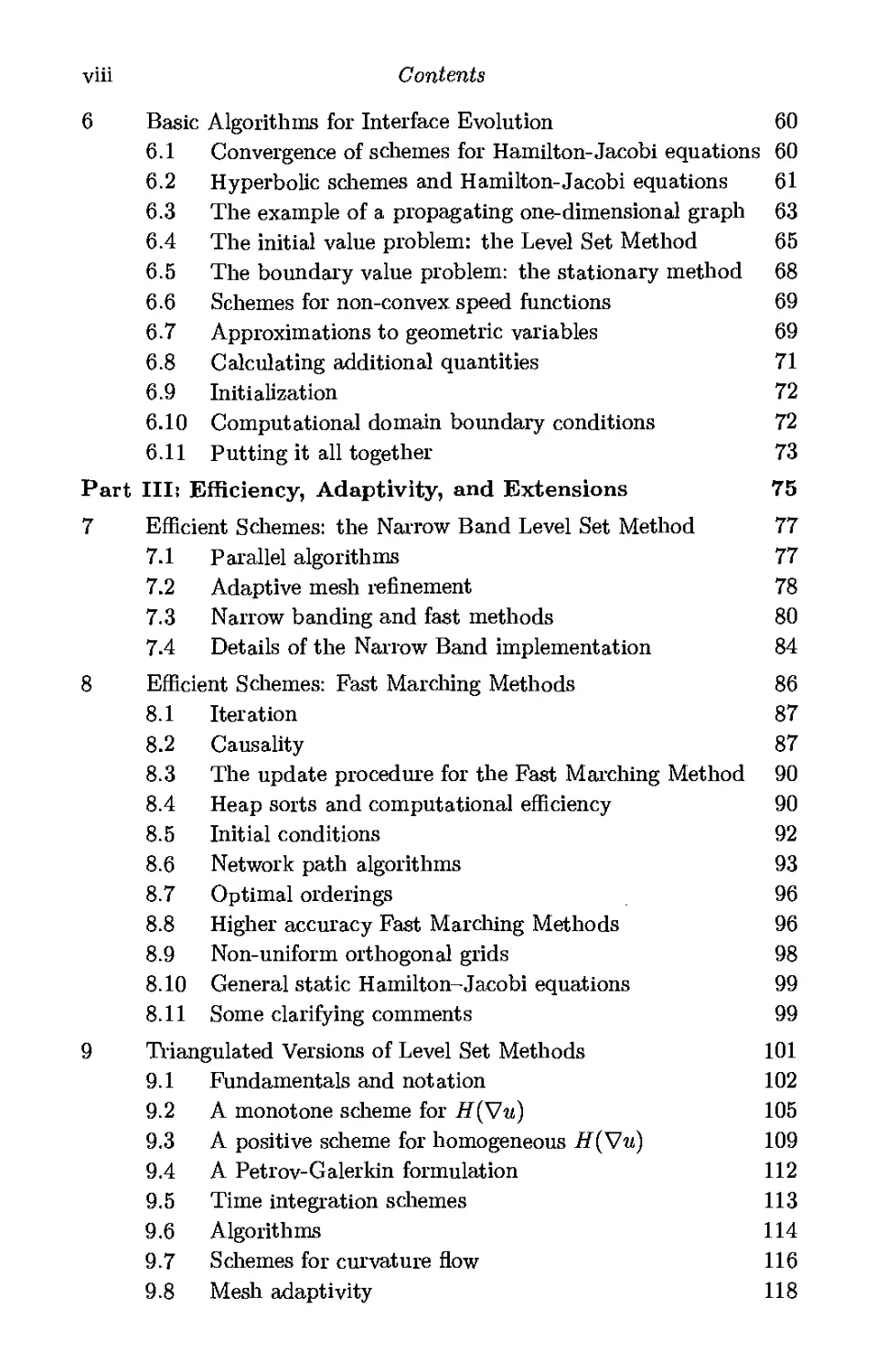
6 Basic Algorithms for Interface Evolution 60
6.1 Convergence of schemes for Hamilton-Jacobi equations 60
6.2 Hyperbolic schemes and Hamilton-Jacobi equations 61
6.3 The example of a propagating one-dimensional graph 63
6.4 The initial value problem: the Level Set Method 65
6.5 The boundary value problem: the stationary method 68
6.6 Schemes for non-convex speed functions 69
6.7 Approximations to geometric variables 69
6.8 Calculating additional quantities 71
6.9 Initialization 72
6.10 Computational domain boundary conditions 72
6.11 Putting it all together 73
Part III: Efficiency, Adaptivity, and Extensions 75
7 Efficient Schemes: the Narrow Band Level Set Method 77
7.1 Parallel algorithms 77
7.2 Adaptive mesh refinement 78
7.3 Narrow banding and fast methods 80
7.4 Details of the Narrow Band implementation 84
8 Efficient Schemes: Fast Marching Methods 86
8.1 Iteration 87
8.2 Causality 87
8.3 The update procedure for the Fast Marching Method 90
8.4 Heap sorts and computational efficiency 90
8.5 Initial conditions 92
8.6 Network path algorithms 93
8.7 Optimal orderings 96
8.8 Higher accuracy Fast Marching Methods 96
8.9 Non-uniform orthogonal grids 98
8.10 General static Hamilton-Jacobi equations 99
8.11 Some clarifying comments 99
9 Triangulated Versions of Level Set Methods 101
9.1 Fundamentals and notation 102
9.2 A monotone scheme for H(Vu) 105
9.3 A positive scheme for homogeneous H(S/u) 109
9.4 A Petrov-Galerkin formulation 112
9.5 Time integration schemes 113
9.6 Algorithms 114
9.7 Schemes for curvature flow 116
9.8 Mesh adaptivity 118

Contents
IX
10 Triangulated Fast Marching Methods 120
10.1 The update procedure 120
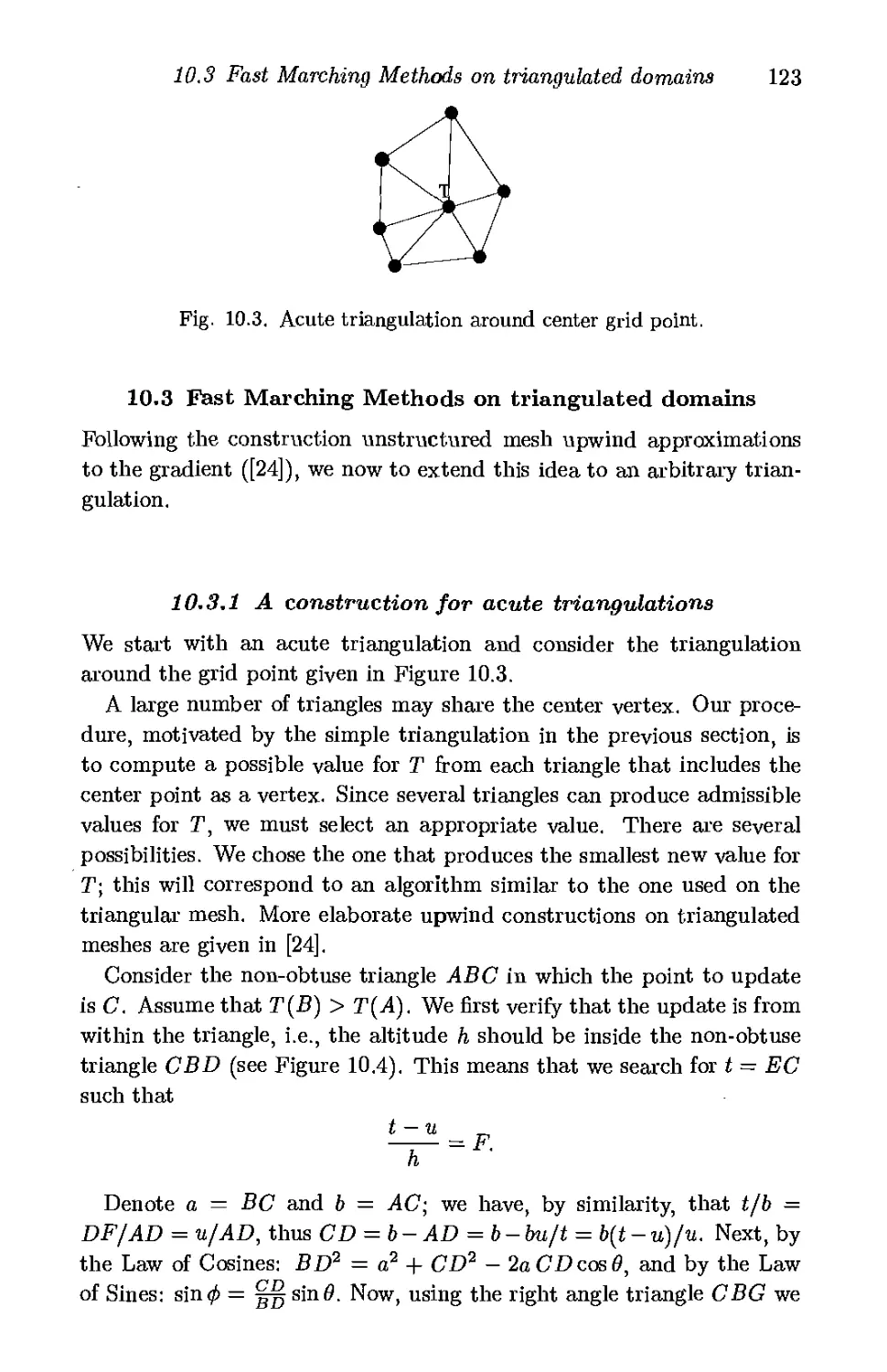
10.2 A scheme for a particular triangulated domain 121
10.3 Fast Marching Methods/on triangulated domains 123
11 Constructing Extension Velocities 127
11.1 The need for extension velocities 127
11.2 Various approaches to extension velocities 129
11.3 Equations for extension velocities 131
11.4 Building extension velocities 133
11.5 A quick demonstration 137
11.6 Re-initialization 138
12 Tests of Basic Methods 141
12.1 The basic Cartesian Level Set Method 141
12.2 Triangulated Level Set Methods for H-J equations. 146
12.3 Accuracy of Fast Marching Methods 150
12.4 Tests of extension velocity methodology 153
13 Building Level Set and Fast Marching Applications 161
Part IV; Applications 165
14 Geometry 167
14.1 Statement of problem 167
14.2 Equations of motion 169
14.3 Results 169
14.4 Flows under more general metrics 175
14.5 Volume-preserving flows 175
14.6 Motion under the second derivative of curvature 177
14.7 Triple points: variational and diffusion methods 183
15 Grid Generation 191
15.1 Statement of problem 191
15.2 Equations of motion 193
15.3 Results, complications, and future work 196
16 Image Enhancement and Noise Removal 200
16.1 Statement of problem 200
16.2 Equations of motion 202
16.3 Results 208
16.4 Related work 211
17 Computer Vision: Shape Detection and Recognition 214
17.1 Shape-from-shading 215
17.2 Shape detection/recovery 218

χ
Contents
17.3 Surface evolution and the stereo problem 227
17.4 Reconstruction of obstacles in inverse problems 229
17.5 Shape recognition 231
18 Combustion, Solidification, Fluids, and Electromigration 240
18.1 Combustion 241
18.2 Crystal growth and dendritic solidification 249
18.3 Fluid mechanics 255
18.4 Additional applications 258
18.5 Void evolution and electromigration 261
19 Computational Geometry and Computer-aided Design 267
19.1 Shape-Offsetting 267
19.2 Voronoi diagrams 268
19.3 Curve flows with constraints 269
19.4 Minimal surfaces and surfaces of prescribed curvature 270
19.5 Extensions to surfaces of prescribed curvature 274
19.6 Boolean operations on shapes 277
19.7 Extracting and combining two-dimensional shapes 281
19.8 Shape smoothing 282
20 Optimality and First Arrivals 284
20.1 Optimal path planning 284
20.2 Constructing shortest paths on weighted domains 289
20.3 Constructing shortest paths on manifolds 292
20.4 Seismic traveltimes 298
20.5 Aircraft collision avoidance using Level Set Methods 305
20.6 Visibility evaluations 307
21 Etching and Deposition in Microchip Fabrication 313
21.1 Physical effects and background 313
21.2 Equations of motion for etching/deposition 317
21.3 Additional numerical issues 324
21.4 Two-dimensional results 325
21.5 Three-dimensional simulations 342
21.6 Timings 348
21.7 Validation with experimental results 349
22 Summary/New Areas/Future Work 357
Bibliography 360
376

Preface to the Second Edition
The beginning of this work on Level Set Methods and Fast Marching
Methods can be found in the author's dissertation on the theory and
numerics of propagating interfaces, under the direction of Alexandre
Chorin at the University of California at Berkeley. That work continued
through a National Science Foundation (NSF) Postdoctoral Fellowship
at the Lawrence Berkeley National Laboratory (LBNL) and the Courant
Institute of Mathematical Sciences. As I look back on those years, I am
extraordinarily grateful for the opportunity that such support gave me
to develop these ideas, free from other burdens and responsibilities.
That work on interface methods and its subsequent development at
Berkeley have been supported in part by the Applied Mathematical
Sciences section of the Department of Energy through the Mathematics
Department at LBNL, by NSF awards through the University of
California at Berkeley Mathematics Department, and most recently through
the Office of Naval Research. Again, I am grateful for all of this support.
I have had the good fortune to work with many collaborators in the
development of these ideas. The time-dependent level set formulation
of these ideas on interface motion was co-authored with S. J. Oslier,
whose trips to Berkeley made for a thoroughly enjoyable collaboration.
The Narrow Band Level Set Method was developed jointly with D. Adal·-
steinsson, as was all the work on etching and deposition in semiconductor
manufacturing. The work on medical imaging and shape segmentation
was joint with R. Malladi, whose help on devising the Fast Marching
Method was invaluable. Finally, the triangulated unstructured versions
of the Level Set Method are joint with T. Barth of National Aeronautics
and Space Administration (NASA) Ames Research Center.
An early application of these techniques, due to D. Chopp, concerns
minimal surfaces and includes the genesis of ideas about narrow banding

Xll
Preface to the Second Edition
and complex boundary conditions. The work on Level Set Methods
for crystal growth and dendritic solidification is joint with J. Strain
and capitalizes on his boundary integral formulation of the equations
of motion. The realization that level set techniques can be applied to
shape recovery is due to R. Malladi; many others have capitalized on his
ideas. The application of these techniques to image processing began
with the work of L. Alvarez, J. M. Morel, and P. L. Lions and the work
of S. Osher and L. Rudin; the work on image processing presented here
relies heavily on those contributions. The application of the techniques
to problems in combustion and fluid interfaces discussed here is joint
work with С Rhee, J. Zhu and L. Talbot, and the work on adaptive
mesh refinement relies on the work of B. Milne.
I am fortunate to have on-going collaborations with very talented
colleagues, including M. Popovici of 3DGeo Corporation with whom the
work on migration and seismic imaging was developed; R. Kimmel, with
whom the work on geodesies and the development of a triangulated Fast
Marching Method was developed, as well as robotic navigation and
optimal path planning; O. Hald, whose analysis of non-convex Hamiltonians
was invaluable; as well as L. Borucki and J. Rey in a wide collection of
semiconductor issues. At the same time, I am equally fortunate to have
been recently benefited from new collaborations with J. Li, A. Sarti, A.
Vladimirsky, J. Wei, A. Wiegmann, and J. Wilkening.
Many other people have contributed to the current state-of-the-art of
level set methods, including T. Aslam, M. Barlaud, J. Вепсе, М. Brewer,
J. Bzdil, R. Caflisch, V. Caselles, T. Chan, S. Chen, Y. Chen, R. Deriche,
V. Dhir, E. Fatemi, 0. Faugeras, R. Fedkiw, E. Harabetian, E. Holm, T.x
Hou, R. Keriven, H.P. Langtangen, D. Lesselier, A. Litman, B. Merri-
man, E. Pascli, V. Prasad, S. Ruuth, F. Santosa, P. Smereka, N. Sochen,
G. Son, S. Stewart, M. Sussman, H. Zhang, H. Zhao, and L.L. Zheng.
Their work lias advanced both the theory and practice of level set
methods. I would like to thank W. Coughran for suggesting the application of
level set methods to semiconductor simulations, A. Neureuther for many
helpful discussions on etching and deposition, B. Knight for
encouragement in the application of level set methods to fluid interface problems,
C. Ritchie and G. Chiang for their insightful suggestions about shape
recovery in medical imaging, T. Baker for helpful conversations about
grid generation, L. Gray for suggesting the application of level set
methods to material sintering, and С Evans for his valuable comments on
the initial manuscript. I also wish to thank the students in Math 273

Preface to the Second Edition
XI11
during the fall of 1995 for their insightful comments, critical reviewing,
and careful suggestions.
I am also indebted to the many readers of the first edition who have
responded with detailed suggestions, and I have been guided by their
comments in writing this new edition. At the risk of repetition, I would
like to again thank D. Adalsteinsson, D. Chopp, R. Kimmel, R. Malladi,
B. Milne, A. Vladimisky, J. Wilkening and J. Zhu. I am
extraordinarily fortunate to have had them as colleagues at the Lawrence Berkeley
Laboratoiy.
Finally, I would like to thank Alan Harvey of Cambridge University
Press for his thoughtful suggestions and enthusiasm for this project.
His calm hand and unfailing humor have made this a pleasure, and his
guidance, wise counsel, and wisdom were invaluable. This second and
expanded edition is largely due to his optimism, encouragement, and
patience.
Berkeley, California, 1999

This page intentionally left blank

Introduction
Propagating interfaces occur in a wide variety of settings, and include
ocean waves, burning flames, and material boundaries. Less obvious
boundaries are equally important and include shapes against
backgrounds, handwritten characters, and iso-intensity contours in images.
Furthermore, there are applications not commonly thought of as moving
interface problems, including optimal path planning and construction of
shortest geodesic paths on surfaces, which can be recast as front
propagation problems with significant advantages.
The goal of this book is both to unify these ideas and to design
a general framework for modeling the evolution of boundaries. The
aim is to provide computational techniques for tracking moving
interfaces and to give some hint of the flavor and breadth of applications.
The work includes examples from physics, chemistry, fluid
mechanics, combustion, image processing, materials sciences, fabrication of
microelectronic components, computer vision, control theory, seismology,
computer-aided-design, and a collection of other areas. The intended
audience includes mathematicians, applied scientists, practicing
engineers, computer graphics artists, and anyone interested in the evolution
of boundaries and interfaces.
Our perspective comes from a large and rapidly growing body of work
which relies on a partial differential equations approach for
understanding, analyzing, and computing interface motion. At the core lay two
computational techniques: "Fast Marching Methods" and "Level Set
Methods". Both exploit a fundamental shift in how one views moving
boundaries. They rethink the Lagrangian geometric perspective and
replace it with an Eulerian, partial differential equation. Fast Marching
Methods result from a boundary value problem for the evolving interface,
while Level Set Methods result from an associated initial value problem.

XVI
Introduction
In both cases, several advantages stem from this view of propagating
interfaces:
• First, from a theoretical/mathematical point of view, some
complexities of front motion are illuminated, in particular, the role of
singularities, weak solutions, shock formation, entropy conditions, and
topological change in the evolving interface.
• Second, from a numerical perspective, natural and accurate ways of
computing delicate quantities emerge, including the ability to build
high order advection schemes, compute local curvature in two and
three dimensions, track sharp corners and cusps, and handle subtle
topological changes of merger and breakage.
• Third, from an implementation point of view, since the approaches
are based on underlying partial differential equations, robust schemes
result from numerical parameters set at the beginning of the
computation. The error is thus controlled by
(i) the order of the numerical method,
(ii) the grid spacing Δ/ι,
(iii) in the case of Level Set Methods, the time step Δι; no such
requirement exists for Fast Marching Methods.
• Fourth, computational adaptivity is the key to these techniques. In
the case of Level Set Methods, the most efficient and preferred
approach is the "Narrow Band Level Set Method", which focuses
computational labor around the evolving boundary. In the case of Fast
Marching Methods, use of standard sorting techniques yields
extraordinarily fast and optimally efficient algorithms. In both cases, a clear
path to parallelism is available.
This book surveys what is intended to be an illustrative subset of
past and current applications of these techniques. We do not assume
that the reader is familiar with ail of the details required to develop
these schemes; the aim is to include the necessary theory and details to
provide implementation guidelines.
The first edition of this book was entitled Level Set Methods. Tlie
augmented title Level Set Methods and Fast Marching Methods of this
new edition embraces the large landscape shared by these two techniques
in framing, illuminating, and solving problems with evolving boundaries.

Introduction
χνιι
Outline
This book is divided into four parts. Part I focuses on the formulation
of the boundary value and initial value partial differential equations
which comprise our two views of interface motion. Part II introduces the
theory and numerics underlying Fast Marching Methods and Level Set
Methods. Part III introduces the adaptive issues required to construct
efficient schemes and variations on the fundamental techniques. Finally,
Part Iv surveys some application areas.
In Part I, Chapter 1 begins with the underlying boundary value and
initial value partial differential equations perspective on moving
interfaces, and discusses the theoretical and computational advantages of
these approaches. It ends with a preview of the rest of the book and
provides an outline of the interconnection of the techniques, the
relevant theory, numerics, and application strategies. This "look ahead" is
meant to provide a structure for the remainder of the book, directing
the interested reader to various components of the methodologies.
Part II begins in Chapter 2 with a general statement of the
problem of a moving interface and discusses the mathematical theory of
curve/surface motion, including the growth/decay of total variation,
singularity development, entropy conditions, weak solutions, and shocks in
the dynamics of moving fronts. This material lias been developed in a
collection of papers that are referred to in the text. The viscosity
theory of Hamilton-Jacobi equations, which buttresses both computational
techniques, is briefly surveyed in Chapter 3.
Chapters 4, 5, and 6 present numerical results which lead up to the
Fast Marching and Level Set techniques. Chapter 4 begins with an
overview of traditional methods for tracking interfaces, including string
methods and cell methods, and makes a first attempt at solving a
partial differential equation for front propagation The failure of this first
attempt stems from the relationship between front propagation and
hyperbolic conservation laws and is the subject of Chapter 5. Chapter
6 then provides a detailed description of straightforward (though
inefficient) algorithms for solving the initial value and boundary value
problems.
Part III provides complete details on state-of-the-art Fast Marching
and Level Set algorithms. It begins in Chapter 7 with a discussion of
computational adaptivity. After surveying work on parallel and
adaptive mesh approaches, the chapter focuses on the Narrow Band Level
Set Method. This is the most efficient and accurate way to implement

XV111
Introduction
level set methods, Next, in Chapter 8, Fast Marching Methods are
introduced, which are the optimal way to solve Hamilton-Jacobi equations
which arise from certain interface motion problems. The techniques
require a detailed discussion of causality in upwind schemes and optimal
heap sort algorithms. Higher accuracy versions of both Narrow Band
and Fast Marching Methods are supplied.
Next, in Chapters 9 and 10, the entire framework is moved to a
triangulated unstructured mesh setting. Schemes for the Level Set Method
are given, including monotone schemes, positive schemes, Petrov-Galerkin
schemes, as well as explicit and implicit schemes with discontinuity
capturing. In the case of Fast Marching Methods, upwind causality schemes
for both acute and non-acute triangulations are introduced. These two
sets of schemes provide versatile techniques for interface propagation
problems on manifolds and in irregular domains.
Chapter 11 explains how to build general level set methods in many
physical problems. It examines how to build appropriate and
natural methods for moving the neighboring level sets, which is required in
order to implement level set techniques. Detailed techniques for
generating smooth level set flows which avoids all re-initialization are given,
as are techniques for obtaining sub-grid accuracy. In Chapter 12, the
numerical accuracy and robustness tests are measured, including scheme
convergence rates, tests of triangulated techniques, examination of mass
conservation and accuracy. Finally, in Chapter 13, the underlying
philosophy of Narrow Band and Fast Marching Methods applications is
discussed.
Part IV focuses on applications of both the Narrow Band Level Set
Method and Fast Marching Methods to a collection of problems. Here,
the intent is to show the breadth of current applications and to serve
as a guidepost for further research. Chapter 14 begins with some pure
geometry problems, including curve/surface shrinkage, the existence of
self-similar surfaces, flows under more complex metrics, sintering and
second derivative of curvature flows, triple points, multiple interfaces,
and constraint-based flows. Chapter 15 extends this work and shows how
these techniques can be used in grid generation, giving many examples
of body-fitted logical rectangular grids around complex bodies in two
and three dimensions. Chapter 16 moves to image processing and views
images as collections of iso-intensity contours; by constructing a suitable
speed law, these contours can be allowed to propagate in a way that both
removes noise and enhances desired regions.
Chapter 17 focuses on aspects of computer vision. It begins with

Introduction
xix
the problem of shape-from-shading and then shows how to transform
image segmentation problems into moving interface versions of active
contours; when driven by gradients in the image field, these contours
extract desired shapes from images. Applications are drawn from a wide
collection of medical data, including three-dimensional scans of cortical
and cardiac structures. Once images are segmented, the next step is
recognition, which is discussed in the context of automatic identification
of meteorological data and optical character recognition.
Chapter %8 provides examples of interface problems in which the
physics on each side of the interface both drives the front and is
affected by the front location and properties. Several areas are discussed,
including combustion and flame propagation, crystal growth and
dendritic solidification, fluid interface transport and two-phase flow, and
electromigration. In all four, the front is driven both by local effects
and by underlying transport terms. General guidelines for arbitrary
fluid/material interface problems are given. Additional applications
include boiling, groundwater transport, and liquid bridges.
Chapter 19 focuses on various aspects of computational geometry and
computer-aided-design. It begins with efficient algorithms for shape-
offsetting. Next, techniques for constructing minimal surfaces are given
which rely on constrained fronts evolving under mean curvature until
final minimal steady states are achieved. The chapter ends with
problems of shape smoothing, of importance in removing noise from range
images as well as machine part manufacturing. This is performed using
variants of the image smoothing schemes presented earlier.
Chapter 20 applies Fast Marching methods to a variety of problems in
computing first arrivals, optimization, and control. It begins with
problems in path planning and navigation under constraints. It then gives
an optimal algorithm for constructing shortest path geodesies on
complex triangulated manifolds, including a technique for ruling surfaces.
It then discusses first arrival times of seismic waves in geophysical
migration modeling and problems applying level set methods to air-traffic
control. The chapter ends with some new algorithms for computing
visibility in complex scenes.
Chapter 21 presents the most sophisticated application of Fast
Marching/Level Set methodologies to date, namely the simulation of etching,
deposition, and photolithography development in the micro fabrication
of semiconductor components. Here, photolithography development in
planar and non-planar domains, etching and deposition with non-convex
ion-milling sputter effects, re-emission and re-deposition mechanisms

XX
Introduction
with small sticking coefficients, passive sidewall activation, surface
diffusion and re-flow, as well as full three-dimensional effects are discussed.
This requires the use of efficient visibility schemes, schemes for sintering,
fast solution of flux integral equations, and sub-grid adaptivity schemes.
By no means is this an exhaustive review of the work that exists on
East Marching Methods and Level Set Methods. A body of work has
been reluctantly skipped in the effort to keep this book to reasonable
length. The interested reader is referred to a wide range of simulations
developed using these methodologies; references will be given
throughout the text. The goal of this book is to provide windows into these
techniques as guides for further interface studies.
The author can be reached at setliian@math.berkeley.edu. A general
article on Fast Marching Methods and Level Set Methods may be found
in [237], other reviews may be found in [238] and [235]. Finally, a web
page devoted to the topic of Fast Marching Methods and Level Set
Methods may be found at http://math.berkeley.edu/~sethian/level_set.html.

Equations of Motion for Moving
Interfaces
Part I presents the underlying partial differential equations
perspective on moving interfaces. One view leads to a
boundary value partial differential equation for the
evolving front, the other leads to a time-dependent initial value
problem. The goal is to lay out clearly the two views and
discuss the theoretical and computational advantage of these
approaches.

1
Formulation of Interface Propagation
Outline: We formulate the boundary value and initial value partial
differential equations which describe interface motion. These will
eventually lead to the Fast Marching Method and the Narrow Band Level Set
Method; for now, however, we focus on the theoretical and computational
advantages that come from these perspectives.
~F = F(L}G}I)
Outside \ I Outside
Fig. 1.1. Curve propagating with speed F in normal direction.
Consider a boundary, ei ther a curve in two dimensions or a surface in
three dimensions, separating one region from another. Imagine that this
curve/surface moves in a direction normal to itself (where the normal
direction is oriented with respect to an inside and an outside) with a
known speed function F. The goal is to track the motion of this interface
as it evolves. We are concerned only with the motion of the interface in
3

4
Formulation of Interface Propagation
its normal direction; throughout, we shall ignore motions of the interface
in its tangential directions.
The speed function F, which may depend on many factors, can be
written as:
F = F(LiGiI)) (1.1)
where
• L= Local properties are those determined by local geometric
information, such as curvature and normal direction.
• G~ Global properties of the front are those that depend on the shape
and position of the front. For example, the speed might depend on
integrals along the front and/or associated differential equations. As a
particular case, if the interface is a source of heat that affects diffusion
on either side of the interface, and a jump in the diffusion in turn
influences the motion of the interface, then this would be characterized
as global property.
• J— Independent properties are those that are independent of the shape
of the front, such as an underlying fluid velocity that passively
transports the front.
Much of the challenge in interface problems comes from producing
an adequate model for the speed function F\ this is a separate issue
independent of the goal of an accurate scheme for advancing the interface
based on the model for F. In this chapter, it is assumed that the speed
function F is known. The goal of Part IV is to formulate good models
for F for a collection of applications.
Given F and the position of an interface, the objective is to track the
evolution of the interface. Our first task is to formulate this evolution
problem in an Eulerian framework, that is, one in which the underlying
coordinate system remains fixed.
1.1 A boundary value formulation
Assume for the moment that F > 0, hence the front always moves
"outward." One way to characterize the position of this expanding front
is to compute the arrival time T(xt y) of the front as it crosses each point
(ζ,τ/), as shown in Figure 1.2.

1.1 A boundary value formulation
—
ч
(
\
У
N
\
)
1
Τ
ч
•
Fig. 1.2. Calculation of crossing time at (ж,1/) for expanding front F > 0.
The equation for this arrival function T(x}y) is easily derived. In one
dimension, using the fact that distance = rate * time (see Figure 1.3),
we have that
dx
TOO
Fig. 1.3. Setup for boundary value formulation.
In multiple dimensions, VT is orthogonal to the level sets of Г, and,
similar to the one-dimensional case, its magnitude is inversely proportional
to the speed. Hence
|VT|F=1,
Τ = 0 on Γ,
(1.2)
where Γ is the initial location of the interface.
Thus, the front motion is characterized as the solution to a
boundary value problem. If the speed F depends only on position, then the
equation reduces to what is known as the "Eikonal" equation. As an
example, the arrival surface T(x,y) for a circular front expanding with
unit speed F = 1 is shown in Figure 1.4.

6 Formulation of Interface Propagation
Fig. 1.4. Transformation of front motion into boundary value problem.
1.2 An initial value formulation
Conversely, suppose now that the front moves with a speed F that is
neither strictly positive nor negative. Then we must account for the fact
that the front can move forward and backward, and hence can pass over
a point (xty) several times. Thus, the crossing time T(x}y) is not a
single-valued function. Our way of taking care of this is to embed the
initial position of the front as the zero level set of a higher-dimensional
function φ. We can then link the evolution of this function φ to the
propagation of the front itself through a time-dependent initial value
problem. At any time, the front is given by the zero level set of the
time-dependent level set function φ (see Figure 1.5).
In order to derive an equation of the motion for this level set function
φ and match the zero level set of φ with the evolving front, we first
require that the level set value of a particle on the front with path x(t)
must always be zero, and hence
^(ι(ί),ί)=0. (1.3)
By the chain rule,
& + V#c(0,i).a:'(i)=0. (1.4)
Since F supplies the speed in the outward normal direction, then x'(t) ·
η ~ F} where η = νφ/\νφ\. This yields an evolution equation for φλ
namely

1.2 An initial value formulation 7
Fig. 1.5. Transformation of front motion into initial value problem.
& + F|V0| = O, (1.5)
given <f>(x}t = 0).
This is the level set equation given by Osher and Sethian [187]. For
certain forms of the speed function Ft one obtains a standard Hamilton-
Jacobi equation. Equation 1.5 describes the time evolution of the level
set function φ in such a way that the zero level set of this evolving
function is always identified with the propagating interface; see Figure
1.5.
Thus, we can summarize our two perspectives. Let Γ be a curve in the
plane propagating in a direction normal to itself with speed F such that
V(t) gives the position of the front at time t. Then, we wish to solve
Boundary Value Formulation Initial Value Formulation
|VT|F=.l <f>t + F\V<j>\ = 0
Front= Γ(ί) = {(x,y)\T(x,y) = t} Front=r(i) = {{x,y)\<f>(x}y,t) = 0}
Requires F > 0 Applies for arbitrary F
(1.6)

8
Formulation of Interface Propagation
1.3 Advantages of these perspectives
There are certain advantages associated with these two perspectives on
propagating interfaces.
• Both are unchanged in higher dimensions, that is, for hypersurfaces
propagating in three dimensions and higher.
• Topological changes in the evolving front Γ are handled naturally.
The position of the front at time t is given either by the zero level set
ф(х}у} t) — 0 of the evolving function φ or by the level set T(x} y) = t
of the boundary value solution. This set need not be a single curve,
and it can break and merge as t advances. In both cases, the key fact
is that the boundary value solution T(x,y) and the level set function
φ remain single-valued (see Figure 1.6).
The level set surface φ (dark gray):
Two separate initial fronts (in light gray).
Later in time: the interface topology has changed,
yielding a single curve as the zero level set.
Fig. 1.6. Topological change.

1.3 Advantages of these perspectives
9
Both rely on viscosity solutions of the associated partial differential
equations in order to guarantee that the unique, entropy-satisfying
weak solution is be obtained.
Both are accurately approximated by computational schemes which
exploit techniques borrowed from the numerical solutions of
hyperbolic conservation laws. For example, schemes may be developed by
using a discrete grid in x-y domain and substituting finite difference
approximations1 for the spatial and temporal derivatives. As
illustration, using a uniform mesh of spacing h, with grid nodes (z,i), and
employing the standard notation that <f& is the approximation to the
solution (f>{ih>jh,n£U), where Δι is the time step, one might write
At +FIV^5I = 0· (1-7)
Here, a forward difference scheme in time has been used, and [Vij$jl
represents some appropriate finite difference operator for the spatial
derivative. Thus, an explicit finite difference approach is possible.
The construction of correct entropy-satisfying approximations to the
difference operator is the subject of Part II; for now, the important
fact is that one has an explicit error control on the basis of the initial
spatial discretization and the order of the numerical scheme.
Intrinsic geometric properties of the front are easily determined in
both formulations. For example, at any point of the front, the normal
vector is given by
_ νφ _ ντ
n=w\ or n=jvrr (L8)
and the curvature of the front at any point is easily obtained from the
divergence of the unit normal vector to the front, i.e.,
K = j v ' iv*l ίΦΙ+ΦΙ)*'* ι n ол
V ' |VT| ~ (T2+T2)3/2
Both methods are made efficient through the use of adaptive
computational strategies, which lead to Narrow Band Level Set Methods
and Fast Marching Methods.
Finite difference approximations will be discussed in detail in Chapter 5.

10
Formulation of Interface Propagation
At the same time, there are significant differences between the two
approaches.
• The most obvious difference is that the initial value level set
formulation allows for both positive and negative speed functions F; the
front may move forward and backward as it evolves. The boundary
value perspective is restricted to fronts that always move in the same
direction, because it requires a single crossing time Τ at each grid
point, and hence a point cannot be revisited. Thus, models involving
more complex speed functions F, such as those including curvature,
are most naturally framed as initial value level set problems.
• Conversely, positive speed functions F which depend on position and
vary widely from point to point are best framed as boundary value
problems and approximated through the use of Fast Marching
Methods. This is because
(i) The boundary value formulation requires no time step, and
hence its approximation is not subject to CFL conditions, un- ·
like Level Set Methods.
(ii) Through the use of heap sort algorithms, Fast Marching
Methods can be made extremely computationally efficient, far
eclipsing Level Set Methods.
1.4 A general framework
We can be slightly informal and describe both formulations with the
general partial differential equation
aut+H{Du,x) = 0. (1.10)
Here, Du represents the partials oi и in each variable, for example, ux
and uy. In the case of the Eikonal equation, α = 0, and the function Η
reduces to Η = F\4u\ — 1.
One of the main subtleties that arises in solving this equation is that
the solution need not be differentiable, even with arbitrarily smooth
boundary data. This non-differentiability is intimately connected to the
notion of appropriate weak solutions. Our goal will be to construct
numerical techniques which naturally account for this non-differentiability
in the construction of accurate and efficient approximation schemes and
admit physically correct non-smooth solutions.

1.5 A look ahead/A look back
11
1.5 A look ahead/A look back
It is worthwhile to stop and explain how these techniques were
developed and what lies ahead. The first step in the development of these
ideas started with the analysis of corners and singularities in
propagating interfaces. In [222, 225], the role of curvature as a regularizing or
smoothing term was investigated, and it was shown that this regularizing
role connects to the notion of entropy conditions and shocks in
hyperbolic conservation laws in gas dynamics. This is the subject of Chapter
2. A more formal view comes from considering viscosity solutions of
Hamilton-Jacobi equations, which is the subject of Chapter 3.
The second step in the development of accurate and efficient numerical
techniques for interface evolution comes from the realization that the
schemes from computational fluid mechanics, specifically designed for
approximating the solution to hyperbolic conservation laws, can be used
to solve the equations of front propagation. This was the view developed
in [226], and is at the core of modern interface methods:
"Most algorithms place marker particles along the front and
advance the position of the particles in accordance with a set of
finite difference approximations to the equations of motion. Such
schemes usually go unstable and blow up as the curvature builds
around a cusp, since small errors in the position produce large
errors in the determination of the curvature. One alternative
is to consider the reformulation equations of motion as a
conservation law with viscosity and solve these equations with the
techniques developed for gas dynamics. These techniques, based
on high-order upwind formulations, are particularly attractive,
since they are highly stable, accurate and preserve monotonicity.
We have made some preliminary tests of such schemes applied
to our problem of propagating fronts in crystals and flames, with
extremely encouraging results..."
To execute this strategy, we need schemes from hyperbolic conservation
laws; this is the subject of Chapters 4 and 5.
The combination of these three subjects then leads to the two
numerical schemes given in Chapter 6: the Level Set Method ([187]) for the
initial value problem, and an iterative method for the boundary value
problem. They are made efficient in Chapters 8 and 9 through adap-
tivity, leading to Narrow Band Level Set Methods, see [2], and Fast
Marching Methods, see [233]. Finally, after a series of extensions of

12
Formulation of Interface Propagation
the basic techniques are developed in Part III, many applications are'
described in Part IV.
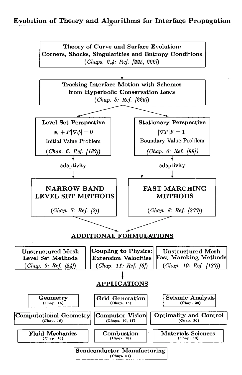
The interconnectedness of past work on methods for interface
propagation and the set of applications to be discussed are shown in Figure
1.7. There are many other contributors to the evolution of these ideas;
the chart is meant to give perspective on how the theory, algorithms,
and applications have evolved. We urge the reader to consult the
bibliography to get a more complete sense of the literature and the range of
work underway.
1.6 A larger perspective
Fast Marching Methods and Level Set Methods offer powerful techniques
for tracking moving interfaces. This book (like its previous edition) aims
to demonstrate how these techniques are applied across a wide spectrum
of applications. However, there are many other ways to compute
solutions to these problems besides the techniques offered here. Marker
particle techniques, Volume-of-fluid simulations, Fourier techniques, and
phase field models all offer valuable approaches. For each application
area given, there is a substantial literature which describes other
approaches. At the same time, new techniques and algorithms are always
under development, and one of the surest ways to render a body of work
obsolete is to pronounce that it can't be improved upon. With that in
mind, our goal here is to capture the flavor, intuitive feel, and details of
Fast Marching and Level Set Methods.

1.6 Λ larger perspective
13
Theory of Curve and Surface Evolution:
Corners, Shocks, Singularities and Entropy Conditions
(Chaps. 2,4: Ref [225, 222])
Tracking Interface Motion with Schemes
from Hyperbolic Conservation Laws
(Chap. 5: Ref. [226])
Level Set Perspective
^ + F|V^| = 0
Initial Value Problem
(Chap. 6: Ref. [187])
Ϊ
adaptivity
NARROW BAND
LEVEL SET METHODS
(Chap. 7: Ref [2])
Stationary Perspective
|VT|F=1
Boundary Value Problem
(Chap. 6: Ref [99])
Ϊ
adaptivity
L_
FAST MARCHING
METHODS
(Chap. 8: Ref. [233])
ADDITIONAL FORMULATIONS
Unstructured Mesh
Level Set Methods
(Chap. 9: Ref. [24])
Coupling to Physics:
Extension Velocities
(Chap. 11: Ref. [6])
Unstructured Mesh
Fast Marching Methods
(Chap. 10: Ref. [137])
I
APPLICATIONS
Geometry
(Chap. 14)
Computational Geometry
(Chap. 10)
Fluid Mechanics
(Chap. 18)
Grid Generation
(Chap. 15)
Computer Vision
(Chape, 10, 17)
Combustion
(Chap. 18)
Seismic Analysis
(Chap. 20)
Optimality and Control
(Chap, 30)
Materials Sciences
(Chap. 18)
Semiconductor Manufacturing
(Chap, 21)
Fig. 1.7. Evolution of theory and algorithms for interface propagations.

— Part II —■
Theory and Algorithms
Part II begins with a theoretical analysis of propagating
interfaces, with the goal of analyzing the stability and
smoothness of solutions as functions of initial position and speed.
We discuss both Lagrangian and Eulerian formulations of
the equations of motion. This leads to the link between
propagating interfaces and hyperbolic conservation laws, as well
as a discussion of singularities and weak solutions.
Formally, this connects to the theory of viscosity solutions,
which is summarized. We then discuss traditional schemes
for tracking interfaces, which are followed by a review of
numerical schemes for conservation laws. Finally, basic
schemes for our initial and boundary value formulations of
interface motion are given.

2
Theory of Curve and Surface
Evolution
Outline: We formulate the equations of motion of a propagating curve,
study its stability, and show that corners (singularities in the curvature)
can develop as the front evolves. We then show that these corners are
analogous to shocks in the solution of hyperbolic conservation laws and
that a solution can be naturally constructed beyond the appearance of
these corners through the notion of an entropy-satisfying weak solution.
2.1 Fundamental formulation
Let 7 be a simple, smooth, closed initial curve in R2} and let 7(i) be the
one-parameter family of curves generated by moving 7 along its normal
vector field with speed F. Here, F is the given scalar function. Thus
ft · a?i = F, where χ is the position vector of the curve, t is time, and η
is the unit normal to the curve.
A natural approach is to consider a parameterized form of the
equations. In this discussion, we further restrict ourselves and imagine that
the speed function F depends only on the local curvature к of the curve,
that is, F = F{k)} Let the position vector x(s,t) parameterize 7 at
time t, where 0 < s < St and assume periodic boundary conditions
x{0,t) = £(S,t). The curve is parameterized so that the interior is on
the left in the direction of increasing s (see Figure 2.1). Let n(s,t) be
the parameterization of the outward normal and let K(s,t) be the
parameterization of the curvature. The equations of motion can then be
Curvature is a vector that points in the direction normal to the curve; since we are
always taking the speed function in the normal direction, we shall abuse notation
and write, for example, F = —к. With our sign convention, a counterclockwise
parameterized curve has positive curvature.
17

18 Theory of Curve and Surface Evolution
x{s,t = Q)fy{s,t = 0)
у dt ι et) r "■
Fig. 2.1. Parameterized view of propagating curve,
written in terms of individual components x = {x,y) as
(2.1)
1U — _- Ρ Гу..Д.-b.jW*] f »<■ ^
where we have used the parameterized expression к = ^"г^Г^Л" f°r ^be
curvature inside the speed function F{k) and the fact that the normal
is given by η = (ys, -χ8)/{χ2 + У2)1/2. This is a "Lagrangian"
representation because the range of {x{s}t)}y(s,t)) describes the moving front.
2.2 Total variation: stability and the growth of oscillations
What happens to oscillations in the initial curve as it moves? We
summarize the argument by Sethian [225] showing that the decay of
oscillations depends only on the sign of FK at к = 0. Recall that the metric
g(s,t) ~ (x2 +y2)1/2 measures the "stretch" of the parameterization.
Define the total oscillation (also known as the total variation) of the
front
Var(i)= / \K(s,t)\g(s,t)ds. (2.2)
./o
Without the absolute value sign around the curvature, this evaluates
to 2π; the absolute value sign allows Var(i) to measures the amount of

2.2 Total variation: stability and the growth of oscillations 19
Original curve Decrease in variation Increase in variation
Fig. 2.2. Change in variation Var(t).
"wrinkling". Our goal is to see if this wrinkling increases or decreases
as the front evolves; two possible flows are shown in Figure 2.2.
Differentiation of the curvature and the metric with respect to time,
together with substitution from Eqn. 2.1 produces2 the corresponding
evolution equations for the metric and curvature, namely,
«ί^-ίΤ^ίΓ1)·-*2*;
9t = 9kF.
(2.3)
(2.4)
(Here, g~l is 1/ij, not the inverse.) Suppose we have an initial curve
moving with speed F(k) which stays smooth. Evaluation of the time
change of the total variation in the solution yields the following [225]:
Proposition: Consider a front moving along its normal vector field
with speed F(k), as in Eqn. 2.1. Assume that the evolving curve 7(i)
is simple, three times differentiable for 0 < s < S and 0 < t < T,
and non-convex, so that k(s, 0) changes sign. Assume that F is twice
differentiable. Then, for 0 < t < T,
• if FK(0) < 0 (FK(0) > 0), then
rfVM(O < 0 /JVar(t) ^ Λ
dt \ dt J '
• if FK(0) < 0 (FK(0) > 0) and κβ(0) φ 0, then
dVai-(t) „ /dVarft) „
"^<0 (л2 >0
(2.5)
(2.6)
2 With some work!

20 Theory of Curve and Surface Evolution
Remarks: The proposition states that if FK < 0 wherever к = 0, then
the total variation decreases as the front moves and the front "smooths
out," that is, the energy of the front dissipates. Here, we assume that
the front remains twice differentiate in the interval 0 < ΐ < T; in the
next section, we discuss what happens if the front ceases to be smooth
and develops a corner. In the special case that -y(t) is convex for all ΐ,
the proposition is trivial, since Var(i) — jQ ngds = 2π.
Outline of proof of proposition: To prove the proposition, the
integral is broken up into sections where the curvature changes sign. The
time differentiation of the total variation can then be passed to each
section of the curve. Using the expressions for the time derivatives of
both the metric and the curvature and noting the change in sign of the
curvature к from one section to the next, the decay or growth in the
total variation can be evaluated. A full proof may be found in [225].
Two important cases can be easily checked. A speed function F(k) =
1 - ex. for 6 > 0 has derivative FK = -6, and hence the total variation
decays. Conversely, a speed function of the form F(k) = 1 + ек yields a
positive speed derivative, and hence oscillations grow. We shall see that
the sign of the curvature term in this case corresponds to the backward
heat equation and hence must be unstable.
2.3 The role of entropy conditions and weak solutions
The above proposition includes the assumption that the front stays
smooth. In all but the simplest flows, this smoothness is soon lost.
For example, consider the periodic initial cosine curve
7(0) = (1-*,[1+сов21г*]/2) (2.7)
propagating with speed F(k) = 1. (The parameterization is chosen so
that the inside is on the left as we move in the direction of increasing
s.) The exact solution to this problem at time t may be constructed by
advancing each point of the front in its normal direction a distance t. In
terms of our parameterization of the front, the solution is given by
^-^4Ж=г,+,(м°Щ| (2'8)

2.3 The role of entropy conditions and weak solutions 21
(a) Swallowtail (F = 1.0) (b) Entropy solution (F = 1.0)
Fig. 2.3. Cosine curve propagating with unit speed.
As can be seen in Figure 2.3, the front develops a sharp corner in finite
time. Once this corner develops, the normal is ambiguously defined,
and it is not clear how to continue the evolution. Thus, beyond the
formation of the discontinuity in the derivative, we will need a weak
solution, so called because the solution weakly satisfies the definition of
differentiability.3
How can a solution be continued beyond the formation of a singularity
in the curvature corresponding to a corner in the front? A reasonable
answer depends on the nature of the interface under discussion. If the
interface is viewed as a geometric curve evolving under the prescribed
speed function, then one possible weak solution is the "swallowtail"
solution formed by letting the front pass through itself; this solution is
in Figure 2.3(a). This solution is in fact the one given by Eqns. 2.8 and
2.9; the lack of differentiability at the center point does not destroy the
solution, since the exact solution is written only in terms of the initial
data.
3 A solution is said to be a "weak solution" of a differential equation if it satisfies an
integral formulation of the equation. The advantage of such a formulation is that it
may not require the aame degree of differentiability of a potential solution, and thus
may allow more general solutions. As an example, consider the one-dimensional
wave equation щ = ux. A solution to this equation must be differentiable in both
χ and t. However, if we integrate both sides of the equation with respect to χ over
the interval [a, b], we then obtain ^ j udx = u(b) — u(a), which does not require
that the solution be differentiable in space. Weak aoiutions wili be discussed in
more detail in Chapter 5.

22
Theory of Curve and Surface Evolution
Globally closest points to boundary data
Fig. 2.4. Huygens' solution to propagation F= 1.
However, suppose the moving curve is regarded as an interface
separating two regions. From a geometrical argument, the front at time t
should consist of only the set of all points located a distance t from the
initial curve. Figure 2.3(b) shows this alternate weak solution. Roughly
speaking, we want to remove the "tail" from the "swallowtail"; see [225].
One way to build this solution is through a Huygens' principle
construction; the solution is developed by imagining wave fronts emanating with
unit speed from each point of the boundary data and the envelope of
these wave fronts always corresponds to the "first arrivals". This will
automatically produce the solution given on the right in Figure 2.3. This
is the approach taken in [225].
We note that there is a vertical ridge along which two points on the
boundary curve are the same distance away, as shown in Figure 2.3b.
Along this ridge, the solution is non-differentiable, and the gradient is
not defined.
Both of these constructions can be viewed as solutions to the problem
of a front propagating with unit speed. However, the solution that we
want, corresponding to the shortest distance or "first arrival," is the one
obtained throngh the Huygens' construction. Another way to obtain
the solution is through the notion of an entropy condition posed by
Sethian in [222, 225]; if we imagine the boundary curve as a source for
a propagating fiame, then the expanding flame satisfies the requirement
that once a point in the domain is ignited by the expanding front, it
stays burnt. This construction yields the entropy-satisfying Huygens'
construction given in Figure 2,4.
What does this "entropy condition" have to do with the notion of
"entropy"? While the answer will be made more precise in Chapter 5,

2.3 The vole of entropy conditions and weak solutions 23
(a) Shock (b) Rarefaction fan
Fig. 2.5. Front propagating with unit normal Speed.
an intuitive answer is as follows. "Entropy" refers to the organization of
information. In general terms, an entropy condition is one that says that
no new information can be created during the evolution of the problem.
Our example shows that once the entropy condition is invoked, some
information about the initial data is lost. Indeed, the entropy condition
"once a particle is burnt, it stays burnt" means that once a corner has
developed, the solution is no longer reversible. The problem cannot be
run "backward" in time; if we try to do so, the initial data will not be
retrieved. Thus, some information about the solution is forever lost.
As further illustration, consider the case of a V-shaped front
propagating normal to itself with unit speed (F = 1). In Figure 2.5(a), the
point of the front is downward; as the front moves inward with unit
speed, a "shock" propagates upward as the front pinches off, and a rule
is required to select the correct solution to stop the solution from being
multiple-valued. Conversely, in Figure 2.5(b), the point of the front is
upward; in this case the unit normal speed results in a circular fan that
connects the left state with slope +1 to the right state, which has slope
-1.
It is important to summarize a key point in this discussion. The
choice of weak solution given by our entropy condition4 rests on the
perspective that the front separates two regions and the assumption that
one is interested in tracking the progress of one region into the other.
Considerable confusion about the level set perspective has resulted from
a misunderstanding of the basic assumption inherent in this model.
4 Strictly speaking, this notion of an entropy condition wiil have meaning oniy for a
propagating graph; a more precise view wiil be given in Chapter 3. Nonetheless,
we shall be somewhat loose with our use of the word "entropy."

24 Theory of Curve and Surface Evolution
(a) F = 1 - 0.025k (b) F = 1 - 0.25k
Fig. 2.6. Propagating triple sine curve.
2.4 Effects of curvature: the viscous limit and the link to
hyperbolic conservation laws
Consider now a speed function of the form F = 1 - бк, where e is a
constant. The modifying effects of the term ек axe profound, and in
fact pave the way toward constructing accurate numerical schemes that
adhere to the correct entropy condition.
Following Sethian [225], the curvature evolution equation given by
Eqn. 2.3 can be rewritten as
Kt = €каа +6К3 - к2, (2.10)
where the second derivative of the curvature к is taken with respect to
arc length a. This is a reaction-diffusion equation; the drive toward
singularities due to the reaction term (ек3 - к2) is balanced by the
smoothing effect of the diffusion term (ек.аа).
Consider again the cosine front given in Eqn. 2.7 and the speed
function F(k) — 1 - €K, e > 0. As the front moves, the trough at s = η +1/2
is sharpened by the negative reaction term (because к < 0 at such
points) and smoothed by the positive diffusion term. For 6 > 0, it can
be shown (see [225, 187]) that the moving front stays C°°. Figure 2.6
shows two cases of a propagating initial triple sine curve. For έ small
(Figure 2.6(a)), the troughs sharpen up. For 6 large (Figure 2.6(b)),
parts of the boundary with high values of positive curvature initially
move downward, and concave parts of the front move quickly up.

2.4 Effects of curvature
25
(a) F-l- 0.25k (b) Entropy solution (F = 1.0)
Fig. 2.7. Entropy solution is the limit of viscous solutions.
For, 6 > 0, we have a smooth fiow, as shown in Figure 2.7(a). However,
with 6 = 0, we have a pure reaction equation Kt = -к2, and the
developing corner can be seen in the exact solution k(s, t) = k(s,0)/(1 + ΐκ(β,Ο)).
This is singulai- in finite t if the initial curvature is anywhere negative.
The entropy solution to this problem when F = 1 is shown in Figure
2.7(b).
The central observation, key to the notion of entropy solutions in front
propagation (see [225]), is the following link:
Consider the propagating cosine curve and the two solutions
• Curvature (*)> obtained by evolving the initial front with F€ = 1 - en,
• X;onetant(t)> obtained with speed function F = \ and the entropy
condition.
Then, at any time T,
UmXL^jr) = XconBtant(T). (2.11)
Thus, the limit of motion with curvature, known as the 'Viscous limit",
is the entropy solution for the constant speed case.

26
Theory of Curve and Surface Evolution
Why is this known as the viscous limit, and what does this have to do
with viscosity? To see why this is an appropriate name, we turn to the
link between propagating fronts and hyperbolic conservation laws. The
following material, taken from [225], is presented in considerably more
depth in Chapter 5. The ideas are presented here as motivation.
An equation for u(xyt) of the form
ut + [G{u)]x=0, (2.12)
is known as a "hyperbolic conservation law". A simple example is
Burgers' equation, given by
«(+«1^=0, (2.13)
which describes the motion of a compressible fiuid in one dimension. The
solution to this equation can develop discontinuities, known as "shocks",
where the fiuid undergoes a sudden expansion or compression. These
shocks (for example, a sonic boom) can arise from arbitrarily smooth
initial data; they are functions of the equation itself. Fluid viscosity
appears as a diffusive term on the right-hand side, namely,
Щ +uux = euxx, (2.14)
and this second derivative acts like a smoothing term and stops the
development of such shocks. For e > 0 it can be shown that the solution
must remain smooth for all time.
What does this have to do with our propagating front equation?
Consider the initial front given by the graph of f{x), with / and f periodic
on [0,1], and suppose that the propagating front remains a graph for all
time. Let φ be the height of the propagating function at time t, and thus
φ(χ, 0) = f(x). The tangent at (x} φ) is (1, φχ). Referring to Figure 2.8,
the change in height V in a unit time is related to the speed F in the
normal direction by
£_й±й^, (,15)
and thus the equation of motion becomes
1>t = F{\+$lYt*. (2.16)
Use of the speed function F(k) = 1 — ек and the formula к = —фхх/{1 +
<Й)3/2 yields
φ, - (1+tf)"9^^. (2-17)

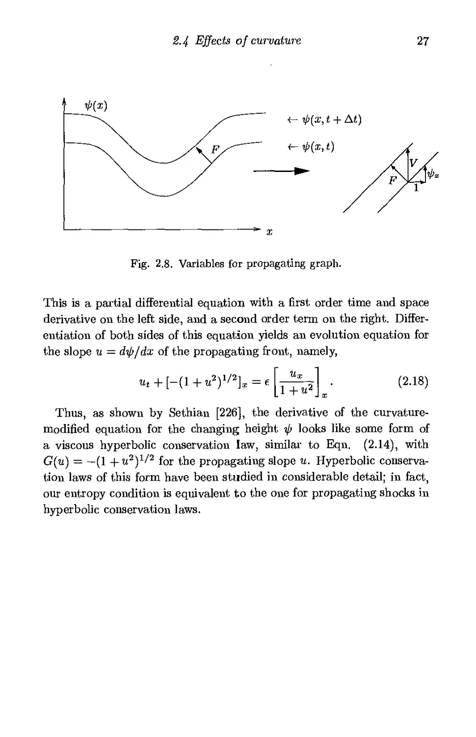
2.4 Effects of curvature 27
ip(x,t + At)
Fig. 2.8. Variables for propagating graph.
This is a partial differential equation with a first order time and space
derivative on the left side, and a second order term on the right.
Differentiation of both sides of this equation yields an evolution equation for
the slope и = άφ/dx of the propagating front, namely,
ut
+ [-(1+ηψ% = ε
1 +w
(2.18)
Thus, as shown by Sethian [226], the derivative of the curvature-
modified equation for the changing height φ looks like some form of
a viscous hyperbolic conservation law, similar to Eqn. (2.14), with
G(u) = —(1 +U2)1/2 for the propagating slope u. Hyperbolic
conservation laws of this form have been studied in considerable detail; in fact,
our entropy condition is equivalent to the one for propagating shocks in
hyperbolic conservation laws.

28 Theory of Curve and Surface Evolution
To summarize the discussion so far:
(i) A front propagating at a constant speed can form corners as it
evolves. At such points, the front is no longer differentiable and
a weak solution must be constructed to continue the solution.
(ii) The correct weak solution, motivated by viewing the front as an
evolving interface separating two regions, comes by means of an
entropy condition.
(iii) A front propagating at a speed 1 — en for e > 0 does not form
corners and stays smooth for all time. Furthermore, as the
dependence on curvature vanishes, the limit of this motion is the
entropy-satisfying solution obtained for the constant speed case.
(iv) If the propagating curve remains a graph as it moves, there is a
direct link between the equation of motion and a one-dimensional
hyperbolic conservation law for the evolving slope. The role of
curvature in a propagating front is analogous to the role of
viscosity in this hyperbolic conservation law.
(v) By considering the initial front as a boundary value, a boundary
value partial differential equation can be developed in two and
three dimensions for a speed function F which does not change
sign. This will lead to the Fast Marching Method.
(vi) By embedding the motion of a hypersurface as the zero level set
of a higher dimensional function, an initial value partial
differential equation can be obtained that will permit arbitrary speed
functions together with curves and surfaces moving in two and
three space dimensions. This will lead to the Level Set Method.
Before proceeding to numerical schemes, we first consider a more
formal view of the above, which is known as the theory of viscosity
solutions.

3
Viscosity Solutions and
Hamilton-Jacobi Equations
Outline: We present the formal definition of the viscosity solution of
a Hamilton-Jacobi equation. This solution is based on its behavior at
extrema, which turns out to be a more appropriate way of characterizing
the correct weak solution. Using this definition, one then proves that
the viscosity solution is the limit of smooth solutions as the smoothing
term goes to zero.
So fax, our presentation of interface propagation has taken a geometric
approach. We have tried to present an intuitive feel for the mechanism
linking moving fronts and hyperbolic conservation laws. We have done so
for two reasons. First, as we have seen, the notion of what happens when
a corner develops in an evolving graph neatly parallels the development
of shocks and rarefaction fans described by the conservation law for the
evolving slope. Second, the rich wealth of numerical schemes developed
for hyperbolic equations will be used to build schemes for the initial and
boundary value perspectives.
Formally, however, this link cannot be extended to higher dimensions.
Recall that for a curve which can be written as a graph propagating with
speed F in its normal direction, the change in the height of the function
φ (Eqn. 2.16) is given by
φι = Ρ(1+ψΙγ/*. (3.1)
Differentiation of both sides of this equation yields an evolution equation
for the slope и = άφ/dx of the propagating front, namely,
(3.2)
X
Ut
+ [-(1+νψ2]χ = ε
l+u-
29

30 Viscosity Solutions and Hamilton-Jacobi Equations
which is a viscous hyperbolic conservation law with G{u) = — (1+u2)1/2
for the propagating slope u.
In contrast, imagine either a level set view that embeds the curve in
the higher dimensional level set function φ through
4* + Π4ί+Φΐ)1/2 = ο, (3.3)
or the boundary value view which yields the arrival time function Τ
through
|VT|F=1. (3.4)
Suppose we take the first equation and try letting и — φχ and υ = фу.
If we then differentiate both sides with respect to χ and τ/, we get a pair of
equations for и and v. These are linked by the equality of mixed partials
in which uy = vx. Thus, unlike our formulation for a propagating curve,
we cannot simply take the theory for hyperbolic conservation laws and
"integrate it upward".
Instead, we work directly with the partial differential equations and
add a viscous right-hand side. Once again, the solution to this equation
is smooth for all time, and the limit as the viscosity term goes to zero
produces the appropriate weak solution. In fact, the preferred
alternative proceeds along a different line. First, the "viscosity solution" which
allows corners is defined in terms of its behavior at extrema, and is shown
to be equivalent to the classical (smooth) solution where the solution is
smooth. Then, under certain restrictions, it is shown that this viscosity
solution is equal to the limit as the viscous smoothing term vanishes.
This is the theory of viscosity solutions of Hamilton-Jacobi equations
introduced by Crandall and Lions [74]; see also Crandall, Evans, and
Lions [71] and Crandall, Ishii, and Lions [72]. In the rest of this brief
chapter, we shall make these ideas somewhat more precise; for further
details, see Evans [86].
3.1 Viscosity solutions of Hamilton—Jacobi equations
Consider either the level set equation φι + Р\Чф\ = 0 or the stationary
equation \4T\F ~ 1. If the speed F depends only on position χ and first
derivatives of φ, these are particular cases of the more general Hamilton-

3.1 Viscosity solutions of Hamilton-Jaoobi equations 31
Jacobi equation1
aut+H{Du,x)=0, (3.5)
where H(Du,x) = F\4u\ ~ (1 — a), and a is either zero or one. Here,
Dit represents the partials of и in each variable, for example, ux and uy.
Assume that the Hamiltonian Я is a smooth function of its arguments.
We want to admit non-smooth solutions that allow corners, similar to
the previous desire to admit non-smooth solutions of a hyperbolic
conservation law. A natural approach, in parallel with the earlier discussion,
is to add a viscosity term, that is,
ащ + H(Du, x) = eAu, (3.6)
where e is a positive constant. Then, given a solution ue to the foregoing,
we want to show that such a solution is smooth, and that the limit of
these solutions as e vanishes gives an appropriate weak solution.
Rather than define the weak solution as a limit of smooth solutions,
Crandall, Evans, and Lions [71], reformulating an earlier definition by
Crandall and Lions [74], define a weak solution as follows:
Definition: A function и is said to be a viscosity solution of
Eqn. (1.10), if, for all smooth test functions v,
(i) if и — ν has a local maximum at a point (x0, t0), then
vt{x0,t0) +H{Dv{x0,t0),x0) < 0 (3.7)
(ii) if и — υ has a local minimum at a point (x0, t0), then
vt{x0,t0) +H{Dv{x0,t0),x0) > 0. (3.8)
Note that nowhere in this definition is the viscosity solution и
differentiated; everything is done in terms of the test function v. This is done
so that one can use the usual trick of integration by parts and move all
the derivatives onto the test function in exchange for some boundary
conditions.
This is only a definition. Several tilings need to be checked before it
can be viewed as a reasonable solution to the Hamilton-Jacobi equation.
In fact, the following can be shown:
1 We are going to ignore curvature-driven fronts for a few moments, because such
flows contain second derivatives.

32 Viscosity Solutions and Hamilton-Jacobi Equations
• Ifи is a smooth solution of the Hamilton-Jacobi equation, then it is
a viscosity solution.
In other words, any classical solution that stays smooth for all time
satisfies the two inequalities in the above definition.
• If a viscosity solution и is differentiable at some point, then it satisfies
the Hamilton-Jacobi equation at that point.
In other words, where the viscosity solution is smooth, it gives the
same answer as the classical solution.
• This viscosity solution is unique, given appropriate initial conditions.
That is, there is only one viscosity solution satisfying the definition.
• The solution produced by taking the limit of the smooth solutions ue
as e goes to zero is the viscosity solution.
We shall prove none of these here. Precise statements and proofs may
be found in [74, 71, 86]. The salient point is that the viscosity solution
is now defined in a way that does not require differentiation, and can be
proven to be the unique viscous limit of the smoothed Hamilton-Jacobi
equation.
3.2 Some additional comments and references
While methods for numerically approximating moving fronts have
received much attention, the theoretical analysis of moving curves and
surfaces has itself been a subject of considerable interest. The work of
Gage [97], Gage and Hamilton [98], and Grayson [105], discussed later
in this book, opened up the analysis of curve evolution under curvature,
leading to the beautiful result that a closed curve shrinking under its
curvature collapses smoothly to a point.
Using a very different approach, Brakke [35] applied varifold theory
to the problem of a hypersurface moving under its curvature, and in so
doing provided a wide-ranging perspective for these problems, including
cases in which the evolving curves were not necessarily smooth.
There has been considerable theoretical analysis of the Bulerian
partial differential equations view of interface motion and its relation to
other perspectives on front propagation. The fiame/entropy model from
[222] served as the basis for theoretical analysis by Barles [19]. The
embedding of the front as a higher dimensional function meant that

3.2 Some additional comments and references 33
some of the issues of topological change and corner formation could be
studied in a more natural manner. Furthermore, the transformation
of geometry problems into a partial differential equation setting meant
that some powerful analytic techniques, including regularity of solutions,
viscous solutions of Hamilton-Jacobi equations, and tools for analyzing
existence and uniqueness, could be applied.
Using our perspective developed in [225, 187], Evans and Spruck [88,
89, 90, 91] and Chen, Giga, Goto, and Ishii [57, 101, 102] performed
detailed analysis of curvature flow in a series of papers. They exploited
much of the work on viscosity solutions of partial differential equations
(see Lions [153]), which itself was inspired by the corresponding work
applied to hyperbolic conservation laws. Their papers examined the
regularity of curvature flow equations, pathological cases, and the link
between the level set perspective and the varifold approach of Brakke.
These papers opened up a series of investigations into further issues; we
also refer the interested reader to Evans, Soner, and Souganidis [87], and
Ilmanen [119, 120].
For the stationary boundary value view, the interested reader is
referred to a large body of literature, including relevant theory by Barles
and Souganidis [22], Crandall, Evans, and Lions [71], Lions [153], and
Souganidis [253], and numerical algorithms by Bardi and Falcone [18],
Falcone, Giorgi, and Loretti [93], Kimmel and Bruckstein [130], and
Rouy and Tourin [207].
Finally, there has also been considerable work on the analysis of
relevant numerical algorithms for viscosity solutions outside of the context
of interface propagation. Crandall and Lions [74] analyzed an explicit
finite difference scheme; see also, for example, Souganidis [253]. Most of
these schemes are finite difference expressions that contain some forms
of smoothing, often in the spirit of the method of artificial viscosity.
Convergent schemes result from the standard criteria of monotonicity
and consistency.

4
Traditional Techniques for Tracking
Interfaces
Outline: Before focusing on the initial and boundary value partial
differential equations view of evolving fronts, we consider other numerical
methods for tracking interfaces. We then make a first attempt at
solving a partial differential equation for front propagation using a central
difference scheme, and show why this fails to capture the correct weak
solution.
4.1 Marker/string methods
A standard approach to modeling moving fronts comes from discretizing
the Lagrangian form of the equations of motion given in Eqn. (2.1). In
this approach, the parameterization is discretized into a set of marker
particles whose positions at any time are used to reconstruct the front.
This approach is known under a variety of names, including marker
particle techniques, string methods, and nodal methods. In two dimensions,
the front may be reconstructed as line segments; in three dimensions,
triangles are often used.
This approach can be illustrated through a straightforward scheme
that constructs a simple difference approximation to the Lagrangian
equations of motion. Divide the parameterization interval [0, S] into
Μ equal intervals of size As, yielding Μ + 1 mesh points Si = г As,
i = 0,... ,M, as shown in Figure 4.1. Divide time into equal intervals
of length Δί. The image of each mesh point iAs at each time step nAt
is a marker point (ж™, τ/f) on the moving front. The goal is a numerical
algorithm that will produce new values {x™+1, y™+l) from the previous
positions; we follow the discussion in [225].
First, we approximate parameter derivatives at each marker point by
using neighboring mesh points. Central difference approximations based
34

4.1 Marker/string methods
35
(4.1)
(4.2)
Fig. 4.1. Discrete parameterization of curve,
on Taylor series (see Chapter 5) yield
^r^+i-^i rfgr„,ga-i-g"-i
ds ~ 2Δ5 ' ds ~ 2As
ds2 ~ Δ52 ' ds2 ~ Δ52
Similarly, time derivatives may be replaced by the forward difference
approximations
aXi ^ ^г xi аУг ^ Щ У±_ /д Q-\
dt At dt ~ Δι ^ ' }
Substitution of these approximations into the equations of motion given
by Eqn. 2.1 produces the scheme
{Xi ,y. )_K,,J+MF(4) ((^+ι_,η_ι)2+(ί/ΐνι_^ι)2)ν2'
(4.4)
where
(№i-^-i)a+(ga.i-g?-i)2)3/2
(4.5)
Using the fact that the curve is closed, this is a complete recipe for
updating the positions of the particles from one time step to the next.

36 Traditional Techniques for Tracking Interfaces
(a) Δί = O.OOl (b) Δί - 0.0001 (с) Δί = 0.00001
Fig. 4.2. Marker particle solution to F = 1 — .25k.
Observe that the fixed discretization interval As has dropped out of
the expression. Consequently, as marker particles come together,
quotients on the right-hand side of Eqn. 4.4 approach zero over zero, yielding
a very sensitive calculation. The computed curvature can change
drastically from one particle to the next because of small and unavoidable
errors in the positions.
We can observe this unstable accumulation of small errors by using a
marker particle scheme to follow our previous initial cosine curve
propagating with speed 1 — ек, е = .25. Since e > 0, the exact solution is
always smooth and differentiable. Fifty marker points are used, together
with a time step of At = 0.001. Although the propagating front begins
to sharpen as expected (see Figure 4.2(a)), oscillations soon develop,
which grow uncontrollably. These oscillations result from a feedback
cycle: (1) small errors in approximate marker positions produce (2)
local variations in the computed derivatives leading to (3) variation in the
computed particle velocities causing (4) uneven advancement of markers,
which yields (5) larger errors in approximate marker positions. Within
a few time steps, the small oscillations in the curvature have grown and
the computed solution becomes unbounded. Figure 4.2(a) shows the
calculation until the computer program stops running.
Suppose we try to increase accuracy by using a smaller time step.
Figure 4.2(b) and Figure 4.2(c) show calculations with At = 0.0001 and
At = 0.00001, respectively. With time step Δί = .0001, once again the
solution becomes unstable, and the smooth decay of the trough is not
seen. Only in the finest case using a time step of Δί = 0.00001 is the
solution acceptable. For any e > 0 there is a bound on the minimum
distance between particles, and thus a small enough time step does exist

4.1 Marker/string methods
37
to ensure stability. However, note that if we had chosen a smaller value of
e, the marker trajectories would have come closer together, and a smaller
time step would be required for stability. As an example, with the value
of e = 0.1 (a large value, when one considers the role of curvature to be
similar to that of surface tension), the time step required for stability
is At = 0.000005. For values of e much smaller, this approach becomes
impractical.
What can be done? Typically, there are three remedies:
• "Smooth" the speed function so that the marker points stay far enough
apart to allow a reasonable time step.
• Redistribute marker particles according to arc length (or a related
quantity) every few time steps so that they stay far enough apart.
• Invent some filtering technique to remove "noise" (oscillations) in the
particle positions as they develop.
While all three techniques are used in practice, they are not appealing.
They all boil down to the same tiling; they alter the equations of motion
in non-obvious ways. Significant amounts of smoothing may be required
to ensure a practical time step. Thus, one sacrifices the most
interesting propagation characteristics, such as front sharpening and curvature
singularities, simply in order to keep the calculation alive. Calculation
of arc length to redistribute the particles adds a additional smoothing
term to the speed function that is difficult to analyze. The computed
solution may be far from the desired one. In the worst case, time and
effort will be spent solving an unrelated problem.
The situation is even bleaker in the limiting case e = 0. As discussed
earlier, a solution forms a sharp corner, and an entropy condition must
be invoked to produce a reasonable weak solution beyond the formation
of the singularity. However, a marker particle approach does not "know"
about the necessary entropy condition, because it attempts to track a
Lagrangian formulation in which the swallowtail solution given in Figure
2.3(a) is an acceptable weak solution. In Figure 4.3 we show a marker
particle solution that incorporates the swallowtail solution.
No time step, no matter how small, can produce a scheme which
correctly incorporates the entropy condition given in [222]. In fact, for
e > 0, the equations for the markers themselves reduce to a linearly
unstable hyperbolic system (see [187]). From an algorithmic point of
view, markers must somehow be eliminated from the discretization as
corners form and information about the initial data is lost. This
corresponds to deleting the "tail" from the swallowtail, as discussed earlier;

38 Traditional Techniques for Tracking Interfaces
Fig. 4.3. Marker particle solution to swallowtail under F = 1.
in some arenas, this procedure is called "de-looping". While there have
been procedures for doing so in two dimensions [112], de-looping in three
dimensions is not for the fainthearted, and such codes can break down
in complex situations.
These drawbacks to marker particle/Lagrangian methods result from
stability and local singularity problems. Topological changes in the
moving front are also problematic. Consider two separate expanding flames.
Suppose these fronts merge and the boundary becomes a single curve. It
is difficult to produce a systematic way of removing those markers that
no longer sit on the actual boundary. The bookkeeping of removing,
redistributing, and connecting markers is complex, and an arduous task
for higher-dimensional interface problems.
To summarize, Lagrangian approximations provide numerical schemes
based on a parameterized description of the moving front. They can be
accurate for small-scale motions of interfaces. However, because they
follow a local representation of the front rather than using a global one
that is able to take into account the proper entropy conditions and weak
solutions, they can suffer from instability and topological limitations.
4.2 Volume-of-fluid techniques
A different approach to front motion is provided by volume-of-fluid
techniques, introduced by Noh and Woodward [183] and based instead on an
Eulerian view. These techniques have appeared in a variety of forms and

4-2 Volume-of-fluid techniques
39
/
/
\
^
/
s
'
""■
^
N
\
\
s
К
\
J
0
0
0
0
0
0
0
0
0
0
0
0
0
.4
.7
.9
.8
0
0
0
0
0
.2
.9
1.0
.9
.8
0
0
0
0
0
.2
1.0
.8
.1
0
0
0
0
0
.0
.1
.9
.8
0
.4
1.0
1.0
.4
.3
.7
.2
.9
1.0
.6
.8
1.0
1.0
.5
.6
1.0
.7
1.0
1.0
1.0
1.0
1.0
1.0
.7
.2
.8
1.0
1.0
1.0
1.0
1.0
1.0
1.0
.9
0
0
.3
.7
1.0
.5
.4
1.0
1.0
.7
0
0
0
0
0
0
0
.5
.5
.3
0
0
0
0
0
0
0
0
0
0
Grid Volume fractions
Fig. 4.4. Vohime-of-fhiid method.
have been reintroduced under many names, such as the "cell method"
and the "method of partial fractions."
The basic idea (see Figure 4.4) is as follows. Imagine a fixed grid on
the computational domain, and assign values to each grid cell based on
the fraction of that cell containing material inside the interface. Given a
closed curve, we assign a value of unity to those cells completely inside
this curve, a cell value of zero to those completely outside, and a fraction
between 0 and 1 to cells that straddle the interface, based on the amount
of the cell inside the front.
The idea, then, is to rely solely on these "cell fractions," shown in
Figure 4.4, to characterize the interface location. Approximation techniques
are then used to reconstruct the front from these cell fractions. The
original Noh and Woodward algorithm was known as "SLIC", for "Simple
Line Interface Calculation," and reconstructed the front as either a
vertical line or a horizontal line.
In order to evolve the interface, the cell fractions on this fixed grid are
updated to reflect the progress of the front. Suppose that one wishes
to advect a front passively under the transport velocity u* (here, this is
not a speed normal to the front, but merely a transport term). Noh
and Woodward provide a methodology in which the value in each cell
is updated under this transport velocity in each coordinate direction by
locally reconstructing the front and then exchanging material in neigh-

40 Traditional Techniques for Tracking Interfaces
0.0
1.0
1.0
0.0
.7
1.0
0.0
.4
1.0
0.0
.8
1.0
0.0
.5
1.0
0.0
.2
1.0
Volume Reconstructed Front New volume
fractions front advection fractions
Fig. 4.5. Reconstruction and advection of volume fractions.
boring cells under this motion. After completing coordinate sweeps, one
has produced new cell fractions at the next time step corresponding to
the updated front. In Figure 4.5, we show the advection of an interface
under a simple vertical velocity field и = (0,1).
Since the introduction of volume-of-fluids methods, many elaborate
reconstruction techniques have been developed to include pitched slopes
and curved surfaces, see Chorin [65], Hirt and Nicholls [113], and Lafau-
rie, Nardone, Scardovelli, Zaleski, and Zanetti [142]. The resulting
accuracy depends on the sophistication of the reconstruction and the
"advection sweeps" which advance the material. Some of the most elaborate
and accurate versions of these schemes to date are due to Puckett [198].
The original SLIC algorithm was designed for transport under an
advection velocity field that depended on the location of the front, but not
the local shape/orientation of the front. A valuable extension to volume-
of-fiuid techniques was developed by Chorin [65], who provided a way
of using these methods for a speed function given in a direction normal
to the front. As we have seen earlier, corners and cusps can develop,
and an entropy condition must be invoked to provide the correct weak
solution beyond the occurrence of singularities. Chorin did so by relying
on a Huygens' principle construction. He considered each spot on the
front as a point source, and approximated the envelope of the influence
of these sources to give the new position of the front. By advancing the
front in enough directions to approximate this point source, this
construction satisfies the entropy condition and provides the correct weak
solution. This version of SLIC was used in a collection of flame
propagation/combustion calculations; see Chorin [65], Ghoniem, Chorin, and
Oppenheim [100], and Sethian [224].
It is the Eulerian nature of volume-of-fluid techniques that allows
them to avoid many of the Lagrangian time step and topological change

4.3 Constructing an approximation to the gradient 41
problems that plague marker particle methods. As such, they can be
quite useful.
However, there are some drawbacks:
• Such techniques are inaccurate. Since the approximation to the front
through volume fractions is relatively crude, a large number of cells
are often required to obtain reasonable results.
• Evolution under complex speed functions is problematic. The results
are noticeably dependent on the underlying orientation of the grid).
These problems become worse in the presence of directional velocity
fields, such as those arising from non-convex laws.
• Calculation of intrinsic geometric properties of the front, such as
curvature and normal direction, may be inaccurate.
• Considerable work may be required to develop higher order versions
of such schemes. In higher dimensions, accurate calculations of mean
and Gaussian curvatures, especially at saddle points, are difficult to
perform.
Nonetheless, such schemes can be powerful, and we refer the interested
reader to Puckett [198]. г
4.3 A first attempt at constructing an approximation
to the gradient
We now turn to our previous partial differential equations (PDE) view
of evolving interfaces, and attempt to construct a numerical
approximation. The marker particle method discretizes the front. The volume-
of-fluid (VOF) method divides the domain space into cells that contain
fractions of material. Our Eulerian PDE approach divides the domain
into grid points that hold approximations to either the level set
function <f)(x,y,z,t) or the arrival time function T(x,y,z). Thus, we need
accurate approximations to the gradients Чф and VT.
1 In fact, the author's interest in front propagation schemes stemmed from Chorin'a
1980 Huygene' principle construction [65]. Chorin use of discrete, cell-based front
algorithms to mimic this expanding wavefront construction, while somewhat crude,
was the first to try viewing motion in a normal direction as the Huygens' expansion.
An attempt by the author, who was Chorin's Ph.D. student, to try this technique
in three dimensions led to his 1982 doctoral dissertation [222] analyzing curve and
surface evolution and developing entropy conditions for front propagation in the
context of a flame/entropy model, the 1985 paper [225] on the role of curvature as
viscosity and connections of front motion with hyperbolic conservation laws, and
the 1987 paper [226] proposing using upwind shock schemes for tracking interfaces.
These ied to Level Set Methods [187] and Fast Marching Methods [233].

42 Traditional Techniques for Tracking Interfaces
To motivate these approximations, we turn to the simpler case of an
evolving curve whose position can always be described as the graph of
a function. The equation of motion for the height function φ(χ,ί) was
given in Eqn. 2.16 by
Just as was done in the Lagrangian case, one might try a scheme
which replaces all spatial derivatives with central differences and the
time derivative with a forward difference. However, such an algorithm
may not work. Let F(k) = 1 and consider the initial value problem
Фг = (1 + Ф1)1/2, (4-7)
The initial front is a "V" formed by rays meeting at (1/2,0). Invoking
the Huygens' construction, the solution at any time t is the set of all
points located a distance t from the initial "V." To build a central
difference numerical scheme, we mesh the interval [0,1] into 2M — 1 points
and form the approximation to the spatial derivative фх in Eqn. 4.7
given by2
φί Δί
1 +
2Δζ
(4.9)
For all χ ^ 1/2, φι is correctly calculated to be \/2, since the graph
is linear on either side of the corner and thus the central difference
approximation is exact. However, since хм = 1/2, by symmetry, фм+ι =
фм-ι, thus the right-hand side is 1 at хм- This has nothing to do with
the size of the space step Δα or the time step Δί. As long as we use
an odd number of evenly spaced number of points the approximation to
φι atx = 1/2 gets no better, no matter how small we take the numerical
parameters. It is simply due to the way in which the derivative φχ is
approximated. Figure 4.6 shows results using this scheme, with the time
derivative φι replaced by a forward difference scheme.
It is easy to see what has gone wrong. In the exact solution, фь = \/2
for all χ ^ 1/2. This should also hold at x = 1/2 where the slope
фх is not defined; the Huygens' construction sets фг(х = 1/2, t) equal
2 We postpone a discussion of finite difference approximations untii Chapter 5.

4-3 Constructing an approximation to the gradient 43
Exact solution Central differences Central differences
Δί = 0.005 Δί = 0.0005
Fig. 4.6. Central difference approximation to level set equation.
to \imx-^i/2ilH· Unfortunately, the central difference approximation
chooses a different (and, for our purpose, wrong) limiting solution. It
sets the undefined slope φχ equal to the average of the left and right
slopes. As the calculation progresses, this miscalculation of the slope
propagates outward from the spike as oscillations. Eventually, these
oscillations cause blowup in the code.
It is clear that more care must be taken in formulating an algorithm.
We require schemes that can approximate the gradient term \Уф\ in a
way that correctly accounts for the corners. This is the topic of the next
chapter.

5
Hyperbolic Conservation Laws
Outline: The aim of this chapter is to develop numerical schemes
which both solve the both initial value equation
<f>t+F\4<f>\=0
and the boundary value equation
F\VT\ = 1
and select the correct weak solution corresponding to the viscous limit
of the associated curvature-driven equation. This chapter is a review of
the basics of the technology for hyperbolic conservation laws, and it may
be skipped if the reader is already acquainted with this material; good
reviews may be found in the monograph by Lax [145] and the book by
LeVeque [149]. The goal at the end of this chapter is an understanding
of basic schemes for approximating a single hyperbolic conservation law.
To motivate such schemes, we start with a simple first order, constant
coefficient wave equation.
5.1 The linear wave equation
5.1.1 First order schemes
Consider the one-dimensional wave equation
ut(x,t) +ux(x,t) =0, with u(x,0) = f(x). (5.1)
The exact solution to this equation is given by u[xy t) — f[x — i), which
can be checked by differentiation using the chain rule. This means that
the solution и at any point χ at time t is the same as the value of the
initial data at the point χ — t on the χ axis. Another way to say this
44

5Λ The linear wave equation
45
Fig. 5.1. Solution to ut = —ux is constant along lines of slope 1.
is that the solution и is constant on lines of slope 1 drawn in the χ — t
plane (see Figure 5.1).
Consider a point A located in the χ — t plane (see Figure 5.1). The
solution at point A can be found by tracing back along a line with slope
1 to the point В on the initial line; hence we say that the domain of
dependence of the point A is the point B. Conversely, the domain of
influence of point В is the set of all points on the line with slope 1
emanating from B, We now show that these curves in χ — t space,
which give rise to domains of dependence and influence and are known
as characteristics, are important in constructing appropriate numerical
schemes.
In order to approximate the equation ut +ux ~ 0, we begin by
following the standard approach and discretize x — t space into a collection
of grid points so that Ax = h and Δί = к. Thus every grid point can
be represented by the coordinate p-air (i,n) corresponding to the point
(ih,nk) (see Figure 5.2).
Consider now the various ways of approximating the equation Ut +
ux ~ 0, which we rewrite as Щ = —ux. We begin with the left side of
the equation. The solution и at time t +Δί can be expanded as a Taylor
series in time around the point (#, £); thus we have
u(x,t+k) =u(x,t) +ut(x,t)k + 0{k2),
(5.2)
where the expression О (к2) includes all terms of order к2 or higher.
Rearranging this expression, we can then write the time derivative at

46
Hyperbolic Conservation Laws
г, η
Κ Τ ' ' '
Fig. 5.2. Computational grid.
the point (x, t) as
(5.3)
This is known as a forward difference operator for the time variable,
because we have used a Taylor series ahead in time to approximate щ.
Define the notation
D+tu Ξ u(x,t+k)-u{x,t)
к
We can then rewrite Eqn. 5.3 as
ut = D+tu + 0{k).
What about the spatial derivative ux1 Define the operators
jy+xu — u(x+hyt)-u(x,t)
D~xu = u(-x^ -"(s-M)
h >
ηΟα;,, = u(.x+h,t)-u(x-h,t)
In the same manner, we can construct forward, backward, or centered
Taylor series expansions in χ for the value и around the point (a;, i) can
be constructed to produce
(5.4)
(5.5)
(5.6)
ux = D+xu + 0(A), ux=D~x% + 0(h), ux = DQxu + 0(h2).
(5.7)
Although the last is a more accurate approximation, we shall see in a
later section that accuracy is not the only concern. Nonetheless, these
approximations lead to three distinct schemes for computing the solution
to the equation щ = —ux. Let u" be the computed solution at time nk
at the point ih. We then have the schemes

5.1 The linear wave equation
47
(i) Forward scheme: u™+1 — uf ~ kD+xuf.
(ii) Backward scheme: u"+1 = uf - kD~xuf.
(iii) Centered scheme: <+1 = u? - kD0xuf.
Which scheme should we use? One view lies in the previous
discussion about domains of dependence and characteristics. Recall that the
solution и is constant along lines of slope 1 in the χ — t plane; this means
that information is propagating from the left to the right. Consider now
the three difference operators:
• D+x computes the new value at i using information at i and i -f 1;
thus information for the solution propagates from right to left.
• D~x computes the new value at i using information at i and i — 1;
thus information for the solution propagates from left to right.
• DQx computes the new value at г using information at % + 1 and г — 1;
thus information for the solution propagates from both sides.
From this discussion alone, we can dismiss the forward difference scheme
from consideration. The backward scheme is referred to as an upwind
scheme, because it uses values upwind of the direction of information
propagation; clearly, this is desirable. Another way to say this is that
"the numerical domain of dependence should contain the mathematical
domain of dependence."
Thus, the backward difference scheme correctly respects the upwind
nature of the differential equation and sends information in the direction
that correctly matches the differential equation.1
5.1.2 Higher order schemes for the linear wave
Can we construct a scheme of higher order space accuracy by trying to
knock off more terms in the Taylor series? Using Taylor series and the
1 An associated issue is the "stability" of a scheme, that is, what it does to smaii
errors in the initial data. A more precise way to analyze the stability is through
a "Fourier stability analysis," which is performed by considering a set of discrete
grid data as wave numbers of the discrete Fourier transform of some periodic
function. Then the differential operators in the scheme are equivalent to algebraic
operations on the data, and an "amplification factor" can be derived that measures
how energy in a particular wave number {that is, data) is amplified from one time
step to the next. Stability is examined by finding those values for the time step
and space step such that the amplification factor is iess than unity; if such a
condition is satisfied, then small errors in the solution cannot grow uncontrollably.
Typically, the stability of a scheme depends on a balance between the time step
kt the space step ht and the speed of the equation; this is known as the Courant-
Friedrichs-Levy condition. For our constant unit speed wave equation, stability
for the backward scheme will require that k/h < 1.

48
Hyperbolic Conservation Laws
equation Ut = —ux, we have that
к2 k2
u(x,t + k) = u + kut + —utt + 0(k3) = u-kux + —uxx + 0{k3). (5.8)
Thus, this suggests the scheme
up1 = < - kD°*u? + ^-D+X-Xuf. (5.9)
(Here, the notation D+X~xu? is the centered approximation to the
second derivative given by D+*~*u = 4°+^-M*.*)+»('-V).) This
scheme is known as Lax-Wendroff, and is second order accurate.
The last term in the Lax-Wendroff scheme looks like a diffusion term.
We can think of this scheme as approximating the solution to the advection-
diffusion equation
к
«ί = -ux + -uxx, (5.10)
where the size of the smoothing second derivative term depends on the
time step. This is very closely related to the discussion of viscous limits
in Chapters 2 and 3. Lax-Wendroff uses a second order diffusive term
to smooth discontinuities in the solution. As the numerical method
is refined, the scheme converges to the correct solution to the original
problem.
Why not always use a higher order scheme? If the solution is smooth
for all time, then the additional accuracy offered by a higher order
scheme may be worth it. However, preserving corners may be
important, and higher order schemes can smooth them out. In order to build
schemes that handle corners correctly, we need to focus on techniques
that can treat sharp discontinuities.
5.2 The non-linear wave equation
5.2.1 Discontinuous solutions and shocks
Let's continue and examine a wave equation with a non-constant speed.
Consider an equation of the form
ut+a{x)ux = 0, (5.11)
in which the propagation speed depends on a known function α (a;) of
the position. We can build variations of the previous upwind schemes
that will select the correct direction of the "upwinding." The direction

5.2 The поп-linear wave equation
49
depends on the sign of a. For example, the scheme
un+i = un _ At[mzx(0,ai)D-xu? + тт(0,аг)Г>+а:<] (5.12)
chooses the correct direction of the upwinding so that the difference
scheme always includes the mathematical domain of dependence.2 Note
how this scheme works. When the propagation speed a is positive (as
it was in our constant coefficient case), information travels from left to
right, and the backward difference operator is selected; when the wave
speed a is negative, the forward difference operator is selected. As in
the constant speed wave equation, we will need to pick a time step such
that k/h < 1/M, where Μ is a maximum bound on the wave speed a.
Pushing further, what about the fully non-linear equation, for
example,
ut +uux = 0, (5.13)
in which the propagation speed depends on the value of и itself? We
first observe that the solution и is still constant along lines that leave
the initial line t = 0 in χ — t space. To see that this is true, consider a
particle moving through the χ ~ t plane whose position χ at any time t
is parameterized by s. Then, by the chain rule,
du(x(s),t(s)) _ dx dt _ dt
= Ux— + Uf— = —
ds ds ds ds
dx
dt
(5.14)
Now, suppose the trajectory of the particle is set so that ^ = u. The
right-hand side is zero by the differential equation, and thus ^ = 0.
Thus, и is constant along the trajectories, known as "characteristics,"
which means that the slope does not change, hence these characteristics
are straight lines. However, the straight lines are no not necessarily
parallel, and this gives rise to ambiguity in the evolving equations.
As an example, consider the earlier non-linear equation and initial
data
Г 1 z<0 1
u(x,0)=l 1-х 0 < x < 1 >. (5.15)
I 0 x>l J
For these data, the characteristics are straight lines along which the
solution и is constant and hence transported; they are shown in Figure
5.3.
2 Here, gu means a(ih).

50 Hyperbolic Conservation Laws
Shock: l/slope = shock speed
/
J
Ά
Ί
Fig. 5.3. Converging characteristics: formation of shocks.
Fig. 5.4. Diverging characteristics: a gap in the solution.
At some finite time fi, the characteristics collide. Each colliding
characteristic leaves the initia line with slope - and carries its own value
of u. Along the line that marks the collision, known as a shock, the
solution discontinuous!у jumps from the left state (which corresponds
to а и value of 1, as seen from the initial data) to the right state of 0.
Beyond the collision time it is not clear how to carry the solution ahead
uniquely in time.
If the problem is reversed, the issue is equally unclear. Consider now
the same equation with initial data
»(».o)={; ii°a}. (5.i6)

5.2 The non-linear wave equation
51
Fig. 5.5. Rarefaction shock.
Fig. 5.6. Rarefaction fan.
Again, the characteristics are straight lines transporting the solution;
the solution is graphed in Figure 5.4.
The empty gap containing the question mark is called a "rarefaction
zone" because of its connection with fluid mechanics; the solution must
somehow expand from и — 0 on the left to и = 1 on the right to fill in
the rarefied area. What is the proper way to build the solution in the
empty gap? One can think of at least two solutions.
One option is to put in a shock, as shown in Figure 5.5. An alternative
is to connect the two states by means of a fan, as in Figure 5.6. Which
solution is correct? In order to answer all of these questions, consider
the associated viscous non-linear wave equation
ut +uu.x = euxx.
(5.17)
This is the same non-linear wave equation with a second derivative added
to the right-hand side. This viscous second derivative smooths out sharp

52
Hyperbolic Conservation Laws
corners as they develop. Thus, the solution stays smooth for all time; see
Lax [145] and Chorin and Marsden [67]. We thus choose our solution to
the non-linear wave equation with zero viscosity to be the one obtained
as the limit of the solution to the viscous non-linear equation as the
viscosity coefficient e vanishes. It can be shown that an alternate way
to construct this "entropy solution" comes from enforcing an "entropy
condition" which requires that characteristics flow into shocka (Figure
5.3), rather than emanate from them (Figure 5.5). Using this definition,
the rarefaction fan of Figure 5.6 is the entropy solution. Our goal is
to build numerical schemes for the non-linear equation that satisfy this
entropy condition.
Before doing so, it is instructive to recall the initial V shapes of
Figure 2.5 propagating with constant speed. When the corner pointed in-
wardfthat is, the slope on the left was negative and that on the right was
positive), a corner formed in the propagating curve, and a shock formed
where the normals collided. In the case of an outward pointing corner,
where the signs of the slopes were switched, a fan developed as the front
moved outwards. Both solutions are limiting solutions of the equation
for a front propagating with сurvature-dependent speed (1 — en) as the
curvature coefficient e vanishes. This is analogous to the earlier
discussion and is the fundamental reason why we are led to analyzing schemes
for shocks and hyperbolic equations.
5.2.2 Weak solutions, flux condition, and approximation
schemes
We now discuss numerical schemes that allow physically reasonable and
entropy-satisfying non-differentiable solutions, known as "weak
solutions." Consider the first order non-linear hyperbolic equation
ut+[G(u)]x=0. (5.18)
If G(u) = u, this gives the linear constant coefficient case; if G(u) ~
u2/2, this gives the non-linear equation щ + uux = 0. Integration of
both sides of the equation produces
0 = / {ut + [G{u)]x)dx
b r-b
utdx + / [G(u)]xdx
J a
■L

5.2 The non-linear wave equation
fb
53
d_
dt
f udx + G{u(b,t))-G(u(a}t)). (5.19)
Ja
Thus.
d_
dt
I udx = G{u(a,t))-G(u(b,t)). (5.20)
Ja
This leads to a physical interpretation of the hyperbolic conservation
law given in Eqn. 5.18; the change in the amount of и between a and b
is equal to the fiux G(u) flowing into the interval. G(u) is referred to as
the flux function (see Figure 5.7).3
u(x,t)
G(u(a}t))
*~G(u(M))
Fig. 5.7. Flux G of substance и into interval [a, b].
We say that и is conserved under Eqn. (5.20) because there is a
balance between the change of и in the interval [a, b] and the flux of
material into the interval. The reason we have re-written Eqn. 5.18 in
the conservative form of Eqn. 5.20 is that the latter does not assume
that the solution is differentiable with respect to x. Thus, the solution
class of equations has been markedly broadened.
Eqn. 5.18 allows us to compute the speed of the shock in Figure 5.3
as follows. Pick three points xi} x*, and x2 such that at time t the shock
is at (ϊ*(ΐ),ΐ) with xi(t) < x*(t) < X2{t). Let щ be the constant initial
state to the left of the shock, and u2 the constant initial state to the
right of the shock. Then the shock speed S = ^f- can be found by the
following:
Гж2 ^ Г ^a;.(t) ί·α2(ί)
/ u(xtt)dx ~ ■— / u(x,t)dx+ / u(x,
Jx! dt Λι JxJt)
,t)dx
3 Typically, everyone uaes F for fiux instead of G, but we have reserved F for the
speed function of propagating interfaces in our level set equation, and it's too late
now.

54
Hyperbolic Conservation Laws
d_
dt
f.(i) pX2
щах + / u2dx
= -г [{x* (i) - x\ )t*i + {X2 - ζ* {t))u2]
dx* dx*
dt dt
= («i -u2)S. (5.21)
Thus, using the conservation form (Eqn. 5.20), we have the Rankine-
Hugoniot condition for the shock speed, given by
5=gW-g(4 (5.22)
U2~Ui v '
The plan is to construct weak solutions to the conservation form of
Eqn. 5.20 that are viscous limits of the hyperbolic conservation laws.
This leads to schemes that will satisfy the conservation form of the
equation and will give rise to correct entropy solutions which will remain
smooth away from discontinuities.
5.2.2.1 The method of artificial viscosity
One straightforward approach is to approximate numerically the viscous
version of the equation. In other words, we solve the equation
ut + [G{u)]x = cuXXi (5.23)
using a scheme that performs upwinding in the proper direction and
relies on the viscosity term to keep things smooth. Thus, recalling our
scheme (Eqn. 5.12) that picks out the correct direction of the upwinding,
we have the scheme
UT+1 = u? - Ai[max(0, u^D^u? + min(0, Ui)D+xu? + cD-xD+xu?].
(5.24)
While this scheme works, it is not great. Often, the amount of required
artificial diffusion (a large value for e) causes significant rounding at
sharp corners. Nonetheless, it has a long history and is used in many
settings. As one might guess, many variants exist, in particular those
that try to detect and invoke smoothing only where needed.
5.2.2.2 Less diffusive schemes: Lax-FHedrichs
From a practical point of view, a desirable scheme selects the entropy
solution and also confines shocks to a few grid points (that is, doesn't
smear things out). The previous method of artificial viscosity selects

5.2 The non-linear wave equation
55
n+l
.Gi-1/2 Gi+1/2
• к- О -« · ^ О -* ·
Ui~l д{т-1ущ) щ g(Ui,ui+1)
цг+1
Fig. 5.8. Update of и through numerical flux function g.
the entropy solution, since it adds a diffusive smoothing term. Our goal
now is to limit smearing.
Suppose we try to construct schemes that respect the conservation
form of the equation. Consider again the conservation law
«* + [С(«)]я=0, (5.25)
any solution of which also satisfies an integral form of the equation given
by
— [ udx = G(u(a,t))-G{u(b,t)). (5.26)
A discrete version of the integral form leads to the following definition:
Definition: A scheme is in conservation form if there exists
a "numerical flux function" g{ui-\,Ui) (g(Ui,Uj+1)) which
approximates values for (?£_ι/2 {Gi+ip) {see Figure 5.8), such
that
<+1 ~ «? _ gj+l/2 ~ fi-1/2 „_
~~Kt " Ax * (5J7)
Tliis definition is natural. It asks that potential scheme at least
approximate the hyperbolic conservation law, subject to the consistency
requirement д(и,и) = G(u). But how does one also guarantee that the
scheme picks out the correct entropy-satisfying weak solution? One
answer lies in a further restriction. Consider a scheme W that takes three
arguments, the values of uj1, uf_u uf+1 and hands back the value of и at
i at the next time step. We say that a 3-point finite difference scheme
of the form u™+1 = W(u2_ltuf,u^+l) is said to be monotone if W is a
non-decreasing function of all its arguments. The main fact can now be
stated, though we shall not prove it (see Sod [251] and LeVeque [149]):

56
Hyperbolic Conservation Laws
A conservative, monotone scheme produces a solution that satisfies the
entropy condition. Thus, we need only check monotonicity and
conservation form in order to verify that a scheme gives the correct entropy
condition.
Consequently, this means that to construct a viable scheme, we need
only make sure that it is in conservation form and that it is a monotone
increasing function of its arguments. One such simple scheme, built from
central difference approximations, is called the Lax-Friedridis method,
and is given by
<+1 = \K-i + «й-il " ^[Gi+i ~ G,.!], (5.28)
where λ = At/Ax. First, it is straightforward to check that this scheme
is monotone if ^λ < 1 and second, it can be put into conservation form
by means of the numerical flux function
Slp(«i,«2) = -^(u2 - «i) + ^[G{u2) + G(«!)]. (5.29)
This is a straightforward way of approximating the solution to the
general hyperbolic equation. There are other such schemes of this general
type, including the Lax-Wendrorf method and Fromm's method.
5.2.2.3 Even less diffusive schemes:
exact and approximate Riemann solvers
One advantage of a Lax-Friedrichs scheme is that one need know almost
nothing about the structure of the flux function G. One drawback is that
it still introduces considerable diffusion into the solution. In other words,
sharp discontinuities are smoothed over many number of grid cells, and
hence fronts do not stay sharp. In cases where one knows more about
the structure of the flux function G, more can be done. In this section,
we focus on schemes that keep corners (and hence fronts) as sharp as
possible, and limit smearing to only a few grid cells. We will apply them
when the flux G is convex4, that is, when d2G/du2 > 0.
Given a convex flux function G{u), we want to devise a numerical
scheme to solve ut + [G(w)]s = 0. A fundamental idea, due to Godunov
(see [145, 149, 251]), is to take the initial data {«"}, a = 1,... ,7V, and
construct an exact solution to this piecewise constant data at time step
η + 1 by solving a local Riemann problem for each interval. At any
time n, stand over each interval at the intermediate grid point i — 1/2
Thinga work for non-convex fiux functions, with some modification.

5.2 The non-linear wave equation
57
i -Zj2 i -1(2 i + 1/2 i +f3/2
Fig. 5.9. Setup of local Riemann problem.
and consider the local problem given by the solution to the hyperbolic
problem with initial data: 5
The exact solution can be constructed by means of the wave
pictures shown previously; we use either a shock, with speed given by the
Rankine-Hugoniot condition, or a rarefaction in the case of an expansion
wave. The exact solution of each interval's individual Riemann problem
is known at time step η + 1 at the half grid points; all that remains
is to patch the solution together to produce values at the grid points
themselves (see Figure 5.9). There are many ways to patch; Godunov
constructed a method that averages the solution over staggered intervals
and uses that to construct a discrete solution at grid points i at time
n + 1.
Since the invention of this approach, an array of flux functions g have
been developed that solve either exactly or approximately the local
Riemann problem to construct the solution at the next time step. The
philosophy is always the same. First, make sure that the conservation
form of the equation is preserved. Second, make sure that the entropy
condition is satisfied. Third, try to give smooth (highly accurate)
answers away from the discontinuities. We now follow and refer the reader
to an excellent discussion of these issues by Colella and Puckett [69].
One of the easiest such approximate numerical fiuxes is the Engquist-
5 Here, the coordinate system for each cell is chosen so for each individual Riemann
problem, χ = 0 corresponds to the point between the two states.

58
Hyperbolic Conservation Laws
Ul
Ui
a(ui) > 0
a(u2) > 0
to the right
til
Ui
a(ui) <0
a{u2) < 0
to the left
Ul
U2
a(ui) < 0
a(u2) > 0
rarefaction
«1
L^^
U2
a(ui) > 0
a(u2) < 0
shock
Fig. 5.10. Possible solutions to local Riemann problem.
Osher (EO) sclieme [83]. This flux is given by
min ί -ι-,θ) du. (5.31)
To see why this is a good scheme, we recall that
Щ + [G{u% = 0, (5.32)
and assume that G{u) is convex; hence ^^ > 0. Performing the
differentiation produces
dG
du
(5.33)
Thus, ^ = a{u) is the speed of propagation. Standing in the middle of
an interval with a grid point on the left with value u\ and one on the
right with value u2, we consider all of the cases (see Figure 5.10):
(i) a(ui),a(u2) > 0: The wave should simply move to the right;
indeed, since the integrand is zero, gEo(«i,«2) = G(ui).
(ii) a(ui),a(u2) < 0: The wave should simply move to the left; since
the integrand is then ^, integration by the fundamental theorem
of calculus produces gEo(«i, u2) = G(u2).
(Hi) a(ui) < 0,a(w2) > 0: A rarefaction develops, since the speed on
the left is negative and those characteristics go to the left, while
the speed on the right is positive and hence those characteristics
go to the right. The sclieme then picks the inverse image of zero;
thus gEO(iii,ii2) = G(a"J(0)).
(iv) a(u\) > 0,a(w2) < 0: A shock must develop, since the speed on
the left is positive and hence those characteristics move to the
right, while the speed on the right is negative and hence those
characteristics move to the left. The exact solution from the local

5.2 The non-linear wave equation
59
Riemann problem depends on the shock speed S; if S > 0, then
the left value G(ui) is the answer, while if S < 0, then the right
value G(u2) is the answer.
In all except the shock case, this scheme yields the right solution. Let's
look more closely at what happens in the shock case (iv). The exact
solution is either G(ui) or G(u2), depending on the sign of the wave
speed Sy which comes from the Rankine-Hugoniot condition. However,
the scheme gives
min ( -j-jO J du
_, λ Γ"Ι(0) (dG \ f»a . fdG \ ,
= G(ui) + / min -^—.0 \ du + / mm -^—,0 du.
JU1 \du J Ja-1(0) \du )
The first integral on the right is zero, since the wave speed is positive
from «i on the left until a_1(0). Thus the solution given by the scheme
is
flBo(«i,«2) = G(«i) + G{u2) - G{a-\0)), (5.34)
and see that this scheme is more diffusive than the exact solution. Thus,
discontinuities are somewhat smoothed. Fortunately, the characteristics
help sharpen things up again, so that the scheme has only a little
diffusion. In the specific case of the non-linear wave equation щ + [u2]x = 0
one can directly write down the scheme introduced in [187] as
fl(«i, u2) = (max(«i, 0)2 + min(w2, 0)2). (5.35)
Thus, all the four cases are nicely selected; three of them give the exact
solution, and the fourth case adds a little diffusion to the exact solution.
Now that we have a suitable (that is, entropy-satisfying, with
relatively little diffusion) difference scheme, we can return to the
approximation of the gradients in both the initial value and boundary value
formulations. Again, we point out that the subject of schemes to solve
hyperbolic conservation laws is vast, and we have ignored many issues
involving higher order schemes, convergence issues, and implementation
tricks. We refer the interested reader to LeVeque [149], Sod [251], and
Colella and Puckett [69] for more comprehensive discussions of the field.

6
Basic Algorithms for Interface
Evolution
Outline: In this chapter, we provide schemes for solving the basic
initial and boundary value formulations of interface motion. Our aim is
to motivate and present schemes based on the link between Hamilton-
Jacobi equations and hyperbolic conservation laws. As we have seen
earlier, these two views are formally equivalent for only one-dimensional
equations. Nonetheless, the numerical methodology can be used to
motivate multi-dimensional schemes for both views of interface propagation.
These schemes are followed by a collection of implementation issues.
6.1 Convergence of schemes for Hamilton-Jacobi equations
We are about to build numerical schemes for Hamilton-Jacobi
equations which converge to the viscosity solution. This is, in fact, relatively
straightforward to do. Crandall and Lions [74] proved that consistent
monotone schemes converge to the correct viscosity solution; this result
is analogous to the one for hyperbolic conservation laws. Thus, we could
simply write down schemes based on Eqn. 5.35 and then check that they
satisfy the necessary requirements for convei-gence to viscosity solutions.
The operators will be easily seen to be consistent, since they use first
or higher order finite difference operators and a Taylor series expansion
of the error can be shown to go to zero as the time and space step
are refined. Proving monotonicity for the most basic first order scheme
will be straightforward, simply by checking what happens to monotone
data. Higher order schemes are typically not' monotone; instead, one
uses the notions of monotonicity preserving schemes to show
convergence. We refer the interested reader to [74] and [188] for checks of the
convergence properties of the higher order schemes presented here and
for other schemes as well.
60

6.2 Hyperbolic schemes and Hamilton-Jacobi equations 61
However, rather than write schemes down and prove that they satisfy
the requirements for convergence, we are instead going to motivate our
schemes for Hamilton-Jacobi schemes based on those for hyperbolic
conservation laws. This is done for several reasons. First, the reasoning
behind upwind methods Hamilton-Jacobi schemes is naturally understood
from the perspective of propagating wave direction and characteristics.
Second, the straightforward linkage of the one-dimensional equations for
front propagation and shocks makes this a natural approach. Third, this
upwinding view is critical to the workings of the Fast Marching Method,
because it will induce a causality relationship in the ordering of points.
6.2 Hyperbolic schemes and Hamilton-Jacobi equations
6.2.1 One-dimensional schemes
We begin by recalling that both the initial value formulation фь-\-Р\Чф\ ~
0 and the boundary value formulation ^|УТ| = 1 can often be cast in
the form of the general Hamilton-Jacobi equation l
aUt+H(Ux,Uy,U£,x,y,z)=0. (6.1)
The function Η is known as the "Hamiltonian"; for the initial value
problem we have the Hamiltonian 2
H(Ux,Uy> Uz, x, y, z) = Fy/u* + Щ + Щ, (6.2)
and for the boundary value problem we have the Hamiltonian
H{UXt Uy,UKix,y, z) = Fy/Щ + Щ + Щ - 1. (6.3)
Let's focus on a one-dimensional version, that is,
aUt+H(Ux) = 0. (6.4)
If we let Ux = и and differentiate, we get the hyperbolic conservation
law
щ + [Н(и)]х=0. (6.5)
1 Again, we will ignore curvature-driven fiowa until later in this chapter.
2 We have trapped ourselves into a notational difficulty. The letter и ia typically uaed
for the unknown function in both the Hamilton-Jacobi equation and in hyperbolic
conservation laws. Since we are about to go back and forth between the two, we
will temporarily let U be the solution of the Hamilton-Jacobi equation, and let и
be the solution of the hyperbolic conservation law.

62 Basic Algorithms for Interface Evolution
• · ·
t
Φ*-ι Ότ*φ 4ч Οϊχφ Φί+ι
Fig. 6.1. Update of φ through numerical Hamlltonian.
In the last chapter, we have seen that numerical fluxes g can be
constructed that will accurately approximate this equation through the
expression
«Г'-"Г= 9«.<+.)-9«-ь<) f6(n
Δι Αχ ' ^ ' }
Let's look alittle more carefully at this expression in terms of the
computational grid shown in Figure 5.8. The value of Я at the point (г —1/2) Да;
(called Η^\μ) is approximated by the numerical flux function g as
ffi-i/3**fl(«"-i.«"). (6-7)
Similarly, at the point i + 1/2,
Я4+1/2«А(«?,«?+1). (6-8)
Then from Figure 5.8, the right-hand side of Eqn. 6.6 is just the central
difference operator applied to the numerical flux function g. As the grid
size goes to zero, consistency requires that g(u,u) = H(u).
This is enough to build a scheme for our one-dimensional Hamilton-
Jacobi equation; we can directly write
aUt + H(u) = 0. (6.9)
In terms of the computational grid in Figure 6.1, construction of £/гп+1
requires U™ as well as a value for Η (и™). Fortunately, an approximate
value for #(wf) is exactly what is given by the numerical flux function;
thus we have
#(«")« fl(«i-l/2,«i+l/2). (6.Ю)
All that remains is to construct values for и in the middle of our
computational cells. Since и = Ux, forward and backward difference

6.3 The example of a propagating one-dimensional graph 63
approximations in φ can be used to construct those values. Thus (see
Figure 6.1), we have
(TTn _ ττη ττη _ ττη\
where g is one of the numerical flux functions and, again, we have
substituted forward and backward difference operators on U for the values
of U at the left and right states.
6.2.2 Higher-dimensional schemes
Schemes for higher-dimensional Hamilton-Jacobi equations for
symmetric Hamiltonians can be built by simply replicating in each space
variable. By building on our one-dimensional case, consider a convex3
Hamiltonian H. Then using our numerical flux function, we can
approximate
Ut+H(UXiUy,Uz) = 0 (6.12)
by
(ττη _ ττη ττη _ ττη
Uijk Ui-lJ,k "i+lj.fc ui,jtk
Δ^ "' Ax '
Uijk Ui,j-l,k "i.j+l.fc Ui>j,k
Ay ' Ay
Uijk Uij,k-l Uij,k+l Ui>3,k \ ,„ ^,
Az ' Az · V · )
6.3 The example of a propagating one-dimensional graph
To illustrate these ideas on a simple scheme, let's return to the example
of the propagating graph of a function from R to R. In Section 3.3, a
central difference approximation was used to track the propagation of a
simple corner moving with speed F = 1, under the restriction that the
3 In N dimensions, If Η is smooth, then Η is convex if „ }/ > 0, where Ρ =
(pi,---,VN). Alternatively, Η is convex if #{Ap + {l~A)g) < Atf{p) + {1 -\)H(q)
for all 0 < λ < 1, ρ, q G Я". Hamiltonians are not always convex; in Chapter 20,
a non-convex speed function which depends on φ and фх, фу> and φζ will arise
naturally out of problems in Ion milling and sputter etching.

64 Basic Algorithms for Interface Evolution
front remained the graph of a function as it evolved. The equation of
motion for the height function φ was given in Eqn. 2.16 by
ψί = Ρ(1+ψΙγ/2. (6.14)
The central difference scheme failed because it did not handle the
singularity at the corner correctly. Armed with this knowledge, we can write
a straightforward scheme. In this case, the Hamiltonian is
Η(β1) = Γ(1 + β21γ/\
and thus we simply apply the scheme given in Chapter 5 with F = 1.
Figure 6.2 shows the application of the upwind scheme given in Eqn.
6.15. The exact answer is shewn, together with two simulations. The
first uses the entropy-satisfying scheme with only 20 points (Figure
6.2(b)), the second (Figure 6.2(c)) with 100 points. In the first
approximation, the entropy condition is satisfied, but the corner is somewhat
smoothed because of the small number of points used. In the more
refined calculation, the corner remains sharp, and the exact solution is
very closely approximated.
(a) Exact solution (b) Scheme with 20 Points (c) Scheme with 100 Points
Fig. 6.2. Upwind, entropy-satisfying approximations to the level set equation.
It is important to point out that far more sophisticated schemes exist
than the ones presented here. In the applications of these schemes to
hyperbolic problems and shock dynamics, high order resolution schemes
are often necessary, because differentiation of the numerical flux function
g leads to additional smearing. However, in our case, because we are
solving Ut+H{u) = 0 rather than и±-\-[Н(и)]х, the spatial differentiation
is not required. For almost all practical purposes, the first and second
order schemes presented below are adequate. Complete details of these
schemes for advancing the initial and boundary value equations under
convex and non-convex Hamiltonians are given below.

6.4 The initial value problem: the Level Set Method 65
6.4 The initial value problem: the Level Set Method
We can now construct the most basic scheme for the initial value
problem. We begin with the one-dimensional case, and hence H(u) = \fu?.
We can once again simply apply the scheme given by Eqn. 5.35 in
Chapter 5 and, for speed F = 1, write
Φ?+1 =<j>i-&t (max^r^O)2 + тт(Д^,0)2)1/2. (6.15)
This is the level set scheme given in [187]. (Here, we are using a slightly
different shorthand notation; for example, Dfx means Ό^χφ.) A
multidimensional version of the level set scheme [187] is then
Sls(«1)«2,«i,«2,wi,W2) = [max(w1(0)2 + min(u2,0)2 + (6.16)
max(wi,0)2 + min(w2,0)2 +
max(wi, Ο)2 + min(io2,0)2]1/2.
Thus we have
(i) First order space convex:
ΦΐΑ1 = <ftsk - Ai[max(iiJ.A;,0)V+ + nnn(Fijk,0)V-], (6.17)
where
V+ = [max(L>-,0)2 +min(L>g,0)2 +
max(^,0)2 + min(L»^,0)2 +
™«TOi.O)2 +mm(L>+*,0)2]1/2 (6.18)
V- = [max(L>^,0)2+min(L>^,0)2 +
тах^,0)2 + шт(^,0)Ч
max(^,0)2 + min(L>^,0)2]1/2. (6.19)
Here, we have used a shorthand notation in which Ό+Χφ™ is
written as Dfx, etc.

66 Basic Algorithms for Interface Evolution
(ii) Second order space convex:
The above schemes can be extended to higher order. The basic
trick is to build a switch that turns itself off whenever a shock is
detected; otherwise, it will use a higher order approximation to
the left and right values by means of a higher order polynomial
using an ENO construction (see Harten et al. [110]). These
details will not be presented; see [110, 187]. The scheme is the
same as before, however, this time V+ and V" are given by
V+= [тах(Л,0)2+тт(Я,0)2 +
max(C, 0)2 + mm(D} 0)2 +
max(S, 0)2 + mm(F, 0)2]1/2 (6.20)
V~ = [ max(B, 0)2 + mm(A, 0)2 +
max(£),0)2 + min(C,0)2 +
max(F,0)2 +min(E,0)2]1/2, (6.21)
where
Ax
A = D^t + -едГ,^) (6.22)
В = D+l - ^m(D+l+*, D+%-*) (6.23)
С = П7Ук + ^т{В7з1-У,в:з1-У) (6.24)
D=D+t-^m(D+l+y,D+l-y) (6.25)
Az
'ijk Τ 2 '"bV"ijk ' "ijk
Ε = DT' + —m{D^k-'Ml-') (6.26)
F = Щ1 ~ ¥чЩн+*>Ч1-*)* (6·27)
and the switch function is given by
χ if |χ| < |y|
m(x,y)= < {y if\x\>\y\ J Xy~° }. (6.28)
0 xy < 0
These are the basic level set schemes presented in [187]. We note that
these schemes are explicit in time and hence can be programmed in a
straightforward manner.

6.4 The initial value problem: the Level Set Method 67
6.4·! Stability and the CFL condition
There are inherent time step requirements in the above first order time
explicit schemes. Analogous with the underlying wave equation, we have
a CFL condition which, for an advective speed function F and the first
order space scheme, requires the front to cross no more than one grid
cell each time step. Thus, we require that
max FAt < Ax,
where the maximum is taken over values for F at all possible grid points,
not simply those corresponding to the zero level set.4 In practice, one
can quickly scan the range of values for the speed function F and choose
an appropriate time step accordingly.
6.^.2 Higher order time schemes
One way to make these schemes higher order in time is through Runge-
Kutta methods. The most straightforward is a second order Heun's
method, as follows. Let ф^к be the solution at time step nAt. We first
calculate a temporary value at time (η + 1)Δί by advancing the level
set function one time step using the previous schemes. Thus (using the
first order method, for example), let
<C1}* = ф%к - Ai[max(f?;fc)0)Vn+ + min(^bO)V^], (6.29)
where we have written Fn and the upwind approximations to the
gradients Vn+ and Vn" with superscripts η to indicate that these are
evaluated using the φ function at time step nAt, and let φ\^ stand for
this temporary update. We then form the actual second order in time
update, namely
Φΐ,ί1) = Φΐ,-Αψ
max(F/k , 0)V"+ + min^, 0)Vn" +
max(F^+,'*)0)V*fl++min(F^f',)*)0)V*n-
(6.30)
where the superscript (n + 1)* means that we use the temporary value
ФШ1]* to evaIuate ^ί» уп*+> ала vn*"· This is a second order
method; higher order versions are built in much the same way using
higher order Runge-Kutta schemes. Fully implicit versions are
somewhat more complex, owing to the subtleties in fully implicit upwind
shock schemes.
We shall return to this issue later.

68 Basic Algorithms for Interface Evolution
6.5 The boundary value problem: the stationary method
We can continue and develop first and second order schemes for the
stationary boundary value view. Recall that we wish to solve
\VT\F(x,y) = 1.0 such that Г = {{х,у)\Т(х>У) = 0}
where Г is the starting position of the interface. Substituting the
numerical Hamiltonian from the previous section and Chapter 5, we can
immediately produce the following two schemes:
(i) First order space convex:
max(L^T,0)2+min(L>+*T,0)2
+ max(Oiy,0)2+min(O^)0)2
+ max(L>^T, 0)2 + min(L»^T, 0)2
η 1/2
ijk
(ii) Second order space convex:
(6.31)-
max(A0)2 + min(B,0)2
+ max(C, 0)2 + mm(-D, 0)2
+ max(E,0)2 +min(F,0)2
η 1/2
ijk
where A, By C, D, E, and F ax*e defined as before.
(6.32)
These schemes ai'e non-linear equations for the grid values Тцк. One
approach is to iterate, beginning with an appropriate starting guess. For
example, since the first version (Eqn. 6.31) is, in essence, a quadratic
equation for the value at each grid point (assuming the others are held
fixed), one can iterate until convergence. Typically, one iterates several
times through the entire set of grid points until a converged solution is
readied (see, for example, [207, 93, 18]). The Fast Marching Method,
which will be described in Chapter 8, is a very fast way to solve this
set of non-linear equations so that no iteration is required. Instead, an
optimal ordering of the grid points is produced so that the equations
can be solved with single application of a backsolve.

6.6 Schemes for non-convex speed functions 69
6.6 Schemes for non-convex speed functions
Given a non-convex speed function F, we can extend our schemes in a
variety of ways. One such set of schemes was introduced by Osher and
Shu [188]; it results from replacing the Hamiltonian i^V^I with the
Lax-Friedrichs numerical flux function. For the Level Set Method, this
yields the following schemes for the general Hamiltonian H(u,v,w):
(i) First order space non-convex:
Cj^fe-Δΐ
/ D~l + D±? D~l + Dt.l D~t + D+t \
U [ *JK ' гзк ъзк ' tjk tjk ' tjk \ ,fi oo\
H о ' о ' о (Ь·00)
where аи (αυ> aw) is a bound on the partial derivative of the
Hamiltonian with respect to the first (second, third) argument,
and the non-convex Hamiltonian is a user-defined input function.
(ii) Second order space non-convex:
<f>ijk ~ Фцк ~ ЩН(——, —-—, —-—) (6.34)
-\au{B -A)- \av{D -C)- \aw{F - E)]t
where A, B, C, Dy Ey and F are defined as before. For details,
see Osher and Shu [188], as well as Adalsteinsson and Sethian
[3, 4, 5].
For the stationary boundary value problem, one can pose similar
expressions.
6.7 Approximations to geometric variables
As discussed earlier, one advantage of the partial differential equations
perspective is that geometric properties of the interface, such as
curvature and normal direction, are easily calculated. For example, consider
the case of a curve propagating in the plane, formulated as an initial
value level set problem. The expression for the curvature of the zero
level set assigned to the interface itself (as well as all other level sets) is
given by
_ π V0 _ фххфу - 2фуфхфху + ФууФх , λ
К-У'Щ- (φι + фу · (6·35)

70 Basic Algorithms for Interface Evolution
In the case of a surface propagating in three space dimensions, one has
many choices for the curvature of the front, including the mean curvature
км and the Gaussian curvature kq. Both may be conveniently expressed
in terms of the level set function φ:
((фуу + φζζ)φχ + {φχχ + Фгг)фу + {φχχ + Фуу)Фг
__ _ — Щяфуфху — 2φχφζφχζ — 2фуфгфуг
"м" V'|V0|" (Φχ+ΦΙ + ΦΙ)3'2
(6.36)
фЦфууФгг ~ Φΐζ) + Φΐ(φχχφζζ ~ φΙζ) + ф1{фххфуу ~ ф1у)
+ 2[фхфу{фхгфуг ~ фхуфгг) + фуфг{фхуфхг — Фугфхх)
__ + фхфг{фхуФуг ~ фхгфуу)
к°~ {ΦΙ + ΦΙ + ΦΙΥ
(6.37)
As discussed in [190], this level set formulation can be extended by
replacing the Euclidean metric with an arbitrary metric gij. To do so
requires the Christoffel symbols, which can be calculated by
ΓΗ(έω+έ9<·-έΨ' (6·38)
where дц is the inverse metric and the usual Einstein summation is
assumed. While somewhat time-consuming to evaluate, these expressions
extend the level set framework to quite general geometric flows.
Construction of the normal itself can require a more sophisticated
scheme than simply building the difference approximation to V0. This
is because the normal can undergo a jump at corners. This suggests the
following technique, introduced by Sethian and Strain [243]. First, the
one-sided difference approximations to the unit normal in each possible
direction are formed. All four limiting normals are then averaged to
produce the approximate normal at the corner. Thus, the normal nij is
formed by first letting
<-w^ (6·39)
, - tj ' *J
[(ЩХ)2 + (^П/2 КЩХ)2 + (ЩУ)2]1/2
(D+-x D~y) (D~x D~y)
—i^j >»*,)— —Wj ,"tJ)— (640)

6.8 Calculating additional quantities
71
and then normalizing so that пц = п*3-/\п^\. If any of the one-sided
approximations to \Чф\ is zero over zero, that term is not considered
and the weights are adjusted accordingly.
6.8 Calculating additional quantities
The speed function F used to advect an interface can depend on a wide
variety of terms. As we have just seen, calculating curvature and normal
directions is straightforward. Further geometric properties, such as the
length of the interface and the enclosed area, are equally straightforward
to calculate, and can in fact expressed in a pure level set framework. One
approach laid out and utilized extensively in [282] is as follows. If there
is only one interface, then an expression for the enclosed area A is given
by
A= f H(-4>(x,y))dxdy, (6.41)
Jd
where Я is the standard Heaviside function, namely
1 χ >0
H(x)= ,
^} ■ 0 χ<0
The length L of the interface is similarly specified, namely
L = f S(<J>(x,y))\4<f>(x,y)\dxdy (6.42)
Jd
where δ(χ) is the delta function. Since both the Heaviside function
and the delta function must be numerically approximated, this requires
regularized versions whidi smear their influence over a few grid cells.
When a more accurate evaluation is required, a good approach is to
simply find the interface, using any of the standard contour plotters,
and then perform an accurate numerical quadrature. Values from the
curvature used in the integration along this interface are taken from the
grid calculated level set curvature values. If there is more than one
interface (in other words, the zero level set of φ yields more than one curve),
there are two approaches. Again, one can either find the interfaces and
then evaluate each separately, or one can modify the Heaviside and delta
functions to keep track of which one of the interfaces is involved in the
integral. Our experience has been that in applications requiring accuracy,
Ending the front explicitly, which only requires sweeping through the
narrow band (discussed later), is the best approadi. Volume-conserving

72 Basic Algorithms for Interface Evolution
flows requiring accurate evaluation of the enclosed area are discussed
and tested in the applications section.
6.θ Initialization
Both the initial value and boundary value approaches require additional
data. The level set approach requires an initial function 0(ж, t = 0) with
the property that the zero level set of that initial function corresponds
to the position of the initial front. A straightforward5 technique is to
compute the signed distance function from each grid point to the initial
front. As a practical rule, accuracy is required only near the initial front
itself, and a discrete value based on grid distances can suffice far away.
In Chapter 11 we discuss how to use Fast Marching Methods to quic*kly
initialize level set problems.
Iterative algorithms for the boundary value formulation require
starting guesses which satisfy the boundary condition. If the boundary data
(that is, the initial position Γ(ΐ = 0) of the front) do not correspond to
mesh points, additional care is required.
6.10 Computational domain boundary conditions
The use of a finite computational grid requires boundary conditions. If
the speed function F causes the front to expand (such as in the case
F ~ 1), upwind schemes will naturally default to outward-flowing
onesided differences at the boundary of the domain, and there is no need
for particular attention to boundary conditions. However, in the case
of level set problems in which the speed function causes more complex
motion, we have usually chosen periodic boundary conditions. These are
implemented by creating an extra layer of ghost cells around the domain
whose values are simply direct copies of the φ values along the actual
boundaries. By limiting the given difference schemes to grid points
actually on and inside the boundary, the value of φ is correctly updated
with mirror (reflection) boundary conditions. At the end of each time
step, the new values on the boundary are copied to the ghost cells.
5 And expensive.

6.11 Putting it all together
73
6.11 Putting it all together
As an example, imagine that we are given an initial closed curve that is
evolving under three simultaneous motions. First, it is expanding with
a constant speed F0 in its normal direction. Second, it is moving with
speed proportional to its curvature. Third, it is being passively advected
by an underlying velocity field U(x,y,t) whose direction and strength
depend on position and time, but not on the front itself. This entire
motion can then be written in terms of the speed function as an explicit
level set scheme:
F = Fprop + Fcurv + Fadv, (6.43)
where Fprop — F0 is the propagation expansion speed, Fcurv = — ек is the
dependence of the speed on the curvature, and Fadv = U(x, y,t)-n is the
advection speed, where η is the normal to the front.
Rather than simply plug this speed function into the schemes, it is
a better idea to rearrange terms a bit. Since the normal is given by
ft = V0/|V0|, the level set equation may be re-written as
<h +Fo|V0| + U{x,y,t) · Чф=ек\Чф\. (6.44)
The first term on the left (after the time derivative) describes motion
in the direction normal to the front and must be approximated through
the entropy-satisfying schemes discussed earlier. The second term on
the left corresponds to pure passive advection. This term may be
approximated through simple upwind schemes. That is, we check the sign
of each component of U and construct one-sided upwind differences in
the appropriate directions. As discussed earlier, the term on the right,
which depends on the curvature, is a parabolic contribution to the
equation of motion, and hence the use of an upwind scheme, designed for a
hyperbolic advection term, is inappropriate. Loosely speaking, this term
is like a non-linear heat equation, and information propagates in both
directions. Consequently, in terms of our numerical scheme, the most
straightforward approach is to use central difference approximations to
each of the derivatives in the expression on the right-hand side. For the
sake of completeness, we write the complete first order convex scheme

74 Basic Algorithms for Interface Evolution
to approximate Eqn. 6.44 as
-[max(Foii)0)V+ +nun(FOij,0)V-]
f [тах«,-,0)^+тт«,0)^ \
(6.45)
where U = (u,v), and ifj^ is the central difference approximation to
the curvature expression given in Eqn. (6.35).
The basic level set and stationary schemes have been presented for
both the initial value and boundary value formulations. It is important
to point out that, in most cases, far more efficient techniques have been
developed. The preferred approaches exploit aspects of adaptivity and
result in the Narrow Band Level Set Method for the initial value
approach, and Fast Marching Methods for the stationary boundary value
view. These are the first two topics addressed in Part III.
Φ5+1 = ^-+Δί

Part III
Efficiency, Adaptivity, and Extensions
Part III presents efficient schemes for computing interface
motion, based on adaptivity in the case of Narrow Band
level set methods, and causality in the case of Fast Marching
Methods. After these schemes are discussed, both
methodologies are moved to triangulated unstructured grids.
Algorithms to couple these techniques to applications are
provided, followed by basic numerical tests of the methods, and
then a few remarks about implementation.

This page intentionally left blank

7
Efficient Schemes: the Narrow Band
Level Set Method
Outline: The Level Set Method presented above is a relatively
straightforward version that may be easily programmed. However it is not
particularly fast, nor does it make efficient use of data structures and
computational resources. In this chapter^ we consider more sophisticated
versions of the basic scheme.
7.1 Parallel algorithms
The straightforward approach is to solve the initial value partial
differential equation for the level set function φ in the entire computational
domain. We call this a "full matrix approach," since one is updating all
the level sets, not just the zero level set corresponding to the front itself.
The advantage of this approach is that the data structures and
operations are extremely clear, and it is a good starting point for building
level set codes.
There are circumstances in which this approach is desirable. If all the
level sets are themselves important (such as in problems encountered in
image processing discussed in a later section), then computation over
the entire domain is required. In this case, one simple speedup is
obtained through a parallel computation. Since each grid point is updated
by a nearest neighbor stencil using only grid points on each side, this
technique is close to "embarrassingly parallel." A parallel version of the
Level Set Method was developed by Sethian [227] for the Connection
Machine CM-2 and CM-5. In the CM-2, nodes are arranged in a hyper-
cube fashion; in the CM-5, nodes are arranged in a fat-tree. The code
was written in global CMFortran, and at each grid point CSHIFT
operators were used to update the level set function. A time-explicit second
77

78 Efficient Schemes: the Narrow Band Level Set Method
Ж
Fig. 7.1. Cell hierarchy.
order space method was used to update the level set equation^ Output
was controlled by linking the level set evolution to a parallel volume
rendering routine, with associated display through access to a parallel frame
buffer. As expected, the operation count per time step reduces to 0(1),
since in most cases the full grid can be placed into physical memory.
Thus, most applications of updating propagating interfaces according to
given speed functions transpire as real-time movies, the main limitation
being the speed of display.
7.2 Adaptive mesh refinement
One version of an efficient Level Set Method comes from pursuing an
adaptive mesh refinement strategy. This is the approach taken by Milne
[178], motivated by the adaptive mesh refinement work by Berger and
Colella [26]. Adaptivity may be desired in regions where level curves
develop high curvature or where speed functions change rapidly; if the
zero level curve identified with a front is the object of interest, then the
mesh can be adaptively refined around its location. To illustrate this
approach, Figure 7.1 shows mesh cells that are hierarchically refined
around a large curvature in the zero level set of φ. Calculations are
performed on both the fine grids and the coarse grids. The grid ,cell
boundaries always lie along χ — у — ζ coordinate lines and patches do
not overlap; no attempt is made to align the refined cells with the front.
The data structures for the adaptive mesh refinement are fairly
straightforward. However, considerable care must be taken at the
interfaces between coarse and fine cells. In particular, a subtle update
strategy for φ is required at so-called "hanging nodes" where the boundary
between two levels of refinement do not have a full set of nearest neigh-

7.2 Adaptive mesh refinement
79
hS>
O
-Θ
-O
Fig. 7.2. Grid values at boundary between refinement levels.
bors. To illustrate, Figure 7.2 shows a two-dimensional adaptive mesh;
the goal is to determine an accurate update strategy for the hanging
nodes marked "o".
The strategy laid out by Milne for updating φ at such points is as
follows. Consider the archetypical speed function F(k) = 1 — ек.
• The advection term 1 leads to a hyperbolic equation. Straightforward
interpolation of the updated values of φ from the coarse cell grid is
used to produce the new value of φ at o. More sophisticated technology
is not required, since we are modeling the update according to the
numerical flux function g, not the derivative of the numerical flux
function as required for hyperbolic conservation laws.
• In the case of the curvature term -ек, the situation is not so
straightforward, since this corresponds to a parabolic term that cannot be
approximated through simple interpolation. Milne showed that
straightforward interpolation from updated values on the coarse grid to the
fine grid provides poor answers. Using this procedure, the
boundary between the two levels of refinement acts as a source of noise,
and significant error is generated at the boundary. When tested on
the simple heat equation using a coarse/fine mesh, this approach
produces more error in the computed solution than would be produced
using a coarse mesh everywhere. Instead, Milne devised the following
technique. Values from both the coarse grid and refined grid around
the hanging node are used to construct a least squares solution for φ
before the update. This solution surface is then formally differentiated
to produce the various first and second derivatives in each component
direction. These values are then used to produce the update value for
φ in the same manner as all other nodes.

80 Efficient Schemes: the Narrow Band Level Set Method
7 ' ν Η Β
н N
S " "Ζ-^'ΆΒ
s ^
*- ^ - -*
.— ■ ^
4
II,-- 5
У Li
11"-»," " ~1~
-
1
Fig. 7.3. Two-dimensional slice of adaptive mesh for propagating surface.
As illustration, Figure 7.3 shows a two-dimensional slice of a fully
three-dimensional adaptive mesh calculation of a surface collapsing
under its mean curvature. As will be discussed in a later section, because
one principal axis of curvature is very large and positive, the dumbbell
neck pinches off and breaks into two.
7.3 Narrow banding and fast methods
When one is interested in only a specific front, there are several
disadvantages with the full matrix approach. As formulated, each grid point
contains the value of the level set function at that point, and thus there
is an entire family of contours, only one of which is the zero level set (see
Figure 7.4). The level set method stands at each grid point and updates
its value to correspond to the motion of the surface. This produces a
new contour value at that grid point.
A more efficient approach is to work only near the front of interest.
There are several reasons to do so.
• Speed: Performing calculations over the entire computational domain
requires 0(N2) operations per time step in two dimensions, and 0(N3)
operations in three dimensions, where N is the number of grid points
along a side. As an alternative, an efficient modification is to perform
work only in a neighborhood of the zero level set; this is known as

7.3 Narrow banding and fast methods 81
Fig. 7.4. Dark line is zero level set corresponding to front.
the Narrow Band approach. If we assume that the front has roughly
0(N2) points in three dimensions, then the operation count in three
dimensions drops to 0(kN2), where к is the number of cells in the
narrow band, a significant cost reduction.
• Calculating Extension Variables: As will be discussed in detail in
Chapter 11, the level set approach requires a speed function F defined
on all of the domain; not simply on the zero level set corresponding
to the front. Recall that three types of arguments may influence the
front speed F: local, global, and independent. Some of these variables
may have meaning only on the front itself, and it may be both difficult
and awkward to design a speed function that extrapolates the
velocity away from the zero level set in a smooth fashion. Thus, another
advantage of the Narrow Band approach is that this extension need
be done only for points lying near the front, as opposed to all points
in the computational domain.
• Time Steps: The full-matrix approach requires a time step that sat-

82 Efficient Schemes: the Narrow Band Level Set Method
Fig. 7.5. Grid points in dark area are members of narrow band.
isfies a CFL condition with regard to the maximum velocity over the
entire domain, not simply in response to the speed of the front itself.
In a narrow band implementation, the time step can be adaptively
chosen in response to the maximum velocity field achieved within the
narrow band. This is advantageous when the front speed changes
substantially as it moves (such as in curvature flow). In such problems,
the CFL restriction for the velocity field for all the level sets may be
much more stringent than the one for those sets within the narrow
band.
The above "Narrow Band Method" was introduced by Chopp [59],
used in recovering shapes from images by Malladi, Sethian and Vemuri
[168], and analyzed extensively by Adalsteinsson and Sethian [2]. The
idea is straightforward and can be understood by means of two figures.
Figure 7.5 shows the placement of a narrow band around the familiar
initial front. The entire two-dimensional grid of data is stored in a square
array. A one-dimensional array is then used to keep track of the points in
this narrow band (shaded grid cells in Figure 7.5 are located in a narrow

7.3 Narrow banding and fast methods
83
Fig. 7.6. Pointer array tags interior and boundary band points.
band around the front of a user-defined width); see Figure 7.6. Only
the values of φ within the narrow band are updated. Values of φ at grid
points on the boundary of the narrow band are frozen. When the front
moves near the edge of the tube boundary, the calculation is stopped,
and a new tube is built with the zero level set interface boundary at the
center. This rebuilding process is known as "re-initialization." Because
the front does not move all the way to the boundary, these boundary
conditions do not adversely affect the motion of the zero level set.
Thus, the Narrow Band Method consists of the following loop:
(i) Tag Alive points in narrow band.
(ii) Build Land Mines to indicate near edge.
(iii) Initialize Far Away points outside the narrow band with large
positive (negative) values if values are outside (inside) the front
itself,
(iv) Solve level set equation until Land Mine hit.
(v) Rebuild and loop.
Use of narrow bands leads to level set front advancement algorithms
that are equivalent in terms of complexity to traditional marker
methods and cell techniques, while maintaining the advantages of topological
merger, accuracy, and easy extension to multiple dimensions.
Typically, the Narrow Band Level Set Method is about ten times faster on
a 160 χ 160 grid than the full matrix method. Such a speedup is
substantial, and in three-dimensional simulations can make the difference
between computationally intensive problems and those that can be done
with relative ease.

84 Efficient Schemes: the Narrow Band Level Set Method
К Points
Level set function
Narrow band level set function
(b)
Fig. 7.7. Full level set and narrow band formulations.
7.4 Details of the Narrow Band implementation
We now discuss the Narrow Band approach in a little more detail.
Consider the simple problem of a point, initially at χ = 1, moving with
speed F along the positive ж-axis. The "Langrangian formulation" of
this problem requires solving the ordinary differential equation
dx{t) _
dt
= F
x{t = 0) = 1.
Alternatively, the level set formulation, initialized with the signed
distance function, requires solving the partial differential equation1
Φί(Μ) + *ΊΦ*Ι = °
0(ж,г = о) -χ-ι.
Rather than use all the grid points, the Narrow Band approach stores
values for φ at grid points only within the narrow band. Figure 7.7a
shows the full level set function, while Figure 7.7b shows a level set
function defined only on a narrow band of width К points. We update
the grid values in this narrow band. When the zero level set reaches the
edge of the narrow band, we stop and rebuild.
As discussed previously, the data structure for this Narrow Band
implementation is very straightforward. Making the Narrow Band Method
of higher order is also straightforward, since the update is unconcerned
Of course, it is silly to frame this problem as a level set method; we set Lt up only
In order to explain further the Narrow Band approach.

7.4 Details of the Narrow Band implementation 85
with the band structure. A more subtle issue is the choice of an
appropriate width к for the narrow band. We consider the two extremes.
-If the narrow band is infinitely large, it is never rebuilt, and this
technique becomes equivalent to the full matrix approach. No computational
speedup is obtained. At the other extreme, if the narrow band is three
grid points across, one must re-initialize (that is, build a new signed
distance function from the zero level set) almost every time step, and the
cost of this re-initialization becomes significant. Our experience
indicates that a narrow band width of about six grid points on either side of
the zero level set is a reasonable balance between re-initialization costs
and update costs. Further details on the accuracy, typical tube sizes,
and number of times a tube must be rebuilt may be found in Adalsteins-
son and Sethian [2]. Details about techniques for re-initialization and
associated error are described in Chapter 11.
There are several variants of our Narrow Band Level Set Method. For
example, rather than pick a fixed size for the narrow band, one might
decide to pick a thin band where the speed function F is small and
increase its size at places where the speed function F is large. This will
have the effect that the interface moves towards the edge of the narrow
band more uniformly.
Another variant is to characterize the narrow band by the values of
the level set function 0, rather than by distance in the domain space,
and dynamically add grid points to the narrow band as it moves based
on the values of the level set function. Points whose \ф\ values go above
a certain threshold level are removed, while neighbors are added around
those that dip below the threshold. When new grid points are added,
they must be given appropriate φ values. This is accomplished by
reinitializing every time step to return to the signed distance function. As
new grid points are added, the φ function in the entire narrow band is
reinitialized, and the calculation is advanced one time step. This variant
on our Narrow Band method was used in [54, 262] and requires constant
re-initialization. Further discussion of the effects of re-initialization and
the accuracy of Narrow Band methods will be discussed in Chapters 11
and 12.

8
Efficient Schemes: Fast Marching
Methods
Outline: Tlie standard methods for the boundary value view require
iteration. We now describe Fast Marching Methods, which allow one
to solve the boundary value problem without iteration. To do so, an
optimal ordering of the grid points is produced so that one can solve the
non-linear system with a single application of a backsolve.
Our goal is to construct algorithms to solve the Eikonal equation1
\VT\F = 1. Recall our one-sided difference scheme given in Eqn.. 6.31,
namely,
max(L»--^,0)2 + min(L»^T,0)2
+ max(L>^T,0)2 + min(L>^T,0)2
+ max(L»-T,0)2 + min(L>+*T,0)2
1/2
ijk
(8.1)
A slightly different upwind .scheme, given in [207], will turn out to be
more convenient, namely,
max(^T,-L>+*T,0)2
+ тах(1?ц?Г1-1?+?Г)0)5
+ max{D7.lT,~-D+*hTt0)'
-.1/2
Ujk
(8.2)
1 Before we start, we point out a slightly confusing issue which in fact is at the
heart of the efficiency of Fast Marching Methods. The Eikonal equation ie a
boundary value problem. However, we are going to devise numerical schemes that
will efficiently build the solution outward from the boundary data. While this
sounds like an initial value problem, it is only our algorithmic construction that
has this propagation view.
86

8.1 Iteration
87
8.1 Iteration
How might one solve Eqn. 8.2? One solution, as given in [207], is through
iteration. Consider a stencil of a grid point and its six neighbors, as
shown in Figure 8.1.
T.
i-lj,k
i+ij-k
Fig. 8.1. Updating a grid point.
Observe that Eqn. 8.2 is a quadratic equation for Tijki assuming
that the neighboring grid values for Τ are given. Thus, one solution
comes from updating the value of и at each grid point according to this
quadratic until a solution is reached:
For iter—l,n;
For ij,k—l,dim
Solve Quadratic for T!^+i, given
TriCer miter rriiCer /jitter miter rriiter /Q 0\
i-l,3,k)J-i+l,3,k,J-i,j-l,k,1i,j + ilki-'-i,j,k-liJ-i,3,k + l {°·ύ)
EndFor
EndFor
An operation count on this approach, assuming N points in each
direction, yields at least 0(JV4) labor. Here, we are taking an optimistic
guess of roughly N steps to converge; in reality, iteration can often take
much longer to converge.
The key to Fast Marching Methods lies in the observation that this
iteration contains a very specific causality relationship. We now describe
the Fast Marching Method; for details, see [233, 235].
8.2 Causality
The central idea behind the Fast Marching Method is to systematically
construct the solution Τ using only upwind values. We observe that the

88 Efficient Schemes: Fast Marching Methods
Fig. 8.2. Beginning of Fast Marching Method.
upwind difference structure of Eqn. 8.2, (as well as Eqn. 8.1), allows us
to propagate information "one way," that is, from smaller values of Τ to
larger values. The Fast Marching Method rests on building the solution
of Eqn. 8.2 outward from the smallest Τ value, stepping away from
the boundary condition in a downwind direction. We sweep the front
along by considering points in a thin zone around the existing front, and
marching this thin zone forward, freezing the values of existing points
and bringing new ones into the narrow band structure. The key is in
the selection of which grid point in the narrow band to update.
Consider a two-dimensional version of the Eikonal equation |УТ|^ =
1 in which the boundary value is known at the origin, shown as a black
sphere in Figure 8.2. The light gray spheres are grid points where the
solution value is unknown.
We start the algorithm by solving Eqn. 8.2 by marching "downwind"
from the known value, computing new values at each of the four
neighboring grid points; as shown in Figure 8.3. This provides possible values
for и at each grid point m_1i0, иι,ο,^ο,-ι,ωο,ι, shown as dark gray spheres
in Figure 8.3.
We now would like to march downwind from these values given at the
dark gray spheres. Observe that dark gray sphere with the smallest Τ
must have the correct value. This is because upwinding dictates that
no point can be affected by grid points containing larger values of T.
Thus, we may freeze the value of Τ at this smallest dark gray sphere2
and proceed with the algorithm, as shown in Figure 8.3.
Since recomputing the Τ values at downwind neighboring points can-
that is, turn it into a black sphere and consider its value known.

8.2 Causality
89
Update "downwind" Compute new possible values
Choose smallest dark gray sphere Freeze value at A, update
(for example, "A") neighboring downwind points
Choose smallest dark gray sphere Freeze value at D, update
(for example, "D") neighboring downwind points
Fig. 8.3. Update procedure for Fast Marching Method.
not yield a value smaller than that at any of the known points, we can
systematically move forward. We march the solution outwards, always
transforming the dark gray grid point with minimum trial value for Τ
into a known value, and readjusting downwind neighbors (see Figure
8.4). This means that we need never go back and "revisit" a point with
a known value; that value will remain unchanged by all later calculations.
Another way to look at our algorithm is that each minimum trial value

90 Efficient Schemes: Fast Marching Methods
NARROW BAND OF TRIAL VALUES
Fig. 8.4. Progress of Fast Marching Methofl.
begins an application of Huygens' principle, and the expanding wave
front touches and updates all others. For more details, see [235, 233].
8.3 The update procedure for the Fast Marching Method
Thus, the Fast Marching Method is as follows: First, tag points the
boundary value points as Known. Then tag as Trial all points that are
one grid point away. Finally, tag as Far all other grid points. Then the
loop is as follows:
(i) Begin loop: Let A be the Trial point with the smallest Τ value.
(ii) Add the point A to Known; remove it from Trial.
(iii) Tag as Trial all neighbors of A that are not Known. If the
neighbor is in Far, remove, and add to the set Trial.
(iv) Recompute the values of Τ at all Trial neighbors of A according
to Eqn. 8.2 by solving the quadratic equation.
(v) Return to top of loop.
8.4 Heap sorts and computational efficiency
The key to an efficient version of this technique lies in devising a fast
way of locating the grid point in the narrow band with the smallest value
for T. An efficient scheme to do so is discussed in [233]; here we follow
that discussion.3
3 The work and contributions of Dr. Ravikanth Malladi were Invaluable in building
the initial version of the Fast Marching Method.

8-4 Heap sorts and computational efficiency 91
We use a min-heap data structure (see Sedgewick [221]) with back
pointers to store the Τ values. In an abstract sense, a min-heap is a
. "complete binary tree" with the property that the value at any given
node is less than or equal to the values at its children. In practice, it is
more efficient to represent a heap sequentially as an array by storing a
node at location к and its children at locations 2k and 2k + 1. From this
definition, the parent of a given node at к is located at k/2. Therefore,
the root which contains the smallest element is stored at location к = 1
in the array. Finding the parent or children of a given element are simple
array accesses which take 0(1) time.
The values of Τ are stored, together with the indices which give their
locations in the grid structure. The marching algorithm works by first
looking for the smallest element in the NarrowBand\ this FindSmallest
operation involves deleting the root and using one sweep of DownHeap to
ensure that the remaining elements satisfy the heap property. The
algorithm proceeds by tagging the neighboring points that are not Alive.
The Far Away neighbors are added to the heap using an Insert
operation, and values at the remaining points are updated using Eqn. 8.2.
Insert works by increasing the heap size by one and trickling the new
element upward to its correct location using an UpHeap operation. Lastly,
to ensure that the updated и values do not violate the heap property,
we need to perform an UpHeap operation starting at that location and
proceeding up the tree.
The DownHeap and UpHeap operations (in the worst case) carry an
element all the way from root to bottom or vice versa. Therefore, this
takes O(logM) time assuming there are Μ elements in the heap. It
is important to note that the heap, which is a complete binary tree, is
always guaranteed to remain balanced. All that remains is the operation
of searching for the NarrowBand neighbors of the smallest element in
the heap. This can be made 0(1) in time by maintaining back pointers
from the grid to the heap array. Without the back pointers, the search
takes time 0(M) in the worst case.
As an example, Figure 8.5 shows a typical heap structure and an
UpHeap operation after the element at location (2,7) gets updated from
3.1 to 2.0.
Thus, since the total work in changing the value of one element of the
heap and bubbling its value upward is O(logJW), where Μ is the size of
the heap, this produces a worst case total operation count of Μ log Μ for
the Fast Marching Method on a grid of Μ total points. If we imagine a
three-dimensional grid of N points in each direction, the Fast Marching

92 Efficient Schemes: Fast Marching Methods
Т = 0.6(г _2,j = 8)
Τ = 1.3(3,51*—~~~"^^ " ~~~~?<Г = 2-3(6,8)
Τ =2.0(4,5) ιζ \.T = 3.0(4,5) Т^3.1(2,7)Д \т = 2.9(3,2)
Step 1: Change и value at (2,7)
T=0.6(z = 2,j=8)
Τ =1.3(3, 5
Τ-2.0(4,5)
Γ= 1.3(3,5
Τ = 2.0(4,5)
^=2.3(6,8)
Τ-2.9(3, 2)
Step 2: New value at (2,7); UpHeap
T = 0.6(i = 2,j = 8)
= 2.0(2,7)
Τ =2.9(3,2)
Heap property restored
Fig. 8.5. Heap structure and UpHeap+ operation.
Method reduces the total operation count to N3 log N. Essentially, each
grid point is visited once to compute its arrival time value.
8.5 Initial conditions
The above technique considered a flat initial interface for which trial
values at the narrow band points could be easily initialized. Given an
arbitrary closed curve or surface as the initial location of the front, one
can use the original Narrow Band Level Set Method to initialize the
problem. First, label all grid points as Far Away, and assign them Τ

8.6 Network path algorithms
93
STAR'
Network Path
Fig. 8.6. Network path problem.
values of oo. Then, in a very small neighborhood around the interface,
construct the signed distance function from the initial hypersurface Γ.
Propagate that surface both forward and backward in time under the
speed law F until a layer of grid points is crossed in each direction,
computing the signed crossing times as in [230]. Then collect the points
with negative crossing times as Known points with Τ value equal to
the crossing times, and the points with positive crossing times as Trial
points with Τ value equal to the positive crossing times. Then begin the
East Marching Method. A more sophisticated technique for initializing
the Fast Marching Method is given in [6].
8.6 Network path algorithms
The Fast Marching Method is reminiscent of Dijkstra's algorithm [78],
which is a method for finding the shortest path on a network with
prescribed weights for each link between nodes. As illustration, imagine
one is given a rectangular network with an equal unit cost for each link
(see Figure 8.6).
Dijkstra's method takes a starting point and expands outward, visiting
each node and storing a sum of the total cost. The "front" is advanced
by looking for the node reached with the smallest current cost, and
then advancing to neighbors. In this sense, the method is similar to the
Fast Marching Method. Suitably programmed by means of a heap as
described above, the method is an Ο (Ν log Ν) method of computing the
cost of going from point A to any other point in a network of η nodes.
However, if the two points are positioned relative to the network so

94
START
Efficient Schemes: Fast Marching Methods
S Method:
FINISH
1 1
1
1
1
-+
5
1 1 1
<h—о—i
1
η
START*
^r ι ι
f-—о «>—
1 1
• i
1 1
—О )
1
1 1
-o 1
1
1 1
~ l[
ll 1
\ · )
1 1
» 4» К
1
Υ—
(b) Fast Marching Method:
Optimal diagonal path
Multiple "shortest paths"
Fig. 8.7. Inconsistent vs. consistent algorithms.
that the optimal path is a straight line diagonal between the two, such
a graph search algorithm cannot distinguish among the various network
graphs of equal cost connecting points A and B. In our front evolution
view, the actual problem one wants to approximate is the solution of
the continuous problem, not the network solution. Dijktra's method
is inconsistent with the underlying continuous problem. Refinement of
the network will not produce a solution which converges to the correct
diagonal shortest path. While it is possible to add diagonal links to
the network to produce the diagonal using Dijkstra's method, the Fast
Marching Method provides an approach which directly approximates the
solution of the underlying partial differential equation through consistent
numerical approximations. It finds the correct diagonal with relatively
few nodes and with no additional computational labor.
8.6.1 The Link between Dijkstra's method and Huygens9
principle
We can dig a little deeper and reframe Dijkstra's method in the
terminology of Huygens' principle. Suppose we consider a rectangular mesh
with a "cost function" ^7 defined at each mesh point. Here, we consider
a particle moving along the edges connecting these grid points, and the
cost function is the amount of time the particle must wait at a node
before being allowed to move on. If Fij is large, then the particle does
not need to wait long; as F decreases, the particle must wait longer. Of
all possible paths from start to finish, our goal is to find the one that
requires the least amount of total time.

8.6 Network path algorithms
95
Dijkstra's method fans out from the starting point in all possible
paths, computing a running temporary total cost for each new grid point
as it is reached. The update rule to evaluate this temporary trial cost
TtrW at the mesh point (itj) is
Tff* = mmiTi-UtTi+ijiTij-itTtj+i) + -=-. (8.4)
In other words, we look at the total time required to reach each neighbor,
and then take the smallest one, plus the time required to reach the node
itself, as the new total time Щ",р at the grid point (i,j). Dijkstra's
method, similar to the East Marching Method, then chooses the smallest
of all such trial values, converts it to "known", and then fans out to
produce trial updates 7ltrlal at all the neighbors of the known point,
according to Eqn. 8.4.
This "fanning out" from the smallest temporary point is the
equivalent of Huygens' principle. We imagine a wave front expanding from
each point, and the process of taking the envelope of that wave front
is equivalent to the use of the minimum value in Eqn. 8.4. In the case
of Dijkstra's method, the fanning out is confined to the network path
edges; in the case of the continuous problem solved by the Fast Marching
Method, the fanning out occurs with a sub-grid approximation to the
continuous problem. We can make the link more explicit by rewriting
Eqn. 8.4 with forward and backward difference schemes as follows:
With surrounding values fixed, let T/jlal be the smallest value of
Tij such that
™x(L^T, -Di?kTtD7?kTt -ί^Τ,Ο) = ^-. (8.5)
Thus, we can see what Dijkstra's method is doing. Given a rectangular
mesh, Dijkstra's method produces a non-unique solution to the equation
ι ι !
maxIw-^Wyl = ·=ρ-,
while the East Marching Method finds the unique viscosity solution of
the static Hamilton-Jacobi equation
(«ϊ+«ϊ)Ι/2=^-.
гъэк
Both rely on a Huygens' principle wave front and use the minimum value
update idea, however the Fast Marching Method is consistent with the
underlying viscosity solution of the partial differential equation.

96 Efficient Schemes: Fast Marching Methods
8.7 Optimal orderings
A different way to look at the East Marching Method is by returning to
the iterative loop given in Eqn. 8.3, namely
For iter=rl,n;
For ij,k=l,dim
Solve Quadratic for T^ek'+1, given
rj-iiter rriiter miter rrriter rj-iiter miter /q s*\
EndFor
EndFor.
The Fast Marching Method is a re-ordering of the points so that the
inner loop becomes a straightforward backsolve, and hence no outer loop
iteration is necessary. The price of computing the correct re-ordering,
done while the loop is in process, is the 0(log N) steps required to
reorder the heap as the values as changed.
8.8 Higher accuracy Fast Marching Methods
As presented, the Fast Marching Method is a first order scheme, owing
to the use of a first order approximation to the gradient, namely,
max(L>^T,-L>+^,0)4ll/2
Щк
(8.7)
max(LC*T,-L^7\0)2+
We now produce a way of designing Fast Marching Methods with higher
accuracy.
We begin by noting a slightly different implementation of the Fast
Marching Method:4 when a Trial trial value (which are the tentative
values in the heap) is being recomputed, use only Known values in the
computation. We now introduce a way of using second order operators in
the Fast Marching Method. We first note that a second order backward
approximation to the first derivative Tx is given by
which may be compactly written as
Tx и D~XT Η -Ό~Χ~ΧΤ.
it
4 This different coding was suggested by D. Adalsteinsson.

8.8 Higher accuracy Fast Marching Methods 97
A similar expression holds for the forward difference, namely
Tx и D+XT -d+x+xT.
it
Consider now the switch functions defined by (the expressions are similar
in у and z)
switchijkx =
1 if Тг~2,з,к and Ti_iijik are known and Tj_2j,k < Ti-^k
0 otherwise
switch^ =
1 if Ti+2j,fc and Ti+iJik are known and Ti+2ij,k < Ti+i j,k
0 otherwise
We can then use these operators in the Fast Marching Method, namely,
max
max
max
—хДхл- X—Xr
^T+switclw^D^T
D$T-Β*Μ*ι$ψΌ$+*Τ
+
0741т+впЫ*£1%Ц;ГУ Τΐ , - \DtlT - Bwitch,tky^D,Y+yT
1ijk 2 ^ijk
ijk~
'ijk 2 ^ijk
+
^T+switcli^fD—^
^T-switcliJkzfD^T
,0
,0
,0
2 -
2
2
,1/2
— 1
(8.8)
This scheme attempts to use a second order one-sided upwind stencil
whenever points are available, but reverts to a first order scheme in the
other cases. We note two points. First, in order to start the scheme, we
must use a higher order scheme to produce accurate values in a band
around the boundary values. Second, we have chosen a very
"conservative" higher order version of our Fast Marching Method; it is possible
to devise versions which invoke the first order scheme less often.
8.8.1 Accuracy/order of this scheme
At this point, it is reasonable to ask if this really is a second order scheme.
If a scheme reverts to first order at some point, doesn't that render the
entire error first order? The answer is, in fact, "not necessarily", for the
situation is more subtle. As an example, consider an integration scheme

98 Efficient Schemes: Fast Marching Methods
to solve the simple ordinary differential equation
ffqj
j- = f{x, У) y{% = 0) = given.
Suppose we want the value of y{x) at χ = 10, and suppose further that
we use a second order scheme to integrate from χ = 0 to χ = 5, then a
first order scheme for one space step Ax from x = 5tox = 5-\- Axt and
then a second order scheme the rest of the way to χ = 10. This in fact
is a global second order scheme. To see that this is so, we observe that
the scheme error from χ — 0 to χ = 5 is locally third order, and globally
second order, as is the scheme from χ = 5 + Ax to χ = 10. The error
from x = 5tox = 5 + Ax is locally second order. Hence the total error
is globally second order. The point in this (admittedly rigged) example
is that, as the mesh is refined, the total number of points where the first
order scheme is invoked does not increase.
Thus, the question of whether or not the "second order" Fast
Marching Method is really second order depends on how often the switches
evaluate to zero, and on how the number of those points where a first
order method is invoked changes as the mesh is refined. In many
simulations, the number of points where the first order stencil must be chosen
is relatively small, and the fraction of such points among the total often
decreases as the mesh is refined. In these cases, the error is
experimentally observed to be considerably reduced using this approach. The
advantages of using second order operators wherever possible can be seen
most clearly along diagonals, where the first order approximation to the
gradient is significantly worse than the second order version. One can
also use third and higher order one-sided differences; the degree to which
these yield higher accuracy will again depend on how often the first
order scheme is invoked. Numerical tests of the accuracy of this scheme
are reported in Chapter 12. Further discussion of higher accuracy Fast
Marching Methods may be found in [239].
8.9 Non-uniform orthogonal grids
The implementation of Fast Marching Methods on non-uniform
orthogonal meshes is straightforward. Non-uniform Cartesian meshes are
handled by the difference operators. Cylindrical and spherical coordinate
meshes require the standard altered expressions for the gradient in the
upwind direction. Since the use of these altered expressions does not

8.10 General static Hamilton-Jacobi equations 99
affect flow of the Fast Marching Method, the actual algorithm remains
unchanged; only the update formula changes.
8.10 General static Hamilton-Jacobi equations
Suppose we try to extend the above techniques to a more general static
Hamiltonian-Jacobi equation. Thus, let u{x) be a scalar function from
x = {xi,..., жп): и : RN —l· R- The goal is to solve the static Hamilton-
Jacobi equation
H{Du)X)=0 (8.9)
where Du represents the derivatives in each of the component variables
uXl,..., uXN. As initial conditions, assume that и is known on a subset
ίΐ of RN (without loss of generality, assume that w^Oonil).
Assume that Η is convex. As an example, we consider a
two-dimensional problem and five point stencil. (Operators with larger stencils
and more space dimensions are allowed.) Suppose we approximate the
Hamiltonian by a consistent difference operator of the form
^(tty.Ui-i^Ui+ij, ik,j-i,Ui,j+i,Xij) = 0. (8.10)
If this scheme allows us to write щ$ only in terms of smaller values of и
at the neighboring points, then we can use the Fast Marching Method
to systematically produce the solution. Of course, construction of such
a scheme may not be straightforward, and some work may be required
to devise a scheme that satisfies the above requirement (while, of course,
remaining consistent and producing the viscosity solution in the sense
of the previous chapter). However, if such a scheme can be generated,
the Fast Marching Method can be used. One additional such scheme is
given in Chapter 17.
8.11 Some clarifying comments
Both Narrow Band Level Set Methods and Fast Marching Methods
require careful construction of upwind, entropy-satisfying schemes and
make use of the dynamics and geometry of front propagation analyzed
in [225]. However, we note that the time-dependent level set method
advances the front in unison, while the Fast Marching Method constructs
"scaffolding" to build the time solution surface Τ one grid point at a
time. This means that the time at which the surface crosses a grid point
(that is, its Τ value) is found before nearby values are determined. As

100 Efficient Schemes; Fast Marching Methods
such, there is no notion of a time step in the stationary method; one is
simply constructing the stationary surface in an upwind fashion.
Finally, we revisit the issue of operation counts. Consider a
computational domain in three space dimensions with N points in each grid
direction. An adaptive Narrow Band Method focuses all the
computational labor onto a thin band around the zero level set, thus reducing the
labor to 0(N3k), where к is the width of this narrow band, providing
the optimal technique for implementing level set methods. On the other
hand, the Fast Marching Method is an optimal "adaptive" technique
which drops the computational labor involved in solving the boundary
value formulation to 0(JV3logJV). At first glance, the computational
efficieny of Fast Marching Methods may not be evident on the basis
of these operation counts. However, two additional advantages provide
the large computational savings. First, because the Narrow Band Level
Set Method is solving a time-dependent problem, time step restrictions
in terms of CFL conditions based on the speed F influences the
number of steps required to evolve a front; in contrast, the Fast Marching
Method has no such restrictions. The speed F of the front is irrelevant
to the efficiency of the method. Second, the number of elements in the
heap depends on the length of the front; in most cases, this length is
small enough that, for all practical purposes, the sort is very fast and
essentially 0(1).

9
Triangulated Versions of Level Set
Methods
Outline: In previous chapters, we have concentrated on methods for
Cartesian orthogonal meshes. However, in some applications,
triangulated unstructured mesh versions of our schemes are desired. The
reasons include the versatility of meshes which are body-fit to moving
interfaces, the ability to adaptively refine the mesh in regions of interest,
and the ability to use irregular meshes to tessellate complex regions and
manifolds. In this chapter, we develop triangulated unstructured mesh
versions of Level Set Methods and general schemes for Hamilton-Jacobi
equations.l
While finite difference approximations on fixed, logically rectangular
meshes offer high degrees of accuracy and programming ease, in some
situations a triangulated unstructured mesh approximation is preferable.
Reasons for desiring such a discretization include:
• Adaptive mesh refinement: Adaptive mesh refinement is
straightforward in a triangulated setting because of the ability to subdivide
elements while avoiding nonconforming approximations, i.e., "hanging
nodes." Thus, in problems where one wants additional resolution, not
just around the interface, but in response to other variables as well,
this approach is valuable. While adaptive Cartesian level set methods
have been built (see [178]), such methods have additional
complications, especially in the presence of parabolic curvature terms.
• Interface-fitted coordinates: In some moving interface problems,
1 T. Barth's contribution of unstructured mesh technologies was instrumental to the
implementation of level set and Hamilton-Jacobi solvers in triangulated settings.
This material is taken with little change from the paper by Barth and Sethian
[24].
101

102 Triangulated Versions of Level Set Methods
jump conditions across the boundary are critical for both solving
partial differential equations on either side of the interface and
evaluating the speed of the interface. Interpolation of these terms to
neighboring grid elements can be delicate. In contrast, an interface-fitted
coordinate system often offers a straightforward way to build
accurate approximations to these terms. In a triangulated setting, a local
interface-fitted set of nodes, similar to mesh adaptivity, can be a
considerable advantage.
• Propagating interfaces on manifolds: In some applications, one
wants to compute the motion of interfaces on non-planar manifolds
such as the surface of a body. In this case, a unstructured mesh may
be more readily available than an orthogonal rectilineal· coordinate
system.
In this chapter, we consider triangulated unstructured mesh methods
for the level set equation and for the general Hamilton-Jacobi equation.
We begin with the simplest possible scheme, which is a monotone update
scheme. While valuable, this scheme lacks smoothness, and can be
replaced by positive coefficient schemes, which are then given. This then
leads to Petrov-Galerkin schemes, including those with discontinuity-
capturing operators. This methodology was developed by Barth and
Set Man [24]; much of this first section is taken from that reference, and
we refer the interested reader to [24] (see also ([23])). This chapter
assumes some familiarity with the basic ideas of finite element methods,
including the ideas of basis functions and variational/energy schemes.
We refer the interested reader to the excellent introduction to this field
provided by С Johnson [122].
Θ.1 Fundamentals and notation
We begin with the general form of the Hamilton-Jacobi equation, namely,
щ + tf (Vu) = f{x) (ж, t) € Ω χ R+
u{x,0) =u0{x). (9.1)
Let Τ denote a triangulation set in Rd, T= {ϊΊ,Ϊ2ι·· · ,ϊ1^},
composed of simplices covering Ω such that Τ = UTj, where the intersection
of two distinct elements can only be along the common edge. We will also
refer to the vertex set V = {«i,«2,.·· ι v\v\}· Unless otherwise stated,
the solution on Τ is approximated by elements in a standard piecewise

9.1 Fundamentals and notation 103
Fig. 9.1. Notation for finite elements.
linear finite element subspace denoted by V/[. For {x,i) 6 V/[ x R+,
the numerical solution at vertex Vj at a time nAt is denoted by uj\ see
Figure 9.1.
Suppose we consider a numerical approximation of Eqn. 9.1 of the
form
u]+1 = «J - Δι 7^(ν«ϊ, Vu£,..., Vujy,, x). (9.2)
Here, the numerical Hamiltonian is written as
ЕЙа;(я(У«)-/(4 ,
nj(Vu1)Vu2)...)Vuirbx) = -r , ,. Tl, α >0.
(9.3)
As written, the numerical Hamiltonian which updates the value of и
at the vertex j can, in theory, use values of the gradient from all of the
simplices. The contribution of each element to the update is given by the
weighting coefficients al} = OjfVuj). As will be shown, these coefficients
are bounded and positive. In developing numerical discretizations, we
follow Crandall and Lions [73], Osher and Sethian [187], and Abgrall [1]
in proposing design criteria that reflect properties of the underlying H-J
differential equation (without source term):
(i) Consistency. If u{x^t) varies linearly in space and time,
consistency dictates that the numerical scheme (9.2) must yield the
exact evolution:
u{xhnAt) = u0(xj)-nAt tf(Vuo)· (9.4)

Triangulated Versions of Level Set Methods
In other words, a reasonable scheme must exactly approximate
a linear solution. In our formulations this is always satisfied,
since the assumed form of the numerical Hamiltonian (Eqn. 9.3)
satisfies
tt(Vu, Vu,..., Vu) = tf(Vu), (9.5)
and we will produce schemes such that at least one non-zero aj
exists for each interior vertex vj location.
Monotonicity. Crandall and Lions [73] have previously shown
that consistent, monotone schemes for the H-J equations are
stable and converge to the correct viscosity limit solution.
Monotonicity, as used here, can be defined in terms of order
preservation, i.e.,
un > vn implies un+1 > vn+1. (9.6)
In other words, if one set of data is larger than another set, then
that ordering must be preserved for all time. One way to guar-
antee this monotonicity is to utilize the partial derivatives -^f-.
For self-maps of the form
u^+1=u]~AtGj{un)) (9.7)
it is sufficient to show that
^<0 and 0<Δί<^), Vije{l,2 |K|},i^j
(9.8)
for the scheme to be monotone.
Monotonicity will turn out to be too restrictive. Effective schemes
can be obtained by satisfying a weaker positivity condition, namely
I vi
u^1 = «J -At Σ #(«η) («? " «?)· (9·9)
with
/ w\ γ1
%>0 and 0<Δΐ< Σ $} ■ .7=1,2,...,|П
(9.10)
This is a statement about the scheme itself (that is, the effect
of /?j), rather than a statement about the partials of G. Both the

9.2 A monotone scheme for #(Vu)
N.
105
Fig. 9.2. Basis element.
monotone and positive schemes satisfy a global discrete maximum
principle, namely
min _ u? < tf+1 < ( 4maxiiri <, V j = 1,2,..., |V|,
i=l,2,...,\V\ J г=1,2,...,|У|
as well as the local maximum principle
(9.11)
.min u?<t£+1<.max <, V j = 1,2,..., |V|, (9.12)
гЕвирр^
lesuppj-
where supp^- denotes the index support set for the discretized
scheme at vertex vj .
Our goal is to produce procedures for calculating the a'- coefficients
so that monotonicity and/or positivity properties can be obtained for
specific Hamiltonians.
9.2 A monotone scheme for #(Vu)
We begin with a very straightforward scheme. Consider a d-dimensional
simplex Τ with linearly varying u(x) uniquely defined by vertex values
Ui and linear basis functions Ni(x) defined by Ni(xj) = <5у, where 5ц is
zero except when i = j (see Figure 9.2).
d+l
Uix) = ΣΝί{χ) Ui-
(9.13)
i=l
The gradient Vu in simplex Τ is readily computed in terms of gradients

106 Triangulated Versions of Level Set Methods
of the basis functions
4u = Y^4NiUi. (9.14)
lb gain a better geometric intuition, the gradient formula is rewritten
in terms of inward pointing normals щ scaled by the measure of the
(d — l)-facet opposite vertex vi in the simplex, i.e.,
Чи-1^^)^я'и'- (9Д5)
Note that
^ni=0, (9.16)
because of the scaling of normals and the fact that the surface of a
simplex is closed. We can now define the gradient of the Hamiltonian
with respect to the gradient arguments
VH~
I дих \
дн
диу
\ : )
(9.17)
Next, form (#(Vu)l = jTH(Vu) dQ} which is the Hamiltonian
integrated in a simplex, and differentiate with respect to the simplex
unknowns, thus
д
(ff(V«))
τ __
дщ =^(V^-m), i = l,2,...,d+l. (9.18)
Because of the scaling of normals and the constancy of #(Vu) within a
linear simplex, we must have that
i=l
In order to enforce the monotonicity conditions (Eqn. 9.8), we need
to consider the orientations of V# relative to the geometry of simplex
T. Figure 9.3 shows the correct way to maintain monotonicity for a
single isolated two-dimensional simplex. The various cases produce the
following:

9.2 A monotone scheme for H(Vu)
107
ct!=l a|'=0 a|.=0
VH-iij < 0
vH-n,.<a
a!=0aj=0a[=l
VH-n<0
H-nj£0
a|=0 a]=l aj=0
VH-nj<0
νΗ·ηΛ<0
Fig. 9.3. Typical 2-D simplex Τι showing inward pointing normals, index
convention, and sector demarcation.
Vtf -щ <0,Vtf-nfc <0:
u?+1 = u?
At
(tf(Vun))
meas(r)
(9.20)
Vff · щ < 0, Vtf · nfc < О:
«Гl = «?
Δι
meas(T)
(9.21)
VH -щ< 0, Vtf · nj < 0:
Δι
(H(V«n))
теэз(Т)
(9.22)
This construction is equivalent to the idea of upwinding and accounts
for the correct direction of propagation of information. In the more
general case in which several simplices contribute to the update at a
single vertex, the generalized numerical Hamiltonian formula (Eqn. 9.3)
can be used, namely
»Γ' = «ίΒ
Δί
Ей of, (ff(Vu-))
Τι
'1Я л(
Eili^measfrO
(9.23)

108 Triangulated Versions of Level Set Methods
Fig. 9.4. Iriangles surrounding vq with linearly varying u[x). Iso-levels of
constant u(x) are shown as straight parallel lines and the arrow denotes the
constant gradient vector VH at vertex vo.
where
ai Π Vtf-nfc<0, к = \у2у...уа + 1,зфкЛ χ
J \Q otherwise J '
(9.24)
The sclieme is consistent if, given the form of the numerical Hamilto-
nian, it can be shown that there exists at least one simplex producing
a nonzero a'- coefficient when u{x) varies linearly over the entire
support of the scheme. From Figure 9.4, it is clear that this must always
happen. Consider a constant gradient vector V# located at a vertex vq
to be updated. By simply tracing backward along the gradient vector
into a simplex Tm surrounding Vo, this must lead to a simplex which
contributes a nonzero a™.
As straightforward as this scheme is, it suffers from a flaw. The
numerical Hamiltonian fails to be a Lipschitz continuous function and varies
discontinuously with certain small perturbations in its arguments. This
can greatly reduce the accuracy of solutions. In [24], a virtual edge
flipping strategy was developed which uses adjacent information to
reorient the diagonal and hence ensures that information comes without
this discontinuous jump. We note two factors about this edge-flipping
strategy:
• It increases the support of the update of a point and hence requires
more computation per update.
• The edge flipping requires that adjacent triangle pairs form convex
quadrilaterals, which means that the underlying triangulation must
be acute.

9.3 A positive scheme for homogeneous #(Vu) 109
Nonetheless, this monotone scheme is a straightforward approach to
solving the Hamilton-Jacobi equation.
9.3 A positive scheme for homogeneous H(Vu)
To gain Lipschitz continuity of the numerical Hamiltonian without
resorting to virtual edge flipping and hence preserving the locality of an
update, the condition of monotonicity is relaxed in favor of a positivity
condition. In this new framework, we want to show that the d -f1
coefficients alA for the simplex T/ are continuous functions of the gradient
vector Vu. For accuracy reasons a' should also be bounded and
positive. Note that since monotone schemes depend fundamentally on the
quantity
oUi a
any new positive scheme should, in principle, also depend on this
quantity. This would ensure that monotone updates would be recovered
whenever possible.
Recall Euler's theorem for homogeneous functions: A function F(uf v) :
R χ R -?· R is homogeneous of degree ρ if F(tu,tv) = tpF(u)v)t and
hence we must have that
OF dF
We now focus attention on Hamiltonians #(Vw) which are homogeneous
functions of degree ρ in Vu. In this case, Euler's theorem yields the
following relation for a simplex Τ in Rd:
1 1 d+1
(tf(Vu)) =-УН-Уи = — ^,{ЧН-т)щ. (9.26)
Next, define
so that Eqn. 9.26 can be expressed in the following canonical form:
d+l d+l
(h{Vu)) =Y^KiUis with ^*Q = 0. (9.28)
i=l i=l
We can now draw upon a number of well-known techniques for
constructing positive coefficient schemes for conservation laws due to Roe

по
Triangulated Versions of Level Set Methods
[204] [205] and Deconinck et al. [77]. The basis for these schemes is the
following straightforward manipulation of the canonical form:
d+\ d+l d+\
i=l j=l i=l
-1
/d+1 \ /d+1 \ d+1
-1
/d+1 \ * fd+l \ d+1
d+l /d-\-l \ * d+1
= № № ΣΚτ^-ηι). (9.29)
ΐ=ι \/=ι / j=i
mJ+1 i^· ^-id+1
^+1 цг-
Ill deriving this formula, the identity γ%Σ\ Κά = £^ϊί Kf+Σ,'Ζϊ KJ =
0 has been used. Eqn. 9.29 motivates a decomposition of the Hamilto-
nian in a simplex Τ of the form
d+1
(*(ν«))τ = Σί.,
i=l
(9.30)
with
/d+i \ 1 d+i
(9.31)
When written in matrix form,
y$d+i)
+
/ «1 \
V Ud+l I
(9.32)
the decomposition reveals a sign pattern useful in constructing a positive
coefficient schemes satisfying Eqn. (9.9). To do so, simply let
a =
δ*
м;
(9.33)

9.3 A positive scheme for homogeneous #(V«) 111
and insert into the prototype numerical Hamiltonian
ЕИ^(Я(7«)) Σϊτ[δ1
«i(Vui,Vu2)...)V«|r|) =
ЕЙ aj meas(Ti) ЕЙ «5 measfTi)"
(9.34)
Since the coefficient terms depend continuously on V# and the simplex
geometry, Lipschitz continuity of the numerical Hamiltonian is obtained.
Note that, by construction, Είίι α) — 1- Й *s по* difficult to show
that for certain Hamiltonians (e.g. H(Vu) = |Vw|p) and non-obtuse
triangulations, a'- are nonnegative and hence bounded. In this case the
conditions for a positive coefficient scheme are obtained:
|V|
u]+1=u]-At 53 /3}(«n)(«J-«?), (9.35)
with
β}>0 and 0<Δΐ< > θ} , > = 1,2 |V-|. (9.36)
For general (obtuse) tri angulations and homogeneous Hamiltonians,
additional nonlinearity must be introduced into the formulation so that a
positive coefficient scheme is obtained. Deconinck et. al. [77], in the
context of conservation law equation discretizations, suggest a simple
nonlinear modification of a'- to obtain a positive coefficient scheme for
general tri angulations, namely
max(0,a^-)
EEimax(0,aO
3 = ^T ~V- c9·37)
The inclusion of this modification produces a robust scheme for the
H-J equations (with source term), i.e.,
e!S «5- (h(vu) -/(*))
^■(VUl,VU2,...,VV|,z) = -^- —~- (9.38)
Ei=l aj meas(Ti)
This nonlinear modification still allows the scheme to be written in the
positive coefficient form (9.35).

112 Triangulated Versions of Level Set Methods
9.4 A Petrov-Galerkin formulation
Finally, we consider one more scheme, which is a stabilized finite element
approximation for the Hamilton-Jacobi equation
ut + tf(Vu) = 0. (9.39)
Again, the Hamiltonian #(Vu) is assumed to be homogeneous of degree
p, that is,
H{Vu)=p-1 V# -Vu (9.40)
for positive p. The formulation considered here is inspired by the
stabilized Petrov-Galerkin methods developed for conservation law equations
(see Johnson [122] for a detailed discussion). Let Vk denote fc-th order
interpolation polynomials in each simplex Τ and Vn = Ω χ 7n the space-
time slab with In = [t7], i™+1]. For a given positive integer к define the
usual trial space
y£ = {vh\vh e C°{Vn),vh\TXJn e vk{T χ Г) vr e r}, (9.41)
i.e. Vh is the space of continuous piecewise polynomial functions of
degree к for the space-time slab Vn. Note that between space-time
slabs, Vй is allowed to jump discontinuously, i.e. и,1(ж,£") ф uh(x,t"^).
Next define the inflow/outflow portions of the boundary Г:
Г_|_=Г\Г_={жеГ:п(ж)-У# >0}. (9.42)
Now, the following stabilized finite element approximation with weakly
imposed boundary conditions can be stated:
Finite Element Formulation:
Find uh e V£ such that for all wh e V£
B{u'\wh)gal + B(uh,wh)ls + B(uh,wh)bc = 0, (9.43)
with
B{u,w)9ai= / / w(ut+H(Vu)) dtldty
B{u,w)ls= f /(wi+^-1(VH.Vw))r(ui+^-1(VH-Vu)) dQdt,
B(u,w)bc= J [ w {g-u)p-1 (V# -n) dV dt
+ / w{tl){u(tl) - «(£)) dQ, (9.44)

9.5 Time integration schemes
113
for r > 0 and V# = V#(Vu) everywhere in (9.44).
The motivation for the least-squares stabilization B(utw)i3 comes
from looking at the variation of the quadratic potential
V(u)= f \т (щ-\-р-1(ЧН -VutfdV (9.45)
JO"- *
for constant V# where
δΤ> = lim — V(u-\-aw) = B(u,w)ls, Vw e V. (9.46)
σ—>0 d(7
It can be shown that the least squares term removes energy from the
system. However, unlike monotone and positive coefficient discretizations,
this is not enough to control oscillations in the solution. Consequently,
small solution oscillations are sometimes present near slope
discontinuities. To remove these oscillations, a discontinuity-capturing operator is
employed that is similar to the one commonly used for conservation law
discretizations:
(9.47)
In this formula, e is a small computer dependent parameter, and q is a
parameter with typical values q € {1, 2, oo}. This form of the
discontinuity capturing can be viewed as a form of non-linear artificial viscosity.
Finally, a reasonable form for the parameter r is
-1/2
(9.48)
For details, see [24].
9.5 Time integration schemes
The Hamilton-Jacobi and level set equations both require accurate time
integration schemes. In a relatively straightforward manner, single- and
two-stage Runge-Kutta time advancement schemes can be built for the
monotone and positive schemes (see below). For the Petrov-Galerkin
schemes, the formulation permits piecewise constant in time elements.
Higher order accuracy in time is naturally achieved using piecewise
discontinuous polynomial approximations in time.

114 Triangulated Versions of Level Set Methods
9.6 Algorithms
For the sake of completeness, we include below the implementation of
each scheme for the level set equation. Again, we refer the interested
reader to [24], where further schemes are laid out. These include schemes
which focus on a space-time formulation, view time as an additional
space-like variable, and converge to a solution of the space-time
formulation.
9.6.1 The explicit positive coefficient scheme
Consider the level set equation
фь +F(V<j>,x)\V<j>\ = f{x), xend (9.49)
discretized using the positive coefficient scheme described in Sec. 9.3.
This algorithm can be implemented using the following algorithmic steps:
(1) Initialize φ* = щ - 0, г = 1,2,..., |v|.
(2) For each TeT, i = 1,2,... ,tf + 1
„, local . ι / \
Τ —f simplex(xi,X2}...,Xii4.i)
Ni(x) = {Ni(x)eri \Ni{xj)=SiSl j = l,2,...,d+l, xeT}
F = Ц=г f Р(^ф)ах
ι=—Kn f κχ)dx
ni=d meas(T) VNt
d+l
% d \Чф\
d+l
5ф=Σ Κι &
1=1
/d+l \ -1 d+l
\l=l / 1=1
. _ тах.(0, δφί/δφ)
φ* =φ* +&i {δφ - / meas(T))
Щ = Wi +&i meas(T)
End for
Single-stage integration

9.6 Algorithms 115
(3) For each ы €. V
Фг =Фг - At -£s-
EndFor
Two-stage integration
(3) For each щ €. V
Фг = Фг ~ Δΐ -£f
Фг =2№i+<Pi ) ~ Τ ^η+1/2
EndFor
9.6.2 The explicit Petrov-Galerkin scheme
Once again consider the level set equation
фь + F(V0, z)|V0| = f{x), x e Ud. (9.50)
The Petrov-Galerkin implementation follows closely the implementation
for the positive coefficient scheme:
(1) Initialize 0* = щ = 0, i = 1,2,. ..,|V|.
(2) For each Г е Г, i = 1,2,... ,d + 1
Г -^ simplex(a;i,a;2,... ,#d+i)
Μ(χ) = {Λ/ί(χ)£7>ι |^Ы=<^-, ^Μ,.,.,ίί + Ι, xGT}
F= Ц=г [ F{V<f>)dx
meas(T) Ут
7 - —Ц^ / /И <**
Й< =d meas(T) VN{
(Ч-ι
if1
_ ГУф-Пг
г = т(0)
d+l
<ty = ^ Κι φι
1=1
α» = ^ + τ ϋί"ί
φΙ=φ*+αί {δφ - J meas{T))
Wi =Wi-\-Oi{ meas(T)
End for
Single-stage integration
(3) For each Vi e V

116 Triangulated Versions of Level Set Methods
,7i4-l _ ,n \± i^*)*1
Φι = Φί - Δι -jJh-
EndFor
Two-stage Integration
(3) For each ы € V
EndFor
^ = 5 (& + & ) _ "2 '4+1/2
9.7 Schemes for curvature flow
As discussed earlier, many physically relevant problems require a second
derivative curvature flow term к \Чф\ for the level set equation
фг + {Р-ек) |V0| = O, (9.51)
for locally constant e. Recall that к., the mean curvature of the level set
function 0, is given by
S = VW (9'52)
In discretizing the curvature term, we follow our previous reasoning that
the numerical stability will be dictated by the highest order differential
term. This motivates a study of the following model equation on Ω С R2
with boundary Г:
*-eV-ivfi=0· xeil
Φ(χ,0) =φο{χ), χ e Ω
ф{х,Ь)=д(х), же Г. (9.53)'
This corresponds to flow under curvature, which can now be restated in
variational form. Let Sh denote the space of finite-dimensional functions
on the grid with bounded energy, jQ \Vu\ dx, satisfying the Dirichlet
boundary condition and Vh the same space of finite-dimensional
functions with bounded energy which satisfy homogeneous boundary
conditions. Given these spaces, the variational goal is to find φ e Sh, such
that for all гу е V\
f , f Vw ■ V<* ,
/ wut dx + e —r——τ-*- dχ = 0
Jn Jn \νφ\
ф{х,0)=фо{х), ж е ίΐ
φ{χ,ΐ)=9{χ), же Г. (9.54)

9.7 Schemes for curvature flow
117
Fig. 9.5. Discretization weight geometry for the edge e(Vi,Vj).
Examining Eqn. 9.54 with linear elements, and with some manipulation,
one can produce weights of the form (see Figure 9.5)
Щ =
1 ГсоЬап(а^) cotan(o^)
2 I |V0| + |V0|'
(9.55)
where Ni denotes the set of vertices adjacent to vertex υ$.
Thus, the strategy for the general level set curvature flow term
V0
|V0| V
|V0|
(9.56)
is to obtain a pointwise estimate at each vertex Vi of the form
Ш ν ■
V0
\щ\
|V4
Ете^г meas(T) '
(9.57)
where Wj are the weights described above, Ni denotes the triangle
neighbor set incident to w^, and (V0)i is the pointwise lumped-Galerkin
approximation, i.e.
<УФ)г =
T,TeNiST^u dx
Erew* meas(T) "
(9.58)
This term is easily incorporated into the previously discussed explicit
schemes. For details, see [24].

118 Triangulated Versions of Level Set Methods
(a) Candidate triangle (b) Gonformal subdivision (c) Subdivision resolution
Fig. 9.6. Conformed refinement steps for a 2D triangle.
Fig. 9.7. Steiner refinement: site insertion at circumcenter location (left) and
edge reconfiguration (right).
9.8 Mesh adaptivity
One of the central virtues of a triangulated domain formulation, as
opposed to a rectilinear framework, is the ease in implementing mesh
adaptivity. Mesh adaptation either can be part of the initial mesh
construction, or can occur dynamically as the solution evolves. Two basic
adaptation strategies are:
• Conformal adaptation: The term "conformal adaptation" comes from
the fact that a two-dimensional triangle can be divided into four sub-
triangles, each having the same angles as the original triangle. Using
this idea, a natural two-step algorithm exists to sub-divide any
triangle; first, the selected triangle is conformally sub-divided by
connecting the midpoints of each side, and then these side "hanging nodes" are
then resolved by connecting them to the far vertex. The result is again
a triangulated grid with no hanging nodes. The technique extends to
three dimensions (see for example [154]), although the method ceases
to preserve angles.
• Steiner/Delaunay adaptation: The Steiner/Delaunay adaptation
technique exploits the well-known circumcircle/circumsphere characteriza-

9.8 Mesh adaptivity
119
tion of unconstrained Delaunay triangulations, i.e., that the circum-
circle/circumsphere of any triangle/tetrahedron does not contain any
other vertex in the triangulation. For example in Figure 9.7, the
triangle T(vi,V2,v3) is refined by adding a site at the circumcenter location
and reconfiguring edges using an edge flipping procedure to restore the
Delaunay characterization; see [58], [209].
In Chapter 12, we analyze the performance of these triangulated
schemes on some test problems.

10
Triangulated Fast Marching Methods
Outline: In this chapter, we extend our algorithms for unstructured
meshes and develop Fast Marching Methods for triangulated domains.
This is done in three stages. First, we reinterpret the Cartesian Fast
Marching Method presented earlier as an algorithm on a regular
triangular grid formed by cutting each square into triangles. Using this as
motivation, we then extend this scheme in a natural way to provide an
upwind causality scheme for acute triangulations. We then end by
showing one way to use this methodology on non-acute meshes.
Now that we have built versions of our basic schemes for solving
Hamilton-Jacobi equations and Level Set Methods on triangulated meshes,
the natural next step is to extend these ideas to Fast Marching
Methods. A triangulated Fast Marching Method for solving the Eikonal and
related equations is particularly useful for computing geodesic
shortest paths on manifolds and predicting photolithography development in
non-planar regions. The triangulated version of Fast Marching Methods
was first developed by Kimmel and Sethian [137], using the unstructured
mesh methodology of Barth and Sethian [24], and applied to the problem
of constructing geodesic shortest paths on manifolds. Various examples
were given there, and we follow that work closely in this presentation.
For further details, see [137].
10.1 The update procedure
As an introduction, recall the update procedure in the Fast Marching
Method for readjusting the values of neighbors which are downwind
to known points. This is the procedure by which new trial values are
created for Τ in the heap of nearby points. Imagine a uniform square
120

10.2 A scheme for a particular triangulated domain 121
α τ τ,
i
Fig. 10.1. Construction of upwind solution on orthogonal mesh.
grid and suppose that the goal is to update the value of Τ at the center
point (i,j). We label the values of Τ at the surrounding grid points
Та = Ti-ij, TB = Ti+ij, Tc = Tij-i, and TD = Tiij+i (see Figure
10.1). Some of the values may be infinite, corresponding to Far values.
Standing at the center point, the Fast Marching Method attempts to
solve the quadratic equation given by each quadrant. For example, we
refer to possible contributors A and C. Without loss of generality, there
are two cases:
(i) If only Та is known, then we find the solution Τ < Та to the
"quadratic" equation
(Т-ТА)2 = к2^}
ij
where h is the uniform grid spacing.
(ii) If Та and Tc are known, then we take the real solution Τ >
Τ a,Tc to the quadratic equation
(Τ -ΤΑγ + (T -Tcf = h2-^,
ij
For each possible up-down/left-right pair, we construct all possible real
solutions; we then accept as the updated point the one that produces
the smallest value of T. This is the Fast Marching Method described in
[233, 235].
10.2 A scheme for a particular triangulated domain
We now to extend this method to triangular domains. In order to do so,
we shall build a monotone update procedure on the triangulated mesh.
As motivation, we consider the obvious triangulation of a square grid in
the plane, and imagine the triangulation given in Figure 10.2.
If we consider the values Та and Tc as Known, and look at the

122
Triangulated Fast Marching Methods
Fig. 10.2. Simple triangulation for building a monotone update operator.
triangle formed by the points which hold Та, Tq and T, we can easily
write down the equation of the plane determined by the known values
Та and Те, as well as the unknown value T, namely (with h as the side
length)
Τ-TA
h
x +
T~TC
h
V + T=z.
Computing the gradient, we then want to select a value of Τ such that
\T-Ta\
h
2
+
\T-Tc]
h
τ2
F?.
*3
In other words, we are lifting the plane by a value Τ > Та, Тс at the
center point itj in order to have a gradient magnitude equal to 1/F.
We note that this is the exact same construction as the one produced by
the "orthogonal" construction. Note also that in this case the gradient
vector, with origin at the center point, always points into the triangle
from which it is updated. This is not necessarily the case for an arbitrary
acute triangle. In order to establish monotonicity we will need to verify
this condition.
The inability to solve this quadratic corresponds to an inability to
tilt at an appropriate angle, and the requirement that the solution Τ
be greater than the contributors means that the solution is always
constructed in an upwind manner. Using the same update rules as before
and the heap structure to maintain a list of Trial points, this provides
a method for executing the Fast Marching Method on this simple
triangulation.

10.3 Fast Marching Methods on triangulated domains
123
Fig. 10.3. Acute triangulation around center grid point.
10.3 Fast Marching Methods on triangulated domains
Following the construction unstructured mesh upwind approximations
to the gradient ([24]), we now to extend this idea to an arbitrary
triangulation.
10,3.1 A construction for acute triangulations
We start with an acute triangulation and consider the triangulation
around the grid point given in Figure 10.3.
A large number of triangles may share the center vertex. Our
procedure, motivated by the simple triangulation in the previous section, is
to compute a possible value for Τ from each triangle that includes the
center point as a vertex. Since several triangles can produce admissible
values for T, we must select an appropriate value. There are several
possibilities. We chose the one that produces the smallest new value for
T\ this will correspond to an algorithm similar to the one used on the
triangular mesh. More elaborate upwind constructions on triangulated
meshes are given in [24].
Consider the non-obtuse triangle ABC in which the point to update
is C. Assume that T{B) > Τ (A). We first verify that the update is from
within the triangle, i.e., the altitude h should be inside the non-obtuse
triangle CBD (see Figure 10.4). This means that we search for t — EC
such that
h
Denote a — ВС and b = AC; we have, by similarity, that t/b =
DF/AD = u/AD, thus CD = b- AD = b-bu/t = b(t-u)/u. Next, by
the Law of Cosines: BD2 = a2 + CD2 - 2a CD cos 0, and by the Law
of Sines: sin0 = j^ sinf?. Now, using the right angle triangle CBG we

124
Triangulated Fast Marching Methods
дШк
c*^
Fig. 10.4. Given the triangle ABC, such that и = T{B) - T{A), find T(C) =
T(A) -\-t such that (t - u)/h = F. Left: a perspective view of the triangle
stencil supporting the T() values that form a lifted plane with a gradient
magnitude equal to F. Right: the trigonometry on the plane defined by the
triangle stencil. *.
have
CD . n a CD sine
h = asm φ = a -=-=- sin θ — -.
BO y/a2 +CD2 -2a CD cos б
This yields a quadratic equation for t:
(a2 _|_ b2 - 2ab cos 6)t2 + 2bu{a cos θ - b)t + b2 (u2 - F2a2 sin2 Θ) = 0.
The solution t must satisfy и < ΐ, and should be updated from within
the triangle, namely:
. b(t — -u) a
acosv < v . ' <
t ' cosΘ'
Thus, the update procedure is given as follows:
If u<t and acose < ^^ < ^,
then T(C) = min{T(C),t + T(A)};
else T(C) = min{T(C),bF + T(A),cF +T(B)}.
(10.1)
This is our scheme to extend the Fast Marching Method to acute
triangulated domains.

10.3 Fast Marching Methods on triangulated domains 125
Triangulated surface patch
Unfolded triangulated patch
and
Obtuse angle ^—-^7*
splitting sectionJQ~ yS
Fig. 10.5. Tbp: a triangulated surface patch. Bottom: the initialization of
the construction for the splitting section. Right: the unfolded patch and
the splitting section expansion up to the first vertex S, and the virtual edge
connecting the two vertices AB.
10.3.2 Extension to general triangulations
Finally, we note that we have required an acute triangulation. This is
so that any front entering the side of a triangle will have two points
to provide values before the third is computed. In other words, for
monotonicity, we restrict the update to come from within the triangle,
i.e., the gradient of the solution at a grid point should point into the
triangle from which it is updated. The most straightforward way to
enforce this requirement is to build a non-obtuse triangulation, thus
making sure that the grid captures all incoming fronts.
One approach to handle non-acute triangulations, which we now
describe, is to build numerical support locally at obtuse angles by splitting
these angles in a special way. An obtuse angle at vertex A can be
updated by its neighboring points in a consistent way only at a limited
section of upcoming fronts. Connecting the vertex to any point in this
section splits the obtuse angle into two acute ones.
The difficulty with this approach is that we need to reach back and use
more triangles than simply the one containing the point to be updated.
These other triangles might not be coplanar, since the unstructured
mesh may lie on a'convoluted surface. The idea is to extend this section
by recursively unfolding the adjacent triangle(s), until a new vertex В

126
Triangulated Fast Marching Methods
is included in the extended section. Then the vertices are connected by
a virtual directional edge from В to A (i.e., A may be updated by B).
The length of the edge AB is equal to the distance between A and В on
the unfolded triangles plane.
Finally, we note that a complexity analysis for this unfolding
procedure was given in [137], showing that the 0(N\ogN) operation count
is maintained. We refer the interested reader there for further details.
Further discussion of triangulated Fast Marching Methods, higher order
versions, and extensions to the basic techniques may be found in [244].

— 11
Coupling to Applications: The Fast
Construction of Extension Velocities
Outline: Up until now, we have assumed that the speed function F
is defined not only on the zero level set, but on all level sets
throughout the computational domain. In many applications, particularly those
which link these interface techniques with underlying physics, this is not
so. Consequently, we need an "extension velocity" which, starting with
a given velocity prescribed at the interface, builds an appropriate
velocity field everywhere in the computational domain. In this chapter,
we explain the technique of Adalsteinsson and Sethian [6] which merges
Fast Marching Methods and level set methods in order to build fast and
appropriate extension velocities for the neighboring level sets}
ll.l The need for extension velocities
Let us begin by recalling the basic idea of Level Set Methods, namely
that an interface propagating with speed F is embedded as the zero level
set of the higher-dimensional level set function 0, yielding
0*+F|V0|=O. (11.1)
A somewhat hidden point is that the speed F is assumed to have been
defined for all the level sets, not just the zero level set corresponding
to the interface. Thus, not only is the interface embedded in a higher
dimensional function, but the speed F of the interface is itself embedded
in a higher-dimensional function. More accurately, we should write
0*+Feirt|V0|=O,_ (11.2)
1 This material is taken from [6] with little change.
127

128 Constructing Extension Velocities
Fig. 11.1. Building extension velocities.
where .Fext, is some velocity field which, at the zero level set, equals the
given speed F. In other words,
Fext = F at points (ж, у) where φ = 0
This new velocity field Fext is known as the "extension velocity."
How much freedom does one have in this extension construction (see
Figure 11.1)? In fact, there is considerable room to maneuver. The
extension velocity Fext should, in the limit as one approaches the zero
level set, yield the speed F of the zero level set, i.e.,
\imFext(x) = F(a), (11.3)
x—>a
where a is a point on the front. Beyond these requirements, there is
considerable freedom. We now provide a fast methodology for constructing
a particular choice of extension velocity. The technique comes from
exploiting the Fast Marching Method.2
There are three reasons for building our particular choice of extension
velocity.
(i) No natural speed function:. In some physical problems, the
velocity is given only at the front itself. For example,
semiconductor manufacturing simulations of the etching and
deposition process require determination of the visibility of the
interface with respect to the etching/deposition beam (see [3, 4, 5]).
2 The methodology may be used in either the Cartesian or triangulated settings.
It is somewhat more straightforward in the triangulated case, and hence we will
focus on explaining it in the Cartesian framework.

11.2 Various approaches to extension velocities 129
There is no natural velocity off the front, since it is unclear what
is meant by the "visibility" of the other level sets. In this case,
an extension velocity must be specifically constructed.
(ii) Sub-grid resolution:. As demonstrated in a later example,
there are problems in which the speed of the interface changes
very rapidly or discontinuously as the front moves through the
domain. In such cases, the exact location of the interface
determines the speed, and constructing a velocity from the position of
the interface itself, rather than from the coarse grid velocities, is
desirable.
(iii) Maintaining a nice level set representation:. Under some
velocities, such as those which arise in fluid mechanics simulations
[54, 262, 282], the level sets have a tendency to either bunch up
or spread out, which is seen when φ becomes either very steep
or flat. The extension velocity discussed here is designed so that
an initial signed distance function is essentially maintained as
the front moves; this will be demonstrated in Chapter 12. The
reason to maintain the signed distance function is because, by
keeping a uniform separation for the level sets around the front,
calculation of variables such as curvature becomes more accurate.
Our algorithm avoids all re-initialization, which can often perturb
the front, and the problem of bundling or stretching is greatly
ameliorated.
In the rest of this chapter, we explain the approach devised by Adal-
steinsson and Sethian [6]. We refer the reader to that paper for a more
detailed explanation and many examples.
11.2 Various approaches to extension velocities
The original level set calculations in [187] were concerned with interface
problems with geometric propagation speeds, and hence an extension
velocity was naturally built by using the geometry of each given level
set. In more η on-geometric/local applications, many different extension
velocities have been employed. In many fluid simulations, one can choose
to directly use the fluid velocity itself to act as Fe>lt. This is what was
done by Rliee, Talbot, and Sethian [202] in a series of simulations of
turbulent combustion. They built an extension velocity using an underlying
elliptic partial differential equation coupled to a source term along the
interface. This was also done in the two phase flow simulations of Chen,

130 Constructing Extension Velocities
Fig. 11.2. Constructing extension velocities.
Hou, Merriman, and Osher [54] and Sussman, Smereka, and Osher [262].
In these detailed simulations, some bunching and flattening of the level
set function occurs. This is repaired at every time step through a
reinitialization process which rebuilds the signed distance function using
an iterative process given in [262].
When there is no choice available for an extension velocity, Malladi,
Sethian, and Vemuri in [169] suggested extrapolating the velocity from
the front. Their idea is to simply extrapolate; standing at each grid
point, the value of the speed function at the closest point on the front
is used at the grid point. This technique requires location of the closest
grid point (see Figure 11.2).
Another approach is to build a speed function from the front using
some other, possibly less physical quantity. Sethian and Strain [243]
developed a numerical simulation of dendritic solidification; in this model,
the velocity at the interface depended on a jump condition across the
interface and hence had no meaning for the other "non-physical" level
sets. A boundary integral expression was developed for the velocity on
the interface and evaluated both on and off the front to provide an
extension velocity. The crystal growth study of Chen, Merriman, Osher,
and Smereka [55] worked directly with the partial differential equations
(rather than the conversion to a boundary integral), and built an
extension velocity by solving an advection equation in each component, again
coupled to a re-initialization procedure. We refer the interested reader
to [55] for a collection of simulations performed using this approach.
The important point is that the velocity field Fext used to move the

11.3 Equations for extension velocities
131
level sets neighboring the zero level set need have nothing to do with
the velocity suggested by the physics in the rest of the domain. It need
only agree with the velocity F at the zero level set corresponding to the
interface.
11.3 Equations for extension velocities
What are desirable properties of an extension velocity? First, it should
match the given velocity on the front itself. Second, it is desirable if it
moves the neighboring level sets in such a way that the signed distance
function is preserved. Consider for a moment an initial signed distance
function φ[χ,ί = 0), and suppose one builds an extension velocity which
satisfies
VFext · V0 = 0. (11.4)
It is straightforward to show that under this velocity field, the level set
function φ remains the signed distance function for all time, assuming
that both F and φ are smooth. To see that this is so (see [282]),
suppose that initially \Чф(х,1 = 0)| = 1, and we move under the level set
equation φι + FeKt|V0| = 0; then we note that
<2|V<*|2 d ,„ „ ч d„
= -2V<f> · VFext|V0| - 2V0 · V|V0|FeKt.
The first term on the right is zero because of the way the extension
velocity is constructed; the second is zero because \4φ(χ,ί = 0)| = 1.
Thus, one solution satisfies |V0[ = 1; this plus a uniqueness result for
this differential equation shows that |V0| = 1 for all time.
Thus, the strategy introduced in [6] is as follows. We shall use a two-
tiered system. Given a level set function at time n, namely $1·, we first
construct a signed distance function φ^ around the zero level set using
the Fast Marching Method. Simultaneous with this construction, we
construct the extension velocity Fext satisfying Eqn. 11.4. We then use
this velocity to update the level set function φη.
There are several important things to note about this approach:
• This construction finds an extension velocity which is then used to
update the level set function. One can, of course, use a method of as
high an order method as one chooses for the level set update. If one
wants to perform this update restricted to a narrow band using the

132
Constructing Extension Velocities
narrow band methodology of [2], one is free to do so. However, this
methodology provides a way of doing so in all of space very rapidly,
i.e., O(NlogN), where N is the total number of points where one
wants to build this extension velocity.
• In this approach, one can choose never to re-initialize the level set
function as follows:
(i) Consider a level set function φ11 at time step nAt = 0.
(ii) Build the extension velocity by simultaneously constructing a
temporary signed distance function φΐΕτπρ and an extension
velocity such that
V0tenip · VF„e = 0,
with 0temp matching φη at their zero level sets, and Fext
matching the F given on the interface,
(iii) Then advance the level set function φη under the computed
extension velocity to produce a new φη+ι by solving φι +
FW|V0|=O.
This algorithm never re-initializes the evolving level set function, yet
moves it under a velocity field that maintains the signed distance
function. This avoids a large set of problems that have plagued some
implementations of level set methods, namely that re-initialization
steps can perturb the position of the front corresponding to the zero
level set.
• In this approach, we explicitly find the zero level set corresponding to
the interface in order to build the extension velocity. This may seem
slightly "illegal": one of the appealing features of level set methods is
that the front need not be explicitly constructed and that all of the
methodology may be executed on the underlying grid. Here, we choose
to explicitly build the front. However, we neither move nor update
that representation. In cases of speed functions that depend on factors
like visibility, this is completely natural. The central virtue of level
set methods lies in the update of the level set function on a discrete
mesh to embed the motion of the interface itself. This strategy and
philosophy are maintained.
To summarize, given a front velocity F, this choice of extension
velocity allows one to update an interface represented by an initial signed
distance function in such a way that the signed distance function is
maintained, and the front is never re-initialized. If one chooses to use the
adaptive methodologies given in the narrow band approach, occasional

11.4 Building extension velocities 133
rebuilding of the narrow band may be required, but this is performed
only occasionally.
11.4 Building extension velocities
Recall that given a level set function φη, our goal is to build an extension
velocity Fext such that if |V0| = 1, then updating under this extension
velocity maintains this unit gradient. We solve the equation
V0temp · VFext = 0
so that фЬетр is the signed distance function which has the same zero
level set as the level set function фп. We stress that we do not use
this computed signed distance to re-initialize the level set function; it
is used instead only in the construction of Fext. We now explain this
construction,
11.4-1 Constructing signed distances
Suppose we are given a level set function фп, where the superscript η
indicates the time step in the usual notation, and suppose that this level
set function does not correspond to the signed distance function. We
can use the Fast Marching Method to compute the signed distance фЬетр
by solving the Eikonal equation
|VT| - 1
on either side of the interface, with the boundary condition that Τ = 0 on
the zero level set of φ. The solution Τ will then be our temporary signed
distance function ф1егар. The Fast Marching Method is run separately
for grid points outside and inside the front (we note that whether a
grid point is inside or outside is immediately apparent from the level set
function фп).
The only difficulty is in the initialization stage of the Fast Marching
Method, that is, the computation of the approximate distances of the set
of Trial points in order to begin the East Marching Method.3 We now
show how to find the initial set of Trial values for grid points outside
of a two dimensional front; points inside the front and points close to a
three-dimensional surface are handled similarly.
Begin by initially tagging as Trial those grid points where one of the
3 See the section on Fast Marching Methods for the meaning of the notation Trial,
etc.

134
Constructing Extension Velocities
d e
Fig. 11.3. All cases for tlie neighborhood of a point.
neighbors lies inside the front. We must assign values at these points
to approximate the distances to the front. While this can be computed
exactly for a smooth front, a faster method can be designed which uses
only the intersection of the front with the grid lines. This is particularly
useful when the front is given as the zero level set of a function defined
at the grid points, and a smooth representation is not available.
Up to rotation there are five possible cases that need to be considered,
as are shown in Figure 11.3.
• In Figure 11.3a, only one of the neighboring points is on the other
side of the front. Here we-define the value to be the distance s to the
intersection point on the line connecting tlie two grid points. This
value is larger than the real distance to the front, but most likely
the value at the grid point on the other side is the distance to the
same point, so that the zero level set will not have moved after the
re-initialization.
• In Figure 11.3b, two of the neighbors are on the other side of the
front. In this case the value is defined as the exact distance to the
line segment between the two intersection points. If s and t are the
distances to the intersection points, the exact distance d satisfies

11.4 Building extension velocities
135
The left-hand-side is an upwind approximation to the gradient of the
distance function, since the distance is zero at the intersection points.
This suggests what the solution should be for the remaining three
cases, and how it should be computed in three dimensions.
• In Figure 11.3c, the distance is the positive solution to
\unn(aua2)) \t J
• In Figure 11.3d, the distance is
d = min(si,s2).
• In Figure 11.3e, the distance is the positive solution to
mm(sv,s2)J ^min(ti,t2)
11^.2 Constructing the velocity extension Fext
We now extend a speed function given along an interface to grid points
around the front. This extension should extend the speed in a continuous
manner, and avoid, if possible, the introduction of any discontinuities in
the speed close to the front. Recall that we want to construct a speed
function Fext that satisfies the equation
VFexi · V0temp = 0.
The idea is to march outward using the Fast Marching Method,
simultaneously attaching to each grid point both the distance from the
front and the extended speed value. We first compute the signed
distance 0temp to the front using the Fast Marching Method as described
in the previous section. As the Fast Marching Method constructs the
signed distance at each grid point, we simultaneously update the speed
value Fext according to Eqn. 11.4.2. In the gradient stencil, we use only
neighboring points close to the front to maintain the upwind ordering of
the point construction.
In more detail, and similar to the construction of signed distances, we
first need to find tlie speed values for the initial set of Trial points in
order to begin the technique, and then update the extension value when
the distance value is updated according to the above equation.
One technique for building extension velocities near the front is to
copy the speed of the closest grid point. Instead, we take a weighted
= 1.

136
Constructing Extension Velocities
average of the speed values at the points which are used in computing
the distance, where the weight is proportional to one over the square of
the distance; this is equivalent to solving the equation VFBKt · V0temp = 0.
As an example, consider the cases in Figure 11.3. For simplicity,
assume that we axe computing the extension value for the point (г, j) in
the center.
• For Figure 11.3a, the extension speed is / = f(i,j — s).
• For Figure 11.3b, the gradient is given by
d d
l'~s
The equation VF„, · V0temp — 0 is then given by
f-f{i + U) f-fM-s)
0 =
= d
t ' s
f-fji+tj) f-f(i,j-s)
i 1 ~T 1
d d
V~8
in which case
f_jr/(*+*»j)+ £/(«» J-')
t2 + s3
This equation indicates the solution for the remaining cases and for
the three-dimensional case. Our expression assumes that the speed of
the interface is given at the intersection points of the interface with
the grid lines. If the speed is given at other points, one can either use
interpolation to get the speed values or modify the previous algorithm.
For Figure 11.3c, the equation is
/ ~ i + -*-
i2 "I" sa
where s = si if |st| < \s2\; otherwise s = 32-
For Figure 11.3d, the equation is
where s is chosen as in the term before.
For Figure 11.3e, the equation is
,_ £/ft+ *,J)+ £/(«■ J+')
J ~ \ , ι >
Ψ + 3*
where s and t are chosen between the entry from {3-1,32} and {^1,^2}
which are smaller in absolute value.

11.5 A quick demonstration
137
Once values for both the signed distance and the extension function
are established at Trial points, we need only update extension values.
As the distance value is updated using the Fast Marching Method, a
new extension value is chosen such that VFext · V0lemp — 0, where the
gradient of Fext and 0temp are calculated using the points that contributed
in the update of φ. If no points from a grid direction are used, the
corresponding component of the gradient is zero.
As an example, consider the case shown in Figure 11.3b. Here the
new distance value at (г, j) is found by solving Eqn. 6.31. Assuming
that (г + 1, j) and (г, j — 1) are the points that are used in updating the
distance, if ν is the new extension value, it then has to satisfy an upwind
version of Eqn. 8.2, namely
(ΦΖΐ,ί-ΦΐΓ ΦΪΓ-ΦΐΡΛ (Ъ+1,з-у *-*Ь--Л_ n
I, h ' h )'\ h ' h )
Since (г -f 1, j) and (г, j — 1) are known, F is defined at those points, and
this equation can be solved with respect to ν to produce
_ Pi+ιΛΦΤτ - ей)+з.:м№:г - ат-i)
v (ΦΤΓ - «СУ + (Cp - ΦΤ,ΐ'ι)
This means that, at the end, 4Fext ■ V0temp — 0, is satisfied for all points
on the grid, except the points along the front itself. At those points,
the previous construction will satisfy the equation when the gradient
approximation is computed using points on the front, as mentioned
earlier. For complete details, see [6].
11.5 A quick demonstration
As a quick demonstration of extension velocities (we shall return to this
topic many times in the remainder of the book), consider an initial circle
expanding with speed
F{x,y)=ay + b,
where a and b are chosen so that F(x,2) = 1.0 and ^(ж,10) = 10.0.
Thus, the motion elongates the circle as it propagates outward. In
Figure 11.4, we show the results of this calculation. On the left, we show
the initial front, together with the front at time Τ = 0.633 and the other
level sets. The initial front is shown as a light dashed line, while the
front at a later time is shown as a dark dashed curve. This calculation
is performed without extending the front velocity to the neighboring

138
Constructing Extension Velocities
No extension Using extension velocity
Fig. 11.4. Motion under elongation speed function: the small dark circle in
each figure is the initial front. The larger dark circle and the neighboring
level curves are computed at time t = 0.633. There is no re-initialization nor
rebuilding of the evolving level set function in either calculation.
curves. Instead, the speed Fe7fl is taken directly from the analytic
function given earlier. On the right, the same calculation is repeated by
extending the velocity off of the front using our algorithm. The figure
on the left shows stretching of the neighboring level sets, while the one
calculated using our extension velocity algorithm maintains nicely the
signed distance function, as seen by the evenly spaced level set function
lines.
11.6 Re-initialization
"Re-initialization" refers to the idea of stopping a level set calculation
at some point in time and rebuilding a level set function corresponding
to the signed distance function. There are several reasons one might
choose to do this.
• First, as part of the Narrow Band Level Set Method, if the front
approaches the edge of the computational domain, one typically wants
to stop the calculation and rebuild a new Narrow Band which evenly
straddles the zero level set corresponding to the front. In the case
of a very small narrow band, as was utilized in [54, 262], this
reinitialization must be done at virtually every time step.
• Second, suppose one chooses to use a speed function defined on the
neighboring level sets which does not preserve the signed distance

11.6 Re-initialization
139
function as the level set function evolves. For example, in simulations
that directly use a fluid velocity calculated on the entire computational
domain (see [202, 54, 262]), the level sets that neighbor the zero level
set move with velocities that considerably distort and stretch the field
φ. In this case, one must re-initialize the level set function very often
in order to rebuild this signed distance function.
There are several ways to accomplish this re-initialization. In Chopp's
work on minimal surfaces [59], he needed to reattach level sets to a
bounding wire frame. His technique for re-initializing stopped the
calculation and simply recomputed the signed distance function by
standing at each grid point in a narrow band and finding the distance to
the front. This sounds expensive; however, judicious use of quadtree
and octree structures, common in particle methods and adaptive mesh
refinement, make this a viable technique.
Another approach is to use Fast Marching Methods, as described
earlier in this chapter. One runs the Fast Marching Method first forward,
and then backward, in both cases solving the Eikonal equation:
\VT\ = 1.
The computed signed distance function 0temp is simply substituted for
the current level set function, providing a very fast way of re-initializing
beyond one or two cells away from the front.
A different technique was introduced by Sussman, Smereka, and Osher
[262], based on an observation of J.-M. Morel. Its virtue is that the level
set function is re-initialized without explicitly finding the zero level set.
Consider the partial differential equation
0t = sign(0)(l-|V0|), (П.5)
where sign(0) gives the sign of φ. Given any initial data for φ, solving
this equation to steady state provides a new value for φ with the property
that | V0| = 1, since convergence occurs when the right-hand side is zero.
The sign function controls the flow of information in Eqn. 11.5. If φ is
negative, information flows one way, and if φ is positive, then information
flows the other way. The net effect is to "straighten out" the level sets on
either side of the zero level set and produce a φ function with [V0| = 1
corresponding to the signed distance function. Thus, the strategy is
to stop the level set calculation periodically and solve Eqn. 11.5 until
convergence. If done often enough, the initial guess is often close to the
signed-distance function and few iterations are required. This technique

140
Constructing Extension Velocities
was used extensively in [262, 54, 55, 176, 282] as part of some fluid and
materials sciences calculations.
One potential disadvantage of this iterative re-initialization scheme
is the relative crudeness of the switch function based on checking the
sign of the level set equation. Considerable motion of the zero level set
can occur during the re-initialization, since the sign function does not
do an accurate job of using information about the exact location of the
front. As pointed out by Sussman and Patemi [259], this approach has
the problem that the "larger the number of iterations, the more the zero
level set would stray from the expected position." In other words, the
re-initialization algorithm causes the front to move. This can manifest
itself in an unnecessary loss of mass in fluid flow calculation. A flx
for this problem was introduced by Sussman and Patemi in the same
paper ([259]); by solving an associated variational problem during the
iteration, the total amount of mass can be conserved, and the position of
the zero level set remains almost unchanged during the iterations. The
variational construction makes sure that the iteration algorithm is not
allowed to change the total amount of mass in any given cell by enforcing
a constraint. Sussman and Patemi have shown some nice results using
their algorithm, and their approach is a good idea if one chooses to
re-initialize every time step using an iterative approach.
Nonetheless, our suggested approach is to avoid re-initialization as
much as possible. Problems with loss of mass and movement of the zero
level set can be avoided if one uses the extension velocity methodology
presented in this chapter. Since the extension methodology produces
a velocity field which essentially maintains the signed distance
function, and because this approach never replaces the evolving level set
function, it provides an accurate, straightforward, and highly efficient
way of advancing fronts under complex velocity fields. By doing so,
re-initialization is sparingly reserved only for occasional rebuilding of
narrow bands.

12
Tests of Basic Methods
Outline: We perform some basic tests of the numerical accuracy of
Level Set Methods and Fast Marching Methods. The goal is to examine
the accuracy of first and second order schemes for the level set equation,
to measure grid effects and conservation of mass, to analyze the
accuracy of triangulated Level Set Methods based on both positivity schemes
and Petrov-Galerkin methods, to examine first and second order Fast
Marching Methods, and to test various aspects of the extension velocity
methodology.
12.1 The basic Cartesian Level Set Method
We begin with tests of the basic first and second order Level Set Method
introduced in [187]. In order to do so, we must take into account three
separate sources of error:
(i) Initialization error: Error associated with the building the
initial signed distance function on a discrete mesh from a smooth
initial curve.
(ii) Update error: Error associated with updating the time-dependent
level set equation.
(Hi) Measurement error: Error associated with extracting the
position of the front φ — 0 from the level set function; this may
involve the use of a contour plotter or other diagnostics.
Deciding how to remove the first and third sources of error in this list
requires some thought. As an example, consider the very simple case of
a circle expanding with unit speed, which will serve as one of our test
examples. The first issue is to build a discrete signed distance function
141

142 Tests of Basic Methods
Scheme/Grid
First Order
Second Order
21x21
.0360907
.012602
41x41
.0187256E
.0031896
81x81
.00226235
.0008339
Error = Computed crossing time at (1,1) - exact crossing time
Fig. 12.1. Grid orientation effects.
φ{χ> yt t — 0) on a uniform grid of mesh size h centered at the origin. One
can think of at least three ways to build this signed distance function:
(i) At each grid point i,j, compute the distance dij to the origin,
and let the initial signed distance be defined by ф™р° = dy — 1.
(ii) Standing at each grid point i,j, numerically compute the signed
distance Гц to the initial unit circle, and let ф^0 — U·
(iii) Construct values for the initial signed distance function ф^° so
that the area enclosed by the level curve φ — С, when found using
some chosen form of numerical quadrature, will exactly equal the
correct enclosed area; one can think of many variants of this idea.
Note the differences in these ideas. The first initialization utilizes the
exact analytic initial data. The second contains the numerical error
associated with finding the distance to the initial curve, assuming that
this is not done analytically. The third focuses on the error associated
with the eventual diagnostic used to analyze the result.
We shall use the first technique; that is, to construct grid values with
regard to the exact distance to the origin. Our interest therefore will be
in the decay in accuracy as the solution evolves, not in the initial error.
For the purposes of our tests, we shall also ignore measurement error.
First, we test the accuracy of the first and second order schemes. We
begin with a circle of radius 0.5 as the initial datum, and allow it to
expand with speed F — 1. The computation of the position of the front
along either the ж or у axis will be almost exact, since the problem
defaults to one-dimensional quadrature. Hence, to both measure the
error and analyze grid effects, in Figure 12.1 we compute the crossing
time when the front (that is, the zero level set) crosses the point (1,1);
obviously this should happen at Τ — \/2 — 0.5. We choose a time step
of 0.9 times the maximum CFL number allowed. As the error vanishes
under grid refinement, the front becomes circular and shows little effect
of the grid orientation. The distortion is considerably less for the second
order scheme, and, as the mesh is refined, the distortion of the circle is
lessened.

12.1 The basic Cartesian Level Set Method
Scheme/Grid
First order
Second order
11x11
8.639%
2.845%
21x21
4.038%
.64671%
41x41
1.987%
.28064%
81x81
.9905%
.02904%
143
Fig. 12.2. Percentage change in total area at Τ = 1 under translation.
Next, we check conservation of mass. We begin by noting that there
has been considerable discussion in the literature about the conservation
of mass properties of level set methods. Of all front tracking techniques,
volume-of-fluid schemes are the most conservative methods, because
they are explicitly built to conserve mass. Any fluid that is removed
from one cell must be placed in another cell, and hence the volume
fractions are conserved. However, this does not ensure that the mass goes
to the right place; it only guarantees that the total amount is conserved.
There are two separate sources of error in mass conservation for level
set methods. The first is the numerical error associated with the scheme
used to advance the partial differential equation. The second is the
choice of velocity field used in this update. From now on, we will always
use the extension velocity approach described in the previous chapter.
We begin with the simple problem of a circle advecting with velocity
(1,0). Thus, the solution is just a circle translating to the right, and the
shape should remain unchanged; again, we use our extension velocity
approximation to build speed functions for the neighboring level sets.
To test the level set method, we will view this as a front propagating in
its normal direction with speed
ί·=(ΐ,ο)·(ι^τ).
and thus we solve
|V0|
^ + (i.o)-(t^tt)|V0|
|V0|
0.
In Figure 12.2, the results of this experiment are shown. The circle
is moved until time Τ = 1.0, and then the percentage change in the
area is measured. As can well be seen, the error decreases as the mesh
is resolved, and higher order schemes yield more favorable results. We
note that there is some arbitrariness in the choice of time step. For the
first order method, we choose 0.9 times the maximum allowed by the
Courant condition; for the second order method, we choose a time step
which provides the best value for the mass conservation. Of course, since

144 Tests of Basic Methods
Scheme/Grid
First order
Second order
21x21
51.88%
18.00%
41x41
37.981%
2.276%
81x81
16.77%
.5999%
161x161
6.14%
.09758%
Percentage Change in Total Area at Τ = 1 under solid body rotation.
Fig. 12.3. Conservation of mass.
the flow is essentially translation to the right, the quality of the results
must be viewed with some caution.
A more difficult test comes from considering the solid body rotation of
a circle of radius one centered at (—1,0). We consider a half rotational
cycle of the circle so that it returns to a point opposite its starting point.
We use a velocity field (u,v) = (—у, ж), again projected onto the normal
to the front, so that we are solving
0i + F|V0| = O,
with F — (—y, a;) · τ^ψι- ^η Figure 12.4 we show the motion of this circle
for various grid refinements under both first and second order methods.
We note that for crude enough meshes, considerable diffusion takes place,
and the front motion is limited. As the meshes are refined, we approach
almost complete conservation of mass, as can be seen in the table given
in Figure 12.3. This table shows the percentage change in the enclosed
area. We note that for both very crude and very fine meshes, the error
associated with measuring the enclosed area contributes to variations in
the measured values. Even better results can be achieved by artfully
picking the optimal time step.

12. t The basic Cartesian Level Set Method 145
Mesh=21x2l: first order Mesh=21x21: second order
Mesh=41x41: first order Mesh=41x41: second order
Mesh=r81x81: first order Mesh=81x81: second order
Mesh= 161x161: first order Mesh= 161x161: second order
Fig. 12.4. Solid body rotation of unit circle under mesh refinement.

Tests of Basic Methods
Fig, 12,5, Smooth level set solutions: coarsest mesh (left) and crossing time
solution (right).
IVs ΙΟ' 10' IV1 10' W
ισ> ia' 10'
Fig. 12.6. Smooth level set solns: absolute crossing time solution error.
Positive coefficient scheme (left), explicit Petrov-Galerkin (middle), and implicit
Petrov-Galerkin (right).
12.2 Triangulated Level Set Methods for H—J equations.
Next, we study some aspects of the error associated with the triangulated
level set and Hamilton-Jacobi algorithms. Here, we merely summarize
some of the numerical tests given in [24] and refer the interested reader
there for more details.
12.2.1 Smooth solutions
As a first example, the level set equation is solved starting from smooth
initial solution data corresponding to an oval. Exterior to the oval, the
solution remains smooth for the entire calculation.
Figure 12.5 shows the mesh and crossing time solution computed using
the positive coefficient scheme. We do not compute the crossing time so-

12.2 Triangulated Level Set Methods for H-J equations. 147
Fig. 12.7. Non-smooth level set solutions: coarsest mesh (left) and crossing
time solution (right).
Tggj^l
л
Fig. 12.8. Non-smooth level set solutions: absolute crossing time solution
error. Positive coefficient scheme (left), explicit Petrov-Galerkin (middle),
and implicit Petrov-Galerkin (right).
lution interior to the specified oval curve. Graphs of the absolute crossing
time error using the explicit positive coefficient, explicit Petrov-Galerkin,
and implicit Petrov-Galerkin schemes are shown in Figure 12.6. The two
explicit schemes yield slightly less than first order accuracy. In contrast,
the implicit Petrov-Galerkin scheme yields full second order accuracy in
Li and Lqo norms and first order accuracy in the Hl semi-norm. These
are optimal convergence rates in these norms for linear elements.

148
Tests of Basic Methods
12.2.2 Non-smooth solutions
As a second example, the level set equation is solved starting from
smooth initial solution data corresponding to a star-shaped curve which
remains only Lipschitz smooth during time evolution.
Figure 12.7 shows the mesh and crossing time solution computed using
the positive coefficient scheme. Note the non-oscillatory resolution of the
slope-discontinuous corner. Graphs for absolute error in the crossing
time solution are shown in Figure 12.8. The two explicit schemes again
show slightly less than first order accuracy in L2 and L^ with further
degradation in the H1 semi-norm. The implicit Petrov-Galerkin with
discontinuity capturing term parameter Ode — -1 retains second order
accuracy in L2, first order accuracy in Li, and one-half order accuracy
in the Hl semi-norm.
12.2.3 Mesh adaptation and curvature flow
Next, we show examples of mesh adaptation and curvature flow.
Figure 12.9 shows three different uses of mesh adaptation for evolving front
problems. Figure 12.9a shows conformal adaptation around the front
itself; Figure 12.9b shows Steiner adaptation around regions of high
curvature in the evolving front; Figure 12.9c shows interface conforming
Steiner adaptation around regions of high curvature in the evolving
solution.
Next, we consider a speed function of the form F = —к, where к is the
two-dimensional curvature. This will be discussed in more detail in the
applications section. For now, we simply note that such a flow has some
sort of regularizing effect. In Figure 12.10, we show a mesh adapted
around the zero level set in the top row, and the resulting interface in
the row below.

12.2 Triangulated Level Set Methods for H-J equations. 149
(a)
Interface proximity
adaptation
(b)
Curvature adaptation
Interface conforming
adaptation
Fig. 12.9. Various mesh adaptations for evolving interface problems.
h-*.'
■■■;■■: ί.^^..·..!.;.^---.!·/.
Fig. 12.10. Mesh refinement and curvature flow.

150
Tests of Basic Methods
12.3 Accuracy of Fast Marching Methods
Next, we\ examine the accuracy of the Fast Marching Method. The
"second order" scheme is the one which uses second order one-sided
operators whenever possible. Figure 12.11 shows an equi-distance set of
points from the origin, computed using (i) the exact distance, (ii) the first
order scheme and (iii) the "second order" scheme on an extremely crude
626 grid. As can be seen, the "second order" method is considerably
better. Figure 12.11 also gives the error associated with computing the
distance function from a single point located at the origin.
Equidistant points from origin: crude 6x6 Grid
Solid = exact, Short dashed/dotted — 1st order, Long dashed — 2nd order.
Grid
2Γ*
51J
101е
151d
Li Error
1st Order
0.019790
0.009409
0.004610
0.002289
L2 Error
2nd Order
0.0072O3
0.002410
0.000461
0.000071
Loo Error
1st Order
0.034042
0.017063
0.008570
0.004325
Loo Error
2nd Order
0.012921
0.004325
0.000734
0.000205
Fig. 12.11. First and second order computations of distance from origin.

12.3 Accuracy of Fast Marching Methods 151
Next, we repeat this test, but use the East Marching Method to
compute the distance from two points, one located at (0.5,0.25) and the
other at (0.5,0.75). Here, the solution is non-differentiable, and the
viscosity solution is chosen. Once again, the "second order" method is
considerably more accurate. Figure 12.12 shows a calculation on a rough
21x21 grid; the table in Figure 12.12 below shows the error under mesh
refinement.
Equidistant points from two points: crude 21x21 Grid
Solid — exact, Short dashed/dotted = 1st order, Long dashed = 2nd order.
Grid
21d
41J
8Γ*
161J
L2 Error
1st Order
0.0096
0.0051
0.0028
0.0014
Li Error
2nd Order
0.00500
0.00119
0.00028
0.00006
Loo Error
1st Order
0.0185
0.0101
0.0056
0.0028
Loo Error
2nd Order
0.01047
0.00230
0.00055
0.00014
Fig. 12.12. First and "second order" computations of distance from two
points.

152
Tests of Basic Methods
Finally, we repeat this test using a grid rotation and compute the
distance from two points, one located at (0.25,0.75) and the other at
(0.75,0.25). The L% error is still second-order convergent for the second
order scheme, while the Lqq error is first order. This is to be expected;
first order error occurs along the shock lines, which, due to the grid
alignment, occurs between grid points. Figure 12.13 shows a calculation
on a rough 21x21 grid; the table in Figure 12.13 below shows the error
under mesh refinement.
Equidistant points from two points: crude 21x21 Grid
Solid — exact, Short dashed/dotted = 1st order, Long dashed = 2nd order.
Grid
21d
41J
81J
161d
L2 Error
1st Order
.01410
.00646
.00311
.0015
L2 Error
2nd Order
.005329
.001832
.000409
.000113
Loo Error
1st Order
.02534
.01228
.00607
.00303
Loo Error
2nd Order
.013800
.005449
.002538
.001346
у
Fig. 12.13. First and "second order" computations of distance from two
points.

12.4 Tests of extension velocity methodology 153
12.4 Tests of extension velocity methodology
Next, we perform numerical tests of the extension velocity construction,
designed to examine the following:
• How much time does it take to construct the extension velocities?
• How well do extension velocities maintain the signed distance
function?
• What is the advantage of using this technique in problems with sub-
grid effects?
By way of description, we denote by "extension method" the Fast
Marching Method extension algorithm given previously, while defining
the "no extension'' method to be the one which uses a velocity defined
and available at each particular level set. Also, we shall distinguish
between the Narrow Band Method which limits computation to the narrow
band, and the full matrix method, which operates on the entire
computational domain. The tests in this section are taken without change from
[6], and we refer the interested reader there for further details.
12.4·! Timings
Tube width
7 cells
11 cells
15 cells
21 cells
Full domain
100x100 grid
# Points in domain
1500
2340
3124
4144
10000
Time
8.8ms
11.7ms
14.8ms
18.5ms
39ms
300x300 grid
Φ Points in domain
4740
7660
10604
14780
90000
Time
52ms
66ms
80ms
100ms
475ms
Fig. 12.14. Timings table for elongation flow.
We return to the previous example of the motion of an elongated circle
motion and calculate the amount of time required to build the extension
velocities. Figure 12.14 provides detailed timing measurements1 and
shows how the time required to build our extension velocity depends on
the number of grid points where we want values. As the grid is refined,
there are more points on the front, and hence the extension takes longer.
We show results for various widths of the narrow band, and then finally
for the "full" method which constructs extension velocities at all grid
points in the full computational domain. As expected, the timings go up
1 350MHz - 604e - PowerPC processor

154 Tests of Basic Methods
Grid Size
60
120
240
600
Narrow band
Extension
less than 1 sec
5s
30
450
No extension
less than 1 sec
2s
9
94
Full
Extension
3s
22s
180
3500
method
No extension
less than 1 sec
12s
96
1600
Fig. 12.15. Simple advection with velocity (2,3).
as the number of grid points increases; the increase is essentially linear,
since the logJV term is almost one for these values.
The next question concerns the time required to construct the
extension velocity take versus simply using the given value. Figure 12.15
compares the execution speeds2 for the full method vs. extension
approach for a narrow band of width 6 cells on either side of the interface.
These results show that the execution speed for the extension
problem is roughly three to four times slower than the direct method. It has
worse scaling, which is to be expected as the cost of extending the speed
to Μ grid points is Ο (Μ log Μ). However, we note an important fact. It
costs almost nothing to evaluate the speed function in this example. In
problems where calculation of the speed function is itself time-consuming
(for example, in the evaluation of a boundary integral to determine the
speed function), minimizing the number of points at which this must be
performed leads to significant speedup. As soon as the cost of
computing the speed at the grid points is more than O(logJW), the extension
technique becomes competitive, and in fact can be faster than the direct
method.
12.4-2 Maintaining the signed distance function
Next, we verify that our algorithm constructs an extension velocity
which maintains the signed distance function, assuming that we start
with an initialization which itself has the property that \V<p(x,y,t —
0)| = 1. We consider two separate problems, each designed to cause
significant shearing, stretching, and compression of the neighboring level
set functions.
First, we consider a speed function of the form
F = 2. * (R - (3 + 2ΐ)) sin(40) + 2.
2 Sim Sparc II.

12.4 Tests of extension velocity methodology 155
-----' \
Initial front Level sets using given F Level sets using extension velocity
(a) (b) (c)
Fig. 12.16. Effect of no-extension and ext-ension velocities on neighboring level
sets: there is no re-initialization of the level set function at any time.
where R= (x2 + τ/2)1//2, θ is the angle between the vector (ж, у) and the
positive χ axis, and t is the time. Here, the initial circle is centered at
the origin with radius 3. The calculation is performed on a 101 χ 101
grid. We show (i) the initial values (Figure 12.16a), (ii) the position
of the neighboring level sets at time t ~ 0.8 using the given velocity
field ("no extension") (Figure 12.16b), and (iii) the results using our
extension velocity ("extension") (Figure 12.16c). The use of the given
velocity causes the level sets neighboring the zero level set (shown as a
dark line) to wildly diverge, while using the extension velocity causes the
level sets to remain equally spaced and conforming with the zero level
set. One can imagine the difficulty involved in computing quantities like
curvature from the neighboring level sets in the no-extension case. The
exact solution to this problem (as can be seen from the velocity field)
is a circle with radius given at time t by (3 + 2t), which matches our
computed solution.
We now repeat this calculation for another example and provide a
quantitative measurement for the error involved. This time, we use a
velocity field of the form
F=((#-3)2+l)-(2 + sin(4f9)).
The calculation is performed on a 401 χ 401 grid. We start with the
same initial data as given in Figure 12.17a. This velocity field produces
significant distortions in the front. In Figure 12.17, we show the front
at time t ~ 0.45 and t = 0.90 both without the extension and with our
extension velocity. It is clear that the extension velocity preserves the

156 Tests of Basic Methods
(a) Initial shape (b) No Extension, t—0.45 (c) No Extension, t=0.90
(d) Initial shape (e) Extension, t=0.45 (f) Extension, t=0.90
Fig. 12.17. Effects of no-extension and extension velocities on neighboring
level sets (there is no re-initialization of the level set function at any time.)
initial property of the signed distance function, namely |V0| = 1, as can
be seen by the equal spacings of the neighboring level sets.
Once again, the equal spacing of the contour lines show that in the
extension case, the signed distance function has been maintained. We
note that the two computations of the non-zero level set contours are in
fact supposed to be different; however, the zero level sets coincide.
Next, we analyze the error as a function of mesh size in the computed
solution. We do this as follows. We assume that the finest calculation
on an 800 χ 800 grid of the extension velocity is the correct reference
solution (for both first and second order methods) and compute the
signed distance function from that zero level set at time t — 0.90. We
do this as follows. We take the points on the reference path and for each
point calculate the minimum distance to the path we want to compare
it to. This gives an array of distances which are then used for the norm
evaluations for the Loo, £i, and Li error. The calculation is made on
a physical box of size 20 χ 20. The results are shown in Figure 12.18
for a first and second order spatial method. As expected, the error in

12.4 Tests of extension velocity methodolpgy 157
Grid
50*
100*
200*
400*
Grid
50*
100*
200*
400*
First Order
No extension
Loo
.00818
.00434
0.00211
.0011
L,
.00356
.00185
.00090
.00047
L2
.00418
.00219
.00111
.00059
Extension
Loo
.00732
.00327
.00137
.00045
In
.00329
.00136
.00056
.00018
L2
.00402
.00171
.00071
.00023
Second Order
No extension
Loo
.00365
.00103
.00039
.00025
Ly
.00138
.00042
.00016
.00008
L2
.00163
.00049
.00019
.00011
Extension
Loo
.00279
.00075
.00019
.00004
Li
.00107
.00027
.00006
0.00001
L2
.00138
.00036
.00009
.00002
Fig. 12.18. Error analysis for no-extension and extension calculations.
the computed solution for the interface using the extension velocity is
considerably better than that computed using the no-extension solution.
12>4'3 Capturing sub-grid effects
Finally, we show how this approach can help capture sub-grid effects
by using the speed extension rather than the natural speed at the grid
points.
As a first test, consider the problem of a front propagating with a
speed F and subject to the constraint that the evolving interface cannot
enter into a region Ω in the domain. This region Ω is referred to as a
"mask," since it inhibits all motion. There are several solutions to this
problem, depending on the degree of accuracy required.
The simplest solution is to set the speed function F equal to zero
for all grid points inside ίΐ. The location of all points inside Ω can
be determined before any calculation is carried out. This technique
ensures that the front will stop within one grid cell of the mask. Figure
12.19 shows a plane front propagating with speed F = 1 in the upward
direction, with a rectangular block in the center of the domain serving
as a mask. In Figure 12.19(a), the speed function is reset to zero inside
the mask region. As the front propagates upward it is stopped in the
vicinity of the mask and forced to bend around it.
The calculations in Figure 12.19(a) are performed on a very crude
13 χ 13 mesh in order to accentuate a problem with this approach; the

158
Tests of Basic Methods
\ iV ! TV* ι /
(a) Velocity — 0 inside rectangle (b) φ reset by mask
Fig. 12.19. Front propagating upwards around masking block: 13 χ 13 grid.
front is only guaranteed to stop within one grid cell of the obstacle itself.
This is because the level set method constructs an interpolated speed
between grid points. By setting the speed function to zero on and in the
mask, the front slows down before it actually reaches the mask. Note
that since this means one grid cell normal to the mask's boundary, a
considerable amount of error can result.
A different fix, which eliminates some of this problem, comes from
an alternate view; see Sethian [235]. Given a mask area Ω, construct
the signed-distance function фи by taking the positive distance if inside
Ω and the negative distance if outside (note that this is sign choice is
the opposite of the one we typically use). Then we limit motion into
the masked region, not by modifying the speed function, but instead by
resetting the evolving level set function. Let φ* be the value produced
by advancing the level set φη one time step. Then let
фп+1=тах{ф*;фп).
(12.1)
This resets the level set function so that penetration is not possible; of
course, this is accurate only to the order of the grid. Results using this
scheme are shown in Figure 12.19(b). Again, we have used a very coarse
grid to accentuate the differences. For the opposite problem, in which a
region ίΐ acts as a source, the solution is equally straightforward and is
given by φη+1 = min(0*, — фп); this is the technique used in [202].
While straightforward, none of these approaches is satisfactory; the
evolving front still enters the mask to a considerable degree.
Alternatively, we can use our extension velocity methodology and we extend

12.4 Tests of extension velocity methodology 159
from the value of the speed function F on the front itself, it picks up the
correct velocity with subgrid accuracy and does not so closely depend
on the computational grid used to update the level set function φ. As
an illustration, consider a problem in which there is a dramatic range of
speed values within a narrow spatial range. We take a domain in which
the speed in the normal direction is 1, except in a thin annulus of width
two grid cells where the speed is 100. As a practical motivation, one
might consider an etching problem in which a very thin band of easily
etched materials lies embedded within a material with much slower etch
rate. We start with an initial front that intersects the circle, and we
advect the front according to the given speed function. We note the
difference between the extension and the direct approach:
• Extension: The speed at any point on the front can be calculated
precisely by checking if it is inside this annulus or not. This speed is
then extended onto the surrounding grid points. This leads to a more
accurate detection of the front location and the accompanying etch
rate; the existence of the thin fast etch region is noted as the front
passes through.
• Direct (No extension): Speeds are defined only in terms of the
value of the etch function at each grid point. Thus, if grid points near
the annulus are used, they may provide speed values which do not
accurately reflect the local etch rate at the interface itself.
The results of the simulations for a 30 χ 30 grid are shown in Figure
12.20. On the left, the direct solution method is shown; on the right,
the extension technique is used. The underlying grid is indicated by the
dotted lines. On the left side, considerable jaggedness occurs, since the
effective speed of the front at each point will be an average of the speed
at the surrounding grid points. A much smoother and more accurate
evolving profile is obtained using the extension technique shown in the
figures on the right. The extension velocity allows two fronts to come
together and merge, as expected.

60 Tests of Basic Methods
Pig. 12.20. Left = No extension. Right = Extension method.

13
Building Level Set and Fast Marching
Applications
Outline: To end this part, we provide some guidelines about how to
implement Level Set and Fast Marching methods.
When all is said and done, how does one actually implement Level
Set Methods and Fast Marching Methods in complex physical models?
First, we stress the obvious. In order to devise either a level set or
Fast Marching simulation, one must have a good model for the interface
velocity. The numerical algorithms presented in this book say how to
move an interface with a prescribed speed; they assume that one
already knows how to choose that velocity. A good numerical algorithm
efficiently (and, if possible, elegantly) does what it is told to do. But it
cannot (and should not) make modeling decisions about physics.
With that said, we return to the level set formulation, namely
As we shall see throughout the applications which follows, this speed
Fext can depend on a wide collection of terms, including such factors
as the local curvature, the normal to the curve or surface, passive ad-
vection fields, and solutions to partial differential equations with jump
conditions and/or source terms determined by the interface location.
We can make a somewhat abstract categorization of the terms which
can influence the speed function F>
161

162 Building Level Set and Fast Marching Applications
• i?NaturaI: These are terms that depend on local shape properties of the
interface, such as the curvature, second derivative of the curvature,
normal direction, etc. As such, they have a natural definition, not just
for the zero level set but for all the level sets. Thus, we can easily build
the extension velocity F^tu"al by simply evaluating this component
at each grid point using the level set passing through that grid point.
Other examples of such influences include passive advection velocities,
that is, those which depend on the location in the domain.
• jTR^ficted, These are terms that have meaning only on the front itself.
An example from semiconductor simulations is the determination of
visibility of each point on the interface with respect to some outside
source. In this case, we suggest using the extension methodology of
Chapter 11 to build a speed function p^tattictea at each grid point in
the Narrow Band.
• pPh*e'QB\ These are terms that come from the specific location of the
interface, and they typically require solving an associated partial
differential equation with jump conditions, boundaiy conditions, or source
terms which depend on the interface location. We can write
фг+Р™Гса(Ф=0)\Щ\ = 0, '
where the expression Р™уа'"*а(ф = 0) is meant to signify that the
velocity depends on the particular location of the zero level set. In such
cases, the first step is use the position of the interface as input to
the appropriate partial differential equation. The next step is to solve
this equation. The final step is the construction of the extension
velocity. Typically, there are two choices. If the solution of the partial
differential equation gives a velocity field everywhere, one might try
to use that as the extension velocity. On the other hand, this can
cause level set lines to stretch and bunch. Our experience indicates
that evaluating this velocity field on the zero level set to produce a
velocity on the front, and then using the extension velocity algorithm
discussed earlier will provide the smoothest approach. Using this
extension velocity field, and re-initializing only sparingly, if at all, helps
maintain mass conservation and numerical accuracy.
For Fast Marching Methods, the key is to find a causal update algorithm
which satisfies the viscosity framework. For the Eikonal equation, this

Building Level Set and Fast Marching Applications 163
has been presented in detail earlier. The scheme must have the
causality feature that one need not go back and change a known value, and
the approximation must converge to the given static Hamilton-Jacobi
equation. An appropriate and viable update strategy for a slightly more
complex static Hamilton-Jacobi equation is given in the applications
section. In general, this is the most challenging part of applying the
Fast Marching Method.
In the next part of the book, we discuss a variety of applications which
employ level set methods and Fast Marching Methods. Throughout, we
shall note the construction of extension velocities, alternative ways to
formulate problems, and further tricks of the trade.

■ Part IV
Applications
In this part, we present a series of applications of Fast
Marching Methods and Level Set Methods. The intent is
to indicate the range of problems that may be framed in
this perspective.

This page intentionally left blank

14
Geometry:
Curve/Surface Shrinkage and
Self-similar Surfaces
Outline: We begin with the application of Level Set Methods to
problems in the geometric evolution of curves and surfaces. The motion
here depends only on geometric properties such as normal direction and
curvature; nonetheless, this is a rich area.
14.1 Statement of problem
Given a hypersurface in Rn propagating with some speed F(k) , we have
previously considered speed functions of the form F(tz) ~ 1 — e«, where
к is the curvature. We now focus on the speed function F ~ —к.
Wliy does one care about such a speed function? One answer is that
this motion corresponds to a geometric version of the heat equation.
Substituting the speed function into the level set equation (Eqn. 1.5)
we have
V0
<t>t =
V
|V0|J
|V0|, (ИЛ)
where we have substituted V ■ j^4- for the curvature к. Thus, motion
under curvature resembles a non-linear heat equation; large oscillations
are immediately smoothed out, and long-term solutions result from
dissipation of information about the initial state.
Another reason, as we shall see in later sections, is that motion by
curvature plays an important role in many applications. Because it
corresponds to a diffusion-like term, it can be used to relax and reshape
boundaries, find minimal energy configurations, account for surface
tension in flexible membranes, and act as a viscous term in physical
phenomena.
Thus, as a precursor to a collection of problems, we investigate motion
167

168
Geometry
of an interface under its own curvature. We would like to study several
questions:
(i) What happens to a simple closed curve moving under its
curvature?
(ii) What happens to a hypersurface in higher dimensions?
(iii) Are there self-similar structures under this motion, that is, hy-
persurfaces that do not change shape as they evolve?
(iv) What happens to surfaces moving under geometric flows
determined by more general metrics?
(v) What happens to modifications of curvature fiow that preserve
the enclosed area?
(vi) What happens to curves moving under higher derivatives of
curvature?
(vii) What happens with multiple regions, that is, the motion of triple
points under curvature flow, and flows of multiple surfaces?
The first question about the evolution of a simple closed curve moving
under its curvature was definitively answered through the remarkable
work of Gage and Grayson. First, Gage [97, 98] showed that any convex
curve moving under such a motion remains convex and must shrink to
a point. Grayson [105] followed this work with the beautiful result that
all simple closed curves must shrink to a point, regardless of their initial
shape.
What about the second question? We first note that there are
several different curvatures for hypersurfaces in Й3 and higher, including
the mean curvature and Gaussian curvature. Focusing on mean
curvature, Huisken [117] has shown that convex shapes shrink to spheres as
they collapse, analogous to the result of Gage. However, Grayson [106]
showed that non-convex shapes may in fact not shrink to a sphere and
provided the counterexample of the dumbbell. A narrow handle of a
dumbbell may have such a small inner radius that the mean curvature
of the saddle point at the neck may still be positive, and hence the neck
will pinch off. A study of motion under Gaussian curvature may be
found in [185].
Next, what about self-similar shapes? In two dimensions, it is clear
that a circle collapsing under its own curvature remains a circle; this
can be seen by integrating the ordinary differential equation for the
changing radius. In three dimensions, a sphere is self-similar under mean
curvature flow, since its curvature is always constant. Are there other
shapes?

14>2 Equations of motion
169
Looking at variants of curvature flow, how general is the level set
framework? For flows such as those which preserve enclosed area, how
well do these numerical methods perform?
Next, what about fiow under speeds that depend on derivatives of
the curvature? Such fiows are important in building elastica, in shape
segmentation in computer vision, in surface diffusion in metal reflow in
semiconductor manufacturing, and in the sintering of materials. Are
there similar results for these problems?
Finally, the motions of multiple surfaces require a new formulation
of the level set perspective. As discussed earlier, the standard level set
formulation of [187] assumes that the interface is a hypersurface with a
clear notion of inside and outside. When three or more separate regions
come together at a single point, how can one devise techniques to model
curvature flow?
14.2 Equations of motion
The transformation of these questions to a level set framework is
particularly straightforward. Each level set moves under its own curvature, and
the level set equation (Eqn. 14.1) is solved everywhere. Thus, the
problem we "care" about is embedded in an entire family of such problems,
each of which proceeds according to the prescribed motion.
14.3 Results
We begin with a calculation designed to illustrate Grayson's theorem. In
Figure 14.1, an odd-shaped initial curve is viewed as the zero level set of
a function defined on all of Й2. Here, for illustration, black corresponds
to φ < 0, while white corresponds to φ > 0, and the zero level set is the
boundary between the two. As the level curves flow under curvature,
the ensuing motion carries each to a circle that then disappears. In
the evolution of the front, one clearly sees that the large oscillations
disappear quickly. As the front becomes circular, the motion slows, and
the front eventually disappears.
Next, Grayson's counterexample of the collapse of a dumbbell in three
dimensions under its mean curvature is computed. In Figure 14.2, taken
from Sethian [228], the two-dimensional cross section of the motion of a
dumbbell collapsing under its mean curvature is shown at various times.
Because the principal radius of curvature around the neck is so small,

170
Geometry
ι ■
« ί « i; *
Fig. 14.1. F(k) = -к.
it dominates the negative value of the other principal radius, and the
handle shrinks inward and disappears.
This result shows that a simply connected surface propagating under
its mean curvature in three dimensions can break into two separate
surfaces. In fact, a different choice of initial surface shows that the front can
go from a single surface to five separate surfaces before each collapses
to a sphere and disappears. Figure 14.3, taken from Chopp and Sethian
[61], shows two connected dumbbells. As the handles collapse, the necks
break off and leave a remaining pillow-like region behind. This pillow
region collapses as well, and eventually all five regions disappear.
Finally, what about the existence of self-similar surfaces that remain
morphologically unchanged as they evolve under curvature? Obviously,
a sphere is one such shape. To find another, imagine a torus-shaped

Ц.З Results
171
Fig. 14.2. Cross section of three-dimensional dumbbell evolution. Ίορ: initial
shape. Bottom: evolution.
object. If the torus is fat, then the inside will pinch off and become
sphere-like; the shape will then continue to evolve and collapse to a
point. On the other hand, if the initial shape is closer to a thin ring,
the ring will collapse down and disappear all at once. This suggests
the existence of an intermediate shape between the two that exactly
balances these two competing pulls so that the shape stays the same as
the object collapses. In fact, Angenent [13] was the first to prove the
existence of a self-similar torus that preserves this balance.
Are there other self-similar shapes? Here, we describe an algorithm
due to Chopp that yields a collection of such surfaces. The following

172 Geometry
Fig. 14.3. Collapse of two-handled dumbbell.
discussion is taken from Chopp [60]; we refer the interested reader to
that work.
In order to produce self-similar shapes, we need two things. First,
since hypersurfaces get smaller as they move under their curvature, a
mechanism is needed to "rescale" their motion so that the evolution can
be continued towards a possible self-similar shape. Second, a way of
testing self-similarity is required.
Chopp first constructed an evolution equation associated with rescal-
ing. Begin with the level set equation for mean curvature flow, given
by
<f>t = к\Чф\. (14.2)
Then define a new function φ as
φ{χ,ί) = <f>(a(t)x,t)/a2(t) - Щ, (143)
where σ(ί) acts as a stretching function, and L(t) will be used to pick
out the level set corresponding to the front of interest. Differentiating
Eqn. 14.3 with respect to t and combining with Eqn. 14.2 produces a

Ц.З Results 173
new partial differential equation for φ given by
where κψ is the mean curvature of the level set surface of φ through the
point {x,t).
The functions σ(ί) and L(t) are determined dynamically as time evolves.
The stretching function σ(ί) is chosen so that the zero level set of φ has
constant volume for all t. Assuming that the interior of a surface is given
by <f>(x,t) < 0, we define
V{t) = f dV.
Then
so that
σ(ί) 3V{t)'
Note that the function V'(t)/3V(t) is independent of scale. This scale-
independent function can be evaluated using φ instead of φ. It is
approximated numerically by assuming φ(χ,ί) = φ(χ,ί), and then letting
φ(χ, t) fiow by mean curvature alone (i.e., σ remains fixed) to φ(χ, ί+Δί).
The change of volume can be used to compute Vf{t)jZV{t).
The level function L(t) is determined by using a predetermined
function p(£, t) that depends solely on the geometry of the level surface
φ{χ,ί) — I. In the case of the torus, ρ measures a ratio of the inner
radius of the torus to the thickness of the cross section of the torus. In
this way, ρ —> 0 if the torus evolves toward a sphere, and ρ —\ -foo if
the torus evolves toward a thin ring. Furthermore, a self-similar torus
would necessarily have gf = 0, because the geometric ratio should
remain constant. The level function L(t) is then defined by the equation
^(L(t),t) ~ 0. In this context, the self-similar solution is the limiting
level surface L(t) οΐφ(χ,ί). For details, see [60].
How does one check that the surfaces so obtained are indeed self-
similar? Here, one can use a simple condition given by Huisken [118]
that is sufficient for self-similarity. Suppose that Γ0 is a 2-manifold such
that for each point x € Γο,
κ(χ) = (2Τ)-ιΡχ·η, (14.5)

174
Geometry
(a) Self-similar cube with holes (b) Self-similar octahedron with holes
Fig. 14.4. Self-similar shapes.
where η is the unit normal to Го at χ and Τ is some constant, Define
Г4=(2(Г-г))1/2Го· Then
(A \ 1
JtTt) =(2(T~-t)y!>K°-n = -Kn- (14'6>
Therefore, Tt is equivalent to curvature flow with initial surface Г0, and
hence Го must be a self-similar solution. The constant Τ is the time to
singularity for the surface Го. This test can be implemented numerically
in a fairly straightforward manner,
Using the above technique, Chopp has identified a series of self-similar
surfaces. One family of surfaces is constructed as follows. Begin with a
sphere, and drill a hole in each of the three coordinate directions, One
can think of each hole as exiting the face of a cube, producing a surface
of genus five. As this surface evolves under mean curvature flow, the
holes expand and contort, The final shape, shown in Figure 14,4(a), is
numerically self-similar.
This construction continues through Chopp's observation that "every
regular polyhedron with holes will produce a corresponding self-similar
solution for mean curvature flow" (see [60]). Figure 14.4(b) shows
another surface, produced by starting with a sphere with six cylinders
drilled into it through the diagonals. This is equivalent to an
octahedron, and yields a surface of genus seven. This construction of regular

14-4 Flows under more general metrics
175
polyhedra of higher and higher order yields a family of self-similar
surfaces.
The above technique produces one class of self-similar surfaces. Chopp
has also constructed a second class of unbounded self-similar surfaces
using a slightly different ρ function. This second class revealed further
theoretical results; for example, see Angenent, Ilmanen and Chopp [14].
These and other such pictures may be found in Chopp [60].
14.4 Flows under more general metrics
As discussed earlier, the fundamental level set embedding approach can
be extended to complex fiows under more general metrics. Pasch [190]
has concentrated on a Schwarzschild-type metric and produced some
very nice results. First, Pasch deals with the inevitable small time step
problem inherent in parabolic problems by using an exponential
integrator. He considers and compares two options. First, he uses an integrator
which uses numerical differentiation to extract directional derivatives.
Next, he uses one which uses the exact Jacobian for the derivative
evaluation. The two competing techniques are carefully compared.
Pasch looks at several different fiows. He begins with a study of the
classical Schwarzschild model, using a metric on the time slice r = 0 of
the form
/ ч ( m\4
with r = \p\. This metric corresponds to a stable minimal surface around
the singularity, representing the horizon with a static hole in general
relativity. For m = 1, the horizon is the sphere around zero with radius
1/2. Pasch studies flows starting with an initial torus, and the ensuing
pinching and motion. He also studies neck formation starting from an
initial ellipsoid and motion with under a three singularity flow. We refer
the reader to [190] for these and further results.
14.5 Volume-preserving flows
We now consider a variant on the level set flow, given in [61], and
examine F = — (к, — KAve), where к is the curvature of the interface, and
KAve is the average curvature of the interface, defined as
_ ίφ=ο Kds
L=ods

176
Geometry
Initial area
0.50765
Initial length
11.6723
Final area
0.50410
Final length
2.51732
ι ; *—ι
Percentage change
.699%
Percentage change
78.42 %
Fig. 14,5. Changes in area and length under constant volume flow.
Here, our notation means that the integrals are performed along the
level set φ ~ 0; s is arclength. The denominator is just the length of the
curve; while the numerator is the integral of the curvature around the
curve. We note that this is a variant on the level set flow for constructing
surfaces of prescribed curvature given, in [61]. The area enclosed by the
interlace under this flow remains constant, since we have that
Vol(i) = jFda = - j{n - KAve)ds = -( Inds - KAve Ids] = 0.
(14.7)
Numerically, we must calculate the length and the integral of the
curvature. In each cell containing the zero level set we find the interface
and then perform integration in that cell. Finding such cells requires
only a quick sweep through the narrow band. Whenever quantities such
as curvature are needed, we interpolate those values from the mesh.
Summing up over such cell contributions provides the desired integrated
quantities.1
In Figure 14.5 and Figure 14.6 we show this constant volume flow
applied to the "blob" studied earlier for curvature flow. In Figure 14.5,
we show the change in area vs. the change in length. As the calculation
proceeds, the results show that area is conserved even for such a wildly
distorted initial shape. In 14.6 we show the evolving flow; the calculation
is not run to its final circular state.
1 We note that in this, as well as some other applications, we actually construct the
zero level set in each cell as part of building the front velocity. There is nothing
intrinsically wrong or undesirable with this approach. Our partial differential
equations view of evolving interfaces often uses this construction. The key is to
avoid moving this constructed representation.

Ц>6 Motion under the second derivative of curvature 177
л <* «
Fig. 14.6. F(k)= -(«"«Ave)·
14.6 Motion under the second derivative of curvature:
surface diffusion
The methodology can be extended to another practical problem, which,
while still purely geometrical, pushes our approach quite a bit further.
Sintering (see [141, 195, 275]) is the process under which a compact
consisting of many particles is heated to such a high temperature that
the particles become a viscous creeping fluid, and the particles begin to
coalesce together. One of the oldest technological examples involves the
production of bricks; other examples include formation of rock strata
from sandy sediments and the motion of thin films of metals in the
microfabrication of electronic components.

178
Geometry
Iter-1 Iter=100 lter=200
Fig. 14.7. Motion of eiupse under speed F — καα.
At issue is the solution of the equations for creeping flow, in which the
body forces on the boundary of the materials depend on the tangential
stress derivative on the boundary. In one component of this model,
the interface speed F in its normal direction depends on the second
derivative of the curvature, where the derivatives are taken with respect
to arc length a. Thus, in our level set framework, one wants (in two
dimensions) to follow a curve propagating with speed F ~ —екаа. Thus,
φί +екаа|У0| = фг +е
V0
!V0|J
-o.
фь = -cV
V·
V0
(фу,~фх)
[V0|J \νΦ\
{Фу,-фх)
\νΦ\
(14.8)
This means that the speed depends on the fourth derivative of the level
set function. We immediately note that a circle is a stable object, since
the curvature is constant. A little examination leads one to think that
an ellipse undergoes a restoring force which brings it back into a circle.
What about more complex shapes? The problem is quite subtle.
Numerical experiments are notoriously unstable when they involve
computing fourth derivatives2, and are eloquently described by Van de Vorst
[275]; he uses marker particle schemes together with elaborate remeshing
strategies to keep the calculation alive.
A level set approach to this problem was developed by Chopp and
Sethian [62]. In that work, the individual derivatives in the above
expression were approximated by central difference approximations and
are used to study the motion of a sequence of closed curves to analyze
flow under the second derivative of curvature given by Eqn. 14.8. Here,
we summarize some of the results in [62]. First, in Figure 14.7, we show
the evolution of a simple ellipse under this motion. The transformation
2 For example, computing the solution to the biharmonic equation is delicate.

Ц.6 Motion under the second derivative of curvature 179
lter-1 lter=100
lter=200
Fig. 14.8. Motion of elongated eiiipse under speed F = к,
shows the elliptical initial state on the left, followed by the evolution into
a circle, which then remains fixed after a large number of calculations.
This might seem to indicate that a convex shape remains convex as it
flows under this evolution equation. This in fact is not true, as seen by
examining the motion of a slightly more elongated ellipse in Figure 14.8.
At points of high curvature, the interface moves inward, leaving a bulge
which propagates around to the flatter sides until the interface balances
itself out. In the case of sharp corners, the effect is more pronounced,
as seen in Figure 14.9. Figure 14,9 shows the evolution of several non-
convex initial shapes, all of which approach the stable state of a circle.
The curves are shown at uneven times, and the flows are not completed.
' Second derivative flow becomes even more murky in the face of
topological change. Imagine two ellipses, each with a large ratio between
the major and minor axes. If they are put side by side (rather than
end to end), the flatter sides will cross over each other, and one expects

180
Geometry
Η
*
' ψ
Fig. 14.9. Motion of non-convex curves under speed F = καα.

14-6 Motion under the second derivative of curvature 181
Fig. 14.10. Motions of two ellipses under the second derivative of curvature.
(at least in many physical situations) some sort of merger, as in Figure
14.10.
This example underlies the difference between curvature flow (F =
—к) and flow by the second derivative of curvature. In the former, a
maximum principle ensures that two separate closed curves will always
remain separate under this flow. This allows the sort of natural
embedding prescribed by a level set interpretation. In contrast, flow by the
second derivative of curvature has no such property, as demonstrated in
the previous example. Hence, the notion of embedding the motion of
the two ellipses in a single "level set function" requires thought.
In order to execute true merger of two regions moving under the second
derivative of curvature, care must be taken. In Fig. 14.11, taken from
[62], we show the merger of two rectangular regions. The results show
how the regions come together. Finally, in Figure 14.12, also taken from
[62], we show an example of three-dimensional flow under the Laplacian
of curvature, revealing the smoothing effects of this flow. For details,
see [62].
Finally, we note a recent paper on the topic of motion under second
derivative of curvature flow by Esclier, Mayer, and Simonett [84]. On the
theoretical side, in any number of dimensions, they prove that the area
of the bounding interface is non-decreasing under this flow and that the
enclosed volume remains constant. They also discuss the existence and
uniqueness of solutions to this flow. In addition, they provide a series
of numerical experiments using a marker particle approach showing the
motion of a figure-eight, as well as the motion of a single closed curve
that crosses over itself during its evolution and then returns to being a
simple curve.

182
Geometry
Fig. 14.11. Merger of two separate regions under F = к,
Fig. 14.12. Fiow under Lapiacian of Curvature

Ц.7 Triple points: variational and diffusion methods 183
Fig. 14.13. Regions A and В expand into region C,
14.7 Triple points: variational and diffusion methods
14-7.1 Statement of problem
As initially designed in [187], the level set technique applies to problems
in which there is a clear distinction between an "inside" and "outside."
This is because the interface is the transition between positive and
negative values for the level set function. Extensions to multiple (more than
two) interfaces have been made in some specific cases. In the case in
which interfaces axe passively transported and behave nicely, one may
be able to use only one level set function and judiciously assign different
values at the interfaces. For example, the zero level set may correspond
to the boundary between two regions A and B, with the level set value
10 corresponding to the interface between two regions В and С If A and
С never touch, then this technique may be used to follow the interfaces
in some cases.
However, in the general case involving the emergence and motion of
triple points, a different approach is required, since many different
situations can occur (see, for example, Bronsard and Wetton [40] and Taylor,
Cahn, and Handwerker [263]). Consider the following example, as
illustrated in Figure 14.13. Regions A and В are both circular disks growing
into region С with speed unity in the direction normal to each
interface. At some point, the interfaces will touch and meet at a triple point,
where a clear notion of "inside" and "outside" cannot be assigned in a
consistent manner.
One solution lies in recasting the interface motion as the motion of
one level set function for each material. We now discuss a technique,
presented in [231, 232], which works in some cases, but is by no means
general enough to handle full complexity.

184
Geometry
(b)
(с)
(d) (e) (f)
("Influence Matrix | on A | on В | on С |
Effect of A
0.0
1.0
Effect of В
0.0
1.0
Effect of С
0.0
0.0
Fig. 14.14. A and В move into С with speed 1, stop at each other
Imagine N separate regions and a full set of all possible pairwise speed
functions Fjj that describe the propagation speed of region / into region
J: F is taken as zero if region / cannot penetrate J. The idea is to
advance each interface to obtain a trial value for each interface with
respect to motion into every other region, and then combine the trial
values to obtain the maximum possible motion of the interface.
In general, then, we proceed as follows. Given a region /, obtain N — 1
trial level set functions ф*3 by moving the region / into each possible
region J, J — 1,..., JV (J φ I) with speed Fu. During the motion of
region / into region J, assume that all other regions are impenetrable,
that is, use the masking rule given by Eqn. (12.1). We then test the
penetrability of region J itself, leaving the value of φ*3 unchanged if
Fu φ 0, else modifying it with the maximum of itself and — φ*3. Finally,

14>7 Triple points: variational and diffusion methods 185
| Influence matrix
| Effect of A
| Effect of В
| Effect of С
on A
-
0.0
0.0
on В
3.0
0.0
on С |
1.0 |
2.0 |
- |
Fig. 14.15. A into С with speed 1, A in В with speed 3, В in С with speed 2.
to allow region / to evolve as much as possible, we take the minimum
over all possible motions to obtain the new position; this is the re-ignition
idea described earlier. Complete details may be found in Sethian [231].
Three examples are shown to illustrate this approach. Given regions
A, B, and C, the influence matrix describes the interactions between
each pair of regions. The interaction of each region with itself is left
blank. The interaction of any pair of regions must be zero in one of the
two interactions.
In Figure 14.14, regions A and В expand with unit speed into region C,
but cannot penetrate each other. They advance and meet; the boundary
between the two becomes a vertical straight line.
Next, we consider a problem with different evolution rates. In Figure
14.15, region A grows with speed 1 into region С (and region С grows
with speed 0 into region A), and region В grows with speed 2 into region
С Once they come into contact, region A dominates region В with
speed 3, thus region В grows through С and then is "eaten up" by the
advancing region A. Note what happens. Region A advances with speed
3 to the edge of region B, which is advancing only with speed 2 into
region C.
Finally, in Figure 14.16 the motion of a triple point between regions A,
B, and С is shown. Assume that region A penetrates В with speed 1, В

Geometry
I Influence matrix | on A | on В j on С |
| Effect of A | - | l.Q | 0,0 |
| Effect of В | 0,0 | - | 1,0 |
| Effect of С | 1.0 | 0.0 | - |
Fig. 14.16. Spiraiing triple point: 98 x 98 grid.
penetrates С with speed 1, and С penetrates A with speed 1. The exact
solution is given by a spiral with no limiting tangent angle as the triple
point is approached. The triple point itself does not move. In Figure
14.16, results are shown from a calculation on a 98 χ 98 grid. Starting
from the initial configuration, the regions spiral around each other, with
the leading tip of each spiral controlled by the grid size. In other words,
we are unable to resolve spirals tighter than the grid size, which therefore
controls the fine scale description of the motion. However, we note that
the triple point remains fixed. A series of additional calculations using
this approach may be found in [232].
Several words of caution are in order. This approach is expensive, in
that one considers the interaction of each region with every other region.
In some particular cases, significantly fewer interactions are required (see
for example, [5]), which makes this a valuable approach. Regardless of
the computational speed involved, an additional complexity may stem
from difficulty in constructing the details of the influence matrix.
14.7.2 More complex motions
The true motion of multiple interfaces and multiple junctions is, in many
cases, highly complex. As illustration, imagine a triple point, in which

14-7 Triple points: variational and diffusion methods 187
(a) Initial state (b) Final state (c) Level set
Fig. 14.17, Evolution of triple point under curvature.
each of the three regions is attempting to move according to its own
curvature. In Figure 14.17(a), we show an initial configuration, and in
Figure 14.17(b) we show the final configuration, which consists of the
three lines meeting in equal angles of 120 degrees.
If one attempts to apply the level set method for multiple interfaces
described in the previous section, a difficulty occurs because each level
function attempts to move away from the others, creating a gap.
To see this more clearly, we consider the motion of three interfaces
under curvature as in Figure 14.18a. We draw end points for each of
the curves to give boundary conditions, although we shall think of these
curves as stretching off to infinity. The first question to deal with is
the meaning of "curvature" at the triple point. This issue has been
discussed in detail in many papers (see, for example, [199, 263]), and we
refer the reader there for some theoretical discussions. Following these
views, we evaluate the curvature from each side as determined by the
region's boundary, and then view curvature flow as the net effect of all
these forces.
It seems clear from an energy argument that the final configuration
should be a triple point in which the angles are all 120 degrees, as shown
in Figure 14.18b. However, imagine one were to apply a straightforward
level set method to this problem, using one level set function for each
region, negative inside and positive outside. As discussed previously, each
level set function would evaluate the curvature for its own level set
representation, and the triple point would "pull apart". In Figure 14.17(c),
we show this gap developing when a level set technique is applied to the
final state.
To tackle these and similar problems, two techniques for curvature-
driven flow were proposed in a paper by Merriman, Bence and Osher
[176]. This was followed by the "variational level set method" given in

188 Geometry
\
Fig. 14.18a. Initial position Fig. 14.18b. Final position
Fig. 14.18. Motion of triple point under curvature.
[282], which provides a nice extension of level set methods to problems
of multiple interfaces, based on the theoretical work of [199], and also
by Ruuth's fast spectral-based approach [211]. We now discuss some of
these ideas, and refer the interested reader to the cited papers for more
details and a large number of sample calculations and convergence tests.
14-7.3 Diffusion-generation curvature motion
The first scheme given by Merriman, Bence, and Osher in [176] is as
follows. Suppose one characterizes each region г by a characteristic function
Xi and labels this initial position Xi{t = 0). Then imagine diffusing each
region by the heat equation for time step Δί to obtain temporary values
X*(t = Δί). This can be thought of as convolution with a Gaussian
distribution. One can then rebuild sharp characteristic sets by letting
the biggest value of these temporary values determine the region that
owns a point. In other words, the new characteristic function for each
region г is given by
Xi{t - Δί) = {х,у\х№ = ΔίΧ^ίΟ > Xj(i = Δ0(3.ϊ)}
where the j index represents testing over the other characteristic
functions. One can thus think of this algorithm as diffusing a little,
sharpening things up, and then repeating.
This is an appealing algorithm. To begin, although the algorithm is
linear, it approximates curvature flow, which is a non-linear equation.
It handles topological merger and works in both two and three
dimensions. A series of impressive calculations of triple points moving under
curvature flow was presented in [176]; theoretical proofs about the
convergence of this technique to curvature flow were presented in [21, 85].
The algorithm used to approximate the diffusion step in the above was
a finite-difference based solution to the heat equation. An alternative

14-7 Triple points: variational and diffusion methods 189
approach, based on a spectral approximation to the Gaussian smoothing
and resulting in a fast technique, was developed by Ruuth in [211]; some
recent work in [212] carries these ideas even further. We refer the
interested reader to these papers, as well as to continued work on extending
the diffusion approach to more complex curvature-driven motion and
other works on curvature flow using level set methods (see, for example,
[179]).
14·7·4 Constraint-based level set flows
A different algorithm, also posed in [176], tries to explicitly deal with the
fact that the level set functions pull apart when viewing each region as
its own level set problem. In this technique, one directly confronts the
developing gap and resets the level set functions to close this gap. This
is done through enforcing a constraint condition at the end of each time
step as follows. First, given the level set functions 0" at time n, where
the index i corresponds to the different level set functions, compute
temporary new level set functions called φ* at time (n+ 1)Δΐ, and then
reset them by
гфЗ
This keeps the triple point in place; however, the cost is that the level
set functions can develop spontaneous zero crossings later in time. A
remedy is to re-initiaKze all the level sets using any of the re-initialization
techniques described in the previous chapter.
A more sophisticated version of this technique, which relies on the
theoretical formalisms developed by Reitich and Soner [199] and allows
more complex energy balances between the competing regions, was
developed by Zhao, Chan, Merriman and Osher in [282]. The idea is to
define an energy of the combined set of interfaces, and then to minimize
this energy subject to the constraint equation
η
i=l
This constraint equation keeps the level sets together without
overlapping. In fact, rather than solve this set of constraints, they replace it
by a single least squares constraint equation. The energy minimizer is
re-interpreted as a level set flow problem, in which the amount of overlap
and/or vacuum between level sets helps drive the sets either together or
apart as part of the energy-minimizing motion. This technique limits

190
Geometry
angles to the classical condition of energy balance at triple points
dependent on surface tension ratios, and is not straightforward in the case
of many distinct regions. Nonetheless, it has proved quite powerful as
a way of computing a wide collection of steady-state energy minimizing
bubble configurations, and we refer the interested reader to [282, 283].

15
Grid Generation
Outline: We continue with the "pure" geometry problem of grid
generation. The goal is to create a logically rectangular, body-fitted grid,
that is, a grid such that each grid point has four (six) neighbors in two
dimensions (three dimensions), and a set of grid lines corresponds to
the body. If we view the body itself as an interface and advancing the
interface away from the body, a level set framework provides a natural
grid construction.
15.1 Statement of problem
Imagine that one is given a closed body, either as a curve in two space
dimensions or as a surface in three space dimensions. In many situations,
one wishes to generate a logically rectangular, body-fitted grid around
or inside this body. By "logically rectangular" we mean that each node
of the grid has four neighbors (in two dimensions; in three dimensions
there are six neighbors); by "body-fitted", we mean that the grid aligns
itself with the body so that one set -of coordinate lines matches the body
itself. Such grids are of importance in a variety of areas. For example,
in computational fluid dynamics, one might desire a finite difference
approximation at each grid point to the Navier-Stokes equations that
describe fluid flow around the body. Often, the solution requires that
the fluid velocity vanish in the direction both normal and tangential to
the solid body. A coordinate system aligned with the body can make
the imposition of these boundary conditions considerably easier.
This problem of grid generation'^ difficult, in part because of two
competing desires: (1) cell uniformity, in which all grid cells are of
approximately the same area, and (2) mesh orthogonality, which contributes to
the accuracy of the finite difference approximation. Only in very special
191

192
Grid Generation
cases can both be obtained. The science and art lie in balancing these
two goals.
The subject of grid generation is vast, and there are many competing
techniques. The reader is referred to the books by Knupp and Steinberg
[140] and Castillo [52], as well as the work of Eiseman [81] and Thompson
et al. [267]. Of course, rectangular grids are not the only possibility;
unstructured grids, in which points and their neighbors are less regularly
linked, play important roles in a variety of applications. Nonetheless,
the focus here will be on logically rectangular, structured grids that
balance the competing-demands of uniformity in cell sizes and mesh
orthogonality.
Broadly speaking, techniques for constructing logically rectangular
grids include the following:
• Algebraic/approximation methods: In these techniques, a grid of points
is placed around the body such that one coordinate line of these points
is fitted to the body. The points are then adjusted and fit according to
a variety of approximation functions, including polynomial techniques
and fitting functions.
• Elliptic methods'. In these techniques, an elliptic partial differential
equation is solved throughout the entire domain, often through
iteration or direct techniques. Grid lines are particular solution values of
the equation.
• Hyperbolic techniques'. Here, a front is advanced away from the body
in such a way as to produce an appropriate set of grid lines as the
front propagates outward.
• Vanational methods: The positions of the grid points are produced
through minimizing certain functionals.
Each of the above techniques has virtues and drawbacks. In general,
the difficult issues may be summarized as follows:
• Very close to the body, it can be difficult to construct cells that
conform to the body landscape and describe a smooth transition into the
flow region.
• In the neighborhood of sharp inward corners, grid lines have a
tendency to cross over themselves or create cells with inappropriate aspect
ratios.
• In the neighborhood of sharp outward cusps, such as in edges of
airfoils, grid lines often yield highly uneven cells, especially in regions
where high accuracy is desired.

15.2 Equations of motion
193
• Gridding together multiple bodies is, for the most part, difficult and
still an art. None of the above techniques can easily anticipate other
bodies when creating grids, and stitching together individual grids for
each region into a coherent whole can be problematic.
Level set techniques offer a method for tackling some of these issues.
The idea, as presented in Sethian [230], is to exploit the geometric
nature of the problem and view the body itself as the initial position of
an interface that must be advanced outwards away from the body. The
initial position of the interface and its positions at later times form one
set of grid lines; its orthogonal set forms the other. This technique
roughly falls into the category of a hyperbolic solver. However, by
solving the correct evolution equation for an advancing front, the difficulties
of shock formation and colliding characteristics that plague most
hyperbolic techniques are avoided. User intervention is kept to a minimum.
For the most part, grids are generated automatically without the need
to adjust parameters.
15.2 Equations of motion
The basic philosophy is to view the body itself as the zero level set of a
function, and advance the front away from the body, for either an interior
or exterior grid, using a chosen speed function F(k). At discrete chosen
time intervals, zero contours of the level set function φ are constructed
and serve as one set of grid lines. Lines transverse to these grid lines
are then constructed. The discussion begins with two-dimensional grids;
three-dimensional grids follow later.
15,2.1 Construction of body-fitted lines
First, one must construct an appropriate speed function to generate
body-fitted coordinate lines outside a given body. Previous analysis (see
[225]) shows that a front propagating with speed F{k) = 1 — en evolves
towards a circle and hence yields a far-field circular grid. The rate at
which the evolving front becomes circular depends on the choice of e; the
larger the value of ef the faster the decay in the variation of curvature
around the front. In order to ensure that no points of initially high
positive curvature move backward, a minimum positive threshold speed
value is chosen. The choice of this threshold value depends on the initial
node placement. If a rectangular far-field grid is desired, the developing

194
Grid Generation
circular grid can be blended with a distant rectangle; periodic grids are
obtained from periodic boundary conditions.
With a different choice of speed function, interior grids may be
generated. In the case of a convex initial shape, the front must always
remain convex, and hence the speed function F[k) = —к is effective.
Once again, in the case of a non-convex initial body, points with high
curvature (in this case, high negative curvature) can move against the
flow of the grid; again, a remedy is to include a threshold value which
ensures that the front always moves inward, i.e.,
F(«)% min(-«,Flh„ihold). (15.1)
For three-dimensional grids, we have seen that fronts may change
topology as they evolve. However, in many examples where an interior grid is
desired, the above speed function will yield flow toward a single point.
15,2.2 Construction of transverse lines
Given the above set of body-fitted field lines, transverse lines must be
constructed. The goal is to balance the competing desire of
orthogonality and equal area/size in the construction of the field lines. This
construction of transverse lines produces a grid which may be later
adjusted through a variety of elliptic and parabolic smoothers available
from more traditional techniques.
The basic technique constructs field lines by following trajectories
normal to outward-evolving grid lines. This corresponds to following
the gradient of the level function φ. Place N nodes at points X,,
% = 1,. ..,JV, on the initial body, and solve the N ordinary
differential equations
? = *">&■ . (15·2'
where Xi(t) is the location of the ith grid point at time t; a second order
(Heun's) method can be used.
For any choice of e greater than zero, the transverse lines cannot
intersect. However, for non-convex initial curves, the constructed transverse
lines can come quite close together. The larger the choice of the
smoothing parameter e, the more the transverse gradient lines are kept apart,
however, at a cost of a large separation of the body-fitted field lines.
Figure 15.1 shows exterior grids generated above a periodic cosine front
for various choices of the smoothing parameter. For e small (Figure

15.2 Equations of motion 195
(a) F=l.~ 0.25k (b) F = 1. - 0.75к (с) Adjusted transversals
Fig. 15.1. Construction of transversals for propagating sine curve.
15.1(a)), the transverse lines come close together. For e large (Figure
15.1(b)), transverse lines are kept apart, but the rapid motion of the
evolving front leaves cells with large aspect ratios. Judicious choice of
the smoothing parameter based on the initial node placement can solve
some of these problems.
However, in the case of significant curvature variation in the initial
body, some transversal adjustment is desirable. This is accomplished in
two ways. First, transverse line trajectories may be readjusted so that
their separation distance is proportional to the separation distance along
the previous field line. Full use of this technique results in uniform cells;
however, grid line orthogonality is not maintained. Second, transverse
lines may be readjusted according to the length of the given field line;
the total length of the field line is computed, and transverse nodes are
readjusted to maintain equal spacings. points where the derivative of
the curvature vanishes, which may be calculated from a suitable
difference expression acting on 0, act as stable points in this process and are
not adjusted. Once again, this technique is linearly-weighted against the
basic trajectory advection. In addition, a one-dimensional diffusion
operator can be applied to the body-fitted field lines to separate transverse
lines. Figure 15.1(c) shows the use of these techniques applied to the
construction of a full set of grid lines above the cosine curve.
Finally, we note several details of the level set grid generation
technique:
• Node placement on the boundary and the ensuing interior/exterior
grid can be automatically controlled; placement can depend on local
curvature, external functional dependence, or user-controlled
specifications.

196
Grid Generation
Fig. 15.2. Body-fitted grids generated using level set approach: I.
• In the case of corners and cusps in the initial boundaries, node
placement may be altered to produce a rarefaction fan of smooth grid lines
away from the singularities.
• In some cases, particularly with interior grids, some sort of refinement
or coarsening is required; this can be accomplished by hierarchically
subdividing or coarsening the grid.
For details, see [230].
15.3 Results, complications, and future work
A variety of grids can be generated using the approach outlined above;
the following figures are all taken from Sethian [230]. In Figure 15.2,
grids around some relatively straightforward objects are generated to
show the idea behind the approach. In Figure 15.3, exterior and interior
grids around significantly oscillatory objects are developed (note the
ability of the method to resolve deep intrusions and extrusions). In
Figure 15.4, grids around sharp objects are constructed, and in Figure
15.5, additional complex grids are produced.

15.3 Results^ complications, and future work 197
Fig. 15.3. Body-fitted grids generated using level set approach: 11.
Several improvements to the above techniques are desired. First, in
the case of highly non-convex bodies, the above techniques will not work:
sides of the body will grow together before the front has "time" to escape.
In this case, some sort of domain decomposition is required. Second, the
use of more standard techniques for modifying the grid, once the basic
design is achieved, might prove fruitful. In particular, the grids
generated using this approach may make excellent initial grids for variational
and algebraic methods. Finally, extension of this work to multiple
bodies requires hybrid techniques, similar to those commonly used in other

198
Grid Generation
Fig. 15.4. Body-fitted grids generated using level set appi-oach: 111.
schemes, in which single grids are patched together or allowed to
overlap. An attractive approach currently under study is the use of these
level set techniques for grids near bodies, coupled with a transition to
Cartesian grids away from the body; this may be of particular use in
fluid dynamics calculations where body-fitted coordinates are attractive
to resolve boundary layer calculations, while far-field Cartesian grids are
appropriate to connect complex geometries.

15.3 Results, complications, and future work
Fig. 15.5. Body-fitted grids generated using level set approach: IV.

16
Image Enhancement and Noise
Removal
Outline: The previous two sections concerned geometrical motion of a
particular hypersurface of interest. In this chapter, we present schemes
for image enhancement and noise removal in which all the level sets
have meaning. An image is interpreted as a collection of iso-intensity
contours which can be evolved. Flow under curvature both removes spikes
of noise (since they correspond to high curvature objects) and smooths
out oscillations in boundaries, all the while essentially preserving sharp
boundaries. Variations on curvature flow lead to effective schemes for a
variety of image processing applications.
16.1 Statement of problem
Define an image to be an intensity map / given at each point (x,y) of
a two-dimensional domain. The range of the function I(x,y) depends
on the type of image. For black-and-white images, the range is either
0 or 255 (here we employ the standard convention that 0 corresponds
to black and 255 corresponds to white). For gray-scale images, I(x,y)
maps each pixel into a value between 0 and 255. For color images, I(x, y)
is a vector-valued function into some color-space such as RGB or HSI.
Given such an image, common aims are to remove noise from the
image (see Figure 16.1) without sacrificing useful detail and to enhance
or highlight certain features. This i-s a subjective goal; the classification
of some information as "noise" and other information as "useful" detail
is in the eye of the beholder, and techniques to correspondingly filter
images must, at some level, reflect this subjective decision. One natural
filter exploits the idea of scale - one can try to filter out information that
occupies a small amount of the domain, such as spots of non-matching
colors or small oscillations in boundaries of objects.
200

16.1 Statement of problem
201
Fig. 16.1. An image I(x, y) with noise.
One of the most straightforward and widely used methods for
removing noise is the Gaussian filter, in which both one-dimensional and two-
dimensional signals are smoothed by convolving them with a Gaussian
kernel; the degree of blurring is controlled by the characteristic width of
the Gaussian filter. To understand how this works, imagine a gray-scale
intensity function I(x, τ/), and suppose "noise" is added to this image by
replacing 10% of the pixels with new values drawn randomly between 0
and 255 (see again Figure 16.1). When the intensity function is viewed
as a surface plotted above the x-y plane, the changed pixels will appear
as sharp upwards and downwards spikes. If this surface is convolved
with a Gaussian filter, the spikes will be reduced and will blend into
the background values. In this sense, the Gaussian filter removes noise-
However, the Gaussian is an isotropic operator. Because it smooths in
all directions, sharp boundaries will also be blurred (see Figure 16.2).
Consequently, one goal is to improve upon this basic idea and try to
remove noise without too much blurring. Various techniques have been
introduced to improve upon this basic idea, including Wiener filters
[82], anisotropic diffusion schemes that perform intraregion smoothing
in preference to interregion smoothing (see Perona and Malik (194]), and
more recently wavelet processing (Ruskai et al. (210])- We now discuss
some aspects of applying the level set methodology to this problem.

202 Image Enhancement and Noise Removal
Original image Gaussian smoothing Continued smoothing
Fig. 16.2. Noise removal through Gaussian smoothing/heat operator.
16,2 Equations of motion
16.2.1 Curvature-Striven noise reduction
As a starting point, imagine evolving the intensity I(x, y) under the flow
/t = V2/. (16.1)
This is just the heat operator applied to the image intensity, and it is
easy to believe that the "noise" will be removed. However, the cost
will be smearing of the sharp boundaries in the real image. First, let's
rewrite Eqn. 16.1 in a slightly odd form, namely,
It = F\VI\ where F = η^τ- (16-2)
This is just our level set equation with a bizarre "speed" function and
the level set function φ replaced by the intensity function. Note,
however, that this is a corrupt view, since nothing is propagating normal
to the level curves. Instead, smoothing isotropically takes place in all
directions. Sharp boundaries are smeared.
Now, consider an alteration to Eqn. 16.2, which was introduced by
Alvarez, Lions, and Morel [9]. If the denominator gradient is passed
inside the divergence operator, it yields the evolution equation
/t = F|V/|, where F = V · ^ = к, (16.3)
where here we have noted that V
|v/| '
t^j| — к. This is our standard
curvature evolution equation. The attractive quality of this approach
is that sharp boundaries are preserved; smoothing takes place inside a
region, but not across region boundaries.

16.2 Equations of motion
203
An alternative method takes a total variation approach to the problem
(see Rudin, Osher, and Fatemi (208]), and leads, once again, to a level
set methodology and reduces to a very similar curvature-based speed
function given by F(k) = k/|V/|. Following these works, variations on
these approaches were produced by Sapiro and Tannenbaum (215]; in
that work, a speed function of the form F(k) = к,1/3 was employed.
In each of these schemes, all information is eventually removed through
continued application of the scheme. This is because Grayson's theorem
says that each contour shrinks to zero and disappears. Consequently,
a "stopping criterion" is required. A level set scheme for noise removal
and image enchancement that does not require such a stopping
criterion was introduced by Malladi and Sethian (159]. The scheme results
from returning to the original ideas of curvature flow, and exploiting a
"Min/Max" function that correctly selects the optimal motion to remove
noise. It has two highly desirable features:
(i) It defines an intrinsic, adjustable definition of scale within the
algorithm. All noise below that level is removed, and all features
above that level are preserved.
(ii) The algorithm stops automatically once the sub-scale noise is
removed. Continued application of the scheme produces no change.
These two features are quite powerful and lead to a series of open
questions about the morphology of shape and asymptotics of scale
removal. In the next section, we describe this Min/Max scheme for noise
removal and image enhancement; for details, see (161, 159, 162].
16.2.2 The Min/Max flow
Our starting point is the standard speed function F{k) = —к. In the rest
of this discussion, we need to be particularly careful about signs. Imagine
a curve initialized so that the interior of the disk has a negative value
for the signed distance function φ and the exterior has a positive value
for the signed distance function φ. Then the normal V0/|V0| points
outward, and the curvature defined as V · τ^4 is always positive on all
the convex level contours. Thus, a flow under speed function F ~ —к
corresponds to the collapsing curvature flow, since the boundary moves
in the direction of its normal with negative speed, and hence moves

204 Image Enhancement and Noise Removal
(a) F = min(K, 0.0) (b) F = тах(к, 0.0)
Fig. 16.3. Motion of curve under Min/Max flow.
inwards. We will also refer to a new speed function F in the context of
a rewritten level set equation
4* = РШ\ (16-4)
From now on, F = —F. The reason for doing so is that it produces fewer
minus signs in the discussion below. Thus, a curve collapsing under its
curvature will correspond to speed F = к. This will be the convention
for the remainder of this chapter.
Now, consider two variations on the basic curvature flow given by
• F(«) =mm(«,0.0)
• F(«) = тах(к,0.0)
As shown in Figure 16.3, flow under F(«) = min(K,0.0) allows the
inward concave fingers to grow outward, while suppressing the motion of
the outward convex regions. Thus, the motion halts as soon as the
convex hull is obtained.1 Conversely, flow under F(k) = тах(к,0.0) allows
the outward regions to grow inward while suppressing the motion of
the inward concave regions. Once the shape becomes fully convex, the
curvature is always positive and the flow becomes the same as regular
curvature flow, in which case the shape collapses to a point.
1 The limiting convex hull is a consequence of our level set embedding perspective. If
we just look at a single curve propagating with speed тт{к, 0.0), there are cases
in which the curve gets "hung up" and cannot perform the topological change
required to produce the convex hull. However, a level set now under this speed
function will change topology and produce the convex hull.

16.2 Equations of motion
205
To summarize the above, flow under F = ιηϊη(κ,Ο.Ο) preserves some
of the structure of the curve, while flow under F = тах(к, 0.0) diffuses
away all of the information.
16.2.2.1 Min/Max flow on structures of a prescribed scale
The goal is to select the correct choice of flow that both smooths out
small oscillations, and maintains the essential properties of the shape.
In order to do so, we introduce the idea of the Min/Max switch.
Consider the following speed function (161, 159]:
pstencii=k _ / min(«,0) if AvdSJJ < 0
^min/max | max(Kj 0) if AVeJ(™} > 0 " {° >
where Ave^fc'\ is defined as the average value of φ in a disk of radius
R = kh centered around the point (ж, τ/).2 Here, h is the grid size of the
grid. Thus, given a "stencil radius'' к, the above yields a speed function
that depends on the average value of φ in the neighborhood of a given
size, and the value of the curvature of the level curve going through
In order to examine this speed function in some detail, consider a
black region on a white background, chosen so that the interior has a
negative value of φ and the exterior a positive value of φ.
• Stencil radius к = 0
If the radius R = 0 [к = 0), then the choice of min(/t, 0) or тах(к, 0)
depends only on the value of φ. All the level curves in the black region
will attempt to form their convex hull, when seen from the black side,
and all the level curves in the white region will attempt to form their
convex hull. The net effect will be no motion of the zero level set
itself, and the boundary will not move.
• Stencil radius к = 1
If the average is taken over a stencil of radius h, then some
movement of the zero level corresponding to the boundary is possible. If
there are some oscillations in the front boundary on the order of one
or two pixels, then the average value of φ at the point (x,y) can have
a different sign than the value at (a;, y) itself. In this case, the flow will
act as if it were selected from the "other side". Some motion will be
allowed until these first-order oscillations are removed and a balance
2 When Λ = 0, we choose the value of φ at the grid point Itself, rather than the
limiting value.

206 Image Enhancement and Noise Removal
between the two sides is again reached. Once this balance is reached,
further motion is suppressed.
• Stencil radius к
By taking averages over larger stencils, larger amounts of smoothing
are applied to the boundary. In other words, decisions about where
features belong are based on larger and larger perspectives. Once
features on the order of size к are removed from the boundary, balance
is reached and the flow stops automatically. At one extreme, let к =
со. Since the average will compute to a value close to the background
color, on this scale all structures are insignificant, and the max flow
will be chosen everywhere, forcing the boundary to disappear.
To illustrate this hierarchical flow, we start with an initial shape in
Figure 16.4(a) and first perform thS; Min/Max flow until a steady state is
reached with stencil size zero in Figure 16.4(b); with this stencil size, the
final and initial states are the same. Min/Max flow is then performed
until a steady state is achieved with stencil size к — 1 in Figure 16.4(c),
and then Min/Max flow is again applied with a larger stencil until a
steady state is achieved in Figure 16.4(d).
The curve stops because of three effects. First, the curve is embedded
in a level set framework. Second, the calculation is performed on a grid.
Third, the "piling up" of level sets, as discussed above, causes shear in
the level set function. The definition of "stop" is that the curve motion
has essentially gone to zero, and that running the calculation for an
extremely long time would be required for any appreciable motion to
occur.
These results can be summarized as follows:
• The Min/Max flow switch selects the correct motion to diffuse the
small-scale pixel notches into the boundary.
• The larger, global properties of the shape are maintained.
• Furthermore, and equally important, the flow stops once these
notches are diffused into the main structure.
• Edge definition is maintained, and, in some global sense, the area
inside the boundary is preserved.
• The noise removal capabilities of the Min/Max flow are scale-dependent
and can be hierarchically adjusted.
• The scheme requires only a nearest neighbor stencil evaluation.

16.2 Equations of motion 207
(a) Initial boundary (b) Min/Max flow:
Noisy shape Stencil radius—0; Τ = oo
(c) Min/Max flow: (d) Continued Min/Max flow:
Stencil radius=l; Τ = oo Stencil radius=2; Τ — oo
Fig. 16.4. Motion of star-shaped region with noise under Min/Max flow at
various stencil levels.
16.2.2.2 Extension of Min/Max scheme to gray-scale, texture,
and color images
This technique applies to black and white images. An extension to
grayscale images can be made by replacing the fixed threshold test value of
0 with a value that depends on the local neighborhood. As designed in
[159], let rthreahoId be the average value of the intensity obtained in the
direction perpendicular to the gradient direction. Note that since the
direction perpendicular to the gradient is tangent to the iso-intensity

208 Image Enhancement and Noise Removal
contour through (x,y), either the two points used to compute !rthresh0id
are either in the same region or the point (x,y) is an inflection point,
in which case the curvature is in fact zero and the Min/Max flow will
always yield zero. Here, choosing a larger stencil means computing this
tangential average over end points located farther apart.
Formally then, a Min/Max scheme applicable to many types of images,
becomes
_fmax(«,0) if AveJ(=$ < TthtMa
FMin/Max - | ^^ 0) otherw^e/ (16-6)
Further details about this scheme applied to a wide range of images,
including salt-and-pepper and multiplicative images, and Gaussian noise
applied to black and white, gray scale, textured, and color images, may
be found in [161]. *
16.3 Results
First, we show some examples of binary images with gray-scale noise
under Min/Max flow, taken from Malladi and Sethian [161, 159]. The
Min/Max function switch is taken around 128, which is halfway between
0 for black and 255 for white. Figure 16.5 shows a handwritten character
with noise. 10% noise means that at 10% of the pixels, the given value
is replaced with a number chosen from a uniform distribution between 0
and 255. The left column gives the original figure with the corresponding
percentage of noise; the right column gives reconstructed values. The
figures on the right are converged; continued application of the scheme
yields no significant change in the results.
Next, gray-scale noise is removed from a gray-scale image. Noise is
added to the figure by replacing a prescribed percentage of the pixels
with a new value, chosen from a uniform random distribution between
0 and 255. The results are obtained as follows. Begin with two levels
of noise: 25% noise in Figure 16.6(a) and 50% noise in Figure 16.6(d).
First, the Μίη/Max flow from Eqn. 16.6 is applied until a steady-state is
readied in each case (Figure 16.6(b) and Figure 16.6(e)). This removes
most of the noise. Then the scheme is continued with a larger threshold
stencil for the threshold to remove further noise (Figure 16.6(c) and
Figure 16.6(f)). For the larger stencil, we compute the average Ave
over a larger disk and compute the threshold value Tthteehold using a
correspondingly longer tangent vector.

16.3 Results
209
(a) 25.0% noise
(c) 50.0% noise
(e) 65.0% noiae
£B
AH
(b) Restored
£B
AH
(d) Restored
AH
(f) Restored
(g) 80.0% noiae
(h) Restored
Fig. 16.5. Image restoration of binary images with gray-scale salt-and-pepper
noise using Min/Max flow: restored shapes have converged (T = oo).

210
Image Enhancement and Noise Removal
(a) 25% Noise (b) Min/Max flow (c) Cont. Larger stencil
(d) 40% Noise
(e) Min/Max flow (f) Cont. Larger stencil
Fig. 16.6. Min/Max flow. The left column is the original with noise, the
center column is the steady-state of Min/Max flow, the right column is the
continuation to steady-state of the Min/Max flow using a larger stencil.
(a) Image with noiae
(b) Min/Max: final
Fig. 16.7. Min/Max flow applied to multiplicative noise.

16.4 Related work
211
Next, the effect of this Min/Max scheme on multiplicative noise added
to a gray-scale image is considered. Figure 16.7 shows the reconstruction
of an image with 15% multiplicative noise.
These schemes can also be used to remove noise and accentuate
features in medical images. In Figure 16.8, original and reconstructed
images are shown. Here, no noise is artificially added; instead, the goal is
to enhance certain features within the given images for later recovery.
Finally, this Min/Max algorithm can be applied to an image to which
100% Gaussian gray-scale noise has been superimposed; a random
component drawn from a Gaussian distribution with mean zero is added to
each (every) pixel. Figure 16.9 shows the "noisy" original together with
the reconstructed Min/Max flow image. We note that the printing
process itself "de-noises" images and refer the reader to a large collection
of images located at http://math.lbl.gov/~malladi for a better
appreciation of the noisy and reconstructed images.
16.4 Related work
A large body of work has developed around the use of curvature flows
and level set methods to remove noise from images. Much of the work
has concerned better operators that maintain sharp edges, anisotropic
diffusion to follow texture and oriented gradients, and extensions of the
techniques to color images. We refer the reader to work by Blomgren
and Chan on extending total variation methods to vector-valued images
[29], by Carmonaon building higher order adaptive smoothing
respecting feature directions [48], by Caselles, Morel, and Sbert on building
fundamental axioms for image processing [51], by Chan and Wong on
recovering images and blind convolution using total variation [53], by
Cottet and El Ayyadi on time-delay anisotropic diffusion schemes using
Volterra models [70], by Guichardon morphological, affine, and Galilean
invariants and scale-spaces for movies [108], by Perona on building
diffusion schemes to pick up orientations [193], by Sapiro and Tannenbaum
on affine invariant scale space [214]. by Sochen, Kimmel, and Malladi
on general frameworks for image diffusion and the mathematics
underlying linked partial differential equation schemes for color vision
processing [250, 132], by Teboul, Blanc-Feraud, Aubert, and Barlaud on
variational methods for edge preserving flows [264], and by Weickert,
ter Haar Romeny, and Viergever [279] on semi-implicit schemes and
relieving time step restrictions for non-linear diffusion filters. For further
references, we refer the reader to the book by ter Haar Romeny [206].

212 Image Enhancement and Noise Removal
(a) Original image (b) Min/Max: final
(c) Original image (d) Min/Max: final
(e) Original image (f) Min/Max: final
Fig. 16.8. Min/Max flow with selective smoothing.

16.4 Related work
(a) Original image with Gaussian noise
(b) Reconstructed Min/Max flow
Fig. 16.9. Continuous Gaussian noise added to image.

17
Computer Vision:
Shape Detection and Recognition
Outline: In this chapter, we discuss three different aspects of
computer vision: shape-from-shading, shape segmentation and recovery from
images, and shape recognition. Given an image, one goal in shape
detection/recovery is to isolate and build a coherent mathematical description
of a particular shape that can be used in a variety of forms. The goal in
shape recognition is to identify this extracted shape. Both problems can
be pursued in the Level Set/Fast Marching framework.
In this chapter, we continue our analysis of images from the
perspective of what is known as "computer vision." We are interested in an
entire chain of events which starts with a raw image, usually obtained
from physical devices, such as computer-aided-tomography (CT) scans,
and ends with an extracted shape which i%then analyzed and
understood.
As an example, suppose one is given a medical scan, with the goal of
isolating and identifying tumors. If the tumors are manifested as areas
of contrasts markedly different from the background, one might try to
isolate these shapes from the image, build a mathematical/geometric
model to describe the shapes, and then analyze the extracted shapes.
This chained process requires several steps. First, one may want to
remove noise from the original image. Next, en chance merit or sharpening
of particular regions can help prepare them for the segmentation step
that finds the boundary of the shape. After a particular shape is
segmented, recovered from the image, and then represented in a
mathematical form (such as a tessellated surface or implicitly defined function), a
next step may be to compute volume, surface area, geometric
characteristics, etc., leading to a final stage of recognition and classification. The
chain of these events is shown in Figure 17.1.
214

17.1 Shape-from-shading 215
Fig. 17.1. Various stages in analysis of image data.
In the previous chapter, we have shown how Level Set Methods can
be used to perform some partial differential equations-based aspects of
image de-noising and enhancement. In this section, we apply both Level
Set and East Marching Methods to aspects of edge detection, shape
recovery, representation, and recognition.
17.1 Shape- from-shading
We begin with a well-known and easy-to-state problem from computer
vision. This will be our first example of shape extraction from an
image. The goal is to reconstruct a three-dimensional object from a single
gray-scale image. To illustrate, imagine a non-self-shadowing surface,
illuminated from a single (and fax· away) point light source. At each point
of the surface, one can define the brightness map / which depends on
the reflectivity of the surface and the angle between the incoming light
ray and the surface normal. Points of the surface where the normal is
parallel to the incoming beam are brightest; those where the normal is
almost orthogonal are darkest (again, self-shadowing surfaces are
prohibited). The goal of shape-from-shading is to reconstruct the surface
from its brightness function /; one of the earliest works on this topic is
provided by Horn and Brooks [115]. *
We point out right away that the problem as posed does not have a
unique solution. For example, imagine a beam coming straight up. It
1 As an example, a photograph of the surface of the moon is a good candidate for
a shape-from-shading reconstruction; the sun is a faraway and single light source.

216 Computer Vision: Shape Detection and Recognition
(a) Original (b) Brightness (c) Reconstructed
Fig. 17.2. Shape-from-shading reconstruction of paraboloid surface.
is impossible to differentiate a surface from its mirror image from the
brightness function. That is, a deep valley could also be a mountain
peak. Other ambiguities can exist; we refer the reader to Rouy and
Tourin[207] and Kimmel and Bruckstein [130] and the recent work of
Ulicli [273]. Nonetheless, in its simplest form, the shape-from-shading
problem provides an example oi'-an Eikonal equation that can be solved
using the East Marching Method.
Begin by considering an actual surface T(x,y). The surface normal is
then given by
_ = (-Tx,-Ty,l)
(iVTf + iy/a·
(17.1)
Let [α,β, η) be the direction from the light source. In the simplest
case of a Lambertian surface, the brightness map is given by
I{xty) = (α,/3,7) -п.
(17.2)
Thus, the shape-from-shading problem is to reconstruct the surface
T{x,y) given the brightness map I{x,y).
We first consider the case in which the light comes straight down; that
is, the viewer and the light source are located along the same direction.
Then the light source vector is (0,0,1), and thus
Rearranging terms produces an Eikonal equation for the surface, namely,
|ντΐ = Λ/-^-ι.
(17.4)
As initial conditions for this problem, imagine that the values of Τ are
known at extrema of the surface. We can construct a viable solution
surface using the Fast Marching Method.

17.1 Shape-from-shading
217
(a) Original (b) Brightness (c) Reconstructed
Fig. 17.3, Shape-from-shading reconstruction of double Gaussian surface.
17.1.1 Examples of shape-from-shading
To demonstrate, we start with a given surface, first compute the
brightness map /, and then reconstruct the surface by solving the above
Eikonal equation. Figure 17.2 shows a paraboloid surface of the form
Τ = 3 — 3(ж2 + у2). Figure 17.2(a) shows the original surface, Figure
17.2(b) shows the brightness map I(x)y), and Figure 17.2(c) shows the
reconstructed surface. This surface is "built" by setting Τ = 3 at the
point where the maximum is obtained, and then solving the Eikonal
equation.
As a more complex example, consider a double Gaussian function of
the form
T{x,y) = Зе-(жа+у2> _2е-2°((--05)а+(У--05)а). (17.5)
Figure 17.3 shows the original figure, the brightness map and the
reconstructed surface.
In the above two examples, we imagined a case when the light source
was in the same direction as the viewer. The Fast Marching Method
can be used in the case of an oblique light source, in which the light
source vector is different from that of the viewer (see [136]). The idea
is to transform to the coordinate system of the light source, so that one
gets, in this new coordinate system, the Eikonal equation. To make
this transformation requires some information about the surface itself.
In more detail, again consider a light source vector (a,/?,7). There is
an extra degree of freedom in the coordinate system; we can choose a
coordinate system such that β = 0, and thus rotate the image so that
(a, 0,7) · (0,1,0) = 0. In this case, the shading image is given by
1(х,у) = (а,0,-у)-п, (17.6)
where η is defined as before. The presence of the a term means that Tx
factors into the expression? Define the new coordinate system by (x,z)

218 Computer Vision: Shape Detection and Recognition
(y remains unchanged). If the brightness map I(x) was given in this
coordinate system, then this would revert to an Eikonal equation in this
new coordinate system, and the Fast Marching Method could be used
directly. However, we must modify the brightness map to account for
this transformation, and hence
I{x,y) = I(-yx + az,y),
using this reverse transformation. Thus, we may propagate outward,
using the smallest value of ζ to evaluate this brightness map. This then
allows us to produce a upwind approximation that can be solved using
the Fast Marching Method, Ebr details, see [136],
17.2 Shape detection/recovery
We now return to the more difficult problem of edge detection,
segmentation, and shape recovery. Reconsider a medical image, in which the
goal is to isolate a tumor from a background image. We again imagine
that the tumor corresponds to a region whose pixels are of a different
grayness intensity; this may result from the particular scanning device,
use of contrast agents, etc. The goal is to locate this shape within the
image, and then perform shape analysis and perhaps recognition.
17.2.1 Thresholding
At first blush, the most straightforward approach to this problem is
to use some sort of threshold; simply decide that the boundary of the
desired shape corresponds to pixels whose values lie between the values
on the inside and those on the exterior. Indeed, for regions with very
sharply delimited contrasts between the interior and the exterior, this
works well. In many cases, however, the raw image contains noise in
the form of errant pixels whose values stray quite far from those of their
neighbors. Simple thresholding may interpret small rings around these
pixels as boundaries, yielding a noisy and poor representation of the
desired boundary. As illustration, in Figure 17,4a, we show a white
region against a gray background; a few spots of gray "noise'' are shown
on the white background. If we attempt to recover the boundary between
the white and gray by simply displaying pixel values between the two,
we get the multiple boundaries outlined in black (Fig, 17.4b).

17.2 Shape detection/recovery
219
(a) Original image (b) Thresholding
(c) Initial expanding front (d) Final expanding front
Fig. 17.4. Thresholding vs. front propagation.
17.2.2 An expanding interface view
As ал alternative, imagine propagating a front to "lock on" to the
boundary. Stalling from a seed (Figure 17.4c), the idea is to grow a front until
it stops at the boundary (Figure 17.4d). The strategy of using level set
methods for shape recovery was invented by Malladi; his idea was to
exploit these techniques to grow "around" the false noise boundaries,
and settle only on the larger, true boundary. There are two key
components of this technique: first, the ability of our algorithms to naturally
execute topological change, and second, a stopping criterion built from
the image gradient.
Here, we follow the discussion in Malladi, Sethian, and Vemuri [168];
further work using the level set scheme in the context of shape recovery
may be found in [158, 160, 163, 165, 166, 169] and the work of Caselles,
Catte, Coll, and Dibos [49]. We refer the interested reader to those
papers for motivation, details, and a large number of examples.

220 Computer Vision: Shape Detection and Recognition
Given an image with the goal of isolating a shape within the image,
the approach is motivated by the active force contour /snake approach to
shape recovery given by Kass, Witkin, and Terzopoulos [123]. Consider
a speed function of the form ±1 — ек, where e is a constant. As seen
earlier, the constant acts as an advection term. The uniform expansion
(contraction) with speed 1 (—1), depending on the sign, corresponds to
the inflation force used by Cohen [68]. The diffusive second term en
smooths out the high curvature regions and has the same regularizing
effect as the internal deformation energy term in thin-pi ate-membrane
splines [123].
The goal now is to define a speed function from the image data that
acts as a halting criterion for this speed function. Multiply the above
speed function by the term
i,(I',1 = q?(api' (17'7)
where the expression Ga*I denotes the image convolved with a Gaussian
smoothing filter whose characteristic width'is σ. The term V (Ga * I(x, y))
is essentially zero except where the image gradient changes rapidly, in
which case the value becomes large. Thus, the filter gr(x, y) is close to
unity away from boundaries, and drops to zero near sharp changes in
the image gradient. These changes presumably correspond to the edges
of the desired shape. In other words, the filter function anticipates steep
drops in the image gradient, and retards the evolving front from passing
out of the desired region.
Thus, the algorithm works as follows. A small front (typically a single
seed point) is initialized inside the desired region, grows outwards, and
stops at the shape boundary as the filter term reduces the speed function
F to near zero. This approach has several desirable aspects.
• The initial front can consist of many fronts; because of the topological
capabilities of the level set method, these fronts will merge into a single
front as it grows into the particular shape.
• The front can follow intricate twists and turns in the desired boundary.
• The technique can be used to extract three-dimensional shapes as well
by initializing in a ball inside the desired region.
• Small isolated spots of noise where the image gradient changes
substantially are ignored; the front propagates around these points, breaks
into two, and the ring around the isolated spot closes back in on itself
and then disappears.

17.2 Shape detection/recovery
221
(a) t = 0.0000 (b) t = 0.0600 (c) t = 0.12350
(d) t = 0.2000 (e) t = 0.2750 (f) t = 0.3910
Fig. 17.5. Reconstruction of a shape with significant protrusions: an arterial
tree structure.
As a demonstration, the recovery of the structure of an arterial tree
is considered (taken from [168]). The real image has been obtained by
clipping a portion of a digital subtraction angiogram. This is an example
of a shape with extended branches and significant protrusions. The front
is initialized in Figure 17.5(a). In subsequent frames the front evolves
into the branches and finally in Figure 17.5(f) completely reconstructs
the complex tree structure. Thus, a single initialization of the shape
model sprouts branches and recovers all the connected components of a
given shape. Calculations were carried out on a 64 χ 64 grid with a time
step of Δι = 0.001.
17,2.3 Combining algorithms
Two additional tools yield a complete approach. First, the shape
recovery work can be pre-processed with the Min/Max approach to noise
removal and enhancement. By doing so, artificial boundaries in the
image, which may slow down or derail the evolving front, can be removed.
Second, the Fast Marching Method can be used to greatly accelerate

222 Computer Vision: Shape Detection and Recognition
the initial propagation from the seed structure to the near boundary;
Narrow Band Level Set Methods are then used to achieve accurate final
results. This is the approach taken, in [167] (see also [162]), and is now
the preferred technique.
In more detail, we consider flow evolution of the form
Φι + 9/(1 - м)\Чф\ - PVP · νφ = 0. (17.8)
This equation consists of three terms:
• A driving expansion (or deflation.) force which is synthesized from the
image gradient. Here, we take this speed function to be of the form
*expandM = W(») = 1+, VG^ од ,·
• A surface tension force which depends on the curvature and acts as a
sort of elastica on the front, namely
i*curv(z) = -9'ι{η)-εκ.
This term and the previous one form the model introduced by Malladi,
Sethian, and Vemuri [168] and used extensively in [158, 160,163, 165,
166, 169].
• A force which attracts the surface towards the boundary, which lias a
stabilizing effect, especially when there is a large variation in the image
gradient value. This term denotes the projection of an (attractive)
force vector on the surface normal. This force, introduced in [50], is
realized as the gradient of a potential field. Here,
Ρ(χ) = -\ν(Οσ*Ι(χ))\
attracts the surface to the edges in the image; the coefficient β controls
the strength of this attraction.
The two-stage approach is as follows. First, we solve for the flow using
the main driving term and the Fast Marching Method. Thus, we solve
9i\VT\ = 1
until the solution has almost reached the desired edge; this occurs where
the solution \VT\ is large, and hence the flow has almost stopped. This
provides initial conditions for the Narrow Band Level Set Method, and
the full edge-detect ion/segmentation problem (Eqn. 17.8) is then begun.
This is the approach introduced in [162].

17.2 Shape detection/recovery 223
(с) Initialization (d) Extracted shape
Fig. 17.6. Shape extraction of liver data.
In Figure 17.6, taken from Malladi and Sethian [162], these
combined techniques are applied to the reconstruction of a liver from two-
dimensional slices. Results of two different initialization sequences are
shown. In Figure 17.6(a), a single contour is used in the initialization.
In Figure 17.6(b) the final shape is obtained. Figure 17.6(c) shows an
initialization with two separate contours of different height slices; here,
the two fronts merge, and in Figure 17.6(d) the final shape is obtained.
Next, level set shape recovery techniques are applied to the difficult
problem of extracting the left and right ventricles of the heart. In these
calculations, the problem is initialized by simultaneously tagging both
the left and right ventricles-, both are found at the end of stage one by the
evolving fronts. Note that in the evolution of the right ventricle front,
the papillary muscle is also found (see Figure 17.7); this results from
a single contour that wraps around the papillary muscle and separates
into an inner and outer ring. After the inner walls of the left and right
ventricles are recovered, the outer wall of the right ventricle is extracted.
This is done by temporarily relaxing the stopping criterion, and allowing
the front to move past the inner wall of the right ventricle. Once this

224 Computer Vision: Shape Detection and Recognition
(a) Initialization (b) Intermediate shape (c) End of stage one
(d) Intermediate stage two .(e) End^of stage two
Fig. 17.7. Shape extraction from heart data.
occurs, the stopping criterion is turned back on, and the front expands
in stage two until the outer wall is found.
This technique for shape detection/recovery can be performed in three
dimensions if three-dimensional data are available. Figure 17.8 shows a
fully three-dimensional reconstruction of two femurs and surrounding
thighs, taken from [160].
We show a few additional three-dimensional reconstructions to
indicate the power of this approach. In Figure 17.9, we show a three-
dimensional reconstruction of the liver (the ζ axis from head to toe is not
to scale). Figure 17.9a shows a two-dimensional slice and the outlined
two-dimensional contour; Figure 17.9b shows the full three-dimensional
reconstructed shape displayed embedded in the same two-dimensional
slice.

17.2 Shape detection/recovery 225
N\
(a) Initial (b) Rapidly evolving
(c) Nearing completion (d) Final
Fig. 17.8. Stages in reconstruction of femurs from 3D data.
Finally, in Figure 17.10, we show the final snapshot of a full
reconstruction of the brain from MRI data. The results are obtained by
starting with some spheres as initial data and employing the Fast Marching
Method with suitable stopping criterion, followed by the Narrow Band
Level Set Method to provide an accurate final portrait. We refer the
reader to additional work using our Level Set/Fast Marching technology
for shape segmentation by Paragios and Deriche [189] and Kichenas-
samy, Kumar, Olver, Tannenbaum and Yezzi [127], as well as a
particularly detailed application to three-dimensional confocal image analysis
in cytology by Sarti, Ortiz, Lockett and Malladi [216].

226 Computer Vision: Shape Detection and Recognition
(b) Three-dimensional reconstruction
Fig. 17.9. Reconstruction of three-dimensional liver.

Llf.3 Surface evolution and the stereo problem 227
Fig. 17.10. Reconstruction of cortical structure.
17.3 Surface evolution and the stereo problem
An algorithm for solving the stereo problem has recently been developed
by Faugeras and Keriven [95] using many of the ideas of surface evolution
according to Level Set Methods and the shape segmentation approach
just described. Here, we briefly describe that work; for a clear exposition
and details, see the original work [95].
The stereo problem may be thought of as follows. Several
two-dimensional images of a three-dimensional scene are recorded; the goal is to use
these two-dimensional images to reconstruct the three dimensional scene.
Given that the orientation and placement of the cameras which record
the two-dimensional scenes are known, the goal is to establish
correspondence between a particular pixel in one image and its location in
the other frames; this is known as "registration". The idea is illustrated
in Figure 17.11, taken after the one in [95].

228 Computer Vision: Shape Detection and Recognition
Fig. 17.11. The stereo problem: given a pixel Mi in image 1, the goal is to find
the corresponding pixel M; in image г such that all of these pixels correspond
to the original three-dimensional point M.
Once these pixels are found for every point in all the images, the rays
may be traced backward to construct the three-dimensional image.
Faugeras and Keriven treat this problem as follows. First, they view
the problem as a variational problem involving a functional which must
be minimized in order to obtain the best registration of the images with
each other. This then leads to Euler-Lagrange equations for this
functional, yielding a set of partial differential equations which are
interpreted as the flow of a surface toward the solution, using some of the
above segmentation and level set flow ideas.
The mathematical derivation of this approach is somewhat lengthy.
We shall give only a brief sketch of the argument. Faugeras and Keriven
build a level set function и from R3 to R\ the coordinates of the points
in the scene which are on the surfaces of the objects present are defined
by the zero level set u(x,y,z) = 0. The goal is to start from an initial
surface S and flow it in its normal direction under the flow field
St = βΝ,
where the function β is related to the functional which measures the
matching between the images. The idea is to drive this flow under the
functional being minimized. We will write down neither the exact form
of the functional nor the actual evolution equation; suffice it to say
that the equation includes as its first term the driving term used in the
previous shape segmentation algorithm. The other terms are particular

17.4 Reconstruction of obstacles in inverse problems 229
to the stereo problem. The resulting algorithms are appealing, and we
refer the reader to [95] for the complete details and test examples.
17.4 Reconstruction of obstacles in inverse problems
The next application could rightfully be included in the later chapter
on optimization and first arrivals, since it has little to do with computer
vision. But the techniques of shape segmentation and recovery are the
fundamental tools at play, and hence we include it here.
Consider a problem in which the unknown is a given region which is
either simply or multiply connected. As data, one has a known input
and the output response, as well as an understanding of the process
by which the given region affects the output. For example, a typical
inverse scattering problem is one in which the response to an unknown
object is measured under a given input, and the goal is to locate the
object itself. One can view the previous sections on medical imaging,
segmentation and shape recovery as an inverse problem; the scanning
device is the input, the output is the image density pixel map, and the
unknown is the position and shape of the object that created the pixel
map. In a series of clever papers, Santosa [213] and Litman, Lesselier,
and Santosa [148] use a level set approach to find the unknown region
by constructing a speed function F whose motion seeks to minimize
the residual of a given functional. Here, we briefly discuss the work by
Santosa; for details, see [213].
As an example, and following [213], imagine the inverse scattering
problem in which we are given a differential equation A such that
A(u)=g (17.9)
and g is the data of the problem. The goal is to find the region D such
that
«(*)=( «<«for*1»B ). (17.10)
v ' у uext for χ not in D J v '
In one example, uext is the sound speed of the exterior propagating
medium and uint is replaced by the boundary conditions on the boundary
dD. Define W(u) as
W{u) = \\\A{u)-g\\l (17.11)
Thus, the goal is to construct a value for the solution и which minimizes
W in the least squares sense. The first step in [213] is to characterize

230 Computer Vision: Shape Detection and Recognition
Original cutout Real part of wave Imag. part of wave data
Fig. 17.12. Exact solution and received diffraction wave (from Santosa, 1996).
the boundary using a level set function φ that is negative inside D and
positive outside. Thus, the boundary (which is as of yet unknown) is
the zero level set of φ. The goal is to evolve this level set function in
such a way that the final answer minimizes this functional. After some
manipulation, Santosa then produces a level set evolution equation of
the form
фь + [J(u)T(A(u) - 9)]\νφ\ = 0, (17.12)
where J{u)T is the transpose of the Jacobian of A(u) at и (see [213] for
the derivation). Thus, the problem has been converted into a familiar
level set form, with the following features; W(u) is non-decreasing and
the flow stops (that is, фг = 0) when the actual solution A(u) = g is
achieved.
Santosa produces two nice examples using this approach, first of de-
convolution in two dimensions, and second of reconstruction of a
diffraction screen. We reproduce his results of the second to give some idea
of the approach. The problem concerns a diffraction screen
reconstruction. An opaque screen with a cutout of unknown shape is subjected to
a harmonic plane wave with wave number к propagating normal to the
cutout. The real and imaginary values of the plane wave are recorded
downstream, and the goal is to reconstruct the cutout domain. In
Figure 17.12, taken from [213], the original cutout and the received real and
imaginary parts of the wave are shown.
In Figure 17.13, the evolution of the zero level set under the speed
given in Eqn. 17.12 is shown; the cutout is nicely captured by the
evolving front. We refer the reader to the original paper [213] for details

17.5 Shape recognition 231
Fig. 17.13. Evolution of zero level set to extract cutout shape (from Santosa,
1996).
and further examples, as well as to the work of Litman, Lesselier and
Santosa [148].
17.5 Shape recognition
In this section, we discuss two projects to couple Level Set/Fast
Marching segmentation with recognition. The ultimate goal, starting with a
raw image, is to extract and identify particular regions located in
complex images.
17.5.1 Pre-processing recognition for shape reconstruction
Given a satellite image of the earth, one goal is to process this image
to categorize meteorological data. The image may contain several
different types of objects, including sea, land, shallow convective clouds,
and deep convective clouds. Many current automated techniques use
versions of neural net classifiers which classify individual pixels or small
regions, using as input particular spectral and texture features,
occurring in both visible and infrared channels. Such classifiers respond with

232 Computer Vision: Shape Detection and Recognition
Fig. 17.14. Classification of raw image using neural net (MLP) classifier.
posterior probabilities for each pixel, indicating the likelihood of that
pixel belonging to one of the categories. Thus, the output is a set of
pixel intensities. An appealing next step is to segment these pixel
images to connect the boundaries and extract a shape model. This is what
was done in [38]; here, we review that work as an example of shape
recognition coupled with our front evolution approach. We refer the
interested reader to [38] as well as [37] for considerably more material and
background.
Starting with a meteorological image, as shown in Figure 17.14, a set
of feature vectors is chosen, and then a neural net classifier is built to
yield posterior probabilities. The output of these probabilities is shown
as a gray-scale pixel map on the far right.
In order to perform a Level Set/Fast Marching segmentation of this
image, we must synthesize an appropriate speed function from the image
output. Since there are multiple pixel densities at each pixel location
due to the various posterior probabilities, it is not straightforward to
produce a single speed law F. A clever way of blending these
probabilities to produce an appropriate speed law is given in [37]; we refer the
reader there for details. Briefly, the various posterior probabilities are
combined, together with weights, to produce a best fit.
Applying the Level Set/Fast Marching framework for image
segmentation and shape recovery is now straightforward, using the methodology
described earlier in this chapter. Figure 17.15 shows shape recovery
of the deep convective posterior probability image for two choices of a
smoothing parameter e which controls the amount of curvature used in
the speed function.
Finally, in Figure 17.16, we show the shape extraction results for two
different cloud types, overlaid on top of the original images. These
images are taken from [38]; we refer the reader to the original work and
to [37] for additional results and a more detailed discussion.

17.5 Shape recognition 233
(а) с = 0.0 (b) с = 0.05
Fig. 17.15. Shape recovery of a deep convective cloud for two different
smoothing parameter values.
(a) Deep convection (b) Shallow convection
Fig. 17.16. Shape recovery of deep convection and shallow convection overlaid
onto original visible image.
17.5.2 Handwritten character recognition
Given a shape that has been represented in some fashion, suppose we
try to use a neural net classifier to help identify the shape. This is a
notoriously hard problem, touching on psychology, artificial intelligence,
and cognitive and computer science. One of the first steps is to find a
representation of the shape boundary that is amenable to comparison
with other shapes. Two common representations axe:

234 Computer Vision: Shape Detection and Recognition
• Boundary-based approaches: Here, the goal is to focus on the
boundary of the shape. In these techniques, chain codes, introduced by
Freeman [96], encode a shape by traversing the shape boundary
assuming either a 4 or an 8 connectivity. Polygonal approximations
(Pavlidis [191]) describe a complex boundary by a sequence of straight
lines. Shape features such as one-dimensional moments (Gonzalez and
Wintz [104]) and Fourier descriptors (Pearson and Fu [192]) axe
computed from the shape boundary. In addition, these features can be
made invariant to similarity and affine transformations (Arbter et. al.
[15] and Crimmins [75]). Such an invariant representation markedly
aids in recognition techniques.
• Region-based approaches: Here, the goal is to focus on the region as
a whole. Among the region-based shape representation schemes, one
of the most typical is a "skeleton" approach (Blum [30]) or a medial-
axis transform approach (Lee [146]). There axe many skeletonization
algorithms; see Leymarie and Levine [151], Mayya and Rajan [172],
Ogniewicz and Ilg [184], and references therein. Although skeletons
provide a compact shape description, they may contain a large number
of redundant edges that may minimally contribute to shape
information. Efficient edge pruning schemes are discussed in [139, 172, 184].
A different approach is to use a level set perspective to represent
and recognize shapes. Once again, the boundary of the shape is
represented as the zero level set of the signed distance function; we note
that other distance transforms have been used before for image analysis,
see Danielson [76] and Borgefors [31]. There are several advantages to
this approach. First, boundary- and region-based representations axe
implicitly contained in the signed distance function; the boundary is
simply its zero level set. Second, the notion of "holes" in the boundary
is seamlessly contained in this representation; unlike a boundary-based
representation, a small "hole" in the object does not create an entire
new set of features in the object. Third, and most importantly, a level
set representation permits the evolution of the shape which can be used
to accentuate certain features. One possibility is to exploit the level set
evolution equation both to classify and to "perturb'' boundaries to help
find a way to classify them.
As an example, consider the shape of a handwritten numeral 2 in
Figure 17.17(a). This shape can be represented by its boundary or by its
skeleton, as shown in Figure 17.17(b). Alternatively, the shape boundary
can be embedded in the signed distance function φ defined in a square

17.5 Shape recognition 235
Fig. 17.17. Representations of the numeral 2
region enclosing it. Figure 17.17(c) shows the level sets (equal distance
contours) of the function φ. Furthermore, a level set representation can
be modified to find ал acceptable classification.
This was the approach taken by Malladi and Sethian [158], where a
level set perspective was used to classify handwritten characters (optical
character recognition). To be sure, there exists a full gamut of shape
features for this problem, and a thorough review on historical
development of OCR (optical character recognition) technology may be found in
Mori et al. [180]. Such schemes include statistical classification methods
with global feature analysis schemes such as moments and
mathematical transforms (Fourier, Walsh, wavelet), and syntactical methods used
with structural features such as loops, junctions, strokes, convexities,
etc. (see Suen et al. [257]). By no means axe we suggesting that level set
methods offer an optimal way to perform this task. However, they offer
an interesting way to explore the notion of shape perturbation, and we
now describe this approach in somewhat more detail.
17.5.2.1 Training the neural network
To begin, a database was built from a large collection of numeral samples
extracted from the NIST special databases 3 and 7 of segmented
characters. First, the signed distance function was computed on a square
grid for a collection of numeral shapes. A back-propagation neural
network classifier was then used as a recognition system. The network was
trained on a random set of N sample shapes. The network weights axe
stored and then tested against N testing samples. The feature vector
was the signed distance function expressed on a 16 χ 16 grid. Briefly,
the neural network was a fully-connected architecture consisting of 256

236 Computer Vision: Shape Detection and Recognition
input nodes, 10 internal nodes, and 10 output nodes corresponding to
10 numeral classes.
A series of preprocessing steps must be performed prior to training.
First, a noise removal step was executed; second, the boundary of each
numeral was traced using a chain code procedure. Following this, size
normalization was achieved by finding the bounding rectangle of every
numeral shape and mapping it into a square region of side 0.5 and
centered at the origin. During this processing step, care must be taken not
to skew the shape artificially either horizontally or vertically. Next, the
signed distance function was computed in the square region by
considering all the contours found by the chain code procedure.
Given the level set signed-distance function description of character
shapes, a multiple neural net approach is used to achieve high
reliability as follows. The different neural nets correspond to using different
underlying grids to evaluate the signed distance function. This can be
thought of as a version of adaptive mesh refinement: a feature vector
results from a particular underlying grid. The network is first trained on
one feature vector grid using a random set of 3189 numeral samples and
upon convergence is tested on another set of 3158 samples. Given a
testing numeral sample, the trained network classifies it with a confidence
value lying in the interval [0 ... l]. Reliability is improved by accepting
only classifications made with high confidence and discarding the rest.
The neural net classification is repeated using a different feature vector
obtained by evaluation on a different grid; results are accepted only if
both classification networka agree. The best results obtained using this
approach yield a rate of 99.56% correct, with 12.88% discards, on NIST
database 3, and 99.18% correct, with 38.65% discards, on NIST database
7 (database 7 is considerably harder). Here, "discards" are characters
that do not fall into acceptance criteria levels, and hence the network
does not offer a guess as to their nature. "
While the results axe encouraging, given the small number of
characters used in the training, the idea of using successive sieves of network
classifiers means that relatively large numbers of discards are generated.
These discards are then subjected to "perturbation."
17.5.2.2 Perturbing the characters: searching neural net space
The strategy is to evolve the signed distance function under the level
set equation to generate perturbations of characters in the discard set.
These perturbations are constantly checked against the existing neural
net classifiers for acceptance. If one of the perturbations moves within

17.5 Shape recognition
237
the classification range, it is accepted. Hence, perturbations are
performed in neural net space, creating an expanding ball around the given
discard, and the first point on that ball that falls into some network's
acceptance criteria is accepted.
What remains is to generate a set of flow rules that form the
perturbations. Flow rules taken from previous level set applications include:
• Curvature flow; The interface (that is, the boundary between the
inside and outside of a character) is moved inward in its normal direction
according to its curvature. As shown previously, this flow smooths out
oscillations in the shape boundary.
• Outward constant flow: The interface propagates outward with
constant speed (see [225, 228]); as discussed previously, this flow removes
oscillations and closes off holes.
• Horizontal anisotropic flow: As discussed in [243], anisotropic flow is
an integral part of crystal growth and dendritic solidification. The
anisotropic symmetry gives preferred directions of growth. Twofold
symmetry in the horizontal direction is taken, which means that shapes
move under speed laws that prefer to move them in horizontal
directions.
• Vertical anisotropic flow: The same as the above, except that flow in
the vertical direction is preferred.
• Growing limbs': One would like a flow that performs the opposite of
the curvature flow, in that limbs (regions of high positive curvature)
grow outward. However, as is clear from [225], this is an ill-posed (and
numerically unstable) backward heat equation. Instead, a scheme was
invented which grows limbs for a short time. Begin by flowing under
curvature flow for a given number of time steps. Then, using this
final shape and the initial shape, interpolate backwards in time to
a previous state, which will have larger "limbs" at places where the
initial curvature is positive. Repeat the process of curvature flow to
smooth oscillations in the front, plus backward time interpolation to
extend limbs farther. This process is unstable, in that refining the time
step produces uncontrollable oscillations. However, done on a coarse
enough scale, it produces shapes that exaggerate and accentuate limbs
and protrusions.
As an example, in Figure 17.18, the perturbation of a sample
handwritten numeral 9 is shown under several different flow rules.
Using these flow rules, the discarded characters axe perturbed and

238 Computer Vision: Shape Detection and Recognition
Fig. 17.18. Perturbations of numeral under flow rules.
then compared with the neural net classifiers. Under this strategy,
recognition rates of 99.08%, with 6% discard, are obtained for NIST database
3; for NIST database 7, 98.05% correct is achieved with around 20%
discard. This represents a considerable improvement over the static results.
A sample of the characters that this technique successfully recognizes is
shown in Figure 17.19.

17.5 Shape recognition
<Ί * J G
1 f ΰ S
¥-9.4 β
S 3 ч V
Fig. 17.19. Hand-written NIST characters correctly

18
Interface Methods for Combustion,
Solidification, Fluid Mechanics, and
Electromigration
Outline: In this chapter, we review some applications of Level Set
Methods to interface problems in which the front acts as an internal
boundary condition to a partial differential equation and the solution of
this equation controls the motion of the front. In combustion problems,
the interface is a sharp reaction zone which both drives the fluid
dynamics and is driven by the velocity field. In solidification problems, the
interface represents a solid/liquid boundary, and jump conditions across
the interface drive the dynamics. In fluid mechanics problems, the
interface separates fluids, and the role of surface tension and/or density
differences between the two fluids are important. In electromigration
problems, moving internal boundaries provide conditions for elliptic and
parabolic differential equations. Such problems fit nicely into the
extension velocity framework and algorithms presented in Chapter 11.
In this chapter, we review some applications of Level Set Methods to
interface problems in which the front acts as an internal boundary
condition to a partial differential equation, and the solution of this equation
controls the motion of the front. Such problems fit nicely into the
extension velocity framework and algorithms presented in Chapter 11, in
which the velocity at the front itself, obtained by solving a set of partial
differential equations on either side of the interface (together with some
jump conditions), is then extended to the neighboring level sets, and
then all the φ grid values are updated within the narrow band.
As examples, we consider problems from combustion, solidification,
fluid mechanics, and electromigration, as well as some other
applications. In combustion problems, the interface is a sharp reaction zone
which both drives the fluid dynamics and is driven by the velocity field.
In solidification problems, the interface represents a solid/liquid bound-
240

18.1 Combustion
241
ату, and jump conditions across the interface drive the dynamics. In
fluid mechanics problems, the interface typically separates fluids of
different densities and/or viscosities, and the role of gravity and/or surface
tension are important. In electromigration problems, moving internal
boundaries provide conditions for elliptic and parabolic differential
equations.
The common link in these applications is the presence of a term in
the equations of motion represented by a Dirac delta function along the
interface. This term will induce the interplay between the interface and
the partial differential equations off of the front. Our emphasis will be
on the algorithmic issues involved in applying the level set formulation
to the setting under discussion, rather than a detailed discussion of the
relevant physics. We shall try to give some sense of how these level set
applications evolved, as well as touch on the results. Some of these
applications do not employ the extension velocity methodology of Chapter
11. In these cases, we will try discuss the basic ideas used to construct
a velocity field for the neighboring level sets from the partial differential
equation itself. The interested reader is referred to the literature cited
below for detailed descriptions of the algorithms and results.
18.1 Combustion
In many combustion phenomena, it is reasonable to view a
propagating reaction zone as an infinitely thin flame front. In this view, the
combustion reaction dynamics happen over a thin zone relative to the
underlying fluid mechanics; resolving the width and inner structure of
the flame may not be as important as modeling the larger-scale
interactions between the flame and fluid mechanics. This view of a flame as
an infinitely thin zone lends itself to a level set formulation, in which
the flame is a sharp interface propagating normal to itself with a speed
function F. The interactions between the flame motion and the fluid
dynamics can be quite intricate and depend on such factors as the
following:
• The burning velocity: The flame speed in the normal direction,
relative to the underlying fluid velocity, can depend on temperature,
pressure, and the fuel mass fraction which represents the species in the
system; this flame speed can be modified by the effects of curvature,
following a model due to Markstein [170].

242 Combustion, Solidification, Fluids, and Electromigration
• Exothermic expansion: Along the flame front, the fluid can
undergo a change in density corresponding to expansion as it is converted
from reactants to products; thus, the flame can act as a delta function
source of volume.
• Vorticity production: Pressure gradients tangential to the flame
cause different accelerations in light and heavy fluids. This causes a
production of vorticity across the flame, since the pressure gradient is
not always aligned with the density gradient.
• Underlying nuid mechanics*. Fluid dynamics tiansports the flame,
causing mixing and bringing new reactants into contact with the
flame/high temperature zone; this in turn modifies the burning and
hence creates a velocity field which influences the hydrodynamics.
There are many additional factors that go into this model, which is
known as premixed turbulent combustion. As one might guess, the
various scales at work require delicate and careful schemes. The interplay
among flame zones, acoustic waves, large pressure variations and
temperature gradients is subtle.
The implementation of level set methods in this context is quite
natural. The flame is viewed as a zero level set of a higher-dimensional
function, and the effects of curvature and normal direction are easily
computed from the level set function. Here, we discuss in some detail
three different uses of level set methods for these combustion problems.
One is based on a Lagrangian vortex method for tracking the fluid
mechanics, another relies on a finite difference scheme for solving Euler
equations in conservation form, and the third deals purely with the
geometry of detonation shock dynamics.
18.1.1 Vorticity, exothermicity, flame stretch, and wrinkling
In a study by Rhee, Talbot, and Sethian [202], a flame is viewed as
an infinitely thin reaction zone separating two regions of different but
constant densities. The hydrodynamic flow field is two-dimensional and
inviscid, and the Mach number is vanishingly small. This corresponds to
the equations of zero Mach number combustion, introduced by Majda
and Sethian [156]. The flame propagates into the unburnt gas at a
prescribed flame speed Su that depends on the local curvature.
The reason for this flame speed dependence on curvature comes from
the role of heat conduction. Imagine a slightly perturbed planar flame
front. The concave part of the perturbed flame is surrounded by burnt

18.1 Combustion
243
gases, which provide more heating to the reactants than would occur
with a purely planar interface. Conversely, the convex part of the
perturbed flame is surrounded by unburnt gases, which heat up the
reactants less. This model, due to Markstein [170], indicates that the flame
speed depends on the local curvature, that is,
S.^^S^^I-Lk), (18.1)
where S°nbarBb is the speed of a planar flame and L is a constant. For
details on this model, see [202, 224, 100, 223].
The flame is represented as the zero level set whose speed is controlled
by local curvature and whose position is advanced according to both
burning and hydrodynamic advection under the fluid flow field. At the
same time, the position of the interface acts as a source of exothermic
volume on the right-hand side of a Poisson equation for the velocity. In
addition, the local stretch of the interface in the tangential direction acts
as a source of vorticity that also contributes to the hydrodynamic flow
field. We now explain this model in more detail and follow the discussion
in [202].
18Λ.1.1 Equations of motion
Following the derivation by Pindera and Talbot [196], the velocity U is
decomposed into the three components
υ = υΛ + υν+ϋν, (18.2)
where Us is the incompressible velocity field due to exothermic expansion
along the front, Uv is the rotational velocity field due to stretch-induced
vorticity, and Up is the potential velocity of the incident flow. Thus, the
individual component fields satisfy
V -Us = mS{x- xf); V x U8 = 0, (18.3)
VxUv=w{x);V-Uv=0, (18.4)
t/p = V$;V-t/p=0, (18.5)
where m is the volume source strength per unit length associated with
the amount of expansion along the flame front, Xf is the location of the
flame, ω(χ) is the vorticity field, Φ is the vector potential of the incident
flow, and δ(χ) is the two-dimensional Dirac delta function. The volume

244 Combustion, Solidification, Fluids, and Electromigration
expansion m is related to the normal velocity Sunbur^t of the flame on the
unburnt side through
m - ^""burnt Ρ^]±ο
lli — ^iinburut,
Pburnt
(18.6)
where pbUrnt (punbaTat) is the density in the burnt (unburnt) gases. The
vorticity transport equation, obtained by taking the curl of the Navier-
Stokes equation (discussed in the next section) is given by
where Ρ is the pressure, ρ is the density, and ν is the viscosity.
A formula for the vorticity jump [ω] was produced by Hayes [111] in
the inviscid limit, and is given by
ω =
1
/w
/w
it
nt
pu
-Pu
1
nbur
nburr
nt
t
Pun burnt pburnt
VT (A,„burntSunburnt)
^■ + UT{VrUr-VnK)-vJ^
(18.8)
where r is the tangential direction, UT is the flow velocity at the flame
in the direction tangential to the flame, Vr is its gradient along the
flame, and Vn is the absolute normal flame speed. Here, d/dt is the time
derivative taken at a point which lies on the front. Defining the flame
stretch К as
ι a a
where A is an elemental flame front area, we then have
(18.9)
Η = (— —Wo^b.™^..·.™*) (18.10)
\Рь«тгЛ Penbornt/
(18.11)
Pburnt ^unburnt
«±+υτκ-ν„ψ
dt στ
Punburnt ^unburnt
This gives the amount of vorticity produced due to flame propagation.
18.1.1.2 Algorithm and construction of extension velocities
The flame is tracked by identifying the flame interface as the zero level
set of the level set function. The curvature is determined using the
expression given in Eqn. 6.35. The vortical field Uv is represented by a
collection of vortex blobs using Chorin's vortex method [64]; see also

18.1 Combustion
245
[229]. The exothermic field is determined by solving a Poisson
equation on the underlying grid with the given right-hand side by smearing
the Dirac delta function to the neighboring grid points. The no-flow
boundary is satisfied by the addition of a potential flow that exactly
cancels the existing flow field. Finally, the tangential stretch component
is evaluated by tracing back the values of UT along a normal vector from
the given position backward and normal to the front to evaluate the
derivative Vn = ^.
The algorithm explicitly marches ahead in time as follows. Imagine
that the various fluid velocities UVj Us, and Up are all known at a given
time step, as is the level set function φ that describes the location of the
flame. The algorithm advances from one time step to the next through
the following steps:
(i) Given the level set function, the local curvature is evaluated.
(ii) Cells containing the front are located, and volume sources m are
extrapolated to nearby grid points. If Al is an element of flame,
then the strength m = I -"nburnt ^^ 1 SuAl} is area-weighted
V pburnl /
to neighboring grid points,
(iii) The volumetric flow field is determined by solving the Poisson
equation ν2Ψ = Д/, where Д, are the volume weights. Then we
have Us = V*.
(iv) The flame stretch is computed, and new vortex elements are
added to the flow by evaluating the right-hand side of Eqn. 18.11.
(v) The vortical flow ΙΙυ is calculated by using a vortex method over
the total accumulated vortices.
(vi) The entire velocity field is assembled.
(vii) The potential flow Uv is computed to account for the incident
flow field. A suitable Neumann boundary condition is supplied
so that the total flow satisfies the no-slip boundary condition,
(viii) The vortex elements are updated, and the level set function is
advanced under both curvature-controlled burning and hydrody-
namic advection.
In terms of extension velocities, we note the following:
• Flame speed: The flame velocity F in the normal direction is
determined from Eqn. 18.1. This is evaluated for all the level sets, not just
the zero level set, and this provides a natural velocity for all the level
sets.

246 Combustion, Solidification, Fluids, and Electromigration
Ai I ■ I »il ι Ι ι I
(a) Flame with exothermicity
(b) Flame with exothermicity and vorticity
Fig. 18.1. Comparison of flame brush.
• The exothermic velocity Us: The Poisson equation is solved on a finite
difference grid, and the computed velocity at each grid point serves
as the extension velocity.
• The vorticity velocity Uv: The Biot-Savart law is used to compute the
associated velocity field everywhere from the vortex elements; this
produces an extension velocity at the grid points.
• The boundary conditions Up: This too is solved on a fixed grid using a
fast matrix solver and provides the extension velocity field everywhere.
Because the extension methodology of Chapter 11 was not used in [202],
periodic re-initialization of the level set function was required. This
was performed by finding the front and recomputing the exact signed
distance.

18.1 Combustion
247
18.1.1.8 Results
Figure 18.1, taken from [202], shows two results from this algorithm
used to model an anchored flame, with upstream turbulence imposed by
a statistical distribution of positive and negative vortices. The goal is to
understand the effects of exothermicity and flame-induced vorticity on
the flame wrinkling and stability. In. Figure 18.1(a), an anchored flame in
the oncoming turbulent field under the effects of exothermic expansion
due to the density jump across the flame is shown; here, different time
snapshots are superimposed upon each other to show the flame "brush."
In Figure 18.1(b), the effects of both volume expansion and vorticity
generation along the flame front are included. The resulting flow field
generates a significantly wider flame brush, as the vorticity induces flame
wrinkling which influences the exothermicity of the surrounding flow
field.
18.1.2 A hybrid scheme for tracking deflagrations
The technique of building a numerical scheme to explicitly locate and
describe an interface is known as "front tracking"; conversely, an
algorithm that solves for a physical variable everywhere and characterizes
the interface by certain values of this variable (or where its gradient is
sharp) is known as "front capturing". In other words, front tracking
techniques explicitly represent the front (such as with marker particles),
while front capturing techniques locate the interface using a variable
defined everywhere. Smiljanovski, Moser, and Klein [247] have devised a
hybrid front capturing and tracking algorithm for deflagration
combustion fronts using a level set method. Here, we briefly discuss that work;
for details, see [247].
In [247], the Euler. equations are solved on a fixed mesh using high
order upwind finite difference schemes for hyperbolic conservation laws.
Their approach is applicable to problems in which strong density jumps
(shocks) interact with the combustion dynamics. The coupling between
the fluid dynamics and the flame is as follows. A fixed regular grid is
employed. The level set function is used to explicitly locate the front,
calculate the normal to the front, and extract volume fractions of pre-
and post-discontinuity states. The underlying Euler equations are then
solved throughout the domain, incorporating the effects of temperature
and density. Unlike front tracking methods, which treat the two sides of
the flame front separately, and hence suffer from oddly shaped regions

248 Combustion, Solidification, Fluids, and Electromigration
when the front cuts through a cell at awkward places, accurate numerical
fluxes for the whole cell are built in [247], using detailed information
about the local geometry provided by the level set method. Knowing
the front geometry, separate pre- and post-front numerical flux densities
are obtained, then yielding updated values.
The central idea is thus to track the front using a Level Set Method,
and then incorporate local geometric information to construct
appropriate flux averages in the cell. By doing so, one can treat general
propagation with all the advantages of the level set view of front tracking, such
as topological change and the ability to calculate geometric quantities,
while still maintaining the attractiveness of a scheme that executes in
essentially the same manner across all cells.
The velocity field produced from the Euler solution is used to provide
the front velocity for the neighboring level sets, hence the gradient of φ
can stretch or bunch up, requiring re-initialization; this re-initialization
is performed using the iterative technique suggested in [262].
In [247], this technology is applied to the interaction of a flame with
a shock in one dimension, the burn out of a combustion chamber in
one dimension, two-dimensional merger of flame kernels, and an
analysis of two-dimensional transition to detonation, in which flame-induced
pressure waves precondition the gas and the resulting feedback leads to
shock formation and, finally, detonation. We refer the reader to [247]
for these and other applications.
18.1.3 Modeling detonation shock dynamics
In [16], Aslam, Bzdil, and Stewart uses the geometrical aspects of Level
Set Methods to track evolution of detonation fronts. Detonation shock
dynamics is an asymptotic theory that describes the evolution of a
multidimensional and curved detonation shock. If one were to treat this
system in its entirety, the resulting equations would include the
compressible Euler equations, an equation of state, and a reaction rate law.
However, an asymptotic analysis produces an intrinsic surface evolution
equation for the detonation shock velocity of the form (see [16])
Dn = DCJ - α(κ),
where DCJ is the one-dimensional steady Chapman-Jouget velocity for
the explosive, and α(κ) is a function of the curvature к which is a
material property of the explosive. This falls naturally under the analysis

18.2 Crystal growth and dendritic solidification 249
of the speed law F = 1 - ек. studied in [222, 225]. What makes this
application interesting is the incorporation of angle boundary conditions
which describe the interaction of detonation waves with inert
boundaries at material interfaces. As the shock hits this boundary, a series of
angle-related boundary conditions must be applied. Since the
detonation shock (as tracked by the zero level set function) is not necessarily
aligned with the material interface,. Aslam, Bzdil, and Stewart employ
an additional static (unchanging) level set function which characterizes
the material boundary; this is similar to the sub-grid masking work
described earlier in Chapter 12. This auxiliary level set function provides
orientation information about the material boundary.
In their approach, a way of converting the evolving detonation shock
to the appropriate one-dimensional problem normal to this interface is
required. The idea is to exploit the Immersed Interface Method, due
to LeVeque and Li [150]; in these techniques, coefficients in the partial
differential equation are adjusted through one-sided Taylor series
expansions to account for the presence of the interface. Thus, the idea is to
solve the purely geometric surface evolution of detonation shocks in
interior regions, which are coupled together through appropriate boundary
conditions induced at material interfaces.
Using this approach, a series of problems are computed, including the
response of an initially planar Chapman-Jouget detonation front to the
sudden loss of confinement at a straight edge, the formation of a Mach
reflection when a detonation front enters a converging channel, and the
diffraction of detonation shock when entering a diverging channel. We
refer the interested reader to [16] for results and further discussion.
18.2 Crystal growth and dendritic solidification
Next, we discuss an application of Level Set Methods to front
propagation which links interface motion to a heat diffusion equation on either
side of the evolving interface, together with some jump conditions. We
discuss two approaches applying these evolution techniques to the
problem of crystal growth and dendritic solidification.
18.2.1 Background
Imagine a container filled with a liquid such as water, which has been
smoothly and uniformly cooled below its freezing point so that the
liquid does not freeze. The system is now in a "metastable" state, where

250 Combustion, Solidification, Fluids, and Electro-migration
a small disturbance such as dropping a tiny seed of the solid phase into
the liquid will initiate a rapid and unstable process known as dendritic
solidification. The solid phase will grow from the seed by sending out
branching fingers into the distant cooler liquid nearer the undercooled
wall. This growth process is unstable; small perturbations of the
initial data can produce large changes in the time-dependent solid-liquid
boundary.
Mathematically, this phenomenon can be modeled as a moving
boundary problem. The temperature field satisfies a heat equation in each
phase, coupled through two boundary conditions on the unknown
moving solid-liquid boundary, as well as initial and boundary conditions on
the container walls. The moving boundary conditions explicitly involve
geometric properties of the boundary itself, such as the local curvature
and the normal direction, as well as the temperature field. For further
details, see Calm and Hilliard [42], Gurtin [109], and Mullins and Sekerka
[182].
18.2.2 Equations of motion
Following [243], the model under consideration includes the effects of
undercooling, crystalline anisotropy, surface tension, molecular kinetics,
and initial conditions. Consider a square container 5, filled with the
liquid and solid phases of some pure substance. The unknowns are the
temperature u(x,t) for χ in 5, and the solid-liquid boundary Γ(ΐ).
The temperature field и is taken to satisfy the heat equation in each
phase, together with an initial condition in В and boundary conditions
on the container walls:
ut = V2u inBoffr(i), (18.12)
u{x,t) = uQ{x) in В at t = 0, (18.13)
u{x,t) = Ub{&) for χ on dB. (18.14)
Since the position and velocity of the moving boundary Γ(ΐ) are
unknown, two boundary conditions on Γ(ΐ) are required to determine и
and Γ(ί). Let η be the outward normal to the boundary, pointing from
solid to liquid. The first boundary condition is the classical Stefan
condition:
du~
dn_
= -HV on Γ(ΐ). (18.15)

18.2 Crystal growth and dendritic solidification 251
Here [ди/дп] is the jump in the normal component of heat flux ди/дп
from solid to liquid across Γ(ΐ), V is the normal velocity of Γ(ΐ), taken
positive if the liquid is freezing, and the constant Η is the dimensionless
latent heat of solidification. The signs of geometric quantities are chosen
so that if ди/дп < 0 in the liquid phase and ди/дп = 0 in the solid
phase, then [ди/дп] is negative and V > 0, indicating that the solid
phase is glowing. The speed V of the interface is linked to the jump in
heat flux across the boundary. Physically this means that undercooling
drives solid growth. The latent heat of solidification controls the balance
between geometry and temperature effects.
The second boundary condition on Γ(ΐ) is the classical Gibbs-Thomson
relation, modified to include crystalline anisotropy and molecular
kinetics as well as the surface tension:
u{x,t) = -ек(п)к ~ev{n)V for χ on Γ(ί). (18.16)
This says that the temperature on the interface depends on the
surface tension and the velocity V. Here к is the curvature at χ on Γ(ΐ),
taken positive if the center of the osculating circle lies in the solid. The
anisotropy functions are modeled by
£*(") = e*(l - Acos(kA0 + Θ0)), (18.17)
ev(n) = ev(l - A cos(MA0 + Θ0)), (18.18)
where θ is the angle between η and the χ axis, and eK, ev, A, Ma, and
f?o are constants depending on the material and the experimental setup.
For example, if eK = 0 (ev = 0), there are no surface tension (molecular
kinetic) effects. For A = 0, the system is isotropic, while if A > 0, the
solid is M^-fold symmetric with a symmetry axis at angle f?o to the χ
axis. Typically A < 1. For a sketch, see Figure 18.2.
18.2.3 A boundary integral approach
A variety of techniques can be used to approximate numerically these
equations of motion. One approach is to solve the heat equation
numerically in each phase and try to move the boundary so that the two
boundary conditions are satisfied; see Chorin [66], Smith [249], Kelly
and Ungar [125], Meyer [177], Sullivan, Lynch, and O'Neill [258], and
Dziuk and Schmidt [79, 219]. Another approach is to recast the
equations of motion as a single integral equation on the moving boundary

252 Combustion, Solidification, Fluids, and Electro migration
u(x,t=0)=uo(x)
Ut=Au
Γ(0 =
[du/dn=-HFj
и(х,0=-еу[п)к- Efin)F
t
u(x,t)=uB(x)
Fig. 18.2. Equations of motion and configuration.
and solve the integral equation numerically, as is done by Kessler and
Levine [126], Langer [143], Meiron [175], and Strain [255].
The first application of Level Set Methods to crystal growth and
dendritic solidification was by Sethian and Strain [243]. In that work,
information about the speed of the interface is extended to the other level
sets by means of a boundary integral along the front that is evaluated
everywhere in space. The central idea is to exploit a transformation
due to Strain [255], that converts the equations of motion into a
single, history-dependent boundary integral equation on the solid-liquid
boundary that can be evaluated by a combination of fast techniques.
This boundary integral equation is given by
ек{п)к -\-ev(n)V +U + Η J J K{x,x ,t-t) V{x\t)dx'dt =0
Jo Jv(t')
(18.19)
for all χ on the interface Γ(ί), where К is the heat kernel. Note that
the velocity V depends not only on the position of the front but also on
its previous history. Thus, as shown by Strain [255], information about
the temperature off the front is stored in the previous history of the
boundary.

18.2 Crystal growth and dendritic solidification 253
As in other level set applications, the interface is then identified with
the zero level set of φ. All that remains is to extend the velocity to the
grid points so that all of the level sets can be advanced. This is done
by evaluating Eqn. 18.19 throughout the narrow band. An accurate
evaluation of the integral then comes from breaking it up into two
components: first, a history part that contains information about the past
beyond a certain time, and second, a local part that is accurate in a
close space/time neighborhood. The advantage to this split is that each
part can be evaluated by its own accurate and fast technique (see Strain
[254, 255, 256] and Greengard and Strain [107]). In order to evaluate
this history integral, the zero level set is found and used to produce a
set of quadrature points. These points are then used to evaluate the
integral equation and compute the velocity V at each grid point.
The use of a boundary integral allows one to calculate results for an
absolutely sharp interface. No smearing of the surface tension or heat
release are present. As such, it allows one to compute the evolution of
sharp boundaries without the diffusive effects that come from a grid. In
[243], an extension velocity is constructed by evaluating the boundary
integral both on and off the front. With the more modern technology
of Chapter 11, a new approach would be to rely on the Fast Marching
methodology to first compute this boundary integral on the front, and
then use the extension velocity which preserves the distance function.
18.2.3.1 Results
Figure 18.3 shows one example from [243], in which the effect of changing
the latent heat of solidification Я is analyzed. Since the latent heat Я
controls the balance between the pure geometric effects and the solution
of the history-dependent heat integral, increasing Я puts more emphasis
on the heat equation/jump conditions. Calculations are performed on
a unit box, with a constant undercooling on the side walls of u& — — 1.
The kinetic coefficient is €v = .001, the surface tension coefficient is
€K ~ 0.001, and there is no crystalline anisotropy (Ma = 0, A = 0).
The initial shape was a perturbed circle with average radius R = 0.15
and perturbation size Ρ = 0.08 and L = 4 limbs, A 96 χ 96 mesh is
used with time step Δΐ = 0.00125. The calculations are all shown at the
same time.
In the calculations shown, Я is varied. In Figure 18.3(a), Я = 0.75
and the dominance of geometric motion serves to create a rapidly
evolving boundary that is mostly smooth. Я is increased in each successive
figure, ending with Я = 1.0 in Figure 18.3(d). As the latent heat of solid-

254 Combustion, Solidification, Fluids, and Electromigration
Upper left: Я =0.75 Upper right: Я = 0.833
Lower left: Я = 0.916 Lower right: Я = 1.0
Fig. 18.3. Effect of changing latent heat.
ificatlon is increased, the growing limbs expand outward less smoothly,
and instead develop flat ends.
These flat ends are unstable and serve as precursors to tip splitting.
Note that the influence of the heat integral slows down the evolving
boundary. Presumably, increasing latent heat decreases the most
unstable wavelength, as described by linear stability theory. The final shape
shows side branching, tip splitting, and the strong effects of the side
walls.

18.3 Fluid mechanics
255
18.2.4 A full grid approach
A later application of these interface techniques was developed by Chen
et. al. in [55]. In that approach, the authors work directly with the
Eulerian formulation of the problem, that is, with a heat equation
described in each region, using a finite difference scheme for solving the
heat equation. The virtue of this approach is that the entire problem is
treated on a single grid as a pure finite difference problem.
There are several points to note about this approach. A
straightforward explicit finite difference scheme is used away from the interface. At
and near the interface, one-sided (upwind) differencing is used, with the
values of the curvature computed using the standard level set approach.
The Gibbs-Thomson relation is used as a boundary condition for the
construction of these one-sided operators; the velocity F of the interface
is built by evaluating the temperature jump. In order to use this
technique, an extension velocity is built off of the front by solving an advec-
tion equation. The chosen advection equation requires re-initialization
of the front at every time step, using the methodology of [262]. This full
domain approach was used to produce a collection of nice results, and
we refer the reader to [262].
18.3 Fluid, mechanics
There have been numerous applications of Level Set Methods to interface
tracking in fluid mechanics, including problems in two-phase flow, bubble
dynamics, and compressible flow. Here, we summarize some of those
works.
Two early applications of fluid dynamics problems to track the
interface were the projection method calculations of compressible gas
dynamics of Mulder, Osher, and Sethian [181] and the combustion calculations
of Zhu and Sethian [285]. Each viewed the interface as the zero level set
and tracked the interface to separate the two regions.
To begin, Mulder, Osher, and Sethian [181] studied the evolution of
rising bubbles in compressible gas dynamics. The level set equation
for the evolving interface separating two fluids of differing densities was
incorporated inside the conservation equations for the fluid dynamics.
Both the Kelvin-Helmholtz instability and the Rayleigh-Taylor
instability were studied; the density ratio was about 30 to 4, and both gases
were treated as perfect gases. Considerable discussion was devoted to the
advantages and disadvantages of embedding the level set equation as an

256 Combustion, Solidification, Fluids, and Electromigration
additional conservation law. These early level set calculations suffered
from considerable smoothing of the fluid variables near the interface, in
part because of the particular choice of extension velocities (the fluid
velocity throughout the region was used, without any attempt to either
extend the correct speed from the front or re-initialize the evolving level
set function), and in part because of incomplete understanding of the
interactions between this formulation and the fluid solvers. These issues
were addressed in later papers, discussed below.
Next, in the combustion calculations of Zhu and Sethian [285], the
interface was a flame propagating from the burnt region into the un-
burnt region. Unlike the above calculations concerning flame stability
in flame holders, in these calculations the flame was viewed as a "cold
flame": the hydrodynamic flow field affected the position of the flame,
but the advancing flame did not in turn affect the hydrodynamic field. In
these calculations, the hydrodynamic field was computed using Chorin's
projection method [63], coupled with the level set approach; in fact, a
second order version developed by Bell, Colella, and Glaz [25] was used.
The problem under study was the evolution of a flame inside a swirling
two-dimensional chamber. The results showed the intermixing that can
occur, the creation of pockets of unburnt fuel surrounded by burnt
pockets, and the relationship between flame speed and mixing levels.
These two works were followed by Level Set Methods applied to the
motion of incompressible, immiscible fluids in which steep gradients in
density and viscosity existed across the interface. In these problems, the
role of surface tension was crucial and formed an important part of the
algorithm. A valuable series of calculations using a level set approach
were carried out by Sussman, Smereka, and Osher [262] and Chang, Hou,
Merriman, and Osher [54]. As in [285], the hydrodynamic flow field, was
updated using a second order projection method.
We now discuss these ideas in more detail. Begin with the Navier-
Stokes equations, that is,
ut + (« · V)« = F + ~{-VP + μЧ2u + ST). (18.20)
Here, и is the fluid velocity, F is a forcing term (typically gravity), ρ is
the fluid density, μ is the fluid velocity, Ρ is the pressure, and ST is the
surface tension of the interface. Assume a sharp fluid interface between
two fluids with different densities pl and p2, and also that the flow is
incompressible, and thus
V-« = 0. (18.21)

18.3 Fluid mechanics
257
The surface tension term acts normal to the fluid interface and is
proportional to the curvature, due to a balance of force argument between
the pressure on each side of the interface. This leads to the relation
ST = σκδ(ά)η, (18.22)
where σ is the coefficient of surface tension, к is the curvature, η is the
normal to the interface, d is the distance to the front, and S(d) is the
Dirac delta function. Thus, surface tension acts as an additional forcing
term in the direction normal to the fluid interface, Once again, similar
to the combustion example, the strategy is to smear this delta function
to neighboring grid points.
Using a formulation developed by Brackbill, Kothe, and Zemach [34],
Sussman, Smereka, and Osher [262] and Chang, Hou, Merriman, and
Oslier [54] performed this smearing as follows. Begin with the surface
tension expression σκδ(ά)η. By replacing the normal η by V0/)V0|,
and noting that the distance d is approximated by Φΐ\νφ\ (this is just
the slope formula), we have that
σκδ{ά)η = σκ{φ)δ{φ)νφ. (18.23)
This recasts the surface tension in the level set framework. If φ is
always re-initialized to the distance function, the delta function itself can
be smoothed over several grid points, using one of many smoothing
operators. Some further details are required; in particular, one must take
special care in the differencing of the curvature term necessitated by the
projection method. For details, see {262].
Thus, the equations of motion become as follows:
ut + (« · V)« = F + i(-VP + /iV2u + σκ{φ)δ{φ)νφ), (18.24)
V-« = 0. (18.25)
These equations are solved using variations of Chorin's [63] projection
method, which works as follows. The method is a fractional step method
in which a temporary updated velocity field u"evr is produced at time
step τι + 1 by solving the above Navier-Stokes equation. By using the
Hodge decomposition, this temporary velocity field is decomposed into
two components, namely
where V · ν — 0; w then corresponds to the pressure, and the
incompressible part of the velocity is then extracted to satisfy the requirement

258 Combustion, Solidification, Fluids, and Electromigration
that V · и = 0 (for details, see [63]). The surface tension term, which
acts only on the interface itself, is smeared out to the underlying finite
difference grid by taking the derivative of a smoothed Heaviside function
(see [262, 260]); this results in some smearing of the actual physics in
the case of large density ratios between the different fluids.
In Zhu and Sethian [286], the fall of a heavy fluid bubble in a lighter
density fluid was studied using these techniques as a test calculation for
a fully three-dimensional code under development. Figure 18.4 shows
the results of one such calculation. The initial shape is a circle, and a
sequence is shown as the bubble falls. The density ratio between the
heavy and light fluids is 2 to 1; in the time evolution, one sees the
development of the typical spiral vortical rollups.
These basic ideas coupling between Level Set Methods to fluid
mechanics have been revisited in a collection of recent papers aimed at
improving the efficiency of the calculations. In [260], considerable attention
is focused on constructing a re-initialization technique that does not
artificially move the fluid interface every time step. Sussman and Smereka
[261] studied axisymmetric three-dimensional free boundary problems
using these approaches, including calculations of a rising bubble
bursting at a free surface. Using the Immersed Interface Method of LeVeque
and Li [150], Hou, Li, Osher and Zhao studied Hele-Shaw flow using
a level set method in [116]. We refer the reader to these, as well as
[54, 262, 286], for further details.
Finally, we mention the work of Zhang, Zheng, Prasad, and Hou [281],
which constructs a.curvilinear level set method for deformable free
surface problems arising in solidification. In this work, level set methods are
coupled with multizone adaptive grid generation techniques on which a
curvilinear finite volume discretization is employed. As before, the
underlying Navier-Stokes equations include the effects of surface tension
and density variation. The adaptive grid code is based on a constrained
adaptive optimization approach, and the fluid equations are updated
using a finite difference approximation. Using this approach, the authors
have studied mold filling and spreading, merger, and solidification of
molten droplets on a cold substrate. We refer the reader to [281] for a
detailed explanation and results.
18.4 Additional applications
Here, we briefly cover a few more application areas for Level Set Methods
coupled to external partial differential equations.

18.4 Additional applications
259
ί = 0
ί = 0.2
ί = 0.4
ί = 0.6
ΐ = 0.7 ί = 0.8
Fig. 18.4. Palling bubble: density ratio 2:1.

260 Combustion, Solidification, Fluids, and Electromigration
18.4-1 Groundwater flow
Holm and Langtangen [114] addressed the simulation of groundwater
flow for two-phase porous media, where the phases are separated by a
sharp interface. They assume two incompressible, homogeneous fluids
in a porous medium and assume that the saturation of each fluid is
either zero or one. Thus, there is no macroscopic mixing of the two
fluids. Darcy's law applies for each fluid, and the effects of permeability,
viscosity, pressure, density and gravity are included. A finite element
Petrov-Galerkin formulation is used, and mesh refinement about the
interface is employed. Using this approach, they studied a series of
problems, including the stability of a water-air system, motion of fresh
and saltwater interfaces, seepage through a dam, and contamination
transport. We refer the reader to [114] for further details.
18.4-2 Film boiling
Son and Dhir [252] extended level set methods for two-phase flow to
include the effects of liquid-vapor phase change in a study of the
mechanisms behind bubble release patterns in the evolution of the liquid-vapor
interface. An energy equation for film boiling is derived to satisfy the
condition that the vapor-liquid interface is maintained at the saturation
temperate; this provides an additional boundary condition. The effects
of volume expansion due to liquid-vapor phase change, similar to those
in the combustion processes described earlier, are included in the mass
conservation equation. As in the previous methods, Chorin's projection
method is used to solve the time evolution of the velocity and pressure.
Using these techniques, Son and Dhir perform numerical simulations and
compare with the experiment the effect of wall superheat on bubble
release and the change in this mechanism under increasing temperatures.
For details, see [252].
18.4-3 The Marangoni effect
Chen, Bi, and Jiang [56] study the liquid bridges that form due to
differential heating and surface tension in fluids. At issue is the stability of
the flow surface which arises in the processing of liquid metals or other
small Prandtl number fluids. The work in [56] studies the position of
the free boundary that arises in internally heated circulating flows under
surface tension. This extension of the level set work on fluid mechanics

18.5 Void evolution and electromigration 261
includes the effect of temperature as part of the evolution equations.
A semi-implicit scheme is used to integrate the equation; an implicit
scheme is used for the viscous terms and an explicit Adams-Bashfoith
scheme is used for the non-linear convection terms.
18.5 Void evolution and electromigration
We end this chapter with an application of Level Set Methods coupled
with Immersed Interface Methods to study void evolution and
electromigration in the study of the reliability and failure of materials. The basic
ideas is to study the failure of materials resulting from the migration of
vacancies under diffusion and driven by electric potentials. These
vacancies grow in voids, which can eventually become large enough to cause a
breakdown in the electrical properties of the metal. The work described
is taken from [245], and a much more detailed explanation with many
examples may be found in that reference.
18.5.1 Set up and equations of motion
The basic problem may be thought of as follows. Imagine a
two-dimensional rectangular domain A which represents a metal. An electric
potential ф(х}у) will be put across the domain by requiring that the potential
be a fixed constant on the left wall, and that the derivative -^ be given
on the right wall. The top and bottom walls have insulating
boundary conditions corresponding to no current flow through the walls, i.e.,
|^ = 0. Inside the metal are vacancies represented by V which diffuse
according the diffusion equation and are driven by the electric
potential; boundary conditions are also supplied for the vacancy concentration
V(x, y). Finally, as part of the initial conditions, a set of void regions
denoted by Г -are supplied. Boundary conditions for the potential φ and
the vacancy concentration V are given on the void/metal boundaries.
The setup and variables are shown in Figure 18.5.
The problem evolves under time as follows. The position Γ of the void
boundary supplies boundary conditions for a Poisson problem for the
potential. This provides a driving force for the diffusion of vacancies in
the metal, which is represented through an advection-diffusion equation
for the concentration. The solution of this equation provides a flux for
the growth of the void boundary, and the change in the void shape
and position creates a new electric potential which affects the vacancy
distribution.

262 Combustion, Solidification, Fluids, and Electromigration
dV <3Ψ
V=C
ψ=0
dn an
dn
=known
constant
Fig. 18.5. Setup for electromigration problem.
We may thus write the equations of motion as follows. Let Γ be the
void boundary. Our goal is to solve the following:
• Electric potential: Given the position Γ of the voids, find the
electric potential φ in the region A satisfying the Poisson equation:
V2^ = 0,
(18.26)
subject to the boundary conditions
дф
dn
= 0 on Г
фп = 0 on left , — = Constant on right
C* ft
0^=0 on top and bottom
Vacancy diffusion /transport: Solve the advection/diffusion
equation for the vacancy concentration:
dt
yn
Όννη-^-νφ
subject to the boundary conditions
dV
V(x,y,t) = Gq on left — =0 on right
dV
-7Γ- = 0 on top and bottom V = 0 on Γ
ση

18.5 Void evolution and electromigration 263
• Void motion: Solve the evolution of the void boundary Γ under the
normal velocity field given by
Qyn+l
F=^--,r (18.27)
18.5.2 Flow of algorithm
In [245], these equations of motion are solved using a combination of
Narrow Band Level Set Methods and Immersed Interface Methods (see
[150]). The idea is to use an operator-split technique in which one first
solves for the potential given the position of the void boundary, then uses
this potential to update the vacancy equation, and then computes the
vacancy flux to advance the position of the void boundary. To begin,
the boundary Γ is represented by the zero level set of φ. Given the
boundary, the potential φ is obtained by solving Poisson's equation for
the potential in the entire domain, and adjusting the five-point stencil at
the boundary by using Taylor series to account for the internal boundary
condition. This gives the potential in the domain A. The advection-
diffusion equation is then solved with the given boundary conditions.
The normal derivative of the concentration provides the normal velocity
F to the interface. The extension methodology discussed earlier is used
to build a velocity field throughout the narrow band, which is then used
to update the level set function which advances the void boundary. The
sequence is then repeated.
18.5.3 Results
Here, we briefly describe some results on these and some modified
equations. For complete details, see [245]. We can consider a non-dimensional
set of equations, namely,
V2^ = 0 Potential equation, (18.28)
Vt = VV +β4ν · V^ Concentration evolution equation, (18.29)
dV
F = a~|r Void growth equation (18.30)
We can make the assumption that the concentration diffusion is fast
relative to the void growth. Thus we are led to a steady-state diffusion
equation at each time step of the form
0 = V2V + βνν · νφ (18.31)

264 Combustion, Solidification, Fluids, and Electromigration
Fig. 18.6. Calculation of potential around voids.
Given this quasi-steady state solution, we can then compute the
concentration flux to find the interface speed, and then update the interface.
To begin, in Figure 18.6 we show the ability of the Immersed Interface
Method to compute the potential around several arbitrary regions. As
expected, the potential lines are correctly calculated to be normal to the
void boundaries.
Figure 18.7 shows an example of the growth of a single void on a
80 χ 80 grid. We chose a - 0.001 and β = 2.0. On the left, an initial
circular vacancy grows into an oblong shape in response to the potential
and the concentration diffusion equation. A time sequence is shown, and
at the final state the accompanying equi-concentration curves are also
shown. On the right, the potential function contours are shown.
Finally, we show the growth of multiple voids using this approach,
again taken from [245]. Figure 18.8 shows two simulations. On the left,
three voids are considered with β = 0, and on the right, with β = 10.0.
Thus, the left figure ignores the effect of vacancy transport term and void
growth relies only on vacancy diffusion, while the right figure includes the
electric transport effect. On the left, equi-concentration lines are drawn
for the last shape computed, while on the right lines of constant potential

18.5 Void evolution and electromigmtion 265
Evolution of circular void Potential function contours
Equi-concentration curves of final state
Fig. 18.7. Growth of a single void.
are drawn. The boundary conditions for this problem are different from
those given for the previous case, and are chosen so that a circle would
grow radially outward so that the enclosed area increases at a constant
rate.
For a detailed discussion of the coupling of Level Set Methods and
Immersed Interface Methods to problems in electromigration and for
additional results, see [245].

Combustion, Solidification, Fluids, and Electromigration
80
/3=0
/3-10
Fig. 18.8. Growth of three voids.

19
Computational Geometry and
Computer-aided Design
Outline: In this chapter, we explore the application of our techniques to
problems in computational geometry and computer-aided-design (CAD).
The key is to represent curves and surfaces, both as building blocks and
as complex boundaries, using implicit functions. We begin with shape-
offsetting, and then the use of these techniques to construct Voronoi
diagrams. We then discuss techniques to construct minimal surfaces
and surfaces of prescribed curvature, and end with algorithms for shape
and surface smoothing.
19.1 Shape-Offsetting
The problem of shape-offsetting is straightforward; given a closed shape
in two or three dimensions, compute the offset, obtained by propagating
the boundary in its normal direction with constant unit speed. This
easy example is part of a much larger set of tools required to machine
parts in an efficient and automatic fashion.
All that is required is to compute the distance to the boundary and
plot the level curves. A technique for doing so using a level set approach
was given by Kimmel and Bruckstein [131]. The Fast Marching Method
offers an alternative and highly efficient approach by working directly
with the Eikonal equation.
Since the speed is given by F = 1, we then must solve
|VT| = 1, (19.1)
where the initial condition is Τ = 0 on and inside the given shape. In
Figure 19.1, the boundary is represented as a dark heavy line, and we
show the larger shape-offsets obtained using the Fast Marching Method.
Using the Fast Marching Method on triangulated domains, we can
267

268 Computational Geometry and Computer-aided Design
Fig. 19.1. Shape-offsetting of spiral.
extend these ideas to shape-offsetting on surfaces. In [138], the above
shape-offsetting was repeated. Figure 19.2 shows shape-offsetting on
tori. The original curve is shown in black, while the offsets are shown in
white around the curve.
19.2 Voronoi diagrams
Given a collection of seed points, the Voronoi diagram subdivides a
domain into different regions. Each region contains all points which
are closer to one seed point than any other. There are various ways to
construct these diagrams.
We can use the Fast Marching Method to construct Voronoi diagrams
on a flat region in a straight forward manner. In order to construct
Voronoi diagrams on manifolds, we use the triangulated version. Given
the seed points, we first compute the distance from each of the initial
given source points simultaneously using a single heap structure and
allow one vertex overlap between distance maps from different sources.
We then traverse the triangles, and, for each triangle, linearly interpolate
the intersection curve between the two different distance maps. For

19.3 Curve flows with constraints 269
Fig. 19.2. Offsets on four tori.
details of this approach and additional examples, see [138]. In Figure
19.3, we show several Voronoi diagrams on the surfaces of different tori.
19.3 Curve flows with constraints
Next, we study the motion of a constrained interface. This motion is
useful in the construction of segments of curves which satisfy various
equilibria propeities, subject to some other fixed conditions, and has
applications in the design of splines, surfaces patches, etc. The approach
is straightforward (see [157]). In a small neighborhood of those points
where the constraint is desired, the level set function is held fixed (that
is, the speed function F is set to zero). This constrains the motion.
The use of narrow banding and some re-initialization helps ensure that
neighboring level sets do not come together. Figure 19.4 shows two
examples of this technique. Starting with an oddly shaped region, pick
five points on the initial front, and do not allow these points to move.
The points are located at the ends of the white segments. Allowing
the front to evolve under curvature flow F = —к produces the polygonal
final steady state, with the constraint points at the vertices. Because the
curvature is zero along each segment^ and the speed function evaluates

270 Computational Geometry and Computer-aided Design
Fig. 19.3. Voronoi diagrams on four tori.
to zero; at all unconstrained points, no additional motion can occur
(see Figure 19.4a). On the right (Figure 19.4b), we start with this final
polygonal shape and pick five other constraint points. Again, We flow
under curvature to produce a polygonal shape, with these new constraint
points at the vertices.
19.4 Minimal surfaces and surfaces of prescribed curvature
Consider a closed curve Γ in R3 with the goal of constructing a
membrane with boundary Γ and minimal surface area. In some cases, this
can be achieved as follows. Consider some initial surface S(t = 0) whose
boundary is Γ. Let S(t) be the family of surfaces (parameterized by t)
obtained by allowing the initial surface S(t = 0) to evolve under mean
curvature, with the boundary of S(t) always given by Γ. Defining the
surface S by S = Hindoo S(t), one expects that the surface S will be a
minimal surface for the boundary Γ. There are several computational
approaches for building minimal surfaces based on this approach,
including Brakke's Surface Evolver program [36].
Chopp [59] developed a level set approach to this problem by
embedding the motion of the surface as the zero level set of a higher dimen-

19.4 Minimal surfaces and surfaces of prescribed curvature 271
Evolution of initial curve Evolution of constrained Initial polygon
to polygon constrained at vertices to different polygon
(a) (b)
Fig. 19.4. Constrained flows.
sional function. Thus, given an initial surface S(0) passing through Γ,
construct a family of neighboring surfaces by viewing S(0) as the zero
level set of some function φ over all of R3. Using the level set equation
(Eqn. 1.5), evolve φ according to the speed law F(k) = —к. Then a
possible minimal surface S will be given by
S= \\т{х\ф{х,1)=Ъ}. (19.2)
The difficult challenge with this approach is to guarantee that the
evolving zero level set is always attached to the boundary Г. This is
accomplished by creating a set of boundary conditions on those grid points
closest to the wire frame that rink together the neighboring values of φ
in order to force the level set φ = 0 through Γ. The underlying idea
is most easily explained through a one-dimensional example. Here, we
follow the discussion by Chopp [59].
19·4·1 Equations of motion/algorithm
Consider the warmup problem of finding the shortest distance between
two points A and В in the plane. The goal is to give conditions on the
level set function φ(χ,ί) = 0 defined in R? so that φ(Α,ί) = φ(Β,ί) = 0
for all time.
In Figure 19.5, an initial curve is shown which corresponds to the
level set φ(χ,ί) = 0, together with boundary points A and B. Sup-

272 Computational Geometry and Computer-aided Design
Φ"(0)
Fig. 19.5. Grid point-s around the boundary.
φ φ
Φ"ι(0)
Fig. 19.6. Grid points around the boundary.
pose that the point A is located in between two grid points gi and g<i
(Figure 19-6). In order to force φ(Α,ί) = 0 for all time, we can
require that <f)(gi,t) = — 0(9d,i). Chopp's scheme determines the normal
direction, and labels points in that direction as "independent"; points
on the other side are hence dependent and controlled by the values for
the independent points. More precisely, label the subscripts d and г for
dependent and independent, and set the dependent point in terms of the
independent point. This binds the dependent points to the independent
points in a way that forces the zero level set through the points A and
B. In general, the boundary conditions will be represented as a vector
equation of the form
Vdep = Avind, (19.3)
where
*>dep - ·
4>{9d,i]
ФЫ,2,
find = <
Φ{9ί,ι]
Ф{9г,2,
(19.4)
. ф{да,т) ) Ι Φ{9ί,η,
and A is an m χ η matrix. The matrix A is determined from the chosen

19.4 Minimal surfaces and surfaces of prescribed curvature 273
mesh and wire frame, and both the classification of dependent and
independent points and the matrix A need be computed only once at the
beginning of the calculation. This links the set of all dependent points
in terms of the set of all independent points in such a way that the level
set φ — 0 is forced to pass through the wire frame. Complete details of
the automatic technique for generating this list of boundary conditions
may be found in [59].
One additional issue comes into play in the evolution of the level set
function φ toward a minimal surface. By the above set of boundary
conditions, only the zero level set φ — 0 is constrained. Thus the other
level surfaces are free to move at will, which means that on one side of
the level set φ = 0 the surfaces will crowd together, while on the other
side they will pull away from the zero level set. This causes numerical
difficulties in the evaluation of derivatives for the curvature over such
a steep gradient. A re-initialization procedure is used to remedy this
situation;1 after a given number of time steps, the level set φ = 0 is
computed, and the function φ is re-initialized by directly computing the
signed distance function. This uniformly redistributes the level sets so
that the calculation can proceed.
19.4.2 Results
We consider a test example of the minimal surface spanning two rings,
which has an exact solution given by the catenoid
r(x) = acosh(x/a), (19.5)
where r(x) is the radius of the catenoid at a point χ along the χ axis
and a is the radius of the catenoid at the center point χ = 0. Suppose
that the boundary consists of two rings of radius R located at ±b on the
χ axis. Then the parameter a is determined from the expression
R = acosh{b/a). (19.6)
If there is no real value of a that solves this expression, then a catenoid
solution between the rings does not exist. For a given #, if the rings
are closer than some minimal distance 2bmBX apart, then there are two
distinct catenoid solutions, one of which is stable and the other is not.
For rings exactly 6raax apart, there is only one solution. For rings more
than 6raax apart, there is no catenoid solution.
1 In fact, this was the first such re-initialization procedure developed for Level Set
Methods.

274 Computational Geometry and Computer-aided Design
Fig. 19.7. Minimal surface: Catenoid
In Figure 19.7, taken from [59], the minimal surface spanning two
rings each of radius 0.5 and at positions χ = ±0.277259 is computed. A
cylinder spanning the two rings is taken as the initial level set φ = 0.
A 27 χ 47 x 47 mesh with space step 0.025 is used. The final shape is
shown in Figure 19.7.
Next, in Figure 19.8 (again taken from [59]), this same problem is
computed, but the rings are placed far enough apart so that a catenoid
solution cannot exist. Starting with a cylinder as the initial surface, the
evolution of this surface is computed as it collapses under mean curvature
while remaining attached to the two wire frames. As the surface evolves,
the middle pinches off, and the surface splits into two surfaces, each of
which quickly collapses into a disk. The final shape of a disk spanning
each ring is indeed a minimal surface for this problem. This example
illustrates a virtue of a level set approach. No special cutting or ad hoc
decisions are employed to decide when to break the surface. By viewing
the zero level set as but one member of a family of flowing surfaces, a
smooth transition occurs.
19.5 Extensions to surfaces of prescribed curvature
This technique can be extended to produce surfaces of constant but
nonzero mean curvature (see Chopp and Sethian [61]). To do so requires
further inspection of the suggestive example of a front propagating with
speed F(n) = I — ек. Suppose that e = 1, and consider the evolution of
the partial differential equation
0i + (l-K)|V0|=O, (19.7)

19,5 Extensions to surfaces of prescribed curvature 275
(a) T = 0.0 (b) Τ - 0.41
(с) Т = 0.42 (d) Τ - 0.50
Fig. 19.8. Splitting of catenoid.
where again, the mean curvature is given by Eqn. (6.36), and choose
initial data given by
<P(x,y,z}t = 0) = (x2 +i/2 +ζψ2 - 1. (19.8)
The zero level set is initially the sphere of radius one, which remains fixed
under the motion F(k) = 1— к. All level surfaces inside the unit sphere
have mean curvature greater than one, and hence propagate inward,
while all level surfaces outside the unit sphere have mean curvature less
than one, and hence propagate outward. Thus, the level sets on either
side of the zero level set unit sphere pull apart. If one were to apply the
level set algorithm in free space, the gradient |V0| would flatten out to
zero across the unit sphere surface, causing numerical difficulties.
However, the re-initialization process described earlier periodically rescales
the labeling of the level sets, and thus |V0| is renormalized, producing

276 Computational Geometry and Computer-aided Design
(a) no - 2.5 (b) ко = 1.0 (с) к0 = 0.0
(d) ко = -0.33 (e) ко =-0.35 (f) к0 =-1.0
Fig. 19,9. Surfaces of constant mean curvature.
a final surface of constant mean curvature к—1. Thus, in order to
construct a surface of constant curvature kq, start with any initial surface
passing through the initial wire frame and allow it to propagate with
speed
F(k)= k0-k. (19.9)
Here, as before, the "constant advection term" ко is taken as the
hyperbolic component Fa and treated using the entropy-satisfying upwind
difference solver, while the parabolic term к is taken as Fb and is
approximated using central differences.
Using the two ring "catenoid" problem as a guide (taken from [61]),
in Figure 19.9 this technique is used to compute the surface of constant
curvature spanning the two rings. In each case, the initial shape is the
cylinder spanned by the rings. The final computed shapes are shown

19,6 Boolean operations on shapes
277
for a variety of different mean curvatures. In Figure 19.9(a) a surface
of mean curvature к = 2,50 is given: the rings are located a distance
0,61 apart and have diameter 1,0, The resulting surface bulges out to
fit against the two rings. In Figure 19.9(b) a surface of mean curvature
к = 1,0 is found, which corresponds to the initial surface. The slight
bowing is due to the relatively coarse 40 χ 40 χ 40 mesh. In Figure
19.9(c) the catenoid surface of mean curvature к — 0.0 is given. We
isolated the value of к = —0.33 as a value close to the breaking point
(Figure 19.9(d)). In Figure 19.9(e), a mean curvature value of к = —0.35
is prescribed, causing the initial bounding cylinder to collapse onto the
two rings and bulge out slightly. Finally, in Figure 19.9(f), bowing out
disks corresponding to surfaces of mean curvature к = —1.00 are shown.
These techniques can be extended to the construction of surfaces of non-
constant curvature. For details, see [59, 61, 60, 133].
19.6 Boolean operations on shapes
In CAD/CAM designs, as well as many other aspects of computational
geometry, one often works with a shape descriptor for geometric objects
which is based on representations of the boundaries. For example, a
polygon in a plane is efficiently represented by a set of ordered vertices;
the connectedness of these vertices then produces edges which describe
the shape. In three dimensions, multi-sided irregular objects are
described in the same hierarchical manner: ordered points yield edges.
which in turn yield facets which then connect to describe the given
shape. In solid modeling, such operations may need to be performed
many times on complex structures.
This is often the most compact way to describe objects and is one of
the most common approaches used in a wide collection of software and
commercial shape descriptors. Nonetheless, there is a drawback to this
approach, namely, that it can be challenging to perform operations on
these shapes.
For example, given two closed curves, each described by set of ordered
nodes, how does one easily form the union of these curves? Obviously;
the goal is to somehow remove those grid points which do not lie on the
actual exterior boundary. This can require some effort in two
dimensions; in three dimensions, considerable care must be taken to devise
an algorithm that deals with all the cases of facets intersecting other
facets. It is not easy. Similarly, constructing algorithms to build
intersections and subtractions (one shape "minus" another) can be complex.

278 Computational Geometry and Computer-aided Design
In the case of performing these Boolean operations on a relatively small
number of shapes, this is a workable technique; when large numbers of
objects are considered, a different approach is sometimes preferable.
A more precise definition of the problem is as follows. Given two
regions Ωα and Ω^, the standard operations include forming £lA U Ω^,
Ωα Π Ωβ, and Ω^ — Ωβ. In [236], a technique was introduced for
performing Boolean shape operations on implicit surfaces. We now discuss
that approach.
19.6.1 Boolean operations on implicit functions
Suppose we form the signed distance functions фл and фв for the two
regions. Then
• Ωα U Ωβ = тт(фА, фв)
• Ω^ΐΊΩβ = тах(фА,фв)
• ΩΛ - Ωβ = тах(0л, -фв)
Our plan is to develop fast algorithms to build these signed distance
functions and execute these operations.
We first point out a straightforward way to execute these tasks.
Suppose we are given R regions, labeled к = 1,,.., R, and each described
by Rk polygons. We can execute Boolean operations on these shapes by
first laying down a grid and then computing the signed distance function
фк on this grid for each region. We can then perform any combination
of Boolean operations, for example,
[{φι U ф3) П (02 U φ5)] - [{ф5 - ф2) U fa], (19.10)
by parsing from the inside to the outside. Each triple [implicit function,
Boolean operation, implicit function] is replaced by another level set
function using the min and max operations given above.
We note the following.
• The level of accuracy is determined by the size of the grid. When these
Boolean operations are combined with a level set evolution algorithm,
the objects already exist on an underlying grid.
• The signed distance functions фь are reuseable. That is, the expense
is in the calculation of the signed-distance functions for each region.
Once these signed distance functions are stored, they can be quickly
combined under Boolean operations; additionally, new regions then

19,6 Boolean operations on shapes
279
can be added to the operations by calculating their φ values and
including them in the operations.
• The signed distance functions are easily translated and rescaled. Thus,
a library of φ values can be quickly translated or rescaled. Thus, the
individual objects can be moved around the domain with ease.
Rotation is also straightforward; however, some interpolation is required.
• Three-dimensional application is straightforward.
There are two drawbacks to the above algorithm. First, the use of
a grid to perform the operations gives an intrinsic resolution scale to
the problem. Thus, if the polygon has, for example, long thin spikes,
a fine grid may be required to resolve the large aspect ratio. Second,
this algorithm is expensive. As a rough operation count, imagine that
we have Ρ polygons, each with S sides, and the calculation is performed
on an Ν χ Ν grid. Calculating each signed distance function requires
finding the distance from N2 points to S sides; thus we require 0(N2SP)
operations to find all the values for фь. Then, if we perform a simple
union, for example, this requires Ρ comparisons of N2 points, producing
a total operation count of 0{N2PS + PN2). There are faster ways to
do this.
19.6.2 A faster algorithm for Boolean shape operations
A faster algorithm results from exploiting the work on Fast Marching
Methods. Construct φ for each polygon as follows. For each pair of
vertices, construct the line segment connecting the two and locate all grid
points that lie on the boundaries of cells that are intersected by the line
segment; this is done by following the line through the grid and tagging
the mesh points. By respecting the orientation of the line segment,
the signed distance function can easily be assigned at the nearby mesh
points. This signed distance function is calculated, and the grid point
is tagged as having a value for φ for this region. The location of this
grid point is added to a list of all tagged grid points. One can proceed
through all segments, and then through all remaining polygons.
The above (max/min) functions can be executed to produce the
Boolean operations, with one extra trick. We perform the operation only at
those tagged grid points that are on the list, taking as contributions
only those values that have been registered. Values that have not been
registered do not contribute to the Boolean operations.

280 Computational Geometry and Computer-aided Design
Polygon 1 Polygon 2 Polygon 3
Polygon 4 Polygon 5 Polygon 6
Polygon 7 All "together
Fig. 19.10, Initial shapes.
A rough operation count can be made on this method. For each
side, we tag N points; thus, constructing the signed distance function
requires O(SN) operations. Assuming that a total of PSN points are
tagged, then the total operation count to compute the union over all
Ρ polygons is 0(PSN + PN), which is a savings of N3, All that is
required to compute the boundary is a contour plotter that looks for the
zero level set in cells where all values exist. The same algorithm extends
in a straightforward manner to three dimensions.

19.7 Extracting and combining two-dimensional shapes 281
Union
Intersection
(1U2)
&
4
((5-3) U (6-1))
(6 U 7)
((4 U 5) U 7)
(((4 U 5) П (6-3))-7) ((4-5)-6)
Fig. 19,11. Boolean operations.
((6-3) U 5)
19.7 Results: Extracting and combining two-dimensional
shapes
Figure 19,10 shows a collection of shapes. Each shape is implicitly
defined by means of a signed distance function calculated in a narrow band
around the boundary using the Fast Marching Method.
Figure 19.11 shows the results of applying our algorithm to execute
a variety of Boolean operations on these shapes. First, φ values are
constructed for each shape; performing the various Boolean operations
is then an extremely fast operation.

282 Computational Geometry and Computer-aided Design
19.8 Shape smoothing
Suppose one is given a rough surface. This roughness may be due either
to noise in the description of the surface or to oscillations in the shape
that one would like to remove. For example, in images reconstructed
from range data, oscillations on the surface may be undesirable;
similar problems arise with ultrasound data. Another example might be a
surface which is produced by experimental apparatus. We would like
to extract the essential object and ignore the small-scale oscillations.
Our goal is to somehow remove the noise and oscillations on this surface
without altering, in a substantial way, the underlying shape.
Before discussing this problem further, we point out, as we did in the
section on noise reduction, that theTe must be some clear decision made
about what one is trying to remove before one can just plow ahead.
For example, given a surface, one straightforward approach is to run
mean curvature flow on an implicitly defined version of the object. This
evolves all the level sets under the speed function F = — к. As we have
seen, this will remove noise, but it wall also have the effect of shrinking
the entire region.
Suppose we would like to smooth the shape without significantly
affecting the enclosed volume. One approach might be to use the volume-
preserving flows presented earlier; however, these require the expense of
computing the average surface curvature.
Instead, we now describe an algorithm due to Malladi and Sethian
[160] which exploits the Min/Max flow described in the previous chapter
on image processing. Recall the Min/Max flow (Eqn, 16.6), namely
_ Г тах(к,0) if AveJgf) < TlMd \
mw/mM " 1 ηήη(κ,Ο) otherwise / * { }
The threshold determines the size of the smoothing level. It is
geometrically based on physical space. It removes oscillations on the order
of the threshold and then stops. We show two examples of this shape
smoothing. In Figure 19.12, we see that mean curvature flow shrinka
the basic underlying shape as the oscillations are removed, while the
Min/Max flow tries to maintain the underlying shape. Figure 19.13
shows Min/Max flow applied to a noisy ultrasound image.

19>8 Shape smoothing
283
Original noisy Mean curvature flow Min/Max flow
Fig. 19.12. Two different shape smoothing flows.
Original ultrasound Min/Max flow
Fig. 19,13. Min/Max shape smoothing flow applied to ultrasound image.

20
Optimality and First Arrivals
Outline: The Eikonal equation, which gives the first arrival or viscosity
solution, is at the core of several applications involving optimization.
In this chapter, we explore some examples. The main tool in all our
applications will be the Fast Marching Method. We discuss problems
in path planning, computation of first arrivals in seismic traveltimes,
constructing shortest geodesic paths, control, computing visibilities, and
line-of-sight evaluations.
One aspect of viscosity solutions is that they extract, among all
possible solutions, the one that corresponds to the first arrival of information
from the initial disturbance. This is in keeping with the view that the
information can be traced back to the initial data via the shortest path.
This leads to a set of applications of our algorithm methodology designed
to produce optimal solutions, based on minimum distances or shortest
arrival times.
20.1 Optimal path planning
As a first application, we use the East Marching Method to solve
problems in path planning. Here, we follow the approach laid out by Kimmel
and Sethian [135]. Given initial and final positions of an object and a
domain which may contain obstacles, the goal is to find the shortest
possible path from the initial state to the final state. The domain may
have a weighted metric on it, so that it might cost more to traverse
some areas than others; depending on the application under study, the
object may also be free to rotate as it moves. As an example, consider a
L-shaped object moving in a two-dimensional area, with several
impenetrable and oddly shaped obstacles in the region. If the object is free to
284

20.1 Optimal path planning
285
rotate as it moves, then this is a problem with three degrees of freedom.
One says that the configuration space is three-dimensional. If there is a
movable arm attached to the robot, then the problem has a four
dimensional configuration. A robot moving in three-dimensional space exists
in a six-dimensional configuration space;1 including arm motion adds
significantly greater complexity. Because our techniques are based on
laying down a grid in configuration space, without modification they are
restricted to problems with relatively low degrees of freedom.
20.1.1 Statement of problem
Given a cost function F(xl,X2) ..,яп) and a starting point A in Rni the
goal is to find the path 7(7-)': [0,00) -j· Rn from A to any point В in Rn
which minimizes the integral
/ РШ)аг, (20.1)
JA=j(0)
where r is the arc length parameterization of 7, namely, |7T| = 1, and
L is the total length of 7. More specifically, in two dimensions, suppose
we are given the cost function F(x)y) and stalling point A. Let T(x,y)
be the minimal cost required to travel from A to the point {xiy)i that
is,
T{xiV) = min f *'" F(7(r))dr, (20.2)
Τ J A
with |7t| — 1. The level set T(xty) = С is the set of all points in R2
that can be reached with minimal cost С and the minimal cost paths
are orthogonal to the level curves. Thus, we have
\VT\=F(x,y). (20.3)
Our goal is to apply the Fast Marching Method to solve this Eikonal
equation to produce T(x,y) in all of R2. Then, given a point В in R2y
explicit construction of the shortest path comes through back
propagation from В to Л via the solution of the ordinary differential equation
Xt = -VT, given X(0) = B, (20.4)
until we reach the starting point A.
More precisely, given the arrival times T, we can construct the
optimal path by tracing backward from the final configuration to the initial
1 Three coordinates for position and three for orientation of the body.

Optimality and First Arrivals
Fig. 20.1. Two-dimensional navigation on variable domain.
one by solving the ordinary differential equation given in Eqn. 20.4. We
do so by using second order Heun's method to integrate the ordinary
differential equation. Starting from an initial point P0, we take one step
using Euler's method to compute a temporary value. We then evaluate
VT at this point by bilinear interpolation from the values of the gradient
at each corner of the cell which contains the particular. These gradient
values at cell corners axe found by straight for ward upwind differences
using neighboring values. Once the gradient is evaluated at the temporary
point, Heun's method is used to construct an average gradient. This is
used to advance the position of the point, and the process is repeated.
20.1.2 Results
20.1.2.1 Two degrees of freedom
We begin with a straightforward application of the technique to two-
dimensional path planning with constraints. In Figure 20.1 we show
the optimal path from point A to point В in a dual-valued domain; the
speed F on the left is half the value of the speed on the right. On the
left, we show the initial and end points, together with the two domains;
on the right, we show the equal time Τ solutions obtained using the Fast
Marching Method together with the optimal path obtained by solving
the ordinary partial differential equation. The results, as expected, show
the effects of Snell's law in the shortest path between two differing media.
In Figure 20.2 we add constraints to the motion in the form of
impenetrable rectangles. We set the speed function F to zero inside these
regions, and the corresponding alteration in the optimal path is shown.

20.1 Optimal path planning
287
Fig. 20.2. Two-dimensional navigation with constraints on variable domain.
20.1.2.2 Three degrees of freedom
We next turn to two-dimensional problems with three degrees of
freedom. Consider now the problem of navigation with constraints and
rotation. Instead of a robot as a single point, we imagine a two-dimensional
rectangle with a given width and length; thus the initial position A of
the robot in configuration space is specified by the position of the center
of the rectangle, plus an angle θ between 0 and 2π. The final
configuration В is similarly specified, and the goal is to construct the optimal
path from A to B.
In the absence of obstacles, a completely straightforward application of
the Fast Marching Method is possible. We discretize the configuration
space into a three-dimensional grid, that is, we grid both R2 and θ
between 0 and 2π, employing periodic boundary conditions in Θ. Thus,
we solve the Eikonal equation
[«ϊ + «ϊ-μ«ϊ]1/2 = 1. (20.5)
In the presence of obstacles, we take the following approach (see [144]).
Rather than maneuver an oddly shaped robot, we instead consider the
robot as a point and, for every discretized angle θ^ alter the shapes of
the obstacles corresponding to that angle. For example, imagine that
one of the obstacles is a square of unit width and height in the domain.
Suppose the rectangular· robot has length .5, and consider the
discretization of configuration space at the angle 6i = 0. Then, in this direction
the center of the robot can come only within 0.25 of the square in the
positive or negative χ direction; hence we may consider, for this angle,
the equivalent problem of a point robot avoiding an obstacle which has
height 1 and length 1.5.
To do this for all obstacles at all angles requires morphological shape

288
Optimality and First Arrivals
Fig. 20.3. Two-Dimensional navigation around obstacles with rotation.
operations consisting of dilations and translations. In some cases, this
can be done analytically; in other cases, the construction of obstacles
in configuration space can itself be performed using the East Marching
Method. For example, for a robot shaped as a ball of radius r, we can
use the method to compute the distance T° from the obstacles, and

20.2 Constructing shortest paths on weighted domains 289
we thereby obtain the extended obstacle space T° < r and the dilated
free space T° > r in which the robot is considered a free point. In
Figure 20.3 we show several examples of a two-dimensional robot with
rotational angle navigating in two-dimensional space around obstacles.
20.1.2.3 Four Degrees of Freedom
Finally, in Figure 20.4, we consider a motion problem which contains
four degrees of freedom. We consider a stick fixed at the lower point,
with three hinged segments. The goal is to move the stick from one
position (shown in light gray) to the other position. Figure 20.4 shows
the intermediate stages, left to right and top to bottom, as the stick is
moved from the initial position to the final position. We refer the reader
to the original reference [135] for further examples and timings.
20.2 Constructing shortest paths on weighted domains
20.2.1 Shortest paths
The above path planning problem solves the Eikonal equation
in which the speed function F is binary, it is one in the reachable regions
and 0 inside the obstacles.2
There is no reason why we must limit ourselves to binary speed values.
Thus, for continuously varying Ft we may use the same algorithm to
compute the shortest path on a domain with a weighted metric. Once
again, we expand a front using the Fast Marching Method, compute the
arrival times, and then trace backward along the gradient of the arrival
time function to produce the shortest path.
As a simple example, taken from [134], Figure 20.5 shows a domain
of 100 χ 100 grid points in which the speed in the light gray region
is F(xyy) =; 1 for i < 60, and in the dark gray region the speed is
F(xjy) = 5 for i > 60. Thus, there is a speed jump of a factor of five
between the left and right sides. A disturbance is started in the slower
region at the point (30,10), and the equal time contours are computed,
together with the paths from a set of points reaching back to the initial
disturbance.
2 Recall how the Fast Marching Method works; a speed of F — 0 means that it
takes an Infinite amount of time to propagate through an obstacle, and hence the
FarAway value is equivalent to never reaching the point.

290
Optimality and First Arrivals
Fig. 20.4. Optimal motion involving four degrees of freedom.

20.2 Constructing shortest paths on weighted domains 291
(a) Shortest paths for on a weighted domain (b) A perspective view
Fig. 20.5. Computation of shortest paths on weighted domains; a two-valued
media.
Figure 20.5(a) shows these paths drawn on the equal time contours.
Note that the two sets of curves are perpendicular to each other as
expected. In Figure 20.5(b), we plot the path lines on a perspective view
where the height corresponds to the speed. As can be seen, some of
the paths in the slow region reach back to the initial disturbance by
first moving over to the fast region, tracking back along the boundary
between the fast and slow, and then reaching back to the initial
disturbance.
20.2.2 Shortest paths with bounces
We may extend this algorithm to compute the shortest path between
two points that includes a given number of bounces from solid walls or
internal structures. Suppose we are given two points A and В in a closed
domain with weight function F prescribed everywhere throughout the
domain. Figure 20.6 shows two shortest paths for a particular weight
function F\ the first is1 the true shortest path (path 1), and the second is
the shortest path (path 2) that contains a bounce off of a wall. We can
compute path 1 by using the above Fast Marching Method. To compute

292
Optimality and First Arrivals
path 2, we first compute the arrival time Τ for the entire domain. We
then let the arrival time values along the boundary serve as boundary
conditions for a new application of the East Marching Method, providing
the shortest single bounce path from A to B. Repeated applications of
this technique finds multi-bounce shortest paths. This algorithm is
useful for computing reflected bounces and arrivals off of internal and
external structures. For details about this technique and more sophisticated
algorithms to compute multivalued solutions of the Eikonal equation,
see [240].
1
2\ /2
Fig. 20.6. Finding shortest paths with bounces.
20.3 Constructing shortest paths on manifolds
Suppose we now try to compute the shortest paths to an initial point on
manifolds. Here, the issue is that the domain itself is not flat, and hence
we must solve the problem of a front propagating with speed F = 1
on the curved surface itself. This is a problem of considerable interest.
It is connected, for example, to aspects of computer graphics, antenna
placement and wave propagation on bodies, and surface grid generation.
Two approaches to this problem are possible in our front propagation
framework.
20.3.1 A flat domain approach
Consider a surface z{xux2,.., хм)· The objective is to find the shortest
path, known as a minimal geodesic, between two points (Дг(Л)) and

20.3 Constructing shortest paths on manifolds 293
(Byz(B)) on that surface. Here, the discussion and results of Kiinmel
and Sethian [134] are presented almost without change. Imagine the
unit speed propagation of the initial surface curve Γ(ί) along the surface,
where Γ(ΐ = 0) corresponds to the single point (Α,ζζΑ)). The location
of the curve at time t will correspond to the set of all points of distance t
from the point [A, z(A))i and again, the shortest path will correspond to
back propagation along the surface vector field orthogonal to the surface
curves Γ.
Our goal is to reframe the motion of the front on the manifold in
terms of its motion in the domain space (xij X2,..., хм) · For simplicity,
we discuss the problem for a surface which maps R2 into R. Since the
surface z(xy y) is a graph, there exists some speed function F which
provides the corresponding motion of the surface curves projected onto
the x — у plane. The goal is to determine this speed function F.
We first note that the evolution on the surface itself before the
projection is given by
rt = Ν χ Τ, (20.6)
where, using the notation (p, q) = V^, the surface normal is N =
{—P)~<?Л)/лЛ +P2 +92> a11^ 21 is the tangent to the current equal
geodesic distance contour Г. This evolution can be used to compute
the geodesic distance map from a given point or a set of points on the
surface z(x,y). Thus
|^-Т-(ПоЛГхЫ (20.7)
F(Vz,n)
where Π ο (a;, τ/, ζ) = (x, у) is the projection operation onto the χ — у
.coordinate plane.
It can be shown (see [134]) that the tangent Τ is given by
T= {-Uy,Ux,qux-puy)
yjul+u* +{qux-puy)2
Since η = Vw/|Vm|, one can solve for \Vu\ to produce astatic Hamilton-
Jacobi equation of the surface distance map.u, namely,
\Vuf = F(Vz,nf. (20.8)
The result is as the solution of
(\ A- f?\ — 9.4ΊΠ1Ι„11..
= 1. (20.9)
«К1 + я2) + «5(i + ρ2) - ivquxuy
l+P2 + q2

294
Optimality and First Arrivals
with boundary conditions и = 0 at A. This results in the following
Hamiltoniam
#(«*,«») = (1 +ί2)«ϊ + (1 +P2Wy - 2p9UxUy - (1 +P2 +i2)· (20.10)
Again, the objective is to find the surface и that solves the static Ham-
ilton-Jacobi equation given by H(ux,uy) — 0, with the boundary
conditions и = 0 at A.
Finally, given the solution и to the static Hamilton-Jacobi equation,
we need to construct the actual geodesies by back propagating from
the point В to the starting point A by solving the ordinary differential
equation
Xt = -По (Ν χ Τ) given Χ(0) - В. (20.11)
Since N is given as a function of Vz, and Τ is obtained by back projecting
the level set of и onto z7 substitution into the above expression becomes
χ = {ux{l-^Q2)-PQUv,Uy{l-\-p2)-pgux)
This is a l-easonable approach. In many cases, it can be used together
with the Fast Marching Method to produce a consistent viscosity scheme
which satisfies the causality update condition. However, one can easily
imagine a situation in which this is not easy to do. Imagine a surface
or shape such that motion along a diagonal is fax* preferable to motion
along any of the grid lines. This mean that the diagonal point is reached
first, and hence it is impossible to correctly compute the arrival time
at the diagonal point if it relies on earlier and incorrect values at the
neighboring grid points. Thus, we must use an alternative approach.
20.3.2 An O(JVlogiV) method for constructing shortest
geodesic paths on manifolds
The alternative approach, as first presented in [137], is to use the
triangulated Fast Marching Method discussed earlier to solve the
straightforward Eikonal equation |VT| = lona triangulated approximation to
the manifold itself. We then backtrace on the surface itself, solving the
ordinary differential equation
?ψ = -vr,
as

20.3 Constructing shortest paths on manifolds 295
Fig. 20.7. Computing minimal weighted geodesies on triangulated surfaces.
where X(s) traces out the geodesic path. We use a second order Heun's
integration method on the triangulated surface with a switch to a first
order scheme at sonic points in the gradient. When integrating within a
given triangle, its three neighboring triangles support the computation
and are used to interpolate Τ as a second order polynomial whose six
coefficients are computed from those given Τ values at the vertices.
Here, we repeat the examples laid out by Kimmel and Sethian in
[137]. Figure 20.7 presents a perspective view of the triangulation and
shortest paths for two surfaces. Figure 20.7a shows shortest paths on
regular triangulation of the surface given by the function z(x,y) =
0.45sin(27r;c)sin(27rT/) on [0,1] x [0,1], for grid size of 50 x 50. The
minimal geodesies are painted on the triangulated surface and projected
to the χ — у plane. Figure 20.7b gives a polyhedron example, in which
a different speed function F was assigned to each side, causing a Snell
law effect along the edges. The speed F is 2 at the close side with the
start point, 1 at the second top side, and 4 at the side of the destination
point.
Next, we show two additional computations to illustrate the
performance on manifolds with an underlying non-acute (obtuse)
triangulation. Figure 20.8 shows the computation of minimal geodesies on a
torus genus one object, in which some shortest paths in fact cut through
the middle. The equi-distance curves are shown, as well as the shortest
paths. In Figure 20.9, we compute geodesic distances on a synthetic
head.

Optimalzty and First Arrivals
Full view of shortest paths
Cutaway view
Fig. 20.8. Shortest paths on a bead (a genus one 2D manifold).

20.3 Constructing shortest paths on manifolds
297
Side view
Alternative side view
Fig. 20.9. Shortest paths on synthetic head.
We note that the computational complexity is unchanged; we have
given an O(JVlogJV) algorithm for constructing geodesic paths on tri-

298
Optimality and First Arrivals
angulated surfaces, To the best of our knowledge, it is the fastest such
algorithm;3 for details, see [137].
20.4 Seismic traveltimes
Next, we explore applications of Fast Marching Methods to problems
involving the imaging of geophysical data sets. In [242], Sethian and
Popovici used the Fast Marching Method to rapidly construct first
arrival times in seismic analysis and then coupled this work to prestack
migration. Here, we summarize that work. For further details, see [242].
Three-dimensional (3D) prestack migration of surface seismic data is
a tool for imaging the earth's subsurface when complex geological
structures and velocity fields are present. The most commonly used imaging
techniques applied to 3-D prestack surveys are methods based on the
Kirchhoff integral, because of its flexibility in imaging irregularly
sampled data and its relative computational efficiency. In order to perform
this Kirchhoff migration, one approximately solves the wave equation
with a boundary integral method. The reflectivity at every point of
the earth's interior is computed by summing the recorded data on
multidimensional surfaces; the shapes of the summation surfaces and the
summation weights are computed from the Green's functions of the
single scattering wave-propagation experiment (see [220, 200]).
20.4· 1 Background equations
In some more detail, the essence of 3-D prestack migration is expressed
by the following integral equation:
Image (x) = / / / G(xg,x,cj)G(x,xr,cj)Data(x^,xr,cj)dxr<ix3du;,
where χ is the image output location, and xs and xr are the data source
and receiver coordinates, and ω is angular frequency. The Green's
functions G(xs,x,w) and G(x,xr,w) parameterize propagation from source
to image point and from image point to receiver, respectively. In most
It is important to be clear about what ia being claimed. We are not finding the
exact shortest path for a given triangulation of a surface. The solution path using
the above algorithm is the shortest path within an error which depends on the size
of the triangulation. It is an approximate shortest path, constructed in 0(N log N)
steps, where N is the number of triangles used to tessellate the surface. As the
triangulation is refined, the path converges to the exact shortest path.

20-4 Seismic traveltimes 299
R(x,y,z)
Fig. 20.10. In 3-D seismic surveying, seismic waves are generated by surface
sources (shots) S, and the reflected waves are recorded at surface receivers
(geophones) G. The Green's function describes the energy of the wavefield
back-scattered from the reflector point at all possible source and receiver
combinations.
implementations, the calculation is often done instead in the time
domain, and can be expressed as the summation
Image(x) = J^ J^ ^sJ4,Jnput(xs, xr, ts +tT),
where Input is a filtered version of the input data, and the Green's
functions are parameterized by the amplitude terms As and Ar and
traveltimes t3 and tr.
For 3-D prestack Kirchhoff depth migration, the Green's functions are
represented by five-dimensional (5D) tables; these tables are functions of
the source/receiver surface locations (ж, у) and of the reflector position
(&, τ/, z) in the earth's interior. This Green's function parameterization is
usually based on the assumption of acoustic propagation. This Kirchhoff
prestack migration process consists of two stages. First, traveltime tables
are computed and stored. Second, the migrated image is formed by
convolving the prestack data with migration operators derived from the
traveltime tables. Both phases present challenges from the perspective
of the geophysical accuracy and of the computer implementation (see
Figure 20.10).
The key element of 3-D prestack Kirchhoff depth migration is the
calculation of traveltime tables used to parameterize the asymptotic
Green's functions. An efficient traveltime calculation method is
required to generate the 5-D traveltime tables needed for 3-D Kirchhoff

300
Optimality and First Arrivals
migration.4 Also, since depth migration problems are generally applied
in areas of complex velocity structure, the traveltime calculation method
must be robust. Computing 3-D Green's function tables over a 100 x 100
kilometer area (about 430 marine blocks), with sources positioned every
200 meters, requires 1 terabyte of traveltime volumes. Thus, speed is an
important issue.
Designing efficient and accurate traveltime computation methods has
a long history; the past ten years have seen considerable new
advancements, particularly those aimed at a finite difference approach (see Vi-
dale ([277])). Prior to this work, traveltimes were typically computed
using ray tracing. While these ray tracing methods offer a high degree
of accuracy, they also pose interpolation problems in shadow areas and
areas where multiple caustics develop. The use of finite difference
traveltimes ameliorates these interpolation problems in shadow zones, at the
price of foregoing detection of most energetic arrivals in exchange for the
first arrival.
A broad spectrum of traveltime computation methods was developed
in the early 1990's. Vidale extended his finite difference traveltime to
three dimensions [278], while van Trier and Symes [276] introduced a
two-dimensional explicit finite-difference method with a vectorizable
inner kernel that ran efficiently on vector computer platforms. At its core,
the problem of computing first arrival times requires solution of the
Eikonal equation, with the goal of accurately and robustly dealing with
the formation of cusps and corners, topological changes in the solution,
and singularities. Fast Marching Methods, both first and second order
versions, provide viable approaches.
20.4·% Computing Fast Marching Method traveltimes through
a salt structure
We begin by showing the results of using the East Marching Method
to compute three-dimensional travel times through a salt structure.5
We start with the techniques applied to a 3-D SEG/EAGE salt dome
velocity model [12]. The salt dome model was designed to contain major
complex features that are characteristic of complicated Gulf of Mexico
salt structures. It includes a northwesterly plunging stock, a secondary
The Green's function can be reconstructed from traveltime tables that describe
traveltimes from all surface points (x,y) to all subsurface locations (x,y, z); thus
the tables are five-dimensional.
5 All seismic calculations were performed using the implementation of the Fast
Marching Method developed by 3DGeo Corporation.

20.4 Seismic traveltimes
301
reactivation crest southward of the stock, a low-relief eastern fiank, a
faulted southern fiank with a toe thrust, a rounded overhang on the
west flank, five sands that are gas charged (at least one contains both
a gas/oil contact and an oil/water contact), and a shale sheath that
is modeled to be geopressured. The sea fioor map exhibits a counter-
regional fault scarp, a bathymetric rise associated with the sill crest, and
a shelf break at the southeast end of the model. The overall model size
is 13.5 χ 3.5 χ 4.2 kilometer on a 20 meter grid.
The SEG/EAGE Salt Model has a complicated salt-to-sediments
interface which creates complex wave propagation problems. We show
contour traveltimes superimposed on the velocity model which are
representative for the wave propagation patterns encountered while
solving the Eikonal equation in the SEG/EAGE Salt Model. Figure 20.11
shows a traveltime slice through the SEG/EAGE Salt Model with a point
source at the surface. The grid is a 100 x 100 x 100 mesh, with mesh size
equal to 40 meters per cell side. Figure 20.11b shows the formation of
headwaves which travel along the salt-sediment interface. Figure 20.12
shows the result of a horizontal traveltime slice through the traveltime
cube at a depth of 1380 meters and accurately captures the formation
of cusps.
500o 6000 7000 aooo aooo эооо ιοοοο jiooo
X cross section: Y=6860m Υ cross section: X=9720m
(a) (b)
Fig. 20.11. Traveltime slices through SEG/EAGE Salt Model.
20.^.3 Migration using the Fast Marching Method
Figures 20.13 and 20.14 show slices through the three-dimensional
velocity and corresponding structural images obtained from migration on
prestack data obtained from a given data set. On the left, Figure 20.13

302 Optimality and First Arrivah
8000 9000 10000 11000
Horizontal cross section: Z=1380m
Fig. 20.12. Horizontal slice through SEG/EAGE Salt Model.
shows a depth slice through a velocity cube at a depth of 1220 meters;
on the right, the corresponding migrated image slice is shown. The
salt/sediment interface and the semicircular fault cutting through the
salt body are imaged with high resolution. Figure 20.14 compares the
velocity model on the left with tiie corresponding migrated line on the
right for a different slice. The sediment images are imaged at the
correct locations, together with the salt body borders. The areas with
lesser quality are under the salt, most probably because of the
multiple reflected arrivals at this spot from the water bottom and intra-salt
reflections, and also close to the left side of the top of the salt, most
probably also the results of the use of first arrivals in the Fast Marching
Method.
Next, two-dimensional traveltimes were used to image the Marmousi
data, which is a synthetic data set based on a real geologic model from
the Cuanza basin in Angola [32]. The geologic model of the basin
consists of a deltaic sediment interval deposited upon a saliferous evaporitic
series. The sediments are affected by normal growth faults caused by

20-4 Seismic traveltimes
303
4000 eooo booo mooo
Crossune (m)
4000 6000 5000 I0OO0
A. SFiCI/EAGF; veloclly, 1220 m depll)
B. SEG/EnGE C3. firsl arrivals. 1220 m
Fig. 20.13. Velocity model and and migrated image.
ξοοο 4ooo 6000 eooo
Ξοοο looo eooo eooo
A. SEG/EAGE velocity, X=6820 m
B. SEG/EAGE C3. fii-sL arrivals. X=6820 m
Fig. 20.14. Velocity model and migrated image.

304 Optimality and First Arrivals
the salt creep. Under the salt there is a folded carbonate sedimentation
series forming a structural hydrocarbon trap. The challenge is to image
the hydrocarbon trap. The complex velocity model, with strong lateral
velocity variations, is shown in Figure 20.15 on the left. On the right,
the figure shows the migrated images using three-dimensional traveltime
tables computed with the Fast Marching Method, operating in a two-
dimensional mode. The typical challenges in imaging this dataset are
(1) imaging correctly and without artifacts the position of the faults, (2)
imaging the V-shaped termination of the layers, which are zones that
concentrate rays and produce distorted images, (3) imaging correctly
the top of the first anticlinal structure and the bottom of the two salt
intrusions, and (4) imaging the sediments in the second, deep anticlinal
structures. The images shown correctly image the faults, even in the
high velocity layers, and avoid artifacts at the bottom of the V-shaped
fault and layer terminations. The fact that the Fast Marching Method
produces first arrivals, which may not correspond to the most energetic
arrivals, may explain why the second, deeper anticlinal area is missed.
For further discussion of this and other features, see [242], as well as
[268].
зоаа ίοοο sooo бооо τααο βοαα эооо 4οαα бооо coda 7000 θοοο
Α. Marmousi velocity Β. Marmousi migration, firsl arrivals
Fig. 20.15. Velocity model and migrated image, Marmousi data set.

20.5 Aircraft collision avoidance using Level Set Methods 305
20.5 Aircraft collision avoidance using Level Set Methods
An interesting application of Level Set Methods has been developed
by Tomlin [272] to compute solutions to discontinuous Hamilton-Jacobi
equations which model the relative motion of two aircraft in collision
avoidance maneuvers. Here, we briefiy summarize the work in [272].
Consider, for example, the two-aircraft lateral maneuver shown in
Figure 20.16. As soon as the aircraft are within a certain distance of each
other, each aircraft turns 90° to its right and follows a half circle. Once
the half circle is complete, each aircraft returns to its original heading
and continues on its straight path. Current Federal Aviation
Administration restrictions dictate that aircraft must maintain a 5-mile lateral
separation between each other. Also, each aircraft may alter its linear
and angular velocities (control inputs) to avoid collision: it is assumed
that the control actions of aircraft 2 are uncertain, and the goal is to
compute the control actions of aircraft 1 such that separation is
maintained despite this uncertainty. To do this, Tbmlin modeled the system
as a dynamic game between two players: the control u, which models
the actions of aircraft 1, and the disturbance d, which models the actions
of aircraft 2.
5 mile radius
"protected zone"
Fig. 20.16. Two aircraft in three modes of operation: in modes 1 and 3 the
aircraft follow a straight course, and in mode 2 the aircraft follow a half circle.
The maneuver is modeled as in Figure 20.17; {хг,Уг,фг) € й2х[—π,π]
represents the relative position and orientation of aircraft 2 with respect
to aircraft 1. The continuous state space is augmented with a timer
2 6 R to force the transition between the second and third modes, thus
we let χ = {ХпУгуфт^)·
The goal is to determine all initial states χ of aircraft 2 which are
unsafe^ meaning that even if aircraft 1 tries to do its best to avoid
conflict, aircraft 2 has a trajectory from this state for which it will violate

306
Optimality and First Arrivals
Fig. 20.17. In qi the aircraft follow a straight course; in qi the aircraft follow
a half circle; in дз the aircraft return to a straight course.
the separation requirement, lb do this, Tomlin back-propagates a 5 mile
radius disk from the origin through the dynamics of three modes of the
maneuver. This corresponds to evolving the boundary of the disk under
the Hamilton-Jacobi equation
jjm=min{0idjm.f{xXtd.)}. (2tU3)
Here, J(x, t) is the cost of a trajectory starting at state χ at time t (free)
and evolving to time 0, the final time, defined so that J[xt t) is negative
if the final state lies inside the disk, and is positive if the final state
lies outside the disk. Here, f(xyu*,d*) is the vector field describing
the continuous dynamics in each mode and (u*,d*) are the possibly
discontinuous optimal control and worst disturbance actions of the two
aircraft obtained by solving the dynamic game that are functions of χ
and g^1 -. The "min" in Eqn. 20.13 ensures that once a state becomes
unsafe, it stays unsafe.
At any time ΐ, the set {x \ J(x,t) > 0} comprises those states from
which aircraft 1 can keep the system state outside of the 5 mile disk
for at least \t\ seconds, and the set {x 6 X \ J*(x,t) < 0} is the set of
states from which aircraft 2 can force the system into the 5 mile disk in
at most \t\ seconds. Tomlin applies the Level Set Method to compute
the boundary of these sets {χ \ J(x, t) = 0}.
The calculation requires switching between modes 1, 2, and 3.
Tomlin computes the set {ζ | J(x\ t) = 0} in each mode (with different
continuous dynamics f(xyu*,d*))) and then "iterates" between modes,
determining when aircraft 1 should switch modes so that the unsafe set
is minimized. The details of the algorithm are described in [272]; here we
present the only the level set algorithm used to calculate {χ | J(s, t) = 0}

20.6 Visibility evaluations
307
for a single mode and for a two-dimensional example (state variables are
(xT)yr) assuming that the heading фг is constant):
Choose a domain of interest in χ and discretize the domain with a grid
of spacing Дж^Джг. Let хц represent the grid point (iAx\yjAx2) and
let J(xij,t) represent the numerical approximation of J(xij,t)> Using
the boundary condition J(xt0) = l(x)y where l(x) = x2r + y2r — 25,
compute -/(ζ^,Ο) for each хцУ
Let t = 0. While J(xij,t) φ J(xij,t - At), perform the following
steps:
(i) Compute
dj(x,t) dJ(x,t) dJ(x,t) dJfrt)
U [XiJ> dXi ' ЭХ2 } d [Xih dXi ' дХ2 }
(20.14)
using the central difference approximations D°Xl, D°X2,
dxi ox2
(ii) Calculate f(xij,u*,d*) .
(iii) Depending on the sign of f(xij,u*,d*), use either the forward
or backward difference approximations to the partial derivatives
ψΛ and ej^a
σχι 0x2
(iv) Compute J(xij,t — Δι):
[ j(Xi.it) + At^^f(xtj,4*,d*)
Jixi^t-At) = I if MgiiO/(^u*)d*) < о
[ J{xij,t) otherwise.
(20.16)
The resulting unsafe set, incorporating the switching between modes,
is shown as the shaded region in Figure 20.18. For details and further
discussion of differential games and Level Set Methods, see [272].
20.6 Visibility evaluations
Our final application is the evaluation of visibility issues. Here, both
the idea of an implicit representation of an interface and Fast Marching
Methods can be used to provide fast ways to evaluate visibility terms.

308
Optimality and First Arrivals
Fig. 20.18. Minimal unsafe set, shown as the shaded region, in the relative
axis frame. The goal is to generate the relative distance between aircraft at
which the aircraft may switch safely from mode 1 to mode 2. Aircraft must
not switch from qi to дг to the right of the dashed line; aircraft must switch
to the right of the solid line.
20.6.1 Profile visibility
As will be discussed in the next chapter on process simulation in
semiconductor manufacturing, one factor which controls the etching and
deposition process is whether or not an point on an evolving profile is
visible to an oncoming beam. As example, imagine an etching beam
which dislodges particles as it strikes the surface profile; these dislodged
particles leave the interface and are then re-deposited somewhere else
on the profile. Thus, the total flux of particles into any point on the
front depends on computing the amount received from all other points
on the front. There are various models which describe how these
dislodged particles are ejected, including specular reflection (the angle of
incidence equals the angle of refraction) and luminescent reflection (the
angle at which a dislodged particle leaves the surface is uniformly
distributed among all possible angles). In most cases, visibility comes into
play; the amount of material at point A on the surface received from
dislodged particles emanating from another point В on the surface is zero
if there is no direct line of sight between the two points. This means
that some other part of the profile blocks the incoming flux from point
В (see Figure 20.19a).
In order to evaluate this effect,, we require a rapid way to evaluate
whether two points on a profile can "see" each other. A brute force
approach, while easy to program, is costly. Suppose that there are N

20,6 Visibility evaluations
309
points on the curve. By checking all segments between the two points,
it costs O(N) to determine if A can see B, Of course, clever
programming can make this much faster, including quadtree representations and
judicious choices of how to proceed through the list of segments.
(not visible)
В
(visible)
Can A see ΒΊ
(a)
(not visible)
Using implicit representation test
(b)
Fig. 20.19. Visibility test between A and B.
An efficient algorithm comes from exploiting our implicit
representation of the interface. Suppose that the front is in fact represented as
the level set of a function φ which is defined in a narrow band around
the profile. Then we need only check to see if ф{х) > 0 for all points
χ on the segment between A and B. If the level set function is always
positive, then the two points are visible, since the front cannot intersect
the segment. If we have chosen a motion so that the level set function is
always close to the distance function, we can perform this test of whether
ф(х) > 0 along the segment easily as follows. First, pick the midpoint of
the segment and evaluate φ by interpolation from the underlying grid;
the value indicates the distance to the closest point on the front. Hence,
one can move that distance along the line segment in both directions
and then query again. Repeating this process until one either readies"
both A and В (in which case the two points were mutually visible) or
reaches a point where φ < 0 (in which case the two points were not
mutually visible) terminates the algorithm; see Figure 20.19b.
20.6.2 Visibility around obstacles
Another visibility problem may be summarized as follows. Given a
collection of obstacles, find all points in a domain directly visible from a
source at A, For a small number of obstacles, there are standard
computer graphics techniques that typically perform comparison with each
obstacle. As the number of obstacles increases, so does the complexity
of the algorithm.

310
Optimality and First Arrivals
We can instead approach this problem from a partial differential
equations perspective as follows. Given a source at A, imagine the solution
to two separate Eikonal equations:
|VrnQ.Qb3laclea| - 1 |VrobEtaclcE| - F{x,y), (20.17)
where the right-hand side in the obstacles case is set to oo inside the
obstacles and 1 otherwise. We solve each of these problems separately,
using the Fast Marching Method, and then compare the solutions. If the
obstacle blocks the source A from the point (x,y), then the first arrival
time should be larger in the obstacles case. Thus, if Tno.ab3tBCiea(x,y) —
^оЬБЬвсЛев^т/), then the point {x,y) is visible from the source; if, on the
other hand, Тпо.оЬБЬас1еБ(х, у) < Tob3tSkCia3(x, у), then the point is not visible.
In practice, due to numerical error in the scheme, we can use one of two
approaches. In the first approach, we use a threshold on the difference;
that is, we check that
Tno_oh3tacle3{x,y) + threshold < ТоЪвЬас1вз{х,у).
The threshold is chosen as a function of the mesh size h. In the second
approach, we run the method twice; first with a given grid size and then
with a grid size twice as fine, and this then indicates whether an obstacle
is present.
We note two advantages with this approach. First, the computational
speed is independent of the number of obstacles and second, the
technique is unchanged in three dimensions and higher. In Figure 20.20,
we show the shadow zone created around six obstacles for two different
placements of the sources.
The technique may be easily extended to multiple sources by running
each source separately and then comparing the separate ax-rival times
(see Figure 20.21). For further discussion of visibility and related issues,
see [239].

20.6 Visibility evaluations
311
Fig. 20.20. Shadow zoae created by obstacles.

312 Optimality and First Arrivals
4
Fig. 20.21, Shadow zone for two sources.

21
Etching and Deposition in Microchip
Fabrication
Outline: We end with the application of Level Set and Fast
Marching Methods to tracking interfaces in the microfabrication of electronic
components. The goal is to follow the changing surface topography of a
wafer as it is etched, layered, and shaped during the manufacturing
process. These complex simulations rest on many of the previously discussed
techniques, including Narrow Band Level Set methods, Fast Marching
Methods for the Eikonal equation, construction of extension velocities,
masking, discontinuous speed functions, visibility determinations,
algorithms for subtle speed laws and second derivatives of curvature, and fast
integral equation solvers. We present this final chapter in considerable
detail, in order to give the flavor of how a complex interface application
is assembled.
21.1 Physical effects and background
The goal of numerical simulations in microfabrication is to model the
process by which silicon devices are manufactured. Here, we briefly
summarize some of the physical processes. First, a single crystal
ingot of silicon is extracted from molten pure silicon. This silicon ingot
is then sliced into several hundred thin wafers, each of which is then
polished to a smooth finish. A thin layer of crystalline silicon is then
oxidized, a light-sensitive "photoresist" that is sensitive to light is applied,
and the wafer is then covered with a pattern mask that shields part of
the photoresist. This pattern mask contains the layout of the circuit
itself. Under exposure to a light or an electron beam, the exposed
photoresist polymerizes and hardens, leaving, an unexposed material that is
then etched away in a dry etch process, revealing a bare silicon dioxide
layer. Ionized impurity atoms such as'boron, phosphorus, and argon are
313

314 ffiching and Deposition in Microchip Fabrication
then implanted into the pattern of the exposed silicon wafer, and silicon
dioxide is deposited at reduced pressure in a plasma discharge from gas
mixtures at a low temperature. Finally, thin films such as aluminum are
deposited by processes such as plasma sputtering, and contacts to the
electrical components and component interconnections are established.
The result is a device that carries the desired electrical properties.
These processes produce considerable changes in the surface profile as
it undergoes various effects of etching and deposition. This problem is
known as the "surface topography problem" in microfabrication and is
controlled by a large collection by physical factors, including the
visibility of the etching/deposition source from each point of the evolving
profile, surface diffusion along the front, complex flux laws that produce
faceting, shocks and rarefactions, material-dependent discontinuous etch
rates, and masking profiles.
The underlying physics and chemistry that contribute to the motion of
the interface profile are very much areas of active research. Nonetheless,
once empirical models are formulated, the problem ultimately becomes
the familiar one of tracking an interface moving under a speed
function F, This final chapter on Level Set and Fast Marching applications
reviews some recent work on profile advancement for these problems.
Simulations and text in this chapter are taken from Adalsteinsson and
Sethian [3, 4, 5]; complete details may be found therein (see [241] for a
review).
The underlying physical effects involved in etching, deposition, and
lithography are quite complex; excellent overviews can be found in Sclieck-
ler [217], Scheckler, Toh, Hoffstetter, and Neureuther [218], and Toh and
Neureuther [271]; see also Rey, Cheng, McVittie, and Saraswat [201],
McVittie, Rey, Bariya, et al. [173], and Cale and Raupp [44, 45, 46].
The effects may be summarized briefly as follows:
• Deposition: Particles are deposited on the surface, which causes
buildup in the profile. The particles may either isotropically condense from
the surroundings (known as chemical or "wet" deposition), or be
deposited from a source. In the latter case, particles leave the source
and deposit on the surface; the main advantage of this approach is
increased control over the directionality of surface deposition. The rate
of deposition, which controls the growth of the layer, may depend
on source masking, visibility effects between* the source and surface
point, angle-dependent flux distribution of source particles, and the
angle of incidence of the particles relative to the surface normal direc-

21Λ Physical effects and background
315
tion. In addition, particles might not stick, but in fact be re-emitted
back into the domain. This process is know as "re-emission" and the
"sticking coefficient" between zero and one is the fraction of particles
that stick. A sticking coefficient of unity means that all particles stick.
Conversely, a low sticking coefficient means that particles may bounce
many times before they eventually become fixed to the surface.
• Etching: Particles remove material from the evolving profile
boundary. The material may be isotropically removed, known as chemical
or "wet" etching, or chipped away through reactive ion etching, also
known as "ion milling". Similar- to deposition, the main advantage
of reactive ion etching is enhanced directionality, which becomes
increasingly important as device sizes decrease substantially and etching
must proceed in vertical directions without affecting adjacent features.
The total etch rate (see [248]) consists of an ion-assisted rate and a
purely chemical etch rate due to etching by neutral radicals, which
may still have a directional component. As in the above, the
total etch rate due to wet and directional milling effects can depend
on source masking, visibility effects between the source and surface
point, angle-dependent flux distribution of source particles, and the
angle of incidence of the particles relative to the surface normal
direction. In addition, because of chemical reactions that take place
on the surface, etching can cause surface particles to be ejected; this
process is known as "re-deposition". The newly ejected particles are
then deposited elsewhere on the front, depending on their angle and
distribution.
• Lithography: The underlying material is treated by an electromagnetic
wave that alters the resist property of the material. The aerial image
is found, which then determines the amount of crosslinking at each
point in the material. This produces the etch/resist rate at each point
of the material. A profile is then etched into the material, where the
speed of the profile in its normal direction at any point is given by the
underlying etch rate.
In the rest of this section, we formalize the above. Define the
coordinate system with the χ and у axes lying in the plane, and ζ being the
vertical axis. Consider a periodic initial profile h{x^y)^ where h is the
height of the surface above the x-y plane, as well as a source Ζ given as
a surface above the profile; we write Z(x,y) as the height of the source
at (x}y)' Define the source ray as the ray leaving the source and aimed
toward the surface profile. Let φ be the angle variation in the source

316 Etching and Deposition in Microchip Fabrication
ray away from the negative ζ axis; φ runs from 0 to π, though it is
physically unreasonable to have π/2 < φ < π. Let 7 be the angle between
the projection of the source ray in the x, у plane and the positive χ axis.
Let η be the normal vector at a point χ on the surface profile and θ be
the angle between the normal and the source ray.
In Figure 21.1, these variables are indicated. Masks, which force fiux
rates to be zero, are indicated by heavy dark patches on the initial profile.
At each point of the profile, a visibility indicator function Мт(ж,аг') is
assigned which indicates whether the point χ on the initial profile can
be seen by the source point x'.
Source
В (visible)
л 7 .
£ (not visible) v;
Mask
Mask
Fig. 21.1. Variables and setup.

21.2 Equations of motion for etching/deposition 317
21.2 Equations of motion for etching/deposition
The goal is to write the effects of deposition and etching on the speed
F at a point χ on the front. (We shall treat lithography separately,
although it is amenable to the same unified level set approach). We refer
the interested reader to a large collection of previous work on this topic,
including [44, 45, 46, 112, 124, 147, 173, 201, 217, 218, 246, 248, 271].
21.2,1 Individual terms
21.2.1.1 Etching
We consider two separate types of etching:
• Fisotrwic: Isotropic etching. Uniform etching, also known as chemical
or wet etching.
• FDirertB: Direct etching. Etching from an external source; this can
be either a collection of point sources or an external stream coming
from a particular direction. Visibility effects are included, and the
fiux strength can depend on both the solid angle from the emitting
source and the angle between tne profile normal and the incoming
source direction. Etching can include highly sensitive dependence on
angle such as in ion milling.
21.2.1.2 Deposition
We consider four separate types of deposition:
• FpsttropT™'·' isotropic deposition. Uniform deposition, also known as
chemical or wet deposition.
• ^DWectUon'· Direct deposition. Deposition from an external source;
this can be either a collection of point sources, or from an external
stream coming from a particular direction. Visibility effects are
included and the fiux strength can depend on both the solid angle from
the emitting source and the angle between the profile normal and the
incoming source.
• FRe-7epl°ition· Re-deposition Particles that are expelled during the
etching process. These particles then attach themselves to the profile
at other locations. The strength and distribution of the re-deposition
flux function can depend on such factors as the local angle. A re-
deposition coefficient, βRe-depoaition whicli can range from zero to
unity represents the fraction of re-deposition that results from the

318 Etching and Deposition in Microchip Fabrication
etching process. A value of pRe-deposition = 1 means that nothing is
re-deposited and everything sticks.
• ^Re-'emisaion- ^e~ em*ss*0^ deposition. Ρ articles are deposited by
direct deposition might not stick and are may be re-emitted into the
domain. The amount of particles re-emitted depends on a sticking
coefficient pRe-emission· И pRe-emission = 1, nothing is re-emitted.
In Figure 21.1, we generalize all of these effects as the "source." The
plane source is shown in the figure may consist of locations which emit
either unidirectional or point source contributions.
21.2.2 Assembling the terms
We may, somewhat abstractly, assemble the above terms into the single
expression
„ „Etching „Etching „Deposition „Deposition „Deposition „Deposition
Isotropic > Direct "·" Isotropic < Direct > Re—deposition > Re—emissi
(21.1)
The two isotropic terms are evaluated at a point χ by simply
evaluating the strengths at that point. The two direct terms are evaluated at
a point χ on the profile by first computing the visibility to each point
of the source, and then evaluating the fiux function. These terms
require computing an integral over the entire source. To compute the fifth
term at a point ar, we must consider the contributions of every point on
the profile to check for re-deposition particles arising from the etching
process; thus this term requires computing an integral over the profile
itself. The sixth term, F'R^0e^s037lon is more problematic. Since every
point on the front can act as a deposition source of re-emitted particles
that do not stick, the total flux function deposition function comes from
evaluating an integral equation along the entire profile.
In more detail, let ίΐ be the set of points on the evolving profile at
time t, and let Source be the external source. Given two points χ and
x', let Т(ж, χ') be one if the points are visible from one another and zero
otherwise. Let r be the distance from χ to ж', let η be the unit normal
vector at the point x, and finally, let α be the unit vector at the point
x' on the source pointing toward the point χ on the profile. Then we

21.2 Equations of motion for etching/deposition 319
may refine the above terms as:
T?u,„Etching
Г mx Isotropic
+
Ssource CT^SiS?(Г, Ф, 7, θ, Χ)Ύ(Χ, Х')(П · d)<&
+
-πι Deposition
rlux Isotropic
+
Ssource KlufiSi^C·. * 7, β, *)Τ(*. Х')(Й · Й)ЙХ'
+
Λϊ(ΐ - Рне-аероаШоп)Р\иХ^Р^0°^Шоп(г, φ, Ъ θ, хЩх, х'){П · a)dx'
+
. /П(1 " pRe-^issionW^Z^iZonir^, 7, θ, хЩх, х')(п ■ tt)dx'
(21.2)
The integrals are performed in a straightforward manner. The front
is located by constructing the zero level set of 0; in two dimensions it is
represented by a collection of line segments and in three dimensions by
a collection of voxel elements; see [3, 4]. The centroid of each element is
taken as the control point, and the individual fiux terms are evaluated
at each control point. In the case of the two isotropic terms, the fiux
is immediately found. In the case of the two integrals over sources, the
source is suitably discretized and the contributions summed. In the fifth
term, corresponding to re-deposition, the integral over the entire profile
is calculated by computing the visibility to all other control points, and
the corresponding re-deposition term is produced by the effect of direct
deposition. Thus, the fifth term requires N2 evaluations, where N is the
number of control points which approximate the front.

320 Etching and Deposition in Microchip Fabrication
21.2.3 Evaluation of the re-emission term
The sixth and last term is somewhat more time-consuming to evaluate,
since it requires evaluation of the fiux FluxRl^^l^ion ^rom eacn P°*nt
of the interface, each of which depends on the contribution from all other
points. Thus, this is an integral equation which must be solved to
produce the total deposition fiux at any point. In the following discussion,
we shall assume that the total deposition fiux depends on deposition
directly from the source, as well as additional deposition due to
particles which do not stick and are re-emitted.1 We shall call this flux
FIUX Direct/ Re- deposition and Solve for it.
We now introduce some additional notation; in this discussion, we
derive the appropriate integral equation for two-dimensional problems;
the derivation in three dimensions is similar. Let
• ti be the coordinates of point number г, with an associated segment
length ii( i = 1,...,JV,
• Tij be the distance between points i and j}
• 0j be the angle between the normal to point i and the vector tj — ti,
• Ύ^ be the visibility factor, which is one if the points ж; and Xj can
see each other, and zero otherwise,
• βο be the sticking coefficient for the particles coming directly from the
source; βο = 1.0 means that all the particles stick,
• β be the sticking coefficient for secondary bounces,
• Ps be the incoming source strength at point i due to the above light
source,
• IR be the source strength radiated from point г, and
• Is and IR be the vectors (Is,... , 1%) and (IR,..., Щ.
The expression for the flux is an integral equation. Once the problem
is discretized into a matrix relation, there are two numerical approaches
to solving the equation. The first is to use a direct solver for the matrix
equation. In two dimensions, this is practical; for large three dimensional
problems this becomes impractical due to the computational labor. The
second approach is to construct an iterative solution to the integral
equation, based on a series expansion of the interaction matrix. We shall
discuss both approaches; the text and explanation are taken without
change from [5], and we refer the reader there for more details.
Ion-induced re-deposition particles can be included as part of the re-emission
process as well.

21.2 Equations of motion for etching/deposition 321
21.2.3.1 Direct solution of integral equation
The strategy, as discussed in [5], is to first work with the amount Ir
radiated from each point of the surface. This depends on the amount
received from the direct source plus the amount radiated from all other
points on the surface, that is,
^ , 2cos(f#)cosf^)
^ - (i - /ад + α - β) Σ i3r—' "ад- (21-з)
In this equation, there are several things to point out. First, one stands
at each point i and computes the contributions from the source, as well
as from all other points on the front. Second, there are two contributing
cosines in the expression. One is from the receiving point, which contains
a cosine due the collected flux along the segment. The second cosine is
due to the assumption of luminescent reflection: we assume that once a
particle hits, it has an equal probability of heading off in any direction.
Using the model of an assumed cosine distribution around the normal,
this then generates the other cosine term.
Define the matrix Ω by
cosf(9ncos(#)
Пу = 2—^ —ЗД, (21.4)
7IX
*J
when i φ j, and 0 if i = j.
Note that since cos(f?]) = щ · JZ.t\ > ^ can ^e rewritten as
О _ fa'(*j -*Q]["j-(*i-*j)]T / /91 vi
&*v — 77S lii4· (*L·0)
Thus,
Ir = (1 - fa)Is + (1 - P)SURl (21.6)
and we may express Ir in terms of Is by
^ = (1 - βο){Ι - (1 - /3)Ω)_1/5. (21.7)
Thus, the received fiux at the front at a point i is given by
. . ^ j 2cos(0f)cos(f9})
FlUXDirect/Re-deposition = Po*S + β У, R ^ ™*Г j >
. . ., "' ij
3,3&
(21.8)
and, in vector form, we may rewrite this expression as
г l>UXDirect/Re—deposition =
β0Ι5+βηΐΗ. (21.9)

322 Etching and Deposition in Microchip Fabrication
The goal now is to eliminate the expression Ir in the above. We first
rearrange Eqn. 21.6 to get
nb = pV--i^f*. (21'10)
Substitution into the flux equation (Eqn. 21.9 then gives
FlllXDirect/Re-deposition — /1 д\ ^S + ,, _ дТ^Д- (21.11)
Finally, we may substitute the expression for Ir in terms of Is to get
ψΞ§'* + %^ν-[1-β)Β)-4Β. (21.12)
Note the important special case when βο = β (that is, the sticking
coefficient is the same for all bounces), in which case the equation becomes
FIVX Direct/ Re-deposition = β {I ~ (1 ~ β)Ω)~* Is· (21.13)
We note that in these equations, Ω is non-symmetric,
_ ηί·{ίΐ -tj)nj -{U-tj)
7Г
\tj-ti\
(21.14)
and letting L be the diagonal matrix with La = h, Ω — Φ£} and Φ is
symmetric. The equation therefore becomes
This matrix is full and can be quite substantial if the front is complex.
The symmetric solver in LinPack is used; approximations to this
equation and faster summation techniques can also be considered, and are
the subject of current work.
21.2.3.2 Iterative solution of integral equation
We now discuss a different approach, developed by Adalsteinsson and
Sethian [5], which constructs an iterative solution to the integral
equation. This consists of a series expansion in the interaction matrix.
Suitably interpreted, it can be viewed as a "multi-bounce" model, in which
the number of terms in the series expansion corresponds to the number
of bounces that a particle can undergo before its effects are negligible.

21.2 Equations of motion for etching /deposition 323
This approach allows one to check the error remainder term in this
iterative formulation to determine how many terms must be kept. Since
most of the particles either stick or leave the domain after a reasonable
number of bounces, this is an effective approach.
Following [5], begin by defining the reflected intensity Ir^ after the
fc-th bounce, namely,
4,i = (i-#o4.
(21.17)
In
mati
1R,k+i
ix form
= (i-
^ , 2cos(#)cosff^)
this becomes
Ir,o =
lR,k+l =
(i
(1
- fa)Is>
-PWR,k,
(21.18)
(21.19)
(21.20)
where ίΐ is defined as before. Now, define Is,k to be the portion that
sticks at the fc-th bounce. We then have that
Is,о = PoIs>
/s,i =/3Ω(1 -/feKs,
and, in general,
■fs.k+l = 1 _ a^R,k+l = (1 - P)№s,k.
Therefore, by reaching back to the initial expression, we have
/s,*=/3(l-/3)fc-1(l-/3o)n*/s,
and thus the total intensity after N applications is given by
" N
£(l-/3f-W
IN = β{1 - βο)
U=l
Is + iVs.
(21.21)
(21.22)
(21.23)
(21.24)
(21.25)
Each application of the operator may be viewed as either an additional
term in the expansion or an additional included bounce.
We note that there is a recurrence relation for In given by

324 Etching and Deposition in Microchip Fabrication
In+i = 0(1-A))
= 0(1-ft)
7V+1
X)(l-0)fc_ln* is + ft/s
lk=l
N
(1 - β)ϊΐΣ(1 - Pf-W + П ϊ5 + β0Ι5
A:-l
= {1 - β)Ω{ΙΝ - fals) + β(1 - fa)ms + fals
= {ΐ-β)ωΝ + {β~βο)ω5 + βϋι5.
By constructing the remainder term In+i -In, we can measure the
convergence of the expansion and keep enough terms to bound the error
below a user-specified tolerance.
21.3 Additional numerical issues
In order to use Level Set and Fast Marching Methods on these
expressions, there are a few additional issues to tackle.
21.3.1 Visibility
In order to perform these integrations, we must evaluate the visibility
between any two points. Here, we use the methodology described earlier:
quick evaluations of visibility using the level set function φ. If φ is
always positive between two points on the surface, then the two points
are mutually visible.
21,3,2 Extension velocities
Both the total fiux and the visibility have meaning only on the front
itself. In this case, the front extension methodology described earlier is
required in order to build values for the speed function throughout the
narrow band.
21,3.3 Surface diffusion
An additional physical effect comes from surface diffusion. The surface
profile is altered by surface diffusion along the front; this corresponds
to motion by the second derivative of curvature, which is itself a highly
delicate calculation.

21.4 Two-dimensional results 325
Thus, we need to add an additional term of the form
F=l+eKaa, (21.26)
where a is an arc-length parameterization. This term models the effects
of surface diffusion, which relates to the motion of metal boundaries; see
[43, 121] for experimental evidence.
The problem is delicate because Eqn. 21.26 is a time-dependent fourth
order partial differential equation, and the presence of the fourth
derivative requires an exceedingly small time step for stability in an explicit
scheme; the linear fourth order heat equation has a stability time step
requirement of the form 0(At/Ah4). We have seen such an equation
earlier in the chapter on geometric fiows. We point out that such schemes
can in fact be made implicit to allow a larger time step; see [62] for
further discussion.
21.4 Two-dimensional results
21.4-1 Etching/deposition
Figure 21.2 shows a deposition source above a trench, with deposition
material emitted from a line source represented as a solid line above the
trench. The deposition rate is the same in all directions, and shadowing
effects are considered. Figure 21.2(a) shows results for 40 computational
cells across the width of the computational region (between the two
vertical dashed lines), Figure 21.2(b) has 80 cells, and Figure 21.2(c)
has 160 cells. The time step for all three calculations is Δι = .00625.
The calculations are performed with a narrow band tube width of 6 cells
on either side of the front. There is little change between the calculation
with 80 cells and the one with 160 cells, indicating a converged solution.
As the walls pinch toward each other, the visible angle decreases and
the speed diminishes.
Next, consider directional etching into a trench/cavity. Material emits
from the line source at an angle of 30 degrees from the vertical. Figure
21.3 shows results at various times, starting with the initial state. Again,
there is no yield variation in the etch rate due to the angle of incidence
with the normal; the speed of the profile in the normal direction is
just the projection of the directional etch rate in that normal direction.
Because of the effects of shadowing, as the profile evolves it aligns itself
along the incoming unidirectional etching stream.

326 Etching and Deposition in Microchip Fabrication
[a) 40 Cells (b) 80 Cells (c) 160 Cells
Fig. 21.2. Source deposition into trench.
" 7 7~—/
7—7 τ
(a) T =0.0
/ =■ У ~7~
Г~
(b) Τ =2.0
/ / J
1 7 Γ
(с) Τ - 3.0
1~^J~~T
(d)T = 4.0 (e) Τ = 5.0 (f)T = 6.0
Fig. 21.3. Directional etcliing into cavity.

21.4 Two-dimensional results
327
Τ- 1.0
Λ
Τ = 4.0
)WiW"
Τ = 5.0
Τ =6.0
Τ = 7.0 Τ =8.0 Τ =9.0
Fig. 21.4. Chemical etching into multiply masked region.
21.4.2 Masking
The effect of masking is studied using a square with masks covering
segments of the boundary. Imagine the square surrounded by an etching
substance. In Figure 21.4 the etch eats into the non-masked walls. The
resulting front moves into the region and reconnects with other parts of
the advancing front.

328 Etching and Deposition in Microchip Fabrication
21.4-3 Ion milling; non-convex sputter laws
A more sophisticated set of examples arises in simulations (for example,
of ion milling) in which the normal speed of the profile depends on the
angle of incidence between the surface normal and the incoming beam.
This yield function is often empirically fit from experiment, and it has
been observed to cause such effects as faceting at corners (see Leon et
al. [147] and Katardjiev, Carter, and Nobes [124]). As shown in [3, 4],
such yield functions can often give rise to non-convex Hamiltonians, in
which case alternative schemes must be used.
As an example, consider an etching beam coming down in the vertical
direction. In the cases under study here, the angle θ shown in Figure
21.1 refers to the angle between the surface normal and the positive
vertical. For this set of calculations, in order to focus on the geometry
of sputter effects on shocks/rarefaction fan development, visibility effects
are ignored. Let F(f?) be the speed of the front in direction normal to
the surface, and consider three different speed functions:
• F(0) = 1,
• F(0)=cos(0),
• F{6) = [l+4sin2(0)]cos(f9).
The first case corresponds to isotropic etching. We shall now show that
the third case leads to a non-convex Hamiltonian. We have
фъ + F|V0| =4>t + [(1 + A) cos Θ - A cos3 θ]\4φ\. (21.27)
Noting that cos θ = ту^л some manipulation produces
φί + Η{φχ,φν) = Οί (21.28)
.3
where the Hamiltonian Η is now Η = (1 -f А)фу - Αγ~^. It is easy to
check that this Hamiltonian is non-convex for A > 0.
Thus, in the case of this non-convex Hamiltonian, appropriate non-
convex schemes of the sort given earlier are required. Figure 21.5 shows
the results of applying both the convex and the non-convex schemes. In
column A, the effects of purely isotropic motion are shown; thus the yield
function is F = 1. Located above the yield graph are the motions of a
downward square wave under etching. The top row is calculated using
the convex scheme, and the second row using the non-convex scheme.
In column B, the effects of directional motion are shown; thus the yield
function is F = cos(f?). In this case, the horizontal components on the

21-4 Two-dimensional results 329
F(0) = 1 F = cos(0) F= [l + 4sin2(0)]cos(0)
Column A Column В Column С
Fig. 21.5. Ion milling under various yLeld functions. Top row. convex scheme;
Middle row: non-convex scheme; Bottom row: yield curves.
profile do not move, and vertical components move with unit speed.
Column С shows the effects of the yield function F = [l + 4 sin2 (Θ)] cos(0).
The results of these calculations are given in Figure 21.5. The
results show that the effects of angle-dependent yield functions are
pronounced. In column A, the isotropic rate produces smooth corners,
correctly building the necessary rarefaction fans in outward corners and
entropy-satisfying shocks in inward corners, as discussed and analyzed
in [222, 225]. In column B, the directional rate causes the front to be
essentially translated upward, with minimal rounding of the corners. In
column C, the yield function results in faceting of inward corners where
shocks form together with smooth regions. We note that the
application of the convex scheme to the non-convex Hamiltonian in column С
leads to incorrect results, whereas application of the non-convex scheme
produces the expected answer.

330
Etching and Deposition in Microchip Fabrication
Etch ratio =1:1
Etch ratio = 4:1
----- — | |--
ss=^/
Etch ratio = 10:1 Etch ratio = 40:1
Fig. 21.6. Etch ratio = Bottom material rate to top material rate.
21.4-4 Discontinuous etch rates
Next, the effects of etching through different materials are studied. Here,
the etch rates are discontinuous, and sharp corners develop in the
propagating profile. The results are shown in Figure 21.6. A top material
masks a lower material. The profile etches through the lower material
first and underneath the upper material. The profile depends on the
ratio of the etch rates. In Figure 21.6(a), the two materials have the same
etch rate. In this case, the front simply propagates in its normal
direction with unit speed, regardless of which material it is passing through.
In Figure 21.6(b), the bottom material etches four times faster than the
top; in Figure 21.6(c), the ratio is 10 to 1. Finally, in Figure 21.6(d),
the ratio is 40 to 1, and hence the top material acts almost like a mask.

21.4 Two-dimensional results
331
0 S 10 IS 20 36 S3 35 41 "θ 5 ΙΟ 16 И IS Μ IS 40
(a) Etching (b) Etching plus re-deposition
Fig. 21.7. Effect of re-Deposition on unidirectional etching process.
21.4.5 Test cases: re-emission/re-deposition simulations
We begin with straightforward test examples. In Figure 21.7, etching
occurs under the influence of a unidirectional vertical etching beam. In
Figure 21.7a, there is no re-deposition. Conversely, in Figure 21.7b, an
amount of material equal to the amount etched is re-emitted as a point
source at the etching point and re-deposited elsewhere on the front:
constant volume is maintained between the etching and re-emission
processes.
Next, we consider a pure deposition process, in which the sticking
coefficient is varied. In Figure 21.8a, a unidirectional deposition beam
enters from the vertical, and all of the material sticks (sticking
coefficient 1.0). In Figures 21.8b (21.8c), the sticking coefficient is β = 0.5
(β = 0.2). For sticking coefficient values less than unity, the matrix
equation is solved. As the sticking coefficient decreases, the deposition
layer becomes more uniformly distributed. We now turn to more
complex simulations designed to demonstrate various physical effects.
21.4-6 Parameter studies of etching and deposition
We begin with a two-dimensional parameter study of the simultaneous
effects of etching and deposition, ignoring the effects of re-deposition
and re-emission. We use the speed function2
F = (1 - a)Fetch + aFDeposiUon, (21.29)
2 This form for the jon milling term was suggested by J. Rey.

332 Etching and Deposition in Microchip Fabrication
JO IS И Μ 30
Sticking coefficient 1.0
(b)
Sticking coefficient .5
(c)
Sticking coefficient .2
Fig. 21.8. Effect of varying sticking coefficient on deposit ion/re-deposition.
where
Fetch = (5.2249 cos Θ- 5.5914 cos2 Θ + 1.3665 cos4 0), (21.30)
F Deposition — pPlaotTopic + (1 - 0)Fsource. (21.31)
As shown in [3, 4], ion-milling terms of this form yield non-convex
Hamiltonian-Jacobi equations and must be computed using
appropriate upwind schemes. Visibility effects are considered in all terms except
isotropic deposition. The results of varying α and β between 0 and 1
are shown in Figure 21.9.

21.4 Two-dimensional results
333
F = (1 - a)Felch + OtFoeposition
Fetch = (5.2249cos0-5.5914cos20 + 1.3665cos40)cosi
■Γ Deposition = + (1 - ^jFsource
a increases from left to right
β increases from top to bottom
Fig. 21.9. Simultaneous etching and deposition.

334 Etching and Deposition in Microchip Fabrication
21.4-7 Trench depth on re-emission profiles
Next, we study the relationship between body geometry and re-emission
profiles. In Figure 21.10, we show a 3 x 3 matrix displaying the interplay
between body geometry and various values for the sticking coefficient.
We assume a unidirectional deposition beam. A sticking coefficient of
β means that 1 - β of the material is not deposited, but instead is
re-emitted as a point source.
Sticking coefficient=1.0
Sticking coefficients.5
Sticking coefficient=0.2
Fig. 21.10. Body geometry vs. sticking coefficient: unidirectional deposition.

21.4 Two-dimensional results
335
We repeat the study in Figure 21.11, only this time we assume
deposition from a line source above the trench. In both cases, as the depth
of the cavity decreases, more re-emission is felt from the bottom of the
cavity and the deposition spread is more uniform. Furthermore, in both
cases we obsei've a slight lagging of the front in corners; this is due to
leakage in our discretization of the integral for the front. The
problem can be corrected with a non-uniform discretization scheme, which
is discussed elsewhere; see [178].
Sticking coefficients.0
Sticking coefficients. 5
Sticking coefficient-0.2
Fig. 21.11. Body geometry vs. sticking coefficient: line source deposition.

336 Etching and Deposition in Microchip Fabrication
No re-deposition With re-deposition
Fig. 21.12. Combination of ion milling, direct deposition and conformal
deposition.
21.4.8 Multiple effects
An important simulation is obtained by considering a periodic sequence
of structures under the multiple effects of ion-milling, isotropic
deposition, and re-deposition. Here, the goal is to model the faceting that
occurs due to the non-convexity of the ion-milling term (see [3, 4]), as
well as the role of re-deposition in rounding sharp corners as a function
of the re-emission coefficient. A combination of ion-milling, deposition,
and ion-induced sputtered re-deposition is shown in Figure 21.12,
together with conformal deposition and direct deposition. On the left,
the ion-induced sputter re-deposition is set to zero. On the right the
etched material is re-emitted, producing considerable rounding of the
sharp corners.
Next, we consider a complex speed function,3 which consists of a
sensitive angle dependent speed law. A plot of the speed as a function of
θ shows that for some values of f?, deposition dominates over etching,
while for other values, etching is the dominant effect. We add the further
restriction that the initial structure is impenetrable and thus cannot be
etched. In Figure 21.13, we show the effect of the speed law
F = (4.385 - 5.7cos θ + 1.425 cos3 Θ) cos θ (21.32)
on a periodic structure. We observe that the impenetrability of the
material forces the selection of two critical angles, as seen in the sharp
angles at the protruding corners of the structure.
21.4·^ Thin films and nanolayers
Next, we consider a problem in which several effects are combined. We
imagine an initial block in which a mask covers a substrate, and we
3 This example was suggested by J. Rey.

Λ Two-dimensional -results >· 337
30
га
01 _ι . . b 1 , ^ , 1 1
о б jo is го га гй 35 4ο
Fig. 21.13. Impenetrable periodic block under simultaneous etching and
deposition.
envision simultaneous etch and deposition processes. We. imagine that
one material (which will be shown as light gray) is isotropically deposited
on both the mask (shown in dark gray) and the substrate (shown in
black). At the same time that this material is being deposited, it is
being etched under an ion-milling/sputter law such that the etch rate
in the substrate is twice as fast as the etch rate in the mask. Thus, we
have
" = "ISotropicD&positi.on τ ■** SputterEtching, ; (Δί.οό)
FjeotropicDepoaition = -5 FSputter Etching = Factor{x) * COS θ
(21.34)
• Factor(x)= 1.0 if in dark gray material (Mask),
• Factor{x)= 2.0 if in black material (Substrate).
In Figure 21.14, we show the sequence of profile evolution under these
effects. We note the development of the thin nanolayer which covers the
side walls but is fully etched away along the top and the bottom. We
also note the existence of evolving points where several fronts touch. We
stress that the grid used for this calculation is significantly larger than
the size of the nano-layer. Thus, our algorithms provide for significant
sub-grid resolution without resorting to adaptive mesh technology; see
[236] for details of this technology.

Etching and Deposition in Microchip Fabrication
ШЛШМ
(«0 (f)
Fig. 21.14. Combination of isotropic deposition of thiniayer and convex
sputter etching of materials: time sequence.
F = FlsotropicDeposition + Fsputter Etching (21.35)
FlsottopicDeposiiian — >5 Fsp-utter Etching = Factor(x) * COS б (21.36)
Factor(x)= 1.0 if in mask (dark gray) / Factor(x)= 2.0 if in substrate(biack)

21.4 Two-dimensioned results 339
uuu
(a) , Γ (b) (c)
UUU
(d) (e) (f)
ί ;
Likjij
(g) (b) (i)
Fig. 21,15. Combination of isotropic deposition of thin layer and non-convex
sputter etching of materials: time sequence.
F = Fiaot
ropicDepoaition ~\~ FspiitterEtching
(21.37)
FuotropicDeposition - .5 Fs putter Etching = FactOr(x)*(l.+4siXl Θ) COS0
(21.38)
Factor(x)= 1.0 if in mask (dark gray)/ Factor(x)= 2.0 if in substrate(biack)
We repeat the calculation in Figure 21.15, this time using an ion-
miliing sputter etching speed law which promotes faceting due to the
presence of non-convex Hamiltonians (see [3, 4]). Here, we note the
rounding of the side wall layers, as well as the existence of multiple
fronts and thin layer structures.

340 Etching and Deposition in Microchip Fabrication
21.4-Ю Surface diffusion
Two types of surface diffusion can play important roles in coverage and
deposition layers: bulk diffusion, which is the global macro-motion of
the material within the deposited layer, and surface diffusion, which
relates to the motion of metal boundaries. Here, we examine the effects
of surface diffusion on the shape of the deposition layer.4
Cale and Jain [43, 121] have performed carefully fit numerical
experiments to match experimental evidence of surface diffusion effects of
aluminum-(1.5%)copper films. They propose (see Cale and Jain [43],
and Cale and Raupp [44, 45, 46]) a model of the form
д2к
t/(s) - R(s) + constant-^ = 0, (21.39)
08
where t/(s) is the ballistic flux of atoms arriving at the surface position
s, R(s) is the rate of incorporation of atoms into the solid film, and к is
the signed curvature. We refer the reader to [44, 45, 46] for a detailed
discussion of transport equations and related terms. We begin in Figure
21.16a by showing the effects of surface diffusion on a modei problem of
isotropic deposition, that is, we examine a speed function F = 1 + екаа
for varying values of e.
We next turn to a more realistic case and consider a speed function
which contains isotropic deposition and an ion-miliing non-convex etch
function together with surface diffusion. In Figure 21.16b we consider
the speed function
F = 4- (l+4sin2f9)+eKaa. (21.40)
4 We thank T. Cale and J. Rey for illuminating conversations about the role and
effects of surface diffusion.

21*4 Two-dimensional results 341
F = l
F - 1 + .00025кс
F - 1 + .001καα F = 1+ .002kqq
(a) Effects of surface diffusion on isotropic deposition: F = 1 - екс
F = 4-(1 + 4щп',б)
F = 4- (l + 4sin20) + .0005k,
F = 4 - (1 + 4sin2 6) + .001καα F = 4 - (1 + 4s№'16) + .002kqq
(b) Effects of surface diffusion on deposition pius ion miiiing: F - 4 - (1 + 4sin2 Θ) + екс
Fig. 21.16. Effects of surface diffusion.

342 Etching and Deposition in Microchip Fabrication
Fig. 21.17. Lithographic development on 50 x 50 x 50 grid.
21.5 Three-dimensional simulations
21.5.1 Photolithography development
We begin three-dimensional simulations with a problem in
photolithography. Once the electromagnetic and optical simulations are performed,
the problem of photolithography development reduces to that of
following an initially plane interface propagating downward in three
dimensions. The speed in the normal direction is given as a supplied rate
function at each point. The speed F — F(x,y,z) depends only on
position; however, it may change extremely rapidly. The goal in lithography
development is to track this evolving front. In order to develop
realistic structures in three-dimensional- development profiles, a grid of size
300 χ 300 χ 100 is not unreasonable. A fast algorithm is of considerable
value in the development step.
In Sethian [233], the Fast Marching Method has been applied to
lithography development. As a warm-up test example, Figure 21.17 shows the
evolution until Τ — 10 of a flat profile at height ζ — 1 in the unit cube
centered at (.5, .5, .5) under a model Gaussian rate function given by
F{x,y,z) = е-64^2>(соз2(122) + .01), (21.41)
where r = y/(x — .5)2 + (y — .5)2. This rate function F models the effect
of standing waves which change the resist properties of the material and
cause sharp undulations and turns in the evolving profile.

21.5 Three-dimensional simulations 343
t]
Grid Size
50x50x50
100x100x100
150x150x150
200x200x200
Time to load
rate file
0.1 sees
1.2 sees
3.9 sees
9.0 sees
Time to
propagate front
0.5 sees
5.1 sees
20.0 sees
55.0 sees
Total time
0.6 sees
6.3 sees
23.9 sees
64 sees
Fig. 21.18. Timings for development to Τ = 10: Sparc 10.
Grid size
Breakthrough
time Tfinal
Relative Error
(\ Computed — Exact| \
^ Exact )
50d
9.8090801
.05387
1000
10.33976
.00268
150*
10.36608
.00014
200J
10.36669
.00008
Exact
10.36761
0.0
Fig. 21.19. Accuracy of calculation of breakthrough time.
Figure 21.18 shows timings for our Gaussian speed function. Note
that loading the rate file is a significant part of the total compute time.
In Figure 21.19 accuracy is evaluated using the breakthrough time
tfinal wnen tne profile reaches the bottom center point. The exact
answer (computed using fourth order Runge-Kutta) is Tgnaj = 10.36761.
To show a more realistic example of lithography development, a rate
function calculated using the three-dimensional exposure and
postexposure bake modules of TMA's Depict 4.0 [269] is coupled to the Fast
Marching Method. Figure 21.20(a) shows the top view of a mask placed
on the board. The dark areas correspond to areas that are exposed to
light. The standing waves in the etching profile are due to factors such
as the reflectivity of the surface. In Figure 21.20(b) a view of the
developed profile is shown from underneath; the etching of the holes and the
presence of standing waves can be seen easily. For further results, see
[234].

344 Etching and Deposition in Microchip Fabrication
4-
(a) Masting pattern
(b) Lithographic development: View from below
Fig. 21.20. Lithographic development using Fast Marching Method.

21.5 Three-dimensional simulations
345
Initial Final
Fig. 21.21. Isotropic etching into a hole.
Initial Midway Final
Fig. 21.22. Source deposition into a hole.
21.5.2 Etching and deposition
We begin with a straightforward calculation of isotropic etching into a
hole, taken from [4]. In Figure 21.21 we show a square hole from which
a material is being isotropically etched, corresponding to a simple speed
function of F = —1. As expected, the sides of the cavity are cleanly
etched away, leaving smoothed, rounded walls.
We follow with a calculation of source deposition from a plate located
above the hole. The effects of visibility and shading are included. Along
the entire plate, deposition material is emitted uniformly in each
direction. In Figure 21.22, we show two three-dimensional time plots of the
evolving profile. The trench begins to pinch off due to the effects of
visibility and a bulb-shaped profile evolves.
Next, Figure 21.23 shows the effects of unidirectional etching under
a bridge structure. The bridge initially has a thin curtain stretched
underneath it; the thickness of the curtain is smallest at the middle.
Here, the pillars shadow the profile, and their effect can be seen on the
flat part of the surface as the bridge is etched away.
We end the basic calculations section with the modeling (Figure 21.24)

346 Etching and Deposition in Microchip Fabrication
Initial Midway
Final
Fig. 21.23. Unidirectional etching of bridge.
of the effect of non-convex sputter etch/ion milling of a saddle surface.
The non-convex speed law F = (1 + 4sin2(f?)) cosf? causes faceting of
sharp corners and rounded polishing; for details of this effect, see [4].
21.5.3 Complex simulations
Next, we include an example of three-dimensional effects of re-deposition.
The initial shape is a double-L, and we consider a combination of two
cosine flux deposition sources. That is, the initial flux at each point is
given by
Flux{x) = cos5(0i) cos(02) + cos(fli) cos(02); (21.42)
in addition, the second deposition term is given a sticking coefficient of
0.1, thus we also consider the effects of re-deposit ion. Here, f?i is the
angle that the vector ν from χ to у makes with the normal at x, and
f?2 is the angle that the vector ν makes with the vertical. The results

21.5 Three-dimensional simulations
347
Initial Shape: Τ = 0 F=[l + A sin2 (Θ)] cos(0) T = 2
ir^[i + 4sin2(e)]cos(e) T=4 ^=[1 + 4зт2(0)]соз(0) Τ = 6
ir - [i + 4 sin2 (6)] cos(6) Τ - 8 Final rotated
Fig. 21.24. Downward saddle under sputter etch.

348 Etching and Deposition in Microchip Fabrication
(a) Initial position (b) Time evolution
(c) 2d cross-section
Fig. 21.25. Three-dimensional evolution under cosine source distribution with
sticking coefficient 0.1.
are shown after some time evolution in Fig. 21.25b; a two-dimensional
cross-sectional cut is shown in Figure 21.25c.
21.6 Timings
The computational labor required in these calculations depends on the
grid resolution required to represent the front and the complexity of
the physical effects under consideration. Figure 21.26 and Figure 21.27
give rough timings for various sizes and physical complexities for a Sun
Ultra. The lithography timings were computed using the Fast Marching
Method given in [233].

21.7 Validation with experimental results 349
Test
Lithography
(Fast Marching)
Isotropic
(Narrow Band)
Unidirectional
(with visibility)
Etching and
re-deposition
Deposition and
re-deposition
(Iterative model)
Run time
6.9ms
82ms
0.4s
1.7s
1.1s
50 by 50
Steps
NA
24
17
25
17
time/step
NA
34ms
23ms
68ms
65ms
100 by 100
Run time Steps time/step
26ms
0.4s
2.3s
14s
12s
NA
49
34
51
39
NA
8ms
70ms
0.3s
0.3s
Fig. 21.26. Two-dimensional timings.
Test
Lithography
(Fast Marching)
Isotropic
(Narrow Band)
Unidirectional
(with visibility)
Etching and
re-deposition
Deposition and
re-deposition
(Iterative model)
40
Run time
0.16s
1.3s
16.7s
224s
265s
by 40 by
Steps
NA
8
24
12
11
40
time/step
NA
0.16s
0.7s
19s
24s
80
Run time
2.1s
13.6s
270s
260m
290m
by 80 by
Steps
NA
24
47
25
23
80
time/step
NA
0.6s
5.7s
10m
12.6m
Fig. 21.27. Three-dimensional timings.
21.7 Validation with experimental results
We end both this chapter and the book with a collection of applications
of the Level Set/Fast Marching methodology comparing simulations with
experiment analyzing various aspects of surface thin film physics. All
the simulations in this section are performed using TERRAIN;5 a
commercial version of these techniques built by Technology Modeling
Associates and specifically designed for process simulation. For further
details about this code and its capabilities, see [270].
5 We thank Juan Rey, Brian LI, and Jiangwel LI for providing theae results.

350 Etching and Deposition in Microchip Fabrication
Fig. 21.28. Ion-milling: experiment (top) vs. simulation (bottom).
21.7.1 Ion milling
We begin with a comparison with experiment of an ion-milling process.
Figure 21.28 shows an experiment on the top and a simulation at the
bottom. We note that both the simulation and the experiment show the
crossing non-convex curves on top of the structures, the sharp points,
and the sloping sides.

21.7 Validation with experimental results 351
Fig. 21.29. PECVD, small-scale structure: experiment (left) vs. simnlation
(right).
Fig. 21.30. PECVD, small-scale strnctnre: experiment (left) vs. simnlation
(right).
21.7.2 Plasma-enhanced chemical vapor deposition
Next, we show comparison with experiment of two plasma-enhanced
chemical vapor deposition (PECVD) simulations. We show a series of
experiments. First, two smaller structure calculations are used to verify
the ability to match experiment. Figures 21.29 and 21.30 show these
results. Figures 21.31 and 21.32 show more simulations for more complex
structures.

352 Etching and Deposition in Microchip Fabrication
Fig. 21.31. PECVD: experiment (top) vs. simulation (bottom).

21.7 Validation with experimental results
353
У US
U Γι I- Ε R t 1
f Ι Γ U 3 О Χ = О 0 0 Θ
NTSD-SGGfi
1 0 . 0k V X13.0K' й . 00μ m
Fig. 21.32. PECyD: experiment (top) vs. simnlation (bottom).

354 Etching and Deposition in Microchip Fabrication
21.7.3 Spin-on-glass
Next, in Figure 21.33, we show a spin-on-glass (SOG) simulation; in
which the spin deposition is shown in sequence on top of a complex
structure.
Time 0 Time 1
Time 2 Time 3
Fig. 21.33. Spin-on-Glass: simnlation time seqnence.
21.7-4 SRAM simulations
Finally, we show SRAM comparisons between experiment and
simulations for both small structures (Figure 21.34) and large structures
(Figure 21.35). Each figure shows the original layout together with the
actual pattern printed through photolithography, followed by the
sequential processing steps.

21.7 Validation with experimental results 355
Original
Printed layont
Simulation: Step three Simulation: Step fonr
Fig. 21.34. SRAM simulation: Experiment and simnlation.

356
Etching and Deposition in Microchip Fabrication
Original
Printed layont
Simnlation: Step three Simnlation: Step fonr
Fig. 21.35. SRAM simnlation: Experiment and simnlation.

22
Summary/New Areas/Future Work
To expand on a sentiment expressed in the first edition of this book, the
range of Level Set Methods and now Fast Marching Methods, extends far
beyond the work covered here. In particular, the algorithms have now
reached a level of maturity that one need not rethink the formulation
for each new topic. As a general guideline, suppose one has an equation
of motion for an evolving interface. The underlying physics/chemistry
which drives the interface is solved using either a finite difference or finite
element grid. This produces a velocity on the interface. One then uses
the extension velocity methodology, based on the Past Marching Method
and presented earlier, to build the velocities for each neighboring level
set. This provides an update law for the Narrow Band Level Set Method
at all nearby grid points. These values axe updated at grid points, along
with the grid values of the appropriate physical quantities, and the entire
problem is advanced one time step. While faster, more accurate, and
sometimes more artful versions can be devised for particular physical
problems, this approach is robust, reliable, and straightforward.
As brief closing references, we direct the reader to some additional
topics. On the theoretical side, considerable analysis of level set
methods has been performed in recent years; see, for example, Brakke [35],
Ecker and Huisken [80], Evans and Spruck [88, 89, 90, 91], Chen, Giga,
Goto, and Isliii [57, 101, 102], and Ambrosio and Soner [11]. These
works have concentrated on many aspects, including questions of
existence and uniqueness, pathological cases, extensions of these ideas to
fronts of co-dimension greater than one (such as evolving curves in three
dimensions), coupling with diffusion equations, and links between the
level set technique and Brakke's original varifold approach.
On the theoretical /numerical analysis side, level set techniques exploit
the considerable technology developed in the area of viscous solutions to
357

358
Summary/New Areas/Future Work
Hamilton-Jacobi equations; see the work in Barles [20] and in Crandall,
Evans, Ishii, and Lions [71, 72, 74, 153].
A wide range of applications relate to level set methods, including
work on minimal arrival times by Falcone [92], and flame propagation
work by Zhu and Ronney [284]. We also refer the reader to a study of
various interface techniques in [203] and the collection of papers from the
International Conference on Mean Curvature Flow [41]. Fast Marching
Methods, while somewhat newer, are also being developed in a host of
settings, including applications to CAD/CAM, ruling of surfaces, grid
generation, optics, antenna design, and wave dynamics.
This book on Level Set Methods and Fast Marching Methods has
aimed to provide some framework for transforming new interface
problems into a partial differential equations framework. The field is growing
rapidly, and it is with regret that many new developments have been left
out. Finally, to repeat something said in the first chapter, this is not the
last word on the subject of interfaces. Many other techniques work well
in a collection of complex settings. The reader is reminded that, given
only a hammer, everything starts to look like a nail. As a general rule,
a good, varied, and somewhat dispassionate tool chest is invaluable.
Level Set Methods and Fast Marching Methods require careful thought,
as well as a little artistry. The payoff is robust, accurate, and versatile
algorithms for highly complex problems.

Summary/New Areas/Future Work
359
Acknowledgements
All calculations were performed at the University of California at
Berkeley and the Lawrence Berkeley Laboratory. The detailed applications of
Level Set and Fast Marching Methods discussed in this work are joint
with D. Adalsteinsson, T. Barth, D. Chopp, R. Kimmel, R. Malladi, B.
Milne. M. Popovici, C. Rhee, J, Strain, L. Talbot, A. Vladimirsky, J.
Wilkening, and J. Zhu.
E-mail may be sent to the author at sethian@math.berkeley.edu. In
addition, a web page devoted to interface techniques may be found at
http://math.berkeley.edu/~sethian/level_set.html.

Bibliography
[I] Abgrall, R., Numerical Discretization of the First-Order
Hamilton-Jacobi Equation on Triangular Meshes, Comm. Pure Appl.
Math., 49, pp. 1339-1373, 1996
[2] Adalsteinsson, D., and Sethian, J. Α., A Fast Level Set Method for
Propagating Interfaces, J. Сотр. Phys., 118, 2, pp. 269-277, 1995.
[3] Adalsteinsson, D., and Sethian, J.A., A Unified Level Set Approach to
Etching, Deposition and Lithography I: Algorithms and Two-dimensional
Simulations, J. Сотр. Phys., 120, 1, pp. 128-144, 1995.
[4] Adalsteinsson, D., and Sethian, J.Α., A Unified Level Set Approach to
Etching, Deposition and Lithography II: Three-dimensional Simulations, J.
Сотр. Phys., 122, 2, pp. 348-366, 1995.
[5] Adalsteinsson, D., and Sethian, J.A., A Unified Level Set Approach to
Etching, Deposition and Lithography III: Complex Simulations and
Multiple Effects, J. Сотр. Phys., 138, 1, pp. 193-223, 1997.
[6] Adalsteinsson, D., and Sethian, J.Α., The Fast Construction of
Extension Velocities in Level Set Methods, 148, 1999, pp. 2-22.
[7] Adalsteinsson, D., Kimmel, R., Malladi, R., and Sethian, J.Α., Fast
Marching Methods for Computing the Solutions to Static Hamilton—Jacobi
Equations, СРАМ Report 667, Univ. of California, Berkeley, 1996.
[8] Altschuler, S., Angenent, S.B., and Giga, Y., Mean Curvature Flow
through Singularities for Surfaces of Rotation, J. Geom. Anal. ,5,3,
pp.293-358, 1995.
[9] Alvarez, L., Lions, P.L., and Morel, M., Image Selective Smoothing and
Edge Detection by Nonlinear Diffusion. II, SIAM J. Num. Anal. 29, 3, pp.
845-866, 1992.
[10] Alvarez, L., and Mazorra, L., Signal and Image Restoration using
Shock Filters and Anisotropic Diffusion, SIAM J. Num. Anal., 31, 2, pp.
590-605, 1994.
[II] Ambrosio, L., and Soner, H.M., Level Set Approach to Mean Curvature
Flow in Arbitrary Co-dimension, J. Diff. Geom, 43, 4, pp. 693-737, 1996.
[12] Amlnzadeh, F., Burkhard, N., Long, J., Kunz, Т., and Duclos, P.,
Three dimensional SEG/EAEG models - an update, The Leading Edge,
15, pp. 131-136, 1996.
[13] Angenent, S., Shrinking Doughnuts, in "Proceedings of Nonlinear
360

Bibliography
361
Diffusion Equations and Their Equilibrium States", 3, Eds. N.G. Lloyd et
al., Birkhauser, Boston, MA, 1992.
[14] Angenent, S., Umanen, Т., and Chopp., D.L., Т., A Computed
Example of Nonuniqueness of Mean Curvature Flow in R3 , Comm.
Partial Diff. Eqns., 20, 11-1, pp. 1937-1958, 1995.
[15] Arbter, K., Snyder, W.E., Burkhardt, H., and Hirzinger, G.,
Application of Affine-invariant Fourier Descriptors to Recognition of 3-D
Objects, IEEE Trans, on Patt. Anal, and Mach. Intell., 12, 7, pp. 640-647,
1990.
[16] Aslam, Т., Bzdil, J., and Stewart, D., Level Set Methods Applied to
Modeling Detonation Shock Dynamics, J. Сотр. Phys., 126, pp.390-409,
1996.
[17] Bajcsy, R., and Solina, F., Three-Dimensional Object Representation
Revisited, in "Proceedings of First International Conference on Computer
Vision", pp. 231-240, London, England, 1987.
[18] Bardi, M., and Falcone, M., An Approximation Scheme for the
Minimum Time Function, SIAM J. Control Optim, 28, pp. 950-965,
(1990),
[19] Barles, G., Remarks on a Flame Propagation Model, INRIA Report
464, 1985.
[20] Barles, G., Discontinuous Viscosity Solutions of First Order
Hamilton-Jacobi Equations: A Guided Visit, Non-linear Analysis: Theory,
Methods, and Applications, 20, 9, pp. 1123-1134, 1993.
[21] Barles, G., and Georgelin, C, A simple proof of convergence for an
approximation scheme for computing motions by mean curvature, SIAM J.
Numer. AnaL, 32, 2, 484-500, 1995.
[22] Barles, G., and Souganidis, P.E., Convergence of Approximation
Schemes for Fully Non-linear Second Order Equations, Asymptotic Anal.,
4, pp. 271-283, 1991.
[23] Barth, T.J., and Sethian, J.A., Implementation of Hamilton-Jacobi and
Level Set Equations on Triangulated Domains, von Karman Institute
Lecture Series, Computational Fluid Mechanics, 1998.
[24] Barth, T.J., and Sethian, J.A., Numerical Schemes for the
Hamilton- Jacobi and Level Set Equations on Triangulated Domains, J.
Сотр. Phys., 145, 1, pp. 1-40, 1998.
[25] Bell, J.В., Colella, P., and Glaz, H.M., A Second-Order Projection
Method for the Incompressible Navier-Stokes Equations, J. Сотр. Phys.,
85, pp. 257-283, 1989.
[26] Berger, M., and Colella, P., Local Adaptive Mesh Refinement for Shock
Hydrodynamics, J. Сотр. Phys., 1, 82, pp. 62-84, 1989.
[27] Binford, Т.О., Visual Perception by Computer, invited talk, IEEE
Systems and Control Conference, Miami, FL.
[28] Blake, Α., and Zisserman, Α., Visual Reconstruction, MIT Press,
Cambridge, MA, 1987.
[29] Blomgren, P. and Chan, T.F., Color TV: Total Variation Methods for
Restoration of Vector-Valued Images, IEEE Trans. Image Proa, 7,3,
pp.304-309, 1998.
[30] Blum, H., A Transformation for Extracting New Descriptors of Shape,
in "Models for the Perception of Speech and Visual Form", Ed. W.
Wathen-Dunn, MIT Press, Cambridge, MA, 1967.
[31] Borgefors, G., Distance Transformations in Digital Images, Computer

362
Bibliography
Vision, Graphics, and Image Processing, 34, pp. 344-371, 1986.
[32] Bourgeois, Α., Bourget, M., Lailly, P., Poulet, M., Ricarte, P., and
Versteeg R., Marmousi, model and data, Proceedings of the 1990 EAEG
Workshop on Practical Aspects of Seismic Data Inversion, 1991.
[33] Bourlioux, Α., A Coupled Level-Set Volume of Fluid Algorithm for
Tracking Material Interfaces, Sixth International Symposium on
Computational Fluid Dynamics, Sept. 4-8, 1995, Lake Tahoe, NV.
[34] Brackbill, J.U., Kothe, D.B., and Zemach, C, A Continuum Method
for Modeling Surface Tension, J. Сотр. Phys., 100, pp. 335-353, 1992.
[35] Brakke, K.A., The Motion of a Surface by Its Mean Curvature,
Princeton University Press, Princeton, NJ, 1978.
[36] Brakke , K.A.., Surface Evolver Program, Research Report GCC 17,
the Geometry Supercomputer Project, University of Minnesota,
Minneapolis, MN, 55455, 1990.
[37] Brewer, M.R., Neural Networks for Meteorological Satellite Image
Interpretation, PhD. Thesis, University of Oxford, 1997.
[38] Brewer, M.R., Malladi, R, Pankiewicz, G., Conway, В., and
Tarassenko, L., Methods for Large-Scale Segmentation of Cloud Images,
1997 EUMETSAT Meteorological Satellite Data Users' Conference,
Brussels, 1997.
[39] Bronsard, L., and Kohn, R.V., Motion By Mean Curvature as the
Singular Limit of Ginzburg-Landau Dynamics, J. Diff. Eqns., 90, 2, pp.
211-237, 1991.
[40] Bronsard, L., and Wetton, В., A Numerical Method for Tracking Curve
Networks Moving with Curvature Motion, J. Сотр. Phys., 120, 1, pp.
66-87, 1995.
[41] Buttazzo, G., and Visitin, Α., Motion by Mean Curvature and Related
Topics, Proceedings of the International Conference at Trento, 1992,
Walter de Gruyter, New York, 1994.
[42] Cahn, J.E., and Hilliard, J.E., Free energy of a nonuniform system. 1.
Interfacial free energy, Jour. Chem. Phys. 28, pp. 358-367, 1958.
[43] Gale, T.S., Jain, M.K., Tracy, C.J., and Duffin, R., submitted for
publication, J. Vac. Sci, Tech, B, 1996,
[44] Gale, T.S., and Raupp, G.B., Free Molecular Transport and Deposition
in Cylindrical Features, J. Vac. Sci. Tech., B, 8, A, pp. 649-655, 1990.
[45] Gale, T.S., and Raupp, G.B., Free Molecular Transport and Deposition
in Long Rectangular Trenches, J. Appl. Phys., 68, 7, pp. 3645-3652, 1990.
[46] Gale, T.S., and Raupp, G.B., A Unified Line-of-Sight Model of
Deposition in Rectangular Trenches, J. Vac. Sci. Tech., B, 8, 6, pp.
1242-1248, 1990.
[47] Canny, J., A Computational Approach to Edge Detection, IEEE Trans.
on Patt. Anal, and Mach. Intell., 8, pp. 679-698, 1986.
[48] Carmona, R., Adaptive Smoothing Respecting Feature Directions, IEEE
Trans. Image Proc, 7,3, pp. 353-358, 1998.
[49] Caselles, V., Catte, F., Coll, Т., and Dibos, F., A Geometric Model for
Active Contours in Image Processing, Numer. Math., 66, pp. 1-31, 1993.
[50] Caselles, V., Kimmel, R., Sapiro, G., Geodesic active contours, Proc.
Fifth IEEE International Conference on Computer Vision, ICCV '95,
pages 694-699^ Cambridge, USA, June 1995.
[51] Caselles, V., Morel,J-M, Sbert, C, An Axiomatic Approach to Image
Interpolation, IEEE Trans. Image Proc, 7,3, pp. 376-386, 1998.

Bibliography
363
[52] Castillo, J.E., Mathematical Aspects of Grid Generation, Frontiers in
Applied Mathematics, 8, SIAM Publications, Philadelphia, PA, 1991.
[53] Chan, Т., and Wong, C-K, Total Variation Blind Deconvolution, IEEE
Trans. Image Proa, 7,3, pp. 370-375, 1998.
[54] Chang, Y.C., Hou, T.Y., Merrirnan, В., and Osher, S.J., A Level Set
Formulation of Eulerian Interface Capturing Methods for Incompressible
Fluid Flows, Jour. Сотр. Phys., 124, pp. 449-464, 1996.
[55] Chen, S., Merrirnan, В., Osher, S., and Smereka, P., A Simple Level Set
Method for Solving Stefan Problems, J. Сотр. Phys., 138, pp. 8-29, 1997.
[56] Chen, Y., Bi, Y., and Jiang, Т., The Liquid Bridge vjith Marangoni
Effect, Communications in Nonlinear Science and Numerical Simulation, 1,
1, pp. 48-51, 1996.
[57] Chen, Y., Giga, Y., and Goto, S-, Uniqueness and Existence of
Viscosity Solutions of Generalized Mean Curvature Flow Equations, J.
Diff. Geom, 33, 749, 1991.
[58] Chew, L.P., Guaranteed-Quality Triangular Meshes, Technical Report,
TR 89-983, Cornell University Department of Computer Science, March,
1989
[59] Chopp, D.L., Computing Minimal Surfaces via Level Set Curvature
Flow, Jour, of Сотр. Phys., 106, pp. 77-91, 1993.
[60] Chopp, D.L., Numerical Computation of Self-Similar Solutions for
Mean Curvature Flow J. Exper. Math., 3, 1, pp. 1-15, 1994.
[61] Chopp, D.L., and Sethian, J.Α., Flow Under Curvature: Singularity
Formation, Minimal Surfaces, and Geodesies, Jour. Exper. Math., 2, 4,
pp. 235-255, 1993.
[62] Chopp, D.L., and Sethian, J.A., Motion by Intrinsic Laplacian of
Curvature, СРАМ Report PAM-746, Dept. of Mathematics, Univ. of
California, Berkeley,Sept. 1998, accepted for publication, Nov. 1998, in
press, Interfaces and Free Boundaries, 1999.
[63] Chorin, A. J., Numerical Solution of the Navier-Stokes Equations,
Math. Сотр., 22, pp. 745, 1968.
[64] Chorin, A. J., Numerical Study of Slightly Viscous Flow, J. Fluid
Mech., 57, pp. 785-796, 1973.
[65] Chorin, A.J., Flame Advection and Propagation Algorithms, J. Сотр.
Phys., 35, pp. 1-11, 1980.
[66] Chorin, A.J., Curvature and Solidification, J. Сотр. Phys., 57, pp.
472-490, 1985.
[67] Chorin, A.J., and Marsden, J.E.3 A Mathematical Introduction to Fluid
Mechanics, Springer-Verlag, New York, NY, 1980.
[68] Cohen, L.D., On Active Contour Models and Balloons, Computer
Vision, Graphics, and Image Processing, 53, 2, pp. 211-218, 1991.
[69] Colella, P., and Puckett, E.G., Modern Numerical Methods for Fluid
Flow, Lecture Notes, Department of Mechanical Engineering, University of
California, Berkeley, CA, 1994.
[70] Cottet, G.H., and El Ayyadi, M-, A Volterra Type Model for Image.
Processing, IEEE Trans. Image Proc, 7,3, pp. 292-303, 1998.
[71] Crandall, M.G., Evans, L.C., and Lions, P-L., Some Properties of
Viscosity Solutions of Hamilton-Jacobi Equations, Iran. AMS, 282, pp.
487-502, 1984.
[72] Crandall, M.G., Ishii, H., and Lions, P-L., User's Guide to Viscosity
Solutions of Second Order Partial Differential Equations, Bull. AMS, 27/1,

364
Bibliography
pp. 1-67, 1992.
[73] Crandall, M.G. and Lions, P.L., Two Approximations of Solutions of
Hamilton-Jacobi Equations, Math. Сотр., 167, 43, pp. 1-19, 1984
[74] Crandall, M.G., and Lions, P-L., Viscosity Solutions of
Hamilton-Jacobi Equations, Tran. AMS, 277, pp. 1^3, 1983.
[75] Crimmins, Т., A Complete Set of Fourier Descriptors for
Two-dimensional Shapes, IEEE Trans, on Syst. Man, and Cyber., 12, 6,
1982.
[76] Danlelson, P.E,, Euclidean distance mapping, Computer Graphics and
Image Processing, 14, pp. 227-248, 1980.
[77] Deconinck, H., Struijs, R., and Roe, P.L., Compact Advection Schemes
on Unstructured Grids, von Karman Institute Lecture Series 1988-05, VKI
LS 1993-04, Computational Fluid Dynamics, 1993
[78] Dijkstra, E.W., A Note on Two Problems in Connection with Graphs,
Numerische Matliematic, 1:269-271, 1959.
[79] Dziuk, Gerhard, An Algorithm for Evolutionary Surfaces, Num. Math.
58, pp. 603-611, 1991.
[80] Ecker, K., Huisken, G., Interior Estimates for Hypersurfaces Moving by
Mean Curvature, Inventiones Mathematica, 105, 3, pp. 547-569, 1991.
[81] Eiseman, P.R, Grid Generation for Fluid Mechanics Computations,
Ann. Rev. Fluid Mech., 17, pp. 487-522, 1985.
[82] Elliot, D.F. aiid Rao, K.R., Fast Transforms: Algorithms, Analyses,
Applications, Academic Press, New York, NY, 1982.
[83] Engquist, В., and Osher, S.J., Stable and Entropy-Satisfying
Approximations for Transonic Flow Calculations, Math. Сотр., 34, 45,
1980.
[84] Escher, J., Mayer, U., and Simonett, G-, On the Surface Diffusion
Flow, Proc. Intern. Conf. on Navler Stokes Equations and Related
Problems, TEV/VSP, Vilnius/Utrecht, 1998.
[85] Evans, L.C., Convergence of an algorithm for mean curvature motion,
Indiana Univ. Math. J., 42, 553-557, 1993.
[86] Evans, L.C., Partial Differential Equations, Berkeley Mathematics
Lecture Notes Series, Vol. ЗА, ЗВ, Center for Pure and Applied
Mathematics, University of California,.Berkeley, CA, 1994.
[87] Evans, L.C., Soner, H.M., and Souganldis, P.E., Phase Transitions and
Generalized Motion by Mean Curvature, Communications on Pure and
Applied Mathematics, 45, pp. 1097-1123, 1992.
[88] Evans, L.C., and Spiuck, J., Motion of Level Sets by Mean Curvature
I, J. Diff. Geom, 33, 635, 1991.
[89] Evans, L.C., and Spruck, J., Motion of Level Sets by Mean Curvature
II, Transactions of the American Mathematical Society, 330, 1, pp.
321-332,1992.
[90] Evans, L.C., and Spruck, J., Motion of Level Sets by Mean Curvature
III, J. Geom. Anal. 2, pp. 121-150, 1992. '
[91] Evans, L.C., and Spruck, J., Motion of Level Sets by Mean Curvature
IV, J. Geom. Anal., 5, 1, pp. 77-114, 1995.
[92] Falcone, M., The Minimum Time Problem and Its Applications to
Front Propagation, in "Motion by Mean Curvature and Related Topics",
Proceedings of the International Conference at Trento, 1992, Walter de
Gruyter, New York, 1994.
[93] Falcone, M., Giorgi, Т., and Loretti, P., Level Sets of Viscosity

Bibliography
365
Solutions: Some Applications to Fronts and Rendez-Vous Problems,
SIAMJ. Appl. Math., 54, 5, pp. 1335-1354, 1994.
[94] Fatemi, E., Engquist, В., and Osher, S.J., Numerical Solution of the
High Frequency Asymptotic Wave Equation for the Scalar Wave Equation,
J. Сотр. Phys,. 120, pp. 145-155, 1995.
[95] Faugeras, O., and Keriven, R., Variational Principles, Surface
Evolution, PDE's, Level Set Methods, and the Stereo Problem, IEEE
Trans. Image Proa, 7, 3, pp. 336-344, 1998.
[96] H. Freeman, On the Encoding of Arbitrary Geometric Configurations,
IEEE Trans, on Electronic Computers, EC-10, pp. 260-268, 1961.
[97] Gage, M., Curve Shortening Makes Convex Curves Circular,
Inventiones Mathematica, 76, pp. 357, 1984.
[98] Gage, M., and Hamilton, R., The Equation Shrinking Convex Planes
Curves, J. Diff. Geom, 23, pp. 69, 1986.
[99] Garabedian, P., Partial Differential Equations, Wiley, New York, 1964.
[100] Ghoniem, A.F., Chorin, A.J., and Oppenheim, A.K., Numerical
Modeling of Turbulent Flow in a Combustion Tunnel, Philos. Trans. Roy.
Soc. Lond. Α., 304, pp. 303-325, 19S2.
[101] Giga, Y., and Goto, S., Motion of Hypersurfaces and Geometric
Equations, Journal of the Mathematical Society of Japan, 44, pp. 99, 1992.
[102] Giga, Y., Goto, S., Ishii, H., Global Existence of Weak Solutions for
Interface Equations Coupled with Diffusion Equations, SIAM J. Math.
Anal., 23, N4, pp. 821-835, 1992.
[103] Girao P.M., Kohn, R.V., Convergence of a Crystalline Algorithm for
the Heat Equation in One Dimension and for the Motion of a Graph by
Weighted Curvature, Num. Math., 67, 1, pp. 41-70. 1994.
[104] Gonzalez, R, C, and Wintz, P., Digital Image Processing (2nd Ed.),
Addison-Wesley, Reading, MA, 1987.
[105] Grayson, M., The Heat Equation Shrinks Embedded Plane Curves to
Round Points, J. Diff. Geom., 26, pp. 285, 1987.
[106] Grayson, M., A Short Note on the Evolution of Surfaces Via Mean
Curvatures, J. Diff. Geom., 58, pp. 555, 1989.
[107] Greengard, L., and Strain, J., A Fast Algorithm for Evaluating Heat
Potentials, Comm. Pure Appl. Math., XLIII, pp. 949-963, 1990.
[108] Guichard, F., A Morphological, Affine, and Galilean Invariant
Scale-Space for Movies, IEEE Trans. Image Proc., 7,3, pp. 444-456, 1998.
[109] Gurtin, M.E., On the Two-Phase Stefan Problem with Interfacial,
Energy and Entropy, Arch. Rat. Mech. Anal., 96, pp. 199-241, 1986.
[110] Haiten, A,, Engquist, В., Osher, S., and Chakravarthy, S., Uniformly
High Order Accurate Essentially Νση-oscillatory Schemes. Ill, J. Сотр.
Phys., 71, 2, pp. 231-303, 1987.
[Ill] Hayes, W.D., The Vorticity Jump Across a Gasdynamic
Discontinuity, J. Fluid Mech., 2, pp. 595-600, 1959.
[112] Helmsen, J.J., A Comparison of Three-Dimensional Photolithography
Development Methods, Ph.D. Dissertation, EECS, University of California,
Berkeley, CA, 1994.
[113] Hirt, C.W., and Nicholls, B.D., Volume of Fluid (VOF) Method for
Dynamics of Free Boundaries, J. Сотр. Phys., 39, pp. 201-225, 1981.
[114] Holm, E., and Langtangen, H., A Method for Simulating Sharp Fluid
Interfaces in Groundwater Flow, submitted for publication, Advances in
Water Resouces, April, 1998.

366
Bibliography
[115] Horn, B.K.P., and Brooks, Eds., Shape from Shading, MIT Press,
Cambridge, MA, 1989.
[116] Hou, T.Y., Li, Zhilin, L., Osher, S.J., and Zhao. H.K., A Hybrid
Method for Moving Interfaces Problems with Application to the Hele-Shaw
Flow, J. Сотр. Phys., 134, 2, pp. 236-52, 1997.
[117] Huisken, G., Flow by Mean Curvature of Convex Surfaces into
Spheres, J. Diff. Geom., 20, pp. 237, 1984.
[118] Huisken, G., Asymptotic Behavior for Singularities of the Mean
Curvature Flow, J. Diff. Geom., 31, pp. 285-299, 1991.
[119] Umanen, Т., Generalized Flow of Sets by Mean Curvature on a
Manifold, Indiana University Mathematics Journal, 41, 3, pp. 671-705,
1992.
[120] Umanen, Т., Elliptic Regularization and Partial Regularity fir Motion
by Mean Curvature, Memoirs of the American Mathematical Society, 108,
520, 1994.
[121] Jain, M.K., Gale, T.S., Tracy, C.J., and Duffin, R.L., Curvature
Driven Surface Diffusion of Aluminum-(1.5)Copper During Sputter
Deposition, Proceedings, 11th VMIC Conference, 1992.
[122] Johnson, C, Numerical Solution of Partial Differential Equations by
the Finite Element Method, Cambridge University Press, Cambridge, 1987.
[123] Kass, M., Witkin, Α., and Terzopoulos, D., Snakes: Active Contour
Models, International Journal of Computer Vision, pp. 321-331, 1988.
[124] Katardjiev, I.V., Carter, G., Nobes, M.J., Precision Modeling of the
Mask-Substrate Evolution During Ion Etching, J. Vac. Science Technology,
A 6, 4, pp. 2443-2450, 1988.
[125] Kelly, F.X., and Ungar, L.H., Steady and Oscillatory Cellular
Morphologies in Rapid Solidification, Phys. Rev. B, 34, pp. 1746-1753,
1986.
[126] Kessler, D.A., and Levine, H., Stability of Dendritic Crystals, Phys.
Rev. Lett., 57, pp. 3069-3072, 198&.
[127] Kichenassamy, S., Kumar, Α., Olver, P., Tannenbaum, A.., and Yezzi,
Α., Gradient Flows and Geometric Active Contours, Proc. Fifth IEEE
International Conference on Computer Vision, ICCV '95, pages 810-815,
Cambridge, USA, June 1995.
[128] Kimmel, R., Curve Evolution on Surfaces, Ph.D. Thesis, Dept, of
Electrical Engineering, Technion, Israel, 1995.
[129] Kimmel, R., Amir, Α., and Bruckstein, A.M., Finding Shortest Paths
on Surfaces Using Level Sets Propagation, IEEE Trans. Patt. Anal.
Machine Intell., 17, 6, pp. 635-640, 1995.
[130] Kimmel, R., and Bruckstein, Α., Shape from Shading via Level Sets,
Center for Intelligent Systems Report No. 9209, Technion-Israel Institute
of Technology, June 1992.
[131] Kimmel, R., and Bruckstein, Α., Shape Offsets via Level Sets,
Computer-Aided Design, 25, 3, pp. 154-161, 1993.
[132] Kimmel, R., Malladi, R, and Sochen, N., Images as Embedded Maps
and Minimal Surfaces: Movies, Color, Texture, and Medical Images, to
appear, International Journal of Computer Vision, 1999.
[133] Kimmel, R., and Sapiro, G., Shortening Three-Dimensional Curves
via Two-Dimensional Flows, Compter. Math. Applic, 29, 3, pp. 49-62,
1995.
[134] Kimmel, R., and Sethian, J.A.S Fast Marching Methods for

Bibliography
367
Computing Distance Maps and Shortest Paths, СРАМ Report 669, Univ.
of California, Berkeley, 1996.
(135] Kimmel, R., and Sethian, J.Α., Fast Marching Methods for Robotic
Navigation with Constraints, Center for Pure and Applied Mathematics
Report, Univ. of California, Berkeley, May 1996, submitted for
publication, Int. Journal Robotics Research, 1998.
[136] Kimmel, R., and Sethian, J.Α., An Optimal Time Algorithm for
Shape from Shading, LBNL-41660, Lawrence Berkeley National
Laboratory, Berkeley, California, April 1998.
[137] Kimmel, R., and Sethian, J.Α., Fast Marching Methods on
Triangulated Domains, Proc. Nat. Acad. Sci., 95, pp, 8341-8435, 1998.
[138] Kimmel, R., and Sethian, J.Α., Fast Voronoi Diagrams and Offsets on
Triangulated Surfaces, submitted for publication, CAD Special issue on
Offsets, Sweeps, and Minkowsky Sums, G. Elber, Ed., July, 1998.
[139] Kimmel, R., Shaked, D., Kiryati, N., and Bruckgtein, A.M.,
Skeletonization via Distance Maps and Level Sets, Computer Vision and
Image Understanding (CVIU) 62, 4, pp. 382-391, 1995.
[140] Knupp, P.M., and Steinberg, S., The Fundamentals of Grid
Generation, preprint 1993.
[141] Kuiken, H.K., Viscous Sintering: the Surface-tension-driven Flow of a
Liquid Form under the Influence of Curvature Gradients at its Surface, J.
Fluid Mech., 214, pp. 503-515, 1990.
[142] Lafaurie, В., Nardone, C, Scardovelli, R., Zaleski, S., and Zanetti, G.,
Modelling Merging and Fragmentation in Multiphase Flows with SURFER,
J. Сотр. Phys, 113, 1, pp. 134^7, 1994.
[143] Langer, J.S., Instabilities and Pattern Formation in Crystal Growth,
Rev. Mod. Phys., 52, pp. 1-28, 1980.
[144] Latombe, J.C., Robot motion planning, Kluwer Academic Publishers,
Boston, MA, 1991.
[145] Lax, P.D., Hyperbolic Systems of Conservation Laws and the
Mathematical Theory of Shock Waves, SI AM Reg. Conf. Series, Lectures
in Applied Math, 11, pp. 1-47, 1970.
[146] Lee, D-T., Medial Axis Transformation of a Planar Shape, IEEE
IVans. Patt. Anal. Machine Intell., 4, pp. 363-369, 1982.
[147] Leon, F.A., Tazawa, S., Saito, K., Yoshi, Α., and Scharfetter, D.L.,
Numerical Algorithms for Precise Calculation of Surface Movement in 3-D
Tbpography Simulation, 1993 International Workshop on VLSI Process and
Device Modeling: YPAD.
[148] Litman, Α., Lesselier, D., and Santosa, F., Reconstruction of a
Two-dimensional Binary Obstacle by Controlled Evolution of a Level set,
Inverse Problems, 13, pp. 685-706, 1998.
[149] LeVeque, R.J., Numerical Methods for Conservation Laws,
Birkhauser, Basel, 1992.
[150] LeVeque, R.J., and Li, Z., The Immersed Interface Method for Elliptic
Equations with Discontinuous Coefficients and Singular Sources, SIAM J.
Num. Anal'., 13, pp. 1019-Ю44, 1994.
[151] Leymarie, F., and Levine, M.D., Simulating the Grassfire Transform
using an Active Contour Model, IEEE Trans. Patt. Anal. Machine Intell.,
14, 1, pp. 56-75, 1992.
[152] Li, X.L., Study of Three-Dimensional Rayleigh-Taylor Instability in
Compressible Fluids Through Level Set Method and Parallel Computation,

368
Bibliography
Phys. Fluids A, 5, 1, pp. 1904-1913, 1993.
(153] Lions, P.L., Generalized Solution of Hamilton-Jacobi Equations,
Pittman, London, 1982.
[154] Lohner, R.L. and Baum, J.D., Numerical Simulation of Shock
Interaction with Complex Geometry Structures Using a New h-Refinement
Scheme on Unstructured Grids, 28th AIAA Aerospace Sciences Mtg, 1990
[155] Lorenson, W.E., and Cline, H.E., Marching Cubes: A High Resolution
3D Surface Construction Algorithm, Computer Graphics, 21, 4, 1987.
[156] Majda, Α., and Sethian, J.Α., Derivation and Numerical Solution of
the Equations of Low Mach Number Combustion, Combustion Science and
Technology, 42, pp. 185-205, 1984.
[157] Malladi, R., Constrained Flows, LBL Internal Report, Lawrence
Berkeley National Laboratory, University of California, 1997.
[158] Malladi, R., and Sethian, J. Α., A Unified Approach for Shape
Segmentation, Representationt and Recognition, Center for Pure and
Applied Mathematics, Report 614, University of California, Berkeley, 1994
[159] Malladi, R., and Sethian, J.A., Image Processing via Level Set
Curvature Flow, Proc. Natl. Acad, of Sci., 92, 15, pp. 7046-7050, 1995.
[160] Malladi, R., and Sethian, J.A., Level Set Methods for Curvature Flow,
Image Enhancement, and Shape Recovery in Medical Images, Proc. of
Conf. on Visualization and Mathematics, June, 1995, Berlin, Germany,
Springer-Verlag, Heidelberg, Germany, 1997.
[161] Malladi, R., and Sethian, J.Α., Image Processing: Flows under
Min/Max Curvature and Mean Curvature, Graphical Models and Image
Processing, 58,2, pp. 127-141, 1996.
[162] Malladi, R, and Sethian, J.A., A Unified Approach to Noise Removal,
Image Enhancement, and Shape Recovery, IEEE Trans, on Image
Processing, 5, 11, pp. 1554-68, 1996.
[163] Malladi, R., Sethian, J.Α., and Vemuri, B.C., A Fast Level Set based
Algorithm for Topology-Independent Shape Modeling J. Math. Imaging and
Vision, 6, 2/3, pp. 269-290, 1996.
[164] Malladi, R., and Sethian, J.Α., An 0(Nlog N) Algorithm for Shape
Modeling, Proc. Nat. Acad. Sci., Vol. 93, pp. 9389-9392, 1996.
[165] Malladi, R., and Sethian, J.Α., Shape Modeling in Medical Imaging
with Marching Methods, Report LBNL-39541, LBNL, University of
California, Berkeley, Oct. 1996.
[166] Malladi, R,, and Sethian, J.Α., Level Set and Fast Marching Methods
in Image Processing and Computer Vision, Proceedings of IEEE
International Conference on Image Processing, Lausanne, Switzerland,
Sept. 16-19, 1996.
[167] Malladi, R, and Sethian, J.A., An O(NlogN) Algorithm for Shape
Modeling, with R. Malladi, Proceedings of the National Academy of
Sciences, Vol. 93, pp. 9389-9392, September 1996.
[168] Malladi, R., Sethian, J.Α., and Vemuri, B.C., Evolutionary Fronts for
Topology-independent Shape Modeling and Recovery, in Proceedings of
Third European Conference on Computer Vision, Stockholm, Sweden,
Lecture Notes in Computer Science, 800, pp. 3-13, 1994.
[169] Malladi, R., Sethian, J.Α., and Vemuri, B.C., Shape Modeling with
Front Propagation: A Level Set Approach, IEEE Trans, on Pattern
Analysis and Machine Intelligence, 17, 2, pp. 158-175, 1995.
[170] Markstein, G.H., Nonsteady Flame Propagation, Pergamon Press,

Bibliography
369
1964.
[171] Marr, D., and Hildreth, E., A Theory of Edge Detection, Proc. of
Royal Soc. (London), B207, pp. 187-217, 1980.
[172] Mayya, N., and Raj an, V.T., "Voronoi Diagrams of Polygons: A
Framework for Shape Representation,", Jour. Math. Imaging and Vision,
6, 4, pp. 355-378, 1996.
[173] McVittie, J.P., Rey, J.C., Bariya, A.J., et al., SPEEDIE: A Profile
Simulator for Etching and Deposition, Proceedings of the SPIE - The
International Society for Optical Engineering, 1392, pp. 126-38, 1991.
[174] McVittie, J.P., Rey, J.C., Cheng, L.Y., and IslamRaja, M.M, LPCVD
Profile Simulation Using a Re-emission Model, IEEE International
Electron Devices Meeting 1990. Technical Digest, New York, NY, pp.
917-20, 1990.
[175] Meiron, D.I., Boundary Integral Formulation Of The
Two-Dimensional, Symmetric Model Of Dendritic Growth, Physica D, 23,
pp. 329-339, 1986.
[176] Merriman, В., Вепсе, J., and Osher, S.J., Motion of Multiple
Junctions: A Level Set Approach, Jour. Conjp. Pliys., 112, 2, pp. 334-363,
1994.
[177] Meyer, G. H., Multidimensional Stefan Problems, SIAM J. Num.
Anal., 10, pp. 552-538, 1973.
[178] Milne, B. Adaptive Level Set Methods Interfaces, PhD. Thesis, Dept.
of Mathematics, University of California, Berkeley, CA., 1995.
[179] Moisan, L., Ajfine Plane Curve Evolution: A Fully Consistent
Scheme, IEEE Trans. Image Proc, 7, 3, pp. 411-420, 1998.
[180] Mori, S., Suen, C.Y., and Yamamoto, K., Historical review of OCR
research and development, Proc. of the IEEE, 80, 7, pp. 1029-1057, 1992.
[181] Mulder, W., Osher, S.J., Sethian, J.Α., Computing Interface Motion
in Compressible Gas Dynamics, Jour. Сотр. Phys., 100, pp. 209-228,
1992.
[182] Mullins, W.W., and Sekerka, R.F., Morphological Stability of a
Particle Growing by Diffusion or Heat Flow, Jour. Appl. Phys., 34,
pp.323-329, 1963
[183] Noh, W., and Woodward, P., A Simple Line Interface Calculation.
Proceedings, Fifth International Conference on Fluid Dynamics, Eds. A.I.
vn de Vooran and P.J, Zandberger, Springer-Verlag, 1976.
[184] Ogniewicz, R., and Hg, M., Voronoi Skeletons: Theory and
Application, Proc. of Conf, on Сотр. Vis. and Patt. Recog., Champaign,
IL, pp. 63-69, 1992.
[185] Oliker, V., Evolution of Non-parametric Surfaces with Speed
Depending on Curvature: I, The Gauss Curvature Case, Indiana Univ.
Math. Journal, 40, 1, pp. 237-258, 1991.
[186] Osher, S,, and Rudln, L.I., Feature-oriented Image Enhancement
Using Shock Filters, SIAM J. Num. Anal., 27, pp. 919-940, 1990.
[187] Osher, S., and Sethian, J.Α., Fronts Propagating with
Curvature-Dependent Speed: Algorithms Based on Hamilton-Jacobi
Formulations, Journal of Computational Physics, 79, pp. 12^49, 1988.
[188] Osher, S., and Shu, C, High-Order Nonoscillatory Schemes for
Hamilton-Jacobi Equations, Jour. Сотр. Phys., 28, pp. 907-922, 1991.
[189] Paraglos, N., and Deriche, R., A PDE-based Level-Set Approach for
Detection and Tracking of Moving Objects, INRIA preprint 3173, Institut

370
Bibliography
National de Recherche en Informatique et en Automatic, May, 1997.
[190] Pasch, E., The level set method for mean curvature flow on (R3,g),
Preprint, SFB 382, Mathematisches Insitut, Universitat Tuebingen,
[191] Pavlidis, Т., Polygonal Approximations by Newton's Method, IEEE
Trans, on Computers, C-26, 8, pp. 800-807, 1977.
[192] Pearson, E., And Fu, K.S., Shape Discrimination Using Fourier
Descriptors, IEEE Trans. System, Man, and Cyber., SMC-7, 3, pp.
170-179, 1977.
[193] Perona, P., Orientation Diffusions, IEEE Trans. Image Proc, 7,3, pp.
457-467, 1998.
[194] Perona, P., and Malik, J., Scale-space and Edge Detection Using
Anisotropic Diffusion, IEEE Trans. Pattern Analysis and Machine
Intelligence, 12, 7, pp. 629-639, 1990.
[195] Pimienta, P.J.P., Garboczi, E. J., and Carter, W. C, Cellular
Automaton Algorithm for Surface Mass Transport due to Curvature
Gradients: Simulations of Sintering Сотр. Materials Science, 1, pp.
63-77, 1992.
[196] Pindera, M.Z., and Talbot, L., Flame-Induced VorUcity: The Effects
of Stretch, Twenty-First Symposium (Int'I) on Combustion, The
Combustion Institute, Pittsburgh, PA, pp. 1357-1366, 1986.
[197] Press, W.H., Teukolsky, S.A., Vetterling, W.T., and Flannery, B.P.,
Numerical Recipes, Cambridge University Press, New York, 1988.
[198] Puckett, E.G., A Volume-of-Fluid Interface Tracking Algorithm with
Applications to Computing Shock Wave Refraction, Proceedings of the 4th
International Symposium on Computational Computational Fluid
Dynamics, Davis, California, 1991.
[199] Reitich, F., and Soner, H.M., Three-phase boundary motions under
constant velocities. I. The vanishing surface tension limit., Proc. Royal.
Soc. Edin., Α., 126, 4, 837-865, 1996.
[200] Rietveld, W. E. A. and Berkhout, A. J., Prestack depth migration by
means of controlled illumination, Geophysics, 59, 5, pp. 801-809, 1994.
[201] Rey, J.C., Lie-Yea Cheng, McVittie, J.P., and Saraswat, K.C., Monte
Carlo Low Pressure Deposition profile Simulations, Journal of Vacuum
Science and Technology A (Vacuum, Surfaces, and Films), May-June 1991,
9, 3, 1, pp. 1083-1087.
[202] Rhee, C, Talbot, L., and Sethian, J.Α., Dynamical Study of a
Premixed V flame, Jour. Fluid Mech., 300, pp. 87-115, 1995.
[203] Rider, W.J., and Kothe, D.B., Stretching and Ibaring Interface
Tracking Methods, 12th AIAA CFD Conference, AIAA-95-1717, San
Diego, CA., June 20, 1995
[204] Roe, P.L., Linear Advection Schemes on Triangular Meshes, CoA
8720, Cranfleld Institute of Technology, 1987
[205] Roe, P.L., "Optimum" Upwind Advection on a Triangular Mesh,
ICASE 90-75, 1990
[206] ter Haar Romeny, В., Ed., Geometry Driven Diffusion in Computer
Vision, Kluwer, 1994.
[207] Rouy, E. and Tourin, Α., A Viscosity Solutions Approach to
Shape-Prom-Shading, SIAM J. Num. Anal, 29, 3, pp. 867-884, 1992.
[208] Rudin, L., Osher, S., and Fatemi, E., Nonlinear Total
Variation-Based Noise Removal Algorithms, Moderations Matematiques
pour le traitement d'images, INRIA, pp. 149-179, 1992.

Bibliography
371
[209] Ruppert, J., A New and Simple Algorithm for Quality
Two-Dimensional Mesh Generation, UCB/CSD 92/694, University of
California, Berkeley, Dept. of Computer Science, 1992
[210] W. B. Ruskai et al., Wavelets and their Applications, Jones and
Barlett Publishers, Boston, MA 1992.
[211] Ruuth, S.J., Efficient Algorithms for Diffusion-Generated Motion by
Mean Curvature, J. Сотр. Phys., pp. 144, 2, pp. 603-625, 1998.
[212] Ruuth, S.J., and Merriman, В., Convolution Generated Motion and
Generalized Huyghens' Principles for Interface Motion, preprint, Dept. of
Mathematics, UCLA, 1998.
[213] Santosa, F., A Level Set Approach for Inverse problems Involving
Obstacles, ESIAM Control Optimization and Calculus of Variations, 1, pp.
17-33, 1996.
[214] Sapiro, G., and Tannenbaum, Α., Ajfine Invariant Scale-Space, Int.
Jour. Сотр. Vision, 11, 1, pp. 25-44, 1993.
[215] Sapiro, G., and Tannenbaum, Α., Image Smoothing Based on Ajfine
Invariant Flow, Proc. of the Conference on Information Sciences and
Systems, Johns Hopkins University, March 1993.
[216] Sarti, Α., Ortiz, C, Lockett, S., and Malladi, R., A Unified Geometric
Model for 3D Confocal Image Analysis in Cytology, LBL Report, Lawrence
Berkeley National Laboratory, University of California, May, 1998,
SIBGRAPI 98 proceedings, Rio de Janeiro, 1998, submitted to IEEE
Trans, on Biomedical Engineering.
[217] Scheckler, E.W., Ph.D. Dissertation, EECS, University of California,
BeTkeley, CA, 1991.
[218] Scheckler, E.W., Toh, K.K.H., Hoffstetter, D.M., and Neureuther,
A.R, 3D Lithography, Etching and Deposition Simulation, Symposium on
VLSI Technology, Oiso, Japan, pp. 97-98, 1991.
[219] Schmidt, Alfred, Computation of Three-dimensional Dendrites with
Finite Elements, 125, pp. 293-312, 1996.
[220] Schneider, W.A. Jr., Robust and efficient upwind finite-difference
traveltime calculations in three dimensions, Geophysics, 60, pp. 1108-1117,
1995.
[221] Sedgewick, R., Algorithms, Addison-Wesley, Reading, MA, 1988.
[222] Sethian, J.Α., An Analysis of Flame Propagation, Ph.D. Dissertation,
Dept. of Mathematics, University of California, Berkeley, CA, 1982.
[223] Sethian, J.A., The Wrinkling of a Flame Due to Viscosity, Fire
Dynamics and Heat Transfer, Eds. J.G. Quintiere, R.A. Alpert and R.A.
Altenkirch, HTD, ASME, New York, NY, 25, pp. 29-32, 1983.
[224] Sethian, J.Α., Turbulent Combustion in Open and Closed Vessels, J.
Сотр. Phys., 54, pp. 425-456, 1984.
[225] Sethian, J.A., Curvature and the Evolution of Fronts, Comm, in
Math. Phys., 101, pp. 487-499, 1985.
[226] Sethian, J. Α., Numerical Methods for Propagating Fronts, in
Variational Methods for Free Surface Interfaces, Eds. P. Concus and R.
Finn, Springer-Verlag, NY, 1987.
[227] Sethian, J.Α., Parallel Level Set Methods for Pivpagating Interfaces
on the Connection Machine, Unpublished manuscript, 1989.
[228] Sethian, J.A., Numerical Algorithms for Propagating Interfaces:
Hamilton-Jracobi Equations and Conservation Laws, Journal of Differential
Geometry, 31, pp. 131-161, 1990.

372
Bibliography
[229] Sethian, J.Α., A Brief Overview of Vortex Methods, m Vortex
Methods and Vortex Motion, Eds. K. Gustafson and J.A. Sethian, SIAM
Publications, Philadelphia, PA, 1991.
[230] Sethian, J.Α., Curvature Flow and Entropy Conditions Applied to
Grid Generation, J. Сотр. Phys., 115, pp. 440-454, 1994.
[231] Sethian, J.A-, Algorithms for Tracking Interfaces in CFD and
Material Science, Annual Review of Computational Fluid Mechanics, 1995.
[232] Sethian, J. Α., Level Set Techniques for Tracking Interfaces: Fast
Algorithms, Multiple Regions, Grid Generation and Shape/Character
Recognition, Proceedings of the International Conference on Curvature
Flows and Related Topics, Trento, Italy, 1994, Eds. A. Damlamian, J.
Spruck, and A. Visintin, Gakuto Intern. Series, Tokyo, Japan, 5, pp.
215-231, 1995.
[233] Sethian, J. Α., A Fast Marching Level Set Method for Monotonically
Advancing Fronts, Proc. Nat. Acad. Sci., 93, 4, pp.1591-1595, 1996.
[234] Sethian, J.Α., Fast Marching Level Set Methods for
Three-Dimensional Photolithography Development, Proceedings, SPIE
1996 International Symposium on Microlithography, Santa Clara,
California, March, 1996.
[235] Sethian, J.Α., A Review of the Theory, Algorithms, and Applications
of Level Set Methods for Propagating Interfaces, Acta Numerica,
Cambridge University Press, 1996.
[236] Sethian, J.Α., Level Set Methods: Evolving Interfaces in Geometry,
Fluid Mechanics, Computer Vision, and Materials Sciences, First Edition,
Cambridge University Press, 1996.
[237] Sethian, J.Α., Tracking Interfaces with Level Sets, American Scientist,
pp. 254-263, May-June, 1997.
[238] Sethian, J.Α., Fast Marching Methods and Level Set Methods for
Propagating Interfaces von Karman Institute Lecture Series,
Computational Fluid Mechanics, 1998.
[239] Sethian, J.Α., Fast Marching Methods, SIAM Review, 41, July, 1999.
[240] Sethian, J. Α., Algorithms for Multi- Valued Solutions of the Eikonal
Equation, in progress, 1999.
[241] Sethian, J.Α., and Adalsteinsson, D., An Overview of Level Set
Methods for Etching, Deposition, and Lithography Development, IEEE
Transactions on Semiconductor Devices, 1996. 10, 1, pp.167-184, 1997.
[242] Sethian, J.Α., and Popovici, M., Fast Marching Methods Applied to
Computation of Seismic Travel Times, Geophysics, 64, 2, 1999.
[243] Sethian, J.A. and Strain, J.D., Crystal Growth and Dendritic
Solidification J. Сотр. Phys., 98, pp. 231-253, 1992.
[244] Sethian, J.A., and Vladimirsky, Α., Extensions to Triangulated Fast
Marching Methods, to be submitted for publication, 1999.
[245] Sethian, J.Α., and Wilkening, J., Interface Tracking Techniques for
Electromigration and Metallization Failure, to be submitted for
publication, 1998.
[246] Sherwin, W., Karniadakis, G.E., and Orszag, S.A,. Numerical
Simulation of the Ion Etching Process, J. Сотр. Phys., 110, 2, pp.
373-398, 1994.
[247] Smiljanovksi, V., Moser, V., and Klein, R., A Capturing-Tracking
Hybrid Scheme for Deflagration Discontinuities, Combustion Theory and
Modelling, 1, 183-216, 1997

Bibliography
373
[248] Singh, V.K., Shaqfeh, S.G., and McVittie, J.P., Simulation of Profile
Evolution in Silicon Reactive Ion Etching with Re-emission and Surface
Diffusion, J. Vac. Sci. Tech., B. 10, 3, pp. 1091-1104, 1993.
[249] Smith, J. В., Shape Instabilities and Pattern Formation in
Solidification: A New Method for Numerical Solution of the Moving
Boundary Problem, Jour. Сотр. Phys., 39, pp. 112-127, 1981.
[250] Sochen, N., Kimmel, R., and Malladi, R., A General Framework for
Low Level Vision, IEEE Trans. Image Proc, 7,3, pp. 310-318, 1998.
[251] Sod, G.A., Numerical Methods in Fluid Dynamics, Cambridge
University Press, 1985.
[252] Son, G., and Dhir,V.K., Numerical Simulation of Film Boiling Near
Critical Pressures with a Level Set Method, J. Heat Transfer, 120, pp.
183-192, 1998.
[253] Souganidis, P.E., Approximation Schemes for Viscosity Solutions of
Hamilton-Jacobi Equations, J. Diff. Eqns., 59, pp. 1-43, 1985.
[254] Strain, J., Linear Stability of Planar Solidification Fronts, Physica D,
30, pp. 297-320, 1988
[255] Strain, J., A Boundary Integral Approach to Unstable Solidification, J.
Сотр. Phys., 85, pp. 342-389, 1989.
[256] Strain, J., Velocity Effects in Unstable Solidification. SIAM Jour.
Appl. Math., 50, pp. 1-15, 1990.
[257] Suen, C.Y., Nadal, C, Legault, R, Mai, T.A., and Lam, L.,
Computer Recognition of Unconstrained Handwritten Numerals, Proc. of
the IEEE, 80, 7, pp. 1162-1180, 1992.
[258] Sullivan, J. M., Lynch, D. R., and O'Neill, К. О, Finite Element
Simulation of Planar Instabilities during Solidification of an Undercooled
Melt, Jour. Сотр. Phys., 69, pp. 81-111, 1987.
[259] Sussman, M., and Fatemi, E., An Efficient, Interface-Preserving Level
Set Re-Distancing Algorithm and its Application to Interfacial
Incompressible Fluid Flow, preprint, 1995.
[260] Sussman, M., Eatemi, E., Smereka, P., and Osher, S., An Improved
Level Set Method for Incompressible Two-Phase Flows, Computers and
Fluids, 27, 5-6, pp. 663-80,1998.
[261] Sussman, M., Smereka, P., Axisymmetric Free Boundary Problems,
preprint, 1998.
[262] Sussman, M., Smereka, P. and Osher, S.J., A Level Set Method for
Computing Solutions to Incompressible Two-Phase Flow, J. Сотр. Phys.
114, pp. 146-159, 1994.
[263] Taylor, J.E., Cahn, J.W., Handwerker, C.A., Geometric models of
crystal growth., Acta Metallurgica et Materialia, 40, 7, pp. 1443-1474,
1992.
[264] Teboul, S., Blanc-Feraud, L., Aubert, G., and Barlaud, M.,
Variational Approach for Edge-Preserving Regulalization Using Coupled
PDE's. IEEE Trans. Image Proc, 7,3, pp. 387-397, 1998.
[265] Terzopoulos, D., Regularization of Inverse Visual Problems Involving
Discontinuities, IEEE Trans, on Patt. Anal, and Mach. Intell., 8, 2, pp.
413-424, 1986.
[266] Terzopoulos, D., Witkin, Α., and Kass, M., Constraints on
Deformable Models: Recovering 3D Shape and NonHgid Motion, Artificial
Intelligence, 36, pp. 91-123, 1988.
[267] Thompson, J., Warsi, Z.U.A., and Mastin, C.W., Numerical Grid

374
Bibliography
Generation, Foundations and Applications, North-Holland, Amsterdam,
1985.
[268] 3DGeo Corporation, Computing and Imaging using Fast Marching
Metiwds, 3DGeo Corporation, Internal Report, June, 1998.
[269] Technology Modeling Associates, Three-Dimensional
Photolithography Simulation with Depict 4.0, Technology Modeling
Associates, Internal Documentation, January 1996.
[270] Terrain, Topography simulation for 1С technology; Reference manual,
Avant! Corporation, Fremont, CA, U.S.A., 1998.
[271] Toh, K.K.H., and Neureuther, A.R., Three-Dimensional Simulation of
Optical Lithography, Proceedings SPIE, Optical/Laser Microlithography
IV, 1463, pp. 356-367, 1991.
[272] Tomlin, C, Hybrid Control in Air Traffic Managennent Systems,
Ph.D. Thesis, Electrical Engineering and Computer Sciences, University of
California at Berkeley, 1998.
[273] Ulich, G., Provably Convergent Methods for the Linear and Nonlinear
Shape from Shading Problem, J. Math. Imaging, 9, 1, pp. 69-82, 1998.
[274] Vemuri, B.C., and Malladi, R., Constructing Intrinsic Parameters
with Active Models for Invariant Surface Reconstruction, IEEE Trans, on
Patt. Anal, and Mach. Intell., 15, 7, pp. 668-681, 1993.
[275] Van de Vorst, G.A.L., Modeling and Numerical Simulation of Viscous
Sintering, PhD. Thesis, Eindhoven University of Technology,
Febodruk-Enschede, The Netherlands, 1994.
[276] van Trier, J., and Symes, W.W., Upwind Finite-difference
Calculations of Traveltimes, Geophysics, 56, 6, pp. 812-821, 1991.
[277] Vidale, J., Finite-Difference Calculation of Travel Times, Bull, of
Seism. Soc. of Amer., 78, 6, pp. 2062-2076, 1988.
[278] Vidale, J., Finite-difference calculation of traveltimes in three
dimensions, Geophysics, 55, pp. 521-526, 1990.
[279] Weickert, J., ter Haar Romeny, В., and Viergever. M., Efficient and
Reliable Schemes for Non-linear Diffusion Filtering, IEEE Trans. Image
Proc, 7,3, pp. 398-410, 1998.
[280] Young, M.S., Lee, D., Lee., R., and Neureuther, A.R., Extension of
the Hopkins Theory of Partially Coherent Imaging to Include Thin-Film
Interference Effects SPIE Optical/Laser Microlithography VI, 1927, pp.
452-463, 1993.
[281] Zhang, H., Zheng, L.L., Prasad, V., and Hou, Т., A Curvilinear Level
Set Formulation for Highly Deformable Free Surface Problems with
Application to Solidification, Numerical Heat Transfer, Part B, Vol. 34, pp.
1-20, 1997.
[282] Zhao, H-K., Chan, Т., Merriman, В., and Osher, S., A Variational
Level Set Approach to Multiphase Motion, Jour. Сотр. Phys., 127, pp.
179-195, (1996).
[283] Zhao, H-K., Merriman, В., Osher, S., and Wang, L., Capturing the
Behaviour of Bubbles and Drops Using the Variational Level Set Approach,
J. Сотр. Phys., 143, 2, pp. 495-518, 1998.
[284] Zhu, J., and Ronney, P.D., Simulation of Front Propagation at Large
Non-dimensional Flow Disturbance Intensities, Comb. Sci. Tech., 100, pp.
183-201, 1995.
[285] Zhu, J., and Sethian, J.Α., Projection Methods Coupled to Level Set
Interface Techniques, J. Сотр. Phys., 102, pp. 128-138, 1992.

Bibliography
375
[286] Zhu, J., and Sethian, J.Α., Tracking Two-Phase Flow Problems in
Two and Three Dimensions, in progress, 1998.

Index
Accuracy of Faat Marching Method,
141, 151
Accuracy of Level Set Method, 141
Adaptive mesh refinement, 78
Aircraft collision, 305
Area
calculation of, 71
Artificial viscosity, 54
Boolean operations on shapes, 278
Boundary conditions, 72
Boundary value formulation, 4
iterative schemes, 68, 87
Cell methods, 39
CFL condition, 10, 67
Characteristics, 45, 49
Chopp surfaces, 172
Combustion, 241
deflagrations, 247
detonations, 248
flame fronts, 241
Computer vision, 218
shape recognition, 231
Conservation form, 55
Convex
functions, 56, 63
schemes, 63
Crystal growth, 249
Curvature, 17
equation of motion, 19, 24
Fast Marching calculation of, 9
Gaussian, 70
level set calculation of, 9, 69
mean, 70
motion under, 167
singularity in, 21
smoothing effects of, 24
De-noising, 200
Delta function, 241, 245, 257
Dendritic solidification, 249
Deposition, 314
Diffusion methods, 188
Dijkstra's method, 93
Discontinuous speed functions, 330
Domain of dependence, 45, 49
Domain of influence, 45
Eikonal equation, 5, 216, 267
Entropy condition, 22, 25
Entropy solution, 52
Etching, 314
Eulerian formulation, 4, 38, 41
Extension velocities, 127
need for, 128
re-initialization, 138
Fast level set methods, 77
adaptive mesh refinement, 78
narrow band methods, 80
parallel algorithms, 77
Fast Marching Method, 86, 342
accuracy, 151
advantages, xvi, 8
boundary value formulation, 4
causality, 87
cost, 100
for general static H-J eqns., 99
heap sort, 90
higher order versions, 96
history, 11
implementation philosophy, 161
optimal ordering, 96
triangulated version, 120
update procedure, 90
Fast marching methods, 342
cost, 92
relation to network path algorithms,
93
376

Index
377
Film boiling, 260
Finite difference approximations, 46
Flame stability, 242
Flux function, 53
numerical flux function, 55, 62
Gaussian filter, 200, 220
Geodesies on surfaces, 292
Godunov, 56
Grayson's theorem, 168, 169
Grid generation, 191
Groundwater flow, 260
Hamilton-Jacobi equation, 31
Fast Marching methods for, 99
static, 293
Hamiltonian, 31, 61, 328
Heap sort, 90
Huygens' principle, 22, 42, 94
Hyperbolic conservation law, 26, 27, 30,
44
Image, 200
intensity map, 200
Image processing, 200
Alvarez-Morel-Lions scheme, 202
de-noising, 200
Gaussian filter, 200
gray scale, textured, color images, 207
Min/Max flow, 203
min/max flow, 205
Notion of scale, 203, 205
notion of scale, 200
stopping criteria, 203, 206
Immersed interface method, 249
Influence matrix, 185
Initial value formulation, 6
Intensity шар, 200
Intrinsic properties, 9
Inverse problems, 229
ion-milling, 328
irreversible, 23
Lagrangian formulation, 18, 34
Lax-Friedrichs, 56
Lax-Weudroff, 48
Length
calculation of, 71
Level Set Method
advantages, xvi, 8, 41
boundary conditions, 72
central difference approximation, 42
conservation of mass, 143
convex schemes, 63
diffusion methods, 188
finite element version, 101
first order schemes 65
higher order time schemes, 67
history, 11
implementation philosophy, 161
initial value formulation, 6, 63
initialization, 72
narrow band method, 80
non-convex schemes, 69, 329
second order schemes, 66
variational formulation, 183
Marangoni effect, 260
Marker particle schemes, 34
disadvantages, 36
Masking, 157
Metric
calculation of, 70
Microfabrication, 313
Miu/Max flow, 203
gray scale, textured, color images, 207
prescribed scale, 205
stopping criteria, 205
Minimal surfaces, 270
catenoid, 273
surfaces of prescribed curvature, 274
Monotone schemes, 55
Motion under
curvature, 167
mean curvature, 169
second derivative of curvature, 177
Multiple interfaces, 183
Narrow Band Method, 80
advantages, 80
algorithm, 83
cost, 81, 100
variants, 85
Neural network, 235
Non-convex
functions, 328
schemes, 69, 328, 329
Normals
calculation of, 70
Numerical flux function, 55, 62
Optical character recognition, 233, 235
Optimal path planning, 284
Oscillations in front, 18
Parallel algorithms, 77
Parameterized formulation, 17
Photolithography development, 313, 342
Projection method, 255
Rankine-Hugoniot, 54
Rarefaction fan
in conservation law, 51
in front, 23

378
Reinitialization, 138
Riemann problem, 56
Seismic travel times, 298
Self-similar shapes, 168, 170
Semiconductor manufacturing, 313
deposition, 314
etching, 314
Ion-milling, 328
Sputter effects, 328
timings, 343
Shape recognition, 218, 231
meteorological data, 231
optical character recognition, 233
Shape recovery, 218
Shape smoothing, 282
Shape-from-shading, 215
Shape-offsetting, 267
Shock
in conservation law, 26, 50
in front, 23
Shortest paths, 292
Singularity
curvature, 21
swallowtail, 21
Sintering, 177
Skeleton, 234
SLIC, 39
Speed function, 4
discontinuous speed functions, 330
global properties of front, 4
independent properties of front, 4
local properties of front, 4
Stereo problem, 227
Stopping criteria, 206
Surface diffusion, 177
Surface Evolver, 270
Swallowtail, 21, 22
Taylor series, 45
Thresholding, 218
Topological change, 168, 169, 220, 274
Total variation, 18
Triple point, 186
Triple points
constraint-based flows, 189
diffusion methods, 188
Two-phase flow, 255
Upwind, 47, 48
Viscosity, 25
viscosity solution, 30, 31
viscous limit, 25
viscous non-linear wave equation, 51
Viscosity solutions, 31
VisibiJity, 307, 314, 316
Index
around obstacles, 309
profile, 308
Volume-of-fiuid methods, 38, 39
Volume-preserving flows, 176
Voronoi diagrams, 268
Wave equation
constant coefficient, 44
non-constant coefficient, 48
non-linear, 49
Weak solution, 21, 52
swallowtail, 21

This book is an introduction to level set methods and fast
marching methods, which are powerful numerical techniques
for analyzing and computing interface motion in a host of
settings. They rely on a fundamental shift in how one views
moving boundaries, rethinking the natural geometric
Lagrangian perspective and exchanging it for an Eulerian,
initial value partial differential equation perspective. The
resulting numerical techniques can be used to track three-
dimensional complex fronts that can develop sharp corners
and change topology as they evolve.
This new edition of Professor Sethian's successful text
includes the latest advances in fast marching methods and
extends the original volume to cover new areas of application.
The book begins with an introduction to the dynamics of
moving curves and surfaces. Next, efficient computational
techniques for approximating viscosity solutions to partial
differential equations are developed, using the numerical
technology from hyperbolic conservation laws. A large
collection of applications are given, including examples from
physics, chemistry, fluid mechanics, combustion, image
processing, materials science, fabrication of microelectronic
components, computer vision, computer-aided design,
and optimal control theory.
This book will be a useful resource for mathematicians,
applied scientists, practicing engineers, computer graphic
artists, and anyone interested in the evolution of boundaries
and interfaces.
James Sethian received his Ph.D. in mathematics from
the University of California, Berkeley, where he is now a
full professor.
CAMBRIDGE
UNIVERSITY PRESS
www.cambridge.org
7-3
5577'