/


Автор: Casella G. Berger R.L.
Теги: mathematics higher mathematics statistics statistical physics duxbury thompson learning statistical inference
ISBN: 0-534-24312-6
Год: 2002


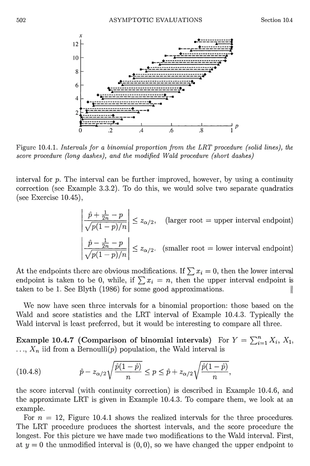
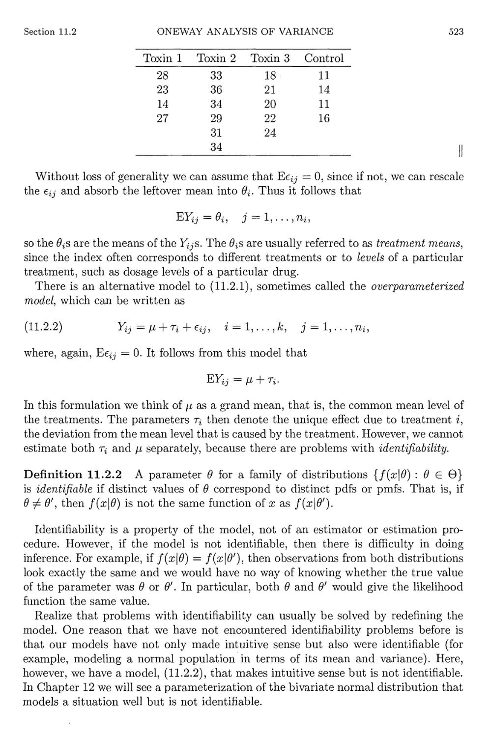
Текст
Statistical Inference
Second Edition
George Casella
Roger LBerger
DUXBURY ADVANCED SERIES
Statistical Inference
Second Edition
George Casella
University of Florida
Roger L. Berger
North Carolina State University
DUXBURY
*
THOMSON LEARNING
Australia • Canada • Mexico • Singapore • Spain • United Kingdom • United States
DUXBURY
*
THOMSON LEARNING
Sponsoring Editor: Carolyn Crockett
Marketing Representative: Torn Ziolkowski
Editorial Assistant: Jennifer Jenkins
Production Editor: Tom Novack
Assistant Editor: Ann Day
Manuscript Editor: Carol Reitz
Permissions Editor: Sue Ewing
Cover Design: Jennifer Mackres
Interior Illustration: Lori Heckelman
Print Buyer: Vena Dyer
Typesetting: Integre Technical Publishing Co.
Cover Printing: Phoenix Color Corp
Printing and Binding: RR Donnelley
All products used herein are used for identification purposes only and may be trademarks
or registered trademarks of their respective owners.
COPYRIGHT © 2002 the Wadsworth Group. Duxbury is an imprint of the Wadsworth
Group, a division of Thomson Learning Inc.
Thomson Learning™ is a trademark used herein under license.
For more information about this or any other Duxbury products, contact:
DUXBURY
511 Forest Lodge Road
Pacific Grove, CA 93950 USA
www.duxbury.com
1-800-423-0563 (Thomson Learning Academic Resource Center)
All rights reserved. No part of this work may be reproduced, transcribed or used in any
form or by any means—graphic, electronic, or mechanical, including photocopying,
recording, taping, Web distribution, or information storage and/or retrieval
systems—without the prior written permission of the publisher.
For permission to use material from this work, contact us by
www.thomsonrights.com
fax: 1-800-730-2215
phone: 1-800-730-2214
Printed in United States of America
10 9 8
Library of Congress Cataloging-in-Publication Data
Casella, George.
Statistical inference / George Casella, Roger L. Berger.—2nd ed.
p. cm.
Includes bibliographical references and indexes.
ISBN 0-534-24312-6
L Mathematical statistics. 2. Probabilities. I. Berger, Roger L.
II. Title.
QA276.C37 2001
519.5—dc21
2001025794
p°*££^
^*ecyc^°
To Anne and Vicki
Duxbury titles of related interest
Daniel, Applied Nonparametric Statistics 2
Derr, Statistical Consulting: A Guide to Effective Communication
Durrett, Probability: Theory and Examples 2nd
Graybill, Theory and Application of the Linear Model
Johnson, Applied Multivariate Methods for Data Analysts
Kuehl, Design of Experiments: Statistical Principles of Research Design and Analysis 2nd
Larsen, Marx, & Cooil, Statistics for Applied Problem Solving and Decision Making
Lohr, Sampling: Design and Analysis
Lunneborg, Data Analysis by Resampling: Concepts and Applications
Minh, Applied Probability Models
Minitab Inc., MINITAB™ Student Version 12 for Windows
Myers, Classical and Modern Regression with Applications 2nd
Newton & Harvill, StatConcepts: A Visual Tour of Statistical Ideas
Ramsey & Schafer, The Statistical Sleuth 2nd
SAS Institute Inc., JMP-IN: Statistical Discovery Software
Savage, INSIGHT: Business Analysis Software for Microsoft® Excel
Scheaffer, Mendenhall, & Ott, Elementary Survey Sampling 5th
Shapiro, Modeling the Supply Chain
Winston, Simulation Modeling Using @RISK
To order copies contact your local bookstore or call 1-800-354-9706. For more
information contact Duxbury Press at 511 Forest Lodge Road, Pacific Grove, CA 93950,
or go to: www.duxbury.com
Preface to the Second Edition
Although Sir Arthur Conan Doyle is responsible for most of the quotes in this book,
perhaps the best description of the life of this book can be attributed to the Grateful
Dead sentiment, "What a long, strange trip it's been."
Plans for the second edition started about six years ago, and for a long time we
struggled with questions about what to add and what to delete. Thankfully, as time
passed, the answers became clearer as the flow of the discipline of statistics became
clearer. We see the trend moving away from elegant proofs of special cases to
algorithmic solutions of more complex and practical cases. This does not undermine the
importance of mathematics and rigor; indeed, we have found that these have become
more important. But the manner in which they are applied is changing.
For those familiar with the first edition, we can summarize the changes succinctly
as follows. Discussion of asymptotic methods has been greatly expanded into its own
chapter. There is more emphasis on computing and simulation (see Section 5.5 and
the computer algebra Appendix); coverage of the more applicable techniques has
been expanded or added (for example, bootstrapping, the EM algorithm, p-values,
logistic and robust regression); and there are many new Miscellanea and Exercises.
We have de-emphasized the more specialized theoretical topics, such as equivariance
and decision theory, and have restructured some material in Chapters 3-11 for clarity.
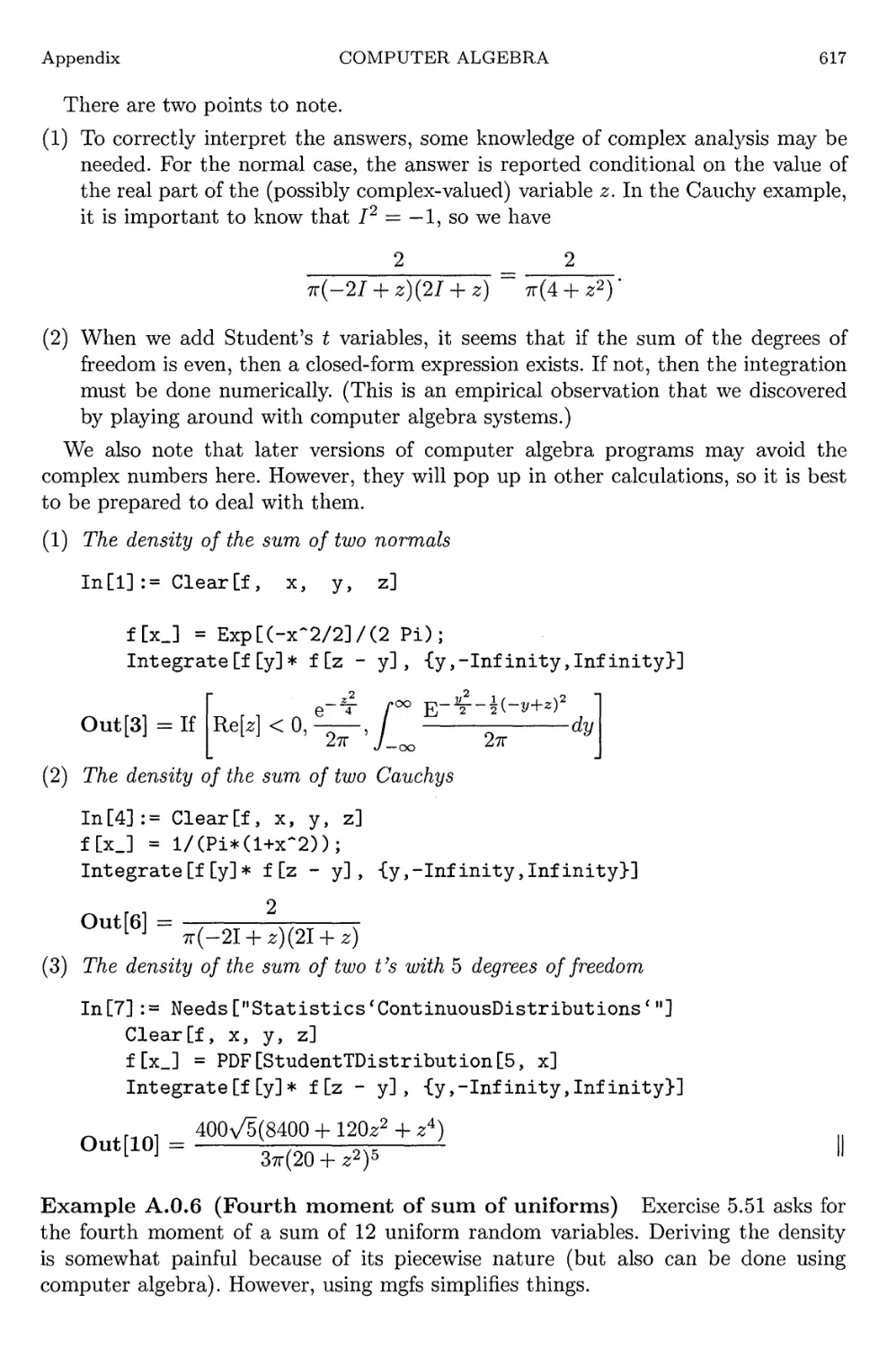
There are two things that we want to note. First, with respect to computer algebra
programs, although we believe that they are becoming increasingly valuable tools,
we did not want to force them on the instructor who does not share that belief.
Thus, the treatment is "unobtrusive" in that it appears only in an appendix, with
some hints throughout the book where it may be useful. Second, we have changed
the numbering system to one that facilitates finding things. Now theorems, lemmas,
examples, and definitions are numbered together; for example, Definition 7.2.4 is
followed by Example 7.2.5 and Theorem 10.1.3 precedes Example 10.1.4.
The first four chapters have received only minor changes. We reordered some
material (in particular, the inequalities and identities have been split), added some new
examples and exercises, and did some general updating. Chapter 5 has also been
reordered, with the convergence section being moved further back, and a new section on
generating random variables added. The previous coverage of invariance, which was
in Chapters 7-9 of the first edition, has been greatly reduced and incorporated into
Chapter 6, which otherwise has received only minor editing (mostly the addition of
new exercises). Chapter 7 has been expanded and updated, and includes a new section
on the EM algorithm. Chapter 8 has also received minor editing and updating, and
vi PREFACE TO THE SECOND EDITION
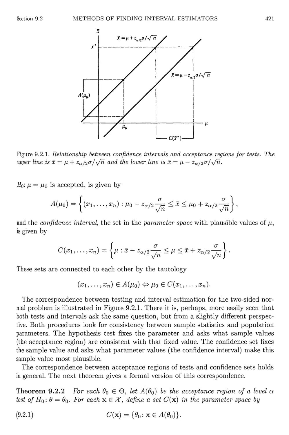
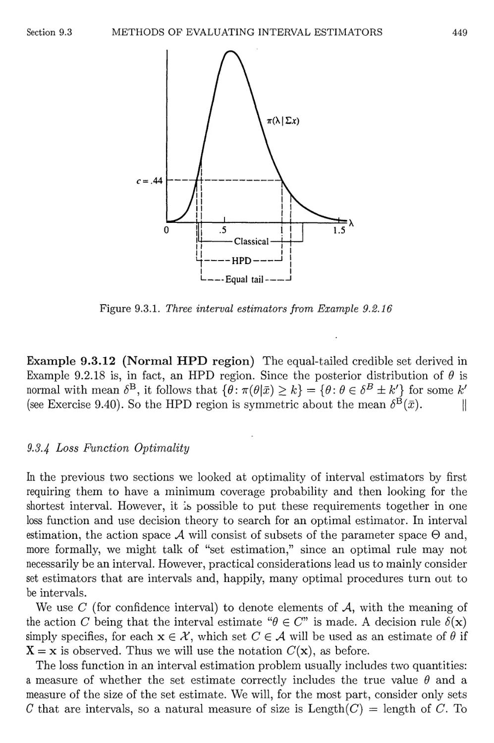
has a new section on p-values. In Chapter 9 we now put more emphasis on pivoting
(having realized that "guaranteeing an interval" was merely "pivoting the cdf'). Also,
the material that was in Chapter 10 of the first edition (decision theory) has been
reduced, and small sections on loss function optimality of point estimation, hypothesis
testing, and interval estimation have been added to the appropriate chapters.
Chapter 10 is entirely new and attempts to lay out the fundamentals of large sample
inference, including the delta method, consistency and asymptotic normality,
bootstrapping, robust estimators, score tests, etc. Chapter 11 is classic oneway ANOVA
and linear regression (which was covered in two different chapters in the first
edition). Unfortunately, coverage of randomized block designs has been eliminated for
space reasons. Chapter 12 covers regression with errors-in-variables and contains new
material on robust and logistic regression.
After teaching from the first edition for a number of years, we know (approximately)
what can be covered in a one-year course. From the second edition, it should be
possible to cover the following in one year:
Chapter 1
Chapter 2
Chapter 3
Chapter 4
Chapter 5
Sections 1-7 Chapter 6: Sections 1-3
Sections 1-3 Chapter 7: Sections 1-3
Sections 1-6 Chapter 8: Sections 1-3
Sections 1-7 Chapter 9: Sections 1-3
Sections 1-6 Chapter 10: Sections 1, 3, 4
Classes that begin the course with some probability background can cover more
material from the later chapters.
Finally, it is almost impossible to thank all of the people who have contributed in
some way to making the second edition a reality (and help us correct the mistakes in
the first edition). To all of our students, friends, and colleagues who took the time to
send us a note or an e-mail, we thank you. A number of people made key suggestions
that led to substantial changes in presentation. Sometimes these suggestions were just
short notes or comments, and some were longer reviews. Some were so long ago that
their authors may have forgotten, but we haven't. So thanks to Arthur Cohen, Sir
David Cox, Steve Samuels, Rob Strawderman and Tom Wehrly. We also owe much to
Jay Beder, who has sent us numerous comments and suggestions over the years and
possibly knows the first edition better than we do, and to Michael Perlman and his
class, who are sending comments and corrections even as we write this.
This book has seen a number of editors. We thank Alex Kugashev, who in the
mid-1990s first suggested doing a second edition, and our editor, Carolyn Crockett,
who constantly encouraged us. Perhaps the one person (other than us) who is most
responsible for this book is our first editor, John Kimmel, who encouraged, published,
and marketed the first edition. Thanks, John.
George Casella
Roger L. Berger
Preface to the First Edition
When someone discovers that you are writing a textbook, one (or both) of two
questions will be asked. The first is "Why are you writing a book?" and the second is
"How is your book different from wThat's out there?" The first question is fairly easy
to answer. You are writing a book because you are not entirely satisfied with the
available texts. The second question is harder to answer. The answer can't be put
in a few sentences so, in order not to bore your audience (who may be asking the
question only out of politeness), you try to say something quick and witty. It usually
doesn't work.
The purpose of this book is to build theoretical statistics (as different from
mathematical statistics) from the first principles of probability theory. Logical development,
proofs, ideas, themes, etc., evolve through statistical arguments. Thus, starting from
the basics of probability, we develop the theory of statistical inference using
techniques, definitions, and concepts that are statistical and are natural extensions and
consequences of previous concepts. When this endeavor was started, we were not sure
how well it would work. The final judgment of our success is, of course, left to the
reader.
The book is intended for first-year graduate students majoring in statistics or in
a field where a statistics concentration is desirable. The prerequisite is one year of
calculus. (Some familiarity with matrix manipulations would be useful, but is not
essential.) The book can be used for a two-semester, or three-quarter, introductory
course in statistics.
The first four chapters cover basics of probability theory and introduce many
fundamentals that are later necessary. Chapters 5 and 6 are the first statistical chapters.
Chapter 5 is transitional (between probability and statistics) and can be the starting
point for a course in statistical theory for students with some probability background.
Chapter 6 is somewhat unique, detailing three statistical principles (sufficiency,
likelihood, and invariance) and showing how these principles are important in modeling
data. Not all instructors will cover this chapter in detail, although we strongly
recommend spending some time here. In particular, the likelihood and invariance principles
are treated in detail. Along with the sufficiency principle, these principles, and the
thinking behind them, are fundamental to total statistical understanding.
Chapters 7-9 represent the central core of statistical inference, estimation (point
and interval) and hypothesis testing. A major feature of these chapters is the division
into methods of finding appropriate statistical techniques and methods of evaluating
these techniques. Finding and evaluating are of interest to both the theorist and the
Vlll
PREFACE TO THE FIRST EDITION
practitioner, but we feel that it is important to separate these endeavors. Different
concerns are important, and different rules are invoked. Of further interest may be
the sections of these chapters titled Other Considerations. Here, we indicate how the
rules of statistical inference may be relaxed (as is done every day) and still produce
meaningful inferences. Many of the techniques covered in these sections are ones that
are used in consulting and are helpful in analyzing and inferring from actual problems.
The final three chapters can be thought of as special topics, although we feel that
some familiarity with the material is important in anyone's statistical education.
Chapter 10 is a thorough introduction to decision theory and contains the most
modern material we could include. Chapter 11 deals with the analysis of variance (oneway
and randomized block), building the theory of the complete analysis from the more
simple theory of treatment contrasts. Our experience has been that experimenters are
most interested in inferences from contrasts, and using principles developed earlier,
most tests and intervals can be derived from contrasts. Finally, Chapter 12 treats
the theory of regression, dealing first with simple linear regression and then covering
regression with "errors in variables." This latter topic is quite important, not only to
show its own usefulness and inherent difficulties, but also to illustrate the limitations
of inferences from ordinary regression.
As more concrete guidelines for basing a one-year course on this book, we offer the
following suggestions. There can be two distinct types of courses taught from this
book. One kind we might label "more mathematical," being a course appropriate for
students majoring in statistics and having a solid mathematics background (at least
l| years of calculus, some matrix algebra, and perhaps a real analysis course). For
such students we recommend covering Chapters 1-9 in their entirety (which should
take approximately 22 weeks) and spend the remaining time customizing the course
with selected topics from Chapters 10-12. Once the first nine chapters are covered,
the material in each of the last three chapters is self-contained, and can be covered
in any order.
Another type of course is "more practical." Such a course may also be a first course
for mathematically sophisticated students, but is aimed at students with one year of
calculus who may not be majoring in statistics. It stresses the more practical uses of
statistical theory, being more concerned with understanding basic statistical concepts
and deriving reasonable statistical procedures for a variety of situations, and less
concerned with formal optimality investigations. Such a course will necessarily omit
a certain amount of material, but the following list of sections can be covered in a
one-year course:
Chapter Sections
1 All
2 2.1, 2.2, 2.3
3 3.1, 3.2
4 4.1, 4.2, 4.3, 4.5
5 5.1, 5.2, 5.3.1, 5.4
6 6.1.1,6.2.1
7 7.1, 7.2.1, 7.2.2, 7.2.3, 7.3.1, 7.3.3, 7.4
8 8.1, 8.2.1, 8.2.3, 8.2.4, 8.3.1, 8.3.2, 8.4
PREFACE TO THE FIRST EDITION
ix
9 9.1, 9.2.1, 9.2.2, 9.2.4, 9.3.1, 9.4
11 11.1, 11.2
12 12.1, 12.2
If time permits, there can be some discussion (with little emphasis on details) of the
material in Sections 4.4, 5.5, and 6.1.2, 6.1.3, 6.1.4. The material in Sections 11.3 and
12.3 may also be considered.
The exercises have been gathered from many sources and are quite plentiful. We
feel that, perhaps, the only way to master this material is through practice, and thus
we have included much opportunity to do so. The exercises are as varied as we could
make them, and many of them illustrate points that are either new or complementary
to the material in the text. Some exercises are even taken from research papers. (It
makes you feel old when you can include exercises based on papers that were new
research during your own student days!) Although the exercises are not subdivided
like the chapters, their ordering roughly follows that of the chapter. (Subdivisions
often give too many hints.) Furthermore, the exercises become (again, roughly) more
challenging as their numbers become higher.
As this is an introductory book with a relatively broad scope, the topics arc not
covered in great depth. However, we felt some obligation to guide the reader one
step further in the topics that may be of interest. Thus, we have included many
references, pointing to the path to deeper understanding of any particular topic. (The
Encyclopedia of Statistical Sciences, edited by Kotz, Johnson, and Read, provides a
fine introduction to many topics.)
To write this book, we have drawn on both our past teachings and current work. We
have also drawn on many people, to whom we are extremely grateful. We thank our
colleagues at Cornell, North Carolina State, and Purdue—in particular, Jim Berger,
Larry Brown, Sir David Cox, Ziding Feng, Janet Johnson, Leon Gleser, Costas Goutis,
Dave Lansky, George McCabe, Chuck McCulloch, Myra Samuels, Steve Schwager,
and Shayle Searle, who have given their time and expertise in reading parts of this
manuscript, offered assistance, and taken part in many conversations leading to
constructive suggestions. We also thank Shanti Gupta for his hospitality, and the
library at Purdue, which was essential. We are grateful for the detailed reading and
helpful suggestions of Shayle Searle and of our reviewers, both anonymous and non-
anonymous (Jim Albert, Dan Coster, and Tom Wehrly). We also thank David Moore
and George McCabe for allowing us to use their tables, and Steve Hirdt for supplying
us with data. Since this book was written by two people who, for most of the time,
were at least 600 miles apart, we lastly thank Bitnet for making this entire thing
possible.
George Casella
Roger L. Berger
"We have got to the deductions and the inferences," said Lestrade, winking at me.
"I find it hard enough to tackle facts, Holmes, without flying away
after theories and fancies."
Inspector Lestrade to Sherlock Holmes
The Boscombe Valley Mystery
Contents
1 Probability Theory 1
1.1 Set Theory 1
1.2 Basics of Probability Theory 5
1.2.1 Axiomatic Foundations 5
1.2.2 The Calculus of Probabilities 9
1.2.3 Counting 13
1.2.4 Enumerating Outcomes 16
1.3 Conditional Probability and Independence 20
1.4 Random Variables 27
1.5 Distribution Functions 29
1.6 Density and Mass Functions 34
1.7 Exercises 37
1.8 Miscellanea 44
2 Transformations and Expectations 47
2.1 Distributions of Functions of a Random Variable 47
2.2 Expected Values 55
2.3 Moments and Moment Generating Functions 59
2.4 Differentiating Under an Integral Sign 68
2.5 Exercises 76
2.6 Miscellanea 82
3 Common Families of Distributions 85
3.1 Introduction 85
3.2 Discrete Distributions 85
3.3 Continuous Distributions 98
3.4 Exponential Families 111
3.5 Location and Scale Families 116
XIV
CONTENTS
3.6 Inequalities and Identities 121
3.6.1 Probability Inequalities 122
3.6.2 Identities 123
3.7 Exercises 127
3.8 Miscellanea 135
4 Multiple Random Variables 139
4.1 Joint and Marginal Distributions 139
4.2 Conditional Distributions and Independence 147
4.3 Bivariate Transformations 156
4.4 Hierarchical Models and Mixture Distributions 162
4.5 Covariance and Correlation 169
4.6 Multivariate Distributions 177
4.7 Inequalities 186
4.7.1 Numerical Inequalities 186
4.7.2 Functional Inequalities 189
4.8 Exercises 192
4.9 Miscellanea 203
5 Properties of a Random Sample 207
5.1 Basic Concepts of Random Samples 207
5.2 Sums of Random Variables from a Random Sample 211
5.3 Sampling from the Normal Distribution 218
5.3.1 Properties of the Sample Mean and Variance 218
5.3.2 The Derived Distributions: Student's t and Snedecor's F 222
5.4 Order Statistics 226
5.5 Convergence Concepts 232
5.5.1 Convergence in Probability 232
5.5.2 Almost Sure Convergence 234
5.5.3 Convergence in Distribution 235
5.5.4 The Delta Method 240
5.6 Generating a Random Sample 245
5.6.1 Direct Methods 247
5.6.2 Indirect Methods 251
5.6.3 The Accept/Reject Algorithm 253
5.7 Exercises 255
5.8 Miscellanea 267
6 Principles of Data Reduction 271
6.1 Introduction 271
6.2 The Sufficiency Principle 272
6.2.1 Sufficient Statistics 272
6.2.2 Minimal Sufficient Statistics 279
6.2.3 Ancillary Statistics 282
6.2.4 Sufficient, Ancillary, and Complete Statistics 284
CONTENTS
xv
6.3 The Likelihood Principle 290
6.3.1 The Likelihood Function 290
6.3.2 The Formal Likelihood Principle 292
6.4 The Equivariance Principle 296
6.5 Exercises 300
6.6 Miscellanea 307
Point Estimation 311
7.1 Introduction 311
7.2 Methods of Finding Estimators 312
7.2.1 Method of Moments 312
7.2.2 Maximum Likelihood Estimators 315
7.2.3 Bayes Estimators 324
7.2.4 The EM Algorithm 326
7.3 Methods of Evaluating Estimators 330
7.3.1 Mean Squared Error 330
7.3.2 Best Unbiased Estimators 334
7.3.3 Sufficiency and Unbiasedness 342
7.3.4 Loss Function Optimality 348
7.4 Exercises 355
7.5 Miscellanea 367
Hypothesis Testing 373
8.1 Introduction 373
8.2 Methods of Finding Tests 374
8.2.1 Likelihood Ratio Tests 374
8.2.2 Bayesian Tests 379
8.2.3 Union-Intersection and Intersection-Union Tests 380
8.3 Methods of Evaluating Tests 382
8.3.1 Error Probabilities and the Power Function 382
8.3.2 Most Powerful Tests 387
8.3.3 Sizes of Union-Intersection and Intersection-Union Tests 394
8.3.4 p-Values 397
8.3.5 Loss Function Optimality 400
8.4 Exercises 402
8.5 Miscellanea 413
Interval Estimation 417
9.1 Introduction 417
9.2 Methods of Finding Interval Estimators 420
9.2.1 Inverting a Test Statistic 420
9.2.2 Pivotal Quantities 427
9.2.3 Pivoting the CDF 430
9.2.4 Bayesian Intervals 435
XVI
CONTENTS
9.3 Methods of Evaluating Interval Estimators 440
9.3.1 Size and Coverage Probability 440
9.3.2 Test-Related Optimally 444
9.3.3 Bayesian Optimality 447
9.3.4 Loss Function Optimality 449
9.4 Exercises 451
9.5 Miscellanea 463
10 Asymptotic Evaluations 467
10.1 Point Estimation 467
10.1.1 Consistency 467
10.1.2 Efficiency 470
10.1.3 Calculations and Comparisons 473
10.1.4 Bootstrap Standard Errors 478
10.2 Robustness 481
10.2.1 The Mean and the Median 482
10.2.2 M-Estimators 484
10.3 Hypothesis Testing 488
10.3.1 Asymptotic Distribution of LRTs 488
10.3.2 Other Large-Sample Tests 492
10.4 Interval Estimation 496
10.4.1 Approximate Maximum Likelihood Intervals 496
10.4.2 Other Large-Sample Intervals 499
10.5 Exercises 504
10.6 Miscellanea 515
11 Analysis of Variance and Regression 521
11.1 Introduction 521
11.2 Oneway Analysis of Variance 522
11.2.1 Model and Distribution Assumptions 524
11.2.2 The Classic ANOVA Hypothesis 525
11.2.3 Inferences Regarding Linear Combinations of Means 527
11.2.4 The ANOVA F Test 530
11.2.5 Simultaneous Estimation of Contrasts 534
11.2.6 Partitioning Sums of Squares 536
11.3 Simple Linear Regression 539
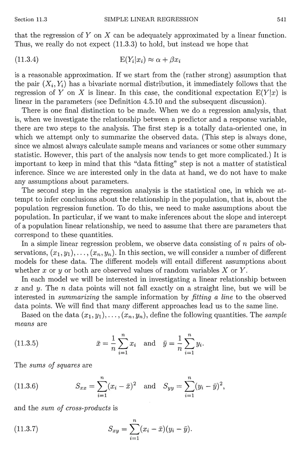
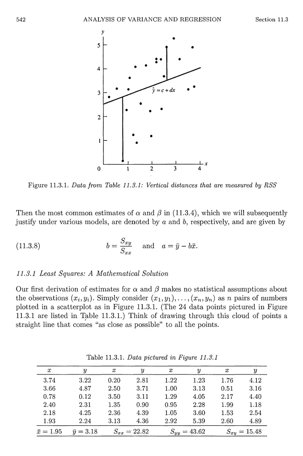
11.3.1 Least Squares: A Mathematical Solution 542
11.3.2 Best Linear Unbiased Estimators: A Statistical Solution 544
11.3.3 Models and Distribution Assumptions 548
11.3.4 Estimation and Testing with Normal Errors 550
11.3.5 Estimation and Prediction at a Specified x = x0 557
11.3.6 Simultaneous Estimation and Confidence Bands 559
11.4 Exercises 563
11.5 Miscellanea 572
CONTENTS
XVI1
12 Regression Models 577
12.1 Introduction 577
12.2 Regression with Errors in Variables 577
12.2.1 Functional and Structural Relationships 579
12.2.2 A Least Squares Solution 581
12.2.3 Maximum Likelihood Estimation 583
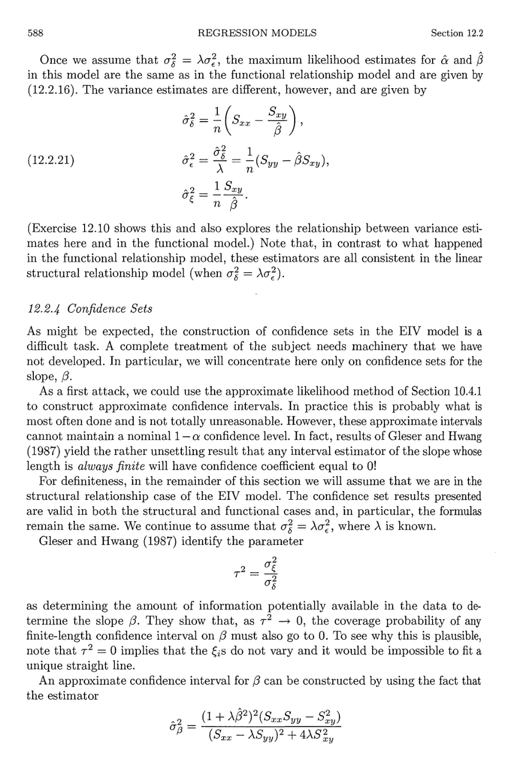
12.2.4 Confidence Sets 588
12.3 Logistic Regression 591
12.3.1 The Model 591
12.3.2 Estimation 593
12.4 Robust Regression 597
12.5 Exercises 602
12.6 Miscellanea 608
Appendix: Computer Algebra 613
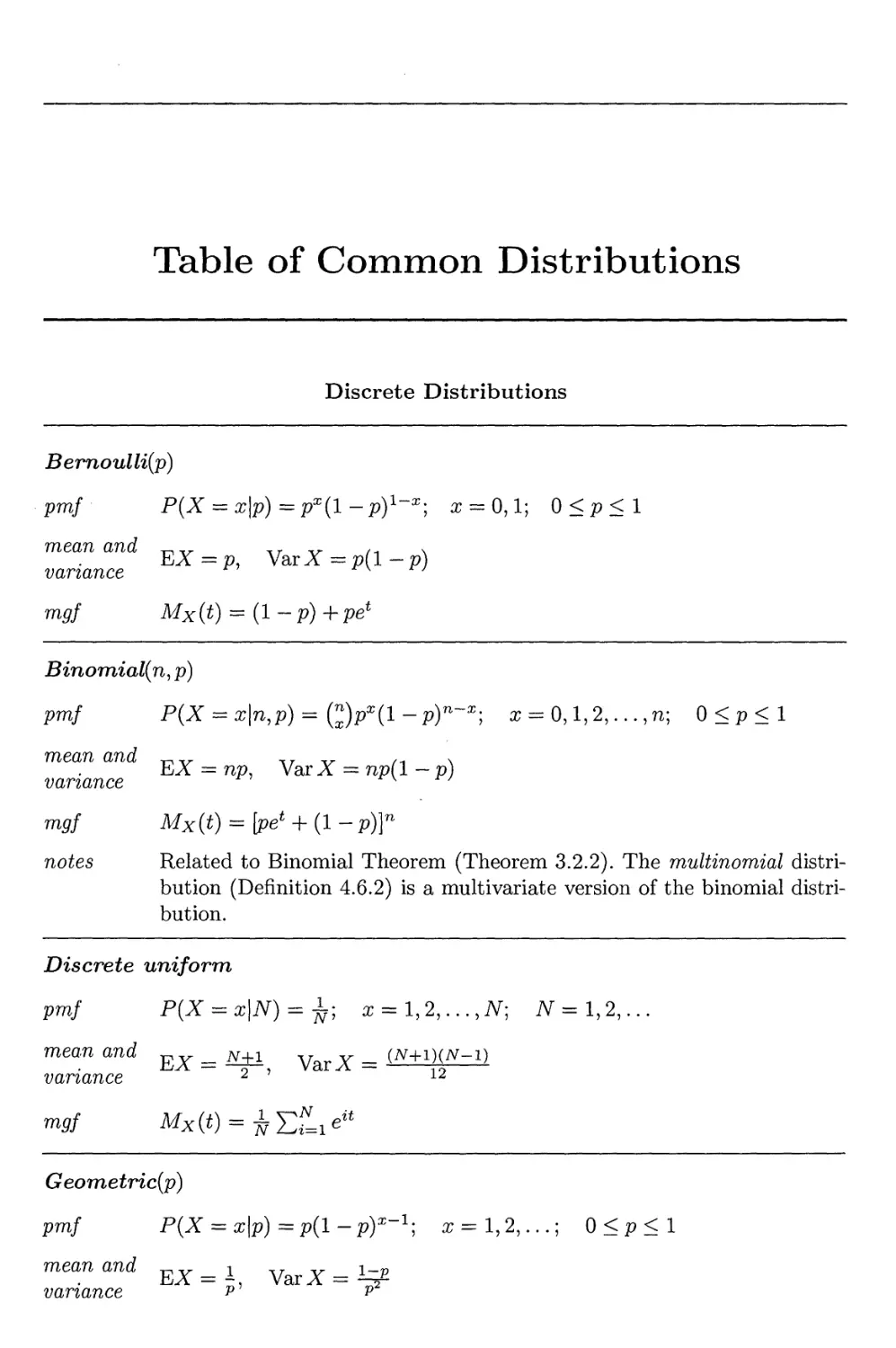
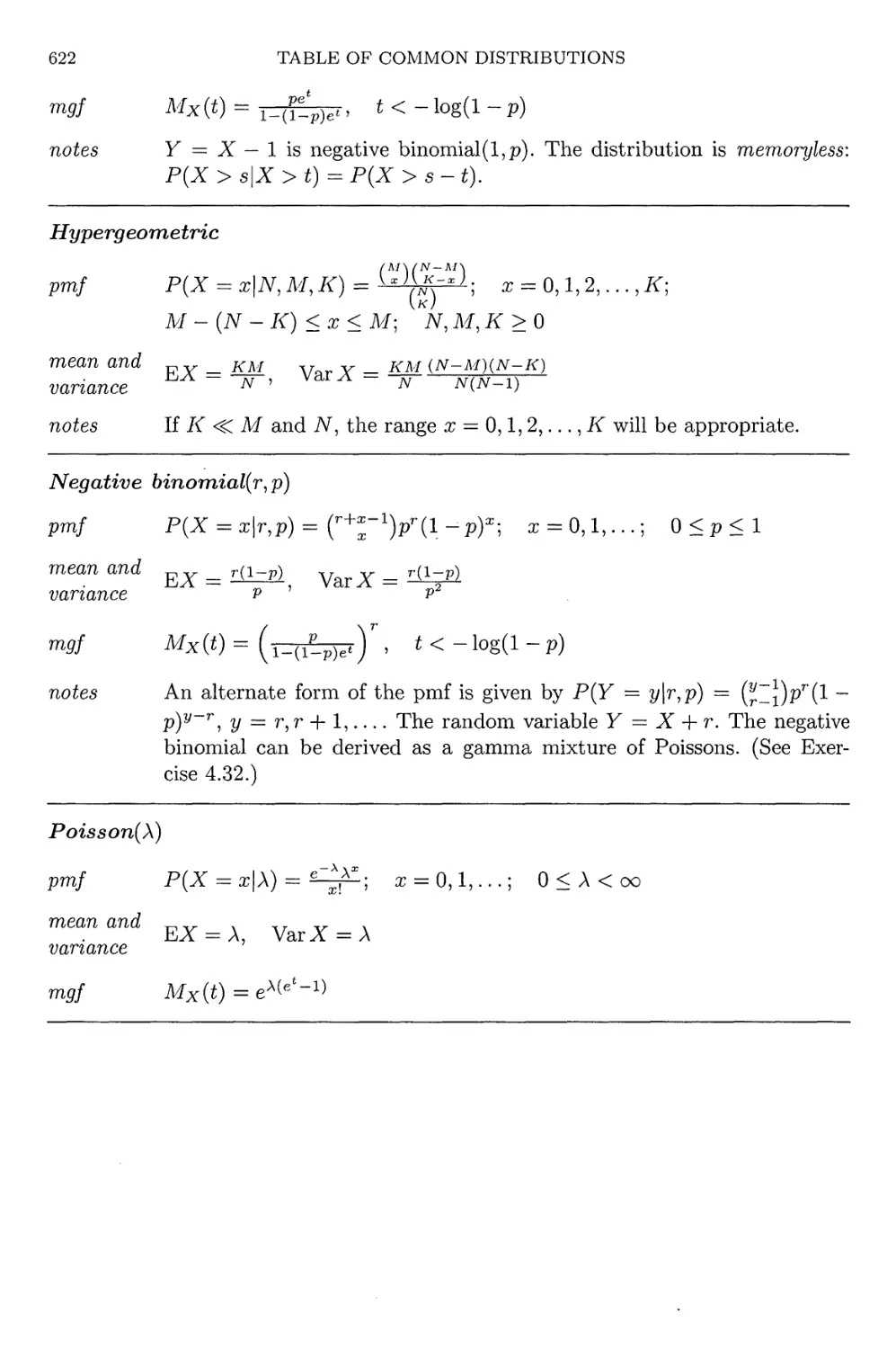
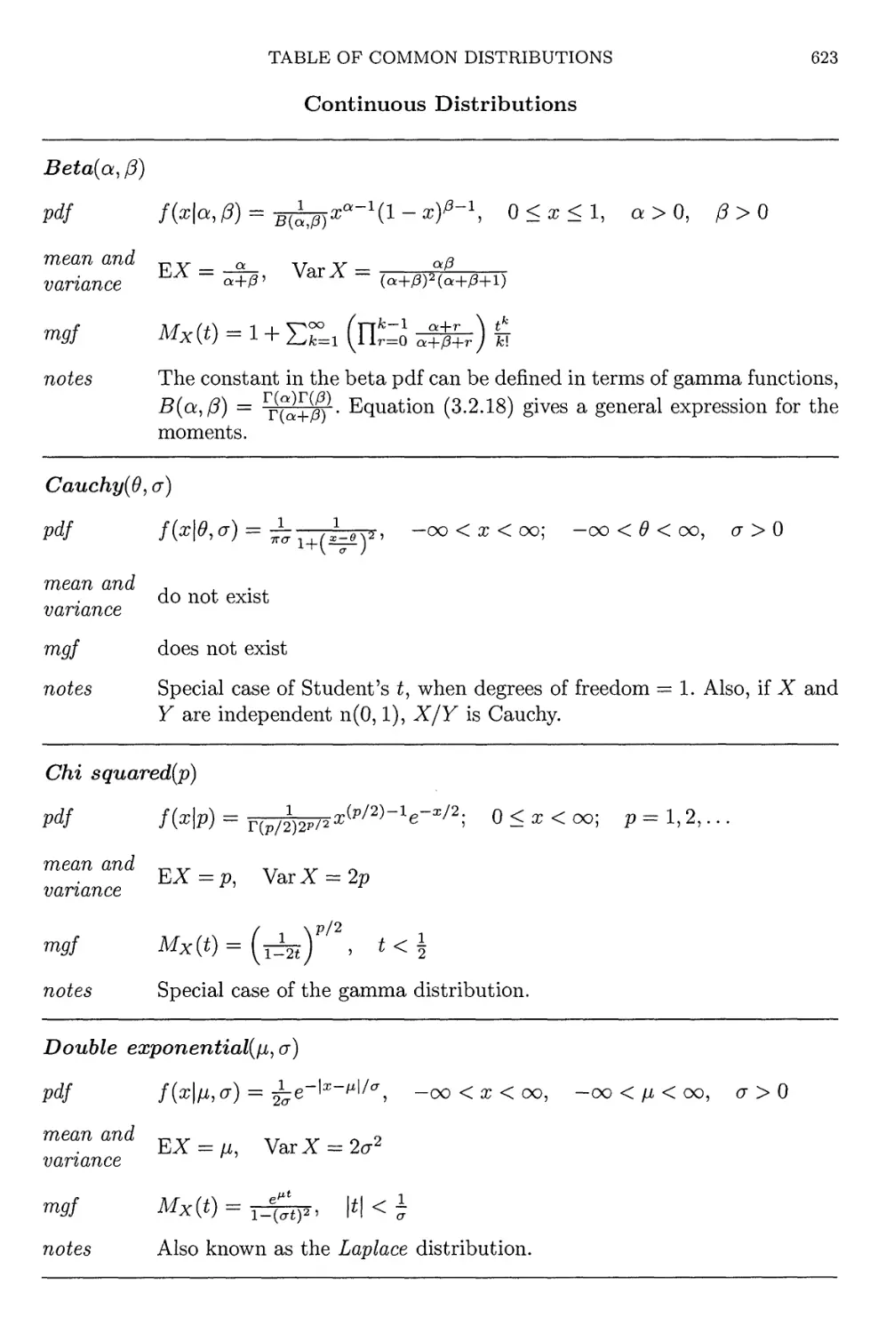
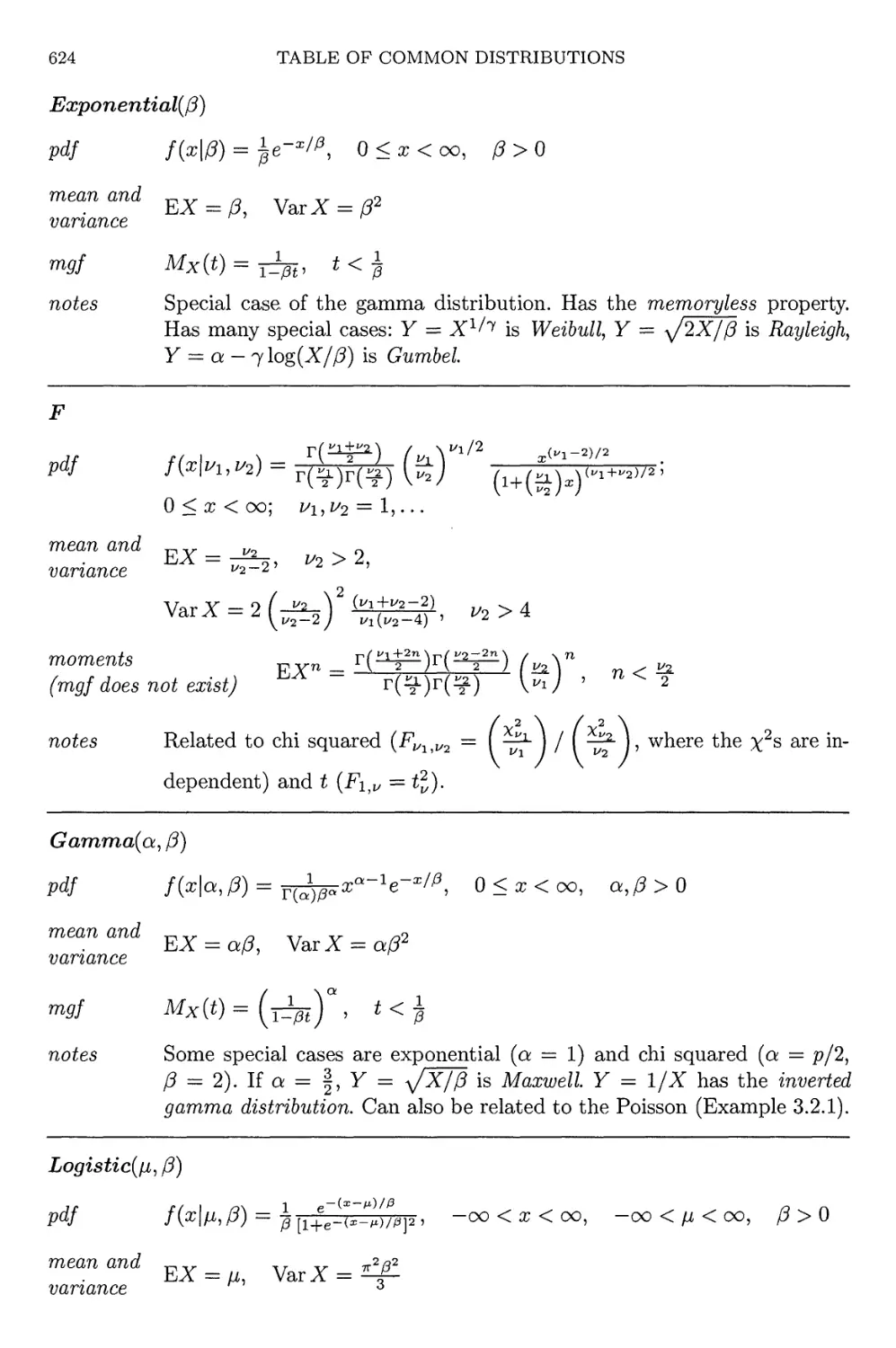
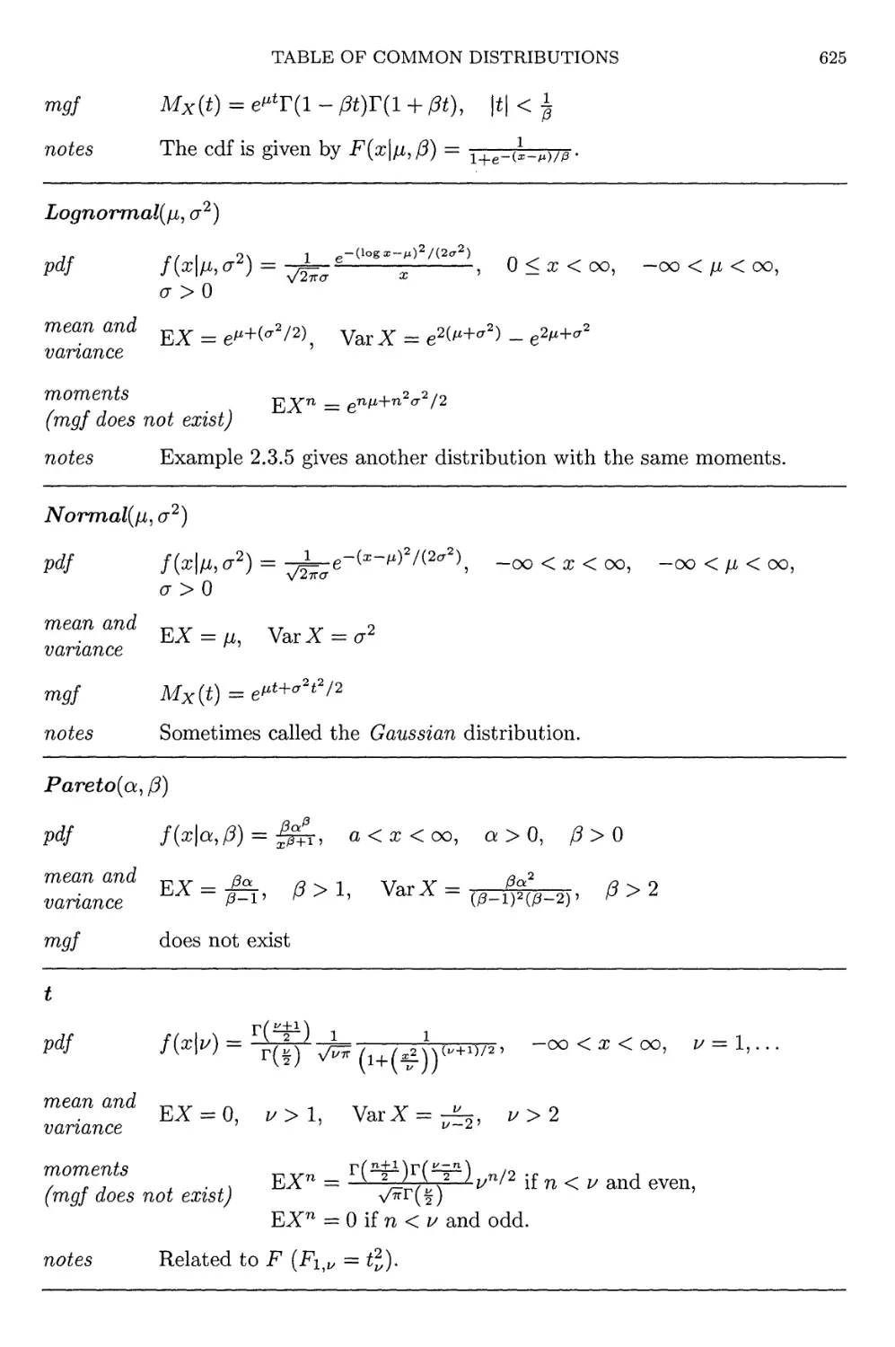
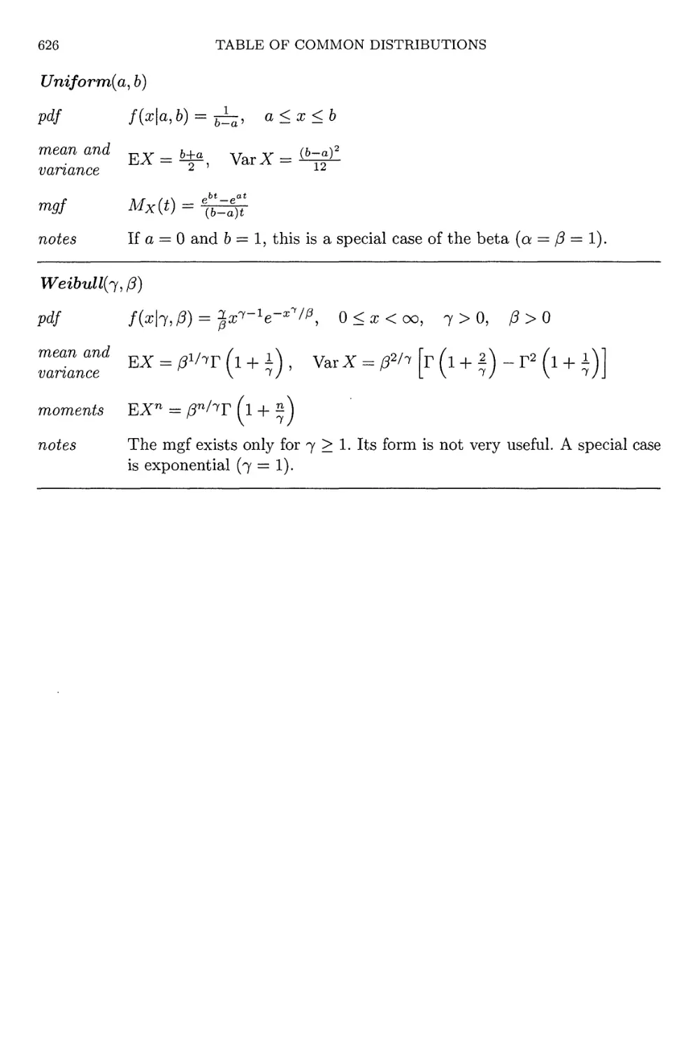
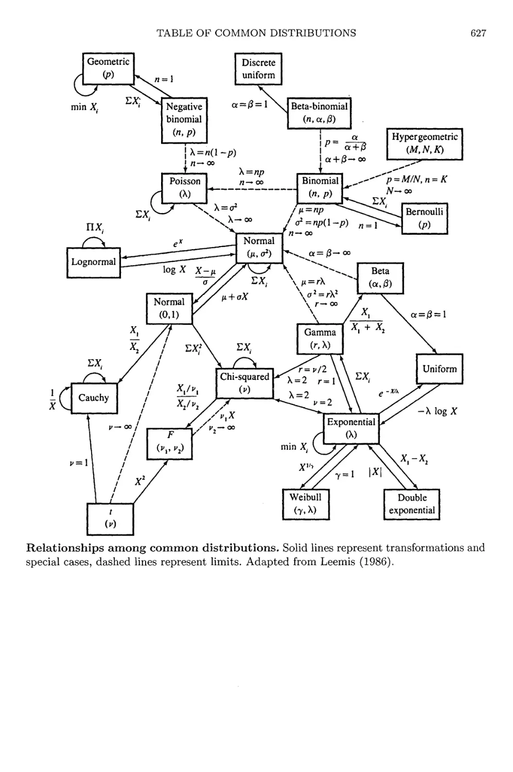
Table of Common Distributions 621
References 629
Author Index 645
Subject Index
649
List of Tables
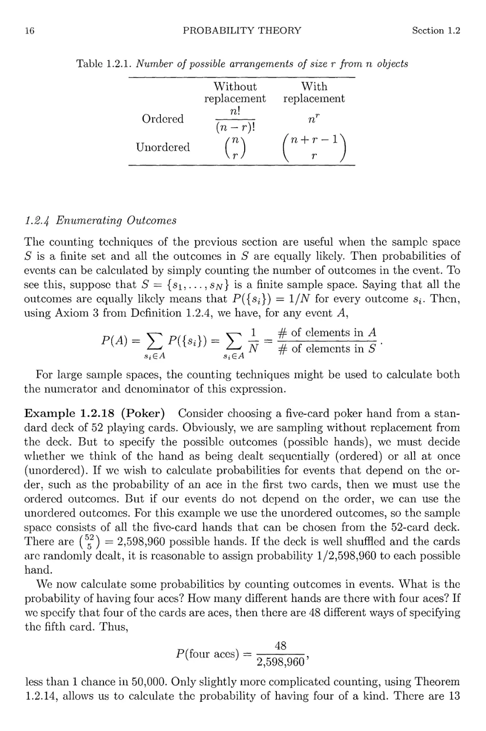
1.2.1 Number of arrangements 16
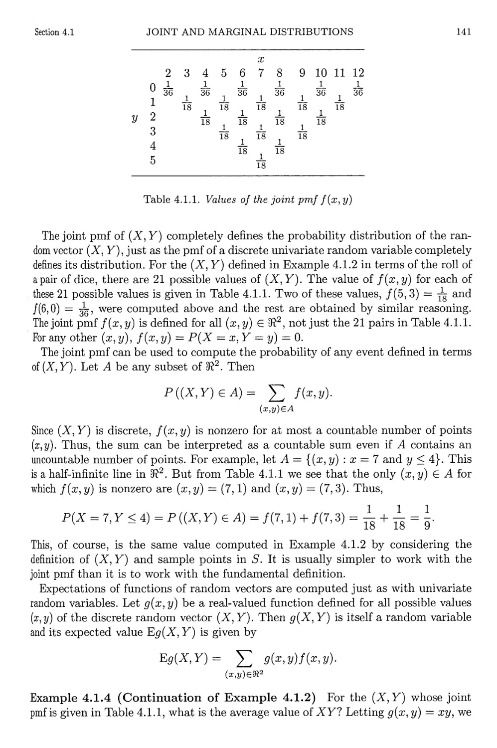
4.1.1 Values of the joint pmf f{x, y) 141
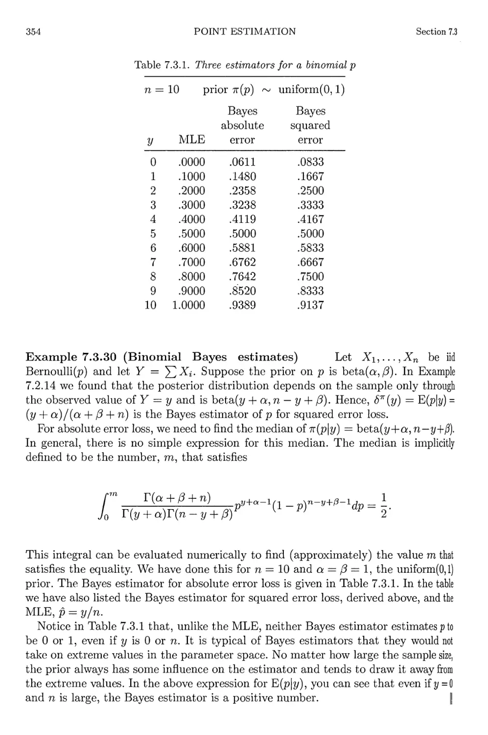
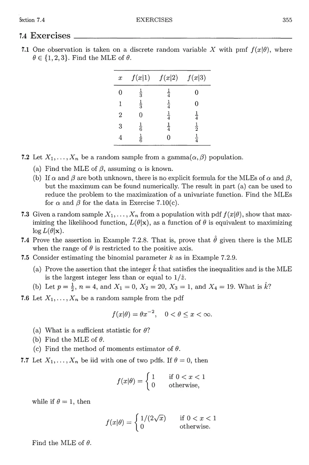
7.3.1 Three estimators for a binomial p 354
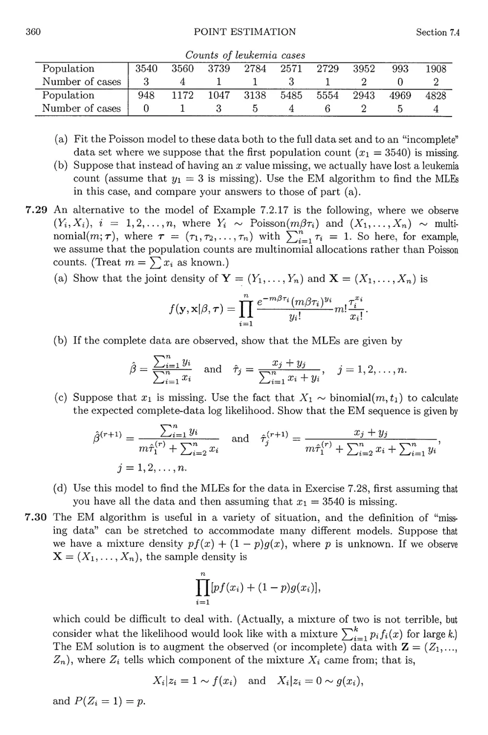
Counts of leukemia cases 360
8.3.1 Two types of errors in hypothesis testing 383
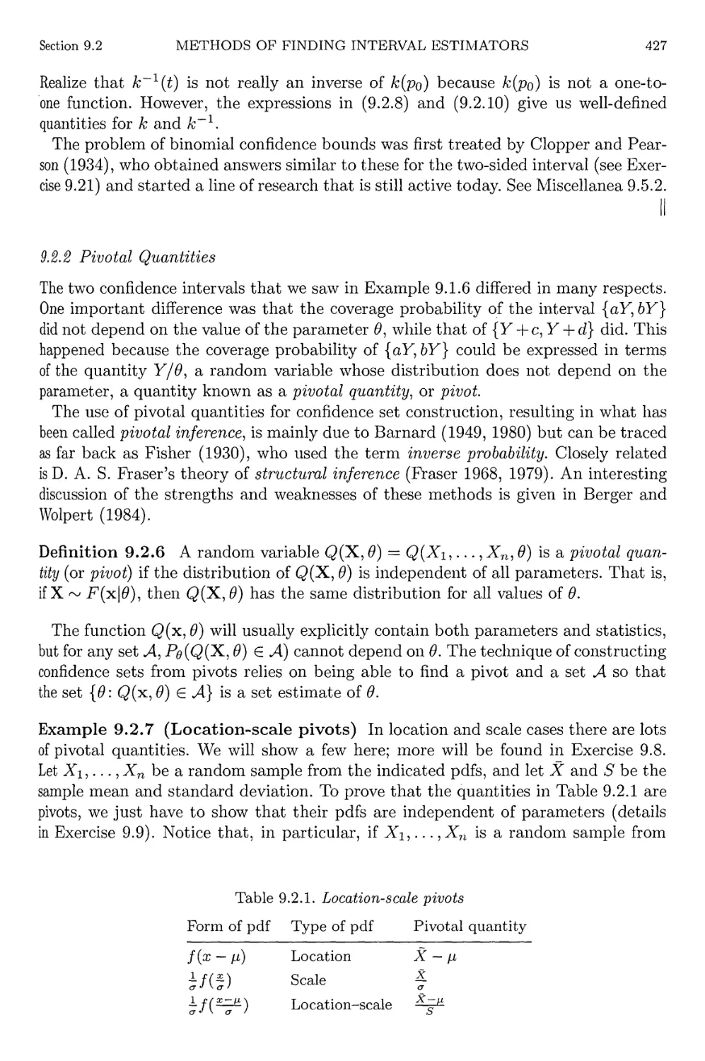
9.2.1 Location-scale pivots 427
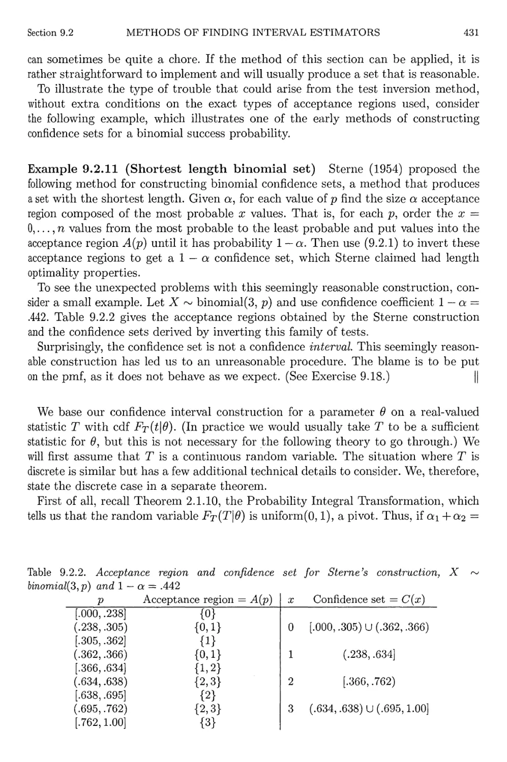
9.2.2 Sterne's acceptance region and confidence set 431
Three 90% normal confidence intervals 441
10.1.1 Bootstrap and Delta Method variances 480
Median/mean asymptotic relative efficiencies 484
10.2.1 Huber estimators 485
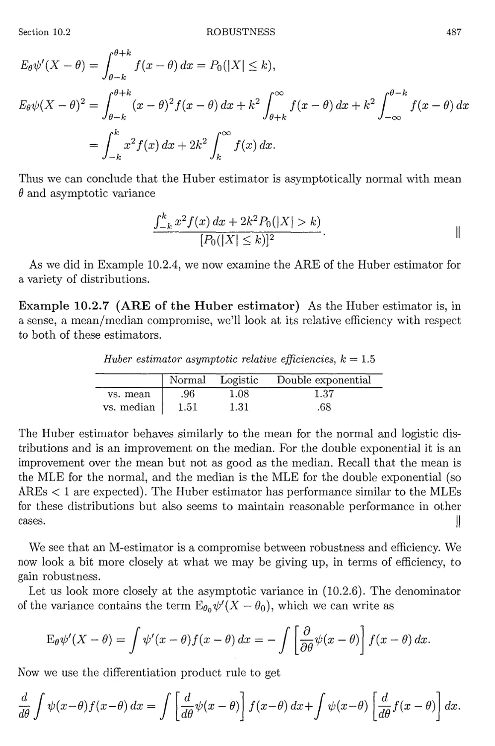
Huber estimator asymptotic relative efficiencies, fc = 1.5 487
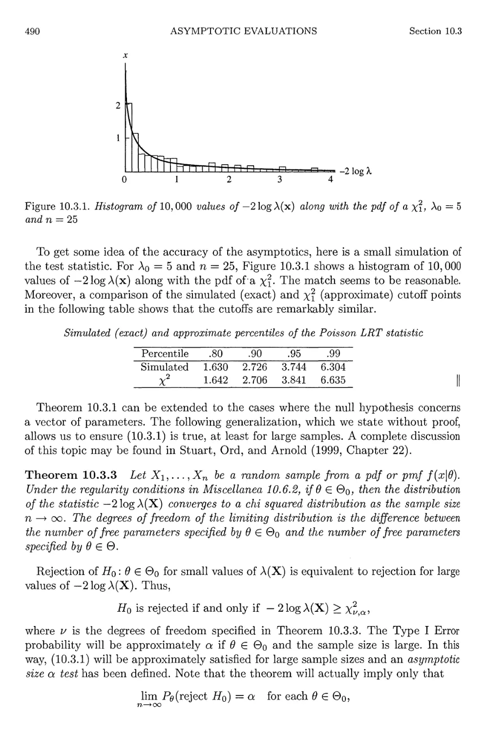
Poisson LRT statistic 490
10.3.1 Power of robust tests 497
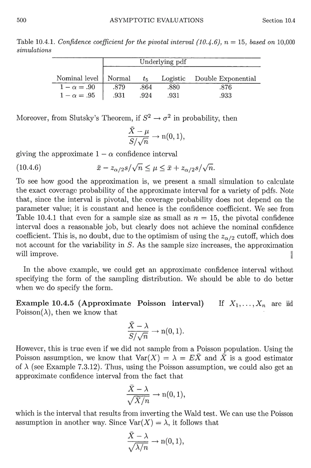
10.4.1 Confidence coefficient for a pivotal interval 500
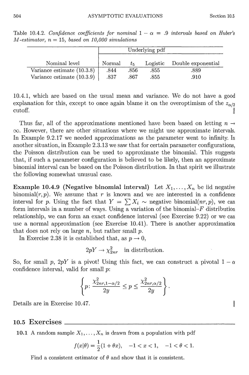
10.4.2 Confidence coefficients for intervals based on Huber's M-estimator 504
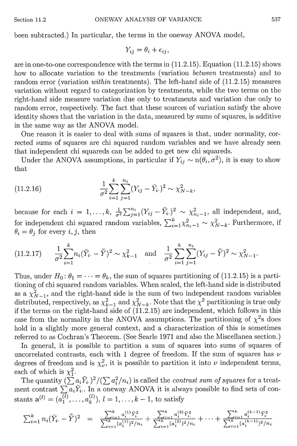
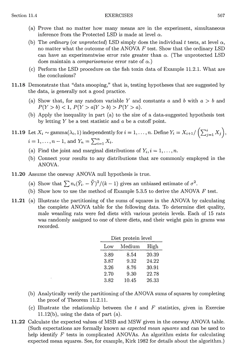
11.2.1 ANOVA table for oneway classification 538
11.3.1 Data pictured in Figure 11.3.1 542
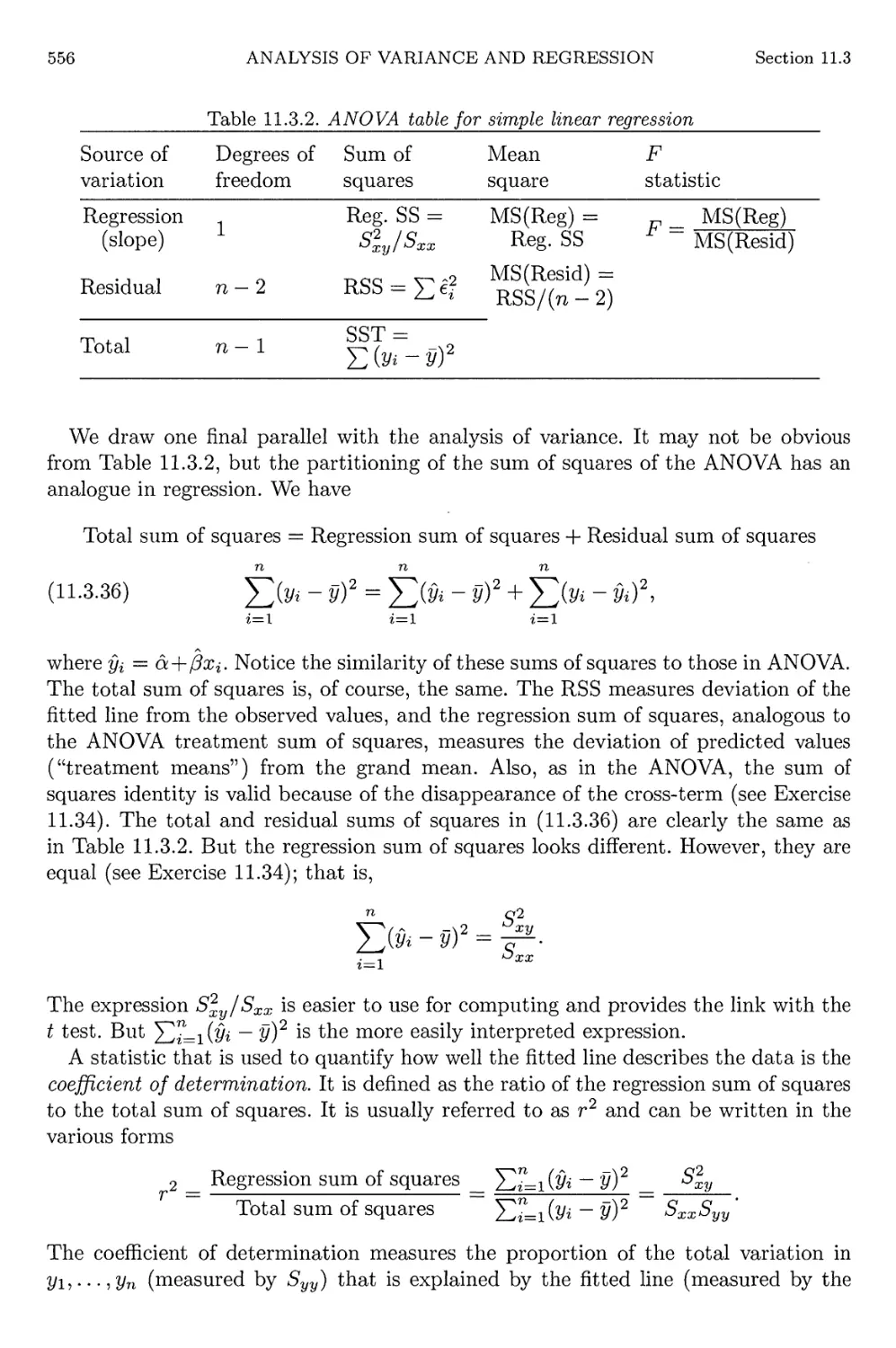
11.3.2 ANOVA table for simple linear regression 556
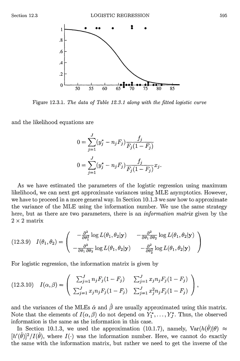
12.3.1 Challenger data 594
12.4.1 Potoroo data 598
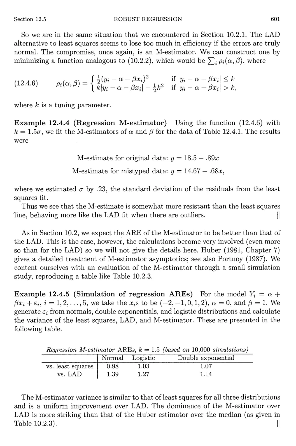
Regression M-estimator asymptotic relative efficiencies 601
List of Figures
1.2.1
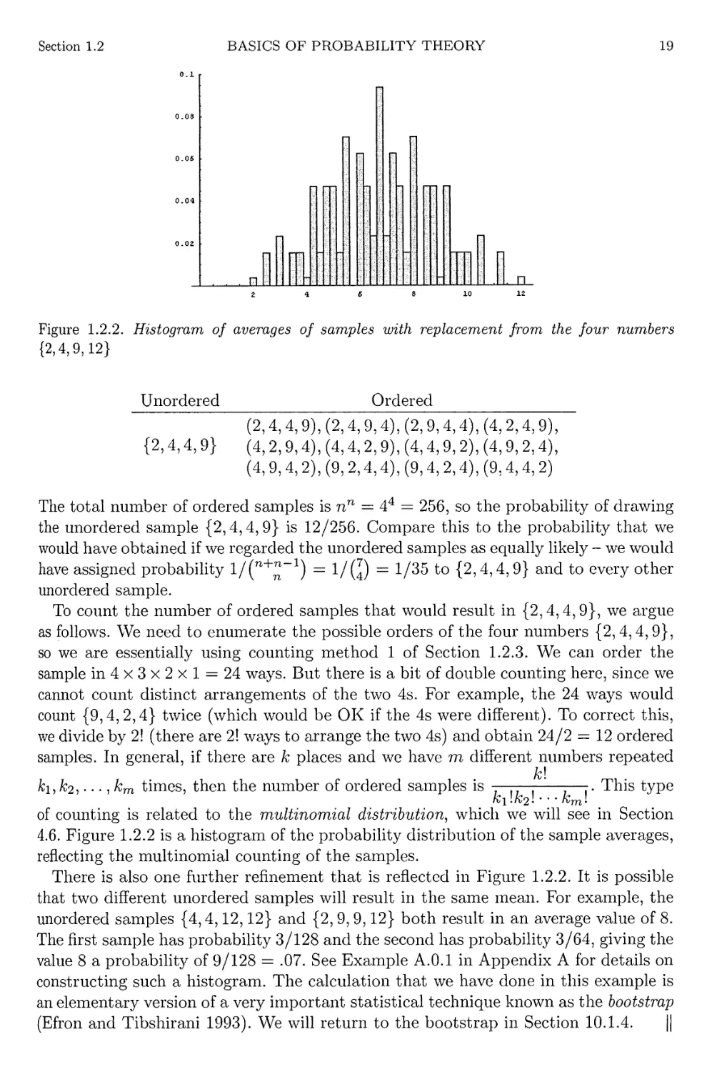
1.2.2
1.5.1
1.5.2
1.6.1
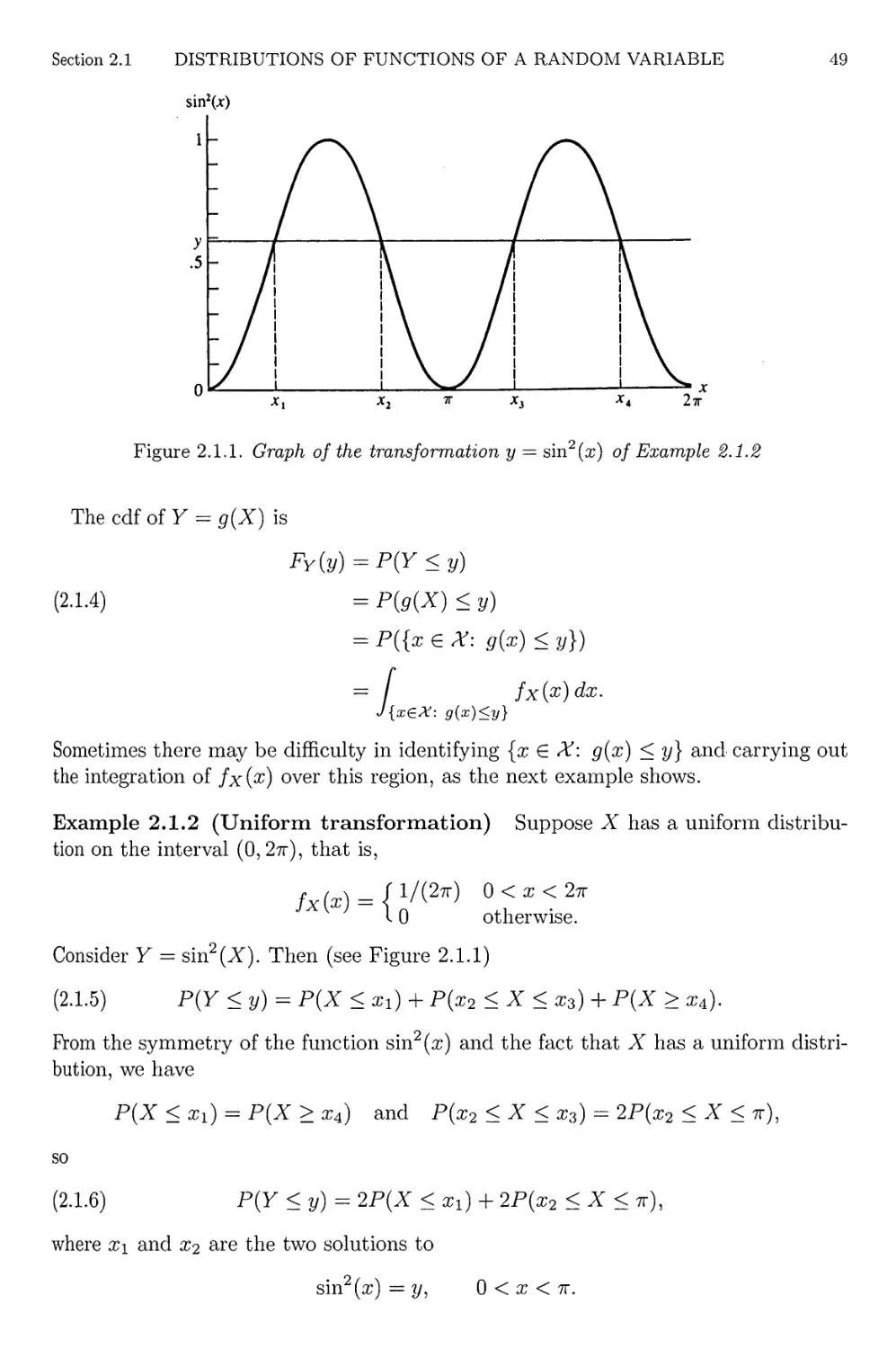
2.1.1
2.1.2
2.3.1
2.3.2
2.3.3
3.3.1
3.3.2
3.3.3
3.3.4
3.3.5
3.3.6
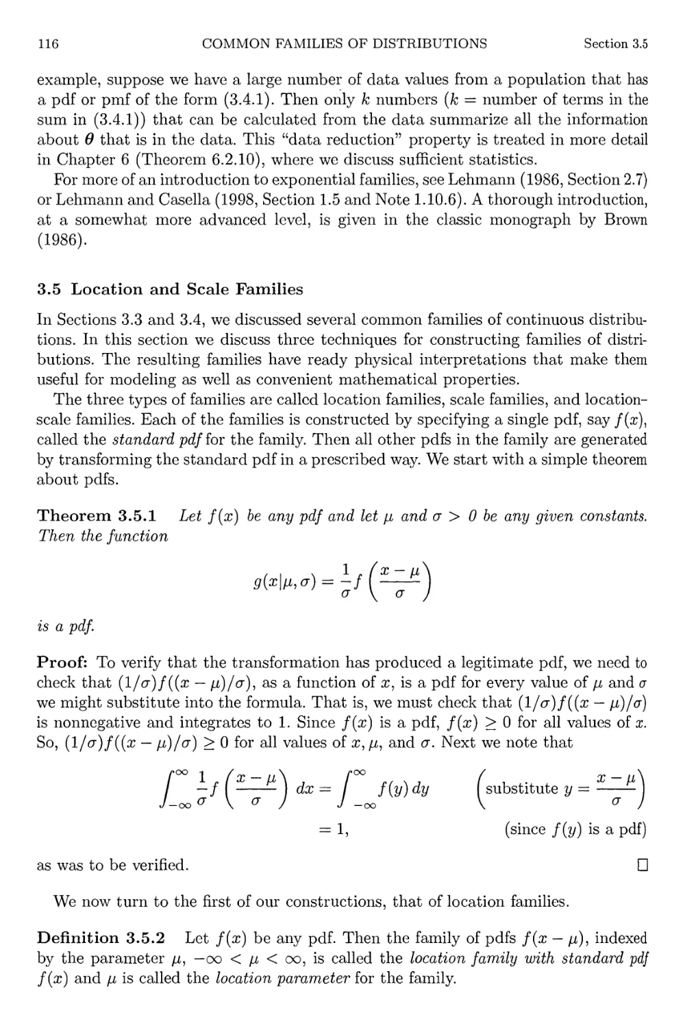
3.5.1
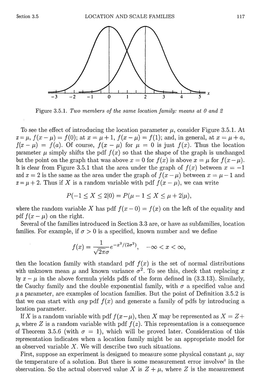
3.5.2
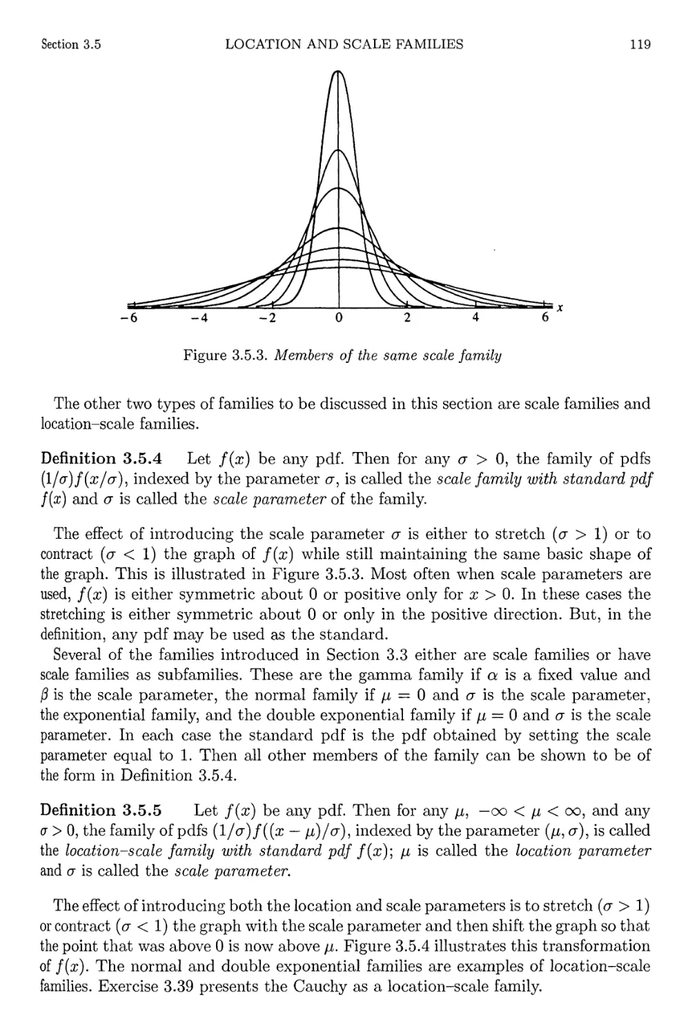
3.5.3
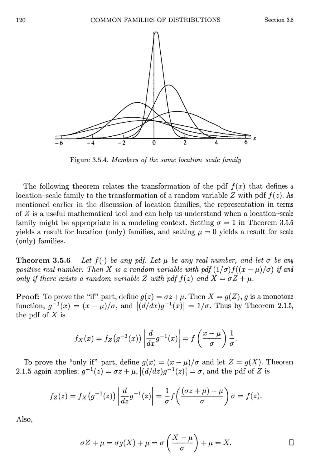
3.5.4
4.1.1
4.5.1
4.5.2
4.7.1
4.7.2
5.4.1
5.6.1
5.6.2
5.6.3
Dart board for Example 1.2.7
Histogram of averages
Cdf of Example 1.5.2
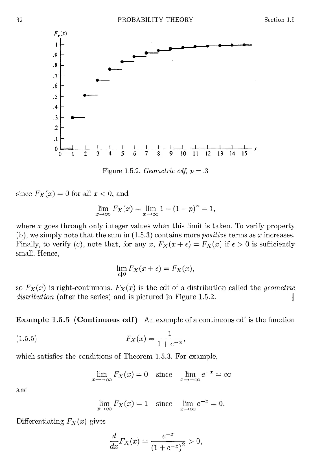
Geometric cdf, p — .3
Area under logistic curve
Transformation of Example 2.1.2
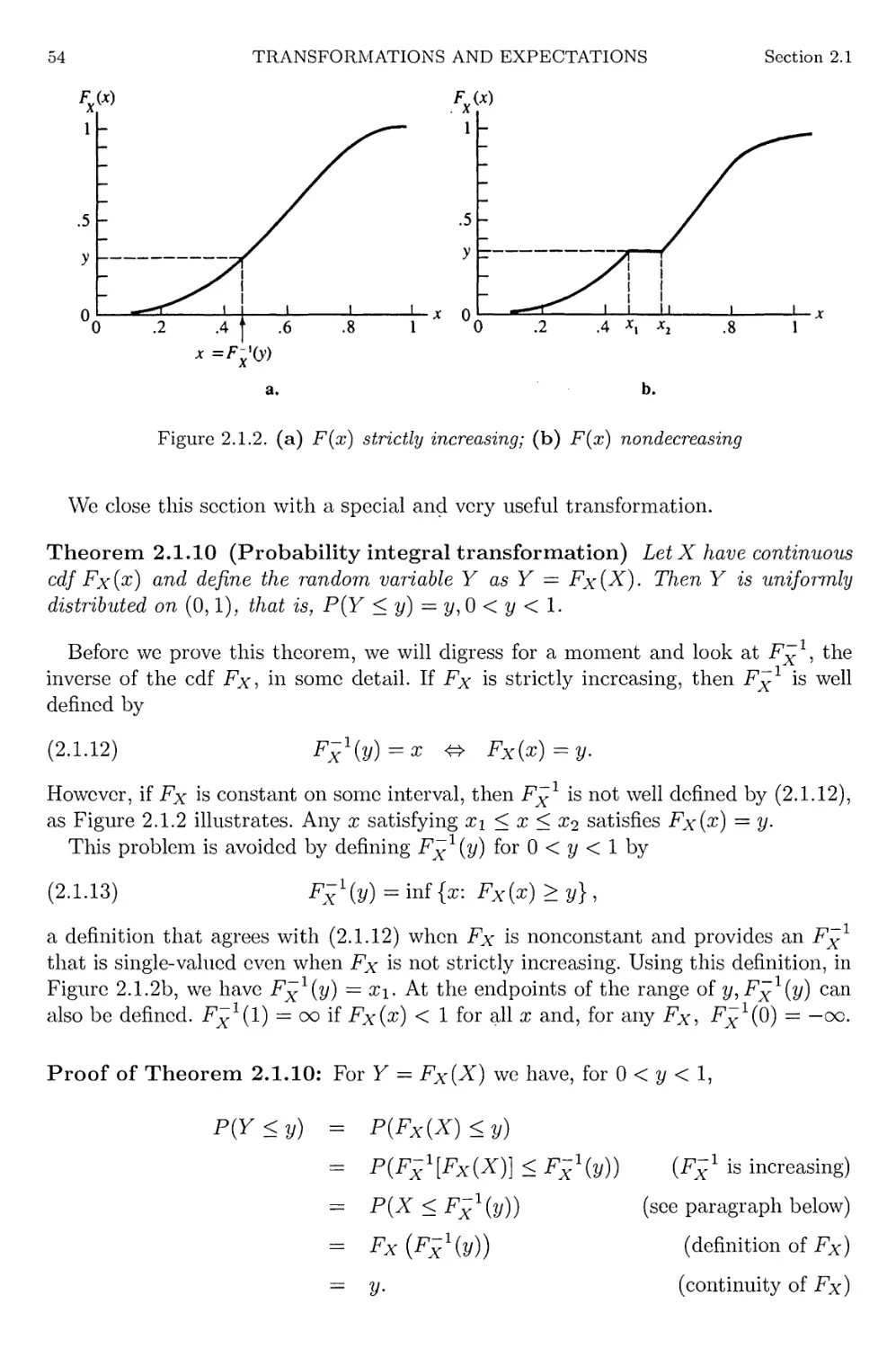
Increasing and nondecreasing cdfs
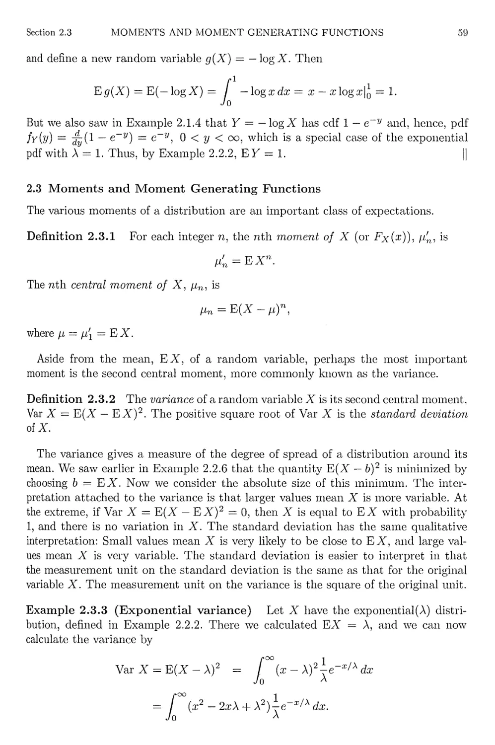
Exponential densities
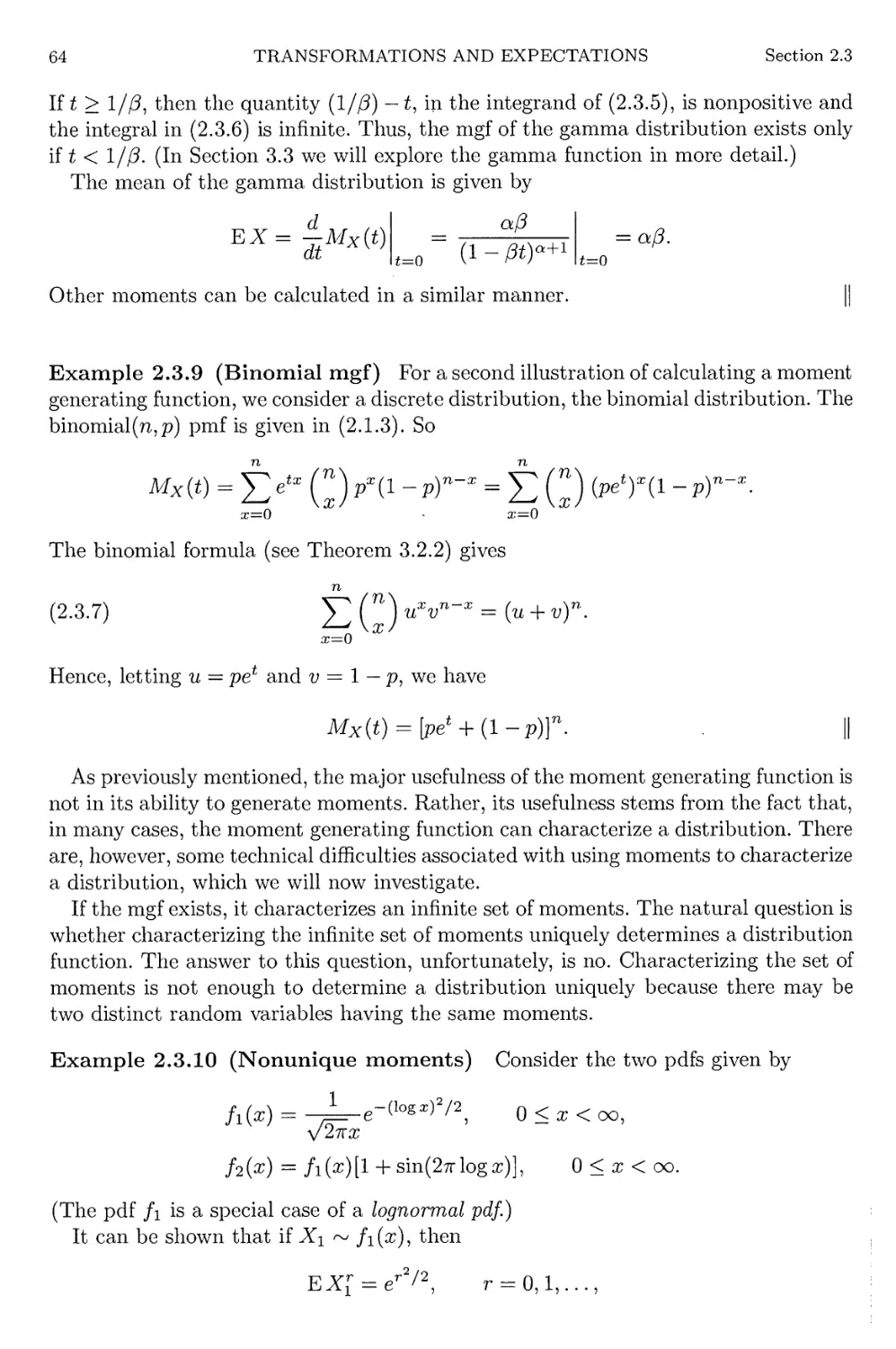
Two pdfs with the same moments
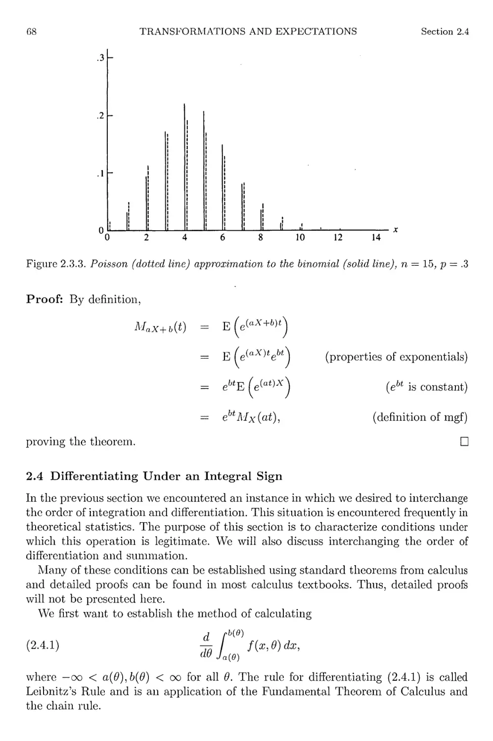
Poisson approximation to the binomial
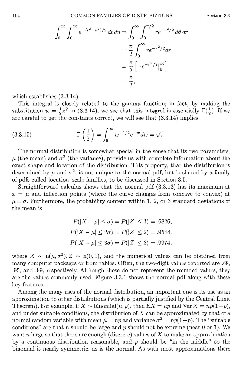
Standard normal density
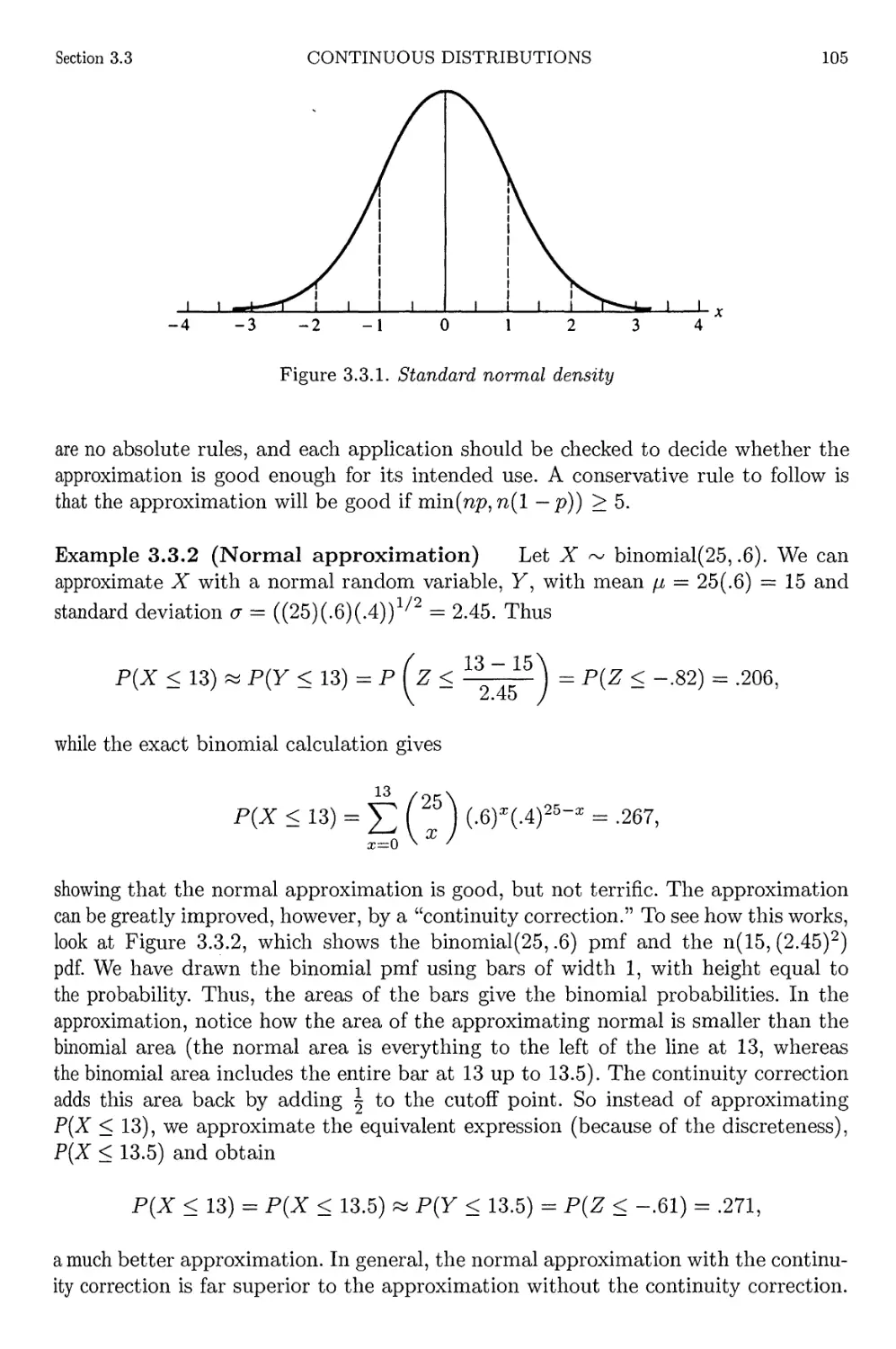
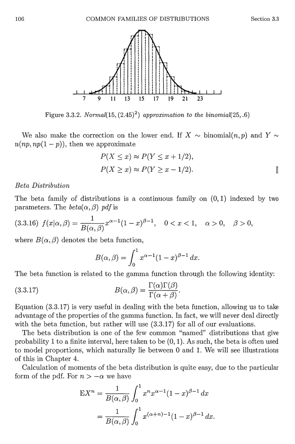
Normal approximation to the binomial
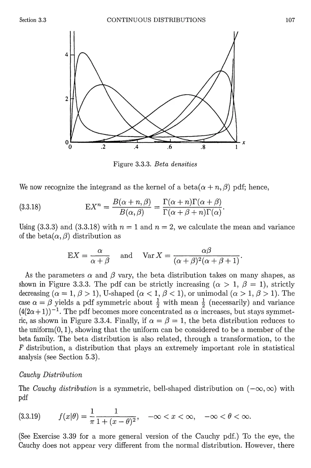
Beta densities
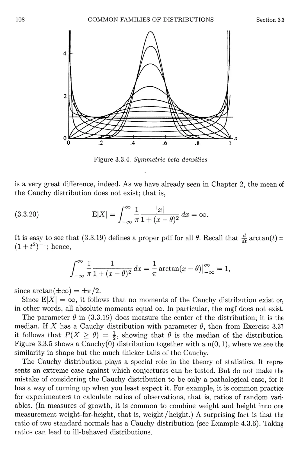
Symmetric beta densities
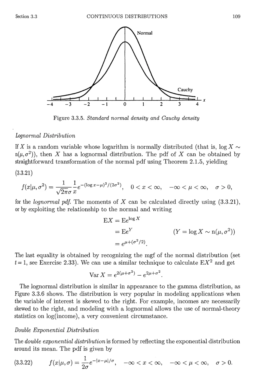
Standard normal density and Cauchy density
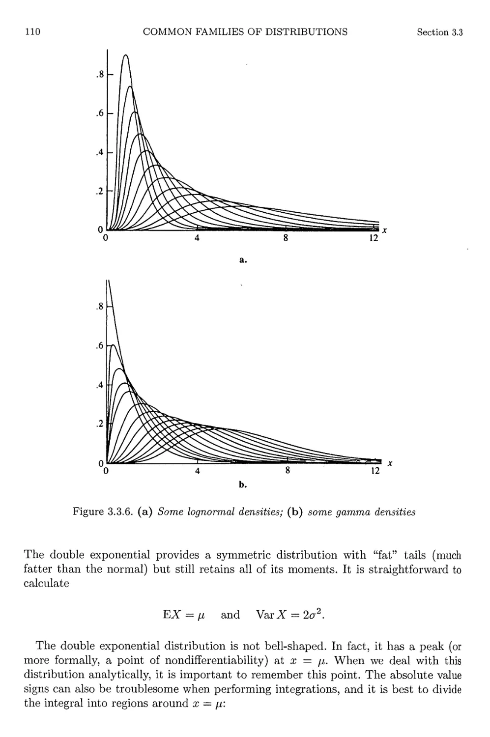
Lognormal and gamma pdfs
Location densities
Exponential location densities
Members of the same scale family
Location-scale families
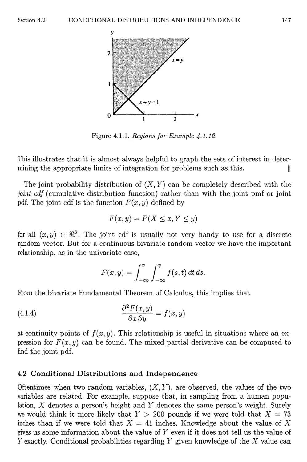
Regions for Example 4.1.12
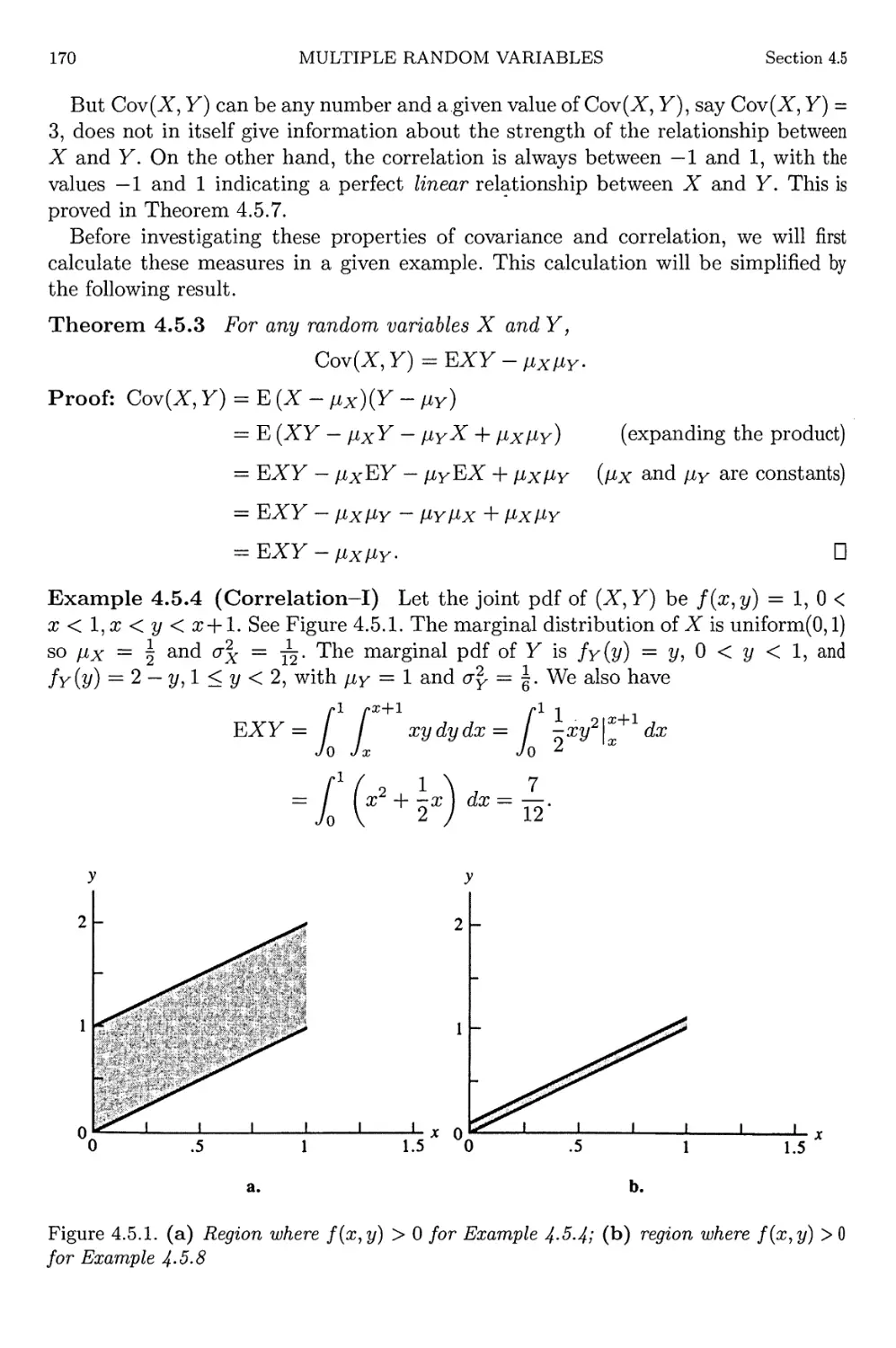
Regions for Examples 4.5.4 and 4.5.8
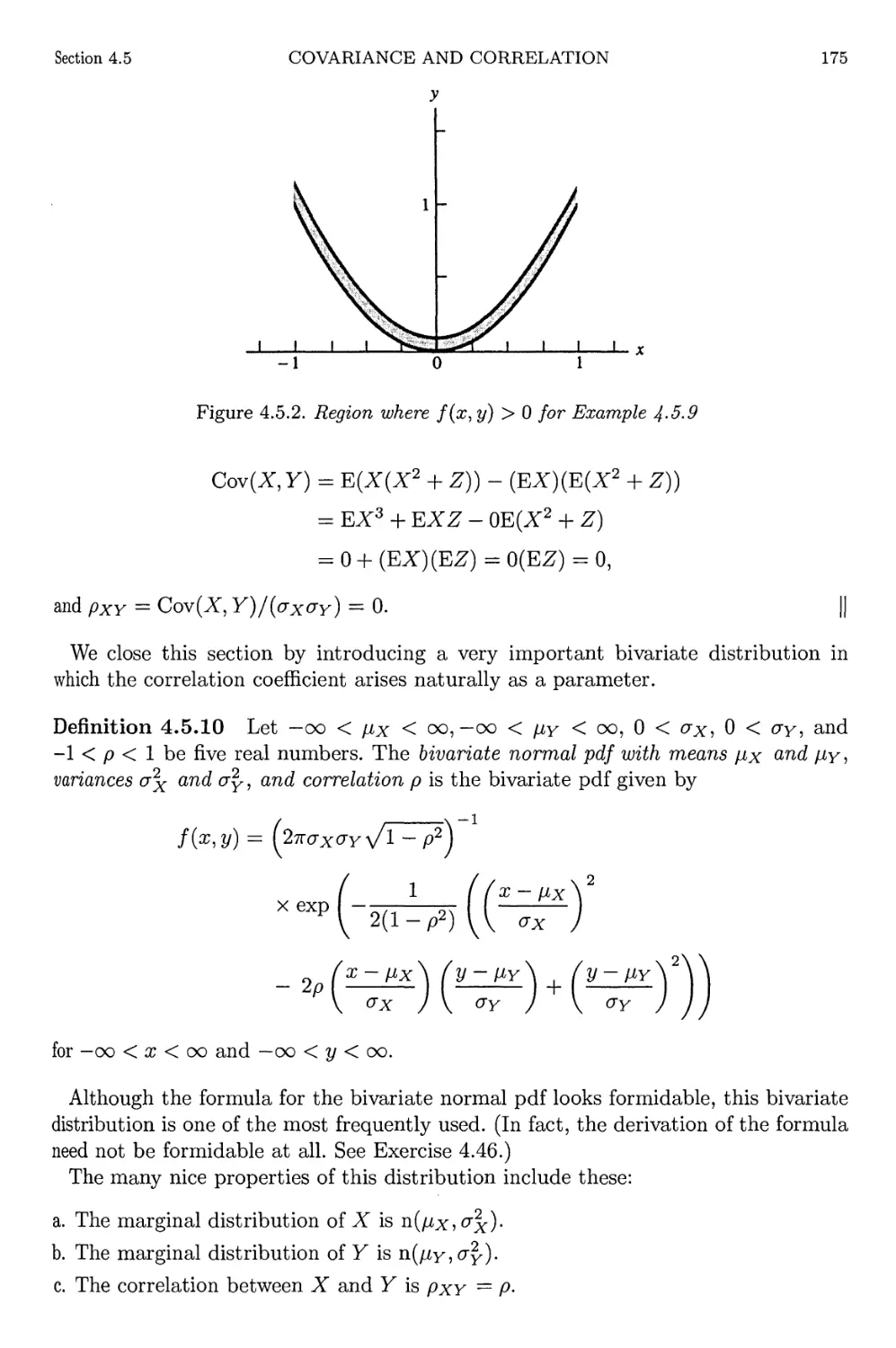
Regions for Example 4.5.9
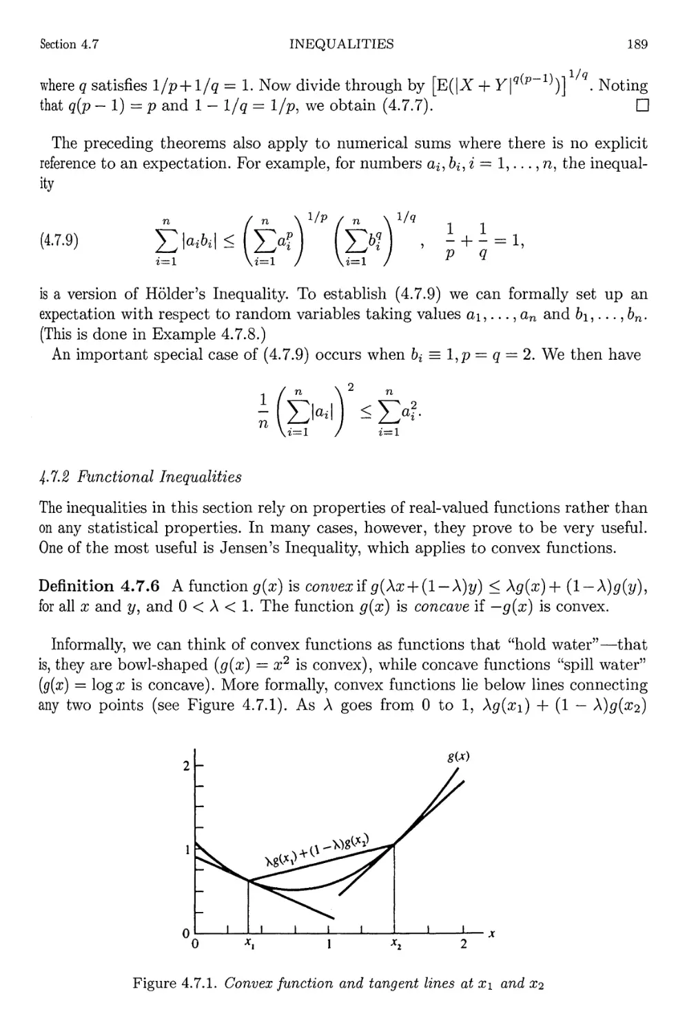
Convex function
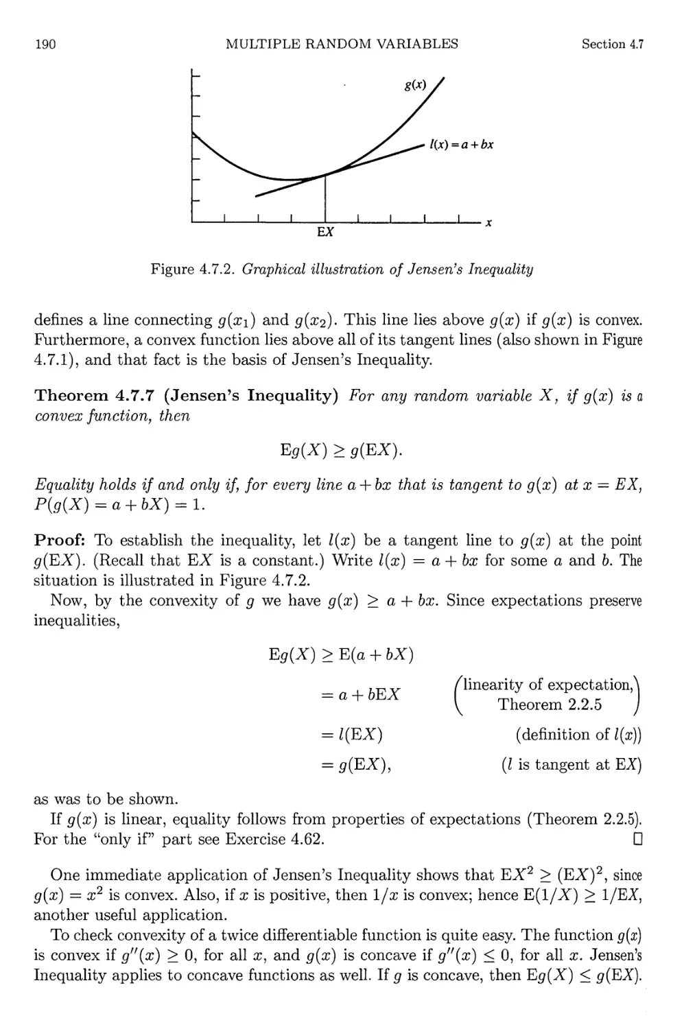
Jensen's Inequality
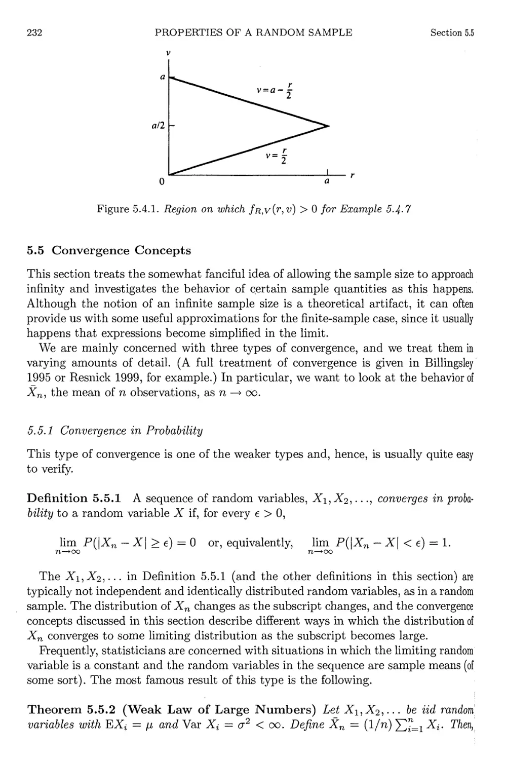
Region on which fii,v{r,v) > 0 for Example 5.4.7
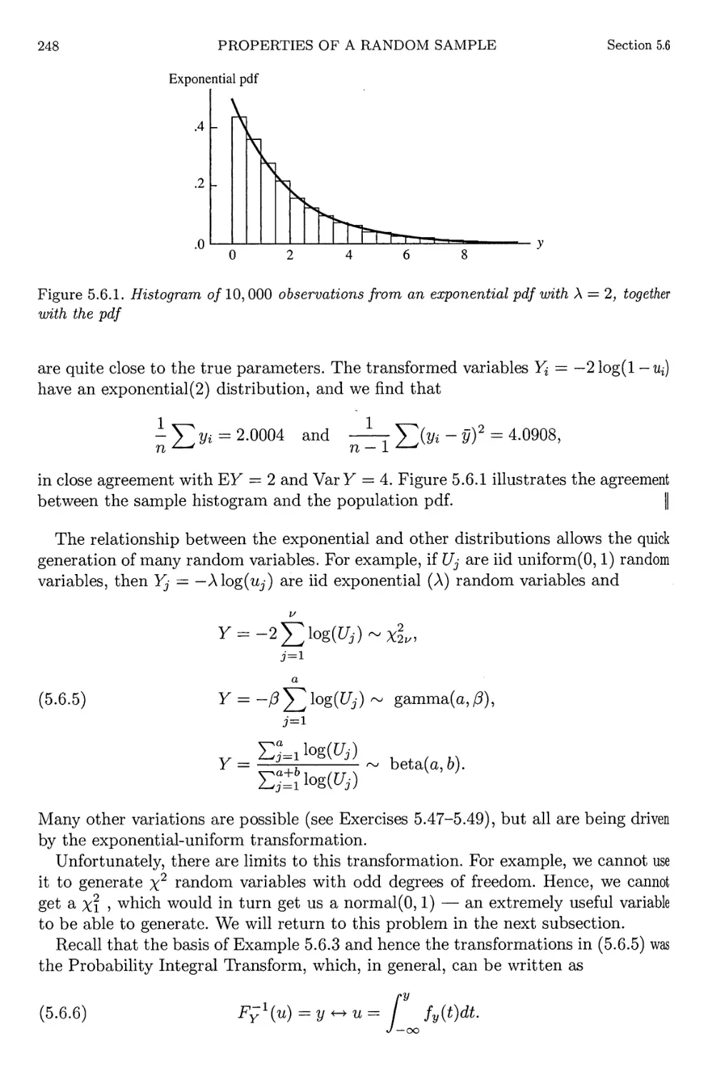
Histogram of exponential pdf
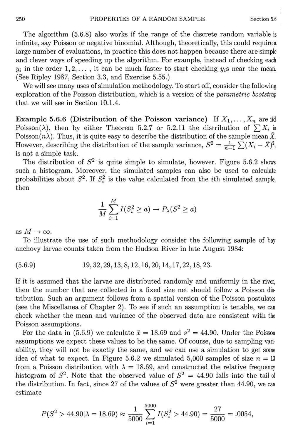
Histogram of Poisson sample variances
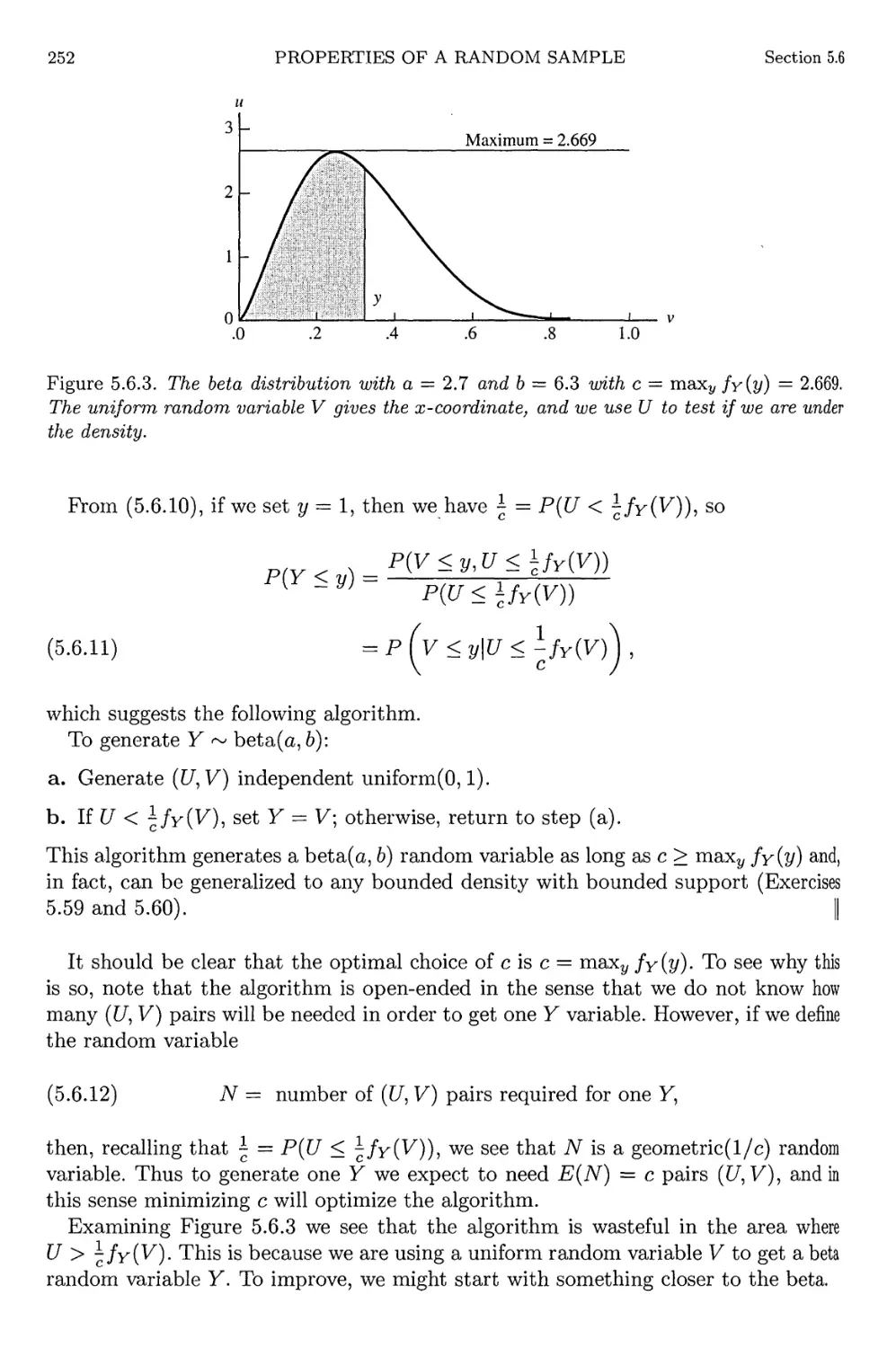
Beta distribution in accept/reject sampling
9
19
30
32
36
49
54
60
65
68
105
106
107
108
109
110
117
118
119
120
147
170
175
189
190
232
248
251
252
XX
LIST OF FIGURES
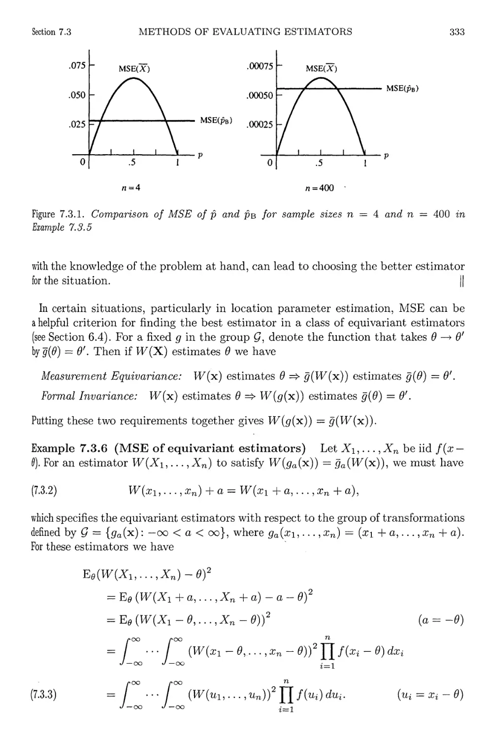
7.3.1 Binomial MSE comparison 333
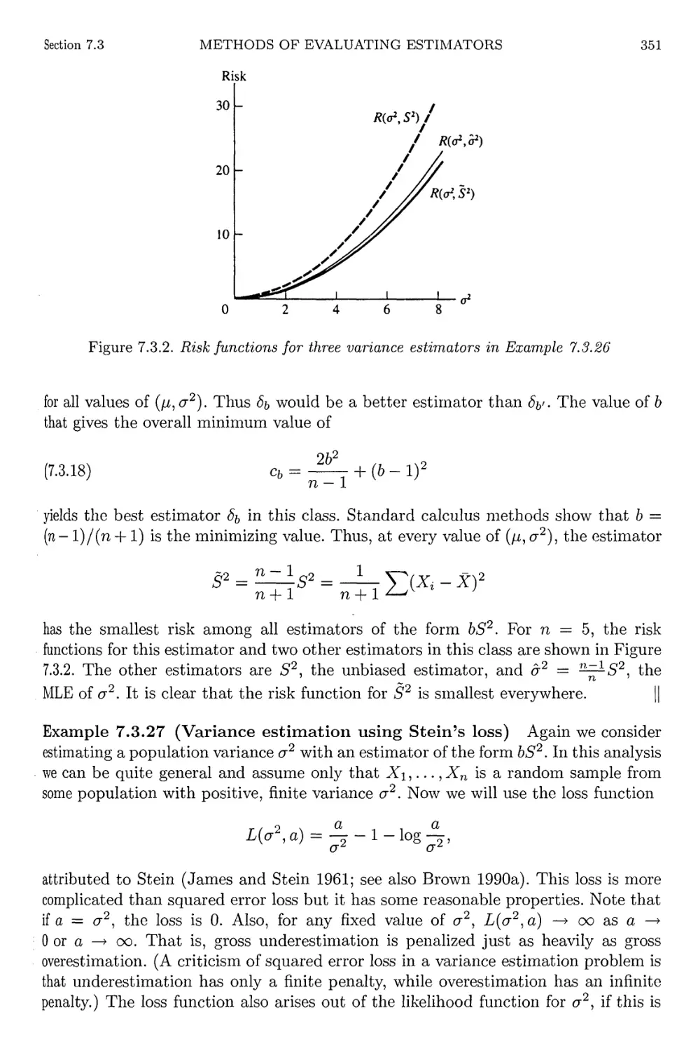
7.3.2 Risk functions for variance estimators 351
8.2.1 LRT statistic 377
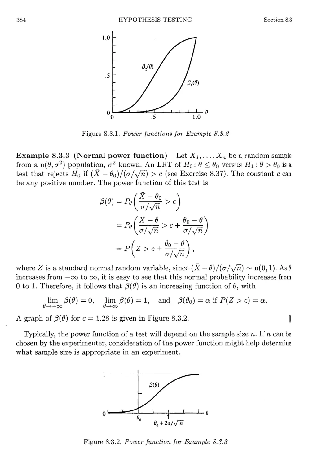
8.3.1 Power functions for Example 8.3.2 384
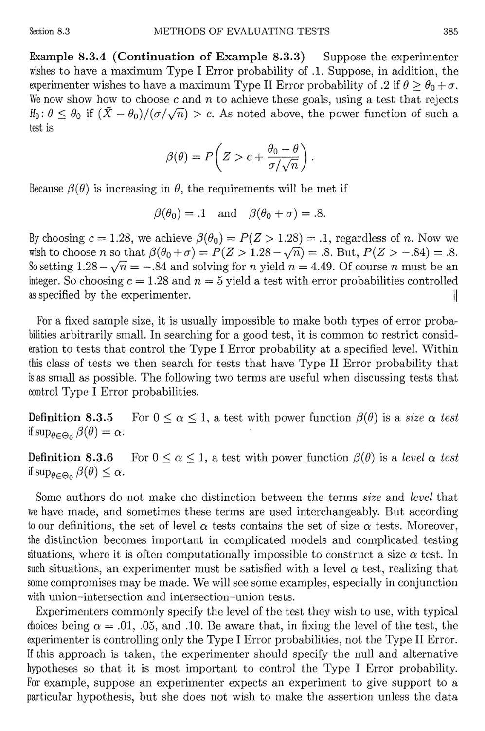
8.3.2 Power functions for Example 8.3.3 384
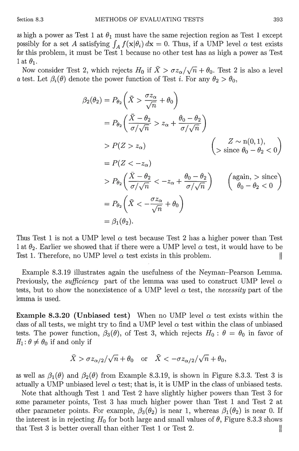
8.3.3 Power functions for three tests in Example 8.3.19 394
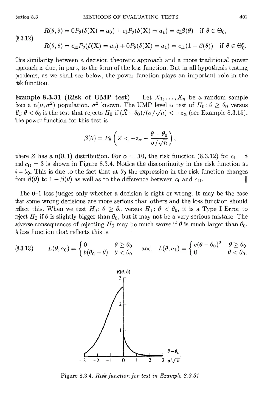
8.3.4 Risk function for test in Example 8.3.31 401
9.2.1 Confidence interval-acceptance region relationship 421
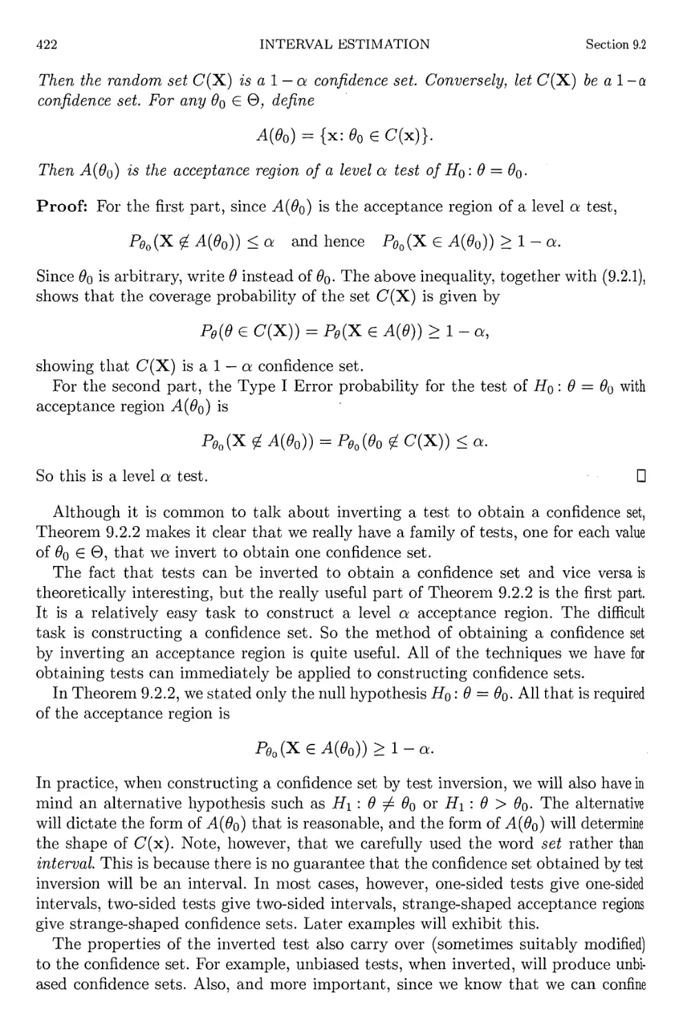
9.2.2 Acceptance region and confidence interval for Example 9.2.3 423
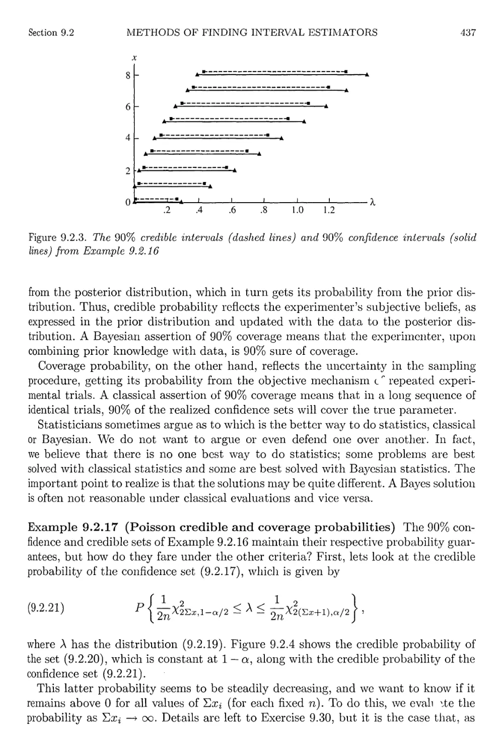
9.2.3 Credible and confidence intervals from Example 9.2.16 437
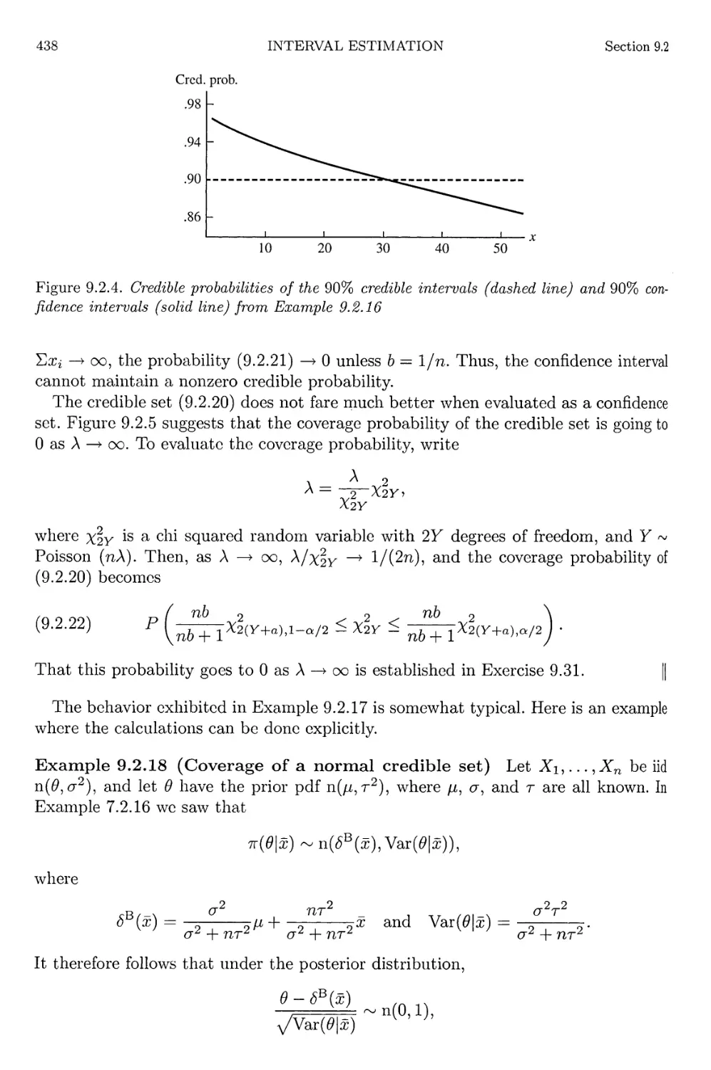
9.2.4 Credible probabilities of the intervals from Example 9.2.16 438
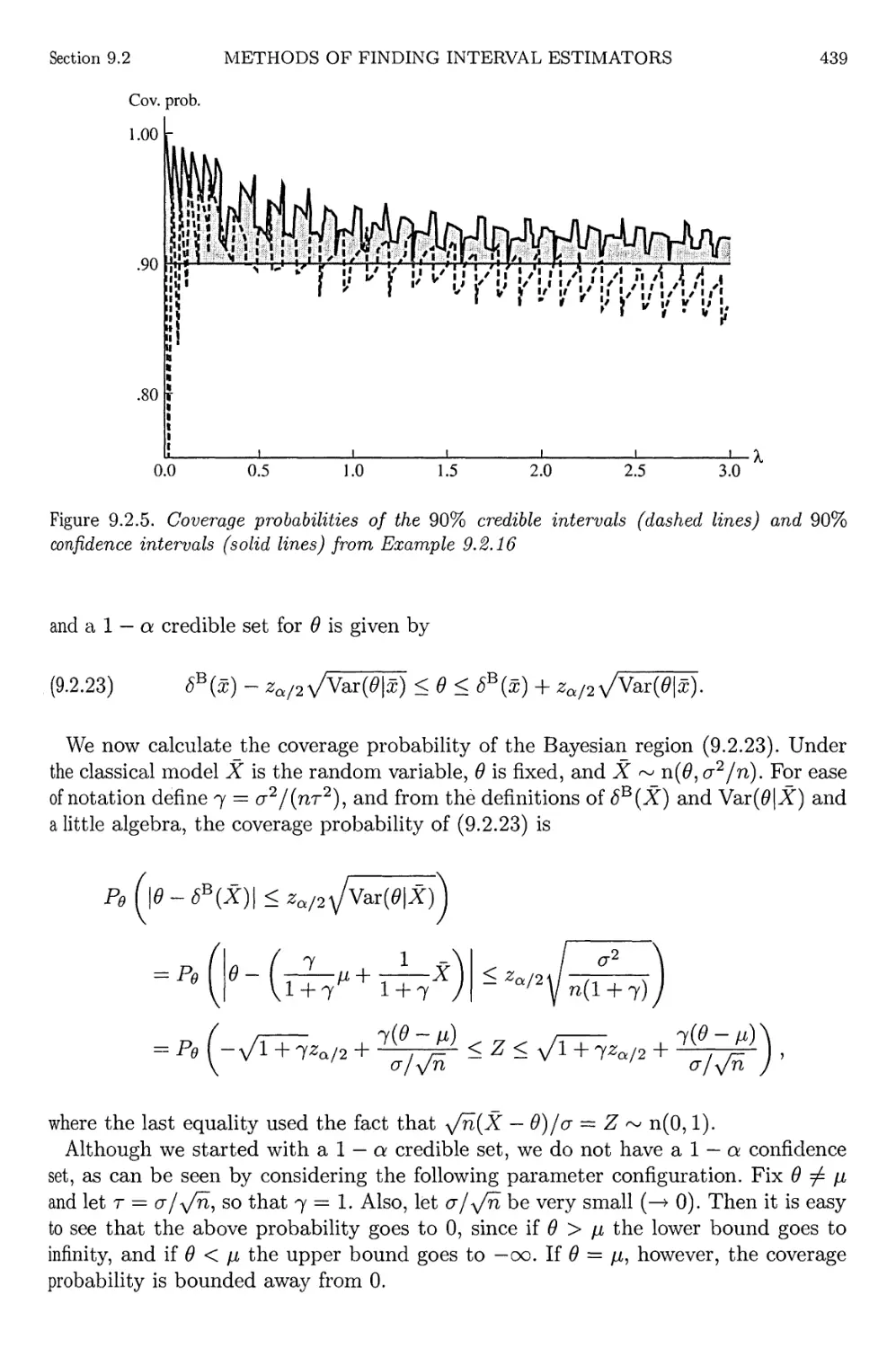
9.2.5 Coverage probabilities of the intervals from Example 9.2.16 439
9.3.1 Three interval estimators from Example 9.2.16 449
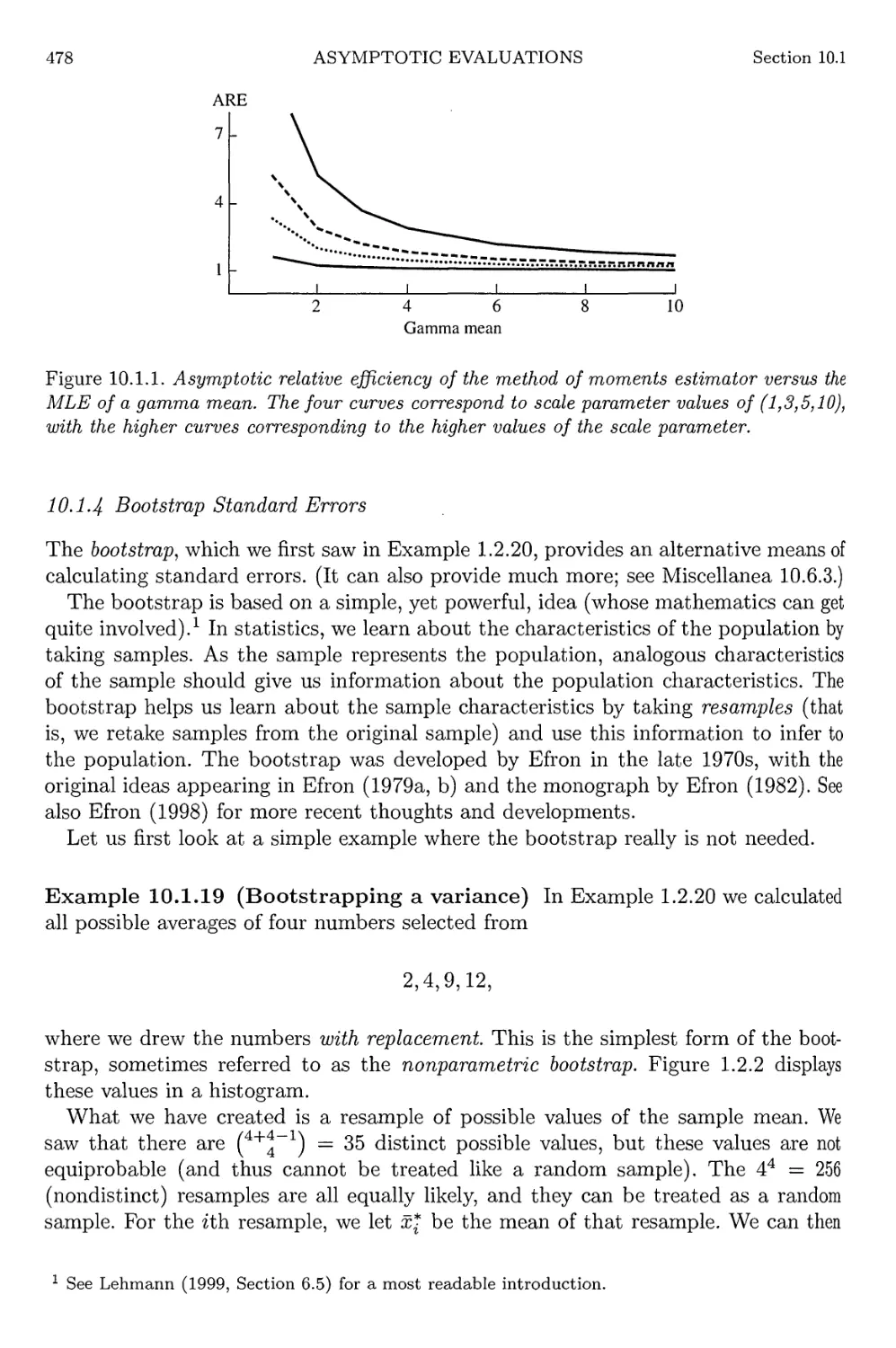
10.1.1 Asymptotic relative efficiency for gamma mean estimators 478
10.3.1 Poisson LRT histogram 490
10.4.1 LRT intervals for a binomial proportion 502
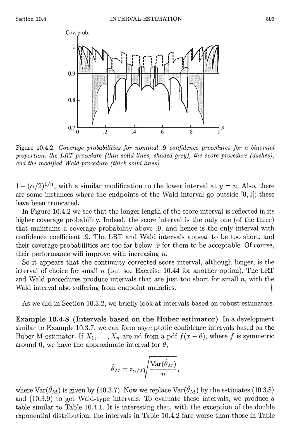
10.4.2 Coverage probabilities for nominal .9 binomial confidence procedures 503
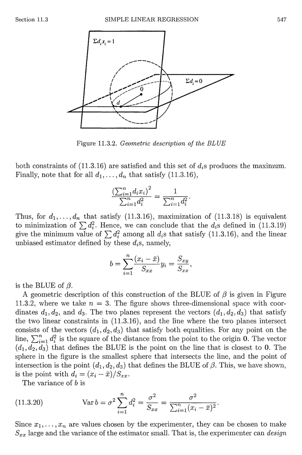
11.3.1 Vertical distances that are measured by RSS 542
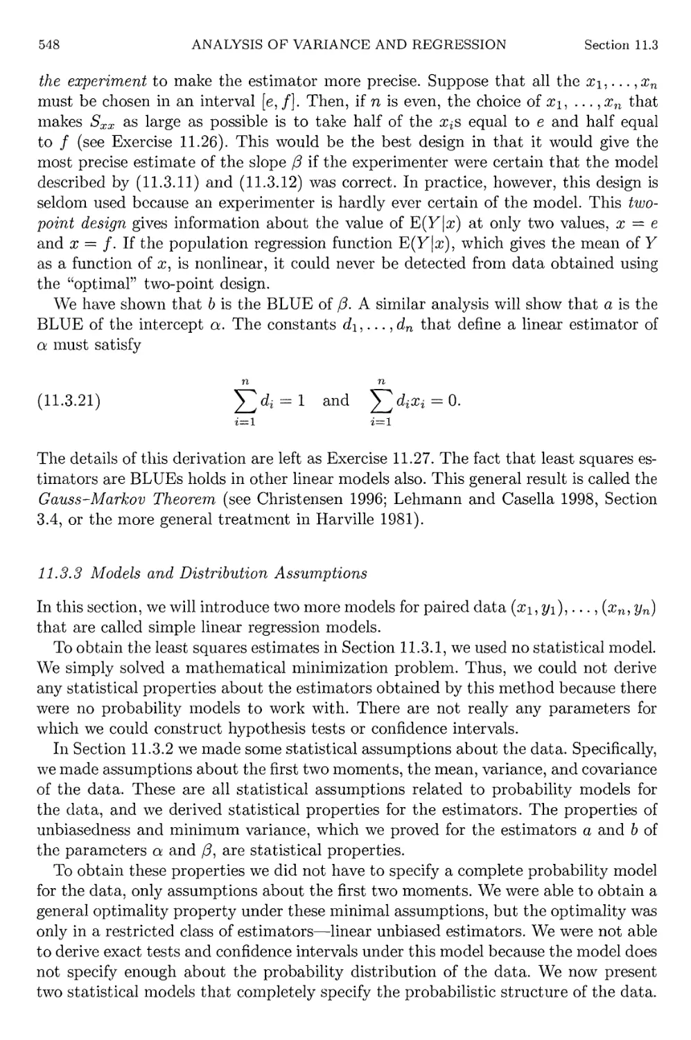
11.3.2 Geometric description of the BLUE 547
11.3.3 SchefFe bands, t interval, and Bonferroni intervals 562
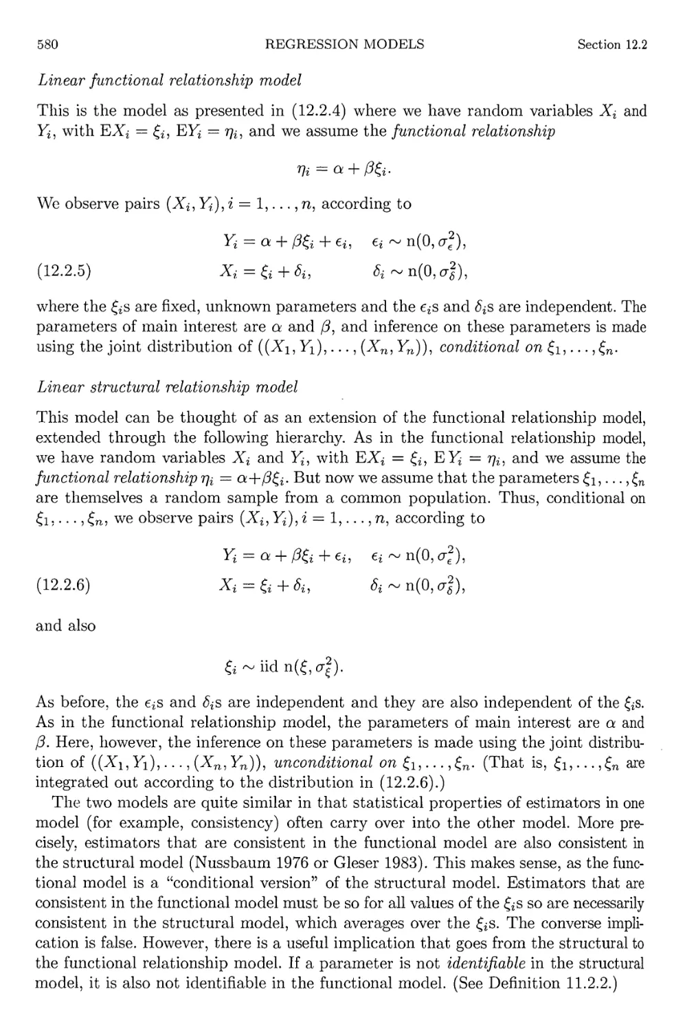
12.2.1 Distance minimized by orthogonal least squares 581
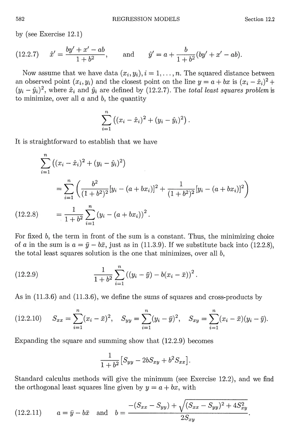
12.2.2 Three regression lines 583
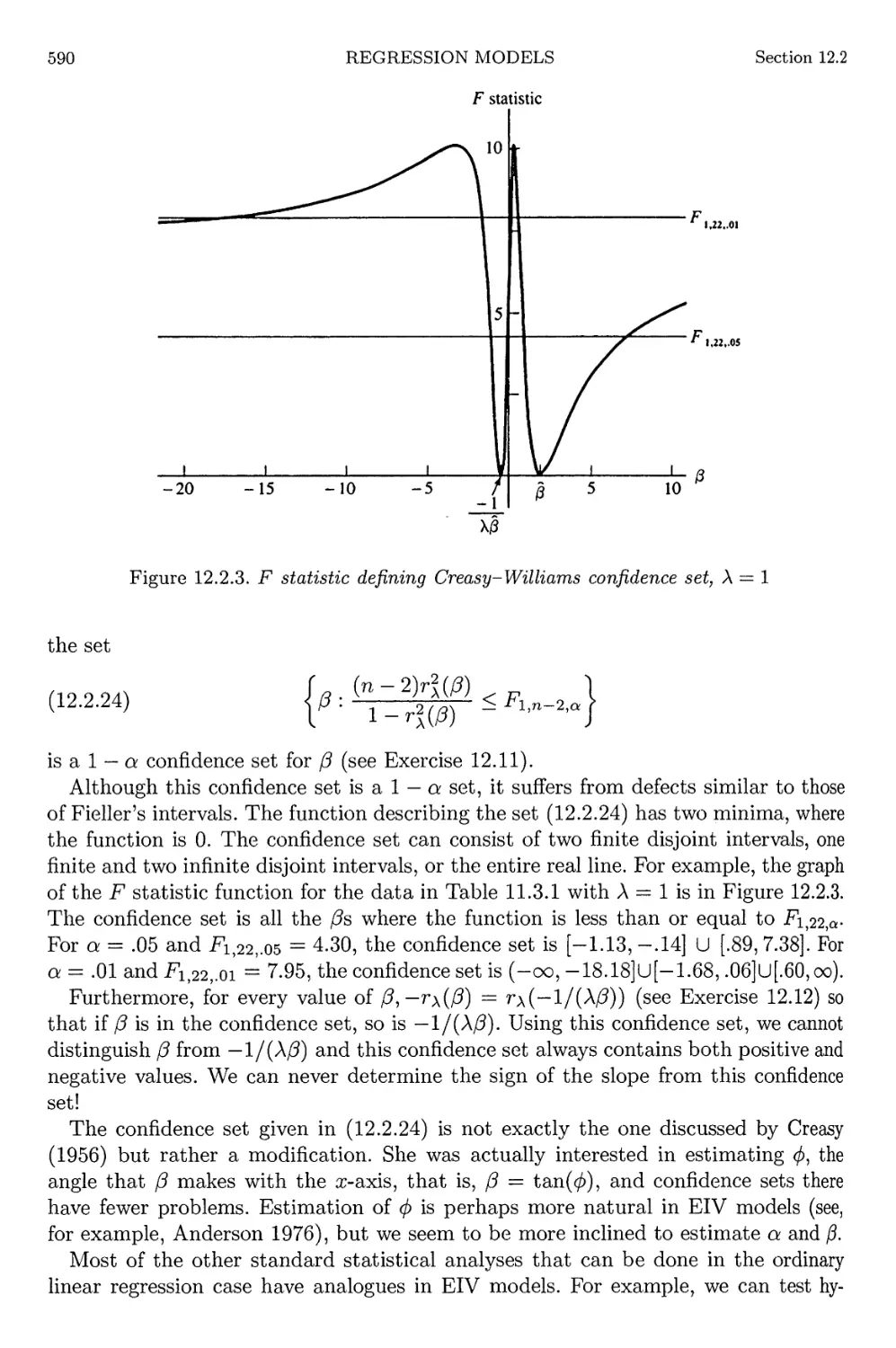
12.2.3 Creasy-Williams F statistic 590
12.3.1 Challenger data logistic curve 595
12.4.1 Least squares, LAD, and M-estimate fits 599
List of Examples
1.1.3
1.2.2
1.2.3
1.2.5
1.2.7
1.2.10
1.2.12
1.2.13
1.2.15
1.2.18
1.2.19
1.2.20
1.3.1
1.3.3
1.3.4
1.3.6
1.3.8
1.3.10
1.3.11
1.3.13
1.4.2
1.4.3
1.4.4
1.5.2
1.5.4
1.5.5
1.5.6
1.5.9
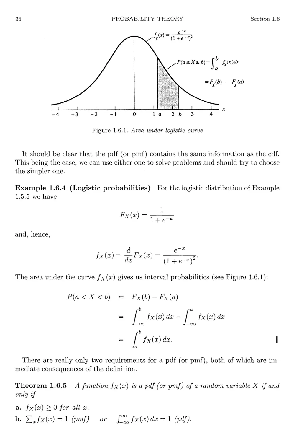
1.6.2
1.6.4
2.1.1
2.1.2
2.1.4
2.1.6
Event operations
Sigma algebra-I
Sigma algebra-II
Defining probabilities-I
Defining probabilities-II
Bonferroni's Inequality
Lottery-I
Tournament
Lottery-II
Poker
Sampling with replacement
Calculating an average
Four aces
Continuation of Example 1.3.1
Three prisoners
Coding
Chevalier de Mere
Tossing two dice
Letters
Three coin tosses-I
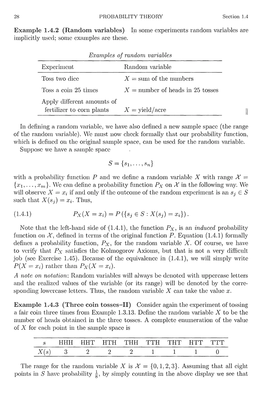
Random variables
Three coin tosses-II
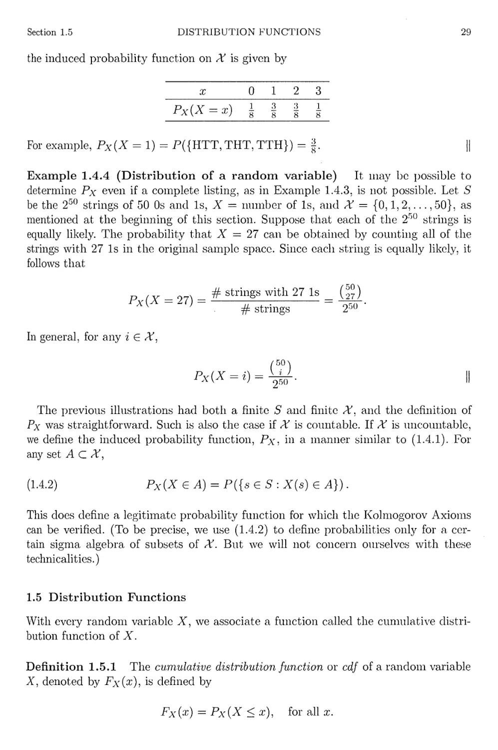
Distribution of a random variable
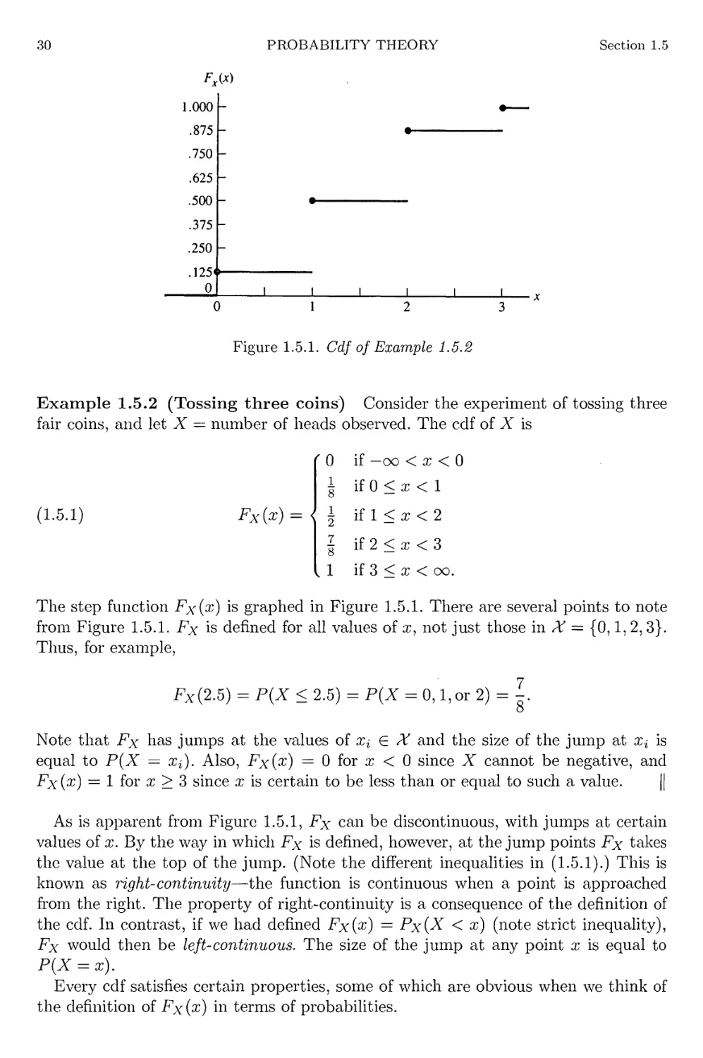
Tossing three coins
Tossing for a head
Continuous cdf
Cdf with jumps
Identically distributed random variables
Geometric probabilities
Logistic probabilities
Binomial transformation
Uniform transformation
Uniform-exponential relationship-I
Inverted gamma pdf
3
6
6
7
8
11
13
13
14
16
17
18
20
20
21
23
24
25
26
27
28
28
29
30
31
32
33
33
34
36
48
49
51
51
xxii
LIST OF EXAMPLES
2.1.7 Square transformation 52
2.1.9 Normal-chi squared relationship 53
2.2.2 Exponential mean 55
2.2.3 Binomial mean 56
2.2.4 Cauchy mean 56
2.2.6 Minimizing distance 58
2.2.7 Uniform-exponential relationship-II 58
2.3.3 Exponential variance 59
2.3.5 Binomial variance 61
2.3.8 Gamma mgf 63
2.3.9 Binomial mgf 64
2.3.10 Nonunique moments 64
2.3.13 Poisson approximation 66
2.4.5 Interchanging integration and differentiation-I 71
2.4.6 Interchanging integration and differentiation-II 72
2.4.7 Interchanging summation and differentiation 73
2.4.9 Continuation of Example 2.4.7 74
3.2.1 Acceptance sampling 88
3.2.3 Dice probabilities 91
3.2.4 Waiting time 93
3.2.5 Poisson approximation 94
3.2.6 Inverse binomial sampling 96
3.2.7 Failure times 98
3.3.1 Gamma-Poisson relationship 100
3.3.2 Normal approximation 105
3.4.1 Binomial exponential family 111
3.4.3 Binomial mean and variance 112
3.4.4 Normal exponential family 113
3.4.6 Continuation of Example 3.4.4 114
3.4.8 A curved exponential family 115
3.4.9 Normal approximations 115
3.5.3 Exponential location family 118
3.6.2 Illustrating Chebychev 122
3.6.3 A normal probability inequality 123
3.6.6 Higher-order normal moments 125
3.6.9 Higher-order Poisson moments 127
4.1.2 Sample space for dice 140
4.1.4 Continuation of Example 4.1.2 141
4.1.5 Joint pmf for dice 142
4.1.7 Marginal pmf for dice 143
4.1.8 Dice probabilities 144
4.1.9 Same marginals, different joint pmf 144
4.1.11 Calculating joint probabilities-I 145
LIST OF EXAMPLES
xxiii
4.1.12 Calculating joint probabilities-II 146
4.2.2 Calculating conditional probabilities 148
4.2.4 Calculating conditional pdfs 150
4.2.6 Checking independence-I 152
4.2.8 Checking independence-II 153
4.2.9 Joint probability model 154
4.2.11 Expectations of independent variables 155
4.2.13 Mgf of a sum of normal variables 156
4.3.1 Distribution of the sum of Poisson variables 157
4.3.3 Distribution of the product of beta variables 158
4.3.4 Sum and difference of normal variables 159
4.3.6 Distribution of the ratio of normal variables 162
4.4.1 Binomial-Poisson hierarchy 163
4.4.2 Continuation of Example 4.4.1 163
4.4.5 Generalization of Example 4.4.1 165
4.4.6 Beta-binomial hierarchy 167
4.4.8 Continuation of Example 4.4.6 168
4.5.4 Correlation-I 170
4.5.8 Correlation-II 173
4.5.9 Correlation-Ill 174
4.6.1 Multivariate pdfs 178
4.6.3 Multivariate pmf 181
4.6.8 Mgf of a sum of gamma variables 183
4.6.13 Multivariate change of variables 185
4.7.4 Covariance inequality 188
4.7.8 An inequality for means 191
5.1.2 Sample pdf-exponential 208
5.1.3 Finite population model 210
5.2.8 Distribution of the mean 215
5.2.10 Sum of Cauchy random variables 216
5.2.12 Sum of Bernoulli random variables 217
5.3.5 Variance ratio distribution 224
5.3.7 Continuation of Example 5.3.5 225
5.4.5 Uniform order statistic pdf 230
5.4.7 Distribution of the midrange and range 231
5.5.3 Consistency of S2 233
5.5.5 Consistency of S 233
5.5.7 Almost sure convergence 234
5.5.8 Convergence in probability, not almost surely 234
5.5.11 Maximum of uniforms 235
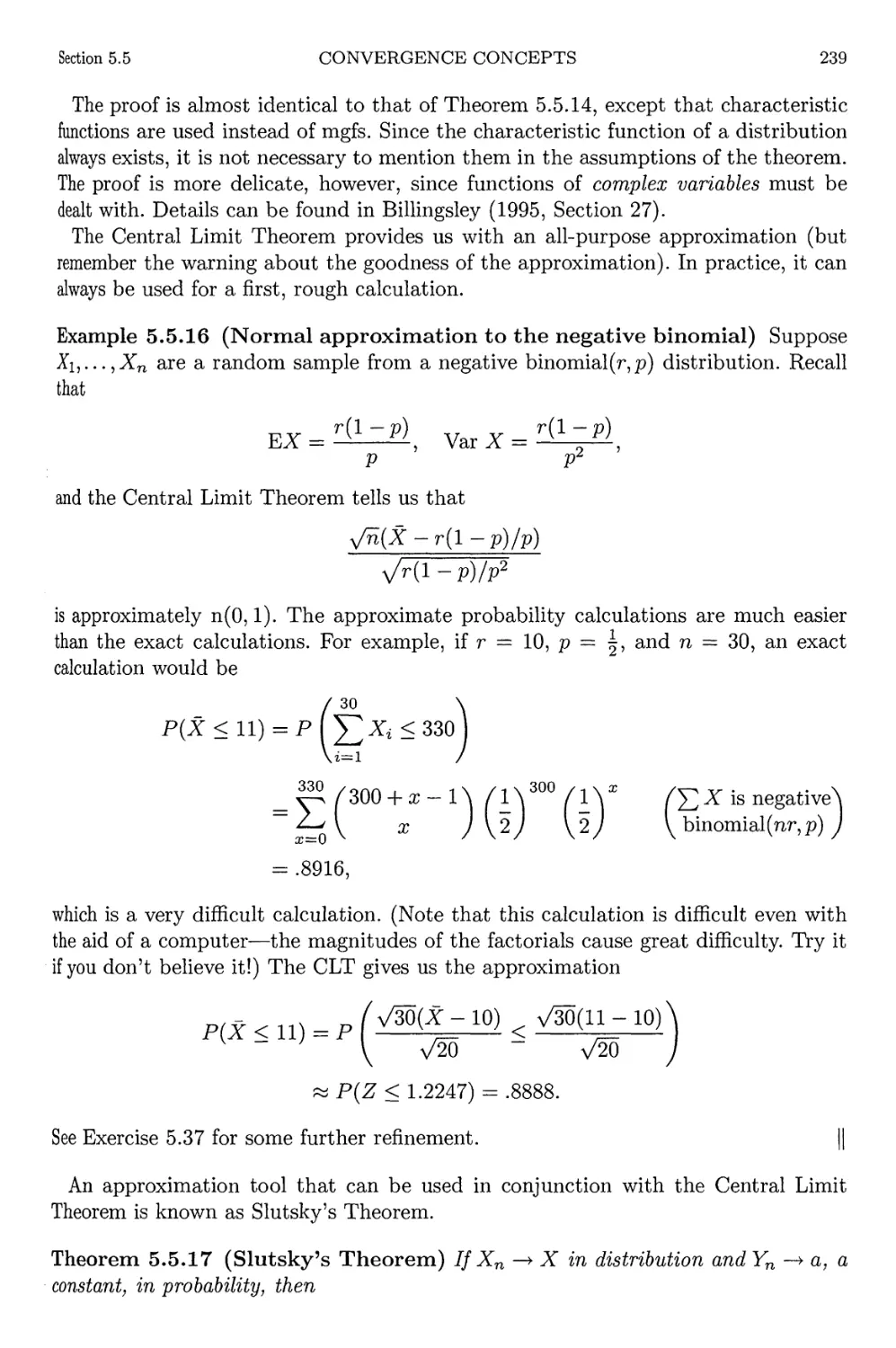
5.5.16 Normal approximation to the negative binomial 239
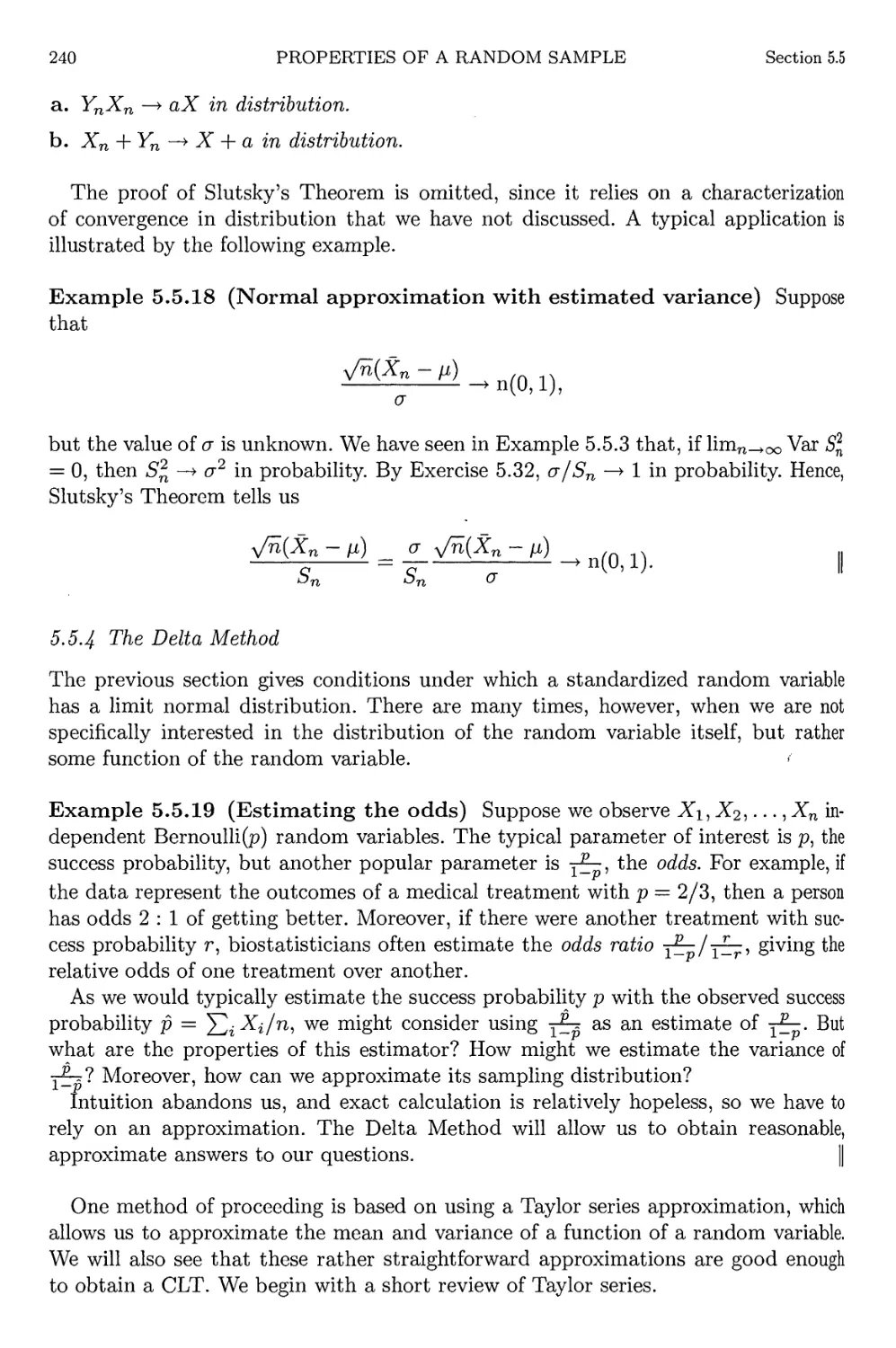
5.5.18 Normal approximation with estimated variance 240
5.5.19 Estimating the odds 240
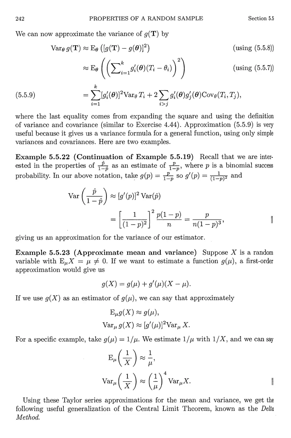
5.5.22 Continuation of Example 5.5.19 242
XXIV
LIST OF EXAMPLES
5.5.23 Approximate mean and variance 242
5.5.25 Continuation of Example 5.5.23 243
5.5.27 Moments of a ratio estimator 244
5.6.1 Exponential lifetime 246
5.6.2 Continuation of Example 5.6.1 246
5.6.3 Probability Integral Transform 247
5.6.4 Box-Muller algorithm 249
5.6.5 Binomial random variable generation 249
5.6.6 Distribution of the Poisson variance 250
5.6.7 Beta random variable generation—I 251
5.6.9 Beta random variable generation-II 254
6.2.3 Binomial sufRcient statistic 274
6.2.4 Normal sufRcient statistic 274
6.2.5 SufRcient order statistics 275
6.2.7 Continuation of Example 6.2.4 277
6.2.8 Uniform sufRcient statistic 277
6.2.9 Normal sufRcient statistic, both parameters unknown 279
6.2.12 Two normal sufRcient statistics 280
6.2.14 Normal minimal sufRcient statistic 281
6.2.15 Uniform minimal sufficient statistic 282
6.2.17 Uniform ancillary statistic 282
6.2.18 Location family ancillary statistic 283
6.2.19 Scale family ancillary statistic 284
6.2.20 Ancillary precision 285
6.2.22 Binomial complete sufRcient statistic 285
6.2.23 Uniform complete sufRcient statistic 286
6.2.26 Using Basu's Theorem-I 288
6.2.27 Using Basu's Theorem-II 289
6.3.2 Negative binomial likelihood 290
6.3.3 Normal fiducial distribution 291
6.3.4 Evidence function 292
6.3.5 Binomial/negative binomial experiment 293
6.3.7 Continuation of Example 6.3.5 295
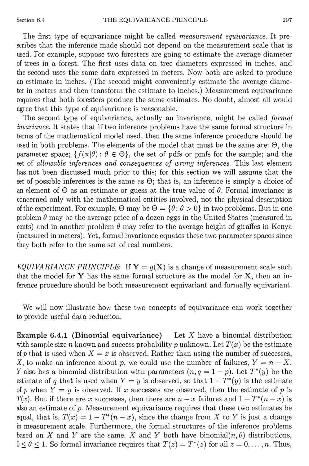
6.4.1 Binomial equivariance 297
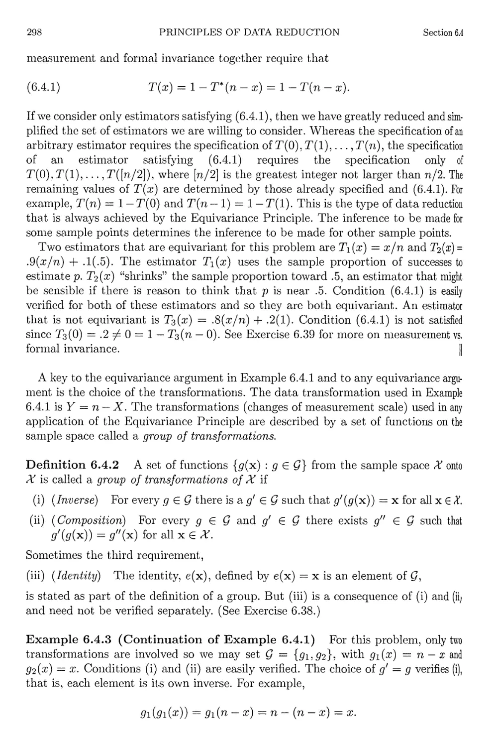
6.4.3 Continuation of Example 6.4.1 298
6.4.5 Conclusion of Example 6.4.1 299
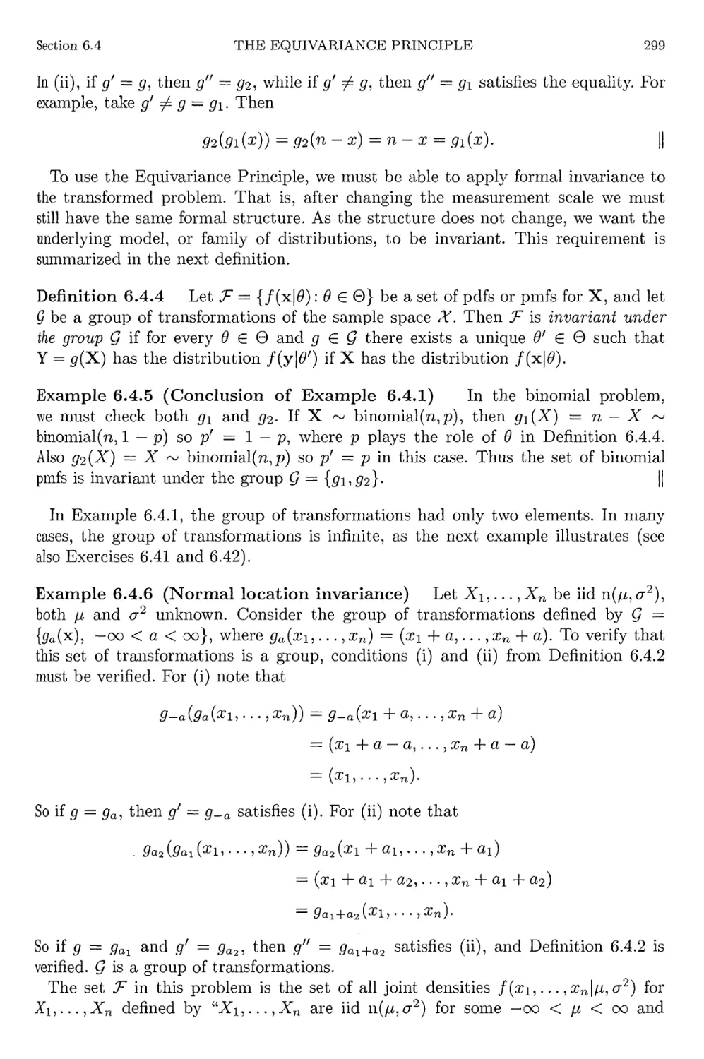
6.4.6 Normal location invariance 299
7.2.1 Normal method of moments 313
7.2.2 Binomial method of moments 313
7.2.3 Satterthwaite approximation 314
7.2.5 Normal likelihood 316
7.2.6 Continuation of Example 7.2.5 317
7.2.7 Bernoulli MLE 317
LIST OF EXAMPLES
XXV
7.2.8
7.2.9
7.2.11
7.2.12
7.2.13
7.2.14
7.2.16
7.2.17
7.2.18
7.2.19
7.3.3
7.3.4
7.3.5
7.3.6
7.3.8
7.3.12
7.3.13
7.3.14
7.3.16
7.3.18
7.3.21
7.3.22
7.3.24
7.3.25
7.3.26
7.3.27
7.3.28
7.3.29
7.3.30
Restricted range MLE
Binomial MLE, unknown number of trials
Normal MLEs, fi and a unknown
Continuation of Example 7.2.11
Continuation of Example 7.2.2
Binomial Bayes estimation
Normal Bayes estimators
Multiple Poisson rates
Continuation of Example 7.2.17
Conclusion of Example 7.2.17
Normal MSE
Continuation of Example 7.3.3
MSE of binomial Bayes estimator
MSE of equivariant estimators
Poisson unbiased estimation
Conclusion of Example 7.3.8
Unbiased estimator for the scale uniform
Normal variance bound
Continuation of Example 7.3.14
Conditioning on an insufficient statistic
Unbiased estimators of zero
Continuation of Example 7.3.13
Binomial best unbiased estimation
Binomial risk functions
Risk of normal variance
Variance estimation using Stein's loss
Two Bayes rules
Normal Bayes estimates
Binomial Bayes estimates
318
318
321
322
323
324
326
326
327
328
331
331
332
333
335
338
339
340
341
343
345
346
347
350
350
351
353
353
354
8.2.2
8.2.3
8.2.5
8.2.6
8.2.7
8.2.8
8.2.9
8.3.2
8.3.3
8.3.4
8.3.7
8.3.8
8.3.10
8.3.14
8.3.15
Normal LRT
Exponential LRT
LRT and sufficiency
Normal LRT with unknown variance
Normal Bayesian test
Normal union-intersection test
Acceptance sampling
Binomial power function
Normal power function
Continuation of Example 8.3.3
Size of LRT
Size of union-intersection test
Conclusion of Example 8.3.3
UMP binomial test
UMP normal test
375
376
378
378
379
380
382
383
384
385
386
387
387
390
390
XXVI
LIST OF EXAMPLES
8.3.18 Continuation of Example 8.3.15 392
8.3.19 Nonexistence of UMP test 392
8.3.20 Unbiased test 393
8.3.22 An equivalence 395
8.3.25 Intersection-union test 396
8.3.28 Two-sided normal p-value 398
8.3.29 One-sided normal p-value 398
8.3.30 Fisher's Exact Test 399
8.3.31 Risk of UMP test 401
9.1.2 Interval estimator 418
9.1.3 Continuation of Example 9.1.2 418
9.1.6 Scale uniform interval estimator 419
9.2.1 Inverting a normal test 420
9.2.3 Inverting an LRT 423
9.2.4 Normal one-sided confidence bound 425
9.2.5 Binomial one-sided confidence bound 425
9.2.7 Location-scale pivots 427
9.2.8 Gamma pivot 428
9.2.9 Continuation of Example 9.2.8 429
9.2.10 Normal pivotal interval 429
9.2.11 Shortest length binomial set 431
9.2.13 Location exponential interval 433
9.2.15 Poisson interval estimator 434
9.2.16 Poisson credible set 436
9.2.17 Poisson credible and coverage probabilities 437
9.2.18 Coverage of a normal credible set 438
9.3.1 Optimizing length 441
9.3.3 Optimizing expected length 443
9.3.4 Shortest pivotal interval 443
9.3.6 UMA confidence bound 445
9.3.8 Continuation of Example 9.3.6 446
9.3.11 Poisson HPD region 448
9.3.12 Normal HPD region 449
9.3.13 Normal interval estimator 450
10.1.2 Consistency of X 468
10.1.4 Continuation of Example 10.1.2 469
10.1.8 Limiting variances 470
10.1.10 Large-sample mixture variances 471
10.1.13 Asymptotic normality and consistency 472
10.1.14 Approximate binomial variance 474
10.1.15 Continuation of Example 10.1.14 475
10.1.17 AREs of Poisson estimators 476
10.1.18 Estimating a gamma mean 477
LIST OF EXAMPLES
xxvii
10.1.19
10.1.20
10.1.21
10.1.22
10.2.1
10.2.3
10.2.4
10.2.5
10.2.6
10.2.7
10.3.2
10.3.4
10.3.5
10.3.6
10.3.7
10.4.1
10.4.2
10.4.3
10.4.4
10.4.5
10.4.6
10.4.7
10.4.8
10.4.9
10.6.2
11.2.1
11.2.3
11.2.6
11.2.9
11.2.12
11.3.1
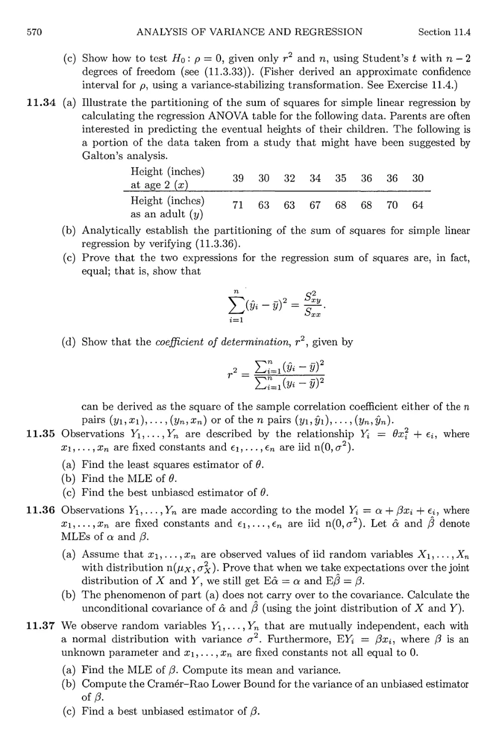
11.3.4
12.2.1
12.3.1
12.3.2
12.4.1
12.4.2
12.4.3
12.4.4
12.4.5
A.0.1
A.0.2
A.0.3
Bootstrapping a variance
Bootstrapping a binomial variance
Conclusion of Example 10.1.20
Parametric bootstrap
Robustness of the sample mean
Asymptotic normality of the median
AREs of the median to the mean
Huber estimator
Limit distribution of the Huber estimator
ARE of the Huber estimator
Poisson LRT
Multinomial LRT
Large-sample binomial tests
Binomial score test
Tests based on the Huber estimator
Continuation of Example 10.1.14
Binomial score interval
Binomial LRT interval
Approximate interval
Approximate Poisson interval
More on the binomial score interval
Comparison of binomial intervals
Intervals based on the Huber estimator
Negative binomial interval
Influence functions of the mean and median
Oneway ANOVA
The ANOVA hypothesis
ANOVA contrasts
Pairwise differences
Continuation of Example 11.2.1
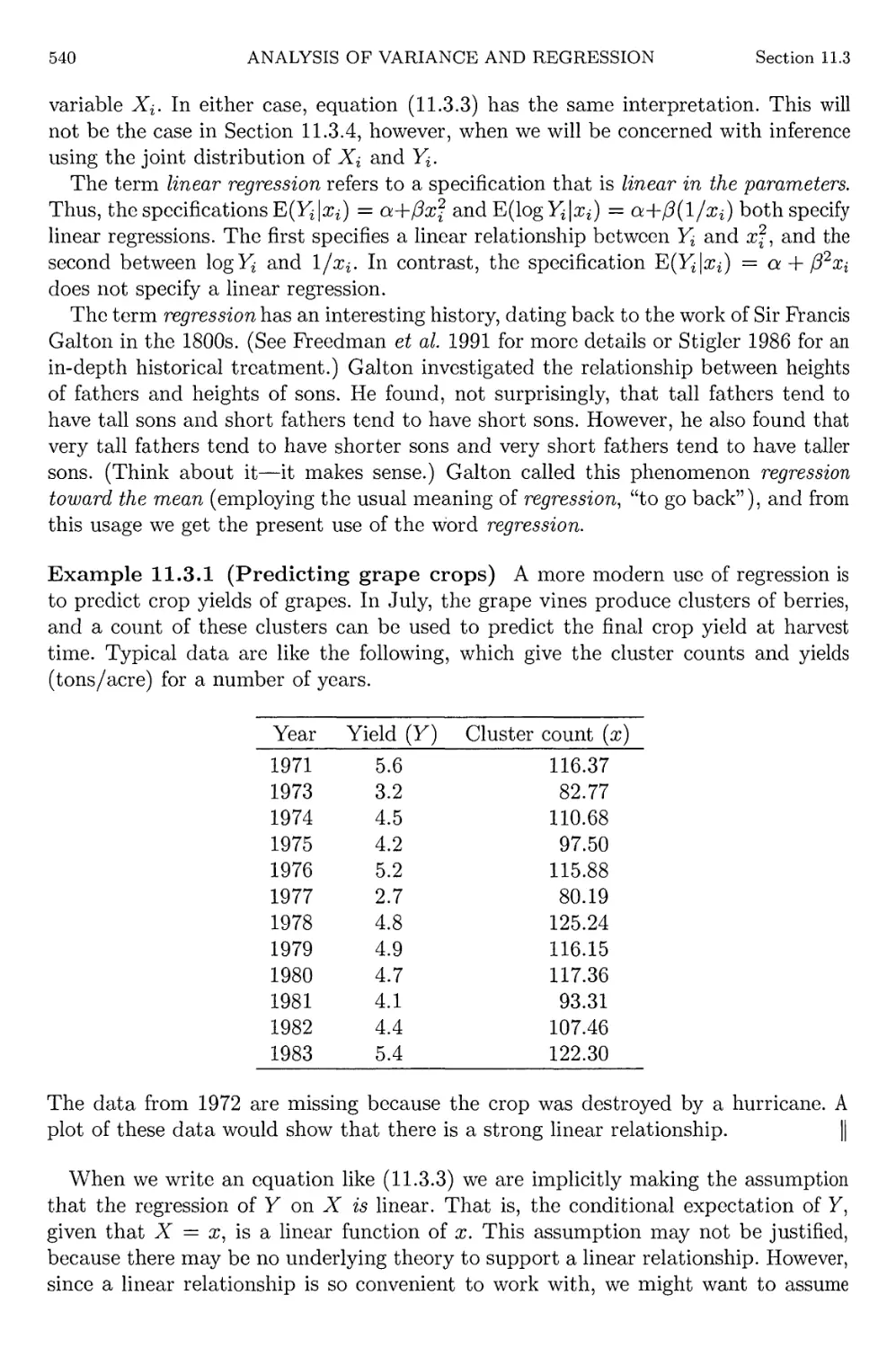
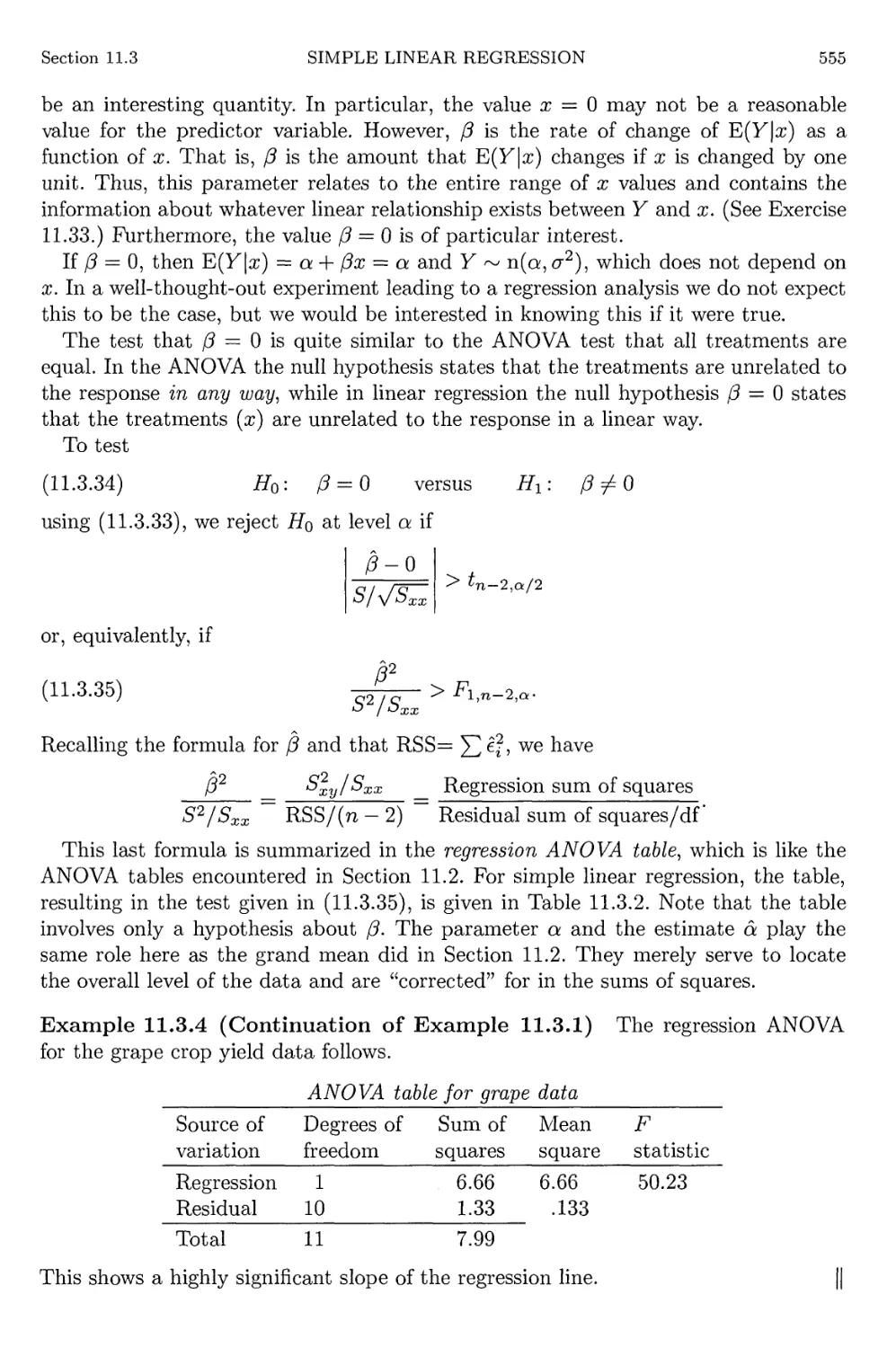
Predicting grape crops
Continuation of Example 11.3.1
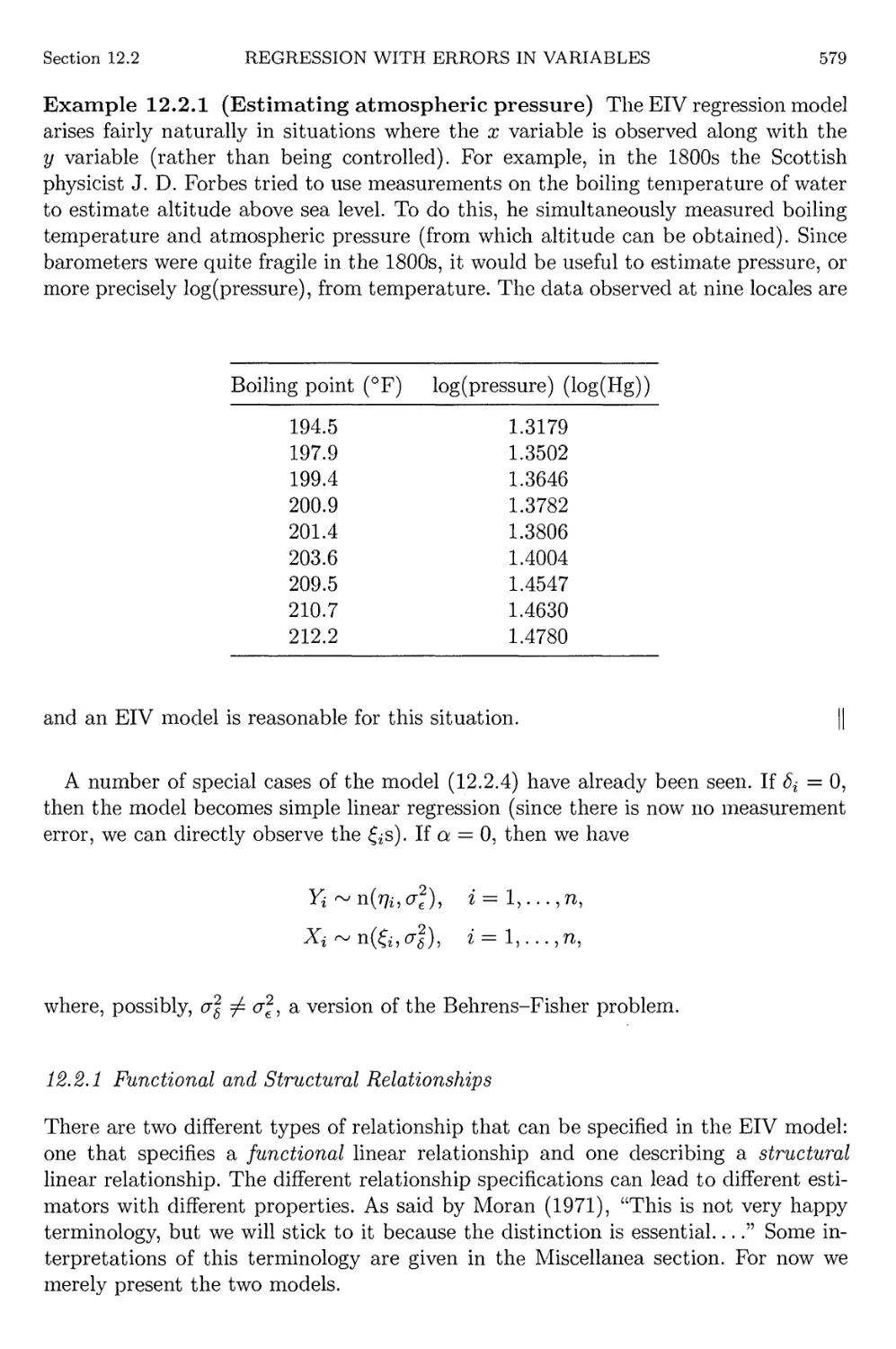
Estimating atmospheric pressure
Challenger data
Challenger data continued
Robustness of least squares estimates
Catastrophic observations
Asymptotic normality of the LAD estimator
Regression M-estimator
Simulation of regression AREs
Unordered sampling
Univariate transformation
Bivariate transformations
478
479
479
480
482
483
484
485
486
487
489
491
493
495
496
497
498
499
499
500
501
502
503
504
518
522
525
529
534
538
540
555
579
594
596
597
598
599
601
601
613
614
614
XXVI11
LIST OF EXAMPLES
A.0.4 Normal probability 616
A.0.5 Density of a sum 616
A.0.6 Fourth moment of sum of uniforms 617
A.0.7 ARE for a gamma mean 618
A.0.8 Limit of chi squared mgfs 619
f
Chapter 1
Probability Theory
"You can, for example, never foretell what any one man will do, but you can
say with precision what an average number will be up to. Individuals vary, but
percentages remain constant. So says the statistician."
Sherlock Holmes
The Sign of Four
The subject of probability theory is the foundation upon which all of statistics is
built, providing a means for modeling populations, experiments, or almost anything
else that could be considered a random phenomenon. Through these models,
statisticians are able to draw inferences about populations, inferences based on examination
of only a part of the whole.
The theory of probability has a long and rich history, dating back at least to the
seventeenth century when, at the request of their friend, the Chevalier de Mere, Pascal
and Fermat developed a mathematical formulation of gambling odds.
The aim of this chapter is not to give a thorough introduction to probability theory;
such an attempt would be foolhardy in so short a space. Rather, we attempt to outline
some of the basic ideas of probability theory that are fundamental to the study of
statistics.
Just as statistics builds upon the foundation of probability theory, probability
theory in turn builds upon set theory, which is where we begin.
1.1 Set Theory
One of the main objectives of a statistician is to draw conclusions about a population
of objects by conducting an experiment. The first step in this endeavor is to identify
the possible outcomes or, in statistical terminology, the sample space.
Definition 1.1.1 The set, 5, of all possible outcomes of a particular experiment is
called the sample space for the experiment.
If the experiment consists of tossing a coin, the sample space contains two outcomes,
heads and tails; thus,
5 = {H,T}.
If, on the other hand, the experiment consists of observing the reported SAT scores
of randomly selected students at a certain university, the sample space would be
2
PROBABILITY THEORY
Section 1.1
the set of positive integers between 200 and 800 that are multiples of ten—that
is, S = {200,210,220,..., 780,790,800}. Finally, consider an experiment where the
observation is reaction time to a certain stimulus. Here, the sample space would
consist of all positive numbers, that is, S = (0, oo).
We can classify sample spaces into two types according to the number of elements
they contain. Sample spaces can be either countable or uncountable; if the elements of
a sample space can be put into 1-1 correspondence with a subset of the integers, the
sample space is countable. Of course, if the sample space contains only a finite number
of elements, it is countable. Thus, the coin-toss and SAT score sample spaces are both
countable (in fact, finite), whereas the reaction time sample space is uncountable, since
the positive real numbers cannot be put into 1-1 correspondence with the integers.
If, however, we measured reaction time to the nearest second, then the sample space
would be (in seconds) S = {0,1, 2,3,...}, which is then countable.
This distinction between countable and uncountable sample spaces is important
only in that it dictates the way in which probabilities can be assigned. For the most
part, this causes no problems, although the mathematical treatment of the situations
is different. On a philosophical level, it might be argued that there can only be
countable sample spaces, since measurements cannot be made with infinite accuracy. (A
sample space consisting of, say, all ten-digit numbers is a countable sample space.)
While in practice this is true, probabilistic and statistical methods associated with
uncountable sample spaces are, in general, less cumbersome than those for countable
sample spaces, and provide a close approximation to the true (countable) situation.
Once the sample space has been defined, we are in a position to consider collections
of possible outcomes of an experiment.
Definition 1.1.2 An event is any collection of possible outcomes of an experiment,
that is, any subset of S (including S itself).
Let A be an event, a subset of S. We say the event A occurs if the outcome of the
experiment is in the set A. When speaking of probabilities, we generally speak of the
probability of an event, rather than a set. But we may use the terms interchangeably.
We first need to define formally the following two relationships, which allow us to
order and equate sets:
AcB^x£A=>x£B) (containment)
A = B & Ac B and BcA (equality)
Given any two events (or sets) A and J3, we have the following elementary set
operations:
Union: The union of A and J3, written A U jB, is the set of elements that belong to
either A or B or both:
AUB = {x:x e Aor x e B}.
Intersection: The intersection of A and 5, written AD5, is the set of elements that
belong to both A and B:
AnB = {x: x e A and x e B}.
Section 1.1
SET THEORY
3
Complementation: The complement of A, written Ac, is the set of all elements
that are not in A:
Ac = {x:x£A}.
Example 1.1.3 (Event operations) Consider the experiment of selecting a card
at random from a standard deck and noting its suit: clubs (C), diamonds (D), hearts
(H), or spades (S). The sample space is
S = {C,D,H,S},
and some possible events are
A = {C,D} and £ = {D,H,S}.
From these events we can form
Au£ = {C,D,H,S}, AHB = {D}, and AC = {H,S}.
Furthermore, notice that AUB = S (the event S) and (AUB)C = 0, where 0 denotes
the empty set (the set consisting of no elements). ||
The elementary set operations can be combined, somewhat akin to the way addition
and multiplication can be combined. As long as we are careful, we can treat sets as if
they were numbers. We can now state the following useful properties of set operations.
Theorem 1.1.4 For any three events, A, B, and C, defined on a sample space S,
a. Commutativity Au B = BuA,
AHB = BHA;
b. Associativity Au (B U C) = (AU B) U C,
An(BnC) = (AnB)nC;
c. Distributive Laws A n (B U C) = (A D B) U (A n C),
A{J(BnC) = (AuB)n(AU C);
d. DeMorgan's Laws (A U B)c = Ac n B°,
(AnJ3)c = ACUBC.
Proof: The proof of much of this theorem is left as Exercise 1.3. Also, Exercises 1.9
and 1.10 generalize the theorem. To illustrate the technique, however, we will prove
the Distributive Law:
AD (B U C) = (AD B) U (An C).
(You might be familiar with the use of Venn diagrams to "prove" theorems in set
theory. We caution that although Venn diagrams are sometimes helpful in visualizing
a situation, they do not constitute a formal proof.) To prove that two sets are equal.
it must be demonstrated that each set contains the other. Formally, then
An(BuC) = {xeS:xeA?mdxe (BUG)};
(^nB)u(^nC) = {xeS:xe(AnB)ovxe (AnC)}.
4
PROBABILITY THEORY
Section 1.1
We first show that A n (B U C) C (A fl B) U (A n C). Let x G (A n (5 U C)). By the
definition of intersection, it must be that a;e(BuC). that is, either x £ B oy x € C.
Since x also must be in A, we have that either a;e(inB)orxG (AflC); therefore,
a: G ((A nB)U(^n C)),
and the containment is established.
Now assume x £ ((AnB)U(AnC)). This implies that x G (AnB) or x G (AnC).
If x G (A fl B), then x is in both A and B. Since # G £,x G (5 U C) and thus
x G (An(i?UC)). If, on the other hand, x G (AnC), the argument is similar, and we
again conclude that x G (An(BUC)). Thus, Ave have established (AnB)U(AnC) C
i fl (B U C), showing containment in the other direction and, hence, proving the
Distributive Law. □
The operations of union and intersection can be extended to infinite collections of
sets as well. If Ai, A2, A3,... is a collection of sets, all defined on a sample space 5,
then
[J Ai = {x G S : x G Ai for some z},
oc
Pi A; = {x G 5 : z G Ai for all z}.
i=l
For example, let S = (0,1] and define Ai = [(1/z), 1]. Then
OC OC'
(J Ai = Q[(l/i), 1] = {a <E (0,1] : x G [(1/z), 1] for some i}
i=l i=l
= {a:€(0,l]} = (0,1];
OO
n^=riK1/^l] = {xe(0,l]:xe[(l/i),l]ioial\i}
7,= 1 i = l
= {x G (0,1] : x G [1,1]} = {1}. (the point 1)
It is also possible to define unions and intersections over uncountable collections of
sets. If r is an index set (a set of elements to be used as indices), then
I) Aa = {x G S : x G Aa for some a},
aer
P| Aa = {x G S : x G Aa for all a}.
aGT
If, for example, we take T = {all positive real numbers} and Aa = (0, a], then
UaerAa = (0, oo) is an uncountable union. While uncountable unions and
intersections do not play a major role in statistics, they sometimes provide a useful mechanism
for obtaining an answer (see Section 8.2.3).
Finally, we discuss the idea of a partition of the sample space.
Section 1.2
BASICS OF PROBABILITY THEORY
5
Definition 1.1.5 Two events A and B are disjoint (or mutually exclusive) if AnB =
0. The events Ai,A2,... are pairwise disjoint (or mutually exclusive) if Ai D Aj = 0
for all z ^ j.
Disjoint sets are sets with no points in common. If we draw a Venn diagram for
two disjoint sets, the sets do not overlap. The collection
Ai = [z,2 + l), z = 0,1,2,...,
consists of pairwise disjoint sets. Note further that U^l0Ai — [0, oo).
Definition 1.1.6 If .Ai,^?*-- are pairwise disjoint and \J(^zlAi = 5, then the
collection Ai, A2,... forms a partition of S.
The sets Ai = [i,i + 1) form a partition of [0, 00). In general, partitions are very
useful, allowing us to divide the sample space into small, nonoverlapping pieces.
1.2 Basics of Probability Theory
When an experiment is performed, the realization of the experiment is an outcome in
the sample space. If the experiment is performed a number of times, different outcomes
may occur each time or some outcomes may repeat. This "frequency of occurrence" of
an outcome can be thought of as a probability. More probable outcomes occur more
frequently. If the outcomes of an experiment can be described probabilistically, we
are on our way to analyzing the experiment statistically.
In this section we describe some of the basics of probability theory. We do not define
probabilities in terms of frequencies but instead take the mathematically simpler
axiomatic approach. As will be seen, the axiomatic approach is not concerned with
the interpretations of probabilities, but is concerned only that the probabilities are
defined by a function satisfying the axioms. Interpretations of the probabilities are
quite another matter. The "frequency of occurrence" of an event is one example of a
particular interpretation of probability. Another possible interpretation is a subjective
one, where rather than thinking of probability as frequency, we can think of it as a
belief in the chance of an event occurring.
1.2.1 Axiomatic Foundations
For each event A in the sample space S we want to associate with A a number
between zero and one that will be called the probability of A, denoted by P(A). It
would seem natural to define the domain of P (the set where the arguments of the
function P(-) are defined) as all subsets of S; that is, for each A C S we define P(A)
as the probability that A occurs. Unfortunately, matters are not that simple. There
are some technical difficulties to overcome. We will not dwell on these technicalities;
although they are of importance, they are usually of more interest to probabilists
than to statisticians. However, a firm understanding of statistics requires at least a
passing familiarity with the following.
6
PROBABILITY THEORY
Section 1.2
Definition 1.2.1 A collection of subsets of S is called a sigma algebra (or Borel
field), denoted by 23, if it satisfies the following three properties:
a. 0 e B (the empty set is an element of 23).
b. If A 6 23, then Ac 6 B (B is closed under complementation).
c. If A\, A<i,... G 23, then U^-A; G 23 (23 is closed under countable unions).
The empty set 0 is a subset of any set. Thus, 0 C S. Property (a) states that this
subset is always in a sigma algebra. Since S = 0°, properties (a) and (b) imply that
S is always in B also. In addition, from DeMorgan's Laws it follows that B is closed
under countable intersections. If Ai, A2,... 6 23, then A\, A^,... G B by property (b),
and therefore U^A^ 6 23. However, using DeMorgan's Law (as in Exercise 1.9), we
have
/ 00 \ c 00
(1.2.1) u^ = rv-
Thus, again by property (b), D^Ai 6 23.
Associated with sample space S we can have many different sigma algebras. For
example, the collection of the two sets {0, S} is a sigma algebra, usually called the
trivial sigma algebra. The only sigma algebra we will be concerned with is the smallest
one that contains all of the open sets in a given sample space 5.
Example 1.2.2 (Sigma algebra—I) If S is finite or countable, then these
technicalities really do not arise, for we define for a given sample space 5,
B = {all subsets of 5, including S itself}.
If S has n elements, there are 2n sets in B (see Exercise 1.14). For example, if S =
{1, 2,3}, then B is the following collection of 23 = 8 sets:
{1} {1,2} {1,2,3}
{2} {1,3} 0
{3} {2,3} ||
In general, if S is uncountable, it is not an easy task to describe B. However, B is
chosen to contain any set of interest.
Example 1.2.3 (Sigma algebra—II) Let S = (—00,00), the real line. Then B is
chosen to contain all sets of the form
[a, 6], (a, 6], (a, 6), and [a, b)
for all real numbers a and 6. Also, from the properties of 23, it follows that B
contains all sets that can be formed by taking (possibly countably infinite) unions and
intersections of sets of the above varieties. II
Section 1.2
BASICS OF PROBABILITY THEORY
7
We are now in a position to define a probability function.
Definition 1.2.4 Given a sample space S and an associated sigma algebra 23, a
probability function is a function P with domain B that satisfies
1. P(A) > 0 for all AeB.
2. P(S) = 1.
3. IfAuA2,...eB are pairwise disjoint, then P(U^1Ai) = ESiP(^)-
The three properties given in Definition 1.2.4 are usually referred to as the Axioms
of Probability (or the Kolmogorov Axioms, after A. Kolmogorov, one of the fathers of
probability theory). Any function P that satisfies the Axioms of Probability is called
a probability function. The axiomatic definition makes no attempt to tell what
particular function P to choose; it merely requires P to satisfy the axioms. For any sample
space many different probability functions can be defined. Which one(s) reflects what
is likely to be observed in a particular experiment is still to be discussed.
Example 1.2.5 (Defining probabilities—I) Consider the simple experiment of
tossing a fair coin, so S = {H,T}. By a "fair" coin we mean a balanced coin that is
equally as likely to land heads up as tails up, and hence the reasonable probability
function is the one that assigns equal probabilities to heads and tails, that is,
(1.2.2) P({H}) = P({T}).
Note that (1.2.2) does not follow from the Axioms of Probability but rather is
outside of the axioms. We have used a symmetry interpretation of probability (or just
intuition) to impose the requirement that heads and tails be equally probable. Since
S = {H} U {T}, we have, from Axiom 2, P({H} U {T}) = 1. Also, {H} and {T} are
disjoint, so P({H} U {T}) - P({H}) + P({T}) and
(1.2.3) P({H})+P({T}) = 1.
Simultaneously solving (1.2.2) and (1.2.3) shows that P({H}) = P({T}) = |.
Since (1.2.2) is based on our knowledge of the particular experiment, not the axioms,
any nonnegative values for P({H}) and P({T}) that satisfy (1.2.3) define a legitimate
probability function. For example, we might choose P({H}) = ^ and P({T}) = |. ||
We need general methods of defining probability functions that we know will always
satisfy Kolmogorov's Axioms. We do not want to have to check the Axioms for each
new probability function, like we did in Example 1.2.5. The following gives a common
method of defining a legitimate probability function.
Theorem 1.2.6 Let S = {$i,..., sn} be a finite set. Let B be any sigma algebra of
subsets of S. Let pi,... ,pn be nonnegative numbers that sum to 1. For any A e B,
define P{A) by
{i:si€A}
8 PROBABILITY THEORY Section 1.2
(The sum over an empty set is defined to be 0.) Then P is a probability function on
B. This remains true if S = {si, $2, -..} is a countable set.
Proof: We will give the proof for finite S. For any A £ B, P(A) = J2{rSieA} Pi — ^'
because every pi > 0. Thus, Axiom 1 is true. Now,
n
p(s)= y, p< = E* = 1-
{i'.SieS} i=l
Thus, Axiom 2 is true. Let A\,...,Ak denote pairwise disjoint events. (B contains
only a finite number of sets, so we need consider only finite disjoint unions.) Then,
P(6A = £ w = E £ «= !>(*>•
The first and third equalities are true by the definition of P(A). The disjointedness of
the AjS ensures that the second equality is true, because the same PjS appear exactly
once on each side of the equality. Thus, Axiom 3 is true and Kolmogorov's Axioms
are satisfied. □
The physical reality of the experiment might dictate the probability assignment, as
the next example illustrates.
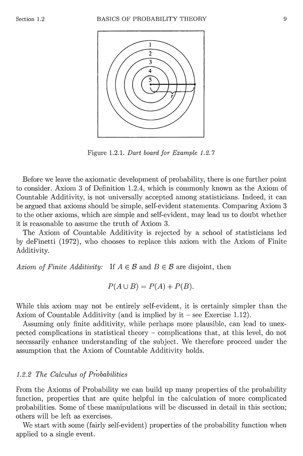
Example 1-2-7 (Defining probabilities-II) The game of darts is played by
throwing a dart at a board and receiving a score corresponding to the number assigned
to the region in which the dart lands. For a novice player, it seems reasonable to
assume that the probability of the dart hitting a particular region is proportional to
the area of the region. Thus, a bigger region has a higher probability of being hit.
Referring to Figure 1.2.1, we see that the dart board has radius r and the distance
between rings is r/5. If we make the assumption that the board is always hit (see
Exercise 1.7 for a variation on this), then we have
_ , N Area of region i
P (scoring i points)
Area of dart board
For example
7rr2 - 7r(4r/5)2 _ /^
7rr2 V 5
P (scoring 1 point) = —^ = 1 — ( -
It is easy to derive the general formula, and we find that
r>/ • • • x (6-i)2-(5-i)2 . ,
P (scoring t points) = —y , % — 1,..., 5,
independent of tt and r. The sum of the areas of the disjoint regions equals the area of
the dart board. Thus, the probabilities that have been assigned to the five outcomes
sum to 1, and, by Theorem 1.2.6, this is a probability function (see Exercise 1.8). ||
Section 1.2 BASICS OF PROBABILITY THEORY 9
Figure 1.2.1. Dart board for Example 1.2.7
Before we leave the axiomatic development of probability, there is one further point
to consider. Axiom 3 of Definition 1.2.4, which is commonly known as the Axiom of
Countable Additivity, is not universally accepted among statisticians. Indeed, it can
be argued that axioms should be simple, self-evident statements. Comparing Axiom 3
to the other axioms, which are simple and self-evident, may lead us to doubt whether
it is reasonable to assume the truth of Axiom 3.
The Axiom of Countable Additivity is rejected by a school of statisticians led
by deFinetti (1972), who chooses to replace this axiom with the Axiom of Finite
Additivity.
Axiom of Finite Additivity: If A 6 B and B £ B are disjoint, then
P{AUB) = P{A) + P{B).
While this axiom may not be entirely self-evident, it is certainly simpler than the
Axiom of Countable Additivity (and is implied by it - see Exercise 1.12).
Assuming only finite additivity, while perhaps more plausible, can lead to
unexpected complications in statistical theory - complications that, at this level, do not
necessarily enhance understanding of the subject. We therefore proceed under the
assumption that the Axiom of Countable Additivity holds.
1.2.2 The Calculus of Probabilities
From the Axioms of Probability we can build up many properties of the probability
function, properties that are quite helpful in the calculation of more complicated
probabilities. Some of these manipulations will be discussed in detail in this section;
others will be left as exercises.
We start with some (fairly self-evident) properties of the probability function when
applied to a single event.
10 PROBABILITY THEORY Section 1.2
Theorem 1.2.8 If P is a probability function and A is any set in By then
a. P(0) = 0, where 0 is the empty set;
b. P(A) < 1;
c. P(AC) = 1-P(A).
Proof: It is easiest to prove (c) first. The sets A and Ac form a partition of the
sample space, that is, S = A U Ac. Therefore,
(1.2.4) P(AUAC) = P{S) = 1
by the second axiom. Also, A and Ac are disjoint, so by the third axiom,
(1.2.5) P{A U Ac) = P(A) + P(AC).
Combining (1.2.4) and (1.2.5) gives (c).
Since P(AC) > 0, (b) is immediately implied by (c). To prove (a), we use a similar
argument on S = S U 0. (Recall that both S and 0 are always in B.) Since S and 0
are disjoint, we have
1 = P(S) = P(S U 0) = P(S) + P(0),
and thus P(0) = 0. □
Theorem 1.2.8 contains properties that are so basic that they also have the
flavor of axioms, although we have formally proved them using only the original three
Kolniogorov Axioms. The next theorem, which is similar in spirit to Theorem 1.2.8,
contains statements that are not so self-evident.
Theorem 1.2.9 If P is a probability function and A and B are any sets in B, then
a. P(B n Ac) = P(B) ~ P{A n B);
b. P(A UB) = P(A) + P(B) - P(A n B)\
c. If Ac B, then P(A) < P(B).
Proof: To establish (a) note that for any sets A and B we have
B = {BC\A}u{BnAc},
and therefore
(1.2.6) P(B) = P({B n A} U {B n Ac}) = P(B n A) + P(B n Ac),
where the last equality in (1.2.6) follows from the fact that B 0 A and B fl A° are
disjoint. Rearranging (1.2.6) gives (a).
To establish (b), we use the identity
(1.2.7) A\jB = AU{BnAc}.
Section 1.2 BASICS OF PROBABILITY THEORY 11
A Venn diagram will show why (1.2.7) holds, although a formal proof is not difficult
(see Exercise 1.2). Using (1.2.7) and the fact that A and B fi Ac are disjoint (since A
and Ac are), we have
(1.2.8) P(A UB) = P(A) + P(B n Ac) = P(A) + P(B) - P(A n B)
from (a).
If A C B, then A D B = A. Therefore, using (a) we have
0 < P(B n Ac) = P(B) - P(A),
establishing (c). □
Formula (b) of Theorem 1.2.9 gives a useful inequality for the probability of an
intersection. Since P(AU B) < 1, we have from (1.2.8), after some rearranging,
(1.2.9) P(A DB)> P(A) + P(B) - 1.
This inequality is a special case of what is known as Bonferroni's Inequality (Miller
1981 is a good reference). Bonferroni's Inequality allows us to bound the probability of
a simultaneous event (the intersection) in terms of the probabilities of the individual
events.
Example 1.2.10 (Bonferroni's Inequality) Bonferroni's Inequality is
particularly useful when it is difficult (or even impossible) to calculate the intersection
probability, but some idea of the size of this probability is desired. Suppose A and
B are two events and each has probability .95. Then the probability that both will
occur is bounded below by
P(A DB)> P(A) + P{B) - 1 = .95 + .95 - 1 = .90.
Note that unless the probabilities of the individual events are sufficiently large, the
Bonferroni bound is a useless (but correct!) negative number. ||
We close this section with a theorem that gives some useful results for dealing with
a collection of sets.
Theorem 1.2.11 If P is a probability function, then
a. P(A) = J2Zip(A n c%) for anV Petition Cu C2, ■..;
b. PiU^Ai) < Y,TLiP(Ai) for any sets AUA2,.... (Boole's Inequality)
Proof: Since Ci, C2,... form a partition, we have that Ci fl Cj = 0 for all i ^ j, and
S = U?l1Ci. Hence,
/ 00 \ 00
A = AnS = Anl{JcA = {J(Ana),
12 PROBABILITY THEORY Section 1.2
where the last equality follows from the Distributive Law (Theorem 1.1.4). We
therefore have
P(A) = P(\J(AnCi)
a=l
Now, since the Ci are disjoint, the sets A n Ci are also disjoint, and from the properties
of a probability function we have
/ oo \ oc
p U(Anco) =X)J°(^nci),
establishing (a).
To establish (b) we first construct a disjoint collection A1? A2,..., with the property
that U^A* = Uf^iAi. We define A* by
K3 = l J
, % — 2, o,...,
where the notation A\i? denotes the part of A that does not intersect with B. In more
familiar symbols, A\B = AnBc. It should be easy to see that U^A* = U-^A,;, and
wre therefore have
nU^rO^HEw.
a=l / \i=l / i=l
where the last equality follows since the A* are disjoint. To see this, we write
A* nA*k=\ Ai\ [\JAn\n\ A^- ( U Ai I I (definition of A*)
= I Ai n I (J A, J 1 n I Ak n I (J A, J I (definition of "\")
= < A?: n p| AJ I n < Ak n p| A^ I (DeMorgan's Laws)
Now if i > k, the first intersection above will be contained in the set A£, which will
have an empty intersection with A/tV If k > i, the argument is similar. Further, by
construction A* C A/, so P(A*) < P{At) and we have
00 00
X>(A*)<Em)>
establishing (b). D
Section 1.2
BASICS OF PROBABILITY THEORY
13
There is a similarity between Boole's Inequality and Bonferroni's Inequality. In
fact, they are essentially the same thing. We could have used Boole's Inequality to
derive (1.2.9). If we apply Boole's Inequality to Ac, we have
/ n \ n
\z=l / i=l
and using the facts that UA^ = {C)Ai)c and P(A^) = 1 - P(A;), we obtain
(n \ n
r\Ai)<n-J2P(Ai).
i=l / i=l
This becomes, on rearranging terms,
(n \ n
Z = l / 2=1
which is a more general version of the Bonferroni Inequality of (1.2.9).
1.2.3 Counting
The elementary process of counting can become quite sophisticated when placed in
the hands of a statistician. Most often, methods of counting are used in order to
construct probability assignments on finite sample spaces, although they can be used
to answer other questions also.
Example 1.2.12 (Lottery—I) For a number of years the New York state lottery
operated according to the following scheme. From the numbers 1, 2, ... ,44, a person
may pick any six for her ticket. The winning number is then decided by randomly
selecting six numbers from the forty-four. To be able to calculate the probability of
winning we first must count how many different groups of six numbers can be chosen
from the forty-four. |[
Example 1.2*13 (Tournament) In a single-elimination tournament, such as the
U.S. Open tennis tournament, players advance only if they win (in contrast to double-
elimination or round-robin tournaments). If we have 16 entrants, we might be
interested in the number of paths a particular player can take to victory, where a path is
taken to mean a sequence of opponents. ||
Counting problems, in general, sound complicated, and often we must do our
counting subject to many restrictions. The way to solve such problems is to break them
down into a series of simple tasks that are easy to count, and employ known rules
of combining tasks. The following theorem is a first step in such a process and is
sometimes known as the Fundamental Theorem of Counting.
Theorem 1.2.14 If a job consists of k separate tasks? the ith of which can be done
in Ui ways, i = 1,..., k, then the entire job can be done in n\ x ri2 x • ■ • x n^ ways.
14
PROBABILITY THEORY
Section 1.2
Proof: It suffices to prove the theorem for k' = 2 (see Exercise 1.15). The proof is
just a matter of careful counting. The first task can be done in ri\ ways, and for each
of these ways we have ri2 choices for the second task. Thus, we can do the job in
(1 x n2) + (1 x n2) H h (1 x n2) = nx x n2
V s, '
?7,i terms
ways, establishing the theorem for k = 2. □
Example 1.2.15 (Lottery~II) Although the Fundamental Theorem of Counting
is a reasonable place to start, in applications there are usually more aspects of a
problem to consider. For example, in the New York state lottery the first number
can be chosen in 44 ways, and the second number in 43 ways, making a total of
44 x 43 = 1,892 ways of choosing the first two numbers. However, if a person is
allowed to choose the same number twice, then the first two numbers can be chosen
in 44 x 44 = 1,936 ways. ||
The distinction being made in Example 1.2.15 is between counting with replacement
and counting without replacement There is a second crucial element in any counting
problem, whether or not the ordering of the tasks is important. To illustrate with the
lottery example, suppose the winning numbers are selected in the order 12, 37, 35, 9,
13, 22. Does a person who selected 9, 12, 13, 22, 35, 37 qualify as a winner? In other
words, does the order in which the task is performed actually matter? Taking all of
these considerations into account, we can construct a 2 x 2 table of possibilities:
Possible methods of counting
Without With
replacement replacement
Ordered | | [
Unordered | [ |
Before we begin to count, the following definition gives us some extremely helpful
notation.
Definition 1.2,16 For a positive integer n, n\ (read n factorial) is the product of
all of the positive integers less than or equal to n. That is,
n! = n x (n - 1) x (n - 2) x • • • x 3 x 2 x 1.
Furthermore, we define 0! = 1.
Let us now consider counting all of the possible lottery tickets under each of these
four cases.
1. Ordered, without replacement From the Fundamental Theorem of Counting, the
first number can be selected in 44 ways, the second in 43 ways, etc. So there are
44!
44 x 43 x 42 x 41 x 40 x 39 = — = 5,082,517,440
possible tickets.
Section 1.2
BASICS OF PROBABILITY THEORY
15
2. Ordered, with replacement Since each number can now be selected in 44 ways
(because the chosen number is replaced), there are
44 x 44 x 44 x 44 x 44 x 44 = 446 = 7,256,313,856
possible tickets.
3. Unordered, without replacement We know the number of possible tickets when the
ordering must be accounted for, so what we must do is divide out the redundant
orderings. Again from the Fundamental Theorem, six numbers can be arranged in
6x5x4x3x2x1 ways, so the total number of unordered tickets is
44 x 43 x 42 x 41 x 40 x 39 _ 44!
6x5x4x3x2x1 ""^38!"7'059'052-
This form of counting plays a central role in much of statistics—so much, in fact,
that it has earned its own notation.
Definition 1.2,17 For nonnegative integers n and r, where n > r, we define the
symbol (™), read n choose r, as
n\ n!
r! (n — r)\'
In our lottery example, the number of possible tickets (unordered, without
replacement) is (464). These numbers are also referred to as binomial coefficients, for reasons
that will become clear in Chapter 3.
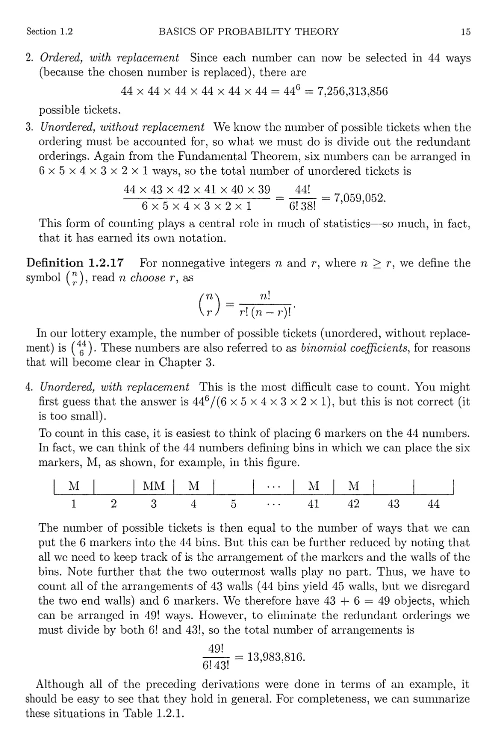
4. Unordered, with replacement This is the most difficult case to count. You might
first guess that the answer is 446/(6 x5x4x3x2xl), but this is not correct (it
is too small).
To count in this case, it is easiest to think of placing 6 markers on the 44 numbers.
In fact, we can think of the 44 numbers defining bins in which we can place the six
markers, M, as shown, for example, in this figure.
| M | 1 MM 1 M | 1 ••- | M | M 1 1 1
1 2 3 4 5 41 42 43 44
The number of possible tickets is then equal to the number of ways that we can
put the 6 markers into the 44 bins. But this can be further reduced by noting that
all we need to keep track of is the arrangement of the markers and the walls of the
bins. Note further that the twTo outermost walls play no part. Thus, we have to
count all of the arrangements of 43 walls (44 bins yield 45 walls, but we disregard
the two end walls) and 6 markers. We therefore have 43 + 6 — 49 objects, which
can be arranged in 49! ways. However, to eliminate the redundant orderings we
must divide by both 6! and 43!, so the total number of arrangements is
49!
— = 13,983,816.
Although all of the preceding derivations were done in terms of an example, it
should be easy to see that they hold in general. For completeness, we can summarize
these situations in Table 1.2.1.
16
PROBABILITY THEORY
Section 1.2
Table 1.2.1. Number of possible arrangements of size r from n objects
Without With
replacement replacement
n!
Ordered 7 —— nr
(n — r)\
Unordered
o
1.2.4 Enumerating Outcomes
The counting techniques of the previous section are useful when the sample space
S is a finite set and all the outcomes in S are equally likely. Then probabilities of
events can be calculated by simply counting the number of outcomes in the event. To
see this, suppose that S — {si,..., s^} is a finite sample space. Saying that all the
outcomes are equally likely means that P({sj}) — l/N for every outcome Si. Then,
using Axiom 3 from Definition 1.2.4, we have, for any event A,
P(a\ - V P(U D-Vi- # of elements in A
±-{A) - 2^ n\Si}) - 2., N ~ # of elemCnts in S '
For large sample spaces, the counting techniques might be used to calculate both
the numerator and denominator of this expression.
Example 1.2.18 (Poker) Consider choosing a five-card poker hand from a
standard deck of 52 playing cards. Obviously, we are sampling without replacement from
the deck. But to specify the possible outcomes (possible hands), we must decide
whether we think of the hand as being dealt sequentially (ordered) or all at once
(unordered). If we wish to calculate probabilities for events that depend on the
order, such as the probability of an ace in the first two cards, then we must use the
ordered outcomes. But if our events do not depend on the order, we can use the
unordered outcomes. For this example we use the unordered outcomes, so the sample
space consists of all the five-card hands that can be chosen from the 52-card deck.
There are (552) = 2,598,960 possible hands. If the deck is well shuffled and the cards
arc randomly dealt, it is reasonable to assign probability 1/2,598,960 to each possible
hand.
We now calculate some probabilities by counting outcomes in events. What is the
probability of having four aces? How many different hands are there with four aces? If
we specify that four of the cards are aces, then there are 48 different ways of specifying
the fifth card. Thus,
48
Pffour aces) = ——r———,
v ; 2,598,960'
less than 1 chance in 50,000. Only slightly more complicated counting, using Theorem
1.2.14, allows us to calculate the probability of having four of a kind. There are 13
Section 1.2
BASICS OF PROBABILITY THEORY
17
ways to specify which denomination there will be four of. After we specify these four
cards, there are 48 ways of specifying the fifth. Thus, the total number of hands with
four of a kind is (13) (48) and
F(rour of a kind) = —
2,598,960 2,598,960'
To calculate the probability of exactly one pair (not two pairs, no three of a kind,
etc.) we combine some of the counting techniques. The number of hands with exactly
one pair is
(1.2.11) 13 [ o I [ o 43 = 1,098,240.
Expression (1.2.11) comes from Theorem 1.2.14 because
13 = zjjz of ways to specify the denomination for the pair,
V2,
'12'
= # of ways to specify the two cards from that denomination,
= # of ways of specifying the other three denominations,
\3,
43 = # of ways of specifying the other three cards from those denominations.
Thus,
1,098,240
P(exactly one pair) =
2,598,960'
When sampling without replacement, as in Example 1.2.18, if we want to calculate
the probability of an event that does not depend on the order, we can use either
the ordered or unordered sample space. Each outcome in the unordered sample space
corresponds to r! outcomes in the ordered sample space. So, when counting outcomes
in the ordered sample space, we use a factor of r! in both the numerator and
denominator that will cancel to give the same probability as if we counted in the unordered
sample space.
The situation is different if we sample with replacement. Each outcome in the
unordered sample space corresponds to some outcomes in the ordered sample space,
but the number of outcomes differs.
Example 1.2.19 (Sampling with replacement) Consider sampling r = 2 items
from n = 3 items, with replacement. The outcomes in the ordered and unordered
sample spaces are these.
Unordered {1,1} {2,2} {3,3} {1,2} {1,3} {2,3}
Ordered (1,1) (2,2) (3,3) (1,2), (2,1) (1,3), (3,1) (2,3), (3,2)
Probability 1/9 1/9 1/9 2/9 2/9 2/9
18
PROBABILITY THEORY
Section 1.2
The probabilities come from considering the nine outcomes in the ordered sample
space to be equally likely. This corresponds to the common interpretation of "sampling
with replacement"; namely, one of the three items is chosen, each with probability 1/3;
the item is noted and replaced; the items are mixed and again one of the three items
is chosen, each with probability 1/3. It is seen that the six outcomes in the unordered
sample space are not equally likely under this kind of sampling. The formula for the
number of outcomes in the unordered sample space is useful for enumerating the
outcomes, but ordered outcomes must be counted to correctly calculate probabilities.
ii
Some authors argue that it is appropriate to assign equal probabilities to the
unordered outcomes when "randomly distributing r indistinguishable balls into n
distinguishable urns." That is, an urn is chosen at random and a ball placed in it, and
this is repeated r times. The order in which the balls are placed is not recorded so,
in the end, an outcome such as {1,3} means one ball is in urn 1 and one ball is in
urn 3.
But here is the problem with this interpretation. Suppose two people observe this
process, and Observer 1 records the order in which the balls are placed but Observer 2
does not. Observer 1 will assign probability 2/9 to the event {1,3}. Observer 2,
who is observing exactly the same process, should also assign probability 2/9 to this
event. But if the six unordered outcomes are written on identical pieces of paper and
one is randomly chosen to determine the placement of the balls, then the unordered
outcomes each have probability 1/6. So Observer 2 will assign probability 1/6 to the
event {1,3}.
The confusion arises because the phrase "with replacement" will typically be
interpreted with the sequential kind of sampling we described above, leading to assigning
a probability 2/9 to the event {1,3}. This is the correct way to proceed, as
probabilities should be determined by the sampling mechanism, not whether the balls are
distinguishable or indistinguishable.
Example 1-2.20 (Calculating an average) As an illustration of the
distinguishable/indistinguishable approach, suppose that we are going to calculate all possible
averages of four numbers selected from
2,4,9,12
where we draw the numbers with replacement. For example, possible draws are
{2,4,4,9} with average 4.75 and {4,4,9,9} with average 6.5. If we are only
interested in the average of the sampled numbers, the ordering is unimportant, and thus
the total number of distinct samples is obtained by counting according to unordered,
with-replacement sampling.
The total number of distinct samples is (n_h^~1)- But now, to calculate the
probability distribution of the sampled averages, we must count the different ways that a
particular average can occur.
The value 4.75 can occur only if the sample contains one 2, two 4s, and one 9.
The number of possible samples that have this configuration is given in the following
table:
Section 1.2
BASICS OF PROBABILITY THEORY
19
0.1
o.os
0.06
0.04
0.02
. nfl
n n
r r4 1 i '
n
n
m
n
1. n
Figure 1.2.2. Histogram of averages of samples with replacement from the four numbers
{2,4,9,12}
Unordered
Ordered
(2,4,4,9), (2,4,9,4), (2,9,4,4), (4,2,4,9),
(4,2,9,4), (4,4,2,9), (4,4,9,2), (4,9,2,4),
(4,9,4,2), (9,2,4,4), (9,4,2,4), (9,4,4,2)
{2,4,4,9}
The total number of ordered samples is nn = 44 = 256, so the probability of drawing
the unordered sample {2,4,4,9} is 12/256. Compare this to the probability that we
would have obtained if we regarded the unordered samples as equally likely - we would
have assigned probability l/(n+^_1) = 1/Q = 1/35 to {2,4,4,9} and to every other
unordered sample.
To count the number of ordered samples that would result in {2,4,4, 9}, we argue
as follows. We need to enumerate the possible orders of the four numbers {2,4,4,9},
so we are essentially using counting method 1 of Section 1.2.3. We can order the
sample in 4x3x2x1 = 24 ways. But there is a bit of double counting here, since we
cannot count distinct arrangements of the two 4s. For example, the 24 ways would
count {9,4, 2,4} twice (which would be OK if the 4s were different). To correct this,
we divide by 2! (there are 2! ways to arrange the two 4s) and obtain 24/2 = 12 ordered
samples. In general, if there are k places and we have m different numbers repeated
k\
&i, &2j • • • , km times, then the number of ordered samples is _ t_ t -—-. This type
/ci!/c2!-'-/cm!
of counting is related to the multinomial distribution, which we will see in Section
4.6. Figure 1.2.2 is a histogram of the probability distribution of the sample averages,
reflecting the multinomial counting of the samples.
There is also one further refinement that is reflected in Figure 1.2.2. It is possible
that two different unordered samples will result in the same mean. For example, the
unordered samples {4,4,12,12} and {2, 9, 9,12} both result in an average value of 8.
The first sample has probability 3/128 and the second has probability 3/64, giving the
value 8 a probability of 9/128 = .07. See Example A.0.1 in Appendix A for details on
constructing such a histogram. The calculation that we have done in this example is
an elementary version of a very important statistical technique known as the bootstrap
(Efron and Tibshirani 1993). We will return to the bootstrap in Section 10.1.4. ||
20
PROBABILITY THEORY
Section 1.3
1.3 Conditional Probability and Independence
All of the probabilities that we have dealt with thus far have been unconditional
probabilities. A sample space was defined and all probabilities were calculated with
respect to that sample space. In many instances, however, we are in a position to
update the sample space based on new information. In such cases, we want to be able
to update probability calculations or to calculate conditional probabilities.
Example 1.3.1 (Four aces) Four cards are dealt from the top of a well-shuffled
deck. What is the probability that they are the four aces? We can calculate this
probability by the methods of the previous section. The number of distinct groups of
four cards is
(52j =270,725.
Only one of these groups consists of the four aces and every group is equally likely,
so the probability of being dealt all four aces is 1/270,725.
We can also calculate this probability by an "updating" argument, as follows. The
probability that the first card is an ace is 4/52. Given that the first card is an ace.
the probability that the second card is an ace is 3/51 (there are 3 aces and 51 cards
left). Continuing this argument, we get the desired probability as
4 3 2 1 1
X X X
52 51 50 49 270,725
In our second method of solving the problem, we updated the sample space after
each draw of a card; we calculated conditional probabilities.
Definition 1.3-2 If A and B are events in £, and P(B) > 0, then the conditional
probability of A given B, written P(A\B), is
(1.3.1) P{A\B) = ^1.
Note that what happens in the conditional probability calculation is that B becomes
the sample space: P(B\B) = 1. The intuition is that our original sample space, 5,
has been updated to B. All further occurrences are then calibrated with respect to
their relation to B. In particular, note what happens to conditional probabilities of
disjoint sets. Suppose A and B are disjoint, so P(A D B) — 0. It then follows that
P{A\B) = P{B\A) = b.
Example 1-3.3 (Continuation of Example 1.3.1) Although the probability of
getting all four aces is quite small, let us see how the conditional probabilities change
given that some aces have already been drawn. Four cards will again be dealt from a
well-shuffled deck, and we now calculate
P(4 aces in 4 cards | i aces in % cards), i = 1, 2,3.
Section 1.3 CONDITIONAL PROBABILITY AND INDEPENDENCE 21
The event {4 aces in 4 cards} is a subset of the event {i aces in i cards}. Thus, from
the definition of conditional probability, (1.3.1), we know that
P(4 aces in 4 cards | i aces in i cards)
P({4 aces in 4 cards} n {i aces in i cards})
P(i aces in i cards)
P(4 aces in 4 cards)
P(i aces in i cards)
The numerator has already been calculated, and the denominator can be calculated
with a similar argument. The number of distinct groups of i cards is (°?), and
(4)
P(i aces in i cards) = Y2 .
\ i /
Therefore, the conditional probability is given by
(?) (4-i)!48! 1
P(4 aces in 4 cards | i aces in i cards) =
(542)(t) (52-0' (I-')'
For z = 1, 2, and 3, the conditional probabilities are .00005, .00082, and .02041,
respectively. ||
For any B for which P(B) > 0, it is straightforward to verify that the probability
function P(-\B) satisfies Kolmogorov's Axioms (see Exercise 1.35). You may suspect
that requiring P(B) > 0 is redundant. Who would want to condition on an event of
probability 0? Interestingly, sometimes this is a particularly useful way of thinking of
things. However, we will defer these considerations until Chapter 4.
Conditional probabilities can be particularly slippery entities and sometimes require
careful thought. Consider the following often-told tale.
Example 1.3-4 (Three prisoners) Three prisoners, A, B, and C, are on death
row. The governor decides to pardon one of the three and chooses at random the
prisoner to pardon. He informs the warden of his choice but requests that the name
be kept secret for a few days.
The next day, A tries to get the warden to tell him who had been pardoned. The
warden refuses. A then asks which of B or C will be executed. The warden thinks for
a while, then tells A that B is to be executed.
Warden's reasoning: Each prisoner has a ^ chance of being pardoned. Clearly,
either B or C must be executed, so I have given A no information about whether
A will be pardoned.
A's reasoning: Given that B will be executed, then either A or C will be pardoned.
My chance of being pardoned has risen to |.
It should be clear that the warden's reasoning is correct, but let us see v hy. Let
AS, and C denote the events that A, B, or C is pardoned, respectively. We know
22 PROBABILITY THEORY Section 1.3
that P(A) = P(B) = P(C) = \. Let W denote the event that the warden says B will
die. Using (1.3.1), A can update his probability of being pardoned to
P{Am = p^nm.
What is happening can be summarized in this table:
Prisoner pardoned Warden tells A
A B dies 1 each with equal
A C dies J probability
B C dies
C Bdies
Using this table, we can calculate
P(W) = P(warden says B dies)
= P(warden says B dies and A pardoned)
+ P(warden says B dies and C pardoned)
+ P(warden says B dies and B pardoned)
1 1 « 1
= - + - + 0 = -.
6 3 2
Thus, using the warden's reasoning, we have
P(A D W)
P{A\W)
(1.3.2)
P{W)
P(warden says B dies and A pardoned) 1/6 1
P(warden says B dies) 1/2 3'
However, A falsely interprets the event W as equal to the event Bc and calculates
P{Af\Bc) 1/3 1
P{A\BC) =
P{BC) 2/3 2'
We sec that conditional probabilities can be quite slippery and require careful
interpretation. For some other variations of this problem, see Exercise 1.37. ||
Re-expressing (1.3.1) gives a useful form for calculating intersection probabilities,
(1.3.3) P(A r\B) = P{A\B)P(B),
which is essentially the formula that was used in Example 1.3.1. We can take
advantage of the symmetry of (1.3.3) and also write
(1.3.4) P(A n B) = P{B\A)P{A).
Section 1.3 CONDITIONAL PROBABILITY AND INDEPENDENCE 23
When faced with seemingly difficult calculations, we can break up our calculations
according to (1.3.3) or (1.3.4), whichever is easier. Furthermore, we can equate the
right-hand sides of these equations to obtain (after rearrangement)
(1-3-5) P(A\B) = P(B\A)^y
which gives us a formula for "turning around" conditional probabilities. Equation
(1.3.5) is often called Bayes' Rule for its discoverer. Sir Thomas Bayes (although see
Stigler 1983).
Bayes' Rule has a more general form than (1.3.5), one that applies to partitions of
a sample space. We therefore take the following as the definition of Bayes' Rule.
Theorem 1.3-5 (Bayes' Rule) Let Ai,A2,... be a partition of the sample space,
and let B be any set. Then, for each i = 1,2,...,
PIMB)- WWW
T.T=1P(B\Aj)P(AjY
Example 1.3.6 (Coding) When coded messages are sent, there are sometimes
errors in transmission. In particular, Morse code uses "dots" and "dashes," which are
known to occur in the proportion of 3:4. This means that for any given symbol,
3 4
P(dot sent) = - and P(dash sent) = -.
Suppose there is interference on the transmission line, and with probability | a dot
is mistakenly received as a dash, and vice versa. If we receive a dot, can we be sure
that a dot was sent? Using Bayes' Rule, we can write
i-i/i ii .ixi-i/i .iii x P(dot sent)
P(dot sent | dot received) = P(dot received | dot sent)-
P(dot received)
Now, from the information given, we know that P(dot sent) = | and P(dot received]
dot sent) = |. Furthermore, we can also write
P(dot received) = P(dot received D dot sent) + P(dot received n dash sent)
= P(dot received | dot sent)P(dot sent)
+ P(dot received | dash sent)P(dash sent)
_ 7 3 1 4 __ 25
~8X7 + 8X7 " 56'
Combining these results, we have that the probability of correctly receiving a dot is
• ,n (7/8) x (3/7) 21
P(dot sent | dot received) = v ' ' v / ' = —. ||
ZO/OO Zo
24 PROBABILITY THEORY Section 1.3
In some cases it may happen that the occurrence of a particular event, P, has no
effect on the probability of another event, A Symbolically, we are saying that
(1.3.6) P(A\B) = P(A).
If this holds, then by Bayes' Rule (1.3.5) and using (1.3.6) we have
(1.3.7) P(B\A) = P(A\B)^ = P(A)^& = P(B),
so the occurrence of A has no effect on P. Moreover, since P(B\A)P(A) = P(Af)B),
it then follows that
P(AnB) = P(A)P(B)i
which we take as the definition of statistical independence.
Definition 1,3.7 Two events, A and P, are statistically independent if
(1.3.8) P(A nB) = P(A)P(B).
Note that independence could have been equivalently defined by either (1.3.6) or
(1.3.7) (as long as either P(A) > 0 or P(B) > 0). The advantage of (1.3.8) is that
it treats the events symmetrically and will be easier to generalize to more than two
events.
Many gambling games provide models of independent events. The spins of a roulette
wheel and the tosses of a pair of dice are both series of independent events.
Example 1.3.8 (Chevalier de Mere) The gambler introduced at the start of the
chapter, the Chevalier de Mere, was particularly interested in the event that he could
throw at least 1 six in 4 rolls of a die. We have
P(at least 1 six in 4 rolls) — 1 — P(no six in 4 rolls)
4
= 1 — TT P(no six on roll i),
i=l
where the last equality follows by independence of the rolls. On any roll, the
probability of not rolling a six is |, so
P(at least 1 six in 4 rolls) = 1 - I - ) = .518. ||
Independence of A and B implies independence of the complements also. In fact,
we have the following theorem.
Section 1.3 CONDITIONAL PROBABILITY AND INDEPENDENCE 25
Theorem 1.3.9 If A and B are independent events, then the following pairs are
also independent:
a. A and Bc,
b. Ac and B,
c. Ac and Bc.
Proof: We will prove only (a), leaving the rest as Exercise 1.40. To prove (a) we
must show that P(A n Bc) = P(A)P(BC). From Theorem 1.2.9a we have
P(AnBc) = P(A)-P(AC\B)
= P{A) - P(A)P(B) (A and B are independent)
= P(A)(1-P(B))
= P(A)P(BC). D
Independence of more than two events can be defined in a manner similar to (1.3.8),
but we must be careful. For example, we might think that we could say A, B, and C
are independent if P(ADBnC) = P(A)P(B)P(C). However, this is not the correct
condition.
Example 1.3.10 (Tossing two dice) Let an experiment consist of tossing two
dice. For this experiment the sample space is
S = {(1,1), (1,2),..., (1,6), (2,1),..., (2,6),... ,(6,1),..., (6,6)};
that is, S consists of the 36 ordered pairs formed from the numbers 1 to 6. Define the
following events:
A = {doubles appear} - {(1,1), (2, 2), (3, 3), (4,4), (5,5), (6, 6)},
B = {the sum is between 7 and 10},
C = {the sum is 2 or 7 or 8}.
The probabilities can be calculated by counting among the 36 possible outcomes. We
have
P(A) = ±, P(B) = ^ and P^ = \-
Furthermore,
P(A DB nC) = P(the sum is 8, composed of double 4s)
_ 1
~ 36
1 1 1
=6X2X3
= P(A)P(B)P(C).
26 PROBABILITY THEORY Section 1.3
However,
P(D (1C) = P(sum equals 7 or 8) = ~ ^ P{B)P{C).
Similarly, it can be shown that P(A n B) / P(A)P(-B); therefore, the requirement
P(A flBnC) = P(A)P(B)P(C) is not a strong enough condition to guarantee
pairwise independence. ||
A second attempt at a general definition of independence, in light of the
previous example, might be to define A, B: and C to be independent if all the pairs are
independent. Alas, this condition also fails.
Example 1.3.11 (Letters) Let the sample space S consist of the 3! permutations
of the letters a, b, and c along with the three triples of each letter. Thus,
aaa bbb ccc
abc -bca cba
acb bac cab
Furthermore, let each element of S have probability |. Define
Ai = {zth place in the triple is occupied by a}.
It is then easy to count that
P(A*) = \> * = 1,2,3,
and
P{AX n a2) = P{AX n A3) = P(A2 n A3) = i,
so the Ais are pairwise independent. But
P(A, n A2 n A3) = i ^ P{Al)P{A2)P{Az),
so the A{S do not satisfy the probability requirement. ||
The preceding two examples show that simultaneous (or mutual) independence of
a collection of events requires an extremely strong definition. The following definition
works.
Definition 1.3.12 A collection of events A\,..., An are mutually independent if
for any subcollection A^,..., Aik, we have
p(rK)=rp(^)-
Section 1.4
RANDOM VARIABLES
27
Example 1.3.13 (Three coin tosses—I) Consider the experiment of tossing a
coin three times. A sample point for this experiment must indicate the result of each
toss. For example, HHT could indicate that two heads and then a tail were observed.
The sample space for this experiment has eight points, namely,
{HHH, HHT, HTH, THH, TTH, THT, HTT, TTT}.
Let Hi, i = 1, 2,3, denote the event that the ith toss is a head. For example,
(1.3.9) Hx = {HHH, HHT, HTH, HTT}.
If we assign probability | to each sample point, then using enumerations such as
(1.3.9), we see that P(#i) = P{H2) = P(H3) = |. This says that the coin is fair and
has an equal probability of landing heads or tails on each toss.
Under this probability model, the events i?i, H2, and H3 are also mutually
independent. To verify this we note that
P{HX HH2n H3) = P({HHH}) =l-=l-.X-.l- = P(Hl)P(H2)P(H3).
To verify the condition in Definition 1.3.12, we also must check each pair. For example,
P(#i n H2) = P({HHH, HHT}) = | = \ ■ \ = P^P^).
The equality is also true for the other two pairs. Thus, i?i, H2, and H3 are mutually
independent. That is, the occurrence of a head on any toss has no effect on any of
the other tosses.
It can be verified that the assignment of probability | to each sample point is the
only probability model that has P{Hi) = P(H2) = P(H3) = \ and HUH2, and H3
mutually independent. ||
1.4 Random Variables
In many experiments it is easier to deal with a summary variable than with the
original probability structure. For example, in an opinion poll, we might decide to
ask 50 people whether they agree or disagree with a certain issue. If we record a "1"
for agree and "0" for disagree, the sample space for this experiment has 250 elements,
each an ordered string of Is and 0s of length 50. We should be able to reduce this to
a reasonable size! It may be that the only quantity of interest is the number of people
who agree (equivalently, disagree) out of 50 and, if we define a variable X = number
of Is recorded out of 50, we have captured the essence of the problem. Note that the
sample space for X is the set of integers {0,1,2,..., 50} and is much easier to deal
with than the original sample space.
In defining the quantity X, we have defined a mapping (a function) from the original
sample space to a new sample space, usually a set of real numbers. In general, we
have the following definition.
Definition 1.4.1 A random variable is a function from a sample space S into the
real numbers.
28 PROBABILITY THEORY Section 1.4
Example 1.4.2 (Random variables) In some experiments random variables are
implicitly used; some examples are these.
Examples of random variables
Experiment Random variable
Toss two dice X = sum of the numbers
Toss a coin 25 times X = number of heads in 25 tosses
Apply different amounts of
fertilizer to corn plants X = yield/acre II
In defining a random variable, we have also defined a new sample space (the range
of the random variable). We must now check formally that our probability function,
which is defined on the original sample space, can be used for the random variable.
Suppose we have a sample space
S = {si,...,eSn}
with a probability function P and we define a random variable X with range X =
{.x'i,..., xm}. We can define a probability function Px on X in the following way. We
will observe X — X{ if and only if the outcome of the random experiment is an Sj G S
such that X(sj) = X{. Thus,
(1.4.1) PX(X = a*) = P ({sj e S : X(sj) = Xi}).
Note that the left-hand side of (1.4.1), the function Px, is an induced probability
function on X, defined in terms of the original function P. Equation (1.4.1) formally
defines a probability function, Px, for the random variable X. Of course, we have
to verify that Px satisfies the Kolmogorov Axioms, but that is not a very difficult
job (see Exercise 1.45). Because of the equivalence in (1.4.1), we will simply write
P(X = Xi) rather than PX(X = x{).
A note on notation: Random variables will always be denoted with uppercase letters
and the realized values of the variable (or its range) will be denoted by the
corresponding lowercase letters. Thus, the random variable X can take the value x.
Example 1.4.3 (Three coin tosses-II) Consider again the experiment of tossing
a fair coin three times from Example 1.3.13. Define the random variable X to be the
number of heads obtained in the three tosses. A complete enumeration of the value
of X for each point in the sample space is
s
X(s)
HHH
3
HHT
2
HTH
2
THH
2
TTH
1
THT
1
HTT
1
TTT
0
The range for the random variable X is X = {0,1,2, 3}. Assuming that all eight
points in S have probability |, by simply counting in the above display we see that
Section 1.5
DISTRIBUTION FUNCTIONS
29
the induced probability function on PC is given by
X
Px(X = x)
0
l
8
1
3
8
2
3
8
3
l
8
For example, PX(X = 1) = P({HTT, THT, TTH}) = |. ||
Example 1.4.4 (Distribution of a random variable) It may be possible to
determine Px even if a complete listing, as in Example 1.4.3. is not possible. Let S
be the 250 strings of 50 0s and Is, X = number of Is, and X = {0,1, 2,..., 50}, as
mentioned at the beginning of this section. Suppose that each of the 2r>0 strings is
equally likely. The probability that X — 27 can be obtained by counting all of the
strings with 27 Is in the original sample space. Since each string is equally likely, it
follows that
p fv _07\- # strings with 27 Is _ (*°)
Px{X ~ 2?) ~ " #^ri^ " "2^'
In general, for any i e X,
Px(X = i)
150
The previous illustrations had both a finite 5 and finite X. and the definition of
Px was straightforward. Such is also the case if X is countable. If X is uncountable,
we define the induced probability function, Px, in a manner similar to (1.4.1). For
any set A C X,
(1.4.2) PX{X eA) = P({s e S : X(s) e A}).
This does define a legitimate probability function for which the Kolmogorov Axioms
can be verified. (To be precise, we use (1.4.2) to define probabilities only for a
certain sigma algebra of subsets of X. But we will not concern ourselves with these
technicalities.)
1.5 Distribution Functions
With every random variable X, we associate a function called the cumulative
distribution function of X.
Definition 1.5.1 The cumulative distribution function or cdf of a random variable
X, denoted by Fx(x), is defined by
Fx(x) = PX(X < x), for all x.
30
PROBABILITY THEORY
Section 1.5
Fx(x)
1.000
.875
.750
.625
.500
.375
.250
1 O^J
Oi
h-
-
-
-
>■
L
a_^___
f™"^~""^
i i
^«^——^
•
i i i
•—
i
0
Figure 1.5.1. Cdf of Example 1.5.2
Example 1.5.2 (Tossing three coins) Consider the experiment of tossing three
fair coins, and let X — number of heads observed. The cdf of X is
( 0 if -oo < x < 0
(1.5.1)
Fx{x)={
\ if 0 < x < 1
\ if 1 < a? < 2
| if 2 < a? < 3
I 1 if 3 < x < oo.
The step function Fx(x) is graphed in Figure 1.5.1. There are several points to note
from Figure 1.5.1. Fx is defined for all values of x, not just those in X = {0,1,2, 3}.
Thus, for example,
Fx(2.5) = P(X < 2.5) = P(X = 0,1,or 2) = -.
Note that Fx has jumps at the values of Xi £ X and the size of the jump at Xi is
equal to P(X = xi). Also, Fx(x) = 0 for x < 0 since X cannot be negative, and
Fx(x) — 1 for x > 3 since x is certain to be less than or equal to such a value. ||
As is apparent from Figure 1.5.1, Fx can be discontinuous, with jumps at certain
values of x. By the way in which Fx is defined, however, at the jump points Fx takes
the value at the top of the jump. (Note the different inequalities in (1.5.1).) This is
known as right-continuity—the function is continuous when a point is approached
from the right. The property of right-continuity is a consequence of the definition of
the cdf. In contrast, if we had defined Fx(x) = Px(X < x) (note strict inequality),
Fx would then be left-continuous. The size of the jump at any point x is equal to
P{X = x).
Every cdf satisfies certain properties, some of which are obvious when we think of
the definition of Fx(x) in terms of probabilities.
Section 1.5
DISTRIBUTION FUNCTIONS
31
Theorem 1.5.3 The function F(x) is a cdf if and only if the following three
conditions hold:
a. limx_^_ooF(x) = 0 and limx^ooF(x) = 1.
b. F(x) is a nondecreasing function of x.
c. F(x) is right-continuous; that is, for every number x$, limxjxo F{x) = F(xq).
Outline of proof: To prove necessity, the three properties can be verified by writing
F in terms of the probability function (see Exercise 1.48). To prove sufficiency, that
if a function F satisfies the three conditions of the theorem then it is a cdf for some
random variable, is much harder. It must be established that there exists a sample
space S, a probability function P on S, and a random variable X defined on S such
that F is the cdf of X. □
Example 1.5.4 (Tossing for a head) Suppose we do an experiment that consists
of tossing a coin until a head appears. Let p = probability of a head on any given toss,
and define a random variable X — number of tosses required to get a head. Then, for
any x = 1,2,...,
(1.5.2) P(X = x) = (l-p)s-1p,
since we must get x — 1 tails followed by a head for the event to occur and all trials
are independent. From (1.5.2) we calculate, for any positive integer x,
(1.5.3) P(X <x)=J2P(X = i) = YJ(1-PY~lP-
The partial sum of the geometric series is
(1.5.4) £t*-. = Iz^, M1,
fc = l
a fact that can be established by induction (see Exercise 1.50). Applying (1.5.4) to
our probability, we find that the cdf of the random variable X is
Fx(x) = P(X <x)
l-(l-p):
l-(l-p)'P
= l-(l-pf, 3 = 1,2,... .
The cdf Fx(x) is flat between the nonnegative integers, as in Example 1.5.2.
It is easy to show that if 0 < p < 1, then Fx{x) satisfies the conditions of Theorem
1.5.3. First,
lim Fx{x)=0
X'—>— OO
32
PROBABILITY THEORY
Section 1.5
Fx(x)
1
.9
.8
.7
.6
.5
.4
.3
.2
.1
0
■> • •
■J I I I I I L
J L
J L
0 1 2 3 4 5 6 7 8 9 10 11 12 13 14 15
Figure 1.5.2. Geometric cdf, p = .3
since Fx (x) = 0 for all x < 0, and
lim Fx(x) — lim 1 — (1 — p)x — 1,
x—>oo
x-^oo
where x goes through only integer values when this limit is taken. To verify property
(b), we simply note that the sum in (1.5.3) contains more positive terms as x increases.
Finally, to verify (c), note that, for any x, Fx(x + e) = Fx(x) if e > 0 is sufficiently
small. Hence,
lim Fx (x + e) = Fx {x),
ej.0
so Fx{x) is right-continuous. Fx{x) is the cdf of a distribution called the geometric
distribution (after the series) and is pictured in Figure 1.5.2. ||
Example 1.5.5 (Continuous cdf) An example of a continuous cdf is the function
(1.5.5) - - *
Fx(x) = ~
+ e~x?
which satisfies the conditions of Theorem 1.5.3. For example,
lim Fx(x) — 0 since lim e~x = oo
X—► — OO
X—►— OO
and
lim Fx(x) = 1 since lim e~x = 0.
x—►oo x—»oo
Differentiating Fx(x) gives
,—x
-j-Fx(x) = 2 ^ v,,
>0,
Section 1.5
DISTRIBUTION FUNCTIONS
33
showing that Fx(x) is increasing. Fx is not only right-continuous, but also continuous.
This is a special case of the logistic distribution. \\
Example 1.5.6 (Cdf with jumps) If Fx is not a continuous function of x, it is
possible for it to be a mixture of continuous pieces and jumps. For example, if we
modify Fx(x) of (1.5.5) to be, for some e,1 > e > 0,
1-6 if y < 0
(1.5.6) FY(y)
1 + e
-y
£ + !i^4 iiy>0,
then Fy{y) is the cdf of a random variable Y (see Exercise 1.47). The function Fy
has a jump of height e at y = 0 and otherwise is continuous. This model might
be appropriate if we were observing the reading from a gauge, a reading that could
(theoretically) be anywhere between — oo and oo. This particular gauge, however,
sometimes sticks at 0. We could then model our observations with Fy, where e is the
probability that the gauge sticks. ||
Whether a cdf is continuous or has jumps corresponds to the associated random
variable being continuous or not. In fact, the association is such that it is convenient
to define continuous random variables in this way.
Definition 1.5.7 A random variable X is continuous if Fx{x) is a continuous
function of x. A random variable X is discrete if Fx(x) is a step function of x.
We close this section with a theorem formally stating that Fx completely
determines the probability distribution of a random variable X. This is true if P(X G A) is
defined only for events AmB1, the smallest sigma algebra containing all the intervals
of real numbers of the form (a, 6), [a, 6), (a, 6], and [a, b]. If probabilities are defined
for a larger class of events, it is possible for two random variables to have the same
distribution function but not the same probability for every event (see Chung 1974,
page 27). In this book, as in most statistical applications, we are concerned only with
events that are intervals, countable unions or intersections of intervals, etc. So we do
not consider such pathological cases. We first need the notion of two random variables
being identically distributed.
Definition 1.5.8 The random variables X and Y are identically distributed if, for
every set A e B\ P(X e A) = P{Y e A).
Note that two random variables that are identically distributed are not necessarily
equal. That is, Definition 1.5.8 does not say that X = Y.
Example 1.5.9 (Identically distributed random variables) Consider the
experiment of tossing a fair coin three times as in Example 1.4.3. Define the random
variables X and Y by
X = number of heads observed and Y = number of tails observed.
34
PROBABILITY THEORY
Section 1.6
The distribution of X is given in Example 1.4.3, and it is easily verified that the
distribution of Y is exactly the same. That is, for each k = 0,1, 2,3, we have P(X =
k) = P(Y = A:). So X and Y are identically distributed. However, for no sample
points do we have X(s) = Y(s). \\
Theorem 1.5.10 The following two statements are equivalent:
a. The random variables X and Y are identically distributed.
b. Fx(x) = Fy{x) for every x.
Proof: To show equivalence we must show that each statement implies the other.
We first show that (a) => (b).
Because X and Y are identically distributed, for any set A e B1, P{X G A) =
P(Y e A). In particular, for every x, the set (—oo,x] is in 231, and
Fx(x) = P(X e (-oo,x]) = P{Y e (-oo,a;]) = FY(x).
The converse implication, that (b) => (a), is much more difficult to prove. The
above argument showed that if the X and Y probabilities agreed on all sets, then
they agreed on intervals. We now must prove the opposite; that is, if the X and Y
probabilities agree on all intervals, then they agree on all sets. To show this requires
heavy use of sigma algebras; we will not go into these details here. Suffice it to say that
it is necessary to prove only that the two probability functions agree on all intervals
(Chung 1974, Section 2.2). □
1.6 Density and Mass Functions
Associated with a random variable X and its cdf Fx is another function, called either
the probability density function (pdf) or probability mass function (pmf). The terms
pdf and pmf refer, respectively, to the continuous and discrete cases. Both pdfs and
pmfs are concerned with "point probabilities'' of random variables.
Definition 1.6.1 The probability mass function (pmf) of a discrete random variable
X is given by
fx(x) = P(X = x) for all x.
Example 1.6.2 (Geometric probabilities) For the geometric distribution of
Example 1.5.4, we have the pmf
fx(x) = P(X = x) = {(l-P)X~1P for* = 1,2,...
L 0 otherwise.
Recall that P(X = x) or, equivalently, fx{x) is the size of the jump in the cdf at x. We
can use the pmf to calculate probabilities. Since we can now measure the probability
of a single point, we need only sum over all of the points in the appropriate event.
Hence, for positive integers a and 6, with a < 6, we have
P(a < X < b) = J2fx(k) = £(1 -vf-'p
k=a k—a
Section 1.6 DENSITY AND MASS FUNCTIONS 35
As a special case of this we get
b
(1.6.1) P(X<b) = Y,fx(k) = Fx(b). ||
fc=l
A widely accepted convention, which we will adopt, is to use an uppercase letter
for the cdf and the corresponding lowercase letter for the pmf or pdf.
We must be a little more careful in our definition of a pdf in the continuous case.
If we naively try to calculate P(X = x) for a continuous random variable, we get the
following. Since {X = x] C {x — e < X < x] for any e > 0, we have from Theorem
1.2.9(c) that
P(X = x) < P(x - e < X < x) = Fx(x) - Fx(x - e)
for any e > 0. Therefore,
0 < P(X = x)< \im[Fx(x) - Fx{x - e)] = 0
by the continuity of Fx- However, if we understand the purpose of the pdf, its
definition will become clear.
Prom Example 1.6,2, we see that a pmf gives us "point probabilities." In the discrete
case, we can sum over values of the pmf to get the cdf (as in (1.6.1)). The analogous
procedure in the continuous case is to substitute integrals for sums, and we get
P(X<x) = Fx(x)= f fx(t)
J — oo
dt.
Using the Fundamental Theorem of Calculus, if fx(x) is continuous, we have the
further relationship
(1.6.2) A.Fx{x) = fx{x).
Note that the analogy with the discrete case is almost exact. We "add up" the "point
probabilities" fx{x) to obtain interval probabilities.
Definition 1.6.3 The probability density function or pdf, fx(%)i of a continuous
random variable X is the function that satisfies
(1.6.3) Fx{x) = I fx{t) dt for all x.
J — oo
A note on notation: The expression "X has a distribution given by Fx(x)" is
abbreviated symbolically by UX ~ Fx(x)" where we read the symbol "~" as "is distributed
as." We can similarly write X ~ fx(x) or, if X and Y have the same distribution,
X~Y.
In the continuous case we can be somewhat cavalier about the specification of
interval probabilities. Since P(X = x) — 0 if X is a continuous random variable,
P{a < X < b) = P{a < X < b) = P{a < X < b) = P(a < X < 6).
36
PROBABILITY THEORY
€
Section 1.6
y^x{x) (1+e-*)2
0<X<£)=f fx(x)dx
= Fx(b) - Fx(a)
Figure 1.6.1. Area under logistic curve
It should be clear that the pdf (or pmf) contains the same information as the cdf.
This being the case, we can use either one to solve problems and should try to choose
the simpler one.
Example 1.6.4 (Logistic probabilities) For the logistic distribution of Example
1.5.5 we have
Fx(x) =
1
1 + e~x
and, hence,
d c x
fx(x) = -rFx{x) = 3.
dx (l4-e~x)
The area under the curve fx{x) gives us interval probabilities (see Figure 1.6.1):
P(a<X<b) = Fx{b)-Fx(a)
"b pa
fx(x)dx- / fx{x)dx
■L
OO
b
f—oo
fx{x)dx.
There are really only two requirements for a pdf (or pmf), both of which are
immediate consequences of the definition.
Theorem 1.6.5 A function fx(x) is a pdf (or pmf) of a random variable X if and
only if
a. fx(x) > 0 for all x.
b- Ex/xfa) = 1 (Pmf) or I-Z, f*(x) dx = X (Pdf)-
Section 1.7
EXERCISES
37
Proof: If fx(%) is a pdf (or pmf), then the two properties are immediate from the
definitions. In particular, for a pdf, using (1.6.3) and Theorem 1.5.3, we have that
/oo
fx(t)dt.
OO
The converse implication is equally easy to prove. Once we have fx{%)> we can define
Fx{x) and appeal to Theorem 1.5.3. □
From a purely mathematical viewpoint, any nonnegative function with a finite
positive integral (or sum) can be turned into a pdf or pmf. For example, if h(x) is
any nonnegative function that is positive on a set A, 0 elsewhere, and
/ h(x) dx = K < oo
J{x£A}
for some constant K > 0, then the function fx{%) = h(x)/K is a pdf of a random
variable X taking values in A.
Actually, the relationship (1.6.3) does not always hold because Fx(%) may be
continuous but not differentiable. In fact, there exist continuous random variables
for which the integral relationship does not exist for any fx(%)- These cases are
rather pathological and we will ignore them. Thus, in this text, we will assume that
(1.6.3) holds for any continuous random variable. In more advanced texts (for
example, Billingsley 1995, Section 31) a random variable is called absolutely continuous if
(1.6.3) holds.
1.7 Exercises
1.1 For each of the following experiments, describe the sample space.
(a) Toss a coin four times.
(b) Count the number of insect-damaged leaves on a plant.
(c) Measure the lifetime (in hours) of a particular brand of light bulb.
(d) Record the weights of 10-day-old rats.
(e) Observe the proportion of defectives in a shipment of electronic components.
1.2 Verify the following identities.
(a) A\B = A\(A nB) = AC)Bc
(b) B = (BnA)\J(Bn Ac)
(c) B\A = BnAc
(d) AuB = AU(BDAC)
38
PROBABILITY THEORY
Section 1.7
1.3 Finish the proof of Theorem 1.1.4. For any events A, j3, and C defined on a sample
space 5, show that
(a) AUB = BUA and AnB = BnA. (commutativity)
(b) A U (B U C) = {A U B) U C and An (B C\C) = (AD B) DC. (associativity)
(c) (A U B)c = ACHBC and (A n B)c = Ac U Pc. (DeMorgan's Laws)
1.4 For events A and 12, find formulas for the probabilities of the following events in terms
of the quantities P(A), P(P), and P(A n B).
(a) either A or B or both
(b) either A or B but not both
(c) at least one of A or B
(d) at most one of A or B
1.5 Approximately one-third of all human twins are identical (one-egg) and two-thirds are
fraternal (two-egg) twins. Identical twins are necessarily the same sex, with male and
female being equally likely. Among fraternal twins, approximately one-fourth are both
female, one-fourth are both male, and half are one male and one female. Finally, among
all U.S. births, approximately 1 in 90 is a twin birth. Define the following events:
A = {a U.S. birth results in twin females}
B = {a U.S. birth results in identical twins}
C = {a U.S. birth results in twins}
(a) State, in words, the event AnB DC.
(b) Find P(AnBnC).
1.6 Two pennies, one with P(head) = u and one with P(head) = w7 are to be tossed
together independently. Define
po = P(0 heads occur),
pi = P(l head occurs),
p2 = P(2 heads occur).
Can u and w be chosen such that po = Pi = P2? Prove your answer.
1.7 Refer to the dart game of Example 1.2.7. Suppose we do not assume that the
probability of hitting the dart board is 1, but rather is proportional to the area of the dart
board. Assume that the dart board is mounted on a wall that is hit with probability
1, and the wall has area A.
(a) Using the fact that the probability of hitting a region is proportional to area,
construct a probability function for P(scoring i points), i = 0,... ,5. (No points
are scored if the dart board is not hit.)
(b) Show that the conditional probability distribution P(scoring i points|board is hit)
is exactly the probability distribution of Example 1.2.7.
1.8 Again refer to the game of darts explained in Example 1.2.7.
(a) Derive the general formula for the probability of scoring i points.
(b) Show that P(scoring i points) is a decreasing function of z, that is, as the points
increase, the probability of scoring them decreases.
(c) Show that P(scoring i points) is a probability function according to the Kol-
mogorov Axioms.
Section 1.7
EXERCISES
39
1.9 Prove the general version of DeMorgan's Laws. Let {Aa: a G T} be a (possibly
uncountable) collection of sets. Prove that
(a) (UaAa)c = naAca. (b) (nft^)c-UaA«.
1.10 Formulate and prove a version of DeMorgan's Laws that applies to a finite collection
of sets Ai,..., An-
1.11 Let 5 be a sample space.
(a) Show that the collection B = {0, S} is a sigma algebra.
(b) Let B = {all subsets of 5, including S itself}. Show that B is a sigma algebra.
(c) Show that the intersection of two sigma algebras is a sigma algebra.
1.12 It was noted in Section 1.2.1 that statisticians who follow the deFinetti school do not
accept the Axiom of Countable Additivity, instead adhering to the Axiom of Finite
Additivity.
(a) Show that the Axiom of Countable Additivity implies Finite Additivity.
(b) Although, by itself, the Axiom of Finite Additivity does not imply Countable
Additivity, suppose we supplement it with the following. Let Ai D A2 D — - D
An D ■ • • be an infinite sequence of nested sets whose limit is the empty set, which
we denote by An | 0. Consider the following:
Axiom of Continuity: If An | 0, then P(An) -> 0.
Prove that the Axiom of Continuity and the Axiom of Finite Additivity imply
Countable Additivity.
1.13 If P(A) = ~ and P(BC) = ±, can A and B be disjoint? Explain.
1.14 Suppose that a sample space S has n elements. Prove that the number of subsets that
can be formed from the elements of S is 2n.
1.15 Finish the proof of Theorem 1,2.14. Use the result established for k = 2 as the basis
of an induction argument.
1.16 How many different sets of initials can be formed if every person has one surname and
(a) exactly two given names? (b) either one or two given names?
(c) either one or two or three given names?
(Answers: (a) 263 (b) 263 + 262 (c) 264 + 263 + 262)
1.17 In the game of dominoes, each piece is marked with two numbers. The pieces are
symmetrical so that the number pair is not ordered (so, for example, (2,6) = (6,2)).
How many different pieces can be formed using the numbers 1, 2,... , n?
(Answer: n(n + l)/2)
1.18 If n balls are placed at random into n cells, find the probability that exactly one cell
remains empty.
(Answer: Q)n\fnn)
1.19 If a multivariate function has continuous partial derivatives, the order in which the
derivatives are calculated does not matter. Thus, for example, the function f{x,y) of
two variables has equal third partials
(a) How many fourth partial derivatives does a function of three variables have?
(b) Prove that a function of n variables has (n+^~1) rth partial derivatives.
1.20 My telephone rings 12 times each week, the calls being randomly distributed among
the 7 days. What is the probability that I get at least one call each day?
(Answer: .2285)
40
PROBABILITY THEORY
Section 1.7
1.21 A closet contains n pairs of shoes. If 2r shoes are chosen at random (2r < n), what is
the probability that there will be no matching pair in the sample?
(Answer: (2"r)227(£))
1.22 (a) In a draft lottery containing the 366 days of the year (including February 29),
what is the probability that the first 180 days drawn (without replacement) are
evenly distributed among the 12 months?
(b) What is the probability that the first 30 days drawn contain none from September?
(Answers: (a) .167 x 1(T8 (b) (33306) / (33606))
1.23 Two people each toss a fair coin n times. Find the probability that they will toss the
same number of heads.
(Answer: (!)"(-))
1.24 Two players, A and B, alternately and independently flip a coin and the first player
to obtain a head wins. Assume player A flips first.
(a) If the coin is fair, what is the probability that A wins?
(b) Suppose that P(head) = p, not necessarily |. What is the probability that A
wins?
(c) Show that for all p, 0 < p < 1, P(A wins) > \. [Hint: Try to write P(A wins)
in terms of the events £1, £2,..., where Ei = {head first appears on ith toss}.)
(Answers: (a) 2/3 (6) j^yz)
1.25 The Smiths have two children. At least one of them is a boy. What is the probability
that both children are boys? (See Gardner 1961 for a complete discussion of this
problem.)
1.26 A fair die is cast until a 6 appears. What is the probability that it must be cast more
than five times?
1.27 Verify the following identities for n > 2.
(a) ELo(-l)fc ft) = 0 (b) £Li* ft) = H2-1
(c)£:=1(-i)fc+1fcU)=o
1.28 A way of approximating large factorials is through the use of Stirling's Formula:
n! « V^nn+(1/2)e-n,
a complete derivation of which is difficult. Instead, prove the easier fact,
n\
lim -7777^ = a constant.
n_>oo nn+(l/2)e-n
{Hint: Feller 1968 proceeds by using the monotonicity of the logarithm to establish
that
/k rk+l
logxdx < logk < / logxdx, fc = l,...,n,
..-1 Jk
and hence
I log x dx < log n! < / log x dx.
Now compare logn! to the average of the two integrals. See Exercise 5.35 for another
derivation.)
1.29 (a) For the situation of Example 1.2.20, enumerate the ordered samples that make up
the unordered samples {4,4,12,12} and {2,9,9,12}.
Section 1.7
EXERCISES
41
(b) Suppose that we had a collection of six numbers, {1,2,7,8,14,20}. What is the
probability of drawing, with replacement, the unordered sample {2, 7, 7, 8,14,14}?
(c) Verify that an unordered sample of size k. from m different numbers repeated
k\
fci, fe, • • •, km times, has 7 ,_ , —-—r ordered components, where k\ + k<z H \-
fci!fc2! • • -kmi
(d) Establish that the number of multinomial coefficients, and hence the number of
distinct bootstrap samples, is ( +7^~1)- IR other words,
1.30 For the collection of six numbers, {1,2, 7, 8,14,20}, draw a histogram of the
distribution of all possible sample averages calculated from samples drawn with replacement.
1.31 For the situation of Example 1.2.20, the average of the original set of numbers
{2,4,9,12} is 21, which has the highest probability.
(a) Prove that, in general, if we sample with replacement from the set {xi, X2, •.., #n}>
the outcome with average {x\+X2-\ \-xn)/n is the most likely, having probability
n!
nn *
(b) Use Stirling's Formula (Exercise 1.28) to show that n\/nn « V^mr/e71 (Hall 1992,
Appendix I).
(c) Show that the probability that a particular x% is missing from an outcome is
(1-i)n -^e"1 asn-^oo.
1.32 An employer is about to hire one new employee from a group of N candidates, whose
future potential can be rated on a scale from 1 to N. The employer proceeds according
to the following rules:
(a) Each candidate is seen in succession (in random order) and a decision is made
whether to hire the candidate.
(b) Having rejected m—1 candidates (m > 1), the employer can hire the mth candidate
only if the mth candidate is better than the previous m — 1.
Suppose a candidate is hired on the ith trial. What is the probability that the best
candidate was hired?
1.33 Suppose that 5% of men and .25% of women are color-blind. A person is chosen at
random and that person is color-blind. What is the probability that the person is
male? (Assume males and females to be in equal numbers.)
1.34 Two litters of a particular rodent species have been born, one with two brown-haired
and one gray-haired (litter 1), and the other with three brown-haired and two gray-
haired (litter 2). We select a litter at random and then select an offspring at random
from the selected litter.
(a) What is the probability that the animal chosen is brown-haired?
(b) Given that a brown-haired offspring was selected, what is the probability that the
sampling was from litter 1?
1.35 Prove that if P(-) is a legitimate probability function and B is a set with P{B) > 0,
then P(-\B) also satisfies KolmogorovJs Axioms.
1.36 If the probability of hitting a target is |, and ten shots are fired independently, what
is the probability of the target being hit at least twice? What is the conditional
probability that the target is hit at least twice, given that it is hit at least once?
PROBABILITY THEORY
Section 1.7
37 Here we look at some variations of Example 1.3.4.
(a) In the warden's calculation of Example 1.3.4 it was assumed that if A were to be
pardoned, then with equal probability the warden would tell A that either B or C
would die. However, this need not be the case. The warden can assign probabilities
7 and 1 — 7 to these events, as shown here:
Prisoner pardoned
A
A
B
C
Warden tells A
B dies
C dies
C dies
B dies
with probability 7
with probability 1 — 7
Calculate P(A\W) as a function of 7. For what values of 7 is P(A\W) less than,
equal to, or greater than |?
(b) Suppose again that 7 = ^, as in the example. After the warden tells A that B
will die, A thinks for a while and realizes that his original calculation was false.
However, A then gets a bright idea, A asks the warden if he can swap fates with C.
The warden, thinking that no information has been passed, agrees to this. Prove
that A's reasoning is now correct and that his probability of survival has jumped
tof!
A similar, but somewhat more complicated, problem, the "Monte Hall problem" is
discussed by Selvin (1975). The problem in this guise gained a fair amount of
notoriety when it appeared in a Sunday magazine (vos Savant 1990) along with a correct
answer but with questionable explanation. The ensuing debate was even reported on
the front page of the Sunday New York Times (Tierney 1991). A complete and
somewhat amusing treatment is given by Morgan et aL (1991) [see also the response by vos
Savant 1991]. Chun (1999) pretty much exhausts the problem with a very thorough
analysis.
38 Prove each of the following statements. (Assume that any conditioning event has
positive probability.)
(a) If P(B) = 1, then P(A\B) = P{A) for any A.
(b) UAcB, then P(B\A) = 1 and P(A\B) = P(A)/P(B).
(c) If ^4 and B are mutually exclusive, then
(d) P(AnBnc) = p(a\bnC)P(B\C)P(C).
39 A pair of events A and B cannot be simultaneously mutually exclusive and independent.
Prove that if P(A) > 0 and P(B) > 0, then:
(a) If A and B are mutually exclusive, they cannot be independent.
(b) If A and B are independent, they cannot be mutually exclusive.
40 Finish the proof of Theorem 1.3.9 by proving parts (b) and (c).
41 As in Example 1.3.6, consider telegraph signals "dot" and "dash" sent in the proportion
3:4, where erratic transmissions cause a dot to become a dash with probability \ and
a dash to become a dot with probability |.
(a) If a dash is received, what is the probability that a dash has been sent?
Section 1.7
EXERCISES
43
(b) Assuming independence between signals, if the message dot-dot was received,
what is the probability distribution of the four possible messages that could have
been sent?
1.42 The inclusion-exclusion identity of Miscellanea 1.8.1 gets it name from the fact that
it is proved by the method of inclusion and exclusion (Feller 1968, Section IV. 1). Here
we go into the details. The probability P(Uf==1Ai) is the sum of the probabilities of
all the sample points that are contained in at least one of the AiS. The method of
inclusion and exclusion is a recipe for counting these points.
(a) Let Ek denote the set of all sample points that are contained in exactly k of the
events AuA2,...,An. Show that P(U?=1Ai) = ]T)"=1 p(^0-
(b) Without loss of generality, assume that Ek is contained in Ai, A^ ..., Ak. Show
that P(Ek) appears k times in the sum Pi, (z\ times in the sum P2, (3J times in
the sum P3, etc.
(c) Show that
'-GH3- -(9='-
(See Exercise 1.27.)
(d) Show that parts (a) — (c) imply Y^=i ^(^0 = Pi — P2 = • • • ± Pn, establishing
the inclusion-exclusion identity.
1.43 For the inclusion-exclusion identity of Miscellanea 1.8.1:
(a) Derive both Boole's and Bonferroni's Inequality from the inclusion-exclusion
identity.
(b) Show that the Pi satisfy Pi > Pj if i < j and that the sequence of bounds in
Miscellanea 1.8.1 improves as the number of terms increases.
(c) Typically as the number of terms in the bound increases, the bound becomes more
useful. However, Schwager (1984) cautions that there are some cases where there
is not much improvement, in particular if the AiS are highly correlated. Examine
what happens to the sequence of bounds in the extreme case when Ai = A for
every i. (See Worsley 1982 and the correspondence of Worsley 1985 and Schwager
1985.)
1.44 Standardized tests provide an interesting application of probability theory. Suppose
first that a test consists of 20 multiple-choice questions, each with 4 possible answers.
If the student guesses on each question, then the taking of the exam can be modeled
as a sequence of 20 independent events. Find the probability that the student gets at
least 10 questions correct, given that he is guessing.
1.45 Show that the induced probability function defined in (1.4.1) defines a legitimate
probability function in that it satisfies the Kolmogorov Axioms.
1.46 Seven balls are distributed randomly into seven cells. Let Xi = the number of cells
containing exactly i balls. What is the probability distribution of X3? (That is, find
P(Xs = x) for every possible x.)
1.47 Prove that the following functions are cdfs.
(a) | + ^tan_1(x), x 6 (—00, 00) (b) (1 + e~x) , # 6 (—00,00)
(c) e~e *, x e (-00, 00) (d) 1 - e~x, x G (0, 00)
(e) the function defined in (1.5.6)
1.48 Prove the necessity part of Theorem 1.5.3.
44
PROBABILITY THEORY
Section 1.8
1.49 A cdf Fx is stochastically greater than a cdf Fy if Fx(t) < Fy(t) for all t and Fx(t) <
Fy(t) for some t. Prove that if X ~ Fx and y ~ Fy, then
P(X >t)> P(Y > t) for every t
and
P(X >t)> P(Y > t) for some t,
that is, X tends to be bigger than Y.
1.50 Verify formula (1.5.4), the formula for the partial sum of the geometric series.
1.51 An appliance store receives a shipment of 30 microwave ovens, 5 of which are (unknown
to the manager) defective. The store manager selects 4 ovens at random, without
replacement, and tests to see if they are defective. Let X = number of defectives
found. Calculate the pmf and cdf of X and plot the cdf.
1.52 Let X be a continuous random variable with pdf f(x) and cdf F(x). For a fixed number
xo, define the function
a(r) _ / /(*)/[! - F(xo)} x>xQ
9[X)~\0 x<xQ.
Prove that g(x) is a pdf. (Assume that F(xq) < 1.)
1.53 A certain river floods every year. Suppose that the low-water mark is set at 1 and the
high-water mark Y has distribution function
FY(y) =P(Y<y) = l-\, 1 < y < oo.
if
(a) Verify that Fy(y) is a cdf.
(b) Find fY(y), the pdf of Y.
(c) If the low-water mark is reset at 0 and we use a unit of measurement that is -^ of
that given previously, the high-water mark becomes Z — 10(Y — 1). Find Fz(z).
1.54 For each of the following, determine the value of c that makes f(x) a pdf.
(a) f(x) = csinx, 0 < x < tt/2 (b) f(x) = ce~|x|, -oo < x < oo
1.55 An electronic device has lifetime denoted by T. The device has value V — 5 if it fails
before time t = 3; otherwise, it has value V = 2T. Find the cdf of V, if T has pdf
fr{t) = ^e-t^\ t>0.
1.0
1.8 Miscellanea
1.8.1 Bonferroni and Beyond
The Bonferroni bound of (1.2.10), or Boole's Inequality (Theorem 1.2.11), provides
simple bounds on the probability of an intersection or union. These bounds can be
made more and more precise with the following expansion.
For sets Ai,A2,... Arl, we create a new set of nested intersections as follows. Let
P^JTPiA,)
i=l
Section 1.8 MISCELLANEA 45
n
l<i<j<n
n
l<?,<j<fc<n
pn = p(i4inA2n---nAn).
Then the inclusion-exclusion identity says that
P(A1 {jA2U---UAn) = P1-P2 + P3-P4 + ".±Pn.
Moreover, the Pi are ordered in that Pi > Pj if i < j, and we have the sequence of
upper and lower bounds
Pi>P(U^slAi) > Pi-Pi
pi_P2 + P3>p(Un=iA.) > Pl_p2 + p3_p4
See Exercises 1.42 and 1.43 for details.
These bounds become increasingly tighter as the number of terms increases, and
they provide a refinement of the original Bonferroni bounds. Applications of these
bounds include approximating probabilities of runs (Karlin and Ost 1988) and
multiple comparisons procedures (Naiman and Wynn 1992).
Chapter 2
Transformations and Expectations
"We want something more than mere theory and preaching now, though."
Sherlock Holmes
A Study in Scarlet
Often, if we are able to model a phenomenon in terms of a random variable X
with cdf Fx(x)) we will also be concerned with the behavior of functions of X. In
this chapter we study techniques that allow us to gain information about functions
of X that may be of interest, information that can range from very complete (the
distributions of these functions) to more vague (the average behavior).
2.1 Distributions of Functions of a Random Variable
If X is a random variable with cdf Fx(x), then any function of Ar, say g(X), is
also a random variable. Often g(X) is of interest itself and we write Y = g{X) to
denote the new random variable g(X). Since Y is a function of X, we can describe
the probabilistic behavior of Y in terms of that of X. That is, for any set A,
P(Y e A) = P(g(X) e A),
showing that the distribution of Y depends on the functions Fx and g. Depending
on the choice of #, it is sometimes possible to obtain a tractable expression for this
probability.
Formally, if we write y = g(x), the function g(x) defines a mapping from the original
sample space of X, X, to a new sample space, y. the sample space of the random
variable Y. That is,
g(x): X^y.
We associate with g an inverse mapping, denoted by g~l, which is a mapping from
subsets of y to subsets of X, and is defined by
(2.1.1) g-\A) = {xeX: g(x) e A} .
Note that the mapping g~l takes sets into sets; that is, g~l(A) is the set of points
in X that g{x) takes into the set A. It is possible for A to be a point set, say A = {y}.
Then
9~\{y})-{xeX: g(x) = y}.
48 TRANSFORMATIONS AND EXPECTATIONS * Section 2.1
In this case we often write g^1(y) instead of g~l({y})> The quantity g~l{y) can still
be a set, however, if there is more than one x for which g(x) = y. If there is only one x
for which g(x) — y, then g~1(y) is the point set {#}, and we will write g"l(y) = x. If
the random variable Y is now defined by Y = g(X), we can write for any set A C y>
P(Y eA) = P(g(X) e A)
P({x G X: g(x) € A})
P{Xeg-\A)).
This defines the probability distribution of Y. It is straightforward to show that this
probability distribution satisfies the Kolmogorov Axioms.
If X is a discrete random variable, then X is countable. The sample space for
Y = g(X) is y = {y: y = g(x), x G X}, which is also a countable set. Thus, Y is also
a discrete random variable. From (2.1.2), the pmf for Y is
fY(y) = P{Y = y)= J2 P(X = x)= J2 /*(*)> for y € ^,
and fy(y) = 0 for y £y. In this case, finding the pmf of Y involves simply identifying
g~l(y), for each y G y, and summing the appropriate probabilities.
Example 2.1.1 (Binomial transformation) A discrete random variable X has
a binomial distribution if its pmf is of the form
(2.1.3) fx(x) = P{X = x)=(^)pe(l-p)n-x, z = 0,l,...,n,
where n is a positive integer and 0 < p < 1. Values such as n and p that can
be set to different values, producing different probability distributions, are called
parameters. Consider the random variable Y = g(X), where g(x) = n — x\ that is,
Y = n-X. Here X - {0,1,..., n} and y = {y: y = g(x), x G X} = {0,1,..., n}.
For any y € y, n — x = g(x) = y if and only if x = n — y. Thus, g~l{y) is the single
point x = n — y, and
Mv) = E Ms)
= fx(n-y)
= ( n )pn-y(l-p)n-{n-y)
\n-yj
fn\ n .y n_y ( Definition 1.2.17 \
= (y)^-PyP "■ (implies (J) = (A)J
Thus, we see that Y also has a binomial distribution, but with parameters n and
i-p. II
If X and Y are continuous random variables, then in some cases it is possible to
find simple formulas for the cdf and pdf of Y in terms of the cdf and pdf of X and
the function g. In the remainder of this section, we consider some of these cases.
(2.1.2)
Section 2.1 DISTRIBUTIONS OF FUNCTIONS OF A RANDOM VARIABLE
sin2(jt)
1
49
Figure 2.1.1. Graph of the transformation y = sin2(a) of Example 2.1.2
The cdf of Y = g(X) is
My)
(2.1.4)
= P(Y < y)
= P{g{X) < y)
= P({x e X: g(x) < y})
fx{x)dx.
J{x£X: g(x)<y}
Sometimes there may be difficulty in identifying {x € X: g(x) < y} and carrying out
the integration of fx (x) over this region, as the next example shows.
Example 2.1.2 (Uniform transformation) Suppose X has a uniform
distribution on the interval (0, 2tt), that is,
/jt(l) = (l/(ar) 0<*<2,r
10 otherwise.
0 otherwise.
Consider Y = sin2(X). Then (see Figure 2.1.1)
(2.1.5) P(Y <y) = P(X < xi) + P{x2 < X < x3) + P(X > x4).
Prom the symmetry of the function sin2(x) and the fact that X has a uniform
distribution, we have
P(X < x^ = P{X > x4) and P(x2 < X < x3) = 2P{x2 < X < tt),
so
(2.1.6) P(Y <y) = 2P(X < Xl) + 2P(x2 < X < tt),
where X\ and x2 are the two solutions to
sin2(x) =j/, 0 < x < 7r.
50
TRANSFORMATIONS AND EXPECTATIONS
Section 2.1
Thus, even though this example dealt with a seemingly simple situation, the resulting
expression for the cdf of Y was not simple. ||
When transformations are made, it is important to keep track of the sample spaces
of the random variables; otherwise, much confusion can arise. When the
transformation is from X to Y = g(X), it is most convenient to use
(2.1.7) X = {x: fx(x) > 0} and y = {y: y = g(x) for some x e X} .
The pdf of the random variable X is positive only on the set X and is 0 elsewhere.
Such a set is called the support set of a distribution or, more informally, the support
of a distribution. This terminology can also apply to a pmf or, in general, to any
nonnegative function.
It is easiest to deal with functions g(x) that are monotone, that is, those that satisfy
either
u > v => g(u) > g(v) (increasing) or u < v => g{u) > g(v) (decreasing).
If the transformation x —> g(x) is monotone, then it is one-to-one and onto from
X —> y. That is, each x goes to only one y and each y comes from at most one x
(one-to-one). Also, for y defined as in (2.1.7), for each y G y there is an x 6 X such
that g(x) = y (onto). Thus, the transformation g uniquely pairs xs and ys. If g is
monotone, then g~l is single-valued; that is, g~l(y) = x if and only if y — g(x). If g
is increasing, this implies that
{x e X: g(x) <y} = {x e X: g-\g{x)) < g~\y)}
(2.1.8) ={xeX: x<g~\y)}.
If g is decreasing, this implies that
{x e X: g(x) < y} = {x € X: g-\g{x)) > g~l (y)}
(2.1.9) ={xeX: x>g-\y)}.
(A graph will illustrate why the inequality reverses in the decreasing case.) If g(x) is
an increasing function, then using (2.1.4), we can write
FY{y)= / fx(x)dx= / fx(x)dx = Fx(g-1(y)).
If g(x) is decreasing, we have
/»OC
Fy(y) - / fx(x) dx = l- FX (g'^y)).
Jg-Hv)
The continuity of X is used to obtain the second equality. We summarize these results
in the following theorem.
Section 2.1 DISTRIBUTIONS OF FUNCTIONS OF A RANDOM VARIABLE 51
Theorem 2.1.3 Let X have cdf Fx(x), let Y — g(X), and let X and y be defined
as in (2A.7).
a. If g is an increasing function on X, Fy(y) = Fx (g~1(y)) for y £y.
b. If g is a decreasing function on X andX is a continuous random variable, Fy{y) =
l-Fx(g-l{y))foryey.
Example 2.1.4 (Uniform-exponential relationship—I) Suppose X ~ fx{%) =
1 if 0 < x < 1 and 0 otherwise, the uniform(0,1) distribution. It is straightforward
to check that Fx{x) = x, 0 < x < 1. We now make the transformation Y = g(X) =
-logX. Since
-r9(x) = -r-(-l°gaO = — < °> for 0 < £ < 1,
dx dx x
g(x) is a decreasing function. As X ranges between 0 and 1, — logx ranges between 0
and oo, that is, y = (0, oo). For y > 0, y = — logx implies x = e~y, so g~1(y) = e~y.
Therefore, for y > 0,
FY(y) = l-Fx (g-\y)) = 1 - Fx(fi-v) = 1 - e^. (Fx(x) = x)
Of course, Fy(y) = 0 for y < 0. Note that it was necessary only to verify that
g(x) = — logx is monotone on (0,1), the support of X. \\
If the pdf of Y is continuous, it can be obtained by differentiating the cdf The
resulting expression is given in the following theorem.
Theorem 2.1.5 Let X have pdf fx(%) and let Y = g(X), where g is a monotone
function. Let X and y be defined by (2.1.7). Suppose that fx(%) i>s continuous on X
and that g~l(y) has a continuous derivative on y. Then the pdf ofY is given by
(2.1.10) fY(y) = \ /x(5 1(?/))
fy9-\v)\ yey
0 otherwise.
Proof: Prom Theorem 2.1.3 we have, by the chain rule,
| fx (g~l{y)) j-g^iv) if g is increasing
fY(y) = -j-FY(y) = I V
[ ~fx(g~l{y))j-g~l(y) if g is decreasing,
which can be expressed concisely as (2.1.10). D
Example 2.1.6 (Inverted gamma pdf) Let fx(%) t>e the gamma pdf
f(x) = t W-^"1^7^ 0 < x < oo,
where /? is a positive constant and n is a positive integer. Suppose we want to find the
pdf of g(X) = 1/X. Note that here the support sets X and y are both the interval
52 TRANSFORMATIONS AND EXPECTATIONS Section 2.1
(0,oo). If we let y = g(x), then g~l{y) = \/y and ^g~l{y) = -l/y2. Applying the
above theorem, for y £ (0,00), we get
My) = fx(g-Hy))
dy
1 flY e-i/(/?t/)_l
(n- l)\Pn \yj y2
1 flY e-i/{0v)
(n- l)\(3n \yj
a special case of a pelf known as the inverted gamma pdf. \\
In many applications, the function g may be neither increasing nor decreasing;
hence the above results will not apply. However, it is often the case that g will be
monotone over certain intervals and that allows us to get an expression for Y = g{X).
(If g is not monotone over certain intervals, then we are in deep trouble.)
Example 2.1.7 (Square transformation) Suppose X is a continuous random
variable. For y > 0, the cdf of Y — X2 is
Fy(v) = P(Y <y) = P{X2 <y) = P(-y/y <X<^y).
Because x is continuous, we can drop the equality from the left endpoint and obtain
Fy(y) = P(-y/y < X < y/y)
= P(X<^)^P(X<-^) = Fx(y/y)-Fx(-y/y).
The pelf of Y can now be obtained from the cdf by differentiation:
fy(y) = ^/y(y)
= ^[Fx(Vy)-Fx(-^y)}
where we use the chain rule to differentiate Fx(\/y) and Fx(—\/y)- Therefore, the
pdf is
(2.1.11) fv(y) = ^= (fx{y/y) + fx(-Vy)).
Notice that the pdf of Y in (2.1.11) is expressed as the sum of two pieces, pieces
that represent the intervals where g(x) = x2 is monotone. In general, this will be the
case. II
Section 2.1 DISTRIBUTIONS OF FUNCTIONS OF A RANDOM VARIABLE
53
Theorem 2.1.8 Let X have pdf fx{%), let Y — g(X), and define the sample
space X as in (2.1.7). Suppose there exists a partition, Aq, Ai,..., Ak, of X such that
P(X E Ao) = 0 and fx(x) is continuous on each Ai. Further, suppose there exist
functions g\{x),... ,gk{x), defined on Ai,..., A^, respectively, satisfying
i- 9(x) =9i(x), forx e Ai,
ii. gi(x) is monotone on Ai,
iii. the set y = {y: y = g-i(x) for some x G Ai} is the same for each i = 1,.
and
iv. 5,~1(y) has a continuous derivative on y, for each i = 1,..., k.
Then
k,
fy(y)
_ El, fx(g-\y))
i*-1®
0
yey
otherwise.
The important point in Theorem 2.1.8 is that X can be divided into sets A\,.... Ak
such that g(x) is monotone on each Ait We can ignore the "exceptional set" Aq since
P(X 6 Ao) = 0. It is a technical device that is used, for example, to handle endpoints
of intervals. It is important to note that each gi{x) is a one-to-one transformation
from Ai onto y . Furthermore, g^1{y) is a one-to-one function from y onto Ai such
that, for y 6 y, g~l{y) gives the unique x = g^1{y) G Ai for which Qi{x) = y. (See
Exercise 2.7 for an extension.)
Example 2.1.9 (Normal-chi squared relationship) Let X have the standard
normal distribution,
fx(x)
1
V27T
-x2/2
—oo < x < oo.
Consider Y = X2. The function g(x) = x2 is monotone on (—oo,0) and on (0, oo).
The set y = (0, oo). Applying Theorem 2.1.8, we take
A) = {0};
i4i = (-oo,0),
42 = (0,oo),
gi(x) = x2
g2(x) = x2
The pdf of Y is
fy(y) =
-(-v/y)2/2
2tt
1 1
2v/y
+
911(y) = -y/y;
921(y) = Vy-
,-(v^)2/2
2?r
2v^
,-y/2
I'KyfQ
0 < y < oo.
The pdf of Y is one that we will often encounter, that of a chi squared random ariable
with 1 degree of freedom. ||
54
TRANSFORMATIONS AND EXPECTATIONS
Section 2.1
x =Fxx(y)
a.
b*
Figure 2.1.2. (a) F(x) strictly increasing; (b) F(x) nondecreasing
We close this section with a special and very useful transformation.
Theorem 2.1.10 (Probability integral transformation) LetX have continuous
cdf Fx{%) Q>nd define the random variable Y as Y = Fx(X). Then Y is uniformly
distributed on (0,1), that is, P(Y <y)=y, 0<y<l.
Before we prove this theorem, we will digress for a moment and look at F^1, the
inverse of the cdf Fx, in some detail. If Fx is strictly increasing, then F^1 is well
defined by
(2.1.12)
Fx1(v)=x <* Fx(x)=y.
However, if Fx is constant on some interval, then F^1 is not well defined by (2.1.12),
as Figure 2.1.2 illustrates. Any x satisfying x\ < x < x2 satisfies Fx(x) = y.
This problem is avoided by defining F^1(y) for 0 < y < 1 by
(2.1.13)
F^(y) = inf{x: Fx(x) > y}
a definition that agrees with (2.1.12) when Fx is nonconstant and provides an F^1
that is single-valued even when Fx is not strictly increasing. Using this definition, in
Figure 2.1.2b, we have F^l(y) = x\. At the endpoints of the range of y,F^1(y) can
also be defined. F^x(l) = oo if Fx(x) < 1 for all x and, for any Fx, F^x(0) = —oc.
Proof of Theorem 2.1.10: For Y = FX{X) we have, for 0 < y < 1,
P(Y<y) = P(Fx(X)<y)
= P(Fxl[Fx(X)]<Fx\y))
= P(X<Fxl(y))
= FxiFxHy))
= y-
(F^1 is increasing)
(see paragraph below)
(definition of Fx)
(continuity of Fx)
Section 2.2
EXPECTED VALUES
55
At the endpoints we have P(Y < y) = 1 for y > 1 and P(Y < y) = 0 for y < 0,
showing that Y has a uniform distribution.
The reasoning behind the equality
P {F^(FX(X)) < FxHv)) = Pi* < Fx\v))
is somewhat subtle and deserves additional attention. If Fx is strictly increasing, then
it is true that F%1{Fx{%)) = oo. (Refer to Figure 2.1.2a.) However, if Fx is flat, it
may be that F% {Fx{%)) ^ %• Suppose Fx is as in Figure 2.1.2b and let x G [xi,^]-
Then F^1(Fx(x)) = X\ for any x in this interval. Even in this case, though, the
probability equality holds, since P(X < x) = P(X < X\) for any x G [xi,X2]. The
flat cdf denotes a region of 0 probability (P{x\ < X < x) — Fx{%) — Fx(x\) = 0).
□
One application of Theorem 2.1.10 is in the generation of random samples from a
particular distribution. If it is required to generate an observation X from a population
with cdf Fx, we need only generate a uniform random number [7, between 0 and 1,
and solve for x in the equation Fx(x) = u. (For many distributions there are other
methods of generating observations that take less computer time, but this method is
still useful because of its general applicability.)
2.2 Expected Values
The expected value, or expectation, of a random variable is merely its average value,
where we speak of "average" value as one that is weighted according to the probability
distribution. The expected value of a distribution can be thought of as a measure of
center, as we think of averages as being middle values. By weighting the values of
the random variable according to the probability distribution, we hope to obtain a
number that summarizes a typical or expected value of an observation of the random
variable.
Definition 2.2.1 The expected value or mean of a random variable g(X), denoted
byEp(X), is
Eg(X) =
/_ g{x) fx(%) dx if X is continuous
Exe* 9(%) fx (x) = £xe* g{x)P{X = x) if X is discrete,
provided that the integral or sum exists. If E|p(X)| = oo, we say that Eg(X) does
not exist. (Ross 1988 refers to this as the "law of the unconscious statistician." We
do not find this amusing.)
Example 2.2.2 (Exponential mean) Suppose X has an exponential (A)
distribution, that is, it has pdf given by
fx{x) = Te~*7\ 0 < x < oo, A > 0.
56 TRANSFORMATIONS AND EXPECTATIONS Section 2.2
Then E X is given by
f°° 1
EX - / -xerx/xdx
Jo *
= —xe
-rr.r-x/y0°
/•OO
+ / e~x'x dx (integration by parts)
Jo
"0 jo
/»oo
= / e~x/xdx - A. ||
Jo
Example 2.2.3 (Binomial mean) If X has a binomial distribution, its pmf is
given by
P(X = x)=(nx)px(l-Pr-x, * = 0,l,...,n,
where n is a positive integer, 0 < p < 1, and for every fixed pair n and p the pmf
sums to 1. The expected value of a binomial random variable is given by
n n
x—0 x=l
(the x = 0 term is 0). Using the identity x (™) = n (^~* J, we have
ex = x>(":jV(i-p)n~x
71-1
= ^ n ( n ~ ) PV+1(l ~ p)n~(y+1) (substitute y = x-l)
y=0
n-1
np
y=o
i:1(n/)p'a-p)"-,-v
= rap,
since the last summation must be 1, being the sum over all possible values of a
binomial(n — 1, p) pmf. ||
Example 2.2.4 (Cauchy mean) A classic example of a random variable whose
expected value does not exist is a Cauchy random variable, that is, one with pdf
fx{x) = nTT^' ~oo<x<oo.
It is straightforward to check that J_ fx(%) d% — 1? but E|X| = oo. Write
E|xi= r\?i—!—dx=- r -i—dx.
' ' J-oo 7T 1 + X2 IT J0 1+X2
Section 2.2 EXPECTED VALUES 57
For any positive number M,
Jo l + x2 2
M
log(l + M2)
Thus,
2 fM r 1
E\X\ = lim - / ~dx=- lim log(l + M2)=oo
1 ' M—oo 7T J0 1 + X2 7T AJ->oo ^ }
and EX does not exist. ||
The process of taking expectations is a linear operation, which means that the
expectation of a linear function of X can be easily evaluated by noting that for any
constants a and 6,
(2.2.1) E(aX + b)=aEX + b.
For example, if X is binomial(n,p), so that EX = np, then
E(X — np) — E X — np = np — np = 0.
The expectation operator, in fact, has many properties that can help ease calcu-
lational effort. Most of these properties follow from the properties of the integral or
sum, and are summarized in the following theorem.
Theorem 2.2,5 Let X be a random variable and let a,b, and c be constants. Then
for any functions gi(x) and g2(x) whose expectations exist,
a. E(agi{X) + bg2(X) + c) = aEgi{X) + bEg2(X) + c.
b. Ifgi{x) > 0 for all x, then Egx(X) > 0.
c. Ifgi(x) > g2(x) for all x, then Eg^X) > Eg2(X).
d. If a < g\{x) < b for all x9 then a < Eg\{X) < 6.
Proof: We will give details for only the continuous case, the discrete case being
similar. By definition,
E(agi(X)+bg2(X) + c)
/OO
{agi{x) + bg2{x) + c)fx{x) dx
-oo
/oo /»oo /»oo
agi(x)fx(x)dx+ / bg2{x)fx(x)dx + / cfx(x)dx
-oo J—oo J— oo
by the additivity of the integral. Since a, 6, and c are constants, they factor out of
their respective integrals and we have
E(agi(X) + bg2(X) + c)
/oo /*oo /»oo
9i (x) fx (x) dx + b / g2 (x) fx (x) dx + c / fX(x)dx
-oo J—oo J— oo
= aE9l(X) + bEg2(x) + c,
establishing (a). The other three properties are proved in a similar manner. □
58
TRANSFORMATIONS AND EXPECTATIONS
Section 2.2
Example 2.2.6 (Minimizing distance) The expected value of a random variable
has another property, one that we can think of as relating to the interpretation of
EX as a good guess at a value of X.
Suppose we measure the distance between a random variable X and a constant b by
(X — b)2. The closer b is to X, the smaller this quantity is. We can now determine the
value of b that minimizes E(X — b)2 and, hence, will provide us with a good predictor
of X. (Note that it does no good to look for a value of b that minimizes (X — 6)2,
since the answer would depend on X, making it a useless predictor of X.)
We could proceed with the minimization of E(X — b)2 by using calculus, but there
is a simpler method. (See Exercise 2.19 for a calculus-based proof.) Using the belief
that there is something special about EX, we write
E(X-bf = E(X-EX + EX-bf (liSt^g11)
= E((X-EX) + (EX-6))2 (group terms)
= E(X -EX)2 + (EX - bf + 2E((X - EI)(EI - b)) ,
where we have expanded the square. Now, note that
E ({X - EI)(EI - b)) = (EX - b)E(X - EX) = 0,
since (EX — b) is constant and comes out of the expectation, and E(X — EX) =
EX - EX = 0. This means that
(2.2.2) E(X - b)2 = E(X - EX)2 + (EX - b)2.
We have no control over the first term on the right-hand side of (2.2.2), and the
second term, which is always greater than or equal to 0, can be made equal to 0 by
choosing b = EX. Hence,
(2.2.3) minE(X - b)2 = E(X - EX)2.
6
See Exercise 2.18 for a similar result about the median. ||
When evaluating expectations of nonlinear functions of X, we can proceed in one
of two ways. From the definition of Eg(X), we could directly calculate
/oo
g(x)fx(x)dx.
-OO
But we could also find the pdf fy(y) of Y = g(X) and we would have
/oc
yfr(y)dy.
-oc
Example 2.2.7 (Uniform-exponential relationship—II) Let X have a uniform(0,l^
distribution, that is, the pdf of X is given by
lx\x) ~ \ 0 otherwise,
Section 2.3 MOMENTS AND MOMENT GENERATING FUNCTIONS 59
and define a new random variable g(X) = — logX. Then
Eg(X) = E(-logX) = / -logxdx = x ~ x\ogx\l^ 1.
Jo
But we also saw in Example 2.1.4 that Y = — logX has cdf 1 — e~~y and, hence, pdf
fy{y) — ^(1 "" e~y) = e~yi 0 < y < oo, which is a special case of the exponential
pdf with A = 1. Thus, by Example 2.2.2, Ey = l. ||
2.3 Moments and Moment Generating Functions
The various moments of a distribution are an important class of expectations.
Definition 2.3.1 For each integer n, the nth moment of X (or Fx(x)), jifn^ is
The nth central moment of X, fin: is
fjLn = E(X-fj)n,
where \.i = \i\ = E X.
Aside from the mean, EX, of a random variable, perhaps the most important
moment is the second central moment, more commonly known as the variance.
Definition 2.3.2 The variance of a random variable X is its second central moment,
Var X = E(X — EX)2. The positive square root of Var X is the standard deviation
ofX.
The variance gives a measure of the degree of spread of a distribution around its
mean. We saw earlier in Example 2.2.6 that the quantity E(X — b)2 is minimized by
choosing b = EX. Now we consider the absolute size of this minimum. The
interpretation attached to the variance is that larger values mean X is more variable. At
the extreme, if Var X = E(X — EX)2 = 0, then X is equal to EX with probability
1, and there is no variation in X. The standard deviation has the same qualitative
interpretation: Small values mean X is very likely to be close to EX, and large
values mean X is very variable. The standard deviation is easier to interpret in that
the measurement unit on the standard deviation is the same as that for the original
variable X. The measurement unit on the variance is the square of the original unit.
Example 2.3.3 (Exponential variance) Let X have the exponential (A)
distribution, defined in Example 2.2.2. There we calculated EX = A, and we can now
calculate the variance by
VarX = E(X-A)2 = / (x - X)2-e~x/x dx
Jo A
{x2-2x\ + \2)\e-x/xdx.
-L
60
TRANSFORMATIONS AND EXPECTATIONS
Section 2.3
Figure 2.3.1. Exponential densities for A = 1, |, ^
To complete the integration, we can integrate each of the terms separately, using
integration by parts on the terms involving x and x2. Upon doing this, we find that
Var X = A2. ||
We sec that the variance of an exponential distribution is directly related to the
parameter A. Figure 2.3.1 shows several exponential distributions corresponding to
different values of A. Notice how the distribution is more concentrated about its mean
for smaller values of A. The behavior of the variance of an exponential, as a function
of A, is a special case of the variance behavior summarized in the following theorem.
Theorem 2.3.4 If X is a random variable with finite variance, then for any
constants a and b,
V&r(aX + b) = a2Vsx X.
Proof: From the definition, we have
Var(aX + b) = E ((aX + b) - E(aX + b)f
= E{aX - aEX)2 (E(aX + b) = aEX + 6)
- a2E(X -EX)2
= a2VarX. □
It is sometimes easier to use an alternative formula for the variance, given by
(2.3.1) Var X = EX2 - (EX)2,
which is easily established by noting
Section 2.3 MOMENTS AND MOMENT GENERATING FUNCTIONS 61
VarX = E(X-EX)2 = E[X2 - 2XE X ■}-(E X)2]
= EI2-2(EI)2 + (EI)2
= EI2-(EX)2,
where we use the fact that E(IEX) = (EI)(EI) = (EX)2, since EX is a constant.
We now illustrate some moment calculations with a discrete distribution.
Example 2.3.5 (Binomial variance) Let X ~ binomial(n,p), that is,
P(X = x) = (J1) px(l - p)n-'x, x = 0,1,..., n.
We have previously seen that EI = np. To calculate Var X we first calculate EI2.
We have
n
(2.3.2) EX2 = J2*2 (n)lf'(l-p)n~x.
x=Q
In order to sum this series, we must first manipulate the binomial coefficient in a
manner similar to that used for EX (Example 2.2.3). We write
(13.3) s> Q =
n\ f n — 1
X- TTT^ 77 = XTL
(x — l)!(n — x)\ \x — 1/ "
The summand in (2.3.2) corresponding to x = 0 is 0, and using (2.3.3), we have
EX2 = nf>(""jV(l-pr-*
= nY(y + l)(n )pv+1(l-p)n-l-y (setting y = x - 1)
U v y '
= npf^vi71 ~ *) Py(l-p)n-l-y+npf2 (U ~ l) Py(l-p)n-'-y.
Now it is easy to see that the first sum is equal to (n — l)p (since it is the mean of a
binomial(n — l,p)), while the second sum is equal to 1. Hence,
(2.3.4) EX2 = n(n - \)p2 + np.
Using (2.3.1), we have
Var X = n(n — l)p2 + np — (np)2 = —rip2 + np = np (1 — p). ||
Calculation of higher moments proceeds in an analogous manner, but usually the
mathematical manipulations become quite involved. In applications, moments of
order 3 or 4 are sometimes of interest, but there is usually little statistical reason for
examining higher moments than these.
62 TRANSFORMATIONS AND EXPECTATIONS Section 2.3
We now introduce a new function that is associated with a probability distribution,
the moment generating function (mgf). As its name suggests, the mgf can be used
to generate moments. In practice, it is easier in many cases to calculate moments
directly than to use the mgf. However, the main use of the mgf is not to generate
moments, but to help in characterizing a distribution. This property can lead to some
extremely powerful results when used properly.
Definition 2.3.6 Let X be a random variable with cdf Fx- The moment generating
function (mgf) of X (or Fx), denoted by Mx(i), is
Mx(t) = Eetx,
provided that the expectation exists for t in some neighborhood of 0. That is, there
is an h > 0 such that, for all t in — h < t < h, Eetx exists. If the expectation does
not exist in a neighborhood of 0, we say that the moment generating function does
not exist.
More explicitly, we can write the mgf of X as
/oc
etxfx(%) dx if X is continuous,
-oc
or
Mx (*) = Y^ etxp(x = x) if x is discrete.
X
It is very easy to see how the mgf generates moments. We summarize the result in
the following theorem.
Theorem 2.3.7 If X has mgfMx(t), then
EXn = M£°(0),
where we define
M$H0) = §;Mx(t)\ .
ai \t=o
That is, the nth moment is equal to the nth derivative of Mx(t) evaluated at t = 0.
Proof: Assuming that we can differentiate under the integral sign (see the next
section), we have
/■DO
(xetx)fx(x)dx
-OO
= EXetx.
Section 2.3
MOMENTS AND MOMENT GENERATING FUNCTIONS
63
Thus,
d_
dt
Mx(t)
t=o
= EXetx\t=Q = EX.
Proceeding in an analogous manner, we can establish that
dn
dt
~Mx(t)
= EXne
nAX\
t=0
\t=0
EXn.
D
Example 2.3.8 (Gamma mgf) In Example 2.1.6 we encountered a special case
of the gamma pdf,
/(*) =
1
T(a)Pa
x
a-ie-x/0^ o < a; < oo, a > 0, /3 > 0,
where T(a) denotes the gamma function, some of whose properties are given in Section
3.3. The mgf is given by
Mx(t)
(2.3.5)
r(a)/?° Jo
eixxa-le-x^dx
OC
xa-le-(±-t)x
dx
r(a)0" J0
X
"-^e-^^dx.
We now recognize the integrand in (2.3.5) as the kernel of another gamma pdf.
(The kernel of a function is the main part of the function, the part that remains
when constants are disregarded.) Using the fact that, for any positive constants a
and 6,
/(*) =
T(a)ba
a-lg-x/6
is a pdf, we have that
I
o T(a)&<
-x
■1e~x/bdx = l
and, hence
(2.3.6)
/ xa-le-x/bdx = T(a)ba.
Jo
Applying (2.3.6) to (2.3.5), we have
64
TRANSFORMATIONS AND EXPECTATIONS
Section 2.3
If t > 1//3, then the quantity (1//3) — i, in the integrand of (2.3.5), is nonpositive and
the integral in (2.3.6) is infinite. Thus, the mgf of the gamma distribution exists only
if t < 1/(3. (In Section 3.3 we will explore the gamma function in more detail.)
The mean of the gamma distribution is given by
ex=|mx(()
t=Q " (1 - #)*+!
= a(3.
Other moments can be calculated in a similar manner.
Example 2.3.9 (Binomial mgf) For a second illustration of calculating a moment
generating function, we consider a discrete distribution, the binomial distribution. The
binomial (n,p) pmf is given in (2.1.3). So
x=0 - x=0
The binomial formula (see Theorem 3.2.2) gives
n
(2.3.7) Y, (n) uxvn-x = {u + v)n.
x=0
Hence, letting u ~ pel and v = 1 — py we have
Mx(t) = \pet + (l-p)]n. ||
As previously mentioned, the major usefulness of the moment generating function is
not in its ability to generate moments. Rather, its usefulness stems from the fact that,
in many cases, the moment generating function can characterize a distribution. There
are, however, some technical difficulties associated with using moments to characterize
a distribution, which we will now investigate.
If the mgf exists, it characterizes an infinite set of moments. The natural question is
whether characterizing the infinite set of moments uniquely determines a distribution
function. The answer to this question, unfortunately, is no. Characterizing the set of
moments is not enough to determine a distribution uniquely because there may be
two distinct random variables having the same moments.
Example 2-3.10 (Nonunique moments) Consider the two pdfs given by
fl(x) = -L-e-flog*)2^ 0<x<oo,
\/2nx
/2(a) = h{x)[l + sin(27rlogx)], 0 < x < 00.
(The pdf /1 is a special case of a lognormal pdf.)
It can be shown that if X\ ~ /i(#), then
EX[ = er2/2, r = 0,l,...,
Section 2.3 MOMENTS AND MOMENT GENERATING FUNCTIONS 65
Figure 2.3.2. Two pdfs with the same moments: fi(x)
fi(x)[l + sin(27rlog#)]
i=-e-<loe*>2/2 and fr(x) =
\/27rx
so Xi has all of its moments. Now suppose that X<i ~ fiix). We have
*oo
EXJ =
%rfi (%) [1 + sin(27r log x)] dx
'o
= EX{+ / xrf1(x)sm(2nlogx)dx.
Jo
However, the transformation y = logx — r shows that this last integral is that of
an odd function over (—oo, oo) and hence is equal to 0 for r = 0,1, Thus, even
though X\ and X<i have distinct pdfs, they have the same moments for all r. The two
pdfs are pictured in Figure 2.3.2.
See Exercise 2.35 for details and also Exercises 2.34, 2.36, and 2.37 for more about
mgfs and distributions. ||
The problem of uniqueness of moments does not occur if the random variables
have bounded support. If that is the case, then the infinite sequence of moments
does uniquely determine the distribution (see, for example, Billingsley 1995, Section
30). Furthermore, if the mgf exists in a neighborhood of 0, then the distribution is
uniquely determined, no matter what its support. Thus, existence of all moments is
not equivalent to existence of the moment generating function. The following theorem
shows how a distribution can be characterized.
Theorem 2.3.11 Let Fx{x) and Fy(y) be two cdfs all of whose moments exist,
a. If X and Y have bounded support, then Fx{u) = Fy(u) for all u if and only if
EXr = EYr for all integers r = 0,1,2,... .
b. If the moment generating functions exist and Mx(t) = My(t) for all t in some
neighborhood of 0, then Fx{u) = Fy{u) for all u.
66
TRANSFORMATIONS AND EXPECTATIONS
Section 2*3
In the next theorem, which deals with a sequence of mgfs that converges, we do
not treat the bounded support case separately. Note that the uniqueness
assumption is automatically satisfied if the limiting mgf exists in a neighborhood of 0 (see
Miscellanea 2.6.1).
Theorem 2.3.12 (Convergence of mgfs) Suppose {^, i = 1,2,...} is a
sequence of random variables, each with mgf Mx{ (t) . Furthermore, suppose that
lim Mxi(t) = Mx(t), for all t in a neighborhood of 0,
and Mx(t) is an mgf Then there is a unique cdf Fx whose moments are determined
by Mx(t) and, for all x where Fx{x) is continuous, we have
lim FXi(x) = Fx{x).
That is, convergence, for \t\ < h, of mgfs to an mgf implies convergence of cdfs.
The proofs of Theorems 2.3.11 and 2.3.12 rely on the theory of Laplace transforms.
(The classic reference is Widder 1946, but Laplace transforms also get a
comprehensive treatment by Feller 1971.) The defining equation for Mx(t), that is,
/oo
etxfx(x)dx,
-OO
defines a Laplace transform (Mx(t) is the Laplace transform of fx(x))- A key fact
about Laplace transforms is their uniqueness. If (2.3.8) is valid for all t such that
|i| < /i, where h is some positive number, then given Mx(t) there is only one function
fx(%) that satisfies (2.3.8). Given this fact, the two previous theorems are quite
reasonable. While rigorous proofs of these theorems are not beyond the scope of this
book, the proofs are technical in nature and provide no real understanding. We omit
them.
The possible nonuniqueness of the moment sequence is an annoyance. If we show
that a sequence of moments converges, we will not be able to conclude formally that
the random variables converge. To do so, we would have to verify the uniqueness of
the moment sequence, a generally horrible job (see Miscellanea 2.6.1). However, if
the sequence of mgfs converges in a neighborhood of 0, then the random variables
converge. Thus, we can consider the convergence of mgfs as a sufficient, but not
necessary, condition for the sequence of random variables to converge.
Example 2.3.13 (Poisson approximation) One approximation that is usually
taught in elementary statistics courses is that binomial probabilities (see Example
2.3.5) can be approximated by Poisson probabilities, which are generally easier to
calculate. The binomial distribution is characterized by two quantities, denoted by n
and p. It is taught that the Poisson approximation is valid "when n is large and np
is small," and rules of thumb are sometimes given.
The Poisson(A) pmf is given by
e~~x\x
P(X = x) = —, s = 0,l,2,...,
T.l
Section 2.3 MOMENTS AND MOMENT GENERATING FUNCTIONS 67
where A is a positive constant. The approximation states that if X ~ binomial(n,p)
and Y ~ Poisson(A), with A = np, then
(2.3.9)
P(X= x) « P(Y= x)
for large n and small np. We now show that the mgfs converge, lending credence to
this approximation. Recall that
(2.3.10)
Mx(t) = [pet + (l-p)]n.
For the Poisson(A) distribution, we can calculate (see Exercise 2.33)
MY{t) = ex^'-1\
and if we define p — A/n, then Mx(t) —> My(t) as n —> oo. The validity of the
approximation in (2.3.9) will then follow from Theorem 2.3.12.
We first must digress a bit and mention an important limit result, one that has wide
applicability in statistics. The proof of this lemma may be found in many standard
calculus texts.
Lemma 2,3.14 Let ai,a2,... be a sequence of numbers converging to a, that is,
limn_^oo an = a. Then
lim (i+*L)n = e*.
Returning to the example, we have
1
Mx(t) = \pet + (l-p)}n =
l + -(el -l)(np)
n
n
l
i n
l + -(e£-l)A
n
because A = np. Now set an = a = (e* — 1)A, and apply Lemma 2.3.14 to get
lim Mx(t) = ex(et-V = MY(t),
n—»oc
the moment generating function of the Poisson.
The Poisson approximation can be quite good even for moderate p and n. In Figure
2.3.3 we show a binomial mass function along with its Poisson approximation, with
A = np. The approximation appears to be satisfactory. ||
We close this section with a useful result concerning mgfs.
Theorem 2.3.15 For any constants a and b, the mgf of the random variable aX+b
is given by
bt 7i r
MaX+b(t) = eotMx(at).
68
TRANSFORMATIONS AND EXPECTATIONS
Section 2.4
.2\-
lh
10
12
14
Figure 2.3.3. Poisson (dotted line) approximation to the binomial (solid line), n = 15, p — .3
Proof: By definition,
MaX+b(t)
E (e<«*+6>*)
E (e<°*>*ew
ebtE L(at)x\
ebtMx(at),
proving the theorem.
(properties of exponentials)
(ebt is constant)
(definition of mgf)
□
2.4 Differentiating Under an Integral Sign
In the previous section we encountered an instance in which we desired to interchange
the order of integration and differentiation. This situation is encountered frequently in
theoretical statistics. The purpose of this section is to characterize conditions under
which this operation is legitimate. We will also discuss interchanging the order of
differentiation and summation.
Many of these conditions can be established using standard theorems from calculus
and detailed proofs can be found in most calculus textbooks. Thus, detailed proofs
will not be presented here.
We first want to establish the method of calculating
(2.4.1)
dO
-6(0)
la(0)
f(x, 9) dx,
where —oo < a(Q),b(6) < oo for all 9. The rule for differentiating (2.4.1) is called
Leibnitz's Rule and is an application of the Fundamental Theorem of Calculus and
the chain rule.
Section 2.4
DIFFERENTIATING UNDER AN INTEGRAL SIGN
69
Theorem 2.4.1 (Leibnitz's Rule) If f(x,9), a{9), andb{9) are differentiable with
respect to 9, then
d fb{e) d d fb{0) d
-j^ f^9)dx^f(b(9),9)-b(9)-f(a(9),9)-a(9) + j^ -^f(x,9)dx.
Notice that if a{9) and b{9) are constant, we have a special case of Leibnitz's Rule:
d_
d9
J f(x,9)dx = J,-^f(xi9)dx.
Thus, in general, if we have the integral of a differentiable function over a finite range,
differentiation of the integral poses no problem. If the range of integration is infinite,
however, problems can arise.
Note that the interchange of derivative and integral in the above equation equates
a partial derivative with an ordinary derivative. Formally, this must be the case since
the left-hand side is a function of only #, while the integrand on the right-hand side
is a function of both 9 and x.
The question of whether interchanging the order of differentiation and integration
is justified is really a question of whether limits and integration can be interchanged,
since a derivative is a special kind of limit. Recall that if f(x, 9) is differentiable, then
W «'<<» = &,
f(x,0 + 6)-f(x,0)
so we have
f°° d f00
f(x,9 + 6)-f(x.,9)
dx,
while
d9
/OC />00
f{x,9 + S)~f{x,9)
dx.
Therefore, if we can justify the interchanging of the order of limits and integration,
differentiation under the integral sign will be justified. Treatment of this problem
in full generality will, unfortunately, necessitate the use of measure theory, a topic
that will not be covered in this book. However, the statements and conclusions of
some important results can be given. The following theorems are all corollaries of
Lebesgue's Dominated Convergence Theorem (see, for example, Rudin 1976).
Theorem 2.4.2 Suppose the function h{x,y) is continuous at yo for each x, and
there exists a function g(x) satisfying
i. |/i(#, y)\ < g(x) for all x and y,
ii- fZo9(x)dx<0°-
Then
*OG
lim / h(x, y) dx =
v-+yo J-oo
*OG
-OC
lim h(x,y)dx.
y^yo
70
TRANSFORMATIONS AND EXPECTATIONS
Section 2.4
The key condition in this theorem is the existence of a dominating function g(x),
with a finite integral, which ensures that the integrals cannot be too badly behaved.
We can now apply this theorem to the case we are considering by identifying h(x, y)
with the difference (f(x, 9 + 8)- f(x, 0))/6.
Theorem 2.4.3 Suppose f(x,9) is differentiable at 9 = 9q, that is,
/(sA + g)-/(*,«o) = d_
ffo 8 d0,{ ' J
0=00
exists for every x, and there exists a function g(x, 90) and a constant 8q > 0 such that
f(x,00 + 6)-f{x,9o)
i.
< g(x, 0q), for all x and \8\ < 6q,
ii- f-oo9fa90)dx< oo.
Then
d f00
(2.4.2) -J f(x,0)dx
0=0o
09
me)
0=0o
dx.
Condition (i) is similar to what is known as a Lipschitz condition, a condition
that imposes smoothness on a function. Here, condition (i) is effectively bounding
the variability in the first derivative; other smoothness constraints might bound this
variability by a constant (instead of a function g)) or place a bound on the variability
of the second derivative of /.
The conclusion of Theorem 2.4.3 is a little cumbersome, but it is important to realize
that although we seem to be treating 9 as a variable, the statement of the theorem
is for one value of 9. That is, for each value 9q for which /(#, 9) is differentiable at
9q and satisfies conditions (i) and (ii), the order of integration and differentiation can
be interchanged. Often the distinction between 9 and #o is not stressed and (2.4.2) is
written
(2.4.3)
±jyx,e)dx = £lef(x,e)dx
Typically, f(x,9) is differentiable at all #, not at just one value 90. In this case,
condition (i) of Theorem 2.4.3 can be replaced by another condition that often proves
easier to verify. By an application of the mean value theorem, it follows that, for fixed
x and 0O? and |<5| < <5q,
f(x,9o + 6)-f(x,90) _ 8_
8 " 80 n ' j
9=00-{-S* (x)
for some number <5*(x), where |£*(#)| < <5q. Therefore, condition (i) will be satisfied
if we find a g{x, 9) that satisfies condition (ii) and
(2.4.4)
|/M)
9=6'
< g{x, 0) for all 9' such that \9' - 9\ < 60.
Section 2.4
DIFFERENTIATING UNDER AN INTEGRAL SIGN
71
Note that in (2.4.4) 60 is implicitly a function of 0, as is the case in Theorem 2.4.3.
This is permitted since the theorem is applied to each value of 9 individually. From
(2.4.4) we get the following corollary.
Corollary 2.4.4 Suppose f(x,9) is differentiable in 9 and there exists a function
g(x,9) such that (24-4) is satisfied and J™ g(x,9)dx < oo. Then (2Jh3) holds.
Notice that both condition (i) of Theorem 2.4.3 and (2.4.4) impose a uniformity
requirement on the functions to be bounded; some type of uniformity is generally
needed before derivatives and integrals can be interchanged.
Example 2.4.5 (Interchanging integration and differentiation-!) Let X
have the exponential(A) pdf given by f(x) = (1/A)e~a;/A, 0 < x < oo, and suppose
we want to calculate
(2.4.5)
dX dX
r»OC
W±
A
-x/xdx
for integer n > 0. If we could move the differentiation inside the integral, we would
have
d_
dX
EXn= f
Jo
d_
x
1
■x/x dx
(2.4.6)
=1 SG-1)^*
= ^EXn+1--EXn.
X2 X
To justify the interchange of integration and differentiation, we bound the derivative
ofxn(l/X)e-'x/x.Now
d_
3X
xne-xX
x e
-x/X
A2
x
A
1
<
rpTXp XI A / >y
A2
(^ + l)- (since f > 0)
For some constant <50 satisfying 0 < <50 < A, take
xne-x/(\+6o) / x
g(x,\) =
(A-<50)2 \X-8o
+ 1
We then have
\'d fxne~x/x
3A 1 A
A=A'
< g(x, A) for all A; such that |A; — A| < 8q.
Since the exponential distribution has all of its moments, f^^ g(x. A) dx < oo as long
as A — £o > 0, so the interchange of integration and differentiation is justified. ||
The property illustrated for the exponential distribution holds for a large class of
densities, which will be dealt with in Section 3.4.
72
TRANSFORMATIONS AND EXPECTATIONS
Section 2.4
Notice that (2.4.6) gives us a recursion relation for the moments of the exponential
distribution,
(2.4.7)
EXn+1 = AEXn + A2-^- EXn,
dX
making the calculation of the (n+ l)st moment relatively easy. This type of
relationship exists for other distributions. In particular, if X has a normal distribution with
mean \i and variance 1, so it has pdf f(x) = {l/y/2n)e~(x~^ /2, then
EXn+l = uEXn--^EXn.
dji
We illustrate one more interchange of differentiation and integration, one involving
the moment generating function.
Example 2.4.6 (Interchanging integration and differentiation—II) Again
let X have a normal distribution with mean \i and variance 1, and consider the mgf
ofX,
tx
Mx(t) = Ee^ =
V^J-c
etxe-(x-n)2/2dXt
In Section 2.3 it was stated that we can calculate moments by differentiation of Mx(t)
and differentiation under the integral sign was justified:
(2.4.8)
|^W = |Ee« = E|e»=E(Jfe").
We can apply the results of this section to justify the operations in (2.4.8). Notice
that when applying either Theorem 2.4.3 or Corollary 2.4.4 here, we identify t with
the variable 9 in Theorem 2.4.3. The parameter \i is treated as a constant.
From Corollary 2.4.4, we must find a function g{x,t), with finite integral, that
satisfies
(2.4.9)
A^p-(*-m)2/2
at
e e
< g(x, t) for all tf such that \tf — t\ < 6$.
t=tf
Doing the obvious, we have
8
at
etxe-(x~fi)2/2
xetxe-(x-fi)2/2
< \x\etxe-{x-ri2/2.
It is easiest to define our function g{x, t) separately for x > 0 and x < 0. We take
\x\e(tSo)xe-(x-ii)2/2 if x <Q
g(x,t) =
j x\ e(t+6o)xe-(x-v)2/2 if 3 > 0.
It is clear that this function satisfies (2.4.9); it remains to check that its integral is
finite.
Section 2.4 DIFFERENTIATING UNDER AN INTEGRAL SIGN 73
For x > 0 we have
g(x,t) = xe-^2-2^l+t+6^+^/2.
We now complete the square in the exponent; that is, we write
x2 - 2x(fi + t + So) + fi2
= x2 - 2x{[i + t + 60) + {fi + t + So)2 - fa + t + 60)2 + V2
= (x-{tJL + t + So))2 +fi2 -{[i + t + So)2,
and so, for x > 0,
g(x,t) = xe~[a:~(/i+t+6o)]2/2e~[/"2~(/"+£+^o)2]/2.
Since the last exponential factor in this expression does not depend on x, J0°° g(x,t) dx
is essentially calculating the mean of a normal distribution with mean [i+t+So, except
that the integration is only over [0, cxd). However, it follows that the integral is finite
because the normal distribution has a finite mean (to be shown in Chapter 3). A
similar development for x < 0 shows that
g(x,t) = |x|e-[x-^+*"*°)l3/2e-^"^+t"fi°)3]/2
and so J g(x, t) dx < cxd. Therefore, we have found an integrable function satisfying
(2.4.9) and the operation in (2.4.8) is justified. ||
We now turn to the question of when it is possible to interchange differentiation
and summation, an operation that plays an important role in discrete distributions.
Of course, we are concerned only with infinite sums, since a derivative can always be
taken inside a finite sum.
Example 2.4.7 (Interchanging summation and differentiation) Let X be a
discrete random variable with the geometric distribution
P(X = x) = 0(1 - Of, x = 0,1,..., 0 < 0 < 1.
We have that Yl^Lo ^(1"~ @)x = ■"■ anc^ Pr°vided that the operations are justified,
x=0 x~0
OO
= ^[(i-v-^(i-r1]
x-Q
OO
= gY,w-6)'-TzeT,xe<-1-ir-
x=0 x=0
Since X^Lo 0(1 — 0)x — 1 for all 0 < 0 < 1, its derivative is 0. So we have
- OO 1 OO
(2.4.10) - J2 o(i - or - —e £x9{1 ~e)x = °-
x=0 x=0
74 TRANSFORMATIONS AND EXPECTATIONS Section 2.4
Now the first sum in (2.4.10) is equal to 1 and the second sum is EX; hence (2.4.10)
becomes
or
1-0
EX =
9 '
We have, in essence, summed the series Yl^Lox^(^ ~~ Q)x by differentiating. ||
Justification for taking the derivative inside the summation is more straightforward
than the integration case. The following theorem provides the details.
Theorem 2.4.8 Suppose that the series Yl^Lo M^? x) converges for all 9 in an
interval (a, b) of real numbers and
L -§Qh(9,x) is continuous in 9 for each x,
ii- YlT=o ^M^) converges uniformly on every closed bounded subinterval of (a. 6).
Then
(2.4.11) ^EM*.*) = E^ft(fl,*)-
x=0 x=0
The condition of uniform convergence is the key one to verify in order to establish
that the differentiation can be taken inside the summation. Recall that a series
converges uniformly if its sequence of partial sums converges uniformly, a fact that we
use in the following example.
Example 2.4.9 (Continuation of Example 2.4.7) To apply Theorem 2.4.8 we
identify
h(9, x) = 0(1 - 0)x
and
^h(e:x) = (i-er-ex(i-er-\
and verify that X^^Lo W h(6^x) converges uniformly. Define Sn{9) by
Sn{0) = Y,[(l - 0)* - 0x{l - Q)*-1]
.7—0
The convergence will be uniform on [c, d} C (0,1) if, given e > 0? w7e can find an N
such that
n>N=> \Sn(9) - 500(0)1 < e for all 9 e [c,d].
Section 2.4 DIFFERENTIATING UNDER AN INTEGRAL SIGN 75
Recall the partial sum of the geometric series (1.5.3). If y ■£ 1, then we can write
1 - yn+1
Applying this, we have
fc=o y
x=0
n n q
£>(1-«)*-• =«£--(!-«)«
x=0 x—0
= -»sD1-J)'
d<9 ft
x=0
- dd
\-{i-e)n+1
Here we (justifiably) pull the derivative through the finite sum. Calculating this
derivative gives
^fa(i-g)'-i=(1~(1"g)"+1);(n+1)g(1"g)n,
x=0
and, hence,
1 - (1 - 6)n+1 (1 - (1 - 0)n+1) - (n + 1)0(1 - 0)n
Sn(0) =
e e
= (n + l)(l-#)n.
It is clear that, for 0 < 6 < 1, S^ = limn_»oo Sn{9) = 0. Since Sn(6) is continuous,
the convergence is uniform on any closed bounded interval. Therefore, the series of
derivatives converges uniformly and the interchange of differentiation and summation
is justified. ||
We close this section with a theorem that is similar to Theorem 2.4.8, but treats
the case of interchanging the order of summation and integration.
Theorem 2.4.10 Suppose the series Y^=o M^>x) converges uniformly on [a, b] and
that, for each xy h(O^x) is a continuous function of 6. Then
dO.
a x=0 x=0^a
76 TRANSFORMATIONS AND EXPECTATIONS Section 2.5
2.5 Exercises .
2.1 In each of the following find the pdf of Y. Show that the pdf integrates to 1.
(a) Y = X3 and fx(x) = 42z5(l - x), 0 < x < 1
(b) Y = AX + 3 and fx(x) = 7e~7x, 0 < x < oo
(c) Y = X2 and /x(x) = 30x2(l - z)2, 0 < x < 1
(See Example A.0.2 in Appendix A.)
2.2 In each of the following find the pdf of Y.
(a) Y = X2 and fx(x) = 1, 0 < x < 1
(b) y = -logX and X has pdf
(n + m+1)!
n!m!
fx(x) = ;—; xn(l — x)TO, 0 < a; < 1, ra, n positive integers
(c) y = ex and X has pdf
fx{x) — —$ xe~^x/<T* , 0 < x < oo, a2 a positive constant
a2
2.3 Suppose X has the geometric pmf fx{x) = f (f) > x = 0,1?2,— Determine the
probability distribution of y = X/(X + 1). Note that here both X and Y are discrete
random variables. To specify the probability distribution of y, specify its pmf.
2.4 Let A be a fixed positive constant, and define the function f(x) by /(rr) = |Ae~Acc if
x > 0 and /(a) - |AeA* if x < 0.
(a) Verify that f(x) is a pdf.
(b) If X is a random variable with pdf given by f(x), find P(X < t) for all t. Evaluate
all integrals.
(c) Find P(\X\ < t) for all t Evaluate all integrals.
2.5 Use Theorem 2.1.8 to find the pdf of Y in Example 2.1.2, Show that the same answer
is obtained by differentiating the cdf given in (2.1.6).
2.6 In each of the following find the pdf of Y and show that the pdf integrates to 1.
(a) fx{x) = ±e-W, -oo<x<oo; Y = \X\3
(b) /X(a0 = i(s + 1)2, -Kx<l; y = l-X2
(c) fx(x) = \{x + l)2, -K x < 1; Y = 1 - X2 if X < 0 and y = l-XifX>0
2.7 Let X have pdf fx(x) = %{x + 1), -1 < x < 2.
(a) Find the pdf of Y = X2. Note that Theorem 2.1.8 is not directly applicable in
this problem.
(b) Show that Theorem 2.1.8 remains valid if the sets Aq^A\^... ,-Afc contain X, and
apply the extension to solve part (a) using Aq = 09 Ai = (—1,1). and A<i = (1,2).
2.8 In each of the following show that the given function is a cdf and find F^1(y).
r \ t? ( \ S ° if x < °
(a) Fx(s) = ^ _ e_, .f ^ > Q
Section 2.5
EXERCISES
77
(e*/2
(b) Fx(x) = { 1/2
I 1 - (e1-*^)
(c) **(*)
_ / e*/4
(e-74)
if x<0
if 0 < x < 1
if 1 <x
if z<0
if z>0
Note that, in part (c), Fx(x) is discontinuous but (2.1.13) is still the appropriate
definition of F^iy)-
2.9 If the random variable X has pdf
/(*) =
^ Kx<3
0 otherwise.
find a monotone function u(x) such that the random variable Y = u(X) has a
uniform(0,1) distribution.
2.10 In Theorem 2.1.10 the probability integral transform was proved, relating the uniform
cdf to any continuous cdf. In this exercise we investigate the relationship between
discrete random variables and uniform random variables. Let X be a discrete random
variable with cdf Fx{x) and define the random variable Y as Y = Fx(X).
(a) Prove that Y is stochastically greater than a uniform(0,1); that is, if U ~ uniform
(0,1), then
P(Y >y)>P(U>y) = l-y, for all y, 0 < y < 1,
P(Y > y) > P(U > y) = 1 - y, for some y, 0 < y < 1.
(Recall that stochastically greater was defined in Exercise 1.49.)
(b) Equivalently, show that the cdf of Y satisfies Fy{y) < y for all 0 < y < 1 and
Fy{y) < y for some 0 < y < 1. (Hint: Let xo be a jump point of Fx, and
define yo = Fx(#o)- Show that P(Y < yo) = yo. Now establish the inequality by
considering y = yo + e. Pictures of the cdfs will help.)
2.11 Let X have the standard normal pdf, fx(x) = (l/\/27r)e_a; /2.
(a) Find EX2 directly, and then by using the pdf of Y = X2 from Example 2.1.7 and
calculating E Y\
(b) Find the pdf of Y = |X|, and find its mean and variance.
2.12 A random right triangle can be constructed in the following manner. Let X be a random
angle whose distribution is uniform on (0,7r/2). For each X, construct a triangle as
pictured below. Here, Y = height of the random triangle. For a fixed constant d, find
the distribution of Y and E7.
78 TRANSFORMATIONS AND EXPECTATIONS Section 2.5
2.13 Consider a sequence of independent coin flips, each of which has probability p of being
heads. Define a random variable X as the length of the run (of either heads or tails)
started by the first trial. (For example, X = 3 if either TTTH or HHHT is observed.)
Find the distribution of X, and find EX.
2.14 (a) Let X be a continuous, nonnegative random variable [f(x) = 0 for x < 0]. Show
that
/»oo
EX = [1-Fx{x)]dx,
Jo
where Fx(x) is the cdf of X.
(b) Let X be a discrete random variable whose range is the nonnegative integers. Show
that
oo
EX = ^(l-Fx(fc)),
fc=0
wrhere Fx(k) = P(X < k). Compare this with part (a).
2.15 Betteley (1977) provides an interesting addition law for expectations. Let X and Y be
any two random variables and define
X A Y = min(X, Y) and XVY = max(X, Y).
Analogous to the probability law P(A UB) = P(A) + P(B) - P(A n B), show that
E(X vy) = EI + E7- E(X A Y).
(Hint: Establish that X+ Y = (X V Y) + (X AY).)
2.16 Use the result of Exercise 2.14 to find the mean duration of certain telephone calls,
where we assume that the duration, T, of a particular call can be described
probabilistically by P(T > t) = ae~xt + (1 — a)e~Mt, where a, A, and jjl are constants, 0 < a < 1,
A > 0, fM > 0.
2.17 A median of a distribution is a value m such that P(X < m) > | and P(X > m) > \.
(If X is continuous, m satisfies J_ f(x) dx — J f(x) dx = |.) Find the median of
the following distributions.
(a) f(x) = 3x2, 0 < x < 1 (b) f(x) = ——^—3-, -00 < x < 00
7T(1 + X )
2.18 Show that if X is a continuous random variable, then
minE|X-a| = E\X -m\y
a
where m is the median of X (see Exercise 2.17).
2.19 Prove that
-^E(I-fl)2 = 0^EI = a
da
by differentiating the integral. Verify, using calculus, that a — EX is indeed a
minimum. List the assumptions about Fx and fx that are needed.
2.20 A couple decides to continue to have children until a daughter is born. What is the
expected number of children of this couple? (Hint: See Example 1.5.4.)
2.21 Prove the "two-way" rule for expectations, equation (2.2.5), which says Eg(X) = E Y,
where Y = g(X). Assume that g(x) is a monotone function.
Section 2.5
EXERCISES
79
2.22 Let X have the pdf
f(x) = _i-x2e-x2/^, 0 < x < oo, ,3 > 0.
(a) Verify that /(x) is a pdf. (b) Find EX and Var X.
2.23 Let X have the pdf
/(x) = |(l + aOi -1<s<1.
(a) Find the pdf of F = X2. (b) Find E r and Var Y.
2.24 Compute EX and Var X for each of the following probability distributions.
(a) fx{x) = axa"\ 0 < x < 1, a>0
(b) fx(x) = i,a; = l,2,...,n,n>0an integer
(c) fx{x) = \{x~lf,0<x<2
2.25 Suppose the pdf fx(x) of a random variable X is an even function. (fx(%) is an ei;en
function if fx(%) = fx(—%) for every x\) Show that
(a) X and —X are identically distributed.
(b) Mx(t) is symmetric about 0.
2.26 Let /(re) be a pdf and let a be a number such that, for all e > 0, f(a + e) = f(a — e).
Such a pdf is said to be symmetric about the point a.
(a) Give three examples of symmetric pdfs.
(b) Show that if X ~ /(#), symmetric, then the median of X (see Exercise 2.17) is
the number a.
(c) Show that if X ~ /(x), symmetric, and EX exists, then EI-a.
(d) Show that f{x) — e"~'T, x > 0, is not a symmetric pdf.
(e) Show that for the pdf in part (d), the median is less than the mean.
2.27 Let f(x) be a pdf, and let a be a number such that if a > x > y, then /(a) > f(x) >
f(y), and if a < x < y, then /(a) > f(x) > /(y). Such a pdf is called unimodal with
a mode equal to a.
(a) Give an example of a unimodal pdf for which the mode is unique.
(b) Give an example of a unimodal pdf for which the mode is not unique.
(c) Show that if f(x) is both symmetric (see Exercise 2.26) and unimodal, then the
point of symmetry is a mode.
(d) Consider the pdf f(x) = e~a;, x > 0. Show that this pdf is unimodal. What is its
mode?
2.28 Let nn denote the nth central moment of a random variable X. Two quantities of
interest, in addition to the mean and variance, are
-—rr—- and tt4 = -n
(M2)3/2 l4
The value ci'3 is called the skewness and <x± is called the kurtosis. The skewness measures
the lack of symmetry in the pdf (see Exercise 2.26). The kurtosis, although harder to
interpret, measures the peakedness or flatness of the pdf.
80
TRANSFORMATIONS AND EXPECTATIONS
Section 2.5
(a) Show that if a pdf is symmetric about a point a, then t*3 = 0.
(b) Calculate c*3 for f(x) = e~x, x > 0, a pdf that is skewed to the right
(c) Calculate c*4 for each of the following pdfs and comment on the peakedness of
each.
1 —x2/2
f(x) = e ' , —oo < x < oo
V27T
/(x) = |, -Kx<l
/(re) = -e"'1', —oo < a: < oo
Ruppert (1987) uses influence functions (see Miscellanea 10.6.4) to explore further the
meaning of kurtosis, and Groeneveld (1991) uses them to explore skewness; see also
Balanda and MacGillivray (1988) for more on the interpretation of c*4.
2.29 To calculate moments of discrete distributions, it is often easier to work with the
factorial moments (see Miscellanea 2.6.2).
(a) Calculate the factorial moment E[X(X — 1)] for the binomial and Poisson
distributions.
(b) Use the results of part (a) to calculate the variances of the binomial and Poisson
distributions.
(c) A particularly nasty discrete distribution is the beta-binomial, with pmf
p, , / i \ G)(-1-')
where n, a, and b are integers, and y = 0,1,2,..., n. Use factorial moments to
calculate the variance of the beta-binomial. (See Exercise 4.34 for another approach
to this calculation.)
2.30 Find the moment generating function corresponding to
(a) f(x) = i, 0<x< c.
(b) /(x) = %, 0<x<c.
c
(c) f(x) = jo e"|ir"a|//?, -oo < x < oo, -oo < a < oo, /? > 0.
(d) P(X = s)= (r + ^~1\pr(l-p)x, a; = 0,1,..., 0<p< l,r > 0 an integer.
2^31 Does a distribution exist for which Mx(t) = t/(l - t), |«| < 1? If yes, find it. If no,
prove it.
2-32 Let Mx(t) be the moment generating function of X, and define S(t) = log(Mx(t)).
Show that
is«
j2
= EI and ^755(0
t=o dt2
= Var X.
2*33 In each of the following cases verify the expression given for the moment generating
function, and in each case use the mgf to calculate EX and Var X.
Section 2.5
EXERCISES
81
(a) P(X = s) = ^/L, Mx(t) = e**-l\ £ = 0,1,...; A>0
(b) P(X = x)=p(l-p)x, Mx(t)= !_(!%).,,, s = 0,l,...; 0<p<l
(c) fx(x) = e'{x~^2<j2\ Mxit) = e^2t2/2, -oo < x < oo; -oo < /x < oo, a > 0
2.34 A distribution cannot be uniquely determined by a finite collection of moments, as this
example from Romano and Siegel (1986) shows. Let X have the normal distribution,
that is, X has pdf
r / \ 1 — X2, II
jx[x) = —;= e ' , —oo < x < oo.
V27T
Define a discrete random variable Y by
P (y = vS) = P (y = -V3) = |, p (y = o) = |
Show that
EXr = EFr for r= 1,2,3,4,5.
(Romano and Siegel point out that for any finite n there exists a discrete, and hence
nonnormal, random variable whose first n moments are equal to those of X.)
2.35 Fill in the gaps in Example 2.3.10.
(a) Show that if X\ ~ /l(^), then
EX^ = er2/2} r = 0,l,....
So fi(x) has all of its moments, and all of the moments are finite.
(b) Now show that
*00
T
r
l xrfi (x) sin(27r log x) dx = 0
Jo
for all positive integers r, so EX[ = EX£ for all r. (Romano and Siegel 1986
discuss an extreme version of this example, where an entire class of distinct pdfs
have the same moments. Also, Berg 1988 has shown that this moment behavior
can arise with simpler transforms of the normal distribution such as Xs.)
2.36 The lognormal distribution, on which Example 2.3.10 is based, has an interesting
property. If we have the pdf
f(x) = _^e-0°g*)2/2? 0 < x < oo,
V2ttx
then Exercise 2.35 shows that all moments exist and are finite. However, this
distribution does not have a moment generating function, that is,
/»oo tx
Mx(t)= / 4_e-(log*)2/2dz
JQ y/2lCX
does not exist. Prove this.
2.37 Referring to the situation described in Miscellanea 2.6.3:
(a) Plot the pdfs /i and fi to illustrate their difference.
(b) Plot the cumulant generating functions K\ and K2 to illustrate their similarity.
82
TRANSFORMATIONS AND EXPECTATIONS
Section 2.6
(c) Calculate the moment generating functions of the pdfs f\ and /2. Are they similar
or different?
(d) How do the pdfs f\ and /*2 relate to the pdfs described in Example 2.3.10?
2.38 Let X have the negative binomial distribution with pmf
f(x)=--^ + Xx~1yPr(l-Pr, s = 0,l,2,...,
where 0 < p < 1 and r > 0 is an integer.
(a) Calculate the mgf of X.
(b) Define a new random variable by Y = 2pX. Show that, as p j 0, the mgf of Y
converges to that of a chi squared random variable with 2r degrees of freedom by
showing that
»°tM"W = (r^)r- "i<i
2.39 In each of the following cases calculate the indicated derivatives, justifying all
operations.
w &£«-** o> A XT'-"*
2.40 Prove
E (fc)pfe(1 -p)n_fc = ("-^ (") f^t—^i-tfdt.
{Hint: Integrate by parts or differentiate both sides with respect to p.)
2.6 Miscellanea
2.6.1 Uniqueness of Moment Sequences
A distribution is not necessarily determined by its moments. But if Y^Li W>rrk/k\
has a positive radius of convergence, where X ~ Fx and EXr = jj!r, then the
moment sequence is unique, and hence the distribution is uniquely determined
(Billingsley 1995, Section 30). Convergence of this sum also implies that the moment-
generating function exists in an interval, and hence the moment-generating function
determines the distribution
A sufficient condition for the moment sequence to be unique is Carleman's
Condition (Chung 1974). If X ~ Fx and we denote EXr = /jl't. then the moment
sequence is unique if
oc 1
§ (M'2r)I/(2r) = +0°'
This condition is, in general, not easy to verify.
Section 2.6
MISCELLANEA
83
Feller (1971) has a very complete development of Laplace transforms, of which mgfs
are a special case. In particular, Feller shows (similar to Billingsley) that whenever
w-£^
converges on an interval — to < t < to? *o > 0, the distribution Fx is uniquely
determined. Thus, when the mgf exists, the moment sequence determines the
distribution Fx uniquely.
It should be clear that using the mgf to determine the distribution is a difficult
task. A better method is through the use of characteristic functions, which are
explained below. Although characteristic functions simplify the characterization of
a distribution, they necessitate understanding complex analysis. You win some and
you lose some.
2.6.2 Other Generating Functions
In addition to the moment generating function, there are a number of other
generating functions available. In most cases, the characteristic function is the most
useful of these. Except for rare circumstances, the other generating functions are
less useful, but there are situations where they can ease calculations.
Cumulant generating function For a random variable X, the cumulant generating
function is the function log[Mx(t)]- This function can be used to generate the
cumulants of X, which are defined (rather circuitously) as the coefficients in the
Taylor series of the cumulant generating function (see Exercise 2.32).
Factorial moment generating function The factorial moment-generating function
of X is defined as Etx, if the expectation exists. The name comes from the fact
that this function satisfies
dtr
^~Etx
= E{X(X-l)---(X-r + l)},
where the right-hand side is a factorial moment If X is a discrete random variable,
then we can write
Etx =Y^txP(X = x),
and the factorial moment generating function is called the probability-generating
function, since the coefficients of the power series give the probabilities. That is,
to obtain the probability that X = fe, calculate
k\ dtk
84
TRANSFORMATIONS AND EXPECTATIONS
Section 2.6
Characteristic function Perhaps the most useful of all of these types of functions
is the characteristic function. The characteristic function of X is defined by
4>x(t) = Ecux,
where i is the complex number \/—T, so the above expectation requires complex
integration. The characteristic function does much more than the mgf does. When
the moments of Fx exist, <px can be used to generate them, much like an mgf. The
characteristic function always exists and it completely determines the distribution.
That is, every cdf has a unique characteristic function. So we can state a theorem
like Theorem 2.3.11, for example, but without qualification.
Theorem 2*6*1 (Convergence of characteristic functions) Suppose X&,
k = 1,2,..., is a sequence of random variables, each with characteristic function
<!>xk(t)- Furthermore, suppose that
lim (pxk(i) — 4)x(t)'f for all t in a neighborhood of 0,
k—>oo
and 4>xif) 'i>s a characteristic function. Then, for all x where Fx{%) is continuous,
lim FXk(x) = Fx(x).
k—^oo
A full treatment of generating functions is given by Feller (1968). Characteristic
functions can be found in almost any advanced probability text; sec Billingsley
(1995) or Resnick (1999).
2.6.3 Does the Moment Generating Function Characterize a Distribution?
In an article with the above title, McCullagh (1994) looks at a pair of densities
similar to those in Example 2.3.10 but having pdfs
/i=rc(0,l) and f2 = fi(x)
with cumulant generating functions
Kx(t) = t2/2 and K2(t) = Kx(t) + log
1 + - sin(27rx)
1 + \e~2^ sin(27ri)
He notes that although the densities are visibly dissimilar, the cgfs arc virtually
identical, with maximum difference less than 1.34 x 10~9 over the entire range
(less than the size of one pixel). So the answer to the question posed in the title
is uyes for mathematical purposes but a resounding no for numerical purposes."
In contrast, Waller (1995) illustrates that although the mgfs fail to numerically
distinguish the distributions, the characteristic functions do a fine job. (Waller et
al 1995 and Luceho 1997 further investigate the usefulness of the characteristic
function in numerically obtaining the cdfs.) See Exercise 2.37 for details.
Chapter 3
Common Families of Distributions
"How do all these unusuals strike you, Watson?"
"Their cumulative effect is certainly considerable, and yet each of them is quite
possible in itself."
Sherlock Holmes and Dr. Watson
The Adventure of the Abbey Grange
3,1 Introduction
Statistical distributions are used to model populations; as such, we usually deal with
a family of distributions rather than a single distribution. This family is indexed
by one or more parameters, which allow us to vary certain characteristics of the
distribution while staying with one functional form. For example, we may specify that
the normal distribution is a reasonable choice to model a particular population, but
we cannot precisely specify the mean. Then, we deal with a parametric family, normal
distributions with mean /i, where \i is an unspecified parameter, —oo < jjl < oo.
In this chapter we catalog many of the more common statistical distributions,
some of which we have previously encountered. For each distribution we will give
its mean and variance and many other useful or descriptive measures that may aid
understanding. We will also indicate some typical applications of these distributions
and some interesting and useful interrelationships. Some of these facts are summarized
in tables at the end of the book. This chapter is by no means comprehensive in its
coverage of statistical distributions. That task has been accomplished by Johnson and
Kotz (1969-1972) in their multiple-volume work Distributions in Statistics and in the
updated volumes by Johnson, Kotz, and Balakrishnan (1994, 1995) and Johnson,
Kotz, and Kemp (1992).
3.2 Discrete Distributions
A random variable X is said to have a discrete distribution if the range of X, the
sample space, is countable. In most situations, the random variable has integer-valued
outcomes.
86
COMMON FAMILIES OF DISTRIBUTIONS
Section 3.2
Discrete Uniform Distribution
A random variable X has a discrete uniform (l,iV) distribution if
(3.2.1) P(X = x\N) = jj, * = l,2,...,iV,
where AT is a specified integer. This distribution puts equal mass on each of the
outcomes 1, 2,... ,7V.
A note on notation: When we are dealing with parametric distributions, as will almost
always be the case, the distribution is dependent on values of the parameters. In
order to emphasize this fact and to keep track of the parameters, we write them
in the pmf preceded by a "|" (given). This convention will also be used with cdfs,
pdfs, expectations, and other places where it might be necessary to keep track of the
parameters. When there is no possibility of confusion, the parameters may be omitted
in order not to clutter up notation too much.
To calculate the mean and variance of X, recall the identities (provable by
induction)
A. _ fc(fc + i) V *2 - fc(fc + Wk + ^
We then have
and
6
N N 1 AT 4-1
EX = £ xP(X = x\N) = y£xN = ~Y~
x—l x=l
^ N 6
x=l
and so
2 ^v\2
VarX = EX2-(EX)
2
(N + l)(2N + l) fN + 1'
= 6 {—)
__ (N + 1)(N-1)
12
This distribution can be generalized so that the sample space is any range of
integers, JV0, N0 + 1,..., Nu with pmf P{X = x\N0, N±) = l/(JVi - N0 + 1).
Hypergeometric Distribution
The hypergeometric distribution has many applications in finite population sampling
and is best understood through the classic example of the urn model.
Section 3.2
DISCRETE DISTRIBUTIONS
87
Suppose we have a large urn filled with N balls that are identical in every way
except that M are red and N — M are green. We reach in, blindfolded, and select
K balls at random (the K balls are taken all at once, a case of sampling without
replacement). What is the probability that exactly x of the balls are red?
The total number of samples of size K that can be drawn from the iV balls is ( ^ ),
as was discussed in Section 1.2.3. It is required that x of the balls be red, and this
can be accomplished in f ^ J ways, leaving f ^"L^f ) ways of filling out the sample
with K — x green balls. Thus, if we let X denote the number of red balls in a sample
of size K, then X has a hypergeometric distribution given by
(3.2.2) P(X = x\N, M, K) = Ax -> x = 0,l,...,K.
(k)
Note that there is, implicit in (3.2.2), an additional assumption on the range of X.
Binomial coefficients of the form (™) have been defined only if n > r, and so the
range of X is additionally restricted by the pair of inequalities
M >x and N-M>K-x,
which can be combined as
M-(N-K)<x< M.
In many cases K is small compared to M and Ar, so the range 0 < x < K will be
contained in the above range and, hence, will be appropriate. The formula for the
hypergeometric probability function is usually quite difficult to deal with. In fact, it
is not even trivial to verify that
K K
(m\ {n-m
x=0 x=0
The hypergeometric distribution illustrates the fact that, statistically, dealing with
finite populations (finite AT) is a difficult task.
The mean of the hypergeometric distribution is given by
K (u\ (n-m\ k /m\ (n-m\
EX - V x^X V f ~X ' = V x ^ X '} *~X ' . (summand is 0 at x = 0)
To evaluate this expression, we use the identities (already encountered in Section 2.3)
_ N_ (N-l\
88
COMMON FAMILIES OF DISTRIBUTIONS
Section 3.2
and obtain
K MfM~1\fN-M\ K (M-l\ (N-M
EX = f- I *-i J U-* J ^ KM yA *-* A *-«
^ N_ (N-l\ N ^ (N-l\
We now can recognize the second sum above as the sum of the probabilities for another
hypergeometric distribution based on parameter values AT — 1, M — 1, and K — 1.
This can be seen clearly by defining y = x — 1 and writing
K (M-l\ (N-M\ k_x (M-l\ f (AT-l)-(M-lA
" [x-l ) \ K-x J _ y^ V y ) V JC-l-y )
^ [N-l\ ~~ ^ (N-l\
K-l
= E p{y = y\N -1, m -1, ^ -1) = i,
where Y" is a hypergeometric random variable with parameters AT — 1, M — 1, and
If — 1. Therefore, for the hypergeometric distribution,
FX-KM
EX~—-
A similar, but more lengthy, calculation will establish that
Var X ~ ~N~ { N(N-l) J •
Note the manipulations used here to calculate EX. The sum was transformed to
another hypergeometric distribution with different parameter values and, by recognizing
this fact, we were able to sum the series.
Example 3.2.1 (Acceptance sampling) The hypergeometric distribution has
application in acceptance sampling, as this example will illustrate. Suppose a retailer
buys goods in lots and each item can be either acceptable or defective. Let
AT = # of items in a lot,
M — # of defectives in a lot.
Then we can calculate the probability that a sample of size K contains x defectives.
To be specific, suppose that a lot of 25 machine parts is delivered, where a part is
considered acceptable only if it passes tolerance. We sample 10 parts and find that
none are defective (all are within tolerance). What is the probability of this event if
there are 6 defectives in the lot of 25? Applying the hypergeometric distribution with
AT = 25, M = 6, if = 10, we have
(SMS)
(3)
P{X = 0) = ,25* = -028,
showing that our observed event is quite unlikely if there are 6 (or more!) defectives
in the lot. II
Section 3.2
DISCRETE DISTRIBUTIONS
89
Binomial Distribution
The binomial distribution, one of the more useful discrete distributions, is based on
the idea of a Bernoulli trial. A Bernoulli trial (named for James Bernoulli, one of
the founding fathers of probability theory) is an experiment with two, and only two,
possible outcomes. A random variable X has a Bernoulli(p) distribution if
(3.2.3) X = (i with probability p Q<
v 7 |^ 0 with probability 1 — p, ™ ~"
The value X = 1 is often termed a "success" and p is referred to as the success
probability. The value X = 0 is termed a "failure." The mean and variance of a
Bernoulli(p) random variable are easily seen to be
EX = lp + 0(l-p)=p,
Var X = (1 - pfp + (0 - pf{\ - p) = p(l - p).
Many experiments can be modeled as a sequence of Bernoulli trials, the simplest
being the repeated tossing of a coin; p = probability of a head, X = 1 if the coin
shows heads. Other examples include gambling games (for example, in roulette let
X — 1 if red occurs, so p = probability of red), election polls (X = 1 if candidate A
gets a vote), and incidence of a disease (p = probability that a random person gets
infected).
If n identical Bernoulli trials are performed, define the events
Ai = {X = 1 on the ith trial}, i = 1, 2,..., n.
If we assume that the events A\^..., An are a collection of independent events (as is
the case in coin tossing), it is then easy to derive the distribution of the total number
of successes in n trials. Define a random variable Y by
Y = total number of successes in n trials.
The event {Y = y) will occur only if, out of the events Ai,...,An, exactly y of
them occur, and necessarily n — yoi them do not occur. One particular outcome (one
particular ordering of occurrences and nonoccurrences) of the n Bernoulli trials might
be A\ n A2 n A§ n • • • n An_i n A^. This has probability of occurrence
P(A! n A2 n A% n. ■ ■ n An.t n Acn) = PP(i - P) P(i - p)
= py{i-pY-y,
where we have used the independence of the Ai§ in this calculation. Notice that the
calculation is not dependent on which set of y Ais occurs, only that some set of y
occurs. Furthermore, the event {Y ~ y} will occur no matter which set of y AiS
occurs. Putting this all together, we see that a particular sequence of n trials with
exactly y successes has probability py(l — p)n~y of occurring. Since there are ( n )
90
COMMON FAMILIES OF DISTRIBUTIONS
Section 3.2
such sequences (the number of orderings of y Is and n — y 0s), we have
P(Y = y\n,V) = (™) Py(l - p)n-v, y = 0,1,2,..., n,
and Y is called a binomial(n,p) random variable.
The random variable Y can be alternatively, and equivalently, defined in the
following way: In a sequence of n identical, independent Bernoulli trials, each with success
probability p, define the random variables Xi,..., Xn by
„ _ J 1 with probability p
1 \ 0 with probability 1 - p.
The random variable
Y = £X,
1=1
has the binomial(r?,p) distribution.
The fact that X^=o ^(^ ~ v) ~ ^ follows from the following general theorem.
Theorem 3.2.2 (Binomial Theorem) For any real numbers x and y and integer
n>0,
n
(3.2.4) {x + y)n^Y,{ai)xiyn~i-
Proof: Write
(x + yy> = {x + y)(x + y) (x + y),
and consider how the right-hand side would be calculated. From each factor (x + y) we
choose either an x or y, and multiply together the n choices. For each i = 0,1,..., n,
the number of such terms in which x appears exactly i times is (™). Therefore, this
term is of the form (™) x%yn~% and the result follows. □
If we take x — p and y = 1 — p in (3.2.4), we get
l = (p + (l-p))n = X) (")?*(!-?)""•,
i=0
and we see that each term in the sum is a binomial probability. As another special
case, take x = y = 1 in Theorem 3.2.2 and get the identity
i=0
Section 3.2
DISCRETE DISTRIBUTIONS
91
The mean and variance of the binomial distribution have already been derived in
Examples 2.2.3 and 2.3.5, so we will not repeat the derivations here. For completeness,
we state them. If X ~ binomial(n,p), then
EX = up, VarX = np(l — p).
The mgf of the binomial distribution was calculated in Example 2.3.9. It is
Mx(t) = \pet + (l-p)]n.
Example 3.2.3 (Dice probabilities) Suppose we are interested in finding the
probability of obtaining at least one 6 in four rolls of a fair die. This experiment can be
modeled as a sequence of four Bernoulli trials with success probability p = | = P(die
shows 6). Define the random variable X by
X = total number of 6s in four rolls.
Then X ~ binomial(4, |) and
P(at least one 6) = P(X > 0) = 1 - P{X = 0)
= 1-1
= 1-1
=.518.
.) (J) (i.
IV
Now we consider another game; throw a pair of dice 24 times and ask for the
probability of at least one double 6. This, again, can be modeled by the binomial
distribution with success probability p, where
p = P(roll a double 6) = —.
So, if Y — number of double 6s in 24 rolls, Y ~ binomial (24, ^) and
P(at least one double 6) = P(Y > 0)
= 1 - P{Y = 0)
-ft)®"©"
= .491.
This is the calculation originally done in the eighteenth century by Pascal at the
request of the gambler de Mere, who thought both events had the same probability.
(He began to believe he was wrong when he started losing money on the second bet.)
92 COMMON FAMILIES OF DISTRIBUTIONS Section 3.2
Poisson Distribution
The Poisson distribution is a widely applied discrete distribution and can serve as a
model for a number of different types of experiments. For example, if we are modeling
a phenomenon in which we are waiting for an occurrence (such as waiting for a bus,
waiting for customers to arrive in a bank), the number of occurrences in a given
time interval can sometimes be modeled by the Poisson distribution. One of the basic
assumptions on which the Poisson distribution is built is that, for small time intervals,
the probability of an arrival is proportional to the length of waiting time. This makes
it a reasonable model for situations like those indicated above. For example, it makes
sense to assume that the longer we wait, the more likely it is that a customer will
enter the bank. See the Miscellanea section for a more formal treatment of this.
Another area of application is in spatial distributions, where, for example, the
Poisson may be used to model the distribution of bomb hits in an area or the distribution
of fish in a lake.
The Poisson distribution has a single parameter A, sometimes called the intensity
parameter. A random variable X, taking values in the nonnegative integers, has a
Poisson(X) distribution if
(3.2.5) P(X = x\X) = —^, x = 0,1,....
To see that Y^T=o P(X = ^|A) — 1, recall the Taylor series expansion of ey,
OO A
i=0
Thus,
OO OC ^ x
£>(X = x|A) = e-*]T^=e-V = l.
The mean of X is easily seen to be
EX --
x=0
XI
x=0 X-
X—l
Xe A \ — (substitute y — x — 1)
y^yl
-A
Section 3.2 DISCRETE DISTRIBUTIONS 93
A similar calculation will show that
VarX-A,
and so the parameter A is both the mean and the variance of the Poisson distribution.
The mgf can also be obtained by a straightforward calculation, again following from
the Taylor series of ev'. We have
Mx{t) = ex&-1\
(See Exercise 2.33 and Example 2.3.13.)
Example 3.2.4 (Waiting time) As an example of a waiting-for-occurrence
application, consider a telephone operator who, on the average, handles five calls every
3 minutes. What is the probability that there will be no calls in the next minute? At
least two calls?
If we let X = number of calls in a minute, then X has a Poisson distribution with
EX = A= f. So
P(no calls in the next minute) = P{X = 0)
e-5/3(f)°
0!
= e-5/3 = >189;
P(at least two calls in the next minute) = P(X > 2)
- 1 - P{X = 0) - P(X = 1)
= 1 — .189 ^Al-
= .496. ||
Calculation of Poisson probabilities can be done rapidly by noting the following
recursion relation:
(3.2.6) P{X = x) = -P(X = x-l), x = 1,2,....
x
This relation is easily proved by writing out the pmf of the Poisson. Similar relations
hold for other discrete distributions. For example, if Y ~ binomial(n,p), then
(3.2.7) P(Y = y)= ("~y + 1) P p{Y = y - 1).
iJ XT
The recursion relations (3.2.6) and (3.2.7) can be used to establish the Poisson
approximation to the binomial, which we have already seen in Section 2.3, where the
approximation was justified using mgfs. Set A = np and, if p is small, we can write
n — y + 1 p _ np — p(y — 1) A
y i - p y-py ~ y
94
COMMON FAMILIES OF DISTRIBUTIONS
Section 3.2
since, for small p, the terms p(y — 1) and py can be ignored. Therefore, to this level
of approximation, (3.2.7) becomes
(3.2.8) P(Y = y) = -P(Y = y-l),
which is the Poisson recursion relation. To complete the approximation, we need only
establish that P(X = 0) « P(Y = 0), since all other probabilities will follow from
(3.2.8). Now
^-o)-(i-p)-(i-2)--(i-J)"
upon setting up = A. Recall from Section 2.3 that for fixed A, limn_,00(l — (A/n))n =
e~A, so for large n we have the approximation
P(Y = 0) = ( 1 - - 1 « e"A - P{X = 0),
completing the Poisson approximation to the binomial.
The approximation is valid when n is large and p is small, which is exactly when
it is most useful, freeing us from calculation of binomial coefficients and powers for
large n.
Example 3.2.5 (Poisson approximation) A typesetter, on the average, makes
one error in every 500 words typeset. A typical page contains 300 words. What is the
probability that there will be no more than two errors in five pages?
If we assume that setting a word is a Bernoulli trial with success probability p — ^™
(notice that we are labeling an error as a "success") and that the trials are
independent, then X = number of errors in five pages (1500 words) is binomial(1500, ^).
Thus
P(no more than two errors) = P(X < 2)
1500 \ fJ_Y A49ST
x=Q , x J V500/ V500
which is a fairly cumbersome calculation. If we use the Poisson approximation with
A = 1500(^) = 3, we have
P(X < 2) « e"3 M + 3 + y J = .4232. ||
Section 3.2
DISCRETE DISTRIBUTIONS
95
Negative Binomial Distribution
The binomial distribution counts the number of successes in a fixed number of Bernoulli
trials. Suppose that, instead, we count the number of Bernoulli trials required to get
a fixed number of successes. This latter formulation leads to the negative binomial
distribution.
In a sequence of independent Bernoulli(p) trials, let the random variable X denote
the trial at which the rth success occurs, where r is a fixed integer. Then
(3.2.9) P(X = x\r,p) =(XrZ\) P^1 ~ P)X~T> x = r' r + X' • • •'
and we say that X has a negative binomial(r,p) distribution.
The derivation of (3.2.9) follows quickly from the binomial distribution. The event
{X = x] can occur only if there are exactly r — 1 successes in the first x — 1 trials,
and a success on the xth trial. The probability of r — 1 successes in x — 1 trials is the
binomial probability ( *Z{) pr~1(l — p)x~~Ti and with probability p there is a success
on the xih trial. Multiplying these probabilities gives (3.2.9).
The negative binomial distribution is sometimes defined in terms of the random
variable Y = number of failures before the rth success. This formulation is statistically
equivalent to the one given above in terms of X = trial at which the rth success occurs,
since Y = X — r. Using the relationship between Y and X, the alternative form of
the negative binomial distribution is
(3.2.10)
Unless otherwise noted, when we refer to the negative binomial(r,p) distribution we
will use this pmf.
The negative binomial distribution gets its name from the relationship
-2) (-r-y + 1)
M = (-i)»f-r>U(-i)»(-rX-'-1K
J [ ] \y) [ ] (y)(y--
-i)(y-2) (2)(i)
which is, in fact, the defining equation for binomial coefficients with negative integers
(see Feller 1968 for a complete treatment). Substituting into (3.2.10) yields
which bears a striking resemblance to the binomial distribution.
The fact that X^o ^0^ = J/) = 1 is not easy to verify but follows from an extension
of the Binomial Theorem, an extension that includes negative exponents. We will not
pursue this further here. An excellent exposition on binomial coefficients can be found
in Feller (1968).
The mean and variance of Y can be calculated using techniques similar to those
used for the binomial distribution:
96
COMMON FAMILIES OF DISTRIBUTIONS
Section 3.2
Ey=i>fr+!/~iy(i-j>)!'
t=i V v J
2=0
Now write z = j/ — 1, and the sum becomes
Ey=f>(rtz)pr(i-pri
(1 — p) y—^ /(r + 1) + z - 1\ r+i/i \* /summand is negative^
p JL^i \ y_ J P \ P) y binomial Dmf
(i-p)
p ^ \ z J p \ P) ^ binomial pmf
P
Since the sum is over all values of a negative binomial(r + l,p) distribution, it equals
1. A similar calculation will show
Vary = r(1:p).
There is an interesting, and sometimes useful, reparameterization of the negative
binomial distribution in terms of its mean. If we define the parameter \i = r(l — p)/p,
then EY = ji and a little algebra will show that
Vary = ll+ -ll.
r
The variance is a quadratic function of the mean. This relationship can be useful in
both data analysis and theoretical considerations (Morris 1982).
The negative binomial family of distributions includes the Poisson distribution as
a limiting case. If r —> oo and p —» 1 such that r(l — p) —> A, 0 < A < oo, then
V
Varr = to^A,
which agree with the Poisson mean and variance. To demonstrate that the negative
binomial(r,p) —> Poisson(A), we can show that all of the probabilities converge. The
fact that the mgfs converge leads us to expect this (see Exercise 3.15).
Example 3.2.6 (Inverse binomial sampling) A technique known as inverse
binomial sampling is useful in sampling biological populations. If the proportion of
Section 3.2
DISCRETE DISTRIBUTIONS
97
individuals possessing a certain characteristic is p and we sample until we see r such
individuals, then the number of individuals sampled is a negative binomial random
variable.
For example, suppose that in a population of fruit flies we are interested in the
proportion having vestigial wings and decide to sample until we have found 100 such
flies. The probability that we will have to examine at least N flies is (using (3.2.9))
p(x>^)=f;(a:991)^(i-pr
I891)p100(i-rt1-100.
x=100 x '
i-E
For given p and iV, we can evaluate this expression to determine how many fruit
flies we are likely to look at. (Although the evaluation is cumbersome, the use of a
recursion relation will speed things up.) ||
Example 3.2.6 shows that the negative binomial distribution can, like the Poisson,
be used to model phenomena in which we are waiting for an occurrence. In the negative
binomial case we are waiting for a specified number of successes.
Geometric Distribution
The geometric distribution is the simplest of the waiting time distributions and is a
special case of the negative binomial distribution. If we set r = 1 in (3.2.9) we have
P(X = x\p)=p(l-Pr-\ a: =1,2,...,
which defines the pmf of a geometric random variable X with success probability p.
X can be interpreted as the trial at which the first success occurs, so we are "waiting
for a success." The fact that X^Li P(X = x) = 1 follows from properties of the
geometric series. For any number a with \a\ < 1,
oo
^ l-a'
X=l
which we have already encountered in Example 1.5.4.
The mean and variance of X can be calculated by using the negative binomial
formulas and by writing X = Y + 1 to obtain
EX - EY + 1 = - and Var X = ^—^.
p pl
The geometric distribution has an interesting property, known as the "memoryless"
property. For integers s > t, it is the case that
(3.2.11) P(X > s\X >t) = P(X >s- t);
98
COMMON FAMILIES OF DISTRIBUTIONS
Section 3.3
that is, the geometric distribution "forgets" what has occurred. The probability of
getting an additional s — t failures, having already observed t failures, is the same as
the probability of observing s — t failures at the start of the sequence. In other words,
the probability of getting a run of failures depends only on the length of the run, not
on its position.
To establish (3.2.11), we first note that for any integer n,
P(X > n) = P(no successes in n trials)
(3.2.12) =(1-P)n,
and hence
P(Y^*\Y^+\ P(X > s and X > t)
P(X>s\X>t) = r^-^
_ P{X > s)
~ P(X > t)
= (l-p)*-'
= P(X>s-t).
Example 3.2.7 (Failure times) The geometric distribution is sometimes used to
model "lifetimes" or "time until failure" of components. For example, if the probability
is .001 that a light bulb will fail on any given day, then the probability that it will
last at least 30 days is
P(X > 30) = Y, •001(1 " -GO1)*"1 = (-999)30 - .970. ||
x'=31
The memoryless property of the geometric distribution describes a very special
"lack of aging" property. It indicates that the geometric distribution is not applicable
to modeling lifetimes for which the probability of failure is expected to increase with
time. There are other distributions used to model various types of aging; see, for
example, Barlow and Proschan (1975).
3.3 Continuous Distributions
In this section we will discuss some of the more common families of continuous
distributions, those with well-known names. The distributions mentioned here by no means
constitute all of the distributions used in statistics. Indeed, as was seen in Section
1.6, any nonnegative, integrable function can be transformed into a pdf.
Uniform Distribution
The continuous uniform distribution is defined by spreading mass uniformly over an
interval [a, b]. Its pdf is given by
i t-^— if x G [a, b]
(3.3.1) f(x\a,b) = \b~a
0 otherwise.
Section 3.3
CONTINUOUS DISTRIBUTIONS
99
It is easy to check that / f(x) dx = 1. We also have
f —
2
b f^ _ b+a\2 (h „\2
Varx=/ &zi£U =<»-«>
b-a 12
Gamma Distribution
The gamma family of distributions is a flexible family of distributions on [0, oo) and
can be derived by the construction discussed in Section 1.6. If a is a positive constant,
the integral
/•OO
/ t^e^dt
Jo
is finite. If a is a positive integer, the integral can be expressed in closed form;
otherwise, it cannot. In either case its value defines the gamma function,
/»00
(3.3.2) I\a)= / t
Jo
oo
dt.
The gamma function satisfies many useful relationships, in particular,
(3.3.3) T(a + 1) = ar(a), a > 0,
which can be verified through integration by parts. Combining (3.3.3) with the easily
verified fact that T(l) = 1, we have for any integer n > 0,
(3.3.4) r(n) = (n-l)!.
(Another useful special case, which will be seen in (3.3.15), is that T{\) = ^.)
Expressions (3.3.3) and (3.3.4) give recursion relations that ease the problems of
calculating values of the gamma function. The recursion relation allows us to calculate
any value of the gamma function from knowing only the values of T(c), 0 < c < 1.
Since the integrand in (3.3.2) is positive, it immediately follows that
(3.3.5) /(«) = *^rl_j 0<t<oo,
r(a)
is a pdf. The full gamma family, however, has two parameters and can be derived by
changing variables to get the pdf of the random variable X = (3T in (3.3.5), where j3
is a positive constant. Upon doing this, we get the gamma{a, j3) family,
(3.3.6) f(x\arf) = -jl—x«-ie-*/f>i 0<x<oo, a > 0, 0 > 0.
The parameter a is known as the shape parameter, since it most influences the peaked-
ness of the distribution, while the parameter (3 is called the scale parameter, since
most of its influence is on the spread of the distribution.
100 COMMON FAMILIES OF DISTRIBUTIONS Section 3.3
The mean of the gamma(a, 8) distribution is
1 f°°
(3.3.7) EX - =7-77- / xxa-le~x/P dx.
To evaluate (3.3.7), notice that the integrand is the kernel of a gamma(a + 1, (5) pdf.
From (3.3.6) we know that, for any a, 8 > 0,
/»oo
(3.3.8) / xa-xe-x^ dx = r(a)/T,
Jo
so we have
1 f°°
EX = ——— / xne~x^dx
i*)Pa Jo
r(<
r(a)p
_ aV{a)p
Y{a)
= aj3.
1 I> + l)Pa+1
(from (3.3.3))
Note that to evaluate EX we have again used the technique of recognizing the
integral as the kernel of another pdf. (We have already used this technique to calculate
the gamma mgf in Example 2.3.8 and, in a discrete case, to do binomial calculations
in Examples 2.2.3 and 2.3.5.)
The variance of the gamma(a, /?) distribution is calculated in a manner analogous
to that used for the mean. In particular, in calculating EX2 we deal with the kernel
of a gamma(o! + 2,/5) distribution. The result is
VarX = a/?2.
In Example 2.3.8 we calculated the mgf of a gamma(a:,/?) distribution. It is given
by
Example 3.3.1 (Gamma-Poisson relationship) There is an interesting
relationship between the gamma and Poisson distributions. If X is a gamma(a, (3) random
variable, where a is an integer, then for any x.
(3.3.9) P(X <x) = P(Y > a),
where Y ~ Poisson(a,//3). Equation (3.3.9) can be established by successive
integrations by parts, as follows. Since a is an integer, we write T(a) — (a — 1)! to get
P{X<x) = - ^r-r- f e^e-^dt
1
{a - l)\pa
-ta-1pe~t^\x+ P {a - l)ta~20e
Jo
■W dt
Section 3.3 CONTINUOUS DISTRIBUTIONS 101
where we use the integration by parts substitution u = ta~1, dv = e~1^ dt.
Continuing our evaluation, we have
P(X<x) = 7 ~L ,xa-1e~x^ + -/ * , / ta-2e-l^dt
= 7 * , ria"2e"t//?dt-P(Y = a- 1),
where Y ~ Poisson(:r//?). Continuing in this manner, we can establish (3.3.9). (See
Exercise 3.19.) ||
There are a number of important special cases of the gamma distribution. If we set
a = p/27 where p is an integer, and f3 = 2, then the gamma pdf becomes
(3.3.10) f(x\p) = r{p/l)2P/2xiP/2)~le~X/2> ° < x < °°'
which is the chi squared pdf withp degrees of freedom. The mean, variance, and mgf
of the chi squared distribution can all be calculated by using the previously derived
gamma formulas.
The chi squared distribution plays an important role in statistical inference,
especially when sampling from a normal distribution. This topic will be dealt with in
detail in Chapter 5.
Another important special case of the gamma distribution is obtained when we set
a = 1. We then have
(3.3.11) f(x\/3) = ^e~x/P> 0 < x < oo,
the exponential pdf with scale parameter (3. Its mean and variance were calculated in
Examples 2.2.2 and 2.3.3.
The exponential distribution can be used to model lifetimes, analogous to the use
of the geometric distribution in the discrete case. In fact, the exponential distribution
shares the "memoryless" property of the geometric. If X ~ exponential^), that is,
with pdf given by (3.3.11), then for s > t > 0,
P(X > s\X > t) = P(X > s -t),
since
P(X>s,X>t)
P(X > s\X >t) =
P(X > t)
P(X > s)
P{X > t)
JT^e-^dx
sr^-^dx
es/P
(since s > t)
>-t/p
102
COMMON FAMILIES OF DISTRIBUTIONS
Section 3.3
= e~(s-t)/0
= P(X >s-t).
Another distribution related to both the exponential and the gamma families is
the Weibull distribution. If X ~ exponential^), then Y = X1^ has a Weibull(7,0)
distribution,
(3.3.12) fY(yh^) = ^yJ-1e-y'y/^ 0<y<oo, 7 > 0, P > 0.
Clearly, we could have started with the Weibull and then derived the exponential
as a special case (7 = 1). This is a matter of taste. The Weibull distribution plays
an extremely important role in the analysis of failure time data (see Kalbfleisch and
Prentice 1980 for a comprehensive treatment of this topic). The Weibull, in particular,
is very useful for modeling hazard functions (see Exercises 3.25 and 3.26).
Normal Distribution
The normal distribution (sometimes called the Gaussian distribution) plays a central
role in a large body of statistics. There are three main reasons for this. First, the
normal distribution and distributions associated with it are very tractable analytically
(although this may not seem so at first glance). Second, the normal distribution
has the familiar bell shape, whose symmetry makes it an appealing choice for many
population models. Although there are many other distributions that are also bell-
shaped, most do not possess the analytic tractability of the normal. Third, there is
the Central Limit Theorem (see Chapter 5 for details), which shows that, under mild
conditions, the normal distribution can be used to approximate a large variety of
distributions in large samples.
The normal distribution has two parameters, usually denoted by ji and a*2, which
are its mean and variance. The pdf of the normal distribution with mean /x and
variance a2 (usually denoted by n(jU, a*2)) is given by
(3.3.13) f(x\fr a2) = —rL_e-(*-M)2/(20, -00 < x < 00.
\/27ra
If X ~ n(/i, cr2), then the random variable Z = (X — fi)/a has a n(0,1) distribution,
also known as the standard normal This is easily established by writing
e-(*-M)7(20 dx
e-*2/2 dt, I substitute t = -
showing that P(Z < z) is the standard normal cdf.
Section 3.3
CONTINUOUS DISTRIBUTIONS
103
It therefore follows that all normal probabilities can be calculated in terms of the
standard normal. Furthermore, calculations of expected values can be simplified by
carrying out the details in the n(0,1) case, then transforming the result to the n(/i, a2)
case. For example, if Z ~ n(0,1),
EZ = -jL= f°° ze~z2/2dz = --Le-*2/2
V2tt J-oo V^
r2^
oo
= 0,
— oo
and so, if X ~ n(/i, a2), it follows from Theorem 2.2.5 that
EX = E(fi + aZ)=fji + aEZ = p.
Similarly, we have that VarZ = 1 and, from Theorem 2.3.4, VarX = a2.
We have not yet established that (3.3.13) integrates to 1 over the whole real line.
By applying the standardizing transformation, we need only to show that
r»QO
1= f e~z^2dz = 1.
2lT J-OO
V^K J-
Notice that the integrand above is symmetric around 0, implying that the integral
over (—oo,0) is equal to the integral over (0, oo). Thus, we reduce the problem to
showing
(3.3.14) re-"^.^
JO 2
The function e~z ^2 does not have an antiderivative that can be written explicitly
in terms of elementary functions (that is, in closed form), so we cannot perform the
integration directly. In fact, this is an example of an integration that either you know
how to do or else you can spend a very long time going nowhere. Since both sides of
(3.3.14) are positive, the equality will hold if we establish that the squares are equal.
Square the integral in (3.3.14) to obtain
r»00 /»00
+2 , 2
pOO PC
Jo Jo
e-^+^)/2dtdu.
The integration variables are just dummy variables, so changing their names is
allowed. Now, we convert to polar coordinates. Define
t = r cos 9 and u = r sin 9.
Then t2 + u2 = r2 and dtdu = r d9 dr and the limits of integration become 0 < r <
oo, 0 < 9 < 7r/2 (the upper limit on 9 is tt/2 because t and u are restricted to be
positive). We now have
104 COMMON FAMILIES OF DISTRIBUTIONS Section 3.3
/•oo />oo /»oo /*7r/2
/ / e-(t2+u2V2dtdu= / / re-r2'2d6dr
Jo Jo Jo Jo
7T I J2
re r l2dr
which establishes (3.3.14).
This integral is closely related to the gamma function; in fact, by making the
substitution w = \z2 in (3.3.14), we see that this integral is essentially r(^). If we
are careful to get the constants correct, we will see that (3.3.14) implies
oo
(3.3.15) r U ) = / ™~1/2e-wdw = yft.
The normal distribution is somewhat special in the sense that its two parameters,
jjl (the mean) and a2 (the variance), provide us with complete information about the
exact shape and location of the distribution. This property, that the distribution is
determined by fi and a2, is not unique to the normal pdf, but is shared by a family
of pdfs called location-scale families, to be discussed in Section 3.5.
Straightforward calculus shows that the normal pdf (3.3.13) has its maximum at
x = fi and inflection points (where the curve changes from concave to convex) at
\i ± a. Furthermore, the probability content within 1, 2, or 3 standard deviations of
the mean is
P(\X -ii\<a) = P(\Z\ < 1) = .6826,
P(\X - /x| < 2a) = P(\Z\ < 2) = .9544,
P(\X -/ll\< 3a) = P(\Z\ < 3) = .9974,
where X ~ n(/i,a2),Z ~ n(0,1), and the numerical values can be obtained from
many computer packages or from tables. Often, the two-digit values reported are .68,
.95, and .99, respectively. Although these do not represent the rounded values, they
are the values commonly used. Figure 3.3.1 shows the normal pdf along with these
key features.
Among the many uses of the normal distribution, an important one is its use as an
approximation to other distributions (which is partially justified by the Central Limit
Theorem). For example, if X ~ binomial(n,p), then EX = np and VarX = np(l —p))
and under suitable conditions, the distribution of X can be approximated by that of a
normal random variable with mean fi = np and variance a2 =np(l—p). The "suitable
conditions" are that n should be large and p should not be extreme (near 0 or 1). We
want n large so that there are enough (discrete) values of X to make an approximation
by a continuous distribution reasonable, and p should be "in the middle" so the
binomial is nearly symmetric, as is the normal. As with most approximations there
Section 3.3
CONTINUOUS DISTRIBUTIONS
105
Figure 3.3.1. Standard normal density
are no absolute rules, and each application should be checked to decide whether the
approximation is good enough for its intended use. A conservative rule to follow is
that the approximation will be good if min(np, n(l — p)) > 5.
Example 3.3,2 (Normal approximation) Let X ~ binomial(25, .6). We can
approximate X with a normal random variable, Y, with mean fi — 25(.6) = 15 and
standard deviation a = ((25)(.6)(.4))1/2 = 2.45. Thus
P(X < 13) « P(Y < 13) = P [Z <
13-15*
2.45
= P(Z < -.82) = .206,
while the exact binomial calculation gives
13
P{X < 13) = Y,
x=0
'25'
X
(•6)x(.4)
25-x
- .267,
showing that the normal approximation is good, but not terrific. The approximation
can be greatly improved, however, by a "continuity correction." To see how this works,
look at Figure 3.3.2, which shows the binomial(25, .6) pmf and the n(15, (2.45)2)
pdf. We have drawn the binomial pmf using bars of width 1, with height equal to
the probability. Thus, the areas of the bars give the binomial probabilities. In the
approximation, notice how the area of the approximating normal is smaller than the
binomial area (the normal area is everything to the left of the line at 13, whereas
the binomial area includes the entire bar at 13 up to 13.5). The continuity correction
adds this area back by adding ^ to the cutoff point. So instead of approximating
P(X < 13), we approximate the equivalent expression (because of the discreteness),
P(X < 13.5) and obtain
P(X < 13) = P(X < 13.5) « P(Y < 13.5) - P(Z < -.61) = .271,
a much better approximation. In general, the normal approximation with the
continuity correction is far superior to the approximation without the continuity correction.
106
COMMON FAMILIES OF DISTRIBUTIONS
Section 3.3
I I I I
9 11 13 15 17 19 21 23
Figure 3.3.2. Normal(15, (2.45)2) approximation to the binomial(25, .6)
We also make the correction on the lower end. If X ~ binomial(n,p) and Y ~
n(np, np(l — p)), then we approximate
P{X <x)^P(Y <x+l/2),
P(X>x)^P(Y>x-1/2). ||
Beta Distribution
The beta family of distributions is a continuous family on (0,1) indexed by two
parameters. The beta(a,/3) pdf'is
(3.3.16) f(x\at0)= -,1 -.x^il-xf-1, 0 < x < 1, a > 0, /? > 0,
where B{a,(3) denotes the beta function,
B
Jo
The beta function is related to the gamma function through the following identity:
T(a)T(P)
(3.3.17)
B(a,p) =
T(a + (3)'
Equation (3.3.17) is very useful in dealing with the beta function, allowing us to take
advantage of the properties of the gamma function. In fact, we will never deal directly
with the beta function, but rather will use (3.3.17) for all of our evaluations.
The beta distribution is one of the few common "named" distributions that give
probability 1 to a finite interval, here taken to be (0,1). As such, the beta is often used
to model proportions, which naturally lie between 0 and 1. We will see illustrations
of this in Chapter 4.
Calculation of moments of the beta distribution is quite easy, due to the particular
form of the pdf. For n > —a we have
EXn= * m / xnxa~1{l-x)(3-ldx
B{pL,p) Jo
B(a,P) J0
Section 3.3
CONTINUOUS DISTRIBUTIONS
107
Figure 3.3.3. Beta densities
We now recognize the integrand as the kernel of a beta(of + n, p) pdf; hence,
(3.3.18)
EXn-
B(a + n,p) _ T(a + n)T(a + p)
B(a,p) ~ r(a + P + n)r(a)
Using (3.3.3) and (3.3.18) with n = 1 and n = 2, we calculate the mean and variance
of the beta(of,/3) distribution as
EX
a
a + p
and Var X =
aj3
{a + p)2(a + p+l)
As the parameters a and p vary, the beta distribution takes on many shapes, as
shown in Figure 3.3.3. The pdf can be strictly increasing (a > 1, (3 = 1), strictly
decreasing (a = 1, P > 1), U-shaped (a < 1, p < 1), or unimodal (a > 1, P > 1). The
case a = /3 yields a pdf symmetric about | with mean | (necessarily) and variance
(4(2a + l))~1. The pdf becomes more concentrated as a increases, but stays
symmetric, as shown in Figure 3.3.4. Finally, if a = p = 1, the beta distribution reduces to
the uniforrn(0,1), showing that the uniform can be considered to be a member of the
beta family. The beta distribution is also related, through a transformation, to the
F distribution, a distribution that plays an extremely important role in statistical
analysis (see Section 5.3).
Cauchy Distribution
The Cauchy distribution is a symmetric, bell-shaped distribution on (—00,00) with
pdf
(3.3.19) f(x\0) =
irl + (x-9)2'
-00 < x < 00, —00 < 9 < 00.
(See Exercise 3.39 for a more general version of the Cauchy pdf.) To the eye, the
Cauchy does not appear very different from the normal distribution. However, there
108 COMMON FAMILIES OF DISTRIBUTIONS Section 3.3
Figure 3.3.4. Symmetric beta densities
is a very great difference, indeed. As we have already seen in Chapter 2, the mean of
the Cauchy distribution does not exist; that is,
(3.3.20) Em = £IIT|L_(fc = 00.
It is easy to see that (3.3.19) defines a proper pdf for all 0. Recall that ^ arctan(i) =
(1 + i2)-1; hence,
/ —~, 7 ^7 dx — - arctan(:r - 9)\°° = 1,
J-oo 7T 1 + (x - 9)2 7T V ;|-°°
since arctan(±oo) = ±7r/2.
Since E|X| = oo, it follows that no moments of the Cauchy distribution exist or,
in other words, all absolute moments equal oo. In particular, the mgf does not exist.
The parameter 9 in (3.3.19) does measure the center of the distribution; it is the
median. If X has a Cauchy distribution with parameter 9, then from Exercise 3.37
it follows that P(X > 9) — |, showing that 9 is the median of the distribution.
Figure 3.3.5 shows a Cauchy(0) distribution together with a n(0,1), where we see the
similarity in shape but the much thicker tails of the Cauchy.
The Cauchy distribution plays a special role in the theory of statistics. It
represents an extreme case against which conjectures can be tested. But do not make the
mistake of considering the Cauchy distribution to be only a pathological case, for it
has a way of turning up when you least expect it. For example, it is common practice
for experimenters to calculate ratios of observations, that is, ratios of random
variables. (In measures of growth, it is common to combine weight and height into one
measurement weight-for-height, that is, weight/height.) A surprising fact is that the
ratio of two standard normals has a Cauchy distribution (see Example 4.3.6). Taking
ratios can lead to ill-behaved distributions.
Section 3.3
CONTINUOUS DISTRIBUTIONS
109
Figure 3.3.5. Standard normal density and Cauchy density
Lognormal Distribution
If X is a random variable whose logarithm is normally distributed (that is, logX ~
n(/x,a2)), then X has a lognormal distribution. The pdf of X can be obtained by
straightforward transformation of the normal pdf using Theorem 2.1.5, yielding
(3.3.21)
f{x\^a2) = —^Ie-(logx"/i)2/(2a2), 0 < x < oo, -oo < ii < oo, a > 0,
V27T<JX
for the lognormal pdf. The moments of X can be calculated directly using (3.3.21),
or by exploiting the relationship to the normal and writing
EX-Eelog*
= EeY (Y = \ogX ~n(fi,a2))
The last equality is obtained by recognizing the mgf of the normal distribution (set
t= 1, see Exercise 2.33). We can use a similar technique to calculate EX2 and get
Var X = e2<*+*2> - e2*+°\
The lognormal distribution is similar in appearance to the gamma distribution, as
Figure 3.3.6 shows. The distribution is very popular in modeling applications when
the variable of interest is skewed to the right. For example, incomes are necessarily
skewed to the right, and modeling with a lognormal allows the use of normal-theory
statistics on log(income), a very convenient circumstance.
Double Exponential Distribution
The double exponential distribution is formed by reflecting the exponential distribution
around its mean. The pdf is given by
(3.3.22) f(x\fJL,a) = —-e"|x*M'/a, -oo < x < oo, -oo < fi < oo, a > 0.
2<j
110
COMMON FAMILIES OF DISTRIBUTIONS
Section 3.3
0 4 8 12
b.
Figure 3.3.6. (a) Some lognormal densities; (b) some gamma densities
The double exponential provides a symmetric distribution with ufat" tails (much
fatter than the normal) but still retains all of its moments. It is straightforward to
calculate
EX = fi and VarX = 2<72.
The double exponential distribution is not bell-shaped. In fact, it has a peak (or
more formally, a point of nondifferentiability) at x = /i. When we deal with this
distribution analytically, it is important to remember this point. The absolute value
signs can also be troublesome when performing integrations, and it is best to divide
the integral into regions around x = \±\
Section 3.4 EXPONENTIAL FAMILIES 111
/OO
JLe-\x-fi\/<r fa
-oo 2a
(3.3.23) - ^ ^e^x-^'adx+ f°° ±e^x'^c
Notice that we can remove the absolute value signs over the two regions of integration.
(This strategy is useful, in general, in dealing with integrals containing absolute values;
divide up the region of integration so the absolute value signs can be removed.)
Evaluation of (3.3.23) can be completed by performing integration by parts on each
integral.
There are many other continuous distributions that have uses in different
statistical applications, many of which will appear throughout the rest of the book. The
comprehensive work by Johnson and co-authors, mentioned at the beginning of this
chapter, is a valuable reference for most useful statistical distributions.
3.4 Exponential Families
A family of pdfs or pmfs is called an exponential family if it can be expressed as
/ k N
(3.4.1) f(x\0) = h(x)c(e)exp(^wi{e)ti(x)
Here h(x) > 0 and t\ (x),..., tk(x) are real-valued functions of the observation x (they
cannot depend on 0), and c(6) > 0 and wi(0),..., Wk(Q) &re real-valued functions of
the possibly vector-valued parameter 0 (they cannot depend on x). Many common
families introduced in the previous section are exponential families. These include the
continuous families—normal, gamma, and beta, and the discrete families—binomial,
Poisson, and negative binomial.
To verify that a family of pdfs or pmfs is an exponential family, we must identify the
functions h(x),c(6),Wi(0), and U(x) and show that the family has the form (3.4.1).
The next example illustrates this.
Example 3.4.1 (Binomial exponential family) Let n be a positive integer and
consider the binomial(n,p) family with 0 < p < 1. Then the pmf for this family, for
x = 0,..., n and 0 < p < 1, is
f{x\p)={n)px(l-p)n~x
112
COMMON FAMILIES OF DISTRIBUTIONS
Section 3.4
Define
wi(p) = log I J , 0 < p < 1, and £1(2) = a.
Then we have
(3.4.3) f(x\p) = h(x)c{p) expK(p)ti(x)],
which is of the form (3.4.1) with k = 1. In particular, note that h(x) > 0 only if
x = 0,..., n and c(p) is defined only if 0 < p < 1. This is important, as (3.4.3) must
match (3.4.2) for all values of x and is an exponential family only if 0 < p < 1 (so the
functions of the parameter are only defined here). Also, the parameter values p = 0
and 1 are sometimes included in the binomial model, but we have not included them
here because the set of x values for which-f(x\p) > 0 is different for p — 0 and 1 than
for other p values. ||
The specific form of (3.4.1) results in exponential families having many nice
mathematical properties. But more important for a statistical model, the form of (3.4.1)
results in many nice statistical properties. We next illustrate a calculational shortcut
for moments of an exponential family.
Theorem 3.4.2 If X is a random variable with pdf or pmf of the form (3.4-1),
then
(3.4.5) V.r(t^V)) =-£*****>-*(t^«X)
Although these equations may look formidable, when applied to specific cases they
can work out quite nicely. Their advantage is that we can replace integration or
summation by differentiation, which is often more straightforward.
Example 3.4.3 (Binomial mean and variance) From Example 3.4.1 we have
d d p 1
—wi{p) = —log
dp dp 1 — p p(l — p)
d 1 , N d , , . -n
logc(p) = —7ilog(l — p)
dp dp 1 — p
and thus from Theorem 3.4.2 we have
E (-rL-x\ = -=-
\p(l-p) J l-p
Section 3.4 EXPONENTIAL FAMILIES 113
and a bit of rearrangement yields E(X) = np. The variance identity works in a similar
manner. ||
The proof of Theorem 3.4.2 is a calculus excursion and is relegated to Exercise 3.31.
See also Exercise 3.32 for a special case.
We now look at another example and some other features of exponential families.
Example 3.4.4 (Normal exponential family) Let f{x\(i^a2) be the n(jU,<T2)
family of pdfs, where 0 = (fi, <r), — oo < \x < oo, a > 0. Then
f{x\fi,a2) = —=-exp
(x - i^y
(3.4.6)
Define
1 / LL2 \ ( X2 \XX^
h(x) = 1 for all x;
c(0) = c(/i, a) = /_- exp f —- 1 , —oo < \x < oo, a > 0;
Then
2tt(j
wi{fi,a) = -^, a > 0; w2{ii,(j) = -«, <J > 0;
h(%) = ~^2/2; and t2{x) = x.
f(x\fi,<j2) =h(x)c(fi,a)exp[wi(ij,,a)t1(x) + w2{lJi,<j)t2{x%
which is the form (3.4.1) with k = 2. Note again that the parameter functions are
defined only over the range of the parameter. ||
In general, the set of x values for which f(x\0) > 0 cannot depend on 0 in an
exponential family. The entire definition of the pdf or pmf must be incorporated into
the form (3.4.1). This is most easily accomplished by incorporating the range of x
into the expression for f(x\0) through the use of an indicator function.
Definition 3.4.5 The indicator function of a set A, most often denoted by Ia(%),
is the function
, , (1 xeA
lAM = \0 xtA.
An alternative notation is I(x G A).
Thus, the normal pdf of Example 3.4.4 would be written
f(x\i_i,a2) = /i(x)c(^,a)exp[^i(^,a)ii(x) + ^2(^J^)i2(^)]/(-oo,oo)(^)-
114
COMMON FAMILIES OF DISTRIBUTIONS
Section 3.4
Since the indicator function is a function of only x, it can be incorporated into the
function h(x), showing that this pdf is of the form (3.4.1).
From (3.4.1), since the factor exp(-) is always positive, it can be seen that for
any 0 G 0, that is, for any 0 for which c(0) > 0, {x : f(x\0) > 0} = {x : h(x) >
0} and this set does not depend on 0. So, for example, the set of pdfs given by
f(x\9) — 9~l exp(l — (x/0)),O < 9 < x < oo, is not an exponential family even
though we can write #_1exp(l — (x/9)) = h(x)c(9) exp(w(9)t(x)), where h(x) = e1,
c(9) = 9~l, w{9) = #-1, and t(x) = —x. Writing the pdf with indicator functions
makes this very clear. We have
/(x|^) = ^1exp(l-(^))/[,,oo)(x).
The indicator function cannot be incorporated into any of the functions of (3.4.1) since
it is not a function of x alone, not a function of 9 alone, and cannot be expressed as
an exponential. Thus, this is not an exponential family.
An exponential family is sometimes reparameterized as
(3.4.7) f(x\V) = h(x)c*(V)exp (f^vMx)
Here the h(x) and U(x) functions are the same as in the original
parameterization (3.4.1). The set H = irj = (7/1,... ,77*): J^ h{x) exp (y^=1 mU{x)\ dx < 00}
is called the natural parameter space for the family. (The integral is replaced by a
sum over the values of x for which h(x) > 0 if X is discrete.) For the values of
r] G 7Y, we must have c*(rj) = /^o/i(x)exp (^=1 WiU(%)) dx\ to ensure that
the pdf integrates to 1. Since the original f(x\0) in (3.4.1) is a pdf or pmf, the set
{77 = (tui(0),... ,Wk(0)): 0 £ 0} must be a subset of the natural parameter space.
But there may be other values of 77 G Ti also. The natural parameterization and the
natural parameter space have many useful mathematical properties. For example, Ti
is convex.
Example 3.4.6 (Continuation of Example 3.4.4) To determine the natural
parameter space for the normal family of distributions, replace Wi(fjL,<r) with % in
(3.4.6) to obtain
(3.4.8) /(sta.i/j) = ^exp (-i£) exp (-ML + „iX\ .
The integral will be finite if and only if the coefficient on x2 is negative. This means
7]i must be positive. If r]i > 0, the integral will be finite regardless of the value
of 772. Thus the natural parameter space is {(771,772) : r]i > 0, —00 < 772 < 00}.
Identifying (3.4.8) with (3.4.6), we see that 7/2 = [xjo1 and 7/1 = 1/cr2. Although
natural parameters provide a convenient mathematical formulation, they sometimes
lack simple interpretations like the mean and variance. ||
Section 3.4
EXPONENTIAL FAMILIES
115
In the representation (3.4.1) it is often the case that the dimension of the vector
9 is equal to fc, the number of terms in the sum in the exponent. This need not be
so, and it is possible for the dimension of the vector 6 to be equal to d < k. Such an
exponential family is called a curved exponential family.
Definition 3.4.7 A curved exponential family is a family of densities of the form
(3.4.1) for which the dimension of the vector 0 is equal to d < k. If d = k, the family
is a full exponential family. (See also Miscellanea 3.8.3.)
Example 3.4.8 (A curved exponential family) The normal family of Example
3.4.4 is a full exponential family. However, if we assume that o1 = \j? , the family
becomes curved. (Such a model might be used in the analysis of variance; see Exercises
11.1 and 11.2.) We then have
(3.4.9)
1 / 1\ / x2 x\
For the normal family the full exponential family would have parameter space
(/i,a2) = $ft x (0, oo), while the parameter space of the curved family (^, a2) = (/z, fi2)
is a parabola. ||
Curved exponential families are useful in many ways. The next example illustrates
a simple use.
Example 3,4.9 (Normal approximations) In Chapter 5 we will see that if
X\,... , Xn is a sample from a Poisson(A) population, then the distribution of X =
TiiXi/n is approximately
X~n(A,A/n),
a curved exponential family.
The n(A, X/n) approximation is justified by the Central Limit Theorem (Theorem
5.5.14). In fact, we might realize that most such CLT approximations will result in
a curved normal family. We have seen the normal binomial approximation (Example
3.3.2): If Xi,..., Xn are iid Bernoulli(p), then
X~n(p,p(l-p)/n),
approximately. For another illustration, see Example 5.5.16. ||
Although the fact that the parameter space is a lower-dimensional space has some
influence on the properties of the family, we will see that curved families still enjoy
many of the properties of full families. In particular, Theorem 3.4.2 applies to curved
exponential families. Moreover, full and curved exponential families have other
statistical properties, which will be discussed throughout the remainder of the text. For
116
COMMON FAMILIES OF DISTRIBUTIONS
Section 3.5
example, suppose we have a large number of data values from a population that has
a pdf or pmf of the form (3.4.1). Then only k numbers (k = number of terms in the
sum in (3.4.1)) that can be calculated from the data summarize all the information
about 0 that is in the data. This "data reduction" property is treated in more detail
in Chapter 6 (Theorem 6.2.10), where we discuss sufficient statistics.
For more of an introduction to exponential families, see Lehmann (1986, Section 2.7)
or Lehmann and Casella (1998, Section 1.5 and Note 1.10.6). A thorough introduction,
at a somewhat more advanced level, is given in the classic monograph by Brown
(1986).
3.5 Location and Scale Families
In Sections 3.3 and 3.4, we discussed several common families of continuous
distributions. In this section we discuss three techniques for constructing families of
distributions. The resulting families have ready physical interpretations that make them
useful for modeling as well as convenient mathematical properties.
The three types of families are called location families, scale families, and location-
scale families. Each of the families is constructed by specifying a single pdf, say f(x))
called the standard pdf for the family. Then all other pdfs in the family are generated
by transforming the standard pdf in a prescribed way. We start with a simple theorem
about pdfs.
Theorem 3.5.1 Let f(x) be any pdf and let fi and a > 0 be any given constants.
Then the function
is a pdf
Proof: To verify that the transformation has produced a legitimate pdf, we need to
check that (l/a)f((x — fi)/a), as a function of x, is a pdf for every value of \i and a
we might substitute into the formula. That is, we must check that (l/a)f((x — fJ,)/(r)
is nonnegative and integrates to 1. Since f(x) is a pdf, f(x) > 0 for all values of x.
So, (l/a)f((x — fj)/<j) > 0 for all values of x, [i, and a. Next we note that
f° \f (^) d* = f f(v) dy (substitute y = ^)
= 1, (since f(y) is a pdf)
as was to be verified. □
We now turn to the first of our constructions, that of location families.
Definition 3.5.2 Let f(x) be any pdf. Then the family of pdfs f(x — ^), indexed
by the parameter \i, — oo < \i < oo, is called the location family with standard pdf
f(x) and fi is called the location parameter for the family.
Section 3.5
LOCATION AND SCALE FAMILIES
117
Figure 3.5.1. Two members of the same location family: means at 0 and 2
To see the effect of introducing the location parameter /^, consider Figure 3.5.1. At
x = /i, f(x — fi) = /(0); at x = \x + 1, f(x — fi) = /(l); and, in general, at x = \x + a,
/(a - \x) — /(a). Of course, /(a: — /x) for ^ = 0 is just /(#). Thus the location
parameter \x simply shifts the pdf f(x) so that the shape of the graph is unchanged
but the point on the graph that was above x = 0 for f(x) is above x = \x for f(x — fi).
It is clear from Figure 3.5.1 that the area under the graph of f{x) between x — — 1
and x = 2 is the same as the area under the graph of f(x — fi) between x = \i — 1 and
x = /i + 2. Thus if X is a random variable with pdf f(x — fA), we can write
P(-l < X < 2|0) = P(^ - 1 < X < ^ + 2|//),
where the random variable X has pdf /(x — 0) = f{x) on the left of the equality and
pdf f(x — (jl) on the right.
Several of the families introduced in Section 3.3 are, or have as subfamilies, location
families. For example, if a > 0 is a specified, known number and we define
f{x) = —rL-e"*2/(2cr2), -oo < x < oo,
V27T(J
then the location family with standard pdf f(x) is the set of normal distributions
with unknown mean \x and known variance <r2. To see this, check that replacing x
by x — fi in the above formula yields pdfs of the form defined in (3.3.13). Similarly,
the Cauchy family and the double exponential family, with a a specified value and
/i a parameter, are examples of location families. But the point of Definition 3.5.2 is
that we can start with any pdf f(x) and generate a family of pdfs by introducing a
location parameter.
If X is a random variable with pdf f(x — fi), then X may be represented as X = Z+
/i, where Z is a random variable with pdf f(z). This representation is a consequence
of Theorem 3.5.6 (with a = 1), which will be proved later. Consideration of this
representation indicates when a location family might be an appropriate model for
an observed variable X. We will describe two such situations.
First, suppose an experiment is designed to measure some physical constant /i, say
the temperature of a solution. But there is some measurement error involved in the
observation. So the actual observed value X is Z + jU, where Z is the measurement
118
COMMON FAMILIES OF DISTRIBUTIONS
Section 3.5
error. X will be greater than \i if Z > .0 for this observation and less than \i if
Z < 0. The distribution of the random measurement error might be well known from
previous experience in using this measuring device to measure other solutions. If this
distribution has pdf f(z), then the pdf of the observed value X is f(x — /x).
As another example, suppose the distribution of reaction times of drivers on a
coordination test is known from previous experimentation. Denote the reaction time
for a randomly chosen driver by the random variable Z. Let the pdf of Z describing the
known distribution be f(z). Now, consider "applying a treatment" to the population.
For example, consider what would happen if everyone drank three glasses of beer. We
might assume that everyone's reaction time would change by some unknown amount
/i. (This very simple model, in which everyone's reaction time changes by the same
amount /x, is probably not the best model. For example, it is known that the effect
of alcohol is weight-dependent, so heavier people are likely to be less affected by the
beers.) Being open-minded scientists, we might even allow the possibility that \i < 0,
that is, that the reaction times decrease. Then, if we observe the reaction time of a
randomly selected driver after "treatment," the reaction time would be X = Z + \i
and the family of possible distributions for X would be given by f(x — fi).
If the set of x for which f(x) > 0 is not the whole real line, then the set of x for
which f(x — jj) > 0 will depend on \i. Example 3.5.3 illustrates this.
Example 3.5.3 (Exponential location family) Let f(x) = e x, x > 0, and
f(x) = 0, x < 0. To form a location family we replace x with x — \x to obtain
/(*M
0 X- fJL < 0
e-(z-/i) X > fl
0 x < \i.
Graphs of f(x\fi) for various values of \x are shown in Figure 3.5.2. As in Figure 3.5.1,
the graph has been shifted. Now the positive part of the graph starts at \x rather than
at 0. If X measures time, then \i might be restricted to be nonnegative so that X
will be positive with probability 1 for every value of fi. In this type of model, where
\x denotes a bound on the range of X, \i is sometimes called a threshold parameter. \\
Figure 3.5.2. Exponential location densities
Section 3.5
LOCATION AND SCALE FAMILIES
119
Figure 3.5.3. Members of the same scale family
The other two types of families to be discussed in this section are scale families and
location-scale families.
Definition 3.5.4 Let f(x) be any pdf. Then for any a > 0, the family of pdfs
(l/a)f(x/<j)) indexed by the parameter cr, is called the scale family with standard pdf
f(x) and a is called the scale parameter of the family.
The effect of introducing the scale parameter a is either to stretch (a > 1) or to
contract (a < 1) the graph of f[x) while still maintaining the same basic shape of
the graph. This is illustrated in Figure 3.5.3. Most often when scale parameters are
used, f(x) is either symmetric about 0 or positive only for x > 0. In these cases the
stretching is either symmetric about 0 or only in the positive direction. But, in the
definition, any pdf may be used as the standard.
Several of the families introduced in Section 3.3 either are scale families or have
scale families as subfamilies. These are the gamma family if a is a fixed value and
/? is the scale parameter, the normal family if \x = 0 and a is the scale parameter,
the exponential family, and the double exponential family if \x = 0 and a is the scale
parameter. In each case the standard pdf is the pdf obtained by setting the scale
parameter equal to 1. Then all other members of the family can be shown to be of
the form in Definition 3.5.4.
Definition 3.5.5 Let fix) be any pdf. Then for any \i, —oo < \x < oo, and any
a > 0, the family of pdfs (l/a)f((x — aOA7)? indexed by the parameter (fi, <r), is called
the location-scale family with standard pdf f(x); \x is called the location parameter
and (j is called the scale parameter.
The effect of introducing both the location and scale parameters is to stretch (a > 1)
or contract (a < 1) the graph with the scale parameter and then shift the graph so that
the point that was above 0 is now above /i. Figure 3.5.4 illustrates this transformation
of f(x). The normal and double exponential families are examples of location-scale
families. Exercise 3.39 presents the Cauchy as a location-scale family.
120
COMMON FAMILIES OF DISTRIBUTIONS
Section 3.5
Figure 3.5.4. Members of the same location-scale family
The following theorem relates the transformation of the pdf f(x) that defines a
location-scale family to the transformation of a random variable Z with pdf f(z). As
mentioned earlier in the discussion of location families, the representation in terms
of Z is a useful mathematical tool and can help us understand when a location-scale
family might be appropriate in a modeling context. Setting a = 1 in Theorem 3.5.6
yields a result for location (only) families, and setting \x — 0 yields a result for scale
(only) families.
Theorem 3.5.6 Let /(•) be any pdf. Let \x be any real number, and let a be any
positive real number. Then X is a random variable with pdf (l/a)f((x — fi)/c) if and
only if there exists a random variable Z with pdf f(z) and X = aZ + \x.
Proof: To prove the "if" part, define g(z) = az + fi. Then X = g(Z), g is a monotone
function, g~l(x) = (x — \i)j(J, and \(d/dx)g~l(x)\ = 1/cr. Thus by Theorem 2.1.5,
the pdf of X is
fx(x) = fz(g-\x))
dx
9~l(x)
= f
X — 11
To prove the "only if" part, define g(x) = (x — \x)ja and let Z = g(X). Theorem
2.1.5 again applies: g"1(z) = az + fi, \(d/dz)g~~1(z)\ = <r, and the pdf of Z is
fz(z) = fx{g-1(z))
d -1/ ^
Tz9 {z)
i/(("+;)-"),a/M,
Also,
aZ + ji = crg(X) + fi = o ( ) + fi = X.
D
Section 3.6
INEQUALITIES AND IDENTITIES
121
An important fact to extract from Theorem 3.5.6 is that the random variable
Z = (X — (j,)/a has pdf
h(z) = \f (^) = /(*)•
That is, the distribution of Z is that member of the location-scale family
corresponding to p = 0, a = 1. This was already proved for the special case of the normal family
in Section 3.3.
Often, calculations can be carried out for the "standard" random variable Z with
pdf f(z) and then the corresponding result for the random variable X with pdf
(l/<r)f((x — (jl)/<t) can be easily derived. An example is given in the following, which
is a generalization of a computation done in Section 3.3 for the normal family.
Theorem 3.5.7 Let Z be a random variable with pdf f(z). Suppose EZ and Var Z
exist If X is a random variable with pdf (l/a)f((x — fJ>)/cr), then
EX = oEZ + fi and Var X = a2 Var Z.
In particular, if EZ = 0 and Var Z — 1, then EX = fi and Var X = a2.
Proof: By Theorem 3.5.6, there is a random variable Z* with pdf f(z) and X =
<jZ* + fx. So EX = aEZ* +ii = gEZ + pi and Var X = a2Var Z* = a-2Var Z. U
For any location-scale family with a finite mean and variance, the standard pdf f(z)
can be chosen in such a way that EZ = 0 and Var Z = 1. (The proof that this choice
can be made is left as Exercise 3.40.) This results in the convenient interpretation
of p and a2 as the mean and variance of X, respectively. This is the case for the
usual definition of the normal family as given in Section 3.3. However, this is not the
choice for the usual definition of the double exponential family as given in Section
3.3. There, Var Z = 2.
Probabilities for any member of a location-scale family may be computed in terms
of the standard variable Z because
p(*<,)-p(^<£z*)-p(zs£z£).
Thus, if P(Z < z) is tabulated or easily calculable for the standard variable Z, then
probabilities for X may be obtained. Calculations of normal probabilities using the
standard normal table are examples of this.
3.6 Inequalities and Identities
Statistical theory is literally brimming with inequalities and identities—so many that
entire books are devoted to the topic. The major work by Marshall and Olkin (1979)
contains many inequalities using the concept of majorization. The older work by
Hardy, Littlewood, and Polya (1952) is a compendium of classic inequalities. In this
section and in Section 4.7 we will mix some old and some new, giving some idea of the
122
COMMON FAMILIES OF DISTRIBUTIONS
Section 3.6
types of results that exist. This section is devoted to those identities and inequalities
that arise from probabilistic concerns, while those in Section 4.7 rely more on basic
properties of numbers and functions.
3.6.1 Probability Inequalities
The most famous, and perhaps most useful, probability inequality is Chebychev's
Inequality. Its usefulness comes from its wide applicability. As with many important
results, its proof is almost trivial.
Theorem 3.6.1 (Chebychev's Inequality) Let X be a random variable and let
g(x) be a nonnegative function. Then, for any r > 0,
w)>r)<».
Proof:
/oo
g{x)fx{x)dx
-OO
I,
> I g(x)fx(x)dx
{x:g(x)>r}
(g is nonnegative)
L
> r / fx(x)dx
[x:g(x)>r}
= rP (g(X) > r).
Rearranging now produces the desired inequality.
(definition)
□
Example 3.6.2 (Illustrating Chebychev) The most widespread use of
Chebychev's Inequality involves means and variances. Let g(x) = (x—(j,)2/a2, where \x = EX
and a2 = VarX. For convenience write r = t2. Then
pfc^>*
1
t2'
Doing some obvious algebra, we get the inequality
and its companion
P(\X -v\>ta)<^
P(\X-(i\<ta)>l-±,
which gives a universal bound on the deviation \X — fi\ in terms of a. For example,
taking t = 2, we get
P(\X -n\>2a)<± = .25,
so there is at least a 75% chance that a random variable will be within 2a of its mean
(no matter what the distribution of X). \\
Section 3.6
INEQUALITIES AND IDENTITIES
123
While Chebychev's Inequality is widely applicable, it is necessarily conservative.
(See, for example, Exercise 3.46 and Miscellanea 3.8.2.) In particular, we can often
get tighter bounds for some specific distributions.
Example 3.6.3 (A normal probability inequality) If Z is standard normal,
then
fee-*2'2
(3.6.1) P(\Z\ >t)< J , for all t > 0.
V 7T t
Compare this with Chebychev's Inequality.For t = 2, Chebychev gives P(\Z\ > t) <
.25 but vW^Oe"2/2 = .054, a vast improvement.
To prove (3.6.1), write
oo
1 f°°
-e~x2/2dx f since x/t>l
t \ for x > t
V^Jt
1 e~t2/2
~ V2tt t
and use the fact that P(\Z\ >t) = 2P{Z > t). A lower bound on P(\Z\ > t) can be
established in a similar way (see Exercise 3.47). ||
Many other probability inequalities exist, and almost all of them are similar in
spirit to Chebychev's. For example, we will see (Exercise 3.45) that
P(X>a) <e-atMx(t),
but, of course, this inequality requires the existence of the mgf. Other inequalities,
tighter than Chebychev but requiring more assumptions, exist (as detailed in
Miscellanea 3.8.2).
3.6.2 Identities
In this section we present a sampling of various identities that can be useful not only
in establishing theorems but also in easing numerical calculations. An entire class of
identities can be thought of as "recursion relations," a few of which we have already
seen. Recall that if X is Poisson(A), then
(3.6.2) P(X = ^ + l)=:-A_P(X = rr),
allowing us to calculate Poisson probabilities recursively starting from P(X = 0) =
e~\ Relations like (3.6.2) exist for almost all discrete distributions (see Exercise 3.48).
Sometimes they exist in a slightly different form for continuous distributions.
124 COMMON FAMILIES OF DISTRIBUTIONS Section 3.6
Theorem 3.6.4 LetXa^ denote a gamrna(a^p) random variable with pdf f(x\a, P),
where a >1. Then for any constants a and b}
(3.6.3) P(a < X^ <b)=p (/(a|a, p) - /(6|a, P)) + P{a < Xa-lt0 < b).
Proof: By definition,
P(a < XaS < 6) = j^j [x°"le'XW dx
xa~ll3e-x'l3\ba+ I (a-\)x"-i0e-xl')dx
J a
l
T(a)0a
where we have done an integration by parts with u = xa~l and dv = e~x^dx.
Continuing, we have
P(a < Xa,p <b)={3 (/(a|a, 0) - /(6|a, 0)) + ^^ J x^e'** dx.
Using the fact that T(a) = (a — l)T(a — 1), we see that the last term is P(a <
*a-l,/J < b). D
If a is an integer, repeated use of (3.6.3) will eventually lead to an integral that
can be evaluated analytically (when a = 1, the exponential distribution). Thus, we
can easily compute these gamma probabilities.
There is an entire class of identities that rely on integration by parts. The first
of these is attributed to Charles Stein, who used it in his work on estimation of
multivariate normal means (Stein 1973, 1981).
Lemma 3.6.5 (Stein's Lemma) Let X ~ n(0,cr2); and let g be a differentiable
function satisfying E\gf(X)\ < oo. Then
E[g(X)(X-9)}=a2Eg'(X).
Proof: The left-hand side is
1 /•oo
E [g(X)(X - 9)} = -yL- / g(x)(x - 0)e-(*-*)2/(2*2) dx.
Use integration by parts with u = g(x) and dv = (x — 6)e~^x~e^ l2a dx to get
1
E[g(X)(X-d)} =
\/2tt(j
/oo
g'ixje-^-^/^M
-OO J
The condition on gf is enough to ensure that the first term is 0 and what remains on
the right-hand side is <j2Egf(X). □
Section 3.6 INEQUALITIES AND IDENTITIES 125
Example 3.6.6 (Higher-order normal moments) Stein's Lemma makes
calculation of higher-order moments quite easy. For example, if X ~ n(0, a2), then
EX3^EX2(X -6 + 6)
= EX2(X-6)+6EX2
= 2a2EX + 6EX2 (g(x) = x2, g'(x) = 2x)
= 2a26 + 6(a2+62)
= 36a2 + 63. ||
Similar integration-by-parts identities exist for many distributions (see Exercise
3.49 and Hudson 1978). One can also get useful identities by exploiting properties of
a particular distribution, as the next theorem shows.
Theorem 3.6.7 Let Xp denote a chi squared random variable with p degrees of
freedom. For any function h(x),
(3.6.4) Eh{xl)=pE('lMA)
\ Xp+2 )
provided the expectations exist
Proof: The phrase "provided the expectations exist" is a lazy way of avoiding
specification of conditions on h. In general, reasonable functions will satisfy (3.6.4). We
have
1 f°°
Eh^=rm^l h^xiP/2)~le-x/2dx
T(p/2)2P/zJ0 \ x J
where we have multiplied the integrand by x/x. Now write
rmw2_r((P + 2)/2)2(p+2)/^
so we have
Eh(y2) - - f° (!^1\ rr((p+2)/2)-1e-:c/2dx
V 4+2 J
Some moment calculations are very easy with (3.6.4). For example, the mean of a
Xpis
cP
f4±A =
\4+2j
EXi = pE Mr1 =pE(l)=p,
126 COMMON FAMILIES OF DISTRIBUTIONS Section 3.6
and the second moment is
E(x2pf = PE (%^-) = PE (xl+2) = pip + 2).
So Var xj = p(p + 2) - p2 = 2p.
We close our section on identities with some discrete analogs of the previous
identities. A general version of the two identities in Theorem 3.6.8 is due to Hwang (1982).
Theorem 3.6.8 (Hwang) Let g{x) be a function with — oc < Eg{X) < oo and
—oo < g(—l) < oo. Then:
a. If X ^ Poisson(\),
(3.6.5) E(\g(X)) = E(Xg(X-l)).
b. If X rsj negative binomial{r^p)y
(3.6.6) E ((1 - p)g(X)) = E (r+ * _ ^ ~ ^) '
Proof: We will prove part (a), saving part (b) for Exercise 3.50. We have
E(Ap(X)) = ;>>(*) i-^
X,
x—0
00 e~x\x+1
Now transform the summation index, writing y = x + 1. As x goes from 0 to oo, y
goes from 1 to oo. Thus
E(\9(x)) = Y^y9(y-i)1-r-
00 e_AAs/
= yj 2/p(y — 1) j— (added term is 0)
y=o y-
= E(Xg(X-l)),
since this last sum is a Poisson(A) expectation. □
Hwang (1982) used his identity in a manner similar to Stein, proving results about
multivariate estimators. The identity has other applications, in particular in moment
calculations.
Section 3.7 EXERCISES 127
Example 3.6.9 (Higher-order Poisson moments) For X ~ Poisson(A), take
g(x) = x2 and use (3.6.5):
E(AX2) = E (X(X - l)2) = E(X3 - 2X2 + X).
Therefore, the third moment of a Poisson(A) is
EX3 = AEX2 + 2EX2 - EX
= A(A + A2) + 2(A -f A2) - A
= A3 + 3A2 + A.
For the negative binomial, the mean can be calculated by taking g(x) = r + x in
(3.6.6):
E((l-p)(r + X)) = E^ + ^_l(r + X-l)^EX,
so, rearranging, we get
(EX)((l-p)-l) = -r(l-p)
or
EX=r(l-p)
P
Other moments can be calculated similarly. ||
3.7 Exercises
3.1 Find expressions for EX and Var X if X is a random variable with the general discrete
uniform(iVo, N\) distribution that puts equal probability on each of the values Nq,No +
1,..., Ni. Here No < Ni and both are integers.
3.2 A manufacturer receives a lot of 100 parts from a vendor. The lot will be unacceptable if
more than five of the parts are defective. The manufacturer is going to select randomly
K parts from the lot for inspection and the lot will be accepted if no defective parts
are found in the sample.
(a) How large does K have to be to ensure that the probability that the manufacturer
accepts an unacceptable lot is less than .10?
(b) Suppose the manufacturer decides to accept the lot if there is at most one defective
in the sample. How large does K have to be to ensure that the probability that
the manufacturer accepts an unacceptable lot is less than .10?
3.3 The flow of traffic at certain street corners can sometimes be modeled as a sequence
of Bernoulli trials by assuming that the probability of a car passing during any given
second is a constant p and that there is no interaction between the passing of cars at
different seconds. If we treat seconds as indivisible time units (trials), the Bernoulli
model applies. Suppose a pedestrian can cross the street only if no car is to pass during
the next 3 seconds. Find the probability that the pedestrian has to wait for exactly 4
seconds before starting to cross.
128 COMMON FAMILIES OF DISTRIBUTIONS Section 3.7
3.4 A man with n keys wants to open his door and tries the keys at random. Exactly one
key will open the door. Find the mean number of trials if
(a) unsuccessful keys are not eliminated from further selections.
(b) unsuccessful keys are eliminated.
3.5 A standard drug is known to be effective in 80% of the cases in which it is used. A new
drug is tested on 100 patients and found to be effective in 85 cases. Is the new drug
superior? {Hint: Evaluate the probability of observing 85 or more successes assuming
that the new and old drugs are equally effective.)
3.6 A large number of insects are expected to be attracted to a certain variety of rose plant.
A commercial insecticide is advertised as being 99% effective. Suppose 2,000 insects
infest a rose garden where the insecticide has been applied, and let X ~ number of
surviving insects.
(a) What probability distribution might provide a reasonable model for this
experiment?
(b) Write down, but do not evaluate, an expression for the probability that fewer than
100 insects survive, using the model in part (a).
(c) Evaluate an approximation to the probability in part (b).
3.7 Let the number of chocolate chips in a certain type of cookie have a Poisson
distribution. We want the probability that a randomly chosen cookie has at least two chocolate
chips to be greater than .99. Find the smallest value of the mean of the distribution
that ensures this probability.
3.8 Two movie theaters compete for the business of 1,000 customers. Assume that each
customer chooses between the movie theaters independently and with "indifference."
Let N denote the number of seats in each theater.
(a) Using a binomial model, find an expression for N that will guarantee that the
probability of turning away a customer (because of a full house) is less than 1%.
(b) Use the normal approximation to get a numerical value for N.
3.9 Often, news stories that are reported as startling "one-in-a-million" coincidences are
actually, upon closer examination, not rare events and can even be expected to occur.
A few years ago an elementary school in New York state reported that its incoming
kindergarten class contained five sets of twins. This, of course, was reported throughout
the state, with a quote from the principal that this was a "statistical impossibility".
Was it? Or was it an instance of what Diaconis and Mosteller (1989) call the "law of
truly large numbers"? Let's do some calculations.
(a) The probability of a twin birth is approximately 1/90, and we can assume that
an elementary school will have approximately 60 children entering kindergarten
(three classes of 20 each). Explain how our "statistically impossible" event can be
thought of as the probability of 5 or more successes from a binomial(60,1/90). Is
this even rare enough to be newsworthy?
(b) Even if the probability in part (a) is rare enough to be newsworthy, consider that
this could have happened in any school in the county, and in any county in the
state, and it still would have been reported exactly the same. (The "law of truly
large numbers" is starting to come into play.) New York state has 62 counties, and
it is reasonable to assume that each county has five elementary schools. Does the
Section 3.7
EXERCISES
129
event still qualify as a "statistical impossibility", or is it becoming something that
could be expected to occur?
(c) If the probability in part (b) still seems small, consider further that this event
could have happened in any one of the 50 states, during any of the last 10 years,
and still would have received the same news coverage.
In addition to Diaconis and Mosteller (1989), see Hanley (1992) for more on
coincidences.
3.10 Shuster (1991) describes a number of probability calculations that he did for a court
case involving the sale of cocaine. A Florida police department seized 496 suspected
packets of cocaine, of which four were randomly selected and tested and found to
actually be cocaine. The police then chose two more packets at random and, posing
as drug dealers, sold the packets to the defendant. These last two packets were lost
before they could be tested to verify that they were, indeed, cocaine.
(a) If the original 496 packets were composed of N packets of cocaine and M = 496—N
noncocaine, show that the probability of selecting 4 cocaine packets and then 2
noncocaine packets, which is the probability that the defendant is innocent of
buying cocaine, is
(b) Maximizing (in M and N) the probability in part (a) maximizes the defendant's
"innocence probability". Show that this probability is .022, attained at M = 165
and N = 331.
3.11 The hypergeometric distribution can be approximated by either the binomial or the
Poisson distribution. (Of course, it can be approximated by other distributions, but in
this exercise we will concentrate on only these two.) Let X have the hypergeometric
distribution
P(X = x\N,M,K) = Kx)f\K-*}, x = 0,l,...,K.
Kk)
(a) Show that as N —> oo, M -»• oo, and M/N -* p,
P(X = x\N,M,K) -► (K)px(l-p)K~x, x = 0,l,...,K.
(Stirling's Formula from Exercise 1.23 may be helpful.)
(b) Use the fact that the binomial can be approximated by the Poisson to show that
if N -* oo, M -> oo, K -* oo, M/N -> 0, and KM/N -* A, then
P(X = x\N,M,K)-+ —^-, z = 0,l,....
xl
(c) Verify the approximation in part (b) directly, without using the Poisson
approximation to the binomial. (Lemma 2.3.14 is helpful.)
130 COMMON FAMILIES OF DISTRIBUTIONS Section 3.7
3.12 Suppose X has a binomial(n, p) distribution and let Y have a negative binomial(r,p)
distribution. Show that Fx(r — 1) = 1 — Fy(n — r).
3.13 A truncated discrete distribution is one in which a particular class cannot be observed
and is eliminated from the sample space. In particular, if X has range 0,1, 2,... and
the 0 class cannot be observed (as is usually the case), the 0-truncated random variable
Xt has pmf
Find the pmf, mean, and variance of the 0-truncated random variable starting from
(a) X ~ Poisson(A).
(b) X ~ negative binomial(r,p), as in (3.2.10).
3.14 Starting from the 0-truncated negative binomial (refer to Exercise 3.13), if we let r -*
0, we get an interesting distribution, the logarithmic series distribution. A random
variable X has a logarithmic series distribution with parameter p if
P(X = x)= ~(1"P)X, x = 1, 2,..., 0 < p < 1.
xlogp
(a) Verify that this defines a legitimate probability function.
(b) Find the mean and variance of X. (The logarithmic series distribution has proved
useful in modeling species abundance. See Stuart and Ord 1987 for a more detailed
discussion of this distribution.)
3.15 In Section 3.2 it was claimed that the Poisson(A) distribution is the limit of the negative
binomial(r,p) distribution as r —» oo, p —» 1, and r(l — p) —» A. Show that under these
conditions the mgf of the negative binomial converges to that of the Poisson.
3.16 Verify these two identities regarding the gamma function that were given in the text:
(a) r(a + 1) = aT(a)
(b) T(i) = v^
3.17 Establish a formula similar to (3.3.18) for the gamma distribution. If X ~ gamma(a,/3),
then for any positive constant v,
= P?{y + a)
T(a) '
3.18 There is an interesting relationship between negative binomial and gamma random
variables, which may sometimes provide a useful approximation. Let Y be a negative
binomial random variable with parameters r and p, where p is the success probability.
Show that as p —> 0, the mgf of the random variable pY converges to that of a gamma
distribution with parameters r and 1.
3.19 Show that
a —1 _
OL — 1 —Z 7 \ A *^ ^
z e
r(a) ^ y
y=0
v-^ xye~x
dz = 2^ —, & = 1,2,3,
(Hint: Use integration by parts.) Express this formula as a probabilistic relationship
between Poisson and gamma random variables.
Section 3.7
EXERCISES
131
3.20 Let the random variable X have the pdf
f(x) = -4=e~x2/2, 0 < x < oo.
(a) Find the mean and variance of X. (This distribution is sometimes called a folded
normal)
(b) If X has the folded normal distribution, find the transformation g(X) — Y and
values of a and j3 so that Y ~ gamma(a, (3).
3.21 Write the integral that would define the mgf of the pdf
... 11
/0*0 =
7T 1 + X2 '
Is the integral finite? (Do you expect it to be?)
3.22 For each of the following distributions, verify the formulas for EX and Var X given in
the text.
(a) Verify VarX if X has a Poisson(A) distribution. (Hint: Compute EX(X — 1) =
EX2 - EX.)
(b) Verify Var X if X has a negative binomial (r,p) distribution.
(c) Verify VarX if X has a gamma(a, /?) distribution.
(d) Verify EX and VarX if X has a beta(a, (3) distribution.
(e) Verify EX and VarX if X has a double exponential(/x, a) distribution.
3.23 The Pareto distribution, with parameters a and /3, has pdf
f(x) — —£TT> a < x < oo, a > 0, (3 > 0.
xP+L
(a) Verify that f(x) is a pdf.
(b) Derive the mean and variance of this distribution.
(c) Prove that the variance does not exist if (3 < 2.
3.24 Many "named" distributions are special cases of the more common distributions
already discussed. For each of the following named distributions derive the form of the
pdf, verify that it is a pdf, and calculate the mean and variance.
(a) If X ~ exponential(/3), then Y — X1//7 has the Weibull^, (3) distribution, where
7 > 0 is a constant.
(b) If X ~ exponential(/3), then Y — (2X//3)1//2 has the Rayleigh distribution.
(c) If X ~ gamma(a, 6), then Y = 1/X has the inverted gamma IG(a, 6) distribution.
(This distribution is useful in Bayesian estimation of variances; see Exercise 7.23.)
(d) If X ~ gamma(|, /3), then Y = (X//?)1//2 has the Maxwell distribution.
(e) If X ~ exponential(l), then Y — a — 7logX has the Gumbel(a,^) distribution,
where — oo < a < oo and 7 > 0. (The Gumbel distribution is also known as the
extreme value distribution.)
3.25 Suppose the random variable T is the length of life of an object (possibly the lifetime
of an electrical component or of a subject given a particular treatment). The hazard
function hr{t) associated with the random variable T is defined by
, /^ ,. P(t<T<t + 6\T>t)
hT(t) = hm^o—■ 7 ! -.
132
COMMON FAMILIES OF DISTRIBUTIONS
Section 3.7
Thus, we can interpret hr{t) as the rate of change of the probability that the object
survives a little past time £, given that the object survives to time t. Show that if T is
a continuous random variable, then
M«) = j^jj =-| log (1-«■(«))•
3.26 Verify that the following pdfs have the indicated hazard functions (see Exercise 3.25).
(a) If T ~ exponential^), then hT(t) = 1/(3.
(b) If T ~ Weibull(7,/3), then hT{t) = (7//3)*7"1.
(c) If T ~ logistic(/x,/3), that is,
FtW = i + e-(t-M)//3'
then hT{t) = (l//3)FT(t).
3.27 For each of the following families, show whether all the pdfs in the family are unimodal
(see Exercise 2.27).
(a) uniform(a, b)
(b) gamma(a, /?)
(c) n(/*,<72)
(d) beta(a,/3)
3.28 Show that each of the following families is an exponential family.
(a) normal family with either parameter \x or a known
(b) gamma family with either parameter a or /3 known or both unknown
(c) beta family with either parameter a or /? known or both unknown
(d) Poisson family
(e) negative binomial family with r known, 0 < p < 1
3.29 For each family in Exercise 3.28, describe the natural parameter space.
3.30 Use the identities of Theorem 3.4.2 to
(a) calculate the variance of a binomial random variable.
(b) calculate the mean and variance of a Poisson (A) random variable.
3.31 In this exercise we will prove Theorem 3.4.2.
(a) Start from the equality
differentiate both sides, and then rearrange terms to establish (3.4.4). (The fact
that -£ logs (a;) = g'(x)/g(x) will be helpful.)
(b) Differentiate the above equality a second time; then rearrange to establish (3.4.5).
(The fact that -^ \ogg{x) = (g"{x)/g{x)) - (g'(x)/g(x))2 will be helpful.)
Section 3.7
EXERCISES
133
3.32 (a) If an exponential family can be written in the form (3.4.7), show that the identities
of Theorem 3.4.2 simplify to
E(ti(X)) = -^-logc'(f|),
Var(ti(X)) = -5^logc*(f|).
dm
JO.
H
(b) Use this identity to calculate the mean and variance of a gamma(a, b) random
variable.
3.33 For each of the following families:
(i) Verify that it is an exponential family,
(ii) Describe the curve on which the 0 parameter vector lies,
(iii) Sketch a graph of the curved parameter space.
(a) n(0,6)
(b) n(#,a#2), a known
(c) gamma(a, 1/a)
(d) f(x\9) — Cexp (—(x — #)4), C a normalizing constant
3.34 In Example 3.4.9 we saw that normal approximations can result in curved exponential
families. For each of the following normal approximations:
(i) Describe the curve on which the 9 parameter vector lies.
(ii) Sketch a graph of the curved parameter space.
(a) Poisson approximation: X ~ n(A, X/n)
(b) binomial approximation: X ~ n(p,p(l —p)/n)
(c) negative binomial approximation: X <~ n(r(l — p)/p, r(l — p)Jnp2)
3.35 (a) The normal family that approximates a Poisson can also be parameterized as
n(e6>,e<9), where —oo < 9 < oo. Sketch a graph of the parameter space, and
compare with the approximation in Exercise 3.34(a).
(b) Suppose that X ~ gamma(a, /?) and we assume that EX = \i. Sketch a graph of
the parameter space.
(c) Suppose that X% ~ gamma(ai, &), i = 1,2,..., n, and we assume that EXi = \i.
Describe the parameter space (ai,..., an, /3i,..., /3n).
3.36 Consider the pdf f(x) = f (x6 - x8), -1< x < 1. Graph (1/<t)/((x - fj)/cr) for each
of the following on the same axes.
(a) \i = 0, a = 1
(b) \i = 3, a = 1
(c) \i = 3, a = 2
3.37 Show that if f(x) is a pdf, symmetric about 0, then \i is the median of the location-scale
pdf (l/cr)f((x — ix)f<j), —oo < x < oo.
3.38 Let Z be a random variable with pdf f(z). Define za to be a number that satisfies this
relationship:
a = P(Z>za)= / f(z)dz
r
134
COMMON FAMILIES OF DISTRIBUTIONS
Section 3.7
Show that if X is a random variable with pdf (l/a)f((x — fx)/cr) and xa = cZa +/i,
then P(X > xa) = a. (Thus if a table of za values were available, then values of xa
could be easily computed for any member of the location-scale family.)
3.39 Consider the Cauchy family defined in Section 3.3. This family can be extended to a
location-scale family yielding pdfs of the form
f{x\fx, a) = ? -r-, -oo < x < oo.
»* o+(*?))
The mean and variance do not exist for the Cauchy distribution. So the parameters
fjL and a2 are not the mean and variance. But they do have important meaning. Show
that if X is a random variable with a Cauchy distribution with parameters fx and a)
then:
(a) \i is the median of the distribution of X, that is, P(X > fx) = P(X < fx) = |.
(b) fx + a and fx — a are the quartiles of the distribution of X, that is, P(X > fx + a) -
P(X < fx — a) = \. {Hint: Prove this first for /x = 0 and a — 1 and then use
Exercise 3.38.)
3.40 Let /(x) be any pdf with mean \i and variance a2. Show how to create a location-scale
family based on f(x) such that the standard pdf of the family, say /*(x), has mean 0
and variance 1.
3.41 A family of cdfs {F(x\0), 9 6 6} is stochastically increasing in 9 if 6\ > 62 => -F(x|0i)
is stochastically greater than F(x|^2). (See Exercise 1.49 for the definition of
stochastically greater.)
(a) Show that the n(/x, a2) family is stochastically increasing in fx for fixed a2.
(b) Show that the gamma(a, (3) family of (3.3.6) is stochastically increasing in (3 (scale
parameter) for fixed a (shape parameter).
3.42 Refer to Exercise 3.41 for the definition of a stochastically increasing family.
(a) Show that a location family is stochastically increasing in its location parameter.
(b) Show that a scale family is stochastically increasing in its scale parameter if the
sample space is [0,oo).
3.43 A family of cdfs {F(x\9), 9 € 9} is stochastically decreasing in 9 if 9\ > #2 =>■ F[x\Q^
is stochastically greater than F(x\6\). (See Exercises 3.41 and 3.42.)
(a) Prove that if X ~ Fx{x\d)^ where the sample space of X is (0,00) and Fx(x\6) is
stochastically increasing in 0, then Fy(y\9) is stochastically decreasing in 0, where
Y = 1/X.
(b) Prove that if X <~ Fx(x\9), where Fx(x\9) is stochastically increasing in 9 and
9 > 0, then Fx(x\jj) is stochastically decreasing in 9.
3.44 For any random variable X for which EX2 and E|X| exist, show that P(|-X"| > b) does
not exceed either EX2/b2 or E|X|/&, where b is a positive constant. If f(x) — e~x for
x > 0, show that one bound is better when 6 = 3 and the other when b — \[2. (Notice
Markov's Inequality in Miscellanea 3.8.2.)
3.45 Let X be a random variable with moment-generating function Mx(t), —h <t < h.
(a) Prove that P(X > a) < e"atMx(t), 0 < t < h. (A proof similar to that used for
Chebychev's Inequality will work.)
Section 3.8
MISCELLANEA
135
(b) Similarly, prove that P(X < a) < e~atMx{t), -h<t<0.
(c) A special case of part (a) is that P(X > 0) < Eetx for all t > 0 for which
the mgf is defined. What are general conditions on a function h(t, x) such that
P(X > 0) < Eh(t,X) for all t > 0 for which Eh(t,X) exists? (In part (a),
h(t,x) = etx.)
3.46 Calculate P(\X — fjtx\ > kax) for X ~ uniform(0,1) and X ~ exponential A), and
compare your answers to the bound from Chebychev's Inequality.
3.47 If Z is a standard normal random variable, prove this companion to the inequality in
Example 3.6.3:
™ >- *) * ^iV*'
3.48 Derive recursion relations, similar to the one given in (3.6.2), for the binomial, negative
binomial, and hypergeometric distributions.
3.49 Prove the following analogs to Stein's Lemma, assuming appropriate conditions on the
function g.
(a) If X ~ gamma(a,/3), then
E(g(X)(X-ap))=pE(Xg'(X)).
(b) If X~beta(a,/?)f then
E
g(X)((3-(a-l)-
X
E ((1 - X)g'(X)) .
3.50 Prove the identity for the negative binomial distribution given in Theorem 3.6.8, part
(b).
3.8 Miscellanea
3.8.1 The Poisson Postulates
The Poisson distribution can be derived from a set of basic assumptions, sometimes
called the Poisson postulates. These assumptions relate to the physical properties
of the process under consideration. While, generally speaking, the assumptions are
not very easy to verify, they do provide an experimenter with a set of guidelines
for considering whether the Poisson will provide a reasonable model. For a more
complete treatment of the Poisson postulates, see the classic text by Feller (1968)
or Barr and Zehna (1983).
Theorem 3.8.1 For each t > 0, let Nt be an integer-valued random variable with
the following properties. (Think of Nt as denoting the number of arrivals in the
time period from time 0 to time t.)
i) Nq = 0 (start with no arrivals)
.M . Ar J7vr AT ., , , f arrivals in disjoint time\
u) s<t^Ns and Nt - Ns are independent [ peHods are inJdependent)
136 COMMON FAMILIES OF DISTRIBUTIONS Section 3.8
.... Ar , Ar Ar ., ,. „ ,. , ., , , /number of arrivals depends\
in) Ns and Nt+S - Nt are identically distributed. { Qnly ^ period fen^ J
. j r P(Nt = 1) _ x / arrival probability proportional \
wJ limt_o i -* yi0 peri0C[ iength, if length is small)
v) lim^—o —-—7 ^ = 0 (no simultaneous arrivals)
If i-v hold, then for any integer n,
P(Nt = n) = e
n\
that is, Nt ~ Poisson(Xt).
The postulates may also be interpreted as describing the behavior of objects
spatially (for example, movement of insects), giving the Poisson application in spatial
distributions.
3.8.2 Chebychev and Beyond
Ghosh and Meeden (1977) discuss the fact that Chebychev's Inequality is very
conservative and is almost never attained. If we write Xn for the mean of the
random variables Xi? Xi,. •., Xn, then Chebychev's Inequality states
P{\Xn-n\>ka)<^.
They prove the following theorem.
Theorem 3.8,2 // 0 < a < oo; then
a. If n = 1, the inequality is attainable for k > 1 and unattainable for 0 < k < 1.
b. Ifn = 2, the inequality is attainable if and only if k = 1.
c. If n> 3, the inequality is not attainable.
Examples are given for the cases when the inequality is attained. Most of their
technical arguments are based on the following inequality, known as Markov's
Inequality.
Lemma 3.8.3 (Markov's Inequality) // P(Y > 0) = 1 and P(Y = 0) < 1,
then, for any r > 0,
EY
pry >r)<
r
with equality if and only if P(Y = r) = p = 1 — P(Y = 0), 0 < p < 1.
Markov's Inequality can then be applied to the quantity
Y =
to get the above results.
a2
Section 3.8 MISCELLANEA 137
One reason Chebychev's Inequality is so loose is that it puts no restrictions on
the underlying distribution. With the additional restriction of unimodality, we can
get tighter bounds and the inequalities of Gauss and Vysochanskii-Petunin. (See
Pukelsheim 1994 for details and elementary calculus-based proofs of these
inequalities.)
Theorem 3.8.4 (Gauss Inequality) Let X ~ f, where f is unimodal with
mode v, and define r2 = E(X — v)2. Then
gj for all e > JW>t
1 - ^ for all e < ^JA/?>t.
Although this is a tighter bound than Chebychev, the dependence on the mode
limits its usefulness. The extension of Vysochanskii-Petunin removes this
limitation.
Theorem 3.8.5 (Vysochanskii-Petunin Inequality) Let X ~ /, where f is
unimodal, and define £2 = E(X — a)2 for an arbitrary point a. Then
, gj for all e > a/8/3C
P{\X-a\>e)<{ 9el - V ' s
f^-i for all e < y/%fe.
Pukelsheim points out that taking a = ji — E(X) and e = 3<j, where a2 = Var(X),
yields
P(|X-/i|>3(7)<i-<.05J
the so-called three-sigma rule, that the probability is less than 5% that X is more
than three standard deviations from the mean of the population.
3.8.3 More on Exponential Families
Is the lognormal distribution in the exponential family? The density given in
(3.3.21) can be put into the form specified by (3.4.1). Hence, we have put the
lognormal into the exponential family
According to Brown (1986, Section 1.1), to define an exponential family of
distributions we start with a nonnegative function v(x) and define the set J\f by
M=ie: t e0xv{x)dx<ooX.
If we let X(6) = Jx e0xu(x) dx, the set of probability densities defined by
e0xy(r)
138
COMMON FAMILIES OF DISTRIBUTIONS
Section 3.8
is an exponential family. The moment-generating function of f(x\6) is
Mx(t) = fxe>°f(x\9)dx=*j±Q
and hence exists by construction. If the parameter space 0 is equal to the set TV,
the exponential family is called full Cases where 0 is a lower-dimensional subset
of M give rise to curved exponential families.
Returning to the lognormal distribution, we know that it does not have an mgf, so
it can't satisfy Brown's definition of an exponential family. However, the
lognormal satisfies the expectation identities of Theorem 3.4.2 and enjoys the sufficiency
properties detailed in Section 6.2.1 (Theorem 6.2.10). For our purposes, these are
the major properties that we need and the main reasons for identifying a member
of the exponential family. More advanced properties, which we will not investigate
here, may need the existence of the mgf.
Chapter 4
Multiple Random Variables
"I confess that I have been blind as a mole, but it is better to learn wisdom late
than never to learn it at all"
Sherlock Holmes
The Man with the Twisted Lip
4.1 Joint and Marginal Distributions
In previous chapters, we have discussed probability models and computation of
probability for events involving only one random variable. These are called univariate
models. In this chapter, we discuss probability models that involve more than one
random variable—naturally enough, called multivariate models.
In an experimental situation, it would be very unusual to observe only the value of
one random variable. That is, it would be an unusual experiment in which the total
data collected consisted of just one numeric value. For example, consider an
experiment designed to gain information about some health characteristics of a population
of people. It would be a modest experiment indeed if the only datum collected was
the body weight of one person. Rather, the body weights of several people in the
population might be measured. These different weights would be observations on
different random variables, one for each person measured. Multiple observations could
also arise because several physical characteristics were measured on each person. For
example, temperature, height, and blood pressure, in addition to weight, might be
measured. These observations on different characteristics could also be modeled as
observations on different random variables. Thus, we need to know how to describe
and use probability models that deal with more than one random variable at a time.
For the first several sections we will discuss mainly bivariate models, models involving
two random variables.
Recall that, in Definition 1.4.1, a (univariate) random variable was defined to be a
function from a sample space S into the real numbers. A random vector, consisting
of several random variables, is defined similarly.
Definition 4.1.1 An n~dimensional random vector is a function from a sample space
S into 3ftn, n-dimensional Euclidean space.
Suppose, for example, that with each point in a sample space we associate an
ordered pair of numbers, that is, a point (a;, y) e 3£2, where 3£2 denotes the plane. Then
140
MULTIPLE RANDOM VARIABLES
Section 4.1
we have defined a two-dimensional (or bivariate) random vector (X, Y). Example 4.1.2
illustrates this.
Example 4.1.2 (Sample space for dice) Consider the experiment of tossing
two fair dice. The sample space for this experiment has 36 equally likely points and
was introduced in Example 1.3.10. For example, the sample point (3,3) denotes the
outcome in which both dice show a 3; the sample point (4,1) denotes the outcome in
which the first die shows a 4 and the second die a 1; etc. Now, with each of these 36
points associate two numbers, X and Y. Let
X = sum of the two dice and Y = (difference of the two dicej.
For the sample point (3,3), X = 3 + 3 = 6 and Y = |3 - 3| = 0. For (4,1), X = 5 and
Y = 3. These are also the values of X and Y for the sample point (1,4). For each of
the 36 sample points we could compute the values of X and Y. In this way we have
defined the bivariate random vector (X, Y).
Having defined a random vector (X, K), we can now discuss probabilities of events
that are defined in terms of (X, Y). The probabilities of events defined in terms of
X and Y are just defined in terms of the probabilities of the corresponding events
in the sample space 5. What is P(X = 5 and Y = 3)? You can verify that the only
two sample points that yield X = 5 and Y = 3 are (4,1) and (1,4). Thus the event
"X = 5 and Y = 3" will occur if and only if the event {(4,1), (1,4)} occurs. Since
each of the 36 sample points in S is equally likely,
P ({(4,1), (1,4)}) = 1 = 1.
Thus,
P(X = Sandy = 3) = -^.
Henceforth, we will write P(X = 5, Y = 3) for P(X — 5 and Y = 3). Read the comma
as "and." Similarly, P{X = 6, Y = 0) = ^ because the only sample point that yields
these values of X and Y is (3,3). For more complicated events, the technique is the
same. For example, P(X = 7, Y < 4) = ~ = ^ because the only four sample points
that yield X = 7 and Y < 4 are (4,3), (3,4), (5,2), and (2,5). ||
The random vector (X, Y) defined above is called a discrete random vector because
it has only a countable (in this case, finite) number of possible values. For a discrete
random vector, the function f(x,y) defined by f(x,y) — P(X = x, F = y) can be
used to compute any probabilities of events defined in terms of (X, Y).
Definition 4.1.3 Let (X, Y) be a discrete bivariate random vector. Then the
function f(x,y) from 3ft2 into 3ft defined by f(x,y) = P(X = x,Y — y) is called the
joint probability mass function or joint pmf of (X, Y). If it is necessary to stress the
fact that / is the joint pmf of the vector (X, Y) rather than some other vector, the
notation fxyy(%,y) will be used.
Section 4.1
JOINT AND MARGINAL DISTRIBUTIONS
141
X
2 3 4 5 6 7 8 9 10 11 12
0 h
1
y 2
3
4
5
1
18
1
36
1
18
1
18
1
18
1
36
1
18
1
18
1
18
1
18
1
18
1
36
1
18
1
18
1
18
1
18
1
36
1
18
1
18
1
36
Table 4.1.1. Values of the joint pmf f(x, y)
The joint pmf of (X, Y) completely defines the probability distribution of the
random vector (X, y), just as the pmf of a discrete univariate random variable completely
defines its distribution. For the (X, Y) defined in Example 4.1.2 in terms of the roll of
a pair of dice, there are 21 possible values of (X, Y). The value of /(x, y) for each of
these 21 possible values is given in Table 4.1.1. Two of these values, /(5,3) = jg and
/(6,0) = ^, were computed above and the rest are obtained by similar reasoning.
The joint pmf /(x, y) is defined for all (x, y) G 3ft2, not just the 21 pairs in Table 4.1.1.
For any other (x, y), f(x, y) = P{X = x, Y = y) = 0.
The joint pmf can be used to compute the probability of any event defined in terms
of (X,F). Let A be any subset of 5ft2. Then
P((x,y)eA)= ]T f{x,y).
(x,y)€A
Since (X,Y) is discrete, f(x,y) is nonzero for at most a countable number of points
(x,y). Thus, the sum can be interpreted as a countable sum even if A contains an
uncountable number of points. For example, let A — {(x, y) : x = 7 and y < 4}. This
is a half-infinite line in 9ft2. But from Table 4.1.1 we see that the only (x,y) G A for
which f(x,y) is nonzero are (x,y) = (7,1) and (x>y) = (7,3). Thus,
P(X = 7, Y < 4) = P ((X, Y)eA) = /(7,1) + /(7,3) = ^ + ^ = 1.
This, of course, is the same value computed in Example 4.1.2 by considering the
definition of (X, Y) and sample points in S. It is usually simpler to work with the
joint pmf than it is to work with the fundamental definition.
Expectations of functions of random vectors are computed just as with univariate
random variables. Let #(x, y) be a real-valued function defined for all possible values
(x,y) of the discrete random vector (X, Y). Then #(X, Y) is itself a random variable
and its expected value E#(X, Y) is given by
Eg(X,Y)= Y, 9(x,y)f(x,y).
(x,y)em2
Example 4.1.4 (Continuation of Example 4.1.2) For the (X,Y) whose joint
pmf is given in Table 4.1.1, what is the average value of XY? Letting g(x, y) = xy, we
142
MULTIPLE RANDOM VARIABLES
Section 4.1
compute EXY = E#(X, Y) by computing xyf(x, y) for each of the 21 (x, y) points in
Table 4.1.1 and summing these 21 terms. Thus,
EXY = (2)(0)1 + (4)(0)^ + • • • + (8)(4)i + (7)(5)1 = 13~. ||
The expectation operator continues to have the properties listed in Theorem 2.2.5
when the random variable X is replaced by the random vector (X, Y). For example,
if g\{x,y) and #2(^7 y) are two functions and a, 6, and c are constants, then
E(a9l (X, Y) + bg2 (X,Y)+c)= aE9l (X, Y) + 6Ep2 (X, Y) + c.
These properties follow from the properties of sums exactly as in the univariate case
(see Exercise 4.2).
The joint pmf for any discrete bivariate random vector (X, Y) must have certain
properties. For any (x,y), f(x,y) > 0 since /(#, y) is a probability. Also, since (X, Y)
is certain to be in 9ft2,
£ /(x,y) = P((X,y)G«2)=l.
It turns out that any nonnegative function from 5ft2 into 9ft that is nonzero for at most
a countable number of (x,y) pairs and sums to 1 is the joint pmf for some bivariate
discrete random vector (X, Y). Thus, by defining /(#, ?/), we can define a probability
model for (X, Y) without ever working with the fundamental sample space S.
Example 4.1.5 (Joint pmf for dice) Define f(x,y) by
/(0,0) = /(0,l) = i,
/(1,0) = /(1,1) = |,
f(xiV) = Q f°r anY other (a;, y).
Then f{x,y) is nonnegative and sums to 1, so f(x,y) is the joint pmf for some
bivariate random vector (X, Y). We can use f(x, y) to compute probabilities such as
P(X = Y) = /(0,0) + /(M) = \. All this can be done without reference to the
sample space S. Indeed, there are many sample spaces and functions thereon that
lead to this joint pmf for (X, Y). Here is one. Let S be the 36-point sample space for
the experiment of tossing two fair dice. Let X = 0 if the first die shows at most 2 and
X = 1 if the first die shows more than 2. Let Y = 0 if the second die shows an odd
number and Y = 1 if the second die shows an.even number. It is left as Exercise 4.3
to show that this definition leads to the above probability distribution for (X, Y). \
Even if we are considering a probability model for a random vector (X, Y"), there
may be probabilities or expectations of interest that involve only one of the random
variables in the vector. We may wish to know P(X = 2), for instance. The variable X
is itself a random variable, in the sense of Chapter 1, and its probability distribution
Section 4.1
JOINT AND MARGINAL DISTRIBUTIONS
143
is described by its pmf, namely, fx(%) = P{X = x). (As mentioned earlier, we now
use the subscript to distinguish fx(%) from the joint pmf /x,y(#>2/)-) We now call
fx{x) the marginal pmf of X to emphasize the fact that it is the pmf of X but in
the context of the probability model that gives the joint distribution of the vector
(X,y). The marginal pmf of X or Y is easily calculated from the joint pmf of (X, Y)
as Theorem 4.1.6 indicates.
Theorem 4.1.6 Let (X,Y) be a discrete bivariate random vector with joint pmf
/x,y (#>?/)• Then the marginal pmfs of X and Y, fx{%)"= P{X — x) and fy(y) =
P(Y = y), are given by
fx{x) = ^2fXyy(x,y) and fY(y) = ]T/x,y(x,y).
Proof: We will prove the result for fx(%)- The proof for fy(y) is similar. For any
x 6 3ft , let Ax = {(x^y) : —oo < y < oo}. That is, Ax is the line in the plane with
first coordinate equal to x. Then, for any x G 5R,
fx(x) = P(X = x)
= P(X = x, -oo < Y < oo) (P(-oo < Y < oo) = 1)
= P((X, Y) e Ax) (definition of Ax)
(x,y)EAx
= ^2fx,y(x,y). D
Example 4.1.7 (Marginal pmf for dice) Using the result of Theorem 4.1.6, we
can compute the marginal distributions for X and Y from the joint distribution given
in Table 4.1.1. To compute the marginal pmf of Y, for each possible value of Y we
sum over the possible values of X. In this way we obtain
MO) = /x,y (2,0) + fx,Y (4,0) + fx,v (6,0)
+fx,Y (8,0) + fXtY (10,0) + fx,y (12,0)
_ 1
~ 6"
Similarly, we obtain
Ml) = & M2) = |, /y(3) = J, /y(4) = i, /y(5) = i.
Notice that /y(0) + /y(l) + /y(2) + /y(3) + /y(4) + /y(5) = 1, as it must, since these
are the only six possible values of Y. ||
The marginal pmf of X or Y is the same as the pmf of X or Y defined in Chapter 1.
The marginal pmf of X or Y can be used to compute probabilities or expectations that
involve only X ovY. But to compute a probability or expectation that simultaneously
involves both X and Y, we must use the joint pmf of X and Y.
144
MULTIPLE RANDOM VARIABLES
Section 4,1
Example 4.1.8 (Dice probabilities) Using the marginal pmf of Y computed in
Example 4.1.7, we can compute
Also,
P(y<3) = /y(0) + /y(l) + /y(2) = i + A + | = |
EY3 = 03fY(0) + • • • + 53/y(5) = 20~.
The marginal distributions of X and Y, described by the marginal pmfs fx{%) and
fy(y)i d° n°t completely describe the joint distribution of X and Y. Indeed, there are
many different joint distributions that have the same marginal distributions. Thus, it
is hopeless to try to determine the joint pmf, fx,Y(xjV)j from knowledge of only the
marginal pmfs, fx(x) and fy(y)- The next example illustrates the point.
Example 4.1.9 (Same marginals, different joint pmf) Define a joint pmf by
/(0,0) = &, /(1,0) = £, /(0,1) = /(1,1) = £,
f{x,y) = 0 for all other values.
The marginal pmf of Y is fY{0) = /(0,0) + /(l,0) - \ and fY(l) = /(0,1) + /(1,1) =
|. The marginal pmf of X is /x(0) = | and fxO-) = §• Now check that for the joint
pmf given in Example 4.1.5, which is obviously different from the one given here, the
marginal pmfs of both X and Y are exactly the same as the ones just computed.
Thus, we cannot determine what the joint pmf is if we know only the marginal pmfs.
The joint pmf tells us additional information about the distribution of (X, Y) that is
not found in the marginal distributions. |
To this point we have discussed discrete bivariate random vectors. We can also
consider random vectors whose components are continuous random variables. The
probability distribution of a continuous random vector is usually described using a
density function, as in the univariate case.
Definition 4.1.10 A function f{x,y) from 5R2 into Ift is called a joint probability
density function or joint pdf of the continuous bivariate random vector (X, Y) if, for
every A C 3ft2,
P((X,Y)€A) = J Jf(x,y)dx
dy.
A joint pdf is used just like a univariate pdf except now the integrals are double
integrals over sets in the plane. The notation J JA simply means that the limits of
integration are set so that the function is integrated over all (x, y) G A. Expectations
of functions of continuous random vectors are defined as in the discrete case with
integrals replacing sums and the pdf replacing the pmf. That is, if g{x,y) is a real-
valued function, then the expected value of g(X,Y) is defined to be
/oo /»oo
/ g(x,y)f(x,y)dxdy.
-oo J — oo
Section 4.1
JOINT AND MARGINAL DISTRIBUTIONS
145
It is important to realize that the joint pdf is defined for all (#, y) £ 3ft2. The pdf may
equal 0 on a large set A if P({X, Y) G A) = 0 but the pdf is defined for the points in
A
The marginal probability density functions of X and Y are also defined as in the
discrete case with integrals replacing sums. The marginal pdfs may be used to compute
probabilities or expectations that involve only XorY. Specifically, the marginal pdfs
of X and Y are given by
oo
— OO < X < OO,
/oo
f(x,y)dy,
4.1.3)
fy(y) = / /(»»y) dx, -oo < y < oo.
«/—oo
Any function /(#, y) satisfying fix, y) > 0 for all (x, y) G 3£2 and
/oo /»oo
/ f(x,y)dxdy
-oo J —oo
is the joint pdf of some continuous bivariate random vector (X,Y). All of these
concepts regarding joint pdfs are illustrated in the following two examples.
Example 4.1,11 (Calculating joint probabilities-I) Define a joint pdf by
ft \- / fay2 °<x<l ando<y <i
J{^y)-^0 otherwise.
(Henceforth, it will be understood that f{x,y) = 0 for (#, y) values not specifically
mentioned in the definition.) First, we might check that f(x,y) is indeed a joint pdf.
That /(x,y) > 0 for all (x,y) in the defined range is fairly obvious. To compute the
integral of f(xyy) over the whole plane, note that, since f(x,y) is 0 except on the
unit square, the integral over the plane is the same as the integral over the square.
Thus we have
/OO POO p\ /»1 /»1
/ f(x,y)dxdy= / / 6xy2dxdy= / Sx2y2\Qdy
-oo J—oo JO JO Jo
= f 2>y2dy = y3\\ = l.
Jo
Now, consider calculating a probability such as P(X + Y > 1). Letting A = {(#, y) :
we can re-express this as P((X, Y) G A). Prom Definition 4.1.10, to
calculate the probability we integrate the joint pdf over the set A. But the joint pdf
is 0 except on the unit square. So integrating over A is the same as integrating over
only that part of A which is in the unit square. The set A is a half-plane in the
northeast part of the plane, and the part of A in the unit square is the triangular
region bounded by the lines x = 1, y = 1, and x + y = 1. We can write
146 MULTIPLE RANDOM VARIABLES Section 4.1
A = {(x,y):x + y>l,0<x<l,0<y<l}
= {(x, y) : x > 1 - y, 0 < x < 1,0 < y < 1}
= {(rc,2/) :l-2/<x< 1,0 <y < 1}.
This gives us the limits of integration we need to calculate the probability. We have
P(X + Y>1) = I J f{x,y)dxdy = [ f 6xy2dxdy =
J A J JO Jl-y
_9_
10'
Using (4.1.3), we can calculate the marginal pdf of X or Y. For example, to calculate
fx(x), we note that for x > 1 or x < 0, /(#, y) = 0 for all values of y. Thus for x > 1
or x < 0,
/oo
f(x,y)dy = 0.
-CO
For 0 < x < 1, /(#, ?/) is nonzero only if 0 < y < 1. Thus for 0 < x < 1,
/OO /»1
f{x,y)dy= I §xy2dy = 2xy
-oo </0
1
o
This marginal pdf of X can now be used to calculate probabilities involving only X.
For example,
i -• -s
2
7 2
Example 4.1.12 (Calculating joint probabilities—II) As another example of a
joint pdf, let f{x,y) = e~y,0 < x < y < oo. Although e~v does not depend on x)
f(x,y) certainly is a function of x since the set where f(x,y) is nonzero depends on
x. This is made more obvious by using an indicator function to write
f(x,y) = e~yI{{UjV):0<u<v<oo}(xJy).
To calculate P(X + Y > 1), we could integrate the joint pdf over the region that is the
intersection of the set A = {(x, y) : x + y > 1} and the set where f(x,y) is nonzero.
Graph these sets and notice that this region is an unbounded region (lighter shading
in Figure 4.1.1) with three sides given by the lines x = y,x + y — 1, and x = 0. To
integrate over this region we would have to break the region into at least two parts
in order to write the appropriate limits of integration.
The integration is easier over the intersection of the set B = {(x, y) : x + y < 1}
and the set where f(x,y) is nonzero, the triangular region (darker shading in Figure
4.1.1) bounded by the lines x = y, x + y = 1, and x = 0. Thus
P(X + Y>1) = 1-P(X + Y<1) = 1- f2 [ e~ydydx
J0 Jx
= 1 - / (e~x - e"(1-*)) dx = 2e-x'2
Jo
e~\
Section 4.2 CONDITIONAL DISTRIBUTIONS AND INDEPENDENCE 147
Figure 4.1.1. Regions for Example £.1.12
This illustrates that it is almost always helpful to graph the sets of interest in
determining the appropriate limits of integration for problems such as this. ||
The joint probability distribution of (X, Y) can be completely described with the
joint cdf (cumulative distribution function) rather than with the joint pmf or joint
pelf. The joint cdf is the function F(x1 y) defined by
F{x,y) = P(X<x,Y<y)
for all (x,y) G 3ft2. The joint cdf is usually not very handy to use for a discrete
random vector. But for a continuous bivariate random vector we have the important
relationship, as in the univariate case,
F(x,y) = f [ f(s,t)dtds.
From the bivariate Fundamental Theorem of Calculus, this implies that
d2F(x,y)
(4.1.4)
dxdy
= ffay)
at continuity points of f(x,y). This relationship is useful in situations where an
expression for F{x,y) can be found. The mixed partial derivative can be computed to
find the joint pdf.
4.2 Conditional Distributions and Independence
Oftentimes when two random variables, (X, y), are observed, the values of the two
variables are related. For example, suppose that, in sampling from a human
population, X denotes a person's height and Y denotes the same person's weight. Surely
we would think it more likely that Y > 200 pounds if we were told that X = 73
inches than if we were told that X — 41 inches. Knowledge about the value of X
gives us some information about the value of Y even if it does not tell us the value of
Y exactly. Conditional probabilities regarding Y given knowledge of the X value can
148
MULTIPLE RANDOM VARIABLES
Section 4.2
be computed using the joint distribution of (X,Y). Sometimes, however, knowledge
about X gives us no information about Y. We will discuss these topics concerning
conditional probabilities in this section.
If (X, Y) is a discrete random vector, then a conditional probability of the form
P(Y = y\X = x) is interpreted exactly as in Definition 1.3.2. For a countable (maybe
finite) number of x values, P(X — x) > 0. For these values of x, P(Y = y\X = x) is
simply P{X = x, Y = y)/P(X — x), according to the definition. The event {Y = y)
is the event A in the formula and the event {X = x} is the event B. For a fixed value
of x, P(Y = y\X = x) could be computed for all possible values of y. In this way the
probability of various values of y could be assessed given the knowledge that X = x
was observed. This computation can be simplified by noting that in terms of the joint
and marginal pmfs of X and Y, the above probabilities are P(X = x, Y = y) = f(x,y)
and P{X = x) = fx(%)> This leads to the following definition.
Definition 4.2.1 Let (X,Y) be a discrete bivariate random vector with joint pmf
f(x, y) and marginal pmfs fx(%) and fy(y)- For any x such that P(X = x) = fx(%) >
0, the conditional pmf ofY given that X = x is the function of y denoted by f(y\x)
and defined by
For any y such that P(Y = y) = fy(y) > 0, the conditional pmf of X given that
Y = y is the function of x denoted by f(x\y) and defined by
f(x\y) = P(X = x\Y = y) = &£.
Since we have called f(y\x) a pmf, we should verify that this function of y does
indeed define a pmf for a random variable. First, f(y\x) > 0 for every y since /(x, y) >
0 and fx(%) > 0- Second,
Y fx(x) fx(x)
Thus, f(y\x) is indeed a pmf and can be used in the usual way to compute probabilities
involving Y given the knowledge that X = x occurred.
Example 4.2.2 (Calculating conditional probabilities) Define the joint pmf
of(X,Y)by
/(0,10) = /(0,20) = £, /(l, 10) = /(l, 30) =
18, and /(2,30) = ^.
/(1,20) = ^, and /(2,30) = ^.
We can use Definition 4.2.1 to compute the conditional pmf of Y given X for each of
the possible values of X, x = 0,1, 2. First, the marginal pmf of X is
Section 4.2 CONDITIONAL DISTRIBUTIONS AND INDEPENDENCE 149
/x(0) = /(0,10) + /(0,20) = ^,
/x(l) = /(l,10) + /(l,20) + /(l,30) = ^,
/x(2) = /(2,30) = ^.
For x = 0, f{0^y) is positive only for y — 10 and y = 20. Thus f(y\0) is positive only
for y — 10 and y = 20, and
«* - ft - i
That is, given the knowledge that X = 0, the conditional probability distribution
for Y is the discrete distribution that assigns probability | to each of the two points
y = 10 and y = 20.
For x = 1, /(2/|l) is positive for y = 10, 20, and 30, and
1« O
/(10|l) = /(30|l) = f = ^,
if 10
/(20|1) = f = 4
18
and for # = 2,
/(30|2) = f = 1.
18
The latter result reflects a fact that is also apparent from the joint pmf. If we know
that X = 2, then we know that Y must be 30.
Other conditional probabilities can be computed using these conditional pmfs. For
example,
P(Y > 10|X = 1) = /(20|1) + /(30|1) - ^
or
P(Y > 10|X = 0) = /(20|0) = \
2'
\iX and Y are continuous random variables, then P(X = x) — 0 for every value of
x. To compute a conditional probability such as P(Y > 200|X = 73), Definition 1.3.2
cannot be used since the denominator, P(X = 73), is 0. Yet in actuality a value of X
is observed. If, to the limit of our measurement, we see X = 73, this knowledge might
give us information about Y (as the height and weight example at the beginning of
this section indicated). It turns out that the appropriate way to define a conditional
probability distribution for Y given X = x, when X and Y are both contir ;ous, is
analogous to the discrete case with pdfs replacing pmfs (see Miscellanea 4.9.3).
150
MULTIPLE RANDOM VARIABLES
Section 4.2
Definition 4.2.3 Let (X,Y) be a continuous bivariate random vector with joint
pdf f(x,y) and marginal pdfs fx{%) &nd fy(y)- For any x such that fx(%) > 0, the
conditional pdf of Y given that X = x is the function of y denoted by f(y\x) and
defined by
For any y such that fy(y) > 0, the conditional pdf of X given that Y = y is the
function of a; denoted by f{x\y) and defined by
To verify that f(x\y) and /(2/|a;) are indeed pdfs, the same steps can be used as in
the earlier verification that Definition 4.2.1 had defined true pmfs with integrals now
replacing sums.
In addition to their usefulness for calculating probabilities, the conditional pdfs or
pmfs can also be used to calculate expected values. Just remember that f(y\x) as a
function of y is a pdf or pmf and use it in the same way that we have previously used
unconditional pdfs or pmfs. If g(Y) is a function of y, then the conditional expected
value of g{Y) given that X = x is denoted by E(g(Y)\x) and is given by
/oo
9{y)f(y\x)dy
y -°°
in the discrete and continuous cases, respectively. The conditional expected value has
all of the properties of the usual expected value listed in Theorem 2.2.5. Moreover,
E(Y\X) provides the best guess at Y based on knowledge of X, extending the result
in Example 2.2.6. (See Exercise 4.13.)
Example 4.2.4 (Calculating conditional pdfs) As in Example 4.1.12, let the
continuous random vector (X,Y) have joint pdf f(x,y) — e~v', 0 < x < y < oo.
Suppose we wish to compute the conditional pdf of Y given X = x. The marginal pdf
of X is computed as follows. If x < 0, f(x> y) = 0 for all values of y, so fx(%) = 0. If
x > 0, f(x, y) > 0 only if y > x. Thus
/oo /»oo
f(x7y)dy= / e~ydy = e~x.
-oo J x
Thus, marginally, X has an exponential distribution. From Definition 4.2.3, the
conditional distribution of Y given X = x can be computed for any x > 0 (since these
are the values for which fx(x) > 0). For any such x,
Jx{x) e x
and
/x(x) e
Section 4.2 CONDITIONAL DISTRIBUTIONS AND INDEPENDENCE
151
Thus, given X = x, Y has an exponential distribution, where x is the location
parameter in the distribution of Y and (3 = 1 is the scale parameter. The conditional
distribution of Y is different for every value of x. It then follows that
roo
E(Y\X = x)= ye-{y-x) dy = \ + x.
JX
The variance of the probability distribution described by f(y\x) is called the
conditional variance ofY given X = x. Using the notation V&r(Y\x) for this, we have,
using the ordinary definition of variance,
Var(>» = E(Y2|x) - (E(Y\x))2.
Applying this definition to our example, we obtain
Var(F\x) = / y2e-(y-x) dy - I ye^y'x) dy) = 1.
In this case the conditional variance of Y given X = x is the same for all values
of x. In other situations, however, it may be different for different values of x. This
conditional variance might be compared to the unconditional variance of Y\ The
marginal distribution of Y is gamma(2,1), which has Var y = 2. Given the knowledge
that X = x, the variability in Y is considerably reduced. ||
A physical situation for which the model in Example 4.2.4 might be used is this.
Suppose we have two light bulbs. The lengths of time each will burn are random
variables denoted by X and Z. The lifelengths X and Z are independent and both
have pdf e~x,x > 0. The first bulb will be turned on. As soon as it burns out, the
second bulb will be turned on. Now consider observing X, the time when the first
bulb burns out, and Y = X + Z, the time when the second bulb burns out. Given that
X = x is when the first burned out and the second is started, Y = Z + x. This is like
Example 3.5.3. The value x is acting as a location parameter, and the pdf of Y, in this
case the conditional pdf of Y given X = #, is f(y\x) = fz(y — x) = e~"(y~~x\y > x.
The conditional distribution of Y given X = x is possibly a different probability
distribution for each value of x. Thus we really have a family of probability
distributions for Yy one for each x. When we wish to describe this entire family, we will use the
phrase "the distribution of Y\X" If, for example, X is a positive integer-valued
random variable and the conditional distribution of Y given X = x is binomial(:r,p), then
we might say the distribution of Y\X is binomial(X,p) or write Y\X ~ binomial(X,p).
Whenever we use the symbol Y\X or have a random variable as the parameter of a
probability distribution, we are describing the family of conditional probability
distributions. Joint pdfs or pmfs are sometimes defined by specifying the conditional
f{y\x) and the marginal /x(^)- Then the definition yields f(x,y) = f(y\x)fx(%)-
These types of models are discussed more in Section 4.4.
Notice also that E(g(Y)\x) is a function of x. That is, for each value of x, E(g(Y)\x)
is a real number obtained by computing the appropriate integral or sum. Thus,
E(g(Y)\X) is a random variable whose value depends on the value of X. If X = x,
152
MULTIPLE RANDOM VARIABLES
Section 4.2
the value of the random variable E(g(Y)\X) is E(g(Y)\x). Thus, in Example 4.2.4,
we can write E(Y\X) = 1+X.
In all the previous examples, the conditional distribution of Y given X = x was
different for different values of x. In some situations, the knowledge that X = x does
not give us any more information about Y than what we already had. This important
relationship between X and Y is called independence. Just as with independent events
in Chapter 1, it is more convenient to define independence in a symmetric fashion
and then derive conditional properties like those we just mentioned. This we now do.
Definition 4,2.5 Let (X,Y) be a bivariate random vector with joint pdf or pmf
f(x,y) and marginal pdfs or pmfs fx{%) &nd fy(y). Then X and Y are called
independent random variables if, for every x G 3ft and y G 3ft,
(4.2.1) f{x,y) = fx{x)Mv)-
If X and Y are independent, the conditional pdf of Y given X = x is
f(v\*) = TT^ (definition)
= Ix@£M (from (4.2.1))
fx{x)
= fy(y),
regardless of the value of x. Thus, for any A C 3ft and x G 3ft, P(Y G A|#) =
fAf(y\x)dy = fAfy(y)dy = P(Y G A). The knowledge that X = x gives us no
additional information about Y.
Definition 4.2.5 is used in two different ways. We might start with a joint pdf or
pmf and then check whether X and Y are independent. To do this we must verify
that (4.2.1) is true for every value of x and y. Or we might wish to define a model
in which X and Y are independent. Consideration of what X and Y represent might
indicate that knowledge that X = x should give us no information about Y. In this
case we could specify the marginal distributions of X and Y and then define the joint
distribution as the product given in (4.2.1).
Example 4,2.6 (Checking independence-I) Consider the discrete bivariate
random vector (X, F), with joint pmf given by
/(10,l) = /(20,l) = /(20,2) = ^,
/(10,2) = /(10,3) = J, and /(20,3) = £.
The marginal pmfs are easily calculated to be
/x(10) = /x(20) = \ and /y(l) = |, /y(2) = A, and /y(3) = \.
The random variables X and Y are not independent because (4.2.1) is not true for
every x and y. For example,
/(lO,3) = i^ii = /Y(lO)/y(3).
Section 4.2 CONDITIONAL DISTRIBUTIONS AND INDEPENDENCE 153
The relationship (4.2.1) must hold for every choice of x and y if X and Y are to be
independent. Note that /(10,1) = ^ = \\ = /x(10)/y(l). That (4.2.1) holds for
some values of x and y does not ensure that X and Y are independent. All values
must be checked. ||
The verification that X and Y are independent by direct use of (4.2.1) would
require the knowledge of fx (#) and fy{y). The following lemma makes the verification
somewhat easier.
Lemma 4,2.7 Let (X, Y) be a bivariate random vector with joint pdf or pmf f(x, y).
Then X and Y are independent random variables if and only if there exist functions
g(x) and h(y) such that, for every x G 3ft and y G 9ft,
ffay) =g(x)h(y).
Proof: The "only if" part is proved by defining g(x) = fx(%) and h(y) = fy(y) and
using (4.2.1). To prove the "if" part for continuous random variables, suppose that
f{x,y) =g(x)h(y). Define
/oo /»oo
g(x) dx = c and / h(y) dy = d,
-oo «/— oo
where the constants c and d satisfy
cd = I / g(x) dx J I / h(y) dy J
/oo /»oo
/ g{x)h{y)dxdy
-OO «/— OO
/OO /»CO
/ f(x,y)dxdy
-OO J — OO
= 1. (/(a;, j/) is a joint pdf)
Furthermore, the marginal pdfs are given by
(4.2.3)
/oo /»oo
g(x)h(y) dy = p(ar)d and /y (y) = / g(x)h(y) dx = h(y)c.
-oo J —oo
Thus, using (4.2.2) and (4.2.3), we have
f(x,y) = g(x)h{y) = g(x)h(y)cd = fx(x)fY(y),
showing that X and Y are independent. Replacing integrals with sums proves the
lemma for discrete random vectors. □
Example 4.2.8 (Checking independence-II) Consider the joint pdf f(x, y) =
±x2y4e~y-(x/2\x > 0 and y > 0. If we define
, , f x2e~xl2 x > 0 , ,, , f 2/4e-y/384 y > 0
^ = io *<0 and ^Ho y<0,
154
MULTIPLE RANDOM VARIABLES
Section 4.2
then f(x, y) = g{x)h{y) for all x G 3ft and all y G 3ft. By Lemma 4.2.7, we conclude that
X and Y are independent random variables. We do not have to compute marginal
pdfs. I
If X and Y are independent random variables, then from (4.2.1) it is clear that
f(x,y) > 0 on the set {(x,y) : x G A and y G i?}, where A = {x : fx(%) > 0}
and B = {y : fy(y) > 0}. A set of this form is called a cross-product and is usually
denoted by A x B. Membership in a cross-product can be checked by considering the x
and y values separately. If f(x, y) is a joint pdf or pmf and the set where f(x, y) > 0
is not a cross-product, then the random variables X and Y with joint pdf or pmf
f(x, y) are not independent. In Example 4.2.4, the set 0 < x < y < oo is not a cross-
product. To check membership in this set we must check that not only 0 < x < oo
and 0 < y < oo but also x < y. Thus the random variables in Example 4.2.4 are not
independent. Example 4.2.2 gives an example of a joint pmf that is positive on a set
that is not a cross-product.
Example 4.2.9 (Joint probability model) As an example of using independence
to define a joint probability model, consider this situation. A student from an
elementary school in Kansas City is randomly selected and X = the number of living
parents of the student is recorded. Suppose the marginal distribution of X is
MO) = .01, fx(l) = .09J and /x(2) = .90.
A retiree from Sun City is randomly selected and Y = the number of living parents
of the retiree is recorded. Suppose the marginal distribution of Y is
MO)-.70, /y(l) = .25, and /y(2) = .05.
It seems reasonable to assume that these two random variables are independent.
Knowledge of the number of parents of the student tells us nothing about the number
of parents of the retiree. The only joint distribution of X and Y that reflects this
independence is the one defined by (4.2.1). Thus, for example,
/(0,0) = /x(0)/y(0) = .0070 and /(0,1) = /x(0)/y(l) = .0025.
This joint distribution can be used to calculate quantities such as
P(X = y) = /(0,0) + /(l,l) + /(2,2)
= (.01)(.70) + (.09)(.25) + (.90)(.05) - .0745. |
Certain probabilities and expectations are easy to calculate if X and Y are
independent, as the next theorem indicates.
Theorem 4.2.10 Let X and Y be independent random variables.
a. For any A C $t and B C 9£ , P{X G A,Y G B) = P(X e A)P(Y G B); that is,
the events {X G A} and {Y G B} are independent events.
Section 4.2 CONDITIONAL DISTRIBUTIONS AND INDEPENDENCE 155
b.'Letg(x) be a function only of x and h(y) be a function only ofy. Then
E(g(X)h(Y)) = (Eg(X))(Eh(Y)).
Proof: For continuous random variables, part (b) is proved by noting that
/oo /»oo
/ g(x)h(y)f(x,y)dxdy
-oo J—oo
/oo /»oo
/ g{x)h{y)fx{x)fy{y)dxdy (by (4.2.1))
-oo J — oo
/oo /»oo
h{y)fY{y) j g{x)fx{x)dxdy
-oo J — oo
= (Eg(X)) (Eh(Y)).
The result for discrete random variables is proved by replacing integrals by sums.
Part (a) can be proved by a series of steps similar to those above or by the following
argument. Let g(x) be the indicator function of the set A. Let h(y) be the indicator
function of the set B. Note that g(x)h(y) is the indicator function of the set C C$12
defined by C = {(x,y) : x G A,y G B}. Also note that for an indicator function such
as g(x)iEg(X) = P(X G A). Thus using the expectation equality just proved, we
have
P(X G A, Y g B) = P ((X, Y)eC) = E (g(X)h(Y))
= (Eg(X)) (Eh(Y)) - P(X G A)P(Y G B). □
Example 4.2.11 (Expectations of independent variables) Let X and Y be
independent exponential 1) random variables. Prom Theorem 4.2.10 we have
P(X > 4, Y < 3) = P(X > 4)P(Y < 3) = e"4(l - e"3).
Letting g(x) = x2 and h(y) = y, we see that
E(X2Y) = (EX2) {EY) = (Var X + (EX)2) EY = (1 + 12)1 = 2. ||
The following result concerning sums of independent random variables is a simple
consequence of Theorem 4.2.10.
Theorem 4.2.12 Let X and Y be independent random variables with moment
generating functions Mx(t) and My(t). Then the moment generating function of the
random variable Z = X + Y is given by
Mz(t) = Mx(t)MY(t).
Proof: Using the definition of the mgf and Theorem 4.2.10, we have
Mz(t) = Eetz = Ee^W = E{etxetY) = (Eetx)(EetY) = Mx{t)MY{t). □
156
MULTIPLE RANDOM VARIABLES
Section 4.3
Example 4.2.13 (Mgf of a sum of normal variables) Sometimes Theorem
4.2.12 can be used to easily derive the distribution of Z from knowledge of the
distribution of X and Y. For example, let X ~ n(//,<72) and Y ~ 11(7, r2) be independent
normal random variables. From Exercise 2.33, the mgfs of X and Y are
Mx(t) = exp(^i + a2t2/2) and My{t) = exp(7i + r2i2/2).
Thus, from Theorem 4.2.12, the mgf of Z = X + Y is
Mz{t) = Mx(t)MY(t) = exp ((/z + 7)i + (a2 + r2)i2/2) .
This is the mgf of a normal random variable with mean fj, + 7 and variance a2 + r2.
This result is important enough to be stated as a theorem. ||
Theorem 4.2.14 Let X ~ n(/z, <j2) and Y ~ 11(7, r2) 6e independent normal random
variables. Then the random variable Z = X + Y has a n(fi + 7, a2 + r2) distribution.
If /(#> y) is the joint pdf for the continuous random vector (X, Y), (4.2.1) may fail
to hold on a set A of (x, y) values for which fAJ dxdy = 0. In such a case X and Y
are still called independent random variables. This reflects the fact that two pdfs that
differ only on a set such as A define the same probability distribution for (X, Y). To
see this, suppose f(x,y) and /*(ar,2/) are two pdfs that are equal everywhere except
on a set A for which JA J dxdy = 0. Let (X, Y) have pdf f{x,y), let (X*, Y*) have
pdf /*(#, ?/), and let J3 be any subset of 9ft2. Then
P((X,Y)eB) = J Jf{x,y)dxdy
= / f{x,y)dxdy
JBnAc J
= / f*(x,y)dxdy
JBnAc J
= J Jf*(x,y)dxdy = P((X*,Y*)eB).
Thus (X, Y) and (X*, Y*) have the same probability distribution. So, for example,
f(x,y) = e~x~y", x > 0 and 2/ > 0, is a pdf for two independent exponential random
variables and satisfies (4.2.1). But, /*(x,y), which is equal to f(x,y) except that
/* (x, y) — 0 if x = y, is also the pdf for two independent exponential random variables
even though (4.2.1) is not true on the set A = {(x,x) : x > 0}.
4.3 Bivariate Transformations
In Section 2.1, methods of finding the distribution of a function of a random variable
were discussed. In this section we extend these ideas to the case of bivariate random
vectors.
Let (X, Y) be a bivariate random vector with a known probability distribution.
Now consider a new bivariate random vector (17, V) defined by U = g\ (X, Y) and V =
Section 4.3
BIVARIATE TRANSFORMATIONS
157
02(-^j Y), where gi (x, y) and g2(x^ 2/) are some specified functions. If B is any subset of
S2,then(E7, V) G £ if and only if (X, Y) e A, where A = {(x,y) : (gi(xJy),g2(xJy)) G
5}. Thus P((U, V)eB) = P((X, Y) e A), and the probability distribution of (U, V)
is completely determined by the probability distribution of (X, Y).
If (X, Y) is a discrete bivariate random vector, then there is only a countable set
of values for which the joint pmf of (X, Y) is positive. Call this set A. Define the
set B = {(u,v) : u = gi(x,y) and v = g2(x^y) for some (xyy) G A}. Then B is the
countable set of possible values for the discrete random vector (17, V). And if, for any
(uyv) G B, Auv is defined to be {(x,y) G A : g\{x,y) = u and g2(x,y) = ^}? then the
joint pmf of ([/, V), fuy(u^ v), can be computed from the joint pmf of (X, Y) by
(4.3.1) fu,v(u,v) = P(U = u,V = v) = P((XtY) G ^U) = £ /x,y (*,</)•
(x,y)eAuv
Example 4.3.1 (Distribution of the sum of Poisson variables) Let X and
Y be independent Poisson random variables with parameters 0 and A, respectively.
Thus the joint pmf of (X, Y) is
0xe~° Xye~x
/x,y(z,y) = j —, x = 0,1,2,..., y -0,1,2,....
x, y.
The set A is {(x, y) : x = 0,1,2,... and y = 0,1,2,...}. Now define U = X + Y
and F = Y. That is, gi(x,y) = x + y and g2{x,y) = 2/- We will describe the set
6, the set of possible (u, v) values. The possible values for v are the nonnegative
integers. The variable v = y and thus has the same set of possible values. For a
given value of v,u = x + y = x + v must be an integer greater than or equal to v
since x is a nonnegative integer. The set of all possible (u, v) values is thus given by
B = {(u, v) : v = 0,1,2,... and u = v, v + 1, v + 2,...}. For any (u, v) G B, the only
(x,y) value satisfying x + y = u and y = visx = /u — ^ and y = v. Thus, in this
example, i4uv always consists of only the single point (^ — 1?, ^). From (4.3.1) we thus
obtain the joint pmf of (£/, V) as
* t \ * r ^ 0u-ve-° \ve~x 1/= 0,1,2,...,
fav(«,«) = /x,r(»-".«)-(u_p)| „, . „ = „,„+1,„ + 2,....
In this example it is interesting to compute the marginal pmf of U. For any fixed
nonnegative integer u, /t/,y (u, i/) > 0 only for ^ = 0,1,..., ?i. This gives the set of v
values to sum over to obtain the marginal pmf of U. It is
fu (u) = Y, 7 v r" = e S ? ^ "T' ^ = 0,1,2,....
^ ('U — v)\ v\ *-^*{u — v)\v\
This can be simplified by noting that, if we multiply and divide each term by u!, we
can use the Binomial Theorem to obtain
/cr(«) = ^-7— £ r ) A^^ = ^—— (6 + A)*, « = 0,1,2
This is the pmf of a Poisson random variable with parameter 6 + A. This result is
significant enough to be stated as a theorem. ||
158
MULTIPLE RANDOM VARIABLES
Section 4.3
Theorem 4.3.2 If X ~ Poisson(#) and Y ~ Poisson(A) and X and Y are
independent, then X + Y ~ Poisson(# + A).
If (X, Y) is a continuous random vector with joint pdf fx,y(x, y), then the joint pdf
of ([/, V) can be expressed in terms of fx,y (x, y) in a manner analogous to (2.1.8). As
before, A = {{x,y): fx,y{x,y) > 0} and B = {{u,v):u = gi(x,y) and v = g2(x,y)
for some (x,y) G A}. The joint pdf fuy(u->v) will be positive on the set B. For the
simplest version of this result we assume that the transformation u = gi(x,y) and
v = g2(x,y) defines a one-to-one transformation of A onto B. The transformation is
onto because of the definition of B. We are assuming that for each (u, v) G B there is
only one (x,y) G A such that (u,v) = (gi{x,y),g2(x,y)). For such a one-to-one, onto
transformation, we can solve the equations u = gi(x,y) and v = g2(Xj V) for x and y
in terms of u and v. We will denote this inverse transformation by x = h\(u, v) and
y = Ji2(U)V). The role played by a derivative in the univariate case is now played by
a quantity called the Jacobian of the transformation. This function of (w, v), denoted
by J, is the determinant of a matrix of partial derivatives. It is defined by
J =
dx
du
dy
du
dx
dv
dy
dv
dx dy
du dv
dy dx
du dv'
where
dx _ dh\{u,v) dx dh\{u,v) dy __ dh2(u,v)
du du dv dv du
du
dy dh2(u,v)
and "s- = —i—
dv ov
We assume that J is not identically 0 on B. Then the joint pdf of ([/, V) is 0 outside
the set B and on the set B is given by
(4.3.2)
fuy{u, v) = fx,y(hi(u, v), h2(u, v))\J\,
where \J\ is the absolute value of J. When we use (4.3.2), it is sometimes just as
difficult to determine the set B and verify that the transformation is one-to-one as
it is to substitute into formula (4.3.2). Note these parts of the explanations in the
following examples.
Example 4.3.3 (Distribution of the product of beta variables) Let X ~
beta(a,/3) and Y ~ beta(a + ,#,7) be independent random variables. The joint pdf
of (X, Y) is
fx Y(X V) = r(a + fls«-Vl - ^1^ + ^ + 7) a+M(1 _ yy-l
Jx,y{x,y) r(a)r(/?)z U x) r(a + p)V(7)y {L V) '
0 <x < 1, 0 < 2/ < 1.
Consider the transformation U = XY and V = X. The set of possible values for V
is 0 < v < 1 since V = X. For a fixed value of V = v, U must be between 0 and v
since X = V = v and Y is between 0 and 1. Thus, this transformation maps the set
Section 4.3
BIVARIATE TRANSFORMATIONS
159
A onto the set B = {(u, v) : 0 < u < v < 1}. For any {u^ v) G #, the equations u = xy
and v = x can be uniquely solved for x = h\{u, v) = v and y = /^(^ v) = ^fa- Note
that if considered as a transformation defined on all of 3ft2, this transformation is not
one-to-one. Any point (0, y) is mapped into the point (0,0). But as a function defined
only on A, it is a one-to-one transformation onto B. The Jacobian is given by
J =
dx dx
du dv
dy_ dy_
du dv
0
1
V
1
u
-y*
1
—
V
Thus, from (4.3.2) we obtain the joint pdf as
a+p-l
U\7-l 1
V
0 < u < v < 1.
The marginal distribution of V = X is, of course, a beta(a, (3) distribution. But the
distribution of U is also a beta distribution:
fu{u) = / fuy(u,v)dv
J u
r(a)r(/3)r(7)" /„U J r J IWav-
The expression (4.3.3) was used but some terms have been rearranged. Now make the
univariate change of variable y = (u/v — u)/(l — u) so that dy — — u/[v2(l — u)]dv to
obtain
r(a + /? + 7) a-lf _ u^+7-ijW(7)
r(tt + /? + 7) a-1(1 _ )/3+7_i 0 x
To obtain the second identity we recognized the integrand as the kernel of a beta
pdf and used (3.3.17). Thus we see that the marginal distribution of U is beta(a, (3+j).
Example 4.3.4 (Sum and difference of normal variables) Let X and Y be
independent, standard normal random variables. Consider the transformation U =
X+Y and V = X—Y. In the notation used above, U = gi(X, Y) where gi(x, y) = x+y
and V = g2(XJY) where 52(^2/) = % ~ 2/- The joint pdf of X and Y is, of course,
fxy ixiy) = (27r)_1 exp(—x2/2) exp(—y2/2), —oo < x < oo, —oo < y < oo. So the set
160
MULTIPLE RANDOM VARIABLES
Section 4.3
A = 3ft2. To determine the set B on which .fu,v(u,v) IS positive, we must determine
all the values that
(4.3.4) u = x + y and v = x — y
take on as (#, y) range over the set A = 9ft2. But we can set u to be any number and
v to be any number and uniquely solve equations (4.3.4) for x and y to obtain
(4.3.5) x = hi (u, v) = —-— and y = h2{u,v) =—-—.
This shows two things. For any (u, v) € 3ft2 there is an (x, y) G A (defined by (4.3.5))
such that u = x + y and v — x — y. So B, the set of all possible (u, v) values, is 5ft2.
Since the solution (4.3.5) is unique, this also shows that the transformation we have
considered is one-to-one. Only the (x,y) given in (4.3.5) will yield u = x + y and
v = x — y. Prom (4.3.5) the partial derivatives of x and y are easy to compute. We
obtain
dx dx
du dv
dy dy
du dv
-
i
2
1
2
1
2
1
2
Substituting the expressions (4.3.5) for x and y into fx,Y{%,y) ^nd using \J\ = ^, we
obtain the joint pdf of (17, V) from (4.3.2) as
fu,v(u,v) = fxAhi{u,v)M{u,v))\J\ = i-e-((«+«)/2)a/2c-((u-i,)/2)V2l
for — oo < u < oo and — oo < v < oo. Multiplying out the squares in the
exponentials, we see that the terms involving uv cancel. Thus after some simplification and
rearrangement we obtain
The joint pdf has factored into a function of u and a function of v. By Lemma
4.2.7, U and V are independent. Prom Theorem 4.2.14, the marginal distribution of
U = X+Y is n(0,2). Similarly, Theorem 4.2.12 could be used to find that the marginal
distribution of V is also n(0, 2). This important fact, that sums and differences of
independent normal random variables are independent normal random variables, is
true regardless of the means of X and V, so long as VarX = VarF. This result is
left as Exercise 4.27. Theorems 4.2.12 and 4.2.14 give us the marginal distributions
of U and V. But the more involved analysis here is required to determine that U and
V are independent. ||
In Example 4.3.4, we found that U and V are independent random variables. There
is a much simpler, but very important, situation in which new variables U and V,
defined in terms of original variables X and V, are independent. Theorem 4.3.5 describes
this.
Section 4.3
BIVARIATE TRANSFORMATIONS
161
Theorem 4.3.5 Let X and Y be independent random variables. Let g(x) be a
function only of x and h(y) be a function only ofy. Then the random variables U = g(X)
and V = h(Y) are independent.
Proof: We will prove the theorem assuming U and V are continuous random
variables. For any u € 3ft and v £ 9ft , define
Au = {x : g(x) < u] and Bv = {y : h(y) < v}.
Then the joint cdf of (U, V) is
Fuy (u, v) = P(U < uy V < v) (definition of cdf)
= P(X <= Au, Y e Bv) (definition of U and V)
= P(X G AU)P(Y G Bv). (Theorem 4.2.10)
The joint pdf of (U, V) is
d2
fu,v{u,v) = -Q^Fuy{u,v) (by (4.1.4))
where, as the notation indicates, the first factor is a function only of u and the second
factor is a function only of v. Hence, by Lemma 4.2.7, U and V are independent. □
It may be that there is only one function, say U = gi(X,Y), of interest. In such
cases, this method may still be used to find the distribution of U. If another convenient
function, V = g2{X,Y)^ can be chosen so that the resulting transformation from
[X,Y) to (£7, V) is one-to-one on A, then the joint pdf of (£7, V) can be derived using
(4.3.2) and the marginal pdf of £7 can be obtained from the joint pdf. In the previous
example, perhaps we were interested only in £7 == XY. We could choose to define
V — X, recognizing that the resulting transformation is one-to-one on A. Then we
would proceed as in the example to obtain the marginal pdf of U. But other choices,
such as V = Y, would work as well (see Exercise 4.23).
Of course, in many situations, the transformation of interest is not one-to-one.
Just as Theorem 2.1.8 generalized the univariate method to many-to-one functions,
the same can be done here. As before, A = {{x,y) : fxyy(%,y) > 0}. Suppose
Ao,Ai,..., Ak form a partition of A with these properties. The set Ao, which may
be empty, satisfies P((X, Y) G Aq) = 0. The transformation £7 = g1(X,Y) and
V = 92{X,Y) is a one-to-one transformation from Ai onto B for each i = l,2,...,fc.
Then for each i, the inverse functions from B to Ai can be found. Denote the ith
inverse by x = hu{u,v) and y = h2i(u,v)> This ith inverse gives, for (u,v) G Z3, the
unique (x,y) G Ai such that (u,v) = (gi(x^y)^g2(x^y)). Let J; denote the Jacobian
computed from the ith inverse. Then assuming that these Jacobians do not vanish
identically on B, we have the following representation of the joint pdf, fuy(u,v):
k
(4.3.6) fuy{u,v) = ^fxv(hii{u,v),h2i(u1v))\Ji\.
i=l
162
MULTIPLE RANDOM VARIABLES
Section 4.4
Example 4.3.6 (Distribution of the ratio of normal variables) Let X and
Y be independent n(0,1) random variables. Consider the transformation U = X/Y
and V = \Y\. (U and V can be defined to be any value, say (1,1), if Y = 0 since
P(Y = 0) = 0.) This transformation is not one-to-one since the points (x,y) and
(—x, — y) are both mapped into the same (u, v) point. But if we restrict consideration
to either positive or negative values of y, then the transformation is one-to-one. In
the above notation, let
Ai = {{x,y) :j/>0}, A2 = {(x,y) :y<0}, and A0 = {(x,y) :y = 0}.
Aq,Au and A2 form a partition of A = 3£2 and P({X,Y) € A0) = P(Y = 0) = 0.
For either A\ or A2, if (x,y) G Ai, v = \y\ > 0, and for a fixed value of v = \y[
u = x/y can be any real number since x can be any real number. Thus, B = {(u,v):
v > 0} is the image of both A\ and A2 under the transformation. Furthermore, the
inverse transformations from B to A\ and B to A2 are given by x = hu(u,v) = uv)
y = h>2i(u,v) = v, and x = h\2{u,v) = — uv, y = h22(u,v) = —v. Note that the
first inverse gives positive values of y and the second gives negative values of y. The
Jacobians from the two inverses are J\ = J2 = v. Using
/x,y(x,!/) = ie-2/2e-^i
from (4.3.6) we obtain
fv.vM = JLe-W/V*/" \v\ + ±e-(—)*/»«-(-'')'/» M
= ^e"^2"1"1^2/2, -oo <^<oo, 0<^<oo.
From this the marginal pdf of U can be computed to be
Jo K
= — / e~(n2+1)*/2 dz z = v2) (change of variable)
2?r Jo
__ 1 2 / integrand is kernel of \
~ 2^ (u2 + 1) ^exponential (/? = 2/(u2 + 1)) pdfj
1
7V(U2 + 1)
So we see that the ratio of two independent standard normal random variables is a
Cauchy random variable. (See Exercise 4.28 for more relationships between normal
and Cauchy random variables.) |
4.4 Hierarchical Models and Mixture Distributions
In the cases we have seen thus far, a random variable has a single distribution, possibly
depending on parameters. While, in general, a random variable can have only one
distribution, it is often easier to model a situation by thinking of things in a hierarchy.
Section 4.4 HIERARCHICAL MODELS AND MIXTURE DISTRIBUTIONS
163
Example 4.4.1 (Binomial-Poisson hierarchy) Perhaps the most classic
hierarchical model is the following. An insect lays a large number of eggs, each surviving
with probability p. On the average, how many eggs will survive?
The "large number" of eggs laid is a random variable, often taken to be Poisson(A).
Furthermore, if we assume that each egg's survival is independent, then we have
Bernoulli trials. Therefore, if we let X = number of survivors and Y = number of
eggs laid, we have
X|y ~binomial(y,p),
Y ~ Poisson(A),
a hierarchical model. (Recall that we use notation such as X\Y ~ binomial(Y,p) to
mean that the conditional distribution of X given Y = y is binomial(y,p).) \\
The advantage of the hierarchy is that complicated processes may be modeled by
a sequence of relatively simple models placed in a hierarchy. Also, dealing with the
hierarchy is no more difficult than dealing with conditional and marginal distributions.
Example 4.4.2 (Continuation of Example 4.4.1) The random variable of
interest, X = number of survivors, has the distribution given by
oo
y=0
==f^P(X = x\Y = v)P(Y = v) ( definitionof ^
£—1 v \ u> \ at V conditional nrobabilitv /
y=0
00 -- • - re~x\y
^conditional probability,/
E\fy\ xt-x \y-x] I e~"^u I /conditional probability\
_l\x)P[ P) \[~yT\9 V isOify<x )
y—^
since X\Y = y is binomial(y,p) and Y is Poisson(A). If we now simplify this last
expression, canceling what we can and multiplying by \x f\x, we get
p(X = a)_(AP)-e-^((l-p)Ar"
y=x
(Ap)*e-^((1
x\ ^
t=0
(Ap)*e-A (1_p)x
x\ C
XI
(y - XV-
^<«-
= y-x)
/ sum is a kernel for
ya Poisson distribution
so X ~ Poisson(Ap). Thus, any marginal inference on X is with respect to a Pois-
son(Ap) distribution, with Y playing no part at all. Introducing Y in the hierarchy
164
MULTIPLE RANDOM VARIABLES
Section 4.4
was mainly to aid our understanding of the model. There was an added bonus in
that the parameter of the distribution of X is the product of two parameters, each
relatively simple to understand.
The answer to the original question is now easy to compute:
EX = Ap,
so, on the average, Xp eggs will survive. If we were interested only in this mean and did
not need the distribution, we could have used properties of conditional expectations.
Sometimes, calculations can be greatly simplified be using the following theorem.
Recall from Section 4.2 that E(X\y) is a function of y and E(X|y) is a random
variable whose value depends on the value of Y.
Theorem 4.4.3 If X and Y are any two random variables, then
(4.4.1) EX = E(E(X\Y)),
provided that the expectations exist.
Proof: Let f(x,y) denote the joint pdf of X and Y. By definition, we have
(4.4.2) EX= f fxf(x,y)dxdy=[\fxf(x\y)dx
fy(y)dy,
where f(x\y) and fy{y) are the conditional pdf of X given Y — y and the marginal pdf
of y, respectively. But now notice that the inner integral in (4.4.2) is the conditional
expectation E(X|y), and we have
EX = JE(X\y)fY(y)dy = E(E(X|Y)),
as desired. Replace integrals by sums to prove the discrete case. D
Note that equation (4.4.1) contains an abuse of notation, since we have used the
UE" to stand for different expectations in the same equation. The "E" in the left-
hand side of (4.4.1) is expectation with respect to the marginal distribution of X
The first "E" in the right-hand side of (4.4.1) is expectation with respect to the
marginal distribution of Y, while the second one stands for expectation with respect
to the conditional distribution oiX\Y. However, there is really no cause for confusion
because these interpretations are the only ones that the symbol "E" can take!
We can now easily compute the expected number of survivors in Example 4.4.1.
From Theorem 4.4.3 we have
EX = E(E(X\Y))
= E(pY) (since X\Y ~ binomial(Y,p))
— pX. (since Y ~ Poisson(A))
Section 4.4 HIERARCHICAL MODELS AND MIXTURE DISTRIBUTIONS 165
The term mixture distribution in the title of this section refers to a distribution
arising from a hierarchical structure. Although there is no standardized definition for
this term, we will use the following definition, which seems to be a popular one.
Definition 4.4.4 A random variable X is said to have a mixture distribution if the
distribution of X depends on a quantity that also has a distribution.
Thus, in Example 4.4.1 the Poisson(Ap) distribution is a mixture distribution since
it is the result of combining a binomial(Y>p) with Y ~ Poisson(A). In general, we can
say that hierarchical models lead to mixture distributions.
There is nothing to stop the hierarchy at two stages, but it should be easy to
see that any more complicated hierarchy can be treated as a two-stage hierarchy
theoretically. There may be advantages, however, in modeling a phenomenon as a
multistage hierarchy. It may be easier to understand.
Example 4.4.5 (Generalization of Example 4.4.1) Consider a generalization
of Example 4.4.1, where instead of one mother insect there are a large number of
mothers and one mother is chosen at random. We are still interested in knowing
the average number of survivors, but it is no longer clear that the number of eggs
laid follows the same Poisson distribution for each mother. The following three-stage
hierarchy may be more appropriate. Let X = number of survivors in a litter; then
X|y ~binomial(y,p),
Y\A ~ Poisson(A),
A ~ exponential^),
where the last stage of the hierarchy accounts for the variability across different
mothers.
The mean of X can easily be calculated as
EX = E{E(X\Y))
— E(pY) (as before)
= E(E(py|A))
= E(pA)
= p/?, (exponential expectation)
completing the calculation. ||
In this example we have used a slightly different type of model than before in that
two of the random variables are discrete and one is continuous. Using these models
should present no problems. We can define a joint density, f(x,y,\); conditional
densities, f(x\y), f(x\y, A), etc.; and marginal densities, /(#), f(x,y), etc. as before.
Simply understand that, when probabilities or expectations are calculated, discrete
variables are summed and continuous variables are integrated.
166
MULTIPLE RANDOM VARIABLES
Section 4.4
Note that this three-stage model can also be thought of as a two-stage hierarchy
by combining the last two stages. If Y\A ~ Poisson(A) and A ~ exponential^), then
P(Y = y) = P{Y = y,0<A<oo)
f(v, A) dX
J
Jo
'0
/ /(y|A)/(A)dA
Jo
»oo
'0
e~x\y
y~x/(3dX
l Txve-^^dx (f?r*]
\y\ J0 \Pdf kernel^
y+i
1 / 1 V
This expression for the pmf of Y is the form (3.2.10) of the negative binomial pmf.
Therefore, our three-stage hierarchy in Example 4.4.5 is equivalent to the two-stage
hierarchy
X|y~binomial(y,p),
Y ~ negative binomial I p = - , r = 1 1 .
However, in terms of understanding the model, the three-stage model is much easier
to understand!
A useful generalization is a Poisson-gamma mixture, which is a generalization of a
part of the previous model. If we have the hierarchy
y|A~Poisson(A),
A ~ gamma(a,/?),
then the marginal distribution of Y is negative binomial (see Exercise 4.32). This
model for the negative binomial distribution shows that it can be considered to be
a "more variable" Poisson. Solomon (1983) explains these and other biological and
mathematical models that lead to the negative binomial distribution. (See Exercise
4.33.)
Aside from the advantage in aiding understanding, hierarchical models can often
make calculations easier. For example, a distribution that often occurs in statistics is
the noncentral chi squared distribution. With p degrees of freedom and noncentrality
parameter A, the pdf is given by
oo
xp/2+k-le-x/2 \ke-\
(4.4.3) /(z|A,p) = £_____
K — U
Section 4.4 HIERARCHICAL MODELS AND MIXTURE DISTRIBUTIONS 167
an extremely messy expression. Calculating EX, for example, looks like quite a chore.
However, if we examine the pdf closely, we see that this is a mixture distribution,
made up of central chi squared densities (like those given in (3.2.10)) and Poisson
distributions. That is, if we set up the hierarchy
X\K ~ Xp+2K>
K ~ Poisson(A),
then the marginal distribution of X is given by (4.4.3). Hence
EX = E(E(X\K))
= E(p + 2K)
= p + 2A,
a relatively simple calculation. Var X can also be calculated in this way.
We close this section with one more hierarchical model and illustrate one more
conditional expectation calculation.
Example 4.4.6 (Beta-binomial hierarchy) One generalization of the binomial
distribution is to allow the success probability to vary according to a distribution. A
standard model for this situation is
X\P ~ binomial(P), i = 1,..., n,
P~beta(a,/?).
By iterating the expectation, we calculate the mean of X as
EX = E[E(X|P)] = E[nP] - n—^—. ||
Calculating the variance of X is only slightly more involved. We can make use of
a formula for conditional variances, similar in spirit to the expected value identity of
Theorem 4.4.3.
Theorem 4.4.7 (Conditional variance identity) For any two random variables
X and Y,
(4.4.4) Var X = E (Vbx(X\Y)) + Var (E(X\Y)),
provided that the expectations exist.
Proof: By definition, we have
Var X - E ([X - EX)2) = E ([X - E(X\Y) + E(X\Y) - EX)2) ,
where in the last step we have added and subtracted E(Xjy). Expanding the square
in this last expectation now gives
Var X - E ([X - E(X|y)]2) + E ([E(X\Y) - EX]2)
(4.4.5) + 2E {[X - E(X\Y)][E(X\Y) - EX]).
168 MULTIPLE RANDOM VARIABLES Section 4.4
The last term in this expression is equal to 0, however, which can easily be seen by
iterating the expectation:
(4.4.6)
E ([X - E(X\Y)][E(X\Y) - EX}) = E (E {[X - E(X\Y)][E(X\Y) - EX]|Y}).
In the conditional distribution X\Y, X is the random variable. So in the expression
E{[X - E(X\Y)][E(X\Y) - EX]\Y} ,
E(X\Y) and EX are constants. Thus,
E{[X - E(X|Y)][E(X|Y) - EX]\Y} = (E(X\Y) - EX) (E{[X - E(X|Y)]|Y})
= (E(X|Y) - EX) (E(X|Y) - E(X|Y))
= (E(X|Y)-EX)(0)
= 0.
Thus, from (4.4.6), we have that E((X- E(X|Y))(E(X|Y) - EX)) = E(0) = 0.
Referring back to equation (4.4.5), we see that
E ([X - E(X|Y)]2) = E (E {[X - E(X|Y)]2|Y})
= E (Var(X|Y))
and
E ([E{X\Y) - EX}2) = Var (E(X|Y)),
establishing (4.4.4). D
Example 4.4.8 (Continuation of Example 4.4.6) To calculate the variance of
X, we have from (4.4.4),
Var X = Var (E(X|P)) + E (Var(X|P)).
Now E(X|P) = nP, and since P ~ beta(a, /?),
Var (E(X|P)) = Var(nP) = n
2 aP
(a + P)2(a + P + l)'
Also, since X|P is binomial(n,P), Var(X|P) = nP(l - P). We then have
E [Var(X|P)] = nE [P(l - P)] = n^±^ j\{l- ^^(l - pf~ldp.
Notice that the integrand is the kernel of another beta pdf (with parameters a +1
and P + 1) so
E(Var(X|P)) = nr(a + /?)
r(q + i)r(/? + i)
T{a + P + 2)
T(a)T(P)
Adding together the two pieces and simplifying, we get
aj3(a + /3 + n)
a(3
= n-
{OL+P)(OL + P+l)'
VarX = n
(a + /?)2(a + /3 + l)"
Section 4.5
COVARIANCE AND CORRELATION
169
4,5 Covariance and Correlation
In earlier sections, we have discussed the absence or presence of a relationship
between two random variables, independence or nonindependence. But if there is a
relationship, the relationship may be strong or weak. In this section we discuss two
numerical measures of the strength of a relationship between two random variables,
the covariance and correlation.
To illustrate what we mean by the strength of a relationship between two random
variables, consider two different experiments. In the first, random variables X and Y
are measured, where X is the weight of a sample of water and Y is the volume of
the same sample of water. Clearly there is a strong relationship between X and Y. If
(X, Y) pairs are measured on several samples and the observed data pairs are plotted,
the data points should fall on a straight line because of the physical relationship
between X and Y. This will not be exactly the case because of measurement errors,
impurities in the water, etc. But with careful laboratory technique, the data points
will fall very nearly on a straight line. Now consider another experiment in which X
and Y are measured, where X is the body weight of a human and Y is the same
human's height. Clearly there is also a relationship between X and Y here but the
relationship is not nearly as strong. We would not expect a plot of (X,Y) pairs
measured on different people to form a straight line, although we might expect to
see an upward trend in the plot. The covariance and correlation are two measures
that quantify this difference in the strength of a relationship between two random
variables.
Throughout this section we will frequently be referring to the mean and variance
of X and the mean and variance of Y. For these we will use the notation EX = /ix?
EY" = /iy, VarX = g\, and Var y = g\. We will assume throughout that 0 < a2x <
oo and 0 < g\ < oo.
Definition 4.5.1 The covariance of X and Y is the number defined by
Cov(X, Y) = E ((X - fix)(Y - fiY)).
Definition 4.5.2 The correlation of X and Y is the number defined by
Cov(X,y)
Pxv = -■
dxcry
The value pxv is also called the correlation coefficient.
If large values of X tend to be observed with large values of Y and small values of
X with small values of Y, then Cov(X, Y) will be positive. If X > /ix? then Y > \iy
is likely to be true and the product {X — jix){Y ""My) wl^ be positive. If X < fix,
then Y < fxy is likely to be true and the product (X ■- fxx)(Y — fiy) will again be
positive. Thus Cov(X, Y) = E(X - fxx)(Y■— Hy) > 0- If large values of X tend to be
observed with small values of Y and small values of X with large values of Y, then
Cov(X, Y) will be negative because when X > nx, Y will tend to be less than \iy
and vice versa, and hence [X — px)(Y — /iy) will tend to be negative. Thus the sign
of Cov(X, Y) gives information regarding the relationship between X and Y.
170
MULTIPLE RANDOM VARIABLES
Section 4.5
But Cov(X, Y) can be any number and a given value of Cov(X, Y), say Cov(X, V) =
3, does not in itself give information about the strength of the relationship between
X and Y. On the other hand, the correlation is always between —1 and 1, with the
values —1 and 1 indicating a perfect linear relationship between X and Y. This is
proved in Theorem 4.5.7.
Before investigating these properties of covariance and correlation, we will first
calculate these measures in a given example. This calculation will be simplified by
the following result.
Theorem 4.5.3 For any random variables X and Y,
Cov(X, Y) = EXY - ixxliy.
Proof: Cov(X, Y) = E(X- fix){Y - fiy)
= E (XY - fxxY - fiyX + fix fly) (expanding the product)
= EXY - fixEY - fiyEX + fixVy (fJ>x and fly are constants)
= EXY - fixity - 1*yHx + V>xV>y
= EXY-nx(J,y. □
Example 4.5.4 (Correlation-I) Let the joint pdf of (X,Y) be f(x,y) = 1, 0 <
x < 1, x < y < x + 1. See Figure 4.5.1. The marginal distribution of X is uniform(0,l)
so fix = \ and ax = ±. The marginal pdf of Y is fY(y) = y, 0 < y < 1, and
fY(y) = 2 — y,l<y<2, with fly = I and aY = g- We also have
Figure 4.5.1. (a) Region where f{x,y) > 0 for Example 4-5-4; (b) region where f(x,y) > 0
for Example 4-5-8
Section 4.5
COVARIANCE AND CORRELATION
171
Using Theorem 4.5.3, we have Cov(X, Y) — ^ — («) (1) = ^. The correlation is
Cov(X,y) 1/12 1
PXY =
oxoy yJ\j^^JY[§ y/2m
In the next three theorems we describe some of the fundamental properties of
covariance and correlation.
Theorem 4.5.5 If X and Y are independent random variables, then Cov(X, Y) = 0
and pxv = 0.
Proof: Since X and Y are independent, from Theorem 4.2.10 we have EXY =
(EX)(EF). Thus
Cov(X, Y) = EXY - (EX)(EY) = (EX)(EY) - (EX)(EY) = 0
and
gxvy &X&Y
Thus, the values Cov(X, Y) = pxy = 0 in some sense indicate that there is no
relationship between X and Y. It is important to note, however, that Theorem 4.5.5
does not say that if Cov(X, Y) = 0, then X and Y are independent. For example, if
X ~ f{x — #), symmetric around 0 with EX = #, and Y is the indicator function
Y = I(\X — 0| < 2), then X and Y are obviously not independent. However,
/oo p2 p2
xI{\x-6\ < 2)f(x-0) dx= (t+0)f(t) dt = 6 f(t) dt = EXEY,
-cx> J— 2 J— 2
where we used the fact that, by symmetry, J_2 tf(t) dt = 0. So it is easy to find
uncorrelated, dependent random variables.
Covariance and correlation measure only a particular kind of linear relationship
that will be described further in Theorem 4.5.7. Also see Example 4.5.9, which
discusses two random variables that have a strong relationship but whose covariance and
correlation are 0 because the relationship is not linear.
Covariance also plays an important role in understanding the variation in sums of
random variables, as the next theorem, a generalization of Theorem 2.3.4, indicates.
(See Exercise 4.44 for a further generalization.)
Theorem 4.5.6 If X and Y are any two random variables and a and b are any two
constants, then
Var(aX + bY) = a2Var X + 62Var Y + 2a6Cov(X, Y).
If X and Y are independent random variables? then
Var(aX + bY) = a2Var X + 62Var Y.
172
MULTIPLE RANDOM VARIABLES
Section 4.5
Proof: The mean of aX + bY is E(aX + bY) = aEX + bEY = afix + bfiy. Thus
Var(aX + bY) = E ((aX + bY) - (afix + bfiy))2
= E{a{X-fix) + b{Y-fiY))2
= E (a2(X - fix)2 + b2(Y - fxY)2 + 2ab(X - fix)(Y - fly))
= a2E{X - fix)2 + b2E(Y - fiy)2 + 2abE(X - fix){Y - My)
- a2Var X + 62Var Y + 2a6Cov(X, Y).
If X and Y are independent, then, from Theorem 4.5.5, Cov(X, Y) — 0 and the second
equality is immediate from the first. □
Prom Theorem 4.5.6 we see that if X and Y are positively correlated (Cov(J£, Y)
> 0), then the variation in X + Y is greater than the sum of the variations in X
and Y. But if they are negatively correlated, then the variation in X + Y is less than
the sum. For negatively correlated random variables, large values of one tend to be
observed with small values of the other and in the sum these two extremes cancel.
The result, X + y, tends not to have as many extreme values and hence has smaller
variance. By choosing a = 1 and b — —1 we get an expression for the variance of the
difference of two random variables, and similar arguments apply.
The nature of the linear relationship measured by covariance and correlation is
somewhat explained by the following theorem.
Theorem 4.5.7 For any random variables X and Y',
a. -1 < pxv < 1.
b. \pxy\ = 1 if and only if there exist numbers a ^ 0 and b such that P(Y =
aX + b) = 1. If pxy = 1, then a > 0, and if pxv = —1? then a < 0.
Proof: Consider the function h(t) defined by
h(t) = E((X - fix)t + (Y - fiy))2 .
Expanding this expression, we obtain
h(t) = t2E(X - fix)2 + 2tE(X - flX)(Y - fly) + E(y - fly)2
= t2a2x+2tCov(X,Y)+(j2r.
This quadratic function of t is greater than or equal to 0 for all values of t since it is
the expected value of a nonnegative random variable. Thus, this quadratic function
can have at most one real root and thus must have a nonpositive discriminant. That
is,
(2Cov(X, y))2 - 4<4<4 < 0-
This is equivalent to
—cxcry < Cov(X, y) < ax&Y-
Section 4.5
COVARIANCE AND CORRELATION
173
Dividing by ox^y yields
^ Cov(X, Y)
-1 < = pxY < 1.
(TxO-y
Also, \pxy | = 1 if and only if the discriminant is equal to 0. That is, \pxy I = 1 if and
only if h(t) has a single root. But since ((X — fix)t + (X — Mf))2 > 0, the expected
value h{t) = E((X - p,x)t + (Y - fiY))2 = 0 if and only if
P([(X-f,x)t + (Y-(xY)}2 = 0) = l.
This is equivalent to
P((X-nx)t + (Y-nY) = 0) = l.
This is P(Y = aX + b) = 1 with a = —t and 6 = \ixt + My? where t is the root of
h(t). Using the quadratic formula, we see that this root is t = — Cov(X, Y)/a\. Thus
a= -t has the same sign as p^y, proving the final assertion. □
In Section 4.7 we will prove a theorem called the Cauchy-Schwarz Inequality. This
theorem has as a direct consequence that pxy is bounded between —1 and 1, and we
will see that, with this inequality, the preceding proof can be shortened.
If there is a line y = ax + b, with a ^ 0, such that the values of (X, Y) have a high
probability of being near this line, then the correlation between X and Y will be near
1 or -1. But if no such line exists, the correlation will be near 0. This is an intuitive
notion of the linear relationship that is being measured by correlation. This idea will
be illustrated further in the next two examples.
Example 4.5.8 (Correlation—II) This example is similar to Example 4.5.4, but we
develop it differently to illustrate other model building and computational techniques.
Let X have a uniform(0,1) distribution and Z have a uniform(0, jq) distribution.
Suppose X and Z are independent. Let Y = X + Z and consider the random vector
(X, Y). The joint distribution of (X, Y) can be derived from the joint distribution of
(X, Z) using the techniques of Section 4.3. The joint pdf of (X,Y) is
f(x, y) = 10, 0 < a: < 1, x<y<x + —.
Rather than using the formal techniques of Section 4.3, we can justify this as follows.
Given X = x, Y = x + Z. The conditional distribution of Z given X = x is just
uniform(0, jq) since X and Z are independent. Thus x serves as a location parameter
in the conditional distribution of Y given X = x, and this conditional distribution
is just uniform(x, x + ^). Multiplying this conditional pdf by the marginal pdf of X
(uniform(0,1)) yields the joint pdf above. This representation of Y = X + Z makes
the computation of the covariance and correlation easy. The expected values of X
and Y are EX = \ and EY = E(X + Z) - EX + EZ = \ + ^ = ^, giving
Cov(X, Y) = EXY - (EX){EY)
= EX(X + Z)- (EX){E{X + Z))
174
MULTIPLE RANDOM VARIABLES
Section 4.5
= EX2 + EXZ - (EX)2 - (EX)(EZ)
= EX2 - (EX)2 + (EX)(EZ) - (EX)(EZ) (^^f °f)
„2 l
= "x 12'
From Theorem 4.5.6, the variance of Y is ay = Var(X + Z) = VarX + VarZ =
J_ j L_ Thus
12 ^ 1200' illUb
Pxy
k _-/ioo
i /i~ i v ioi
12 V 12 + 1200
This is much larger than the value of pxy = l/\/2 obtained in Example 4.5.4. The
sets on which /(#, y) is positive for Example 4.5.4 and this example are illustrated in
Figure 4.5.1. (Recall that this set is called the support of a distribution.) In each case,
(X,Y) is a random point from the set. In both cases there is a linearly increasing
relationship between X and Y, but the relationship is much stronger in Figure 4.5.1b,
Another way to see this is by noting that in this example, the conditional distribution
of Y given X = x is uniform(x,x + ^). In Example 4.5.4, the conditional distribution
of Y given X = x is uniform(x, x + 1). The knowledge that X = x gives us much
more information about the value of Y in this model than in the one in Example
4.5.4. Hence the correlation is nearer to 1 in this example. ||
The next example illustrates that there may be a strong relationship between X
and y, but if the relationship is not linear, the correlation may be small.
Example 4.5.9 (Correlation-Ill) In this example, let X have a uniform(-l,l)
distribution and let Z have a uniform(0, y^) distribution. Let X and Z be independent.
Let Y = X2 + Z and consider the random vector (X,Y). As in Example 4.5.8,
given X = x, Y = x2 + Z and the conditional distribution of Y given X = x is
uniform(x2,x2 + ^). The joint pdf of X and y, the product of this conditional pdf
and the marginal pdf of X, is thus
/(x, y) = 5, -1< x < 1, x2 < y < x2 + —.
The set on which f(x,y) > 0 is illustrated in Figure 4.5.2. There is a strong
relationship between X and y, as indicated by the conditional distribution of Y given
X = x. But the relationship is not linear. The possible values of (X, Y) cluster around
a parabola rather than a straight line. The correlation does not measure this
nonlinear relationship. In fact, pxy = 0. Since X has a uniform(—1,1) distribution,
EX = EX3 = 0, and since X and Z are independent, EXZ = (EX)(EZ). Thus,
Section 4.5
COVARIANCE AND CORRELATION
y
175
Figure 4.5.2. Region where f(x, y) > 0 for Example 4-5.9
Cov(X,y) = E(X{X2 + Z)) - {EX)(E{X2 + Z))
= EX3 + EXZ - 0E(X2 + Z)
= 0+(EX)(EZ) = 0(EZ) = 0,
and pxv = Cov(X, Y)/(axo-Y) = 0. ||
We close this section by introducing a very important bivariate distribution in
which the correlation coefficient arises naturally as a parameter.
Definition 4.5.10 Let —oo < \ix < oo, —oo < (iy < oo, 0 < ax, 0 < cry, and
-1 < p < 1 be five real numbers. The bivariate normal pdf with means \xx and /zy,
variances ax and aY, and correlation p is the bivariate pdf given by
f{x,y) = (^tto-xo-yV1 ~ P2)
x exp
2p
2(1-p2) w ox
x- yx\ fy-v>Y
^x J
t
for -oo < x < oo and —oo < y < oo.
Although the formula for the bivariate normal pdf looks formidable, this bivariate
distribution is one of the most frequently used. (In fact, the derivation of the formula
need not be formidable at all. See Exercise 4.46.)
The many nice properties of this distribution include these:
a. The marginal distribution of X is n(^x^x)-
b. The marginal distribution of Y is n(/zy,Oy).
c. The correlation between X and Y is pxv — P-
176 MULTIPLE RANDOM VARIABLES Section 4.5
d. For any constants a and 6, the distribution of aX + bY is n(ap,x + biiY,c?o\ +
b2Oy + 2abpax<yy)-
We will leave the verification of properties (a), (b), and (d) as exercises (Exercise
4.45). Assuming (a) and (b) are true, we will prove (c). We have by definition
Cov(X,F)
PXY —
axo-y
E(X - IAxW - fly)
= E
&X&Y
'X-fiX\ (Y-hy*
ox / V cry
=/:/:(^)(^f)"-'-*
Make the change of variable
,= (!IMU»IW:) and ,= f£ZMV
V °x ) \ cry / \ °x )
Then x = axt + \ix, V = (o'Ys/t) + A*y? and the Jacobian of the transformation is
J = ax&Y/t. With this change of variable, we obtain
/ ^/ ^H^,-™- +A/y)
/ s( 2nax <?y \A - P2)
-OO J — OO
t
dsdt
OO «/ — OO
x exp ("2(rbj (*2"2ps+(?)')) if dsdt
Noting that |*| = V^ and £2 - 2ps + (f )2 = (^f^) + (1 - yt?2)i2, we can rewrite
this as
f°° 1 f t2\\ f°° s
PXY = L IT, ^ (-1) J -^2nJ(l-p2)t2 GXP
*°° rt / /rt _a2\2
^) ■*
v^vFTP V 2(i-p^
di.
The inner integral is E5, where 5 is a normal random variable with E5 = pt2 and
Var5 = (1 — p2)i2- Thus the inner integral is pt2. Hence we have
"°° ^+2 / +2
Pxy = / -^= exp ( -^- ] dt.
But this integral is pET2, where T is a n(0,1) random variable. Hence ET2 = 1 and
Pxy = P-
Section 4.6
MULTIVARIATE DISTRIBUTIONS
177
All the conditional distributions of Y given X = x and of X given Y = y are also
normal distributions. Using the joint and marginal pdfs given above, it is
straightforward to verify that the conditional distribution of Y given X — x is
n(fxY + p{<Jy/<JX){x - fix)^y{l - p2))-
As p converges to 1 or —1, the conditional variance ay (1 — p2) converges to 0. Thus,
the conditional distribution of Y given X — x becomes more concentrated about the
point p<y+p{cry/crx){x—p>x)i and the joint probability distribution of (X, Y) becomes
more concentrated about the line y = fly + p(ay/crx){z — P>x)- This illustrates again
the point made earlier that a correlation near 1 or —1 means that there is a line
y = ax + b about which the values of (X, Y) cluster with high probability.
Note one important fact: All of the normal marginal and conditional pdfs are
derived from the starting point of bivariate normality. The derivation does not go in the
opposite direction. That is, marginal normality does not imply joint normality. See
Exercise 4.47 for an illustration of this.
4.6 Multivariate Distributions
At the beginning of this chapter, we discussed observing more than two random
variables in an experiment. In the previous sections our discussions have concentrated
on a bivariate random vector (X, Y). In this section we discuss a multivariate random
vector (Xl, ..., Xn). In the example at the beginning of this chapter, temperature,
height, weight, and blood pressure were observed on an individual. In this example,
n = 4 and the observed random vector is (Xi, X2, X3, X4), where X\ is temperature,
X2 is height, etc. The concepts from the earlier sections, including marginal and
conditional distributions, generalize from the bivariate to the multivariate setting.
We introduce some of these generalizations in this section.
A note on notation: We will use boldface letters to denote multiple variates. Thus,
we write X to denote the random variables X\,..., Xn and x to denote the sample
#1,..., xn.
The random vector X = (Xi, ... , Xn) has a sample space that is a subset of 5ftn.
If (Xi,..., Xn) is a discrete random vector (the sample space is countable), then the
joint pmf of (Xi,..,, Xn) is the function defined by /(x) = /(x1?..., xn) = P{X\ —
Xi,..., Xn = xn) for each (#1,..., xn) G 5Rn. Then for any A C 5Rn,
(4.6.1) P(Xei) = ^/(x).
If (Xi,..., Xn) is a continuous random vector, the joint pdf of (Xi,..., Xn) is a
function /(xi,... ,xn) that satisfies
(4.6.2) P(X € A) = J • • • J /(x)dx =/•••/ /(*i> ■ ■ ■. xn) dba ■ • • dxn.
These integrals are n-fold integrals with limits of integration set so that the integration
is over all points xeA
178
MULTIPLE RANDOM VARIABLES
Section 4.6
Let #(x) = #(xi,... , xn) be a real-valued function defined on the sample space of
X. Then #(X) is a random variable and the expected value of g(X.) is
/OO POO
•••/ </(x)/(x)dx and Eg(X) = ]T </(x)/(x)
in the continuous and discrete cases, respectively. These and other definitions are
analogous to the bivariate definitions except that now the integrals or sums are over
the appropriate subset of 5ft71 rather than 5ft2.
The marginal pdf or pmf of any subset of the coordinates of (Xi,..., Xn) can be
computed by integrating or summing the joint pdf or pmf over all possible values of
the other coordinates. Thus, for example, the marginal distribution of (Xi, ... , X^),
the first k coordinates of (Xi,..., Xn), is given by the pdf or pmf
/oo /»oo
••• / f{xu...,xn)dxk+i--dxn
-oo J — oo
or
(4.6.5) f(xu...,xk) = Y2 f(xi,...,xn)
for every (rri,..., Xk) £ 5ftfc- The conditional pdf or pmf of a subset of the coordinates
of (Xi,..., Xn) given the values of the remaining coordinates is obtained by dividing
the joint pdf or pmf by the marginal pdf or pmf of the remaining coordinates. Thus,
for example, if /(xi,..., Xk) > 0, the conditional pdf or pmf of (X&+i,.. ., Xn) given
Xi = xi,..., Xk = Xk is the function of (xk+i,...,xn) defined by
(4.6.6) /(xfc+i,...,xn|xi,...,xfc) = 1?'"' n .
J\X\<i..., Xk)
These ideas are illustrated in the following example.
Example 4.6.1 (Multivariate pdfs) Let n = 4 and
*t x f \{x\+A +xl+xl) 0<Xi< l,i = 1,2,3,4
/(X"^'X3'X4) = \0 otherwise.
This nonnegative function is the joint pdf of a random vector (Xi,X2,X3,X4) and
it can be verified that
/oo /»oo /»oo /»oo
/ / / f{xi,X2,xs,X4)dxidx2dx3dx4
-oo J — oo J — oo J — oo
~ -(xl + xl+xl+xf)dxidx2dxsdx4
Jo Jo Jo Jo 4
= 1.
Section 4.6 MULTIVARIATE DISTRIBUTIONS 179
This joint pdf can be used to compute probabilities such as
1 1 - -
= 7 (xi ^~ x2 + x3 + xl) dxi dx2dx3 dx4.
Ji J 0 J0 J0 4
Note how the limits of integration restrict the integration to those values of (#1, #2, £3,
Xi) that are in the event in question and for which /(xi,X2,X3,X4) > 0. Each of the
four terms, \x\> |x|, etc., can be integrated separately and the results summed. For
example,
1 1 - -
Jl L Jo L~4xUxldX2dX3dXi = ^6-
The other three integrals are y^, ^, and ^. Thus
„/v 1 v 3 ^ 1\ 3 7 3 21 151
P Xi < -,X2 < T,X4> - = 7^ + 77^7 + 77 +
2' * 4' 2/ 256 1024 64 256 1024
Using (4.6.4), we can obtain the marginal pdf of (Xi,^) by integrating out the
variables xs and X4 to obtain
r»00 /»00
/ f(Xl>X2,X3jX4)dX3dX4
-oo J — 00
= / / ^(^1 + ^2 + ^3 + X!) ^3 ^4 = ^ fa? + x|) + -
for 0 < xi < 1 and 0 < X2 < 1. Any probability or expected value that involves only
Xi and X2 can be computed using this marginal pdf. For example,
/oo /»oo
/ ^1^2/(^1,^2)^1 dx2
-oo J — oo
= x\x2 f -(a;? + x|) + - J dxi dx2
*1 /*1 /o o 1
-X1X2 + 7^1^2 + o^l^ ] ^Xl ^X2
1:
ri 13 3, 1 \, 3 3 1 5
= / (jg*» + 8X2 + iX2) dx" = 32 + 32 + 8 = 16
For any (#1,0:2) with 0 < x\ < 1 and 0 < X2 < l,f(xi,X2) > 0 and the conditional
pdf of (XsjX^ given X\ = x\ and X2 = X2 can be found using (4.6.6). For any such
(^1^2)? f(xi,X2,X3,X4) > 0 if 0 < xs < 1 and 0 < #4 < 1, and for these values of
(£3,24), the conditional pdf is
180
MULTIPLE RANDOM VARIABLES
Section 4.6
f(x3,X4\xi,X2)
f(Xi,X2,X3,X4)
' f(xi
,x2)
4 {xl + x2 + x3 "+" #4)
!(*?
X^ ~t~ 30*2
+ x\) + \
-f~ X3 + X4
X| T X2 ~t~ o
For example, the conditional pdf of {X^.X^) given X\ = ^ and X2 = | is
(l)2 + (§)2+^3 + ^4_ 5 9 2 9
/ ( ^3,^4
This can be used to compute
Xl ~ 3'*2 ~ Sj " (I)" + (j)2 + 2 " 11 + 11^3 + U^.
P(X3>7,X4<^|X1 = i X2 = ?
=/V* (n+nx'+n*Odx3^4
_ _5_
" 88 + 1408 ' 352 1408'
Before giving examples of computations with conditional and marginal distributions
for a discrete multivariate random vector, we will introduce an important family of
discrete multivariate distributions. This family generalizes the binomial family to the
situation in which each trial has n (rather than two) distinct possible outcomes.
Definition 4.6.2 Let n and m be positive integers and let pi,...,pn be
numbers satisfying 0 < pi < 1, i = 1,... , n, and Y17=iPi = -'-• Then the random
vector (Xi,...,Xn) has a multinomial distribution with m trials and cell probabilities
Pi,.. .,pn if the joint pmf of (X\,..., Xn) is
I n Xi
/(si,...,sw) = ,m\ ,PP VXn=m\\{^-
1=1
on the set of (xi,..., xn) such that each xi is a nonnegative integer and Y^=ixi = m*
The multinomial distribution is a model for the following kind of experiment. The
experiment consists of m independent trials. Each trial results in one of n distinct
possible outcomes. The probability of the ith outcome is pi on every trial. And X{
is the count of the number of times the ith outcome occurred in the m trials. For
n = 2, this is just a binomial experiment in which each trial has n = 2 possible
outcomes and X\ counts the number of "successes" and X2 = m — X\ counts the
number of "failures" in m trials. In a general multinomial experiment, there are n
different possible outcomes to count.
Section 4.6
MULTIVARIATE DISTRIBUTIONS
181
Example 4.6.3 (Multivariate pmf) Consider tossing a six-sided die ten times.
Suppose the die is unbalanced so that the probability of observing a 1 is ^, the
probability of observing a 2 is ^-, and, in general, the probability of observing an
i is ^j-. Now consider the random vector (Xi,... ,Xe), where Xi counts the
number of times i comes up in the ten tosses. Then (Xi^.^Xq) has a multinomial
distribution with m = 10 trials, n = 6 possible outcomes, and cell probabilities
Pi = ^l>P2 = ^Y)--->P6 = 3x- The formula in Definition 4.6.2 may be used to
calculate the probability of rolling four 6s, three 5s, two 4s, and one 3 to be
/(0,0,1,2,3,4) =
10!
0!0!1!2!3!4!
.0059.
The factor m\f(x\\ xn\) is called a multinomial coefficient It is the number
of ways that m objects can be divided into n groups with x\ in the first group, x<i
in the second group, ..., and xn in the nth group. A generalization of the Binomial
Theorem 3.2.2 is the Multinomial Theorem.
Theorem 4.6.4 (Multinomial Theorem) Let m and n be positive integers. Let A
be the set of vectors x = (xi,... ,xn) such that each Xi is a nonnegative integer and
Yd=ixi = m' Then, for any real numbers pi,... ,pn,
Theorem 4.6.4 shows that a multinomial pmf sums to 1. The set A is the set of
points with positive probability in Definition 4.6.2. The sum of the pmf over all those
points is, by Theorem 4.6.4, (pi H \-pn)m = lm = 1.
Now we consider some marginal and conditional distributions for the multinomial
model. Consider a single coordinate Xi. If the occurrence of the ith outcome is labeled
a "success" and anything else is labeled a "failure," then Xi is the count of the
number of successes in m independent trials where the probability of a success is pi
on each trial. Thus Xi should have a binomial (m,^) distribution. To verify this the
marginal distribution of Xi should be computed using (4.6.5). For example, consider
the marginal pmf of Xn. For a fixed value of xn 6 {0,1,... ,n}, to compute the
marginal pmf f(xn), we must sum over all possible values of (xi,... ,xn_i). That is,
we must sum over all (xi,... ,xn_i) such that the x^s are all nonnegative integers
and Y^i~i
Xi lib Xfi* Denote this set by B. Then
E
m! „*! „sn(™-*n)!(l-Pn)m Xr
Pi Pn
, xx! xn\^ ™ (m - O! (1 - pn)m-Xn
182
MULTIPLE RANDOM VARIABLES
Section 4.6
TYll
Xn. (m-xn)V
(m - xn)\ ( v\ \ ( Pn-i \
X
E
But using the facts that x\-{ h xn-\ ~ra — xn and p\ H h Pn-i = 1 — Pn and
Theorem 4.6.4, we see that the last summation is 1. Hence the marginal distribution
of Xn is binomial(m, pn). Similar arguments show that each of the other coordinates
is marginally binomially distributed.
Given that Xn = xn, there must have been m — xn trials that resulted in one of the
first n — 1 outcomes. The vector (Xi,..., Xn_i) counts the number of these m — xn
trials that are of each type. Thus it seems that given Xn = xn, (Xi,..., Xn_i) might
have a multinomial distribution. This is true. From (4.6.6), the conditional pmf of
(Xi,..., Xn_i) given Xn = xn is
J ^1) * • * ? ^n—1 |«^ny — /»/ x
(Pi)351 (Pn)*"
(m-xn)! / Pl \gl /Pn-i yn"x
This is the pmf of a multinomial distribution with m — xn trials and cell probabilities
Pi/(1 — pn)i • • • ,pn-i/(l ~~ Pn). In fact, the conditional distribution of any subset of
the coordinates of (Xi,..., Xn) given the values of the rest of the coordinates is a
multinomial distribution.
We see from the conditional distributions that the coordinates of the vector (Xi,
..., Xn) are related. In particular, there must be some negative correlation. It turns
out that all of the pairwise covariances are negative and are given by (Exercise 4.39)
Cov(XuXj) = E[(Xi-pi)(Xj -pj)] = -mpiPj.
Thus, the negative correlation is greater for variables with higher success probabilities.
This makes sense, as the variable total is constrained at m, so if one starts to get big,
the other tends not to.
Definition 4.6.5 Let Xi,...,Xn be random vectors with joint pdf or pmf
/(xi,... ,xn). Let /x^Xi) denote the marginal pdf or pmf of X*. Then Xi,... ,Xn
are called mutually independent random vectors if, for every (xi,... ,xn),
/(xi,... ,xn) = /xi(xi) /xn(xn) = U/Xi(xi).
If the X^s are all one-dimensional, then Xi,..., Xn are called mutually independent
random variables.
Section 4.6
MULTIVARIATE DISTRIBUTIONS
183
If Xl, ..., Xn are mutually independent, then knowledge about the values of some
coordinates gives us no information about the values of the other coordinates. Using
Definition 4.6.5, one can show that the conditional distribution of any subset of the
coordinates, given the values of the rest of the coordinates, is the same as the marginal
distribution of the subset. Mutual independence implies that any pair, say Xi and
\Xj) are pairwise independent. That is, the bivariate marginal pdf or pmf, f{x^Xj)^
satisfies Definition 4.2.5. But mutual independence implies more than pairwise
independence. As in Example 1.3.11, it is possible to specify a probability distribution for
(Xi,..., Xn) with the property that each pair, (Xi, Xj), is pairwise independent but
Xi,..., Xn are not mutually independent.
Mutually independent random variables have many nice properties. The proofs of
the following theorems are analogous to the proofs of their counterparts in Sections
4.2 and 4.3.
Theorem 4.6.6 (Generalization of Theorem 4.2.10) Let Xu ... ,Xn be
mutually independent random variables. Let gi,... ,gn be real-valued functions such that
gi(xi) is a function only of Then
Etei(Xx) gn(Xn)) = (Eg^X,)) (Egn(Xn)).
Theorem 4.6.7 (Generalization of Theorem 4.2.12) Let Xi,... ,Xn be
mutually independent random variables with mgfs MXl (£),..., MXn(<)• Let Z = X\ -\ h
Xn. Then the mgf of Z is
Mz(t) = MXl{t) MXn(t).
In particular, if X\,... ,In all have the same distribution with mgf Mx(t), then
Mz(t) = (Mx(t))n.
Example 4.6.8 (Mgf of a sum of gamma variables) Suppose Xi,..., Xn are
mutually independent random variables, and the distribution of Xi is gamma(a;,/3).
From Example 2.3.8, the mgf of a gamma(a,/3) distribution is M(t) = (1 - pt)~~a.
Thus, if Z = Xx + • • • + Xn, the mgf of Z is
Mz{t) = MXl(t) MXn{t) = (1 - (3t)~^ (1 - pt)-a" = (1 - #)-("!+■•■+««).
This is the mgf of a gamma(ai + • • • + c*n,/3) distribution. Thus, the sum of
independent gamma random variables that have a common scale parameter (3 also has a
gamma distribution. ||
A generalization of Theorem 4.6.7 is obtained if we consider a sum of linear functions
of independent random variables.
Corollary 4.6.9 Let X!,...,Xn be mutually independent random variables with
mgfs MXl (£),..., MXn(t). Let ai,..., an and &i,..., bn be fixed constants. Let Z =
[aiXi + &i) H h (anXn + bn). Then the mgf of Z is
Mz(t) = (c^E6*>)MXl(ait) MXn(ant).
184
MULTIPLE RANDOM VARIABLES
Section 4.6
Proof: From the definition, the mgf of Z is
Mz(t) = Eetz
- (et{zbi))E(etaiXl etanX^ /properties of exponentials\
^ ' ^ ' \ and expectations J
= (e'(E6i))MXl(ai*) MXn{ant), (Theorem 4.6.6)
as was to be shown. Q
Undoubtedly, the most important application of Corollary 4.6.9 is to the case of
normal random variables. A linear combination of independent normal random
variables is normally distributed.
Corollary 4.6.10 Let X\,..., Xn be mutually independent random variables with
Xi ~ n(/^,<j?). Let ai,..., an and &i,..., bn be fixed constants. Then
n / n n
Z = ^(aiXi + bi) ~ n I ^(diHi + &*), ^a^aj
Proof: Recall that the mgf of a n(//,<j2) random variable is M{t) = e^+cr l '2.
Substituting into the expression in Corollary 4.6.9 yields
MZ(t) = (et&b^^fii^t+afalt2^ ^a^t+alal t2/2
= e((E(aifM+bi))t-h(Ea2i(T2)t2/2)
the mgf of the indicated normal distribution. D
Theorem 4.6.11 (Generalization of Lemma 4.2.7) Let Xi,... , Xn be random
vectors. Then Xi,...,Xn are mutually independent random vectors if and only ij
there exist functions <^(x^),i = 1,... ,n, such that the joint pdf or pmf of (Xi,... ,Xn)
can be written as
/(Xi, . . . , Xn) = 01 (Xi) 0n(xn).
Theorem 4.6.12 (Generalization of Theorem 4.3.5) Let Xi,...,Xn be
independent random vectors. Let gifa) be a function only o/x^z = 1, ... , n. Then tk
random variables Ui — ^(X^), i = 1,..., n, are mutually independent
We close this section by describing the generalization of a technique for finding the
distribution of a transformation of a random vector. We will present the generalization
of formula (4.3.6) that gives the pdf of the new random vector in terms of the pdf
of the original random vector. Note that to fully understand the remainder of this
section, some knowledge of matrix algebra is required. (See, for example, Searle 1982.)
In particular, we will need to compute the determinant of a matrix. This is the only
place in the book where such knowledge is required.
Section 4.6
MULTIVARIATE DISTRIBUTIONS
185
Let (Xi,..., Xn) be a random vector with pdf /x(^i3 • • •, ^n)- Let A = {x :/x(x) >
0}. Consider a new random vector {U\,..., t/n), defined by U\ = gi (Xi,..., Xn), U2 =
g2{Xi,..., Xn),..., Un = SnC^i, • • •> ^n). Suppose that A07Ai,...,Ak form a
partition of A with these properties. The set A$, which may be empty, satisfies
P((X1?...,Xn) e A0) = 0. The transformation (Uu...,Un) = (01 (X),... ,flrn(X))
is a one-to-one transformation from ^ onto # for each i = 1,2, ...,fc. Then for
each i, the inverse functions from B to Ai can be found. Denote the zth inverse by
xi = hu(uu...,un)9 x2 = h2i(uu...,un),.. .jXn = hni(ui,. ..,un). This ith inverse
gives, for (tzi,. ..,tzn) £ #5 the unique (zi,... ,£n) G Ai such that (wi,...,tzn) =
(ffi(^i? • • • > #n)j • • •»9n(xi> • • •, #n))- Let J^ denote the Jacobian computed from the
ith inverse. That is,
dhu(u)
Ji =
dxi
dui
dx2
du\
dxn
dxi
du2
dx2
du2
dxn
du\ du2
dx\
dun
dx2
dun
dxn
dun
—
dhu(u)
dui
dh2i(u)
du\
dhni{\i)
dhu(u)
du2
dh2i(u)
du2
dhni(u)
dui
dui
dun
dh2i(u)
dun
dhni(u)
the determinant of an n x n matrix. Assuming that these Jacobians do not vanish
identically on B, we have the following representation of the joint pdf, /u(^i,..., wn),
foru€#:
k
(4.6.7) /u(wi, • • •,Un) — ]P/x(hii(wi,...,w„),..., hni(ui,... ,un))\ Ji\.
i=l
Example 4.6.13 (Multivariate change of variables) Let (Xi,X2,X3,X4) have
joint pdf
fx(xi,X2,X3,X4) = 24e~Xl~X2~X3~X4, 0 < Xi < x2 < x3 < xA < oo.
Consider the transformation
U\ — X\, U2 = X2 — Xi, Us = Xs — X2, C/4 = X4 — X3.
This transformation maps the set A onto the set B = {u: 0 < U{ < 00, i = 1,2,3,4}.
The transformation is one-to-one, so & = 1, and the inverse is
Xi = Uu X2 = Ul + U2, X3 = U1 + U2 + U3, X4 = *7i + t/2 + tf3 + t/4-
The Jacobian of the inverse is
J
10 0 0
110 0
1110
1111
= 1.
186
MULTIPLE RANDOM VARIABLES
Section 4.7
Since the matrix is triangular, the determinant is equal to the product of the diagonal
elements. Thus, from (4.6.7) we obtain
fuiui . .. ua) = 24e~ni""^Ul+n2^~^ni+ti2+n3^~^ni+ti2+n3+U4^
_ 24e~4ni~3ti2-2/x3-w4
on B. From this the marginal pdfs of C/i, C/2, C/3, and C/4 can be calculated. It turns
out that fu(ui) = (5 - z)e~(5~z)Ui,0 < ^; that is, Ui ~ exponential(l/(5 - i)). From
Theorem 4.6.11 we see that C/i, f/2, C/3, and C/4 are mutually independent random
variables. ||
The model in Example 4.6.13 can arise in the following way. Suppose Y\, Y2,13, and
I4 are mutually independent random variables, each with an exponential 1)
distribution. Define X\ = min(yi, Y^ls,!^)? X2 = second smallest value of (Yi, 1^,13,14),
X3 = second largest value of (Yi,y2?^3? Y4), and X4 = max(Yi,I2,13,14)• These
variables will be called order statistics in Section 5.5. There we will see that the joint
pdf of (Xi,X2,X3,X4) is the pdf given in Example 4.6.13. Now the variables C/2,
C/3, and C/4 defined in the example are called the spacings between the order
statistics. The example showed that, for these exponential random variables (Yi,... ,7n),
the spacings between the order statistics are mutually independent and also have
exponential distributions.
4.7 Inequalities
In Section 3.6 we saw inequalities that were derived using probabilistic arguments. In
this section we will see inequalities that apply to probabilities and expectations but
are based on arguments that use properties of functions and numbers.
4>7J Numerical Inequalities
The inequalities in this subsection, although often stated in terms of expectations,
rely mainly on properties of numbers. In fact, they are all based on the following
simple lemma.
Lemma 4.7.1 Let a and b be any positive numbers, and let p and q be any positive
numbers (necessarily greater than 1) satisfying
(4.7.1) - + - = 1.
p q
Then
(4.7.2) -ap + hq > ab
P Q i
with equality if and only if ap = bq. [
Section 4.7 INEQUALITIES 187
Proof: Fix b, and consider the function
g(a) = -ap + -bq - ab.
P Q
To minimize 5(a), differentiate and set equal to 0:
4-g(a) = 0=> a?-1 -b = 0=>b = ap~l.
da y '
A check of the second derivative will establish that this is indeed a minimum. The
value of the function at the minimum is
Irf. + I (0P-i)« - a*"-' = ia» + io' - a" (& " 1)? = P™°WS)
p q v ' p q \ from (4.7.1) J
= 0. (again from (4.7.1))
Hence the minimum is 0 and (4.7.2) is established. Since the minimum is unique
(why?), equality holds only if ap~1 = 6, which is equivalent to ap = bq, again from
(4.7.1). □
The first of our expectation inequalities, one of the most used and most important,
follows easily from the lemma.
Theorem 4.7.2 (Holder's Inequality) Let X andY be any two random variables,
and let p and q satisfy (4-7.1). Then
(4.7.3) \EXY\ < E\XY\ < {E\X\p)1/p (E\Y\q)1/q .
Proof: The first inequality follows from - \XY\ < XY < \XY\ and Theorem 2.2.5.
To prove the second inequality, define
1*1 A h \Y\
a = !—-zr-r- and b =
(E\X\P)1/P (E\Y\q)1/q'
Applying Lemma 4.7.1, we get
l \x\p i |y|« \xy\
PE\X\P qE\Y\« ~ (E\X\p)1/p(E\Y\q)1/q'
Now take expectations of both sides. The expectation of the left-hand side is 1, and
rearrangement gives (4.7.3). □
Perhaps the most famous special case of Holder's Inequality is that for which p =
q= 2. This is called the Cauchy-Schwarz Inequality.
Theorem 4.7.3 (Cauchy-Schwarz Inequality) For any two random variables X
and Y,
(4.7.4) \EXY\ < E\XY\ < (E|X|Y/2(E|y|2)1/2-
188 MULTIPLE RANDOM VARIABLES Section 4.7
Example 4.7.4 (Covariance Inequality-I) If X and Y have means fix and fiy
and variances o\ and jy, respectively, we can apply the Cauchy-Schwarz Inequality
to get
\E(X - px){Y - hy)\ < {E(X - f,x)2}1/2 {E(Y - /,y)2}1/2 .
Squaring both sides and using statistical notation, we have
(Cov(x,y))2<<4<4.
Recalling the definition of the correlation coefficient, /?, we have proved that 0 <
p2 < 1. Furthermore, the condition for equality in Lemma 4.7.1 still carries over, and
equality is attained here only if X — fix = c(Y — fiy), for some constant c. That is,
the correlation is ±1 if and only if X and Y are linearly related. Compare the ease
of this proof to the one used in Theorem 4.5.7, before we had the Cauchy-Schwarz
Inequality. ||
Some other special cases of Holder's Inequality are often useful. If we set Y = 1 in
(4.7.3), we get
(4.7.5) E\X\ < {E(\X\p)}1/p, 1< p < oo.
For 1 < r < p, if we replace \X\ by \X\r in (4.7.5), we obtain
E|X|r<{E(|Xr)}1/p.
Now write s — pr (note that s > r) and rearrange terms to get
(4.7.6) {E|Xf }1/r < {EjX|5}1/5, 1< r < s < oo,
which is known as Liapounov's Inequality.
Our next named inequality is similar in spirit to Holder's Inequality and, in fact,
follows from it.
Theorem 4.7.5 (Minkowski's Inequality) Let X and Y be any two random
variables. Then for 1 < p < oo,
(4.7.7) [E\X + Y\p}1/P < [E|X|P]1/P + [E|y|p]Vp.
Proof: Write
E\X + Y\p - E (\X + Y\\X + Yf-1)
(4.7.8) < e (\x\\x + yr1) + e (\y\\x + y^1),
where we have used the fact that |X + y| < \X\ + \Y\ (the triangle inequality; see
Exercise 4.64). Now apply Holder's Inequality to each expectation on the right-hand
side of (4.7.8) to get
E(\X + Y\P) < [EdXnj'/^ElX + yl^"1)]1^
+ [E(|yH]1/p[E|x + y|<7(p-1)]1/g,
Section 4.7 INEQUALITIES 189
where q satisfies l/p+l/q = 1. Now divide through by [E(|X + Y\q^p~ ')] . Noting
that q(p -l)=p and l-l/q= 1/p, we obtain (4.7.7). □
The preceding theorems also apply to numerical sums where there is no explicit
reference to an expectation. For example, for numbers a,i,bi,i = 1,..., n, the
inequality
(4,,) Ei-Ai^(g*) (£«) . -r1'
is a version of Holder's Inequality. To establish (4.7.9) we can formally set up an
expectation with respect to random variables taking values ai,..., an and 61,..., bn.
(This is done in Example 4.7.8.)
An important special case of (4.7.9) occurs when hi = l,p = q — 2. We then have
^.7.^ Functional Inequalities
The inequalities in this section rely on properties of real-valued functions rather than
on any statistical properties. In many cases, however, they prove to be very useful.
One of the most useful is Jensen's Inequality, which applies to convex functions.
Definition 4.7.6 A function g{x) is convex \i g{\x + {l — \)y) < Xg(x)+ (1 —A)p(y),
for all x and y, and 0 < A < 1. The function g{x) is concave if —g(x) is convex.
Informally, we can think of convex functions as functions that "hold water"—that
is, they are bowl-shaped (g(x) — x2 is convex), while concave functions "spill water"
(g(x) = logo; is concave). More formally, convex functions lie below lines connecting
any two points (see Figure 4.7.1). As A goes from 0 to 1, Xg(xi) + (1 — X)g(x2)
Figure 4.7.1. Convex function and tangent lines at x\ and X2
190
MULTIPLE RANDOM VARIABLES
Section 4.7
l(x)=a + bx
Figure 4.7.2. Graphical illustration of Jensen's Inequality
defines a line connecting g{x\) and 3(^2). This line lies above g{x) if g(x) is convex.
Furthermore, a convex function lies above all of its tangent lines (also shown in Figure
4.7.1), and that fact is the basis of Jensen's Inequality.
Theorem 4.7.7 (Jensen's Inequality) For any random variable Xy if g(x) is a
convex function, then
Eg(X)>g(EX).
Equality holds if and only if, for every line a + bx that is tangent to g(x) at x = EX,
P{g(X) = a + bX) = l.
Proof: To establish the inequality, let l(x) be a tangent line to g(x) at the point
g(EX). (Recall that EX is a constant.) Write l(x) = a + bx for some a and b. The
situation is illustrated in Figure 4.7.2.
Now, by the convexity of g we have g(x) > a + bx. Since expectations preserve
inequalities,
Eg(X) > E(a + bX)
= a + bEX
= l(EX)
= <?(EX),
(linearity of expectation^
Theorem 2.2.5 )
(definition of l(x))
(I is tangent at EX)
as was to be shown.
If g(x) is linear, equality follows from properties of expectations (Theorem 2.2.5).
For the "only if" part see Exercise 4.62. □
One immediate application of Jensen's Inequality shows that EX2 > (EX)2, since
g{x) = x2 is convex. Also, if x is positive, then 1/x is convex; hence E(l/X) > 1/EJ,
another useful application.
To check convexity of a twice differentiable function is quite easy. The function g(x)
is convex if g"{x) > 0, for all x, and g(x) is concave if g"{x) < 0, for all x. Jensen's
Inequality applies to concave functions as well. If g is concave, then Eg(X) < g(EX).
: Section 4.7 INEQUALITIES 191
Example 4.7.8 (An inequality for means) Jensen's Inequality can be used to
prove an inequality between three different kinds of means. If ai,..., an are positive
numbers, define
1
<2a = — (ai + a<i H h an)5 (arithmetic mean)
&G = [o>iQ>2 an] , (geometric mean)
an = —t r-. (harmonic mean)
l(j_ + J_ + ... + _!_)
An inequality relating these means is
cin < ac < aA-
To apply Jensen's Inequality, let X be a random variable with range ai,..., an and
P(X = ai) = 1/rc, i = 1,..., n. Since logx is a concave function, Jensen's Inequality
shows that E(logX) < log(EX); hence,
1 n (l n \
logaG = -^loga^ = E(logX) < log(EX) = log I - J^a* = logaA,
ni=i \n i=i /
so ac < aA- Now again use the fact that logo; is concave to get
log -L = log f ±£-) = logE^ > E flog i) - -E(logX).
Since E(logX) = logao, it then follows that log(l/an) > log(l/ac), or ac > an. \\
The next inequality merely exploits the definition of covariance, but sometimes
proves to be useful. If X is a random variable with finite mean \x and g(x) is a
nondecreasing function, then
E(g(X)(X-fi))>0,
since
E(g(X)(X - »))
= E (g(X)(X - ^/(-oc.o)^ -/*))+ E (g{X)(X - »)I[0,oo)(X - //))
>E(^)(X-Ai)/(_OO|0)(X-^))
+ E (g(fj,)(X — [j,)I[0jOO)(X — //)) (since g is nondecreasing)
= 5(/x)E(X - fi)
= 0.
A generalization of this argument can be used to establish the following inequality
(see Exercise 4.65).
192
MULTIPLE RANDOM VARIABLES
Section 4.8
Theorem 4.7.9 (Covariance Inequality-II) Let X be any random variable and
g(x) and h(x) any functions such thatEg(X), Eh(X), andE(g(X)h(X)) exist
a. If g(x) is a nondecreasing function and h{x) is a nonincreasing function, then
E(g(X)h(X))<(Eg(X))(Eh(X)).
b. If g(x) and h{x) are either both nondecreasing or both nonincreasing, then
E (g(X)h(X)) > (Eg(X)) (Eh(X)).
The intuition behind the inequality is easy In case (a) there is negative correlation
between g and h, while in case (b) there is positive correlation. The inequalities merely
reflect this fact. The usefulness of the Covariance Inequality is that it allows us to
bound an expectation without using higher-order moments.
4.8 Exercises :
4.1 A random point (X,Y) is distributed uniformly on the square with vertices (1,1),
(1,-1), (—1,1), and (—1,-1). That is, the joint pdf is f(x,y) = \ on the square.
Determine the probabilities of the following events.
(a) X2 + Y2 < 1
(b) 2X - Y > 0
(c) \X + Y\<2
4.2 Prove the following properties of bivariate expectations (the bivariate analog to
Theorem 2.2.5). For random variables X and Y7 functions gi(x,y) and g2(x1y)^ and
constants a, 6, and c:
(a) E(a9l(X, Y) + bg2{X, Y) + c) = aE(9l(X, Y)) + bE(g2(X, Y)) + c.
(b) Ugifay) > 0, then E(gi(X,Y)) > 0.
(c) Itgi(x,y) > g2(x,y)} then E(9l(X9Y)) > E(g2(XyY)).
(d) If a < gi (x, y) < 6, then a < E(gi (X, Y)) < 6.
4.3 Using Definition 4.1.1, show that the random vector (X, Y) defined at the end of
Example 4.1.5 has the pmf given in that example.
4.4 A pdf is defined by
ft \ _ / C(x + 2V) if 0 < y < 1 and 0 < a; < 2
JM)- j0 otherwise.
(a) Find the value of C.
(b) Find the marginal distribution of X.
(c) Find the joint cdf of X and Y.
(d) Find the pdf of the random variable Z = 9/(X + l)2.
4.5 (a) Find P(X > VY) if X and Y are jointly distributed with pdf
f{x,y) = x + y, 0<z<l, 0<y<l.
(b) Find P{X2 < Y < X) if X and Y are jointly distributed with pdf
f(x, y) = 2x, 0 < x < 1, 0 < y < 1.
Section 4.8
EXERCISES
193
4.6 A and B agree to meet at a certain place between 1 PM and 2 PM. Suppose they
arrive at the meeting place independently and randomly during the hour. Find the
distribution of the length of time that A waits for B. (If B arrives before A, define A's
waiting time as 0.)
4.7 A woman leaves for work between 8 AM and 8:30 AM and takes between 40 and 50
minutes to get there. Let the random variable X denote her time of departure, and
the random variable Y the travel time. Assuming that these variables are independent
and uniformly distributed, find the probability that the woman arrives at work before
9 AM.
4.8 Referring to Miscellanea 4.9.1.
(a) Show that P(X = m\M = m) = P{X = 2m\M = m) = 1/2, and verify the
expressions for P(M = x\X = x) and P(M = x/2\X = x).
(b) Verify that one should trade only if ir(x/2) < 2ir(x)y and if it is the exponential A)
density, show that it is optimal to trade if x < 21og2/A.
(c) For the classical approach, show that P(Y = 2x\X = m) = 1 and P(Y — x/2\X =
2m) — 1 and that your expected winning if you trade or keep your envelope is
E{Y) = 3m/2.
4.9 Prove that if the joint cdf of X and Y satisfies
FXiy{x,y) = Fx{x)Fy{y),
then for any pair of intervals (a, 6), and (c, d),
P(a < X < 6,c < Y < d) = P(a < X < b)P{c <Y <d).
4.10 The random pair (X, Y) has the distribution
Y
o
£~l
3
4
1
i
12
1
6
0
X
2
i
6
0
1
3
3
i
12
1
6
0
(a) Show that X and Y are dependent.
(b) Give a probability table for random variables U and V that have the same marginals
as X and Y but are independent.
4.11 Let U = the number of trials needed to get the first head and V = the number of trials
needed to get two heads in repeated tosses of a fair coin. Are U and V independent
random variables?
4.12 If a stick is broken at random into three pieces, what is the probability that the pieces
can be put together in a triangle? (See Gardner 1961 for a complete discussion of this
problem.)
4.13 Let X and Y be random variables with finite means.
(a) Show that
min E (Y - g(X))2 = E (Y - E(Y\X))2 ,
where g(x) ranges over all functions. (E(F|X) is sometimes called the regression
ofY on X, the "best" predictor of Y conditional on X.)
(b) Show that equation (2.2.3) can be derived as a special case of part (a).
194
MULTIPLE RANDOM VARIABLES
Section 4.8
4.14 Suppose X and Y are independent n(0,1) random variables.
(a) FindP(X2 + F2 < 1).
(b) Find P(X2 < 1), after verifying that X2 is distributed Xi-
4.15 Let X rsj Poisson(#), Y ~ Poisson(A), independent. It was shown in Theorem 4.3.2 that
the distribution of X + Y is Poisson(# + A). Show that the distribution of X\X +7 is
binomial with success probability 6/(6 + A). What is the distribution of Y\X + Y?
4.16 Let X and Y be independent random variables with the same geometric distribution.
(a) Show that U and V are independent, where U and V are defined by
U = min(X, Y) and V = X- Y.
(b) Find the distribution of Z = X/(X + Y), where we define Z = 0\fX + Y = 0.
(c) Find the joint pmf of X and X + Y.
4.17 Let X be an exponential 1) random variable, and define Y to be the integer part of
X + 1, that is
Y - i + 1 if and only if i < X < i + 1, i = 0,1,2,
(a) Find the distribution of Y. What well-known distribution does Y have?
(b) Find the conditional distribution of X — 4 given Y > 5.
4.18 Given that g(x) > 0 has the property that
/ g(x)dx = l,
Jo
show that
ffay) = / o o , ^,y > 0,
7ry^x2 +y2
is a pdf.
4.19 (a) Let X\ and X2 be independent n(0,1) random variables. Find the pdf of (X\-
X2)2/2.
(b) If Xt, i = 1, 2, are independent gamma(aj, 1) random variables, find the marginal
distributions of X\/(X\ + X2) and X2/(Xi + X2).
4.20 Xi and X2 are independent n(0, a2) random variables.
(a) Find the joint distribution of Y\ and I2, where
Yi = X\ + X% and Y2 = Xl
Yi
1
(b) Show that Y± and Y2 are independent, and interpret this result geometrically.
4.21 A point is generated at random in the plane according to the following polar scheme. A
radius R is chosen, where the distribution of R2 is x2 with 2 degrees of freedom.
Independently, an angle 6 is chosen, where 6 ~ uniform(0,27r). Find the joint distribution
of X = Rcos6 and Y = Rsin6.
Section 4.8
EXERCISES
195
4.22 Let (X, Y) be a bivariate random vector with joint pdf f(x, y). Let £7 = aX + b and
V — cY + d, where a, 6, c, and d are fixed constants with a > 0 and c > 0. Show that
the joint pdf of (£7, V) is
/ x 1 * fu-b v-d\
fu,v(% v) = —f[ ——, —— ) .
4.23 For X and y as in Example 4.3.3, find the distribution of XY by making the
transformations given in (a) and (b) and integrating out V.
(a) U = XY, V = y
(b) U = XY, V = X/Y
4.24 Let X and Y be independent random variables with X ~ gamma(r, 1) and Y ~
gamma(s, 1). Show that Z\ — X + Y and Z<z = X/(X + Y) are independent, and find
the distribution of each. (Z\ is gamma and Z<i is beta.)
4.25 Use the techniques of Section 4.3 to derive the joint distribution of (X, Y) from the
joint distribution of (X, Z) in Examples 4.5.8 and 4.5.9.
4.26 X and Y are independent random variables with X ~ exponential(A) and Y ~
exponential^). It is impossible to obtain direct observations of X and Y. Instead, we
observe the random variables Z and W, where
Z = min{X, y} and W =
(This is a situation that arises, in particular, in medical experiments. The X and Y
variables are censored.)
(a) Find the joint distribution of Z and W.
(b) Prove that Z and W are independent. (Hint: Show that P(Z < z\W = i) =
P(Z <z) for i = 0 or 1.)
4.27 Let X ~ n(/x, a2) and let Y ~ n(7, cr2). Suppose X and y are independent. Define
U = X + y and V = X — y. Show that £7 and V are independent normal random
variables. Find the distribution of each of them.
4.28 Let X and Y be independent standard normal random variables.
(a) Show that X/(X + Y) has a Cauchy distribution.
(b) Find the distribution of X/|y |.
(c) Is the answer to part (b) surprising? Can you formulate a general theorem?
4.29 Jones (1999) looked at the distribution of functions of X and Y when X = RcosO and
y = i?sin#, where 9 ~ £7(0, 2it) and jR is a positive random variable. Here are two of
the many situations that he considered.
(a) Show that X/Y has a Cauchy distribution.
(b) Show that the distribution of (2XY)/y/X2 + Y2 is the same as the distribution
of X. Specialize this result to one about n(0, a2) random variables.
4.30 Suppose the distribution of Y, conditional on X = x, is n(:r, x2) and that the marginal
distribution of X is uniform(0,1).
(a) Find EY, Vary, and Cov(X,y).
(b) Prove that Y/X and X are independent.
\iZ = X
if Z = Y.
196
MULTIPLE RANDOM VARIABLES
Section 4.8
4.31 Suppose that the random variable Y has a binomial distribution with n trials and
success probability X, where n is a given constant and X is a uniform(0,1) random
variable.
(a) Find EY and Var Y.
(b) Find the joint distribution of X and Y.
(c) Find the marginal distribution of Y.
4.32 (a) For the hierarchical model
Y|A ~ Poisson(A) and A ~ gamma(a, /3)
find the marginal distribution, mean, and variance of Y. Show that the marginal
distribution of Y is a negative binomial if a is an integer,
(b) Show that the three-stage model
Y\N ~ binomiaI(iV,p), N\A ~ Poisson(A), and A ~ gamma(a,i8)
leads to the same marginal (unconditional) distribution of Y.
4.33 (Alternative derivation of the negative binomial distribution) Solomon (1983) details
the following biological model. Suppose that each of a random number, TV, of insects
lays Xi eggs, where the XiS are independent, identically distributed random variables.
The total number of eggs laid is H = X\ + • • • + Xn- What is the distribution of if?
It is common to assume that N is Poisson(A). Furthermore, if we assume that each Xi
has the logarithmic series distribution (see Exercise 3.14) with success probability p,
we have the hierarchical model
H\N = Xx + • • • + XNj P(Xi = t) = r=^-(1"p)\
N ~ Poisson(A).
Show that the marginal distribution of H is negative binomial(r,p), where r =
—A/log(p). (It is easiest to calculate and identify the mgf of H using Theorems 4.4.3
and 4.6.7. Stuart and Ord 1987, Section 5.21, also mention this derivation of the
logarithmic series distribution. They refer to H as a randomly stopped sum.)
4.34 (a) For the hierarchy in Example 4.4.6, show that the marginal distribution of X \$
given by the beta-binomial distribution,
n\ V{a + /?) T(x + a)T(n - x + (3)
^-)-C)^
T{a)T{p) T(a + P + n)
(b) A variation on the hierarchical model in part (a) is
X\P ~ negative binomial(r, P) and P ~ beta(a, /?).
Find the marginal pmf of X and its mean and variance. (This distribution is the
beta-Pascal)
4.35 (a) For the hierarchy in Example 4.4.6, show that the variance of X can be written
VarX = nEP(l - EP) + n(n - 1) Var P.
(The first term reflects binomial variation with success probability EP, and the
second term is often called "extra-binomial" variation, showing how the
hierarchical model has a variance that is larger than the binomial alone.)
Section 4.8
EXERCISES
197
(b) For the hierarchy in Exercise 4.32, show that the variance of Y can be written
Var Y = EA + Var A = \x + -/i2,
a
where /i = EA. Identify the "extra-Poisson" variation induced by the hierarchy.
4.36 One generalization of the Bernoulli trials hierarchy in Example 4.4.6 is to allow the
success probability to vary from trial to trial, keeping the trials independent. A
standard model for this situation is this. Let (Xi, Pi),..., (Xn, Pn) be independent random
vectors with
Xi\Pi ~ Bernoulli (Pi), i = 1,... , n,
Pi ~beta(a,/3).
This model might be appropriate, for example, if we are measuring the success of a
drug on n patients and, because the patients are different, we are reluctant to assume
that the success probabilities are constant. (This can be thought of as an empirical
Bayes model; see Miscellanea 7.5.6.)
A random variable of interest is Y = X^ILi Xi> ^e total number of successes.
(a) Show that EY = na/{a + /?).
(b) Show that Var Y = nap/(a + /?)2, and hence Y has the same mean and variance
as a binomial(n, -^hz) random variable. What is the distribution of Y?
(c) Suppose now that the model is
Xi\Pi ~ binomial^, P;), i = 1,..., /c,
Pi ~ beta(a,/3).
Show that for Y = Y,LiX*> EY = £+£ E*=i n* and Vary = Ej=iVarX^
where
VarX^n, «^ + P + ^)
{a + p)2(a + P + l)'
4.37 A generalization of the hierarchy in Exercise 4.34 is described by D. G. Morrison
(1978), who gives a model for forced binary choices. A forced binary choice occurs
when a person is forced to choose between two alternatives, as in a taste test. It
may be that a person cannot actually discriminate between the two choices (can you
tell Coke from Pepsi?), but the setup of the experiment is such that a choice must be
made. Therefore, there is a confounding between discriminating correctly and guessing
correctly. Morrison modeled this by defining the following parameters:
p = probability that a person can actually discriminate,
c — probability that a person discriminates correctly.
Then
C = P+1(1-P) = \(1+P), \<c<1>
where ^(1 — p) is the probability that a person guesses correctly. We now run the
experiment and observe Xi,... ,Xn ~ Bernoulli(c), so
P(XXi = k\c)=(nk)ck(l-c)n-k.
198
MULTIPLE RANDOM VARIABLES
Section 48
However, it is probably the case that p is not constant from person to person, so p is
allowed to vary according to a beta distribution,
P ~ beta(a, 6).
(a) Show that the distribution of EX* is a mixture of beta-binomials.
(b) Find the mean and variance of EX*.
4.38 (The gamma as a mixture of exponentials) Gleser (1989) shows that, in certain cases,
the gamma distribution can be written as a scale mixture of exponentials, an identity
suggested by different analyses of the same data. Let f(x) be a gamma(r, A) pdf.
(a) Show that if r < 1, then f(x) can be written
Jo v
where
(Hint: Make a change of variable from v to 16, where u = x/u — x/X.)
(b) Show that p\(v) is a pdf, for r < 1, by showing that
/ px{v)dv = l.
Jo
(c) Show that the restriction r < 1 is necessary for the representation in part (a)
to be valid; that is, there is no such representation if r > 1. (Hint: Suppose
f(x) can be written f(x) = J^°(e~x^u jv)q\(v)dv for some pdf q\(v). Show that
£ log (f(x)) > 0 but £ log (f™(e-x/u/v)qx(v)dv) < 0, a contradiction.)
4.39 Let (Xi,... ,Xn) have a multinomial distribution with m trials and cell probabilities
Pi ? • • • )Pn (see Definition 4.6.2). Show that, for every i and j,
( Pi \
Xi\Xj = Xj ~ binomial I m — Xjy
I-Pi J
Xj ~ binomial (m,pj)
and that Cov(Xi,Xj) — —mpipj.
4.40 A generalization of the beta distribution is the Dirichlet distribution. In its bivariate
version, (X, Y) have pdf
f(x, y) = Cxa-1yb~1(l -x- y)c~\ 0 < x < 1, 0 < y < 1, 0<y<l-x<l,
where a > 0, b > 0, and c > 0 are constants.
(a) Show that C=£;r+{l+r%y
(b) Show that, marginally, both X and Y are beta.
(c) Find the conditional distribution of Y\X = x, and show that Y/(l—x) is beta(fe,c).
(d) Show that E(XY) = (Q+b+c^ra+b+c\ ? and find their covariance.
Section 4.8
EXERCISES
199
4.41 Show that Cov(X, c) = 0 for any random variable X with finite mean and any
constant c.
4.42 Let X and Y be independent random variables with means \xx, Hy and variances <j2x ,
ay, Find an expression for the correlation of XY and Y in terms of these means and
variances.
4.43 Let X\,X2, and X$ be uncorrelated random variables, each with mean /x and variance
a2. Find, in terms of /i and a2, Cov(Xi + X2, X2 + X3) and Cov(Xi + X2, Xi - X2).
4.44 Prove the following generalization of Theorem 4.5.6: For any random vector
(Xl, ... ,In)5
(n \ n
YlXi)= S Var Xi+2 S c°v(Xi' xj)-
i=l J i=l l<i<j<n
4.45 Show that if (X, Y) ~ bivariate normal (/ix, Hy , v\<> &y<> p), then the following are true.
(a) The marginal distribution of X is n(/j,x,cr%) and the marginal distribution of Y
is n(/iy,ay).
(b) The conditional distribution of Y given X = x is
n(jUy +p(o-y/o-x)(x-/ix),0-y(l - p2)).
(c) For any constants a and 6, the distribution of aX + bY is
n(a/ix + fyxvi a ax + 6 cry + 2abpaxcry).
4.46 (^4 derivation of the bivariate normal distribution) Let Zi and Z2 be independent
n(0,1) random variables, and define new random variables X and Y by
X = axZi + bxZ2 + ex and Y — ayZ\ + byZ2 + cy,
where ax,bx,cx,aY,&Y, and cy are constants.
(a) Show that
EX = cx, VarX = a^+&x,
EY = cY, Vary = ay+6y,
Cov(X, Y) — ax ay + bxby.
(b) If we define the constants ax, &x, ex, ay, by, and Cy by
/1 + p , /l-p
/1 + p , /1-p
ay==\/9~~ay' = ~V 2 Cry? Cy=/iy,
where /xx^y i^x^y, and p are constants, — 1 < p < 1, then show that
EX = /jlx, V&rX = a%,
Ey-/iy, Vary = 0-^,
pxy = p.
(c) Show that (X, Y) has the bivariate normal pdf with parameters fxx, ^YjCx^y
and p.
200
MULTIPLE RANDOM VARIABLES
Section 4.8
(d) If we start with bivariate normal parameters /ix, \xy, <t%> a\, and p, we can define
constants ax> &x, ex, ay, by, and cy as the solutions to the equations
2 2 , l2
lix =cx, <?x = ax +bx,
ixy — cy, aY = aY + by,
paxcry — axay + bxby.
Show that the solution given in part (b) is not unique by exhibiting another
solution to these equations. How many solutions are there?
4.47 {Marginal normality does not imply bivariate normality,) Let X and Y be
independent n(0, 1) random variables, and define a new random variable Z by
if XY > 0
if XY < 0.
(a) Show that Z has a normal distribution.
(b) Show that the joint distribution of Z and Y is not bivariate normal. (Hint: Show
that Z and Y always have the same sign.)
4.48 Gelman and Meng (1991) give an example of a bivariate family of distributions that
are not bivariate normal but have normal conditionals. Define the joint pdf of (X, Y)
as
f(x, y) oc exp |-| [Ax2y2 + x2 + y2 - 2Bxy - 2Cx - 2Dy] } ,
where A,B,C,D are constants.
(a) Show that the distribution of X\Y — y is normal with mean jfffi^ and variance
A 2 ,1. Derive a corresponding result for the distribution of Y\X — x.
(b) A most interesting configuration is A — 1,£ — 0,C = D = 8. Show that this joint
distribution is bimodal.
4.49 Behboodian (1990) illustrates how to construct bivariate random variables that are
uncorrected but dependent. Suppose that /i, /2, Pi, 92 are univariate densities with
means /xi, /i2, £i, £2, respectively, and the bivariate random variable (X, Y) has density
(X,y) ~ ah{x)9l{y) + (1 - a)/2(o;)04(y),
where 0 < a < 1 is known.
(a) Show that the marginal distributions are given by fx(%) = afi(x) + (1 — a)/2(a))
and /y(x) = agi(y) + (1 - a)g2(y).
(b) Show that X and y are independent if and only if [fi(x) — f2(x)][gi(y)—g2(y)] = 0.
(c) Show that Cov(X, y) = a(l—a)[/ii — /X2J[£i— £2], and thus explain how to construct
dependent uncorrected random variables.
(d) Letting /1, /2, pi, #2 be binomial pmfs, give examples of combinations of
parameters that lead to independent (X, Y) pairs, correlated (X, Y) pairs, and
uncorrected but dependent (X, y) pairs.
Section 4.8
EXERCISES
201
4.50 If (X, Y) has the bivariate normal pdf
/(*'y) = 2tt(i -pyi-exp [wh)(x2 -2pxy + y2)) '
show that Corr(X, Y) = p and Corr(X2,Y2) = p2. (Conditional expectations will
simplify calculations.)
4.51 Let X, Y, and Z be independent uniform(0,1) random variables.
(a) Find P(X/Y < t) and P(XY < t). (Pictures will help.)
(b) Find P(XY/Z < t).
4.52 Bullets are fired at the origin of an (as, y) coordinate system, and the point hit, say
(X, Y), is a random variable. The variables X and Y are taken to be independent n(0,1)
random variables. If two bullets are fired independently, what is the distribution of the
distance between them?
4.53 Let A, £?, and C be independent random variables, uniformly distributed on (0,1).
What is the probability that Ax2+Bx+C has real roots? (Hint: If X ~ uniform(0,1),
then — logX ~ exponential. The sum of two independent exponentials is gamma.)
4.54 Find the pdf of Uf^Xi, where the Xis are independent uniform(0,1) random variables.
(Hint: Try to calculate the cdf, and remember the relationship between uniforms and
exponentials.)
4.55 A parallel system is one that functions as long as at least one component of it functions.
A particular parallel system is composed of three independent components, each of
which has a lifelength with an exponential(A) distribution. The lifetime of the system
is the maximum of the individual lifelengths. What is the distribution of the lifetime
of the system?
4.56 A large number, N = mfc, of people are subject to a blood test. This can be
administered in two ways.
(i) Each person can be tested separately. In this case N tests are required,
(ii) The blood samples of k people can be pooled and analyzed together. If the test
is negative, this one test suffices for k people. If the test is positive, each of the k
persons must be tested separately, and, in all, k + 1 tests are required for the k
people.
Assume that the probability, p, that the test is positive is the same for all people and
that the test results for different people are statistically independent.
(a) What is the probability that the test for a pooled sample of k people will be
positive?
(b) Let X — number of blood tests necessary under plan (ii). Find EX.
(c) In terms of minimizing the expected number of blood tests to be performed on
the N people, which plan [(i) or (ii)] would be preferred if it is known that p is
close to 0? Justify your answer using the expression derived in part (b).
4.57 Refer to Miscellanea 4.9.2.
(a) Show that A\ is the arithmetic mean, A-\ is the harmonic mean, and Aq =
limr_o Ar is the geometric mean.
(b) The arithmetic-geometric-harmonic mean inequality will follow if it can be
established that Ar is a nondecreasing function of r over the range —oo < r < oo.
202 MULTIPLE RANDOM VARIABLES Section 4.8
(i) Verify that if log Ar is nondecreasing in r, then it will follow that Ar is non-
decreasing in r.
(ii) Show that
(iii) Define <n = #£/ ]T). x\ and write the quantity in braces as
log(rc) ~y^ailog(l/aQ,
where ^ a* = 1. Now prove that this quantity is nonnegative, establishing the
monotonicity of AT and the arithmetic-geometric-harmonic mean inequality
as a special case.
The quantity ^\ ai log(l/ai) is called entropy, sometimes considered an absolute
measure of uncertainty (see Bernardo and Smith 1994, Section 2.7). The result of part (iii)
states that the maximum entropy is attained when all probabilities are the same
(randomness) .
{Hint: To prove the inequality note that the a* are a probability distribution, and we
can write
Elog(i)=2>.og(l),
i
and Jensen's Inequality shows that Elog (£) < log (E^).)
4.58 For any two random variables X and Y with finite variances, prove that
(a) Cov(X, Y) - Cov(X,E(Y|X)).
(b) X and Y — E(Y\X) are uncorrelated.
(c) Var(Y - E(Y\X)) = E(Var(Y|X)).
4.59 For any three random variables X, Y, and Z with finite variances, prove (in the sprit
of Theorem 4.4.7) the covariance identity
Cov(X, Y) = E(Cov(X, Y\Z)) + Cov(E(X|Z),E(Y|Z)),
where Cov(X, Y\Z) is the covariance of X and Y under the pdf /(x, y\z).
4.60 Referring to Miscellanea 4.9.3, find the conditional distribution of Y given that Y — X
for each of the three interpretations given for the condition Y = X.
4.61 DeGroot (1986) gives the following example of the Borel Paradox (Miscellanea 4.9.3):
Suppose that X\ and X2 are iid exponential 1) random variables, and define Z =
(X2 — l)/X\. The probability-zero sets {Z = 0} and {X2 — 1} seem to be giving us
the same information but lead to different conditional distributions.
(a) Find the distribution of X\\Z = 0, and compare it to the distribution of -X1IX2 =
1.
(b) For small e > 0 and xi > 0, £2 > 0, consider the sets
B\ = {(a?i,X2) : — £ < < e} and B2 = {(xi,X2) : 1 — e < X2 < 1 +e}.
Draw these sets and support the argument that B\ is informative about X\ but
B2 is not.
Section 4.9 MISCELLANEA 203
(c) Calculate P(Xi < x\Bi) and P(X\ < #|jE?2), and show that their limits (as e —> 0)
agree with part (a).
{Communicated by L. Mark Berliner, Ohio State University.)
4.62 Finish the proof of the equality in Jensen's Inequality (Theorem 4.7.7). Let g(x) be a
convex function. Suppose a + bx is a line tangent to g{x) at x — EX, and g(x) > a + bx
except at x = EX. Then Eg(X) > g(EX) unless P(X = EX) = 1.
4.63 A random variable X is defined by Z = logX, where EZ = 0. Is EX greater than, less
than, or equal to 1?
4.64 This exercise involves a well-known inequality known as the triangle inequality (a
special case of Minkowski's Inequality).
(a) Prove (without using Minkowski's Inequality) that for any numbers a and b
\a + b\< \a\ + \b\.
(b) Use part (a) to establish that for any random variables X and Y with finite
expectations,
E|x + y| <E|x| + E|y|.
4.65 Prove the Covariance Inequality-II by generalizing the argument given in the text
immediately preceding the inequality.
4.9 Miscellanea
^.9.1 The Exchange Paradox
The "Exchange Paradox" (Christensen and Utts 1992) has generated a lengthy
dialog among statisticians. The problem (or the paradox) goes as follows:
A swami puts m dollars in one envelope and 2m dollars in another. You and
your opponent each get one of the envelopes (at random). You open your
envelope and find x dollars, and then the swami asks you if you want to
trade envelopes. You reason that if you switch, you will get either x/2 or 2x
dollars, each with probability 1/2. This makes the expected value of a switch
equal to (1/2) (x/2) + (1/2) (2a;) = 5x/4, which is greater than the x dollars
that you hold in your hand. So you offer to trade.
The paradox is that your opponent has done the same calculation. How can
the trade be advantageous for both of you?
(i) Christensen and Utts say, "The conclusion that trading envelopes is always
optimal is based on the assumption that there is no information obtained by
observing the contents of the envelope," and they offer the following resolution.
Let M ~ 7r(ra) be the pdf for the amount of money placed in the first envelope,
and let X be the amount of money in your envelope. Then P(X = m\M =
m) = P(X = 2m\M = m) = 1/2, and hence
P(M = x\X = ar) = , *^X\ /oX and P(M = x/2\X = x) = , ^2) /a,.
V ' ^ 7r{x) + 7T{x/2) K ! ' } 7r(x) + 7T(x/2)
204
MULTIPLE RANDOM VARIABLES
Section 4.9
It then follows that the expected winning from a trade is
tt(x) tt(x/2)
-2x +
X
7r(x) + 7r(x/2)"~ ' tt(x) + tt(x/2) 2 '
and thus you should trade only if tt(x/2) < 2tt(x). If 7r is the exponential(A)
density, it is optimal to trade if x < 21og2/A.
(ii) A more classical approach does not assume that there is a pdf on the amount
of money placed in the first envelope. Christensen and Utts also offer an
explanation here, noting that the paradox occurs if one incorrectly assumes that
P(Y = y\X = x) = 1/2 for all values of X and Y, where X is the amount
in your envelope and Y is the amount in your opponent's envelope. They
argue that the correct conditional distributions are P(Y = 2x\X = m) = 1 and
P(Y = x/2\X = 2m) — 1 and that your expected winning if you trade is
E(Y) = 3ra/2, which is the same as your expected winning if you keep your
envelope.
This paradox is often accompanied with arguments for or against the Bayesian
methodology of inference (see Chapter 7), but these arguments are somewhat
tangential to the underlying probability calculations. For comments, criticisms, and
other analyses see the letters to the editor from Binder (1993), Ridgeway (1993)
(which contains a solution by Marilyn vos Savant), Ross (1994), and Blachman
(1996) and the accompanying responses from Christensen and Utts.
4.9.2 More on the Arithmetic-Geometric-Harmonic Mean Inequality
The arithmetic-geometric-harmonic mean inequality is a special case of a general
result about power means, which are defined by
-Y,
-rlr* —
x:
n
i=l
for X{ > 0. Shier (1988) shows that Ar is a nondecreasing function of r; that is,
Ar < Arf if r < r1 or
l/r
1 n \ 1 n
1 1/r'
for r < r'.
It should be clear that A\ is the arithmetic mean and A-\ is the harmonic mean.
What is less clear, but true, is that ^o = limr_>o Ar is the geometric mean. Thus,
the arithmetic-geometric-harmonic mean inequality follows as a special case of the
power mean inequality (see Exercise 4.57).
4.9.3 The Borel Paradox
Throughout this chapter, for continuous random variables X and Y", we have been
writing expressions such as E(Y|X = x) and P(Y < y\X = x). Thus far, we have
not gotten into trouble. However, we might have.
Formally, the conditioning in a conditional expectation is done with respect to a
sub sigma-algebra (Definition 1.2.1), and the conditional expectation E(Y|<?) is
Section 4.9
MISCELLANEA
205
defined as a random variable whose integral, over any set in the sub sigma-algebra
(/, agrees with that of X. This is quite an advanced concept in probability theory
(see Billingsley 1995, Section 34).
Since the conditional expectation is only defined in terms of its integral, it may
not be unique even if the conditioning is well-defined. However, when we condition
on sets of probability 0 (such as {X = a;}), conditioning may not be well defined,
so different conditional expectations are more likely to appear. To see how this
could affect us, it is easiest to look at conditional distributions, which amounts to
calculating E[I(Y <y)\X = x\.
Proschan and Presnell (1998) tell the story of a statistics exam that had the
question "If X and Y are independent standard normals, what is the conditional
distribution of Y given that Y = XT Different students interpreted the condition
Y = X in the following ways:
(1) Zi - 0, where ZX=Y-X\
(2) Z2 = 1, where Z2 = Y/X\
(3) Z3 - 1, where Z3 = I(Y = X).
Each condition is a correct interpretation of the condition Y = X, and each leads
to a different conditional distribution (see Exercise 4.60).
This is the Borel Paradox and arises because different (correct) interpretations of
the probability 0 conditioning sets result in different conditional expectations. How
can we avoid the paradox? One way is to avoid conditioning on sets of probability
0. That is, compute only E(y|X e B), where B is a set with P(X £ B) > 0.
So to compute something like E(y|X = x), take a sequence Bn I x, and define
E(Y\X = x) = lim
n—>oo ^{Y\X G Bn). We now avoid the paradox, as the different
answers for E(F|X = x) will arise from different sequences, so there should be no
surprises (Exercise 4.61).
Chapter 5
Properties of a Random Sample
Tra afraid that I rather give myself away when I explain," said he. "Results
without causes are much more impressive."
Sherlock Holmes
The Stock-Broker's Clerk
5.1 Basic Concepts of Random Samples
Often, the data collected in an experiment consist of several observations on a variable
of interest. We discussed examples of this at the beginning of Chapter 4. In this
chapter, we present a model for data collection that is often used to describe this
situation, a model referred to as random sampling. The following definition explains
mathematically what is meant by the random sampling method of data collection.
Definition 5.1.1 The random variables Xi,..., Xn are called a random sample of
size n from the population f{x) if Xi,..., Xn are mutually independent random
variables and the marginal pdf or pmf of each Xi is the same function f{x). Alternatively,
Xi,...,Xn are called independent and identically distributed random variables with
pdf or pmf f(x). This is commonly abbreviated to iid random variables.
The random sampling model describes a type of experimental situation in which
the variable of interest has a probability distribution described by f(x). If only one
observation X is made on this variable, then probabilities regarding X can be
calculated using f{x). In most experiments there are n > 1 (a fixed, positive integer)
repeated observations made on the variable, the first observation is Xl, the second is
X25 and so on. Under the random sampling model each Xi is an observation on the
same variable and each Xi has a marginal distribution given by f(x). Furthermore,
the observations are taken in such a way that the value of one observation has no
effect on or relationship with any of the other observations; that is, X1?..., Xn are
mutually independent (See Exercise 5.4 for a generalization of independence.)
Prom Definition 4.6.5, the joint pdf or pmf of Xi,..., Xn is given by
n
(5.1.1) f(xu • • • ,xn) = f{xi)f{x2) f(xn) = Y[ /O0-
This joint pdf or pmf can be used to calculate probabilities involving the sample.
Since Xi,... ,Xn are identically distributed, all the marginal densities f(x) are the
208 PROPERTIES OF A RANDOM SAMPLE Section 5.1
same function. In particular, if the population pdf or pmf is a member of a parametric
family, say one of those introduced in Chapter 3, with pdf or pmf given by f(x\9))
then the joint pdf or pmf is
n
(5.1.2) f(xu...,xn\0) = 1[[f{xi\0),
2 = 1
where the same parameter value 6 is used in each of the terms in the product. If, in a
statistical setting, we assume that the population we are observing is a member of a
specified parametric family but the true parameter value is unknown, then a random
sample from this population has a joint pdf or pmf of the above form with the value of
6 unknown. By considering different possible values of 6, we can study how a random
sample would behave for different populations.
Example 5.1.2 (Sample pdf-exponential) Let Xi,..., Xn be a random sample
from an exponential(/?) population. Specifically, Xi,..., Xn might correspond to the
times until failure (measured in years) for n identical circuit boards that are put on
test and used until they fail. The joint pdf of the sample is
/fa,.. .,xn\j3) = f[f(xi\P) = f[ ie-*^ = J-e-^+-+^.
»=i »=ip p
This pdf can be used to answer questions about the sample. For example, what is
the probability that all the boards last more than 2 years? We can compute
P(X1>2,...,X„>2)
= e"2//? / • • • / TT -e~Xi//3 dx2-- dxn (integrate out x{\
J2 J2 ■ oP
(integrate out the remaining XiS successively)
= (e-2'*)n
= e~2n/p.
If /?, the average lifelength of a circuit board, is large relative to n, we see that this
probability is near 1.
The previous calculation illustrates how the pdf of a random sample defined by
(5.1.1) or, more specifically, by (5.1.2) can be used to calculate probabilities about
the sample. Realize that the independent and identically distributed property of a
random sample can also be used directly in such calculations. For example, the above
calculation can be done like this:
Section 5.1
BASIC CONCEPTS OF RANDOM SAMPLES
209
P(Xi>2,...,X„>2)
= P{Xi > 2) • • • P(Xn > 2) (independence)
= [P(X1 > 2)}n (identical distributions)
= (e_2//^)n (exponential calculation)
= e~2n^. ||
The random sampling model in Definition 5.1.1 is sometimes called sampling from
an infinite population. Think of obtaining the values of ATi,..., Xn sequentially. First,
the experiment is performed and X\ = x\ is observed. Then, the experiment is
repeated and X2 = X2 is observed. The assumption of independence in random sampling
implies that the probability distribution for X2 is unaffected by the fact that X\ — x\
was observed first. "Removing" x\ from the infinite population does not change the
population, so X2 = #2 is still a random observation from the same population.
When sampling is from a finite population, Definition 5.1.1 may or may not be
relevant depending on how the data collection is done. A finite population is a finite set
of numbers, {xi,..., xn}< A sample Xi,..., Xn is to be drawn from this population.
Four ways of drawing this sample are described in Section 1.2.3. We will discuss the
first two.
Suppose a value is chosen from the population in such a way that each of the N
values is equally likely (probability = 1/N) to be chosen. (Think of drawing
numbers from a hat.) This value is recorded as X\ = x\. Then the process is repeated.
Again, each of the N values is equally likely to be chosen. The second value chosen is
recorded as X2 = #2- (If the same number is chosen, then x\ = X2.) This process of
drawing from the N values is repeated n times, yielding the sample X\,..., Xn. This
kind of sampling is called with replacement because the value chosen at any stage is
"replaced" in the population and is available for choice again at the next stage. For
this kind of sampling, the conditions of Definition 5.1.1 are met. Each X{ is a discrete
random variable that takes on each of the values xi,... , £jv with equal probability.
The random variables X\,..., Xn are independent because the process of choosing
any Xi is the same, regardless of the values that are chosen for any of the other
variables. (This type of sampling is used in the bootstrap—see Section 10.1.4.)
A second method for drawing a random sample from a finite population is called
sampling without replacement Sampling without replacement is done as follows. A
value is chosen from {#1,..., xn} in such a way that each of the N values has
probability 1/JV of being chosen. This value is recorded as X\ = x\. Now a second value
is chosen from the remaining N — 1 values. Each of the N — 1 values has probability
l/(N — 1) of being chosen. The second chosen value is recorded as X2 = X2- Choice
of the remaining values continues in this way, yielding the sample Xi,... ,Xn. But
once a value is chosen, it is unavailable for choice at any later stage.
A sample drawn from a finite population without replacement does not satisfy all
the conditions of Definition 5.1.1. The random variables Xi,..., Xn are not mutually
independent. To see this, let x and y be distinct elements of {xi,... ,£jv}. Then
P(X2 = y\Xi = y) = 0, since the value y cannot be chosen at the second stage
if it was already chosen at the first. However, P(X2 = y\Xi — x) = 1/(N — 1). The
210
PROPERTIES OF A RANDOM SAMPLE
Section 5.1
probability distribution for X2 depends on the value of X\ that is observed and, hence,
Xi and X2 are not independent. However, it is interesting to note that Xi,..., Xn
are identically distributed. That is, the marginal distribution of Xi is the same for
each i = 1,..., n. For X\ it is clear that the marginal distribution is P{X\ = x) =
1/N for each x 6 {xi,...,xn}. To compute the marginal distribution for X2, use
Theorem 1.2.11(a) and the definition of conditional probability to write
N
P(X2 =x) = J2 p(x2 = x\Xt = xi)P{Xl = Xi).
i=l
For one value of the index, say fc, x = x^ and P(X2 = x\Xi = Xk) = 0. For all other
j ^ fe, P{X2 = x\Xi = Xj) = 1/(N - 1). Thus,
(5.1.3) *>(*, = ,) = (*_!) (_!_£)_£.
Similar arguments can be used to show that each of the X^s has the same marginal
distribution.
Sampling without replacement from a finite population is sometimes called simple
random sampling. It is important to realize that this is not the same sampling
situation as that described in Definition 5.1.1. However, if the population size N is large
compared to the sample size n, X\,..., Xn are nearly independent and some
approximate probability calculations can be made assuming they are independent. By saying
they are "nearly independent" we simply mean that the conditional distribution of
Xi given Xi,..., X^i is not too different from the marginal distribution of X{. For
example, the conditional distribution of X2 given X\ is
P{X2 = xi\Xx =Xl)=0 and P{X2 = x\Xx = Xl) = -rr—- for x ^ xx.
This is not too different from the marginal distribution of X2 given in (5.1.3) if
iV is large. The nonzero probabilities in the conditional distribution of Xi given
Xi,..., Xi-i are l/(N — i + 1), which are close to 1/JV if i < n is small compared
with N.
Example 5.1.3, (Finite population model) As an example of an approximate
calculation using independence, suppose {1,...,1000} is the finite population, so
N = 1000. A sample of size n = 10 is drawn without replacement. What is the
probability that all ten sample values are greater than 200? If X\,..., X\q were mutually
independent we would have
P(XX > 200,..., X10 > 200) - P{XX > 200) P{X10 > 200)
Section 5.2 SUMS OF RANDOM VARIABLES FROM A RANDOM SAMPLE
211
To calculate this probability exactly, let Y be a random variable that counts the
number of items in the sample that are greater than 200. Then Y has a hypergeometric
[N = 1000, M = 800, K = 10) distribution. So
P(X1 > 200,..., X10 > 200) = P{Y = 10)
mm
= .106164.
Thus, (5.1.4) is a reasonable approximation to the true value. ||
Throughout the remainder of the book, we will use Definition 5.1.1 as our definition
of a random sample from a population.
5.2 Sums of Random Variables from a Random Sample
When a sample Xi,... , Xn is drawn, some summary of the values is usually
computed. Any well-defined summary may be expressed mathematically as a function
T(xij..., xn) whose domain includes the sample space of the random vector [X\,...,
Xn). The function T may be real-valued or vector-valued; thus the summary is a
random variable (or vector), Y = T(Xi, ..., Xn). This definition of a random variable as
a function of others was treated in detail in Chapter 4, and the techniques in Chapter
4 can be used to describe the distribution of Y in terms of the distribution of the
population from which the sample was obtained. Since the random sample Xi,..., Xn
has a simple probabilistic structure (because the X^s are independent and identically
distributed), the distribution of Y is particularly tractable. Because this distribution
is usually derived from the distribution of the variables in the random sample, it is
called the sampling distribution of Y. This distinguishes the probability distribution
of Y from the distribution of the population, that is, the marginal distribution of
each X{. In this section, we will discuss some properties of sampling distributions,
especially for functions T{x\,.,., xn) defined by sums of random variables.
Definition 5.2.1 Let Xi,..., Xn be a random sample of size n from a population
and let T{x\,... ,xn) be a real-valued or vector-valued function whose domain
includes the sample space of (Xi,..., Xn). Then the random variable or random vector
Y = T(Xi,..., Xn) is called a statistic. The probability distribution of a statistic Y
is called the sampling distribution ofY.
The definition of a statistic is very broad, with the only restriction being that a
statistic cannot be a function of a parameter. The sample summary given by a statistic
can include many types of information. For example, it may give the smallest or largest
value in the sample, the average sample value, or a measure of the variability in the
sample observations. Three statistics that are often used and provide good summaries
of the sample are now defined.
212
PROPERTIES OF A RANDOM SAMPLE
Section 5.2
Definition 5.2.2 The sample mean is the arithmetic average of the values in a
random sample. It is usually denoted by
X
Xi + • • • + Xr
i n
= -yx.
n n
Definition 5.2.3 The sample variance is the statistic defined by
The sample standard deviation is the statistic defined by S = VS2.
As is commonly done, we have suppressed the functional notation in the above
definitions of these statistics. That is, we have written S rather than S(Xi,... ,Xn).
The dependence of the statistic on the sample is understood. As before, we will denote
observed values of statistics with lowercase letters. So #, s2, and s denote observed
values of X, S2: and S.
The sample mean is certainly familiar to all. The sample variance and standard
deviation are measures of variability in the sample that are related to the population
variance and standard deviation in ways that we shall see below. We begin by deriving
some properties of the sample mean and variance. In particular, the relationship for
the sample variance given in Theorem 5.2.4 is related to (2.3.1), a similar relationship
for the population variance.
Theorem 5.2.4 Let #i,..., xn be any numbers and x — (x\ + f- xn)/n. Then
a. mina YJi=iixi ~ a)2 = Td=i(xi ~ %)2>
b. (n - l)s2 = £!Li(*i - x? = Sr=i A ~ nx\
Proof: To prove part (a), add and subtract x to get
n n
y^pTt - a)2 = ^2{x{ - x + x - a)2
i=l i=l
n n n
- J2&i ~x)2 + 2 ]T0* -x)(x-a) + J2& - a)2
n n
= /^(^ — x)2 + Yj(x — a)2. (cross term is 0)
i=l 2=1
It is now clear that the right-hand side is minimized at a = x. (Notice the similarity
to Example 2.2.6 and Exercise 4.13.)
To prove part (b), take a = 0 in the above. D
The expression in Theorem 5.2.4(b) is useful both computationally and theoretically
because it allows us to express s2 in terms of sums that are easy to handle.
We will begin our study of sampling distributions by considering the expected
values of some statistics. The following result is quite useful.
Section 5.2 SUMS OF RANDOM VARIABLES FROM A RANDOM SAMPLE 213
Lemma 5.2.5 Let Xi,..., Xn be a random sample from a population and let g{x)
he a function such thatEg(Xi) andV&v 9(X\) exist. Then
(5.2.1) E^^(^))=^(%(^i))
and
(5.2.2) Var ( f>pQ) J - n(Var g(X1)).
Proof: To prove (5.2.1), note that
/ n \ n
Since the X^s are identically distributed, the second equality is true because Eg(Xi) is
the same for all i. Note that the independence of X±,..., Xn is not needed for (5.2.1)
to hold. Indeed, (5.2.1) is true for any collection of n identically distributed random
variables.
To prove (5.2.2), note that
Var ^)hE
TV \ \ TV / Tt
]T>TO~E X>(X;)
l IV I
= E ~
J^igiXJ-EgiXi))
2
(definition of variance)
/expectation property and\
y rearrangement of terms J
In this last expression there are n2 terms. First, there are n terms (g(Xi) — Eg(Xi)) ,
i = 1,..., n, and for each, we have
E {g(Xi) — Eg(Xi)) = Var g(Xi) (definition of variance)
= Var g(Xi). (identically distributed)
The remaining n(n — 1) terms are all of the form (g(Xi) — Eg(Xi)) [g{Xj) — Eg(Xj)),
with i ^ j. For each term,
E [(,(*) - Eg(Xt)) (g(Xj) - E5(X3))] = Cov (g(Xil g^X,)) (tow")
_ /independence\
^Theorem 4.5.5/
Thus, we obtain equation (5.2.2). □
Theorem 5.2.6 Let X±>... ,Xn be a random sample from a population wi'h mean
\i and variance <j2 < oo. Then
214
PROPERTIES OF A RANDOM SAMPLE
Section 5.2
a.
b.
c.
EX = n,
VarX =
ES2 = a2
a2
n
.
Proof: To prove (a), let g(Xi) = -X^/n, so Eg(Xi) = /i/n. Then, by Lemma 5.2.5,
■*-■(£*)-:'(£*)-=
—nEXi = a.
n
Similarly for (b), we have
Var X = Var (l |>) = ± Var (j>) = 1
For the sample variance, using Theorem 5.2.4, we have
1
nVar X± = —.
n
ESZ = E
n — 1
£*?-»*
.i=l
= -^— (nEXi - nEX2)
°\
establishing part (c) and proving the theorem.
□
The relationships (a) and (c) in Theorem 5.2.6, relationships between a statistic
and a population parameter, are examples of unbiased statistics. These are discussed
in Chapter 7. The statistic X is an unbiased estimator of /x, and S2 is an unbiased
estimator of <j2 . The use of n — 1 in the definition of S2 may have seemed unintuitive.
Now we see that, with this definition, ES'2 = a2. If S2 were defined as the usual
average of the squared deviations with n rather than n — 1 in the denominator, then
ES2 would be ^^a2 and S2 would not be an unbiased estimator of <r2.
ft _
We now discuss in more detail the sampling distribution of X. The methods from
Sections 4.3 and 4.6 can be used to derive this sampling distribution from the
population distribution. But because of the special probabilistic structure of a random
sample (iid random variables), the resulting sampling distribution of X is simply
expressed.
First we note some simple relationships. Since X = ^{X\ H h Xn), if f(y) is the
pdf of Y = (X\ H h Xn), then fx (x) = nf(nx) is the pdf of X (see Exercise 5.5).
Thus, a result about the pdf of Y is easily transformed into a result about the pdf of
X. A similar relationship holds for mgfs:
Mx (t) = EetX = EetiXl+'"+x^/n = EeWn>y = MY{t/n).
Since X\,..., Xn are identically distributed, Mxi (t) is the same function for each I
Thus, by Theorem 4.6.7, we have the following.
Section 5.2 SUMS OF RANDOM VARIABLES FROM A RANDOM SAMPLE
215
Theorem 5.2.7 Let Xi,... ,Xn be a random sample from a population with mgf
Mx{t). Then the mgf of the sample mean is
Mx(t) = [Mx(t/n)}n.
Of course, Theorem 5.2.7 is useful only if the expression for Mx (t) is a familiar mgf.
Cases when this is true are somewhat limited, but the following example illustrates
that, when this method works, it provides a very slick derivation of the sampling
distribution of X.
Example 5.2.8 (Distribution of the mean) Let Xi,..., Xn be a random sample
from a n(^, a2) population. Then the mgf of the sample mean is
Mx it) =
' / t a2(t/n)2^^n
/ / t a2{t/n)2
expfn[/*- + —^—
= exp fit +
(o-2/n)t2
Thus, X has a n(^,<j2/n) distribution.
Another simple example is given by a gamma(a,/5) random sample (see
Example 4.6.8). Here, we can also easily derive the distribution of the sample mean. The
mgf of the sample mean is
Mx(t)
on n
l-P(t/n).
1
l-{P/n)ti
which we recognize as the mgf of a gamma(na,/3/n), the distribution of X. ||
If Theorem 5.2.7 is not applicable, because either the resulting mgf of X is
unrecognizable or the population mgf does not exist, then the transformation method of
Sections 4.3 and 4.6 might be used to find the pdf of Y = (Xi H 1- Xn) and X. In
such cases, the following convolution formula is useful.
Theorem 5.2.9 If X and Y are independent continuous random variables with pdfs
fx{%) and fy{y), then the pdf of Z = X + Y is
(5.2.3)
/oo
fx(w)fy(z-w)dw.
Proof: Let W = X. The Jacobian of the transformation from (X, Y) to (Z, W) is 1.
So using (4.3.2), we obtain the joint pdf of (Z, W) as
fz,w{z,w) = fx,y{w,z-w) = fx{w)fY(z-w).
Integrating out w, we obtain the marginal pdf of Z as given in (5.2.3).
□
The limits of integration in (5.2.3) might be modified if fx or fy or both are
positive for only some values. For example, if fx and fy are positive for only positive
216
PROPERTIES OF A RANDOM SAMPLE
Section 5.2
values, then the limits of integration are O.and z because the integrand is 0 for values
of w outside this range. Equations similar to the convolution formula of (5.2.3) can
be derived for operations other than summing; for example, formulas for differences,
products, and quotients are also obtainable (see Exercise 5.6).
Example 5.2.10 (Sum of Cauchy random variables) As an example of a
situation where the mgf technique fails, consider sampling from a Cauchy distribution. We
will eventually derive the distribution of Z, the mean of Zi,..., Zn, iid Cauchy(0,1)
observations. We start, however, with the distribution of the sum of two independent
Cauchy random variables and apply formula (5.2.3).
Let U and V be independent Cauchy random variables, U ~ Cauchy(0, a) and
V ~ Cauchy(0,r); that is,
1 1 1 1 -00 < U < 00,
7T<7 1 + {u/a)2 7TT 1 + (v/T)2 —OO < V < CO.
Based on formula (5.2.3), the pdf of Z = U + V is given by
f°° 1 1 1 1
(5.2.4) fz(z) = / . — ——r( r-r-r^ dw, -00 < Z < 00.
This integral is somewhat involved but can be solved by a partial fraction
decomposition and some careful antidifferentiation (see Exercise 5.7). The result is
1 1
(5.2.5) fz(z) — —7 7^ 7—77 r^7> -~°° < z < 00.
K J J W 7r(a + r)l + (z/(o- + T))2'
Thus, the sum of two independent Cauchy random variables is again a Cauchy, with
the scale parameters adding. It therefore follows that if Zi,..., Zn are iid Cauchy(0,1)
random variables, then J2%i 1S Cauchy(0,n) and also Z is Cauchy(0,1)! The sample
mean has the same distribution as the individual observations. (See Example A.0.5
in Appendix A for a computer algebra version of this calculation.) |
If we are sampling from a location-scale family or if we are sampling from certain
types of exponential families, the sampling distribution of sums of random variables,
and in particular of X, is easy to derive. We will close this section by discussing these
two situations.
We first treat the location-scale case discussed in Section 3.5. Suppose Xl, ...,Xn
is a random sample from (l/a)f((x—/^)/c), a member of a location-scale family. Then
the distribution of X has a simple relationship to the distribution of Z, the sample
mean from a random sample from the standard pdf f(z). To see the nature of this
relationship, note that from Theorem 3.5.6 there exist random variables Zi,...,Zn
such that Xi = uZi + \x and the pdf of each Zi is f(z). Furthermore, we see that
Zi,..., Zn are mutually independent. Thus Zi,..., Zn is a random sample from f(z).
The sample means X and Z are related by
ln ln l/n \ -
X = -VXi = -y^{<jZi + n) = - [a^Zi + nii] = <rZ + p.
n f—f n *ri n \ f—f /
Section 5.2 SUMS OF RANDOM VARIABLES FROM A RANDOM SAMPLE 217
Thus, again applying Theorem 3.5.6, we find that if g(z) is the pdf of Z, then
[l/a)g((x — /j>)/(t) is the pdf of X. It may be easier to work first with Zi,...,Zn
land f(z) to find the pdf g(z) of Z. If this is done, the parameters \x and a do not have
to be dealt with, which may make the computations less messy. Then we immediately
know that the pdf of X is (l/a)g((x — /j)/ct).
I In Example 5.2.10, we found that if Zi,...,Zn is a random sample from a
Cauchy(0,1) distribution, then Z also has a Cauchy(0,1) distribution. Now we can
conclude that if Xi,.,.,Xn is a random sample from a Cauchy(^,<r) distribution,
then X also has a Cauchy(^,<j) distribution. It is important to note that the
dispersion in the distribution of X, as measured by <r, is the same, regardless of the sample
sizen. This is in sharp contrast to the more common situation in Theorem 5.2.6 (the
population has finite variance), where Var X = a2 jn decreases as the sample size
increases.
When sampling is from an exponential family, some sums from a random sample
have sampling distributions that are easy to derive. The statistics Ti,... , T& in the
next theorem are important summary statistics, as will be seen in Section 6.2.
Theorem 5-2-11 Suppose Xi,..., Xn is a random sample from a pdf or pmf f(x\9),
where
f{x\6) = h{x)c(6) exp IJ2 Wi(0)*i(s) J
is a member of an exponential family. Define statistics Ti,..., T& by
n
Ti(Xi,...yXn) = ^ti(Xj), i = l,...,/c.
If the set {(wi(6), 102(0), • • • > Wfc(0)),0 G 0} contains an open subset of$lk, then the
distribution of (Ti,..,, Tfe) is an exponential family of the form
(5.2.6) fT(uu .. .,uk\0) = H^ ... ,uk)[c(e)]nexp( f^w^m J .
The open set condition eliminates a density such as the n(#, 62) and, in general,
eliminates curved exponential families from Theorem 5.2.11. Note that in the pdf
or pmf of (Ti,... ,T&), the functions c(6) and Wi(6) are the same as in the original
family although the function H(ui,..., uk) is, of course, different from h(x). We will
not prove this theorem but will only illustrate the result in a simple case.
Example 5.2.12 (Sum of Bernoulli random variables) Suppose Xi,...,Xn
is a random sample from a Bernoulli(p) distribution. Prom Example 3.4.1 (with n = 1)
we see that a Bernoulli(p) distribution is an exponential family with k = l,c(p) =
(l-p),wi(p) = log(p/(l — p)), and ti(x) = x» Thus, in the previous theorem, T\ =
Ti(Xi,..., Xn) = X± + h Xn. Prom the definition of the binomial distribution in
Section 3.2, we know that Tx has a binomial(n,p) distribution. From Example 3.4.1
we also see that a binomial(n, p) distribution is an exponential family with the same
Wi(p) and c(p) = (1 — p)n. Thus expression (5.2.6) is verified for this example. ||
218 PROPERTIES OF A RANDOM SAMPLE Section 5.3
5.3 Sampling from the Normal Distribution
This section deals with the properties of sample quantities drawn from a normal
population—still one of the most widely used statistical models. Sampling from a
normal population leads to many useful properties of sample statistics and also to
many well-known sampling distributions.
5.3.1 Properties of the Sample Mean and Variance
We have already seen how to calculate the means and variances of X and S2 in
general. Now, under the additional assumption of normality, we can derive their full
distributions, and more. The properties of X and S2 are summarized in the following
theorem.
Theorem 5.3-1 Let Xi,... ,In be a random sample from a n(/i,a2) distribution,
and let X = (l/n)^^ and S2 = [l/(n - l)]£?=iW - X)2. Then
a. X and S2 are independent random variables,
b. X has a n(/i, a2/n) distribution,
c. (n — l)S2/a2 has a chi squared distribution with n — 1 degrees of freedom.
Proof: First note that, from Section 3.5 on location-scale families, we can assume,
without loss of generality, that ji = 0 and a = 1. (Also see the discussion preceding
Theorem 5.2.11.) Furthermore, part (b) has already been established in Example 5.2.8,
leaving us to prove parts (a) and (c).
To prove part (a) we will apply Theorem 4.6.12, and show that X and S2 are
functions of independent random vectors. Note that we can write S2 as a function of
n — 1 deviations as follows:
~i>-*>:
77, - I
i=l
= ;^t((Xi-1)2+S>-*)2)
n-l
n
£(* - x)
i=i
2
+ g(* xf\. (Er=i(Xi_x)=o
Thus, S2 can be written as a function only of (X2 — X,..., Xn — X). We will now
show that these random variables are independent of X. The joint pdf of the sample
Xi,...,Xn is given by
f(xi,..., xn) = (2sn/2e"(1/2)^'^, -00 < Xi < 00.
Section 5.3
SAMPLING FROM THE NORMAL DISTRIBUTION
219
Make the transformation
V\ =x,
V2 = x2- x,
yn = xn x.
This is a linear transformation with a Jacobian equal to 1/n. We have
f{Vu---,yn)
n
rW2)(vi-zUv<)2e-H/2)zZ*(vi+vi)\ -oo < y« < oo
(2tt)»/2
(t~)' ^~"'tfl"*ll /r,_WT,_^/9e~^/^L^=2tfi'r^<=2W^ J | , -co < yi < co.
71 ^ V2 e(-ny2)/2'
1/2
(2^)(n-l)/2e
Since the joint pdf of Yi,..., Yn factors, it follows from Theorem 4.6.11 that Y\ is
independent of Y2^ .. jYn and, hence, from Theorem 4.6.12 that X is independent
ofS2. D
To finish the proof of the theorem we must now derive the distribution of S'2. Before
doing so, however, we digress a little and discuss the chi squared distribution, whose
properties play an important part in the derivation of the pdf of S2. Recall from
Section 3.3 that the chi squared pdf is a special case of the gamma pdf and is given
by
f(x) = w /n\n /9g(p/2)"1e"a/2> 0 < x < oo,
JK } T(p/2)2P/2
where p is called the degrees of freedom. We now summarize some pertinent facts
about the chi squared distribution.
Lemma 5.3.2 (Facts about chi squared random variables) We use the
notation Xp to denote a chi squared random variable with p degrees of freedom.
a. If Z is a n(0,1) random variable, then Z2 ~ Xi/ ^a^ is> the square of a standard
normal random variable is a chi squared random variable.
b. 7/ Xl, ..., Xn are independent and X{ ~ x2., then X\ + • • • + Xn ~ Xp!+...+pn/
that is, independent chi squared variables add to a chi squared variable, and the
degrees of freedom also add.
Proof: We have encountered these facts already. Part (a) was established in
Example 2.1.7. Part (b) is a special case of Example 4.6.8, which has to do with sums of
independent gamma random variables. Since a x^ random variable is a gamma(p/2, 2),
application of the example gives part (b). . □
Proof of Theorem 5.3.1(c): We will employ an induction argument to establish
the distribution of £2, using the notation X& and S% to denote the sample mean
and variance based on the first k observations. (Note that the actual ordering of the
220
PROPERTIES OF A RANDOM SAMPLE
Section 5.3
observations is immaterial—we are just considering them to be ordered to facilitate
the proof.) It is straightforward to establish (see Exercise 5.15) that
(5.3.1) (n - 1)5* = (n- 2)5^ + (^) (Xn - Xn^f.
Now consider n = 2. Defining 0 x S2 = 0, we have from (5.3.1) that
^2 = 2^2 ""^) '
Since the distribution of (X2 — X{)/\/2 is n(0,1), part (a) of Lemma 5.3.2 shows that
S2 ~ Xi- Proceeding with the induction, we assume that for n = k,(k — l)S2 ~ xLi*
For n — k + 1 we have from (5.3.1)
(5.3.2) kS2k+l = (k - l)5fc2 + (-^) (Xk+1 - Xkf.
According to the induction hypothesis, (k — l)S2 ~ x|-i- If we can establish that
(k/(k + l))(Xfe+i - X/c)2 ~ x?> independent of S|, it will follow from part (b) of
Lemma 5.3.2 that hS%+1 ~ x&> and the theorem will be proved.
The independence of (Xk+i — X^)2 and S| again follows from Theorem 4.6.12.
The vector (Xk+i,Xk) is independent of 5| and so is any function of the vector.
Furthermore, Xk+i — Xk is a normal random variable with mean 0 and variance
Var(Xfc+i - Xk) = ——,
and therefore (k/(k + l))(-Xfc+i — Xfc)2 ~ Xi> an(l the theorem is established. D
The independence of X and S2 can be established in a manner different from that
used in the proof of Theorem 5.3.1. Rather than show that the joint pdf factors, we
can use the following lemma, which ties together independence and correlation for
normal samples.
Lemma 5.3.3 Let Xj ~ n(^, cr?), j = 1,..., n, independent For constants a^ and
brj (j = 1,..., n; i = 1,..., k; r = 1,..., m), where k + m <n, define
n
Ui = y ^ (LijJLj, % — 1, . . . , fc,
j = l
Vr = 2_\ brjXj, r = 1,..., m.
a. The random variables Ui and Vr are independent if and only if Cov(C/i, Vr) = 0.
Furthermore, Gov(Ui, Vr) = ]Cj=i ^ijKjO'2'
b. TTze random vectors (U\,..., £/*.) arcd (Vi,..., Vm) are independent if and only ij
Ui is independent of Vr for all pairs i, r (i = 1,..., k; r = 1,..., m).
Proof: It is sufficient to prove the lemma for jii = 0 and a2 = 1, since the general
statement of the lemma then follows quickly. Furthermore, the implication from in-
Section 5.3
SAMPLING FROM THE NORMAL DISTRIBUTION
221
dependence to 0 covariance is immediate (Theorem 4.5.5) and the expression for the
covariance is easily verified (Exercise 5.14). Note also that Corollary 4.6.10 shows that
Ui and Vr are normally distributed.
Thus, we are left with proving that if the constants satisfy the above restriction
(equivalently, the covariance is 0), then we have independence under normality. We
prove the lemma only for n = 2, since the proof for general n is similar but necessitates
a detailed n-variate transformation.
To prove part (a) start with the joint pdf of X\ and X2,
fxux2(xux2) = — e-(V2)(*?+^ „oc < XuX2 < ^
Make the transformation (we can suppress the double subscript in the n = 2 case)
u = aixi + a2x2j v = biXi + b2x2,
so
xx =
b2u — a2v
a\b2 — bia2'
x2 =
a\V — b\u
a\b2 — b\a2
with Jacobian
J =
a\b2 — bia2
Thus, the pdf of U and V is
fu,v(u,v) = fxux2
=^exp{
b2u — a2v a\V — b\u
a\b2 - b\a2' a\b2 — b\a2
-1
\J\
[(b2u - a2v)2 + (cuv - btu)2] \ \J\,
2(aib2 - ha2)2
-oo < u, v < oo. Expanding the squares in the exponent, we can write
(b2u - a2vf + (a±v - hu)2 = (b\ + b\)u2 + (a\ + al)v2 - 2(aibi + a2b2)uv.
The assumption on the constants shows that the cross-term is identically 0. Hence, the
pdf factors so, by Lemma 4.2.7, U and V are independent and part (a) is established.
A similar type of argument will work for part (b), the details of which we will
not go into. If the appropriate transformation is made, the joint pdf of the vectors
([/i,..., Uk) and (Vi,..., Vm) can be obtained. By an application of Theorem 4.6.11,
the vectors are independent if the joint pdf factors. From the form of the normal pdf,
this will happen if and only if Ui is independent of Vr for all pairs i, r (i = 1,..., k; r =
l,...,m). □
This lemma shows that, if we start with independent normal random variables,
covariance and independence are equivalent for linear functions of these random vari-
222
PROPERTIES OF A RANDOM SAMPLE
Section 5.3
ables. Thus, we can check independence for normal variables by merely checking the
covariance term, a much simpler calculation. There is nothing magic about this; it
just follows from the form of the normal pdf. Furthermore, part (b) allows us to
infer overall independence of normal vectors by just checking pairwise independence, a
property that does not hold for general random variables.
We can use Lemma 5.3.3 to provide an alternative proof of the independence oiX
and S2 in normal sampling. Since we can write S2 as a function of n — 1 deviations
(X2 — X,... ,Xn — X), we must show that these random variables are uncorrected
with X. The normality assumption, together with Lemma 5.3.3, will then allow us to
conclude independence.
As an illustration of the application of Lemma 5.3.3, write
1=1 x /
xj-x = YJ[$ij---)Xi
where 6{j = 1 if i = j and 5^- = 0 otherwise. It is then easy to show that
showing that X and Xj — X are independent (as long as the XiS have the same
variance).
5,3.2 The Derived Distributions: Student's t and Snedecor's F
The distributions derived in Section 5.3.1 are, in a sense, the first step in a statistical
analysis that assumes normality. In particular, in most practical cases the variance,
a2, is unknown. Thus, to get any idea of the variability of X (as an estimate of /x), it -
is necessary to estimate this variance. This topic was first addressed by W. S. Gosset
(who published under the pseudonym of Student) in the early 1900s. The landmark
work of Student resulted in Student's t distribution or, more simply, the t distribution.
If Xl, ..., Xn are a random sample from a n(/x, cr2), we know that the quantity
(5.3.3) *^£
is distributed as a n(0,1) random variable. If we knew the value of u and we measured
X, then we could use (5.3.3) as a basis for inference about \i, since \x would then be
the only unknown quantity. Most of the time, however, <j is unknown. Student did
the obvious thing—he looked at the distribution of
a quantity that could be used as a basis for inference about fi when u was unknown.
Section 5.3 SAMPLING FROM THE NORMAL DISTRIBUTION 223
: The distribution of (5.3.4) is easy to derive, provided that we first notice a few
simplifying maneuvers. Multiply (5.3.4) by a/a and rearrange slightly to obtain
The numerator of (5.3.5) is a n(0,1) random variable, and the denominator is
wXn-i/(n ~~ 1)? independent of the numerator. Thus, the distribution of (5.3.4) can
be found by solving the simplified problem of finding the distribution of I)Tjf\/V/p,
where U is n(0,1), V is x% and U and V are independent. This gives us Student's t
distribution.
Definition 5.3.4 Let Xi,..., Xn be a random sample from a nQu, a2) distribution.
The quantity (X — fj)/(S/y/n) has Student's t distribution with n — 1 degrees of
freedom. Equivalently, a random variable T has Student's t distribution with p degrees
of freedom, and we write T ~ tp if it has pdf
(5.3.6) h(t)= ^ ^(t + ^^i,/,. -oo<*<oo.
Notice that if p = 1, then (5.3.6) becomes the pdf of the Cauchy distribution, which
occurs for samples of size 2. Once again the Cauchy distribution has appeared in an
ordinary situation.
The derivation of the t pdf is straightforward. If we start with U and V defined
above, it follows from (5.3.5) that the joint pdf of U and V is
fov(u>v) = 7^W^e"n2/2r (g) 2P/2viP/2)~le~V/2> -oo<u<oo, 0 < v < oo.
(Recall that U and V are independent.) Now make the transformation
u
t = . .. , w = v.
Vv/p
The Jacobian of the transformation is {w/p)1!2, and the marginal pdf of T is given
by
«>=f'4©"*") ©'"-
i -f /»oo / \ 1/2
/ e-(l/2)tVpw(p/2)-le-»/2f«^ dw
(27r)1/2r(|)2p/2(/0 Vp
_i X f°° g-Ci/^Ci+tV^^^CCp+i)^)-! rfu.
(27r)i/2r(f)2P/V/2yo
224
PROPERTIES OF A RANDOM SAMPLE
Section 5,3
Recognize the integrand as the kernel of a gamma((p + l)/2, 2/(1 + t2/p)) pdf. We
therefore have
Mt)
(27T)1/2r(f)2P/V/2
1 (P+1J/2
l+t2/P
which is equal to (5.3.6).
Student's t has no mgf because it does not have moments of all orders. In fact, if
there are p degrees of freedom, then there are only p — 1 moments. Hence, a t\ has
no mean, a £2 has no variance, etc. It is easy to check (see Exercise 5.18) that if Tp is
a random variable with a tp distribution, then
ETp = 0, ifp>l,
(5.3.7)
p-2
VarTp = -^, ifp>2.
Another important derived distribution is Snedecor's F, whose derivation is quite
similar to that of Student's t. Its motivation, however, is somewhat different. The F
distribution, named in honor of Sir Ronald Fisher, arises naturally as the distribution
of a ratio of variances.
Example 5.3.5 (Variance ratio distribution) Let Xl, ..., Xn be a random
sample from a n(^x5 v2x) population, and let Yi,..., Ym be a random sample from an
independent n(/zy, ay) population. If we were interested in comparing the variability
of the populations, one quantity of interest would be the ratio <j\/<Jy- Information
about this ratio is contained in 5x/£y, the ratio of sample variances. The F
distribution allows us to compare these quantities by giving us a distribution of
(r o o\ Sx/Sy _ ^x/crx
{ } cj\lcj2y S\lcjy
Examination of (5.3.8) shows us how the F distribution is derived. The ratios Sx/a\
and Sy/dy are each scaled chi squared variates, and they are independent. ||
Definition 5.3.6 Let Xi,..., Xn be a random sample from a n(^x5 Cx) population,
and let Yi,..., Ym be a random sample from an independent n(/zy, ay) population.
The random variable F = (S\/v2x)/{Sy/(7y) has Snedecor's F distribution with
n — 1 and m — 1 degrees of freedom. Equivalently, the random variable F has the F
distribution with p and q degrees of freedom if it has pdf
(5-39) Mx)=mm(J tHvh)A^ 0<x<°°-
The F distribution can be derived in a more general setting than is done here.
A variance ratio may have an F distribution even if the parent populations are not
normal. Kelker (1970) has shown that as long as the parent populations have a
certain type of symmetry (spherical symmetry), then the variance ratio will have an F
distribution.
Section 5.3
SAMPLING FROM THE NORMAL DISTRIBUTION
225
The derivation of the F pdf, starting from normal distributions, is similar to the
derivation of Student's t. In fact, in one special case the F is a transform of the t. (See
Theorem 5.3.8.) Similar to what we did for the £, we can reduce the task of deriving
the F pdf to that of finding the pdf of (U/p)/(V/q), where U and V are independent,
17 ~ xl ^n(i V ~ xj- (See Exercise 5.17.)
Example 5.3.7 (Continuation of Example 5.3.5) To see how the F distribution
may be used for inference about the true ratio of population variances, consider the
following. The quantity {S'x/cr^)/ (Sy/ay) has an Fn_iiTn_i distribution. (In general,
we use the notation FPjq to denote an F random variable with p and q degrees of
freedom.) We can calculate
EFn-i,m_i - E ( X2n"l^(n"l1\) (by definition)
xi-i\Efrn-l
^-1/ VXm-i
n — 1\ fm — 1
- E ( *2=\ ) E ( ^—~ ) (independence)
\n — 1/ \m
m — 1
(chi squared calculations)
m-3
Note that this last expression is finite and positive only if m > 3. We have that
and, removing expectations, we have for reasonably large m,
S2xlSl ^m-l
v'x/o'y m — 3
as we might expect.
i,
The F distribution has many interesting properties and is related to a number of
other distributions. We summarize some of these facts in the next theorem, whose
proof is left as an exercise. (See Exercises 5.17 and 5.18.)
Theorem 5.3.8
a. If X ~ Fptq, then 1/X ~ FqyP; that is, the reciprocal of an F random variable is
again an F random variable.
b. IfX~tq, thenX2~Fhq.
c. IfX ~ FPtq, then (p/q)X/(l + (p/q)X) ~ beta(p/2,q/2).
226
PROPERTIES OF A RANDOM SAMPLE
Section 5.4
5.4 Order Statistics
Sample values such as the smallest, largest, or middle observation from a random
sample can provide additional summary information. For example, the highest flood
waters or the lowest winter temperature recorded during the last 50 years might be
useful data when planning for future emergencies. The median price of houses sold
during the previous month might be useful for estimating the cost of living. These
are all examples of order statistics.
Definition 5-4.1 The order statistics of a random sample X\,..., Xn are the sample
values placed in ascending order. They are denoted by ^(i), • • • > X(ny
The order statistics are random variables that satisfy X^ < • * • < X(ny In
particular,
X(2) = second smallest Xi,
Xrn\ = max X{.
{U) l<i<n
Since they are random variables, we can discuss the probabilities that they take on
various values. To calculate these probabilities we need the pdfs or pmfs of the order
statistics. The formulas for the pdfs of the order statistics of a random sample from
a continuous population will be the main topic later in this section, but first, we will
mention some statistics that are easily defined in terms of the order statistics. ■
The sample range, R = X(n) — X^), is the distance between the smallest and largest
observations. It is a measure of the dispersion in the sample and should reflect the
dispersion in the population.
The sample median, which we will denote by M, is a number such that
approximately one-half of the observations are less than M and one-half are greater. In terms
of the order statistics, M is defined by
(5.4.1) M=> X((n+1)/2) if n is odd
{
ix(n/2) + X(n/2+i)) /2 if n is even.
The median is a measure of location that might be considered an alternative to the
sample mean. One advantage of the sample median over the sample mean is that it
is less affected by extreme observations. (See Section 10.2 for details.)
Although related, the mean and median usually measure different things. For
example, in recent baseball salary negotiations a major point of contention was the owners'
contributions to the players' pension fund. The owners' view could be paraphrased as,
"The average baseball player's annual salary is $433,659 so, with that kind of money,
the current pension is adequate." But the players' view was, "Over half of the players
make less than $250,000 annually and, because of the short professional life of most
Section 5.4
ORDER STATISTICS
227
players, need the security of a larger pension." (These figures are for the 1988 season,
not the year of the dispute.) Both figures were correct, but the owners were discussing
the mean while the players were discussing the median. About a dozen players with
salaries over $2 million can raise the average salary to $433,659 while the majority of
the players make less than $250,000, including all rookies who make $62,500. When
discussing salaries, prices, or any variable with a few extreme values, the median gives
abetter indication of "typical" values than the mean. Other statistics that can be
defined in terms of order statistics and are less sensitive to extreme values (such as
the a-trimmed mean discussed in Exercise 10.20) are discussed in texts such as Tukey
(1977).
For any number p between 0 and 1, the (100p)th sample percentile is the observation
such that approximately rip of the observations are less than this observation and
n(l - p) of the observations are greater. The 50th sample percentile (p = .5) is
the sample median. For other values of p, we can more precisely define the sample
percentiles in terms of the order statistics in the following way.
Definition 5.4.2 The notation {&}, when appearing in a subscript, is defined to be
the number b rounded to the nearest integer in the usual way. More precisely, if i is
an integer and i — .5 < b < i + .5, then {b} = i.
The (100p)th sample percentile is X^np^ if ^ < p < .5 and X(n+i_|n(1_p)}) if
.5 < p < 1 — 2j^. For example, if n = 12 and the 65th percentile is wanted, we note
that 12 x (1 -n65) = 4.2 and 12 + 1 - 4 = 9. Thus the 65th percentile is X(9). There
is a restriction on the range of p because the size of the sample limits the range of
sample percentiles.
The cases p < .5 and p > .5 are defined separately so that the sample percentiles
exhibit the following symmetry. If the (100p)th sample percentile is the ith smallest
observation, then the (100(1 — p))th sample percentile should be the ith largest
observation and the above definition achieves this. For example, if n = 11, the 30th sample
percentile is X^) and the 70th sample percentile is -X"(9).
In addition to the median, two other sample percentiles are commonly identified.
These are the lower quartile (25th percentile) and upper quartile (75th percentile). A
measure of dispersion that is sometimes used is the interquartile range, the distance
between the lower and upper quartiles.
Since the order statistics are functions of the sample, probabilities concerning order
statistics can be computed in terms of probabilities for the sample. If Xl5...,Xn
are iid discrete random variables, then the calculation of probabilities for the order
statistics is mainly a counting task. These formulas are derived in Theorem 5.4.3.
If Xi,..., Xn are a random sample from a continuous population, then convenient
expressions for the pdf of one or more order statistics are derived in Theorems 5.4.4
and 5.4.6. These can then be used to derive the distribution of functions of the order
statistics.
Theorem 5.4.3 Let Xi,...,Xn be a random sample from a discrete distribution
with pmf fx(%i) = Pi, where x\ < x2 < • • * are the possible values of X in ascending
228
PROPERTIES OF A RANDOM SAMPLE
Section 5.4
order. Define
Pi=Pi
P2=Pi+ Pi
Pi = Pi + P2 H + Pi
Let -X"(i),..., X(n) denote the order statistics from the sample. Then
(5.4.2) P(X{j) <Xi)=J2 Q Afc(l - Pi)71'"
k=j
and
(5.4.3) P(XU) = **)=£ Q [if (1 - Pi)n~k - iti(l " ^-i)n-fc].
k-j
Proof: Fix i, and let Y be a random variable that counts the number of Xi,..., Xn
that are less than or equal to Xi. For each of Xi,..., Xn, call the event {Xj < X{] a
"success" and {Xj > Xi] a "failure." Then Y is the number of successes in n trials.
The probability of a success is the same value, namely Pi = P(Xj < £;), for each
trial, since Xi,... ,Xn are identically distributed. The success or failure of the jth
trial is independent of the outcome of any other trial, since Xj is independent of the
other X^s. Thus, Y ~ binomial(n,Pi).
The event {X^^ < Xi] is equivalent to the event {Y > j}; that is, at least j of the
sample values are less than or equal to X{. Equation (5.4.2) expresses this binomial
probability,
P(X{j) < Xi) = P(Y > j).
Equation (5.4.3) simply expresses the difference,
P(X(j) = Xi) = P(X{j) < Xi) - P{X{j) < xt-i).
The case i = 1 is exceptional in that P(X(7) = x±) = P(X(^ < x\). The definition
of Pq = 0 takes care of this exception in (5.4.3). D
If Xi,..., Xn are a random sample from a continuous population, then the situation
is simplified slightly by the fact that the probability is 0 that any two XjS are equal,
freeing us from worrying about ties. Thus P(X(X) < X(2) < • * • < X(n)) = 1 and the
sample space for (X(i),..., X(n)) is {(^i,..., xn) : x\ < X2 < • • • < xn}. In Theorems
5.4.4 and 5.4.6 we derive the pdf for one and the joint pdf for two order statistics,
again using binomial arguments.
Section 5.4 ORDER STATISTICS 229
Theorem 5.4.4 Let X^,... ,X(n) denote the order statistics of a random sample,
Xi,...,Xn, from a continuous population with cdf Fx(x) and pdf fx(x). Then the
"tffofXy) is
(5.4.4) fX{j)(x) = {j_1)^n_jyfx(x)[Fx(x)}j-l[l - Fx{x))n-j.
Proof: We first find the cdf of X^ and then differentiate it to obtain the pdf. As
in Theorem 5.4.3, let Y be a random variable that counts the number of Xi,..., Xn
less than or equal to x. Then, defining a "success" as the event {Xj < x}, we see that
Y ~ binomial(n,Fx(x))- (Note that we can write Pi = Fx(xi) in Theorem 5.4.3.
Also, although Xi,..., Xn are continuous random variables, the counting variable Y
is discrete.) Thus,
FXu){x) = P(Y>j) = J2Q [Fx(x)]k[l - Fx(x)]n-\
k—j
and the pdf of X(j) is
/*«(*) = dx~Fxu)(x)
= £ (fc) (* I^W]*"111 " Fx(x))n-k fx(x)
k~j
- (n - k)[Fx(x)]k[l - Fx{x)}n~k-lfx{x)) (chain rule)
^ Jfx{x)[Fx{x)]j-l[l - Fx(x)]n-j
J J
n
+
k=j+l
n-1
f: Q klFxix)]"-^! - Fx(x)f-kfx(x)
- E Q (»- *)hm*)i*[i - ftwr-'w.) (* =")
k—j ^ '
n!
jf—i ri 27 /^Mn~J
-/x^tFx^-^l-Fx^)]
(j-l)!(n-j)!-
n-i y x /change\
(5A5) + E ( fc + i Mfc + !) lpx(xt I1 ~ FxixW'^fxix) dummy
k=j ^ ' \ variable/
- E (I) (»-fc> i^wi* t1 - ftwr'"1 few-
k=j
Noting that
(^ UO^-aidhH*)^
230
PROPERTIES OF A RANDOM SAMPLE
Section 5.4
we see that the last two sums in (5.4.5) cancel. Thus, the pdf fx(j) (x) is given by the
expression in (5.4.4). D
Example 5.4.5 (Uniform order statistic pdf) Let Xi,...,Xn be iid
uniform(0,1), so fx{x) = 1 for x G (0,1) and Fx(x) = x for x 6 (0,1). Using
(5.4.4), we see that the pdf of the jih order statistic is
■xj-l(l-x){
F(n + 1) W-lfl _ „\(n-j + l)-l
r(i)r(n - j +1)
Thus, the jth. order statistic from a uniform(0,1) sample has a beta^n — j +1)
distribution. Prom this we can deduce that
2)
E-X77-\ = and Var X(i) = -, -zrr,
U) n + 1 - u; (n + l)2(n +
The joint distribution of two or more order statistics can be used to derive the
distribution of some of the statistics mentioned at the beginning of this section. The
joint pdf of any two order statistics is given in the following theorem, whose proof is
left to Exercise 5.26.
Theorem 5.4.6 Let -X^i),.. • ,-^(n) denote the order statistics of a random sample,
Xi,... ,Xn, from a continuous population with cdf Fx(x) and pdf fx(x). Then the
joint pdf of X^ and Xy^ 1 < i < j < n, is
(5.4.7) fxWixw(%v) = ^_mj_l_i)^n_j)^
x [Fx(v) - Fxiu)]*-1-^ - Fx(v)]n-j
for — oo < u < v < oo.
The joint pdf of three or more order statistics could be derived using similar but
even more involved arguments. Perhaps the other most useful pdf is fxWi„.,x{n)
(#1,..., xn), the joint pdf of all the order statistics, which is given by
fx x (X, x ) = Snlfx^i) fx(xn)
—oo < x\ < • • • < xn < oo
otherwise.
The n! naturally comes into this formula because, for any set of values a?i,...,xn,
there are n! equally likely assignments for these values to X\^..., Xn that all yield the
same values for the order statistics. This joint pdf and the techniques from Chapter
4 can be used to derive marginal and conditional distributions and distributions of
other functions of the order statistics. (See Exercises 5.27 and 5.28.)
We now use the joint pdf (5.4.7) to derive the distribution of some of the functions
mentioned at the beginning of this section.
Section 5.4
ORDER STATISTICS
231
Example 5.4.7 (Distribution of the midrange and range) Let Xi,..., Xn be
iid uniform(0, a) and let -X^i),... >X(n) denote the order statistics. The range was
earlier defined as R = X^ — -^(i)- The midrange, a measure of location like the
sample median or the sample mean, is defined by V = (^(i) +X^)/2. We will derive
the joint pdf of R and V from the joint pdf of X^ and X^ny From (5.4.7) we have
that
n(n - 1) (xn xi\n~2
fxw,xw (xuxn) = —^— {- - -)
n(n — l)(xn — x\)n~2
an
0 < Xi < xn < a.
Solving for X^ and X(n), we obtain X^ = V — R/2 and X^ = V + R/2. The Ja-
cobian for this transformation is —1. The transformation from (-X^j, ^(n)) to (i?, V)
maps {(^i,xn): 0 < Xi < xn < a} onto the set {(r,v): 0 < r < a, r/2 <v<a — r/2}.
To see this, note that obviously 0 < r < a and for a fixed value of r, v ranges from r/2
(corresponding to x± = 0,#n = r) to a — r/2 (corresponding to x\ = a — r,xn = a).
Thus, the joint pdf of (R, V) is
IrAt^) = ^JlJl , 0< r < a, r/2 < « < a - r/2.
The marginal pdf of i? is thus
. , . fa-r/2 n(n - l)r"~2
Mr) - / — dv
Jr/2 an
(5.4.8)
n(n — l)rn 2(a — r)
= — - - L 0<r<o.
an
If o = 1, we see that R has a beta(n —1,2) distribution. Or, for arbitrary o, it is easy
to deduce from (5.4.8) that R/a has a beta distribution. Note that the constant a is
a scale parameter.
The set where fR,v(r, v) > 0 is shown in Figure 5.4.1, where we see that the range
of integration of r depends on whether v > a/2 or v < a/2. Thus, the marginal pdf
of V is given by
, , , f2v n(n - l)rn-2 , n(2v)n"1 n
fv{v) = L ~^^ dr = ~^~~' 0<v^a/2'
and
fv(v) = jo ■^—^ dr= an » a/2<v<a.
This pdf is symmetric about a/2 and has a peak at a/2.
232 PROPERTIES OF A RANDOM SAMPLE Section 5.5
Figure 5.4.1. Region on which fny{r,v) > 0 for Example 5.^.1
5.5 Convergence Concepts
This section treats the somewhat fanciful idea of allowing the sample size to approach
infinity and investigates the behavior of certain sample quantities as this happens.
Although the notion of an infinite sample size is a theoretical artifact, it can often
provide us with some useful approximations for the finite-sample case, since it usually
happens that expressions become simplified in the limit.
We are mainly concerned with three types of convergence, and we treat them in
varying amounts of detail. (A full treatment of convergence is given in Billingsley
1995 or Resnick 1999, for example.) In particular, we want to look at the behavior of
Xn, the mean of n observations, as n —» oo.
5.5.1 Convergence in Probability
This type of convergence is one of the weaker types and, hence, is usually quite easy
to verify.
Definition 5.5.1 A sequence of random variables, Xi,X2,..., converges in
probability to a random variable X if, for every e > 0,
lim P(\Xn -X\>e) = 0 or, equivalently, lim P(\Xn - X\ < e) = 1.
n—*oo n—»oo
The Xi,^2,... in Definition 5.5.1 (and the other definitions in this section) are
typically not independent and identically distributed random variables, as in a random
sample. The distribution of Xn changes as the subscript changes, and the convergence
concepts discussed in this section describe different ways in which the distribution of
Xn converges to some limiting distribution as the subscript becomes large.
Frequently, statisticians are concerned with situations in which the limiting random
variable is a constant and the random variables in the sequence are sample means (of
some sort). The most famous result of this type is the following.
Theorem 5.5.2 (Weak Law of Large Numbers) Let Xi,X2,... be iid random
variables with EXi = \i and Var Xi — a2 < oo. Define Xn — (1/n) J27=i ^- Then,
Section 5.5 CONVERGENCE CONCEPTS 233
jor every e > 0,
lim P(\Xn - fi\ < e) = 1;
n—*oo
that is, Xn converges in probability to \i.
Proof: The proof is quite simple, being a straightforward application of Chebychev's
Inequality We have, for every e > 0,
P(\Xn -M| > e) = F((X„ -m)2 > «*) < 5&f^ = ^ = 4-
Hence, P(|Xn — ^| < e) = 1 — P(\Xn - fi\ > e) > 1 - a2/(ne2) -> 1, as n -» oo. □
The Weak Law of Large Numbers (WLLN) quite elegantly states that, under
general conditions, the sample mean approaches the population mean as n —» oo. In fact,
there are more general versions of the WLLN, where we need assume only that the
mean is finite. However, the version stated in Theorem 5.5.2 is applicable in most
practical situations.
The property summarized by the WLLN, that a sequence of the "same" sample
quantity approaches a constant as n —» oo, is known as consistency. We will examine
this property more closely in Chapter 7.
Example 5.5.3 (Consistency of S2) Suppose we have a sequence Xi,X2,... of
iid random variables with EX^ = \x and Var Xi = a2 < oo. If we define
1 n
Sn = ^—ji X/Xi " Xn)2'
can we prove a WLLN for S2? Using Chebychev's Inequality, we have
P[\Sn - a | > 6) < -2 = ^
and thus, a sufficient condition that S2 converges in probability to a2 is that Var S2 —»
0 as n —> oo. ||
A natural extension of Definition 5.5.1 relates to functions of random variables.
That is, if the sequence X\, X2,... converges in probability to a random variable X or
to a constant a, can we make any conclusions about the sequence of random variables
h(Xi), h(X2),... for some reasonably behaved function hi This next theorem shows
that we can. (See Exercise 5.39 for a proof.)
Theorem 5.5.4 Suppose that Xi,X2,... converges in probability to a random
variable X and that h is a continuous function. Then h(Xi), ^(^2),... converges in
probability to h(X).
Example 5.5.5 (Consistency of 5) If S2 is a consistent estimator of <r2, then
by Theorem 5.5.4, the sample standard deviation Sn = y/fS2^ = h(S%) is a consistent
estimator of a. Note that Sn is, in fact, a biased estimator of a (see Exercise 5.11),
but the bias disappears asymptotically. ||
234 PROPERTIES OF A RANDOM SAMPLE Section 5.5
5.5.2 Almost Sure Convergence
A type of convergence that is stronger than convergence in probability is almost sure
convergence (sometimes confusingly known as convergence with probability i). This
type of convergence is similar to pointwise convergence of a sequence of functions,
except that the convergence need not occur on a set with probability 0 (hence the
"almost" sure).
Definition 5.5.6 A sequence of random variables, Xi,X2,..., converges almost
surely to a random variable X if, for every e > 0,
P( lim \Xn-X\ <e) = l.
Notice the similarity in the statements of Definitions 5.5.1 and 5.5.6. Although they
look similar, they are very different statements, with Definition 5.5.6 much stronger.
To understand almost sure convergence, we must recall the basic definition of a
random variable as given in Definition 1.4.1.,A random variable is a real-valued function
defined on a sample space 5. If a sample space S has elements denoted by s, then
Xn(s) and X(s) are all functions defined on 5. Definition 5.5.6 states that Xn
converges to X almost surely if the functions Xn(s) converge to X(s) for all s 6 S
except perhaps for s e AT, where N C S and P(N) = 0. Example 5.5.7 illustrates
almost sure convergence. Example 5.5.8 illustrates the difference between convergence
in probability and almost sure convergence.
Example 5.5.7 (Almost sure convergence) Let the sample space S be the
closed interval [0,1] with the uniform probability distribution. Define random
variables Xn(s) = s + sn and X(s) = s. For every s e [0,1), sn —► 0 as n —► oo and
Xn(s) —> s — X(s). However, Xn(l) = 2 for every n so Xn(l) does not converge to
1 = X(l). But since the convergence occurs on the set [0,1) and P([0,1)) = l}Xn
converges to X almost surely. |
Example 5.5.8 (Convergence in probability, not almost surely) In this
example we describe a sequence that converges in probability, but not almost surely.
Again, let the sample space S be the closed interval [0,1] with the uniform probability
distribution. Define the sequence X±, X2,... as follows:
Xi(s) = s + J[o,i](s), X2(s) = s + I[0ii](s), Xs{s) = s + %ij(s),
XA(s) = s + I[0,i](s), Xb(s) = s + %§](s), Xq{s) = s + %i](s),
etc. Let X(s) = s. It is straightforward to see that Xn converges to X in probability.
As n —> oo,P(|Xn — X\ > e) is equal to the probability of an interval of s values
whose length is going to 0. However, Xn does not converge to X almost surely.
Indeed, there is no value of s e S for which Xn(s) —> s = X(s). For every 5, the
value Xn(s) alternates between the values s and s + 1 infinitely often. For example,
if s = §,Xi(«) = If ,X2(s) = 1|,X3(«) = §,X4« = |,^5W = lf^eW = |, etc.
No pointwise convergence occurs for this sequence. ||
Section 5.5
CONVERGENCE CONCEPTS
235
As might be guessed, convergence almost surely, being the stronger criterion, implies
convergence in probability. The converse is, of course, false, as Example 5.5.8 shows.
However, if a sequence converges in probability, it is possible to find a subsequence
that converges almost surely. (Resnick 1999, Section 6.3, has a thorough treatment of
the connections between the two types of convergence.)
Again, statisticians are often concerned with convergence to a constant. We now
state, without proof, the stronger analog of the WLLN, the Strong Law of Large
Numbers (SLLN). See Miscellanea 5.8.4 for an outline of a proof.
Theorem 5.5.9 (Strong Law of Large Numbers) Let Xl,X2, ... be iid random
variables with EXi = fi and Var Xi = a2 < oo, and define Xn = (1/^^7=1^-
Then, for every e > 0,
P(lim \Xn-ti\<e) = l;
n—*oo
that is, Xn converges almost surely to ji.
For both the Weak and Strong Laws of Large Numbers we had the assumption
of a finite variance. Although such an assumption is true (and desirable) in most
applications, it is, in fact, a stronger assumption than is needed. Both the weak and
strong laws hold without this assumption. The only moment condition needed is that
E|X;| < oo (see Resnick 1999, Chapter 7, or Billingsley 1995, Section 22).
5.5.3 Convergence in Distribution
We have already encountered the idea of convergence in distribution in Chapter 2.
Remember the properties of moment generating functions (mgfs) and how their
convergence implies convergence in distribution (Theorem 2.3.12).
Definition 5.5.10 A sequence of random variables, Xi, X^,..., converges in
distribution to a random variable X if
lim FxM = Fx{x)
n—»oo
at all points x where Fx (x) is continuous.
Example 5.5.11 (Maximum of uniforms) If Xi, X2,... are iid uniform(0,1) and
X(n) = maxi<^<n J*Q, let us examine if (and to where) X(n) converges in distribution.
As n —> 00, we expect X(nj to get close to 1 and, as X^ must necessarily be less
than 1, we have for any e > 0,
P(\X{n) - 1| > e) = P(X(n) > 1 + e) + P(X(n) < 1 - e)
= 0 + P(X(n)<l-s).
Next using the fact that we have an iid sample, we can write
P(X(n) < 1 - e) = P(Xi < 1 - e, i = 1,... n) = (1 - e)n,
236
PROPERTIES OF A RANDOM SAMPLE
Section 5.5
which goes to 0. So we have proved that X(n) converges to 1 in probability. However,
if we take e = t/n, we then have
P{X(n) < 1 - t/n) = (1 - t/n)n -> e~\
which, upon rearranging, yields
P(n(l-X(n))<i)^l-e-t;
that is, the random variable n(l —X(n)) converges in distribution to an exponential(l)
random variable. |
Note that although we talk of a sequence of random variables converging in
distribution, it is really the cdfs that converge, not the random variables. In this very
fundamental way convergence in distribution is quite different from convergence in
probability or convergence almost surely. However, it is implied by the other types of
convergence.
Theorem 5.5.12 If the sequence of random variables, Xi,X2,..., converges in
probability to a random variable X, the sequence also converges in distribution to X.
See Exercise 5.40 for a proof. Note also that, from Section 5.5.2, convergence in
distribution is also implied by almost sure convergence.
In a special case, Theorem 5.5.12 has a converse that turns out to be useful. See
Example 10.1.13 for an illustration and Exercise 5.41 for a proof.
Theorem 5.5.13 The sequence of random variables, Xi,X2,..., converges in
probability to a constant ji if and only if the sequence also converges in distribution to fi.
That is, the statement
P (\Xn - fji\ > e) —> 0 for every e > 0
is equivalent to
P(Xn<x)
0 if x < fi
1 if x > fi.
The sample mean is one statistic whose large-sample behavior is quite important.
In particular, we want to investigate its limiting distribution. This is summarized in
one of the most startling theorems in statistics, the Central Limit Theorem (CLT).
Theorem 5.5.14 (Central Limit Theorem) Let X\,X<i,.. * be a sequence of Hi
random variables whose mgfs exist in a neighborhood of 0 (that is, Mx± (i) exists for
\t\ < h, for some positive h). Let EXi — \x and Var Xi = a2 > 0. (Both \x and a2 are
finite since the mgf exists.) Define Xn = (1/n) X^=i ^- ^ei Gn{x) denote the cdf oj
y/ri{Xn — ii)jo. Then, for any x, — oo < x < oo,
lim Gn{x)= T -±=e-y2/2dy;
that is, y/n(Xn — (j)/o has a limiting standard normal distribution.
Section 5.5
CONVERGENCE CONCEPTS
237
Before we prove this theorem (the proof is somewhat anticlimactic) we first look at
its implications. Starting from virtually no assumptions (other than independence and
finite variances), we end up with normality! The point here is that normality comes
from sums of "small" (finite variance), independent disturbances. The assumption of
finite variances is essentially necessary for convergence to normality. Although it can
be relaxed somewhat, it cannot be eliminated. (Recall Example 5.2.10, dealing with
the Cauchy distribution, where there is no convergence to normality.)
While we revel in the wonder of the CLT, it is also useful to reflect on its
limitations. Although it gives us a useful general approximation, we have no automatic
way of knowing how good the approximation is in general. In fact, the goodness of
the approximation is a function of the original distribution, and so must be checked
case by case. Furthermore, with the current availability of cheap, plentiful computing
power, the importance of approximations like the Central Limit Theorem is somewhat
lessened. However, despite its limitations, it is still a marvelous result.
Proof of Theorem 5.5.14: We will show that, for \t\ < h, the mgf of y/n(Xn —n)/cr
converges to et /2, the mgf of a n(0,1) random variable.
Define Yi = (Xi — //)/a, and let My(t) denote the common mgf of the Y^s, which
exists for \t\ < ah and is given by Theorem 2.3.15. Since
(5.5.1) ^-^IVli,
v i—l
we have, from the properties of mgfs (see Theorems 2.3.15 and 4.6.7),
(5-5-2) M^x^yM = M^=iYi/VE(t)
= ME?=iYi (-j=) (Theorem 2.3.15)
= (MY (-7=)) • (Theorem 4.6.7)
We now expand My(t/i/n) in a Taylor series (power series) around 0. (See
Definition 5.5.20.) We have
(,,3) M^) = E^)^
AC—U
where M^](0) = (dk/dtk) MY(t)\t=Q. Since the mgfs exist for \t\ < h, the power
series expansion is valid if t < yfnah.
Using the facts that My — 1, My * = 0, and My * = 1 (by construction, the mean
and variance of Y are 0 and 1), we have
238
PROPERTIES OF A RANDOM SAMPLE
Section 5.5
where Ry is the remainder term in the Taylor expansion,
r(k),^{t/y/n)k
MtO-s*^'
k\
An application of Taylor's Theorem (Theorem 5.5.21) shows that, for fixed t ^ 0, we
have
lim «y(t/yg) =
n—>oo
(*/V^)s
Since £ is fixed, we also have
(5.5.5)
n—oo (1/^/n)2
lim ni^y
n—kx>
(vW
= 0,
and (5.5.5) is also true at t = 0 since Ry(0/y/n) = 0. Thus, for any fixed t, we can
write
(5.5.6) lim [My (4=
n-+oo ^ \Vn,
= lim
n—>oo
= lim
n—kx>
= e"2
1 + <</#! + fl/«
2!
n
1 /i2
1 + - -+n^y.
n \ 2 \ v n
n
by an application of Lemma 2.3.14, where we set an = (t2/2) + nRy(t/y/n). (Note
that (5.5.5) implies that an —> t2/2 as n —> oo.) Since e* /2 is the mgf of the n(0,l)
distribution, the theorem is proved. D
The Central Limit Theorem is valid in much more generality than is stated in
Theorem 5.5.14 (see Miscellanea 5.8.1). In particular, all of the assumptions about
mgfs are not needed—the use of characteristic functions (see Miscellanea 2.6.2) can
replace them. We state the next theorem without proof. It is a version of the Central
Limit Theorem that is general enough for almost all statistical purposes. Notice that
the only assumption on the parent distribution is that it has finite variance.
Theorem 5.5.15 (Stronger form of the Central Limit Theorem) Let
Xi,X2,... be a sequence of iid random variables with EXi = fi and 0 < Var X{ =
a2 < oo. Define Xn = (1/n) Y^i-i ^- Let Gn(x) denote the cdf of yJn(Xn — jj)/a.
Then, for any x, — oo < x < oo,
lim Gn(x) = f -Le"^
n-*°° J-oo V27T
/2
dy;
that is, \/n(Xn — /j,)/a has a limiting standard normal distribution.
Section 5.5
CONVERGENCE CONCEPTS
239
The proof is almost identical to that of Theorem 5.5.14, except that characteristic
functions are used instead of mgfs. Since the characteristic function of a distribution
always exists, it is not necessary to mention them in the assumptions of the theorem.
The proof is more delicate, however, since functions of complex variables must be
dealt with. Details can be found in Billingsley (1995, Section 27).
The Central Limit Theorem provides us with an all-purpose approximation (but
remember the warning about the goodness of the approximation). In practice, it can
always be used for a first, rough calculation.
Example 5.5.16 (Normal approximation to the negative binomial) Suppose
Xi,...,Xn are a random sample from a negative binomial(r,p) distribution. Recall
that
EX=r(1-p), VarX = r(17p),
P PZ
and the Central Limit Theorem tells us that
y^(X-r(l-p)/p)
is approximately n(0,1). The approximate probability calculations are much easier
than the exact calculations. For example, if r — 10, p = |, and n = 30, an exact
calculation would be
30
P(X < 11) = P J]Xi<330
= y, /300 + x-l\ /n300 /l\x f£X is negative\
2^Q\ x ) \2J \2J \binomial(nr,p) J
= .8916,
which is a very difficult calculation. (Note that this calculation is difficult even with
the aid of a computer—the magnitudes of the factorials cause great difficulty. Try it
if you don't believe it!) The CLT gives us the approximation
f(x<n)=i>r30^-10)<^1i--10)
l x/20 ~ x/20
« P(Z < 1.2247) = .8888.
See Exercise 5.37 for some further refinement. ||
An approximation tool that can be used in conjunction with the Central Limit
Theorem is known as Slutsky's Theorem.
Theorem 5-5-17 (Slutsky's Theorem) If Xn —> X in distribution and Yn —» a, a
constant, in probability, then
240
PROPERTIES OF A RANDOM SAMPLE
Section 5.5
a. YnXn —> aX in distribution.
b. Xn + Yn —* X + a in distribution.
The proof of Slutsky's Theorem is omitted, since it relies on a characterization
of convergence in distribution that we have not discussed. A typical application is
illustrated by the following example.
Example 5.5.18 (Normal approximation with estimated variance) Suppose
that
VH(X,,-M)
a
but the value of a is unknown. We have seen in Example 5.5.3 that, if limn_»oo Var Si
= 0, then S% —► a2 in probability. By Exercise 5.32, ajSn —> 1 in probability. Hence,
Slutsky's Theorem tells us
Vn(Xn - ix) = a y/n(Xn-fi) _^
on bn c
5.54 The Delta Method
The previous section gives conditions under which a standardized random variable
has a limit normal distribution. There are many times, however, when we are not
specifically interested in the distribution of the random variable itself, but rather
some function of the random variable.
Example 5.5.19 (Estimating the odds) Suppose we observe Xl, X2,..., Xn
independent Bernoulli(p) random variables. The typical parameter of interest is p, the
success probability, but another popular parameter is j^-, the odds. For example, if
the data represent the outcomes of a medical treatment with p = 2/3, then a person
has odds 2 : 1 of getting better. Moreover, if there were another treatment with
success probability r, biostatisticians often estimate the odds ratio -j^/y^r, giving the
relative odds of one treatment over another.
As we would typically estimate the success probability p with the observed success
probability p = J2iXi/n, we might consider using y^ as an estimate of -^—. But
what are the properties of this estimator? How might we estimate the variance of
y^-x? Moreover, how can we approximate its sampling distribution?
Intuition abandons us, and exact calculation is relatively hopeless, so we have to
rely on an approximation. The Delta Method will allow us to obtain reasonably
approximate answers to our questions. ||
One method of proceeding is based on using a Taylor series approximation, which
allows us to approximate the mean and variance of a function of a random variable.
We will also see that these rather straightforward approximations are good enough
to obtain a CLT. We begin with a short review of Taylor series.
Section 5.5 CONVERGENCE CONCEPTS 241
Definition 5.5.20 If a function g(x) has derivatives of order r, that is, g^r\x) =
j^g(x) exists, then for any constant a, the Taylor polynomial of order r about a is
TAx) = ± «(*-«)«.
Taylor's major theorem, which we will not prove here, is that the remainder from
the approximation, g(x) — Tr(x), always tends to 0 faster than the highest-order
explicit term.
Theorem 5.5.21 (Taylor) If g^r\a) = ^<?(a0| exists, then
g(x)-TT{x)
"m,J' (x-af _U-
In general, we will not be concerned with the explicit form of the remainder. Since
we are interested in approximations, we are just going to ignore the remainder. There
are, however, many explicit forms, one useful one being
x 9{r+l\t)
g(x)-Tr(x)= 9 }{)(x- t)rdt.
For the statistical application of Taylor's Theorem, we are most concerned with
the first-order Taylor series, that is, an approximation using just the first derivative
(taking r = 1 in the above formulas). Furthermore, we will also find use for a
multivariate Taylor series. Since the above detail is univariate, some of the following will
have to be accepted on faith.
Let Ti,..., Tk be random variables with means #i,..., #&, and define T = (Ti,...,
Tib) and 0 = (#i,..., 0k). Suppose there is a differentiate function g(T) (an estimator
of some parameter) for which we want an approximate estimate of variance. Define
flJM^sWl..-.,.....,.-..-
The first-order Taylor series expansion of g about 6 is
k
g(t) = g(0) + ^2gi{e){ti - 0i) + Remainder.
i=l
For our statistical approximation we forget about the remainder and write
k
(5.5.7) gW^gW + ^gimu-Oi).
Now, take expectations on both sides of (5.5.7) to get
'fe
(5.5.8) E0g(T) « g{6) + ^gfi(0)E0(Ti - 0t)
i=i
= g{0). (Ti has mean 0i)
242 PROPERTIES OF A RANDOM SAMPLE Section 5.5
We can now approximate the variance of g(T) by
Var, g(T) « Ee (fe(T) - g{0)]2) (using (5.5.8))
* E* ((HtAe){Ti - **>) ) (using (5-57))
fe
(5.5.9) = Y2\d(0)]2VKoTi + 2Y/gl(O)9'j(0)CoMTuTj),
where the last equality comes from expanding the square and using the definition
of variance and covariance (similar to Exercise 4.44). Approximation (5.5.9) is very
useful because it gives us a variance formula for a general function, using only simple
variances and covariances. Here are two examples.
Example 5.5.22 (Continuation of Example 5.5.19) Recall that we are
interested in the properties of j^ as an estimate of y^-, where p is a binomial success
probability. In our above notation, take g{p) = y^- so gf{p) = n * )2 and
Var(l^)^^^2Var^)
p(l-p) p
(1 — p)2\ n n(l — p)3'
giving us an approximation for the variance of our estimator.
Example 5.5.23 (Approximate mean and variance) Suppose X is a random
variable with E^X = /i ^ 0. If we want to estimate a function g{jj)^ a first-order
approximation wotild give us
?(i) = #)+ft)(i-M).
If we use g(X) as an estimator of g(fj), we can say that approximately
En9(X) « g(fi),
Var^(X)«[5'(/i)]2VarMX
For a specific example, take g(fi) = lf/i. We estimate 1/fi with 1/X, and we can say
e"(t)4
Var"(T)"©4var^ I
Using these Taylor series approximations for the mean and variance, we get the
following useful generalization of the Central Limit Theorem, known as the Delta
Method.
Section 5.5
CONVERGENCE CONCEPTS
243
Theorem 5.5.24 (Delta Method) Let Yn be a sequence of random variables that
satisfies \/n(Yn — 0) —» n(0, a2) in distribution. For a given function g and a specific
value of 9, suppose that gf{9) exists and is not 0. Then
(5.5.10) Vn[g(Yn) - g{6)) -» n(0, a2[g'{0)}2) in distribution.
Proof: The Taylor expansion of g(Yn) around Yn = 0 is
(5.5.11) g(Yn) = g{9) + g\9){Yn -6)+ Remainder,
where the remainder —» 0 as Yn —> 6. Since Yn —» 9 in probability it follows that the
remainder —» 0 in probability. By applying Slutsky's Theorem (Theorem 5.5.17) to
Mg(Yn) - 9(e)] = g'(e)yfr(Yn - #),
the result now follows. See Exercise 5.43 for details. □
Example 5.5.25 (Continuation of Example 5.5.23) Suppose now that we have
the mean of a random sample X. For jjl ^ 0, we have
in distribution.
If we do not know the variance of X\, to use the above approximation requires an
estimate, say S2. Moreover, there is the question of what to do with the If jjl term, as
we also do not know fi. We can estimate everything, which gives us the approximate
variance
Furthermore, as both X and S2 are consistent estimators, we can again apply Slutsky's
Theorem to conclude that for fi ^ 0,
(*)s
in distribution.
Note how we wrote this latter quantity, dividing through by the estimated standard
deviation and making the limiting distribution a standard normal. This is the only way
that makes sense if we need to estimate any parameters in the limiting distribution.
We also note that there is an alternative approach when there are parameters to
estimate, and here we can actually avoid using an estimate for fi in the variance (see
the score test in Section 10.3.2). ||
There are two extensions of the basic Delta Method that we need to deal with to
complete our treatment. The first concerns the possibility that g'ifi) = 0. This could
244
PROPERTIES OF A RANDOM SAMPLE
Section 5.5
happen, for example, if we were interested in estimating the variance of a binomial
variance (see Exercise 5.44).
If gf{9) = 0, we take one more term in the Taylor expansion to get
9(Yn) = g{0) + g'(e)(Yn -6)-}- ^7r(Yn - 0)2 + Remainder.
If we do some rearranging (setting g' = 0), we have
(5.5.12) g(Yn) - g{e) = ^p-(Yn - 6)2 + Remainder.
Now recall that the square of a n(0,1) is a Xi (Example 2.1.9), which implies that
n(Yn - 6)2 2
in distribution. Therefore, an argument similar to that used in Theorem 5.5.24 will
establish the following theorem.
Theorem 5.5.26 (Second-order Delta Method) LetYn be a sequence of random
variables that satisfies y/n{Yn — 9) —» n(0,<r2) in distribution. For a given function g
and a specific value of 9, suppose that gf{9) = 0 and g"(9) exists and is not 0. Then
(5.5.13) n[g{Yn) - g(9)] -> ^^-j^-xl in distribution.
Approximation techniques are very useful when more than one parameter makes
up the function to be estimated and more than one random variable is used in the
estimator. One common example is in growth studies, where a ratio of weight/height
is a variable of interest. (Recall that in Chapter 3 we saw that a ratio of two normal
random variables has a Cauchy distribution. The ratio problem, while being important
to experimenters, is nasty in theory.)
This brings us to the second extension of the Delta Method, to the multivariate
case. As we already have Taylor's Theorem for the multivariate case, this extension
contains no surprises.
Example 5.5.27 (Moments of a ratio estimator) Suppose X and Y are random
variables with nonzero means fix and hy, respectively. The parametric function to
be estimated is g(fix^y) = ttx/Hy- It is straightforward to calculate
gifix^v) = —
dux Vy
and
Tr—g{lix,V>Y) = —r-
0\ly jly
Section 5.6
GENERATING A RANDOM SAMPLE
245
The first-order Taylor approximations (5.5.8) and (5.5.9) give
x \ „. f*x
E
and
Y J »y
X \ . 1 _. v , n\„ __ ax
Varf-£-) «-^VarX + ^fVary-2^Cov(X,y)
V y J fip My My
VarX Vary 0Cov{XyY)\
' ' 2 J '
Thus, we have an approximation for the mean and variance of the ratio estimator, and
the approximations use only the means, variances, and covariance of X and Y. Exact
calculations would be quite hopeless, with closed-form expressions being unattainable.
We next present a CLT to cover an estimator such as the ratio estimator. Note that
we must deal with multiple random variables although the ultimate CLT is a
univariate one. Suppose the vector-valued random variable X = (Xl,...,Xp) has mean
fi = (/ii,..., fjip) and covariances Cov(X^,Xj) = a^, and we observe an independent
random sample Xi,..., Xn and calculate the means Xi = ]T)/fc=i -^fc> ^ ~ 1, •.. ,p.
For a function p(x) = g{x\>..., xp) we can use the development after (5.5.7) to write
v
g(xu ..., xp) « g(fn,. ..,/ip) + ^2g'k(ii)(xk - fik),
k=i
and we then have the following theorem.
Theorem 5.5.28 (Multivariate Delta Method) Let Xi,...,Xn be a random
sample with E(Xij) = jii and Cov(Xik,Xjk) = <Tij. For a given function g with
continuous first partial derivatives and a specific value of /x = (/xi,..., fip) for which
r> = EE^^>.^>>0,
y/n[g{X\)..., Xs) — g(fiii..., /%»)] —> n(0, r2) in distribution .
The proof necessitates dealing with the convergence of multivariate random
variables, and we will not deal with such multivariate intricacies here, but will take
Theorem 5.5.28 on faith. The interested reader can find more details in Lehmann and
Casella (1998, Section 1.8).
5.6 Generating a Random Sample
Thus far we have been concerned with the many methods of describing the
behavior of random variables—transformations, distributions, moment calculations, limit
theorems. In practice, these random variables are used to describe and mcJel real
phenomena, and observations on these random variables are the data that we collect.
246 PROPERTIES OF A RANDOM SAMPLE Section 5.6
Thus, typically, we observe random variables Xi,..., Xn from a distribution f(x\6)
and are most concerned with using properties of f(x\0) to describe the behavior of
the random variables. In this section we are, in effect, going to turn that strategy
around. Here we are concerned with generating a random sample Xl, ..., Xn from a
given distribution f(x\9).
Example 5.6.1 (Exponential lifetime) Suppose that a particular electrical
component is to be modeled with an exponential(A) lifetime. The manufacturer is
interested in determining the probability that, out of c components, at least t of them will
last h hours. Taking this one step at a time, we have
Pi = ^(component lasts at least h hours)
(5.6.1) =P(X>h\\),
and assuming that the components are independent, we can model the outcomes of
the c components as Bernoulli trials, so
p2 = P(at least t components last h hours)
(5.6.2) = ]T
Although calculation of (5.6.2) is straightforward, it can be computationally
burdensome, especially if both t and c are large numbers. Moreover, the exponential
model has the advantage that p\ can be expressed in closed form, that is,
C°° 1
(5.6.3) Pi = / Te~X/X dx = e~h/X-
However, if each component were modeled with, say, a gamma distribution, then p\
may not be expressible in closed form. This would make calculation of p2 even more
involved. |
A simulation approach to the calculation of expressions such as (5.6.2) is to generate
random variables with the desired distribution and then use the Weak Law of Large
Numbers (Theorem 5.5.2) to validate the simulation. That is, if Y$, i = 1,... ,n, are
iid, then a consequence of that theorem (provided the assumptions hold) is
1 n
(5.6.4) _y^fc(y.)_>Eh(Y)
n *rii
in probability, as n —> oo. (Expression (5.6.4) also holds almost everywhere, a
consequence of Theorem 5.5.9, the Strong Law of Large Numbers.)
Example 5.6.2 (Continuation of Example 5.6.1) The probability P2 can be
calculated using the following steps. For j = 1,..., n:
c—k
Section 5.6
GENERATING A RANDOM SAMPLE
247
a. Generate Xi,... , Xc iid ~ exponential (A).
b. Set Yj — 1 if at least t X{S are > h\ otherwise, set Yj = 0.
Then, because Yj ~ Bernoulli^) and EYj = p2>
1 n
— V^ lj —> p2 as n —» oo. ||
Examples 5.6.1 and 5.6.2 highlight the major concerns of this section. First, we must
examine how to generate the random variables that we need, and second, we then use
a version of the Law of Large Numbers to validate the simulation approximation.
Since we have to start somewhere, we start with the assumption that we can
generate iid uniform random variables Ui,..., Um. (This problem of generating uniform
random numbers has been worked on, with great success, by computer scientists.)
There exist many algorithms for generating pseudo-random numbers that will pass
almost all tests for uniformity. Moreover, most good statistical packages have a
reasonable uniform random number generator. (See Devroye 1985 or Ripley 1987 for
more on generating pseudo-random numbers.)
Since we are starting from the uniform random variables, our problem here is really
not the problem of generating the desired random variables, but rather of transforming
the uniform random variables to the desired distribution. In essence, there are two
general methodologies for doing this, which we shall (noninformatively) call direct
and indirect methods.
5.6.1 Direct Methods
A direct method of generating a random variable is one for which there exists a closed-
form function g(u) such that the transformed variable Y = g(U) has the desired
distribution when U ~ uniform(0,1). As might be recalled, this was already
accomplished for continuous random variables in Theorem 2.1.10, the Probability Integral
Transform, where any distribution was transformed to the uniform. Hence the inverse
transformation solves our problem.
Example 5.6.3 (Probability Integral Transform) If Y is a continuous random
variable with cdf Fy, then Theorem 2.1.10 implies that the random variable Fy1^),
where U ~ uniform(0,1), has distribution Fy. If Y ~ exponential A), then
Fy1{U) = -\\og(l-U)
is an exponential (A) random variable (see Exercise 5.49).
Thus, if we generate C/i,..., Un as iid uniform random variables, Y$ = — Alog(l —
(/;), i = 1,... ,n, are iid exponential(A) random variables. As an example, for n =
10,000, we generate u±, U2,..., ^10,000 an<^ calculate
- V^ Ui = .5019 and V(u; - u)2 = .0842.
Prom (5.6.4), which follows from the WLLN (Theorem 5.5.2), we know that U —►
W = 1/2 and, from Example 5.5.3, S2 -» Var J7 = 1/12 = .0833, so our estimates
248
PROPERTIES OF A RANDOM SAMPLE
Exponential pdf
Section 5.6
— y
Figure 5.6.1. Histogram of 10,000 observations from an exponential pdf with \ — 2f together
with the pdf
are quite close to the true parameters. The transformed variables Yi = —21og(l — Uj)
have an exponential(2) distribution, and we find that
-Y]yi = 2.0004 and V(^ - yf = 4.
0908,
in close agreement with EY = 2 and Vary = 4. Figure 5.6.1 illustrates the agreement
between the sample histogram and the population pdf.
The relationship between the exponential and other distributions allows the quick
generation of many random variables. For example, if Uj are iid uniform(0,1) random
variables, then Yj = —Alog(uy) are iid exponential (A) random variables and
Y^-^log^-)
3=1
~Xlu,
(5.6.5)
Y = -P^log(Uj) ~ gamma(o,/3),
Y =
ELiiogW)
ya+b
E?:jiog(^)
beta(a, b).
Many other variations are possible (see Exercises 5.47-5.49), but all are being driven
by the exponential-uniform transformation.
Unfortunately, there are limits to this transformation. For example, we cannot use
it to generate x2 random variables with odd degrees of freedom. Hence, we cannot
get a Xi j which would in turn get us a normal(0,1) — an extremely useful variable
to be able to generate. We will return to this problem in the next subsection.
Recall that the basis of Example 5.6.3 and hence the transformations in (5.6.5) was
the Probability Integral Transform, which, in general, can be written as
(5.6.6)
Fy\u)=y^u= f fy(t)dt.
Section 5.6
GENERATING A RANDOM SAMPLE
249
Application of this formula to the exponential distribution was particularly handy,
as the integral equation had a simple solution (see also Exercise 5.56). However, in
many cases no closed-form solution for (5.6.6) will exist. Thus, each random variable
generation will necessitate a solution of an integral equation, which, in practice, could
be prohibitively long and complicated. This would be the case, for example, if (5.6.6)
were used to generate a Xi-
When no closed-form solution for (5.6.6) exists, other options should be explored.
These include other types of generation methods and indirect methods. As an example
of the former, consider the following.
Example 5.6.4 (Box-Muller algorithm) Generate U\ and (72, two independent
uniform(0,1) random variables, and set
R=^-2\ogU2 and Q = 1vUx.
Then
X = i?cos0 and Y = Rsm6
are independent normal(0,1) random variables. Thus, although we had no quick
transformation for generating a single n(0,1) random variable, there is such a method for
generating two variables. (See Exercise 5.50.) ||
Unfortunately, solutions such as those in Example 5.6.4 are not plentiful. Moreover,
they take advantage of the specific structure of certain distributions and are, thus,
less applicable as general strategies. It turns out that, for the most part, generation of
other continuous distributions (than those already considered) is best accomplished
through indirect methods. Before exploring these, we end this subsection with a look
at where (5.6.6) is quite useful: the case of discrete random variables.
If Y is a discrete random variable taking on values yi < %}2 < • • • < y/c, then
analogous to (5.6.6) we can write
(5.6.7) P[FY(Vi) <U< FY(yi+1)] = FY(yi+1) - FY(yi)
= P{Y = yi+1).
Implementation of (5.6.7) to generate discrete random variables is actually quite
straightforward and can be summarized as follows. To generate Yi ~ Fy(y),
a. Generate U ~ uniform(0,1).
b. liFyiyi) < U < Fy(yi+l), set Y = yi+i.
We define yo = -co and Fy(yo) = 0.
Example 5.6.5 (Binomial random variable generation) To generate a Y ~
binomial(4, |), for example, generate U ~ uniform(0,1) and set
0 if 0 < U < .020,
1 if .020 < U < .152
2 if .152 < U < .481
3 if .481 < U < .847
U if .847 <[/<!. II
(5.6.8) Y = {
250 PROPERTIES OF A RANDOM SAMPLE Section 5.6
The algorithm (5.6.8) also works if the range of the discrete random variable is
infinite, say Poisson or negative binomial. Although, theoretically, this could require a
large number of evaluations, in practice this does not happen because there are simple
and clever ways of speeding up the algorithm. For example, instead of checking each
yi in the order 1,2,... , it can be much faster to start checking y^s near the mean.
(See Ripley 1987, Section 3.3, and Exercise 5.55.)
We will see many uses of simulation methodology. To start off, consider the following
exploration of the Poisson distribution, which is a version of the parametric bootstrap
that we will see in Section 10.1.4.
Example 5.6.6 (Distribution of the Poisson variance) If Xj.,..., Xn are iid
Poisson(A), then by either Theorem 5.2.7 or 5.2.11 the distribution of Y^^-i *s
Poisson(nA). Thus, it is quite easy to describe the distribution of the sample mean X.
However, describing the distribution of the sample variance, S2 = ^j XX^ ~~ X)2)
is not a simple task.
The distribution of S2 is quite simple to simulate, however. Figure 5.6.2 shows
such a histogram. Moreover, the simulated samples can also be used to calculate
probabilities about S2. If S2 is the value calculated from the ith simulated sample,
then
1 M
-J2nS2>a)-*Px(S2>a)
z=l
as M —> oo.
To illustrate the use of such methodology consider the following sample of bay
anchovy larvae counts taken from the Hudson River in late August 1984:
(5.6.9) 19,32,29,13,8,12,16,20,14,17,22,18,23.
If it is assumed that the larvae are distributed randomly and uniformly in the river,
then the number that are collected in a fixed size net should follow a Poisson
distribution. Such an argument follows from a spatial version of the Poisson postulates
(see the Miscellanea of Chapter 2). To see if such an assumption is tenable, we can
check whether the mean and variance of the observed data are consistent with the
Poisson assumptions.
For the data in (5.6.9) we calculate x = 18.69 and s2 = 44.90. Under the Poisson
assumptions we expect these values to be the same. Of course, due to sampling
variability, they will not be exactly the same, and we can use a simulation to get some
idea of what to expect. In Figure 5.6.2 we simulated 5,000 samples of size n = 13
from a Poisson distribution with A = 18.69, and constructed the relative frequency
histogram of S2. Note that the observed value of S2 = 44.90 falls into the tail of
the distribution. In fact, since 27 of the values of S2 were greater than 44.90, we can
estimate
1 5000 27
P(S2 > 44.90|A = 18.69) « — ]T I(S? > 44.90) = — = .0054,
i=l
Section 5.6
GENERATING A RANDOM SAMPLE
251
Relative frequency
.04
.02
nc\
J~n h-
JT1
H11111111
j\\\\\\\\\\
rrm_
Ih-ri
IllllllllllllllllTlT^
10 20 30
Poisson sample variance
40
Figure 5.6.2. Histogram of the sample variances, S2, of 5,000 samples of size 13 from a
Poisson distribution with A = 18.69. The mean and standard deviation of the 5,000 values
are 18.86 and 7.68.
which leads us to question the Poisson assumption; see Exercise 5.54. (Such findings
spawned the extremely bad bilingual pun "Something is fishy in the Hudson—the
Poisson has failed.") ||
5.6.2 Indirect Methods
When no easily found direct transformation is available to generate the desired
random variable, an extremely powerful indirect method, the Accept/Reject Algorithm,
can often provide a solution. The idea behind the Accept/Reject Algorithm is,
perhaps, best explained through a simple example.
Example 5.6.7 (Beta random variable generation—I) Suppose the goal is to
generate Y ~ beta(a,6). If both a and 6 are integers, then the direct transformation
method (5.6.5) can be used. However, if a and 6 are not integers, then that method
will not work. For definiteness, set a = 2.7 and 6 = 6.3. In Figure 5.6.3 we have put
the beta density fy (y) inside a box with sides 1 and c > maxy fy (y). Now consider
the following method of calculating P(Y < y). If (£/, V) are independent uniform(0,1)
random variables, then the probability of the shaded area is
»y rfy(v)/c
dudv
p(v<y,U<\fr(V))=lyJo
(5.6.10) =- f fY{v)dv
c Jo
= -P(Y < y).
c
So we can calculate the beta probabilities from the uniform probabilities, which
suggests that we can generate the beta random variable from the uniform random
variables.
252
PROPERTIES OF A RANDOM SAMPLE
Section 5.6
Maximum = 2.669
Figure 5.6.3. The beta distribution with a = 2.7 and b = 6.3 with c — maxyfy(y) = 2.669.
The uniform random variable V gives the x-coordinate, and we use U to test if we are under
the density.
From (5.6.10), if we set y = 1, then we have J = P(U < \fy(V)), so
P{V<y,U<\fY{V))
P(Y <y) =
P{U<\fy{V))
(5.6.11)
= P[V<y\U<-fY(V)\,
which suggests the following algorithm.
To generate Y ~ beta(a, b):
a. Generate ([/, V) independent uniform(0,1).
b. If U < \fy{V), set Y = V; otherwise, return to step (a).
This algorithm generates a beta(a, b) random variable as long as c > maxy fy{y) and,
in fact, can be generalized to any bounded density with bounded support (Exercises
5.59 and 5.60). |
It should be clear that the optimal choice of c is c = maxy fy(y). To see why this
is so, note that the algorithm is open-ended in the sense that we do not know how
many ([/, V) pairs will be needed in order to get one Y variable. However, if we define
the random variable
(5.6.12)
iV = number of ([/, V) pairs required for one Y,
then, recalling that ~ = P(U < ^/y(V)), we see that iV is a geometric(l/c) random
variable. Thus to generate one Y we expect to need E(N) = c pairs (£/, V), and in
this sense minimizing c will optimize the algorithm.
Examining Figure 5.6.3 we see that the algorithm is wasteful in the area where
U > ~fy(V). This is because we are using a uniform random variable V to get a beta
random variable Y. To improve, we might start with something closer to the beta
Section 5.6
GENERATING A RANDOM SAMPLE
253
The testing step, step (b) of the algorithm, can be thought of as testing whether
the random variable V "looks like" it could come from the density fy. Suppose that
V ~ fy, and we compute
M = sup ^44 < oo.
y fv{y)
A generalization of step (b) is to compare U ~ uniform(0,1) to jjfv{V)/fy(V). The
larger this ratio is, the more V "looks like" a random variable from the density /y,
and the more likely it is that U < -^ fy (V) /fy (V). This is the basis of the general
Accept/Reject Algorithm.
5.6.3 The Accept/Reject Algorithm
Theorem 5.6.8 Let Y ~ fy(y) and V ~ fviV), where fy and fy have common
support with
M = sup fy(y)/fy(y) < oo.
V
To generate a random variable Y ~ fy:
a. Generate U ~ uniform(0,1), V ~ fy, independent.
b. IfU< jjfy(V)/fy(V), set Y = V; otherwise, return to step (a).
Proof: The generated random variable Y has cdf
P(Y <y) = P(V < y|stop)
= p(v<y
U<jjfy(V)/fv(V)
P(y<v,u<-kfY{v)/MV))
PiP < itfy(v)/MV))
/-Scc/o*/y(">//VW^/vW*
fy{v)dv,
-oo
which is the desired cdf. □
/:
Note also that
M = sup fy{y)/fy(y)
v
p(u<^fy(V)/fv(V)Sn
P(Stop)'
254
PROPERTIES OF A RANDOM SAMPLE
Section 5.6
so the number of trials needed to generate one Y is a geometric (1/M) random variable,
and M is the expected number of trials.
Example 5.6.9 (Beta random variable generation-II) To generate Y ~
beta(2.7,6.3) consider the algorithm:
a. Generate U ~ uniform(0,1), V ~ beta(2, 6).
b. If U < jf f$y\ 5 set Y = V; otherwise, return to step (a).
This Accept/Reject Algorithm will generate the required Y as long as
suPy fy(y)/fv(y) < M < oo. For the given densities we have M = 1.67, so the
requirement is satisfied. (See Exercise 5.63.)
For this algorithm EN = 1.67, while for the algorithm of Example 5.6.7, which
uses the uniform V, we have EN = 2.67. Although this seems to indicate that the
latter algorithm is faster, remember that generating a beta(2,6) random variable
will need eight uniform random variables. Thus, comparison of algorithms is not
always straightforward and will include consideration of both computer speed and
programming ease. " ||
The importance of the requirement that M < oo should be stressed. This can be
interpreted as requiring the density of V (often called the candidate density) to have
heavier tails than the density of Y (often called the target density). This requirement
tends to ensure that we will obtain a good representation of the values of F, even
those values that are in the tails. For example, if V ~ Cauchy and Y ~ n(0,1), then
we expect the range of V samples to be wider than that of Y samples, and we should
get good performance from an Accept/Reject Algorithm based on these densities.
However, it is much more difficult to change n(0,1) random variables into Cauchy
random variables because the extremes will be under represented.
There are cases, however, where the target density has heavy tails, and it is difficult
to get candidate densities that will result in finite values of M. In such cases the
Accept/Reject Algorithm will no longer apply, and one is led to another class of
methods known as Markov Chain Monte Carlo (MCMC) methods. Special cases of
such methods are known as the Gibbs Sampler and the Metropolis Algorithm. We
state the latter.
Metropolis Algorithm Let Y ~ fy(y) and V ~ fv(v), where fy and fy have
common support. To generate Y ~ fy:
0. Generate V ~ fv. Set Z0 = V.
For i = 1,2,...:
1. Generate Ui ~ uniform(0,1) , Vi ~ fy, and calculate
pi = mm <{ t /T7X • -7-77J—7,1
2. Set
Z* =
fv{Vi)
Vi
Zi-l
fy{Zi-i)
if Ui < pi
if Ui > pi.
Section 5.7 EXERCISES 255
Then, as i —» oo , Zi converges to Y in distribution.
Although the algorithm does not require a finite M, it does not produce a random
variable with exactly the density /y, but rather a convergent sequence. In practice,
after the algorithm is run for a while (i gets big), the Zs that are produced behave
very much like variables from /y. (See Chib and Greenberg 1995 for an elementary
introduction to the Metropolis Algorithm.)
Although MCMC methods can be traced back to at least Metropolis et al (1953),
they entered real prominence with the work of Gelfand and Smith (1990), building
on that of Geman and Geman (1984). See Miscellanea 5.8.5 for more details.
5.7 Exercises
5.1 Color blindness appears in 1% of the people in a certain population. How large must
a sample be if the probability of its containing a color-blind person is to be .95 or
more? (Assume that the population is large enough to be considered infinite, so that
sampling can be considered to be with replacement.)
5.2 Suppose Xi,X2,... are jointly continuous and independent, each distributed with
marginal pdf f(x)} where each X% represents annual rainfall at a given location.
(a) Find the distribution of the number of years until the first year's rainfall, Xl, is
exceeded for the first time.
(b) Show that the mean number of years until X\ is exceeded for the first time is
infinite.
5.3 Let Xi}..., Xn be iid random variables with continuous cdf Fx, and suppose EXi = fi.
Define the random variables Y\,..., Yn by
f 1 if Xi > ii
1 \0 if Xi < ii.
Find the distribution of Yl^i^i-
5.4 A generalization of iid random variables is exchangeable random variables, an idea
due to deFinetti (1972). A discussion of exchangeability can also be found in Feller
(1971). The random variables Xi,... ,Xn are exchangeable if any permutation of any
subset of them of size k (k < n) has the same distribution. In this exercise we will
see an example of random variables that are exchangeable but not iid. Let Xi\P ~ iid
Bernoulli(P), i = l,...,n, and let P ~ uniform(0,1).
(a) Show that the marginal distribution of any k of the Xs is the same as
P (Xi = xi,..., Xk = xk) = [ p'(l - pf-'dp - tl(k ~ t)]
(k + iy.'
where t = ^2i=1 Xi- Hence, the Xs are exchangeable,
(b) Show that, marginally,
P (Xi = XU . . . , Xn = Xn) # II?=iP (Xi = Xi) ,
so the distribution of the Xs is exchangeable but not iid.
256
PROPERTIES OF A RANDOM SAMPLE
Section 5.7
(deFinetti proved an elegant characterization theorem for an infinite sequence of
exchangeable random variables. He proved that any such sequence of exchangeable
random variables is a mixture of iid random variables.)
5.5 Let Xi,..., Xn be iid with pdf fx(x), and let X denote the sample mean. Show that
fx(x) = nfXl+-+xn(nx),
even if the mgf of X does not exist.
5.6 If X has pdf fx (x) and Y, independent of X, has pdf fy (y), establish formulas, similar
to (5.2.3), for the random variable Z in each of the following situations.
(a) Z = X-Y
(b) Z = XY
(c) Z = X/Y
5.7 In Example 5.2.10, a partial fraction decomposition is needed to derive the distribution
of the sum of two independent Cauchy random variables. This exercise provides the
details that are skipped in that example.
(a) Find the constants A, 5, C, and D that satisfy
l + (w/a)2 1 + ((z-w)/t)2
Aw B Cw D
l + (w/a)2 l + (w/a)2 l + ((z-w)/r)2 1 + ((z - w)/r)2'
where A, 5, C, and D may depend on z but not on w.
(b) Using the facts that
/ — dt — - log(l + t ) + constant and / — dt — arctan(i) + constant,
evaluate (5.2.4) and hence verify (5.2.5).
(Note that the integration in part (b) is quite delicate. Since the mean of a Cauchy
does not exist, the integrals f°° . . fAw, ,2 dw and f°° -.,, Cw,/ ,$ dw do not exist.
However, the integral of the difference does exist, which is all that is needed.)
Section 5.7 EXERCISES 257
5.8 Let Xi,..., Xn be a random sample, where X and S2 are calculated in the usual way.
(a) Show that
Assume now that the XiS have a finite fourth moment, and denote 6\ = EXi, 6j =
E(Xi-01y9j = 2,3,4.
(b) Show that Var £2 = J(04 - iJEf^).
(c) Find Cov(X, S2) in terms of #i,..., #4. Under what conditions is Cov(X, 52) = 0?
5.9 Establish the Lagrange Identity, that for any numbers ai, a2,..., an and 61,62,. - •, 6n,
2a*) (Xa2)" (^2aibi) = Yl 2 (aibj ~a^)2-
Use the identity to show that the squared correlation coefficient is equal to 1 if and
only if all of the sample points lie on a straight line (Wright 1992). (Hint: Establish
the identity for n = 2; then induct.)
5.10 Let Xl, ..., Xn be a random sample from a n(/x, a2) population.
(a) Find expressions for 0i,..., #4, as defined in Exercise 5.8, in terms of \x and a2.
(b) Use the results of Exercise 5.8, together with the results of part (a), to calculate
Var S2.
(c) Calculate Var S2 a completely different (and easier) way: Use the fact that
(n-l)S>2~X»-i-
5.11 Suppose X and S2 are calculated from a random sample Xi,...,Xn drawn from a
population with finite variance a2. We know that ES2 = a2. Prove that ES < a, and
if a2 > 0, then ES < a.
5.12 Let Xi,...,Xn be a random sample from a n(0,1) population. Define
Yx =
n
si>4 «-;Ew
i=l
Calculate EYi and EY2, and establish an inequality between them.
5.13 Let Xi,... yXn be iid n(^, <r2). Find a function of 52, the sample variance, say g(S2),
that satisfies Eg(S2) = a. (Hint: Try g(S2) — ca/5^, where c is a constant.)
5.14 (a) Prove that the statement of Lemma 5.3.3 follows from the special case of fii = 0
and a2 = 1. That is, show that if Xj — ctjZj + jij and Zj ~ n(0,1), j = 1,... ,n,
all independent, exij, Orj are constants, and
/ n n \ n n
Cov I y Q>ijZj-> yPr3^i 1 = ^ ^ / aijZj and / brjZj are independent,
then
/ n n \ n n
^0V I /va^'^' 2v^'^0 ) ~ 0 ^ / ctyXj and \brjXj are independent,
(b) Verify the expression for Cov (X^n=i a^3^h ^n=\brjXj j in Lemma 5.3.3.
258 PROPERTIES OF A RANDOM SAMPLE Section 5.7
5.15 Establish the following recursion relations for means and variances. Let Xn and S% be
the mean and variance, respectively, of Xl, ..., Xn. Then suppose another observation,
Xn+i, becomes available. Show that
W An+i = —^ .
(b) nS2n+1 = (n - 1)S* + (^) (Xn+i - Xnf.
5.16 Let Xt,z = 1,2,3, be independent with n(i,i2) distributions. For each of the following
situations, use the XiS to construct a statistic with the indicated distribution.
(a) chi squared with 3 degrees of freedom
(b) t distribution with 2 degrees of freedom
(c) F distribution with 1 and 2 degrees of freedom
5.17 Let X be a random variable with an FPiq distribution.
(a) Derive the pdf of X.
(b) Derive the mean and variance of X.
(c) Show that 1/X has an Fq# distribution.
(d) Show that (p/q)X/[l + (p/q)X\ has a beta distribution with parameters p/2 and
9/2.
5.18 Let X be a random variable with a Student's t distribution with p degrees of freedom.
(a) Derive the mean and variance of X.
(b) Show that X2 has an F distribution with 1 and p degrees of freedom.
(c) Let f(x\p) denote the pdf of X. Show that
_L„-*2/2
lim f(x\p) -> -=
at each value of #, —oo < x < oo. This correctly suggests that as p —> oo, X
converges in distribution to a n(0,1) random variable. (Hint: Use Stirling's Formula.)
(d) Use the results of parts (a) and (b) to argue that, as p —► oo, X2 converges in
distribution to a Xi random variable.
(e) What might you conjecture about the distributional limit, as p —> oo, of qFq,p!
5.19 (a) Prove that the %2 distribution is stochastically increasing in its degrees of freedom;
that is, if p > g, then for any a, P(Xp > a) ^ P{Xq > a)> with strict inequality for
some a.
(b) Use the results of part (a) to prove that for any z/, kFu.v is stochastically increasing
in k.
(c) Show that for any A;, z/, and a, kF^^.u > (k — IJFq^-i,^. (The notation Fa^-\j,
denotes a level-a cutoff point; see Section 8.3.1. Also see Miscellanea 8.5.1 and
Exercise 11.15.)
5.20 (a) We can see that the t distribution is a mixture of normals using the following
argument:
P(Tv<t) = P\ Z <t)= [ P{Z< tV^/^M P (xl = x) dxy
\VXl/v J Jo
Section 5.7
EXERCISES
259
where Tv is a t random variable with v degrees of freedom. Using the Fundamental
Theorem of Calculus and interpreting P{xt — ux) as a pdf, we obtain
* /.\ l 1 -t2x/2v\/z 1 / \(i//2)-l -x/2 i
a scale mixture of normals. Verify this formula by direct integration,
(b) A similar formula holds for the F distribution; that is, it can be written as a
mixture of chi squareds. If F\,v is an F random variable with 1 and v degrees of
freedom, then we can write
P(Fi,„ <i/t)= / P{xl<ty)U
Jo
(y) dy,
where fv{y) is a xl pdf- Use the Fundamental Theorem of Calculus to obtain an
integral expression for the pdf of i7^, and show that the integral equals the pdf.
(c) Verify that the generalization of part (b),
p(Fm,v <^tj= f P(X2m < ty) My) dy,
is valid for all integers m > 1.
5.21 What is the probability that the larger of two continuous iid random variables will
exceed the population median? Generalize this result to samples of size n.
5.22 Let X and Y be iid n(0,1) random variables, and define Z — min(X, Y). Prove that
z2 ~ xl
5.23 Let Ui,i = 1,2,..., be independent uniform(0,1) random variables, and let X have
distribution
P{X = x) = -, 1 = 1,2,3,...,
where c = l/(e — 1). Find the distribution of
Z = min{I/i,...,£7x}.
(Hint: Note that the distribution of Z\X = x is that of the first-order statistic from
a sample of size x.)
5.24 Let Xl, ..., Xn be a random sample from a population with pdf
f / x f 1/0 if 0<x<6
Jx{x) - |Q otherwise.
Let X(i) < • • • < X(n) be the order statistics. Show that X(i)/X(n) and X(n) are
independent random variables.
5.25 As a generalization of the previous exercise, let Xl, ..., Xn be iid with pdf
_ {fcxa~x if0<x<6>
[ 0 otherwise.
Let X(i) < ••• < X(n) be the order statistics. Show that X(i)/X(2),X(2)/X(3),...,
X(n_i)/X(n), and X(n) are mutually independent random variables. Find the
distribution of each of them.
260
PROPERTIES OF A RANDOM SAMPLE
Section 5.7
5.26 Complete the proof of Theorem 5.4.6.
(a) Let U be a random variable that counts the number of X\,..., Xn less than or
equal to u, and let Vbea random variable that counts the number of Xi,... >Xn
greater than u and less than or equal to v. Show that ([/, V,n — U — V) is a
multinomial random vector with n trials and cell probabilities (Fx(u)jFx(v)-
Fx(u),l-Fx(v)).
(b) Show that the joint cdf of X^ and X^j) can be expressed as
FX{i),xU)(u,v) = P(U>i,U + V>j)
j—1 n—k
k=i m=j — k
fc=i m=j — k
x[l-Fx(t;)]n-fc-m + P(/7>j).
(c) Find the joint pdf by computing the mixed partial as indicated in (4.1.4).
(The mixed partial of P(U > j) is 0 since this term depends only on u, not v. For
the other terms, there is much cancellation using relationships like (5.4.6).)
5.27 Let Xi,..., Xn be iid with pdf fx(x) and cdf Fx(x)9 and let X(i) < ■ • • < X(n) be
the order statistics.
(a) Find an expression for the conditional pdf of X^) given X^) in terms of fx and
Fx.
(b) Find the pdf of V\R = r, where V and R are defined in Example 5.4.7.
5.28 Let Xl, ... yXn be iid with pdf fx(x) and cdf Fx{x), and let X^^ < • • • < X^t) and
-^Oi) < ' * * < ^(jm) be any two disjoint groups of order statistics. In terms of the pdf
fx (x) and the cdf Fx (x), find expressions for
(a) The marginal cdf and pdf of -X"^),..., X(ity
(b) The conditional cdf and pdf of X^),..., X^) given X^),..., X(jrny
5.29 A manufacturer of booklets packages them in boxes of 100. It is known that, on the
average, the booklets weigh 1 ounce, with a standard deviation of .05 ounce. The
manufacturer is interested in calculating
P(100 booklets weigh more than 100.4 ounces),
a number that would help detect whether too many booklets are being put in a box.
Explain how you would calculate the (approximate?) value of this probability. Mention
any relevant theorems or assumptions needed.
5.30 If Xi and X2 are the means of two independent samples of size n from a population
with variance <r2, find a value for n so that P(\Xi — X2I < or/5) ~ .99. Justify your
calculations.
5.31 Suppose X is the mean of 100 observations from a population with mean ji and variance
a2 = 9. Find limits between which X — fi will lie with probability at least .90. Use
both Chebychev's Inequality and the Central Limit Theorem, and comment on each.
Section 5.7
EXERCISES
261
5.32 Let Xl,X2, ... be a sequence of random variables that converges in probability to a
constant a. Assume that P(Xi > 0) = 1 for all i.
(a) Verify that the sequences defined by Yi = y/Xl and Y( = ajX% converge in
probability.
(b) Use the results in part (a) to prove the fact used in Example 5.5.18, that cr/Sn
converges in probability to 1.
5.33 Let Xn be a sequence of random variables that converges in distribution to a random
variable X. Let Yn be a sequence of random variables with the property that for any
finite number c,
lim P(Yn > c) = 1.
Show that for any finite number c,
lim P(Xn + Yn >c) = l.
n—»oo
(This is the type of result used in the discussion of the power properties of the tests
described in Section 10.3.2.)
5.34 Let Xl, ..., Xn be a random sample from a population with mean \x and variance a2.
Show that
E^(xn-M)=Q and Var ^i{xn - n) = L
a a
Thus, the normalization of Xn in the Central Limit Theorem gives random variables
that have the same mean and variance as the limiting n(0,1) distribution.
5.35 Stirling's Formula (derived in Exercise 1.28), which gives an approximation for
factorials, can be easily derived using the CLT.
(a) Argue that, if X% ~ exponential l),i = 1,2,..., all independent, then for every #,
where Z is a standard normal random variable.
(b) Show that differentiating both sides of the approximation in part (a) suggests
1 (^) V 27T
and that x = 0 gives Stirling's Formula.
5.36 Given that JV — n, the conditional distribution of Y is y^n. The unconditional
distribution of iV is Poisson(#).
(a) Calculate EY and Var Y (unconditional moments).
(b) Show that, as 6 -» oo, (Y - EY)/\/Vax Y -> n(0,1) in distribution.
5.37 In Example 5.5.16, a normal approximation to the negative binomial distribution was
given. Just as with the normal approximation to the binomial distribution given in
Example 3.3.2, the approximation might be improved with a "continuity correction."
For XiS defined as in Example 5.5.16, let Vn = X]™=1 X{. For n = 10,p = .7, and r — 2,
calculate P(Vn = v) for v = 0,1,..., 10 using each of the following three methods.
262
PROPERTIES OF A RANDOM SAMPLE
Section 5.7
(a) exact calculations
(b) normal approximation as given in Example 5.5.16
(c) normal approximation with continuity correction
5.38 The following extensions of the inequalities established in Exercise 3.45 are useful
in establishing a SLLN (see Miscellanea 5.8.4). Let Jfi,X2,... ,-Xn be iid with mgf
Mx(t), -h<t <h, and let Sn = Y%=i Xi and ^n = Sn/n.
(a) Show that P(Sn > a) < e"at[Mx(i)]n, for 0 < t < h, and P(Sn < a) <
e"at[Mx(t)]n, for -h<t<0.
(b) Use the facts that Mx(0) = 1 and M'x{0) = E(X) to show that, if E(X) < 0,
then there is a 0 < c < 1 with P(Sn > a) < cn. Establish a similar bound for
P(Sn < a).
(c) Define Y{ = Xi — fi — e and use the above argument, with a — 0, to establish that
P{Xn-H>e) <cn.
(d) Now define Yi = —Xi + fA — e, establish an equality similar to part (c), and combine
the two to get
P(\Xn -t*\>e)< 2cn for some 0 < c < 1.
5.39 This exercise, and the two following, will look at some of the mathematical details of
convergence.
(a) Prove Theorem 5.5.4. (Hint: Since h is continuous, given e > 0 we can find a 6
such that \h(xn) —h(x)\ < e whenever \xn —x\ < 6. Translate this into probability
statements.)
(b) In Example 5.5.8, find a subsequence of the XiS that converges almost surely, that
is, that converges pointwise.
5.40 Prove Theorem 5.5.12 for the case where Xn and X are continuous random variables.
(a) Given t and e, show that P(X < t - e) < P(Xn < t) + P(\Xn - X\ > e). This
gives a lower bound on P(Xn < t).
(b) Use a similar strategy to get an upper bound on P(Xn < t).
(c) By pinching, deduce that P(Xn < t) -> P(X < t).
5.41 Prove Theorem 5.5.13; that is, show that
P (|X„ - d >e)-0 for every e ^ P(Xn<x)-{J |^ ^
(a) Set e = \x — fi\ and show that if x > /x, then P(Xn < x) > P(\Xn — fi\ < e)> while
if x < /x, then P(Xn < x) < P(\Xn — /z| >s). Deduce the => implication.
(b) Use the fact that {x : \x — ji\ > e} = {x : x ~ ji < —e} U {x : x — ji > s} to deduce
the 4= implication.
(See Billingsley 1995, Section 25, for a detailed treatment of the above results.)
5.42 Similar to Example 5.5.11, let Xl,X2, ... be iid and X(n) — maxi<^<n Xi.
(a) If Xi beta(l,/3), find a value of v so that nu(l — X(n)) converges in distribution.
(b) If Xi exponential 1), find a sequence an so that X(n) — an converges in distribution.
Section 5.7
EXERCISES
263
5.43 Fill in the details in the proof of Theorem 5.5.24.
(a) Show that if \fn(Yn — ji) —> n(0,<72) in distribution, then Yn —» fx in probability.
(b) Give the details for the application of Slutsky's Theorem (Theorem 5.5.17).
5.44 Let Xi,i = 1,2,..., be independent Bernoulli(p) random variables and let Yn =
(a) Show that yfn{Yn — p) —» n [0,p(l — p)] in distribution.
(b) Show that for p ^ 1/2, the estimate of variance Yn(l — Yn) satisfies y/n[Yn(l — Yn)
— p(l — p)] —> n [0, (1 — 2p)2p(l — p)] in distribution.
(c) Show that for p = 1/2, n [Yn(l — Yn) — |] —> — |x? m distribution. (If this
appears strange, note that Yn(l — Yn) < 1/4, so the left-hand side is always negative.
An equivalent form is An [| — Yn(l — Fn)] —» XiO
5.45 For the situation of Example 5.6.1, calculate the probability that at least 50% of the
components last 100 hours when
(a) c = 300, X ~ gamma(a, 6), a = 4, b = 25.
(b) c = 100, X ~ gamma(a, 6), a = 20,6 = 5.
(c) c = 100, X ~ gamma(a, 6), a = 20.7,6 = 5.
(Hint: In parts (a) and (b) it is possible to evaluate the gamma integral in closed form,
although it probably isn't worth the effort in (b). There is no closed-form expression for
the integral in part (c), which has to be evaluated through either numerical integration
or simulation.)
5.46 Referring to Exercise 5.45, compare your answers to what is obtained from a normal
approximation to the binomial (see Example 3.3.2).
5.47 Verify the distributions of the random variables in (5.6.5).
5.48 Using strategies similar to (5.6.5), show how to generate an Fm,n random variable,
where both m and n are even integers.
5.49 Let U ~ uniform(0,1).
(a) Show that both — \ogU and — log(l — 17) are exponential random variables.
(b) Show that X = log^^ is a logistic(0,1) random variable.
(c) Show how to generate a logistic(/i, /?) random variable.
5.50 The Box-Muller method for generating normal pseudo-random variables (Example
5.6.4) is based on the transformation
Xi = cos(27r[/i)v/-21og[/2, X2 = sin(27r[/i) v/-21og[/2,
where U\ and U2 are iid uniform(0,l). Prove that X\ and X2 are independent n(0,1)
random variables.
5.51 One of the earlier methods (not one of the better ones) of generating pseudo-random
standard normal random variables from uniform random variables is to take X =
2ji==1 Ui — 6, where the i7is are iid uniform(0,1).
(a) Justify the fact that X is approximately n(0,1).
(b) Can you think of any obvious way in which the approximation fails?
(c) Show how good (or bad) the approximation is by comparing the first four moments.
(The fourth moment is 29/10 and is a lengthy calculation—mgfs and computer
algebra would help; see Example A.0.6 in Appendix A.)
264
PROPERTIES OF A RANDOM SAMPLE
Section 5.7
5.52 For each of the following distributions write down an algorithm for generating the
indicated random variables.
(a) Y ~ binomial(8, §)
(b) Y ~ hypergeometric N = 10, M = 8, K = 4
(c) Y~ negative binomial(5, |)
5.53 For each of the distributions in the previous exercise:
(a) Generate 1,000 variables from the indicated distribution.
(b) Compare the mean, variance, and histogram of the generated random variables
with the theoretical values.
5.54 Refer to Example 5.6.6. Another sample of bay anchovy larvae counts yielded the data
158,143,106,57, 97,80,109,109,350,224,109,214,84.
(a) Use the technique of Example 5.6.6 to construct a simulated distribution of S2 to
see if the assumption of Poisson counts is tenable.
(b) A possible explanation of the failure of the Poisson assumptions (and increased
variance) is the failure of the assumption that the larvae are uniformly distributed
in the river. If the larvae tend to clump, the negative binomial(r,p) distribution
1 — 2
(with mean [i — t—~ and variance fi + ~r) is a reasonable alternative model. For
[i = x, what values of r lead to simulated distributions that are consistent with
the data?
5.55 Suppose the method of (5.6.7) is used to generate the random variable Y, where y% = i,
i = 0,1,2,... . Show that the expected number of comparisons is E(Y + 1). (Hint: See
Exercise 2.14.)
5.56 Let Y have the Cauchy distribution, fy(y) = 7+^5 —00 < y < 00 .
(a) Show that FY(y) = tan_1(y) .
(b) Show how to simulate a Cauchy(a, 6) random variable starting from a uniform(0,1)
random variable.
(See Exercise 2.12 for a related result.)
5.57 Park et aL (1996) describe a method for generating correlated binary variables based
on the follow scheme. Let Xi,X2,X3 be independent Poisson random variables with
mean Ai, A2, A3, respectively, and create the random variables
Yi = Xi + X3 and Y2 = X2 + X3.
(a) Show that Cov(yx, Y2) = A3.
(b) Define Zi = I{Y% = 0) and pi = e~(Ai+As). Show that Zi are Bernoulli^) with
Corr(Zl,Z2)= PiP^3-1)
VPi(l - Pi)\/P2(l - V2)
(c) Show that the correlation of Z\ and Z2 is not unrestricted in the range [—1,1],
but
Coyy(Zi,Z2) <mm W—f- {,\ —h r
{\ Pi{l-P2) y P2{l-Pi)
Section 5.7
EXERCISES
265
5.58 Suppose that £/i, t/2,..., Un are iid uniform(0,1) random variables, and let Sn =
X^=i ^* Define the random variable N by
N = min{fc : Sfc > 1}.
(a) Show that P{Sk <t)= tk/k\ if 0 < t < 1.
(b) Show that P(AT = n) = P(5n-i < 1) - P(5n < 1) and, surprisingly, that E(N) =
e, the base of the natural logarithms.
(c) Use the result of part (b) to calculate the value of e by simulation.
(d) How large should n be so that you are 95% confident that you have the first four
digits of e correct?
(Russell 1991, who attributes the problem to Gnedenko 1978, describes such a
simulation experiment.)
5.59 Prove that the algorithm of Example 5.6.7 generates a beta(a, 6) random variable.
5.60 Generalize the algorithm of Example 5.6.7 to apply to any bounded pdf; that is, for
an arbitrary bounded pdf f(x) on [a, 6], define c = maxa<x<6 /(#)• Let X and Y be
independent, with X ~ uniform(a, 6) and Y ~ uniform(0, c). Let d be a number greater
than 6, and define a new random variable
fx i£Y<f(X)
\d ifY>f(X).
(a) Show that P(W <w) = f™f(t)dt/[c(b - a)] for a < w < 6.
(b) Using part (a), explain how a random variable with pdf f(x) can be generated.
(Hint: Use a geometric argument; a picture will help.)
5.61 (a) Suppose it is desired to generate Y ~ beta(a, 6), where a and 6 are not
integers. Show that using V ~ beta([a], [6]) will result in a finite value of M =
*upyfy(y)/fv(y) .
(b) Suppose it is desired to generate Y ~ gamma(a, 6), where a and 6 are not
integers. Show that using V ~ gamma([a],6) will result in a finite value of M =
supyfy{y)/fv{y) •
(c) Show that, in each of parts (a) and (b), if V had parameter [a] +1, then M would
be infinite.
(d) In each of parts (a) and (b) find optimal values for the parameters of V in the
sense of minimizing E(N) (see (5.6.12)).
(Recall that [a] = greatest integer < a .)
5.62 Find the values of M so that an Accept/Reject Algorithm can generate Y ~ n(0,1)
using U ~ uniform(0,1) and
(a) V ~ Cauchy.
(b) V ~ double exponential.
(c) Compare the algorithms. Which one do you recommend?
5.63 For generating Y ~ n(0,1) using an Accept/Reject Algorithm, we could generate U ~
uniform, V ~ exponential(A) , and attach a random sign to V (± each with equal
probability). What value of A will optimize this algorithm?
5.64 A technique similar to Accept/Reject is importance sampling^ which is quite useful for
calculating features of a distribution. Suppose that X ~ fy but the pdf / is difficult
266
PROPERTIES OF A RANDOM SAMPLE
Section 5.7
to simulate from. Generate Yi, Y2, • • •, Ym, iid from g, and, for any function h,
calculate ^ Yy^Li g(yj)fo(X*)- We assume that the supports of / and g are the same and
Vavh(X) <oo. l
(a) Show that E (± ££1 $#M*i)) = EM*)-
(b) Show that i 2Hi |^y^(^) -» E/i(X) in probability.
(c) Although the estimator of part (a) has the correct expectation, in practice the
estimator
f> ( f(Yi)/g(Yi)
trVE7=1/(^)M^)
is preferred. Show that this estimator converges in probability to Eh(X). Moreover,
show that if h is constant, this estimator is superior to the one in part (a). (Casella
and Robert 1996 further explore the properties of this estimator.)
5.65 A variation of the importance sampling algorithm of Exercise 5.64 can actually produce
an approximate sample from /. Again let X ~ f and generate Yi, Y2,..., Ym, iid from
g. Calculate qi = [/(Yi)/p(Y;)]/[^™ x /(^)/<?(Y?)]. Then generate random variables
X* from the discrete distribution on Yi, Y2,..., Ym, where P(X* = Y*) — qk. Show
that X{, X£,..., X* is approximately a random sample from /.
(Hint: Show that P(X* < x) = Y^iLi Qi^O^i ^ x)> ^et m ~~* °°> anc* use the WLLN in
the numerator and denominator.)
This algorithm is called the Sampling/Importance Resampling (SIR) algorithm by
Rubin (1988) and is referred to as the weighted bootstrap by Smith and Gelfand (1992).
5.66 If Xi,..., Xn are iid n(/i, a2), we have seen that the distribution of the sample mean
X is n(/i, a2/n). If we are interested in using a more robust estimator of location, such
as the median (5.4.1), it becomes a more difficult task to derive its distribution.
(a) Show that M is the median of the X;s if and only if (M — fi)/a is the median of
(Xi — /i)/o\ Thus, we only need consider the distribution of the median from a
n(0,1) sample.
(b) For a sample of size n = 15 from a n(0,1), simulate the distribution of the median
M.
(c) Compare the distribution in part (b) to the asymptotic distribution of the median
yfn(M — yi) ~ n[0, l/4/2(0)], where / is the pdf. Is n = 15 large enough for the
asymptotics to be valid?
5.67 In many instances the Metropolis Algorithm is the algorithm of choice because either
(i) there are no obvious candidate densities that satisfy the Accept/Reject supremum
condition, or (ii) the supremum condition is difficult to verify, or (iii) laziness leads us
to substitute computing power for brain power.
For each of the following situations show how to implement the Metropolis Algorithm
to generate a sample of size 100 from the specified distribution.
(a) X ~ j;f[(x — ij)/(j], f = Student's t with v degrees of freedom, v, /i, and a known
(b) X ~ lognormal(/i, a2), /i, a2 known
(c) X ~ Weibull(a,/0), a, (3 known
5.68 If we use the Metropolis Algorithm rather than the Accept/Reject Algorithm we are
freed from verifying the supremum condition of the Accept/Reject Algorithm. Of
J HYi)
Section 5.8
MISCELLANEA
267
course, we give up the property of getting random variables with exactly the
distribution we want and must settle for an approximation.
(a) Show how to use the Metropolis Algorithm to generate a random variable with
an approximate Student's t distribution with v degrees of freedom, starting from
n(0,1) random variables.
(b) Show how to use the Accept/Reject Algorithm to generate a random variable with
a Student's t distribution with v degrees of freedom, starting from Cauchy random
variables.
(c) Show how to use transformations to generate directly a random variable with a
Student's t distribution with v degrees of freedom,
(d) For v = 2,10,25 compare the methods by generating a sample of size 100. Which
method do you prefer? Why?
(Mengersen and Tweedie 1996 show that the convergence of the Metropolis Algorithm
is much faster if the supremum condition is satisfied, that is, if sup f/g < M < oo,
where / is the target density and g is the candidate density.)
5.69 Show that the pdf fy(y) is a stable point of the Metropolis Algorithm. That is, if
Zi ~ fv(y), then Zi+i ~ fy(y).
5.8 Miscellanea
5.8 J More on the Central Limit Theorem
For the case of a sequence of iid random variables, necessary and sufficient
conditions for convergence to normality are known, with probably the most famous
result due to Lindeberg and Feller. The following special case is due to Levy. Let
Xi,X2,... be an iid sequence with EXi = fi < oo, and let Vn = X^Li ^* The
sequence Vn will converge to a n(0,1) random variable (when suitably normalized)
if and only if
Ita t*P(\Xl-M>t)
«~~E((X1-/02/[-,,t|CXi-/'))
Note that the condition is a variance condition. While it does not quite require
that the variances be finite, it does require that they be "almost" finite. This is an
important point in the convergence to normality—normality comes from summing
up small disturbances.
Other types of central limit theorems abound—in particular, ones aimed at relaxing
the independence assumption. While this assumption cannot be done away with,
it can be made less restrictive (see Billingsley 1995, Section 27, or Resnick 1999,
Chapter 8).
5.8.2 The Bias of S2
Most of the calculations that we have done in this chapter have assumed that the
observations are independent, and calculations of some expectations have relied on
this fact. David (1985) pointed out that, if the observations are dependent, then
S2 may be a biased estimate of a2. That is, it may not happen that ES2 = a2.
However, the range of the possible bias is easily calculated. If X1?...,Xn are
268
PROPERTIES OF A RANDOM SAMPLE
Section 5.8
random variables (not necessarily independent) with mean /jl and variance a2,
then
n
(n - 1)E52 = E Y^(Xi " V)2 ~ ™{X " V? ) = no2 - n Var X.
Var X can vary, according to the amount and type of dependence, from 0 (if
all of the variables are constant) to a2 (if all of the variables are copies of X{).
Substituting these values in the above equation, we get the range of ES'2 under
dependence as
0<ES2<-^-<72.
n — 1
5.8.3 Chebychev's Inequality Revisited
In Section 3.6 we looked at Chebychev's Inequality (see also Miscellanea 3.8.2),
and in Example 3.6.2 we saw a particularly useful form. That form still requires
knowledge of the mean and variance of a random variable, and in some cases we
might be interested in bounds using estimated values for the mean and variance.
If Xl, ..., Xn is a random sample from a population with mean \i and variance a2,
Chebychev's Inequality says
P(\X-n\>ka)<±.
Saw et al (1984) showed that if we substitute X for fi and S2 for cr2, we obtain
1 / n(n+l)k2 \
P(\X-X\ >kS) <
where
n + 1* \n-l + (n + l)k2
and
if v is even
g(t) = { v if v is odd and t < a
if v is odd and t > a
, . , n + 1 (n + l)(n + l-i/)
v = largest integer < , a =
t 1 + v{n + 1 - v)
5.8.4 More on the Strong Law
As mentioned, the Strong Law of Large Numbers, Theorem 5.5.9, can be proved
under the less restrictive condition that the random variables have only a finite
mean (see, for example, Resnick 1999, Chapter 7, or Billingsley 1995, Section 22).
However, under the assumptions of the existence of an mgf, Koopmans (1993) has
presented a proof that Uses only calculus.
The type of convergence asserted in the SLLN is the convergence that we are most
familiar with; it is pointwise convergence of the sequence of random variables Xn
Section 5.8
MISCELLANEA
269
to their common mean fi. As we saw in Example 5.5.8, this is stronger form of
convergence than convergence in probability, the convergence of the weak law.
The conclusion of the SLLN is that
P(Um|Xn-/i|<c) = l;
n—>oo
that is, with probability 1, the limit of the sequence of {Xn} is //. Alternatively,
the set where the sequence diverges has probability 0. For the sequence to diverge,
there must exist 8 > 0 such that for every n there is a k > n with \Xk — lA > 8.
The set of all Xk that satisfy this is a divergent sequence and is represented by the
set
As = r%sl\J£sn{\Xk-v\>6}.
We can get an upper bound on P(A$) by dropping the intersection term, and then
the probability of the set where the sequence {Xn} diverges is bounded above by
P(A6) < P(U%*Ln{\Xk - M| > 8})
oo
< Y^ p(i\Xk - lA > <$}) (Boole's Inequality, Theorem 1.2.11)
OO
<2Vcfc, 0<c<l,
/c=n
where Exercise 5.38(d) can be used to establish the last inequality. We then note
that we are summing the geometric series, and it follows from (1.5.4) that
~ cn
P(AS) <2>ck = 2 > 0 as n -* oo,
f-^ 1 — c
and, hence, the set where the sequence {Xn} diverges has probability 0 and the
SLLN is established.
5.8.5 Markov Chain Monte Carlo
Methods that are collectively known as Markov Chain Monte Carlo (MCMC)
methods are used in the generation of random variables and have proved extremely
useful for doing complicated calculations, most notably, calculations involving
integrations and maximizations. The Metropolis Algorithm (see Section 5.6) is an
example of an MCMC method.
As the name suggests, these methods are based on Markov chains, a probabilistic
structure that we haven't explored (see Chung 1974 or Ross 1988 for an
introduction). The sequence of random variables Xl, X2,... is a Markov chain if
P(Xk+l e A\XU ■ ■ ■ ,Xk) = P(Xk+1 e A\Xk)\
that is, the distribution of the present random variable depends, at most, on the
immediate past random variable. Note that this is a generalization of independence.
270
PROPERTIES OF A RANDOM SAMPLE
Section 5.8
The Ergodic Theorem, which is a generalization of the Law of Large Numbers, says
that if the Markov chain X\, X2,... satisfies some regularity conditions (which are
often satisfied in statistical problems), then
1 n
" Yl h^Xi} "* Eh(x) as n -+ 00,
n i=i
provided the expectation exists. Thus, the calculations of Section 5.6 can be
extended to Markov chains and MCMC methods.
To fully understand MCMC methods it is really necessary to understand more
about Markov chains, which we will not do here. There is already a vast
literature on MCMC methods, encompassing both theory and applications. Tanner
(1996) provides a good introduction to computational methods in statistics, as
does Robert (1994, Chapter 9), who provides a more theoretical treatment with a
Bayesian flavor. An easier introduction to this topic via the Gibbs sampler (a
particular MCMC method) is given by Casella and George (1992). The Gibbs sampler
is, perhaps, the MCMC method that is still the most widely used and is
responsible for the popularity of this method (due to the seminal work of Gelfand and
Smith 1990 expanding on Geman and Geman 1984). The list of references involving
MCMC methods is prohibitively long. Some other introductions to this literature
are through the papers of Gelman and Rubin (1992), Geyer and Thompson (1992),
and Smith and Roberts (1993), with a particularly elegant theoretical introduction
given by Tierney (1994). Robert and Casella (1999) is a textbook-length treatment
of this field.
Chapter 6
Principles of Data Reduction
"...we are suffering from a plethora of surmise, conjecture and hypothesis. The
difficulty is to detach the framework of fact - of absolute undeniable fact - from
the embellishments of theorists and reporters."
Sherlock Holmes
Silver Blaze
6.1 Introduction
An experimenter uses the information in a sample X\,..., Xn to make inferences
about an unknown parameter 6. If the sample size n is large, then the observed
sample #i,..., xn is a long list of numbers that may be hard to interpret. An experimenter
might wish to summarize the information in a sample by determining a few key
features of the sample values. This is usually done by computing statistics, functions of
the sample. For example, the sample mean, the sample variance, the largest
observation, and the smallest observation are four statistics that might be used to summarize
some key features of the sample. Recall that, we use boldface letters to denote multiple
variates, so X denotes the random variables X\,..., Xn and x denotes the sample
X\j.. . , Xn.
Any statistic, T(X), defines a form of data reduction or data summary. An
experimenter who uses only the observed value of the statistic, T(x), rather than the entire
observed sample, x, will treat as equal two samples, x and y, that satisfy T(x) = T(y)
even though the actual sample values may be different in some ways.
Data reduction in terms of a particular statistic can be thought of as a partition
of the sample space X. Let T = {t : t = T(x) for some x G X} be the image of
X under T(x). Then T(x) partitions the sample space into sets A^t € T, defined
by At = {x : T(x) = t}. The statistic summarizes the data in that, rather than
reporting the entire sample x, it reports only that T(x) = t or, equivalently, xGAf.
For example, if T(x) = X\ + • • • + xn, then T(x) does not report the actual sample
values but only the sum. There may be many different sample points that have the
same sum. The advantages and consequences of this type of data reduction are the
topics of this chapter.
We study three principles of data reduction. We are interested in methods of data
reduction that do not discard important information about the unknown parameter 6
and methods that successfully discard information that is irrelevant as far as gaining
knowledge about 0 is concerned. The Sufficiency Principle promotes a method of data
272
PRINCIPLES OF DATA REDUCTION
Section 6.2
reduction that does not discard information about 6 while achieving some
summarization of the data. The Likelihood Principle describes a function of the parameter,
determined by the observed sample, that contains all the information about 6 that is
available from the sample. The Equivariance Principle prescribes yet another method
of data reduction that still preserves some important features of the model.
6.2 The Sufficiency Principle
A sufficient statistic for a parameter 6 is a statistic that, in a certain sense, captures
all the information about 6 contained in the sample. Any additional information
in the sample, besides the value of the sufficient statistic, does not contain any more
information about 6. These considerations lead to the data reduction technique known
as the Sufficiency Principle.
SUFFICIENCY PRINCIPLE: If T(X) is a sufficient statistic for 0, then any inference
about 6 should depend on the sample X only through the value T(X). That is, if x
and y are two sample points such that T(x) = T(y)J then the inference about 0
should be the same whether X = x or X = y is observed.
In this section we investigate some aspects of sufficient statistics and the Sufficiency
Principle.
6.2.1 Sufficient Statistics
A sufficient statistic is formally defined in the following way.
Definition 6.2.1 A statistic T(X) is a sufficient statistic for 6 if the conditional
distribution of the sample X given the value of T(X) does not depend on 9.
If T(X) has a continuous distribution, then Pq(T(X.) = t) — 0 for all values of t A
more sophisticated notion of conditional probability than that introduced in Chapter
1 is needed to fully understand Definition 6.2.1 in this case. A discussion of this can be
found in more advanced texts such as Lehmann (1986). We will do our calculations in
the discrete case and will point out analogous results that are true in the continuous
case.
To understand Definition 6.2.1, let t be a possible value of T(X), that is, a value
such that Po(T(X) = t) > 0. We wish to consider the conditional probability Pq(X-
x|T(X) = t). If x is a sample point such that T(x) ^ i, then clearly P0{X = x|T(X) =
t) = 0. Thus, we are interested in P(X = x|T(X) = T(x)). By the definition, if T(X)
is a sufficient statistic, this conditional probability is the same for all values of 6 so
we have omitted the subscript.
A sufficient statistic captures all the information about 6 in this sense. Consider
Experimenter 1, who observes X = x and, of course, can compute T(X) = T(x). To
make an inference about 6 he can use the information that X = x and T(X) — T(x).
Now consider Experimenter 2, who is not told the value of X but only that T(X) =.
T(x). Experimenter 2 knows P(X = y|T(X) = T(x)), a probability distribution on
Section 6.2
THE SUFFICIENCY PRINCIPLE
273
^T(x) = {y: ^(y) = ^(x)}? because this can be computed from the model without
knowledge of the true value of 9. Thus, Experimenter 2 can use this distribution and a
randomization device, such as a random number table, to generate an observation Y
satisfying P(Y = y|T(X) = T(x)) = P(X = y|T(X) = T(x)). It turns out that, for
each value of 0, X and Y have the same unconditional probability distribution, as we
shall see below. So Experimenter 1, who knows X, and Experimenter 2, who knows Y,
have equivalent information about 9. But surely the use of the random number table
to generate Y has not added to Experimenter 2's knowledge of 9. All his knowledge
about 9 is contained in the knowledge that T(X) = T(x). So Experimenter 2, who
knows only T(X) = T(x), has just as much information about 9 as does Experimenter
1, who knows the entire sample X = x.
To complete the above argument, we need to show that X and Y have the same
unconditional distribution, that is, P#(X = x) = P$(Y = x) for all x and 0. Note
that the events {X = x} and {Y = x} are both subsets of the event {T(X) = T(x)}.
Also recall that
P(X - x|T(X) = T(x)) - P(Y - x|T(X) = T(x))
and these conditional probabilities do not depend on 0. Thus we have
P*(X = x)
= Pe(X = x and T(X) = T(x))
= P(X = x|T(X) = r(x))P,(T(X) = T(x)) (^^5^^)
= P(Y = x|T(X) = T(x))Pe(T(X) = T(x))
= P9(Y = x and T(X) = T(x)) •
= P„(Y = x).
To use Definition 6.2.1 to verify that a statistic T(X) is a sufficient statistic for
6, we must verify that for any fixed values of x and t, the conditional probability
Pfl(X = x|T(X) = t) is the same for all values of 0. Now, this probability is 0 for all
values of 0 if T(x) ^ t. So, we must verify only that Pe(X = x|T(X) = T(x)) does
not depend on 9. But since {X = x} is a subset of {T(X) = T(x)},
P,(X = x|T(X) = T(x)) =
Pe(X = x and T{X) = T(x))
P,(r(X)=r(x))
P^(X = x)
P,(T(X)=T(x))
P(x|6>)
q(TM\ey
where p(x.\9) is the joint pmf of the sample X and q(t\0) is the pmf of T(X). Thus,
T(X) is a sufficient statistic for 9 if and only if, for every x, the above ratio of pmfs
is constant as a function of 9. If X and T(X) have continuous distributions, then the
274
PRINCIPLES OF DATA REDUCTION
Section 6.2
above conditional probabilities cannot be interpreted in the sense of Chapter 1. But
it is still appropriate to use the above criterion to determine if T(X) is a sufficient
statistic for 0.
Theorem 6.2.2 If p(x.\9) is the joint pdf or pmf o/X and q(t\9) is the pdf or pmj
ofT(K), then T(X) is a sufficient statistic for 6 if for every x in the sample space,
the ratio p(x\9)/q(T(x)\9) is constant as a function of 9.
We now use Theorem 6.2.2 to verify that certain common statistics are sufficient
statistics.
Example 6.2.3 (Binomial sufficient statistic) Let Xi,..., Xn be iid Bernoulli
random variables with parameter 0,0 < 0 < 1. We will show that T(X) = X\-\ YXn
is a sufficient statistic for 0. Note that T(X) counts the number of XiS that equal 1,
so T(X) has a binomial(n, 0) distribution. The ratio of pmfs is thus
p(x|0) U9Xi(l-9)
l-Xi
q(T{x)\0) (?)0'(l-0)»-*
0£xiQ _ ^S(l-Xi)
(?)0*(l-0)n-*
$t(l-$)n-t
(define t = Ea:*)
(YieXi = 0Exi)
1
(?)
1
(n V
Since this ratio does not depend on 6, by Theorem 6.2.2, T(X) is a sufficient statistic
for 0. The interpretation is this: The total number of Is in this Bernoulli sample
contains all the information about 9 that is in the data. Other features of the data,
such as the exact value of X3, contain no additional information. ||
Example 6.2.4 (Normal sufficient statistic) Let X\,...,Xn be iid n((i,a2),
where a2 is known. We wish to show that the sample mean, T(X) = X = (Xi -\ +
Xn)/n, is a sufficient statistic for \i. The joint pdf of the sample X is
/(xim)=n^™2)-1/2 exp (-(** - m)7(2<t2))
i=i
= (27ra2)-"/2 exp -J2(Xi - fi)2/(2c72)
1=1
Section 6.2
THE SUFFICIENCY PRINCIPLE
275
(27r<72) n/2 exp I ~y^Xxj - x + x - ji)2 /(2a2) j (add and subtract x)
i=l
n
(6.2.1) - (27R72)-n/2 exp - Y^(x* - ^)2 + n& ~ V? /(2<r2)
vl=l
The last equality is true because the cross-product term Y^i^\{xi ~~ ^)(^ ~~ AO may
be rewritten as (x — I^Yl^i^i "~ ^)» and SILi^ — S) = 0. Recall that the sample
mean X has a n(/z, cr2/n) distribution. Thus, the ratio of pdfs is
/(X[fl) _ (27T0r2)-n/2 exp (_ (J^fo - 5)2 + n(g _ ^2) ^2))
q(T(x)|0) (27ra2/n)-1/2 exp(-n(x - ^)2/(2ct2))
= n-1/2(27r<72)-(-1)/2exp [-^{xi - xf /(2a2) ) ,
Z=l
which does not depend on /i. By Theorem 6.2.2, the sample mean is a sufficient
statistic for fi. ||
In the next example we look at situations in which a substantial reduction of the
sample is not possible.
Example 6.2.5 (Sufficient order statistics) Let Xl, ... , Xn be iid from a pdf
/, where we are unable to specify any more information about the pdf (as is the case
in nonparametric estimation). It then follows that the sample density is given by
n n
(6.2.2) /(x)=n/(**)=n/(*<o).
i=l i=l
where x^ < x^) < ' • * < #(n) are the order statistics. By Theorem 6.2.2, we can
show that the order statistics are a sufficient statistic. Of course, this is not much of a
reduction, but we shouldn't expect more with so little information about the density
/•
However, even if we do specify more about the density, we still may not be able to
get much of a sufficiency reduction. For example, suppose that / is the Cauchy pdf
f{x\0) = Trfffiflp or the logistic pdf f(x\6) = , e _(x_e)^2- We then have the same
reduction as in (6.2.2), and no more. So reduction to the order statistics is the most
we can get in these families (see Exercises 6.8 and 6.9 for more examples).
It turns out that outside of the exponential family of distributions, it is rare to have
a sufficient statistic of smaller dimension than the size of the sample, so in many cases
it will turn out that the order statistics are the best that we can do. (See Lehmann
and Casella 1998, Section 1.6, for further details.) ||
It may be unwieldy to use the definition of a sufficient statistic to find a sufficient
statistic for a particular model. To use the definition, we must guess a statistic T(X)
to be sufficient, find the pmf or pdf of T(X), and check that the ratio of pdfs or
276
PRINCIPLES OF DATA REDUCTION
Section 6.2
pmfs does not depend on #. The first step requires a good deal of intuition and
the second sometimes requires some tedious analysis. Fortunately, the next theorem,
due to Halmos and Savage (1949), allows us to find a sufficient statistic by simple
inspection of the pdf or pmf of the sample.1
Theorem 6.2.6 (Factorization Theorem) Let /(x|0) denote the joint pdf or
pmf of a sample X. A statistic T(X) is a sufficient statistic for 0 if and only if there
exist functions g(t\0) and /i(x) such that, for all sample points x and all parameter
points 0,
(6.2.3) f{x\0)=g(T(x)\9)h(x).
Proof: We give the proof only for discrete distributions.
Suppose T(X) is a sufficient statistic. Choose g(t\0) = Po(T(X) = t) and h(x) =
P(X = x|T(X) = T(x)). Because T(X) is sufficient, the conditional probability
defining h(x) does not depend on 0. Thus this choice of /i(x) and g(t\0) is legitimate,
and for this choice we have
/(x|0) = P*(X = x)
= Pe(X = x and T(X) = T(x))
= Pe(T(X) = T(x))P(X = x|T(X) = T(x)) (sufficiency)
= 0(r(x)|0)Mx).
So factorization (6.2.3) has been exhibited. We also see from the last two lines above
that
P9(T(X) = T(x)) = g(T{x)\0)t
so g(T(x)\0) is the pmf of T(X).
Now assume the factorization (6.2.3) exists. Let q(t\6) be the pmf of T(X). To
show that T(X) is sufficient we examine the ratio f(x\0)/q(T(x)\O). Define Ar(x) =
{y:T(y) = T(x)}.Then
/(x|fl) g(T(x)\0)h{X)
q(T(x)\0) q(T(x)\0)
g{T{x)\e)h{x)
*ATv>9{T{y)\0)h(y)
g(T(x)\0)h(x)
g(T(X)\e)EAT(x)h(y)
sAT(x)My)'
1 Although, according to Halmos and Savage, their theorem "may be recast in a form more akin
in spirit to previous investigations of the concept of sufficiency." The investigations are those of
Neyman (1935). (This was pointed out by Prof. J. Beder, University of Wisconsin, Milwaukee.)
(since (6.2.3) is satisfied)
(definition of the pmf of T)
(since T is constant on ^t(x))
Section 6.2
THE SUFFICIENCY PRINCIPLE
277
Since the ratio does not depend on 0, by Theorem 6.2.2, T(X) is a sufficient statistic
for 0. □
To use the Factorization Theorem to find a sufficient statistic, we factor the joint
pdf of the sample into two parts, with one part not depending on 0. The part that
does not depend on 9 constitutes the /i(x) function. The other part, the one that
depends on 9, usually depends on the sample x only through some function T(x) and
this function is a sufficient statistic for 0. This is illustrated in the following example.
Example 6.2.7 (Continuation of Example 6.2.4) For the normal model
described earlier, we saw that the pdf could be factored as
(6.2.4) /(x|/i) = (27r<72)-/2 exp (- £>, - x)2/(2cr2) J exp(-n(x - fi)2/(2a2)).
We can define
n
h(x) = (2™2)-n/2 exp I - $>« - x)2/(2cr2) J ,
which does not depend on the unknown parameter //. The factor in (6.2.4) that
contains /x depends on the sample x only through the function T(x) = x, the sample
mean. So we have
g(t\n)=exip(-n(t-ti)2/(2a2))
and note that
/(x|M) = Mx)s(r(x)|/i).
Thus, by the Factorization Theorem, T(X) = X is a sufficient statistic for (j,. ||
The Factorization Theorem requires that the equality /(x|0) = g(T(x)\0)h(x) hold
for all x and 0. If the set of x on which /(x|0) is positive depends on 0, care must
be taken in the definition of h and g to ensure that the product is 0 where / is 0. Of
course, correct definition of h and g makes the sufficient statistic evident, as the next
example illustrates.
Example 6.2.8 (Uniform sufficient statistic) Let Xi>... ,Xn be iid
observations from the discrete uniform distribution on 1,..., 9. That is, the unknown
parameter, 0, is a positive integer and the pmf of Xi is
f(x\0) = f? a; = l,2,...,0
I 0 otherwise.
Thus the joint pmf of Xl, ..., Xn is
9~n :
0 otherwise.
/(x|0) = { ° U ^6{lr..^}forz = l,...,n
278 PRINCIPLES OF DATA REDUCTION Section 6.2
The restriction uXi G {1,...,#} for i = l,...,n" can be re-expressed as UX{ 6
{l,2,...}fori = l,...,n (note that there is no 6 in this restriction) and max^ Xi < 0."
If we define T(x) = max; x^
hfx\ = i1 St e {1, 2,...} for i = 1,..., n
' [0 otherwise,
and
^ ' ' ~ \ 0 otherwise,
it is easily verified that /(x|0) = #(T(x)|#)/i(x) for all x and 9. Thus, the largest
order statistic, T(X) = max$'X$, is a sufficient statistic in this problem.
This type of analysis can sometimes be carried out more clearly and concisely using
indicator functions. Recall that Ia(x) is the indicator function of the set A; that is,
it is equal to 1 if x G A and equal to 0 otherwise. Let M ={1,2,...} be the set of
positive integers and let Me = {1, 2,..., 9}. Then the joint pmf of X±,..., Xn is
n n
2=1 1=1
Defining T(x) = maxfX2-, we see that
n / n
Il^te)= E[^^) ^(r(x)).
i=l \i=l
Thus we have the factorization
f(x\o) = e-ni#B(T(x))l1[[Mxi)
The first factor depends on xl5... ,xn only through the value of T(x) — maXj Xjj
and the second factor does not depend on 0. By the Factorization Theorem, T(X) =
maxi ^ is a sufficient statistic for 0. \\
In all the previous examples, the sufficient statistic is a real-valued function of the
sample. All the information about 0 in the sample x is summarized in the single
number T(x). Sometimes, the information cannot be summarized in one number and
several numbers are required instead. In such cases, a sufficient statistic is a vector,
say T(X) = (Ti(X),... ,Tr(X)). This situation often occurs when the parameter is
also a vector, say 0 = (0i,..., 05), and it is usually the case that the sufficient statistic
and the parameter vectors are of equal length, that is, r = s. Different combinations of
lengths are possible, however, as the exercises and Examples 6.2.15, 6.2.18, and 6.2.20
illustrate. The Factorization Theorem may be used to find a vector-valued sufficient
statistic, as in Example 6.2.9.
Section 6.2
THE SUFFICIENCY PRINCIPLE
279
Example 6.2.9 (Normal sufficient statistic, both parameters unknown)
Again assume that Xi,...,Xn are iid n(//,o*2) but, unlike Example 6.2.4, assume
that both /i and a2 are unknown so the parameter vector is 6 = (//,cr2). Now when
we use the Factorization Theorem, any part of the joint pdf that depends on either
fi or a2 must be included in the g function. From (6.2.1) it is clear that the pdf
depends on the sample x only through the two values Ti(x) = x and T2(x) = s2 =
Y!i=i(xi ~~ ^)2/(n — 1)- Thus we can define /i(x) = 1 and
g{t\0) = g{t1M\^(T2)
= (27ra2)-"/2 exp (- (n(h - fx)2 + (n - l)t2) /(2a2)) .
Then it can be seen that
(6.2.5) /(x|//,a2) = 5(T1(x),T2(x)|//,a2)/i(x).
; Thus, by the Factorization Theorem, r(X) = (7i(X), r2(X)) = (X, S2) is a sufficient
statistic for (/i, a2) in this normal model. ||
Example 6.2.9 demonstrates that, for the normal model, the common practice of
summarizing a data set by reporting only the sample mean and variance is justified.
The sufficient statistic (X, S2) contains all the information about (/x, a2) that is
available in the sample. The experimenter should remember, however, that the definition
of a sufficient statistic is model-dependent. For another model, that is, another family
of densities, the sample mean and variance may not be a sufficient statistic for the
population mean and variance. The experimenter who calculates only X and S2 and
totally ignores the rest of the data would be placing strong faith in the normal model
assumption.
It is easy to find a sufficient statistic for an exponential family of distributions
using the Factorization Theorem. The proof of the following important result is left
as Exercise 6.4.
Theorem 6.2.10 Let Xi,..., Xn be iid observations from a pdf or pmf f{x\6) that
belongs to an exponential family given by
f(x\0) = h(x)c(6)exp (Y^MO)ti(x) ) ,
where 0 = (0i,02> • • • >0d)> d < k. Then
j=i
n
r(x)= x^^(^)---E^W)
is a sufficient statistic for 6.
6.2.2 Minimal Sufficient Statistics
In the preceding section we found one sufficient statistic for each model considered.
In any problem there are, in fact, many sufficient statistics.
280
PRINCIPLES OF DATA REDUCTION
Section 6.2
It is always true that the complete sample, X, is a sufficient statistic. We can factor
the pdf or pmf of X as /(x|0) = /(T(x)|0)/i(x), where T(x) = x and h(x) = 1 for all
x. By the Factorization Theorem, T(X) = X is a sufficient statistic.
Also, it follows that any one-to-one function of a sufficient statistic is a sufficient
statistic. Suppose T(X) is a sufficient statistic and define T*(x) = r(T(x)) for all x,
where r is a one-to-one function with inverse r"1. Then by the Factorization Theorem
there exist g and h such that
/(x|0) = g(T(x)\0)h(x) = cKr-^nx))! Wx).
Defining <?*(£|0) = p(r_1(i)|0), we see that
/(x|^) = ^(r*(x)|^)Mx).
So, by the Factorization Theorem, T*(X) is a sufficient statistic.
Because of the numerous sufficient statistics in a problem, we might ask whether one
sufficient statistic is any better than another. Recall that the purpose of a sufficient
statistic is to achieve data reduction without loss of information about the parameter
0; thus, a statistic that achieves the most data reduction while still retaining all the
information about 0 might be considered preferable. The definition of such a statistic
is formalized now.
Definition 6.2.11 A sufficient statistic T(X) is called a minimal sufficient statistic
if, for any other sufficient statistic T7(X),T(x) is a function of T"(x).
To say that T(x) is a function of T'(x) simply means that if T"(x) = T"(y), then
T(x) = T(y). In terms of the partition sets described at the beginning of the chapter,
if {Bt*:t' G T7} are the partition sets for T*(x) and {At: t G T} are the partition sets
for T(x), then Definition 6.2.11 states that every Bt> is a subset of some At. Thus, the
partition associated with a minimal sufficient statistic, is the coarsest possible
partition for a sufficient statistic, and a minimal sufficient statistic achieves the greatest
possible data reduction for a sufficient statistic.
Example 6.2.12 (Two normal sufficient statistics) The model considered in
Example 6.2.4 has Xi,..., Xn iid n(/i, a2) with a2 known. Using factorization (6.2.4),
we concluded that T(X) = X is a sufficient statistic for /x. Instead, we could write
down factorization (6.2.5) for this problem (a*2 is a known value now) and correctly
conclude that T'(X) = (X,S2) is a sufficient statistic for \i in this problem. Clearly
T(X) achieves a greater data reduction than T'(X) since we do not know the sample
variance if we know only T(X). We can write T(x) as a function of T"(x) by defining
the function r(a, b) = a. Then T(x) =x = r(x, s2) = r(Tr(x)). Since T(X) and T;(X)
are both sufficient statistics, they both contain the same information about \l. Thus,
the additional information about the value of 52, the sample variance, does not add
to our knowledge of fi since the population variance a2 is known. Of course, if a2
is unknown, as in Example 6.2.9, T(X) = X is not a sufficient statistic and T'(X)
contains more information about the parameter (/x, a2) than does T(X). |
Using Definition 6.2.11 to find a minimal sufficient statistic is impractical, as was
using Definition 6.2.1 to find sufficient statistics. We would need to guess that T(X)
Section 6.2
THE SUFFICIENCY PRINCIPLE
281
was a minimal sufficient statistic and then verify the condition in the definition. (Note
that we did not show that X is a minimal sufficient statistic in Example 6.2.12.)
Fortunately, the following result of Lehmann and Scheffe (1950, Theorem 6.3) gives
an easier way to find a minimal sufficient statistic.
Theorem 6.2.13 Let /(x|0) be the pmforpdfofa sample X. Suppose there exists a
function T(x) such that, for every two sample points x and y; the ratio f (x.\6) / f (y\9)
is constant as a function of 9 if and only i/T(x) — T(y). Then T(X) is a minimal
sufficient statistic for 9.
Proof: To simplify the proof, we assume /(x|0) > 0 for all x € X and 9.
First we show that T(X) is a sufficient statistic. Let T = {t: t = T(x) for some
x G A*} be the image of X under T(x). Define the partition sets induced by T(x) as
At = {x: T(x) = £}. For each A^ choose and fix one element xt & At. For any x G Af,
xT(x) is the fixed element that is in the same set, At, as x. Since x and xT(x) are
in the same set At,T(x) = T(xr(x)) and> hence, /(x|0)//(xt(x)|0) is constant as a
function of 0. Thus, we can define a function on A* by h(x) = /(x|#)//(xT(x)|#) and
/i does not depend on 9. Define a function on T by #(£|#) = /(xj|0). Then it can be
seen that
f, im /(xr(x)l^)/(x|g) ( ., ,
/W } = /(xn,)|g) = 9{TixMh{K)
and, by the Factorization Theorem, T(X) is a sufficient statistic for #.
Now to show that T(X) is minimal, let T"(X) be any other sufficient statistic.
By the Factorization Theorem, there exist functions g' and h! such that /(x|0) =
5/(r'(x)|6')/i/(x). Let x and y be any two sample points with T'(x) = T'(y). Then
/(x|fl) = g'(T'(x)\e)h'(x) = fr'(x)
fW) 9'(T'(y)\0)h'(y) h'(y)'
Since this ratio does not depend on 0, the assumptions of the theorem imply that
T(x) = T(y). Thus, T(x) is a function of T'(x) and T(x) is minimal. D
Example 6.2.14 (Normal minimal sufRcient statistic) Let Xl, ..., Xn be iid
n(//,a2), both y^ and a*2 unknown. Let x and y denote two sample points, and let
(x,sx) and (y, s2) be the sample means and variances corresponding to the x and y
samples, respectively. Then, using (6.2.5), we see that the ratio of densities is
/(xjM, o-2) = (2tt<t2)-"/2 exp (- [n(x - M)2 + (n - 1)4] /(2<t2))
/(y|/*, °2) (27ra2)--/2 exp (- [n(y - rf2 + (n - l)s2] /(2<r2))
- exp ([-n(x2 - f) + 2nfx(x -y)-(n- l)(s2 - s2,)] /(2a2)).
This ratio will be constant as a function of ji and a2 if and only if x = y and s2 = s2.
Thus, by Theorem 6.2.13, (X,,S2) is a minimal sufficient statistic for (//, a*2). ||
If the set of xs on which the pdf or pmf is positive depends on the parameter 0,
then, for the ratio in Theorem 6.2.13 to be constant as a function of 0, the numerator
282
PRINCIPLES OF DATA REDUCTION
Section 6.2
and denominator must be positive for exactly the same values of 9. This restriction
is usually reflected in a minimal sufficient statistic, as the next example illustrates.
Example 6.2.15 (Uniform minimal sufficient statistic) Suppose X±,... ,Xn
are iid uniform observations on the interval (0, 0 + 1), — oo < 9 < oo. Then the joint
pdf of X is
/w«) = (i •<*<0+m=i.-.».
J v j J [0 otherwise,
which can be written as
f(x\Q) = / * max* ^z - 1 < ^ < min^ x%
I 0 otherwise.
Thus, for two sample points x and y, the numerator and denominator of the ratio
/(x|0)//(y|0) will be positive for the same values of 9 if and only if min; x% = miniyi
and maxi X{ = max; y^ And, if the minima and maxima are equal, then the ratio is
constant and, in fact, equals 1. Thus, letting X^ = min^X; and X(n) = max^-Xi,
we have that T(X) = (X(x),X(n)) is a minimal sufficient statistic. This is a case in
which the dimension of a minimal sufficient statistic does not match the dimension
of the parameter. ||
A minimal sufficient statistic is not unique. Any one-to-one function of a minimal
sufficient statistic is also a minimal sufficient statistic. So, for example, T'(X) =
(X(n) — ^(i)> {X(n) +X(x))/2) is also a minimal sufficient statistic in Example 6.2.15
and T"(X) = (Ef=1Xi, £f=1X?) is also a minimal sufficient statistic in Example 6.2.14.
6.2.3 Ancillary Statistics
In the preceding sections, we considered sufficient statistics. Such statistics, in a sense,
contain all the information about 9 that is available in the sample. In this section we
introduce a different sort of statistic, one that has a complementary purpose.
Definition 6.2.16 A statistic S(X) whose distribution does not depend on the
parameter 9 is called an ancillary statistic.
Alone, an ancillary statistic contains no information about 9. An ancillary statistic
is an observation on a random variable whose distribution is fixed and known,
unrelated to 9. Paradoxically, an ancillary statistic, when used in conjunction with other
statistics, sometimes does contain valuable information for inferences about 9. We will
investigate this behavior in the next section. For now, we just give some examples of
ancillary statistics.
Example 6.2.17 (Uniform ancillary statistic) As in Example 6.2.15, let
Xi,...,Xn be iid uniform observations on the interval (9,9 + 1),—oo < 9 < oo,
Let X(x) < • • • < X(n) be the order statistics from the sample. We show below that
the range statistic, R = X^ — -X"(i)5 is an ancillary statistic by showing that the pdf
Section 6.2
THE SUFFICIENCY PRINCIPLE
283
of R does not depend on 9. Recall that the cdf of each X{ is
fO x<9
F(x\9) = lx-9 9<x<9+l
11 9 + 1 < x.
Thus, the joint pdf of X^ and X(n), as given by (5.4.7), is
g(x(lhx(n)\e) = {<n- l)^{n) - *(i))n~2 0 < z(i) < x{n) <0 + l
; [0 otherwise.
Making the transformation R = X^ —X^ and M — (X^ + X(n))/2, which has the
inverse transformation X^ — (2M — R)/2 and X^ = (2M + R)/2 with Jacobian 1,
we see that the joint pdf of R and M is
h(r,m\9)
{
= J n(n - l)rn~2 0 < r < 1,0 + (r/2) < m < 9 + 1 - (r/2)
0 otherwise.
(Notice the rather involved region of positivity for h(r,m\6).) Thus, the pdf for R is
,0+l-(r/2)
h(r\6) = / n(n~ l)rr
J9+(r/2)
*n-2dm
f0+(r/2)
= n(n - l)rn~2(l - r), 0 < r < 1.
This is a beta pdf with a = n — 1 and (3 = 2. More important, the pdf is the same
for all 9. Thus, the distribution of R does not depend on 0, and R is ancillary. ||
In Example 6.2.17 the range statistic is ancillary because the model considered there
is a location parameter model. The ancillarity of R does not depend on the uniformity
of the X{S, but rather on the parameter of the distribution being a location parameter.
We now consider the general location parameter model.
Example 6.2.18 (Location family ancillary statistic) Let Xi,... ,Xn be iid
observations from a location parameter family with cdf F{x — 0), — oo < 0 < oo. We
will show that the range, R = X(n) — X(i), is an ancillary statistic. We use Theorem
3.5.6 and work with Zi,..., Zn iid observations from F{x) (corresponding to 0 = 0)
with Xi = Z\ + 0,..., Xn = Zn + 0. Thus the cdf of the range statistic, R, is
FR(r\9) = Pe(R < r)
= Pq (max Xi — minX^ < r)
i i
= Pe(max(Zi + 9)- min(Zi + 9) < r)
i i
= Pe(maxZi - minZi + 9 - 9 < r)
i i
= Po(maxZi — mmZ{ < r).
i i
The last probability does not depend on 9 because the distribution of Zi,..., Zn does
not depend on 9. Thus, the cdf of R does not depend on 9 and, hence, R is an ancillary
statistic. II
284
PRINCIPLES OF DATA REDUCTION
Section 6.2
Example 6.2.19 (Scale family ancillary statistic) Scale parameter families
also have certain kinds of ancillary statistics. Let Xi,..., Xn be iid observations from
a scale parameter family with cdf F(x/a),a > 0. Then any statistic that depends
on the sample only through the n — 1 values X\jXn,... , Xn_i/Xn is an ancillary
statistic. For example,
Xi -\ [- Xn Xi Xn„i
— ^_... _|- _|_ ^
J^n J^n ^n
is an ancillary statistic. To see this fact, let Zi,..., Zn be iid observations from F(x)
(corresponding to a = 1) with Xi = aZ{. The joint cdf of X\jXn,..., Xn-i/Xn is
F(yi>...,yn-ik) = P<j(Xi/Xn <yu...,Xn-i/Xn <yn-i)
= Pa(aZ1/(aZn) < yu...,<rZn-i/(aZn) <yn-i)
= Pa(Zi/Zn < yu...,Zn-i/Zn < yn_i).
The last probability does not depend on a because the distribution of Z\,..., Zn does
not depend on cr. So the distribution of X\jXn^... ,Xn-\jXn is independent of a,
as is the distribution of any function of these quantities.
In particular, let X\ and X2 be iid n(0,cr2) observations. From the above result,
we see that X\fX<i has a distribution that is the same for every value of o\ But, in
Example 4.3.6, we saw that, if a = X^X^jX^ has a Cauchy(0,1) distribution. Thus,
for any a > 0, the distribution of X\(X% is this same Cauchy distribution. ||
In this section, we have given examples, some rather general, of statistics that are
ancillary for various models. In the next section we will consider the relationship
between sufficient statistics and ancillary statistics.
6.2.4 Sufficient, Ancillary, and Complete Statistics
A minimal sufficient statistic is a statistic that has achieved the maximal amount of
data reduction possible while still retaining all the information about the parameter
6. Intuitively, a minimal sufficient statistic eliminates all the extraneous information
in the sample, retaining only that piece with information about 6. Since the
distribution of an ancillary statistic does not depend on #, it might be suspected that a
minimal sufficient statistic is unrelated to (or mathematically speaking, functionally
independent of) an ancillary statistic. However, this is not necessarily the case. In
this section, we investigate this relationship in some detail.
We have already discussed a situation in which an ancillary statistic is not
independent of a minimal sufficient statistic. Recall Example 6.2.15 in which X^ ..., Xn were
iid observations from a uniform(#, 6 + 1) distribution. At the end of Section 6.2.2, we
noted that the statistic (X^ — -X"(i), (X^+X^)/2) is a minimal sufficient statistic,
and in Example 6.2.17, we showed that X^ — X^ is an ancillary statistic. Thus, in
this case, the ancillary statistic is an important component of the minimal sufficient
Section 6.2
THE SUFFICIENCY PRINCIPLE
285
statistic. Certainly, the ancillary statistic and the minimal sufficient statistic are not
independent.
To emphasize the point that an ancillary statistic can sometimes give important
information for inferences about #, we give another example.
Example 6.2.20 (Ancillary precision) Let X\ and X2 be iid observations from
the discrete distribution that satisfies
Pe(X = 9) = Pe(X = 0 + 1) = P0(X = 9 + 2) = 1,
where 0, the unknown parameter, is any integer. Let X^ < X(2) be the order statistics
for the sample. It can be shown with an argument similar to that in Example 6.2.15
that (i?, M), where R = X(2) — -^(1) &nd M = (X^ + X(2))/2, is a minimal sufficient
statistic. Since this is a location parameter family, by Example 6.2.17, R is an ancillary
statistic. To see how R might give information about 0, even though it is ancillary,
consider a sample point (r^m), where m is an integer. First we consider only ra; for
this sample point to have positive probability, 9 must be one of three values. Either
Q = m or 9 = m — 1 or 0 = m — 2. With only the information that M = m, all
three 9 values are possible values. But now suppose we get the additional information
that R = 2. Then it must be the case that X^ = m — 1 and X@) = m + 1. With
this additional information, the only possible value for 9 is 9 = m — 1. Thus, the
knowledge of the value of the ancillary statistic R has increased our knowledge about
9. Of course, the knowledge of R alone would give us no information about 9. (The
idea that an ancillary statistic gives information about the precision of an estimate
of 0 is not new. See Cox 1971 or Efron and Hinkley 1978 for more ideas.) ||
For many important situations, however, our intuition that a minimal sufficient
statistic is independent of any ancillary statistic is correct. A description of situations
in which this occurs relies on the next definition.
Definition 6.2.21 Let f(t\9) be a family of pdfs or pmfs for a statistic T(X). The
family of probability distributions is called complete if E#p(T) = 0 for all 9 implies
Pg(g(T) = 0) = 1 for all 9. Equivalently, T(X) is called a complete statistic.
Notice that completeness is a property of a family of probability distributions, not
of a particular distribution. For example, if X has a n(0,1) distribution, then defining
g(x) = x, we have that Eg(X) = EX = 0. But the function g{x) = x satisfies
P(g(X) = 0) — P{X = 0) = 0, not 1. However, this is a particular distribution, not a
family of distributions. If X has a n(0,1) distribution, —00 < 9 < 00, we shall see that
no function of X, except one that is 0 with probability 1 for all 9, satisfies Eog(X) = 0
for all 9. Thus, the family of n(0,1) distributions, — 00 < 9 < 00, is complete.
Example 6.2.22 (Binomial complete sufficient statistic) Suppose that T has
a binomial(n,p) distribution, 0 < p < 1. Let g be a function such that Epg(T) = 0.
286
PRINCIPLES OF DATA REDUCTION
Section 6.2
Then
0 = Epg(T) = J2g(t)(n)pt(l-Pr-t
t=o
t=0
for all p, 0 < p < 1. The factor (1 — p)n is not 0 for any p in this range. Thus it must
be that
-E-Ofcy-g-O
t n
for all r, 0 < r < oo. But the last expression is a polynomial of degree n in r, where the
coefficient of rl is g(t)(™). For the polynomial to be 0 for all r, each coefficient must be
0. Since none of the (™) terms is 0, this implies that g(t) = 0 for t = 0,1,..., n. Since
T takes on the values 0,1,..., n with probability 1, this yields that Pp(g(T) = 0) = 1
for all p, the desired conclusion. Hence, T is a complete statistic. |
Example 6.2.23 (Uniform complete sufficient statistic) Let Xi,...,Xn be
iid uniform(0,0) observations, 0 < 6 < oo. Using an argument similar to that in
Example 6.2.8, we can see that T(X) = max^ X{ is a sufficient statistic and, by
Theorem 5.4.4, the pdf of T(X) is
/(t|9) = /nt-1fl- O<t<0
10 otherwise.
Suppose g(t) is a function satisfying Eog(T) = 0 for all $. Since Eeg(T) is constant
as a function of #, its derivative with respect to 9 is 0. Thus we have that
^V y yrule for differentiationy
The first term in the next to last line is the result of an application of the Fundamental
Theorem of Calculus. The second term is 0 because the integral is, except for a
constant, equal to Eog(T), which is 0. Since 6~1ng(6) = 0 and 9~~ln ^ 0, it must
be that g{6) = 0. This is true for every 6 > 0; hence, T is a complete statistic. (On
a somewhat pedantic note, realize that the Fundamental Theorem of Calculus does
Section 6.2 THE SUFFICIENCY PRINCIPLE 287
not apply to all functions, but only to functions that are Riemann-integrable. The
equation
is valid only at points of continuity of Riemann-integrable g. Thus, strictly speaking,
the above argument does not show that T is a complete statistic, since the condition
of completeness applies to all functions, not just Riemann-integrable ones. Prom a
more practical view, however, this distinction is not of concern since the condition of
Riemann-integrability is so general that it includes virtually any function we could
think of.) ||
We now use completeness to state a condition under which a minimal sufficient
statistic is independent of every ancillary statistic.
Theorem 6.2.24 (Basil's Theorem) IfT(X) is a complete and minimal
sufficient statistic, then T(X) is independent of every ancillary statistic.
Proof: We give the proof only for discrete distributions.
Let S(X) be any ancillary statistic. Then P(S(X) = s) does not depend on 6 since
5(X) is ancillary. Also the conditional probability,
P(S(X) = s\T(X) = t) = P(X e {x: 5(x) = s}\T(X) = t),
does not depend on 6 because T(X) is a sufficient statistic (recall the definition!).
Thus, to show that S'(X) and T(X) are independent, it suffices to show that
(6.2.6) P(S(X.) = s\T(X) = t) = P(S(X) = s)
for all possible values t € T. Now,
F(5(X) = s) = £ P(5(X) = s|T(X) = t)P$(T(X) = t).
Furthermore, since Y^teT Po(T(X) = t) = 1, we can write
P{S(X) = s) = £>(S(X) = 8)Pe(T(X) = t).
Therefore, if we define the statistic
g(t) = P(S(X) = s\T(K) = *) - P(5(X) = s),
the above two equations show that
E<tfCO = Y, 9(t)Pe(T(X) = t) = 0 for all 0.
Since T(X) is a complete statistic, this implies that g(t) = 0 for all possible values
t e T. Hence (6.2.6) is verified. □
288 PRINCIPLES OF DATA REDUCTION Section 6.2
n
Basu's Theorem is useful in that it allows us to deduce the independence of two
statistics without ever finding the joint distribution of the two statistics. To use
Basu's Theorem, we need to show that a statistic is complete, which is sometimes a
rather difficult analysis problem. Fortunately, most problems we are concerned with
are covered by the following theorem. We will not prove this theorem but note that
its proof depends on the uniqueness of a Laplace transform, a property that was
mentioned in Section 2.3.
Theorem 6.2.25 (Complete statistics in the exponential family) Let
Xi,... ,Xn be iid observations from an exponential family with pdf or pmf of the
form
(6.2.7) f(x\0) = h(x)c(0)exp [ ^^(6%(x)
where 0 = (0i, 02,... > 0fc)- Then the statistic
/ n n
T(X)= lj2ti(Xi)iJ2t2(Xi)1...1^2tk(Xi)
\i=l z=l i=l
is complete if {(w\(0),..., u^(0)):0 G 0} contains an open set in Uk.
The condition that the parameter space contain an open set is needed to avoid a
situation like the following. The n(#,02) distribution can be written in the form (6.2.7);
however, the parameter space (#,02) does not contain a two-dimensional open set,
as it consists of only the points on a parabola. As a result, we can find a
transformation of the statistic T(X) that is an unbiased estimator of 0 (see Exercise 6.15).
(Recall that exponential families such as the n(0, #2), where the parameter space is a
lower-dimensional curve, are called curved exponential families; see Section 3.4.) The
relationship between sufficiency, completeness, and minimality in exponential families
is an interesting one. For a brief introduction, see Miscellanea 6.6.3.
We now give some examples of the use of Basu's Theorem, Theorem 6.2.25, and
many of the earlier results in this chapter.
Example 6.2.26 (Using Basu's Theorem-I) Let X1?..., Xn be iid exponential
observations with parameter #. Consider computing the expected value of
s(X) = Xn
X,+--- + X.,
n
We first note that the exponential distributions form a scale parameter family and
thus, by Example 6.2.19, g(X) is an ancillary statistic. The exponential distributions
also form an exponential family with t{x) = x and so, by Theorem 6.2.25,
n
T(X) = £^
1 = 1
Section 6.2
THE SUFFICIENCY PRINCIPLE
289
is a complete statistic and, by Theorem 6.2.10, T(X) is a sufficient statistic. (As noted
below, we need not verify that T(X) is minimal, although it could easily be verified
using Theorem 6.2.13.) Hence, by Basu's Theorem, T(X) and <?(X) are independent.
Thus we have
0 = EeXn = E0T{X)g(X) = (E0T(X))(Eeg(X)) = n0Eog{X).
Hence, for any 0, Eog(X) = n_1. ||
Example 6.2.27 (Using Basu's Theorem-II) As another example of the use
of Basu's Theorem, we consider the independence of X and 52, the sample mean
and variance, when sampling from a n(/i, a2) population. We have, of course, already
shown that these statistics are independent in Theorem 5.3.1, but we will illustrate
the use of Basu's Theorem in this important context. First consider a2 fixed and let \i
vary, —oo < \i < oo. By Example 6.2.4, X is a sufficient statistic for \i. Theorem 6.2.25
may be used to deduce that the family of n(/x, a2/n) distributions, —oo < \i < oo,
a2/n known, is a complete family. Since this is the distribution of X, X is a complete
statistic. Now consider S2. An argument similar to those used in Examples 6.2.18 and
6.2.19 could be used to show that in any location parameter family (remember a2 is
fixed, \i is the location parameter), S2 is an ancillary statistic. Or, for this normal
model, we can use Theorem 5.3.1 to see that the distribution of S2 depends on the
fixed quantity a2 but not on the parameter \i. Either way, S2 is ancillary and so, by
Basu's Theorem, S2 is independent of the complete sufficient statistic X. For any //,
and the fixed a2, X and S2 are independent. But since a2 was arbitrary, we have that
the sample mean and variance are independent for any choice of /i and a2. Note that
neither X nor S2 is ancillary in this model when both \i and u2 are unknown. Yet, by
this argument, we are still able to use Basu's Theorem to deduce independence. This
kind of argument is sometimes useful, but the fact remains that it is often harder to
show that a statistic is complete than it is to show that two statistics are independent.
It should be noted that the "minimality" of the sufficient statistic was not used
in the proof of Basu's Theorem. Indeed, the theorem is true with this word omitted,
because a fundamental property of a complete statistic is that it is minimal.
Theorem 6.2.28 If a minimal sufficient statistic exists, then any complete statistic
is also a minimal sufficient statistic.
So even though the word "minimal" is redundant in the statement of Basu's
Theorem, it was stated in this way as a reminder that the statistic T(X) in the theorem is
a minimal sufficient statistic. (More about the relationship between complete
statistics and minimal sufficient statistics can be found in Lehmann and Scheffe 1950 and
Schervish 1995, Section 2.1.)'
Basu's Theorem gives one relationship between sufficient statistics and ancillary
statistics using the concept of complete statistics. There are other possible definitions
of ancillarity and completeness. Some relationships between sufficiency and ancillarity
for these definitions are discussed by Lehmann (1981).
290
PRINCIPLES OF DATA REDUCTION
Section 6.3
6.3 The Likelihood Principle
In this section we study a specific, important statistic called the likelihood function
that also can be used to summarize data. There are many ways to use the likelihood
function some of which are mentioned in this section and some in later chapters. But
the main consideration in this section is an argument which indicates that, if certain
other principles are accepted, the likelihood function must be used as a data reduction
device.
6.3.1 The Likelihood Function
Definition 6.3.1 Let /(x|0) denote the joint pdf or pmf of the sample X =
(Xlj..., Xn). Then, given that X = x is observed, the function of 0 defined by
L(0|x) = /(x|0)
is called the likelihood function.
If X is a discrete random vector, then L(0\x) = P#(X = x). If we compare the
likelihood function at two parameter points and find that
P6l(X = x) = L(^|x) > L(02|x) = P*2(X = x),
then the sample we actually observed is more likely to have occurred if 6 = 0\ than if
9 = 02? which can be interpreted as saying that 9\ is a more plausible value for the true
value of 9 than is 02. Many different ways have been proposed to use this information,
but certainly it seems reasonable to examine the probability of the sample we actually
observed under various possible values of 9. This is the information provided by the
likelihood function.
If X is a continuous, real-valued random variable and if the pdf of X is continuous
in x, then, for small e, Pq{x — e < X < x + e) is approximately 2ef(x\9) = 2eL(8\x)
(this follows from the definition of a derivative). Thus,
P0l (x - e < X < x + e) _ L(fli[up
Pe2(x-e <X <x + e) ~ L{92\xY
and comparison of the likelihood function at two parameter values again gives an
approximate comparison of the probability of the observed sample value, x.
Definition 6.3.1 almost seems to be defining the likelihood function to be the same
as the pdf or pmf. The only distinction between these two functions is which variable
is considered fixed and which is varying. When we consider the pdf or pmf /(x|0),
we are considering 9 as fixed and x as the variable; when we consider the likelihood
function Z,(0|x), we are considering x to be the observed sample point and 0 to be
varying over all possible parameter values.
Example 6.3.2 (Negative binomial likelihood) Let X have a negative
binomial distribution with r = 3 and success probability p. If x = 2 is observed, then the
likelihood function is the fifth-degree polynomial on 0 < p < 1 defined by
L{V\2) = Pp{X = 2)=(^\p\l-pf.
Section 6.3
THE LIKELIHOOD PRINCIPLE
291
In general, if X = x is observed, then the likelihood function is the polynomial of
degree 3 + #,
z,(P|x) = (3+^1)p3(i-Pr. ii
The Likelihood Principle specifies how the likelihood function should be used as a
data reduction device.
LIKELIHOOD PRINCIPLE: If x and y are two sample points such that L(0\x) is
proportional to L(0|y), that is, there exists a constant C(x, y) such that
(6.3.1) L(0\x) = C(x, y)L(6\y) for all 0,
then the conclusions drawn from x and y should be identical.
Note that the constant C(x,y) in (6.3.1) may be different for different (x, y) pairs
but C(x, y) does not depend on 0.
In the special case of C(x,y) = 1, the Likelihood Principle states that if two
sample points result in the same likelihood function, then they contain the same
information about 0. But the Likelihood Principle goes further. It states that even
if two sample points have only proportional likelihoods, then they contain equivalent
information about 0. The rationale is this: The likelihood function is used to compare
the plausibility of various parameter values, and if L(^|x) = 2L(#i|x), then, in some
sense, 02 is twice as plausible as 0\. If (6.3.1) is also true, then L(^|y) = 2L(0i|y).
Thus, whether we observe x or y we conclude that 02 is twice as plausible as 0\.
We carefully used the word "plausible" rather than "probable" in the preceding
paragraph because we often think of 0 as a fixed (albeit unknown) value. Furthermore,
although /(x|0), as a function of x, is a pdf, there is no guarantee that L(0|x), as a
function of 0, is a pdf.
One form of inference, called fiducial inference, sometimes interprets likelihoods
as probabilities for 0. That is, L(0\x) is multiplied by M(x) = (J^oQL{0\x)d0)-1
(the integral is replaced by a sum if the parameter space is countable) and then
M(x)L(0\x) is interpreted as a pdf for 0 (provided, of course, that M(x) is finite!).
Clearly, L{0\x) and L(6\y) satisfying (6.3.1) will yield the same pdf since the constant
C(x,y) will simply be absorbed into the normalizing constant. Most statisticians do
not subscribe to the fiducial theory of inference but it has a long history, dating back
to the work of Fisher (1930) on what was called inverse probability (an application of
the probability integral transform). For now, we will for history's sake compute one
fiducial distribution.
Example 6.3.3 (Normal fiducial distribution) Let Xi,... ,Xn be iid n(/i, <r2),
a2 known. Using expression (6.2.4) for L(/i|x), we note first that (6.3.1) is satisfied if
and only if x = y, in which case
/ n n \
C(x,y) = exp -X>< - x)2/{2a2) + J> - yf/{2a2) .
\ t=l 2=1 /
292 PRINCIPLES OF DATA REDUCTION Section 6.3
Thus, the Likelihood Principle states that the same conclusion about \x should be
drawn for any two sample points satisfying x = y. To compute the fiducial pdf for /i,
we see that if we define M(x) = nn^2 exp(Y^=1(xi - ^)V(2^2)), then M(x)L(//|x)
(as a function of fi) is a n(x,a2/n) pdf. This is the fiducial distribution of \i, and a
fiducialist can make the following probability calculation regarding ji.
The parameter fi has a n(x, a2/n) distribution. Hence, (/i — x)/(a/y/n) has a n(0,l)
distribution. Thus we have
.95 = P (-1.96 < ^£ < 1.96 )
\ °/Vn J
= P(-1.96a/v/n < ji - x < 1.96a/Vn)
= P(x - 1.96a/y/n < p < x + 1.96a/^fn).
This algebra is similar to earlier calculations but the interpretation is quite different.
Here x is a fixed, known number, the observed data value, and \i is the variable with
the normal probability distribution. |
We will discuss other more common uses of the likelihood function in later chapters
when we discuss specific methods of inference. But now we consider an argument
that shows that the Likelihood Principle is a necessary consequence of two other
fundamental principles.
6.3.2 The Formal Likelihood Principle
For discrete distributions, the Likelihood Principle can be derived from two intuitively
simpler ideas. This is also true, with some qualifications, for continuous distributions.
In this subsection we will deal only with discrete distributions. Berger and Wolpert
(1984) provide a thorough discussion of the Likelihood Principle in both the discrete
and continuous cases. These results were first proved by Birnbaum (1962) in a
landmark paper, but our presentation more closely follows that of Berger and Wolpert.
Formally, we define an experiment E to be a triple (X, 0, {/(x|0)})> where X is a
random vector with pmf /(x|0) for some 6 in the parameter space 0. An-experimenter,
knowing what experiment E was performed and having observed a particular sample
X = x, will make some inference or draw some conclusion about 6. This conclusion
we denote by Ev(J5,x), which stands for the evidence about 6 arising from E andx.
Example 6.3.4 (Evidence function) Let E be the experiment consisting of
observing Xi,..., Xn iid n(/i, <r2), a2 known. Since the sample mean, X, is a sufficient
statistic for \i and EX = /i, we might use the observed value X = x as an estimate
of ii. To give a measure of the accuracy of this estimate, it is common to report the
standard deviation of X^a/y/n. Thus we could define Ev(E,x) = (x,a/y/n). Here
we see that the x coordinate depends on the observed sample x, while the a/^/n
coordinate depends on the knowledge of E. ||
To relate the concept of an evidence function to something familiar we now restate
the Sufficiency Principle of Section 6.2 in terms of these concepts.
Section 6.3
THE LIKELIHOOD PRINCIPLE
293
FORMAL SUFFICIENCY PRINCIPLE: Consider experiment E = (X, 0, {/(x|0)})
and suppose T(X) is a sufficient statistic for 0. If x and y are sample points satisfying
T(x) - T(y), then Ev(£\x) = Ev(£,y).
Thus, the Formal Sufficiency Principle goes slightly further than the Sufficiency
Principle of Section 6.2. There no mention was made of the experiment. Here, we are
agreeing to equate evidence if the sufficient statistics match. The Likelihood Principle
can be derived from the Formal Sufficiency Principle and the following principle, an
eminently reasonable one.
CONDITIONALITY PRINCIPLE: Suppose that E± = (Xa, 9, {fi(xi\6)}) and E2
= (X2, 9.1/2(^2\9)}) are two experiments, where only the unknown parameter 9
need be common between the two experiments. Consider the mixed experiment in
which the random variable J is observed, where P(J = 1) = P(J = 2) = \
(independent of 0, Xl5 or X2), and then experiment Ej is performed. Formally,
the experiment performed is E* = (X*,<9, {/*(x*|0)}), where X* = (j,Xj) and
r(x*\0) = nU^m = \fi<&\0). Then
(6.3.2) Ev(^,(j,x,)) = Ev(^.,x,).
The Conditionality Principle simply says that if one of two experiments is randomly
chosen and the chosen experiment is done, yielding data x, the information about 9
depends only on the experiment performed. That is, it is the same information as
would have been obtained if it were decided (nonrandomly) to do that experiment
from the beginning, and data x had been observed. The fact that this experiment
was performed, rather than some other, has not increased, decreased, or changed
knowledge of 0.
Example 6.3.5 (Binomial/negative binomial experiment) Suppose the
parameter of interest is the probability p, 0 < p < 1, where p denotes the probability
that a particular coin will land "heads" when it is flipped. Let E\ be the experiment
consisting of tossing the coin 20 times and recording the number of heads in those
20 tosses. E\ is a binomial experiment and {fi(%i\p)} is the family of binomial(20,p)
pmfs. Let E>2 be the experiment consisting of tossing the coin until the seventh head
occurs and recording the number of tails before the seventh head. E2 is a negative
binomial experiment. Now suppose the experimenter uses a random number table to
choose between these two experiments, happens to choose E2, and collects data
consisting of the seventh head occurring on trial 20. The Conditionality Principle says
that the information about 9 that the experimenter now has, Ev(j£*, (2,13)), is the
same as that which he would have, Ev(jE2,13), if he had just chosen to do the negative
binomial experiment and had never contemplated the binomial experiment. ||
The following Formal Likelihood Principle can now be derived from the Formal
Sufficiency Principle and the Conditionality Principle.
FORMAL LIKELIHOOD PRINCIPLE: Suppose that we have two experiments,
Ei = (Xi, 0, {/i(xi|0)}) and E2 = (X2, 0, {^(^l^)}), where the unknown parameter
$ is the same in both experiments. Suppose x* and X2 are sample points from E\ and
294
PRINCIPLES OF DATA REDUCTION
Section 6.3
E2, respectively, such that
(6.3.3) £(0|xa) = CL(e\x.*)
for all 6 and for some constant C that may depend on s.\ and x£ but not 0. Then
Ev(£i,xI)=Ev(i%,x5).
The Formal Likelihood Principle is different from the Likelihood Principle in Section
6.3.1 because the Formal Likelihood Principle concerns two experiments, whereas the
Likelihood Principle concerns only one. The Likelihood Principle, however, can be
derived from the Formal Likelihood Principle by letting E<z be an exact replicate of
E\. Thus, the two-experiment setting in the Formal Likelihood Principle is something
of an artifact and the important consequence is the following corollary, whose proof
is left as an exercise. (See Exercise 6.32.)
LIKELIHOOD PRINCIPLE COROLLARY: If E = (X, 0, {/(x|0)}) is an experiment,
then Ev(£,x) should depend on E and x only through L(<9|x).
Now we state Birnbaum's Theorem and then investigate its somewhat surprising
consequences.
Theorem 6.3-6 (Birnbaum's Theorem) The Formal Likelihood Principle
follows from the Formal Sufficiency Principle and the Conditionality Principle. The
converse is also true.
Proof: We only outline the proof, leaving details to Exercise 6.33. Let E\^ £2, xj,
and X2 be as defined in the Formal Likelihood Principle, and let E* be the mixed
experiment from the Conditionality Principle. On the sample space of E* define the
statistic
**«>-{8:3
if j = 1 and xi = x^ or if j = 2 and X2 = X2
otherwise.
The Factorization Theorem can be used to prove that T(J, Xj) is a sufficient statistic
in the E* experiment. Then the Formal Sufficiency Principle implies
(6.3.4) Ev(£*, (l,x?)) = Ev(E*, (2,x2*)),
the Conditionality Principle implies
(6.3.5) Ev(£r,(l,xJ))=Ev(£?ljxI)
Ev(£7*,(2,x5))=Ev(^2,x5),
and we can deduce that Ev(£q,x*) = Ev(i?2,X2), the Formal Likelihood Principle.
To prove the converse, first let one experiment be the E* experiment and the other
Ej. It can be shown that Ev(£*, (j,Xj)) = Ev(i?j,Xj), the Conditionality Principle.
Then, if T(X) is sufficient and T(x) = T(y), the likelihoods are proportional and the
Formal Likelihood Principle implies that Ev(£, x) = Ev(£, y), the Formal Sufficiency
Principle. Q
Section 6.3
THE LIKELIHOOD PRINCIPLE
295
Example 6.3.7 (Continuation of Example 6.3.5) Consider again the binomial
and negative binomial experiments with the two sample points x\ — 7 (7 out of 20
heads in the binomial experiment) and x% = 13 (the 7th head occurs on the 20th flip
of the coin). The likelihood functions are
L(p\xi = 7) = I I p7(l — p)rs for the binomial experiment
and
L(p\x2 = 13) = ( J p7(l — p)13 for the negative binomial experiment.
These are proportional likelihood functions, so the Formal Likelihood Principle states
that the same conclusion regarding p should be made in both cases. In particular,
the Formal Likelihood Principle asserts that the fact that in the first case sampling
ended because 20 trials were completed and in the second case sampling stopped
because the 7th head was observed is immaterial as far as our conclusions about p are
concerned. Lindley and Phillips (1976) give a thorough discussion of the binomial-
negative binomial inference problem. ||
This point, of equivalent inferences from different experiments, may be amplified by
considering the sufficient statistic, T, defined in the proof of Birnbaum's Theorem and
the sample points x* = 7 and x;£ = 13. For any sample points in the mixed experiment,
other than (1, 7) or (2,13), T tells which experiment, binomial or negative binomial,
was performed and the result of the experiment. But for (1,7) and (2,13) we have
T(l, 7) = T(2,13) = (1, 7). If we use only the sufficient statistic to make an inference
and if T = (1,7), then all we know is that 7 out of 20 heads were observed. We do
not know whether the 7 or the 20 was the fixed quantity.
Many common statistical procedures violate the Formal Likelihood Principle. With
these procedures, different conclusions would be reached for the two experiments
discussed in Example 6.3.5. This violation of the Formal Likelihood Principle may seem
strange because, by Birnbaum's Theorem, we are then violating either the Sufficiency
Principle or the Conditionality Principle. Let us examine these two principles more
closely.
The Formal Sufficiency Principle is, in essence, the same as that discussed in Section
6.1. There, we saw that all the information about 9 is contained in the sufficient
statistic, and knowledge of the entire sample cannot add any information. Thus,
basing evidence on the sufficient statistic is an eminently plausible principle. One
shortcoming of this principle, one that invites violation, is that it is very model-
dependent. As mentioned in the discussion after Example 6.2.9, belief in this principle
necessitates belief in the model, something that may not be easy to do.
Most data analysts perform some sort of "model checking" when analyzing a set
of data. Most model checking is, necessarily, based on statistics other than a
sufficient statistic. For example, it is common practice to examine residuals from a model,
statistics that measure variation in the data not accounted for by the model. (We will
see residuals in more detail in Chapters 11 and 12.) Such a practice immediately
violates the Sufficiency Principle, since the residuals are not based on sufficient statistics.
296 PRINCIPLES OF DATA REDUCTION Section 6.4
(Of course, such a practice directly violates the Likelihood Principle also.) Thus, it
must be realized that before considering the Sufficiency Principle (or the Likelihood
Principle), we must be comfortable with the model.
The Conditionality Principle, stated informally, says that "only the experiment
actually performed matters." That is, in Example 6.3.5, if we did the binomial
experiment, and not the negative binomial experiment, then the (not done) negative
binomial experiment should in no way influence our conclusion about 0. This
principle, also, seems to be eminently plausible.
How, then, can statistical practice violate the Formal Likelihood Principle, when
it would mean violating either the Principle of Sufficiency or Conditionality? Several
authors have addressed this question, among them Durbin (1970) and Kalbfleisch
(1975). One argument, put forth by Kalbfleisch, is that the proof of the Formal
Likelihood Principle is not compelling. This is because the Sufficiency Principle is
applied in ignorance of the Conditionality Principle. The sufficient statistic, T(J^Xj))
used in the proof of Theorem 6.3.6 is defined on the mixture experiment. If the
Conditionality Principle were invoked first, then separate sufficient statistics would
have to be defined for each experiment. In this case, the Formal Likelihood Principle
would no longer follow. (A key argument in the proof of Birnbaum's Theorem is that
T(J, Xj) can take on the same value for sample points from each experiment This
cannot happen with separate sufficient statistics.)
At any rate, since many intuitively appealing inference procedures do violate the
Likelihood Principle, it is not universally accepted by all statisticians. Yet it is
mathematically appealing and does suggest a useful data reduction technique.
6.4 The Equivariance Principle
The previous two sections both describe data reduction principles in the following
way. A function T(x) of the sample is specified, and the principle states that if x and
y are two sample points with T(x) — T(y), then the same inference about 9 should be
made whether x or y is observed. The function T(x) is a sufficient statistic when the
Sufficiency Principle is used. The "value" of T(x) is the set of all likelihood functions
proportional to L(0\x) if the Likelihood Principle is used. The Equivariance Principle
describes a data reduction technique in a slightly different way. In any application of
the Equivariance Principle, a function T(x) is specified, but if T(x) = T(y), then the
Equivariance Principle states that the inference made if x is observed should have a
certain relationship to the inference made if y is observed, although the two inferences
may not be the same. This restriction on the inference procedure sometimes leads to a
simpler analysis, just as do the data reduction principles discussed in earlier sections.2
Although commonly combined into what is called the Equivariance Principle, the
data reduction technique we will now describe actually combines two different
equivariance considerations.
2 As in many other texts (Schervish 1995; Lehmann and Casella 1998; Stuart, Ord, and Arnold
1999) we distinguish between equivariance^ in which the estimate changes in a prescribed way as
the data are transformed, and invariance, in which the estimate remains unchanged as the data
are transformed.
Section 6.4
THE EQUIVARIANCE PRINCIPLE
297
The first type of equivariance might be called measurement equivariance. It
prescribes that the inference made should not depend on the measurement scale that is
used. For example, suppose two foresters are going to estimate the average diameter
of trees in a forest. The first uses data on tree diameters expressed in inches, and
the second uses the same data expressed in meters. Now both are asked to produce
an estimate in inches. (The second might conveniently estimate the average
diameter in meters and then transform the estimate to inches.) Measurement equivariance
requires that both foresters produce the same estimates. No doubt, almost all would
agree that this type of equivariance is reasonable.
The second type of equivariance, actually an invariance, might be called formal
invariance. It states that if two inference problems have the same formal structure in
terms of the mathematical model used, then the same inference procedure should be
used in both problems. The elements of the model that must be the same are: 0, the
parameter space; {/(x|0): 9 G 9}, the set of pdfs or pmfs for the sample; and the
set of allowable inferences and consequences of wrong inferences. This last element
has not been discussed much prior to this; for this section we will assume that the
set of possible inferences is the same as 0; that is, an inference is simply a choice of
an element of 0 as an estimate or guess at the true value of 9. Formal invariance is
concerned only with the mathematical entities involved, not the physical description
of the experiment. For example, 0 may be 0 = {9: 9 > 0} in two problems. But in one
problem 9 may be the average price of a dozen eggs in the United States (measured in
cents) and in another problem 9 may refer to the average height of giraffes in Kenya
(measured in meters). Yet, formal invariance equates these two parameter spaces since
they both refer to the same set of real numbers.
EQUIVARIANCE PRINCIPLE: If Y = g(X) is a change of measurement scale such
that the model for Y has the same formal structure as the model for X, then an
inference procedure should be both measurement equivariant and formally equivariant.
We will now illustrate how these two concepts of equivariance can work together
to provide useful data reduction.
Example 6.4.1 (Binomial equivariance) Let X have a binomial distribution
with sample size n known and success probability p unknown. Let T(x) be the estimate
of p that is used when X = x is observed. Rather than using the number of successes,
X, to make an inference about p, we could use the number of failures, Y = n — X.
Y also has a binomial distribution with parameters (n,q = 1 —p). Let T*(y) be the
estimate of q that is used when Y = y is observed, so that 1 — T*(y) is the estimate
of p when Y = y is observed. If x successes are observed, then the estimate of p is
T(x). But if there are x successes, then there are n — x failures and 1 — T*(n — x) is
also an estimate of p. Measurement equivariance requires that these two estimates be
equal, that is, T(x) = 1 — T*(n — x), since the change from X to Y is just a change
in measurement scale. Furthermore, the formal structures of the inference problems
based on X and Y are the same. X and Y both have binomial(n, 9) distributions,
0 < 9 < 1. So formal invariance requires that T(z) = T*(z) for all z = 0,..., n. Thus,
298
PRINCIPLES OF DATA REDUCTION
Section 6.4
measurement and formal invariance together require that
(6.4.1) T(x) = l-T*(n-x) = l-T(n- x).
If we consider only estimators satisfying (6.4.1), then we have greatly reduced and
simplified the set of estimators we are willing to consider. Whereas the specification of an
arbitrary estimator requires the specification of T(0), T(l),..., T(ri), the specification
of an estimator satisfying (6.4.1) requires the specification only of
T(0)?T(1),... ,T([rc/2]), where [n/2] is the greatest integer not larger than n/2. The
remaining values of T(x) are determined by those already specified and (6.4.1). For
example, T(n) = 1 -T(0) and T(n- 1) = 1 -T(l). This is the type of data reduction
that is always achieved by the Equivariance Principle. The inference to be made for
some sample points determines the inference to be made for other sample points.
Two estimators that are equivariant for this problem are T\{x) = x/n and T2(x) =
.9(x/n) + .1(.5). The estimator Ti(x) uses the sample proportion of successes to
estimate p. T2(x) "shrinks" the sample proportion toward .5, an estimator that might
be sensible if there is reason to think that p is near .5. Condition (6.4.1) is easily
verified for both of these estimators and so they are both equivariant. An estimator
that is not equivariant is Ts(x) = .8(x/n) + .2(1). Condition (6.4.1) is not satisfied
since Ts(0) = .2 7^ 0 = 1 — T^(n — 0). See Exercise 6.39 for more on measurement vs.
formal invariance. fl
A key to the equivariance argument in Example 6.4.1 and to any equivariance
argument is the choice of the transformations. The data transformation used in Example
6.4.1 is Y = n — X. The transformations (changes of measurement scale) used in any
application of the Equivariance Principle are described by a set of functions on the
sample space called a group of transformations.
Definition 6.4.2 A set of functions {<?(x) '- g £ G} from the sample space X onto
X is called a group of transformations of X if
(i) {Inverse) For every g G Q there is a gf G Q such that g'(g(x)) = x for all x€X.
(ii) (Composition) For every g G Q and gf G Q there exists gn G Q such that
^(^(x))=5//(x)forallxG^.
Sometimes the third requirement,
(iii) (Identity) The identity, e(x), defined by e(x) — x is an element of Q,
is stated as part of the definition of a group. But (iii) is a consequence of (i) and (ii;
and need not be verified separately. (See Exercise 6.38.)
Example 6.4.3 (Continuation of Example 6.4.1) For this problem, only two
transformations are involved so we may set Q = {pi.#2}, with gi(x) = n — x and
g2(x) = x. Conditions (i) and (ii) are easily verified. The choice of g* = g verifies (i),
that is, each element is its own inverse. For example,
gi(gi(x)) = gi(n -x) = n-(n-x) = x.
Section 6.4
THE EQUIVARIANCE PRINCIPLE
299
In (ii), if gf = 0, then gn — 02, while if gf ^ 0, then gff = gi satisfies the equality. For
example, take gf 7^ g = g\. Then
92(91(2)) = 92(n -x) = n-x = gi(x). \\
To use the Equivariance Principle, we must be able to apply formal invariance to
the transformed problem. That is, after changing the measurement scale we must
still have the same formal structure. As the structure does not change, we want the
underlying model, or family of distributions, to be invariant. This requirement is
summarized in the next definition.
Definition 6.4.4 Let T — {/(x|0): 0 G 9} be a set of pdfs or pmfs for X, and let
Q be a group of transformations of the sample space X. Then T is invariant under
the group Q if for every 6 e 0 and g G Q there exists a unique 9' £ 0 such that
Y = g(X.) has the distribution f(y\Of) if X has the distribution /(x|0).
Example 6.4.5 (Conclusion of Example 6.4.1) In the binomial problem,
we must check both g\ and 02. If X ~ binomial(n,p), then g\(X) = n — X ~
binomial(n, 1 — p) so pf = 1 — p, where p plays the role of 6 in Definition 6.4.4.
Also #2PO = X ~ binomial(n,p) so pf = p in this case. Thus the set of binomial
pmfs is invariant under the group Q = {01,02}- II
In Example 6.4.1, the group of transformations had only two elements. In many
cases, the group of transformations is infinite, as the next example illustrates (see
also Exercises 6.41 and 6.42).
Example 6.4.6 (Normal location invariance) Let X\,... ,Xn be iid n(/x,cr2),
both fj, and a2 unknown. Consider the group of transformations defined by Q =
{#a(x), —00 < a < ex)}, where 0a(#i,..., xn) = (x\ + a,..., xn + a). To verify that
this set of transformations is a group, conditions (i) and (ii) from Definition 6.4.2
must be verified. For (i) note that
g-a(ga(x1,...,xn)) = g-a(xi +a, ...,xn + a)
= (xi + a — a,..., xn + a — a)
— yXi, . . . , Xn).
So if 0 = 0a, then gf = 0_a satisfies (i). For (ii) note that
. 0a2(0ai(£l,.-.,£n)) =0a2(^l +aU...,Xn + aX)
= (xi + ai + a2,..., xn + ai + a2)
So if 0 = gai and g1 = ga2, then 0" = gai+a2 satisfies (ii), and Definition 6.4,2 is
verified. Q is a group of transformations.
The set T in this problem is the set of all joint densities /(#i,... ,xn|/i,cr2) for
Xi,...,Xn defined by uXi,...,Xn are iid n(//,a2) for some — 00 < // < 00 and
300
PRINCIPLES OF DATA REDUCTION
Section 6.5
a1 > 0." For any a, — oo < a < oo, the random variables Yi,..., Yn defined by
(Yu... ,Yn) = ga(Xu ... ,Xn) = (Xi + a,... ,Xn + a)
are iid n(/x + a, cr2) random variables. Thus, the joint distribution of Y = ga(X) is in
T and hence T is invariant under Q. In terms of the notation in Definition 6.4.4, if
6 = (/x, a2), then 0' = (fi + a, a2). ||
Remember, once again, that the Equivariance Principle is composed of two distinct
types of equivariance. One type, measurement equivariance, is intuitively reasonable.
When many people think of the Equivariance Principle, they think that it refers
only to measurement equivariance. If this were the case, the Equivariance Principle
would probably be universally accepted. But the other principle, formal invariance, is
quite different. It equates any two problems with the same mathematical structure,
regardless of the physical reality they are trying to explain. It says that one inference
procedure is appropriate even if the physical realities are quite different, an assumption
that is sometimes difficult to justify.
But like the Sufficiency Principle and the Likelihood Principle, the Equivariance
Principle is a data reduction technique that restricts inference by prescribing what
other inferences must be made at related sample points. All three principles
prescribe relationships between inferences at different sample points, restricting the set
of allowable inferences and, in this way, simplifying the analysis of the problem.
6.5 Exercises
6.1 Let X be one observation from a n(0,a2) population. Is |X| a sufficient statistic?
6.2 Let X\,..., Xn be independent random variables with densities
fxiix\&) = {
eie~x x>i6
0 x < %6.
Prove that T = mini(Xi/i) is a sufficient statistic for 9.
6.3 Let Xi,..., Xn be a random sample from the pdf
f(x\fx,<t) = -e {x M)/a, /i<x<oo, 0<<t<oo.
Find a two-dimensional sufficient statistic for Qu, <r).
6.4 Prove Theorem 6.2.10.
6.5 Let X\,..., Xn be independent random variables with pdfs
f(x.\o\-f*s -i(e-i)<xi<i{e + i)
JW;-|0 otherwiSe,
where 0 > 0. Find a two-dimensional sufficient statistic for 9.
6.6 Let Xi,...,Xn be a random sample from a gamma(a,/3) population. Find a two-
dimensional sufficient statistic for (a,/?).
6.7 Let f(x, y|0i, 02, #3, #4) be the bivariate pdf for the uniform distribution on the
rectangle with lower left corner (61,62) and upper right corner (#3,64) in 9ft2. The parameters
satisfy 6\ < #3 and 62 < 64- Let (Xi, Yi),..., (Xn, Yn) be a random sample from this
pdf. Find a four-dimensional sufficient statistic for (61,62^63,64)-
Section 6.5
EXERCISES
301
6.8 Let Xi}..., Xn be a random sample from a population with location pdf f(x—0). Show
that the order statistics, T(Xi,..., Xn) = (-^(l) j • • • ? ^(n))? &re a sufficient statistic
for 0 and no further reduction is possible.
6.9 For each of the following distributions let Xi,... }Xn be a random sample. Find a
minimal sufficient statistic for 6.
(a) f(x\0) = ~^=e~(x~e) /2, -oo < x < oo, -oo < 9 < oo (normal)
(b) f(x\0) = e~~^~^, 0 < x < oo, —oo < 0 < oo (location exponential)
(c) f(x\0) = / e .(a._g)N3> —°° < ^ < oo, —oo < 0 < oo (logistic)
(d) /(s|0) = ^Y+(t^P]' -oo<£<oo, -oo < 9 < oo (Cauchy)
(e) f(x\0) = ^e~'x"0', —oo < a; < oo, —oo < 0 < oo (double exponential)
6.10 Show that the minimal sufficient statistic for the uniform(0,0 + 1), found in Example
6.2.15, is not complete.
6.11 Refer to the pdfs given in Exercise 6.9. For each, let X(i) < • • • < X(n) be the ordered
sample, and define Y; = X(n) — X^^i = 1,..., n — 1.
(a) For each of the pdfs in Exercise 6.9, verify that the set (Yi,..., Yn_i) is ancillary
for 6. Try to prove a general theorem, like Example 6.2.18, that handles all these
families at once.
(b) In each case determine whether the set (Yi,..., Yn_i) is independent of the
minimal sufficient statistic.
6.12 A natural ancillary statistic in most problems is the sample size. For example, let TV
be a random variable taking values 1, 2,... with known probabilities pi,p2, ♦ •., where
Spi = 1. Having observed N = ny perform n Bernoulli trials with success probability
0, getting X successes.
(a) Prove that the pair (X,N) is minimal sufficient and N is ancillary for 0. (Note
the similarity to some of the hierarchical models discussed in Section 4.4.)
(b) Prove that the estimator X/N is unbiased for 0 and has variance 0(1 — 0)E(1/Ar).
6.13 Suppose Xi and X2 are iid observations from the pdf f(x\a) = axa~1e~x , x > 0, a >
0. Show that (logXi)/(log-X*2) is an ancillary statistic.
6.14 Let Xl, ..., Xn be a random sample from a location family. Show that M — X is an
ancillary statistic, where M is the sample median.
6.15 Let Xi,..., Xn be iid n(0, a02), where a is a known constant and 0 > 0.
(a) Show that the parameter space does not contain a two-dimensional open set.
(b) Show that the statistic T ~ (X, S2) is a sufficient statistic for 0, but the family of
distributions is not complete.
6.16 A famous example in genetic modeling (Tanner, 1996 or Dempster, Laird, and Rubin
1977) is a genetic linkage multinomial model, where we observe the multinomial vector
(xi,a?2,a?3,#4) with cell probabilities given by (| + f, \(1 - 0), ^(1 - 0), f).
(a) Show that this is a curved exponential family.
(b) Find a sufficient statistic for 0.
(c) Find a minimal sufficient statistic for 0.
302
PRINCIPLES OF DATA REDUCTION
Section 6.5
6.17 Let Xi,... , Xn be iid with geometric distribution
\X-l
pe(x = x) = e(i - ey-\ x =1,2,..., o < e < i.
Show that EXi is sufficient for 6, and find the family of distributions of EX;. Is the
family complete?
6.18 Let Xi,...,Xn be iid Poisson(A). Show that the family of distributions of EXi is
complete. Prove completeness without using Theorem 6.2.25.
6.19 The random variable X takes the values 0, 1, 2 according to one of the following
distributions:
P(X = 0) P(X = 1) P(X = 2)
Distribution 1 p Sp 1 — 4p 0 < p < \
Distribution 2 p p2 1 — p — p2 0 < p < ^
In each case determine whether the family of distributions of X is complete.
6.20 For each of the following pdfs let Xi,...,Xn be iid observations. Find a complete
sufficient statistic, or show that one does not exist.
(a) f(x\0) = ff, 0<x<9, 9>0
(b) f(x\9) = ^i+g, 0 < * < oo, 9>0
(c) f(x\9) = {-^f-y 0 < x < 1, 6 > 1
(d) f(x\0) = e-^x~6) exp(-e"(cc-^), -oo < x < oo, -oo < 9 < oo
(e) /W) = (J)^(l-tf)2-af x = 0,l,2, 0<^<1
6.21 Let X be one observation from the pdf
f(x\6)=(^y (l-e)1-^, x = -1,0,1, O<0<1.
(a) Is X a complete sufficient statistic?
(b) Is |X| a complete sufficient statistic?
(c) Does f(x\9) belong to the exponential class?
6.22 Let Xi,..., Xn be a random sample from a population with pdf
f(x\O) = 0x$-17 0<x< 1, 0>O.
(a) Is EX; sufficient for 91
(b) Find a complete sufficient statistic for 9.
6.23 Let Xi,..., Xn be a random sample from a uniform distribution on the interval (5,20),
9 > 0. Find a minimal sufficient statistic for 9. Is the statistic complete?
6.24 Consider the following family of distributions:
V = {PX(X = x) : PX{X = x)= Xxe~x/x\; x = 0,1, 2,...; A = 0 or 1}.
This is a Poisson family with A restricted to be 0 or 1. Show that the family Pis
not complete, demonstrating that completeness can be dependent on the range of the
parameter. (See Exercises 6.15 and 6.18.)
Section 6.5
EXERCISES
303
6.25 We have seen a number of theorems concerning sufficiency and related concepts for
exponential families. Theorem 5.2.11 gave the distribution of a statistic whose
sufficiency is characterized in Theorem 6.2.10 and completeness in Theorem 6.2.25. But if
the family is curved, the open set condition of Theorem 6.2.25 is not satisfied. In such
cases, is the sufficient statistic of Theorem 6.2.10 also minimal? By applying Theorem
6.2.13 to T(x) of Theorem 6.2.10, establish the following:
(a) The statistic (^Xi.^X2) is sufficient, but not minimal sufficient, in the n(//, //)
family.
(b) The statistic ^Xf is minimal sufficient in the n(//,//) family.
(c) The statistic (^Xj,^X?) is minimal sufficient in the n(//,/x2) family.
(d) The statistic (^Xi^^Xf) is minimal sufficient in the n(^, a2) family.
6.26 Use Theorem 6.6.5 to establish that, given a sample Xi,..., Xn, the following statistics
are minimal sufficient.
(a)
(b)
(c)
(d)
(e)
Statistic
X
E*i
max Xi
X(l),. • • ,-X"(n)
X(l)y • • ,-X"(n)
Distribution
n(M)
gamma(a,/J), a known
uniform(0, 0)
Cauchy(0,1)
logistic (/;,,/?)
6.27 Let Xi,.., , Xn be a random sample from the inverse Gaussian distribution with pdf
/(*|A*,A)=(;
,2ttx3
(a) Show that the statistics
X ^1/2 -A(*~,,)2
e 2^2* , 0 < x < oo.
and T =
n
X
are sufficient and complete,
(b) For n = 2, show that X has an inverse Gaussian distribution, nX/T has a x«-i
distribution, and they are independent. (Schwarz and Samanta 1991 do the general
case.)
The inverse Gaussian distribution has many applications, particularly in modeling of
lifetimes. See the books by Chikkara and Folks (1989) and Seshadri (1993).
6.28 Prove Theorem 6.6.5. (Hint: First establish that the minimal sufficiency of T(X) in the
family {/o(x),..., /fc(x)} follows from Theorem 6.2.13. Then argue that any statistic
that is sufficient in T must be a function of T(x).)
6.29 The concept of minimal sufficiency can be extended beyond parametric families of
distributions. Show that if Xi,..., Xn are a random sample from a density / that is
unknown, then the order statistics are minimal sufficient.
(Hint: Use Theorem 6.6.5, taking the family {/o(x),..., /jt(x)} to be logistic densities.)
6.30 Let Xi,..., Xn be a random sample from the pdf f(x\ft) = e~^_M\ where —oo < /x <
x < oo.
(a) Show that X(i) = mini Xi is a complete sufficient statistic.
(b) Use Basu's Theorem to show that X(i) and S2 are independent.
304
PRINCIPLES OF DATA REDUCTION
Section 6.5
6.31 Boos and Hughes-Oliver (1998) detail a number of instances where application of
Basu's Theorem can simplify calculations. Here are a few.
(a) Let Xi,..., Xn be iid n(//, <72), where a2 is known.
(i) Show that X is complete sufficient for //, and S2 is ancillary. Hence by Basu's
Theorem, X and S2 are independent,
(ii) Show that this independence carries over even if a2 is unknown, as knowledge
of a2 has no bearing on the distributions. (Compare this proof to the more
involved Theorem 5.3.1(a).)
(b) A Monte Carlo swindle is a technique for improving variance estimates. Suppose
that Xi,..., Xn are iid n(^, a2) and that we want to compute the variance of the
median, M.
(i) Apply Basu's Theorem to show that Var(M) = Var(Af-X)+Var(X); thus we
only have to simulate the Var(M — X) piece of Var(M) (since Var(X) = a2/n).
(ii) Show that the swindle estimate is more precise by showing that the variance of
M is approximately 2[Var(Af )]2/(7V — 1) and that of M — X is approximately
2[Var(M - X)]2/(7V - 1), where TV is the number of Monte Carlo samples.
(c) (i) If X/Y and Y are independent random variables, show that
„,'X\k _ E(Xk)
®-
E(Yk)
(ii) Use this result and Basu's Theorem to show that if Xi,. ..,Xn are iid
gamma(a,]9), where a is known, then for T — y^. X%
E(x(0|T)=E(^nrW»
ET
6.32 Prove the Likelihood Principle Corollary. That is, assuming both the Formal Sufficiency
Principle and the Conditionality Principle, prove that if E = (X,0, {/(x|0)}) is an
experiment, then Ev(i?,x) should depend on E and x only through L(0|x).
6.33 Fill in the gaps in the proof of Theorem 6.3.6, Birnbaum's Theorem.
(a) Define g{t\B) = g((j^i)W) = /*((i^-)|0) and
Mi)X.) = (C iftf,x,) = (2,x5)
I 1 otherwise.
Show that T(j, Xj) is a sufficient statistic in the E* experiment by verifying that
p(T0\x^)|tf)/i(j,xi) = r(axi)|«)
for all C/>xj)-
(b) As T is sufficient, show that the Formal Sufficiency Principle implies (6.3.4). Also
the Conditionality Principle implies (6.3.5), and hence deduce the Formal
Likelihood Principle.
(c) To prove the converse, first let one experiment be the E* experiment and the
other Ej and deduce that Ev(£T, (j, Xj)) — Ev(K/,x<7*), the Conditionality
Principle. Then, if T(X) is sufficient and T(x) = T(y), show that the likelihoods are
proportional and then use the Formal Likelihood Principle to deduce Ev(i?, x) =
Ev(i?,y), the Formal Sufficiency Principle.
Section 6.5
EXERCISES
305
6.34 Consider the model in Exercise 6.12. Show that the Formal Likelihood Principle implies
that any conclusions about 6 should not depend on the fact that the sample size n
was chosen randomly. That is, the likelihood for (n,x), a sample point from Exercise
6.12, is proportional to the likelihood for the sample point x, a sample point from a
fixed-sample-size binomial(n, 8) experiment.
6.35 A risky experimental treatment is to be given to at most three patients. The treatment
will be given to one patient. If it is a success, then it will be given to a second. If it
is a success, it will be given to a third patient. Model the outcomes for the patients
as independent Bernoulli(p) random variables. Identify the four sample points in this
model and show that, according to the Formal Likelihood Principle, the inference
about p should not depend on the fact that the sample size was determined by the
data.
6.36 One advantage of using a minimal sufficient statistic is that unbiased estimators will
have smaller variance, as the following exercise will show. Suppose that T\ is sufficient
and T2 is minimal sufficient, U is an unbiased estimator of #, and define Ui = E(U\Ti)
and U2 = E(U\T2).
(a) Show that U2 = E(Ui\T2).
(b) Now use the conditional variance formula (Theorem 4.4.7) to show that Var U2 <
VaxE/i.
(See Pena and Rohatgi 1994 for more on the relationship between sufficiency and
unbiasedness.)
6.37 Joshi and Nabar (1989) examine properties of linear estimators for the parameter in
the so-called "Problem of the Nile," where (X, Y) has the joint density
/ (x,y\9) = exp{-(6x + y/0)}, x > 0, y > 0.
(a) For an iid sample of size n, show that the Fisher information is 1(6) = 2n/62.
(b) For the estimators
r=V£*/E* and ^=vT>I>>
show that
(i) the information in T alone is [2n/(2n + 1)] J(0);
(ii) the information in (T, U) is 1(6);
(iii) (T, U) is jointly sufficient but not complete.
6.38 In Definition 6.4.2, show that (iii) is implied by (i) and (ii).
6.39 Measurement equivariance requires the same inference for two equivalent data points:
x, measurements expressed in one scale, and y, exactly the same measurements
expressed in a different scale. Formal invariance, in the end, leads to a relationship
between the inferences at two different data points in the same measurement scale.
Suppose an experimenter wishes to estimate #, the mean boiling point of water, based
on a single observation X, the boiling point measured in degrees Celsius. Because of the
altitude and impurities in the water he decides to use the estimate T(x) = .5x+.5(100).
If the measurement scale is changed to degrees Fahrenheit, the experimenter would
use T*(y) = .5y + .5(212) to estimate the mean boiling point expressed in degrees
Fahrenheit.
(a) The familiar relation between degrees Celsius and degrees Fahrenheit would lead
us to convert Fahrenheit to Celsius using the transformation |(T*(y) — 32). Show
306
PRINCIPLES OF DATA REDUCTION
Section 6.5
that this procedure is measurement equivariant in that the same answer will be
obtained for the same data; that is, §(T*(y) - 32) = T(x).
(b) Formal invariance would require that T(x) = T*(x) for all x. Show that the
estimators we have defined above do not satisfy this. So they are not equivariant
in the sense of the Equivariance Principle.
6.40 Let X\,..., Xn be iid observations from a location-scale family. Let Tipfi,... }Xn)
and T2(Xi,..., Xn) be two statistics that both satisfy
Ti(axi + 6,..., ax7l + 6) = aTi(xi,..., xn)
for all values of xi,..., xn and b and for any a > 0.
(a) Show that T1/T2 is an ancillary statistic.
(b) Let R be the sample range and S be the sample standard deviation. Verify that
R and S satisfy the above condition so that R/S is an ancillary statistic.
6.41 Suppose that for the model in Example 6.4.6, the inference to be made is an estimate
of the mean fx. Let T(x) be the estimate used if X = x is observed. If ga(X) = Y = y
is observed, then let T*(y) be the estimate of fi + a, the mean of each Yi. If \i + a is
estimated by T*(y), then fx would be estimated by T*(y) — a.
(a) Show that measurement equivariance requires that T(x) = T*(y) — a for all x =
(xi,... ,#n) and all a.
(b) Show that formal invariance requires that T(x) =T*(x) and hence the
Equivariance Principle requires that T(xi>..., xn) + a = T(a?i + a,..., scn + a) for all
(a?i,... ,#n) and all a.
(c) If Xi,... ,Xn are iid f(x — 0), show that, as long as E0X1 = 0, the estimator
W(Xi,..., Xn) = X is equivariant for estimating 0 and satisfies EqW = 0.
6.42 Suppose we have a random sample Xi,... ,X7X from ^f((x — 0)/a), a location-scale
pdf. We want to estimate 0, and we have two groups of transformations under
consideration:
Q\ = {.9a,c(x): —00 < a < 00, c> 0},
where ga,c(xi, - - •, #?x) = (cxi + a,..., cxn + a), and
£2 = {pa(x): -00 < a < 00},
where ga(xi,... ,xn) = (xi + a,... ,xn + a).
(a) Show that estimators of the form
W(XU. . . }Xn) = X + k,
where k is a nonzero constant, are equivariant with respect to the group Q2 but
are not equivariant with respect to the group Q\.
(b) For each group, under what conditions does an equivariant estimator W satisfy
E$W = #, that is, it is unbiased for estimating 0?
6.43 Again, suppose we have a random sample X\^..., Xn from -f((x — 0)/<x)> a location-
scale pdf, but we arc now interested in estimating a2. We can consider three groups
of transformations:
Qx = {pa,c(x): -00 < a < 00, c> 0},
Section 6.6
MISCELLANEA
307
where ga,c(xi,...,xn) = (cxi + a,... ,cxn + a);
Qi = {pa(x): -oo < a < oo},
where ga{x\^... >xn) = (xi + a,... ,xn + a); and
£3 = (Pc(x): c > 0},
where pc(a?i,.. .,xn) = (cxi,... ,cxn).
(a) Show that estimators of a2 of the form kS2, where fc is a positive constant and
52 is the sample variance, are invariant with respect to Q2 and equivariant with
respect to the other two groups.
(b) Show that the larger class of estimators of a2 of the form
w(xu...,xn) = JjS\s2,
where <j>(x) is a function, are equivariant with respect to Q3 but not with respect
to either Q\ or £2, unless <f>{x) is a constant (Brewster and Zidek 1974).
Consideration of estimators of this form led Stein (1964) and Brewster and Zidek
(1974) to find improved estimators of variance (see Lehmann and Casella 1998,
Section 3.3).
6.6 Miscellanea
6.6.1 The Converse of Basu's Theorem
An interesting statistical fact is that the converse of Basu's Theorem is false. That
is, if T(X) is independent of every ancillary statistic, it does not necessarily follow
that T(X) is a complete, minimal sufficient statistic. A particularly nice treatment
of the topic is given by Lehmann (1981). He makes the point that one reason the
converse fails is that ancillarity is a property of the entire distribution of a statistic,
whereas completeness is a property dealing only with expectations. Consider the
following modification of the definition of ancillarity. *
Definition 6.6.1 A statistic V(X) is called first-order ancillary if E6>V(X) is
independent of 6.
Lehmann then proves the following theorem, which is somewhat of a converse to
Basu's Theorem.
Theorem 6.6.2 Let T be a statistic with VarT < 00. A necessary and sufficient
condition for T to be complete is that every bounded first-order ancillary V is
uncorrelated (for all 9) with every bounded real-valued function ofT.
Lehmann also notes that a type of converse is also obtainable if, instead of
modifying the definition of ancillarity, the definition of completeness is modified.
308
PRINCIPLES OF DATA REDUCTION
Section 6.6
6.6.2 Confusion About Ancillarity
One of the problems with the concept of ancillarity is that there are many different
definitions of ancillarity, and different properties are given in these definitions. As
was seen in this chapter, ancillarity is confusing enough with one definition—with
five or six the situation becomes hopeless.
As told by Buehler (1982), the concept of ancillarity goes back to Sir Ronald Fisher
(1925), "who left a characteristic trail of intriguing concepts but no definition."
Buehler goes on to tell of at least three definitions of ancillarity, crediting, among
others, Basu (1959) and Cox and Hinkley (1974). Buehler gives eight properties of
ancillary statistics and lists 25 examples.
However, it is worth the effort to understand the difficult topic of ancillarity, as
it can play an important role in inference. Brown (1996) shows how ancillarity
affects inference in regression, and Reid (1995) reviews the role of ancillarity (and
other conditioning) in inference. The review article of Lehmann and Scholz (1992)
provides a good entry to the topic.
6.6.3 More on Sufficiency
1. Sufficiency and Likelihood
There is a striking similarity between the statement of Theorem 6.2.13 and the
Likelihood Principle. Both relate to the ratio L(0|x)/L(0|y), one to describe a
minimal sufficient statistic and the other to describe the Likelihood Principle.
In fact, these theorems can be combined, with a bit of care, into the fact that
a statistic T(x) is a minimal sufficient statistic if and only if it is a one-to-one
function of L{0\x) (where two sample points that satisfy (6.3.1) arc said to have
the same likelihood function). Example 6.3.3 and Exercise 6.9 illustrate this
point.
2. Sufficiency and Necessity
We may ask, "If there are sufficient statistics, why aren't there necessary
statistics?" In fact, there are. According to Dynkin (1951), we have the following
definition.
Definition 6.6.3 A statistic is said to be necessary if it can be written as a
function of every sufficient statistic.
If we compare the definition of a necessary statistic and the definition of a
minimal sufficient statistic, it should come as no surprise that we have the
following theorem.
Theorem 6.6.4 A statistic is a minimal sufficient statistic if and only if it
is a necessary and sufficient statistic.
3. Minimal Sufficiency
There is an interesting development of minimal sufficiency that actually follows
from Theorem 6.2.13 (see Exercise 6.28) and is extremely useful in establishing
minimal sufficiency outside of the exponential family.
Section 6.6
MISCELLANEA
309
Theorem 6.6.5 (Minimal sufficient statistics) Suppose that the family of
densities {/o(x),..., /fc(x)} all have common support Then
a. The statistic
TOO = (l±W MS MXA
1 ) V/o(X)'/o(X)"--'/o(X)y
is minimal sufficient for the family {/0(x),..., /^(x)}.
b. If J7 is a family of densities with common support, and
(i) /<(x)6^,i = 0,l,...,fc,
(ii) T(x) 25 sufficient for T,
then T(x) zs minimal sufficient for T.
Although Theorem 6.6.5 can be used to establish the minimal sufficiency of X
in a n(#, 1) family, its real usefulness comes when we venture outside of simple
situations. For example, Theorem 6.6.5 can be used to show that for samples
from distributions like the logistic or double exponential, the order statistics are
minimal sufficient (Exercise 6.26). Even further, it can extend to nonparamctric
families of distributions (Exercise 6.26).
For more on minimal sufficiency and completeness, see Lelimann and Casella
(1998, Section 1.6).
Chapter 7
Point Estimation
"What! you have solved it already?"
"Well, that would be too much to say. I have discovered a suggestive fact, that
is all"
Dr. Watson and Sherlock Holmes
The Sign of Four
7.1 Introduction
This chapter is divided into two parts. The first part deals with methods for finding
estimators, and the second part deals with evaluating these (and other) estimators. In
general these two activities are intertwined. Often the methods of evaluating
estimators will suggest new ones. However, for the time being, we will make the distinction
between finding estimators and evaluating them.
The rationale behind point estimation is quite simple. When sampling is from a
population described by a pdf or pmf /(#|0), knowledge of 6 yields knowledge of the
entire population. Hence, it is natural to seek a method of finding a good estimator
of the point 0, that is, a good point estimator. It is also the case that the parameter
9 has a meaningful physical interpretation (as in the case of a population mean) so
there is direct interest in obtaining a good point estimate of 0. It may also be the
case that some function of 0, say r(0), is of interest. The methods described in this
chapter can also be used to obtain estimators of r(0).
The following definition of a point estimator may seem unnecessarily vague.
However, at this point, we want to be careful not to eliminate any candidates from
consideration.
Definition 7.1.1 A point estimator is any function W(X\,..., Xn) of a sample;
that is, any statistic is a point estimator.
Notice that the definition makes no mention of any correspondence between the
estimator and the parameter it is to estimate. While it might be argued that such a
statement should be included in the definition, such a statement would restrict the
available set of estimators. Also, there is no mention in the definition of the range
of the statistic W(Xi, ..., Xn). While, in principle, the range of the statistic should
coincide with that of the parameter, we will see that this is not always the case.
312 POINT ESTIMATION Section 7.2
There is one distinction that must be made clear, the difference between an estimate
and an estimator. An estimator is a function of the sample, while an estimate is the
realized value of an estimator (that is, a number) that is obtained when a sample is
actually taken. Notationally, when a sample is taken, an estimator is a function of the
random variables Xl, ..., Xn, while an estimate is a function of the realized values
#1,..., xn.
In many cases, there will be an obvious or natural candidate for a point estimator
of a particular parameter. For example, the sample mean is a natural candidate for
a point estimator of the population mean. However, when we leave a simple case like
this, intuition may not only desert us, it may also lead us astray. Therefore, it is
useful to have some techniques that will at least give us some reasonable candidates
for consideration. Be advised that these techniques do not carry any guarantees with
them. The point estimators that they yield still must be evaluated before their worth
is established.
7.2 Methods of Finding Estimators
In some cases it is an easy task to decide how to estimate a parameter, and often
intuition alone can lead us to very good estimators. For example, estimating a parameter
with its sample analogue is usually reasonable. In particular, the sample mean is a
good estimate for the population mean. In more complicated models, ones that often
arise in practice, we need a more methodical way of estimating parameters. In this
section we detail four methods of finding estimators.
7.2 J Method of Moments
The method of moments is, perhaps, the oldest method of finding point estimators,
dating back at least to Karl Pearson in the late 1800s. It has the virtue of being
quite simple to use and almost always yields some sort of estimate. In many cases,
unfortunately, this method yields estimators that may be improved upon. However,
it is a good place to start when other methods prove intractable.
Let Xl, ... ,Xn be a sample from a population with pdf or pmf /(#|0i,... A).
Method of moments estimators are found by equating the first k sample moments
to the corresponding k population moments, and solving the resulting system of
simultaneous equations. More precisely, define
1 n
mi = -£*'' /A=EX\
n *—'
i=i
'" z=l
(7.2.i) ;
n. *•—'
m2 = -z2
Section 7.2
METHODS OF FINDING ESTIMATORS
313
The population moment fi'j will typically be a function of 6\,..., 6k, say fi'j {6\,..., 6 k)•
The method of moments estimator {6\,... ,6k) of (#i,..., 6k) is obtained by solving
the following system of equations for (#i,..., 6k) in terms of (mi,..., rrik):
mi = fi'1(6l,...,6k),
m2 = fif2{6i,...,6k),
(7.2.2) :
™fc = /A(0i,---A)-
Example 7.2.1 (Normal method of moments) Suppose X\,... ,Xn are iid
n(B,a2). In the preceding notation, 6\ = 6 and 62 = o2. We have m\ — X, m2 =
(1/n) Y^X-i, fi\ = 6, jjl'2 = 62 + cr2, and hence we must solve
X = 0, -Yx2 = 62 + a2.
Solving for 6 and a2 yields the method of moments estimators
6 = X and a2 = ^Yx2i^X2 = -Y{Xi~X)\ \\
In this simple example, the method of moments solution coincides with our intuition
and perhaps gives some credence to both. The method is somewhat more helpful,
however, when no obvious estimator suggests itself.
Example 7.2.2 (Binomial method of moments) Let Xi,...,Xn be iid
binomial(fc,p), that is,
P(Xi = x|A:,p)=QV(l-p)fc-», x = 0,l,...,k.
Here we assume that both k and p are unknown and we desire point estimators
for both parameters. (This somewhat unusual application of the binomial model has
been used to estimate crime rates for crimes that are known to have many unreported
occurrences. For such a crime, both the true reporting rate, p, and the total number
of occurrences, fc, are unknown.)
Equating the first two sample moments to those of the population yields the system
of equations
X = kp,
lb
which now must be solved for k and p. After a little algebra, we obtain the method
of moments estimators
k — -=
x - (i/n) u*i - x)2
314
POINT ESTIMATION
Section 7.2
and
X
Admittedly, these are not the best estimators for the population parameters. In
particular, it is possible to get negative estimates of k and p which, of course, must
be positive numbers. (This is a case where the range of the estimator does not coincide
with the range of the parameter it is estimating.) However, in fairness to the method
of moments, note that negative estimates will occur only when the sample mean is
smaller than the sample variance, indicating a large degree of variability in the data.
The method of moments has, in this case, at least given us a set of candidates for
point estimators of k and p. Although our intuition may have given us a candidate
for an estimator of p, coming up with an estimator of k is much more difficult. |
The method of moments can be very useful in obtaining approximations to the
distributions of statistics. This technique, sometimes called "moment matching," gives
us an approximation that is based on matching moments of distributions. In theory,
the moments of the distribution of any statistic can be matched to those of any
distribution but, in practice, it is best to use distributions that are similar. The following
example illustrates one of the most famous uses of this technique, the approximation
of Satterthwaite (1946). It is still used today (see Exercise 8.42).
Example 7.2.3 (Satterthwaite approximation) If Y^i = 1, ...,&, are
independent Xri random variables, we have already seen (Lemma 5.3.2) that the
distribution of ]T Yi is also chi squared, with degrees of freedom equal to ^ T{. Unfortunately,
the distribution of X^a^, where the a$s are known constants, is, in general, quite
difficult to obtain. It does seem reasonable, however, to assume that a xli f°r some
value of z/, will provide a good approximation.
This is almost Satterthwaite's problem. He was interested in approximating the
denominator of a t statistic, and Y2ai^i represented the square of the denominator
of his statistic. Hence, for given ai,..., a^, he wanted to find a value of v so that
k x2
2_\aiYi ~ — (approximately).
Since E(x£A0 — 1, to match first moments we need
/ k \ k k
E I ^aiYi 1 = ^aiEYi = Y^airi = !>
\2=1 / 2=1 2 = 1
which gives us a constraint on the a^s but gives us no information on how to estimate
v. To do this we must match second moments, and we need
Section 7.2
METHODS OF FINDING ESTIMATORS
315
Applying the method of moments, we drop the first expectation and solve for z/,
yielding
v =
(Eti <^)2 -1
Thus, straightforward application of the method of moments yields an estimator of
v, but one that can be negative. We might suppose that Satterthwaite was aghast at
this possibility, for this is not the estimator he proposed. Working much harder, he
customized the method of moments in the following way. Write
E (]T OiYi) = Var QT) a^) + (e ]T a^)'
H*i
'Var(Ea^)
(EE^)2
Now equate second moments to obtain
2(E^aiYi)2
KeE^)2
+ i
+ i
(E XaiYi = 1)
v =
Finally, use the fact that Yi,
to write
VarQ>^)-
Yk are independent chi squared random variables
Var(£a^)=£az2Var^
aum2
= *£
Ti
(V*rYi = 2(EYi)2/ri)
Substituting this expression for the variance and removing the expectations, we obtain
Satterthwaite's estimator
v
(Sfl»y»)s
Eai y2
r\ i
This approximation is quite good and is still widely used today. Notice that
Satterthwaite succeeded in obtaining an estimator that is always positive, thus alleviating
the obvious problems with the straightforward method of moments estimator. ||
7.2.2 Maximum Likelihood Estimators
The method of maximum likelihood is, by far, the most popular technique for deriving
estimators. Recall that if Xi, ..., Xn are an iid sample from a population with pdf
or pmf /(#|0i,..., 0k), the likelihood function is defined by
(7.2.3)
L(0|x) = L{0U .. -,0k\xu- >*n) = TT , f(xi\0u ■ ■ ■, Bh).
316
POINT ESTIMATION
Section 7,2
Definition 7.2.4 For each sample point x, let 0(x) be a parameter value at which
L(6\x) attains its maximum as a function of 0, with x held fixed. A maximum likelihood
estimator (MLE) of the parameter 9 based on a sample X is 0(X).
Notice that, by its construction, the range of the MLE coincides with the range of
the parameter. We also use the abbreviation MLE to stand for maximum likelihood
estimate when we are talking of the realized value of the estimator.
Intuitively, the MLE is a reasonable choice for an estimator. The MLE is the
parameter point for which the observed sample is most likely. In general, the MLE is a
good point estimator, possessing some of the optimality properties discussed later.
There are two inherent drawbacks associated with the general problem of finding
the maximum of a function, and hence of maximum likelihood estimation. The first
problem is that of actually finding the global maximum and verifying that, indeed,
a global maximum has been found. In many cases this problem reduces to a simple
differential calculus exercise but, sometimes even for common densities, difficulties do
arise. The second problem is that of numerical sensitivity. That is, how sensitive is
the estimate to small changes in the data? (Strictly speaking, this is a mathematical
rather than statistical problem associated with any maximization procedure. Since
an MLE is found through a maximization procedure, however, it is a problem that
we must deal with.) Unfortunately, it is sometimes the case that a slightly different
sample will produce a vastly different MLE, making its use suspect. We consider first
the problem of finding MLEs.
If the likelihood function is diffcrentiable (in 0$), possible candidates for the MLE
are the values of (0i,..., 6k) that solve
(7.2.4) JLm*) = 0, * = l,...,fc.
Note that the solutions to (7.2.4) are only possible candidates for the MLE since the
first derivative being 0 is only a necessary condition for a maximum, not a sufficient
condition. Furthermore, the zeros of the first derivative locate only extreme points
in the interior of the domain of a function. If the extrema occur on the boundary
the first derivative may not be 0. Thus, the boundary must be checked separately for
extrema.
Points at which the first derivatives are 0 may be local or global minima, local or
global maxima, or inflection points. Our job is to find a global maximum.
Example 7.2.5 (Normal likelihood) Let Xi,...,Xn be iid n(0,1), and let
L(0\x) denote the likelihood function. Then
L(0\x) - 17 1 r-(i/2)^-fl)2 _ _J_p(-i/2)££=1(xi-0)2
iLi(27r)17 ~ (2^)n/2
The equation (d/d6)L(6\x) = 0 reduces to
n
Y^(xi - 0) = 0,
2 = 1
Section 7.2
METHODS OF FINDING ESTIMATORS
317
which has the solution 9 = x. Hence, x is a candidate for the MLE. To verify that
x is, in fact, a global maximum of the likelihood function, we can use the following
argument. First, note that 9 = x is the only solution to J2(xi ~ 0) = ^ hence x is the
only zero of the first derivative. Second, verify that
^L(0]x)|,=s<O.
Thus, x is the only extreme point in the interior and it is a maximum. To finally verify
that x is a global maximum, we must check the boundaries, ±oo. By taking limits it
is easy to establish that the likelihood is 0 at ±oo. So 9 = x is a global maximum and
hence X is the MLE. (Actually, we can be a bit more clever and avoid checking ±oo.
Since we established that x is a unique interior extremum and is a maximum, there
can be no maximum at ±oo. If there were, then there would have to be an interior
minimum, which contradicts uniqueness.) ||
Another way to find an MLE is to abandon differentiation and proceed with a
direct maximization. This method is usually simpler algebraically, especially if the
derivatives tend to get messy, but is sometimes harder to implement because there
are no set rules to follow. One general technique is to find a global upper bound on
the likelihood function and then establish that there is a unique point for which the
upper bound is attained.
Example 7.2.6 (Continuation of Example 7.2.5) Recall (Theorem 5.2.4) that
for any number a,
n n
^T(xi - a)2 > ^T(xi - x)2
i=i ?;=i
with equality if and only if a = x. This implies that for any 9,
e-(l/2)£(^-0)2 < e-(l/2)E(^,-x)2
with equality if and only if 9 = x. Hence X is the MLE. ||
In most cases, especially when differentiation is to be used, it is easier to work
with the natural logarithm of L(0|x), logL(0|x) (known as the log likelihood), than it
is to work with L(9\x) directly. This is possible because the log function is strictly
increasing on (0, oo), which implies that the extrema of L(9\x) and log L(9\x.) coincide
(see Exercise 7.3).
Example 7.2.7 (Bernoulli MLE) Let Xu ..., Xn be iid Bernoulli(p). Then the
likelihood function is
n
lcpIx) = Y[pxi(i-py-xi=py(i-p)n-y,
i=l
318
POINT ESTIMATION
Section 7.2
where y — ^,Xi. While this function is not all that hard to differentiate, it is much
easier to differentiate the log likelihood
log L(p\x) = ylogp +(n-y) log(l -p).
If 0 < y < n, differentiating logL(p|x) and setting the result equal to 0 give the
solution, p = y/n. It is also straightforward to verify that y/n is the global maximum
in this case. If y = 0 or y = n, then
IokL(pIx) = / nlog(1" p) if y = o
v ' ) \ nlogp if y = n.
In either case logL(p|x) is a monotone function of p, and it is again straightforward
to verify that p = y/n in each case. Thus, we have shown that ^Xi/n is the MLE
of p. I
In this derivation we have assumed that the parameter space is 0 < p < 1. The
values p = 0 and 1 must be in the parameter space in order for p = y/n to be the
MLE for y = 0 and n. Contrast this with Example 3.4.1, where we took 0 < p < 1 to
satisfy the requirements of an exponential family.
One other point to be aware of when finding a maximum likelihood estimator is
that the maximization takes place only over the range of parameter values. In some
cases this point plays an important part.
Example 7.2.8 (Restricted range MLE) Let X\,..., Xn be iid n(0,1), where it
is known that 9 must be nonnegative. With no restrictions on 0, we saw that the MLE
of 9 is X; however, if X is negative, it will be outside the range of the parameter.
If x is negative, it is easy to check (see Exercise 7.4) that the likelihood function
a,
L(#|x) is decreasing in 9 for 9 > 0 and is maximized at 9 = 0. Hence, in this case,
the MLE of 6 is
9 = X if X > 0 and 9 = 0 if X < 0. ||
If L(0\x) cannot be maximized analytically, it may be possible to use a computer
and maximize L(0\x) numerically. In fact, this is one of the most important features
of MLEs. If a model (likelihood) can be written down, then there is some hope of
maximizing it numerically and, hence, finding MLEs of the parameters. When this
is done, there is still always the question of whether a local or global maximum has
been found. Thus, it is always important to analyze the likelihood function as much
as possible, to find the number and nature of its local maxima, before using numeric
maximization.
Example 7.2.9 (Binomial MLE, unknown number of trials) Let Xi,...,
Xn be a random sample from a binomial(fc,p) population, where p is known and k is
unknown. For example, we flip a coin we know to be fair and observe xi heads but
we do not know how many times the coin was flipped. The likelihood function is
L(fcix,P)=n(*y*(i-p)
Section 7.2
METHODS OF FINDING ESTIMATORS
319
Maximizing L(fc|x,p) by differentiation is difficult because of the factorials and
because k must be an integer. Thus we try a different approach.
Of course, L(fc|x,p) = 0 if k < max^. Thus the MLE is an integer k > max^
that satisfies L(k\x,p)/L(k - l|x,p) > 1 and L(k + l|x,p)/L(fc|x,p) < 1. We will
show that there is only one such k. The ratio of likelihoods is
L(fc|x,p) = (fe(l-p))n
L(*-l|x,p) IELi (*-**)'
Thus the condition for a maximum is
n n
(k(l-p))n> Y[(k-Xi) and {(k + l){l-p))n<Y[{k+l-Xi).
2=1 1=1
Dividing by kn and letting z = l//c, we want to solve
n
{i - v)n = \{{i - xiZ)
2 = 1
for 0 < z < l/max^-. The right-hand side is clearly a strictly decreasing function
of z for z in this range with a value of 1 at z — 0 and a value of 0 at z = 1/ max$ a^.
Thus there is a unique z (call it z) that solves the equation. The quantity 1/z may not
be an integer. But the integer k that satisfies the inequalities, and is the MLE, is the
largest integer less than or equal to 1/z (see Exercise 7.5). Thus, this analysis shows
that there is a unique maximum for the likelihood function and it can be found by
numerically solving an nth-degree polynomial equality. This description of the MLE
for k was found by Feldman and Fox (1968). See Example 7.2.13 for more about
estimating k. \\
A useful property of maximum likelihood estimators is what has come to be known
as the invariance property of maximum likelihood estimators (not to be confused with
the type of invariance discussed in Chapter 6). Suppose that a distribution is indexed
by a parameter 0, but the interest is in finding an estimator for some function of 9,
say r(0). Informally speaking, the invariance property of MLEs says that if 9 is the
MLE of 9, then r(0) is the MLE of r(9). For example, if 6 is the mean of a normal
distribution, the MLE of sin(0) is sin(X). We present the approach of Zehna (1966),
but see Pal and Berry (1992) for alternative approaches to MLE invariance.
There are, of course, some technical problems to be overcome before we can
formalize this notion of invariance of MLEs, and they mostly focus on the function r(0) that
we are trying to estimate. If the mapping 9 —> r(0) is one-to-one (that is, for each
value of 6 there is a unique value of r(0), and vice versa), then there is no problem.
In this case, it is easy to see that it makes no difference whether we maximize the
likelihood as a function of 0 or as a function of r(0) — in each case we get the same
answer. If we let r\ = r(0), then the inverse function T^1(r/) = 0 is well defined and
the likelihood function of r(0), written as a function of 77, is given by
n
2=1
320
POINT ESTIMATION
Section 7.2
and
supL*(?7|x) = supL(r-1(?7)|x) = supL(0|x).
r) J) 0
Thus, the maximum of L*(7/|x) is attained at r\ = r(0) = r(0), showing that the MLE
ofr(0) isr(0).
In many cases, this simple version of the invariance of MLEs is not useful because
many of the functions we are interested in are not one-to-one. For example, to estimate
02, the square of a normal mean, the mapping 9 —» 92 is not one-to-one. Thus, we
need a more general theorem and, in fact, a more general definition of the likelihood
function of r(0).
If r(0) is not one-to-one, then for a given value r\ there may be more than one
value of 9 that satisfies r(0) = 77. In such cases, the correspondence between the
maximization over r\ and that over 6 can break down. For example, if 9 is the MLE of
0, there may be another value of 0, say 0q, for which r(0) = t(0q). We need to avoid
such difficulties.
We proceed by defining for r(0) the induced likelihood function L*, given by
(7.2.5) L*(v\x) = sup L(0|x).
{$:t{9)=V}
The value fj that maximizes L*(r/|x) will be called the MLE of r\ = r(0), and it can
be seen from (7.2.5) that the maxima of L* and L coincide.
Theorem 7.2.10 (Invariance property of MLEs) If 9 is the MLE of 9, then
for any function r(0), the MLE ofr(9) is r(0).
Proof: Let fj denote the value that maximizes L*(r)\x). We must show that L*(t)|x) =
L*[t(0)|x]. Now, as stated above, the maxima of L and L* coincide, so we have
L*(f)\x) = sup sup ^(0|x) (definition of L*)
V {0:r(e)=r,}
= supL(0|x)
0
= L(0|x), (definition of 0)
where the second equality follows because the iterated maximization is equal to the
unconditional maximization over 0, which is attained at 0. Furthermore
L(0|x)= sup L(0|x) (0 is the MLE)
{O:t(O)=t0)}
- L*[r(0)|x]. (definition of L*)
Hence, the string of equalities shows that L*(r)|x) = L*(r(0)|x) and that r(0) is the
MLEofr(0). D
Section 7.2
METHODS OF FINDING ESTIMATORS
321
Using this theorem, we now see that the MLE of #2, the square of a normal mean,
isX2. We can also apply Theorem 7.2.10 to more complicated functions to see that,
for example, the MLE of ^Jp{l — p), where p is a binomial probability, is given by
Before we leave the subject of finding maximum likelihood estimators, there are a
few more points to be mentioned.
The invariance property of MLEs also holds in the multivariate case. There is
nothing in the proof of Theorem 7.2.10 that precludes 0 from being a vector. If
the MLE of (01?..., 0k) is (#i,..., Ok), and if t(#i, ..., Ok) is any function of the
parameters, the MLE of t(#i, ...,#&) is t(#i, ..., §k).
If 6 = (0i,..., Ok) is multidimensional, then the problem of finding an MLE is that
of maximizing a function of several variables. If the likelihood function is differentiate,
setting the first partial derivatives equal to 0 provides a necessary condition for an
extremum in the interior. However, in the multidimensional case, using a second
derivative condition to check for a maximum is a tedious task, and other methods
might be tried first. We first illustrate a technique that usually proves simpler, that
of successive maximizations.
Example 7.2.11 (Normal MLEs, ji and a unknown) Let X\,... ,Xn be iid
n(0,a2), with both 0 and a2 unknown. Then
L(e'ff2|x)=(2^e"(1/2)E'''=1<^S)2/'2
and
logL(0,a2|x) = -^log27r — loga2 - ±f>4 - Of /a2.
2
i=l
The partial derivatives, with respect to 6 and cr2, are
d
logL(0,a2|x) = ^f>i-0)
de .
2=1
and
logL(^a2|x) = -^ + ^^-0)2.
da2 * v ' ' y 2a2 2a4
i=l
Setting these partial derivatives equal to 0 and solving yields the solution 9 = x,a2 =
rT1 Y^i=\(xi ~~ x)2- To verify that this solution is, in fact, a global maximum, recall
first that if 0 ^ x, then J2(xi ~~ @)2 > J2(xi ~~ x)2- Hence, for any value of a2,
(7 2 6^ X -(l/2)S?=1(xj-x)2/a2 > 1 e-W2)X?=i{xi-e)2/*2
[ } (27ra2)-/2e - (27ra2)-/2e
Therefore, verifying that we have found the maximum likelihood estimators is reduced
to a one-dimensional problem, verifying that (cr2)~n/2exp(—^ J2(xi~x)2/°'2) achieves
322
POINT ESTIMATION
Section 7.2
its global maximum at a2 = n~1J2(xi ~~ ^)2- This is straightforward to do using
univariate calculus and, in fact, the estimators (X, n~1 J2(Xi — X)2) are the MLEs.
We note that the left side of the inequality in (7.2.6) is known as the profile likelihood
for a2. See Miscellanea 7.5.5. |
Now consider the solution to the same problem using two-variate calculus.
Example 7.2.12 (Continuation of Example 7.2.11) To use two-variate
calculus to verify that a function H(61,62) has a local maximum at (#1, §2), it must be
shown that the following three conditions hold.
a. The first-order partial derivatives are 0,
^-H(eue2)\ei=iul)^ = 0 and ±H(eue2)\ei=iu(>2=k = 0.
b. At least one second-order partial derivative is negative,
wH(eue2)\ei=i§ue2^2<o or wH(olfo2)\ei=$itth=§2<o.
J. Zd
c. The Jacobian of the second-order partial derivatives is positive,
d2 uta a.\ d2
agar #(0i, 02) mTde;11^1'9'^
-&£m2-H{eue2) jLh{Pi,o2)
01=01,02=02
d2 d2 ( d2
oe2
d6\
dOM
>o.
For the normal log likelihood, the second-order partial derivatives are
d2
oe2
}2
logL(0,cr^|x) =
—n
a<
V 7 2 = 1
f)2 1 n
logL(0,o-2|x) = --I 2(^-0).
39 da2
i=\
Properties (a) and (b) are easily seen to hold, and the Jacobian is
-?X>-«)
2=1
a'
n
i=l
2=1
Section 7.2
METHODS OF FINDING ESTIMATORS
323
*Lfi
-6)
Z=l
J=l
e^x,a2=a2
O*6
-n2 n2^9
a*
Ml?*-**)
1 n2 „
a6 2
Thus, the calculus conditions are satisfied and we have indeed found a maximum.
(Of course, to be really formal, we have verified that (x,<j2) is an interior maximum.
We still have to check that it is unique and that there is no maximum at infinity.)
The amount of calculation, even in this simple problem, is formidable, and things will
only get worse. (Think of what we would have to do for three parameters.) Thus, the
moral is that, while we always have to verify that we have, indeed, found a maximum,
we should look for ways to do it other than using second derivative conditions. ||
Finally, it was mentioned earlier that, since MLEs are found by a maximization
process, they are susceptible to the problems associated with that process, among
them that of numerical instability. We now look at this problem in more detail.
Recall that the likelihood function is a function of the parameter, 0, with the data,
x, held constant. However, since the data are measured with error, we might ask how
small changes in the data might affect the MLE. That is, we calculate 9 based on
L(#|x), but we might inquire what value we would get for the MLE if we based our
calculations on L(#|x + e), for small e. Intuitively, this new MLE, say #1, should be
close to 0 if e is small. But this is not always the case.
Example 7.2.13 (Continuation of Example 7.2.2) Olkin, Petkau, and Zidek
(1981) demonstrate that the MLEs of k and p in binomial sampling can be highly
unstable. They illustrate their case with the following example. Five realizations of a
binomial(&,p) experiment are observed, where both k and p are unknown. The first
data set is (16, 18, 22, 25, 27). (These are the observed numbers of successes from
an unknown number of binomial trials.) For this data set, the MLE of k is k = 99.
If a second data set is (16, 18, 22, 25, 28), where the only difference is that the 27
is replaced with 28, then the MLE of k is k = 190, demonstrating a large amount of
variability. ||
Such occurrences happen when the likelihood function is very flat in the
neighborhood of its maximum or when there is no finite maximum. When the MLEs can
be found explicitly, as will often be the case in our examples, this is usually not a
problem. However, in many instances, such as in the above example, the MLE cannot
be solved for explicitly and must be found by numeric methods. When faced with
such a problem, it is often wise to spend a little extra time investigating the stability
of the solution.
324 POINT ESTIMATION Section 7.2
7.2.3 Bayes Estimators
The Bayesian approach to statistics is fundamentally different from the classical
approach that we have been taking. Nevertheless, some aspects of the Bayesian approach
can be quite helpful to other statistical approaches. Before going into the methods
for finding Bayes estimators, we first discuss the Bayesian approach to statistics.
In the classical approach the parameter, 0, is thought to be an unknown, but fixed,
quantity. A random sample Xi,...,Xn is drawn from a population indexed by 0
and, based on the observed values in the sample, knowledge about the value of 8 is
obtained. In the Bayesian approach 6 is considered to be a quantity whose variation
can be described by a probability distribution (called the prior distribution). This is
a subjective distribution, based on the experimenter's belief, and is formulated before
the data are seen (hence the name prior distribution). A sample is then taken from
a population indexed by 6 and the prior distribution is updated with this sample
information. The updated prior is called the posterior distribution. This updating
is done with the use of Bayes' Rule (seen in Chapter 1), hence the name Bayesian
statistics.
If we denote the prior distribution by ir{9) and the sampling distribution by /(x|#),
then the posterior distribution, the conditional distribution of 6 given the sample, x,
is
(7.2.7)
tt(0|x) = /(x|0)7r(0)/m(x),
(/(x|0)7r(0) = /(x,Q)
where m(x) is the marginal distribution of X, that is,
(7.2.8)
m(x) - / /(x|0)7r(0)d0.
Notice that the posterior distribution is a conditional distribution, conditional upon
observing the sample. The posterior distribution is now used to make statements
about 6, which is still considered a random quantity. For instance, the mean of the
posterior distribution can be used as a point estimate of 6.
A note on notation: When dealing with distributions on a parameter, 0, we will break
our notation convention of using uppercase letters for random variables and lowercase
letters for arguments. Thus, we may speak of the random quantity 6 with distribution
7r(0). This is more in line with common usage and should not cause confusion.
Example 7.2,14 (Binomial Bayes estimation) Let Xi,...,Xn be iid
Bernoulli(p). Then Y = ^Xi is binomial(n,p). We assume the prior distribution
on p is beta(a, (3). The joint distribution of Y and p is
f(y,p)
py(i-p)n-y
T(a + P)
a-l
/n\ T(a + P) +a_1( _ yfl_y+/3_1
\y) r(a)r(pf ( p)
(1-p)
p-1
/conditional x marginal
V f(y\p)x ?r(p) J
Section 7.2
METHODS OF FINDING ESTIMATORS
325
The marginal pdf of Y is
(729) f(v) = t ftv P)dP = (n) F(Q + /3) nv + amn-y + 0)
a distribution known as the beta-binomial (see Exercise 4.34 and Example 4.4.6). The
posterior distribution, the distribution of p given y, is
My)
F(n + a + /3) ^.q,!^ _^n_y+/3_^
f(y,p) = _
f(y) T{y + a)T{n-y + (3)
which is beta(y + a,n — y + (3). (Remember that p is the variable and y is treated
as fixed.) A natural estimate for p is the mean of the posterior distribution, which
would give us as the Bayes estimator of p,
U + ® t,
Pb =
a + (3 + n
Consider how the Bayes estimate of p is formed. The prior distribution has mean
a/(a + /?), which would be our best estimate of p without having seen the data.
Ignoring the prior information, we would probably use p = y/n as our estimate of p.
The Bayes estimate of p combines all of this information. The manner in which this
information is combined is made clear if we write ps as
a + (3 \ / a
Pb = ' ......
a + (3 + nj \a + /3J
Thus pB is a linear combination of the prior mean and the sample mean, with the
weights being determined by a, /3, and rz.
When estimating a binomial parameter, it is not necessary to choose a prior
distribution from the beta family. However, there was a certain advantage to choosing the
beta family, not the least of which being that we obtained a closed-form expression
for the estimator. In general, for any sampling distribution, there is a natural family
of prior distributions, called the conjugate family.
Definition 7.2.15 Let T denote the class of pdfs or pmfs f(x\0) (indexed by 6). A
class Yl of prior distributions is a conjugate family for T if the posterior distribution
is in the class Yl for all / e T, all priors in [}, and all x G X.
The beta family is conjugate for the binomial family. Thus, if we start with a beta
prior, we will end up with a beta posterior. The updating of the prior takes the form of
updating its parameters. Mathematically, this is very convenient, for it usually makes
calculation quite easy. Whether or not a conjugate family is a reasonable choice for a
particular problem, however, is a question to be left to the experimenter.
We end this section with one more example.
326
POINT ESTIMATION
Section 7.2
Example 7.2.16 (Normal Bayes estimators) Let X ~ n(0, a*2), and suppose
that the prior distribution on 9 is n(/x,r2). (Here we assume that a*2, /x, and r2 are
all known.) The posterior distribution of 9 is also normal, with mean and variance
given by
E(9\x)
(7.2.10)
Var(0|x)
(See Exercise 7.22 for details.) Notice that the normal family is its own conjugate
family. Again using the posterior mean, we have the Bayes estimator of 9 is E(9\X).
The Bayes estimator is, again, a linear combination of the prior and sample means.
Notice also that as r2, the prior variance, is allowed to tend to infinity, the Bayes
estimator tends toward the sample mean. We can interpret this as saying that, as the
prior information becomes more vague, the Bayes estimator tends to give more weight
to the sample information. On the other hand, if the prior information is good, so
that a2 > t2, then more weight is given to the prior mean. |
7.2.4 The EM Algorithm1
A last method that we will look at for finding estimators is inherently different in its
approach and specifically designed to find MLEs. Rather than detailing a procedure
for solving for the MLE, we specify an algorithm that is guaranteed to converge to
the MLE. This algorithm is called the EM (Expectation-M.aximization) algorithm. It
is based on the idea of replacing one difficult likelihood maximization with a sequence
of easier maximizations whose limit is the answer to the original problem. It is
particularly suited to "missing data" problems, as the very fact that there are missing data
can sometimes make calculations cumbersome. However, we will see that filling in the
"missing data" will often make the calculation go more smoothly (We will also see
that "missing data" have different interpretations-see, for example, Exercise 7.30.)
In using the EM algorithm we consider two different likelihood problems. The
problem that we are interested in solving is the "incomplete-data" problem, and the
problem that we actually solve is the "complete-data problem." Depending on the
situation, we can start with either problem.
Example 7.2.17 (Multiple Poisson rates) We observe Xi,... ,Xn and Yi,...,
yn, all mutually independent, where Yi ~ Poisson(/3r^) and Xi ~ Poisson(r^). This
would model, for instance, the incidence of a disease, Y^ where the underlying rate is
a function of an overall effect (3 and an additional factor T{. For example, Ti could be
a measure of population density in area i, or perhaps health status of the population
in area i. We do not see ti but get information on it through Xi.
t2 + a*
;X +
a2 + T-
7fr
a2r2
<J2 + T
2'
This section contains material that is somewhat specialized and more advanced. It may be skipped
without interrupting the flow of the text.
Section 7.2
METHODS OF FINDING ESTIMATORS
327
The joint pmf is therefore
/((^i, yi), (x2,2/2), • • •, fan, 2fo)|& ri, r2,..., r„)
e-^GUrOWe-^tei)*
:1
(7.2.11)
=n
w!
a-.;
The likelihood estimators, which can be found by straightforward differentiation (see
Exercise 7.27) are
(7.2.12)
0=TZ^ and Ti = 7TT
i = i,2,
n.
The likelihood based on the pmf (7.2.11) is the complete-data likelihood, and
((ei>2/i)> (#2*2/2)5 •••? (^n?2/n)) is called the complete data. Missing data, which is
a common occurrence, wrould make estimation more difficult. Suppose, for example,
that the value of x\ was missing. We could also discard y\ and proceed with a sample
of size n— 1, but this is ignoring the information in y\. Using this information would
improve our estimates.
Starting from the pmf (7.2.11), the pmf of the sample with x\ missing is
00
(7.2.13)
Y^ /((#i?2/i),(#2,2/2),...,(#n,?/n)|/5,r1,r2,...,rn).
xi=0
The likelihood based on (7.2.13) is the incomplete-data likelihood. This is the
likelihood that we need to maximize. ||
In general, we can move in either direction, from the complete-data problem to the
incomplete-data problem or the reverse. If Y = (Yi,..., Yn) are the incomplete data.
and X = (Xi,... ,Xm) are the augmented data, making (Y,X) the complete data,
the densities #(-|0) of Y and /(-|0) of (Y,X) have the relationship
(7.2.14)
9(y\0)= //(y,x|0)dx
with sums replacing integrals in the discrete case.
If we turn these into likelihoods, L(0\y) = g(y\0) is the incomplete-data likelihood
and L(0|y,x) = /(y,x|0) is the complete-data likelihood. If L(0\y) is difficult to work
with, it will sometimes be the case that the complete-data likelihood will be easier to
work with.
Example 7.2.18 (Continuation of Example 7.2.17) The incomplete-data
likelihood is obtained from (7.2.11) by summing over x\. This gives
L(P, Ti, T2, . . . , Tn\yU (x2, 2/2), • • - , (Zn, Vn))
(7.2.15)
n
n
-0Ti
(Pn)y*
Vi\
n
\i=2
^{Ti)Xi
Xi
328 POINT ESTIMATION Section 7.2
and (yi, (#2,2/2), • • • 9 (#n,2/n)) is the incomplete data. This is the likelihood that we
need to maximize. Differentiation leads to the MLE equations
En
_ i=l Vi
En a
(7.2.16) I/i= fiA
^ +Vj =fj0 + l)i .? = 2,3,...,n,
which we now solve with the EM algorithm. ||
The EM algorithm allows us to maximize L(0\y) by working with only L(0|y,x)
and the conditional pdf or pmf of X given y and 0, defined by
(7.2.17) L(0|y,x) = /(y,x|0), L(9\y) = g(y\0), and fc(x|0,y) = ^j^-
Rearrangement of the last equation in (7.2.17) gives the identity
(7.2.18) log L(0\y) = logL(0|y, x) - log fc(x|0, y).
As x is missing data and hence not observed, we replace the right side of (7.2.18)
with its expectation under fe(x|0',y), creating the new identity
(7.2.19) logL(^|y)=E[logL(^|y,X)|^y]-E[logfc(X|^y)|^y].
Now we start the algorithm: Prom an initial value 0(°) we create a sequence 6^
according to
(7.2.20) 0(r+1) = the value that maximizes E [logL(0|y,X)|0(r),y
The "E-step" of the algorithm calculates the expected log likelihood, and the "M-
step" finds its maximum. Before we look into why this algorithm actually converges
to the MLE, let us return to our example.
Example 7.2.19 (Conclusion of Example 7.2.17) Let (x, y) = ((#1,2/1),
(Z2,y2),...,(zn,2/n)) denote the complete data and (x(_i),y) = (yu (2:2,2/2),...,
(#n>2/n)) denote the incomplete data. The expected complete-data log likelihood is
EpogL(/9,ri,r2,...,rn|(x>y))|rW,(x(_1),y)]
= £ log (f[ e-*(fc)Vi e^(n)**\ e-^\r^r
Xl=o \t=i yil Xi' J Xl[
n n
= ^ [~@Ti + 2/i(1°S/3 + loSri) ~ l°&yi-} + X! [~T* + Xi l0gT* " l0%Xi'}
i=2
e Ti [Ti J)Xl
i=l i=2
OO
(7.2.21) + J2 l-n+xi bgn - logzi!]
Sl=o Xl!
Section 7.2
METHODS OF FINDING ESTIMATORS
329
Y^-Pn + 2/»(log/3 + logri)] + £[-Ti + a?i logrj + X^["ri + xi lQgri] x I
Vt=l 2=2 a; 1=0 X"
- l^logj/i! + ^loga;t-!+ ^ logo*! ^j —
where in the last equality we have grouped together terms involving (5 and T{ and
terms that do not involve these parameters. Since we are calculating this expected
log likelihood for the purpose of maximizing it in j3 and t;, we can ignore the terms
in the second set of parentheses. We thus have to maximize only the terms in the first
set of parentheses, where we can write the last sum as
oo
e-T"(T1(r))* _ (r)
(7.2.22) -n + log n ]£ xi -j-1- = -n + r[r) log n.
xi=0 Xl-
When substituting this back into (7.2.21), we see that the expected complete-data
likelihood is the same as the original complete-data likelihood, with the exception
that x\ is replaced by Tj . Thus, in the rth step the MLEs are only a minor variation
of (7.2.12) and are given by
(7.2.23) ffr+1>= fp=iyi , ffr+D = Ji0 + Vi ,
r1(r)+E?=2** ^(-+i) + l
(r+1) _ Xj + y,-
This defines both the E-step (which results in the substitution of r[r) for xi) and
the M-step (which results in the calculation in (7.2.23) for the MLEs at the rth
iteration. The properties of the EM algorithm give us assurance that the sequence
(fir\ f{ , r\; ,..., Tn ) converges to the incomplete-data MLE as r —► oo. See
Exercise 7.27 for more. ||
We will not give a complete proof that the EM sequence {6^} converges to the
incomplete-data MLE, but the following key property suggests that this is true. The
proof is left to Exercise 7.31.
Theorem 7.2.20 (Monotonic EM sequence) The sequence {6>(r)} defined by
(7.2.20) satisfies
(7.2.24) L (<9(r+1)|y) > L (#(r)|y) ,
with equality holding if and only if successive iterations yield the same value of the
maximized expected complete-data log likelihood, that is,
E
logL(^+1)|y,X)|^),y] = E [logL (#r>|y,x) \&r\y
330
POINT ESTIMATION
Section 7.3
7.3 Methods of Evaluating Estimators
The methods discussed in the previous section have outlined reasonable techniques for
finding point estimators of parameters. A difficulty that arises, however, is that since
we can usually apply more than one of these methods in a particular situation, we
are often faced with the task of choosing between estimators. Of course, it is possible
that different methods of finding estimators will yield the same answer, which makes
evaluation a bit easier, but, in many cases, different methods will lead to different
estimators.
The general topic of evaluating statistical procedures is part of the branch of
statistics known as decision theory, which will be treated in some detail in Section 7.3.4.
However, no procedure should be considered until some clues about its performance
have been gathered. In this section we will introduce some basic criteria for evaluating
estimators, and examine several estimators against these criteria.
7.3A Mean Squared Error
We first investigate finite-sample measures of the quality of an estimator, beginning
with its mean squared error.
Definition 7.3.1 The mean squared error (MSE) of an estimator W of a parameter
9 is the function of 9 defined by E0(W -6)2.
Notice that the MSE measures the average squared difference between the estimator
W and the parameter 0, a somewhat reasonable measure of performance for a point
estimator. In general, any increasing function of the absolute distance \W — 0\ would
serve to measure the goodness of an estimator (mean absolute error, E^O^F — 0|), is
a reasonable alternative), but MSE has at least two advantages over other distance
measures: First, it is quite tractable analytically and, second, it has the interpretation
(7.3.1) E0(W - 0)2 = Vaxfl W + (EeW - 6)2 = Var^ W + (Bias# W)2,
where we define the bias of an estimator as follows.
Definition 7.3.2 The bias of a point estimator W of a parameter 6 is the difference
between the expected value of W and 0; that is, Bias# W = EqW — 6. An estimator
whose bias is identically (in 6) equal to 0 is called unbiased and satisfies EqW = 6 for
all0.
Thus, MSE incorporates two components, one measuring the variability of the
estimator (precision) and the other measuring its bias (accuracy). An estimator that
has good MSE properties has small combined variance and bias. To find an estimator
with good MSE properties, we need to find estimators that control both variance and
bias. Clearly, unbiased estimators do a good job of controlling bias.
For an unbiased estimator we have
Eq(W-6)2 = V^qW,
and so, if an estimator is unbiased, its MSE is equal to its variance.
Section 7.3 METHODS OF EVALUATING ESTIMATORS 331
Example 7.3.3 (Normal MSE) Let Xu ... ,Xn be iid n(/x, a2). The statistics X
and S2 are both unbiased estimators since
EX = fi, ES2 = a2, for all fi and a2.
(This is true without the normality assumption; see Theorem 5.2.6.) The MSEs of
these estimators are given by
E(X - fi)2 =VarX =
a2
n
2a4
n-1
The MSE of X remains a2/n even if the normality assumption is dropped. However,
the above expression for the MSE of S2 does not remain the same if the normality
assumption is relaxed (see Exercise 5.8). ||
Although many unbiased estimators are also reasonable from the standpoint of
MSE, be aware that controlling bias does not guarantee that MSE is controlled. In
particular, it is sometimes the case that a trade-off occurs between variance and bias
in such a way that a small increase in bias can be traded for a larger decrease in
variance, resulting in an improvement in MSE.
Example 7.3.4 (Continuation of Example 7.3.3) An alternative estimator
for a2 is the maximum likelihood estimator a2 = ^ Ya=i(^ ~~ ^)2 = ^TT^2- ^ *s
straightforward to calculate
^ = E (l^lsA = ^±o\
\ n J n
so <j2 is a biased estimator of cr2. The variance of a2 can also be calculated as
72
Vara2 = Var S2 = Var S2 = -i ^—,
n J \ n J n
and, hence, its MSE is given by
2 _ a22 = 2(n - l)g" + /n-J_a2 _ A 2 = /2n-
nz \ n J \ n
We thus have
showing that a2 has smaller MSE than 52. Thus, by trading off variance for bias, the
MSE is improved. ||
332
POINT ESTIMATION
Section 7.3
We hasten to point out that the above example does not imply that S2 should be
abandoned as an estimator of a2. The above argument shows that, on the average, <r2
will be closer to a2 than S2 if MSE is used as a measure. However, a2 is biased and
will, on the average, underestimate a2. This fact alone may make us uncomfortable
about using a2 as an estimator of a2. Furthermore, it can be argued that MSE, while a
reasonable criterion for location parameters, is not reasonable for scale parameters, so
the above comparison should not even be made. (One problem is that MSE penalizes
equally for overestimation and underestimation, which is fine in the location case. In
the scale case, however, 0 is a natural lower bound, so the estimation problem is not
symmetric. Use of MSE in this case tends to be forgiving of underestimation.) The
end result of this is that no absolute answer is obtained but rather more information
is gathered about the estimators in the hope that, for a particular situation, a good
estimator is chosen.
In general, since MSE is a function of the parameter, there will not be one "best"
estimator. Often, the MSEs of two estimators will cross each other, showing that
each estimator is better (with respect to the other) in only a portion of the parameter
space. However, even this partial information can sometimes provide guidelines for
choosing between estimators.
Example 7.3.5 (MSE of binomial Bayes estimator) Let Xi,...,Xn be iid
Bernoulli(p). The MSE of j3, the MLE, as an estimator of p, is
Let Y = Y^ Xi and recall the Bayes estimator derived in Example 7.2.14, p& = a+l^n.
The MSE of this Bayes estimator of p is
Ep(pb -p)2 = VarppB + (BmsppB)2
= Varp (
_ np(l-p) i
(a + j3 + n)2 \a + j3 + n
In the absence of good prior information about p, we might try to choose a and /?
to make the MSE of ps constant. The details are not too difficult to work out (see
Exercise 7.33), and the choice a = (3 = \/n/4 yields
Y + ^fn/l 2 n
pB = , X and E('PB - V) =
n + V^ 4(n + v^)2'
If we want to choose between p& and p on the basis of MSE, Figure 7.3.1 is helpful.
For small n, pB is the better choice (unless there is a strong belief that p is near 0
or 1). For large rc, p is the better choice (unless there is a strong belief that p is close
to 7?). Even though the MSE criterion does not show one estimator to be uniformly
better than the other, useful information is provided. This information, combined
Section 7.3
METHODS OF EVALUATING ESTIMATORS
333
MSE(X)
.00075
.00050
MSE(pb) 000251
k=4
n =400 ■
MSE(pb)
Figure 7.3.1. Comparison of MSE of p and ps for sample sizes n
Example 7.3.5
4 and n — 400 in
with the knowledge of the problem at hand, can lead to choosing the better estimator
for the situation. ||
In certain situations, particularly in location parameter estimation, MSE can be
a helpful criterion for finding the best estimator in a class of equivariant estimators
(see Section 6.4). For a fixed g in the group Q, denote the function that takes 6 —> 0'
by g(8) = 6f. Then if W(X) estimates 9 we have
Measurement Equivariance: W(x.) estimates 6 => g(W(x)) estimates g{9) = 6'.
Formal Invariance: W(x) estimates 6 => W(g(x)) estimates g(0) = 6f.
Putting these two requirements together gives W(g(x)) = g(W(x)).
Example 7.3.6 (MSE of equivariant estimators) Let X\,..., Xn be iid f(x —
0). For an estimator W(Xi,... ,Xn) to satisfy W(ga(x)) = ga(W(x)), we must have
(7.3.2)
W(xi,...,xn) + a = W(xi +a,... ,xn +a),
which specifies the equivariant estimators with respect to the group of transformations
defined by Q = {ga(x) • —oo < a < oo}, where ga{x\, • • •, #n) = (#i + a,..., #n + a).
For these estimators we have
Ee(W(Xu...,Xn)-0)2
(7.3.3)
- Ee (W(X1 + a,..., Xn + a) - a - 6)2
= E,(iy(X!-0,...,Xn-0))2
/oo /»co n
■ ■■ (w(xl-e,...,xn-e)fl[f(xi
-co J—oo ^__<L
/CO /»CO n
■.. / {W(u1,...,Un))2Y[f(ui)dui.
-CO J — CO
(a = -6)
— 0) dxi
(ui = Xi~6)
i=l
334
POINT ESTIMATION
Section 7.3
This last expression does not depend on 0; hence, the MSEs of these equivariant
estimators are not functions of 0. The MSE can therefore be used to order the equivariant
estimators, and an equivariant estimator with smallest MSE can be found. In fact,
this estimator is the solution to the mathematical problem of finding the function W
that minimizes (7.3.3) subject to (7.3.2). (See Exercises 7.35 and 7.36.) ||
7.3.2 Best Unbiased Estimators
As noted in the previous section, a comparison of estimators based on MSE
considerations may not yield a clear favorite. Indeed, there is no one "best MSE" estimator.
Many find this troublesome or annoying, and rather than doing MSE comparisons of
candidate estimators, they would rather have a "recommended" one.
The reason that there is no one "best MSE" estimator is that the class of all
estimators is too large a class. (For example, the estimator 0 = 17 cannot be beaten
in MSE at 0 — 17 but is a terrible estimator otherwise.) One way to make the problem
of finding a "best" estimator tractable is to limit the class of estimators. A popular
way of restricting the class of estimators, the one we consider in this section, is to
consider only unbiased estimators.
If W\ and W2 are both unbiased estimators of a parameter 0, that is, E^P^i =
E0W2 = 0, then their mean squared errors are equal to their variances, so we should
choose the estimator with the smaller variance. If we can find an unbiased estimator
with uniformly smallest variance—a best unbiased estimator—then our task is done.
Before proceeding we note that, although we will be dealing with unbiased
estimators, the results here and in the next section are actually more general. Suppose
that there is an estimator W* of 0 with Eq W* = r{6) ^ 0, and we are interested in
investigating the worth of W*. Consider the class of estimators
Cr = {W: E0W = t(O)}.
For any W\, W2 £ Cr, Bias# W\ = Bias^ W2, so
E0{W1 - 0)2 - E0{W2 - 0)2 = Vare Wl - Var^ W2,
and MSE comparisons, within the class Cr, can be based on variance alone. Thus,
although we speak in terms of unbiased estimators, we really are comparing estimators
that have the same expected value, r(0).
The goal of this section is to investigate a method for finding a "best" unbiased
estimator, which we define in the following way.
Definition 7-3.7 An estimator W* is a best unbiased estimator of\r (0) if it satisfies
EqW* = r(0) for all 0 and, for any other estimator W with EqW = r(0), we have
Var,9 W* < Var# W for all 6. W* is also called a uniform minimum variance unbiased
estimator (UMVUE) of r(0).
Finding a best unbiased estimator (if one exists!) is not an easy task for a variety
of reasons, two of which are illustrated in the following example.
Section 7.3 METHODS OF EVALUATING ESTIMATORS 335
Example 7.3.8 (Poisson unbiased estimation) Let Xi,...,Xn be iid
Poisson(A), and let X and S2 be the sample mean and variance, respectively.
Recall that for the Poisson pmf both the mean and variance are equal to A. Therefore,
applying Theorem 5.2.6, we have
EAX - A, for all A,
and
EXS2 = A, for all A,
so both X and S2 are unbiased estimators of A.
To determine the better estimator, I or 52, we should now compare variances.
Again from Theorem 5.2.6, we have VarA X = A/n, but VarA S2 is quite a lengthy
calculation (resembling that in Exercise 5.10(b)). This is one of the first problems in
finding a best unbiased estimator. Not only may the calculations be long and involved,
but they may be for naught (as in this case), for we will see that Var^ X < Var^ S2
for all A.
Even if we can establish that X is better than 52, consider the class of estimators
Wa(X,S2) = aX + (l-a)S2.
For every constant a}E\Wa(X, S2) — A, so we now have infinitely many unbiased
estimators of A. Even if X is better than S2, is it better than every Wa(X, S2)?
Furthermore, how can we be sure that there are not other, better, unbiased estimators
lurking about? ||
This example shows some of the problems that might be encountered in trying to
find a best unbiased estimator, and perhaps that a more comprehensive approach is
desirable. Suppose that, for estimating a parameter r{6) of a distribution /(#|0), we
can specify a lower bound, say B(0), on the variance of any unbiased estimator of
r(0). If we can then find an unbiased estimator W* satisfying Var<9 W* = B{6), we
have found a best unbiased estimator. This is the approach taken with the use of the
Cramer-Rao Lower Bound.
Theorem 7.3.9 (Cramer-Rao Inequality) Let X\,..., Xn be a sample with pdf
/(x|0), and let W(X) = W{X\,... ,Xn) be any estimator satisfying
^EeW(X) = J^ [W(x)/(x|0)] dx
(7.3.4) and
VareW(X) < oo.
Then
(iEdW(X))2
(7.3.5) Vara (W(X)) >
E,((|>g/(X|0))2)'
336
POINT ESTIMATION
Section 7.3
Proof: The proof of this theorem is elegantly simple and is a clever application of the
Cauchy-Schwarz Inequality or, stated statistically, the fact that for any two random
variables X and Y",
(7.3.6) [Cov(X,Y)]2 < (VarX)(VarY).
If wc rearrange (7.3.6) we can get a lower bound on the variance of X,
[Cov(x,r)p
VarX>
Vary
The cleverness in this theorem follows from choosing X to be the estimator W(X)
and Y to be the quantity ^ log/(X|0) and applying the Cauchy-Schwarz Inequality.
First note that
jzEeWlX) = f W(x)
v PC
(7.3.7)
x
— E<9
= E,9
y<m
dx
w(x)^f{m
W /(X|(9)
w(x)~\ogf(x\e)
(multiply by f(X\9)/f(X\9))
(property of logs)
which suggests a covariance between W(X) and -^ log f (X\d). For it to be a co-
variance, we need to subtract the product of the expected values, so we calculate
E9 {-§q log/(X|0)). But if we apply (7.3.7) with W(x) = 1, we have
(7.3.8)
E,(^log/(X|0))=^E0[1] = O.
Therefore Cove(W(X), -j^ log/(X|0)) is equal to the expectation of the product, and
it follows from (7.3.7) and (7.3.8) that
(7.3.9) Cov, (V(X),^log/(X|0)) =Ee (V(X)j^ log/(X|0)) = ^EeW(X).
Also, since E^( J^ log/(X|0)) = 0 we have
(7.3.10)
Var, (^log/(X|<9)) = E, ( (^log/(X|0)
Using the Cauchy-Schwarz Inequality together with (7.3.9) and (7.3.10), we obtain
(iEeW(X))2
Var0 (W(X)) >
E,((|>g/(X|0))2)'
proving the theorem.
D
Section 7.3
METHODS OF EVALUATING ESTIMATORS
337
If we add the assumption of independent samples, then the calculation of the lower
bound is simplified. The expectation in the denominator becomes a univariate
calculation, as the following corollary shows.
Corollary 7.3.10 (Cramer—Rao Inequality, iid case) If the assumptions of
Theorem 7.3.9 are satisfied and, additionally, if X1?... 7Xn are iid with pdf f(x\0), then
Vare W(X) >
Proof: We only need to show that
(iEoW(x)y
nE0((J>g/(X|0))2)'
E9\ ( ^log/(X|0)) j =nE0((^\ogf(X\e))2
Since Xi,..., Xn are independent,
E*(^log/(X|<9)) =Ee[[^\ogJlf{Xi\6)
1=1
n
d
=M Ejsfcswi*)
A=l
(property of logs)
(7.3.11)
For i ^ j we have
= SEe 1 ( ~qq log f(Xi\e) ) I (expand the square)
+ EE* (^ log/(Xi|0)^ log/C^I^)
E^log/^l^^log/^l^)
= Eflf ^log/(X<|0)) E^log/^)) (independence)
= 0. (from (7.3.8))
Therefore the second sum in (7.3.11) is 0, and the first term is
^E0((^1Og/(X^)) ) =nE4(^l0g/(X|^) )' (identical distributions)
which establishes the corollary.
□
338
POINT ESTIMATION
Section 7.3
Before going on we note that although the Cramer-Rao Lower Bound is stated
for continuous random variables, it also applies to discrete random variables. The
key condition, (7.3.4), which allows interchange of integration and differentiation,
undergoes the obvious modification. If f(x\0) is a pmf, then we must be able to
interchange differentiation and summation. (Of course, this assumes that even though
f(x\6) is a pmf and not differentiate in x, it is differentiate in 9. This is the case
for most common pmfs.)
The quantity Eq ( (^ log/(X|0)) J is called the information number, or Fisher
information of the sample. This terminology reflects the fact that the information
number gives a bound on the variance of the best unbiased estimator of 9. As the
information number gets bigger and we have more information about #, we have a
smaller bound on the variance of the best unbiased estimator.
In fact, the term Information Inequality is an alternative to Cramer-Rao Inequality,
and the Information Inequality exists in much more general forms than is presented
here. A key difference of the more general form is that all assumptions about the
candidate estimators are removed and are replaced with assumptions on the underlying
density. In this form, the Information Inequality becomes very useful in comparing the
performance of estimators. See Lehmann and Casella (1998, Section 2.6) for details.
For any differentiable function r(0) we now have a lower bound on the variance of
any estimator W satisfying (7.3.4) and EqW = r(0). The bound depends only on r(0)
and f(x\0) and is a uniform lower bound on the variance. Any candidate estimator
satisfying EqW = r(6) and attaining this lower bound is a best unbiased estimator
ofr(0).
Before looking at some examples, we present a computational result that aids in
the application of this theorem. Its proof is left to Exercise 7.39.
Lemma 7.3.11 If f{x\0) satisfies
|s,(|log/W)) =
(true for an exponential family), then
^\ogf(x\o)\f(x\e)
dx
M ( ^log/(W) j =-E9(jJlog/(W).
Using the tools just developed, we return to, and settle, the Poisson example.
Example 7.3.12 (Conclusion of Example 7.3.8) Here r(A) = A, so r'(A) = 1.
Also, since we have an exponential family, using Lemma 7.3.11 gives us
E4[^^f[f^xn ) =-™EA(J^iog/(x|A))
' & , /e-AA*\\
-nEA —r log
8X2 ° V X!
Section 7.3 METHODS OF EVALUATING ESTIMATORS 339
= -nEx(J^(-\ + Xlog\-logX\))
n
= A"
Hence for any unbiased estimator, W, of A, we must have
Vzx\W> -.
n
Since VarA X = A/n, X is a best unbiased estimator of A. ||
It is important to remember that a key assumption in the Cramer-Rao Theorem
is the ability to differentiate under the integral sign, which, of course, is somewhat
restrictive. As we have seen, densities in the exponential class will satisfy the
assumptions but, in general, such assumptions need to be checked, or contradictions such as
the following will arise.
Example 7.3.13 (Unbiased estimator for the scale uniform) Let Xi,...,
Xn be iid with pdf f(x\6) = 1/6,0 < x<6. Since ^ log f(x\0) = -1/0, we have
E,
d_
oe
log/W)
i_
The Cramer-Rao Theorem would seem to indicate that if W is any unbiased estimator
of0,
Vbi0W> —.
n
We would now like to find an unbiased estimator with small variance. As a first guess,
consider the sufficient statistic Y = max(Xi,... , Xn), the largest order statistic. The
pdf of Y is fy(y\0) = nyn-li6n, 0 < y < 0, so
Jo 9n n + 1
showing that ^tly is an unbiased estimator of 6. We next calculate
2
v* 2±M =
n+1
m
l
n(n + 2)
Vare Y
E9Y2-
n
n + 1
■e
n
n + 2
e2-
n
rT+1'
■6
e\
340 POINT ESTIMATION Section 7.3
which is uniformly smaller than 62/n. This indicates that the Cramer-Rao Theorem
is not applicable to this pdf. To see that this is so, we can use Leibnitz's Rule (Section
2.4) to calculate
d f6 _ d f „, A
dQ 7q h{x)/(x\e) dx=Mj0 h{x)edx
±
J h(x)^/(x\e)dx,
unless h{9)/9 = 0 for all 6. Hence, the Cramer-Rao Theorem does not apply. In
general, if the range of the pdf depends on the parameter, the theorem will not be
applicable. |
A shortcoming of this approach to finding best unbiased estimators is that, even if
the Cramer-Rao Theorem is applicable, there is no guarantee that the bound is sharp.
That is to say, the value of the Cramer-Rao Lower Bound may be strictly smaller than
the variance of any unbiased estimator. In fact, in the usually favorable case of f(x\0)
being a one-parameter exponential family, the most that we can say is that there
exists a parameter r(9) with an unbiased estimator that achieves the Cramer-Rao
Lower Bound. However, in other typical situations, for other parameters, the bound
may not be attainable. These situations cause concern because, if we cannot find an
estimator that attains the lower bound, we have to decide whether no estimator can
attain it or whether we must look at more estimators.
Example 7.3.14 (Normal variance bound) Let Xi,...,Xn be iid n(/i,cr2),
and consider estimation of cr2, where jjl is unknown. The normal pdf satisfies the
assumptions of the Cramer-Rao Theorem and Lemma 7.3.11, so we have
and
(27ra2)1/2
-E(a(SFlos/(xkff2)
2<j4*
Thus, any unbiased estimator, W, of a2 must satisfy
Var(W|/i,a2)>—.
n
) 2a* a6
\^a )--E{2*-*-—a^-
H, a2
1
Section 7.3
METHODS OF EVALUATING ESTIMATORS
341
In Example 7.3.3 we saw
2a4
Var(S>,^) =
n-V
so S2 does not attain the Cramer-Rao Lower Bound. ||
In the above example we are left with an incomplete answer; that is, is there a better
unbiased estimator of a2 than S2, or is the Cramer-Rao Lower Bound unattainable?
The conditions for attainment of the Cramer-Rao Lower Bound are actually quite
simple. Recall that the bound follows from an application of the Cauchy-Schwarz
Inequality, so conditions for attainment of the bound are the conditions for equality
in the Cauchy-Schwarz Inequality (see Section 4.7). Note also that Corollary 7.3.15 is
a useful tool because it implicitly gives us a way of finding a best unbiased estimator.
Corollary 7.3.15 (Attainment) Let Xi,..., Xn be iid f(x\0), where f(x\0)
satisfies the conditions of the Cramer-Rao Theorem. Let L(6\x) = Yli=i fixi\@) denote
the likelihood function. IfW(X) = W(Xi.... ,Xn) is any unbiased estimator ofr(0),
then W(X) attains the Cramer-Rao Lower Bound if and only if
(7.3.12) a(0)[W(x) - r(6)} = ^ logL(0|x)
for some function a(6).
Proof: The Cramer-Rao Inequality, as given in (7.3.6), can be written as
o x ,2
CovJw(X),-logn/PW
i=l
n n
< Var,W(X)Var, ( — logf^/P^)
09
i—1
and, recalling that EeW = r(0), E^logn^i f(xi\e)) = 0> and using the results
of Theorem 4.5.7, we can have equality if and only if W(x) — r(0) is proportional to
IjlogfliLi f{%i\0)- That is exactly what is expressed in (7.3.12). D
Example 7.3.16 (Continuation of Example 7.3.14) Here we have
2 / '2
and hence
L(u a2\x) - - -{imvutxi-tf/*
d 2| n (^ {xi - fif 2
log L(fr a2|x) = -h - — - <J2
da2 * ^' ' } 2<j4\^ n
\t=i
Thus, taking a(a2) = n/(2a4) shows that the best unbiased estimator of a2 is
Yd=i(xi ~ V')2/71) which is calculable only if/i is known. If \i is unknown, thv bound
cannot be attained. II
342
POINT ESTIMATION
Section 7.3
The theory developed in this section still leaves some questions unanswered. First,
what can we do if f(x\0) does not satisfy the assumptions of the Cramer-Rao
Theorem? (In Example 7.3.13, we still do not know if n^LY is a best unbiased estimator.)
Second, what if the bound is unattainable by allowable estimators, as in Example
7.3.14? There, we still do not know if S2 is a best unbiased estimator.
One way of answering these questions is to search for methods that are more widely
applicable and yield sharper (that is, greater) lower bounds. Much research has been
done on this topic, with perhaps the most well-known bound being that of Chapman
and Robbins (1951). Stuart, Ord, and Arnold (1999, Chapter 17) have a good
treatment of this subject. Rather than take this approach, however, we will continue the
study of best unbiased estimators from another view, using the concept of sufficiency.
7.3.3 Sufficiency and Unbiasedness
In the previous section, the concept of sufficiency was not used in our search for
unbiased estimates. We will now see that consideration of sufficiency is a powerful
tool, indeed.
The main theorem of this section, which relates sufficient statistics to unbiased
estimates, is, as in the case of the Cramer-Rao Theorem, another clever application
of some well-known theorems. Recall from Chapter 4 that if X and Y are any two
random variables, then, provided the expectations exist, we have
EX = E[E(X\Y)],
(7.3.13)
VarX - Var[E(X|y)] +E[Var(X|y)].
Using these tools we can prove the following theorem.
Theorem 7.3.17 (Rao-Blackwell) Let W be any unbiased estimator ofr(0), and
let T be a sufficient statistic for 0. Define <p(T) = E(W\T). Then Ee<p(T) = r{6) and
Var,9 (f>(T) < Var,9 W for all 9; that is, <j>(T) is a uniformly better unbiased estimator
ofr{0).
Proof: From (7.3.13) we have
t(6) = EeW = E9[E(W\T)} = Eecf>(T),
so 4>{T) is unbiased for r(9). Also,
Vare W = Var0 [E(W|T)] + Ee \Vai(W\T)]
= Vare (j)(T) + Eg\Vai(W\T)]
>Vaie<j>(T). (Var(W|T)>0)
Hence 4>{T) is uniformly better than W, and it only remains to show that (f)(T) is
indeed an estimator. That is, we must show that <p(T) = E{W\T) is a function of only
Section 7.3
METHODS OF EVALUATING ESTIMATORS
343
the sample and, in particular, is independent of 9. But it follows from the definition of
sufficiency, and the fact that W is a function only of the sample, that the distribution
of W\T is independent of 9. Hence 4>{T) is a uniformly better unbiased estimator of
t{0). □
Therefore, conditioning any unbiased estimator on a sufficient statistic will result
in a uniform improvement, so we need consider only statistics that are functions of a
sufficient statistic in our search for best unbiased estimators.
The identities in (7.3.13) make no mention of sufficiency, so it might at first seem
that conditioning on anything will result in an improvement. This is, in effect, true,
but the problem is that the resulting quantity will probably depend on 9 and not be
an estimator.
Example 7.3.18 (Conditioning on an insufficient statistic) Let Xi,X2 be
iidn(0,1). The statistic X = \(Xi + X2) has
E0X = 9 and Var^X = -.
Consider conditioning on Xi, which is not sufficient. Let <f>(X\) = Eq(X\Xi). It follows
from (7.3.13) that E00(Xi) = 0 and Vare0(Xi) < Var0 X, so <£(Xi) is better than
X. However,
0(X1) = E,(X|X1)
= \e9(x1\x1) + ±e9(x2\x1)
since E^(-X"2|-X"i) = EqX2 by independence. Hence, <f)(Xi) is not an estimator. ||
We now know that, in looking for a best unbiased estimator of r(0), we need
consider only estimators based on a sufficient statistic. The question now arises that
if we have E$4> = r(0) and 4> is based on a sufficient statistic, that is, E(<p\T) = 0, how
do we know that <f> is best unbiased? Of course, if <f> attains the Cramer-Rao Lower
Bound, then it is best unbiased, but if it does not, have we gained anything? For
example, if <£* is another unbiased estimator of r(0), how does E(<fi*\T) compare to
<j)l The next theorem answers this question in part by showing that a best unbiased
estimator is unique.
Theorem 7.3.19 If W is a best unbiased estimator ofr(9), then W is unique.
Proof: Suppose Wf is another best unbiased estimator, and consider the estimator
W* = \{W + W). Note that E0W* = r(9) and
344
POINT ESTIMATION
Section 7.3
V&T& W* = Var0 (\w+ hv' J
= ivar0 VP + ^Var,, W + icove(W, W") (Exercise 4.44)
(7.3.14)
< iVar0 W + iVar0 W + i [(Var0 W) (Var0 W')]1/2 (Cauchy-Schwarz)
ft TC Li
= Vaie W. (Var^ W = Var^ W)
But if the above inequality is strict, then the best unbiasedness of W is contradicted,
so we must have equality for all 9. Since the inequality is an application of Cauchy-
Schwarz, we can have equality only if Wf = a(9)W + b(Q). Now using properties of
covariance, we have
Cove(W, Wf) = Cove[W, a(9)W + b(9)]
= Cov0[W,a(9)W]
= a(0)Vaxe W,
but Covq(W, Wf) = Var^ W since we had equality in (7.3.14). Hence a{9) — 1 and,
since EqW9 = r(0), we must have b(9) = 0 and W — W, showing that W is unique.
D
To see when an unbiased estimator is best unbiased, we might ask how could we
improve upon a given unbiased estimator? Suppose that W satisfies EqW — r(0),
and we have another estimator, C7, that satisfies EqU = 0 for all 0, that is, U is an
unbiased estimator of 0. The estimator
4>a = W + all,
where a is a constant, satisfies EQ(j)a = r{9) and hence is also an unbiased estimator
of r(0). Can (j)a be better than W? The variance of 4>a is
Vare 4>a = Var^ (W + aU) = Var^ W + 2aCove(W, 17) + a2Var^ U.
Now, if for some 9 = 9q,Coyq0(W,U) < 0, then we can make 2q,Covq0(W,U) +
a2Var#0 U < 0 by choosing a G (0, —2Covq0(W, Lr)/Var6?0 U). Hence, 4>a will be better
than W at 9 = 9o and W cannot be best unbiased. A similar argument will show that
if Cov0o(W, U) > 0 for any 0q, W alS0 cannot be best unbiased. (See Exercise 7.53.)
Thus, the relationship of W with unbiased estimators of 0 is crucial in evaluating
whether W is best unbiased. This relationship, in fact, characterizes best
unbiasedness.
Theorem 7.3.20 If EqW = t(0),W is the best unbiased estimator of r(0) if and
only if W is uncorrected with all unbiased estimators of 0.
Proof: If W is best unbiased, the above argument shows that W must satisfy
Covq(W, U) — 0 for all 0, for any U satisfying EqU = 0. Hence the necessity is
established.
Section 7.3
METHODS OF EVALUATING ESTIMATORS
345
Suppose now that we have an unbiased estimator W that is uncorrected with all
unbiased estimators of 0. Let Wf be any other estimator satisfying EqW = EqW =
r(0). We will show that W is better than W. Write
W' = W+(W'-W),
and calculate
(7.3.15) Vare W' = Var^ W + Var^ {Wf - W) + 2Cov0(W, W' - W)
where the last equality is true because Wf — W is an unbiased estimator of 0 and
is uncorrelated with W by assumption. Since Var^ {Wf - W) > 0, (7.3.15) implies
that Var# Wf > V&yq W. Since Wf is arbitrary, it follows that W is the best unbiased
estimator of r(0). □
Note that an unbiased estimator of 0 is nothing more than random noise; that is,
there is no information in an estimator of 0. (It makes sense that the most sensible
way to estimate 0 is with 0, not with random noise.) Therefore, if an estimator
could be improved by adding random noise to it, the estimator probably is defective.
(Alternatively, we could question the criterion used to evaluate the estimator, but in
this case the criterion seems above suspicion.) This intuition is what is formalized in
Theorem 7.3.20.
Although we now have an interesting characterization of best unbiased estimators,
its usefulness is limited in application. It is often a difficult task to verify that an
estimator is uncorrelated with all unbiased estimators of 0 because it is usually difficult
to describe all unbiased estimators of 0. However, it is sometimes useful in determining
that an estimator is not best unbiased.
Example 7.3.21 (Unbiased estimators of zero) Let X be an observation from
auniform(#,# + 1) distribution. Then
re+1 i
E0X = / xdx = 0+-,
Je 2
and so X — ^ is an unbiased estimator of 0, and it is easy to check that Var# X = ~.
For this pdf, unbiased estimators of zero are periodic functions with period 1. This
follows from the fact that if h(x) satisfies
.0+1
/ h(x) dx = 0, for all 0,
Je
then
r.0 + 1
'e
d f6Jrl
0=— h(x) dx = h(9 + 1) - h(0), for all 0.
346
POINT ESTIMATION
Section 7.3
Such a function is h(x) = sin(27nr). Now .
Cov^X - f,sin(27rX)) - Cov^(X,sin(27rX))
[0+1
Jo
XC0S(27TX)
= 2^
- CQS(27rg)
C0S(27TX) _
r ax
2n
(integration by parts)
where we used cos(27r(# + 1)) = cos(27r#) and sin(27r(0 + 1)) = sin(27r#).
Hence X — ^ is correlated with an unbiased estimator of zero, and cannot be a
best unbiased estimator of 9. In fact, it is straightforward to check that the estimator
X — ~ + sin(27rX)/(27r) is unbiased for 9 and has variance less than ^ for some 0
values. ||
To answer the question about existence of a best unbiased estimator, what is needed
is some characterization of all unbiased estimators of zero. Given such a
characterization, we could then see if our candidate for best unbiased estimator is, in fact,
optimal.
Characterizing the unbiased estimators of zero is not an easy task and requires
conditions on the pdf (or pmf) with which we are working. Note that, thus far in
this section, we have not specified conditions on pdfs (as were needed, for example,
in the Cramer-Rao Lower Bound). The price we have paid for this generality is the
difficulty in verifying the existence of the best unbiased estimator.
If a family of pdfs or pmfs f(x\0) has the property that there are no unbiased
estimators of zero (other than zero itself), then our search would be ended, since any
statistic W satisfies Covq(W, 0) = 0. Recall that the property of completeness, defined
in Definition 6.1.4, guarantees such a situation.
Example 7.3.22 (Continuation of Example 7.3.13) For Xi,... ,Xn iid
uniform^, 0), we saw that n~^Y is an unbiased estimator of 9, where Y = max{Xi,...,
Xn}. The conditions of the Cramer-Rao Theorem are not satisfied, and we have not
yet established whether this estimator is best unbiased. In Example 6.2.23, however,
it was shown that Y is a complete sufficient statistic. This means that the family of
pdfs of Y is complete, and there are no unbiased estimators of zero that are based
on y. (By sufficiency, in the form of the Rao-Blackwell Theorem, we need consider
only unbiased estimators of zero based on Y.) Therefore, ^-^Y is uncorrected with
all unbiased estimators of zero (since the only one is zero itself) and thus ~^Y is
the best unbiased estimator of 9. \\
It is worthwhile to note once again that what is important is the completeness of the
family of distributions of the sufficient statistic. Completeness of the original family
is of no consequence. This follows from the Rao-Blackwell Theorem, which says that
we can restrict attention to functions of a sufficient statistic, so all expectations will
be taken with respect to its distribution.
Section 7.3
METHODS OF EVALUATING ESTIMATORS
347
We sum up the relationship between completeness and best unbiasedness in the
following theorem.
Theorem 7.3.23 Let T be a complete sufficient statistic for a parameter 6, and
let <j>(T) be any estimator based only on T. Then 4>{T) is the unique best unbiased
estimator of its expected value.
We close this section with an interesting and useful application of the theory
developed here. In many situations, there will be no obvious candidate for an unbiased
estimator of a function r(0), much less a candidate for best unbiased estimator.
However, in the presence of completeness, the theory of this section tells us that if we
can find any unbiased estimator, we can find the best unbiased estimator. If T is
a complete sufficient statistic for a parameter 9 and /i(Xi,..., Xn) is any unbiased
estimator of r(0), then 4>(T) = E(/i(Xi,..., Xn)\T) is the best unbiased estimator of
r(9) (see Exercise 7.56).
Example 7.3.24 (Binomial best unbiased estimation) Let X\,..., Xn be iid
binomial(&, 9). The problem is to estimate the probability of exactly one success from
abinomial(&,#), that is, estimate
r(9) = P0(X = 1) = k9(l - 9)
fc-i
Now Ya=i Xi ~ binomial(&n, 9) is a complete sufficient statistic, but no unbiased
estimator based on it is immediately evident. When in this situation, try for the
simplest solution. The simple-minded estimator
h(x M ifXi = l
^ l) I 0 otherwise
satisfies
E9h(xl)= J2h(x1)(k)e^(i-e)k-^
X1=Q VXl/
k$(l - 9)
k-l
and hence is an unbiased estimator of k6(l — 9)k 1. Our theory now tells us that the
estimator
4>\^xA =E\h(x1)\f^fXi
is the best unbiased estimator of k9(l — 9)k~~1. (Notice that we do not need to actually
calculate the expectation of <KX^=i^)> we know that it has the correct expected
value by properties of iterated expectations.) We must, however, be able to evaluate
<t>. Suppose that we observe Ya=i ^i = *• Then
348
POINT ESTIMATION
Section 7.3
w=E(^)ii>=<l (^xzrJ?)
\ not depend on 0 J
= plx1 = l\Y^Xi = t) (ft is 0 or 1)
n
i=l
_ Pe(Xi = l,Yli=iXi = t) / definition of \
~~ Pe(Y^r=iXi = t) ^conditional probabilityy
= Pe(X1 = l,'£Z=2Xi = t-l) (X^lls)
Pe(E?=ixi = t) ^redundantj
= Pe(Xi = l)Pg(Er=2 Xi = t-l) (Xl is independent
JMEr=i** = *) " \otx2,...,xn )
Now Xi ~ binomial(&;,#), Yl7=2^i ~ binomial (A; (n — 1),0), and X^Li-^* ~
binomial(&n, 0). Using these facts we have
\k9(l - 0)k-1] [f fcfc1} Vt_1(l " ^)fc^-1)-(*-1)l
0(t) = ia - y J
^W(l_0)fcn-i
= fc-
fc(n—
t
r/')
(?)
Note that all of the 6s cancel, as they must since J27=i X% is sufficient. Hence, the
best unbiased estimator of k6(l — 9)k~l is
fk(n-l)
,2 = 1
We can assert unbiasedness without performing the difficult evaluation of
MHHUXi)]. II
7.3.4 Loss Function Optimality
Our evaluations of point estimators have been based on their mean squared error
performance. Mean squared error is a special case of a function called a loss function,
The study of the performance, and the optimality, of estimators evaluated through
loss functions is a branch of decision theory.
After the data X = x are observed, where X ~ /(x|0), 9 6 6, a decision regarding
6 is made. The set of allowable decisions is the action space, denoted by A Often in
point estimation problems A is equal to 0, the parameter space, but this will change
in other problems (such as hypothesis testing—see Section 8.3.5).
The loss function in a point estimation problem reflects the fact that if an action
a is close to 9, then the decision a is reasonable and little loss is incurred. If a is far
Section 7.3
METHODS OF EVALUATING ESTIMATORS
349
from 0, then a large loss is incurred. The loss function is a nonnegative function that
generally increases as the distance between a and 0 increases. If 9 is real-valued, two
commonly used loss functions are
absolute error loss, L(9,a) = \a — 9\,
and
squared error loss, L(0, a) = (a — 0)2.
Both of these loss functions increase as the distance between 9 and a increases, with
minimum value L(0, 9) = 0. That is, the loss is minimum if the action is correct.
Squared error loss gives relatively more penalty for large discrepancies, and absolute
error loss gives relatively more penalty for small discrepancies. A variation of squared
error loss, one that penalizes overestimation more than underestimation, is
L(9,a)
((a-9)2 if a < 0
\10(a-9)2 if a > 6>.
A loss that penalizes errors in estimation more if 9 is near 0 than if |0| is large, a
relative squared error loss, is
LIS a) - (a-3)2
Notice that both of these last variations of squared error loss could have been based
instead on absolute error loss. In general, the experimenter must consider the
consequences of various errors in estimation for different values of 9 and specify a loss
function that reflects these consequences.
In a loss function or decision theoretic analysis, the quality of an estimator is
quantified in its risk function; that is, for an estimator <5(x) of 0, the risk function, a
function of 0, is
(7.3.16) R(e,6) = E0L(e,6(X)).
At a given 0, the risk function is the average loss that will be incurred if the estimator
5(x) is used.
Since the true value of 0 is unknown, we would like to use an estimator that has
a small value of R(9,8) for all values of 0. This would mean that, regardless of the
true value of 0, the estimator will have a small expected loss. If the qualities of two
different estimators, 6\ and 62, are to be compared, then they will be compared by
comparing their risk functions, R(0,6i) and i?(0,^2)- If R{6,8i) < i?(0,62) for all
0 G 0, then 6± is the preferred estimator because 8\ performs better for all 0. More
typically, the two risk functions will cross. Then the judgment as to which estimator
is better may not be so clear-cut.
The risk function for an estimator 6 is the expected loss, as defined in (7.3.16). For
squared error loss, the risk function is a familiar quantity, the mean squared error
(MSE) that was used in Section 7.3.1. There the MSE of an estimator was defined as
350 POINT ESTIMATION Section 7.3
MSE(0) - E0(8(X) - 6>)2, which is just E0L(e, 6(X)) = R{9,6) if L(9, a) = (a- Of.
As in Chapter 7 we have that, for squared error loss,
(7.3.17) R(0,8) = Vare 8{X) + (E06(X) - 6)2 = Var# 6(X) + (Bias# 6(X))2 .
This risk function for squared error loss clearly indicates that a good estimator should
have both a small variance and a small bias. A decision theoretic analysis would judge
how well an estimator succeeded in simultaneously minimizing these two quantities.
It would be an atypical decision theoretic analysis in which the set V of allowable
estimators was restricted to the set of unbiased estimators, as was done in Section
7.3.2. Then, minimizing the risk would just be minimizing the variance. A decision
theoretic analysis would be more comprehensive in that both the variance and bias
are in the risk and will be considered simultaneously. An estimator would be judged
good if it had a small, but probably nonzero, bias combined with a small variance.
Example 7.3.25 (Binomial risk functions) In Example 7.3.5 we considered
Xi,...,Xn, a random sample from a Bernoulli(p) population. We considered two
estimators,
-b = S2U* + v^7i and x = l±x,
n + v n n z—'
The risk functions for these two estimators, for n = 4 and n — 400, were graphed in
Figure 7.3.1, and the comparisons of these risk functions are as stated in Example
7.3.5. On the basis of risk comparison, the estimator j$b would be preferred for small
n and the estimator X would be preferred for large n. ||
Example 7.3.26 (Risk of normal variance) Let Xl, ..., Xn be a random sample
from a n(//,cr2) population. Consider estimating a2 using squared error loss. We will
consider estimators of the form £&(X) = 652, where S2 is the sample variance and &
can be any nonnegative constant. Recall that ES2 = a2 and, for a normal sample,
Var£2 = 2cr4/(n — 1). Using (7.3.17), we can compute the risk function for <5& as
R((^a2),8b) = Var&S2 + (E&S2 - a2)2
= b2Vzr S2 + (bES2 - a2)2
+ (&-l)V (using VarS2)'
n — 1
n
%+(b-if
a4.
The risk function for 6b does not depend on \i and is a quadratic function of a2. This
quadratic function is of the form Chip2)2\ where c& is a positive constant. To compare1
two risk functions, and hence the worth of two estimators, note that if c& < Q/, their
R{(fro%6h) = cb(a2)2 < cb,(a2y = R((fi,a2),6b,)
Section 7.3
METHODS OF EVALUATING ESTIMATORS
351
Risk
30 |
20
10
tf^.S2)/
Rio1,'a2)
Rtf'S1)
Figure 7.3.2. Risk functions for three variance estimators in Example 7.3.26
for all values of (//, a2). Thus <5& would be a better estimator than 8y. The value of b
that gives the overall minimum value of
(7.3.18)
Cb
2b2
n-1
+ (b-l)<
yields the best estimator 6^ in this class. Standard calculus methods show that b =
(n- l)/(n + 1) is the minimizing value. Thus, at every value of (/i, a2), the estimator
s2 =
n-1
n +
i*2~E(*
X)'-
has the smallest risk among all estimators of the form bS2. For n = 5, the risk
functions for this estimator and two other estimators in this class are shown in Figure
7.3.2. The other estimators are S2, the unbiased estimator, and <r2 = ^^-S2, the
MLE of a2. It is clear that the risk function for S2 is smallest everywhere. ||
Example 7.3.27 (Variance estimation using Stein's loss) Again we consider
estimating a population variance a2 with an estimator of the form bS2. In this analysis
we can be quite general and assume only that X\,..., Xn is a random sample from
some population with positive, finite variance a2. Now we will use the loss function
L(o\a) = — -1-log—,
attributed to Stein (James and Stein 1961; see also Brown 1990a). This loss is more
complicated than squared error loss but it has some reasonable properties. Note that
if a = cr2, the loss is 0. Also, for any fixed value of <r2, L(a2,a) —> oo as a —>
0 or a —> oo. That is, gross underestimation is penalized just as heavily as gross
overestimation. (A criticism of squared error loss in a variance estimation problem is
that underestimation has only a finite penalty, while overestimation has an infinite
penalty.) The loss function also arises out of the likelihood function for a2, if this is
352
POINT ESTIMATION
Section 7.3
a sample from a normal population, and thus ties together good decision theoretic
properties with good likelihood properties (see Exercise 7.61).
For the estimator <5& = bS2, the risk function is
R{a\6h) =E(^--1-
GA
= 6E— - 1 - Elog—T
s2
= b — log b — 1 — E log —.
The quantity Elog(£2/cr2) may be a function of a2 and other population parameters
but it is not a function of 6. Thus R(<r2, 8b) is minimized in 6, for all u2^ by the value
of b that minimizes b — log 6, that is, b = 1. Therefore the estimator of the form bS2
that has the smallest risk for all values of a2 is <5i = 52. ||
We can also use a Bayesian approach to the problem of loss function optimality,
where we would have a prior distribution, 7r(0). In a Bayesian analysis we would use
this prior distribution to compute an average risk
/ R(9,8)7r(9)d9,
Je
known as the Bayes risk Averaging the risk function gives us one number for assessing
the performance of an estimator with respect to a given loss function. Moreover, we
can attempt to find the estimator that yields the smallest value of the Bayes risk. Such
an estimator is called the Bayes rule with respect to a prior n and is often denoted
6*.
Finding the Bayes decision rule for a given prior n may look like a daunting task,
but it turns out to be rather mechanical, as the following indicates. (The technique
of finding Bayes rules by the method given below works in greater generality than
presented here; see Brown and Purves 1973.)
For X ~ /(x|0) and 9 ~ 7r, the Bayes risk of a decision rule 8 can be written as
/ R{9,8)7r(9)d9= I / L{0,6(x))f(x\0)dx\ir(0)d0.
Now if we write /(x|0)7r(0) = 7r(0|x)m(x), where 7r(0|x) is the posterior distribution
of 9 and m(x) is the marginal distribution of X, we can write the Bayes risk as
(7.3.19) / R(9,8)7r(9)d9 =
Je Jx
[ L(0,(5(x))7r(0|x)rf0
ye
ra(x) <ix.
The quantity in square brackets is the expected value of the loss function with respect
to the posterior distribution, called the posterior expected loss. It is a function only of
x, and not a function of 0. Thus, for each x, if we choose the action <5(x) to minimize
the posterior expected loss, we will minimize the Bayes risk.
Section 7.3
METHODS OF EVALUATING ESTIMATORS
353
Notice that we now have a recipe for constructing a Bayes rule. For a given
observation x, the Bayes rule should minimize the posterior expected loss. This is quite
unlike any prescription we have had in previous sections. For example, consider the
methods of finding best unbiased estimators discussed previously. To use Theorem
7.3.23, first we need to find a complete sufficient statistic T. Then we need to find
a function <j)(T) that is an unbiased estimator of the parameter. The Rao-Blackwell
Theorem, Theorem 7.3.17, may be helpful if we know of some unbiased estimator of
the parameter. But if we cannot dream up some unbiased estimator, then the method
does not tell us how to construct one.
Even if the minimization of the posterior expected loss cannot be done analytically,
the integral can be evaluated and the minimization carried out numerically. In fact,
having observed X = x, we need to do the minimization only for this particular x.
However, in some problems we can explicitly describe the Bayes rule.
Example 7.3.28 (Two Bayes rules) Consider a point estimation problem for a
real-valued parameter 6.
a. For squared error loss, the posterior expected loss is
/ (0 - a)27r(0|x) djQ = E ((0 - a)2|X = x) .
Here 0 is the random variable with distribution 7r(0|x). By Example 2.2.6, this
expected value is minimized by ^(x) = E(0|x). So the Bayes rule is the mean of
the posterior distribution.
b. For absolute error loss, the posterior expected loss is E (|0 — a||X = x). By applying
Exercise 2.18, we see that this is minimized by choosing ^(x) = median of 7r(0|x).
In Section 7.2.3, the Bayes estimator we discussed was ^(x) = E(0|x), the posterior
mean. We now see that this is the Bayes estimator with respect to squared error loss.
If some other loss function is deemed more appropriate than squared error loss, the
Bayes estimator might be a different statistic.
Example 7.3.29 (Normal Bayes estimates) Let Xi,..., Xn be a random
sample from a n(0, a2) population and let 7r(0) be n(^,r2). The values a2, ii, and r2 are
known. In Example 7.2.16, as extended in Exercise 7.22, we found that the posterior
distribution of 0 given X = x is normal with
2 2 /
E(6\x) = 2 i T( 2/ \* + 2I/2/ \*JL
t1 + {crz/n) rz + {crz/n)
and
Var(0|£) =
r2a2/n
r2 + {<72/n)'
For squared error loss, the Bayes estimator is ^(x) = E(6\x). Since the posterior
distribution is normal, it is symmetric about its mean and the median of 7r(0|x) is
equal to E(0|S). Thus, for absolute error loss, the Bayes estimator is also ^(x) =
E(0\x). ||
354
POINT ESTIMATION
Section 7.3
Table 7.3.1. Three estimators for a binomial p
n =
y
0
1
2
3
4
5
6
7
8
9
10
10 prior 7r(p) ~
MLE
.0000
.1000
.2000
.3000
.4000
.5000
.6000
.7000
.8000
.9000
1.0000
Bayes
absolute
error
.0611
.1480
.2358
.3238
.4119
.5000
.5881
.6762
.7642
.8520
.9389
uniform(0,1)
Bayes
squared
error
.0833
.1667
.2500
.3333
.4167
.5000
.5833
.6667
.7500
.8333
.9137
Example 7.3.30 (Binomial Bayes estimates) Let Xi,...,Xn be iid
Bernoulli(p) and let Y = X^X*. Suppose the prior on p is beta(a,/3). In Example
7.2.14 we found that the posterior distribution depends on the sample only through
the observed value of Y = y and is bet&(y + a, n — y + /?). Hence, 67r(y) = E(p|j/) =
(y + a)/(a + /3 + n) is the Bayes estimator of p for squared error loss.
For absolute error loss, we need to find the median of 7t(p\y) = beta(?/+a, n—y+fi).
In general, there is no simple expression for this median. The median is implicitly
defined to be the number, m, that satisfies
T(a + (3 + n) y+a_lf _ vn_y+jg_i , 1
r(y + a)r(n-y + P)
ptH-a-l^ _ py-y+[1-ldp = _m
This integral can be evaluated numerically to find (approximately) the value m that
satisfies the equality We have done this for n = 10 and a = (3 — 1, the uniform(0,l)
prior. The Bayes estimator for absolute error loss is given in Table 7.3.1. In the table
we have also listed the Bayes estimator for squared error loss, derived above, and the
MLE, p = y/n.
Notice in Table 7.3.1 that, unlike the MLE, neither Bayes estimator estimates p to
be 0 or 1, even if y is 0 or n. It is typical of Bayes estimators that they would not
take on extreme values in the parameter space. No matter how large the sample size,
the prior always has some influence on the estimator and tends to draw it away from
the extreme values. In the above expression for E(p|y), you can see that even if y =0
and n is large, the Bayes estimator is a positive number. |
Section 7.4 EXERCISES 355
7.4 Exercises
7.1 One observation is taken on a discrete random variable X with pmf f(x\Q), where
0 € {1,2,3}. Find the MLE of 6.
X
0
1
2
3
4
/(*|1)
1
3
1
3
0
1
6
1
6
/(*|2)
1
4
1
4
1
4
1
4
0
/(*|3)
0
0
1
4
1
2
1
4
7.2 Let Xi, ..., Xn be a random sample from a gamma(a,/3) population.
(a) Find the MLE of /?, assuming a is known.
(b) If a and /3 are both unknown, there is no explicit formula for the MLEs of a and /3,
but the maximum can be found numerically. The result in part (a) can be used to
reduce the problem to the maximization of a univariate function. Find the MLEs
for a and (5 for the data in Exercise 7.10(c).
7.3 Given a random sample Xi,..., Xn from a population with pdf f(x\0)7 show that
maximizing the likelihood function, L(0|x), as a function of 9 is equivalent to maximizing
logL(0|x).
7.4 Prove the assertion in Example 7.2.8. That is, prove that 9 given there is the MLE
when the range of 9 is restricted to the positive axis.
7.5 Consider estimating the binomial parameter k as in Example 7.2.9.
(a) Prove the assertion that the integer k that satisfies the inequalities and is the MLE
is the largest integer less than or equal to 1/z.
(b) Let p = |, n = 4, and Xi = 0, X2 = 20, X3 = 1, and X4 = 19. What is fc?
7.6 Let Xi,..., Xn be a random sample from the pdf
f(x\9) = 9x~2, 0<9<x<co.
(a) What is a sufficient statistic for 9?
(b) Find the MLE of 9.
(c) Find the method of moments estimator of 9.
7.7 Let Xi,..., Xn be iid with one of two pdfs. If 9 = 0, then
f(x\0) = / * if 0 < x < 1
■'^ ^ 1 0 otherwise,
while if 0 = 1, then
J v ' ' 10 otherwise.
Find the MLE of 6.
356
POINT ESTIMATION
Section 7.4
7.8 One observation, X, is taken from a n(0,cr2) population.
(a) Find an unbiased estimator of <j2.
(b) Find the MLE of a.
(c) Discuss how the method of moments estimator of a might be found.
7-9 Let Xi,...,Xn be iid with pdf
f{x\9) = \, 0<x<9, 6>0.
6
Estimate 6 using both the method of moments and maximum likelihood. Calculate the
means and variances of the two estimators. Which one should be preferred and why?
7.10 The independent random variables Xi,... , Xn have the common distribution
(0 if x < 0
P(Xi < x\a, (3) = I (x/(3)a iiO<x<P
[l if x > /?,
where the parameters a and (3 are positive.
(a) Find a two-dimensional sufficient statistic for (a, /?).
(b) Find the MLEs of a and /?.
(c) The length (in millimeters) of cuckoos' eggs found in hedge sparrow nests can be
modeled with this distribution. For the data
22.0, 23.9, 20.9, 23.8, 25.0, 24.0, 21.7, 23.8, 22.8, 23.1, 23.1, 23.5, 23.0, 23.0,
find the MLEs of a and /?.
7.11 Let Xi,..., Xn be iid with pdf
f(x\9) = 9x°~\ 0 < a; < 1, 0<6><oo.
(a) Find the MLE of 9, and show that its variance —* 0 as n —> oo.
(b) Find the method of moments estimator of 6.
7.12 Let Xi,..., Xn be a random sample from a population with pmf
P0(X = x) =ex(l-0)1~x, x = 0orl, 0<6<^.
(a) Find the method of moments estimator and MLE of 6.
(b) Find the mean squared errors of each of the estimators.
(c) Which estimator is preferred? Justify your choice.
7.13 Let Xi,..., Xn be a sample from a population with double exponential pdf
f(x\0) = -e_|x_<?l, -oo < x < oo, -oo < 0 < oo.
Find the MLE of 9. (Hint: Consider the case of even n separate from that of odd
n, and find the MLE in terms of the order statistics. A complete treatment of this
problem is given in Norton 1984.)
7.14 Let X and Y be independent exponential random variables, with
f(x\\) = \e~x/\ x > 0, /(y|/i) = -e-^, y > 0.
Section 7.4
EXERCISES
357
We observe Z and W with
Z = min(X, Y) and W =
In Exercise 4.26 the joint distribution of Z and W was obtained. Now assume that
(Ziy Wi),i = 1,..., n, are n iid observations. Find the MLEs of A and \i.
7.15 Let X\,Xi,..., Xn be a sample from the inverse Gaussian pdf,
/(4M)=(^) exP{-A(*-^)2/(2^)}, x>0.
(a) Show that the MLEs of /x and A are
p,n = X and An = ^ ,j_ yr.
(b) Tweedie (1957) showed that /in and Xn are independent, /in having an inverse
Gaussian distribution with parameters (jl and nA, and nX/Xn having a Xn-i
distribution. Schwarz and Samanta (1991) give a proof of these facts using an induction
argument.
(i) Show that fa has an inverse Gaussian distribution with parameters \x and 2A,
2A/A2 has a Xi distribution, and they are independent,
(ii) Assume the result is true for n = k and that we get a new, independent
observation x. Establish the induction step used by Schwarz and Samanta
(1991), and transform the pdf /(x,/^, A*) to /(x,/i^+i, A^+i). Show that this
density factors in the appropriate way and that the result of Tweedie follows.
. 7.16 Berger and Casella (1992) also investigate power means, which we have seen in Exercise
4.57. Recall that a power mean is defined as [^ ]CiLixi] *"• ^his definition can be
further generalized by noting that the power function xr can be replaced by any
continuous, monotone function /i, yielding the generalized mean h~l (^ X^ILi h(xi))*
(a) The least squares problem mina X^(x*~~a)2 *s sometimes solved using transformed
variables, that is, solving mina ^JA(xi) — h(a)]2. Show that the solution to this
latter problem is a = h~l((l/n) ^\ h{xi)).
(b) Show that the arithmetic mean is the solution to the untransformed least squares
problem, the geometric mean is the solution to the problem transformed by h{x) —
logx, and the harmonic mean is the solution to the problem transformed by h(x) =
1/x.
(c) Show that if the least squares problem is transformed with the Box-Cox
Transformation (see Exercise 1L3), then the solution is a generalized mean with h(x) — xx.
(d) Let Xi,...,Xn be a sample from a lognormal(/i,cr2) population. Show that the
MLE of ix is the geometric mean.
(e) Suppose that Xi,... ,Xn are a sample from a one-parameter exponential family
f(x\0) — exp{0h(x) — H(Q)}g(x), where h = H' and h is an increasing function.
(i) Show that the MLE of 0 is § = h'l{{l/n) £. h(xi)).
(ii) Show that two densities that satisfy h = Hf are the normal and the inverted
gamma with pdf f(x\9) = 9x~2 exp{—0/x] for x > 0, and for the normal the
MLE is the arithmetic mean and for the inverted gamma it is the harmonic
mean.
if Z = X
if Z = Y.
358
POINT ESTIMATION
Section 7.4
7.17 The Borel Paradox (Miscellanea 4.9.3) can also arise in inference problems. Suppose
that Xi and X2 are iid exponential(#) random variables.
(a) If we observe only X2, show that the MLE of 0 is 6 = X2.
(b) Suppose that we instead observe only Z = (X2 — l)/X\. Find the joint distribution
of (Xi, Z), and integrate out X\ to get the likelihood function.
(c) Suppose that X2 = 1. Compare the MLEs for 9 from parts (a) and (b).
(d) Bayesian analysis is not immune to the Borel Paradox. If tt(6) is a prior density
for #, show that the posterior distributions, at X2 = 1, are different in parts (a)
and (b).
(Communicated by L. Mark Berliner, Ohio State University.)
7.18 Let (Xi, Yi),..., (Xn, Yn) be iid bivariate normal random variables (pairs) where all
five parameters are unknown.
(a) Show that the method of moments estimators for /ix,£*Y,0*x> &y>P are fix =
x,fj,y = y,a\ = ££(zi - z)2,cry = i £(!/*-y)2,P = £ £(z* - £)(#-
y)/(£x£y).
(b) Derive the MLEs of the unknown parameters and show that they are the same as
the method of moments estimators. (One attack is to write the joint pdf as the
product of a conditional and a marginal, that is, write
f{x,y\iix,HY,Ox<>GY,P) = f(y\x>Vx,HY,crxJcrY,p)f(x\nx>crx),
and argue that the MLEs for fix and a\ are given by x and ~ Yl(Xi ~~ %?-
Then, turn things around to get the MLEs for \iy and cry. Finally, work with the
"partially maximized" likelihood function L(£,y,<3x,<jy,p|x,y) to get the MLE
for p. As might be guessed, this is a difficult problem.)
7.19 Suppose that the random variables Yi,..., Yn satisfy
Yi — (3xi +€i, i = 1,... ,n,
where fixed constants, and ei,..., en are iid n(0, a2), a2 unknown.
(a) Find a two-dimensional sufficient statistic for (/?, a2).
(b) Find the MLE of /3, and show that it is an unbiased estimator of /?.
(c) Find the distribution of the MLE of /?.
7.20 Consider Yi,..., Yn as defined in Exercise 7.19.
(a) Show that ^ Yi/ ^ Xi is an unbiased estimator of /?.
(b) Calculate the exact variance of ^ Y%f ^ x% and compare it to the variance of the
MLE.
7-21 Again, let Yi,..., Yn be as defined in Exercise 7.19.
(a) Show that [£(Yi/xi)] / n is also an unbiased estimator of /3.
(b) Calculate the exact variance of [XX^Vx0] ln an<^ compare it to the variances of
the estimators in the previous two exercises.
7.22 This exercise will prove the assertions in Example 7.2.16, and more. Let Xi,...,Xn be
a random sample from a n(0, a2) population, and suppose that the prior distribution
on 0 is n(/i, r2). Here we assume that a2^ /i, and r2 are all known.
(a) Find the joint pdf of X and 0.
(b) Show that rn(x|cr2,/i, r2), the marginal distribution of X, is n(/i, (a2fn) + r2).
(c) Show that 7r(0|a;, cr2,/i, r2), the posterior distribution of 0, is normal with mean
and variance given by (7.2.10).
Section 7.4
EXERCISES
359
7.23 If S2 is the sample variance based on a sample of size n from a normal population,
we know that (n — l)S2/a2 has a Xn-i distribution. The conjugate prior for a2 is the
inverted gamma pdf, IG(a,(3), given by
xfa2) = - - e"1/^2) 0 < a2 < oo
where a and /3 are positive constants. Show that the posterior distribution of a is
i-l r(n-l)S2 . li
2 ' I 2 t- ^J
IG(a+ 2=i, [<w"1)g + i]"1). Find the mean of this distribution, the Bayes estimator
0f<72.
7.24 Let Xi,...,Xn be iid Poisson(A), and let A have a gamma(a,/3) distribution, the
conjugate family for the Poisson.
(a) Find the posterior distribution of A.
(b) Calculate the posterior mean and variance.
7.25 We examine a generalization of the hierarchical (Bayes) model considered in Example
7.2.16 and Exercise 7.22. Suppose that we observe Xi,... , Xn, where
Xi\6i ~n(^i,cr2), i = l,...,n, independent,
6i ~ n(/i,r2), i--l,...,n, independent.
(a) Show that the marginal distribution of X% is n(/i,cr2 + r2) and that, marginally,
Xi,..., Xn are iid. (Empirical Bayes analysis would use the marginal distribution
of the XiS to estimate the prior parameters /i and r2. See Miscellanea 7.5.6.)
(b) Show, in general, that if
Xi\9i ~ f(x\6i), i = 1,... ?n, independent,
9i ~ 7r(0|r), % — 1,..., n, independent,
then marginally, Xi,..., Xn are iid.
7.26 In Example 7.2.16 we saw that the normal distribution is its own conjugate family.
It is sometimes the case, however, that a conjugate prior does not accurately reflect
prior knowledge, and a different prior is sought. Let Xi,..., Xn be iid n(#, cr2), and let
9 have a double exponential distribution, that is, tt(9) — e~'6/'//a/(2a),a known. Find
the mean of the posterior distribution of 9.
7.27 Refer to Example 7.2.17.
(a) Show that the likelihood estimators from the complete-data likelihood (7.2.11) are
given by (7.2.12).
(b) Show that the limit of the EM sequence in (7.2.23) satisfies (7.2.16)
(c) A direct solution of the original (incomplete-data) likelihood equations is possible.
Show that the solution to (7.2.16) is given by
q _ EIU Vi f _ m f. _ xd + Vj
and that this is the limit of the EM sequence in (7.2.23).
7.28 Use the model of Example 7.2.17 on the data in the following table adapted from
Lange et ah (1994). These are leukemia counts and the associated populations for a
number of areas in New York State.
360 POINT ESTIMATION Section 7.4
Counts of leukemia cases
Population
Number of cases
Population
Number of cases
3540
3
948
0
3560
4
1172
1
3739
1
1047
3
2784
1
3138
5
2571
3
5485
4
2729
1
5554
6
3952
2
2943
2
993
0
4969
5
1908
2
4828
4
(a) Fit the Poisson model to these data both to the full data set and to an "incomplete"
data set where we suppose that the first population count (xi = 3540) is missing.
(b) Suppose that instead of having an x value missing, we actually have lost a leukemia
count (assume that y\ — 3 is missing). Use the EM algorithm to find the MLEs
in this case, and compare your answers to those of part (a).
7.29 An alternative to the model of Example 7.2.17 is the following, where we observe
(Yi,X{), i = 1,2, .,Mn, where Y% ~ Poisson (rn/M) and (XiJ...iXn) ~
multinomial^; r), where r = (ri,T2,..., rn) with XX=i Ti = ■'■• ^° ^ere' f°r example,
we assume that the population counts are multinomial allocations rather than Poisson
counts. (Treat m = ^ Xi as known.)
(a) Show that the joint density of Y = (Yi,..., Yn) and X = (Xi,..., Xn) is
/(y,x|/?,r) = [[ -J—-+-m\^
y%\ Xi\
i = l
(b) If the complete data are observed, show that the MLEs are given by
/3=fip^ and fj= *j+y* , j = l,2,...fn.
(c) Suppose that xi is missing. Use the fact that Xi ~ binomial(m, ti) to calculate
the expected complete-data log likelihood. Show that the EM sequence is given by
ffr+1>= (^=lVi and ff+1> = _r5 ^±^ ,
mr| + >Ji=2 x* mri + E;=2 x* + 2Ji=i Vi
j = 1,2, . ..,n.
(d) Use this model to find the MLEs for the data in Exercise 7.28, first assuming that
you have all the data and then assuming that x\ = 3540 is missing.
7.30 The EM algorithm is useful in a variety of situation, and the definition of
"missing data" can be stretched to accommodate many different models. Suppose that
we have a mixture density pf(x) + (1 — p)g{x), where p is unknown. If we observe
X = (Xi,..., Xn), the sample density is
n
\pf(Xi) + (l-p)g(Xi)l
i=l
which could be difficult to deal with. (Actually, a mixture of two is not terrible, but
consider what the likelihood would look like with a mixture Yli=iPifi(x) f°r larSe k.)
The EM solution is to augment the observed (or incomplete) data with Z = (Zi,...,
Zn), where Zi tells which component of the mixture Xi came from; that is,
Xi\zi = 1 ~ f(xi) and Xi\zi = 0 ~ g(xi),
and P(Zi = l)=p.
Section 7.4 EXERCISES 361
(a) Show that the joint density of (X, Z) is given by rELifr-f M^W1 -PM2*)1-**]-
(b) Show that the missing data distribution, the distribution of Zi\xi,p is Bernoulli
with success probability pf(xi)/(pf(xi) + (1 — p)g(xi)).
(c) Calculate the expected complete-data log likelihood, and show that the EM
sequence is given by
p(r+D _ 1 V^ V{r)f{Xj)
= -T
i—1
7.31 Prove Theorem 7.2.20.
(a) Show that, using (7.2.19), we can write
logL(0(r)|y) = E [logL(0(r)|y,X)|0(r),y] - E [logA;(X|0(r),y)|0(r),y] ,
and, since 0(r+1) is a maximum, logL(0(r+1)|y>X) > E [logL(0(r)|y,X)|0(r),y].
When is the inequality an equality?
(b) Now use Jensen's inequality to show that
E [logA;(X|0(r+1),y)|0(r),y] < E [logfc(X|0(p),y)|0(r),y] ,
which together with part (a) proves the theorem.
(Hint: If / and g are densities, since log is a concave function, Jensen's inequality
(4.7.7) implies
J log f^j g(x) dx < log (J ^g(x) dx\ = log (J f(x) dx^j = 0.
By the property of logs, this in turn implies that
log[f(x)]g(x) dx < / \og[g{x)]g(x) dx.)
I
7.32 The algorithm of Exercise 5.65 can be adapted to simulate (approximately) a sample
from the posterior distribution using only a sample from the prior distribution. Let
Xi,... ,Xn ~ f(%\0), where 9 has prior distribution tt. Generate 0i,..., 0m from 7r,
and calculate qi = L(^|x)/^\ L(^/|x), where L(d\x) = Ylif(Xi\@) *s ^e likelihood
function.
(a) Generate 61,.,. ,9*, where P(6* = 6i) = qi. Show that this is a (approximate)
sample from the posterior in the sense that P(9* < t) converges to J_ tt(#|x) d9.
(b) Show that the estimator X^r=i h(@j)/r converges to E[/i(0)|x], where the
expectation is with respect to the posterior distribution.
(c) Ross (1996) suggests that Rao-Blackwellization can improve the estimate in part
(b). Show that for any j,
E[h(9*)\9u ...,0m]= ^m * , , T h(0i)L(0i\x)
Z^=iM^lx) ~
has the same mean and smaller variance than the estimator in part (b).
7.33 In Example 7.3.5 the MSE of the Bayes estimator, pb, of a success probability was
calculated (the estimator was derived in Example 7.2.14). Show that the choice a —
(3 — yn/A yields a constant MSE for pb-
362
POINT ESTIMATION
Section 7.4
7.34 Let Xi,..., Xn be a random sample from a binomial(n,p). We want to find equivariant
point estimators of p using the group described in Example 6.4.1.
(a) Find the class of estimators that are equivariant with respect to this group.
(b) Within the class of Bayes estimators of Example 7.2.14, find the estimators that
are equivariant with respect to this group.
(c) From the equivariant Bayes estimators of part (b), find the one with the smallest
MSE.
7.35 The Pitman Estimator of Location (see Lehmann and Casella 1998 Section 3.1, or the
original paper by Pitman 1939) is given by
r° *nn i/o*-*)<**
where we observe a random sample Xi,... ,Xn from f(x — 0). Pitman showed that
this estimator is the location-equivariant estimator with smallest mean squared error
(that is, it minimizes (7.3.3)). The goals of this exercise are more modest.
(a) Show that dp(X) is invariant with respect to the location group of Example 7.3.6.
(b) Show that if f(x - 9) is n(0,1), then dP(X) = X.
(c) Show that if f(x - 9) is uniform(0 - ±, 9 + ±), then dP(X) = |(X(]) + X(n)).
7.36 The Pitm,an Estimator of Scale is given by
dp(X) =
where we observe a random sample X\y..., Xn from ^f(x/a). Pitman showed that this
estimator is the scale-equivariant estimator of ar with smallest scaled mean squared
error (that is, it minimizes E(d — ar)2/cr2r).
(a) Show that dp(X) is equivariant with respect to the scale group, that is, it satisfies
dp(cXi,. . . ,CXn) = Crdp(Xi,. ..,Xn),
for any constant c > 0.
(b) Find the Pitman scale-equivariant estimator for a2 if Xi,... , Xn, are iid n(0,a2).
(c) Find the Pitman scale-equivariant estimator for ,8 if Xi,..., Xn are iid exponential^)
(d) Find the Pitman scale-equivariant estimator for 6 if Xi,..., Xn are iid uniform(O,0),
7.37 Let Xi,..., Xn be a random sample from a population with pdf
/W) = ^' -e<x<e, e>o.
Find, if one exists, a best unbiased estimator of 6.
7.38 For each of the following distributions, let Xi,... , Xn be a random sample. Is there
a function of 9, say g{Q), for which there exists an unbiased estimator whose variance
attains the Cramer-Rao Lower Bound? If so, find it. If not, show why not.
(a) f(x\6) = 9x°~\ 0 < x < 1, 9>0
(b) f(x\O) = l^0x, 0<x<l, 0>l
7.39 Prove Lemma 7.3.11.
7.40 Let Xi,... , Xn be iid Bernoulli(p). Show that the variance of X attains the Cramer-
Rao Lower Bound, and hence X is the best unbiased estimator of p.
Section 7.4
EXERCISES
363
7.41 Let Xi,... ? Xn be a random sample from a population with mean fi and variance a2.
(a) Show that the estimator ]C™=i aiXi is an unbiased estimator of /x if 5^™=1 a* = 1.
(b) Among all unbiased estimators of this form (called linear unbiased estimators) find
the one with minimum variance, and calculate the variance.
7.42 Let W\,..., Wk be unbiased estimators of a parameter 6 with Var Wi — a2 and
Cov(Wi,Wri) = Oifi^ j.
(a) Show that, of all estimators of the form ^caW^ where the a^s are constant and
E^(^aiWi) = #, the estimator W* = ^4—z—~- has minimum variance.
(b) Show that Var W* = ^ x 9 .
7.43 Exercise 7.42 established that the optimal weights are q* = (l/^VCE ■ ^/a] )• A result
due to Tukey (see Bloch and Moses 1988) states that if W — E- q%Wi is an estimator
based on another sets of weights qi > 0, )^\ <^ = 1, then
VarW 1
Var W* ~ 1 - A2 '
where A satisfies (1 + A)/(l — A) = &max/&min? and 6max and 6min are the largest and
smallest of bi — qifq*.
(a) Prove Tukey's inequality.
(b) Use the inequality to assess the performance of the usual mean ^\ W%jk as a
function of ^iax/a^in
7.44 Let Xi,..., Xn be iid n(#, 1). Show that the best unbiased estimator of 62 is X2 —(1/n).
Calculate its variance (use Stein's Identity from Section 3.6), and show that it is greater
than the Cramer-Rao Lower Bound.
7.45 Let Xi, X<i,..., Xn be iid from a distribution with mean fi and variance <j2, and let S2
be the usual unbiased estimator of <r2. In Example 7.3.4 we saw that, under normality,
the MLE has smaller MSE than S2. In this exercise will explore variance estimates
some more.
(a) Show that, for any estimator of the form a£2, where a is a constant,
MSE(aS2) = E[aS2 - a2]2 = a2 Var(S2) + (a - 1) V.
(b) Show that
n \ n — 1/
where k — E[X — /j]4/ct4 is the kurtosis. (You may have already done this in
Exercise 5.8(b).)
(c) Show that, under normality, the kurtosis is 3 and establish that, in this case, the
estimator of the form aS2 with the minimum MSE is j^tjS2. (Lemma 3.6.5 may
be helpful.)
(d) If normality is not assumed, show that MSE(a£2) is minimized at
n-1
a =
(„ + 1) + <"-3)("-l> '
which is useless as it depends on a parameter.
364
POINT ESTIMATION
Section 7.4
(e) Show that
(i) for distributions with k > 3, the optimal a will satisfy a < ^jf;
(ii) for distributions with k < 3, the optimal a will satisfy ^j < a < 1.
See Searls and Intarapanich (1990) for more details.
7.46 Let X\, X2, and X3 be a random sample of size three from a uniform(0, 29) distribution,
where 9 > 0.
(a) Find the method of moments estimator of 9.
(b) Find the MLE, Q, and find a constant k such that Ee(k9) = 0.
(c) Which of the two estimators can be improved by using sufficiency? How?
(d) Find the method of moments estimate and the MLE of 0 based on the data
1.29, .86, 1.33,
three observations of average berry sizes (in centimeters) of wine grapes.
7.47 Suppose that when the radius of a circle is measured, an error is made that has
a n(0, a2) distribution. If n independent measurements are made, find an unbiased
estimator of the area of the circle. Is it best unbiased?
7.48 Suppose that Xi,i = 1,... ,n, are iid Bernoulli(p).
(a) Show that the variance of the MLE of p attains the Cramer-Rao Lower Bound.
(b) For n > 4, show that the product X1X2X3X4 is an unbiased estimator of p4, and
use this fact to find the best unbiased estimator of p4.
7.49 Let Xi,...,Xn be iid exponential(A).
(a) Find an unbiased estimator of A based only 011Y — min{Xi,..., Xn}*
(b) Find a better estimator than the one in part (a). Prove that it is better.
(c) The following data are high-stress failure times (in hours) of Kevlar/epoxy
spherical vessels used in a sustained pressure environment on the space shuttle:
50.1, 70.1, 137.0, 166.9, 170.5, 152.8, 80.5, 123.5, 112.6, 148.5, 160.0, 125.4.
Failure times are often modeled with the exponential distribution. Estimate the
mean failure time using the estimators from parts (a) and (b).
7.50 Let Xi,.*.,Xn be iid n(0,02),0 > 0. For this model both X and cS are unbiased
estimators of #, where c = n ^ ^' .
(a) Prove that for any number a the estimator aX+(l—a)(cS) is an unbiased estimator
of 0.
(b) Find the value of a that produces the estimator with minimum variance.
(c) Show that (X, S2) is a sufficient statistic for 6 but it is not a complete sufficient
statistic.
7.51 Gleser and Healy (1976) give a detailed treatment of the estimation problem in the
n(0, a02) family, where a is a known constant (of which Exercise 7.50 is a special case).
We explore a small part of their results here. Again let Xi,...,Xn be iid n(0,02),
9 > 0, and let X and cS be as in Exercise 7.50. Define the class of estimators
T={T:T = aiX + a2(cS)},
where we do not assume that ai + a2 = 1.
(a) Find the estimator T G T that minimizes E0(6 - T)2; call it T*.
Section 7.4
EXERCISES
365
(b) Show that the MSE of T* is smaller than the MSE of the estimator derived in
Exercise 7.50(b).
(c) Show that the MSE of T*+ = max{0,T*} is smaller than the MSE of T*.
(d) Would 6 be classified as a location parameter or a scale parameter? Explain.
7.52 Let Xi,...,Xn be iid Poisson(A), and let X and S2 denote the sample mean and
variance, respectively. We now complete Example 7.3.8 in a different way. There we
used the Cramer-Rao Bound; now we use completeness.
(a) Prove that X is the best unbiased estimator of A without using the Cramer-Rao
Theorem.
(b) Prove the rather remarkable identity E(S2\X) = X, and use it to explicitly
demonstrate that VarS2 > VarX.
(c) Using completeness, can a general theorem be formulated for which the identity
in part (b) is a special case?
7.53 Finish some of the details left out of the proof of Theorem 7.3.20. Suppose W is an
unbiased estimator of r(0), and U is an unbiased estimator of 0. Show that if, for some
0 = 0o, Cove0(W, U) ^ 0, then W cannot be the best unbiased estimator of r(0).
7.54 Consider the "Problem of the Nile" (see Exercise 6.37).
(a) Show that T is the MLE of 9 and U is ancillary, and
Er=r(n+lffIXn-l/2)9 Md Er^T(n+1)^-1)^
[r(n)]2 [r(n)J2
(b) Let Zi = (n — l)/^Xi and Z2 = Y2^i/n- Show that both are unbiased with
variances Q2/(n — 2) and #2/n, respectively.
(c) Find the best unbiased estimator of the form aZi + (l — a)Z2, calculate its variance,
and compare it to the bias-corrected MLE.
7.55 For each of the following pdfs, let Xi>... ,Xn be a sample from that distribution. In
each case, find the best unbiased estimator of 9r. (See Guenther 1978 for a complete
discussion of this problem.)
(a) f(x\9) = J, 0<x<6yr <n
(b) f(x\0) = e-(x-e\ x>6
(c) f(x\9) = t_* b, 0 < x < 6, b known
7.56 Prove the assertion made in the text preceding Example 7.3.24: If T is a complete
sufficient statistic for a parameter 0, and h(Xi^..., Xn) is any unbiased estimator of
r(0), then 4>(T) — E(/i(Xi,... ,Xn)|T) is the best unbiased estimator of r(6).
7.57 Let Xi,... ,Xn+i be iid Bernoulli(p), and define the function h(p) by
h(p) = P[Y^Xi>Xn+i
Ph
j-i
the probability that the first n observations exceed the (n + l)st.
(a) Show that
T(X1>...,Xn+1)-|0 othe^
is an unbiased estimator of h(p).
(b) Find the best unbiased estimator of h(p).
366
POINT ESTIMATION
Section 7.4
7.58 Let X be an observation from the pdf
f(x\6)=(^y (1-0)1"1*1, x = -1,0,1; O<0<1.
(a) Find the MLE of 0.
(b) Define the estimator T(X) by
T(X)
2 if x = 1
0 otherwise.
Show that T{X) is an unbiased estimator of 9.
(c) Find a better estimator than T(X) and prove that it is better.
7.59 Let Xiy... >Xn be iid n(/i,cr2). Find the best unbiased estimator of ap, where p is a
known positive constant, not necessarily an integer.
7.60 Let Xi,... , Xn be iid gamma(a,/3) with a known. Find the best unbiased estimator
of 1/0.
7.61 Show that the log of the likelihood function for estimating cr2, based on observing
S2 ~ a2x^lv, can be written in the form
2 2
log L(a2\s2) =,K1^-K2\og^+Ks,
where K\,K^ and Kz are constants, not dependent on a2. Relate the above log
likelihood to the loss function discussed in Example 7.3.27. See Anderson (1984a) for a
discussion of this relationship.
7.62 Let Xi,..., Xn be a random sample from a n(0, a2) population, a2 known. Consider
estimating 6 using squared error loss. Let tt(9) be a n(/x, r2) prior distribution on 6 and
let 6* be the Bayes estimator of 9. Verify the following formulas for the risk function
and Bayes risk.
(a) For any constants a and &, the estimator 5(x) = aX + b has risk function
2
R(0,6) = a2— + {b-(l- a)9)2.
(b) Let rf = a2 J[nr2 + a2). The risk function for the Bayes estimator is
R(e,6*) = (i-r1)2^+T12(e-ri2.
(c) The Bayes risk for the Bayes estimator is
B{<k,8*)=t\
7.63 Let X ~ n(/x, 1). Let 8* be the Bayes estimator of \i for squared error loss. Compute and
graph the risk functions, #(^,5*), for 7r(/x) ~ n(0,1) and 7r(fi) ~ n(0,10). Comment
on how the prior affects the risk function of the Bayes estimator.
7.64 Let Xi,...,Xn, be independent random variables, where X% has cdf F(x\9i). Show
that, for i = 1,... ,n, if 6ji(Xi) is a Bayes rule for estimating 6% using loss L{d%,a$
and prior TTi(^), then ^(X) = {SKl{X\)y...^67rn(Xn)) is a Bayes rule for estimating
9 = (0i,..., 6n) using the loss X^=i ^(^ a0 anc* Prior ^(^ = EKLi ^(^0-
Section 7.5
MISCELLANEA
367
7.65 A loss function investigated by Zellner (1986) is the LINEX (LINear-EXponential)
loss, a loss function that can handle asymmetries in a smooth way. The LINEX loss is
given by
L(6,a) = ec{a~e) -c(a-0)-l,
where c is a positive constant. As the constant c varies, the loss function varies from
very asymmetric to almost symmetric.
(a) For c = .2, .5, 1, plot L(#, a) as a function of a — 9.
(b) If X ~ F(x\6), show that the Bayes estimator of #, using a prior tt, is given by
8*(X) = ^\ogE(e-c0\X).
(c) Let Xi,...,-Xn be iid n(#,<r2), where a2 is known, and suppose that 6 has the
noninformative prior it(6) = 1. Show that the Bayes estimator versus LINEX loss
is given by 8B(X) = X- (ca2/(2n)).
(d) Calculate the posterior expected loss for 8B(X) and X using LINEX loss.
(e) Calculate the posterior expected loss for 6B(X) and X using squared error loss.
7.66 The jackknife is a general technique for reducing bias in an estimator (Quenouille,
1956). A one-step jackknife estimator is defined as follows. Let Xi,..., Xn be a random
sample, and let Tn = Tn(Xiy..., Xn) be some estimator of a parameter 6. In order to
"jackknife" Tn we calculate the n statistics Tn^\ i = 1,..., n, where Tn^ is calculated
just as Tn but using the n — 1 observations with Xi removed from the sample. The
jackknife estimator of #, denoted by JK(Tn), is given by
n
JK(Tn) = nTn - ^ ^Tn(i).
i=\
(In general, JK(Tn) will have a smaller bias than Tn. See Miller 1974 for a good review
of the properties of the jackknife.)
Now, to be specific, let X\y... ,Xn be iid Bernoulli(#). The object is to estimate 92.
(a) Show that the MLE of 02, (£™=1 Xi/n)2, is a biased estimator of 6 .
(b) Derive the one-step jackknife estimator based on the MLE.
(c) Show that the one-step jackknife estimator is an unbiased estimator of 62. (In
general, jackknifing only reduces bias. In this special case, however, it removes it
entirely.)
(d) Is this jackknife estimator the best unbiased estimator of #2? If so, prove it. If not,
find the best unbiased estimator.
7.5 Miscellanea
7.5.1 Moment Estimators and MLEs
In general, method of moments estimators are not functions of sufficient statistics;
hence, they can always be improved upon by conditioning on a sufficient statistic.
In the case of exponential families, however, there can be a correspondence between
a modified method of moments strategy and maximum likelihood estimation. This
correspondence is discussed in detail by Davidson and Solomon (1974), who also
relate some interesting history.
368
POINT ESTIMATION
Section 7.5
Suppose that we have a random sample X = (Xi,...,Xn) from a pdf in the
exponential family (see Theorem 5.2.11)
fc
f(x\9) = h(x)c(9)exp[ J^WiWUix) ,
,i=l
where the range of f(x\9) is independent of 0. (Note that 9 may be a vector.) The
likelihood function is of the form
/ k n \
L(6>|x) =fT(x)[c(6l)]nexp ^^(»)E*'W '
and a modified method of moments would estimate wi{9),i — 1,..., fc, by w$(0),
the solutions to the k equations
n I n
Davidson and Solomon, extending work of Huzurbazar (1949), show that the
estimators Wi{B) are, in fact, the MLEs of Wi{9). If we define rji = Wi(0), i = 1,...,k}
then the MLE of g(r\i) is equal to g{f\{) = g(wi(0)) for any one-to-one function
g. Calculation of the above expectations may be simplified by using the facts
(Lehmann 1986, Section 2.7) that
dwi{9)
EeiUiXj)) = —— log(c(0)), i = l,...,k, j = l,...,n;
o2
CovoiUiXj), tv(Xj)) = d ,ndwi /m lo§ (c(#))> M' = 1, • • •, fc, j = 1,... ,n.
7.5.2 Unbiased Bayes Estimates
As was seen in Section 7.2.3, if a Bayesian calculation is done, the mean of the
posterior distribution usually is taken as a point estimator. To be specific, if X
has pdf f(x\9) with Eq(X) — 9 and there is a prior distribution 7r(0), then the
posterior mean, a Bayesian point estimator of 0, is given by
E(0\x)= f97r{9\x)d9.
A question that could be asked is whether E(9\X) can be an unbiased estimator
of 9 and thus satisfy the equation
E0[E(9\X))= I J9ir(9\x)d9
f(x\9)dx = 9.
The answer is no. That is, posterior means are never unbiased estimators. If they
were, then taking the expectation over the joint distribution of X and 9, we could
Section 7.5
MISCELLANEA
369
write
E[(X - 9)2} = E[X2 - 2X9 + 92} (expand the square)
- E (E(X2 - 2X9 + 62\6)) (iterate the expectation)
= E (E(X2|6>) - 292 + 92) (E(X|0) - EeX = 9)
= E(E(X2\9)-92)
— E(X2) — E{92) (properties of expectations)
doing the conditioning one way, and conditioning on X, we could similarly calculate
E[(X - 9)2] = E (E[X2 - 2X9 + 6>2|X])
= E (X2 — 2X2 + E(02|jn) I ^(^1^) = ^ )
^ VI;; \jyy assumption^
= E(02)~E(X2).
Comparing the two calculations, we see that the only way that there is no
contradiction is if E(X2) = E(02), which then implies that E(X - 9)2 = 0, so X = 9.
This occurs only if P(X = 9) = 1, an uninteresting situation, so we have argued to
a contradiction. Thus, either E{X\9) ^ 9 or E(#|X) ^ X, showing that posterior
means cannot be unbiased estimators. Notice that we have implicitly made the
assumption that E(X2) < oo, but, in fact, this result holds under more general
conditions. Bickel and Mallows (1988) have a more thorough development of this
topic. At a more advanced level, this connection is characterized by Noorbaloochi
andMeeden (1983).
1.5.3 The Lehmann-Scheffe Theorem
The Lehmann-Scheffe Theorem represents a major achievement in mathematical
statistics, tying together sufficiency, completeness, and uniqueness. The
development in the text is somewhat complementary to the Lehmann-Scheffe Theorem,
and thus we never stated it in its classical form (which is similar to Theorem
7.3.23). In fact, the Lehmann-Scheffe Theorem is contained in Theorems 7.3.19
and 7.3.23.
Theorem 7.5.1 (Lehmann-Scheffe) Unbiased estimators based on complete
sufficient statistics are unique.
Proof: Suppose T is a complete sufficient statistic, and <f>(T) is an estimator with
E0(f>(T) = t(9). Prom Theorem 7.3.23 we know that (f>(T) is the best unbiased
estimator of r(0), and from Theorem 7.3.19, best unbiased estimators are unique.
□
This theorem can also be proved without Theorem 7.3.19, using just the
consequences of completeness, and provides a slightly different route to Theorem 7.3.23.
370
POINT ESTIMATION
Section 7,5
7.5.4 More on the EM Algorithm
The EM algorithm has its roots in work done in the 1950s (Hartley 1958) but
really came into statistical prominence after the seminal work of Dempster, Laird,
and Rubin (1977), which detailed the underlying structure of the algorithm and
illustrated its use in a wide variety of applications.
One of the strengths of the EM algorithm is that conditions for convergence to the
incomplete-data MLEs are known, although this topic has obtained an additional
bit of folklore. Dempster, Laird, and Rubin's (1977) original proof of convergence
had a flaw, but valid convergence proofs were later given by Boyles (1983) and Wu
(1983); see also Finch, Mendell, and Thode (1989).
In our development we stopped with Theorem 7.2.20, which guarantees that the
likelihood will increase at each iteration. However, this may not be enough to
conclude that the sequence {9^} converges to a maximum likelihood estimator. Such
a guarantee requires further conditions. The following theorem, due to Wu (1983),
guarantees convergence to a stationary point, which may be a local maximum or
saddlepoint.
Theorem 7-5.2 If the expected complete-data log likelihood E[logL(0|y,x)|0',y]
is continuous in both 9 and 0f, then all limit points of an EM sequence {9^} an
stationary points of L{0\y), and L(9^\y) converges monotonically to L(9\y) for
some stationary point 9.
In an exponential family computations become simplified because the log likelihood
will be linear in the missing data. We can write
E[logZ(0|y,x)|0',y] = E^
iog(My,x)eE^(^-^))|y
= Ee> [log/i(y,X)] + 2>(0)E*, m\y] - B(0).
Thus, calculating the complete-data MLE involves only the simpler expectation
Good overviews of the EM algorithm are provided by Little and Rubin (1987),
Tanner (1996), and Shafer (1997); see also Lehmann and Casella (1998, Section
6.4). McLachlan and Krishnan (1997) provide a book-length treatment of EM.
7.5.5 Other Likelihoods
In this chapter we have used the method of maximum likelihood and seen that it
not only provides us with a method for finding estimators, but also brings along a
large-sample theory that is quite useful for inference.
Likelihood has many modifications. Some are used to deal with nuisance parameters
(such as profile likelihood); others are used when a more robust specification is
desired (such as quasi likelihood); and others are useful when the data are censored
(such as partial likelihood).
Section 7.5
MISCELLANEA
371
There are many other variations, and they all can provide some improvement
over the plain likelihood that we have described here. Entries to this wealth of
likelihoods can be found in the review article of Hinkley (1980) or the volume of
review articles edited by Hinkley, Reid, and Snell (1991).
7.5.6 Other Bayes Analyses
1. Robust Bayes Analysis The fact that Bayes rules ma}' be quite sensitive to the
(subjective) choice of a prior distribution is a cause of concern for many Bayesian
statisticians. The paper of Berger (1984) introduced the idea of a robust Bayes
analysis. This is a Bayes analysis in which estimators are sought that have good
properties for a range of prior distributions. That is, we look for an estimator
<5* whose performance is robust in that it is not sensitive to which prior 7r, in a
class of priors, is the correct prior. Robust Bayes estimators can also have good
frequentist performance, making then rather attractive procedures. The review
papers by Berger (1990, 1994) and Wasserman (1992) provide an entry to this
topic.
2. Empirical Bayes Analysis In a standard Bayesian analysis, there are usually
parameters in the prior distribution that are to be specified by the experimenter.
For example, consider the specification
X|0~n(0,l),
6>|r2~n(0,r2).
The Bayesian experimenter would specify a prior value for r2 and a Bayesian
analysis can be done. However, as the marginal distribution of X is n(0, r2 +1),
it contains information about r and can be used to estimate r. This idea of
estimation of prior parameters from the marginal distribution is what distinguishes
empirical Bayes analysis. Empirical Bayes methods are useful in constructing
improved procedures, as illustrated in Morris (1983) and Casella and Hwang
(1987). Gianola and Fernando (1986) have successfully applied these types of
methods to solve practical problems. A comprehensive treatment of empirical
Bayes is Carlin and Louis (1996), and less technical introductions are found in
Casella (1985, 1992).
3. Hierarchical Bayes Analysis Another way of dealing with the specification
above, without giving a prior value to r2, is with a hierarchical specification,
that is, a specification of a second-stage prior on r2. For example, we could use
X|0~n(0,l),
0|r2~n(O,r2),
r2~ uniform(0, oo) (improper prior).
Hierarchical modeling, both Bayes and non-Bayes, is a very effective tool and
usually gives answers that are reasonably robust to the underlying model. Their
usefulness was demonstrated by Lindley and Smith (1972) and, since then, their
use and development have been quite widespread. The seminal paper of Gelfand
372 POINT ESTIMATION Section 7.5
and Smith (1990) tied hierarchical models to computing algorithms, and the
applicability of Bayesian methods exploded. Lehmann and Casella (1998, Section
4.5) give an introduction to the theory of hierarchical Bayes, and Robert and
Casella (1999) cover applications and connections to computational algorithms.
Chapter 8
Hypothesis Testing
"It is a mistake to confound strangeness with mystery."
Sherlock Holmes
A Study in Scarlet
8.1 Introduction
In Chapter 7 we studied a method of inference called point estimation. Now we move
to another inference method, hypothesis testing. Reflecting the need both to find and
to evaluate hypothesis tests, this chapter is divided into two parts, as was Chapter 7.
We begin with the definition of a statistical hypothesis.
Definition 8.1.1 A hypothesis is a statement about a population parameter.
The definition of a hypothesis is rather general, but the important point is that a
hypothesis makes a statement about the population. The goal of a hypothesis test
is to decide, based on a sample from the population, which of two complementary
hypotheses is true.
Definition 8.1.2 The two complementary hypotheses in a hypothesis testing
problem are called the null hypothesis and the alternative hypothesis. They are denoted
by Hq and H\, respectively.
If 6 denotes a population parameter, the general format of the null and alternative
hypotheses is Ho: 9 G Go and Hi: 9 G 0q, where Go is some subset of the parameter
space and 0q is its complement. For example, if 9 denotes the average change in a
patient's blood pressure after taking a drug, an experimenter might be interested in
testing Ho: 9 = 0 versus Hi: 9 ^ 0. The null hypothesis states that, on the average,
the drug has no effect on blood pressure, and the alternative hypothesis states that
there is some effect. This common situation, in which Ho states that a treatment has
no effect, has led to the term "null" hypothesis. As another example, a consumer might
be interested in the proportion of defective items produced by a supplier. If 9 denotes
the proportion of defective items, the consumer might wish to test Ho *• 0 > 9o versus
H\: 6 < #o- The value 9q is the maximum acceptable proportion of defective items,
and Ho states that the proportion of defectives is unacceptably high. Problems in
which the hypotheses concern the quality of a product are called acceptance s, mpling
problems.
374
HYPOTHESIS TESTING
Section 8.2
In a hypothesis testing problem, after observing the sample the experimenter must
decide either to accept Hq as true or to reject Ho as false and decide Hi is true.
Definition 8.1.3 A hypothesis testing procedure or hypothesis test is a rule that
specifies:
i. For which sample values the decision is made to accept Ho as true,
ii. For which sample values Ho is rejected and Hi is accepted as true.
The subset of the sample space for which Ho will be rejected is called the rejection
region or critical region. The complement of the rejection region is called the acceptance
region.
On a philosophical level, some people worry about the distinction between
"rejecting Hq' and "accepting Hi" In the first case, there is nothing implied about what
state the experimenter is accepting, only that the state defined by Ho is being rejected.
Similarly, a distinction can be made between "accepting i?o" and "not rejecting i?0."
The first phrase implies that the experimenter is willing to assert the state of nature
specified by Ho, while the second phrase implies that the experimenter really does not
believe H0 but does not have the evidence to reject it. For the most part, wre will not
be concerned with these issues. We view a hypothesis testing problem as a problem
in which one of two actions is going to be taken—the actions being the assertion of
HqotHl
Typically, a hypothesis test is specified in terms of a test statistic W(Xi,.. .,Xn)
= W(X), a function of the sample. For example, a test might specify that Ho is to be
rejected if X, the sample mean, is greater than 3. In this case W"(X) = X is the test
statistic and the rejection region is {(a?i,... ,xn) : x > 3}. In Section 8.2, methods
of choosing test statistics and rejection regions are discussed. Criteria for evaluating
tests are introduced in Section 8.3. As with point estimators, the methods of finding
tests carry no guarantees; the tests they yield must be evaluated before their worth
is established.
8.2 Methods of Finding Tests
We will detail four methods of finding test procedures, procedures that are useful in
different situations and take advantage of different aspects of a problem. We start
with a very general method, one that is almost always applicable and is also optimal
in some cases.
8.2.1 Likelihood Ratio Tests
The likelihood ratio method of hypothesis testing is related to the maximum likelihood
estimators discussed in Section 7.2.2, and likelihood ratio tests are as widely applicable
as maximum likelihood estimation. Recall that if Xi,..., Xn is a random sample from
Section 8.2
METHODS OF FINDING TESTS
375
a population with pdf or pmf f(x\9) (9 may be a vector), the likelihood function is
defined as
n
L(0\xu...,xn)=L(0\x) = /(x|0) = Y[f(xi\0).
Let 0 denote the entire parameter space. Likelihood ratio tests are defined as follows.
Definition 8.2.1 The likelihood ratio test statistic for testing Ho: 9 G Go versus
Hi:9eQc0 is
sup£(#|x)
AW = sup£(#|x)*
e
A likelihood ratio test (LRT) is any test that has a rejection region of the form {x: A(x)
< c}, where c is any number satisfying 0 < c < 1.
The rationale behind LRTs may best be understood in the situation in which f(x\6)
is the pmf of a discrete random variable. In this case, the numerator of A(x) is the
maximum probability of the observed sample, the maximum being computed over
parameters in the null hypothesis. (See Exercise 8.4.) The denominator of A(x) is
the maximum probability of the observed sample over all possible parameters. The
ratio of these two maxima is small if there are parameter points in the alternative
hypothesis for which the observed sample is much more likely than for any parameter
point in the null hypothesis. In this situation, the LRT criterion says H0 should be
rejected and Hi accepted as true. Methods for selecting the number c are discussed
in Section 8.3.
If we think of doing the maximization over both the entire parameter space
(unrestricted maximization) and a subset of the parameter space (restricted maximization),
then the correspondence between LRTs and MLEs becomes more clear. Suppose #,
an MLE of 6, exists; 9 is obtained by doing an unrestricted maximization of L(0|x).
We can also consider the MLE of #, call it 9$, obtained by doing a restricted
maximization, assuming Go is the parameter space. That is, #o = #o(x) is the value of
0 6 0o that maximizes L(0\x). Then, the LRT statistic is
A(x) = «
£(0|x)
Example 8,2.2 (Normal LRT) Let Xi,...,Xn be a random sample from a
n(0,1) population. Consider testing Ho:9 = 9q versus Hi : 9 ^ 0o- Here 9q is a
number fixed by the experimenter prior to the experiment. Since there is only one
value of 9 specified by Ho, the numerator of A(x) is L(0o\x). In Example 7.2.5 the
(unrestricted) MLE of 9 was found to be X, the sample mean. Thus the denominator
of A(x) is L{x\x). So the LRT statistic is
376
(8.2.1)
A(x)
HYPOTHESIS TESTING
(27r)-/2exp [-£?=i 0r;-£)72]
Section 8.2
exp
n
^\2
J2(xi - Oof+J2(xi - *)
i=l i=l
The expression for A(x) can be simplified by noting that
n n
/2
2=1
i=l
Thus the LRT statistic is
(8.2.2) A(x) = exp [-n(x - 60)2/2].
An LRT is a test that rejects Ho for small values of A(x). From (8.2.2), the rejection
region, {x: A(x) < c}, can be written as
{x: \x - 6o\ > y/-2(logc)/n}.
As c ranges between 0 and 1, y/—2(log c)/n ranges between 0 and oo. Thus the
LRTs are just those tests that reject Ho*. 0 — Oo if the sample mean differs from the
hypothesized value #o by more than a specified amount. |
The analysis in Example 8.2.2 is typical in that first the expression for A(X) from
Definition 8.2.1 is found, as we did in (8.2.1). Then the description of the rejection
region is simplified, if possible, to an expression involving a simpler statistic, \X - 0O|
in the example.
Example 8.2.3 (Exponential LRT) Let Xi,..., Xn be a random sample from
an exponential population with pdf
nm =
-{x-e)
0
x>6
x < 0,
where —oo < 6 < oo. The likelihood function is
L(0|x) =
-YiXi+nO
0
0 < X(i)
0 > £(i).
(a?(i) = minx;)
Consider testing Ho: 0 < #o versus Hi: 9 > 0q> where Oo is a value specified by the
experimenter. Clearly L(0\x) is an increasing function of 0 on —oo < 0 < x^iy Thus,
the denominator of A(x), the unrestricted maximum of L(0|x), is
L(rc(i)|x) = e-Sa?i+ra(D.
If #(i) < Oo, the numerator of A(x) is also L(x(i)|x). But since we are maximizing
L(0\x) over 0 <0o, the numerator of A(x) is L(0$\x) if x^ > 0q. Therefore, the
likelihood ratio test statistic is
A(x) =
1 Z(i) < 0O
e-n(xw-e0) X{i) > 0Qt
Section 8.2
METHODS OF FINDING TESTS
377
60 + 4n
(J)
Figure 8.2.1. A(x), a function only of X(iy
A graph of A(x) is shown in Figure 8.2.1. An LRT, a test that rejects Ho if A(X) < c,
is a test with rejection region {x: x^ > 6q —^p}- Note that the rejection region
depends on the sample only through the sufficient statistic X(iy That this is generally
the case will be seen in Theorem 8.2.4. ||
Example 8.2.3 again illustrates the point, expressed in Section 7.2.2, that
differentiation of the likelihood function is not the only method of finding an MLE. In
Example 8.2.3, L{6\x) is not differentiable at 6 = x^iy
If T(X) is a sufficient statistic for 6 with pdf or pmf g(t\6), then we might
consider constructing an LRT based on T and its likelihood function L*(9\t) = g(t\6),
rather than on the sample X and its likelihood function L(#|x). Let A*(t) denote
the likelihood ratio test statistic based on T. Given the intuitive notion that all the
information about 9 in x is contained in T(x), the test based on T should be as good
as the test based on the complete sample X. In fact the tests are equivalent.
Theorem 8.2.4 IfT(X) is a sufficient statistic for 6 and A*(t) and A(x) are the
LRT statistics based on T and X; respectively, then A*(T(x)) = A(x) for every x in
the sample space.
Proof: From the Factorization Theorem (Theorem 6.2.6), the pdf or pmf of X can
be written as /(x|#) = #(T(x)|#)/i(x)? where g(t\6) is the pdf or pmf of T and /i(x)
does not depend on 9. Thus
A(x) =
supL(0|x)
_eo
supL(0|x)
e
sup/(x|0)
sup/(x|0)
9
sups(T(x)|0)/i(x)
_eo
sups(T(x)|0)Zi(x)
G
(T is sufficient)
378
HYPOTHESIS TESTING
Section 8.2
supfl(T(x)|0)
_6o
sup g(T(x)\0)
G
supL*(0|T(x))
_Go
supL*(0|T(x))
e
(h does not depend on 9)
(g is the pdf or pmf of T)
= A*(T(x)). D
The comment after Example 8.2.2 was that, after finding an expression for A(x), we
try to simplify that expression. In light of Theorem 8.2.4, one interpretation of this
comment is that the simplified expression for A(x) should depend on x only through
T(x) if T(X) is a sufficient statistic for 0.
Example 8.2.5 (LRT and sufficiency) In Example 8.2.2, we can recognize that
X is a sufficient statistic for 0. We could use the likelihood function associated with
X (X ~ n(0, -)) to more easily reach the conclusion that a likelihood ratio test of
Hq\ 0 = 0q versus H\\0^-0q rejects Hq for large values of \X — 0q\.
Similarly in Example 8.2.3, X(i) = minX; is a sufficient statistic for 0. The
likelihood function of X^ (the pdf of X^) is
r*ro\ ^ fne-^d)-*) 0 < xm
This likelihood could also be used to derive the fact that a likelihood ratio test of
Ho- 0 < 6q versus Hi: 0 > 6$ rejects Hq for large values of ^(i). |
Likelihood ratio tests are also useful in situations where there are nuisance
parameters, that is, parameters that are present in a model but are not of direct inferential
interest. The presence of such nuisance parameters does not affect the LRT
construction method but, as might be expected, the presence of nuisance parameters might
lead to a different test.
Example 8.2.6 (Normal LRT with unknown variance) Suppose Xi,...,Xn
are a random sample from a n(/i, <72), and an experimenter is interested only in
inferences about //, such as testing Hq: fi < yUo versus Hi: fi > /n0. Then the parameter
a2 is a nuisance parameter. The LRT statistic is
A(x) =
max L(/i,cr2|x)
{fJ,,cr2'.IJ,<IJ,o>cr2>0}
max L(jU, (j2|x)
{/z,<t2:—oo</i<oo,<J2>0}
max L(/x, cr2|x)
{//,<t2:/z</z0,<t2>0}
L(/i,<T2|x)
where ft and a2 are the MLEs of fi and a2 (see Example 7.2.11). Furthermore, if
A < A^o? then the restricted maximum is the same as the unrestricted maximum,
Section 8.2
METHODS OF FINDING TESTS
379
while if ft > (jlq, the restricted maximum is L{[io, <5olx)> where <5q = E (^ — fio) A&-
Thus
Jl if A</^o
A(X) — < L(/xo,gg|x) .f r
{ L(£,*2|x) Xt /* > ^°*
With some algebra, it can be shown that the test based on A(x) is equivalent to a test
based on Student's t statistic. Details are left to Exercise 8.37. (Exercises 8.38-8.42
also deal with nuisance parameter problems.) |[
8.2.2 Bayesian Tests
Hypothesis testing problems may also be formulated in a Bayesian model. Recall
from Section 7.2.3 that a Bayesian model includes not only the sampling distribution
/(x|0) but also the prior distribution 7r(0), with the prior distribution reflecting the
experimenter's opinion about the parameter 9 prior to sampling.
The Bayesian paradigm prescribes that the sample information be combined with
the prior information using Bayes' Theorem to obtain the posterior distribution
7r(0|x). All inferences about 6 are now based on the posterior distribution.
In a hypothesis testing problem, the posterior distribution may be used to calculate
the probabilities that Hq and Hi are true. Remember, 7r(0|x) is a probability
distribution for a random variable. Hence, the posterior probabilities P(9 G 0o|x) = P(Hq
istrue|x) and P(9 G 0q|x) = P{Hi *s true|x) may be computed.
The probabilities P(Hq is true|x) and P(Hi is true|x) are not meaningful to the
classical statistician. The classical statistician considers 9 to be a fixed number.
Consequently, a hypothesis is either true or false. If 9 G 0o, P(Hq is true|x) = 1 and
P(Hi is true|x) = 0 for all values of x. If 9 G 0q, these values are reversed. Since
these probabilities are unknown (since 9 is unknown) and do not depend on the
sample x, they are not used by the classical statistician. In a Bayesian formulation of a
hypothesis testing problem, these probabilities depend on the sample x and can give
useful information about the veracity of Hq and Hi.
One way a Bayesian hypothesis tester may choose to use the posterior distribution
is to decide to accept Hq as true if P(9 G 0o|X) > P(9 G ©o|X) and to reject Ho
otherwise. In the terminology of the previous sections, the test statistic, a function
of the sample, is P(9 G 0q|X) and the rejection region is {x: P(9 G ©olx) > |}.
Alternatively, if the Bayesian hypothesis tester wishes to guard against falsely
rejecting Hq, he may decide to reject Hq only if P(9 G 0[j|X) is greater than some large
number, .99 for example.
Example 8.2.7 (Normal Bayesian test) Let Xi,...,Xn be iid n(0,(j2) and
let the prior distribution on 9 be n(/z, r2), where <72,jU, and r2 are known. Consider
testing Hq: 9 < 9q versus Hi: 9 > 9q. From Example 7.2.16, the posterior 7r(0|:r) is
normal with mean (nr2x + a2ii)/{nr2 + a2) and variance a2r2/(nr2 + a2).
If we decide to accept Hq if and only if P(9 G 0O|X) > P(9 G 0q|X), then we will
accept Hq if and only if
l<P(9ee0\x) = p(e<e0\x).
380
HYPOTHESIS TESTING
Section 8.2
Since 7r(0|x) is symmetric, this is true if and only if the mean of 7r(0|x) is less than
or equal to 9q. Therefore Ho will be accepted as true if
nrz
and Hi will be accepted as true otherwise. In particular, if f.i = 9q so that prior
to experimentation probability \ is assigned to both Hq and H\, then Hq will be
accepted as true if x < 9q and Hi accepted otherwise. ||
Other methods that use the posterior distribution to make inferences in hypothesis
testing problems are discussed in Section 8.3.5.
8.2.3 Union-Intersection and Intersection-Union Tests
In some situations, tests for complicated null hypotheses can be developed from tests
for simpler null hypotheses. We discuss two related methods.
The union-intersection method of test construction might be useful when the null
hypothesis is conveniently expressed as an intersection, say
(8.2.3) H0:6e p| 07.
Here T is an arbitrary index set that may be finite or infinite, depending on the
problem. Suppose that tests are available for each of the problems of testing H^: 6 G
07 versus i?i7: 9 G 0^. Say the rejection region for the test of #o7 is {x: T7(x) G i?7}.
Then the rejection region for the union-intersection test is
(8.2.4) |J{x: T7(x)GiM.
7er
The rationale is simple. If any one of the hypotheses iJ07 is rejected, then Hq, which,
by (8.2.3), is true only if i?07 is true for every 7, must also be rejected. Only if each of
the hypotheses Hq1 is accepted as true will the intersection Hq be accepted as true.
In some situations a simple expression for the rejection region of a union-intersection
test can be found. In particular, suppose that each of the individual tests has a
rejection region of the form {x: T7(x) > c}, where c does not depend on 7. The rejection
region for the union-intersection test, given in (8.2.4), can be expressed as
(J {x: T7(x) > c} = {x: supT7(x) > c}.
7er ^eT
Thus the test statistic for testing Hq is T(x) = sup7€r T7(x). Some examples in which
T(x) has a simple formula may be found in Chapter 11.
Example 8.2.8 (Normal union-intersection test) Let Xi,... ,Xn be a
random sample from a n(/x, a2) population. Consider testing Hq: fj, = jiq versus H\: \i^
Hq, where (jlq is a specified number. We can write Hq as the intersection of two sets,
Hq: {ijl: fi < fiQ}f){fi: {i > //o}.
Section 8.2
METHODS OF FINDING TESTS
381
The LRT of i?oL • M < /^o versus Hn,: fi> fiQ is
reject H0L: fi < /x0 in favor of i?iL: n> Hq if 0/ ° > *l
(see Exercise 8.37). Similarly, the LRT of Hqu : fi> {j,q versus H\\j: /i < fiQ is
reject Hqu : /x > fiQ in favor of i^u: M < A*o if m r- ^ %•
o/vn
Thus the union-intersection test of Hq: (jl = /io versus i?i: /i ^ /^o formed from these
two LRTs is
reject H0 if ^- > tL or < ty.
If *l = —*u > 0, the union-intersection test can be more simply expressed as
\X — /xol
reject #0 if ' ' > th.
S/y/n
It turns out that this union-intersection test is also the LRT for this problem (see
Exercise 8.38) and is called the two-sided t test. ||
The union-intersection method of test construction is useful if the null hypothesis
is conveniently expressed as an intersection. Another method, the intersection-union
method, may be useful if the null hypothesis is conveniently expressed as a union.
Suppose we wish to test the null hypothesis
(8.2.5) Ho:0e (J 07.
Suppose that for each 7 G I\ {x : T7(x) G Ry} is the rejection region for a test of
#o7: # £ ©7 versus i?i7 : 6 G 0^. Then the rejection region for the intersection-union
test of Hq versus Hi is
(8.2.6) p|{x:T7(x)Gi?7}.
7er
Prom (8.2.5), Hq is false if and only if all of the #07 are false, so Hq can be rejected
if and only if each of the individual hypotheses Hq^ can be rejected. Again, the test
can be greatly simplified if the rejection regions for the individual hypotheses are all
of the form {x: T7(x) > c} (c independent of 7). In such cases, the rejection region
for Hq is
H {x: T7(x) >c} = {x: inf T7(x) > c}.
Here, the intersection-union test statistic is inf7Er T7(X), and the test rejects Hq for
large values of this statistic.
382
HYPOTHESIS TESTING
Section 8.3
Example 8.2.9 (Acceptance sampling) The topic of acceptance sampling
provides an extremely useful application of an intersection-union test, as this example
will illustrate. (See Berger 1982 for a more detailed treatment of this problem.)
Two parameters that are important in assessing the quality of upholstery fabric
are #i, the mean breaking strength, and 62, the probability of passing a flammability
test. Standards may dictate that 6\ should be over 50 pounds and 62 should be over
.95, and the fabric is acceptable only if it meets both of these standards. This can be
modeled with the hypothesis test
H0: {0i < 50 or 62 < .95} versus Hx: {Qx > 50 and 62 > .95},
where a batch of material is acceptable only if Hi is accepted.
Suppose Xi,..., Xn are measurements of breaking strength for n samples and
are assumed to be iid n(#i,(T2). The LRT of Hq\\ Q\ < 50 will reject i?oi if (X -
50)/(S/\/n) > t. Suppose that we also have the results of m flammability tests,
denoted by Yj,..., Ym, where Yi = 1 if the zth sample passes the test and Y$ = 0
otherwise. If Y1}..., Ym are modeled as iid Bernoulli^) random variables, the LRT
will reject H02: #2 < .95 if YhLi Yi > & (see Exercise 8.3). Putting all of this together,
the rejection region for the intersection-union test is given by
£-50 , ^
> b
(x, y): r- > t and Y] y{
Thus the intersection-union test decides the product is acceptable, that is, Hi is true,
if and only if it decides that each of the individual parameters meets its standard, that
is, Hu is true. If more than two parameters define a product's quality, individual tests
for each parameter can be combined, by means of the intersection-union method, to
yield an overall test of the product's quality. ||
8.3 Methods of Evaluating Tests
In deciding to accept or reject the null hypothesis #0, an experimenter might be
making a mistake. Usually, hypothesis tests are evaluated and compared through
their probabilities of making mistakes. In this section we discuss how these error
probabilities can be controlled. In some cases, it can even be determined which tests
have the smallest possible error probabilities.
8.3.1 Error Probabilities and the Power Function
A hypothesis test of Ho : 9 G 0o versus Hi : 6 G Qq might make one of two types
of errors. These two types of errors traditionally have been given the non-mnemonic
names, Type I Error and Type II Error. If 6 G Go but the hypothesis test incorrectly
decides to reject i?0, then the test has made a Type I Error. If, on the other hand,
0 G 0q but the test decides to accept i?o, & Type II Error has been made. These two
different situations are depicted in Table 8.3.1.
Suppose R denotes the rejection region for a test. Then for ^ G 0O, the test will
make a mistake if x G R, so the probability of a Type I Error is Pq(X G R). For
Section 8.3
METHODS OF EVALUATING TESTS
383
Table 8.3.1. Two types of errors in hypothesis testing
Ho
Truth
Hi
Decision
Accept Ho
Correct
decision
Type II
Error
Reject Ho
Type I
Error
Correct
decision
8 e ©o, the probability of a Type II Error is P${K G i?c). This switching from R to
Rc is a bit confusing, but, if we realize that P#(X G Rc) = 1 — P^(X G i?), then the
function of 0,P#(X G jR), contains all the information about the test with rejection
region R. We have
p / v m _ / Probability of a Type I Error if 0 G 0o
°^ I one minus the probability of a Type II Error if 0 G 0q.
This consideration leads to the following definition.
Definition 8.3.1 The power function of a hypothesis test with rejection region R
is the function of 0 defined by j3(9) =Pj(X6 R).
The ideal power function is 0 for all 6 G 6o and 1 for all 0 G 6q. Except in trivial
situations, this ideal cannot be attained. Qualitatively, a good test has power function
near 1 for most 0 G 0q and near 0 for most 0 G 0o-
Example 8.3.2 (Binomial power function) Let X ~ binomial(5,0). Consider
testing H0: 0 < \ versus H\ : 0 > |. Consider first the test that rejects #0 if and
only if all "successes" are observed. The power function for this test is
0i{O) = Pe(X eR) = Pe(X = 5) = 05.
The graph of /?i(0) is in Figure 8.3.1. In examining this power function, we might
decide that although the probability of a Type I Error is acceptably low (/?i(0) <
(1)5 - .0312) for all 0 < \, the probability of a Type II Error is too high (/?i(0) is
too small) for most 0 > |. The probability of a Type II Error is less than | only if
0 > (|)ly/5 = -87. To achieve smaller Type II Error probabilities, we might consider
using the test that rejects Hq if X = 3, 4, or 5. The power function for this test is
W) = Pe(X = 3,4, or 5) = Q 03(1 - Of + Q) 04(1 - 9)1 + Q) 05(1 - Of.
The graph of /?2(0) is also in Figure 8.3.1. It can be seen in Figure 8.3.1 that the
second test has achieved a smaller Type II Error probability in that /32(0) is larger for
0 > |. But the Type I Error probability is larger for the second test; /32(0) is larger
for 0 < |. If a choice is to be made between these two tests, the researcher must
decide which error structure, that described by /?i(0) or that described by #2(0)> is
more acceptable. ||
384
HYPOTHESIS TESTING
Section 8.3
j—i—i—i—1_ 0
Figure 8.3.1. Power functions for Example 8.3.2
Example 8.3.3 (Normal power function) Let Xi,..., Xn be a random sample
from a n(0,a2) population, a2 known. An LRT o£ H0: 6 < 60 versus Hi: 9 > 90 is a
test that rejects H0 if (X — Oo)/(cr/y/n) > c (see Exercise 8.37). The constant c can
be any positive number. The power function of this test is
P(0) = Pe
= Pe
X-Op
X-6
o/y/n
> c
>c +
On-6
\
= P\Z>c +
e.
6\
cr/y/nj '
where Z is a standard normal random variable, since (X — 0)/(a/' y/n) ~ n(0,1). As 6
increases from —oo to oo, it is easy to see that this normal probability increases from
0 to 1. Therefore, it follows that (3(9) is an increasing function of 0, with
lim j3(9) = 0, lim (3(9) = 1, and /?(0O) = a if P(Z > c) = a.
0—► — oo Q—>oo
A graph of (3(0) for c = 1.28 is given in Figure 8.3.2. ||
Typically, the power function of a test will depend on the sample size n. If n can be
chosen by the experimenter, consideration of the power function might help determine
what sample size is appropriate in an experiment.
' L-0
0o + 2aA/7T
Figure 8.3.2. Power function for Example 8.3.3
Section 8.3
METHODS OF EVALUATING TESTS
385
Example 8.3.4 (Continuation of Example 8.3.3) Suppose the experimenter
wishes to have a maximum Type I Error probability of .1. Suppose, in addition, the
experimenter wishes to have a maximum Type II Error probability of .2 if 9 > O^+cr.
We now show how to choose c and n to achieve these goals, using a test that rejects
Ho: 6 < Oo if (X — Oo)/(cr/y/n) > c. As noted above, the power function of such a
test is
Because f3(9) is increasing in 0, the requirements will be met if
P(0o) = .l and J3(00 + a) = .8.
By choosing c = 1.28, we achieve /?(0o) = P(Z > 1-28) = .1, regardless of n. Now we
wish to choose n so that P(0o + a) = P(Z > 1.28- y/ri) = .8. But, P(Z > -.84) = .8.
So setting 1.28 — yfn = —.84 and solving for n yield n = 4.49. Of course n must be an
integer. So choosing c = 1.28 and n = 5 yield a test with error probabilities controlled
as specified by the experimenter. ||
For a fixed sample size, it is usually impossible to make both types of error
probabilities arbitrarily small. In searching for a good test, it is common to restrict
consideration to tests that control the Type I Error probability at a specified level Within
this class of tests we then search for tests that have Type II Error probability that
is as small as possible. The following two terms are useful when discussing tests that
control Type I Error probabilities.
Definition 8.3.5 For 0 < a < 1, a test with power function (3{6) is a size a test
ifsup0€eo/?(0) = a.
Definition 8.3.6 For 0 < a < 1, a test with power function (3{6) is a level a test
ifsup0Geo/3(0) <a.
Some authors do not make die distinction between the terms size and level that
we have made, and sometimes these terms are used interchangeably. But according
to our definitions, the set of level a tests contains the set of size a tests. Moreover,
the distinction becomes important in complicated models and complicated testing
situations, where it is often computationally impossible to construct a size a test. In
such situations, an experimenter must be satisfied with a level a test, realizing that
some compromises may be made. We will see some examples, especially in conjunction
with union-intersection and intersection-union tests.
Experimenters commonly specify the level of the test they wish to use, with typical
choices being a = .01, .05, and .10. Be aware that, in fixing the level of the test, the
experimenter is controlling only the Type I Error probabilities, not the Type II Error.
If this approach is taken, the experimenter should specify the null and alternative
hypotheses so that it is most important to control the Type I Error probability.
For example, suppose an experimenter expects an experiment to give support to a
particular hypothesis, but she does not wish to make the assertion unless the data
386
HYPOTHESIS TESTING
Section 8.3
really do give convincing support. The test can be set up so that the alternative
hypothesis is the one that she expects the data to support, and hopes to prove. (The
alternative hypothesis is sometimes called the research hypothesis in this context.)
By using a level a test with small a, the experimenter is guarding against saying the
data support the research hypothesis when it is false.
The methods of Section 8.2 usually yield test statistics and general forms for
rejection regions. However, they do not generally lead to one specific test. For example, an
LRT (Definition 8.2.1) is one that rejects H0 if A(X) < c, but c was unspecified, so
not one but an entire class of LRTs is defined, one for each value of c. The restriction
to size a tests may now lead to the choice of one out of the class of tests.
Example 8.3.7 (Size of LRT) In general, a size a LRT is constructed by choosing
c such that sup6lG0o P#(A(X) < c) = a. How that c is determined depends on the
particular problem. For example, in Example 8.2.2, Go consists of the single point
0 = 0Q and y/n(X - 0O) ~ n(0,1) if 0 = 0O. So the test
reject H0 if \X - 0O\ > za/2/Vn,
where za/2 satisfies P(Z > za/2) — ol{2 with Z ~ n(0,1), is the size a LRT.
Specifically, this corresponds to choosing c = exp(—z^/2/2), but this is not an important
point.
For the problem described in Example 8.2.3, finding a size a LRT is complicated
by the fact that the null hypothesis Hq : 9 < 9q consists of more than one point. The
LRT rejects Hq if X^ > c, where c is chosen so that this is a size a test. But if
c = (— loga)/n + 9o, then
P0o (X{1) > c) = e-<c-°^ = a.
Since 9 is a location parameter for -^(i),
Pe (X{1) > c) < P$0 (X{1) > c) for any 0 < 0O.
Thus
sup (3(0) = sup Pe{X{l) > c) = Po0(x(i) > c) = a
oee0 o<o0
and this c yields the size a LRT. ||
A note on notation: In the above example we used the notation zaj2 to denote the
point having probability a/2 to the right of it for a standard normal pdf. We will
use this notation in general, not just for the normal but for other distributions as
well (defining what we need to for clarity's sake). For example, the point za satisfies
P(Z > za) = a, where Z ~ n(0,l); tn-i,a/2 satisfies P(Tn_i > in_i>a/2) = a/2,
where Tn_i ~ in_i; and xj,i-a satisfies P(xl > X?,i-J = 1 - a, where \2P is a chi
squared random variable with p degrees of freedom. Points like za/2, za^ £n_i)a/2> and
Xp,i-a are known as cutoff points.
Section 8.3
METHODS OF EVALUATING TESTS
387
Example 8.3.8 (Size of union—intersection test) The problem of finding a
size a union-intersection test in Example 8.2.8 involves finding constants £l and t\j
such that
(X -no X -no \
SUP P° foTT ~ th °r /c2T ~ iu l= a'
oee0 \yJS2/n \JS2jn J
But for any (/n^cr2) = 9 € Go, H = Ho and thus (X — Ho)/\/S2/n has a Student's
t distribution with n — 1 degrees of freedom. So any choice of t\j = in_iji_ai and
<L = in-i,a25 w^h ai + a2 = a5 will yield a test with Type I Error probability of
exactly a for all 9 G 6o- The usual choice is t^ = —t\j — £n-i,a/2- II
Other than a levels, there are other features of a test that might also be of concern.
For example, we would like a test to be more likely to reject Ho if 0 € 0q than if
0 G ©o- All of the power functions in Figures 8.3.1 and 8.3.2 have this property,
yielding tests that are called unbiased.
Definition 8.3.9 A test with power function (3(6) is unbiased if (3(9f) > (3(9") for
every 9f G G§ and 0" G 0O.
Example 8.3.10 (Conclusion of Example 8.3.3) An LRT of H0:9 < 60 versus
H\: 0 > 9o has power function
where Z ~ n(0,1). Since (3(6) is an increasing function of 9 (for fixed 0O), it follows
that
(3(9) > (3(90) = max/3(t) for all 9 > 60
t<0o
and, hence, that the test is unbiased. ||
In most problems there are many unbiased tests. (See Exercise 8.45.) Likewise,
there are many size a tests, likelihood ratio tests, etc. In some cases we have imposed
enough restrictions to narrow consideration to one test. For the two problems in
Example 8.3.7, there is only one size a likelihood ratio test. In other cases there
remain many tests from which to choose. We discussed only the one that rejects
#0 for large values of T. In the following sections we will discuss other criteria for
selecting one out of a class of tests, criteria that are all related to the power functions
of the tests.
8.3.2 Most Powerful Tests
In previous sections we have described various classes of hypothesis tests. Some of
these classes control the probability of a Type I Error; for example, level a tests have
Type I Error probabilities at most a for all 9 G Go- A good test in such a class would
388 HYPOTHESIS TESTING Section 8.3
also have a small Type II Error probability, that is, a large power function for 6 G 6g. ,
If one test had a smaller Type II Error probability than all other tests in the class, it
would certainly be a strong contender for the best test in the class, a notion that is'
formalized in the next definition.
Definition 8.3.11 Let C be a class of tests for testing Hq: 0 G Go versus #i: 0 e
0q. A test in class C, with power function (3(0), is a uniformly most powerful (UMP)
class C test if (3(0) > (3f(9) for every 0 G 0q and every (3f(0) that is a power function ^
of a test in class C.
In this section, the class C will be the class of all level a tests. The test described
in Definition 8.3.11 is then called a UMP level a test. For this test to be interesting,
restriction to the class C must involve some restriction on the Type I Error probability.
A minimization of the Type II Error probability without some control of the Type
I Error probability is not very interesting. (For example, a test that rejects Hq with
probability 1 will never make a Type II Error. See Exercise 8.16.)
The requirements in Definition 8.3.11 are so strong that UMP tests do not exist in
many realistic problems. But in problems that have UMP tests, a UMP test might
well be considered the best test in the class. Thus, we would like to be able to identify
UMP tests if they exist. The following famous theorem clearly describes which tests
are UMP level a tests in the situation where the null and alternative hypotheses both
consist of only one probability distribution for the sample (that is, when both Hq and
H\ are simple hypotheses).
Theorem 8.3.12 (Neyman-Pearson Lemma) Consider testing H0 : 0 = 0O
versus H\\0 = 0\7 where the pdf or pmf corresponding to 0i is /(x|6^),i — 0,1, using
a test with rejection region R that satisfies
*eR if /(x|0!) > fc/(x|0o)
(8.3.1) and
x€i?c if /(x|0i) < fc/(x|0o),
for some k > 0, and
(8.3.2) a = Peo(XeR).
Then
a. (Sufficiency) Any test that satisfies (8.3.1) and (8.3.2) is a UMP level a test
b. (Necessity) If there exists a test satisfying (8.3.1) and (8.3.2) with k > 0; then
every UMP level a test is a size a test (satisfies (8.3.2)) and every UMP level a test
satisfies (8.3.1) except perhaps on a set A satisfying P<90(X G A) = P^2(X Gi) =
0.
Proof: We will prove the theorem for the case that /(x|0o) an<3 /(x|0i) are pdfs of
continuous random variables. The proof for discrete random variables can be
accomplished by replacing integrals with sums. (See Exercise 8.21.)
Section 8.3
METHODS OF EVALUATING TESTS
389
Note first that any test satisfying (8.3.2) is a size a and, hence, a level a test
because sup^G0o P#(X e R) — Pe0(X G R) = a, since Go has only one point.
To ease notation, we define a test function, a function on the sample space that
is 1 if x G R and 0 if x G i?c. That is, it is the indicator function of the rejection
region. Let 0(x) be the test function of a test satisfying (8.3.1) and (8.3.2). Let <f>'(x)
be the test function of any other level a test, and let p(0) and /?'(0) be the power
functions corresponding to the tests 6 and 0', respectively. Because 0 < 0'(x) < 1,
(8.3.1) implies that (</>(x) - 0'(x))(/(x|0i) - fc/(x|0o)) > 0 for every x (since <f> = l if
/(x|0i) > fc/(x|0o) and 0 - 0 if /(x|0i) < fc/(x|0o)). Thus
(8.3.3) 0 < J[4>(k) - 0'(x)][/(x|0i) - fc/(x|0o)] dx
Statement (a) is proved by noting that, since <f>' is a level a test and (f> is a size a
test, p(00) - (3'(00) =a- (3'(60) > 0. Thus (8.3.3) and k > 0 imply that
0 < m) ~ P'(0i) - *(Wo) ~ P'(0o)) < P(0i) - /3'(0i),
showing that /?(0i) > /?'(0i) and hence 0 has greater power than </>'. Since <f>f was an
arbitrary level a test and 0\ is the only point in Oq, <f> is a UMP level a test.
To prove statement (b), let cf>f now be the test function for any UMP level a test.
By part (a), 0, the test satisfying (8.3.1) and (8.3.2), is also a UMP level a test, thus
flft) = /?'(#!). This fact, (8.3.3), and fc > 0 imply
a - pf(60) = p(0o) - 0'(OO) < 0.
Now, since <f>f is a level a test, j3f(0o) < a. Thus pf(0o) = a, that is, <£' is a size a
test, and this also implies that (8.3.3) is an equality in this case. But the nonnegative
integrand (</>(x) — 0'(x))(/(x|0i) —fc/(x|0o)) will have a zero integral only if <// satisfies
(8.3.1), except perhaps on a set A with fA f(x.\$i) dx = 0. This implies that the last
assertion in statement (b) is true. □
The following corollary connects the Neyman-Pearson Lemma to sufficiency.
Corollary 8.3.13 Consider the hypothesis problem posed in Theorem 8.3A2.
Suppose T(X.) is a sufficient statistic for 9 andg{t\9i) is thepdforpmfofT corresponding
to 6i, i = 0,1. Then any test based on T with rejection region S (a subset of the sample
space of T) is a UMP level a test if it satisfies
teS if g{t\0{) > kg(t\0o)
(8.3.4) and
t e Sc if g(t\0{) < kg(t\0o)>
for some k > 0, where
(8.3.5) a = Peo{TeS).
390
HYPOTHESIS TESTING
Section 8,3
Proof: In terms of the original sample X, the test based on T has the rejection
region R = {x: T(x) G S}. By the Factorization Theorem, the pdf or pmf of X can
be written as f(x\$i) = g(T(x)\9i)h(x), i = 0,1, for some nonnegative function h(x).
Multiplying the inequalities in (8.3.4) by this nonnegative function, we see that R
satisfies
x e R if /(x|0i) = p(T(x)|^)^(x) > kg(T(x)\e0)h(x) = fc/(x|0o)
and
x G Rc if /(x|0i) = 5(T(x)|^1)^(x) < ^(T(x)|^0)^(x) = fc/(x|0o).
Also, by (8.3.5),
Pdo(^eR) = Pdo(T(X)eS) = a.
So, by the sufficiency part of the Neyman-Pearson Lemma, the test based on T is a
UMP level a test. □
When we derive a test that satisfies the inequalities (8.3.1) or (8.3.4), and hence is a
UMP level a test, it is usually easier to rewrite the inequalities as /(x|0i)//(x|0o) > k.
(We must be careful about dividing by 0.) This method is used in the following
examples.
Example 8.3.14 (UMP binomial test) Let X ~ binomial(2,#). We want to
test Hq: 9 = ~ versus Hi: 9 = f. Calculating the ratios of the pmfs gives
/(0|g=f) = l /(l|0=j) = 3 /(2|*=j) = 9
/(0|6> = |) 4' /(1|0=I) 4' an /(2|<9=±) 4-
If we choose | < k < |, the Neyman-Pearson Lemma says that the test that rejects
H0 if X = 2 is the UMP level a - P(X = 2\0=\) = \ test. If we choose \<k<\,
the Neyman-Pearson Lemma says that the test that rejects H§ if X = 1 or 2 is the
UMP level a = P{X = 1 or 2|0 = \) = f test. Choosing k < \ or k > | yields the
UMP level a = 1 or level a — 0 test.
Note that if fe — |, then (8.3.1) says we must reject H0 for the sample point x = 2
and accept #o for # = 0 but leaves our action for x = 1 undetermined. But if we
accept #o for x = 1, we get the UMP level a = \ test as above. If we reject H§ for
x = 1, we get the UMP level a = | test as above. ||
Example 8.3.14 also shows that for a discrete distribution, the a level at which a
test can be done is a function of the particular pmf with which we are dealing. (No
such problem arises in the continuous case. Any a level can be attained.)
Example 8.3.15 (UMP normal test) Let X1?..., Xn be a random sample from
a n(0, a2) population, a1 known. The sample mean X is a sufficient statistic for 9.
Consider testing H0: 9 = 9$ versus H\\ 9 = #i, where #o > #i- The inequality (8.3.4),
g(x\9\) > kg(x\9o), is equivalent to
(2<j2\Qgk)jn-9l + 9i
X< 2{9l-90)
Section 8.3
METHODS OF EVALUATING TESTS
391
The fact that 9\ — 90 < 0 was used to obtain this inequality. The right-hand side
increases from — oo to oo as k increases from 0 to oo. Thus, by Corollary 8.3.13, the
test with rejection region x < c is the UMP level a test, where a = Po0{X < c). If a
particular a is specified, then the UMP test rejects H0 if X < c = —oz^l^Jn + #o-
This choice of c ensures that (8.3.5) is true. ||
Hypotheses, such as Hq and Hi in the Neyman-Pearson Lemma, that specify only
one possible distribution for the sample X are called simple hypotheses. In most
realistic problems, the hypotheses of interest specify more than one possible distribution
for the sample. Such hypotheses are called composite hypotheses. Since Definition
8.3.11 requires a UMP test to be most powerful against each individual 9 G 0q,
the Neyman-Pearson Lemma can be used to find UMP tests in problems involving
composite hypotheses.
In particular, hypotheses that assert that a univariate parameter is large, for
example, H: 6 > #o> or small, for example, H: 9 < #o, are called one-sided hypotheses.
Hypotheses that assert that a parameter is either large or small, for example, H: 9 ^ 9$,
are called two-sided hypotheses. A large class of problems that admit UMP level a
tests involve one-sided hypotheses and pdfs or pmfs with the monotone likelihood
ratio property.
Definition 8.3.16 A family of pdfs or prnfs {g{t\9): 9 e ©} for a univariate random
variable T with real-valued parameter 9 has a monotone likelihood ratio (MLR) if,
for every #2 > #i> g(t\&2)/g(t\0i) is a monotone (nonincreasing or nondecreasing)
function of t on {t: g(t\9i) > 0 or g(t\02) > 0}. Note that c/0 is defined as 00 if 0 < c.
Many common families of distributions have an MLR. For example, the normal
(known variance, unknown mean), Poisson, and binomial all have an MLR. Indeed,
any regular exponential family with g(t\9) = h(t)c(9)ew^t has an MLR if w(9) is a
nondecreasing function (see Exercise 8.25).
Theorem 8.3,17 (Karlin-Rubin) Consider testing Ho : 9 < 9$ versus Hi :
9 > 9q. Suppose that T is a sufficient statistic for 9 and the family of pdfs or pmfs
{g{t\9): 9 e 0} of T has an MLR. Then for any t0, the test that rejects Ho if and
only ifT>to is a UMP level a test, where a = Pe0(T > to).
Proof: Let (3{9) = Pq{T > to) be the power function of the test. Fix 9f > 9o and
consider testing HfQ: 9 = 9o versus H[: 9 = 9f. Since the family of pdfs or pmfs of T
has an MLR, (3{9) is nondecreasing (see Exercise 8.34), so
i. sup0<0o/?(#) — j3(9o) = a, and this is a level a test,
ii. If we define
terg{t\eQy
where T = {t: t > t0 and either g(t\9') > 0 or g(t\90) > 0}, it follows that
9{t\0o)
392
HYPOTHESIS TESTING
Section 8.3
Together with Corollary 8.3.13, (i) and (ii) imply that 0(0') > /3*(6% where j3*(6)
is the power function for any other level a test of Hq, that is, any test satisfying
(3(0q) < a. However, any level a test of Hq satisfies (3*(0q) < sup^e0o (3*(9) < a.
Thus, )3(0f) > P*(9') for any level a test of Hq. Since & was arbitrary, the test is a
UMP level a test. □
By an analogous argument, it can be shown that under the conditions of Theorem
8.3.17, the test that rejects Hq : 6 > 6q in favor of Hi: 6 < 90 if and only if T < to is
a UMP level a = P$0(T < t0) test.
Example 8.3.18 (Continuation of Example 8.3.15) Consider testing Hq: 6>
9q versus H[: 0 < 9q using the test that rejects Hq if
As X is sufficient and its distribution has an MLR (see Exercise 8.25), it follows from
Theorem 8.3.17 that the test is a UMP level a test in this problem.
As the power function of this test,
m = Pe(x<-^ + eoy
is a decreasing function of 0 (since 0 is a location parameter in the distribution of X),
the value of a is given by sup6»^0 j3{9) = (3(0q) = a. ||
Although most experimenters would choose to use a UMP level a test if they knew
of one, unfortunately, for many problems there is no UMP level a test. That is, no
UMP test exists because the class of level a tests is so large that no one test dominates
all the others in terms of power. In such cases, a common method of continuing the
search for a good test is to consider some subset of the class of level a tests and
attempt to find a UMP test in this subset. This tactic should be reminiscent of what
we did in Chapter 7, when we restricted attention to unbiased point estimators in
order to investigate optimality. We illustrate how restricting attention to the subset
consisting of unbiased tests can result in finding a best test.
First we consider an example that illustrates a typical situation in which a UMP
level a test does not exist.
Example 8.3.19 (Nonexistence of UMP test) Let X\,..., Xn be iid n((9,a2),
a2 known. Consider testing H0: 9 = 90 versus H\\ 9 ^ 0q. For a specified value of a,
a level a test in this problem is any test that satisfies
(8.3.6) P0o (reject H0) < a.
Consider an alternative parameter point 0\ < 9q. The analysis in Example 8.3.18
shows that, among all tests that satisfy (8.3.6), the test that rejects Hq if X <
—<JZafyfn + 9Q has the highest possible power at 0\. Call this Test 1. Furthermore, by
part (b) (necessity) of the Neyman-Pearson Lemma, any other level a test that has
Section 8.3
METHODS OF EVALUATING TESTS
393
as high a power as Test 1 at 9\ must have the same rejection region as Test 1 except
possibly for a set A satisfying fA /(x|0^) dx = 0. Thus, if a UMP level a test exists
for this problem, it must be Test 1 because no other test has as high a power as Test
lat0i.
Now consider Test 2, which rejects Hq if X > crza/y/ri + 0q. Test 2 is also a level
a test. Let Pi(9) denote the power function of Test i. For any #2 > #o>
(X — $2 00 -02\
= P02 i r- > za + , n
>p(z>*«) ( Z~^'1)' n)
K ' \> since 00-02 < 0/
= P(Z < -Za)
P (X — 62 Bq-02\ /again, > since\
= Pi(02).
Thus Test 1 is not a UMP level a test because Test 2 has a higher power than Test
1 at #2- Earlier we showed that if there were a UMP level a test, it would have to be
Test 1. Therefore, no UMP level a test exists in this problem. ||
Example 8.3.19 illustrates again the usefulness of the Neyman-Pearson Lemma.
Previously, the sufficiency part of the lemma was used to construct UMP level a
tests, but to show the nonexistence of a UMP level a test, the necessity part of the
lemma is used.
Example 8.3.20 (Unbiased test) When no UMP level a test exists within the
class of all tests, we might try to find a UMP level a test within the class of unbiased
tests. The power function, Ps(9)^ of Test 3, which rejects Hq : 9 = 9$ in favor of
Hi: 9 y^ 9q if and only if
X > (Tza/2/Vn + 9q or X < -(rza/2/\/rn + 0o,
as well as (3\{9) and faiO) fr°ni Example 8.3.19, is shown in Figure 8.3.3. Test 3 is
actually a UMP unbiased level a test; that is, it is UMP in the class of unbiased tests.
Note that although Test 1 and Test 2 have slightly higher powers than Test 3 for
some parameter points, Test 3 has much higher power than Test 1 and Test 2 at
other parameter points. For example, #3(02) is near 1, whereas /?i(#2) is near 0. If
the interest is in rejecting Hq for both large and small values of 9, Figure 8.3.3 shows
that Test 3 is better overall than either Test 1 or Test 2. II
394
HYPOTHESIS TESTING
Section 8.3
Figure 8.3.3. Power functions for three tests in Example 8.3.19; fiz{6) is the power function
of an unbiased level a = .05 test
8.3.3 Sizes of Union-Intersection and Intersection-Union Tests
Because of the simple way in which they are constructed, the sizes of union-intersection
tests (UIT) and intersection-union tests (IUT) can often be bounded above by the
sizes of some other tests. Such bounds are useful if a level a test is wanted, but the
size of the UIT or IUT is too difficult to evaluate. In this section we discuss these
bounds and give examples in which the bounds are sharp, that is, the size of the test
is equal to the bound.
First consider UITs. Recall that, in this situation, we are testing a null hypothesis
of the form Hq: 9 G 0o, where 9o = flyer ©7- To be specific, let A7(x) be the LRT
statistic for testing Hq1 : 9 G 67 versus i?i7 : 9 G 07, and let A(x) be the LRT
statistic for testing Hq : 9 G 0o versus Hi : 9 G 0q- Then we have the following
relationships between the overall LRT and the UIT based on A7(x).
Theorem 8.3.21 Consider testing Hq : 9 G 0o versus Hi : 9 G 0q, where Qq =
flyer ®7 and ^y(x) is defined in the previous paragraph. Define T(x) = inf7GrA7(x),
and form the UIT with rejection region
{x: A7(x) < c for some 7 G T} = {x: T(x) < c}.
Also consider the usual LRT with rejection region {x: A(x) < c}. Then
a. T(x) > A(x) for every x;
b. If Pt(9) and (3\(9) are the power functions for the tests based on T and A;
respectively, then Pt(9) < Px(9) for every 9 G 0;
c. If the LRT is a level a test, then the UIT is a level a test.
Proof: Since 0o = fl7er ®7 c ®7 f°r any 7? from Definition 8.2.1 we see that for
any x,
A7(x) > A(x) for each 7 G T
Section 8.3
METHODS OF EVALUATING TESTS
395
because the region of maximization is bigger for the individual A7. Thus T(x) =
inf7€r A7(x) > A(x), proving (a). By (a), {x: T(x) < c} C {x: A(x) < c}, so
Pt(0) = Pe (T(X) < c) < Pe (A(X) < c) = px(9),
proving (b). Since (b) holds for every 0,sup6,€6o (3t{9) < sup6>eGo j3\{9) < a, proving
(c). a
Example 8.3.22 (An equivalence) In some situations, T(x) = A(x) in Theorem
8.3.21. The UIT built up from individual LRTs is the same as the overall LRT. This
was the case in Example 8.2.8. There the UIT formed from two one-sided t tests was
equivalent to the two-sided LRT. ||
Since the LRT is uniformly more powerful than the UIT in Theorem 8.3.21, we
might ask why we should use the UIT. One reason is that the UIT has a smaller Type
I Error probability for every ^G0O. Furthermore, if Hq is rejected, we may wish to
look at the individual tests of H0j to see why. As yet, we have not discussed inferences
for the individual H0j. The error probabilities for such inferences would have to be
examined before such an inference procedure were adopted. But the possibility of
gaining additional information by looking at the i?o7 individually, rather than looking
only at the overall LRT, is evident.
Now we investigate the sizes of IUTs. A simple bound for the size of an IUT is
related to the sizes of the individual tests that are used to define the IUT. Recall that
in this situation the null hypothesis is expressible as a union; that is, we are testing
H0: 6 e 60 versus Hi: 9 € 6q, where 0O = [J 07.
An IUT has a rejection region of the form R = fl7er^7? where i?7 is the rejection
region for a test of H07: 9 G 67.
Theorem 8.3.23 Let a7 be the size of the test of #o7 with rejection region i?7.
Then the IUT with rejection region R — pLer^y Z5 a ^eve^ a = sup7era7 test.
Proof: Let 9 e Qq. Then 9 G 67 for some 7 and
P0(X eR) < Pe(X e #7) < a7 < a.
Since 9 G 60 was arbitrary, the IUT is a level a test. □
Typically, the individual rejection regions R1 are chosen so that a7 = a for all 7.
In such a case, Theorem 8.3.23 states that the resulting IUT is a level a test.
Theorem 8.3.23, which provides an upper bound for the size of an IUT, is somewhat
more useful than Theorem 8.3.21, which provides an upper bound for the size of a
UIT. Theorem 8.3.21 applies only to UITs constructed from likelihood ratio tests. In
contrast, Theorem 8.3.23 applies to any IUT.
The bound in Theorem 8.3.21 is the size of the LRT, which, in a complicated
problem, may be difficult to compute. In Theorem 8.3.23, however, the LRT need not
396
HYPOTHESIS TESTING
Section 8.3
be used to obtain the upper bound. Any test of Hq7 with known size a7 can be used,
and then the upper bound on the size of the IUT is given in terms of the known sizes
a7,7 G r.
The IUT in Theorem 8.3.23 is a level a test. But the size of the IUT may be much
less than a; the IUT may be very conservative. The following theorem gives conditions
under which the size of the IUT is exactly a and the IUT is not too conservative.
Theorem 8.3.24 Consider testing Hq : 0 G Uj=i ®j> where k is a finite positive
integer. For each j = l,...,fc, let Rj be the rejection region of a level a test of
H0j. Suppose that for some i = 1,..., k, there exists a sequence of parameter points,
0i G Oi, I = 1, 2,..., such that
i. lim/^oo P0l (X G Ri) = a,
ii. for each j = 1,... ,fc, j ^ i, lim^oo Pe£ (X G Rj) = 1.
Then, the IUT with rejection region R = fl^i Rj ^ a s^ze a test.
Proof: By Theorem 8.3.23, R is a level a test, that is,
(8.3.7) sup Pe(X G R) < a.
oee0
But, because all the parameter points Q\ satisfy 9i G 6^ C 6o,
sup Pe(X G R) > lim P0l(X G R)
k
= ]\m Pei(X e f] Rj)
3=1
*&I>Cx€iW-<*-i> (^5?)
= (fe » 1) + a - (fc - 1) (by (i) and (ii))
= a.
This and (8.3.7) imply the test has size exactly equal to a. Q
Example 8.3.25 (Intersection-union test) In Example 8.2.9, let n = m — 58,
t = 1.672, and b = 57. Then each of the individual tests has size a = .05
(approximately). Therefore, by Theorem 8.3.23, the IUT is a level a = .05 test; that is,
the probability of deciding the product is good, when in fact it is not, is no more
than .05. In fact, this test is a size a = .05 test. To see this consider a sequence of
parameter points Q\ — (#i/,#2), with 0u —» oo as / —> oo and 02 = .95. All such
parameter points are in 0q because 02 < .95. Also, Pet(X. G Ri) —» 1 as 0u —► oo,
while P0l(X e R2) = .05 for all / because 02 - .95. Thus, by Theorem 8.3.24, the
IUT is a size a test. |
Note that, in Example 8.3.25, only the marginal distributions of the X[,..., Xn and
^i, • • • ,Ym were used to find the size of the test. This point is extremely important
Section 8.3
METHODS OF EVALUATING TESTS
397
and directly relates to the usefulness of IUTs, because the joint distribution is often
difficult to know and, if known, often difficult to work with. For example, X{ and
Yi may be related if they are measurements on the same piece of fabric, but this
relationship would have to be modeled and used to calculate the exact power of the
IUT at any particular parameter value.
134 p-Values
After a hypothesis test is done, the conclusions must be reported in some statistically
meaningful way. One method of reporting the results of a hypothesis test is to report
the size, a, of the test used and the decision to reject H0 or accept Hq. The size of
the test carries important information. If a is small, the decision to reject H0 is fairly
convincing, but if a is large, the decision to reject Hq is not very convincing because
the test has a large probability of incorrectly making that decision. Another way of
reporting the results of a hypothesis test is to report the value of a certain kind of
test statistic called a p-value.
Definition 8.3.26 A p-value p(X) is a test statistic satisfying 0 < p(x) < 1 for
every sample point x. Small values of p(X) give evidence that Hi is true. A p-value
is valid if, for every ^G0O and every 0 < a < 1,
(8.3.8) Pe (p(X) < a) < a.
If p(X) is a valid p-value, it is easy to construct a level a test based on p(X). The
test that rejects H0 if and only if p(X) < a is a level a test because of (8.3.8). An
advantage to reporting a test result via a p-value is that each reader can choose the a
he or she considers appropriate and then can compare the reported p(x) to a and know
whether these data lead to acceptance or rejection of Hq. Furthermore, the smaller
the p-value, the stronger the evidence for rejecting Hq. Hence, a p-value reports the
results of a test on a more continuous scale, rather than just the dichotomous decision
"Accept Hq" or "Reject HQ."
The most common way to define a valid p-value is given in Theorem 8.3.27.
Theorem 8.3.27 Let W(X) be a test statistic such that large values of W give
evidence that Hi is true. For each sample point x, define
(8.3.9) p(x) = sup Pe (W{X) > W(x)).
oee0
Then, p(X) is a valid p-value.
Proof: Fix 0 e G0. Let Fe(w) denote the cdf of -W(X). Define
pfl(x) - Pe (W{X) > W(x)) = Pe (~W(X) < -W(x)) = Fe (-W(x)).
Then the random variable pe(X) is equal to Fe(—W(X)). Hence, by the Probability
Integral Transformation or Exercise 2.10, the distribution of p$(X) is stochastically
398
HYPOTHESIS TESTING
Section 8.3
greater than or equal to a uniform(0,1) distribution. That is, for every 0 < a < 1,
Pe(po(X) < a) < a. Because p(x) = sup6>/eGop6>/(x) > pe(x) for every x,
Pe (p(X) < a) < Pe (p*(X) < a) < a.
This is true for every 9 G 0o and for every 0 < a < 1; p(X) is a valid p-value. D
The calculation of the supremum in (8.3.9) might be difficult. The next two
examples illustrate common situations in which it is not too difficult. In the first, no
supremum is necessary; in the second, it is easy to determine the 6 value at which
the supremum occurs.
Example 8.3.28 (Two-sided normal p-value) Let Xi,...,Xn be a random
sample from a n(/x, a2) population. Consider testing Hq: fx = {Iq versus H\\ \i^f=- //q.
By Exercise 8.38, the LRT rejects H0 for large values of W(X) = \X- fi0\/(S/y/n).li
fi = /xo, regardless of the value of a, (X — /zq)/(Sj\/n) has a Student's t distribution
with n — 1 degrees of freedom. Thus, in calculating (8.3.9), the probability is the
same for all values of 0, that is, all values of o\ Thus, the p-value from (8.3.9) for this
two-sided t test is p(x) = 2P(Tn_i > \x — fj,o\/(s/y/n)), where Tn_x has a Student's
t distribution with n — 1 degrees of freedom. ||
Example 8.3.29 (One-sided normal p-value) Again consider the normal model
of Example 8.3.28, but consider testing H0: fi < /i0 versus Hi: /i > /zq. By Exercise
8.37, the LRT rejects H0 for large values of W(X) = (X - tio)/(S/^/n). The following
argument showTs that, for this statistic, the supremum in (8.3.9) always occurs at a
parameter (/xo, 0"), and the value of a used does not matter. Consider any ji < ^ and
any a:
P^a (W(X) > W(x)) = P^ (ljj-j£ > W(x))
= P/v(TB_1>^(x) + ^)
<P(Tn-l>W(x)).
Here again, Tn_i has a Student's t distribution with n — 1 degrees of freedom. The
inequality in the last line is true because /zq > M and (/io~^)/(£/v^) is a nonnegative
random variable. The subscript on P is dropped here, because this probability does
not depend on (/i, a). Furthermore,
p (rn_! > w(x» = p^ (^jff > w^)) = iW (vr(x) > w(x»,
and this probability is one of those considered in the calculation of the supremum in
(8.3.9) because (/lo,^) £ @o- Thus, the p-value from (8.3.9) for this one-sided t test
is p(x) = PiT^ > W(x)) = P(Tn_! > (x - to)/(s/y/n)). ||
Section 8.3
METHODS OF EVALUATING TESTS
399
Another method for defining a valid p-value, an alternative to using (8.3.9), involves
conditioning on a sufficient statistic. Suppose £(X) is a sufficient statistic for the
model {/(x|0) : ^ 6 0O}. (To avoid tests with low power it is important that £ is
sufficient only for the null model, not the entire model {/(x|0) : 9 e 0}.) If the null
hypothesis is true, the conditional distribution of X given S = s does not depend on
0. Again, let W(X.) denote a test statistic for which large values give evidence that
Hi is true. Then, for each sample point x define
(8.3.10) p(x) = P(W(X) > W(x)\S = £(x)).
Arguing as in Theorem 8.3.27, but considering only the single distribution that is the
conditional distribution of X given S = s, we see that, for any 0 < a < 1,
P(p(X) <a\S = s) <a.
Then, for any 0 G 6o, unconditionally we have
Pe (p(X) < a) = Y,P(P(X) < a\S = s) Pe (£ = s) < Y,aPe (S = s) ^ a-
s s
Thus, p(X) defined by (8.3.10) is a valid p-value. Sums can be replaced by integrals for
continuous 5, but this method is usually used for discrete 5, as in the next example.
Example 8.3.30 (Fisher's Exact Test) Let Si and £2 be independent
observations with Si ~ binomial(ni,pi) and S2 ~ binomial(n2,P2). Consider testing
#o: Pi = P2 versus Hi: pi > P2- Under #0, if we let p denote the common value of
Pi = P2> the joint pmf of (Si, £2) ^s
n2-S2
= f711^ fn2\psi^2^1_p^n1+n2-(s1-hs2)t
Thus, £ = £1 + £2 is a sufficient statistic under i70. Given the value of £ = 5, it is
reasonable to use £1 as a test statistic and reject H0 in favor of Hi for large values
of £1, because large values of £1 correspond to small values of £2 — s — Si. The
conditional distribution £1 given £ = s is hypergeometric(rii +n2, ni, s) (see Exercise
8.48). Thus the conditional p-value in (8.3.10) is
min{ni,s}
j=si
the sum of hypergeometric probabilities. The test defined by this p-value is called
Fisher's Exact Test. ||
400
HYPOTHESIS TESTING
Section 8.3
8.3.5 Loss Function Optimality
A decision theoretic analysis, as in Section 7.3.4, may be used to compare hypothesis
tests, rather than just comparing them via their power functions. To carry out this
kind of analysis, we must specify the action space and loss function for our hypothesis
testing problem.
In a hypothesis testing problem, only two actions are allowable, "accept H0" or
"reject Ho" These two actions might be denoted ao and ai, respectively. The action
space in hypothesis testing is the two-point set A = {a0, a\}. A decision rule <5(x) (a
hypothesis test) is a function on X that takes on only two values, ao and a\. The set
{x: <5(x) = ao} is the acceptance region for the test, and the set {x: <5(x) = a\] is
the rejection region, just as in Definition 8.1.3.
The loss function in a hypothesis testing problem should reflect the fact that, if
9 e 0o and decision a\ is made, or if 9 G 0q and decision ao is made, a mistake has
been made. But in the other two possible cases, the correct decision has been made.
Since there are only two possible actions, the loss function L(9,a) in a hypothesis
testing problem is composed of only two parts. The function L(#, ao) is the loss
incurred for various values of 9 if the decision to accept Ho is made, and L(9,ai) is
the loss incurred for various values of 6 if the decision to reject H$ is made.
The simplest kind of loss in a testing problem is called 0-1 loss and is defined by
m oo) = | x Q G @c and L(0, ai) = | Q Q e Qc
With 0-1 loss, the value 0 is lost if a correct decision is made and the value 1 is lost
if an incorrect decision is made. This is a particularly simple situation in which both
types of error have the same consequence. A slightly more realistic loss, one that gives
different costs to the two types of error, is generalized 0-1 loss,
(8.3.11) £(»,<*) = {£ Itll and £(0,0,) = {* %**
In this loss, c\ is the cost of a Type I Error, the error of falsely rejecting H0, and c\\
is the cost of a Type II Error, the error of falsely accepting Ho. (Actually, when we
compare tests, all that really matters is the ratio cn/ci, not the two individual values.
If c\ = en, we essentially have 0-1 loss.)
In a decision theoretic analysis, the risk function (the expected loss) is used to
evaluate a hypothesis testing procedure. The risk function of a test is closely related
to its power function, as the following analysis shows.
Let (3(6) be the power function of the test based on the decision rule 8. That is, if
R = {x: <S(x) = ai} denotes the rejection region of the test, then
P(9) = Pe(XeR) = Pe(6(X) = al).
The risk function associated with (8.3.11) and, in particular, 0-1 loss is very simple.
For any value of 6 e 0, L(6, a) takes on only two values, 0 and c\ if 9 G 0o and 0 and
cu if 9 6 0rj- Thus the risk is
Section 8.3
METHODS OF EVALUATING TESTS
401
(8.3.12)
R(0,6) = 0P0(6(X) = oo) + ciPe(6(X) = at) = dj3(0) if 9 e 90,
R(0,6) = cnPe(S(X) = oo) + 0Pe(6{X) = ai) = cn(l - P(9)) if 9 e Oc0.
This similarity between a decision theoretic approach and a more traditional power
approach is due, in part, to the form of the loss function. But in all hypothesis testing
problems, as we shall see below, the power function plays an important role in the
risk function.
Example 8.3.31 (Risk of UMP test) Let Xi,...,Xn be a random sample
from a n(/x,<72) population, a2 known. The UMP level a test of Hq: 9 > 9q versus
Hi: 9 < 90 is the test that rejects H0 if (X— 90)/(a/y/n) < —za (see Example 8.3.15).
The power function for this test is
P(6) = Pe(z<-za
e-0o\
where Z has a n(0,1) distribution. For a = .10, the risk function (8.3.12) for c\ = 8
and en — 3 is shown in Figure 8.3.4. Notice the discontinuity in the risk function at
Q=6q. This is due to the fact that at #o the expression in the risk function changes
from (5(9) to 1 — @(9) as well as to the difference between c\ and c\\. ||
The 0-1 loss judges only whether a decision is right or wrong. It may be the case
that some wrong decisions are more serious than others and the loss function should
reflect this. When we test H0: 0 > 9q versus H\: 9 < 9o, it is a Type I Error to
reject Hq if 9 is slightly bigger than 9q, but it may not be a very serious mistake. The
adverse consequences of rejecting Hq may be much worse if 9 is much larger than #o-
A loss function that reflects this is
(8.3.13) L(Mo) =
0)
0>90
9<90
and L(9, ai)
c{9 - 90)2 9>90
0 9 < eQ,
-3 -2 -1 0
3 ol\J~n
Figure 8.3.4. Risk function for test in Example 8.3.31
402
HYPOTHESIS TESTING
Section 8.4
where 6 and c are positive constants. For example, if an experimenter is testing
whether a drug lowers cholesterol level, Hq and Hi might be set up like this with
#o = standard acceptable cholesterol level. Since a high cholesterol level is associated
with heart disease, the consequences of rejecting Hq when 9 is large are quite serious.
A loss function like (8.3.13) reflects such a consequence. A similar type of loss function
is advocated by Vardeman (1987).
Even for a general loss function like (8.3.13), the risk function and the power
function are closely related. For any fixed value of #, the loss is either L(#, a$) or L(0, a\).
Thus the expected loss is
R(9,6) = L(0, a0)P0(6{X) = a0) + L(0, ai)Pe(8(X) = ai)
(8.3.14) = L(0,ao)(l - 13(0)) + W>ai)/W
The power function of a test is always important when evaluating a hypothesis test.
But in a decision theoretic analysis, the weights given by the loss function are also
important.
8.4 Exercises
8.1 In 1,000 tosses of a coin, 560 heads and 440 tails appear. Is it reasonable to assume
that the coin is fair? Justify your answer.
8.2 In a given city it is assumed that the number of automobile accidents in a given year
follows a Poisson distribution. In past years the average number of accidents per year
was 15, and this year it was 10. Is it justified to claim that the accident rate has
dropped?
8.3 Here, the LRT alluded to in Example 8.2.9 will be derived. Suppose that we observe
m iid Bernoulli(0) random variables, denoted by Yi,..., Ym> Show that the LRT of
H0:6 < 6o versus Hi:9>90 will reject H0 if YT=i Yi > b-
8.4 Prove the assertion made in the text after Definition 8.2.1. If f(x\9) is the pmf of a
discrete random variable, then the numerator of A(x), the LRT statistic, is the maximum
probability of the observed sample when the maximum is computed over parameters in
the null hypothesis. Furthermore, the denominator of A(x) is the maximum probability
of the observed sample over all possible parameters.
8.5 A random sample, Xi,..., ATn, is drawn from a Pareto population with pdf
9v°
/(*") = ^TT^oo)^), 0 > 0, v > 0.
(a) Find the MLEs of 9 and i/.
(b) Show that the LRT of
Ho: 9 — 1, v unknown, versus Hi: 9 ^ 1, v unknown,
has critical region of the form {x: T(x) < ci or T(x) > C2}, where 0 < a < c<i
and
TlXi
T — log I 7-1: r^T—
Section 8.4
EXERCISES
403
(c) Show that, under #0, 2T has a chi squared distribution, and find the number of
degrees of freedom. (Hint: Obtain the joint distribution of the n — 1 nontrivial
terms Xi/(mimXi) conditional on min^X*. Put these n — 1 terms together, and
notice that the distribution of T given mini Xi does not depend on mini Xi, so it
is the unconditional distribution of X.)
8.6 Suppose that we have two independent random samples: Xi,..., Xn are exponential(#),
and Yi,..., Ym are exponential(^).
(a) Find the LRT of H0 : 0 = \x versus HwBjui.
(b) Show that the test in part (a) can be based on the statistic
_sxL_
Y>Xi + HYi'
(c) Find the distribution of X when Ho is true.
8.7 We have already seen the usefulness of the LRT in dealing with problems with nuisance
parameters. We now look at some other nuisance parameter problems.
(a) Find the LRT of
Ho:6<0 versus Hi:9>0
based on a sample X\,..., Xn from a population with probability density function
/(x|0s A) = je~(x~9^xI[Qj00)(x), where both 0 and A are unknown.
(b) We have previously seen that the exponential pdf is a special case of a gamma pdf.
Generalizing in another way, the exponential pdf can be considered as a special case
of the Weibull(7,/3). The Weibull pdf, which reduces to the exponential if 7 = 1,
is very important in modeling reliability of systems. Suppose that Xi,..., Xn is a
random sample from a Weibull population with both 7 and 0 unknown. Find the
LRT of Ho: 7 = 1 versus Hnj^l.
8.8 A special case of a normal family is one in which the mean and the variance are related,
the n(0, a0) family. If we are interested in testing this relationship, regardless of the
value of (9, we are again faced with a nuisance parameter problem.
(a) Find the LRT of Ho: a = 1 versus Hi: a / 1 based on a sample Xi,..., Xn from
a n(0, a6) family, where 6 is unknown.
(b) A similar question can be asked about a related family, the n(0, a92) family. Thus,
if X\y..., Xn are iid n(0, aO2), where 8 is unknown, find the LRT of Ho : a = 1
versus Hi: a ^ 1.
8.9 Stefanski (1996) establishes the arithmetic-geometric-harmonic mean inequality (see
Example 4.7.8 and Miscellanea 4.9.2) using a proof based on likelihood ratio tests.
Suppose that Yi,...,Fn are independent with pdfs A;e~Am, and we want to test
Ho: Ai = • • • = An vs. Hi: Xi are not all equal.
(a) Show that the LRT statistic is given by (^"Vdl- ^)_1 and hence deduce the
arithmetic-geometric mean inequality.
(b) Make the transformation Xi — 1/Yi, and show that the LRT statistic based on
Xi,... )Xn is given by [n/^(l/X;)]n/J]^ Xi and hence deduce the geometric-
harmonic mean inequality.
8.10 Let Xi)...,Xn be iid Poisson(A), and let A have a gamma(a,/3) distribution, the
conjugate family for the Poisson. In Exercise 7.24 the posterior distribution of A was
found, including the posterior mean and variance. Now consider a Bayesian test of
Ho: A < Ao versus Hi: A > Ao.
404
HYPOTHESIS TESTING
Section 8.4
(a) Calculate expressions for the posterior probabilities of Ho and Hi.
(b) If a = | and /? = 2, the prior distribution is a chi squared distribution with 5
degrees of freedom. Explain how a chi squared table could be used to perform a
Bayesian test.
8.11 In Exercise 7.23 the posterior distribution of cr2, the variance of a normal population,
given 52, the sample variance based on a sample of size n, was found using a conjugate
prior for a2 (the inverted gamma pdf with parameters a and /?). Based on observing
S2, a decision about the hypotheses Ho: & < 1 versus Hi: a > 1 is to be made.
(a) Find the region of the sample space for which P(a < l\s2) > P(a > l|s2), the
region for which a Bayes test will decide that a < 1.
(b) Compare the region in part (a) with the acceptance region of an LRT. Is there
any choice of prior parameters for which the regions agree?
8.12 For samples of size n — 1,4,16,64,100 from a normal population with mean \x and
known variance cr2, plot the power function of the following LRTs. Take a = .05.
(a) Ho : fx < 0 versus Hi: fx > 0
(b) Ho: fx — 0 versus Hi: fx ^ 0
8.13 Let Xi, X2 be iid uniform(#, 9 + 1). For testing H0: 9 = 0 versus H\\ 9 > 0, we have
two competing tests:
0i(Xi) -.Reject H0 if Xi > .95,
<h(xu x*) Reject Ho if X1 + X2 > C.
(a) Find the value of C so that 4>2 has the same size as 4>i.
(b) Calculate the power function of each test. Draw a well-labeled graph of each power
function.
(c) Prove or disprove: $2 is a more powerful test than cj>\.
(d) Show how to get a test that has the same size but is more powerful than 02.
8.14 For a random sample X\,..., Xn of Bernoulli(p) variables, it is desired to test
Ho: p = .49 versus H1: p = .51.
Use the Central Limit Theorem to determine, approximately, the sample size needed
so that the two probabilities of error are both about .01. Use a test function that
rejects Ho if X^=i Xi *s larSe-
8.15 Show that for a random sample Xi,...,Xn from a n(0,cr2) population, the most
powerful test of Ho: c = go versus Hi: a = a\, where <ro < <7\, is given by
^Xi) = [0 ifEX2<c.
For a given value of a, the size of the Type I Error, show howT the value of c is explicitly
determined.
8.16 One very striking abuse of a levels is to choose them after seeing the data and to
choose them in such a way as to force rejection (or acceptance) of a null hypothesis.
To see what the true Type I and Type II Error probabilities of such a procedure are,
calculate size and power of the following two trivial tests:
Section 8.4
EXERCISES
405
(a) Always reject Jfo, no matter what data are obtained (equivalent to the practice
of choosing the a level to force rejection of Ho).
(b) Always accept Ho, no matter what data are obtained (equivalent to the practice
of choosing the a level to force acceptance of Ho).
8.17 Suppose that Xi,..., Xn are iid with a beta(/i, 1) pdf and Yi,..., Ym are iid with a
beta(#, 1) pdf. Also assume that the Xs are independent of the Vs.
(a) Find an LRT of Ho: 9 — \x versus H\\Q^ix.
(b) Show that the test in part (a) can be based on the statistic
SlogX,
ElogXi + Elogyi'
(c) Find the distribution of T when Ho is true, and then show how to get a test of
size a ~ .10.
8.18 Let Xi,... ,Xn be a random sample from a n(9,a2) population, a2 known. An LRT
of Ho: 6 — 9o versus Hi: 6 ^ 6o is a test that rejects Ho if \X — 9o\/{cr/^fn) > c.
(a) Find an expression, in terms of standard normal probabilities, for the power
function of this test.
(b) The experimenter desires a Type I Error probability of .05 and a maximum Type
II Error probability of .25 at 6 = #o + &> Find values of n and c that will achieve
this.
8.19 The random variable X has pdf f(x) = e~x,x > 0. One observation is obtained on
the random variable Y = X°, and a test of Ho : 0 = 1 versus Hi : 9 — 2 needs to
be constructed. Find the UMP level a = .10 test and compute the Type II Error
probability.
8.20 Let X be a random variable whose pmf under Ho and Hi is given by
x 12 3 4 5 6 7
f(x\H0) .01 .01 .01 .01 .01 .01 .94
f{x\Hi) .06 .05 .04 .03 .02 .01 .79
Use the Neyman-Pearson Lemma to find the most powerful test for Ho versus Hi with
size a = .04. Compute the probability of Type II Error for this test.
8.21 In the proof of Theorem 8.3.12 (Neyman-Pearson Lemma), it was stated that the
proof, which was given for continuous random variables, can easily be adapted to cover
discrete random variables. Provide the details; that is, prove the Neyman-Pearson
Lemma for discrete random variables. Assume that the a level is attainable.
8.22 Let Xi,..., Xi0 be iid Bernoulli(p).
(a) Find the most powerful test of size a = .0547 of the hypotheses H0: p = i versus
Hi: p — |. Find the power of this test.
(b) For testing Ho : p < \ versus Hi : p > |, find the size and sketch the power
function of the test that rejects Ho if X^-=i ^i — ^*
(c) For what a levels does there exist a UMP test of the hypotheses in part (a)?
8.23 Suppose X is one observation from a population with beta(#, 1) pdf.
(a) For testing Ho : 9 < 1 versus Hi: 9 > 1, find the size and sketch the power function
of the test that rejects Ho if X > |.
(b) Find the most powerful level a test of Ho: 9 = 1 versus Hi: 9 = 2.
(c) Is there a UMP test of Ho: # < 1 versus Hi: 9 > 1? If so, find it. If not, prove so.
406
HYPOTHESIS TESTING
Section 8.4
8.24 Find the LRT of a simple Ho versus a simple Hi. Is this test equivalent to the one
obtained from the Neyman-Pearson Lemma? (This relationship is treated in some
detail by Solomon 1975.)
8.25 Show that each of the following families has an MLR.
(a) n(#,<j2) family with a2 known
(b) Poisson(#) family
(c) binomial(n, 6) family with n known
8.26 (a) Show that if a family of pdfs {f(x\6): 9 G 0} has an MLR, then the corresponding
family of cdfs is stochastically increasing in 9. (See the Miscellanea section.)
(b) Show that the converse of part (a) is false; that is, give an example of a family
of cdfs that is stochastically increasing in 9 for which the corresponding family of
pdfs does not have an MLR.
8.27 Suppose g{t\9) = h(t)c(9)ew^t is a one-parameter exponential family for the random
variable T. Show that this family has an MLR if w{9) is an increasing function of 6.
Give three examples of such a family.
8.28 Let f{x\9) be the logistic location pdf
(l+e(*-*))2'
e
f(x\9) — J? ~°° < x < °°> ~"°° < 9 < oo.
(a) Show that this family has an MLR.
(b) Based on one observation, X, find the most powerful size a test of Ho : 9 = 0
versus Hi: 9 = 1. For a — .2, find the size of the Type II Error.
(c) Show that the test in part (b) is UMP size a for testing Ho: 9 < 0 versus Hi: 9 > 0.
What can be said about UMP tests in general for the logistic location family?
8.29 Let X be one observation from a Cauchy(#) distribution.
(a) Show that this family does not have an MLR.
(b) Show that the test
6( ) - / l if l < X < 3
10 otherwise
is most powerful of its size for testing Ho: 9 = 0 versus Hi: 9 = 1. Calculate the
Type I and Type II Error probabilities.
(c) Prove or disprove: The test in part (b) is UMP for testing Ho : 9 < 0 versus
Hi: 9 > 0. What can be said about UMP tests in general for the Cauchy location
family?
8.30 Let f{x\9) be the Cauchy scale pdf
9 1
f(x\9) = ~n2 , 2, -oo<x<oo, 9>0.
7T V2, + X2,
(a) Show that this family does not have an MLR.
(b) If X is one observation from f(x\9), show that \X\ is sufficient for 9 and that the
distribution of |X| does have an MLR.
8.31 Let Xi,..., Xn be iid Poisson(A).
(a) Find a UMP test of H0: A < A0 versus H±: A > A0.
(b) Consider the specific case Ho : A < 1 versus Hi : A > 1. Use the Central Limit
Theorem to determine the sample size n so a UMP test satisfies P(reject Ho\\ -
1) = .05 and P(reject H0\X = 2) = .9.
Section 8.4
EXERCISES
407
8.32 Let Xi,..., Xn be iid n(#, 1), and let 9o be a specified value of 9.
(a) Find the UMP, size a, test of H0:6> 90 versus Hi: 9 < 90.
(b) Show that there does not exist a UMP, size a, test of Ho: 9 = 9o versus H\: 9 ^ 9o.
8.33 Let Xi,..., Xn be a random sample from the uniform(#, 9 + 1) distribution. To test
Ho: 9 = 0 versus Hi: 9 > 0, use the test
reject #o if 1^ > 1 or Yi > fc,
where fc is a constant, Y± — min{Xi,..., Xn}, Yn = max{Xi,..., Xn}-
(a) Determine k so that the test will have size a.
(b) Find an expression for the power function of the test in part (a).
(c) Prove that the test is UMP size a.
(d) Find values of n and k so that the UMP .10 level test will have power at least .8
if 0> 1.
8.34 In each of the following two situations, show that for any number c, if 9% < #2, then
P9i(T>c)<Pg2(T>c).
(a) 9 is a location parameter in the distribution of the random variable T.
(b) The family of pdfs of T, {g(t\9) : 6> 6 0}, has an MLR.
8.35 The usual t distribution, as derived in Section 5.3.2, is also known as a central t
distribution. It can be thought of as the pdf of a random variable of the form T =
n(0, l)/y/xv/vj where the normal and the chi squared random variables are
independent. A generalization of the t distribution, the noncentral t} is of the form Tf =
n(^, 1)/'y/xv/v, where the normal and the chi squared random variables are
independent and we can have \x / 0. (We have already seen a noncentral pdf, the noncentral
chi squared, in (4.4.3).) Formally, if X ~ n(^, 1) and Y ~ ^? independent of X,
then T' - X/y/Y/ v has a noncentral t distribution with v degrees of freedom and
noncentrality parameter 8 = yp?-
(a) Calculate the mean and variance of T'.
(b) The pdf of T' is given by
e-s2/2 ~ (2/v)k/2(8t)k F([u + k +1]/2)
/r'm = nfe^S
Show that this pdf reduces to that of a central t if 6 = 0.
(c) Show that the pdf of Tf has an MLR in its noncentrality parameter.
8.36 We have one observation from a beta(l,#) population.
(a) To test H0: 0i < 9 < 92 versus Hi: 9 < 9i or 9 > 92) where 9i = 1 and 92 = 2,
a test satisfies Fjq14> = .5 and Eq24> = .3. Find a test that is as good, and explain
why it is as good.
(b) For testing Ho: 9 — 9i versus Hi: 9 / #i, with 9i = 1, find a two-sided test (other
than 4> = .1) that satisfies E^^ = .1 and -~Eo((f))\ = 0.
8.37 Let Xi,..., Xn be a random sample from a n(#, a2) population. Consider testing
H0:9<9o versus Hi:9>90.
408
HYPOTHESIS TESTING
Section 8.4
(a) If a2 is known, show that the test that rejects Ho when
X>60 + Zay/^y
n
is a test of size a. Show that the test can be derived as an LRT.
(b) Show that the test in part (a) is a UMP test.
(c) If a2 is unknown, show that the test that rejects Ho when
X>60 + tn-i,ax/S2/n
is a test of size a. Show that the test can be derived as an LRT.
8.38 Let Xi,..., Xn be iid n(#, <j2), where 9o is a specified value of 9 and a2 is unknown.
We are interested in testing
H0: 9 = 90 versus Hx:9^ 6>0.
(a) Show that the test that rejects Ho when
\X-00\>
, n
is a test of size a.
(b) Show that the test in part (a) can be derived as an LRT.
8.39 Let (Xi, Yi),..., (Xn, Yn) be a random sample from a bivariate normal distribution
with parameters fix, {ly^o-j^o-y^p. We are interested in testing
Ho: fix — fiy versus H\: fix ^ fir.
(a) Show that the random variables Wi — Xi — Yi are iid n(fiw, <Tw)•
(b) Show that the above hypothesis can be tested with the statistic
W
Tw =
VnSW
where W = J XT=i w* and sw = j^TZ=i(w* ~ W)2. Furthermore, show
that, under #o, Tw ~ Student's t with n— 1 degrees of freedom. (This test is
known as the paired-sample t test)
8.40 Let (Xi, Vi),..., (Xn, Fn) be a random sample from a bivariate normal distribution
with parameters fix,fiy<> &Jc)aY<> P-
(a) Derive the LRT of
Ho: fix = fiy versus Hi: fix ^ fiy,
where <j2x^(Jy^ and p are unspecified and unknown.
(b) Show that the test derived in part (a) is equivalent to the paired t test of Exercise
8.39.
(Hint: Straightforward maximization of the bivariate likelihood is possible but
somewhat nasty. Filling in the gaps of the following argument gives a more elegant
proof.)
Make the transformation u = x — y,v = x + y. Let f(x,y) denote the bivariate
normal pdf, and write
ffay) =g(v\u)h(u),
Section 8.4
EXERCISES
409
where g(v\u) is the conditional pdf of V given 17, and h(u) is the marginal pdf
of U. Argue that (1) the likelihood can be equivalently factored and (2) the piece
involving g(v\u) has the same maximum whether or not the means are restricted.
Thus, it can be ignored (since it will cancel) and the LRT is based only on h(u).
However, h(u) is a normal pdf with mean fix — fly, and the LRT is the usual
one-sample t test, as derived in Exercise 8.38.
8.41 Let Xi,...,-X"n be a random sample from a n(/zx>0x)> and let Yi,...,Ym be an
independent random sample from a n(/iy,cry). We are interested in testing
Hq: fix — fly versus Hi: fix ^ fly
with the assumption that a\ = oy — <j2*
(a) Derive the LRT for these hypotheses. Show that the LRT can be based on the
statistic
where
/ n m
(n + m - 2)
i=l
(The quantity 5p is sometimes referred to as a pooled variance estimate. This type
of estimate will be used extensively in Section 11.2.)
(b) Show that, under Ho, T ~ tn+m-2- (This test is known as the two-sample t test)
(c) Samples of wood were obtained from the core and periphery of a certain Byzantine
church. The date of the wood was determined, giving the following data.
Core Periphery
1294 1251 1284 1274
1279 1248 1272 1264
1274 1240 1256 1256
1264 1232 1254 1250
1263 1220 1242
1254 1218
1251 1210
Use the two-sample t test to determine if the mean age of the core is the same as
the mean age of the periphery.
8.42 The assumption of equal variances, which was made in Exercise 8.41, is not always
tenable. In such a case, the distribution of the statistic is no longer a t. Indeed, there
is doubt as to the wisdom of calculating a pooled variance estimate. (This problem, of
making inference on means when variances are unequal, is, in general, quite a difficult
one. It is known as the Behrens-Fisher Problem.) A natural test to try is the following
modification of the two-sample t test: Test
H0: fix = fly versus Hi: fix y^ fiy',
410 HYPOTHESIS TESTING Section 8.4
where we do not assume that a\ — <?y-> using the statistic
X-Y
where
n m
s- = ^tE^«-^2 «* s-= ^r E^ - ?)2-
The exact distribution of Tf is not pleasant, but we can approximate the distribution
using Satterthwaite's approximation (Example 7.2.3).
(a) Show that
-| ^- ~ ^ (approximately),
aX a_Y_ V
n ' m
where ^ can be estimated with
sx , £V. \
71 m
V —
a4 c4
n2(n—1) ra2(ra—1)
(b) Argue that the distribution of Tf can be approximated by a £ distribution with v
degrees of freedom.
(c) Re-examine the data from Exercise 8.41 using the approximate t test of this
exercise; that is, test if the mean age of the core is the same as the mean age of the
periphery using the Tf statistic.
(d) Is there any statistical evidence that the variance of the data from the core may
be different from the variance of the data from the periphery? (Recall Example
5.4.1.)
8.43 Sprott and Farewell (1993) note that in the two-sample t test, a valid t statistic can be
derived as long as the ratio of variances is known. Let X\,..., Xnx be a sample from a
n(/Lti, a2) and Yi,..., Yn2 a sample from a 11(^2, p2&2), where p2 is known. Show that
(X - Y) - foi - Ate)
J^ £2_ /(ni-l)s^-f(n2-l)s^/p2
71% 712 V Til-{-712—2
s2
has Student's t distribution with n\ + n<i — 2 degrees of freedom and 2y2 has an F
p sx
distribution with ri2 — 1 and ni — 1 degrees of freedom.
Sprott and Farewell also note that the t statistic is maximized at pz —
2 niy/ni -ls2x
n2\Jri2 - 14'
and they suggest plotting the statistic for plausible values of p2, possibly those in a
confidence interval.
8.44 Verify that Test 3 in Example 8.3.20 is an unbiased level a test.
Section 8.4
EXERCISES
411
8.45 Let Xij... }Xn be a random sample from a n(#,cr2) population. Consider testing
Ho: 9 < 6o versus Hi: 9 > 90.
Let Xrn denote the sample mean of the first m observations, Xi,... ,Xm, for m =
1,... ,n. If a2 is known, show that for each m = 1,... , n, the test that rejects Ho
when
im > #0 + Za. \/a2/m
is an unbiased size a test. Graph the power function for each of these tests if n = 4.
8.46 Let X±,..., Xn be a random sample from a n(#, cr2) population. Consider testing
H0:6i<6 <62 versus iJx: 9 < 9X or 9 > 62.
(a) Show that the test
reject H0 if X > 92 + tn^iya/2y/S2/n or X < 9i - t7l„1,a/2y/S2/n
is not a size a test.
(b) Show that, for an appropriately chosen constant fc, a size a test is given by
reject H0 if \X - 0\ > k^/S2/n,
where 9 = (9± + 92)/2.
(c) Show that the tests in parts (a) and (b) are unbiased of their size. (Assume that
the noncentral t distribution has an MLR.)
8.47 Consider two independent normal samples with equal variances, as in Exercise 8.41.
Consider testing Ho: \ix — ixy < —8 or fix ~ ixy > 8 versus Hi: —8<fix—^Y < 5,
where 8 is a specified positive constant. (This is called an equivalence testing problem.)
(a) Show that the size a LRT of Hq : fix — fiy < —8 versus H± : \xx — ixy > —8
rejects H§ if
_ x-Y-(-8)
± — i rH t'Ti+m—2,a.-
\lSV (n + m)
(b) Find the size a LRT of H^ : \xx — hy >8 versus H* : fix — fiy < 8.
(c) Explain how the tests in (a) and (b) can be combined into a level a test of Ho
versus H\.
(d) Show that the test in (c) is a size a test. (Hint: Consider a —> 0.)
This procedure is sometimes known as the two one-sided tests procedure and was
derived by Schuirmann (1987) (see also Westlake 1981) for the problem of testing bioe-
quivalence. See also the review article by Berger and Hsu (1996) and Exercise 9.33 for
a confidence interval counterpart.
8.48 Prove the assertion in Example 8.3.30 that the conditional distribution of £i given S
is hypergeometric.
8.49 In each of the following situations, calculate the p-value of the observed data.
(a) For testing Ho : 9 < ~ versus Hi : 9 > |, 7 successes are observed out of 10
Bernoulli trials.
412
HYPOTHESIS TESTING
Section 8.4
(b) For testing Hq : A < 1 versus Hi : A > lyX = 3 are observed, where X ~
Poisson(A).
(c) For testing Ho: A < 1 versus Hi: X> l,X\ = 3, X2 = 5, and X3 = 1 are observed,
where X* ~ Poisson(A), independent.
8.50 Let Xi,...,Xn be iid n(#, cr2), cr2 known, and let 9 have a double exponential
distribution, that is, tt(6) = e~'6l'//a/(2a), a known. A Bayesian test of the hypotheses
Ho : 9 < 0 versus Hi : 6 > 0 will decide in favor of #1 if its posterior probability is
large.
(a) For a given constant K, calculate the posterior probability that 6 > K, that is,
P{9 > K\xu...,xn,a).
(b) Find an expression for lima^oo P(9 > K\xi,..., Xn, a).
(c) Compare your answer in part (b) to the p-value associated with the classical
hypothesis test.
8.51 Here is another common interpretation of p-values. Consider a problem of testing Hq
versus Hi. Let W(X) be a test statistic. Suppose that for each a, 0 < a < 1, a critical
value Ca can be chosen so that {x : W(x) > c&} is the rejection region of a size a test
of Hq. Using this family of tests, show that the usual p-value p(x), defined by (8.3.9),
is the smallest a level at which we could reject Ho, having observed the data x.
8.52 Consider testing Ho : 9 G (J-=i ®J' ^or eac^ <? = !>•••?&? ^et Pj(x) denote a valid
p-value for testing Hqj : 9 G 0j. Let p(x) — maxi<j<fcPj(x).
(a) Show that p(X) is a valid p-value for testing Ho-
(b) Show that the a level test defined by p(X) is the same as an a level IUT defined
in terms of individual tests based on the Pj{x)s.
8.53 In Example 8.2.7 we saw an example of a one-sided Bayesian hypothesis test. Now we
will consider a similar situation, but with a two-sided test. We want to test
Ho : 9 = 0 versus Hi: 9 ^ 0,
and we observe Xi,..., Xni a random sample from a n(0, a2) population, a2 known.
A type of prior distribution that is often used in this situation is a mixture of a point
mass on 9 = 0 and a pdf spread out over Hi. A typical choice is to take P(9 — 0) = |,
and if 9 ^ 0, take the prior distribution to be ^n(0,r2), where r2 is known.
(a) Show that the prior defined above is proper, that is, P(—00 < 9 < 00) = 1.
(b) Calculate the posterior probability that Ho is true, P(9 = 0|xi,... ,xn).
(c) Find an expression for the p-value corresponding to a value of 5.
(d) For the special case a2 = r2 = 1, compare P{9 = 0|xi,... yxn) and the p-value
for a range of values of x. In particular,
(i) For n = 9, plot the p-value and posterior probability as a function of 5, and
show that the Bayes probability is greater than the p-value for moderately
large values of x.
(ii) Now, for a = .05, set x = Z0i/2/-\/ny fixing the p-value at a for all n. Show
that the posterior probability at x = Z^/2/f^/n goes to 1 as n —> 00. This is
Lindley's Paradox.
Note that small values of P(0 = 0|o?i,... ,xn) are evidence against Ho, and thus
this quantity is similar in spirit to a p-value. The fact that these two quantities
can have very different values was noted by Lindley (1957) and is also examined
by Berger and Sellke (1987). (See the Miscellanea section.)
Section 8.5
MISCELLANEA
413
8.54 The discrepancies between p-values and Bayes posterior probabilities are not as
dramatic in the one-sided problem, as is discussed by Casella and Berger (1987) and also
mentioned in the Miscellanea section. Let Xi,...,Xn be a random sample from a
n(#, a2) population, and suppose that the hypotheses to be tested are
Ho: 6 < 0 versus Hi: 9 > 0.
The prior distribution on 9 is n(0, r2),r2 known, which is symmetric about the
hypotheses in the sense that P(9 < 0) = P(9 >0) = §.
(a) Calculate the posterior probability that .fiTo is true, P(9 < 0|xi,... ,a?n).
(b) Find an expression for the p-value corresponding to a value of x, using tests that
reject for large values of X.
(c) For the special case a2 = r2 = 1, compare P(9 < 0|xi,... ,xn) and the p-value
for values of x > 0. Show that the Bayes probability is always greater than the
p-value.
(d) Using the expression derived in parts (a) and (b), show that
lim P(9 < 0|xi,... ,xn) = p-value,
T2—►OO
an equality that does not occur in the two-sided problem.
8.55 Let X have a n(#, 1) distribution, and consider testing Ho: 9 > #o versus Hi: 9 < #o-
Use the loss function (8.3.13) and investigate the three tests that reject Ho if X <
—Zee + 9q for a = .1, .3, and .5.
(a) For b = c — 1, graph and compare their risk functions.
(b) For b = 3, c = 1, graph and compare their risk functions.
(c) Graph and compare the power functions of the three tests to the risk functions in
parts (a) and (b).
8.56 Consider testing Ho'- p < | versus H±: p > |, where X ~ binomial(5,p), using 0-1
loss. Graph and compare the risk functions for the following two tests. Test I rejects
Ho if X = 0 or 1. Test II rejects H0 if X = 4 or 5.
8.57 Consider testing Ho : fx < 0 versus Hi : \x > 0 using 0-1 loss, where X ~ n(/i, 1).
Let 6C be the test that rejects H0 if X > c. For every test in this problem, there is
a 8C in the class of tests {<5C, —oo < c < oo} that has a uniformly smaller (in /x) risk
function. Let 6 be the test that rejects Hq if 1 < X < 2. Find a test Sc that is better
than 6. (Either prove that the test is better or graph the risk functions for 8 and 8C
and carefully explain why the proposed test should be better.)
8.58 Consider the hypothesis testing problem and loss function given in Example 8.3.31,
and let a = n = 1. Consider tests that reject H0 if X < —Z& + 9o. Find the value of a
that minimizes the maximum value of the risk function, that is, that yields a minimax
test
8.5 Miscellanea
8.5.1 Monotonic Power Function
In this chapter we used the property of MLR quite extensively, particularly in
relation to properties of power functions of tests. The concept of stochastic ordering
can also be used to obtain properties of power functions. (Recall that stochastic
414
HYPOTHESIS TESTING
Section 8.5
ordering has already been encountered in previous chapters, for example, in
Exercises 1.49, 3.41-3.43, and 5.19. A cdf F is stochastically greater than a cdf G
if F(x) < G(x) for all #, with strict inequality for some x, which implies that if
X ~ F, Y ~ G, then P(X > x) > P(Y > x) for all x, with strict inequality for
some x. In other words, F gives more probability to greater values.)
In terms of hypothesis testing, it is often the case that the distribution under the
alternative is stochastically greater than under the null distribution. For example,
if we have a random sample from a n(0, a2) population and are interested in testing
Hq: 6 < 6q versus Hi: 0 > 0q, it is true that all the distributions in the alternative
are stochastically greater than all those in the null. Gilat (1977) uses the property
of stochastic ordering, rather than MLR, to prove monotonicity of power functions
under general conditions.
8.5.2 Likelihood Ratio As Evidence
The likelihood ratio L(0i\x)/L(9q\x) — /(x|0i)//(x|0o) plaYs an important role in
the testing of Hq : 6 = 6$ versus Hi: 0 = 0i. This ratio is equal to the LRT statistic
A(x) for values of x that yield small values of A. Also, the Neyman-Pearson Lemma
says that the UMP level a test of Hq versus H\ can be defined in terms of this
ratio. This likelihood ratio also has an important Bayesian interpretation. Suppose
ttq and tt\ are our prior probabilities for 0O and 0i. Then, the posterior odds in
favor of 0i are
P(0 = 0ilx) = /(x|fli)7ri/m(x) = /(x[fli) t^
P{6 = 0o|x) /(x|0o)7ro/m(x) /(x|0o) * tt0'
tti/ttq are the prior odds in favor of 0i. The likelihood ratio is the amount these
prior odds should be adjusted, having observed the data X = x, to obtain the
posterior odds. If the likelihood ratio equals 2, then the prior odds are doubled. The
likelihood ratio does not depend on the prior probabilities. Thus, it is interpreted
as the evidence in the data favoring H\ over H0. This kind of interpretation is
discussed by Royall (1997).
8.5.3 p-Values and Posterior Probabilities
In Section 8.2.2, where Bayes tests were discussed, we saw that the posterior
probability that Hq is true is a measure of the evidence the data provide against (or for)
the null hypothesis. We also saw, in Section 8.3.4, that p-values provide a measure
of data-based evidence against Ho. A natural question to ask is whether these two
different measures ever agree; that is, can they be reconciled? Berger (James, not
Roger) and Sellke (1987) contended that, in the two-sided testing problem, these
measures could not be reconciled, and the Bayes measure was superior. Casella and
Berger (Roger 1987) argued that the two-sided Bayes problem is artificial and that
in the more natural one-sided problem, the measures of evidence can be reconciled.
This reconciliation makes little difference to Schervish (1996), who argues that, as
measures of evidence, p-values have serious logical flaws.
Section 8.5
MISCELLANEA
415
8.5.4 Confidence Set p- Values
Berger and Boos (1994) proposed an alternative method for computing p-values. In
the common definition of a p-value (Theorem 8.3.27), the "sup" is over the entire
null space ©o- Berger and Boos proposed taking the sup over a subset of 0O called
C. This set C = C(X) is determined from the data and has the property that, if
6 e 0o, then Pq{9 € C(X)) > 1 - /?. (See Chapter 9 for a discussion of confidence
sets like C.) Then the confidence set p-value is
pc(x)= sup Pe (W(X) > W(x)) + /?.
0ec(x)
Berger and Boos showed that pc is a valid p-value.
There are two potential advantages to pc- The computational advantage is that
it may be easier to compute the sup over the smaller set C than over the larger
set 0Q. The statistical advantage is that, having observed X, we have some idea of
the value of 0; there is a good chance 6 G C. It seems irrelevant to look at values
of 6 that do not appear to be true. The confidence set p-value looks at only those
values of 9 in 0O that seem plausible. Berger and Boos (1994) and Silvapulle (1996)
give numerous examples of confidence set p-values. Berger (1996) points out that
confidence set p-values can produce tests with improved power in the problem of
comparing two binomial probabilities.
Chapter 9
Interval Estimation
"I fear," said Holmes, "that if the matter is beyond humanity it is certainly
beyond me. Yet we must exhaust all natural explanations before we fall back
upon such a theory as this."
Sherlock Holmes
The Adventure of the DeviVs Foot
9.1 Introduction
In Chapter 7 we discussed point estimation of a parameter #, where the inference is a
guess of a single value as the value of 9. In this chapter we discuss interval estimation
and, more generally, set estimation. The inference in a set estimation problem is the
statement that u6 € C," where Cc0 and C = G{x) is a set determined by the value
of the data X = x observed. If 9 is real-valued, then we usually prefer the set estimate
C to be an interval. Interval estimators will be the main topic of this chapter.
As in the previous two chapters, this chapter is divided into two parts, the first
concerned with finding interval estimators and the second part concerned with evaluating
the worth of the estimators. We begin with a formal definition of interval estimator,
a definition as vague as the definition of point estimator.
Definition 9.1.1 An interval estimate of a real-valued parameter 6 is any pair of
functions, L{x\>..., xn) and U(x\,..., xn), of a sample that satisfy L(x) < U(x) for
all x e X. If X — x is observed, the inference L(x) < 6 < U(x) is made. The random
interval [L(X),f/(X)] is called an interval estimator.
We will use our previously defined conventions and write [£(X), 17(X)] for an
interval estimator of 6 based on the random sample X = (Xi,..., Xn) and [£(x), U(x)] for
the realized value of the interval. Although in the majority of cases we will work with
finite values for L and (7, there is sometimes interest in one-sided interval estimates.
For instance, if L(x) = —oo, then we have the one-sided interval (—oo, 17(x)] and the
assertion is that "0 < ?7(x)," with no mention of a lower bound. We could similarly
take U(x) = oo and have a one-sided interval |X(x), oo).
Although the definition mentions a closed interval [L(x), C/(x)], it will sometimes
be more natural to use an open interval (£(x), U(x)) or even a half-open and half-
closed interval, as in the previous paragraph. We will use whichever seems most
418
INTERVAL ESTIMATION
Section 9.1
appropriate for the particular problem at hand, although the preference will be for a
closed interval.
Example 9.1.2 (Interval estimator) For a sample X\, X2, X3, X4 from a n(/i, 1),
an interval estimator of \i is [X — 1, X + 1]. This means that we will assert that \i is
in this interval. ||
At this point, it is natural to inquire as to what is gained by using an interval
estimator. Previously, we estimated \x with X, and now we have the less precise
estimator [X" — 1, X +1]. We surely must gain something! By giving up some precision
in our estimate (or assertion about //), we have gained some confidence, or assurance,
that our assertion is correct.
Example 9.1.3 (Continuation of Example 9.1.2) When we estimate \i by X)
the probability that we are exactly correct, that is, P(X = //), is 0. However, with
an interval estimator, we have a positive probability of being correct. The probability
that \x is covered by the interval [X — 1, X + 1] can be calculated as
P(H e [X - 1, X + 1]) = P(X -l<fi<X + l)
= P(-1<X-M<1)
— is standard normal
V\/V4 1
Thus we have over a 95% chance of covering the unknown parameter with our interval
estimator. Sacrificing some precision in our estimate, in moving from a point to an
interval, has resulted in increased confidence that our assertion is correct. ||
The purpose of using an interval estimator rather than a point estimator is to have
some guarantee of capturing the parameter of interest. The certainty of this guarantee
is quantified in the following definitions.
Definition 9.1.4 For an interval estimator |X(X), U(X)] of a parameter #, the
coverage probability of [L(X),C/(X)] is the probability that the random interval
[L(X), U(X.)] covers the true parameter, #. In symbols, it is denoted by either P$(9 6
[L(X),£/(X)]) or P(0 e [L(X),tf(X)]|6>).
Definition 9.1.5 For an interval estimator [L(X),(7(X)] of a parameter #, the
confidence coefficient of [L(X),/7(X)] is the infimum of the coverage probabilities,
M0Po(ee[L(x),u(X)}).
There are a number of things to be aware of in these definitions. One, it is important
to keep in mind that the interval is the random quantity, not the parameter. There-
Section 9.1
INTRODUCTION
419
fore, when we write probability statements such as Pq(9 G [£(X), f/(X)]), these
probability statements refer to X, not 6. In other words, think of P$(9 € [£(X), (7(X)])?
which might look like a statement about a random 0, as the algebraically equivalent
Po(L(X.) < 0, U(X) > 0), a statement about a random X.
Interval estimators, together with a measure of confidence (usually a confidence
coefficient), are sometimes known as confidence intervals. We will often use this term
interchangeably with interval estimator. Although we are mainly concerned with
confidence intervals, we occasionally will work with more general sets. When working in
general, and not being quite sure of the exact form of our sets, we will speak of
confidence sets. A confidence set with confidence coefficient equal to some value, say 1 — a,
is simply called a 1 — a confidence set
Another important point is concerned with coverage probabilities and confidence
coefficients. Since we do not know the true value of #, we can only guarantee a coverage
probability equal to the infimum, the confidence coefficient. In some cases this does
not matter because the coverage probability will be a constant function of 0. In other
cases, however, the coverage probability can be a fairly variable function of 9.
Example 9.1.6 (Scale uniform interval estimator) Let Xl,...,X71 be a
random sample from a uniform(0,9) population and let Y = max{Xi,... :Xn], We
are interested in an interval estimator of 9. We consider two candidate estimators:
[a7, bY], 1 < a < 6, and [Y + c, Y + d], 0 < c < d, where a, 6, c, and d are specified
constants. (Note that 0 is necessarily larger than y.) For the first interval we have
P0{9 e [aY,bY}) = P0(aY <9<bY)
We previously saw (Example 7.3.13) that fY(y) = nyn~l/6n, 0 < y < 6, so the pdf of
T is fT(t) = nin_1, 0 < t < 1. We therefore have
The coverage probability of the first interval is independent of the value of 9, and
thus (^)n — (£)n is the confidence coefficient of the interval.
For the other interval, for 6 > d a similar calculation yields
Pe{9 e [Y + c, Y + d}) = P0(Y + c<9<Y + d)
= P^1-^<T<1-|) (T = Y/0)
420
INTERVAL ESTIMATION
Section 9.2
In this case, the coverage probability depends on 6. Furthermore, it is straightforward
to calculate that for any constants c and d,
lim (1-;} -[l--\ = 0,
showing that the confidence coefficient of this interval estimator is 0. ||
9.2 Methods of Finding Interval Estimators
We present four subsections of methods of finding estimators. This might seem to
indicate that there are four different methods for finding interval estimators. This
is really not so; in fact, operationally all of the methods presented in the next four
subsections are the same, being based on the strategy of inverting a test statistic.
The last subsection, dealing with Bayesian intervals, presents a different construction
method.
9.2.1 Inverting a Test Statistic
There is a very strong correspondence between hypothesis testing and interval
estimation. In fact, we can say in general that every confidence set corresponds to a test
and vice versa. Consider the following example.
Example 9.2.1 (Inverting a normal test) Let Xi,...,Xn be iid n(/x,a2) and
consider testing H0: \± = {Iq versus H\\ /i/ j.iq. For a fixed a level, a reasonable test (in
fact, the most powerful unbiased test) has rejection region {x: \x — /iq\ > za/2(r/\/n}.
Note that Hq is accepted for sample points with \x — /iq\ < zaj2a j ^/n or, equivalently,
a ^ a
Since the test has size a, this means that P(H0 is rejected^ = jio) = a or, stated
in another way, P(Hq is accepted]^ — /io) = 1 — a. Combining this with the above
characterization of the acceptance region, we can write
P[X - za/2—f= <Mo < X + za/2-T=M = Vo) =l-a.
But this probability statement is true for every (1q. Hence, the statement
PAX
m
Za/2—F- < M < X + Za/2—= = 1 - <*
y 71 V^v
is true. The interval [x — za/2a/f\fn, x + za/2<r/\/n\, obtained by inverting the
acceptance region of the level a test, is a 1 — a confidence interval. ||
We have illustrated the correspondence between confidence sets and tests. The
acceptance region of the hypothesis test, the set in the sample space for which
Section 9.2
METHODS OF FINDING INTERVAL ESTIMATORS
421
/yfn
ary
Figure 9.2.1. Relationship between confidence intervals and acceptance regions for tests. The
upper line is x = fi + za/2o-/^/n and the lower line is x = /x — za/2a/^/n.
Hq: fi = fiQ is accepted, is given by
MVo) = \ &U • • • ,^n) : MO ~ za/2~F= < X < fJL0 + Za/2—= \ ,
and the confidence interval, the set in the parameter space with plausible values of /i,
is given by
C(Xi,...,Xn) = <fJLl X- Za/2—f= <M < S + ^a/2-^ L
These sets are connected to each other by the tautology
(si,..., xn) e A(fjio) <^ fio € C0zi,...,a;n).
The correspondence between testing and interval estimation for the two-sided
normal problem is illustrated in Figure 9.2.1. There it is, perhaps, more easily seen that
both tests and intervals ask the same question, but from a slightly different
perspective. Both procedures look for consistency between sample statistics and population
parameters. The hypothesis test fixes the parameter and asks what sample values
(the acceptance region) are consistent with that fixed value. The confidence set fixes
the sample value and asks what parameter values (the confidence interval) make this
sample value most plausible.
The correspondence between acceptance regions of tests and confidence sets holds
in general. The next theorem gives a formal version of this correspondence.
Theorem 9.2.2 For each #0 G 6, let A(60) be the acceptance region of a level a
test of Hq: 9 = 0q. For each xG/f, define a set C(x) in the parameter space by
(9.2.1)
C(x) = {0o:x€i4(0o)}.
422
INTERVAL ESTIMATION
Section 9.2
Then the random set C(X) is a 1 — a confidence set. Conversely, let C(X) be al-a
confidence set. For any 6q G O, define
A{0O) = {x: 0O G C(x)}.
Then A(0q) is the acceptance region of a level a test of H0: 0 = 0$.
Proof: For the first part, since A(0q) is the acceptance region of a level a test,
P6o(X £ A(0O)) < a and hence P0o(X G A(0O)) > 1 - a.
Since 0q is arbitrary, write 0 instead of 0O. The above inequality, together with (9.2.1),
shows that the coverage probability of the set C(X) is given by
Po(0 G C(X)) = P0(X G A{0)) > 1 - a,
showing that C(X) is a 1 — a confidence set.
For the second part, the Type I Error probability for the test of Hq : 0 = 0$ with
acceptance region A(0q) is
P0Q(X £ A(0o)) = P0o(eo 0 C(X)) < a.
So this is a level a test. Q
Although it is common to talk about inverting a test to obtain a confidence set,
Theorem 9.2.2 makes it clear that we really have a family of tests, one for each value
of #o G 0, that we invert to obtain one confidence set.
The fact that tests can be inverted to obtain a confidence set and vice versa is
theoretically interesting, but the really useful part of Theorem 9.2.2 is the first part.
It is a relatively easy task to construct a level a acceptance region. The difficult
task is constructing a confidence set. So the method of obtaining a confidence set
by inverting an acceptance region is quite useful. All of the techniques we have for
obtaining tests can immediately be applied to constructing confidence sets.
In Theorem 9.2.2, we stated only the null hypothesis Ho: 0 — #o- All that is required
of the acceptance region is
P0o(X e A(0O)) > 1 - a.
In practice, when constructing a confidence set by test inversion, we will also have in
mind an alternative hypothesis such as H\ : 0 ^ #o or H\ : 0 > 0q. The alternative
will dictate the form of A(0o) that is reasonable, and the form of A(0q) will determine
the shape of C(x). Note, however, that we carefully used the word set rather than
interval This is because there is no guarantee that the confidence set obtained by test
inversion will be an interval. In most cases, however, one-sided tests give one-sided
intervals, two-sided tests give two-sided intervals, strange-shaped acceptance regions
give strange-shaped confidence sets. Later examples will exhibit this.
The properties of the inverted test also carry over (sometimes suitably modified)
to the confidence set. For example, unbiased tests, when inverted, will produce
unbiased confidence sets. Also, and more important, since we know that we can confine
Section 9.2
METHODS OF FINDING INTERVAL ESTIMATORS
423
C(x)= X: f-yJ-J e ' =>£*
■C(x)
Figure 9.2.2. Acceptance region and confidence interval for Example 9.2.3. The acceptance
region is A(\q) — -jx : (X^^/Ao)™e-^* ° > fc* !• and £/ie confidence region is C(x) =
{A:(Ei^A)"e-S."A>fc*}.
attention to sufficient statistics when looking for a good test, it follows that we can
confine attention to sufficient statistics when looking for good confidence sets.
The method of test inversion really is most helpful in situations where our intuition
deserts us and we have no good idea as to what would constitute a reasonable set.
We merely fall back on our all-purpose method for constructing a reasonable test.
Example 9.2.3 (Inverting an LRT) Suppose that we want a confidence interval
for the mean, A, of an exponential(A) population. We can obtain such an interval by
inverting a level a test of H0: X = X0 versus H1: A ^ A0.
If we take a random sample Xi,..., Xnj- the LRT statistic is given by
1 jo — ZjXi/ Aq
A0
JL_p-£zi/Ao
A0
nX0
n
supA £e-WA (Ei|/n)ne-"
For fixed Aq, the acceptance region is given by
E\ n
Xi \ e-Vxi/\0 > fc
ene-Exi/A0<
(9.2.2)
A(X0)= x:
Ao
where &* is a constant chosen to satisfy P\0(X e A(Xo)) = 1 —a. (The constant en/nn
has been absorbed into fc*.) This is a set in the sample space as shown in Figure 9.2.2.
Inverting this acceptance region gives the 1 — a confidence set
C(x)= A:
A
n
e-Sxi/A > k*
This is an interval in the parameter space as shown in Figure 9.2.2.
The expression defining C(x) depends on x only through Ylxi- So the confidence
interval can be expressed in the form
(9.2.3)
C(YPi) = {A: £Q><) < A < U(J2xi)},
424 INTERVAL ESTIMATION Section 9.2
where L and U are functions determined by the constraints that the set (9.2.2) has
probability 1 — a and
If we set
(9-2-5) ifey=a and wk)=b'
where a > b are constants, then (9.2.4) becomes
(9.2.6) ane~a = bne~\
which yields easily to numerical solution. To work out some details, let n = 2 and
note that J2^i ~ gamma(2, A) and J2^i/^ ~ gamma(2,1). Hence, from (9.2.5), the
confidence interval becomes {A: ^ ^a^ < A < £ J2xi}> where a and b satisfy
and, from (9.2.6), a2e~a = b2e~b. Then
<2^£<fl)=l_a
Pfb<Lli<a) = i te-tdt
_.-(6+1)_.-(o + 1). («ion)
To get, for example, a 90% confidence interval, we must simultaneously satisfy the
probability condition and the constraint. To three decimal places, we get a = 5.480,
b = .441, with a confidence coefficient of .90006. Thus,
The region obtained by inverting the LRT of Ho : 9 = 60 versus Hi : 9 ^ 0O
(Definition 8.2,1) is of the form
accept Ho if ^^ < fc(0o),
with the resulting confidence region
(9.2.7) {6:L{9\x) >fc'(x,0)},
for some function kf that gives 1 — a confidence.
In some cases (such as the normal and the gamma distribution) the function k1
will not depend on 9. In such cases the likelihood region has a particularly pleasing
Section 9.2
METHODS OF FINDING INTERVAL ESTIMATORS
425
interpretation, consisting of those values of 6 for which the likelihood is highest.
We will also see such intervals arising from optimality considerations in both the
frequentist (Theorem 9.3.2) and Bayesian (Corollary 9.3.10) realms.
The test inversion method is completely general in that we can invert any test and
obtain a confidence set. In Example 9.2.3 we inverted LRTs, but we could have used a
test constructed by any method. Also, note that the inversion of a two-sided test gave
a two-sided interval. In the next examples, we invert one-sided tests to get one-sided
intervals.
Example 9.2.4 (Normal one-sided confidence bound) Let Xi,...,Xn be a
random sample from a n(/x, a2) population. Consider constructing a 1 — a upper
confidence bound for //. That is, we want a confidence interval of the form C(x) =
(-oo, U(x)]. To obtain such an interval using Theorem 9.2.2, we will invert one-sided
tests oi Hq\ fi = fio versus H\\ fi < /z0. (Note that we use the specification of Hi to
determine the form of the confidence interval here. Hi specifies "large" values of ^o?
so the confidence set will contain "small" values, values less than a bound. Thus, we
will get an upper confidence bound.) The size a LRT of H0 versus Hi rejects Ho if
5/Vn ha
(similar to Example 8.2.6). Thus the acceptance region for this test is
A(no) = < x : x > Ho - tn-i^—= \
and x G A(fio) <& x + tn-i^asfy/n > /xo- According to (9.2.1), we define
C(x) = {jU0 : x G A(fi0)} = \no :x + tn_iia— > fx0 L
By Theorem 9.2.2, the random set C(X) = (—oo, X+tn-i^aS/^/n\ is a 1—a confidence
set for fi. We see that, indeed, it is the right form for an upper confidence bound.
Inverting the one-sided test gave a one-sided confidence interval. ||
Example 9.2.5 (Binomial one-sided confidence bound) As a more difficult
example of a one-sided confidence interval, consider putting a 1 — a lower confidence
bound on p, the success probability from a sequence of Bernoulli trials. That is, we
observe Xi,..., Xnj where Xi ~ Bernoulli(p), and we want the interval to be of the
form (L(xi,... ,£n), 1], where Pp(p G (L(Xi,..., Xn), 1]) > 1 — a. (The interval we
obtain turns out to be open on the left, as will be seen.)
Since we want a one-sided interval that gives a lower confidence bound, we consider
inverting the acceptance regions from tests of
Ho' P = Po versus Hi: p > p0-
To simplify things, we know that we can base our test on T = Yl^i^i ~ bino-
mial(n,p), since T is sufficient for p. (See the Miscellanea section.) Since the binomial
426
INTERVAL ESTIMATION
Section 9.2
distribution has monotone likelihood ratio (see Exercise 8.25), by the Karlin-Rubin
Theorem (Theorem 8.3.17) the test that rejects HQ if T > k(p0) is the UMP test of its
size. For each p0y we want to choose the constant k(p0) (it can be an integer) so that
we have a level a test. We cannot get the size of the test to be exactly a, except for
certain values of po> because of the discreteness of T. But we choose k(po) so that the
size of the test is as close to a as possible, without being larger. Thus, k(po) is defined
to be the integer between 0 and n that simultaneously satisfies the inequalities
fc(Po)
(9.2.8)
fc(po)-l
n
PVo(l - Po)n-y > 1 - <*
£ r ) rf(l-«,)"-* <1-a.
Because of the MLR property of the binomial, for any k — 0,..., n, the quantity
/(pow^Ef!!)^1-^)11"*
is a decreasing function of po (see Exercise 8.26). Of course, /(0|0) = 1, so fc(0) =
0 and /(po|0) remains above 1 — a for an interval of values. Then, at some point
/(Po|0) = 1 — a and for values of po greater than this value, /(po|0) < 1 — a. So,
at this point, k(p0) increases to 1. This pattern continues. Thus, k(p0) is an integer-
valued step-function. It is constant for a range of p0; then it jumps to the next bigger
integer. Since k(po) is a nondecreasing function of po? this gives the lower confidence
bound. (See Exercise 9.5 for an upper confidence bound.) Solving the inequalities in
(9.2.8) for k(po) gives both the acceptance region of the test and the confidence set.
For each p0, the acceptance region is given by A(po) = {t : t < k(p0)}, where k(po)
satisfies (9.2.8). For each value of i, the confidence set is C(t) = {po: t < k(po)}- This
set, in its present form, however, does not do us much practical good. Although it is
formally correct and a 1 — a confidence set, it is defined implicitly in terms of po and
we want it to be defined explicitly in terms of Pq.
Since k(po) is nondecreasing, for a given observation T = t,k(po) < t for all po
less than or equal to some value, call it fc_1(i). At k~~l{t), k(po) jumps up to equal t
and k(p0) > t for all p0 > k'1^). (Note that at p0 = /c"x(i), f(p0\t - 1) = 1 - a. So
(9.2.8) is still satisfied by k(pQ) =t-l. Only for p0 > fc_1(i) is k(pQ) > t.) Thus, the
confidence set is
(9.2.9) C(t) = {p0: t < k(p0)} = {po'-Po > k~\t)},
and we have constructed a 1—a lower confidence bound of the form C(T) = (k~l (T), 1].
The number k~1(t) can be defined as
(9.2.10) k'^t) = sup | p : Y, (n) PV(1 ~ PT'V >1-ol
Section 9.2
METHODS OF FINDING INTERVAL ESTIMATORS
427
Realize that k~~l(t) is not really an inverse of k(po) because k(po) is not a one-to-
one function. However, the expressions in (9.2.8) and (9.2.10) give us well-defined
quantities for k and A;"1.
The problem of binomial confidence bounds was first treated by Clopper and
Pearson (1934), who obtained answers similar to these for the two-sided interval (see
Exercise 9.21) and started a line of research that is still active today. See Miscellanea 9.5.2.
ii
9.2.2 Pivotal Quantities
The two confidence intervals that we saw in Example 9.1.6 differed in many respects.
One important difference was that the coverage probability of the interval {aY, bY}
did not depend on the value of the parameter 6, while that of {Y + c,Y + d} did. This
happened because the coverage probability of {aY, bY} could be expressed in terms
of the quantity Y/0, a random variable whose distribution does not depend on the
parameter, a quantity known as a pivotal quantity, or pivot
The use of pivotal quantities for confidence set construction, resulting in what has
been called pivotal inference, is mainly due to Barnard (1949, 1980) but can be traced
as far back as Fisher (1930), who used the term inverse probability. Closely related
is D. A. S. Fraser's theory of structural inference (Fraser 1968, 1979). An interesting
discussion of the strengths and weaknesses of these methods is given in Berger and
Wolpert (1984).
Definition 9.2.6 A random variable Q(X, 0) = Q{X\,..., Xn, 0) is a pivotal
quantity (or pivot) if the distribution of Q(X, 9) is independent of all parameters. That is,
if X ^ F(x|0), then Q(X, 9) has the same distribution for all values of 0.
The function Q(x, 9) will usually explicitly contain both parameters and statistics,
but for any set A, Pq(Q(X, 9) G A) cannot depend on 9. The technique of constructing
confidence sets from pivots relies on being able to find a pivot and a set A so that
the set {9: Q(x, 0) G ^4} is a set estimate of 0.
Example 9.2.7 (Location-scale pivots) In location and scale cases there are lots
of pivotal quantities. We will show a few here; more will be found in Exercise 9.8.
Let Xi,..., Xn be a random sample from the indicated pdfs, and let X and S be the
sample mean and standard deviation. To prove that the quantities in Table 9.2.1 are
pivots, we just have to show that their pdfs are independent of parameters (details
in Exercise 9.9). Notice that, in particular, if X±y... yXn is a random sample from
Table 9.2.1. Location-scale pivots
Form of pdf Type of pdf Pivotal quantity
f(x - Ax)
J/(f)
Location X — \x
Scale ^
Location-scale ^-^
428
INTERVAL ESTIMATION
Section 9.2
a n(//,(j2) population, then the t statistic (X — fj)/(S/y/n) is a pivot because the t
distribution does not depend on the parameters fi and a2. ||
Of the intervals constructed in Section 9.2.1 using the test inversion method, some
turned out to be based on pivots (Examples 9.2.3 and 9.2.4) and some did not
(Example 9.2.5). There is no all-purpose strategy for finding pivots. However, we can be
a little clever and not rely totally on guesswork. For example, it is a relatively easy
task to find pivots for location or scale parameters. In general, differences are pivotal
for location problems, while ratios (or products) are pivotal for scale problems.
Example 9.2.8 (Gamma pivot) Suppose that Xi,..., Xn are iid exponential(A).
Then T = J2 X{ is a sufficient statistic for A and T ~ gamma(n, A). In the gamma pdf
t and A appear together as t/X and, in fact the gamma(?i, A) pdf (r(n)An)~1in_1e~t/A
is a scale family. Thus, if Q(T, A) = 2T/A, then
Q(T, A) ~ gamma(n, A(2/A)) — gamma(n, 2),
which does not depend on A. The quantity Q(T, A) = 2T/A is a pivot with a
gamma(n, 2), or xin> distribution. |
We can sometimes look to the form of the pdf to see if a pivot exists. In the above
example, the quantity t/X appeared in the pdf and this turned out to be a pivot. In
the normal pdf, the quantity [x — [x)ja appears and this quantity is also a pivot. In
general, suppose the pdf of a statistic T, f(t\0), can be expressed in the form
(9.2.11) /(#)=S(QM))
for some function g and some monotone function Q (monotone in t for each #). Then
Theorem 2.1.5 can be used to show that Q(T,6) is a pivot (see Exercise 9.10).
Once we have a pivot, how do we use it to construct a confidence set? That part is
really quite simple. If Q(X,0) is a pivot, then for a specified value of a we can find
numbers a and 6, which do not depend on #, to satisfy
Pe(a<Q(X,0)<b) > 1 - a.
Then, for each 9$ e 0,
(9.2.12) A(90) = {x: a < Q(x, 0O) < b}
is the acceptance region for a level a test of #o • 9 = 6$. We will use the test inversion
method to construct the confidence set, but we are using the pivot to specify the
specific form of our acceptance regions. Using Theorem 9.2.2, we invert these tests to
obtain
(9.2.13) C(x) = {90:a< Q(x, 0O) < &},
and C(X) is a 1 — a confidence set for 9. If 9 is a real-valued parameter and if, for each
xG^, Q(x,0) is a monotone function of 0, then C(x) will be an interval. In fact, if
d_
dt
Q&0)
Section 9.2 METHODS OF FINDING INTERVAL ESTIMATORS 429
Q(x, 9) is an increasing function of 9, then C(x) has the form L(x, a) < 9 < £7(x, b).
If Q(x, 9) is a decreasing function of 9 (which is typical), then C(x) has the form
L(x,6) <0 < t/(x,a).
Example 9.2.9 (Continuation of Example 9.2.8) In Example 9.2.3 we obtained
a confidence interval for the mean, A, of the exponential (A) pdf by inverting a level
a LRT of Hq : A = Ao versus Hi: A ^ Ao. Now we also see that if we have a sample
Xh ..., Xn, we can define T = ]T X{ and Q(T, A) = 2T/A ~ xL-
If we choose constants a and b to satisfy P(a < x!n — ^) — 1 "~ a? then
P\U < ^ < b) = Px(a < Q(T, A) < 6) = P(a < XL < &) = 1
a.
Inverting the set A(A) = {t: a < f < 6} gives C(i) - {A: f < A < f}, which is a
1-a confidence interval. (Notice that the lower endpoint depends on b and the upper
endpoint depends on a, as mentioned above. Q(£,A) = 2i/A is decreasing in A.) For
example, if n = 10, then consulting a table of x2 cutoffs shows that a 95% confidence
interval is given by {A: ^7 < A < ^}. ||
For the location problem, even if the variance is unknown, construction and
calculation of pivotal intervals are quite easy. In fact, we have used these ideas already but
have not called them by any formal name.
Example 9.2.10 (Normal pivotal interval) It follows from Theorem 5.3.1 that
if Xi,..., Xn are iid n(/x, <r2), then (X — (j)/{(j/^/n) is a pivot. If a2 is known, we can
use this pivot to calculate a confidence interval for fi. For any constant a,
P\ —a < —7—7= < a) = P(—a < Z < a), (Z is standard normal)
and (by now) familiar algebraic manipulations give us the confidence interval
f o _ 0*1
< fi: x — a—7= < \i < x + a-
If a2 is unknown, we can use the location-scale pivot g/~£* Since Jr-^= has
Student's t distribution,
p(-a < |y^| < a\ = P(-a < Tn_x < a).
Thus, for any given a, if we take a = £n-i,a/2? we find that a 1 — a confidence interval
is given by
(9.2.14) Ifiix- tn_ha/2-y= <fi<x + tn-ha/2-r= > ,
which is the classic 1 — a confidence interval for fi based on Student's t distribution.
430
INTERVAL ESTIMATION
Section 9.2
Continuing with this case, suppose that we also want an interval estimate for a.
Because (n — l)S2/a2 ~ Xn-i? (n ~~ l)S2/cr2 is also a pivot. Thus, if we choose a and
b to satisfy
P [a < (n ~J)S2 <b^=P{a<X2n-i<b)=l-a,
we can invert this set to obtain the 1 — a confidence interval
or, equivalently,
One choice of a and b that will produce the required interval is a = Xn-i i-a/2 an(^
b — Xn~i a/2- This choice splits the probability equally, putting a/2 in each tail of the
distribution. The Xn-i distribution, however, is a skewed distribution and it is not
immediately clear that an equal probability split is optimal for a skewed distribution.
(It is not immediately clear that an equal probability split is optimal for a symmetric
distribution, but our intuition makes this latter case more plausible.) In fact, for the
chi squared distribution, the equal probability split is not optimal, as will be seen in
Section 9.3. (See also Exercise 9.52.)
One final note for this problem. We now have constructed confidence intervals for
\i and a separately. It is entirely plausible that we would be interested in a confidence
set for fi and a simultaneously. The Bonferroni Inequality is an easy (and relatively
good) method for accomplishing this. (See Exercise 9.14.) ||
9.2.3 Pivoting the CDF
In previous section we saw that a pivot, Q, leads to a confidence set of the form
(9.2.13), that is
C(x)-{(90:a<Q(x,6>0)<6}.
If, for every x, the function Q(x, 6) is a monotone function of 0, then the confidence set
C(x) is guaranteed to be an interval. The pivots that we have seen so far, which were
mainly constructed using location and scale transformations, resulted in monotone Q
functions and, hence, confidence intervals.
In this section we work with another pivot, one that is totally general and, with
minor assumptions, will guarantee an interval.
If in doubt, or in a strange situation, we would recommend constructing a confidence
set based on inverting an LRT, if possible. Such a set, although not guaranteed to
be optimal, will never be very bad. However, in some cases such a tactic is too
difficult, either analytically or computationally; inversion of the acceptance region
Section 9.2
METHODS OF FINDING INTERVAL ESTIMATORS
431
can sometimes be quite a chore. If the method of this section can be applied, it is
rather straightforward to implement and will usually produce a set that is reasonable.
To illustrate the type of trouble that could arise from the test inversion method,
without extra conditions on the exact types of acceptance regions used, consider
the following example, which illustrates one of the early methods of constructing
confidence sets for a binomial success probability.
Example 9.2.11 (Shortest length binomial set) Sterne (1954) proposed the
following method for constructing binomial confidence sets, a method that produces
a set with the shortest length. Given a, for each value of p find the size a acceptance
region composed of the most probable x values. That is, for each p, order the x =
0,..., n values from the most probable to the least probable and put values into the
acceptance region A(p) until it has probability 1 — a. Then use (9.2.1) to invert these
acceptance regions to get a 1 — a confidence set, which Sterne claimed had length
optimality properties.
To see the unexpected problems with this seemingly reasonable construction,
consider a small example. Let X ~ binomial(3, p) and use confidence coefficient 1 — a =
.442. Table 9.2.2 gives the acceptance regions obtained by the Sterne construction
and the confidence sets derived by inverting this family of tests.
Surprisingly, the confidence set is not a confidence interval This seemingly
reasonable construction has led us to an unreasonable procedure. The blame is to be put
on the pmf, as it does not behave as we expect. (See Exercise 9.18.) ||
We base our confidence interval construction for a parameter 9 on a real-valued
statistic T with cdf .Ft (£[#)• (In practice we would usually take T to be a sufficient
statistic for 6, but this is not necessary for the following theory to go through.) We
will first assume that T is a continuous random variable. The situation where T is
discrete is similar but has a few additional technical details to consider. We, therefore,
state the discrete case in a separate theorem.
First of all, recall Theorem 2.1.10, the Probability Integral Transformation, which
tells us that the random variable Ft(T\0) is uniform(0,1), a pivot. Thus, if ai +0^2 =
Table 9.2.2. Acceptance region and confidence set for Sterne's construction, X ~
binomial(3)P) and 1 — a == .442
V
[.000, .238]
(.238, .305)
[.305, .362]
(.362, .366)
[.366, .634]
(.634, .638)
[.638, .695]
(.695,.762)
[.762,1.00]
Acceptance region =
{0}
{0,1}
{1}
{0,1}
{1,2}
{2,3}
{2}
{2,3}
{3}
= Mp)
X
0
1
2
3
Confidence set = C(x)
[.000, .305) U (.362, .366)
(.238, .634]
[.366, .762)
(.634, .638) U (.695,1.00]
432
INTERVAL ESTIMATION
Section 9.2
a, an a-level acceptance region of the hypothesis H0 : 6 = 6$ is (see Exercise 9.11)
{t:ai <FT(t\9Q) <l-a2},
with associated confidence set
{0:ai <FT(t\9) < l-a2}.
Now to guarantee that the confidence set is an interval, we need to have Fr(t\0) to
be monotone in 6. But we have seen this already, in the definitions of stochastically
increasing and stochastically decreasing. (See the Miscellanea section of Chapter 8
and Exercise 8.26, or Exercises 3.41-3.43.) A family of cdfs F(t\0) is stochastically
increasing in 9 (stochastically decreasing in 9) if, for each t e T, the sample space of
T, F(t\0) is a decreasing (increasing) function of 9. In what follows, we need only the
fact that F is monotone, either increasing or decreasing. The more statistical concepts
of stochastic increasing or decreasing merely serve as interpretational tools.
Theorem 9.2.12 (Pivoting a continuous cdf) Let T be a statistic with
continuous cdf Fr(t\0). Let a\ + a2 = a with 0 < a < 1 be fixed values. Suppose that for
each t eT, the functions #l(0 and 9\j(t) can be defined as follows.
i. If Fr(t\0) is a decreasing function of 9 for each t1 define 0h(t) and 0\j(t) by
FT{t\9u(t)) = au FT{t\9L(t)) = 1 - a2.
ii. If Fr(t\0) is an increasing function of 9 for each t, define #l(£) and 9jj(t) by
Mt\0u(t)) = 1 - a2, FT(t\9L(t)) = at.
Then the random interval [0l(T), 0\j(T)] is a 1 — a confidence interval for 9.
Proof: We will prove only part (i). The proof of part (ii) is similar and is left as
Exercise 9.19.
Assume that we have constructed the 1 — a acceptance region
{*:ai <FT(t\0o) < l-a2}.
Since Fr(t\0) is a decreasing function of 9 for each t and 1 — a2 > qji, 9^(t) < 9\j(t),
and the values #l(£) and 0u(t) axe unique. Also,
FT(t\0) <ai &0>0u(t),
FT(t\0)> l-a2^9<9L(t),
and hence {9 : ax < FT(t\9) < 1 - a2} = {9 : 9L(T) <9< 0u(T)}. □
We note that, in the absence of additional information, it is common to choose
<^i = a2 = a/2. Although this may not always be optimal (see Theorem 9.3.2), it is
certainly a reasonable strategy in most situations. If a one-sided interval is desired,
however, this can easily be achieved by choosing either ai or a2 equal to 0.
Section 9.2 METHODS OF FINDING INTERVAL ESTIMATORS 433
The equations for the stochastically increasing case,
(9.2.15) FT(t\0u(t)) = ai, FT(t\0L(t)) = 1 - a2,
can also be expressed in terms of the pdf of the statistic T. The functions 6\j (t) and
9i(t) can be defined to satisfy
/t /»oo
/rH0u(*)) du = ai and / /tH0l(*)) ^ = a2-
A similar set of equations holds for the stochastically decreasing case.
Example 9.2.13 (Location exponential interval) This method can be used to
get a confidence interval for the location exponential pdf. (In Exercise 9.25 the answer
here is compared to that obtained by likelihood and pivotal methods. See also Exercise
9.41.)
If Xi,...,Xn are iid with pdf f{x\fi) = e^^x"fJ,>)I[fly00)(x)1 then Y = min{Xi,
..., Xn} is sufficient for fi with pdf
Fix a and define Hl(v) and fi\j{y) to satisfy
fU /»oo
/ ne-n(u-^{y)) du=^ / ne-n{-u-^v)) du=^.
Jw(.y) 2 Jy 2
These integrals can be evaluated to give the equations
1 _ p-n(y-fJ.v(y)) _ 2t p-n(y-fJ.h{y)) _ 2L
which give us the solutions
Mu(j/) = V + - log (l - |J , fih{y) = y + - log (|j .
Hence, the random interval
c(y) = {,:r + I1og(f)<M<y + iiog(i-f)},
a 1 — a confidence interval for fi. ||
Note two things about the use of this method. First, the actual equations (9.2.15)
need to be solved only for the value of the statistics actually observed. If T = to is
observed, then the realized confidence interval on 6 will be [0l(*o)>0u(*o)]- Thus, we
need to solve only the two equations
/to poo
/rH0u(*o)) du = ai and / /t(w|0l(*o)) du = a2
-oo J to
for #l(*o) &nd 0u(*o)- Second, realize that even if these equations cannot be solved
analytically, we really only need to solve them numerically since the proof that we
have a 1 — a confidence interval did not require an analytic solution.
We now consider the discrete case.
434
INTERVAL ESTIMATION
Section 9.2
Theorem 9.2.14 (Pivoting a discrete cdf) Let T be a discrete statistic with cdf
Fr(t\0) = P{T < t\0). Let a± + a2 = a with 0 < a < 1 be fixed values. Suppose that
for each t € T; 0h(t) and 0jj(t) can be defined as follows.
i. If FT(t\0) is a decreasing function of 0 for each t, define 0h(t) and 0\j(t) by
P(T < t\0u(t)) = au P(T > t\0L(t)) = a2.
ii. If Fr(t\0) is an increasing function of 0 for each t, define 0h{t) and 0\j(t) by
P(T > t\0u(t)) = au P(T < t\0L(t)) = a2.
Then the random interval [0i,(T),0\j(T)] is a l — a confidence interval for 0.
Proof: We will only sketch the proof of part (i). The details, as well as the proof of
part (ii), are left to Exercise 9.20,
First recall Exercise 2.10, where it was shown that Ft(T\0) is stochastically greater
than a uniform random variable, that is, Pq(Ft{T\0) < x) < x. Furthermore, this
property is shared by Ft(T\0) = P(T > t\0), and this implies that the set
{0 : FT{T\0) < ax and FT{T\0) < a2}
is a 1 — a confidence set.
The fact that Fr(t\0) is a decreasing function of 0 for each t implies that F(t\9) is
a nondecreasing function of 0 for each t. It therefore follows that
0 > 0v(t) => FT(t\0) < f,
and hence {0 : FT(T\0) < on and FT{T\0) < a2} = {0 : 0L(T) <0< 0u(T)}. D
We close this section with an example to illustrate the construction of Theorem
9.2.14. Notice that an alternative interval can be constructed by inverting an LRT
(see Exercise 9.23).
Example 9.2.15 (Poisson interval estimator) Let Xi,...,Xn be a random
sample from a Poisson population with parameter A and define Y = Yl^i- Y is
sufficient for A and Y ~ Poisson(nA). Applying the above method with a\ = a2 =
a/2, if Y = 2/0 is observed, we are led to solve for A in the equations
(9.2.16) f>-^ = f and f) e-»<*f = f.
Recall the identity, from Example 3.3.1, linking the Poisson and gamma families.
Applying that identity to the sums in (9.2.16), we can write (remembering that y$ is
the observed value of Y)
f = Ee""Aiir = P{Y s Volx) = p{^+» > H ■
Section 9.2
METHODS OF FINDING INTERVAL ESTIMATORS
435
where X2(v +1) *s a c^ squared random variable with 2(y0 + 1) degrees of freedom.
Thus, the solution to the above equation is to take
~~ 2nX2(yo+1),a/2*
Similarly, applying the identity to the other equation in (9.2.16) yields
k=yo
Doing some algebra, we obtain the 1 — a confidence interval for A as
I9'2'17) {A: ^x!yo>l-a/2 ^ A ^ ^^(»o + l),a/2} •
(At y0 = 0 we define Xo,i_a/2 = °0
These intervals were first derived by Garwood (1936). A graph of the coverage
probabilities is given in Figure 9.2.5. Notice that the graph is quite jagged. The jumps
occur at the endpoints of the different confidence intervals, where terms are added or
subtracted from the sum that makes up the coverage probability. (See Exercise 9.24.)
For a numerical example, consider n — 10 and observe yo = Ylxi = 6- A 90%
confidence interval for A is given by
2qXi2,.95 — ^ - 20^14, .05'
which is
.262 < A < 1.184.
Similar derivations, involving the negative binomial and binomial distributions, are
given in the exercises. ||
9.2.4 Bayesian Intervals
Thus far, when describing the interactions between the confidence interval and the
parameter, we have carefully said that the interval covers the parameter, not that
the parameter is inside the interval. This was done on purpose. We wanted to stress
that the random quantity is the interval, not the parameter. Therefore, we tried to
make the action verbs apply to the interval and not the parameter.
In Example 9.2.15 we saw that if yo = ^=1 %i = 6, then a 90% confidence interval
for A is .262 < A < 1.184. It is tempting to say (and many experimenters do) that "the
probability is 90% that A is in the interval [.262, 1.184]." Within classical statistics,
however, such a statement is invalid since the parameter is assumed fixed. Formally,
the interval [.262, 1.184] is one of the possible realized values of the random interval
I^nXiy; 95> ^X%y+d 05] an<^' siRce the parameter A does not move, A is in the realized
interval [.262, 1.184] with probability either 0 or 1. When we say that the realized
436
INTERVAL ESTIMATION
Section 9.2
interval [.262, 1.184] has a 90% chance of coverage, we only mean that we know that
90% of the sample points of the random interval cover the true parameter.
In contrast, the Bayesian setup allows us to say that A is inside [.262, 1.184] with
some probability, not 0 or 1. This is because, under the Bayesian model, A is a random
variable with a probability distribution. All Bayesian claims of coverage are made with
respect to the posterior distribution of the parameter.
To keep the distinction between Bayesian and classical sets clear, since the sets
make quite different probability assessments, the Bayesian set estimates are referred
to as credible sets rather than confidence sets.
Thus, if 7r(0|x) is the posterior distribution of 9 given X = x, then for any set
i4c0, the credible probability of A is
(9.2.18) P(0 e A\x) = [ tt(9\x) d0,
J A
and A is a credible set for 6. If 7r(0|x) is a pmf, we replace integrals with sums in the
above expressions.
Notice that both the interpretation and construction of the Bayes credible set are
more straightforward than those of a classical confidence set. However, remember that
nothing comes free. The ease of construction and interpretation comes with additional
assumptions. The Bayesian model requires more input than the classical model.
Example 9.2.16 (Poisson credible set) We now construct a credible set for the
problem of Example 9.2.15. Let X\,..., Xn be iid Poisson(A) and assume that A has
a gamma prior pdf, A ~ gamma(a, b). The posterior pdf of A (see Exercise 7.24) is
(9.2.19) 7r(A|£^ = £*) = gamma(a + J>, [n + (1/&)]-1).
We can form a credible set for A in many different ways, as any set A satisfying
(9.2.18) will do. One simple way is to split the a equally between the upper and lower
endpoints. From (9.2.19) it follows that 2(n^+1)/\ ^ xha+Bxi) (assum^n§ that a is an
integer), and thus a 1 — a credible interval is
(9'2'20) \A: 2(n6+l)X^+«),i-oE/2 < A < 2(n&+l)X^+a)'a/2} *
If we take a = b = 1, the posterior distribution of A given YlX = Y2X can then
be expressed as 2(n + 1)A ~ X^sx+i)- ^s *n Example 9.2.15, assume n = 10 and
J2X — 6. Since X14, .95 = 6.571 and x?4,.05 = 23.685, a 90% credible set for A is given
by [.299, 1.077].
The realized 90% credible set is different from the 90% confidence set obtained in
Example 9.2.15, [.262,1.184]. To better see the differences, look at Figure 9.2.3, which
shows the 90% credible intervals and 90% confidence intervals for a range of x values.
Notice that the credible set has somewhat shorter intervals, and the upper endpoints
are closer to 0. This reflects the prior, which is pulling the intervals toward 0. ||
It is important not to confuse credible probability (the Bayes posterior probability)
with coverage probability (the classical probability). The probabilities are very
different entities, with different meanings and interpretations. Credible probability comes
Section 9.2
METHODS OF FINDING INTERVAL ESTIMATORS
437
x
*^
A
4|_ A-
A-
ot
m
J I I !
.2 .4 .6 .8 1.0 1.2
Figure 9.2.3. The 90% credible intervals (dashed lines) and 90% confidence intervals (solid
lines) from Example 9.2.16
from the posterior distribution, which in turn gets its probability from the prior
distribution. Thus, credible probability reflects the experimenter's subjective beliefs, as
expressed in the prior distribution and updated with the data to the posterior
distribution. A Bayesian assertion of 90% coverage means that the experimenter, upon
combining prior knowledge with data, is 90% sure of coverage.
Coverage probability, on the other hand, reflects the uncertainty in the sampling
procedure, getting its probability from the objective mechanism ln repeated
experimental trials. A classical assertion of 90% coverage means that in a long sequence of
identical trials, 90% of the realized confidence sets will cover the true parameter.
Statisticians sometimes argue as to which is the better way to do statistics, classical
or Bayesian. We do not want to argue or even defend one over another. In fact,
we believe that there is no one best way to do statistics; some problems are best
solved with classical statistics and some are best solved with Bayesian statistics. The
important point to realize is that the solutions may be quite different. A Bayes solution
is often not reasonable under classical evaluations and vice versa.
Example 9.2.17 (Poisson credible and coverage probabilities) The 90%
confidence and credible sets of Example 9.2.16 maintain their respective probability
guarantees, but how do they fare under the other criteria? First, lets look at the credible
probability of the confidence set (9.2.17), which is given by
where A has the distribution (9.2.19). Figure 9.2.4 shows the credible probability of
the set (9.2.20), which is constant at 1 — a, along with the credible probability of the
confidence set (9.2.21).
This latter probability seems to be steadily decreasing, and we want to know if it
remains above 0 for all values of YiXi (for each fixed n). To do this, we evah \te the
probability as Ea^ —> oc. Details are left to Exercise 9.30, but it is the case that, as
438
INTERVAL ESTIMATION
Section 9.2
Cred. prob.
.98 k
.94
.90
.86
10
20
30
40
50
Figure 9.2.4. Credible probabilities of the 90% credible intervals (dashed line) and 90%
confidence intervals (solid line) from Example 9.2A6
Y,Xi —> oo, the probability (9.2.21) —> 0 unless b = 1/n. Thus, the confidence interval
cannot maintain a nonzero credible probability.
The credible set (9.2.20) does not fare much better when evaluated as a confidence
set. Figure 9.2.5 suggests that the coverage probability of the credible set is going to
0 as A —► oo. To evaluate the coverage probability, write
A =
A 2
A2Y
where y^Y is a chi squared random variable with 2Y degrees of freedom, and Y ~
Poisson (nA). Then, as A —> oc, A/x|y —► V(2n), and the coverage probability of
(9.2.20) becomes
nb
nb
(9.2.22) P (^n6+1X2(Y+a),l-a/2 < X2Y < nb + j X2(y+a),a/2 J *
That this probability goes to 0 as A —> oc is established in Exercise 9.31. ||
The behavior exhibited in Example 9.2.17 is somewhat typical. Here is an example
where the calculations can be done explicitly.
Example 9.2.18 (Coverage of a normal credible set) Let Xi,...,Xn be iid
n(#,<72), and let 9 have the prior pdf n(/i,r2), where /x, <x, and r are all known. In
Example 7.2.16 we saw that
tt(0\x) ~ n(£B0r),Var(#|5;)),
where
S*(x) =
a
a1 + nr-
rM +
nr
a1 + nr-
;x and Var(0|x) =
a2r2
a2 + nr'
It therefore follows that under the posterior distribution,
9-8B{x)
v/Var(^|x)
n(0,l),
Section 9.2
METHODS OF FINDING INTERVAL ESTIMATORS
439
.80S
:!
s
t
!
0.0
0.5
1.0
1.5
2.0
2.5
3.0
Figure 9.2.5. Coverage probabilities of the 90% credible intervals (dashed lines) and 90%
confidence intervals (solid lines) from Example 9.2.16
and a 1 — a credible set for 9 is given by
(9.2.23) <5B (x) - za/2 y/Var{9\x) <9<6B(x) + za/2 y/Var(9\x).
We now calculate the coverage probability of the Bayesian region (9.2.23). Under
the classical model X is the random variable, 9 is fixed, and X ~ n(0, a2 Jn). For ease
of notation define 7 = <j2/(nr2), and from the definitions of 8B{X) and Vai(9\X) and
a little algebra, the coverage probability of (9.2.23) is
Pe (\9~8B(X)\ < za/2y/vB,r(9\X)
= Pe
9-
7 -v+^-X
1 + 7 I + 7"
^z«min{x + l)
= Pe \-y/lT^za/2 + ^ij£ <Z< y/TTjza/2 +
7(0-A*)'
a/y/n .
where the last equality used the fact that y/n(X — 9)/a = Z ~ n(0,1).
Although we started with a 1 — a credible set, we do not have al-a confidence
set, as can be seen by considering the following parameter configuration. Fix 9 =£ ji
and let r = a/y/n, so that 7=1. Also, let a/y/ri be very small (—» 0). Then it is easy
to see that the above probability goes to 0, since if 9 > fi the lower bound goes to
infinity, and if 9 < (i the upper bound goes to —00. If 9 = /i, however, the coverage
probability is bounded away from 0.
440
INTERVAL ESTIMATION
Section 9.3
On the other hand, the usual 1 — a confidence set for 9 is {6: \6 — x\ < za/2cr/yjn}.
The credible probability of this set (now 6 ~ tt(6\x)) is given by
P*(\0-x\<za/2^
= P* (\[0 - SB(x)} + [6B(x) -x}\< za/2^=
= P*
X
where the last equality used the fact that (6 — 6B(x))/^Vai(6\x) = Z ~ n(0,1).
Again, it is fairly easy to show that this probability is not bounded away from 0,
showing that the confidence set is also not, in general, a credible set. Details are in
Exercise 9.32. ||
9.3 Methods of Evaluating Interval Estimators
We now have seen many methods for deriving confidence sets and, in fact, we can
derive different confidence sets for the same problem. In such situations we would,
of course, want to choose a best one. Therefore, we now examine some methods and
criteria for evaluating set estimators.
In set estimation two quantities vie against each other, size and coverage probability.
Naturally, we want our set to have small size and large coverage probability, but such
sets are usually difficult to construct. (Clearly, we can have a large coverage probability
by increasing the size of our set. The interval (—oo, oo) has coverage probability 1!)
Before we can optimize a set with respect to size and coverage probability, we must
decide how to measure these quantities.
The coverage probability of a confidence set will, except in special cases, be a
function of the parameter, so there is not one value to consider but an infinite number
of values. For the most part, however, we will measure coverage probability
performance by the confidence coefficient, the infimum of the coverage probabilities. This
is one way, but not the only available way of summarizing the coverage probability
information. (For example, we could calculate an average coverage probability.)
When we speak of the size of a confidence set we will usually mean the length of the
confidence set, if the set is an interval. If the set is not an interval, or if we are dealing
with a multidimensional set, then length will usually become volume. (There are also
cases where a size measure other than length is natural, especially if equivariance is
a consideration. This topic is treated by Schervish 1995, Chapter 6, and Berger 1985,
Chapter 6.)
9.3.1 Size and Coverage Probability
We now consider what appears to be a simple, constrained minimization problem. For
a given, specified coverage probability find the confidence interval with the shortest
length. We first consider an example.
Section 9.3 METHODS OF EVALUATING INTERVAL ESTIMATORS 441
Example 9.3,1 (Optimizing length) Let X\,... , Xn be iid n(^,a2), where a is
known. From the method of Section 9.2.2 and the fact that
Z= * ~ M
<JJ\fn
is a pivot with a standard normal distribution, any a and b that satisfy
P(a < Z < b) = 1 - a
will give the 1 — a confidence interval
f - t a - a 1
< fi : x — 6—7= < fi < x — a-
Which choice of a and b is best? More formally, what choice of a and b will minimize
the length of the confidence interval while maintaining 1 — a coverage? Notice that
the length of the confidence interval is equal to (6 — a)ajy/n but, since the factor
v/y/n is part of each interval length, it can be ignored and length comparisons can
be based on the value of b — a. Thus, we want to find a pair of numbers a and b that
satisfy P(a<Z<6) = l — a and minimize b — a.
In Example 9.2.1 we took a = —za/2 and b = za/2, but no mention was made of
optimality. If we take 1 — a = .90, then any of the following pairs of numbers give
90% intervals:
Three 90% normal confidence intervals
a b Probability b — a
-1.34 2.33 P(Z < a) - .09, P(Z > b) = .01 3^67
-1.44 1.96 P(Z < a) = .075, p\z > b) = .025 3.40
-1.65 1.65 P\z < a) = .05, P(Z > b) = .05 3.30
This numerical study suggests that the choice a = —1.65 and b = 1.65 gives the best
interval and, in fact, it does. In this case splitting the probability a equally is an
optimal strategy. ||
The strategy of splitting a equally, which is optimal in the above case, is not always
optimal. What makes the equal a split optimal in the above case is the fact that the
height of the pdf is the same at —za/2 and za/2- We now prove a theorem that will
demonstrate this fact, a theorem that is applicable in some generality, needing only
the assumption that the pdf is unimodaL Recall the definition of unimodal: A pdf
f(x) is unimodal if there exists x* such that f(x) is nondecreasing for x < x* and
f(x) is nonincreasing for x > x*. (This is a rather weak requirement.)
Theorem 9.3.2 Let f(x) be a unimodal pdf. If the interval [a, b] satisfies
I jbaf{x)dx = 1-a,
ii. f(a) = f(b) > 0; and
442
INTERVAL ESTIMATION
Section 9.3
iii. a < x* < b, where x* is a mode of f(x),
then [a, b] is the shortest among all intervals that satisfy (i).
Proof: Let [a', U] be any interval with bf — a! < b — a. We will show that this implies
f , f(x) dx < 1 — a. The result will be proved only for a' < a, the proof being similar
if a < a'. Also, two cases need to be considered, bf < a and bf > a.
If b; < a, then o! <bf < a < x* and
»b'
f(x) dx < f{bf){bf - af) (x < bf < x* =» f(x) < f(b'))
<f{a)(bf-af)
<f{a){b-a)
»b
dx
f fix)
J a
<
= 1 — a,
(&' < a < x* =» f(bf) < /(a))
(6' - a' < b - a and f(a) > 0)
(ii), (iii), and unimodality "\
=^ f(x) > f(a) for a < x < b)
0)
completing the proof in the first case.
If bf > a, then a' < a <bf < b for, if bf were greater than or equal to &, then b1 -a1
would be greater than or equal to b — a. In this case, we can write
rb pb pa pb
I f{x)dx— I f(x)dx+ / f(x)dx— / f(x)dx
J a' J a \Ja' Jb'
= (!-«) +
na pb
f(x) dx — / /(x) dx
if Jbf
and the theorem will be proved if we show that the expression in square brackets is
negative. Now, using the unimodality of /, the ordering af < a <bf < &, and (ii), we
have
and
Thus,
/
J a'
f
Jb'
f(x)dx<f(a)(a-a')
f(x)dx>f(b)(b-b').
[af(x)dx- f f(x)dx<f(a)(a-a')-f(b)(b-b')
Ja' Jb'
= f(a) [(a - a') - (b - b')} (/(a) = /(&))
= f(a) [(&' - a') - (b - a)],
which is negative if (&' — af) < (b — a) and f(a) > 0. D
Section 9.3 METHODS OF EVALUATING INTERVAL ESTIMATORS 443
If we are willing to put more assumptions on /, for instance, that / is continuous,
then we can simplify the proof of Theorem 9.3.2. (See Exercise 9.38.)
Recall the discussion after Example 9.2.3 about the form of likelihood regions, which
we now see is an optimal construction by Theorem 9.3.2. A similar argument, given
in Corollary 9.3.10, shows how this construction yields an optimal Bayesian region.
Also, we can see now that the equal a split, which is optimal in Example 9.3.1, will
be optimal for any symmetric unimodal pdf (see Exercise 9.39). Theorem 9.3.2 may
even apply when the optimality criterion is somewhat different from minimum length.
Example 9.3.3 (Optimizing expected length) For normal intervals based on
the pivot £7-/= we know that the shortest length 1 — a confidence interval of the form
7 S - S
x — o—=z < fji < x —
Ctrl yfn
has a = —tn-i,a/2 and b = tn_i,a/2- The interval length is a function of s, with
general form
Length(s) = (b — a)
y/n'
It is easy to see that if we had considered the criterion of expected length and wanted
to find a 1 — a interval to minimize
Ea(Length(5)) - (6 - a)%£ = (6 - a)c(n)- G
y/n y/n'
then Theorem 9.3.2 applies and the choice a — — £n-i,a/2 and b = tn_ija/2 again
gives the optimal interval. (The quantity c(n) is a constant dependent only on n. See
Exercise 7.50.) ||
In some cases, especially when working outside of the location problem, we must be
careful in the application of Theorem 9.3.2. In scale cases in particular, the theorem
may not be directly applicable, but a variant may be.
Example 9.3.4 (Shortest pivotal interval) Suppose X ~ gamma(A;,/3). The
quantity Y = X/fi is a pivot, with Y ~ gamma(fc, 1), so we can get a confidence
interval by finding constants a and b to satisfy
(9.3.1) P(a < Y < b) - 1 - a.
However, blind application of Theorem 9.3.2 will not give the shortest confidence
interval. That is, choosing a and b to satisfy (9.3.1) and also fy(a) = fy(b) is not
optimal. This is because, based on (9.3.1), the interval on j3 is of the form
{'<-b*'*i}
so the length of the interval is (^ — \)x\ that is, it is proportional to (1/a) — (1/&)
and not to b — a.
444
INTERVAL ESTIMATION
Section 9.3
Although Theorem 9.3.2 is not directly applicable here, a modified argument can
solve this problem. Condition (a) in Theorem 9.3.2 defines & as a function of a, say
6(a). We must solve the following constrained minimization problem:
Minimize, with respect to a: £ — -^y
subject to: f^a) fY(y) dy = 1 - a.
Differentiating the first equation with respect to a and setting it equal to 0 yield the
identity db/da = b2/a2. Substituting this in the derivative of the second equation,
which must equal 0, gives f(b)b2 = f(a)a2 (see Exercise 9.42). Equations like these
also arise in interval estimation of the variance of a normal distribution; see Example
9.2.10 and Exercise 9.52. Note that the above equations define not the shortest overall
interval, but the shortest pivotal interval, that is, the shortest interval based on the
pivot X/p. For a generalization of this result, involving the Neyman-Pearson Lemma,
see Exercise 9.43. ||
9.3.2 Test-Related Optimality
Since there is a one-to-one correspondence between confidence sets and tests of
hypotheses (Theorem 9.2.2), there is some correspondence between optimality of tests
and optimality of confidence sets. Usually, test-related optimality properties of
confidence sets do not directly relate to the size of the set but rather to the probability
of the set covering false values.
The probability of covering false values, or the probability of false coverage,
indirectly measures the size of a confidence set. Intuitively, smaller sets cover fewer values
and, hence, are less likely to cover false values. Moreover, we will later see an equation
that links size and probability of false coverage.
We first consider the general situation, where X ~ /(x|0), and we construct a 1-a
confidence set for 0, C(x), by inverting an acceptance region, A(6). The probability
of coverage of C(x), that is, the probability of true coverage, is the function of 0 given
by Pq(9 € C(X)). The probability of false coverage is the function of 6 and 0' defined
by
Pe (0' e C(X)),0 ^ 0', if C(X) - [L(X), C/(X)],
(9.3.2) Pe (0' e C(X)), & < 0, if C(X) = [L(X), oc),
Pe (0' e C(X)), 0' > 0, if C(X) = (-oo, C/(X)],
the probability of covering 0' when 0 is the true parameter.
It makes sense to define the probability of false coverage differently for one-sided
and two-sided intervals. For example, if we have a lower confidence bound, we are
asserting that 0 is greater than a certain value and false coverage would occur only if
we cover values of 0 that are too small. A similar argument leads us to the definitions
used for upper confidence bounds and two-sided bounds.
A 1 — a confidence set that minimizes the probability of false coverage over a
class of 1 — a confidence sets is called a uniformly most accurate (UMA) confidence
Section 9.3 METHODS OF EVALUATING INTERVAL ESTIMATORS 445
set. Thus, for example, we would consider looking for a UMA confidence set among
sets of the form [L(x),oo). UMA confidence sets are constructed by inverting the
acceptance regions of UMP tests, as we will prove below. Unfortunately, although a
UMA confidence set is a desirable set, it exists only in rather rare circumstances (as
do UMP tests). In particular, since UMP tests are generally one-sided, so are UMA
intervals. They make for elegant theory, however. In the next theorem we see that a
UMP test of Ho: 0 = 9o versus Hi: 9 > 90 yields a UMA lower confidence bound.
Theorem 9.3.5 Let X ~ /(x|0); where 9 is a real-valued parameter. For each
#o £ ©; let A*(9o) be the UMP level a acceptance region of a test of Ho: 9 = 9$
versus H\\ 9 > 9o- Let C*(x) be thel—a confidence set formed by inverting the UMP
acceptance regions. Then for any other 1 — a confidence set C\
P0{9f e C*(X)) < P0{9f G C(X)) for all 9f < 9.
Proof: Let 9f be any value less than 9. Let A{9f) be the acceptance region of the level
a test of Ho: 9 = 9f obtained by inverting C Since A* (9') is the UMP acceptance
region for testing Ho: 9 = 9f versus Hi: 9 > 9', and since 9 > &\ we have
P0(9f e C*(X)) = P0(X e A*(0')) (invert the confidence set)
Notice that the above inequality is "<" because we are working with probabilities of
acceptance regions. This is 1 — power, so UMP tests will minimize these acceptance
region probabilities. Therefore, we have established that for 9f < 9, the
probability of false coverage is minimized by the interval obtained from inverting the UMP
test. D
Recall our discussion in Section 9.2.1. The UMA confidence set in the above theorem
is constructed by inverting the family of tests for the hypotheses
H0: 9 = 90 versus Hi: 9 > 0Qj
where the form of the confidence set is governed by the alternative hypothesis. The
above alternative hypotheses, which specify that #o is less than a particular value,
lead to lower confidence bounds; that is, if the sets are intervals, they are of the form
[L(X),oo).
Example 9.3.6 (UMA confidence bound) Let Xi,..., Xn be iid n(ju, a2), where
a2 is known. The interval
C{x) = \ fi : fji > x — za
\fn t
is a 1 — a UMA lower confidence bound since it can be obtained by inverting the
UMP test of H0: jjl = {jlq versus Hi: \i > ^o-
446
INTERVAL ESTIMATION
Section 9.3
The more common two-sided interval,
C(x) = I [l : X - Zcx/2-7^ <f*<X + Za/2
y/nt
is not UMA, since it is obtained by inverting the two-sided acceptance region from
the test of Hq: \i = jjlq versus H\: \i ^ /io, hypotheses for which no UMP test exists.
In the testing problem, when considering two-sided tests, we found the property of
unbiasedness to be both compelling and useful. In the confidence interval problem,
similar ideas apply. When we deal with two-sided confidence intervals, it is reasonable
to restrict consideration to unbiased confidence sets. Remember that an unbiased test
is one in which the power in the alternative is always greater than the power in the
null. Keep that in mind when reading the following definition.
Definition 9.3.7 A 1 — a confidence set C(x) is unbiased if Pq{6' G C(X)) < 1 - a
for all 6^6'.
Thus, for an unbiased confidence set, the probability of false coverage is never
more than the minimum probability of true coverage. Unbiased confidence sets can
be obtained by inverting unbiased tests. That is, if A(0q) is an unbiased level a
acceptance region of a test of Hq : 9 = Qq versus Hi : 6 ^ Qq and C(x) is the 1 - a
confidence set formed by inverting the acceptance regions, then C(x) is an unbiased
I — a confidence set (see Exercise 9.46).
Example 9.3.8 (Continuation of Example 9.3.6) The two-sided normal interval
C(x) = ifjLl X - Zct/2-fc < M < & + Za/2~^ f
is an unbiased interval. It can be obtained by inverting the unbiased test of Hq : \i = //0
versus Hi: \i ^ ii0 given in Example 8.3.20. Similarly, the interval (9.2.14) based on
the t distribution is also an unbiased interval, since it also can be obtained by inverting
a unbiased test (see Exercise 8.38). JJ
Sets that minimize the probability of false coverage are also called Neyman-shortest
The fact that there is a length connotation to this name is somewhat justified by the
following theorem, due to Pratt (1961).
Theorem 9.3.9 (Pratt) Let X be a real-valued random variable with X ~ f(x\6)t
where 6 is a real-valued parameter. Let C(x) — [L(x),U(x)] be a confidence interval
for 6. If L(x) and U(x) are both increasing functions of x, then for any value 0*;
(9.3.3) Efl.(Length[C(X)]) = / P0*(e e C(X)) 6B.
Theorem 9.3.9 says that the expected length of C(x) is equal to a sum (integral) of
the probabilities of false coverage, the integral being taken over all false values of the
parameter.
Section 9.3 METHODS OF EVALUATING INTERVAL ESTIMATORS 447
Proof: Prom the definition of expected value we can write
E<?.(Length[C(X)])= f Length[C{x)]f(x\d*)dx
Jx
<x
= [{U(x)-L(x)]f{x\0*)dx
Jx
\ de
L{x)
L-\0)
f{x\6*)dx
(definition of length)
/ using 6 as a \
ydummy variable^
invert the order of \
integration—see belowy
/ / f(x\0*)dx
Je [Ji/-1^)
[ [PG*(U-l(0) < X < L_1(0))] d6 (definition)
Je
'e
= [ [Pe*{0eC{X)))dd
Je
-J
[Pe*(0eC(X))}d6.
(invert the \
acceptance regiony
(one point does \
not change valuey
The string of equalities establishes the identity and proves the theorem. The
interchange of integrals is formally justified by Fubini's Theorem (Lehmann and Casella
1998, Section 1.2) but is easily seen to be justified as long as all of the integrands
are finite. The inversion of the confidence interval is standard, where we use the
relationship
0 e {0: L{x) <6< U(x)} & x G {x: U^{6) <x< L"1^)} ,
which is valid because of the assumption that L and U are increasing. Note that the
theorem could be modified to apply to an interval with decreasing endpoints. □
Theorem 9.3.9 shows that there is a formal relationship between the length of a
confidence interval and its probability of false coverage. In the two-sided case, this
implies that minimizing the probability of false coverage carries along some guarantee
of length optimality. In the one-sided case, however, the analogy does not quite work.
In that case, intervals that are set up to minimize the probability of false coverage
are concerned with parameters in only a portion of the parameter space and length
optimality may not obtain. Madansky (1962) has given an example of a 1 — a UMA
interval (one-sided) that can be beaten in the sense that another, shorter 1 —a interval
can be constructed. (See Exercise 9.45.) Also, Maatta and Casella (1987) have shown
that an interval obtained by inverting a UMP test can be suboptimal when measured
against other reasonable criteria.
9.3.3 Bayesian Optimality
The goal of obtaining a smallest confidence set with a specified coverage probability
can also be attained using Bayesian criteria. If we have a posterior distribution 7r(0|x),
448
INTERVAL ESTIMATION
Section 9.3
the posterior distribution of 6 given X = x, we would like to find the set C(x) that
satisfies
(i) / 7r(0|x)dx==l-a
JC(x)
(ii) Size (C(x)) < Size (C"(x))
for any set C"(x) satisfying fCrM 7r(#|x)dx > 1 — a.
If we take our measure of size to be length, then we can apply Theorem 9.3.2 and
obtain the following result.
Corollary 9.3.10 If the posterior density 7r(0|x) is unimodal, then for a given value
of a, the shortest credible interval for 6 is given by
{6 : tt(0|x) > k} where f 7r(6\x)d6 = 1 - a.
J {0:Tr(6\x)>k}
The credible set described in Corollary 9.3.10 is called a highest posterior density
(HPD) region, as it consists of the values of the parameter for which the posterior
density is highest. Notice the similarity in form between the HPD region and the
likelihood region.
Example 9.3.11 (Poisson HPD region) In Example 9.2.16 we derived a 1 -a
credible set for a Poisson parameter. We now construct an HPD region. By Corollary
9.3.10, this region is given by {A: 7r(A| J2%) > fc}, where k is chosen so that
l-a= f 7r(A|5>)dA.
J{A:7r(A|Ex)>/c}
Recall that the posterior pdf of A is gamma(a + ]Tx, [n + (1/&)]"1), so we need to find
Ajr, and A<y such that
tt(Al| 2J#) = fl"(A[/| /Je) and / 7r(A| }] x)d\ = 1 — a.
If we take a = b = 1 (as in Example 9.2.16), the posterior distribution of A given
Y^,X = J2X can be expressed as 2(n + 1)A ~ X^rnx+i) an(^' if ^ = 10 and J2X =^
the 90% HPD credible set for A is given by [.253, 1.005].
In Figure 9.3.1 we show three 1 — a intervals for A: the 1 — a equal-tailed Bayes
credible set of Example 9.2.16, the HPD region derived here, and the classical 1-a
confidence set of Example 9.2.15. ||
The shape of the HPD region is determined by the shape of the posterior distribu-i
tion. In general, the HPD region is not symmetric about a Bayes point estimator but,
like the likelihood region, is rather asymmetric. For the Poisson distribution this is
clearly true, as the above example shows. Although it will not always happen, we can
usually expect asymmetric HPD regions for scale parameter problems and symmetric
HPD regions for location parameter problems.
Section 9.3 METHODS OF EVALUATING INTERVAL ESTIMATORS 449
.5 1
— Classical
l
Lj HpD 1
I
I Equal tail '
Figure 9.3.1. Three interval estimators from Example 9.2.16
Example 9.3.12 (Normal HPD region) The equal-tailed credible set derived in
Example 9.2.18 is, in fact, an HPD region. Since the posterior distribution of 9 is
normal with mean £B, it follows that {9: n(9\x) > k} = {9: 9 e 6B ± k'} for some kf
(see Exercise 9.40). So the HPD region is symmetric about the mean 6B(x). \\
9.3.4 Loss Function Optimality
In the previous two sections we looked at optimality of interval estimators by first
requiring them to have a minimum coverage probability and then looking for the
shortest interval. However, it is possible to put these requirements together in one
loss function and use decision theory to search for an optimal estimator. In interval
estimation, the action space A will consist of subsets of the parameter space 0 and,
more formally, we might talk of "set estimation," since an optimal rule may not
necessarily be an interval. However, practical considerations lead us to mainly consider
set estimators that are intervals and, happily, many optimal procedures turn out to
be intervals.
We use C (for confidence interval) to denote elements of *4, with the meaning of
the action C being that the interval estimate "9 G C" is made. A decision rule <5(x)
simply specifies, for each x G X, which set C G A will be used as an estimate of 9 if
X = x is observed. Thus we will use the notation (7(x), as before.
The loss function in an interval estimation problem usually includes two quantities:
a measure of whether the set estimate correctly includes the true value 9 and a
measure of the size of the set estimate. We will, for the most part, consider only sets
C that are intervals, so a natural measure of size is Length(C) = length of (7. To
450
INTERVAL ESTIMATION
Section 9.3
express the correctness measure, it is common to use
Ic^) = \o It a
That is, Ic{@) — 1 if the estimate is correct and 0 otherwise. In fact, Ic{&) is just the
indicator function for the set C. But realize that C will be a random set determined
by the value of the data X.
The loss function should reflect the fact that a good estimate would have Length(C)
small and Ic{Q) large. One such loss function is
(9.3.4) L(0, C) = &Length(C) - Ic(0),
where b is a positive constant that reflects the relative weight that we want to give to
the two criteria, a necessary consideration since the two quantities are very different.
If there is more concern with correct estimates, then b should be small, while a large
b should be used if there is more concern with interval length.
The risk function associated with (9.3.4) is particularly simple, given by
R(9, C) = bE0 [Length(C(X))] - E,/C(x)(0)
= bEe [Length(C(X))] - P*(IC(X)W = 1)
= bEe [Length(C(X))] - Pe(9 € C(X)).
The risk has two components, the expected length of the interval and the coverage
probability of the interval estimator. The risk reflects the fact that, simultaneously,
we want the expected length to be small and the coverage probability to be high,
just as in the previous sections. But now, instead of requiring a minimum coverage
probability and then minimizing length, the trade-off between these two quantities is
specified in the risk function. Perhaps a smaller coverage probability will be acceptable
if it results in a greatly decreased length.
By varying the size of b in the loss (9.3.4), we can vary the relative importance
of size and coverage probability of interval estimators, something that could not be
done previously. As an example of the flexibility of the present setup, consider some
limiting cases. If b = 0, then size does not matter, only coverage probability, so the
interval estimator C = (—oo, oc), which has coverage probability 1, is the best decision
rule. Similarly, if b = oo, then coverage probability does not matter, so point sets are
optimal. Hence, an entire range of decision rules are possible candidates. In the next
example, for a specified finite range of 6, choosing a good rule amounts to using the
risk function to decide the confidence coefficient while, if b is outside this range, the
optimal decision rule is a point estimator.
Example 9.3.13 (Normal interval estimator) Let X ~ n(^, a2) and assume a2
is known. X would typically be a sample mean and a2 would have the form r2/n,
where r2 is the known population variance and n is the sample size. For each c > 0,
define an interval estimator for \x by C(x) = [x — ca, x + ca]. We will compare these
estimators using the loss in (9.3.4). The length of an interval, Length(C(x)) = 2ca,
Section 9.4
EXERCISES
451
does not depend on x. Thus, the first term in the risk is b(2ca). The second term in
the risk is
Pf.ift e C(X)) = P»(X ~ca<ix<X + ca)
= P,(-c<^<c)
= 2P(Z<c)-l,
where Z ~ n(0,1). Thus, the risk function for an interval estimator in this class is
(9.3.5) R(fi, C) = b(2ca) - [2P(Z < c) - 1].
The risk function is constant, as it does not depend on /x, and the best interval
estimator in this class is the one corresponding to the value c that minimizes (9.3.5).
If ba > 1/\/2tt, it can be shown that R(fi, C) is minimized at c = 0. That is, the
length portion completely overwhelms the coverage probability portion of the loss, and
the best interval estimator is the point estimator C(x) — [x,x]. But if ba < l/v^r,
the risk is minimized at c = y —2\og(ba\/2ii). If we express c as za/2 for some a,
then the interval estimator that minimizes the risk is just the usual 1 — a confidence
interval. (See Exercise 9.53 for details.) ||
The use of decision theory in interval estimation problems is not as widespread as
in point estimation or hypothesis testing problems. One reason for this is the difficulty
in choosing b in (9.3.4) (or in Example 9.3.13). We saw in the previous example that
a choice that might seem reasonable could lead to unintuitive results, indicating that
the loss in (9.3.4) may not be appropriate. Some who would use decision theoretic
analysis for other problems still prefer to use only interval estimators with a fixed
confidence coefficient (1 — a). They then use the risk function to judge other qualities
like the size of the set.
Another difficulty is in the restriction of the shape of the allowable sets in A. Ideally,
the loss and risk functions would be used to judge which shapes are best. But one
can always add isolated points to an interval estimator and get an improvement in
coverage probability with no loss penalty regarding size. In the previous example we
could have used the estimator
C(x) = [x — ca, x + ca] U {all integer values of /x}.
The "length" of these sets is the same as before, but now the coverage probability is
1 for all integer values of fi. Some more sophisticated measure of size must be used
to avoid such anomalies. (Joshi 1969 addressed this problem by defining equivalence
classes of estimators.)
9.4 Exercises
9.1 If L(x) and U{x) satisfy Pe{L(X) < 9) = 1 - ax and Pe(U{X) > 0) = 1 - a2, and
L(x) < U(x) for all x, show that Pe{L(X) < 9 < U(X)) = 1 - ai - a2.
452 INTERVAL ESTIMATION Section 9.4
9.2 Let Xi,..., Xn be iid n(#, 1). A 95% confidence interval for 9 is x ± 1.96/y^- Let p
denote the probability that an additional independent observation, Xn+1, will fall in
this interval. Is p greater than, less than, or equal to .95? Prove your answer.
9.3 The independent random variables Xt,..., Xn have the common distribution
(0 if x < 0
P(Xi <x) = < (x/p)" if 0 < x < p
[l if x > (3.
(a) In Exercise 7.10 the MLEs of a and j3 were found. If a is a known constant, ao,
find an upper confidence limit for /5 with confidence coefficient .95.
(b) Use the data of Exercise 7.10 to construct an interval estimate for /?. Assume that
a is known and equal to its MLE.
9.4 Let X\,..., Xn be a random sample from a n(0, a%), and let Yi,..., Ym be a random
sample from a n(0,(jy), independent of the Xs. Define A — cry/a%.
(a) Find the level a LRT of Ho: A = Ao versus Hi: A / Ao.
(b) Express the rejection region of the LRT of part (a) in terms of an F random
variable.
(c) Find al-a confidence interval for A.
9.5 In Example 9.2.5 a lower confidence bound was put on p, the success probability from
a sequence of Bernoulli trials. This exercise will derive an upper confidence bound.
That is, observing ATi,...,Xn, where X% ~ Bernoulli(p), we want an interval of the
form [0,C/(xi,...,xn)), where PP(p E [0, U(Xu ..., Xn))) > 1 - a.
(a) Show that inversion of the acceptance region of the test
Ho : p = po versus Hi: p < po
will give a confidence interval of the desired confidence level and form.
(b) Find equations, similar to those given in (9.2.8), that can be used to construct the
confidence interval.
9.6 (a) Derive a confidence interval for a binomial p by inverting the LRT of Ho: p = po
versus Hi: p / po-
(b) Show that the interval is a highest density region from py(l — p)n~v and is not
equal to the interval in (10.4.4).
9.7 (a) Find the 1 — a confidence set for a that is obtained by inverting the LRT of
Ho : a = ao versus H\ : a ^ ao based on a sample Xl, ..., Xn from a n(#,a#)
family, where 6 is unknown,
(b) A similar question can be asked about the related family, the n(#,a#2) family. If
Xi,... ,Xn are iid n(#, aQ2), where 0 is unknown, find the 1 — a confidence set
based on inverting the LRT of Ho: a = ao versus Hi: a / ao-
9.8 Given a sample Xi>... ,Xn from a pdf of the form ^f((x — 6)/<r), list at least five
different pivotal quantities.
9.9 Show that each of the three quantities listed in Example 9.2.7 is a pivot.
9.10 (a) Suppose that T is a real-valued statistic. Suppose that Q(t,0) is a monotone
function of t for each value of 0 € G. Show that if the pdf of T, /(£|0), can be
expressed in the form (9.2.11) for some function g7 then Q(T,9) is a pivot,
(b) Show that (9.2.11) is satisfied by taking g = 1 and Q(t,9) = F0(t), the cdf of T.
(This is the Probability Integral Transform.)
Section 9.4
EXERCISES
453
9.11 If T is a continuous random variable with cdf Fr(t\0) and ai +a2 — a, show that an a
level acceptance region of the hypothesis Ho : 6 — 9o is {t : ai < Fr(£[#o) < 1 — ^2},
with associated confidence 1 — a set {# : ai < Fr(t|^) < 1 — 012}.
9.12 Find a pivotal quantity based on a random sample of size n from a n(#,#) population,
where 6 > 0. Use the pivotal quantity to set up a 1 — a confidence interval for 6.
9.13 Let X be a single observation from the beta(#, 1) pdf.
(a) Let Y — — (logX)"1. Evaluate the confidence coefficient of the set [y/2,y\.
(b) Find a pivotal quantity and use it to set up a confidence interval having the same
confidence coefficient as the interval in part (a).
(c) Compare the two confidence intervals.
9.14 Let Xi,...,Xn be iid n(/z, a2), where both parameters are unknown. Simultaneous
inference on both ji and a can be made using the Bonferroni Inequality in a number
of ways.
(a) Using the Bonferroni Inequality, combine the two confidence sets
f - ks ^ ^ ks\ J f 2 (n - l)s2 ^ 2 / {n - l)s21
<li\x 7= < n<x+ -=> and < a : TJ— < a < — >
I Vn V^J I b a J
into one confidence set for (/i, a). Show how to choose a, 6, and k to make the
simultaneous set a 1 — a confidence set.
(b) Using the Bonferroni Inequality, combine the two confidence sets
<H:x < a<x+ ~t=> and < a : —L— < a < — }
[ yjn A/nJ 1^ b a J
into one confidence set for (//, a). Show how to choose a, 6, and k to make the
simultaneous set a 1 — a confidence set.
(c) Compare the confidence sets in parts (a) and (b).
9.15 Solve for the roots of the quadratic equation that defines Fieller's confidence set for the
ratio of normal means (see Miscellanea 9.5.3). Find conditions on the random variables
for which
(a) the parabola opens upward (the confidence set is an interval).
(b) the parabola opens downward (the confidence set is the complement of an interval).
(c) the parabola has no real roots.
In each case, give an interpretation of the meaning of the confidence set. For example,
what would you tell an experimenter if, for his data, the parabola had no real roots?
9.16 Let Xi,..., Xn be iid n(#, a2), where a1 is known. For each of the following hypotheses,
write out the acceptance region of a level a test and the 1 — a. confidence interval that
results from inverting the test.
(a) H0: 6 = 60 versus Hi:9^60
(b) H0: 6 > 60 versus Hx:0 < 60
(c) Ho: 6 < 60 versus Hi:6>60
9.17 Find a 1 — a confidence interval for 6, given Xi,..., Xn iid with pdf
(a) f(x\0) = l, 6-\<x<6+\.
(b) f(x\9) - 2x/e2, 0 < x < 6, 9 > 0.
9.18 In this exercise we will investigate some more properties of binomial confidence sets
and the Sterne (1954) construction in particular. As in Example 9.2.11, we will again
consider the binomial(3,p) distribution.
454
INTERVAL ESTIMATION
Section 9.4
(a) Draw, as a function of p, a graph of the four probability functions PP(X = x\
x — 0,..., 3. Identify the maxima of PP(X — 1) and PP(X = 2).
(b) Show that for small e, PP{X = 0) > PP(X = 2) for p = ± + e.
(c) Show that the most probable construction is to blame for the difficulties with the
Sterne sets by showing that the following acceptance regions can be inverted to
obtain al-a = .442 confidence interval
p Acceptance region
[.000, .238] {0}
(.238, .305) {0, 1}
[.305, .362] {1}
(.362, .634) {1, 2}
[.634, .695] {2}
(.695, .762) {2, 3}
[.762,1.00] {3}
(This is essentially Crow's 1956 modification of Sterne's construction; see
Miscellanea 9.5.2.)
9-19 Prove part (b) of Theorem 9.2.12.
9.20 Some of the details of the proof of Theorem 9.2.14 need to be filled in, and the second
part of the theorem needs to be proved.
(a) Show that if Ft(T\6) is stochastically greater than or equal to a uniform random
variable, then so is FT(T\0). That is, tfPe(FT(T\6) < x) < x for every x, 0 < x < 1,
then Pe{FT(T\6) < x) < x for every x, 0 < x < L
(b) Show that for ca + a2 = a, the set {6 : FT{T\Q) < ax and FT{T\0) < a2} is a
1 — a confidence set.
(c) If the cdf Fr(t\0) is a decreasing function of 6 for each t, show that the function
Fr{t\0) defined by Fr{t\9) — P{T >t\9) is a nondecreasing function of 6 for each
t.
(d) Prove part (b) of Theorem 9.2.14.
9.21 In Example 9.2.15 it was shown that a confidence interval for a Poisson parameter can
be expressed in terms of chi squared cutoff points. Use a similar technique to show
that if X ~ binomial(n,p), then a 1 — a. confidence interval for p is
1 f=jir2(a!+l),2(n-a!))a/2
< P <
J- H x ^2(n-x+l),2x,a/2 J- + ^T^^2(x+l),2(n-x),a/2
where FUlil/2,a is the upper a cutoff from an F distribution with v\ and z/2 degrees of
freedom, and we make the endpoint adjustment that the lower endpoint is 0 if x — 0
and the upper endpoint is 1 if x = n. These are the Clopper and Pearson (1934)
intervals.
(Hint: Recall the following identity from Exercise 2.40, which can be interpreted in
the following way. If X ~ binomial(n,#), then P$(X > x) = P(Y < 6), where Y ~
beta(x,n — x + 1). Use the properties of the F and beta distributions from Chapter
5.)
9.22 If X ~ negative binomial(r,p), use the relationship between the binomial and negative
binomial to show that a 1 — a confidence interval for p is given by
1 . . ~-f2r,2a:,a/2
< p < X '
1 + ^-F2(x+l),2r,cx/2 1 + £^2r,2x,a/2
with a suitable modification if x = 0.
Section 9.4
EXERCISES
455
9.23 (a) Let Xi}..., Xn be a random sample from a Poisson population with parameter A
and define Y — ^X%. In Example 9.2.15 a confidence interval for A was found
using the method of Section 9.2.3. Construct another interval for A by inverting
an LRT, and compare the intervals,
(b) The following data, the number of aphids per row in nine rows of a potato field,
can be assumed to follow a Poisson distribution:
155, 104, 66, 50, 36, 40, 30, 35, 42.
Use these data to construct a 90% LRT confidence interval for the mean number
of aphids per row. Also, construct an interval using the method of Example 9.2.15.
9.24 For X ~ Poisson(A), show that the coverage probability of the confidence interval
[L(X), U{X)\ in Example 9.2.15 is given by
PA(A G [L(X),U(X))) = Y^Iil(x)9u(x))(X)
-\Xx
xi
x=0
and that we can define functions X\(X) and xu{X) so that
xu(A) _
px(\e[L(X),u(X)})= J2
X \x
e~AX
xl
Hence, explain why the graph of the coverage probability of the Poisson intervals
given in Figure 9.2.5 has jumps occurring at the endpoints of the different confidence
intervals.
9.25 If Xi,...,Xn are iid with pdf /(x|/i) = e~(*~^J[^oo)(aO> then y = min{Xi,.. .,Xn}
is sufficient for \x with pdf
/y(^)-ne-^-^7[M>oo)(y).
In Example 9.2.13 a 1 — a confidence interval for fi was found using the method of
Section 9.2.3. Compare that interval to 1 — a intervals obtained by likelihood and
pivotal methods.
9.26 Let Xi,...,Xn be iid observations from a beta(#, 1) pdf and assume that 9 has a
gamma(r, A) prior pdf. Find a 1 — a Bayes credible set for 9.
9.27 (a) Let Xi>... 7Xn be iid observations from an exponential (A) pdf, where A has the
conjugate IG(a, b) prior, an inverted gamma with pdf
\a)b* '
Show how to find a 1 — a Bayes HPD credible set for A.
(b) Find a 1 — a Bayes HPD credible set for or2, the variance of a normal
distribution, based on the sample variance s2 and using a conjugate IG(a, b) prior for
*^) = Tk?(\)+le~inb*' 0<A<°°-
a\
(c) Starting with the interval from part (b), find the limiting 1 — a Bayes HPD credible
set for a2 obtained as a —* 0 and b —* oo.
9.28 Let Xi,..., Xn be iid n(#, or2), where both 9 and or2 are unknown, but there is only
interest on inference about 9. Consider the prior pdf
a n(yLt,T2<72) multiplied by an IG(a, b).
e~1/{ba2).
456 INTERVAL ESTIMATION Section 9.4
(a) Show that this prior is a conjugate prior for this problem.
(b) Find the posterior distribution of 9 and use it to construct a 1 — a credible set for
e.
(c) The classical 1 — a. confidence set for 6 can be expressed as
|6>:|6>-x|2<Fi,n-i,a^|.
Is there any (limiting) sequence of t2, a, and b that would allow this set to be
approached by a Bayes set from part (b)?
9.29 Let Xi,..., Xn are a sequence of n Bernoulli(p) trials.
(a) Calculate a 1 — a credible set for p using the conjugate beta(a, b) prior.
(b) Using the relationship between the beta and F distributions, write the credible set
in a form that is comparable to the form of the intervals in Exercise 9.21. Compare
the intervals.
9.30 Complete the credible probability calculation needed in Example 9.2.17.
(a) Assume that a is an integer, and show that T — 6 A ~ X2(a+Ex)-
(b) Show that
as v —» oo. (Use moment generating functions. The limit is difficult to evaluate—
take logs and then do a Taylor expansion. Alternatively, see Example A.0.8 in
Appendix A.)
(c) Standardize the random variable T of part (a), and write the credible probability
(9.2.21) in terms of this variable. Show that the standardized lower cutoff point
—» oo as YtXi —> oo, and hence the credible probability goes to 0.
9.31 Complete the coverage probability calculation needed in Example 9.2.17.
(a) If X2Y ls a chi squared random variable with Y ~Poisson(A), show that E(x2r) =
2A, Var(xir) = 8A, the mgf of Xy is given by exp (—A + jr^), and
as A —> oo. (Use moment generating functions.)
(b) Now evaluate (9.2.22) as A —► oo by first standardizing X2Y- Show that the
standardized upper limit goes to —oo as A —> oo, and hence the coverage probability
goes to 0.
9.32 In this exercise we will calculate the classical coverage probability of the HPD
region in (9.2.23), that is, the coverage probability of the Bayes HPD region using the
probability model X ~ n(6,a2/n).
(a) Using the definitions given in Example 9.3.12, prove that
Pe (\0 - 6B(X)\ < ^/2V/Var(^|X))
= Pe
v cr/vn v a■/y/n
Section 9.4
EXERCISES
457
(b) Show that the above set, although a 1 — a credible set, is not a 1 — a confidence
set. (Fix 9 ^ /z, let r = &/y/n, so that 7=1. Prove that as a2/n —» 0, the above
probability goes to 0.)
(c) If 6 = /z, however, prove that the coverage probability is bounded away from 0.
Find the minimum and maximum of this coverage probability.
(d) Now we will look at the other side. The usual 1 — a confidence set for 6 is
{6 : \9 — x\ < zOLj2(jl\fn\. Show that the credible probability of this set is
given by
Px (|0 ~x\< za/2<r/y/n)
- p \ /rrz. j_ t(^ - v) ^ 7 ^ frrz, , 7(5 - v)
and that this probability is not bounded away from 0. Hence, the 1 — a confidence
set is not a 1 — a credible set.
9.33 Let X ~ n(/z, 1) and consider the confidence interval
Ca(x) = {/J,: min{0, (x — a)} < /x < max{0, (x + a)}} .
(a) For a — 1.645, prove that the coverage probability of Ca{x) is exactly .95 for all
//, with the exception of // = 0, where the coverage probability is 1.
(b) Now consider the so-called noninformative prior 7r(/z) = 1. Using this prior and
again taking a = 1.645, show that the posterior credible probability of Ca(%) is
exactly .90 for —1.645 < x < 1,645 and increases to .95 as \x\ —» 00.
This type of interval arises in the problem of bioequivalence, where the objective
is to decide if two treatments (different formulations of a drug, different delivery
systems of a treatment) produce the same effect. The formulation of the
problem results in "turning around" the roles of the null and alternative hypotheses
(see Exercise 8.47), resulting in some interesting statistics. See Berger and Hsu
(1996) for a review of bioequivalence and Brown, Casella, and Hwang (1995) for
generalizations of the confidence set.
9.34 Suppose that Xiy..., Xn is a random sample from a n(/z, a2) population.
(a) If a2 is known, find a minimum value for n to guarantee that a .95 confidence
interval for ji will have length no more than a/4.
(b) If a2 is unknown, find a minimum value for n to guarantee, with probability .90,
that a .95 confidence interval for \x will have length no more than a j4.
9.35 Let Xi,...,Xn be a random sample from a n(/x,a2) population. Compare expected
lengths of 1 — a confidence intervals for \x that are computed assuming
(a) a2 is known.
(b) a2 is unknown.
9.36 Let Xi,...,Xn be independent with pdfs fxi(x\9) = el0~xI[ioyCo)(x)t Prove that
T = mim(Xi/i) is a sufficient statistic for 9. Based on T, find the 1 — a confidence
interval for 9 of the form [T + a, T + b] which is of minimum length.
9.37 Let Xi,...,Xn be iid uniform(0,9), Let Y be the largest order statistic. Prove that
Y/9 is a pivotal quantity and show that the interval
{*»*«<;&}
is the shortest 1 — a pivotal interval.
458
INTERVAL ESTIMATION
Section 9.4
9.38 If, in Theorem 9.3.2, we assume that / is continuous, then we can simplify the proof.
For fixed c, consider the integral Ja ° f(x)dx.
(a) Show that £ £+c f(x) dx = f(a + c) - /(a).
(b) Prove that the unimodality of / implies that J f(x) dx is maximized when a
satisfies f(a + c) — f(a) = 0.
(c) Suppose that, given a, we choose c* and a* to satisfy J\ f(x)dx — 1 -
a and /(a* + c*) — /(a*) = 0. Prove that this is the shortest 1 — a
interval.
9.39 Prove a special case of Theorem 9.3.2. Let X ~ f{x), where / is a symmetric unimodal
pdf. For a fixed value of 1 — a, of all intervals [a, b] that satisfy J f(x) dx = 1 — a, the
shortest is obtained by choosing a and b so that f" f(x) dx = a/2 and J!00 f(x) dx =
a/2.
9.40 Building on Exercise 9.39, show that if / is symmetric, the optimal interval is of the
form m ± fc, where m is the mode of / and k is a constant. Hence, show that (a)
symmetric likelihood functions produce likelihood regions that are symmetric about
the MLE if k! does not depend on the parameter (see (9.2.7)), and (b)
symmetric posterior densities produce HPD regions that are symmetric about the posterior
mean.
9.41 (a) Prove the following, which is related to Theorem 9.3.2. Let X ~ f(x), where / is
a strictly decreasing pdf on [0, oo). For a fixed value of 1 — a, of all intervals [a, 6]
that satisfy J f(x)dx — l — ay the shortest is obtained by choosing a = 0 and 6
so that J f(x) dx = 1 — a.
(b) Use the result of part (a) to find the shortest 1 — a confidence interval in Example
9.2.13.
9.42 Referring to Example 9.3.4, to find the shortest pivotal interval for a gamma scale
parameter, we had to solve a constrained minimization problem.
(a) Show that the solution is given by the a and 6 that satisfy J fy (y) dy = 1 - a
and/(6)62 = /(a)a2.
(b) With one observation from a gamma(fc, (3) pdf with known shape parameter fc,
find the shortest 1 — a (pivotal) confidence interval of the form {/3: x/b < /? <
x/a}.
9.43 Juola (1993) makes the following observation. If we have a pivot Q(X,0), a 1 -a
confidence interval involves finding a and b so that P(a < Q < b) = 1 — a. Typically
the length of the interval on 6 will be some function of a and 6 like 6 — a or 1/62 — 1/a2.
If Q has density / and the length can be expressed as J g(t) dt the shortest pivotal
interval is the solution to
pb pb
min / g(t) dt subject to / f{t)dt — 1 — a
<a^} J a J a
or, more generally,
min / g(t) dt subject to / f(t) dt > 1 — a.
(a) Prove that the solution is C = {t : g(t) < \f(t)}, where A is chosen so that
J /(£) dt = 1 — a. (Hint: You can adapt the proof of Theorem 8.3.12, the Neyman-
Pearson Lemma.)
Section 9.4
EXERCISES
459
(b) Apply the result in part (a) to get the shortest intervals in Exercises 9.37 and
9.42.
9.44 (a) Let Xi,..., Xn be iid Poisson(A). Find a UMA 1 — a confidence interval based on
inverting the UMP level a test of Ho: A = Ao versus Hi: A > Ao-
(b) Let f(x\9) be the logistic(#, 1) location pdf. Based on one observation, x, find the
UMA one-sided 1 — a confidence interval of the form {9: 9 < U(x)}.
9.45 Let Xi,..., Xn be iid exponential(A).
(a) Find a UMP size a hypothesis test of Ho: A = Ao versus Hi: A < Ao.
(b) Find a UMA 1 —a confidence interval based on inverting the test in part (a). Show
that the interval can be expressed as
C*{xu ■ ■ ■, xn) = \\: 0 < A < ^£^1.
(c) Find the expected length of C*(#i,... ,xn).
(d) Madansky (1962) exhibited a 1 — a interval whose expected length is shorter than
that of the UMA interval. In general, Madansky's interval is difficult to calculate,
but in the following situation calculation is relatively simple. Let 1 — a = .3 and
n = 120. Madansky's interval is
CM(xi,...,xn) = {\:0<\< X{1) ^
log(.99)
which is a 30% confidence interval. Use the fact that X24o,.7 — 251.046 to show
that the 30% UMA interval satisfies
E [Length (C*(xu . •., xn))] = -956A > E [Length (CM(^i,..., xn))] = .829A.
9.46 Show that if A(9o) is an unbiased level a acceptance region of a test of Ho : 9 — 9o
versus Hi: 9 7^ 9o and C(x) is the 1 — a confidence set formed by inverting the acceptance
regions, then C(x) is an unbiased 1 — a confidence set.
9.47 Let Xi,..., Xn be a random sample from a n(#, a2) population, where a2 is known.
Show that the usual one-sided 1 — a upper confidence bound {9: 9 < x + za<j/y/n} is
unbiased, and so is the corresponding lower confidence bound.
9.48 Let Xi,...,Xn be a random sample from a n(#,<r2) population, where a2 is
unknown.
(a) Show that the interval 9 < x+tn~ii0t-j^ can be derived by inverting the acceptance
region of an LRT.
(b) Show that the corresponding two-sided interval in (9.2.14) can also derived by
inverting the acceptance region of an LRT.
(c) Show that the intervals in parts (a) and (b) are unbiased intervals.
9.49 (Cox's Paradox) We are to test
Ho: 9 = 9o versus Hi: 9 > #0,
where 9 is the mean of one of two normal distributions and #o is a fixed but arbitrary
value of 9. We observe the random variable X with distribution
Y J n(#, 100) with probability p
\ n(#, 1) with probability 1 — p.
460
INTERVAL ESTIMATION
Section 9.4
(a) Show that the test given by
reject H0 if X > do + z^a,
where a — 1 or 10 depending on which population is sampled, is a level a
test. Derive a 1 — a confidence set by inverting the acceptance region of this
test.
(b) Show that a more powerful level a test (for a > p) is given by
reject Ho if X > 6o + Z(a-p)/(i-p) and (7=1; otherwise always reject Ho-
Derive a 1 — a confidence set by inverting the acceptance region of this test, and
show that it is the empty set with positive probability. (Cox's Paradox states that
classic optimal procedures sometimes ignore the information about conditional
distributions and provide us with a procedure that, while optimal, is somehow
unreasonable; see Cox 1958 or Cornfield 1969.)
9.50 Let X ~ f(x\6), and suppose that the interval {9 : a(X) < 9 < b(X)} is a UMA
confidence set for 6.
(a) Find a UMA confidence set for 1/6. Note that if a(x) < 0 < &(#), this set is
{1/6 : lfb{x) < 1/6} U {1/6 : 1/6 < l/a{x)}. Hence it is possible for the UMA
confidence set to be neither an interval nor bounded.
(b) Show that, if h is a strictly increasing function, the set {h(6): h(a(X)) < h(6) <
h(b(X))} is a UMA confidence set for h{9). Can the condition on h be relaxed?
9.51 If Xi,..., Xn are iid from a location pdf f(x — 6), show that the confidence set
C(#i,... ,xn) = {6\ x — ki < 9 < x + fo} ,
where ki and fe are constants, has constant coverage probability. {Hint: The pdf of
X is of the form fx(% — 6).)
9.52 Let Xi,...,Xn be a random sample from a n(/x, a2) population, where both [x and
a2 are unknown. Each of the following methods of finding confidence intervals for a2
results in intervals of the form
but in each case a and 6 will satisfy different constraints. The intervals given in
this exercise are derived by Tate and Klett (1959), who also tabulate some cutoff
points.
Define fP(t) to be the pdf of a Xp random variable with p degrees of freedom. In order !
to have a 1 — a confidence interval, a and b must satisfy
/ /n-i(t)di = l-a,
J a
but additional constraints are required to define a and b uniquely. Verify that each of
the following constraints can be derived as stated.
(a) The likelihood ratio interval: The 1 — a confidence interval obtained by inverting
the LRT of Ho : c = ao versus Hi : a ^ <to is of the above form, where a and 6
also satisfy fn+2(a) = fn+2{b).
Section 9.4
EXERCISES
461
(b) The minimum length interval: For intervals of the above form, the 1 — a
confidence interval obtained by minimizing the interval length constrains a and b to
satisfy /n+3(a) = fn+3(b).
(c) The shortest unbiased interval: For intervals of the above form, the 1 — a
confidence interval obtained by minimizing the probability of false coverage among all
unbiased intervals constrains a and b to satisfy /n+i(a) = /n+i(6). This interval
can also be derived by minimizing the ratio of the endpoints.
(d) The equal-tail interval: For intervals of the above form, the 1 — a confidence
interval obtained by requiring that the probability above and below the interval be
equal constrains a and b to satisfy
J /«-!(<)* = f, J /«-i(t)d* = f.
(This interval, although very common, is clearly nonoptimal no matter what length
criterion is used.)
(e) For a = .1 and n = 3, find the numerical values of a and b for each of the above
cases. Compare the length of this intervals.
9.53 Let X ~ n(/z, cr2),(J2 known. For each c > 0, define an interval estimator for fi by
C(x) = [x — cor, x + ca] and consider the loss in (9.3.4).
(a) Show that the risk function, i?(/z, C), is given by
R(ijl, C) = b(2ca) - P{-c <Z <c).
(b) Using the Fundamental Theorem of Calculus, show that
±MIJL,C) = 2ba--^e-c2?2
do V27T
and, hence, the derivative is an increasing function of c for c > 0.
(c) Show that if ba > 1/v^tt, the derivative is positive for all c > 0 and, hence,
R(fj,,C) is minimized at c = 0. That is, the best interval estimator is the point
estimator C(x) = [
(d) Show that if ba < 1/v^tt, the c that minimizes the risk is c = y— 21og(6<j\/27r)-
Hence, if b is chosen so that c = za/2 for some a, then the interval estimator that
minimizes the risk is just the usual I—a confidence interval.
9.54 Let X ~ n(//, <r2),' but now consider a2 unknown. For each c > 0, define an interval
estimator for n by C(x) = [x — cs,x + cs], where s2 is an estimator of a2 independent
of X, uS2 J a2 ~ Xu (f°r example, the usual sample variance). Consider a modification
of the loss in (9.3.4),
L((/a,cr),C) - -Length(C) - /c(/i).
a
(a) Show that the risk function, i2((/i, 0"), C), is given by
R{{li,<y)tC) - b{2cM) - [2P(T < c) - 1],
where T ~ U and M = ES/a.
(b) If 6 < 1/V27T, show that the c that minimizes the risk satisfies
6 v^U + cO
(«H-l)/2
2tt
462
INTERVAL ESTIMATION
Section 9.4
(c) Reconcile this problem with the known a2 case. Show that as v —► oo, the
solution here converges to the solution in the known a2 problem. (Be careful of the
rescaling done to the loss function.)
9.55 The decision theoretic approach to set estimation can be quite useful (see Exercise
9.56) but it can also give some unsettling results, showing the need for thoughtful
implementation. Consider again the case of X ~ n()tz, <j2), a2 unknown, and suppose
that we have an interval estimator for \x by C(x) = [x — cs,x + cs], where s2 is an
estimator of a2 independent of X, vS2/a2 ~ xl- This is, of course, the usual t interval,
one of the great statistical procedures that has stood the test of time. Consider the
loss
L((/z,<x),C) = b Length(C) - /c(/i),
similar to that used in Exercise 9.54, but without scaling the length. Construct another
procedure Cf as
w __ f [x — cs, x + cs] if s < K
where K is a positive constant. Notice that Cf does exactly the wrong thing. When s2
is big and there is a lot of uncertainty, we would want the interval to be wide. But C"
is empty! Show that we can find a value of K so that
fl((/i, cr), Cf) < /?((//, <r), C) for every (/i, a)
with strict inequality for some (/i, a).
9.56 Let X ~ f{x\9) and suppose that we want to estimate 6 with an interval estimator
C using the loss in (9.3.4). If 0 has the prior pdf 7r(0), show that the Bayes rule is
given by
Cw = {9:tt(6\x) >6}.
(Hint: Write Length(C) = Jc 1 d9 and use the Neyman-Pearson Lemma.)
The following two problems relate to Miscellanea 9.5.4.
9.57 Let Xij... ,Xn be iid n(/x, a2), where a2 is known. We know that a 1 — a confidence
interval for [x is x ± za/2-7~.
(a) Show that a 1 — a prediction interval for Xn+i is x ± zCK/2Cf\/l + ~.
(b) Show that a 1 — a tolerance interval for 100p% of the underlying population is
given by x ± a ^p/2 + **0 j.
(c) Find al-a prediction interval for Xn+i if a2 is unknown.
(If a2 is unknown, the 1 — a tolerance interval is quite an involved calculation.)
9.58 Let Xi,...,Xn be iid observations from a population with median m. Distribution-
free intervals can be based on the order statistics X(i) < • • • < X^ in the following
way.
(a) Show that the one-sided intervals (—oo,X(n)] and [x(i),oo) are each confidence
intervals for m with confidence coefficient 1 — (l/2)n, and the confidence coefficient
of the interval [x(i),X(n)j is 1 — 2(l/2)n.
(b) Show that the one-sided intervals of part (a) are prediction intervals with
coefficient n/(n + 1) and the two-sided interval is a prediction interval with coefficient
(n-l)/(n+l).
Section 9.5
MISCELLANEA
463
(c) The intervals in part (a) can also be used as tolerance intervals for proportion p of
the underlying population. Show that, when considered as tolerance intervals, the
one-sided intervals have coefficient 1 — pn and the two-sided interval has coefficient
1 — pn — n(l — p)pn~l. Vardeman (1992) refers to this last calculation as a "nice
exercise in order statistics."
9.5 Miscellanea
9.5.1 Confidence Procedures
Confidence sets and tests can be related formally by defining an entity called a
confidence procedure (Joshi 1969). If X ~ f(x\0), where x € X and ^£0, then a
confidence procedure is a set in the space X x 0, the Cartesian product space. It
is defined as
{(x,0):(x,0)eC}
for a set C e X x 0.
From the confidence procedure we can define two slices, or sections, obtained by
holding one of the variables constant. For fixed x, we define the 9-section or
confidence set as
C(x) = {0:(x,0) eC}.
For fixed #, we define the x-section or acceptance region as
A{O) = {x:{x,0)eC}.
Although this development necessitates working with the product space X x 0,
which is one reason we do not use it here, it does provide a more straightforward
way of seeing the relationship between tests and sets. Figure 9.2.1 illustrates this
correspondence in the normal case.
9.5.2 Confidence Intervals in Discrete Distributions
The construction of optimal (or at least improved) confidence intervals for
parameters from discrete distributions has a long history, as indicated in Example 9.2.11,
where we looked at the Sterne (1954) modification to the intervals of Clopper and
Pearson (1934). Of course, there are difficulties with the Sterne construction, but
the basic idea is sound, and Crow (1956) and Blyth and Still (1983) modified
Sterne's construction, with the latter producing the shortest set of exact intervals.
Casella (1986) gave an algorithm to find a class of shortest binomial confidence
intervals.
The history of Poisson interval research (which often includes other discrete
distributions) is similar. The Garwood (1936) construction is exactly the Clopper-
Pearson argument applied to the binomial, and Crow and Gardner (1959) improved
the intervals. Casella and Robert (1989) found a class of shortest Poisson intervals.
464
INTERVAL ESTIMATION
Section 9.5
Blyth (1986) produces very accurate approximate intervals for a binomial
parameter, Leemis and Trivedi (1996) compare normal and Poisson approximations, and
Agresti and Coull (1998) argue that requiring discrete intervals to maintain
coverage above the nominal level may be too stringent. Blaker (2000) constructs
improved intervals for binomial, Poisson, and other discrete distributions that have a
nesting property: For a < a', the 1 — a intervals contain the corresponding 1 — a1
intervals.
9.5.3 Fieller's Theorem
Fieller's Theorem (Fieller 1954) is a clever argument to get an exact confidence set
on a ratio of normal means.
Given a random sample (Xl, Yi),..., (Xn, Yn) from a bivariate normal distribution
with parameters (ji^o Mr > ax> ay> P)> a confidence set on 9 = \iy j \ix can be formed
in the following way. For i = 1,..., n, define Z$i = Yi — 9Xi and Z$ = Y — 9X. It
can be shown that Zq is normal with mean 0 and variance
Ve = - (cr£ - 29paYax + 92a2x) .
n v /
Vq can be estimated with Vq, given by
Ve= , l ^Y,{Zoi-Ze)2
n(n - 1) f—'
= \SY — 29Syx + 0 Sx) ,
n — 1 v ;
where
n *—^* n ^—^ n A—'
i=l i=l i—l
Furthermore, it also can be shown that EV$ = Vq, Vq is independent of Zq, and
(n - l)Ve/Ve ~ Xn-i- Hence, Ze/yVe and the set
defines a 1 — a confidence set for 9, the ratio of the means. This set defines a
parabola in 9, and the roots of the parabola give the endpoints of the confidence
set. Writing the set in terms of the original variables, we get
e: if - %^f52) °2 -2 ($y - %Tis^)* + (s2 - %=r^2)s
One interesting feature of this set is that, depending on the roots of the parabola,
it can be an interval, the complement of an interval, or the entire real line (see
Section 9.5
MISCELLANEA
465
Exercise 9,15). Furthermore, to maintain 1 — a confidence, this interval must be
infinite with positive probability. See Hwang (1995) for an alternative based on
bootstrapping, and Tsao and Hwang (1998, 1999) for an alternative confidence
approach.
9.5.4 What About Other Intervals?
Vardeman (1992) asks the question in the title of this Miscellanea, arguing that
mainstream statistics should spend more time on intervals other than two-sided
confidence intervals. In particular, he lists (a) one-sided intervals, (b) distribution-
free intervals, (c) prediction intervals, and (d) tolerance intervals.
We have seen one-sided intervals, and distribution-free intervals are intervals whose
probability guarantee holds with little (or no) assumption on the underlying cdf
(see Exercise 9.58). The other two interval definitions, together with the usual
confidence interval, provide use with a hierarchy of inferences, each more stringent
than the previous.
If Xi, X21..., Xn are iid from a population with cdf F(x\0), and C(x) = [Z(x), u(x)]
is an interval, for a specified value 1 — a it is a
(i) confidence interval if Pq[1(X) < 6 < u(X)] > 1 — a;
(ii) prediction interval if Pq[1(X) < Xn+\ < u(K)] > 1 — a;
(iii) tolerance interval if, for a specified value p, P$[F(u(X.)\6) — F(l(X)\6) > p] >
1 — a.
So a confidence interval covers a mean, a prediction interval covers a new random
variable, and a tolerance interval covers a proportion of the population. Thus, each
gives a different inference, with the appropriate one being dictated by the problem
at hand.
Chapter 10
Asymptotic Evaluations
"I know, my dear Watson, that you share my love of all that is bizarre and
outside the conventions and humdrum routine of everyday life."
Sherlock Holmes
The Red-headed League
All of the criteria we have considered thus far have been finite-sample criteria. In
contrast, we might consider asymptotic properties, properties describing the behavior
of a procedure as the sample size becomes infinite. In this section we will look at
some of such properties and consider point estimation, hypothesis testing, and
interval estimation separately. We will place particular emphasis on the asymptotics of
maximum likelihood procedures.
The power of asymptotic evaluations is that, when we let the sample size become
infinite, calculations simplify. Evaluations that were impossible in the finite-sample
case become routine. This simplification also allows us to examine some other
techniques (such as bootstrap and M-estimation) that typically can be evaluated only
asymptotically.
Letting the sample size increase without bound (sometimes referred to as "asymp-
topia") should not be ridiculed as merely a fanciful exercise. Rather, asymptotics
uncover the most fundamental properties of a procedure and give us a very powerful
and general evaluation tool.
10.1 Point Estimation
10 J J Consistency
The property of consistency seems to be quite a fundamental one, requiring that the
estimator converges to the "correct" value as the sample size becomes infinite. It is
such a fundamental property that the worth of an inconsistent estimator should be
questioned (or at least vigorously investigated).
Consistency (as well as all asymptotic properties) concerns a sequence of estimators
rather than a single estimator, although it is common to speak of a "consistent
estimator." If we observe Xi, X2,... according to a distribution f(x\0), we can construct
a sequence of estimators Wn = Wn(Xi,..., Xn) merely by performing the same
estimation procedure for each sample size n. For example, X± = X\, X2 = (X± + X2)/2^
X3 = (X\ + X2 + -X"3)/3, etc. We can now define a consistent sequence.
468
ASYMPTOTIC EVALUATIONS
Section 10.1
Definition 10.1.1 A sequence of estimators Wn = Wn(Xi,... ,Xn) is a consistent
sequence of estimators of the parameter 9 if, for every e > 0 and every 9 G 0,
(10.1.1) limn^ooPodWn - 0| < e) = 1.
Informally, (10.1.1) says that as the sample size becomes infinite (and the sample
information becomes better and better), the estimator will be arbitrarily close to the
parameter with high probability, an eminently desirable property. Or, turning things
around, we can say that the probability that a consistent sequence of estimators
misses the true parameter is small. An equivalent statement to (10.1.1) is this: For
every e > 0 and every 9 G 6, a consistent sequence Wn will satisfy
(10.1.2) lim^ooP^I^ - 9\ > e) = 0.
Definition 10.1.1 should be compared to Definition 5.5.1, the definition of convergence
in probability. Definition 10.1.1 says that a consistent sequence of estimators converges
in probability to the parameter 6 it is estimating. Whereas Definition 5.5.1 dealt with
one sequence of random variables with one probability structure, Definition 10.1.1
deals with an entire family of probability structures, indexed by 9. For each different
value of #, the probability structure associated with the sequence Wn is different. And
the definition says that for each value of #, the probability structure is such that the
sequence converges in probability to the true 9. This is the usual difference between a
probability definition and a statistics definition. The probability definition deals with
one probability structure, but the statistics definition deals with an entire family.
Example 10.1.2 (Consistency of X) Let X\,X2,... be iid n(0,1), and consider
the sequence
1 n
xn = — y X{.
Recall that Xn ~ n(0,1/n), so
Pe(\Xn - 9\ < e) = J ^ (^) h e-WW*"-9?dxn (definition)
(substitute y = xn -9)
(substitute t = y^/nj
(Z~n(0,l))
—> 1 as n —> co,
and, hence, Xn is a consistent sequence of estimators of 9. \\
—e
(s)
2 ^-(n/2)^2
dy
±-Ye-(W2dt
2n )
P(-eVn < Z < ev/n)
Section 10.1
POINT ESTIMATION
469
In general, a detailed calculation, such as the above, is not necessary to verify
consistency. Recall that, for an estimator Wn> Chebychev's Inequality states
so if, for every 9 G 0,
lim Ee[{Wn - 0)2] = 0,
n—*oo
then the sequence of estimators is consistent. Furthermore, by (7.3.1),
(10.1.3) Ee[(Wn - Of] = Var, Wn + [Bias0Wn]2.
Putting this all together, we can state the following theorem.
Theorem 10.1.3 IfWn is a sequence of estimators of a parameter 9 satisfying
i. limn^ocVar^ Wn = 0,
ii. Imin^ooBisseWn = 0,
for every 9 G 0, then Wn is a consistent sequence of estimators of 9.
Example 10.1.4 (Continuation of Example 10.1.2) Since
E6>Xn = 9 and Var^ Xn = —,
n
the conditions of Theorem 10.1.3 are satisfied and the sequence Xn is consistent.
Furthermore, from Theorem 5.2.6, if there is iid sampling from any population with
mean 0, then Xn is consistent for 9 as long as the population has a finite variance. ||
At the beginning of this section we commented that the worth of an inconsistent
sequence of estimators should be questioned. Part of the basis for this comment is
the fact that there are so many consistent sequences, as the next theorem shows. Its
proof is left to Exercise 10.2.
Theorem 10.1.5 Let Wn be a consistent sequence of estimators of a parameter 9.
Let ax, a2,... and &i, &2? • • • ^e sequences of constants satisfying
i. limn_ocan = 1,
ii. lim^oo&n = 0.
Then the sequence Un = anWn + bn is a consistent sequence of estimators of 9.
We close this section with the outline of a more general result concerning the
consistency of maximum likelihood estimators. This result shows that MLEs are consistent
estimators of their parameters and is the first case we have seen in which a method
of finding an estimator guarantees an optimality property.
To have consistency of the MLE, the underlying density (likelihood function) must
satisfy certain "regularity conditions" that we will not go into here, but see
Miscellanea 10.6.2 for details.
470
ASYMPTOTIC EVALUATIONS
Section 10.1
Theorem 10.1.6 (Consistency of MLEs) Let X1;X2,..., be iid f(x\0), and let
L(0\x) = niLi f(xi\@) be the likelihood function. Let 0 denote the MLE of 0. Let r(0)
be a continuous function of 6. Under the regularity conditions in Miscellanea 10.6.2
on f(x\0) and, hence, L(0|x), for every e > 0 and every 0 e Q;
\imn^ooPe(\T{0)--T(0)\>e) = Q.
That is, r(0) is a consistent estimator of r{9).
Proof: The proof proceeds by showing that ^ logL(0|x) converges almost surely to
E^(log/(X|^)) for every 6 E 0. Under some conditions on jf(x|#), this implies that
0 converges to 0 in probability and, hence, r{0) converges to r(0) in probability. For
details see Stuart, Ord, and Arnold (1999, Chapter 18). □
10.1.2 Efficiency
The property of consistency is concerned with the asymptotic accuracy of an
estimator: Does it converge to the parameter that it is estimating? In this section we look
at a related property, efficiency, which is concerned with the asymptotic variance of
an estimator.
In calculating an asymptotic variance, we are, perhaps, tempted to proceed as
follows. Given an estimator Tn based on a sample of size n, we calculate the finite-sample
variance VarTn, and then evaluate limn-^ kn VarTn, where kn is some normalizing
constant. (Note that, in many cases, VarTn —> 0 as n —> oo, so we need a factor kn
to force it to a limit.)
Definition 10.1.7 For an estimator Tn, if limn_^oc kn VarTn = r2 < oo, where
{kn} is a sequence of constants, then r2 is called the limiting variance or limit of the
variances.
Example 10.1.8 (Limiting variances) For the mean Xn of n iid normal
observations with EX = \x and Var X = a2, if we take Tn = Xnj then limn Var Xn = a2 is
the limiting variance of Tn.
But a troubling thing happens if, for example, we were instead interested in
estimating l//x using 1/Xn. If we now take Tn = 1/Xn, we find that the variance is
VarTn = co, so the limit of the variances is infinity But recall Example 5.5.23, where
we said that the "approximate" mean and variance of 1/Xn are
n-i
and thus by this second calculation the variance is VarTn w -^ < oo. ||
This example points out the problems of using the limit of the variances as a large
sample measure. Of course the exact finite sample variance of 1/X is oo. However, if
Section 10.1
POINT ESTIMATION
471
\i 7^ 0, the region where l/X gets very large has probability going to 0. So the second
approximation in Example 10.1.8 is more realistic (as well as being much more useful).
It is this second approach to calculating large sample variances that we adopt.
Definition 10.1.9 For an estimator Tn, suppose that kn(Tn — r(9)) —» n(0,a2) in
distribution. The parameter a2 is called the asymptotic variance or variance of the
limit distribution of Tn.
For calculations of the variances of sample means and other types of averages, the
limit variance and the asymptotic variance typically have the same value. But in more
complicated cases, the limiting variance will sometimes fail us. It is also interesting
to note that it is always the case that the asymptotic variance is smaller than the
limiting variance (Lehmann and Casella 1998, Section 6.1). Here is an illustration.
Example 10.1.10 (Large-sample mixture variances) The hierarchical model
Yn\Wn = wn~n (0, wn + (1 - wn)al) ,
Wn ~ Bernoulli(pn),
can exhibit big discrepancies between the asymptotic and limiting variances. (This
is also sometimes described as a mixture model, where we observe Yn ~ n(0,1) with
probability pn and Yn ~ n(0,a^) with probability 1 — pn.)
First, using Theorem 4.4.7 we have
Var(rn) = Pn + (1 - pn)v\.
It then follows that the limiting variance of Yn is finite only if limn_>00(l —pn)&n < oo.
On the other hand, the asymptotic distribution of Yn can be directly calculated
using
P{Yn <a) = pnP{Z < a) + (1 - pn)P(Z < a/an).
Suppose now we let pn —> 1 and an —> oo in such a way that (1 —pn)a^ —» oo. It then
follows that P(Yn < a) —» P(Z < a), that is, Yn —> n(0,1), and we have
limiting variance = lim pn + (1 — pn)&n = °°>
asymptotic variance = 1.
See Exercise 10.6 for more details. ||
In the spirit of the Cramer-Rao Lower Bound (Theorem 7.3.9), there is an optimal
asymptotic variance.
Definition 10.1.11 A sequence of estimators Wn is asymptotically efficient for a
parameter r{6) if V^t^n — t(@)] ~^ n[0?^(^)] m distribution and
Ee({£elogf(X\e)) )
that is, the asymptotic variance of Wn achieves the Cramer-Rao Lower Bound.
472
ASYMPTOTIC EVALUATIONS
Section 10.1
Recall that Theorem 10.1.6 stated that, under general conditions, MLEs are
consistent. Under somewhat stronger regularity conditions, the same type of theorem
holds with respect to asymptotic efficiency so, in general, we can consider MLEs to
be consistent and asymptotically efficient. Again, details on the regularity conditions
are in Miscellanea 10.6.2.
Theorem 10.1.12 (Asymptotic efficiency of MLEs) Let Xi,X2,.-., be iid
A
f{x\9), let 9 denote the MLE of 6, and let r{6) be a continuous function of 9. Under
the regularity conditions in Miscellanea 10.6.2 on f(x\9) and, hence, L(0|x),
vft[r(0)-T(0)]-*n[O, *(*)],
A
where v{9) is the Cramer-Rao Lower Bound. That is, r(0) is a consistent and
asymptotically efficient estimator of r{9).
Proof: The proof of this theorem is interesting for its use of Taylor series and its
exploiting of the fact that the MLE is defined as the zero of the likelihood function.
We will outline the proof showing that 9 is asymptotically efficient; the extension to
r(0) is left to Exercise 10.7.
Recall that Z(0|x) = X^log/(#i|0) *s ^e l°g likelihood function. Denote derivatives
(with respect to 9) by /',£", Now expand the first derivative of the log likelihood
around the true value #o,
(10.1.4) /'(0|x) - ;'(0o|x) + {e- eQ)i"{eQ\yi) + • • •,
where we are going to ignore the higher-order terms (a justifiable maneuver under
the regularity conditions).
A
Now substitute the MLE 9 for 9, and realize that the left-hand side of (10.1.4) is 0.
Rearranging and multiplying through by \fn gives us
(10.1.5) W>-<k)^——= ^>(w .
If we let I(0q) = E[l'(9o\X)]2 = l/M^) denote the information number for one
observation, application of the Central Limit Theorem and the Weak Law of Large
Numbers will show (see Exercise 10.8 for details)
1 Z'(0o|X)-»n[O,J(0o)], (in distribution)
y/n
(10.1.6)
-1"{00\X) -► I($o). (in probability)
lb
Thus, if we let W ~ n[0, /(0o)]> then \fn(9—9o) converges in distribution to W/I(0q) ~
n[0, l//(0o)]> proving the theorem. D
Example 10.1.13 (Asymptotic normality and consistency) The above
theorem shows that it is typically the case that MLEs are efficient and consistent. We
Section 10.1
POINT ESTIMATION
473
want to note that this phrase is somewhat redundant, as efficiency is defined only
when the estimator is asymptotically normal and, as we will illustrate, asymptotic
normality implies consistency. Suppose that
y/n— > Z in distribution,
a
where Z ~ n(0,1). By applying Slutsky's Theorem (Theorem 5.5.17) we conclude
so Wn — /x —> 0 in distribution. From Theorem 5.5.13 we know that convergence in
distribution to a point is equivalent to convergence in probability, so Wn is a consistent
estimator of \x. ||
10.1.3 Calculations and Comparisons
The asymptotic formulas developed in the previous sections can provide us with
approximate variances for large-sample use. Again, we have to be concerned with
regularity conditions (Miscellanea 10.6.2), but these are quite general and almost always
satisfied in common circumstances. One condition deserves special mention, however,
whose violation can lead to complications, as we have already seen in Example 7.3.13.
For the following approximations to be valid, it must be the case that the support of
the pdf or pmf, hence likelihood function, must be independent of the parameter.
If an MLE is asymptotically efficient, the asymptotic variance in Theorem 10.1.6
is the Delta Method variance of Theorem 5.5.24 (without the 1/n term). Thus, we
can use the Cramer-Rao Lower Bound as an approximation to the true variance of
the MLE. Suppose that Xu... ,Xn are iid f(x\0), 9 is the MLE of 0, and In{9) =
E# (Jj log L(0|X)) is the information number of the sample. From the Delta Method
and asymptotic efficiency of MLEs, the variance of h{9) can be approximated by
fusing the identityA
y of Lemma 7.3.11 J
the denominator is In(0), the \
observed information number/
Furthermore, it has been shown (Efron and Hinkley 1978) that use of the observed
information number is superior to the expected information number, the information
number as it appears in the Cramer-Rao Lower Bound.
Notice that the variance estimation process is a two-step procedure, a fact that is
somewhat masked by (10.1.7). To estimate Var# h(0), first we approximate Vara h{9)\
then we estimate the resulting approximation, usually by substituting 9 for 9. The
resulting estimate can be denoted by Var^ h{9) or Var<9 h(0).
(10.1.7) Vax(/i(0)|0) r ^^
In(9)
\h\9)f
E,(-^logL(0|X))
-&logL(0|X)|fl=d'
474 ASYMPTOTIC EVALUATIONS Section 10.1
It follows from Theorem 10.1.6 that — ^-§#2 logL (^|X)|0=^ is a consistent estimator
of I(6) j so it follows that Var^ h(6) is a consistent estimator of Var# h(0).
Example 10.1.14 (Approximate binomial variance) In Example 7.2.7 we saw
that p = ^2 Xi/n is the MLE of p, where we have a random sample Xi,..., Xn from
a Bernoulli(p) population. We also know by direct calculation that
n
and a reasonable estimate of Varpp is
P(l-P)
(10.1.8) Varpp =
n
If we apply the approximation in (10.1.7), with h(p) = p, we get as an estimate of
Varpp,
1
Varp p «
Recall that
and so
J^logL(p|x)|p=#
logL(p\x) = nplog(p) + n(l - p) log(l -p),
921ogL(p|x) = -2| »(!-#)
dp2 p2 (1 — p)2 *
Evaluating the second derivative at p = p yields
np n(l — p) n
52
^logL(p|x)
p=p
p2 (1-p)2 p(l-p)
which gives a variance approximation identical to (10.1.8). We now can apply Theorem
10.1.6 to assert the asymptotic efficiency of p and, in particular, that
Vn(p-p) ^n[0,p(l-p)]
in distribution. If we also employ Theorem 5.5.17 (Slutsky's Theorem) we can conclude
that
p^j^
Estimating the variance of p is not really that difficult, and it is not necessary to
bring in all of the machinery of these approximations. If we move to a slightly more
complicated function, however, things can get a bit tricky. Recall that in Exercise
5.5.22 we used the Delta Method to approximate the variance of p/(l—p), an estimate
Section 10.1
POINT ESTIMATION
475
of the odds p/(l — p). Now we see that this estimator is, in fact, the MLE of the odds,
and we can estimate its variance by
Var
P
dp
(*):
p=p
i-p,
32
dp2
logL(p|x)
p=p
l(l-p)+p
[ (l-p)2.
n
p(l-p)
P
i2
P=P
P~P
n(l — p)3'
Moreover, we also know that the estimator is asymptotically efficient. ||
The MLE variance approximation works well in many cases, but it is not infallible.
In particular, we must be careful when the function h(9) is not monotone. In such
cases, the derivative h! will have a sign change, and that may lead to an
underestimated variance approximation. Realize that, since the approximation is based on the
Cramer-Rao Lower Bound, it is probably an underestimate. However, nonmonotone
functions can make this problem worse.
Example 10.1.15 (Continuation of Example 10.1.14) Suppose now that we
want to estimate the variance of the Bernoulli distribution, p(l—p). The MLE of this
variance is given by p(l — p), and an estimate of the variance of this estimator can
be obtained by applying the approximation of (10.1.7). We have
Var(p(l-p))
*0Ki-rt)
p=p
-^logL(p|x)
(1-2P)Vp
p=p
n
p(l-p)
p=p
= p{l-p){l-2p)2
n
which can be 0 if p = |, a clear underestimate of the variance of p(l — p). The fact
that the function p(l — p) is not monotone is a cause of this problem.
Using Theorem 10.1.6, we can conclude that our estimator is asymptotically efficient
as long asp^ 1/2. lip = 1/2 we need to use a second-order approximation as given
in Theorem 5.5.26 (see Exercise 10.10). ||
476
ASYMPTOTIC EVALUATIONS
Section 10.1
The property of asymptotic efficiency gives us a benchmark for what we can hope
to attain in asymptotic variance (although see Miscellanea 10.6.1). We also can use
the asymptotic variance as a means of comparing estimators, through the idea of
asymptotic relative efficiency.
Definition 10.1.16 If two estimators Wn and Vn satisfy
V^n-r(0)]^n[O,<r^]
\^[K-r(^)]^n[0,4]
in distribution, the asymptotic relative efficiency (ARE) of Vn with respect to Wn is
ARE(Vn,Wn) = "
Example 10.1.17 (AREs of Poisson estimators) Suppose that Xi,-X*2,... are
iid Poisson(A), and we are interested in estimating the 0 probability. For example,
the number of customers that come into a bank in a given time period is sometimes
modeled as a Poisson random variable, and the 0 probability is the probability that no
one will enter the bank in one time period. If X ~ Poisson(A), then P(X = 0) = e~\
and a natural (but somewhat naive) estimator comes from defining Yi = I(Xi = 0)
and using
1
n jL-J
2 = 1
The l$s are Bernoulli(e~A), and hence it follows that
E(f) = e'x and Var(f) - 6 ^ ~ e \
n
Alternatively, the MLE of e"A is e~A, where A = J2i^t/n is ^e MLE of A. Using
Delta Method approximations, we have that
Ae~2A
E(e~A) w e"A and Var(e~A) « .
n
Since
Vn(f - e~A) -> n[0, e~A(l - e"A)]
^(e-A-e-A)^n[0,Ae-2A]
in distribution, the ARE of f with respect to the MLE e""A is
Ae~2A A
ARE(f, e"A)
e-A(l-e-A) eA-1
Examination of this function shows that it is strictly decreasing with a maximum of
1 (the best that f could hope to do) attained at A = 0 and tailing off rapidly (being
less than 10% when A = 4) to asymptote to 0 as A —> oo. (See Exercise 10.9.) |
Section 10.1
POINT ESTIMATION
477
Since the MLE is typically asymptotically efficient, another estimator cannot hope
to beat its asymptotic variance. However, other estimators may have other
desirable properties (ease of calculation, robustness to underlying assumptions) that make
them desirable. In such situations, the efficiency of the MLE becomes important in
calibrating what we are giving up if we use an alternative estimator.
We will look at one last example, contrasting ease of calculation with optimal
variance. In the next section the robustness issue will be addressed.
Example 10.1.18 (Estimating a gamma mean) Difficult as it may seem to
believe, estimation of the mean of a gamma distribution is not an easy task. Recall
that the gamma pdf f(x\a,(3) is given by
The mean of this distribution is a/3, and to compute the maximum likelihood
estimator we have to deal with the derivative of the gamma function (called the digamma
function), which is never pleasant. In contrast, the method of moments gives us an
easily computable estimate.
To be specific, suppose we have a random sample Xi, X2,..., Xn from the gamma
density above, but reparameterized so the mean, denoted by \x = a(3, is explicit. This
gives
and the method of moments estimator of \x is X, with variance f3/j,/n.
To calculate the MLE, we use the log likelihood
l(^p\x) = J2\ogf(xi\n,p).
To ease the computations, assume that (3 is known so we solve j-l^, /?|x) = 0 to get
the MLE /L There is no explicit solution, so we proceed numerically.
By Theorem 10.1.6 we know that (l is asymptotically efficient. The question of
interest is how much do we lose by using the easier-to-calculate method of moments
estimator. To compare, we calculate the asymptotic relative efficiency,
ARE((L,X) = [PfA
e(-:t^(m,/?P0
and display it in Figure 10.1.1 for a selection of values of (3. Of course, we know that
the ARE must be greater than 1, but we see from the figure that for larger values of
13 it pays to do the more complex calculation and use the MLE. (See Exercise 10.11
for an extension, and Example A.0.7 for details on the calculations.) ||
478
ASYMPTOTIC EVALUATIONS
Section 10.1
ARE
2 4 6 8 10
Gamma mean
Figure 10.1.1. Asymptotic relative efficiency of the method of moments estimator versus the
MLE of a gamma mean. The four curves correspond to scale parameter values of (1,3,5,10),
with the higher curves corresponding to the higher values of the scale parameter.
10.1.4 Bootstrap Standard Errors
The bootstrap, which we first saw in Example 1.2.20, provides an alternative means of
calculating standard errors. (It can also provide much more; see Miscellanea 10.6.3.)
The bootstrap is based on a simple, yet powerful, idea (whose mathematics can get
quite involved).1 In statistics, we learn about the characteristics of the population by
taking samples. As the sample represents the population, analogous characteristics
of the sample should give us information about the population characteristics. The
bootstrap helps us learn about the sample characteristics by taking resamples (that
is, we retake samples from the original sample) and use this information to infer to
the population. The bootstrap was developed by Efron in the late 1970s, with the
original ideas appearing in Efron (1979a, b) and the monograph by Efron (1982). See
also Efron (1998) for more recent thoughts and developments.
Let us first look at a simple example where the bootstrap really is not needed.
Example 10.1.19 (Bootstrapping a variance) In Example 1.2.20 we calculated
all possible averages of four numbers selected from
2,4,9,12,
where we drew the numbers with replacement This is the simplest form of the
bootstrap, sometimes referred to as the nonparametric bootstrap. Figure 1.2.2 displays
these values in a histogram.
What we have created is a resample of possible values of the sample mean. We
saw that there are (4+4_1) = 35 distinct possible values, but these values are not
equiprobable (and thus cannot be treated like a random sample). The 44 = 256
(nondistinct) resamples are all equally likely, and they can be treated as a random
sample. For the ith resample, we let x* be the mean of that resample. We can then
4
1 See Lehmann (1999, Section 6.5) for a most readable introduction.
Section 10.1
POINT ESTIMATION
479
estimate the variance of the sample mean X by
1 n"
(10.1.9) Var*(X) = -^ £>* - **)2,
where #* = —^ X^=i *o tk6 mean of the resamples. (It is standard to let the notation
* denote a bootstrapped, or resampled, value.)
For our example we have that the bootstrap mean and variance are x* = 6.75 and
Var*(X) = 3.94. It turns out that, as far as means and variances are concerned, the
bootstrap estimates are almost the same as the usual ones (see Exercise 10.13). ||
We have now seen how to calculate a bootstrap standard error, but in a problem
where it is really not needed. However, the real advantage of the bootstrap is that,
like the Delta Method, the variance formula (10.1.9) is applicable to virtually any
estimator. Thus, for any estimator 0(x) = 0, we can write
1 "n
(10.1.10) Var*(0) = ——- £(# - 0*)2,
Ti 1 .
1=1
where 9* is the estimator calculated from the ith resample and 9* = ^ J^ILi ^*> ^ie
mean of the resampled values.
Example 10.1.20 (Bootstrapping a binomial variance) In Example 10.1.15,
we used the Delta Method to estimate the variance of p(l — p). Based on a sample of
size n, we could alternatively estimate this variance by
1 nU
Var*(p(l -p)) = —— Y^m-PTi -P(l -P)*)2- II
1=1
But now a problem pops up. For our Example 10.1.19, with n = 4, there were
256 terms in the bootstrap sum. In more typical sample sizes, this number grows so
large as to be uncomputable. (Enumerating all the possible resamples when n > 15
is virtually impossible, certainly for the authors.) But now we remember that we are
statisticians - we take a sample of the resamples.
Thus, for a sample x = (xi, #2, • • •, #n) and an estimate #(xi, x2,..., xn) = 0, select
B resamples (or bootstrap samples) and calculate
(10.1.11) VarJO?) = -^ f>? - h2-
2=1
Example 10.1.21 (Conclusion of Example 10.1.20) For a sample of size n = 24,
we compute the Delta Method variance estimate and the bootstrap variance estimate
of p(l — p) using B = 1000. For p ^ 1/2, we use the first-order Delta Method variance
of Example 10.1.15, while for p = 1/2, we use the second-order variance estimate
of Theorem 5.5.26 (see Exercise 10.16). We see in Table 10.1.1 that in all cases the
480
ASYMPTOTIC EVALUATIONS
Section 10.1
Table 10.1.1. Bootstrap and Delta Method variances of p(l — p). The second-order Delta
Method (see Theorem 5.5.26) is used when p = 1/2. The true variance is calculated
numerically assuming that p = p.
p = 1/4 p = 1/2 p = 2/3
Bootstrap .00508 .00555 .00561
Delta Method .00195 .00022 .00102
TYue .00484 .00531 .00519
bootstrap variance estimate is closer to the true variance, while the Delta Method
variance is an underestimate. (This should not be a surprise, based on (10.1.7), which
shows that the Delta Method variance estimate is based on a lower bound.)
The Delta Method is a "first-order" approximation, in that it is based on the first
term of a Taylor series expansion. When that term is zeroed out (as when p — 1/2), we
must use the second-order Delta Method. In contrast, the bootstrap can often have
"second-order" accuracy, getting more than the first term in an expansion correct
(see Miscellanea 10.6.3). So here, the bootstrap automatically corrects for the case
p = 1/2. (Note that 2424 « 1.33 x 10¹³, an enormous number, so enumerating the
bootstrap samples is not feasible.) |
The type of bootstrapping that we have been talking about so far is called the
nonparametric bootstrap, as we have assumed no functional form for the population
pdf or cdf. In contrast, we may also have a parametric bootstrap.
Suppose we have a sample Xi,X2,...,Xn from a distribution with pdf f(x\9))
where 9 may be a vector of parameters. We can estimate 9 with 9, the MLE, and
draw samples
xr,x2v..,x*~/(*i<?).
If we take B such samples, we can estimate the variance of 9 using (10.1.11). Note
that these samples are not resamples of the data, but actual random samples drawn
from f(x\Q), which is sometimes called the plug-in distribution.
Example 10.1.22 (Parametric bootstrap) Suppose that we have a sample
-1.81,0.63,2.22,2.41,2.95,4.16,4.24,4.53,5.09
with x = 2.71 and s2 = 4.82. If we assume that the underlying distribution is normal,
then a parametric bootstrap would take samples
xr,X2V..,X;~n(2.71,4.82).
Based on B = 1000 samples, we calculate Var^(/S'2) = 4.33. Based on normal
theory, the variance of S2 is 2(cr2)2/8, which we could estimate with the MLE
2(4.82)2/8 = 5.81. The data values were actually generated from a normal
distribution with variance 4, so VarS'2 — 4.00. The parametric bootstrap is a better estimate
here. (In Example 5.6.6 we estimated the distribution of S2 using what we now know
is the parametric bootstrap.) |
Section 10.2
ROBUSTNESS
481
Now that we have an all-purpose method for computing standard errors, how do
we know it is a good method? In Example 10.1.21 it seems to do better than the
Delta Method, which we know has some good properties. In particular, we know that
the Delta Method, which is based on maximum likelihood estimation, will typically
produce consistent estimators. Can we say the same for the bootstrap? Although
we cannot answer this question in great generality, we say that, in many cases, the
bootstrap does provide us with a reasonable estimator that is consistent.
To be a bit more precise, we separate the two distinct pieces in calculating a
bootstrap estimator.
a. Establish that (10.1.11) converges to (10.1.10) as B —» oo, that is,
Var^(#V^Var*(0).
b. Establish the consistency of the estimator (10.1.10), which uses the entire bootstrap
sample, that is,
Var*(0)n^°°Var(0).
Part (a) can be established using the Law of Large Numbers (Exercise 10.15). Also
notice that all of part (a) takes place in the sample. (Lehmann 1999, Section 6.5, calls
Var#(#) an approximator rather than an estimator.)
Establishing part (b) is a bit delicate, and this is where consistency is established.
Typically consistency will be obtained in iid sampling, but in more general situations
it may not occur. (Lehmann 1999, Section 6.5, gives an example.) For more details
on consistency (necessarily at a more advanced level), see Shao and Tu (1995, Section
3.2.2) or Shao (1999, Section 5.5.3).
10.2 Robustness
Thus far, we have evaluated the performance of estimators assuming that the
underlying model is the correct one. Under this assumption, we have derived estimators
that are optimal in some sense. However, if the underlying model is not correct, then
we cannot be guaranteed of the optimality of our estimator.
We cannot guard against all possible situations and, moreover, if our model is
arrived at through some careful considerations, we shouldn't have to. But we may be
concerned about small or medium-sized deviations from our assumed model. This
may lead us to the consideration of robust estimators. Such estimators will give up
optimality at the assumed model in exchange for reasonable performance if the
assumed model is not the true model. Thus we have a trade-off, and the more important
criterion, optimality or robustness, is probably best decided on a case-by-case basis.
The term "robustness" can have many interpretations, but perhaps it is best
summarized by Huber (1981, Section 1.2), who noted:
... any statistical procedure should possess the following desirable features:
(1) It should have a reasonably good (optimal or nearly optimal) efficiency at
the assumed model.
482
ASYMPTOTIC EVALUATIONS
Section 10.2
(2) It should be robust in the sense that small deviations from the model
assumptions should impair the performance only slightly
(3) Somewhat larger deviations from the model should not cause a catastrophe.
We first look at some simple examples to understand these items better; then we
proceed to look at more general robust estimators and measures of robustness.
10.2.1 The Mean and the Median
Is the sample mean a robust estimator? It may depend on exactly how we formalize
measures of robustness.
Example 10.2.1 (Robustness of the sample mean) Let A^, X2,..., Xn be iid
n(/z, a2). We know that X has variance Var(X) = <r2/n, which is the Cramer-Rao
Lower Bound. Hence, X satisfies (1) in that it attains the best variance at the assumed
model.
To investigate (2), the performance of. X under small deviations from the model,
we first need to decide on what this means. A common interpretation is to use an
8-contamination model; that is, for small <5, assume that we observe
y ( n(/i, a2) with probability 1 — 6
% I f(x) w^h probability <5,
where f(x) is some other distribution.
Suppose that we take f(x) to be any density with mean 9 and variance r2. Then
n n n
This actually looks pretty good for X, since if 9 « /i and a « r, X will be near
optimal. We can perturb the model a little more, however, and make things quite
bad. Consider what happens if f(x) is a Cauchy pdf. Then it immediately follows
that Var(X) = 00. (See Exercises 10.18 for details and 10.19 for another situation.) |
Turning to item (3), we ask what happens if there is an usually aberrant observation.
Envision a particular set of sample values and then consider the effect of increasing
the largest observation. For example, suppose that X(n) = x, where x —► 00. The
effect of such an observation could be considered "catastrophic." Although none of the
distributional properties of X are affected, the observed value would be "meaningless."
This illustrates the breakdown value, an idea attributable to Hampel (1974).
Definition 10.2.2 Let X^ < • • • < X(n) be an ordered sample of size n, and let Tn
be a statistic based on this sample. Tn has breakdown value &, 0 < b < 1, if, for every
e>0,
lim Tn < 00 and lim Tn — 00.
^({(l-6)n})-*°0 X({(l-(^+e))n})-^00
(Recall Definition 5.4.2 on percentile notation.)
Section 10.2
ROBUSTNESS
483
It is easy to see that the breakdown value of X is 0; that is, if any fraction of
the sample is driven to infinity, so is the value of X. In stark contrast, the sample
median is unchanged by this change of the sample values. This insensitivity to extreme
observations is sometimes considered an asset of the sample median, which has a
breakdown value of 50%. (See Exercise 10.20 for more about breakdown values.)
Since the median is improving on the robustness of the mean, we might ask if we
are losing anything by switching to a more robust estimator (of course we must!).
For example, in the simple normal model of Example 10.2.1, the mean is the best
unbiased estimator if the model is true. Therefore it follows that at the normal model
(and close to it), the mean is a better estimator. But, the key question is, just how
much better is the mean at the normal model? If we can answer this, we can make
an informative choice on which estimator to use-and which criterion (optimality or
robustness) we consider more important. To answer this question in some generality
we call on the criterion of asymptotic relative efficiency.
To compute the ARE of the median with respect to the mean, we must first establish
the asymptotic normality of the median and calculate the variance of the asymptotic
distribution.
Example 10.2.3 (Asymptotic normality of the median) To find the limiting
distribution of the median, we resort to an argument similar to that in the proof of
Theorems 5.4.3 and 5.4.4, that is, an argument based on the binomial distribution.
Let Xi,...,Xn be a sample from a population with pdf / and cdf F (assumed to
be differentiate), with P(Xi < (j) — 1/2, so (jl is the population median. Let Mn be
the sample median, and consider computing
lim P (Vn(Mn - //) < a)
for some a. If we define the random variables Yi by
y . _ ( 1 if Xi < fi + a/^/n
\ 0 otherwise,
it follows that Yi is a Bernoulli random variable with success probability pn = F(/u,+
a/\/n). To avoid complications, we will assume that n is odd and thus the event
{Mn < fji + a/^fn} is equivalent to the event {J2i Yi > (n + l)/2}.
Some algebra then yields
P (Vn(Jtf, - „) < a) = P ( ft Yi ' mn > (" + W2 " nP'
y/npn(l-pn) \/npn(l - pn)
Now pn —> p — F(f_i) = 1/2, so we expect that an application of the Central Limit
Theorem will show that ,* % = converges in distribution to Z, a standard normal
random variable. A straightforward limit calculation will also show that
(n+l)/2-npn ,f . f ,
^/npn{\ -pn)
484
ASYMPTOTIC EVALUATIONS
Section 10.2
Putting this all together yields that
P (y/E(Mn - /x) < a) - P (Z > -2af(fi)).
and thus y/n(Mn — /i) is asymptotically normal with mean 0 and variance l/[2f(p)]2.
(For details, see Exercise 10.22, and for a rigorous, and more general, development of
this result, see Shao 1999, Section 5.3.) ||
Example 10.2.4 (AREs of the median to the mean) As there are simple
expressions for the asymptotic variances of the mean and the median, the ARE is easily
computed. The following table gives the AREs for three symmetric distributions. We
find, as might be expected, that as the tails of the distribution get heavier, the ARE
gets bigger. That is, the performance of the median improves in distributions with
heavy tails. See Exercise 10.23 for more comparisons.
Median/mean asymptotic relative efficiencies
Normal Logistic ■ Double exponential
.64 .82
10.2.2 M-Estimators
Many of the estimators that we use are the result of minimizing a particular
criterion. For example, if Xi,X2,... ,Xn are iid from f{x\0), possible estimators are
the mean, the minimizer of XXX* ~~ a)2! the median, the minimizer of Yl \xi ~~ a\\
and the MLE, the maximizer of nUi f(xi\@) (or ^ie minimizer of the negative
likelihood). As a systematic way of obtaining a robust estimator, we might attempt to
write down a criterion function whose minimum would result in an estimator with
desirable robustness properties.
In an attempt at defining a robust criterion, Huber (1964) considered a compromise
between the mean and the median. The mean criterion is a square, which gives it
sensitivity, but in the "tails" the square gives too much weight to big observations. In
contrast, the absolute value criterion of the median does not overweight big or small
observations. The compromise is to minimize a criterion function
n
(10.2.1) £>(:*-a),
where p is given by
if \x\ < k
if \x\ > k.
The function p(x) acts like x2 for \x\ < k and like \x\ for \x\ > k. Moreover, since \k2 =
k\k\ — |fc2, the function is continuous (see Exercise 10.28). In fact p is differentials.
The constant k, which can also be called a tuning parameter, controls the mix, with
small values of k yielding a more amedian-like" estimator.
Section 10.2 ROBUSTNESS 485
Table 10.2.1. Huber estimators
k
Estimate
0
-.21
1
.03
2
-.04
3
.29
4
.41
5
.52
6
.87
8
.97
10
1.33
Example 10.2.5 (Huber estimator) The estimator defined as the minimizer of
(10.2.1) and (10.2.2) is called a Huber estimator . To see how the estimator works,
and how the choice of k matters, consider the following data set consisting of eight
standard normal deviates and three "outliers":
x = -1.28, -.96, -.46, -.44, -.26, -.21, -.063, .39, 3, 6, 9
For these data the mean is 1.33 and the median is —.21. As k varies, we get the
range of Huber estimates given in Table 10.2.1. We see that as k increases, the Huber
estimate varies between the median and the mean, so we interpret increasing k as
decreasing robustness to outliers. ||
The estimator minimizing (10.2.2) is a special case of the estimators studied by
Huber. For a general function p, we call the estimator minimizing ]TV p{xi — 9) an
M-estimator, a name that is to remind us that these are maximum-likelihood-type
estimators. Note that if we choose p to be the negative log likelihood — l{6\x), then
the M-estimator is the usual MLE. But with more flexibility in choosing the function
to be minimized, estimators with different properties can be derived.
Since minimization of a function is typically done by solving for the zeros of the
derivative (when we can take a derivative), defining ip = p', we see that an M-estimator
is the solution to
n
(10.2.3) ^2^(xi-9) = 0.
2=1
Characterizing an estimator as the root of an equation is particularly useful for getting
properties of the estimator, for arguments like those used for likelihood estimators
can be extended. In particular, look at Section 10.1.2, especially the proof of Theorem
10.1.12. We assume that the function p(x) is symmetric, and its derivative ip(x) is
monotone increasing (which ensures that the root of (10.2.3) is the unique minimum).
Then, as in the proof of Theorem 10.1.12, we write a Taylor expansion for %j) as
n n n
5>(a* -0) = Y,il>{xi - 0O) + (0 - 0O) ]>>'(*< - 0o) + • • •,
where #o is the true value, and we ignore the higher-order terms. Let 6m be the
solution to (10.2.3) and substitute this for # to obtain
n n
o - Y,^Xi - °o) + fa* - e0)J2^(xi - 0o) + • • •,
i=l i=l
486
ASYMPTOTIC EVALUATIONS
Section 10.2
where the left-hand side is 0 because 9 m is the solution. Now, again analogous to the
proof of Theorem 10.1.12, we rearrange terms, divide through by y/n, and ignore the
remainder terms to get
y/n(0M - 0o) = i ^n—777 :rr-
Now we assume that #o satisfies Eo0ip(X — #o) = 0 (which is usually taken as the
definition of 0q). It follows that
n
i=l
(10.2.4)-iy^^0) = ^
in distribution, and the Law of Large Numbers yields
(10.2.5) - £ if/{xi - 90) - E^'(X - ^o)
Z=l
in probability. Putting this all together we have
n(O,E0oiP(X-0o)2)
(10.2.6)
\fo{0M - e0) -> n 0,
[E^X-flo)]2.
Example 10.2.6 (Limit distribution of the Huber estimator) If Xi,... :Xn
are iid from a pdf f(x — 0), where / is symmetric around 0, then for p given by (10.2.2)
we have
(10.2.7)
and thus
x if \x\ < k
*l>(x) = { k if x > k
—k if x < —k
»0+k
dx
dx
rV-tK
Ee^(X -9) = (x- 9)f(x - 9)
Jo-k
/0 — k /»oo
f(x ~9)dx + k f(x- 9)
-oo Je+k
/k p — k foo
Vf(y) dy-k f{y) dy + k f(y) dy = 0,
-k J— oo Jk
where we substitute y = x — 9. The integrals add to 0 by the symmetry of /. Thus,
the Huber estimator has the correct mean (see Exercise 10.25).
To calculate the variance we need the expected value of ipf. While ij) is not
differentiate, beyond the points of nondifferentiability (x — ±k) tf will be 0. Thus, we only
need deal with the expectation for \x\ < A:, and we have
Section 10.2
ROBUSTNESS
487
*0+k
Egif>'(X -0)= f(x -6)dx = P0{\X\ < fc),
Je-k
/>0+k /»oo />v — /c
Eeif>(X -6)2= (x- 9)2f(x -0)dx + k2 f(x -9)dx + k2 / f{x - 9)
Je-k Je+k J-oo
od-k
-0)dx
rk
/ x2f{x)
J-k
"OO
dx + 2k2 / f(x)dx.
Jk
Thus we can conclude that the Huber estimator is asymptotically normal with mean
9 and asymptotic variance
J*kx2f(x)dx + 2k2Po(\X\>k)
[Po(\X\ < fc)]2 • «
As we did in Example 10.2.4, we now examine the ARE of the Huber estimator for
a variety of distributions.
Example 10.2.7 (ARE of the Huber estimator) As the Huber estimator is, in
a sense, a mean/median compromise, we'll look at its relative efficiency with respect
to both of these estimators.
Huber estimator asymptotic relative efficiencies, k — 1.5
vs. mean
vs. median
Normal Logistic Double exponential
.96 1.08 1.37
1.51 1.31 .68
The Huber estimator behaves similarly to the mean for the normal and logistic
distributions and is an improvement on the median. For the double exponential it is an
improvement over the mean but not as good as the median. Recall that the mean is
the MLE for the normal, and the median is the MLE for the double exponential (so
AREs < 1 are expected). The Huber estimator has performance similar to the MLEs
for these distributions but also seems to maintain reasonable performance in other
cases. j|
We see that an M-estimator is a compromise between robustness and efficiency. We
now look a bit more closely at what we may be giving up, in terms of efficiency, to
gain robustness.
Let us look more closely at the asymptotic variance in (10.2.6). The denominator
of the variance contains the term EoQip'(X — 6q), which we can write as
E,
}^(X ~9)= /V(x - 0)f(x -Q)dx = - f
I**-*)
f{x - 0) dx.
Now we use the differentiation product rule to get
d
d6
I\p(x-0)f(x-6)dx= f
de
tp(x - 9)
f{x-9)dx+ fip(x-0)
Te"*-V
dx.
488
ASYMPTOTIC EVALUATIONS
Section 10.3
The left hand side is 0 because Eetp(X — 6) = 0, so we have
/
de
ip{x - 0)
Te^~9)
dx
d6
log/(a?-0)
f(x — 6) dx,
where we use the fact that -fjzg{y)/g(y) — j- logg(y)- This last expression can be
written Eq\tJ){X — Q)l'(0\X)}, where 1{9\X) is the log likelihood, yielding the identity
Eeil>'(X -9) = -E0
f^(x-e)
= Ee[i>(X - 0)l'(O\X)\
(which, when we choose ip = V, yields the (we hope) familiar equation — E0[Z"(0|X)] =
Eel'(0\X)2; see Lemma 7.3.11).
It is now a simple matter to compare the asymptotic variance of an M-estimator
to that of the MLE. Recall that the asymptotic variance of the MLE, 0, is given by
1/E0Z'(0|X)2, so we have
(10.2.9)
are(^)=je^x -y yiff. < i
Eeil>(X - 9)2Eel'(9\X)
2 —
by virtue of the Cauchy-Swartz Inequality. Thus, an M-estimator is always less
efficient than the MLE, and matches its efficiency only if %j) is proportional to Z; (see
Exercise 10.29).
In this section we did not try to classify all types of robust estimators, but rather we
were content with some examples. There are many good books that treat robustness in
detail; the interested reader might try Staudte and Sheather (1990) or Hettmansperger
andMcKean (1998).
10.3 Hypothesis Testing
As in Section 10.1, this section describes a few methods for deriving some tests in
complicated problems. We are thinking of problems in which no optimal test, as
defined in earlier sections, exists (for example, no UMP unbiased test exists) or is
known. In such situations, the derivation of any reasonable test might be of use. In
two subsections, we will discuss large-sample properties of likelihood ratio tests and
other approximate large-sample tests.
10.3.1 Asymptotic Distribution of LRTs
One of the most useful methods for complicated models is the likelihood ratio method
of test construction because it gives an explicit definition of the test statistic,
A(x) =
supL(0|x)
_eo
supL(0|x)'
e
Section 10.3
HYPOTHESIS TESTING
489
and an explicit form for the rejection region, {x : A(x) < c}. After the data X =
x are observed, the likelihood function, L(#|x), is a completely defined function of
the variable 9. Even if the two suprema of L(#|x), over the sets ©o and 0, cannot
be analytically obtained, they can usually be computed numerically. Thus, the test
statistic A(x) can be obtained for the observed data point even if no convenient
formula defining A(x) is available.
To define a level a test, the constant c must be chosen so that
(10.3.1) sup Pe(\(X) <c)<a.
oeGo
If we cannot derive a simple formula for A(x), it might seem that it is hopeless to
derive the sampling distribution of A(X) and thus know how to pick c to ensure
(10.3.1). However, if we appeal to asymptotics, we can get an approximate answer.
Analogous to Theorem 10.1.12, we have the following result.
Theorem 10.3.1 (Asymptotic distribution of the LRT—simple H0) For
testing Hq : 9 = #o versus H\ : 9 ^ 9$} suppose Xi,... ,Xn are iid f(x\0), 9 is the MLE
of 9, and f{x\9) satisfies the regularity conditions in Miscellanea 10.6.2. Then under
#0; as n —» oo;
—21ogA(X) —> Xi ^n distribution,
where xl is a x2 random variable with 1 degree of freedom.
Proof: First expand logL(9\x) = Z(0|x) in a Taylor series around 0, giving
l(6\x) - l(9\x) + l'(0\x)(0 -9) + l"(6\x){6 "^ + • • •.
Now substitute the expansion for /(#o|x) in — 2 log A(x) = — 2J(0o|x) + 2/(0|x), and
get
-21ogA(x)^-r(0|x)(0o-0)2,
where we use the fact that J'(0|x) = 0. Since — Z"(0|x) is the observed information
In{9) and £/n(0) -* I(0o) it follows from Theorem 10.1.12 and Slutsky's Theorem
(Theorem 5.5.17) that -21ogA(X) -> xl □
Example 10.3.2 (Poisson LRT) For testing Ho : A = Ao versus Hi : A ^ A0
based on observing Xi,..., Xn iid Poisson(A), we have
/ p-n\0\2xi\ ^
-21ogA(x) = -2 log p£- = 2n (A0 - A) - Alog(A0/A)
^ e~nAASrri J L
where A = YjXi/n is the MLE of A. Applying Theorem 10.3.1, we would reject Hq at
level a if -2 log A(x) > xf
490
ASYMPTOTIC EVALUATIONS
Section 10,3
-2 log X
Figure 10.3.1. Histogram of 10,000 values of —21ogA(x) along with the pdf of a x1> Ao — 5
and n = 25
To get some idea of the accuracy of the asymptotics, here is a small simulation of
the test statistic. For Ao = 5 and n = 25, Figure 10.3.1 shows a histogram of 10,000
values of — 2 log A(x) along with the pdf of a Xi- The match seems to be reasonable.
Moreover, a comparison of the simulated (exact) and Xi (approximate) cutoff points
in the following table shows that the cutoffs are remarkably similar.
Simulated (exact) and approximate percentiles of the Poisson LRT statistic
Percentile
Simulated
x2
.80
1.630
1.642
.90
2.726
2.706
.95
3.744
3.841
.99
6.304
6.635
Theorem 10.3.1 can be extended to the cases where the null hypothesis concerns
a vector of parameters. The following generalization, which we state without proof,
allows us to ensure (10.3.1) is true, at least for large samples. A complete discussion
of this topic may be found in Stuart, Ord, and Arnold (1999, Chapter 22).
Theorem 10.3.3 Let X\,..., Xn be a random sample from a pdf or pmf f(x\0).
Under the regularity conditions in Miscellanea 10.6.2, if 9 € Go, then the distribution
of the statistic —21ogA(X) converges to a chi squared distribution as the sample size
n —» oc. The degrees of freedom of the limiting distribution is the difference between
the number of free parameters specified by 9 € Go and the number of free parameters
specified by 9 e G.
Rejection of Ho: 9 G Go for small values of A(X) is equivalent to rejection for large
values of -21ogA(X). Thus,
Ho is rejected if and only if — 2 log A(X) > xla>
where v is the degrees of freedom specified in Theorem 10.3.3. The Type I Error
probability will be approximately a if 9 G Go and the sample size is large. In this
way, (10.3.1) will be approximately satisfied for large sample sizes and an asymptotic
size a test has been defined. Note that the theorem will actually imply only that
lim Pq(reject Hq) = a for each 9 G Go,
>oo
Section 10.3 HYPOTHESIS TESTING 491
not that the sup6,G@0 P# (reject #0) converges to a. This is usually the case for
asymptotic size a tests.
The computation of the degrees of freedom for the test statistic is usually
straightforward. Most often, 0 can be represented as a subset of ^-dimensional Euclidian
space that contains an open subset in IK"7, and ©o can be represented as a subset of
p-dimensional Euclidian space that contains an open subset in !ftp, where p < q. Then
q — p = u is the degrees of freedom for the test statistic.
Example 10.3.4 (Multinomial LRT) Let 9 = (pi,P2,P3,P4,Ps), where the pjS
are nonnegative and sum to 1. Suppose X1?... ,Xn are iid discrete random variables
and P$(Xi = j) = pj,j = 1,...,5. Thus the pmf of Xi is f(j\0) = p3- and the
likelihood function is
where yj = number of #1,..., xn equal to j. Consider testing
Hq\ pi = P2 = P3 and p^ = p5 versus Hi: Ho is not true.
The full parameter space, 0, is really a four-dimensional set. Since p$ = I—P1—P2 —
P3 — P4> there are only four free parameters. The parameter set is defined by
4
Y^Pj<! and Pj>0, j = l,...,4,
3=1
a subset of 3ft4 containing an open subset of 3ft4. Thus q = 4. There is only one free
parameter in the set specified by Ho because, once pi,0 < p\ < |, is fixed, P2 = P3
must equal p\ and p± = p$ must equal X~2Pl • Thus p = 1, and the degrees of freedom
isi/ = 4-l = 3.
To calculate A(x), the MLE of 6 under both ©o and 0 must be determined. By
setting
d
-— logL(0|x) = 0 for each of j = 1,... ,4,
and using the facts that p$ = 1 — pi — P2 — pz — p^ and y5 — n — y\ — 2/2 — 2/3 — 2/4,
we can verify that the MLE of Pj under 0 is pj = Vj/n. Under Ho, the likelihood
function reduces to
2/
Again, the usual method of setting the derivative equal to 0 shows that the MLE of
Pi under H0 is pw = (y1 + y2 + 2/3)/(3n). Then p10 = p20 = P30 and p40 = P50 =
(1 — 3j3io)/2. Substituting these values and the pj values into L(9\x) and combining
terms with the same exponent yield
A(x) =
(yi±y2±m\yi fyi±y2±m\y2 (yi+y2 + yz\m (v±±y£\V4 (y±±v£\Vs
{ Zyi J \ 2>V2 ) \ 3^/3 ) \ 2y4 ) \ 2y5 J '
492
ASYMPTOTIC EVALUATIONS
Section 10.3
Thus the test statistic is
5
(10.3.2) -21ogA(x) = 2]£ifclog
i=l
where mi = m2 = m^ = (2/1 +2/2 + 2/3)/3 and m^ = 7715 = (2/4 + 2/5)/2. The asymptotic
size a test rejects H0 if —21ogA(x) > xi,a- This example is one of a large class
of testing problems for which the asymptotic theory of the likelihood ratio test is
extensively used. ||
10.3.2 Other Large-Sample Tests
Another common method of constructing a large-sample test statistic is based on
an estimator that has an asymptotic normal distribution. Suppose we wish to test
a hypo^hesijs about a real-valued parameter #, and Wn = W(X\^..., Xn) is a point
estimator of 0, based on a sample of size n, that has been derived by some method.
For example, Wn might be the MLE of 9. An approximate test, based on a normal
approximation, can be justified in the following way. If <r^ denotes the variance of
Wn and if we can use some form of the Central Limit Theorem to show that, as
n —» 00, (Wn — 9)/an converges in distribution to a standard normal random variable,
then (Wn ~ 0)1 a n can be compared to a n(0,1) distribution. We therefore have the
basis for an approximate test.
There are, of course, many details to be verified in the argument of the previous
paragraph, but this idea does have application in many situations. For example, if
Wn is an MLE, Theorem 10.1.12 can be used to validate the above arguments. Note
that the distribution of Wn and, perhaps, the value of on depend on the value of 0.
The convergence, therefore, more formally says that for each fixed value of 9 € 6,
if we use the corresponding distribution for Wn and the corresponding value for <jn,
(Wn — 9)/an converges to a standard normal. If, for each n, <jn is a calculable constant
(which may depend on 6 but not any other unknown parameters), then a test based
on (Wn — 0)/an might be derived.
In some instances, an also depends on unknown parameters. In such a case, we look
for an estimate Sn of <jn with the property that an/Sn converges in probability to 1.
Then, using Slutsky's Theorem (as in Example 5.5.18) we can deduce that (Wn—9)/Sn
also converges in distribution to a standard normal distribution. A large-sample test
may be based on this fact.
Suppose we wish to test the two-sided hypothesis Hq : 9 = #0 versus Hi: 9 ^ 9q.
An approximate test can be based on the statistic Zn = (Wn — 9o)/Sn and would
reject Ho if and only if Zn < —za/2 or Zn > za/2> If #0 is true, then 9 — 9q and Zn
converges in distribution to Z ~ n(0,1). Thus, the Type I Error probability,
Pe0(Zn < -za/2 or Zn > za/2) -> P(Z < -za/2 or Z > za/2) =
and this is an asymptotically size a test.
Now consider an alternative parameter value 9 ^ 9q. We can write
(10.3.3) Zn = ^ = ^ + ^.
^n ^n &n
a.
Section 10.3
HYPOTHESIS TESTING
493
No matter what the value of 9, the term (Wn — 9)/Sn —» n(0,1). Typically, it is also
the case that an —» 0 as n —> oo. (Recall, <rn = VarWn, and estimators typically
become more precise as n —» oo.) Thus, 5n will converge in probability to 0 and the
term (9 — 9$)/Sn will converge to +oo or —oo in probability, depending on whether
(9 — 9q) is positive or negative. Thus, Zn will converge to +oo or —oo in probability
and
Pe (reject H0) = Po{Zn < -za/2 or Zn > za/2) -> 1 as n -> oo.
In this way, a test with asymptotic size a and asymptotic power 1 can be constructed.
If we wish to test the one-sided hypothesis Hq : 9 < 9q versus Hi: 9 > 9$, a similar
test might be constructed. Again, the test statistic Zn = (Wn — 0o)/Sn would be used
and the test would reject Hq if and only if Zn > za. Using reasoning similar to the
above, we could conclude that the power function of this test converges to 0, a, or 1
according as 9 < 9q, 9 — #o, or 9 > 9$. Thus this test too has reasonable asymptotic
power properties.
In general, a Wald test is a test based on a statistic of the form
_ Wn - 90
where #o is a hypothesized value of the parameter 0, Wn is an estimator of 0, and Sn
is a standard error for Wnj an estimate of the standard deviation of Wn. If Wn is the
MLE of 0, then, as discussed in Section 10.1.3, 1/^/In{Wn) is a reasonable standard
error for Wn. Alternatively, lf\Jin{Wn), where
In(Wn) = --^ logL(9\X)
vV \o=wn
is the observed information number, is often used (see (10.1.7)).
Example 10.3.5 (Large-sample binomial tests) Let Xi,... ,Xn be a random
sample from a Bernoulli(p) population. Consider testing Hq : p < po versus H\ :
V > Po> where 0 < po < 1 is a specified value. The MLE of p, based on a sample
of size n, is pn = X^=i ^Vn- Since pn is just a sample mean, the Central Limit
Theorem applies and states that for any p, 0 < p < 1, (pn — p)/crn converges to a
standard normal random variable. Here on = \/p(l — p)fn, a value that depends on
the unknown parameter p. A reasonable estimate of an is Sn = >/pn(l — pn)/n, and
it can be shown (see Exercise 5.32) that an/Sn converges in probability to 1. Thus,
for any p, 0 < p < 1,
i'n~V n(0,l).
V
Pn(l-Pn)
The Wald test statistic Zn is defined by replacing p by po, and the large-sample Wald
test rejects Hq if Zn > za. As an alternative estimate of <rn, it is easily checked that
494
ASYMPTOTIC EVALUATIONS
Section 10.3
l/In(Pn) — Pn(l — Pn)/n- So, the same statistic Zn obtains if we use the information
number to derive a standard error for pn.
If there was interest in testing the two-sided hypothesis Hq : p = p0 versus Hi:
P ¥" Po> where 0 < po < 1 is a specified value, the above strategy is again applicable.
However, in this case, there is an alternative approximate test. By the Central Limit
Theorem, for any p, 0 < p < 1,
n(0,l).
\/p(l-p)/n
Therefore, if the null hypothesis is true, the statistic
(10.3.4) Z'n = P?~P\f ~ n(0,1) (approximately).
The approximate level a test rejects Hq if \Z'n\ > za/2-
In cases where both tests are applicable, for example, when testing Hq : p = po> it is
not clear which test is to be preferred. The power functions (actual, not approximate)
cross one another, so each test is more powerful in a certain portion of the parameter
space. (Ghosh 1979) gives some insights into this problem. A related binomial
controversy, that of the two-sample problem, is discussed by Robbins 1977 and Eberhardt
and Fligner 1977. Two different test statistics for this problem are given in Exercise
10.31.)
Of course, any comparison of power functions is confounded by the fact that these
are approximate tests and do not necessarily maintain level a. The use of a continuity
correction (see Example 3.3.2) can help in this problem. In many cases, approximate
procedures that use the continuity correction turn out to be conservative; that is,
they maintain their nominal a level (see Example 10.4.6). ||
Equation (10.3.4) is a special case of another useful large-sample test, the score
test. The score statistic is defined to be
S(9) = ^\ogf(X\9) = ^]ogL(0\X).
From (7.3.8) we know that, for all 0, Eq S(9) = 0. In particular, if we are testing
Hq: 9 = 9o and if Hq is true, then S(9Q) has mean 0. Furthermore, from (7.3.10),
V8i6S{0) = Eo((J§logL{0\X)yj^
the information number is the variance of the score statistic. The test statistic for the
score test is
Zs = S{eQ)/s/U6o).
If Hq is true, Zs has mean 0 and variance 1. From Theorem 10.1.12 it follows that Zs
converges to a standard normal random variable if Hq is true. Thus, the approximate
Section 10.3 HYPOTHESIS TESTING 495
level a score test rejects Hq if \Zs\ > za/2- If Hq is composite, then 6$, an estimate
of 9 assuming Hq is true, replaces 9q in Z$. If 0q is the restricted MLE, the restricted
maximization might be accomplished using Lagrange multipliers. Thus, the score test
is sometimes called the Lagrange multiplier test
Example 10.3.6 (Binomial score test) Consider again the Bernoulli model from
Example 10.3.5, and consider testing Hq: p = po versus Hi: p ^= pq. Straightforward
calculations yield
S(p)= ,f"-fy and In(p)= U
p(l-p)/n p(l-pY
Hence, the score statistic is
y/Inipo) \/po{l-Po)/n
the same as (10.3.4). ||
One last class of approximate tests to be considered are robust tests (see Miscellanea
10.6.6). From Section 10.2, we saw that if Xi,... ,Xn are iid from a location family
and 6m is an M-estimator, then
(10.3.5) Vn(0M - 0o) -► n (o, Var*0 0m)) ,
where Var#0(#M) = [E%>'(x-e )12 ls ^e asYmPtotic variance. Thus, we can construct
a "generalized" score statistic,
Zgs = yn-
yVar0o(0M)
or a generalized Wald statistic,
6 m — #o
Zgw = y/n
yVaxoo0M)
where V&yo0(6m) can be any consistent estimator. For example, we could use a
bootstrap estimate of standard error, or simply substitute an estimator into (10.2.6) and
use
do.3.6) v£i(**)= *ELiM*«-'")Ja
The choice of variance estimate can be important; see Boos (1992) or Carroll, Ruppert,
and Stefanski (1995, Appendix A.3) for guidance.
496
ASYMPTOTIC EVALUATIONS
Section 10.4
Example 10.3.7 (Tests based on the Huber estimator) If X\,..., Xn are iid
from a pdf f(x — 0), where / is symmetric around 0, then for the Huber M-estimator
using the p function in (10.2.2) and the ip function (10.2.7), we have an asymptotic
variance
[k,x2f(x)dx + k2P0(\X\ >k)
Therefore, based on the asymptotic normality of the M-estimator, we can (for
example) test Ho : 9 = $o vs. Hi : 6 ^ 60 at level a by rejecting Hq if \Zqs\ > za/2-
To be a bit more practical, we will look at the approximate tests that use an estimated
standard error. We will use the statistic Zqw, but we will base our variance estimate
on (10.3.7), that is
Var2(^M) =
i E?=i(*< - oM)2i(\xi - eM\ <k) + k2 (1 EILi /(to - eM\ > kj)
(10.3.8) ^ 2 -■
(i-^ELiAN-^mI<^))
Also, wc added a "naive" test, Zj^, that uses a simple variance estimate
(10.3.9) Var3(^M) = - J^o* - 0M)2.
ft
i=l
How do these tests fare? Analytical evaluation is difficult, but the small simulation
in Table 10.3.1 shows that the za/2 cutoffs are generally too small (neglecting to
account for variation in the variance estimates), as the actual size is typically greater
than the nominal size. However, there is consistency across a range of distributions,
with the double exponential being the best case. (This last occurrence is not totally
surprising, as the Huber estimator enjoys an optimality property against distributions
with exponential tails; see Huber 1981, Chapter 4.) ||
10.4 Interval Estimation
As we have done in the previous two sections, we now explore some approximate and
asymptotic versions of confidence sets. Our purpose is, as before, to illustrate some
methods that will be of use in more complicated situations, methods that will get
some answer. The answers obtained here are almost certainly not the best but are
certainly not the worst. In many cases, however, they are the best that we can do.
We start, as previously, with approximations based on MLEs.
10.4*1 Approximate Maximum Likelihood Intervals
From the discussion in Section 10.1.2, and using Theorem 10.1.12, we have a general
method to get an asymptotic distribution for a MLE. Hence, we have a general method
to construct a confidence interval.
Section 10.4
INTERVAL ESTIMATION
497
Table 10.3.1. Power, at specified parameter values, of nominal a = .1 tests based on Zgw
and Zn9 for a sample of size n = 15 (10,000 simulations)
Normal
Zgw Zn
Underlying pdf
£5 Logistic
Zgw Zn Zgw Zn
Double exponential
Zgw Zn
00
0o + -25<7
00 + .5cr
00 + .75<T
0o + lo-
0o + 2cr
.16
.27
.58
.85
.96
1.
.16
.29
.60
.87
.97
1.
.14
.29
.65
.89
.98
1.
.13
.27
.63
.89
.97
1.
.15
.27
.59
.85
.96
1.
.15
.27
.60
.87
.97
1.
.11
.31
.70
.92
.98
1.
.09
.26
.64
.90
.98
1.
If Xl, ..., Xn are iid f(x\0) and 9 is the MLE of #, then from (10.1.7) the variance
of a function h(9) can be approximated by
Var(/i(0)|0)
^logL(0|x)|,=,~
Now, for a fixed but arbitrary value of 0, we are interested in the asymptotic
distribution of
h(0) - h{B)
y/v*r(h(O)\0)
It follows from Theorem 10.1.12 and Slutsky's Theorem (Theorem 5.5.17) (see
Exercise 10.33) that
h(§) - h{6)
yjv^(h(9)\0)
giving the approximate confidence interval
n(0,l),
h{9) - za/2^Var(h{0)\0) < h{0) < h{0) + za/2yjvar(h{§)\0).
Example 10.4.1 (Continuation of Example 10.1.14) We have a random sample
X\,..., Xn from a Bernoulli(p) population. We saw that we could estimate the odds
ratio p/(l — p) by its MLE p/(l — p) and that this estimate has approximate variance
1 — pj n(l — p)3'
We therefore can construct the approximate confidence interval
T^p ~ Z«/2VVar (ir#) ^ TT^ T^|+ WVar (ir
v.
498
ASYMPTOTIC EVALUATIONS
Section 10.4
A more restrictive form of the likelihood approximation, but one that, when
applicable, gives better intervals, is based on the score statistic (see Section 10.3.2). The
random quantity
(10.4.1) Q(X|tf)= ^l0gI(*|X)
has a n(0,1) distribution asymptotically as n —» oo. Thus, the set
(10.4.2) {0:|Q(x|0)|<*a/2}
is an approximate 1 — a confidence set. Notice that, applying results from Section
7.3.2, we have
E,W(X|g))= frC*"*^'*)) =0
^/-Eed^logL^IX))
and
(10.4.3) Var.(Q(X|«)) = V'te^l*)) =
-E,(^log£(0|X))
and so this approximation exactly matches the first two moments of a n(0,1) random
variable. Wilks (1938) proved that these intervals have an asymptotic optimality
property; they are, asymptotically, the shortest in a certain class of intervals.
Of course, these intervals are not totally general and may not always be applicable
to a function h(9). We must be able to express (10.4.2) as a function of h{9).
Example 10.4.2 (Binomial score interval) Again using a binomial example, if
Y — X^iLi^' where each Xi is an independent Bernoulli(p) random variable, we
have
#- log L(p\Y)
'-Ep(^logL(p|y))
y _ n~y
p 1-p
>/
p(i-p)
P-P
y/p{l-p)/n
where p = y/n. From (10.4.2), an approximate 1 — a confidence interval is given by
Section 10.4
INTERVAL ESTIMATION
499
This is the interval that results from inverting the score statistic (see Example 10.3.6).
To calculate this interval we need to solve a quadratic in p; see Example 10.4.6 for
details. ||
In Section 10.3 we derived another likelihood test based on the fact that —2 log A(X)
has an asymptotic chi squared distribution. This suggests that if Xi,..., Xn are iid
f(x\0) and 0 is the MLE of 0, then the set
PO.4.5) {*:-2log(f|g),xL
is an approximate 1 — a confidence interval. This is indeed the case and gives us yet
another approximate likelihood interval.
Of course, (10.4.5) is just the highest likelihood region (9.2.7) that we originally
derived by inverting the LRT statistic. However, we now have an automatic way of
attaching an approximate confidence level.
Example 10.4.3 (Binomial LRT interval) For Y = Y^=i ^u where each Xi is
an independent Bernoulli(p) random variable, we have the approximate 1 — a
confidence set
This confidence set, along with the intervals based on the score and Wald tests, are
compared in Example 10.4.7. ||
10.4-2 Other Large-Sample Intervals
Most approximate confidence intervals are based on either finding approximate (or
asymptotic) pivots or inverting approximate level a test statistics. If we have any
statistics W and V and a parameter 9 such that, as n —> oc,
then we can form the approximate confidence interval for 9 given by
w - za/2v < e < w + za/2v,
which is essentially a Wald-type interval. Direct application of the Central Limit
Theorem, together with Slutsky's Theorem, will usually give an approximate confidence
interval. (Note that the approximate maximum likelihood intervals of the previous
section all reflect this strategy.)
Example 10.4.4 (Approximate interval) If X\,..., Xn are iid with mean fi and
variance a2, then, from the Central Limit Theorem,
^-n(0,l).
a y/n
500 ASYMPTOTIC EVALUATIONS Section 10.4
Table 10.4.1. Confidence coefficient for the pivotal interval (10.4>6)> n = 15, based on 10,000
simulations
Nominal level
1 - a = .90
1 - a = .95
Underlying pdf
Normal £5 Logistic Double Exponential
.879 .864 .880 .876
.931 .924 .931 .933
Moreover, from Slutsky's Theorem, if S2 —» a1 in probability, then
giving the approximate 1 — a confidence interval
(10.4.6) x - za/2s/y/n < \x < x + z^sfy/n.
To see how good the approximation is, we present a small simulation to calculate
the exact coverage probability of the approximate interval for a variety of pdfs. Note
that, since the interval is pivotal, the coverage probability does not depend on the
parameter value; it is constant and hence is the confidence coefficient. We see from
Table 10.4.1 that even for a sample size as small as n = 15, the pivotal confidence
interval does a reasonable job, but clearly does not achieve the nominal confidence
coefficient. This is, no doubt, due to the optimism of using the za/2 cutoff, which does
not account for the variability in S. As the sample size increases, the approximation
will improve. ||
In the above example, we could get an approximate confidence interval without
specifying the form of the sampling distribution. We should be able to do better
when we do specify the form.
Example 10.4.5 (Approximate Poisson interval) If Xi,...,Xn are iid
Poisson(A), then we know that
s/^n(M)-
However, this is true even if we did not sample from a Poisson population. Using the
Poisson assumption, we know that Var(X) = A = EX and J is a good estimator
of A (see Example 7.3.12). Thus, using the Poisson assumption, we could also get an
approximate confidence interval from the fact that
which is the interval that results from inverting the Wald test. We can use the Poisson
assumption in another way. Since Var(X) = A, it follows that
4=-n(0,l),
y/\/n
Section 10.4
INTERVAL ESTIMATION
501
resulting in the interval corresponding to the score test, which is also the likelihood
interval of (10.4.2) and is best according to Wilks (1938) (see Exercise 10.40). ||
Generally speaking, a reasonable rule of thumb is to use as few estimates and as
many parameters as possible in an approximation. This is sensible for a very simple
reason. Parameters are fixed and do not introduce any added variability into an
approximation, while each statistic brings more variability along with it.
Example 10.4.6 (More on the binomial score interval) For a random sample
Xij..., Xn from a Bernoulli(p) population, we saw in Example 10.3.5 that, as n —► oo,
both
P-P d P-P
\/piX-p)/n VP^-P)/71
converge in distribution to a standard normal random variable, where p = Y^xi/n-
In Example 10.3.5 we saw that we could base tests on either approximation, with the
former being the Wald test and the latter the score test. We also know that we can
use either approximation to form a confidence interval for p. However, the score test
approximation (with fewer statistics and more parameter values) will give the interval
(10.4.4) from Example 10.4.2, which is the asymptotically optimal one; that is,
p:
p-p
y/p(l-p)/n
< zocl2
is the better approximate interval.
It is not immediately clear what this interval looks like, but we can explicitly solve
for the set of values. If we square both sides and rearrange terms, we are looking for
the set of values of p that satisfy
'v. (P-v? < *2„^} ■
This inequality is a quadratic in p, which can be put in a more familiar form through
some further rearrangement:
Since the coefficient of p2 in the quadratic is positive, the quadratic opens upward
and, thus, the inequality is satisfied if p lies between the two roots of the quadratic.
These two roots are
2p + z2a/2/n ± J(2p + z2a/2/»)2-4p2(l + *s /n)
(10.4.7) ¥—-— tt-t-, ,
2(1 + zl/2/n)
and the roots define the endpoints of the confidence interval for p. Altho _gh the
expressions for the roots are somewhat nasty, the interval is, in fact, a very good
502
ASYMPTOTIC EVALUATIONS
Section 10.4
J
12
10
8
6
4
C
*i"-"=
♦i^ -
♦-i-
E
f-iz :
21-*1 =
1* a *
■—
_ ♦ -z
■^ a ~
-^-----------
A
.""""Jll-""!.""""^
♦ _
"♦ _-
A -*
: :* "
—-■
1 1
r ♦ - "?
.-.._„.__._.._„._._....▲
-------"----J ♦
-JJT-^
5?
——=^»
1^;*
3L*
i i
Figure 10.4.1. Intervals for a binomial proportion from the LRT procedure (solid lines), the
score procedure (long dashes), and the modified Wald procedure (short dashes)
interval for p. The interval can be further improved, however, by using a continuity
correction (see Example 3.3.2). To do this, we would solve two separate quadratics
(see Exercise 10.45),
- i l
y/p{l-p)/n
P-2^-P
< za/2> (larger root = upper interval endpoint)
VV(l-p)/n
<
zaf2- (smaller root = lower interval endpoint)
At the endpoints there are obvious modifications. If ^ Xi = 0, then the lower interval
endpoint is taken to be 0, while, if Ylxi — n-> then the upper interval endpoint is
taken to be 1. See Blyth (1986) for some good approximations. ||
We now have seen three intervals for a binomial proportion: those based on the
Wald and score statistics and the LRT interval of Example 10.4.3. Typically the
Wald interval is least preferred, but it would be interesting to compare all three.
Example 10.4.7 (Comparison of binomial intervals) For Y — ^ILi^> -^i>
..., Xn iid from a Bernoulli(p) population, the Wald interval is
(10.4.8)
P-z.J&^Kplfi + Z^J*1-®
n
n
the score interval (with continuity correction) is described in Example 10.4.6, and
the approximate LRT is given in Example 10.4.3. To compare them, we look at an
example.
For n = 12, Figure 10.4.1 shows the realized intervals for the three procedures.
The LRT procedure produces the shortest intervals, and the score procedure the
longest. For this picture we have made two modifications to the Wald interval. First,
at y = 0 the unmodified interval is (0, 0), so we have changed the upper endpoint to
Section 10.4
INTERVAL ESTIMATION
503
Cov. prob.
nfilHi
f
fl
f%1
N h
H
1M h
fVvN
1 f n1
mi mi
11
1 1 1 1
h
1
M
{
i
Figure 10.4.2. Coverage probabilities for nominal .9 confidence procedures for a binomial
proportion: the LRT procedure (thin solid lines, shaded grey), the score procedure (dashes),
and the modified Wald procedure (thick solid lines)
1 — (a/2)1/71, with a similar modification to the lower interval at y = n. Also, there
are some instances where the endpoints of the Wald interval go outside [0,1]; these
have been truncated.
In Figure 10.4.2 we see that the longer length of the score interval is reflected in its
higher coverage probability. Indeed, the score interval is the only one (of the three)
that maintains a coverage probability above .9, and hence is the only interval with
confidence coefficient .9, The LRT and Wald intervals appear to be too short, and
their coverage probabilities are too far below .9 for them to be acceptable. Of course,
their performance will improve with increasing n.
So it appears that the continuity corrected score interval, although longer, is the
interval of choice for small n (but see Exercise 10.44 for another option). The LRT
and Wald procedures produce intervals that are just too short for small n, with the
Wald interval also suffering from endpoint maladies. ||
As we did in Section 10.3.2, we briefly look at intervals based on robust estimators.
Example 10.4.8 (Intervals based on the Huber estimator) In a development
similar to Example 10.3.7, we can form asymptotic confidence intervals based on the
Huber M-estimator. If Xi?..., Xn are iid from a pdf f(x — #), where / is symmetric
around 0, we have the approximate interval for #,
where Var(^M) is given by (10.3.7). Now we replace Var(^M) by the estimates (10.3.8)
and (10.3.9) to get Wald-type intervals. To evaluate these intervals, we produce a
table similar to Table 10.4.1. It is interesting that, with the exception of the double
exponential distribution, the intervals in Table 10.4.2 fare worse than those in Table
504
ASYMPTOTIC EVALUATIONS
Section 10.5
Table 10.4.2. Confidence coefficients for nominal 1 — a = .9 intervals based on Huber's
M-estimator, n = 15, based on 10,000 simulations
Nominal level
Variance estimate (10.3.8)
Variance estimate (10.3.9)
Underlying pdf
Normal
.844
.837
£5 Logistic
.856 .855
.867 .855
Double exponential
.889
.910
10.4.1, which are based on the usual mean and variance. We do not have a good
explanation for this, except to once again blame it on the overoptimism of the za/2
cutoff. II
Thus far, all of the approximations mentioned have been based on letting n ->
00. However, there are other situations where we might use approximate intervals.
In Example 9.2.17 we needed approximations as the parameter went to infinity. In
another situation, in Example 2.3.13 we saw that for certain parameter configurations,
the Poisson distribution can be used to approximate the binomial. This suggests
that, if such a parameter configuration is believed to be likely, then an approximate
binomial interval can be based on the Poisson distribution. In that spirit we illustrate
the following somewhat unusual case.
Example 10.4.9 (Negative binomial interval) Let Xi,...,Xn be iid negative
binomial(r,p). We assume that r is known and we are interested in a confidence
interval for p. Using the fact that Y = ^2,Xi ~ negative binomial(nr,p), we can
form intervals in a number of ways. Using a variation of the binomial-F distribution
relationship, we can form an exact confidence interval (see Exercise 9.22) or we can
use a normal approximation (see Exercise 10.41). There is another approximation
that does not rely on large n, but rather small p.
In Exercise 2.38 it is established that, as p —» 0,
2pY —» xlnr m distribution.
So, for small p, 2pY is a pivot! Using this fact, we can construct a pivotal 1 - a
confidence interval, valid for small p:
{^2nr\l-a/2 . . ^2nr,o:/2 I
Details are in Exercise 10.47. ||
10.5 Exercises
10.1 A random sample X\,... ,Xn is drawn from a population with pdf
f(x\B) = hl + 6x), -1<x<1, -l<9<\.
Find a consistent estimator of 6 and show that it is consistent.
Section 10.5
EXERCISES
505
10.2 Prove Theorem 10.1.5.
10.3 A random sample Xi,..., Xn is drawn from a population that is n(0,0), where 0 > 0.
(a) Show that the MLE of 0, 0, is a root of the quadratic equation 02 + 0 — W = 0,
where W = (1/n) J^ILi ^' anc* determine which root equals the MLE.
(b) Find the approximate variance of 0 using the techniques of Section 10.1.3.
10.4 A variation of the model in Exercise 7.19 is to let the random variables Yi,... ,Yn
satisfy
Yi — (3Xi + €*, i = 1,... ,n,
where Xi,..., Xn are independent n(//, r2) random variables, ei,..., en are iid
n(0, <r2), and the Xs and es are independent. Exact variance calculations become
quite difficult, so we might resort to approximations. In terms of //,r2, and a2, find
approximate means and variances for
(a) 5]^«/E^
(b) £*/£*•
(c) £(>VXi)/n.
10.5 For the situation of Example 10.1.8 show that for Tn = >/n/Xn:
(a) Var (Tn) = oo.
(b) If ji 7^ 0 and we delete the interval (—6, 6) from the sample space, thenVar (Tn) <
oo.
(c) If \x y£ 0, the probability content of the interval (—5, 5) approaches 0 as n —^ oo.
10.6 For the situation of Example 10.1.10 show that
(a) EYn = 0 and Var(Tn) = pn + (1 - pn)a2.
(b) P(Yn < a) —* P(Z < a), and hence Yn —> n(0,1) (recall that pn —» 1, an —» oo,
and (1 -pn)cr2 -* oo).
10.7 In the proof of Theorem 10.1.12 it was shown that the MLE 0 is an asymptotically
efficient estimator of 0. Show that if r(0) is a continuous and differentiate function
of 0, then r(0) is a consistent and asymptotically efficient estimator of r(0).
10.8 Finish the proof of Theorem 10.1.6 by establishing the two convergence results in
(10.1.6).
(a) Show that
where W< = ^(X|g) has
mean 0 and variance I(60)■ Now use the Central Limit
Theorem to establish the convergence to n[0,1(6o)]-
(b) Show that
"n* (^lX)--^^i -"2_ /(Xi|6>)
and that the mean of the first piece is I(0o) and the mean of the second piece
is 0. Apply the WLLN.
506
ASYMPTOTIC EVALUATIONS
Section 10.5
10.9 Suppose that Xi,..., Xn are iid Poisson(A). Find the best unbiased estimator of
(a) e_A, the probability that X = 0.
(b) Ae~A, the probability that X — 1.
(c) For the best unbiased estimators of parts (a) and (b), calculate the asymptotic
relative efficiency with respect to the MLE. Which estimators do you prefer?
Why?
(d) A preliminary test of a possible carcinogenic compound can be performed by
measuring the mutation rate of microorganisms exposed to the compound. An
experimenter places the compound in 15 petri dishes and records the following
number of mutant colonies:
10, 7, 8, 13, 8, 9, 5, 7, 6, 8, 3, 6, 6, 3, 5.
Estimate e~A, the probability that no mutant colonies emerge, and Ae_A, the
probability that one mutant colony will emerge. Calculate both the best unbiased
estimator and the MLE.
10.10 Continue the calculations of Example 10.1.15, where the properties of the estimator
of p(l — p) were examined.
(a) Show that, if p / 1/2, the MLE p(l — p) is asymptotically efficient.
(b) If p = 1/2, use Theorem 5.5.26 to find a limiting distribution of p(l —p).
(c) Calculate the exact expression for Var[p(l — p)]. Is the reason for the failure of
the approximations any clearer?
10.11 This problem will look at some details and extensions of the calculation in Example
10.1.18.
(a) Reproduce Figure 10.1.1, calculating the ARE for known (3. (You can follow the
calculations in Example A.0.7, or do your own programming.)
(b) Verify that the ARE(X,/i) comparison is the same whether (3 is known or
unknown.
(c) For estimation of (3 with known //, show that the method of moment estimate
and MLEs are the same. (It may be easier to use the (a, (3) parameterization.)
(d) For estimation of (3 with unknown /z, the method of moment estimate and MLEs
are not the same. Compare these estimates using asymptotic relative efficiency,
and produce a figure like Figure 10.1.1, where the different curves correspond to
different values of \i.
10.12 Verify that the superefficient estimator dn of Miscellanea 10.6.1 is asymptotically
normal with variance v{9) = 1 when 9 / 0 and v{9) = a2 when 9 = 0. (See Lehmann
and Casella 1998, Section 6.2, for more on superefficient estimators.)
10.13 Refer to Example 10.1.19.
(a) Verify that the bootstrap mean and variance of the sample 2,4,9,12 are 6.75 and
3.94, respectively.
(b) Verify that 6.75 is the mean of the original sample.
(c) Verify that, when we divide by n instead of n — 1, the bootstrap variance of the
mean, and the usual estimate of the variance of the mean are the same.
(d) Show how to calculate the bootstrap mean and standard error using the f4"^"1) =
35 distinct possible resamples.
(e) Establish parts (b) and (c) for a general sample Xi, X2,..., Xn.
10.14 In each of the following situations we will look at the parametric and nonparametric
bootstrap. Compare the estimates, and discuss advantages and disadvantages of the
methods.
Section 10.5
EXERCISES
507
(a) Referring to Example 10.1.22, estimate the variance of S2 using a nonparametric
bootstrap.
(b) In Example 5.6.6 we essentially did a parametric bootstrap of the distribution
of S2 from a Poisson sample. Use the nonparametric bootstrap to provide an
alternative histogram of the distribution.
(c) In Example 10.1.18 we looked at the problem of estimating a gamma mean.
Suppose that we have a random sample
0.28,0.98,1.36,1.38,2.4,7.42
from a gamma(a, (3) distribution. Estimate the mean and variance of the
distribution using maximum likelihood and bootstrapping.
10.15(a) Show that Var^(^) of (10.1.11) converges to Var*(0) of (10.1.10) as B -* oo.
(b) For fixed B and i = 1,2,..., calculate the bootstrap variance Var^. (9). Use the
Law of Large Numbers to show (1/rn) X^i Var#. (0) —» Var*(0) as m —* oo.
10.16 For the situation of Example 10.1.21, if we observed that p = 1/2, we might use a
variance estimate from Theorem 5.5.26. Show that this variance estimate would be
equal to 2[Var(p)]2.
(a) If we observe p = 11/24, verify that this variance estimate is .00007.
(b) Using simulation, calculate the "exact variance" of p(l — p) when n = 24 and
p = 11/24. Verify that it is equal to .00529.
(c) Why do you think the Delta Method is so bad in this case? Might the second-
order Delta Method do any better? What about the bootstrap estimate?
10.17 Efron (1982) analyzes data on law school admission, with the object being to examine
the correlation between the LSAT (Law School Admission Test) score and the first-
year GPA (grade point average). For each of 15 law schools, we have the pair of data
points (average LSAT, average GPA):
(576,3.39) (635,3.30) (558,2.81) (578,3.03) (666,3.44)
(580,3.07) (555,3.00) (661,3.43) (651,3.36) (605,3.13)
(653, 3.12) (575, 2.74) (545,2.76) (572,2.88) (594, 2.96)
Calculate the correlation coefficient between LSAT score and GPA.
Use the nonparametric bootstrap to estimate the standard deviation of the
correlation coefficient. Use B = 1000 resamples, and also plot them in a histogram.
Use the parametric bootstrap to estimate the standard deviation of the
correlation coefficient. Assume that (LSAT, GRE) has a bivariate normal distribution,
and estimate the five parameters. Then generate 1000 samples of 15 pairs from
this bivariate normal distribution.
If (X, Y) are bivariate normal with correlation coefficient p and sample
correlation r, then the Delta Method can be used to show that
Vn(r-p)->n(0,(l-p2)2).
Use this fact to estimate the standard deviation of r. How does it compare to
the bootstrap estimates? Draw an approximate pdf of r.
Fisher's z-transformation is a variance-stabilizing transformation for the
correlation coefficient (see Exercise 11.4). If (X, Y) are bivariate normal with correlation
coefficient q and sample correlation r, then
508
ASYMPTOTIC EVALUATIONS
Section 10.5
is approximately normal. Use this fact to draw an approximate pdf of r.
(Establishing the normality result in part (d) involves some tedious matrix
calculations; see Lehmann and Casella 1998, Example 6.5). The z-transformation
of part (e) yields faster convergence to normality than the Delta Method of
part (d). Diaconis and Holmes 1994 do an exhaustive bootstrap for this problem,
enumerating all 77, 558, 760 correlation coefficients.)
10.18 For the situation of Exercise 10.2.1, that is, if Xi,-X*2,... ,Xn are iid, where Xi ~
n(/i, a2) with probability 1 — <5 and Xi ~ f(x) with probability <5, where f(x) is any
density with mean 9 and variance r2, show that
V«(Jf) = (1 - Sf- + ST- + tfc!)!.
n n n
Also deduce that contamination with a Cauchy pdf will always result in an infinite
variance. {Hint: Write this mixture model as a hierarchical model. Let Y = 0 with
probability 1 - S and Y = 1 with probability 8. Then Var(X*) = E[Var(X*)|F] +
Var(E[Xi|r]).)
10.19 Another way in which underlying assumptions can be violated is if there is correlation
in the sampling, which can seriously affect the properties of the sample mean. Suppose
we introduce correlation in the case discussed in Exercise 10.2.1; that is, we observe
Xi,..., Xn, where Xi ~ n(0, a2), but the XiS are no longer independent.
(a) For the equicorrelated case, that is, Corr(Xi,Xj) = p for i ^ j, show that
t r / ,->\ <j2 ra — 1 o
Var(X) = — + pa,
n n
so Var(X) /> 0 as n —* oo.
(b) If the XiS are observed through time (or distance), it is sometimes assumed that
the correlation decreases with time (or distance), with one specific model being
Corr(Xi^Xj) = p'1--7*'. Show that in this case
Var(X) = — + — n - ,
n n2 1 — p y 1 — p J
so Var(X) —» 0 as n —* oo. (See Miscellanea 5.8.2 for another effect of correlation.)
(c) The correlation structure in part (b) arises in an autoregressive AR(1) model,
where we assume that Xi+i = pXi + 8i, with Si iid n(0,1). If \p\ < 1 and we
define a2 = 1/(1 - p2), show that Corr(Xi,X*) = p1"1.
10.20 Refer to Definition 10.2.2 about breakdown values.
(a) If Tn = Xn, the sample mean, show that 6 = 0.
(b) If Tn = Mn, the sample median, show that b = .5.
An estimator that "splits the difference" between the mean and the median in
terms of sensitivity is the a-trimmed mean, 0 < a < \, defined as follows. X%,
the a-trimmed mean, is computed by deleting the an smallest observations and
the an largest observations, and taking the arithmetic mean of the remaining
observations.
(c) If Tn — Xn, the a-trimmed mean of the sample, 0 < a < |, show that 0 < b < |.
10.21 The breakdown performance of the mean and the median continues with their scale
estimate counterparts. For a sample Xi,..., Xn:
Section 10.5
EXERCISES
509
(a) Show that the breakdown value of the sample variance S2 = ^2(Xi — X)2/(n — 1)
is 0.
(b) A robust alternative is the median absolute deviation, or MAD, the median of
\Xi - M|, \X2 - M|,..., \Xn - M|, where M is the sample median. Show that this
estimator has a breakdown value of 50%.
10.22 This exercise will look at some of the details of Example 10.2.3.
(a) Verify that, if n is odd, then
P (y/n(M. -ri<.)-f(p- nP\ > <",+ ^ - nP"
\ V nPn(l - Pn) ynpn{l ~ Pn)
(b) Verify that pn —► p = F(//) — 1/2 and
(n + l)/2-npn ,, . ,
v/npn(l -pn)
(tfmfc Establish that <n+1)^|~nPn is the limit form of a derivative.)
(c) Explain how to go from the statement that
P (y/n(Mn - ii) < a) -> P (Z > -2a/(/x))
to the conclusion that y/n(Mn — ji) is asymptotically normal with mean 0 and
variance l/[2/(/i)]2.
(Note that the CLT would directly apply only if pn did not depend on n. As it does,
more work needs to be done to rigorously conclude limiting normality. When the
work is done, the result is as expected.)
10.23 In this exercise we will further explore the ARE of the median to the mean,
ARE(Mn;X).
(a) Verify the three AREs given in Example 10.2.4.
(b) Show that ARE(Mn, X) is unaffected by scale changes. That is, it doesn't matter
whether the underlying pdf is f(x) or (l/a)f(x/a).
(c) Calculate ARE(Mn,X) when the underlying distribution is Student's t with v
degrees of freedom, for v = 3, 5,10, 25, 50, oo. What can you conclude about the
ARE and the tails of the distribution?
(d) Calculate ARE(Mn,X) when the underlying pdf is the Tukey model
X ~ \ /rt 2
n(0,1) with probability 1 — 8
n(0, (J2) with probability 8.
Calculate the ARE for a range of 8 and a. What can you conclude about the
relative performance of the mean and the median?
10.24 Assuming that 60 satisfies Eq0^(X - 0o) = 0, show that (10.2.4) and (10.2.5) imply
(10.2.6).
10.25 If f(x) is a pdf symmetric around 0 and p is a symmetric function, show that J ip{x-
6)f(x — 6)dx-= 0, where %j) = p' is an odd function. Show that this then implies that
if X\,..., Xn are iid from f(x — 6) and 9m is the minimizer of £\ p(xi — 6), then $m
is asymptotically normal with mean equal to the true value of 9.
510
ASYMPTOTIC EVALUATIONS
Section 10.5
10.26 Here we look at some details in the calculations in Example 10.2.6.
(a) Verify the expressions for Egip^X — 6) and Eo[ip(X — 6>)]2, and hence verify the
formula for the variance of 9m-
(b) When calculating the expected value of ip\ we noted that ift was not differentiable,
but we could work with the differentiable portion. Another approach is to realize
that the expected value of i\) is differentiable, and that in (10.2.5) we could write
£X>'(*< - Bo) - ^E0oV(* - 0)
0=00
Show that this is the same limit as in (10.2.5).
10.27 Consider the situation of Example 10.6.2.
(a) Verify that IF(X, x) = x - /x.
(b) For the median we have T(F) = m if P(X < m) = 1/2 or m = F~x{l/2), If
X ~ F$, show that
1 " j 1(1- 6)F(a) + 6 otherwise
and thus
T(F6) =
F^i^T^r) otherwise.
(c) Show that
1
8
F'1
2/(m)'
2(1 -8)
and complete the argument to calculate IF(M,x).
(Hint: Write as — F~l f 2(i~s) )' an<^ arSue that the limit is a£|$=o- This latter
quantity can be calculated using implicit differentiation and the fact that (1 -
6)-1=2F(a6).)
10.28 Show that if p is defined by (10.2.2), then both p and p are continuous.
10.29 From (10.2.9) we know that an M-estimator can never be more efficient than a
maximum likelihood estimator. However, we also know when it can be as efficient.
(a) Show that (10.2.9) is an equality if we choose ip(x — 6) — clf(6\x), where / is the
log likelihood and c is a constant.
(b) For each of the following distributions, verify that the corresponding ip functions
give asymptotically efficient M-estimators.
(i) Normal: f(x) = e"x2/2/(V2n), *l>(x) = x
(ii) Logistic: f(x) = e~~x/(l + e~x)2, ip(x) = tanh(x), where tanh(x) is the
hyperbolic tangent
(iii) Cauchy: f(x) = [tt(1 + x2)}~\ ip{x) = 2x/(l + x2)
(iv) Least informative distribution:
* Ce~x2/2 \x\ < c
with ip(x) = max{—c, min(c, x)} and C and c are constants.
(See Huber 1981, Section 3.5, for more details.)
.2 ,
/(*) =
Section 10.5
EXERCISES
511
10.30 For M-estimators there is a connection between the ip function and the breakdown
value. The details are rather involved (Huber 1981, Section 3.2) but they can be
summarized as follows: If ^ is a bounded function, then the breakdown value of the
associated M-estimator is given by
&* =
V
where rj = min
V>(—oo) ip (oo)
l+7/? 1 /0(°°) ' ^( — °°) J '
(a) Calculate the breakdown value of the efficient M-estimators of Exercise 10.29.
Which ones are both efficient and robust?
(b) Calculate the breakdown value of these other M-estimators
(i) The Huber estimator given by (10.2.1)
(ii) Tukey's biweight: ip(x) = x(c2 — x2) for \x\ < c and 0 otherwise, where c is
a constant
(iii) Andrew's sine wave: ift(x) — csm(x/c) for \x\ < ctt and 0 otherwise
(c) Evaluate the AREs of the estimators in part (b) with respect to the MLE when
the underlying distribution is (i) normal and (ii) double exponential.
10.31 Binomial data gathered from more than one population are often presented in a
contingency table. For the case of two populations, the table might look like this:
Successes
Failures
Total
Population
1 2
Si
Fi
ni
S2
F2
n2
Total
S = Si + S2
F = F1+F2
n — n\ + n2
where Population 1 is binomial(ni ,£>i), with S\ successes and F\ failures, Population 2
is binomial(n2,P2)? with S2 successes and F2 failures, and Si and 52 are independent.
A hypothesis that is usually of interest is
Ho : p\ — P2 versus Hi: pi / P2.
(a) Show that a test can be based on the statistic
T =
(Pi -P2)'
(i + i)(p(l"P))J
where pi = Si/ni, P2 = S2/n2, and p = (Si + ^/(m + ^2). Also, show that as
m, U2 —> co, the distribution of T approaches %i- (This is a special case of a test
known as a chi squared test of independence.)
(b) Another way of measuring departure from Ho is by calculating an expected
frequency table. This table is constructed by conditioning on the marginal totals
and filling in the table according to Ho: px = P2, that is,
Expected frequencies
1 2
Successes
Failures
Total
mS
n\ + n2
7l\ +712
n2S
ni +n2
n2F
ni+n2
ni
n2
Total
S = Si + S2
F = Fi + F2
n = ni +n2
512
ASYMPTOTIC EVALUATIONS
Section 10.5
Using the expected frequency table, a statistic T* is computed by going through
the cells of the tables and computing
*" = £
(observed — expected)'
expected
+ ••• +
niS ' 112F
ni+n2 n1+n2
Show, algebraically, that T* = T and hence that T* is asymptotically chi squared,
(c) Another statistic that could be used to test equality of pi and p2 is
r** = Pi~P2
Pl(l-Pl) P2(1"P2)
n\ "*■" 712
34
6
19
16
Show that, under #o, 71** is asymptotically n(0,1), and hence its square is
asymptotically xi- Furthermore, show that*(T**)2 ^ T*.
(d) Under what circumstances is one statistic preferable to the other?
(e) A famous medical experiment was conducted by Joseph Lister in the late 1800s.
Mortality associated with surgery was quite high, and Lister conjectured that
the use of a disinfectant, carbolic acid, would help. Over a period of several years
Lister performed 75 amputations with and without using carbolic acid. The data
are given here:
Carbolic acid used?
Yes No
Yes '
Patient lived?
No
Use these data to test whether the use of carbolic acid is associated with patient
mortality.
10.32 (a) Let (Xi,...,Xn) ~ multinomial(ra,pi,... ,pn). Consider testing Ho : pi = p2
versus Hi: pi / £>2. A test that is often used, called McNemar's Test, rejects Ho
if
(Xi - X2)2 o
Xi + X2 >Xl'a'
Show that this test statistic has the form (as in Exercise 10.31)
E (observed — expected)2
expected
where the X^s are the observed cell frequencies and the expected cell frequencies
are the MLEs of rap^, under the assumption that pi = p2-
(b) McNemar's Test is often used in the following type of problem. Subjects are asked
if they agree or disagree with a statement. Then they read some information
Section 10.5
EXERCISES
513
about the statement and are asked again if they agree or disagree. The numbers
of responses in each category are summarized in a 2 X 2 table like this:
Before
Agree Disagree
Agree
x3
Xi
x2
x4
After
Disagree
The hypothesis Ho : pi = p2 states that the proportion of people who change
from agree to disagree is the same as the proportion of people who change from
disagree to agree. Another hypothesis that might be tested is that the proportion
of those who initially agree and then change is the same as the proportion of
those who initially disagree and then change. Express this hypothesis in terms of
conditional probabilities and show that it is different from the above Ho, (This
hypothesis can be tested with a x2 test like those in Exercise 10.31.)
10.33 Fill in the gap in Theorem 10.3.1. Use Theorem 10.1.12 and Slutsky's Theorem
(Theorem 5.5.17) to show that y/-l"(0\x) (0-90) -m(0,l), and therefore-2 log A(X) ->
xi
10.34 For testing Ho : p = po versus H± : p =^ po> suppose we observe Xi,...,Xn iid
Bernoulli (p).
(a) Derive an expression for —21ogA(x), where A(x) is the LRT statistic.
(b) As in Example 10.3.2, simulate the distribution of —21ogA(x) and compare it to
the x2 approximation.
10.35 Let Xi,..., Xn be a random sample from a n(/x, a2) population.
(a) If \x is unknown and a2 is known, show that Z — y/n{X — fio)/cr is a Wald
statistic for testing Ho: \x — \io-
(b) If a2 is unknown and \x is known, find a Wald statistic for testing Ho: a — cro.
10.36 Let Xi,... , Xn be a random sample from a gamma(a,/3) population. Assume a is
known and (3 is unknown. Consider testing Ho: (3 = (3o-
(a) What is the MLE of (31
(b) Derive a Wald statistic for testing i?o> using the MLE in both the numerator and
denominator of the statistic.
(c) Repeat part (b) but using the sample standard deviation in the standard error.
10.37 Let Xi,..., Xn be a random sample from a n(/x, a2) population.
(a) If/x is unknown and a2 is known, show that Z = \/n(X — ^o)/f& is a score statistic
for testing Ho: fi = /xo-
(b) If a2 is unknown and \x is known, find a score statistic for testing if0: <? = 0"O'
10.38 Let Xi,... ,Xn be a random sample from a gamma(o:,/3) population. Assume a is
known and (3 is unknown. Consider testing Ho : (3 = (3o. Derive a score statistic for
testing ifo-
10.39 Expand the comparisons made in Example 10.3.7.
(a) Another test based on Huber's M-estimator would be one that used a variance
estimate, based on (10.3.6). Examine the performance of such a test statistic,
and comment on its desirability (or lack of) as an alternative to either (10.3.8)
or (10.3.9).
(b) Another test based on Huber's M-estimator would be one that used a variance
from a bootstrap calculation. Examine the performance of such a test statistic.
514
ASYMPTOTIC EVALUATIONS
Section 10.5
(c) A robust competitor to 9m is the median. Examine the performance of tests of
a location parameter based on the median.
10.40 In Example 10.4.5 we saw that the Poisson assumption, together with the Central
Limit Theorem, could be used to form an approximate interval based on the fact that
Show that this approximation is optimal according to Wilks (1938). That is, show
that
X-\= ^logL(A|X)
V^ ^-E»(£logL(A|X))'
10.41 Let Xi,..., Xn be iid negative binomial(r, p). We want to construct some
approximate confidence intervals for the negative binomial parameters.
(a) Calculate Wilks' approximation (10.4.1) and show how to form confidence
intervals with this expression.
(b) Find an approximate 1 — a confidence interval for the mean of the negative
binomial distribution. Show how to incorporate the continuity correction into
your interval.
(c) The aphid data of Exercise 9.23 can also be modeled using the negative binomial
distribution. Construct an approximate 90% confidence interval for the aphid
data using the results of part (b). Compare the interval to the Poisson-based
intervals of Exercise 9.23.
10.42 Show that (10.4.5) is equivalent to the highest likelihood region (9.2.7) in that for
any fixed a level, they will produce the same confidence set.
10.43 In Example 10.4.7, two modifications were made to the Wald interval.
(a) At y — 0 the upper interval endpoint was changed to 1 — (a/2)1/'n, and at y = n
the lower interval endpoint was changed to (a/2)1'71. Justify the choice of these
endpoints. (Hint: see Section 9.2.3.)
(b) The second modification was to truncate all intervals to be within [0,1], Show
that this change, together with the one in part (a), results in an improvement
over the original Wald interval.
10.44 Agresti and Coull (1998) "strongly recommend" the score interval for a binomial
parameter but are concerned that a formula such as (10.4.7) might be a bit formidable
for an elementary course in statistics. To produce a reasonable binomial interval
with an easier formula, they suggest the following modification to the Wald interval:
Add 2 successes and 2 failures; then use the original Wald formula (10.4.8). That
is, use ft — (y + 2)/(n + 4) instead of ft = y/n. Using both length and coverage
probability, compare this interval to the binomial score interval. Do you agree that
it is a reasonable alternative to the score interval?
(Samuels and Lu 1992 suggest another modification to the Wald interval based on
sample sizes. Agresti and Caffo 2000 extend these improved approximate intervals to
the two sample problem.)
10.45 Solve for the endpoints of the approximate binomial confidence interval, with
continuity correction, given in Example 10.4.6. Show that this interval is wider than the
Section 10.6
MISCELLANEA
515
corresponding interval without continuity correction, and that the continuity
corrected interval has a uniformly higher coverage probability. (In fact, the coverage
probability of the uncorrected interval does not maintain 1 — a; it dips below this
level for some parameter values. The corrected interval does maintain a coverage
probability greater than 1 — a for all parameter values.)
10.46 Expand the comparisons made in Example 10.4.8.
(a) Produce a table similar to Table 10.4.2 that examines the robustness of intervals
for a location parameter based on the median. (Intervals based on the mean are
done in Table 10.4.1.)
(b) Another interval based on Huber's M-estimator would be one that used a variance
from a bootstrap calculation. Examine the robustness of such an interval.
10.47 Let X±y..., Xn be iid negative binomial(r,p).
(a) Complete the details of Example 10.4.9; that is, show that for small p, the interval
{X2nryl-Ck/2 ^ ^ X2nr.cc/2 I
is an approximate 1 — a confidence interval.
(b) Show how to choose the endpoints in order to obtain a minimum length 1 — a
interval.
10.48 For the case of Fieller's confidence set (see Miscellanea 9.5.3), that is, given a random
sample (Xi, Yi),..., (Xn> Yn) from a bivariate normal distribution with parameters
(//x>My? ^x^yjp)) find &n approximate confidence interval for 9 = jiy/i^x- Use the
approximate moment calculations in Example 5.5.27 and apply the Central Limit
Theorem.
10.6 Miscellanea
10.6.1 Superefficiency
Although the Cramer-Rao Lower Bound of Theorem 7.3.9 is a bona fide lower
bound on the variance, the lower bound of Definition 10.1.11 and Theorem 10.1.6,
which refers to the asymptotic variance, can be violated. An example of an
estimator that beats the bound of Definition 10.1.11 was given by Hodges (see LeCam
1953).
If Xi,..., Xn are iid n(#, 1), the Cramer-Rao Lower Bound for unbiased estimators
of 9 is v{9) = 1/n. The estimator
J X if \X\ > l/n1/*
dn-\ aX if \X\ < 1/n1/*
satisfies
Vn(4-flHn[0,^)],
in distribution, where v(9) = 1 when 0^0 and v(0) = a2 when 6 = 0. If a < 1,
inequality (7.2.5) is therefore violated at 9 = 0.
516
ASYMPTOTIC EVALUATIONS
Section 10.6
Although estimators such as <in, called superefficient, can be constructed in some
generality, they are more of a theoretical oddity than a practical concern. This is
because the values of 9 for which the variance goes below the bound are a set of
Lebesgue measure 0. However, the existence of superefficient estimators serves to
remind us to always be careful in our examination of assumptions for establishing
properties of estimators (and to be careful in general!).
10.6.2 Suitable Regularity Conditions
The phrase "under suitable regularity conditions" is a somewhat abused phrase,
as with enough assumptions we can probably prove whatever we want. However,
"regularity conditions" are typically very technical, rather boring, and usually
satisfied in most reasonable problems. But they are a necessary evil, so we should deal
with them. To be complete, we present a set of regularity conditions that suffice to
rigorously establish Theorems 10.1.6 and 10.1.12. These are not the most general
conditions but are sufficiently general for many applications (with a notable
exception being if the MLE is on the boundary of the parameter space). Be forewarned,
the following is not for the fainthearted and can be skipped without sacrificing
much in the way of understanding.
These conditions mainly relate to differentiability of the density and the ability to
interchange differentiation and integration (as in the conditions for Theorem 7.3.9).
For more details and generality, see Stuart, Ord, and Arnold (1999, Chapter 18),
Ferguson (1996, Part 4), or Lehmann and Casella (1998, Section 6.3).
The following four assumptions are sufficient to prove Theorem 10.1.6, consistency
of MLEs:
(Al) We observe Xi,..., Xn, where Xi ~ f{x\6) are iid.
(A2) The parameter is identifiable; that is, if 0 ^ 0', then f(x\9) / f(x\0f).
(A3) The densities f(x\9) have common support, and f(x\0) is differentiate in 9.
(A4) The parameter space £7 contains an open set u of which the true parameter
value #o is an interior point.
The next two assumptions, together with (A1)-(A4) are sufficient to prove Theorem
10.1.12, asymptotic normality and efficiency of MLEs.
(A5) For every x G X, the density f(x\9) is three times differentiate with
respect to 0, the third derivative is continuous in 0, and J f(x\9)dx can be
differentiated three times under the integral sign.
(AQ) For any 0q G £7, there exists a positive number c and a function M(x) (both
of which may depend on 9q) such that
ds
d9's
, log f(x\9)
< M(x) for all x G X, 0O - c < 6 < 90 + c,
with E0o[M{X)] < oo .
Section 10.6
MISCELLANEA
517
10.6.3 More on the Bootstrap
Theory
The theory behind the bootstrap is quite sophisticated, being based on Edge-
worth expansions. These are expansions (in the spirit of Taylor series
expansions) of distribution functions around a normal distribution. As an example,
for Xi,..., Xn iid with density / with mean and variance \x and <r2, an Edge-
worth expansion of the cdf of >^-m) is (Hall 1992, Equation 2.17)
P (^VLzA <w]= $(w) + (j)(w) \^=k{w2 - 1) + Rn
\ a J \p>/n
where nRn is bounded, <3> and (j) are, respectively, the distribution and density
function of a standard normal and k = E{X\ — fi)3 is the skewness. The first
term in the expansion is the "usual" normal approximation, and as we add more
terms, the expansion becomes more accurate.
The amazing thing about the bootstrap is that in some cases it automatically
gets the second term in the expansion correct (hence achieving "second-order"
accuracy). This does not happen in all cases, but one case in which it does occur
is in bootstrapping a pivotal quantity. The Edgeworth theory of bootstrap is
given a thorough treatment by Hall (1992); see also Shao and Tu (1995).
Practice
We have used the bootstrap only to calculate standard errors, but it has many
other uses, with perhaps the most popular being the construction of confidence
intervals. There are also many variations of the bootstrap developed for different
situations. In particular, dealing with dependent data is somewhat delicate. For
an introduction to the many uses of the bootstrap and much more, see Efron
and Tibshirani (1993).
Limitations
Although the bootstrap is perhaps the single most important development in
statistical methodology in recent times, it is not without its limitations and
detractors. Outside of the cases of iid sampling and pivotal quantities, the
bootstrap is less automatic but still can be extremely useful. For an interesting
treatment of these issues, see LePage and Billard (1992) or Young (1994).
10.6.4 Influence Functions
A measure of catastrophic occurrences that does consider distributional properties
is the influence function, which also measures the effect of an aberrant observation.
The influence function has an interpretation as a derivative, which also turns out
to have some interesting consequences.
The influence function of a statistic is actually calculated using its population
counterpart. For example, the influence function of the sample mean is calculated
using the population mean, as it seeks to measure the influence of perturbing the
population. Similarly, the influence function of the sample median is calculated
using the population median. To treat this idea in a consistent manner, it makes
518
ASYMPTOTIC EVALUATIONS
Section 10.6
sense to think of an estimator as a function that operates on the cdf F or its sample
counterpart, the empirical cdf (Definition 1.5.1) Fn. Such functions, that actually
have other functions as arguments are known as junctionals.
Note that for a sample Xi,X2,... ,Xn, knowledge of the sample is equivalent to
knowledge of the empirical cdf Fn, as Fn has a jump of size 1/n at each Xit Thus,
a statistic T = T{X\, X2,...,Xn) can equivalently be written T{Fn). In doing so,
we can then denote its population counterpart as T(F).
Definition 10.6.1 For a sample X\, X2,..., Xn from a population with cdf F>
the influence function of a statistic T = T(Fn) at a point x is
where X ~ F$ if
IF(T,x) = \\m±[T(Fs)-T(F)},
Y ( F with probability 1 — 6
\ x with probability 6}
that is, Fs is a mixture of F and a point x.
Example 10.6.2 (Influence functions of the mean and median) Suppose
that we have a population with continuous cdf F and pdf /. Let // denote the
population mean and X the sample mean, and let T(-) be the functional that
calculates the mean of a population. Thus T(Fn) = X, T(F) = /x, and
T(Fs) = (l-6)tM + 6x,
so IF(X, x) = x — /z, and as x gets larger, its influence on X becomes increasingly
large.
For the median M, we have (see Exercise 10.27)
if x > m
. 2/(m)
IF(M,x) = {
-27k) otherwise-
So, in contrast to the mean, the median has a bounded influence function. ||
Why is a bounded influence function important? To answer that, we look at the
influence function of an M-estimator, of which the mean and median are special
cases.
Let 6m be the M-estimator that is the solution to J2i ^P(xi "" ^) = 0, where
X\,..., Xn are iid with cdf F. In Section 10.2.2 we saw that 9m will be a consistent
estimator of the value 9$ that satisfies Eo0ip(X — 60) =0. The influence function
of 9m is
rpm ^- ^O*-0o) _ i/>(x-0o)
- / ^(i - 0o)f(t) dt -E0(^(X - eQ))'
Section 10.6
MISCELLANEA
519
Now if we recall (10.2.6), we see that the expected square of the influence function
gives the asymptotic variance of 9m, that is,
Vn&f - 0o) - n (0, E0o[IF0Mt X)]2)
in distribution. Thus, the influence function is directly related to the asymptotic
variance.
10.6.5 Bootstrap Intervals
In Section 10.1.4 we saw the bootstrap to be a simple, general technique for
obtaining a standard error of any statistic. In calculating these standard errors, we
actually construct a distribution of a statistic, the bootstrap distribution. Then, a
natural question arises. Is there a simple, general method of using the bootstrap
distribution to make a confidence statement? The bootstrap can indeed be used
to construct very good confidence intervals but, alas, the simplicity of application
that it enjoys in calculating standard errors does not carry over into confidence
intervals.
Methods based on using percentiles of the bootstrap distribution, or on
bootstrapping a i-statistic (pivot), would seem to have potential for being generally
applicable. However, Efron and Tibshirani (1993, Section 13.4) note that "neither
of these intervals works well in general." Hall (1992, Chapter 3) prefers the i-
statistic method and points out that bootstrapping a pivot is a superior technique
in general.
Percentile and percentile-^ intervals are only the tip of a vast development of
bootstrap confidence intervals, many of which are excellent performers. However, we
cannot summarize these procedures in one simple recipe; different problems will
require different techniques.
10.6.6 Robust Intervals
Although we went into some detail about robustness of point estimators in Section
10.2, aside from Examples 10.3.7 and 10.4.8, we did not give much detail about
robust tests and confidence intervals. This is not a comment on the importance of
the subject but has more to do with space.
When we examined point estimators for robustness properties, the main concerns
had to do with performance under deviations (both small and large) from the
underlying assumptions. The same concerns are carried over to tests and intervals,
with the expectation that robust point estimators will lead to robust tests and
intervals. In particular, we would want robust tests to maintain power and robust
intervals to maintain coverage over a range of deviations from the underlying model.
That this is the case is indicated by the fact (see Staudte and Sheather 1990, Section
5.3.3) that the power function of a test can be related to the influence function
of the point estimate on which it is based. Of course, this immediately implies
that coverage properties of a related interval estimate can also be related to the
influence function.
520 ASYMPTOTIC EVALUATIONS Section 10.6
A nice introduction to robust tests, through estimating equations and score tests,
is given by Boos (1992). The books by Staudte and Sheather (1990) and Hettman-
sperger and McKean (1998) are also excellent sources, as is the now-classic book
by Huber (1981).
Chapter 11
Analysis of Variance and Regression
"I've wasted time enough," said Lestrade rising. "I believe in hard work and not
in sitting by the fire spinning fine theories."
Inspector Lestrade
The Adventure of the Noble Bachelor
11.1 Introduction
Up until now, we have modeled a random variable with a pdf or pmf that depended
on parameters to be estimated. In many situations, some of which follow, a random
variable can be modeled not only with unknown parameters but also with known (and
sometimes controllable) covariates. This chapter describes the methodologies of
analysis of variance (ANOVA) and regression analysis. They are based on an underlying
assumption of a linear relationship and form a large core of the statistical methods
that are used in practice.
The analysis of variance (commonly referred to as the ANOVA) is one of the most
widely used statistical techniques. A basic idea of the ANOVA, that of partitioning
variation, is a fundamental idea of experimental statistics. The ANOVA belies its
name in that it is not concerned with analyzing variances but rather with analyzing
variation in means.
We will study a common type of ANOVA, the oneway ANOVA. For a thorough
treatment of the different facets of ANOVA designs, there is the classic text by
Cochran and Cox (1957) or the more modern, but still somewhat classic, treatments
by Dean and Voss (1999) and Kuehl (2000). The text by Neter, Wasserman, and
Whitmore (1993) provides a guide to overall strategies in experimental statistics.
The technique of regression, in particular linear regression, probably wins the prize
as the most popular statistical tool. There are all forms of regression: linear, nonlinear,
simple, multiple, parametric, nonparametric, etc. In this chapter we will look at the
simplest case, linear regression with one predictor variable. (This is usually called
simple linear regression, as opposed to multiple linear regression, which deals with
many predictor variables.)
A major purpose of regression is to explore the dependence of one variable on
others. In simple linear regression, the mean of a random variable, Y, is modeled
as a function of another observable variable, x, by the relationship EY = a + (3x.
In general, the function that gives EY" as a function of x is called the population
regression function.
522
ANALYSIS OF VARIANCE AND REGRESSION
Section 11.2
Good overall references for regression models are Christensen (1996) and Draper
and Smith (1998). A more theoretical treatment is given in Stuart, Ord, and Arnold
(1999, Chapter 27).
11.2 Oneway Analysis of Variance
In its simplest form, the ANOVA is a method of estimating the means of several
populations, populations often assumed to be normally distributed. The heart of the
ANOVA, however, lies in the topic of statistical design. How can we get the most
information on the most populations with the fewest observations? The ANOVA design
question is not our major concern, however; we will be concerned with inference, that
is, with estimation and testing, in the ANOVA.
Classic ANOVA had testing as its main goal—in particular, testing what is known
as "the ANOVA null hypothesis." But more recently, especially in the light of greater
computing power, experimenters have realized that testing one hypothesis (a
somewhat ludicrous one at that, as we shall see) does not make for good experimental
inference. Thus, although we will derive the test of the ANOVA null, it is far from
the most important part of an analysis of variance. More important is estimation,
both point and interval. In particular, inference based on contrasts (to be defined) is
of major importance.
In the oneway analysis of variance (also known as the oneway classification) we
assume that data, Y^-, are observed according to a model
(11.2.1) Yij = 6i + €ij, i = l,...,fc, j = l,...,7ii,
where the 9i are unknown parameters and the e^- are error random variables.
Example 11.2.1 (Oneway ANOVA) Schematically, the data, y^, from a oneway
ANOVA will look like this:
Treatments
1 2 3 ... k
2/n 2/2i 2/31 ••• 2/fci
2/12 2/22 2/32 •" Vk2
: : : Vkz
2/3n3 •
2/lru
2/2n2 Vkrik
Note that we do not assume that there are equal numbers of observations in each
treatment group.
As an example, consider the following experiment performed to assess the relative
effects of three toxins and a control on the liver of a certain species of trout. The data
are the amounts of deterioration (in standard units) of the liver in each sacrificed fish.
Section 11.2
ONEWAY ANALYSIS OF VARIANCE
523
Toxin 1
28
23
14
27
Toxin 2
33
36
34
29
31
34
Toxin 3
18
21
20
22
24
Control
11
14
11
16
Without loss of generality we can assume that Eey — 0, since if not, we can rescale
the €ij and absorb the leftover mean into 0^. Thus it follows that
Ely =$i, j = l,...,7l;,
so the 9{S are the means of the lys. The #;s are usually referred to as treatment means,
since the index often corresponds to different treatments or to levels of a particular
treatment, such as dosage levels of a particular drug.
There is an alternative model to (11.2.1), sometimes called the overparameterized
model, which can be written as
(11.2.2) Yij = fi + Ti+eij, i = l,...,/c, j = l,...,rii,
where, again, Eey = 0. It follows from this model that
Ely = fl + n.
In this formulation we think of /x as a grand mean, that is, the common mean level of
the treatments. The parameters r$ then denote the unique effect due to treatment z,
the deviation from the mean level that is caused by the treatment. However, we cannot
estimate both t$ and \i separately, because there are problems with identifiability.
Definition 11.2.2 A parameter 9 for a family of distributions {f(x\0) : 9 E 0}
is identifiable if distinct values of 9 correspond to distinct pdfs or pmfs. That is, if
9 7^ 0*', then f(x\0) is not the same function of o: as f(x\0').
Identifiability is a property of the model, not of an estimator or estimation
procedure. However, if the model is not identifiable, then there is difficulty in doing
inference. For example, if f(x\0) = f{x\9f), then observations from both distributions
look exactly the same and we would have no way of knowing whether the true value
of the parameter was 9 or 0'. In particular, both 9 and 9f would give the likelihood
function the same value.
Realize that problems with identifiability can usually be solved by redefining the
model. One reason that we have not encountered identifiability problems before is
that our models have not only made intuitive sense but also were identifiable (for
example, modeling a normal population in terms of its mean and variance). Here,
however, we have a model, (11.2.2), that makes intuitive sense but is not identifiable.
In Chapter 12 we will see a parameterization of the bivariate normal distribution that
models a situation well but is not identifiable.
524
ANALYSIS OF VARIANCE AND REGRESSION
Section 11.2
In the parameterization of (11.2.2), there are k + 1 parameters, (/x, Ti,..., r^), but
only A: means, EY^-, z = 1,..., k. Without any further restriction on the parameters,
more than one set of values for (/x,ri,... ,r^) will lead to the same distribution. It
is common in this model to add the restriction that J2i=i T% = 0> which effectively
reduces the number of parameters to k and makes the model identifiable. The
restriction also has the effect of giving the r^s an interpretation as deviations from an
overall mean level (See Exercise 11.5.)
For the oneway ANOVA the model (11.2.1), the cell means model, which has a more
straightforward interpretation, is the one that we prefer to use. In more complicated
ANOVAs, however, there is sometimes an interpretive advantage in model (11.2.2).
11.2.1 Model and Distribution Assumptions
Under model (11.2.1), a minimum assumption that is needed before any estimation
can be done is that Ee^- = 0 and Var €y < oo for all i,j. Under these assumptions, we
can do some estimation of the 0$s (as in Exercise 7.41). However, to do any confidence
interval estimation or testing, we need distributional assumptions. Here are the classic
ANOVA assumptions.
Oneway ANOVA assumptions
Random variables Y{j are observed according to the model
*ij == t/i r £ij ^ 2 = 1, . . . , rC, J = 1, . . . , 71%,
where
(i) Eeij = 0, Varey = of < oo, for all i,j. Cov(e^,e^/) = 0 for all i, i1', j, and f
unless i = i! and j = j'.
(ii) The e%j are independent and normally distributed (normal errors).
(hi) of = (j2 for all i (equality of variance, also known as homoscedasticity).
Without assumption (ii) we could do only point estimation and possibly look for
estimators that minimize variance within a class, but we could not do interval
estimation or testing. If we assume some distribution other than normal, intervals and
tests can be quite difficult (but still possible) to derive. Of course, with reasonable
sample sizes and populations that are not too asymmetric, we have the Central Limit
Theorem (CLT) to rely on.
The equality of variance assumption is also quite important. Interestingly, its
importance is linked to the normality assumption. In general, if it is suspected that the
data badly violate the ANOVA assumptions, a first course of attack is usually to try
to transform the data nonlinearly. This is done as an attempt to more closely satisfy
the ANOVA assumptions, a generally easier alternative than finding another model
for the untransformed data. A number of common transformations can be found in
Snedecor and Cochran (1989); also see Exercises 11.1 and 11.2. (Other research on
transformations has been concerned with the Box-Cox family of power
transformations. See Exercise 11.3.)
Section 11.2
ONEWAY ANALYSIS OF VARIANCE
525
The classic paper of Box (1954) shows that the robustness of the ANOVA to the
assumption of normality depends on how equal the variances are (equal being better).
The problem of estimating means when variances are unequal, known as the Behrens-
Fisher problem, has a rich statistical history which can be traced back to Fisher (1935,
1939). A full account of the Behrens-Fisher problem can be found in Stuart, Ord,
and Arnold (1999).
For the remainder of this chapter we will do what is done in most of the experimental
situations and we will assume that the three classic assumptions hold. If the data are
such that transformations and the CLT are needed, we assume that such measures
have been taken.
11.2.2 The Classic ANOVA Hypothesis
The classic ANOVA test is a test of the null hypothesis
H0: 0i = 62 = • • • = 0fc,
a hypothesis that, in many cases, is silly, uninteresting, and not true. An experimenter
would not usually believe that the different treatments have exactly the same mean.
More reasonably, an experiment is done to find out which treatments are better (for
example, have a higher mean), and the real interest in the ANOVA is not in testing
but in estimation. (There are some specialized situations where there is interest in
the ANOVA null in its own right.) Most situations are like the following.
Example 11.2.3 (The ANOVA hypothesis) The ANOVA evolved as a method
of analyzing agricultural experiments. For example, in a study of the effect of various
fertilizers on the zinc content of spinach plants {y%j), five treatments are investigated.
Each treatment consists of a mixture of fertilizer material (magnesium, potassium,
and zinc) and the data look like the layout of Example 11.2.1. The five treatments,
in pounds per acre, are
Treatment
1
2
3
4
5
Magnesium
0
0
50
200
0
Potassium
0
200
200
200
200
Zinc
0
0
0
0
15
The classic ANOVA null hypothesis is really of no interest since the experimenter is
sure that the different fertilizer mixtures have some different effects. The interest is
in quantifying these effects. ||
We will spend some time with the ANOVA null but mostly use it as a means to
an end. Recall the connection between testing and interval estimation established in
Chapter 9. By using this connection, we can derive confidence regions by deriving,
then inverting, appropriate tests (an easier route here).
526
ANALYSIS OF VARIANCE AND REGRESSION
Section 11.2
The alternative to the ANOVA null is simply that the means are not all equal; that
is, we test
(11.2.3) H0: 0i = 62 = * - - = 0^ versus Hi: 6i ^ 6j, for some z, j.
Equivalently, we can specify Hi as Hi: not Hq. Realize that if Hq is rejected, we can
conclude only that there is some difference in the 0$s, but we can make no inference
as to where this difference might be. (Note that if Hi is accepted, we are not saying
that all of the ^s are different, merely that at least two are.)
One problem with the ANOVA hypotheses, a problem shared by many multivariate
hypotheses, is that the interpretation of the hypotheses is not easy. What would be
more useful, rather than concluding just that some ^s are different, is a statistical
description of the #^s. Such a description can be obtained by breaking down the
ANOVA hypotheses into smaller, more easily describable pieces.
We have already encountered methods for breaking down complicated hypotheses
into smaller, more easily understood pieces—the union-intersection and intersection-
union methods of Chapter 8. For the ANOVA, the union-intersection method is best
suited, as the ANOVA null is the intersection of more easily understood univariate
hypotheses, hypotheses expressed in terms of contrasts. Furthermore, in the cases we
will consider, the resulting tests based on the union-intersection method are identical
to LRTs (see Exercise 11.13). Hence, they enjoy all the properties of likelihood tests.
Definition 11.2.4 Let t = (£1, ...,£&) be a set of variables, either parameters or
statistics, and let a = (ai,..., a/~) be known constants. The function
fc
(11.2.4) J^aiU
i=l
is called a linear combination of the Us. If, furthermore, Ylai — 0> it is called a
contrast
Contrasts are important because they can be used to compare treatment means.
For example, if we have means #1,..., 6k and constants a = (1, —1,0,..., 0), then
fc
/ v <*>$% = 61—62
i=l
is a contrast that compares 61 to 62. (See Exercise 11.10 for more about contrasts.)
The power of the union-intersection approach is increased understanding. The
individual null hypotheses, of which the ANOVA null hypothesis is the intersection, are
quite easy to visualize.
Theorem 11.2.5 Let 6 = (#1,..., 6k) be arbitrary parameters. Then
fc
0X =62 = *•• = 6k^^Tja^i = ° for al1 a e ^'
where A is the set of constants satisfying A = {a = (ai,..., a&): ]T ai = 0}; that is,
all contrasts must satisfy Y^ai®i = 0-
Section 11.2
ONEWAY ANALYSIS OF VARIANCE
527
Proof: If 0i = • • • = dk = 0, then
k k k
2_\ &%9% = /_\ &i& — 9 2^j ai = ^? (because a satisfies Yl ai = 0)
z=l 2=1 i=l
proving one implication (=>). To prove the other implication, consider the set of
a; e A given by
ai = (l,-l,0,...,0), a2 = (0,l,-l,0,...,0), ..., a^-i = (0,...,0,1,-1).
(The set (ai, a2,..., a^_i) spans the elements of A. That is, any &e A can be written
as a linear combination of (ai,a2,... , a^i).) Forming contrasts with these a^s, we
get that
&i => Oi = 02) a2 => 92 = 0$, ..., a^-i =>■ 9k-i = 9ki
which, taken together, imply that 9\ = • - * = 0*, proving the theorem. D
It immediately follows from Theorem 11.2.5 that the ANOVA null can be expressed
as a hypothesis about contrasts. That is, the null hypothesis is true if and only if the
hypothesis
h k
Hq : \J didi = 0 for all {a\,..., a&) such that 2_\ a% = 0
is true. Moreover, if Ho is false, we now know that there must be at least one nonzero
contrast. That is, the ANOVA alternative, Hi: not all 9{S equal, is equivalent to the
alternative
fc fc
Hi: 2_\ai®i ¥" 0 f°r some (ai,...,a,k) such that Vjai = 0.
Thus, we have gained in that the use of contrasts leaves us with hypotheses that
are a little easier to understand and perhaps are a little easier to interpret. The real
gain, however, is that the use of contrasts now allows us to think and operate in a
univariate manner.
11.2.3 Inferences Regarding Linear Combinations of Means
Linear combinations, in particular contrasts, play an extremely important role in
the analysis of variance. Through understanding and analyzing the contrasts, we can
make meaningful inferences about the 9iS. In the previous section we showed that the
ANOVA null is really a statement about contrasts. In fact, most interesting inferences
in an ANOVA can be expressed as contrasts or sets of contrasts. We start simply with
inference about a single linear combination.
Working under the oneway ANOVA assumptions, we have that
Yij ~ n(0*, a2), i = 1,..., fc, j = lJ...,ni.
528 ANALYSIS OF VARIANCE AND REGRESSION Section 11.2
Therefore,
% = — Y^ YV ~ n(^> °2/ni) > * = 1, . . . , fc.
A note on notation: It is a common convention that if a subscript is replaced by a
* (dot), it means that subscript has been summed over. Thus, Yi. = YllLi^ij and
Yj = Yli=i^ij' The addition of a "bar" indicates that a mean is taken, as in Y$.
above. If both subscripts are summed over and the overall mean (called the grand
mean) is calculated, we will break this rule to keep notation a little simpler and write
? = (1/*)£?=i ££i Yijt where N = £*=! r*.
For any constants a — (ai,...,afc), ]Cz=ia^- 1S a^so normal (see Exercise 11.8)
with
/ k \ k / k \ fc?
E ^oA ) = ^o^ and Varj^a^. ] = a2 ]£ ^-
and furthermore
i=l J i=l \i=l / i=l *
Z^%-\ a^' 2-/2 = l a*^ . . /g ^\
V ^2 E?=i <*?M
r\j
Although this is nice, we are usually in the situation of wanting to make inferences
about the 0$s without knowledge of a. Therefore, we want to replace a with an
estimate. In each population, if we denote the sample variance by 5?, that is,
Ui
Si = 1 ^(^i " ^w ? i = 1,..., fc,
1 j = l
then 5? is an estimate of a2 and (n* — l)S2/a2 ~ x^-i- Furthermore, under the
ANOVA assumptions, since each 5f estimates the same o*2, we can improve the
estimators by combining them. We thus use the pooled estimator of o*2, 52, given by
(n-2-5> sl = wzi X> - ^ = jv^fc E5>« - ?*)2-
^=1 i=zl j=zl
Note that N — k = Yl(ni ~~ 1)* Since the S2s are independent, Lemma 5.3.2 shows
that (N — k)S2/a2 ~ x2N_k. Also, S2 is independent of each Y^ (see Exercise 11.6)
and thus
(11.2.6) ^i^-Syfligi „ ^_fcj
V^ E?=i **2M
Student's t with N — k degrees of freedom.
Section 11.2
ONEWAY ANALYSIS OF VARIANCE
529
To test
Hq: 2_\ai@i — 0 versus Hi: Yja^ ^ 0
z=l
i=l
at level a, we would reject Hq if
(11.2.7)
E?=i aiYi-
y/s$ Eti a?M
> *N-fc,a/2-
(Exercise 11.9 shows some other tests involving linear combinations.) Furthermore,
(11.2.6) defines a pivot that can be inverted to give an interval estimator of J2ai@i-
With probability 1 — a,
/ j ai *i- *N—k,a
/2
i=\
N
fe 2 ^
(11.2.8)
— ^ ai"^' ~*~ ^-fc.a
/2
i=l
1
3££-
Z = l
Example 11.2.6 (ANOVA contrasts) Special values of a will give particular
tests or confidence intervals. For example, to compare treatments 1 and 2, take a =
(1,-1,0, ...,0). Then, using (11.2.6), to test H0 : 0i = 02 versus Hx : 61 ^ 02, we
would reject Hq if
Yi- - %
sp \i[ + ^k)
> *N-fc,a/2-
Note, the difference between this test and the two-sample t test (see Exercise 8.41)
is that here information from treatments 3, ...,&, as well as treatments 1 and 2, is
used to estimate a2.
Alternatively, to compare treatment 1 to the average of treatments 2 and 3 (for
example, treatment 1 might be a control, 2 and 3 might be experimental treatments,
and we are looking for some overall effect), we would take a = (1, — |, — |, 0,..., 0)
and reject H0: 6± = \{62 + 03) if
Yi. - hY2. - \YZ.
IQ2 fl.JL
> *N-fc,a/2-
Using either (11.2.6) or (11.2.8), we have a way of testing or estimating any linear
combination in the ANOVA. By judiciously choosing our linear combination we can
530
ANALYSIS OF VARIANCE AND REGRESSION
Section 11.2
learn much about the treatment means. For example, if we look at the contrasts
01 ~~ #2? #2 ~ #3? &nd 9\ — #3, we can learn something about the ordering of the 0^s.
(Of course, we have to be careful of the overall a level when doing a number of tests
or intervals, but we can use the Bonferroni Inequality. See Example 11.2.9.)
We also must use some care in drawing formal conclusions from combinations of
contrasts. Consider the hypotheses
Ho : 0i = i(02 + 03) versus Hx: 01 < i(02 + 03)
and
H0: 02 = #3 versus Hx: 02 < #3.
If we reject both null hypotheses, we can conclude that #3 is greater than both 6\ and
02, although we can draw no formal conclusion about the ordering of 62 and 6\ from
these two tests. (See Exercise 11.10.) ||
Now we will use these univariate results about linear combinations and the
relationship between the ANOVA null hypothesis and contrasts given in Theorem 11.2.5
to derive a test of the ANOVA null hypothesis.
11.24 The ANOVA F Test
In the previous section we saw how to deal with single linear combinations and, in
particular, contrasts in the ANOVA. Also, in Section 11.2, we saw that the ANOVA
null hypothesis is equivalent to a hypothesis about contrasts. In this section we will
use this equivalence, together with the union-intersection methodology of Chapter 8,
to derive a test of the ANOVA hypothesis.
From Theorem 11.2.5, the ANOVA hypothesis test can be written
k k
Ho: yj diOi = 0 for all a G A versus Hi: /Ja^ ^ 0 for some a G A,
i=l i=l
where A = {a = (ai,..., a&) : X^z=ia^ = 0}. To see this more clearly as a union-
intersection test, define, for each a, the set
k
Q* = {9=(eu...,6k):Y/ai9i = 0}.
i=i
Then we have
0 G {0: 0i = 02 = • • • = 0k} ^^9a for all a G A & 0 G f] 0a,
showing that the ANOVA null can be written as an intersection.
Now, recalling the union-intersection methodology from Section 8.2.3, we would
reject Ho: 0 G na€to40a (and, hence, the ANOVA null) if we can reject
H0&: #G0a versus Hu: 6 $ 0a
Section 11.2 ONEWAY ANALYSIS OF VARIANCE 531
for any a. We test Hoa with the t statistic of (11.2.6),
(11.2.9) Ta =
\JSl EjU aVni
We then reject Hoa if Ta > k for some constant k. From the union-intersection
methodology, it follows that if we could reject for any a, we could reject for the a
that maximizes Ta. Thus, the union-intersection test of the ANOVA null is to reject
Ho if supa Ta > fc, where k is chosen so that P#0(supaTa > k) = a.
Calculation of supaTa is not straightforward, although with a little care it is not
difficult. The calculation is that of a constrained maximum, similar to problems
previously encountered (see, for example, Exercise 7.41, where a constrained minimum
is calculated). We will attack the problem in a manner similar to what we have done
previously and use the Cauchy-Schwarz Inequality. (Alternatively, a method such
as Lagrange multipliers could be used, but then we would have to use second-order
conditions to verify that a maximum has been found.)
Most of the technical maximization arguments will be given in the following lemma
and the lemma will then be applied to obtain the supremum of Ta. The lemma is
just a statement about constrained maxima of quadratic functions. The proof of the
lemma may be skipped by the fainthearted.
Lemma 11.2.7 Let (^i,...,^) be constants and let (ci,...,Cfc) be positive
constants. Then, for A = {a = (ai,..., ak): ]T a$ = 0},
(11.2.10) ma* - \ = £*(«, - vcf,
where vc = ]P CiVij Yl ci- The maximum is attained at any a of the form ai = Kci(vi —
vc), where K is a nonzero constant.
Proof: Define B = {b = (&i,..., &fc): ]T)&i == 0 and X^fM = 1}* For any aei,
define b = (&i,...,6fe) by
7 ai
and note that b e B. For any aei,
(Et=i Wi)
2
k
= Yl hvi
We will find an upper bound on (J2^ivi)2 f°r bGi3, and then we will show that the
maximizing a given in the lemma achieves the upper bound.
Since we are dealing with the sum of products, the Cauchy-Schwarz Inequality
(see Section 4.7) is a natural thing to try, but we have to be careful to build in the
532
ANALYSIS OF VARIANCE AND REGRESSION
Section 11.2
constraints involving the qs. We can do this in the following way. Define C = ^Q
and write
i(&«)'={g(>(S)[
c2
This is the square of a covariance for a probability measure defined by the ratios
Ci/C. Formally, if we define random variables B and V by
bi
Ci
PlB = -£,V = Vi\=-g, * = l,...,fc,
then EB = EM *)(<*/C) = Zh/C = 0. Thus,
2
Eg)w(§)U(E^
= (Cov(B,V))2
< (Var £)(VarF)
(EB = 0)
(Cauchy-Schwarz Inequality)
-(±(5)a(§))(g^-«W(§)
Using the fact that ^bf/ci = 1 and canceling common terms, we obtain
(11.2.11) (]C6^) ^Y^ci(vi-vc)2 for any be 5.
Finally, we see that if a$ = Kci(vi — vc) for any nonzero constant K, then asi and
, Kci(vj -vc) Cj(vi - vc)
yHLi(Kci(vi - vc))2/ci y£*Li <*& - vc)2
Since YLciivi - *>c) = 0,
T,i=lCi(Vi-Vc)Vi
Y^hvi
i=l
\/T,LlCi(Vi-Vc)2
£i=l Ci(Vi-VcY'
Y^ci(vi -^c)2,
i=l
and the inequality in (11.2.11) is an equality. Thus, the upper bound is attained and
the function is maximized at such an a, □
Section 11.2 ONEWAY ANALYSIS OF VARIANCE 533
Returning to Ta of (11.2.9), we see that maximizing Ta is equivalent to maximizing
T*. We have
tI = ± -k '- = ^—k—U {Ui = n - et)
Noting that S% has no effect on the maximization, we can apply Lemma 11.2.7 to the
above expression to get the following theorem.
Theorem 11.2.8 ForTa defined in expression (11.2.9),
E!U "*((£.-r) - (ft-0))2
(11.2.12) sup T* =
C2 '
where Y — Y71^-/^71^ an<^ ® == Yni®i/Ylni- Furthermore, under the ANOVA
assumptions,
(H.2.13) sup Ta2 ~ (k - l)Fk-hN-k9
a:\J (ii=0
that is, supa:Sa.=0T^/(fc ~~ 1) ^as an F distribution with k — 1 am. N — k degrees of
freedom. (Recall that N = Y^ni-)
Proof: To prove (11.2.12), use Lemma 11.2.7 and identify Vi with Ui and q with ?i^.
The result is immediate.
To prove (11.2.13), we must show that the numerator and denominator of (11.2.12)
are independent chi squared random variables, each divided by its degrees of freedom.
From the ANOVA assumptions two things follow. The numerator and denominator
are independent and S% ~ a2x1N_k/{N ~k). A little work must be done to show that
k
-^]T> {{%-¥)- (ft - d))2 ~Xl_v
2=1
This can be done, however, and is left as an exercise. (See Exercise 11.7.) D
If Hq : 9i = 62 = - * • = Ok is true, Oi = 6 for all i = 1,..., k and the Oi — 9 terms
drop out of (11.2.12). Thus, for an a level test of the ANOVA hypotheses
Hq\ #1 = 82 = - • • = Ok versus Hi: 6i^ Oj for some i, j,
we reject Hq if
(11-2.14) *- '— >(k- l)Fk-lfN-k,a.
534
ANALYSIS OF VARIANCE AND REGRESSION
Section 11.2
This rejection region is usually written as
2
Eti^((y;.-y)) /(*-i)
reject H0 if F = ^ — > Fk-1}N-k,a,
and the test statistic F is called the ANOVA F statistic.
11.2.5 Simultaneous Estimation of Contrasts
We have already seen how to estimate and test a single contrast in the ANOVA; the
t statistic and interval are given in (11.2.6) and (11.2.8). However, in the ANOVA we
are often in the position of wanting to make more than one inference and we know
that the simultaneous inference from many a level tests is not necessarily at level a.
In the context of the ANOVA this problem has already been mentioned.
Example 11.2.9 (Pairwise differences) Many times there is interest in pairwise
differences of means. Thus, if an ANOVA has means #i,..., 0^, there may be interest
in interval estimates of 9\ — #2, #2 — #3, #3 — #4> etc. With the Bonferroni Inequality,
we can build a simultaneous inference statement. Define
Cij — l9i — 9j\ Oi — Oj eYi. — Yj. ± tN-k,a/2\ Sp ( — "^ "
Then P{Cij) = 1—a for eachCij, but, for example, P(Cu and C23) < 1 —a. However,
this last inference is the kind that we want to make in the ANOVA.
Recall the Bonferroni Inequality, given in expression (1.2.10), which states that for
any sets A\,..., ^4n,
n \ n
p n^UE^)-^-1)-
In this case we want to bound P(n^jC^), the probability that all of the pairwise
intervals cover their respective differences.
If we want to make a simultaneous 1 — a statement about the coverage of m
confidence sets, then, from the Bonferroni Inequality, we can construct each confidence
set to be of level 7, where 7 satisfies
1 -a = 5^7- (m- 1),
or, equivalently,
7-1 .
m
A slight generalization is also possible in that it is not necessary to require each
individual inference at the same level. We can construct each confidence set to be of
Section 11.2
ONEWAY ANALYSIS OF VARIANCE
535
level 7i, where 7$ satisfies
m
l-a = Y^li- (m- !)•
In an AN OVA with k treatments, simultaneous inference on all k(k — l)/2 pairwise
differences can be made with confidence 1 — a if each £ interval has confidence 1 —
2a/[/c(/c-l)]. ||
An alternative and quite elegant approach to simultaneous inference is given by
Scheffe (1959). Scheffe's procedure, sometimes called the S method, allows for
simultaneous confidence intervals (or tests) on all contrasts. (Exercise 11.14 shows that
Scheffe's method can also be used to set up simultaneous intervals for any linear
combination, not just for contrasts.) The procedure allows us to set a confidence
coefficient that will be valid for all contrast intervals simultaneously', not just a specified
group. The Scheffe procedure would be preferred if a large number of contrasts are to
be examined. If the number of contrasts is small, the Bonferroni bound will almost
certainly be smaller. (See the Miscellanea section for a discussion of other types of
multiple comparison procedures.)
The proof that the Scheffe procedure has simultaneous 1 — a coverage on all
contrasts follows easily from the union-intersection nature of the ANOVA test.
Theorem 11.2.10 Under the ANOVA assumptions, z/M = y/(k — l)Fk-i,N-k,a,
then the probability is 1 — a that
J^aiYi.-M
i=l
N
K, 9 K K
\
1=1 * t=l 2=1
simultaneously for o//ae.4 = {a=(ai,..., a*.): ^ a% — 0}-
Proof: The simultaneous probability statement requires M to satisfy
k 2
sP2E-
]P GiYi. - ^ ai°i
i=l
<Mt
a2
\\SlYl~ for all a G .4
1-a
\i=l
or, equivalently,
P{Tl < M2 for all a G A) = 1 - a,
where Ta is defined in (11.2.9). However, since
P{Tl < M2 for all a G A) = P [ sup T2 < M2
Theorem 11.2.8 shows that choosing M2 = (k— l)Fk-i,N-k,a satisfies the probability
requirement.
□
536
ANALYSIS OF VARIANCE AND REGRESSION
Section 11.2
One of the real strengths of the Scheffe procedure is that it allows legitimate "data
snooping." That is, in classic statistics it is taboo to test hypotheses that have been
suggested by the data, since this can bias the results and, hence, invalidate the
inference. (We normally would not test Hq : 9\ = #2 just because we noticed that Y\.
was different from Y%. See Exercise 11.18.) However, with Scheffe's procedure such a
strategy is legitimate. The intervals or tests are valid for all contrasts. Whether they
have been suggested by the data makes no difference. They already have been taken
care of by the Scheffe procedure.
Of course, we must pay for all of the inferential power offered by the Scheffe
procedure. The payment is in the form of the lengths of the intervals. In order to guarantee
the simultaneous confidence level, the intervals may be quite long. For example, it
can be shown (see Exercise 11.15) that if we compare the t and F distributions, for
any v, a, and fc, the cutoff points satisfy
*i/,a/2 < y(k - 1)^-1,z/,a,
and so the Scheffe intervals are always wider, sometimes much wider, than the single-
contrast intervals (another argument in favor of the doctrine that nothing substitutes
for careful planning and preparation in experimentation). The interval length
phenomenon carries over to testing. It also follows from the above inequality that Scheffe
tests are less powerful than t tests.
11.2.6 Partitioning Sums of Squares
The ANOVA provides a useful way of thinking about the way in which different
treatments affect a measured variable—the idea of allocating variation to different
sources. The basic idea of allocating variation can be summarized in the following
identity.
Theorem 11.2.11 For any numbers yij,i — 1,..., &, and j = 1,... ,n^;
(n.2.15) Y,Y,{vij -y)2 = 2>;(&. -f)2 + ]T]T(^ -ft.)2,
2=1 j = l i—1 i=l j—1
where % = ± £V yi5 and y = J2i niViJ Hi ni-
Proof: The proof is quite simple and relies only on the fact that, when we are dealing
with means, the cross-term often disappears. Write
k rii k ni
i~\ j = l i=zl j—\
expand the right-hand side, and regroup terms. (See Exercise 11.21.) D
The sums in (11.2.15) are called sums of squares and are thought of as measuring
variation in the data ascribable to different sources. (They are sometimes called
corrected sums of squares, where the word corrected refers to the fact that a mean has
Section 11.2
ONEWAY ANALYSIS OF VARIANCE
537
been subtracted.) In particular, the terms in the oneway ANOVA model,
*ij — "i r €%j )
are in one-to-one correspondence with the terms in (11.2.15). Equation (11.2.15) shows
how to allocate variation to the treatments (variation between treatments) and to
random error (variation within treatments). The left-hand side of (11.2.15) measures
variation without regard to categorization by treatments, while the two terms on the
right-hand side measure variation due only to treatments and variation due only to
random error, respectively. The fact that these sources of variation satisfy the above
identity shows that the variation in the data, measured by sums of squares, is additive
in the same way as the ANOVA model.
One reason it is easier to deal with sums of squares is that, under normality,
corrected sums of squares are chi squared random variables and we have already seen
that independent chi squareds can be added to get new chi squareds.
Under the ANOVA assumptions, in particular if Y^ ~ n(#?;, tx2), it is easy to show
that
(11.2.16) 4£X>«-S.)2~-J
Ui
i=i j=i
because for each i = l,...,fc, ^Y^LiO^ij ~~ ^*)2 ~ Xn;-i? a^ independent, and,
for independent chi squared random variables, X^=iXn;-i ~ Xjv-fc- Furthermore, if
9i = Qj for every i, j, then
(11.2.17) ^ni(yi.-y)2-XJ-i and i^ft-y)2-^
i=l - z=l j=l
Thus, under Hq : 9\ — • • • = #&, the sum of squares partitioning of (11.2.15) is a
partitioning of chi squared random variables. When scaled, the left-hand side is distributed
as a Xn-ii an<^ the right-hand side is the sum of two independent random variables
distributed, respectively, as x2_i an<^ XN-k- Note that the x2 partitioning is true only
if the terms on the right-hand side of (11.2.15) are independent, which follows in this
case from the normality in the ANOVA assumptions. The partitioning of x2s does
hold in a slightly more general context, and a characterization of this is sometimes
referred to as Cochran's Theorem. (See Searle 1971 and also the Miscellanea section.)
In general, it is possible to partition a sum of squares into sums of squares of
uncorrelated contrasts, each with 1 degree of freedom. If the sum of squares has v
degrees of freedom and is x2? it is possible to partition it into v independent terms,
each of which is Xi-
The quantity (^ ai^i-)2/(^2 a?/n^) *s called the contrast sum of squares for a
treatment contrast ^ a^.. In a oneway ANOVA it is always possible to find sets of
constants a^ — (a[ ,... ?ai )5 J = 1,... ,& — 1, to satisfy
_ JH-,^n , ELX2'^ , , EL*
£Li»i«.->r = A'-,1 (■'»,„ i +^'-!J^:: +■■•+
(fc-l)y2
ELM1')2'** E^i3')2/** El^-1^
538
Source of
variation
Between
treatment
groups
ANALYSIS OF VARIANCE AND REGRESSION
Table 11.2.1.
Degrees of
freedom
k-1
ANOVA table for
Sum of
squares
SSB-
oneway classification
Mean
square
MSB =
SSB/(/c - 1)
Section 11.2
F
statistic
P MSB
b " MSW
Within SSW - MSW =
treatment N-k £ "£(yij - ft.)2 SSW/(iV - k)
groups
Total
N-l
SST =
EEfe-f)2
and
(11.2.18)
Ek ai a-
2 = 1
n*
= 0 foralU^J'.
Thus, the individual contrast sums of squares are all uncorrelated and hence
independent under normality (Lemma 5.3.3). When suitably normalized, the left-hand side of
(11.2.18) is distributed as a xl-i and the right-hand side is k — 1 Xis- (Such contrasts
are called orthogonal contrasts. See Exercises 11.10 and 11.11.)
It is common to summarize the results of an ANOVA F test in a standard form,
called an ANOVA table, shown in Table 11.2.1. The table also gives a number of
useful, intermediate statistics. The headings should be self-explanatory.
Example 11.2.12 (Continuation of Example 11.2.1)
the fish toxin data is
The ANOVA table for
Source of
variation
Treatments
Within
Degrees
freedom
3
15
of
Sum of
squares
995.90
190.83
Mean
square
331.97
12.72
F
statistic
26.09
Total
18
1,186.73
The F statistic of 26.09 is highly significant, showing that there is strong evidence
the toxins produce different effects. ||
»
It follows from equation (11.2.15) that the sum of squares column "adds"—that is,
SSB + SSW — SST. Similarly, the degrees of freedom column adds. The mean square
column, however, does not, as these are means rather than sums.
Section 11.3
SIMPLE LINEAR REGRESSION
539
The ANOVA table contains no new statistics; it merely gives an orderly form for
calculation and presentation. The F statistic is exactly the same as derived before
and, moreover, MSW is the usual pooled, unbiased estimator of o*2, S% of (11.2.5)
(see Exercise 11.22).
11.3 Simple Linear Regression
In the analysis of variance we looked at how one factor (variable) influenced the means
of a response variable. We now turn to simple linear regression, where we try to better
understand the functional dependence of one variable on another. In particular, in
simple linear regression we have a relationship of the form
(11.3.1) Yi = a + pXi + eu
where Yi is a random variable and Xi is another observable variable. The quantities a
and /3, the intercept and slope of the regression, are assumed to be fixed and unknown
parameters and €i is, necessarily, a random variable. It is also common to suppose
that Eei = 0 (otherwise we could just rescale the excess into a), so that, from (11.3.1),
we have
(11.3.2) EYi = a + j3xi.
In general, the function that gives EY as a function of x is called the population
regression function. Equation (11.3.2) defines the population regression function for
simple linear regression.
One main purpose of regression is to predict Yi from knowledge of Xi using a
relationship like (11.3.2). In common usage this is often interpreted as saying that Yi
depends on a^. It is common to refer to Yi as the dependent variable and to refer to Xi as
the independent variable. This terminology is confusing, however, since this use of the
word independent is different from our previous usage. (The XiS are not necessarily
random variables, so they cannot be statistically "independent" according to our
usual meaning.) We will not use this confusing terminology but will use alternative,
more descriptive terminology, referring to Yi as the response variable and to Xi as the
predictor variable.
Actually, to keep straight the fact that our inferences about the relationship between
Yi and Xi assume knowledge of x^ we could write (11.3.2) as
(11.3.3) E(Yi\xi) = a + Pxi.
We will tend to use (11.3.3) to reinforce the conditional aspect of any inferences.
Recall that in Chapter 4 we encountered the word regression in connection with
conditional expectations (see Exercise 4.13). There, the regression of Y on X was
defined as E(y|o;), the conditional expectation of Y given X = x. More generally, the
word regression is used in statistics to signify a relationship between variables. When
we refer to regression that is linear, we can mean that the conditional expectation of
Y given X = x is a linear function of x. Note that, in equation (11.3.3), it does not
matter whether xi is fixed and known or it is a realization of the observable random
540
ANALYSIS OF VARIANCE AND REGRESSION
Section 11.3
variable Xit In either case, equation (11.3.3) has the same interpretation. This will
not be the case in Section 11.3.4, however, when we will be concerned with inference
using the joint distribution of Xi and 1*.
The term linear regression refers to a specification that is linear in the parameters.
Thus, the specifications E(Yi\xj) = a+{3xf and E(log Yi\xi) = a+/3(l/xi) both specify
linear regressions. The first specifies a linear relationship between Y{ and x\, and the
second between logY* and 1/xi. In contrast, the specification E(Y^) = a + P2X(
does not specify a linear regression.
The term regression has an interesting history, dating back to the work of Sir Francis
Galton in the 1800s. (See Freedman et al. 1991 for more details or Stigler 1986 for an
in-depth historical treatment.) Galton investigated the relationship between heights
of fathers and heights of sons. He found, not surprisingly, that tall fathers tend to
have tall sons and short fathers tend to have short sons. However, he also found that
very tall fathers tend to have shorter sons and very short fathers tend to have taller
sons. (Think about it—it makes sense.) Galton called this phenomenon regression
toward the mean (employing the usual meaning of regression, "to go back"), and from
this usage we get the present use of the word regression.
Example 11.3.1 (Predicting grape crops) A more modern use of regression is
to predict crop yields of grapes. In July, the grape vines produce clusters of berries,
and a count of these clusters can be used to predict the final crop yield at harvest
time. Typical data are like the following, which give the cluster counts and yields
(tons/acre) for a number of years.
Year Yield (Y) Cluster count (x)
1971
1973
1974
1975
1976
1977
1978
1979
1980
1981
1982
1983
5.6
3.2
4.5
4.2
5.2
2.7
4.8
4.9
4.7
4.1
4.4
5.4
116.37
82.77
110.68
97.50
115.88
80.19
125.24
116.15
117.36
93.31
107.46
122.30
The data from 1972 are missing because the crop was destroyed by a hurricane. A
plot of these data would show that there is a strong linear relationship. ||
When we write an equation like (11.3.3) we are implicitly making the assumption
that the regression of Y on X is linear. That is, the conditional expectation of Y,
given that X = x, is a linear function of x. This assumption may not be justified,
because there may be no underlying theory to support a linear relationship. However,
since a linear relationship is so convenient to work with, we might want to assume
Section 11,3
SIMPLE LINEAR REGRESSION
541
that the regression of Y on X can be adequately approximated by a linear function.
Thus, we really do not expect (11.3.3) to hold, but instead we hope that
(11.3.4) E(Y±\xi) at a + fa
is a reasonable approximation. If we start from the (rather strong) assumption that
the pair {X^Yi) has a bivariate normal distribution, it immediately follows that the
regression of Y on X is linear. In this case, the conditional expectation E(Y"|#) is
linear in the parameters (see Definition 4.5.10 and the subsequent discussion).
There is one final distinction to be made. When we do a regression analysis, that
is, when we investigate the relationship between a predictor and a response variable,
there are two steps to the analysis. The first step is a totally data-oriented one, in
which we attempt only to summarize the observed data. (This step is always done,
since we almost always calculate sample means and variances or some other summary
statistic. However, this part of the analysis now tends to get more complicated.) It is
important to keep in mind that this "data fitting" step is not a matter of statistical
inference. Since we are interested only in the data at hand, we do not have to make
any assumptions about parameters.
The second step in the regression analysis is the statistical one, in which we
attempt to infer conclusions about the relationship in the population, that is, about the
population regression function. To do this, we need to make assumptions about the
population. In particular, if we want to make inferences about the slope and intercept
of a population linear relationship, we need to assume that there are parameters that
correspond to these quantities.
In a simple linear regression problem, we observe data consisting of n pairs of
observations, (#1,2/1)5..., (xn, yn). In this section, we will consider a number of different
models for these data. The different models will entail different assumptions about
whether x or y or both are observed values of random variables X or Y.
In each model we will be interested in investigating a linear relationship between
x and y. The n data points will not fall exactly on a straight line, but we will be
interested in summarizing the sample information by fitting a line to the observed
data points. We will find that many different approaches lead us to the same line.
Based on the data (#1,2/1),..., (#n, yn), define the following quantities. The sample
means are
n « n
(11.3.5) x=-^TJxi and y = - ^2/2-
The sums of squares are
n n
(11.3.6) Sxx = ^T(xt ~ xf and syy = ]0^ " ^
i=l z=l
and the sum of cross-products is
n
(11.3.7) sxy = Y^(xi - x){yi - y)-
i=l
542
ANALYSIS OF VARIANCE AND REGRESSION
y
Section 11.3
5
4
3
2
1
_ •
•
• • ^
• ^*,
i
•
•
•
Li
•
f
• •
•
•
•
•
""y =c + dr
• •
•
1 1
#
•
•
Lx
0 12 3 4
Figure 11.3.1. Data from Table 11.3.1: Vertical distances that are measured by RSS
Then the most common estimates of a and (3 in (11.3.4), which we will subsequently
justify under various models, are denoted by a and 6, respectively, and are given by
(11.3.8)
Q
S.
and a = y — bx.
XX
11.3A Least Squares: A Mathematical Solution
Our first derivation of estimates for a and (3 makes no statistical assumptions about
the observations {xi^yi). Simply consider (#1,2/1),..., (#n, yn) as n pairs of numbers
plotted in a scatterplot as in Figure 11.3.1. (The 24 data points pictured in Figure
11.3.1 are listed in Table 11.3.1.) Think of drawing through this cloud of points a
straight line that comes aas close as possible" to all the points.
Table 11.3.1. Data pictured in Figure 11.3.1
X
3.74
3.66
0.78
2.40
2.18
1.93
y
3.22
4.87
0.12
2.31
4.25
2.24
X
0.20
2.50
3.50
1.35
2.36
3.13
y
2.81
3.71
3.11
0.90
4.39
4.36
X
1.22
1.00
1.29
0.95
1.05
2.92
y
1.23
3.13
4.05
2.28
3.60
5.39
X
1.76
0.51
2.17
1.99
1.53
2.60
y
4.12
3.16
4.40
1.18
2.54
4.89
x = 1.95 y = 3.18
22.82
'yy
43.62
Sxv = 15.48
Jxy
Section 11.3
SIMPLE LINEAR REGRESSION
543
For any line y — c + dx, the residual sum of squares (RSS) is defined to be
n
RSS = £(^~(c + ^))2.
The RSS measures the vertical distance from each data point to the line c + dx and
then sums the squares of these distances. (Two such distances are shown in Figure
11.3.1.) The least squares estimates of a and (3 are defined to be those values a and b
such that the line a + bx minimizes RSS. That is, the least squares estimates, a and
b, satisfy
n n
min Y](yi - (c + dx{))2 = Y](yi ~(a + bx{))2.
i=l i=l
This function of two variables, c and d, can be minimized in the following way. For
any fixed value of d, the value of c that gives the minimum value can be found by
writing
n n
J2{Vi - (c + dxi))2 = ]T((^ - dxi) - c)2.
i=l i=l
From Theorem 5.2.4, the minimizing value of c is
1 n
(11.3.9) c=- Y^(Vi - dx{) =y-dx.
n t—i
Thus, for a given value of d, the minimum value of RSS is
n n
^{{yi - dx{) -(y- dx))2 = ^jT((yi ~ y) - d(xi - x))2 = Syy - 2dSxy + d2Sxx.
i=l i=l
The value of d that gives the overall minimum value of RSS is obtained by setting
the derivative of this quadratic function of d equal to 0. The minimizing value is
>xy
(11.3.10) d =
This value is, indeed, a minimum since the coefficient of d2 is positive. Thus, by
(11.3.9) and (11.3.10), a and b from (11.3.8) are the values of c and d that minimize
the residual sum of squares.
The RSS is only one of many reasonable ways of measuring the distance from the
line c + dx to the data points. For example, rather than using vertical distances we
could use horizontal distances. This is equivalent to graphing the y variable on the
horizontal axis and the x variable on the vertical axis and using vertical distances as
we did above. Using the above results (interchanging the roles of x and y), we find
the least squares line is x = o! + bfy, where
bf = —^- and a! = x — b'y.
"yy
Reexpressing the line so that y is a function of x, we obtain y = —(af/b') + (l/bf)x.
544
ANALYSIS OF VARIANCE AND REGRESSION
Section 11.3
Usually the line obtained by considering horizontal distances is different from the
line obtained by considering vertical distances. Prom the values in Table 11.3.1, the
regression of y on x (vertical distances) is y = 1.86 + .68a;. The regression of x on
y (horizontal distances) is y — —2.31 + 2.82a:. In Figure 12.2.2, these two lines are
shown (along with a third line discussed in Section 12.2). If these two lines were the
same, then the slopes would be the same and 6/(1/6') would equal 1. But, in fact,
6/(1/6') < 1 with equality only in special cases. Note that
1/0 ^xx^yy
Using the version of Holder's Inequality in (4.7.9) with p = q — 2, a; = Xi — x, and
bi — yi — y, we see that (Sxy)2 < SxxSyy and, hence, the ratio is less than 1.
If x is the predictor variable, y is the response variable, and we think of predicting
y from x, then the vertical distance measured in RSS is reasonable. It measures the
distance from yi to the predicted value of yi^yi — c + dxi. But if we do not make this
distinction between x and y, then it is unsettling that another reasonable criterion,
horizontal distance, gives a different line.
The least squares method should be considered only as a method of "fitting a
line" to a set of data, not as a method of statistical inference. We have no basis
for constructing confidence intervals or testing hypotheses because, in this section,
we have not used any statistical model for the data. When we think of a and 6
in the context of this section, it might be better to call them least squares solutions
rather than least squares estimates because they are the solutions of the mathematical
problem of minimizing the RSS rather than estimates derived from a statistical model.
But, as we shall see, these least squares solutions have optimality properties in certain
statistical models.
11.3.2 Best Linear Unbiased Estimators: A Statistical Solution
In this section we show that the estimates a and 6 from (11.3.8) are optimal in the
class of linear unbiased estimates under a fairly general statistical model. The model
is described as follows. Assume that the values known, fixed values.
(Think of them as values the experimenter has chosen and set in a laboratory
experiment.) The values 2/1,... ,yn are observed values of uncorrelated random variables
Yi,... ,Yn. The linear relationship assumed between the a:s and the ys is
(11.3.11) EYi = a + (5xu i = 1,..., n,
where we also assume that
(11.3.12) V&vYi=a2.
There is no subscript in a2 because we are assuming that all the Y^s have the same
(unknown) variance. These assumptions about the first two moments of the Y^s are the
only assumptions we need to make to proceed with the derivation in this subsection.
For example, we do not need to specify a probability distribution for the Yi,..., Yn.
Section 11.3
SIMPLE LINEAR REGRESSION
545
The model in (11.3.11) and (11.3.12) can also be expressed in this way. We assume
that
(11.3.13) Yi = a + j3xi + ei9 i = 1,..., n,
where e\,..., en are uncorrected random variables with
(11.3.14) Eei = 0 and Vare?: = a2.
The €i,..., en are called the random errors. Since Y{ depends only on e?: and the e?;s
are uncorrelated, the Y*s are uncorrelated. Also, from (11.3.13) and (11.3.14), the
expressions for EYi and Var Y; in (11.3.11) and (11.3.12) are easily verified.
To derive estimators for the parameters a and /?, we restrict attention to the class
of linear estimators. An estimator is a linear estimator if it is of the form
n
(11.3.15) ^2diYi,
2=1
where di,...,dn are known, fixed constants. (Exercise 7.39 concerns linear
estimators of a population mean.) Among the class of linear estimators, we further restrict
attention to unbiased estimators. This restricts the values of di, ..., dn that can be
used.
An unbiased estimator of the slope (3 must satisfy
n
E]T^ = /?,
2=1
regardless of the true value of the parameters a and p. This implies that
n n n
j3 = EY,diYi = Y,diEY* = ^2di(a + (3xi)
2 = 1 2=1 2=1
n \ / n
liXi
= a(X>)+/?(X>
,2=1 / \2=1
This equality is true for all a and j3 if and only if
n n
(11.3.16) ^d- = 0 and ^^ = 1.
2=1 2=1
Thus, di,..., dn must satisfy (11.3.16) in order for the estimator to be an unbiased
estimator of j3.
In Chapter 7 we called an unbiased estimator "best" if it had the smallest variance
among all unbiased estimators. Similarly, an estimator is the best linear unbiased
estimator {BLUE) if it is the linear unbiased estimator with the smallest variance.
We will now show that the choice of di = {xi — x)/Sxx that defines the estimator
b = Sxy /Sxx is the best choice in that it results in the linear unbiased estimator of 0
546
ANALYSIS OF VARIANCE AND REGRESSION
Section 11.3
with the smallest variance. (The d^s must be known, fixed constants but the x^s arG
known, fixed constants, so this choice of d^s is legitimate.)
A note on notation: The notation Sxy stresses the fact that Sxy is a random
variable that is a function of the random variables Yi,..., Yn. Sxy also depends on the
nonrandom quantities x\:..., xn.
Because Yi,...,Y^ are uncorrected with equal variance a2, the variance of any
linear estimator is given by
n n
i2
i=l i—1 i=l i—l
Var ^Td^ = Yjd2V^Yi = Y^d2^2 = a2^Td2
The BLUE of (5 is, therefore, defined by constants di,...,dn that satisfy (11.3.16)
and have the minimum value of Y2l=i d2- (The presence of a2 has no effect on thG
minimization over linear estimators since it appears as a multiple of the variance of
every linear estimator.)
The minimizing values of the constants di, . ..,dn can now be found by using
Lemma 11.2.7. To apply the lemma to our minimization problem, make the following
correspondences, where the left-hand sides are notation from Lemma 11.2.7 and the
right-hand sides are our current notation. Let
k = n, Vi = Xi, d = 1, and a^ = dt*,
which implies vc = x. If di is of the form
(11.3.17) di = Ka(vi - vc) = K(xi -x), i = 1,..., n,
then, by Lemma 11.2.7, di,..., dn maximize
(11.3.18) {Eh*%)2
among all di,..., dn that satisfy Yl di = 0. Furthermore, since
{(di,...,dn) : ]Pd* = 0,^diXi = 1} C {(dx,...,dn) :]Pd; = 0},
if d^s of the form (11.3.17) also satisfy (11.3.16), they certainly maximize (11.3.18)
among all di,..., dn that satisfy (11.3.16). (Since the set over which the maximum is
taken is smaller, the maximum cannot be larger.) Now, using (11.3.17), we have
^ d{Xi = ^ K(xi - x)xi = KSX
i=l i=l
The second constraint in (11.3.16) is satisfied if K = ^—. Therefore, with di,... ,dv
defined by
(11.3.19) d, = ^=^, z = l,...,n,
^xx
Section 11.3
SIMPLE LINEAR REGRESSION
547
Figure 11.3.2. Geometric description of the BLUE
both constraints of (11.3.16) are satisfied and this set of diS produces the maximum.
Finally, note that for all d\,..., dn that satisfy (11.3.16),
(E?=AxiY
i
Thus, for di,...,dn that satisfy (11.3.16), maximization of (11.3.18) is equivalent
to minimization of J2^i- Hence, we can conclude that the diS defined in (11.3.19)
give the minimum value of J2^f &m°ng all di$ that satisfy (11.3.16), and the linear
unbiased estimator defined by these rf^s, namely,
»=E
n , _.
-^ (Xi - X)
Vi =
is the BLUE of j3.
A geometric description of this construction of the BLUE of (3 is given in Figure
11.3.2, where we take n = 3. The figure shows three-dimensional space with
coordinates di,d2, and d$. The two planes represent the vectors (^1,^2^3) that satisfy
the two linear constraints in (11.3.16), and the line where the two planes intersect
consists of the vectors (^1,^2,^3) that satisfy both equalities. For any point on the
line, Y^=i ^1 ls the square of the distance from the point to the origin 0. The vector
(^1,^2,^3) that defines the BLUE is the point on the line that is closest to 0. The
sphere in the figure is the smallest sphere that intersects the line, and the point of
intersection is the point (di, d25 ^3) that defines the BLUE of /?. This, we have shown,
is the point with di — (x{ — x)/Sx
The variance of b is
'XX*
n
(11.3.20)
Varfc = a2SPd1 = — = w =r~.
f-f Sxx ~- ./V.-<rV2
2 = 1
Y^=1(xi-xy
Since values chosen by the experimenter, they can be chosen to make
SXx large and the variance of the estimator small. That is, the experimenter can design
548
ANALYSIS OF VARIANCE AND REGRESSION
Section 11.3
the experiment to make the estimator more precise. Suppose that all the #i,... ,xn
must be chosen in an interval [e, /]. Then, if n is even, the choice of x\, ..., xn that
makes Sxx as large as possible is to take half of the a^s equal to e and half equal
to / (see Exercise 11.26). This would be the best design in that it would give the
most precise estimate of the slope p if the experimenter were certain that the model
described by (11.3.11) and (11.3.12) was correct. In practice, however, this design is
seldom used because an experimenter is hardly ever certain of the model. This two-
point design gives information about the value of E(y|:r) at only two values, x = e
and x = f. If the population regression function E(y|#), which gives the mean of Y
as a function of #, is nonlinear, it could never be detected from data obtained using
the "optimal" two-point design.
We have shown that 6 is the BLUE of (3. A similar analysis will show that a is the
BLUE of the intercept a. The constants di,..., dn that define a linear estimator of
a must satisfy
n n
(11.3.21) Y^di = l and ]P dtXi = 0.
i=l i=l
The details of this derivation are left as Exercise 11.27. The fact that least squares
estimators are BLUEs holds in other linear models also. This general result is called the
Gauss-Markov Theorem (see Christensen 1996; Lehmann and Casella 1998, Section
3.4, or the more general treatment in Harville 1981).
11.3.3 Models and Distribution Assumptions
In this section, we will introduce two more models for paired data (#i, yi),..., (xrlJ yn)
that are called simple linear regression models.
To obtain the least squares estimates in Section 11.3.1, we used no statistical model.
We simply solved a mathematical minimization problem. Thus, we could not derive
any statistical properties about the estimators obtained by this method because there
were no probability models to work with. There are not really any parameters for
which we could construct hypothesis tests or confidence intervals.
In Section 11.3.2 we made some statistical assumptions about the data. Specifically,
we made assumptions about the first two moments, the mean, variance, and covariance
of the data. These are all statistical assumptions related to probability models for
the data, and we derived statistical properties for the estimators. The properties of
unbiasedness and minimum variance, which we proved for the estimators a and b of
the parameters a and /?, are statistical properties.
To obtain these properties we did not have to specify a complete probability model
for the data, only assumptions about the first two moments. We were able to obtain a
general optimality property under these minimal assumptions, but the optimality was
only in a restricted class of estimators—linear unbiased estimators. We were not able
to derive exact tests and confidence intervals under this model because the model does
not specify enough about the probability distribution of the data. We now present
two statistical models that completely specify the probabilistic structure of the data.
Section 11.3
SIMPLE LINEAR REGRESSION
549
Conditional normal model
The conditional normal model is the most common simple linear regression model and
the most straightforward to analyze. The observed data are the n pairs, (rci, yi),...,
(xn, yn). The values of the predictor variable, x\,..., #n, are considered to be known,
fixed constants. As in Section 11.3.2, think of them as being chosen and set by the
experimenter. The values of the response variable, y1?..., yn, are observed values of
random variables, Yi,...,yn. The random variables Yi,...,Yn are assumed to be
independent. Furthermore, the distribution of the Y*s is normal, specifically,
(11.3.22) Yi ~ n(a + (3xu a2), i = 1,..., n.
Thus the population regression function is a linear function of x, that is, E(y|#) =
a + ftr, and all the Y{S have the same variance, <r2. The conditional normal model
can be expressed similar to (11.3.13) and (11.3.14), namely,
(11.3.23) Yi = a + Pxi + eu i= l,...,ra,
where ei,..., en are iid n(0, a2) random variables.
The conditional normal model is a special case of the model considered in
Section 11.3.2. The population regression function, E(Y|:r) = a + fix, and the variance,
Vary = a2, are as in that model. The uncorrelatedness of Yi,...,yn (or, equiva-
lently, ei,..., en) has been strengthened to independence. And, of course, rather than
just the first two moments of the distribution of Yi,... , Y^, the exact form of the
probability distribution is now specified.
The joint pdf of yi,...,yn is the product of the marginal pdfs because of the
independence. It is given by
/(y|a, ft (J2) = f(yu • • •, 2/nK ft a2)
n
n ^
i=l
(11.3.24) = n -=- exp [-(y< - (a + (3xi))2/(2a2)]
' n \
J^iVi ~ a - Pxi)2 /(2a2)
1
exp
(27r)n/2crn
,i=l
It is this joint probability distribution that will be used to develop the statistical
procedures in Sections 11.3.4 and 11.3.5. For example, the expression in (11.3.24) will
be used to find MLEs of a, ft and a2.
Bivariate normal model
In all the previous models we have discussed, the values of the predictor variable,
have been fixed, known constants. But sometimes these values are actually
observed values of random variables, Xi,..., Xn. In Galton's example in Section 11.3,
550
ANALYSIS OF VARIANCE AND REGRESSION
Section 11.3
#i,... ,xn were observed heights of fathers. But the experimenter certainly did not
choose these heights before collecting the data. Thus it is necessary to consider models
in which the predictor variable, as well as the response variable, is random. One such
model that is fairly simple is the bivariate normal model A more complex model is
discussed in Section 12.2.
In the bivariate normal model the data (£i,?/i),..., (xn,yn) are observed values
of the bivariate random vectors (Xi, Yi),..., (Xn, Yn). The random vectors are
independent and the joint distribution of (X$, Y$) is assumed to be bivariate normal.
Specifically, it is assumed that
(X$, Yi) ~ bivariate normal(^x> P>y> ^x,^y, p)-
The joint pdf and various properties of a bivariate normal distribution are given
in Definition 4.5.10 and the subsequent discussion. The joint pdf of all the data
(Xi, Yi),..., (Xn, Yn) is the product of these bivariate pdfs.
In a simple linear regression analysis, we are still thinking of x as the predictor
variable and y as the response variable. That is, we are most interested in predicting
the value of y having observed the value of x. This naturally leads to basing inference
on the conditional distribution of Y given X = x. For a bivariate normal model,
the conditional distribution of Y given X = x is normal. The population regression
function is now a true conditional expectation, as the notation suggests, and is
(11.3.25) E(Y\x) = fiY + p—(x - nx) =
O'X
ay
fJLY - P HX
°x
+
ay
P
°X
x.
The bivariate normal model implies that the population regression is a linear function
of x. We need not assume this as in the previous models. Here E(y|:r) = a + )3x,
oy
ay
where /? = p— and a = fiy — p—p,x- Also, as in the conditional normal model, the
ox
ox
conditional variance of the response variable Y does not depend on x,
(11.3.26)
Var(Y|:r) = 4(l-p2).
For the bivariate normal model, the linear regression analysis is almost always
carried out using the conditional distribution of (Yi,..., Yn) given Xi = x\,..., Xn =
xn, rather than the unconditional distribution of (Xi, Yi),..., (Xn, Yn). But then we
are in the same situation as the conditional normal model described above. The fact
that observed values of random variables is immaterial if we condition
on these values and, in general, in simple linear regression we do not use the fact
of bivariate normality except to define the conditional distribution. (Indeed, for the
most part, the marginal distribution of X is of no consequence whatsoever. In linear
regression it is the conditional distribution that matters.) Inference based on point
estimators, intervals, or tests is the same for the two models. See Brown (1990b) for
an alternative view.
11.3.4 Estimation and Testing with Normal Errors
In this and the next subsections we develop inference procedures under the conditional
normal model, the regression model defined by (11.3.22) or (11.3.23).
Section 11.3
SIMPLE LINEAR REGRESSION
551
First, we find the maximum likelihood estimates of the three parameters, a,/?,
and a2. Using the joint pdf in (11.3.24), we see that the log likelihood function is
log£(a,/3,<72|x,y) = ~\ log(2,r) - \ loga2 - SLidft^-fo)^
For any fixed value of <r2, log L is maximized as a function of a and (3 by those values,
a and /3, that minimize
n
^2(yi -a- pXi)2.
But this function is just the RSS from Section 11.3.1! There we found that the
minimizing values are
J3 = b= -^ and a = a = y~~bx = y — fix.
Thus, the least squares estimators of a and j3 are also the MLEs of a and /?. The
values a and /? are the maximizing values for any fixed value of a2. Now, substituting
in the log likelihood, to find the MLE of a2 we need to maximize
This maximization is similar to finding the MLE of a2 in ordinary normal sampling
(see Example 7.2.11), and we leave the details to Exercise 11.28. The MLE of a2,
under the conditional normal model, is
1 n
the RSS, evaluated at the least squares line, divided by the sample size. Henceforth,
when we refer to RSS we mean the RSS evaluated at the least squares line.
In Section 11.3.2, we showed that d and $ were linear unbiased estimators of a and
p. However, a2 is not an unbiased estimator of a2. For the calculation of Ecr2 and in
many subsequent calculations, the following lemma will be useful.
Lemma 11.3.2 Let Yi,...,Yn be uncorrelated random variables with VarYi = a2
for alii = 1,..., n. Let ci,..., cn and di,..,, dn be two sets of constants. Then
/ n n \ / n \
Covlj^CiYi^diYA = l^**)*2-
Proof: This type of result has been encountered before. It is similar to Lemma 5.3.3
and Exercise 11.11. However, here we do not need either normality or independence
ofYi,...,Yn. □
552 ANALYSIS OF VARIANCE AND REGRESSION
We next find the bias in a1. From (11.3.23) we have
€i = Yi-a- 0Xi.
We define the residuals from the regression to be
(11.3.27) ei = Yi-CL-Pxu
and thus
a2 = iVe;2 = -RSS.
Section 11.3
i—1
It can be calculated (see Exercise 11.29) that
E€i = 0,
and a lengthy calculation (also in Exercise 11.29) gives
(11.3.28)
Vare; = Ee? = ( + -^ \ - ^x) + x2 - 2{xt - x)2 - 2x{x I I aA
Ti dvx \ Tl
i=i
Thus,
i—l
1 n
n *-^
+ -7T- I - Yl x23 + Xi ~ 2(Xi ~ ^)2 ~~ 2X<
Yi &xx \ ri
X
3 = 1
a
n-2 1
n nS-r
(e^2+e^-2^-^(e^)2}
/n-2
\ n
n-2 ,
a'
n
+ 0 ^
The MLE a2 is a biased estimator of a2. The more commonly used estimator of tr2,
which is unbiased, is
n
(11.3.29) S2 = -a
v ; n-2 n-2
= ^X>-«-^)2 = -^£
i=l
n - 2 ^-f ~*
To develop estimation and testing procedures, based on these estimators, we need
to know their sampling distributions. These are summarized in the following theorem.
Section 11.3
SIMPLE LINEAR REGRESSION
553
Theorem 11.3.3 Under the conditional normal regression model (11.3.22), the sam-
pling distributions of the estimators a, j3} and S are
a ~ n a,
^XX . t / \
nS.
i=i
'XX
with
Cov(a,/3)
-a2x
Furthermore, (a, (3) and S2 are independent and
(n - 2)S2 2
~ Y o.
^2 An-2-
Proof: We first show that a and /3 have the indicated normal distributions. The
estimators a and J3 are both linear functions of the independent normal random
variables Yi,..., Yn. Thus, by Corollary 4.6.10, they both have normal distributions.
Specifically, in Section 11.3.2, we showed that J3 = Y^i=i d%Y^ where the di are given
in (1L3.19), and we also showed that
E/3 = j3 and Var/3 =
XX
n
The estimator a = Y — (3x can be expressed as a = X^=i c*^> where
1 (xi — x)x
Ci = —
n S*
'xx
and thus it is straightforward to verify that
1 (xi — x)x
CiEjIi = 2_^ [
n
E& = 2>Er, = El"
(a + pXi) = a,
Var a = a2 2J cj = a
2
i=l
nS.
1 n
JXX • 1
Xa
showing that a and J3 have the specified distributions. Also, Cov(d, /?) is easily
calculated using Lemma 11.3.2. Details are left to Exercise 11.30.
We next show that a and (3 are independent of S , a fact that will follow from
Lemma 11.3.2 and Lemma 5.3.3. From the definition of e; in (11.3.27), we can write
(11.3.30)
where
1 if i = j
6ij~\0 ifi^j ' Cj'~n
1 (Xj — x)x
and cL
(Xj - X)
'XX
'XX
554
ANALYSIS OF VARIANCE AND REGRESSION
Section 11.3
Since a = Y^CiYi and J3 = ^d^, application of Lemma 11.3.2 together with some
algebra will show that
Cov(q, a) = Cov(ei, ft) = 0, i = 1,..., n.
Details are left to Exercise 11.31. Thus, it follows from Lemma 5.3.3 that, under
normal sampling, S2 = J2 ^l/(n ™" 2) is independent of a and /3.
To prove that (n — 2)S2/a2 ~ Xn-2> we wr*te (n - 2)52 as the sum of n - 2
independent random variables, each of which has a Xi distribution. That is, we find
constants a^-, z = 1,..., n and j = 1,..., n — 2, that satisfy
n n-2 / n \ 2
(11.3.31) £3 = ££*;* ,
where
n n
Y2ai3=°i i = l,...,n-2, and ^a^a^/=0, jV/-
The details are somewhat involved because of the general nature of the ^s. We omit
details. □
The RSS from the linear regression contains information about the worth of a
polynomial fit of a higher order, over and above a linear fit. Since, in this model, we
assume that the population regression is linear, the variation in this higher-order fit
is just random variation. Robson (1959) gives a general recursion formula for finding
coefficients for such higher-order polynomial fits, a formula that can be adapted to
explicitly find the a^s of (11.3.31). Alternatively, Cochran's Theorem (see Miscellanea
11.5.1) can be used to establish that X^i/0"2 ~ Xn-2-
Inferences regarding the two parameters a and /3 are usually based on the following
two Student's t distributions. Their derivations follow immediately from the normal
and x2 distributions and the independence in Theorem 11.3.3. We have
(11.3.32) &~a
and
(H.3.33) J-lP^t^.
The joint distribution of these two t statistics is called a bivariate Student's t
distribution. This distribution is derived in a manner analogous to the univariate case.
We use the fact that the joint distribution of a and $ is bivariate normal and the
same variance estimate S is used in both univariate t statistics. This joint distribution
would be used if we wanted to do simultaneous inference regarding a and /?. However,
we shall deal only with the inferences regarding one parameter at a time.
Usually there is more interest in /3 than in a. The parameter a is the expected
value of Y at x = 0, E(F|a; = 0). Depending on the problem, this may or may not
Section 11.3
SIMPLE LINEAR REGRESSION
555
be an interesting quantity. In particular, the value x = 0 may not be a reasonable
value for the predictor variable. However, (3 is the rate of change of E(F|a;) as a
function of x. That is, (3 is the amount that E(F|a;) changes if x is changed by one
unit. Thus, this parameter relates to the entire range of x values and contains the
information about whatever linear relationship exists between Y and x. (See Exercise
11.33.) Furthermore, the value /? = 0 is of particular interest.
If (3 = 0, then E(F|a;) = a + f3x = a and Y ~ n(a, a2), which does not depend on
£. In a well-thought-out experiment leading to a regression analysis we do not expect
this to be the case, but we would be interested in knowing this if it were true.
The test that (3 = 0 is quite similar to the ANOVA test that all treatments are
equal. In the ANOVA the null hypothesis states that the treatments are unrelated to
the response in any way, while in linear regression the null hypothesis (3 = 0 states
that the treatments (x) are unrelated to the response in a linear way.
To test
(11.3.34) H0: p = 0 versus Hx: (3^0
using (11.3.33), we reject Hq at level a if
0-0
S/y/Sa
>tn-
n—2,a/2
or, equivalently, if
(H-3.35) -JL- > Fhn_2,a.
*J / dxx
Recalling the formula for (3 and that RSS= Y2^h we have
j32 Sxy/Sxx Regression sum of squares
S2/Sxx RSS/(n — 2) Residual sum of squares/df'
This last formula is summarized in the regression ANOVA table, which is like the
ANOVA tables encountered in Section 11.2. For simple linear regression, the table,
resulting in the test given in (11.3.35), is given in Table 11.3,2. Note that the table
involves only a hypothesis about (3. The parameter a and the estimate a play the
same role here as the grand mean did in Section 11.2. They merely serve to locate
the overall level of the data and are "corrected7' for in the sums of squares.
Example 11.3.4 (Continuation of Example 11.3.1) The regression ANOVA
for the grape crop yield data follows.
ANOVA table for grape data
Source of Degrees of Sum of Mean F
variation freedom squares square statistic
Regression 1 6.66 6.66 50.23
Residual 10 1.33 .133
Total 11 7.99
This shows a highly significant slope of the regression line.
556
Source of
variation
Regression
(slope)
Residual
Total
ANALYSIS OF VARIANCE AND REGRESSION Section 11.3
Table 11.3.2. ANOVA table for simple linear regression
Degrees of
freedom
1
n-2
n-1
Sum of
squares
Reg. SS -
^xyi^xx
RSS = £e;2
SST =
Mean
square
MS(Reg) =
Reg. SS
MS(Resid) =
RSS/(n - 2)
F
statistic
p MS(Reg)
~ MS(Resid)
We draw one final parallel with the analysis of variance. It may not be obvious
from Table 11.3.2, but the partitioning of the sum of squares of the ANOVA has an
analogue in regression. We have
Total sum of squares — Regression sum of squares + Residual sum of squares
n n n
(11.3.36) £(y< - y)2 = J2(Vi ~ V)2 + EG" - &)*'
1=1
i—l
i=l
where iji = a + pXi. Notice the similarity of these sums of squares to those in ANOVA.
The total sum of squares is, of course, the same. The RSS measures deviation of the
fitted line from the observed values, and the regression sum of squares, analogous to
the ANOVA treatment sum of squares, measures the deviation of predicted values
("treatment means") from the grand mean. Also, as in the ANOVA, the sum of
squares identity is valid because of the disappearance of the cross-term (see Exercise
11.34). The total and residual sums of squares in (11.3.36) are clearly the same as
in Table 11.3.2. But the regression sum of squares looks different. However, they are
equal (see Exercise 11.34); that is,
E(fc - yf = ^
• i ^XX
The expression S^y/Sxx is easier to use for computing and provides the link with the
t test. But Y^i=i(yi ~ y)2 IS ^e more easily interpreted expression.
A statistic that is used to quantify how well the fitted line describes the data is the
coefficient of determination. It is defined as the ratio of the regression sum of squares
to the total sum of squares. It is usually referred to as r2 and can be written in the
various forms
Regression sum of squares ]CILi(& ~ v)
^2 Si
_ "xy
Total sum of squares YH=i{Vi ~ v)2 SxxS\
yy
The coefficient of determination measures the proportion of the total variation in
j/i,..., yn (measured by Syy) that is explained by the fitted line (measured by the
Section 11.3
SIMPLE LINEAR REGRESSION
557
regression sum of squares). Prom (11.3.36), 0 < r2 < 1. If yi,... ,yn all fall exactly
on the fitted line, then yi = yi for all i and r2 = 1. If yi,... ,2/n are n°t close to the
fitted line, then the residual sum of squares will be large and r2 will be near 0. The
coefficient of determination can also be (perhaps more straightforwardly) derived as
the square of the sample correlation coefficient of the n pairs (2/1, #i),..., (yn> xn) or
of the n pairs (yu £1),..., (yn, yn).
Expression (11.3.33) can be used to construct a 100(1 — a)% confidence interval for
j3 given by
(11.3.37) 0 - £n_2,a/2-= </?</? + tn_2,a/2-
V ^xx V ^
V ^ara; V *^#a;
Also, a level a test of H$: [3 = fio versus Hi: /3 7^ {3$ rejects Hq if
(11.3.38)
/?-A)
S/V3
#x
>*n-
2,a/2-
As mentioned above, it is common to test Hq : j3 = 0 versus i?i: /3 ^ 0 to determine
if there is some linear relationship between the predictor and response variables.
However, the above test is more general, since any value of (3q can be specified. The
regression ANOVA, which is locked into a "recipe," can test only Hq: (3 = 0.
11.3.5 Estimation and Prediction at a Specified x = xq
Associated with a specified value of the predictor variable, say x = xq, there is a
population of Y values. In fact, according to the conditional normal model, a random
observation from this population is Y ~ n(a+/foo, a2). After observing the regression
data (#1,2/1),..., (xn,yn) and estimating the parameters a,/3, and a2, perhaps the
experimenter is going to set x — xq and obtain a new observation, call it Yq. There
might be interest in estimating the mean of the population from which this observation
will be drawn, or even predicting what this observation will be. We will now discuss
these types of inferences.
We assume that (xi,Yi),..., {xn,Yn) satisfy the conditional normal regression
model, and based on these n observations we have the estimates &,/?, and S . Let
xq be a specified value of the predictor variable. First, consider estimating the mean
of the Y population associated with xq, that is, E(y|#o) = ct + (3xq. The
obvious choice for our point estimator is d + (3xq. This is an unbiased estimator since
E(d + /3xq) = Ed + (Ej3)x0 = a + (3xq. Using the moments given in Theorem 11.3.3,
we can also calculate
Var (d + j3x0) = Var d + (Var fyx* + 2x0 Cov(d, (3)
ct2Xq 2a2x0x
nS.
2 J^ rr2r2 9rr2'
/ jxi ^ q q
XX __-. ^XX ^XX
2 / - n
a ' L V^~2 -2 , -2 o~ ™ . ~2
Z —1
) xf - x1 + x2 - 2x0x + Xq (±x)
558
ANALYSIS OF VARIANCE AND REGRESSION
Section 11.3
U
n
1
£*?-; E
V 72 &xx
2'
X?;
~\2
+ (x0 - x)
/recombineA
I terms /
(E*?-£(5>i)2 = S«0
Finally, since a and J3 are both linear functions of Yi,... ,Yn, so is a + /3#o- Thus
d + /3#o has a normal distribution, specifically,
(11.3.39)
a + /fao ~ n ( a + /*c0, 0" I - H ~
V \ 71 £>xx
By Theorem 11.3.3, (d,/3) and S12 are independent. Thus S2 is also independent of
6t + J3x0 (Theorem 4.6.12) and
a + /3x0 - (a + /foo)
^ £>;rx
^n-2-
(x0-x)2
This pivot can be inverted to give the 100(1 — a)% confidence interval for a + /foo>
1 (xq — X)
a + (3x0~ tn-.2,a/2S\l - + —^
n
>xx
(11.3.40)
1 (xo - x)2
< a + px0 < a + pxo+tn_2,a/2S\j- + —~
n
The length of the confidence interval for o,+(3xq depends on the values of a?i,..., xn
through the value of {xq — x)2/Sxx. It is clear that the length of the interval is shorter
if xo is near x and minimized at xq = x. Thus, in designing the experiment, the
experimenter should choose the values Xi,..., xn so that the value Xq^ at which the
mean is to be estimated, is at or near x. It is only reasonable that we can estimate
more precisely near the center of the data we observed.
A type of inference we have not discussed until now is prediction of an, as yet,
unobserved random variable Y\ a type of inference that is of interest in a regression
setting. For example, suppose that a: is a college applicant's measure of high school
performance. A college admissions officer might want to use x to predict V, the
student's grade point average after one year of college. Clearly, Y has not been observed
yet since the student has not even been admitted! The college has data on former
students, (#1,2/1),..., (#n,2/n), giving their high school performances and one-year
GPAs. These data might be used to predict the new student's GPA.
Definition 11.3.5 A 100(1 — a)% prediction interval for an unobserved random
variable Y based on the observed data X is a random interval [L(X), U(X)] with the
property that
Pe(L(K) < Y < U(X)) > 1 - a
for all values of the parameter 9.
Section 11.3
SIMPLE LINEAR REGRESSION
559
Note the similarity in the definitions of a prediction interval and a confidence
interval. The difference is that a prediction interval is an interval on a random variable,
rather than a parameter. Intuitively, since a random variable is more variable than
a parameter (which is constant), we expect a prediction interval to be wider than a
confidence interval of the same level. In the special case of linear regression, we see
that this is the case.
We assume that the new observation Y$ to be taken at x = xq has a n(a+ /?oro, &2)
distribution, independent of the previous data, (xi, Yi),..., (xn, Yn). The estimators
a,/3, and S2 are calculated from the previous data and, thus, Y0 is independent of
d, /?, and S2. Using (11.3.39), we find that Y$ — (a + J3xo) has a normal distribution
with mean E(Yq — (a + J3xo)) = a + (3xq — (a + pxo) = 0 and variance
Var(y0-(d + /3*0)) = Var Y0 + Var (a + px0) = a2 + a2 (- + (a?0" ^ V
ft i-'XX
Using the independence of S2 and Yq — (a + ^o), we see that
Y0-(a + pxp)
which can be rearranged in the usual way to obtain the 100(1 — a)% prediction
interval,
* + /fc0 - *„-2,a/2St/l + " + ^^ ^^
n 5.
XX
(11.3.41) < r0 < a + (3x0 + tn-2,a/2SJl + -+(X0Q X)2
^a:a:
Since the endpoints of this interval depend only on the observed data, (11.3.41) defines
a prediction interval for the new observation Yq.
11.3.6 Simultaneous Estimation and Confidence Bands
In the previous section we looked at prediction at a single value Xq. In some
circumstances, however, there may be interest in prediction at many xos. For example, in the
previously mentioned grade point average prediction problem, an admissions officer
probably has interest in predicting the grade point average of many applicants, which
naturally leads to prediction at many Xos.
The problem encountered is the (by now) familiar problem of simultaneous
inference. That is, how do we control the overall confidence level for the simultaneous
inference? In the previous section, we saw that a 1 — a confidence interval for the
mean of the Y population associated with xq1 that is, E(F|ieo) = ol + /?Xq, is given by
560
ANALYSIS OF VARIANCE AND REGRESSION
Section 11.3
- , a * c I1 , (X° ~x)2
'XX
1 (xo - x)2
< a+ px0 < a + Px0 + tn-2,a/2S\l- + ^
w n
>xx
Now suppose that we want to make an inference about the Y population mean at a
number of xo values. For example, we might want intervals for E(Y\xoi), i = 1,... , ra.
We know that if we set up m intervals as above, each at level 1 — a, the overall
inference will not be at the 1 — a level.
A simple and reasonably good solution is to use the Bonferroni Inequality, as used
in Example 11.2.9. Using the inequality, we can state that the probability is at least
1 — a that
a + pXQi - tn-2,a/(2m)^\/ ~ H ?T
V Tl Unr
'XX
VI (Xo- — X)2
Tl Ux
simultaneously for i = 1,... ,ra. (See Exercise 11.39.)
We can take simultaneous inference in regression one step further. Realize that our
assumption about the population regression line implies that the equation E(Y\x) =
a + px holds for all x; hence, we should be able to make inferences at all x. Thus, we
want to make a statement like (11.3.42), but we want it to hold for all x. As might be
expected, as he did for the ANOVA, Scheffe derived a solution for this problem. We
summarize the result for the case of simple linear regression in the following theorem.
Theorem 11.3.6 Under the conditional normal regression model (11.3.22), the
probability is at least 1 — a that
a + /3x-MaSxl-+{x *)2
n S.
XX
1 (x- x)2
(11.3.43) < a + px < a + /3x + MaSxl-+y '
n S.
XX
simultaneously for all x? where Ma = y/2F2,n-2,a-
Proof: If we rearrange terms, it should be clear that the conclusion of the theorem
is true if we can find a constant Ma that satisfies
^(a + Px)-(a + px)^j
2
\
h + (x-x)2l
< Ml for all x
La
l-Q
/
or, equivalently,
Section 11.3
SIMPLE LINEAR REGRESSION
\
561
P | max
X
((d + #c)-(a+ /?*))'
S2
Tl &xx
<M,
a
= 1 — a.
j
The parameterization given in Exercise 11.32, which results in independent estimators
for a and /?, makes the above maximization easier. Write
& + px = Y + J3(x-x),
a -f fix = fiy + /?(# - #),
(//y = EY = a + @x)
and, for notational convenience, define t = x — x. We then have
((a + /?*) - (a + /fr;)) ((y - /zy) + 0- p)t)
S2
S2
and we want to find Ma to satisfy
((Y - »Y) + 0 - P)t)
P | max
S2
1 + JL
< A£ I = 1
a.
Note that 52 plays no role in the maximization, merely being a constant. Applying
the result of Exercise 11.40, a direct application of calculus, we obtain
((Y - Hy) + 0- fit) n(y _ ^)2 + Sxx0 - (3)2
max
t
S-
L + JL
(11.3.44)
a2/n
+
s2
cr2/Sxx
S2/^
(multiply by a2fa2)
From Theorem 11.3.3 and Exercise 11.32, we see that this last expression is the
quotient of independent chi squared random variables, the denominator being divided
by its degrees of freedom. The numerator is the sum of two independent random
variables, each of which has a x( distribution. Thus the numerator is distributed as
x|» the distribution of the quotient is
(Y-Vvf I/Ml2
a2/n
v2/Sxa
S2/a<
2F2
n-2j
and
P I max
((Y - w) + 0 - fit)'
S2
! + -*!
TI *^xx
<m;
= l-a
n_2> proving the theorem.
D
562
ANALYSIS OF VARIANCE AND REGRESSION
Section 11.3
5
4
3
2
1
_ •
•
^r*
/
V
/ •
-/
/
•
/
x
. /T.
.4 1 -
:V
• u^
/*
,' .
• •
•
_J 1 !_
1
Two 90% Bonferroni intervals at *= 1,3
90% / interval at jc = 3.5
90% Scheffe bands
Figure 11.3.3. Scheffe bands, t interval (at x = 3.5,), and Bonferroni intervals (at x — 1 and
x = 3) for data in Table 11.3.1
Since (11.3.43) is true for all a;, it actually gives a confidence band on the entire
population regression line. That is, as a confidence interval covers a single-valued
parameter, a confidence band covers an entire line with a band. An example of the
Scheffe band is given in Figure 11.3.3, along with two Bonferroni intervals and a single
t interval. Notice that, although it is not the case in Figure 11.3.3, it is possible for the
Bonferroni intervals to be wider than the Scheffe bands, even though the Bonferroni
inference (necessarily) pertains to fewer intervals. This will be the case whenever
^n —2,a/(2rn)
>2F2
,n—2,a?
where m is defined as in (11.3.42). The inequality will always be satisfied for large
enough m, so there will always be a point where it pays to switch from Bonferroni to
Scheffe, even if there is interest in only a finite number of xs. This "phenomenon,"
that we seem to get something for nothing, occurs because the Bonferroni Inequality
is an all-purpose bound while the Scheffe band is an exact solution for the problem
at hand. (The actual coverage probability for the Bonferroni intervals is higher than
1 — a.) There are many variations on the Scheffe band. Some variations have different
shapes and some guarantee coverage for only a particular interval of x values. See the
Miscellanea section for a discussion of these alternative bands.
In theory, the proof of Theorem 11.3.6, with suitable modifications, can result
in simultaneous prediction intervals. (In fact, the maximization of the function in
Exercise 11.40 gives the result almost immediately.) The problem, however, is that
the resulting statistic does not have a particularly nice distribution.
Finally, we note a problem about using procedures like the Scheffe band to make
inferences at x values that are outside the range of the observed xs. Such procedures
Section 11.4
EXERCISES
563
are based on the assumption that we know the population regression function is
linear for all x. Although it may be reasonable to assume the regression function is
linear over the range of xs observed, extrapolation to xs outside the observed range is
usually unwise. (Since there are no data outside the observed range, we cannot check
whether the regression becomes nonlinear.) This caveat also applies to the procedures
in Section 11.3.5.
11.4 Exercises
11.1 An ANOVA variance-stabilizing transformation stabilizes variances in the following
approximate way. Let Y have mean 6 and variance v(6).
(a) Use arguments as in Section 10.1.3 to show that a one-term Taylor series
approximation of the variance of g(y) is given by Var (g(Y)) = [-^g(0)]2v(9).
(b) Show that the approximate variance of g*(Y) is independent of 0, where g*(y) =
11.2 Verify that the following transformations are approximately variance-stabilizing in
the sense of Exercise 11.1.
(a) Y ~ Poisson, g*(y) = y/y
(b) Y ~ binomial(n,p),p*(y) = sin~1(y/y/n)
(c) Y has variance v{&) = K62 for some constant K,g*(y) = log(y).
(Conditions for the existence of variance-stabilizing transformations go back at least
to Curtiss 1943, with refinements given by Bar-Lev and Enis 1988, 1990.)
11.3 The Box-Cox family of power transformations (Box and Cox 1964) is defined by
{
,.(„). J (vx -i)A ifA^o
Mogy if A = 0,
where A is a free parameter.
(a) Show that, for each y,g\(y) is continuous in A. In particular, show that
lim(yA-l)/A = logy.
A-+0
(b) Find the function v(6), the approximate variance of Y, that g\(y) stabilizes.
(Note that v(0) will most likely also depend on A.)
Analysis of transformed data in general and the Box-Cox power transformation in
particular has been the topic of some controversy in the statistical literature. See
Bickel and Doksum (1981), Box and Cox (1982), and Hinkley and Runger (1984).
11.4 A most famous (and useful) variance-stabilizing transformation is Fisher's
z-transforrnation, which we have already encountered in Exercise 10.17. Here we will
look at a few more details. Suppose that (X, Y) are bivariate normal with correlation
coefficient q and sample correlation r.
(a) Starting from Exercise 10.17, part (d), use the Delta Method to show that
\hm)^m
is approximately normal with mean 0 and variance 1/n.
564
ANALYSIS OF VARIANCE AND REGRESSION
Section 11.4
(b) Fisher actually used a somewhat more accurate expansion (Stuart and Ord 1987,
Section 16.33) and established that the quantity in part (a) is approximately
normal with
q J l 4-p2
mean = — — and variance = +
2(n-l) n-1 2(n-l)2'
Show that for small q and moderate n, we can approximate this mean and
variance by 0 and l/(n — 3), which is the most popular form of Fisher's z-
transformation.
11.5 Suppose that random variables Yij are observed according to the overparameter-
ized oneway ANOVA model in (11.2.2). Show that, without some restriction on the
parameters, this model is not identifiable by exhibiting two distinct collections of
parameters that lead to exactly the same distribution of the Yys.
11.6 Under the oneway ANOVA assumptions:
(a) Show that the set of statistics (Yi>, Y2.,..., Yk-,S%) is sufficient for (61,62, -..,
(b) Show that S2 = 77^1X^1=1 (Ui ~ 1)$? 1S independent of each Yi.,i = l,...,/c.
(See Lemma 5.3.3).
(c) If a2 is known, explain how the ANOVA data are equivalent to their canonical
version in Miscellanea 11.5.6.
11.7 Complete the proof of Theorem 11.2.8 by showing that
i=l
(Hint: Define Ui = Y%. — 0*, i = 1,..., k. Show that U% are independent n(0, a2 jrn).
Then adapt the induction argument of Lemma 5.3.2 to show that ^ rn(Ui — U)2/a2 ~
xl-u where U = ^rnUi/^rti.)
11.8 Show that under the oneway ANOVA assumptions, for any set of constants a =
(ai,..., a/c), the quantity YlaiYi- *s normally distributed with mean ^a^ and
variance a2 ^af/rii. (See Corollary 4.6.10.)
11.9 Using an argument similar to that which led to the t test in (11.2.7), show how to
construct a t test for
(a) #0: J2 Cbi^i — $ versus H\: ]P 0,161 ^ 8.
(b) Ho: ^2 a$i ^ ^ versus H\: ]P ai6i > <5, where <5 is a specified constant.
11.10 Suppose we have a oneway ANOVA with five treatments. Denote the treatment means
by 0i,..., #5, where 6\ is a control and 62 y.. -, 6s are alternative new treatments, and
assume that an equal number of observations per treatment is taken. Consider the
four contrasts Y^a$i defined by
1 1 1 1'
ai
Ci _i _i _i _i\
a2=(0,l,-i,-i,-i),
as =(0,0,1,-5,-5),
a4 = (0,0,0,1,-1).
Section 11.4
EXERCISES
565
(a) Argue that the results of the four t tests using these contrasts can lead to
conclusions about the ordering of #1,..., #5. What conclusions might be made?
(b) Show that any two contrasts ^<2iYi. formed from the four a^s in part (a) are
uncorrelated. (Recall that these are called orthogonal contrasts.)
(c) For the fertilizer experiment of Example 11.2.3, the following contrasts were
planned:
ax-(-1,1,0,0,0),
a2=(0,-l,i,i,0),
a3 = (0,0,1,-1,0),
H4 = (0,-1,0,0,1,).
Show that these contrasts are not orthogonal. Interpret these contrasts in the
context of the fertilizer experiment, and argue that they are a sensible set of
contrasts.
11.11 For any sets of constants a — (ai,..., a*) and b = (&i,..., &&), show that under the
oneway ANOVA assumptions,
Cov(^aiyi.,E^i-)=^2E—•
Hence, in the oneway ANOVA, contrasts are uncorrelated (orthogonal) if ^2a^i/ni
= 0.
11.12 Suppose that we have a oneway ANOVA with equal numbers of ooservations on each
treatment, that is, m = n, i = 1,..., k. In this case the F test can be considered an
average t test.
(a) Show that a t test of Ho : 9i = 6^ versus Hi : 6i ^ 6^ can be based on the
statistic
lii' S*(2/n) '
(b) Show that
&(& - 1) Z^"'= F'
where F is the usual ANOVA F statistic. {Hint: See Exercise 5.8(a).)
{Communicated by George McCabe, who learned it from John Tukey.)
11.13 Under the oneway ANOVA assumptions, show that the likelihood ratio test of Hq :
0i = 02 = • • • = 0k is given by the F test of (11.2.14).
11.14 The Scheffe simultaneous interval procedure actually works for all linear
combinations, not just contrasts. Show that under the oneway ANOVA assumptions, if
M = yJkFk,N-k,a (note the change in the numerator degrees of freedom), then the
probability is 1 — a that
566
ANALYSIS OF VARIANCE AND REGRESSION
Section 11.4
simultaneously for all a — (ai,..., a/c). It is probably easiest to proceed by first
establishing, in the spirit of Lemma 11.2.7, that if vi,..., Vk are constants and ci,..., Ch
are positive constants, then
max
E!U0?/C
The proof of Theorem 11.2.10 can then be adapted to establish the result.
11.15 (a) Show that for the t and F distributions, for any v, ce, and fc,
*i/,a/2 < y{k ~ l)Fk-l9„9OL.
(Recall the relationship between the t and the F. This inequality is a consequence
of the fact that the distributions kFk^ are stochastically increasing in k for fixed
v but is actually a weaker statement. See Exercise 5.19.)
(b) Explain how the above inequality shows that the simultaneous Scheffe intervals
are always wider than the single-contrast intervals.
(c) Show that it also follows from the above inequality that Scheffe tests are less
powerful than t tests.
11.16 In Theorem 11.2.5 we saw that the ANOVA null is equivalent to all contrasts being 0.
We can also write the ANOVA null as the intersection over another set of hypotheses.
(a) Show that the hypotheses
Ho : 0i = 62 = • • * = Ok versus Hi: 6i ^ 6j for some i, j
and the hypotheses
Hq : 0i — 6j = 0 for all i, j versus Hi: 6i — 9j =^ 0 for some i, j
are equivalent.
(b) Express Ho and Hi of the ANOVA test as unions and intersections of the sets
e« ={0=(0i,...A):0i-0;=O}.
Describe how these expressions can be used to construct another (different)
union-intersection test of the ANOVA null hypothesis. (See Miscellanea 11.5.2.)
11.17 A multiple comparison procedure called the Protected LSD (Protected Least
Significant Difference) is performed as follows. If the ANOVA F test rejects Ho at level a,
then for each pair of means 6i and 6i>, declare the means different if
\Yi.-%.\
I C2
V \ni + nif)
Note that each t test is done at the same a level as the ANOVA F test. Here we are
using an experimentwise a level, where
_ / at least one false
experimentwise a = P\ . . .. _
I assertion of difference
all the means
are equal
Section 11.4 EXERCISES 567
(a) Prove that no matter how many means are in the experiment, simultaneous
inference from the Protected LSD is made at level a.
(b) The ordinary (or unprotected) LSD simply does the individual t tests, at level ce,
no matter what the outcome of the ANOVA F test. Show that the ordinary LSD
can have an experimentwise error rate greater than a, (The unprotected LSD
does maintain a comparisonwise error rate of a.)
(c) Perform the LSD procedure on the fish toxin data of Example 11.2.1. What are
the conclusions?
11.18 Demonstrate that "data snooping," that is, testing hypotheses that are suggested by
the data, is generally not a good practice.
(a) Show that, for any random variable Y and constants a and b with a > b and
P(Y > b) < 1, P(Y > a\Y >b)> P(Y > a).
(b) Apply the inequality in part (a) to the size of a data-suggested hypothesis test
by letting Y be a test statistic and a be a cutoff point.
11.19 Let Xi ~ gamma(Ai, 1) independently for i = 1,..., n. Define Yi = X%+\f (Y^=i Xj ).
i = 1,..., n - 1, and Yn = Y^=i Xi*
(a) Find the joint and marginal distributions of Y$, i = 1,..., n.
(b) Connect your results to any distributions that are commonly employed in the
ANOVA.
Assume the oneway ANOVA null hypothesis is true.
(a) Show that Y2ni(Yi- ~~ ^)2/(^ ~~ 1) gives an unbiased estimate of cr2.
(b) Show how to use the method of Example 5.3.5 to derive the ANOVA F test.
(a) Illustrate the partitioning of the sums of squares in the ANOVA by calculating
the complete ANOVA table for the following data. To determine diet quality,
male weanling rats were fed diets with various protein levels. Each of 15 rats
was randomly assigned to one of three diets, and their weight gain in grams was
recorded.
Diet protein level
Low
3.89
3.87
3.26
2.70
3.82
Medium High
8.54 20.39
9.32 24.22
8.76 30.91
9.30 22.78
10.45 26.33
(b) Analytically verify the partitioning of the ANOVA sums of squares by completing
the proof of Theorem 11.2.11.
(c) Illustrate the relationship between the t and F statistics, given in Exercise
11.12(b), using the data of part (a).
11.22 Calculate the expected values of MSB and MSW given in the oneway ANOVA table.
(Such expectations are formally known as expected mean squares and can be used to
help identify F tests in complicated ANOVAs. An algorithm exists for calculating
expected mean squares. See, for example, Kirk 1982 for details about the algorithm.)
568
ANALYSIS OF VARIANCE AND REGRESSION
Section 11.4
11.23 Use the model in Miscellanea 11.5.3.
(a) Show that the mean and variance of Yij are EYij = [j, + Ti and Var Y^ = <j% + <r2.
(b) If Ylai ~ 0' show that the unconditional variance of ^a?;l^. is Var (^ctiYi.) =
i(cr2 + cr%)(l — p)^2ah where p = intraclass correlation.
11.24 The form of the Stein estimator of Miscellanea 11.5.6 can be justified somewhat by
an empirical Bayes argument given in Efron and Morris (1972), which can be quite
useful in data analysis. Such an argument may have been known by Stein (1956),
although he makes no mention of it. Let Xi ~ n(0i, l),i = 1,... ,p, and 9i be iid
n(0,r2).
(a) Show that the X;s, marginally, are iid n(0, r2 +1), and, hence, ^ Xf/(r2 + 1) ~
(b) Using the marginal distribution, show that E(l-((p-2)/£J=1X?)) = r2/(r2+l)
if p > 3. Thus, the Stein estimator of Miscellanea 11.5.6 is an empirical Bayes
version of the Bayes estimator <5f (X) = [t2/(t2 + l)]Xi.
(c) Show that the argument fails if p < 3 by showing that E(l/Y) — oo if Y ~ xl
with p < 3.
11.25 In Section 11.3.1, we found the least squares estimators of a and (5 by a two-stage
minimization. This minimization can also be done using partial derivatives.
(a) Compute ^|p and ^p and set them equal to 0. Show that the resulting two
equations can be written as
/ « \ / » A "
nc + | y Xi | a = y iji and ^x* I c + I £^Xi \d = ^^iVi-
\i=l J \i=l / i=l
(These equations are called the normal equations for this minimization problem.)
(b) Show that c = a and d = b are the solutions to the normal equations.
(c) Check the second partial derivative condition to verify that the point c = a and
d = b is indeed the minimum of RSS.
11.26 Suppose n is an even number. The values of the predictor variable, xi,...,xn, all
must be chosen to be in the interval [e, /]. Show that the choice that maximizes Sxx
is for half of the Xi equal to e and the other half equal to /. (This was the choice
mentioned in Section 11.3.2 that minimizes Var b.)
11.27 Observations (x?;, Y^), i = 1,... , n, follow the model Y% — a + fixi + a, where Ee^ = 0,
Vare; = cr2, and Cov(e;,ej) = 0 if i ^ j. Find the best linear unbiased estimator of
a.
11.28 Show that in the conditional normal model for simple linear regression, the MLE of
a1 is given by
n
l
^ = -J>i " & - fatf
n
11.29 Consider the residuals t\,..., en defined in Section 11.3.4 by it = Yi — a — fixi.
(a) Show that Ee* = 0.
(b) Verify that
Var ii = Var Yf + Var a + xf Var $ - 2Cov(Y;, a) - 2Xi Cov(Yi, $) + 2xiCov(a, $).
Section 11.4
EXERCISES
569
(c) Use Lemma 11.3.2 to show that
Cov(Yi,a) = a2(^+{Xi~^) and Cov(Y4J) = a2^-^,
and use these to verify (11.3.28).
11.30 Fill in the details about the distribution of d left out of the proof of Theorem 11.3.3.
(a) Show that the estimator d = y — (3x can be expressed as d = X^Li Ci^' where
_ 1 (xi — x)x
Ci — — .
^ &XX
(b) Verify that
Ed — a and Var a — a
n
2
nSQ
Sxx ^
(c) Verify that
Cov(&,$) = ~.
11.31 Verify the claim in Theorem 11.3.3, that Ci is uncorrelated with d and /?. (Show that
h = Y^ 6j Vj, where the ejS are given by (11.3.30). Then, using the facts that we can
write d — Yl0^ an<^ P ~ ^2^jYj9 verify that YleJcJ ~ ^ejdj — 0 and apply
Lemma 11.3.2.)
11.32 Observations (x^, Y^), i — 1,..., n, are made according to the model
Yi = a + (3xi + €i,
where X\,..., Xn are fixed constants and ei,..., en are iid n(0, a2). The model is then
reparameterized as
Yi — a + 0{xi - x) + ei.
Let d and /? denote the MLEs of a and /?, respectively, and d and /3 denote the
MLEs of ex and /?', respectively.
(a) Show that /?' = /3.
(b) Show that d' 7^ d . In fact, show that d' = Y. Find the distribution of d'.
(c) Show that a! and /? are uncorrelated and, hence, independent under normality.
11.33 Observations (Xi, Yi), i = 1,..., n, are made from a bivariate normal population with
parameters (txx^Y, &%>&YiP)i and the model Yi = a + 0Xi + a is going to be fit.
(a) Argue that the hypothesis Ho : f3 = 0 is true if and only if the hypothesis
HQ: p = 0 is true. (See (11.3.25).)
(b) Show algebraically that
/5
= y/n-2-
where r is the sample correlation coefficient, the MLE of p.
570
ANALYSIS OF VARIANCE AND REGRESSION
Section 11.4
(c) Show how to test Ho: p = 0, given only r2 and n, using Student's t with n - 2
degrees of freedom (see (11.3.33)). (Fisher derived an approximate confidence
interval for p, using a variance-stabilizing transformation. See Exercise 11.4.)
11.34 (a) Illustrate the partitioning of the sum of squares for simple linear regression by
calculating the regression ANOVA table for the following data. Parents are often
interested in predicting the eventual heights of their children. The following is
a portion of the data taken from a study that might have been suggested by
Galton's analysis.
Height (inches) 3Q 3Q ^ u ^ ^ 36 3Q
at age 2 (x)
Height (inches) n 63 63 67 6g 6g 70 64
as an adult (y)
(b) Analytically establish the partitioning of the sum of squares for simple linear
regression by verifying (11.3.36).
(c) Prove that the two expressions for the regression sum of squares are, in fact,
equal; that is, show that
£<*
y)2 = ^-
„2
(d) Show that the coefficient of determination, r , given by
2
r =
EIU(^-2/)2
can be derived as the square of the sample correlation coefficient either of the n
pairs (yi,xi),...,(2/n,xn) or of the n pairs (yi,yi),... ,(j/n,J/n).
11.35 Observations Yi,...,Yn are described by the relationship Yi = 9xf + e*, where
X\,..., Xyi are fixed constants and 6i,..., Cfi are iidn(0,a2).
(a) Find the least squares estimator of 6.
(b) Find the MLE of 6.
(c) Find the best unbiased estimator of 6.
11.36 Observations Yi,..., Yn are made according to the model Yi = a + fix% + €i, where
xi,...,xn are fixed constants and ei,...,en are iid n(0,cr2). Let d and $ denote
MLEs of a and /?.
(a) Assume that 3>i, • • •, Xfi are observed values of iid random variables X±,..., Xn
with distribution n(]Ux, &%). Prove that when we take expectations over the joint
distribution of X and Y, we still get Ed — a and E/3 = /?.
(b) The phenomenon of part (a) does not carry over to the covariance. Calculate the
unconditional covariance of d and $ (using the joint distribution of X and Y).
11.37 We observe random variables Yi,...,Yn that are mutually independent, each with
a normal distribution with variance cr2. Furthermore, EY^ = f3x^ where (3 is an
unknown parameter and x\,..., xn are fixed constants not all equal to 0.
(a) Find the MLE of /?. Compute its mean and variance.
(b) Compute the Cramer-Rao Lower Bound for the variance of an unbiased estimator
of/3.
(c) Find a best unbiased estimator of p.
Section 11.4
EXERCISES
571
(d) If you could place the values xi,... , xn anywhere within a given nondegenerate
closed interval [A, B], where would you place these values? Justify your answer.
(e) For a given positive value r, the maximum probability estimator of /3 with respect
to r is the value of D that maximizes the integral
pD + r
/ f(yi,...,yn\P)dj3,
J D-r
where /(j/i,..., Vn\P) is the joint pdf of Yi,..., Yn. Find this estimator.
11.38 An ecologist takes data (x^, Y;), % = 1,..., n, where Xi is the size of an area and Yi is
the number of moss plants in the area. We model the data by Yi ~ Poisson(#Xi), Y;s
independent.
(a) Show that the least squares estimator of 6 is ^XiY^/^X;. Show that this
estimator has variance #X^x*/(]Cxi)2- Also, compute its bias.
(b) Show that the MLE of 6 is ^2^/YlXi an<^ ^as variance 9/Y2Xi* Compute its
bias.
(c) Find a best unbiased estimator of 6 and show that its variance attains the
Cramer-Rao Lower Bound.
11.39 Verify that the simultaneous confidence intervals in (11.3.42) have the claimed
coverage probability.
11.40 (a) Prove that if a, 6, c, and d are constants, with c > 0 and d > 0, then
(a + bt)2 a2 b2
max —-2- = — + —.
t c + dtz c a
(b) Use part (a) to verify equation (11.3.44) and hence fill in the gap in Theorem
11.3.6.
(c) Use part (a) to find a Scheffe-type simultaneous band using the prediction
intervals of (11.3.41). That is, rewriting the prediction intervals as was done in
Theorem 11.3.6, show that
max
t
{(Y - py) + 0- 0)tf _ ^(Y - ^9f + Sxx0 - J3f
(d) The distribution of the maximum is not easy to write down, but we could
approximate it. Approximate the statistic by using moment matching, as done in
Example 7.2.3.
11.41 In the discussion in Example 12.4.2, note that there was one observation from the
potoroo data that had a missing value. Suppose that on the 24th animal it was
observed that O2 = 16.3.
(a) Write down the observed data and expected complete data log likelihood
functions.
(b) Describe the E step and the M step of an EM algorithm to find the MLEs.
(c) Find the MLEs using all 24 observations.
(d) Actually, the O2 reading on the 24th animal was not observed, but rather the
CO2 was observed to be 4.2 (and the O2 was missing). Set up the EM algorithm
in this case and find the MLEs. (This is a much harder problem, as you now have
to take expectations over the xs. This means you have to formulate the regression
problem using the bivariate normal distribution.)
572 ANALYSIS OF VARIANCE AND REGRESSION Section 11.5
11.5 Miscellanea
11.5.1 Cochran's Theorem
Sums of squares of normal random variables, when properly scaled and centered,
are distributed as chi squared random variables. This type of result is first due to
Cochran (1934). Cochran's Theorem gives necessary and sufficient conditions on
the scaling required for squared and summed iid normal random variables to be
distributed as a chi squared random variable. The conditions are not difficult, but
they are best stated in terms of properties of matrices and will not be treated here.
It is an immediate consequence of Cochran's Theorem that in the oneway ANOVA,
the x2 random variables partition as discussed in Section 11.2.6. Furthermore,
another consequence is that in the Randomized Complete Blocks ANOVA (see
Miscellanea 11.5.3), the mean squares all have chi squared distributions.
Cochran's Theorem has been generalized to the extent that necessary and sufficient
conditions are known for the distribution of squared normals (not necessarily iid)
to be chi squared. See Stuart and Ord (1987, Chapter 15) for details.
11.5.2 Multiple Comparisons
We have seen two ways of doing simultaneous inference in this chapter: the Scheffe
procedure and use of the Bonferroni Inequality. There is a plethora of other
simultaneous inference procedures. Most are concerned with inference on pairwise
comparisons, that is, differences between means. These procedures can be applied
to estimate treatment means in the oneway ANOVA.
A method due to Tukey (see Miller 1981), sometimes known as the Q method,
applies a Scheffe-type maximization argument but over only pairwise differences,
not all contrasts. The Q distribution is the distribution of
(Yi.-Yj.)-(ei-ej)\
\Js% (i + i) |'
where ni = n for all i. (Hayter 1984 has shown that if m ^ Uj and the n above is
replaced by the harmonic mean n^, where 1/rih = |((l/n^) + (1/rij)), the resulting
procedure is conservative.) The Q method is an improvement over Scheffe's S
method in that if there is interest only in pairwise differences, the Q method is
more powerful (shorter intervals). This is easy to see because, by definition, the Q
maximization will produce a smaller maximum than the S method.
Other types of multiple comparison procedures that deal with pairwise differences
are more powerful than the S method. Some procedures are the LSD (Least
Significant Difference) Procedure, Protected LSD, Duncan's Procedure, and Student-
Neumann-Keuls' Procedure. These last two are multiple range procedures. The
cutoff point to which comparisons are made changes between comparisons.
One difficulty in fully understanding multiple comparison procedures is that the
definition of Type I Error is not inviolate. Some of these procedures have changed
the definition of Type I Error for multiple comparisons, so exactly what is meant
Q — max
Section 11.5
MISCELLANEA
573
by "a level" is not always clear. Some of the types of error rates considered are
called experimentwise error rate, comparisonwise error rate, and familywise error
rate. Miller (1981) and Hsu (1996) are good references for this topic. A humorous
but illuminating treatment of this subject is given in Carmer and Walker (1982).
11,5.3 Randomized Complete Block Designs
Section 11.2 was concerned with a oneway classification of the data; that is, there
was only one categorization (treatment) in the experiment. In general, the ANOVA
allows for many types of categorization, with one of the most commonly used
ANOVAs being the Randomized Complete Block (RCB) ANOVA.
A block (or blocking factor) is categorization that is in an experiment for the
express purpose of removing variation. In contrast to a treatment, there is usually no
interest in finding block differences. The practice of blocking originated in
agriculture, where experimenters took advantage of similar growing conditions to control
experimental variances. To model this, the actual blocks in the experiment were
considered to be a random sample from a large population of blocks (which makes
them a random factor).
RCB ANOVA assumptions
Random variables Yij are observed according to the model
Yij\b = ^ + n + bj+ eijj i = 1,..., k, j = 1,..., r,
where:
(i) The random variables e^- ~ iid n(0, a2) for i = 1,..., k and j = 1,..., r
(normal errors with equal variances),
(ii) The random variables jBi, ..., jBr, whose realized (but unobserved) values are
the blocks &i,..., 6r, are iid n(0, a%) and are independent of e^- for all i, j.
The mean and variance of Y^ are
E Y^ = n + n and Var Y^ = a2D + a*2.
Moreover, although the Y^-s are uncorrelated conditionally, there is correlation in
the blocks unconditionally. The correlation between Y^ and Yj/j in block j, with
i y£ i1\ is
CoviYijiYj'j) = a%
v/(Var^)(Vary^) " <r%+*2'
a quantity called the intraclass correlation. Thus, the model implies not only that
there is coirelation in the blocks but also that there is positive correlation. This
is a consequence of the additive model and the assumption that the es and Bs are
independent (see Exercise 11.23). Even though the Y^-s are not independent, the
intraclass correlation structure still results in an analysis of variance where ratios
of mean squares have the F distribution (see Miscellanea 11.5.1).
574
ANALYSTS OP VARIANCE AND REGRESSION
Section 11.5
11.5.4 Other Types of Analyses of Variance
The two types of ANOVAs that we have considered, oneway ANOVAs and RGB
ANOVAs, are the simplest types. For example, an extension of a complete block
design is an incomplete block design. Sometimes there are physical constraints
that prohibit putting all treatments in each block and an incomplete block design
is needed. Deciding how to arrange the treatments in such a design is both difficult
and critical. Of course, as the design gets more complicated, so does the analysis.
Study of the subject of statistical design, which is concerned with getting the most
information from the fewest observations, leads to more complicated and more
efficient ANOVAs in many situations. ANOVAs based on designs such as fractional
factorials, Latin squares, and balanced incomplete blocks can be efficient methods
of gathering much information about a phenomenon. Good overall references for
this subject are Cochran and Cox (1957), Dean and Voss (1999), and Kuehl (2000).
11.5.5 Shapes of Confidence Bands
Confidence bands come in many shapes, not just the hyperbolic shape defined by
the Scheffe band. For example, Gafarian (1964) showed how to construct a straight-
line band over a finite interval. Gafarian-type bands allow statements of the form
P(a + fix — da < a + (3x < a + fix + da for all x G [a, b]) = 1 — a.
Gafarian gave tables of da. A finite-width band must, necessarily, apply only to a
finite range of x. Any band of level 1 — a must have infinite length as \x\ —> 00.
Casella and Strawderman (1980), among others, showed how to construct Scheffe-
type bands over finite intervals, thereby reducing width while maintaining the same
confidence as the infinite Scheffe band. Naiman (1983) compared performance of
straight-line and Scheffe bands over finite intervals. Under his criterion, one of
average width, the Scheffe band is superior. In some cases, an experimenter might
be more comfortable with the interpretation of a straight-line band, however.
Shapes other than straight-line and hyperbolic are possible. Piegorsch (1985)
investigated and characterized the shapes that are admissible in the sense that their
probability statements cannot be improved upon. He obtained "growth conditions"
that must be satisfied by an admissible band. Naiman (1983, 1984, 1987) and
Naiman and Wynn (1992, 1997) have developed this theory to a very high level,
establishing useful inequalities and geometric identities to further improve
inferences.
11.5.6 Stein7s Paradox
One part of the analysis of variance is concerned with the simultaneous estimation
of a collection of normal means. Developments in this particular problem, starting
with Stein (1956), have had a profound effect on both the theory and applications
of point estimation.
A canonical version of the analysis of variance is to observe X — (Xi,...,Xp)}
independent normal random variables with Xi ~ n(^, 1), i — 1,... ,p, with the
objective being the estimation of 6 = (#1,..., 0p). Our usual estimate of B% would
Section 11.5
MISCELLANEA
575
be Xi, but Stein (1956) established the surprising result that, if p > 3, the estimator
of 9i given by
/ <n _ o \
Xi
is a better estimator of Bi in the sense that
v v
Y^e (Xi - erf >Y,Ee [6?(X) - 6,)'
i=l i=l
That is, the summed mean squared of Stein's estimator is always smaller, and
usually strictly smaller, than that of X.
Notice that the estimators are being compared using the sum of the
componentwise mean squared errors, and each 6f can be a function of the entire vector
(Xi,..., Xp). Thus, all of the data can be used in estimating each mean. Since the
XiS are independent, we might think that restricting 6f to be just a function of
Xi would be enough. However, by summing the mean squared errors, we tie the
components together.
In the oneway ANOVA we observe
i = 1,..., fc, independent,
where the K-.s are the cell means. The Stein estimator takes the form
This Stein-type estimator can further be improved by choosing a meaningful place
toward which to shrink (the above estimator shrinks toward 0). One such estimator,
due to Lindley (1962), shrinks toward the grand mean of the observations. It is
given by
Other choices of a shrinkage target might be even more appropriate. Discussion of
this, including methods for improving on confidence statements, such as the Scheffe
S method, is given in Casella and Hwang (1987). Morris (1983) also discusses
applications of these types of estimators.
There have been many theoretical developments using Stein-type estimators, not
only in point estimation but also in confidence set estimation, where it has been
shown that recentering at a Stein estimator can result in increased coverage
probability and reduced size. There is also a strong connection between Stein estimators
and empirical Bayes estimators (see Miscellanea 7.5.6), first uncovered in a series
576 ANALYSIS OF VARIANCE AND REGRESSION Section 11.5
of papers by Efron and Morris (1972, 1973, 1975), where the components of 6 are
tied together using a common prior distribution. An introduction to the theory
and some applications of Stein estimators is given in Lehmann and Casella (1998,
Chapter 5).
Chapter 12
Regression Models
"So startling would his results appear to the uninitiated that until they learned
the processes by which he had arrived at them they might well consider him as
a necromancer."
Dr. Watson, speaking about Sherlock Holmes
A Study in Scarlet
12.1 Introduction
Chapter 11 was concerned with what could be called "classic linear models." Both
the ANOVA and simple linear regression are based on an underlying linear model
with normal errors. In this chapter we look at some extensions of this model that
have proven to be useful in practical problems.
In Section 12.2, the linear model is extended to models with errors in the predictor,
which is called regression with errors in variables (EIV). In this model the predictor
variable X now becomes a random variable like the response variable Y. Estimation
in this model encounters many unforeseen difficulties and can be very different from
the simple linear regression model.
The linear model is further generalized in Section 12.3, where we look at logistic
regression. Here, the response variable is discrete, a Bernoulli variable. The Bernoulli
mean is a bounded function, and a linear model on a bounded function can run into
problems (especially at the boundaries). Because of this we transform the mean to
an unbounded parameter (using the logit transformation) and model the transformed
parameter as a linear function of the predictor variable. When a linear model is put
on a function of a response mean, it becomes a generalized linear model
Lastly, in Section 12.4, we look at robustness in the setting of linear regression. In
contrast to the other sections in this chapter where we change the model, now we
change the fitting criterion. The development parallels that of Section 10.2.2, where
we looked at robust point estimates. That is, we replace the least squares criterion
with one based on a p-function that results in estimates that are less sensitive to
underlying observations (but retain some efficiency).
12.2 Regression with Errors in Variables
Regression with errors in variables (EIV), also known as the measurement error
model, is so fundamentally different from the simple linear regression of Section 11.3
578
REGRESSION MODELS
Section 12.2
that it is probably best thought of as a completely different topic. It is presented as a
generalization of the usual regression model mainly for traditional reasons. However,
the problems that arise with this model are very different.
The models of this section are generalizations of simple linear regression in that we
will work with models of the form
(12.2.1) Yi = a + pXi + ei,
but now we do not assume that the xs are known. Instead, we can measure a random
variable whose mean is X{. (In keeping with our notational conventions, we will speak
of measuring a random variable Xi whose mean is not xi but &.)
The intention here is to illustrate different approaches to the EIV model, showing
some of the standard solutions and the (sometimes) unexpected difficulties that arise.
For a more thorough introduction to this problem, there are the review article by
Gleser (1991); books by Fuller (1987) and Carroll, Ruppert, and Stefanski (1995);
and a volume edited by Brown and Fuller (1991). Kendall and Stuart (1979, Chapter
29) also treat this topic in some detail.
In the general EIV model we assume that we observe pairs {x^yi) sampled from
random variables (Xi,Yi) whose means satisfy the linear relationship
(12.2.2) EYi = a + 0(EXi).
If we define
EYi = r]i and EXf = &,
then the relationship (12.2.2) becomes
(12.2.3) % = <* + /%,
a linear relationship between the means of the random variables.
The variables & and r]i are sometimes called latent variables, a term that refers
to quantities that cannot be directly measured. Latent variables may be not only
impossible to measure directly but impossible to measure at all For example, the
IQ of a person is impossible to measure. We can measure a score on an IQ test, but
we can never measure the variable IQ. Relationships between IQ and other variables,
however, are often hypothesized.
The model specified in (12.2.2) really makes no distinction between X and Y. If
we are interested in a regression, however, there should be a reason for choosing Y as
the response and X as the predictor. Keeping this specification in mind, of regressing
F on I, we define the errors in variables model or measurement error model as this.
Observe independent pairs (X^ Y*), i = 1,..., n, according to
Yi = a + (3£i + €i, €i ~ n(0,a2e),
(12.2.4) Xi = ii + 8u 5i~n(0,a|).
Note that the assumption of normality, although common, is not necessary. Other
distributions can be used. In fact, some of the problems encountered with this model
are caused by the normality assumption. (See, for example, Solari 1969.)
Section 12.2
REGRESSION WITH ERRORS IN VARIABLES
579
Example 12.2.1 (Estimating atmospheric pressure) The EIV regression model
arises fairly naturally in situations where the x variable is observed along with the
y variable (rather than being controlled). For example, in the 1800s the Scottish
physicist J. D. Forbes tried to use measurements on the boiling temperature of water
to estimate altitude above sea level. To do this, he simultaneously measured boiling
temperature and atmospheric pressure (from which altitude can be obtained). Since
barometers were quite fragile in the 1800s, it would be useful to estimate pressure, or
more precisely log(pressure), from temperature. The data observed at nine locales are
Boiling point (°F) log(pressure) (log(Hg))
194.5
197.9
199.4
200.9
201.4
203.6
209.5
210.7
212.2
1.3179
1.3502
1.3646
1.3782
1.3806
1.4004
1.4547
1.4630
1.4780
and an EIV model is reasonable for this situation. ||
A number of special cases of the model (12.2.4) have already been seen. If 8{ = 0,
then the model becomes simple linear regression (since there is now no measurement
error, we can directly observe the &s). If a = 0, then we have
Yi ~n(7ft,of), i= l,...,n,
Xi ~n(&,cr£), i = l,...,n,
where, possibly, a\ ^ o^, a version of the Behrens-Fisher problem.
12.2.1 Functional and Structural Relationships
There are two different types of relationship that can be specified in the EIV model:
one that specifies a functional linear relationship and one describing a structural
linear relationship. The different relationship specifications can lead to different
estimators with different properties. As said by Moran (1971), "This is not very happy
terminology, but we will stick to it because the distinction is essential " Some
interpretations of this terminology are given in the Miscellanea section. For now we
merely present the two models.
580
REGRESSION MODELS
Section 12.2
Linear functional relationship model
This is the model as presented in (12.2.4) where we have random variables Xi and
Y^, with EXi = &, EY{ = ?7i, and we assume the functional relationship
We observe pairs (Xi,yj:), i = 1,..., n, according to
Yi = a + (3£i + €f, €i ~ n(0,<j€2),
(12.2.5) *<=& + «*, *4~n(0,<7!),
where the ^s are fixed, unknown parameters and the qs and <5^s are independent. The
parameters of main interest are a and /3, and inference on these parameters is made
using the joint distribution of ((Xi, Yi),..., (Xn, Yn)), conditional on^i,..., £n.
Linear structural relationship model
This model can be thought of as an extension of the functional relationship model,
extended through the following hierarchy. As in the functional relationship model,
we have random variables Xi and Y^ with EXi = &, EYi = r}^ and we assume the
functional relationship r/i = a+/3£i. But now we assume that the parameters £i,... ,£n
are themselves a random sample from a common population. Thus, conditional on
£i,..., £n, we observe pairs (J*Q, y^), z = 1,..., n, according to
Yi = a + f3£i + €*, €i - n(0, <re2),
(12.2.6) Xi = £i + 6ij ^~n(0,cr|),
and also
&~iidn(f,cr|).
As before, the e^s and <%s are independent and they are also independent of the &s.
As in the functional relationship model, the parameters of main interest are a and
P. Here, however, the inference on these parameters is made using the joint
distribution of ((Xi, Yi),..., (Xn,Yn)), unconditional on £i,... ,£n. (That is, £i,... ,£n are
integrated out according to the distribution in (12.2.6).)
The two models are quite similar in that statistical properties of estimators in one
model (for example, consistency) often carry over into the other model. More
precisely, estimators that are consistent in the functional model are also consistent in
the structural model (Nussbaum 1976 or Gleser 1983). This makes sense, as the
functional model is a "conditional version" of the structural model. Estimators that are
consistent in the functional model must be so for all values of the &s so are necessarily
consistent in the structural model, which averages over the &s. The converse
implication is false. However, there is a useful implication that goes from the structural to
the functional relationship model. If a parameter is not identifiable in the structural
model, it is also not identifiable in the functional model. (See Definition 11.2.2.)
Section 12.2 REGRESSION WITH ERRORS IN VARIABLES 581
4
3
2
1
0 12 3 4
Figure 12.2.1. Distance minimized by orthogonal least squares
As we shall see, the models share similar problems and, in certain situations, similar
likelihood solutions. It is probably easier to do statistical theory in the structural
model, while the functional model often seems to be the more reasonable model for
many situations. Thus, the underlying similarities come in handy.
As already mentioned, one of the major differences in the models is in the
inferences about a and /?, the parameters that describe the regression relationship. This
difference is of utmost importance and cannot be stressed too often. In the functional
relationship model, this inference is made conditional on £1?... , £n, using the joint
distribution of X and Y conditional on £i,... , £n. On the other hand, in the
structural relationship model, this inference is made unconditional on £i,... ?£n, using the
marginal distribution of X and Y with £1?..., £n integrated out.
12.2.2 A Least Squares Solution
As in Section 11.3.1, we forget statistics for a while and try to find the "best" line
through the observed points (xi,yi), i = l,...,n. Previously, when it was assumed
that the xs were measured without error, it made sense to consider minimization
of vertical distances. This distance measure implicitly assumes that the x value is
correct and results in ordinary least squares. Here, however, there is no reason to
consider vertical distances, since the xs now have error associated with them. In fact,
statistically speaking, ordinary least squares has some problems in EIV models (see
the Miscellanea section).
One way to take account of the fact that the xs also have error in their measurement
is to perform orthogonal least squares, that is, to find the line that minimizes
orthogonal (perpendicular to the line) distances rather than vertical distances (see Figure
12.2.1). This distance measure does not favor the x variable, as does ordinary least
squares, but rather treats both variables equitably. It is also known as the method of
total least squares. Prom Figure 12.2.1, for a particular data point (x*\yf), the point
on a line y = a + bx that is closest when we measure distance orthogonally is given
r (*'
L
Ordinary
least
squares
I distance
1
,/)
\ Orthogonal
\ least ^
\ squares ^s^
\ distance >^
i i i i
582 REGRESSION MODELS Section 12.2
by (see Exercise 12.1)
(12.2.7) xf=by'^~a\ and y> = a+^(by'+ x( - ab).
Now assume that we have data {x^ j/f), i = 1,..., n. The squared distance between
an observed point {x^yi) and the closest point on the line y = a + bx is (xi — xi)2 +
(yi "* Vi)2) where x% and yi are defined by (12.2.7). The total least squares problem is
to minimize, over all a and &, the quantity
n
It is straightforward to establish that we have
n
Y, {(Xi ~ Xi)2 + (Vi - Vi)2)
i-l
v^ ( b2 1 \
= z2 ((1 + 62)2[^ - (a +&^)]2 + (i + ^ly* - (a+bx^2)
(12.2.8) = —^ ]T (yt -(a + bXi))2 .
+ ■ i=l
For fixed &, the term in front of the sum is a constant. Thus, the minimizing choice
of a in the sum is a = y — frr, just as in (11.3.9). If we substitute back into (12.2.8),
the total least squares solution is the one that minimizes, over all &,
(12.2.9) T^ E ((W " V) * b& - *))S
2 = 1
As in (11.3.6) and (11.3.6), we define the sums of squares and cross-products by
n n n
(12.2.10) Sxx = ^{xi - x)2, Syy = ^2(yi - y)2, Sxy = ^(^ - x)(yi - y).
i=l i=l i=l
Expanding the square and summing show that (12.2.9) becomes
1
1 + 62
L yy ^boXy "r b oXxJ
Standard calculus methods will give the minimum (see Exercise 12.2), and we find
the orthogonal least squares line given by y = a + frr, with
— \&xx ~~ &yy) + \ \&xx ~ &yy) + ^&xy
(12.2.11) a = y-bx and b= ^ .
Section 12.2
REGRESSION WITH ERRORS IN VARIABLES
583
Figure 12.2.2. Three regression lines for data in Table 11.3.1
As might be expected, this line is different from the least squares line. In fact, as
we shall see, this line always lies between the ordinary regression of y on x and the
ordinary regression of x on y. This is illustrated in Figure 12.2.2, where the data in
Table 11.3.1 were used to calculate the orthogonal least squares line y = —.49 +1.88a;.
In simple linear regression we saw that, under normality, the ordinary least squares
solutions for a and ft were the same as the MLEs. Here, the orthogonal least squares
solution is the MLE only in a special case, when we make certain assumptions about
the parameters.
The difficulties to be encountered with likelihood estimation once again illustrate
the differences between a mathematical solution and a statistical solution. We
obtained a mathematical least squares solution to the line fitting problem without much
difficulty. This will not happen with the likelihood solution.
12.2.3 Maximum Likelihood Estimation
We first consider the maximum likelihood solution of the functional linear relationship
model, the situation for the structural relationship model being similar and, in some
respects, easier. With the normality assumption, the functional relationship model
can be expressed as
Yi ~n(a + /?&,cr€2) and X* ~n(&,cr2), i = l,...,n,
584
REGRESSION MODELS
Section 12.2
where the X;s and F;s are independent. Given observations (x,y) = ((xi,yi),.
(%n,yn)), the likelihood function is
(12.2.12)
L(a,/?,£i,...,£n,crf,(7e2|(x,y)) =
(27f)n (a|(j2)W2
exp
-E
L i=l
2o*s
exp
-E
Mvi-(* + /%))5
2(7
The problem with this likelihood function is that it does not have a finite maximum.
To see this, take the parameter configuration & = Xi and then let g\ —» 0. The value
of the function goes to infinity, showing that there is no maximum likelihood solution.
In fact, Solari (1969) has shown that if the equations defining the first derivative of
L are set equal to 0 and solved, the result is a saddle point, not a maximum. Notice
that as long as we have total control over the parameters, we can always force the
likelihood function to infinity. In particular, we can always take a variance to 0, while
keeping the exponential term bounded.
We will make the common assumption, which not only is reasonable but also
alleviates many problems, that aj = Aof, where A > 0 is fixed and known. (See Kendall
and Stuart 1979, Chapter 29, for a discussion of other assumptions on the variances.)
This assumption is one of the least restrictive, saying that we know only the ratio of
the variances, not the individual values. Moreover, the resulting model is relatively
well behaved.
Under this assumption, we can write the likelihood function as
(12.2.13) L(a,ft6L,...,£„,^|(x,y))
An/2
(2tt)» (*%)>
exp
E
fa - b)2 + \(yi - (a + 0&)'
2*2
which we can now maximize. We will perform the maximization in stages, making
sure that, at each step, we have a maximum before proceeding to the next step. By
examining the function (12.2.13), we can determine a reasonable order of
maximization.
First, for each value of a,/?, and cr|, to maximize L with respect to £i,... ,£n we
minimize Yn=i ((Xi ™ &)2 + KVi ~ (a + /^&))2) • (See Exercise 12.3 for details.) For
each i, we have a quadratic in & and the minimum is attained at
«■ =
Xi + \j3(yj - a)
l + Xp2
On substituting back we get
n
A
]T ((Xi - £*)2 + Kyi - [a + m))2) = y^xp E (v* - (* + #*))
i=l i=l
Section 12.2
REGRESSION WITH ERRORS IN VARIABLES
585
The likelihood function now becomes
max L(a,/?,£i,...,£„,of|(x,y))
(12.2.14)
An/2
(2tt)» (tr|)»
exp
2o*
A
1 + A/32 ^
^ (yi - (a + pxi))d
i=l
Now, we can maximize with respect to a and /3, but a little work will show that we
have already done this in the orthogonal least squares solution! Yes, there is somewhat
of a correspondence between orthogonal least squares and maximum likelihood in the
EIV model and we are about to exploit it. Define
(12.2.15) a* = V\a, J3* = V\(3, y\ = y/\yu i = l,...,n.
The exponent of (12.2.14) becomes
A
l + A/52
n .. n
£ (y< - (a + (3Xi))2 = —-2 E (V* ~ (<** + ^*))2 ,
which is identical to the expression in the orthogonal least squares problem. Prom
(12.2.11) we know the minimizing values of a* and /?*, and using (12.2.15) we obtain
our MLEs for the slope and intercept:
(12.2.16) a = y-j3x and $ =
-~{&xx ~~ ^&yy) + y \&xx ~~ ADyy) + 4Aox£
2A£
xy
It is clear from the formula that, at A = 1, the MLEs agree with the orthogonal least
squares solutions. This makes sense. The orthogonal least squares solution treated
x and y as having the same magnitude of error and this translates into a variance
ratio of 1. Carrying this argument further, we can relate this solution to ordinary
least squares or maximum likelihood when the xs are assumed to be fixed. If the xs
are fixed, their variance is 0 and hence A = 0. The maximum likelihood solution for
general A does reduce to ordinary least squares in this case. This relationship, among
others, is explored in Exercise 12.4.
Putting (12.2.16) together with (12.2.14), we now have almost completely
maximized the likelihood. We have
(12.2.17)
max L(a,/?,^,...,^n,^|(x,y))
An/2
(2*)» (o*y
exp
A
2<x21 + \p jr{
n
Now maximizing L with respect to <jg is very similar to finding the MLE of a2
in ordinary normal sampling (see Example 7.2.11), the major difference being the
exponent of n, rather than n/2, on cr|. The details are left to Exercise 12.5. The
586
REGRESSION MODELS
Section 12.2
resulting MLE for crj is
(12'2'18) ^ = ^T^gMd+K>2-
From the properties of MLEs, it follows that the MLE of <j\ is given by of = <r|/A
and & = a + pXi. Although the ^s are not usually of interest, they can sometimes
be useful if prediction is desired. Also, the &s are useful in examining the adequacy
of the fit (see Fuller 1987).
It is interesting to note that although a and J3 are consistent estimators, a$ is not.
More precisely, as n —» oo,
a —> a in probability,
J3 —> (3 in probability,
but
O JL Q
ag —> -as in probability.
General results on consistency in EIV functional relationship models have been
obtained by Gleser (1981).
We now turn to the linear structural relationship model. Recall that here we assume
that we observe pairs {X^ 1^), % = 1,..., n, according to
y<~n(a + /?&,<r€2),
Xi ~n(&,af),
& ~n(£,af),
where the &s are independent and, given the &s, the J*Qs and Y$s are independent. As
mentioned before, inference about a and /? will be made from the marginal distribution
of Xi and Y^, that is, the distribution obtained by integrating out &. If we integrate
out &, we obtain the marginal distribution of {X^Yi) (see Exercise 12.6):
(12.2.19) (Xi,Yi)~ bivanditenoTm3l(^a + p^aj + al,a^ + p2a^Pal).
Notice the similarity of the correlation structure to that of the RCB ANOVA (see
Miscellanea 11.5.3). There, conditional on blocks, the observations were uncorrelated, but
unconditionally, there was correlation (the intraclass correlation). Here, the functional
relationship model, which is conditional on the &s, has uncorrelated observations, but
the structural relationship model, where we infer unconditional on the &s, has
correlated observations. The &s are playing a role similar to blocks and the correlation
that appears here is similar to the intraclass correlation. (In fact, it is identical to the
intraclass correlation if (3 = 1 and a J = of.)
To proceed with likelihood estimation in this case, given observations (x,y) =
((#i>2/i)j • • • > (#n?2/n))> the likelihood function is that of a bivariate normal, as was
encountered in Exercise 7.18. There, it was seen that the likelihood estimators in
the bivariate normal could be found by equating sample quantities to population
quantities. Hence, to find the MLEs of a, /?, £, of, cr|, and cr|, we solve
Section 12.2
REGRESSION WITH ERRORS IN VARIABLES
587
y = a + /3£,
(12.2.20) -Syy^al + fPal,
Q _^.2,-2
n
1
n
~&Xy — P®£*
Note that we have five equations, but there are six unknowns, so the system is
indeterminate. That is, the system of equations does not have a unique solution and
there is no unique value of the parameter vector (a,/?,£,of ,a|,cr|) that maximizes
the likelihood.
Before we go on, realize that the variances of Xi and Y{ here are different from the
variances in the functional relationship model. There we were working conditional on
£i> • • • > £n> and here we are working marginally with respect to the &s. So, for example,
in the functional relationship model we write VarX^ = <jg (where it is understood
that this variance is conditional on £i,..., £n), while in the structural model we write
VarX^ = <r| + <t| (where it is understood that this variance is unconditional on
£i) • • • >£n)« This should not be a source of confusion.
A solution to the equations in (12.2.20) implies a restriction on /3, a restriction that
we have already encountered in the functional relationship case (see Exercise 12.4).
Prom the above equations involving the variances and covariance, it is straightforward
to deduce that
<j| > 0 only if-Sxx > ±Sxl/,
which together imply that
g\ > 0 only if Syy > /3Sxy,
27 < 1/31 < yy
&xx |£>:
xy\
(The bounds on (3 are established in Exercise 12.9.)
We now address the identifiability problem in the structural relationship case, a
problem that can be expected since, in (12.2.19) we have more parameters than are
needed to specify the distribution. To make the structural linear relationship model
identifiable, we must make an assumption that reduces the number of parameters
to five. It fortunately happens that the assumption about variances made for the
functional relationship solves the identifiability problem here. Thus, we assume that
ag = Aof, where A is known. This reduces the number of unknown parameters to five
and makes the model identifiable. (See Exercise 12.8.) More restrictive assumptions,
such as assuming that <jg is known, may lead to MLEs of variances that have the
value 0. Kendall and Stuart (1979, Chapter 29) have a full discussion of this.
588
REGRESSION MODELS
Section 12.2
Once we assume that a2 = Act2, the maximum likelihood estimates for a and ft
in this model are the same as in the functional relationship model and are given by
(12.2.16). The variance estimates are different, however, and are given by
a-2 — * ( q ^xy i
°b ~ n \bxx " ~J) '
(12.2.21) &* = ?l = -{Sw-PS*v),
*€ =
A n
n p
(Exercise 12.10 shows this and also explores the relationship between variance
estimates here and in the functional model.) Note that, in contrast to what happened
in the functional relationship model, these estimators are all consistent in the linear
structural relationship model (when a\ = Aa2).
12.2.4 Confidence Sets
As might be expected, the construction of confidence sets in the EIV model is a
difficult task. A complete treatment of the subject needs machinery that we have
not developed. In particular, we will concentrate here only on confidence sets for the
slope, p.
As a first attack, we could use the approximate likelihood method of Section 10.4.1
to construct approximate confidence intervals. In practice this is probably what is
most often done and is not totally unreasonable. However, these approximate intervals
cannot maintain a nominal 1 — a confidence level. In fact, results of Gleser and Hwang
(1987) yield the rather unsettling result that any interval estimator of the slope whose
length is always finite will have confidence coefficient equal to 0!
For definiteness, in the remainder of this section we will assume that we are in the
structural relationship case of the EIV model. The confidence set results presented
are valid in both the structural and functional cases and, in particular, the formulas
remain the same. We continue to assume that a\ = Act2, where A is known.
Gleser and Hwang (1987) identify the parameter
2
as determining the amount of information potentially available in the data to
determine the slope p. They show that, as r2 —» 0, the coverage probability of any
finite-length confidence interval on P must also go to 0. To see why this is plausible,
note that r2 = 0 implies that the &s do not vary and it would be impossible to fit a
unique straight line.
An approximate confidence interval for p can be constructed by using the fact that
the estimator
^2 (1 + A/3 ) (SxxSyy — Sxy)
<Ja =
\SXX — XSyy) + 4A5
Section 12.2
REGRESSION WITH ERRORS IN VARIABLES
589
is a consistent estimator of <x|, the true variance of /? . Hence, using the CLT together
with Slutsky's Theorem (see Section 5.5), we can show that the interval
^_£«^ ^W
is an approximate 1 — a confidence interval for (3. However, since it has finite length,
it cannot maintain 1 — a coverage for all parameter values.
Gleser (1987) considers a modification of this interval and reports the infimum of
its coverage probabilities as a function of r . Gleser's modification, Cg(/3), is
(12.2.22) $ - tn-W*f> </?</?+ h^£l.
Vn — 2 V n — 2
Again using the CLT together with Slutsky's Theorem, we can show that this is an
approximate 1 — a confidence interval for (3. Since this interval also has finite length,
it also cannot maintain 1 — a coverage for all parameter values. Gleser does some
finite-sample numerical calculations and gives bounds on the infima of the coverage
probabilities as a function of r2. For reasonable values of n (>10), the coverage
probability of a nominal 90% interval will be at least 80% if r2 > .25. As r2 or n
increases, this performance improves.
In contrast to Cq((3) of (12.2.22), which has finite length but no guaranteed coverage
probability, we now look at an exact confidence set that, as it must, has infinite length.
The set, known as the Creasy-Williams confidence set, is due to Creasy (1956) and
Williams (1959) and is based on the fact (see Exercise 12.11) that if a2 = Aa2, then
Cov(p\Yi + XuYi-pXi)=0.
Define r\{(3) to be the sample correlation coefficient between fiXYi + Xi and Yi—{3Xi,
that is,
rx{p) = S?=i ((jgAy< + xj) - (p\y + x)) ((y< - fe) - (y - fix))
_ pXSyy + (1 — P X)Sxy ~ (3SXX
(12.2.23)
V \P X byy + ApXbXy "T &xx)\&yy ^P^xy "f" P &xx)
Since fiXYi + Xi and Yi — j3Xi are bivariate normal with correlation 0, it follows (see
Exercise 11.33) that
~ tn-2
^-r'i(P)
for any value of (3. Thus, we have identified a pivotal quantity and we conclude that
590
REGRESSION MODELS
F statistic
Section 12.2
1,22,.01
I.22..05
Figure 12.2.3. F statistic defining Creasy-Williams confidence set, A = 1
the set
(12.2.24)
' (n-2)ij(fl
is a 1 — a confidence set for (3 (see Exercise 12.11).
Although this confidence set is a 1 — a set, it suffers from defects similar to those
of Fieller's intervals. The function describing the set (12.2.24) has two minima, where
the function is 0. The confidence set can consist of two finite disjoint intervals, one
finite and two infinite disjoint intervals, or the entire real line. For example, the graph
of the F statistic function for the data in Table 11.3.1 with A = 1 is in Figure 12.2.3.
The confidence set is all the /3s where the function is less than or equal to Fi^a-
For a = .05 and Fi,22,.05 = 4.30, the confidence set is [-1.13, -.14] U [.89, 7.38]'. For
a = .01 and Fi,22,.oi = 7.95, the confidence set is (-oo, -18.18]U[-1.68, .06]U[.60,oo).
Furthermore, for every value of (3,—r\((3) = r\(—l/(\(3)) (see Exercise 12.12) so
that if (3 is in the confidence set, so is —l/(A/3). Using this confidence set, we cannot
distinguish (3 from — l/(A/3) and this confidence set always contains both positive and
negative values. We can never determine the sign of the slope from this confidence
set!
The confidence set given in (12.2.24) is not exactly the one discussed by Creasy
(1956) but rather a modification. She was actually interested in estimating <£, the
angle that (3 makes with the x-axis, that is, (3 = tan(0), and confidence sets there
have fewer problems. Estimation of <j> is perhaps more natural in EIV models (see,
for example, Anderson 1976), but we seem to be more inclined to estimate a and /3.
Most of the other standard statistical analyses that can be done in the ordinary
linear regression case have analogues in EIV models. For example, we can test hy-
Section 12.3
LOGISTIC REGRESSION
591
potheses about (5 or estimate values of EY^. More about these topics can be found in
Fuller (1987) or Kendall and Stuart (1979, Chapter 29).
12.3 Logistic Regression
The conditional normal model of Section 11.3.3 is an example of a generalized linear
model (GLM). A GLM describes a relationship between the mean of a response
variable Y and an independent variable x. But the relationship may be more complicated
than the E Y^ = a+(3xi of (11.3.2). Many different models can be expressed as GLMs.
In this section, we will concentrate on a specific GLM, the logistic regression model.
12.8.1 The Model
A GLM consists of three components: the random component, the systematic
component, and the link function.
(1) The response variables Yi,..., Yn are the random component They are assumed
to be independent random variables, each with a distribution from a specified
exponential family. The l^s are not identically distributed, but they each have a
distribution from the same family: binomial, Poisson, normal, etc.
(2) The systematic component is the model. It is the function of the predictor variable
Xi, linear in the parameters, that is related to the mean of Y^. So the systematic
component could be a + (3xi or a + j3/x^ for example. We will consider only
a + (3xi here.
(3) Finally, the link junction g{p) links the two components by asserting that g(fxi) =
a + fixi, where \ii = EY{.
The conditional normal regression model of Section 11.3.3 is an example of a GLM.
In that model, the responses Y^s all have normal distributions. Of course, the normal
family is an exponential family, which is the random component. The form of the
regression function is a + (3xi in this model, which is the systematic component.
Finally, the relationship (ii = E Yi = a + fixi is assumed. This means the link function
is g(ij,) = fi. This simple link function is called the identity link
Another very useful GLM is the logistic regression model In this model, the
responses Yi,..., Yn are independent and Yi ~ Bernoulli(71^). (The Bernoulli family is
an exponential family.) Recall, EY^ = 7^ = P(Yi = 1). In this model, tt* is assumed
to be related to xi by
(12.3.1) log (YZ^) =® + fix*.
The left-hand side is the log of the odds of success for Y{. The model assumes this
log-odds (or logit) is a linear function of the predictor x. The Bernoulli pmf can be
written in exponential family form as
7ry(l — -k)1~~v = (1 — 7r) exp < j/log
TTi
1-
TTi
592
REGRESSION MODELS
Section 12.3
The term log(7r/(l — tt)) is the natural parameter of this exponential family, and in
(12.3.1) the link function g(ir) = log(7r/(l — tt)) is used. When the natural parameter
is used in this way, it is called the canonical link
Equation (12.3.1) can be rewritten as
TTi
\ _|_ ea+f3xi
or, more generally,
(12.3.2) tt(x) =
ea+px
1 + ea+Px'
We sec that 0 < tt(x) < 1, which seems appropriate because tt(x) is a probability.
But, if it is possible that tt(x) = 0 or 1 for some x, then this model is not appropriate.
If we examine tt(x) more closely, its derivative can be written
(12.3.3) ^-^ = Ptt(x)(1 - tt(x)).
As the term tt(x)(1 — tt(x)) is always positive, the derivative of tt(x) is positive, 0, or
negative according as (3 is positive, 0, or negative. If P is positive, tt(x) is a strictly
increasing function of x\ if P is negative, tt(x) is a strictly decreasing function of x; if
P = 0, tt(x) = ea/(l + ea) for all x. As in simple linear regression, if P = 0, there is no
relationship between tt and x. Also, in a logistic regression model, 7r(—a/P) — 1/2. A
logistic regression function exhibits this kind of symmetry; for any c, tt((—a/P) + c) =
l-7r((-a//?)-c).
The parameters a and P have meanings similar to those in simple linear regression.
Setting x = 0 in (12.3.1) yields that a is the log-odds of success at x = 0. Evaluating
(12.3.1) at x and x + 1 yields, for any x,
i°g (rS^iy) - >°g (r^y = «+«*+1) -«- «»)=/»•
Thus, /? is the change in the log-odds of success corresponding to a one-unit increase
in x. In simple linear regression, P is the change in the mean of Y corresponding to
a one-unit increase in x. Exponentiating both sides of this equality yields
(12.3.4) e" = ^Vffl-f.t1"-
7T(X)/(1 — 7T{X))
The right-hand side is the odds ratio comparing the odds of success at x+1 to the odds
of success at x. (Recall that in Examples 5.5.19 and 5.5.22 we looked at estimating
odds.) In a logistic regression model this ratio is constant as a function of x. Finally,
(12.3.5) _J^p)_ = ep_^)_.
1 — 7V(X + 1) 1 — 7r(x)'
that is, e13 is the multiplicative change in the odds of success corresponding to a
one-unit increase in x.
Section 12.3
LOGISTIC REGRESSION
593
Equation (12.3.2) suggests other ways of modeling the Bernoulli success probability
7r(x) as a function of the predictor variable x. Recall that F(w) = ew/(l + ew) is the
cdf of a logistic(0,1) distribution. In (12.3.2) we have assumed 7r(x) = F(a + (3x).
We can define other models for n(x) by using other continuous cdfs. If F(w) is the
standard normal cdf, the model is called probit regression (see Exercise 12.17). If a
Gumbel cdf is used, the link function is called the log-log link.
12.3.2 Estimation
In linear regression, where we use a model such as Y{ = a + fixi + eu the technique of
least squares was an option for calculating estimates of a and ft. This is no longer the
case here. In the model (12.3.1) with Yi ~ Bernoulli(7^), we no longer have a direct
connection between Yi and a + (3xi (which is why we need a link function). Thus,
least squares is no longer an option.
The estimation method that is most commonly used is maximum likelihood. In
the general model we have Yi ~ Bernoulli(71^), where tt(x) = F(a + fix). If we let
Fi = F(a + (3xi), then the likelihood function is
n n
L(a,0\y)=n*-fa)vi(i - Tfe))i~vi=n^1 - F^~vi
with log likelihood
logX(a,/3|y) = £ |log(l - F<) + j«log (j^r) } •
We obtain the likelihood equations by differentiating the log likelihood with respect
to a and (3. Let dF(w)/dw = f(w), the pdf corresponding to F(w), and let fi =
f(a + /3xi). Then
d\og(l-Fi) fi Fifi
da 1-Ft Fi(l-Fi)
and
(12.3.6) 7?-log'' Fi ^ fi
8a *\1-Fij Fi(l-Fi)
Hence,
n
9 , T, „, , X^, ^ /,
(12.3.7) ^oSL{a,0\y) = j:{yi-F&
A similar calculation yields
(12.3.8) — log^a^ly)^^-^) J^_ gi.
594
REGRESSION MODELS
Section 12.3
For logistic regression, with F(w) = ew/(l + ew), fi/[Fi(l - Fi)] = 1, and (12.3.7)
and (12.3.8) are somewhat simpler.
The MLEs are obtained by setting (12.3.7) and (12.3.8) equal to 0 and solving for
a and (3. These are nonlinear equations in a and (3 and must be solved numerically.
(This will be discussed later.) For logistic and probit regression, the log likelihood is
strictly concave. Hence, if the likelihood equations have a solution, it is unique and
it is the MLE. However, for some extreme data the likelihood equations do not have
a solution. The maximum of the likelihood occurs in some limit as the parameters go
to ±oo. See Exercise 12.16 for an example. This is because the logistic model assumes
0 < n(x) < 1, but, for certain data sets, the maximum of the logistic likelihood occurs
in a limit with 7r(x) = 0 or 1. The probability of obtaining such data converges to 0
if the logistic model is true.
Example 12.3.1 (Challenger data) A by now infamous data set is that of space
shuttle O-ring failures, which have been linked to temperature. The data in Table
12.3.1 give the temperatures at takeoff and whether or not an O-ring failed.
Solving (12.3.6) and (12.3.7) using F(a + (3xi) = ea^Xi/{l + ea+(3xi) yields MLEs
a = 15.043 and (3 = —.232. Figure 12.3.1 shows the fitted curve along with the data.
The space shuttle Challenger exploded during takeoff, killing the seven astronauts
aboard. The explosion was the result of an O-ring failure, believed to be caused by
the unusually cold weather (31° F) at the time of launch. The MLE of the probability
of O-ring failure at 31° is .9996. (See Dalai, Fowlkes, and Hoadley 1989 for the full
story.)
Table 12.3.1. Temperature at flight time (° F) and failure of O-rings (1 = failure, 0 = success)
Flight no.
Failure
Temp.
Flight no.
Failure
Temp.
14
1
53
2
1
70
9
1
57
11
1
70
23
1
58
6
0
72
10
1
63
7
0
73
1
0
66
16
0
75
5
0
67
21
1
75
13
0
67
19
0
76
15
0
67
22
0
76
4
0
68
12
0
78
3
0
69
20
0
79
8
0
70
~nr
0
81
17
0
70
We have, thus far, assumed that at each value of x^ we observe the result of only one
Bernoulli trial. Although this often the case, there are many situations in which there
are multiple Bernoulli observations at each value of x. We now revisit the likelihood
solution in this more general case.
Suppose there are J different values of the predictor x in the data set xi,... ,xj.
Let rij denote the number of Bernoulli observations at x^ and let Y? denote the
number of successes in these rij observations. Thus, Y? ~ binomial(n7-,7r(:Ej)). Then
the likelihood is
J J
L(a,p\y*) = UAx^Hl - ^Xj)r^ = \{F^ {I-F^'^.,
J=l 3=1
Section 12.3
LOGISTIC REGRESSION
595
50 55 60 65
75 80 85
Figure 12.3.1. The data of Table 12.3.1 along with the fitted logistic curve
and the likelihood equations are
Si
As we have estimated the parameters of the logistic regression using maximum
likelihood, we can next get approximate variances using MLE asymptotics. However,
we have to proceed in a more general way. In Section 10.1.3 we saw how to approximate
the variance of the MLE using the information number. We use the same strategy
here, but as there are two parameters, there is an information matrix given by the
2x2 matrix
(12.3.9) I(0u02) =
^\ogL(0u02\y) -s^logL^fcly)
d
d2
TOfggjlogL^^aly) -^\ogL(0ue2\y)
For logistic regression, the information matrix is given by
(12.3.10) J(a,/3) =
E/=i njFjil - Fj) ZU ^jFj(l - Fd)
Eti *&&(! - Fj) Eti *?»i*i(l - F3)
and the variances of the MLEs a and (5 are usually approximated using this matrix.
Note that the elements of /(a, (3) do not depend on Y^,..., Yj. Thus, the observed
information is the same as the information in this case.
In Section 10.1.3, we used the approximation (10.1.7), namely, Var(h(0)\9) «
[h'(0)}2/1(9), where /(•) was the information number. Here, we cannot do exactly
the same with the information matrix, but rather we need to get the inverse of the
596
REGRESSION MODELS
Section 12.4
matrix and use the inverse elements to approximate the variance. Recall that the
inverse of a 2 x 2 matrix is given by
fab Y1 = 1 ( d -b\
\ c d J ~ ad - be \ -c a J *
To obtain the approximate variances, the MLEs are used to estimate the parameters
in the matrix (12.3.10), and the estimates of the variances, [se(d)]2 and [se(/3)]2, are
the diagonal elements of the inverse of J(d, (3). (The notation se(a) stands for standard
error of (a).)
Example 12.3.2 (Challenger data continued) The estimated information
matrix of the estimates from the Challenger data is given by
£/=! *i(l --fy E/=1^(1-Fj) \ / 3.15 214.75 \
1 ' ' E/=1^F,(1-F,) Tt.rfFtd-Pti) ) V2".75 14728.5 j ■
where Fj = ea+@Xj/(I + ea+PXj) and has inverse
_i / 54.44 -.80
-.80 .012 J '
The likelihood asymptotics tell use that, for example, (3 ± za/2se(P) is, for large
samples, an approximate 100(1 — a)% confidence interval for p. So for the Challenger
data we have a 95% confidence interval of
(3 e -.232 ± 1.96 x v^012 => -.447 < (3 < -.017,
supporting the conclusion that (3 < 0. ||
It is, perhaps, most common in this model to test the hypothesis Hq : ft = 0,
because, as in simple linear regression, this hypothesis states there is no relationship
between the predictor and response variables. The Wald test statistic, Z = /3/se(/3),
has approximately a standard normal distribution if Hq is true and the sample size
is large. Thus, Ho can be rejected if \Z\ > za/2- Alternatively, Ho can be tested with
the log LRT statistic
-2 log A(y*) = 2[logL(d, /%*) - L(a0,0|y*)],
where d0 is the MLE of a assuming (3 = 0. With standard binomial arguments
(see Exercise 12.20), it can be shown that do = Y^=iy^/n = X)j=i Vj/J2j=i nr
Therefore, under Ho, —2 log A has an approximate Xi distribution, and we can reject
Ho at level a if —2 log A > Xi,a*
We have introduced only the simplest logistic regression and generalized linear
models. Much more can be found in standard texts such as Agresti (1990).
Section 12.4 ROBUST REGRESSION 597
12.4 Robust Regression
As in Section 10.2, we now want to take a look at the performance of our procedures
if the underlying model is not the correct one, and we will take a look at some robust
alternatives to least squares estimation, starting with a comparison analogous to the
mean/median comparison.
Recall that, when observing x\, #2,.. •, #n> we can define the mean and the median
as minimizers of the following quantities:
mean: min < 2~2(Xi ~~ m)2 r > median: min < Yj \xi ~~ ml f •
For simple linear regression, observing (2/1, #1), (2/25 #2)? • • • > (yn9 xn), we know that
least squares regression estimates satisfy
least squares: min < /^[y% — (a + bxi)]2 > ,
and we analogously define least absolute deviation (LAD) regression estimates by
least absolute deviation: min < V^ \yi — (a + bxi)\ > .
a'b Ife J
(The LAD estimates may not be unique. See Exercise 12.25.)
Thus, we see that the least squares estimators are the regression analogues of the
sample mean. This should make us wonder about their robustness performance (as
listed in items (l)-(3) of Section 10.2).
Example 12.4.1 (Robustness of least squares estimates) If we observe (2/1, #1),
(y2,x2), ..., (yn,xn), where
Yi = a + (3xi +Si,
and the e% are uncorrelated with Es{ = 0 and Var£i = a2, we know that the least
squares estimator b with variance a1 j Yl(xi — x)2 is the BLUE of /?, satisfying (1) of
Section 10.2.
To investigate how b performs for small deviations, we assume that
v / x __ f a2 with probability 1 — 6
\ t2 with probability 6.
Writing b = Y^ &iY%-> where di = (xi — x)f Yl(xi ~ ^)2> we now ^ave
Var(6) = £d? Varfo) = ^ijg^ff.
This shows that, as with the sample mean, for small perturbations b perform pretty
well. (But we could, of course, blow things up by contaminating with a Cauchy pdf,
598 REGRESSION MODELS Section 12.4
Table 12.4.1. Values of CO2 and O2 in the pouches of 23 potoroos (McPherson 1990)
Animal
%02
%C02
Animal
%02
%C02
Animal
%02
%C02
1
20
1
9
18.2
2.1
17
16.5
4.0
2
19.6
1.2
10
18.6
2.1
18
17.2
3.3
3
19.6
1.1
11
19.2
1.2
19
17.3
3.0
4
19.4
1.4
12
18.2
2.3
20
17.8
3.4
5
18.4
2.3
13
18.7
1.9
21
17.3
2.9
6
19
1.7
14
18.5
2.4
22
18.4
1.9
7
19
1.7
15
18
2.6
23
16.9
3.9
8
18.3
2.4
16
17.4
2.9
for example.) The behavior of the least squares intercept a is similar (see Exercise
12.22). See also Exercise 12.23 to see how bias contamination affects things. ||
We next look at the effect of a "catastrophic" observation and compare least squares
to its median-analogous alternative, least absolute deviation regression.
Example 12*4.2 (Catastrophic observations) McPherson (1990) describes an
experiment in which the levels of carbon dioxide (CO2) and oxygen (O2) were
measured in the pouches of 24 potoroos (a marsupial). Interest is in the regression of CO2
on O2, where the experimenter expects a slope of —1. The data for 23 animals (one
had missing values) are given in Table 12.4.1. For the original data, the least squares
and LAD lines are quite close:
least squares: y = 18.67 — .89a;,
least absolute deviation: y = 18.59 — .89a;.
However, an aberrant observation can upset least squares. When entering the data
the O2 value of 18 on Animal 15 was incorrectly entered as 10 (we really did this).
For this new (incorrect) data set we have
least squares: y = 6.41 — .23#,
least absolute deviation: y = 15.95 — .75#,
showing that the aberrant observation had much less of an effect on LAD. See Figure
12.4.1 for a display of the regression lines.
These calculations illustrate the resistance of LAD, as opposed to least squares.
Since we have the mean/median analogy, we can surmise that this behavior is reflected
in breakdown values, which are 0% for least squares and 50% for LAD. ||
However, the mean/median analogy continues. Although the LAD estimator is
robust to catastrophic observations, it loses much in efficiency with respect to the
least squares estimator (see also Exercise 12.25).
Section 12.4
ROBUST REGRESSION
599
15
LAD
M-estimate
v>$#
-L
-L
16
17
18
19 20
Figure 12.4.1. Least squares, LAD, and M-estimate fits for the data of Table 12.4 A, for both
the original data and the data with (18,2.6) mistyped as (10,2.6). The LAD and M-estimate
lines are quite similar, while the least squares line reacts to the changed data.
Example 12A.3 (Asymptotic normality of the LAD estimator) We adapt
the argument leading to (10.2.6) to derive the asymptotic distribution of the LAD
estimator. Also, to simplify things, we consider only the model
that is, we set a = 0. (This avoids having to deal with a bivariate limiting
distribution.)
In the terminology of M-estimators, the LAD estimator is obtained by minimizing
^2p(V% ~ M = ^\yi- (3xi\
i=l
i=l
n
(12.4.1)
= ^2(Vi - fai)I(yi > (3xi) - (yi - (3xi)I(yi < fai).
i=l
We then calculate if) — pf and solve Yli ^{Vi ~~ Pxi) = 0 f°r P> where
ip(yi - (3xi) = xj(yi > fai) - xrffa < fai).
If Pl is the solution, expand ^ in a Taylor series around p:
n
d
n
^2ip(yi - faxi) = X^G/; - fai) + (fa - /^Tf" Yl^yi ~~ @LXi)
1=1
i=l
dPi
i=l
+
$L=P
Although the left-hand side of the equation is not equal to 0, we assume that it
approaches 0 as n —> oc (see Exercise 12.27). Then rearranging we obtain
600
REGRESSION MODELS
-1 x^n
Section 12.4
(12.4.2)
y/n0L ~ P)
7R E<=i *l>(Vi ~ fe)
l d
d/3L
127=1 ^iVi ~ @LXi)
Pl=P
First look at the numerator. As E^^Y* — PlXi) = 0 and Vai"0(Yi — PlXi) = xf, it
follows that
(12.4.3) -± J2 ^{Yi ~ hi) = v^
n
— ^(Yi-fai)
n f—'
^=1
n(0,^),
where a^ = limn_>oo ^ X)ILi xf • Turning to the denominator, we must be a bit careful
as if) has points of nondifferentiabiUty. We therefore first apply the Law of Large
Numbers before differentiating, and use the approximation
1 d
n - n ,
Z=l
i=l
n
(12.4.4)
1/7
= - 5Z jo" [^(^ > /^O^) - XiPp(Yi < P0Xi)}
2=1
n
= - J] xif(PoXi - (3xi) + xff(P0Xi - fix*).
ft
i=l
If we now evaluate the derivative at /?o = /3, we have
n dpo
n
Y^^iVi- PoXi)
i=l
/3o=/3
2=1
and putting this together with (12.4.2) and (12.4.3), we have
(12.4.5) ^fo-fl^^-^—y
Finally, for the case of a = 0, the least squares estimator is J3 = Y^=i xiVi/ Ya=i xf
and satisfies
Vn(0-/?)->nfo,^,)
so that the asymptotic relative efficiency of (3l to (3 is
are(^)=wm^f)=4/(0)2-
whose values are the same as those given in Table 10.2.1, comparing the median to
the mean. Thus, for normal errors the ARE of the LAD estimator to least squares
is only 64%, showing that the LAD estimator gives up a good bit of efficiency with
respect to least squares. ||
Section 12.5
ROBUST REGRESSION
601
So we are in the same situation that we encountered in Section 10.2.1. The LAD
alternative to least squares seems to lose too much in efficiency if the errors are truly
normal. The compromise, once again, is an M-estimator. We can construct one by
minimizing a function analogous to (10.2.2), which would be J2iPi(aiP)> where
M94a\ n(n, m - / ^Vi ~a~fe)2 if \yi ~a~fel - k
[ Dj ^^^-{kly.-a-Px.l-^k2 if \Vi-a-j3xi\>k,
where A: is a tuning parameter.
Example 12.4.4 (Regression M-estimator) Using the function (12.4.6) with
k = 1.5a, we fit the M-estimators of a and (3 for the data of Table 12.4.1. The results
were
M-estimate for original data: y = 18.5 — .89#
M-estimate for mistyped data: y = 14.67 — .68a;,
where we estimated a by .23, the standard deviation of the residuals from the least
squares fit.
Thus we see that the M-estimate is somewhat more resistant than the least squares
line, behaving more like the LAD fit when there are outliers. ||
As in Section 10.2, we expect the ARE of the M-estimator to be better than that of
the LAD. This is the case, however, the calculations become very involved (even more
so than for the LAD) so we will not give the details here. Huber (1981, Chapter 7)
gives a detailed treatment of M-estimator asymptotics; see also Portnoy (1987). We
content ourselves with an evaluation of the M-estimator through a small simulation
study, reproducing a table like Table 10.2.3.
Example 12.4.5 (Simulation of regression AREs) For the model Yi = a +
(3xi + Si, i = 1,2,..., 5, we take the a^s to be (—2, —1,0,1,2), a = 0, and (3 = 1. We
generate si from normals, double exponentials, and logistic distributions and calculate
the variance of the least squares, LAD, and M-estimator. These are presented in the
following table.
Regression M-estimator AREs, k = 1.5 (h
vs. least squares
vs. LAD
Normal Logistic
0.98 1.03
1.39 1.27
zsed on 10,000 simulations)
Double exponential
1.07
1.14
The M-estimator variance is similar to that of least squares for all three distributions
and is a uniform improvement over LAD. The dominance of the M-estimator over
LAD is more striking than that of the Huber estimator over the median (as given in
Table 10.2.3). ||
602 REGRESSION MODELS Section 12.5
12.5 Exercises
12.1 Verify the expressions in (12.2.7). (Hint: Use the Pythagorean Theorem.)
12.2 Show that the extrema of
+
are given by
f(ty = i + b2 [Syy ~~ 2b^xy + b2$xx]
~(ixx ~~ &yy) ^ V \&xx &yy) ' ^&xy
Show that the "+" solution gives the minimum of /(&).
12.3 In maximizing the likelihood (12.2.13), we first minimized, for each value of a,/?, and
cxj, the function
n
/(6,---,e») = X)((Xi-^)2 + A(y«-(a + /9eO)2)
with respect to £i,..., £n.
(a) Prove that this function is minimized at
.* Xj + XP(yj - a)
* " 1 + A/32
(b) Show that the function
£>a ((*, y), (£, a + /?£)) = (x - e)2 + A(y - (a + /3£))2
defines a metric between the points (x, y) and (£, a + j3£). A metric is a distance
measure, a function D that measures the distance between two points A and B.
A metric satisfies the following four properties:
i. D(A9A) = 0.
ii. D(A,B) >0if A^B.
iii. D(A,B) = D(B,A) (reflexive),
iv. D(A, B) < D(A, C) + D{C, B) (triangle inequality).
12.4 Consider the MLE of the slope in the EIV model
A/xv ~~\&xx ~~ ADyy) + y((Jxx ~~ ^Dyy) + 4:AoXy
P(A) = 77T$ >
£ADxy
where A = o-^/a^ is assumed known.
(a) Show that limx-^o/3(A) — Sxy/Sxx, the slope of the ordinary regression of y on
x.
(b) Show that limx-^oo /?(A) = SyyfSxy, the reciprocal of the slope of the ordinary
regression of a: on y.
(c) Show that /3(A) is, in fact, monotone in A and is increasing if Sxy > 0 and
decreasing if Sxy < 0.
(d) Show that the orthogonal least squares line (A = 1) is always between the lines
given by the ordinary regressions of y on x and of x on y.
Section 12.5
EXERCISES
603
(e) The following data were collected in a study to examine the relationship between
brain weight and body weight in a number of animal species.
Species
Arctic fox
Owl monkey
Mountain beaver
Guinea pig
Chinchilla
Ground squirrel
Tree hyrax
Big brown bat
Body weight (kg)
(x)
3.385
.480
1.350
1.040
.425
.101
2.000
.023
Brain weight (g)
(y)
44.50
15.50
8.10
5.50
6.40
4.00
12.30
.30
Calculate the MLE of the slope assuming the EIV model. Also, calculate the
least squares slopes of the regressions of y on x and of x on y, and show how
these quantities bound the MLE.
12.5 In the EIV functional relationship model, where A = <j\I<j\ is assumed known, show
that the MLE of a\ is given by (12.2.18).
12.6 Show that in the linear structural relationship model (12.2.6), if we integrate out &,
the marginal distribution of (Xi,Yi) is given by (12.2.19).
12.7 Consider a linear structural relationship model where we assume that & has an
improper distribution, £* ~ uniform(—oo, oo).
(a) Show that for each i,
(27r) asa€
exp
'(si-6)S
2a,2
exp
' (yi - (a + fti))'
2a?
d£i
V^^/p
o-l+o-l
exp
l(yi-(a + /*gj))2
2 /32<7?+a-
rl
(Completing the square in the exponential makes the integration easy.)
(b) The result of the integration in part (a) looks like a pdf, and if we consider it a
pdf of Y conditional on X, then we seem to have a linear relationship between
X and Y. Thus, it is sometimes said that this "limiting case" of the structural
relationship leads to simple linear regression and ordinary least squares. Explain
why this interpretation of the above function is wrong.
12.8 Verify the nonidentifiability problems in the structural relationship model in the
following ways.
(a) Produce two different sets of parameters that give the same marginal distribution
to(Xi,yo.
(b) Show that there are at least two distinct parameter vectors that yield the same
solution to the equations given in (12.2.20).
12.9 In the structural relationship model, the solution to the equations in (12.2.20) implies
a restriction on /3, the same restriction seen in the functional relationship case (see
Exercise 12.4).
(a) Show that in (12.2.20), the MLE of a\ is nonnegative only if Sxx > (l/J3)Sxy.
Also, the MLE of ae is nonnegative only if Syy > 0S:
xy
604
REGRESSION MODELS
Section 12.5
(b) Show that the restrictions in part (a), together with the rest of the equations in
(12.2.20), imply that
<\P\<
\SX
^xx \kJxy\
12.10 (a) Derive the MLEs for (a,/3, afjcxf ,a|) in the structural relationship model by
solving the equations (12.2,20) under the assumption that <j\ = Aof.
(b) Calculate the MLEs for (a, /3, of, cxf, <x|) for the data of Exercise 12.4 by assuming
the structural relationship model holds and that af = Aof.
(c) Verify the relationship between variance estimates in the functional and
structural relationship models. In particular, show that
Var Xi (structural) = 2Var X% (functional).
That is, verify
(sxx - ?f) =-^JT(yi - (& + $xi))2.
V P J i + a/3 jri
(d) Verify the following equality, which is implicit in the MLE variance estimates
given in (12.2.21). Show that
S
12.11 (a) Show that for random variables X and Y and constants a, 6, c, d>
Cov(aY + bX, cY + dX) = acVar Y + (bc + ad)Cov(X, Y) + bdVar X
(b) Use the result in part (a) to verify that in the structural relationship model with
Cov((3XYi + Xi,Yi - 0Xi) = 0,
the identity on which the Creasy-Williams confidence set is based.
(c) Use the results of part (b) to show that
y/(n-2)rx((3)
====— ~ tn-2
for any value of /3, where r\((3) is given in (12.2.23). Also, show that the
confidence set defined in (12.2.24) has constant coverage probability equal to 1 — a.
12.12 Verify the following facts about 0 (the MLE of (3 when we assume af = Aa^), r\((3)
of (12.2.23), and CA(/3), the Creasy-Williams confidence set of (12.2.24).
(a) J3 and — l/(A/3) are the two roots of the quadratic equation defining the zeros of
the first derivative of the likelihood function (12.2.14).
(b) vx(f3) = -rA(-l/(A/5)) for every /3.
(c) If p e Cx0), then -l/(A/3) G Cx0).
12.13 There is an interesting connection between the Creasy-Williams confidence set of
(12.2.24) and the interval CG0 ) of (12.2.22).
Section 12.5
EXERCISES
605
(a) Show that
CG(/?) = <(/?: ^J^ < Fl,n-2,a
where /3 is the MLE of /? and &p is the previously defined consistent estimator
of <jj.
(b) Show that the Creasy-Williams set can be written in the form
P ' *?/(» - 2)
(1 + A/3/3)2
(1 + A/32)2
< jFl,n-2,c
Hence Cg{$) can be derived by replacing the term in square brackets with 1, its
probability limit. (In deriving this representation, the fact that 0 and — l/(A/3)
are roots of the numerator of r\{(3) is of great help. In particular, the fact that
rl((3) _\2S2xy(P-PnP+(VW)Y
l-rl(P) (l + XP^(SxxSyy-Siy)
is straightforward to establish.)
12.14 Graph the logistic regression function tt(x) from (12.3.2) for these three cases: a =
P = l, a = (3 = 2, and a = (3 = 3.
12.15 For the logistic regression function in (12.3.2), verify these relationships.
(a) 7r(-a/p) = 1/2
(b) 7r((-a/j3) + c) = 1 - 7r((-a/(3) - c) for any c
(c) (12.3.3) for d7t(x)/dx
(d) (12.3.4) about the odds ratio
(e) (12.3.5) about the multiplicative change in odds
(f) (12.3.6) and (12.3.8) regarding the likelihood equations for a Bernoulli GLM
(g) For logistic regression, fi/(Fi(l - Fi)) = {3 in (12.3.7) and (12.3.8)
12.16 Consider this logistic regression data. Only two values, x = 0 and 1, are observed.
For x = 0 there are 10 successes in 10 trials. For x = 1 there are 5 successes in 10
trials. Show that the logistic regression MLEs a and /? do not exist for these data by
verifying the following.
(a) The MLEs for tt(0) and tt(1), not restricted by (12.3.2), are given by tt(0) = l
and 7r(l) — .5.
(b) The overall maximum of the likelihood function given by the estimates in part
(a) can not be achieved at any finite values of the logistic regression parameters
a and /?, but can be achieved in the limit as {3 —> —oo and a = —/3.
12.17 In probit regression, the link function is the standard normal cdf $(x) = P{Z < x),
where Z ~ n(0,1). Thus, in this model we observe (Yi,#i), (Y2,£2), * - •, (^n,xn),
where Yi ~ Bernoulli^;) and 7T; = <&(a + (3xi).
(a) Write out the likelihood function and show how to solve for the MLEs of a and (3.
(b) Fit the probit model to the data of Table 12.3.1. Comment on any differences
from the logistic fit.
606
REGRESSION MODELS
Section 12.5
12.18 Brown and Rothery (1993, Chapter 4) discuss a generalization of the linear logistic
model to the quadratic model
log f _* J = a + (5xi + 7x ■
(a) Write out the likelihood function and show how to solve for the MLEs of a, /?,
and 7.
(b) Using the log LRT, show how to test the hypothesis Hq : 7 = 0, that is, that the
model is really linear logistic.
(c) Fit the quadratic logistic model to the data in the table on survival of spar-
rowhawks of different ages.
Age
No. of birds
No. surviving
1
77
35
2
149
89
3
182
130
4
118
79
5
78
52
6
46
28
7
27
14
8
10
3
9
4
1
(d) Decide whether the better model for the sparrowhawks is linear or quadratic,
that is, test #0:7 = 0.
12.19 For the logistic regression model:
(a) Show that ( ^ .=1 Y^*, ^ .=1 Y?Xj 1 is a sufficient statistic for (a, /3).
(b) Verify the formula for the logistic regression information matrix in (12.3.10).
12.20 Consider a logistic regression model and assume (3 = 0.
(a) If 0 < X^=i yi ^ n> sh°w *ha* the MLE of tt(x) (which does not depend on x in
this case) is tt = EILi Vi/n'
(b) If 0 < Y%=i Vi < n, show that the MLE of a is a0 = log ((^=1 y%)/(n - ^=1 #))•
(c) Show that if XT=i V* = ^ or n> ^° does not exist? but the LRT statistic for testing
Ho: P = 0 is still well defined.
12.21 Let Y ~ binomial(n, tt), and let tt = Y/n denote the MLE of tt. Let W = log (tt/(1 - tt))
denote the sample logit, the MLE of log (7r/(l — 7r)). Use the Delta Method to show
that l/(mr(l — 7r)) is a reasonable estimate of Var W.
12.22 In Example 12.4.1 we examined how small perturbations affected the least squares
estimate of slope. Perform the analogous calculation and assess the robustness (to
small perturbations) of the least squares estimate of intercept.
12.23 In Example 12.4.1, in contrast to Example 10.2.1, when we introduced the
contaminated distribution for £*, we did not introduce a bias. Show that if we had, it would
not have mattered. That is, if we assume
(EEi VareO = i ^'^ With Probability l ~ 6
*' 1(//,r2) with probability 5,
then:
(a) the least squares estimator b would still be an unbiased estimator of /3.
(b) the least squares estimator a has expectation a + 5/x, so the model may just as
well be assumed to be Yi = a + 8fx + (3xi + £*.
12.24 For the model Yi = (3xi +£i, show that the LAD estimator is given by £(£*+!), where
U = Vi/xi, £(1) < • * • < i(n) and, if x^ is the x value paired with i(^), fc* satisfies
T!f=i \xn)\ < Er=fc*+i tool and HTJ1 \xn)\ > Etn=fc*+2 tool-
Section 12.5
EXERCISES
607
12.25 A problem with the LAD regression line is that it is not always uniquely defined.
(a) Show that, for a data set with three observations, (#i,yi), (#1,2/2), and (#3,2/3)
(note the first two #s are the same), any line that goes through (#3,2/3) and lies
between (#i,yi) and (#1,2/2) is a least absolute deviation line.
(b) For three individuals, measurements are taken on heart rate (x, in beats per
minute) and oxygen consumption (y, in ml/kg). The (#,y) pairs are (127, 14.4),
(127, 11.9), and (136, 17.9). Calculate the slope and intercept of the least squares
line and the range of the least absolute deviation lines.
There seems to be some disagreement over the value of the least absolute deviation
line. It is certainly more robust than least squares but can be very difficult to compute
(but see Portnoy and Koenker 1997 for an efficient computing algorithm). It also
seems that Ellis (1998) questions its robustness, and in a discussion Portnoy and
Mizera (1998) question Ellis.
Exercises 12.26-12.28 will look at some of the details of Example 12.4*3.
12.26 (a) Throughout Example 12.4.3 we assumed that £ X^i x^ ~^ ax < 00. Show that
this condition is satisfied by (i) #i = 1 (the case of the ordinary median) and (ii)
\xi\ < 1 (the case of bounded #i).
(b) Show that, under the conditions on x% in part (a), ~ ^™=1 ^{y% — /5l#0 -^ 0 in
probability.
12.27 (a) Verify that ^1 Ylti Wi ~ 0*0 -> n (0,o£).
(b) Verifythat ± £?=1 ^E0[1>(Yi - /te)]^ = 2/(0)± £*=1 s^ and, with part
(a), conclude that y/n0L - /3) -* n fo, 4/(0)2^ )•
12.28 Show that the least squares estimator is given by 0 = X^ILi XiViI XT=i xt> an<^
y/Z0-/3)^n(O,l/**).
12.29 Using a Taylor series argument as in Example 12.4.3, derive the asymptotic
distribution of the median in iid sampling.
12.30 For the data of Table 12.4.1, use the parametric bootstrap to assess the standard
error from the LAD and M-estimator fit. In particular:
(a) Fit the line y = a + f3x to get estimates a and J3.
(b) Calculate the residual mean squared error a2 = ^^ X^i^ ~ (& + /3#;)]2*
(c) Generate new residuals from n(0, a2) and re-estimate a and /?.
(d) Do part (c) B times and calculate the standard deviation of a and /3.
(e) Repeat parts (a)-(d) using both the double exponential and Laplace distributions
for the errors. Compare your answers to the normal.
12.31 For the data of Table 12.4.1, we could also use the nonparametric bootstrap to assess
the standard error from the LAD and M-estimator fit.
(a) Fit the line y = a + (3x to get estimates & and f3.
(b) Generate new residuals by resampling from the fitted residuals and re-estimate
a and (3.
(c) Do part (c) B times and calculate the standard deviation of a and J3.
608
REGRESSION MODELS
Section 12.6
12.6 Miscellanea
12.6A The Meaning of Functional and Structural
The names functional and structural are, in themselves, a prime source of confusion
in the EIV model. Kendall and Stuart (1979, Chapter 29) give a detailed
discussion of these concepts, distinguishing among relationships between mathematical
(nonrandom) variables and relationships between random variables. One way to
see the relationship is to write the models in a hierarchy in which the structural
relationship model is obtained by putting a distribution on the parameters of the
functional model:
Functional
relationship
model
€i ~n(0,<7€2)
*i~n(0,(7!)
Structural
relationship
model
The difference in the words may be understood through the following distinction,
not a universally accepted one. In the subject of calculus, for example, we often see
the equation y = f(x)} an equation that describes a functional relationship, that
is, a relationship that is assumed to exist between variables. Thus, from the idea
that a functional relationship is an assumed relationship between two variables,
the equation r]i = a + /?&, where r\i = E(Y$|&), is a functional (hypothesized)
relationship in either the functional or structural relationship model.
On the other hand, a structural relationship is a relationship that arises from the
hypothesized structure of the problem. Thus, in the structural relationship model,
the relationship 77 — EYj = a + /3£ = a + (3EXi can be deduced from the structure
of the model; hence it is a structural relationship.
To make these ideas clearer, consider the case of simple linear regression where we
assume that there is no error in the xs. The equation E{Yi\xi) = a + j3xi is a
functional relationship, a relationship that is hypothesized to exist between E(Yi\xi)
and Xi. We can, however, also do simple linear regression under the assumption
that the pair (Xi,Yi) has a bivariate normal distribution and we operate
conditional on the X{S. In this case, the relationship E(Y;|a^) = a-\- (3xi follows from the
structure of the hypothesized model and hence is a structural relationship.
Notice that, with these meanings, the distinction in terminology becomes a
matter of taste. In any model we can deduce structural relationships from functional
relationships, and vice versa. The important distinction is whether the nuisance
parameters, the £2s, are integrated out before inference is done.
12.6.2 Consistency of Ordinary Least Squares in EIV Models
In general it is not a good idea to use the ordinary least squares estimator to
estimate the slope in EIV regression. This is because the estimator is inconsistent.
Section 12.6
MISCELLANEA
609
Suppose that we assume a linear structural relationship (12.2.6). We have
£?=i«-*)(*-F)
P =
n
Ew - ^
i=i
$iXi(Xi-x)<yi-Y)
n
*£(*-*)=
z=l
Cov(x,y)
VarX
1
/?*?
2 i 2 '
(as n —» oo, using the WLLN)
(from (12.2.19))
showing that (3 cannot be consistent. The same type of result can be obtained in
the functional relationship case.
The behavior of/3 in EIV models is treated in Cochran (1968). Carroll, Gallo, and
Gleser (1985) and Gleser, Carroll, and Gallo (1987) investigated conditions under
which functions of the ordinary least squares estimator are consistent.
12.6.3 Instrumental Variables in EIV Models
The concept of instrumental variables goes back at least to Wald (1940), who
constructed a consistent estimator of the slope with their help. To see what an
instrumental variable is, write the EIV model in the form
Xi = & + Si,
and do some algebra to get
Yi = a + 0Xi + [ei-06i].
An instrumental variable, Z^ is a random variable that predicts Xi well but is
uncorrelated with Vi = ei — (38i. If such a variable can be identified, it can be
used to improve predictions. In particular, it can be used to construct a consistent
estimator of /?.
Wald (1940) showed that, under fairly general conditions, the estimator
a _ %> - %)
Pw —
-X(l) - X(2)
is a consistent estimator of /? in identifiable models, where the subscripts refer to
two groupings of the data. A variable Zj, which takes on only two values to define
610
REGRESSION MODELS
Section 12.6
the grouping, is an instrumental variable. See Moran (1971) for a discussion of
Wald's estimator.
Although instrumental variables can be of great help, there can be some problems
associated with their use. For example, Feldstein (1974) showed instances where
the use of instrumental variables can be detrimental. Moran (1971) discussed the
difficulty of verifying the conditions needed to ensure consistency of a simple
estimator like /3W. Fuller (1987) provided an in-depth discussion of instrumental
variables. A model proposed by Berkson (1950) exploited a correlation structure
similar to that used with instrumental variables.
12.6.4 Logistic Likelihood Equations
In a logistic regression model, the likelihood equations are nonlinear in the
parameters, and they must be solved numerically. The most commonly used method
for solving these equations is the Newton-Raphson method. This method begins
with an initial guess (a^\$^) for the value of the MLEs. Then the log likelihood
is approximated with a quadratic function, its second-order Taylor series about
the point (a^\p^). The next guess for the values of the MLEs, (a^2\p^), is
the maximum of this quadratic function. Now another quadratic approximation
is used, this one centered at (a^2\/3(2)), and its maximum is the next guess for
the values of the MLEs. The Taylor series approximations involve the first and
second derivatives of the log likelihood. These are evaluated at the current guess
(£<*>,/?<*>). These are the same second derivatives that appear in the information
matrix in (12.3.10). Thus, a byproduct of this method of solving the likelihood
equations is estimates of the variances and covariance of a and (3. The convergence
of the guesses (a^\p^) to the MLEs (d,/3) is usually rapid for logistic regression
models. It often takes only a few iterations to obtain satisfactory approximations.
The Newton-Raphson method is also called iteratively reweighted least squares. At
each stage, the next guess for (a, /?) can be expressed as the solution of a least
squares problem. But, this is a least squares problem in which the different terms
in the sum of squares function are given different weights. In this case the weights
are njF^\l-F^t]), where F^ = F(&W +^t)xj) and F is the logistic cdf. This is
the inverse of an approximation to the variance of the jth sample logit (see Exercise
12.21). The weights are recalculated at each stage, because the current guesses for
the MLEs are used. That leads to the name "iteratively reweighted." Thus, the
Newton-Raphson method is approximately the result of using the sample logits as
the data and performing a weighted least squares to estimate the parameters.
12.6.5 More on Robust Regression
Robust alternatives to least squares have been an object of study for many years,
and there is a vast body of literature addressing a variety of problems. In Section
12.4 we saw only a brief introduction to robust regression, but some of the
advantages and difficulties should be apparent. There are many good books that treat
robust regression in detail, including Hettmansperger and McKean (1996), Staudte
and Sheather (1990), and Huber (1981). Some other topics that have received a
lot of attention are discussed below.
Section 12.6
MISCELLANEA
611
Trimming and transforming
The work of Carroll, Ruppert, and co-authors has addressed many facets of
robust regression. Ruppert and Carroll (1979) is a careful treatment of the
asymptotics of trimming (the trimmed mean is discussed in Exercise 10.20),
while Carroll and Ruppert (1985) examine alternatives to least squares when the
errors are not identical. Later work looked at the advantages of transformations
in regression (Carroll and Ruppert 1985, 1988).
Other robust alternatives
We looked at only the LAD estimator and one M-estimator. There are, of course,
many other choices of robust estimators. One popular alternative is the least
median of squares (LMS) estimator of Rousseeuw (1984); see also Rousseeuw
and Leroy 1987). There are also R-estimators, rank-based regression estimators
(see the review paper by Draper 1988). More recently, there has been work on
data depth (Liu 1990, Liu and Singh 1992) with applications to regression in
finding the deepest line (Rousseeuw and Hubert 1999).
Computing
Prom a practical view, computation of robust estimates can be quite challenging,
as we are often faced with a difficult minimization problem. The review paper by
Portnoy and Koenker (1997) is concerned with computation of LAD estimates.
Hawkins (1993, 1994, 1995) has a number of algorithms for computing LMS and
related estimates.
APPENDIX
Computer Algebra
Computer algebra systems allow for symbolic manipulation of expressions. They can
be particularly helpful when we are faced with tedious, rote calculations (such as
taking the second derivative of a ratio). In this appendix we illustrate the use of such
a system in various problems. Although use of a computer algebra system is in no
way necessary to understand and use statistics, it not only can relieve some of the
tedium but also can lead us to new insights and more applicable answers.
Realize that there are many computer algebra systems, and there are numerous
calculations with which they can be helpful (sums, integrals, simulations, etc.). The
purpose of this appendix is not to teach the use of these systems or to display all
their possible uses, but rather to illustrate some of the possibilities.
We illustrate our calculations using the package Mathematical There are other
packages, such as Maple®, that could also be used for these calculations.
Chapter 1
Example A.0.1 (Unordered sampling) We illustrate Mathematica code for
enumerating the unordered outcomes from sampling with replacement from {2,4,9,12},
as described in Example 1.2.20. After enumerating the outcomes and calculating the
multinomial weights, the outcomes and weights are sorted. Note that to produce the
histogram of Figure 1.2.2 requires a bit more work. For example, there are two
distinct outcomes that have average value 8, so to produce a picture like Figure 1.2.2,
the outcomes {8, y§g} and {8, ^} need to be combined into {8, ifg}.
Enumeration such as this gets very time consuming if the set has more than 7
numbers, which results in (173) = 27,132 unordered outcomes.
(1) The "DiscreteMath" package contains functions for counting permutations and
combinations.
In[l]:= Needs ["DiscreteMathcCombinatorica*"]
(2) We let x = collection of numbers. The number of distinct samples is Numberof-
Compositions[n,m] = C*^"1).
In[2]:* x ={2,4,9,12};
n=Length[x] ;
ncomp=NumberOf Compositions [n,n]
Out [4]- 35
614 COMPUTER ALGEBRA Appendix
(3) We enumerate the samples (w), calculate the average of each of the samples (avg),
and calculate the weights for each value (wt). The weight is the multinomial
coefficient that corresponds to the configuration.
In[5] := w = Compositions [n, n] ;
wt = n!/(Apply[Times, Factorial /Q w, l]*n~n);
avg = w . x/n;
Sort [Transpose[{avg, wt}] ]
Out[8] = {2,1/256}, {5/2,1/64}, {3,3/128}, {7/2,1/64}, {15/4,1/64},
{4,1/256}, {17/4,3/64}, {9/2,1/64},{19/4,3/64},{5,3/64},
{21/4,1/64},{11/2,3/128},{11/2,3/64},{6,1/64},{6,3/64},
{25/4,3/64}, {13/2,3/128},{27/4,3/32},{7,3/128},{29/4,1/64},
{29/4,3/64}, {15/2,3/64}, {31/4,1/64}, {8,3/128}, {8,3/64},
{17/2,3/64}, {35/4,3/64},{9,1/256},{37/4,3/64},{19/2,1/64},
{39/4,1/64}, {10,1/64}, {21/2,3/128}, {45/4,1/64}, {12,1/256} ||
Chapter 2
Example A.0.2 (Univariate transformation) Exercise 2.1(a) is a standard
univariate change of variable. Such calculations are usually easy for a computer algebra
program.
(1) Enter f(x) and solve for the transformed variable.
In[l]:=f[x_] := 42*(x~5)*(l - x)
sol = Solve[y == x~3, x]
Out[2] = {{X- > y^},{x- > _(-l)V3j,l/3}j{a._ > _(_1)2/3y2/3}}
(2) Calculate the Jacobean.
In[3]:= D[x/.sol[[l]],y]
°ut[3] = 3^3
(3) Calculate the density of the transformed variable.
In[4]:= f[x/.sol[[l]]]* D[x/.sol[[l]] ,y]
Out [4] = U(l-y1/3)y ||
Chapter 4
Example A.0.3 (Bivariate transformations) We illustrate some bivariate
transformations. It is also possible, with similar code, to do multivariate transformations.
In the first calculation we illustrate Example 4.3.4 to obtain the distribution of the
sum of normal variables. Then we do Example 4.3.3, which does a bivariate
transformation of a product of beta densities and then marginalizes.
Appendix COMPUTER ALGEBRA 615
(1) Sum of normal variables. Out[4] is the joint distribution, and Out[5] is the
marginal
In[l]:=f[x_,y_]:=(l/(2*Pi))*E~(-x~2/2)*E~(-y~2/2)
So:=Solve[{u==x+y,v==x-y>,{x,y}]
g:=f[x/.So,y/.So]*Abs[Det[Outer[D,First[{x, y37. So] , {u,v}]]]
Simplify [g]
Out [4] = '
47T
In [5]:= Integrate[g,{v,0,Infinity}]
(
Out [5] = \
( _j£
e 4
4v^F
(2) Product of beta variables. (The package "ContinuousDistributions" contains pdfs
and cdfs of many standard distributions.) OutflOj is the joint density of the
product of the beta variables, and OutfllJ is the density of u. The If statement is
read If (test, true, false), so if the test is true, the middle value is taken. In most
situations the test will be true, and the marginal density is the given beta density.
In[6]:= Needs["Statistics'ContinuousDistributions'"]
Clear[f, g, u, v, x, y, a, b, c]
f[x_, yj := PDF[BetaDistribution[a, b] ,x]
*PDF[BetaDistribution[a + b, c], y]
So := Solve[{u == x*y, v == x}, {x, y>]
g[u_, v_] = f [x /. So, y /. So]
*Abs [Det [Outer [D, First [{x, y} /. So], {u, v}]]]
Integrate[g[u, v] ,{v,0,l>]
{(-[ _ ?±\-l+c(-i _ q.\-l+b( u\-l+a+bv-l+a
1 Vl i I \JLL
Abs[v]Beta[a, b]Beta[a + b, c]
Out[ll] = I If(Re[&] > 0&&Re[& + c] < l&Mm[a] == 0&&w > 0&&w < 1),
-r r f (1 - u)-1+b+c (—) (-w)cw-1+a+6Gamma[6]Gamma[l -b-c]
Gamma [1 — cj \ \u J
I
Abs[v]Beta[a, b]Beta[a + b, c]
616
COMPUTER ALGEBRA
Appendix
Example A.0.4 (Normal probability) The calculation asked for in Exercise
4.14(a) can be easily handled. We first do a direct calculation, and Mathematica
easily does the integral numerically but doesn't find the closed form expression. Note
that the answer is given in terms of the erf function, defined by
erf(z) = 4= / e~t2dt.
V71" Jo
If we re-express the probability in terms of a chi squared random variable, then the
closed-form expression is found.
(1) To evaluate the integral we set up the integrand and the limits of integration.
In[l]:= Needs["Statistics'ContinuousDistributions'"]
Clear[f, g, x, y]
f[x_, y_] = PDFCNormalDistributionCO, l],x]
*PDF[NormalDistribution[0, I],y]
Out [3] =
g[x_] = Sqrt[l - x~2]
e 2 2
2tt
(2) We now evaluate the double integral and get the Erf function. The command N[%]
numerically evaluates the previous line.
In [5]:= Integrate [f[x, y] , {x, -1, 1}, {y, -g[x], g[x]}]
N[%]
f1 e-^Erf (£=^-\dx
Out [6] = 0.393469
(3) We of course know that X2 + Y2 is a chi squared random variable with 2 degrees
of freedom. If we use that fact we get a closed-form answer.
In [7] : = Clear [f, t]
f[t_] = PDF[ChiSquareDistribution[2] , t] ;
Integrate [f [t] , {t, 0, 1}]
N[%]
Out[10]=i(2-^)
Out[ll] = 0.393469 ||
Chapter 5
Example A.0.5 (Density of a sum) The calculation done in Example 5.2.10,
which illustrates Theorem 5.2.9, is quite an involved one. We illustrate such a
calculation in three cases: normal, Cauchy, and Student's t.
Appendix
COMPUTER ALGEBRA
617
There are two points to note.
(1) To correctly interpret the answers, some knowledge of complex analysis may be
needed. For the normal case, the answer is reported conditional on the value of
the real part of the (possibly complex-valued) variable z. In the Cauchy example,
it is important to know that I2 = — 1, so we have
tt(-27 + z)(2I + z) tt(4 + 22)*
(2) When we add Student's t variables, it seems that if the sum of the degrees of
freedom is even, then a closed-form expression exists. If not, then the integration
must be done numerically. (This is an empirical observation that we discovered
by playing around with computer algebra systems.)
We also note that later versions of computer algebra programs may avoid the
complex numbers here. However, they will pop up in other calculations, so it is best
to be prepared to deal with them.
(1) The density of the sum of two normals
In[l] := Clear [f, x, y, z]
f [xj = Exp[(-x~2/2]/(2 Pi);
Integrate [f [y] * f [z - y] , {y,-Infinity, Infinity}]
Out [3] = If
e~T r
Re[z}< 0,-^r,y_
i f°° E-^-it-iz+s)2
oo
2tt
dy
(2) The density of the sum of two Cauchys
In[4]:= Clear[f} x, y, z]
f[x_] = l/(Pi*(l+x~2));
Integrate[f[y]* f[z - y], {y,-Infinity,Infinity}]
°Ut[6] = n(-21 + l)(21 + z)
(3) The density of the sum of two t's with 5 degrees of freedom
In[7]:= Needs ["Statistics'ContinuousDistributionsc"]
Clear [f, x, y, z]
f [x_] = PDF[StudentTDistribution[5, x]
Integrate[f [y]* f[z - y], {y,-Infinity,Infinity}]
= 400^(8400+ 120** + **)
L J 3tt(20 + 22)5 "
Example A.0.6 (Fourth moment of sum of uniforms) Exercise 5.51 asks for
the fourth moment of a sum of 12 uniform random variables. Deriving the density
is somewhat painful because of its piecewise nature (but also can be done using
computer algebra). However, using mgfs simplifies things.
618 COMPUTER ALGEBRA Appendix
(1) First calculate the mgf ofXi, a uniform random variable, and then o/Xw=i-^
where the X{S are independent
In[l]:= M[t_] = Integrate [Exp[t*x] , {x, 0, 1}]
In [2]:= Msum[t_] = M[t]^12
-1 4- e*
Out[i] = -1±L
Out[2] = ( lJ12e>
(2) Calculate the fourth derivative of the mgf of X^=i ^ — 6. It is too big to print
out.
In [3]:= g[t_]=D[Exp[-6*t]*Msum [t],{t,4}];
(3) The value g[0] is the fourth moment; however, just substituting 0 results in division
by 0, so we have to do this calculation as a limit.
In[4]:= g[0]
Power:infy: Infinite expression -^ encountered.
In [5] := Limit [g[t] ,t->0]
Out[5] = ^ II
Chapter 7
Example A.0.7 (ARE for a gamma mean) The calculations done in Example
10.1.18, which led to Figure 10.1.1, were done in Mathematica. The following code
will produce one of the ARE graphs.
(1) The second derivative of the log likelihood is taken symbolically.
In[l]:= Needs ["StatisticscContinuousDistributionsi"]
Clear[m, b, x]
f[x_, m_, b_] = PDF[GammaDistribution[m/b, b] , x] ;
loglike2[m_, b__, xj = D[Log[f[x, m, b]], {m, 2}];
(2) The asymptotic variance is calculated by integrating this second derivative with
respect to the density.
In [5]:= var[m_, b_] := 1/(-Integrate[loglike2[m, b, x]*f[x, m, b],
{x, 0, Infinity}])
(3) The following code sets up the plot.
In [6]: =
mu = {1, 2, 3, 4, 6, 8, 10};
beta = 5;
mlevar = Table [var[mu[[i]] , beta], {i, 1, 7}];
momvar = Table[mu[[i]]*beta, {i, 1, 7}];
ARE = momvar/mlevar
Appendix
COMPUTER ALGEBRA
619
Out[10] = {5.25348,2.91014,2.18173,1.83958,1.52085,1.37349,1.28987}
In [11] :=ListPlot [Transpose [{mil, ARE}], Plot Joined -> True,
PlotRange -> {{0, mu[[7]]}, {0, 8», AxesLabel -> {"Gamma mean",..
"ARE"}] "
Chapter 9
Example A.0.8 (Limit of chi squared mgfs) Calculation of the limiting
distribution in Exercise 9.30(b) is delicate but is rather straightforward in Mathematica.
(1) First calculate the mgf of a chi squared random variable with n degrees of freedom.
(Of course, this step is really not necessary.)
In[l]:= Needs["Statistics'ContinuousDistributions'"]
f[x_] = PDF[ChiSquareDistribution[n] , x] ;
Integrate [Exp [t*x] *f [x] , {x, 0, Infinity}]
Out [3] =
2n/2If
n/2
Re[n] > 0&&Re[i] < ±, (± - t)n/ Gamma[f ],/0°°e-§+txx~1+^dx
Gamma[|]
(2) As the test condition is satisfied, the mgf of Xn is the middle term. Now take the
2 _
limit of the mgf of X;V^ ■
In[4]:M[t_] = (1 - 2*t)~(-n/2);
Limit[Exp[-n*t/Sqrt[2*n]]*M[t/Sqrt [2*n]], n -> Infinity]
Out[5] = e% ||
Table of Common Distributions
Discrete Distributions
Bernoulli(p)
pmf P{X = x\p) = px(l - p)l~x) a; = 0,1; 0 < p < 1
mean and „„ , r „ ^ x
EX = p, VarA =p(l-p)
variance v J
mgf Mx{t) = {l-p)+pel
Binomial(n,p)
pmf P(X = x\n,p) = Q)px(l - p)n~x; x = 0,1,2,..., n; 0 < p < 1
mean and „„ Tr v ^ x
Ea = np, Var X = np(l — p)
variance v 7
notes Related to Binomial Theorem (Theorem 3.2.2). The multinomial
distribution (Definition 4.6.2) is a multivariate version of the binomial
distribution.
Discrete uniform
pmf P(X = x\N) = i; x = 1, 2,..., AT; AT = 1,2,...
mean and
fanance
Geometric(p)
pmf P(X = x\p) = p(l - p)^"1; a; = 1, 2,...; 0 < p < 1
mean and „„ i „ „ i_«
bA = -, Var A = —2^
variance p p
622
mgf
notes
TABLE OF COMMON DISTRIBUTIONS
^— *<-log(l-p)
Y = X — 1 is negative binomial(l,p). The distribution is memoryless:
P{X > s\X >t) = P(X >s-t).
Hypergeometric
(M\(N-M\
pmf P(X = x\N, M, K) = [x)k\-x); x = 0,1,2,..., K;
M-(N -K)<x< M; JV,M,K>0
mean and
variance
uy_ KM Vflr V - KM (N-M)(N-K)
^A - "AT' VarA - "TV N(N-l)
notes If iif <§C M and JV, the range x = 0,1, 2,..., K will be appropriate.
Negative binomial(r^p)
pmf P(X=x\rip) = (r+l'1)pr(l^p)^ x = 0,l,...; 0<p<l
EX = ril^, VarX = ^i^
mean and
variance
p
mgf
notes
Mx(t)=(T^^)\ t<-log(l-p)
An alternate form of the pmf is given by P(Y = y\r,p) = (;Li)pr(l ™
p)y~r, y = r, r + 1, The random variable Y = X + r. The negative
binomial can be derived as a gamma mixture of Poissons. (See
Exercise 4.32.)
Poisson(X)
pmf P{X = x\X) =- *-^
X!
I J
z = 0,l,...; 0 < A < oo
mean and
EX = X, VarX = A
farzance
mgf Mx(t) = e*<t-»
TABLE OF COMMON DISTRIBUTIONS 623
Continuous Distributions
Beta(a, (3)
pdf f{x\a,(3) = -n^F)xa-l{l-xY-\ 0<s<l, a>0, /? >0
mean and _ _^_ y _ aj9
variance ~ <*+/?' ~ («+/3)2(a+/3+i)
mgf MX (*) = ! + £~ i (nS sSfc) £
noies The constant in the beta pdf can be defined in terms of gamma functions,
(2+/J? • EQuation (3.2.18) gives a general expression for the
moments.
Cauchy(9, a)
pdf f(x\0ya) = ^1+/i^^? -oo < x < oo; -cxx 5 < oo, a > 0
mean and 1 . ,
do not exist
variance
mgf does not exist
notes Special case of Student's £, when degrees of freedom = 1. Also, if X and
Y are independent n(0,1), X/Y is Cauchy.
Chi squared(p)
Pdf f(*\P) = r(p/h2P'*x{p/2)~le~x/2'> °<^<°°; P=l>2,...
mean and ^^r Tr _r _
EX=p, VarX = 2p
variance
mgf Mx(t)=(Tit) , i<§
no£e«s Special case of the gamma distribution.
Double exponential^!, a)
pdf /(s|m> °r) = ^e~\x~^/a, -oo < x < oo, -oo < ^ < oo, cr > 0
mean and ^^r Tr -r _ 9
EX = u, VarX = 2(j^
variance
mgf Mx{t) = T^w, |t|<I
notes Also known as the Laplace distribution.
624
TABLE OF COMMON DISTRIBUTIONS
Exponential{(3)
pdf
mean and
variance
mgf
notes
f(x\(3) = ^e~x/P, 0 < z < oo, P>0
EX = P, VqiX = (32
Mx(t) = T^rv t<±
Special case of the gamma distribution. Has the memoryless property.
Has many special cases: Y = X1^ is Weibull, Y = a/2X//? is Rayleigh,
Y = a — 7 \og{X((3) is Gumbel.
F
pdf
mean and
variance
WW?
0 < x < oo; v\,v2 = 1,
/(*K*a)-r(*)r(^)UJ (i+(ia),)("+
+ ^2)/2 '
EX = -^, ^2>2,
i/2-2
VarX = 2(^)2^±^f, v2>A
moments r(a+22)r(J3^) /^n <
(mgf does not exist) r(^-)r(^) W/
n<f
notes Related to chi squared {FUl^V2 =
dependent) and t {Fi^u = t%).
/
Xu2
V2
, where the x2s are in-
Gamma(a, (3)
pdf
mean and
variance
mgf
notes
f(x\a, J3) = Y(^xa~le~x/^ 0<x<oo, a, /? >0
EX = aj3, VarX = a/?2
Mx(t)=(T^l)\ t<$
Some special cases are exponential (a = 1) and chi squared (a = p/2,
/? = 2). Ifa=f,Y = x/X//? is Maxwell Y = 1/X has the inverted
gamma distribution. Can also be related to the Poisson (Example 3.2.1).
Logistic{iJ,,(3)
,-(x-/x)//3
pd/ f{x\ii,p) = ± [1+ee-(,-M)//J]2
mean and
—ex) < x < oo, —oo < /x < oo? /3 > 0
2/C?2
variance
EX = (i, VarX = ^f
TABLE OF COMMON DISTRIBUTIONS 625
mgf Mx(t) = e^T(l - pt)T{l + #), \t\ < $
notes The cdf is given by F(x\fi, (3) = 1+e-&-M)/0 •
Lognormal{ix, a2)
rr2\
\/27r<T x
pd/ /(z|/x,o-J) =-^-^ , 0<:r<oo, -oo < \x < oo,
(7>0
mean and £X = ^-k^/2) y^ x = ^(,,+a2) _ e2M+a2
variance '
moments EXn = en/x+nv2/2
fm#/ does not exz's^
notes Example 2.3.5 gives another distribution with the same moments.
Normal^, a2)
pdf f(x\fj,, a2) = -7^e_(x_M)2/(2a2)) -oo < x < oo, -oo < \i < oo,
o->0
mean and „,, , r ,, ?
EX = u, VarX = o-"!
variance
mgf Mx(t)=e»t+a2t2/2
notes Sometimes called the Gaussian distribution.
Pareto(a, (3)
pdf f(x\a>j3) = $rr, a<x<oo, a > 0, /3>0
0a/3
meanand EX = ^_ 0>l Y&rX= ff p>2
variance P-1 Kp-^rKP-^)1
mgf does not exist
pdf f(x\v) = ^' j^ r1+,Ay»+D/2 > -oo<rr<oo, v = 1,
mean and „,, ,, ,, „ rt
EX = 0, z/>l, VarX = -^, */> 2
variance v~2
moments „xrn r(2±i)r(^£) /2 .c ,
/ , , . . ^ EXn = v VCA\ 'i/w/J if n < v and even,
(mgf does not exist) v^r(f j
EXn = 0 if n < v and odd.
notes Related to F (Fi,,, = t2).
626 TABLE OF COMMON DISTRIBUTIONS
Uniform(a, b)
pdf f(x\a, 6) = ^, a<x<b
mean and EX = b+a yar,Y = {b~a)2
variance 2 ' 12
mgf Mx(t) = $=£
notes If a = 0 and 6 = 1, this is a special case of the beta (a = (5 = 1).
Weibull{-i,(3)
pdf /(z|7, /?) = Ja^e-*7/^, 0 < a; < oo, 7 > 0, /? > 0
mean and
variance
EX = /?V7r (l + l) , VarX = ^ [r (l + ^) - T2 (l + i)
moments EXn = /?n^r (l + *)
notes The mgf exists only for 7 > 1. Its form is not very useful. A special case
is exponential (7 = 1).
TABLE OF COMMON DISTRIBUTIONS
627
t
Weibull
<7.X)
Double
exponential
Relationships among common distributions. Solid lines represent transformations and
special cases, dashed lines represent limits. Adapted from Leemis (1986).
References
1. Agresti, A. (1990). Categorical Data Analysis. New York: Wiley.
2. Agresti, A., and Caffo, B. (2000). Simple and Effective Confidence Intervals for
Proportions and Differences of Proportions Result from Adding Two Successes and Two
Failures. Amer. Statist 54 280-288.
3. Agresti, A., and Coull, B. A. (1998). Approximate Is Better Than "Exact" for Interval
Estimation of Binomial Proportions. Amer. Statist. 52 119-126.
4. Anderson, T. W. (1976). Estimation of Linear Functional Relationships: Approximate
Distributions and Connection with Simultaneous Equations in Econometrics (with
discussion). J. Roy. Statist. Soc. Ser. B 38 1-36.
5. Anderson, T. W. (1984). An Introduction to Multivariate Statistical Analysis, 2nd
edition. New York: Wiley.
6. Balanda, K. P., and MacGillivray, H. L. (1988). Kurtosis: A Critical Review. Amer.
Statist 42 111-119.
7. Bar-Lev, S. K., and Enis, P. (1988). On the Classical Choice of Variance Stabilizing
Transformations and an Application for a Poisson Variate. Biometrika 75 803-804.
8. Bar-Lev, S. K., and Enis, P. (1990). On the Construction of Classes of Variance
Stabilizing Transformations. Statist Prob. Let. 10 95-100.
9. Barlow, R.? and Proschan, F. (1975). Statistical Theory of Life Testing. New York:
Holt, Rinehart and Winston.
10. Barnard, G. A. (1949). Statistical Inference (with discussion). J. Roy. Statist. Soc. Ser.
B 11 115-139.
11. Barnard, G. A. (1980). Pivotal Inference and the Bayesian Controversy (with
discussion). Bayesian Statistics (J. M. Bernardo, M. H. DeGroot, D. V. Lindley, and A. F.
M. Smith, eds.). Valencia: University Press.
12. Barr, D. R., and Zehna, P. W. (1983). Probability: Modeling Uncertainty. Reading, MA:
Addison-Wesley.
13. Basu, D. (1959). The Family of Ancillary Statistics. Sankhya, Ser. A 21 247-256.
14. Bechhofer, R. E. (1954). A Single-Sample Multiple Decision Procedure for Ranking
Means of Normal Populations with Known Variances. Ann. Math. Statist. 25 16-39.
15. Behboodian, J. (1990). Examples of Uncorrelated Dependent Random Variables Using
a Bivariate Mixture. Amer. Statist 44 218.
16. Berg, C. (1988). The Cube of a Normal Distribution Is Indeterminate. Ann. Prob. 16
910-913.
630
REFERENCES
17. Berger, J. O. (1984). The Robust Bayesian Viewpoint (with discussion). Robustness of
Bayesian Analysis (J. Kadane, ed.), 63-144. Amsterdam: North-Holland.
18. Berger, J. O. (1985). Statistical Decision Theory and Bayesian Analysis, 2nd edition.
New York: Springer-Verlag.
19. Berger, J. O. (1990). Robust Bayesian Analysis: Sensitivity to the Prior. J. Statist
Plan. Inf. 25 303-328.
20. Berger, J. O. (1994). An Overview of Robust Bayesian Analysis (with discussion). Test
3 5-124.
21. Berger, J. O., and Sellke, T. (1987). Testing a Point Null Hypothesis: The
Irreconcilability of P Values and Evidence (with discussion). J. Amer. Statist Assoc. 82 112-122.
22. Berger, J. O., and Wolpert, R. W. (1984). The Likelihood Principle. Institute of
Mathematical Statistics Lecture Notes—Monograph Series. Hayward, CA: IMS.
23. Berger, R. L. (1982). Multiparameter Hypothesis Testing and Acceptance Sampling.
Technometrics 24 295-300.
24. Berger, R. L. (1996). More Powerful Tests from Confidence Interval P Values. Amer.
Statist 50 314-318.
25. Berger, R. L., and Boos, D. D. (1994). P Values Maximized over a Confidence Set for
the Nuisance Parameter. J. Amer. Statist. Assoc. 89 1012-1016.
26. Berger, R. L., and Casella, G. (1992). Deriving Generalized Means as Least Squares
and Maximum Likelihood Estimates. Amer. Statist 46 279-282.
27. Berger, R. L., and Hsu, J. C. (1996) Bioequivalence Trials, Intersection-Union Tests
and Equivalence Confidence Sets (with discussion). Statist. Sci. 11 283-319.
28. Berkson, J. (1950). Are There Two Regressions? J. Amer. Statist. Assoc. 45 164-180.
29. Bernardo, J. M., and Smith, A. F. M. (1994). Bayesian Theory. New York: Wiley.
30. Betteley, I. G. (1977). The Addition Law for Expectations. Amer. Statist. 31 33-35.
31. Bickel, R J., and Doksum, K. A. (1981). An Analysis of Transformations Revisited. J.
Amer. Statist. Assoc. 76 296-311.
32. Bickel, R J., and Mallows, C. L. (1988). A Note on Unbiased Bayes Estimates. Amer.
Statist 42 132-134.
33. Billingsley, R (1995). Probability and Measure, 3rd edition. New York: Wiley.
34. Binder, D. A. (1993). Letter to the Editor about the "Exchange Paradox." Amer.
Statist 47 160.
35. Birnbaum, A. (1962). On the Foundations of Statistical Inference (with discussion). J.
Amer. Statist Assoc. 57 269-306.
36. Blachman, N. M. (1996). Letter to the Editor about the "Exchange Paradox." Amer.
Statist. 50 98-99.
37. Blaker, H. (2000). Confidence Curves and Improved Exact Confidence Intervals for
Discrete Distributions. Can. J. Statist. 28.
38. Bloch, D. A., and Moses, L. E. (1988). Nonoptimally Weighted Least Squares. Amer.
Statist 42 50-53.
39. Blyth, C. R. (1986). Approximate Binomial Confidence Limits. J. Amer. Statist. Assoc.
81 843-855; correction 84 636.
REFERENCES
631
40. Blyth, C. R., and Still, H. A. (1983). Binomial Confidence Intervals. J. Amer. Statist
Assoc. 78 108-116.
41. Boos, D. D. (1992). On Generalized Score Tests (Com: 93V47 P311-312). Amer. Statist
46 327-333.
42. Boos, D. D., and Hughes-Oliver, J. M. (1998). Applications of Basu's Theorem. Amer.
Statist 52 218-221.
43. Box, G. E. P. (1954). Some Theorems on Quadratic Forms Applied in the Study of
Analysis of Variances Problems I: Effect of Inequality of Variance in the One-Way
Classification. Ann. Math. Statist 25 290-302.
44. Box, G. E. P., and Cox, D. R. (1964). An Analysis of Transformations (with discussion).
J. Roy. Statist Soc. Ser. B 26 211-252.
45. Box, G. E. R, and Cox, D. R. (1982). An Analysis of Transformations Revisited,
Rebutted. J. Amer. Statist. Assoc. 77 209-210.
46. Box, G. E. P., and Muller, M. (1958). A Note on the Generation of Random Normal
Variates. Ann. Math. Statist 29 610-611.
47. Boyles, R. A. (1983). On the Convergence of the EM Algorithm. J. Roy. Statist Soc.
Ser. B 45 47-50.
48. Brewster, J. F., and Zidek, J. V. (1974). Improving on Equivariant Estimators. Ann.
Statist 2 21-38.
49. Brown, D., and Rothery, P. (1993). Models in Biology: Mathematics, Statistics and
Computing. New York: Wiley.
50. Brown, L. D. (1986). Fundamentals of Statistical Exponential Families with Applications
in Statistical Decision Theory. Institute of Mathematical Statistics Lecture Notes—
Monograph Series. Hayward, CA: IMS.
51. Brown, L. D. (1990a). Comment on the Paper by Maatta and Casella. Statist Set 5
103-106.
52. Brown, L. D. (1990b). An Ancillarity Paradox Which Occurs in Multiple Linear
Regression (with discussion). Ann. Statist 18 471-492.
53. Brown, L. D., Casella, G., and Hwang, J. T. G. (1995). Optimal Confidence Sets,
Bioequivalence, and the Limagon of Pascal. J. Amer. Statist. Assoc. 90 880-889.
54. Brown, L. D., and Purves, R. (1973). Measurable Selections of Extrema. Ann. Statist
1 902-912.
55. Brown, P. J., and Fuller, W. A. (1991). Statistical Analysis of Measurement Error
Models and Applications. Providence, R.I.: American Mathematical Society.
56. Buehler, R. J. (1982). Some Ancillary Statistics and Their Properties (with discussion).
J. Amer. Statist Assoc. 77 581-594.
57. Carlin, B. P., and Louis, T. A. (1996). Bayes and Empirical Bayes Methods for Data
Analysis. London: Chapman and Hall.
" 58. Carmer, S. G., and Walker, W. M. (1982). Baby Bear's Dilemma: A Statistical Tale.
Agronomy Journal 74 122-124.
59. Carroll, R. J., Gallo, P., and Gleser, L. J. (1985). Comparison of Least Squares and
Errors-in-Variables Regression, with Special Reference to Randomized Analysis of Co-
variance. J. Amer. Statist Assoc. 80 929-932.
632
REFERENCES
60. Carroll, R. J., and Ruppert, D. (1985). Transformations: A Robust Analysis. Techno-
metrics 27 1-12.
61. Carroll, R. J., and Ruppert, D. (1988). Transformation and Weighting in Regression.
London: Chapman and Hall.
62. Carroll, R. J., Ruppert, D., and Stefanski, L. A. (1995). Measurement Error in
Nonlinear Models. London: Chapman and Hall.
63. Casella, G. (1985). An Introduction to Empirical Bayes Data Analysis. Amer. Statist
39 83-87.
64. Casella, G. (1986). Refining Binomial Confidence Intervals. Can. J. Statist 14 113-129.
65. Casella, G. (1992). Illustrating Empirical Bayes Methods. Chemolab 16 107-125.
66. Casella, G., and Berger, R. L. (1987). Reconciling Bayesian and Frequentist Evidence in
the One-Sided Testing Problem (with discussion). J. Amer. Statist. Assoc. 82 106-111.
67. Casella, G., and George, E. I. (1992). Explaining the Gibbs Sampler. Amer. Statist. 46
167-174.
68. Casella, G., and Hwang, J. T. (1987). Employing Vague Prior Information in the
Construction of Confidence Sets. J. Mult Analysis 21 79-104.
69. Casella, G., and Robert, C. (1989). Refining Poisson Confidence Intervals. Can. J.
Statist 17 45-57.
70. Casella, G., and Robert, C. P. (1996). Rao-Blackwellisation of Sampling Schemes.
Biometrika 83 81-94.
71. Casella, G., and Strawderman, W. E. (1980). Confidence Bands for Linear Regression
with Restricted Predictor Variables. J. Amer. Statist. Assoc. 75 862-868.
72. Chapman, D. G., and Robbins, H. (1951). Minimum Variance Estimation Without
Regularity Assumptions. Ann. Math. Statist. 22 581-586.
73. Chib, S., and Greenberg, E. (1995). Understanding the Metropolis-Hastings Algorithm.
Ann. Math. Statist 49 327-335.
74. Chikkara, R. S., and Folks, J. L. (1989). The Inverse Gaussian Distribution: Theory,
Methodology, and Applications. New York: Marcel Dekker.
75. Christensen, R. (1996). Plane Answers to Complex Questions. The Theory of Linear
Modelsy 2nd edition. New York: Springer-Verlag.
76. Christensen, R., and Utts, J. (1992). Bayesian Resolution of the "Exchange Paradox."
Amer. Statist. 46 274-278.
77. Chun, Y. H. (1999). On the Information Economics Approach to the Generalized Game
Show Problem. Amer. Statist 53 43-51.
78. Chung, K. L. (1974). A Course in Probability Theory. New York: Academic Press.
79. Clopper, C. J., and Pearson, E. S. (1934). The Use of Confidence or Fiducial Limits
Illustrated in the Case of the Binomial. Biometrika 26 404-413. (Also in The Selected
Papers of E. S. Pearson^ New York: Cambridge University Press, 1966.)
80. Cochran, W. G. (1934). The Distribution of Quadratic Forms in a Normal System with
Applications to the Analysis of Variance. Proceedings of the Cambridge Philosophical
Society 30 178-191.
81. Cochran, W. G. (1968). Errors of Measurement in Statistics. Technometrics 10 637-666.
REFERENCES
633
82. Cochran, W. G., and Cox, G. M. (1957). Experimental Designs, 2nd edition. New York:
Wiley.
83. Cornfield, J. (1969). The Bayesian Outlook and Its Application (with discussion).
Biometrika 25 617-657.
84. Cox, D. R. (1958). Some Problems Connected with Statistical Inference. Ann. Math.
Statist 29 357-372.
85. Cox, D. R. (1971). The Choice Between Ancillary Statistics. J. Roy. Statist Soc. Ser.
B 33 251-255.
86. Cox, D. R., and Hinkley, D. V. (1974). Theoretical Statistics. London: Chapman and
Hall.
87. Creasy, M. A. (1956). Confidence Limits for the Gradient in the Linear Functional
Relationship. J. Roy. Statist. Soc. Ser. B 18 65-69.
88. Crow, E. L. (1956). Confidence Intervals for a Proportion. Biometrika 43 423-425.
89. Crow, E. L., and Gardner, R. S. (1959). Confidence Intervals for the Expectation of a
Poisson Variable. Biometrika 46 441-453.
90. Curtiss, J. H. (1943). On Transformations Used in the Analysis of Variance. Ann. Math.
Statist 14 107-122.
91. Dalai, S. R., Fowlkes, E. B., and Hoadley, B. (1989). Risk Analysis of the Space Shuttle:
Pre-Challenger Prediction of Failure. J. Amer. Statist Assoc. 84 945-957.
92. David, H. A. (1985). Bias of S2 Under Dependence. Amer. Statist. 39 201.
93. Davidson, R. R., and Solomon, D. L. (1974). Moment-Type Estimation in the
Exponential Family. Communications in Statistics 3 1101-1108.
94. Dean, A., and Voss, D, (1999). Design and Analysis of Experiments. New York: Springer-
Verlag.
95. deFinetti, B. (1972). Probability, Induction, and Statistics. New York: Wiley.
96. DeGroot, M. H. (1986). Probability and Statistics, 2nd edition. New York: Addison-
Wesley.
97. Dempster, A. P., Laird, N. M., and Rubin, D. B. (1977). Maximum Likelihood from
Incomplete Data via the EM Algorithm. J. Roy. Statist. Soc. Ser. B 39 1-22.
98. Devroye, L. (1985). Non-Uniform Random Variate Generation. New York: Springer-
Verlag.
99. Diaconis, P., and Holmes, S. (1994). Gray Codes for Randomization Procedures.
Statistics and Computing 4 287-302.
100. Diaconis, P., and Mosteller, F. (1989). Methods for Studying Coincidences. J. Amer.
Statist Assoc. 84 853-861.
101. Draper, D. (1988). Rank-Based Robust Analysis of Linear Models. I. Exposition and
Review (with discussion). Statist. Sci. 3 239-271.
102. Draper, N. R., and Smith, H. (1998). Applied Regression Analysis, 3rd edition. New
York: Wiley.
103. Durbin, J. (1970). On Birnbaum's Theorem and the Relation Between Sufficiency,
Conditionally, and Likelihood. J. Amer. Statist Assoc. 65 395-398.
634
REFERENCES
104. Dynkin, E. B. (1951). Necessary and Sufficient Statistics for a Family of Probability
Distributions. English translation in Selected Translations in Mathematical Statistics
and Probability 1 (1961), 23-41.
105. Eberhardt, K. R., and Fligner, M. A. (1977). A Comparison of Two Tests for Equality
of Two Proportions. Amer. Statist. 31 151-155.
106. Efron, B. F. (1979a). Bootstrap Methods: Another Look at the Jackknife. Ann. Statist
7 1-26.
107. Efron, B. F. (1979b). Computers and the Theory of Statistics: Thinking the
Unthinkable. SIAM Review 21 460-480.
108. Efron, B. F. (1982). The Jackknife, the Bootstrap, and Other Resampling Plans.
Philadelphia: Society for Industrial and Applied Mathematics.
109. Efron, B. F. (1998). R. A. Fisher in the 21st Century (with discussion). Statist. Sci. 13
95-122.
110. Efron, B. F., and Hinkley, D. V. (1978). Assessing the Accuracy of the Maximum
Likelihood Estimator: Observed Versus Expected Fisher Information. Biometrika 65
457-487.
111. Efron, B. F., and Morris, C. N. (1972). Limiting the Risk of Bayes and Empirical Bayes
Estimators Part II: The Empirical Bayes Case. J. Amer. Statist. Assoc. 67 130-139.
112. Efron, B. F., and Morris, C. N. (1973). Stein's Estimation Rule and Its Competitors—
An Empirical Bayes Approach. J. Amer. Statist Assoc. 68 117-130.
113. Efron, B. F., and Morris, C. N. (1975). Data Analysis Using Stein's Estimator and Its
Generalizations. J. Amer. Statist. Assoc. 70 311-319.
114. Efron, B., and Tibshirani, R. J. (1993). An Introduction to the Bootstrap. London:
Chapman and Hall.
115. Ellis, S. (1998). Instability of Least Squares, Least Absolute Deviation and Least
Median of Squares Linear Regression (with discussion). Statist Sci. 13 337-350.
116. Feldman, D., and Fox, M. (1968). Estimation of the Parameter n in the Binomial
Distribution. J. Amer. Statist Assoc. 63 150-158.
117. Feldstein, M. (1974). Errors in Variables: A Consistent Estimator with Smaller MSE
in Finite Samples. J. Amer. Statist. Assoc. 69 990-996.
118. Feller, W. (1968). An Introduction to Probability Theory and Its Applications, Volume
I. New York: Wiley.
119. Feller, W. (1971). An Introduction to Probability Theory and Its Applications, Volume
II. New York: Wiley.
120. Ferguson, T. S. (1996). A Course in Large Sample Theory. London: Chapman and Hall.
121. Fieller, E. C. (1954). Some Problems in Interval Estimation. J. Roy. Statist. Soc. Ser.
B 16 175-185.
122. Finch, S. J., Mendell, N. R., and Thode, H. C. (1989). Probabilistic Measures of
Adequacy of a Numerical Search for a Global Maximum. J. Amer. Statist. Assoc. 84
1020-1023.
123. Fisher, R. A. (1925). Theory of Statistical Estimation. Proceedings of the Cambridge
Philosophical Society 22 700-725.
124. Fisher, R. A. (1930). Inverse Probability. Proceedings of the Cambridge Philosophical
Society 26 528-535.
REFERENCES
635
125. Fisher, R. A. (1935). The Fiducial Argument in Statistical Inference. Annals of Eugenics
6 391-398. (Also in R. A. Fisher, Contributions to Mathematical Statistics, New York:
Wiley, 1950.)
126. Fisher, R. A. (1939). The Comparison of Samples with Possibly Unequal Variances.
Annals of Eugenics 9 174-180. (Also in R. A. Fisher, Contributions to Mathematical
Statistics, New York: Wiley, 1950.)
127. Fraser, D. A. S. (1968). The Structure of Inference. New York: Wiley.
128. Fraser, D. A. S. (1979). Inference and Linear Models, New York: McGraw-Hill.
129. Freedman, D., Pisani, R., Purves, R., and Adhikari, A. (1991). Statistics, 2nd edition.
New York: Norton.
130. Fuller, W. A. (1987). Measurement Error Models. New York: Wiley.
131. Gafarian, A. V. (1964). Confidence Bands in Straight Line Regression. J. Amer. Statist
Assoc. 59 182-213.
132. Gardner, M. (1961). The Second Scientific American Book of Mathematical Puzzles and
Diversions. New York: Simon & Schuster.
133. Garwood, F. (1936). Fiducial Limits for the Poisson Distribution. Biometrika 28 437-
442.
134. Gelfand, A. E., and Smith, A. F. M. (1990). Sampling-Based Approaches to Calculating
Marginal Densities. J. Amer. Statist Assoc. 85 398-409.
135. Gelman, A., and Meng, X.-L. (1991). A Note on Bivariate Distributions That Are
Conditionally Normal. Amer. Statist. 45 125-126.
136. Gelman, A., and Rubin, D. B. (1992). Inference from Iterative Simulation Using
Multiple Sequences (with discussion). Statist. Set. 7 457-511.
137. Geman, S., and Geman, D. (1984). Stochastic Relaxation, Gibbs Distributions and the
Bayesian Restoration of Images. IEEE Trans. Pattern Anal Mach. Intell. 6 721-741.
138. Geyer, C. J., and Thompson, E. A. (1992). Constrained Monte Carlo Maximum
Likelihood for Dependent Data (with discussion). J. Roy. Statist. Soc. Ser. B 54 657-699.
139. Ghosh, B. K. (1979). A Comparison of Some Approximate Confidence Intervals for the
Binomial Parameter. J. Amer. Statist. Assoc. 74 894-900.
140. Ghosh, M., and Meeden, G. (1977). On the Non-Attainability of Chebychev Bounds.
Amer. Statist 31 35-36.
141. Gianola, D., and Fernando, R. L. (1986). Bayesian Methods in Animal Breeding Theory.
Journal of Animal Science 63 217-244.
142. Gilat, D. (1977). Monotonicity of a Power Function: An Elementary Probabilistic Proof.
Amer. Statist. 31 91-93.
143. Gleser, L. J. (1981). Estimation in a Multivariate Errors-in-Variables Regression Model:
Large-Sample Results. Ann. Statist. 9 24-44.
144. Gleser, L. J. (1983). Functional, Structural, and Ultrastructural Errors-in-Variables
Models. Proceedings of the Business and Economic Statistics Section, 57-66.
Alexandria, VA: American Statistical Association.
145. Gleser, L. J. (1987). Confidence Intervals for the Slope in a Linear Errors-in-Variables
Regression Model. Advances in Multivariate Statistical Analysis, (K. Gupta, ed.), 85-
109. Dordrecht: D. Reidel.
636
REFERENCES
146. Gleser, L. J. (1989). The Gamma Distribution As a Mixture of Exponential
Distributions. Amer. Statist 43 115-117.
147. Gleser, L. J. (1991). Measurement Error Models (with discussion). Chem. Int. Lab. Sys.
10 45-67.
148. Gleser, L. J., Carroll, R. J., and Gallo, P. (1987). The Limiting Distribution of Least
Squares in an Errors-in-Variables Regression Model. Ann. Statist. 15 220-233.
149. Gleser, L. J., and Healy, J. D. (1976). Estimating the Mean of a Normal Distribution
with Known Coefficient of Variation. J. Amer. Statist. Assoc. 71 977-981.
150. Gleser, L. J., and Hwang, J. T. (1987). The Nonexistence of 100(1 - a)% Confidence
Sets of Finite Expected Diameter in Errors-in-Variables and Related Models. Ann.
Statist. 15 1351-1362.
151. Gnedenko, B. V. (1978). The Theory of Probability. Moscow: MIR Publishers.
152. Groeneveld, R. A. (1991). An Influence Function Approach to Describing the Skewness
of a Distribution. Amer. Statist. 45 97-102.
153. Guenther, W. C. (1978). Some Easily Found Minimum Variance Unbiased Estimators.
Amer. Statist 32 29-33.
154. Hall, P. (1992). The Bootstrap and Edgeworth Expansion. New York: Springer-Verlag.
155. Halmos, P. R., and Savage, L. J. (1949). Applications of the Radon-Nikodym Theorem
to the Theory of Sufficient Statistics. Ann. Math. Statist 20 225-241.
156. Hampel, F. R. (1974). The Influence Curve and Its Role in Robust Estimation. J. Amer.
Statist Assoc. 69 383-393.
157. Hanley, J. A. (1992). Jumping to Coincidences: Defying Odds in the Realm of the
Preposterous. Amer. Statist 46 197-202.
158. Hardy, G. H., Littlewood, J. E., and Polya, G. (1952). Inequalities, 2nd edition. London:
Cambridge University Press.
159. Hartley, H. O. (1958). Maximum Likelihood Estimation from Incomplete Data.
Biometrics 14 174-194.
160. Harville, D. A. (1981). Unbiased and Minimum-Variance Unbiased Estimation of
Estimable Functions for Fixed Linear Models with Arbitrary Covariance Structure. Ann.
Statist. 9 633-637.
161. Hawkins, D. M. (1993). The Feasible Set Algorithm for Least Median of Squares
Regression. Computational Statistics and Data Analysis 16 81-101.
162. Hawkins, D. M. (1994). The Feasible Solution Algorithm for Least Trimmed Squares
Regression. Computational Statistics and Data Analysis 17 186-196.
163. Hawkins, D. M. (1995). Convergence of the Feasible Solution Algorithm for Least
Median of Squares Regression. Computational Statistics and Data Analysis 19 519-538.
164. Hayter, A. J. (1984). A Proof of the Conjecture That the Tukey-Kramer Multiple
Comparison Procedure Is Conservative. Ann. Statist. 12 61-75.
165. Hettmansperger, T. P., and McKean, J. W. (1998). Robust Nonparametric Statistical
Methods. London: Kendall's Library of Statistics, 5. Edward Arnold; New York: Wiley.
166. Hinkley, D. V. (1980). Likelihood. Can. J. Statist 8 151-163.
167. Hinkley, D. V., Reid, N., and Snell, L. (1991). Statistical Theory and Modelling. In
Honor of Sir David Cox. London: Chapman and Hall.
REFERENCES
637
168. Hinkley, D. V., and Runger, G. (1984). The Analysis of Transformed Data (with
discussion). J. Amer. Statist Assoc. 79 302-320.
169. Hsu, J. C. (1996). Multiple Comparisons: Theory and Methods. London: Chapman and
Hall.
170. Huber, P. J. (1964). Robust Estimation of a Location Parameter. Ann. Math. Statist.
35 73-101.
171. Huber, P. J. (1981). Robust Statistics. New York: Wiley.
172. Hudson, H. M. (1978). A Natural Identity for Exponential Families with Applications
in Multiparameter Estimation. Ann. Statist. 6 473-484.
173. Huzurbazar, V. S. (1949). On a Property of Distributions Admitting Sufficient
Statistics. Biometrika 36 71-74.
174. Hwang, J. T. (1982). Improving on Standard Estimators in Discrete Exponential
Families with Applications to Poisson and Negative Binomial Cases. Ann. Statist 10 857-
867.
175. Hwang, J. T. (1995). Fieller's Problems and Resampling Techniques. Statistica Sinica
5 161-171.
176. James, W., and Stein, C. (1961). Estimation with Quadratic Loss. Proceedings of the
Fourth Berkeley Symposium on Mathematical Statistics and Probability 1 361-380.
Berkeley: University of California Press.
177. Johnson, N. L., and Kotz, S. (1969-1972). Distributions in Statistics (4 vols.). New
York: Wiley.
178. Johnson, N. L., Kotz, S., and Balakrishnan, N. (1994). Continuous Univariate
Distributions, Volume i, 2nd edition. New York: Wiley.
179. Johnson, N. L., Kotz, S., and Balakrishnan, N. (1995). Continuous Univariate
Distributions, Volume 2, 2nd edition. New York: Wiley.
180. Johnson, N. L., Kotz, S., and Kemp, A. W. (1992). Univariate Discrete Distributions,
2nd edition. New York: Wiley.
181. Jones, M. C. (1999). Distributional Relationships Arising from Simple Trigonometric
Formulas. Amer. Statist 53 99-102.
182. Joshi, S. M., and Nabar, S. P. (1989). Linear Estimators for the Parameter in the
Problem of the Nile. Amer. Statist 43 40-41.
183. Joshi, V. M. (1969). Admissibility of the Usual Confidence Sets for the Mean of a
Univariate or Bivariate Normal Population. Ann. Math. Statist 40 1042-1067.
184. Juola, R. C. (1993). More on Shortest Confidence Intervals. Amer. Statist 47 117-119.
185. Kalbfleisch, J. D. (1975). Sufficiency and Conditionality. Biometrika 62 251-268.
186. Kalbfleisch, J. D., and Prentice, R. L. (1980). The Statistical Analysis of Failure Time
Data. New York: Wiley.
187. Karlin, S., and Ost, F. (1988). Maximal Length of Common Words Among Random
Letter Sequences. Ann. Prob. 16 535-563.
188. Kelker, D. (1970). Distribution Theory of Spherical Distributions and a Location-Scale
Parameter Generalization. Sankhya, Ser. A 32 419-430.
189. Kendall, M., and Stuart, A. (1979). The Advanced Theory of Statistics, Volume II:
Inference and Relationship^ 4th edition. New York: Macmillan.
638
REFERENCES
190. Kirk, R. E. (1982). Experimental Design: Procedures for the Behavorial Sciences, 2nd
edition. Pacific Grove, CA: Brooks/Cole.
191. Koopmans, L. H. (1993). A Note on Using the Moment Generating Function to Teach
the Laws of Large Numbers. Amer. Statist 47 199-202.
192. Kuehl, R. O. (2000). Design of Experiments: Statistical Principles of Research Design
and Analysis, 2nd edition. Pacific Grove, CA: Duxbury.
193. Lange, N., Billard, L., Conquest, L., Ryan, L., Brillinger, D., and Greenhouse, J. (eds.).
(1994). Case Studies in Biometry. New York: Wiley-Interscience.
194. Le Cam, L. (1953). On Some Asymptotic Properties of Maximum Likelihood Estimates
and Related Bayes' Estimates. Univ. of Calif. Publ. in Statist. 1 277-330.
195. Leemis, L. M. (1986). Relationships Among Common Univariate Distributions. Amer.
Statist 40 143-146.
196. Leemis, L. M., and Trivedi, K. S. (1996). A Comparison of Approximate Interval
Estimators for the Bernoulli Parameter. Amer. Statist 50 63-68.
197. Lehmann, E. L. (1981). An Interpretation of Completeness and Basu's Theorem. J.
Amer. Statist Assoc. 76 335-340.
198. Lehmann, E. L. (1986). Testing Statistical Hypotheses, 2nd edition. New York: Wiley
199. Lehmann, E. L. (1999). Introduction to Large-Sample Theory. New York: Springer-
Verlag.
200. Lehmann, E. L., and Casella, G. (1998). Theory of Point Estimation^ 2nd edition. New
York: Springer-Verlag.
201. Lehmann, E. L., and Scheffe, H. (1950, 1955, 1956). Completeness, Similar Regions,
and Unbiased Estimation. Sankhya, Ser. A 10 305-340; 15 219-236; correction 17 250.
202. Lehmann, E. L., and Scholz, F. W. (1992). Ancillarity. Current Issues in Statistical
Inference: Essays in Honor of D. Basu (M. Ghosh and P. K. Pathak, eds.). Hayward,
CA: IMS Monograph Series, 32-51.
203. LePage, R., and Billard, L. (eds.). (1992). Exploring the Limits of Bootstrap. New York:
Wiley.
204. Lindley, D. V. (1957). A Statistical Paradox. Biometrika 44 187-192.
205. Lindley, D. V. (1962). Discussion of the Article by Stein. J. Roy. Statist. Soc. Ser. B
24 265-296.
206. Lindley, D. V., and Phillips, L. D. (1976). Inference for a Bernoulli Process (a Bayesian
View). Amer. Statist 30 112-119.
207. Lindley, D. V., and Smith, A. F. M. (1972). Bayes Estimates for the Linear Model. J.
Roy. Statist. Soc. Ser. B 34 1-41.
208. Little, R. J. A., and Rubin, D. B. (1987). Statistical Analysis with Missing Data. New
York: Wiley.
209. Liu, R. Y. (1990). On a Notion of Data Depth Based on Random Simplices. Ann.
Statist. 18 405-414.
210. Liu, R. Y., and Singh, K. (1992). Ordering Directional Data: Concepts of Data Depth
on Circles and Spheres. Ann. Statist 20 1468-1484.
211. Lucefio, A. (1997). Further Evidence Supporting the Numerical Usefulness of
Characteristic Functions. Amer. Statist. 51 233-234.
REFERENCES
639
212. Maatta, J. M., and Casella, G. (1987). Conditional Properties of Interval Estimators
of the Normal Variance. Ann. Statist 15 1372-1388.
213. Madansky, A. (1962). More on Length of Confidence Intervals. J. Amer. Statist. Assoc.
57 586-589.
214. Marshall, A. W., and Olkin, I. (1979). Inequalities: Theory of Majorization and Its
Applications. New York: Academic Press.
215. McCullagh, P. (1994). Does the Moment Generating Function Characterize a
Distribution? Amer. Statist 48 208.
216. McLachlan, G., and Krishnan, T. (1997). The EM Algotithm and Extensions. New York:
Wiley.
217. McPherson, G. (1990). Statistics in Scientific Inverstigation. New York: Springer-Verlag.
218. Mengersen, K. L., and Tweedie, R. L. (1996). Rates of Convergence of the Hastings
and Metropolis Algorithms. Ann. Statist 24 101-121.
219. Metropolis, N., Rosenbluth, A. W., Rosenbluth, M. N., Teller, A. H.? and Teller, E.
(1953). Equations of State Calculations by Fast Computing Machines. J. Chem. Phys.
21 1087-1092.
220. Miller, R. G. (1974). The Jackknife—A Review. Biometrika 61 1-15.
221. Miller, R. G. (1981). Simultaneous Statistical Inference, 2nd edition. New York: Springer-
Verlag.
222. Moran, P. A. P. (1971). Estimating Structural and Functional Relationships. J. Mult
Analysis. 1 232-255.
223. Morgan, J. P., Chaganty, N. R., Dahiya, R. C, and Doviak, M. J. (1991). Let's Make
a Deal: The Player's Dilemma (with discussion). Amer. Statist 45 284-289.
224. Morris, C. N. (1982). Natural Exponential Families with Quadratic Variance Functions.
Ann. Statist 10 65-80.
225. Morris, C. N. (1983). Parametric Empirical Bayes Inference: Theory and Applications
(with discussion). J. Amer. Statist. Assoc. 78 47-65.
226. Morrison, D. G. (1978). A Probability Model for Forced Binary Choices. Amer. Statist
32 23-25.
227. Naiman, D. Q. (1983). Comparing Scheffe-Type to Constant Width Confidence Bounds
in Regression. J. Amer. Statist. Assoc. 78 906-912.
228. Naiman, D. Q. (1984). Optimal Simultaneous Confidence Bounds. Ann. Statist 12
702-715.
229. Naiman, D. Q. (1987). Simultaneous Confidence Bounds in Multiple Regression Using
Predictor Variable Constraints. J. Amer. Statist Assoc. 82 214-219.
230. Naiman, D. Q., and Wynn, H. P. (1992). Inclusion-Exclusion-Bonferroni Identities and
Inequalities for Discrete Tube-Like Problems via Euler Characteristics. Ann. Statist.
20 43-76.
231. Naiman, D. Q., and Wynn, H. P. (1997). Abstract Tubes, Improved Inclusion-Exclusion
Identities and Inequalities and Importance Sampling. Ann. Statist. 25 1954-1983.
232. Neter, J., Wasserman, W., and Whitmore, G. A. (1993). Applied Statistics. Boston:
Allyn & Bacon.
640
REFERENCES
233. Neyman, J. (1935). Su un Teorema Concernente le Cosiddette Statistiche Sufficienti.
Inst. Ital. Atti. Giorn. 6 320-334.
234. Noorbaloochi, S., and Meeden, G. (1983). Unbiasedness As the Dual of Being Bayes.
J. Amer. Statist. Assoc. 78 619-623.
235. Norton, R. M. (1984). The Double Exponential Distribution: Using Calculus to Find
an MLE. Amer. Statist. 38 135-136.
236. Nussbaum, M. (1976). Maximum Likelihood and Least Squares Estimation of
Linear Functional Relationships. Mathematische Operationsforschung und Statistik, Ser.
Statistik 7 23-49.
237. Olkin, I., Petkau, A. J., and Zidek, J. V. (1981). A Comparison of n Estimators for the
Binomial Distribution. J. Amer. Statist. Assoc. 76 637-642.
238. Pal, N., and Berry, J. (1992). On Invariance and Maximum Likelihood Estimation.
Amer. Statist. 46 209-212.
239. Park, C. G., Park, T., and Shin, D. W. (1996). A Simple Method for Generating
Correlated Binary Variates. Amer. Statist. 50 306-310.
240. Pena, E. A., and Rohatgi, V. (1994). Some Comments About Sufficiency and Unbiased
Estimation. Amer. Statist. 48 242-243.
241. Piegorsch, W. W. (1985). Admissible and Optimal Confidence Bands in Simple Linear
Regression. Ann. Statist. 13 801-810.
242. Pitman, E. J. G. (1939). The Estimation of the Location and Scale Parameters of a
Continuous Population of Any Given Form. Biometrika 30 200-215.
243. Portnoy, S. (1987). A Central Limit Theorem Applicable to Robust Regression
Estimators. J. Mult. Analysis. 22 24-50.
244. Portnoy, S., and Koenker, R. (1997). The Gaussian Hare and the Laplacian Tortoise:
Computability of Squared-Error Versus Absolute-Error Estimators. Statist. Sci. 12
279-300.
245. Portnoy, S., and Mizera, I. (1998). Discussion of the Paper by Ellis. Statist. Sci. 13
344-347.
246. Pratt, J. W. (1961). Length of Confidence Intervals. J. Amer. Statist. Assoc. 56 549-
567.
247. Proschan, M. A., and Presnell, B. (1998). Expect the Unexpected from Conditional
Expectation. Amer. Statist. 52 248-252.
248. Pukelsheim, F. (1994). The Three Sigma Rule. Amer. Statist. 48 88-91.
249. Quenouille, M. H. (1956). Notes on Bias in Estimation. Biometrika 43 353-360.
250. Reid, N. (1995). The Role of Conditioning in Inference (with discussion). Statist. Sci.
10 138-166.
251. Resnick, S. I. (1999). A Probability Path. Basel: Birkhauser.
252. Ridgeway, T. (1993). Letter to the Editor about the "Exchange Paradox." Amer.
Statist. 47 311.
253. Ripley, B. D. (1987). Stochastic Simulation. New York: Wiley.
254. Robbins, H. (1977). A Fundamental Question of Practical Statistics (letter to the
editor). Amer. Statist. 31 97.
REFERENCES
641
255. Robert, C. P. (1994). The Bayesian Choice. New York: Springer-Verlag.
256. Robert, C. P., and Casella, G. (1999). Monte Carlo Statistical Methods. New York:
Springer-Verlag.
257. Robson, D. S. (1959). A Simple Method for Constructing Orthogonal Polynomials
When the Independent Variable Is Unequally Spaced. Biometrics 15 187-191.
258. Romano, J. P., and Siegel, A. F. (1986). Counterexamples in Probability and Statistics.
Pacific Grove, CA: Wadsworth and Brooks/Cole.
259. Ross, S. M. (1988). A First Course in Probability Theory, 3rd edition. New York:
Macmillan.
260. Ross, S. M. (1994). Letter to the Editor about the "Exchange Paradox." Amer. Statist
48 267.
261. Ross, S. M. (1996). Bayesians Should Not Resample a Prior Sample to Learn About
the Posterior. Amer. Statist 50 116.
262. Rousseeuw, P. J. (1984). Least Median of Squares Regression. J. Amer. Statist. Assoc.
79 871-880.
263. Rousseeuw, P. J., and Hubert, M. (1999). Regression Depth (with discussion). J. Amer.
Statist Assoc. 94 388-433.
264. Rousseeuw, P. J., and Leroy, A. M. (1987). Robust Regression and Outlier Detection.
New York: Wiley.
265. Royall, R. M. (1997). Statistical Evidence: A Likelihood Paradigm. London: Chapman
and Hall.
266. Rubin, D. B. (1988). Using the SIR Algorithm to Simulate Posterior Distributions.
Bayesian Statistics 3 (J. M. Bernardo, M. H. DeGroot, D. V. Lindley, and A. F. M.
Smith, eds.), 395-402. Cambridge, MA: Oxford University Press.
267. Rudin, W. (1976). Principles of Real Analysis. New York: McGraw-Hill.
268. Ruppert, D. (1987). What Is Kurtosis? Amer. Statist 41 1-5.
269. Ruppert, D., and Carroll, R. J. (1979). Trimmed Least Squares Estimation in the Linear
Model. J. Amer. Statist Assoc. 75 828-838.
270. Russell, K. G. (1991). Estimating the Value of e by Simulation. Amer. Statist. 45
66-68.
271. Samuels, M. L., and Lu, T.-F. C. (1992). Sample Size Requirements for the Back-of-
the-Envelope Binomial Confidence Interval. Amer. Statist. 46 228-231.
272. Satterthwaite, F. E. (1946). An Approximate Distribution of Estimates of Variance
Components. Biometrics Bulletin (now called Biometrics) 2 110-114.
273. Saw, J. G., Yang, M. C. K., and Mo, T. C. (1984). Chebychev's Inequality with
Estimated Mean and Variance. Amer. Statist. 38 130-132.
274. Schafer, J. L. (1997). Analysis of Incomplete Multivariate Data. London: Chapman and
Hall.
275. Scheffe, H. (1959). The Analysis of Variance. New York: Wiley.
276. Schervish, M. J. (1995). Theory of Statistics. New York: Springer-Verlag.
277. Schervish, M. J. (1996). P Values: What They Are and What They Are Not. Amer.
Statist 50 203-206.
642
REFERENCES
278. Schuirmann, D.J. (1987). A Comparison of the Two One-Sided Tests Procedure and
the Power Approach for Assessing the Equivalence of Average Bioavailability. J.
Pharmacokinetics and Biopharmaceutics 15 657-680.
279. Schwager, S. J. (1984). Bonferroni Sometimes Loses. Amer. Statist 38 192-197.
280. Schwager, S. J. (1985). Reply to Worsley. Amer. Statist 39 236.
281. Schwarz, C. J., and Samanta, M. (1991). An Inductive Proof of the Sampling
Distributions for the MLEs of the Parameters in an Inverse Gaussian Distribution. Amer.
Statist 45 223-225.
282. Searle, S. R. (1971). Linear Models. New York: Wiley.
283. Searle, S. R. (1982). Matrix Algebra Useful for Statistics. New York: Wiley.
284. Searls, D. T., and Intarapanich, P. (1990). A Note on an Estimator for the Variance
That Utilizes the Kurtosis. Amer. Statist 44 295-296.
285. Selvin, S. (1975). A Problem in Probability (letter to the editor). Amer. Statist 29 67.
286. Seshadri, V. (1993). The Inverse Gaussian Distribution. A Case Study in Exponential
Families. New York: Clarendon Press.
287. Shao, J. (1999). Mathematical Statistics. New York: Springer-Verlag.
288. Shao, J., and Tu, D. (1995). The Jackknife and the Bootstrap. New York: Springer-
Verlag.
289. Shier, D. P. (1988). The Monotonicity of Power Means Using Entropy. Amer. Statist
42 203-204.
290. Sinister, J. J. (1991). The Statistician in a Reverse Cocaine Sting. Amer. Statist 45
123-124.
291. Silvapulle, M. J. (1996). A Test in the Presence of Nuisance Parameters. J. Amer.
Statist Assoc. 91 1690-1693.
292. Smith, A. F. M., and Gelfand, A. E. (1992). Bayesian Statistics Without Tears: A
Sampling-Resampling Perspective. Amer. Statist. 46 84-88.
293. Smith, A. F. M., and Roberts, G. O. (1993). Bayesian Computation via the Gibbs
Sampler and Related Markov Chain Monte Carlo Methods (with discussion). J. Roy.
Statist Soc. Ser. B 55 3-24.
294. Snedecor, G. W., and Cochran, W. G. (1989). Statistical Methods, 8th edition. Ames:
Iowa State University Press.
295. Solari, M. E. (1969). The "Maximum Likelihood Solution" of the Problem of Estimating
a Linear Functional Relationship. J. Roy. Statist. Soc. Ser. B 31 372-375.
296. Solomon, D. L. (1975). A Note on the Non-Equivalence of the Neyman-Pearson and
Generalized Likelihood Ratio Tests for Testing a Simple Null Versus a Simple
Alternative Hypothesis. Amer. Statist 29 101-102.
297. Solomon, D. L. (1983). The Spatial Distribution of Cabbage Butterfly Eggs. Life Science
Models, Volume 4 (H. Marcus-Roberts and M. Thompson, eds.), 350-366. New York:
Springer-Verlag.
298. Sprott, D. A., and Farewell, V. T. (1993). The Difference Between Two Normal Means.
Amer. Statist 47 126-128.
299. Staudte, R. G., and Sheather, S. J. (1990). Robust Estimation and Testing. New York:
Wiley.
REFERENCES
643
300. Stefanski, L. A. (1996). A Note on the Arithmetic-Geometric-Harmonic Mean
Inequalities. Amer. Statist 50 246-247.
301. Stein, C. (1956). Inadmissibility of the Usual Estimator for the Mean of a Multivariate
Normal Distribution. Proceedings of the Third Berkeley Symposium on Mathematical
Statistics and Probability 1 197-206. Berkeley: University of California Press.
302. Stein, C. (1964). Inadmissibility of the Usual Estimator for the Variance of a Normal
Distribution with Unknown Mean. Ann. Inst Statist Math. 16 155-160.
303. Stein, C. (1973). Estimation of the Mean of a Multivariate Distribution. Proceedings of
the Prague Symposium on Asymptotic Statistics. Prague: Charles Univ. 345-381.
304. Stein, C. (1981). Estimation of the Mean of a Multivariate Normal Distribution. Ann.
Statist 9 1135-1151.
305. Sterne, T. E. (1954). Some Remarks on Confidence or Fiducial Limits. Biometrika 41
275-278.
306. Stigler, S. M. (1983). Who Discovered Bayes' Theorem? Amer. Statist 37 290-296.
307. Stigler, S. M. (1984). Kruskal's Proof of the Joint Distribution of X and S2. Amer.
Statist 38 134-135.
308. Stigler, S. M. (1986). The History of Statistics: The Measurement of Uncertainty Before
1900. Cambridge, MA: Harvard University Press.
309. Stuart, A., and Ord, J. K. (1987). Kendall's Advanced Theory of Statistics, Volume I:
Distribution Theory, 5th edition. New York: Oxford University Press.
310. Stuart, A., and Ord, J. K. (1991). Kendall's Advanced Theory of Statistics? Volume II,
5th edition. New York: Oxford University Press.
311. Stuart, A., Ord, J. K., and Arnold, S. (1999). Advanced Theory of Statistics, Volume
2A: Classical Inference and the Linear Model, 6th edition. London: Oxford University
Press.
312. Tanner, M. A. (1996). Tools for Statistical Inference: Observed Data and Data
Augmentation Methods, 3rd edition. New York: Springer-Verlag.
313. Tate, R. F., and Klett, G. W. (1959). Optimal Confidence Intervals for the Variance of
a Normal Distribution. J. Amer. Statist Assoc. 54 674-682.
314. Tierney, J. (1991). Behind Monte Hall's Door: Puzzle, Debate and Answer? The New
York Times, July 21, 1991.
315. Tierney, L. (1994). Markov Chains for Exploring Posterior Distributions (with
discussion). Ann. Statist. 22 1701-1786.
316. Tsao, C. A., and Hwang, J. T. (1998). Improved Confidence Estimators for Fieller's
Confidence Sets. Can. J. Statist 26 299-310.
317. Tsao, C. A., and Hwang, J. T. (1999). Generalized Bayes Confidence Estimators for
Fieller's Confidence Sets. Statistica Sinica 9 795-810.
318. Tukey, J. W. (1977). Exploratory Data Analysis. Reading, MA: Addison-Wesley.
319. Tweedie, M. C. K. (1957). Statistical Properties of Inverse Gaussian Distributions I.
Ann. Math. Statist 28 362-377.
320. Vardeman, S. B. (1987). Discussion of the Articles by Casella and Berger and Berger
and Sellke. J. Amer. Statist Assoc. 82 130-131.
644
REFERENCES
321. Vardeman, S. B. (1992). What About Other Intervals? Amer. Statist 46 193-197;
correction 47 238.
322. vos Savant, M. (1990). Ask Marilyn. Parade Magazine, September 9, 15.
323. vos Savant, M. (1991). Letter to the Editor. Amer. Statist 45 347.
324. Wald, A. (1940). The Fitting of Straight Lines When Both Variables Are Subject to
Error. Ann. Math. Statist 11 284-300.
325. Waller, L. A. (1995). Does the Characteristic Function Numerically Distinguish
Distributions? Amer. Statist 49 150-151.
326. Waller, L. A., Turnbull, B. W., and Hardin, J. M. (1995). Obtaining Distribution
Functions by Numerical Inversion of Characteristic Functions with Applications. Amer.
Statist. 49 346-350.
327. Wassermann, L. (1992). Recent Methodological Advances in Robust Bayesian Inference
(with discussion). Bayesian Statistics 4- Proceedings of the Fourth Valencia
International Meeting, 483-502. Oxford: Clarendon Press.
328. Westlake, W. J. (1981). Bioequivalence Testing - A Need to Rethink. Biometrics 37
591-593.
329. Widder, D. V. (1946). The Laplace Transform. Princeton, NJ: Princeton University
Press.
330. Wilks, S. S. (1938). Shortest Average Confidence Intervals from Large Samples. Ann.
Math. Statist 9 166-175.
331. Williams, E. J. (1959). Regression Analysis. New York: Wiley.
332. Worsley, K. J. (1982). An Improved Bonferroni Inequality and Applications. Biometrika
69 297-302.
333. Worsley, K. J. (1985). Bonferroni (Improved) Wins Again. Amer. Statist 39 235.
334. Wright, T. (1992). Lagrange's Identity Reveals Correlation Coefficient and Straight-
Line Connection. Amer. Statist. 46 106-107.
335. Wu, C. F. J. (1983). On the Convergence of the EM Algorithm. Ann. Statist 11 95-103.
336. Young, G. A. (1994). Bootstrap: More Than a Stab in.the Dark? (with discussion).
Statist Sci. 9 382-415.
337. Zehna, P. W. (1966). Invariance of Maximum Likelihood Estimators. Ann. Math. Statist
37 744.
338. Zellner, A. (1986). Bayesian Estimation and Prediction Using Asymmetric Loss
Functions. J. Amer. Statist Assoc. 81 446-451.
Author
Agresti, A., 464, 514, 596
Anderson, T. W., 366, 590
Arnold, S., 296, 342, 470, 490, 516,
522, 525
Balakrishnan, N., 85
Balanda, K. P., 80
Bar-Lev, S. K., 563
Barlow, R., 98
Barnard, G. A., 427
Barr, D. R., 135
Basu, D., 308
Behboodian, J., 200
Berg, C., 81
Berger, J. O., 292, 371, 412, 414,
427, 440
Berger, R. L., 357, 382, 411, 413-415, 457
Berkson, J., 610
Bernardo, J. M., 202
Berry, J., 319
Betteley, I. G., 78
Bickel, P. J., 369, 563
Billard, L., 517
Billingsley, P., 37, 65, 82, 84, 205, 232, 235,
239, 262, 267, 268
Binder, D. A., 204
Birnbaum, A., 292
Blachman, N. M., 204
Blaker, H., 464
Bloch, D. A., 363
Blyth, C. R., 463, 464, 502
Boos, D. D., 304, 415, 495, 520
Box, G. E. P., 525, 563
Boyles, R. A., 370
Brewster, J. F., 307
Brown, D., 606
Brown, L. D., 116, 137, 308, 351, 352,
457, 550
Index
Brown, P. J., 578
Buehler, R. J., 308
Carlin, B. P., 371
Carmer, S. G., 573
Carroll, R. J., 495, 578, 609, 611
Casella, G., 116, 245, 266, 270, 275, 296,
307, 309, 338, 357, 362, 370-372, 413,
414, 447, 457, 463, 506, 508, 516, 548,
574-576
Chapman, D. G., 342
Chikkara, R. S., 303
Christensen, R., 203, 522, 548
Chun, Y. H., 42
Chung, K. L., 33, 34, 82, 269
Clopper, C. J., 427, 454, 463
Cochran, W. G., 521, 524, 572, 574, 609
Cornfield, J., 460
Coull, B. A., 464, 514
Cox, D. R., 285, 308, 460, 563
Cox, G. M., 521, 574
Creasy, M. A., 589, 590
Crow, E. L., 454, 463
Curtiss, J. H., 563
Dalai, S. R., 594
David, H. A., 267
Davidson, R. R., 367
Dean, A., 521, 574
deFinetti, B., 9, 255
DeGroot, M. H., 202
Dempster, A. P., 301, 370
Devroye, 247
Diaconis, P., 128, 129, 508
Doksum, K. A., 563
Draper, D., 611
Draper, N. R., 522
646
AUTHOR INDEX
Durbin, J., 296
Dynkin, E. B., 308
Eberhardt, K. R., 494
Efron, B. F., 19, 285, 473, 478, 507, 517,
519, 568, 576
Ellis, S., 607
Enis, P., 563
Farewell, V. T., 410
Feldman, D., 319
Feldstein, M., 610
Feller, W., 40, 43, 66, 83, 84, 95, 135, 255
Ferguson, T. S., 516
Fernando, R. L., 371
Fieller, E. C, 464
Finch, S. J., 370
Fisher, R. A., 291, 308, 427, 525
Fligner, M. A., 494
Folks, J. L., 303
Fowlkes, E. B., 594
Fox, M., 319
Fraser, D. A. S., 427
Freedman, D., 540
Fuller, W. A., 578, 586, 591, 610
Gafarian, A. V., 574
Gallo, R, 609
Gardner, M., 40, 193
Gardner, R. S., 463
Garwood, F., 435, 463
Gelfand, A. E., 255, 266, 270, 371
Gelman, A., 200, 270
Geman, S., 255, 270
George, E. I., 270
Geyer, C. J., 270
Ghosh, B. K., 494
Ghosh, M., 136
Gianola, D., 371
Gilat, D., 414
Gleser, L. J., 198, 364, 578, 580, 586, 588,
589, 609
Gnedenko, B. V., 265
Groeneveld, R. A., 80
Guenther, W. C., 365
Hall, 41, 517, 519
Halmos, P. R., 276
Hampel, F. R., 482
Hanley, J. A., 129
Hardy, G. H., 121
Hartley, H. O., 370
Harville, D. A., 548
Hawkins, D. M., 611
Hayter, A. J., 572
Healy, J. D., 364
Hettmansperger, T. P., 488, 520, 610
Hinkley, D. V., 285, 308, 371, 473, 563
Hoadley, B., 594
Holmes, S., 508
Hsu, J. C., 411, 457, 573
Huber, 481
Huber, P. J., 484, 496, 510, 511, 520,
601, 610
Hubert, M., 611
Hudson, H. M., 125
Hughes-Oliver, J. M., 304
Huzurbazar, V. S., 368
Hwang, J. T., 126, 371, 457, 465, 575, 588
Intarapanich, P., 364
James, W., 351
Johnson, N. L., 85, 111
Jones, M. C., 195
Joshi, S. M., 305
Joshi, V. M., 451, 463
Juola, R. C., 458
Kalbfleisch, J. D., 102, 296
Karlin, S., 45
Kelker, D., 224
Kemp, A. W., 85
Kendall, M., 578, 584, 587, 591, 608
Kirk, R. E., 567
Klett, G. W., 460
Koenker, R., 607, 611
Koopmans, L. H., 268
Kotz, S., 85
Krishnan, T., 370
Kuehl, R. O., 521, 574
Laird, N. M., 301, 370
Lange, N., 359
LeCam, L., 515
Leemis, L. M., 464
AUTHOR INDEX
Lehmann, E. L., 116, 245, 272, 275, 281,
289, 296, 307-309, 338, 362, 368, 370,
372, 447, 478, 481, 506, 508, 516, 548,
576
LePage, R., 517
Leroy, A. M., 611
Lindley, D. V., 295, 371, 412, 575
Little, R. J. A., 370
Littlewood, J. E., 121
Liu, R. Y., 611
Louis, T. A., 371
Lu, T.-F. C, 514
Luceno, A., 84
Maatta, J. M., 447
MacGillivray, H. L., 80
Madansky, A., 447, 459
Mallows, C. L., 369
Marshall, A. W., 121
McCullagh, P., 84
McKean, J. W., 488, 520, 610
McLachlan, G., 370
McPherson, G., 598
Meeden, G., 136, 369
Mendell, N. R., 370
Meng, X.-L., 200
Mengersen, 267
Metropolis, 255
Miller, R. G., 11, 367, 572, 573
Misera, I., 607
Moran, R A. P., 579, 610
Morgan, J. P., 42
Morris, C. N., 96, 371, 568, 575, 576
Morrison, D. G., 197
Moses, L. E., 363
Mosteller, F., 128, 129
Nabar, S. P., 305
Naiman, D. Q., 45, 574
Neter, J., 521
Neyman, J., 276
Noorbaloochi, S., 369
Norton, R. M., 356
Nussbaum, M., 580
Olkin, I., 121, 323
Ord, J. K., 296, 342, 490, 516, 522, 525,
564, 572
Ord, K. J., 130, 196, 470
Ost, F., 45
Pal, N., 319
Park, C. G., 264
Pearson, E. S., 427, 454, 463
Pena, E. A., 305
Petkau, A. J., 323
Phillips, L. D., 295
Piegorsch, W. W., 574
Pitman, E. J. G., 362
Polya, G., 121
Portnoy, S., 601, 607, 611
Pratt, J. W., 446
Prentice, R. L., 102
Presnell, B., 205
Proschan, F., 98
Proschan, M. A., 205
Pukelsheim, F., 137
Purves, R., 352
Quenouille, M. H., 367
Reid, N., 308, 371
Resnick, S., 84, 232, 235,
267, 268
Ridgeway, T., 204
Ripley, 247, 250
Robbins, H., 342, 494
Robert, C., 266, 270, 463
Robert, C. P., 270, 372
Roberts, 270
Robson, D. S., 554
Rohatgi, V., 305
Romano, J. P., 81
Ross, S. M., 55, 204, 269, 361
Rothery, P., 606
Rousseeuw, P. J., 611
Royall, R. M., 414
Rubin, 270
Rubin, D. B., 266, 301, 370
Rudin, W., 69
Runger, G., 563
Ruppert, D., 80, 495, 578, 611
Russell, K. G., 265
Samanta, M., 303, 357
Samuels, M. L., 514
648
AUTHOR INDEX
Sattcrthwaite, F. E., 314
Savage, L. J., 276
Saw, J. G., 268
Scheffe, H., 281, 289, 535
Schervish, M. J., 289, 296, 414, 440
Scholz, F. W., 308
Schuirmann, D. J., 411
Schwager, S. J., 43
Schwarz, C. J., 303, 357
Searle, S. R., 184, 537
Searls, D. T., 364
Sellke, T., 412, 414
Selvin, S., 42
Seshadri, V., 303
Shafer, J. L., 370
Shao, J., 481, 484, 517
Sheather, S. J., 488, 519, 520, 610
Shier, D. P., 204
Sinister, J. J., 129
Siegel, A. F., 81
Silvapulle, M. J., 415
Singh, K., 611
Smith, A. F. M., 202, 255, 266, 270,
371, 372
Smith, H., 522
Snedecor, G. W., 524
Sncll, L., 371
Solari, M. E., 578, 584
Solomon, D. L., 166, 196, 367, 406
Sprott, D. A., 410
Staudte, R. G., 488, 519, 520, 610
Stefanski, L. A., 403, 495, 578
Stein, C, 124, 307, 351, 568, 574, 575
Sterne, T. E., 431, 453, 463
Stigler, S. M., 23, 540
Still, H. A., 463
Strawderman, W. E., 574
Stuart, A., 130, 196, 296, 342, 470, 490,
516, 522, 525, 564, 572, 578, 584, 587,
591, 608
Tanner, M., 270, 301, 370
Tate, R. F., 460
Thode, H. C, 370
Thompson, 270
Tibshirani, R. J., 19, 517, 519
Tierney, J., 42, 270
Trivedi, K. S., 464
Tsao, C. A., 465
Tu, D., 481, 517
Tukey, J. W., 227
Tweedie, M. C. K., 267, 357
Utts, J., 203
Vardeman, S. B., 402, 463, 465
Vos Savant, M., 42
Voss, D., 521, 574
Wald, A., 609
Walker, W. M., 573
Waller, L. A., 84
Wasserman, L., 371
Wasserman, W., 521
Westlake, W. J., 411
Whitmore, G. A., 521
Widder, D. V., 66
Wilks, S. S., 498, 501, 514
Williams, E. J., 589
Wolpert, R. W., 292, 427
Worsley, K. J., 43
Wright, T., 257
Wu, C. F. J., 370
Wynn, H. R, 45, 574
Young, G. A., 517
Zehna, P. W., 135, 319
Zellner, A., 367
Zidek, J. V., 307, 323
Subject
Accept-Reject algorithm, 251, 253
Acceptance sampling, 373, 382
hypergeometric, 88
Action space, 400
Algorithm
accept-reject, 251, 253
EM, 326, 370
complete-data, 326
complete-data likelihood, 327
convergence, 329, 370
incomplete-data, 326
incomplete-data likelihood,
327
missing data, 326
importance sampling, 265
Metropolis, 254
Algorithms
Markov chain Monte Carlo,
269
Ancillary statistic, 282, 308
exponential, 288
location family, 283, 301
location-scale family, 306
sample size, 301
scale family, 284
uniform, 282
usefulness, 285
ANOVA
assumptions, 524
Bonferroni Inequality, 534
cell means model, 524
confidence interval, 529
contrast sum of squares, 537
contrasts, 526, 529, 530, 534
data snooping, 536, 567
equality of variance, 524
expected mean squares, 567
F test, 534
relation to t test, 565
identifiability, 523
Index
levels of a factor, 523
linear combinations, 528
LRT, 565
null hypothesis, 525
oneway, 522
orthogonal contrast, 538
other models, 574
overparameterized model, 523
Scheffe's method, 535, 565
Stein estimation, 574
sufficient statistic, 564
sum of squares, 536
t test, 528
relation to F test, 565
table, 538
transformation of data, 524, 563
treatment means, 523
union-intersection test, 526, 530
variance estimator, 528
Approximation
binomial by normal, 105
binomial by Poisson, 66, 93
hypergeometric by binomial, 129
hypergeometric by Poisson, 129
negative binomial by normal, 239
Arithmetic mean, 191
Asymptotic efficiency, 471
Asymptotic Relative Efficiency, 476
Huber estimator, 487
median to mean, 484
Asymptotic variance (see also Variance),
470
relation to influence function, 519
Autoregressive model, 508
Axiom of Continuity, 39
Axiom of Countable Additivity, 9, 39
Axiom of Finite Additivity, 9, 39
Basu's Theorem, 287
converse, 307
650
SUBJECT INDEX
Bayes estimator
Bernoulli, 324, 332
normal, 326, 358
normal variance, 359
relation to unbiased estimator, 368
Bayes risk, 352
Bayes' rule, 23
prior distribution, 352
Behrens-Fisher problem, 409, 525, 579
Bernoulli trials (see also Distribution
Bernoulli), 89
Beta function (see also Distribution
beta), 106
Bias, 330
Binomial coefficients, 15
Binomial Theorem, 90
Birnbaum's Theorem, 294, 304
Bootstrap, 19, 478, 519
nonparametric, 478
parametric, 250, 480
Borel field (see also Sigma algebra), 6
Borel Paradox, 204
Box-Muller transformation, 249
Breakdown value (see also Point
estimator, breakdown value), 482,
508
Carleman's Condition, 82
Central Limit Theorem (CLT), 236,
238, 267
Characteristic function, 84
convergence, 84
use in CLT, 239
Chi squared test of independence, 511
Cochran's Theorem, 537, 572
Coefficient of determination, 556
Coincidences, 128
Completeness, 285
ancillarity, 287, 307
Basu's Theorem, 287
best unbiased estimator, 347
binomial, 285
exponential, 289, 303
exponential family, 288
independence, 287
Poisson, 302
sufficiency, 287
uniform, 286
Concave function, 189
Conditional probability, 20
multiplication rule, 22
properties, 42
Conditionality Principle, 293
interpretations, 296
Confidence coefficient, 418, 441
relation to risk, 451
Confidence interval (see also Confidence set;
Confidence procedure; Credible Set),
417
ANOVA, 529
approximate, 499
binomial, 497
maximum likelihood, 497
negative binomial, 504
Poisson, 500
binomial
relation to F distribution, 455
bioequivalence, 458
bootstrap, 519
construction, 431, 434, 454
decision theoretic, 450
difficulty, 452
mean, 451
expected length
normal, 444
exponential, 433
pivotal, 429
Fieller, 465
length
gamma, 444
normal, 444
optimal, 442
relation to false coverage,
447
relation to HPD, 444
unimodal, 442
likelihood, 424
location, 461
LRT
binomial, 453
exponential, 423
negative binomial
relation to F distribution,
455
normal, 418, 420
pivotal, 429
one-sided, 417
binomial, 425
normal, 425
SUBJECT INDEX
651
Poisson, 434
ratio of means, 465
regression, 557, 559
relation to set estimator, 419
robust, 519
shortest
binomial, 431, 454
UMA
length dominance, 460
normal, 460
uniform, 419
variance, 461
Confidence procedure (see also Confidence
set; Confidence interval), 464
Confidence set
EIV, 588
frequent ist-Bayesian
interpretations, 435
pivotal
EIV, 589
relation to hypothesis test, 421
size, 441
UMA, 445
normal, 446
relation to UMP test, 446
unbiased, 447
normal, 447
relation to unbiased test, 447
Conjugate family, 325
Consistency (see also Point estimator
consistent), 233
Contingency table, 511
Continuity correction, 105
Contrasts, 526
Convergence
almost sure, 234
almost surely, 268
ergodic theorem, 269
in distribution, 235, 239, 492
relation to convergence in probability,
236
in probability, 232
relation to convergence in distribution,
236
to a constant, 236
strong law, 235
weak law, 232
with probability one, 234
Convex function, 189
Convolution, 215
Correlation (see also Covariance), 169, 172
binary, 264
coefficient, 169
Counting formulas, 16
Counting methods, 13
Covariance (see also Correlation), 169
independence, 171
linear functions, 604
Coverage probability, 418
frequentist-Bayesian interpretation, 436
relation to risk, 451
Cox's paradox, 460
Cramer-Rao Lower Bound, 335
necessary condition, 341
Credible set (see also Confidence set,
Confidence interval, Confidence
procedure), 436
normal, 439
Poisson, 436
relation to confidence set,
normal, 440, 457
Cross product set, 154
Cumulative distribution function (cdf),
29
independence, 193
joint, 147
mixed, 33
monotone transformation, 51
properties, 31
Cutoff point, 386
Decision theory, 348, 400
Degrees of freedom, 101
Delta method, 240
DeMorgan's Laws (see also Set operation),
6, 39
Determinant, 158, 185
Disjoint sets, 5
Disjoint sets independence, 42
Distribution
Bernoulli, 89
limit, 263
beta, 106
generating, 248, 251, 254, 265
product, 158
relation to binomial, 82
relation to gamma, 195
relation to F, 225
beta-binomial, 196
652
SUBJECT INDEX
Distribution (continued)
binomial, 48, 89
exponential family, 111
generating, 249
mean, 56
mgf, 64
moments, 112
recursion relation, 93
relation to beta, 82
relation to multinomial, 181
relation to negative binomial, 130
relation to Poisson, 194
variance, 61
bivariate normal, 175, 199
correlation, 507
bivariate t, 554
Cauchy, 107, 134
generation, 77
mean, 56
relation to normal, 162, 195
chi squared, 101
generating, 248
properties, 219
relation to negative binomial, 82
relation to normal, 53
discrete
generating, 249
discrete uniform, 86
double exponential, 109
exponential, 101
generating, 247
hazard function, 132
mean, 55
memoryless, 101
recursion relation, 72
relation to gamma, 198
relation to uniform, 51
variance, 59
exponential family
curved, 217
extreme value, 131
F, 224
folded normal, 131
reciprocal, 225
relation to beta, 225
relation to t, 225
gamma, 99
generating, 248, 265
mgf, 63
moments, 130
recursion relation, 124
relation to beta, 195
relation to exponential, 198
relation to inverted gamma, 51
relation to negative binomial, 130
relation to Poisson, 100, 130
sum, 183
Gaussian, 102
geometric, 97
cdf, 32
memoryless, 97
pmf, 34
Gumbel, 131
hypergeometric, 86
inverse Gaussian, 303, 357
inverted gamma
relation to gamma, 51
logarithmic series, 130
logistic
cdf, 33
hazard function, 132
pdf, 36
lognormal, 109
mgf, 81
moments, 64
Maxwell, 131
mixture, 165
Bernoulli-beta, 167, 168
binomial-beta, 196
binomial-negative binomial, 166
binomial-Poisson, 163
binomial-Poisson-exponential, 165
chi squared-Poisson, 167
exponential, 198
logarithmic series-Poisson, 196
normal-gamma, 259
Poisson-gamma, 166, 196
t-F, 259
multinomial, 19, 180
covariance, 182, 198
relation to binomial, 181
negative binomial, 95, 196
quadratic variance, 96
relation to binomial, 130
relation to chi squared, 82
relation to gamma, 130
relation to Poisson, 96
noncentral chi squared, 166
normal, 102
bivariate, 200
SUBJECT INDEX
exponential family, 113
generating, 249
linear combination, 184, 220
ratio, 162
recursion relation, 72
relation to Cauchy, 162, 195
relation to chi squared, 53
relation to ty 258
standard, 102
sum, 156, 159
Pareto, 131
Poisson, 92
mgf, 67
normal approximation, 115
postulates, 135
recursion relation, 93, 123
relation to binomial, 194
relation to gamma, 100, 130
relation to negative binomial, 96, 130
sum, 157
Rayleigh, 131
t, 223
noncentral, 407
relation to normal, 258
relation to F, 225
truncated, 130
Tukey, 509
uniform, 98
maximum, 235
order statistic, 230
relation to exponential, 51
Weibull, 102, 131
hazard function, 132
Dot notation, 528
Efficiency (see also Point estimation),
470
EM Algorithm (see also Algorithm, EM),
326, 370
Empirical Bayes estimator, 371
Empty set, 3
Entropy, 202
Equivariance (see also Invariance), 296
binomial, 297
measurement, 297, 305
location, 306
Equivariance Principle, 297
interpretations, 300
Ergodic theorem, 269
Errors in variables regression (EIV), 577
confidence set, 588
consistency, 586, 588, 608
functional relationship, 580, 608
identifiability, 580, 587
MLE
functional, 585
relation to least squares, 602
structural, 586
relation to RCB, 586
structural relationship, 580, 608
Event, 2
Evidence, 292
Exchange paradox, 203
Exchangeable, 255
Expected value, 55
bivariate, 141, 144
properties, 192
conditional, 150
minimizing, 193
independence, 155, 183
iterated, 164
joint, 178
minimizing property, 58
of maxima and minima, 78
properties, 57
sum, 213
two calculation methods, 58
Exponential family, 111, 132
curved, 115, 288
normal approximations, 133
lognormal, 137
moments, 112
natural parameter, 114
sums, 217
Factorial, 14
Factorization Theorem, 276
Fiducial inference, 291
Fieller's Theorem, 465
Fisher's Exact Test, 399
Forced binary choice, 197
Functional, 518
Fundamental Theorem of Calculus, 35,
147
Fundamental Theorem of Counting, 13
Gamma function (see also Distribution
gamma), 99
654
SUBJECT INDEX
Gauss-Markov Theorem, 548
Generalized linear model, 591
Generalized means, 357
Generating function
cumulant, 83
factorial moment, 83
probability, 83
Geometric mean, 191
Geometric series
differentiation, 73
partial sum, 31
Gosset, W. S., 222
Grand mean, 528
Group
location, 299, 333
location-scale, 306
of transformations, 298
scale, 307
Harmonic mean, 191
Hazard function, 102, 131
Hierarchical Bayes estimator, 371
Highest posterior density (HPD) regi
449
Homoscedasticity, 524
Hwang's Lemma, 126
Hypothesis, 373
alternative, 373
composite, 391
null, 373
one-sided, 391
research, 386
simple, 388, 391
two-sided, 391
Hypothesis test, 373
abuse, 404
acceptance region, 374
asymptotic, 512
Bernoulli, 493
Bayes, 414
normal, 379
p-value, 412
bioequivalence, 411
contingency table, 511
decision theoretic, 400
mean, 401
intersection-union, 381
Bernoulli, 382, 396
level, 395
normal, 382, 396
Lagrange multiplier, 495
level of test, 385
McNemar's test, 512
minimax, 413
power, 383
binomial, 383
monotone, 413
normal, 384
relation to risk, 400
rejection region, 374
relation to confidence set, 421
sample size
asymptotic, 490
normal, 385
score, 494
size of test, 385
sufficiency, 389
type I error, 382, 385
type II error, 382, 385
UMP, 388
binomial, 390
normal, 390, 392, 408
relation to UMA set, 446
uniform, 407
unbiased, 387
relation to unbiased set,
447
union-intersection, 380
level, 394
normal, 380, 387
Identifiability, 523
ANOVA, 523
EIV, 580, 587
Identity
beta, 135
binomial coefficients, 40, 87
chi squared, 125
conditional covariance, 202
covariance, 604
expectation
continuous, 78
discrete, 78
exponential family, 112
gamma, 135
inclusion-exclusion, 43, 45
integration-by-parts, 124
Lagrange, 257
SUBJECT INDEX
negative binomial, 126
Poisson, 126
lid, 207
Independence
completeness, 287
covariance, 171
disjoint, 42
events, 24
mutual, 26
properties, 25
expected value, 155, 183
random variables, 152, 161, 182, 207
sums, 155
Indicator function, 113
Inequality
arithmetic-geometric-harmonic mean,
Bonferroni-Boole similarity, 13
Bonferroni's, 11, 13, 44, 430
ANOVA, 534
regression, 560
Boole, 11, 44
Cauchy-Schwarz, 173, 187
Chebychev's, 122, 136, 233, 268, 469
covariance, 192
Gauss, 137
Holder's, 187, 544
Jensen's, 190
Liapounov's, 188
logarithm, 40
Markov's, 136
means, 191
mgf, 134, 262
Minkowski's, 188
normal, 123, 135
power mean, 204
triangle, 188, 203
Vysochanskii-Petunin, 137
Influence function, 517
relation to asymptotic variance, 519
Information number, 338, 473
Instrumental variable, 609
Interchange
differentiation and summation, 74
integration and summation, 75
Invariance
distribution, 299
formal, 297
location, 306
normal, 299
Inverse binomial sampling, 96
Jacobian, 158
Karlin-Rubin Theorem, 391
Kernel, 63
Kolmogorov's Axioms, 7
conditional probability, 21
induced probability, 28, 29, 48
Kurtosis, 79, 363
Levy Theorem, 267
Lagrange multiplier test, 495
Laplace transform, 66, 288
Latent variables, 578
Law of Large Numbers
Strong, 235
Weak, 232
Least squares estimate, 543
consistency
EIV, 608
EIV, 581
intercept, 582
relation to MLE, 602
slope, 582
normal equations, 568
of intercept, 543
of slope, 543
Lebesgue's Dominated Convergence
Theorem, 69
Lehmann-Scheffe Theorem, 369
Leibnitz's Rule, 69
Likelihood function, 290
induced, 320
log likelihood, 318, 355
negative binomial, 290
sufficiency, 308
Likelihood Principle, 291
binomial and negative binomial, 295
Birnbaum's Theorem, 294, 304
formal, 292, 293
interpretations, 295
sample size, 305
Likelihood ratio test (LRT), 375
ANOVA, 565
asymptotic, 490
beta, 405
exponential, 376, 378, 386, 403
MLE, 375
multinomial, 491
Neyman-Pearson Lemma, 406
656
SUBJECT INDEX
Likelihood Ratio Test (continued)
normal, 375, 378, 386, 408
nuisance parameter, 378
two-sample, 409
Pareto, 402
sufficient statistic, 377
Lindeberg-Feller Condition, 267
Linear combination, 526
Link function, 591
identity, 591
logit, 591
probit, 593
Location family
pivotal quantity, 427
Location-scale family, 116
location parameter, 116, 119
pivotal quantity, 427
scale parameter, 119
standard pdf, 116, 119
stochastic order, 407
Logistic regression, 591
Loss function, 348
absolute error, 353
generalized zero-one, 400
hypothesis testing, 400
interval estimation, 450
likelihood, 351
point estimation, 353
posterior expected loss, 352
squared error, 353
Stein's loss, 351
zero-one, 400
Mapping, 47
inverse, 47
Markov chain Monte Carlo, 269
Maximum likelihood estimator (MLE),
315
asymptotic efficiency, 472
Bernoulli, 317
approximate variance, 474
binomial, 318, 323
bivariate normal, 358
calculus, 322
consistency, 470
EIV, 586, 588
instability, 323
invariance, 320
LRT, 375
normal, 316, 321
relation to method of moments, 367
Maximum of quadratic functions, 531, 546,
561, 566, 571
Maximum probability estimator, 571
Mean squared error, 330, 353
Median, 78
minimizing property, 78
Mere dice problem, 24, 91
Metric, 602
Metropolis Algorithm, 254
Moment generating function (mgf), 62, 84
convergence, 66
identically distributed, 65
independent random variables, 155
properties, 67
sample mean, 215
sum, 183
use in CLT, 237
Moments, 59
nonuniqueness, 64, 81
uniqueness, 82
Monotone likelihood ratio (MLR), 391
binomial, 406
Cauchy, 406
exponential family, 406
logistic, 406
noncentral £, 407
normal, 406
Poisson, 406
stochastic order, 406
Monte Carlo
swindle, 304
Monte Hall problem, 42
Multinomial coefficient, 181
Multinomial Theorem, 181
Multiple comparisons, 572
comparisonwise error rate, 566
experimentwise error rate, 567
protected LSD, 566
Tukey's Q method, 572
Necessary statistic, 308
Neighborhood, 62
Neyman shortest, 447
Neyman-Pearson Lemma, 388
LRT, 406
Nile
problem, 305
SUBJECT INDEX
Normal equations, 568
Nuisance parameter, 378
Odds, 475
Odds ratio, 592
One-to-one transformation, 50, 158
Onto transformation, 50, 158
Order statistics, 226
cdf, 228
joint cdf, 260
joint pdf, 230
pdf, 229
pmf, 228
spacings, 186
sufficient, 301
Orthogonal least squares, 581
Overparameterized model
ANOVA, 523
P-value, 397
conditional, 399
relation to Bayes test, 414
Pairwise disjoint sets, 5
Paradox
Borel, 204
exchange, 203
Parallel system, 201
Parameter, 48
Parameter space, 348
Parametric bootstrap, 250
Partition, 5, 23, 271, 280
Percentile, 227
Pitman Estimator (see also Point e:
invariant), 362
Pivotal quantity, 427
gamma, 428
general form, 428
location family, 427
location-scale family, 427
scale family, 427
Point estimate, 312
Point estimation
efficiency, 470, 471
Maximum likelihood estimator
asymptotic efficiency, 472
Point estimator, 311
approximation, 242
Bayes
empirical, 371
hierarchical, 371
robust, 371
breakdown value, 482
consistent, 468
maximum likelihood estimator,
470
normal, 468
consistent bootstrap, 481
correlation
limit distribution, 507
decision theoretic, 353
binomial, 354
variance, 350
efficient, 476
empirical Bayes
normal, 359
equivariant
location, 306
location-scale, 306
measurement, 333
generalized means, 357
invariant
formal, 333
mean squared error, 333
Pitman, 362
jackknife, 367
linear, 363, 545
M-estimator
asymptotically efficient, 510
mean
influence function, 518
mean squared error
Bernoulli, 332
variance, 330
median
influence function, 518
limit distribution, 483
median absolute deviation, 509
method of moments, 312
binomial, 313
chi squared, 314
normal, 313
relation to MLE, 367
power means, 357
ratio, 244
robust, 481
Huber estimator, 485
limit distribution, 486
M-estimator, 484
sufficiency, 342
658
SUBJECT INDEX
Poisson postulates, 135
Posterior distribution, 324
Posterior expected loss (see also Loss
function), 352
Power means, 204, 357
Pratt's Theorem, 447
Prediction interval, 558
Prior distribution, 324
conjugate
gamma, 359
Poisson, 359
Probability density function (pdf), 35
bivariate transformation, 158
conditional, 150, 178
construction, 36
even, 79
joint, 144, 177
marginal, 145, 178
monotone transformation, 51
multivariate transformation, 185
piecewise monotone
transformation, 53
properties, 36
sample, 208
symmetric, 79
truncated, 44
unimodal, 79
Probability function, 7
finite set, 7
induced, 28
properties, 9
Probability integral transformation, 54, 247
confidence interval, 431
discrete, 77, 434
Probability mass function (pmf), 34
conditional, 148, 178
construction, 36
joint, 177
bivariate, 140
marginal, 143, 178
properties, 36
sample, 208
Probability of false coverage, 445
Problem of the Nile, 365
Quartile, 227
Random number generation, 55, 263
Random sample generating, 245
Random variable, 27
absolutely continuous, 37
censored, 195
continuous, 33
discrete, 33
identically distributed, 33
moments, 65
Random vector, 139
continuous, 144
discrete, 140
Randomized complete block design (RCB)
relation to EIV, 586
Randomly stopped sum, 196
Rao-Blackwell Theorem, 342
Regression, 521, 539
ANOVA table, 555
bivariate normal, 549
BLUE of intercept, 548
BLUE of slope, 547
coefficient of determination, 556
conditional expectation, 193, 539
conditional normal, 549
confidence band, 562
confidence interval, 557
data fitting, 541, 544
dependent variable, 539
design, 547
extrapolation, 563
independent variable, 539
inference, 541
least absolute deviation, 597, 607
linear, 540, 548
linear in xy 539
maximum probability estimator, 571
MLE, 551
biased, 551
sampling distribution, 553
population, 521, 539
prediction interval, 558, 559
predictor variable, 539
r2, 556
residuals, 551
response variable, 539
sum of squares, 541, 556
t statistic, 554
t test, 555, 557
toward the mean, 540
zero intercept, 358
Regularity conditions, 516
Resampling, 478, 479
SUBJECT INDEX
Risk function, 349
Robust
Tukey model, 509
Sample, 207
exponential family, 217
finite population, 209
infinite population, 209
mean, 212
Cauchy, 216
expected value, 214
location-scale, 217
mgf, 215
normal, 215, 218
pdf, 256
recursion relation, 258
trimmed, 508
median, 226
midrange, 231
pdf, pmf, 208
range, 226
simple random, 210
standard deviation, 212
variance, 212
bias, 267
expected value, 214
identity, 257
normal, 218
recursion relation, 258
with replacement, 209
without replacement, 209
Sample range
uniform, 231
Sample size
hypothesis test—normal, 385
Sample space, 1
Sampling
with replacement, 478
Sampling distribution, 211
Satterthwaite approximation, 314,
410
Scale family
pivotal quantity, 427
SchefFe's method, 535
ANOVA, 565
Score statistic, 494
Set estimator
relation to confidence interval,
419
Set operations
associativity, 3
commutativity, 3
complementation, 3
DeMorgan's Laws, 3
Distributive Law, 3
identities, 37
intersection, 2
countable, 4
uncountable, 4
union, 2
countable, 4
uncountable, 4
Sigma algebra, 6
countable, 6
generated, 34
properties, 39
trivial, 6
uncountable, 6
Skewness, 79
Slutsky's Theorem, 239, 492
Standard deviation, 59
Statistic, 211
Stein estimation
ANOVA, 574
Stein's Lemma, 124
Stirling's formula, 40, 261
Stochastic order
decreasing, 134
greater, 44, 77
increasing, 134, 432
chi squared, 258
F, 258
location-scale family, 407
MLR, 406
power, 413
Strong Law of Large Numbers, 268
Structural inference, 427
Sufficiency Principle, 272
formal, 293
interpretations, 295
Sufficient statistic, 272
ANOVA, 564
Bernoulli, 274
discrete uniform, 277
exponential family, 279
Factorization Theorem, 276
minimal, 280, 303
characterization, 281
necessary. 308
660
SUBJECT INDEX
Sufficient statistic (continued)
normal, 281
uniform, 282, 301
normal, 274, 277, 279, 280
Sum of squares
residual, 543
Superefficiency, 515
Support, 50
t test (see also Likelihood ratio test
(LRT) t test), 379
ANOVA, 528
approximate, 409
LRT, 379
paired, 408
two-sided, 381
paired, 408
regression, 557
two-sample, 409
two-sided, 409
UMP
unbiased, 408
union-intersection, 387
Taylor series, 240, 485
Taylor's Theorem, 241
use in CLT, 237
Test function, 389
Test statistic, 374
Threshold parameter, 118
Total least squares, 581
Tr ansformat ion
Box-Cox, 357
Box-Muller, 249
Fisher's z, 507
monotone, 50
probability integral, 247
Trimmed mean, 508
Tuning parameter, 484
Unbiased estimator, 214, 330
0, 344
best, 334
binomial, 347
characterization, 344
completeness, 347
Poisson, 338
sufficiency, 343
uniform, 346
unique, 343
linear, 363
location, 306
normal, 331
standard deviation, 364
Poisson, 335
relation to Bayes estimator, 368
uniform, 339, 345
variance bound, 340
Union-intersection test
ANOVA, 526
Variance, 59
asymptotic, 470
conditional, 151, 167
limiting, 470, 471
properties, 60
quadratic function of mean, 96
sum, 171, 199, 213
Taylor approximation, 242
Venn diagram, 3
Warden problem, 21, 42