Cambridge studies in advanced mathematics


.



-


-


-


-


..


..


.


· Is. · e i I bili




GEOMETRY OF SETS AND MEASURES IN
EUCLIDEAN SPACES
Fractals and rectifiability
Pertti Mattila
University of Jyviiskylii, Finland
__ CAMBRIDGE
. UNIVERSITY PRESS

Published by the Press Syndicate of the University of Cambridge
The Pitt Building, Thumpington Street, Cambridge CB2 lRP
40 West 20th Street, New York, NY 10011-4211, USA
10 Stamford Road, Oakleigh, Melbourne 3166, Australia
@ Cambridge University Press 1995
Parts of this work were first published by Universidad Extremadura in 1986
This edition first published 1995
Printed in Great Britain at the University Press, Cambridge
Library of Congress cataloguing in publication data available
British Library cataloguing in publication data available
ISBN 0 521 46576 1 hardback

To Vappn

.1I ", IIdll publ,.,,/II,I
I \\ I L HtJlc-uJulw ..tlt" III"" ,111 ItIIl l 1111, tit, ,': 'I
., ". PC" t\1 '11 £!II"ll" '''H''!I
,S PT. .J.)hIL...' (_n. ....1, tm hJ"""'"
J \\. H c'hjkhCJI "",.,,/III'/',r ",,1, ,,111,"
., .J.I" I\nluuu' H.'II1f "",t/flm .\,'11'" "1/11'" IIf",.. ..'",/ ,,/du,"
4i H t"tUH [,,'uhIIlC'f,tI,. In II" 1.",.'f,,,,,.I1,,,, II!' ./,,:-." ,I,d"..
; .I l..IUl1iM'k' P.J ,",C 01 t '''f",./uda)f' III h../It.',-d,d" ,.,/"/.".",,1/,,,,11
'" 11 l;ttMlJ1nll it {'flllmllllc,'''''' , ",'/ Ii,,,,, II
t. f' B 1 hhUm ('h.III1.I, ,.,tlf dlt""'" 'fII./ ,1,. . "/tU/I'O/H'/" "1 """, 'I' WI I'"
1ft .I .\M'hlt"'...r F""I, 1"''''1' ""m'l
I J ,1,1. \IJu.rll1 LCII r:I,..I",..... "f"I"". ,,,, m {I
I  1"\ .0'\1:-. 1'11. /,,,/111,11,,"11' mftt/",,' I
LS . PI"'c'h H,tJ, 1"',,1,,, It ,"'" ."1 .""ml" , ..
'1  J I\Jattt'f:il11J ." ,,,I""/"f I"." "1 fI,,' ",u",p ", II" I,'" ""11111 :, "'.111'" t,.,,;
!:. U.I. B.u\('h J/".I",,,, Iwmu"tJ'"
Ie, \. S \'raclarcq.,u I"'wrillf'f",,, /0 It.rll,wI,,, ",,,rI,,.o(,,, w, ... ",'Mt"III. J." '1"''''.:'
I';" '" nit k..  f, ) JIU1\\.MtClv (;"'"J1 ", /""1 II" """,/,"
I  1. ,I ('urwilJ.\ F P Gn...nlc'ut R,'],,,..., "/"t",,,.. "I"tlJHJI,.,,1 1.11 ""'"1'" "",, fl" II' C'PI,IIf'al,,,,,,.
U' H H Ih",'h . R Ptc'( IUIIJI C,II,JI",' "ll,',,, '111'" ", "'llol,HI"
10 n. J,hu,'u r"twdllt'/m'!/I" "", , "" SU't/d :II'H/"I,,, 1111'111"
".) :\\..I c '.,111..:-. fl, pre:f, "Idt"m.. "ml ,.ltdtf,d, '," "I /11,11, t/n",/,..
I H h:,Utit,l SI"dh'...I"./Im.... ,,,,,,...tU(,I,u..l,c' ,111('" "f",/ ,'JI"",.."....
j r \\'o )HL"VC \'k IJ,III,,'" 041"'H... {", ."",I!,s:!..
2(, .. I. (mill'" }.- f A I :\ hlrr,H ('I,u",.1 "It" I,,,,,.. "",/ I J"", "llt '"I,., oi ", /1m 111"'11' mmly.o,l,,,
:!';' .\. Fruhltc'Ja , I .I. T.l\'lur ,4.1'1"''''111 " ",uhf , tl" ,till
 K (:,!t'h,,1 ,," \\''-\ Ku k 'fo/l"," ", III' I,,, fJ rl,t JHIII" lilt '" "
:!. .I!: Ihl1nphu"\':o. R,1', dum ,,1't I "/M '1/1'/ "Oil f" ,/,,,'IP"
;m I) J. BC'I1!\Ou /(r 1'''' X"",,,, ,"II.. ",,,1 . u/lllh'lJ{cN/fJ I
:41 I).. U'".L'oe.I, Hili" Nt"tf"f",,,... ,11111 (I,/t,mlllIrHI" 1/
.t: (' Allci,a\ k \ PUPlw (',.hllm"I,NII..,tI 111' ,/,,,,/.. /I: ,,)","/", ",rl/"'" ,/IIH",,,
.J:; CO ").t'll, t'j III }.., """ , I'" 1'rId.,,' ""till"",
U \. \'...),ruM'f 1! ,\. C:. PI nch  I" 'III' 1 "1 "'tn ' ''" ," I, ""1,/",,..
:=-, .1 PnIL" ,\. Ie' Tak,"u:o. IImli ,/N,I" '1'1. ..I"lnltltl ,,,,,, ,/"1f'" 01 ,,,,,,,,,..1,,11, 1'1"".,,1/".,....
:c \. \1,'\'('1 U 'If" I, t.. ,,,,., tt/"'",fnr... 1
:s" (' \\'t'lh,'I.4" IIII'(HI", #JtI" I" hc.""t/'HIU,,,I ,rill' I.",
J!' \\' Unll1:-. ,\'.1 H('r/u ('"I".,...\[,I(",d"1/ """..
1:1 \. Scuut h 1-.""'/""',1 Bill ,/I , 1IIt/"../"",
II (; Lu 11111011 (', t/unlltJ/'''/1J "l /J,./lIJrt!,I'IIItr/"l", , "11.'" .. J
:! E. U I):n'.c' ....pfllwllJ"..,l'lJ """ ,I,JI,'", "'m/ "IH Id/m .
I: .1 Dic'2-.H'1. H .Iard",\\' ,," A Tftuc hocu'tll. /U ,,,,wlnlmy "Ili mtm...
-1-1 I' :\Iultl)n r:""",t'llIJ f" ...' f... '/Ild "'fltMU'I .. t:r , 'u il«(#'", "1"'('(":0.
I. n ).ilJk., PW."""1 Ir", "lIIm, f"", f",,,... '''Il/ ,J'UU:H,,"
jft (: Tc'nc nhutuu ''''nN/lit IJoil 'I' flm,I"f" o",II'I'"IIIth,h..,,, ,,,,mht, I", III II
I, (' P/-:..kIlJt 111 "1,,, blllu mtn)llul'/l,'" lit f "WII/, : I""." 1'/0'" 'I"CII/" 11" I
IX Y \I,"\t"1 .\. R ("..lflllilU n',,,,,,, t.. '111'1 "1"""'0'" ;1
1'. R SI aul(,\ FIHmlt'wlt.., ""111I,,,,,,fm,,'
.0 ( It',I' "UU ('llff",,1 "(,,, I.",.. ,wd tilt f ",...!Ctc'ell .",,'tl'"
!',J \1 :\1t1hu "il111w,,,,, I,t/,..
-t \' ,hu".fjrl\'U' (""fIt, f,'" · ""1",111",,,"
,i:; n \ C)t>iklcoiIJ (;"'1,/... "" (,',,/,11.'': ';1"11/1'0
;"-\ .I L,'I',)II,'I /",'dUl'... ,III ,'/dm 1",,,,11,..
':t U (jump .t"'m,w,/.",, tu,m..
!if; G Lituuauu C"I",,,,,,I,tI,'J ,,[ J>11,,/t'ld IlIlHI',;,1I "111 I. t!t.. /I
.J, n ( huk,' ,,,,. H .\ Da\('\' ."iall,r,,/ dim'"",.. )," Ill, lI'tJIIIlU "I!I"/"",...I
!m P 'f'I\'I,.r PI'r",tlt',,1 J"",,,I,,',IIIIIo ul ""tllt,",IfI/,,1o
lift :\1 BI'Ua)UUtJ)U ,\; n, Slml]> Lmlll",h""",/'HllJ
I,' ',J., 1\' X 1....Jt1 ('"1," ' ,,,.. III t'(,rllll"""..

Contents
Acknowledgements
.
. . . . . .. . . . . . . . . . . . . . . . . . . . . . . . . . . . . . . . . . . . . . XI
B . · ..
&sIC notatIon ............................................... XII
Introd uction ................................................... 1
1. General measure theory .............,....,.,...,...,,,.,..,.,......... 7
Some basic notation .............................................. 7
Measures ........................................................ 8
Integrals ........................................................ 13
Image measures .,................................................ 15
Weak convergence ............................................... 18
Approximate identities ................................,.......... 19
Exercises ....................................................... 22
2. Covering and differentiation ................................ 23
A 5r-covering theorem .......................................... 23
Vitali's covering theorem for the Lebesgue measure ..............26
Besicovitch'8 covering theorem .................................. 28
Vitali'8 covering theorem for Radon measures ....................34
Differentiation of measures ...................................... 35
Hardy-Littlewood maximal function ............................. 40
Measures in infinite dimensional spaces .......................... 42
Exercises .....................................................,.,. 43
3. Ini!UBt En11res ........ ...................................44
Baar measure ................................................... 44
Uniformly distributed measures ................................. 45
The orthogonal group. . . . . . . . . . . . . . . . . . ., . . . . . . . . . . . . . . . . . . . . . . . . 46
The Grassmannian of m- planes .................................. 48
The isometry group ............................................. 52
The affine subs paces ............................................ 53
Exercises ...........................................,...,......... 53
4. Hausdorff mure8 and dimension ........................ 54
Caratheodory's construction .....................................54
Hausdorff measures ....................................,......... 55
Hausdorff dimension ............................................ 58
Generalized Hausdorff measures ................................. 59
Cantor sets ..................................................... 60
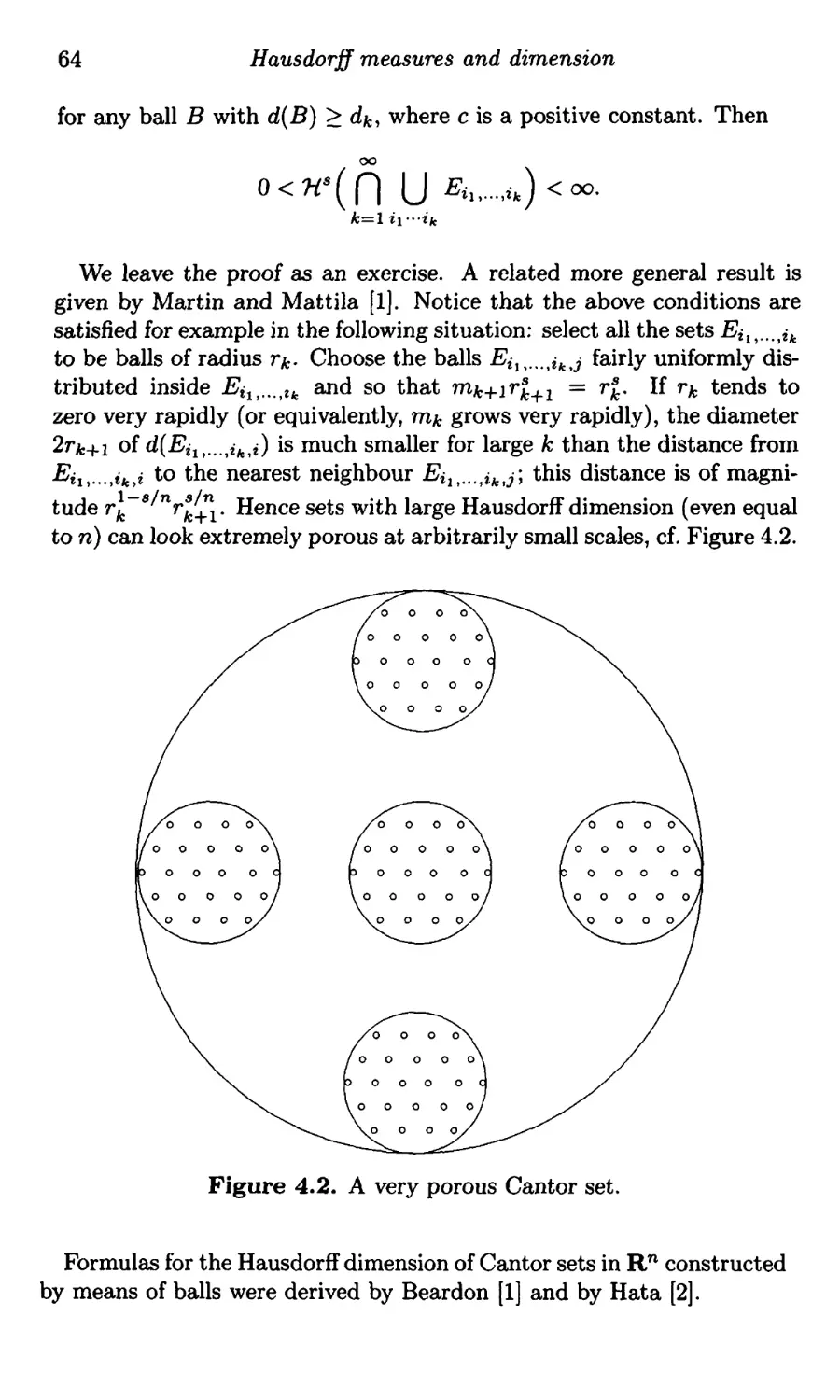
Self-similar and related sets .........................,............ 65
Limit sets of Mobius groups ..................................... 69
..
VII

...
VIII
Contents
Dynamical systems and Julia sets ............................... 71
Harmonic measure ............................................... 72
Exercises ....................................................... 73
5. Other measures and dimensions ............................ 75
Spherical measures .............................................. 75
Net measures ................................................... 76
Minkowski dimensions .......................................... 76
Packing dimensions and measures ............................... 81
Integralgeometric measures ...................................... 86
Exercises ....................................................... 88
6. Density theorems for Hausdorff and packing measures ... 89
Density estimates for Hausdorff measures ........................ 89
A density theorem for spherical measures ........................ 92
Densities of Radon measures .................................... 94
Density theorems for packing measures .......................... 95
Remarks related to densities .................................... 98
Exercises ....................................................... 99
7. Lipschitz maps .............................................. 100
Extension of Lipschitz maps ................................... .100
Differentiability of Lipschitz maps .............................. 100
A Sard- type theorem ........................................... 103
flausdorffrneasures of level sets .................................104
The lower density of Lipschitz images .......................... 105
Ilemarks on Lipschitz nrraps ........ ........ ....................106
Exercises ...................................................... 107
8. Energies, capacities and subsets of finite measure ...... .109
Energies ....................................................... 109
Capacities and Hausdorff measures ............................. 110
F'rostman ' s lemma in R n ....................................... 112
Dimensions of product sets ..................................... 115
VVeighted lIausdorffmeasures ..................................117
Frostman's lemma in compact metric spaces ................... .120
Existence of subsets with finite Hausdorff measure ............. .121
Exercises ...................................................... 124
9. Orthogonal projections .................................... .126
Lipschitz maps and capacities .................................. 126
Orthogonal projections, capacities and Hausdorff dimension .... 127
Self-similar sets with overlap ................................... 134
Brownian motion ............................................... 136
Exercises ...................................................... 138
10. Intersections with planes ................................... 139
Slicing measures with planes .................................... 139

Contents
"
IX
Plane sections, capacities and Hausdorff measures
. . . . . . . . . . . . . . 142
Exercises ...................................................... 145
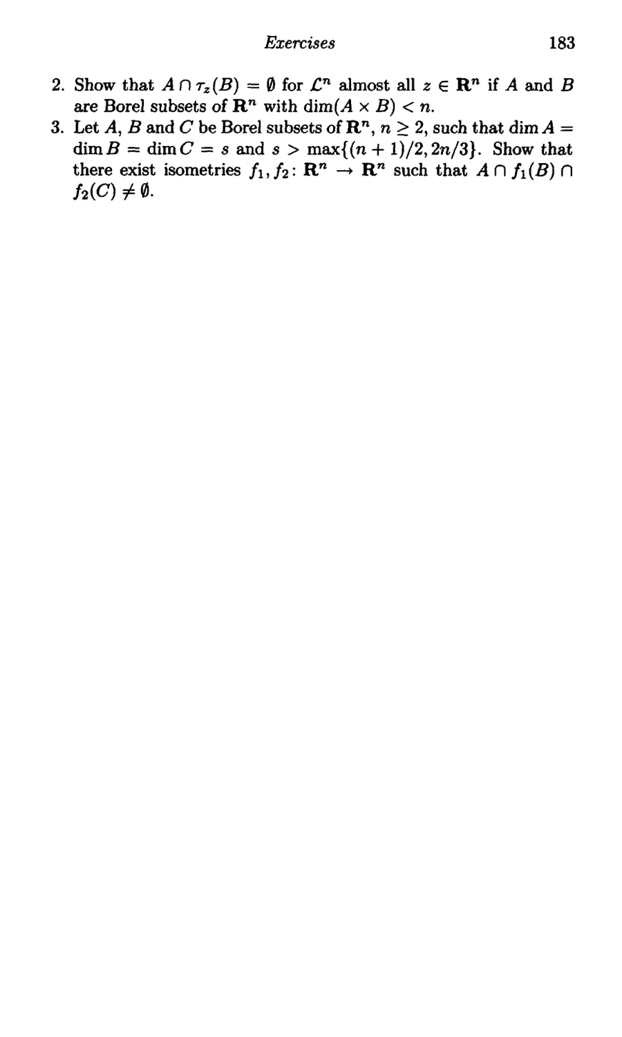
11. Local structure of s-dimensional sets and measures ..... .146
Distribution of measures with finite energy ..................... 146
Conical densities ............................................... 152
Porosity and Hausdorff dimension .............................. 156
Exercises ...................................................... 158
12. The Fourier transform and its applications .............. 159
Basic formulas ................................................. 159
The Fourier transform and energies ............................ 162
Distance sets .................................................. 165
Borel su brings of R ............................................ 166
Fourier dimension and Salem sets ....................."...".... 168
Exercises ...................................................... 169
13. Intersections of general sets ............................... 171
Intersection measures and energies ............................. 1 71
Hausdorff dimension and capacities of intersections ......."""... 177
Examples and remarks ......................................... 180
Exercises ...........................................".......... 182
14. Tangent measures and densities ........................... 184
Definitions and examples .........................."........".". 184
Preliminary results on tangent measures ....................... .186
Densities and tangent measures ................................. 189
s- uniform measures ............................................ 191
Marstrand ' s theorem ......................".."."".".""".."."".. 192
A metric on measures .......................................... 194
Tangent measures to tangent measures are tangent measures ... 196
Proof of Theorem 11.11 ........................................ 198
Remarks .........................."........"....""............. 200
Exercises ...................................................... 200
15. Rectifiable sets and approximate tangent planes ........ 202
Two examples ................................................. 202
m- rectifiable sets ..................."......."".""""".."....".".. 203
Linear approximation properties ............................... 205
Rectifiabili ty and measures in cones ............................ 208
Approximate tangent planes ................................... 212
Remarks on rectifiability ............."....".................... 214
Uniform rectifiability ........................................... 215
Exercises ...................................................... 218
16. Rectifiability, weak linear approximation and tangent
measures .............."....."........"...................... 220
A lemma on projections of purely unrcctifiable sets ............. 220

x
Contents
Weaklinearapproximation,densitiesandprojections...........222Rβctiaabilitymdtangentmeasures............................228
Exercises......................................................230
17.Rectiaabilityanddensities.................................231Structureofm-uniformmeasures...............................231Recusabilityanddensityone..................................240
Preiss'stheorem...............................................241
Rmtiaabilityandpackingmeasures............................247
Rmnarks.......................................................247
Exercises......................................................249
18.Rec创aabilitymdorthogonalprojections.................250Besicovitch-Federerprojectiontheorem........................250
Rmnarbonprojections........................................258Beskovitchsets................................................260
Exercises......................................................264
19.RectiaabilityandanalyticcapacityinthecomplexpIMEe265AnalyticcapacityandreEnow,blesets...........................265Andyticcapacity,RieszcapacityandHausdorfrmeasures.......267Cauchytrans岛rmsofcomplexmeasures........................269Cauchytransformsmdtmgentmeasues.......................273Analyticcapacityandrectiaability.............................275
Variousrern创-ks...............................................276
Exercises......................................................279
20.Rectiaabilityandsingularintegrals.......................281Basicsingularintegrals........................................281
Symmetricmeasures...........................................283
Existenceofprincipalvaluesandtangentmeasures.............284Symmetricmeasureswithdensitybounds......................285Existenceofprincipalvaluesimpliesrectiaability...............288LP.boundedness侃dweak(1,1)inequalities....................289Adualitymethodforweak(1,1)...............................292Asmoothingofsingularintegraloperators.....................295Kolmogorov'sinequality.......................................298
Cotlar'sinequality.............................................299
Aweak(1,1)inequalityforcomplexmeasures..................301Rectiaabilityimpliesexistenceofprincipalvalues...............301
Exercises......................................................304
R启femmes...................................................305
Listofnotation.............................................334
Indexofterminology.......................................337


Acknowledgements
This book grew out of the lecture notes Mattila [12] which were based
on the lectures on geometric measure theory that I gave in Jarandilla de
la Vera in 1984 at a summer school organized by Asociacion Matematica
Espanola and Universidad de Extremadura. I renew my thanks to
Miguel de Guzman and the other organizers of this meeting as well
as to the inspiring audience. The preparation of this book was also
greatly influenced by the course I gave as a visitor of Centre de Recerca
Matematica at Universitat Autonoma de Barcelona in the spring of 1992.
I want to thank the Centre for its hospitality and financial support; in
particular my thanks are due to Joaquim Bruna, Manuel Castellet and
Joan Verdera, and again to the active participants of the lectures. I am
much obliged to Kenneth Falconer, Maarit Jarvenpaa and David Preiss,
who corrected many mistakes and suggested numerous improvements in
the first versions of the manuscript. Several other mathematicians have
made useful comments that have been of great help to me. In particular
I am grateful for this to Guy David, Tero Kilpelainen, Peter Moilers,
Joan Orobitg, Yuval Peres and Stephen Semmes. For skilful typing with
1EX I want to thank Eira Henriksson and Marja-Leena Rantalainen, and
for other assistance Ari Lehtonen. Finally I would like to thank David
Tranah and others from the Cambridge University Press for their help
in the production of the book.
For financial support I am indebted to the Academy of Finland in
different forms and during long periods. Parts of this book were written
during the fall term 1991 at Stanford University and at the Institute
for Advanced Study in Princeton, and during May-June 1992 at Insti-
tut des Hautes Etudes Scientifiques in Bures-sur- Yvette; I acknowledge
with gratitude the financial support and the fruitful atmosphere of these
institutes.
.
Xl

Basic notation
We introduce here the notation for some basic concepts which are not
defined in the text. A more extensive glossary of notation is given at
the end of the book.
Z, the set of integers.
R, the set of real numbers.
R = Ru {-oo,oo}.
C, the set of complex numbers.
z , Re z and 1m z are the complex conjugate, real part and imaginary
part of z E C.
R n, the n-dimensional euclidean space equipped with the inner
product x · y and norm JxJ.
sn-l = {x E Rn : Ixl = I}, the unit sphere.
[a, b], (a, b), (a, b) and (a, b] are the closed, open and half-open
intervals in R with end-points a, b E R .
£n, the Lebesgue measure on R n .
a(n) = £n{x E Rn : fxl < I}, the volume of the unit ball.
A = CI A, the closure of the set A.
8A, the boundary of A.
XA, the characteristic function of A.
A + B = {x + y : x E A, y E B}.
A + a = {x + a : x E A}.
card A, the number points in the set A; possibly 0 or 00.
U A = U AEA A, the union of the set family A.
n A, the intersection of A.
We often use notatioIl like {x : f'(x) > O} to mean the set of those
points x where the derivative f'(x) exists and is positive.
The symbol 0 denotes the end of the proof.
xii

Introd uction
This is a book on geometric measure theory. The main theme is
the study of the geometric structure of general Borel sets and Borel
measures in the euclidean n-space R n . There will be emphasis on "small
irregular" sets having Lebesgue measure zero but being quite different
from smooth curves and surfaces. Examples are Cantor-type sets, non-
rectifiable curves having tangent nowhere, etc., ill S}lort, sets to which
the general descriptive term fractal applies. An abundance of such sets
comes from dynamical systems: Julia-sets for rational functions of one
complex variable, etc. Very general curve- and surface-like objects are
also studied extensively. These are rectifiable sets and measures. They
include smooth curves and surfaces and share many of their geometric
properties when interpreted in a measure-theoretic sense. They form an
optimal class possessing such properties.
Many of the basic ideas developed here originate in the pioneering
work done by Besicovitch [1], [4] and [5J, by Federer [1], by Marstrand
[1] and by Preiss [4]. Besicovitch laid down the foundations of geomet-
ric measure theory by describing to an amazing extent the structure of
the subsets of the plane having finit.e one-dimensional Hausdorff measure
(i.e. length). Federer extended Besicovitch's work to m-dimensional sub-
sets of Rn, m being an integer, and Marstrand analysed general fractals
in the plane whose Hausdorff dimension need not be an integer. Preiss
solved one of the most long-standing fundamental open problems, intro-
ducing and using effectively tangent measures.
Good introductory texts to the mathematical theory of fractals are
the books of Edgar [1] and of Falconer [4], [16]. Closest to this text is
Falconer [4]. The relation between this book and those of Falconer is
roughly that we shall develop the general theory here beyond Falconer's
books but we are not paying much attention to applications, except for
the last two chapters, which Falconer does not deal with. Many of the
topics discussed here are also treated in the extensive book of Federer
[3J, often in a more general form. Only Chapters 2 and 3 of Federer [3J
are relevant to our present subject. Chapters 4 and 5 there are devoted
to currents and their applications to the calculus of variations. This
theory is based on rectifiability but we shall not consider it here. More
recent texts on this extremely active area of geometric measure theory
are L. Simon [1], Hardt and Simon [1] and Giusti [1]. A good survey on
geometric measure theory is given in Federer [4]. The book of Morgan
[1] serves as an excellent introductory text to many basic concepts and
1

2
Introduction
ideas. The books of Evans and Gariepy [1] and Ziemer [1] also deal
with some parts of geometric measure theory, for example area and
coarea theorems, sets of finite perimeter, which are not considered here.
Taylor's obituary on Besicovitch, Taylor [1], is interesting in particular
for the historical development of the theory.
Fractals and fractal measures arise in mathematics in many ways; for
example in number theory via Diophantine approximation, in proba-
bility via Brownian motion and other stochastic processes, in dynam-
ical systems as strange attractors, in complex analysis as limit sets of
Kleinian groups, etc. We shall not pay much attention to these relations;
discussions on them and further references can be found for example in
Barnsley [IJ, Edgar (IJ, Falconer (4], [16], Mandelbrot [11 and Peitgen
and Richter [IJ. Mandelbrot [1] also uses fractals to model many physical
phenomena. Computer simulation of fractal images is widely considered
in Peitgen and Saupe [1] and Barnsley [1]. Tricot [6] works with many
examples and concepts related to curves.
This book splits roughly into three parts. Chapters 1-7 give back-
ground in measure theory and develop the required tools and results,
mainly in terms of Hausdorff measures and dimension. The second part
consists of Chapters 8-14. There sets and measures are considered with-
out dimensional restrictions. Thus this part applies to getting informa-
tion about sets and measures whose dimension need not be an integer.
In the last part, Chapters 15-20, we investigate integral dimensional sets
and measures and the unifying concept there is rectifiability.
I shall now briefly describe the topic of each chapter. In Chapter 1
we set up much of the measure-theoretic terminology and notation to be
used throughout the rest of the book. We shall mainly prove only the
results that cannot be found in standard books of measure theory and
real analysis. In Chapter 2 we prove covering theorems of Vitali and
Besicovitch and use them to obtain a basic differentiation theorem for
measures. In Chapter 3 we introduce and prove some properties of the
natural invariant measures on the spaces of orthogonal transformations
of Rn and of linear and affine m-dimensional subspaces of Rn.
The main theme of Chapter 4 is the introduction of one of our ba-
sic tools, s-dimensional Hausdorff measures 'H,s and Hausdorff dimen-
sion, dim, although we also give a general construction leading to many
other measures as well. We study several examples and briefly consider
self-similar and related sets. In Chapter 5 we discuss other concepts
of dimension and related measures, in particular Minkowski dimension,
packing dimension and packing measures. In Chapter 6 we prove the ba-
sic density estinlates for Hausdorff and packing measures. For instance,

Introduction
3
they say that if s is a positive number and A an 1{,8 measurable subset
of Rn with 1{8(A) < 00, then at 1{8 almost all points x E A,
(1)
2- 8 < limsup(2r)-s1t 8 (AnB(x,r)) < 1,
r!O
where B(x, r) is the closed ball with centre x and radius r.
Chapter 7 gives a brief treatment of Lipschitz maps. For example we
prove Rademacher's theorem on their differentiability almost everywhere
and a simple Sard-type theorem.
In Chapter 8 we introduce some potential-theoretic methods and con-
cepts to study Hausdorff dimension, that is, we use the s-energies
Is(J.t) = !! Ix - yl-S dJ.txdJ.tY
for Radon measures J.t on Rn and the capacities related to them. We
prove Frostman's lemma stating that a Borel set has positive s-dimen-
sional Hausdorff measure if and only if it supports a non-zero Radon
measure J.L such that
(2)
p,(B(x, r» < r 8 for all x E R n and r > o.
Since (2) is closely related to the condition Is(J.t) < 00 this leads to a
definition of the Hausdorff dimension in terms of capacities. In fact,
these relations mean that a large part of this book could be interpreted
as a study of geometric properties of Radon measures J.L on R n satisfying
either (2) or the inequality Is(p,) < 00. We shall also use Howroyd's new
technique in general compact metric spaces to prove Frost man 's lemma
and the theorem on the existence of subsets with positive and finite
Hausdorff measure inside a given set with infinite measure.
Chapter 9 studies how Hausdorff dimension transforms under orthog-
onal projections. The main results, essentially due to Marstrand, say
that a given Borel subset of Rn with Hausdorff dimension s projects
into a set of Hausdorff dimension s on almost all linear m-dimensional
subspaces of Rn provided s < m. In the case s > m, the projections
have generically positive m-dimensional measure. In Chapter 10 we show
that such an s-dimensional set intersects "usually" (n - m) -dimensional
affine subspaces of R n in a set of Hausdorff dimension max{ 0, s - m}.
In both of these chapters we use a potential-theoretic approach. Thus
we prove similar and sharper results for capacities and measures with
finite s-energy.

4
Introduction
The density theorems for Hausdorff measures of Chapter 6, such as
the inequalities (1), give the first information as to how much measure
we can expect to find in small balls. In Chapter 11 we find out more
about how this measure is distributed in narrow cones. For example, if
n - 1 < s < n, a > 0 and A is an rt S measurable subset of R n with
'H,S(A) < 00, then at 11,s almost all points x E A
limsupr- s 1i S (AnB{x,r) nC{a,x») > c(a) > 0,
r!O
where C(a, x) is a cone with vertex x and opening angle Q. Again we
work with general Radon measures and their s-energies.
In Chapter 12 we bring in another effective tool to study Hausdorff
dimension, capacities and energy-integrals; this is the Fourier transform.
We develop some preliminary results and as an application give a simple
proof of Falconer for estimating the Hausdorff dimension of distance sets.
Other applications will be presented in Chapter 13 where we study the
generic Hausdorff dimension of the intersection of two Borel sets A and
B moving in Rn. It turns out that
(3)
dim{A nIB) > dim A + dimB - n
for many euclidean motions f, provided dim B > (n + 1) /2; this assump-
tion may be superfluous. We also give conditions which guarantee that
equality holds in (3).
In Chapter 14 we introduce the tangent measures in the sense of Preiss.
They contain information about the local structure of a given Radon
measure J.l in a similar but often more complicated way as the derivative
of a function tells us about the local behaviour. The tangent measures
of J..t at a point a consist of all non-zero locally finite weak limits of the
sequences of measures
A f--+ ciJ.L(riA + a) where Ti ! 0 and 0 < Ci < 00.
As the first application of tangent measures we prove Marstrand's the-
orem according to which for any non-integral number s there exists no
non-zero Borel measure tt in Rn such that the positive and finite limit
limrlor-sJ..t(B(x,r» would exist for J-L almost all x ERn.
Then we start the last, integral dimensional, part of the book. First,
in Chapter 15 we define m-rectifiable sets as a natural and convenient
generalization of nice m-dimensional surfaces, such as at submanifolds,
Lipschitz graphs, etc. They are sets which except possibly for a set

Introduction
5
of 1(,m measure zero lie on countably many C 1 submanifolds. We give
a characterization of rectifiability in terms of the almost everywhere
existence of approximate tangent planes. In Chapter 16 we continue the
study of the tangential properties in connection with rectifiability in a
more technical manner. This leads to a characterization of rectifiability
using only "weak, rotating" tangent planes; the approximating plane is
allowed to depend on the scale. We also formulate such results in terms
of tangent measures. As side-products we derive information about the
density and projection properties of rectifiable sets.
Chapter 1 7 discusses the theorem of Preiss characterizing rectifiabil-
ity in terms of the existence of densities. The main part of this is the
fol1owing statement: if m is a positive integer and J..L is a Borel mea-
sure on Rn such that the positive and finite limit limr!o r-mJt(B(x, r»)
exists for It almost all x E an, then J.L is m-rectifiable in the sense
that there exist m-dimensional C 1 submanifolds M 1 , M2,. .. such that
JL(Rn \ U  1 M i ) = O. The tangent measures playa fundamental role
in the proof. The complete proof is very complicated and we shall give
only parts of it and derive a weaker result.
Chapter 18 is mainly devoted to the proof of the fundamental theorem
of Besicovitch and Federer characterizing rectifiability with projection
properties.. More precisely, let A be an 1-{,m measurable subset of Rn
with 'Hm(A) < 00. Then A meets every m-dimensional C 1 submanifold
of R n in a zero 'H m measure if and only if 'H m (Pv A) = 0 for almost
all orthogonal projections Pv: Rn  V onto m-dimensionallinear sub-
spaces V of Rn.
The last two chapters involve relations of rectifiability to complex
and harmonic analysis. In Chapter 19 we discuss a classical problem of
complex analysis: what are the null-sets for analytic capacity, or, in other
words, which compact subsets of the complex plane are removable for
bounded analytic functions? We try to explain how this open problem is
related to rectifiability and we prove some partial results. In Chapter 20
we study the behaviour of certain natural singular integrals with respect
to measures. It has turned out that here too there are many connections
to rectifiability. We prove some results concerIliIlg the almost everywhere
existence of principal values and discuss briefly some others, like the
boundedness on £2.
A sufficient prerequisite for reading this book is the knowledge of ba-
sic theory of measure and integratioll. On some occasions we shall use
the Hahn-Banach theorem and once the Krein-Milman theorem, but
they are only needed for certain specific results. In Chapter 12 we shall
take for granted some properties of Fourier transforms and distributions.

6
Introduction
After that they will only be needed in Chapter 13. Chapter 19 assumes
some very basic facts from complex analysis. The complete understand-
ing of the last part of Chapter 20 would require a great deal from the
theory of singular integrals. We shall not treat the theory of Suslin (i.e.
analytic) sets as there are many good sources for that, see e.g. Carleson
[1], Dellacherie [1], Federer [3], Hayman and Kennedy [1] or Rogers [1].
This would not be needed if we were to restrict the formulation of the
results to closed sets, but often generalization to Borel sets seems to re-
quire the theory of Suslin sets. In particular, we shall prove Frostman's
lemma, Theorem 8.8, only for closed sets and many of the results of
Chapters 9-13 depend on it. Most of the results which we state for the
more familiar Borel sets actually hold for Suslin sets.
The list of references is long but there is no attempt at completeness.
In particular concerning the topics which are related to the material of
this book, but are not developed here, the choice of the references has
been to some extent arbitrary. There are many more works on self-
similarity, dynamical systems, etc. which could, and perhaps should,
have been mentioned. However, I hope that the remarks in the text and
the references given open the way to the interested reader to discover
more about the literature.

1. General nteasure theory
In this chapter we shall introduce some general measure-theoretic con-
cepts, terminology, and results which wi}] be needed later on. But we
shall also assume that the reader is familiar with basic measure theory.
Most of the material needed can be found in several standard books
such as Halmos [1], Hewitt and Stromberg II], Munroe [IJ, Royden [1],
Rudin [1], and many others including Federer [3] and Rogers [1]. Many
of the proofs will be omitted. In this chapter we shall also introduce a
great deal of notation and terminology to be used throughout the book.
We shall generally follow the most standardized terminology of measure
theory with one notable exception. Following Federer and Rogers we
shall call measure what is usually called outer measure.
Some basic notation
We shall work in a metric space X with a metric d, although most of
the measure theory presented here goes through in more general settings.
Later on we aha]} however mainly stay in the euclidean n-space R n. Here
are the basic notations used in metric spaces throughout this book.
The closed and open balls with celltre x E X and radius r, 0 < r < 00,
are denoted by
B(x,r) = {y EX: d(x,y) :5 r},
U(x,r) = {y EX: d(x,y) < r}.
In R n we also set
B(r) = B(O, r), U(r) = U(O, r), S(x, r) = 8B(x, r) and S(r) = 8(0, r).
The diameter of a non-empty subset A of X is
d(A) = sup{ d(x, y) : x, YEA}.
We agree d(0) = o. If x E X and A and B are non-empty subsets of
X, the distance from x to A and the distance between A and Bare,
respectively,
d(x, A) = inf{ d(x, y) : YEA},
d(A, B) = inf{ d(x, y) : x E A, Y E B}.
For € > 0 the closed e-neighbourhood of A is
A(e) = {x EX: d(x, A) < £}.
7

8
General measure theory
Measures
A measure for \IS will be a non-negative, monotonic, subadditive set
function vanishing for the empty set.
1.1. Definition. A set function J.l: {A : A c X} --. [0,00] = {t : 0 <
t < oo} is called 8 measure if
(1) J.l(0) = 0,
(2) J.t(A) < Jl(B) whenever A c B C X,
00 00
(3) JL( U Ai) < LJL(A i ) whenever A},A2"" C X.
i= 1 i= 1
Usually in measure theory a measure means a non-negative countably
additive set function defined on some u-algebra of subsets of X, which
need not be the whole power set {A : A c X}. However, considering
measures in the sense of Definition 1.1 is a convenience rather than a
restriction. That is, if v is a count ably additive non-negative set function
on a O'-algebra A of subsets of X, it can be extended to a measure v*
on X (in the sense of Definition 1.1) by
(1.2)
v*(A) = inf{v(B) : A c B E A},
see Exercise 1. On the other hand, a measure Jl gives a countably addi-
tive set function when restricted to the u-algebra of J,t measurable sets.
1.3. Definition. A set A c X is I-L measumble if
p,(E) = p,(E n A) + I-L(E \ A) for all E c X.
We collect the well-known basic properties of measurable sets in the
following theorem.
1.4. Theorem. Let Jl be a measure on X and let M be the family of
all J.t measurable subsets of X .
(1) M is a 17-algebra, that is,
(i) 0 E M and X E M,
(ii) jf A E M, then X \ A E M,
(iii) jf AI, A 2 ,... E M, then U  1 Ai E M.

Measures
9
(2) If JL(A) = 0, then A E M.
(3) If AI, A 2 , · · · E M are pairwise disjoint, then
00 00
Il( U Ai) = LIl(A i ).
i=l i=l
(4) If AI, A 2 ,... E M, then
00
(i) p( U Ai) = i p(A i ) provided Al C A 2 C.. .,
i=l
00
(ii) p( n Ai) = i Il(A i ) provided Al ::> A 2 ::> ... and p(A I ) < 00.
i=l
It is also good to remember that the first statement of (4) holds with-
out the measurability assumption if J.L is regular, that is, for every A c X
there is a it measurable set B c X such that A c Band p,(A) = j.L(B).
Recall that the family of Borel sets in X is the smallest a-algebra
containing the open (or equivalently closed) subsets of X. We shall
often consider measures with some of the following properties.
1.5. Definition. Let p, be a measure on X.
(1) JJ is locally finite if for every x E X there is r > 0 such that
p,(B(x, r)) < 00.
(2) JL is a Borel measure if all Borel sets are J.L measurable.
(3) J.L is Borel regular if it is a Borel measure and if for every A c X
there is a Borel set B c X such that A C B and p,(A) = j.L(B).
(4) J.L is a Radon measure if it is a Borel measure and
(i) JL(K) < 00 for compact sets K eX,
(ii) JL(V) = sup{J.L(K) : K c V is compact} for open sets V C X,
(iii) p(A) = inf{/-l(V) : A c V, V is open} for A c x.
We shall give a few simple examples. Many others will be encountered
later on.
1.6. Examples.
(1) The Lebesgue measure £n on Rn is a Radon measure.

10
General measure theory
(2) The Dirac measure 6a at a point a E X is defined by 6a(A) = 1,
if a E A, 6a{A) = 0, if a  A (that is, 6a(A) = XA(a». It is a
Radon measure on any metric space X.
(3) The counting measure n on X is defined by letting n(A) be the
number of elements in A, possibly 00. It is Borel regular on any
metric space X, but it is a Radon measure only if every compact
subset of X is finite, that is, X is discrete.
In general, Radon measures are always Borel regular as a rather im-
mediate consequence of the definition. The converse is not true as the
above example (3) shows. However, locally finite Borel regular measures
in complete separable metric spaces are Radon measures, see e.g. Jacobs
[1, Theorem V.5.3] or Schwartz [1, Part I,  11.3]. In R n this will be
stated in Corollary 1.11. Clearly in R n the local finiteness means that
compact sets have finite measure.
Borel measures in metric spaces are often called metric (outer) mea-
sures, because the following, Caratheodory's, criterion gives a very con-
venient necessary and sufficient metric condition for the measurability
of Borel sets.
1.7. Theorem. Let JJ be a measure on X. Then JJ is a Borel measure
if and only if
JL(A U B) = Jl(A) + Jl(B) whenever A, B c X with d(A, B) > O.
The proof of the more essential "if" part is given in many text-books,
e.g. Munroe [1], Falconer [4], Federer [3], L. Simon [1]. The easier "only
if" part is left 88 an exercise.
Given a measure p, and a subset A of X we can form a new measure
by restricting p, to A.
1.8. Definition. The restriction oE a measure /-L to a set A eX, p,L A,
is defined by
(pLA)(B) = JJ(A n B) for B c X.
It is clear that p, L A is a measure. Many of the relations between JJ
and J.t L A are easy to derive. For example,
1.9. Theorem.
(1) Every J.L measurable set is also J.L L A measurable.
(2) IE p, is Borel regular and A is I-t measurable with /-L(A) < 00, then
JJ L A is Borel regular.

Measures
11
Proof. The first statement is readily checked from the definitions. Note
that A can be quite arbitrary there. We prove the second part.
Let B be a Borel set with A c Band Jl(A) = IJ,(B). Then JL(B\A) = O.
Given C C X let D be a Borel set with BnC c D and JL(BnC) = p,(D).
Then C c D u (X \ B) = E, say, and
(tt L A)(E) < J.L(B n E) = JL(B n D) < jJ,(D)
= jl(BnC) = JL(AnC) = (ttLA)(C).
Thus (JL L A)(E) = (JL L A)(C), and so JL L A is Borel regular. 0
The following approximation theorem will be extremely useful, see
e.g. Evans and Gariepy [1, Theorem 1.1.4], Federer [3, Theorem 2.2.2]
or L. Simon [1, Theorem 1.3].
1.10. Theorem. Let JL be it Borel regular measure on X, A a J.t mea-
surable set, and e > O.
(1) If JL(A) < 00, there is a closed set C c A such that JL(A \ C) < c.
(2) If there are open sets Vi, \12,. .. such that A c U  1 1ti and
JL{\Ii) < 00 for all i, then there is an open set V such that A c V
and J.L(V \ A) < €.
Note. The result holds for any Borel measure provided A is a Borel set.
In R n it follows immediately that the set C in (1) can be taken to be
compact. This holds of course in any a-compact space X, where every
closed set is a countable union of compact sets.
Proof. (1) Replacing JL by the restriction JLLA we may assume Jj(X) < 00
by Theorem 1.9 (2). We first verify that all Borel sets A have the required
property for all € > 0 by using the definition of the Borel sets. The first
natural attempt would be to show that the family of all A satisfying
(1) for all € > 0 is a a-algebra, but then we would have problems in
showing that it is closed under complementation. Thus we introduce
the seemingly smaller family A of all subsets A of X such that for every
€ > 0 there are a closed set C and an open set V such that C cAe V
and J.L(V \ C) < c. It is now rather straightforward to verify that A is a
u-algebra, which contains the closed sets, and thus also the Borel sets.
Hence (1) is established for Borel sets A.
If A is a Jj measurable set with p,(A) < 00 there is a Borel set B such
that A c Band J.t(A) = Jj(B). Then p,(B\A) = 0 and B\A is contained

12
General measure theory
in a Borel set D with J.t(D) = o. Thus E = B \ D is a Borel set with
E c A and JL(A \ E) = O. Hence knowing (1) for E yields it also for A.
(2) Applying (1) to the sets Vi \ A we find closed sets C i C Vi \ A such
that Jl(Vi \ A \ C i ) < c:/2i for i = 1,2,.... Then A c V = Ui(Vi \ C i ),
which is an open set with Jl(V \ A) < €. 0
1.11. Corollary. A measure J.l on R n is a Radon measure if and only
if it is locally finite and Borel regular.
The proof is left as an exercise.
In what follows we shall mainly work with Borel regular measures or
Radon measures for convenience. But often they could quite easily be
replaced by Borel measures or locally finite Borel measures, for example
with the help of Exercise 1.
We shall often encounter measures J.l which are carried by a proper
subset F of X, that is, Jl(X \ F) = O. It is not hard to see that in
the case where JL is a Borel measure and X is separable, there exists a
unique smallest closed set with this property.
1.12. Definition. If J.L is a Borel measure on a separable metric space
X, the support of Jl, spt J.t, is the smallest closed set F such that
p(X \ F) = o.
In other words,
spt P, = X \ U {V : V open, p,(V) = O}
= X \ {x: 3r > 0 such that Il(B(x,r» = O}.
1.13. Examples. (1) Let f be a non-negative continuous function on
R n. Define a measure /-L f by
p,j(A) = 1 f d£n
for £,n measurable sets A. Then the support of J.lf agrees with that of f:
spt J.L f = spt f = CI {x : f ( x) =F O},
where CI refers to closure.

Integrals
13
(2) Let Q = {ql, Q2, . . . } be an enumeration of the rational numbers,
and
00
J-l = L 2- i h q ;,
i=l
where 6 qi is the Dirac meastlre at qi as in 1.6 (2). Then tt is a finite
Radon measure on R with spt it = R. Nevertheless, J.l is carried by the
countable set Q in the sense that J.t(R \ Q) = O.
Integrals
The integral
L f dJ-l = L f(x) dJ-lx
with respect to a measure J.l over a set A of a function f is defined in the
usual way, as well as the J.l measurability and integrability of f. When
the domain of the integration A is the whole space X, we often omit it
using the notation
J f dJ-l = L f dJ-l.
In R n we abbreviate the Lebesgue integral
L f(x) dx = L f(x) d£n x .
The integral J f dJ.t is defined for any non-negative J.l measurable func-
tion on X. Even when f: X ---+ fO,oo] is not JL measurable we can define
the lower and upper integrals by
1 f dJ-l = sp J 'P dJ-l and J* f dJ-l = if J VJ dJ-l,
where c.p and 1/J run through the J.l measurable functions X -+ [0, 00] such
that <p < f < 1/J.
The Jl integrability of f: X  R (in the last two chapters of f: X ---+
C) means that f is J.L measurable and J IfJ dJ.L < 00. As usual, for
1 < p < 00 the space of J.L measurable functions f: X -+ R (or C) with
J II,P dp < 00 is denoted by LP(/.l), and LOO(tt) is the space of functions
which are essentially bounded with respect to It.
A function f: A ---+ R is a Borel function if A is a Borel set and the sets
{x E A : I(x) < c} are Borel sets for all c E R. A mapping f: X ---+ y
between metric spaces X and Y is a Borel mapping if f-l(U) is a Borel
set for every open set U C Y.
We shall mention here only a few of the well-known properties of the
integral. The following form of Fubini's theorem will be frequently used.

14
General measure theory
1.14. Theorem. Suppose that X and Y are separable metric spaces,
and JJ and v are locally finite Borel measures on X and Y, respectively.
If f is a non-negative Borel function on X x Y, then
II f(x, y) dp.x dvy = II f(x, y) dvy dp.x.
In particular, when f is the characteristic function of a Borel set A,
I p.({x: (x,y) E A}) dvy = I v({y: (x,y) E A}) dp.x.
There are many more general forms of Fubini's theorem, see e.g. He-
witt and Stromberg [1], Evans and Gariepy [1, 91.4], Federer [3,  2.6] or
Jacobs [1, Chapter VI]. To formulate an extension, define the product
measure JL x II by
00
(p. X v)( C) = inf L p.( Ai) v( B i )
i=l
where the infimum is taken over all sequences AI, A 2 , · .. of /-l measurable
sets and B 1, B 2 , . .. of v measurable sets such that
00
C c U Ai X B i .
i=l
Here 0 · 00 = 00 · 0 = o. It is easy to see that J.l x v is a measure over
X x Y. Moreover, if both It and 1I are either Borel, Borel regular, or
Radon measures, /.l x II has the same property. The statement of Theorem
1.14 is valid for all JL x II measurable functions f which are non-negative
or IL x II integrable (i.e. J fff d(tt x v) < (0), and the iterated integrals
agree with the IL x v integral:
I fd(p. x v) = II f(x,y)dp,xdvy.
The assumption that X and Yare separable, which of course implies
that X x Y is separable, guarantees that the Borel sets and functions
are p, x 1/ measurable, see e..g. Hewitt and Stromberg [1, Exercise 21.19].
As an application of Fubini's theorem we record the following useful
formula.

Image measures
15
1.15. Theorem. Let J1, be a Borel measure and f a non-negative Borel
function on a separable metric space X. Then
f f dp, = 1 00 p,( {x EX: f(x) > t}) dt.
Proof. Let A = {(x, t) : f(x) > t}. Then
1 00 I-£({X EX: I(x) > t}) dt = 1 00 1-£( {x : (x, t) E A}) dt
= f .c 1 ({tE [0,(0): (x,t)EA})dJLx= f .c 1 ([0,f(x)])dJLx
= ! f(x) dp,x.
o
Another way to look at the Radon measures and integrals with respect
to them is to consider them as linear functionals on Co(X), the space of
compactly supported continuous real-valued functions on X. That is, if
p, is a Radon measure on X, we can associate to it the linear functional
L: Co (X) -+ R, Lf = ! f dJL.
This is obviously positive in the sense that
Lf > 0 for f > o.
In the case where X is locally compact the converse also holds, see e.g.
Rudin [1, 2.14].
1.16. Riesz representation theorem. Let X be a locally compact
metric space and L: Co(X) --+ R a positive linear functional. Then
there is a unique Radon measure /.L such that
LI = ! I dJL for f E Co(X).
Image measures
We can map measures from one metric space X to another, Y.

16
General measure theory
1.17. Definition. The image of a measure tL under a mapping f: X -+
Y is defined by
f{L(A) = J1(f-l A) for A c 
It is apparent that f#p is a measure on Y. It is also immediate that
A is f#J.L measurable whenever /-1 (A) is J1 measurable. Hence if IJ, is
a Borel measure and f a Borel function, ftt is a Borel measure. The
following simple criterion on the Radonness of futL will suffice for us. For
more general results, see e.g. Federer [3, 2.2.17] or Schwartz [1, Part I,
 1.5] .
1.18. Theorem. Let X and Y be separable metric spaces. If f: X -+
Y is continuous and {L is a Radon measure on X with compact support,
then fuJ.L is a Radon measure. Moreover, spt fuJ1 = f(spt J1).
Proof Replacing X by the subspace spt J..L we may assume X is compact.
Statement (i) of Definition 1.5(4) is trivial, as It, and hence also flJ.L, are
finite measures. We leave (ii) as an exercise and prove only (iii).
Let A c Y and € > O. Since {L is a Radon measure there is an
open set U C X such that /-1 A c U and JJ(U) < It(f- 1 A) + €. Set
V = Y \ f(X \ U). Then V is open, as X is compact, A C V and
f#J.L(V) = j,t(f-l (Y \ f (X \ U)))
= 1L(X \ f-l(f(X \ U))) ::; j,t(U)
< J-l(f-l A) + c = f#1L(A) + c.
This yields (iii). We leave the last statement on supports also as an
exercise. 0
The following theorem can be proven via a rather straightforward
approximation by simple functions. It can also be easily deduced from
Theorem 1.15.
1.19. Theorem. Suppose f: X --+ Y is a Borel mapping, J.L is a Borel
measure on X, and 9 is a nOll-negative Borel function on Y. Then
1 9 dfdP, = 1 (g 0 f) dp,.
When Y is locally compact, all this could also be done in the reverse
order: letting
£g = l(g 0 f)dp, for 9 E Co(Y)

Image measures
17
we obtain a linear functional on Co(Y) which by the Riesz representation
theorem 1.16 corresponds to a Radon measure fUIJ.
It is clear that pulling back measures is not nearly ag natural as push-
ing them forward: the formula J.t(A) = v(f A) does not usually define a
Borel measure even for very nice measures lJ if f fails to be injective.
Still it is often possible to find such pull-backs abstractly. The following
proof can be found in Schwartz [1, Part I,  1.5] and in Fuglede [1].
1.20. Theorem. Let X and Y be compact metric spaces and f: X -+
Y a continuous surjection. For any Radon measure v on Y there exists
a Radon measure Il on X such that fJ.t = v.
Proof. We define a functional p: Co(X)  R by
p(cp) = v(Y)max{cp(x) : X EX}.
Clearly p is a seminorm, that is, p(cp + 1/;) < p(<p) + p(1j;) and p(Acp) =
'\p(cp) for cp,1/J E Co(X) and 0 < ,\ < 00. Since f is surjective we can
define a linear form ,\ on the vector subspace {1j; 0 f : 1/J E Co (Y)} by
A(1/J 0 f) = J 1/Jdv.
It satisfies
>-(1/J 0 f) < v(Y)max{1I'(Y) : y E Y}
= v(Y) max{('l/J 0 f)(x) : X E X} = p(1/J 0 f).
By the Hahn-Banach theorem, see e.g. Rudin [2, Theorem 3.2J, >- ex-
tends to a linear form Jl on Co(X) satisfying
p,(cp) < p(<p) for <p E Co(X).
In particular, p,(cp) < 0 if <p < 0, whence J.L(<p) = -J.l( -cp) > 0, if cp > O.
By the Riesz representation theorem 1.16 J..t can be identified with a
Radon measure. As J.L extends '\, we have, by Theorem 1.19,
J 1/1 dv = f (1/1 0 J) dJ.t = / 1/1 dhJ.t for 1/J E Co (Y).
Thus fnll = v by the uniqueness part of the Riesz representation theorem
1.16. 0

18
General measure theory
Weak convergence
Next we consider a convergence of measures.
1.21. Definition. Let J-L, P,l, P,2,. .. be Radon measures on a metric
space X. We say that the sequence (ILi) converges weakly to p"
w
J-ti  J.L,
jf
.lim J cpdp,i = J VJdp, for all <P E Co(X).
IOO
1.22. Examples.
(1) In R, 6 i  0 as i  00.
(2) Let
1 k
/l-k = k L hilk'
i=l
Then J.Lk  £,1 L [0, 1].
The weak convergence is useful because a very general compactness
theorem holds. We prove it only for Rn.
1.23. Theorem. If P,1,P,2,... are Radon measures on Rn with
sup{p,i(K) : i = 1,2, . . . } < 00
for all compact sets KeRn, then there is a weakly convergent sub-
sequence of (P,i).
Proof The space Co(Rn) is separable under the norm
1I<p1I = max{IVJ(x)l: x ERn},
whence it has a countable dense subset D. For example, choosing func-
tions CPi E Co (Rn), i = 1,2,..., with <Pi = 1 on B(i), one can by the
Weierstrass approximation theorem take for D the set of all products
<PiP where i = 1,2,... and P runs through polynomials with rational
coefficients. For each VJ E D the bounded sequence (J <pdJ-li) of real

Approximate identities
19
numbers has a convergent sub-sequence. Using the diagonal method we
can thus extract a sub-sequence (P,ik) such that the limit
Lcp = lim f t.p dP,ik
k-+oo
exists and is finite for all <p ED. The denseness of D then implies that
this actually holds for all cp E Co (R n ) , and the Riesz representation
theorem 1.16 gives the limit measure. 0
As Example 1.22 shows JLi  J.L need not imply that JLi(A)  JL(A)
even when A = Rn, see also Exercise 9. However, the following semi-
continuity properties hold.
1.24. Theorem. Let J.ll, J.l2,. .. be Radon measures on a locally com-
pact metric space. If Pi  It, K c X js compact and G c X is open,
then
(1)
(2)
p,( K) > lim sup /-li (K),
ioo
p,( G) < li inf Pi ( G).
tOO
Proof. (1) Let E > O. By property (4) (iii) of Definition 1.5 there is an
open set V such that K c V and p(V) < p,(K) + £. By Urysohn's
lemma, see e.g. Rudin [1, 2.12J, there is <p E Co (X) such that 0 :5 <p < 1,
<p = 1 on K and spt<p C V. Thus
p.(K) > p.(V) - € > f cpdp. - €
= .lim j <PdJ,ti - C > limsuPJ.ti(K) - £,
 --t- 00 i --+ 00
and (1) follows.
(2) is proven similarly through approximation of G with compact sets
from inside. 0
Approximate identities
We shall now show that arbitrary Radon measures in R n can be ap-
proximated weakly by smooth functions, that is, by measures of the form
A .....-+ fA gd£n where g E coo(Rn), the space of infinitely differentiable
real-valued functions on Rn. First we define convolutions.

20
General measure theory
1.25. Definition. Let f and 9 be real-valued functions on R n and Jl,
a Radon measure on Rn. The convolutions f * g of f 8Ild g, and f * It
of f and /-l, are defined by
f * g(x) = J f(x - y) g(y) dy,
f * p,(x) = J f(x - y) dp,y,
provided the integral exists.
We now consider an approximate identity {1PE}e>O. By this we mean
that each 1/Je is a non-negative continuous function on R n such that
spt 11'£ C B(c) and J 11'£ d£n = 1.
Any continuous function 1jJ: Rn -+ [0,00) with spt1/; C B(l) and
J 'l/J d£,n = 1 obviously gives such an approximate identity by
1fJe(x) = e- n 1fJ(x/c).
In particular we may take
'l/Je(x) = c(e)e- 1 /(e: 2 -lx I2 ) for 'xl < e,
1/Je(x) = 0 for Ixl > c,
where c(c) is determined by J 1/Je d£,n = 1, to get an approximate identity
consisting of Coo functions. It is shown in many text-books that for
any such approximate identity consisting of Coo functions the functions
1/JE * f, where f E LP(Rn), are also Coo and they converge to f in LP.
We now study 1/Je * /-l in the same spirit.
1.26. Theorem. Let {1/Je}e>O be an approximate identity and Jj a
Radon measure on Rn. Then the functions 1P€ * J.L are infinitely differ-
entiable and they converge weakly to Jj as c ! 0, that is,
lim J <p( We * J.L) d£,n = J cp dJ.L
EJO
for all <p E Co(Rn). If JL(Rn) < 00, this holds for all uniformly continu-
ous bounded functions <p: Rn -+ R.
Proof. By studying the difference quotients and using induction one can
verify in a straightforward manner that for all i j E {I".., n}, j =
1,...,k,
ail · · · 8ik (1Pe * J.l) = (Oil · · · 8ik 1/1€) * p"

Approximate identities
21
where Oi means the partial derivative with respect to the i-th coordinate.
It follows that 1/Je * J.-l has partial derivatives of all orders.
To prove the second statement we use Fubini's theorem, change of
variable and the facts that spt 1/Je c B(E) and J 1/Je d£n = 1 to compute
J <pC 1/JE * JL) d/:,n - J <p dp.
= / 11'( x) J 1/Je (x - y) dJLY dx - / <p(y) J 1/Je (x) dx dp,y
= J [I <p(x) 1/Je(x - y) dx - 1 <p(y) 1/JE(X) dX] dp.y
= j r r [<p(x + y) - <P(y)]1/JE(X) dxdp.y.
J B(E)
Since <P is uniformly continuous with compact support and J tPe d£,n = 1,
this goes to zero as E ! o. The last statement follows also by the above
proof. 0
We finish this chapter with some remarks on lower semicontinuous
functions. We shall need this concept only for non-negative functions.
One way to define them is to say that a non-negative function 9 on Rn is
lower semicontinuous if there are non-negative functions 'Pi E Co(Rn),
i = 1,2, . . . , such that C{)l < <P2 < · .. and 9 = limi-+oo <Pi. An equivalent
definition is that the sets {x : g(x) > c} are open for all c E R. Examples
are characteristic functions of open sets and x 1-+ Jx'p, pER (with value
00 at 0 if p < 0).
The following simple lemma will be needed in Chapter 12.
1.27. Lemma. Let {?Pe }E:>o be an approximate identity, It a Radon
measure on Rn, and 9 a non-negative lower semicontinuous function on
Rn. Then
/ (9 * It) dJl < lim inf 1 [(g * "p€) * Jl] dJ.-l.
£10
Proof. Approximating J-L by the restrictions J.t L B(k), k = 1,2,..., we
may assume that Jl has compact support. For t.p E Co(Rn), cp * 1/Je --+ cp
uniformly as € 1 0, whence
I ( C{) * J.t) dp, = lim J [( <p * 1/;£) * J.L] dJ.t.
€o
Applying this, the definition of lower semicontinuity and the monotone
convergence theorem, we get the required inequality. 0

22
General measure theory
Exercises.
1. Show that 11* defined by (1.2) is a measure agreeing with v on A,
and, moreover, that 11* is Borel regular if A is contained in the
family of Borel sets.
2. Show that if J..L is a measure, A c B, B is p, measurable and
J-t(A) = p,(B) < 00, then J.t(AnC) = J.t(BnC) for all J.L measurable
sets C.
3. Verify the statements in Examples 1.6 (2) and (3) concerning
Dirac and counting measures. What are the measurable sets with
respect to them?
4. Prove that a Borel measure J.L satisfies the condition of Theorem
1.7.
5. Prove Corollary 1.11.
6. Show that lup, in Theorem 1.18 satisfies condition (ii) of Definition
1.5 (4), and that spt fup, = f(spt Jj).
7. Let J.L be a finite Borel measure on Rn with compact support.
Show that there exists b ERn, the centre of mass of J.t, such that
b.v= (/ X.Vdp,x)/ JL(Rn) forvER n .
8. Let {1/Je:}E>O be an approximate identity in Rn and cp E Co(Rn).
Show that 1/JE * <P -. cp uniformly 88 € ! o.
9. Let tLl,tL2,... and J.L be Radon measures on Rn with J-ti  Jl.
Show that if A is a bounded subset of an and J.L(8A) == 0, then
limi-.oo i(A) = p(A).

2. Covering and differentiation
In the first part of this chapter we prove some covering theorems which
are among the most fundamental tools of measure theory. They are used
to create connections between local and global properties of measures,
and they also reflect the geometry of the space. Covering theorems and
their applications have been studied much more extensively in Federer
[3], Guzman [1], and Hayes and Pane [1]. The presentations of Evans
and Gariepy [1], Giusti [1], L. Simon [1] and Ziemer {I] are rather close
to ours.
We prove two types of covering theorems. The difference between
them is that the first ones apply to a larger class of coverings and a
narrower class of measures whereas in the second type the coverings are
more restricted but the measures can be very general; for example all
Radon measures on Rn are included. In both cases we first prove a
geometric result on collections of balls in Rn and then apply it to get a
Vitali-type covering theorem for measures.
At the end of this chapter we apply these covering theorems to prove
some basic differentiation theorems for measures.
A 5r-covering theorem
For 0 < t < 00, x E Rn, 0 < r < 00, we shall use the notation
tB = B(x, tr) when B = B(x, r).
In a general metric space the centre and radius of a ball need not be
unique and for t = 5 we use the definition
5B = U {B' : B' is a closed ball with B' n B ::/= 0 and d( B') < 2d( B)} .
Then d(5B) < 5d(B). The special value t = 5 appears in covering
theorems in a natural way.
A metric space X is called boundedly compact if all bounded closed
subsets of X are compact. The following theorem holds more gener-
ally, for example in separable metric spaces. A similar proof with some
technical complications works in that case.
23

24
Covering and differentiation
2.1. Theorem. Let X be a boundedly compact metric space and B a
family of closed balls in X such that
sup {deB) : B E B} < 00.
Then there is a finite or countable sequence B i E B of disjoint balls such
that
U B C U 5B i .
BeB i
Proof We simplify slightly by assuming that B is of the form
B = {B(x,r(x)) : x E A},
where A is a bounded subset of X. We comment on the modification
required for the general case at the end of the proof. Let
M=sup{r(x):xEA} and
Al = {x E A : 3M/4 < r(x) < M}.
Choose an arbitrary Xl E Al and then inductively
k
Xk+1 E Al \ U B(Xi! 3r(Xi))
i=l
(1)
as long as Al \U  1 B(Xi, 3r(Xi)) "# 0. The balls B(Xi, r(xi)) thus chosen
are obviously disjoint in view of the definition of Al and lie in a compact
subset of X. We can only have finitely many of them, say k 1 , since we
cannot pack infinitely many disjoint balls of radius 3M /4 into a compact
subset of X. Thus we have
kl
Al C U B(Xi! 3r(Xi))'
i=l
As r(x) < 2r(xi) for x EAt, i = 1,...,k 1 , this gives
k]
U B(x! rex)) c U B(Xi! 5r(xi))'
xeA 1 i=l
Let
A 2 = {x E A: ()2M < rex) < 1 M },
k 1
A = {x E A 2 : B(x, rex)) n U B(Xi! r(xi)) = 0}.
i=l

A 5r-covering theorem
25
If x E A 2 \A, there is i E {I, . . . , kl} such that B(x, r(x) )nB(Xi, r(xi» 
0, whence
d(x, Xi) < r(x) + r(xi)  3r(xi).
This shows
(2)
kl
A2 \ A c U B(Xi' 3r(xi»'
i=l
Choose Xkl +1 E A 2 arbitrarily and then inductively
k
Xk+1 E A \ U B(xi,3r(xi»'
i=k 1 +1
As above there is k2 such that the balls B(Xi) r(xi)), i = 1,.. . , k 2 , are
disjoint and
k2
A c U B(Xil 3r (Xi»'
i=kl +1
Combining this with (2) we get as before
k2
U B(x, r(x» C U B(Xil 5r(xi»'
xEA2 i=l
Proceeding in this manner we find the required balls.
We made two restrictions on the family B. First we assumed that for
each x E A there is only one ball B(x, r(x)). We can reduce to this
special case by selecting for each centre x a ball B (x, r (x )) E B such
that r(x) > f: sup{r : B(x, r) E B} and by observing that in (1) and
later the number 3 could be replaced by 8/3. Then we can use the above
proof to get the required covering from these balls B(x, r(x».
Secondly we assumed that the centres lie in a bounded set. To avoid
this the proof can be modified by choosing the new points Xi not too far
from a fixed point a EX; for example if x and y were possible selections
and d(y, a) > 2d( x, a) we would make a rule that we cannot pick y. 0
Remark. Using the Hausdorff maximality principle one can give a shorter
proof and obtain a much more general result; for example families of
balls can be replaced by many other families of sets, cf. Federer [3,
2.8.4-6] .

26
Covering and differentiation
Vitali's covering theorem for the Lebesgue measure
We can now easily derive a Vitali-type covering theorem for the
Lebesgue measure £,n.
2.2. Theorem. Let A c an and suppose that B is a family of closed
balls in Rn such that every point of A is contained in an arbitrarily
small ball belonging to B, that is,
(1)
inf {d(B) : x E B E B} = 0 for x E A.
Then there are disjoint balls Bi E 8 such that
£n( A \ l)Bi) = O.

Moreover, given € > 0 the balls B i can be chosen so that
L £n(Bi) < £n(A) + c.
i
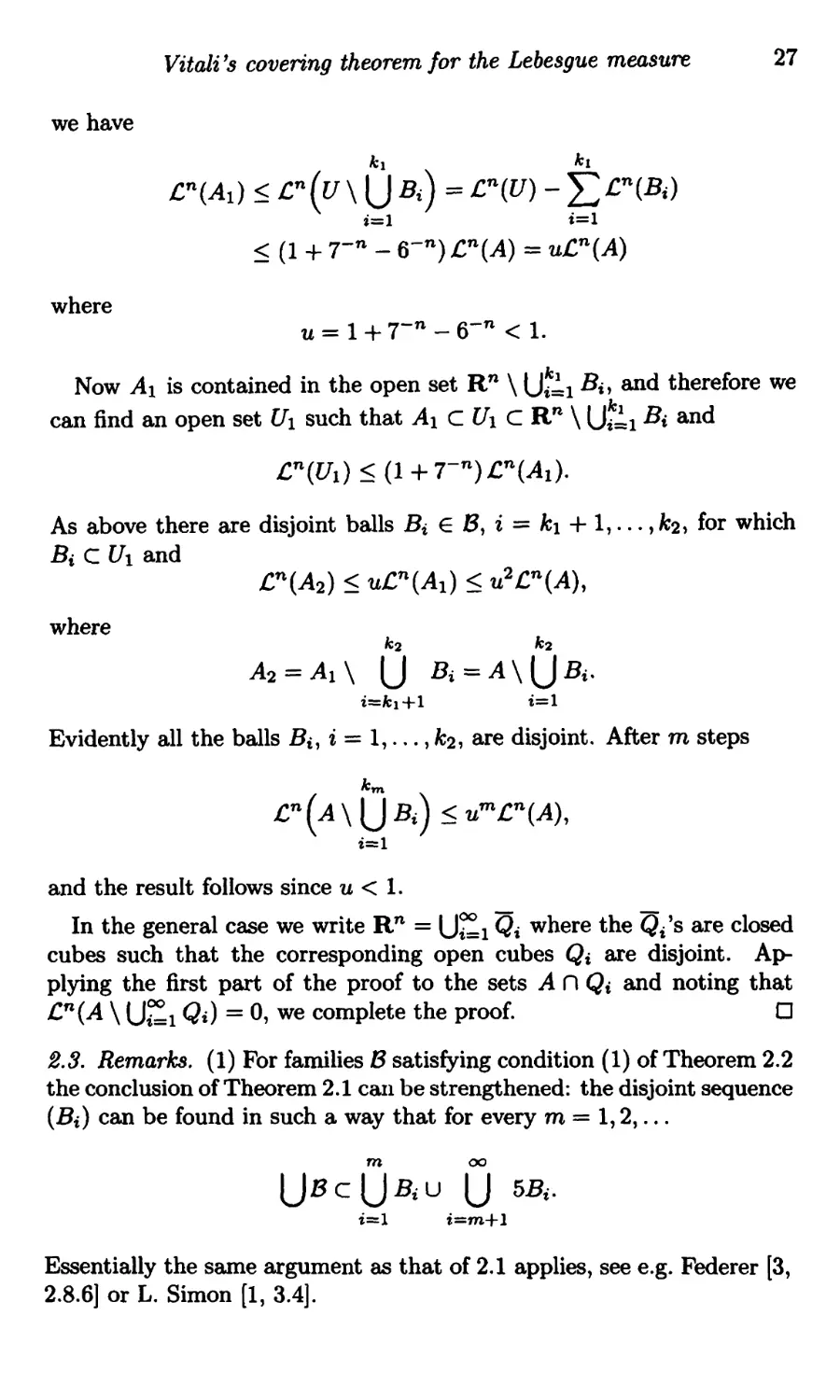
Proof The last statement will be clear from the proof. Assume first
that A is bounded. Choose an open set U such that A c U and
£,n(u) < (1 + 7- n ) £,n(A).
Applying Theorem 2.1 to the collection of those balls of 8 which are
contained in U, we find disjoint balls B i = B(Xi, Ti) E B such that
B i C U and
A c U B(Xi, 5ri)'

Then
5- n £n(A) < 5- n l:.c n (B(Xi, 5r i» = L£n(B i ),
i i
and so there is k 1 , such that
k 1
6- n £n(A) < L£n(B i ).
i=l
Letting
k 1
Al = A \ UBi,
i=l

Vitali's covering theorem for the Lebesgue measure 27
we have
k 1 kl
.en (Ad < .en ( u \ U B i ) = .en(U) - L .en (B i )
i=l i=l
< (1 + 7- n - 6- n ) £n(A) = u.cn(A)
where
u = 1 + 7- n - 6- n < 1.
Now Al is contained in the open set R n \ U :l l Bi! and therefore we
can find an open set U l such that Al C U l eRn \ U :': l B i and
£,n(u 1 ) < (1 + 7- n ) .en (AI).
As above there are disjoint balls B i E B, i = k 1 + 1, · · . , k2, for which
B i C U 1 and
£n(A2) < u.cn(A 1 ) < u 2 £n(A),
where
k2 k2
A 2 = Al \ U B i = A \ UBi.
i=kl +1 i=1
Evidently all the balls B i , i = 1, . . . , k 2 , are disjoint. After m steps
ktn
.en ( A \ UBi) < urn .en (A),
i=1
and the result follows since u < 1.
00 - -
In the general case we write R n = Ui=l Qi where the Qi'S are closed
cubes such that the corresponding open cubes Qi are disjoint. Ap-
plying the first part of the proof to the sets A n Qi and noting that
.c"(A \ U  1 Qi) = 0, we complete the proof. 0
2.3. Remarks. (1) For families B satisfying condition (1) of Theorem 2.2
the conclusion of Theorem 2.1 call be strengthened: the disjoint sequence
(B i ) can be found in such a way that for every m = 1,2, .. .
m 00
UBC UBiU U 5Bi.
i=l i=m+l
Essentially the same argument as that of 2.1 applies, see e.g. Federer [3,
2.8.6] or L. Simon [1, 3.4].

28
Covering and differentiation
(2) All that we really used of the Lebesgue measure in the proof of
Theorem 2.2 was the equality (,n(B(x,5r)) = 5 n .c n (B(x, r)), in fact
only the inequality " < ". It is rather straightforward to modify the
above proof to see that the theorem remaiI1S valid if {,n is replaced by
any Radon measure J..t on R n such that for some r, 1 < r < 00,
limsup {Jt(B(y, rr»/ JL(B(y, r») : x E B{y, r)} < 00
r!O
for J.L almost all x ERn.
Moreover, the balls can be replaced by more general families of closed
sets and Rn by more general spaces, see Federer [3, 2.8] for example.
However, the above theorem is not valid even for all very nice Radon
measures on R n, as the followiIlg example shows.
2.4. Example. Let J..t be the Radon measure on R 2 defined by
Jl{A) = (,l({X E R: (x,O) E A}),
that is, J.l is the length measure on the x-axis. The family
B = {B((x,y),y): x E R,O < y < oo}
covers A = {(x,O) : x E R} in the sense of Theorem 2.2 but for any
countable subcollection HI, B 2 , . .. we have
00
JL(An UBi) = O.
i=l
Here A touches only the boundaries of the balls of B. By a slight
modification we could find a family B such that each point of A is an
interior point of arbitrarily small balls of B and yet the conclusion of
Theorem 2.2 fails. However, if we should require that each point of A
is the centre (in fact, not too far from the centre would be enough) of
arbitrarily sIIlall balls of B, we would get the conclusion of Theorem 2.2.
Next we shall develop a covering theorem of this type.
Besicovitch's covering theorem
Again we shall first prove a theorem on families of balls in R n. This is
called Besicovitch's covering theorem, which originates from Besicovitch
[6] and [7]. More general covering theory was developed simultaneously

Besicovitch '8 covering theorem
29
by Morse [1]. For some recent developments concerning the best con-
stants in the Besicovitch covering theorem, see Loeb [1], J. M. Sullivan [1]
and Fiiredi and Loeb [1].
We shall begin with a simple lemma from plane geometry. Instead
of the following elementary geometric considerations one can also easily
deduce it from the cosine formula for the angle of a triangle in terms of
the side-lengths.
2.5. Lemma. Suppose that a, b E R2, 0 < JaJ < Ja - bJ and 0 < JbJ <
Ja - bl. Then the angle between the vectors a and b is at least 60 0 , that
.
1S,
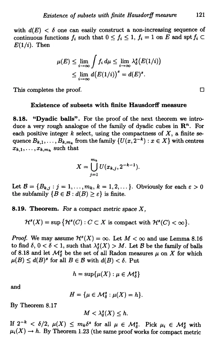
I alia' - bllbll > 1.
Proof We have a  B(b, rbf) and b rt B(a, far). Let L be the mid-normal
to the segment [0, aJ with the end-points 0 and a, and let H be the closed
half-plane with boundary L such that 0 = 0 E H. Let T be the triangle
OAB as in Figure 2.1.
Then b E H \ T, which yields that the angle between a and b is at
least 60 0 . 0
2.6. Lemma. There is a positive integer N(n) depending only on n
with the following property. Suppose there exist k points a}, . . . , ak in
an and k positive numbers Tl, . . . , Tk such that
k
airf.B(aJrj) Eorj"fi, and nB(ai,rdi-0.
i==l
Then k < N(n).
Proof. We may assume ai "f 0 for all i = 1,. . . , k and
k
o E n B(ai, ri)'
i=l
Then
lai I < Ti < lai - aj I for i "f j.
Applying Lemma 2.5 with a = ai and b = aj for i "f j in the two-
dimensional plane containing 0, at and aj, we obtain
(1) I adlail- aj/lajll > 1 fori"f j.
Since the unit sphere sn-l is compact there is an integer N(n) with the
following property: if Yl, · · . , Yk E sn-l with IYi - Yj I > 1 for i "f j, then
k < N(n). B:y (1), N(n) is what we want. 0

30
Covering and differentiation
o
b B
H
L
T
I a I
"2
a
T
L
A
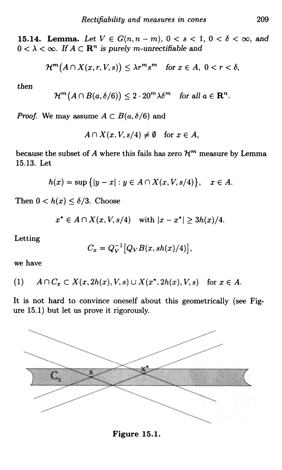
Figure 2.1.
2.7. Besicovitch's covering theorem. There are integers P(n) and
Q(n) depending only on n with the following properties. Let A be a
bounded subset ofRn, and let B be a family of closed balls such that
each point of A is the centre of some ball of B.
(1) There is a finite or countable collection of balls B i E B such that
they cover A and every point ofRn belongs to at most P(n) balls
B i , that is,
XA < L XB i < P(n).
i
(2) There are families 8 1 , . . . ,8 Q (n) c B covering A such that each
B i is disjoint, that is,
Q(n)
A c U UBi
i=l

Besicovitch'8 covering theorem
31
and
B n B' = 0 for B, B' E B i with B =1= B ' .
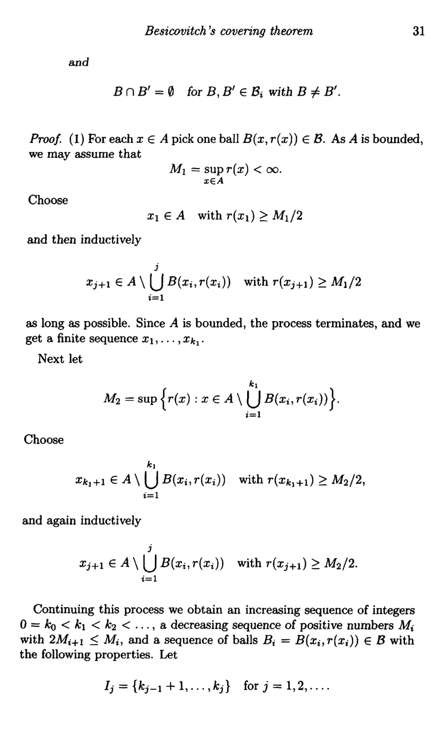
Proof (1) For each x E A pick one ball B(x, r(x)) E 8. As A is bounded,
we may assume that
M 1 = sup r(x) < 00.
xEA
Choose
Xl E A with r(x}) > M 1 /2
and then inductively
J
Xj+l E A \ U B(Xi, r(xd) with r(xj+d > Md2
i=l
as long as possible. Since A is bounded, the process terminates, and we
get a finite sequence Xl, · · · , Xk 1 .
Next let
kl
M2 = sup {rex) : x E A \ U B(Xi, r(Xi))}'
i=l
Choose
k]
Xk 1 +1 E A \ U B(xi,r(xi)) with r(xkl+d > M2/2,
i=l
and again inductively
J
Xj+! E A \ U B(Xi, r(xi)) with r(xj+!) > M2/2.
i=l
Continuing this process we obtain an increasing sequence of integers
o = ko < k 1 < k 2 < · · · , a decreasing sequence of positive numbers M i
with 2Mi+l < M i , and a sequence of balls B i = B(Xi, r(xi» E B with
the following properties. Let
Ij = {k j - 1 + 1,... ,k j } for j = 1,2,....

32
Covering and differentiation
Then
(3)
M j /2 < r{Xi) < M j for i E Ij,
j
Xj+l E A \ U B i for j = 1, 2, · · · ,
i==l
(4)
(5)
Xi E A \ U U Bj for i Elk.
m:Fk jEl m
The first two properties follow immediately from the construction. To
verify the third property, let m =I:- k, j E 1m and i Elk. If m < k,
Xi rt. Bj by (4). If k < m, then r(xj) < r(xi), Xj rt. B i by (4), and so
Xi  Bj.
Since M i  0, (3) implies r{xi) --+ 0, and it follows from the construc-
tion that
00
A c U B i .
i=1
To establish also the second statement of (1), suppose a point x be-
longs to p balls B i , say
p
X E n Bm, ·
i=l
We shall show that p < P(n) = 16 n N(n) with N(n) as in Lemma 2.6.
Using (5) and Lemma 2.6 we see that the indices mi can belong to at
most N (n) different blocks Ij, that is,
card {j : Ij n {mi : i = 1,... ,p} =I:- 0} < N(n).
Consequently it suffices to show that
(6) card (Ij n {mi : i = 1,. . . ,p}) < 16 n for j = 1,2,.. . .
Fix j and write
I j n {mi : i = 1, . . . , p} = {£1, . . . , l q } .
By (3) and (4) the balls B(Xii' r(xi1))' i = 1,... ,q, are disjoint and
they are contained in B(x,2M j ). Hence, with a(n) = £,n(B(O, 1»,
q
qa(n)(M j /8)n < 2:.c n (B(Xtp r(Xti»)
i=l
< .c n (B(x,2M j )) = o(n)(2M j )n,

Besicovitch'8 covering theorem
33
and so q < 16 n as desired. This proves (6), and thus also (1).
(2) Let B 1 , B2,. .. be the balls found in (1). Letting B i = B(Xi, ri),
there are for each c > 0 only finitely many balls B i with ri > e because
of (1) and the boundedness of A. Thus we may assume rl . > r2 > ... ·
Let B 1 ,1 = Bl and then inductively if B 1 ,1, . . . , B 1 ,j have been chosen,
B1,j+l = Bk where k is the smallest integer with
j
Bk n U BI,i = 0.
i=l
We continue this as long as possible getting a finite or countable disjoint
subfamily
B 1 = {B 1 ,1, B 1 ,2, · · · }
of {B 1 , B2' · . · }.
If A is not covered by U 8 1 , we define first B 2 ,1 = Bk where k is
the smallest integer for which Bk fj. B 1 - Again we define inductively
B 2 ,j+1 = Bk with the smallest k such that
j
Bk n U B 2 ,i = 0.
i=1
With this process we find subfamilies Bl' 8 2 , . .. of {B 1, B2, . _ . }, each
B i being disjoint. We claim that
m
A c U UBk for some m < 4 n P(n) + 1.
k=1
Suppose m is such that there is x E A \ U ;: 1 U Bk. We then have
to show that m < 4 n P(n)_ SiIlce the balls B i cover A we can find
i with x E B i - Then for each k = 1,..., m, B i  Bk, which means
by the construction of Bk that B i n Bk,ik =1= 0 for some ik for which
ri < Tk,ilc' Ti and Tk,ik being the radii of B i and Bk,ilc' respectively.
Hence there are balls B of radius Ti/2 contained in (2B i ) n Bk,ik for all
k = 1, . . . , m. Since each point of Rn is contained in at most P(n) balls
Bk,ik' k = 1,..., m, this is also true for the smaller balls B, that is
m
LXB < P(n)XUk..lB'
k=1

34
Covering and differentiation
Using the fact B C 2B i , we then have
m
2 n o:(n) ri = £n(2Bi) > £n ( U B)
k=l
m
= J XUl B d£n > P(n)-l / L XB d£n
k=l
m
= P{n)-l L £n{B) = mP{n)-l 2- n o:(n) ri.
k=l
Hence m < 4 n P(n) as required.
o
Vitali's covering theorem for Radon measures
We can now easily establish a Vitali-type covering theorem for arbi-
trary Radon measures on R n .
2.8. Theorem. Let Jl be 8, Radon measure on Rn, A c Rn and B a
family of closed balls such that each point of A is the centre of arbitrarily
small balls of B, that is,
inf{r:B(x,r)eB}=O forxEA.
Then there are disjoint balls B i E B such that
Jl(A \UB i ) = O.
i
Proof. We may assume J.L(A) > o. Suppose first A is bounded. By
Definition 1.5 (4) there is an open set U such that A c U and
J,L(U) < (1 + (4Q(n))-1) Il(A),
where Q(n) is as in Besicovitch's covering theorem 2.7. By that theorem
we can find B 1 ) . . . , BQ(n) C B such that each B i is disjoint and
Q(n)
A c U UBi C U.
i==l
Then
Q(n)
Jl(A) < L Jl(UB i ),
i=l

Differentiation of measures
35
and consequently there is an i with
JL(A) < Q(n) JL( U Bi)'
Further, for some finite subfamily B of B i we have
JL(A) < 2Q(n) JL( U 8).
Letting
Al = A \U8,
we get
JL(AI) < JL(U \ U8) = Jj(U) - JL(U8)
< (1 + Q(n)-l - !Q(n)-l) J.t(A) = uJ.t(A)
with u = 1 - !Q(n)-l < 1. We can now continue by the same principle
as in the proof of Theorem 2.2.
In order to get rid of the assumption that A is bounded, we may mod-
ify the last step of the proof of Theorem 2.2 making use of the fact that
J.t(V) can be positive for at most countably many parallel hyperplanes
V. 0
Differentiation of measures
We shall now turn to the differentiation theory of measures.
2.9. Definition. Let p, and A be loc811y finite Borel measures on Rn.
The upper and lower derivatives of It with respect to ,X at a point x E Rn
are defined by
- . p,(B(x, r»)
D(JL, A, x) = h!up A(B(x, r» ,
D( \ ) 1 . · f J.L(B(x,r)
- JL,A,X = l!n >'(B(x,r»'
At the points x where the limit exists we define the derivative of p, by
D(tt, A, x) = D (/-l, A, x) = D (p" >.., x).

36
Covering and differentiation
2.10. Remarks. Here we interpret % = O. The above derivatives are
Borel functions. Let us consider the proof only in the case A = .en, which
is essentially all we shall need. More generally, see for example Federer
[3, 2.9.6]. Show first that the function x t-+ J..L(B(x, r)) is upper semicon-
tinuous (that is, Xi  x implies lim SUPioo P,(B(Xi, r)) < j.t(B(x, r))).
Then using the facts that J.L(B(x, r)) is monotonic and [,n(B(x, r)) con-
tinuous in r, prove that the upper and lower limits do not change if r
is restricted to positive rationals. Thus the Borel measurability of the
upper and lower derivatives reduces to the fact tllat the suprema and
infima of countable families of Borel functions are Borel functions.
Later on we shall encounter other functions of the same kind which
can be shown to be Borel functions by similar reasoning.
2.11. Definition. Let J.t and A be measures on Rn. We say that J.L is
absolutely continuous with respect to A if
A(A) = 0 implies Jl(A) = 0 for all A c R n .
In this case we write
Jl « A.
The following theorem contains the basic ingredients of the differen-
tiation of It with respect to A.
2.12. Theorem. Let /-L and A be Radon measures on Rn.
(1) The derivative D(J-l, A,X) exists and is finite for A almost all x E
Rn.
(2) For all Borel sets BeRn,
L D(p" A, x) dAX < p,(B)
with equality jf tt  A.
(3) J.t« A if and only if D (J.l, A, x) < 00 for J.t almost all x E Rn.
For the proof we will need the following lemma.
2.13. Lemma. Let J.l and A be Radol1 n]easures on R n , 0 < t < 00
and A eRn.
(1) If D (J.L, A, x) < t for all x E A, then Jl(A) < t'x(A).
(2) If D (J.t,,X, x) > t for all x E A, then J..L(A) > tA(A).

Differentiation of measures
37
Proof. (1) Let e > O. Using Definition 1.5 (4) we find an open set U
such that A c U and A(U) < A(A) + e. An application of Theorem 2.8
gives disjoint closed balls B i C U such that
J.L(B i ) < (t+c)'x(B i ) and J.L(A \ l)Bi) =0.

Then
J.L(A) < L /.t(B i ) < (t + c) I: 'x(B i )
i i
< (t + £) >-'(U) < (t + c)('\(A) + c).
Letting c ! 0, we get Jl(A) < tA(A), which proves (1). (2) can be proven
in the same way. 0
Proof of Theorem 2.12. For 0 < r < 00, 0 < s < t < 00, let
A.,t,r = {x E B(r): D (j.t,>...,x) < s < t < D (J.l,>"',x)},
At,r = {x E B(r) : D (J,L, A, x) > t}.
By Lemma 2.13
tA(As,t,r) < Jl(As,t,r) < sA(As,t,r) < 00,
uA(Au,r) < Jl(Au,r) < J-L(B(r)) < 00.
These inequalities yield A( As,t,r) = 0 since s < t, and A(nu>o Au,r) =
lim u -+ oo A( Au,r) = o. But the complement of the set {x : 3D(Jl, A, x) <
oo} is the union of the sets As,t,r and nu>o Au,r where sand t run
through the positive rationals with s < t and r runs through the positive
integers. Hence it is of ,\ measure zero, which settles (1).
To prove (2) choose 1 < t < 00 and let
Bp = {x E B : t P < D(Jl,),., x) < t p + 1 }, P = 0, :f:l, :i:2,. ...
Then by part (1) of this theorem already proved and by part (2) of
Lemma 2.13,
l D(J.L,'x, x) d'xx = p foe L p D(J.L,,X, x) d'xx
00 00
< L t p +1 ,X (B p ) < t I: /.t(B p ) < t/.t(B).
p=-oo p=-oo

38
Covering and differentiation
Letting t ! 1, we get f B D(j.t,'\, x) d,\x < j.t(B).
If J..l « A, the sets of A measure zero also have J.l measure zero. Hence,
noting also that by (1) D(j.t,'\, x) = D('\, J.L, x) -1 > 0 for J.t almost all
x, we have J.L(B) = 2: ;0 -00 Jl(Bp) , and a similar argument as above
making use of part (1) of Lemma 2.13 gives the opposite inequality.
By (1), D (p" A, x) < 00 A almost everywhere, and hence if J.t  A this
also holds J..L almost everywhere.
Finally, to prove the other half of (3), suppose D (J.t, J.., x) < 00 for J-L
almost all x ERn. Let A c Rn with '\(A) = O. For u = 1,2,... Lemma
2.13 (1) gives
Jl({X E A: D (Jl,A,X) < u}) < uA(A) = 0,
and so JL(A) = O.
o
As a corollary we obtain immediately a density theorem and a theorem
on differentiation of integrals.
2.14. Corollary. Let A be a Radon measure on Rn.
(1) If A c R n is ,\ measurable, then the limit
I . '\(AnB(x,r»
1m
r!O '\(B(x,r))
exists and equals 1 for A almost 811 x E A a.nd equals 0 for A
almost all x E Rn \ A.
(2) If f: Rn  R is locally A integrable, then
lim A(Bt )) f f dA = f(x) for A almost all x ERn.
r!O x, r } B(x,r)
Proof (1) follows from (2) with f = XA. To prove (2) we may aSS11me
f > O. Define the Radon measure tt by Jl(A) = fA f d'\. Then J.L « ,\
and Theorem 2.12 (2) gives
L D(J1., A, x) dAX = J1.(B) = L f dA
for all Borel sets B. Obviously this means that f(x) = D(p" A,X) for A
almost all x E Rn, which proves (2). 0

Differentiation of measures
39
2.15. Remarks. (1) If A = [,n one can prove stronger statements using
Theorem 2.2 instead of Theorem 2.8. For example if f is locally £,'n
integrable, then
limsup { .cn(B)-l ( f d.c n - f(x) : B is a ball with x E B
610 JB
and d(B) < b} = 0
for £n almost all x ERn.
(2) The measurability of A in (1) is needed only to prove that the
limit equals zero almost everywhere in R n \ A. That it equals 1 almost
everywhere in A for arbitrary sets follows easily by the Borel regularity
of A and Exercise 1.2.
(3) The statement 2.14 (2) can be strengthened to
lim >.(B/ )) ( If(y) - f(x)1 d>'y = 0
r 10 x, r J B(x,r)
for A almost all x E an. To derive this apply 2.14 (2) to the functions
f - q for the rational numbers q; see Evans and Gariepy [1, Corollary
1.7.1] or Federer [3, 2.9.9J.
2.16. Definition. Radon measures A and J.L on Rn are said to be
mutually singular if there exists a set A c Rn such that A(A) = 0 =
IL(Rn \ A).
The following result is a combined Radon-Nikodym theorem and
Lebesgue decomposition theorem in our setting.
2.17. Theorem. Let J.t and A be finite Radon measures on Rn. Then
there exist a Borel function f and a Radon measure 11 such that A and
II are mutually singular and
J.t(B) = l f d>' + v(B) for Borel sets BeRn.
Moreover, Jl « A jf and only if v = o.
Proof. Set
A = {x E R n : D (Jj,>..,x) < co},
J.Lt = J.L L A and v = J.L L (R n \ A).
Then J.,L = J.Ll +v and A and v are mutually singular by Theorem 2.12 (1).
Moreover, Lemma 2.13 (1) gives J..tl « A, whence J.Ll has the desired rep-
resentation by Theorem 2.12 (2) with f = D(J1,l,'\, ). The last statement
is obvious. 0

40
Covering and differentiation
Hardy-Littlewood maximal function
We end this chapter by applying Besicovitch's covering theorem to
the Hardy-Littlewood maximal function Mp" which we first define. We
shall need Mp, and Theorem 2.19 only in the last chapter.
2.18. Definition. Let J.l be a Radon measure on R n . Set, for x ERn,
Mp.f(x) = sup (8/ )) [ If I dJ1.,
r>O J1. x, r J B(x,r)
if f is a J..t measurable function, and
v(B(x, r))
Mp.v(x) = sup (8( )) '
r>O J.l x, r
if v is a Radon measure on R n . We shall also define the non-centred
maximal operator M p, by
M Jlv(x) = sup {v(B)j J..t(B) : B is a closed ball with x E B},
and analogously AI p,f ·
The following theorem says that the operator M p, is bounded in £P (J..t )
for 1 < p < 00 and of weak type (1,1).
2.19. Theorem. There exist constants C p < 00, 1 < p < 00, depend-
ing only on nand p with the following property: if Jl is a Radon measure
on R n , then
(1) J (Mp.f)P dJ1. < C p f IfIP dJ1. when 1 < p < 00,
for Jl measurable functions f, and
(2)
J..t({x E R n : Mp,v(x) > t}) < C1t-1v(R n )
for Radon measures v.
If J.L satisfies the doubling condition J..t(5B) < cJl(B) for all balls B,
then (1) holds for M Jl in place of Mp, and (2) holds in the sharper form
(3) j.t({x: M llv(x) > t}) < ct-1v({x: Mp, v(x) > t}).

Hardy-Littlewood maximal function
41
Proof We first prove (2). Let 0 < R < 00 and
A R = {x E B(R) : Mp.II(x) > t}.
For each x E AR we can pick a radius r(x) > 0 such that v(B(x, r(x))) >
tp,(B(x,r(x))). Applying Besicovitch's covering theorem 2.7 to the fam-
ily {B(x, r(x)) : x EAR}, we find a subfamily {B i : i = 1,2,...} such
that
XAn < L XB. < Pen).
t
Then
IL(AR) < L IL(B i ) < c 1 2: v(B i )
i i
= t- 1 J2;X B i dv < r 1 P(n)v(Rn).
z
Since this holds for all 0 < R < 00, (2) follows.
We prove (1) using a simple interpolation between (2) and the trivial
fact MJl.f(x) < IffULOO(It) for x ERn. We may assume f to be non-
negative. Let t > 0 and define 9 by
g(x) = { f(x), if f(x) > t/2,
0, if f(x) < t/2.
Then f < 9 + t/2, whence MJ.Lf < Mp,9 + t/2 and
{x : MJl.f(x) > t} c {x : MIJ-g(x) > t/2}.
Applying (2) to 9 (or rather to 9 dJ-L) we obtain
1J({x: Mf(x) > t}) < JL({x: MJl.g(x) > t/2})
< 2C t t- 1 J 9dJ.L = 2C 1 t- 1 j f dJJ.
{x:f(x» t/2}
Thus by Theorem 1.15, change of variable and FUbini's theorem,
J(M,.J)P dp, = 1 00 JL({X : M,.J(x)P > u}) du
= P 1 00 t P - 1 JL ( {x : M ,.,1 (x) > t}) dt
< 2C 1 P foo t p - 2 j f(x) dJLxdt
Jo {x:f(x» t/2}
J f2f(x)
= 2C 1 P I(x) Jo t p - 2 dt dlL x
= 2 P C 1 P(p - 1)-1 J l(x)P dJLX,

42
Covering and differentiation
which proves (1).
To prove (3) we use Theorem 2.1 instead of Besicovitch's covering
theorem. Defining
B R = {x E B(R) : MJ-t v(x) > t}
we find disjoint closed balls B i , i = 1,2, . . . , such that
BR C U 5B i and tJ.t(Bd < V(Bi)'
i
Then M J.'v(x) > t for x E B i , and we obtain
J.t(B R ) < LJ.t(5B i ) < C LJ.t(B i )
i i
< ct- 1 Lv(Bi) < cr1v({x: M v(x) > t}).
Thus (3) follows. Again (1) for M J.t can be verified as above. 0
Measures in infinite dimensional spaces
2.20. It is an immediate consequence of the above covering and differ-
entiation theorems that if two locally finite Borel measures on R n agree
for all balls of R n, then they are identical. This fails in general compact
metric spaces; an example was given by Davies [3]. Preiss and Tiser [2]
proved that if J.L and v are Borel measures on a separable Banach space
X such that JL(B) = v(B) < 00 for all balls of X, then JL = v. In fact,
they only need large balls, for example those with deB) > 1. The suf-
ficiency of small balls, e.g. those with d(B) < 1, is unknown in Banach
spaces, but Christensen [3] proved that they suffice in separable Hilbert
spaces.
There is no obvious unique candidate which would take the place
of the Lebesgue measure in infinite dimensions. The most natural re-
placements in Hilbert spaces are the Gaussian measures, and it is an
interesting question whether the Vitali covering theorem and density
and differentiation theorems with balls hold for them. In general they
fail, but for some Gaussian measures they hold according to the results
of Preiss and Tiser, see Preiss [1]--[3], Preiss and TiBer [1] and Tiser [1].

Exercises
43
Exercises.
1. Prove Theorem 2.1 without the restriction on B made in the be-
ginning of the proof, that is, complete the details for the argu-
ments at the end of the proof.
2. Estimate the numbers N(n)., P(n) and Q(n) of 2.6 and 2.7 for
n = 1, 2 and general n.
3. Complete the measurability proof of 2.10.
4. Use the Lebesgue density theorem, i.e. Corollary 2.14 (1) for A =
£,n, to prove the following theorem of Steinhaus:
Let A c Rn be £n measurable with .cn(A) > o. Then the
difference set {x - y : x, YEA} contains some ball B (c), c > O.
5. Prove that if G is an £n measurable subset of R n and also a
subgroup of the additive group Rn, then either £n( G) = 0 or
G = Rn. Hint: Use Steinhaus's theorem.
6. Let J.L and A be Radon measures on Rn such that J.L « A. Prove
that
/ D(J.L, A, X)2 dAx = / D(J.L, A, x) dJ.Lx.
7. Prove the statement of Remark 2.15 (2).
8. Let A be a Radon measure on Rn and A eRn. Show that
1 . A(AnB(x,r)) n
:m A(B(x, r» = 0 for A almost all x E R \ A
if and only if A is .,\ measurable.
9. Let p, and .,\ be Radon measures on an. Show that JJ and A are
mutually singular if and only if D(J.L,"\, x) = 00 for J.L almost all
x E an.

3. Invariant lDeasures
Haar measure
In many of the subsequent developments relations between subsets
of Rn and m-dimcnsional planes in Rn will playa fundamental role.
For example, we shall compare a set with its orthogonal projections
on "t-planes and with its intersections witli 1ft-planes. Often typical
statements will hold not for all m-planes but for almost all m-planes.
To nlake this "alrnost all" precise we need a measure on the space of
all m-dimensional linear subspaces of R n . Also several of the proofs
and statements of the results involve integration with respect to such a
measure. III the same spirit we shall also use measures on the spaces of
linear and affine isometries of R n. This is all part of the more general
theory of invariant measures on homogeneous spaces, see e.g. Federer [3,
2.7]. However, from the general theory we shall only take for granted
the well-known existence of a Haar measure on a compact topological
group. Recall that G is a topological group if it is both a topological
Hausdorff space and a group such that the group operations (g, h)  gh
and 9 t-+ g-1 are contintlOUS.
3.1. Theorem. If G is a compact topological group, there is a unique
invariant Radon measure J.L OIl G such tbat p,(G) = 1. The invariance of
J.l means that for all A c G, 9 E G,
J.l(A) = J.l({gh : h E A}) = J.l({hg: h E A}).
For a proof see e.g. Halmos [1] or Munroe [1]. In fact, we shall prove
the uniqueness in Theorem 3.4 for all the cases we shall need.
Note that any non-empty open subset U of G has a positive J.L measure
in the situation of Theorem 3.1. In fact, by the compactness we can
cover G by finitely many sets giU = {gih : h E U} all having the same
measure.
The uniqueness part of Theorem 3.1 is often a convenient way of
proving formulas. For example, we obtain
(3.2)
Jl(A) = J.l( {g_ol : 9 E A}) for A c G,
since the right hand side also defines an invariant measure.
44

Uniformly distributed measures
45
Uniformly distributed measures
We shall only need the existence of Haar measure in the case G =
O(n), the orthogonal group of R n ; see below for the definition. It has
the additional property of beiIlg a metric space with an invariant metric
d, that is,
d(gh, gk) = d(hg, kg) = d(h, k) for all g, h, kEG.
It follows that gB(h, r) = B(gh, r), and the invariance of J1, implies that
all balls with the same radius have the same measure. Such measures
are called uniformly distributed.
3.3. Definition. A Borel regular measure J.L on a metric space X is
called uniformly distributed if
o < J,L(B(x, r) = J,L(B(y, r») < 00 for x, y E X, 0 < r < 00.
We shall now give a simple proof due to Christensen [1] of the unique-
ness of uniformly distributed measures.
3.4. Theorem. Let J.L and v be uniformly distributed Borel regular
measures on a separable metric space X. Then there is a constant c
such that J.L = cv.
Proof. Let 9 and h be the functions giving the J.L and v measures of the
balls of radius r:
g(r) = J.l(B(x, r», h(r) = v(B(x, r») for x E X, 0 < r < 00.
Let U be a non-empty bounded open subset of X. Clearly the limit
limrlO (v(U n B(x, r»)/h(r)) exists and equals 1 for x E U. Hence by
Fatou's lemma and Fubini's theorem
p,(U) = [ limh(r)-l v (UnB{x,r))dp,x
Ju r!O
< lim inf h(r)-l J v(U n B(x, r» dJ.Lx
r!O
= liminfh(r)-l [ p,(B{y,r))dvy
r!O Ju
= (liminfg(r)/h(r)) v(U).
r!O

46
Invariant measures
Interchanging J.l and v we obtain similarly
v(U) < ( liminf hir ) j,t(U).
r 10 9 r
It follows that the lirnit c = limrlO (g(r)jh(r)) exists and J.l(U) = cv(U)
for every open set U. That J.L = cv then follows by Theorem 1.10 (2) and
the Borel regularity of J.L and v. 0
For example, the Lebesgue measure .en and the Hausdorff measure
1-l n (see  4) are uniformly distributed Borel regular measures on Rn.
Hence 'H,n = c.e n .
Kirchheim and Preiss [1] proved, see also Kirchheim [1], that the sup-
port of a uniformly distributed measure on Rn is a real-analytic variety.
A characterization of such measures seems to be a very difficult problem.
For partial results, see Christellsen [2] and Kirchheim and Preiss [1].
The orthogonal group
3.5. The orthogonal group D(n) consists of all linear maps g: R n  Rn
preserving the inner product,
g(x). g(y) = x. y for all x,y ERn,
or equivalently preserving the distance,
Ig(x) - g(y)1 = Ix - yl for all x,y ERn.
(The equivalence is easy to check.) Then D(n) is a compact subspace of
the metric space of all linear maps Rn  Rn equipped with the usual
metric
d(g, h) = IIg - hlr = sup Ig(x) - h(x)l.
Ixl=l
With composition as a group operation it is also a topological group.
We denote by On its invariant measure with On ( O( n)) = 1. Since d is
invariant under composition, On is uniformly distributed.
The members of O(n) consist of rotations and rotations composed
with a reflexion over some hyperplane. Another way to view them is
to observe that they map orthonormal basis to orthonormal basis, and
conversely given two orthonormal bases Ul, . . . , Un and VI, . . . , V n of Rn
one can define 9 E O(n) by setting g(Ui) = Vi and extending linearly.

The orthogonal group
47
One of the basic properties of O( n) is that it acts transitively on sn-l:
for any x, y E sn-l there exists 9 E O(n) such that g(x) = y.
In the case n = 2, 0(2) is very simple. It consists of rotations around
the origin and of rotations composed with the reflexion over the x-axis.
Thus 82 can be identified with, for example, the normalized Lebesgue
measure on [-21r, 21t"]; the negative angles corresponding to the transfor-
mations containing reflexion. Alternatively it could be identified with
the normalized length measure on the unit circle. In higher dimensions
such an identification is no longer possible, but still the (In measures of
many subsets of O(n) can be reduced to the (n -I)-dimensional surface
measure on sn-l, see Theorem 3.7.
We denote by qn-l the normalized (u n - 1 (sn-l) = 1) surface measure
on sn-l. There are many ways to define it, for example as the normal-
ized restriction of the (n - 1 )-dimensional Hausdorff measure (see  4)
1t n - 1 to sn-l. Another way is to define it in terms of the Lebesgue
measure via the formula
(3.6) u n - 1 (A) = a(n)-l£n({tx: X E A, 0 < t < I}), A c sn-l,
where a(n) = £n(B(l». Then both u n - 1 defined by this formula and
rt n - 1 L sn-l are easily seen to be uniformly distributed measures on
sn-l, whence they are constant multiples of each other by Theorem 3.4.
3.7. Theorem. For any x E sn-l and A c sn-l,
On ({g E O(n) : g(x) E A}) = qn-l(A).
Proof. Defining Ix: O(n) -+ sn-l by Ix(g) = g(x), we have
8n({g E O(n) : g(x) E A}) = (/xu8n)(A)
(recall 1.17). We have to show IxU8n = (Tn-I. Since both give measure
1 for sn-l, it suffices to show by Theorem 3.4 that !xU()n is uniformly
distributed. Given y, z E sn-l there is h E O(n) with h(y) = z. Then
h(B(y, r» = B(z, r) for 0 < r < 00 and so by the invariance of On
(fx"9 n )(B(z,r)) = On({g: Ig(x) - h(y)1 < r})
= 8n{{g: Ih- 1 og(x) - yl < r})
=8n{{g: Ig(x)-yl < r})
= (fx"8 n )(B(y, r)).
Therefore Iz#9 n is uniformly distributed. 0
In Chapter 13 we shall need the following simple lemma.

48
Invariant measures
3.8. Lemma. For any x, y E Rn, x # 0, and 6 > 0,
8 n ({g: Ix - g(y)1 < 6}) < c6 n - 1 Ixll-n,
where c is a constant dependillg only on n. Moreover,
8 n ({g: Ix - g(y)1 < 6}) = 0 if Ilxl -Iyll > 6.
Proof The last statement is trivial because {g : Ix - g(y)1 < 6} = 0
if "xl - 'yJI > fJ. Suppose "xl - 'yll < 6, x # 0 and y # O. Then
Ix - g(y)1 < 6 implies
Ix / Ixl - g(y / 'yl) I < 2fJ / lxi,
because
Ix - g(lxl y / ryJ) I < Ix - g(y)1 + 1(1 -Ixl / 'y') g(y)1
= Ix - g(y)1 + HYI-Ixll < 26.
Thus we may assume x, y E sn-l. Using Theorem 3.7 we obtain
8n({g: Ix - g(y)/ < 6}) = 8n({g: g(y) E B(x,6)})
= u n - 1 (B(x, fJ) n sn-l) < c6 n - 1 ,
where c is a constant depending only on n.
o
The Grassmannian of m-planes
3.9. Let m be an integer with 0 < m < n. We shall now introduce
a natural measure on the so-called Grassmannian manifold G(n, m) of
all m-dimensionallinear subspaces of Rn. In the case n = 2, m = 1,
this is trivial, since we can parametrize the lines through the origin in
the plane by the angle tiley make with the positive x-axis, and then
the one-dimensional Lebesgue measure on [0,1r] induces a measure on
G(2,1). In fact, for the lines we can do almost the same in any Rn,
because every line through the origin pierces the unit sphere in exactly
two points, and thus the surface measure on sn-l induces a measure on
G(n,I). From this we could also handle G(n, n - 1) by identifying any
hyperplane with its orthogonal complement. However, for 2 < m < n-2
there is no such simple and concrete method, and it is better to start
from the Haar measure on O(n); see however Exercise 6.

The Grassmannian of m-planes
49
One way to get a natural metric on G(n, m) is to identify V E G(n, m)
with the orthogonal projection
Pv: an -+ 
Then we can define for V, W E G(n, m)
d( W) = II P v - Pwll,
where U U is again the usual operator norm for linear maps. With this
metric G(n, m) is compact. By simple linear algebra the action of O(n)
on G(n, m) is distance-preserving:
d(g gW) = d(V, W) for 9 E O(n), V, W E G(n, m).
Also O(n) acts transitively on G(n, m): for  W E G(n, m) there is
9 E O(n) such that gV = W. To see this, take orthonormal bases for V
and W, complete them to orthonormal bases of R n, and choose 9 E O( n)
which maps one of these onto the other.
Fixing V E G(n, m) we can now define a Radon probability measure
1'n,m on G(n, m) by
In,m(A) = 8n{ {g : gV E A}) for A C G(n, m).
In other words,
'Yn,m = fV()n with /v(g) = gV.
The invariance of On implies also that In,m is invariant under O(n), that
is, for 9 E O(n), A c G(n, m),
')'n,m(gA) = In,m(A) where gA = {gW : W E A}.
As before, the transitivity and distance-preserving property of the action
of O(n) on G(n, m) imply that every O(n) invariant Radorl measure on
G(n, m) is uniformly distributed and consequently the invariant measure
is unique up to a multiplication with a constant. In particular, this shows
that In,m is independent of the choice of V.
From the uniqueness one also deduces
(3.10)
,n,m(A) = "Yn.n-m{Vl. : V E A} for A c G(n, m),

50
Invariant measures
where VJ.. is the orthogonal complement of V. To prove this show that
the right hand side is D(n) invariant.
As mentioned above, the measures 'T'n,1 and 1'n,n-1 can be reduced to
the surface measure u n - 1 on sn-1. More especially,
"Yn,1 (A) = O'n-l ( U L n 8 n - 1 ), A c G(n, 1),
LEA
"Yn,n-l (A) = O"n-l ( U V..L n sn-l), A c G(n, n - 1).
VEA
Again these formulas follow readily from the uniqueness.
Almost all further information we shall need about the measures 'Yn,m
will be given in the following inequalities.
3.11. Lemma. Letting c = 2 n a(n)-1 we have for any x E an \ {OJ
and 0 < 6 < 00,
I'n,m ({V: d(x, V) < 8}) < c6 n - m (x(m-n,
'"Yn,m({V: fPvxf < 6}) < c6 m fxf-m.
Proof. Since d(x, V..l) = )PvxJ, the second inequality follows from the
first and (3.10). To prove the first one, notice that
d(x, V) = Ix) d(x / JxJ, V),
which allows us to assume x E sn-l. Let
W = {x E R n : Xm+l = . · · = X n = O} E G(n, m).
Then by (3.2), Theorem 3.7 and (3.6)
1'n,m({V : d(x, V) < b}) = 8n{{g: d(x,gW) < b})
= 6 n ({g: d(g-lx, W) < 6}) = 8n({g: d(gx, W) < 6})
= u n - 1 ({y E sn-l : d(y, W) :S 6})
n 1/2
=O"n-l({YES n - 1 : ( L yl) < b})
i=m+ 1
< a(n)-I.c n ({z E R n : IZil < 1 for i < m, IZil < b for i > m})
= o(n)-1 2m(26)n-m = a(n)-l 2 n fJn-m. 0

The Grassmannian of m-planes
51
3.12. Corollary. For 0 < s < m there is a constant c depending only
on m, n and s such that for x E Rn \ {O},
J IPyxl- S d'Yn,m V < clxl- s ,
Proof. Using Theorem 1.15 and Lemma 3.11 we compute
J IPyxl- S d'Yn,m V = 1 00 "Yn,m( {V : IPyx\-S > t}) dt
= 1 00 'Yn,m({V : IPyxl < e l / S }) dt
= [Ix l - S dt + [00 "Yn,m({V: IPyxl $ e l / S }) dt
Jo J,x/- s
< Ixl-S + clxrm [00 c m / 8 dt
J 1 x \- s
= (l+cs/(m-s))l x l- S . 0
We shall further derive some, intuitively obvious information about
generic relative positions of two linear subspaces of Rn. We denote
G(n,O) = {O} and l'n,O = 6 0 on G(n,O).
3.13. Lemma. Let k and m be integers such that 1 < k < n - 1,
o < m < n - I, k + m < n, and let W E G(n, k). Then
l'n,m({V E G(n,m): vnw ¥= {O}}) =0.
Proof. The lemma is clear for n = 2. We proceed by induction on n.
Suppose the lemma holds for n-l in place of n. We may assume m > 1.
For any Borel set A c G(n, m),
(1) 'Yn,m(A} = J "YLJ.,m-1 ({U C L..L : L + U E A}) d'Yn,lL,
where 'YL.l. ,m-l is the invariant measure on the Grassmannian of all linear
(m - 1) -dimensional subspaces of Ll.. This identity follows from the
uniqueness of In,m' since the right hand side defines an O(n) invariant
measure on G(n, m). Evidently,
I'n,l({L E G(n, 1): L c W}) = 0,

52
Invariant measures
and thus the integration in the above formula can be performed over the
lines L with L ct W. For any such L, the conditions (L + U) n W =F {O}
and U C L.l.. imply
L.l.. n (W + L) n U = (W + L) n U # {O}.
Hence by the induction hypothesis, as dim(L.l.. n (W + L)) < k,
lI.L,m-l ({U : (L + U) n W =F {O}})
< I'LJ.,m-l ({U : £1, n (W + L) n U =F {O} }) = o.
Actually, to use the induction hypothesis we also need k < n - 2, but
otherwise m - 1 = 0 and the above statement is trivial. Integrating over
the lines L with L ct Wand taking in (1)
A = {V E G(n,m): VnW # {O}},
we obtain the desired result.
o
If V, W E G(n, m), tllen v.l.. n W # {O} if and only if PvIW: W  V
is one-to-one. Thus we have
3.14. Corollary. If W E G(n, m), then PvIW: W  V is one-to-one
forl'n,m almost all V E G(n,m).
The isometry group
3.15. In addition to the linear isometries (rotations), we shall also con-
sider the group l(n) of geIleral affine isometries (euclidean motions),
which consists of maps f: Rn -+ Rn such that If(x) - f{y)} = Ix - yl
for x, y E Rn. They are exactly the maps composed of rotations and
translations (see Hutchinson [1, 2.3]):
/=Tzog wheregEO(n), zER n , Tz(X)=X+z.
This representation is unique and we can metrize l(n) by
d(!l, !2) = B9} - 92H + JZl - z2t where Ii = T Zi 09i.
Then l(n) becomes a locally compact, separable metric space, and we
can define all illvariant uniforrnly distributed Radon measure An on I (n)
by requiring that for Borel sets A c I (n)
>'n(A) = 1 On({g: Tz 0 9 E A}) d.cnz.
Then for any non-negative Borel function cp on l(n)
1 <pd>'n = 11 <p(Tzog)d8ngd.cnz.

Exercises
53
The affine subs paces
3.16. So far we have only considered the linear m-dimensional subspaces
of R n , that is the m-planes through the origin. But we also want to
use the space A(n, m) of all m-planes of Rn, the affine m-dimensional
subspaces of Rn. Every such m-plane T has a unique representation in
the form
T = Va = V + a wllere V E G(n,m), a E V.i.
Here V +a = {x+a: x E V}; tllUS Va is the m-plane through a parallel
to V. We metrize A(n, m) by
d(V a , Wb) = IfPv - Pwll + la - br,
and define a Radon measure An,m on A(n, m) setting for Borel sets
A c A(n,m)
'\n,m(A) = 1 1t n - m ({a E v-L : Va E A}) d'"Yn,m V
Here 1i n - m is the (n - m )-dimensional Hausdorff measure to be defined
in Chapter 4, but at this point it is enough to know that its restriction
to V 1. is simply a constant multiple of the (n - m )-dimensional Lebesgue
measure on Vi. For non-negative Borel functions cp on A(n,m) we then
have
1 rpd'\n,m = 1[.1. rp(V a ) d1t n - m a d'"Yn,mV':
The measure An m is invariant under the transitive and distance-
,
preserving action of l(n) on A(n, m). From this it follows that it is
uniformly distributed.
We shall also denote pYa = Pv + a for Va as above.
Exercises.
1. Prove formula (3.2).
2. Prove that u n - 1 as defined in (3.6) is a uniformly distributed
measure on sn-l.
3. Show that the length measure on the spiral {( cos t, sin t, t)
t E R} is uniformly distributed.
4. Show that O(n) acts transitively on sn-l and on G(n, m).
5. Complete the details for the proof that "tn,m is uniformly dis-
tributed.
6. Denote by L(VI,..., v m ) the linear subspace spanned by the vec-
tors VI,..., V m ERn. Show that for A C G(n, m),
'Yn,m(A) = Q(n)-mLn x ... x .cn({(VI,...,V m ) E (Rn)m:
IVi I < 1, L (VI, · · · , V m ) E A}).

4. Hausdorff lDeasures and dimension
In this section we introduce Hausdorff measures and dimension for
measuring the metric size of quite general sets. They will be one of
the basic means for studying geometric properties of sets and expressing
results that these studies lead to. Hausdorff measures also provide a
fruitful source for getting examples to which several later results on gen-
eral measures apply. The basic definitions and first results on Hausdorff
measures and dimension are due to Caratheodory [1] and Hausdorff [1].
We shall start with a more general construction, called Caratheodory's
construction. It will yield also many other measures some of which will
be briefly presented in the next chapter.
Caratheodory's construction
4.1. Let X be a metric space, F a family of subsets of X and' a
non-negative function on F. We make the following two assumptions.
(1) For every 6 > 0 there are El, E 2 ,... E :F such that X = U  1 E i
and d{E i ) < D.
(2) For every {) > 0 there is E E :F such that ((E) < 6 and d(E) < 6.
For 0 < 6 < 00 and A c X we define
00 00
tPc5(A) = inf { L ((E i ) : A c U Ei' d(E i ) $; 6, E i E :F}.
i=l i=l
Assumption (1) was only introduced to guarantee that such coverings
always exist. The role of (2) is to have 1/J6(0) = O. It also allows us to
use coverings {Ei}iEI with I finite or countable without changing the
value of 1P6(A).
It is easy to see that 1/;6 is monotonic and subadditive so that it is a
measure. Usually it is highly non-additive and not a Borel measure (see
Exercise 1). Evidently,
1/J6(A) < 1PE(A) whenever 0 < c < 6 < 00.
Hence we can define 't/J = 1/J(F, () by
"p(A) = lim 1/J6(A) = sup 1P6(A) for A c X.
6!O 6>0
The measure-theoretic behaviour of 1/J is much better than that of 1/J6.
54

Hausdorff measures
55
4.2. Theorem.
(1) 1/J is a Borel measure.
(2) If the members of F are Borel sets, 1/1 is Borel regular.
Proof. (1) The proof that 1/J is a measure is straightforward and left to
the reader. To show that 1/J is a Borel measure, we verify the condition
of Theorem 1.7. Let A, B c X with d(A, B) > O. Choose {) with
0<6 < d(A, B)/2. If the sets E 1 , E2, ... E F cover A u B and satisfy
d(E i ) < 6, then none of them can meet both A and B. Hence
L (Ei) > L (Ed + L (E i )
i AnEi0 BnEi0
> 1P6(A) + 1/;6 (B).
Taking the infimum over all such coverings we have 1/J6(AuB) > 1/J6(A) +
1/J6(B). But the opposite inequality holds also as 1/16 is a measure, and
so 1P6(A U B) = 1P6(A) + 1/J6(B). Letting 6 ! 0, we obtain 1/J(A U B) =
1jJ(A) + 1/J(B) as required.
(2) If A c X, choose for every i = 1,2,... sets Eit1' E i ,2,... E F such
that
A C UEi,j, d(Ei,j) < Iii and
J
L(Ei,j) < 1/Jl/i(A) + 1/i.
j
Then B = ni U j Eiti is a Borel set such that A c Band 1/J(A) = 1/;(B).
Thus 1/J is Borel regular. 0
Hausdorff measures
4.3. Let X be separable, 0 < S < 00, and choose
F = {E: E eX},
(E) = (s(E) = d(E)8
with the interpretations 0° = 1 and d(0)S = o. The resulting measure 1/J
is called the s-dimensional Hausdorff measure and denoted by 11 8 . So
1t S (A) = lim 1t 6 (A)
6!O

56
Hausdorff measures and dimension
where
1i 6 (A) = inf { L d(Ei)S : A C U E i , d(Ed < 6}.
i i
The integral dimensional Hausdorff measures play a special role. Let
us start from s = o. It is easy to see that 1{,0 is the counting measure:
1{O(A) = card A = the number of points in A.
Next, for s = 1, 'HI also has a concrete interpretation as a generalized
length measure. In particular, for a rectifiable curve r in Rn, 71 1 (f)
can be shown to equal the length of r. (If the length is defined in
some other reasonable way; of course, 'JtI (f) can also be taken as the
definition of the length of r_) For unrectifiable curves r, 'H 1 (r) = 00.
More generally, if m is an integer, 1 < m < n, and M is a sufficiently
regular m-dimensional surface in R n (for example, a l submanifold),
then the restriction 1t m L M gives a constant multiple of the surface
measure on M. This follows for example from the area formula, see
Federer (3, 3.2.3J or Evans and Gariepy {I, 93.3].
For 8 = n in R n ,
(1)
1-l n = 2 n a(n)-1£n,
whence
(2) 1-{n(B(x, r)) = (2r)n for x E an, 0 < r < 00.
Often one normalizes Hausdorff measures (as in Federer [3] and L. Simon
[1]) so that ?in will equal £n, but since we shall not usually be interested
in the exact values of Hausdorff measures, we use the simpler definition.
The proof of the equality (1) is rather complicated and based on the
so-called isodiametric inequality
£n(A) < 2- n a:(n) d(A)n for A eRn,
see Federer (3, 2.10.33] or Evans and Gariepy (1, 92.2}. But to see that
1{,n = c£n with some positive and finite constant is much easier. All we
have to do is to verify that both 1{,n and £n are uniformly distributed
measures and use Theorem 3.4. (That 1-l n is Borel regular will be noted
in 4.5.) We shall use the formulas (1) and (2) many times, but almost
always the weaker information that they hold with some unspecified
constants would suffice. Only in the proof of Theorem 16.2 do we rely
on the precise form of (2).

Hausdorff measures
57
For any s > n, 'H,s in an is uninteresting since 1t s (Rn) = 0 (see
Theorem 4.7).
Hausdorff measures behave nicely under translations and dilations in
Rn: for A eRn, a ERn, 0 < t < 00,
1t S (A + a) = 1i S (A) where A + a = {x + a : x E A},
'HS(tA) = t S 1t S (A) where tA = {tx : x E A}.
These are readily verified from the definition. In particular,
1t S (B(x, r)) = c(s, n) r S for x ERn, 0 < r < 00.
But, as follows from Theorem 4.7, c(s, n) is positive and finite only when
s = n; for s > n, c(s, n) = 0, for s < n, c(s, n) = 00. Thus only 'H,n is
uniformly distributed in Rn. To prove that 0 < c(n, n) < 00, one can
use any of the standard proofs for the fact that the unit ball (or cube)
has positive and finite Lebesgue measure.
We shall now derive some simple properties of Hausdorff measures in
a general separable metric space X.
4.4. Theorem. Let 0 < s < n and (E) = d(E)8 for E c X. If
(1) :F = {F eX: F is closed} or
(2) :F = {U eX: U is open} or
(3) X = Rn and:F = {K c Rn : K is convex},
then 1jJ(F, () = '}-{s.
The first and last statement follow from the fact that the closure
and convex hull of a set E have the same diameter as E. The second
statement holds since for any c > 0, {x : d( x, E) < c} is open and has
diameter at most d( E) + 2e. We leave the details as an exercise.
Recalling Theorem 4.2 (2) we have
4.5. Corollary. 1{,s is Borel regular.
Notice that usually 11,5 is not a Radon measure since it need not be
locally finite. For example, if 8 < n every non-empty open set in R n has
non-q-finite riB measure. But taking any 'H s measurable set A in Rn
with 1i B (A) < 00, the restriction 1t s LA is a Radon measure by Theorem
1.9 (2) and Corollary 1.11.
Often one is only interested in knowing which sets have ?is measure
zero. For this it is enough to use any of the approximating measures
11'6, for example 1t; in fact we don't really need any measure at all.

58
Hausdorff measures and dimension
4.6. Lemma. Let A c X, 0 < s < 00 and 0 < 6 < 00. Then the
following conditions are equivalent:
(1) 'HS(A) = O.
(2) 1i 6 (A) = O.
(3) 'V € > 0 3 E 1 ,E2, ... c X such that
A c U E i a.nd L d(Ei)S < c.
i
t
The proof is left as an exercise.
We shall now compare measures 'H s with each other.
4.7. Theorem. For 0 < s < t < 00 and A c X,
(1) 1t S (A) < 00 implies 1i t (A) = 0,
(2) 1t t (A) > 0 implies 1t S (A) = 00 .
Proof. To prove (1), let A C Ui E i with d(E i ) < 6 and E i d(Ei)S 
1t 6 (A) + 1. Then
1tHA) < L d(Ei)t < 6 t - s L d(Ei)8 < 6 t - s (1tHA) + 1),
i i
which gives (1) as 6 .! O.
(2) is really only a restatement of (1). But we have emphasized this
simple theorem by doublestating it, because it leads to one of the most
fundamental concepts of this book, the Hausdorff dimension.
Hausdorff dimension
According to Theorem 4.7 we may define
4.8. Definition. The Hausdorff dimension of a set A c X is
dim A = sup{s : '}-lS(A) > O} = sup{s : 1t 8 (A) = co}
= inf {t : ?it ( A) < oo} = inf {t : 1{t ( A) = O}.
(Sometimes some of these sets may be empty, but we leave the obvious
interpretations to the reader.)

Generalized Hausdorff measures
59
Clearly the Hausdorff dimension has the natural properties of mono-
tonicity and stability with respect to countable unions:
dim A < dim B for A c B eX,
00
dimUAi=spdimAi forAiCX, i=1,2,....
. 1 1-
=
To state the definition in other words, diln A is the unique number (it
may be 00 in some metric spaces) for which
s < dim A implies 1-t S (A) = 00,
t > dim A implies 1-l t (A) = O.
At the borderline case s = dim A we cannot have any general non-
trivial information about the value 1t 8 (A); all three cases 1i S (A) = 0,
o < 1t S (A) < 00, 1t S (A) = 00 are possible. But if for some given A we
can find s such that 0 < 1t S (A) < 00, then s must equal dimA.
Since an has infinite but u-finite 1t n measure, it follows that
dimR n = n.
Hence 0 S dim A < n for all A eRn. We shall soon see that for all
8 E [O,n], dim A = s for some subset A of an.
To find the Hausdorff dimension or to estimate the Hausdorff mea-
sures of a given set, it is always possible and often advantageous to use
coverings with some simpler sets like balls or, in R n, dyadic cubes. This
is easy to see and we shall return to it in the next chapter.
Recalling Lemma 4.6 (3) we observe that we do not really need Haus-
dorff measures to define Hausdorff dimension.
Generalized Hausdorff' measures
4.9. Although the Hausdorff dimension measures the metric size of any
subset of our metric space, the values of the Hausdorff measures often
do not give much extra information. This is so since there may be no
value s for which the set has positive and finite 'H 8 measure. But often
replacing (s(E) = d(E)S by some other function of the diameter, one
can find measures measuring the given set in a more delicate manner.

60
Hausdorff measures and dimension
Let h: (0,00) --+ [0,00) be a non-decreasing function with h(O) = o.
We take again
:F = {E : E c X} and ((E) = h(d(E)
(with d(0) = 0). Then the corresponding measure 1/J(F, () = Ah is called
the Hausdorff h measure. Of course, Ah = 'fis when h(t) = t S .
There are many cases where some other h than t S is more useful and
natural. Among the most important are sets related to Brownian motion
in R n. For example, the trajectories of the Brownian motion in R n have
positive and a-finite Ah measure almost surely with (for small t)
h(t) = t 2 log1ogt- 1
h(t) = t 2 Iogt- 1 Iogloglogt- 1
in the case n > 3, and
in the case n = 2.
In particular, their dimension is 2 almost surely. For more 011 this topic,
see Falconer [4], [16], Kahane [3), Adler [1) and Taylor [2]. The gener-
alized Hausdorff measures are also useful in many questions of complex
analysis, see e.g. Makarov [1] and Pommerenke [1). Their scaling prop-
erties were studied by Mauldin and Williams [4]. Some Hausdorff-type
measures in big metric spaces were examined by Johnson and Rogers
[1] .
We have now introduced measures for measuring the size of very gen-
eral sets. It is time to look at some examples with which Hausdorff
measures are convenient and useful. We begin with the most classical.
Cantor sets
4.10. Cantor sets in R 1 . Let 0 < A < 1/2. Denote 1 0 ,1 = [0,1], and
let 1 1 ,1 and 1 1 ,2 be the intervals [0, A] and [1 - A, 1], respectively. We
continue this process of selecting two subintervals of each already given
interval. If we have defined intervals Ik-l,l, . . . ,Ik-1,2k-1, we define Ik,l,
· · · ,Ik,2k by deleting from the middle of each I k - 1 ,j an interval of length
(1 - 2A) d(Ik-l,j) = (1 - 2A) Ak-l. All the intervals Ik,j thus obtained
have length A k .
We define a kind of limit set of this construction by
00 2 k
C(A) = n U [k,jo
k=Oj=l

Cantor set.,;
61
1 0 . 1
I) 1
11 2
1 21
131
I Z2
1 2 . 3
1 24
1 3 . 8
Figure 4.1. A Cantor set.
Then C(A) is an uncountable compact set without interior points and
with zero Lebesgue measure. The most commonly used case is the Can-
tor middle-third set C(1/3), see Figure 4.1.
We shall now study the Hatlsdorff measures and dimension of C("\).
As usual, it is much simpler to find upper bounds than lower bounds
for the Hausdorff measures. This is due to the definition: a judiciously
chosen covering will give an upper estimate, btlt a lower estimate requires
finding an infimum over arbitrary coverings.
For every k = 1,2,. .. , C(A) C U j Ik,j, and so
2 k
1-l,,(C(» < L:d(h,j)S = 2kks = (2s)k.
j=l
In order for this upper bound to be useful, it should stay bounded as
k -. 00. The smallest value of s for which this happens is given by
2s = 1, that is,
s = log 2/ log(l/ ,\).
For this choice we have
1t S (C(A» = lim 1tlk(C(A» < 1.
koo
Thus dim C(A) < s.
Next we shall show
(1)
'HS(C(») > 1/4,
which will give
dimC(A) = log2/log{1/A).

62
Hausdorff measures and dimension
To prove (1), it suffices to show that
(2)
L d(I;)S > 1/4
j
whenever open intervals 1 1 ,1 2 , . .. cover C(A). Since C(A) is compact,
finitely many Ij's cover C(A) so that we may assume that there were
only II'...' In to begin with. Since C(A) has no interior points, we
can, making Ij slightly larger if necessary, assume that the end-points
of each Ij are outside C(A). Then there is 6 > 0 such that the distance
from all these end-points to C(A) is at least 6. Choosing k so large that
6 > A k = d(Ik,i), it follows that every interval Ik,i is contained in some
Ij.
We shall now show that for any open interval I and any fixed i,
(3)
L d(It.i)S < 4d(I)s.
It,iCI
This gives (2), since
2 k
4 L d(I;)S > L L d(Ik.d s > L d(Ik.i)S = 1.
J j Ilc,iClj i=l
To verify (3), suppose there are some intervals It,i inside I and let n
be the smallest integer for which I contains some Inti- Then n < l. Let
I n ,jl' · · · ,Intjp be all the n-th generation intervals which meet I. Then
p < 4, since otherwise I would contain some In-1,i. Thus
p p
4d(I)S > L d(ln.;m)S = L L d(It.i)8 > L d(It.i)s.
m=l m=] It"Cln,jm It,iCI
Actually it is not hard to show that (2) can be improved to E d(Ij)8 >
1, which gives the precise value 1t S (C(A» = 1, see Falconer [4, Theo-
rem 1.14]. However, the above argument can be generalized to many
situations where the exact value of the measure is practically impossible
to compute. Marion [1]-[2] calculated the exact value of the Hausdorff
measure for a large class of self-similar sets.
Note that dim C(A) measures the sizes of the Cantor sets C(A) in a
natural way: when A increases, the sizes of the deleted holes decrease and
the sets C(A) become larger, and also dim C(A) increases. Notice also
that when A runs from 0 to 1/2, dim C(A) takes all the values between
o and 1.

Cantor sets
63
4.11. Generalized Cantor sets in R 1 . Instead of keeping constant
the ratios of the lengths of the intervals in every two successive stages
of the construction, we can vary it in the following way. Let T = (Ai)
be a sequence of numbers in the open interval (0,1/2). We construct a
set C(T) otherwise as above, but take the intervals Ik,j to have length
Akd(Ik-1,i). Then for every k we get 2 k intervals Ik,j of length
Sk = Al · · · Ak.
Let h: [0, 00)  [0,00) be a continuous increasing function such that
(1)
h(Sk) = 2- k .
Then by the above argument
1/4 < Ah(C(T)) < 1.
Conversely, we can start from any continuous increasing function
h: [0,00) -+ [0,00) such that h(O) = 0 and h(2r) < 2h(r) for 0 < r < 00,
and inductively select 1, 2,... such that (1) is valid. Thus for any
such h there is a compact set Ch C RI such that 0 < Ah(Ch) < 00.
Choosing h(r) = r S log(l/r) for small values of r, where 0 < S < 1,
we have dim Ch = sand 1t S (C h ) = O. On the other hand, choosing
h(r) = r S / log(l/r) for small r, where 0 < s < 1, C h has non-q-finite 11,8
measure and dimension s. In particular, the extreme cases s = 1 and
s = 0 give a set of the dimension 1 with zero Lebesgue measure and an
uncountable set of dimension zero.
4.12. Cantor sets in Rn. We can use the same ideas as above to
construct Cantor-type sets in Rn having a given Hausdorff dimension
s. We can start from a ball, cube, rectangle etc. and at each stage of
the construction select similar geometric figures inside the previous ones.
One can then often use the following proposition.
Suppose for k = 1,2,... we have compact sets Ei1,o..,i", ij = 1,..., mj,
such that
E. .. c E. .
Zl,oo.,k,k+I tl,..o,Zk'
dk = 8.?C d(Eilpoo,ik)  0 as k --+ 00,
tIoootk
mk+l
 d ( E. . . ) 8 - d ( E. . ) 8
 'tI,.o.,k,J - l,...,tk'
j=l
L d(Ei1,....ik)S < cd(B)S
BnE'lt. .tik#0

64
Hausdorff measures and dirnension
for any ball B with d(B) > d k , where c is a positive constant. Then
00
o < 1-{s (n U Ei1....,i k ) < 00.
k=l it ...ik
We leave the proof as an exercise. A related more general result is
given by Martin and Mattila [1]. Notice that the above conditions are
satisfied for example in the following situation: select all the sets Ei1,...,ik
to be balls of radius Tk. Choose the balls E i1 ,...,ik,j fairly uniformly dis-
tributed inside Ei1,...,tk and so that mk+l rk+l = Tk e If Tk tends to
zero very rapidJy (or equivalently, mk grows very rapidly), the diameter
2rk+l of d(Ei1,...,ile,i) is much smaller for large k than the distance from
Ei1,...,i/c,i to the nearest neighbour E i1 ,...,ik,j; this distance is of magni-
tude r-s/nr:. Hence sets with large Hausdorff dimension (even equal
to n) can look extremely porous at arbitrarily small scales, cf. Figure 4.2.
Figure 4.2. A very porous Cantor set.
Formulas for the Hausdorff dimension of Cantor sets in R n constructed
by means of balls were derived by Beardon [1] and by Rata [2].

Self-similar and related sets
65
Self-similar and related sets
4.13. Self-similar sets. Roughly speaking, a subset of R n is self-
similar if it can be split into parts which are geometrically similar to the
whole set. The Cantor sets C(A) in 4.10 are simple examples. If the
parts C('x) n [O,'x] and C(A) n [1- A, 1] are magnified in ratio 1/ A we get
(a translate of) the original Cantor set. We shall briefly describe parts
of the more general elegant theory of Hutchinson. For more details see
Hutchinson [1), Falconer [4] or [16J.
The self-similarity of C(A) above can be expressed by the formula
C(A) = 8 1 (C(A) U 82(0('\)
where the similarity maps S 1, 8 2 : R  R are defined by 8 1 (x) = AX,
S2(X) = Ax+l-A. Another standard example is von Koch's "snowflake"
curve, see Figure 4.3. In the construction one replaces at each stage a
segment of length d by four segments of length d/3 as in the figure. The
von Koch curve K is a limit of the polygonal curves thus obtained. It is
a non-rectifiable curve having tangents at none of its points. It can also
be presented in terms of similarity maps Si in the form
K = S}KUS2KuS3KuS4K.
Here 8 1 , . . . , 8 4 are the orientation-preserving similarities of ratios 1/3
of the plane which map the first initial segment onto the four next ones.
We now state the basic ideas of Hutchinson'8 general theory. A map-
ping S: R n  R n is called a similitude if there is r, 0 < r < 1, such
that
18(x) - S(y)1 = rlx - yJ for x, y E R n .
Similitudes are exactly those maps S which can be written as
8(x) = rg(x) + z, x ERn,
for some 9 E O(n), z E Rn and 0 < r < 1. Suppose S = {Sl,. . . , SN},
N > 2, is a finite sequence of similitudes with contraction ratios
T} , . . . , r N . We say that a non-empty compact set K is invariant UD-
der S if
N
K = USiK.
i=l
Then for any such S there exists a unique invariant compact set. A
quick way to prove this is to use the fact that the family of all non-empty

66
Hausdorff measures and dimension
/
/\
/\
Figure 4.3. The von Koch curve.
compact subsets of an is a complete metric space with the Hausdorff
metric p,
peE, F) = max{d(x, F), d(y, E) : x E E, Y E F},
see e.g. Federer [3, 2.10.21] or Rogers [1,  2.6]. The map S: E t-+
u  1 SiE is readily seen to be a contraction in the Hausdorff metric,
whence it has a unique fixed point, cf. e.g. Edgar (I, 2.1.36]. By defini-
tion, this is the invariant set we wanted.
In additioIl, it follows by the simple general properties of contractions
in complete metric spaces that however we choose an initial compact set
FeRn, the iterations
N N
Sm(F) = So... 0 S(F) = U ... U Sit 0." 0 Si... (F)
it =1 i m =1

Self-similar and related sets
will converge to K. Moreover, for any m the set K satiofies I
N N
K = U ... U Sit 0 · .. 0 Si... (K).
il=l i m =l
Since
d(Sh 0 .. · 0 Si m (K)) < (l N Ti)md(K) -+ 0, as m -+ 00,
an invariant set can be expressed as a union of arbitrarily small sets
geometrically similar to itself.
We define an invariant set under S to be self-similar if with s = dim K,
1t 8 (Si(K) n Sj(K)) = 0 for i # j.
This definition is rather awkward to use, but the following somewhat
stronger separation condition, called the open set condition, is very con-
venient:
There is a non-empty open set 0 such that
N
U Si(O) C 0 and Si(O) n 8j(0) = 0 for i # j.
i=l
This is satisfied if the different parts Si ( K) are disjoint as for the
classical Cantor sets. Then we can use as 0 the e-neighbourhood {x :
d( x, K) < €} for sufficiently small e. The open set condition also holds
in many other interesting cases. For example, in the case of the von
Koch curve we can take for 0 the open triangle which is the interior
of the convex hull of the polygonal line consisting of the first four line
segments, see Figure 4.3. Under the open set condition the dimension
of K is explicitly determined by the contraction ratios Tl, . . . , r N of the
similitudes Si in S:
4.14. Theorem. liS satisfies the open set condition, then the invariant
set K is self-similar and 0 < ff,8(K) < 00, whence s = dimK, where 8
is the unique number for which
N
(1) L:r! = 1.
i=l
Moreover, there are positive and finite numbers a and b such that
ars < '}tS(K n B(x, r» < br s for x E K, 0 < r < 1.
For a proof see Hutchinson [1] or Falconer [4].
If in the above rl = · · · = r N = r we have dim K = log N / log ( 1/ r) in
accordance with what we previously proved about the Cantor sets C(.x).
For the von Koch curve K this gives dim K = log 4/ log 3.

68
Hausdorff measures and dimension
4.15. Further remarks on self-similarity and related concepts.
Theorem 4.14 was essentially proven by Moran [1] as long ago as the
forties. But he did not take the sequences of similitudes as the gener-
ating objects. This point of view of Hutchinson is extremely useful for
developing the theory and for the computer generation of pictures of
self-similar sets. Hutchinson's paper also illuminated considerably the
constructions in the book of Mandelbrot [1]. After Hutchinson's work a
huge literature on self-similar and related sets and measures has grown.
The references below cover only part of it. For geIleral views, see the
books Bandt, Flachsmeyer and Haase [lJ, Barnsley [1], Barnsley and
Demko [1], Belair and Dubuc (1], Edgar [1], Falconer [4], [16], Guzman,
Martin, Moran and Reyes (1], Mandelbrot (IJ, Peitgen and Richter (1]
and Peitgen and Saupe [I). We make a few more specific comments on
the recent literature.
The open set condition has been used and studied in many papers.
Schief [1 J showed that it is equivalent to the apparently stronger form
where the open set 0 is required to intersect the self-similar set K. More-
over, he showed that these conditions hold if and only if the invariant set
K has positive and finite rt S measure where s is given by 4.14 (1), see also
Schief [2]. A characterization of the condition 0 < 1f,S(K) < 00 was also
given by Bandt and Graf [IJ. Falconer Ill] proved for some "generic"
sequences of similitudes that the Hausdorff dimension of the invariant
set is given as in Theorem 4.14 without the assumption about the open
set condition. We shall give this proof in 9.13. Strichartz [2] and [5]-[7]
studied the behaviour of Fourier transforms of measures on self-similar
and related sets, see also Lau [2J, Lau and Wang fl] and Jorgensen
and Pedersen [1]. Other results on self-similar sets and closely related
constructions can be found e.g. in Andersson [1], Bandt [1]-[3], Bandt
and Kuschel [1], Bandt and Stahnke [I), Barlow and Bass [1], Barlow
and Perkins [1], Barnsley (2], Brucks [1], Dekking [1]-(2), Deliu, Geron-
imo, Shonkwiler and Hardin IIJ, Falconer [15J, [25], Fan [1], Feiste [1],
Gadde (I], Geronimo and Hardin [1), Graf [2], Hata [1], [4], Hayashi [1],
Kenyon [1], Kigami [1J, Lalley [1], Lindstrf2lm [IJ, Marion [2]-[3J, Mat-
tila [5], Mauldin and Williams [3], Moran [1]-[4), Peres [2], Reyes [1]-
[2J, Rushing [IJ, Spear [I), Stella [IJ, Tsujii [11, Wallin [1], Wallin and
Wingren [1] and Wicks [1].
Instead of keeping the sequence of similitudes fixed at each stage of
the construction, one could let it vary randomly according to a given
probability distribution. Such statistically self-similar sets have been
studied e.g. in Arbeiter [1], Falconer [9], [14], [16, Chapter 15], Falconer
and Grimmett [1], Graf [11, Graf, Mauldin and Williams [1], Hawkes [3J-

Limit sets of Mobius groups
69
[4], Mauldin and Williams [1J and Peyriere [2]. In these works one often
finds a formula which gives almost surely the Hausdorff dimension. A
more precise result was derived by Graf, Mauldin and Williams [1]. They
were able to find the dimension function h for which the random self-
similar set has almost surely positive and finite Ah measure. A closely
related theory was developed by U. Zahle [1]-[3], see also Patzschke and
U. Zahle [1], and Patzschke and M. Zahle [2} and (4].
If the similitudes are replaced by general contractions the invariant
compact set can be shown to exist as above. The case where these
contractions are affine maps R n  R n has been widely studied. The
computation of the Hausdorff dimension of such self-affine sets turns
out to be much more difficult. The first such results were found by Bed-
ford [1] and McMullen [1J; for extensions and refinements, see Bedford
and Urbanski [IJ, Gatzouras and Lalley [1], Kenyon and Peres [2], Lal-
ley and Gatzouras [IJ and Peres [1]. Falconer [12J derived a dimension
formula for "generic" self-affine sets in terms of the singular values of
the maps, see also Falconer and Marsh [1], and estimated the dimen-
sion in the same spirit for a fixed self-affine set in Falconer [18], see also
Falconer [16, 9.4].
Many graphs of nowhere differentiable functions are self-affine in the
above sense or in a somewhat modified sense. One of the intriguing
open questions is whether the Hausdorff dimension of the graph of the
Weierstrass function
00
L ,X(s-2)k sin(,Xk t ), t E R,
k=l
where A > 1, 1 < s < 2, equals s. A good estimate has been given by
Mauldin and Williams [2]. For other results, see e.g. Barnsley, Elton,
Hardin and Massopust [1], Bedford [3]-[4], Chamizo and Cordoba [1],
Dubuc [1], Dubuc and Tricot [1], Edgar [1], Falconer [16], Hata [3],
Hu and Lau (1]-[3], Kamae (1], Kono [1], Ledrappier [1], Przytycki and
Urbanski [IJ, Rezakhanlou (1], Shiota and Sekiguchi (1] and Urbanski
[1 ]--[21.
Limit sets of Mobius groups
4.16. The book of Nicholls [1] is a good source for the topics described
below. Let G be an infinite discrete group of Mobius transformations
acting on the unit ball B(I) in Rn, n > 2. Then G is countable and for
any x in the open ball U (1) the images gx, 9 E G, accumulate only on

70
H ausdorJJ measures and dimension
the boundary sn-l. The set L(G) of the limit points of {gx : 9 E G} is
called the limit set of G. It is a compact subset of sn-l independent of
x and for many groups G it is a fractal. Often one finds the Hausdorff
dimension of L( G) by studying the series
 e -6d(O,gO) ,  0
L.J u> ,
gEG
where d is the hyperbolic metric of U(l). Let 6(G) be the infimum of
the values 6 > 0 for which this series converges. Then 6(G) < n - 1 and
for example for the so-called geometrically finite groups G,
6(G) = dimL(G) < n - 1
by the results of Patterson [1], Sullivan [3] and Thkia [1], see also Strat-
mann and Velani [1] and Thkia [2]. Many interesting measure-theoretic
and other results were derived by Bishop and Jones [1].
Such results as described above can be proven and more insight found
with the help of G-conformal measures J.L of dimension 6 on L( G) which
are characterized by the property
tL(gA) = L Ig'1 6 dtL for 9 E G
and for Borel sets A c L(G). Here Ig'l is the norm of the derivative g'.
Relying on the earlier work of Patterson (I], D. Sullivan [1] introduced
them in this form. Patterson and Sullivan showed that in many cases
such a conformal measure exists for 6 = 6(G). It can be obtained as
a weak limit of suitable linear combinations of the Dirac measures 6go,
9 E G. Sometimes it is equivalent to 1t 6 (G) L L(G) and sometimes to
the packing measure on L(G), which will be introduced in 5.10, see
Sullivan [3].
In Velani [1] and Dodson, Melian, Pestana and Velani [1] the Patterson
-Sullivan measures were used to study some subsets of L(G) which have
a number-theoretic (Diophantine approximation) flavour. Results on the
Hausdorff dimension of various number-theoretic sets are described in
Rogers [1,  3.2], Falconer (4, 8.5] and [16, Chapter 10); for more recent
ones, see Baker [1], Dickinson [1], Dodson (1)-[2], Dodson and Hasan [1],
Dodson, Rynne and Vickers [1]-[2] and Mauldin and Urbanski [2]. The
last paper also deals with Apollonian packing. For more on this topic,
see e.g. Falconer [4, 8.4] and Tricot [3], and in particular Brooks [1] for
relations to discrete groups.

Dynamical systems and Julia sets
71
Dynamical systems and Julia sets
4.17. In dynamical systems one is often led to study an expanding map
j and a closed invariant set J such that j(J) = J = j-l(J). In many
cases J is a fractal and it has a nearly self-similar or self-affine structure,
which can be a starting point for introducing measures on J related
to the dynamics of f and for estimating the Hausdorff dimension of
J. Often J is characterized as the largest set where the iteration x 
f(x) --+ f{f(x)) --+ · .. is in some sense chaotic. For general describtions,
see Falconer [4, 8.7] and [16, Chapters 13 and 14].
A widely investigated particular case is that of the Julia sets J of
complex-analytic or meromorphic maps f in the complex plane C. If
f( z) = z2, the Julia set is the unit circle Sl. Adding a small constant
c E C the Julia set J c of z  z2 + c is a fractal Jordan curve. For c
further away from the origin J c assumes various forms; it may be a self-
intersecting fractal curve or a Cantor-type set. The Mandelbrot set M
serves as a directory; the parameters c in different parts of M correspond
to different properties of J c . For pictures and explanations, see Peitgen
and Richter (1]. Recent good books on the iteration of rational maps in
C are those of Beardon [2] and Carleson and Gamelin [1].
For the polynomials z2 + c the Julia set J c is close to 8 1 when c
is close to zero. Ruelle [1] proved for the Hausdorff dimension that
dim J c  1 + Ic1 2 / log 16 for small c and that dim J c is a real-analytic
function of c E C. He also gave a formula, see Ruelle (2], based on the
earlier work of Bowen [IJ for dim J c in terms of the ergodic-theoretic
concepts of pressure and entropy. In fact, Ruelle proved such results for
much more general transformations f: J -+ J. The works of Bowen and
Ruelle have inspired many later investigations, see e.g. Bedford [IJ-[2],
Denker and Seck [IJ, Denker and Urbanski [1]-[3), Falconer [13], [15],
[21], Falconer and Marsh [2], McLaughlin [1], Mauldin and Urbanski [1]
and K. Simon [I}. Many of the aforementioned papers on self-similar
and self-affine sets also contain dynamical aspects, and the literature on
the measure- and dimension-theoretic properties of dynamical systems
has exploded during the last ten years. A theory applying to a variety of
situations has been developed by Mauldin and Urbanski (2]. Dynamical
systems related to Cantor sets have been studied for example in Sulli-
van [4], Bedford's article in Belair and Dubuc [1], Bedford and Fisher
[2J-[3] and Rand [1J.
Another somewhat related approach to studying the geometric
measure-theoretic properties of Julia sets was developed by Sullivan (2].
In analogy to the case of limit sets discussed above Sullivan showed that

72
Hausdorff measures and dimension
if I is a rational map on C, there exists for some positive numbers 6 a
Radon measure J.L on the Julia set J of f such that
Jt(f(A)) = L If'(z)IO dJtz
for Borel sets A c J. Such I-conformal measures are obtained as weak
limits of measures of the form Efk(y)=% c(y) by as k -i' 00 where z is a
point outside J and fk is the k-tll iterate of f. Suppose f is expanding on
J, that is, there is k such that l(fk)'(z)1 > 1 for z E J. Then, as Sullivan
showed, for fJ = dim J there exists a unique I-conformal probability
measure and it is comparable to ft° L J. Later Denker and Urbanski
[1]-[4] have extended such results to many non-expanding cases. As in
the case of limit sets the I-conformal measure turns out to be sometimes
equivalent to the packing measure on J, see Denker and Urbanski [2].
Recently Shishikura [1] has shown that the boundary of the Man-
delbrot set has Hausdorff dimension two. Astala [1J used fractal type
methods with dynamical systems to solve several problems in the the-
ory of plane quasiconformal mappings, including a problem on Hausdorff
dimension.
Harmonic measure
4.18. Let G be an open connected set in Rn with not too small bound-
ary F (this means that F has positive classical capacity). For x E G let
W x be the harmonic measure at x. Roughly speaking this is to say that
W x is a Radon probability measure on F such that for bounded contin-
uous functions cp = F  R the harmonic function in G with boundary
values cp is given by x J---7 J cp dw x . The measure W x can also be described
as the first hitting probability on F for the Brownian motion starting
from x. For this and other properties of the harmonic measure, see e.g.
Garnett [3J and Pommerenke [1].
For any Xl and X2 in G the measures W X1 and W X2 are mutually abso-
lutely continuous, thus we can speak about the absolute continuity and
singularity of the harmonic measure on F with respect to Hausdorff mea-
sures without referring to any particular point x. 0ksendal [1] proved
that the harmonic measure and the Lebesgue measure £n are always mu-
tually singular. Note that c,n(F) may be positive but 0ksendal's result
tells us that there is A C F such that .cn(A) = 0 and wx(F\A) = O. This
is a reflection of the fact that the harmonic measure tends to concentrate
on the parts of the boundary of G which are more "easily accessible"

Exercises
73
from G. From the Brownian motion point of view this is quite natural;
the most accessible points are most likely to be hit first. If the boundary
is very complicated, most of it is "hidden" and only a small part easily
accessible. Guided by this 0ksendal [2] also conjectured that in R 2 the
harmonic measure is singular with respect to the Hausdorff measures 'H,s
for s > 1. This was proved by Makarov [1] for simply connected domains
G C R 2 . Moreover, he obtained much more precise information about
relations between harmonic measure and the generalized Hausdorff mea-
sures A h , see also Pomulerenkc [1]. Earlier Carleson 12] had proved such
results for many self-similar, not necessarily connected, boundaries. He
employed interesting dynamical methods. Later this aspect has been
developed e.g. by Przytycki, Urbanski and Zdunik [1], Volberg [1] and
Denker and Urbanski [4]. Jones and Wolff [1] solved the problem for gen-
eral domains in R 2 by showing that the harmonic measure always lives
in a set of Hausdorff dimension at most one. Later Wolff [1] sharpened
this by showing that it lives in a set of a-finite 1-(1 Ineasure.
In Rn Bourgain [2J proved that there is a constant w(n) < n such that
the harmonic measures in Rn are singular with respect to the Hausdorff
measures 1{s for s > w(n). According to the above w(2) = 1. Wolff [2]
showed that w(3) > 2.
For other properties of harmonic measure mixing geometry and com-
plex analysis, see e.g. Carleson and Jones [1] and Jones and Makarov
[1] .
Exercises.
1. Let U be an open ball in Rn, n > 2, with d(U) = b. Show that
for 0 < s < 1, 1t 6 (U) = 1t 6 ( U ) = 1i 6 (8U).
2. Prove Theorem 4.4.
3. Prove Lemma 4.6.
4. Show that if hand k are non-decreasing non-negative functions
on [0,00) with value 0 at 0 and if limr!o (h(r)/k(r)) = 0, then
Ak(A) < 00 implies Ah(A) = O.
5. Construct an example to show that the conclusion of the preced-
ing exercise may fail if the assumption limr!o (h(r)/k(r») = 0 is
replaced by liminf r10 (h(r)jk(r)) = o.
6. Prove that the Cantor-type set of 4.12 has positive and finite Jis
measure.
7. Show that for the self-similar set K = u f 1 SiK the open set
condition is satisfied if the different parts SiK are disjoint.
8. Prove that the Hausdorff metric (} is a metric.
9. Show that the map S in 4.13 is a contraction with respect to g.

74
Hausdorff measures and dimension
10. Let K = U t' 1 Si K be the invariant set under the similitudes
Si: Rn  Rn. Sho,v that if SlK,..., SNK are disjoint and
o < 1-l S (K) < 00, then E  1 Lip(Si)8 = 1.

5. Other measures and dilIlensions
The main part of this chapter wi}} deal with Minkowski and packing
dimensions and packing measures and their relations to Hausdorff mea-
sures. We begin with two slight modifications of Hausdorff measures.
Spherical measures
5.1. Let 0 < t < 00. If we apply CarathOOdory's construction 4.1 taking
F to be the family of all closed (or open) balls in a separable metric
space X and ((B) = d(B)t, the resulting measure 1jJ(F, () is called t-
dimensional spherical measure. We denote it by st. In R n, for n > 2
and 0 < t < n, it differs from the t-dimensional Hausdorff measure, but
they are related by the inequalities
1t t (A) < St(A) < 2 t f{t(A).
The left hand inequality follows immediately from the definitions and
the right one from the fact that any bounded set E C X is contained in
a ball of diameter 2d(E). Hence for example for finding the Hausdorff
dimension of a given set, we can use spherical measures and coverings
with balls in place of Hausdorff measures and more general coverings.
We give an example of a compact set Sin R 2 for which 1f,t(S) < st(S).
The self-similar set indicated by Figure 5.1, a Sierpinski gasket, suffices.
Besicovitch [1,  47] studied in detail for t = 1 a modified example giving
the biggest possible ratio Sl(A)/1t 1 (A) = 2/,;3.
Figure 5.1. A Sierpinski gasket.
75

76
Other measures and dimensions
Net measures
5.2. The net measures are denoted by Nt and they are obtained from
the Caratheodory construction in Rn by taking agaill ((E) = d(E)t and
as F the family of half-open dyadic cubes in Rn, that is, cubes of the
form
{x ERn :k i 2- m < Xi < (k i +l)2- m fori= 1,...,n}
where k i and m are arbitrary integers. The net measures are often
easier to handle than Hausdorff measures, because every family A of
such dyadic cubes with sUPQEA d( Q) < 00 has a disjoint subfamily with
the same union; select those cubes in A which are not contained in any
other. As for spherical measures one gets
1t t (A) < (A) < 4 t n t / 2 1i t (A).
For applications of net measures to Hausdorff measures, see e.g. Falconer
[4, Chapter 5] and Rogers [1, Chapter 2].
The Hausdorff dimension is a natural parameter to measure the metric
size of any given set in a metric space. However, it is not the only one.
There are other parameters whose use is well justified from the point of
view both of the geometric contents of the very definitions and of the
applications.
Minkowski dimensions
5.3. The Hausdorff dimension is defined by looking at the coverings of
a set by small sets E i and inspecting the sums Ed(Ei)s. As noted
before the sets E i could be arbitrary or they could be balls or, in R n ,
dyadic cubes. One of the most immediate modifications from this leads
to coverings with balls, for example, of the same size. Although the
following makes sense in allY metric space, we restrict attention to R n .
Let A be a non-empty bounded subset of R n . For 0 < C < 00, let
N(A, c) be the smallest number of c-balls needed to cover A:
k
N(A,e) = min {k : A C U B(xi,e) for some Xi E Rn}.
i=l
The upper and lower Minkowski dirnensions of A are defined by
dim MA = inf{s: limsupN(A,e)e S = O}
e!O

Minkowski dimensions
77
and
dim M A = inf { s : lim inf N(A, 6) C- S = O}.
---- elO
It is obvious that
dim MA = inf{s : limsupN(A,e)6 S < oo}
elO
= sup{s: limsupN(A,e)e S = co}
E:!O
= sup{s: limsupN(A,e)e S > O},
E!O
and similarly for dim M A .
It follows immediately from the definitions that
dim A < dim MA < dim MA < n,
and these inequalities can be strict. For the left inequality one can get
an example even from countable compact sets. For instance,
dim M({O} U {Iii: i = 1,2,...}) = 1/2.
We leave the proof as an exercise.
We now briefly indicate how to construct a compact set E c R 1
with dim ME < dim ME. Let 0 < s < t < 1. As in 4.10, start con-
structing a Cantor set C(A) of Hausdorff dimension less than s, i.e.
s > log 2/ log(lj A). Thus we have two subintervals I 1 )1 and 1 1 )2 whose
lengths d l satisfy 2df < 1. In each 1 1 ,j perform now the construction of
C(J.L) of dimension greater than t sufficiently many times so that you will
have altogether 2 k2 subintervals 1 2 ,1,..., 12,2k2 of [0,1] whose lengths d 2
satisfy 2k2d > 1. After that continue again with the construction of
C(A) and so on. The resulting Cantor set of this process will have the
lower Minkowski dimension at most s and the upper at least t. We omit
the details.
To obtain a compact set E C R 1 with 0 < s = dim E < dim ME =
t < 1, perform a Cantor construction where inside the intervals I al-
ready selected one chooses many intervals 1j of different sizes such that
E j d(Ij)S = d(I)S but N(U j IJ' c) c- t > 1 for all 0 < c < d(I). A combi-
nation and modification of these ideas shows that for any 0 < s < t <
u < 1 there is a compact set E c a l with dim E = s, dim ME = t and
dim ME = u.

78
Other measures and dimensions
There are some obvious equivalent definitions of Minkowski dimen-
sions. For example,
 . log N(A, e)
dlmMA = hmsup 1 (1/) ,
E10 og €
. . . f log N (A, e)
dlm MA = hmm 1 (/) ·
€!O og 1 €
The proofs are left as exercises. The corresponding formulas can be given
also in terms of the packing numbers peA,€") instead of the covering
numbers N(A, e). Let P(A, £) be the greatest number of disjoint £-bal1s
with centres in A:
P(A,£) = max{k : there are disjoint balls B(xi,e),
i = 1,. . . , k, with Xi E A}.
Then
(5.4)
N(A,2e) < peA, €) < N(A, £/2).
To verify the first inequality, let k = P( A, £) and choose disjoint balls
B(Xi, c), Xi E A, i = 1,..., k. If there exists X E A \ U  I B(Xi, 2c),
the balls B(Xl' g), . . . , B(Xk, c), B(x, c) would be disjoint giving k + 1 <
peA, e) = k. Hence the balls B(Xi, 2£) cover A, and so N(A,2e) < k =
peA, e).
For the second inequality let N = N(A, €/2) and k = peA, c), and
choose XI,... , XN E an, Yl,'", Yk E A such that A c U  I B(Xi' c/2)
and the balls B(Yj, £), j = 1,. . . , k, are disjoint. Then each Yj belongs
to some B(Xi, £/2) and no B(Xi, e/2) contains more than one point Yj,
the balls B(Yj, c) being disjoint. Thus k < N, which gives P(A, e) <
N(A, e/2).
The inequalities (5.4) give immediately the formulas for the Minkowski
dimensions in terms of P( A, c). For example,
-;- . log P(A, £)
dimMA = hmsup 1 (1/) ·
E!O og £
The Minkowski dimensions can also easily be seen to be determined
-
with dyadic cubes: let Nm(A) be the number of dyadic cubes ("boxes")
of side-length 2- m which meet A. Then
-
 . log Nm(A)
dlmMA = hmsup 1 2 ·
m-.oo m og

Minkowski dimensions
79
This formulation has led to the term box counting dimension for dim M
(or dim M ), nowadays widely used especially by experimentalists, who
want to compute the dimension by counting the boxes, see Falconer
(16] and Feder [1]. Minkowski dimensions have also many other names.
They are sometimes called metric, fractal or capacity dimensions. From
our point of view the last term is very misleading, since the potential-
theoretic capacity and capacitary dimension, which we shall introduce
in Chapter 8, are quite different things.
The term Minkowski dimension really has a rather different origin,
namely in terms of the Minkowski contents.
5.5. Minkowski contents. Let A be a non-empty bounded subset of
Rn. Recall that for 0 < e < 00 the closed E-neighbourhood of A is
A(e) = {x E R n : d(x,A) $ e}.
The Lebesgue measure of A(e) can almost be given in terms of the
covering and packing numbers:
(5.6) P(A, e) o(n) en < £n(A(c)) < N(A, e) a(n)(2e)n.
These inequalities follow immediately from the facts that any union of
e:-balls with centres in A is contained in A(e), and any union of (2e:)-balls
covers A(e) if the union of the corresponding e-balls covers A. Hence it
is clear that the Minkowski dimensions of A depend on the behaviour
of £n(A(e)) as e ! O. To formulate this, define the s-dimensional upper
and lower Minkowski contents of A by
M*S(A) = limsup(2e)S-n£n(A(e)),
e!O
M:(A) = lim inf(2e)S-n .cn(A(e)).
e!O
Then
dim MA = inf{s : M*8(A) = O} = sup{s : M*S(A) > O}
and
dim MA = inf{s : M:(A) = O} = sup{s : M:(A) > O}.
The Minkowski contents are not measures as they are not subadditive.
By (5.4) and (5.6) we have 2-s-na:(n) 1-l S (A) < M:(A) which, except for
improving the constant, is about all we can say on their general relations

80
Other measures and dimensions
to Hausdorff measures. But for nice sets both Minkowski contents equal
a constant multiple of the Hausdorff measure. For example if r is a
rectifiable curve, then M*l(r) = M;(r) = 1i 1 (r). For more general
results, see Federer [3, 3.2.37-44].
The behaviour of the covering and packing numbers N (A, c) and
P(A, c) as e ! 0 was studied in Lalley (1J for self-similar sets and in more
general situations applying also to discrete groups, recall 4.16, in Lalley
[2]. Lapidus and Pomerance [1 J characterized the compact subsets of R
for which the upper and lower Minkowski contents agree and Lapidus
and Maier [lJ derived a connection of this to the Riemann hypothesis,
see also Falconer [22]. This is related to the question of the distribution
of the eigenvalues of the Laplacian on domains with fractal boundaries,
which is studied also by Evans and Harris [1]. For some other geomet-
ric questions related to Minkowski content and dimension, see Martio
and Vuorinen [1], Mattila and Vuorinen [1], Salli [2J and Tricot [4J-[6J.
Harrison and Norton (lJ-[2] developed a theory for integrating Holder
continuous differential forms over fractal boundaries. They proved a
general Gauss-Green theorem in which the Minkowski dimension of the
boundary and the Holder continuity exponent of the admissible forms
are delicately related.
Recently there has been a lot of interest in the question, when do the
Hausdorff and Minkowski dimensions agree. Often this is a consequence
of the existence of a sufficiently regular measure. The following simple
proof was given by Salli [2]. A more general formulation was found by
Young [IJ.
5.7. Theorem. Let A be a non-empty bounded subset ofRn. Suppose
there are a Borel measure It on Rn and positive numbers a, b, TO and s
such that 0 < p,(A) < p(Rn) < 00 and
o < ar s < J..L(B(x, r») < brs < 00 Eor x E A, 0 < r < ro.
Then dim A = dim MA = dim MA = s.
Proof. If A is covered by sets E i such that 0 < d(El,) < TO aIld AnE i ¥ 0,
we can pick points Xi E A n E i and A is then also covered by the balls
B(Xi, d(E i )). Thus
b Ld(Ei)S > LtL(B(Xi,d(E i )) > tt(A) > O.
i i
This gives 'H 8 (A) > p,(A)/b, whence
s < dimA < dim MA < dim MA.

Packing dimensions and measures
81
On the other hand, let 0 < c < TO, k = P(A, e), and choose disjoint
balls B(Xi, €), Xi E A, i = 1, ... , k. Then
k
aP(A,£)e S < LJL(B(Xi'£)) ::; JL(R n ),
i:::l
which implies dim MA < s.
Combining this with Hutchinson's result Theorem 4.14, we obtain
o
5.8. Corollary. Let K be a self-similar set generated by similitudes
for which the open set condition holds. Then dim MK = dim K.
In fact, according to a result of Falconer [15] dim M K = dim K for any
compact set K which is invariant under a finite family of similitudes or
even contractive conformal transformations. In particular, no separation
condition is needed.
Many of the references in 4.15 also deal with the Minkowski dimen-
sion and compare it to the Hausdorff dimension for self-affine sets and
attractors of dynamical systems. Often these dimensions differ for spe-
cific self-affine sets, see Gatzouras and Lalley [1], Kenyon and Peres [2]
aIld Lalley and Gatzouras [1], but in some cases they agree "generically" ,
see Falconer [12J, and also Bedford and Urbanski [1].
Packing dimensions and measures
5.9. Packing dimensions. Earlier we observed that even a compact
countable set can have positive Minkowski dimension. This is a reflec-
tion of the fact that the Minkowski dimensions are lacking one of the
fundamental properties of the Hausdorff dimension:
00
dim ( U Ai) = sup{ dim Ai : i = 1, 2, · · · }.
i=l
We can easily modify the Minkowski dimensions to arrive at dimen-
sions which have this property. We call them upper and lower packing
dimensions and they can be defined for any subset A of Rn by
co
dimp A = inf { sp dim MAi : A = U Ai, Ai is bounded},
 . 1
t=
00
dimp A = inf { sp dim MAi : A = U Ai, Ai is bounded}.
t . 1
t=

82
Other measures and dimensions
Clearly,
dim A < dimp A < dim MA
and
dimp A < dimp A < dim MA.
All these inequalities can be strict, see Tricot [2] for some examples. But
now dimp A = 0 for all countable sets. In 6.13 we shall give a condition
weaker than that of Theorem 5. 7 which guarantees that dimp A will equal
dim A.
The upper packing dimension can also be defined in terms of the
packing measures, which we now introduce. Because of this the upper
packing dimension is often called just packing dimension.
5.10. Packing measures. Let 0 < S < 00. For A c Rn and 0 < 6 <
00, put
P;(A) = sup I: d(Bi)8
i
where the supremum is taken over all disjoint families (packings) of
closed balls {B 1 , B2,...} such that d{B i ) < fJ and the centres of the
Bi's are in A. Then Pl(A) is non-decreasing with respect to 6 and we
set
PS(A) = limPt(A) = inf Pt(A).
610 6>0
Obviously ps is monotonic and PS(0) = 0, but unfortunately it is not
countably subadditive. To get a measure out of it we use a standard
procedure and define
00 00
PS(A) = inf { L P8(Ai) : A = U Ai}'
i=l i=l
Then ps is a Borel regular measure on Rn.
That ps is a Borel measure can be verified as in the case of Caratheo-
dory's construction in Chapter 4. To see that it is Borel regular, notice
first that always Pt( A ) = PI (A), whence PS( A ) = PS(A). Hence
00 00
P 8 (A) = inf {L P8(Fi) : A C U Fi' F i is closed},
i=l i=l
from which the Borel regularity follows as in 4..2.. This last formula also
gives for Borel sets BeRn,
00 00
PS(B) = inf {LPS(B i ) : B = UBi, Bis are disjoint Borel sets}.
i=l i=l

Packing dimensions and measures
83
Observe also that trivially P8(A) < PS(A).
It is evident that
pt(A) = 0 whenever PS(A) < 00 and 0 < 8 < t.
Hence the packing measures determine a dimension in the same way as
Hausdorff measures. We now show that it is the upper packing dimension
defined earlier via the upper Minkowski dimension. This is essentially
due to Tricot [2J.
5.11. Theorem. For any A eRn,
dimp A = inf{s: PS(A) = O} = inf{s: P8(A) < co}
= sup{s : PS(A) > O} = sup{s: PS(A) = oo}.
Proof. The last four terms are easily seen to equal, and we shall only
show
diIIlp A = d = inf{s : PS(A) = O}.
Clearly, for bounded sets B eRn,
P(B, £/2) £8 < P;(B),
which leads to dimp A < d.
To prove the opposite inequality, let 0 < t < s < d and Ai C Rn
be bounded with A = U  1 Ai. It is enough to show that dim MA i > t
for some i. Since PS(A) > 0, there is i such that PS(A i ) > O. Let
o < a < P8(Ai). Then for 6 > 0, Pl(A i ) > Q and there exist disjoint
closed balls B 1 , B 2 ,... with centres in Ai such that d(Bj) < 6 and
Ld(Bj)S > a.
j
Assuming 6 < 1, let for m = 0,1,2, . . . , k m be the number of the balls
Bj for which 2- m - 1 < d(Bj)  2- m . Then
00
L k m 2-ms > Ld(Bj)S > a.
m=O j
This yields for some integer N > 0,
2 Nt ( 1 - 2 t - S ) a < k
- N,

84
Other measures and dimensions
since otherwise
00 00
L k m 2-ms < L 2 mt (1 - 2 t - S ) 2- ms o: = 0:.
m=O m=O
Since d(Bj) < 6 for all j, we have 2- N - 1 < 6. Therefore
P ( A. 2- N - 1 ) > k > 2 Nt ( 1 - 2 t - S ) a
t, - N - ,
which gives
sup P(Ai,e)e t > P(Ai,2-N-l)2-Nt-t > 2- t (l- 2 t - S )a.
O<E: < c5
Letting 6 1 0, we obtain
limsupP(Ai,e)e t > 0,
e!O
and so dim M Ai > t as required.
o
Next we compare packing measures to Hausdorff measures.
5.12. Theorem. For all A c Rn, 1-{S(A) < PS(A).
Proof. It suffices to show 'H,S(A) < PS(A), and for this we may assume
PS(A) < 00. Let e > 0 and choose 6 > 0 such that P!(A) < PS(A) +
e. Let B 1 , B 2 ,... be disjoint closed balls with centres in A such that
d{B i ) < 6 and
(1)
L d(Bi)S < Pt(A) < L d(Bi)S + e.
t
t
Since Pt(A) < 00, there is k for which
(2)
00
L d(Bi)S < c.
i=k+l
We can apply the covering theorem 2.1 to the family of closed balls
B(x, r) such that x E A, lOr < 6, and
k
B(x,r) c an \ UBi.
i=l

Packing dimensions and measures
85
Then we find disjoint closed balls B, B, . .. of diameter at most fJ /5
with centres in A such that
(3)
k
A \ U B i C U 5B;
i=l j
and that the combined collection {Bi : i = 1,..., k}U{Bj : j = 1,2,...}
is also disjoint. Hence by (1) and (2)
k 00
Ld(Bi)8 + Ld(Bj)8 < Pt(A) < L d (B i )8 +e
i=l j i=l
k
< L d(Bi)8 + 2e,
i=l
and so
L d(B;)8 < 2e.
J
Consequently by (3)
k
1t 6 (A) < L d(Bi)8 + L d(5Bj)8
i== 1 j
k
= Ld(Bi)8 + 58 Ld(BjY
i=l j
< P/(A) + 5 s 2€ < PS(A) + (1 + 5 8 2) c.
Letting fJ ! 0 and c ! 0, we get 1-l S (A) < PS(A).
o
5.13. Remarks. In Theorem 5.12 the strict inequality is possible even
in the sense that 1f,S(A) = 0 and PS(A) = 00. On the other hand, the
equality 0 < 'HS(A) = PS(A) < 00 holds in some sense rather rarely; it
forces 8 to be an integer and A rectifiable in a sense to be defined later.
We come to this in Chapter 17. Anyway, for nice integral dimensional
sets riB and ps agree and so pi, p2, _ .. also generalize the classical
concepts of length, area,_ . _ measures.
Packing measures were introduced by Tricot [2], Taylor and
Tricot [1]-[2] and Sullivan [3]. Sullivan showed that the natural measure
on limit sets of Kleinian groups sometimes is given as a packing measure;
sometimes it is given as a Hausdorff measure. For later results of this

86
Other measures and dimensions
type on dynamical systems, see Denker and Urbanski [2J. For some other
results on packing measures, see Alestalo and Viiisaia [1], Cutler [4]-[5],
Edgar [2], Haase [IJ-[4], Joyce and Preiss [IJ, Mattila and Mauldin [1],
Meinershagen llJ, Peres [3], Rezakhanlou [1) and Saint Raymond and
Tricot [1].
For other dimensional concepts, some of them related to ergodic and
information theory, see e.g. Billingsley [1J, Blei [1], Cajar {I], Cutler
[2J-[3], Cutler and Olsen [1], Falconer [16], Hu and Lan [21, Nusse and
Yorke [1], Olsen [1], Pesin IIJ-[2], Reyes and Rogers [I), Rogers [2],
Tricot [1] and Walters [1].
Other measures that agree with constant multiples of Hausdorff mea-
sures for nice integral dimensional sets are the integralgeometric mea-
sures which we shall define here and then briefly discuss their properties
without going into the proofs.
Integralgeometric measures
5.14. As a starting point we can take an integra1geometric formula for
the length of a rectifiable curve r in R 2 : for each line L count the number
of points in the intersection r n L and integrate this number over all lines
L C R 2 . Doing this with affine (n - m)-dimensional subspaces of Rn,
we can define for any Borel set A eRn
Ii(A) = Ii 1iO(An Pv l{a}) d1imad"Yn,mV
(recall that 1{,0 counts the number of points). Then Ii is called the m-
dimensional integralgeometric (or Favard) measure (with parameter 1) in
Rn. On a smooth m-dimensional surface it agrees with a constant mul-
tiple of the Hausdorff measure 1f,m. For very general integralgeometric
formulas involving the measures Ir, see Federer [2]. This paper also
studies relations to the topological dimension.
It turns out that Zr can also be defined via Carathoodory's con-
struction. At the same time we get a one-parameter family of integral-
geometric measures. To do this we choose F to be the family of all Borel
subsets of Rn and for 1 < t < 00 we let <;n be the function defined on
Borel sets by
(;n(B) = (l1im(PvB)td"Yn,mV) lit, if 1 < t < 00,
(::'(B) =esssup{1tm(PvB): V E G(n,m)}.

Integralgeometric measures
87
(Of course, the essential supremum is taken with respect to 1'n,m.) The
1'n,m measurability of the function V ....-+ 1f,m(Pv B) is not at all clear,
but it can be demonstrated with the aid of the theory of Suslin sets, see
Federer [3, 2.10.5].
For t = 1 the above two definitions of If' agree, see Federer [3,
2.10.15]. For a fixed m the measures I["", 1 < t < 00, have the same
null-sets: Z["'(A) = 0, if and only if A is contained in a Borel set B such
that 'Hm(PvB) = 0 for I'n,m almost all V E G(n, m), see Federer [3,
2.10.5]. But in general the relation between these measures for a fixed
m and varying t is not yet clear. Mattila [10] constructed a compact
subset E of R 2 for which II (A) < II (A) = 00 for t > 1, but it is not
known whether Z["' is a constant multiple of T;6 for 1 < t < 00.
The question what happens to the null-sets of integralgeometric mea-
sures under smooth maps was studied by Mattila [11]. It was shown
that a C 2 diffeomorphism f: R 2 -+ R 2 preserves the null-sets of If if
and only if it is affine. The non-trivial part is to construct for a given
non-affine C 2 diffeomorphism I: R 2 --+ R 2 a compact set E C R2 such
that It (E) = 0 and If (I E) > O. The basic idea is the following. Since f
is not affine it sends many line segments to curves which are not straight
line segments. Consider a parallelogram P as in Figure 5.2. Suppose
that the images of the line segments which are parallel to shorter sides
of P and join the longer sides are curved. Then we can put many narrow
parallel parallelograms Pt inside P in such a way that the length of some
projections of Ui P; is small but f(Ui P;) projects onto the same set as
f(P} in every direction. We repeat a similar "Venetian blind" construc-
tion inside each Pi turning the direction of the new parallelograms and
continue to get the desired Cantor set E. The difficulty is that since f
is smooth small line segments are curved very little under f and so the
parallelograms must be put very close to each other in order to preserve
the projections on the image side. But this has the effect that on the do-
main side there are very few directions where the projections are small.
For overcoming this probJem and other details, see Mattila [11J.
P.
I
f
...
Figure 5.2.

88
Other measures and dimensions
Other closely related integralgeometric concepts are Vitushkin's vari-
ations of sets, see Ivanov [1], and those used by Murai [2] in complex
analysis.
Exercises.
1. Let A = {OJ U {Iii : i = 1,2,...}. Show that dim MA -
dim MA = 1/2.
2. Prove the formulas of 5.3 for dim MA and dim MA in terms of
log N(A, e).
3. Show that 2-s-n a (n) 1l 8 (A)  M:(A).
4. Show that dim M(A U B) = max{ dim MA, dim MB} for bounded
subsets A and B of R n . Give an example where this fails for
dim M.
5. Show that for any A c Rn and € > 0 there exists an increasing
sequence Al C A 2 c... c A of bounded sets Ai such that
A = U  1 Ai and dim MA i < dimpA + € for all i.
6. Show that for bounded sets A c Rm and BeRn, dim M(A x
B) < dim MA + dim MB.
7. Construct an example to show that there need not be equality in
the preceding exercise.
8. What can be said about the lower Minkowski dimension of carte-
sian products?

6. Density theoreDlS for Hausdorff
and packing measures
One of the most important single results for the Lebesgue measure is
the Lebesgue density theorem. Here we shall first look at how much of
it can be extended to s-dimensional Hausdorff measures in Rn. Then
we shall study similar questions for packing measures.
Density estimates for Hausdorff measures
We first define the spherical densities for the Hausdorff measures.
6.1. Definition. Let 0 < s < 00, A c Rn and a E Rn. The upper and
lower s-densities of A at a are defined by
8*8(A, a) = limsup(2r)-s1i 8 (A n B(a, r»),
r!O
e:(A, a) = liminf(2r)-s'}ts (A n B(a, r».
r!O
If they agree, their common value is called the s-dimensional density of
A at a and denoted by
eS(A,a) = e*S(A,a) = e:(A,a).
In the case s = n, these are the usual Lebesgue densities, and the
Lebesgue density theorem (recall Corollary 2.14) tells us that en (A, a) =
1 for £n almost all a E A and, provided A is £n measurable, en(A, a) =
o for £n almost all a E an \ A. In general, we can say much less for
Hausdorff measures. However, the following theorem is often a very
useful substitute for studying local properties of sets with positive and
finite s-dimensional Hausdorff measure.
6.2. Theorem. Suppose A c Rn with 1t 8 (A) < 00.
(1) 2- 8 < e*8(A, x) < 1 for 1f,s almost all x E A.
(2) If A is'H s measurable, 8*S(A,x) = 0 for1{8 almost all x E Rn\A.
Proof. Let us first prove the left hand inequality of (1). The set of those
x E A for which 8*S(A, x) < 2- 8 is the union of the sets
Bk = {x E A: 1{S(An B(x,r)) < (kl(k + I))r S for 0 < r < Ilk},
k = 1, 2, . . . .
89

90 Density theorems for Hausdorff and packing measures
Hence it suffices to show that rf,8(Bk) = 0 for every k. Fix k, put
t = kl(k+ 1), and let c > O. We can cover Bk by sets E 1 ,E 2 ,... such
that 0 < d(E i ) < Ilk, Bk n E i # 0, and
Ld(Ei)S < 1t S (B k ) +c:.
t
For each i pick Xi E Bk n E i and let ri = d(E i ). Then Bk n E i C
A n B(Xi, ri) and
1t S (Bk) < L1t S (B k n E i ) < L1t S (A n B(xi,ri))
i i
< L tri = t L d(Ei)S < t(1t S (Bk) + e).
i i
Letting g ! 0, we get H,8(Bk) < t1t 8 (B k ). Since rtS(Bk) < 00 and t < 1,
we have 1-{S(B k ) = o.
To prove the right hand inequality in (1) we first observe that we may
assume A to be a Borel set because of the Borel regularity of 11,8. As
above, letting t > 1 and setting
B = {x E A: 8*S(A,x) > t},
it suffices to show 11 8 (B) = o. Let c > 0 and 6 > O. Applying Theorem
1.10 (2) to the restriction 1-l 8 LA, we find an open set U such that B c U
and 11, 8 (AnU) < 'HS(B) +e. For every x E B there are arbitrarily small
numbers r such that 0 < r < 612, B(x, r) C U and
1{S(AnB(x,r») > t(2r)s.
By Theorem 2.8 there are such disjoint balls B 1 , B 2 , . .. for which
11, 8 (B \ Ui B i ) = O. Thus
1t S (B) + e > 1t S (A n U) > L1t S (A n B i )
i
> tLd(Bi)S > t1t6(BnUBi) = t1t 6 (B).
i i
The last equality follows from 11 6 (B \ Ui B i ) = 0 and the subadditivity
of 1t 6 . Letting e ! 0 and 6 1 0 and using t > 1, we get 1{,8(B) = o.
To prove (2) we show that for any t > 0 the set
B= {XER n \A:8*S(A,x) >t}

Density estimates for Hausdorff measures
91
has zero 11,8 measure. Let g > O. Since (1{,8 L A)(B) = 0, we find by
Theorem 1.10 (2) an open set U such that B c U and '}tS(A n U) < E.
For every x E B there is r(x) > 0 such that B(x,r(x)) C U and
?is (A n B(x, r(x))) > t(2r(x))s.
By Theorem 2.1 there are Xl, X2, . .. E B such that the balls B i
B{Xi, r{xi» are disjoint and the balls 5B i cover B. Then
t1l(B) < t L d( 5B i)8 = t 58 L d(Bi)S
i i
< 5 8 L:1-l S (AnB i ) < 5 8 1-l S (AnU) < 58€:.
i
Letting € ! 0 we get 1t (B) = 0, whence ?is (B) = 0 by Lemma 4.6. 0
As a corollary we obtain that the values of the densities are preserved
almost everywhere in measurable subsets.
6.3. Corollary. Let A and B be 'J-t8 measurable subsets of Rn with
B c A and 1{,S(A) < 00. Then for 1{,s almost all x E B,
8 ttc8 (B,x) = 8*S(A,x) and e:CB,x) = e:(A,x).
Proof Apply (2) to A \ B.
o
6.4. Remarks. (1) Theorem 6.2 is essentially due to Besicovitch [1].
Because of it the upper densities are in general more useful than the
lower densities. It may well happen that a compact set with positive and
finite 11 8 measure has zero lower density at every point. For example,
consider the very porous sets discussed at the end of 4.12.
(2) The upper bound in 6.2 (1) is always sharp and the lower bound
2- S is the best possible for s < 1. It may not be the best possible for
s > 1; in fact) it is not known if 2- 8 could always be replaced by 1/2.
For some values of 8 M. Chlebik (unpublished) has found better lower
bounds for the spherical measure.
(3) There are many closely related and more general density theorems.
For example, proving first a covering theorem with more general sets
than balls, one can show with similar arguments that if ?tS(A) < 00,
then
limsup {1t S (A n E)/d(E)S : x E E, 0 < d(E) < b } = 1
6!O

92 Density theorems for Hausdorff and packing measures
for 1f,8 almost all x E A, see Falconer [4, Theorem 2.3] or Federer
[3, 2.10.17). This generalizes 6.2 (1). Below in Theorem 6.6 we shall
prove the corresponding result for spherical measures. For more general
density theorems of the above type applying to the generalized Haus-
dorff measures Ah and many others, see Federer [3, 2.10], Davies and
Samuels [1] and H. W. Pu and H. H. Pu [1]. Some other local questions
related to Hausdorff measures are treated in Barlow and Taylor [1] and
Kirchheim [21.
(4) Theorem 6.2 holds also if the densities are defined in terIIlS of 1-l
in place of 'H,s. Of course, this is an irnprovement only in the case of the
lower bound 2- 8 . The proof is the same. For other density and covering
results for 1-t, see Fernstrom [1), Mateu and Orobitg [1], Mattila and
Orobitg [1], Melnikov and Orobitg [1] and O'Farrellll].
(5) As noted in Theorem 4.14 more can be said about the densities of
the self-similar K with the open set condition. In particular, 0 < a S
e: (K, x) < 8*8(K, x) < b < oc for x E K. Moreover, Salli [1] proved
that for some c,
8*S(K, x) = c for fiB almost all x E K,
and the analogous statement holds for the lower densities provided the
different parts Si(K) are disjoint. This is essentially an ergodicity result
on the similitudes generating K. In fact, Salli proved his results for
much more general conical densities instead of the spherical ones.
Compact sets E satisfying (like the self-similar sets with the open set
condition)
o < ar 8 < 1{8(En B(x,r)) < br 8 < 00 for x E E, 0 < r < 1,
have recently been investigated ill different situations.. For example,
Jonsson and Wallin [1] have used them in connection with some function
spaces, David, Semmes and others have studied them together with some
problems in complex and harmonic analysis, see Cllrist [1], David [4] and
David and Semmes [1]-[2]. They are often called regular or Ahlfors-
David regular.
A density theorem for spherical measures
Recall the definition of the spherical measure SS from 5.1.

A density theorem for spherical measures
93
6.5. Definition. For A eRn and a ERn set
(]s (A, a) = m sup { SS 1B8B) : B is a closed ball with
a E Band d(B) < 6}.
6.6. Theorem. If A c R n with SS(A) < 00, then (1'S(A, x) = 1 for SS
almost all x E A.
Proof. The proof of US (A, x) > 1 is similar to that of e*s (A, x) > 2- 8
in 6.2 and is left as an exercise. As in the proof of 8*S(A,x) < 1, we
may assume A to be a Borel set. Let 1 < t < 1 + 5- s - 1 and
B= {xEA:u 8 (A,x) >t}.
We have to show SS(B) = o. Assume SS(B) > 0 and again as in the
proof of 6.2 we can find an open set U containing B such that
(1) SS(A n U) < t 1 / 3 s s (B) < (1 + 5- s - I )SS(B).
By the definition of 8 8 there is f1 > 0 such that
(2)
L d(Bi)S > r 1 / 3 S s (B) > !SS(B)
i
whenever Bl,B2'..' are closed balls with d(B i ) < 6 covering SS almost
all of B. Using the covering theorem 2.1 and the definition of B, we
find disjoint closed balls B 1 , B2,... such that B i C U, d(Bi) < 6/5,
B c Ui 5B i and
(3)
SS(A n B i ) > t d(Bi)s.
Then by (2),
SS(AnUBi) = LSS(AnB i ) > Ld(Bi)8
i i i
= 5- s L d(5B i )S > 5- s 2- 1 s s (B).
1.
Hence for some k l ,
kl
SS (A n U B i ) > 5- s 2- 1 s s (B).
1=1

94 Density theorems for Hausdorff and packing measures
Set c = 1 - 5- 8 4- 1 and C 1 = An U :l 1 B i . Then by (1)
8 S (B \ G 1 ) < S8((A \ G 1 ) n U)
< SS(A n U) - 5- 8 2- 1 S S (B) < cSS(B).
If 8 8 (B \ G 1 ) > 0, we can repeat the same argument to find disjoint
balls Bkl+1"'" Bk2 contained in U \ U :l 1 B i such that d(B i ) < 6/5,
(3) holds and for C 2 = An U : 2 1 B i ,
8 S (B \ G 2 ) < cSS(B \ G 1 ) < c 2 S S (B).
Continuing this we obtain a finite or countable sequence of disjoint closed
balls B 1 , B 2 ,... with d(B i ) < 6, B i C U, satisfying (3) and
(4)
S8(B \ UBi) = O.
i
Then by (4), (2), (3) and (1),
t- I / 3 S S (B) < Ld(Bi)S < C 1 LSS(AnBi)
i i
< t-1SS(A n U) < t- 2 / 3 S 8 (B),
whence t 1 / 3 s s (B) < S8(B). As t > 1, this is a contradiction. 0
Since 1-l s < 8 8 < 2 s 1f,s we have immediately
6.7. Corollary. If A c Rn with ?is(A) < 00, then for ?is almost all
x E A,
n: sup { 1isds B) : B is a closed ball with
x E Band d( B) < 6} < 1.
Densities of Radon measures
The densities can of course be defined for general measures.

Density theorems for packing measures
95
6.8. Definition. Let 0 < s < 00 and let J.L be a measure on R n. The
upper and lower s-densities of p, at a E Rn are defined by
8*8 (JL, a) = lim sup(2r) -s JL( B( a, r)),
r!O
e: (JL, a) = lim inf(2r) -8 J.L(B( a, r)).
r!O
If they agree, their common value
8 8 (p" a) = e*s (/-L, a) = e: (J.l, a)
is called the s-density of J.L at a.
If J.L is a Borel measure, the above densities are Borel functions; see
Exercise 3. Information on upper s-densities can be used to compare It
with 1{,s.
6.9. Theorem. Let J1 be a Radon measure on Rn, A eRn, and
o < A < 00.
(1) Ife*S(I-t, x) < A for x E A, then J.L(A) < 2 S A1t 8 (A).
(2) IfS*S(JL, x) > A for x E A, then J.L(A) > A1{S(A).
This can be proven with similar arguments to Theorem 6.2. To prove
(2), consider open sets V with A c V and the Borel sets {x E V :
8*8(JL, x) > -X} which contain A. On the other hand, Theorem 6.2 (1)
follows from Theorem 6.9 when applied to J.L = 1(,8 L A.
Density theorems for packing measures
For packing measures the lower densities are more useful than the
upper densities.
6.10. Theorem. Suppose A c Rn with PS(A) < 00. Then
e: (PS L A, x) = 1 for p8 almost all x E A.
Proof. Recalling Exercise 1.2 and using the Borel regularity of ps we
may assume that A is a Borel set. Then ps L A is a Radon measure by
Theorem 1.9(2) and Corollary 1.11. To prove that the lower density is

96 Density theorems for Hausdorff and packing measures
at least one almost everywhere in A, it suffices to show that for any t,
o < t < 1, the set
B = {x E A: e:(1'SLA,x) < t}
h88 zero 1' s measure. Let E c B and e > o. There is 6 > 0 such
that P;(E) < PS(E) + e. Applying Theorem 2.8 we find disjoint balls
B i = B(Xi, ri), i = 1,2, . . . , such that d(B i ) < 6, Xi E E,
1'S(A n B i ) < t d(Bi)S
and
pS ( E \ U B i ) = O.
i
Then
PS(E) < LPS(E n B i ) < LPS(A n B i )
i i
< t L d(Bd S < tP;(E) < t(PS(E) + e).
i
Letting e 1 0, we have 1'8 (E) < tPS (E) for E c B. Therefore, whenever
B = Ui E i ,
PS(B) < LPS(Ed < t L PS(Ei),
i i
which implies PS(B) < tPS(B) and so PS(B) = O.
To prove the opposite inequality, let t > 1, ro > 0 and
B = {x E A: 1' 8 (AnB(x,r)) > t(2r)S for 0 < r < ro}.
It is enough to show PS(B) = o. One easily sees that B is a Borel set,
recall 2.10.
Let c > o. Due to Theorem 1.10 applied to 1'SLA there are a compact
set F and an open set U such that F c B c U and PS(A n U) <
PS(B) + e < PS(F) + 2e. Let 0 < 6 < min{ro, d(F, Rn \ U)}. If
B 1 , B 2 , . .. are disjoint closed balls with centres in F and with d( B i ) < b,
then B i C U and
tLd(Bi)S < LPS(AnB i ) < pS(AnU) < PS(B) +e.
i 
Thus tP/(F) < 1'S(B) +e and, letting 6 tend to zero, tPS(F) < PS(B) +
c. Consequently,
tP8(B) < t(PS(F) + e) < t(PS(F) + £) < 1'S(B) + (1 + t) €.
Letting € 1 0, we have t1'8(B) < PS(B) < 00, which gives 1'S(B) = 0 as
t > 1. 0
As in 6.9 similar proofs give

Density theorems for packing measures
97
6.11. Theorem. Let Jl. be a Radon measure on Rn, A c R n and
o < ,\ < 00.
(1) IfS:(J1.,x) < .x for x E A, then J1.(A) < .xPS(A).
(2) If e:(J.L, x) > A for x E A, then IL(A) > AP8(A).
Combining the information we have about the Hausdorff and packing
measures, we have
6.12. Theorem. Let A c Rn with PS(A) < 00. Then PB(A) = 'HS(A)
if and only if the density eS(A, x) exists and equals 1 for p8 almost all
x E A.
Proof. Assume PS(A) = 1{,S(A). Using the Borel regularity and Exercise
1.2, we may assume that A is a Borel set. Then, as '}18 < ps by Theorem
5.12, we have PS(B) = 11 8 (B) for all Borel sets B c A. Hence by
Theorems 6.10 and 6.2 (1) for 11,s almost all x E A,
1 = e:(p8 L A, x) = e:(A, x) < 8*S(A, x) < 1.
Thus eS(A, x) = 1 for 11,8 almost all x E A. Since Jis and ps agree for
Borel subsets of A, they agree for all subsets of A by the Borel regularity.
Hence 8 8 (A, x) = 1 for ps almost all x E A.
Suppose eS(A, x) = 1 for p8 almost all x E A. Let B be a Borel set
with A C Band 1t 8 (A) = 1-{S(B). We have a:(B,x) = e:(A,x) for
x E Rn by Exercise 1.2 and Theorem 5.12 (which gives 1-{S(A) < 00).
Then by Theorem 6.11 (2) applied to the Radon measure J.l = 1-{8 L B,
'}18(A) > 1i 8 ({x E A: e:(B,x) > I})
> PS({x E A: e:(A,x) > 1}) = PS(A).
Thus 'HS(A) = PS(A) by Theorem 5.12.
o
In Chapters 14 and 17 we shall see that the condition as (A, x) = 1
for 11, B almost all x E A (which holds by the above theorem if PS(A) =
1i S (A) < 00) brings strong restrictions. It implies that s must be an
integer, if 1t 8 (A) > 0, and A rather regular; 1f,s almost all of it can be
covered with countably many s-dimensional C l submanifolds.
In terms of the lower densities we get the following sufficient condition
for the Hausdorff and upper packing dimensions to agree.

98 Density theorems for Hausdorff and packing measures
6.13. Theorem. Let A c R n with 0 < 1t S (A) < 00. If e:(A, x) > 0
for ps almost all x E A, then dim pA = dim A.
Proof We assume that A is a Borel set and leave the modification of
the usual type to the reader. As noted in 5.9, s = dim A < dimp A.
Let B = {x E A : e:(A,x) = O} and C = {x E A : 8*8(A,x) > I}.
Then PS(B) = o. By Theorem 6.2 (1), 1{,S(C) = 0, which by Theorem
6.11 (2) implies PS(C \ B) = 0, whence PS(B U C) = O. We can write
A \ (B u C) = U  1 Ai where tIle sets Ai are bounded, 1-(,S(A i ) > 0, and
with some ri > 0, 0 < ai < b i < 00,
airs < 1t S (A n B(x,r)) < birs for x E Ai, 0 < r < ri.
Then dimp (B U C) < s by Theorem 5.11, and for i > 1, dim MAi -
dimA i = s by Theorem 5.7, and so by 5.9 dimp Ai = s. Consequently,
dimp A = s. 0
Remarks related to densities
6.14. (1) Recently there has been a great interest in the multifractaI
structure of Borel measures p, on Rn. For 0 < a < 00 let Ao: be the set
of those x for which JL(B(x, r» behaves like rO: for small r. Usually this
means more precisely that
Ao: = { x: lim logJL(B(x,r)) = a } .
r!O logr
The problem is what one can say about dim Ao. For general Borel
measures there is very little to say but it has turned out that if tt is
for example in some sense self-similar, then dim Ao: can be computed
from a simple formula. For such results see e.g. Brown, Michon and
Peyriere [1], Cawley and Mauldin [1], Deliu, Geronimo, Shonkwiler and
Hardin [IJ, Edgar and Mauldin [1], Falconer (16], (23], Fan [2J, Geronimo
and Hardin [1], Jaffard [lJ, King and Geronimo [1], Lopes [lJ[2J, Olsen
[1 ]-[2], Pesin [1 ]-[2], Peyriere [3] and Rand [1].
(2) Somewhat related to the above are the works of Cutler [1] and
Kahane and Katznelson [1] who disintegrate a general measure I-L into
its a-dimensional components, see also Cutler [2J-[3] and Cutler and
Dawson [1]. Cutler works directly with the Hausdorff dimension whereas
Kahane and Katznelson use potential-theoretic concepts (cf. Chapter 8).
(3) For the Cantor sets C(A) of 4.10,
e:(C(A),X) < 8*S(C(A),X) for x E C(A)

Exercises
99
with s = dimC(A) so that the density does not exist. However, Bedford
and Fisher [1] found that a different average density does exist. That
is, they show that for E = C(I/3), and also for many other sets, with
s = dim E, the limit
1 1 T
lim T et81{,S(EnB(x,e-t))dt
T-+oo 0
exists and equals a constant for 'Its almost all x E E. In fact, by the re-
sults of Falconer [20] and Patzschke and M. Zahlc [4] this holds more gen-
erally for self-similar and even self-conformal sets in R n when the open
set condition holds. The proofs of these results are ergodic-theoretic in
nature. For related results, see also Bedford and Kamae [1], Falconer
and Springer [1J, Graf [3J, Patzschke and M. Zahle (1] and [3].
Exercises.
1. Show that for the Cantor sets C(A) of 4.10, 0 < e:(C(A), x) <
e*S(C(A),X) < 00 for x E C(A) with s = dimC(A).
2. Use the set described at the end of 4.12 to give an example of a
compact set A c Rn such that 0 < 1{S(A) < 00 and e:(A, x) = 0
for x E A.
3. Prove that for a Borel measure J.L the densities e*s (p" ) and
e:(IJ" ) defined in 6.8 are Borel functions. Hint: Recall 2.10.
4. Let J.L be a Radon measure on Rn. Prove that J.L « 'liB if and
only if e*8 (J.L, x) < 00 for J.t almost all x E Rn.
5. Let Jj be a Radon measure on Rn. Prove that J.L « p8 if and
only if e: (p" x) < 00 for J.L almost all x ERn.
6. Let J..t be a Radon measure on Rn and t > o. Show that
dim { x: liminf logJ.t(B(x,r)) < t } < t
r!O logr - -
and
diIDp { X: limsup logJ.t(B(x,r)) < t } < t.
r!O logr
7. Let J.t be a Radon measure on R n and t > o. Show that if A and
B are subsets of Rn with p,(A) > 0, J.L(B) > 0,
1 - · f log Jl(B(x, r))
1m In 1 > t for x E A
r!O ogr -
and
limsup logJ.t(B(x,r)) >t forxEB,
r! 0 log r -
then dim A > t and dimp B > t.

7. Lipschitz maps
In this chapter we present some of the basic properties of Lipschitz
maps and their relations to Hausdorff measures.
7.1. Definition. A map f: A -+ R n , A c Rm, is a Lipschitz map if
there is a constant L < 00 such that
I!(x) - f(y)1 < Llx - yl for x, yEA.
The smallest such constant L is called the Lipschitz constant of f and
denoted by Lip(f).
Extension of Lipschitz maps
Lipschitz maps can be extended:
7.2. Theorem. If f: A --+ Rn, A c Rm, is a Lipschitz map, there is 8
Lipschjtz map g: Rm  Rn such that f = giA.
Proof. We can extend every coordinate function Ii of f by the formula
9i(X) = inf {fi(Y) + Lip(!i) Ix - yl : YEA}.
Then 9 = (91, · · · , 9n) is the required map.
o
In the above proof Lip(gi) = Lip(fi)' whence Lip(g) < vfnLip(f). It
is much more difficult to show that one can actually find an extension 9
with Lip(g) = Lip(f). This is called Kirszbraun's theorem, see Federer
[3, 2.10.43}.
Differentiability of Lipschitz maps
We shall now prove Rademacher's theorem according to which Lip-
schitz maps are differentiable almost everywhere. If f: am --+ R n is
differentiable at a point x E Rm, we denote by f'(x) its derivative at X;
it is a linear map Rm --+ Rn. The following proof is from L. Simon [IJ.
100

Differentiability of Lipschitz maps
101
7.3. Theorem. If f = R m -+ R n is a Lipschitz map, then f is differen-
tiable £m almost everywhere in R m .
Proof. By studying the coordinate functions we may assume n = 1. We
shall consider the case m = 1 to be known; the Lipschitz functions in one
dimension are of bounded variation and their differentiability is studied
in many text-books.
For e E sm-1 and x E Rm, denote by oef(x) the derivative of f at
x in the direction e, if it exists. Let Be be the set of those x E Rm for
which 8e!(x) does not exist. Then by simple standard arguments Be is
£m measurable. Applying the one-dimensional case to t 1--+ f(x + te),
we find for all x E R m that
1-(,1 (Be n {x + te : t E R}) = O.
Hence by Fubini's theorem, £m(Be) = O. So we have shown that for any
e E sm-l, oef(x) exists for £m almost all x E R m .
Next we prove that oe/(x) is given by the gradient V I(x) -
(Ol/(X),. . . , Om/(X)) as expected:
(1) Be f (x) = e · V f (x ) for {,m almost all x E R m .
Here ail = 8 Ui f are the partial derivatives in the standard basis {Ui}.
Let cp E Co (R m ). By a change of variable we have for h =F 0,
J h- 1 [f(x + he) - f(x)] r.p(x) dx = - J h- 1 [r.p(x) -<p(x - he)] f(x) dx.
Since f is Lipschitz, we can let h ---+ 0 and use Lebesgue's dominated
convergence theorem and partial integration to obtain
J 8ef(x) <p(x)dx = - J f(x) 8er.p(x) dx
= - J f(x)(e. V<p(x)) dx = - f e · Uj J f(x) 8jr.p(x) dx
)=1
m
= H e. Uj J <p(x) Ojf(x) dx = J r.p(x)(e. V f(x» dx.
Since this holds for all <p E Co(Rm), we get (1).
Let {e}, e2, · · .} be a dense subset of 8 m - I . For each i, let Ai be the
set of those x E Rtn for which V' f(x) and 8eif(x) exist and 8eif(x) =

102
Lipschitz maps
ei · V f(x). Denote A = n  1 Ai. Then by what we have proven so far,
£m(Rm \ A) = o.
We shall now show that f is differentiable at all points of A. For
x E A, e E sm-l and h > 0, let
Q(x, e, h) = h- 1 [f(x + he) - f(x)] - e · V f(x).
It suffices to show that for a given x E A, limh!o Q(x, e, h) = 0 uniformly
in e. First note that for e, e' E sm-l, with L = Lip(f),
IQ(x, e, h) - Q(x, e', h)1 < (m + 1) Lie - e'l.
Let e > O. By the compactness of sm-l there is N E N such that if
e E sm-l then Ie - eil < e/(2(m + l)L) for some i E {1,..., N}. By the
definition of A, limh--+o Q(x, ei, h) = 0 for all i. Thus there is 6 > 0 such
that
IQ(x,ei,h)1 < c/2 for 0 < h < 8, i E {l,...,N}.
Hence if e E sm-l and 0 < h < 8, we can choose i E {I,..., N} with
Ie - eil < c:/(2(m + 1) L) and obtain
IQ{x,e,h)! < IQ(x,e,h) - Q{x,ei,h)/ + IQ(x,ei,h)1
< (m + 1) Lie - eil + E/2 < E,.
This completes the proof.
o
When m = 1, Rademacher's theorem is very precise: if A c R with
£1 (A) = 0, there is a Lipschitz map R  R which is not differentiable at
any point of A, see Zahorski (1]. Rather surprisingly this is not true when
m > 2. Preiss [5] has shown that there exists a Borel (even G6) subset
A of R 2 such that £2(A) = 0 and every Lipschitz function R2  R is
differentiable at some point of A.
The following strong approximation with C 1 maps is often usefu1.
7.4. Theorem. IE f: R m  R n is a Lipschitz map and c > 0, there is
a continuously differentiable map g: R m  R n such that
£m({x: f(x) =f g(x)}) < c.
We shall neither prove nor use this result. It can be proven with the
help of Rademacher's theorem and Whitney's extension theorem for Cl
maps, see Federer [3, 3.1.16J.
The proof of the following theorem is a simple exercise based on the
definition of H,m.

A Bard-type theorem
103
7.5. Theorem. If f: Rm ---+ Rn is a Lipschitz map, 0 < s < m, and
A c Rm, then
1f8(f A) < Lip(f)81f8(A).
In particular,
dim(f A) < dim A.
A Sard-type theorem
We now prove a simple version of Sard's theorem for Lipschitz maps.
A very general form can be found in Federer [3, 3.4.3]. For related
results, see also Norton [1] and [2].
7.6. Theorem. If f: R m  Rn is a Lipschitz map, then
1fm({f(x) : dim(f'(x)Rm) < m}) = O.
Proof. Let 0 < R < 00 and set
A = {x E B(R): dim(f'(x)Rm) < m}.
Let c > 0 and L = Lip(f). If x E A and W x = f'(x)Rm + f(x) =
{f'(x)y + f(x) : y E am}, then for sufficiently small r > 0,
f B(x, r) C B(f(x), Lr) n {y : d(y, W x ) < er}.
Since dim W x < m - 1 we have with some constant c depending only on
m,
1t:(fB(x,r)) < c£r(Lr)m-l.
By Vitali'8 covering theorem 2.2 we can find disjoint such balls B i =
B(Xi, ri) such that
00
.em ( A \ U B i ) = 0 and
i=l
00
L (,m(B i ) < (,m(A) + e.
i=l
Then fA c CUi f B i ) U I{A \ Ui B i ) and 1fm(f(A \ Ui B i ») = 0 by
Theorem 7.5. Hence
00 00
1-t(JA) < L1i(JBi) < cLm-Ie Lri
i==l i=l
< cLm- 1 a(m)-lc(£m(A) + c),
and the theorem follows letting e 1 0 and recalling Lemma 4.6. 0

104
Lipschitz maps
Hausdorff measures of level sets
We shall now study Hausdorff measures of level sets under Lipschitz
maps.
7.7. Theorem. Let A eRn and let f: A --+ R m be a Lipschitz map.
If m < s < n, then
J* 1{s-m(A n f-l{y}) d£my < a(m) Lip(f)m'}fs(A).
Here J* denotes the upper integral, recall Chapter 1.
Proof We cover A for every k = 1,2,. .. with closed sets Ek,l, Ek,2,. . .
such that d(Ek,i) < Ilk and
.L d(E k ,i)8 < 1lf/k(A) + Ilk.
i
Let
Fk,i = {y E R m : Ek,i n !-I{y} # 0}.
If y, Z E Fk,i, there are u, v E An Ek,i such that f(u) = y and f(v) = z.
Then
Iy - zl < Lip(f)lu - vi < Lip(f) d(Ek,i),
whence d(Fk,i) < Lip(f) d(Ek,i) and
.cm(Fk,i) < a(m)(Lip(!)d(Ek,i))m.
Using Fatou's lemma we obtain
f* '}fs-m(A n J-l{y}) d£my
= f * lim 'H / km (A n 1-1 {y}) d£my
k-+oo
< f lfd(Ek,i n J-l{y})s-md£my
z.
< liminf2: f d(Ek,i nf-l{y}r- m d£Tn y
k--+oo J F,
i k,1
< lir:f  d(Ek,i)s-m £m(Fk,i)

< a(m) Lip(j)m liminf" d(Ek,i)S
koo 
i
< a(m) Lip(f)m lim inf(1-lf/k(A) + Ilk)
k-+oo
= a(m) Lip(f)m1t s (A).
o

The lower density of Lipschitz images
105
7.8. Remarks. The opposite inequality is in general false with any con-
stants. For example, if A = E x E where E c R with 1-{s/2(E) > 0,
s > 1, and £,l(E) = 0, and f is the projection on the x-axis, then the
left hand side is zero though 'HS(A) > 0 (cf. Theorem 8.10). So there is
no Fubini theorem for Hausdorff measures.
A more general inequality thaI1 that in Theorem 7.7 is proven in Fed-
erer [3, 2.10.25].
It is a relatively simple matter to show that the integrand in Theorem
7.7 is (,m measurable if A is H 8 measurable and ?i,S(A) < 00. Indeed,
for sets with fiS(A) = 0, the integrand is zero almost everywhere by
Theorem 7.7 and hence measurable. For compact sets a short argument
is needed, and the rest follows by the approximation theorem 1.10. The
integrand is also measurable for arbitrary Borel sets, but this seems to
require the theory of Stlslin sets, see Dellacherie [1 J for a proof.
The lower density of Lipschitz images
We shall now give a simple proof to show that a Lipschitz image of
Rm has positive m-dimensionallower density almost everywhere. Ge-
ometric properties of such Lipschitz images will be extensively studied
from Chapter 15 on, and it will then be shown that the density even
exists and equals one.
7.9. Theorem. If f: am --+ Rn is a Lipschitz map and A c R m is
£,m measurable, then e:n(f A, x) > 0 for 'H,m almost all x E fA.
Proof We may assume .cm(A) < 00. Let E = fA, £ > 0, let C be a
compact subset of E such that e(E, x) < £ for x E C and let U be
open with A c U and £,m(u) < 00. We shall show that
rtm(C) < ce£m(u),
where c depends only on m and L with L = Lip(f). We assume L > O.
Then the approximation theorem 1.10 (1) implies
1-l m ({X E E: e:n(E,x) = O}) < 1{m({x E E: e:n(E,x) < £})
< ce.cm(A)
for all £ > 0, and the theorem follows.

106
Lipschitz maps
Because of the covering theorem 2.8 we can find disjoint closed balls
B i = B(Xi, ri) and points Yi, i = 1,2,..., such that Xi E C, Yi E A,
I(Yi) = Xi,
1(,m(E n B i ) < ed(Bi)m,
D i =B{Yi,ri/L) cU and
00
1i m ( C \ U B i ) = O.
i=l
Then fD i c B i , whence the Di's are disjoint. Consequently,
00 00
1i m (C) = L1i m (CnB i ) < C Ld(Bi)m
i=l i=1
00
= cc: L £m(Di) < cc:£m(u),
i=l
as required.
o
The proof of Theorem 7.9 is from Martin and Mattila [2] where an
analogous result is proved for Holder continuous maps.
Remarks on Lipschitz maps
7.10. We comment here on some other interesting measure-theoretic
properties of Lipschitz maps. For many others see Federer [3].
(1) It is easy to see that any £,1 measurable subset A of R with
£1 (A) > 0 can be mapped with a Lipschitz map onto an interval. To do
this we may assume A C [0,00) and define f by
I(x) = £1 (A n [0, xJ) for x E A.
The corresponding question in higher dimensions is much more diffi-
cult. Recently Preiss [6] proved that if A is an £,2 measurable subset of
R2 with £,2(A) > 0, there is a Lipschitz map I: A --+ R2 such that f A
is a disc. In Rn for n > 3 the problem is unsolved.
(2) Let A be a compact subset of R 2 such that 1(,l(A) > O. Is there a
Lipschitz map f: A  R such that £,1 (I A) > O? In general the answer
is negative; a counterexample is constructed by Vitushkin, Ivanov and
Melnikov [1]. It even satisfies the regularity condition
r/c < 'H1(AnB(x,r») < cr forxEA, O<r < 1.
For some sets like self-similar sets satisfying the open set condition, recall
4.13, such a map is fairly easy to construct.

Exercises
107
7.11. Bi-Lipschitz maps. A map f: A  B, A c Rm, BeRn, is a
bi-Lipschitz map if f is Lipschitz and it has Lipschitz inverse 1-1: B -+
A. Here are some recent measure-theoretic results on them.
(1) The following was proved by Jones [1] generalizing an earlier result
of David [3]. For any positive integers m and nand c > 0 there exists
an integer N (c) such tllat if Q is the unit cube of R n, m > n, and if
f: Q --+ am with Lip(f) = 1, then there are B 1 ,. . . ,BN C Q, N <
N(e), such that
N
'H (J ( Q \ U B i )) < €
i=l
and each "Bi is bi-Lipschitz with Lip ((fIBi)-l) < N(£).
(2) Buczolich [1] proved that a bi-Lipschitz map f: A -+ B, where A,
BeRn are £,n measurable, preserves every Lebesgue density point; for
almost every such point this is easy.
(3) Falconer and Marsh [2] and [3] studied the question of which self-
similar or certain related sets are bi-Lipschitz equivalent. Obviously such
sets must have the same Hausdorff dimension, and inside some classes
this also suffices.
(4) Saaranen (unpublished) proved that if 0 < s < t < 1, E c Rn is
a compact set such that for some 0 < a < b < 00,
ar 8 < 1i 8 (EnB(x,r)) < br s for x E E, 0 < r < 1,
then E is hi-Lipschitz equivalent with some subset of C(A) where C(A)
is the Cantor set of 4.10 with dim C(A) = t. Evidently, for topoJogical
reasons, this fails for s > 1.
Exercises.
1. Let F be a closed subset of R n . Show that x  d(x, F) is a
Lipschitz function.
2. Construct a Lipschitz function f: [0, 1]  R which is not differ-
entiable at the points of C(A), where C(,x) is as in 4.10. (See also
Darst [1] for the differentiability properties of the usual Cantor
function. )
A map f: A -+ Rn, A c Rm, is Holder continuous with expo-
nent a, 0 < a < 1, if there is L < 00 such that
If(x) - f(y)1 < LJx - ylCt for x, YEA.

108
Lipschitz maps
3. Modify Theorem 7.2 and its proof to Holder continuous maps.
4. Generalize Theorem 7.5 to Holder continuous maps.
5. Construct a Holder continuous parametrization f: [0, 1]  K for
the von Koch curve K, recall 4.13, which is not differentiable at
any point of [0,1). What can be said about the Holder exponent
of f?
6. Show that the Minkowski and packing dimensions cannot increase
under Lipschitz maps. Derive also estimates for Holder continu-
ous maps.

8. Energies, capacities and subsets of finite Illeasure
Energies
One of the basic themes of this book is the study of geometric prop-
erties of general Radon measures J.L on Rn. Conditions we often impose
on them guarantee that not too much measure is concentrated on small
regions. This can be expressed for example by the growth condition with
some positive numbers sand c,
(8.1) J.L(B(x,r)) < cr S for x ERn, 0 < r < 00,
or by the finiteness of t-energy It (p,),
It(p,) = J J Ix - yl-t dp,x dp,y < 00.
We shall see that the conditions (8.1) and (8.2) are very closely related
to each other and also to the Hausdorff measures and dimension.
(8.2)
To get some feeling what (8.1) and (8.2) mean, consider I-L = .clL[O, 1].
Then (8.1) holds if and only if s < 1, and (8.2) holds if and only if t < 1.
This is of course very easy to see. It takes a little more work to show
that for any non-zero Radon measure It on [0, 1], (8.1) can hold only if
s < 1, and (8.2) can hold only if t < 1. Thus in both cases the range
of the possible parameters sand t is bounded from above by 1, which is
also the dimension of [0, 1]. This is no coincidence, and we come to that
in greater generality soon.
Let us compare first the conditions (8.1) and (8.2). Using Theorem
1.15,
J jx - yl-t dp,y = 1 00 /l( {y : jx - yl-t ? u}) du
= 1 00 p,(B(x, u- 1jt )) du = t 1 00 r- t - 1 p,(B(x, r)) dr
by a change of variable. If J.L(Rn) < 00 and if for some s > t, I-L(B(x, r)) <
cr 8 for x ERn, r > 0, then we immediately see that It(l-L) < 00. On the
other hand if Is(p,) < 00, (8.1) need not quite hold, but it holds for a
suitable restriction of J-l. Namely, assuming 0 < tl(Rn) < 00, the Borel
set
A = {x : J Ix - yl-S dp,y < M}
109

110 Energies, capacities and subsets of finite measure
has positive p, measure for some M. If v = p, L A, then
r-Sv(B(x, r)) < f Ix - yl-S dvy < M for x E A, r > O.
J B(x,r)
To see that v really satisfies (8.1), let x E Rn and r > o. If B(x,r)nA =
0, v(B(x, r» = o. If there is z E B(x, r) n A, we have by the above
r-Sv(B(x, r)) < 2 8 (2r)-Sv(B(z, 2r» < 2 8 M.
This discussion shows that the two least upper bounds in the next
definition agree. For A eRn, let
M(A) = {J.t : J.t is a Radon measure with compact support,
spt p, C A and 0 < J.t(Rn) < oo}.
8.3. Definition. The capacitary dimension of a set A eRn is
dime A = sup{s: 3J.t E M(A) with J.t(B(x,r) < r S for x ERn, r> o}
= sup {t : 3p, E M(A) with It(p,) < oo}.
Here the supremum is interpreted as 0 if there are no such parameters
s or t. For the first this occurs only if A = 0. For the second there is no
nOD-zero Radon measure p, on A with It (p,) < 00 for some t > 0 if A is
finite or countable. There are also uncountable compact sets with this
property; in fact, we shall soon see that they are exactly those having
Hausdorff dimension zero.
Capacities and Hausdorff measures
We can also arrive at the capacitary dimension through set functions
called Riesz capacities.
8.4. Definition. Let s > O. The (Riesz) s-capacity of a set A c Rn is
defined by
Cs(A) = sup {Is(p,)-l : p, E M(A) with J.t(Rn) = I}
with the interpretation C 8 (0) = O.
The following result is merely a restatement of the definitions.

Capacities and Hausdorff measures
111
8.5. Theorem. For s > 0 and A c Rn,
dime A = sup{s: Cs(A) > o} = inf {s: Cs(A) = o}.
8.6. Remarks. By a trivial approximation we could drop the require-
ment that the measures Il have compact support in the definitions of
dime A and Cs(A). More generally we could use Borel measures instead
of Radon measures. Alternative definitions and relations to potential
theory and complex analysis can be found e.g. in Carleson [1], Hayman
and Kennedy [1] and Landkof [1].
The capacity C s is a measure on Rn although highly non-additive.
For example if 0 < s < n - 2, then 0 < Cs(B(x, r)) = Cs(U(x, r» =
Cs(S(x,r» < 00 for x ERn, 0 < r < 00, see Landkof [1, pp. 141 and
163] .
Note that Cs(A) > 0 if and only if there is J.l E M(A) with Is(IJ) < 00.
It is clear from the earlier discussion on A = [0, 1] that Cs([O, 1]) > 0 if
and only if 0 < s < 1, whence dime [0, 1] = 1. This holds more generally.
Suppose s > 0, E is 1-{,s measurable and 0 < 1{,S(E) < 00. Then by
Theorem 6.2, e*S(E, x) < 1 for 'H s almost all x E an. Using this one
finds a restriction p, of Jis L A to a suitable subset of E satisfying (8.1).
Thus dime E > s. On the other hand, it follows from the next, rather
simple, theorem that also dime E < s and so dime E = s. Of course, this
extends immediately if E has only u-finite 11 s measure. In particular,
dime Rn = n and Cs(Rn) = 0 for s > n.
In the above discussion we saw that dime E = dim E provided E is
'fis measurable and has positive and u-finite riB measure. One of the
main results of this chapter is Theorem 8.9, which says that this holds,
at least for Borel sets, without the positivity and finiteness assumptions.
The main tool for proving this for closed sets will be Frostman's lemma,
Theorem 8.8. For general Borel sets the theory of Suslin sets is required,
and we omit that part, see Carleson [1], Hayman and Kennedy [1] or
Landkof [1].
Before going on let us make one more trivial observation. In contrast
to Hausdorff measures the finiteness of capacities says very little: it is
easy to see that any bounded set in Rn has finite s-capacity for all s > o.
8.7. Theorem. Let A eRn.
(1) If s > 0 and 1{8(A) < 00, then Cs(A) = O.
(2) dime A  dim A.

112 Energies, capacities and subsets of finite measure
Proof. (1) Suppose Cs(A) > o. Then there is JJ E M(A) with J.l(A) = 1
and Is(J-L) < 00. Thus J Ix - yf-Sdp,y < 00 for JL almost all x ERn,
whence for such x,
lim f Ix - y/-s dp,y = O.
r 10 J B(x,r)
Consequently, given c > 0 there are B C A and fJ > 0 such that p,(B) >
1/2 and
p.(B(x, r» < r S f Ix - yl-S dJLY < Er s for x E B and 0 < r  h.
J B(x,r)
Choose sets E 1 , E 2 , . .. such that
Be UEi, BnE i i= 0, d(E i ) < h and
i
L d(Ei)S < '}tS(A) + 1.
t
Picking Xi E B n E i and setting Ti = d{E i ), we have
1/2 < p,(B) < L P,(B(Xi, ri» < E L ri < E(1t S (A) + 1).
i i
Letting c ! 0 we conclude 1{8(A) = 00, which proves (1).
(2) follows immediately from (1).
o
Frost man '8 lemma in R n
We shall now prove Frostman's lemma for F{7 -sets, that is, countable
unions of closed sets. As remarked before, the case of Borel, and more
generally, Suslin sets is more difficult and treated in Carleson [1]. At
the end of this chapter we shall give a different proof due to Howroyd.
Both proofs apply also to generalized Hausdorff measures Ah.
8.8. Theorem. Let B be a Borel set in Rn. Then 'H 8 (B) > 0 if and
only if there exists J.l E M(B) such that J1.(B(x,r» < r 8 for x E Rn and
r > o. Moreover, we can find Jl so that p(B) > c1t(B) where c > 0
depends only on n.
Proof. If such a J1 exists, a simple argument as in the proof of Theorem
8.7 gives, even for arbitrary sets BeRn, that 1t 8 (B) > o.

Frostman's lemma in Rn
113
To prove the converse part for Fu -sets, we may obviously assume that
B is compact, 'ftanslating B we may also assume that B is contained
in some dyadic cube, Since 'H,8(B) > 0, also 1t(B) > 0, and so there
is c > 0 depending only on n such that for b = crt(B),
L d(Qi)S  b,

whenever the cubes Ql, Q2, . ., cover B.
For m = 1,2,. , . , denote by'Dm the family of dyadic cubes of an with
side-length 2- m , recall 5.2. Define a measure J.l on an by requiring
that for all Q E V m ,
Jl L Q = 2- ma .c n (Q)-l(.c n L Q), if B n Q i= 0,
tL L Q = 0, if B n Q = 0.
Next we modify J.t, defining a measure JL:-l by requiring for all Q E
1)m-l that
m L Q m L Q l ' f Ilm m(Q) < 2 -(m-l)8 ,
m-l = J-l m , r
Jl:-l LQ = 2-{m-l)sJ.l(Q)-1({t:LQ), if Jl(Q) > 2-(m-l)s.
We continue this; I-t-k-l is obtained from JL:-k in such a way that for
Q E D m - k - 1 ,
JL:-k-l L Q = A(Q)(I-t-k L Q) where
'x(Q) = min {I, 2-(m-k-l)sJL:_k(Q)-1}.
We stop as soon as B c Q for some Q E V m - ko and then define p,m =
JL:-k o ' Since at no stage did the measure of any dyadic cube increase,
pm satisfies
Jlm(Q) < 2-(rn-k)s for Q E V m - k , k = 0,1,2, . . . .
FUrther, it follows from the construction that for every x E B there are
k and Q E Vm-k such that x E Q and
J,tm(Q) = 2-(m-k)s = n- s / 2 d(Q)S,

114 Energies, capacities and subsets of finite measure
Picking for each x the largest such Q we obtain disjoint cubes Ql, · · · , Qk
such that B c U : 1 Qi and
k k
J-lm(Rn) = L J-lm(Qi) = n- s / 2 L d(Qi)S > n- s / 2 b.
i=l i=l
Let v m = m(Rn)-lJLm. Then vm(Rn) = 1 and
vm(Q) < b- 1 n 8 / 2 2-(m-k)s for Q E Vm-k, k = 0,1,2,... .
By Theorem 1.23 the sequence (v m ) has a weakly convergent sub-
sequence v mi  v. Clearly v E M(B) (as B is compact) with v(B) = 1.
For any x E Rn and 0 < r < 00, B(x, r) is contained in the interior U
of a union u t 1 Qi of 2 n cubes Q E V p with d(Q) = nl/2 2- P < 4nl/2 T.
Hence for m > p,
vm(U) < 2 n b- 1 n s / 2 2- ps < 2 n + 2s b- l n 8 / 2 r 8 ,
and so by Theorem 1.24 (2)
v(B(x, r») < v(U) < li inf II mi (U) < 2 n + 2s b- 1 n S / 2 r S .
oo
This completes the proof.
o
Using Frostman's lemma we can now give more complete information
about the relations of Hausdorff measures and capacities of Borel sets.
The following theorem is often very useful for the estimation of Hausdorff
dimension from below.
8.9. Theorem. Let A be a Borel set in R n .
(1) If s > 0 and 1-l S (A) < 00, then Cs(A) = O.
(2) If s > 0 and Cs(A) = 0, then 1t t (A) = 0 for t > s.
(3) dime A = dim A.
Proof. (1) was already stated in Theorem 8.7 (1). If rt t (A) > 0, Frost-
man's lemma 8.8 gives tt E M(A) for which p,(B(x, r») < r t . Then for
o < s < t, Is(J.L) < 00 by the discussion at the beginning of this chapter.
Hence Cs(A) > 0 and (2) follows. (3) is an immediate consequence of
(1) and (2). 0

Dimensions of product sets
115
Dimensions of product sets
Frostman's lemma easily gives information about the Hausdorff di-
mension of cartesian products. We shall also study packing dimension
in this connection.
8.10. Theorem. Let A c Rm and BeRn be non-empty Borel sets.
Then
(1) 1t s + t (A x B) > 0 provided rtS(A) > 0 and '}tt(B) > 0,
(2) dim A + dim B < dim(A x B) < dim A + dimp B
and
(3)
dimp (A x B) < dimp A + dimp B.
Proof. To prove the first statement, let J.L E M(A) and v E M(B) be
Radon measures given by Frostman's lemma 8.8 such that p,(B(x, r» <
r S and v(B(y, r» < r t for x E Rm, y E Rn and r > o. Then J.L x II E
M(A x B) and
(p, x v)(B«x, y), r») < (p, x v) (B(x, r) x B(y, r)}
= JL(B(x, r» · v(B(y, r) $ r s + t .
Hence by Frostman's lemma 1t s + t (A x B) > o.
The first inequality in (2) follows easily from (1). Recalling 5.9 one
sees that the second inequality is reduced to
(4) dim(A x B) < dim A + dim MB
for all bounded Borel sets B. To prove this let dim A < s and dim M B < t
so that 1t 8 (A) = 0 and liIIlelo N(B, e)e t = O. Let D > 0 be such that
N(B, e)(2c)t < 1 for 0 < e <. We can cover A with sets E 1 , E 2 ,... .
such that 0 < d(E i ) < 6/2 and Ei d(Ei)S < 1. For each i we can then
cover B with N i balls Bi,j, j = 1,..., N i , of diameter d(E i ) such that
Nid{Ei)t < 1. Then the sets E i x Bi,j together cover A x B. Since
d(E i x Bi,;) < 2d(E i ) < 6, we have
l{s+t ( A x B ) < " d ( E. x B. . ) 8+t
 - L...-  'I.,]
i,j
< 2s+t2:d(EiYNid(Ei)t < 2 s +tL:d(E i )S < 2 s +t.
i i
Letting 6 ! 0 we get 1t s + t (A x B) < 00, which yields (4).
We leave the proof of the last inequality as an exercise.
o

116 Energies, capacities and subsets of finite measure
8.11. Corollary. If A and B are Borel sets in an and dim B = dimp B,
then
dim(A x B) = dim A + dimB.
8.12. Remarks. (1) Remember that the assumption dim B = dimp B
holds for example if B is self-similar, recall Corollary 5.8 and the remark
following it, or if 0 < 1t t (B) < 00 and e(B, y) > 0 for y E B by
Theorem 6.13. In this case the dimension formula of 8.11 was proved
by Besicovitch and Moran [1]. TIle packing dimension part of Theorem
8.10 and its corollary as well as some further inequalities are due to
Tricot [2]. A formulation for measures is given in Haase [3], see also
Hu and Taylor [1]. Without some extra assumption the formula of 8.11
does not hold even for compact sets A and B; an example has been
constructed by Marstrand [2], see also Federer [3, 2.10.29]. In the same
paper Marstrand showed that the inequality dim A +dim B < dim(A x B)
holds for all sets A c Rm and BeRn, see also Falconer [4,  5.3]. This
is considerably harder since Frostman's lemma is not available. With
methods which we shall soon explain, Howroyd II] has extended the
inequality dim A + dim B < dim(A x B) to subsets of arbitrary metric
spaces. For a sharp inequality for Hausdorff measures of product sets, see
Ernst and Freilich [1J. Buczolich [2] constructed some examples related
to product and sum sets.
(2) The above relations between Hausdorff measures and capacities are
essentially due to Frostman [1]. They are an indication of the significance
of Hausdorff measures and dimension in several areas of analysis. For
n > 3, C n - 2 is the classical capacity related to potential theory and
harmonic functions; in R 2 one has to use a logarithmic kernel in place
of IxI2-n. This derives mainly from two facts. First, the function x t-+
Jxt 2 - n is harmonic in Rn \ {O} and it is the fundamental solution for
the Laplace equation Au = O. Secondly, the harmonic functions, Le.
the solutions of Llu = 0, minimize the Dirichlet integral J IVul 2 d£n for
given boundary values. The capacity C n - 2 is related to this variational
problem since it can be shown that for compact sets FeRn,
C n -2(F) = c(n)inf J l'VuI 2 d.c n ,
where the infimum is taken over all functions u E COO with u = 1 on F.
Many other function classes, e.g. solutions of other partial differential
equations, Sobolev spaces, etc., have their natural capacities defined via
a potential-theoretic approach or a minimization process. They can be
used to describe removable singularities, boundary behaviour and other

Weighted Hausdorff measures
117
central properties and they are usually related to Hausdorff measures as
Riesz capacities above, see e.g. Carleson !I], Evans and Gariepy [1], Hay-
man and Kennedy [1], Heinonen, Kilpelainen and Martio [1], Landkof [1]
and Ziemer (1].
A proof similar to that of Frostman's lemma also gives the following
result on the existence of sets with finite Hausdorff measure in a set of
infinite measure, see Davies [1 J. For Fer -sets this proof can be found also
in Falconer [4, Theorem 5.4], for Borel (and Suslin) sets, see Federer [3,
2.10.47-48] and Rogers [1, Chapter 2.7, Theorem 57]. Below we shall
give a new proof due to Howroyd which works in more general metric
spaces.
8.13. Theorem. For any Borel set B eRn,
'H 8 (B) = sup {1-l 8 (C) : C c B is compact with 1t 8 (C) < oo}.
Theorems 8.8 and 8.13 are closely related but in some sense 8.13 seems
to be stronger: using 8.13 and the density upper bound in 6.2 (1) one
easily gets Theorem 8.8, but I do not know any easy way to go in the
other direction.
We shall now describe the II!ethod of Howroyd [1] to prove Frostman's
lemma 8.8 and Theorem 8.13 in compact metric spaces. It also works
for Suslin subsets of complete separable metric spaces. One of the main
tools is the weighted Ha\lSdorff measures that we first study briefly. A
more extensive and general treatment can be found in Federer [3,2.10.24]
and Kelly [1].
For the rest of this chapter X will be a compact metric space and
o < S < 00.
Weighted Hausdorff measures
8.14. For 0 < {) < 00 and any function f: X -+ [0,00) set
>'6(/) = inf L Ci d(Ei)8
i
where the infimum is taken over all finite or countable families {(Ei,Ci)}
such that 0 < Ci < 00, E i C X, d{E i ) < {) and
f < L Ci X E; ·
t

118 Eneryies, capacities and subsets of finite measure
Obviously A(f) is non-increasing in 6 and we can define
AB(f) = lire A6(J).
For A c X and f = XA we set A(A) = A(XA) and AS(A) = AS(XA) so
that
A(A) = inf {L Ci deEds : XA < L Ci XE" Ci > 0, d(E i ) < 6}.
i i
It is easy to verify that
(8.15)
AS(f) < j* f d1f.8.
In fact, this holds as equality, see Federer [3, 2.10.24]. We shall content
ourselves with proving the following simpler special result.
8.16. Lemma. 1i 8 (X) < 30 8 AS(X).
Proof. Let b > 0 and 0 < t < 1. If Ci and E i are such that d{E i ) $
6 and Ei Ci XEi  1, we can find open balls Ui with E i C U i and
d(U i ) < 3d{E i ) < 36. Then Li Ci XU i > t. For k = 1,2,..., the sets
{x : E  1 Ci XU i (x) > t} are open and their union is X. Since X is
compact we can find k such that E  1 Ci XUi > t on X. Let B i be a
closed ball containing U i and with d(B i ) < 2d(U i ). We have now
k
X = {x : L Ci XB, (x) > t}
i=l
and
k
L Ci d(BiY' < 6 8 L Ci deEds.
i=l i
Hence the lemma will follow once we have verified the following general
statement.
If 0 < t < 00, 0 < c < 00, Cl,..., Ck are positive numbers, and
Bl'...' Bk are closed balls with d{B i ) < €, then
k k
(1) 1f.St:({x: LC;XBi(X) > t}) < C 1 5 8 LCid(B i )8.
i=l i=l

Frostman's lemma in compact metric spaces 119
By approximating the Ci'S we may assume that each Ci is a positive
rational, and then by multiplying with a common denominator we may
assume that each Ci is a positive integer. Let m be the least integer with
m  t. Set
k
A = {x: L:CiXBt(X) > t}.
i==l
Denote B = {Bl,. · . , Bk} and define u: B -+ Z by u{B i ) = Ci; obvi-
ously we may assume B i t= Bj for i t= j so that u is well-defined. We
define by induction integer-valued functions vo,. . . , V m on B and sub-
families 8 1 t e . e ,8m of B starting with Vo = u. U sing Theorem 2.1 we
find a disjoint subfamily B 1 of B such that
A C U 5B.
BeBt
Then we define inductively for j = 1,..., m, referring again to 2.1,
disjoint subfamilies Bj of B such that
Bj C {B E B: vj-I(E) > I},
A c U 5B
BEB j
and the functions Vj such that
Vj{B) = vj-l(B) - 1 for B E 8j,
vj(B) = Vj-l (B) for B E B \ Bje
This is possible since for j < m,
A C {x: L vj(B) > m - j},
xEBEB
whence every x E A belongs to some ball B E B with vj(B) > 1. Thus
m m
m1t se (A) < L L d(5B)8 < 58 L L (Vj-l(B) - Vj(B)) d(B)8
j=lBE j=lBE
m
< 58 L L (Vj-l(B) - Vj(B)) d(B)8 < 58 L u(B) d(B)8.
BeBj=l BeB
This gives (1) and completes the proof of the lemma.
o

120 Energies, capacities and subsets of finite measure
Frostman's lemma in compact metric spaces
We now prove Frostman'8 lemma on X using Lemma 8.16 and the
Hahn-Banach theorem.
8.17. Theorem. Let 0 < 6 < 00. There is a Radon measure J.L on X
such that Jl(X) = Ag(X) and
(1) }.L(E) < d(E)S [or all E c X with d(E) < 6.
In particular, if 11 8 (X) > 0 there exist fJ > 0 and JL satisfying (1) and
J.L(X) > o.
Proof The last statement follows from Lemma 8.16. We define a func-
tion p on the space C(X) of continuous real-valued functions on X by
p(f) = inf L Ci d(Ei)S
i
where the infimum is taken over all finite or countable families {(E i , Ci)}
such that 0 < Ci < 00, E i C X, d(E i ) < 6 and
f < LCiXE i .
i
For non-negative f E C(X) we have then p(f) = A'6(f). It is easy to
verify that
p(tf) = t p(/) for f E C(X) and t > 0,
p(! + g) < p(f) + p(g) for 1,9 E C(X).
By the Hahn-Banach theorem, see e.g. Rudin [2, Theorem 3.2], we can
extend the linear functional C t--+ C p( 1 ), C E R, from the subspace of
constant functions to a linear functional L: C(X)  R satisfying
L(I) = pel) = A6(X)
and
-p( - f) < L(f) < pel) for / E C(X).
If f > 0, p( - f) = 0 and so L(f) > o. Hence we can use the Riesz
representation theorem 1.16 to find a Radon measure J.l on X such that
L{/) = f f dJ.l for f E C(X). Then also J.l(X) = A 6 (X). If E c X

Existence of subsets with finite Hausdorff measure 121
with d(E) < 6 one can easily construct a non-increasing sequence of
continuous functions Ii such that 0 < Ii < 1, Ii = 1 on E and spt Ii C
E(l/i). Then
I-L(E) < .lim J lidP, < .lim A6(E(I/i))
--+oo t-..oo
$ .Jim d(E{I/i))8 =d(E)s.
t --to 00
This completes the proof.
o
Existence of subsets with finite Hausdorff measure
8.18. "Dyadic baIls". For the proof of the next theorem we intro-
duce a very rough analogue of the family of dyadic cubes in Rn. For
each positive integer k select, using the compactness of X, a finite se-
quence Bk,l'. . . , Bk,mk from the family {U(x, 2- k ) : x E X} with centres
Xk,l, · · · , xk,mk such that
mk
X = U U(Xk,j, 2- k - 1 ).
j=l
Let B = {Bk,j : j = 1, . . . , mk, k = 1,2,...}. Obviously for each c > 0
the subfamily {B E 8 : d(B) > e} is finite.
8.19. Theorem. For a compact metric space X,
1t 8 (X) = sup {1t 8 (C) : C c X is compact with 1{B(C) < oo}.
Proof. We may assume 1{S(X) = 00. Let M < 00 and use Lemma 8.16
to find 6, 0 < 6 < 1, such that A 6 (X) > M. Let B be the family of balls
of 8.18 and let M6 be the set of all Radon measures J.t on X for which
JL(B) < d(B)8 for all B E B with d(B) < 6. Put
h = sup{J.L(X) : p, E M 6 }
and
H = {I-L E M6 : p,(X) = h}.
By Theorem 8.17
M < A6(X) < h.
If 2- k < h/2, Jl.(X) < mkh B for all Jl. E M6' Pick Jli E M6 with
J.ti(X) -+ h. By Theorem 1.23 (tIle same proof works for compact metric

122 Energies, capacities and subsets of finite measure
spaces instead of R n) (J-ti) has a sub-sequence converging weakly to some
Radon measure J.L. Using Theorem 1.24 we find that J.t E M6. Since also
J.L(X} = h, J-t E H, whence H =F 0. Moreover one easily verifies that H is
convex and compact with respect to the weak topology. Consequently
by the Krein-Milman theorem, see e.g. Rudin [2, Theorem 3.21], there
is an extreme point J-t E H. This implies that if J.L = tILl + (1 - t)J-t2,
o < t < 1, and Ill, J.L2 E H, then J.L = P,l = J-t2.
Let 0 < £ < 6 and 1 < T < 2. Define
D7,€ = U {B E 8 : d(B) < c and TJ.I.(B) > d(B)8}.
We claim that J.t(X \ DTt€) = Q.
To prove this suppose JL(X \ DTte) > 0 and let BI'. . . , Bm be all the
balls of 8 whose diameter is greater than € ordered so that
d(B}) > · · · > d(Bm).
Define inductively for i = 1, . . . , m,
Al = X \ DTtE'
A i + 1 = Ai \ B i
A i + 1 = Ai n B i
if Jl(Ai \ Bi) > Jl(Ai n B i ),
if Jl(Ai \ B i ) < Jl(Ai n B i ).
Let A = Am+l. Then A is a Borel set, J.t(A) > 0, since Jl(A i + 1 ) > lJL(A i )
for i = 1,..., m and Jl(A 1 ) > 0, and either A c B or A n B = 0 for
every B E B with d(B) > £. Using the fact that Jl({x}) = 0 for x E X,
as p, E M 6 , we find Borel sets C 1 and C 2 such that
A = C 1 U C 2 , Cl n C2 = 0 and tt(C 1 ) = /.L(C2) = lJ.L(A).
We verify this as a lemma after the rest of the proof.
We define now Radon measures P,l and Jl2 by
J.Ll (E) = rp,(C 1 n E) + (2 - T) p,(C2 n E) + J.t(E \ A),
J.L2(E) = (2 - r) Jj(C l n E) + TJ.L(C 2 n E) + J.L(E \ A)
for E C X. Then J.t = (J.ll + 112)/2, J-tl(X) = JL2(X) = J.L(X) = h,
JLl(C 1 ) = TJ.L(C 1 ) > JL(C 1 ) and P,2(C 2 ) = TJL(C 2 ) > JL(C 2 ). Thus by
the extremality of Jl Jll and 112 cannot both belong to M 6 - Suppose for
example J.Ll ft M which means that there exists B E B with d(B) < 6
for which /-Ll(B) > d(B)8. Then d(B) < £ since otherwise either A c B

Existence of subsets with finite Hausdorff measure 123
or A n B = 0 and in both cases J.Ll (B) = J.L(B) < d(B)8. Since T > 1 >
2 - T' > 0, we have
TJ.t(B) > Tp,(C] n B) + (2 - T) jl(C 2 n B) + IJ(B \ A)
= J.tl (B) > d(B)8,
whence B C DTtE C X \ A. This gives a contradiction:
d(B)8 < J.Ll (B) = p,(B \ A) < J.t(B) < d(B)s.
Hence we have shown that p,(X \ D",e:) = 0 for all 0 < e < band
1 < T < 2.
Let p be a positive integer with lip < 6 and define
00 00
D = n n D1H/i,l/i.
j=2 i=p
Then p,(X \ D) = 0 and for all xED
limsup{d(B)-Sp,(B) : x E B E 8, deB) < e} = 1.
ElO
For each B E B choose a closed ball B* with B c B* and d(B*) < 2d(B).
Using Theorem 2.1 we can find for any c > 0 disjoint balls B1' B 2 ,... E B
such that p,{B i ) > d(Bi)8/2, d(B i ) $ clIO, and D C U i 5B;. Then
n:(D) < Ld(5Bi)8 < lO S L d (B i )8
i i
< 2. 10 8 L /L(B i ) < 2. lOs/L(X),
,
whence 1{,S(D) < 2 · l08p,(X) < 00. On the other hand, for any sets
E 1 , E2, . .. covering D with d(E i ) < 6/8 we can find, by the definition
of 8, balls B 1 , B 2 ,. · · E B for which E i C B i and d(Bi) < 8d{E i ) which
gives
L d(Ei)8 > 8- s L d(Bi)S ;::: 8- s L jt(B i ) ;::: 8- s /L(X)
i i i
= 8- s h > 8- s M.
Thus 1{,8(D) > 8- 8 M. Since M < 00 was arbitrary, Theorem 1.10 (1)
yields
sup {1i 8 (C) : C c X is compact with 1-l 8 (C) < oo} = 00,
as required. 0
What is left is to prove the following.

124 Energies, capacities and subsets of finite measure


8.20. Lemma. Let Jl, be a Radon measure on X such that Jl,( {x }) = 0
for x E X. If A is a Borel subset of X and 0 < t < Jl,(A), there is a Borel
set B c A with p,(B) = t.


Proof. Let B be the family of all Borel subsets B of A such that Jl,(B) < t.
We introduce a partial order Cp, on B (or more precisely on the set of
equivalence classes where B and C are equivalent if Jl,«(B\C)U(C\B» =
0, but we ignore this) by setting B Cp, C if I-t(B \ C) = o. We want to
apply Zorn's lemma to find a maximal element in B with respect to this
order. To do this we first have to verify that if C is a totally ordered
subfamily of B then C has an upper bound in B. Let


u = sup{Jl,(C) : C E C}.


Since C is totally ordered we can find a sequence C i E C such that
C 1 C C2 c... and Jl,(C i )
 u. Let Co = U
 1 C i . Then JJ(C o ) = u,
Co E B and JJ(C) < Jl,(C o ) for C E C. If C E C we have either C C C i
for some i or C i C C for all i. In the first case C C Co and in the
second Co C C. In both cases Jl,( C \ Co) = O. It follows that Co is an
upper bound for C with respect to CIJ-. Thus by Zorn's lemma there is
a maximal element Bo E B. Then Jl,(B) < Jl,(Bo) for B E B. We have
for JJ almost all x E A \ Bo that Jl,((A \ Bo) nB(x,r») is positive for all
r > 0 and tends to zero as r ! o. From this we see immediately that Bo
cannot be maximal unless Jl,(Bo) = t. This proves the lemma. 0
8.21. Remark. Joyce and Preiss [lJ have recently proved that Theo-
rem 8.13 holds for packing measures in place of Hausdorff measures.
Their method also works in general metric spaces.


Exercises.
1. Show that for A c Rn, Cs(A) > 0 if and only if there is Jj E M(A)
such that the potential x t-+ J Ix - yl-S dJl,y is bounded in Rn.
2. Show that for A eRn,
Cs(A) = sup{Cs(K) : K c A is compact}.
3. Show that if Al C A 2 c... C Rn, then


00
C s ( U Ai) = i!!.
 Cs(A i ).
i=l


4. Give a condition for a non-decreasing function h: [0,00)
 [0,00)
which guarantees that Cs(A) = 0 implies Ah(A) = 0 for Borel sets
A C Rn generalizing Theorem 8.9 (2).




Exercises


125


5. Prove the inequality (3) in Theorem 8.10. Hint: You may use
Exercises 5.5-6.
6. Use Frostman's lemma to prove that 1t S (C(>'» > 0 where C(A)
is as in 4.10 and s = log 2/ log(l/ A).
7. Prove inequality (8.15).




9. Orthogonal projections


In this chapter we compare the size of a subset of R n with the sizes of
its "shadows". More precisely, we look for relations between the Haus-
dorff measures and dimension of the set and its orthogonal projections
on 1 n t m almost all m-dimensionallinear subspaces V E G(n, m); recall
Chapter 3 for the definitions and notations concerning G(n, m). For the
proofs we shall use capacities, and in terms of capacities also the results
find sharper formulations. This study splits naturally into two parts
according to whether for the dimension s of the given Borel set we have
s < m or s > m. In the first case the projections generically have the
same dimension s while in the second they have positive 'H,m measure. It
is clear that in some exceptional directions the dimension may decrease;
for example for product sets. These basic results essentially go back
to Marstrand [1]. At the end of the chapter we give some applications
to self-similar sets and Brownian motion. The projections of integral
dimensional sets will be studied in more details in Chapter 18.


Lipschitz maps and capacities


Note that for the orthogonal projections Pv, V E G(n,m), we have
Lip(Pv) < 1. We have already seen in 7.5 that the Hausdorff measures
and dimension cannot increase under such Lipschitz maps. We shall now
prove the same for capacities. The following proof is due to Fuglede (1]
simplifying the one given in Landkof [1, p. 158].


9.1. Theorem. Let f: A -+ Rm, A eRn, be a Lipschitz map. Then


C s (! A) < Lip(f)8C s (A) for s > o.


Proof. We assume A, and so also f A, is compact. The general case can
be reduced to this by approximation, which we leave to the reader; see
Exercises 8.2 and 8.3. Let v be a Radon measure with spt v c f A and
v(f A) = 1. By Theorem 1.20 there is a Radon measure Jl such that
spt p, C A and f
p, = v. Then


1 = v(f A) = jj(f-1(1 A» = jj(A),


126




Orthogonal projections, capacities and Hausdorff dimension 127


whence by Theorem 1.19,


Is(v) = II Ix - yl-sdj
l-txdf
jJY
= II If(u) - f(v)l- s djJudjJv
> Lip(J)-S I I lu - vl-sdjJu djJv
= Lip(f)-S Is(lJ) > Lip(f)-SC s (A)-I.


Taking infimum over all such v's, we get


C 8 (! A)-l > Lip(f)-SC s (A)-I.


o


Orthogonal projections, capacities and Hausdorff dimension


Before going into positive results in the other direction, we observe
that for any dimensions n, m and s, 0 < s < m < n, there are compact
sets in R n with positive 11 8 uleasuce which are projected to zero ri 8
measure on all m-planes. We give an example only in the plane. It is
taken from Martin and Mattila [1 J. However, I do not know if there are
such self-similar sets K = u f 1 Si(K) even when the different parts are
disjoint and the similitudes Si are composed only of translations and
dilations.


9.2. Example. Given 0 < s < 1 there is a compact set FeR 2 such
that 0 < U,8(F) < 00 and 1t S (P L F) = 0 for all L E G(2, 1).
Start from the disc Bo,o = B(O, TO) and take closed discs BI,l and B 1 ,2
inside it with disjoint interiors, their centres on the x-axis touching the
boundary of Bo,o and having radius rt with 2ri = ro. Perform a similar
operation inside both B 1 ,1 and Bl,2 but this time the new discs B2,2i-t
and B 2 ,2i inside Bt,i lie on a diameter of Bl,i making an angle at with
the x-axis. TIle new radius r2 satisfies again 2ri = rf. Continue this
by turning at the k-th stage the direction of the diameters on which the
new discs lie by angle Ok, see Figure 9.1. Let


00 2 k
F= n UBk,i'
k==l i=l




128


Orthogonal projections


Bo.o


Figure 9.1.


Then by the methods of Chapter 4, 0 < 'H,S(F) < 00. Select the angles
Ok so that Ok ! 0 and Lk Ok = 00 and show that 1i 8 (P L F) = 0 for
L E G(2, 1) (or see Martin and Mattila [1]).


We shall now prove that the capacities behave much better under
projections than the Hausdorff measures do. In the following m and n
will be integers with 0 < m < n.


9.3. Theorem. Let 0 < s < m. There is a constant c depending only
on m, nand s such that for A c Rn,


J* Cs(Pv A)-ld"Yn,m V < cCs(A)-l,


In particular, Cs{A) > 0 implies Cs(PvA) > 0 for In,m almost all V E
G(n, m).


Proof. Let J.L be a Radon measure with compact support such that
sptjJ C A and }.L(A) = 1. Then by Theorem 1.18 the image Pv#J.l is
a Radon measure satisfying SptPvuJ.l C PyA and PV#J.L(PvA) = 1, con-
sequently Cs{Pv A)-l < Is{Pv"J.L). Therefore by Theorem 1.19, Fubini's




Orthogonal projections, capacities and Hausdorff dimension 129


theorem, and Corollary 3.12,


1* Cs(PvA)-ld'Yn,m V < I Is (PvUIl) d"Yn,m V
= II f Ipv(x - y)l- s dllX dllyd"Yn,m V
= If J Ipv(x - y)I- S d"fn,m V dllxdp,y < cIs(p,).


Taking infimum over all such it'S, we get the required inequality. 0
This leads immediately to the following corollary based on the rela-
tions between Hausdorff dimension and capacities, Theorem 8.9, and
Theorem 7.5. It shows that although the Hausdorff measures may mis-
behave under projections, the dimension behaves properly. This simple
approach via capacities was first used by Kaufman [1].


9.4. CoroJlary. If A c R n is a Borel set and dimA < m, then
dim Pv(A) = dimA for
n,m almost all V E G(n,m).


9.5. Remarks. We also have the inequalities


c-1Cs(A) < 1 Cs(Pv A ) d"Yn,m V < Cs{A).


The right hand inequality follows immediately from Theorem 9.1. It is
sufficient to verify the left hand inequality for compact sets A. It is a
rather simple matter to show that the integrand is I'n,m measurable in
this case, see Mattila [2].
We may assume Cs(A) > O. Then Cs(PvA) > 0 for 7'n,m almost all
V E G(n, m) by Theorem 9.3. Hence Holder's inequality and Theorem
9.3 give


1 = (f C s (PVA)1/2Cs (PvA)-1/ 2d "fn,m V ) 2
< J Cs{PvA)d"fn,mV J C 8 (P v A)-ld"fn.m V
< cCs(A)-l / Cs(Pv A ) d"fn,m v:


We are now going to turn to the case s > m. We shall first study the
behaviour of the projected measures PV#J..L for a Radon measure J..L on




130
Orthogonal projections
R n and then apply these results to capacities and Hausdorff dimension.
For these applications we need to show that if 1m (J.L) < 00 then for any
A with J.L(A) > 0, rtm(PvA) > 0 for l'n,m almost all V E G(n,m). But
in some later applications we are going to need a bit more; namely, that
the exceptional set of V's can be taken to be independent of A. Looking
more closely at the definitions, one sees that this means exactly that
PVJ.L is absolutely continuous with respect to 'Jim. Actually we shall
also obtain that the Radon-Nikodym derivative
(9.6) D(Pv#J.L, u) - D(Pv#J.L, rim L V, u)
= lim(2b)-m Pvp,(B(u, b»
610
= lim(26)-mp,({x: lu - Pvxl < 6})
610
is L 2 -integrable with respect to Jim on V for l'n,m almost all V. Such
results could be obtained with the aid of Fourier transform, see Kaufman
[1] and Falconer [4,  6.3J, but we shall employ the differentiation theory
of Chapter 2.
9.7. Theorem. Let It be a Radon measure on Rn with compact sup-
port and with Im(P,) < 00. Then PvJ.L « 11 m for l'n,m almost all
V E G(n, m) and
f [ D(PV#/-L, u)2d1i m ud'Yn.m V < clm(/-L),
where c is a constant depending only on n and m.
Proof. By Theorem 1.18 Pv#1t is a Radon measure with compact support
for V E G(n, m). Using Fatou's lemma, the definition of PVUJ-L, Theorem
1.19, Fubini's theorem and Lemma 3.11, we compute, with D (PvUIt, u) =
D (PvUp" rim L V, u),
f f D (PVd/-L, u) dPVd/-Lud'Yn,m V
< li%nf(26)-m f f PV#/-L(B(u, 6)) dPVd/-Lud'Yn.m V
= liT!nf(26)-m f f /-L({Y: IPv(x - y)1 < 6}) d/-Lxd'Yn.m V
= li%nf(26)-m f f 'Yn.m( {V : Ipv(x - y)/ < 6}) d/-LX d/-LY
< c1m(J.L).

Orthogonal projections, capacities and Hausdorff dimension 131
Thus for ')'n,m almost all V E G(n, m), D (Pvup" u) < 00 for PvUJJ almost
all u E V, which by Theorem 2.12 (3) means PVU/.L  1l m , and so, by
Theorem 2.12 (1), D(PV#IJ, u) exists for Pv#J.L almost all u E V. Since
PVU/.L  1-(,m implies
[ D(PvUp" u)2 d'Hmu = f D(Pvup" u) dPvUp,u,
see Exercise 2.6, the theorem follows.
o
9.8. Corollary. If A c Rn with Cm(A) > 0, then 1{m(PvA) > 0 for
'Yn,m almost all V E G(n, m).
(Recall that Cm(A) > 0 for any Borel set A with dim A > m by
Theorem 8.9.)
Proof. As Cm(A) > 0 there is a Radon measure JL with sptJL c A,
J.t(A) = 1, and Im(jj) < 00. Then PVUJL(PvA) = 1, which gives
1{,m(P v A) > 0 for all V such that PVUJ.L « 1l m . 0
If s > m, the condition Cs(A) > 0 is stronger than Cm(A) > 0, and it
should lead to stronger consequences. Such stronger consequences will
be given by measuring the size of the sections Pv l{U} n A, u E V, in
the following chapter.
Next we study capacities and projections in the case s = m.
9.9. Theorem. Let J.l be a Radon measure on Rn with J.t(Rn) = 1 and
F = spt J.L. Then
f 'Hm(P v F)-ld"Yn,m V < clm(p,),
where c is a constant depending only on m and n.
Proof. Since F is closed, an easy argument shows that V t-+ 1{,ffl(PV F )-l
is a Borel function. We may assume F is compact and Im{P,) < 00. Then
Pyatt « '}tm for fn,m almost all V E G(n, m) by Theorem 9.7. For any
such V we obtain by Theorem 2.12 (2) and Holder's inequality
1 = PvUp,(PV F )2 = (f D( Pv up"U)d'H. m u ) 2
JPvF
< 'Hm(Pv F) [ D(PvUp" u)2 d1t m u.
The required inequality follows now from Theorem 9.7.
o

132
Orthogonal projections
9.10. Corollary. For any A eRn,
f* 1t m (Pv A )-ld'"Yn,mV < cCm(A)-l
and
Cm(A) < c l 1tm (P v A)d'"Y n ,mV
The first inequality follows directly from Theorem 9.9 and the defini-
tion of capacities; see Exercise 8.2. The second follows from the first by
Holder's inequality as in 9.5.
9.11. Remarks. The last results 9.9 and 9.10 are from Mattila [15J.
There also some sharp constants were obtained. The inequalities of
Theorems 9.9 and 9.10 were proved in Mattila [15] with constants which
give equality for balls for m = n - 2 and m = n - 1, but quite likely
not for m < n - 2. For example when n = 2 and m = 1, c = 1/'lr
in 9.9 and 9.10. This also leads to some precise inequalities relating
Lebesgue measure and orthogonal projections. Namely, the classical
capacity C n -2, n > 3, can also be obtained through a minimization of
Dirichlet's integrals, recall 8.12 (2), which yields, see Mattila [15],
L:n(A)m/n < cl(n,m)Cm(A), A eRn,
for m = n - 2 > 1 with equality for balls. Combining this with the afore-
mentioned sharp inequalities between capacities and orthogonal projec-
tions, we obtain for m = n - 2 > 1,
(1)
.cn(A)m/n < c2(n, m) l1tm(PvA) d'"Yn,m V
with equality for balls. This holds also for m = 1, and it was proved by
M. Chlebik (unpublished). He worked with finite unions of convex sets
and not with capacities. For other values of m such optimal inequalities
seem to be unknown. For convex sets they are well-known, see Burago
and Zalgaller [1].
If (1) holds for m = n - 1 in this sharp form, as it does when n = 2,
it leads to the classical isoperimetric inequality. For example, if A is
a bounded open set with smooth boundary, one can show by standard
integralgeometry that
f 1t n - 1 (PvA)d'"Yn,n_l V < c3(n)1t n - 1 (8A)

Orthogonal projections, capacities and Hausdorff dimension 133
with equality for convex sets. In fact by approximation this general-
izes to any bounded Borel set A provided 1-{,n-l(8A) is replaced by the
perimeter P(A) of A in the distributional sense, see Giusti [1], L. Si-
mon [1] or Ziemer [IJ. Combining this with (1) we get the isoperimetric
inequality
.cn(A)(n-l)jn < c4(n) P(A)
with equality for balls.
9.12. Further remarks. (1) We briefly discuss some other sharpenings
for the results concerning projections and dimension. Let us consider
only sets in R 2 . For the higher dimensional variants see Mattila [2],
Kaufman and Mattila (1] and Falconer (3].
Kaufman [1] proved that if A is a Borel set in R 2 with dim A = s < 1,
then
1t S ({L E G(2, 1) : dimPLA < 8}) = O.
This is sharp in the sense that for each s, 0 :5 s < 1, there exists a Borel
set A C R2 such that dim A = sand
dim{L E G(2, 1) : dim PLA < s} = s,
see Kaufman and Mattila (1 J or Falconer (4, Theorem 8.17J; the ex-
ample makes use of number-theoretic results on Hausdorff dimension,
see also Kaufman [2]_ The proof of Kaufman's result is similar to that
given above for Theorem 9.3: replace 1'2,1 with a measure v on G(2, 1)
satisfying I/(B(£,6)) < cbs, and use Frostman's lemma, Theorem 8.8.
Kenyon (2] studied the exceptional set of projections for the Sierpinski
gasket (recall 5.1), see also Peres [2].
In the case 1 < s < 2, Falconer [3] proved for Borel sets A C R2 with
Cs(A) > 0,
'}-l2-S({L E G(2, 1) : '}-ll(P L A) = O}) = 0,
and 2 - s is again the best possible dimension. Falconer also derived an
upper bound (which for n = 2, m = 1 and dimA > 1 is 1 + r - dim A)
for
dim {V E G(n,m) : dimPvA < r}
for a Borel set A c Rn and 0 < r < dim A. It is not known if it is sharp
in all cases. Falconer's proofs make use of the Fourier transform.
(2) Dekking and Grimmett [1J and Falconer [14] obtained results for
the projections of some random Cantor sets in a fixed direction. The

134
Orthogonal projections
problem of determining the dimension of the horizon of landscape, see
Falconer (17], has also a projection flavour.
(3) Davies [5] showed that the results of this chapter are not true for
arbitrary sets without measurability assumptions. His constructions are
based on the continuum hypothesis.
(4) Jarvenpaa [lJ has shown that the analogue of Corollary 9.4 is
not valid for the upper Minkowski and packing dimensions. She also
obtained a lower bound, but Falconer and Howroyd II) proved the sharp
inequality: let Dim denote any of the dimensions dim M, dim M' dim p or
dimp . Then for Borel sets A eRn,
. > Dim A
D1mPv(A) - 1 + (11m -tin) Dim A
for 'Yn,m almost all V E G(n, m).
Self-similar sets with overlap
We now present some applications of the projection theorems. The
first is on "generic" self-similar sets. Recall from 4.13 that for any finite
sequence 8 1 , . . . , S N, N > 2, of similitudes of R n there corresponds a
unique non-empty compact invariant set K such that
N
K = USiK.
i=l
If the open set condition is satisfied, the Hausdorff dimension 8 of K is
given by L  l ri = 1 where ri = Lip(Si) is the contraction ratio of Si.
The projection theorem 9.4 can be used to show that often even without
the open set condition dim K is given by the same formula for "generic"
similitudes 8 1 , . . . , SN. The following result was proved by Falconer [11].
9.13. Theorem. Let 1i: R --+ R, i = 1,..., N, N > 2, be linear
similitudes given by Iix = AiX where Ai =1= 0 and E f 1 IAi I < 1. Then
for £N almost all (c},.. . , CN) ERN the non-empty compact invariant
set K,
N
K = U(T i + ci)(K),
i=l

Self-similar sets with overlap
135
has Hausdorff dimension s where L  1 I Ails = 1.
Proof The idea is to lift the mappings Ii to similitudes Si : R N --+ R N
which satisfy the open set condition, apply the projection theorem 9.4
to the invariant set of the similitudes Si and arrange the situation so
that the statement thus obtained corresponds to the statement desired.
The similitudes Si: R N  R N , i = 1,. . . , N, are defined by
Si(X, y) = (AiX, AiY + ai), x E R, Y E R N - 1 ,
where the vectors ai E R N - 1 are chosen so that for Q = {x E RN :
IXi I < 1 for i = 1, . . · , N},
SiQ c Q and SiQ n SjQ = 0 for i =I j.
This is easily arranged. Furthermore, by a slight perturbation, we may
find the points ai so that the vectors (ai, 1- Ai) ERN, i = 1,...,N,
span R N . By TheoreIIl 4.14 there exists a unique non-empty compact
set H such that
(1)
N
R = U SiR and dim H = s.
i=l
For t E RN-l define Pt: RN ---+ R by
Pt (x, y) = x + t · y, x E R, y ERN -1 .
These mappings are essentially projections and we can apply Corollary
9.4 to them (by either transforming the maps Pt to projections or check-
ing that the proof of 9.4 works directly to them). Thus by (1) we obtain
(2) dimpt(H) = s for £N-I almost all tERN-I.
Since
(Ii + ai · t)(Pt{X, y)) = 'xiX + Ai t . y + ai · t = Pt(Si(X, y)),
we have by (1),
N N
pt{H) = U{Pt 0 Si){H) = U{Ii + ai · t)(pt(H)),
i=l i=l

136
Orthogonal projections
so that pt{H) is the unique non-empty compact invariant set associated
with the similitudes 1i+ai .t, i = 1,..., N. It follows that for any U E R,
pt{H) + u is the invariant set associated with T i + ai · t + (1 - Ai)U,
i = 1,..., N, and, by (2), dim{pt(H) + u) = s for £N-l almost all
tERN -1. This proves the theorem since the mapping (t, u)  (a] · t +
(1- Al)U, . . . , aN. t + (1- An)U) is a linear bijection of R N ; in particular
it is onto and it preserves the sets of £,N measure zero. 0
9.14. Remarks. The above proof generalizes to some higher dimensional
cases but it is not clear if this idea can be used to treat the general case
of linear similitudes T i : Rn --+ Rn. On the other hand, the method
can also be modified to apply to some attractors related to non-linear
mappings, see Falconer [11]. For similar results on the dimension of
generic self-affine sets, see Falconer [12] and Falconer and Marsh [11.
For other applications of the results and methods of this chapter to
invariant sets or related concepts, see Kenyon and Peres [2J, Ledrappier
[1] and Ledrappier arId Young [1].
Brownian motion
Next we give some basic facts about Brownian motion. We shall be
rather brief, for more details, see Falconer [4], [16J and Kahane [3), and
the references given there. A survey on dimensional properties of various
sets related to Brownian motion and other stochastic processes is given
in Taylor [2].
9.15. Brownian motion. The n-dimensional Brownian motion is a
probability measure Pn on the space On of continuous functions w: [0,00)
--+ Rn with w(O) = 0 such that the increments W(t2) - W(tl) and
w(t 4 ) - W(t3) are independent for 0 < tl < t2 < ta < t4 and such that
w(t + h) - w(t) has Gaussian distribution with zero mean and variance
h for t > 0 and h > O. In particular,
(ll 2
Pn({w: Iw(t + h) - w(t)1 < u}) = ch- nj2 10 rn-1e- r j(2h) dr
for t > 0, h > 0 and g > 0, W}lere c is a positive constant. From this one
gets easily with the help of Theorem 1.15 (forgetting here and below the
not so simple measurability questions)
f Iw(t + h) - w(t)l- s dPn w = ct h - sj2
for t > 0, h > 0 and 0 < s < n.
(9.16)

Brownian motion
137
9.17. Lemma. Let 0 < s < 1, with 0 < s < 1/2 if n = 1. If A c [0,00)
a.nd Cs(A) > 0, then C 2s (w(A) > 0 for Pn almost all w EOn.
Proof. By the definition of C s there is a Radon measure Jj E M(A) with
I s (tt) < 00. Then by Theorem 119, Fubini's theorem and (9.16),
1 12s(wuP,) dPn w = 111 Iw(t) - w(u)I- 2S dp,tdp,udPnw
= cIIs(J-L) < 00.
Thus 1 2s (wuJ.l) < 00 for Pn almost alJ w. Since spt(w#J.L) C w(A), we
obtain C 2s (w(A)) > 0 for Pn almost all w EOn. 0
The above lemma combined with Theorem 8.9 gives the almost sure
lower bound 2s, min{2s, I} in the case n = 1, for the Hausdorff dimen-
sion of w(A) when A is a Borel set with dimA = s. That this is also
an upper bound follows from the fact that Pn almost every w is Holder
continuous with exponent A for 0 < A < 1/2, see Falconer [4], [16] or
Kahane [3]. Thus we have
9.18. Theorem. Let A c [0,00) be a Borel set. Then for Pn almost
all W E On,
dimw(A) = 2dimA ifn > 2 or dimA < 1/2,
dimw(A) = 1 ifn = 1 and dimA > 1/2.
In fact, the last statement can be sharpened to L: 1 (w(A)) > 0 and
we shall prove this under the weaker assumption C 1 / 2 (A) > o. A proof
based on the Fourier transform can be found in Kahane (3]. The method
below applying the projection theorem 9.3 was observed by Pavel Et-
inghoff and Yuval Peres. Under the assumption dim A > 1/2 Kaufman
(4] proved that w(A) has even non-empty interior PI almost surely.
9.19. Theorem. Let A c [0,00) with C 1 / 2 (A) > O. Then .c 1 (w(A» >
o for PI almost all w E 0 1 .
Proof. By Lemma 9.17 C 1 (w(A)) > 0 for P2 almost all w: [0,00) -. R 2 .
Hence Corollary 9.8 yields £1 (P9(w(A))) > 0 for 1t 1 almost all () E 8 1
where P9; R 2  R is given by pox = () · x for () E 8 1 . It follows that
for 1{,1 almost all () E 8 1 , £,1 «PO 0 w)(A)) > 0 for P2 almost all w E O 2 .
But {po 0 w : w E 02} equipped with the measure P2 provides a Inodel

138
Orthogonal projections
for the one-dimensional Brownian motion and the theorem follows from
the uniqueness of such a model, see Falconer [16, 9 16.11. 0
9.20. Remarks. (1) Using the quantitative estimate of 9.10 one gets a
quantitative lower bound for £1 (w{A» in 9.19. For other results of a
similar type, see Kahane [3J, Kaufman [3J, [6] and [7].
(2) Applications of projection theorems to convex sets can be found in
Dalla and Larman [1], see also Falconer [4, 98.6J, and to curve packing
problems (see Remark 18.13 (1)) in Falconer [3J and [4,  7].
Exercises.
1. ShowthatdimPvA > dimA+m-nforaIIA eRn, V E G(n,m).
2. Define It: R 2 -+ R by ft(x, y) = x + ty. Show that for Borel sets
A C R 2 with dim A < 1, dim It(A) = dim A for £,1 almost all
t E R.
3. Let E = C('x) x C('x), 0 < ,X < 1/4, recall 4.10, and let s =
log 4/ log(l/'x) so that 0 < 1f,S(E) < 00. Find countably many
lines L E G(2,1) such that 1t S (PLE) = o. (Deciding whether
there can be uncountably many does not seem to be easy.)
4. Let E and s be as in the preceding exercise with 0 < A < 1/4.
Show that there is a non-empty open set G c G(2, 1) such that
1-l S (P L E) > 0 for LEG. Hint: Look for lines L for which PLfE
has Lipschitz inverse. (I don't know if 1-(.S(PLE) > 0 for 1'2,1
almost all L E G(2, 1) except for small A's; see the next exercise.)
5. Let E and s be as above with 2dimE = 4Iog2/Iog(I/A) < 1.
Show that 1{8(P L E) > 0 for 1'2,1 almost all L E G(2,1). Hint:
This idea is due to Marstrand. Conclude from Corollary 8.11 that
J-ll({X - y: x,y E E}) = 0 and show that 1-{S(P L E) > 0 if the
line L is not orthogonal to any vector x - y with x =1= y, x, y E E.

10. Intersections with planes
In the last chapter we saw that if A is a Borel set in R n with dim A =
8 > m, then for 'Yn,m almost all V E G(n, m), 1f,m(P v A) > o. This
means that the set of those a E V for which A n Pv l{a} :/; 0 has
positive rim measure for rn,m almost all V E G(n, m). Here we shall
say much more; "generically" the (n-m)-planes Pv 1 {a} intersect A in
a set of dimension s - m.
The upper bound s - m for the dimension of the intersections follows
easily from the general Fubini-type inequality for Hausdorff measures
and Lipschitz maps proved in Theorem 7.7. It is the lower bound that
is harder to obtain. For this we shall again use capacities. Given A with
Cs(A) > 0, we shall consider a Radon measure J.L E M(A) with Is(J.L) <
00. The main problem will be to construct non-zero Radon measures in
An P v l{a} with finite (s-m) -energy for many intersections An P v l{a}.
We shall do this by a disintegration applying the differentiation theory
of Chapter 2 to PVUJ.L.
Applying Theorem 7.7 to pv) V E G(n,m), we see that if A c an
with 1t S (A) < 00, m < s < n, then for 7t m almost all a E V, 'Hs-m(A n
Pv 1 {a}) < 00, whence dim A n Pv 1 {a} < s - m. We shall now pursue
the 10wer bound.
Slicing measures with planes
10.1. First we shall "slice" an arbitrary Radon measure on Rn with
parallel (n - m) -planes. Fix V E G(n, m) and let W = V.l E G(n, n -
m). Then
Pv 1 {a} = W + a = W a for a E v:
Denote by Ct(Rn) the space of continuous non-negative functions on
Rn with compact support. Equipped with a distance d,
d(cp,1/J) = sup {J<P(x) -1/J(x)) : x E an},
it is a separable metric space (recall the proof of Theorem 1.23).
Let J.t be a Radon measure on R n. For each cp E ct (R n) we define a
Radon measure Yep setting
vrp(A) = l <pdJ1.
139

140
Intersections with planes
for Borel sets A eRn. Then PVUlIcp is a Radon measure by Theorem
1.18 and the differentiation theorem 2.12 (1) guarantees the existence of
the finite limit
(10.2)
JlW,a(CP) = ffl(20)-m Pvvcp(B(a, 0))
= lim(26)-m f cP dJl
DiO JW a (5)
for 11 m almost all a E V (recall that E(b) = {x : d(x, E) < 6}). We
would like, for 'H,m almost all a E V, to identify J-Lw,a with a Radon
measure on W a in such a way that J.tW,a (cp) would equal the integral
J cpdJ.lw,a. By the Riesz representation theorem 1.16 we can do this as
soon as we know that J.lw,a satisfies
JLW,a(O<P + {31/J) = Q:J.tW,a(<P) + (3JlW,a(1/J)
for Q, {3 > 0 and <p, 1/J E ct (R n ). (Then J-LW,a extends to a positive
linear functional on Co(Rn).) The only problem is that we need to
know that for '}tm almost all a E V, Jl W,a ( <p) is defined by (10.2) for all
cp E ct (R n ), that is, the exceptional set of the points a is independent
of <p. This is a consequence of the separability of ct (R n). In fact, let
D be a countable dense subset of ct (R n ), for 'P E Diet E«J be the set
of those a E V for which the finite limit in (10.2) fails to exist, and let
E = UcpED Er.p. Then fim(E) = 0, and it is straightforward to see that
for a E V \ E the limit in (10.2) exists and is finite for all <p E ct(Rn).
Thus we can conclude that for 11 m almost all a E V there exists a Radon
measure JtW,a such that for all <p E ct(Rn),
(10.3)
J <{JdJlw,a = lim(26)-m f <(JdJl.
610 ./W a (5)
We shall now exan1ine some furtller properties of these measures.
First, (10..3) gives immediately
(10.4)
spt J.lw,a C W a n spt JL.
Let g; an  [0,00] be lower semicontinuous. Then 9 is a limit of a
non-decreasing sequence tpi E ct(Rn). Thus (10.3) implies
(10.5 )
j 9dJlw,a < liminf(26)-m f gdJl.
5iO '/Wa(D)

Slicing measures with planes
141
Recalling the interpretation of f <p dJ-LW,a as the derivative of PvUlIcp in
(10.2) and using Theorem 2.12 (2), we obtain for any Borel set B c V,
(10.6)
( J <PdP,w,a d1tma < r <pdp,
18 1Pv1(B)
with equality if PvuIL « 1t m . This readily extends to lower semicontin-
nons functions.
In particular, if Pv#j.L« rt,m, thenj.L(Rn) = J J.Lw,a(Rn)drt,masothat
many of the measures IJW,a are not zero if /-L is not. Heading towards
capacities, we shall now show that many of them have finite (s - m)-
energy provided J..L has finite s-energy and s > m.
10.7. Theorem. There is a constant c depending only on n and m
such that for m < s < n and any Radon measure J.L on R n ,
fJw..L ]s-m(P,w,a)d1tmad'Yn,n-mW < c]s(p,}.
Proof We skip the rather simple measurability arguments; the reader
may consult Mattila [4]. Notice that the function x  Ixlm-s is lower
semicontinuous. Thus applying (10.5), Fatou's lemma, and Fubini's the-
orem twice, we obtain
J f ]s-m(P,W,a} d1t m a d'Yn,n-m W
WJ.
< linf(26)-m J J J J Ix - ylm-sdp,xdP,W,ayd1tmad'Yn,n_mW
W.L W a (6)
= liTLnf(26}-m J J J f Ix - y!m-sdp'W,aydp,xd1tmad'Yn,n_mW
W.L W a (c5)
= li%t nf (28)-m J J J J Ix - ylm- s dp'W,ayd1t m adp,x
{aEW.1. :d(x, W) < 6}
x d"Yn,n-m W
To the two innermost integrals we can apply the inequality (10.6) with
B = {a E W-L : d(x, W a ) < 6}, whence Pw  (B) = {y : IPwJ. (x - y}1 <

142
Intersections with planes
6}. Using also Fubini's theorem, (3.10) and Lemma 3.11, we get
I I Is-m(J-Lw,a)d1imad'Yn,n-mW
w.1.
< li::u(26)-m II J Ix - ylm-sdJ-LydJ-Lxd'Yn,n-mW
{y:IP w .1. (x-y)I < 6}
= linf(20)-m J J Ix - ylm-s'Yn,n_m ({W : Ipw.l. (x - y)1 < 6}) dJ-LY
x dJJx
< cIs(p,)
as required.
o
Plane sections, capacities and Hausdorff measures
We are now ready to handle the capacities.
10.8. Theorem. There is a constant c depending only on n and m
such that for m < s < n and A eRn,
1* (lwJ. Cs_m(AnWa)d1ima)-ld'Yn.n_mW < cCs(A)-l.
In particular, ifCs(A) > 0, then [or1'n,n-m almost all W E G(n,n-m),
rtm({a E W L : Cs-m(A n W a ) > OJ) > O.
Proof We may assume Cs(A) > o. Let e > 0 and let p, be a Radon
measure with compact support such that spt J.t C A, p,(A) = 1 and
Is(p,) < Cs(A)-l + £. Then Is(J.l) < 00 and, as m < sand sptJL
is compact, also Im(J.L) < 00. Therefore by Theorem 9.7 and (3.10),
PWJ..Up' «: 1{,m for 1'n,n-m almost all W E G(n, n - m). Thus by (10.6)
for any such W,
(1)
[ /Lw,a(R n ) d1t m a = /L(R n ) = 1.
lwJ.
Let
Ew = {a E W.l : /Lw,a(R n ) > o}

Plane sections, capacities and Hausdorff measures 143
and set
VW,a = JlW,a(Rn)-lJ-tW,a for a E Ew.
Then by (10.4) spt VW,a C spt tL n W a cAn W a and vW,a(A n Wa) = 1,
whence Is_m(vW,a)-1 S Cs-m(A n Wa). From Theorem 10.7 we see
that for In,n-m almost all W E G(n, n - m), Is-m(VW,a) < 00 for Jim
almost all a E Ew. Hence by (1) and Holder's inequality we have for
In,n-m almost all W E G(n, n - m),
1 = (fw.L /-Lw,a(R n ) d?ima) 2
= (f /-Lw,a(Rn)I s - m (VW,a) 1/2 I s _ m (VW,a)-1/2d1t m a) 2
JEw
< f J,tW,a(R n )2I s - m (vW,a) d?ima f Is_m(VW,a)-ld?ima
JEw JEw
= f Is-m(J,tW,a) d1t m a f Is_m(VW,a)-ld?ima
Jw JEw
5 f Is-m(/-LW,a) d?ima f Cs-m(A n Wa) d'Hma.
JWi .w
Integrating over G(n, n - m) we have by Theorem 10.7
J* (fwJ. Cs-m(A n W a ) d?ima) -1 d"tn,n-m W
< J JwJ. Is-m(J,tW,a) d1t m ad"Yn,n-m W
< c]s(p.) < c(Cs(A)-l + e).
Letting e ! 0 we obtain the desired inequality. 0
10.9. Remark. Again, as in the case of projections in 9.5, Theorem 10.8
leads to an inequality for the integral of Cs-m{A n Wa) in place of its
reciprocal. Also the opposite inequality holds. This follows from a ca-
pacity analogue of Theorem 7.7 proved in Mattila [6], see also Sadullaev
[1]. Thus
c(n,m)Cs(A) < / * J Cs-m(AnWa)d1tmad'Yn,n-mW
· Wool
< c(n, m, s) Cs(A)
for A c R n and m < s < n. In fact, the right hand inequality holds
also for 8 = m provided Co is defined as the logarithmic capacity, see
Mattila {6J and Sadullaev [1].
We now use the measures J.Lwta to derive information about the Haus-
dorff dimension of the (n - m) -plane sections.

144
Intersections with planes
10.10. Theorem. Let m < t < n and let A c Rn be a Borel set with
o < 1-{t(A) < 00. Then for all W E G(n, n - m),
1t t - m (A n W a ) < 00 for 1{,m almost all a E W1.,
and for rn,n-m almost all W E G(n, n - m),
'}tm({a E Wl. : dim(A n W a ) = t - m}) > O.
Proof. The first assertion was already observed at the beginning of this
chapter as an immediate consequence of Theorem 7.7. For the second we
have to show that for In,n-m almost all W E G(n, n-m), dim(AnW a ) >
t-m for a E W..L in a set of positive '}-{m measure. We may assume m < t.
By Frostman's lemma 8.8 there is tt E M(A) such that JJ(B(x, r) < r t
for x ERn, r > O. As noted at the beginning of Chapter 8, Is(p) < 00
for s < t. In particular, Im(J.l) < 00, and by Theorem 9.7, PW.J..J..L « f{,m
for 1'n,n-m almost all W E G(n, n - m). For such a W let
Ew = {a E W.L : JlW,a(R n ) > a}.
Let m < s < t. As Is(Jl) < 00, Theorem 10.7 gives for 1'n,n-m almost
all W E G(n, n - m), Is-m(J..lW,a) < 00 for 11,m almost all a E W.l.
Since sptJLW,a C AnW a , this implies Cs-m(AnW a ) > 0 for?-(,m almost
all a E Ew, whence by Theorem B.9, dim A n W a > S - m. This being
true for all m < s < t, we have for rn,n-m almost all W E G(n, n - m)
that dim A n W a > t - m for 1f,m almost all a E Ew (use a sequence
Si r t to find exceptional subsets of G(n, n - m) and Ew independent
of s). It remains to verify that 1{,m(Ew) > 0 for '"Yn,n-m almost all
W E G(n, n - m). But this holds by the formula (1) in the proof of
Theorem 10.8 whenever PWJ.UJ..l « 1-{,m; in particular for I'n,n-m almost
all W E G(n,n - m). 0
Using the same ingredients one can proceed to other results of a similar
kind, see Mattila [4]. We give one of them without proof.
10.11. Theorem. If m < s < n and A is an 11 8 measurable subset of
Rn with 1t S (A) < 00, then
dim(An(W+x») =s-m and 1i s - m (An(W+x») <00
for 'J-l8 X I'n,n-m almost all (x, W) E A x G(n, n - m).
10.12. Remarks. Theorems 10.10 and 10.11 were first proved by
Marstrand (1] in the case m = 1, n = 2, and later generalized in

Exercises
145
Mattila [2]. The above method is from Mattila 14]. Marstrand also con-
structed an example of a compact set A in R 2 showing that it can happen
that 11 S - 1 (An(W +x)) = 0 for 1-(,8 x 1'2,1 almost all (x, W) E A x G(2, 1)
although 0 < 1t 8 (A) < 00.
It is not known whether the second statement of Theorem 10.11 holds
for s = m; the first one obviously does. For example in R 2 the problem
is: does 1{,l(A) < 00 imply that for 'HI almost all x E A almost all lines
through x meet A in a finite set? See also the remark (1) in 18.10.
The methods of this chapter can be modified to give similar results
when the (n - m) -planes are replaced by isometric images of some fixed
(n - m) -dimensional Cl submanifold of R n, see Mattila [7). In Chap-
ter 13 we shall study the more general problem of determining the generic
dimension of the intersections of two arbitrary Borel sets moving in R n .
For an application of the results of this chapter, see Lang [1].
Benjamini and Peres [1] studied, see also Kenyon and Peres [1], the
dimension of the intersections of E with lines in a fixed direction for
some self-similar sets E C R2. Davies and Fast [1] gave an elegant
method to construct Borel sets E of Hausdorff dimension n in R n such
that for uncountably many lines L E G(n,I), (L + a) n E contains at
most one point for all a ERn. Fast (1] showed that if two rectifiable
plane curves intersect every line in the same number of points, then the
curves must be identical.'
Exercises.
1. Verify that if the limit in (10.2) exists for c.p in a dense subset of
ct (R n), then it exists for all <p E cet (R n ).
2. Let E = C(A) x C(A) with 0 < A < 1/2, recall 4#10. Show that
dim( E n L) < dim E for all lines L in R 2 . A generalization to
self-similar sets and C l submanifolds is given in Mattila [5J.
3. Prove that if r is a rectifiable curve in Rn, then at 'HI almost
every point x E r, the set r n (L + x) is finite for 12,1 almost all
L E G(n, 1).

11. Local structure of s-dirnensional sets
and lIleasures
Let E be an ?i 8 measurable subset of Rn with 0 < 'H,S(E) < 00.
From the upper density estimates in Theorem 6.2 (1) we already know
that for ?is almost all x E E there are arbitrarily small radii r such
that r(,8(E n B(x,r)) I'V r 8 . So we know roughly how much of E there
is in such small balls B(x, r) but we would also like to know something
about how E is distributed there. The bigger s is the more effectively
E should fill B(x, r) in some sense. One way to formulate this is the
following special case of the results of this chapter. Let n - 1 < s :5 n.
Given any fJ > 0 there is c( 6) > 0 such that for 1{,8 almost all x E E
there are arbitrarily small radii r for which
'H,8 (E n B(x, r) n {y : d(y, L) < 6Jx - yt}) > c(6) r 8
for all lines L through x. For s < n - 1 this is of course no longer true,
but as long as s > m, m = 1,. . . , n -1, we will be able to say something
similar about how much there is E near (n - m) -planes. This chapter
is based on Mattila [14}.
Distribution of measures with finite energy
More generally, we shall work first with general measures of finite
energy. Throughout this chapter m and n will be integers with 0 < m <
n. Let J.L be a Radon measure on Rn. We shall use the measures J.Lv,a.
introduced in the preceding chapter. There we only looked at measures
JLV,a parametrized by V E G(n,n-m) and a E V.1., but now we want to
introduce also measures /lv,x on (n - m) -planes V + x through x E Rn.
This is easily done. We simply put
J.tv,x = Itv,a for x E Pv 1 {a}
whenever a E V 1. is such that Jlv,a is defined. Recall that this holds for
'H,m almost all a E V..L.
For any G c G(n, n - m) and x E Rn we shall consider a kind of cone
G x generated by G with vertex at x:
(11.1) Ox = U V x where V x = V + X.
VEG
Note that when m = n - 1 and G is a ball,
G = {L E G(n, 1) : L n sn-l n B(9,6) # 0}
for some (J E sn-l and 6 > 0, we have as G x the ordinary tw(}-sided
cone with vertex x generated by the spherical cap S = sn-I n B(8, 6),
that is, G x = {x + ty : y E 5, t E R}.
Next we derive some information on the measures JLV,x.
146

Distribution of measures with finite energy
147
11.2. Lemma. Let J1, be a Radon measure on Rn with Im(j.t) < 00.
Then J.tV,x is defined for J.l x 1'n,n-m almost all (x, V) E Rn x G(n, n-m).
Moreover, for any non-negative lower semicontinuous function 9 on Rn,
the function (x, V) ...-+ J 9 dJ-lv,x is Borel measurable and there exists a
set E eRn, independent of 9, such that J.L(Rn \ E) = 0 and
ff gdpv,x d'Yn.n-m V < c f g(y) Ix - yl-mdJty for x E E.
Here c is a constant depending only on m and n.
Proof. Let D be the countable dense subset of ct (R n) used in 10.1. Let
Q be the set of the pairs (x, V) for which J.Lv,x exists. Then Q consists
of those (x, V) such that the finite limit
lim(26) -m ( <p dp
6!O .I1f(6)
exists for all cp ED. This is seen to be a Borel set by standard methods.
By 10.1,
1i m (pvJ.{x: (x, V) ft Q}) = 1t m ({a E V1. : J.tV,a is not defined}) = O.
This gives J..L( {x : (x, V) ft Q}) = 0 whenever PV.LUJl  1t m . By
Theorem 9.7 and (3.10), as Im(Jl) < 00, this holds for 'Yn,n-m almost all
V E G(n, n - m). Hence /..Lv,x is defined for p, x 1'n,n-m almost all (x, V).
For the proof of the rest of t.he lemma, we may assume that 9 E
ct (R n) by approximating with a non-decreasing sequence of such func-
tions. Due to the definition of jjv,x and (10.3) we have
f 9dP1f,x = lim(26)-m { gdp for (x, V) E Q.
6!O Jf1f(S)
Since Q is a Borel set whose complement has zero J.L x 1'n,n-m measure,
the Borel measurability of f 9 dJ.Lv,x follows easily from this formula. For
E we may take
E = {x: 'rn,n-m{V: (x, V)  Q} = o}.
Then using the above formula, Fatou's lemma, Fubini's theorem, and
Lemma 3.11 we estimate for x E E,
If gdP1f,x d 'Yn,n-m V
< liminf(26)-m ({ gdpd'Yn,n-m V
6!O .f.l1f(6)
= linf(26)-m I g(Yhn,n-m({V: d(y, V x ) < 6}) dpy
< c f g(y) Ix - yrmdpy. 0

148 Local structure of s-dimensional sets and measures
We derive two corollaries.
11.3. Lemma. Suppose J.L is a Radon measure on an with compact
support and with Im(P,) < 00. Let x E E where E is as in Lemma 11.2.
Then for any Borel set G c G(n, n - m),
L ! Ix - ylm dJ-Lv,xY dl'n,n-m V < CJ-L( G x )
where c is the constant of Lemma 11.2.
Proof Approximating first G from inside with compact sets and then
these compact sets from outside with open sets, it is enough to prove the
lemma for open sets G. Then also G x \ {x} is open. (Actually Lemma
11.2 also holds for Borel functions g, but the approximation is slightly
simpler here.) Applying Lemma 11.2 with
g(y) = Ix - ylmxG%\{x}{Y)
one obtains
L ! Ix - ylmdJ-LV,xY dl'n,n-m V
< !! 9 dJ-Lv,x dl'n,n-m V < CJ-L(G x ).
o
11.4. Lemma. Let Jl be a Radon measure on Rn with compact sup-
port. If m < s < n, I s ("") < 00, and U > 0, then
!! J-Lv,x(B(x, g» dl'n,n-m V dJ-Lx < cg s - m Is (J-L),
where c is the constant of Lemma 11.2.
Proof. By approximation it suffices to prove this for the open balls
U(x, e) instead of B(x, e). Since J..l has compact support, s > m and
Is(p,) < 00, also Im(P,) < 00. Applying Lemma 11.2 to the characteris-
tic functions of the balls U(x, g), x E E, we obtain
J! J-Lv,x(U(x, U» d1'n,n-m V dJ-LX
< C f r [ Ix - yl-mdJ-Lyd/-lX
}U(x,u)
= cg s - m f r [ (Ix - yl/ g)s-mlx - yl-S dp,ydp,x
) U(x,u)
< cg s - m Is(J.L). 0

Distribution of measures with finite energy
149
In the case m = n - 1 we shall in addition to the cones G x consider
the corresponding one-sided cones. We parametrize them using sn-l:
for () E sn-l let L8 be the half-line
Lo = {to : 0 $ t < oo}.
For S C sn-l and x ERn define the one-sided cone Sx generated by S
with vertex at x by
(11.5)
Sx = U L(J + x = {to + x : 0 < t < 00, 0 E S}.
9ES
Letting £(6) = {to t E R}, the measures J,Lt(O),x lead naturally to
measures
J.L9,x = f.Li«(J),x L (Lo + x)
on the half-lines L(J + x.
We shall now prove a theorem on the global distribution of measures
with finite energy. Since the statement is somewhat technical, let us
contemplate it in the light of an example.
Suppose JJ is the Lebesgue measure restricted to the union of p disjoint
balls B}, . . . , Bp in B(l) each of radius r, normalized so that J,L(R n) = 1.
Then JJ(Bi) = lip for all i. Instead of assuming I s (ll) < 00, let us assume
the closely related condition that for some s > n - 1
J,t(B(x,R») < R S for x ERn, R> 0;
recall the discussion at the beginning of Chapter 8. This means essen-
tially that no ball of radius R meets more than roughly pR8 balls B i
for R > r, and we must have p > r- S in order that this could hold for
R = r. Thus the balls B i are not allowed to concentrate too much in
small regions, but they need not be even nearly uniformly distributed
inside B(l). In this situation Theorem 11.6 gives the following informa-
tion: if we fix a small angle, and £ > 0, we can find 6 > 0, independent
of p, such that when looking from a randomly selected ball B i into a
sector with opening angle , we can see with probability at least 1 - £
some other ball Bj, provided p > 1/6; in fact we can see at least p6 such
balls.
11.6. Theorem. Let m < s < n and let c" and I be positive numbers.
Then there is 6 = 8(m, n, 8, £, "'I, I) > 0 such that
J.t{ x : JL(G x ) < 6 for some Borel set G c G(n, n - m)
with ,n,n-m(G) ? ,} < e

150 Local structure of s-dimensional sets and measures
whenever tt is a Radon measure on Rn with sptJl C B(I), tt(Rn) = 1
and Is(p,) < I.
If m = n - 1, we Furthermore have
JL{ x : JL( 53;} < 6 for some Borel set 5 C sn-1 with 1£n-1 (S) > I'} < c.
Proof Let B = B(I). We may of course assume that €" < 1 and I > 1.
Letting c be the constant of Lemma 11.2, define positive numbers (, e
and 6 by
, = ,€/2m+2,
U s - m = (,€()/(8cI) = (,€)2/(2 m + 5 cI),
6 = (!m,(/(4c).
For the Borel set
Al = {x : ,n,n-m ({V: J1v,x(B) < (}) > ,},
we have by Fubini's theorem
!I'JL(A 1 ) < f I'n,n-m ({V: JLv.x(B) < (}) dJLx
= f JL({x: JLv.x(B) < (})dl'n,n-mV:
Since 1s(J1) < 00 and s > m, PV.L"tt « 1f,m for ,n,n-m almost all
V E G(n, n - m) by Theorem 9.7, and for any such V (10.6) yields for
the Borel set C = {a E Vl. n B : Jlv,a(B) < (},
(1) JL({x: JLv,x(B) < (}) = JL( p v l(C» = [JLv.a(B)d1{m a
< (1l m (Vl. n B) = 2 m (.
Combining this with the earlier inequality for p(A 1 ), we get
tt(A 1 ) < 2m+I(/'Y = €/2.
Next we consider the Borel set
A 2 = {x : f JLv,x(B(x, e» dl'n,n-m V > I'(/4}.

Distribution of measures with finite energy 151
Applying Lemma 11.4, we obtain
It(A 2 ) < h(/4)-1 f f It v, x (B(x, 0)) d"(n,n-m V dltx
< ('/4)-lCeS-m Is(p,) < €/2.
Thus JJ(At UA 2 ) < e, and we shall show that, with E as in Lemma 11.2,
for x E E \ (AI U A 2 ) we have Gx > 6 whenever G c G(n, n - m) is a
Borel set with 1'n,n-m(G) > "'I. By Lemma 11.3,
CIt(G x ) > L f Ix - ylmdltv,xY d"(n,n-m V
> Om L Itv,x(B \ B(x, 0)) d"(n,n-m V
> em L Itv,x(B) d"(n,n-m V - em f Itv,x(B(x, e)) d"(n,n-m V
Since x rt AI,
,n,n-m({V E G: Ilv,x(B) > (}) > n,n-m(G) -,/2 > ,/2,
whence
om L J1.v,x(B) d"(n,n-m V > Om("(/2.
Since x  A 2 ,
om f Itv,x(B(x, 0)) d"(n,n-m V < Om"(/4.
Combining these we get
CJJ(G x ) > gm'r(/2 - (}m,(/4 = c6
as required.
To prove the last statement when m = n - 1, we use the measures
/J9,x, 8 E sn-l, introduced above. Since 9,x < t(9),x, the proof runs
as above if we are able to verify the inequality (1) for the measures J.l8,x.
Note that also Lemma 11.3 holds in the form
L f Ix - yln- 1 dIt9,xyd1t n - 1 0 < CJ1.(Sx).

152 Local structure of s-dimensional sets and measures
Set
Bg = {x : }.L9,x(B) < (}.
For each a E £(8).1 for which tLi(9),a is defined, B9 n £(9)a is either a
half-line in direction 8 or the whole line l(8)a depending on whether
tLt(9),a(B) > ( or Jlt(8),a(B) < (. In both cases JJi(9),a(Be) < (. Thus
for rt n - 1 almost all () E sn-l,
J.t(B6) = 1 JLi(6) ,a (Be) d1in- 1 a < (1i n - 1 (i(O)1. n B). 0
i( 9) J.
Conical densities
As an application of the previous theorem we shall derive a result on
the following upper densities for Hausdorff measures.
11.7. Definition. Let 0 < s < n, A c Rn and x E Rn. Define for
'Y > 0,
e (1', A, x) = lim sup(2r) -8 e:n (1', A, x, r)
r!O
where
e:n(7, A, x, r) = inf {'HS(A n G x n B(x, r)) : G c G(n, n - m)
is a Borel set with 1'n,n-m(G) > 7}.
If m = n - 1, we define the corresponding one-sided upper density by
....., .....,
8*8(", A, x) = limsup(2r)-S 8 8 (7, A, x, r)
r!O
where
8 8 (1', A, x, r) = inf {1-l 8 (A n Sx n R(x, r)) : S C sn-l
is a Borel set with 1i n - 1 (S) > l' } .
11.8. Theorem. Let m < s < n, " > 0 and c = c(m, n, 8,1') = 12- 8 6
where 6 = 6(m, n, s, ", 3s12 8 /(s - m)) is defined as in Theorem 11.6.
If A c Rn with 11 8 (A) < 00, then
e(1', A, x) > c for 11 8 almost all x E A.

Conical densities
153
If m = n - 1, we furthermore have
8*8(1', A, x) > c for 11,8 almost all x E A.
Proof. With the help of Exercise 1.2 we may assume that A is 'H,s mea-
surable. If the first statement is false, we may assume, replacing A with
a suitable subset, that 1t S (A) > 0 and e;':('Y,A,x) < c for x E A. Re-
placing A with another subset, we may also assume that there is TO > 0
such that
(1) e(1',A,x,r)<c3sr8 forxEA,O<r<ro,
and by Theorem 6.2 (1),
1{8(A n B(x, r» < 6 S r 8 for x ERn, 0 < r < rO,
(recall the brief argument before 8.3 to get this for all x E an). By
the other inequality in 6.2 (1) we find and fix x E A and r such that
o < r < ro/2 and
1t S (A n B(x, r») > 2- S r 8 .
Define a Radon measure J.t by the formula
p,(E) = 1-{,s ({x + ry : y E E} n A n B(x, r)) /?-{S(A n B(x, r»).
This means that p, is the normalized image of 1{s L (A n B(x, r)) under
the transformation y  (y - x)/r sending the ball B(x, r) to B(l). We
then have sptp, C B(I) and p,(Rn) = 1. For z E Rn and 0 < e < 1,
p,(B(z, u» = 8 (B(x + rz, TO) n A n B(x, r») /1-l S (A n B(x, r»
< 6S(re)8 j(2- S r S ) = 128g8.
Let t = (s + m) /2. Computing as early in Chapter 8 we obtain for
Z ERn,
J Iy - zl-td/-ty = 1 00 /-t(B(z, u- 1 / t )) du
< /-teRn) + [00 J.t(B(z, u- 1 / t )) du
< 1 + 12 8 1 00 u-s/tdu = 1 + 12 8 t/(8 - t) < 3812 8 /(8 - m).

154 Local structure of s-dimensional sets and measures
Hence It(p,) < 3s12 S /(s-m). Theorem 11.6 now tells us that for a set of
points Z E B(O,I) having a positive JJ measure, JJ(G z ) > 6 for all Borel
sets G c G(n, n - m) with ')'n,n-m(G) > ')'. For some such z the point
y = x + rz belongs to A n B(x, r) by the definition of p,. Then for any
Borel set G c G(n, n - m) with In,n-m(G) > "},
1-l 8 (A n B(y, 2r) n G y ) > 1-l 8 (A n B(x, r) n G y )
= JJ(G z ) 'HS(A n B(x, r)) > 62- s r s = c6 s r s ,
whence e:n (y, A, y, 2r) > c6 s r s , which contradicts (1).
This proves the first statement. The second statement follows simi-
larly with the help of the second statement in Theorem 11.6. 0
We now derive as consequences of Theorem 11.8 some angular density
and porosity theorems. For the first we use the following notation.
11.9. Definition. For V E G(n,n - m), a ERn, 0 < Q < 1 and
o < r < 00, we define
X(a,r, a) = {x: d(x - a, V) < alx - ai, Ix - a( < r}.
This is a kind of cone around the plane V +a. The number Q' measures
the opening angle of this cone; in the case n - m = 1 it is the sine of
this angle, see Figure 11.1.
These cones are special cases of the cones G x we considered above. It
is a simple exercise in linear algebra to show that for any V E G(n, n-
m) and a E (0,1) there is an open set G c G(n, n - m) such that
X(a, 00, V, a) = G a \ {a} for a ERn. Obviously the measure of G
depends only on a. In the case m = n - 1, G is a ball on G(n,I).
These observations show that the following theorem is a weaker form of
Theorem 11.8.
11.10. Theorem. Let V E G(n, n - m), m < s < n, 0 < Q < 1, and
let A be a subset ofRn with 'H,8(A) < 00. Then for 1-l S almost all x E A
(1)
limsupr- s 1t S (AnX(x,r, a») > c
r!O
where c is a positive constant depending only on m, n, s and o. In the
case n -1 < s < n we have also for (J E sn-l,
(2)
Iimsupr- s 1t S (AnX+(x,r,9,o)) > c,
r!O

Conical densities
155
where X+(x, r, 8, O!) = Sx is the one-sided cone as in (11.5) correspond-
ing to the spherical cap S = sn-l n B(8, a).
We can read from the proofs explicit expressions for the constants in
Theorems 11.6, 11.8 and 11.10. They may not be very bad in Theo-
rems 11.6 and 11.8, although the best constants are not known. But
the constant c in Theorem 11.10 is certainly far from optimal when
s - m is small. From the above we would get something like 1]1/110. 1 /",
where 11  8 - m when the best possible constant c in 11.10 (1) is of
the form c(n, m) am. In this form Theorem 11.10 was first proved by
Marstrand [1] for n = 2, m = 1, and then generalized by Salli [1) to
arbitrary dimensions. In the case m = n - 1 Marstrand and Salli proved
their results with constant c(n)(s - n + 1) a n - 1 for the one-sided cones
of 11.10 (2). Moreover, Salli had similar results for very general cones.
One cannot replace in Theorem 11.10 the conical upper density by
the corresponding lower density even if A had positive lower density
e: (A, x) for all x E A. In fact, the lower density must be zero very
often according to the following result of Marstrand [1] in R2. For the
formulation of a higher dimensional version, let
H(a,8) = {x E R n : (x - a) · (J > O}
be the half-space containing a + () whose boundary contains a and is
orthogonal to 8. For 1] > 0, let
H(a, 9, TJ) = {x E R n : (x - a). () > 1Jlx - al}
11.11. Theorem. Let 0 < s < n and let A be an 11, s measurable
subset ofRn with 1t 8 (A) < 00.
(1) If TJ > 0, then for 'H,s almost all x E A, e: (A n H(x, 8, TJ), x) = 0
for some (J E sn-l.
(2) Ifn-l < s < n, thenfor1t s almost all x E A, e:(AnH(x,9),x) =
o for some 8 E sn-l.
(3) If 0 < s < 1, then for every (J E S"' -1, e: (A n H (x, 6), x) = 0 for
'}ts almost all x E A.
We shall give a proof for (1) and (2) in Chapter 14 using tangent
measures which will be introduced there. Marstrand's argument from
Marstrand [1, pp. 295-297] could also be generalized, see also Falconer
(4, 4.7] We omit the proof of (3). It can be verified with an argument
similar to that in Marstrand [1, pp. 293-294], see also Falconer [4, pp.
56-57] .

156 Local structure of s-dimensional sets and measures
Porosity and Hausdorff dimension
As another application of Theorem 11.8 we shall show that very
strongly porous sets in R n can have Hausdorff dimension only slightly
above n - 1. First we give some notation.
11.12. Definition. For A eRn, x E R n and r > 0, we set
peA, x, r) = sup { : B(z, e) c B(x, r) \ A for some z E R n }.
The (strong) porosity of A at x is defined as
p(A,x) = liminfp(A, x, r)/r.
rlO
11.13. Remarks. Clearly for x E A, p(A,x,r) is between 0 and r/2 and
p(A, x) between 0 and 1/2.
It is fairly easy to see by a cubical division argument (see e.g. Salli [2]
for a discussion on this) that there is d(p) < n for 0 < p < 1/2 such that
dim A < d(p) whenever A c Rn and p(A,x) > p > 0 for x E A. In the
next theorem we show that d(p) can be chosen to tend to n - 1 as pi!.
11.14. Theorem. For 0 < p < 1/2 there is d(p), n - 1 < d(p) < n,
such that
(1)
limd(p) = n - 1
pT!
and dim A < d(p) whenever A eRn is such that p( A, x) > p for all
x E A.
Proof. Let d(p) be the smallest d such that dim A < d whenever A c Rn
is such that p( A, x) > p for all x E A. Obviously it exists. We should
show that (1) holds. This means that for s > n - 1 there is p(s) < 1/2
such that if d(p) > s then p < p( s ). We stlall verify the following
equivalent statement.
For each s > n - 1 there is p(s) < 1/2 such that if there exist p > 0
and A c Rn with dim A > sand p(A,x) > p for x E A, then p < pes).
Suppose A satisfies these conditions. Then A has a subset B with
dimB > sand p(B,x,r) > pr for x E B, 0 < r < ro, for some ro > O.
Clearly the closure of B, say C, has the same property. As 1{,8(C) = 00,

Porosity and Hausdorff dimension
157
C has by Theorem 8.19 a closed subset F such that 0 < 1t S (F) < 00.
For F we still have
(2)
p(F,x,r) > pr for x E F, 0 < r < roo
We may assume 1/3 < p < 1/2. Let 1/3 < q < p. If B(z, qr) C
B(x, r) c Rn, z I- 0 and S = sn-l n B((z - x)/Iz - xl, 1 - 2q), then
(recall (11.5) for the notation)
(3) Sx n B(x, r/4) C B(x, 2(1 - 2q) r) U B(z, qr).
We leave the simple verification to the reader. Setting'"Y = rt n - 1 (sn-l n
B(8,1- 2q)) for (J E sn-l, let c = c(n -l,n,s,,) be the constant of
Theorem 11.8. Using Theorem 6.2 (1) and Theorem 11.8 we find x E F
and r < ro such that
(4)
'H 8 (F n B(x, 2(1 - 2q) r)) < 5 5 (1 - 2q)Sr S
and
(5)
11 8 (F n s n B(x, r /4)) > c3- s r s
whenever S' C sn-l is a Borel set with 1{n-I(S') > 1. Because of (2)
we can choose z so that B(z, qr) C B(x, r) \ F. Applying (5) to the
spherical cap S as in (3) and using (4), we then have
c3- s r s  1i,S(FnS x nB(x,r/4))
< 11 s (F n [B(x, 2(1 - 2q) r) U B(z, qr)])
= 11 8 (F n B(x, 2(1 - 2q) r)) < 5 8 (1 - 2q)Sr S ,
whence q <  - ells /30. Since q was chosen arbitrarily between 1/3 and
p, we have finally p < ! - ells /30. 0
11.15. Remarks. Salli [2] gave a different more direct proof for Theorem
11.14. It also applies to the Minkowski diInension; but then one has to
assume the uniform inequality
p(A, x, r) > pr for x E A, 0 < r < roo
Salli even derived the optimal behaviour of d(p) when p i l. He showed
that
c
d{p) = n - 1 + log{l/{l _ 2p))

158 Local structure of s-dimensional sets and measures
suffices, where c depends only on n, and that with some other constant
b depending only on n there exists for all p, 0 < p < 1/2, Ap c an such
that p(Ap, x) > p for x E Ap and dimA p > n - 1 + b/log(I/(1 - 2p)).
In Rl, the Cantor sets C(A) of 4.10 serve as examples for the extremal
case. In higher dimensions one can use C(A) x an-I.
Recently porous sets have received much attention in connection with
several problems of analysis. Sets satisfying the porosity condition of
Theorem 11.14 have been studied for example in Vaisala [1]. An even
greater role in analysis has been played by the sets A which are porous
in the weaker sense so that for x E A
I " p(A,x,r) >
1m sup _ p"
r!O r
They were first considered in the works of Denjoy [1] and Dolzenko [2J.
The survey of Zajicek [1] is a good source for recent references and re-
sults. However, there is not much one can say about their Hausdorff
dimension. Even when p = 1/2 such a set A can have Hausdorff dimen-
sion n; recall the very porous sets of large Hausdorff dimension at the
end of 4.12.
Exercises.
Let A = C(A) x C(A) C R 2 , 0 < A < 1/2, where C(A) is the Cantor
set of 4.10.
1. Let ,\ > 1/4, that is, dim A > 1. Verify the conclusions of Theo-
rem 11.10 without relying on the general theory.
2. Let A < 1/4. Show that there exist L E G(2,1) and a > 0 such
that An X(x, 00, L, a) = 0 for all x E A. (Recall Exercise 9.4.)
3. 'Iry to see what happens when A = 1/4. We come to this more
generally in Chapter 15.
4. Estimate the porosity p( A, x, r).
5. Show that there exists (J E 8 1 such that e: (A n H (x, fJ)) = 0 for
?is almost all x E A where s = dim A.

12. The Fourier transforDl and its applications
So far our methods have been mainly geometric combined with
measure theory. We now introduce a very effective analytic tool, the
Fourier transform. It comes up naturally in connection with capacities
and Hausdorff dimension, because the s-energy of a Radon
measure Jj with compact support can be written by the formula Is(Jl) =
c J Ixl s - n lil(x)J 2 dx in terms of the Fourier transform. In some of the ap-
plications the Fourier transform gives an alternative proof for a
geometric one, but there are also several results which have only been
proven with the help of the Fourier transform. We shall discuss some of
them below and some in the next chapter.
Basic formulas
We begin by collecting the basic information about Fourier transforms
in an, which can be found for example in the book of Stein and Weiss [1].
-.
The Fourier transform f of a Lebesgue integrable function f on R n
(which may be complex- or extended-real-valued) is defined by
Ax) = J e- ix . y f{y) dy.
The basic formulas are the COIlvolution formula
(12.1 )
-. ........
(f * g) = 19,
the product formula
(12.2)
! jgd.c n = J jgd.c n ,
the Parseval formula
(12.3)
J f g d£n = (21T)-n J j g d£n,
giving the Plancherel formula when f = g,
(12.4)
J 111 2 d£n = (21T)-n J 1]1 2 d£n.
159

160
The Fourier transform and its applications
Here z denotes the complex conjugate of the complex number z. These
formulas hold in various generalities discussed in Stein and Weiss [1].
They all hold if f and 9 are infinitely differentiable with compact sup-
port and from that they can be extended, with suitable assumptions, to
functions in LP -spaces, measures, and distributions.
There is a very useful formula for the Fourier transform of a radial
function. To write it down we need a Bessel function. We shall denote by
J m the Bessel function of the first kind of order m, see Stein and Weiss
II,  4.3] or G. N. Watson [1, 3.1-40] for its definition and properties.
(Here m will be of the form k/2 for some non-negative integer k.) Below
we shall only list what we are going to need. But first let us note that
in Rn our basic Bessel function will be J(n-2)/2, and this is very simple
when n = 3. Namely, for t > 0 (we only need to consider Jm(t) for
t > 0),
fi sin t
J 1 / 2 (t) = V ; ..ji ·
In fact, the asymptotic behaviour of the Jm's at infinity will be the most
relevant for us, and in that respect all Jm's behave much like J 1 / 2 : for
large t, Jm(t) equals a trigonometric term divided by a square root plus
an error term bounded by CltJ-3/2.
We shall make use of the following properties of the Bessel functions,
which are valid for 0 < t < 00.
(12.5)
(12.6)
(12.7)
IJm(t)j < ct- 1 / 2 ,
IJm(t)1 < ct m ,
 (t m Jm(t» = t m J m - 1 (t).
Here c is an absolute constant.
Let 9 be an £n integrable radial function on Rn; g(x) = <p(lxl). Then
the Fourier transform of 9 is given by, see Stein and Weiss [1, p. 155],
(12.8)
gCx) = c , x , -<n-2)/21°O cpCs) J(n-2)/2(1xl s) sn/2 ds.
Finally we shall also need a formula for the Fourier transform of the
Riesz kernel
ks: R n  R , ks(x) = rxr- s ,
for 0 < s < n. There is a problem on what that should mean since ks
is not integrable, and not even in any V. Motivated by the Parseval

Basic formulas
161
formula (12.3), the Fourier transform g of a function 9 can often be
defined in the distributional sense by requiring that
(12.9)
J g lp d[,n = (27r)-n J g $ d[,n
for all <p E Co(Rn). It takes some work to show that for 9 = ks such
"....
a function ks exists and is given by (see Landkof [1, (1.1.1)] or Stein [1,
V.I.I])
(12.10)
"
ks = c(s, n) kn-s.
(When n = 1, this is rather simple.)
We shall now study Fourier transforms of measures. For a finite Borel
measure J.l its Fourier transform is defined by
fl(x) = J e- ixoll dJ-tY.
Then Ii is a bounded uniformly continuous function. The formulas (12.1-
3) are easily seen to remain valid if f E Co(Rn) and 9 (or rather the
measure 9 d{,n) is replaced by a compactly supported Radon measure
J.L. In order to see this, let {C(Je }e>O be an approximate identity as in
Chapter 1 and recall from Theorem 1.26 that p, * CPt: --... J.L weakly as
c ! O. This gives
"....
lim(p, * <'ot:) (x) = fi(x) for x ERn.
E!O
Note also that
'"
I(tt*<f'e) (x)1 < J.t(Rn) < 00 for x ERn, c > O.
We shall now prove two lemmas on which our applications of the
Fourier transform to the Hausdorff dimension will be based.
12.11. Lemma. Let 9 be a non-negative, locally £n integrable, lower
semicontinuous function on R n. IE the Fourier transform 9 of 9 exists in
the sense of (12.9), then for any Radon measure JJ on Rn with compact
support,
J f g(x - y) dJ-txdJ-ty < (27r)-n f lillpl2 d[,n.

162 The Fourier transform and its applications
Proof Let {'PE}E>O be an approximate identity such that <Pe:(x) =
e-ncp(x/e) with spt<p C B(1/2). Then also {We:}e:>o with 'l/1e = <PE: * <(Je
is an approximate identity and thus by Lemma 1.27
(1) II g(x - y) dJLx dJLY < liI1inf I I (g * tPd(x - y) dJLx dJLY.
Define the Radon measure Ji by
I cp{x) d'jix = J cp{ -x) dJLx for cp E Co(R n ).
'"
Then (x) = fi(x).
Several applications of Fubini'8 theorem and change of variable show
that
(2) I J (g * tPe)(x - y) dp,x dJLY = J g(JLe * lie) d.c n ,
where g(x) = g( -x), IJE = CPE * Jl and lie: = CPe: * ji,. Using (12.9) and
(12.1) (also for JL), we compute
J g(JLe * 'jie) d.c n = (27f)-n J Y (JLe * 'jief'd.c n
= (27f)-n J Y  liLl2 d.c n < (27f)-n J IYlliLl21$el 2 d.c n .
Since $e(x) = $(ex) -+ $(0) = 1 uniformly on compact sets as c 1 0, the
right hand side tends to (27r)-n J r91Iilf 2 d.c n . Hence the lemma follows
from (1) and (2). 0
The Fourier transform and energies
We shall now show that equality holds in the previous lemma for
9 = ks.
12.12. Lemma. Let J1, be a Radon measure on Rn with compact sup-
port. Then for 0 < s < n,
[s(JL) = (27r)-nc(s, n) J Ixl s - n liL(x)12 dx,

The Fourier transform and energies
163
where c(s, n) is the constant of (12.10).
"....
Proof. Since ks > 0 an inspection of the proof of Lemma 12.11 reveals
that all we have to do is to show that equality holds in (1) provided
9 = ks and 'l/JE(X) = e- n 1jJ(x/e) where 1/J is a non-negative function in
COO (R n) with J 'l/J d£n = 1 and spt 1,b C B (1). The last inequality in
the proof of Lemma 12.11 holds as equality if we choose cp so that $ is
real-valued. This is true if <p( -x) = <.p(x) for x ERn.
Thus we need to show that
(1) limsup f f (ks * 'ifJ;}(x - y) dp,xdp,y < /s(p,).
elO J J
Changing variable,
(ks * 'ifJe)(z) = I Iz - cul-s'ifJ(u) duo
The function ks is continuously differentiable in Rn \ {OJ. Thus there
exists a constant Cl such that
(lJ - wf-s < 1 + cllwl for 0 E sn-l, W E B{I/2).
Hence for 0 < e < 1/4, z E Rn \ {O} and u E B(I) with J€JuJ < JzJ,
Iz - €ul- s = Izl-s f z / Izi - eu / Izl(-S
$ Iz,-S(1 +clclulllzl) < IzJ-S(l +CIV£).
Thus we obtain
If (ks * 'ifJe)(X - y) dp,x dp,y
< (1 + Cl v'e) 1s(p,) + f f I Ix - y - cul-S'ifJ(u) dudp,xdJLY
{u:v'Elut>lx-yl}
< (1 + Cl V£) /s(JL) + C2 I f Ix - yl-SdJLX dJLY
{x:lx-y'< Vi}
where C2 is independent of c. The last estimate follows from the inequal-
ity
[ Iz - cul- s du < c3I z l- s ,
J B(l)
whose proof we leave as an exercise. The last sum tends to Is(p,) as
e ! 0, and the lemma is proven. 0
We shall now follow Falconer [6] to give some applications of the
Fourier transform to the Hausdorff dimension. Other applications will
be discussed in the next chapter.

164
The Fourier transform and its applications
12.13. Lemma. Let J.L be a Radon measure on Rn, n  2, with com-
pact support. Then for 0 < € < r < 00 and 0 < t < 1,
p, x p,({(x,y) : r < Ix - yl < r + e})  cr(n-l)/2 et1t+(n_l)/2(p,),
where c is a constant depending only on nand t.
Proof Let 9 be the characteristic function of the annulus {z E Rn : r <
Izi < r + e}. Then 9 is radial and we can use the formula (12.8) to write
l (r+E)'x ,
g(x) = cllxl- n J(n-2)/2(S) sn/2 ds.
rlxl
Here and below Cl, C2, . .. will denote constants depending only on n.
Estimating J(n-2)/2 by (12.5), we get
1 (r+€)IX 1
Ig(x) I  c21xr n s(n-l)/2 ds < C3r(n-l)/2Ixl(1-n)/2c.
rlxl
Using (12.7) and (12.5) we also have the estimate
l (r+E:)'x ,
Ig(x)1 = cllxf-n 1s (sn/2J n / 2 (s)) ds
rJxl
- clfxf-n((r + e)rxl)n j 2 J n j2((r + e:)lxf) - (rlxl)n/2 I n / 2 (rlxl))
< C4 r (n-l)/2 jxj-(n+l)/2.
With the help of these inequalities and Lemmas 12.11 and 12.12 we

Distance sets
165
obtain
p, x ,u({{x,y) : r < Ix - yJ < r + c:})
= !! g(X - y) dJ-tx dJ-tY
$ (27r)-n ! Igllill 2 d£n
< cSr(n-l)/2 [€ J !X!(1-n)/2Ifi(x)!2 dx
{x:lx' < l/e}
+ f Ixl-(n+l)/2Iil(x)1 2 dX]
{x:JxJ>I/€}
< CS€t r (n-l)/2 [ ! Ixl(1-n)/2H- 1 1J1(x)1 2 dx
{x:lxl < l/€}
+ J jxl-(n+l)/ 2H IJ1(x)1 2 dX]
{x:,xl>l/e}
= C5€f r (n-l)/2 J Ixl(n-l)/2H-n 1J1(x)1 2 dx
= C€t r (n-l)/2I t +(n_l)/2(,u).
o
Distance sets
We now apply the above lemma to get information about the Haus-
dorff dimension of distance sets. The distance set of a subset A of R n
.
IS
D(A) = {Ix - y( : x,y E A}.
Recall from Exercise 2.4 that D(A) contains some interval [O,c:], c > 0,
if A is £n measurable and £n(A) > O. But what if A only has Hausdorff
dimension close to n instead of positive Lebesgue measure? The porous
sets of 4.12 can easily be used to show that then, even if dim A = n,
the distance set D(A) need not contain any interval with left end-point
at O. However, it is not known whether D(A) must contain some other
non-degenerate intervals if dim A is sufficiently close to n and A is a
Borel set. The following result of Falconer tells us that at least D(A)
has positive Lebesgue measure if dim A > (n + 1)/2.

166 The Fourier transform and its applications
12.14. Theorem. Let A be a Borel set in an.
(1) If dim A > (n + 1)/2, then .c1(D(A)) > O.
(2) If (n - 1)/2 < dim A < (n + 1)/2, then
dimD(A) > dim A - (n - 1)/2.
Proof. This theorem has really no content in R 1 , so we may assume
n > 2. Clearly we may also assume that A is bounded, say d(A) <
R. TheIl D(A) C [0, R]. Finally, we may assume dimA > (n - 1)/2,
and we choose t < 1 such that 0 < t < dimA - (n - 1)/2. rrhen by
Theorem 8.9 there is a Radon measure J.l with spt J.l c A, Jl(A) = 1 and
I t +(n-l)/2(P) < 00.
Suppose that the open intervals (ri, ri +£i) cover D(A) \ {O} and that
o < €i < Ti < R. Then
(A x A) \ {(x,y) : x = y} C U{(x,y) : Ti < Ix - yl < Ti +£i}'
i
Since I t +(n-l)/2(J.L) < 00, tIle singletons have J..L measure zero and so the
diagonal {(x, y) : x = y} has tt x Il measure zero. Thus by Lemma 12.13
1 = P x p(A x A) < L p x p( {(x, y) : Ti < Ix - yl < Ti + £d)
< cR(n-l)/2 I t +(n-l)/2(/l-) L £.
t
If dimA > (n + 1)/2, we can take t = 1 to obtain
.c 1 (D(A» > [cR(n-l)/2 I(n+1)/2(P)] -1 > o.
In the second case we have similarly 1-l t (D(A)) > O.
o
Borel subrings of R
As a corollary we obtain some information about the possible dimen-
sions of the subrings of the reals.
12.15. Theorem. Let R be a subring of the ordinary ring of the real
numbers. If R is a Borel set, then either 0 < dim R < 1/2 or dim R = 1.
Proof. Since R is a ring, the set
D 2 (R x R) = {Jx - yl2 : x, y E R x R}

Borel 8ubrings of R
167
is contained in R. The map t  t 2 preserves the Hausdorff dimension,
whence dimD2(RxR) = dimD(RxR). By Theoren18.10 dim(RxR) >
2 dim R. Using these facts and Theorem 12.14, we obtain
dimR > dimD 2 (R x R) = dimD(R x R)
> min {l,dim(R x R) -1/2}
> min{1,2dimR-l/2}.
If the minimllm equals 1, we have dim R = 1. Otherwise, dim R >
2dimR - 1/2, which gives dimR < 1/2. 0
Several remarks are now in order:
12.16. Remarks. (1) As noted above, Theorem 12.14 does not say any-
thing if n = 1. And there is really nothing to say. One can construct
compact sets Band C in R such that dim B = 0, dim D( B) = 1, and
dim C = dim D( C) equals any given number between zero and one. That
is, the trivial bounds dim A < dim D(A) < 1 are the best possible.
(2) In higher dimensions n > 2 the best possible bounds in the sit-
uation of Theorem 12.14 are not known. Probably dimA > n/2 could
be enough for £,l(D(A)) > O. This would be sharp as shown by an
example in Falconer [6]. Sharpenings in some cases have been obtained
in Hawkes [2] and Mattila [13]. A very recent progress was achieved
by Bourgain (4] who used his profound Fourier-analytic techniques from
Bourgain [3] to improve the bound (n + 1)/2 for n = 2 and n = 3. For
example, he showed that £l(D(A)) > 0 holds if A is a Borel set in R 2
with dim A > 13/9. His method consists of showing that tile image of
jj x J.t under the distance map is in L2 if Is(J.L) < 00 for 8 sufficiently
large; see Exercise 2. The properties of the difference sets of specific
Cantor sets can be very intricate. A recent extensive study of them is
Larsson [2], see also Larsson [1] and Sannami [1).
(3) Also the sharpness of Theorem 12.15 is unknown; it may be that
any Borel subring of the reals must have Hausdorff dimension 0 or 1.
The problem is also open for the subfields. For subgroups this is not
true: Erdos and Volkmann [IJ, see also Falconer [16, fi 12.4}, have shown
that there exist Borel subgroups of R of all dimensions between 0 and 1.
( 4) The above results for the distance sets and rings hold more gen-
erally for Suslin sets, but they are false for arbitrary subsets of R.
R. O. Davies (unpublished) has constructed using the continuum hy-
pothesis non-Suslin subrings of the reals of all dimensions in [0, IJ. Sim-
ilarly Falconer [6) has shown that there are only some rather straight-
forward inequalities for the dimensions of the distance sets of arbitrary
subsets of an.

168
The Fourier transform and its applications
(5) No proofs for Theorems 12.14 and 12.15 are known without the
Fourier transform. Falconer [51 gave another proof for Theorem 12.15
using orthogonal projections but that too relied on the Fourier trans-
form.
Fourier dimension and Salem sets
12.17. The formula in Lemma 12.12 for Is(J.t) and the relations between
Hausdorff dimension and capacities discussed in Chapter 8 show tllat
the Hausdorff dimension of a Borel set A in R n can be determined by
looking at the behaviour of Fourier transforms of measures supported
by A.. More precisely, dim A equals the supremum of the numbers s
such that there exists a Radon measure J.l with spt J.j C A, J..t( A) = 1 and
J Jxl s - n 'J1(x)J 2 dx < 00. The finiteness of J Jxl s - n lji(x)I 2 dx tells us that
for "most points" x with large norm,
Itt(x)j < clx/- s / 2 ,
However, we cannot usually require this for all x. In fact, such a require-
ment leads to another dimension, called the Fourier dimension, dimF A,
of A. By the definition, dimF A is the unique number in [0, n] such that
for any 0 < s < dimF A there exists a non-zero Radon measure tL with
sptjl c A and (jl(x)J < (X(-s/2 for x ERn, and that for dimF A < s < n
no such measure exists.
We have for any Borel set A c Rn,
dimF A < dim A.
The inequality is often strict. For example, dimF C = 0 for the Cantor
ternary set C = C(1/3) in 4.10; in fact, C supports no non-zero Radon
measure whose Fourier transform would tend to zero at infinity, see Ka-
hane and Salem [11. Sets A for which dimF A = dimA are called Salem
sets. They are very rare as deterministic sets, some non-trivial ones were
constructed by Kahane (2] and hy Kaufman [5]. However, as random
sets they abound. The first constructions by Salem [1] were random, and
more recently Kahane has shown that many really significant random
sets are Salem sets, see Kahane [3). Thus for example if w: (0, 00]  R n
denotes the n-dimensional Brownian motion, then for any compact set
F c [0,00] the image w(F) is almost surely a Salem set. That is, recall
Theorem 9.18,
dimFw(F) = dimw(F) = min{n,2dimF}.

Exercises
169
For further discussions on these topics and also for questions related to
Fourier series, see the books Kahane and Salem [1] and Kahane [3J.
For Salem sets one can improve the previous results on distance sets.
In Mattila [13] it was shown that if a Borel subset A of Rn, n > 1, is a
Salem set, then .c 1 (D(A)) > 0, provided dim A > n/2, and dim D(A) >
2dimD(A) - rl, + 1, provided dim A < n/2. See also Hawkes [2J.
Although V, need not go to zero at infinity for Radon measures J.L with
finite s-energy, the averages
u(JL)(r) = Ln-, Ijl(r()l2 d1t n - 1 (
over spheres S(r) do tend to zero as r  00 if Is(J.l) < 00 for some
o < s < n, n > 2. Moreover,
(1)
u(J.l)(r) < cr- s Is(p,) for r > 0,
provided 0 < s < (n - 1)/2. The decay r- S is the best possible one
can get from the information Is(ll) < 00, cf. Exercise 7. The estimate
(1) was derived in Mattila [13]. It was also shown there for n = 2
that (1) fails for s > (n - 1)/2 and some weaker estimates in Rn when
s > (n - 1)/2 were obtained. Later Sjolin {I] improved these estimates
and constructed counterexamples in R n . Still the best exponent t (cfj)
such that Is(J.t) < 00 implies a(Jl)(r) < r-t(s) for large r is not known
for all s. Information on this can also be obtained from Bourgain [4].
Kaufman [3J studied the decay at infinity along lines through the origin
of the Fourier transforms of Radon measures Il on R 2 . He showed that
if 1 1 (Jt) < 00 then Ii tends to zero along 1'2,1 almost all L E G(2,1).
Moreover, if Is(Jl) < 00 then the Hausdorff dimellsion of the exceptional
set of lines is at most 2 - s.
The construction of Riesz products is often an effective Fourier-
analytic method of building singuJar measures with interesting prop-
erties. They are defined as weak limits of products of trigonometric
functions. For their properties, see Peyriere [1] and Fan [2], and for
some partiCtl1ar examples Freedman and PitInan [lJ and Kahane [2J.
Strichartz [1]-[7] has studied extensively the behaviour of the Fourier
transform of self-similar and other fractal measures, see also Hudson and
Leckband [1], Lau [1] and Lau and Wang [1J.
Exercises.
1. Show that for a finite Bore] measure Jl with compact support the
Fourier transform Ii is a Lipschitz function.

170
The Fourier transform and its applications
2. Let d: Rn x R n  R be the distance function, d(x, y) = Ix - yl.
Show that if J.L is a Radon measure on Rn with compact support
and with I(n+l)/2(tl) < 00, then d#(JJ x p,) « £1 with bounded
Radon-Nikodym derivative. Hint: Use Lemma 12.13.
3. Let C(A), 0 < A < 1/2, be as in 4.10. Show that £l(D(C(A») > 0
if and only if A > 1/3, and tllat ill this case D(C(A)) is an interval.
4. Show that there exist compact sets A eRn with dim A = n such
that D(A) contains no interval [0, €], E > O.
5. Prove that dimF A < dim A for Borel sets A c R n .
6. If A c Rn with dimF A > 0, then the group (G, +) generated by
A equals Rn. Hint: If spt /-L c A, then every k-fold convolution
J.Lk = J.L * · · · * JL has support in G. For sufficiently large k, (lJk)/\ E
L 2 , whence J.Lk « £n. This implies that G contains a closed set
with positive Lebesgue nleasure and the rest follows as in Exercise
2.5.
For a construction of a compact set A c R with dim A = 1 but
G =1= R, where G is the group generated by A, see Beck [1].
7. Let JL be a non-zero Radon measure on Rn with dimspt(tt) = s.
Show that the estimate
u(JL)(r) < r- t for r > 0
can hold only if t < s.

13. Intersections of general sets
In this chapter we study the following integralgeometric question. Let
A and B be Borel sets in R n. What kind of relations are there between
the Hausdorff dimensions of A, B and A n f B when f runs through the
isometries of Rn? What one could hope for is that often
(13.1 )
dim(A n f B) = dirrlA + climB - n
provided the right hand side is non-negative. In the case where B is
an m-plane such results were already established in Chapter 10. Those
methods could be generalized to the case where B is a sufficiently nice
m-dimensional surface, for example a C 1 submanifold.
Intersection measures and energies
As in Chapter 10, we shall use here capacities and energy-integrals.
Starting from Radon measures J.L and v with supports in A and B, re-
spectively, we attempt to construct measures J.t n fuv with supports in
A n fB such that if Is(J-l) < 00, It(v) < 00 and s + t - n > 0, then
Is+t-n(J.L n fu v ) < 00 for almost all f. Unfortunately, we can do this
only under the additional assumption that either s or t is bigger than
(n + 1)/2. This will lead to the inequality" > " in (13.1) for isornetries f
in a set of positive measure provided either dim A or dim B is bigger than
(n + 1)/2. (Of course, one cannot hope this for almost all f, since the
intersection may be empty very often.) The necessity of the (( n + 1) /2)-
assumption is unknown. The opposite inequality " < " in (13.1) can be
false for all isometries f, but we shall show that under some additional
hypotheses, it holds. For integralgeometric formulas relating the mea-
sures of A, B and A n f B in the case where both A and B have some
regularity properties, i.e. they are rectifiable, see e.g. Federer [3, 3.2.48].
Recall that f: R n  R n is an isometry if it preserves distances:
If(x) - f(y)1 = Ix - yl for all x, y ERn. This is equivalent to saying
that
f = Tz 0 9 for some z E an, g E O(n)
(recall the notations from 3.15). In order to construct the measures
J.L n (T z 0 g)u v we shall slice as in 10.1 the product measure J.l x gull by
the n-planes
V z = {(x, y) E an x R n : x = y + z}, Z E an,
171

172
Intersections of general sets
parallel to the diagonal W = {(x, y) : x = y} of R n x R n. The slices
thus obtained are then projected to Rn by 1f', 1f(x, y) = x. The reason
that this gives the desired measures is the simple formula
(13.2)
An (r z 0 g)B = 11" [(A x (gB)) n V z ]
for the intersection of A and (T z 0 g)B. This method is from Mattila [7]
and it is the same as used for the construction of intersection currents
in Federer [3, 4.3.20).
13.3. The intersection measures. Let Jj and 11 be Radon measures
on R n with compact support, and let g E D(n). The orthogonal comple-
ment of W = {(x, y) : X = y} is WJ.. = {(x, y) : x = -y}. Thus by (10.3)
there exists for en almost all z E Rn a Radon measure (jlX9Uv)w,(z,-z)/2
such that for 'l/J E ct(Rn x Rn),
J t/J d(J1. X gU v )w,(z,-z)/2 = m(20)-n ( t/J d(J1. x 9U v )
lW(z.-z)/2(O)
= lim(2o) -n ({ t/J(x, gy) dJ1.x dvy,
610 11{(x,y):IX-gy-zl/v'2 < O}
since PW.L (x, y) = (x - y y - x)/2, and so
W(z,-z)/2(t5) = {(x,y): d((x,y), W(z,-z)/2) < b}
= {(x y) : IPw.J. ((x, y) - (z, -z)/2)I $ b}
= {(x,y): r(x-y-z,y-x+z)' < 6}
= {(x,y) : rx - y - zf/v'2 < 6}.
We define
J1. n (r z 0 g)uv = 2 n / 2 a(n)-1 7ru [(J1. X gv)w,(z,-z)/2]'
where 7r(x, y) = x. Then for cp E ct(Rn)
J <pdJ1. n (r z 0 g)a v
= 2 n / 2 a(n)-1 J <p(7r(x, y)) d(J1. X gv)w,(z,-z)/2(X, y)
= lilll a(n)-l (ov'2)-n ({ <p(x) dJ.Lx dvy
610 11{(x,y):IX-gy-zllv'2 < 6}
= Hnl a( n) -1 b- n j r ( <p(X) dJ1.x dvy.
6!0 1{(x,y):IX-gy-z, < 6}

Intersection measures and energies
173
For 9 E O(n) and z E R n define a continuous map Bg: an x Rn --+ Rn
by
Sg(X, y) = x - gy
and define
Wg,z(b) = {(x, Y) E R n x R n : ISg(x, y) - zl < b}.
Then we have
(13.4) ! CPdJ1. n (r z 0 g)v = lima(n)-16-n [ cp(x) d(J1. x v)(x, y)
6!O Jwg.z. (6)
for cp E ct(Rn). The properties (10.4-6) of the measures ttw,a in Chap-
ter 10 now turn immediately into the following properties for the inter-
section measures.
(13.5) spt JL n (T z 0 9 )U ll C spt J.L n (T z 0 g) (spt II).
Let h be a lower semicontinuous non-negative function on R n . Then
(13.6)
! hdJ1. n (r z 0 g)pv
< lim inf a(n)-lb- n [ h(x) d(J1. x v)(x, y),
6!O JWg,z(6)
and
(13.7)
f ! hdJ1.n(rzog)Vd£nz < [ h(x)d(J1.xv)(x,y)
JB JS;l(B)
for any Borel set BeRn. Equality holds in (13.7) if Sg(J.l x II) « .en.
Note that the application of (10.6) involves a change of variable z 
a = (z, -z)/2 under which d£n z transforms to 2- n / 2 a(n)d(1i n L WJ.)a.
Alternatively one can apply the differentiation theorem 2.12 to Sgn(Il X v)
without going via (10.6). Also the whole construction of the intersection
measures can be performed directly in this way.
In order to use these measures we need analogues of Theorems 9.7 and
10.7. Their proofs are based on the following modification of Lemma
12.13.

174
Intersections of general sets
13.8. Lemma. If(n+ 1)/2 < s < n, 0 < 6 < r < 00, and Jl, is a Radon
measure on Rn with compact support, then
J.L x J.L( {(x, y) : r < Ix - yl < r + 6}) < cIs(J.L) 6r s - 1
where c is a constant depeIlding only on nand s.
Proof. Let 9 be the characteristic function of tile annulus {z E Rn : r <
Jzl < r + <5}. By (12.8) we have again
1 (r+6)lx l
g(x) = cl/xl- n J(n_2)/2(U)u n / 2 du.
rlxl
Here and below the constants Cl, . . . , C4 will depend only on n. If rlxl >
1, we infer from this and (12.5)
Ig(x)/ < c2I x l- n ((r + 6)lxl)n/2-1/2 61xl
< C2 2 (n-l)/2 6(rrxl)(n+l)/2-S r S-ll x ls-n
< C2 2 (n-l)/2 6r S - 1 Jxl s - n .
If rlxl < 1, we use (12.6) to get a similar estimate:
Ig(x)j < c3Ixl- n ((r + 6)lxl)n-l 61xl
< C3 2n - 1 8 (rlxl) n-s r S - 1 Ixl s - n
< C3 2n - 1 6r s - 1 Jxl s - n .
Using these we compute as in the proof of Lemma 12.13
tt x tt( {(x, y) : r < Ix - yj < r + b})
< (21T)-n J Iglljll2 d£n
< C4 8rs - 1 J I x l s - n ljl(x)1 2 dx = c8r S - 1 I s (tt),
by Lemma 12.12, which clearly yields the lemma.
o
The above lemma does not hold for any s < (n + 1)/2 as was shown
in Mattila [9]. However the necessity of the assumption (n + 1)/2 < t in
the applications below is not knOWIl.

Intersection measures and energies
175
13.9. Lemma. Suppose 0 < s < n, 0 < t < n, s + t > n, and
t > (n + 1)/2. If J.l and 1/ are Radon measures on R n with compact
support and if 1 8 (p,) < 00 and It(lI) < 00, then SgU(p, x v) « £n for 8n
almost all 9 E O(n).
Proof. For {) > 0 let
A6 = {(u,v,x,y) E (R n )4: Ilx - ul-Iy - vII < 6 < Ix - ul/2},
B6 = {(u, v, x, y) E {R n )4 : Ix - ul < 2b, Iy - vI < 36}.
Using Fatou's lemma, Theorem 1.19, Fubini's theorem and Lemma 3.8,
we obtain
j r f lirn inf f5-n Sg#(Jt x v)(B(z, f5» dS g # (Jt x v)z d8 n g
J 6!O
< li%nf 6- n J f Jt x v( {(u, v) : ISg(u, v) - Sg(x, y)1 < 6})
x d(J.l x v)(x, y) dOng
= )ir1tnf 6- n f f Jt x v( {(u, v) : Ix - U - g(y - v)1 < 6})
X d(J-t X v)(x, y) dOng
= li%nf 6- n f 8n({g : Ix - U - g(y - v)1 < 6})
X d( X V X  X v)(u,v,x,y)
< c 1 lirninf6- 1 f Ix-uI 1 - n d(JLxvxJtXV)(U,V,x,y)
610 J A6
+ limsup6- n (p, x V X P, X 1I)(B 6 )
6!O
= S + T,
where S denotes the first summand and T the second. We estimate S
using Fubini's theorem and Lemma 13.8:
S = c1 limi nf 6- 1 J Ix - ul1-nv X V { (v, y) :
6lo
{( u,x): Ix- ul > 26}
Ilx - ul-ly - vii < 6} d(Jt x JL)(u,x)
< C2 I t(v) f f Ix - ult-n dJLudJtx
= c2 I n-t(l1,) It (v) < 00

176
Intersections of general sets
because n - t < s, Is(J.L) < 00 and J,l has compact support. To estimate
T, observe that for 6 > 0
(26)-S J f-t(B(x, 26» df-tx < J f Ix - ul- s df-tudf-tx,
{ (u,x):lx-ul < 26}
which goes to zero as 6 ! 0, since Is(p,) < 00. Using Fubini's theorem
and a similar estimate for v we find
T < lim sup 6- s J p,(B(x, 26)) dJLx 6- t J v(B(y, 36)) dvy = o.
c5!O
Hence S + T < 00 and so for On almost all 9 E O(n),
liminf6- n S gU (p, x v)(B(z,6)) < 00 for SgU(JL x v) almost all z E an.
cS!O
For any such g, Theorem 2.12 (3) gives Sg(JL x v) « Ln.
o
Next we prove an inequality for the energy-integrals. More details on
measurabilities can be found in Mattila (4] and (7].
13.10. Lemma. Suppose 0 < s < n, 0 < t < n, s + t > nand
t > (n + 1)/2. If p, and v are Radol1 measures on R n with compact
support and if Is(J-L) < 00 and It(v) < 00, then
II Is+t-n (f-t n (r z 0 g)"v) d£n z dOng < cIs(f-t)It(v),
where c is a constant depending only on nand t.
Proof. Let r = s + t - n. Using (13.6), Fatou's lemma and Fubini's
theorem, we have
f f Ir(f-t n (r z 0 g)UV) d.cnz dOng
= ff!! Ix - ur r d(p, n (T z 0 ghv)xd(p, n (r z 0 g)#v)ud.c n zd8 n g
< liminf a(n)-16-n [[ [[ Ix - ul- r
c5!O J J J JW g . z (6)
X d(JL x v)(x,y)d(J.ln (T z og)Uv)ud£,nzd8n9
= liminf a(n)-16-n [[ [ f ix - ul- r
c5!O J J JW g . z (c5)
X d(J-Ln (r z og)#v)ud(J.L x v)(x,y) d£n z d8 n g.

Hausdorff dimension and capacities of intersections 177
Recalling that W g ,z(6) = {(x, y) : Ix - g(y) - z( < 6}, we use Fubini's
theorem and (13.7) to get
II Ir(J.Ln (T z og),v)d.cnzd(Jng
< liminf a:(n)-16- n j r {{ I Ix - ul- r
- 6!O J J{z:IX-g(y)-z/ < 6}
x d(J.L n (T z 0 g)#v)u d£n z d(p, x II)(X, y) d8 n g
< liminC Q(n)-16- n j r f f Ix - ul- r
- 6!O J J{(u,v):IX-g(y)-(u-g(v»\ < 6}
x d(J.L x v)(u, v) d(J.L x II)(X, y) d 8 n9
= limin! a(n)-16- n I 8n ({g : Ix - u - g(y - v)1 < 6}) Ix - ul- r
6!O
x d(J.L x II X Jj X v)(u, v, x, y).
Defining the sets A6 and B as in the proof of Lemma 13.9 and applying
Lemma 3.8, we obtain
If Ir(Jln (T z og)v)d.cnzdOng
cdiminfo-l f Ix-uI 1 - s - t d(JlxvXJlXv)(u,v,x,y)
610 J A6
+ a(n)-llimsupo-n r Ix - uf-r d(Jl x v x Jl x v)(u, v,x,y).
6!O J B6
As in the proof of Lemma 13.9 one finds that the first summand is
bounded by cIs (J.L)It (v), with c depending only on nand t, and the
second is zero. 0
Hausdorff dimension and capacities of intersections
Now we are ready to prove a result on the dimension of intersections.
13.11. Theorem. Let s, t > 0, s + t > nand t > (n + 1)/2. If A and
B are Borel sets in Rn with 1f,S(A) > 0 and 'Ht(B) > 0, then for ()n
almost all 9 E O(n),
£n ({z E R n : dim(A n (7 z 0 g)B) > s + t - n}) > O.
Proof. By Frostman's lemma 8.8 there are Radon measures p, and II with
compact support such that spt J.L C A, spt v c B, J.t(A) > 0, v(B) > 0,

178
Intersections of general sets
JL(B(x, r)) < r 8 and v(B(x, r)) < r t for x E Rn, r > o. Then (as in
Chapter 8), Ip(p,) < 00 for 0 < p < s and Iq(v) < 00 for 0 < q < t.
When in addition p + q > nand (n + 1)/2 < q < t we have by Lemma
13.10 for On almost all 9 E O(n),
Ip+q_n(p,n (Tz og)v) < 00 for [,n almost all z ERn.
Using Lemma 13.9 and (13.7), we have
/ (Jl n (r z 0 g)uv) (R n ) d£n z = Jl(Rn) v(Rn) > 0
for (In almost all 9 E O(n), whence
.cn(E g ) > 0 where Eg = {z E R n : (JL n (T z 0 g)#v) (R n ) > a}.
Recalling (13.5) we see that Cp+q_n(An(Tzog)B) > 0 for £n almost all
z E Eg and (In almost all 9 E O(n). This gives dim An(Tzog)B > p+q-n
by Theorem 8.9 (1). The theorem follows now letting p j sand q f t
(note that Eg is independent of p and q). 0
The opposite inequality does not hold in this generality, see Example
13.19 and Falconer [7]. However, we shall now show that it holds if A
and B obey the product rule dim(A x B) = dim A + dim B. Recall from
Corollary 8.11 that this holds if the Hausdorff and packing dimensions
of B agree; in particular, if 0 < 1{t(B) < 00 and e(B, y) > 0 for y E B
by Theorem 6.13.
13.12. Theorem. LetAandBbeBorelsetsinRn.lfdim(AxB) > n,
then
dim(A n Tz(B») < dim(A x B) - n
for [,n almost all z ERn.
Proof. As observed in (13.2)
An Tz(B) = 1r((A x B) n V z ),
where 7r(x,y) = x and V z = {(x,y) : x - y = z}. Obviously, l7ra -1fbl =
fa - bl/v'2 for a, b E V z , whence for any s > 0,
rtS(A n Tz(B» = 2- s / 2 1t S «A x B) n V z ).
Now Vz = S-l{Z} for the map S: Rn x Rn  Rn defined by S(x,y) =
x - y. Hence by Theorem 7.7, with c depending on n and t,
/* rtt-n(A n rz(B» d£n z < crtt(A x B)
for any n < t < 2n. This gives immediately the desired inequality. 0
Putting together the last two theorems we obtain

Hausdorff dimension and capacities of intersections 179
13.13. Corollary. Let s, t > 0, s + t > n and t > (n + 1)/2. If A
and B are Borel sets in Rn with dim A = s, 1{S(A) > 0, dim B = t and
1t t (B) > 0, a.nd jf dim(A x B) = s + t, then for On almost all 9 E O(n),
.cn({z E an : dim(A n (T z 0 g)B) = s + t - n}) > o.
The above methods can be used also to get other variants of these
results. We state two. Their proofs can be found in Mattila [7] and [9].
13.14. Theorem. Let s, t > 0, 8 + t > n and t > (n + 1)/2. If A is 'Jts
measurable with 1i S (A) < 00 and B is 1-l t measurable with 1-l t (B) < 00,
then for 1t 8 x 'H t X 8n almost all (x, y, g) E A x B x O(n),
dim A n (Tx 0 g 0 T_y) B > s + t - n.
This holds as equality if in addition,
dim(A x B) = dim A + dimB.
Note that the map Tx 0 gOT _y is composed of a rotation around y and
a translation sending y to x.
13.15. Theorem. 1£s, t > 0, s+t > n andt > (n+1)j2, then for any
A, BeRn
Cs(A) Ct(B) < c 11 CsH-n(A n (T z 0 g)B) d.cnz dOng
where c is a constant depending only on n, sand t.
19.16. Remarks. As was already noted it is not known in the above
theorems whether one of the dimensions must be at least (n + 1) /2, when
n > 2 (see 13.18 for n = 1). Since their sum can always be assumed to
be at least n, one of them is then at least n/2 and so there is a gap of
1/2 of uncertainty. Mattila [13) developed the Fourier-analytic methods
further to give partial results for general dimensions. For example, it
was shown that if one of the sets A and B is a Salem set (recall 12.17 for
the definition), then no extra assumption on the dimension is needed.
If one considers larger transformation groups ill place of isometries
no such assumption is needed either, see Kahane (4) and Mattila [7].
For example if one takes the group generated by the orthogonal group
and the homotheties 6r: Rn --+ Rn, 6r(x) = rx, x E an, 0 < r < 00,

180
Intersections of general sets
analogues of all the results 13.11-15 hold for general dimensions. Here n
can also be 1. The resulting maps are then the similarity maps f: Rn -+
Rn which change the distance by a constant factor, If(x) - f(y)l =
rlx - yl. Then also an integration with respect to r is involved, which
makes things easier. The use of the Fourier transform can be avoided in
this case. More generally, Kahane (4] showed that one can use general
subgroups of all linear bijections R n -+ R n. For example, the following
theorem can be found in Kahane [4J.
13.17. Theorem. Let G be a closed subgroup of the general linear
group of R n which is transitive in R n \ {O} and let T be a Haar measure
of G. If s + t > n and A and B are Borel sets in an with Cs(A) > 0
and Ct(B) > 0, then for T almost all 9 E G,
.cn({z E R n : Cs+t-n(A n (T z 09)B) > O}) > o.
Examples and remarks
We now discuss some examples. The assumption t > (n + 1) /2 makes
the above results rather empty if n = 1, and the following examples
show that there is really nothing to say in this respect.
19.18. Example. There are compact subsets A and B of R such that
dimA = dimB = 1 and An Tz(B) contains at most one point for every
z E R.
Let 0 < s < 1. We just indicate the idea of how to construct compact
sets A and B of dimension s such that every translate of B contains at
most one point of A. We use the very porous Cantor sets discussed at
the end of 4.12. Both A and B will be Cantor sets of the form
00
A= n u I i1 ... ik ,
k=I i1...ik
00
B = n u Ji1".ik'
k=l il...ik
constructed on II = J) = [0,1]. All the intervals Iit".ik and J i1 "' ik have
the same length d k which satisfies
nk+ldk+l = die, d 1 = 1.
Here nk+l is the number of the intervals Ii} ,...,ik,i, i = 1, . . . , nk+l, inside
each Ii1,...,ik and also the number of the intervals Ji1,...,ik,i inside J i1 ,...,ik.
We achieve what we want by distributing the intervals I i1 ,...,ik,i inside

Examples and remarks
181
lit ,...,ik somewhat differently from the intervals J it ,...,ik,i inside J i1 ,...,ik.
The I-intervals are distributed with equal distances Ck starting from the
left end-point and leaving a gap of Ck before the right end-point. For
the J-intervals we use the following trick. If ik = 1 place the intervals
J it ,...,ik ,i inside Ji1,...,ik as in the case of Ii1,...,ik starting from the left
end-point. For ik > 1 translate the intervals to the right by 3(ik -1)dk+l
so that you start from a + 3(ik - 1)d k + 1 where a is the left end-point
of Ji,...,ik. Suppose dk decreases so quickly that 4nkdk+l < Ck. Then it
follows from this construction that for any z E R, the intersection
( n U H1J. . . ) nT ( n U HIJ, . . )
1.} ,. .. , 'I. k ,1. Z J 1 ,. .. ,J k ,J
i=l j=l
can be non-empty for at most one pair of sequences i l ,. 0 . , ik and
jl,... ,jk o This yields that An Tz(B) is either empty or a singleton.
We leave the details, some of which are given in Mattila [7], to the
reader as well as the modification to the case s = 1.
Examples in the opposite direction can be given in any Rn. The fol-
lowing and more were proven b:y Falconer [7], see also Dodson, Rynne
and Vickers [2), Falcoller [16, 8.2 and 10.3], [24] and Rynne [1]; these ref-
erences contain discussions on relations to Diophantine approximation.
The case n = 1 can be found in Mattila [7].
13.19. Example. For any 0 < s < n there exists a Borel set A in R n
such that dim A = sand dinl A n f{A) = s for all similarity maps
f:RnRn.
To get an idea how this might llappen just consider one finite union
of subintervals of I = [0, 1]. Iet 0 < t < s < 1. Choose nl uniformly
distributed intervals I 1 ,1,...,I 1 ,nl C I of length d i . Next choose n2
roughly uniformly distributed intervals in I\U 1 1 I1,i of length d 2 < d l .
Continue this m times. All this can be arranged so that the lengths
d l , . . 0 , d m decrease rapidly and satisfy
m
2: nk d k = 1 and nk d > 1M for k = 1, . . . , m,
k=l
where M is a large number. Thus we have taken a step in a construction
of a set of dimension s. If m is large, the intervals Ik,i will be rather
dense in I and one can see that if z E [0, 1/2) and the intersection
(Ui,k Ik,i) n Tz(Ui,k Ik,i) is covered by intervals J i , then Li d(Ji)t > 1.

182
Intersections of general sets
When we go on with the construction t can be allowed to vary and
approach s guaranteeing that the intersections will have dimension s.
13.20. Remarks. As shown in Example 13.18 the conclusion of Theorem
13.11 does not hold in Rl; in fact it fails even for A = B = C(1/3) where
C(1/3) is the Cantor ternary set of 4.10. This follows from a result of
Hawkes [2] who proved that
dimC(1/3) n (C(1/3) + z) = )og2/(31og3)
for £1 almost all z E (0,1). Kenyon and Peres [1] gave extensions of this
to more general Cantor sets. For some other questions on intersections of
Cantor sets, see Hunt, Kan and Yorke [1] and Kraft [1]. The motivation
for studying Cantor sets in this and many other respects comes from
dynamical systems.
Kahane [4], see also Falconer [16,  16.1], applied intersection results
to study the multiple points, i.e. points visited more than once, and
related questions of Brownian motion and other stochastic processes.
Briefly the idea is the following. Let E and F be compact subsets of R
lying in disjoint closed intervals. Then with positive probability for the
Brownian motion w: [0,00) --+ Rn, n > 2, recall Theorem 9.18,
dim (w(E) nw(F») = max { dimw(E) + dimw(F) - n, o}
= max{2dimE + 2dimF - n,O}.
Intersection results can be used to prove this since, due to the basic prop-
erties of the Brownian motion, w(F) and f(w(F) are sufficiently closely
related random sets for any similarity map f: R n --+ Rn. For example,
if n = 3 and E and F are intervals, it follows that w(E) n w(F) i= 0
with positive probability, which leads to the well-known fact that the
3-dimensional Brownian motion has almost surely double points.
Falconer [19] gave an application of the intersection results on a com-
binatorial problem on Hausdorff dimension. Hawkes [1] studied the di-
mension rule for the intersections from the point of view of independence.
Exercises.
1. Let W E G(n, m). Prove that
dim(V n W) = max{k + m - n,O}
for 1 n t k almost all V E G(n, k).

Exercises
183
2. Show that A n Tz(B) = 0 for .en almost all z E an if A and B
are Borel subsets of an with dim(A x B) < n.
3. Let A, Band C be Borel subsets ofRn, n > 2, such that dimA =
dimB = dimC = s and s > max{(n + 1)/2,2n/3}. Show that
there exist isometries /1, /2: Rn  R n such that A n /1 (B) n
12(C) :/= 0.

14. Tangent lI1easures and densities
In this chapter we introduce tangent measures for a Radon measure
p, on Rn as an effective tool for studying the local structure of JJ. In
this sense they were introduced by Preiss (4], although similar concepts
have been extensively used in geometric measure theory, see Federer [3,
4.3.16] and L. Simon (1, 942]. Taking tangent measures for a measure
is a bit like computirlg tIle derivative of a function, and like derivatives
the tangent measures carry information about the local behaviour of the
measure. In this chapter we shall apply the tangent measures to prove
the following theorem of Marstrand [4]: if 8 is a positive number and if
there exists a Borel measure J.L on R n such that the positive and finite
density
o < eS(J.L, x) = lim(2r)-S J.L(B(x, r)) < 00
r!D
exists in a set of positive Jl measure, then s must be an integer. Note
that the essential assumption here is the existence of the limit, that
is, e:(J.L,x) = e*S(J.L,x). For an easy proof in the case 0 < s < 1,
see Falconer [4,  4.2]. Recall Chapter 6 for the definition and some
properties of the densities.
Definitions and examples
The tangent measures of Jl at a ERn are defined by blowing up Jl by
sequences of expansive homotheties around a, normalizing suitably and
taking weak limits. The map Ta,r that blows up B(a, r) to B(O,I) is
given by
Ta,r(x) = (x - a)/r.
Note that the image of J.l under Ta,r is
Ta,ruP,(A) = J.L(rA + a), A eRn.
For the following definition recall the weak convergence of measures
from Chapter 1.
14.1. Definition. Let p, be a Radon measure on Rn. We say that II
is a tangent measure of Jl at a point a ERn if v is 8 non-zero Radon
measure on Rn and if there exist sequences (ri) and (Ci) of positive
numbers such that ri ! 0 and
CiTa,riUJ.L  v as 1. --+ 00.
184

Definitions and examples
185
The set of all such tangent measures is denoted by Tan(J.L, a).
According to the definition of weak convergence 1.21 and Theorem
1.19 the above means that for c.p E Co(Rn)
.Jim Ci J c.p( (x - a)/ri) dJ-tx = J <()dv.
t..-. 00
Note that even if p, should have compact support all tangent measures
of J.L may have unbounded support; see the examples below.
14.2. Examples. (1) If A is an £n measurable subset of Rn and J.t =
£,n L A, it follows from the density theorem 2..14 (1) that for p, almost
all a ERn (that is, for £,n almost all a E A), Tan(j.t, a) = {c.c n : 0 <
C < oo}. More generally, the same is true if J..L(A) = fA f d£n for some
positive (,n integrable function f, see Lemmas 14.5 and 14.6 below.
(2) Let r be a rectifiable curve in Rn. Then r has a tangent at 11,1
almost all of its points. Let L(a) be the line through 0 in Rn which is
parallel to the tangent of r at a E r. If J..L = HI L r, the length measure
on r, then Tan(JL, a) = {crt 1 L L(a) : 0 < c < oo} for HI almost all
a E r. We shall discuss this situation more generally in connection with
rectifiable sets in Chapter 16.
(3) In the above examples the tangent measures at almost all points
were unique up to the multiplication by a constant. In general Tan(JL, a)
can be very rich, containing many different kinds of measures. In fact,
O'Neil [1] has constructed a Radon measure It on an which has p, almost
everywhere all non-zero Radon measures of an as its tangent measures.
Let us consider the construction suggested by Figure 14.1.
We require that the discs D i are equally spread, they touch the bound-
ary circle of D and Ei d(D i ) = d(D). Starting from the unit disc D and
performing this operation we can construct a Cantor set
00
c - n U D. .
- 1 ,.",k
k=l il ,...,ik
as in 4.12 so that inside each disc D i1 ,...,i/c of diameter dk we have mk
discs Di1,...,ik,j, j = 1, · . . , mk, mk,  3, of diameter d k + 1 with mkdk+l =
dk. Then 0 < 1f,l(C) < 00 and also 0 < e(C,x) $ e*l(C,x) < 00 for
x E C. Let J.L = rt 1 L C. If we keep mk constant, or only bounded,
the tangent measures of J.L will be of the form crt! L E where E is an
unbounded fractal set with positive and locally finite 'HI measure. But

186
Tangent measures and densities
D
.
Figure 14.1.
E is not unique at a given point a E C; different sequences ri 1 0 may
lead to different sets E. If on the other hand mk --+ 00, the tangent
measures are again of the form c1t I L E, but now E is either a line or
a countable union of circles. At 'HI almost every point, Tan(J.L, a) really
contains tangent measures of both types and it also contains eX! LL for
all 0 < C < 00 and all lines L through O.
We can also modify this construction letting for long intervals mk stay
bounded and then for other long intervals mk become very large. Then
Tan(J.L, a) will contain both fractal- and smooth-type tangent measures.
Preliminary results on tangent measures
For any Radon measure J.L, Tan(J.L, a) t 0 for J.t almost all a E Rn.
Although the proof of this is not difficult, see Preiss [4, Theorem 2.5],
we shall only give it below in a special case which will suffice for us later
on.
14.3. Theorem. Let J.L be a Radon measure on Rn. If a E Rn and
(1)
. J.L(B(a,2r))
c = hmsup (B( )) < 00,
r!O J.L a, r

Preliminary results on tangent measures
187
then every sequence (ri) with Ti ! 0 contains a sub-sequence (ri;) such
that the measures
p,(B(a, Tij ))-lTa,rij up.
converge to a tangent measure of J.L at a.
Proof. We have for k = 1,2,. ..
Jim sup J.l(B{ a, r» -1 (Ta,r"1-l )(B(2 k »
r!O
= limsup(B(a, r»-lJ..t(B(a, 2 k r» < c k .
r!O
Thus SUPi p,(B(a, Ti))-l(T a ,riUJ-L)(K) < 00 for all compact sets K, and
the required convergence follows from Theorem 1.23. 0
14.4. Remarks.(I) Even without the doubling condition of Theorem 14.3,
we can still choose the normalization constants Ci to be p,(B(a, Rri))-l
for any R for which II(U(R) > 0 (recall that U(R) and B(R) are the
open and closed, respectively, balls with centre 0 and radius R). That
is, if II = limi--+oo CiTa,riUJ.-L, Theorem 1.24 gives
o < v(U(R) < liinf CiJ.L(U(a, Rri)
 --to 00
< lisUPCiJl(B(a, Rri» < v(B(R)) < 00.
I""'" 00
Thus the sequence CiP,(B(a, Rri» has a sub-sequence converging to a
positive and finite number c, and then cp,(B(a, RTi, »-lTa,rijap,  v.
The assumption (1) in Theorem 14.3 has the following two immediate
consequences.
(2) 0 E spt v for all v E Tan(JI, a).
In fact, if, recalling (1), p,(B(a, Rri»)-lTa,riUJt converges to CV, we
have by Theorem 1.24 (1) for all r > 0,
cv(B{r» > Jim sup J..t(B(a, Rri»-l(Ta,ri#Il)(B(r»
i-.oo
= limsupJ.l(B(a, Rri»-Ip,(B(a, rri» > 0
i--+ 00
by 14.3 (1).
(3) For every II E Tan(p" a) there are a sequence ri ! 0 and a positive
number c such that
II = C .Iim Jl(B(a, ri))-lT a r.JfJ-L,
1-+00 ' \I'

188
Tangent measures and densities
provided 14.3 (1) holds. Since 0 E spt v, this follows with the argument
of (1). Moreover, if for some s,
o < e:(Jl,a) < e*S(jl,a) < 00,
we can find the sequence (r i) so that
lJ = d .Jim risTa,riUJ,L
 --+ 00
for some positive number d.
This follows by choosing a sub-sequence (rij) for which T ij S J,L(B(a, Tij))
converges.
14.5. Lemma. Let J,L be a Radon measure on R nand B a J,L measurable
set. If a E spt JL and
1 . Jl(B(a,r)\B) 0
1m -
rlO J,L(B(a,r)) -,
then Tan (J..L L B, a) = Tan (J-L, a). In particular this holds for J.L almost all
a E B.
Proof. Let Ti 1 0 and Ci > 0 be such that at least one of the sequences
CiTa,riUJl and CiTa.rib(J,L L B) converges weakly to a locally finite Radon
measure v. As in Remark 14.4 (1) we have
limsupciJ.L(B n B(a, Rri») < v(B(R») < 00.
i-+oo
Let cp E Co(Rn). Choose R < 00 such that '',01 < Rand spt cp C B(R).
Then for r > 0,
I J I{) dTa,r"P, - J I{) dTa,r" (p, L B)
= I ( I{)((x - a)/r) dp,x < Rp,(B(a, Rr) \ B).
JRn\B
Thus we obtain
li sup J <pd(CiTa,riJ,L) - J <pd( CiTa,riU(J,L L B))
z-.oo
< Rv(B(R)} limsup tt(B(a, Rri) \ B} = o.
i-.oo J.l(BnB(a,Rri))
It follows that both of the sequences CiTa,riUI-L and CiTa,rid(p,LB} converge
weakly to v. Hence JL and J.l L B have the same tangent measures at a.
The last statement follows from the density theorem 2.14 (1). 0

Densities and tangent measures
189
14.6. Lemma. Let J,L be a Radon measure on Rn, cp a non-negative
locally It integrable function on R n, and ,,\ the Radon measure such that
A(B) = f8 cpdp, for Borel sets B. Then Tan(Jl, a) = Tan(A, a) for A
almost all a E R n .
Proof. Let A = {x : c.p(x) > O} and c > o. By Lusin's theorem there is a
closed set F c A such that A(Rn \ F) < e and cplF is continuous. One
easily checks that Tan(p, L F, a) = Tan(A L F, a) for A almost all a E F.
Hence by Lemma 14.5, Tan(p" a) = Tan('\, a) for A alIIlost all a E F,
and the lemma follows. 0
Densities and tangent measures
According to the following lemma inequalities for the densities of a
measure are turned into uniform estimates for the tangent measures.
14.7. Lemma. Let s be a, positive number, Ji 8 Radon measure on R n
and A the set of the points a ERn such that
o < e: (Il, a) < 8*8 (Il, a) < 00.
The following three statements (1)-(3) hold at p, almost all points a E A.
(1) For every v E Tan(,u, a) there is a positive number c such that
tcr S < v(B(x, r) < cr S for x E spt v, 0 < r < 00,
where t = t(a) = e:(p" a)/e*S(/-L, a).
(2) If also for J,L almost all z E A,
limsup {d(B)-S /L(B) : B is a closed ball with Z E Band deB) < 6}
6!O
< e*S(Ji, z),
then every v E Tan(jl, a) satisfies
v(B(x, r)) < cr S for x E R n , r > 0,
with the same constant c as in (1).
(3) If s < n, there are e E sn-l and v E Tan(ll, a) such that
spt v C {x ERn : x . e > O}.

190
Tangent measures and densities
Moreover, the following uniform estimate holds.
(4) If there exist positive numbers d, t and ro such that
tdr 8 < J.L(B(a,r) < dr s for a E Sptll, 0 < r < TO,
then at every point a E spt p" Tan(IJ, a) =1= 0 and all tangent measures
v E Tan(ll, a) satisfy (1).
Proof. (1) We can write J1, almost all of A as the union of Borel sets
Al,A2'... such that each of the functions e:(J.L, ), e*S(/J, ) and t
oscillate very little in Ai. Decomposing further every Ai into a countable
union we can for a given € > 0 find Borel sets B i C A and positive
numbers Ti, ri and Ci such that IJ(A \ Ui B i ) = 0 and for a E B i ,
o < r < Ti,
Ti < t(a) < Ti + e and TiCiT8 < J.L(B(a, r» < Cir 8 .
It follows that it suffices to verify the following statement.
Let T, C and ro be positive numbers and B c A a Borel set such that
Tcr 8 < p,(B(a, r)) < cr 8 for a E B, 0 < r < rOe
If a is a It-density point of B, then Tcr S < v(B(x, r)) < cr 8 for every
l/ E Tan(ll, a), x E spt 1/ and 0 < r < 00 provided
1 . -s
v = .lm r i .L atriUP,
 --+ 00
for some sequence ri ! O. For this reduction we also use Corollary 2.14
and Remark 14.4 (3). So suppose a E B with
(4)
lim IL(B(a, r) \ B) = 0,
r!O J.L(B(a, r))
v E Tan(jl, a) is as above, x E spt 1I and 0 < r < 00. As x E spt II,
Theorem 1.24 (2) implies for (l > 0
o < v(U(x, U)) < liinf ri 8 (Ta,riUJ.L)(U(x, U)
Z -... 00
= liminfr;sJ.L(U(a + Ti X , UTi))
r!O
= li;m inf r;s tt( B n U( a + ri X , lJri»).
-+oo

s-uniform measures
191
In particular, for any () > 0, B n U(a + ri X , UTi) =1= 0 for all sufficiently
large i. Thus we may select a sequence ai E B such that Xi = (ai -
a)/ri --. x. Then as above we obtain for any r < u < v
v(B(x, r)) < v(U(x, u)) < li inf ri 8 (T a ,r,UJL)(U(x, u))
"'-'00
< Iipl inf ris (Ta,riUJ.t) (U(Xi , v))
t --+ 00
= liinfris/J(U(ai,riv») < cv s .
t --. 00
Letting v ! r we get v(B(x, r)) < cr S . The lower bound is derived in
the same way.
The statement (2) can be verified by a similar argument.
(3) Let a E Rn be such that (1) holds. Since s < n, spt 1I =1= Rn, cf.
Exercise 4. Pick Z E Rn\spt II and let () > 0 be such that U(z, U)nspt v =
o and B(z, U) n spt v contains some point y. By Theorem 14.3 there is
A E Tan(v, y). One easily verifies that spt A is contained in the half-space
{x : x · e > O} where e = (y - z)/Iy - z(; see the end of the proof of
Theorem 14.10.
It remains to show that A E Tan(J-L, a). We postpone this to 14.16.
However, for the proof of Theorem 14.10, where this statement will be
applied, the weaker information that 0 E spt A C {x : x · e > O} and that
the conclusion of Lemma 14.7 (1) holds for A in place of v would suffice.
( 4) follows by an inspection of the proof of (1). 0
s-uniform measures
If in the preceding lemma the density 8 s (J.L, a) exists JL almost ev-
erywhere, the tangent measures v will possess the property of the Ilext
definition.
14.8. Definition. Let s be a positive number. A non-zero Radon
measure II is called s-uniform if there exists a positive number c such
that
o < v(B(x, r)) = c:r S < 00 for x E spt II and 0 < r < 00.
Of course, every s-uniform measure is uniformly distributed on the
metric space apt II in the sense of Definition 3.3.
14.9. Corollary (to Lemma 14.7). Let s be a, positive number, J..t a,
Radon measure on Rn and A the set of the points a E an such th8t the
density 8 s (Jl, a) exists and is positive and finite. Then for Jl almost all
a E A every II E Tan(Jl, a) is s-uniform with 0 E spt v.
The last statement, 0 E spt 11, is contained in Remark 14.4 (2).

192
Tangent measures and densities
Marstrand's theorem
Remember that our goal is to show that if there exists a measure J.J
as in Corollary 14.9 with Jl(A) > 0, then s must be an integer. Since by
Theorem 14.3 J..l. has tangent measures at J.J almost all points, there exist
then by Corollary 14.9 s-uniform measures. Thus we have simplified the
problem; we have to show that the existence of an s-uniform measure
on an forces s to be an integer. We shall now prove this.
14.10. Theorem. Let s be a positive number. Suppose that there
exists a Radon measure Jl on R n such that tbe density 8 s (p" a) exists
and is positive and finite in a set of positive /.L measure. Then s is an
integer.
Proof. If the theorem is false, then, recalling the above remarks, there
exists an s-uniform Radon measure in some Rn for some non-integrals.
Let n be the smallest dimension where this can happen. Then n > O.
We shall derive a contradiction by finding an s-uniform Radon measure
in Rn-l (with RO = {O}).
Using Lemma 14.7 we find e E sn-l and an s-uniform measure v in
an with
o E spt 11 C {x ERn : x · e > O} = H.
For r > 0 let b( r) be the centre of mass of II L B (r) (recall Exercise 1.7),
that is,
b(r) · v = v(B(r))-l [ z. vdvz for all v ERn.
J B(r)
If b(r) = 0 for all r > 0, we have, as spt II C H,
o = [ x · e dvx = [ x · e dvx I
J B(r) J HnB(r)
whence x. e = 0 for v almost all x E Rn, which means spt II C 8H. This
contradicts the minimality of n.
Suppose b(r) i= 0 for some r > O. Let y E spt 11. Using the identities
(see Exercise 5)
[ (r 2 -Ix - Y12) dvx = [ (r 2 -lxI2) dvx
J B(y,r) J B(r)

Marstrand's theorem
193
and
r 2 _ Ix/ 2 - (r 2 - Ix - y12) = lyl2 - 2x · y,
we estimate
1 2b (r) · yl = lI(B(r))-l ( 2x. udllxl
J B(r)
_ lyl2 + lI(B(r))-l { (r 2 - Ix - Y12) dllx
J B(r)
- lI(B(r))-l [ (r 2 -lxI 2 ) dllxl
J B(r)
_ lyl2 + lI(B(r))-l [[ (r 2 -Ix - Y12) dllx
J B(r)
[ (r 2 - Ix - y12) dllx]
J B(y,r)
< lyl2 + v(B(r))-l [ I [ (r 2 - Ix - Y12) dllxl
} B(r)\B(y,r)
+ I [ (r 2 - Ix - u1 2 ) dllx ] .
} B(y,r)\B(r)
Suppose now Iyf < r. If x E B(T) \ B(y, r), we have
o < Ix - yl2 - r 2 < Ix - yl2 - Ixl 2
= (Ix - yl + Ixl) (Ix - yl - Ixl) < 3rlyl.
Similarly we see that for x E B(y, r) \ B(r),
o < r 2 - Ix - Yl2 < Ix(2 - Ix - yI 2 < 3rryr.
Consequently, as v is s-uniform,
1 2b ( r) · y I
< 'yf2 + v(B(r))-13rfyf[v{B(r) \ B(y,r)) + lI(B(y,r) \ B(r))]
 IYl2 + v(B(r))- 13r lyI2v[B(r + fyl) \ B(r - fyf)]
= lyl2 + 6r l - S lyl [(r + lul)8 - (r -lulrJ
 c( r ) I y 1 2 ,
where c(r) is a positive constant depending on r but not on y. Thus we
have shown
(1)
/b(r) · Y/ < c(r)lyl2

194
Tangent measures and densities
for all y E spt v n B(r) \ {O}.
Take once more a tangent measure A E Tan(v,O), say A -
.lim risTo,rilv. We shall show that
2 -to 00
(2)
spt A C V = {y ERn : y · b( r) = O}.
Let 'TJ > 0, R > 0 and set
G = {y E B(R) : Iy' b(r)1 > T/IY/}.
Using Theorem 1.24 (2) we obtain
A(G) < liinfr;S(To,riUll)(G)
Ioo
= liinfr;8v({y E B(Rri) : Iy' b(r)1 > T/lyl}) = 0,
 -to 00
because by (1) Y E B(Rri) n spt v implies for large i,
Iy · b(r)1 < c(r)lyI2 < c(r) Rrilyl < f1lyl.
Hence A(G) = 0 for all TJ > 0 and R > 0, which gives (2). Since A is also
s-uniform, we obtain again a contradiction with the minimality of n. 0
From the proof of the above theorem one also sees the following rather
easy fact.
14.11. Theorem. If v is an n-uniform measure in Rn, then v is a
constant multiple of .en.
Indeed, if spt v = Rn, this follows from Theorem 3.4. Otherwise we
can use the above argument to derive a contradiction.
Falconer and Springer [1] used tangent measures to prove a general-
ization of Theorem 14.10 involving the average densities of 6.14 (3).
A metric on measures
Sometimes it will be convenient to use a metric on the space of mea-
sures in connection with tangent measures. We shall first look at the
weak convergence in this light.

A metric on measures
195
14.12. Definition. Let 0 < r < 00. We denote by .c(r) the set of
all Lipschitz functions f: R n  [0, (0) with spt f c B( r) and with
Lip(f) < 1. For Radon measures JL and v on R n set
Fr(/J, v) = sup { J f d/J - J f dv : f E .c(r)}.
It is easy to see that Fr is a metric on the space of Radon measures
with support in U(r); see Exercise 6. Clearly, Fr(Pi,Jt) --t 0 implies
J f dp,i  J f dp, for all Lipschitz functions f; an  R with spt f c
B(r).
14.13. Lemma. Let J.Ll, JL2, · .. and JL be Radon measures on Rn. Then
JLi  P, if and only iflimioo Fr(J.Li, JL) = 0 for all r > o.
Proof Let J.li  JL. Suppose that for some r > 0, Fr(/Ji, p,) does not
tend to zero. By passing to a sub-sequence we may then assume that
there are E > 0 and Ii E £(r), i = 1,2,.. . , such that
(1)
I J Ii d/Ji - J Ii d/J I > c.
Ascoli's theorem, see e.g. Rudin [2, p. 369], implies that some sub-
sequence of (Ii), which we again may assume to be the whole sequence,
converges uniformly to a function f E £(r). By Theorem 1.24 (1) the
sequence (Pi(B(r))) is bounded, which yields
.lim / Ii djJi = .Jim J f dJLi = J f dJL = Jim J Ii dJL.
'&-+00 ,&-+00 '&-+00
This contradicts (1) and proves Fr(J.Li, J.L)  0 for all r > o.
For the converse, assume liIni-+oo Fr(J.Li, JL) = 0 for all r > o. Let
cp E Co(Rn). Choose r > 1 so that spt <p C B(r - 1). Then cp can be
approximated uniformly with Lipschitz functions whose support lies in
B(r); recall Exercise 1.8. So given c > 0 we can find a Lipschitz function
f such that Jf(x) - c,o(x)J < € for x E Rn and sptf C B(r). Define 9 by
g(x) = max{O, 1 - d(x, B(r))}. Then 9 E £(r + 1) and 9 = 1 on B(r).
Thus
(2) lisuPJLi(B(r)) < l iSUP J 9dJ.Li = J 9 d JL < 00.
z--..oo 2-+00

196
Tangent measures and densities
Using (2) we infer
li sup / cp dJ.Li - / <p dp,
 -t> 00
< li sup / l<p - II dp,i + lisup / f dp,i - / f dJl + / If - <1>' dJl
-.oo -t>OO
< (/ gdJL+JL(B(r)))e.
Hence limi-+oo J <p dPi = J <p dp and so Pi  p.
Next we observe that Fr is separable.
o
14.14. Lemma. There is a countable dense set V of Radon measures
on Rn, that is, for a.ny RBdon measure /J on an and any positive numbers
rand g we can find v E 'D for which Fr(j..t, v) < c.
Proof. It is enough to prove this for a fixed r = 1,2,.. .. Let Qj,l,. · · ,
Qj,mj be all the dyadic cubes of of side-length 2- j , j > 1, which meet
B(r) (recall 5.2). Denote by Xj,i the centre of Qj,i. Then the measures
mj
Pj = L p( Qj,i) OXJ,iI j = I, 2, · · · ,
i=l
satisfy limj --'00 Fr (J.Lj, Jl) = 0 as one easily checks. From this one sees
that the family of all measures of the form E jl Qj,i 6 xj,i' where the qj,i'S
are positive rationals, has the required approximation property. 0
14.15. Remark. For Radon measures J.L and v on an set
00
d(p, v) = L 2- i min {I, Fi(p, v)}.
i=l
It is not hard to show that d is a complete and separable metric on the
space of all Radon measures on Rn. Moreover, the convergence with
respect to d agrees with the weak convergence.
Tangent measures to tangent measures are tangent measures
We now return to the taIlgent measures and prove a theorem which
settles the point that was left open in 14.7 (3).

Tangent measures to tangent measures
197
14.16. Theorem. Let J..t be a Radon measure on R n . Then at J..t almost
all points a E Rn every II E Tan(J..t, a) has the following two properties:
(1) Tx,elI E Tan(J..t,a) for x E sptv, U > o.
(2) Tan(v,x) c Tan(ll,a) for X E sptv.
Proof. (1) Since Tx,e = To,Q 0 Tx,l and To,Q is readily seen to preserve
tangent measures, we may assume that g = 1. For k, m = 1,2,. . . , let
Ak,m be the set of all a E Rn for which there are Va E Tan(J..t, a) and
Xa E spt lIa with
(3)
Fk(Txa,l"lIa, cTa,rUJ..t) > Ilk
for all c > 0 and 0 < r < l/m. We show that t-t(Ak,m) = 0 for all k, m.
Suppose J.l(Ak,m) > 0 for some k, m. Using Lemma 14.14 we find a
set A C Ak,m such that Il(A) > 0 and
(4) Fk(TxQ,lVa, Txb,laVb) < 1/(2k) for a, b E A.
By 2.14 (1) and 2.15 (2) we can find a E A such that
(5)
lirn p(A n B(a, r» = 1.
rlO J-L(B(a, r))
Let Ci > 0 and Ti lObe such that lIa = Iimi-+oo CiTa,TiUJ..t, and let ai E A
be such that
(6)
lai - (a + rixa)1 < d(a + riXa, A) + ri/i.
We prove that
(7)
Urn d(a + riX a , A) = o.
i-+oo Ti
Assuming that this is not the case, we find 6, 0 < 6 < IXal, such
that d(a + riXa, A) > 6ri for infinitely many values i. Then by (5) and
Theorem 1.24
1 1 . J.l(A n B(a, 2rilxal») < 1 1 . · f J.l(B(a + TiXa, bri»)
= 1m - 1m In
i-+oo Jl(B(a,2rilxal)) - i-+oo J.t(B(a,2rilxal)
= l-lirninf Ci T a.riap(B(xa,6») < 1- v a (U(xa,6» < 1.
i-+oo CiTatTiUt-t(B(2Ixal») - lI a (B{2I x al))

198
Tangent measures and densities
Thus (7) holds and consequentIy
1 . lai-(a+riXa)1 0
1m = ·
i-.oo Ti
(8)
As Tai,ri = T(ai-a)/r,l 0 Ta,T'i' (8) yields
.Jim l;Tai,TiUJ..L = .Jim T(a t -a)/ri,lU(CiTa,riUJl)
t-.oo t-.oo
= TXa ,1lIa.
Therefore by Lemma 14.13 there is i such that ri < 11m and
Fk (Txa ,ldlla, CiTai,TiUJl) < 1/ (2k).
This together with (3) and (4) gives
Ilk < Fk(Txo.. )lUVai' ciTai,riUJ,t)
"
< Fk (T Xai ,1UlI ai , TXa ,lUZl a ) + Fk (Txa, lUl.Ia, ciTai,r,UJ.L)
< Ilk.
This contradiction proves J..L(Ak,m) = 0 for all k, m = 1,2, . . .. It follows
now from Lemma 14.13 and the definition of Ak,m that (1) holds for all
a E Rn \ Uk,m Ak,m.
(2) Let a E an and v E Tan(j.t, a) be such that (1) holds. Let x E spt II
and .A = limi-+oo CiTx,riUv E Tan(v, x). For each k = 1,2,... we can
choose ik such that
Fk(Cik Tx,rik UV, A) < Ilk.
By (1), Tx,rik"V E Tan(J-l,a), so there are dk and Uk such that 0 < Uk <
Ilk and
Fk(Cik Tx,rik#V, dkTa,Uk#I-L) < Ilk.
This gives .A = limk-+oo dkTa,Ok1l E Tan(ll, a) and completes the proof.
o
Proof of Theorem 11.11
We now return to the proof of the statements (1) and (2) of Theorem
11.11. With the help of Lemma 14.7(3) this will be easy.

Proof of Theorem 11.11
199
14.17. Proof of Theorem 11.11 (1), (2). First, if (1) fails, we can find 'f/
such that the set of points x E A for which e: (A n H(x, 0,21]), x) > 0
for all (J E sn-l has positive 1-(,s measure. Choose 9 1 ,... , (Jk E sn-l
such that for every () E sn-l there is i = 1, . . . , k with 19 - 9 i l < 17; this
implies for any x ERn,
H{x,9 i ,27]) c H(x,8,1]).
We can find positive numbers c and TO and a Borel subset B of A such
that 1-{,S(B) > 0 and
1-{8 (A n H(x, (Ji, 21]) n B(x, T)) > cr S
for x E B, 0 < T < TO and i = 1, . . . , k, whence
1t S (AnH(x,(J,T/)nB(x,r)) > cr S
for x E B, 0 < T < TO, and for all () E sn-l. Since by Theorem 6.2 (1),
e*S(A, x) < 1 for 1l S almost all x E A, this together with Remark
14.4 (3) implies that at ?is almost all a E B no tangent measure of
'liS L A has support in a half-space with 0 on the boundary. Hence the
negation of (1) leads to a contradiction with Lemma 14.7 (3).
If (2) fails, we can use (1) and Theorem 6.2 (1) to find a Borel subset
B of A and positive numbers TO and c such that 11. 8 (B) > 0,
s < 1t 8 (AnB(x,r») < (3r)S for x E B, 0 < T < ro,
and that for all x E B there are sequences 'f/i 1 0, Ti 1 0 and ()i E sn-l
such that
11 S (A n B(x, ri) n H(x, 8 i ) \ H(x, 9 i , "Ii)) > cr:
for x E B. By passing to a sub-sequence we may assume 8 i -+ () E sn-l.
It follows by Lemma 14.7(1) and similar arguments as before that at 1{,8
almost all points a E B some v E Tan(1i s L A, a) satisfies the following.
There are positive numbers a and band () E sn-l such that
ar S  v(B(x, r)) < br 8 for x E spt 1/, 0 < r < 00,
v({x E R n : x.O = OJ) > o.
Since s > n - 1, this is impossible.
o
As another application of Theorem 14.16 we have the following theo-
rem. In Chapter 17 we shall see that much more is true.

200
Tangent measures and densities
14.18. Theorem. Let m be an integer 0 < m < n and let J.L be a Radon
measure on Rn such that the density em(J.l, a) exists and is positive and
finite at J.l almost all points a ERn. Then at p, almost all points a ERn
there is V E G(n, m) such that Jim L V E Tan(, a).
Proof By Corollary 14.9 at J.l almost all points the tangent measures
of J.L are m-uniform. Inspecting the proof of Theorem 14.10 we see that
for m < n the m-uniform measures possess tangent measures whose
supports lie on a hyperplane. If m = n - 1, this completes the proof
because of Theorem 14.16 (2) and Theorem 14.11. If m < n - 1 we
continue to take new tangent measures, finally finding one whose support
lies on an m-plane. 0
Remarks
14.19. Let K be a self-similar set with the open set condition, recall
4.13, and JL = 1{s L K, where s = dim K. Then (except for trivial cases
such as when K is an interval) JL does not have a unique tangent measure
at any points of K (the uniqueness of course means equality after mul-
tiplication by a constant). However, because of the self-similarity one
would expect that the sceneries would fluctuate only in some restricted
way when one approaches points a E K, that is, Tan(Jl, a) should not
be too wild and it should not depend too strongly on a. Bedford and
Fisher (2J-[3J proved results in this spirit for Cantor sets in R; they
showed that as sets the limits of the blow-ups are unique "up to C 1 + E
diffeomorphisms". Bandt gave a tangent-measure-type formulation. He
proved that if one averages suitably the measures (r- S To"rUJ1,) L B(a, r)
over fR,I] with respect to the measure r- 1 dr and lets R ! 0, then for
J-l almost all a E K one obtains in the limit a unique measure on the
space of Radon measures on B(1) which is independent of a, see Graf
(3). This is not so far away from the average densities of Bedford and
Fisher, recall 6.14 (2); Graf [3] gave a precise connection. Another ori-
gin for Bandt's tangential distribution can be found in the axiomatic
theory for statistical self-similarity developed by U. Zahle [1]-[3], see in
particular Patzschke and M. Zahle [2] where this becomes more visible.
Exercises.
1. Find all the tangent measures for £n L B(I) and 1-{,n-l L sn-l.
2. Prove the statements of Example 14.2 (3) in the case mk ---+ 00.
3. Construct a Radon measure J.L which has a tangent measure v
such that 0  spt v.

Exercises
201
4. Let s > 0 and suppose that there exist a Borel measure v on R n
and positive numbers c and d such that c:r S < v ( B (x, r )) < dr S
for all x E Rn and 0 < yr < 1. Show that s = n.
5. Let II be an s-uniform measure on Rn. Show that for any non-
negative Borel function cp: R  R,
! cp(lz - xl) dvz = ! cp(lz - yl) dvz for x, y E spt v.
6. Show that Fr defined in 14.12 is a metric on the space of Radon
measures tl with spt J.l C U ( r ) ·

15. Rectifiable sets and approximate tangent planes
Rectifiability is one of the most fundamental concepts of geometric
measure theory. Familiar examples of rectifiable sets are rectifiable
curves and m-dimensional C l submanifolds of R n . But for various rea-
sons one should allow more complicated sets to be called in some sense
rectifiable. One such reason is the desire to formulate and prove ana-
logues of classical geometric results in their greatest possible generality.
Also solutions to many natural geometric variational problems are often
rectifiable but not smooth. A third reason is the powerful compactness
theorems for rectifiable surfaces which can only hold if we do not re-
strict ourselves to a too narrow class. This can be formulated vaguely
to mean that anything that can be approximated in a sufficiently strong
sense by rectifiable sets should also be called rectifiable. Let us look at
this statement in the light of two examples.
Two examples
15.1. Example. Let QI,Q2,... be the points with rational coordinates in
the unit disc B = {x E R 2 : Ix I < I}. Let
00
E = U Si where Si = {x E R 2 : Ix - qil = 2- i }.
i=1
Then 1f,l(E) < E  1 211" . 2- i = 27r (if fact, 1-{l(E) = 27r, as one easily
sees). The finite unions of circles u  1 Si should certainly be considered
as rectifiable, if we are to allow something more general than rectifiable
curves. Now E can be approximated from inside by these finite unions
.
In measure:
k
kl 11 1 ( E \ U Si) = O.
i=l
Is this approximation sufficiently strong so that E should also be called
rectifiable? At first glance it seems not. After all E is dense in B
- ,
E n B = B, and so it seems to lose most of the nice properties of
rectifiable curves. For example, it does not have a tangent at any point.
However, it has turned out that it is exactly this kind of approximation
that should preserve the rectifiability. Fortunately it has also turned
out that this approximation preserves most of the nice properties of
202

m-rectifiable sets
203
rectifiable curves if we interpret them correctly. Let us look at what this
means about the tangents of E.
For E to have a tangent line L in the usual sense at the point a would
mean that for any a > 0 the two-sided angular sector S(a, L, a) =
{x : d(x, L) < alx - al} would contain all points of E n B(a, r) for
sufficiently small T. We want to study tangents in a measure-theoretic
sense. Thus we may ignore sets of measure zero and sets with sufficiently
small measure. A convenient way of expressing this for E is that instead
of requiring En B(a, r) \ S(a, L, Ct) to be empty, we only require that
lim r- 1 rt 1 (E n B(a, r) \ Sea, L, a)) = O.
r!O
If this holds for all 0 > 0, we call L an approximate tangent for E.
It can now very quickly be seen that E has an approximate tangent
at 'HI almost all of its points. It is sufficient to verify this for points on
a fixed circle Si. Because of the upper density theorem 6.2 (2) applied
to A = Uj#i Sj \ Si, we have for 1-{1 almost all a in R2 \ A, and thus in
Si,
r-I1-{1 (B(a,r) n (U Sj \ Si)) = Q.
! "4"
J .,- 1.
This gives readily that the ordinary tangent of Si is an approximate
tangent of E.
Let us consider another example.
15.2. Example. Consider the self-similar set F = C(1/4) x C(1/4) where
C(lj4) is the Cantor set of 4.10. Then 0 < fil (F) < 00 and F can
also be approximated with nice rectifiable sets. At the k-th stage of
the construction, F is contained in 4 k squares of side-length 4- k , thus
the union Pk of their boundaries has length 4 and is within distance
4- k from F. Hence F can be approximated in the Hausdorff distaIlce,
recall 4.13, by rectifiable sets with uniformly bounded 'HI measure. Also
?i 1 L P k  c1t I L F weakly. However this approximation is too weak to
preserve any reasonable concept of rectifiability. This is reflected in
the tangential properties of F: at none of its points does F possess an
approximate tangent. We leave the verification as an exercise.
m-rectifiable sets
Recall that r eRn is a rectifiable curve if and only if r = f (I) for
some Lipschitz map f from a bounded interval I c R into Rn. As a
generalization we now define rectifiable sets.
Throughout the rest of this chapter m and n will be a positive integers.

204 Rectifiable sets and approximate tangent planes
15.3. Definition. A set E eRn is called m-rectifiable jf there exist
Lipschitz maps Ii: Rm -+ R n , i = 1, 2, . . . , such that
00
rt m ( E \ U fi(R m )) = O.
i=l
A set FeRn is called purely m-unrectifiable if '}-{,m(E n F) = 0 for
every m-rectifiable set E.
Note that we are not requiring an m-rectifiable set to be of finite 1{,ffl
measure.
It is clear that the set E in Example 15.1 is I-rectifiable. It is not
as immediate, but neither is it very difficult, to prove that the set F
in Example 15.2 is purely l-unrectifiable. Clearly Rn and all of its
subsets are n-rectifiable and also trivially m-rectifiable if m > n. The
O-rectifiable sets are exactly the countable sets. Thus we could usually
assume 0 < m < n.
We have adopted the terminology of Federer [3] in an abbreviated
form. Federer uses the terms countably (Jim, m) rectifiable and purely
(Jim, rr) unrectifiable. These concepts were first introduced for one-
dimensional sets in R 2 by Besicovitch [1]. He took a different starting
point and used the terms regular and irregular. Much of Besicovitch's
theory is treated in the books of Faicolier [4], [16] and the higher dimen-
sional theory extensively in Federer [3] and parts of it in L. Simon [1].
The theory was mainly developed by Besicovitch [1], [4], [5] for m = 1,
n = 2 and by Federer {I] for general m and n.
We shall first discuss some rather immediate consequences of the def-
initions. The first lemma follows easily from the extension theorem 7.2
of Lipschitz maps.
15.4. Lemma. A set E eRn is m-rectifiable if and only if there exist
subsets AI, A 2 , . .. ofR m and Lipschitz maps Ii: Ai  an, i = 1, 2, . . . ,
such that 1f,m(E \ U  1 fi(A i )) = O.
We leave the simple proof of the following lenlma as an exercise.
15.5. Lemma. (1) Every m-rectifiable set has l1-finite 'H,m measure.
(2) Any subset of an m-rectinable set is m-rectifiable.
(3) The countable union of rr-rectifiable sets is m-rectifiable.

Linear approximation properties
205
(4) If E is m-rectinable, there is an m-rectifiable Borel set B such that
E c Band 1i m (B) = rtm(E).
Next we shall show that any subset A of Rn with 1{m(A) < 00 can
be decomposed into an m-rectifiable and a purely m-unrectifiable part.
Thus the study of the structure of sets with finite 1t m measure is reduced
to the study of m-rectifiable and purely m-unrectifiable sets. This will
be the main theme in the rest of the book.
15.6. Theorem. If A c Rn with 1i m (A) < 00 there is an m-rectinable
Borel set B such that A \ B is purely m-unrectiliable., Thus A has a
decomposition into m-rectifiable and purely m-unrectinable subsets E
and F:
A=EUF, E=AnB, F=A\B.
Clearly the above decomposition is unique up to 1{,m null-sets.
Proof. Let M be the supremum of the numbers 1i m (A n B) where B
ranges over all m-rectifiable Borel subsets of R n . We can choose for
every j = 1,2, . .. an m-rectifiable Borel set Bj such that 'H,m(AnB j ) >
M - l/j. Then B = U ;O 1 Bj is the desired set. 0
Linear approximation properties
We shall now study relations between rectifiability and existence of
tangent planes. But first we shall formulate closely related approxima-
tion properties which will be useful later on. For an affine m-plane W
to be a tangent plane (in a measure-theoretic sense to be defined in
15.17) for a set E at a point a means that W n B( a, r) should approx-
imate E n B(a, r) reasonably well for small r. Conditions (15.8) and
(15.9) below give a meaning for this. According to (15.9) most of E lies
near W in B(a,r) and (15.8) says that there are no big holes in E near
W n B(a, r). Definitions 15.7 and 15.10 are introduced mainly for tech-
nical reasons. In particular, we shall prove in the next chapter that the
weak approximability of 15.10 implies rectifiability and this will provide
a substantial part for the proof of the main theorems of Chapter 17. In
terms of the tangent measures of Tim LEthe m-linear approximability
corresponds essentially to the condition 16.5 (2) and the weak m-linear
approximability to 16.5 (3).

206 Rectifiable sets and approximate tangent planes
15.7. Definition. We say that a subset E of Rn is m-linearly approx-
imable if for Jim almost all a E E the following holds: if 1] is a positive
number, there are positive numbers ro and A and an affine m-plane
W E A(n, m) such that a E W and for any 0 < r < ro,
(15.8)
1i m (EnB(x,TJr)) > Arm for x E WnB(a,r),
and
(15.9)
11 m (EnB(a,r) \ W(1]r)) < TJr m .
Recall that W(6) = {x : d(x, W) < 6}. In the next chapter we shall
use the weaker form of this definition where W is allowed to depend
on T.
15.10. Definition. A subset E of Rn is weakly m-linearly approx-
imable if for 11 m almost all a E E the following holds: if 1] is a positive
number, there are positive numbers ro and A such that for any 0 < r < TO
there is W E A(n, m) such that a E W and (15.8) and (15.9) hold.
Clearly these conditions imply e(E, a) > 0 for 1-l m almost all a E
E. Observe also that, if 1-(,m(E) < 00, both types of approximation
properties are preserved for Jim measurable subsets because of Theorem
6.2 (2).
15.11. Theorem. If E is an Jim measurable m-rectifiable subset of
Rn with 1t m (E) < 00, then E is m-linearly approximable.
Proof. Let 0 < 1] < 1, let f: R m  R n be a Lipschitz map with L =
Lip(f), and let B be an r,m measurable subset of R m with f BeE. We
need to verify the properties (15.8) and (15.9) at Jim almost all points
of f B.
By Theorem 7.9, e(f B, a) > 0 for 1-t m almost all a E f B. Hence
we may assume that there are ro > 0 and A > 0 such that
(1) 1t m (EnB(a,r)) > Arm for a E fB, 0 < r < ro;
the original B is up to a set of £m measure zero a countable union of
such subsets, and we may consider each of them separately.
If f is differentiable at a point x, write Lx = f'(x) - f'(x)x+ f(x) and
W x = LxRm. Further, if dim W x = m, let f(x) be the smallest number

Linear approximation properties
207
fJ such that ILxY - Lxxi > 61Y - xl for y E Rm. By Theorems 7.3, 7.5
and 7.6 we may assume f(x) > 0 to exist on B.
Let E > O. Using what was said above and Lebesgue's density theorem
2.14 (1), we can find a compact subset C of B and positive numbers ro
and 6 < min{17/4, I/L} such that £m(B \ C) < c and that for x E C,
(2) I/(y) - LxY/ < 6 2 1x - yl for y E B(x, TO),
(3) f(x) > 215,
(4) d(y,B)<fJ 2 r foryEB(x,r/6),O<r<ro.
We partition C into finitely many Borel subsets C i such that d(C i ) < ro.
Fix i and let x E C i , a = I(x), be such that em(E \ ICi, a) = O. By
Theorems 7.5 and 6.2 (2) it suffices to verify (15.8) and (15.9) at such a
point a. Let 0 < r < 6ro/2 and b E W z n B(a, r), b = LxY. Then by
(3), Y E B(x,r/6). By (4) there is z E B with Iy - zf < 6 2 r, whence
Ix - zf < 2r/6. Then by (2) and the fact that frf'(x)rf < L < 1/6,
I!(z) - bl < I!(z) - Lxzl + ILxz - Lxyl
< 6 2 1x - zl + Liz - yl < 30r.
Thus, 88 46 < T/, we have by (1)
'Hm(EnB(b,T]r)) > 'H m (EnB(f(z),6r») > A6 m r m ,
and we have verified (15.8).
We obtain from (2) that
f(C i n B(x, r/6)) C W x {t5r) C Wx(o/),
and from (3) and (2) using the fact d(C i ) < ro that
j(C i \ B(x,r/6») c an \ B(a,r),
because for y E C" \ B(x,rj6),
la - !(y)1 > /Lx x - Lxyl-ILxY - !(y)1
> 2lx - yl - 6 2 1x - yl > 61x - yl > r.
Thus
B(a, r) n IC i C W x (1Jr).
Since 8 m (E \ ICi, a) = 0, (15.9) follows.
o

208 Rectifiable sets and approximate tangent planes
Rectifiability and measures in cones
It would now follow very quickly that an Jim measurable m-rectifiable
set with Jim (E) < 00 has an approximate tangent plane at 'H m almost all
of its points. But before stating the theorem or defining the approximate
tangent planes we start to prove that the converse also holds. For this
we recall some notation from Chapters 3 and 11.
15.12. Notation. Let V E G(n, n - m) be an (n - m)-plane through
the origin. Recall that Pv: Rn --+ V is orthogonal projection. Let
Qv = P v .!. : R n  V..L
be orthogonal projection onto the orthogonal complement of V (that is,
Pv + Qv = identity map). If a E Rn, 0 < 8 < 1 and 0 < r < 00 we set
X(a, V,s) = {x E R n : d(x - a, V) < six - al}
= {x E R n : IQv(x - a) I < six - an
and
X(a, r, V, s) = X(a, V, s) n B(a, r).
The following lemma is simple but very important. In fact, in all the
proofs below where Lipschitz maps are needed to show rectifiability, the
Lipschitz maps can be produced with the aid of this lemma.
15.13. Lemma. Suppose E eRn, V E G(n,n - m), 0 < s < 1, and
o < r < 00. If
En X(a, T, V, s) = 0 for all a E E,
then E is m-rectitiable.
Proof. Since E is a countable union of sets whose diameters are less than
r, we may assume d(E) < r. Let a E E. If IQva - Qvbl < sla - bl
and Ja - bl < r, then b E X(a, r, V, s), and so b rt E by the hypothesis.
This means that IQva - Qvbl > sla - bl for a, bEE. Hence QvlE is
one-to-one with Lipschitz inverse f = (QvIE)-I, Lip(f) < l/s. Since
QvE lies on an m-plane and E = f(QvE), E is m-rectifiable. 0
We stated this lemma in its simplest form which will be sufficient for
us. However, expressing E suitably as a countable union, one can easily
show that V, sand r can be allowed to depend on a. Next we take a
more essential step, further replacing the emptiness of the intersection
by a bound on its measure.

Rectifiability and measures in cones


209


15.14. Lemma. Let V E G(n, n - m), 0 < s < 1, 0 < fJ < 00, and
o < A < 00. If A c Rn is purely m-unrectifiable and


1i m (AnX(x,r, V,s)) < ArmSm for x E A, 0 < r < fJ,


then


1i m (A n B(a, fJ/6)) < 2. 20 m AfJ m for all a ERn.


Proof. We may assume A c B(a,fJ/6) and


A n X (x, V, s / 4) # 0 for x E A,


because the subset of A where this fails has zero 1i m measure by Lemma
15.13. Let


h(x) = sup {Iy - xl: yEA n X(x, V,s/4)}, x E A.


Then 0 < h(x) < fJ/3. Choose


x* E A n X(x, V, s/4) with Ix - x* I > 3h(x)/4.


Letting


C x = Q V 1 [Qv B (x,sh(x)/4)],


we have


(1) An C x c X(x, 2h(x), V, s) u X(x*, 2h(x), V, s) for x E A.


It is not hard to convince oneself about this geometrically (see Fig-
ure 15.1) but let us prove it rigorously.


Figure 15.1.




210 Rectifiable sets and approximate tangent planes


Let z E AnC x . Then Qvz E QvB(x,sh(x)/4), whence IQv(x-z)1

sh(x)/4. If hex) < Ix - zl, this gives IQv(x - z)1 < six - zl/4, which
means Z E X(x,
 8/4) and so, by the definition of h(x), Ix - zl < h(x).
Thus h(x) < Ix - zl is impossible, and we have Jx - zJ < h(x). Hence
Ix. - zl < 2h(x). Suppose z f/. X(x*, 2h(x), V, s). Then
six. - zl < (Qv x . - Qv z ( < fQv(x* - x)f + IQv(x - z}f
< six - x*(/4 + sh(x)/4 < sh(x)/2.


Using this and Jx - x*1 > 3h(x)J4, we get


Ix - zl > 3h(x)/4 - h(x)/2 = h(x)/4 > IQv(x - z)I/8.


Hence Z E X(x, 2h(x),
 s), which proves (1).
From (1) and the hypothesis we get


1i m (A n Cx) < 2A(2h(x)m s m.


By the covering theorem 2.1 there is a countable set SeA such that
the balls QvB(x,sh(x)/20), XES, in the m-dimensional plane VJ.. are
disjoint and


Qv A C U Qv B (x,sh(x)/4).
xES


This means


A c U C x -
xeS


Hence (recall 'Hm(V L n B(y,r)) = 2 m r m for y E VJ..)


'Hm(A) < L 'Hm(A n Cx) < 2,\ 2 m L(sh(x))m
xES xES


= 2 m +1,\20 m 2- m L'Hm(V.L nB(Qv x ,sh(x)/20))
xES
S 2. 20 m A'H m (v-L n B(Qva,6J2)) = 2. 20 m '\6 m .


o


The following corollary says that a purely m-unrectifiable set is rather
scattered; it approaches almost all of its points from all directions. Recall
from Chapter 11 that sets of Hausdorff dimension bigger than m behave
similarly.




Rectifiability and measures in cones


211


15.15. Corollary. If V E G(n, n - m), 6 > 0 and A c Rn is purely
m-unrectifiable with 1f,m(A) < 00, then
limsup sup (rs)-ml1m(AnX(a,r, V,s)) > 0
s!O O<r<6


for rtm almost all a E A.


Proof. Let B be the set of those points a E A for which the assertion
fails, let A > 0 and define


Ai = {a E A: sup (rs)-m1{m(AnX(a, r, V, s)) < A for 0 < s < Iii}.
O<r<c5


Then At C A 2 C ... and B c U
 1 Ai- By Lemma 15.14 we have for
i = 1, 2, . . . ,


7i m (AinB(a,6/6)) < 2.20 m A6 m fora ERn.


Hence


1{m(B n B(a, b/6») < 2. 20 m Ab m .
Letting A ! 0 we see that B intersects every ball of radius 6/6 in a set
of 1t m measure zero, which yields T{,m(B) = o. 0
We give also a variant for a fixed 8 with a quantitative lower bound.
Compare this with Theorem 11.10 for sets of dimension greater than m.


15.16. Corollary. IE V E G(n, n - m), 0 < s < 1 and A c Rn is
purely m-unrectifiable with 1i m (A) < 00, then
8*m(A n X(a, V, s), a) > 240- m - 1 8 m


for 1-l m almost all a E A.


Proof. The set of points a E A where this fails is contained in the union
of the sets Ai, i = 1,2,. - . , which consist of points a E A for which


l1m(AnX(a,r, V,s») < Asmr m for 0 < r < l/i
with A = ! · 120- m . If 0 < fJ < l/i, Lemma 15.14 yields
rtm(Ai n B(a,6/6)) < 2. 20 m A6 m for a ERn,


whence e*m(A i , a) < 2. 60 m A < 2- m . In view of Theorem 6.2 (1) this
implies 11m (Ai) = 0 and proves the corollary. 0




212 Rectifiable sets and approximate tangent planes


Approximate tangent planes


We can now establish the relations between rectifiability and exis-
tence of tangent planes. As indicated in Example 15.1 we need to use
approximate tangent planes rather than the ordinary ones.


15.17. Definition. Let A c R n , a E Rn and V E G(n, m). We say
that V is an approximate tan.qent m-plane for A at a if 8*m(A, a) > 0
and for all 0 < s < 1,


lim r- m 1t m (A n B(a, r) \ X(a, V, s)) = Q.
r!O


We then write apTanm(A,a) for the set of all approximate tangent m-
planes of A at a. If there is only one plane V in apTanm(A,a), we shall
also write V = apTanm(A, a).


If m = 1, the approximate tangent line is unique, when it exists, but
for m > 2 it need not be unique, see Exercise 4. It would not be difficult
to show directly with the help of Theorem 6.2 that if A is Tim measurable
and 1t m (A) < 00, then the approximate tangent m-plane is unique at
11 m almost all points of A where such a plane exists. But since we are
going to get this information for free from the proof of Theorem 15.19,
we shall not prove it separately.


15.18. Lemma. Let A and B be 11 m measurable subsets of Rn such
that B c A and 1f,m(A) < 00. Then for rim almost all a E B,
apTanm(B,a) = apTanm(A,a). (Note that apTanm(A,a) may also
be empty.)


Proof. This follows directly from Theorem 6.2 (2).


D


15.19. Theorem. Let E be an 1{,m measurable subset of Rn with
1{,m(E) < 00. Then the following are equivalent:
(1) E is m-rectinable.
(2) E is m-linearly approximable.
(3) For '}tm almost all a E E there is a unique approximate tangent
m-plane for E at a.
( 4) For 'H,m almost all a E E there is some approximate tangent
m-plane for E at a.




Approximate tangent planes


213


Proof That (1) implies (2) follows from Theorem 15.11. Using the facts
that 8*m(E, a) < 1 for 1-l m almost all a E E, by Theorem 6.2 (1), and
that
B(a, r) \ X(a, V, s) c (B(a, r) \ Va (csr)) U B(a, cr),
one easily deduces (3) from (2); for the ul1iqueness use (15.8). Clearly
(3) implies (4).
We are left to show that (4) implies (1). By Lemma 15.18 this is the
same as showing that a purely m-unrectifiable set E fails to have an
approximate tangent plane almost everywhere. This is fairly obvious
from Corollary 15.16, but let us fill in the details. So assume E to be
purely m-unrectifiable.
We can cover the compact space G(n, m) with finitely many balls
B(
 1/3) = {V : "P v -Pwll < 1/3}. Hence it is sufficient to show that
for a fixed W the set B of those a E E for which Va E apTanm(E, a) ex-
ists and belongs to B(
 1/3) has 11 m measure zero. Suppose 1t m (B) >
o. Let A > o. Then for some 6 0 > 0 the set C of those points a E B for
which


sup r- m 1t m (BnB(a,r) \X(a, Va, 1/ 3 )) < A3- m
O<r<Do
has positive Jim measure. Since IIPv a - Pwll < 1/3, we have for r > 0,
X(a, r, W.L, 1/3) c B(a, r) \ X(a, Va, 1/3),
because rpw(x - a)1 < 'x - al/3 implies IPv a (x - a)1 < 21x - al/3 and
further IPv.l (x - a)1 > jx - al/3. Thus for a E C,
a
1f m (CnX(a,r,Wl.,I/3») <A3- m r m forO<r<Do.
Choosing A < 240- m - 1 Corollary 15.16 leads to a contradiction. 0
As usual, a characterization of rectifiability leads immediately to a
characterization of pure unrectifiability; Lemma 15.18 and Theorem
15.19 yield the following.
15.20. Corollary. Let E be an 11 m measurable subset of Rn with
1{m(E) < 00. Then E is purely m-unrectifiable if and only if for 'H,m
almost all a E E, apTanm(E,a) = 0.


We have proven the almost everywhere existence of approximate tan-
gent planes for rectifiable sets, and we shall establish other properties
later on, using Rademacher's theorem and Sard's theorem for Lipschitz
maps. Another possibility is to involve deeper analysis to prove the fol-
lowing theorem and then use the properties of 0 1 submanifolds and the
density theorem 6.2 (2) to study rectifiable sets. For this see Federer [3,
Chapter 3].




214 Rectifiable sets and approximate tangent planes


15.21. Theorem. Let E be an 1-l m measurable subset of Rn with
1i,m(E) < 00. Then E is m-rectifiable if and only if there are m-
dimensional C 1 submanifolds M 1 , M2,... of R n such that


00
1{m(E\ U Mi)'
i=l


Remarks on rectiftability


15.22. (1) Joan Orobitg has observed that one can replace 1{m by 1t:
in 15.14-16 without any changes in the arguments. Since also the proof
of the implication (4) => (1) of Theorem 15.19 works for n:, the fol-
lowing statement holds.
If E eRn is such that for 'H,m almost all a E E there exists V E
G(n, m) for which


Um r- m 1t: (E n B(a, r) \ X(a, V, s» = 0
r!O


for 0 < s < 1, then E is m-rectifiable.
Note that one does not have to assume that 11,m(E) < 00, but as a
consequence of rectifiability it follows that E has u-finite 1-(,m measure.
(2) The l-rectifiability is often much easier to obtain than the higher
dimensional rectifiability because of the following result: every compact
connected set KeRn with }ll(K) < 00 is a Lipschitz image of a
subinterval of R, see e.g. Falconer [4, 9 3.2] and David and Semmes [2,
Theorem 1.1.8]. There is no analogue for higher dimensional sets, see
Federer (3, 4.2.25].
(3) Jones [3] gave an interesting characterization of l-rectifiability. Let
E C R 2 be compact. For any dyadic square Q let


{3E(Q) = inf {6 > 0 : En 3Q c L(6d(Q» for some line L} /d(Q)


where 3Q is the square with the same centre as Q and d(3Q) = 3d(Q).
Jones proved that E is contained in some rectifiable curve if and only if


(32(E) = L,PE(Q)2d(Q) < 00,
Q


where the summation is over all dyadic squares. He also gave estimates
for the length of the shortest curve containing E in terms of {32 (E).




Uniform rectifiability


215


This leads immediately to characterizations of I-rectifiable and purely
l-unrectmable subsets of R2. For example, if F c R 2 is 'HI measurable
with n 1 (F) < 00 then F is purely l-unrectifiable if and only if {32(E) =
00 for every E c F with 1t 1 (E) > o.
Jones's proof for the "if' part works also for one-dimensional sets in
Rn. Okikiolu [1] extended the more difficult "only if' part.
(4) Rectifiable sets occur as level sets for Lipschitz functions. Let
f: RR -. R k be Lipschitz with k $ n. Then for (,k almost all y E Rk,
f-l{y} is (n-k)-rectifiable, see Federer [3, 3.2.15J. That f-l{y} has u-
finite 1f,n-k measure follows already from Theorem 7.7. It was not known
until recently whether one could say any more. For example when n = 2
and k = 1 the question was if for £1 almost all y E R, f-l{y} could be
covered with countably many rectifiable curves (without the additional
set of 1(,1 measure zero). Konyagin [1] answered this negatively. He
constructed a C1 function f: [0, 1] x [0,1J ---+ [0, 1) such that for any
y E [0,1], f-l{y} cannot be covered with countably many rectifiable
curves.
(5) Rectifiability in more general metric spaces has recently been stud-
ied in Fremlin (IJ, Kirchheim [3] and Mauldin [1]. In Mauldin and
Urbanski [lJ information is given about 1-rectifiability in connection
with dynamical systems. M. Ziihle [1]-[4] investigated integralgeomet-
ric properties and generalized curvatures for random and deterministic
rectifiable sets. Anzellotti and Serapioni [1] investigated higher order
rectifiability. Zaicev [1] studied tangential properties of sets with finite
variations in the sense of Vitushkin. Relations between rectifiability,
measure-theoretic boundaries and sets of finite perimeter can be found
e.g. in Federer [3], Giusti [1], L. Simon [1] and Ziemer [1].


Uniform rectifiability


15.23. David and Semmes have developed an extensive theory of uni-
formly rectifiable sets, see David and Semmes [1]-[2] and the references
given there. The existence of approximate tangent planes tells us that
a set can be approximated by affine subspaces in small neighbourhoods.
In uniform rectifiability this criterion for rectifiability is replaced by a
quantitative notion, similar to that in Remark 15.22 (3) which gives in-
formation on how often such an approximation is good in dyadic cubes.
David and Semmes also considered many other quantitative aspects of
rectifiability including those which we shall study qualitatively in later
chapters. We shall review some of these below. This study began from
the attempts of David [lJ-[3] and Semmes [1]-[3J to understand on what




216 Rectifiable sets and approximate tangent planes


kind of m-dimensional sets singular integral operators are bounded in L2
(see Chapter 20) and various square function estimates are valid. The
first results on quantitative rectifiability were established by David in
[1] and [3]. A problem in the calculus of variations related to uniform
rectifiability was studied in David and Semmes [3]-[4], Dibos [1], Dibos
and Koepfler [1] and Leger [IJ.
We shall now give a quick overview of some of the criteria for uniform
rectifiability. A much more extensive survey is provided by the long and
excellent introductory chapter of the book David and Semmes [2].
Let m and n be integers, 0 < m < n, and let E be a closed subset of
Rn such that for some constants 0 < c < d < 00,
(1) cr m < rim(E n B(x, r)) < dr m for x E E and r > o.
If m = 1, E is uniformly I-rectifiable if and only if it is contained in a
curve r which is regular in the sense that for some C < 00,
rt1(rnB(x,r)) < Cr for x E f, r > o.
For higher dimensional sets the existing corresponding criterion is more
complicated, involving maps which need not be Lipschitz; see David and
Semmes [2, I (1.62)]. However, the following characterization can be
given with Lipschitz maps, see David and Semmes [2, Theorem 1.1.57].
E is uniformly m-rectifiable if and only if there exist positive numbers
8 and M such that for each x E E and r > 0 there is a Lipschitz map
f: Rm
 Rn for which Lip(f) < M and
rim (E n B(x, r) n f(B(r))) > (}r m .


It is easy to verify from this that uniformly m-rectifiable sets are
m-rectifiable. A corresponding characterization is valid also with bi-
Lipschitz maps; for a result in this direction see also Toro [1].
The next condition is about approximation with planes, see David and
Semmes [2, Theorem l.l.57J. It is an analogue of Jones's ,B2- con dition in
15.22 (3). It is also a manifestation of an analogy between rectifiability
properties of sets and differentiability properties of functions in the spirit
of the Littlewood-Paley theory, see David and Semmes [2, 91.1.3] for
further discussions. See also Stein [1, Chapter VIII] and Dorronsoro [1]
for such differentiability properties. Let for x E E, t > 0,
131(x,t) = inft- m - 1 f d(y, V)d1t m y
v J EnB(x.t)
where the infimum is taken over all affine m-dimensional subspaces of
an.




Uniform rectifiability


217


E is uniformly m-rectifiable if and only if there is C < 00 such that
for all x E E and r > 0


(2)


{r { t- 1 /31 (x, t)2 d1-{m x dt < Cr m .
10 1 EnB(x,r)


Conditions of this type are often called Carleson measure conditions.
Note that (2) implies that often {31 (x, t) must be small, whence there is a
good approximation with m-planes. We shall also discuss other Carleson
measure conditions and for this purpose it is convenient to define the
notion of a Carleson set.


A Borel subset A of E x (0, 00) is a Carleson set if there exists C < 00
such that


(3) l r C 1 1-{m({y E EnB(x,r): (y,t) E A}) dt < Cr m


for x E E and r > o.


In a sense, Carleson sets are small subsets of E x (0,00).
To state another criterion for uniform rectifiability, given in David and
Semmes [2, Theorem 1.2.4], in terms of approximation with m-planes,
define for x E E, t > 0,


(4)


{3(x,t) = inf(t-1sup{d(y, V): y E EnB(x,t)})
v


and its bilateral variant


bj3(x, t) = inf (t- 1 (sup{d(y, V) : y E En B(x, t)}
v
+sup{d(z,E): Z E VnB(x,t)}»)


where the infima are again taken over all m-planes in Rn.


E is uniformly m-rectifiable if and only if for every c > 0 the set


{(x,t) E E x (0,00): b{3(x,t) > e}


is a Carleson set.




218 Rectifiable sets and approximate tangent planes


The weaker condition where b{3(x, t) would be replaced by (3(x, t) is
not sufficient even for rectifiability, see David and Semmes [1, 920].
The above Carleson set condition can be considered as a quantitative
version of the weak m-linear approximation property of 15.10. Hence the
above characterization of uniform rectifiability quantifies the first part
of Theorem 16.2 of the next chapter. Their proofs also have similarities.
If E can be locally approximated by m-planes, then for two points
y, z E E close to each other the symmetric point of z with respect to
y, that is 2y - z, lies usually near E. This symmetry can be used to
characterize uniform rectifiability, see David and Semmes [2, Corollary
1.2.10] .


E is uniformly m- rectifiable if and only if for every £ > 0 the set


{(x, t) E E x (0,00) : sup{C 1 d(2y - z,E) : y,z E En B(x,t)} > c}


is a Carleson set.


A similar symmetry condition appeared also in the proofs of Marstrand
[3], Mattila [1 J and Chlebik [1].
The following is another Littlewood-Paley type condition character-
izing uniform rectifiability. It also provides a link to singular integrals
which will be discussed in Chapter 20.


E is uniformly m-rectifiable if and only if for each compactly supported
odd Coo function 1/J: R n --+ R there is C < 00 such that


k foo L 1 2 - km L 1/1 (2- k (x - y)) I(y) d1t m y/2 d1t m x < C L 1/1 2 d1t m
for all f E L2(11 m L E).


For this see David and Semmes [2, Theorem 1.1.66]. Other criteria
for uniform rectifiability will be discussed in 16.8 (3), 17.12 (3), 19.18 (5)
and 20.29 (2).


Exercises.
1. Show that the set F of Example 15.2 does not possess an approx-
imate tangent at any of its points.
2. Show that the set F of Example 15.2 is purely l-unrectifiable
without using the general theory of rectifiability.




Exercises
219
3. Prove Lemma 15.5.
4. Show that the approximate tangent m-plane as defined in 15.17
is unique if m = 1, and need not be unique if m > 2.
5. Let A c Rn be 1f,m measurable with 1f,m(A) < 00. Show that at
1t m almost all points a E A the following are equivalent:
(1)
(2)
V E apTanm(A, a).
lim r-mrtm(A n B(a, r) \ (6r») = 0
r!O
for all 6 > 0 where Va = V + a.
6. Show that the set C in Example 14.2 (3) is purely l-unrectifiable.
7. Use Theorem 15.21 and the information that a C 1 submanifold
has an ordinary tangent plane at all of its points to prove the
implication (1) ==> (3) of Theorem 15.19.
8. A set SCan is called an m-dimensional Lipschitz graph if there
are V E G(n, m) and a Lipschitz map g: V -+ V..L such that
S = {x + g(x) : x E V}.
Show that a set E c Rn is m-rectifiable if and only if there
are m-dimensional Lipschitz graphs 8 1 ,8 2 ,... such that 'H,m(E\
U  1 Si) = O. Hint: You can assume E = j(Rm) for some Lip-
schitz map f: Rm  Rn. Split the set of those x E am where /
is differentiable and dimf'(x)Rm = m into small parts Ai where
I' (x) approximates f uniformly and I' (x) and I' (y) are close to
each other for x, y E Ai.
9. Let F be a compact subset of R2, € > 0 and E = {x E R2 :
d(x, F) = €}. Prove that E is I-rectifiable. Hint: Show that for
each x E E there are r, 8 and a such that EnX+(x,r,8,a) = 0
with the notation of 11.10. Deduce the rectifiability of E from
this.
Refinements of this result can be found in Oleksiv and Pesin [11.

16. Rectiftability, weak linear approximation
and tangent measures
In the previous chapter we saw that for 11 m measurable sets with
finite 11 m measure rectifiability is equivalent to the m-linear approxima-
tion property. One of the main themes of this chapter is to prove that
the weak m-linear approximation property (recall Definition 15.10) is
enough to imply rectifiability. At the same time we shall derive infor-
mation about densities and projections of rectifiable sets. After that we
shall essentially reformulate these approximation properties in terms of
tangent measures. Below m and n will be integers with 0 < m < n.
A lemma on projections of purely unrectifiable sets
Note that after we have proved Theorem 16.2 the following lemma
will become worthless: only sets with zero ?-{m measure will satisfy its
assumptions.
16.1. Lemma. Let A be an 11 m measurable subset of an with
1t m (A) < 00. If A is purely m-unrectifiable and weakly m-linearly
approximable, then 'H,m(PvA) = 0 for all V E G(n,m).
Proof Let 0 < c < 1/2 and V E G(n, m). Using the weak m-linear
approximation property 15.10 we can find a compact subset C of A and
positive numbers ro, band 'f/ with 17 < be < e, 1t m (A \ C) < e, for which
the following holds: if a E C and 0 < r < TO, then
(1)
'H,m(A n B(a,r)) > 6r m
and there is W E A( n, m) such that a E Wand
(2)
CnB(a,r) \ W(1]r) = 0.
In fact, if one chooses C, ro and fJ so that for a E C and 0 < T < TO (1)
holds (using only the positiveness of lower density for A) and, by (15.9),
that
1t m (A n B(a, 2r) \ W(17r/2») < b(1]r/2)m,
then B(b,'1Jr/2) C B(a,2r) \ W(1]r/2) for b E B(a,r) \ W(TJr) and (2)
follows from (1). Then we also have
(3)
1t m (Pv(A \ C)) < c.
220

Projections of purely unrectifiable sets
221
Since C is purely m-unrectifiable, it follows from Lemma 15.13 that
00
'}fm( U {a E C: CnX(a, 1/i, V-L,TJ) = 0}) = O.
i=]
Hence for rim almost all a E C there are points bEe arbitrarily close
to a such that
(4) Ipv(b - a)1 < 'fJ Ib - al.
Suppose a, bEe satisfy (4) and r = fa - bl < ro. Let W be as in (2)
with a E Wand let e = Pwb. Using (2) we see that
Ie - bl < TJr, r/2 < Ie - al < r, fPv(e - a)1 < 2'TJr.
We can select an orthonormal basis {el'...' em} for W - a so that
Pv(ei) · Pv(ej) = 0 for i 1= j, see e.g. Federer [3, 1.7.3]. Then for
.
some ,
rpVei' $ 2r- 1 I P v(c - a)1 < 41/,
because otherwise we should have
m
IPv(c - a)1 2 = L I (c - a) · ejl21Pvej 1 2
j=1
> 4r- 2 I.Pv(c - a)1 2 1 c - al 2 > IPv(c - a)1 2 .
It follows that Pv (W n B (a, r » is contained in an m-dimensional rect-
angle with one side of length 8TJr and the others of length 2r. Hence
by condition (2), Pv(C n B(a, r» is contained in a rectangle with side-
lengths lOl]r,2r + 2",r, . . . , 2r + 2",r. Therefore, as ", < 1/2 and 11 m =
2 m o(m)-1.c m on am, we have with c = 20 m a(m)-I,
(5) 11 m (p v (CnB(a,r)) < CTJr m .
We can now use the covering theorem 2.8 to find disjoint balls B(ai, ri)
satisfying (5) and such that ai E C and
00
'}fm(c\ UB(ai,r i )) =0.
i=l
Using (5) and (1), we thus obtain
00
'}fm(pv(C)) < L'}fm(Py(C n B(ai, ri)))
i=l
00 00
< CTJ 2: r;n < CTJ8- 1 L '}fm (A n B(ai, ri))
i=l i=l
< cc1t m (A).
Combining with (3), 1i m (P v (A)) < (1 + c11 m (A)) €, and the lemma
follows. 0

222 Rectifiability, weak linear approximation and tangent measures
Weak linear approximation, densities and projections
The first part of the following theorem will be essential in Chapter 17.
16.2. Theorem. Let E be an rt m measurable subset of an with
1i m (E) < 00. Then E is m-rectinable if and only if E is weakly m-
linearly approximable. Moreover, in this case,
(1) em(E, x) = 1 for 1-{m almost all x E E, and
(2) 1i m (PyE) > 0 [or'Yn,m almost all V E G(n,m).
We first sketch the basic ideas for the proof that the weak m-linear
approximation property implies rectifiability, which is the main part, and
a refinement of the argument also gives the rest. In view of Lemma 16.1
it suffices to show that some projection of E has positive 1(,m measure.
Let F be a compact subset of E where 0 < cr m < 1t m (E n B(a, r)) <
dr m < 00 for 0 < r < ro and where the approximation conditions
(15.8) and (15.9) hold uniformly. Consider a ball B(a, r) such that
1t m «E \ F) n B(a, r»/r m is small and most of E n B(a, r) lies close
to an m-plane W. Suppose that the projection of En B(a, r) on W is
small. This implies that we can find many disjoint open cylinders C i
of radii ei <t:: r and orthogonal to W such that the cylinders with the
same centres and radii 5lJi are disjoint, that F n B(a, r) n C i = 0 and
that B(a, r) n 8C i contains a point ei of F, see Figure 16.1. Then for
a large number M, En B(ei, M Ui) is well approximated by an m-plane
Wi. For most indices i there is very little of E in B(a, r) n C i , whence
Wi must be almost orthogonal to W. This will give us so many disjoint
balls B(Xi,j,ei) c B(a,r) with xi,; E F that 1t m (EnU i ,jB(Xi,j,ei))
will be much greater than r m , which is a contradiction.
We now give the detailed proof.
Proof. If E is m-rectifiable, E is m-linearly approximable, whence also
weakly, by Theorem 15.11. Assume that E is weakly m-linearly approx-
imable. We shall show that then E is m-rectifiable and (1) and (2) hold,
which will prove the theorem.
Let e > O. Since E has positive lower density 'H,m almost everywhere
on E, there are a compact subset F of E with 1{,m(E \ F) < e and
positive numbers 6 and TO such that
(3) 1l m (E n B(a, r») > 6r m for a E F, 0 < r < ro.

Weak linear approximation, densities and projections 223
w
WI
Figure 16.1.
Let 'rJ > 0, 1/2 < u < 1, 0 < I < 1, with 11 < ,(I - u)/8. By Theorem
6.2 (2), as in the proof of Lemma 16.1, we can find a compact subset Fl
of F and a positive number Tl < ro such that 1-l m (F \ F]) < € and that
for any a E F I , 0 < r < rl, there is W E A(n,m) for which a E W and
(4)
(5)
Fl n B(a, 2r) \ W(1Jr) = 0,
WnB(a,r) c F(1Jr).
Note that when 1J is fixed, A = A(a) in Definition 15.10 depends only on
a, and we can first take a large subset P' of F such that A(a) > '\0 > 0
for a E F' and then apply em (E \ F, x) = 0 for 'Jim almost all x E F to
find F I C F' so that (5) holds with F in place of E. By Theorem 6.2 for
1f,m almost all a E F I , 8*m(E, a) < 1 and em(E \ F 1 , a) = o. Hence,
as before, we see that for H,m almost all a E F I there exists a positive
number r2 < rl such that for 0 < r < T2 there is an affine subspace
W E A(n, m) with a E W for which
(6)
(7)
(8)
(9)
Fl n B(a, r) \ W(TJr) = 0,
W n B(a, r) c Fl (1Jr),
1-{m (E n B(a, r)) < 3 m r m ,
1-l m ((E \ F I ) n B(a, r») < 400- m tt5rm,

224 Rectifiability, weak linear approximation and tangent measures
with t = 2mim(Um - u 2m ).
Fix such a, rand W, and let V E G(n, m) be such that PvlW: W 
V is one-to-one and "y < II(Pvl(W - a))-111-1. Then
(10)
lPvx - Pvyl > 1'lx - yl for x, yEW:
We shall show that if for given 6, u and "I, the number 1} is sufficiently
small, then
(11)
1-{m(pv(EnB(a,r))) > (2"Yu2r)m.
This will prove all the assertions. First, the rectifiability follows from
Lemma 16.1; if E were not m-rectifiable we could apply (11) to a purely
m-unrectifiable subset of E with positive 1{,m measure. Secondly, choos-
ing V so that V +a = W, we can take 'Y = 1, which gives for 0 < r < r2,
1t m (E n B(a, r)) > (2u 2 r)m
and leads to (1) as 8*m(E,x) < 11i m almost everywhere. Finally (2)
follows since Pv J W is one- to-one for 'Yn, m almost all V E G ( n, m) by
Corollary 3.14, whence 1'n,m({V : II(Pvl(W - a»-lll-l < 1'})  0 as
"y 1 0, and this measure depends only on "y.
Suppose that (11) fails. Set
c = PV(FI n B(a, r») and D = Pv(W n B(a, ur») \ C.
Then C is compact and
1{m(c) < (2'}'u 2 r)m.
By (10), V n B(Pva, ')'ur) c Pv(W n B(a, ur», whence, recalling that
t = 2m"}'m(u m - u 2m ),
(12)
11. m (D) > tr m .
(This is the only place in the book where we really need the precise value
of the constant in 4.3 (2).) We can cover D with balls B(b, e) such that
bED, C n U(b, 0) = 0 and C n 8B(b, g) :J:. 0. Applying the covering
theorem 2.1 to the balls B(b, 5g), we can select a finite number of them,
say B(b i , SUi), i = 1, . . . ,p, such that
(13)
B(b i , 5Ui) n B(b j , 5Uj) = 0 for i :J:. j,

Weak linear approximation, densities and projections 225
and the balls B(b i , 25Ui) cover D, whence by (12)
(14)
p
E ei > 50- m tr m .
i=l
From (7) and the inequality TJ < 1 - u, we obtain
(15)
Ui < 'fJT for i = 1, · · · , p.
We now consider the sets
Si = Pv 1 (B(b i , Ui/2)) n W(1'(l - u) r/4)
and rearrange them so that they contain no points of F for i = 1, . . . , q
and that they contain at least one point, Ci, of F for i = q + 1, . . . , p.
Letting b E W be the point with Pvb = bi, we have b E B(a, ur) and
by (10) and (15) fori=q+l,...,p,
fa - cil < fa - bf + fb - Pwcif + ,PWCi - Cif
< ur + Ib i - PV(PWCi) 1/, + (1 - u) r/4
< ur + Ib i - pVCiI/1' + IpV(l; - PWCi) 1/1 + (1 - u) r/4
< ur + Ui/(21') + (1 - u) r/2
< 1Jr/1'+ (1 +u)r/2.
Since '1} < 7(1 - u)/3, this gives
B(Ci, (}i/ 4 ) C B(a, r).
Moreover
(16) Pv(B(Ci,ei/4)) c VnU(bi,Ui) C V\C.
It follows that
p
(17) U En B(Ci, ei/4) c (E \ Fd n B(a, r).
i=q+l
Since the balls B(Ci' (}i/4) are disjoint by (16) and (13), we obtain from
(3), (17) and (9) that
p
64- m L ei < 400- m t6r m ,
i=q+l

226 Rectifiability, weak linear approximation and tangent measures
whence by (14)
(18)
q
L (ii > 100-mtr m .
i=l
From now on we only consider i = 1, . . . , q. Recalling (6) and how the
balls B(b i , {}i) were chosen, we see that there are points
(19) ei E P v 1 ( 8 B (hi, ei)) n W ( 11r) n F I for i = 1, _ . . , q_
By (15), TJ- 1 Ui < r < rl, and we can apply (5) to get Wi E A(n,m)
with ei E Wi such that
(20) Ai = B( ei, 71- 1 'Y(1 - u) !li/16) n Wi c F( (1 - u) !li/16).
Then b i  PVAi- In fact, if there were x E Ai with PyX = b i , we
could find by (20) a point y E F with Ix - yl < (1 - u) Ui/16. Then
pvY E B(b i , Ui/ 2 ) and by (19), (15) and 11 < 1'(1 - u)/8,
d(y, W) < fy - xl + fx - eif + d(ei, W)
< (1 - u) Ui/16 + 1J1,(1 - u) ei/16 + 1JT
< ,(I - u) r/4,
whence y would belong to Si n F, which is empty_
Let Ii be the closed line segment with end-points b i and PVei- Then
Ii n avPV(A i ) # 0, since b i E Ii \ Pv(A i ) and PVei E Ii n PVAi- Here
8v means the boundary relative to V- Since 8v P v{Ai) = Pv(OwiA i ),
we can find ai E 8w i A i such that PVai E Ii- Let Ji be the closed line
segment connecting ei and ai- Then J i C Ai and PVJi C Ii, whence
by (19)
(21)
IPv x - bil < Ui for x E J i -
By (20) J i is contained in the union of the balls B(x, Ui), x E F. Since
the length of J i is 17- 1 1'(1 - u) Ui/16, we can choose a finite number of
them, say B(Xi,j, Ui), j = 1,. _ _, k, such that
(22)
(23)
(24)
J i n B(Xi,j, Ui) =10,
B(Xi,j, Ui) n B(Xi,t, Ui) = 0 for j =I f,
k > 1'(1 - u)/(16011).

Weak linear approximation, densities and projections 227
One can deduce this with the help of Theorem 2.1 or with elementary
arguments.
Set
k
Bi = U B(Xi,j, Ui) for i = 1, · · · , q.
j=l
It follows from (21) and (22) that PVBi C B{b i ,3Ui), whence by (13)
the sets B i are disjoint. By (22), (15) and TJ < (1 - u)/8,
IXi,j - eil < 1f,1(J i ) + ei = 7]-1,(1 - u) {}i/ 16 + Ui < (1- u)r/4.
With b E B(a, ur) n W, Pvb = b i , as before, (19), (10) and (15) give
lei - b1 $; lei - Pweil + IPwei - b1 < 'TJT + IPV(PWei) - b i l/1
S TIT + IPV(PWei - ei)I/, + IPVei - bill,
S 'TJT + 'TJT /1 + oil"/ < 317 r 1"/ < (1 - u) r 12.
It follows that B i C B(a, r). Using (23), (3) and (24), we obtain
k
1t m (E n Bi) = L1t m (E n B(Xi,j, Ui»
;=1
> k60r > 160- 1 ,,/(1 - u) T/- 1 6gr for i = 1,. .. ,q,
whence by (8) and (18)
q
3 m r m > 1t m (E n B(a, r») > L1t m (E n B i )
i=l
q
> 160- 1 1'(1 - u) 11- 16 L u'i
i=1
> 160- 1 · 100- m ,,/(1 - u) ",-16tr m .
But as we may choose for given 6, u and 'Y an arbitrarily small "1, we
obtain a contradiction. 0
16.3. Remark. Essentially the above proof with m = 2, n = 3 was
given by Marstrand [3] and for general m and n by Mattila (1]. Kirch-
heim [3] showed that the statement (1) of Theorem 16.2 holds also for
m-rectifiable sets in general metric spaces. His proof involves an inter-
esting idea of using semi-norms induced by Lipschitz maps. For a more
standard proof of (1) in Rn, see Federer {3, 3.2.19].

228 Rectifiabitity, weak linear approximation and tangent measures
Rectifiability and tangent measures
We shall now reformulate the equivalence of rectifiability and weak
approximation properties in terms of tangent measures for sets with
positive lower density. For this we first give a definition.
16.4. Definition. A measure 1.1 in R n is called m-flat jf v = c1-{m L V
for some V E G(n, m) and 0 < C < 00. The set oE m-flat measures in
Rn is denoted by 9n,m. For V E G(n, m) we set
Qn,m(V) = {v E Qn,m: sptv = V} = {c11 m L V: 0 < C < oo}.
16.5. Theorem. Let E be an 11 m measurable subset of R n with
1-{m(E) < 00 and e(E,x) > 0 for 1-{m almost all x E E. Then the
following are equivalent:
(1) E is m-rectinable.
(2) For 11 m almost all a E E, Tan(1t m L E, a) = Qn,m(V) for some
V E G(n, m).
(3) For '}tm almost all a E E, Tan('H m L E, a) C Qn,m.
Proof. If E is m-rectifiable, then em(E, a) = 1 and E has a unique
approximate tangent plane Va = ap Tan m (E, a) for 1i m almost all a E E
by Theorems 16.2 (1) and 15.19. Using Corollary 14.9 one then finds that
for 1t m almost all a E E every v E Tan(1t m L E, a) is m-uniform with
spt II C Va. By Theorem 14.11, II = c'H m L Va, and (2) follows.
Clearly (2) implies (3). Finally, we leave it as an exercise to verify
that (3) implies that E is weakly m-linearly approximable and hence
m-rectifiable by Theorem 16.2. 0
In the next chapter it will be more natural to work with general Radon
measures rather than Hausdorff measures on sets. So we now define the
rectifiability of measures and state Theorem 16.5 in this context.
16.6. Definition. We say that a Radon measure Jj on Rn is m-
rectifiable if tL « 1t m and there exists an m-rectifiable Borel set E such
that Jj(Rn \ E) = O.
16.7. Theorem. Suppose that Jl is a Radon measure on Rn with
(1)
o < e:-(J.l, x) < e*m(J.l, x) < 00

Rectifiability and tangent measures
229
for /-l almost all x E Rn. Then the following conditions are equivalent:
(2) J.L is m-rectifiable.
(3) For /.l almost all a ERn, Tan(tl, a) = gn,m(V) for some V E
G(n, m).
(4) For J.t almost all a ERn, Tan(J-t,a) c gn,m.
The density assumptions imply that I-l and 1{m are mutually absolutely
continuous on the set where (1) holds, recall Theorem 6.9. Hence the
theorem follows immediately from Theorem 2.12 (2), Lemma 14.6 and
Theorem 16.5.
16.8. Remarks. (1) For sharper results than Theorem 16.7, see Preiss
[4,  5].
(2) It is fairly easy to see that (1) and (2) in Theorem 16.5 are
equivalent without the assumption on the positiveness of lower den-
sity. However, (3) does not imply them without that assumption. Preiss
[4, 5.8-9] constructed an example of a purely l-unrectifiab1e Borel set
A C R 2 with 1{l(A) < 00 for which at 1f.I almost all points a E A every
v E Tan(H l L A, a) is I-flat. He also gave there an example of a Borel
measure J..L on R, singular, with respect to [,1, such that for J.t almost all
a E R every tangent measure of /l at a is a constant multiple of £1. A
different construction with the help of Riesz products for such a mea-
sure can be found in Freedman and Pitman (1], see also Kahane [1] and
Makarov [2] for singular measures with somewhat similar behaviour.
(3) Theorems 15.19, 16.2, 16.5 and 16.7 give rectifiability criteria in
terms of the approximation with m-planes. It is natural to ask if some
other classes of sets could be used. From Example 14.2 (3) we see that
mere smoothness of the approximating sets is not enough; see also Exer-
cise 4. In the case m = n -1 the proof of Theorem 16.2 can be modified
to deal with approximating sets whose complementary components are
all convex. This was discovered by David and Semmes in the context
of uniform rectifiability, recall 15.23. They developed a Carleson mea-
sure condition in this spirit characterizing uniformly (n - I)-rectifiable
sets, see David and Semmes {2]: Theorem 1.2.18, Proposition 1.2.9 for a
related result on m-dimensional sets, and 91.2.2 for a discussion on the
general approximation problem.
Lemma 16.1 has also an analogue for uniformly rectifiable sets, see
David and Semmes [2, Theorem 1.1.76]. Let E be as in 15.23 (1) and
recall also the definition of (3 from 15.23 (4). In the proof of Lemma 16.1
we only used positive lower density and the property (15.9), but not

230 Rectifiability, weak linear approximation and tangent measures
(15.8), from the definition of the weak approximation property. Thus
Lemma 16.1 can be interpreted roughly as saying that if (3(x, t) is small
for small t and if H,m(PvE) > 0 for some V E G(n, m), then E cannot
be purely unrectifiable. This can easily be turned into a characterization
of m-rectifiability. The following is a corresponding result in the context
of uniform m-rectifiability.
Let E be as in 15.23 (1). Then E is uniformly m-rectifiable if and only
if the following two conditions are satisfied.
( a) There is () > 0 such that for each x E E and r > 0 there is
V E G(n, m) for which
1t m (P v (EnB(x,r)) > 8r m .
(b) For every € > 0 the set
{(x,t) E Ex (0,00): (3(x,t) > €}
is a Carleson set (recall 15.23 (3»).
As was mentioned earlier, in 15.23, condition (b) alone does not im-
ply even m-rectifiability, nor does (a), see e.g. Figure 18.1. The above
criterion for uniform rectifiability is somewhat unsatisfactory since it is
not given only in terms of projections. Such a projection characteri-
zation is still lacking. A natural conjecture is that the validity of (a)
for "many" V's would imply uniform rect ifi ability. For the non-uniform
rectifiability we shall establish a characterization in terms of projections
in Chapter 18.
Exercises.
1. Show that condition (3) of Theorem 16.5 implies that E is weakly
m-linearlyapproximable.
2. Show that conditions (I) and (2) of Theorem 16.5 are equivalent
also without the assumption on the positiveness of lower density.
3. Let JL be a Radon measure on R n such that 0 < e(p" x) <
e*m (p" x) < 00 for JL almost all x ERn. Show that if V E
G(n, m) is such that at J.l almost all points a E Rn there exist
tangent measures II E Tan(Jl, a) with spt v c V, then Qn,m (V) C
Tan(J.l, a) for p, almost all a E Rn.
4. Give an example of a purely l-unrectifiable compact set F C R2
such that 0 < 1-l 1 (F) < 00, 0 < 8(F,x) < 8*1(F,x) < 00 for
x E F and that for all a E F the support of every tangent measure
II E Tan(1t 1 L F, a) is contained in a line. Hint: You may consult
David and Semmes [1,  20].

17. Rectifiability and densities
In this chapter we shall consider the characterization of rectifiability
in terms of densities. We shall prove that condition (1) of Theorem
16.2 is also sufficient for an 11 m measurable set E with 1f,m(E) < 00
to be rectifiable. Then we shall discuss the sufficiency of the weaker
condition that the density em(E, x) exists for 1f,m almost all x E E. We
shall only prove this for m = 1 and sketch a proof for m = 2, n = 3.
The case m = 1 is simpler and can also be found in Falconer [4,  3.3]
with a different argument. The proof for general dimensions m > 2 due
to Preiss [4] is very complicated and we shall only discuss some ideas
behind it. For both results we are going to use tangent measures.
Structure of m-uniform measures
In particular for the latter characterization it is more natural to work
with general Radon measures rather than Hausdorff measures on sets.
Thus we shall study Radon measures J-L for which the positive and finite
density
(17.1)
o < em(J.l, x) = liul(2r)-mJ.l(B(x, r») < 00
rlO
exists J.l almost everywhere. The -goal is to show that such a JJ is rectifi-
able. In view of Theorem 16. 7 one only needs to show that at p, almost
all points every tangent measure v is m-flat. We know from Corollary
14.9 that every such 1I is m-uniform so Preiss's theorem would be proven
if we could show that every m-uniform measure on Rn is m-flat. Un-
fortunately (or fortunately, as things get more exciting) this is not true
for general m, see Preiss [4, 3.20], and that is one of the main reasons
for the extra work needed. But it is true for m = 0, 1 and 2. We shall
prove this for m = 1 and sketch a proof in the case m = 2, n = 3.
The proof that em(E,x) = 1 for Jim almost all x E E implies the
rectifiability of E is simpler because of the following fact. It follows
from Lemma 14.7 (1) and (2) and Corollary 6.7 that in this case at 1-l m
almost all points a E E every II E Tan(1{m L E, a) in addition to being
m-uniform, i.e. v(B(x, r) = cr m for x E spt v, also satisfies
II(B(x, r)) $ cr m for all x E R n
with the same constant c. It turns out that this additional condition
forces II to be m-flat, see Theorem 17.3.
231

232
Rectifiability and densities
For general 'n we shall show that the supports of the m-uniform mea-
sures are contained in certain conics and that the (n - 1) -uniform mea-
sures are constant multiples of 1-l n - 1 restricted to such conics and we
indicate how this information can be used.
In this chapter m and n will be integers with 0 < m < n.
17.2. Definition. Let Q: Rn -+ R be a quadratic polynomial of the
form
n n
Qx = L aijXiXj for x = L xiei
i,j==l i=l
where {el, . . . , en} is an orthonormal basis of R n. The trace of Q, which
is independent of the basis {e 1 , . . · , en}, is
n n
TrQ = L:aii = LQei.
i=l i=l
17.3. Theorem. Let v be an m-uniform measure on Rn such that
o E spt v and
(1) v(B(x, r» = (2r)m for x E spt 1/, 0 < r < 00.
Then there is a polynomial P: R n --+ R such that P  0, the degree of
P is 2 and
sptv C {x: P(x) = O}.
If, in addition,
(2) v(B(x, r» < (2r)m for x E R n , 0 < r < 00,
then there is V E G(n, m) such that
1/ = 1t m L v:
Proof. For r > 0 define b r E Rn by (recall Exercise 1.7)
- m+2 1 2 2
b r · x - 2 m +! m+2 (r - Iyl )(x. y) dvy for x E an,
r B(r)
and a quadratic polynomial Qr by
- m+2 1 2
Qr X - 2 m m+2 (x · y) dvy.
r B(r)

Structure of m-uniform measures
233
Since 0 E spt 1/, (1) implies
(3)
IQrxi < (m + 2)Ixl 2 for x ERn.
Hence it follows that there is a sequence ri  00 for which Qri con-
verges to a quadratic polynomial Q; to achieve this we only need the
convergence of, for example, Qri(ej +ek), j, k = 1,...,n, for the basis
vectors ej. By Theorem 1.15 and (1) we can compute
r 2
{ lyl2 dllY = { 1I( {y : t < lyI 2 < r 2 }) dt
1 B(r) 10
r 2
= ( 2 m (r m _ t m / 2 ) dt = m 2mrm+2.
10 m + 2
This gives
Tr Q = .Jim Tr Qri = .Jim m 2 r JyI2 dvy = m.
'-'00 '-'00 2 m r i 18(rd
Let x E Rn and r > 2jxl. We consider the balls
Bl = B(x, r - Ixl), B 2 = B(r), B3 = B(x, r), B4 = B(x, r + Ixl),
and put
J i = { (r 2 -Iy - x1 2 )2 dllY for i = 1,... ,4.
lBi
Then we have Bl C B 2 C B4 and Bl C B3 C B 4 , whence J 1 < J 2 < J 4
and J 1 $ J3 < J4. Thus
(4)
J J2 - J3 J < J 4 - J1.
For Y E B4 \ B 1 we have
r - Ixl < Iy - xl  r + Ixl,
which implies
-lxl 2 - 2rlxl < r 2 - Iy - xl 2 < 2rfxl - Ixf2,
and because Ix I < r, we get
Ir 2 - fy - xf21 < 3rlxf.

234
Rectifiability and densities
This gives
J4 - J1 = f (r 2 - Iy - x1 2 )2 dvy < 9r 2 1x1 2 v(B4 \ Bd
1 B4 \B1
< 9r2IxI2(v(B(r + 21xl) \ v(B(r - 2I x l))
m+l m+l l 1 3 (1 + 2Ixl/r)m - (1 - 2Ixl/r)m
= 9 · 2 r x 2lxl/r
 9. 2m+12mmrm+llxI3,
by the elementary inequality (1 + t)m - (1 - t)m < m 2 m t for 0 < t < 1.
Thus by (4),
(5) IJ 2 - J 3 1 < 18m4 m r m + 1 IxI 3 .
Computing by Theorem 1.15 and using (1), we find for x E spt v with
2fxf < r,
J3 = f (r 2 -Iy - x1 2 )2 dvy
1 B(x,r)
r 4
= l v ({y : t < (r 2 -Iy - xI 2 )2}) dt
= l r4 v ( B ( x, V r 2 - v't) ) dt = 2 m l r4 (r 2 - v't) m/2 dt
= 2 m l r4 v( B( Vr 2 - Vi)) dt = L(r> (r 2 _IYI 2 )2 dvy.
Note that if (2) holds we have this with inequality for all x E R n with
21xl < r:
J 3 < f (r 2 _ IY12)2 dvy.
1 B(r)
Using the equation Iy - xl 2 = 'yl2 + lxl 2 - 2x · y we then obtain for
x E U(r/2)
(6) J 2 - J 3 > f ((r 2 - Iy - x1 2 )2 - (r 2 - IYI2)2) dvy
1 B(r)
= 4 f (r 2 - lyl2)(y · x) dvy + 4 f (y · X)2 dvy
lB(r) lB(r)
- 21xl 2 f (r 2 - lyl2) dvy + Ixl4 v(B(r»
1 B(r)
- 41xl 2 f (y · x) dvy.
1 B(r)

Structure of m-uniform measures
235
For x E spt II (without assuming (2), this holds as equality. Clearly,
(7)
(8)
IxI 4 11(B(r» = 2mrmJxJ4 < 2mrm+lJxJ3,
41xl 2 f y · X dvy < 2m+2r m +1lxI 3 .
J B(T)
Let x E sptll. Applying (5), (7), (8) and the equality in (6), we find
that there is a constant C such that
14 J (r 2 - lyI2)(y · x) dvy + 4 J (y. x)2 dvy - 21xl 2 J (r 2 - lyl2) dvy
B(r) B(r) B(r)
2m+2
< Crm+l l x J 3.
- m+2
Dividing by
2m+2 1
rm+2 = 2 (r 2 - Jy12) dvy
m + 2 B(r)
we obtain
(9)
J2b r . x + QrX - JxJ2/ < Clxl 3 jr
for x E spt v and r > 2fxf. This gives
.lim b ri · x =  (lxl2 - Q(x)) for x E spt v.
a-+oo
From the definition of b r we see easily that it belongs to the linear span
of spt II. Hence it follows that b rl converges to some b E Rn and (9)
yields
sptll C K = {x E R n : Qx - (x(2 + 2b. x = OJ.
Denoting QIX = Qx - Ixl 2 we have Tr Ql = m - n so that Ql  o.
Letting Px = QIX + 2b. x, the first part of the theorem follows.
Suppose now that (2) holds. As above we infer from (6) and (5) that
(10)
2b r · x + Qrx - Ixl 2 < Clxl 3 /r
for x E Rn with 2JxJ < r. This gives again that b ri  b which in view
of (3) satisfies
2b. x < (m + 3)Jx1 2 for all x ERn.

236
Rectifiability and densities
Clearly this implies b = 0, whence by (10), Qx < txl2 for x E an. Since
Tr Q = m., it follows that
K = {x : Qx = (xr 2 }
must be an m-plane. This can be seen by taking an orthonormal basis
{e},. . . , en} of R n such that Qx = E  1 aiX for x = E : 1 Xiei. Then
o < ai < 1 and L  1 ai = m. Obviously Qx < Ixl 2 for x E Rn \ V
where V is the linear span of {€i : ai = I}. Thus spt v C V and so, as v
is m-uniform, dim V > m. But Tr Q = m inlplies tllen dim V = m and
ai = 0 when ei  V. Thus Qx = LeiEV x and K = V.
Finally Theorem 14.11 together with (1) implies 1/ = '}tm L V. 0
17.4. Remark. The above proof of Theorem 17.3 is essentially from
Kowalski and Preiss [1]. In codimension lone can use Theorem 17.3 to
get a great deal more information about uniform measures.
Let v be an (n - 1) -uniform measure on an with
I/(B(x, r» = (2r)n-l for x E spt 1/, 0 < r < 00.
Then there is a non-zero quadratic polynomial P: R n  R such that
setting K = {x : P(x) = O},
v = 1-(,n-l L K.
To see this observe first that by Exercise 1, v = 11,n-l L spt v. So one
is left to show that sptll = K = {x: P(x) = OJ. For this, see Kowalski
and Preiss [1]. In fact, Kowalski and Preiss prove much more about K.
They show that either K is a hyperplane, or n > 4 and, after a rotation
and translation,
K = {x ERn : x = x? + x + x}.
Conversely, a direct computation shows that for such a K, 1i n - 1 L K is
(n - 1) -uniform.
In general codimensions the structure of the supports of m-uniform
measures is quite open. Recall however the remarks following Theo-
rem 3.4 on the more general uniforully distributed measures.
Next we shall prove that every I-uniform measure on Rn is I-flat. It
is possible to give an elementary proof for this, but we shall continue to
develop tIle proof of Theorem 17.3. We shall also sketch a differential
geometric argument showing that 2-11niform measures on R3 are 2-flat.
For the proof that 2-uniforrIl measures on any Rn are 2-flat, see Preiss [4,
3.17J; we shall explain some ideas behind this at the end of this chapter.

Structure of m-uniforrn measures
237
17.5. Theorem. Let m = 1 or m = 2 and let v be an m-uniform
measure on Rn. Then l/ is m-flat.
Proof for m = 1. Let l/ be a I-uniform measure on Rn normalized so
that 0 E spt v and
v(B(x,r)) = 2r for x E sptv, 0 < r < 00.
We return to the set-up of the proof of Theorem 17.3. We had there
spt l/ C {x E R n : 2b. x = JxJ2 - Qx},
where b ERn, and we can again express Q as
n n
Qx = Laix; for x = LXiei
i=l i=l
with some orthonormal basis {el,..., en} of R n choosing the order so
that a} > a2 > · · · > an > O. Moreover we had Tr Q = E : 1 ai = 1 and
for some sequence Tj -+ 00,
(1) b. x = Jim r;3 { (rJ -IYI2)(X' y) dvy for x ERn.
)-+00 JB(T;)
We claim that at = 1 and ai = 0 for i = 2,..., n, whence Qx = x. If
al < 1, we would have for x E spt v,
2b · x = Ixl 2 - Qx > IXJ2 - al JxJ2,
whence Ixl < 2Ibl/(1 - al). Thus spt 1/ would be bounded, which is
impossible by the I-uniformity of v. Hence al > 1 and then E : 1 ai = 1
implies a} = 1 and ai = 0 for i = 2,. . . , n. Thus we have
(2)
spt l/ C {x : 2b . x = x + · · · + x } .
Next we show that b l = b. el = o. To see this consider the 1-
uniform measures J-Lr = r-lTo,rlJ, r > 0, which satisfy 0 E Sptllr,
J.lr(B(x, e») = 2U for x E spt Jlr, 0 < (} < 00, and
spt JLr C {x : 2b. (rx) = r2(x + · . · + x)}
= {x : (2b · x) / r = x + · · · + x} C {x : b · x > O}.

238
Rectifiability and densities
By Theorem 1.23 there is a sequence rj - 00 such that (ILrj) con-
verges to a Radon measure p, which is readily seen to be I-uniform with
J.L(B(x, e)) = 2g for x E sptp, and 0 < e < 00, and with
spt p, c {x : X2 = · · · = X n = o} n {x : X · b > O}
= {xlel : x1b 1 > o}.
Since the support of jj is contained in the line L = {tel: t E R},
J.l = 'lt l L L by Theorem 14.11. In particular spt p, = L and so b I = o.
(The above argument shows that if rj - 00 and (r;-lTo,rjUv) con-
verges weakly, then the limit is 'HI L L. In fact, this implies that
r-lTo,r#v  'HI L L as r -+ 00, which in the language of Preiss means
that v is flat at infinity, see Preiss [4, 3.12 (9)].)
We have now shown that the support of v is contained in a cylinder
with a bounded basis:
spt v c K = {x : 2(b2X2 + .. · + bnx n ) = x + · .. + x} = R x B.
Let d = deB). Then d < 41bl. Let S+ = {x E sptv : Xl > o} and
s_ = {x E spt v : Xl < o}. The fact that it above equals 'HI L L
implies that both S+ and S- are unbounded. It is easy to verify this
also directly.
Let ro > d be such that B(ro) n S+ -I 0 and B(ro) n S_ -I 0. We
claim that
(3) S(r) n S+ # 0 and S(r) n S- -10 for r > rOe
Suppose for example that there are radii r > ro for which S(r)ns+ = 0.
Then we can find r > ro and 6 > 0 such that there is b E S(r) n S+ and
spt v n B(r + 6) \ B(r) =: 0. Let e = b/lbl and for g > 0,
C(u) = {x: U < Ib-xl < 2U,(b-x).e > Ib-xl/4}.
Then
(4)
sptvn B(b,6) c {x: (b - x). e > o}
and for 0 < u < 6/2, by a simple application of the triangle inequality,
sptv n B(b, 2U) \ B(b, u) \ C(u) C B(r) \ B(r - U/ 2 ),

Structure of m-uniform measures
239
whence
(5) v(C«(J» > II(B(b) 2U) \ B(b, e») - v(B(r) \ B(r - e/ 2 ») = (l.
Let  E Tan(v, b). Then (4) and (5) imply
(6) spt A C {x : x · e :S O})
(7) sptAn{B(2R)\U(R)}n{x:x.e < -l x f/ 4 } #0
for 0 < R < 00. Since"\ is I-uniform, there are, by what we have
proved so far about I-uniform measures, u E sn-l and a bounded set
C C {x : x · u = o} such that spt  C {tu + v : t E R, v E C} and
that both {tu + v E spt A : t > O} and {tu + v E spt A : t < o} are
unbounded. Clearly this contradicts (6) and (7). Thus we have verified
(3).
Next we show that
(8)
sptv\B(ro) C {tel: t E R} = L.
Suppose this is not true and, for example, that S+ \B(ro) is not contained
in L. Using (3) and the fact that d < ro, we can then find points x,
y E S+ such that 2ro < Ixl < fyI, fy - xl < ro, and that 0, x and y do
not lie on the same line. Letting e = (Iyl - Ixl}/2 and 6 = Iy - xl/2, we
have then £ < . Moreover,
B(x, 6) U B(y, 6) c B{lyl + 6) \ U{lxl- 6)
= B(r + c + 6) \ U(r - e - 6),
where r = Ixl + e. By (3) we find z E S(r) n S_. Then
(9) B(x, 6) U B(y, 6) U B(z, € + 6) c B(r + € + 6) \ U(r - € - 6),
and the baIls U(x,6), U(y,) and U(z, c + 15) are disjoint (the first two
are contained in {x : Xl > O} and the third one in {x : Xl < O}). Taking
the v measure of the sets in (9), we obtain 66 + 2e < 46 + 4e, whence
6 < e, which is a contradiction. Thus (8) holds.
Since b l = 0, (8) tells us that b. y = 0 for y E spt v \ B(ro). Therefore
we see from (1) that b = o. Consequently (2) yields that spt veL,
whence v = rt 1 L L by Theorem 14.11. 0
Sketch of proof for m = 2 = n - 1: From Theorem 17.3 we know that
spt v is contained in some quadratic conic K = {x : P(x) = O} such that

240
Rectifiability and densities
K # R3. Outside a closed singular set S of u-finite 1-{I measure K is
locally a smooth surface. By Kowalski and Preiss [1, Theorem 2.2 and
(2.19)], for any x E K \ S and sufficiently small r > 0,
1t 2 (K n B(x, r)) = 4r 2 (1 + 3 1 2 ().1 - >'2)2) + O(r 4 )
where Al and A2 are the principal curvatures of K at x. (For balls in
the intrinsic metric of the smooth surface K \ S an analogous formula
is classical in differential geometry.) Referring to Exercise 1 we have on
the other hand,
1t 2 (spt l/ n B(x, r)) = 4r 2
for x E spt v, 0 < r < 00. Simple arguments like those used in the proof
of Lemma 14.7 show that K n B(x, r) = spt II n B(x, r) for x E spt v \ S
and small r and so Al = A2. By a classical result of differential geometry
this means that K \ S is locally contained either in a plane or a sphere.
Since K is a zero-set of a quadratic polynomial, it follows that apt v is
contained in a finite union of planes and spheres. After this it is an easy
exercise to show that spt v is contained in a plane V, whence l/ = ?i,2 L V
by Theorem 14.11. 0
Rectifiability and density one
We shall now use Theorem 17.3 to deduce a density characterization
of m-rectifiable sets.
17.6. Theorem. Let E be an 11 m measurable subset of Rn with
1-(,m(E) < 00.
(1) E is m-rectifiable if and only if the density em(E, x) exists and
equals 1 for '}tm almost all x E E.
(2) E is purely m-unrectinable if and only if 8":(E, x) < 1 for 1(,m
almost all x E E.
Proof. Due to Theorem 6.2 these statements are equivalent. We prove
(1). From Theorem 16.2 we already know that em(E, x) = 1 almost
everywhere on E if E is m-rectifiable. To prove the converse we combine
Theorems 16.5 and 17.3. First applying Corollary 6.7, Lemma 14.7
and Corollary 14.9 to 1-(,m L E, we see that for 1-{ffl almost all a E E
every v E Tan (11 m L E, a) after a normalization satisfies conditions (1)
and (2) of Theorem 17.3, whence v = 1t m L V for some V E G(n, m).
Consequently E is m-rectifiable by Theorem 16.5. 0

Preiss's theorem
241
17.7. Remarks. Using Theorem 6.6 one can check that the density
em(E, x) with respect to the Hausdorff measure could be replaced in
Theorem 17.6 by the density em(smLE, x) with respect to the spherical
measure.
Chlebik II] improved Theorem 17.6 by proving that there is a constant
c( m) < 1, depending only on m and not on n, such that if e (E, x) 
c(m) for 'H m almost all x E E, then E is m-rectifiable. Chlebik's proof,
which was based on the proofs in Marstrand [3J and Mattila [1], works
also for subsets E of some infinite dimensional Hilbert spaces.
For general m very little is known about the best possible constant
c(m) as above. But for m = 1 there is much more information. For
subsets of R2 Besicovitch showed that
(1) 8;(E, x) > 3/4 for 1{,1 almost all x E E
implies the l-rectifiability of E, see Besicovitch [4] and Falconer [4, 3.24].
Preiss and Tiser [3] improved this by showing that 3/4 can be replaced
by (2+J46)/12  0.732. Their proof works for subsets of general metric
spaces. Besicovitch [1] gave an example of a purely l-unrectifiable subset
of R2 for which e(E, x) = 1/2 for HI almost all x E E and conjectured
that 3/4 could be replaced by 1/2 in (1). This conjecture is still open.
Preiss's theorem
Besicovitch [4] also proved that for 1{I measurable sets E C R2 with
1{,1 (E) < 00 the rectifiability of E follows from the almost everywhere
existence of the density 8 1 (E, x). This was extended for general one-
dimensional Borel measures in R2 by Morse and Randolph (1] and in
Rn by Moore [1]. The corresponding question for m-dimensional sets
and measures remained open for a long time until Preiss [4] solved it
completely. We shall now state his theorem and prove it in the case
m = 1 or 2 (modulo the gaps in the proof of Theorem 17.5). Recall the
definition of a rectifiable measure from 16.6.
17.8. Theorem. Let Il be 8 Radon measure on Rn such that the
density em (J.L, x) exists and is positive and finite Eor JL almost all x ERn.
Then J.L is m-rectinable.
In fact, somewhat less suffices: there is a constant c(n, m) > 1 such
that if
o < e*m(JL, x) < c(n, m) e:n(J,£, x) < 00
for J.L almost all x ERn, then Jl is m-rectifiable, see Preiss [4, 5.7).
Combining Theorem 17.8 with Theorem 16.2 we have immediately for
sets

242
Rectifiability and densities
17.9. Corollary. Let E be an 11,m measurable subset of Rn with
'Jim (E) < 00. Then E is m-rectinable it and only if tbe density em (E, x)
exists for 1-{m almost &11 x E E.
For m = 1 and m = 2 Theorem 17.8 follows now easily. By Corollary
14.9 at p, almost all points all tangent measures of /.J are m-uniform,
whence by Theorem 17.5 they are m-flat. The rectifiability of J.t follows
then from Theorem 16.7.
17.10. A sketch of the proof of Preiss's theorem. We shall now explain
some basic ideas which Preiss used to prove Theorem 17.8. If It is as
in Theorem 17.8 we know by Corollary 14.9 that at J-t almost all points
the tangent measures of J-L are m-uniform and we should know in view
of Theorem 16. 7 that they are m-flat. As noted before, for m = 1 and
m = 2 this follows from the fact that m-uniform measures are m-flat but
for m > 3 we need some other information about m-uniform measures.
Briefly this additional information says that if an m-uniform measure is
not m-flat, then it has to be rather far away from all flat measures. We
know from Theorem 14.18 that IJ has flat tangent measures at p, almost
all points a. Hence it is sufficient to show that Tan{lL, a) is in a suitable
sense connected to guarantee that J.L has only flat tangent measures p,
almost everywhere. Such connectedness is not very difficult to prove;
see Preiss [4, Theorem 2.6] and also Exercise 3.
We give now some details. Let l/ be an m-uniform measure on Rn
normalized so that 0 E spt II and
v(B(x, r» = (2r)m for x E spt v and 0 < r < 00.
In fact, much of what will be said below holds for more general uniformly
distributed measures, see Preiss [4, Section 3].
Instead of the integrals over balls such as fB(r)(Y · z)k dvz, which we
used before, it is better to investigate integrals J(y.z)ke-slzJ2 dvz, s > O.
Note that since e-slzl2 is small when slzl2 is large, the latter integral can
be considered as a smoothing of the former for s = r- 2 . In particular,
1(s) = J e-slzl2 dvz = cs- mj2 = c2- m v(B(s-1 / 2».
Define for k = 1,2,. ..
bk,s(U) = (2s)k(I(s) k!)-l J (z. u)k e -s 1 z I2 dvz, U E an,

Preiss'8 theorem
243
The behaviour of bk,s as s ! 0 will be most important. An easy
estimate is
(1)
Ibkts(u)I < 2 k 5 n k k /2(k!)-lsk/2Jul k
which is based only on the inequality II(B(r)) < 2 m r m . A more delicate
and crucial piece of information is that for odd k this can be improved
to
(2)
Ibk,s(u)1 < CkS(k+l)/2fufk for odd k.
(Note that if v were flat, bk,s would be zero for odd k.) Moreover, bk,s
has a useful Taylor expansion. To see this one firs. 'verifies that
00
(3) E(s-1/jf) f e-slzI2(2j(z.x)j-lxI2j)dvz=O forxEsptv,8>O.
j=l
This is obtained by observing that
! e-slz-xI2 dv = ! e-slzl2 dvz for x E spt v,
whence
00
f 2)8 j / j!) e-slzl2 (2; (z · x); - I x l 2j ) dvz
j=l
= J (e-slzI2+2sz-x - e-slzI2+s/x/2) dvz
= eslxl2 J (e-Slz-x/2 - e- s1z / 2 ) dvz = O.
Thus one obtains (3) by interchanging integration and summation, which
can easily be justified. The equation (3) leads for q = 1, 2, . .. to
(4)
2q q k I 1 2k
L bk.s(X) - L 8  < Sn+9(slxI 2 )q+1/2 for x E sptv.
k=l k=l
For slxl 2 > 1 this is crude and based only on (1) which yields even that
2q q k I ( 2k
L Ibk,s(x)1 + L s  < sn+9(slxI 2 )Q+1/2.
k=l k=l

244
Rectifiability and densities
For slx(2 < lone uses (3) to get
2q q sk Ixl 2k 00 00 sk Ixl2k
L bk,s(X) - L kf < L \bk,s(x)1 + L k! '
k= 1 k= 1 k=2q+ 1 k=q+ 1
which can be estimated by means of (1). From (4) one obtains in par-
ticular (2). For example when k = 1 we infer with q = 1 in (4),
I b l,s(x)l < b2,s(X) + slx/ 2 + sn+9(slxI 2 )3/2
< 4 · sn s l x l2 + slxl 2 + 5n+9(slxI 2 )3/2
by the easier estimate (1) for b2,s.
Using (4) it is possible to get the expansion, see Preiss [4, Theo-
rem 3.6],
(5)
q sj b(j)
bk,s = L . + o(sq) a..c;; s 1 0
j=1 J.
where b) = b)(v) is a polynomial of degree k, b) = 0 when k > 2j,
and
2q
(6) L bq)(x) = I x l 2q for x E spt v, q = 1,2,.. · ·
k=l
Thus for example
(7)
bi 1 \u) = lims- 1 b 1 ,s(u) = lim2I(s)-1 f (z. u)e-sjzj2 dvz,
8!0 8!0
which corresponds to u  b · u in the proof of Theorem 17.3, and
(8)
bl) (u) = lim s-lb 2 ,a( u) = lim 2s 1(s) -1 f ez · U)2 e-slzl2 dvz,
8!0 s!O
which corresponds to Q in the proof of Theorem 17.3.
The first application of the expansions of bk,s is to show that v has a
unique tangent measure at infinity; see Preiss [4, Theorem 3.11]. This
means that there is a Radon measure A such that for every x ERn
(9)
Jim r-mT x rHV = A.
r-t-oo ' 

Preiss's theorem
245
That A is independent of x is rather obvious; the essential part is the
convergence at Borne point, say at o. This can be reduced to the conver-
gence of the measures
v 8 : A 1---+ L e-slzl2 dvz / /(s)
as s ! O. To see that the measures V s converge one can apply (5) to find
that
l im J (z · u)k dv s =
810
1 for k = 0,
o for k odd,
2- k k! bi k / 2 )(u) for k > 2 even.
But the convergence of the moments implies the convergence; this can
be verified with the help of the Fourier transform.
For more details on tIle following, see Preiss [4, Theorem 3.10]. Let
A be given by (9). Then A is m-uniform. It is easy to check the scaling
property
(10)
To,r# = r m ). for r > o.
This gives bs,k(A) = sk/2b k ,1 (A) for s > 0, k = 1,2,.... In view of (5)
we have then
(11) b2k-l,8('x) = 0 and b 2k ,s('x) = skb)('x)/k!
for k = 1, 2, . . .. Recalling also (6) we see that
(12)
spt'x c {x : b) (,x) ( x) = I X 1 2k } .
With this information one can compute for x E spt A, p = 1,2,... , the
integrals J(z · x)P e-81z12 dvz and hence also the integrals J f(z · x) dvz,
when f is a non-negative Borel function on R. These integrals agree with
the corresponding integrals for m-flat measures. This gives in particular
for m > 2 that
(13)
A({Z: (z. xl < I}) = 00 for x E sptA.
From (8) and (11) one infers, see Preiss [4, 3.12],
(14) bl) (v)( u) = 2 J (z · u)2 e-I12 d'xz / J e- 1z12 d'xz = bl) (,X)( u)

246
Rectifiability and densities
for u E Rn, k = 1,2, . . .. In particular,
(15) Trbl)(v) = 2 J IzI 2 e- 1z12 d£m z / J e- 1z12 d£m z = m.
Let us say that II is flat at infinity if the tangent measure A of II at
infinity is m-flat. Before finishing the proof that I-uniform measures are
I-flat we saw and used the fact that they are flat at infinity. This is also
the next step for 2-uniform measures; see Preiss [4, Theorem 3.14]. To
prove this we work with bl) = bl)(v) as we worked with Q before. Let
at > · · · > an > 0 and an orthonormal basis {el,. . . , en} of Rn be such
that bl\X) = E : 1 aix, Then by (15), E : 1 ai = 'Irbl) = m.
By the scaling property (10) we can choose Yt E sn-l n spt A. Then
by (14) and (12), al > bl)(V)(Yd = bl)(A)(Yd = 1. If m = 1, we
can conclude as before from Li ai = 1 that at = 1 and ai = 0 for
i 2 2. If m = 2, one can use (13) and (10) to show that there exists
Y2 E sn-l n spt v such that Yl · Y2 = O. Thus al > bl) (yd = 1 and
a2 > bl) (Y2) = 1. Since Li ai = 2, we conclude al = a2 = 1 and ai = 0
for i > 3. This gives
bl) (A)(X) = bl) (v)(x) = x + x,
whence (12) implies that spt A is contained in a 2-plane and so A is 2-flat.
The selection of Yj'S cannot be continued further and m-uniform mea-
sures need not be flat at infinity if m > 3. However, if 1/ is sufficiently
c]ose to a flat measure then it is flat at infinity. This closeness condition
can be expressed as
(16) Tr (bl)(v) L W) = 2 f I P w z l 2 e- 1z12 dAZ / J e- 1z12 dAZ < w(m)
for some W E G(n, n - m) where w(m) is a positive constant depending
only on m. Under this assumption one can modify the above proof to
show that al = ... = am = 1 and ai = 0 for i > m which again yields
that A is m-flat.
Suppose now that v is flat at infinity;  = 1-l ffl L V for some V E
G(n,m). Then bl)(u) = bl)(v)(u) = IPvul2 by (14). Using (6) this
.
gives
bl)(X) = IxI 2 - bl)(x) = /P V .LxI 2 for x E spt v.

Remarks
247
From this one easily concludes that bP)(x) = 0 for x E V. Thus bP) is
given by bl)(x) = b. x for some b E Vi. and (6) becomes for q = 1,
(17)
spt 11 C {x : b · x = t Pv .1. X 1 2 } .
Using some delicate algebraic calculations one can then prove that b = 0,
see Preiss [4, 3.15]. This shows by (17) that 11 is m-ftat provided it is
flat at infinity and, in particular, that all 2-uniform measures are 2-flat.
At this point there is essentially enough information to complete the
proof of Theorem 17.8 also for m > 3. That is, we have now that
the quantitative condition (16) implies that v is m-flat. Thus we have
a statement of the type "every m-uniform measure is either flat or far
away from any flat measure" (this can also be formulated in terms of the
metrics Fr defined in 14.12; see Preiss [4, 3.14]). Hence a connectedness
argument applies as mentioned before.
Rectifiability and packing measures
We can now use Theorem 17.6 to continue from Theorem 6.12 to
deduce much more about the sets for which Hausdorff and packing mea-
sures agree; this result was proven by Saint Raymond and Tricot (IJ.
17.11. Theorem. Let 0 < s < nand E C Rn with 0 < P8(E) < 00.
Then PS(E) = fiS(E) if and only if s is an integer and ps LEis s-
rectifiable.
Proof. By the Borel regularity of ps and 1{,8 we may assume E to be a
Borel set. If PS(E) = 'H,S(E), Theorem 6.12 says that eS(E, x) = 1 for
1'8, and by Theorem 5.12 also for 1l s, almost all x E E. Hence s is an
integer by Theorem 14.10 and E is s-rectifiable by Theorem 17.6. Since
the equality 1-£8 (E) = ps (E) < 00 and the inequality 11 s < ps imply
PS(A) = 0 for all AcE with 1l 8 (A) = 0, ps LEis also s-rectifiable.
Conversely, if ps LEis s-rectifiable, then ps L E « 11. 8 and we can
use Theorem 17.6 similarly to conclude that eS(E,x) = 1 for p8 almost
all x E E. Hence PS(E) = 1t S (E) by Theorem 6.12. 0
Remarks
17.12. (1) Let h: (0,00) -+ (0,00) be a non-decreasing function with
limr!o her) = O. Starting from the case her) = r S which was considered

248
Rectijiability and densities
above, one can ask more generally: for which functions h does there
exist a non-zero Radon measure p, on R n such that the limit
(1)
j . JL(B(x,r))
1m
r!O h(r)
exists and is positive and finite for J.L almost all x ERn.
It was shown by Mattila [3] that in R 1 this can happen only if the
limit limrJo(h(r)/r) exists and is positive and finite. In this case one can
take for JL the measures which are absolutely continuous with respect
to the Lebesgue measure, and only those. Preiss [4,  6] gave a great
deal of information on such functions h in general dimensions showing
in particular that near zero h must behave, in a weak sense, like r m
for some integer m. However, the precise statement generalizing the
above one-dimensional result is false in an for n > 2. For example, for
h(r) = r/Ilogrl there is a nOD-zero Radon measure J.L on R 2 for which
the positive and finite h-density exists J.L almost everywhere while for
h(r) = rl logrl there is no such measure.
(2) N. A. Watson [1J applied Marstrand's and Preiss's theorems 14.10
and 17.8 to the behaviour of Gauss-Weierstrass and Poisson integrals.
They are solutions of the heat and Laplace equations, respectively.
(3) David and Semmes derived the following density characterization
of uniformly m-rectifiable sets for m = 1,2, and n - 1, recall 15.23 and
see David and Semmes [2, Theorems 1.2.52 and 1.2.56J.
Let m = 1,2, or n - 1 and let E be as in 15.23 (1). For positive
numbers C and € denote by Qm(C,e) the set of (x,t) E E x (0,00) for
which there exists a Borel measure Il such that spt J.l = E,
C- 1 r m < J..t(B(y, r)) < Cr m for y E E and r > 0,
and
'p,(B(y, s» - 8 m I < ct m
for all y E EnB(x, t) and 0 < s < t. Then E is uniformly m-rectifiable if
and only if there exists C such that (E x (0, 00» \ gm (C, e) is a Carleson
set (recall 15.23 (3» for every e > o.
The proof of the "if' part uses the results of Preiss, and Kowalski and
Preiss, described before. For 2 < m < n - 1 no such characterization is
known. This is due to the fact that there is not enough information about
m-uniform measures in this case. The "only if" part, and somewhat
more, holds for all m.

Exercises
249
Exercises.
1. Let II be an m-uniform measure such that spt v is m-rectifiable
and v(B(x, r» = (2r)m for x E spt v, 0 < r < 00. Show that
1/ = 11 m L spt 1/. Hint: Use Theorems 16.2 (1) and 2.12.
2. Show by a direct computation that if r is a smooth curve such
that 'J-{l L r is I-uniform, then r is a line.
3. Let IJ be a Radon measure on R. Show that at p, almost all points
a E R,
Tan(p"a) =1= {cbo : 0 < c < co} U {e£l : 0 < c < co}.
Hint: Pick small ri such that CiTa,ridJ.t looks like 6 0 , then the
"first" T > Ti such that cTa,rP, is not close to 6 0 in some suitable
quantitative sense, and show that cTa,rUf..L cannot yet be close to
£1.
4. Let p, be a Radon measure on Rn and E the set of those x E Rn
for which em (p" x) exists and is positive and finite. Show that
if p,(Rn \ E) = 0, then p,(B) = fBnEem(Jj,x)d1(,mx for Borel
sets BeRn. Hint: You may use the differentiation theory of
Chapter 2.
5. Let v be a 2-uniform measure on R3 such that spt II is contained
in a finite union of planes and spheres. Show that v is 2-flat.

18. Rectifiability and orthogonal projections
Besicovitch-Federer projection theorem
In this chapter we are going to give a characterization of rectifiable
sets in terms of their projection properties. We have already seen in
Theorem 16.2 that if E is an 1t m measurable m-rectifiable subset of R n
with 1{,m(E) > 0, then 1-(,m(Pv E) > 0 for "Yn,m almost all V E G(n, m).
The main result of this chapter is that for a purely m-unrectifiable 1{,m
measurable set A with 1{m(A) < 00 we have 1{,m(Pv A) = 0 for 1'n,m
almost all V E G(n, m). This deep result was proved first by Besico.
vitch [5] in the case n = 2, m = 1, and then by Federer [1] for general
dimensions.
In this chapter m and n will be integers with 0 < m < n.
18.1. Theorem. Let A be an rim measurable subset of an with
'}tm(A) < 00.
(1) A is m-rectinable if and only if 1-(,m (Pv B) > 0 for l'n,m almost
all V E G(n, m) whenever B is an 1-l m measurable subset of A with
1i,m(B) > O.
(2) A is purely m-unrectinable if and only ifrtm(PvA) = 0 for I'n,m
almost all V E G(n, m).
Again these statements are equivalent and in view of Theorem 16.2
we only need to show that a purely m-unrectifiable 1f,m measurable set
with finite 1{m measure projects into zero 1{m measure on almost all m-
planes. This will be done through the lemmas 18.2-9. Roughly speaking
the structure of the proof is the following: for a given V E G (n, n - m) we
shall consider three subsets of A and show that they ail have projection
on V 1. of measure zero, and then we shall show that for almost every
V one of the three alternatives defining these subsets occurs almost
everywhere in A.
In Lemmas 18.2, 18.3, 18.4, 18.7 and 18.9 we shall always assume
that A is an 1-l m measurable subset of Rn with 1t m (A) < 00. For the
notation, recall 15.12. OUf first lemma is an immediate consequence of
Corollary 15.15.
18.2. Lemma. Suppose A is purely m-unrectifiable. Let 6 > 0, V E
G(n, n - m) and
A 1 ,6(V) = {a E A: limsup sup (rs)-mftm(AnX{a,r, V,s)) =o}.
s!O O<r<6
250

Besicovitch-Federer projection theorem
251
Then 71 m (A 1 ,6(V)) = O.
18.3. Lemma. Let fJ > 0, V E G(n, n - m) and
A 2 ,6(V) = {a E A : limsup sup (rs)-m1t m (A n X(a, r, V, s)) = oo}.
s!O O<r<6
Then 1-l m (Qv(A 2 ,6(V») = O.
Proof. Let 0 < M < 00. For all a E A 2 ,6 (V) there are arbitrarily small
S > 0 and some r, 0 < r < 6, such that
(1) rtm(AnX(a,r, V,s)) > M(rs)m = M2-mrtm(QvX(a,r, V,s));
note that Qv X(a, r, V, s) = U(Qva, rs)nv.L. We apply Vitali's covering
theorem 2.2 in the m-plane Vi. to find Qi E A 2 ,6(V), i = 1,2,... , and
the corresponding numbers Si and Ti satisfying (1) such that the m-balls
Qv X ( ai, r i, V, Si) are disjoint and
00
ll m ( Qv (A 2 . 6 (V») \ U Qv X(lIi, Ti, V, 8 i ») = O.
i=I
Then
00
llm(QV(A2.S(V») < Lll m (Qv X (ai, Ti, V; 8i»)
i=l
< M- 1 2 m 1t m (A n X(ai, Ti, V; Si)) < M- 1 2 m 1t m (A).
Letting M -+ 00 we have 1t m (Qv(A 2 ,6(V))) = O. 0
18.4. Lemma. Let V E G(n, n - m) and
A 3 (V) = {a E A: card(A n (V + a» = oo}.
Then 1t m (Qv(A 3 (V») = o.
Proof. Since card = '}to, this is an immediate consequence of Theorem
7.7:
r card(An(V+y))dll m y= r 1l0(AnQ / {y})dllmy
Jv Jv
< crtfn(A) < 00,
whence card(A n (V + y)) < 00 for '}tm almost all y E Vi., which is the
same 38 our assertion. 0
We shall use the following general density theorem of Mickle and Rad6
[lJ. The interest in it lies in the fact that '11 may be very non-additive.
For Borel measures one could say much more by Theorem 2.12. We shall
actually apply it with R n replaced by sn-l and r,n by 1t n - 1 L sn-l, but
the same proof works also in this case.

252
Rectifiability and orthogonal projections
18.5. Theorem. Let \}1 be a measure on R n and E an £n measurable
set with \lI(E) = O. Then for £n almost all x E E,
limsupr- n \l1(B(x,r)) = 0 or = 00.
rlO
We first prove a lemma.
18.6. Lemma. Let q, be a measure on an, F a closed subset of Rn
and 6 and M positive numbers. If
\J!(B(x, r» < Mr n whenever 0 < r < 6 and B(x,r) n F ¥= 0,
then
lim r-nw(B(x, r) \ F) = 0 for £n almost all X E F.
r!O
Proof Let x E F and 0 < r < 6/5. Put
By = d(y, F)/2 for y E B(x, r) \ F.
Then 0 < By < r/2 and B(y, Sy) C B(x,2r) \ F. By Theorem 2.1 there
is a countable set S c B(x, r) \ F such that the balls B(y, By), YES,
are disjoint and
B(x,r)\Fc UB(y,5Sy).
yES
Hence
w(B(x,r) \F) < 5nNf2:s < 5 n Ma(n)-1.c n (B(x,2r) \F).
yES
By the Lebesgue density theorem 2.14,
lim r-n.cn(B(x, 2r) \ F) = 0 for £,n almost all x E F,
rlO
which proves the lemma.
o
To prove Theorem 18.5 we may assume E to be closed. For j -
1, 2, . . . , set
Fj = {x E E: w(B(x,r)) < jr n for 0 < r < lfj}.

Besicovitch-Federer projection theorem
253
Then each Fj is closed and
00
{x E E: limsupr-n\{f(B(x,r)) < oo} = U Fj.
r!O j=l
Hence it suffices to show that limrlor-nW(B(x,r)) = 0 for £n almost
all x E Fj. For this we use Lemma 18.6. If B(x, r) n Fj i:- 0, there is
Y E Fj such that B(x, r) c B(y, 2r) and so \11 (B(x, r)) < 2 n jr n provided
r < Ij(2j). Hence, as \I1(E) = 0, LemIIla 18.6 yields
limr-nW(B(x,r» = limr- n \l1(B(x,r) \ Fj) = 0
r!O r!O
for t,n almost all x E Fj.
o
Now we come to the most difficult lemma.
18.7. Lemma. Let fJ > o. The following holds for 1'n,n-m almost all
V E G(n, n - m). For 1{m almost all a E A either
limsup sup (rs)-mJim(AnX(a,r, V,s)) = 0
s!O O<r<6
or
limsup sup (rs)-m1t m (A n X(a, r, V, s)) = 00
s!O O<r<c5
or
(A \ {a}) n (V + a) n B( a, 6) i:- 0.
Proof. We first prove the lemma in the case m = n - 1 and then essen-
tially reduce the general case to this by some integralgeometry. There
are some measurability problems which we leave to the reader. In fact,
we may and shall assume A to be a-compact in view of Theorem 1.10 (1),
and in this case the required measurabilities are easier to check.
We shall prove, in the case m = n - 1, that given 6 > 0 and a E Rn
we have for Tn,l almost all L E G(n, 1) either
limsup sup (rs)l-n1-{n-l (A n X(a, r, L, s)) = 0
810 O<r<o
or
limsup sup (rS)1- n 1t n - 1 (AnX{a,r,L,s)) =00
s!O O<r<o

254
Rectifiability and orthogonal projections
or
(A \ {a}) n (£ + a) n B(a,6) ! 0.
The statement of Lemma 18.7 (for m = n - 1) follows from this by
Fubini's theorem.
To simplify notation assume a = o. For 9 E sn-l and B c sn-l let
Lo={t9:tER} and L(B) = ULo.
6EB
Define a measure \11 by
\f!(B) = sup r 1 - n 1t n - 1 (AnB(r)nL(B)) forBcS n - 1 ,
O<r<6
and set
c = {(J E sn-l : (A \ {O}) n B(6) n L6 ! 0} .
Since A is CT-compact, so is C. Letting E = sn-l \ C we have 'I1(E) = 0
by the definitions of \II and C. Hence by the obvious analogue of Theorem
18.5 for 1t n - 1 on sn-l we obtain for 1t n - 1 almost all 9 E sn-l either
limsupt1-nw(sn-l nB(9,t)) = 0
t!O
or
limsupt1-nq,(sn-l n B(8, t)) = 00
t!O
or
() E C.
We have for any x, 9 E sn-l with x · 9 > 0
d(x, £6) < Ix - 91 < 2d(x, £6).
This gives
X(O, r, £6, s) C B(r) n L(sn-l n B(9, 2s)) \ {OJ c X(O, r, £6, 38).
Taking into account the definition of \II we see that the three alternatives
proved give the three alternatives desired. Thus we have proven Lemma
18.7 in the case m = n - 1.
To continue we assume m < n - 1 and we first observe that the above
proof gives a little more. Namely, assuming A to be u-compact with
1i m (A) < 00 we have for lm+l,l almost all L E G(m + 1,1) either
limsup sup (r8)-m1{ffl(A n B(r) n (X m + 1 (O, L, s) x Rn-m-l)) = 0
s!O O<r<O

Besicovitch-Federer projection theorem
255
or
limsup SlIp (rs)-mJim(A n B(r) n (Xm+1(O,L, s) x Rn-m-l)) = 00
8!0 0<r<6
or
(A \ {O}) n (L x Rn-m-l) n B(b) =F 0.
Here
xm+l(O,L,s) = {x E Rm+l : d(x,L) < slxl}.
To get this statement apply Theorem 18.5 on 8 m defining
L(B) = U (£0 x Rn-m-l) eRn, B C 8 m ,
(JEB
C = {lJ E 8 m : (A \ {O}) n (L(J X Rn-m-l) n B(b) =F 0},
weB) = sup r-m1-{m(A n B(r) n L(B)) for B c sm.
O<r<6
Otherwise the proof is the same.
So far we have been looking only at (n - m) -planes of the form L x
Rn-m-l, L E G(m + 1, 1), but replacing {O} x Rn-m-l by an arbitrary
W E G(n, n-m-l) we have the same for the planes L+ W where L is a
line in W.L. Every V E G( n, n - m) can be represented in this form, and
if L + W has some property for every Wand almost all lines L in W.l,
then, by simple analysis performed below, almost every V E G(n, n-m)
has the same property. However, the sets xm+l( ) x Rn-m-l are not
exactly the cones of Lemma 18.7, but they are sufficiently closely related
to them by the next lemma. For the details we need some notation.
Let
V = {O} x R n - m E G(n,n - m)
and for 0 < s < 1, j E {m + 1, . . . , n } ,
m
Z (j, 8) = { x ERn : L x < (8 2 / (1 - 8 2 » x; } .
i==l
Note that
Z(m + 1, s) = Xm+1(O, L m + 1 , s) x R n - m - 1
where Lm+l is the xm+t-axis in Rm+l. We also define s., 0 < s* < 1,
by
8. 2 /(1 - 8. 2 ) = (n - m) 8 2 /(1 - 8 2 ).
In order to complete the proof of Lemma 18.7 we need two more
lemmas.

256
Rectifiability and orthogonal projections
18.8. Lemma. U ; m+tZ(j,S) cX(O,V,s) cU ; m+l Z (j,s*).
Proof. This follows immediately from the definition of Z(j, s) and the
fact
m n
X(O, V,s) = {x ERn: LX < s2LX}
i=l i=l
m n
= {x E R n : LX < (8 2 /(1- 8 2 ») L x}. 0
i= 1 i::m+ 1
18.9. Lemma. Let b > 0 and j E {m + 1,..., n}. For (In almost all
9 E O(n) either
(1) limsup sup (rs)-m1-{m(A n B(r) n gZ(j, s») = 0 or
s!O O<r<c5
(2) limsup sup (rs)-mrtm(A n B(r) n gZ(j, s)) = 00 or
s!O O<r<6
(3) (A \ {O}) n g(V) n B(6) # 0.
Proof We give the proof in the case j = m + 1. Let X be the character-
istic function of those 9 E O(n) for which none of the properties (1)-(3)
hold. Assuming again A to be u-compact, X is a Borel function. We
identify, in the obvious way,
O(m + 1) = {g E O(n) : 91{O} x R n - m - 1 is the identity}.
Since gZ(m+ l,s) = xm+l(O,gLm+l'S) X Rn-m-l for 9 E O(m+ 1),
we obta.in from what we have proved so far
f X d(}m+l = O.
JO(m+l)
For any h E O(n), h- 1 (A) satisfies the same hypothesis as A. As the
characteristic function corresponding to h-1(A) is 9  x(h 0 g), we
obtain
(4)
f x(h 0 g) d(}m+lg = O.
JO(m+1)
By the invariance of Bm+l we have for any 9 E O(m + 1)
f X(h) d(}n h = 1 x(h 0 g) d8nh.
JO(n) O(n)

Besicovitch-Federer projection theorem
257
Using these formulas and Fubini'8 theorem, we infer
( X(h) d 8 n h = ( (X(h) d8nhd8m+l
JO(n) JO(m+!) JO(n)
= { (X( h 0 9) d8 n h d8 m +!9
JO(m+!) JO(n)
= 1 1 x(h 0 g) d9 m + 1 gd8 n h = 0,
O(n) O(m+l)
which proves Lemma 18.9.
o
Combining Lemmas 18.8 and 18.9 we get for On almost all 9 E O(n)
either
limsup sup (rs)-m1tm(AnX(O,r,gs)) =0
s!O O<r<6
or
limsup sup (rs)-m?-lm(AnX(O,r,g8)) =00
slO O<r<t5
or
(A \ {O}) n g(V) n B(b) i= 0.
This holds for any a E R n in place of the origin. Hence Lemma 18.7
follows by the definition of ntn-m. 0
We can now finish the proof of Theorem 18.1. Let V E G(n, n - m)
and 6 > o. We use the notations A 1 ,6(V), A 2 ,6(V) of Lemmas 18.2 and
18.3 and also let
A 3 ,6(V) = {a E A: (A \ {a}) n (V + a) n B(a,6) i= 0}.
By Lemma 18.7 we have for ')'n,n-m almost all V E G(n,n - m),
(1) 1t m (A \ (A 1 ,6(V) U A 2 ,6(V) u A 3 ,6(V») = O.
We shall show that if V E G(n, n - m) is such that (1) holds for all
b E S = {Iii: i = 1,2,...}, then 1tm(QvA) = O. This will clearly
prove Theorem 18.1.
First by Lemma 18.2, rt m (A 1 ,6(V» = 0, whence (1) implies
1-l m (A \ (A 2 ,c5(V) U A3 t O(V))) = O.

258
Rectifiability and orthogonal projections
Secondly, nc5ES A 3 ,6(V) c A 3 (V) with A 3 (V) as in Lemma 18.4 and
U (A \ (A2,6(V) u A 3 ,6(V»)  A \ (( U A 2 ,6(V») U ( n A 3 ,6(V»))
fJES 6ES 6ES
:> A \ ( U A2,6(V) U A 3 (V) ),
6ES
which gives
'}tm ( Qv (A \ ( U A 2 ,6 (V) U A3 (V) ) ) )
6eS
< L'}tm(A \ (A 2 ,6(V) U A 3 ,6(V») = O.
DeS
But 1t m (QV(U6ES A2,6(V))) =0 by Lemma 18.3 and ?i m (Qv(A 3 (V») =
o by Lemma 18.4; thus Jim(QvA) = 0 follows and Theorem 18.1 is
proven. D
Remarks on projections
18.10. (1) It is not known if the third alternative in Lemma 18.7 is
really needed. This is essentially the problem mentioned in Remark
10.12. Another related old question is whether there exists a purely 1-
unrectifiable compact subset of R 2 with positive HI measure intersecting
every line in at most k points. The answer is not known for any integer
k > 2.
(2) The preceding proof is essentially from Federer [3,  3.3] but the
presentation was greatly influenced by that of Ross (1]. Actually Federer
proves a more precise result which is in a sense optimal. To explain this
we first give a definition.
If J.t is a measure on Rn, a set E c Rn is called (J-t, m) rectifiable if
there are Lipschitz maps Ii: Rm  R n , i = 1,2, . .., such that
00
Jl ( E \ U Ii (R m ») = o.
i=l
A set A is called purely (Il, m) unrectifiable if p,(A n E) = 0 for every
(Il, m) rectjfiable set E.
Inspecting the proof of Theorem 18.1 we find that it gives the following
result.

Remarks on projections
259
Suppose JL is a Borel regular measure on an and A is a Borel set with
JL(A) < 00 such that the following two conditions are satisfied for 'Yn,m
almost all V E G(n, m):
(i) card(A n Pv 1 {y}) < 00 for 1{,m almost all y E V.
(ii) 'H,m(Pv B) = 0 whenever B c A and #-t(B) = o.
If A is purely (p" m) unrectifiable, then 1i m (Pv A) = 0 for "In,m almost
all V E G(n, m).
These conditions are satisfied for the integralgeometric measure T, of
5.14, see Federer [3, 3.3.14]. Although I;;; (B) = 0 implies 'H,m(Pv B) = 0
for 'Yn,m almost all V E G(n, m), there is a problem with condition (ii):
the exceptional set of V's has to be independent of B. Since I is Borel
regular and for Borel sets B, r;; (B) = 0 if and only if 1{m(Pv B ) = 0
for 1n,m almost all V E G(n, m), the result for Z: can be restated in
the form
T (A) < 00 implies A is (  , m) rectifiable.
The corresponding result for If is false, see Mattila [10]. For zr,
1 < t < 00, its validity is unknown.
(3) In Theorem 18.1 we gave a criterion for rectifiability in terms of
projections. In a way a more precise characterization can be given in
terms of the integralgeometric measures:
If 1 $ t < 00 and 1{,m(A) < 00, then A is m-rectifiable if and
only if 1{,m(A) = ar"(A), where c is a suitable normalization constant
depending only on m, n and t.
See Federer [3, 3.3.13J. In his book Federer also uses Caratheodory's
construction to define many other natural m-dimensional measures and
he shows that all of them agree for m-rectifiable sets.
( 4) The sufficient condition in 18.1 (2) for a set to be purely m-
unrectifiable can be considerably strengthened. For example if r is a
rectifiable curve in the plane R 2 it is not too hard to show that any
1fl measurable subset of r with positive 11,1 measure can project into
a set of length zero in at most one direction. Hence if A c R 2 is 'HI
measurable with 'H 1 (A) < 00 and if we can find two lines L i E G(2,1),
i = 1,2, such that rt1(PLiA) = 0 for i = 1,2, we can conclude that A is
purely l-unrectifiable. Then from this information on only two projec-
tions Theorem 18.1 tells us much more: rt 1 (PLA) = 0 for 1'2,1 almost
all lines L E G(2,1). A corresponding result in general dimensions can
be obtained from Federer [3, 3.2.27].

260
Rectifiability and orthogonal projections
Note however that to conclude from finitely many projections of mea-
sure zero that almost all projections have measure zero we need to know
that A has finite 1{m measure.. For example, if C c R is a Borel set
with £1(C) = 0 and dimC > m/n, then for A = ex... x CeRn,
the projection of A on every m-dimensional coordinate plane has ?i,m
measure zero but as dim A > m by Theorem 8.10 11,m(Pv A) > 0 for
'Yn,m almost all V E G(n, m) by Corollary 9.8.
For Borel sets A of Hausdorff dimension m and of non-u-finite 11 m
measure much stranger things can happen. Falconer [8] proved, see
also Falconer [4, 97.3J, [10] and (16), that it is possible essentially to
give the projections on m-planes in advance and then find A with these
projections, up to 1-{m null-sets. For m = 1 and n = 2 this follows with
a dualization of a result of Davies [2]. Falconer uses a "Venetian blind"
construction similar to that in 5.14 (Figure 5.2). Talagrand [1] has a
related result for projections in R 2 .
(5) Let S be the one-dimensional Sierpinski gasket as in Figure 5.1.
In Guzman [2, p. 214J one finds a method due to Kahane to prove that
1f,l(P L S) = 0 for 12,1 almost all L E G(2,1). However, it seems to be
difficult to decide for which lines L this holds. Kenyon [2] showed that
1{l(P L S) = 0 if the angle between L and the x-axis is irrational.
Applying Corollary 9.4 and Theorem 18.1 to self-similar sets such as S
one obtains self-similar subsets K of R with dim K = 1 and (,l(K) = 0;
see Exercise 2. It is not known whether there exist self-similar subsets
K ofR with dimK = sand 1-(,S(K) = 0 for other values of s, 0 < s < 1,
see Peres [2], recall also Exercises 9.3-5.
(6) Theorem 18.1 is interesting in itself but it has also played a very
important role in the development of the theory of currents and geomet-
ric calculus of variations. When founding the theory of integral currents
Federer and Fleming [1] proved the central compactness theorem using
Theorem 18.1. Later other proofs have been given by Solomon [1], Alm-
gren [2J and White [1]. Other applications of Theorem 18.1 have been
given by Almgren [1] and Zheng [1].
Besicovitch sets
Theorem 18.1 can also be applied to curve packing problems. The
most classical is the existence of the so-called Besicovitch sets. These
are Borel subsets of R 2 of Lebesgue measure zero but still containing a
line in every direction. Besicovitch constructed such a surprising set in
Besicovitch [2] (see Falconer [4], GuzIIlan [1J-f2J and Kahane [1J for this

Besicovitch sets
261
and related constructions) but much later in Besicovitch [8] he observed
that Theorem 18.1 gives them quite easily. We now use Theorem 18.1.
18.11. Theorem. There is a Borel set B C R2 with £,2(B) = 0
containing a line in every direction.
We use Theorem 18.1 to find the following set, which will be used as
the parameter set for our lines.
18.12. Lemma. There is a compact set C C R 2 such that 0 <
11 1 (C) < 00, 7rC = [0,1], where 7r(x,y) = x, and 1{,l(P L C) = 0 for
12,1 almost all L E G(2, 1).
Proof All we need is a compact purely l-unrectifiable set whose projec-
tion on the x-axis is [0, 1]. For example, we can take as C the self-similar
Cantor set the first step of whose construction is in Figure 18.1. There
are many ways to see that C is purely 1-unrectifiable. For instance,
one easily verifies that it has no approximate tangents, or one finds two
directions where it projects into a set of measure zero. 0
Figure 18.1.
de Guzman observed that the method of Kahane presented in Guzman
[2, p. 214] can also be used to show that 1t 1 (P L A) = 0 for 1'2,1 almost
all L E G(2, 1) without referring to Theorem 18.1. In fact, for the proof
of Theorem 18.11 the condition 7-l l (C) < 00 is not needed and thus also

262
Rectifiability and orthogonal projections
for example the "Venetian blind" construction described in 5.14 and
Falconer (16) 6.3] could be used to produce the desired set C.
We now prove Theorem 18.11. Using C as in Lemma 18.12 we consider
the lines
t( a, b) = {(x, y) : y = ax + b } , (a, b) E C,
and define
B = U l(a,b).
(afb)EC
As B = f(C x R) where f(a, b, x) = (x, ax + b), B is a-compact, and
in particular a Borel set. Since 'lrC = [0, 1] there is for every a E [0, 1]
some b E R such that (a, b) E C, whence t(a, b) c B. Thus B contains
a parallel of every line y = ax, 0 < a < 1. Taking the union of four
suitably rotated copies of B we get a Borel set containing a line in every
direction. So all that is left is to show that £2(B) = o.
By Fubini's theorem it is enough to show that almost every vertical
line meets B in a set of 1(,1 measure zero. For any t E R
Bn {(x,y): X = t} = U f(a,b) n {(t,y) : y E R}
(a,b)EC
= {(t, at + b) : (a, b) E C} = {t} X 1rt(C),
where 1Tt(x, y) = tx + y. The map 1rt is almost a projection. That is, if
() = (8 1 , O 2 ) E 8 1 with (}2 =I- 0 and L(J is the line through 0 and (), then
PL(J(X,y) = 'Tr9 1 /8 2 (X,y)(J2(}. It follows that .c1(7rt(C)) = 0 for.c 1 almost
all t E R if and only if 'HI ( PL 9 C) = 0 for HI almost all (J E 8 1 . Since
we have the latter, '}tl(B n {(x,y) : X = t}) = 0 for £1 almost all t E R
as required. 0
18.13. Remarks. (1) It is possible to use similar arguments for other
curve packing problems, too. For example, one can find circles in the
plane centred at every point of the interval {(a, 0) : 0 < a < I} such
that their union has zero area; see Talagrand [1]. To do this, let
S(a,b) = {(x,y) : (x - a)2 + y2 = a 2 + b}
= {(x, y) : y2 = 2ax + b - X2}.
Letting, with C as above,
B= U S(a,b),
(a,b)EC

Besicovitch sets
263
we have
B n {(x,y) : x = t} = {t} x {(2ta + b - t 2 )1/2 : (a, b) E C},
which has 1{1 measure zero if and only if
.e 1 ({2ta + b : (a, b) E C}) = o.
Hence £2(B) = 0 follows as above.
(2) There is also a Borel set of measure zero in R 2 containing a circle
of every radius; see Exercise 3. However, if A c R 2 is Lebesgue mea-
surable with £2(A) > 0 and if r is a positive function on A, then the
union of the circles S(x, r(x»), x E A, has positive Lebesgue measure.
This follows from the work of Bourgain [1] and Marstrand [6]. An anal-
ogous result for spheres in Rn, n > 3, is also true and easier, see Stein
and Wainger (1]. The papers by Bourgain and by Stein and Wainger
contain much more information about the spherical maximal function,
sUPr>O r 1 - n fS(z,r) f d1in-l, yielding the following differentiation theo-
rem over spheres:
If f: R n -+ R is locally in LP for some p > n/(n - 1), then
lirn 1in-l(sn-l )-lr 1 - n f f d1i n - 1 = f(x)
r!O J S(x,r)
for .en almost all x ERn. Tllis is false for p < n / (n - 1). In particular,
for n = 2 this is false for p = 2 which makes the problem more difficult
in R2 than in higher dimensions.
For other results on curve packing problems, see e.g. Falconer [4,  7]
and Sawyer [1].
(3) The problem about the existence of higher dimensional Besicov-
itch sets is partially open. We say that a Borel set B is a Besicovitch
(n, m) set if BeRn, £,n(B) = 0 and B contains a translate of every
V E G(n, m). Rotating Besicovitch (2,1) sets in Rn one can construct
Besicovitch (n, 1) sets for any n, n > 2. Marstrand [51 showed that
there are no Besicovitch (3,2) sets, Falconer [1) proved the same about
Besicovitch (n, m) sets for m > n/2 and Bourgain (3) for 2 m - 1 + m > n.
Falconer's attempt in [2] to show that no Besicovitch (n, m) sets exist
for m > 2 contains an error and the problem is still open.
The Besicovitch sets in R 2 cannot be very small; Davies [4] showed
that their Hausdorff dimension is always 2, see also Falconer [4, Theorem
7.9]. His proof does not work in Rn for n > 3 and there the problem
is open. Bourgain (3] has obtained some partial results. For example,
he showed that if B is a Besicovitch (3, 1) set, then dim B > 7 /3. This
question, as Bourgain's work reveals, seems to be very closely connected
with the behaviour of Fourier transforms on spheres.

264
Rectifiability and orthogonal projections
Exercises.
1. Let A be a subset of some rectifiable curve in R 2 . Show that if
1t 1 (A) > 0 there can be at most one line L E G(2,1) such that
'JtI (PLA) = O.
2. Use Corollary 9.4 and Theorem 18.1 to find self-similar sets K C
R with dimK = 1 and £,l(K) = O. Hint: Use for example the set
E = C(1/4) x C(I/4), recall 4.10, and show that the projections
of E are also self-similar.
3. Construct a Borel set B C R 2 such that £2(B) = 0 and that for
every r > 0 there is x E R 2 such that S(x, r) c B; see Falconer
[4, Theorem 7.10].
4. Show that there exists a Borel set B C R 2 such that .c 2 (R 2 \B) =
o and for every L E G(2, 1) the projection PL(B) has no interior
points in L. Hint: Use Besicovitch sets.
5. Show that there exist Besicovitch (n, 1) sets for n > 2.

19. Rectifiability and analytic capacity
in the cOIDplex plane
Analytic capacity and removable sets
In this chapter we shall discuss a classical problem in complex analysis
and its relations to the rectifiability of sets in the complex plane C. The
problem is the following: which compact sets E c C are removable for
bounded analytic functions in the following sense?
(19.1) If U is an open set in C containing E and I: U \ E -+ C is a
bounded analytic function, then f has an analytic extension to
u.
This problem has been studied for almost a century, but a geometric
characterization of such removable sets is still lacking. We shall prove
some partial results and discuss some other results and conjectures. For
many different function classes a complete solution has been given in
terms of Hausdorff measures or capacities. For example, if the bound-
edness is replaced by the Holder continuity with exponent a, 0 < Q < 1,
then the necessary and sufficient condition for the removability of E is
that 11 1 + Q (E) = 0, see Exercise 4, Dolzenko [1] and Uy (2], and for
the corresponding question for harmonic functions Carleson [1]. Kral [1 J
proved that for the analytic BMO functions the removable sets E are
characterized by the condition ?-lI(E) = O. The problem (19.1) is more
delicate, because the metric size is not the only thing that matters; the
rectifiability structure also seems to be essential as we shall see.
Ahlfors [1] introduced a set function" called analytic capacity, whose
null-sets are exactly the removable sets of (19.1). It is defined for com-
pact sets E c C by
(19.2) "(E) = sup {If'(oo)1 : f is analytic in C \ E with II/Hoo < I}.
Here
II/Hoo = sup {rf(z)l = z E C \ E}
and
1'(00) = lim z{f(z) - I(oo)}
z -t> 00
with
f ( 00) = lim f ( z ).
Z --+ 00
(Usually 1'(00) =1= lirn z -+ oo f'(z).)
265

266 Rectifiability and analytic capacity in the complex plane
Note that if f is as in (19.2) and
g(z) = fez) - f(oo) ,
1 - f(oo)f(z)
then (lgfloo < 1, 9(00) = 0 and g'(oo) = /'(00)/(1 - 1/(00)1 2 ). Thus in
the definition of ')'( E) one can restrict to functions vanishing at infinity.
19.3. Theorem. For a compact set E c C the following conditions
are equivalent:
(1) 'Y(E) = O.
(2) Every bounded analytic function f: C \ E -+ C is constant.
(3) The condition (19.1) holds.
Moreover, these conditions imply that E is totally disconnected.
Proof. We first verify that E is totally disconnected if (2) holds. In fact,
if E should contain a non-degenerate continuum K, we could use the
Riemann mapping theorem to map each component of C \ K conformally
onto U(l), which would give a non-constant bounded analytic function
in C \ K violating (2). Clearly (2) implies (1). On the other hand if (2)
fails, there is a bounded analytic function f: C \ E -+ C with f( 00) = 0
and f(zo) # 0 for some Zo E C \ E. Defining
g(z) = f(z) - f(zo) for z E C \ E, z =J ZO,
Z - Zo
and g(zo) = !'(zo), we see that 9 is bounded and analytic in C \ E with
g'(oo) = - I(zo). Thus ,(E) > O. So (1) and (2) are equivalent.
To see that (2) implies (3), let U be an open set containing E and let
f be bounded and analytic in U \ E. Let z E U \ E. As E is totally
disconnected, we can choose smooth disjoint Jordan curves r 1 and r 2
in U both surrounding E such that z lies inside r 1 and outside r 2 . By
the Cauchy integral formula,
1 i f«() 1 1 f(()
f (z) = _ 2 ' ( d( - _ 2 ' ( d( = h (z) + h (z).
7r1 rl - Z 11'"1 r 2 - z
As long as the above properties are in force, 11 (z) and 12 (z) are inde-
pendent of r 1 and r 2. Moreover, we may use these formulas to define
11 (z) for all z E U and f2(Z) for all z E C \ E. Then 11 is analytic in U
and 12 bounded and analytic in C\E. By (2), /2 = 12(00) = 0, whence
/1 is an analytic extension of f to U.

Analytic capacity, Riesz capacity and Hausdorff measures 267
Finally, if (3) holds it is an easy exercise to show that E cannot have
interior points. Thus the extended functions are also bounded. Conse-
quently, every bounded analytic function in C \ E extends to a bounded
analytic function in C, which by Liouville's theorem must be constant.
o
Although analytic capacity gives a solution to the problem (19.1),
this solution is not geometric. Analytic capacity is an entirely complex-
analytic concept and there are many unsolved problems about it. For
example, it is not known whether it is subadditive or whether its null-
sets are invariant under affine mappings. However, it has turned out to
be very useful in the theory of rational approximation, see Garnett [2],
Zalcman [1], Verdera [3] and Vitushkin [2].
Analytic capacity, Riesz capacity and Hausdorff measures
We shall now give two simple relations between analytic capacity and
Hausdorff measures. Recall that dim E > 1 implies C t (E) > 0 for Borel
sets by Theorem 8.9.
19.4. Theorem. If E c C is compact and C 1 (E) > 0, then )'(E) > O.
Proof. Since C 1 (E) > 0 there is a Radon measure jj with spt Jl C E,
o < p,(E) < 00, and
J dtt(
I( - zl < 1 for z E C.
(Take a suitable restriction of a measure v with It (v) < 00 (see Exercise
8.2).) Setting
f ( z) = J dp,( , z E C \ E,
(-z
a direct computation shows that f has complex derivative in C \ E,
whence it is analytic, 1(00) = 0, and
f'(oo) = lim J (/ 1 1 dp,( = -p,(E) -# O.
zoo z -
Thus ,(E) > o.
o
In the other direction we have a theorem of Painleve from the last
century.

268 Rectifiability and analytic capacity in the complex plane
19.5. Theorem. If E C C is compact and 1-l 1 (E) = 0, then 'Y(E) = O.
Proof. Let z E C \ E and let 0 < € < d(z, E)/2. We can cover the
compact set E with discs Bj, j = 1,..., k, such that E n Bj ¥ 0 and
2:;=1 d(Bj) < c. Let I: C \ E -+ C be analytic with 11/1100 < 1 and
f(oo) = O. Choosing R such that E U {z} c B(R) and letting r =
O(U;=l Bj), we have by the Cauchy integral formula
I(z) =  f I(() d( -  f I(() d(.
271"1 J S(R) ( - Z 271"1 Jr ( - z
Since f( 00) = 0, the first integral tends to zero as R tends to infinity.
Thus
k
1 f If(()1 1 1  1 €
I/(z)1 < 211" Jr I( - zl d1t « 1I"d(z,E)  1t (oB j ) < d(z,E)"
Letting c 1 0, we obtain I(z) = O. Hence ,(E) = o.
o
Our main interest here is to know which compact sets have zero ana-
lytic capacity. The two simple theorems above show that we only have
to worry about sets of Hausdorff dimension one. We shall mainly pay
attention to sets of finite 'HI measure and later on give some comments
on those having infinite, or more essentially, non-u-finite, 1f,1 measure.
We shall see that there are many sets of positive 1f1 measure and zero
analytic capacity. But before this we briefly look at an important class
of sets for which 'HI and, are simultaneously zero. We give the proof
for the following deep theorem only in a very special case.
19.6. Theorem. Let r c C be a rectifiable curve and E a compact
subset of f. Then ,(E) = 0 jf and only jf '}il(E) = 0_
Proof for r c R. Let E eRe C with £,1 (E) > O. Set
g(z) = f 1 d.c1x, z E C \ E.
JE X - Z
By a direct computation the values of 9 are contained in the strip S =
{x+iy: 'y' < 1r}. Let h: S -. U(l) be a conformal map. Then f = hog
is a bounded non-constant analytic function in C \ E, whence ,(E) > O.
o

Cauchy transforms of complex measures
269
19.7. Remark. The above proof gives an estimate ""'((E) > c.c 1 (E) for
E C R. One can show more precisely that 1(E) = £,1 (E)/4 for compact
subsets E of R, see Garnett [2, 1.6.2].
In the general case the proof for Theorem 19.6 has been given in
several stages. See Christ (1], Marshall [1] and Murai [2] for various
aspects of this. Relying on the earlier works of Havin and Havinson [1],
Havin [1] and Davie [lJ, the final step needed to complete the proof
was the theorem of Calderon [IJ stating that the Cauchy transform,
f  Jr(( - Z)-l f() dC;, defines a bounded operator in £2 on Lipschitz
graphs with small Lipschitz constant, see Remark 19.18 (5), Theorem
20.15 and the discussion following it.
An immediate consequence of Theorem 19.6 is that if E is a com-
pact subset of C with 11,l(E) < 00 and I'(E) = 0, then E is purely
1-unrectifiable. Indeed, otherwise 1-(,1 (E n r) > 0 for some rectifiable
curve r and so I(E) > o. A reasonable conjecture seems to be that the
converse also holds.
19.8. Conjecture. Let E c C be compact with ?-lI(E) < 00. Then
'}(E) = 0 if and only if E is purely 1-unrectifiable.
Cauchy transforms of complex measures
We now head towards a partial result on this (see Theorem 19.17
later). In this chapter we shall also use complex measures; all we need
about them can be found in Rudin [lJ. In particular, 10"1 is the variation
measure of the complex meastlre (1 defined for Borel sets Bee by
lal(B)
k k
=sup {l: la{Bi)1 : BI, · · · , Bk are disjoint Borel sets with B= UBi}'
i=l i=l
and spt 0" = spt (0"1. Note that Io-(B)I < IO"{(B) and the inequality may
be strict.
19.9. Theorem. Let E c C be compact with ?t 1 (E) < 00 and let
f: C \ E  C be analytic with IJ/lJoo < 1 and 1(00) = o. Then there is
a complex Radon measure (1 such that spt (1 C E,
1l7(B(z, r)/ < r for z E C and r > 0

270 Rectifiability and analytic capacity in the complex plane
and
I(z) = J du( for z E C \ E.
(-z
Moreover, there is a Borel function <p: E  C such that J<PJ < 1, u(A) =
fA <pd'H l for Borel sets AcE and
f(z) = ( Ip(() d1{l( for z E C \ E.
J E (- z
Proof. Repeating the argument of the proof of Theorem 19.5 with € =
Ilk, k = 1,2,. . . , we can cover E with closed discs Bk)l,.. · , Bk,mk such
that d(Bk,j) < Ilk,
mk
Ld(Bk,j) < 21t 1 (E) + Ilk,
j=l
and, setting rk = 8(U jk 1 Bk,j),
(1)
f(z) = - ( f(() d(
21rl irk ( - z
for z E C \ U jk 1 Bk,j. Consider the complex Radon measures Uk deter-
mined by
! 1/Jdn k =- 2 1 . ( t/J(()f(()d(
7rl irk
for continuous functions 1/J. Then (1) takes the form
f(z) = J (z dUk(
and the Uk'8 have uniformly bounded total variations:
IIUkll = IUk'(C) < 2 1 ( /f(()1 d1{l( < 1{l(E) + 1.
7r irk
Hence by the analogue of Theorem 1.23 for complex measures we can
extract a sub-sequence converging weakly to a complex measure CT. Ob-
viously, spt t7 C E and
f (z) = ! t(z for z E C \ E.

Cauchy transforms of complex measures
271
Let D be an open disc with
(2) 1l1(E n aD) = 0 and lD f I( - zl-l dlul( d1l 1 z < 00.
As
- f dz = 1 for (E D and = 0 for ( ft D ,
27ri J aD ( - z
we obtain by Fubini's theorem
- 2 1 , f j(z)dz = -- 2 1 , f f (do( dz
7r1 laD 7rl laD - z
= f ( - 2i lD (  z ) du( = u(D),
whence
(3)
lu(D)/ < 2 1l1(aD) =  d(D),
Since JB(r) Izl- 1 d£2Z < 00 for all 0 < T < 00, Fubini's theorem yields
that (2), and hence also (3), holds for almost all discs with a fixed centre
(1{,l(E n aD) > 0 can happen for at most countably many radii). From
this (3) follows for all discs D by approximation. Finally, (3) implies
that
(4)
Jul{A) < 1f1{A) for Borel sets AcE.
To see this, let c > 0 and apply the density theorem 6.2 (1) and Vitali's
covering theorem 2.8 to find disjoint discs B i = B(Xi, Ti) such that
(1 +€) 1f1 (An B i ) > ri,
lul ( A \ U B i ) = 0 and
i
lul ( U B i \ A) < c:.
i
Then by (3),
lu(A)1 < u(UB i ) + u(UB i \A) < Llu(Bi)1 +c:
i i i
< LTi +c: < (1 +c:) L1l 1 (AnB i ) +c:
i i
< (1 + e) 1-l 1 (A) + c.
Thus lu(A)1 < 1f1(A) for all Borel sets ACE and (4) follows by the
definition of the total variation.
From (4) we see that u is absolutely continuous with respect to 11,1 LE
with Radon-Nikodym derivative <p such that 1<p1 < 1. This proves the
last statement. 0

272 Rectifiability and analytic capacity in the complex plane
19.10. Corollary. 'Y(E) < 1i 1 (E).
Proof. Since I' ( 00) = - J E cP d1fl, this follows by the definition of 'Y. 0
19.11. Remarks. (1) Similar arguments give the sharper inequality 'Y(E)
< 1t(E).
(2) Because of Theorem 19.9, Conjecture 19.8 is now equivalent to the
following.
Let E be a compact purely l-unrectifiable subset of C with '}tl(E) <
00. If (1 is a non-zero complex Radon measure on C with spt u c E and
1C1(B(z, r»)1 < r for z E C, r > 0, then the Cauchy transform C q ,
J du(
Cu(z) = ( _ z '
cannot be bounded on C \ E.
Forgetting about E we first look at some properties of Ca.
19.12. Lemma. For any complex Radon measure u on C,
J It: - Zl-l dlul( < 00 for £,2 almost all z E C, whence C a is defined
£,2 almost everywhere on C.
This follows immediately from Fubini's theorem and the fact that
I z ,-1 is locally integrable with respect to £2.
We introduce some notation.
19.13. Definitions. Let (1 be a complex Radon measure on C. For
e > 0 and Z E C, set
C E (z) = f dO"( .
u }C\B(Z,E) ( - z
The Cauchy maximal function of (1 at z E C is defined by
C;(z) = sup IC(z)l.
e>O
19.14. Lemma. Let (1 be a complex Radon measure on C, M a positive
number and z E C such that lul(B(z, r» < Mr for r > O. Then
IC;(z)1 < IICail oo + 20M.

Cauchy transforms and tangent measures 273
Here IICo-lioo is the usual Loo-norm of the almost everywhere defined
function Co-.
Proof. Suppose L = II Co- 1100 < 00. For c > 0 and z E C we estimate the
average
1 f f dlul( dJ:,2
1r(e/2)2 J B(z,e/2) J B(z,e) I( - wi w
i 4 i d£2w
  I( I dlul( = 16Iul(B(z, e»/e < 16M.
B(Z,E) 'Ire B{(,2e) - W
Hence there is w E B(z,e/2) with ICo-(w)1 < Land
f dlul( < 16M.
J B(z,e) I( - wi
Thus
IC(z) - C(1(w)1 = f du( J due;
JC\B(z,e) ( - z ( - w
< f Iz - wi dlu/( + f dlul(
- JC\B(z,e) I( - zll( - wi J B(z,e) I( - wi
< f: f Iz - wi dlul( + 16M
;=0 J B(z,2 j +1e)\B(z,2 j e) I( - zll( - wi
 e/2 ;+1
< f;:o 2;e(2;e - e/2) 2 eM + 16M
00
< (L2 1 -; + 16)M = 20M.
j=O
This gives
'C(z)1 < IC(z) - Co-(w) I + ICo-(w)1 < 20M + L. 0
Cauchy transforms and tangent measures
We return to the situation of Theorem 19.9 with an additional as-
sumption and look at the tangent measures (recall Chapter 14).

274 Rectifiability and analytic capacity in the complex plane
19.15. Lemma. Let E C C be 1-(,1 measurable with 1l 1 (E) < 00 and
e(E, z) > 0 for 1fI almost all z E E, and let u be a complex Radon
measure on C with compact support satisfyingsptu C E, lu(B(z, r))J <
r for z E C, r > 0, and IICO'lioo < 00. Then for 10'1 almost all a E C
every v E Tan(1i 1 L E, a) satisfies
I 1 dv( I
sup - < 00.
O<e<R<oo B(R)\B(e) ,
Proof. As in the proof of Theorem 19.9, laJ is absolutely continuous with
respect to 1{,I with the absolute value of the Radon-Nikodym derivative
bounded by 1. Thus u(A) = fA <pd1i 1 for Borel sets AcE where
<p: E --+ C is a Borel function with 'cpl < 1.
Let a E E with 0 < e(E,a) < 8*1(E,a) < 00 and let v E Tan(1l 1 L
E, a). Then there is M < 00 such that
(1) JuJ(B(a, r)) < Mr for r > O.
By Remark 14.4 (3) there exist a positive number c and a sequence rj ! 0
such that
v = c .Jim rjlTa.r;"(1t 1 L E).
J -+(X)
The variations of the blow-ups of u satisfy for R > 0
1isup Irj1Ta,r;#ul(B(R» < lisuprjlJul(B(a, Rrj» < M R,
)--+00 3-+00
whence (see Theorem 1.23) we can extract a sub-sequence from
(rj1Ta,r;#u), which we assume to be the whole sequence, converging
weakly to a complex Radon measure T. Using Lusin's theorem and the
density theorem 6.2 (2) one sees as in the proof of Lemma 14.6 that at
1£11 almost all points a E E, CT = cp(a)v with cp(a) =F O.
Let 0 < € < R < 00 be such that v(8B(e)) = v(8B(R» = O.
This holds for all but at most countably many e's and R's. Then if
Ti - T weakly and "p: C - C is continuous, fB(a,R)\B(a,e) 1/J dTi -
fB(a,R)\B(a,e) "p dT as one easily verifies. Thus we compute
j c-1cp(a) f dv( I _ I [ dr(
J B(R)\B(e) ( J B(R)\B(e) (
I . -I ll dTatrjUU j
= 1m r.
j-JOO J B(R)\B(e) (
= lim f du(
j-+oo J B(a,TjR)\B(a,rje) ( - a
< lisup 2IC;(a)1 < 211C a (loo + 40M,
)-+00

A nalytic capacity and rectifiability
275
where the last inequality follows from Lemma 19.14. By approximation
the same estimate holds for all 0 < € < R < 00, which proves the lemma.
o
19.16. Remark. If we assume the stronger condition JuJ(B(z, r» < r for
Z E C, r > 0, a similar proof gives that for 10'1 almost all a E C every
v E Tan('}tl L E, a) satisfies
sup I [ dv(. < 00 for Z E C.
O<e<R<oo J B(z,R)\B(z,e) (. - Z
Analytic capacity and rectifiability
We can now prove a partial result related to Conjecture 19.8.
19.17. Theorem. Let E be a compact subset oiC with 1f,l(E) < 00.
If for 1t 1 almost all a E E, e (E, a) > 0 and for every v E Tan(1t 1 LE, a)
the support of v is not contained in a line, then ,(E) = o.
Remark. By Theorem 16.5 E is purely l-unrectifiable. It is not difficult
to show that the above condition on the tangent measures is equivalent
to the following: for 1f,I almost all a E E, Tan(1t 1 L E, a) n Q2,1 = 0.
Proof of Theorem. Our assumptions imply the following: for 1-(,1 almost
all a E E and for all v E Tan(1i 1 L E, a), there is s, 0 < s < 1/2, such
that for all r > 0 and L E G(2, 1)
(1)
spt II n B(r) \ X(O, L, s) =F 0.
Recall 15.12 for the notation. Otherwise a suitable tangent measure of v
at 0, which would also be a tangent measure of 'HI L E at a by Theorem
14.16, would have its support contained in a line. Note that 0 E spt v
and l/ fulfils the uniform density estimates of Lemma 14.7. In particular,
at 'HI almost all points a of E every 11 E Tan(1i 1 L E, a) satisfies
(2)
v(B(z,r)) > cr for z E sptv, r > 0,
where c is a positive number depending on a and v.
Suppose 'Y(E) > o. By the definition of 'Y(E) and Theorem 19.9 we
can find a non-zero complex Radon measure 0' such that spt 0' C E,

276 Rectifiability and analytic capacity in the complex plane
1l1(B(z, r))1 < r for Z E C, r > 0, and flCulJoo < 00. By Lemma 19.15
at lal almost all points a E E every v E Tan(H,l L E, a) satisfies
sup r (-I dv( < 00.
e>O J B(I)\B(e)
(3)
Applying Lemma 14.7 we can finally find a E E and II E Tan('H l L E, a)
such that the above conditions (1)-(3) hold and spt v is contained in
some half-plane with 0 as a boundary point. Rotating E, we may assume
(4)
spt II C {x + iy : y < O}.
By (1), there are s, 0 < s < 1/2, and points Zj E B(2- J ) n spt II such
that fZll > IZ2f > ..., the discs Bj = B(zj,slzjf/2) are disjoint and
contained in {z : - 1m Z > s I z 1/2}, where 1m Z denotes the imaginary
part of z. Then (4) and (2) give for k = 1,2,. . . ,
r (-I dv(/ > r Imf dv(
J B(I)\B(jZk \) - J B(I)\B(lzk \) 1(1
k-l k-l
> L 1 (- Im(/1(1 2 ) dv( > ; L 1 1 (1- 1 dv(
j=l Bj j=l B,
k-l (
> s '"' v Bj) > s2c ( k _ 1 )/ 8.
- 2  2(z. f -
j=1 J
Letting k -+ 00, we obtain a contradiction to (3).
o
Various remarks
19.18. (1) There are many purely 1-unrectifiable sets which satisfy the
assumptions of Theorem 19.17. For example, if E is a one-dimensional
self-similar set and E is not a line segment this is easily verified, or see
Mattila [5].
(2) The tangent measure cOlldition of Theorem 19.17 can be somewhat
relaxed. One can use instead of Lemma 14.7 (3) the following lower
density theorem in half-pJanes, due to Besicovitch [3J: if A c R 2 is
1{,I measurable, purely 1-unrectifiable, rt 1 (A) < 00 and e E 8 1 , then
e(1-l1 L {x E A : (x - a) · e > OJ, a) = 0 for HI almost all a E A. Then
a similar proof to that of Theorem 19.17 gives the following.
Let E be a compact purely l-unrectifiable subset of C with rt1(E) <
00. Suppose that for 1-l 1 almost all a E E, e(E,a) > 0 and there

Various remarks
277
is L E G(2,1), depending on a, such that the support of no tangent
measure of fil L E at a is contained in L. Then ')'(E) = O.
For details, see Mattila [8J. There are examples of purely 1-unrectifiable
compact sets E with l(E) < 00 for which e(E,a) > 0 for all a E E
and the above condition is not satisfied. That is, 92,1 C Tan(fil L E, a)
for 1fl almost all a E E. One is given by the construction of Example
14.2 (3). For these particular circle sets Fang [1] showed by a different
method that ,(E) = o. For some others, see Fang [1]-[2].
(3) The first example of a compact set E with 1t 1 (E) > 0 and ,(E) =
o was given by Vitushkin [1]. Later on, Garnett [1], and independently L.
D. Ivanov, proved that ,(E) = 0 for E = C(lj4) x C(lj4) where C(lj4)
is as in 4.10. Other proofs for this set have been given by Murai [1]
and Jones [2], see also Christ [1]. The above arguments are based on
Mattila [8]. There are also many sets E with non-o--finite fil measure
and zero analytic capacity. Garnett [2, 9 IV.2] attempted to characterize
decreasing sequences T = (Ai) for which E = C(T) x C(T), recall 4.11,
has zero analytic capacity. There is a gap in the argument, as was
observed by V. Eiderman, but still Garnett's condition C1(E) = 0 could
be equivalent with ')'(E) = 0 in this case.
(4) If one believes in Conjecture 19.8 one might hope that some of
the equivalent conditions for a set E with fil(E) < 00 to be purely
l-unrectifiable would characterize zero analytic capacity also for com-
pact sets E of non-a-finite 1-(,1 measure. But one notices very quickly
that among these only the projection condition, 1-(,l(P L E) = 0 for ,2,1
almost all L E G(2, 1), that is, If (E) = 0, might do that. Vitushkin [2]
conjectured this, but it also turned out to be false. In Mattila [11] it was
shown that this condition is not conformally invariant (recall 5.14) so it
cannot be the right one, but this does not say which of the two possible
implications is false. Later Jones and Murai [1] gave an example of E
with ,(E) > 0 and Zf(E) = o. It is still not known whether ,(E) = 0
implies Il(E) = o. A deep analysis of the relations between projection
properties, analytic capacity and the behaviour of Cauchy transform can
be found in the book of Murai [2].
(5) The positiveness of analytic capacity is very closely related to the
boundedness of Cauchy integral as an operator on £2. This was the last
key step required to complete the proof of Theorem 19.6. The relation
can be explained more generally. Let E c C be compact and assume
that for some 0 < c < d < 00,
(a) cr < 1f 1 (EnB(z,r») < dr for Z E E, 0 < r < 1.

278 Rectifiability and analytic capacity in the complex plane
Formally the Cauchy integral operator C E on E is C E f (z) = J E (<" -
Z)-1 f«() d1{,1(, but of course the integral is not usually defined at the
points of E. By saying that this operator is bounded on £2 we mean
that there is M < 00 such that
sup f If ((-z)-lf(()d1{,1(2d1t 1 z < M f If12d1t 1
E>OJ E JE\B(z,E) JE
for all f E L2('H 1 L E).
Assuming (a) the following results hold, see Christ [1]-[2].
If CE is bounded on £2, then l(E) > o.
Conversely, if 1'(E) > 0, E has a compact subset F with 1i 1 (F) > 0
for which CF is bounded on £2.
The following question is open: if (a) holds and C E is bounded on
L2, must E be I-rectifiable (or perhaps even uniformly I-rectifiable,
recallI5.23)? According to the above remarks this is a weaker form of
Conjecture 19.8. If one assumes additionally that E satisfies condition
(b) of 16.8 (3), then E is uniformly I-rectifiable, see David and Semmes
[2, Theorem 1.2.33], and Fang [1][2] for a related result. If the Cauchy
kernel Z-l is replaced by xlxl- m - 1 , x E R n , the corresponding result
holds for m-dimensional sets in R n .
We shall discuss more relations between singular integrals and rectifi-
ability in the next chapter. Here we state a characterization for uniform
l-rectifiability as a quadratic estimate for the Cauchy transform. This
corresponds to square function estimates which are central in various
areas of analysis, see e.g. Stein [1] and Jones [2].
Let E be as in 15.23 (1) with m == 1. Then E is uniformly I-rectifiable
if and only if there exists C < 00 such that
L IF'(z)1 2 d(z, E) d£2Z < C L Ifl 2 d1t 1
whenever f E L2(1t 2 L E) and
F(z) = L «( - Z)-l f«() d'Jtlz for z E C \ E.
An analogous result holds for (n-I)-dimensional sets if the kernel z-1
is replaced by xlxI1-n, see David and Semmes [2, Theorem 1.2.41]. The
proof is based on the convexity characterization mentioned in 16.8 (3).

Exercises
279
(6) A very similar problem in Rn seems to be the removability for
harmonic Lipschitz functions. We say that a compact subset E of Rn is
removable for harmonic Lipschitz functions, abbreviated RHL, if when-
ever U is an open set containing E every Lipschitz function u: U  R
which is harmonic in U \ E must be harmonic in U.
In R 2 = C the complex derivative ozu of a harmonic Lipschitz func-
tion u is a bounded analytic function. Hence )'(E) = 0 implies that E
is RHL. It is not known whether the converse holds.
Again it is easy to show that for a compact set E eRn, n > 2,
1t n - l (E) = 0 ==> E is RHL ==> dimE < n - 1. Dy [4] showed that
in Rn, for any n > 2, there are compact RHL-sets with 1{n-l (E) > O.
Other examples were given in Mattila and Paramonov [1]. Analogues
of Theorems 19.6 and 19.17 were established for RHL-sets by Uy [1],
[3] and Mattila and Paramonov [1]. For a capacity, analogous to the
analytic capacity and related to RHL-sets, see Paramonov [1].
(7) Besicovitch [3] showed that if U is an open subset of C and the
set of points E f where a bounded function f: U -+ C fails to have a
complex derivative has zero 1t l measure, then f agrees in U \ Ef with a
function which is analytic in U. The set E f need not be closed; in fact,
it can be dense in U. He also showed that if f is continuous in U and E f
has u-finite 1{1 measure, then f is analytic in U. See also Howard [1].
Kaufman [6J extended Besicovitch's results from bounded and contin-
uous functions to functions in BMO and VMO, respectively. Moreover,
he showed that in these classes the above conditions on the 1t 1 measure
of E f are also necessary.
(8) Khavinson has found interesting connections between geometric
measure theory, Cauchy transforms and rational approximation. For in-
stance, he has discovered a proof for the isoperimetric inequality in the
plane via this route, see Khavinson [1]-[2] and Gamelin and Khavin-
son [IJ.
Exercises.
1. Show that r/2 < )'(B(z, r)) < 2r for z E C, 0 < r < 00.
2. Let E = C(I/4) x C(I/4) with C(I/4) &" in 4.10, and let J1 =
1{1 LE. Show directly, without using the general results, that Cp,
is not bounded on C \ E.
3. Let p, = 1{1 L 8 1 . Is Cp, bounded on C \ B(l)?
4. Let s > 1 and let p, be a Radon measure on C with compact
support such that p,(B(z, r») < r S for z E C and r > o. Show

280 Rectifiability and analytic capacity in the complex plane
that C JJ is a bounded non-constant analytic function in C \ spt J.L
and that it is also Holder continuous with exponent s - 1.
5. Do the computation for the proof of Theorem 19.6 in the case
feR.

20. Rectiftability and singular integrals
Basic singular integrals
The most fundamental singular integral operator is the Hilbert trans-
form H on R:
Hf(x) = J f(t) dt.
t-x
This formula gives only a formal definition; the integral does not usu-
ally exist in the ordinary sense. But for example if f is Lipschitz and
integrable over R, it is easy to check that one can define H f(x) as the
principal value for all x E R,
Hf(x) = lirn ( f(t) dt.
e!O J{t:jx-tl>e} t - x
This is due to cancellation since one can write for 0 < c < 6,
(20.1 )
( f(t) dt- ( f(t) dt = ( f(t) - f(x) dt
J{t:lx-tl>e} t - x J{t:lx-tl>6} t - x J{t:e<lx-tl < 6} t - x
and estimate from this that the limit exists. Much more can be said
about H. For example, it can be extended as a continuous operator
V(R)  V(R) for 1 < p < 00 and if f E Ll(R) the limit (20.1) exists
for £1 almost all x E R 1 .
In higher dimensions a natural generalization is the so-called Calderon
-Zygmund theory. The kernel 1/ x can be replaced by kernels k in R n
which have a similar cancellation property and for which Ik(x)I behaves
like Ixf-n near the origin. Then the operator
f t-+ J k(y - x) f(y) d,Cny
has properties like H. For this theory, see e.g. Stein and Weiss [1] and
Stein [1].
Another way to generalize H to the complex plane C is to keep the
same kernel 1/ z, z E C, but replace the Lebesgue measure by other
measures. This leads to the Cauchy transform C u of a complex Borel
measure (7:
(20.2)
J du(
Cu(z) = ( _ z '
281

282
Rectifiability and singular integrals
This is important in the theory of analytic functions, as we saw in the
previous chapter, because C q is analytic in the complement of sptO',
and often a given analytic function can be represented as C n for some
measure (j.
If r is a sufficiently nice rectifiable curve, the Cauchy transform Cr,
Cr f(z) = f f(() d'H 1 (,
J r ( - z
has similar properties on r to those of H on R, see e.g. Christ [1] and
Murai [2J. For instance, C r : L 2 (r)  L 2 (r) defines a bounded operator
if and only if r satisfies the regularity condition 11,l(r n B(x, r)) < Cr
for z E C, r > 0, by a theorem of David [1], and for any rectifiable curve
r and f E £1 (f) the principal values
Urn f f(() d1t 1 (
E!O Jr\B(z,E) ( - z
exist for fil almost all z E r. For similar results on singular integrals
over surfaces in R n with respect to more general kernels, see David
[2](4], Semmes [1], [3], David and Semmes [1]-[2].
Over purely unrectifiable sets the behaviour of such singular integrals
seems to be just the opposite. In this chapter we shall prove some results
in this direction. For any positive number s we shall consider the natural
s-dimensional generalization of the kernel 1/ z, z E C, in Rn defined by
(20.3)
Ks e . R n \ {O} ----10.. R n , K ( ) I I 8 1
----r 8 X = X - - x.
We shall show that if Jl is a non-zero non-negative Radon measure on
Rn such that 0 < e:(JL,x) < e*S(JL,x) < 00 and such that the principal
values
(20 e 4 )
Ksp,(x) = lim f Ks(Y - x) dp,y
E!O JRn\B(x,E)
exist JL almost everywhere, then s must be an integer and /.l must be
s-rectifiable. This will also lead to a characterization of rectifiable sets
in terms of singular integrals. Here we are using vector-valued integrals
which of course can be defined in terms of the coordinate functions.

Symmetric measures
283
Symmetric measures
We shall use tangent measures in the same sense as before in connec-
tion with densities. It will turn out that the assumption on the existence
of principal values will force the tangent measures to be symmetric in
the following sense.
20.5. Definition. Let v be a non-zero Radon measure on R n. A point
x ERn is called a symmetric point of v if
f ydvy = xv(B(x, r» for all r > O.
J B(x,r)
The set of such symmetric points is denoted by S ( 11 ). If spt 11 C S (v), v
is said to be a symmetric measure.
Note that this is a very restrictive condition. It says that for any
ball B centred at spt v the centre of mass of the restriction v L B is the
centre of this ball. Obvious examples of symmetric measures in R 2 are
for 0 < C < 00, C£2, crt I L L for any line L, and
L (a1t 1 L (L + 2mv) + b1t 1 L (L + (2m + 1) v))
mEZ
for any line L, any vector v # 0 orthogonal to L, and any positive
numbers a and b. It was shown by Mattila [16] that in R2 there are no
other continuous (i.e. measures v with v( {x}) = 0 for x E R2) symmetric
measures. The corresponding result in R n is not known, nor is the
characterization of discrete symmetric measures in R2 (in R 1 this is an
exercise). In Theorem 20.9 we shall give a partial answer in an.
First we give two simple characterizations of symmetry.
20.6. Lemma. Let v be a non-zero Radon measure on Rn and s a
positive number. Then the following three conditions are equivalent for
x ERn;
(1) x E 8(v).
(2) f Ks(Y - x) dvy = 0 for 0 < r < R < 00.
J B(x,R)\B(x,r)
(3) ! (y - x) rp(ly - xl) dllY = 0 for all bounded Borel functions
cp: [0, 00) --+ R such that
! Iy - xl rp(ly - xl) dvy < 00.

284
Rectifiability and singular integrals
Proof. Obviously (3) implies (1) and (2). Suppose that (2) holds. Writ-
.
lng
J (y - x) cp(ly - xl) dvy = J Ks(Y - x)ly - xls+ 1 cp(ly - xl) dvy,
we note that (3) holds if t s + 1 cp(t) is a characteristic function of an in-
terval in (0,00). For a general cp, (3) follows then by a simple approxi-
mation. Similarly (1) implies (3). 0
Existence of principal values and tangent measures
The following lemma motivates our study of symmetric measures.
20.7. Lemma. Let s > o. Suppose J..L is a finite Radon measure on Rn
such that for J.l almost all x ERn, e:(J.l,X) > 0 and KsJ.L(x) exists (as in
(20.4)). Then for tt almost all a E Rn every 1I E Tan(J.-t, a) is symmetric
with 0 E S(II).
Proof. Let £ > o. By the Cauchy criterion for convergence the existence
of KsJ.L(x) means that
(1)
Hrn ( Ks(Y - x) dJ.ly = O.
O<e<6!O J B(x,6)\B(x,e)
Using Egoroff's theorem we find a compact set F such that tt(Rn\F) < €
and the convergence in (1) is uniform for x E F. (We can apply Egorof!'s
theorem to the sequence
sup ( Ks(Y - x) dJ.ly
O<e<6<1/i J B(x,6)\B(x,e)
of J.l measurable functions.) Moreover, F can be chosen so that e:(tt, x) >
o for x E F.
Let a E F be a J.l density point of F, that is,
(2)
Urn J.l(B(a, r) \ F) = 0
r!O p,(B(a,r) ·
Since by Corollary 2.14 this is true for jj almost all a E F, it suffices to
prove the claim at such a point a.

Symmetric measures with density bounds
285
Let l/ = limi-.oc ciTa,riJ-l E Tan(J.l, a) and let x E spt v. We show
that x E 8(v); the argument to show that 0 E 8(11) is similar. Since
x E spt v, (2) implies as in the proof of Lemma 14. 7 (1) that there is a
sequence ai E F such that Xi = (ai - a)/ri -+ x. Remark 14.4 (1) yields
(3) limsupcirf < e:(Jl,a)-llimsupCiJ-l(B(a,ri)) < 00.
ioo i-.oo
If 0 < r < R < 00 and v(8B(x, r)) = v(8B(x, R)) = 0, we can apply
Theorem 1.19, the uniform convergence of (1) on F, and (3) to obtain
( Ks(Y - x) dvy = Jim ( Ks(Y - Xi) dvy
J B(x,R)\B(x,r) t-+oo J B(Xi ,R)\B(Xi ,r)
= .Hm Ci ( Ks(Y - Xi) dTa,riUP,y
t-+oo J B(Xi,R)\B(xi,r)
= Jim Ci { Ks (Ta,ri (y) - Xi) dp,y
t-+oo J B(ai,riR)\B(ai ,ri r )
= ,lim c;ri ( Ks(Y - ai) dp,y = O.
t-+oo J B(ai ,ri R)\B(ai ,ri r )
Since 1I(8B(x, r» can be positive for at most countably many radii r,
we deduce the symmetry of x by a simple approximation and Lemma
20.6. 0
20.8. Remark. The above proof also gives the following statement: if JL
is a symmetric measure such that for some positive numbers C and d,
cr S < J-l(B(x, r)) < dr s for all x E spt J.t and r > 0, then the conclusion
of Lemma 20.7 holds at all points a E spt J-l.
Symmetric measures with density bounds
Next we shall derive information about symmetric measures with
bounded density ratios.
20.9. Theorem. Let s > O. Suppose there exists a symmetric measure
v on R n such that for some positive numbers c and d
(1) cr S < v(B(x, r») < dr s Eor x E spt v and r > Q.
Then s is an integer and v is a constant multiple of ria L V for some
s-plane V.
Proof. We may assume 0 E spt v. Let t > o. The symmetry, (1) and
Lemma 20.6 imply
!(y - x)e-tly-xI2 dvy = 0 for X E sptv,

286
Rectifiability and singular integrals
whence
J (y - x)e _t1Y12 e 2ty . x dvy = O.
Using a Taylor expansion for e 2ty . x , we obtain from this
I(y - x) e-tlYl2 (1 + 2ty. x + t 2 (y. x)2g(ty. x)} dvy = 0,
where 'g(u)' < e 2Jul . Let
let) = J e-tlyl2 dvy.
Dividing by I(t) and using the symmetry of v at 0, we have
(2) -x+2t J ye-tlyj2y.xdvy/l(t)
+ t 2 J (y - x )e-tlyj2 (y · x )2g(ty · x) dvy/ let) = O.
We show that the last term tends to zero as t ! 0, in fact its norm
is bounded by cv'i. Since e-tIYI2Ig(ty · x)1 < e-tIYI2+2tly'xl < be-tIYI2/2
for 0 < t 5 1, with b depending on x, this follows from the following
estimates:
(3) C- 1 t- s / 2 < I(t) $ Ct- s / 2 for t > 0,
(4) I lyl3 e-tIYI2/2 dvy < CC(3+s)/2 for t > 0,
where C is a positive and finite constant depending only on s, c and
d. We prove the right hand inequality in (3); the other two follow by
similar arguments. Using (1) we estimate
00 1
let) = e- t !y/ 2 dv + e- t / YI2 dvy
k(t- 1 / 2 ) f; B(2.+1t-l/2)\B(2it-J/2)
00
< v(B(rl/2» + L e- 22i v(B(2 i +1r 1 / 2 »
i=O
00
< dr S / 2 (1 + Le- 22i 2 8 (i+1») < Ct- s / 2 .
i=O

Symmetric measures with density bounds
287
Defining linear maps At: R n --+ R n for t > 0 by
At X = 2t f ye-tlYl2 y · x dvyj I(t),
we consequently have
(5)
lim AtX = x for x E spt v.
t!O
Let V be the linear subspace of R n spanned by spt v and let k be its
dimension. Clearly (5) holds for all x E V. Our first goal is to show
that k = s. By (1), s < k. By the definition of At we have AtX = 0
whenever x belongs to the orthogonal complement of V. Hence by (5)
the linear maps At converge to the orthogonal projection Pv as t ! O.
Thus we have for their traces (Tr At = E : 1 (Atei) · ei)
(6) Tr At = 2t f e-tlYl2lyj2 dvyj I(t) ---+ Tr Pv = k,
as t ! O.
Suppose now that s =1= k. Then s < k and by (6) there are u > sand
to > 0 such that Tr At > u for 0 < t < to.
Note that
Tr At = -2tI' (t)/ I(t),
whence for t < to, -2tI'(t) > uI(t), which gives that the derivative of
h,
h(t) = t U / 2 I(t),
is negative. Thus h is strictly decreasing on (0, to) and so
t s / 2 I(t) = t(s-u)/2 h(t)  00 as t ! O.
This contradicts (3) and proves that s = k. In particular, s is an integer.
We have now shown that spt v is contained in an s-plane, so we may
assume v is a measure on RS. We must prove that v = eL s .
We first show that spt v = R s. Otherwise we can find an open ball
U = U(b, r) and a point a such that U n spt v = 0 and a E spt v n au.
Let A E Tan (v, a). Then by 14.7(4) and 20.8 A is symmetric, it satisfies
(1) (in place of v) and, with e = (a - b)/Ja - bl,
o E spt A C {x E R 8 : x . e > O}.

288
Rectifiability and singular integrals
The symmetry then implies that spt A C {x : x · e = O}, see Exercise 3,
which leads to a contradiction with (1). So spt II = R8.
Let c.p: R  [0, 00) be continuously differentiable with compact sup-
port. Define
lex) = J cp(lx - yO dvy for x E R S .
Then for i = 1, . . . , n, x E spt v = RS,
Bil(x) = j(X i - Yi)lx - YI-1cp'(lx - yl) dvy = 0
by Lemma 20.6. Hence f is constant. Approximating the characteris-
tic functions of the balls B( r) with such functions cp we find that II is
uniformly distributed. By Theorem 3.4, v = C£8 as required. 0
Existence of principal values implies rectifiability
We can now conclude that principal values do not usually exist for
fractal-type measures:
20.10. Theorem. Let s > O. Suppose there exists a finite non-
zero Radon measure 11 on R n such that for p, almost all x ERn,
o < e:(p"x) < e*S(J.t,X) < 00 and Ksp,(x) exists. Then s is an in-
teger and Jl is s-rectifiable.
Proof. By Lemma 20.7 the tangent measures of p, at p, almost all points
are symmetric. By Lemma 14.7 they also satisfy condition (1) of Theo-
rem 20.9. Hence, by that theorem, s must be an integer and the tangent
measures at 11 almost all points are s-flat. Finally, Theorem 16.7 implies
that J-t is rectifiable. 0
20.11. Remarks. The above results are from Mattila and Preiss [1] where
somewhat more was proved. Assuming only that e: (p" x) > 0 and that
KsJ.l(x) exists for J.t almost all x ERn, one can still prove that at /J
almost all points all tangent measures are flat, but possibly of different
dimensions at different points, see Mattila and Preiss [1]. I do not know
if p, must be in some sense rectifiable. In the case n = 2, s = 1, J.t
was shown to be I-rectifiable under these assumptions in Mattila [16].
However, if s is an integer, 0 < e:(p"x) < 00 and Ksp,(x) exists for p,
almost all x ERn, Theorem 5.6 of Preiss [4] together with Mattila and
Preiss ll] implies that J-L is s-rectifiable.

LP-boundedness and weak (1,1) inequalities 289
Under the assumptions of Theorem 20.10 J.t is absolutely continuous
with respect to 1f8. But if we drop the assumption on the finiteness
of upper density this is no longer clear even in the case n = 1, s = 1:
it does not seem to be known whether there exists a Radon measure
tL on R, singular with respect to (,1, such that KIJJ(X), the principal
value for the Hilbert transform, exists for p, almost all x E R. Note that
8 1 (p, x) = 00 for J.L almost all x E R when J..L is singular as a consequence
of Theorem 2.12.
LP-boundedness and weak (1,1) inequalities
We shall now develop some ideas which will yield a converse to The-
orem 20.10 and which are interesting in their own right, too. The com-
plete treatment would take us too far into the theory of singular integrals
and we will just give references to some parts. First we fix some nota-
tion and terminology. In what follows the spaces LP(p,) will consist of
complex-valued functions.
20.12. Definition. Let m be an integer with 0 < m < n, 0 < C <
00 and k: R n \ {O} -+ C a continuously differentiable function with
k( -x) = -k(x),
(1) Jk(x)1  GJxl- m and IV; k(x)1 < C(j)lxl- m - j
for x E Rn \ {OJ, where Vjk(x) stands for the vector whose coordi-
nates are all the j-th order partial derivatives of k. The corresponding
truncated kernels ke, c > 0, are defined by
( ) _ { k(x) for Ixl > c,
ke x -
o for fxr < €.
Let S be a closed subset of Rn and J.L a Radon measure with spt J.L = S
and
(2) C-1r m < J.J(B(x, r» < Crm for xES and 0 < r < d(S).
For e > 0 and f E Ul < P<OO LP(J.L), we define the truncated operators Te
by
T,J(x) = J ke(x - y) f(y) dp.y
and the corresponding maximal operator T* by
T. f(x) = sup IT£/(x)f.
£>0

290
Rectifiability and singular integrals
Note that TEf(x) is defined since k E is bounded and belongs to Lq(/-L)
for 1 < q < 00 because of (1) and (2).
We shall also consider the same operators for complex Radon measures
u on Rn:
TeO'(x) = f ke(x - y) dO'y,
T*u(x) = sup I Te;u(x)I.
E:>O
We shall assume throughout the rest of this chapter that k, k E , m, C,
S, J-l, Te and T* are as above.
Next we state two basic results on the singular integral operators Te
without proofs.
20.13. Theorem. Suppose that the operators Te, c > 0, are uniformly
bounded on L 2 (J.t). This means that there exists C2 < 00 such that
(1)
f I T e/1 2 dJl < C2 f 1/1 2 dJl
for all f E £2(J.L) and c > o. Then T* is bounded on LP(J-l) for 1 < p < 00
and of weak type (1,1), that is, there are constants C p < 00 such that
(2) f IT* liP dJl < C p f I/IP dJl for I E LP(Jl), 1 < p < 00,
and
(3) Jl( {x : T* I(x) > t}) < C1t- 1 fill dJl for I E Ll(Jl) and t > O.
20.14. Remarks. (1) If m = nand JL = £,n this is one of the basic
results of the Calderon-Zygmund theory, see Stein (1] and Stein and
Weiss [1]. The same technique can be adapted to this more general
situation and even further: Coifman and Weiss [1] develop the theory in
homogeneous spaces; any metric space with a Borel measure It satisfying
J.L(B(x,2r)) < cJ.l(B(x, r») for all x, r is homogeneous. They only present
the corresponding results for the operators T E and not T*, but this
follows then by an application of Cotlar's inequality, see Journe [1, p. 56],
which we shall also prove in Lemma 20.25. The conditions on k can be

V-boundedness and weak (1, 1) inequalities 291
somewhat relaxed, and of course in general metric spaces 20.12 (1) must
be replaced by a different condition.
(2) Clearly 20.12 (2) implies that tt is comparable with 1-{ m LS and we
could work with that measure as well.
(3) The Cauchy kernel z ....-+ 1/ z, z E C, and the Riesz kernels x 1--+
xilxl-m-l, x E an, i = 1, .. . , n, are basic examples to which the above
results apply.
For m = n and I-L = £n the condition 20.13 (1) is most conveniently
verified with the help of the Fourier transform, see Stein and Weiss [1] or
Stein [1]. But we are now mainly interested in the cases where it holds
for m < n. The following is a fundamental result.
20.15. Theorem. Suppose that S is the graph of a Lipschitz function
f: B -+ Rn-m, where B is a ball in R m ,
S = {(x,f(x)) : x E B},
and p, = 'H m L S. Then 20.13 (1) holds and hence also 20.13 (2) and (3).
Moreover, if f E Ll(p,), the principal values
Tf(x) = limTef(x)
e!O
exist for p, almost all XES.
20.16. Remarks. (1) This result was first proved by Calderon {I] for
n = 2 and the Cauchy kernel k(z) = I/z in the case Lip(f) < 6, where
6 is a small absolute constant; recall the discussions from the preceding
chapter. The restriction on Lip(f) was removed by Coifman, McIntosh
and Meyer (1]. See also Murai (2] where many later proofs are pre-
sented. Perhaps the simplest known proofs are given in Coifman, Jones
and Semmes [1]. More general one-dimensional kernels were handled
in Coifman, David and Meyer [lJ. The m-dimensional Lipschitz graphs
and kernels can be reduced to the I-dimensional case by the method
of rotation, see Coifman, David and Meyer [11, David [2, p. 245J and
Guzman [2,  5.3]. In fact, Theorem 20.15 holds for much more general
surfaces S due to results of David and Semmes, see David [4], David and
Semmes flJ-[2] and the references given there. For the last statement of
Theorem 20.15, see David [4, p. 63].
(2) So after condition (1) of Theorem 20.13 has been established, that
general theorem takes care of the rest except the existence of principal

292
Rectifiability and singular integrals
values. In fact, it is not known if the principal values exist Il almost ev-
erywhere in the situation of Theorem 20.13 for example for the Riesz ker-
nels. In view of Theorem 20.10 a positive solution would imply that the
L2-boundedness assumption 20.13 (1) would force S to be m-rectifiable.
Combining with Remark 19.18 (5) we could then conclude that Conjec-
ture 19.8 on analytic capacity is true for sets See satisfying 20.12 (2)
with m = 1.
The reason that the almost everywhere existence of the principal val-
ues can be verified in Theorem 20.15 is the regularity of S. Using that
one can first show by more direct arguments that T f ( x) exists for It
almost all x if f is smooth. Since smooth functions are dense in L 1 (J..t),
the weak type inequality 20.13 (3) can then be used to extend the al-
most everywhere convergence to L1-functions. For a general S satisfying
20.12 (2) we do not have any functions from which we could start.
A duality method for weak (1,1)
It is fairly easy to see that once we have 20.13 (3) for Ll-functions
we have it also for complex Radon measures with support in S. But
we would like to have this weak type inequality for arbitrary complex
Radon measures on R n without any restriction on the support. For this
we shall use the argument of Verdera [2J. It relies on an elegant duality
method which goes back to Uy [1)-[3]. Duality arguments in connection
with singular integrals have also been used in Davie and 0ksendal [1],
Hruscev [1], Murai [2] and Verdera [1]. The presentation below will often
be based on that of Christ [1].
We denote by Z. the complex dual of a Banach space Z, that is, Z*
consists of continuous linear functions Z --+ C. The following form of
the Hahn-Banach theorem can be found in Rudin [2, Theorem 3.4].
20.17. Theorem. Let Z be a Banach space and B 1 , B 2 disjoint non-
empty convex subsets of Z. Suppose B2 is open. Then there exists
A E Z. such that
ReA(X) > RCA(Y) for x E B], Y E B2,
where Re z is the real part of the complex number z.
For a locally compact Hausdorff space X let Cc(X) be the set of
continuous functions cp: X --+ C vanishing at infinity, Le. for every e > 0
there is a compact set K such that 'cp(x)I < c for x E X \ K. Equipped

A duality method for weak (1,1)
293
with the norm IIcpll = sup{rcp(x)( : x E X} it is a Banach space. Let
Mc(X) be the space of complex Radon measures u on X equipped with
the total variation norm 110-11. It is the dual of Cc(X). Let X and Y be
locally compact Hausdorff spaces and L: Mc(X)  Cc(Y) a bounded
linear operator. The transpose of L, L t : Mc(Y) -+ Cc(X) is defined by
J Lu dr = J Ltr du for u E Mc(X), r E Mc(Y),
provided such a linear operator L t exists. (In general the transpose of
L has range in the dual of Mc(X).)
20.18. Theorem. Let X and Y be locally compact Hausdorff spaces,
v a Radon measure on X and L: Mc(X) -+ Cc(Y) a, bounded linear
operator. Suppose that Lt: Mc(Y) -+ Cc(X) is of weak type (1,1), that
is, there is c < 00 such that
(1)
v({x EX: ILtcr(x)1 > t}) < ct- 1 1lulf
for t > 0 and (7 E Mc(Y). Then for any Borel set B c X with 0 <
v(B) < 00, there exists a Borel function h: X  [0,1] such that h(x) = 0
for x E X \ B, J h dv > v(B)/2 and IILhll < 3c. Here h is identified
with the measure A  fA h dv.
Proof. Suppose that this fails for some B. Define
Bo = {f: X  {O,IJ : f is a Borel function with
f = 0 on X \ B and J f dv > v(B)j2},
B 1 = {Lf : f E Bo},
B 2 = {g E Cc(Y) : rlglI < 3c}.
The hypotheses of Theorem 20.17 are satisfied with Z = Cc(Y). Hence
there exists A E CcCY)* = Mc(Y) such that Re A(h) > Re A(g) for
h E B 1 , 9 E B 2 , that i,
Re J L1 dA > Re J gdA for 1 E Bo, 9 E B 2 .
The supremum of the right hand side when 9 runs through B 2 equals
3c1fAIf) whence
(2)
Re J f L t A dv > 3c/IAII for 1 E Bo.

294
Rectifiability and singular integrals
We apply the weak type inequality (1) with t = 2cIlAII/v(B) to obtain
v({x: ILtA(X)1 > t}) < ct- 1 11AII = v(B)/2
so that
v( {x E B : IL t A(x)1 < t}) > v(B)/2.
Letting f be the characteristic function of the Borel set {x E B
'Lt A(x)1 < t}, we have f E Bo and
I J f Lt,X dvl < tv(B) = 2cll'xlI,
contradicting (2). 0
This can also be reversed: the existence of a function h as above for
all compact subsets B of X leads to the weak type inequality (1).
20.19. Theorem. Let X and V be locally compact Hausdorff spaces,
v 8, Radon measure on X and L; Mc(X) --+ Cc(Y) a bounded linear op-
erator whose transpose L t maps Mc(V) into Cc(X). Then the following
two conditions are equivalent:
(1) There is Cl < 00 such that
v({x EX: ILtu(x)1 > t}) < clt-Illutl
for t > 0 and u E Mc(Y).
(2) There is C2 < 00 such that for every compact set F c X,
v(F) < C2 sup {J hdv : h: X .-.. [0,1] is a Borel
function with h = 0 on X \ F and IILhll < I}.
Moreover, the least constants Cl and C2 satisfy cl/8 < C2 < 6CI.
Proof. If (1) holds Theorem 20.18 yields (2) with C2 = 6c). Suppose (2)
holds. Let u E Mc(Y) and let F be a compact subset of the set {x E
X : ReLtu(x) > I}. By (2) there exists a Borel function h: X  [0,1]
with h = 0 on X \ F, IILhll < 1 and v(F) < 2C2 J h dv. Then
J hdv < J hReLt(ldv = Re J Lhd(l < 11(111.
Hence for any a E Mc(Y),
v ( {x EX: Re L t U (x) > I}) < 2C21f (j If .
This easily yields (1) with Cl = 8C2.
o

A smoothing of singular integml operators 295
A smoothing of singular integral operators
20.20. Smoothed operators. We shall now return to our setting
described in 20.12. We would like to apply Theorem 20.19 to the trun-
cated operators Te: of 20.12, but there is a problem, that they do not
map Mc(Rn) to Cc(Rn). Hence we consider the following smoothed
operators. Let c.p be a radial Coo function on Rn with 0 < <p < 1, <p = 0
on B(l) and t.p = 1 on Rn \ B(2). For e > 0 define the smooth kernel ke
by
-
ke:(x) = ",(x/c) k(x)
.......
and the corresponding operator T E by
Tef(x) = J ke(x - y) fey) dp,y
for f E Ul < P<OO LP(tt), and
Teu(x) = J ke(x - y) day
for complex Radon measures (J on R n . Recall also from 2.18 the Hardy-
Littlewood maximal function
M,.d(x) = sup (Bt » [ If I dp
r>O P, x, r J B(x,r)
for p, measurab]e functions f, and we aJso define
lul{B(x, r»
MlJu(x) = MIJ(lul)(x) = sup (B( »
r>O tt x, r
for complex Radon measures (1.
20.21. Lemma. If (J' is a complex Radon measure on Rn, then for
e > 0, x E an,
/Teu(x) - T c l1(x) I < 2 m +1C 2 Ml1(x)
where C is the constant of 20.12.
Proof. Since kc(z) = kc(z) for Izi < £ and for Izi > 2£, and lICe/ < Ikcl,
we have by 20.12 (1) and (2),
IT e l1(x) - T e l1(x)/ < J /kc(x - y) - kc(x - y)/ dll1ly
< 2 [ Ikc(x - y)1 dll1ly
J B(x,2c)\B(x.c)
< 2Ce- m fuf(B(x, 2e)) < 2 m + 1 C 2 MJll1(x). 0

296
Rectifiability and singular integrals
It follows from this lemma and Theorem 2.19 that if Te satisfies a
-
weak type (1,1) inequality so does Tc and vice versa. We are aiming
to apply Theorem 20.19 to transfer a weak type (1,1) inequality from
complex Radon measures supported by S to arbitrary complex Radon
measures on R n. One more link is needed for this.
--
20.22. Lemma. Suppose that Te is bounded on L2(jj). Then for
f E Ll(Jl) n LOO(p,),
IITeflla n < c(llfIlLOO(/L) + IITeflls)
where c < 00 depends only on m, the constant C of Definition 20.12 and
the L2(JL)-norm oEfe.
Here and below
Ucpllx = sup {I<p(x)' : x EX},
and IlfItLOO(Jt) is the usual Loo-norm of f with respect to J.L.
Proof. Let x E R n \ Sand 6 = d(x, S). Choose Xo E S with Ix - xol = 6.
Write f = g+h where 9 = !XB(xo,46). Let y E B(xo,26). Suppose 6 < £.
Since ke(z) = k(z) for Izl > 2€ and Ikel < Ce- m by Definitions 20.12
and 20.20 we can estimate
ITeh(x) - feh(y) I
< 2c£-m
J
B(xo ,4F:)
Ih' dJ,t +
J
Rn \B(xo,4F:)
J
Rn\B(xo,4e)
Ik(x - z) - key - z)1 jf(z)1 dJ.Lz
< 2. 4 m C 2 UfULOO(#l) +
lV'k((z) - z) · (x - y)t If(z)1 dJ.LZ
where (z) lies on the segment joining x to y. Thus J(z) - zJ > 'xo - zJ/2
for z E Rn \ B(xo, 4e) and so by 20.12 (1) the last summand can be

A smoothing of singular integral operators 297
estimated by
2 m +1Clx - yl [ [xo - zj-m-11/(z)ldjLz
JRn\B(xo,4e)
00
< 6.2 m Cb2: [ Ixo-zl-m-1If(z)ldjLz
i=2 J B(xo.2i+ 1 e)\B(xo.2 i e)
00
$; 6 · 2 m CbJl fll LOO(J.I) L(2 i e)-m-ljL(B(xo, 2 i +1 e ))
i=2
00
< 6 · 4 m C 2 bllfllv:>O(J.I)e- 1 2: 2- i
i=2
< 6 · 4mC2I1fIlLoo(#L).
Thus we have, provided 6 < £,
ITeh(x) - Teh(y) I < clllfllLOO(J.I).
If € < fJ we integrate over B(xo, 46) and Rn \ B(xo, 46) and get the same
estimate using the fact that h = 0 on B(xo, 46).
For 9 we have by 20.12 (1) and 20.20,
ITeg(x) I < C [ Iz - xl-ml/(z)1 djLz
J B(xo,46)
< C6- m llfIlLoo(JL)Jl(B(xo, 46» < c211/ULOO(Il)'
since Iz - xl > 6 for Z E spt JL. Thus
- --
(1) ITe/(x)I < c3I1fULOO(Jl) + ITeh(y)1
< callfIlLoo(J.I) + liTe fils + ITeg(y) I
for yES n B(xo, 2fJ). By Holder's inequality and the L2-boundedness
-
of T E ,
1 - 1/2 .-
JT£g(y)J dp,y < (J.lB(xo,26») JlT E 9J)L2(#)
8(xo,26)
< c4bm/2JJgJlL2() < c s 6 m UfJJLOO(Jj)
< CtiJ.L(B(xo, 28))UfflLOO(#L).
Averaging the inequality (1) with respect to y and J.t over B(xo, 26) we
have from this
ITel(x)1 < c(II/IILoo(J.I) + liTe/lis)
as required.
o

298
Rectifiability and singular integrals
20.23. Lemma. Suppose that c < 00,
(1)
J I T el1 2 dll < c J 1// 2 dll for I E £2(p,)
and
(2) p,({x: ITel(x)1 > t}) < ct- 1 Jill dp, for t > 0, I E £1(p,).
Then
(3) Il({x: ,feo-(x) I > t}) < C1 c1 110-1/ fort> 0
and Eor all complex Radon measures u on Rn where Cl depends only on
m, C and c.
Proof. First we observe that (2) yields (3) with Cl = C for complex Radon
measures u with spt u c S. Indeed, for this it suffices to find functions
Ii E £1(p,), i = 1,2,. . · , such that fIliI dp, < 1/0-1/ and Tefi(x)  Tf:o-(x)
for x E R n . It is readily seen that this is achieved for example with
 u(Q)
Ii = L- (Q) XQ
QE'D i JL
where Vi is the set of dyadic cubes of side-length 2- i . Now we apply
Theorem 20.19 with L = fE' X = Y = S and v = J-L. Then L t = -T€
and we see that for any compact set F c S there is a Borel function
h: S  [O,IJ with h = 0 on S \ F, I/fehl/s < 1 and 7c J hdp, > p,(F).
-
By Lemma 20.22, IITehUan < C2, where C2, 1 < C2 < 00, depends only
on m, C and c. Then IIT e (h/C2)!lRn < 1 with p,(F) < 7CC2 J(h/C2) dll
and we can apply Theorem 20.19 to the other direction with X = S,
Y = Rn and II = tt to obtain (3) for all complex Radon measures (1 on
Rn. 0
Kolmogorov's inequality
To extend the weak type (1,1) inequality to the maximal operator
T* we need Cotlar's inequality, and for this the following Kolmogorov
inequality.

Cottar'8 inequality
299
20.24. Lemma. Let 0 < C < 00, let v be a Radon measure on Rn and
f: R n  C a Borel function with
v ( {x : 'f ( x ) r > t}) < ct - 1 for t > o.
Then for 0 < 8 < 1 and for every v-measurable set A c X with v(A) <
00,
L Ills dv < eS(l - s)-lv(A)I-s.
Proof. Using Theorem 1.15 and denoting a = cjv(A) we estimate
L If IS dv = 1 00 v({x E A : I/(x)jS > u}) du
= s 1 00 tS-1v( {x E A : If(x)1 > t}) dt
< s l Q tS-1v(A) dt + s L OO tS-IeC I dt
= aSv(A) + 8(1 - s)-la S - i c = c 8 (1 - s)-lv(A)l-s. 0
Cotlar's inequality
Next we prove a form of Cotlar's inequality involving the truncated
maximal functions
T;u(x) = sup IT6U(X)r
6 > £
for complex Radon measures (7.
20.25. Lemma. Let c > O. Suppose that c < 00 and
(1)
JL ( {x : I Te 0" ( X ) I > t}) < ct - 111 (7 rI for t > 0
and for all complex Radon measures (7 on R n. Then for 0 < s < 1 there
is C s < 00 such that for x E Rn,
(2) IT;u(x) I < es(MIL(lTeuIS)(x)I/ + MlLu(x».
Proof. Let 6 > €. Write B = B(x,6/2) and u = (71 + (72 with (71 =
l1 L B(x, <5). Then
T6 U (X) = T e 0"2(X).

300
Rectifiability and singular integrals
Estimating as in the proof of Lemma 20.22 we find that for some constant
Cl, C < C} < 00,
IT e U 2(X) - Tc 11 2(Y) I < cIMIlO'(x)
for y E B. Thus for y E B,
ITbU(x)1 < I T e U 2(y)J + IT e U 2(X) - T e 11 2(Y)!
< ITeu(y)f + rTeUI (Y)I + c 1 MJLl1(x).
(3)
Assume first s = 1. If T<5O"(x) =1= 0, let 0 < t < ITc5U(x)l. Then by (3)
for Y E B, either rT€l1(y)J > t/3 or (TeUI (y)' > t/3 or c 1 MJ.L11(x) > t/3.
This means that either
(4)
t < 3c I MJLl1(x)
or
(5) B = {y E B : ITeu(y)' > t/3} U {y E B : IT€O"l (y)J > t/3} ·
But
JL( {y E B : ITgO"(y)j > t/3}) < 3C 1 L ITgO"I dJL < 3JL(B)t- 1 M(TgO")(x)
and, by the weak type inequality (1) and 20.12 (2),
J.l({y E B: I TeO"I {y)1 > t/3}) < 3et- l lluIIi
= 3ct- 11l - ( B ( x 6 » 1001(B(x, 6» < 3ct- 1 2 m C 211 ( B ) M U ( x )
fA' , J.l(B(x,b») - -' fA' JL ·
In both cases (4) and (5) with C2 = 3c}2 m C 2 ,
t < 3MJ.t(Te u )(x) + C2Mllu(X).
Since this holds for any 0 < t < IT6a(x)1 and any 6 > e, (2) follows in
the case s = 1.
Assume now 0 < s < 1. rl"hen (3) gives for y E B,
IT6U(x)IS < IT e l1(y)IS + IT e 111(y)IS + cMJLO"(x)s.
Integrating with respect to y and J.l over B, dividing by p,(B) and raisiIlg
to the power 1/ s, we obtain
I Tc5 O"(x) I < c ( M (ITeO"IS)(x) II S+(JL(B) -1 L !TgO"lIS dJL fis + MO"(x»).
The middle term can be estimated by Kolmogorov's inequality 20.24,
JL(B)-l L jTgO"I!s dJL < c S (1- s)-lJL(B)-sIIO"llls < cMO"(x)S,
and (2) follows. 0

Rectifiability implies existence of principal values 301
A weak (1, 1) inequality for complex measures
We now put together the above ingredients to obtain a weak type
(1,1) inequality for the maximal operator T* for general complex Radon
measures on R n .
20.26. Theorem. Suppose that the operators T E , 0 < e < 00, are
uniformly bounded 011 L2(J-L) (as ill Theorem 20.13). Then there exists
Cl < 00 such that
JL({X: T*u(x) > t}) < clt-1flulJ fort> 0
and for any complex Radon measure 0' on R n .
Proof. Since T*O'(x) = limElo TE*O'(x), it suffices to verify this for T; with
Cl independent of e. For this we apply Lemma 20.25. The assumption
(1) there holds because of Theorem 20.13, Lemmas 20.21, 20.23 and
Theorem 2.19. Choose s = 1/2 in Lemma 20.25. Since MJ.I. is of weak
type (1,1) by Theorem 2.19 and MJ.L < MJ.L (recall 2.18), we are left to
show that
(1)
Jl(A) < C2 t - 1 JluJl
where
A = {x : MJ.L (fTt:O'r1/2)(x)2 > t}.
This follows from the weak type (1,1) inequality for MJ.I. in Theorem 2.19
and Kolmogorov's inequality 20.24,
J-t(A) < C3t- 1 / 2 i I T c u 1 1 / 2 dJ-t < C4 C1 / 2 J-t(A)1/2110'I/l/2,
which gives (1).
o
Rectifiability implies existence of principal values
We can now extend the existence of principal values in Theorem 20.15
to rectifiable sets and general complex Radon measures on Rn.

302
Rectifiability and singular integrals
20.27. Theorem. Let E be an 1t m measurable m-rectifiable subset of
R n with 1-l m (E) < 00. If u is a complex Radon measure on R n , then
the principal values
lim J kE; (x - y) duy
c!O
exist for Jim almost all x E E.
Proof. We may assume that E is a compact Lipschitz graph as in Theo-
rem 20.15 since 1t m almost all of E can be covered with count ably many
such Lipschitz graphs recall Exercise 15.8. By the Lebesgue decompo-
sition theorem and Radon-Nikodym theorem for complex measures (Le.
the complex analogue of Theorem 2.17), see Rudin [1, 6.9 and 6.10],
there exist f E £1 (11 m L E) and a complex Radon measure Us such that
IUsl and 11 m L E are mutually singular and
u(B) = [ f d1t m + (18(B)
JEnB
for Borel sets BeRn. Since the principal values exist rim almost
everywhere on E for the first summand by Theorem 20.15, we may
assume that U = Us.
It suffices to verify the following statement.
For every a > 0 there is {3 > 0 such that there exists Aa c E for
which 11 m (Aa) < a and
IT(1(x) - Teu(x) I < Q for x E E \ Aa, b, c E (0, fJ).
Then setting B = n  1 U  k A 2 -i we find that 11 m (B) = 0 and
limelO Teu(x) exists for x E E \ B.
Since E is compact and u and 1{m L E are mutually singular, there
are for any / > 0 an open neighbourhood U of E and a compact subset
F of E such that
lul((U \ E) U (E \ F») < / and 1t m (F) = o.
As E and F are compact we can choose fJ > 0 such that d(E, Rn\u) > (3
and 1{.m(F{3) < / where
FfJ = {x E E : d(x, F) < }.
Let T = u L «(U \ E) U (E \ F)). Then IIrU < 'Y and
T6 U (X) - Teu(x) = T6 T (X) - TcT(x) for x E E \ F{3, 6,£ E (0,,8).

Rectifiability implies existence of principal values 303
Let
A = F{3 U {x E E: T*r(x) > a/2}.
Then for 6, c E (0,{3) and x E E \ A,
JT6U(X) - TeO'(x)J < 2T*r(x) < a.
By Theorem 20.26,
1i m (A) < 'Y + ca-1lJrlJ < (1 + CO-I)".
We obtain the desired inequality by choosing "y sufficiently small. 0
Combining Theorems 20.10 and 20.27 together with Theorem 16.2 (1)
we get the following characterization of rectifiability. Recall the defi-
nition of the vector-valued kernel Km and the principal value KmJL(x)
from (20.3) and (20.4).
20.28. Theorem. (1) Let J1, be a finite Radon measure on Rn with
o < e:n(p" x)  e*m(p" x) < 00 for p, almost all x E an.
Then p, is m-rectinable if and only if KmP,(x) exists for IJ, almost all
x ERn.
(2) Let E be an 1f,m measurable subset of Rn with 1-l m (E) < 00.
Then E is m-rectinable if and only if8':(E, x) > 0 and Km(1t m LE)(x)
exists for 'Jim almost all x E E.
20.29. Remarks. (1) Theorems 20.26 and 20.27 were first proved by
Mattila and Melnikov [1] for the Cauchy kernell/z in C with a more
direct argument. The above proof is from Verdera [2].
(2) Let E eRn, E # 0, be closed such that for some positive numbers
8, c and d,
(1) er s < '}tS(En B(x,r)) < dr 8 for x E E and r > o.
Vihtila [1] proved that if the operators T£ = T; corresponding to the
Riesz kernels x t--+ Xi)X)-s-l, i = 1, . .. . , n, are all uniformly bounded on
L2(1t 8 L E) (a.c; in 20.13 (1)), then s must be an integer. However, as
remarked before in 19.18 (5) and 20.16 (2), it is not known if E must
be s-rectifiable. If one assumes L2-boundedness for all kernels k as in
20.12, then uniform s-rectifiability (recall 15.23) of E follows, see David
and Semmes [1]. In fact, using Theorem 20.9 one can show that it is
enough to use all the kernels k of the form k(x) = cp(x)lxl x- m - 1 where
<p is a radial Coo function on Rn, see David and Semmes [2, Theorem
1.2.59] and Mattila and Preiss [1].

304
Rectifiability and singular integrals
Exercises.
1. Show that if f: R  R is Holder continuous and Lebesgue inte-
grable, then the limit H f(x) as in (20.1) exists for all x E R.
2. Let v be a Radon measure on R. Show that v is symmetric
if and only if either v = e£1 for some positive number c, or
v = d x for some x E R and some positive number e, or v =
EmEZ(a6 x +2my + b6 x +(2m+l)y) for some x, y E R, y =F 0, and
some positive numbers a and b.
3. Let v be a symmetric measure on Rn with 0 E spt v C {x : X n >
O}. Show that spt 11 C {x : X n = O}.
4. Show that if r c R 2 is a smooth curve and 'HI L r is symmetric,
then r is a line.
5. Compute the maximal function H* f,
H* f(x) = sup f (t - X)-l f(t) dt,
e>O J{t:lx-tl>e}
at all points x E R when f = X[O,l].
6. Let S = C(I/4) x C(I/4), recall 4.10, and J.t = 'HI L S for the
setting of 20.12 with k(z) = l/z for z E C \ {O}. Show that
T*J.t(x) = 00 for J.t almost all XES. In particular, the operators
Te are not uniformly bounded on L 2 (J.L).

References
R. J. Adler
[1] The Geometry of Random Fields, John Wiley, 1981.
L. V. Ahlfors
[1] Bounded analytic functions, Duke Math. J. 14 (1947), 1-11.
P. Alestalo and J. Vaisili
[1] Quasisymmetric embeddings of products of cells into the Euclidean space, Ann.
A cad. Sci. Fenn. Sere A 1 Math. 19 (1994), 375-392.
F. J. Almgren, Jr.
[1] Existence and regularity almost everywhere of solutions to elliptic variational
problems with constraints, Mem. Amer. Math. Soc. 165 (1976).
[2] Deformations and multiple-valued functions, Proc. Sympos. Pure Math. 44
(1986), 29-130.
L. M. Andersson
[IJ Recursive construction of fractals, Ann. Acad. Sci. Fenn. Sere A I Math. Dis-
sertationes 86, 1992.
G. Anzellotti and R. Serapioni
(1] Ck-rectifiable sets, J. Reine Angew. Math. 453 (1994), 1-20.
M. Arbeiter
{I] Random recursive construction of self-similar fractal measures. The noncom pact
case, Probab. Theory Related Fields 88 (1991), 497-520.
K. Astala
[1] Area distortion of quasiconformal mappings, to appear in Acta Math.
R. C. Baker
[IJ Singular n-tuples and Hausdorff dimension. II, Math. Proc. Cambridge Philos.
Soc. 111 (1992), 577-584.
C. Bandt
[1] Self-similar sets 1. Topological Markov chains and mixed self-similar sets, Math.
Nachr. 142 (1989), 107-123.
[2] Self-similar sets 3. Constructions with sofic systems, Monatsh. Math. 108
(1989), 89-102.
[3] Self-similar sets 5. Integer matrices and tHings of Rn, Proc. Amer. Math. Soc.
112 (1991), 549-562.
C. Bandt, J. Flachsmeyer and H. Haase (Editors)
[11 Topology, Measures, and Fractals, Mathematical Research 66, Akademie Verlag,
Berlin, 1992.
C. Bandt and S. Graf
[1] Self-similar sets 7. A characterization of self-similar fractals with positive Haus-
dorff measure t Proc. Amer. Math. Soc. 114 (1992), 995-1001.
C. Bandt and Th. Kuschel
[1] Self-similar sets VIII. Average interior distance in some fractals, Rend. Circ.
Mat. Palermo (2) Supple No. 28 (1992),307-317.
305

306
References
c. Bandt and J. Stahnke
(1] Self-similar sets 6. Interior distance on deterministic fractals, prep rin t.
M. T. Barlow and R. F. Bass
II] The construction of Brownian motion on the Sierpinski carpet, Ann. Inst. H.
Poincare Anal. Non Lineaire 25 (1989), 225-257.
M. T. Barlow and E. A. Perkins
[1] Brownian motion on the Sierpinski gasket, Probab. Theory Related Fields 79
(1988), 543-624.
M. T. Barlow and S. J. Taylor
[11 Local dimension and regular points, Math. Proc. Cambridge Philos. Soc. 112
(1992), 361-368.
M. Barnsley
[1] Fractals Everywhere, Academic Press, 1988.
[2] Special Issue: Fractal Approximation, Ed. M. Barnsley, Constr. Approx. 5
(1989), 1-170.
M. F. Barnsley and S. G. Demko (Editors)
[1] Chaotic Dynamics and Fractals, Academic Press, 1986.
M. F. Barnsley, J. Elton, D. Hardin and P. Massopust
(1] Hidden variable fractal interpolation functions, SIAM J. Math. Anal. 20 (1989),
1218-1242.
A. Beardon
[1] On the Hausdorff dimension of general Cantor sets, Proc. Cambridge Philos.
Soc. 61 (1965), 679-694.
[2] Itemtion of Rational Functions, Springer-Verlag, 1991.
A. Beck
[1] A very sparse set of dimension 1, Mathematika 31 (1984), 42-46.
T. Bedford
[1] Crinkly curves, Markov partitions and dimension, Ph.D. Thesis, University of
Warwick, 1984.
[2] Dimension and dynamics of fractal recurrent sets, J. London Math. Soc. () 33
(1986), 89-100.
[3] The box dimension of self-affine graphs and repellers, Nonlinearity 2 (1989),
53-71.
[4] On Weierstrass-like functions and random recurrent sets, Math. Proc. Cam-
bridge Philos. Soc. 106 (1989), 325-342.
T. Bedford and A. M. Fisher
[1] Analogues of the Lebesgue density theorem for fractal sets of reals and integers,
Proc. London Math. Soc. (3) 64 (1992), 95-124.
[2] On the magnification of Cantor sets and their limit models, to appear in
Monatsh. Math.
[3] Ratio geometry, rigidity and the scenery process for hyperbolic Cantor sets,
preprint.

References
307
T. Bedford and T. Kamae
[1) Stieltjes integration and stochastic calculus with respect to self-affine functions,
Japan J. Appl. Math. 8 (1991), 445-459.
T. Bedford and M. Urbanski
[I) The box and Hausdorff dimension of self-affine sets, Ergodic Theory Dynamical
Systems 10 (1990), 627--644.
J. Belair and S. Dubuc (Editors)
[1] F'ractal Geometry and Analysis, Kluwer Academic Publishers, 1991.
I. Benjamini and Y. Peres
[1] On the Hausdorff dimension of fibres, Israel J. Math. 74 (1991), 267-279.
A. S. Besicovitch
[1] On the fundamental geometrical properties of linearly measurable plane sets of
points, Math. Ann. 98 (1928), 422-464.
[2J On Kakeya's problem and a similar one, Math. Z. 27 (1928), 312-320.
(3J On sufficient conditions for a function to be analytic, and behaviour of analytic
functions in the neighbourhood of non-isolated singular points, Proc. London
Math. Soc. 32 (1931), 1-9.
[4J On the fundamental geometrical properties of linearly measurable plane sets of
points II, Math. Ann. 115 (1938), 296-329.
[5] On the fundamental geometrica.l properties of linearly measurable plane sets of
points III, Math. Ann. 116 (1939), 349-357.
[6] A general form of the covering principle and relative differentiation of additive
functions, Proc. Cambridge Philos. Soc. 41 (1945), 103-110.
[7] A general form of the covering principle and relative differentiation of additive
functions II, Proc. Cambridge Philos. Soc. 42 (1946), 1--10.
[8] On fundamental geometric properties of plane line-sets, J. London Math. Soc.
39 (1964), 441-448.
A. S. Besicovitch and P. A. P. Moran
[1] The measure of product and cylinder sets, J. London Math. Soc. 20 (1945),
110-120.
P. Billingsley
[1] Ergodic Theory and Information, John Wiley & Sons, 1965.
C. Bishop and P. W. Jones
[1] Hausdorff dimension and Kleinian groups, preprint.
R. C. Blei
[1] Combinatorial dimensions and fractional Cartesian products in Euclidean
spaces, J. London Math. Soc. (2) 42 (1990), 373-384.
J. Bourgain
[1] Averages in the pla.ne over convex curves and maximal operators, J. Analyse
Math. 47 (1986), 69-85.
[2] On the Hausdorff dimension of harmonic measure in higher dimension, Invent.
Math. 87 (1987), 477-483.

308
References
[3] Besicovitch type maximal operators and applications to Fourier Analysis, Geom.
Funct. Anal. 1 (1991), 147-187.
[4] Hausdorff dimension and distance sets, Israel J. Math. 87 (1994), 193-201.
R. Bowen
[1) Hausdorff dimension of quasi-circles, Publ. Math. IHES 50 (1979), 11-25.
R. Brooks
(1] The spectral geometry of the Apollonian packing, Comm. Pure Appl. Math. 38
(1985), 357-366.
G. Brown, G. Michon and J. Peyriere
[1J On the multifractal analysis of measures, J. Statist. Phys. 66 (1992), 775-790.
K. M. Brucks
[IJ Hausdorff dimension and measure of basin boundaries, Adv. Math. 78 (1989),
168-191.
Z. Buczolich
(1] Density points and bi-Lipschitz functions in am, Proc. Amer. Math. Soc. 116
(1992), 53-59.
[2] Product sets in the plane, sets of the form A + B on the real line and Hausdorff
measures, Acta Math. Hungar. 65 (1994), 107-113.
Yu. D. Burago and V. A. Zalgaller
[1] Geometric Inequalities, Springer-Verlag, 1988.
H. Cajar
[1] Billingsley Dimension tn Probability Spaces, Lecture Notes In Math. 892,
SpringerVerlag, 1981.
A. P. Calderon
[1J Cauchy integrals on Lipschitz curves and related operators, Proc. Nat. Acad.
Sci. U.S.A. 74 (1977), 1324-1327.
C. Caratheodory
[IJ Uber das lineare Mass von Punktmengen, eine Verallgemeinerung des Langen-
begriffs, Nach. Ges. Wiss. Gottingen (1914), 406-426.
L. Carleson
[1] Selected, Problems on Exceptional Sets, Van Nostrand, 1967.
[2] On the support of harmonic measure for sets of Cantor type, Ann. A cad. Sci.
Fenn. Sere A I Math. 10 (1985), 113-123.
L. Carleson and T. W. Gamelin
[11 Complex Dynamics, Springer-Verlag, 1993.
L. Carleson and P. W. Jones
[lJ On coefficient problems for univalent functions and conformal dimension, Duke
Math. J. 66 (1992), 169-206.
R. Cawley and R. D. Mauldin
[lJ Multifractal decompositions of Moran fractals, Adv. Math. 92 (1992), 196-236.
F. Chamizo and A. Cordoba
II) The fractal dimension of a family of Riemann's graphs, C. R. Acad. Sci. Paris
Sere I Math. 317 (1993), 455-460.

References
309
M. Chleblk
[lJ Hausdorff lower s-densities and rectifiability of sets in n-space, preprint.
M. Christ
[1] Lectures on Singular Integral Operators, Regional Conference Series in Mathe-
matics 77, Amer. Math. Soc., 1990.
[2J A T(b) theorem with remarks on analytic capacity and the Cauchy integral,
Colloq.. Math. 60/61 (1990), 601-628.
J. P. R. Christensen
[II On some measures analogous to Haar measure, Math. Scand. 26 (1970
), 103-106.
(2) Uniform measures and spherical harmonics, Math. Scand. 26 (1970), 293-302.
[3J The small ball theorem for Hilbert spaces, Math. Ann. 237 (1978), 273-276.
R. R. Coifman, G. David and Y. Meyer
[1] La solution des conjectures de Calder6n, Adv. Math. 48 (1983), 144-148.
R. R. Coi{man, P. W. Jones and S. Semmes
(I) Two elementary proofs of the £2 boundedness of Cauchy integrals on Lipschitz
curves, J. Amer. Math. Soc. 2 (1989), 553-564.
R. R. Coifman, A. McIntosh and Y. Meyer
[1] L'integrale de Cauchy definit un operateur borne sur L 2 pour les courbes
lipschitziennes, Ann. oj Math. 116 (1982), 361-387.
R. R. Coifman and G. Weiss
(1) Analyse Harm,onique Non-commutative sur Certains Espaces Homogenes, Lec-
ture Notes in Math. 242, Springer-Verlag, 1971.
C. D. Cutler
[1] The Hausdorff measure distribution of finite measures in euclidean space,
Canad. J. Math. 38 (1986), 1459--1484.
[2J Connecting ergodicity and dimension in dynamical systems, Ergodic Theory
Dynamical Systems 10 (1990), 451-462.
[3] Some results on the behavior and estimation of the fractal dimensions of dis-
tributions on attractors, J. Statist. Phys. 62 (1991), 651-708.
(4] The density theorem and Hausdorff inequality for packing measure in general
metric spaces, to appear in Illinois J. Math.
[5) Strong and weak duality principles for fractal dimension in Euclidean space, to
appear in Math. Proc. Cambridge Philos. Soc.
C. D. Cutler and D. A. Dawson
[1] Estimation of dimension for spatially distributed data and related limit
theorems, J. Multivariate Anal. 28 (1989), 115-148.
C. D. Cutler and L. Olsen
[IJ A variational principle for the Hausdorff dimension of fractal sets, to appear in
Math. Scand.
L. Dalla and D. G. Larman
[IJ Convex bodies with almost all k-dimensional sections polytopes, Math. Proc.
Cambridge Philos. Soc. 88 (1980), 395-401.

310
References
R. Darst
[lJ The Hausdorff dimension of the nondifferentiability set of the Cantor function
is [10(2)/10(3)]2, Proc. A mer. Math. Soc. 119 (1993), 105-108.
G.David
[1) Operateurs integraux singuliers sur certaines courbe; du plan complexe, Ann.
Sei. Ecole Norm. Sup. (4) 17 (1984), 157-189.
[2] Operateurs d'integrale singuliere sur les surfaces reguliere;, Ann. Sei. Ecole
Norm. Sup. (4) 21 (1988), 225-258.
f3] Morceaux de graphes lipschitziens et integrales singulieres sur une surface, Rev.
Mat. Iberoamericana 4 (1988), 73-114.
[4J WatJelets and Singular Integrals on Curves and Surfaces, Lecture Notes in
Math. 1465, Springer-Verlag, 1991.
G. David and S. Semmes
[IJ Singular Integrals and Rectifiable Sets in an. Au-delti des graphes lipschitziens,
Asterisque 193, 1991.
[2] Analysis of and on Uniformly Rectifiable Sets, Surveys and Monographs 38,
Amer. Math. Soc., 1993.
[3J On the singular sets of minimizers of the Mumford-Shah functional, to appear
in J. Math. Pures AppL
14] On a variational problem from image processing, to appear in J. Math. Pures
Appl.
A. M. Davie
[IJ Analytic capacity and approximation problems, 7rans. A mer. Math. Soc. 111
(1972), 40 444 .
A. M. Davie and B. 0ksendal
(1] Differentiability properties of finely harmonic functions, Acta Math. 149 (1982),
127-152.
R. 0_ Davies
(1] Subsets of finite measure in analytic sets, lndag. Math. 14 (1952), 488-489.
[2] On accessibility of plane sets and differentiation of functions of two real vari-
ables, Proc. Cambridge Philos. Soc. 48 (1952), 215-232.
[3] Measures not approximable or not specifiable by means of balls, Mathemattka
18 (1971), 157-160.
[4] Some remarks on the Kakeya problem, Proc. Cambridge PhiloB. Soc. 69 (1971),
417-421.
[5] Two counter-examples concerning Hausdorff dimensions of projections, Colloq.
Math. 42 (1979), 53-58.
R. O. Davies and H. Fast
{I] Lebe;gue density influences Hausdorff measure; large sets surface-like from
many directions, Mathematika 25 (1978), 116-119.
R. O. Davies and P. Samuels
[1] Density theorems for measures of Hausdorff type, Bull. London Math. Soc. 6
(1974), 31-36.

References
311
F. M. Dekking
[1] Recurrent sets, Adv. Math. 44 (1982), 78-104.
[2] Replicating superfigures and endomorphisms of free groups, J. Combin. Theory
Sere A 32 (1982), 315-320.
F. M. Dekking and G. R. Grimmett
(IJ Superbranching processes and projections of random Cantor sets, Probab. The-
ory Related Fields 78 (1988), 335-355.
A. Deliu, J. S. Geronimo, R. Shonkwiler and D. Hardin
[1] Dimensions associated with recurrent self-similar sets, Math. Proc. Cambridge
Philo8. Soc. 110 (1991), 327-336.
C. DeUacherie
[1] Ensembles Analytiques, Capacites, Mesures de Hausdorff, Lecture Notes in
Math. 295, Springer-Verlag, 1972.
A. Denjoy
(1] Sur une Propriete des Senes Trigonometriques, Verlag v.d.G.V. der Wis-en
Natuur. Afd., 1920.
M. Denker and C. Seck
[1] A short proof of a theorem of Ruelle, Monatsh. Math. 108 (1989), 295-299.
M. Denker and M. Urbanski
[IJ Hausdorff measures on Julia sets of subexpanding rational maps, Isruel J. Math.
7'6 (1991), 193-214.
[2} Geometric measures for parabolic rational maps, Ergodic Theory Dynamical
Systems 12 (1992), 53-66.
[3] The capacity of parabolic Julia sets, Math. Z. 211 (1992), 73-86.
l4] Re]ating Hausdorff' measures and harmonic measures on parabolic Jordan
curves, J. Reine Angew. Math. 450 (1994), 181-201.
F. Dibos
[1] Uniform rectifiability of image segmentations obtained by a variational method,
J. Math. Pures Appl. 7'8 (1994), 3812.
F. Dibos and G. Koepfter
ll] Propriete de regularite des contours d'une image segmentee, C. R. Aood. Sci.
Paris She. 1 Math. 313 (1991), 573-578.
H. Dickinson
(1] The Hausdorff dimension of systems of simultaneously small linear forms, Math..
ematika 40 (1993), 367-374.
M. M. Dodson
II] Star bodies and Diophantine approximation, J. London Math. Soc. (I) 44
(1991), 1-8.
[2] Hausdorff dimension, lower order and Khintchine's theorem in metric Diophan-
tine
approximation, J. Reine Angew. Math. 432 (1992), 69-76.
M. M. Dodson and S. Hasan
[1) Systems of linear forms and covers for star bodies, Acta Arith. 61 (1992),
119-127.

312
References
M. M. Dodson, M. V. Melian, D. Pestana and S. L. Velani
(1] Patterson measure and ubiquity, to appear in Ann. Acad. Sci. Fenn. Sere A I
Math.
M. M. Dodson, B. P. Rynne and J. A. G. Vickers
[1] Metric Diophantine approximation and Hausdorff dimension on manifolds,
Math. Proc. Cambridge Philos. Soc. 105 (1989) 547-.558.
(2] Diophantine approximation and a lower bound for Hausdorff dimension, Math-
ematika 31 (1990), 59-73.
E. P. Dolzenko
[1] The removability of singularities of analytic functions, Uspehi Mat. Nauk 18
(1963), 135-142. (Russian)
[2] Boundary properties of arbitrary functions, Izv. Akad. Nauk SSSR Sere Mat.
31 (1967), 3-14. (Russian)
J. R. Dorronsoro
[1] A characterization of potential spaces, Proc. Amer. Math. Soc. 95 (1985),
21-31.
B. Dubuc
[1] On Takagi fractal surfaces, Canada Math. Bull. 32 (1989), 377-384.
B. Dubuc and C. Tricot
[11 Variation d'une fonction et dimension de son graphe, C. R. Acad. Sci. Paris
Sere I Math. 306 (1988), 531-533.
G. A. Edgar
[IJ Measure, Topology, and Fractal Geometry, Springer-Verlag, 1990.
[2J Packing measure as a gauge variation, to appear in Proc. Amer. Math. Soc.
G. A. Edgar and R. D. Mauldin
{I} Multifractal decompositions of digraph recursive fracta.ls, Proc. London Math.
Soc. (9) 65 (1992), 604--628.
P. Erdos and B. Volkmann
[1] Additive Gruppen mit vorgegebener Hausdorffscher Dimension, J. Reine
Angew. Math. 221 (1966)) 203-208.
L. R. Ernst and G. Freilich
[1] A Hausdorff measure inequality, 7rans. Amer. Math. Soc, 219 (1976), 361-368.
L. C. Evans and R. F. Gariepy
[1] Measure Theory and Fine Properties of Functions, CRC Press, 1992.
W. D. Evans and D. J. Harris
[IJ Fractals, trees and the Neumann Laplacian, Math. Ann. 296 (1993), 493-527.
K. J. Falconer
[1] Continuity properties of k-plane integrals and Besicovitch sets, Math. Proc.
Cambridge Philos. Soc. 87 (1980), 221-226.
[2] Sections of sets of zero Lebesgue measure, Mathematika 27 (1980), 90-96.
(3) Hausdorff dimension and the exceptional set of projections, Mathematika 29
(1982), 109-115.

References
313
[4J Geometry oj Fractal Sets, Cambridge University Press, 1985.
[5J Rings of fractional dimension, Mathematika 31 (1984), 25-27.
[6] On the Hausdorff dimension of distance sets, Mathematika 32 (1985), 206-212.
[7] Classes of sets with large intersection, Mathematika 32 (1985), 191-205.
[8] Sets with prescribed projections and Nikodym sets, Proc. London Math. Soc.
(9) 53 (1986), 484.
[9] Random fractals, Math. Proc. Cambridge Philos. Soc. 100 (1986), 559-582.
[10] Digital sundia.ls, paradoxical sets, and Vitushkin's conjecture, Math. Intelli-
gencer 9 (1987), 24-27.
[111 The Hausdorff dimension of some fractaJs and attractors of overlapping con..
struction, J. Statist. Phys. 47 (1987), 123-131.
[12] The Hausdorff dimension of self-affine fractals, Math. Proc. Cambridge Philos.
Soc. 103 (1988), 339-350.
[13] A subadditive thermodynamic formalism for mixing repellers, J. Phys. A 21
(1988), L737-L742.
[14] Projections of random Cantor sets, J. Theoret. Probab. 2 (1989), 65-70.
[15] Dimensions and measures of quasi self...similar sets, Proc. Amer. Math. Soc. 106
(1989), 543-554.
[16] Fractal Geometry: Mathematical Foundations and Applications, John Wiley &
Sons, 1990.
[17] The horizon problem for random surfaces, Math. Proc. Cambridge Philos. Soc.
109 (1991), 211-219.
[18] The dimension of self-affine fractals II, Math. Proc. Cambridge Philos. Soc. III
(1992), 169-179.
[19] On a problem of Erdos on fractal combinatorial geometry, J. Combin. Theory
Sere A 59 (1992), 142-148.
{20] Wavelet transforms and order-two densities of fractals, J. Statist. Phys. 67
(1992), 781-793.
[21] Bounded distortion and dimension for non-conformal repellers, Math. Proc.
Cambridge Philos. Soc. 115 (1994).
[22] On the Minkowski measurability of fractals, to appear in Proc. Amer. Math.
Soc.
[231 The multifractal analysis of statistical1y self-similar measures, J. Theoret.
Probab. 7 (1994),681-702.
[24] Sets with large intersections, J. London Math. Soc. 49 (1994), 267-280.
[25] Sub-self-similar sets, preprint.
K. J. Falconer and G. R. Grimmett
[1] On the geometry of random Cantor sets and fractal percolation, J. Theoret.
Probab. 5 (1992), 465485.
K. J. Falconer and J. Howroyd
[1] Projection theorems for box and packing dimensions, preprint.

314
References
K. J. Falconer and D. T. Marsh
[IJ The dimension of affine-invariant fractals, J. Phys. A 21 (1988), L121-LI25.
(2] Classification of quasi-circles by Hausdorff dimension, Nonlinearity 2 (1989),
489-493.
[3] On the Lipschitz equivalence of Cantor sets, Mathematika 39 (1992), 223-233.
K. J. Falconer and O. B. Springer
[1] Order-two density of sets and measures with non-integral dimension, to appear
in Mathematika.
A. H. Fan
(lJ Q-dimensionalite des mesures auto-similaires ergodiques, C. R. A cad. Sci. Paris
Sere I Math. 316 (1993), 647-652.
[2J Quelques proprietes des produits de Riesz, Bull. Sci. Math. () 117 (1993),
421-439.
X. Fang
(1] The Cauchy integral of Calderon and analytic capacity, Ph.D. dissertation, Yale
University, 1990.
[2J The Cauchy integral, analytic capacity and subsets of quasicircles, to appear in
Pacific J. Math.
H.Fast
[1] Inversion of the Crofton transform for sets in the plane, Real Anal. Exchange
19 (1993-94), 59-80.
J. Feder
[1] Fractals, Plenum Press, 1988.
H. Federer
[1] The (<p, k) rectifiable subsets of n space, Trans. Amer. Math. Soc. 62 (1947),
114-192.
[2] Dimension and measure, Trans. Amer. Math. Soc. 62 (1947), 536-547.
[3] Geometric Measure Theory, Springer-Verlag, 1969.
[41 Colloquium lectures on geometric measure theory, Bull. A mer. Math. Soc. 84
(1978), 291-338.
H. Federer and W. H. Fleming
[I) Normal and integral currents, Ann. of Math. 72 (1960), 458-520.
U. Feiste
[1] A generalization of mixed invariant sets, Mathematika 35 (1988), 198-206.
C. I;'ernstrom
[1] On the instability of Hausdorff content, Math. Scand. 60 (1987), 19-30.
D. Freedman and J. Pitman
[1] A measure which is singular and uniformly locally uniform, Proc. Amer. Math.
Soc. 108 (1990), 371-381.
D. H. Fremlin
[1] Spaces of finite length, Proc. London Math. Soc. (3) 64 (1992), 449-486.

References
315
O. Frostman
[1) Potentiel d'equilibre et capacite des ensembles avec quelques applications it, la
theorie des fonctions, Meddel. Lunds. Univ. Mat. Bern. 3 (1935), 1-118.
B. Fug1ede
[1] A simple proof that certain capacities decrease under contraction, Hiroshima
Math. J. 19 (1989), 567-573.
Z. Fiiredi and P. A. Loeb
[1J On the best constant for the Besicovitch covering theorem, to appear in Proc.
A mer. Math. Soc.
E. Gadde
[1] Stable iterated function systems, Doctoral Thesis No 4, University of Umea,
1992.
T. W. Gamelin and D. Khavinson
[1] The isoperimetric inequality and rational approximation, Amer. Math. Monthly
96 (1989), 18-30.
J. Garnett
(IJ Positive length but zero analytic capacity, Proc. Amer. Math. Soc. 21 (1970),
696-699.
(2] Analytic Capacity and Measure, Lecture Notes in Math. 297, Springer-Verlag,
1972.
[3J Applications of Harmonic Measure, John Wiley & Sons, 1986.
D. Gatzouras and S. P. Lalley
[11 Statistically self-affine sets: Hausdorff and box dimensions, J. Theoret, Probab.
7 (1994), 437-468.
J. S. Geronimo and D. P. Hardin
[11 An exact formula for the measure dimension associated with a class of piecewise
linear maps, Constr. Approx. 5 (1989), 89-98.
E. Giusti
[1] Minimal Surfaces and Functions of Bounded Variation, Birkhauser, 1984.
S. Gra£
[1] Statistically self-similar fractals, Probab. Theory Related Fields 74 (1987
), 357-392.
[2J On the characterization of the Hausdorff measure on a self-similar set, to appear
in Proc. Con!. Analisi reale e teoria della misura Capri 199!, in Atti Sern. Mat.
Fis. Univ. Modena.
[31 On Bandt's tangential distribution for self-similar measures, preprint.
S. Graf, R. D. Mauldin and S. C. Williams
[lJ The exact Hausdorff dimension in random recursive constructions, Mem. Amer.
Math. Soc. 381 (1988).
M. de Guzman
[1] Differentiation of Integrals in Rn) Lecture Notes in Math. 481, Springer-Verlag,
1975.
[2J Real Variable Methods in Fourier Analysis, North-Holland, 1981.

316
References
M. de Guzman, M.-A. Martin, M. Moran and M. Reyes
[1] Estructuras Fractales y sus Aplicaciones, Labor, 1993.
H. Haase
[I} Non-O'-finite sets for packing measure, Mathematika 33 (1986), 129-136.
(2) Packing measures on ultrametric spaces, Studia Math. 91 (1988), 189-203.
[3J On the dimension of product measures, Mathematika 37 (1990), 316-323.
[4} The packing theorem and packing measure, Math. Nachr. 146 (1990), 77-84.
P. Halmos
{I] Measure Theory, Van Nostrand, 1950.
R. Hardt and L. Simon
[1] Seminar on Geometric Measure Theory, Birkhauser, 1986.
J. Harrison and A. Norton
[1] Geometric integration on fractal curves in the plane, Indiana Univ. Math. J.
40 (1991), 567--594.
[2] The Gauss-Green theorem for fractal boundaries, Duke Math. J. 67 (1992),
575-588.
M. Hata
[1] On the structure of self-similar sets, Japan J. Appl. Math. 2 (1985), 381-414.
(2] On the Ha.usdorff dimension of spherical limit sets, J. Math. Kyoto Univ. 26
(1986), 605-612.
{3] Singularities of the Weierstrass type functions, J. Analyse Math. 51 (1988),
62-90.
f4] Fractals - on self-similar sets, Sugaku Expositions 6 (1993), 107-123.
F. Hausdorff
[1] Dimension und ausseres Mass, Math. Ann. 79 (1919), 157-179.
V. P. Havin
[1] Boundary properties of integrals of Cauchy type and of conjugate harmonic
functions in regions with rectifiable boundary, Mat. Sb. (N.S.) 68 (110) (1965),
499-517. (Russian)
V. P. Havin and S. J. Havinson
II] Some estimates of analytic capacity, Soviet Math. Dokl. 2 (1961), 731-734.
J. Hawkes
[1] Hausdorff measure, entropy, and the independence of small sets, Proc. London
Math. Soc. (9) 28 (1974), 700-724.
[2] Some algebraic properties of small sets, Quart. J. Math. Oxford Sere 26 (1975),
195-201.
[3] Trees generated by a simple branching process, J. London Math. Soc. (2) 24
(1981), 373-384.
[4J Random re-orderings of intervals complementary to a linear set, Quart. J. Math.
Oxford Sere (2) 35 (1984), 165-172.

References
317
s. Hayashi
[1J Self-similar sets as Tarski's fixed points) Publ. RIMS, Kyoto Univ. 21 (1985),
1059-1066.
C. A. Hayes and C. Y. Pauc
{lJ Derivation and Martingales, Springer-Verlag, 1970.
W. K. Hayman and P. B. Kennedy
[IJ Subharrnonic Functions I, Academic Press, 1976.
J. Heinonen, T. Kilpelinen and O. Martio
[1] Nonlinear Potential Theory of Degenerate Elliptic Equations, Oxford Univer-
sity Press, 1993.
E. Hewitt and H. Stromberg
[1] Real and Abstract Analysis, Springer-Verlag, 1965.
E. J. Howard
[lJ Analyticity of almost everywhere differentiable functions) PTOC. Amer. Math.
Soc. 110 (1990), 745-753.
J. D. Howroyd
{I] On dimension and on the existence of sets of finite, positive Hausdorff measure,
to appear in Proc. London Math. Soc.
S. V. Hruscev
[11 A simple proof of a removable singularity theory for a class of Lipschitz func-
tions, LOMI 113 (1981), 199203.
T. Y. Hu and K. S. Lau
(I} The sum of Rademacher functions and Hausdorff dimension, Math. Proc. Cam-
bridge Philos. Soc. 108 (1990), 97103.
[2] Fractal dimensions and singularities of the Weierstrass type functions, Trans.
Amer. Math. Soc. 335 (1993), 649-665.
[3] Hausdorff dimension of the level sets of Rademacher series, Bull. Polish A cad.
Sci. Math. 41 (1993), 1118.
X. Hu and S. J. Taylor
ll] Fractal properties of products and projections of measures in ad, Math. Proc.
Cambridge Philos. Soc. 115 (1994), 527-544.
S. Hudson and M. Leckband
ll] Hardy's inequaHty and fractal measures, J. Funct. Anal. 108 (1992), 133-160.
B. R. Hunt, I. Kan and J. A. Yorke
(1] When Cantor sets intersect thickly, Trans. Amer. Math. Soc. 339 (1993),
869-888.
J. E. Hutchinson
[1] Fractals and self similarity, Indiana Univ. Math. J. 30 (1981), 713-747.
L. D. Ivanov
[1] Variations of Sets and Functions, Nauka, 1975. (Russian)
K. Jacobs
[1] Measure and Integral, Academic Press, 1978.

318
References
s. Jaffard
[1] Formalisme multifractal pour les fonctions, C. R. A cad. Sci. Paris Sere 1 Math.
317 (1993), 745-750.
M. Jarvenpaa
{I] On the upper Minkowski dimension, the packing dimension, and orthogonal
projections, preprint.
R. A. Johnson and C. A. Rogers
[1] Hausdorff measure and local measure, J. London Math. Soc. (2) 25 (1982),
99-114; part II, ibid. 29 (1984), 67-80.
P. W. Jones
[1] Lipschitz and bi-Lipschitz functions, Rev. Mat. Iberoamericana 4 (1988
), 115-121.
[2] Square Functions, Cauchy Integrals, Analytic Capacity, and Harmonic Mea-
sure, Lecture Notes in Math. 1384, Springer-Verlag, 1989, pp. 24-68.
[31 Rectifiable sets and the traveling salesman problem, Invent. Math. 102 (1990),
1-15.
P. W. Jones and N. G. Makarov
[1] Density properties of harmonic measure, preprint.
P. W. Jones and T. Murai
(1] Positive analytic capacity but zero Buffon needle probability, Pacific J. Math.
133 (1988), 99--114.
P. W. Jones and T. H. Wolff
[1] Hausdorff dimension of the harmonic measure in the plane, Acta Math. 161
(1988), 131-144.
A. Jonsson and H. Wallin
[1J Function Spaces on Subsets of R n , Harwood Academic Publishers, London,
1984.
P. E. T. Jorgensen and S. Pedersen
[1] Harmonic analysis of fractal measures induced by representations of certain
C*-algebras, Bull A mer. Math. Soc. 29 (1993), 228-234.
J.-L. Journe
[1] Calderon-Zygmund Operators, Pseudo-Differential Operators and the Cauchy
Integral of Calderon, Lecture Notes in Math. 994, Springer-Verlag, 1983.
H. Joyce and D. Preiss
[11 On the existence of subsets of finite positive packing measure, to appear in
Mathematika.
J.-P. Kahane
(1] Trois notes sur les ensembles parfaits lineaires, Enseignement Math. 15 (1969),
185-192.
[2] Sur certains ensembles de Salem, Acta Math. Acad. Sci. Hungar. 21 (1970),
87-89.
[3] Some Random Series of Functions, Cambridge University Press, 1986.

References
319
[4J Sur la dimension des intersections, in Aspects of Mathematics and its Applica-
tions, ed. J. A. Barroso, Elsevier Science Publishers B.V., 1986, pp. 419-430.
J.-P. Kahane and Y. Katznelson
[IJ Decomposition des mesures selon la dimension, Colloq. Math. 58 (1990
), 269-279.
J....P. Kahane and R. Salem
[1] Ensembles Parfaits et Series 1'rigonometriqu,es, Hermann, 1963.
T. Kamae
[1] A characterization of self-affine functions, Japan J. Appl. Math. 3 (1986),
271-280.
R. Kaufman
[1J On Hausdorff dimension of projections, Mathematika 15 (1968), 153-155.
{2] An exceptional set for Hausdorff dimension, Mathematika 16 (1969), 57-58.
{3] Planar Fourier transforms and Diophantine approximation, Proc. Amer. Math.
Soc. 40 (1973), 199-204.
[4] Fourier analysis and paths of Brownian motion, Bul,. Soc. Math. Prance 103
(1975), 427-432.
(5J On the theorem of Jarnik and Besicovitch, Acta Arith. 39 (1981), 265-267.
(6] Hausdorff measure, BMO, and analytic functions, Pacific J. Math. 102 (1982),
369-371.
[7J Dimensional properties of one-dimensional Brownian motion, Ann. Probab. 17
(1989), 189--193.
R. Kaufman and P. Mattila
[1] Hausdorff dimension and exceptional sets of linear transformations, Ann. Acad.
Sci. Fenn. Sere A I Math. 1 (1975), 387-392.
J. D. Kelly
II] The increasing sets lemma, and the approximation of analytic sets from within
by compact sets, for measures generated by method III, J. London Math. Soc.
(2) 8 (1974), 29-43.
R. Kenyon
[1} Self replicating tHings, symbolic dynamics and its applications, Contemp. Math.
135 (1991), 239-264. Amer. Math. Soc. (Ed. P. Walters).
[2] Projecting the one-dimensional Sierpinski gasket) preprint.
R. Kenyon and Y. Peres
[1] Intersecting random translates of invaria.nt Cantor sets, Invent. Math. 104
(1991), 601-629.
[21 Hausdorff dimensions of affine-invariant sets and Sierpinski sponges, preprint.
D. Khavinson
II] Sets of finite perimeter, Cauchy integrals and rational approximation, in Ap-
proximation Theory IV, ed. C. K. Chui, L. L. Schumacher and J. D. Ward,
Academic Press, 1983, pp. 567-574.
(2J The Cauchy-Green formula and its applications to problems in rational approxi-
mation on sets with finite perimeter in the complex pJane, J. Funct. Anal. 64
(1985), 112-123.

320
References
J. Kigami
[1] Harmonic calculus on p.c.f. self-similar sets, Trans. Amer. Math. Soc. 335
(1993), 721-755.
J. F. King and J. S. Geronimo
[1] Singularity spectrum for recurrent IFS attractors, Nonlinearity 6 (1992
), 337-348.
B. Kirchheim
[1] Uniformly distributed measures, tangent measures and analytic varieties, in
Proc. Conf. Topology and Measure V, Wissenschaftliche Beitriige der Ernst-
Moritz-Arndt-Universitat, Greifswald, 1988, pp. 54-60.
[2] Superdensity: Dimension of the boundary and applications, Preprint 48, Inst.
Math., PAN, Warszawa (1990), 24-35.
[3J Rectifiable metric spaces: Local structure and regularity of the Hausdorff mea-
sure, Proc. Amer. Math. Soc. 121 (1994), 113-123.
B. Kirchheim and D. Preiss
[1] Uniformly distributed measures in Euclidean spaces, preprint.
N. Kono
(1] On self-affine functions, Japan J. Appl. Math. 3 (1986), 259-269; part II, ibid.
5 (1988), 441-454.
S. Konyagin
{lJ On the level sets of Lipschitz functions, Tatro Mt. Math. Publ. 2 (1993), 51-59.
O. Kowalski and D. Preiss
[1] Besicovitch-type properties of measures and submanifolds, J. Reine Angew.
Math. 379 (1987), 115-151.
R. Kraft
[1] Intersections of thick Cantor sets, Mem. Amer. Math. Soc. 468 (1992).
J. KraI
[1] Semielliptic singularities, Cas. pro pest mat. 109 (1984), 304-322.
S. P. Lalley
[1] The packing and covering functions of some self-similar fractals, Indiana Univ.
Math. J. 37 (1988), 699-709.
[2] RenewaJ theorems in symbolic dynamics, with appJications to geodesic flow,
non-euclidean tessellations and their fractal limits, Acta Math. 163 (1989),
1-55.
S. P. LaHey and D. Gatzouras
[1] Hausdorff and box dimensions of certain self-affine fractals, Indiana Univ. Math.
J. 41 (1992), 533-568.
N. S. Landkof
[1] Foundations of Modem Potential Theory, Springer-Verlag, 1972.
W. C. Lang
[1] Entropy norms of lacunary and random Fourier series, Houston J. Math. 19
(1993), 1-15.

References
321
M. L. Lapidus and H. Maier
(1] The Riemann hypothesis, inverse spectral problem for vibrating fractal strings
and the modified Weyl-Berry conjecture, to appear in J. London Math. Soc.
M. L. Lapidus and C. Pomerance
[1] The Riemann zeta-function and the ondimensional WeyJ-Berry conjecture for
fractal drums, Proc. London Math. Soc. (3) 66 (1993), 41-69.
P. Larsson
[1] L'ensemble difference de deux ensembles de Cantor aleatoires, C. R. A cad. Sci.
Paris Sere I Math. 310 (1990), 735-738.
[2J The difference set of two Cantor sets) Thesis, Uppsala University, 1991.
K.-S. Lau
[1J Fractal measures and mean p-variations, J. Funct. Anal. 108 (1992), 427--457.
[2] Dimension of a family of singular Bernoulli convolutions, J. Funct. Anal. 116
(1993), 335-358.
K.-S. Lau and J. Wang
[I) Mean quadratic variations and Fourier asymptotics of self.similar measures, to
appear in M onatsh. Math.
F. Ledrappier
[1J On the dimension of some graphs, Symbolic dynamics and its applications,
Contemp. Math. 135 (1991), 285-294, Amer. Math. Soc.
F. Ledrappier and L.-S. Young
[IJ Dimension formula for random transformations, Comm. Math Phys. 11 T
(1988), 529-548.
J.-C. Leger
(1) Dne remarque sur Ia regularite d'une image segmentee, to appear in J. Math.
Pures A ppl.
T. Lindstr0m
[IJ Brownian motion on nested fractals, Mem. A mer. Math. Soc. 420 (1990).
P. A. Loeb
[1] An optimization of the Besicovitch covering, Proc. A mer. Math. Soc. 118
(1993), 715-716.
A. Lopes
[1) The dimension spectrum of the maximal measure, SIAM J. Math. Anal. 20
(1989), 12431254.
[2] Dimension spectra and a mathematical model for phase transition, Adv. in
Appl. Math. 11 (1990),475-502.
N. G. Makarov
[1] Distortion of boundary sets under conformal mapping, Proc. London Math.
Soc. (9) 51 (1985), 369-384.
[2] Smooth measures and the law of the iterated logarithm, Math. USSR - Izv. 34
(1990), 455-463.
B. B. Mandelbrot
{I] Fractal Geometry of Nature, Freeman, 1982.

322
References
J. Marion
[1] Le calcul de la mesure de Hausdorff de sous-ensembles parfaits isotypiques de
am, C. R. Acad. Sci. Paris Sere I Math. 289 (1979), 65-68.
[2J Mesure de Hausdorff d'un fractal a similitude interne, Ann. Sci. Math. Quebec
10 (1986), 51-84.
[3] Mesures de Hausdorff d'ensembles fractales, Ann. Sci. Math. Quebec 11 (1987),
111-132.
D. E. Marshall
[IJ Removable Sets for Bounded Analytic Functions, Lecture Notes in Math. 1043,
Springer-Verlag, 1984, pp. 485-490.
J. M. Marstrand
[1] Some fundamental geometrical properties of plane sets of fractional dimensions,
Proc. London Math. Soc. (9) 4 (1954), 257-302.
[2] The dimension of cartesian product sets, Proc. Cambridge Philos. Soc. (3) 50
(1954), 198-202.
[3] Hausdorff two-dimensional measure in 3 space, Proc. London Math. Soc. (3)
11 (1961), 91-108.
[4] The (4), s) regular subsets of n space, TIuns. Amer. Math. Soc. 113 (1964),
369-392.
[5] Packing planes in R3, Mathematilca 26 (1979), 180-183.
[6] Packing circles in the plane, Proc. London Math. Soc. (3) 55 (1987), 37-58.
M..A. Martin and P. Mattila
[1] k-dimensional regularity classifications for s-fractals, 71rons. Amer. Math. Soc.
305 (1988), 293-315.
[2] Hausdorff measures, Holder continuous maps and self-similar fractals, Math.
Proc. Cambridge Philos. Soc. 114 (1993), 37-42.
O. Martio and M. Vuorinen
[1] Whitney cubes, p-capacity, and Minkowski content, Exposition. Math. 5 (1987),
17-40.
J. Mateu and J. Orobitg
[1] Lipschitz approximation by harmonic functions and some applications to spec-
tral synthesis, Indiana Univ. Math. J. 39 (1990), 703-736.
P. Mattila
[1] Hausdorff m regular and rectifiable sets in n-space, Trans. Amer. Math. Soc.
205 (1975), 263-274.
[2J Hausdorff dimension, orthogonal projections and intersections with planes, Ann.
Acad. Sci. Fenn. Sere A I Math. 1 (1975), 227-244.
[3] Densities of measures on the real line, Ann. A cad. Sci. Fenn. Sere A I Math. 4
(1978/1979), 53-61.
[4] Integralgeometric properties of capacities, 1hJ.ns. A mer. Math. Soc. 266 (1981),
539-554.
[5J On the structure of self-similar fractals, Ann. A cad. Sci. Fenn. Sere A I Math.
7 (1982), 189-195.

References
323
[6] An integral inequality for capacities, Math. Scand. 53 (1983), 256-264.
(7J Hausdorff dimension and capacities of intersections of sets in n-space, Acta
Math. 152 (1984), 77-105.
[8] A class of sets with positive length and zero analytic capacity, Ann. A cad. Sci.
Fenn. Sere A I Math. 10 (1985), 387-395.
[9J On the Hausdorff dimension and capacities of intersections, Mathematika 32
(1985), 213-217.
(10) An example illustrating integralgeometric measures, Amer. J. Math. 108
(1986), 693-702.
[11) Smooth maps, null-sets for integralgeometric measure and analytic capacity,
Ann. of Math. 123 (1986), 303-309.
(12] Lecture Notes on Geometric Measure Theory, Universidad de Extremadura,
1986.
[13] Spherical averages of Fourier transforms of measures with finite energy; dimen-
sion of intersections and distance sets, Mathematika 34 (1987), 207-228.
(14J Distribution of sets and measures along planes, J. London Math. Soc. () 38
(1988), 125-132.
[15] Orthogonal projections, Riesz capacities, and Minkowski content, Indiana Univ.
Math. J. 39 (1990), 185-198.
[16J Cauchy singular integrals and rectifiability of measures in the plane, to appear
in Adv. Math.
P. Mattila and R. D. Mauldin
[I) Measurability of measure and dimension functions, preprint.
P. Mattila and M. S. Melnikov
[1] Existence and weak type inequalities for Cauchy integrals of general measures
on rectifiable curves and sets, Proc. Amer. Math. Soc. 120 (1994), 143-149.
P. Mattila and J. Orobitg
[1] On some properties of Hausdorff content related to instability, Ann. Acad. Sci.
Fenn. Ser. A J Math. 19 (1994), 393-398.
P. Mattila and P. V. Paramonov
[1] On geometric properties of harmonic Lipl-capacity, to appear in Pacific J.
Math.
P. Mattila and D. Preiss
[1] Rectifiable measures in an and existence of principal values for singular inte-
grals, to appear in J. London Math. Soc.
P. Mattila and M. Vuorinen
[1] Linear approximation property, Minkowski dimension, and quasiconformal
spheres, J. London Math. Soc. (2) 42 (1990), 249-266.
R. D. Mauldin
[1] Continua with u-finite linear measure, Rend. Circ. Mat. Palermo (2) 28 (1992),
359-369.
R. D. Mauldin and M. Urbanski
[1] Conformal repellors with topological dimension one are Jordan curves, to appear
in Pacific J. Math.

324
References
(2] Dimensions and measures in infinite iterated function systems, preprint.
R. D. Mauldin and S. C. WilliaIIls
(1] Random recursive constructions: asymptotic geometric and topological proper-
ties, Trans. Amer. Math. Soc. 295 (1986), 325-346.
[2] On the Hausdorff dimension of some graphs, Trans. Amer. Math. Soc. 298
(1986), 793-803.
[3] Hausdorff dimension in graph directed constructions, Trans. A mer. Math. Soc.
309 (1988), 811-829.
[4] Scaling Hausdorff measures, Mathematika 36 (1989), 325-333.
J. McLaughlin
[1] A note on the Hausdorff measures of quasi-self-similar sets, Proc. Amer. Math.
Soc. 100 (1987), 183-186.
C. McMullen
[1] The Hausdorff dimension of general Sierpinski carpets, Nagoya Math. J. 96
(1984), 1-9.
S. Meinershagen
[1] The symmetric derivation basis measure and the packing measure, Proc. Amer.
Math. Soc. 103 (1988), 813-814.
M. Melnikov and J. Orobitg
[lJ A counterexample to a Vitali type theorem with respect to Hausdorff content,
Proc. Amer. Math. Soc. 118 (1993),849-856.
E. J. Mickle and T. Rad6
[1] Density theorems for outer measures in n-space, Proc. Amer. Math. Soc. 9
(1958), 433-439.
E. F. Moore
[1] Density ratios and (cP, 1) rectifiability in n-space, Trans. Amer. Math. Soc. 69
(1950), 324-334.
M. Moran
[1] Fractal series, Mathematika 36 (1989), 334348.
[2] Dimension functions for fractal sets associated to series, Proc. Amer. Math.
Soc. 120 (1994), 749-754.
[3] Chaotic control, in European Conference on Iteration Theory 1991, ed. J. P.
Lampreia, J. Llibre, C. Mira, J. Sousa Ramos and G. Y. Targonsky, World
Scientific, 1992, pp. 178-190.
[4] Measure of sets self-similar with respect to infinite systems of similitudes,
preprint.
P. A. P. Moran
[1] Additive functions of intervals and Hausdorff measure, Proc. Cambridge Philos.
Soc. 42 (1946), 15-23.
F. Morgan
[1] Geometric Measure Theory, A Beginner's Guide, Academic Press, 1987.
A. P. Morse
[1] Perfect blankets, Trans. Amer. Math. Soc. 61 (1947), 418-442.

References
325
A. P. Morse a.nd J. F. Randolph
II] The cf> rectifiable subsets of the plane, Trans. Amer. Math. Soc. 55 (1944),
236-305.
M. E. Munroe
[1] Introduction to Measure and Integration, Addison-Wesley, 1953.
T. Murai
[1] Construction of HI functions concerning the estimate of analytic capacity, Bull.
London Math. Soc. 19 (1987), 154-160.
[2] A Real- Vanable Method Jor the Cauchy transform, and Analytic Capacity, Lec-
ture Notes in Math. 1307, Springer-Verlag, 1988.
P. J. Nicholls
[11 The Ergodic Theory of Discrete Groups, London MathematicaJ Society Lecture
Notes Series 143, Cambridge University Press, 1989.
A. Norton
(1] A critical set with nonnull image has large Hausdorff dimension, Trans. A mer.
Math. Soc. 296 (1986), 367-376.
[2] Functions not constant on fractal quasi-arcs of critical points, Proc. A mer.
Math. Soc. 106 (1989), 397-405.
H. E. Nusse and J. A. Yorke
[1] The equality of fractal dimension and uncertainty dimension for certain dynami-
cal systems, Comm. Math. Phys. 150 (1992), 1-21.
A. G. O'Farrell
[IJ Instability pairs, Proc. Roy. Irish A cad. Sect. A 86 (1986), 67-80.
K. Okikiolu
[1] Characterization of subsets of rectifiable curves in R n , J. London Math. Soc.
(2) 46 (1992), 336-348.
B. 0ksendal
[IJ Null sets for measures orthogonal to R(X), Amer. J. Math. 94 (1972), 331-342.
[2] Brownian motion and sets of harmonic measure zero, Pacific J. Math. 95 (1981),
179--192.
I. Va. Oleksiv and N. I. Pesin
[1] Finiteness of the Hausdorff measure of leyel sets of bounded subsets in Euclidean
space, Mat. Zametki 37 (1985), 422-431. (Russian)
L. Olsen
[1J A multifractal formalism, to appear in Adv. Math.
[2] Random Geometrically Graph Directed Self-similar Multifractals, Pitman Re-
search Notes in Mathematics Series 307, Longman Scientific and Technical,
1994.
T. O'Neil
[1J A measure with a large set of tangent measures, to appear in Prac. Amer. Math.
Soc.

326
References
P. V. Paramonov
[1] On harmonic approximation in the CI-norm, Math. USSR - Sb. 71 (1992),
183-207.
s. J. Patterson
[lJ The limit set of a Fuchsian group, Acta Math. 136 (1976), 241-273.
N. Patzschke and M. Zahle
[1 J Fractional differentiation in the self-affine case 1. - Random functions, Stochastic
Process. Appl. 43 (1992), 165-175.
{21 Self-similar random measures are local1y scaJe invariant, Probab. Theory Related
Fields 97 (1993), 559-574.
[3] Fractional differentiation in the self-affine case III. - The density of the Cantor
set, Proc. Amer. Math. Soc. 117 (1993),137-144.
l4J Fractional differentiation in the self-affine case IV. - Random measures, to ap-
pear in Stochastics Stochastics Rep.
N. Patzschke and U. Zahle
[1] Self-similar random measures IV. - The recursive construction model of Fal-
coner, Graf, and Mauldin and Williams, Math. Nachr. 149 (1990), 285--302.
H.-O. Peitgen and P. H. Richter
(1] The Beauty of Fractals, Springer-Verlag, 1986.
H.-O. Peitgen and D. Saupe (Editors)
(I} The Science of Fractallmages, Springer-Verlag, 1988.
Y. Peres
{11 The packing measure of self-affine carpets, Math. Proc. Cambridge Philos. Soc.
115 (1994), 437--450.
{2J Problems on self-similar sets, self-affine sets and expanding maps, to appear
in Proceedings of the Hayashibara Forum, ed. Y. Takahashi, Okayama, 1992.
[3J The self-affine carpets of McMuUen and Bedford have infinite Hausdorff mea-
sure, to appear in Math. Proc. Cambridge Philos. Soc.
Ya. Pesin
[1] Dimension type characterics for invariant sets of dynamical systems, Russian
Math. SUMJeys 43:4 (1988), 111-151.
[2] On rigorous mathematical definitions of correlation dimension and generalized
spectrum for dimensions, J. Statist. Phys. 71 (1993), 529-547.
J. Peyriere
,
[I} Etude de quelques proprietes des produits de Riesz, Ann. lnst. Fourier (Greno-
ble) 25 (1975), 127-169.
[21 Comparaison de deux notions de dimension, Bull. Soc. Math. Prance 114
(1986), 97-103.
{3] Multifractal measures, in Probabilistic and Stochastic Methods in Analysis with
Applications, Adv. ScL Inst. Sere C Math. Phys. Sci. 372, 1992, pp. 175-186.
Ch. Pommerenke
(IJ Boundary Behaviour of Conformal Maps, Springer-Verlag, 1992.

References
327
D. Preiss
[1} Gaussian measures and covering theorems, Comment. Math. Univ. Carolin. 20
(1979), 95-99.
[2) Gaussian measures and the density theorem, Comment. Math. Univ. Carolin.
22 (1981), 181-193.
[3] Differentiation of measures in infinitely dimensional spaces, in Proc. Topology
and Measure III (Greifswald, 1982), Wissensch. Beitr. d. Univ. GreifswaJd, 1983,
pp. 201-207.
[4] Geometry of measures in Rn: distribution, rectifiability, and densities, Ann. 0/
Math. 125 (1987), 537-643.
[51 Differentia.bility of Lipschitz functions on Banach spaces, J. Funct. Anal. 91
(1990), 312-345.
[6J Lipschitzian images of planar sets of positive measure, preprint.
D. Preiss and J. TiBer
[1] Differentiation of Gaussian Measures on Hilbert Space, Lecture Notes in Math.
945, Springer-Verlag, 1981, pp. 194-207.
[2] Measures in Banach spaces are determined by their values on baIJs, Mathematika
38 (1991), 391-397.
(3] On Besicovitch's -problem, J. London Math. Soc. (2) 45 (1992), 279-287.
F. Przytycki and M. Urbanski
(1] On the Hausdorff dimension of some fractal sets, Studia Math. 93 (1989),
155-186.
F. Przytycki, M. Urbanski and M. Zdunik
[1] Harmonic, Gibbs and Hausdorff measures for holomorphic maps I, Ann. of
Math. 130 (1989), 1-40; II, Studia Math. 91 (1991), 189-225.
H. W. Pu and H. H. Pu
II) On upper gauge density, Proc. Amer. Math. Soc. 54 (1976), 185-188.
D. Rand
[1] The singularity spectrum /(0:) for cookie cutters, Ergodic Theory Dynamical
Systems 9 (1989), 527-541.
M. Reyes
[1] An analytic study on the self-similar fractals: Differentiation of integrals, Col-
lect. Math. 40 (1989), 159-167.
[2] An analytic study of functions defined on self-similar fractals, Real Anal. Ex-
change 16 (199O-91)t 197-214.
M. Reyes and C. A. Rogers
[1] Dimension prints of fractal sets, Mathematika 41 (1994), 68-94.
F. Rezakhanlou
[1] The packing measure of the graphs and level sets of certain continuous functions,
Math. Proc. Cambridge Philos. Soc. 104 (1988), 347-360.
C. A. Rogers
{I] Hausdorff Measures, Cambridge University Press, 1970..

328
References
[2] Dimension prints, Mathematika 35 (1988), 1-27.
M. Ross
[1] Federer's structure theorem, Research report, Centre for Mathematical Analy-
sis, Australian National University, 1984.
H. L. Royden
[1] Real Analysis, MacMillan, 1963.
W. Rudin
[1] Real and Complex Analysis, McGraw-Hill, Inc., 1966.
[2] Functional Analysis, McGraw-Hill, Inc., 1973.
D. Ruelle
[1] Repellers for real analytic maps, Ergodic Theory Dynamical Systems 2 (1982),
99-107.
[2) Bowents formula for the Hausdorff dimension of self similar sets, Progr. Phys.
7 (1983), 351-358.
T. B. Rushing
[1] Hausdorff dimension of wild fractals, 1h1ns. Amer. Math. Soc. 334 (1992),
597-613.
B. P. Rynne
[1] Regular and ubiquitous systems, and M-dense sequences, Mathematika 39
(1992), 234-243.
A. Sadullaev
[1] Rational approximation and pluripolar sets t Math. USSR - Sb. 41 (1984),
91-113.
x. Saint Raymond and C. Tricot
[1] Packing regularity of sets in n-space, Math. Proc. Cambridge Philos. Soc. 103
(1988), 133-145.
R. Salem
[1] On singular monotonic functions whose spectrum has a given Hausdorff dimen-
sion, Ark. Mat. 1 (1950), 353-365.
A. Salli
[1] Upper density properties of Hausdorff measures on fractals, Ann. Acad. Sci.
Fenn. Sere A I Math. Dissertationes 55, 1985.
[2] On the Minkowski dimension of strongly porous fractal sets in Rn, Proc. London
Math. Soc. (3) 62 (1991),353-372.
A. Sannami
[1] An example of a regular Cantor set whose difference set is a Cantor set with
positive measure, Hokkaido Math. J. 21 (1992), 7-24.
E. Sawyer
[1] Families of plane curves having translates in a set of measure zero, M athematika
34 (1987), 69-76.
A. Schief
[1] Separation properties for self-similar sets, to appear in Proc. Amer. Math. Soc.

References
329
(2] Self-similar sets in complete metric spaces, preprint.
L. Schwartz
[1] Radon Measures on Arbitrary Topological Spaces and Cylindrical Measures,
Oxford University Press, 1973.
S. Semmes
[1] A criterion for the boundedness of singular integrals on hypersurfaces, 1rans.
Amer. Math. Soc. 311 (1989), 501513.
(2] Differentiable function theory on hypersurfaces in Rn (without bounds on their
smoothness), Indiana Univ. Math. J. 39 (1990), 985-1004.
[3] Analysis vs. geometry on a class of rectifiable hypersurfaces in Rn, Indiana
Univ. Math. J. 39 (1990), 1005-1035.
Y. Shiota and T. Sekiguchi
[1] Hausdorff dimension of graphs of some Rademacher series, Japan J. Appl. Math.
7 (1990), 121-129.
M. Shishikura
[IJ The Hausdorff dimension of the boundary of the Mandelbrot set and Julia sets,
to appear in Ann. of Math.
K. Simon
(1] Hausdorff dimension for non-invertible maps, Ergodic Theory Dynamical Sys-
tems 13 (1993), 199-212.
L. Simon
[1] Lectures on Geometric Measure Theory, Proceedings of the Centre for Mathe-
matical Analysis, Australian National University, 3, 1983.
P. Sjolin
[1] Estimates of spherical averages of Fourier transforms and dimensions of sets,
Mathematika 40 (1993), 322-330.
B. Solomon
[1] A new proof of the closure theorem for integral currents, Indiana Univ. Math.
J. 33 (1984), 393-418.
D. W. Spear
(1] Measures and self-similarity, Adv. Math. 91 (1992), 143-157.
E. M. Stein
[1] Singular Integrals and Differentiability Properties of Functions, Princeton Uni-
versity Press, 1970.
E. M. Stein and S. Wainger
[1] Problems in harmonic analysis related to curvature, Bull. Amer.. Math.. Soc. 84
(1978), 1239-1295.
E. M. Stein and G. Weiss
[1] Introduction to Fourier Analysis on Euclidean Spaces, Princeton University
Press, 1971.
S. Stella
[1) On Hausdorff dimension of recurrent net fractals, Proc. A mer. Math. Soc. 116
(1992), 389-400.

330
References
B. Stratmann and S. Velani
[1J The Patterson measure for geometrically finite groups with parabolic elements,
old and new, preprint.
R. S. Strichartz
[1] Fourier asymptotics of fractal measures, J. Funct. Anal. 89 (1990), 154-187.
[2] Self..simUar measures and their Fourier transforms I, Indiana Univ. Math. J.
39 (1990), 797-817.
[3] Spectral asymptotics of fractal measures on Riemannian manifolds, J. F'unct.
Anal. 102 (1991), 176--205.
[4J Wavelet expansions of fractal measures, J. Geom. Anal. 1 (1991), 269-289.
(5] Self-similarity on nilpotent Lie groups, to appear in Contemp. Math.
[6] Self-similar measures and their Fourier transforms II, 'J1ra.ns. Amer. Math. Soc.
336 (1993), 335-361.
(7] Self-similar measures and their Fourier transforms III, Indiana Univ. Math. J.
42 (1993), 367-411.
D. Sullivan
[IJ The density at infinity of a discrete group of hyperbolic motions, Pub I. Math.
IHES 50 (1979), 171202.
(2) Conformal dynamical systems, in Geometric Dynamics, Lecture Notes in Math.
1007, Springer-Ver1ag, 1983, pp. 725-752.
[3} Entropy, Hausdorff measures old and new, a.nd limit sets of geometrically finite
Kleinian groups, Acta Math. 153 (1984), 259-277.
(4) Differentiable structures on fractal-like sets, Proc. Sympos. Pure Math. 48
(1987), 15-23.
J. M. Sullivan
(1] Sphere packings give bound for the Besicovitch covering theorem, J. Geom.
Anal 4 (1994), 219231.
M. Talagrand
{I] Sur la mesure de la projection d'un compact et certaines families de cercles,
Bull. Sci. Math. (2) 104 (1980), 225-231.
S. J. Taylor
[1] Abram Samoilovitch Besicovitch, Bull. London Math. Soc. 7 (1975), 191-210.
[2] The measure theory of random fractals, Math. Proc. Cambridge Philos. Soc.
100 (1986), 383-406.
S. J. Taylor and C. Tricot
[11 Packing measure a.nd its evaluation for Brownian paths, Trans. Amer. Math.
Soc. 288 (1985), 679-699.
[2] The packing measure of rectifiable subsets of the plane, Math. Proc. Cambridge
Philos. Soc. 99 (1986), 285-296.
J. Tiser
[1] Differentiation theorem for Gaussian measures on Hilbert space, Trans. Amer.
Math. Soc. 308 (1988), 655--666.

References
331
T. Toro
[1] Geometric conditions and existence of bilipschitz parametriza.tions, preprint.
C. Tricot
[1] Douze definitions de la densite logarithmique, C. R. A cad. Sci. Paris Sere I
Math. 293 (1981), 549-552.
(2) Two definitions of fractional dimension, Math. Proc. Cambridge Philos. Soc.
91 (1982), 57-74.
[3J A new proof for the residual set dimension of the apollonian packing, Math.
Proc. Cambridge Philos. 1.90c. 96 (1984), 413-423.
[4J Dimensions awe bord d'un ouvert, Ann. Sci. Math. Quebec 11 (1987),205-235.
(5) Local convex hulls of a curve, and the value of its fractal dimension, Real Anal.
Exchange 15 (1989-90), 675-695.
[6] Courbes et Dimension Fractale, Springer-Verlag, 1993.
Y. Tsujii
(1] Markov-self-similar sets, Hiroshima Math. J. 21 (1991),491-519.
P. Thkia
[1] The Hausdorff dimension of the limit set of a geometrically finite Kleinian group,
Acta Math. 152 (1984), 127-140.
{2J On the dimension of limit sets of geometrically finite Mobius groups, Ann. A cad.
Sci. Fenn. Sere A I Math. 19 (1994), 11-24.
M Urbanski
[1] The Hausdorff dimension of the graphs of continuous selfafline functions, Proc.
Amer. Math. Soc. 108 (1990), 921-930.
[2J The probability distribution and Hausdorff dimension of self-affine functions,
Probab. Theory Related Fields 84 (1990), 377-391.
N.X. Uy
[1) On Riesz transforms of bounded functions of compact supports, Michigan Math.
J. 24 (1977), 169-175.
[2] Removable sets of ana]ytic functions satisfying a Lipschitz condition, Ark. Mat.
17 (1979), 19-27.
[3J An extremal problem on singular integrals, Amer. J. Math. 102 (1980), 279-290.
[4] A removable set for Lipschitz harmonic functions, Michigan Math. J. 37 (1990),
45-51.
J. V iiisa,lii
{lJ Porous sets and quasisymmetric maps, Trons. Amer. Math. Soc. 299 (1987),
525-533.
S. L. Velani
[1] Diophantine approximation and Hausdorff dimension in Fuchsian groups, Math.
Proc. Cambridge Philos. Soc. 113 (1993), 343354.
J. Verdera
[IJ em approximation by solutions of elliptic equations, and Calderon-Zygmund
operators, Duke Math. J. 55 (1987)t 157187.

332
References
[2] A weak type inequality for Cauchy transforms of measures, Publ. Mat. 36
(1992), 1029-1034.
[3] Removability, capacity and approximation, to appear in Complex Potential
Theory, NATO AS! Series, Kluwer Academic Publishers.
M. Vihtilfi
[IJ The boundedness of Riesz s-transforms of measures in an, preprint.
A. G. Vitushkin
[I} Example of a set of positive length but zero analytic capacity, Dokl. Akad.
Nauk. SSSR 127 (1959),246-249. (Russian)
[2] Analytic capacity of sets in problems of approximation theory, Uspehi Mat.
Nauk. 22:6 (1967), 141-199. (Russian)
A. G. Vitushkin, L. D. Ivanov and 1\'1. S. Melnikov
[1] Incommensurability of the minimal linear measure with the length of a set,
Soviet Math. Dokl. 4 (1963), 1160--1164.
A. Volberg
[1] On the dimension of harmonic measure of Cantor repellers, Michigan Math. J.
40 (1993), 239-258.
H. Wallin
[11 Self similarity, Markov's inequality and d-sets, in Proc. Symp. on Constr. Theory
of Functions, Varna '91, Sofia, 1992, pp. 285-297.
H. Wallin and P. Wingren
[IJ Dimensions and geometry of sets defined by polynomial inequalities, J. Approx.
Theory 69 (1992), 231-249.
P. Walters
[1] An Introduction to Ergodic Theory, Springer- Verlag, 1982.
G. N. Watson
[1] Theory of Bessel Functions, Cambridge University Press, 1944.
N. A. Watson
[1] Applications of geometric measure theory to the study of Gauss-Weierstrass and
Poisson integrals, Ann. Acad. Sci. Fenn. Sere A / Math. 19 (1994), 115-132.
B. White
[1] A new proof of the conlpactness theorem for integral currents, Comment. Math.
Helv. 64 (1989), 207-220.
K. R. Wicks
[1] Fractals and Hyperspaces, Lecture Notes in Math. 1492, Springer-Verlag, 1991.
T. H. Wolff
[1] Plane harmonic measures live on sets of u-finite length, Ark. Mat. 31 (1993),
137-172.
[2J Counterexamples with harmonic gradients in R 3 , preprint.
L. S. Young
fl] Dimension, entropy and Lyapunov exponents, Ergodic Theory Dynamical Sys-
tems 2 (1982), 109-124.

References
333
M. Zahle
[1) Random processes of Hausdorff rectifiable closed sets, Math. Nachr. 108 (1982),
49-72.
[2] Integral and current representation of Federer's curvature measures, Arch.
Math. (Basel) 46 (1986), 557-567.
[3] Normal cycles and second order rectifiabJe sets, preprint.
[4] Random cell complexes and generalised sets, Ann. Probab. 16 (1988
), 1742-1766.
U. Zahle
(1) Self-similar random measures I. Notion, carrying Hausdorff dimension and
hyperbolic distribution, Probab. Theory Related Fields 80 (1988), 79-100.
{2] Self-similar random measures II. A generalization to self-affine measures, Math.
Nachr. 146 (1990), 85-98.
[3] Self-similar random measures III. Self-similar random processes, Math. Nachr.
151 (1991), 121-148.
Z. Zahorski
[1] Sur l'ensemble des points de non-derivabilite d'une fonction continue, Bull. Soc.
Math. France 74 (1946), 147-178.
G. Ju. Zaicev
[1) An estimate of the measure of the set of planes almost tangent to a compactum
with bounded variations, Math. USSR - Izv. 16 (1981), 135-150.
L. Zajicek
[1] Porosity and O'-porosity, Real Anal. Exchange 13 (1987-88), 314-350.
L. Zalcman
[IJ Analytic Capacity and Rational Approximation, Lecture Notes in Math. 50,
Springer- Verlag, 1968.
Y. Zheng
[1] Concentration-cancellation for the velocity fields in two dimensional incompress-
ible fluid flows, Comm. Math. Phys. 135 (1991), 581-594.
W. P. Ziemer
(1J Weakly Differentiable Functions, Springer-Verlag, 1989.

List of notation (see also page x)
p. 7, B(x, r), U(x, r), S(x, r), B(r), U(r), S(r), d(A), d(x, A),
d(A, B), A(e)
9 J'9n
p., J..,
p. 10, 60" J.& L A
p. 12, spt J.L
p.13, f'd lJ ' 1,d lJ . l'(X)dx, 1, f., LP(IJ)
p. 14, IJxv
p. 15, Co (X)
p. 16, IUIJ
p. 18, w
IJi -+ IJ
p. 20, / * g, COO (R n ), oil
p. 23, tB
p. 35, D (IL, A, x), D (p., A, x), D(IJ, A, x)
p. 36, P.«A
p. 40, MIJ.I, MlJ.v, M ",I, M ",1/
p. 46, O(n), en
p. 47, n-l
(1
p. 48, G(n, m)
p. 49, Pv, 1'n,m, V.l
p. 52, [en), An, Tz,
p. 53, A(n, m), Va, An,m
p. 54, 1/J(:F, (), 1/J6
p. 55, 11 6 , 11 8
p. 58, dim
p. 60, Ah, C(A)
p. 63, G(T)
p. 75t st
p. 76, , N(A,e), dim M
p. 77, dim M
p. 78, P(A,e)
p. 79, M*s, M:
p. 81, dimp, dim p
p. 82, p8 p8 ps
6 , ,
p. 86, z:n
334

p. 89,
p. 93,
p. 95,
p. 100,
p. 109,
p. 110,
p. 111,
p. 117,
p. 118,
p. 136,
p. 139,
p. 140,
p. 146,
p. 149,
p. 152,
p. 154,
p. 156,
p. 159,
p. 160,
p. 161,
p. 165,
p. 168,
p. 1 72,
p. 184,
p. 185,
p. 195,
p. 208,
p. 212,
p. 228,
p. 232,
p. 265,
p. 269,
p. 270,
p. 272,
p. 282,
p. 283,
p. 289,
p. 292,
List of notation
335
e*8(A, a), e:(A, a), eS(A, a)
US (A, a)
e*S(J-t,a), e:(JL,a), eS(JL,a)
Lip(f), f'(x)
It (p,)
M(A), C s
dime
A6
AS
On, Pn
Ct(R n )
p'W,a
JLV,x, G x
1-'9 ,x, Sx
-- -
e('Y, A, x), e(1', A, x, r), e*8(1', A, x), eS('Y, A, x, r)
X(a, r, V, a)
p(A, x, r), p(A, x)
j
J m , ks
...
JL
D(A)
dimF
JL n (T% 0 9)dv
Ta,r
Tan(p" a)
l:(r), Fr
Qv, X(a, V, 8)
apTanm(A,a)
Qn,m, Qn,m(V)
TrQ
'Y, f' ( 00 ) , II f /I 00
10'1
110'11
C a , C, c;
Ks, KsJ-t(x)
S(v)
Tea', T* 0'
Z., Cc(X)

336
p. 293,
p. 295,
p. 299,
Mc(X), T t
Mp.u
T*
E
List of notation

Index of terIIlinology
absolutely continuous measure 36
affine subspace 53
analytic capacity 265
Apollonian packing 70
approximate identity 20
approximate tangent plane 212
approximating measure 1/16 54
ball
open, closed 7
Besicovitch's covering theorem 30
Besicovitch set 260
Bessel function 160
bi-Lipschitz map 107
Borel function 13
Borel measure 9
Borel regular measure 9
Borel set 9
boundedly compact space 23
box counting dimension 79
Brownian motion 136, 60
Calderon-Zygmund theory 281
Cantor sets
generalized in R 1 63
in R 1 60
in Rn 63
capacitary dimension 110
capacity 110
capacity dimension 79
Caratheodory's construction of measures 54
Caratheodory's criterion for measurability 10
Carleson set 217
Cauchy integral operator 269
337

338
Index of terminology
Cauchy transform 272
maximal 272
truncated 272
center of mass of a measure 22
complex measure 269
total variation of 270
variation of 269
conformal measure 70, 72
convolution 20
convolution formula for Fourier transforms 159
Cotlar's inequality 299
counting measure 10
covering number 76
curve packing 260
density
average 99
of measures 95
of sets 38, 89, 93, 152
derivative
upper, lower, of a measure 35
diameter 7
difference set 43
differentiation theorem
for measures 36
for integrals 38
dimension
box counting 79
capacitary 110
capacity 79
Fourier 168
fractal 79
Hausdorff 58
metric 79
Minkowski 76
packing 81
topological 86
Dirac measure 10
distance
from point to a set 7
between two sets 7
distance set 165

Index of terminology
339
dyadic cubes 76
dynamical systems 71, 86
energy 109
euclidean motion 52
Favard naeasure 86
flat measure 228
Fourier dimension
Fourier transform
fractal dimension
Frostman's lemma
FUbini's theorem
168
159
79
112, 120
14
Gaussian measure
42
generalized Hausdorff measure 60
Grassmannian manifold of linear subspaces 48
Haar naeasure 44
Hardy-Littlewood maximal function 40, 295
harmonic measure 72
Hausdorff dinaension 58
Hausdorff measure 55
generalized 60
weighted 117
Hausdorff metric 66
Hilbert transform 281
Holder continuous map 107
image measure 16
integrable function 13
integral 13
integralgeometric measure 86
intersection measures 1 72
invariant measure 44
invariant metric 45
invariant set 65, 71
isodiametric inequality 56

340 Index of terminology
isometry 52
isometry group 52
isoperimetric inequality 132
Julia set 71
Kirzsbraun's theorem 100
Kolmogorov's inequality 298
Lebesgue decomposition theorem 39
Lebesgue measure 9
limit set 70, 85
linearly approximable 206
Lipschitz constant 100
Lipschitz graph 219
Lipschitz map 100
locally finite measure
9
lower semicontinuous
21
maxima) function
Cauchy 272
Hardy- Littlewood
singular integral
spherical 263
40, 295
289, 299
measurable function
measurable set 8
13
measure 8
absolutely continuous 36
approximating 54
Borel 9
Borel regular 9
conformal 70, 72
counting 10
Dirac 10
Favard 86
flat 228
Ga.ussian 42
Haar 44
harmonic 72
Hausdorff 55
image 16
intersection 172
invariant 44

Index of terminology
341
Lebesgue 9
locally finite 9
net 76
packing 82
product 14
Radon 9
rectifiable 228
restriction 10
singular 39
slice 140
spherical 75
surface measure on sn -1 47
symmetric 283
tangent 184
uniform 191
uniformly distributed 45
metric dimension 79
Minkowski content, upper and lower 79
Minkowski dimension, upper and lower 76
Mobius group 69
multifractal structure of measures 98
net measure 76
norm of a linear map 46
number-theoretic sets 70
open set condition 67
orthogonal complement 50
orthogonal group 46
orthogonal projection 49
packing dimension, upper and lower 81
packing measure
packing number
Painleve's theorem
J>arsevaJ formula
perimeter 133
Plancherel formula 159
82
78
267
159
porosity 156
positive linear functional 15
principal value 281

342
Index of terminology
product formula for Fourier transforms 159
product measure 14
purely unrectifiable
purely (1-', m) unrectifiable set 258
set 204
quadratic polynomial 232
Rademacher's theorem 100
radial function
Fourier transform of 160
Radon measure 9
Radon-Nikodym theorem 39
rectifiable
measure 228
(p" m) rectifiable set 258
set 204
uniformly 215
regular measure 9
removable set
for bounded analytic functions 258
for Lipschitz harmonic functions 271
restriction of a. measure 10
Riesz capacity 110
Riesz kernel
Fourier transform of 161
singular integral kernel 282
Riesz product 169
Riesz representation theorem 15
ring
subring of R 166
rotation 46
Salem set 168
Sard's theorem 103
self-affine set 69
self-similar set 67
sta.tistically 68
O'-a]gebra 8
O'-compact space 11

Index of terminology
343
similitude 65
singular integral 281
Cauchy integral 269
Hilbert transform 281
singular measure 39
slices of measures 140
spherical maximal function 263
spherical measure 75
statistically self-similar set 68
Steinhaus's theorem 43
support
of a function 12
of a measure 12
surface measure on sn-l 47
Suslin set 6
symmetric
measure 283
point 283
tangent measure 184
trace of a quadratic polynomial 232
transitive action 47
translation 52
transpose 293
topological dimension 86
topological group 44
uniformly distributed measure 45
uniformly rectifiable 215
uniform measure 191
variation of a set 88
Vitali's covering theorem 26, 34
Vitushkin's variation 88
von Koch curve 65
weak convergence 18
weakly linearly approximable 206
weak type (1,1) inequality 40, 290
Weierstrass function 69
weighted Hausdorff measure 117

in ... rbac the main th m 0 this book is the tudy 0
. m tne pro. rti 0: n ra) . ts and measures in euclidean sp. es
p .Ii . ti . os 0 thiS th. mclud fractal- . objec ucb. tran _
. ctors for dynamic. I s ms and those fractals used as m.. Is m
th ien Th author pr. id a firm and unified f. undati . n and
. elop all tb n m in t. .1 uch. c. erin  thoo m . ,
u .. m ures and th ir relations to Ri c. p cities and ouri
. S orms. The last third of th book is d ot d t. th 8 sicovitch
. rer th. 0 rectifiable 18 wluch form in. nse the lar  .. t cl.
. u . Is 0 euclidean sp c .. iog many of th properties 0
.. h surf. Th have wid . pplic. non includln  th
1_ her-dim nsional calculus of . . ations Their rei. ions to compl x
I I si and sin  ular inte  rals are . Iso studied . tially self-
n . ined, t I' book is  · table or: duate stud nts and researche m
m mati
mbrid' udi D d DC I . hem. ti
I
D. J. H. Garho  , ; , 
ul ton
tom Di , , , ,
.It , i ,
v s v 1/
ISBN 0-521-65595 1
CAMBRIDGE
l''\:I\1 RSIT'r' PRI 't
" '" ,
9 780521 655958