BRU
4 AT
85
THE GEOMETRY OF
FRACTAL SETS
K.J. FALCONER
-7

CAMBRIDGE TRACTS IN MATHEMATICS
General Editors
H. BASS, H. HALBERSTAM, J.F.C. KINGMAN
J.E. ROSEBLADE & C.T.C. WALL
85 The geometry of fractal sets

This book is dedicated in affectionate memory of
my Mother and Father

K. J. FALCONER
Lecturer in Mathematics, University of Bristol
Sometime Fellow of Corpus Christi College, Cambridge
The geometry of fractal sets
Hi Cambridge
UNIVERSITY PRESS

Published by the Press Syndicate of the University of Cambridge
The Pitt Building, Trumpington Street, Cambridge CB2 IRP
40 West 20th Street, New York, NY 10011-4211 USA
10 Stamford Road, Oakleigh, Melbourne 3166, Australia
© Cambridge University Press 1985
First published 1985
First paperback edition (with corrections) 1986
Reprinted 1987, 1988, 1989, 1990, 1992, 1995
Library of Congress catalogue card number: 84-12091
British Library cataloguing in publication data
Falconer, K.J.
The geometry of fractal sets. - (Cambridge
tracts in mathematics; 85)
1. Geometry 2. Measure theory
I. Title
515.T3 QA447
ISBN 0 521 25694 1 hardback
ISBN 0 521 33705 4 paperback
Transferred to digital printing 2002
TM

Contents
Preface vi Introduction ix Notation xiii
1 Measure and dimension 1
1.1 Basic measure theory 1
1.2 Hausdorff measure 7
1.3 Covering results 10
1.4 Lebesgue measure 12
1.5 Calculation of Hausdorff dimensions and measures 14
2 Basic density properties 20
2.1 Introduction 20
2.2 Elementary density bounds 22
3 Structure of sets of integral dimension 28
3.1 Introduction 28
3.2 Curves and continua 28
3.3 Density and the characterization of regular 1-sets 40
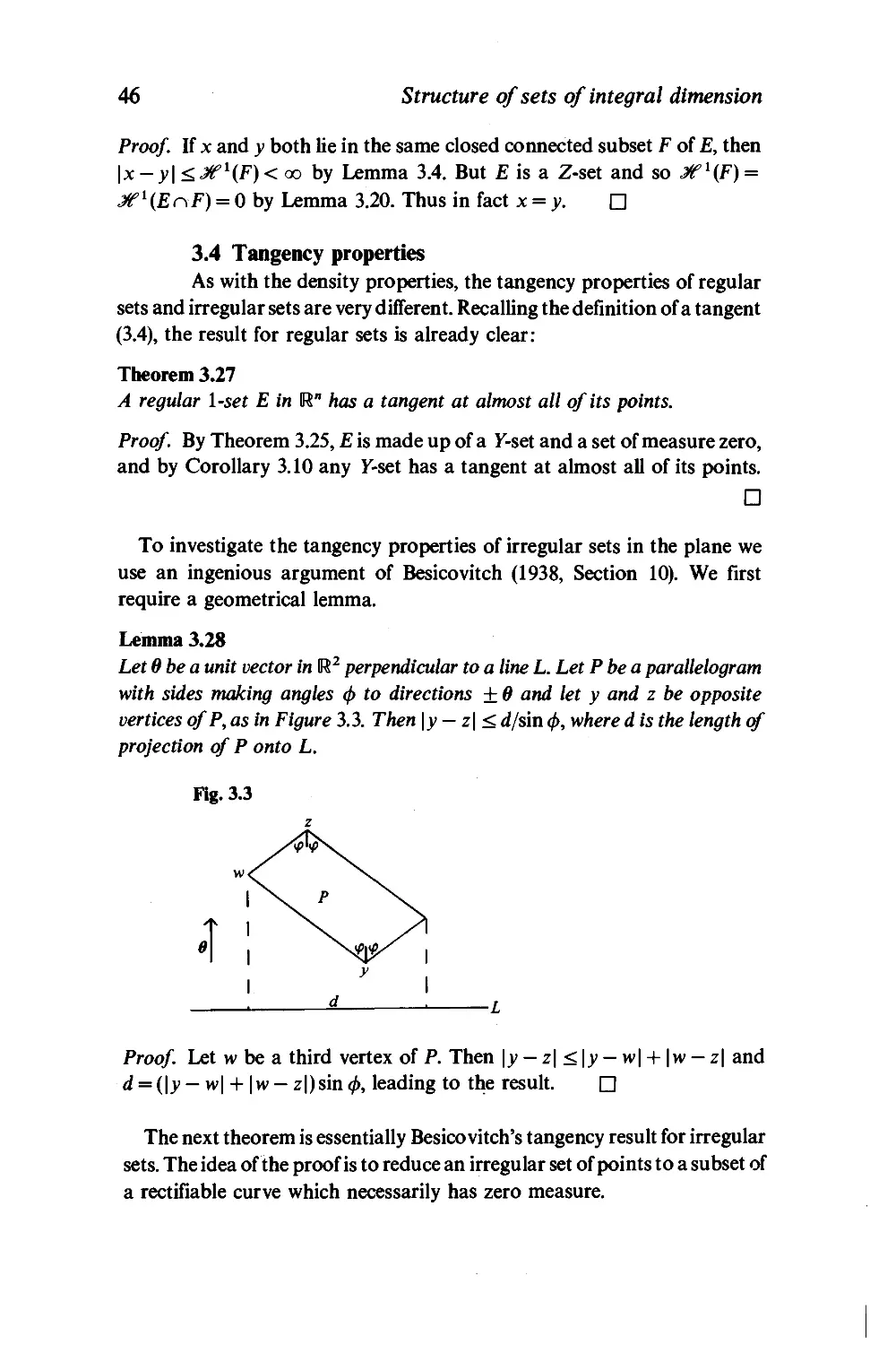
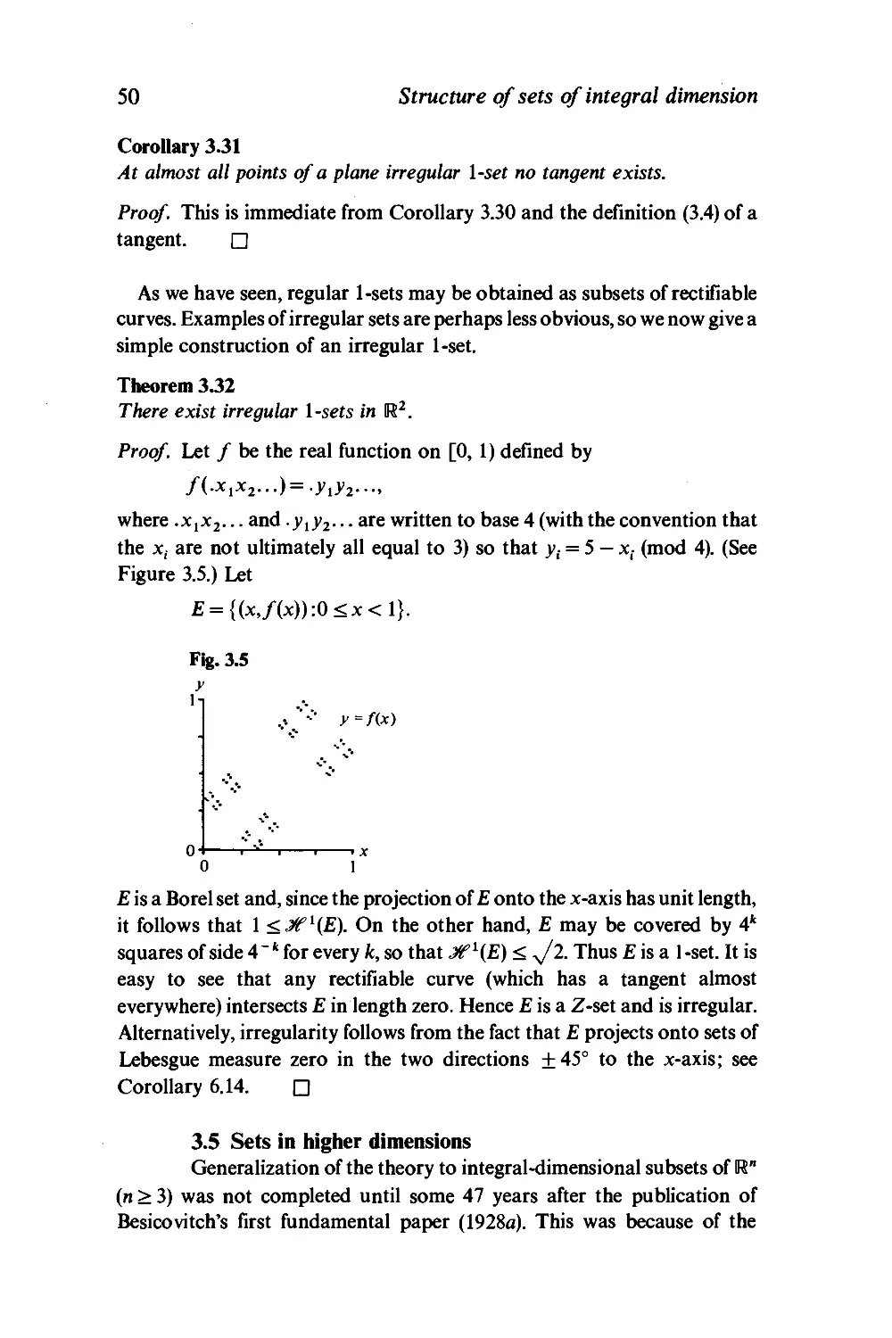
3.4 Tangency properties 46
3.5 Sets in higher dimensions 50
4 Structure of sets of non-integral dimension 54
4.1 Introduction 54
4.2 s-sets with 0 < s < 1 54
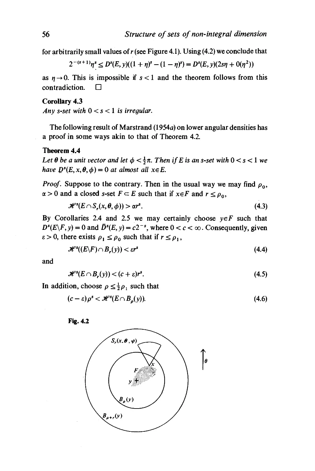
4.3 s-sets with s > 1 57
4.4 Sets in higher dimensions 63
5 Comparable net measures 64
5.1 Construction of net measures 64
5.2 Subsets of finite measure 67
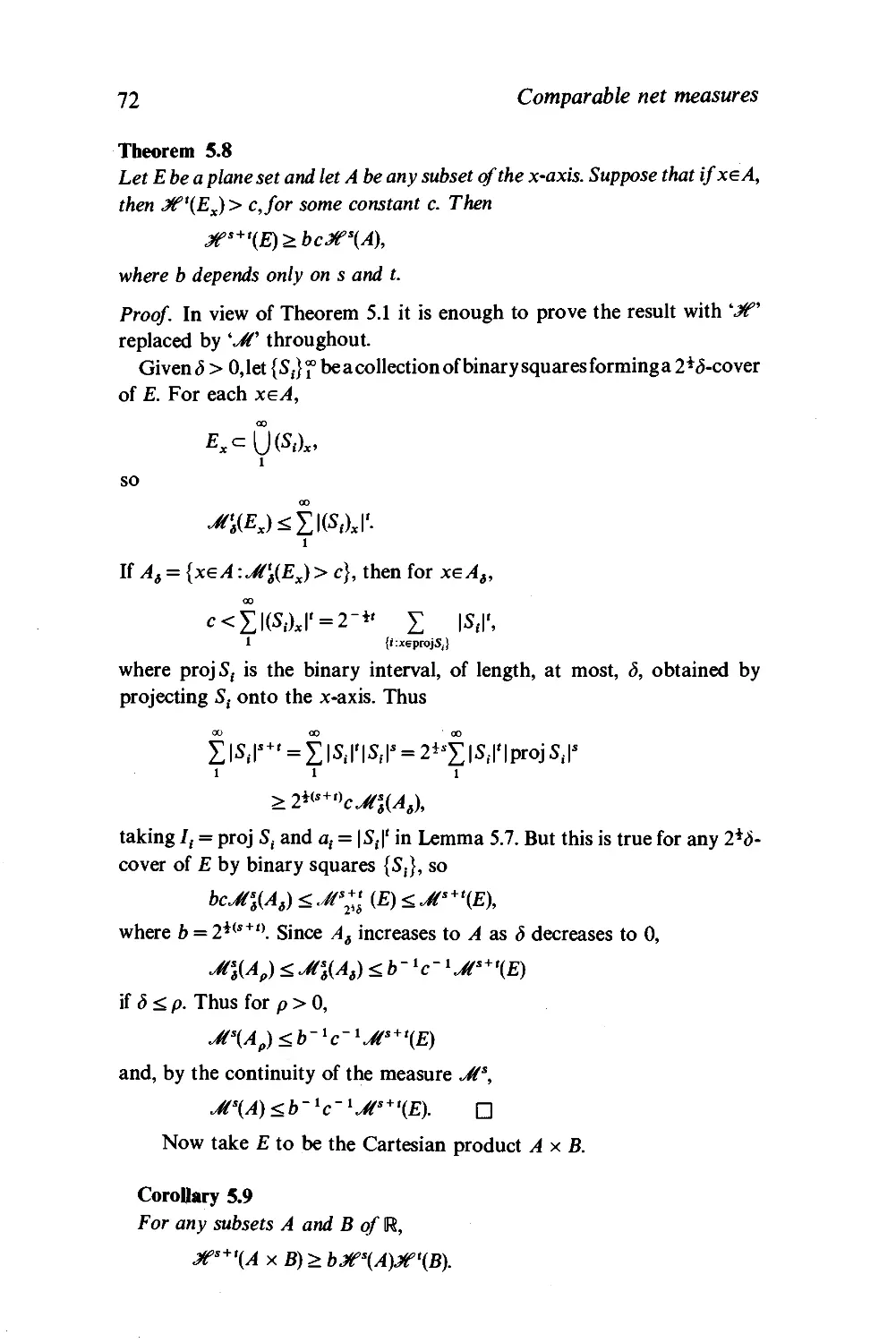
5.3 Cartesian products of sets 70
6 Projection properties 75
6.1 Introduction 75
6.2 Hausdorff measure and capacity 75

VI
Contents
6.3 Projection properties of sets of arbitrary dimension 80
6.4 Projection properties of sets of integral dimension 84
6.5 Further variants 92
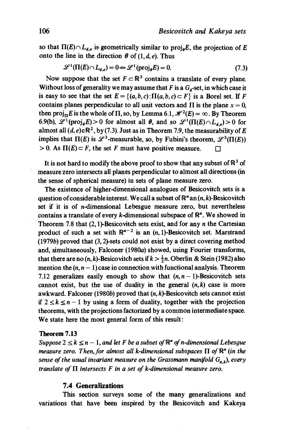
7 Besicovitch and Kakeya sets 95
7.1 Introduction 95
7.2 Construction of Besicovitch and Kakeya sets 96
7.3 The dual approach 101
7.4 Generalizations 106
7.5 Relationship with harmonic analysis 109
8 Miscellaneous examples of fractal sets 113
8.1 Introduction 113
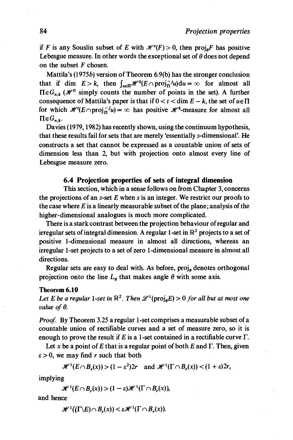
8.2 Curves of fractional dimension 113
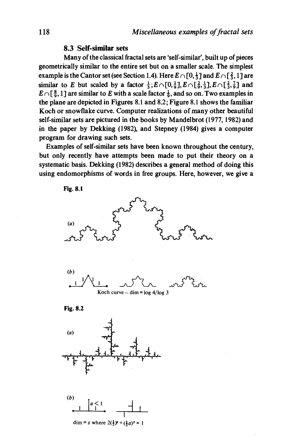
8.3 Self-similar sets 118
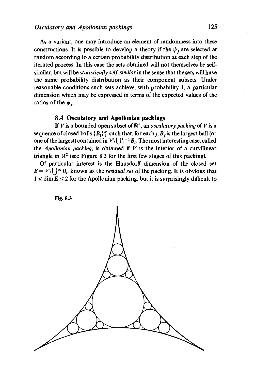
8.4 Osculatory and Apollonian packings 125
8.5 An example from number theory 131
8.6 Some applications to convexity 135
8.7 Attractors in dynamical systems 138
8.8 Brownian motion 145
8.9 Conclusion 149
References 150
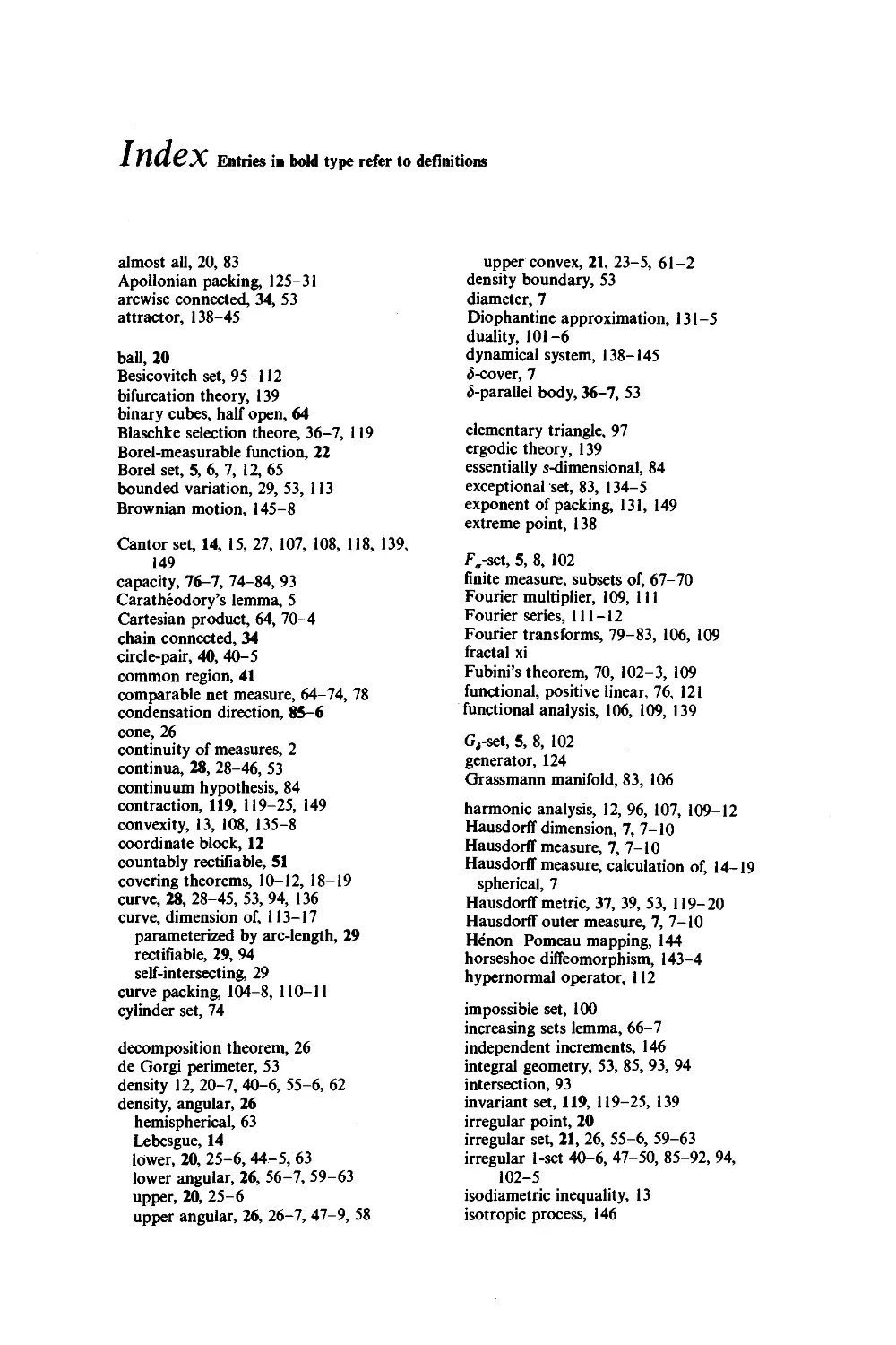
Index 161

Preface
This tract provides a rigorous self-contained account of the mathematics of
sets of fractional and integral Hausdorff dimension. It is primarily
concerned with geometric theory rather than with applications. Much of
the contents could hitherto be found only in original mathematical papers,
many of which are highly technical and confusing and use archaic notation.
In writing this book I hope to make this material more readily accessible
and also to provide a useful and precise account for those using fractal sets.
Whilst the book is written primarily for the pure mathematician, I hope
that it will be of use to several kinds of more or less sophisticated and
demanding reader. At the most basic level, the book may be used as a
reference by those meeting fractals in other mathematical or scientific
disciplines. The main theorems and corollaries, read in conjunction with
the basic definitions, give precise statements of properties that have been
rigorously established.
To get a broad overview of the subject, or perhaps for a first reading, it
would be possible to follow the basic commentary together with the
statements of the results but to omit the detailed proofs. The non-specialist
mathematician might also omit the details of Section 1.1 which establishes
the properties of general measures from a technical viewpoint.
A full appreciation of the details requires a working knowledge of
elementary mathematical analysis and general topology. There is no doubt
that some of the proofs central to the development are hard and quite
lengthy, but it is well worth mastering them in order to obtain a full insight
into the beauty and ingenuity of the mathematics involved.
There is an emphasis on the basic tools of the subject such as the Vitali
covering theorem, net measures, and potential theoretic methods.
The properties of measures and Hausdorff measures that we require are
established in the first two sections of Chapter 1. Throughout the book the
emphasis is on the use of measures in their own right for estimating the size
of sets, rather than as a step in defining the integral. Integration is used only
as a convenient tool in the later chapters; in the main an intuitive idea of
integration should be found perfectly adequate.
Inevitably a compromise has been made on the level of generality
adopted. We work in n-dimensional Euclidean space, though many of the
vn

Vlll
Preface
ideas apply equally to more general metric spaces. In some cases, where the
proofs of higher-dimensional analogues are much more complicated,
theorems are only proved in two dimensions, and references are supplied
for the extensions. Similarly, one- or two-dimensional proofs are sometimes
given if they contain the essential ideas of the general case, but permit
simplifications in notation to be made. We also restrict attention to
Hausdorff measures corresponding to a numerical dimension 5, rather than
to an arbitrary function.
A number of the proofs have been somewhat simplified from their
original form. Further shortenings would undoubtedly be possible, but the
author's desire for perfection has had to be offset by the requirement to
finish the book in a finite time!
Although the tract is essentially self-contained, variations and extensions
of the work are described briefly, and full references are provided. Further
variations and generalizations may be found in the exercises, which are
included at the end of each chapter.
It is a great pleasure to record my gratitude to all those who have helped
with this tract in any way. I am particularly indebted to Prof Roy Da vies for
his careful criticism of the manuscript and for allowing me access to
unpublished material, and to Dr Hallard Croft for his detailed suggestions
and for help with reading the proofs. I am also most grateful to Prof B.B.
Mandelbrot, Prof J.M. Marstrand, Prof P. Mattila and Prof C.A. Rogers
for useful comments and discussions.
I should like to thank Mrs Maureen Woodward and Mrs Rhoda Rees for
typing the manuscript, and also David Tranah and Sheila Shepherd of
Cambridge University Press for seeing the book through its various stages
of publication. Finally, I must thank my wife, Isobel, for finding time to read
an early draft of the book, as well as for her continuous encouragement and
support.

Introduction
The geometric measure theory of sets of integral and fractional dimension
has been developed by pure mathematicians from early in this century.
Recently there has been a meteoric increase in the importance of fractal sets
in the sciences. Mandelbrot (1975,1977,1982) pioneered their use to model
a wide variety of scientific phenomena from the molecular to the
astronomical, for example: the Brownian motion of particles, turbulence in
fluids, the growth of plants, geographical coastlines and surfaces, the
distribution of galaxies in the universe, and even fluctuations of price on the
stock exchange. Sets of fractional dimension also occur in diverse branches
of pure mathematics such as the theory of numbers and non-linear
differential equations. Many further examples are described in the scientific,
philosophical and pictorial essays of Mandelbrot. Thus what originated as
a concept in pure mathematics has found many applications in the sciences.
These in turn are a fruitful source of further problems for the
mathematician. This tract is concerned primarily with the geometric theory of such
sets rather than with applications.
The word fractal' was derived from the latin/ractus, meaning broken, by
Mandelbrot (1975), who gave a 'tentative definition' of a fractal as a set with
its Hausdorff dimension strictly greater than its topological dimension, but
he pointed out that the definition is unsatisfactory as it excludes certain
highly irregular sets which clearly ought to be thought of in the spirit of
fractals. Hitherto mathematicians had referred to such sets in a variety of
ways - 'sets of fractional dimension', 'sets of Hausdorff measure', 'sets with
a fine structure' or Irregular sets'. Any rigorous study of these sets must also
contain an examination of those sets with equal topological and Hausdorff
dimension, if only so that they may be excluded from further discussion. I
therefore make no apology for including such regular sets (smooth curves
and surfaces, etc.) in this account.
Many ways of estimating the 'size' or 'dimension' of thin' or 'highly
irregular' sets have been proposed to generalize the idea that points, curves
and surfaces have dimensions of 0, 1 and 2 respectively. Hausdorff
dimension, defined in terms of Hausdorff measure, has the overriding
advantage from the mathematician's point of view that Hausdorff measure
is a measure (i.e. is additive on countable collections of disjoint sets).
IX

X
Introduction
Unfortunately the Hausdorff measure and dimension of even relatively
simple sets can be hard to calculate; in particular it is often awkward to
obtain lower bounds for these quantities. This has been found to be a
considerable drawback in physical applications and has resulted in a
number of variations on the definition of Hausdorff dimension being
adopted, in some cases inadvertently.
Some of these alternative definitions are surveyed and compared with
Hausdorff dimension by Hurewicz & Wallman (1941), Kahane (1976),
Mandelbrot (1982, Section 39), and Tricot (1981, 1982). They include
entropy, see Hawkes (1974), similarity dimension, see Mandelbrot (1982),
and the local dimension and measure of Johnson & Rogers (1982). It would
be possible to write a book of this nature based on any such definition, but
Hausdorff measure and dimension is, undoubtedly, the most widely
investigated and the most widely used.
The idea of defining an outer measure to extend the notion of the length
of an interval to more complicated sets of real numbers is surprisingly
recent. Borel (1895) used measures to estimate the size of sets to enable him
to construct certain pathological functions. These ideas were taken up by
Lebesgue (1904) as the underlying concept in the construction of his
integral. Caratheodory (1914) introduced the more general 'Caratheodory
outer measures'. In particular he defined '1-dimensionaP or 'linear' measure
in H-dimensional Euclidean space, indicating that s-dimensional measure
might be defined similarly for other integers s. Hausdorff (1919) pointed out
that Caratheodory's definition was also of value for non-integral s. He
illustrated this by showing that the famous 'middle-third' set of Cantor had
positive, but finite, s-dimensional measure if s = log 2/log 3 = 0.6309....
Thus the concept of sets of fractional dimension was born, and Hausdorff's
name was adopted for the associated dimension and measure.
Since then a tremendous amount has been discovered about Hausdorff
measures and the geometry of Hausdorff-measurable sets. An excellent
account of the intrinsic measure theory is given in the book by Rogers
(1970), and a very general approach to measure geometry may be found in
Federer's (1969) scholarly volume, which diverges from us to cover
questions of surface area and homological integration theory.
Much of the work on Hausdorff measures and their geometry is due to
Besicovitch, whose name will be encountered repeatedly throughout this
book. Indeed, for many years, virtually all published work on Hausdorff
measures bore his name, much of it involving highly ingenious arguments.
More recently his students have made many further major contributions.
The obituary notices by Burkill (1971) and Taylor (1975) provide some idea
of the scale of Besicovitch's influence on the subject.

Introduction
XI
It is clear that Besico vitch intended to write a book on geometric measure
theory entitled The Geometry of Sets of Points, which might well have
resembled this volume in many respects. After Besicovitch's death in 1970,
Prof Roy Davies, with the assistance of Dr Helen Alderson (who died in
1972), prepared a version of what might have been Besico vitch's 'Chapter 1'.
This chapter was not destined to have any sequel, but it has had a
considerable influence on the early parts of the present book.
In our first chapter we define Hausdorff measure and investigate its basic
properties. We show how to calculate the Hausdorff dimension and
measure of sets in certain straightforward cases.
We are particularly interested in sets of dimension s which are s-sets, that
is, sets of non-zero but finite 5-dimensional Hausdorff measure. The
geometry of a class of set restricted only by such a weak condition must
inevitably consist of a study of the neighbourhood of a general point. Thus
the next three chapters discuss local properties: the density of sets at a point,
and the directional distribution of a set round each of its points, that is, the
question of the existence of tangents. Sets of fractional and integral
dimension are treated separately. Sets of fractional dimension are
necessarily fractals, but there is a marked contrast between the regular
'curvelike' or 'surface-like' sets and the irregular fractal' sets of integral
dimension.
Chapter 5 introduces the powerful technique of net measures. This
enables us to show that any set of infinite 5-dimensional Hausdorff measure
contains an s-set, allowing the theory of s-sets to be extended to more
general sets as required. Net measures are also used to investigate the
Hausdorff measures of Cartesian products of sets.
The next chapter deals with the projection of sets onto lower-
dimensional subspaces. Potential-theoretic methods are introduced as an
alternative to a direct geometric approach for parts of this work.
Chapter 7 discusses the 'Kakeya problem, of finding sets of smallest
measure inside which it is possible to rotate a segment of unit length. A
number of variants are discussed, and the subject is related by duality to the
projection theorems of the previous chapter, as well as to harmonic
analysis.
The final chapter contains a miscellany of examples that illustrate some
of the ideas met earlier in the book.
References are listed at the end of the book and are cited by date. Further
substantial bibliographies may be found in Federer (1947, 1969), Rogers
(1970) and Mandelbrot (1982).

Notation
With the range of topics covered, particularly in the final chapter, it is
impossible to be entirely consistent with the use of notation. In general,
symbols are defined when they are first introduced; these notes are intended
only as a rough guide.
We work entirely in n-dimensional Euclidean space, IR". Points of IR",
which are sometimes thought of in the vectorial sense, are denoted by small
letters, x, y, z etc. Occasionally we write (x, y) for Cartesian coordinates.
Capitals, E, F, T, etc. are used for subsets of IR", and script capitals, <€, V, J,
for families of sets. We use the convention that the set-inclusion symbol
<= allows the possibility of equality. The diameter of the set £ is denoted by
|£|, though, when the sense is clear, the modulus sign also denotes the
length of a vector in the usual way, thus |x — y\ is the distance between the
points x and y. Constants, b, c, c,, e, S, and indices, i,j, k, are also denoted by
lower case letters which may be subscripted.
The following list may serve as a reminder of the notation in more
frequent use
Sets
W
B,(x)
Sr(x,0,<t>)
C,(x,I)
R(x,y)
Ua,bmE)
£,int£
[£L
Mappings
proj9,projn
U
f°9
xiii
n-dimensional Euclidean space.
closed disc or ball, centre x and radius r.
sector of angle <j> and radius r.
double sector.
common region of the circle-pair with centres x and y.
Grossmann manifold of ^-dimensional subspaces of IR".
line sets.
topological closure, respectively interior, of £.
the ^-parallel body to £.
orthogonal projection onto the line in direction 6, resp.
the plane n.
Fourier transforms of the function / and measure \i.
composition of the mappings, g followed by/

XIV
Notation
Measures etc.
■Ws s-dimensional Hausdorff measure or outer measure.
if" n-dimensional Lebesgue measure.
Jis s-dimensional comparable net measure.
Jt%,M% £-outer measures used in constructing 3tfs and JKS.
if (0 length of the curve T.
dim E Hausdorff dimension of E.
4>t,Ct, /, t-potential, capacity, energy.
Densities
DS(E, x) density of E at x.
Ds(E,x), Ds(E,x), lower, upper densities.
DSC(E, x) upper convex density.
DS(E, x, 0, <j>) lower angular density, etc.

1
Measure and dimension
1.1 Basic measure theory
This section contains a condensed account of the basic measure
theory we require. More complete treatments may be found in Kingman &
Taylor (1966) or Rogers (1970).
Let X be any set. (We shall shortly take X to be n-dimensional Euclidean
space IR".) A non-empty collection y of subsets of X is termed a sigma-field
(or a-field) if y is closed under complementation and under countable
union (so if Eey, then X\Eey and if Eu E2,.. .ey, then [jf=, E^if). A
little elementary set theory shows that a a-field is also closed under
countable intersection and under set difference and, further, that X and the
null set 0 are in y.
The lower and upper limits of a sequence of sets {Ej} are defined as
lim£,= U nEj
j->oo lc= 1 j=k
and
j->cc k=lj=k
Thus jim Ej consists of those points lying in all but finitely many E}, and
lim Ej consists of those points in infinitely many Ej. From the form of these
definitions it is clear that if E} lies in the a-field y for each j, then Hm Ejy
VimEjey. If Hrn Ey= lim Ej, then we write limis,. for the common value;
this always happens if {Ej} is either an increasing or a decreasing sequence
of sets.
Let <& be any collection of subsets of X. Then the a-field generated by <€,
written y(^\ is the intersection of all a-fields containing (€. A
straightforward check shows that y{^€) is itself a a-field which may be thought of as the
'smallest' a-field containing e€.
A measure \i is a function defined on some a-field y of subsets of X and
taking values in the range [0, oo] such that
/i(0) = o (i.i)
and
/{(J£;) = j>(£,-) d-2)

2 Measure and dimension
for every countable sequence of disjoint sets {£,} in if.
It follows from (1.2) that \i is an increasing set function, that is, if £ <= £'
and E,E'sif, then
n(E)<n(E').
Theorem 1.1 (continuity of measures)
Let n be a measure on a a-field if of subsets of X.
(a) //£,<= £2 <=... is an increasing sequence of sets in if, then
/*(lim Ej) = lim rf,Ej)-
j-KX> j-> 00
(b) IfFl -=>F2-=>.. .is a decreasing sequence of sets in if and ^(Fj) < oo, then
H(l\m Fj)= timn(Fj).
./-►OO J-»00
(c) For any sequence of sets {Fj} in if,
H( lim Fj) < lim fi(Fj).
}-> 00 j-> 00
Proof, (a) We may express Uj=i^y as the disjoint union
£x u (J," 2(E}\Ej-1)- Thus by (1.2),
M Hm £,.) = // uV)
2
= limL(£1) + EM£y\£y-1)l
*-oo|_ 2 J
= Um^£1uy(£J.\£y_1)N
= lim n(Ek).
lc-»oo
(b) If Ej = F,\^y, then {£,} is as in (a). Since f)/y = ^i\U^'
Mlim £,) = ,/ft F.)
y-oo \y=i /
= M^)-MU£y)
y
= n(F1)-Umn(EJ)
y-oo

Basic measure theory
= lim(MF,)-M£,))
= lim u(Fj).
j->CO
(c) Now let Ek = f]f^kFj. Then {Ek} is an increasing sequence of sets in £f,
so by (a),
M lim Fj) = J 0 £< ) = lim ,,(£*) < lim M^)- □
Next we introduce outer measures which are essentially measures with
property (1.2) weakened to subadditivity. Formally, an outer measure v on a
set X is a function defined on all subsets of X taking values in [0, oo] such
that
v(0) = O, (1.3)
v(A)<v(A') XA<=A' (1.4)
and
(00 \ 00
U As ) ^ £v(Aj) for any subsets {/I,.} of X. (1.5)
Outer measures are useful since there is always a a-field of subsets on
which they behave as measures; for reasonably defined outer measures this
(j-field can be quite large.
A subset E of X is called v-measurable or measurable with respect to the
outer measure v if it decomposes every subset of X additively, that is, if
v(A) = v(AnE)+v(A\E) (1.6)
for all 'test sets' Ac X. Note that to show that a set E is v-measurable, it is
enough to check that
v(A)>v(AnE) + v(A\E), (1.7)
since the opposite inequality is included in (1.5). It is trivial to verify that if
v(E) = 0, then E is v-measurable.
Theorem 1.2
Let v be an outer measure. The collection Jt of v-measurable sets forms a a-
field, and the restriction of v to Jt is a measure.
Proof. Clearly, 0&Jt, so Jt is non-empty. Also, by the symmetry of (1.6),
A eJt if and only if X\A eJt. Hence Jt is closed under taking complements.
To prove that Jt is closed under countable union, suppose that
EvE2,...eJt and let A be any set. Then applying(1.6) to £1,£2,...in turn

4
Measure and dimension
with appropriate test sets,
v(A) = v(AnE1) + v(A\E1)
= v(AnEt) + v((^\£1)n£2) + v^VE.V^)
=MA^nEMAw>)
Hence
v(A) > £ v((Vli E) " Ej) + v(A 0 £;
for all k and so
v^)> f v((^\U£.)^^) + v(^\.U£y)- (1-8)
On the other hand,
Anjj^jj^jJ^nE^,
so, using (1.5),
v(A) < v(a n[) £y) + v(^UJ £,-)
by (1.8). It follows that [JJLi^6-^' so ^T is a a-field.
Now let £,,£2,... be disjoint sets of Jl. Taking A = \}JLxE-} in (1.8),
(00 \ 00
K)= 1 / /= 1
and combining this with (1.5) we see that v is a measure on M. □
We say that the outer measure v is regular if for every set A there is a v-
measurable set £ containing A with v(A) = v(£).
Lemma 1.3
If v is a regular outer measure and {Aj} is any increasing sequence of sets,
lim v(Aj) = v( lim Aj).
}-* 00 j-> 00
Proof. Choose a v-measurable £y with £y => Xy and v(Ej) = v(i4^) for each/
Then, using (1.4) and Theorem 1.1(c),
v(lim Aj) = v(ljm Aj) < v(]im Ej) < Hm v{Ej) = lim \{Aj).
The opposite inequality follows from (1.4). □

Basic measure theory
5
Now let (X, d) be a metric space. (For our purposes X will usually be n-
dimensional Euclidean space, IR", with d the usual distance function.) The
sets belonging to the a-field generated by the closed subsets of X are called
the Borel sets of the space. The Borel sets include the open sets (as
complements of the closed sets), the Fa-sets (that is, countable unions of
closed sets), the Gs-sets (countable intersections of open sets), etc.
An outer measure v on X is termed a metric outer measure if
v(£uF) = v(£) + v(F) (1.9)
whenever E and F are positively separated, that is, whenever
d(E,F) = M{d(x,y):xeE,yeF} > 0.
We show that if v is a metric outer measure, then the collection of v-
measurable sets includes the Borel sets. The proof is based on the following
version of 'Caratheodory's lemma'.
Lemma 1.4
Let v be a metric outer measure on (X,d). Let {Aj}f be an increasing
sequence of subsets ofX with A = lim Aj, and suppose that d(Aj, A\AJ+1)>0
for each j. Then v(A) = lim v(Aj).
Proof. It is enough to prove that
v(A) < lim v(Aj), (1.10)
y-»oo
since the opposite inequality follows from (1.4). Let Bl = Al and Bj =
Aj\Aj_ ! for ; > 2. If; + 2 < i, then Bj <= Aj and Bt <= A\At_ t <= A\A}+1, so
Bt and B} are positively separated. Thus, applying (1.9) (m — 1) times,
(m \ m
k=l / k=l
(m \ m
\jB2k =£v(B2t).
We may assume that both these series converge - if not we would have
lim v(Aj) = oo, since \Jk=, B2k_, and {Jk=, B2k are both contained inA2m.
y-»oo
Hence
<*-{$,"')-{">»&,'')
k = j+ 1

6
Measure and dimension
<limv(Ai)+ £ Wig.
;->oo k=j+i
Since the sum tends to 0 as ;'-► oo, (1.10) follows. □
Theorem 1.5
Ifv is a metric outer measure on (X,d), then all Borel subsets of X are v-
measurable.
Proof. Since the v-measurable sets form a a-field, and the Borel sets form
the smallest a-field containing the closed subsets of X, it is enough to show
that (1.7) holds when E is closed and A is arbitrary.
Let Aj be the set of points in ^4\£ at a distance at least l/j from E. Then
d(A n E, A j)^l/j, so
v(AnE) + viAj) = v((A n E) u A,) < v(A) (1.11)
for each ;', as v is a metric outer measure. The sequence of sets {^4^} is
increasing and, since E is closed, ^4\£ = \Jf= {Ay Hence, provided that
d(Aj, A\E\Aj+l) > 0for all;, Lemma 1.4 gives v(A\E) < lim v{A}) and (1.7)
y-»oo
follows from (1.11). But if xsA\E\Aj+1 there exists ze£ with d(x,z)<
1/0'+ l),soifyeAjthend(x,y)>d(y,z)-d(x,z)> l/j- 1/0+ l)>0.Thus
d(Aj,A\E\Aj+ x) > 0, as required. □
There is another important class of sets which, unlike the Borel sets, are
defined explicitly in terms of unions and intersections of closed sets. If (X, d)
is a metric space, the Souslin sets are the sets of the form
e= u n*«.b...fc.
hh...k=l
where Eith ik is a closed set for each finite sequence {j,,j2,. ..,it} of
positive integers. Note that, although E is built up from a countable
collection of closed sets, the union is over continuum-many infinite
sequences of integers. (Each closed set appears in the expression in many
places.)
It may be shown that every Borel set is a Souslin set and that, if the
underlying metric spaces are complete, then any continuous image of a
Souslin set is Souslin. Further, if v is an outer measure on a metric space
(X,d), then the Souslin sets are v-measurable provided that the closed sets
are v-measurable. It follows from Theorem 1.5 that if v is a metric outer
measure on (X, d), then the Souslin sets are v-measurable. We shall only
make passing reference to Souslin sets. Measure-theoretic aspects are
described in greater detail by Rogers (1970), and the connoisseur might also
consult Rogers et al. (1980).

Hausdorff measure
7
1.2 Hausdorff measure
For the remainder of this book we work in Euclidean n-space, IR",
although it should be emphasized that much of what is said is valid in a
general metric space setting.
If U is a non-empty subset of IR" we define the diameter of U as
\U\ = sup{\x-y\:x,yeU}. If Ec (J.17. and 0<\U-,\<S for each i, we
say that {l/J is a S-cover of £.
Let £ be a subset of IR" and let s be a non-negative number. For 5 > 0
define
jrj(£) = inff |l/f|s, (1.12)
i=l
where the infimum is over all (countable) ^-covers {(/,.} of £. A trivial check
establishes that Jfss is an outer measure on IR".
To get the Hausdorff s-dimensional outer measure of E we let S -*0. Thus
Jfs(£) = lim^(£) = supjrj(£). (1.13)
»->0 i>0
The limit exists, but may be infinite, since Jf J increases as 3 decreases. Jfs is
easily seen to be an outer measure, but it is also a metric outer measure. For
if S is less than the distance between positively separated sets £ and F, no set
in a S-co\er of £u£ can intersect both £ and F, so that
leading to a similar equality for J^s. The restriction of Jfs to the a-field of
Jf s-measurable sets, which by Theorem 1.5 includes the Borel sets (and,
indeed, the Souslin sets) is called Hausdorff s-dimensional measure.
Note that an equivalent definition of Hausdorff measure is obtained if the
infimum in (1.12) is taken over ^-covers of £ by convex sets rather than by
arbitrary sets since any set lies in a convex set of the same diameter.
Similarly, it is sometimes convenient to consider ^-covers of open, or
alternatively of closed, sets. In each case, although a different value of 3f %
may be obtained for S > 0, the value of the limit Jfs is the same, see Davies
(1956). (If however, the infimum is taken over ^-covers by balls, a different
measure is obtained; Besicovitch (1928a, Chapter 3) compares such
'spherical Hausdorff measures' with Hausdorff measures.)
For any £ it is clear that Jf s(£) is non-increasing as s increases from 0 to
oo. Furthermore, if s < t, then
which implies that if Jf'(£) is positive, then Jf s(£) is infinite. Thus there is a
unique value, dim £, called the Hausdorff dimension of £, such that
Jfs(£)=oo if 0<s<dim£,jfs(£) = Oifdim£<s<oo. (1.14)

8
Measure and dimension
If C is a cube of unit side in IR", then by dividing C into k" subcubes of side
1/fc in the obvious way, we see that if 5 ^ k~ 'n* then Jf %Q < fc"(/c" ini)n
< nin, so that Jfn(C) < oo. Thus if s > n, then 3VS(C) = 0 and jf S(R") = 0,
since IR" is expressible as a countable union of such cubes. It follows
that 0 <, dim E < n for any E <= IR". It is also clear that if E <= E' then
dim E <, dim £'.
An Jf'-measurable set E <= IR" for which 0 < Jf s(£) < oo is termed an
s-set; a 1-set is sometimes called a lineariy measurable set. Clearly, the
HausdorfT dimension of an s-set equals s, but it is important to realize that
an s-set is something much more specific than a measurable set of HausdorfT
dimension s. Indeed, Besicovitch (1942) shows that any set can be expressed
as a disjoint union of continuum-many sets of the same dimension. Most of
this book is devoted to studying the geometric properties of s-sets.
The definition of HausdorfT measure may be generalized by replacing
| Uj\s in (1.12) by h(\ Ut\), where h is some positive function, increasing and
continuous on the right. Many of our results have direct analogues for these
more general measures, though sometimes at the expense of algebraic
simplicity. The HausdorfT 'dimension' oTa set E may then be identified more
precisely as a partition of the functions which measure E as zero or infinity
(see Rogers (1970)). Some progress is even possible if | Ut\s is replaced by
/i((/i), where h is simply a function of the set Ut (see Davies (1969) and
Davies & Samuels (1974)).
We next prove that Jfs is a regular measure, together with the useful
consequence that we may approximate to s-sets from below by closed
subsets. This proof is given by Besicovitch (1938) who also demonstrates
(1954) the necessity of the finiteness condition in Theorem 1.6(b).
Theorem 1.6
(a) // E is any subset of W there is a Gs-set G containing E with Jt?s(G) =
Jfs(E). In particular, Jfs is a regular outer measure.
(b) Any Jfs-measurable set of finite 3fs-measure contains an Fa-set of equal
measure, and so contains a closed set differing from it by arbitrarily small
measure.
Proof, (a) If Jfs(E)= oo, then IR" is an open set of equal measure, so
suppose that Jf S(E) < oo. For each i = 1,2... choose an open 2/i-cover of E,
{Ui}}}, such that
f I ty'<•*",„(£)+ 1/1.
Then £<= G, where G = (X°=1 [jf=l Ui} is a G,-set. Since {UtJ}j is a 2/i-
cover of G, J^s2li(G)<Jf\n(E) + 1/i, and it follows on letting i-» oo that
Jf s(£) = Jf *(G). Since G,-sets are Jf'-measurable, 3VS is a regular outer
measure.

Hausdorff measure
9
(b) Let E be Jf s-measurable with 3^S(E) < oo. Using (a) we may find open
sets 0,,02,...containing E, with Jifs(f]fL1Oi\E)=Jirsif)?L 1Of)-Jfs(£)
= 0. Any open subset of W is an Fff-set, so suppose 0(= (j£LiFy for
each i, where {Fij)} is an increasing sequence of closed sets. Then by
continuity of Jfs,
lim Jfs(£ n Fi}) = Jf s(£ n 0;) = Jf%E).
j-Ko
Hence, given e > 0, we may find jt such that
Jf(£\Ftf()<2-'e (/=1,2,...).
If F is the closed set f)£, Fijt, then
Jfs(F) > Jifs(EnF) > JV%E) - £ Jfs(£\F0l) > Jf s(£) - e.
»= 1
Since F<=f|r=iOi, then Jfs(F\£) ^ Jfs( f|," i Of\£) = 0. By (a) F\E is
contained in some G^-set G with JP(G) = 0. Thus F\G is an Fff-set
contained in E with
3VS{F\G) > 3V\F) - *e\G) > Jfs(£) - e.
Taking a countable union of such Fff-sets over e = ^,-J,i,... gives an Fff-set
contained in E and of equal measure to E. □
The next lemma states that any attempt to estimate the Hausdorff
measure of a set using a cover of sufficiently small sets gives an answer not
much smaller than the actual Hausdorff measure.
Lemma 1.7
Let E be ^-measurable with Jfs(E) < oo, and let e be positive. Then there
exists p>0, dependent only on E and e, such that for any collection ofBorel
sets {Ui}?Ll with 0< |l/j| <p we have
jr(£n(Jl/.)<£|l/i|s + e.
i i
Proof From the definition of Jfs as the limit of 3V\ as S -»0, we may choose
p such that
.*"(£) <£W + ie (1.15)
for any p-cover {Wt} of E. Given Borel sets {Ut} with 0 < | Uf | ^ p, we may
find a p-cover {F(} of £\(J,(/; such that
•^s(au^)+^>ei^is-
Since {(/J u{ KJ is then a p-cover of £,
xf\E)<Yd\ui\°+Yd\vi\°+&

10
Measure and dimension
by (1.15). Hence
Jf( En (J U-\ = Jfs(£) - Jf s( E\{J Utj
=But\s+e. a
Finally in this section, we prove a simple lemma on the measure of sets
related by a 'uniformly Lipschitz' mapping
Lemma 1.8
Let i//:E-*F be a surjective mapping such that
\il/(x)-i//(y)\<c\x-y\ (x,yeE)
for a constant c. Then Jfs(F) < <?3V\E).
Proof. For each i, |^(l/,n£)| < c\ Ut\. Thus if {I/,} is a ^-cover of E, then
{+{U,nE)} is a c<5-cover of F. Also ^f|^(l/,.n£)|s ^C^Wf so that
Jf'cS(F) < (fje's(E), and the result follows on letting 5 -»0. D
1.3 Covering results
The Vitali covering theorem is one of the most useful tools of
geometric measure theory. Given a 'sufficiently large' collection of sets that
cover some set E, the Vitali theorem selects a disjoint subcollection that
covers almost all of E.
We include the following lemma at this point because it illustrates the
basic principle embodied in the proof of Vitali's result, but in a simplified
setting. A collection of sets is termed semidisjoint if no member of the
collection is contained in any different member.
Lemma 1.9
Let ^ be a collection of balls contained in a bounded subset qfW. Then we
may find a finite or countably infinite disjoint subcollection {B(} such that
UB<=UB.:> (1-16)
Be* T
where B't is the ball concentric with Bt and of five times the radius. Further,
we may take the collection {B't} to be semidisjoint.
Proof. We select the {Bj inductively. Let d0 = sup{|B|: Bg#} and choose
B, from # with |B,|>^d0. If B,,..., Bm have been chosen let dm =
sup{|B|: Bg#, B disjoint from (J7^J- If dm = 0 the process terminates.
Otherwise choose Bm+1 from # disjoint from [j"Bi with |Bm+1|>jdm.
Certainly, these balls are disjoint; we claim that they also have the required
covering property. If Bg#, then either B = Bt for some /', or B intersects

Covering results
11
some Bt with 21 Bt \ > \ B \. If this was not the case B would have been selected
in preference to the first ball Bm for which 2 |Bm|<|B|. (Note that, by
summing volumes, £|Bil2 < oo so that |B;| -»0 as i-» oo if infinitely many
balls are selected.) In either case, B <=£*;., giving (1.16). To get the {BJ}
semidisjoint, simply remove Bt from the subcollection if BJ <= B'} for any; # i
noting that B\ can only be contained in finitely many B). D
A collection of sets y is called a Vitali class for E if for each xeE and
<5 > 0 there exists Ue-T with xe U and 0 < | U\ <S.
Theorem 1.10 (Vitali covering theorem)
(a) Let E be an ^-measurable subset of W and let V be a Vitali class of
closed sets for E. Then we may select a (finite or countable) disjoint sequence
{Ut}from r such that either £11/^= oo or J^s(E\[j.(7^ = 0.
(b) If Jfs(E) < oo, then, given e > 0, we may also require that
^\E)<Yd\Ul\s + E.
i
Proof. Fix p > 0; we may assume that | U| ^ p for all Ue ~f~. We choose the
{(/;} inductively. Let Ul be any member of "T. Suppose that Ul,...,Um
have been chosen, and let dm be the supremum of | U | taken over those U in
-T which do not intersect U x,..., Um. If dm = 0, then E <= (J7 Uiso tnat (a)
follows and the process terminates. Otherwise let Um + l be a set in V
disjoint from {J"Ui such that | Um+ x | > \dn.
Suppose that the process continues indefinitely and that £|(/j|s< oo.
For each i let B( be a ball with centre in U{ and with radius 31 Ut \. We claim
that for every k > 1
£\U^<=(M- (1-17)
i t+i
For if xeE (J* (/; there exists Ue'T not intersecting Ult...,Uk with xg(7.
Since | Ut\ -»0, | (7| > 2| (7m | for some m. By virtue of the method of selection
of {U(},U must intersect Ut for some i with k < i < m for which | (/1 <, 21 (7( |.
By elementary geometry U <= B(, so (1.17) follows. Thus if S > 0,
V i / \ i / t+i it+i
provided k is large enough to ensure that \Bt\<S for i>A:. Hence
Jl?ss(E\{J J01/,) = 0 for all £ > 0. so Jf S(£\(J? ^,) = 0, which proves (a).
To get (b), we may suppose that p chosen at the beginning of the proof is
the number corresponding to e and E given by Lemma 1.7. If £ I Ut \s = oo,

12
Measure and dimension
then (b) is obvious. Otherwise, by (a) and Lemma 1.7,
Jf s(£) = Jf S(£\U Ut) + Jfs(E n \J Ut)
■ i
= 0 + Jt?s(En{JUi)
i
<El^ils + e- D
Covering theorems are studied extensively in their own right, and are of
particular importance in harmonic analysis, as well as in geometric measure
theory. Results for very general classes of sets and measures are described in
the two books by de Guzman (1975, 1981) which also contain further
references. One approach to covering principles is due to Besicovitch
(1945a, 1946, 1947); the first of these papers includes applications to
densities such as described in Section 2.2 of this book.
1.4 Lebesgue measure
We obtain n-dimensional Lebesgue measure as an extension of the
usual definition of the volume in IR" (we take 'volume' to mean length in IR1
and area in IR2).
Let C be a coordinate block in IR" of the form
C = [ai,bi)x [a2,62)x- x [an,fcn),
where at < bt for each i. Define the volume of C as
V(C) = (bl-al)(b2-a2)...(bn-an)
in the obvious way. If £ <= IR" let
jSf"(£) = inf^K(Cf), (1.18)
i
where the infimum is taken over all coverings of £ by a sequence {C(} of
blocks. It is easy to see that S£n is an outer measure on IR", known as
Lebesgue n-dimensional outer measure. Further, _£?"(£) coincides with the
volume of £ if £ is any block; this follows by approximating the sum in
(1.18) by a finite sum and then by subdividing £ by the planes containing the
faces of the Ct. Since any block Ct may be decomposed into small subblocks
leaving the sum in (1.18) unaltered, it is enough to take the infimum over 8-
covers of £ for any 8 > 0. Thus S£n is a metric outer measure on IR". The
restriction of S£n to the if-measurable sets or Lebesgue-measurable sets,
which, by Theorem 1.5, include the Borel sets, is called Lebesgue n-
dimensional measure or volume.
Clearly, the definitions of if1 and Jf' on IR1 coincide. As might be
expected, the outer measures S£n and Jf" on IR" are related if n > 1, in fact

Lebesgue measure
13
they differ only by a constant multiple. To show this we require the
following well-known geometric result, the 'isodiametric inequality', which
says that the set of maximal volume of a given diameter is a sphere. Proofs,
using symmetrization or other methods, may be found in any text on
convexity, e.g. Eggleston (1958), see also Exercise 1.6.
Theorem 1.11
The n-dimensional volume of a closed convex set of diameter d is, at most,
n*n(jd)"/(^n)!, the volume of a ball of diameter d.
Theorem 1.12
// £cR", then <£\E) = cje\E), where c„ = ji±72"(jn)!. In particular,
Cj = 1 and c2 = n/4.
Proof. Given e > 0 we may cover £ by a collection of closed convex sets
{I/,} such that £| I/,|" < Jf "(£) + e. By Theorem 1.11 &H(Ut) £ cn\ Ut\", so
JSP"(£) < Z^TO < cje\E) + c„e, giving <£•(£) < cje*{E).
Conversely, let {C;} be a collection of coordinate blocks covering E with
ZV(Ct)<£r(E) + e. (1.19)
i
We may suppose these blocks to be open by expanding them slightly whilst
retaining this inequality. For each i the closed balls contained in Ci of radius,
at most, 5 form a Vitali class for Ct. By the Vitali covering theorem,
Theorem 1.10(a), there exist disjoint balls {B^} j in Ct of diameter, at most, S,
with JT"(CAU "., B^) = 0 and so with JfJCQU "-1 By) = °- Since ^is a
Borel measure, £"_ t if»(By) = JSP"(U"= i^y) £ ^"(Q)- Thus
*ro < z ^;(c,) < z z ^»+ z Wq 0 *0
00 00 00 00
^Z ZIByl"=Z ZO^^y)
<c~l Z ^"(C,) < c-':?•(£) + c; 'e,
>=1
by (1.19). Thus c„JfS(£) ^ •^"(£) + e for a11 e and <*> giving cnJQ£) <
One of the classical results in the theory of Lebesgue measure is the
Lebesgue density theorem. Much of our later work stems from attempts to
formulate such a theorem for Hausdorff measures. The reader may care to
furnish a proof as an exercise in the use of the Vitali covering theorem.
Alternatively, the theorem is a simple consequence of Theorem 2.2.

14 Measure and dimension
Theorem 1.13 (Lebesgue density theorem)
Let E be an ^""-measurable subset ofW. Then the Lebesgue density ofE at x,
a *■<*(*» • (L20)
exists and equals 1 ifxeE and 0 ifx$E, exceptfor a set of x of Z£"-measure 0.
(Br(x) denotes the closed ball of centre x and radius r, and, as always, r tends to
0 through positive values.)
1.5 Calculation of Hausdorff dimensions and measures
It is often difficult to determine the Hausdorff dimension of a set
and harder still to find or even to estimate its Hausdorff measure. In the
cases that have been considered it is usually the lower estimates that are
awkward to obtain. We conclude this chapter by analysing the dimension
and measure of certain sets; further examples will be found throughout the
book. It should become apparent that there is a vast range of s-sets in IR" for
all values of s and n, so that the general theory to be described is widely
applicable.
The most familiar set of real numbers of non-integral Hausdorff
dimension is the Cantor set. Let E0 = [0, 1], £, = [0, 1/3] u [2/3, 1], E2 =
[0, 1/9] u [2/9,1/3] u [2/3, 7/9] u[8/9, 1], etc., where E}+1is obtained by
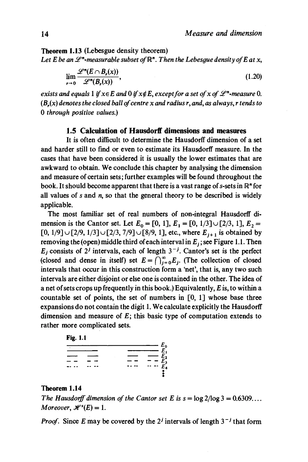
removing the (open) middle third of each interval in E}; see Figure 1.1. Then
Ej consists of 2} intervals, each of length 3~j. Cantor's set is the perfect
(closed and dense in itself) set E= f]JL0Ej. (The collection of closed
intervals that occur in this construction form a 'net', that is, any two such
intervals are either disjoint or else one is contained in the other. The idea of
a net of sets crops up frequently in this book.) Equivalently, E is, to within a
countable set of points, the set of numbers in [0, 1] whose base three
expansions do not contain the digit 1. We calculate explicitly the Hausdorff
dimension and measure of E; this basic type of computation extends to
rather more complicated sets.
Fig. 1.1
_ £0
——— ———£|
- e\
Theorem 1.14
The Hausdorff dimension of the Cantor set E is s = log 2/log 3 = 0.6309
Moreover, 3VS(E) = 1.
Proof. Since E may be covered by the 2J intervals of length 3 J that form

Calculation of Hausdorff dimensions and measures 15
Ej, we see at once that je%.j(E)<2j3~sj = 2J2~J =1. Letting j->ao,
3fs(E) <, 1.
To prove the opposite inequality we show that if J is any collection of
intervals covering E, then
1 < I |/Is- (1.21)
By expanding each interval slightly and using the compactness of E, it is
enough to prove (1.21) when J is a finite collection of closed intervals. By a
further reduction we may take each IeJ to be the smallest interval that
contains some pair of net intervals, J and J\ that occur in the construction
of E. (J and J' need not be intervals of the same Ej.) If J and J' are the largest
such intervals, then / is made up of J, followed by an interval K in the
complement of E, followed by J'. From the construction of the Ej we see
that
\J\,\J'\<\K\. (1.22)
Then
\i\°=(\j\ + \k\ + \j'\y
>(!(m+m))s=2(!uis+iuT)>ms+i./T,
using the concavity of the function f and the fact that 3s = 2. Thus replacing
/ by the two subintervals J and J' does not increase the sum in (1.21). We
proceed in this way until, after a finite number of steps, we reach a covering
of E by equal intervals of length 3~J, say. These must include all the
intervals of E}, so as (1.21) holds for this covering it holds for the original
covering J. □
There is nothing special about the factor \ used in the construction of the
Cantor set. If we let E0 be the unit interval and obtain Ej+lby removing a
proportion 1 — 2k from the centre of each interval of Ej, then by an
argument similar to the above (with (1.22) replaced by |J|, \J'\<,
\K\k/(l - 2k) we may show that je'(f)^Ej) = 1, where s = log2/log(l//c).
We may construct irregular subsets in higher dimensions in a similar
fashion. For example, take E0 to be the unit square in U2 and delete all but
the four corner squares of side k to obtain Et. Continue in this way, at the
yth stage replacing each square of Ej_, by four corner squares of side kj to
get Ej (see Figure 1.2 for the first few stages of construction). Then the same
sort of calculation gives positive upper and lower bounds for Jt?s(()™Ej),
where s = log 4/log (1/fc). More precision is required to find the exact value
of the measure in such cases, and we do not discuss this further.
Instead, we describe a generalization of the Cantor construction on the

16
Measure and dimension
Fig. 1.2
t.'
X
i
:•.'.
'V
'*..'"
J*-...'
•'<'V
'■fljf
*'s'v
1
i. ' *.'%
$#
Sis
VVK.V*
*'a*"'
.•'•-!'':
O.vyV?.-:!
"V>?v>
• \ "v
&£
jfj
»!
^,,;:.<,;
!"•••.
K
m
mm am
in
DC
_£LE
£o
£,
£j
real line. Let s be a number strictly between 0 and 1; the set constructed will
have dimension s. Let E0 denote the unit interval; we define inductively sets
£0=>£, =>£2..., each a finite union of closed intervals, by specifying
EJ+1nI for each interval I of Ej. If I is such an interval, let m > 2 be an
integer, and let J1,J2,...,Jm be equal and equally spaced closed
subintervals of / with lengths given by
i/,r=^i/r,
(1.23)
and such that the left end of Jj coincides with the left end of/ and the right
end of Jm with the right end of /. Thus
m|J,| + (m-l)d = |/| (l^/<m), (1.24)
where d is the spacing between two consecutive intervals J(. Define Ej+1 by
requiring that Ej+1nl = \J"Jt. Note that the value of m may vary over
different intervals / in EJt so that the sets Ei can contain intervals of many
different lengths.
The set E = f] JL 0ES is a perfect nowhere dense subset of the unit interval.
The following analysis is to appear in a forthcoming paper of Davies.
Theorem 1.15
IfE is the set described above, then 3fs{E) = 1.
Proof. An interval used in the construction of £, that is, a component
subinterval of some Ej, is called a net interval. For F <= E let
MF) = inf£|/|*.
(1.25)
where the infimum is taken over all possible coverings of F by collections J
of net intervals. Then ft is an outer measure (and, indeed, a Borel measure)
on the subsets of E. Note that the value of ft is unaltered if we insist that J be
a £-cover of F for case S > 0, since using (1.23) we may always replace a net
interval / by a number of smaller net intervals without altering the sum in
(1.25).
Let J be a cover of E by net intervals. To find a lower bound for J] | / |*
we may assume that the collection J is finite (since each net interval is open

Calculation of Hausdotff dimensions and measures
17
relative to the compact set E) and also that the intervals in J are pairwise
disjoint (we may remove those intervals contained in any others by virtue of
the net property). Let J be one of the shortest intervals of J\ suppose that J
is a component interval of Ejy say. Then J <= / for some interval / in Ej_ t.
Since J is a disjoint cover of E, all the other intervals of Esr\ I must be in J.
If we replace these intervals by the single interval /, the value of ^|/|* is
unaltered by (1.23). We may proceed in this way, replacing sets of net
intervals by larger intervals without altering the value of the sum, until we
reach the single interval [0,1]. It follows that £/6/| I\" = | [0,1] |s = 1, so, in
particular,
n(E) = L
In exactly the same manner we see that if J is any net interval, then
n(JnE) = \J\s. (1.26)
Next we show that
ti(JnE)<\J\* (1.27)
for an arbitrary interval J. Contracting J if necessary, it is enough to prove
this on the assumptions that J <= [0,1] and that the endpoints of J lie in E,
and, by approximating, coincide with endpoints of net intervals contained
in J. Let / be the smallest net interval containing J; say / is an interval of Ej.
Suppose that J intersects the intervals Jq,Jq+l,...,Jr among the
component intervals of Ej+lnl, where 1 < q < r < m. (There must be at least
two such intervals by the minimality of /.) We claim that
\JqnJ\s+\Jq+1\s + - + \Jr-1\s + \JrnJ\°<\J\°. (1.28)
If Jqn J is not the whole of Jq or if Jrn J is not the whole of Jr, then on
increasing J slightly the left-hand side of inequality (1.28) increases faster
than the right-hand side. Hence it is enough to prove (1.28) when J is the
smallest interval containing Jq and Jr. Under such circumstances (1.28)
becomes
fcl/,1'^m, = (*|/,| + (*-l)d)', (1.29)
where k = r — q + 1. This is true if A: = m by (1.23) and (1.24), and is trivial if
k=l, with equality holding in both cases. Differentiating twice, we see that
the right-hand expression of (1.29) is a convex function of £, so (1.29) holds
for 1 < k < m, and the validity of (1.28) follows.
Finally, if either Jq n J or Jr n J is not a single net interval, we may repeat
the process, replacing Jq n J and Jr n J by smaller net intervals to obtain an
expression similar to (1.28) but involving intervals of Ej+2 rather than of
EJ+1. We continue in this way to find eventually that | J\s is at least the sum
of the sth powers of the lengths of disjoint net intervals covering J n E and
contained in J. Thus (1.27) follows from (1.26) for any interval J.

18
Measure and dimension
As (1.25) remains true if the infimum is taken over ^-covers J for any
5 > 0, Jfs(£) ^ M^)- On the other hand, by (1.27),
M£)<EM^n£)<EU,-ls
for any cover {J,} of £, so n(E) < 3V\E). We conclude that Jfs(£) =
ti(E)=L D
Similar constructions in higher dimensions involve nested sequences of
squares or cubes rather than intervals. The same method allows the
Hausdorff dimension to be found and the corresponding Hausdorff
measure to be estimated.
The basic method of Theorem 1.15 may also be applied to find the
dimensions of other sets of related types. For example, if in the construction
of £ the intervals Jt,..., Jm in each / are just 'nearly equal' or 'nearly equally
spaced', the method may be adapted to find the dimension of E. Similarly, if
in obtaining Ej+, from Ej equations (1.23) and (1.24) only hold 'in the limit
as j-* oo', it may still be possible to find the dimension of E.
Another technique useful for finding the dimension of a set is to 'distort' it
slightly to give a set of known dimension and to apply Lemma 1.8. The
reader may wish to refer to Theorem 8.15(a) where this is illustrated.
Eggleston (1952) finds the Hausdorff dimension of very general sets
formed by intersection processes; his results have been generalized by
Peyriere (1977). Recently an interesting and powerful method has been
described by Da vies & Fast (1978). Other related constructions are given by
Randolph (1941), Erdos (1946), Ravetz (1954), Besicovitch & Taylor (1954),
Beardon (1965), Best (1942), Cigler & Volkmann (1963) and Wegmann
(19716), these last three papers continuing earlier works of the same
authors. A further method of estimating Hausdorff measures is described in
Section 8.3.
Exercises on Chapter 1
1.1 Show that if /z is a measure on a <x-field of sets M and E}eJ({\ <, j < oo),
then /*(Iim Ej) ^ fim n{Ej) provided that /*((Jf Ej) < oo.
j-*oo j-*oo
1.2 Let v be an outer measure on a metric space (X, d) such that every Borel set
is v-measurable. Show that v is a metric outer measure.
1.3 Show that the outer measure 3tf" on W is translation invariant, that is,
J?"(x + E) = JtT'(E), where x + E = {x + y.yeE}. Deduce that x + E is
Jf ^-measurable if and only if £ is Jf ^-measurable. Similarly, show that
3#"(cE) = csjes(E), where cE = {cy.yeE}.
1.4 Prove the following version of the Vitali covering theorem for a general
measure /i: let E be a /^-measurable subset of U" with /*(£) < oo. If V is a

Exercises
19
Vitali class of (measurable) sets for E, then there exist disjoint sets
t/„ U2,...e*~ such that n(E\{JiUi) = 0.
1.5 Use the Vitali covering theorem to prove the Lebesgue density theorem.
(Consider the class of balls "T = {Br(x):xeE,r <p and Sen(Br{x)nE) <
aif(Br(x))} for each a < 1 and p > 0.)
1.6 Prove that the area of a plane convex set U of diameter d is, at most, \nd2.
(For one method take a point on the boundary of U as origin for polar
coordinates so that the area of U is \$r(<j>)2d<j>, and observe that r(<j>)2
+ r(<j> + \nf <, d2 for each <j>.)
1.7 Use the Lebesgue density theorem to deduce the result of Steinhaus, that if
£ is a Lebesgue-measurable set of real numbers of positive measure, then
the difference set \y — x :x, yeE} contains an interval (— h,h). Show more
generally that if £ and E' are measurable with positive Lebesgue measure,
then {y — x:xeE,yeE'} contains an interval.
1.8 Let n be a Borel measure on W and let £ be a /^-measurable set with
0 <fi(E)< oo. Show that
(a) if Umr~sn(Br(x)nE)<c< oo for xeE, then Jfs(£)>0,
r-«0
(b) if fimr~sn(Br(x)nE)> c> 0 for xeE, then 3#*(E) < oo.
r-0
(For (a) use the definition of Hausdorff measure, for (b) use the version of
the Vitali covering theorem in Exercise 1.4.)
1.9 Let E be the set of numbers between 0 and 1 that contain no odd digit in
their decimal expansion. Obtain the best upper and lower estimates that
you can for the Hausdorff dimension and measure of E. (In fact E is an s-set
where s = log 5/log 10. This example is intended to illustrate some of the
difficulties that can arise in finding Hausdorff measures, being a little more
awkward than the Cantor set. One approach to such questions is
described in Section 8.3.)

2
Basic density properties
2.1 Introduction
Recall that a subset E of W is termed an s-set (0 < s < n) if E is Jfs-
measurable and 0 < Jt?s(E) < oo. In general we exclude the case of s = 0 as
this often requires separate treatment from other values of s. However, since
0-sets are simply finite sets of points their properties are straightforward.
The next three chapters are concerned with local properties of s-sets, in
particular with questions of density and the existence of tangents. As
measure properties carry over under countable unions, some of the results
may be adapted for measurable sets of <r-finite Jf s-measure (i.e. sets formed
as countable unions of s-sets). Sets of dimension s of non-<r-finite 3fs-
measure are difficult to get any sort of hold on except by finding subsets of
finite measure, and this is discussed in Chapter 5.
Usually, s will be regarded as fixed and, where there is no ambiguity,
terms such as 'measure', 'measurable' and 'almost all' (i.e. 'except for a set of
measure zero') refer to the measure Jfs.
First we define the basic set densities that play a major role in our
development. These densities are natural analogues of Lebesgue density
(1.20), though their behaviour can be very different. The densities are
indicative of the local measure of a set compared with the 'expected'
measure.
Let Br(x) denote the closed ball of centre x and radius r so that
|Br(x)| = 2r. The upper and lower densities (sometimes called upper and lower
spherical or circular densities) of an s-set £ at a point xe M" are defined as
— jfs(£nfi(x))
DS(E, x) = lim —v „ v rV "
~o (2r)s
and
D*(E, x) = hm —
respectively. If D\E, x) = DS(E, x) we say that the density of E at x exists and
we write £>*(£, x) for the common value.
A point xe £ at which D*(E, x) = D"(E, x) = 1 is called a regular point of E;
otherwise x is an irregular point. An s-set E is said to be regular if Jtif s-almost

Introduction
21
all of its points are regular and irregular if almost all of its points are
irregular.
Characterizing regular s-sets and obtaining bounds for the densities of s-
sets are two important aims of this book. There is no analogue of the
Lebesgue density theorem; it is not in general true that an s-set has density 1
at almost all of its points. In fact one of the main results of the subject is that
an s-set cannot be regular unless s is an integer. If s is integral, however, an s-
set decomposes into a regular and an irregular part. Very roughly speaking,
a regular s-set looks like a measurable subset of an s-dimensional manifold
in IR", whereas an irregular set might behave as a Cartesian product of n
Cantor-like sets chosen so that the resulting set is of the required dimension.
Whilst we are mainly concerned with spherical densities, it is also
convenient to introduce the upper convex density of an s-set E at x, defined
as
DSC(E, x) = lim \ sup — _I (2.1)
where the supremum is over all convex sets U with xeU and 0 < | U\ < r.
Any set is contained in a convex set of equal diameter, so this is equivalent
to taking the supremum over all sets U with xeU and 0 < |U\ < r.
Since Br(x) is convex and since if xe U, then U <= Br(x) where r = | U |, we
have the relations
2-sDsc(£, x) < D\E,x) < Dl(E, x). (2.2)
Before we prove the basic results on densities, it may be of value to
enunciate some general principles that are frequently applied.
First, we often need to know that sets of points defined in terms of metric
or measure properties are measurable with respect to an appropriate
measure. In practice in this subject, checking measurability is nearly always
a formality. The sets encountered can usually be expressed in terms of
known measurable sets using combinations of lim, lim, countable unions
and intersections, etc. Or again, we may wish to consider f]l)>0El), say, but
find on examining the definition of the sets Ep that this is the same as the
countable intersection C\f>£Q*EQ over positive rational values of p. Some
demonstrations of measurability are given in Lemma 2.1 but, subsequently,
when a routine check suffices, we often assume without explicit mention
that the sets involved are measurable.
Second, many proofs involve showing that a set of points defined by a
property such as a density condition has measure zero. Typically, we need
to show that the set E = {x: i//(x) > 0} has Hausdorff measure zero, where i//
is some real-valued function. A standard approach is to show that for each

22
Basic density properties
a > 0 the set {x :ij/(x) > a} has measure zero and to point out that the same
must then be true of the countable union E = \Jf=, {x :^(x) > 1//'}. Thus it
is enough to prove that Jf s{x :\l/(x) > a} < e for all a,e > 0.
Third, we mention the idea of'uniformization'. If we require a property to
hold at almost all points of a set E, it is enough to show that, for all e > 0,
there is a subset F of E with the measure of E\F less than e and with the
property holding throughout F. The advantage of this is that F can often be
chosen to behave much more regularly than E. For example, F can
generally be taken as a closed set using Theorem 1.6, and might also be
chosen so that various densities, for example, converge uniformly on F.
Throughout the book, we generally use the letter F to denote this 'working
set', obtained by stripping E of its most violent irregularities. Very often if a
result can be proved for a set under reasonable topological and uniformity
assumptions it is a purely technical matter to extend the result to full
generality.
2.2 Elementary density bounds
In this section we commence our study of fundamental density
properties of s-sets by proving some results which are valid for all values of
s. Such results were first given for linearly measurable sets by Besicovitch
(1928a, 1938), the latter paper containing improved proofs. There is no
difficulty in generalizing this work to s-sets in W for any s and n, as was
indicated by Besicovitch (1945a), Marstrand (1954a) and Wallin (1969).
First we check the measurabihty of the densities as functions of x. It is
sometimes simpler to talk about the measurabihty of a function rather than
of sets defined by that function. The function/: W -»U is measurable (resp.
Borel-measurable, upper semicontinuous) if the set {x :f(x) < c] is a
measurable (resp. Borel, open set for every c); an equivalent definition of
measurabihty is obtained if' <' is replaced by '<','>' or '>'. It follows
from the open set definition of continuity that continuous functions on W
are Borel measurable.
Lemma 2.1
Let E be an s-set.
(a) Jf S(E n Br(x)) is an upper semicontinuous and so Borel-measurable
function of x for each r.
(b) D\E, x) and 5S(£, x) are Borel-measurable functions of x.
Proof, (a) Given r, a, > 0 write
F= {x:Jf{EnBr(x))<oi}.
Let xeF. As e \ 0, then Br+e(x) decreases to Br(x), so by the continuity of
Jf' from above,
Jf(EnBr+e(x)) \Jf(EnBr(x)).

Elementary density bounds
23
Thus we may find e such that Jf *(EnBr+e(x))< a, so if \y — x\ <,e, then
Br(y)<=Br+e(x) and 3tf\E n Br(y)) < a. Hence F is an open subset of W.
This is true for all a, so we conclude that Jf S(E n Br(x)) is upper
semicontinuous in x.
(b) Using part (a),
{x:J^\EnBr(x))<a{2rf}
is open, so, given p > 0,
Fp = {x:Jf s(EnBp(x)) < a(2/f for some r < p)
is the union of such sets and so is open. Now
{x :£>*(£, x)< a} = ft Fp;
since Fp increases as p decreases, we may take this intersection over the
countable set of positive rational values of p. Hence {x: Ds(£, x) < a} is a Gs-,
and so a Borel set for each a, making DS(E, x) a Borel-measurable function
of x. A similar argument establishes the measurability of D*(E, x). □
This lemma enables us to assert that sets such as {x :DS(£, x) > a} are Jfs-
measurable for any s-set E. A further consequence of the proof is that sets of
the form
{x: 3>e\E n Bp(x)) < a(2/f for some r<p}
are 3tfs-measurable (as open sets); a minor variation allows 'some' to be
replaced by 'all'.
We obtain bounds for upper densities first in the case of convex densities,
and then use (2.2) to deduce the corresponding results for circular densities.
The following theorem is obvious if £ is a compact set, but is true more
generally.
Theorem 2.2
IfE is an s-set in W, then Dse(E,x) = 0for Jf'-almost all x$E.
Proof. Fix a > 0; we show that the measurable set
F = {x££:Dsc(E,x)>a}
has zero measure. By the regularity of Jfs we may, given 8 > 0, find a closed
E, <= E with J4fs{E\Ex) < 8. For p > 0 let
-T = {U:U is closed and convex, 0< \U\ <,p, UnEi = 0
and 3#"(EnU)>a\U\°}. (2.3)
Then f is a Vitali class of closed sets for F, using (2.1) and the closure of E,,
and so we may use the Vitali theorem, Theorem 1.10(a), to find a disjoint
sequence of sets {[/J in f with either Y\Ui\'= °° or ^\F\\JU^ = 0.

24 Basic density properties
But by (2.3),
IIUt\°< l-^X"(EnUt) = -Jf'(En (JI/,)
Ot (X i
1 /5
<-Jfs(£\£,)<-<oo,
a a
as the {l/J are disjoint and are disjoint from £,. We conclude that
Jfs(F\u[/i) = 0, so that
•*%(F) < JT J(F\U I/.) + jrj(Fn IJ I/,)
^*(F\lM)+Eltf,ls<o+^.
This is true for any S > 0 and any p > 0, so Jf S(F) = 0, as required. □
Theorem 2.3
IfE is an s-set in W, then Dsc(E,x) = 1 at W-almost all xeE.
Proof, (a) We use the definition of Hausdorff measure to show that
D*C(E, x) > 1 almost everywhere in E. Take a < 1 and p > 0 and let
F = {xeE:Jfs(EnU)<<x\U\s for all convex
1/with xet/and |t/|<p}. (2.4)
Then F is a Borel subset of E. For any e > 0 we may find a p-cover of F by
convex sets {[/,} such that
£|l/,r<JHF) + e.
Hence, assuming that each Ut contains some point of F, and using (2.4),
tf\F) < £ 3f S(F n I/,) < X Jf s(£ n [/,.)
i i
<aXlUi|s<a(Jfs(F) + e).
i
Since a < 1 and the outer inequality holds for all e > 0, we conclude that
3?'(F) = 0. We may define such an F for any p > 0, so, by definition,
D'C(E, x) > a for almost all xeE. This is true for all a < 1, so we conclude that
5|(£,x);> 1 almost everywhere in E.
(b) We use a Vitali method to show that DSC(E, x) < 1 almost everywhere.
Given a > 1, let F = {xeE:Dsc(E, x) > a}, so that F is a measurable subset of
E. Let F0 = {xeF:D*c(E\F, x) = 0}. Then Jfs(F\F0) = 0 by Theorem 2.2.
Using the definition of convex density, Dsc (F, x) ^ D'C(E, x) - D'C(E\F, x) > a
ifxeF0.
Thus
y = {U:U is closed and convex and
jf'(FnU)>a\U\s} (2.5)

Elementary density bounds
25
is a Vitali class for F0, so by Theorem 1.10(b) we may, given e > 0, find a
disjoint sequence of sets { U,}, in ~T with 3f\F0) <, £| U^ + e. By (2.5)
Jfs(F) = Jf5(F0) < -YJfs(Fn [/,) + e <-Jt?s(F) + e.
a a
This inequality holds for any e > 0, so Jf S(F) = 0 if a > 1, as required. □
Results akin to Theorems 22 and 2.3 have been obtained by Freilich
(1966) and Davies & Samuels (1974) for surprisingly general measures of
Hausdorff type.
The analogues of these two theorems for circular densities, which are
rather more important in our development, follow immediately using (2.2).
Corollary 2.4
IfE is an s-set in W, then />*(£, x) = 0at Jf-almost all x outside E.
Corollary 2.5
If E is an s-set in W, then
2-*<Ds(E,x)<l
at almost all xeE.
Corollary 2.4 has a number of important consequences. The first of these
is that the densities of a measurable subset of an s-set coincide with the
densities of the original set at almost all points of the subset. This result is
often used in a preparatory manner; thus when examining a subset with a
certain density property we can discard the remainder of the set leaving the
density property holding almost everywhere.
Corollary 2.6
Let F be a measurable subset of an s-set E. Then D'iF, x) = D'iE, x) and
DS(F, x) = D'iE, x) for almost all xeF.
Proof.
Writing H = E\F we have from Corollary 2.4 that iy(H, x) = 0 at almost all
x in F. For such x
D'(E, x) = D°(F, x) + />*(#, x) = D'iF, x) and
D'(E, x) = D'(F, x) + D°(H, x) = D*(F, x). □
Corollary 2.7
Let E = [JjEj be a countable disjoint union qfs-sets with Jfs(E) < oo. Then
for any k,
D°(Ek, x) = £*(£, x) and D\Ek, x) = D'(E, x).
at almost all xeEK.

26
Basic density properties
Proof Apply Corollary 2.6 to the subset Ek of E. □
Corollary 2.8
Let E be an s-set. IfE is regular resp, irregular then any measurable subset of
E of positive measure is regular resp. irregular.
Proof. This is immediate from Corollary 2.6 and the definition of
regularity. □
Corollary 2.9
The intersection of a regular resp. irregular set and a measurable set is a
regular resp. irregular set. The intersection of a regular set and an irregular
set is of measure zero.
Proof. The first pair of statements follow from Corollary 2.8. The final
statement holds since such an intersection must be both regular and
irregular. □
The next corollary enables us to treat the regular and irregular parts of an
s-set independently.
Corollary 2.10 (decomposition theorem)
If E is an s-set, the set of regular points of E is a regular set, and the set of
irregular points of E is an irregular set.
Proof By Lemma 2.1 the sets of regular and irregular points are both
measurable, so this corollary follows from Corollary 2.6. □
We can also obtain bounds for the upper angular densities of s-sets in
W(n > 2). Angular densities were introduced by Besicovitch (1929, 1938) to
study tangential properties of s-sets. If 0 is a unit vector and <f> an angle, let
S(x,0,<f>) be the closed one-way infinite cone with vertex x and axis in
direction 0 consisting of those points y for which the segment [x, y] makes
an angle of, at most, <f> with 8. Write Sr(x,0,<f>) = Br(x)nS(x,0,<f>) for the
corresponding spherical sector of radius r. Angular densities are defined
analogously to spherical densities, but with Sr(x, 0, <j>) replacing Br(x). Thus
r-o (2rf
and
are the upper and lower angular densities of E at x. A routine check (see
Lemma 2.1) establishes all the desirable measurability properties for the
angular densities and the sets associated with them.

Exercises
27
Comparing the diameter of a spherical sector with its radius, it follows
from the definitions that
/)•(£, x,fl,0)^2-'|S1(x,fl,0)r/H(£,x).
We deduce immediately from Theorem 2.3 that, given 0 and <f>,
D\E,x,e,4)^~'\Si(x,e,4)\'
for almost all xeE. On calculating the diameters of the sectors, this becomes
(2s (0<(t><in)
D\E,x,0,<j>) << (sin <j>f (in<<t><$n)
U (jn<(t><n).
We may obtain a positive lower bound for the upper angular densities if
(f> ;> \n by modifying part (a) of the proof of Theorem 2.3, see Exercise 2.3.
Then
(2 (f7t < (p < 7t).
Estimates for lower densities are somewhat harder to derive, and will be
considered later in certain cases in connection with tangency properties.
Morgan (1935), Gills (1935), Besicovitch (1938) and Dickinson (1939) give
some constructions of sets for which the densities and angular densities take
extreme values.
Exercises on Chapter 2
2.1 If £ is the Cantor set, show that D*(£,x)^2~5 for all x, where s =
log2/log3. Deduce that £ is irregular.
2.2 Define the upper cubical density at x of an s-set E in R" as
Bm Jt?'(EnSr(x))/\Sr(x)\', where here Sr(x) denotes the cube of side r
r-*oo
centred at x with sides parallel to the coordinate axes.
Show that at almost all xeE the upper cubical density of E lies between
2-'n-"2 and 1.
2.3 Show that if £ is an s-set in R"(n ^ 2) and 0 is a unit vector, then
2~' <,D'(E,x,e,in) for almost all xeE. (Follow the proof of Theorem
2.3(a); you will need to use the regularity of Jt' to obtain a closed set to
work with.) Deduce that 2~'<,D'(E,x,0,<£) if 4> £\n.
2.4 Let \jt: R" -* W be a continuously differentiate transformation with non-
vanishing Jacobian. If £ is an s-set show that fy(\ji(E), i//(x)) = D\E, x) for
all x, with a similar result for lower densities.
2.5 Use Corollary 2.4 and Theorem 1.12 to prove the Lebesgue density
theorem, Theorem 1.13.

3
Structure of sets of integral
dimension
3.1 Introduction
In this chapter we discuss the density and tangency structure of s-
sets in W when s is an integer. We know from Corollary 2.10 that an s-set
splits into a regular part and an irregular part, and we find that these two
types of set exhibit markedly different properties. One of our aims is to
characterize regular sets as subsets of countable unions of rectifiable curves
or surfaces, and thus to relate the measure theoretic and the descriptive
topological ideas.
We present in detail the theory of linearly measurable sets or 1-sets in U2.
This work is almost entirely due to Besicovitch (1928a, 1938), the latter
paper including some improved proofs as well as further results. Most of his
proofs seem hard to better except in relatively minor ways and, hopefully, in
presentation. Certainly, some of the geometrical methods used by
Besicovitch involve such a degree of ingenuity that it is surprising that they
were ever thought of at all. Some of the work in this chapter is also described
in de Guzman (1981).
3.2 Curves and continua
Regular 1-sets and rectifiable curves are intimately related. Indeed,
a regular 1-set is, to within a set of measure zero, a subset of a countable
collection of rectifiable curves. This section is devoted to a study of curves,
mainly from a topological viewpoint and in relation to continua of finite
linear measure. Here we work in W as the theory is no more complicated
than for plane curves.
A curve (or Jordan curve) T is the image of a continuous injection
i^:[a,ft]-^IR", where [a,ft]<=R is a closed interval. Any curve is a
continuum, that is, a compact connected set. This follows since the
continuous image of any compact connected set is compact and connected.
In particular, any curve is a Borel set and so is .^-measurable. Moreover, a
continuous bijection between compact sets has a continuous inverse, so
that a curve may be defined as a homeomorphic image of a closed interval.
The length of the curve T is defined as
m
^(n=«upii«t,)-^M)i (3.i)
i=l

Curves and continua
29
where the supremum is taken over all dissections a = t0 < tt <... < tm = b
of [a, b]. If if (r) < oo (that is, if ty is of bounded variation), then T is said to
be rectifiable.
Note that our definition excludes self-intersecting curves, which are
covered by the following lemma.
Lemma 3.1
Let ^/:[a,b]-^W be a continuous mapping, with i^(a)=/= i^(ft). Then i//[a,b]
contains a curve joining \j/{a) to \j/{b).
Proof. For each multiple point x of [a,b] let lx be the largest (closed)
interval [tl,t2] with ^f(tt) = t//(t2) = x. Let J denote the collection of such
intervals that are contained in no others. Then J consists of countably
many disjoint proper closed intervals. Thus we may construct a continuous
surjection/:[a,fc]->[0, 1] such that/(a) = 0, f(b)= 1, and such that if
ti<t2, then/l(f j) <f(t2) with equality if and only if tl and t2 lie in a common
interval of J. Define \ji0: [0,1] -► W by \jj0(u) = x if / " \u) = lx for some
IxeJ and by ^0(u) = \jj(f~l(u)) otherwise. It is easy to check that ^0 is a
continuous injection with i/^O) = \j/(a) and 4i0{\) = i//(b). □
The sum in (3.1) does not decrease with the introduction of additional
dissection points. It is clear that if \j/ [a, b] is split into two curves \j/ [a, c] and
ty [c, b] where a < c < ft, then the sum of the lengths of the new curves equals
the length of the original curve, i.e. if is additive on curves with a common
endpoint.
It is always possible to parametrize a rectifiable curve T by arc length,
that is, to represent T as the image of a function \)/0: [0, if (T)] -* U in such a
way that the length of \)/0 [0, i] is t. This may be achieved by letting ^/0(t) be
the unique point i/^u) for which if(i^[a, «]) = £. If ty represents the
rectifiable curve r by arc length we see from (3.1) that
Wt,)-W2)|£|t,-t2|. (3-2)
In particular, this implies that t/r is an absolutely continuous function.
For a further discussion on the definition of curves see Burkill & Burkill
(1970, p. 246) or Pelling (1977).
Lemma 3.2
If T is a curve, then J^l(T) = if (r).
Proof. Let T be a curve joining z and w. If proj denotes orthogonal
projection from W onto the straight line through z and w, then
|proj x-proj y\<\x-y\ if x,yeW. By Lemma 1.8 j4f\T)>
^(proj r)^^>1([z,w]) = if1([z,w]) = |z-w|, since proj T=>[z,w].

30
Structure of sets of integral dimension
Now suppose that T is defined by ^:[a,ft]-^R". By the above
remark, ^l(^\t,u\) > \\fi(t) - ^(u)| for any t and «. Then if a = t0 < tl <
...<tm = b is any dissection of [a,b],
H^«)-^l-i)I^I^l(^-i,tJ) = ^l(r),
i f
since the arcs i/t[ti-1,tl'\ of r are disjoint except for endpoints. Thus
£e(T)<3f\T).
Finally, assume that if (r) < oo and let ty parametrize r by arc length.
Since ^ is a surjection from [0,if(r)] to r with (3.2) holding, Lemma 1.8
implies that jfl (T) < jfl ([0, if (r)]) = 2(T). D
One consequence of this lemma is that if T is a rectifiable curve, then
Jfs(r) is infinite if s < 1 and zero if s > 1 (see (1.14)).
Corollary 3.3
Let \j/ parametrize the rectifiable curve T by arc length. IfE is any Lebesgue-
measurable subset of[0, if (r)], then i//(E) is an Jf i-measurable subset qfW
andJel(^(E)) = £C1(E).
Proof. By Lemma 3.2 the additive set functions •#"1(^(.)) and if '(•) agree
on closed intervals, so by the usual process of extension of measures (see, for
example, Kingman & Taylor (1966)) they agree on the Lebesgue-
measurable subsets of [0, if (r)]. □
This corollary allows all the usual results on Lebesgue measure on the
line to be transferred to curves. For example, it follows from the Lebesgue
density theorem, Theorem 1.13, that if £ is an Jf '-measurable subset of a
curve T, then at almost all xeE we have Jf^Eniy^il)-^! as
Jf V)->0, where / is a subarc of T containing x.
We do not make further use of this corollary.
We have frequent recourse to the next lemma:
Lemma 3.4
Let Ebe a continuum containing x and y. If\x — y\ = p, then Jfi(EnBp(x))
^ p. In particular, Jf '(£) ^ |£|.
Proof. Let/:R"->[(), oo) be defined by f(z) = \z-x\. Then/ is a
continuous mapping such that
\f(z) -f(w)\ £ |z - w| (z,weR-X (3.3)
The set f(EnBp(x)) contains the interval [0,p], otherwise, for some
r (0 < r < p), £ = (£ n Br(x)) u (£\Bp(x)) would be a decomposition of £ into

Curves and continua
31
disjoint closed sets. Applying Lemma 1.8 to the mapping f
^(EnB^x))^ ^{/(EnB^x)))
>Jf1([0,p]) = i?1([0,p]) = p. □
We may now deduce the basic density property of rectifiable curves.
Lemma 3.5
A rectifiable curve is a regular l-set.
Proof If T is rectifiable, if (T) < oo, so by Lemma 3.2, Jfl(T) < oo. As T
contains at least two distinct points, Lemma 3.4 implies Jf i(T) > 0, so T is
an l-set.
Let x be a point of T other than an endpoint, and suppose x divides T into
two rectifiable subcurves T_ and T+. By Lemma 3.4, 3f l(r_nB/>(x))>p
and Jf1(r+-r>Bp(x))>p if p is sufficiently small, giving Jf1(rnBp(x))
> 2p. Thus at all points of T other than the endpoints, D'(r,x) > 1. Taken
together with Corollary 2.5 this implies that Dl(T, x) exists and equals 1 at
almost all xeT. □
Next we discuss the existence of tangents to rectifiable curves. We say
that an s-set E in U" has a tangent at x in the direction + 6 if D\E, x) > 0 and
for every angle <f> > 0,
lim r-W{En{Br{x)\Sr{x, 6, <t>)\Sr(x, - 0, tf>))) = 0 (3.4)
r-»0
(the line through x in the direction + 0 is of course the tangent line). Clearly,
an s-set can have, at most, one tangent at each of its points.
We give Besicovitch's (1944) elementary proof that a rectifiable curve has
a tangent at almost all of its points. An alternative approach would be to
appeal to standard results on the differentiability of functions of bounded
variation, see Kingman & Taylor (1966, Section 9.1).
Lemma 3.6
Let r be a rectifiable curve with endpoints x and y, and let <j>be a positive
angle. Let E be the set of points on T that belong to pairs of arbitrarily small
subarcs of Fsubtending chords that make an angle of more than 2(p with each
other. Then 3f\E) <(^(T)- |x-j>|)/(1 -cos#
Proof. Let L denote the line through x and y and let "K be the collection of
closed subarcs of T subtending chords that make angles of more than <f>
with L. By the conditions of the lemma, f is a Vitali class for E. Hence using
the covering theorem, Theorem 1.10(b), we may, for any e > 0, find a finite

32 Structure of sets of integral dimension
collection T,,..., Tm of disjoint subarcs of T belonging to "K such that
m m
^i(E)<Yl\ri\ + e<Yinri) + e. (3.5)
i=l i=l
If r'0, r\,..., r'm are the (possibly null) complementary arcs, then
projecting orthogonally onto L and using the fact that projection does not increase
length, we see that
cos*£jS?(rI) + £j2'(r;);>|x-j;|.
i i
Since £ JS?(rf) + £ jS?(r,') = JS?(D we get, using (3.5),
i i
^H^-e^z^r^^^n-ix-^D/a-cos^).
i
The observation that e is arbitrary completes the proof. □
Corollary 3.7
If<f> > 0 and E is the set of points on a rectifiable curve T that belong to pairs of
arbitrarily small subarcs ofT subtending chords that make an angle of more
than 2<j> with each other, then 3^l(E) = 0.
Proof. Given e > 0 we may by (3.1) find points x0, x,,..., xm on T (in that
order and with x0 and xm the endpoints of T) such that
m
i=l
Write T,- for the portion of T between x,-_, and x,-. Then applying Lemma
3.6 to each T,- in turn gives
m m
*f\E)= £ jr»(£nr,)£ £ (^(rj-iXi-x^D/a-costf,)
m
= (jS?(n - Z I*,- - *,_, I)/(l - cos <f>) < 8/(1 - cos <}>).
i=l
ThusJf1(£) = 0. D
Theorem 3.8
A rectifiable curve T has a tangent at almost all of its points.
Proof. Since the continuum T has at least two points, Lemma 3.4 implies
that D*(E, x) > \ at all xeT.
Let ty: [a, ft] -*■ W be a defining function for T. It follows from Corollary
3.7 that for almost all xeT we may find a unit vector 0 such that, given
i//(u)eS(x,0, <p)vS(x, - 0, <f>)

Curves and continua
33
if \u—t\<s, where <f>(t) = x. Moreover, if p is positive, \j/(u)iBp(x) if
\u — t\>e (otherwise choose a sequence of numbers {«,} with \ut —t\ > e
and t/r(u,)->x; then using sequential compactness there exists u with
\u — t\>e and {//(u) = x = i//(t) giving a double point of r). Thus
rn(Bp(x)\Sp(x, 6, (f>)\Sp(x, - 0, (f>)) = 0,
with (3.4) as a trivial consequence. □
Tangents to curves are often thought of in terms of differentiability. A
minor variant of the proof of Theorem 3.8 shows that a rectifiable curve
defined by a function ^ has a tangent at \)/{t) provided the derivative \fi\t)
exists and is non-vanishing.
Besicovitch (1934a, 1956,1957,1960) also considers how the definition of
a tangent can be adapted for curves and sets of infinite linear measure.
A 1-set contained in a countable union of rectifiable curves is called a
Y-set.
Lemmas 3.5 and 3.8 have counterparts for Y-sets.
Corollary 3.9
A Y-set is a regular \-set.
Proof. A 1-set contained in a rectifiable curve has density 1 almost
everywhere, applying Corollary 2.8 to Lemma 3.5. The same is true of a Y-
set by Corollary 27. □
Corollary 3.10
A Y-set has a tangent at almost all of its points.
Proof. By Corollary 3.9, a Y-set has positive lower density almost
everywhere. By Corollary 2.6 applied to Theorem 3.8 a 1-set contained in a
rectifiable curve satisfies (3.4) almost everywhere, so by Corollary 2.7 a Y-set
has a tangent at almost all of its points. □
Eventually we shall show that a regular 1-set is a Y-set, together with a set
of measure zero, and it will follow from Corollary 3.10 that any regular 1-set
has a tangent almost everywhere.
A set with the property described in the next lemma is a sometimes called
a Lipschitz set.
Lemma 3.11
Let Ebea bounded subset ofW such that ifx, yeE the segment [x, y~\ makes
an angle of at most, <j><\n with a fixed line L. Then E is a subset of a
rectifiable curve.

34
Structure of sets of integral dimension
Proof. We may assume that E is closed. Let 11(f) be the hyperplane
perpendicular to L at distance t from some origin, and let a and b be the
extreme values of t for which Yl(t) intersects E. Then Tl(t) can contain, at
most, one point of £ for each t; let i//(t) denote this point if it exists, otherwise
if a < t < b let \jj{t) be the point of 11(f) on the line segment joining the points
of E nearest to 11(f) on either side. The segment [^(fi),^(f2)] makes an
angle of, at most, <f> with L if tx =/= t2, so | ^/(tt) — i//(t2)\<\tl — t2 |/cos <f>. By
(3.1), ty defines a rectifiable curve. □
Next we show that a continuum of finite 3Hfl -measure is, to within a set of
measure zero, a countable collection of rectifiable curves and is therefore
regular. Following Besicovitch (1938) we use arcwise connectivity as an
intermediate stage. Recall that a set E is arcwise connected if, given z, weE,
there is a curve lying inside E that joins z and w. A compact arcwise
connected set is easily seen to be a continuum. We require the following
converse.
Lemma 3.12
A continuum E with Jf 1(E)< oo is arcwise connected.
Proof. This is essentially a consequence of Lemma 3.4. Take z, weE. As E is
connected, E is chain connected, so that for each e > 0 we may find a chain of
points z = x0, x1,...,xm = w in E with |x; — x,_ 11 ^ e for 1 < i < m. (This
follows by showing that the set of points chain connected to z is both open
and closed in E.) By deleting intermediate points of the chain if necessary we
may assume that | x,- — Xj | > e if | i — j | ;> 2. Thus no point of W lies in more
than two of the balls Bie(xt), so, assuming that m > 2 and using Lemma 3.4,
m
2tf\E) > X ^(EnB^iXi)) >$me.
i = 0
Hence if Te denotes the polygonal curve (necessarily not self-intersecting)
obtained by joining x0,xl,...,xm,
m
2>(re)=Yt\xl-xi-l\<me<4Jri(E). (3.6)
i=l
For 0 < t < 1 let i//e(t) be the point on T£ a proportion t along its length, so
that the part of T£ lying between z = ^t(0) and ^e(t) has length t&(rt). Then
if 0<t, <f2<l,
I'M',) - <M'2)I <-ZW'i, tj) ^ Vi ~ h\W\E), (3.7)
by (3.6). The curves {rjtS, all lie in a bounded subset of R", so the family of
functions {^fe}eS1 from [0, 1] to R" is uniformly bounded and, by (3.7), is
equicontinuous. By the Arzela-Ascoli theorem (see, for example, Dunford &

Curves and continua
35
Schwartz (1958, Section iv 6.7)), such a family is sequentially compact, that
is, there is a sequence e(j)->0 and a continuous function i//:[0,1] -*■ W such
that {//e(n converges to ty uniformly on [0,1]. Let i^[0,1] = T. Clearly, i^(0)
= z and i^(l) = w. Also, if xeT, then, given 8 > 0, we may find e(j) < %8 such
that re(J) meets the ball Bit(x). Thus there is some point of £ (that is, a vertex
of rt0-,) in Bs(x). As £ is closed we conclude that xeE, and so T <= £. If \j/ is
injective, then T is a curve. Otherwise we may reduce T to a curve joining z
and w by Lemma 3.1.
Lemma 3.13
Any compact arcwise connected set E with Jf1(E)<co consists of a
countable union of rectifiable curves, together with a set of Jfl-measure zero.
Proof. We define a sequence of curves {T;} inductively. Let T, be a curve in
E joining two of the most distant points of E. Suppose that the curves
ri, T2,..., r\ have been defined. Let x be a point of E at maximum distance,
dk say, from \J\Tj (this maximum is attained as the sets involved are
compact). If dk = 0 the process terminates and the result follows. Otherwise
let rk+ i be a curve in E joining x to \J*T; with rk+, disjoint from \J\ T;
except for an endpoint. By Lemma 3.4,
jeHrk+i)>dk. (3.8)
Then
X d} <X-Jf %•) *Xl(E) < oo, (3.9)
so that dj -* 0. If xeE and the distance d from x to \J f Tj is positive, then
dj < d for somey, and x would have been chosen as the endpoint of r,.+1,
a contradiction. We conclude that E is the closure of [j f Tj. By Lemma 3.2,
i?(r\) = Jf'(r,) <Jfl{E) < oo, so that T} is a rectifiable curve for each;.
Finally, for each value of k, \J\ Tj is closed, so
r = |b,(x) :xe£\y r, and BP(x)n ^^ = 01
is a Vitali class of balls for E\\J\ ry Let x be the centre of some Bei^. Since
x lies in the closure of \J£°+, Tj there are points of this union arbitrarily close
to x. Such points must be connected via a sequence of arcs in [j £°+1 Tj to a
point of \J\ Tj necessarily outside B, so, by Lemma 3.4,
i|fl|<WflnJJr\)
for any B&V. Thus, given e > 0, we may use the Vitali theorem, Theorem

36
Structure of sets of integral dimension
1.10(b), to choose a disjoint sequence of balls {BJ from f such that
<2^(jjr,)
+ e.
\k+i "/
Hence
By (3.9) the right-hand side of this inequality tends to zero as fc-> oo so that
Jf'(AUrr,) = °> as required. □
The above lemma appears to have been proved by Wazewski (1927)
independently of Besicovkch.
Theorem 3.14
Let Ebea continuum with Jf1(E)<co. Then E consists of a countable union
of rectifiable curves, together with a set of Jf1-measure zero.
Proof. Combine Lemmas 3.12 and 3.13. □
Corollary 3.15
Let Ebea continuum with Jfi(E) < oo. Then E is regular and has a tangent at
almost all of its points.
Proof. By Theorem 3.14, £ is a 7-set, together with a set of measure zero,
so the result is immediate from Corollaries 3.9 and 3.10. (A set of measure
zero does not affect the value of the densities and angular densities.) □
Several other results on enclosing regular 1-sets in curves have been
formulated. For example, the exceptional set of points in Theorem 3.14
may be regarded as a subset of length 0 of a possibly self-intersecting
rectifiable curve. Similarly, any continuum E of finite measure may be
enclosed in a (self-intersecting) rectifiable curve of length, at most, 2Jf 1(E)
(see Exercise 3.5).
We complete this section by proving a theorem originally due to Gol'ab
on the semicontinuity of the linear measure of continua. This result is of
considerable importance in geometric measure theory and is used in
geometrical problems to assert the existence of continua or curves of
maximal measure with specified properties. We employ the well-known
selection theorem of Blaschke (1916); this theorem is discussed in a wider
setting in Rogers (1970).
If E c W, the 5-parallel body of E is the closed set of points within

Curves and continua
37
distance 5 of E, that is,
lE]a = {xeRm:ivS\x-y[g6}.
ysE
The Hausdorff metric 8 is defined on the collection of all non-empty
compact subsets of W by
S(E,F) = inf {S:E <= [F], and F <= [£],}.
It is a simple exercise to show that S is a metric.
Theorem 3.16 (Blaschke selection theorem)
Let # be an infinite collection of non-empty compact sets all lying in a bounded
portion B of W. Then there exists a sequence {£,} of distinct sets of <6
convergent in the Hausdorff metric to a non-empty compact set E.
Proof. First we produce a Cauchy sequence of sets from <€. Let {Eltl}t be
any sequence of distinct sets of <€. For each k > 1 we define an infinite
subsequence {£*,}; of {Ek_ 1 J; as follows. Let <%k be a finite collection of
closed balls of diameter, at most, 1/fc covering B. Each Ek_l t intersects
some specific combination of these balls so there must be an infinite
subcollection {EM}; of{Ek_li}i which all intersect precisely the same balls
of 8k, by the pigeon-hole principle (only a finite number of different
combinations are available). If F is the union of the balls of 3ik in this
particular combination, then Eki cfc \_EkJi/k for all i so that d(Eki, F)
< l/k, giving d(Eki, EkJ) <, 2/k for all i,j. Letting £,. = Eit we see at once that
<5(£„.E,)<2/min{U}, (3.10)
so {£,},. is a Cauchy sequence.
Now
00 00
;=i<=j
is a non-empty compact set, being the intersection of a decreasing sequence
of non-empty compact sets. (A bar denotes closure.) By (3.10), \JfLjEi
<= [Ej]2/j, so E <= [Ej]2lj for all;. On the other hand, ifxeE^then by (3.10)
*e[£J2/Jif i > j, so xe[ij^EJ2ljifk > j. Choose yke [j^E, with \x-yk\
< 2/j. By sequential compactness a subsequence of {yk} converges to some
yeW with \x-y\<2/j. But yef)Ui Ui°°=*£. = f;' so *e[£]2y. We
conclude that E; <= [£]2/j. and hence that S(E, E-) < 2/j. Thus {E}} converges to
E in the Hausdorff metric. □
Notice that the latter half of the above proof is essentially a
demonstration that S is a complete metric.

38 Structure of sets of integral dimension
A continuum in which every pair of points is joined by a unique
rectifiable path is called a tree. The next lemma allows us to prove the
semicontinuity theorem for a sequence of trees, and we extend the result to
general continua by approximation.
Lemma 3.17
Let F <=R" be a tree with J(f1(F)<co. Then, given S>0, we can write
F={J't=l Ff, where the F, are continua such that
(^z.'-j^r ^\Ft)=^\F),
(b) \Ft\<S for alii,
(c) k<3S'lJfl(F) + l.
Proof. H\F\ < S we may take k = landF, = F, so assume that |F|> S. Let
x be any point of F, and let m denote the supremum of the path-distances of
points of F from x; then by Lemma 3.4 m < 3fCi(F) < oo, while m >j8
because, otherwise, |F| <S. Let y be a point of F at path-distance greater
than m — %S from x, and let z be the point on the unique path joining y to x
at path-distance m — %8 from x. The point z determines a dissection of F
into two subtrees F1 and F' with z as their only common point, where F1
consists of those points of F whose joins to x pass through z, see Figure 3.1.
Every point of F, is within path-distance^ of z, so |F, | < S. By Lemma 3.4,
|F, | <, Jf1(Fl), and also Jf 1(/r1)is greater than the path-distance from j> to
z, which is at least (m — £<5) — (m — ^<5) = ^<5.
If | F' | > 8 we repeat this process with the tree F' to break off a subtree F2,
and so on, until we are left with a tree Fk of diameter, at most, S. Parts (a) and
(b) of the conclusion are immediate, while (c) follows from (a) since $5 <
.^'(FJif l<i</t-l □
Fig. 3.1

Curves and continua
39
Theorem 3.18
Let {Ej} be a sequence of continua in W convergent in the Hausdorffmetric to
a compact set E. Then E is a continuum and
3Hf\E)<ML^\E}).
Proof. If £ is not connected, then there is a disjoint decomposition E =
G,uG2, where G, and G2 are non-empty closed sets, with the distance
8 between Gt and G2 strictly positive. Then for ;' large enough, E} <=
[Gi]i«u[G2]i„ where [GJ^ and [G2]w are disjoint parallel bodies
containing points of E}, and this contradicts the connectedness of E}. Thus
£ is a continuum.
To prove the inequality we may assume that Jf 1(Ej) <> c < oo for all;'.
For each / choose a finite subset S. of E} in such a way that S. also converges
to E in the Hausdorff metric. (Let 5j-*0, and take a finite set Sj such that
every point of £. lies within Sj of some point in Sj.) By Lemma 3.12 the sets
E. are arc wise connected, so we may find trees F. with S} <= FjC Ej. (Build
up Fj by adding successive 'branches', to join each point of S. by an arc in E}
to the part of F. already constructed.) Then F} -*■ E in the Hausdorff metric.
Fix S > 0. Using Lemma 3.17 we may decompose each tree F} so that Fj
= Uf -1 Fji>where I fm I ^s for aU'' ■/'and where Z*=! I fji I ^ J*"1 Cj)for a11
;. (We may certainly use the same value of k<3S~1c+ 1 for each ;'.)
Applying the Blaschke selection theorem, Theorem 3.16, to {F,,}, for each
i in turn, we may assume, by taking subsequences and renumbering, that
{Fji}j converges in the Hausdorff metric to a non-empty compact set Ht
for 1 < i <k. Certainly, \Ht\ < S for all i, and also E <= (j^H,. Thus
*IW <BH;\ = lim Z\FM\ < Um ^\F.) < Urn Jf\E}),
and the result follows on letting 8->0. D
The following selection result is often useful in geometrical problems.
Corollary 3.19
Let % be an infinite collection of continua, all of Jfl-measure, at most, c and
lying in a bounded portion ofW. Then there exists a sequence of distinct sets
in <# convergent in the Hausdorff metric to a continuum E with J(fl(E)<c.
Proof. We use Theorem 3.16 to obtain a sequence {E}} from <€ convergent
to a non-empty compact set E. Theorem 3.18 ensures that £ is a continuum
with Jf\E)<c. □
Besicovitch (1938) employs Theorem 3.18 and its corollary without full
justification in his development of the theory of 1 -sets, although such results

40
Structure of sets of integral dimension
had already been proved by Go/ab (1929). The above proof is given by
Faber, Mycielski & Pedersen (1983) in connection with the problem of
finding the shortest curve that meets all lines cutting a circle.
Some remarks on analogues of these theorems for higher-dimensional
sets are included in Section 3.5.
3.3 Density and the characterization of regular 1-sets
We now restrict attention to subsets of the plane. In this section we
derive an essential upper bound for the lower densities of an irregular 1-set
and hence characterize regular and irregular 1-sets.
A 1-set is called a Z-set if its intersection with every rectifiable curve is of
Jf'-measure zero.
It follows from Corollary 3.9 that an irregular set is a Z-set. We shall
show that the converse is also true.
Lemma 3.20
The intersection of a Z-set with a continuum of finite Jf1-measure is of
measure zero.
Proof This is immediate from Theorem 3.14 and the definition of a Z-
set. □
The major part of this section is devoted to showing that a Z-set has
upper density strictly less than 1 almost everywhere, and so is irregular. To
this end we use Besicovitch's (1938, Section 15) idea of 'circle-pairs'. (A
circle-pair is a figure formed by two discs of equal radii, each with its centre
on the perimeter of the other.) The proof is complicated but rather
remarkable. We follow the version of Besicovitch's proof given in the
generalization of Morse & Randolph (1944, Section 9). We first require a
topological result on the removal of the interiors of discs from continua.
Recall that a collection of discs is semidisjoint if no member of the collection
is included in any other.
Lemma 3.21
Let Ebe a continuum in U2. Suppose that {B;}f is a countable semidisjoint
collection of closed discs each contained in E and such that \Bt\ > dfor only
finitely many ifor any d>0. Then ifr; is the perimeter of B-„
F = (E\{jBi)u{Jri
i i
is a continuum.
Proof. Note that F = (£\(J,.intBI.)u(J1.r,., so to show F is closed it is
enough to show that (J(r( <= F. If xe(J(r,.\(£\(J;intB()c: (J.intB,., then

Density and the characterization of regular l-sets
41
xe int Bk, say. Let d > 0 be the distance from x to the perimeter of Bk. If Tj
intersects Bid(x), then not only does B} meet Bid(x) but it also meets U2\Bk,
since Bj <£ Bk. Thus | T^| > jd, so only finitely many circles Tj can cut Bid(x).
Since xe (J;r; we conclude that for some fc, xe (J*= t T( = [jJ= t r, <= F, as
required.
To prove that Fis connected, suppose that F = Ft u F2, where Ft and F2
are disjoint closed sets. Let
£1=F,u U Bi. £2 = F2u U B.-
(i:r, = F,) (':r( = F2)
Every T( is contained in either £t or £2 so that £t u£2 = £. Since the
discs {B;} are semidisjoint and FnB:cz \JjTj for each j, it is easy to
check that ElnE2 = 0. The set £t is closed, for if
x e U (i t = f ^!' t'ien x 1S e^^er ^e 1™^ °f a sequence of points in [j * B, for
some k, or else the limit point of a sequence of discs with boundaries in the
closed set Ft and radii tending to 0. In either case xeFt. Similarly, £2 is
closed, so £ = £t u£2 is a disjoint decomposition of £ into closed sets.
Since £ is connected either £t or £2 is empty, and thus either Ft or F2 is
empty. □
The substance of the proof of the upper bound for the lower densities of a
Z-set is contained in the next lemma. We let R(x, y) denote the common
region of the circle-pair with centres x and y, so that R(x,y) =
int(B|x_)l|(x)nB|J[_),|(3;)). Roughly speaking, we show that if the common
regions of the circle-pairs with centres in a 1-set £ contain very much of £,
then it is possible to join up the various components of £ by curves which lie
to an appreciable extent in £.
Lemma 3.22
Let Ebea 1-set in U2 and suppose that a > 0. Let E0 be a compact subset ofE
with Jf1(Eo)>0, such that Jf1(EnR(xl,x2))>x\x1-x2\ifx1,x2eE0.
Then there exists a continuum H such that 0 <^f' (H n£) <,J^1 (H) < 00.
Proof. By the usual process of uniformization we may, using Corollary 2.5,
find Pi>0 and a compact set F<= £0 with ^f'(F)>0 such that
^f1(5r(x)n£)<2-2r if xeF andO<r<Pi. (3.11)
Further, by Corollaries 2.4 and 2.5, there exists a point ye F and a number p
with 0 < p < yoPi such that
Jfl((E\F)nBr(y))<2rlO-3a (0<r<3p) (3.12)
and
Jtr1(FnBp(y))>j-2p=±p. (3.13)

42
Structure of sets of integral dimension
By reducing p if necessary, we may also assume that the perimiter T of the
disc Bp(y) contains some point of F.
Let <# be the family of closed discs
<€ = {Br(x) :xeF n Bp(y), 0<r<2p
andJiri((E\F)nBF(x))><xr}. (3.14)
By Lemma 1.9 we may find a null, finite or countable disjoint collection of
closed discs {Bj in # such that (JB6?B <= (J(B't, where B) is the closed disc
concentric with B; and of five times the radius. Further, we may take the
discs {Bj} to be semidisjoint. Write r( for the perimeter of B).
Letting
G = (FnBp(y))uru{jB't,
i
we define
H = (G\[jB:)u{Jrl, (3.15)
i i
see Figure 3.2 The remainder of the proof, which is divided into six stages,
checks that H is a continuum with the stated properties.
(a) G is closed: since F n Bp(y) and T are closed, it is enough to show that
(J(B; c G. But if ze(J£B;, then either ze{jki=iB[ <= G for some k < oo, or
else z is the limit of points from a subsequence of the discs {B('};. On
summing areas, £ (| Bt |2 < oo, so | B) | -> 0 as i -» oo, thus, z is the limit point
of the centres of these discs which all lie in the closed set Fr\Bp(y).
(b) G is connected:we suppose that G = G1 uG2, where G1 and G2 are
non-empty disjoint closed sets, and derive a contradiction. Any connected
Fig. 3.2

Density and the characterization of regular l-sets 43
subset of G must be contained in either Gt or G2, so assume that r <= Gt.
Each B't has centre in Bp(y), so if B[ contains points on or outside T it must
meet T and therefore be contained in Gt. Thus G2 c int Bp0>)-
Let G\ be the set obtained by adjoining U2\Bp(y) to Gl5 so that G\ is
closed, connected and disjoint from G2. Since both G\ and G2 contain
points of F, let xleFnG'l and x2efnG2 be points that minimize the
distance r = \xl—x2\. This infimum is attained and is positive. As T <= G\
contains a point of F, 0 < r < 2p. The common region /?(xt, x2) is disjoint
from F, otherwise r could be further reduced, so from the hypotheses of the
lemma
0<xr<je1(EnR(x1,x2)) = jel((E\F)nR(x1,x2))
<Jfl((E\F)nBr(x2)).
Since x2eFnBp(y) and r<2p,Br(x2) is a member of # and so
Br(x2) <= (J;B: <= G. Thus Br(x2) = (Br(x2)nG'1)u(Br(x2)nG2) is a
decomposition of Bp(x2) into disjoint closed sets with xt in the first and x2 in
the second. Clearly, this is absurd, since Br(x2) is connected.
(c) H is a continuum:by (a) and (b) G is a continuum, so by Lemma 3.21
H is also a continuum.
(d) £(|B;i<ip: using (3.14), the disjointedness of the B„ and (3.12),
we see that
I|B}| = 5£|B,|£-I.r1((E\F)nB£)
i i # i
<^H(£\^nB3pO0)<^-6plO-3a<£p.
(e) Jf '(H) < oo: since H <= £uTu (J(r„ we have, using (d),
Jf^fl) < Jf *(£) + 2tip + n^B'tl < oo.
i
(f) Jf1(HnE)>0: from the definition of H
Jf1(HnE)>Jtrl(GnE)-Jf1(En{jB'l)
i
ZJr^FnBJyft-Zjr^EnBi)
t
>^l(FnBp(y))-2l}B'i\
i
^2P-4P=4P>°»
using (3.11) (note that \B't\ < 20 p < 2pi), with (3.13) and (d) providing the
final estimates. □

44
Structure of sets of integral dimension
The proof of the theorem on the lower densities of Z-sets is now an easy
consequence of the geometry of circle-pairs. We exploit the fact that a circle-
pair with centres at points of high lower density and normal convex density
must contain a subset of positive measure in its common region.
Theorem 3.23
Let Ebe a Z-set in U2. Then Dl(E,x)<l at almost all xeE.
Proof. Suppose that for some a > 0 the set El = {x :£>'(£,x) >f + a} has
positive measure. Then, using Theorem 2.3, we may, in the usual way, find a
compact 1-set E2<=-El and p > 0 such that
Jtrl(EnBr(x))>(i + «)2r (xeE2,0<r<p) (3.16)
and
Jtl(EnU)<(l+u)\U\ (xeE2nU, 0<\U\<3p). (3.17)
Let E0 be a compact subset of E2 with 0 < Jfi(E0) < oo and |£0| < p. If
xl,x2eE0, then r = \xl — x2\<p,so noting that any circle intersects £ in a
set of measure 0,
Jfi(EnR(xl,x2)) = Jfi(EnBr(xl)) + Jfi(EnBr(x2))
-Jfl(En(Br(Xl)uBr(x2)))
> 2(| + <x)2r - (1 + <x)3r = <xr = x\xl-x2\,
using (3.16) and (3.17) with [/ = Br(x,)nB,(x2). Hence applying Lemma
3.22 to £0 <=■ E, we deduce that there exists a continuum H with
0<jf1(HnE)<Jtl(H)<oc. Since £ is a Z-set this is impossible by
Lemma 3.20. We conclude that #e x(£i) = 0 if a > 0, as required. □
Corollary 3.24
Let E be an irregular l-set in U2. Then D'(£,x) <| at almost all xeE.
Proof. By Corollary 3.9 no subset of £ of positive measure is contained in
any rectifiable curve. Thus £ is a Z-set and the result follows immediately
from Theorem 3.23. □
We have shown that, as far as lower density is concerned, regular and
irregular 1-sets are of a very different nature, regular sets having lower
density 1, and irregular sets having lower density of, at most, | almost
everywhere. It is not possible to construct a 1-set with lower density strictly
between | and 1 on a set of positive measure.
The exact essential upper bound of D1(E,x) is still unknown. Whilst f is
the best value obtained to date, it is generally believed that j is the correct
answer; certainly sets may be constructed with Di(E,x) = j almost
everywhere. It is amusing to note that Besicovitch's (1928 a) first estimate of

Density and the characterization of regular 1-sets
45
the bound was 1 - 1(T2576, before he reduced this to f in his subsequent
(1938) paper.
Besicovitch (1938) also developed his circle-pair method to show that the
density of an irregular set fails to exist almost everywhere, see also
Besicovitch & Walker (1931), Gillis (1934fc) and Morse & Randolph (1944).
We can now characterize regular and irregular 1-sets.
Theorem 3.25
An irregular l-set is a Z-set. A regular l-set consists of a Y-set, together with a
set of Jf1-measure zero.
Proof. If E is irregular, then E intersects every rectifiable curve T in a set of
measure zero, for otherwise E n T would be a y-set and so would be regular.
If E is regular, then D1(E,x)= 1 almost everywhere, so Theorem 3.23
with Corollary 2.6 implies that any measurable subset of E of positive
measure intersects some rectifiable curve in a set of positive measure. We
use this fact to define a sequence of rectifiable curves {1"^}. Choose r, so that
jel(rinE)>^sup{je1(rnE):r is rectifiable}.
If r\,..., Tk have been selected and Ek = E\{J* Tj is of positive measure, let
Tk+! be a rectifiable curve with
Jtr^r^inEJ^^supiJV^rnEJ-.r is rectifiable} >0. (3.18)
The process terminates only if for some k the curves
{r,.}* cover almost all of E, in which case the conclusion is clear. Otherwise,
oo>jel(E)>Ylje1(rk+lnEk),
k
so that Jfl(rk+1nEk)->0. If jVl(E\{J?rj)>0, then we may find a
rectifiable curve T with Jf\rn(E\[jfrj)) = d>0. But jVl(rk+1nEk)
<\d for some k, and T would have been selected in preference to Tk+l,
according to (3.18). Hence 3^l{E\\jfr,) = 0, so E consists of the
y-set [jj (EnTj) and a set of measure zero. □
An irregular l-set, as a Z-set, intersects every rectifiable curve in a set of
measure 0. However, Besicovitch (1928a, Section 43) shows that an
irregular set may be enclosed in a countable union of non-rectifiable curves.
Finally in this section we indicate the 'broken' nature of irregular sets.
Recall that a set is totally disconnected if no two of its points lie in the same
connected component. Thus, given any pair of points in the set, there is a
decomposition into two disjoint closed subsets, each containing one of the
points.
Corollary 3.26
An irregular l-set E is totally disconnected.

46
Structure of sets of integral dimension
Proof. If x and y both lie in the same closed connected subset F of E, then
\x-y\ <JK'i(F)< oo by Lemma 3.4. But £ is a Z-set and so Jfi(F) =
Jf l(E nF) = 0 by Lemma 3.20. Thus in fact x = y. □
3.4 Tangency properties
As with the density properties, the tangency properties of regular
sets and irregular sets are very different. Recalling the definition of a tangent
(3.4), the result for regular sets is already clear:
Theorem 3.27
A regular l-set E in W has a tangent at almost all of its points.
Proof. By Theorem 3.25, E is made up of a y-set and a set of measure zero,
and by Corollary 3.10 any y-set has a tangent at almost all of its points.
□
To investigate the tangency properties of irregular sets in the plane we
use an ingenious argument of Besicovitch (1938, Section 10). We first
require a geometrical lemma.
Lemma 3.28
Let Obea unit vector in U2 perpendicular to a line L. Let Pbea parallelogram
with sides making angles <j> to directions ± 0 and let y and z be opposite
vertices ofP, as in Figure 3.3. Then \y — z\< d/sin <j>, where d is the length of
projection of P onto L.
Fig. 3.3
Proof. Let w be a third vertex of P. Then \y — z\ < \y — w\ + |w — z\ and
d = (\y - w\ + \w- z\)sin <f>, leading to the result. □
The next theorem is essentially Besicovitch's tangency result for irregular
sets. The idea of the proof is to reduce an irregular set of points to a subset of
a rectifiable curve which necessarily has zero measure.

Tangency properties
47
Theorem 3.29
Let E be an irregular l-set in U2. Then, given 0 and 0 < <jx n/2,
D1(E,x,6,(j)) + Dl(E,x,-e,(j))>^sm(t) (3.19)
for almost all xeE.
Proof. Take p, S +, S _ > 0, and let F0 = F0(5 +, S _, p) be the set of x in E for
which both
jr'^nS.tofl,^))^/^.,.
and
(3.20)
Xl{Er\Sr{x, -9,4>))<2r5.
for all r < p. As usual, F0 is measurable; we shall show that if F0 has positive
measure, then S+ +S_ cannot be too small.
If Jf 1(F0) > 0, then by regularity of Jf' we may find a compact subset Ft
of F0 with positive measure. Further, from Theorem 2.3, or directly from the
definition of Jf \ we may, given >/>0, find a closed convex set U with
0<\U\<p and
^r1(f)>(i-';)|t/|, (3.21)
where F = Flr\U. From now on we work inside U.
As F is closed, we may choose yt and zx to be (among) the most distant
pair of points in F which have their connecting segment at an angle of not
more than <j> with 0, so that
ri = I.Vi ~zi\ = sup{\y — z\:zeFnS(y,0,<f>) and
yeFnS(z,-0,<f>)},
where S(y,0,(j)) denotes the infinite sector. The maximality of rt ensures
that
FnS(ylA(t>) = FnSri(yl,0,(t>)
and
FnS(zl,-6,(t)) = FnSri(zl,-0,(t>).
Since rl <p and Fc£we conclude from (3.20) that
jel(FnS(y1,e,cj)))<2rld +
and • (3.22)
Jf1(FnS(zl,-0,(t>))<2rlS_.
Let Pj be the closed parallelogram
P, = S{y1,e,cj))nS(zi,- 0,<j>)

48
Structure of sets of integral dimension
Fig. 3.4
T«
and let Qt be the open region
Ql=mt{S(yl,6,(t>)uS(z1,-e,(t>)},
see Figure 3.4. From (3.22)
Jfl(FnQl)<2rl(5++5_).
The set U\Q1 is compact and has, at most, two components, so provided it
contains a pair of points of F in the same component with joining segment
at an angle of at most <f> to 0, we may in the same way obtain a parallelogram
P2 outside Qt, and an open region Q2. Thus for; = 1,2,... we find points y}
and Zj off lying in the same component of U\{J{'Z {Q„ with r, = | ys, — Zj | as
large as possible, and with
^1(^<2;)<2r/<5++<U, (3.23)
where
Qj = int {S(yp 0, <j>) u S(zp - 0, <j>)}
and
Pj=S(yJ,e,<f>)nS(zj,-e,<f>).
This process either continues indefinitely or until no suitable pair of points
is left.
Let L be a line perpendicular to 0. If ;' > i, then Pj is disjoint from Q., so the
projections of the parallelograms {Pj} onto L are segments with disjoint
interiors. An easy check using Lemma 3.28 sees that
w-**Z-
(3.24)

Tangency properties
49
the '3' allows for the possibility of up to two of the Pj overlapping either side
oft/.
Let y and z be distinct points of F\\J,-Q,. If y and z lie on opposite sides of
some Qj, then \_y, z] makes an angle of at least <f> with 0. If not, and if \_y, z]
makes an angle of less than <j> with 0, then y and z would have been
candidates for y} and z^ at each stage, so the process of selection could not
have terminated and \y — z\ < \y} — Zj\ for all;'. This is impossible as (3.24)
implies \y} — Zj\->0. We conclude that the angle made with L by the
segment joining any pair of points of F\UjQ( is, at most, jit — <j>. By Lemma
3.11 F\ (JiQi is a subset of a rectifiable curve. Thus as F\ [jiQi is a subset of
E, which is a Z-set by Lemma 3.25,
i
Hence, using (3.23), (3.24) and (3.21),
Jf^F) <^Jfl(F nQj) <2(S+ + <UI>;
j j
J(S++S_)\U\ ^6(d++d_) ^u^
< :— <- r—:—jJT (P ).
sincp (1 — >/)sin(p
Given any rj > 0 there is some F with JV' (F) > 0 for which this holds, so
(S+ +<5_)>£sin0.
Thus if S + + S _ < £ sin (j> the set F0(<5 +, S _, p) defined by (3.20) must have
measure zero, and the proof is complete. □
Corollary 3.30
Let E be an irregular l-set in U2. Then,for almost all xeE,
D1(E,x,0,(l>) + D1(E,x,-0,(t>)>ism(t>>-^(t> (3.25)
for all 0 and all 0 < <f>< jit.
Proof. By Theorem 3.29, inequality (3.19) holds for some countable dense
subset of {(0, </>)} for almost all x. Thus, by approximation, (3.19) holds for
all 0 and <j> for almost all x. □
The coefficient on the right-hand side of (3.19) or (3.25) can certainly be
improved. In fact Besicovitch's proof, which uses slightly better estimates
than those of Lemma 3.28 and (3.24), yields j sin <f>, and indeed \ sin <f> in case
(/> > jti. Besicovitch conjectures that the best possible coefficient may be as
large as 2~* (an example in Besicovitch (1982a, Section 11) shows it cannot
be larger than this). However, any positive value leads to the main tangency
result.

50 Structure of sets of integral dimension
Corollary 3.31
At almost all points of a plane irregular l-set no tangent exists.
Proof. This is immediate from Corollary 3.30 and the definition (3.4) of a
tangent. □
As we have seen, regular 1-sets may be obtained as subsets of rectifiable
curves. Examples of irregular sets are perhaps less obvious, so we now give a
simple construction of an irregular l-set.
Theorem 3.32
There exist irregular l-sets in U2.
Proof. Let f be the real function on [0, 1) defined by
f(.xlx2...)=.yly2...,
where .xtx2... and ■yly2- ■ ■ are written to base 4 (with the convention that
the x, are not ultimately all equal to 3) so that y. = 5 — x, (mod 4). (See
Figure 3.5.) Let
£ = {(x,/(x)):0<x<l}.
Fig. 3.5
y
y=f(x)
—i-1—i 1 ■ x
0 1
£ is a Borel set and, since the projection of £ onto the x-axis has unit length,
it follows that 1 <^f'(£). On the other hand, £ may be covered by 4*
squares of side 4~k for every k, so that Jf 1(E) < J2. Thus £ is a l-set. It is
easy to see that any rectifiable curve (which has a tangent almost
everywhere) intersects £ in length zero. Hence £ is a Z-set and is irregular.
Alternatively, irregularity follows from the fact that £ projects onto sets of
Lebesgue measure zero in the two directions ±45° to the x-axis; see
Corollary 6.14. □
3.5 Sets in higher dimensions
Generalization of the theory to integral-dimensional subsets of U"
(n > 3) was not completed until some 47 years after the publication of
Besicovitch's first fundamental paper (1928a). This was because of the

Sets in higher dimensions
51
considerable technical difficulties that had to be overcome; for example, the
theorem that a continuum of finite Jf '-measure is a union of rectifiable
curves has no analogue if s is an integer greater than 1.
An s-set in W is called countably rectifiable if it is of the form
\Jf{Ej)uG,
where Jfs(G) = 0 and where each /. is a Lipschitz function from a bounded
subset Ej of Us to W. (A Lipschitz function / requires that \f(t)-f(u)\ <
c\t — u\ for some constant c.) This is a direct analogue of Besicovitch's
'Y-set, together with a set of measure zero'.
An s-set E in W has a tangent at x if Ds(E,x)>0 and there is an
s-dimensional plane n through x such that for all 4>>0,
lim r-^s(£n(Br(x)\S(x, II, </>))) = 0, (3.26)
r->0
where S(x, II, <f>) denotes the set of ye W with \_y, x] making an angle of at
most <f> with II. If DS(E, x) > 0 and 'lim' in (3.26) is replaced by 'lim', then we
say E has a weak tangent at x.
Theorem 3.33
Let E be an s-set in U" where s is an integer. Then the following statements are
equivalent:
(a) E is regular.
(b) E is countably rectifiable.
(c) E has a tangent at almost all of its points.
As we have seen, Besicovitch (1928a, 1938) showed this for 1-sets in U2.
Federer (1947) demonstrated the equivalence of (b) and (c) in an enormously
complicated paper, and it follows from this and the definition of the tangent
that (b) implies (a). (Federer's concept of restrictedness is equivalent to the
existence of a tangent.) Moore (1950) completed the proofs for 1-sets in W,
Marstrand (1961) for 2-sets in R\ and finally Mattila (1975a) for s-sets in
W. Results of this nature have also been obtained for more general
measures /z. Here we must define regularity simply as the existence of the
density lim r~'n(Br(x)) //-almost everywhere, without reference to the
r-»oo
actual value of the limit. The papers of Federer and Moore mentioned
above consider such generalizations, as do Morse & Randolph (1944), for
subsets of U2 with s = 1, and Marstrand (1964) in the general case. In
particular, Marstrand shows that for general measures, regularity implies
that weak tangents (defined in the obvious way) exist almost everywhere; it
is natural to conjecture that the word 'weak' can be omitted.

52
Structure of sets of integral dimension
Many of these proofs are intimately connected with higher-dimensional
analogues of the projection properties discussed in Chapter 6.
There are considerable difficulties in extending the theory of curves to s-
dimensional surfaces in W if s is an integer and 1 < s < n. The theory is far
more complicated than for curves; indeed great care is required with the
precise meaning that is attached to terms such as 'surface' and 'area'.
Surfaces in U3 have been studied for many years, and for a long time the
accepted definition of surface area was the Lebesgue-Frechet definition as
the supremum of the areas of inscribed polyhedra, by analogy with the
definition of the length of a curve. It was Besicovitch (1945ft) who
demonstrated that this definition was hopelessly inadequate, not even
possessing the basic additive properties of a measure. He proposed that the
most satisfactory definition of area was the Hausdorff JV2-measure, and set
about tackling a variety of problems on surface area from this standpoint.
One question that arises is how to generalize Go|ab's semicontinuity
theorem, Theorem 3.18, to surfaces. Clearly, there is no direct analogue,
since it is possible to approximate to any surface in the Hausdorff metric by
a sequence of rectifiable curves which must surely have zero area.
Besicovitch (1949) showed that Jf2(E) < Jim Jf2{E}) if {£,.} is a sequence of
parametric surfaces convergent to the parametric surface £, provided that
the limiting surface E satisfies reasonable smoothness conditions. A more
recent generalization of GqTab's theorem to higher-dimensional sets is due
to Vitushkin (1966), see also Ivanov (1975). We define the variations of a
compact subset E of W as follows. Let VS(E) be the number of connected
components of E, so that if VS(E) = 1 then £ is a continuum. For 1 ^ s < n
let P(£) = c|K°(£ nll)dri, where II is an (n-s)-dimensional plane and
integration is with respect to the natural invariant measure on the space of
all such planes (as occurs in integral geometry). The normalizing constant c
depends only on n and s and is chosen so that if £ is an s-dimensional cube
then VS(E) is its volume. Then, for a sufficiently smooth, or polyhedral
surface, Vs is simply s-dimensional volume. Originally these variations were
used in the study of convex sets, but they may be applied with advantage to
general compact sets. Vitushkin's semicontinuity theorem states that if {£;}
is a sequence of compact sets in W convergent to £ in the Hausdorff metric,
then VS(E) < Jim V'(Ej) provided that the numbers {Vl(Ej)} are uniformly
j->CO
bounded for 0 < i < s. If s-= 1 this reduces to Gojab's theorem.
A problem of special interest is to find 'minimal surfaces', that is, surfaces
of minimum area that span a closed curve in U3. A careful definition of
'surface' is required and then the problem lends itself to treatment using

Exercises
53
Hausdorff measures. The 'Plateau problem' of whether a surface of
minimum area always exists was finally solved in the affirmative by
Reifenberg(1960). (This paper also lists earlier references.) A survey of some
of these topics is given by Besicovitch (1950).
If £ is a bounded Lebesgue-measurable subset of W with jS?"(£) > 0, the
density boundary dE of E consists of those points in W at which the
Lebesgue density of E either fails to exist or else takes a value other than 0 or
1. The Lebesgue density theorem, Theorem 1.13, implies that jS?"(d£) = 0.
However, in the other direction, it is possible to show that Jt"~ 1(dE) > 0 a
non-trivial result if E has a highly irregular boundary.
A variety of other surface measures have been devised. As well as those
already mentioned, those in common use include the integral-geometric
measures and the de Gorgi perimeter; see Federer (1969) where such
measures are defined and examined in detail.
Exercises on Chapter 3
3.1 Let xji: [a, b~\ -»IR" be a (not necessarily continuous) function of bounded
variation, that is, with
m
var[a,fc]=sup £ W(t,)- </<(';-i)l< °°,
where the supremum is over all dissections a = t0 < tl < • • • < tm = b of
[a, ft]. Show that t/»[a,fc] is contained in a (possibly self-intersecting)
rectifiable curve. (Hint: Use var [a, t] to define a continuous function from
[0,var[a,fr]] to W.) Deduce that J?"(i/«[a,fc])< oo.
3.2 Prove that any arcwise connected set is connected. Exhibit a continuum in
IR2 that is not arcwise connected. (Compare Lemma 3.12.)
3.3 Verify that the Hausdorff metric is a metric.
3.4 Give an example of a sequence of continua {Ej} in IR2 convergent to E in
the Hausdorff metric, such that Jf'(£/)-► °° but with JV\E) < oo.
3.5 Let £ be a continuum with Jfl (E) < oo. Show that there exists a tree Fc£
with Jt?l (E\F) as small as desired. Deduce that E is contained in a (possibly
self-intersecting) curve of length at most 2Jt?l(E).
3.6 Let £ be an irregular 1-set. Given s,c>0, show that there exists S0> 0
such that Jf' (E r\ [F]a) < s if 0 < 5 < 50 for any continuum F with Jf' (F)
< c, where [F]a is the ^-parallel body of F.
3.7 Prove that there exists a compact set F c IR2 of Hausdorff dimension 2
such that every 1-set contained in F is irregular.
3.8 Construct a totally disconnected regular 1-set in IR2. (Compare Corollary
3.26.)

4
Structure of sets of non-integral
dimension
4.1 Introduction
This chapter examines local properties of s-sets in W for non-
integral s. The fundamental result is that any such set is irregular, that is, has
lower circular or spherical density strictly less than 1 at almost all of its
points. Indeed, the stronger result that its density fails to exist at almost all
of its points has also been established. As before, we also examine the
existence of suitably defined tangents, and show that the set of points at
which such tangents exist must have measure zero.
For the case of subsets of the plane, the work is entirely due to Marstrand
(1954a, 1955), the former paper providing a very complete account. As with
sets of integral dimension, higher-dimensional analogues present
formidable difficulties; the natural generalizations were eventually proved by
Marstrand (1964).
4.2 s-sets with 0 < * < 1
First we consider s-sets in IR" for s strictly less than 1. In this case
the basic properties, including non-existence of the density almost
everywhere, are relatively easy to obtain.
The following topological observation about such sets is sometimes
useful.
Lemma 4.1
An s-set E in W with 0 < s < 1 is totally disconnected.
Proof. Let x and y be distinct points in the same connected component of
E. Define a mapping f:W->[0, <x>) by f(z) = \z — x\. Since / does not
increase distances it follows from Lemma 1.8 that Jfs(f(E)) < Jf?s(E) < <x>.
As s < 1 it follows that/(£) is a subset of IR of Lebesgue measure zero and, in
particular, has dense complement. Choosing a number r with r$f(E) and
0 < r < f(y) we have
E={zeE:\z-x\<r}v{zeE:\z-x\>r}.
This is an open decomposition of E with x in one part and y in the other,
contradicting the assumption that x and y belong to the same connected
component of E. □

s-sets with 0 < s < 1
55
The following proof of the density property is a slightly shortened version
of that of Marstrand (1954a).
Theorem 4.2
IfE is an s-set with 0 < s < 1 the density DS(E, x) fails to exist at almost every
point of E.
Proof. If the conclusion is false, E has a measurable subset of positive
measure where the density exists and is at least 2~s >^, by Corollary 2.5.
Choosing p small enough we may find an s-set F <= E such that if xeF, then
£>s(£, x) exists and
Jtrs(EnBr(x))>$(2r)s (4.1)
for all r < p. By regularity of Jfs we may further assume that Fis closed. Let
y be an accumulation point of F and let r\ be a number with 0 < r\ < 1. If Ar n
denotes the annular region Br^+n){y)\Br(l_n){y), then
(2rr°tf\EnArJ = (2r)-^s(£nBr(1 +())(y)) - (2r)-^s(£nBr(I_„(y))
-Ds(E,y)((l + f,)s-(l -,)■) (4.2)
as r -»0. On the other hand, for arbitrarily small values of r we may find xeF
with \x — y\ = r. Then
so (4.1) gives
^ry < tf\E n Bir„(x)) £ Jf'(E n A, J
Fig. 4.1

56
Structure of sets of non-integral dimension
for arbitrarily small values of r (see Figure 4.1). Using (4.2) we conclude that
2-(s+,y < D°(E,y)((\ + rif - (1 - r,f) = D°(E, y)(2sr, + 0(f/2))
as r\ -» 0. This is impossible if s < 1 and the theorem follows from this
contradiction. □
Corollary 4.3
Any s-set with 0 < s < 1 is irregular.
The following result of Marstrand (1954a) on lower angular densities has
a proof in some ways akin to that of Theorem 4.2.
Theorem 4.4
Let Obe a unit vector and let <f> < \n. Then ifE is an s-set with 0 < s < 1 we
have D*{E,x,0,4>) = 0 at almost all xeE.
Proof. Suppose to the contrary. Then in the usual way we may find p0,
a > 0 and a closed s-set F <= E such that if xeF and r < p0,
Jt?s(E n Sr(x, 0,4>)) > ar*. (4.3)
By Corollaries 2.4 and 2.5 we may certainly choose yeF such that
D*(E\F,y) = 0 and D'(E,y) = c2~s, where 0 < c < oo. Consequently, given
£ > 0, there exists p, <,p0 such that if r < pt,
Jtrs((E\F)^B,(y))<srs (4.4)
and
r(£nBr(y))<(c + £)r«. (4.5)
In addition, choose p<\p^ such that
(c-£)/</«(£nB^)). (4.6)
Fig. 4.2

s-sets with s > 1
57
Let x be a point of Fc\Bp(y) that maximizes the scalar product x-9, see
Figure 4.2. Then
(FnBp(y))u(fnSr(x,#i))cFnB(>+r(y)
with the union disjoint except for the point x. Thus
X\F n B,(y)) + 3*\F n S,(x, 0,4,)) < JT(F n Bp + r(y)),
so
*"(£ n Bp(y)) + Jf%E n Sr(x, 0, <£))
< /'(£nBp+,W) + 2.?H(£\F)nBp+r(y)).
If r < p, then p + r <pt so we may use (4.3)-(4.6) to see that
(c - s)ps + «r*<(c + s)(p + rf + 2s(p + rf.
On writing y = r/p this becomes
c - e + af < (c + 3e)(l + y)s,
true for 0 < y < 1. This holds for all £ > 0, so
c + ays < c(l + yf < c + csy
for 0 < y < 1. This contradicts the positivity of a. □
This result remains true for <f> = ^7t provided that the densities are
calculated taking SP(x,0,^7r) as the open semicircle. Da vies has observed
that this follows as a direct n-dimensional analogue of the result on
onesided densities in IR, elegantly proved by Besicovitch (1968) in his
penultimate paper.
The question of tangents to s-sets where 0 < s < 1 is not of particular
interest as the sets are so sparse as to make any idea of approximation by
line segments rather meaningless.
In one sense it is possible for a tangent to exist at all points. Let T be a
smooth curve in IR" defined by a smooth bijection </»: IR -»IR" and let £ be an
s-set in IR. It is easy to see that ip(E) is an s-set in IR" and that for almost all
xeip(E) the tangent to T at x is a tangent to ip(E) at x in the sense of (3.4).
43 s-sets with s > 1
If s > 1 the density and tangency properties of s-sets are much more
complicated, and we restrict detailed exposition to subsets of the plane.
We deal with tangency questions first. One approach is to repeat
Besicovitch's proof of Theorem 3.29 to deduce that the sum of the upper
angular densities of a plane s-set (1 < s < 2) in any opposite pair of angles is
strictly positive almost everywhere. Besicovitch's proof depends on the
intersection of the set under consideration with any rectifiable curve having

58
Structure of sets of non-integral dimension
measure zero; this is certainly true if s > 1 by the remark following Lemma
3.2. Thus it follows from the definition of a tangent (3.4) that a plane s-set
with 1 < s < 2 fails to have a tangent almost everywhere. However, it is easy
to prove a stronger result, and when it comes to questions of circular
density, we require this more delicate information on tangential behaviour.
We follow Marstrand (1954a) in defining a weak tangent. An s-set E has a
weak tangent in direction 0 at x if £>s(x, E) > 0 and if for every (j> > 0,
\jmr-sJe%En(Br(x)\Sr(x,e,<l>)\Sr(x, -0,cf>))) = 0. (4.7)
(Recall Sr(x, 0,4>) is the sector consisting of those points in Br(x) which make
an angle of, at most, 4> at x with the half-line from x in direction 0.)
Unlike the tangent defined in (3.4) it is possible in principle for a set to
have many weak tangents at a point. However, this does not usually
happen.
Lemma 4.5
Let E be an s-set in U2 with 1 < s < 2. Then for almost all xe£,
5s(£,x,e,</»)<4.10s</>s-J
for all 0 and all (j> <\n.
Proof. Fix p > 0 and let
F = {xe£: Jf'(£nB,(x)) < 2S+ Vs for all r <p).
Choose xeF and any 0 and (j> with 0 < <f> < %n. For i = 1,2,
intersection of annulus and sector
Ai = Sir<j>(x,0,(l))\S(i_ lw>(x,0,<£),
so that Sr(x, 0,4>) <= {jlAt u {x} for an integer m less than 2/</». The diameter
of each set A i is at most 10r</> < p if r < p/20, so applying (4.8) to each At that
contains points of F and summing,
J^S(F n S,(x, 0,4>))<,24>-lT + l (lOrQY
or
(2r)~s.?HFnS,(x,0,4>)) <4-10s</»s-',
if r < p/20. Thus D\F, x, 0, (j>) < 4- 10s <£s ~' at almost all x e£, so, since by
Corollary 2.6 DS(E\F, x) = 0 at almost all xeF, the conclusion of the lemma
holds at almost all xeF. By Corollary 2.5 almost all points of £ lie in such an
F for some p > 0, hence the result. □
Corollary 4.6
If E is an s-set in U2 with 1 < s < 2, then at almost all points ofEno weak
tangent exists.
(4.8)
.let Ai be the

s-sets with s > 1
59
Proof. By Lemma 4.5,
\\m(2rrsJf°(En(Br(x)\Sr(x,0,(l>)\Sr(x, -0,4,)))
> D\E,x) - fr(E,x,e,4>) ~ 5s(£,x, - $,</>)
>£>*(£,*)-8-lO^5-1
for all 0 and 4><^n for almost all xeE. At such points either i?s(£, x) = 0 or
(4.7) fails to hold for 4> sufficiently small, so no weak tangent exists. □
To show that an s-set is irregular if 1 < s < 2, we first consider angular
densities rather than circular densities.
Theorem 4.7
Let E be an s-set in U2 with 1 < s < 2. Then ifcjx^n the lower angular
density Ds(E,x,0,4>) is zero for some 0for almost all xeE.
Proof. Fix positive numbers a and p and let
F0 = {x:Jt?s(EnSr(x,0,4>)) > ar* for all
r<pandfor all 0}. (4.9)
We show that Jffs(F0) = 0. Suppose not, then by Corollary 2.5 we may find
Pi^p and a set F <= F0 of positive measure such that if xeF and r < p1,
then
Jfs(£nBr(x))<2!+V. (4.10)
By regularity of Jt?s we may also assume F to be closed.
Let y be a point of F at which the circular density of E\F is zero; by
Corollary 2.6 almost any point of F will suffice. Thus, given s > 0, we may
find p2<Pi such that
^Ts((£\F)nBr(y))<£rs (4.11)
if r <, p2. We now work inside the disc Bp2(y). First we show that there are
points in Bi/>2(y) relatively remote from the set F. Suppose that for some
7 ^ 2P2 all points of BiP2(y) are within distance y of F. Then if xeBiP2(y),
there is a point z of F inside By(x). By (4.9) for any 0,
07s < 3«rs(E n Sy(z, 0,4>))< •#"(£ n By(z))
</J(£nB2r(x)). (4.12)
If y<\p2, then BP2(y) contains (p2/y)2/16 disjoint discs with centres in
Bi/>2(y) and radii 2y. Thus, summing (4.12) over these discs,
Wy)V/16 < JT(EnBn(y)) <2° + lps2,
by (4.10), so y > cp2, where c depends only on a and s. Thus if y < cp2 there is
a disc of radius y contained in Bp2(y) and containing no points of F. Hence

60
Structure of sets of non-integral dimension
Fig. 4.3
we may find a disc Bpi(w) <= Bp2(y) with no points of Fin its interior but with
its boundary containing a point v of F0, with
p2>p3>cp2. (4.13)
Let 0 be the inward normal direction to BP3(w) at v, and let p4 be half the
length of the chords of Bp3(w) through v that make angles </> with 0 (see
Figure 4.3). By elementary geometry,
Pa — Pi cos (j). (4.14)
As the sector Sp4(v,0, </>)liesin Bp3(w)it contains no points of Fother than v.
Thus
tf\E n Sf4(v, 0, <p)) = JT°((E\F) n Sp4(^, 0, </.))
<^((E\F)nBp2(y))
<sps2
<sc1p%, (4.15)
by (4.11), (4.13) and (4.14), with c, dependent only on (j>, a and s. Hence for
any £ > 0 we may find veF0 and pA with 0 < p4 < p and 0 for which (4.15)
holds. This contradicts the definition (4.9) of F0, so we conclude that
Jf S(F0) = 0. The observation that we may do this for any a, p > 0 completes
the proof. □
Corollary 4.8
Let E be an s-set in U2 with 1 < s < 2. Then at almost every point ofE the
lower angular density D"(E,x,0,^7t) is zero for some 0.
Proof. Take a sequence {</»,} increasing to ^rc. By Theorem 4.7 we
may, for almost all xeE, find a sequence of directions {0,} such that

s-sets with s > 1
61
DS(E, x, 0h (j>i) = 0 for each i. Extracting a convergent subsequent, we may
assume that 0,-> 0. It follows that DS(E, x,0, (j>) = 0 for any <f> < %n. Thus,
provided x is also not one of the exceptional points for Lemma 4.5, we see
that Ds(E,x,0,$Tt) = 0 □
We next examine lower angular densities of regular s-sets in IR2 for
1 < s < 2, as a step towards proving that such sets do not exist. The
following ingenious argument of Marstrand (1954a) shows, roughly
speaking, that if such a set is sparse to one side of a line through one of its
points, then it must also be sparse on the other side.
Lemma 4.9
Let E be an s-set in U2, where 1 < s < 2. Let xbea regular point ofE at which
the upper convex density equals 1, and suppose that DS(E, x, — 0,\n) = 0 for
some 0. Then E has a weak tangent at x perpendicular to 0.
Proof.
Since Ds(£, x) = 1 and D\(E, x) = 1 we may, given any r\ > 0, find
arbitrarily small values of p such that
#'(£nBr(x))>2V(l-^) ifr^p, (4.16)
^rs(£nl/)<(l+f;)|C/|s if xeU and 0 < \U\ <2p (4.17)
and
Jtrs(E n Sp(x, - 0, \n)) < 2srjps. (4.18)
Take 0 < <f> <\n, let L be the line through x perpendicular to 0, and let M
and M' be the half-lines from x at angle 4> to 0. For a fixed positive integer m,
we construct inductively a sequence of m + 1 semicircles Sri of radius rt, each
with centre x and based on L, where p = r0>rl>. ..>rm. For each i the
semicircle Sri will have ends y, and y[ on L and cut M and M' at zi and z't.
Suppose Sr. has been constructed. Then Sr(+, is specified by taking y,+1 to
be the point on [x, y,] such that its distance from y[ equals the sum of its
distances from y, and z-. (A straightforward continuity argument shows

62
Structure of sets of non-integral dimension
that such a point exists.) Draw an arc with centre yi+1 through z\ to meet L
at y'i+,. By symmetry the arc with centre y)+, through z; meets L at y1+, (see
Figure 4.4). We denote the (shaded) convex part of SP( cut off by these arcs by
C/j. Then
\U,\ = 2rt+l. (4.19)
We estimate the measure of E contained between two consecutive sectors
bounded by M and M'.
sn(x,e, ct>)\snti(x,e, 4>) <= u,\srit ,(*,«,*«)
<zUtvS,(x,-0,in)\Brt+l(x),
so
tf\E n Sri(x, 0,4>)) - tf\E n Sn +, (x, 0, <£))
<Jt?s(En U{) + Jt?s(EnSp(x, - 0,%n))
-^'(£nBrmW)
<(l+>/)|C/£|s + 2Vs-2sr?+1(l-f/)
<2s+1rirst+l+2srips
<2s+2r\ps,
using (4.16)-(4.19). Summing this estimate over all m sectors,
Jtrs(E n Sp(x, 0,4>)) < 2s+2r}Psm + Jts(E n SrJx, 0,4>))
<2s+2ripsm + 2%l + ri)rsm,
by (4.17). By virtue of the construction, rjp depends only on </> and m, and
this ratio tends to zero as m tends to infinity. Thus, given £ > 0, we may find
m independent of r\ such that
je\Er^ Sp(x,e, 4>))< p%2s+2t]tn + £(1 + ?;)).
This holds for arbitrarily small values of p for any r\ > 0, so DS(E, x, 0,(j)) = O
if 4> < 2n- Since />*(£,x, — 0,\n) = 0, it follows from (4.7) that E has a weak
tangent at x in a direction perpendicular to 0. □
Corollary 4.10
Let E be an s-set in U2 with 1 < s < 2. Then E is irregular.
Proof. At almost all points of E the upper convex density equals 1, by
Theorem 2.3, and i?s(£,x,0,\n) = 0 for some 0, by Corollary 4.8. Hence by
Lemma 4.9 the set E has a weak tangent at almost all of its regular points.
This is inconsistent with Corollary 4.6 unless the set of regular points has
measure zero, in which case E is an irregular s-set. D
Shortly after publishing the above result, Marstrand (1955) extended
the method to prove the stronger fact that the density of an s-set in
IR2(1 < s < 2) fails to exist at almost all of its points.

Exercises
63
For the sake of completeness we gather together the main results of this
chapter.
Theorem 4.11
A plane s-set is irregular unless s is an integer.
Proof. This combines Corollary 4.3 and Corollary 4.10. □
4.4 Sets in higher dimensions
The principal higher-dimensional result is similar to Theorem 4.11.
Theorem 4.12
An s-set in W is irregular unless s is an integer.
This has been proved for 0 < s < 1 in Theorem 4.2, and the proof of
Corollary 4.10 adapts to cover the case n — 1 < s < n. However, for
intermediate values of s, substantial new ideas were required, and the
theorem was eventually proved by Marstrand (1964). Indeed, Marstrand's
work goes much farther than this, not only in that it applies to more general
measures, but also in that it shows that the density fails to exist almost
everywhere if s is non-integral. The proof involves a much deeper study of
weak tangential properties of regular sets.
Exercises on Chapter 4
4.1 Adapt the proof of Theorem 4.2 to show that if E is an s-set with 0 < s < 1,
then D\E,x) <(1 + 2s*-1')*-1 for almost all x.
4.2 Let £ be an s-set (0 < s < 1). Deduce from Theorem 4.4 that for any unit
vector 9 the lower hemispherical density Ds(E,x,6,\n) = Q at almost all
xeE provided that the density is calculated using the open semicircle or
hemisphere. Give an example to show that this is false for the closed
semicircle.
4.3 Prove the following special case of Theorem 4.12: let £ be an s-set in IR3
lying in a smooth (infinitely differentiable, say) surface. Then E is irregular
unless s is an integer.

5
Comparable net measures
5.1 Construction of net measures
Comparable net measures are an extremely useful tool in the study
of Hausdorff measures. Net measures behave much more conveniently than
Hausdorff measures but can nevertheless be constructed to be equivalent
for many purposes. First used by Besicovitch (1952) in his demonstration
that closed sets of infinite ,?f'-measure contain subsets of positive but finite
measure, they were later employed by Marstrand (1954b) in work on the
Hausdorff measure of Cartesian products of sets. In this chapter we are
particularly concerned with these two applications.
We restrict attention here to a basic form of net measure on Euclidean
space. For a wider ranging discussion see Section 2.7 of Rogers (1970)
describing the work of Davies and Rogers.
Net measures are constructed in a similar manner to Hausdorff measures
but using a restricted class JT of covering sets in the definition rather than
the class of all sets. The class Jf is chosen to be a 'net' of sets, with the
essential property that ifUl,U2eJr, then either U1 n U2 = 0 or U1 <= U2
or U2 <= [/,. Moreover, we assume that each set of Jf is contained in finitely
many others. In particular, given any collection of sets in JT, it is possible,
by removing those sets contained in any others, to find a disjoint
subcollection with the same union. As we shall see, we may construct net
measures 'comparable' to Hausdorff measures, that is, with the ratio of the
measures bounded above and below.
To construct the s-dimensional net measure Jt* on IR" let JT be the
collection of all n-dimensional half-open binary cubes, specifically, sets of
the form
[2-x>2~ Vi +1)) * V~km2,2~\m2 +1))
x...x[2-V"K + l))l
where k is a non-negative integer and m,,.. .,mn are integers. (If n = 1 or 2
the net JT consists of half-open binary intervals or squares.) If E <= IR"
and 8 > 0 define
00
^(E) = inf£|S,r, (5.1)
;=i
where the infimum is over all countable ^-covers of E by sets {S,} of jV. By

Construction of net measures
65
the net property it is sufficient to consider covers of E by disjoint collections
of sets of Jf. Then Jt%{E) is an outer measure on IR" that is finite on bounded
subsets of IR". Letting
M\E) = lim JKSS(E) = sup M \{E)
»->o »>o
we obtain a metric outer measure J(s on IR". By Theorem 1.5 the Borel sets
are .^-measurable (as indeed are the Souslin sets). A proof similar to that of
Theorem 1.6 shows that J(s is a regular outer measure.
We demonstrate that J(s and JP are indeed comparable measures; this is
essentially the work of Besicovitch (1952).
Theorem 5.1
There exist constants bn dependent only on the dimension n such that for every
EcW,
tf\{E)<Jl%{E)<bn*e\{E) (5.2)
if0<5< 1, and
tf\E) £ M\E) < bnJt?s(E). (5.3)
Proof. It is immediate from the definitions of the outer measures that
J?"a(E) < JCi,{E). (For Hausdorff measures the infimum is taken over a
larger class of covering sets.)
If U is any set with 0 < | U\ <, d, let k be the integer such that
2~*~1 <\U\<2~\ (5.4)
and let S be a binary cube of side 2~k that intersects U. Then U is contained
in the collection of 3" binary cubes of side 2~k and diameter 2~kn1/2
consisting of S and its immediate neighbours. Subdividing each of these
cubes into 2"2 smaller cubes, U is contained in b„ = y*2nl binary cubes of
diameter
2-*ni/22-"<2J-"„J/2|[/|<|C/|<5, (5.5)
using (5.4). Now let {[/,} be a <5-cover of £ by arbitrary sets. For each i we
have [/,<= U}=! Sy, where {Sy}£L, is a collection of b„ cubes of diameter, at
most, \Ut\<5.
Thus £<= \Ji\JjSy and
oo bn 00
i=lj=l i=l
so the right-hand inequality of (5.2) follows from the definitions of J(% and
•*■ 6-
Inequality (5.3) follows on letting <5 -> 0. □

66
Comparable net measures
We conclude this section by proving two technical lemmas on monotonic
sequences of sets which we will require later in the chapter.
Lemma 5.2
Let {E.} be a decreasing sequence of compact subsets of W. Then, for any
«5>0.
2stf%{ lim Ej) 2> lim ^s2t(Ej). (5.6)
J-* 00 j~* CO
Proof. Let {[/,} be any <5-cover of lim E}. For each i let Vt be an open set
containing U; with \V,\ <2|C/.| and let V denote the open set Uf^.. We
claim that £,<= V for some integer j. Otherwise, {Ej\V} is a decreasing
sequence of non-empty compact sets, which, by an elementary consequence
of compactness, has a non-empty limit set (lim Ej)\ V. Then
2*£| UX > £| Vt\' £ jr°2S(Ej) ^ lim ^UEj),
J-.00
and (5.6) follows by considering all such ^-covers of lim Ey □
If {E}} is any increasing sequence of subsets of IR", then lim Jts(E}) =
J->00
M\ lim Ej) by Lemma 1.3. However, this conclusion also holds for the
J->00
outer measures JCb. This is a particular case of the 'increasing sets lemma'
which is of considerable importance in the theory of Hausdorff measures
and is discussed in detail in Rogers (1970, Section 2.6), Davies (1970) and the
references contained therein. We require the following special case.
Lemma 5.3
Let {Ej} be an increasing sequence of subsets ofW and suppose that each Ej is
a finite union of binary cubes. Then
M%{ lim Ej) = lim M%{E^.
j -* oo j -* oo
Proof. Write E= lim £;= (J^. Since Jl%{E) < J(%{E) for all j, it is
j-><x>
enough to prove that J(%E) < lim M\{E^ on the assumption that the right-
j->00
hand side is finite. As E} is a finite union of binary cubes, the infimum in the
definition of J(%{E^ is attained by some finite disjoint collection of binary
cubes. Suppose for each j that <f t is such a finite d-cover of Ej, so that
X \C\* = J!°s(Ej) (5.7)
Ceyj

Subsets of finite measure
67
and assume that Sfj is one of the numerically smallest collections of cubes
with this property. If Se£fj, then S must contain a point of £y. This point
also lies in EJ+, and thus in some TeSfJ+,. By the net property either S is a
subset of T or T is a subset of S. If T is a proper subset of S, then we may
either replace S by the cubes of SfJ+i that are contained in S to reduce
Y,cey ICl*>or else replace the cubes of SfJ+1 that are contained in S by the
single cube S to reduce either Y.ceyj*, I ^|s or the number of terms in this
sum. We conclude that if SeSfj there exists TeSfJ+ j with S <= T.
Let {Cl, C2,...} be the set of cubes obtained from \JJ= t Sf'j by excluding
any cube contained in some other cube of the collection. Then Ej <= (J ,°11 C,
for each j so that E <= [JfL t Ct and
^J(£)^Z"-ilC,r. (5.8)
But each cube C,. belongs to ^ for all sufficiently large j, from the
conclusion of the previous paragraph. Thus, given k, we may find j{k) such
that the cubes C,,..., Ck all lie in ^7(t). Using (5.8) and (5.7),
^(£)<lim XlCJ'^Km ^ \C\°
= HmJ!°t(Em)<limJ?%EJ),
k-*oo j-*(X>
as required. D
5.2 Subsets of finite measure
One consequence of the results of this section is that there is an
abundance of s-sets, that is, sets of positiveyim'te ^f '-measure. In fact, given
any topologically respectable set E with 2P\E) > 0, we can find a compact
subset F of E with 0 < Jt?*(F) < <x>. If E is not of <7-finite ,?P-measure this is
far from trivial. (A a-finite set is one that may be expressed as a countable
union of sets of finite measure.) Such results were first obtained by
Besicovitch (1952) for closed sets, and were immediately extended to
Souslin sets by Da vies (1952b).
Theorem 5.4
Let Ebe a closed subset of W with J^S(E) = oo.
(a) Let cbea positive number. Then there is a compact subset F ofE such that
Jt?s(F) = c.
(b) There is a compact subset F of E such that Jt?s(F) > 0 and
J(f"(Br(x) nF)<br* (xeUn, r < 1)
for some constant b.
Proof. To keep the notation relatively simple we present the proof for

68 Comparable net measures
n = l. For higher-dimensional cases the procedure is identical but with
binary cubes replacing binary intervals. We may assume that E is bounded.
As JK'(E) = oo we may find an integer m such that
M\-JE)>2scb„
where b1 is the constant of Theorem 5.1.
We define inductively a decreasing sequence {Ek}™ of closed subsets of E.
Let Em = E. For k > m we define Ek+l by specifying its intersection with
each binary interval of length 2~k. Let / be such an interval. If
Jts2-(u+i}(EknI) <2~sk, simply take Ek+lnl = Eknl. Then
J?s2-<*+t)(Ek+lnI) = J!s2-k(EknI)^2-sk, (5.9)
since using / as a covering interval in calculating M\ - k gives an estimate at
least as large as taking intervals of smaller length. On the other hand, if
Jts2-(k+l}(EknI)>2~sk choose Ek+lnl to be a compact subset of
Eknl with Jts2-ik+l)(Ek+lnI) = 2~sk. Such a subset exists as
J?s2-(k+,)(Ek+lr\Ir\(— oo,m]) is continuous in m. Since Jt2-k(Ekr\I)
= 2~sk, (5.9) again holds. We now sum (5.9) over all binary intervals / of
length2~*. Any covering intervals for calculating Jt\-k and ^2-<*+'>must
be contained in some such /, so this gives
Jt2-iu + ,)(Ek+l) = J(2-u(Ek) (k>m).
Iterating,
M2-*{Ek) = J(*2-JEm) (k>m). (5.10)
Let /be a binary interval of length 2 "*. If m < k < r, then Er <= Ek+ j, so,
using (5.9),
^s2-<* + .,(Ern/)<^s2_<t + 1)(£t+1n/)<2-s''.
Thus, in calculating JK'2 - k(Er), any interval / of length 2~k may be replaced
by intervals of lengths, at most, 2~(*+1) without increasing the infimum
value. Hence
Jt\ - <„ + ■ ,(£r) = Ms2 - „(£,) (m < k < r),
so, iterating and incorporating (5.10),
M*2 -m(Er) = M\ .,(£,) = M\ -JEJ (r > m). (5.11)
Let F be the compact set F = f)% Ek. Then using Theorem 5.1 and (5.10),
M\F) < J(\F) = lim Je2-*{F)
<M^2-^Ek)=^2-^Em)<OD. (5.12)
lt->oo

Subsets of finite measure
69
On the other hand, using Lemma 5.2, Theorem 5.1 and (5.11),
2s^rs(f)>2s^rs2-<m+1)(F)> lim J?s2-4Ek)
>b;1 lim^.m(£t)
= b;lJr2-m(EJ>?c
Combining these inequalities,
c^^Ts(F)<oo.
If there is strict inequality on the left, a set of the form F n [m, oo) will have
measure exactly c, using the continuity of the measure Jt?s from above and
below (Theorem 1.1).
A slight variant of the above method proves (b). Let J be a closed binary
interval of length 2~r, where r>m. If we sum (5.9) over the binary
subintervals / of length 2~k that lie in J (/c ^ r) and proceed as before, we get
JKs2-k(EknJ) = JKs2-„(EmnJ) (k>r>m)
in place of (5.10), and thus
Jt?s(Fn J) <, M\ -r(Er n J) < M\ -r(J) < \ J\s
in place of (5.12). Any interval J0 may be enclosed in, at most six consecutive
binary intervals of lengths, at most, \J01, and this leads to the result. The full
details of (b) are left to the reader. □
In view of Theorem 5.4 an obvious question to ask is whether such results
hold for more general classes of set. In his original paper, Besicovitch
extended the theorem to Fffi(r-sets. Da vies (1952b) took the work to its
natural conclusion by proving it for all Souslin sets, using the following
intermediate result.
Theorem 5.5
Let E be any Souslin subset ofW with ^C\E) = oo. Then E contains a closed
subset of infinite W-measure.
Proof. See Davies (1952b) or Rogers (1970). □
Combining this with Theorem 5.4 we get:
Theorem 5.6
Let Ebe a Souslin subset of W with J^S(E) = oo.
(a) For any positive constant c there is a compact subset F of E such that
J^S(F) = c.

70
Comparable net measures
(b) There is a compact subset F of E such that ,¥f\F) > 0 and
J^s(Br(x) r^F)<brs (xeW, r < 1)
for some constant b.
Finally in this section we mention a result of a more pathological nature,
namely that if £ is a compact set of non-<7-finite ,?f'-measure, then E is so
large that it may be decomposed into continuum-many subsets, each of
non-<7-finite ^fs-measure. Davies (1968) and Rogers (1970, Section 2.8)
provide further details of this and related ideas.
5.3 Cartesian products of sets
For notational convenience we restrict our attention throughout
this section to subsets of the plane, though the work extends to higher
dimensions without difficulty. Here (x, y) represents Cartesian coordinates
in IR2. If E is any subset of IR2 we denote by Ex the section consisting of those
points of E which have first coordinate equal to x.
If £ is a Lebesgue-measurable subset of IR2 an immediate consequence of
Fubini's theorem is that Er is if'-measurable for almost all x and
if2(£) =
if'^Jdif'M,
where if! and if2 are 1- and 2-dimensional Lebesgue measure. It is natural
to ask if any such results hold with Hausdorff measures of fractional
dimension replacing Lebesgue measures. For example, if A and B are
subsetsofthe two coordinate axes, are Jfs+'(A x B) and Jf?s(A)J?"(B) equal,
at least to within constant multiple? In fact, as a later example shows, such
results are far from true. A rudimentary attempt at a proof might involve
covering A and B by intervals of length 8, inducing a covering of A x B by
squares of side 5, and thus estimating the various Hausdorff measures.
Unfortunately, interval lengths that result in an 'efficient' cover of A may
give an 'inefficient' cover of B, making such estimates useless. (Of course, the
product measure Jfs x jp" need not be a Hausdorff measure.) It is,
however, possible to obtain inequalities such as
Jt?s+'(A x B)>bJt?%A)Jtf"(B),
This was shown under certain conditions by Besicovitch & Moran (1945)
and other early proofs based on density ideas, were given by Moran (1946,
1949), Freilich (1950) and Eggleston (1950a, 1953b); see also Eggleston
(1950b). However, these proofs are rather technical and also impose
restrictions on A and B. The following very general and elegant approach
using comparable net measures is due to Marstrand (1954b).
The proof depends on the following combinatorial lemma.

Cartesian products of sets
71
Lemma 5.7
Let A be any subset ofU, let {IJ be a countable d-cover of A by binary intervals,
and let {af} be a sequence of positive numbers. Suppose c is a constant such that
£ at>c (5.13)
ir.xeli)
for all xeA. Then
ZotWZcJtyLA). (5.14)
i
Proof. First assume that the collections {/,} and {aj are finite. By reducing
the a{ slightly, we may take each a( to be rational without losing (5.13), then
by multiplying through by a denominator-clearing factor we may further
assume that the a, are integers. Thus taking at copies of the interval /, for
each i it is enough to assume at = 1 for all /.
Under these assumptions (5.13) implies that each x in A lies in at least
[c~\ of the intervals, where [c~\ is the least integer greater than c. As
A <= \J (/( and as the {/,} are binary intervals having the net property, we
may, by taking all those intervals not contained in any other intervals in the
collection, choose a non-overlapping set of intervals containing A, say
{/Jie^ . The remaining intervals still cover A at least [c~| — 1 times over, so
in the same way we may choose a non-overlapping subcollection of these,
{Ii}iey2, that also covers A. Proceeding in this manner we obtain fc")
collections of non-overlapping intervals, {/{}{e55 for j= l,2,...,|"c~l, with
each collection covering A, and with the sets of indices Sft pairwise disjoint.
As |/j| <>b for all i,
ley j
so that, summing over ally, we obtain (5.14) in the case where {/,} is a finite
collection of intervals.
Finally, if {/,}" is an infinite set of binary intervals, set
^ = {xeR: £ at>c\
is*
for each k. From the finite case,
2>|/,-is>c^(^).
But each Ak is a finite union of binary intervals, and the sequence {Ak} is
increasing with A <= \JkAk = lim Ak. By Lemma 5.3,
k-*oo
00
2>|/£ls > c lim M\{Ak) = cJt%{ lim Ak) > cJ(%{A\
1 lt-»00 lt-»00
completing the proof in the infinite case. □

72
Comparable net measures
Theorem 5.8
Let Ebea plane set and let A be any subset of the x-axis. Suppose that ifxeA,
then 3#P,(EX)> c,for some constant c. Then
tfs+\E)>bctfs{A),
where b depends only on s and t.
Proof. In view of Theorem 5.1 it is enough to prove the result with '^f'
replaced by 'JK' throughout.
Given 5 > 0, let {Sj f be a collection of binary squares forminga 2*<5-cover
of E. For each xeA,
so
If As = {xeA:Jt's(Ex) > c}, then for xeAs,
c<£|(S,)x|' = 2-* I \St\\
1 {<:xeprojS,[
where projS( is the binary interval, of length, at most, 5, obtained by
projecting S{ onto the x-axis. Thus
00 00 00
Zisir,=Ei5iris(is=2^isiriprojsiis
>2*<s+<>c^(^),
taking /(= proj St and a, = \S{\' in Lemma 5.7. But this is true for any 2*6-
cover of E by binary squares {S.}, so
bcM%{Ab) < Jl'+l (E) < JKS+'(E),
where b = 2i(s+,). Since As increases to A as 5 decreases to 0,
•*'M,) ^ -*'M,) *b~ lc~lJ(s+,(E)
if 3 <, p. Thus for p > 0,
Jt%Ap)<b-lc-lJ(s+'(E)
and, by the continuity of the measure JKS,
J?s(A)<b-lc-lJ?s+'(E). Q
Now take £ to be the Cartesian product Ax B.
Corollary 5.9
For any subsets A and BofU,
Jfs+\A xB)> bJtrs(A)3?"(B).

Cartesian products of sets
73
We may interpret this in terms of Hausdorff dimension:
Corollary 5.10
For any subsets A and BofU,
dim (AxB)> dim A + dim B.
Notice that these results also hold if t = 0 when 3V'(EX) equals the
number of points in Ex. The value of the constant b is discussed by Ernst &
Freilich (1976).
In general, the inequalities in Theorem 5.8 and its corollaries may not be
reversed, though Besicovitch & Moran (1945) and Taylor (1952) provide
some sufficient conditions on A and B for equality in Corollary 5.10. The
following demonstration that inequality may be strict is offered as a simple
alternative to the example of Besicovitch & Moran (1945).
Theorem 5.11
There exist Borel subsets A and B of Uof Hausdorff dimension 0 such that
Jtl(AxB)>0.
Proof. Let {sj} be a sequence of numbers decreasing to 0 and let
0 = mo<m1<m2<...bea sequence of integers increasing rapidly enough
to ensure that
(ml-m0) + (m3-m2)+-+(m2j_l-m2j_2)<sJm2j ->
(m2-ml) + (m4-m3)+- + (m2j-m2j_l)<sJm2j+i.) *' '
Let A be the subset of [0,1] consisting of those numbers with zero in the rth
decimal place if mi + 1 < r < mJ+1 andj is odd. Similarly, take B as the set of
numbers which have zeros in the rth decimal place if m^ + 1 <r <mJ+l and j
is even. Taking the obvious covers of A by 10* intervals of length 10~m2j,
where
k = (m, - m0) + (m3 - m2) + • • • + (m2;_, - m2)_ 2),
it follows from (5.15) that if s > 0, then Jt'(A) = 0 and, similarly, that
Jf °(B) = 0.
Let proj denote orthogonal projection from the plane onto L, the line
y = x. Then proj(x,y) is the point of L at (signed) distance 2~i(x + y) from
the origin. If «e[0,1] we may find xeA and yeB such that m = x + y (some
of the decimal digits of m are provided by x, the rest by y). Thus proj (A x B)
is a subinterval of L of length 2~*. Using the fact that orthogonal
projection does not increase distances and so, by Lemma 1.8, does not
increase Hausdorff measures,
2~i = jf '(projM x B)) < Jf l(A x B).
If desired, A and B may be made into compact sets by the addition of
countable sets of points. □

74
Comparable net measures
All the results of this section may be enunciated in a much more general
context; see Larman (1967a) and Wagmann (1969a, 1969b, 1971a) who
consider products of sets in very general spaces. In particular, the higher-
dimensional analogue of Corollary 5.9, which may be proved in a similar
way, is:
Theorem 5.12
Let AcW and B<= Um. Then
tf"+,(A x B)>btf\A)Je\B)
for some constant b, where A x BcR"+™.
A cylinder set is a subset of U3 of the form E x /, where £ is a 1-
dimensional subset of U2 and / c U is the unit interval. A major problem,
proposed by Randolph (1936), is to determine when
that is, when 'area = base x height'. The interested reader is referred to
Besicovitch & Moran (1945), Freilich (1965), Ward (1967) and Larman
(1967c) for further details.
Exercises on Chapter 5
5.1 Let £ c IR be an s-set and / the unit interval. Show that £ x / is an (s 4-1)-
set in R2.
5.2 With notation as in Theorem 5.8 show that if £ is a Borel set in R2, then
]**(*,
JT+'(£) £ b #"{Ex)dJtrs{x).
5.3 Let £ c IR be an s-set formed by a Cantor-like process, with £ = (~\f E},
where each Ej has a 5-cover of equal intervals {l/J such that £| Ut\' ^ c,
with 5-»0 as j-* oo. Let F = {x - y:x, yeE} be the difference set for £.
Show that dim F <2 dim £. (Hint: Consider the projection of £ x £ onto
the line x + y = 0.)
5.4 Deduce from Exercise 1.7 that the set
G = {(x, y):y — x is irrational} <=. M2
has full plane Lebesgue measure, but contains no subset Ax B, where A
and B are both Lebesgue measurable sets of positive measure.

6
Projection properties
6.1 Introduction
In this chapter we establish results of the following nature: if E is an
s-set in the plane, then the orthogonal projection of E onto lines in almost
all directions has dimension t, where t = s if s < 1, and t = 1 if s > 1. More
generally, if II is a /c-dimensional subspace of W and if projn denotes
orthogonal projection from W onto II we investigate the Hausdorff
measure of projn£ in terms of that of E. The following lemma gives the
obvious inequality in one direction.
Lemma 6.1
Let E be any subset of W and let II be any subspace. Then
jfs(projn£)<Jfs(£).
Proof. The projection mapping does not increase distances, i.e.
|projn(x) — projn(y)| <|x — y\ (x, yeE), so the lemma is a direct
consequence of Lemma 1.8. □
The major part of this chapter is concerned with estimates in the opposite
sense. The work divides naturally into a general case and a special case. For
a general s-set E we depart from the original geometric proofs of Marstrand
(1954a) and adopt an approach involving capacities of sets. In the special
case where E is an s-set with s integral, the results are delicately balanced;
strikingly different phenomena occur when E is regular and when E is
irregular, and here we follow the geometrical approach of Besicovitch
(1939).
6.2 Hausdorff measure and capacity
This section relates two apparently very different ideas in analysis,
as well as paving the way to studying orthogonal projection of s-sets.
The idea of the capacity of a set was originally developed for treating
electrostatic problems. The theory was extended to more general laws of
attraction in the branch of mathematics known as potential theory, much of
the early work being formulated in the famous thesis of Frostman (1935).
(For more recent accounts see Taylor (1961), Carleson (1967), Hayman &
Kennedy (1976) or Hille (1973).) It turns out that the Hausdorff dimension

76
Projection properties
and the capacity of a set are related, and it is sometimes more convenient to
use the latter concept when studying dimensional properties.
The support of a Borel measure p, sometimes written supp p, is defined as
the smallest closed set S such that j/d/x = 0 for every continuous function/
that vanishes on S; intuitively the support may be thought of as the set on
which p is concentrated.
We quote for future reference a suitable version of the well-known Riesz
representation theorem which identifies measures with linear functionals.
(A complete treatment is given in Kingman & Taylor (1966, Section 9.5), or
Rudin (1970, Chapter 2).) Let S be a compact subset of W. If & is the space
of continuous functions on S we say that i/^:^-> R is a positive linear
functional on !F if
and
«MA1/1 + V'2) = A1'/'</i) + A2.K/2) (A„A26R,/„/26^)
i> (/) > 0 if/(x) > 0 for all xeS.
Clearly, the mapping \p(f) = \sfAp is a positive linear functional on !F for
any finite Borel measure p on S. The Riesz representation theorem tells us
that the converse is also true.
Theorem 6.2 (Riesz representation theorem)
Let Sbea compact subset qfW and let ^i be a positive linear functional on the
space & of continuous functions on S. Then there exists a Borel measure p.
supported by S with p(S) < <x> such that
for allfeP.
/d/i
A Borel measure p. on W, of compact support and with 0 < p(W) < <x>, is
called a mass distribution. The t-potential at a point x due to the mass
distribution p. is defined as
</>,(*) =
My)
\x-y\>
The t-energy of p. is given by
iM =
<pt(x)Ap(x) =
'dplx)dp(y)
\x-y\' "
(6.1)
If £ is a compact subset of W the t-capacity of E, written as C,(E), is defined

Hausdorff measure and capacity
11
by
CAE) = sup \ ——-: E supports p and p(E) = 1 >. (6.2)
n [W J
(Note that potentials and energies may be infinite; we adopt the convention
that l/oo =0.) For an arbitrary subset E of W, define
C,(£) = sup {C,(F):F is compact, F c £}. (6.3)
Some authors give slightly different definitions of capacity, though such
definitions are equivalent in the important sense that the same sets have
capacity zero. A basic result of potential theory is that (6.2) is equivalent to
C,(E)= sup ( sup {l-potential of p at x})"1.
ti:ME)= 1 xesupp/i
Moreover, these various bounds are attained. We do not require such
results here; the details are contained in, for example, Hayman & Kennedy
(1976).
It is apparent that if E c £', then C,(£) < C,(£') for any t. Also, if p is any
mass distribution with I,(p) = <x>, then Is(p) = <x> for any s>t. Thus if C,(£)
= 0, then Cs(£) = 0 if s > t.
We note from the definitions the fundamental fact that C,(£) > 0 if and
only if there exists a mass distribution fi with support contained in £ such
that I,(n) < oo.
Lemma 6.3
Let Ebea compact subset ofW with 3VS(E) < oo. Let \ibea mass distribution
supported by E and let
F0 = {xe£:fim n(Br(x))/r* = 0}.
r->0
Then n(F0) = 0.
Proof. Fix a, p > 0 and let
F = {xeE-.fiiB^x))/^ < a. for all r <p).
If { U,} is any <5-cover of F with S < p, then, assuming that each l/j contains
some point of F, there exist balls {Bj centred in F with \Bt\ < 2| l/,| < 2p
and with Ui c Bt for each i. Thus
i i i
This holds for any <5-cover {Ut}, so p(F) <aJf J(F), giving /i(F) <aJf S(F)
< aJf s(£). Since p and a may be chosen arbitrarily small, it follows that
p(Fo) = 0. □
We now obtain the basic relationship between Hausdorff measures and

78
Projection properties
capacities. Part (a) of Theorem 6.4 was proved by Frostman (1935) using an
early version of a comparable net measure, see also Wallin (1969). Part (b),
due to Erdos & Gillis (1937), has been further generalized by Ugaheri (1942)
and Kametani (1945).
Theorem 6.4
Let Ebe a subset of W.
(a) IfE is a Souslin set with C,(£) = 0, then tf\E) = Ofor all s>t.
(b) Ifjes(E) < oo, then CS(E) = 0.
Proof, (a) Suppose that £ is a Souslin set with Jf S(E) > 0. We show that
C,(£) > 0 if t< s by producing a mass distribution fi supported by a
compact subset of E such that It(fi) < oo.
By Theorem 5.6(b) there exists a compact set F c E with 0 < Jf? S(F) < oo
such that
Jt?s(Br(x)nF) <br° (xeW,r< 1)
for some constant b. Let \i be the restriction of Jfs to F, so that \i is a mass
distribution supported by F. Take xe W and let
m(r) = fi(Br(x)) = Jfs{Br{x) nF)<br° (r < 1).
(6.4)
Then
4>,(x) =
My) ,
\x-y\<.\ \x~y\'
1
r-'dm(r) + fi(W)
My)
= [r-'ro(r)]»++t
/•-^"mWdr + ^R")
<b + bt
r'-'-'dr + ^R")
= b(l + l/(s-l)) + ^s(n
after integrating by parts and using (6.4). Thus </>,(x) is uniformly bounded
on W, so
/,&*) =
(/>,(x)d/i(x) < oo,
as required.
(b) By (6.3) it is enough to prove the result when £ is a compact set. Let (i be
any mass distribution supported by £; we show that Is(n) = oo. Let £0 be
the set
£0 = {xeEMmniB^x))/^ > 0}.
r->0

Hausdorff measure and capacity 79
If xe£0 we may find a sequence {r,} decreasing to 0 such that
for some £ > 0. Unless fi( {x}) > 0 (in which case it is evident that Is((i) = oo) it
follows from the continuity of fi that there exists q( with 0 < qt < r, and
M4)^iof a = 1,2,...),
where A{ is the annular region Brt(x)\Bqi(x). Taking subsequences if
necessary, we may assume that ri+1 < qt for all j, making the {At} disjoint.
Hence if xe£0,
' My)
A,\*-y\'
*.(x) =
My) >y
\x-y\
00
i= 1
By Lemma 6.3 the Borel set E0 contains /i-almost all of the points of E, so
fi(E0) > 0 and
/» =
cj)s(x)dfi(x)=co.
As this is true for any mass distribution \i supported by E we conclude that
c.(£) = a n
Corollary 6.5
If E is a Souslin subset of W, then
dim£ = inf{f:Cr(£) = 0} =sup{l:Cr(£)>0}.
Proof. As Jts(E) = oo for s < dim £ and Jts(E) = 0 for s > dim £(see (1.14)),
the corollary follows immediately. □
Corollary 6.5 is often used in the following form:
Corollary 6.6
Let E be a Souslin subset of W.
(a) Ifl,(fi) < co for some mass distribution \i supported by E, then t < dim £.
(b) Ift < dim £, then there exists a mass distribution \i with support in E such
that I,(n)< oo.
Note that Hausdorff measure and capacity are not completely equivalent
concepts. If dim £ = t there are various possibilities for the relative values of
C,(£) and Jf'(£); see Garnett (1970) or Mattila (1984c) for some examples.
Nowadays, Fourier transforms play a vital part in potential theory (see
Rudin (1973) for a general treatment of transform theory). Here we merely
require the definition, and a consequence of Plancherel's result on

80
Projection properties
transforms of square-integrable functions. Iff and p are, respectively, an
integrable function and a mass distribution on U, their (1-dimensional)
Fourier transforms are given by
f(p) = (2n)-*[f(u)ei">du,'
Mp) = (2x)-*L
eittPdp(u).
(peR)
An elementary result (the Riemann-Lebesgue lemma) asserts that/ and p
are bounded continuous functions
Lemma 6.7
Let p be a mass distribution on U such that
0<
|£(p)|2dp<oo.
Then the support of p. has positive Lebesgue measure.
Proof. PlancherePs theorem states that square-integrable Fourier
transforms correspond to square-integrable functions. Hence p is a Borel
measure such that, for any continuous function f that vanishes outside
some bounded interval,
J-
f(u)dp(u) =
f(u)g(u)Au,
where g is a Borel-measurable function with
0<
\p(p)\2<*P =
\g(u)\2du.
(6.5)
(6.6)
If p were supported by a compact set of zero Lebesgue measure, (6.5) would
imply that g(u) = 0 for almost all u, which is impossible by (6.6). □
6.3 Projection properties of sets of arbitrary dimension
We now prove the most important result on the projection of sets
of general dimension. Results of this kind were first proved directly (without
the use of capacities) by Marstrand (1954a). The potential-theoretic proof
given here is essentially that of Kaufman (1968). So the basic ideas do not
become too clouded by notation, we give the proof in two dimensions and
mention generalizations later. In this case proje denotes orthogonal
projection from U2 onto Le, the line through the origin making angle 0 with
some fixed axis. 1-dimensional Lebesgue measure on subsets of Le will be
denoted by i?1 in the obvious way. Here, 'almost all 0' refers to Lebesgue
measure.

Projection properties of sets of arbitrary dimension
81
Theorem 6.8
Let E be a Souslin subset of U2 with dim E = s.
(a) Ifs < 1, then dim(proje£) = sfor almost all 0e[O,n).
(b) Ifs> 1, then if(proje£)> Ofor almost all 0e[O,n).
Proof, (a) By Lemma 6.1, dim(proje£) <s for all 0. If t< s < 1 we may,
using Corollary 6.6(b), choose a mass distribution \x, with support
contained in a compact subset of £, such that It(n) < oo. The mapping
f\-+\f(x-9)&n(x) is a positive linear functional, so, by the Riesz
representation theorem, Theorem 6.2, we may find a mass distribution (ie on U for
each 0, such that
|}(U)d/ie(U)=(/(xO)d/i(x)
(6.7)
for continuous functions/. (Here 0 denotes the unit vector in direction 0 and
'•'is the usual scalar product, with x identified with the vector from the
origin to x.) By the usual approximation process using the monotone
convergence theorem for integrals, (6.7) holds for any non-negative
measurable function. Identifying ueU with the point u0 on Le we may
regard fie as a mass distribution on Le, with support contained in proje£.
Now,
/,U) =
'dfie(u)dfie(v)
\u-v\>
dfi(x)dfi(y)
\x-0-y0\'
dfi(x)dfi(y)
\(x-y)-0\>
Applying Fubini's theorem to [0, n) x
measurable function of 0 and that
x R2, we see that I,(fie) is a
/,Oxe)d0 = c
dfi(x)dfi(y)
\x-y\'
= Cl,(fl)< 00,
where c= $l\0-t\~'d0 <oo (since t<\ and this integral is independent of
the unit vector t). Thus I,(He) < °° for almost all 0, so we conclude from
Corollary 6.6(a) that dim (proje£) > t. This is true for all t<s, so
dim (proje£) = s for almost all 0.
(b) If s > 1, then there exists a mass distribution fi supported by £ with I^fi)
< oo, by Corollary 6.6(b). As in the proof of (a) we define mass distributions
H9 on Le by (6.7), but on this occasion we examine the Fourier transforms £ie

82 Projection properties
of the measures fie.
\MP)\2 = ^ fe"-*d/i,(u) fe-•^d/i.d;)
using (6.7). Then
1 I* I*
cos (p(x - y)0)dfi(x)dfi(y),
\Mp)\2 + \fie+«(P)\2=-
so that
J \Mp)\2dd = ^ f" ITcos(p|x-y\cos6)dfi(x)dfi(y)d0,
since the definite integral is again independent of the argument of x — y.
Thus, using Fubini's theorem and the definition of the Bessel function,
•M") = (2n)~! Jo" cos («cos 0)dd, we obtain
f2«
\Mp)\2<w =
J0(P\x-y\W(x)dn(y).
(The detailed theory of Bessel functions is described in Watson (1966). If
0 < m < oo Fubini's theorem gives
i"2 n
|£e(p)|2d0dp =
J0(p\x - y\)dpdn(x)dfi(y)
\x-y\ j
•/„("):
<b
Ju=-m\x-y\ \X — y\
dfi(x)dfi(y)
dudfi(x)dfi(y)
\x-y\
= W,(4
where b is independent of m. (The improper Riemann integral l°?xJ0(u)du
is convergent so that the definite integrals J™mJ0(u)du are uniformly
bounded as m varies.)
Letting m -» oo and again using Fubini's theorem (it is easy to see that
fie(p) is continuous in both 6 and p),
'2 n
l/^p)l2dpde^wI(/i)<oo>
so that J-00l/'e(p)l2dp < oo for almost all 0 in [0,;r). By Lemma 6.7 the
support of fie has positive Lebesgue measure for any such 6. But the
support of fig is just the projection of the support of fi (the projection of a
compact set being compact) and this is contained in the Souslin set proje£.

Projection properties of sets of arbitrary dimension
83
Hence proje£ is measurable and has positive Lebesgue measure for almost
all 6. □
Theorem 6.8 has various higher-dimensional analogues depending on
the dimension of the subspaces of projection. Denote by Gnk the
Grassmann manifold consisting of all fe-dimensional subspaces of W. Gnk
may be endowed with a normalized rotation invariant measure in a natural
way, and when we speak of 'almost all TleGnk' we refer to this measure.
Kaufman's method, using higher-dimensional Fourier transforms, and
the method of Marstrand (1954a) generalize without difficulty, see Mattila
(1975b).
Theorem 6.9
Let E be a Souslin subset of W with dim E = s.
(a) Ifs<k, then dim(projn£) = sfor almost all IIeGn k.
(b) If s> k, then projn£ has positive k-dimensional Lebesgue measure for
almost all TleGnk.
An alternative method of obtaining such theorems is to integrate the
Fourier transforms of measures projected onto subspaces, using the
important expression for the energy of a measure fi in terms of its
n-dimensional Fourier transform,
'*■>-'f T^""' «">
J R" \P\
where c depends only on n and t. Formally this equabty is a consequence of
the convolution theorem in transform theory, but a rigorous derivation
requires some care (see Carleson (1967, p. 23)). Falconer (1982) uses such a
method to obtain non-trivial upper bounds on the Hausdorff dimension of
the exceptional sets in Theorems 6.8 and 6.9. (The exceptional sets are the
sets of 6, respectively n, for which the conclusion of the theorems fail.)
Kaufman's original proof and Mattila's (1975b) generalization provide
other information on the size of the exceptional sets. The paper by Kaufman
& Mattila (1975) gives examples of sets in W for which the exceptional set is
as large as possible, see Theorem 8.17.
Recent work of Mattila (1975b) and Falconer (1982) is couched in terms
of capacities rather than Hausdorff measures and is consequently slightly
more general than that above.
Marstrand's (1954a) original enunciation of the projection theorem
includes a variation which is sometimes useful, and which may be adapted
to any of the results discussed. If £ is an s-set in U2 with s > 1, then, for
almost all 6, not only does proje£ have positive Lebesgue measure but also,

84
Projection properties
if F is any Souslin subset of £ with Jf S(F) > 0, then projeF has positive
Lebesgue measure. In other words the exceptional set of 0 does not depend
on the subset F chosen.
Mattila's (19756) version of Theorem 6.9(b) has the stronger conclusion
that if dim E>k, then JUEnJf°(£nproJnJM)dw= <x> for almost all
TleGnk pf ° simply counts the number of points in the set). A further
consequence of Mattila's paper is that if 0 < t< dim E — k, the set of well
for which Jf'(£nproj „•*«)= <x> has positive Jf*-measure for almost all
neGn,k.
Da vies (1979,1982) has recently shown, using the continuum hypothesis,
that these results fail for sets that are merely 'essentially s-dimensional'. He
constructs a set that cannot be expressed as a countable union of sets of
dimension less than 2, but with projection onto almost every line of
Lebesgue measure zero.
6.4 Projection properties of sets of integral dimension
This section, which in a sense follows on from Chapter 3, concerns
the projections of an s-set E when s is an integer. We restrict our proofs to
the case where £ is a linearly measurable subset of the plane; analysis of the
higher-dimensional analogues is much more complicated.
There is a stark contrast between the projection behaviour of regular and
irregular sets of integral dimension. A regular 1-set in U2 projects to a set of
positive 1-dimensional measure in almost all directions, whereas an
irregular 1-set projects to a set of zero 1-dimensional measure in almost all
directions.
Regular sets are easy to deal with. As before, proje denotes orthogonal
projection onto the line Le that makes angle 6 with some axis.
Theorem 6.10
Let Ebea regular 1-set in U2. Then if l(pro}eE) > 0 for all but at most one
value of 0.
Proof. By Theorem 3.25 a regular 1 -set comprises a measurable subset of a
countable union of rectifiable curves and a set of measure zero, so it is
enough to prove the result if £ is a 1-set contained in a rectifiable curve r.
Let x be a point of £ that is a regular point of both £ and T. Then, given
£ > 0, we may find r such that both
Jf i(EnBr(x))>(l -s2)2r and Jt?l(rnBr(x))<(l +e)2r,
implying
Jf l(EnBr(x))>(l -z)tf '(TnB^x)),
and hence
jrl((T\E) n Br(x)) <eJt?l(Tn Br(x)).

Projection properties of sets of integral dimension
85
Since FnBr(x) consists of, at most, a countable number of disjoint arcs,
and since T is rectifiable, we may choose an arc ro c rnBr(x) such that
jt?l(r0\E)<Ejri(r0)<2E\y-z\,
where y and z are the endpoints of ro. Let Le be a line making an angle of (f>
with \_y,z], where cos <f> > le. Then, projecting onto Le and using Lemma
6.1,
<C '(proj^) >\y-z\cos<t>- J?l(pro}e(r0\E))
> \y - z\cos <j> - 3V 1{T0\E)> \y - z|(cos <j> - le) > 0.
Thus if(proje£)>0, except for a set of directions 0 contained in an
interval of length 2 sin "! 2e for all £ > 0, that is, except for, at most, one
direction. □
It is possible to prove results of a more quantitative nature than the
above. For example, the Jf'-measure of a regular 1-set E in U2 may be
found by integrating the number of points in EnL over all lines L in the
plane, where the set of lines is endowed with a suitable invariant measure.
Ideas such as this form the basis of integral geometry; the interested reader
should consult Santalo (1976) or Federer (1969) for further details.
We turn to the projection of irregular 1-sets in the plane. Gillis
(1934a, 1936a) showed that at almost all x in an irregular 1-set E,
lim if l(pro}t(Er\BJtx))/jrl(Er\BJtx)) = 0 for almost all 0, but Besicovitch
r-»0
(1939) proved the natural result that Sel{ptoyeE) = 0 for almost all 0. The
starting point of the proof is the fact that an irregular 1-set has tangents
almost nowhere (Corollary 3.30). Throughout the proof /'s and J's will
denote intervals of directions in [0, n). Following Besicovitch we start with
three definitions.
A direction 0 is a condensation direction of the first kind at the point xeE if
Le(x), the line through x in direction 0, intersects E infinitely often in every
neighbourhood of x.
Given xeE and positive numbers p, t and m we define a subset
T(x, p, £, m) of [0, n) by taking 06 T(x, p, e, m) if and only if there exists r with
0 < r < p and some open interval / with 0el c [0, n) and |/| < £ for which
r-^-^->m\l\. (6.9)
r
(Cr(x, I) denotes the double sector consisting of the points of Br(x) that lie
on Le(x) for some 0el.) Observe that if E is irregular, Jf 1(EnCr(x,I)) is
continuous in r, from which it is easy to see that T(x,p,e,m) is a Lebesgue
measurable subset of [0,;r).
A direction 0 is a condensation direction of the second kind at the point

86
Projection properties
xeEifOeT, where
r=HO P) T(x,p,e,m). (6.10)
p>0«>0 0<m<oo
A point x is called a point of radiation ofE if almost all 0 in [0, n) (in the
sense of Lebesgue measure) are condensation directions of E at x.
The crux of the proof of Besicovitch's theorem on the projection of
irregular sets is contained in the next lemma, which depends on an
ingenious application of Lebesgue's density theorem.
Lemma 6.11
Let Ebea closed irregular l-set in the plane. Then almost all points ofE are
points of radiation.
Proof. We know from Corollary 3.30 that for Jf'-almost all xeE and for
any interval / c [0, n),
m*HEnCM)>m (6n)
r->0 •"■
Fix x as such a point; we show that x is a point of radiation of E.
First note that the set S of condensation directions of the first kind at x is
a Lebesgue-measurable subset of [0, n). For if S(r) is the set of 6 for which
Le(x) n Br(x) contains points of E other than x, then S(r) is the union of the
closed sets {6: there exists yeLe with S < \x — y\ <, r} over positive rational
values of S, making S(r) a Borel set. But S = f)f= x S(l/j), so S is also a Borel
set and is thus Lebesgue measurable.
We aim to show that if p,e and m are positive, then 0eT(x,p,s,m) for
almost all d$S. Let 0e[O, n) be a direction at which the Lebesgue density of
S, lim Sel{S n[0 - r,6 + r])/2r, is zero. (In this context if1 is Lebesgue
r->0
measure on [0, n).) By Lebesgue's theorem, Theorem 1.13, this is true for
almost all d$S. Then, for all sufficiently small intervals / with del cz [0, n),
i?'(Sn/) <JAL. (6.12)
Let / be any such interval with 0 < | /1 < £. As S(r) \ S as r -> 0, there exists
Pi<p such that if r < p1, then
J?i(S(r)nI)<^- (6.13)
20m
Using (6.11) choose r < p1 such that
Jf1(£nCr(x,/))>^- (6.14)

Projection properties of sets of integral dimension 87
If it should happen that
Jt?1(EnCr(x,I))>mr\I\, (6.15)
then, by definition, de T(x, p, e, m). Otherwise, by (6.13) and the definition of
Lebesgue measure, there exists a countable collection of disjoint intervals
{/,.} such that
SWn/cQ/, (6.16)
and
Let Q be the set of indices i for which
Jt?1(EnCr(x,Ii))>mr\Ii\. (6.18)
By (6.17),
£ jr\EnCr(x,IM <mr&\\J I() < ^. (6.19)
But the points of EnCr(x,I) all lie on lines Le(x) with 6eS(r)nI, so by
(6.16),
Q (£ n Cr(x, /,))=>£ n Cr(x, S(r) nI)=>En Cr(x, I).
i=l
Hence
l1Jt1(EnCr(x,It)) = £ JT'(EnQx,/,.))
-l,jrHEnCr(x,It))
>^(EnCr(x,I))-r^->r^-, (6.20)
by (6.19) and (6.14). It follows using (6.18) that by a process of expanding
and combining the intervals {/,}ieQ we may obtain a disjoint collection of
open intervals {Jj}f with
;=i fee
and
Jf1(£nCr(x,J;)) = mr|JJ.| (/=1,2,...); (6.21)
since (6.15) is assumed not to hold, this may be done in such a way that

88
Projection properties
Jcl. From (6.20) and (6.21),
If d'eJ, then d'eJj for some j, so, by (6.21), 6'sT{x,p,e,m). Thus
J c T(x, p, £, m) n /, so
if1(T(x,p,£,m)n/)>^-
This holds for all sufficiently small intervals / containing 0, so we have
shown that for almost all 0<£S, either Oe T(x,p,e,m), or the lower Lebesgue
density of T(x,p,e,m) at 0 is at least l/(20m). It follows from the Lebesgue
density theorem, Theorem 1.13, that the Lebesgue density of T(x,p,e,m) is
zero at almost all points of its complement, so almost all 0 not in S belong to
T(x,p,e,m).
This is true for all values of p, e and m so, as the intersections in (6.10) may
be taken to be countable (since T(x,p,e,m) decreases as p and £ decrease
and as m increases), we conclude that almost all 0 not in S are in T. This
completes the proof of the lemma. □
By a simple modification to the second paragraph of the proof, Lemma
6.11 holds for any irregular 1-set E, though we do not need to use this.
It is not known whether Lemma 6.11 can be strengthened to show that
almost all points of E are points of radiation of the second kind (that is, have
almost all directions as condensation directions of the second kind).
Now consider the product measure JV' x if' on E x [0, n) defined by the
requirement that pf' x if ^(A x B)=je1(A)^'l(B) for Borel sets A and B.
Let G, and G2 be the subsets given by
G; = {(x,6):6 is a condensation direction of the ith kind of £
at x} (i = 1, 2).
Lemma 6.12
IfE is a closed irregular 1-set, then Gl and G2 are Borel subsets ofE x [0, n)
and are thus (Jf1 x if'^-measurable.
Proof, (a) For 0 < r < p write
Grp = {(x,6):xeE and r <\x — y\ <p
for some yeEnLe(x)}.
Then Grp is closed since E is closed. Since Gr increases as r decreases, and
decreases as p decreases,
is a Borel set.

Projection properties of sets of integral dimension 89
(b) As E is irregular, Jf?(EnCr(x,I)) is continuous in x,r and /. Thus if
T'(x,p,s,m) is defined in the same way as T(x,p,e,m) but with strict
inequality in (6.9), then {(x,6):deT'(x,p,E,m)} is open in £ x [0, n). But
G2= f) 0 0 {(x,0):0e7"(x,p,fi,m)}.
p>Oe>0 0<m<oo
(We may write 7" instead of There since T(x,p,£,m) is monotonic in m.)
These intersections may be taken over rational values of p,e and m, so G2 is
a Borel set. □
We can now deduce the projection theorem.
Theorem 6.13
Let E be an irregular l-set in U2. Then
if Hprojefi) = 0 for almost all 0e[O,n).
Proof. First suppose that £ is compact. By Lemma 6.12 the set G = Gx u G2
is a (Jf' x immeasurable subset of £ x [0,;r) and by Lemma 6.11
&l{6:{x,0)eG}=n
for almost all xe£. The conditions for Fubini's theorem hold and we
conclude that for if ^almost all de [0, n) we have (x, 6)e G for 3tf ^almost all
x in £. Let 6 be such a direction so that 6 is a condensation direction for
almost all x, and let L^ be the line through the origin perpendicular to 6 (so
that <f> = 6 + \% (mod n)). We claim that the projection of £ onto this line
has zero Lebesgue measure.
Let £ = £0 u£x u £2, where 3tfl(E0) = 0 and where Et are the points of £
for which 6 is a condensation direction of the ith kind for i = 1,2. Then
(a) By Lemma 6.1 if1(proj^£0) = 0.
(b) To deal with Et we use Theorem 5.8 on the Cartesian product of sets. If
xe£j, then Le(x) intersects £ in infinitely many points, i.e. Jf °(Le(x)n£)
= oo. Regarding U2 as the product L^ x Le and applying Theorem 5.8 with
s = 1 and 1 = 0,
oo >J(r1(E1) > bcJf Hproj^j)
for arbitrarily large c, giving Jf 1(pro}<)tE1) = £f1(pro}<t>E1) = 0.
(c) Let m be any positive number and let "V be the class of subintervals of L^
given by
"T = {J:3VHxeE-.proj^xeJ) > m\ J\}.
Then using (6.9) and the definition of £2 and noting that if del, then Cr(x, /)
may be enclosed in a rectangle of width less than | / \r with one pair of sides in
direction 6, it follows that V is a Vitali cover for proj^£2. By Vitali's

90
Projection properties
theorem, Theorem 1.10(b), given £ > 0, there exist disjoint intervals {J,} of
■f such that
ifHproj^) <XI^I + £ <-^{E) + £.
m
Hence, as 1/m and £ may be chosen arbitrarily small,
^1(proj^£2) = 0.
Taking (a)-(c) together, Jjf 1(pro}<)tE) = 0, and this is true for almost all (p.
Finally, if E is any measurable l-set, we may, using the regularity of jf',
write £ = FuG, where F is compact and Jf1(G)<5. We have shown
if Hproj'eF) = 0 for almost all 6, so if Hproj^F) = if Hproj^G) < Jf \G) < S
by Lemma 6.1. But 5 may be chosen arbitrarily small, so Jf1 (proje£) = 0 for
almost all 0e[O, n). U
The next corollary provides a very useful test for an irregular l-set.
Corollary 6.14
A l-set E in U2 is irregular if and only fit has projections ofLebesgue measure
zero in two distinct directions.
Proof. If E is irregular, then we may certainly find two directions in which
the projections have if ^measure zero, by Theorem 6.13. On the other
hand, if E has a regular part of positive linear measure, then it projects to a
set of positive if ^measure by Theorem 6.10. □
In view of Theorem 6.13, one is prompted to ask whether a l-set can
project to a set of measure zero in all directions. The following construction
of Besicovitch (1928a, Chapter 3) shows this is possible, Morgan (1935)
describes another such construction.
Theorem 6.15
There exists a 1 -set in U2 (with positive #?1 -measure) with projection on every
line of J?1-measure zero.
Proof. Let k > 2 be an integer, and let r be the smallest integer such that
l/k > 2n/r. Let (p be the angle 2n/r. Suppose that P is a parallelogram with
side lengths a and a/2fc and internal angles \(n ±(p). We describe a sequence
of operations that replace P by subsets made up of many smaller
parallelograms similar to P.
First inscribe 2fe parallelograms inside P, each similar to P with shorter
sides of lengths a/(2k)2 equally spaced on the longer sides of P and with
longer sides, of lengths a/2k, making angles \(n — <p) with the longer sides of
P. Do exactly the same thing with each of these new parallelograms to get

Projection properties of sets of integral dimension 91
Fig. 6.1
(2k)2 parallelograms, each similar to P but oriented at angle <j> to P and with
side lengths a/(2k)2 and a/(2k)3, see Figure 6.1. Let Px denote the union of
these parallelograms and let T denote the operation on the parallelogram P
that replaces P by the subset Px. We note that the sum of the lengths of the
longer sides of the parallelograms forming Px is a, and that
ifHprojVM^a/fc if 0 <<?<</.,
where the angle 0 is measured from the direction of the base line of P.
We now perform operation T on each of the parallelograms forming Px
to produce a subset P2 made up of (2k)* parallelograms, each similar to P
and oriented at angle 2<f> to P, and with longer sides of lengths a/(2kf. By
construction, S?1(pro}eP2) < a/k if (/> < 6 < 2$, so as P2 c Px this is true for
O<0<2</>.
We continue in this way, performing operation T on the parallelograms
comprising P;_ x to get Pj, a union of parallelograms, each oriented at angle
j(/> to P, for j = 2,..., r. Since <f> = 2jr/r, the (2fe)2r parallelograms making up
Pr are homothetic (similar and similarly situated) to P. The base lengths of
the parallelograms sum to a and, further, JSf 1(proj9Pr) <, a/k for 0 < 0 <, 2%.
Denote by Tk the operation on P that replaces P by the subset Pr
constructed in this way.
We next define an associated operation Uk which replaces a line segment
S0 of length a by a large collection of parallel line segments. As before let r be
the smallest integer such that 1/fe > 2n/r = $, and erect a parallelogram P
with sides a and a/2k and internal angles $(n ± <f>) on the segment S0 as base.
Perform the operation Tk on P to get a set Pr = Q, say, and let S be the set of
base lines of the parallelograms that form Q. From the corresponding
properties of the parallelograms it follows that S consists of (2k)2r line
segments of total length a, and that S projects to a set of measure, at most,
a/k in all direction. Let Uk be the operation that replaces the segment S0 by
the set of segments S.
Finally, let {kj} be a sequence of integers tending to infinity. Take a unit
segment of the plane and perform operation Ukl on it to get a set St

92
Projection properties
consisting of line segments, with Q, as the set formed by the corresponding
parallelograms. Continue in this way to obtain line segment sets S} and
corresponding parallelogram sets Qj, where Sj is the aggregate of the line
segments obtained by performing the operation Uk on each line segment in
Sj-v
Let E= f\f=1Q.j. Then £ has the required properties: certainly
if '(proje£) = 0 for all 6, since if '(proj9Q,) < l/fe; for all 6. To see that the
Borel set £ is a 1-set, we first note that since E may be covered by m
parallelograms, each of diameter, at most, 2/m for arbitrarily large values of
m, Jf? X(E)<,2. If {V.} is a cover of E by open convex sets, then, by a
compactness argument, Qj c (J.Vt for some/ By construction, the sum of
the base lengths of the parallelograms of Q} that intersect V{ can be, at most,
3|V;|, so \<Y,\Vi\. It follows that %<3V\E) and £ is a 1-set. (In fact
Jf1(£) = 2"i) □
Gillis (1936b) shows that the set described in Theorem 6.15 also projects
to a set of (angular) measure zero from every point in the plane.
We have already seen an irregular 1-set that projects to the unit interval
in at least two directions (Theorem 3.32). Marstrand (1954a) showed that an
irregular 1-set could have SC1(projeE) > 0 for a set of 6 of dimension 1,
improving an earlier result of Gillis (1934a). Such a set will be described in
Theorem 8.17.
Theorems 6.16 and 6.17 below are the natural generalizations of
Theorems 6.10 and 6.13 to higher dimensions:
Theorem 6.16
Let Ebea regular k-set in W, where k is an integer. Then if *(projn£) > Of or
almost all TIeGnk.
Theorem 6.17
Let E be an irregular k-set in W, where k is an integer. Then if *(projn£) = 0
for almost all TleGnk.
These two theorems are proved (for general Hausdorff measures) by
Federer (1947) in his mammoth paper. Much of the work on the structure of
s-sets in n-dimensions depends on these projection results, and a simpler
proof would be a very useful addition to the literature.
6.5 Further variants
We describe briefly some variations on the ideas that we have
described in this chapter.

Further variants
93
First, recall the idea of projective transformation. Given any line L in the
plane, we may find a projective bijection i//L of the plane extended by the line
at infinity that maps the points at infinity onto L. The mapping i//L
transforms lines to lines, and, except at points mapped onto the line at
infinity, is locally analytic. Thus if projx denotes projection from the point x
(i.e. the mapping that takes y to the point of intersection of the half-line from
x through y with the unit circle centre x), we may transform Theorems 6.8,
6.10 and 6.13 under \J/L to get results on projections from the points of the
line L. For example, transforming Theorem 6.8(a) we see that if £ is a plane
Souslin set with dim E = s < 1, then dim (proj x £) = s (as a subset of the unit
circle) for almost all xeL for each line L, and thus (taking a complete set of
parallel lines) for almost all xeU2.
Marstrand (1954a, Section 6) investigated the intersection of a set with
the lines through its points in a way that exhibits the local structure of s-sets.
He proved that if £ is a plane s-set with s > 1, then almost every line through
almost every point of £ intersects £ in a set of dimension s — 1 and finite
Jfs~ ^measure. Mattila (19756) generalized this to higher dimensions in a
natural way and in a later paper (1981) couched some of these results in
terms of capacities.
One may also consider the intersection of s-sets with curves rather than
straight lines. For example, if / is a Lipschitz function so that f~1(x)
is a curve or surface, it is possible to obtain inequalities of the form
|jfs(£n/" \x))Aje\x) <^cJtrs+'(E)
see Federer (1969), and also Mattila (1984a, 19846) for capacity analogues.
If T is a curve and £ is a plane s-set with s > 1, then dim (£n<x(r)) = s — 1
for a set of rigid motions a of positive measure. Mattila (1984a) also
describes higher-dimensional analogues and shows how, at least in
dimension, such results fail for intersections with congruent copies of
irregular sets. On the other hand, if £ itself is rectifiable, we are led to the
results of classical integral geometry described in Federer (1969) or Santalo
(1976). Mattila (1982) also studies these ideas when £ is a self-similar set (see
Section 8.3). In this very special case the dimension of intersection of £ with
curves or surfaces behaves with surprising consistency.
Exercises on Chapter 6
6.1 Prove that capacities are subadditive, that is, C,(£ u £') £ C,(£) + C,(£')
for E, E' a W. Give an example to show that equality need not hold even if
£ and £' are disjoint Borel sets, so that C, is not a Borel measure.
6.2 Let T be a rectifiable curve in R2. Let n(t,0) denote the number of

Projection properties
intersections of r with the line in direction 9 at distance t from the origin.
Obtain Poincare's formula of integral geometry, that
L(r) = i rit,0)dtdO.
J e=oJ «=-oo
Divide the unit square into k2 smaller squares of side \/k{k ^ 3) in the
obvious way. Shade one square in each column of the array so that the
centres of the squares are not collinear. Construct a set £ by a Cantor-type
process by repeatedly replacing each shaded square by a similar copy of
the whole figure and taking the limit set. Show that £ is an irregular 1-set.

7
Besicovitch and Kakeya sets
7.1 Introduction
The Kakeya problem has an interesting history. In 1917
Besicovitch was working on problems on Riemann integration, and was
confronted with the following question: if / is a Riemann integrable
function defined on the plane, is it always possible to find a pair of
orthogonal coordinate axes with respect to which $f(x,y)dx exists as a
Riemann integral for all y, and with the resulting function of y also Riemann
integrable ? Besicovitch noticed that if he could construct a compact set F of
plane Lebesgue measure zero containing a line segment in every direction,
this would lead to a counter-example: For assume, by translating F if
necessary, that F contains no segment parallel to and rational distance from
either of a fixed pair of axes. Let / be the characteristic function of the set F0
consisting of those points of F with at least one rational coordinate. As F
contains a segment in every direction on which both F0 and its complement
are dense, there is a segment in each direction on which / is not Riemann
integrable. On the other hand, the set of points of discontinuity of F is of
plane measure zero, so / is Riemann integrable over the plane by the well-
known criterion of Lebesgue.
Besicovitch (1919) succeeded in constructing a set, known as a
'Besicovitch set', with the required properties. Owing to the unstable situation in
Russia at the time, his paper received limited circulation, and the
construction was later republished in Mathematische Zeitschrift (1928).
At about the same time, Kakeya (1917) and Fujiwara & Kakeya (1917)
mentioned the problem of finding the area of the smallest convex set inside
which a unit segment can be reversed, that is, manoeuvred to lie in its
original position but rotated through 180° without leaving the set. They
conjectured that the equilateral triangle of unit height was the smallest such
set, and recorded an observation of Kubota, that if the convexity condition
was dropped, then a smaller set was possible, namely a three-cusped
hypercycloid. The conjecture in the convex case was proved by Pal (1921)
who reiterated the more interesting question without the convexity
assumption. This became known as the Kakeya problem.
Shortly after Besicovitch's departure from Russia in 1924, it was realized
that a simple modification to the Besicovitch set yielded a solution to the

96
Besicovitch and Kakeya sets
Kakeya problem of arbitrarily small measure (Besicovitch (1928) and
Perron (1928)) and the problem was solved in an unexpected manner.
Perhaps the most significant subsequent development was again due to
Besicovitch (1964a) who found a fundamental relationship between
Besicovitch sets and the geometric measure theory described so far in this
book. Using the techniques of polar reciprocity he demonstrated that the
existence of Besicovitch sets follows as a simple dual result to the projection
theorems for irregular linearly measurable sets. It seems surprising that this
dual relationship had not been noticed before by Besicovitch (who had been
interested in both subjects for years) or by other researchers.
Numerous papers have appeared describing variants on these problems.
For example, plane sets of measure zero containing copies of all polygons or
circles of all radii have been constructed, and the possibility of higher-
dimensional analogues has been considered. Recently, such ideas have been
used to answer hitherto difficult questions of harmonic analysis.
It is worth mentioning that in 1958 the Kakeya problem was selected by
the Mathematical Association of America to be the subject of the first of
their films. Any opportunity of seeing this charming film, narrated by
Besicovitch himself, should not be missed.
7.2 Construction of Besicovitch and Kakeya sets
This section describes the construction of a Besicovitch set, that is,
a set of measure zero containing a line segment in every direction.
Besicovitch's original construction (1919, 1928) has been simplified
considerably (Perron (1928), van Alphen (1942), Rademacher (1962),
Schoenberg (19626), Besicovitch (1963c), Cunningham (1971) and Fisher
(1973)). The basic idea behind all the constructions is to form a 'Perron tree',
a figure obtained by splitting an equilateral triangle of unit height into
many smaller triangles of the same height by dividing up the base, and then
sliding these elementary triangles varying distances along the base line L
(see Figure 7.2). Such a figure certainly contains line segments of unit length
in all directions at angles at least 60° to L. The difficulty is to show that a set
of arbitrarily small measure may be obtained in this way.
Lemma 7.1
Let Tl and T2 be adjacent triangles with bases on a line L, with base lengths b
and heights h. Take \ < a < 1. Then ifT2 is slid a distance 2(1 — a)b along L to
overlap 7\, the resulting figure S consists of a triangle T homothetic (that is,
similar and similarly situated) to triangle T1kjT2 with SC2(T) =
a2if 2(7\ u T2), and two auxiliary triangles. The reduction in area effected by

Construction of Besicovitch and Kakeya sets
97
replacing Tt <uT2 by S is given by
&2(TV u T2) - &2{S) = if2(7\ u T2)(l - a)(3a - 1).
(if2 is plane area or Lebesgue measure.)
Proof. The situation is illustrated in Figure 7.1. The difference in area
between the two figures is very easily found using elementary geometry.
(Note that the calculation is affine invariant.) □
Fig. 7.1
mi
b b
2(1 -a)b
Theorem 7.2
Let T be a triangle with base on a line L. Divide the base of T into 2* equal
segments and join each point of division to the opposite vertex to form 2*
elementary triangles Tl,..., T2*. By choosing k large enough it is possible to
translate the elementary triangles along L to positions such that the area of
the resulting (closed) figure S is as small as desired. Further, ifV is an open set
containing T, this may be achieved with S c V.
Proof. This construction involves repeated applications of the previous
Lemma for a fixed value of a to be specified later. We first work with
consecutive pairs of elementary triangles. For each i(l <i<2k~1) move T2i
along L relative to T2i_ t to get a figure Sj consisting of a triangle T\
(homothetic to T2i_t u T2i) and two auxiliary triangles. By Lemma 7.1 this
may be done so that £C2(Tj) = a.2£C2(T2i_ t u T2i) and with a reduction in
area (comparing S,1 with T2i_ t u T2i) of (1 - <x)(3<x - 1) &2{T2i_ t u T2i). For
the second stage of the construction we work with consecutive Sf. For 1 < i
<2k~2 translate S2i relative to Sji-1to get Sf. Since one side of T\t_ 1 is
parallel and equal to the opposite side of T2i we may, by Lemma 7.1, do this
so that Sf includes a triangle Tf with ^2(T2) = a2[if 2(T2i_,) + ^2(T2i)2
and so that the overlap of T2i_ t and T\t results in a reduction in area of at
least
(1 - a)(3a - l)[if2(ri,._ t) + &2(T2l)-]
= (1 - a)(3a - l)a2^2(r4j_3 u TAi_2 u TM_ l u TAi).

98
Besicovitch and Kakeya sets
Continue in this way; at the (r + l)th stage we obtain S'+1 by moving Sr2i
relative to S^_,(l < i <2*"r)so that theoverlapof triangles T'2i_i and T'2l
results in an area reduction of at least (1 — <x)(3<x — l)a2r times the total area
of the elementary triangles moved to form S2i_, and Sr2i. We end up with a
single figure S\ which we take for S. The stages of construction in the case of
k = 3 are shown in Figure 7.2.
Comparing the areas of (JjSJ for successive values of r, we see that
&2{S) < &2{T) - (1 - <x)(3<x - 1)(1 + a2 + • •• + a2<*" l))& 2(T)
= 1-
(3a-l)(l-a2*)
<£\T\
(1 + a)
By choosing a close enough to 1 (to make (3a — 1)/(1 + a) close to 1) and
then taking k large enough, we can make if 2(S) as small as required.
Finally, if the base length of T is b, then fixing 7\ and locating the other
elementary triangles relative to 7\, no triangle will have been moved by a
distance of more than b during the construction. Thus by dividing the
original triangle into subtriangles of base lengths, at most, e, and
performing the operation described above on each of these subtriangles, we
may obtain a figure of arbitrarily small area by moving none of the
elementary triangles more than e. If e is chosen small enough, this figure will
be contained in the open set V. □
Fig. 7.2

Construction of Besicovitch and Kakeya sets
99
An interesting problem is to determine the smallest area, Am, that can be
obtained by sliding triangles along the base line when T is divided into m
elementary triangles. Schoenberg (1962a, 19626) has shown that Am =
O(l/logm), but it is not even known if Am decreases monotonically in m.
However, all we need for the above proof to work is that lim Am = 0. We
m-»0
use Theorem 7.2 to construct a Besicovitch set.
Theorem 7.3
There exists a plane set of Lebesgue measure zero which contains a unit
segment in every direction.
Proof. We construct a set F of measure zero containing unit segments in all
directions in a 60° sector. Taking the union of F with congruent copies of F
rotated through 60° and 120° then gives a set with the required properties.
The construction consists of repeated applications of Theorem 7.2. Let S,
be an equilateral triangle of unit height based on a line L. Let V, be an open
set containing S, such that if2(F,)<2if2(S1) (where the bar denotes
closure). By Theorem 7.2 we may divide up Sx into a number of elementary
triangles of unit height and with bases on L, and translate the elementary
triangles along L to form a closed figure S2 contained in V1 with SC2(S2)
<2~2. Since S2 is a finite union of triangles, we may find an open set V2
such that S2 <= V2 <= Vt and <£ 2(V2) < 2<£ 2(S2). Similarly, we may split up
each elementary triangle of S2 into further elementary triangles which may
be moved along L in such a way that the resulting figure S3 is contained in
V2 with if2(S3) <2"3. We enclose S3 in an open set V3 with i?2(F3) <
2SC2(S3), and continue in the same way. We obtain a sequence of figures
{S,}, each a finite union of elementary triangles based on L and of unit
height, and a sequence of open sets {Vj such that for each i,
and
i?2(FI.)<2i?2(S()<2-i+1.
Let F be the closed set F= f|£, Vt. We claim that F has the desired
properties. Certainly, SC2(F) = 0. By construction, each S„ and thus each Ff,
contains a unit segment in any direction making an angle of 60° or more
with L. We must show that this is also true of F. Let 6 be some such
direction, and for each i let M, be a unit segment in direction 0 with M^V^
By a standard compactness argument we may assume, taking a
subsequence if necessary, that {A/,} converges in the obvious sense to M, a unit
segment in direction 9. Since {F,} is a decreasing sequence, Mt <= VjF If i > j,
so as Vj is closed, McF, for each /. Thus M <= f]r=iK = F> as
required. □

100
Besicovitch and Kakeya sets
Various other methods of constructing Besicovitch sets have been found:
Kahane (1969) noticed that such a set could be obtained by joining the
points of a Cantor set in the x-axis to the points of a parallel Cantor-like set,
see also Kinney (1970) and Alexander (1975). A further method, using
duality, will be described in Section 7.3.
The same sort of construction may be used to form a Nikodym set; that is,
a subset F of the unit square with if 2(F) = 1 such that for each xe F there is
a line through x intersecting F in the single point x (we say each point of F is
'linearly accessible'). Nikodym's (1927) complicated construction, which
answered a question of Banach, was simplified by Davies (1952a) who
showed that it was even possible to find such a set with uncountably many
such lines through each point of the set. (These constructions are also
described in de Guzman (1975, 1979, 1981), Casas (1978) and Casas & de
Guzman (1981).) Davies (1952a) uses similar ideas to obtain the following
surprising result, quoted here without proof.
Theorem 7.4
Given any plane set G of finite £f2-measure, there exists a set F consisting of a
union of straight lines such that G<=F and <£\G) = <£2{F).
Larman (1971a) also uses such techniques in the construction of his
'impossible set'. He exhibits a compact set F made up of a disjoint union of
closed line segments in R"(n ^ 3) such that if "(F) > 0 but yn(G) = 0, where
G is the union of the corresponding open segments. Thus the measure of F is
concentrated in the endpoints of the segments. (Such constructions are
impossible in U2.)
Next, we use Theorem 7.2 to solve the Kakeya problem. We require the
following easy lemma.
Lemma 7.5
Let Lj and L2 be parallel lines in the plane. Then, given e > 0, there is a set E
containing Ll and L2 with Jif2(E) < s such that a unit segment may be moved
continuously from Ll to L2 without leaving E.
Proof. Let xl and x2 be points on Ll and L2. Let E be the set consisting of
Ll,L2, the segment M joining Xj and x2 and the unit sectors centred at x(
lying between L{ and M (i = 1,2), see Figure 7.3. It is very easy to see that the
total area of E can be made as small as desired by taking xx and x2
sufficiently far apart. Further, a unit segment may be moved from L, to L2
by a rotation in the first sector, a translation along M, and a rotation in the
second sector. □

The dual approach 101
Fig. 7.3
Theorem 7.6
Given e > 0, there exists a set E with if 2(£) < e inside which a unit segment
may be moved continuously to lie in its original position but rotated through
180°.
Proof. We construct a set E0 with 5£ 2(E0) < %e inside which it is possible to
manoeuvre a unit segment to a position at an angle of 60° with its original
direction. Taking three copies of this construction we can then obtain a set
E as required. (We may need Lemma 7.5 if translations are needed between
the three component sets.)
If T is an equilateral triangle of unit height based on the line L, we may
divide Tinto m = 2k elementary triangles and slide them along L to
positions T [,..., T'min such a way that 5£ 2({J7Ti) < £/6 (see Theorem 7.2).
Let £, = {J"T'(. Note that for each i, one side of T[ is parallel to the
opposite side of T'i+,. Therefore, by Lemma 7.5 we may, for each i, add a set
of measure, at most s/6m to £x to allow a unit segment to be moved from
T[ to T'i+!. This gives a set E0 of measure, at most, £e + £(m - l)e/m < js
inside which a unit segment may be rotated through 60°, as required. □
7.3 The dual approach
This section relates Besicovitch sets to the theory of linearly
measurable sets described in Chapters 3 and 6. The basic idea is to
parametrize lines by points in such a way that the projection of a set of
points E in some direction is geometrically similar to the intersection of the
lines parametrized by E with some fixed line. Then we may examine the set
formed as the union of the lines (the 'line set') by projecting E in various
directions.
Besicovitch (1964a) used the technique of polar reciprocity in this way.
Let L(x) be the line at distance l/|x| from the origin and perpendicular to
the radius vector x; thus L(x) is the polar line to x with respect to the unit
circle C. Points at infinity represent lines through the origin in the natural
way. The fundamental property of polar reciprocity is that xeL(y) if and
only if yeL(x). It is easy to see that if proj„ denotes projection onto the line Le

102
Besicovitch and Kakeya sets
through the origin in direction 0, then, for any set E, the intersection of the
line set {L(x) :xeE} with Le is simply the geometric inverse of the set proj„£
with respect to C. Hence the projection theorems of Chapter 6 may be used
to study intersection properties of sets of lines.
For technical reasons we introduce an alternative form of duality,
though the fundamental ideas are the same. For the time being we work in
the plane, with (x,y), etc. denoting Cartesian coordinates.
If (a, b)e U2 let L(a, b) denote the set of points on the line y = a + bx. If E is
a subset of U2 let L(E) be the line set (J (a<b)eEL(a, b). If c is a constant and Lc
is the line x = c, then
L(a,b)nLc = (c,a + be) = (c,(a,b)-(l,c)),
where '•' denotes the usual scalar product in U2. Thus if E <= U2,
L(E)nLc = {(c,(a,b)-(Uc)):(a,b)eE},
so that the set L(E)nLc is geometrically similar to proj„£ with a ratio of
similitude of (1 + c2)*, where c = tan 0. (As usual, proj„ denotes projection
onto the line Le through the origin at an angle 0 to the x-axis.) In particular,
^(L(E)nLc) = 0 <*.if»(proj,£) = 0. (7.1)
Further, considering projections onto the y-axis, we see that if (a, b)eU2,
then proj„/2 (a,b) = b is simply the gradient of the line L(a, b). Thus if £ is any
set of points and fceprojB/2£, then L(£) contains a line of gradient b.
The following theorem gives the fundamental relationship between
linearly measurable sets and line sets.
Theorem 7.7
Let Ebea l-set in U2. Then L(£) is an ^-measurable subset ofU2. IfE is
irregular then &2{L(E)) = 0, and if E is regular then &\UE)) > 0.
Proof. The only slight awkwardness is checking the measurability of L(£),
though, as usual, this presents no serious difficulty (see the comment of
Croft (1965) in his review of Besicovitch's paper).
It is easy to see that L(£) is open if £ is an open set and is closed if £ is
closed. Hence if £ is a G,-set (a countable intersection of open sets) or an Fa-
set (a countable union of closed sets), then L(£) is of the same type.
Suppose Jf1(E) = 0. By the regularity of Jf1 (Theorem 1.6)wemayfind a
Grset £0 with £ <= £0 and Jf x(£0) = 0. By Lemma 6.1 ifx (proj„(£0)) = 0
for all 0, so by (7.1), ^(Lifi^L^) = 0 for all c. But L(£0) is a G,-set and so
is plane measurable. Fubini's theorem is valid so if2 (L(£0)) = 0, giving that
L(£) <= L(£0) is if 2-measurable with ^C2(L(E)) = 0.
Now let £ be any l-set. By regularity, £ = £0 uF, where £0 is an Fff-set

The dual approach
103
and Jtf^F) = 0. Thus L(E) = L(£0)uL(F) is if 2-measurable, as the union
of two measurable sets.
If £ is an irregular 1 -set, then if1 (proj„£) = 0 for almost all 0, by Theorem
6.13. By the duality principle (7.1), yl{L{E)nLc) = 0 for almost all c. As
L(E) is if2-measurable, Fubini's theorem implies that ^f2(L(E)) = 0.
If £ is a regular 1-set, then by Theorem 6.10, £Pi(pro}eE) > 0 for almost
all d, so SC1(L(E)nLc)>0 for almost all c, by (7.1). In this case the
measurability of L(£), together with Fubini's theorem, gives that
if2(L(£))>0. □
Besicovitch (1964a) further showed that if £ is a regular 1-set, then L(£)
has infinite plane measure, provided the multiplicity of the covering by the
line set is taken into account. However, Da vies (1965) was able to construct
a regular 1-set £ with if2(L(£)) < oo, showing that the multiplicity
assumption is crucial. (Although these papers represent lines by polar
reciprocity, the different parametrizations are equivalent under a locally
real-analytic bijection, so that the regularity of the sets is independent of the
parametrization used.)
We now give a simple construction of a Besicovitch set using duality.
This strengthens Theorem 7.3, since we obtain a set of measure zero
containing a complete line (rather than just a segment) in every direction.
Theorem 7.8
There exists a subset of the plane q/Lebesgue measure zero containing a line
in every direction.
Proof. Let £ be an irregular 1-set in R2 such that the projection of £ onto
the y-axis, projB/2£, contains the segment — 1 <y < 1. For example, £
might be the set of Theorem 3.32, together with its reflection in the x-axis.
Consider the line set L(£); by Theorem 7.7 if2(L(£)) = 0. On the other
hand, the remarks prior to Theorem 7.7 imply that L(£) contains lines of all
gradients between — 1 and 1. Taking the union of L(£) with a congruent
copy rotated through £ji we get a subset of R2 with the required
properties. □
Our next application of duality, due to Davies (1971), shows that
Besicovitch sets are necessarily quite large.
Theorem 7.9
Let Fbea subset of the plane containing a line in every direction. Then F has
Hausdorff dimension 2.
Proof Every set is contained in a G,-set of the same dimension, so we lose

104
Besicovitch and Kakeya sets
no generality in assuming F to be Gs. Thus the set £ = {(a, b): L(a, b)<=F}
= 0?=l{(a,b)-Ua,b)^Br(0)<=FnBr(0)} is also Gt and so is Borel
measurable. Since F contains lines in every direction, projB/2 £ is the entire
y-axis and Jf' (£) = oo by Lemma 6.1. By the projection theorem, Theorem
6.8(a), it follows that dim(proj„£) = 1 for almost all 0, so, by the duality
principle, dim (L(E)nLc)= 1 for almost all c. By Theorem 5.8, dimL(£)
= 2, soasL(£)<=F, dimF = 2. □
A slight modification of the above proof shows that if F contains a
segment in every direction, then dim F = 2 (see Davies (1971)). In fact, an
even stronger result is true, namely that if dim F < 2 then F intersects all lines
in almost all directions in a set of 1-dimensional measure zero. This can be
shown using the same basic idea, but employing Marstrand's variation of
the projection theorem mentioned at the end of Section 6.3. (This technique
is used in higher dimensions by Falconer (19806).)
Another curve-packing problem was considered by Besicovitch & Rado
(1968) (in Besicovitch's last paper) and by Kinney (1968), who gave direct
constructions of plane sets of measure zero containing circles of every
radius. It was Davies (1972) who realized that this problem lends itself to the
dual approach.
Theorem 7.10
There exists a subset of the plane of zero Lebesgue measure which contains a
circle of every radius.
Proof. Let £ be a bounded irregular 1-set, such as that described in
Theorem 3.32, with projection onto the x-axis, proj„£, containing the
interval 0 < x < 1. Define a mapping ifr :U2 -*■ U2 by
1,(x,y) = (x(l + y2)*,y).
For each x with 0 < x < 1 there exists y such that (x, y)e E. Thus for any such
value of x we may find a point of the form (x(l + y2)*,y) in ^(£), that is, a
point (a,b)eij/(E) such that a2 - x2b2 = x2 or x = \a\(l + fc2)~*. But this is
precisely the perpendicular distance of the line L(a, b) from the origin, so we
conclude that the line set L(\j/{E)) contains lines at all distances between 0
and 1 from the origin. Further, since ^ is a real-analytic mapping, ^ (£) is an
irregular 1-set (^ maps rectifiable curves to rectifiable curves), so, by
Theorem 7.7, £C2(L(ij/(E))) = 0. Now let F be the set obtained by inverting
L(^(£)) with respect to the origin (in other words, F is the image of L(^(£))
under the transformation given in polar coordinates by (r,0)->(l/r,0)).
Inversion maps sets of measure zero to sets of measure zero, and also
transforms straight lines at distance x from the origin to circles of radius

The dual approach
105
l/(2x) through the origin. Thus F has measure zero and contains circles of
all radii greater than \. By taking a countable union of sets similar to F with
similarity ratios tending to zero, we obtain a set with the required
properties. □
In the light of this construction it is natural to ask whether or not it is
possible for a plane set of measure zero to contain circles with centres at
every point This interesting and difficult problem is as yet unsolved.
Davies's theorem, Theorem 7.4, has a surprising dual. Essentially, we
may find a set that has any desired projection or 'shadow' in each direction.
This generalizes a result of Talagrand (1980).
Theorem 7.11
Let Ge be a subset of U for each 0e[0,n) and suppose that the set
{(0,y)'-y^Ge} is plane Lebesgue measurable. Then there exists a set E a U2
such that for almost all 6 we have {u0:ueGe} <=proj„£ and if1(G(,) =
£C1(proj0E), where 0 is the unit vector in direction 0.
Proof. Let
G = {(c,y):(l +c2)-*yeG0, where c = tan0}. (7.2)
By Theorem 7.4 we may find a line set, L(E), say, containing G and with
jS?2(G) = j&?2(L(£)). As G is plane measurable, it follows from Fubini's
theorem that £Cl(GnLc) = £C1(L(E)nLc) for almost all c, with GnLc
<= L(E)nLc. By the duality principle, the set L(E)nLc is similar to proj,£,
where c = tan 6, with a ratio of similitude of (1 + c2)*. Thus by (7.2) proj„£
and G„ differ by measure zero for almost all 0. □
Finally, we use duality to investigate the possibility of higher-
dimensional analogues of Besicovitch sets.
Theorem 7.12
A subset ofU3 of ^-measure zero cannot contain a translate of every plane.
Proof. After suitable parametrization of the planes in U3, the proof is very
similar to that of Theorem 7.9. For (a, b, c)eU3 let II (a, b, c) denote the set of
points on the plane z = a + bx + cy, and if £<=R3 let II(£)
= \J(a,b,c)eEH(a>b,c). If d,e are constants and Lie is the line x = d,y = e,
then
n(a,b,c)nLde = (d,e,a + bd + ce) = (d,e,(a,b,c)il,d,e)),
where ''is the scalar product in U3. Hence, if £ <= U3,
n(E)nLdfe = {(d,e,(a,b,c)(l,d,e)):(a,b,c)eE},

106
Besicovitch and Kakeya sets
so that n(£)nLd>e is-geometrically similar to proj„£, the projection of £
onto the line in the direction 0 of (l,d,e). Thus
if '(n(£)nLJ = Ooif '(proj^) = 0. (7.3)
Now suppose that the set F <= U3 contains a translate of every plane.
Without loss of generality we may assume that F is a G,-set, in which case it
is easy to see that the set £ = {(a,b,c):Il(a,b,c)<= F} is a Borel set. If F
contains planes perpendicular to all unit vectors and n is the plane x = 0,
then projn£ is the whole of II, so, by Lemma 6.1, Jf 2(£) = oo. By Theorem
6.9(b), jS?1(proj„£)>0 for almost all 0, and so jS?1(n(£)nLde)>0 for
almost all (d, e)eU2, by (7.3). Just as in Theorem 7.9, the measurability of £
implies that II(£) is immeasurable, so, by Fubini's theorem, £C3(Yl(E))
> 0. As II(£) <= F, the set F must have positive measure. □
It is not hard to modify the above proof to show that any subset of R3 of
measure zero intersects all planes perpendicular to almost all directions (in
the sense of spherical measure) in sets of plane measure zero.
The existence of higher-dimensional analogues of Besicovitch sets is a
question of considerable interest. We call a subset of W an (n, fe)-Besicovitch
set if it is of n-dimensional Lebesgue measure zero, but nevertheless
contains a translate of every Ac-dimensional subspace of W. We showed in
Theorem 7.8 that (2, l)-Besicovitch sets exist, and for any n the Cartesian
product of such a set with W~2 is an (n, l)-Besicovitch set. Marstrand
(19796) proved that (3,2)-sets could not exist by a direct covering method
and, simultaneously, Falconer (1980a) showed, using Fourier transforms,
that there are no (n, Jtc)-Besicovitch sets if k > \n. Oberlin & Stein (1982) also
mention the (n, n — 1) case in connection with functional analysis. Theorem
7.12 generalizes easily enough to show that (n, n — l)-Besicovitch sets
cannot exist, but the use of duality in the general (n,k) case is more
awkward. Falconer (19806) proved that (n, fc)-Besicovitch sets cannot exist
if2<fe^n— 1 by using a form of duality, together with the projection
theorems, with the projections factorized by a common intermediate space.
We state here the most general form of this result:
Theorem 7.13
Suppose 2<k<,n — \, and let F be a subset ofW of n-dimensional Lebesgue
measure zero. Then, for almost all k-dimensional subspaces II of W (in the
sense of the usual invariant measure on the Grassmann manifold Gnk), every
translate of II intersects F in a set of k-dimensional measure zero.
7.4 Generalizations
This section surveys some of the many generalizations and
variations that have been inspired by the Besicovitch and Kakeya

Generalizations
107
constructions. (Some of this material is also discussed in Croft (unpublished
mineographed notes), Davies (1971), Cunningham (1974) and Taylor
(1975).)
A general form of problem is: given a collection of geometric figures, is it
possible to find a plane set of measure zero containing a translate, or even
just a congruent copy, of every figure in the collection? The Besicovitch set
provides an answer in the case of translates of all straight lines.
Kinney (1968) observed that, since the Cantor set E is of Lebesgue
measure zero and contains all distances in the range (0,1), the 'Cantor
tartan' (E x [0, l])n([0,1] x E) is of plane measure zero and contains a
congruent copy of every rectangle with sides of less than unit length. Taking
a countable union of similar sets gives a set of measure zero containing
copies of all rectangles. Ward (1970a, 19706) constructed sets of measure
zero containing congruent copies of all polygons; indeed, he produced a set
of Hausdorff dimension 2 — 1/n that contained a congruent copy of every n-
sided polygon. Davies (1971) then modified Besicovitch's original
construction to give a set of measure zero containing a translate of every
polygonal arc, necessarily of dimension 2, by Theorem 7.9. Marstrand
(1972) proved the strongest results of this type in a very general paper
applicable to any topological measure space. He showed, among other
things, that there exists a set of measure zero containing a translate of every
countable union of straight lines, and also that there is a set of Hausdorff
dimension as small as 1 containing a congruent copy of every such union.
Another natural problem to consider is that of packing copies of curved
arcs into sets of measure zero. We have already seen (Theorem 7.10 and
associated remarks) that there exist sets of measure zero containing circles
of all radii, and we have mentioned the unsolved problem for circles of all
centres. Other obvious questions are whether a set of measure zero can
contain copies of all ellipses, conies, or plane curves of degree k for each
k > 1. Whilst it seems to be generally believed that such sets cannot exist,
these problems are of considerable difficulty, not least because of the non-
linearities involved, and nothing has yet been proved. Some relatively weak
results on the dimensions of such sets and on packing higher-dimensional
surfaces in W for n > 3 are given by Falconer (1982). Other such packing
results, usually in three or more dimensions, can be deduced from maximal
theorems in harmonic analysis, see Section 7.5.
Undoubtedly the most significant development in this area is due to
Marstrand (1979a) who solved the 'worm' problem ('what are the minimal
comfortable living quarters for a unit worm?') by showing that for any
subset F of W of n-dimensional measure zero (n > 2) there is some smooth
(C00) curve of unit length which has no congruent copy contained in F.
Indeed, there is such a curve that cannot be transformed into a subset of F

108
Besicovitch and Kakeya sets
by any invertible real-analytic mapping defined on a domain containing the
curve. The complicated proof uses the idea of the entropy of a totally
bounded metric space, that is, an estimate of the number of sets of diameter
e required to cover the space for small e.
Brief mention should also be made of the opposite type of packing
problem: do there exist sets of positive measure containing no congruent or
similar copy of certain specified sets? The best-known result of this type,
due to Steinhaus (1920), is that any subset of the line of positive measure
contains all distances in the range (0, c) for some positive c. (See Exercise 1.7;
Besicovitch & Miller (1948), Besicovitch (1948), Eggleston (1949) and
Besicovitch & Taylor (1952) give various generalizations.) This property is
shared by the Cantor set of measurezero. The Steinhaus result follows from
the Lebesgue density theorem, Theorem 1.13, which also implies that any
subset of the line of positive length contains a similar copy of any finite set of
points. Erdos has posed the intriguing question of whether this remains true
for a countable (convergent) sequence of points and Falconer (1984) gives a
partial solution. Several other variations on this theme are examined by
Davies, Marstrand & Taylor (1960) and Darst & Goffman (1970).
The problem of finding the smallest convex set containing copies of all
figures of certain types really belongs to convexity rather than to geometric
measure theory. We merely point out that in the paper by Pal (1921), which
stimulated much of the research described in this chapter, it was shown that
the equilateral triangle was the smallest plane convex set containing a unit
segment in every direction; the analogous problem in higher dimensions
remains unsolved. Related 'convexity' problems are considered by
Eggleston (1957), Besicovitch (19656) and Wetzel (1973), among others.
We return to the Kakeya problem of manoeuvring a unit segment
through 180° inside a set that is as small as possible. The ultimate solution
was provided by Cunningham (1971) who constructed a simply connected
Kakeya set of arbitrarily small measure contained in the unit disc. The same
paper considers the minimal starshaped Kakeya set, and shows that the
lower bound for its area lies between ji/108 and (5 — 2^/2)^/24,
superseding earlier estimates of Walker (1952), Blank (1963) and Cunningham &
Schoenberg (1965). (A set is starshaped if it has a point joined to all other
points of the set by line segments contained in the set.) The minimal convex
Kakeya set is again the equilateral triangle of unit height (Pal (1921)), with
the 3-dimensional analogue unknown.
Cunningham (1974) considers a trio of problems worthy of mention.
First he finds the area of the smallest subset of a spherical surface inside
which an arc of a great circle can be reversed. The minimal area (previously
established as zero for arcs smaller than a semicircle by Wilker (1971))

Relationship with harmonic analysis
109
depends on the angle subtended by the arc. The second problem discussed
in the paper involves finding small (plane) sets inside which a circular arc of
fixed angle but variable radius can be contracted to a point. In
Cunningham's final variation a 'bird' is defined as a central line segment
(the 'body') with a further segment (the 'wings') attached non-rigidly at each
end. It is shown that it is possible to move the bird continuously across any
bounded set E in such a way that the body passes over all of E whilst the
wings remain in a set of arbitrarily small measure. This problem has
applications in harmonic analysis, and is closely related to the work of
Davies (1952a) on linearly accessible sets.
7.5 Relationship with harmonic analysis
This chapter would not be complete without some mention of its
relationship to harmonic analysis. On the one hand it is sometimes possible
to obtain packing results from more general norm bounds for certain
integrals. On the other, the Kakeya construction has been used to provide
counter-examples to some major conjectures in harmonic analysis. We use
the phrase 'harmonic analysis' loosely, to describe a vast area of
mathematics including Fourier analysis and the theories of differentiation,
maximal operators and multipliers. We can do no more than give a small
number of examples to illustrate the relationship.
In our first example we deduce Theorem 7.12, on the non-existence of
higher-dimensional Besicovitch sets from a functional-analytic inequality.
Suppose f(x) is a measurable function defined on U3. Write \\f\\p
= [ J" R31 /1 pdx]l lp in the usual way, where 1 < p < <x>. Let F(t, 0) denote the
integral of F over the plane perpendicular to the unit vector 0 and distance t
from the origin; F(t, 6) exists for almost all t for all 6 by a simple application
of Fubini's theorem. It is not hard to show, by integrating the Fourier
transform of F with respect to t over all unit vectors 0 and using the fact that
the transform of an integrable function is bounded, that
f ess sup | F{t, 0) 160 < c( || /1|, + || /1| 2) (7.4)
Jt t
for some constant c independent of F. (See Falconer (1980a) or Oberlin &
Stein (1982).)
Now suppose £ is a set of measure zero, and write F0(d) for the
supremum of the plane outer measure of the intersection of E with the
planes perpendicular to 0. Routine methods show that F0 is measurable
with respect to spherical measure. By the regularity of Lebesgue measure we
may find an open set V containing E and of measure less than e, thus if /
is the characteristic function of V, then 11/11! = ||/||2 <£• As V is open,

110
Besicovitch and Kakeya sets
Fo(0) < ess sup F{t, 0), so, by (7.4),
t
\F0(0)dO<2ec.
Since e is arbitrary and F0(d) is non-negative, we conclude that F0(d) = 0 for
almost all 0, in other words all planes in almost all directions intersect £ in
sets of plane measure zero.
This sort of argument may be used the other way round. We know
(Theorem 7.3) that there exists a plane set of measure zero containing a line
in every direction, so if an estimate such as (7.4) were to hold for functions
on U2 (with 0 now denoting a unit vector in the plane), a similar argument to
the above would lead to a contradiction. Hence the Besicovitch set provides
a counter-example to the plausible conjecture that (7.4) is valid for plane
functions.
As stated in Theorem 7.13 and the preceding remarks, (n, fc)-Besicovitch
sets do not exist if k > 1. It is of interest that the method outlined above may
be adapted to show this if k> \n, but not otherwise (see Falconer (1980a)).
This suggests, perhaps, that if 2 <> k < \n the non-existence of (n, k)-
Besicovitch sets is an intrinsically geometric property, rather than a
consequence of a more general functional-analytic result.
We move on to spherical averages and questions of packing spheres. Iff
is a measurable function on W let Fr(x) denote the average of f over the
spherical surface of centre x and radius r, that is, the integral of / over this
surface divided by the (n — l)-dimensional surface area of the sphere. Let
F(x) = supFr(x). (7.5)
r>0
Stein (1976) proved that
\\F\\p<c\\f\\p, (7.6)
provided that n/(n — 1) < p and n > 3. (If, instead, we had defined Fr(x) to be
the average off over the ball of centre x and radius r, then F(x) would be the
Hardy-Littlewood maximal operator, and (7.6) the classical maximal
inequality, holding for all n and 1 < p < oo, see de Guzman (1975).)
We use exactly the same argument as above, but starting with (7.6) rather
than (7.4), to deduce that if n ^ 3 and £ is any subset of W of zero n-
dimensional Lebesgue measure, then, for almost all xeR", all spheres with x
as centre intersect £ in sets of (n — l)-dimensional surface measure zero.
If (7.6) were proved for n = 2 and some value of p this would imply that a
plane set of measure zero could not contain a circle centred at every point,
solving the problem mentioned earlier. On the other hand, if such a packing
of circles of null measure were constructed, this would imply that (7.6) fails

Relationship with harmonic analysis
111
to hold for all p rather than just for p < 2, which is all that is known at
present in U2.
The proof of (7.6) depends crucially on the non-vanishing of the
curvature of the sphere. Similar results hold for averages over other 'well-
curved' surfaces (see Stein & Wainger (1978)), with consequent packing
results, but fail, for example, for the surface of a cube.
Many generalizations of Lebesgue's density theorem concern averages
over sets other than balls. One plausible conjecture (certainly true for
continuous functions) might be that if / is a 'reasonable' function on the
plane, then
inf < 2 fd£C2 :R is a rectangle centred at
(.<* (R) Jr
x withO<|/?|<ri (7.7)
converges to f(x) as r tends to 0 for almost all x, with a similar result for the
supremum. However, a consequence of the existence of Nikodym sets
(discussed after Theorem 7.3) is that such results are not even true for
characteristic function of sets. (We say that the class of all rectangles does
not form a differentiation basis.) For let £ be a Nikodym set, that is, a subset
of the unit square of measure 1 with each of its points on some line
intersecting £ in a single point. By regularity we may find a closed subset F
of £ with the same accessibility property and with if 2(F) > 0. Let / be the
characteristic function of F. As the complement of F is open, it is easy to see
that, by taking thin rectangles with major axes along the 'exceptional lines',
the infimum (7.7) tends to zero as r tends to 0 for all x in F.
The Besicovitch set has provided an important and surprising
counterexample in the theory of Fourier multipliers. Let T be the linear
transformation on the space of pth power integrable functions on U2
defined in Fourier transform notation by
(Tf)\d) = XB(d)f(d),
where XB is the characteristic function of the unit disc. It was known that
l|T/||p<c||/||p (7.8)
for p = 2, and was widely expected that such an inequality would also hold
for all f < p < 4. However, Fefferman (1971) used the Besicovitch set in an
ingenious way to demonstrate that (7.8) fails if p ^ 2. The interested reader
is referred to Fefferman's clearly written paper for further details.
A similar sort of procedure was followed by Mitjagin & Nikisin (1973) to
obtain, for p < 2, a pth power integrable function / on the unit square with

112
Besicovitch and Kakeya sets
its partial Fourier sums unbounded almost everywhere, that is, with
Urn | Y akjexp(2ni(xk + yj))\=co
r->oo )t2Hrp<r
for almost all (x,y)eU2, where {akJ} are the 2-dimensional Fourier
coefficients of/. This is in sharp contrast to the 1-dimensional case where
the Carleson-Hunt theorem states that if/ is pth power integrable for some
p with 1 < p < oo, then the Fourier series of/ converges pointwise almost
everywhere.
Finally, we mention an application to functional analysis: T is a
hypernormal operator on a Hilbert space (that is, with T*T - TT* >0
and no non-trivial reducing space of T normal), if and only if the spectrum
of T has positive measure in all neighbourhoods of all its points. Putnam
(1974) thus uses the Nikodym set to prove a positive result rather than just
to provide a counter-example.
To explore the relevant areas of harmonic analysis more deeply, the
reader is referred to the survey article by Stein & Wainger (1978), the
Americal Mathematical Society conference proceedings on harmonic
analysis, edited by Wainger & Weiss (1979), and the books by de Guzman
(1975,1981). It seems certain that geometric measure theory and harmonic
analysis will continue to influence each other greatly.
Exercises on Chapter 7
7.1 Show that there exists a subset E of R"(n > 2) inside which a unit segment
may be manoeuvred to lie in any direction, with J?"(E) arbitrarily small.
7.2 Let S be a Borel subset of [0,7t). Let F be a subset of R2 containing a line in
every direction in S. Use duality to show that dim F ^ 1 + dim S.
7.3 Show that there exists a subset of R2 of i?2-measure zero that contains a
different straight line passing through every point on the x-axis.
7.4 Show that if £ is a Borel subset of R2 with dim E > 1, then the set of polar
lines of the points of E (with respect to any fixed circle) cover a set of
infinite plane Lebesgue measure.
7.5 If / is a plane measurable function let Fr(x) denote the average of / over
the circumference of the circle of centre x and radius r. It may be shown
(Wainger (1979)) that if £ is the Cantor set,
l|supFl+r(x)||2^c||/(x)||2
reE
for some constant c. Deduce that it is not possible for a plane set of
Lebesgue measure zero to contain a circle centred at each point of R2 with
radius 1 + r for some reE.

8
Miscellaneous examples of fractal
sets
8.1 Introduction
This chapter surveys examples of sets of fractional dimension
which result from particular constructions or occur in other branches of
mathematics or physics and relates them to earlier parts of the book. The
topics have been chosen very much at the author's whim rather than
because they represent the most important occurrences of fractal sets. In
each section selected results of interest are proved and others are cited. It is
hoped that this approach will encourage the reader to follow up some of
these topics in greater depth elsewhere. Most of the examples come from
areas of mathematics which have a vast literature; therefore in this chapter
references are given only to the principal sources and to recent papers and
books which contain further surveys and references.
8.2 Curves of fractional dimension
In this section we work in the (x, y)-coordinate plane and
investigate the Hausdorff dimension of T, the set of points (x,f(x)) forming
the graph of a function / defined, say, on the unit interval.
If/ is a function of bounded variation, that is, if £m= \f(xt) — f(xt_ ^)\ is
bounded for all dissections 0 = xo<x1<-<xin = l, then we are
effectively back in the situation of Section 3.2; T is a rectifiable curve and so a
regular 1-set. However, if / is a sufficiently irregular, though continuous,
function it is possible for Y to have dimension greater than 1. In such cases it
can be hard to calculate the Hausdorff dimension and measure of r from a
knowledge of /. However, if / satisfies a Lipschitz condition it is easy to
obtain an upper bound.
Theorem 8.1
Suppose that
\f(x + h)-f(x)\<ch2-° (8.1)
for all x and all h with 0<h<ho, where c and h0 are positive constants. Then
jr(0<oo.
Proof. Let / be any interval on the x-axis of length h< h0. It follows from
(8.1), by taking a column of squares above /, that the part of r given by

114
Miscellaneous examples of fractal sets
{(x,f(x)):xel} may be covered by, at most, h lch2 s + 1 squares of side/i.
Thus, dividing [0,1] into m equal parts of length h = 1/m < h0, we see that
jr;»„ (r)<m(/i_1c/i2-s+i)(2*A)s<c21+s/2
for a sequence of values of h tending to 0. Thus Jfs(F) <c21+s/2
< oo. □
The easiest way to obtain a function whose graph has a fine structure is to
add together a sequence of functions which oscillate increasingly rapidly.
Thus if X°°lail < °° an(* K~* °°' the function defined by the trigonometric
series
f(x)=ftaisin(Xix) (8.2)
might be expected to have a graph of dimension greater than 1 if the at and
X{ are chosen suitably. Perhaps the best-known example of this type is the
function
00
f{x)=YJ Xs ~ 2)i sin (X'x), (8.3)
i=i
where 1 < s < 2 and X > 1, constructed by Weierstrass to be continuous but
nowhere differentiable. It seems likely that the Weierstrass function has
graph of dimension s, but this does not appear to have been proved
rigorously. (The dimension cannot exceed s, see Exercise 8.3.) A variant of
the Weierstrass function
00
f(x)= £ ^"^'(l-cos/l'x)
i= — oo
was introduced by Mandelbrot (1977). This function has the scaling
property that f(Xx) = X2~sf(x) for all x; again the dimension of the graph
ought to be s. Berry & Lewis (1980) give computer realizations of such
functions and cite references to various physical applications.
For ease of calculation it is convenient to replace the sine functions in
(8.2) by periodic functions of a slightly different form. Let g be the 'zig-zag'
function of period 4 defined on IR by
(x (0<x<l)
g(4k + x)=)2-x (l<x<3)
U - 4 (3 < x < 4),
where k is an integer and 0 < x < 4. (Note in particular that g has derivative
equal to 1 in modulus at all non-integral x.) Then we study the functions
f(x)=Yjaig(Xix) (8.4)

Curves of fractional dimension
115
instead of (8.2). Besicovitch & Ursell (1937) have established the Hausdorff
dimension of the graphs of certain functions of this type:
Theorem 8.2
Let T be the graph of the function
f(x)=tir29ttiX)
(8.5)
for xe[0, 1] where 1 <s<2. Suppose that {Aj is a sequence of positive
numbers with Xi+l/Xt increasing to infinity and logA(+1/logA,-»l. Then
dim r = s.
Proof. If
Xk+\<h<Xk \
(8.6)
then
\f(x + h)-f(x)\ <^r2\g(Ux + h))-g(XiX)\ + 2 X x\~2
1 *+l
<Apr1+2^r2
1 *+l
<2hXk~l+AXk~+\,
provided that k is large enough. Thus, by (8.6),
\f(x + h)-f(x)\<2h2-s + 4h2-" = 6h2-s
if h is sufficiently small. We conclude from Theorem 8.1 that Jfs(r) < <x>.
The lower estimate of the dimension of r is rather more awkward to
obtain. Let S be a square with sides of length h and parallel to the
coordinate axes. Let / be the interval of projection of S onto the x-axis. We
show that the Lebesgue measure of the set E = {x :(x,f(x))eS} cannot be
too big.
Define the partial sums
We assume throughout that we are dealing with values of Ac large enough to
ensure that Xk+l>2Xk> 2, that
\f(x)-fk(x)\ =
Z K~2g(^)
< x xr2 <2xk-+\,
k+\
and that (for non-exceptional x)
1/iMI =
X^rw,*)
^■"k Zj *-l — 2^*
(8.7)
(8.8)

116
Miscellaneous examples of fractal sets
First suppose that the square S has side h = Xkl for some such k. Let m be
the integer such that
xr+i<h=x;i<xr+i_l. (8.9)
Certainly, m > 1. On the other hand, since Xi+ JXt is increasing,
/; \(m-l)(2-s) /j ; \2-s
so that
Hence, on taking logarithms,
m<ak, (8.10)
where a is independent of Jlc.
If m = 1, then by (8.7) (x,f(x)) can lie in S only if (x,fk(x)) lies in the
rectangle St obtained by extending S a distance 2A£+^ <2/i above and
below. The derivative f'k(x) changes sign, at most, once in the interval /. On
each section on which f'k(x) is of constant sign |/^(x)| >^_1 so (x,fk(x))
can lie in St for x in an interval of length, at most, 2X\ ~s times the height of
S^Thus
&\E)< 2-2X1 ~sSh = 20 h*. (8.11)
If m > 1 we can divide / into, at most, two parts, on each of which f'k(x) is
of constant sign. The height of St is h + AX%1\ < SXsk'+\ by (8.9), so in each
part we need only consider x belonging to a subinterval of length
2X1 ~s'$K~+\ when seeking points of E. We divide each of these subintervals
further into parts on which f'k+ j(x) is also of constant sign. In this way we
obtain, at most, 2Xl~s-SXsk~+\ -\Xk+1 + 1 <6(Xk+1/Xkf~1 new intervals from
each of the old.
If m > 2 we repeat the process to obtain from each of the last set of
intervals, at most, 6(Xk+2/Xk+ 1)s~1 intervals on each of which f'k+2(x) is
also of constant sign. Proceeding in this way we eventually see that E is
covered by, at most,
2-6m~1( .^k+2 __K + m-l V =26'"~1| V
\ K Xk+l Xk+m_2J \ Xk )
intervals on each of which f'k+m-i(x) is of constant sign. By (8.7) it follows
that on each such interval, (x, f(x))e S only if (x, fk+m _ t (x))e S2, where S2 is
the rectangle formed by extending S a distance 2Xsk~+ 2m above and below. The
height of S2 is h + 4Xskll, < 5h, so, by considering the gradient offk+m-i

Curves of fractional dimension
117
on each such interval and using (8.8) and (8.9), we have
<20-6'"-1/is<20-6a*/is.
Thus there exist constants b and c such that if'(£) < cbkhs if h = Xkl.
Now suppose that S is a square of side h where Xk+i < h < Xk'. It follows
from above that if t < s,
2' hk
<?l(E\<chkl~s —c2~' k+1
Ak Ak
Hence
^'1(E)<clh', (8.12)
since Xks+,)/2 increases faster than X'k+1 and Xks~,)l2 increases faster than bk
for large fe, in view of the stated growth conditions on Xk.
If {t/J is any cover of r enclose each Ut in a square S, of side equal to | Ut \.
Writing Ei = {x:(x,f(x))eSt}, we must have that [0, 1] <= (JjE,. Thus
s|[/l|' = 2:2-*'|s(|'>cr12:if1(£i)^^r1,
by (8.12). Hence jf'(r)>cf1>0 if t<s, and we conclude that
dim r = s. □
Note that an identical argument shows that, with the same conditions on
the X{, the dimension of the graph of
f(x)=fjXr2g(Xlx + ei)
i— 1
is s, where the 6t are fixed 'phases'.
Besicovitch & Ursell (1937) use a very similar method to show
that if in (8.5) Xi+, = X? for all i, where n = (s- 1)(2 -1)/(2 - s)(t - 1) where
1 < t < s, then dim r = t. Some further computations are given by Love &
Young (1937) and Kline (1945).
Various other definitions of the 'dimension' of curves have been
introduced and compared with Hausdorff dimension. For example, one
might consider the lower or upper limit of £m \f(xt) — f(xt_ t)|s as the
maximum interval length of the dissection tends to zero (see Ville (1936)).
Alternatively, if T(x, x + h) denotes the part of T corresponding to the
interval [x,x + /i], the limits of Jfs(T(x, x + h))/hs as /i-»0 have some
interesting properties (Besicovitch (19646, 1965a, 1967)).

118
Miscellaneous examples of fractal sets
8.3 Self-similar sets
Many of the classical fractal sets are 'self-similar', built up of pieces
geometrically similar to the entire set but on a smaller scale. The simplest
example is the Cantor set (see Section 1.4). Here E n [0, ^] and E n [f, 1] are
similar to E but scaled by a factor ^;£n[0,|],£n[|,^],£n[|,|] and
E r> [f, 1] are similar to £ with a scale factor |, and so on. Two examples in
the plane are depicted in Figures 8.1 and 8.2; Figure 8.1 shows the familiar
Koch or snowflake curve. Computer realizations of many other beautiful
self-similar sets are pictured in the books by Mandelbrot (1977,1982) and
in the paper by Dekking (1982), and Stepney (1984) gives a computer
program for drawing such sets.
Examples of self-similar sets have been known throughout the century,
but only recently have attempts been made to put their theory on a
systematic basis. Dekking (1982) describes a general method of doing this
using endomorphisms of words in free groups. Here, however, we give a
Fig. 8.1
(b)
. y\.
_. _a_) La. ^0 x*j\«_
Koch curve - dim = log 4/log 3
Fig. 8.2
T
-*
"T*'
(a)
„.,J,„l<.„„„^,rtl,
k, a,j
f
Vi'l'f TO V
(b)
\a< 1
1 11
1
dim = s where 2($y + (|a)J = 1

Self-similar sets
119
version of Hutchinson's (1981) elegant treatment (see also Moran (1946)
and Marion (1979)).
A mapping (/r:R"-»R" is called a contraction if |^(x) — \j/{y)\ <c\x — y\
for all x,yeW, where c<\. Clearly, any contraction is a continuous
mapping. We call the infimum value of c for which this inequality holds for
all x, y the ratio of the contraction. A contraction that transforms every
subset of R" to a geometrically similar set is called a similitude. Thus a
similitude is a composition of a dilation, a rotation, a translation and
perhaps a reflection; the ratio is then simply the scale factor of the
similitude.
For the purposes of this section we call a set £ c R" invariant for a set of
contractions \jii,...,\lim if E = {Jf^^E). If in addition the contractions are
similitudes and for some s we have Jfs(£)>0 but Jfs(^,(£)n^<£)) = 0
for i =fcj, then £ is self-similar. (This measure condition ensures that the self-
similar features of £ are not lost by overlaps.) We show that for any finite
set of contractions there exists a unique non-empty compact invariant set
£, and that for a set of similitudes satisfying an 'open set condition' the set £
is a self-similar s-set for a value of s calculable from the contraction ratios.
To fix ideas, the Cantor set is the unique compact set invariant under the
similitudes of the real line
\j/! (x) = x/3, \j/2{x) = (2 + x)/3.
If {il/j\ 7 is a set of contractions, let ifj denote the transformation of subsets
of R" defined by
MF)=\Jil,j(F).
We denote the iterates of ^ by \j/°{F) = F and \j/k+ l(F) = i^*(F))for k > 0.
Note that the work of this section is equally valid for contractions defined
on a compact subset of R".
Theorem 8.3
Given a set of contractions {if/j}™ on R" with contraction ratios rt < 1 there
exists a unique non-empty compact set E such that
£=<A(£) =(>.(£). (8.13)
Further, if F is any non-empty compact subset of W the iterates ifik{F)
converge to E in the Hausdorff metric as fc->oo.
Proof. Let # be the class of all non-empty compact subsets of R". By the
completeness section of the proof of the Blaschke selection theorem,
Theorem 3.16, "^ becomes a complete metric space when endowed with the

120 Miscellaneous examples of fractal sets
Hausdorff metric S. If Fl,F2e(S, then from the definition of S,
£ max W/F^Fj))
j
< (max r-WF^F,).
J
(As the ^ are contractions it follows that if F, is contained in the ^-parallel
body of F2, then ^(F t) is contained in the r^-parallel body of «/^(F2).) Since
max rj < 1, ty is a contraction mapping on "if. By the contraction mapping
j
theorem for complete metric spaces there is a unique Ee<# with i//(E) = E
and, moreover, 5(^k(F), E) -»0 as fc -» 00 for any Fe#. D
It may be shown that the invariant set E is the closure of the set of fixed
points of the mappings ^j,°^j2°---°^jk taken for all finite sequences
Ui>J2>--->Jk} ^h 1 ^Ji^m- (We adopt the convention that (^i°^2)(x)
= (M<M*)),etc.)
Suppose now that s is the number such that
m
Raising this to the feth power we obtain the useful identity
I (rhrh...rhf=U (8.14)
where the sum is over all fc-tuples {j\ ...jk} with 1 <,j{ <m. For any such
sequence and any set F write
*>....* = ^,o---°<Mf)-
The following lemma may be thought of as an analogue of Theorem 8.3
for measures, indeed Hutchinson (1981) gives a proof using the contraction
mapping theorem.
Lemma 8.4
There exists a Borel measure fi with support contained in E such that
n(W) = 1 and such that for any measurable set F,
n(F)=fjr°jtiWJ-i(F)). (8.15)
Proof. Choose xeE and write */1..jk = ^,°-"°^W- For k = l,2,...

Self-similar sets 121
define a positive linear functional on the space !F of continuous functions
on E by
<M/) = Z {rJl...rikYf{xh...h). (8.16)
jl—Jk
Iffe^, then/is uniformly continuous on E, so we may, given £ > 0, find p
such that / varies by less than £ over each EJt Jk whenever k > p (recall that
\Eh„Jk\ ^(maxr/|£|). Since xh...heEh^p ifk>pit follows from (8.16)
j
and (8.14) that \(f>k(f) — <t>k-if)\ ^£ if k,k' S: p. By the general principle of
convergence {<t>k(f)}k 's convergent for each / and the limit defines a
positive linear functional on 3F. By the Riesz representation theorem,
Theorem 6.2, there exists a Borel measure n such that
1
/d/i=lim^(/) (8.17)
for fe&. Putting/ = 1 it is clear from (8.16) that fi(W) = l. For any/eJ^
**(/") = 2/5, X ('-,v'-A)S/(X;1..Jk)
Jl jl...jk
= X^*-i(/°<A,)-
Letting fc -»oo we get
if /e^", using (8.17). By the usual approximation process using the
monotone convergence theorem this also holds for all non-negative
functions /, so (8.15) follows.
Finally, if / is any continuous function vanishing on E, we have
(f,k(f) = 0 for all k by (8.16), so J / d/i = 0 by (8.17). Thus fi is supported by E.
□
It follows that, writing
the measure nh ik has support contained in EJt Jk. Also, from (8.15),
^,...A = Z'-X...^ (8-18)
We say that the open set condition holds for the contractions {\j/}} 7 if there

122
Miscellaneous examples of fractal sets
exists a bounded open set V such that
j- i
with this union disjoint. Then transforming by \j/, ,,
m
J" 1
again with a disjoint union. Thus the sets {Vji jk} (with k arbitrary) form a
net in the sense that any pair of sets from the collection are either disjoint or
else have one included in the other.
If (8.19) holds then E<=V (the bar denoting closure), indeed
£=f)^(F), (8.20)
since {i^*( V) }k is a decreasing sequence of compact sets convergent to E in
the Hausdorff metric by Theorem 8.3, which is impossible if E has points
outside V. Taking images under <A;10-°i/'jj, we have EJt Jkcz V- jk. (Of
course, since the if/j are continuous \ji}{V) <= i//j(V) etc.)
We now assume that the {ifij} are similitudes. We show that if the open set
condition holds, then the invariant set E is self-similar and the Hausdorff
dimension and similarly dimension of E are equal. The similarity dimension,
which has the advantage of being easily calculable, is the unique positive
number s for which
m
The open set condition ensures that the sets i//j(E) cannot overlap too much.
Lemma 8.5
Let {Vt} be a collection of disjoint open subsets of R" such that each V:
contains a ball of radius c t p and is contained in a ball of radius c2 p. Then any
ball B of radius p intersects, at most, (1 + 2c2)"c^" of the sets F;.
Proof. If Fj meets B, then V. is contained in a ball concentric with B and of
radius (1 + 2c2)p. If q of the {F;} meet B, then summing the volumes of
the corresponding interior balls, q(Cip)n <(1 +2c2)"p", giving the stated
bound for q. □
Theorem 8.6
Suppose the open set condition holds for the similitudes {//j with ratios
r,(l <j<m). Then the associated compact invariant set E is an s-set,

Self-similar sets 123
where s is determined by
£^ = i; (8.21)
in particular 0 < Jfs(E) < oo.
Proof. Iterating (8.13) E={Jji...jkEh...jk. By (8.14)
I |£;,...,JS= X |£|s(r,,...rjkr = |£r.
jl---jk Jl ■Jk
As|E/V-i.l <(maxr/|£|^Oasfc^ooweconcludethatjfs(£)<|£|s< oo.
J
The lower bound is obtained using the two lemmas. Suppose that the
open set V for which (8.19) holds contains a ball of radius cx and is
contained in a ball of radius c2. Take any p > 0. For each infinite sequence
{h <h < ■ ■■} w'tn 1 ^Ji< w> curtail the sequence at the least value of k > 1 for
which
(mmrj)p<rh...rJk<p (8.22)
and let £f denote the set of finite sequences obtained in this way. It follows
from the net property of the open sets that {VJt Jk :jl.. .jkeSf} is a disjoint
collection. Each such V, , contains a ball of radius c,r,....r, and hence
Jl'"Jk 1 Jl Jk
one of radius c^minr^p, by (8.22), and similarly is contained in a ball of
J
radius c2rJt.. .rJk and so in a ball of radius c2p. By Lemma 8.5 any ball B of
radius p intersects, at most, q = (1 + 2c2fc ^""(min r,)-" sets of the collection
{yjl...Jk-Jl--Jk^}- Also /i.,...jk(R") = l and 'support^,, .^cE,,.,^
Vji—h f°r anv Ui'---'Jk}- Iterating (8.18) as appropriate we see that
A*= X (r;1-^;,...*'
so that Mfi)^Z(rji-"OJ*^i...AC"^ w^ere ^e sum 's over those
sequences {jx,...,jk} in y for which F^ jk intersects B. Thus, using (8.22),
ti(B)<qps = q2~s\B\s for any ball with |B|<|K|. But, given any cover
{[/,} of E, we may cover E by balls {B,} with |B,| <2|l/,|, so
1 = ME) < 2MB;) < <Z2~S2W < <£| t/,.|s.
We may choose {[/,} to make Z\Ut\s arbitrarily close to Jfs(£), so Jfs(£)
> <jT' > 0, as required. D
Corollary 8.7
If the open set condition holds, then Jfs{il/i(E)r>^/J{E)) = 0 (i=fcj), so, in
particular, E is self-similar.

124
Miscellaneous examples of fractal sets
Proof. Using the fact that the \ji} are similitudes
£ Jtsbl,J(E))= £ rJJT(E) = JHE).
i" i J-1
As 0 < Jfs(£) < qo this can only happen if 3t"($£E)r\ ^.(£)) = 0 (i ^j),
using (8.13) and the additive properties of Jts.
This technique may be used to estimate Hausdorff dimensions if the \j/j
are contractions rather than similarities. We give one useful case here (see
also Exercise 8.5).
Theorem 8.8
Let {i//j}™ be contractions on U for which the open set condition (8.19) holds
with V an open interval. Suppose that for each j,
qj\x-y\Z\Wx)-Wy)\ <rj\x-y\ (8.23)
for all x,yeV. Then s <dim£ <t, where s and t are defined by X7<Zi =
Proof. The method of Theorem 8.6 gives the upper bound. To obtain the
lower bound we proceed as there, but instead of using Lemma 8.5 we use the
fact that if { Vt} are a collection of disjoint intervals, each of length at least
2ctp, then any interval B of length 2p intersects, at most, c\' + 2 of the
Vt. U
When the if/j are merely contractions, it is usually possible to obtain
better estimates for dim£ by working with the mappings {^,...^} for k
larger than 1 and replacing (8.23) by tighter estimates.
The methods of Section 1.5 may also be used to estimate the dimensions
of such sets.
Mandelbrot (1982) has introduced the notion of the generator of a self-
similar set which conveniently specifies a set of similitudes. A generator
consists of a number of straight-line segments and two points specially
identified. We associate with each line segment the similitude which maps
the two special points onto the end points of the segment. Using the
generator a sequence of sets approximating to the self-similar set may be
built up by iterating the process of replacing each line segment by a similar
copy of the generator. The sequences of sets obtained in this way are the sets
^/k(G), where G is the generator. Note that in R2 the similitudes are defined
only to within a reflection, but the orientations may be prescribed by
showing the first iteration. The dimension of the set may easily be calculated
from the generator using Theorem 8.6. The idea is best illustrated by
examples. Figures 8.1(fc) and 8.2(fc) show the generators and the first few
stages of approximation for the curves in Figures 8.1(a) and 8.2(a).

Oscillatory and Apollonian packings
125
As a variant, one may introduce an element of randomness into these
constructions. It is possible to develop a theory if the ^ are selected at
random according to a certain probability distribution at each step of the
iterated process. In this case the sets obtained will not themselves be self-
similar, but will be statistically self-similar in the sense that the sets will have
the same probability distribution as their component subsets. Under
reasonable conditions such sets achieve, with probability 1, a particular
dimension which may be expressed in terms of the expected values of the
ratios of the if/-.
8.4 Oscillatory and Apollonian packings
If V is a bounded open subset of W, an osculatory packing of V is a
sequence of closed balls {B,.}f such that, for eachj, By is the largest ball (or
one of the largest) contained in V\ \J \~l Bt. The most interesting case, called
the Apollonian packing, is obtained if V is the interior of a curvilinear
triangle in R2 (see Figure 8.3 for the first few stages of this packing).
Of particular interest is the Hausdorff dimension of the closed set
E = V\\Jf B(, known as the residual set of the packing. It is obvious that
1 < dim E < 2 for the Apollonian packing, but it is surprisingly difficult to
Fig. 83

126
Miscellaneous examples of fractal sets
show that these inequalities are strict, let alone to obtain good estimates for
dim£. Hirst (1967) was the first to obtain non-trivial estimates, and we
outline his arguments here, with some refinements due to Boyd (1973fc). We
omit the details of some of the tedious but straightforward algebraic
computations.
The following formulae for the inradius and circumradius of a curvilinear
triangle may be proved using elementary trigonometry. The expression for
the inradius, known as Soddy's formula, is proved in Coxeter (1961, p. 12)
and was expressed in rhyme by the physicist Soddy (1936).
Lemma 8.9
Let T be a curvilinear triangle formed by externally touching circles of radii
a, b and c. The inradius r and circumradius p of T are given by
r~l =a~1 +b~1 + c_1 + 2{b~1c~1 + a~1c~1 +a-1fc-1)i,
p2 = {abc)/{a + b + c) = {b~1c~1 +a~1c~1 + a~1b~1)'1.
Let T be any curvilinear triangle, with sides of radii a, b and c and with B
in its inscribed disc. Let Tt, T2 and T3 be the three curvilinear triangles that
remain on removing B from T. Suppose that T, T} have circumradii p,p}.
Lemma 8.10
Ifs > log3/log(l + 2-3"*) = 1.4311..., then ps > p\ + p\ + p%.
Proof. Applying Lemma 8.9 to T and I", we get, after some calculation,
p/pl = l + p(b~1 + c-1)
(where the sides common to T and I", have radii b and c) with similar
formulae for T2 and T3. Hence
P\ + P'2 + P% = Plil+ib-1 + c-1)p)-' + (l+(a-1 +c~l)p)-'
+ (l+(a-1 + b-1)p)-s]
with p = (b~1c~1 +a~1c~1 + b~ 1c~ 1)~i. The expression in square
brackets is homogeneous in a, b and c, so in order to show that it is bounded
above by 1 for any a, b and c we may assume that p = 1. This is a problem in
optimization under constraint and it is not difficult to obtain the desired
bound provided that s> log3/log(l + 2-3"*), see Hirst (1967). □
Now let T be an equilateral curvilinear triangle with sides of unit radius.
Removing the closed inscribed disc B from T we are left with three
curvilinear triangles TlfT2 and T3. Removing the inscribed discs Bl,B2
and B3 of these three triangles leaves nine curvilinear triangles
7}U2(1 < ju j2 <3) with inscribed discs BJij2. We proceed in this way, at
each stage removing the inscribed disc Bjl Jk from Th Jk to give the

Osculatory and Apollonian packings
127
curvilinear triangles Th Jkl, Th Jk2, Th Jk3. (We allocate the indices 1,2,3
consistently to indicate the position of the triangles relative to #,•,...;„•)
Observe that the interiors of the curvilinear triangles thus obtained form a
net of sets. The collection of discs {#,,...;J for all finite sequences
j = {Ju---Jk} witn 1 ^7i <3 gives the Apollonian packing of T.
Theorem 8.11
// E is the residual set for the Apollonian packing then dim E < log 3/
log(l + 2-3"*) = 1.4311....
Proof. Given S > 0 we may choose k large enough to ensure that | Ti | < S
for all sequences j of length k. Since E <= (Jt Ti, where the union is over all
such A>tuples,
*m< X \Th...jk\s<2° x pi..Jk,
jl-.-jk jl'--jk
where pt is the circumradius of Tt. If s>log3/log(l + 2-3~*), then by
repeated applications of Lemma 8.10
Z p5,..a* Z p;,...;k_,<--<IX<ps,
jl--jk jl--jk-l Jl
where p = 3 ~ * is the circumradius of T. Thus .^(E) < (2 • 3 _ *Y for all S > 0,
giving JP(E)<(2-3-*)s. Q
To obtain a lower bound for the dimension of the residual set we estimate
the inradii rt of the curvilinear triangles Tt. Denote the curvatures (that is,
the reciprocals of the radii) of the sides of Tt by tx^P^y^ again with a
consistent convention for orientation, and let
^ = (^+0^ + 0^)*. (8.24)
We may, in principle at least, calculate these radii and curvatures by
repeated applications of Soddy's formula. Let MlyM2 and M3 be the
matrices
Af1 =
°\
M,-
•
M3 =
1
0
0
0
By Lemma 8.9 it follows that the row vectors (a.j,Pi,yi,ai) are related by
(ajP> PipyVipy ffjp) = («j. ft. yj» °i)Mp (P = l>2,3),
where \p denotes the sequence {jl ,...,jk, p}. (It is easy to check that (8.24)
then holds with j replaced by jp:) Hence, iterating,
(oj.A.yj.a,) = (1,1,1, j3)MhMJ2...Mjk, (8.25)

128
Miscellaneous examples of fractal sets
enabling us to find the radius of Bt as
T' = aJ + Pi + y> + 2ff> = 0. l> *» y/3)MhMh- ■ ■ ^(L !. !> 2)'' (8-26)
where the prime denotes the transpose of a vector.
Thus the rates at which the radii of the packing circles tend to zero
depend directly on the behaviour of the matrix products M}lMh.. .Mjk as
k-KXi. The matrices in this product may be regarded as selected at random
from MltM2 and M3 with equal probability and the information we
require is then contained in the probability distribution of the entries in the
matrix product for large k. A theory of products of random matrices is being
developed, see Kingman (1973, 1976), and we indicate a method of
estimating dim£ from below using these ideas rather than the more
complex but computationally more efficient methods of Hirst (1967) and
Boyd (1973a). It may be shown using a modification of the proof of
Kingman (1976), Theorem 2.2, that there is a number X such that the fcth
root of every entry of the matrix M}iMtl. ..Mjk converges to X as k -» oo for
almost every sequence {ji,j2>---} (1 < 7,- < 3) with the natural product
measure on sets of infinite sequences. The important thing is that with the
matrices Mt,M2 and M3 as given, 1 <X< 3.Thusforany£>0wemayfind
m large enough to ensure that for a proportion 1 — £ of all sequences
{Ji<-"<Jm} of length m all entries of M}i...Mim are less than (X + e)m. Of
course, this fact may be verified by direct calculation. For a given e, let <%
denote the set of w-term sequences with this property.
Lemma 8.12
Suppose t < (log 3 + m ~ 1 log( 1 — £))/log(A + e). Let y be a finite set of finite
sequences such that the triangles{Tt :je^}cover the residual set E. Then
lr\>c, (8.27)
where c is a positive constant.
Proof It is enough to prove the lemma on the assumption that each
sequence in Sf has a multiple of m terms. For, replacing each T} by Ty, where
j' consists of the first mq terms of j where q is the quotient on dividing the
number of terms in j by m, increases each term of the sum in (8.27) by a
factor of, at most, 5"*, using (8.26). By the net property of the triangles we
may further assume that {7]:jey} is a disjoint collection except for
common vertices. Let j j, j2,..., \q be one of the longest sequences in £f, where
each j,. is an w-tuple. Then, since the triangles cover E, the sequence

Oscillatory and Apollonian packings 129
J1J2. • • •, J,-1J must be in <? for every m-tuple j. But if je^r, then, by (8.26),
'hV.J = (UJ,y3)Mj,---Mj,-,Mj(U,l,2)'
<(l,l,l,y3)Mji...MJ4.i(l,l,l,2)'U + £r
Thus with t as stated,
j j**
>r\ . ,
so replacing the triangles Tit t _ ti by the single triangle Tti t _t does not
increase the sum in (8.27). We may repeat this process until we reach the
single triangle T when (8.27) is obvious. Hence (8.27) holds for any cover of
£ by a subcollection of the curvilinear triangles. □
Lemma 8.13
Let {Vj} be afinite set of open discs with E <= \J. V{. Then there is afinite set of
sequences y such that E cz \J je#>T j and
Bvi\'^4"lr'r (8-28)
Proof. Clearly, we may assume that each Vi overlaps T and also that none
of the discs contains any other. We consider each disc Vi in turn. Let k be the
greatest integer such that Vt meets just one triangle Tt with the sequence j
containing k terms. We examine two cases separately.
(a) If Vi meets Tjlf Tj2 and Tj3, then Vt must meet at least three of the four
circles forming the boundaries of these triangles, so the radius of Kf is at least
the inradius of the curvilinear triangle formed by these three circles. Thus
i| V;\ > min {rn,ri2,ri3,ri} > £/-,, (8.29)
noting that the radii of the sides of 7} are greater than rt and using Lemma
8.9, and we put j in £f.
(b) Suppose V; meets just two of the triangles Tn, Ti2 and Tj3, without loss
of generality Tn and Tj2. Let w be the point common to Tn and Tj2. If
w£Vh then, just as in (a),
^V^r^^ (8.30)
and we put j in y. Otherwise, weV{. Write B° = Bjl, B1 = Bjl2,
B2 = B jl22>B3 = B jl222> Letm be the least integer such that Bm meets
Vt. Then Bm+1 <= V{ so, using Lemma 8.9 as before,
|K;|>|fr+1|>!|fT|. (8.31)

130
Miscellaneous examples of fractal sets
Let j'e^, where j' = J1222...2 is the sequence corresponding to Bm. By a
symmetrical argument applied to the balls of the form Bj211 A we find a
sequence j" corresponding to a triangle contained in Tj2 which we also put
in <f. Then £nF,.c TyvTy..
We observe that with this construction E<= \JieSfTt, with each EnV;
covered by one or two of the triangles {T^.jeSf}. Combining (8.29)—(8.31)
we get (8.28). □
Theorem 8.14
For the Apollonian packing of the curvilinear equilateral triangle, dim E > 1,
where E is the residual set of the packing.
Proof. Choose £ and m above so that t = (log3 + w_1log(l — e))/
log(A + £)>l. Then, combining Lemmas 8.12 and 8.13, we see that
£,| Vi\' > 4~'c for any finite cover of E by open discs {K,}. If {U,} is any
cover of £ by arbitrary sets we deduce that £,| 17,|' > 2~'4~'c by enclosing
each U, in an open disc Vt and using the compactness of E. Thus
Jf'(E) > 0, as required. □
Of course, it follows that dim£> log3/logA, where X is the limiting
number associated with the matrix products.
Hirst (1967) shows that dim E> 1.001 by estimating the effects of the
products of just four matrices M jt... Mjt in a rather more careful way than
above. Boyd (1973a) has developed numerical methods to find dim E to any
desired accuracy, and it is now known that 1.300 < dim E < 1.315. Larman
(1967fc) adopts a very different method to prove that the dimension of the
residual set of any packing of a region by discs is at least 1.03.
Note that the Apollonian packings of any (concave-sided) curvilinear
triangles are equivalent under a Mobius transformation of the form
z->(az + b)/(cz + d) in complex notation. This is because such mappings,
which may be chosen to map any curvilinear triangle onto any other, have
the property of transforming circles to circles or, exceptionally, to straight
lines. In particular, it follows from Lemma 1.8 that the residual sets of the
Apollonian packings of all curvilinear triangles are of equal dimension.
Further, we may find Mobius transformations \j/u \j/2, ty3 which map Tonto
Tu T2 and T3 respectively, using our earlier notation. Then the residual set
£ is a compact set such that E = [j ?= t i/'/E). Thus although the if/j are just
non-expansive rather than contractive, ideas from Section 8.3 may
nevertheless be adapted to the study of Apollonian packings. A
generalization of this problem is to find the Hausdorff dimension of the set of limit
points of all mappings of the form ty jt °... ° {//Jk, where the tyjt are chosen

An example from number theory
131
from a given set of MSbius transformations, see Patterson (1976), Sullivan
(1979) and Mandelbrot (1983).
An important number associated with any osculatory packing {B,} is the
exponent of the packing e defined as the infimum value of t for which
Y,?_ IBj|' < oo. It turns out that for the Apollonian packing the exponent e
equals the dimension of the residual set E. It is relatively easy to show that
dim E<Le (see Exercise 8.6; Larman (1966) gives a more general result.) The
opposite inequality proved by Boyd (1973fc) is much harder. Careful
consideration of the matrix products is required to show that if t < e there
exists a constant c such that if the curvilinear triangles {Tj :)eSf} cover E,
then y r\ > c. The result then follows from Lemma 8.13.
Eggleston (1953a) studies the residual set resulting from packing an
equilateral triangle with smaller equilateral triangles of opposite
orientation. The configuration indicated in Figure 8.4 leaves a residual set of
dimension log3/log2, which is the smallest value obtainable for any such
packing (see Exercise 8.7).
Fig. 8.4
8.5 An example from number theory
Hausdorff measures have found many applications in the theory of
numbers, particularly in Diophantine approximation. Typically, 'the set of
numbers approximable to a specified accuracy by rationals cannot have too
large Hausdorff dimension'. Here we consider particular results of this type
which provide an instructive example in connection with the projection
theorems of Chapter 6.
As is usual in number theory we let || x || denote the distance of the real
number x from the nearest integer. We require both the one- and two-
dimensional versions of the following theorem.

132
Miscellaneous examples of fractal sets
Theorem 8.15
Take a>0 and a sequence of positive integers n1,n2,... such that
nj+1>nj. (8.32)
(a) Let F be the set of real x such that
InjXlZnj-" (/=1,2,...). (8.33)
77iendimF = l/(l + a).
(b) Let E be the set of(x,y)eU2 such that
\\njx\\,\\njy\\<n7* (/=1,2,...).
Then dim E = 2/(1 + a).
Proof, (a) Writing
FJ= U Vn^-ny1-,™;1 +nj-1-«], (8.34)
i— — oo
then
F=f]Fj. (8.35)
First note that the intersection of F with any interval / may be covered by,
at most, \I | «ji + 2 intervals of length 2nJl ~a, for every/ Since these lengths
tend to 0 as j tends to infinity, the set F n / has finite Jf1K1+"•-measure, so
dim F < 1/(1+ a).
To find a lower bound for the dimension, we take s < 1/(1 + a) and show,
by modifying F slightly to fit Theorem 1.15, that Jfs(F)>0. We may
assume that nJ+^njl '* > 2 for ally, that n] > 4 and that nt > 4; if this is not
so we may ignore small values of j and renumber, using (8.32). Let
mj = [2n,+!«/1 — - 2] > nj+1 njl"a ^ 2, (8.36)
where [ ] denotes 'greatest integer not more than'. Observe that we may
find c> 0 such that
m1...mj_1n7«l+«>c (/>2). (8.37)
For, on replacing^ by j + 1, the left-hand side of this inequality increases by
a factor
m „-s(l+«)„s(l+x) -j. l-s(l+«) (s-l)(l+«)
mjnj+i nj —nj+i nj
>„Jtl-s(l+«)l+(s-l)(l + «)
by (8.36) and (8.32), and this is greater than 1 if j is large enough, since
l-s(l + a)>0.
Each interval of Fj contains either m}, mi + 1 or ntj + 2 complete intervals
of FJ+l depending on the overlaps at either end. To allow for these end
effects we reduce F to F' as follows. Let F'0 be the unit interval. If/ > 0 and

An example from number theory
133
F'j has been specified, define F'J+1 by choosing exactly tni consecutive
complete intervals of FJ+1 from each interval of F'j. Let F' = p)Jl0Fj so
that F'cfn [0,1].
We now construct a subset £ of [0, 1] by the Cantor-like process
described prior to Theorem 1.15. Let £0 = [0, 1] and let El,E2,... be
formed in the manner described there with each interval of £,• containing m.
intervals of EJ+l, so that (1.23) becomes
mj\J\° = \I\° (8.38)
for a typical interval J ofEJ+1 and an interval / of £.. By Theorem 1.15 the
dimension of the set £ = (~Y?^0E. is s.
There is a natural bijection i// from F' to £: if xeF' lies in the kjLh interval
of F'j (counting from the left), then ifj(x) is the unique point that is in the k}th
interval of E} for all/ Suppose that x and y are distinct points of F'. Let 7 be
the least integer such that x and y lie in different intervals of F'j+1; say that y
lies in an interval k to the right of the one containing x. Then
\y-x\>knJ+\ -2n/+V«>$kn]+\. (8.39)
On the other hand, the points \j/{x) and ifj(y) of £ lie in the same interval / of
Ej but with \j/(y) in the interval of EJ+1 lying k to the right of that of \j/(x).
Thus
my)-^(x)\<2k\l\mj'<2k(ml...m}_l)-^mjl
< Ikc^nj1 ""mr1 < 2fcc1«r+11,
where ct = c~1/s, iterating (8.38) and using (8.37) and (8.36). Combining
with (8.39)
my)-iHx)\<4Cl\y-x\.
We conclude from Lemma 1.8 that s = dim £ < dim F' < dim F. This holds
for all s < 1/(1 + a).
(b) One way of proving (b) would be to modify the proofs of Theorem 1.15
and (a) to two dimensions. Alternatively, the set £ = F x F has dimension at
least 2/(1 + a), using Corollary 5.10 on Cartesian product sets together with
part (a). On the other hand, If S is any square of unit side, we may cover
£ nS by (n,- + 2)2 squares of diameter 2inj1 ~* for each / (taking squares
from Fj x Fj). Thus dim (£ n S), and hence dim £, is, at most,
2/(1 +a). □
Observe that the x satisfying (8.33) are those numbers 'closely
approximate' in the sense that |x — Pj/nj\ < njl '* for some rational number Pj/tij
for all /
If inequality (8.33) is required to hold 'for infinitely many/ rather than

134 Miscellaneous examples of fractal sets
'for ally,the corresponding result is harder to prove. In this case the
intersection (8.35) is replaced by an upper limit. We state without proof the
1-dimensional version of Jarnik's theorem. Proofs, all rather technical, are
given by Jarnik (1931), Besicovitch (1934b), Eggleston (1952) and Kaufman
(1970, 1981), see also Good (1941) for an interesting relationship with
continued fractions. Part (b) gives some indication of how rapidly the
solutions increase.
Theorem 8.16
Take P>1.
(a) The set of real numbers xfor which the inequality
\\nx\\ <n~fi
holds for infinitely many n has Hausdorff dimension 2/(1 + /?).
(b) Let m,,m2,... be a rapidly increasing sequence of integers, mj+l> mj,
say. Then the set of real xfor which
\\nx\\ <nmjl~fi and n^m}
holds for some nfor infinitely many j has Hausdorff dimension 2/(1 + ft).
We now consider the projections of the plane set E of Theorem 8.15(b)
onto lines. It turns out that the set of exceptional directions for the
projections is as large as can possibly occur. (Compare Theorem 6.8.)
Theorem 8.17
Let n1,n2..be a rapidly increasing sequence of positive integers, nJ+l> nj,
say. For s < 1 let E be the set of(x,y)eU2 with — 1 <x,y < 1 such that
II«,*IUI"^II <hJ_2/s 0=1,2,...).
Then dim E = s, and the set of directions
{0:dim(projeE)<s} (8.40)
has Hausdorff dimension at least s.
Proof It is immediate from Theorem 8.15(b) that dim£ = s.
ForS>0 let
Ab = {a: || na \\ < nnj2/s for some n with
1 < n < nj ~s for infinitely many j}.
Taking m} = nj ~d and ft = 2/s(l - 5) - 1 in Theorem 8.16(b) gives
dim As = s(l - S). (8.41)
For ae U, let ^0: R2 ^ R be the linear mapping defined by
i/,a(x,y) = ax + y. (8.42)
If aeAs, then for arbitraily large j, there exist integers n and b such that
\<n<n)~a (8.43)

Some applications to convexity
135
and
\na-b\ <nnj2ls
so that
|a-fc/«l<«/2/s. (8.44)
If u,v are integers with \u\, \v\ <«., then, in coordinate notation, write
(«, v) = (qn, - qb) + (r,v + qb),
where u = qn + r with q, r chosen so that 0 < r < n. If a! = b/n,
|/V(", v) = \jia.(qn, - qb) + i//a,(r,» + qb)
= 0 + i/,a.(r,v + qb).
Since (r, v + qb) takes, at most, cnn} distinct values as (m, v) varies, where
c = 3(l + \b\), the same is true of i//a.(u,v) and thus of ^/a(unJl,vnJ'1). But
every point of £ has both coordinates within nj 2/s of (un J*, vnjl) for some
pair of integers u and v, so it follows that \j/a.{E) may be covered by cnni
intervals of length 2(\a'\ + \)njVs. But by (8.44) Wa(x,y)-il/a.(x,y)\
<nj~2ls if \x\,\y\< I so i//a(E) may be covered by cnn. intervals of length
2(\a'\ + 2)nJ2ls. We may do this for arbitraily large ; so J#"Wa(E)) = 0,
provided that nnjnJ2'ls->0 asj-> oo. This is so if t > (1 — %8)s by (8.43).
Thus we have shown that dim (^0(£)) < s if aeAd for any S > 0, that is, if
aeA= \Js>oAs- By (8.41) dim A = s. From the definition of i//a, if a = cot 6
the sets ifj„(E) and proje(£) are geometrically similar and so have the same
Hausdorff dimension. We conclude that dim (proje(£)) < s for a set of 6 of
dimension at least s. □
The above example and its extensions to higher dimensions are due to
Kaufman & Mattila (1975) and supersede those of Marstrand (1954a) and
Kaufman (1969). By results of Mattila (1975) on the maximum dimension of
the exceptional set of directions, the set (8.40) has dimension exactly s.
Number-theoretic examples such as these generally seem to exhibit the
worst possible behaviour from the projection point of view.
Further applications of Hausdorff measure to number theory may be
found in Eggleston (1952), Baker & Schmidt (1970), Rogers (1970) and
Baker (1978). For wider accounts of Diophantine approximation see Baker
(1975) or Schmidt (1980).
8.6 Some applications to convexity
This section describes some of the ways in which sets of Hausdorff
measure arise in the geometry of convex sets. The first two results show that
the irregularities of a convex surface cannot be too great. The third result is
an application of one of the projection theorems.

136
Miscellaneous examples of fractal sets
If K is a (compact) convex body in R3 we say x is a singular point of dK,
the surface of K, if K supports more than one tangent plane at x. The
following theorem, which generalizes to higher dimensions, is due to
Anderson & Klee (1952); Besicovitch (1963a) gives an alternative proof.
Theorem 8.18
Let K be a convex body in R3. Then the set of singular points of dK is
contained in a countable union ofrectifiable curves and so is ofa-finite Jtf1-
measure.
Proof Let n be a plane that misses K, and let / :I1 -»dK be the 'nearest
point' mapping. Thus if xell, then/(x) is the point of K for which
|/(x) — x| is least; since K is convex this point is unique. If x,yeTl, then the
angles < xf(x)f{y) and < yf{y)f(x) of the (possibly skew) quadrilateral
x,f(x),f(y),y must be at least \%, since the segment \_f{x),f{y)~\ is
contained in K and contains candidates for 'nearest points' to x and y. Thus
/ is distance-decreasing, i.e.
\f(x)-f(y)\<\x-y\ (x,yell). (8.45)
Let dKn denote the image of n under f that is, roughly speaking, those
points of dK on the same side of K as n. If z is a singular point of dKn, then
it is easy to see that f~l(z) contains a straight-line segment. Indeed, if z is a
singular point of conical type (with z the vertex of a circular cone containing
K), then f~l(z) contains a disc. Let {L,}f be the countable collection of
segments lying in II which have endpoints with rational coordinates with
respect to some fixed pair of axes in n. If z is a singular point of dKn, then
f~1(z) contains a segment which must cut L, for some i. Thus the singular
points of dKn are contained in U,/(L,.). But using (8.45) we see that the
subset f(Lt) of dK is either a rectifiable curve, or a single point (see Section
3.2). Thus the singular points of dKn lie in a countable collection of
rectifiable curves and so are of a-finite Jf'-measure.
Finally, if n t,..., n4 are planes containing the faces of a tetrahedron that
encloses K, every singular point of dK is a singular point of dKn for some
j(\ <j <4). Thus the singular points of dK form a a-finite regular
1-set. □
Incidentally, it is easy to see from the proof that the set of conical
singularities of a convex body is, at most, countable. (If z is a conical
singularity of dK, then f~l(z) contains a disc, but the plane n can only
contain countably many disjoint discs.)
Klee (1957) asked how large the set of directions of straight-line segments
lying in a convex surface could be. McMinn (1960) solved this problem in
three dimensions and here we give a simplified version of Besicovitch's
(1963fc) proof.

Some applications to convexity
137
Theorem 8.19
Let Kbe a convex body inU3. Then the set of directions of the line segments
contained in dK has a-finite ^-measure. (The directions are regarded as a
subset of the unit sphere.)
Proof. Let Ot and Yl2 be parallel planes which intersect dK in the convex
curves Tt and T2. We first prove that the Jf'-measure of the (compact) set
of directions of the segments in dK which cut both rt and T2 is a-finite.
Define a function/! il^ -* Y2 as follows: Let xel^. For every plane n with
Tt and T2 on the same side, which touches Tx at x and also touches T2,
n n T2 is either a single point or a straight-line segment. The aggregate of
these points or segments over all such n is a single point or a closed subarc
of T2. Let /, (x) be either this point or the midpoint of the arc. Clearly, /, is a
monotonic function and so is of bounded variation. Consequently, the
function g t: T t -»R3 given by the vector difference g x (x) = fx (x) — x is also
of bounded variation. Projecting orthogonally onto II,, projn °gx:
rt ->ni is of bounded variation, so that projn (^(r,)) is a set of finite
Jf'-measure by Exercise 3.1. But projn (0(r,)) is the set of direction
cosines of the segments {[x,/i(x)] rxeTj, so the set of direction of such
segments has finite Jf'-measure.
We define f2: T2 -* Yx in exactly the same way and deduce that the set of
directions of the segments {\_f2(y),y\ '-y^T2) also has finite Jf'-measure.
If [x, y] is a segment in dK with xe T t and ye T2, that is not of the form
[x, /i(x)] or [/2(>'),)'], one or other of two possibilities must occur which
we consider in turn. First x can lie on a straight line segment Lt in Tj
and y on a parallel segment L2 in T2. The set of directions of the segments
{[x,_y] :xeLl,yeL2} clearly has finite .#"-measure. Since a convex curve
can contain only countably many straight-line segments there are, at most,
countably many such pairs of line segments. The second possibility is for x
and y to be, singular points of r, and T2 (that is, points supporting more
than one tangent). This can occur for at most countably many [x, y]. Thus
the set of directions of both types of 'exceptional' segments [x, _y] has
ff-finite Jf1 -measure. Taking all cases together we conclude that the
set of directions of boundary segments cutting both rx and T2 has
ff-finite Jt?'-measure.
Finally, taking all planes parallel to, and at rational distances from, the
three coordinate planes, we obtain a countable collection of pairs of parallel
planes such that every segment in dK intersects some pair of planes in the
collection. Thus the set of directions of boundary segments lies in a
countable collection of <r-finite sets and so is <r-finite. □
Ewald, Larman & Rogers (1970) completed the investigation of the
higher-dimensional analogues of this theorem by showing that if K is a

138
Miscellaneous examples of fractal sets
convex body in R" the measure of the set of orientations (in the G„ k sense) of
the /c-dimensional balls lying in the boundary of K has <r-finite 3fCk{n~k~l)-
measure.
A related problem, concerning the measure of the points on the surface of
a convex body that lie in some boundary segment (or, more generally, k-
dimensional ball) is discussed by Burton (1979). Larman (1971b) considers
the measure of the union of the relative boundaries of the faces of a convex
body.
A well-known result of Klee (1959) states that if K is a convex body in R3
with every plane section a polygon, then K must be a polytope, that is, the
convex hull of a finite set of points. It was conjectured that if K is a convex
body with almost every section in almost every direction a polygon, then K
has, at most, countably many extreme points (boundary points not lying in
the interior of any segment in K). This conjecture was disproved by Dalla &
Larman (1980) who showed that the set of extreme points could have
Hausdorff dimension as large as 1. We do not repeat their intricate
construction here, but simply deduce from the projection theorems that this
is the worst case that can occur.
Theorem 8.20
Let Kbea convex body in R3 with almost every plane section a polygon. Then
the set E of extreme points of K has Hausdorff dimension at most 1.
Proof. This is an easy consequence of Mattila's refinement of the projection
theorems applied to the Borel set E (see the penultimate paragraph of
Section 6.3). If dim E > 1 and 0 < t < dim E — 1, then, for almost all unit
vectors 0,
,?P(£nprojfl~ 1u) = oo
for a set of u on Le of positive if'-measure, where proj# denotes projection
onto L , the line through the origin in direction 0. For such 0 and w, the
plane proj^'w intersects E in an infinite set. Any extreme point of K is
certainly an extreme point of the plane convex set Knproj" 1u, so these
plane sections cannot be polygonal. □
8.7 Attractors in dynamical systems
At the time of writing, one of the growth areas in mathematics and
mathematical physics is the study of 'chaos' and 'strange attractors' in
dynamical systems. We attempt to compress some of the basic ideas of how
such attractors arise into a few pages.
Let / be a mapping of a metric space (usually a subset of R", n > 1) into
itself. We are interested in the behaviour of the sequences of points or orbits
{/""(*)}„ = i for various initial points x, particularly for large values of m.

Attractors in dynamical systems
139
(As usual, fm denotes the mth iterate of/.) For example, the sequences may
be periodic or may converge to a periodic orbit. Alternatively, {fm(x)} may
appear to wander about the metric space almost at random. One is rapidly
led to study invariant sets, that is, sets E for which / (£) <= E. Then if xe E the
iterates fm(x) remain trapped in E for all m. If/ is continuous the closure of
an invariant set is invariant, and a major problem is to find the closed
invariant sets of a given function / In cases of particular interest an
invariant set may exhibit a fine structure. Perhaps the simplest example is
the function /:R->R defined by /(x) = f(l - \2x -1|) for which the
Cantor set is invariant, see Exercise 8.8. Some remarkable sets known as
Julia sets and defined by the requirement that /(£) = E, where / is the
transformation of the complex plane z -* z1 — fi, are illustrated by
Mandelbrot (1982, Section 19) for various values of the parameter fi.
However, the invariant sets of greatest practical importance have some
sort of stability associated with them, otherwise they are unlikely to be
observed in physical situations or in computer realizations. These sets are
known as attractors. Various definitions of attractors have been given;
essentially an attractor of a mapping / is a closed set E such that /(£) c E
and such that if xe V, then the distance from fm(x) to E tends to 0 as m -► oo,
where V is a 'large' set containing E, for example an open neighbourhood of
E. One usually also demands that E is minimal in some sense, perhaps by
requiring that the orbit {fm(x)} be dense in E for some x. If E has a fine
structure, or if there is sensitive dependence on the initial conditions (so that
two nearby points may not remain close under iterates of /), E may be
referred to as a strange attractor. Much work remains to be done to
determine which functions give rise to strange attractors, why such
attractors occur and what their structure is. The subject has become
extremely complex with bifurcation theory, ergodic theory, differential
topology and functional analysis all playing important roles. For an
excellent survey article on mappings in 1 and 2 dimensions see Whitley
(1983).
Considerable progress has been made recently for mappings of a real
interval, largely by Feigenbaum (1978, 1979) and Jonker & Rand (1981a,
19816). Here we examine in detail one such function studied by
Grassberger (1981), which, though apparently rather contrived, is easy to
analyse and is of importance in a more general context.
Consider the functional equation, known as the renormalization
equation,
g(g(x/a))=-g(x)/a, (8.46)
together with the normalization condition that a(0) = 1. It may be shown
with considerable difficulty (see Campanino & Epstein (1981) and Lanford
(1982)) that this equation is satisfied by an even, real-analytic function g on

140
Miscellaneous examples of fractal sets
Fig. 8.5
[-1,1] for a value of a = 2.50290.... (Whilst this solution is locally
unique, it is not known if (8.46) has a solution for any other values of a.) The
function g is given to four decimal places on [ — 1, 1] by
g(x) = 1 - 1.5276*2 + 0.1048*4 + 0.0267*6
- 0.0035 x8 + 0.0008 x1 ° + 0.0003 x12 (8.47)
and its graph is shown in Figure 8.5. We use ideas from Section 8.3 to
estimate the dimension of an attractor of g.
Theorem 8.21
The function g has a unique (unstable) periodic orbit of period 2* for each
k>0, and a closed invariant attractor E with 0.5345 < dim E < 0.5544. 7/
xe[ — 1,1], then either gm(x) is a periodic point for m sufficiently large (this
happens only for countably many x) or else the distance from gm(x) to E tends
to 0 as m-> oo. IfxeE the orbit {gm(x)}f is dense in E.
Proof. Iterating (8.46) and using the evenness of g
)"g(x) (k>0). (8.48)
Writing xm = gm(0) we see that x2« = (- 1/a)* (k >0), and by calculation
that
x, = 1, x2=- 0.3995, x3 = 0.7589, x4 = 0.1596.
Let V be the open interval (x2,xl) and define mappings \pl,\p2on V by
«Mx)=-lx, ijj2(x) = g'll-X-x\ (8.49)
where g~l is always taken to mean the positive value. We note that
so the open set condition holds for the contractions \p l and ip2 (see Section
<(-$•)<

Attractors in dynamical systems
141
8.3). By Theorems 8.3 and 8.8 there is a unique compact set E such that
£ = t/>,(£)ut/>2(£), with s <dim E<t, where
(inf|^'1(x)|)s + (inf^i(x)|)s=l=(sup|^'1(x)|)' + (sup|^^(x)|)'
with the infs. and sups, over xe V. Since the extreme values oig', and thus of
(g~')', are attained at the ends of the interval Fwe get
a-s + (a|0'(x,)|rs=l = a-' + (a|0'Oc,)|)-',
so, calculating the derivatives, 0.5345 < dim E < 0.5544.
It remains to examine the limit behaviour of the iterates of the points.
Since g\_ — 1,1 ] <= Fwe may work entirely in V. Rewriting (8.46) we see that
g( - (l/a)x) = g( - (l/<x)g{x)) (noting that g{ - (l/a)x) > 0), resulting in the
functional identities
g°il/i = il/2°g, 9°4,2 = 4'\ (8-5°)
valid on [— 1, 1]. Thus writing ^Jlh...Jk for \pJi \pj2 ...-\pjk we have
9°<I>11...1=<P22...2°9>
9°<Pn.i2jl...jk = <p22...2iji...Jk (2<i<k + l). (8.51)
Since g(V) <= V it follows that
0(t/,*(F))c,/,*(F), (8.52)
where, as in Section 8.3, ipk(V)={jji Jk iph A( F). Thus any point in \pk( V)
is trapped in t/'*(F) under iterates of g. Further, we see from (8.51) that if
xet/>*( V), then gm{x) visits each of the 2* (disjoint) sets i//Jt A(F) in turn as m
increases.
Let xf = 0.5493... be the unique fixed point of g in [ - 1,1]. By (8.48) the
points (— l/<x)kxf and thus gm{( — l/ot.)kxf) are periodic with period,
at most, 2*. However, by the above remark gm(( — l/<x)kxf) lies in a
different ^^...^(F) for every 2* consecutive values of m (note that
(- \l<xfxfe^x i... i(F), giving an orbit of period 2*.
Now let xe V be a point such that gm(x) never hits one of these periodic
orbits. We show that gm(x) must converge to E. We already know that once
inside i/>*(F) the iterates gm{x) are trapped there (8.52). We show that under
iteration the points of t/'*(F) eventually pass into i/>*+1(F) for each k.
Suppose that gm{x)e^k(V) for some k > 0, say that gm{x) = \j/Ji ,,_Jk(y), where
ye V. The point y cannot be the fixed point xf, otherwise g (x) would have
period 2\ by (8.51). Thus either ye[x2,x4]iu[x3,x1] or else
ye[x4,xf)v(xf,x3~]. In the latter case, since g'(x)< — 1 ohg~1[x4,x3'] =
[ — x2,x3], the iterates of y move away from the unstable fixed point xf
until gr(y)e[x2,x4]v[x3,x1] for some r. Hence in either case we may
find r>0 such that 0rO>)et/*/F) for j=\ or 2. Iterating (8.51),

142
Miscellaneous examples of fractal sets
9r2"°ll'h...jk = 1l'ji...h09r> so we conclude that
g'2k+m(x) = g'2kWh...Jk(y))
Hence any point x of V that does not end up in a periodic orbit eventually
enters \j,\V) for all k. By (8.20) E = f)^0^k(V)> so the distance from gm(x)
to E must tend to zero.
If xe E, then for any k the iterates gm(x) visit each of the 2* sets \//h Jk( P)
in turn, from which it follows that the orbit {gm(x)} is dense in E. □
Note that dim£ may be found to any desired degree of accuracy
by estimating the derivatives of ^y,..jk for large enough k. In fact,
dim E = 0.538 Ruelle (1983) has recently shown that the attractors of
such mappings are actually s-sets, where s is a real number which may be
specified in terms of the 'pressure' of the mapping.
The mapping g described above is, in a sense, characteristic of a much
larger class of mappings of [ — 1,1] which exhibit chaotic behaviour. Let /
be any smooth (say twice differentiable) mapping of [ — 1,1 ] into itself such
that/ has a unique maximum at 0, with/(0) = 1 ,/"(0) < 0,/'(x) > 0 for x < 0
and/'(x) < 0 for x > 0. Letfx be the mapping of [ — 1,1] given byfx(x) =
Xf(x), where 0< X< 1. Then for small X the mapping fx has a single
stable fixed point (stable in the sense that nearby points converge to it under
iterations of fx). On increasing X it may be shown that on reaching a value
X, this fixed point becomes unstable and gives way to a stable pair of points
of period 2. Increasing X further to X2 this cycle bifurcates into a stable cycle
of period 4, at X3 a cycle of period 8 appears and so on. (See May (1976),
Hofstadter (1981) or Feigenbaum (1981) for a more detailed description of
this process, with particular reference to the 'logistic mapping' f{x) =
1 — 2x2, equivalent to the mapping /(x) = 4x(l — x) on [0, 1] after a
coordinate transformation.) Feigenbaum (1978,1979,1981) has discovered
some remarkable properties of the sequence {X}}; he shows that X} increases
to a critical value Xx asy'-> oo in such a way that (XJ+, — Xj)/(XJ+2 — XJ+,)
-► S, where d = 4.669... is a universal constant, that is, does not depend on
the exact form of the function /. The behaviour of the iterates of f^ is
known to be qualitatively similar to that of the function g studied above:
f^ always has a single unstable orbit of period 2* for each k and an
invariant set of Cantor-like character that attracts almost all points of the
interval. On letting X increase beyond Xx stable periodic orbits again
prevail, and these bifurcate in a similar way as X approaches a second
critical value corresponding to the accumulation of cycles of period 3-2J,
and so on.
Feigenbaum shows, by investigating the periodic points offasj-Kx>,

Attractors in dynamical systems
143
that for any function / of the type under consideration,
lim(-a)Vi>/a*) = 0(x)
satisfies the functional equation (8.46), where a = 2.5029... is the number
for which a solution of the equation is known to exist. (A linear scaling of
coordinates allows the assumption a(0) = l.) Thus as far as the limit
behaviour of f^ as m->oo is concerned, the iterates of f^ might be
expected to behave in a similar manner to those of g, not only in a
qualitative manner but also, in some ways, in a quantitative manner. In
particular it might be hoped that the Hausdorff dimension of the attractor
of f^ is always the same as that of g. Grassberger (1981) presents some
computational evidence that this is indeed the case, that at the first
accumulation of bifurcation points kx, the strange attractor known to be
present has dimension 0.538
Of course, similar problems occur in higher dimensions, and the analysis
becomes considerably harder. A transformation of R2 due to Smale (1967),
known as the 'horseshoe diffeomorphism' illustrates how strange attractors
can occur as a result of folding and contraction'. The mapping / on the unit
square S is defined to be qualitatively as indicated in Figure 8.6(a), where
f{a) = a', etc., with the upper and lower halves of the square mapped onto
the two arms of the horseshoe. The first few iterates of fm(S) are indicated in
Figure 8.6(f)) and it is clear that the iterates of all points of S converge to the
Cantor-like set (~)™=0fm(S). By defining / in a suitable manner it is
Fig. 8.6
/OS)
fHS)
f(S)

144
Miscellaneous examples of fractal sets
possible to obtain an attractor of any dimension between 1 and 2. Because
of the width-contracting effect of / the attractor is stable under
perturbations of /.
A mapping of R2 that is harder to analyse is the Henon-Pomeau
mapping given in coordinate form by
f(x,y) = (y+l-ax2,bx),
where a and b are constants. This mapping has a Jacobian of — b at all (x, y),
so contracts areas at a uniform rate. It has attracted much attention since,
to within a linear change of coordinates, it is the most general quadratic
mapping of R2 with this property. It is related to the 1-dimensional
(quadratic) logistic mapping and its attractor might be expected to have a
fine structure for certain (a, b). However, for values of a and b which are
known to yield an invariant set of fractional dimension, it turns out that this
set is not an attractor. Henon & Pomeau (1976) investigate some of the
orbits for a = 1.4 and b = 0.3. For a more recent analysis see Simo (1979)
and also the article by Whitley (1983).
We have so far considered only discrete dynamical systems, but very
similar ideas hold for continuous systems or flows, that is, for solution
curves of systems of differential equations. Write ft{x) for the position
reached by the point x at time t. Then
/(2(/(1W)=/(1+(2W,
assuming that the flow is autonomous (that is, derived from time-
independent differential equations). Again, one seeks closed invariant sets
(for which /,(£) <= E for all t > 0) that are attractors in the sense that
/, (x) visits every neighbourhood of any point of E for arbitrarily large t, for
a large set of x.
A simple modification of Smale's horseshoe mapping provides one
example of how strange attractors can occur for flows. Let ft be a flow inside
a ring V of square section that proceeds round the inside of the ring at a
constant rate, taking unit time to complete a circuit of the ring. Let n be a
plane transverse to the ring and suppose that /, is defined so that /, (x)
= /(x) if xeS= VnYl, where / is the horseshoe mapping on S. (It is
straightforward to define a flow on V with this property.) Then if E is the
attractor for the flow, £nll = (~)™=0fm(S) is the attractor for the
horseshoe mapping. To find the remainder of the attractor we simply follow
this set around the ring to get E = \J}= 0fx (f|«=ofm(S))- Thus the attractor
is locally a product of the horseshoe attractor and a line segment, so has, by
a minor variation of the work of Section 5.3, dimension equal to
1 + dim f)o fm(S). Alternatively, the attractor may be thought of locally as
the product of a 1-dimensional Cantor set and a plane surface.

Brownian motion
145
In practice, the dynamics of flows of differential equations can be
exceedingly complex and this sort of simplistic approach does not carry
very far. Perhaps the system of differential equations most examined in the
search for strange attractors are the equations proposed by Lorenz (1963)
to model aspects of the weather
x = a(y - x), "J
y = rx - y - xz, > (8.53)
i = xy — bz, )
where a, r and b are constants. A thorough account of the attractors
and bifurcations of these equations is given in the book by Sparrow
(1982). Chaotic behaviour occurs for certain values of the parameters,
a = 10, r = 28, b = f being the case usually selected for study.
Temam (1983) examines the Navier-Stokes equation of fluid dynamics.
In particular, he estimates the Hausdorff dimension of an attractor, as well
as the dimension of the singularities of weak solutions as a subset of space-
time.
Recently, attempts have been made to express the dimension of
attractors of dynamical systems in terms of constants of the motion, in
particular in terms of the Lyapunov characteristic exponents of the orbits.
(The Lyapunov exponents are the long-term orbit averages of the
eigenvalues of the localized expansion matrices.) For a survey of these ideas,
together with some examples, see Frederickson, Kaplan, Yorke & Yorke
(1983).
For further discussion of attractors and their relationship with problems
of turbulence, etc., see the volumes of conference proceedings: Temam
(1976), Bernard & Rajiu (1977), Haken (1982), Guckenheimer & Holmes
(1983) and Barenblatt, Iooss & Joseph (1983). A vast amount of work
remains to be done on attractors, indeed many of the results that have been
claimed have still to be put on a rigorous foundation.
8.8 Brownian motion
In 1827 the botanist R. Brown observed that minute particles
suspended in a liquid were in constant motion and described highly
irregular paths. This was later explained as resulting from molecular
bombardment of the particle. A similar phenomenon was noticed in smoke
particles in air. In 1905 Einstein published a mathematical study of this
motion, which eventually led to Perrin's Nobel prize-winning calculation of
Avogardro's number.
A rigorous probabilistic model of Brownian motion was proposed by
Wiener (1923). He constructed the 'Wiener process' which exhibits random

146
Miscellaneous examples of fractal sets
behaviour very similar to that of Brownian motion. Here we outline the
details of this model and give Taylor's (1953) proof that Brownian paths
have Hausdorff dimension 2 with probability one.
If n> 1, let SI denote the class of all continuous paths <w :[0, <»)->• R"
which have <w(0) as the origin. We think of <o(t) as the position at time t of a
particle describing the path <y. It may be shown that there exists a
probability measure p (with p(Q) = 1) defined on a large system of subsets of
SI such that:
(a) the paths have independent increments, that is, <o(t2) — (o(tl) and
00(14) — <w(t3) are independent if tl<t2<t3< t4
(b) co(t + h) — co{t) has Gaussian distribution with zero mean and variance h
for all t. In particular, the distribution of the path increments is stationary
(co(t + h) — co(t) does not depend on t), is isotropic (independent of
direction), and is such that
p{(o:\co(t + h)-(o(t)\<,p}
= ch'"12 P r""' exp( - r2/2h)dr, (8.54)
where c is a normalization constant chosen to ensure that p(£2)= 1.
The probability measure p may be constructed so that a large class
of sets of paths are measurable, including all subsets of CI of the form
{(o: co(t,)6 fi,-(i = 1,2,..., k)}, where the Bt are Borel subsets of R". It is quite
complicated to establish the existence and uniqueness of such a process, the
interested reader is referred, for example, to Hida (1980). In fact, the
measure p may be defined on the class of all (not necessarily continuous)
functions <w:[0, oo)->R", and it follows from the other conditions that the
paths are continuous with probability one.
It is easy to see that projecting a Brownian process in R" onto a subspace
gives a lower-dimensional Brownian process.
The importance of the Brownian probability distribution is that it is the
essentially unique distribution for which the paths have stationary,
independent, isotropic increments of finite variance. These are conditions
which are likely to apply in any physical situation.
Brownian motion may be thought of as the limiting case of a random
walk as the step length tends to zero. The process is statistically self-similar
in the sense that the paths <w(t) and co(y2t)/y have the same probability
distribution for any y > 0.
Lemma 8.22
IfO < X < ^, then for almost all coeCl there exists h0>0 such that
la>(t + h)-a>(t)\<\h\*
for0<,t<l and \h\<h0.

Brownian motion
147
Proof. Let j and m be positive integers. Then (8.54) implies that
p{co:\<o(2-'m)- o)(2'J\m - 1))| > 2'JX}
= c2J"i2 r" - > exp (- r2V ~ >)dr
J 2 "•/*
= c r"-Iexp(-r2/2)dr
<ciexp(-2^A>)
<c22"2J
after a substitution and some sweeping estimates valid if X < \, where c1 and
c2 are independent of j and m. Hence,
p{co:\(o(2-Jm) - co{2'J(m - 1))| > 2'1X
for some j, m with _/ > k and 1 < m < 2j}
<c2f 2^2-2-'' = c22-i.
Thus, for almost all coeCl,
\(0(2-Jm)-a>(2-j(m-l))\<L2-jx for m = l,2,...,2j (8.55)
for ally sufficiently large. We may express any interval (t,t + h)c(0,1)
as a countable union of contiguous binary intervals of the form
(2_J(m — l),2_Jm) with 2~J <h and with, at most, two intervals of each
length. (Take all binary subintervals of (t,t + h) not contained in any other
such intervals.) Then if h is small enough and k is the least integer with
2~* ■< h
\o)(t + h)-o)(t)\ <2 £ 2'jx = 2'kX2/(l-2'x)^hx2/(l-2'x),
j = k
using (8.55) and the triangle inequality, together with the continuity of co(t).
This is true for 0 < t < t + h < 1 if h is sufficiently small, for almost all <y eft
for any X < \, so the conclusion of the lemma follows. □
Theorem 8.23
Brownian paths in W(n ^ 2) have Hausdorff dimension 2 with probability one.
Proof, (a) We use a potential-theoretic method to show that dim <w > 2 for
almost all paths <w. Fix 1 < s < 2. Using (8.54) we get
j
J CO
dp(<w)
B.Qk»(t+*)-<»wr
= ch-"12 | r-s+"-1exp(-r2/2/i)dr = c1/i_s/2
on substituting for r2/h in the integrand, where cx is independent of/i and t.

148
Miscellaneous examples of fractal sets
Thus
dp(co)dtdu _ f1 C1 c,dtdw
,0Mt)-<»(«)r"JoJoi«-«r/2<00"
Then measurability properties of Brownian motion ensure that
\o)(t) — (o(u)\~s is measurable with respect to the product measure on
[0,1] x [0,1] x Q, so we conclude, using Fubini's theorem, that
Cl Cl dtdu
)o)o\a>(t)-co(uW
for almost all <wefl
There is a natural mass distribution na on the path <y, given by fia{E) =
!£x {t :0 < t < 1 and co(t)eE}. Thus for almost all coed the s-energy Is{fiJ is
finite, so, by Corollary 6.6(a), s <dim(<w [0,1]) < dim <y. This is true for all
s < 2, so dim <y > 2 for almost all <wefl
(b) We use a variant of the method of Theorem 8.1 to obtain an upper bound
for the dimension of the paths. Take s > 2. Lemma 8.22 implies that for
almost all coeCl we may find h0 > 0 such that
\(o{t + h)-o){t)\<\h\l's if \h\^h0 and 0^t<t + h^L
For such a path <y the subarc co\t,t + h\ may be enclosed in a ball of radius
hlls if/i < /i0. Consequently, if m is an integer with 1/m </i0, we may enclose
<«[0, 1] = UJ^i^tO- l)/m> ./A"] m m balls, each of radius m~I/s. Thus
•*"*(<»[0, 1]) < m2s(m- I/S)s = 2s if 5 > 2m~I/s. Letting m-»oowe conclude
that Jtf'ia) [0,1]) < 2s if s > 2, so in fact, by (1.14), J(fs(o)[0,1]) = 0 and thus
jr°(o))=0. □
Taylor (1953) also shows that ^f s(co) = 0 for almost all paths in R". More
delicate calculations carried out by Ray (1963) and Taylor (1964) show that
with probability one the Brownian paths have positive but finite Hausdorff
measure with respect to the measure function
h(t) = t2 log-log log log-
(In the definition of Hausdorff measure | C/,.|s is replaced by /i(C/,) and this
allows a finer definition of dimension, see Section 1.2.)
Similar questions have been asked about the almost sure Hausdorff
dimension of double, triple and multiple points of Brownian paths. The
theory has also been extended to more general Levy stable processes. See
Rogers (1970, p. 133), Pruitt & Taylor (1969), Taylor (1973), Pruitt (1975),
Adler (1981) and Mandelbrot (1982, Section 39) for further discussion of
some of these topics and for numerous further references.
J

Exercises
149
8.9 Conclusion
In this chapter we have given accounts of a few of the situations in
which fractal sets occur and to which the ideas discussed earlier in the book
may be applied. Mandelbrot's (1975, 1977, 1982) essays provide a vast
panorama of other such sets, many of which have not yet been subjected to
rigorous mathematical analysis. These essays contain very complete
references to further topics, as does the final chapter of Roger's (1970) book
on applications of Hausdorff measure.
Although much of the work that has been described in this book is not
particularly recent, the subject contains many unsolved problems, some old
and some new. The theory and applications of the geometry of fractal sets
promises to be an active area of research for many years to come. In words
from Besicovitch's film on the Kakeya problem, 'may the efforts of those
who research into these matters be crowned with success'.
Exercises on Chapter 8
8.1 Show that Theorem 8.1 remainstrueifcin(8.1)isallowedtodependonx
8.2 Prove that the graph of a continuously differentiable function on IR is a 1 -
set.
8.3 Show that the graph of the Weierstrass function (8.3) has dimension, at
most, s.
8.4 Let / :[0,1]-IR have graph T. Show that if Xm= !/(*,■)-/(*,--i)ls<cfor
all dissections 0 <, x0 < • • • < xm < 1, then Jf S(T) < oo.
8.5 Suppose that the open set condition (8.19) holds for the contractions {\j/^"
on IR". Suppose further that for each j and all x,y
4;l* - .vl < lf,M - fA/MI =£01*--H-
If E is the invariant set associated with these contractions adapt the proof
of Theorem 8.6 to show that s' <, dim E < t, where s' = s —
log(max(r/4,))/log(min(l/4j)) and where £"«J= 1 =IT/j-
8.6 Let {Bt} f be an osculatory packing of an open set V <=■ IR". Show that
V <=■ [jiB'f, where B\ is the ball concentric with £,. but with twice the radius.
Deduce that the Hausdorff dimension of the residual set is, at most, equal
to the exponent of the packing.
8.7 Show that the residual set of the packing of equilateral triangles shown in
Figure 8.4 is an s-set for s = log 3/log 2. (Note that the residual set is self-
similar.)
8.8 Show that the mapping /: IR -* U given by f(x) = §( 1 - 12x - 11) has 0 as a
fixed point and the Cantor set E as an invariant set. Show that if xe£\{0},
then the iterates fm(x) are dense in E, and that if x$E, then fm(x) -» — oo
as m-» oo. (You may find it helpful to consider base three expansions.)

References
The numbers in square brackets indicate the sections in which each reference is cited.
Adler, R.J. (1981). The Geometry of Random Fields. New York: Wiley. [8.8]
Alexander, R. (1975). 'Random compact sets related to the Kakeya problem'. Proceedings
of the American Mathematical Society, 53, 415-19. [7.2]
van Alphen, H.J. (1942). 'Uitbreiding van een stelling von Besicovitch'. Mathematica,
Zutphen, B, 10, 144-57. [7.2]
Anderson, R.D. & Klee, V.L. (1952). 'Convex functions and upper semi-continuous
functions'. Duke Mathematical Journal, 19, 349-57. [8.6]
Baker, A. (1975). Transcendental Number Theory. Cambridge University Press. [8.5]
Baker, A. & Schmidt, W.M. (1970). 'Diophantine approximation and HausdorfT
dimension'. Proceedings of the London Mathematical Society (3), 21, 1-11. [8.5]
Baker, R.C. (1978). 'Dirichlet's theorem on Diophantine approximation'. Mathematical
Proceedings of the Cambridge Philosophical Society, 83, 37-59. [8.5]
Barenblatt, G. I., Iooss, G & Joseph, D. D. (eds.). (1983). Nonlinear Dynamics and
Turbulence. London: Pitman.
Beardon, A.F. (1965). 'On the HausdorfT dimension of general Cantor sets'. Proceedings of
the Cambridge Philosophical Society, 61,679-94. [1.5]
Bernard, P. & Ratiu, T. (eds.). (1977). Turbulence Seminar (Berkley). Lecture Notes in
Mathematics 615, New York: Springer. [8.7]
Berry, M.V. & Lewis, Z.V. (1980). 'On the Weierstrass-Mandelbrot fractal function'.
Proceedings of the Royal Society of London, A370, 459-84. [8.2]
Besicovitch, A.S. (1919). 'Sur deux questions d'integrabilite des fonctions. J. Soc. Phys.-
Math. (Perm'% 2, 105-23. [7.1, 7.2]
Besicovitch, A.S. (1928a). 'On the fundamental geometrical properties of linearly
measurable plane sets of points'. Mathematische Annalen, 98, 422-64. [1.2, 2.2, 3.1, 3.3,
3.4, 3.5, 6.4]
Besicovitch, A.S. (1928b). 'On Kakeya's problem and a similar one'. Mathematische
Zeitschrtft, 27, 312-20. [7.1, 7.2]
Besicovitch, A.S. (1929). 'On linear sets of points of fractional dimension'. Mathematische
Annalen, 101, 161-93. [2.2]
Besicovitch, A.S. (1934a). 'On tangents to general sets of points'. Fundamenta
Mathematicae, 22, 49-53. [3.2]
Besicovitch, A.S. (19346). 'Sets of fractional dimensions IV: On rational approximation to
real numbers'. Journal of the London Mathematical Society, 9, 126-31. [8.5]
Besicovitch, A.S. (1938). 'On the fundamental geometric properties of linearly measurable
plane sets of points if. Mathematische Annalen, 115, 296-329. [1.2, 2.2, 3.1, 3.2, 3.3, 3.4,
3.5]
Besicovitch, A.S. (1939). 'On the fundamental geometric properties of linearly measurable
plane sets of points nl. Mathematische Annalen, 116, 349-57. [6.2, 6.4]
Besicovitch, A.S. (1942). 'A theorem on s-dimensional measure of sets of points'.
Proceedings of the Cambridge Philosophical Society, 38, 24-7. [1.2]
Besicovitch, A.S. (1944). 'On the existence of tangents to rectifiable curves'. Journal of the
London Mathematical Society, 19, 205-7. [3.2]
Besicovitch, A.S. (1945a). 'A general form of the covering principle and relative
differentiation of additive functions'. Proceedings of the Cambridge Philosophical
Society, 41, 103-10. [1.3, 2.2]

References
151
Besicovitch, A.S. (1945b). 'On the definition and value of the area of a surface'. Quarterly
Journal of Mathematics (Oxford), 16, 88-102. [3.5]
Besicovitch, A.S. (1946). 'A general form of the covering principle and relative
differentiation of additive functions ii'. Proceedings of the Cambridge Philosophical
Society, 42, 1-10. [1.3]
Besicovitch, A.S. (1947). 'Corrections to Besicovitch (1946)'. Proceedings of the Cambridge
Philosophical Society, 43, 590. [1.3]
Besicovitch, A.S. (1948). *On distance sets'. Journal of the London Mathematical Society,
23, 9-14. [7.4]
Besicovitch, A.S. (1949). 'Parametric surfaces ii. Lower semi-continuity of the area'.
Proceedings of the Cambridge Philosophical Society, 45, 14-23. [3.5]
Besicovitch, A.S. (1950). 'Parametric surfaces'. Bulletin of the American Mathematical
Society, 56, 288-96. [3.5]
Besicovitch, A.S. (1952). 'On existence of subsets of finite measure of sets of infinite
measure'. Indagationes Mathematicae, 14, 339-44. [5.1, 5.2]
Besicovitch, A.S. (1954). *On approximation in measure to Borel sets by F„-sets'. Journal
of the London Mathematical Society, 29, 382-3. [1.2]
Besicovitch, A.S. (1956). 'On the definition of tangents to sets of infinite linear measure'.
Proceedings of the Cambridge Philosophical Society, 52, 20-9. [3.2]
Besicovitch, A.S. (1957). 'Analysis of tangential properties of curves of infinite length'.
Proceedings of the Cambridge Philosophical Society, 53, 69-72. [3.2]
Besicovitch, A.S. (1960). Tangential properties of sets and arcs of infinite linear measure'.
Bulletin cfthe American Mathematical Society, 66, 353-9. [3.2]
Besicovitch, A.S. (1963a). *On singular points of convex surfaces'. In Proceedings of
Symposia in Pure Mathematics, 7, 21-3. Providence: American Mathematical Society.
[8.6]
Besicovitch, A.S. (19636). 'On the set of directions of linear segments on a convex surface'.
In Proceedings of Symposia in Pure Mathematics, 7, 24-5. Providence: American
Mathematical Society. [8.6]
Besicovitch, A.S. (1963c). The Kakeya problem'. American Mathematical Monthly, 70,
697-706. [7.2]
Besicovitch, A.S. (1964a). 'On fundamental geometric properties of plane bne-sets'. Journal
of the London Mathematical Society, 39, 441-8. [7.1, 7.3]
Besicovitch, A.S. (1964fc). 'On one-sided densities of arcs of positive two-dimensional
measure'. Proceedings of the Cambridge Philosophical Society, 60, 517-24. [8.2]
Besicovitch, A.S. (1965a). 'Arcs and chords'. Proceedings of the London Mathematical
Society (3), 14A, 28-37. [8.2]
Besicovitch, A.S. (19656). *On arcs that cannot be covered by an open equilateral triangle
of side 1'. Mathematical Gazette, 49, 286-8. [7.4]
Besicovitch, A.S. (1967). 'Arcs and chords if. Journal of the London Mathematical Society,
42, 86-92. [8.2]
Besicovitch, A.S. (1968). 'On linear sets of points of fractional dimensions n\ Journal of
the London Mathematical Society, 43, 548-50. [4.2]
Besicovitch, A.S. & Miller, D.S. (1948). *On the set of distances between the points of a
Caratheodory linearly measurable plane point set'. Proceedings of the London
Mathematical Society (2), 50, 305-16. [7.4]
Besicovitch, A.S. & Moran, P.A.P. (1945). The measure of product and cylinder sets'.
Journal of the London Mathematical Society, 20, 110-20. [5.1, 5.3]
Besicovitch, A.S. & Rado, R. (1968). 'A plane set of measure zero containing
circumferences of every radius'. Journal cfthe London Mathematical Society, 43, 717-9.
[7.3]
Besicovitch, A.S. & Taylor, S.J. (1952). 'On the set of distances between points of a
general metric space'. Proceedings of the Cambridge Philosophical Society, 48, 209-14.
[7.4]

152
References
Besicovitch, A.S. & Taylor, S.J. (1954). 'On the complementary intervals of linear closed
sets of zero Lebesgue measure'. Journal of the London Mathematical Society, 29, 449-
59. [1.5]
Besicovitch, A.S. & Ursell, H.D. (1937). 'Sets of fractional dimensions, v: On dimensional
numbers of some continuous curves'. Journal of the London Mathematical Society, 12,
18-25. [8.2]
Besicovitch, A.S. & Walker, G. (1931). *On the density of irregular linearly measurable
sets of points'. Proceedings of the London Mathematical Society (2), 32, 142-53. [3.3]
Best, E. (1942). 'On sets of fractional dimensions nf, Proceedings of the London
Mathematical Society (2), 47, 436-54. [1.5]
Blank, A.A. (1963). 'A remark on the Kakeya problem'. American Mathematical Monthly,
70, 706-11. [7.4]
Blaschke, W. (1916). Kreis und Kugel. Leipzig. [3.2]
Borel, E. (1895). 'Sur quelques points de la theorie des fonctions'. Ann. Ecole Norm. sup.
(3), 12, 9-55. [Int.]
Boyd, D.W. (1973a). 'Improved bounds for the disc packing constant'. Aequationes
Mathematicae, 9, 99-106. [8.4]
Boyd, D.W. (1973b). The residual set dimension of the Apollonian packing'.
Mathematika, 20, 170-4. [8.4]
Burkill, J.C. (1971). 'Abram Samoilovitch Besicovitch'. Biographical Memoirs of Fellows of
the Royal Society, 17, 1-16. [Int.]
Burkill, J.C. & Burkill, H. (1970). A Second Course in Mathematical Analysis. Cambridge
University Press. [3.2]
Burton, G. (1979). The measure of the s-skeleton of a convex body'. Mathematika, 26,
290-301. [8.6]
Campanino, M. & Epstein, H. (1981). 'On the existence of Feigenbaum's fixed point'.
Communications in Mathematical Physics, 79, 261-302. [8.7]
Caratheodory, C. (1914). 'Uber das lineare Mass von Punktmengeneine
Verallgemeinerung des Langenbegriffs'. Nach. Ges. Wiss. Gottingen, pp. 404-26. [Int.]
Carleson, L. (1967). Selected Problems on Exceptional Sets. Princeton: Van Nostrand.
[6.2]
Casas, A. (1978). 'Aplicaciones de la teoria de medida lineal'. Tesis, Univ. Complutense de
Madrid. [7.2]
Casas, A. & de Guzman, M. (1981). 'On the existence of Nikodym sets and related topics'.
Rendiconti del Circolo Matematico de Palermo (2), 1981, supp. No. 1, 69-73. [7.2]
Cigler, J. & Volkmann, B. (1963). 'Uber die Haufigkeit von Zahlenfolgen mit gegebener
Verteilingsfunktion'. Abhandlungen aus dem Mathematischen Seminar der Universitat
Hamberg, 26, 39-54. [1.5]
Coxeter, H.S.M. (1961). Introduction to Geometry. New York: Wiley. [8.4]
Croft, H.T. (1965). Review of Besicovitch (1964). Mathematical Reviews, 30, # 2122 [7.3]
Cunningham, F. (1971). "The Kakeya problem for simply connected and for star-shaped
sets'. American Mathematical Monthly, 78, 114-29. [7.2, 7.4]
Cunningham, F. (1974). Three Kakeya problems'. American Mathematical Monthly, 81,
582-92. [7.4]
Cunningham, F. & Schoenberg, I.J. (1965). 'On the Kakeya constant'. Canadian Journal of
Mathematics, 17, 946-56. [7.4]
Dalla, L. & Larman, D.G. (1980). 'Convex bodies with almost all /(-dimensional sections
polytopes'. Mathematical Proceedings of the Cambridge Philosophical Society, 88, 395-
401. [8.6]
Darst, R. & Goffman, C. (1970). 'A Borel set which contains no rectangle'. American
Mathematical Monthly, 77, 728-9. [7.4]
Da vies, R.O. (1952a). 'On accessibility of plane sets and differentiation of functions of two
real variables'. Proceedings of the Cambridge Philosophical Society, 48, 215-32. [7.2, 7.4]

References
153
Davies, R.O. (1952b). 'Subsets of finite measure in analytic sets'. Indagationes
Mathematicae, 14, 488-9. [5.2]
Davies, R.O. (1956). 'A property of HausdorfT measure'. Proceedings of the Cambridge
Philosophical Society, 52, 30-4. [1.2]
Davies, R.O. (1965). 'A regular line-set covering finite measure'. Journal of the London
Mathematical Society, 40, 503-8. [7.3]
Davies, R.O. (1968). 'A theorem on the existence of non-a-finite subsets'. Mathematika, 15,
60-2. [5.2]
Davies, R.O. (1969). 'Measures of HausdorfT type'. Journal of the London Mathematical
Society (2), 1, 30-4. [U]
Davies, R.O. (1970). 'Increasing sequences of sets and HausdorfT measure'. Proceedings of
the London Mathematical Society (3), 20, 222-36. [5.1]
Davies, R.O. (1971). 'Some remarks on the Kakeya problem'. Proceedings of the
Cambridge Philosophical Society, 69, 417-21. [7.3, 7.4]
Davies, R.O. (1972). 'Another thin set of circles'. Journal of the London Mathematical
Society (2\ 5, 191-2. [7.3]
Davies, R.O. (1979). Two counter-examples concerning HausdorfT dimensions of
projections'. Colloquium Mathematicum, 42, 53-8. [6.3]
Davies, R.O. (1982). 'Some counter-examples in measure theory'. Proceedings of the
Conference Topology and Measure m. (Vitte, 1980), Part I, pp. 49-55.
Greifswald: Ernst-Moritz-Arndt Universitat. [6.3]
Davies, R.O. & Fast, H. (1978) 'Lebesgue density influences HausdorfT measure; large sets
surface-like from many directions'. Mathematika, 25, 116-19. [1.5]
Davies, R.O., Marstrand, J.M. & Taylor, S.J. (1960). 'On the intersection of transforms of
linear sets'. Colloquium Mathematicum, 7, 237-43. [7.4]
Davies, R.O. & Samuels, P. (1974). 'Density theorems for measures of HausdorfT type'.
Bulletin of the London Mathematical Society, 6, 31-6. [1.2, 2.2]
Dekking, F.M. (1982). 'Recurrent sets'. Advances in Mathematics, 44, 78-104. [8.3]
Dickinson, D.R. (1939). 'Study of extreme cases with respect to the densities of irregular
linearly measurable plane sets of points'. Mathematische Annalen, 116, 359-73.
[2.2]
Dunford, N. & Schwartz, J.T. (1958). Linear Operators, Part i. New York: Interscience.
[3.2]
Eggleston, H.G. (1949). 'Note on certain s-dimensional sets'. Fundament a Mathematicae,
36, 40-3. [7.4]
Eggleston, H.G. (1950a). The Besicovitch dimension of Cartesian product sets'.
Proceedings of the Cambridge Philosophical Society, 46, 383-6. [5.3]
Eggleston, H.G. (1950b). 'A geometrical property of sets of fractional dimension'.
Quarterly Journal of Mathematics, Oxford Series (2), 1, 81-5. [5.3]
Eggleston, H.G. (1952). 'Sets of fractional dimensions which occur in some problems of
number theory'. Proceedings of the London Mathematical Society (2), 54, 42-93. [1.5,
8.5]
Eggleston, H.G. (1953a). 'On closest packing by equilateral triangles'. Proceedings of the
Cambridge Philosophical Society, 49, 26-30. [8.4]
Eggleston, H.G. (1953b). 'A correction to a paper on the dimension of Cartesian product
sets'. Proceedings of the Cambridge Philosophical Society, 49, 437-40. [5.3]
Eggleston, H.G. (1957). Problems in Euclidean Space-Applications of Convexity. London:
Pergamon. [7.4]
Eggleston, H.G. (1958). Convexity. Cambridge University Press. [1.4]
Erdos, P. (1946), 'On the HausdorfT dimension of some sets in Euclidean space'. Bulletin
of the American Mathematical Society, 52, 107-9. [1.5]
Erdos, P. & Gillis, J. (1937). 'Note on the transfinite diameter'. Journal of the London
Mathematical Society, 12, 185-92. [6.2]

154
References
Ernst, L.R. & Freilich, G. (1976). 'A Hausdorff measure inequality'. Transactions of the
American Mathematical Society, 219, 361-8. [5.3]
Ewald, G, Larman, D.G. & Rogers, C.A. (1970). The directions of the line segments and
of the r-dimensional balls in the boundary of a convex body in Euclidean space'.
Mathematika, 17, 1-20. [8.6]
Faber, V., Mycielski, J. & Pedersen, P. (1983). 'On the shortest curve which meets all the
lines which meet a circle'. Annates Polonici Mathematici, to appear. [3.2]
Falconer, K.J. (1980a). 'Continuity properties of /(-plane integrals and Besicovitch sets.
Mathematical Proceedings of the Cambridge Philosophical Society, 87, 221-6. [7.3]
Falconer, KJ. (1980fc). 'Sections of sets of zero Lebesgue measure'. Mathematika, 27, 90-6.
[7.3]
Falconer, KJ. (1982). 'Hausdorff dimension and the exceptional set of projections'.
Mathematika, 29, 109-15. [6.3,7.4]
Fakoner, K J. (1984). .'On a problem of ErdOs on sequences and measurable sets'.
Proceedings of the American Mathematical Society, 90, 77-8. [7.4]
Federer, H. (1947). The (</>, k) rectifiable subsets of n-space'. Transactions of the American
Mathematical Society, 62, 114-92. [Int., 3.5, 6.4]
Federer, H. (1969). Geometric Measure Theory. New York: Springer. [Int., 3.5, 6.4, 6.5]
Fefferman, C. (1971). The multiplier problem for the ball'. Annals of Mathematics, 94,
330-6. [7.5]
Feigenbaum, MJ. (1978). 'Quantitative universality for a class of non-linear
transformations'. Journal of Statistical Physics, 19, 25-52. [8.7]
Feigenbaum, MJ. (1979). The universal metric properties of nonlinear transformations'.
Journal of Statistical Physics, 21, 669-706. [8.7]
Feigenbaum, MJ. (1981). 'Universal behaviour in non-linear systems'. Los Alamos Science,
1, 4-27. [8.7]
Fisher, B. (1973). 'On a problem of Besicovitch'. American Mathematical Monthly, 80,
785-7. [7.2]
Frederickson, p., Kaplan, J., Yorke, E. & Yorke, J. (1983). The Lyapunov dimension of
strange attractors'. Journal of Differential Equations, 49,185-207. [8.7]
Freilich, G. (1950). *On the measure of Cartesian product sets'. Transactions of the
American Mathematical Society, 69, 232-75. [5.3]
Freilich, G. (1965). "Caratheodory measure of cylinders'. Transactions of the American
Mathematical Society, 114, 384-400. [5.3]
Freilich, G. (1966). 'Gauges and their densities'. Transactions of the American
Mathematical Society, 122, 153-62. [2.2]
Frostman, O. (1935). 'Potential d'equilibre et capacite des ensembles avec quelques
applications a la theorie des fonctions'. Meddel. Lunds Univ. Math. Sem., 3,1-118. [6.2]
Fujiwara, M. & Kakeya, S. (1917). 'On some problems of maxima and minima for the
curve of constant breadth and the m-revolvable curve of the equilateral triangle'.
Tohoku Mathematical Journal, 11, 92-110. [7.1]
Gamett, J. (1970). 'Positive length but zero analytic capacity'. Proceedings of the American
Mathematical Society, 24, 696-9. [6.2]
Gillis, J. (1934a). 'On the projection of irregular linearly measurable plane sets of points'.
Proceedings of the Cambridge Philosophical Society, 30,47-54. [6.4]
Gillis, J. (1934fc). *On linearly measurable plane sets of points of upper density {'
Fundamenta Mathematicae, 22, 57-69. [3.3]
Gillis, J. (1935). 'A theorem on irregular linearly measurable sets of points', Journal of the
London Mathematical Society, 10, 234-40. [22]
Gillis, J. (1936a). 'Note on the projection of irregular linearly measurable plane sets of
points'. Fundamenta Mathematicae, 26, 228-33. [6.4]
Gillis, J. (1936b). 'On linearly measurable sets of points'. Comptes Rendus des Seances de
la Societe des Sciences et des Lettres de Varsovie, 28, 49-70. [6.4]

References
155
Go/ab, S. (1929). 'Sur quelques points de la theorie de la longueur'. Ann. Soc. Polon.
Math., 7, 227^11. [3.2]
Good, I.J. (1941). The fractional dimension theory of continued fractions'. Proceedings of
the Cambridge Philosophical Society, 37, 199-288. [8.5]
Grassberger, P. (1981). 'On the Hausdorff dimension of fractal attractors'. Journal of
Statistical Physics, 26, 173-9 [8.7]
Guckenheimer, J. & Holmes, P. (1983). Nonlinear Oscillations, Dynamical Systems, and
Bfurcations of Vector Fields, New York: Springer,
de Guzman, M. (1975). 'Differentiation of Integrals in R"'. Berlin: Springer Lecture Notes
in Mathematics 481. [1.3, 7.2, 7.5]
de Guzman, M. (1979). 'Besicovitch theory of linearly measurable sets and Fourier
analysis'. In Proceedings of Symposia in Pure Mathematics, 35, (IX Harmonic Analysis in
Euclidean Spaces, pp. 61-7. Providence: American Mathematical Society. [7.2]
de Guzman, M. (1981). 'Real variable methods in Fourier analysis'. Amsterdam: North
Holland, Mathematical Studies 46. [1.3, 3.1, 7.2, 7.5]
Haken, H. (1982). (Ed). Evolution of Order and Chaos in Physics, Chemistry and Biology.
New York: Springer Series in Synergetics, 17. [8.7]
Hausdorff, F. (1919). 'Dimension und ausseres Mass'. Mathematische Annalen, 79, 157-79.
[Int.]
Hawkes, J. (1974). 'Hausdorff measure, entropy and the independence of small sets'.
Proceedings of the London Mathematical Society (3), 28, 700-24. [Int.]
Hayman, W.K. & Kennedy, P.B. (1976). Subharmonic Functions, Volume 1. New York:
Academic Press. [6.2]
Henon, M. & Pomeau, Y. (1976). Two strange attractors with a simple structure'. In
Turbulence and Navier-Stokes Equations, ed. R. Temam, pp. 29-68. Lecture Notes in
Mathematics 565, New York: Springer. [8.7]
Hida, T. (1980). Brownian Motion. New York: Springer-Verlag. [8.8]
Hille, E. (1973). Analytic Function Theory, Volume 2, 2nd ed. New York: Chelsea
Publishing Company. [6.2]
Hirst, K.E. (1967). The Apollonian packing of circles'. Journal of the London
Mathematical Society, 42, 281-91. [8.4]
Hofstadter, D.R. (1981). 'Strange attractors: mathematical patterns delicately poised
between order and chaos'. Scientfie American, 245 (November), 16-29. [8.7]
Hurewicz, W. & Wallman, H. (1941). Dimension Theory. Princeton University Press. [Int.]
Hutchinson, J.E. (1981). 'Fractals and self-similarity'. Indiana University Mathematics
Journal, 30, 713-47. [8.3]
Ivanov, L.D. (1975). Variatsii mnozhestv ifunktsii (Russian). Moscow: Nauka. [3.5]
Jarnik, V. (1931). Uber die simultanen diophantischen Approximationen'. Mathematische
Zeitschrft, 33, 505-43. [8.5]
Johnson, R.A. & Rogers, C.A. (1982). 'Hausdorff measure and local measure'. Journal of
the London Mathematical Society (2), 25,99-114. [Int.]
Jonker, L. & Rand, D. (1981a). 'Bifurcations in one dimension I. The non-wandering set'.
Inventiones Mathematicae, 62, 347-65. [8.7]
Jonker, L. & Rand, D. (1981b). 'Bifurcations in one dimension n. A versal model for
bifurcations'. Inventiones Mathematicae, 63, 1-15. [8.7]
Kahane, J.P. (1969). Trois notes sur les ensembles parfaits lineaires'. L'enseignement
Mathematique Revue Internationale (2), 15, 185-92. [7.2]
Kahane, J.P. (1976). 'Mesures et dimensions'. In Turbulence and Navier-Stokes Equations,
ed. R. Temam, pp. 94-103. Lecture Notes in Mathematics 565, New York: Springer. [Int.]
Kakeya, S. (1917). 'Some problems on maxima and minima regarding ovals'. Tohoku
Science Reports, 6, 71-88. [7.1]
Kametani, S. (1945). 'On HausdorfTs measures and generalized capacities with some of
their applications to the theory of functions'. Japanese Journal of Mathematics, 19, 217-
57. [6.2]

156
References
Kaufman, R. (1968). 'On Hausdorff dimension of projections'. Mathematika, 15, 153-5.
[6-3]
Kaufman, R. (1969). 'An exceptional set for Hausdorff dimension'. Mathematika, 16, 57-8.
[8.5]
Kaufman, R. (1970). 'Probability, Hausdorff dimension and fractional distribution'.
Mathematika, 17, 63-7. [8.5]
Kaufman, R. (1981). 'On the theorem of Jarnik and Besicovitch'. Acta Arithmetica, 39,
265-7. [8.5]
Kaufman, R. & Manila, P. (1975). 'Hausdorff dimension and exceptional sets of linear
transformations'. Annates Academiae Scientiarum Fennicae A, 1, 387-92. [6.3, 8.5]
Kingman, J.F.C. (1973). 'Subadditive ergodic theory'. Annals of Probability, 1, 883-909.
[8.4]
Kingman, J.F.C. (1976). 'Subadditive processes'. In Ecole d'Ete de Probabilities de Saint-
Flour V, pp. 167-223. Lecture notes in Mathematics 539, New York: Springer. [8.4]
Kingman, J.F.C. & Taylor, S.J. (1966). Introduction to Measure and Probability.
Cambridge University Press. [1.1, 3.2, 6.2]
Kinney, J.R. (1968). 'A thin set of circles'. American Mathematical Monthly, 75, 1077-81.
[7.3]
Kinney, J.R. (1970). 'A thin set of lines'. Israel Journal of Mathematics, 8, 97-102. [7.2]
Klee, V.L. (1957). 'Research problem no. 5', Bulletin of the American Mathematical Society,
63, 419. [8.6]
Klee, V.L. (1959). "Some characterizations of convex polyhedra'. Acta Mathematica, 102,
79-107. [8.6]
Kline, S.A. (1945). 'On curves of fractional dimension'. Journal of the London
Mathematical Society, 20, 79-86. [8.2]
Lanford, O.E. (1982). 'A computer assisted proof of the Feigenbaum conjectures'. Bulletin
of the American Mathematical Society (2), 6, 427-34. [8.7]
Larman, D.G. (1966). 'On the exponent of convergence of a packing of spheres'.
Mathematika, 13, 57-9. [8.4]
Larman, D.G. (1967a). 'On Hausdorff measure in finite-dimensional compact metric
spaces'. Proceedings of the London Mathematical Society (3), 17, 193-206. [5.3]
Larman, D.G. (1967b). 'On the Besicovitch dimension of the residual set of arbitraily
packed discs in the plane'. Journal of the London Mathematical Society, 42, 292-302.
[8.4]
Larman, D.G. (1967c). 'On the convex measure of product and cylinder sets'. Journal of
the London Mathematical Society, 42, 447-55. [5.3]
Larman, D.G. (1971a). 'A compact set of disjoint line segments in £3 whose end set has
positive measure'. Mathematika, 18, 112-25. [7.2]
Larman, D.G. (1971b). 'On a conjecture of Klee and Martin for convex bodies'.
Proceedings of the London Mathematical Society (3), 23, 668-82. [8.6]
Lebesgue, H. (1904). Lecons sur ['integration et la recherche desfonctions primitives. Paris:
Gauthier-Villars. [Int.]
Lorenz, E.N. (1963). 'Deterministic nonperiodic flows'. Journal of the Atmospheric
Sciences, 20, 130-41. [8.7]
Love, E.R. & Young, L.C. (1937). 'Sur une classe de fonctionnelles lineaires'. Fundamenta
Mathematicae, 28, 243-57. [8.2]
Mandelbrot, B.B. (1975). Les objects fractals: forme, hasard et dimension. Paris:
Flammarion. [Int.]
Mandelbrot, B.B. (1977). Fractals: Form, Chance, and Dimension. San Francisco: W.H.
Freeman & Co. [Int., 8.2, 8.3]
Mandelbrot, B.B. (1982). The Fractal Geometry of Nature. San Francisco: W.H. Freeman
& Co. [Int., 8.3, 8.7, 8.8, 8.9]

References
157
Mandelbrot, B.B. (1983). 'On discs and sigma discs, that osculate the limit sets of groups
of inversions'. Mathematical Intelligencer, 5, No. 2, 9-17. [8.4]
Marion, J. (1979). 'Le calcul de la mesure Hausdorff des sous-ensembles parfaits
isotypiques de R"". Comptes Rendus Acad. Sci. Paris, 289, A65-A68. [8.3]
Marstrand, J.M. (1934a). 'Some fundamental geometrical properties of plane sets of
fractional dimensions'. Proceedings of the London Mathematical Society (3), 4, 257-302.
[2.2, 4.1,4.2, 4.3, 6.1, 6.3, 6.4, 6.5, 8.5]
Marstrand, J.M. (1954fc). 'The dimension of Cartesian product sets'. Proceedings of the
Cambridge Philosophical Society, 50, 198-202. [5.1, 5.3]
Marstrand, J.M. (1955). 'Circular density of plane sets'. Journal of the London
Mathematical Society, 30, 238-46. [4.1, 4.3]
Marstrand, J.M. (1961). 'Hausdorff two-dimensional measure in 3-space', Proceedings of
the London Mathematical Society (3), 11, 91-108. [3.5]
Marstrand, J.M. (1964). The (#,s)-regular subsets of n-space'. Transactions of the
American Mathematical Society, 113, 369-92. [3.5, 4.1, 4.4]
Marstrand, J.M. (1972). 'An application of topological transformation groups to the
Kakeya problem'. Bulletin of the London Mathematical Society, 4, 191-5. [7.4]
Marstrand, J.M. (1979a). 'Packing smooth curves in R»'. Mathematika, 26, 1-12. [7.4]
Marstrand, J.M. (1979fc). 'Packing planes in R3'. Mathematika, 26, 180-3. [7.3]
Mattila, P. (1975a). 'Hausdorff m regular and rectifiable sets in n-space'. Transactions of
the American Mathematical Society, 205, 263-74. [3.5]
Mattila, P. (19756). 'Hausdorff dimension, orthogonal projections and intersections with
planes'. Annates Academiae Scientiarum Fennicae A, 1, 227-44. [6.3, 6.5]
Mattila, P. (1981). 'Integralgeometric properties of capacities'. Transactions of the
American Mathematical Society, 266, 539-54. [6.5]
Mattila, P. (1982). 'On the structure of self-similar fractals'. Annates Academiae
Scientiarum Fennicae A, 7, 189-95. [6.5]
Mattila, P. (1984a). 'Hausdorff dimension and capacities of intersections of sets in n-
space'. Acta Mathematica, 152, 77-105. [6.5]
Mattila, P. (1984b). 'An integral inequality for capacities'. Mathematica Scandinavica,
53, 256-64. [6.5]
Mattila, P. (1984c). 'A class of sets with positive length and zero analytic capacity.
Annates Academiae Scientiarum Fennicae. To appear. [6.2].
May, R.M. (1976). 'Simple mathematical models with very complicated dynamics'. Nature,
261, 459-67. [8.7]
McMinn, T.J. (I960). *On the line segments of a convex surface in E3'. Pacific Journal of
Mathematics, 10, 943-6. [8.6]
Mitjagin, B.S. & Nikisin, E.M. (1973). *On the divergence of Fourier Series almost
everywhere'. Doklady Akademin Nauk SSSR, 210, 23-5. [7.5]
Moore, E.F. (1950). 'Density ratios and (</>, 1) rectifibiality in n-space'. Transactions of the
American Mathematical Society, 69, 324-34. [3.5]
Moran, P.A.P. (1946). 'Additive functions of intervals and Hausdorff measure'.
Proceedings of the Cambridge Philosophical Society, 42, 15-23. [5.3, 8.3]
Moran, P.A.P. (1949). 'On plane sets of fractional dimensions'. Proceedings of the London
Mathematical Society (2% 51, 415-23. [5.3]
Morgan, G.W. (1935). The density directions of irregular linearly measurable plane sets'.
Proceedings of the London Mathematical Society (2), 38, 481-94. [22, 6.4]
Morse, A.P. & Randolph, J.F. (1944). "The <j> rectifiable subsets of the plane'. Transactions
of the American Mathematical Society, 55, 236-305. [3.3,3.5]
Nikodym, O. (1927). 'Sur la mesure des ensembles plans dont tous les points sont
rectali neairement accessibles'. Fundament a Mathematicae, 10, 116-68. [7.2]
Oberlin, D.M. & Stein, E.M. (1982). 'Mapping properties of the Radon transform'.
Indiana University Mathematics Journal, 31, 641-50. [7.3, 7.5]

158
References
Pal. J. (1921). 'Ein Minimumproblem fur Ovale'. Mathematische Anna/en, 83, 311-9.
[7.1. 7.4]
Patterson, S.J. (1976). 'The limit set of a Fuchsian group'. Acta Mathematica, 136, 241-
73. [8.4]
Pelling, M.J. (1977). 'Formulae for the arc-length of a curve in R"'. American
Mathematical Monthly, 84, 465-7. [3.2]
Perron, O. (1928). 'Uber einen Satz von Besicovitch'. Mathematische Zeitschrift, 28,
383-6. [7.1, 7.2]
Peyriere, J. (1977). "Calculs de dimensions de HausdorfT. Duke Mathematical Journal, 44,
591-601. [1.5]
Pruitt, W.E. (1975). 'Some dimension results for processes with independent increments'.
In Stochastic Processes and Related Topics, 1, 133-65, ed. M.L. Puri, New York:
Academic Press. [8.8]
Pruitt, W.E. & Taylor, S.J. (1969). 'Sample path properties of processes with stable
components'. Zeitschrift fur Wahrscheinlichkeitstheorie, 12, 267-89. [8.8]
Putnam, C.R. (1974). 'The role of zero sets in the spectra of hyperaormal operators'.
Proceedings of the American Mathematical Society, 43, 137-40. [7.5]
Rademacher, H. (1962). 'On a theorem of Besicovitch'. In Studies in Mathematical
Analysis-Essays in Honour of G. Polya, pp. 294-6. Stanford University Press. [7.2]
Randolph, J.F. (1936). 'On generalizations of length and area'. Bulletin of the American
Mathematical Society, 42, 268-74. [5.3]
Randolph, J.F. (1941). 'Some properties of sets of the Cantor type'. Journal of the London
Mathematical Society, 16, 38-42. [1.5]
Ravetz, J. (1954). The Denjoy theorem and sets of fractional dimension'. Journal of the
London Mathematical Society, 29, 88-96. [1.5]
Ray, D. (1963). 'Sojourn times and the exact HausdorfT measure of the sample path for
planar Brownian motion'. Transactions of the American Mathematical Society, 106,
436-44. [8.8]
Reifenberg, E.R. (1960). 'Solution of the Plateau problem for m-dimensional surfaces of
varying topological type'. Acta Mathematica, Stockholm, 104, 1-92. [3.5]
Rogers, C.A. (1970). HausdorffMeasure. Cambridge University Press. [Int., 1.1, 1.2, 3.2,
5.1, 5.2, 8.5]
Rogers, C.A. et al. (1980). Analytic Sets. New York: Academic Press. [1.1]
Rudin, W. (1970). Real and Complex Analysis, New York: McGraw Hill. [6.2]
Rudin, W. (1973). Functional Analysis. New York: McGraw Hill. [6.2]
Ruelle, D. (1983). 'Bowen's formula for the HausdorfT dimension of self-similar sets'. In scaling
and self-similarity in physlcs-renormalization in statistical mechanics and dynamics, Progress
in physics, 7 Birkhauser [8.7]
Santalo, L.A. (1976). Integral Geometry and Geometric Probability. Reading,
Massachusetts: Addison-Wesley. [6.4, 6.5]
Schmidt, W.M. (1980). Diophantine Approximation. Berlin: Springer, Lecture Notes in
Mathematics, 785. [8.5]
Schoenberg, I.J. (1962a). 'On certain minima related to the Besicovitch Kakeya problem'.
Mathematica (Cluj), 4 (27), 145-8. [7.2]
Schoenberg, I.J. (19626). 'On the Besicovitch-Perron solution of the Kakeya problem'. In
Studies in Mathematical Analysis-Essays in Honour of G. Polya., pp. 359-63. Stanford
University Press. [7.2]
Simo, C. (1979). 'On the Henon-Pomeau attractor'. Journal of Statistical Physics, 21.
465-94. [8.7]
Smale, S. (1967). 'Differentiable dynamical systems'. Bulletin of the American Mathematical
Society, 73, 747-817. [8.7]
Soddy, F. (1936). The kiss precise'. Nature, 137, 1021. [8.4]
Sparrow, C. (1982). The Lorenz Equations: Bfurcations, Chaos, and Strange Attractors.
New York: Springer-Verlag. [8.7]

References
159
Stein, E.M. (1976). 'Maximal functions; spherical means'. Proceedings of the National
Academy of Sciences of the USA, 73, 2174-5. [7.5]
Stein, E.M. & Wainger, S. (1978). 'Problems in harmonic analysis related to curvature'.
Bulletin of the American Mathematical Society, 84, 1239-95. [7.5]
Steinhaus, H. (1920). 'Sur les distances des points des ensembles de mesure positive'.
Fundementa Mathemattcae, 1, 93-104. [7.4]
Stepney, S. (1984). 'Snowflakes and other monsters'. Acorn User, March 1984. [8.3]
Sullivan, D. (1979). 'The density at infinity of a discrete group of hyperbolic motions'.
Instltut des Hautes Etudes Sclentiflques. Publications Mathematics, 50, 171-202 [8.4]
Talagrand, M. (1980). 'Sur la measure de la projection d'un compact et certaines families
de cercles'. Bulletin Sciences et Mathematiques, 104, 225-31. [7.3]
Taylor, S.J. (1952). 'On Cartesian product sets'. Journal of the London Mathematical
Society, 27, 295-304. [5.3]
Taylor, SJ. (1953). The Hausdorff a-dimensional measure of Brownian paths in n-space'.
Proceedings of the Cambridge Philosophical Society, 48, 31-9. [8.8]
Taylor, S.J. (1961). 'On the connection between Hausdorff measures and generalized
capacities'. Proceedings of the Cambridge Philosophical Society, 57, 524-31. [6.2]
Taylor, S.J. (1964). 'The exact Hausdorff measure of the sample path for planar Brownian
motion'. Proceedings of the Cambridge Philosophical Society, 60, 253-8. [8.8]
Taylor, S.J. (1973). 'Sample path properties of processes with stationary independent
increments'. In Stochastic Analysis, eds. Kendall, D.G. & Harding, E.G., J. Wiley &
Sons. [8.8].
Taylor, S.J. (1975). 'Abram Samoilovitch Besicovitch (obituary)'. Bulletin of the London
Mathematical Society, 7, 191-210. [Int., 7.4]
Temam, R. (1976) (ed.). Turbulence and Navier-Stokes Equations. New York: Springer
Lecture Notes In Mathematics, 565, [8.7]
Temam, R. (1983). Navier-Stokes Equations and Non-linear Functional Analysis.
Philadelphia: Society for Industrial and Applied Mathematics. [8.7]
Tricot, C. (1981). 'Douze definitions de la densite logarithmique'. Comptes Rendus de
seances de Tacade'mie des sciences de Parts (1), 293, 549-52. [Int.]
Tricot, C. (1982). Two definitions of fractional dimension'. Mathematical Proceedings of
the Cambridge Philosophical Society, 91, 57-74. [Int.]
Ugaheri, T. (1942). 'On the Newtonian capacity and the linear measure'. Proceedings of
the Imperial Academy of Japan, 18, 602-5. [6.2]
Ville, A. (1936). 'Ein satz fiber quadratische lange, Ergebrisse eins math'. Kolloqutums
(Wlen), 7, 22-3. [8.2]
Vitushkin, A.G. (1966). 'A proof of the upper semicontinuity of a set variation'. (Russian).
Doklady Akademin Nauk SSSR, 166, 1022-5. Translation: Soviet Math. Dokl, 7
(1966), 206-9. [3.5]
Wainger, S. (1979). 'Applications of Fourier transforms to averages over lower
dimensional sets'. In Proceedings of Symposia in Pure Mathematics, 35, ed. S. Wainger
& G. Weiss, pp. 85-94. Providence: American Mathematical Society. [Ex. 7.5]
Wainger, S. & Weiss, G. (1979) (eds.). 'Harmonic analysis in Euclidean spaces'.
Proceedings of Symposia In Pure Mathematics, 35, Providence: American Mathematical
Society. [7.5]
Walker, R.J. (1952). 'Addendum to Mr Greenwood's paper'. PI Mu Epsilon Journal, 275.
[7.4]
Wallin, H. (1969). 'Hausdorff measures and generalized differentiation'. Mathematische
Annalen, 183, 275-86. [2.2, 6.2]
Ward, D.J. (1967). "The measure of cylinder sets'. Journal of the London Mathematical
Society, 42, 401-8. [5.3]
Ward, D.J. (1970a). 'A set of plane measure zero containing all finite polygonal arcs'.
Canadian Journal of Mathematics, 22, 815-21. [7.4]
Ward, D.J. (1970b). 'Some dimensional properties of generalized difference sets'.
Mathematika, 17, 185-8. [7.4]

160
References
Watson, G.N. (1966). A Treatise on the Theory of Bessel Functions. 3rd. ed. Cambridge
University Press. [6.3]
Wazewski, T. (1927). 'Rectifiable continua in connection with absolutely continuous
functions and mappings'. (Polish). Ann. Soc. Polon. Math., 3, 9-49. [3.2]
Wegmann, H. (1969a). 'Die HausdorfT-Dimension von kartesischen Produktmengen in
metrischen Raumen'. Journal fur die Reine und Angewandte Mathematik, 234, 163-71.
[5.3]
Wegmann, H. (19696). 'Die HausdorfT-Dimension von Mengen reeler Zahlenfolgen'.
Journal fur die Reine und Angewandte Mathematik, 235, 20-8. [5.3]
Wegmann, H. (1971a). 'Die HausdorfT-Dimension von kartesischen Produkten metrischer
Raume'. Journal fur die Reine und Angewandte Mathematik, 246, 46-75. [5.3]
Wegmann, H. (19716). 'Das Hausdorff-Mass von Cantormengen'. Mathematische Annalen,
193, 7-20. [1.5]
Wetzel, J.E. (1973). *Sectorial covers for curves of constant length'. Canadian
Mathematical Bulletin, 16, 367-75. [7.4]
Whitley, D. (1983). 'Discrete dynamical systems in dimensions one and two'. Bulletin of
the London Mathematical Society, 15, 177-217. [8.7]
Wiener, N. (1923). 'Differential space'. Journal of Mathematical Physics, 2, 131-74. [8.8]
Wilker, J.B. (1971). 'The non-Euclidean Kakeya problem'. In Proceedings of the 25th
Summer Meeting of the Canadian Mathematical Congress, pp. 603-7. [7.20]

Entries in bold type refer to definitions
almost all, 20, 83
Apollonian packing, 125-31
arcwise connected, 34, 53
attractor, 138-45
ball, 20
Besicovitch set, 95-112
bifurcation theory, 139
binary cubes, half open, 64
Blaschke selection theore, 36-7, 119
Borel-measurable function, 22
Borel set, 5, 6, 7, 12, 65
bounded variation, 29, 53, 113
Brownian motion, 145-8
Cantor set, 14, 15, 27, 107, 108, 118, 139,
149
capacity, 76-7, 74-84, 93
Caratheodory's lemma, 5
Cartesian product, 64, 70-4
chain connected, 34
circle-pair, 40, 40-5
common region, 41
comparable net measure, 64-74, 78
condensation direction, 85-6
cone, 26
continuity of measures, 2
continua, 28, 28-46, 53
continuum hypothesis, 84
contraction, 119, 119-25, 149
convexity, 13, 108, 135-8
coordinate block, 12
countably rectifiable, 51
covering theorems, 10-12, 18-19
curve, 28, 28-45, 53, 94, 136
curve, dimension of, 113-17
parameterized by arc-length, 29
rectifiable, 29, 94
self-intersecting, 29
curve packing, J04-8, 110-11
cylinder set, 74
decomposition theorem, 26
de Gorgi perimeter, 53
density 12, 20-7, 40-6, 55-6, 62
density, angular, 26
hemispherical, 63
Lebesgue, 14
lower, 20, 25-6, 44-5, 63
lower angular, 26, 56-7, 59-63
upper, 20, 25-6
upper angular, 26, 26-7, 47-9, 58
upper convex, 21, 23-5, 61-2
density boundary, 53
diameter, 7
Diophantine approximation, 131-5
duality, 101-6
dynamical system, 138-145
5-cover, 7
a-parallel body, 36-7, 53
elementary triangle, 97
ergodic theory, 139
essentially s-dimensional, 84
exceptional set, 83, 134-5
exponent of packing, 131, 149
extreme point, 138
F„-set, 5, 8, 102
finite measure, subsets of, 67-70
Fourier multiplier, 109, 111
Fourier series, 111-12
Fourier transforms, 79-83, 106, 109
fractal xi
Fubini's theorem, 70, 102-3, 109
functional, positive linear, 76, 121
functional analysis, 106, 109, 139
G^-set, 5, 8, 102
generator, 124
Grassmann manifold, 83, 106
harmonic analysis, 12, 96, 107, 109-12
Hausdorff dimension, 7, 7-10
Hausdorff measure, 7, 7-10
Hausdorff measure, calculation of, 14-19
spherical, 7
Hausdorff metric, 37, 39, 53, 119-20
Hausdorff outer measure, 7, 7-10
Henon-Pomeau mapping, 144
horseshoe diffeomorphism, 143-4
hypernormal operator, 112
impossible set, 100
increasing sets lemma, 66-7
independent increments, 146
integral geometry, 53, 85, 93, 94
intersection, 93
invariant set, 119, 119-25, 139
irregular point, 20
irregular set, 21, 26, 55-6, 59-63
irregular 1-set 40-6, 47-50, 85-92, 94,
102-5
isodiametric inequality, 13
isotropic process, 146

162
Index
Jarnik's theorem, 134
Jordan curve, 28
Kakeya set, 95-112
Koch curve, 118
Lebesgue density, 14, 86
Lebesgue density theorem, 13-14, 19, 27,
30, 53, 86-8, 111
Lebesgue-Frechet area, 52
Lebesgue measure, 12, 12-14
Lebesgue outer measure, 12
length, 28
Levy process, 148
limit, lower, 1
upper, 1
linearly accessible set, 100, 109
linearly measurable set, 8, 28-53, 84-92,
101-5
Lipschitz mapping, 10, 51, 113
Lipschitz set, 33
logistic mapping, 142
Lorenz equations, 145
Lyapunov exponents, 145
mass distribution, 76, 77-80
maximal operator, 109, 110
measure, 1, 1-6
measurable function, 22
measurable set, 3, 21
metric outer measure, 5, 6, 7, 12, 18, 65
minimal surface, 52-3
Mobius transformation, 130
Navier-Stokes equation, 145
n-dimensional Lebesgue measure, 12-14
net, 14, 64, 122-3, 127
net interval, 16
net measure, 64-5, 64-74
Nikodymset, 100, 111, 112
number theory, 131-5
open set condition, 121, 119-25, 140-1
orbit, 138
orthogonal projection, 75-94
oscillatory packing, 125-31, 149
outer measure, 3
outer measurable, 3
Perron tree, 96-9
PlancherePs theorem, 79-80
Plateau problem, 53
Poincare's formula, 94
polar reciprocity, 96, 101, 112
positively separated, 5
potential theory, 74-84, 147-8
projection, 52, 75, 75-94, 101-6, 134-5,
138
projective transformation, 93
radiation, point of, 86, 88
ratio of a contraction, 119
rectifiable curve, 29, 29-34
regular outer measure, 4, 8-9, 12, 65
regular point, 20, 51
regular set, 20, 26
regular 1-set, 28, 31, 33, 36, 40-6, 51, 84-5,
92, 102-3
Reisz representation theorem, 76, 121
residual set, 125, 125-31, 149
Riemann-Lebesgue lemma, 80
sector, 26, 58, 85
self-similar set, 93, 119, 118-25
semicontinuity theorem, Gofab's, 36-40, 52
Vitushkin's, 52
semidisjoint, 10, 40 '
sigma-field (o--field), 1
sigma-field generated by 1
sigma-finite (o--finite) measure 20, 67, 70
singular point, 135
similarity dimension, 122
similitude, 119, 122-4
Soddy's formula, 126
Souslin set, 6, 67, 69-70, 78-9, 81-4
spherical sector, 26, 58
s-set, 8, 20
s-set(s<l), 54-7, 63, 80-4
(s>l), 57-63,80-4
stationary process, 146
statistically self-similar, 125, 146
Steinhaus'theorem, 19, 108
support, 76, 80
surface, 52
f-capacity, 76
f-energy, 76, 83
t-potential, 76
tangent, 31, 31-3, 36, 46-51, 57-9
tangent, weak, 51, 58, 58-9, 61-2
totally disconnected, 45, 45-6, 53, 54
tree, 38, 53
upper semicontinuous function, 22
variations, 52
Vitali class, 11
Vitali covering theorem, 10-13, 18, 19
volume, 12
weak tangent, 51, 58
Weierstrass function 114, 149
Wiener process, 145-8
worm problem, 107
V-set, 33, 45
Z-set 40, 40-6