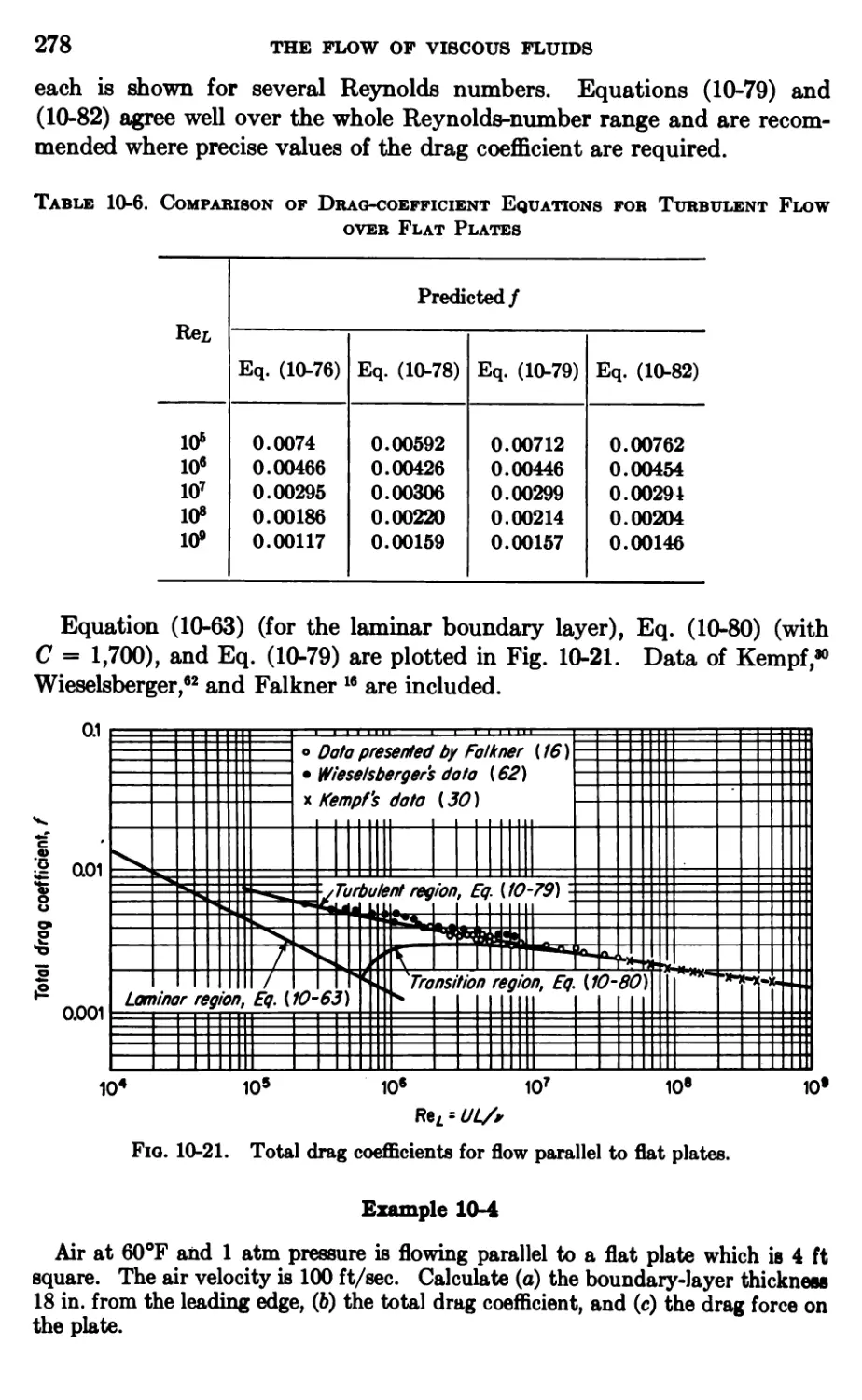
/


Текст
FLUID DYNAMICS AND HEAT TRANSFER
McGRAW-HILL SERIES IN CHEMICAL ENGINEERING
Max S. Peters, Consulting Editor
EDITORIAL ADVISORY BOARD
Charles F. Bonilla. Professor of Chemi- Walter E. Lobo. Consulting Chemical
cal Engineering, Columbia University Engineer
John R. Callaham. Editor-in-chief,
Chemical Engineering. to*** L« Word. Chairman, Depart-
Cecil H. Chilton. Editor-in-Chief, ment of Chemical Engineering, Uni-
Chemical Engineering. versitv of Delaware
Donald Ij. Kate. Chairman, Depart- MottSouder8. Associate Director of
lament of Chemical and Metallurgical 8earch> gheU Development Company
Engineering, University of Michigan
Sidney D. Kirkpatrick. Consulting Edi- Richard H. Wilhelm. Chairman, De-
tor, McGraw-Hill Series in Chemical partment of Chemical Engineering
Engineering, 1929-1960 Princeton University
BUILDING THE LITERATURE OF A PROFESSION
Fifteen prominent chemical engineers first met in New York more than 30 years ago
to plan a continuing literature for their rapidly growing profession. From industry
came such pioneer practitioners as Leo H. Baekeland, Arthur D. Little, Charles L.
Reese, John V. N. Dorr, M. C. Whitaker, and R. S. McBride. From the universities
came such eminent educators as William H. Walker, Alfred H. White, D. D. Jackson,
J. H. James, Warren K. Lewis, and Harry A. Curtis, H. C. Parmelee, then editor of
Chemical & Metallurgical Engineering\ served as chairman and was joined
subsequently by S. D. Kirkpatrick as consulting editor.
After several meetings, this first Editorial Advisory Board submitted its report to the
McGraw-Hill Book Company in September, 1925. In it were detailed specifications
for a correlated series of more than a dozen texts and reference books which have
since become the McGraw-Hill Series in Chemical Engineering.
Since its origin the Editorial Advisory Board has been benefited by the guidance and
continuing interest of such other distinguished chemical engineers as Manson Benedict,
John R. Callaham, Arthur W. Hixson, H. Fraser Johnstone, Webster N. Jones, Paul
D. V. Manning, Albert E. Marshall, Charles M. A. Stine, Edward R. Weidlein, and
Walter G. Whitman. No small measure of credit is due not only to the pionooring
members of the original board but also to those enginooring educatori and
industrialists who have succeeded them in the talk of building a permanent litoruturn for tho
chemical engineering profession.
THE SERIES
Anderson and Wenzel—Introduction to Chemical Engineering
Aries and Newton—Chemical Engineering Cost Estimation
Badger and Banchero—Introduction to Chemical Engineering
Clarke—Manual for Process Engineering Calculations
Comings—High Pressure Technology
Corcoran and Lacey—Introduction to Chemical Engineering Problems
Dodge—Chemical Engineering Thermodynamics
Griswold—Fuelsf Combustion^ and Furnaces
Groggins—Unit Processes in Organic Synthesis
Henley and Bieber—Chemical Engineering Calculations
Huntington—Natural Gas and Natural Gasoline
Johnstone and Thring—Pilot Plants^ Models} and Scale-up Methods in Chemical
Engineering
Katz, Cornell, Kobayashi, Poettmann, Vary, Elenbaas, and
Weinaug—Handbook of Natural Gas Engineering
Kirkbride—Chemical Engineering Fundamentals
Knudsen and Katz—Fluid Dynamics and Heat Transfer
Kohl and Riesenfeld—Gas Purification
Leva—Fluiditation
Lewis, Radasch, and Lewis—Industrial Stoichiometry
Mantell—Absorption
Mantell—Electrochemical Engineering
McAdams—Heat Transmission
McCabe and Smith, J. C.—Unit Operations of Chemical Engineering
Mickley, Sherwood, and Reed—Applied Mathematics in Chemical Engineering
Nelson—Petroleum Refinery Engineering
Perry (Editor)—Chemical Business Handbook
Perry (Editor)—Chemical Engineers' Handbook
Peters—Elementary Chemical Engineering
Peters—Plant Design and Economics for Chemical Engineers
Pierce—Chemical Engineering for Production Supervision
It bid and Sherwood—The Properties of Gases and Liquids
III codes, F. H.—Technical Report Writing
IIiiodes, T. J.—Industrial Instruments for Measurement and Control
Korinson and Gilliland—Elements of Fractional Distillation
Hoiimidt and Marlies—Principles of High-polymer Theory and Practice
H<mwEYER—Process Engineering Economics
Niierwood and Pigford—Absorption and Extraction
HiiHEVB—The Chemical Process Industries
Hmith, J. M.—Chemical Engineering Kinetics
Hmith, J. M., and Van Ness—Introduction to Chemical Engineering Thermodynamics
Thhybal—Liquid Extraction
Tuuybal—Mass-transfer Operations
Tvmdr and Winter—Chemical Engineering Economics
V11.BRANDT and Dryden—Chemical Engineering Plant Design
Volic—Applied Statistics for Engineers
Walab—Reaction Kinetics for Chemical Engineers
Walker, Lewis, McAdams, and Gilliland—Principles of Chemical Engineering
Williams and Johnson—Stoichiometry for Chemical Engineers
Wii*hon and Ries—Principles of Chemical Engineering Thermodynamics
WI lion and Wills—Coalt Coke, and Coal Chemicals
Fluid Dynamics
and Heat Transfer
JAMES G. KNUDSEN
Professor of Chemical Engineering
Department of Chemical Engineering
Oregon State College
DONALD L. KATZ
Professor of Chemical Engineering
Chairman} Department of Chemical and Metallurgical Engineering
University of Michigan
McGRAW-HILL BOOK COMPANY, INC.
New York Toronto London
1958
FLUID DYNAMICS AND HEAT TRANSFER
Copyright © 1958 by the McGraw-Hill Book Company, Inc. Printed
in the United States of America. All rights reserved. This book, or
parts thereof, may not be reproduced in any form without permission
of the publishers. Library of Congress Catalog Card Number 57-10224
in
35260
PREFACE
A large portion of this text was first published in 1954 as Bulletin 37
of the Engineering Research Institute at the University of Michigan. The
material in the original bulletin has been rearranged and expanded
considerably to make it more suitable for class presentation. Some new
material has been included.
Our purpose in preparing this text is essentially the same as that which
prompted the writing of the original bulletin; that is, to present the
fundamentals of fluid dynamics which are basic to an understanding of
convection heat transfer. The material is designed for a one-semester graduate
course in fluid flow and heat transfer, and this fact has necessitated the
omission of many specialized topics ordinarily included in such a course.
Such topics as settling, high-speed gas flow in nozzles and pipes, single-
und two-phase flow through porous media, compressible flow, fluidization,
mixing, conduction, radiation, and natural convection are either omitted
or mentioned only briefly. The student continuing a study of these
subjects will find the fundamental material presented here beneficial to him.
Our approach has been to present, wherever possible, the differential
equations describing the particular fluid-flow or heat-transfer problem
I wing discussed, along with the boundary conditions applicable to the
problem. Detailed solutions of the differential equation are given in only
ii few instances. Whether detailed solutions are given or not, final re-
lulionships are given in a form that can be easily applied to specific fluid-
Mow or heat-transfer problems. We have attempted to compare theoretical
liquations with experimental results. Such comparison gives the student
more faith in the theoretical approach and justifies many of the assump-
1 ions made in the analysis.
A number of illustrative examples have been included to demonstrate
Mm application of relationships presented. The problems at the end of
Mm book will also serve to acquaint the student with the application of
Mm material.
Wo feel that the subjects are presented in logical order. The basic prin-
ciplos of various types of fluid flow are presented in the first eleven chap-
Ini'M, which serve as a foundation for the discussion of several aspects of
luroed-convection heat transfer in the last five chapters. Chapter 3 may
vii
viii
PREFACE
be conveniently omitted from a course on fluid flow and heat transfer.
Some instructors may prefer to present Chap. 10 after Chap. 2.
We are indebted to the Engineering Research Institute of the University
of Michigan for permission to use the figures and much of the text which
appeared in our original bulletin. Figures from other publications are also
used, and appropriate credit is given in each case.
The literature of fluid dynamics and heat transfer is extensive. We
have tried to include the major references, to which the reader is referred
for more detailed discussion and bibliography on special topics.
We are indebted to the many workers, both past and present, without
whose work the science of fluid dynamics and heat transfer would not be
in its present advanced state.
James G. Knudsen
Donald L. Katz
CONTENTS
Preface vii
PART I. BASIC EQUATIONS AND FLOW OF NONVISCOUS FLUIDS
1. Fluids and Fluid Properties ... 3
2. The Differential Equations of Fluid Flow . 23
3. Flow of Nonviscous Fluids ... 44
PART II. THE FLOW OF VISCOUS FLUIDS
4. Laminar Flow in Closed Conduits 75
5. Turbulence 106
6. Dimensional Analysis and Its Application to Fluid Dynamics 129
7. Turbulent Flow in Closed Conduits .... 146
8. The Laminar Sublayer 213
9. Flow in the Entrance Section of Closed Conduits . 226
10. Flow of Incompressible Fluids past Immersed Bodies 246
11. Flow in the Shell Side of Multitube Heat Exchangers . 323
PART III. CONVECTION HEAT TRANSFER
12. The Convection-heat-transfer Coefficient. Dimensional Analysis in
Convection Heat Transfer 351
13. Heat Transfer during Laminar Flow in Closed Conduits .... 361
14. Turbulent-flow Heat Transfer in Closed Conduits. Empirical
Correlations for High-Prandtl-Number Fluids 391
15. The Analogy between Momentum and Heat Transfer 407
16. Heat Transfer with Liquid Metals 456
17. Heat Transfer during Incompressible Flow past Immersed Bodies . 473
APPENDIXES
I. Mathematical Terms and Vector Notation . 525
11. Complex Numbers and Conformal Mapping 528
III. Table of Nomenclature . 534
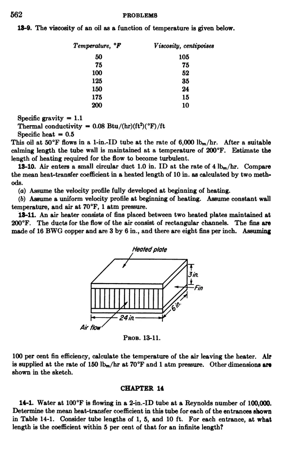
I'roltlema 543
Indtx 567
ix
PART I
BASIC EQUATIONS AND FLOW OF
NONVISCOUS FLUIDS
CHAPTER 1
FLUIDS AND FLUID PROPERTIES
1-1. Fluid Mechanics
The science of fluid mechanics is concerned with the motion of fluids
and the conditions affecting that motion. Fluids at rest are a special case
of fluid motion. Fluid kinematics is the subdivision of fluid mechanics
which is restricted to a consideration of the geometry of motion and is not
concerned with the forces involved. On the other hand, fluid dynamics is
the subdivision of fluid mechanics concerned with the forces acting on the
fluids. A further subdivision of fluid dynamics considers the state of fluid
motion, i.e., fluids at rest or in uniform motion for which the forces are in
equilibrium and fluids in unsteady motion for which the forces causing the
flow are unbalanced.
The kinematics of fluid motion is concerned with such quantities as
velocity, acceleration, and rate of discharge. To define these quantities,
length and time scalars are necessary, and it is usual to express them in
terms of some coordinate system, either rectangular, cylindrical, or spheri-
eal. The choice of coordinate system depends largely on the boundaries
of the particular system being studied. Fluid dynamics, on the other hand,
involves the application of Newton's second law of motion to the moving
mass of fluid. This law states that the applied force is proportional to
the rate of change of momentum. Such forces as pressure, shear, gravity,
uhd inertia are involved. In the momentum term, the mass and velocity
of the fluid must be known.
The various transfer processes which take place in fluids and between
nnlids and fluids are momentum, mass, and heat transfer. During the flow
of all real fluids in ducts or past immersed bodies, energy is dissipated
through the action of viscosity, and this energy, which can be expressed in
lennH of rate of loss of momentum, represents the power required to pump
the fluid. Heat transfer and mass transfer occur in the fluid under the
influence of temperature and concentration differences respectively. The
rate at which these transfer processes occur is determined by the mechanics
3
4 BASIC EQUATIONS AND PLOW OF NONVISCOUS FLUIDS
of fluid flow, knowledge of which is basic in the fundamental study of the
transfer processes and the relationship between them.
1-2. Fluid Properties
Certain physical properties of fluids are involved in any study of fluid
mechanics and the related processes of momentum, mass, and heat
transfer. These properties include density, viscosity, thermal conductivity, heat
capacity, diffusivity, and surface tension.
The physical properties of a fluid or solid are a function of temperature
and pressure. Numerous workers have measured physical properties, and
attempts have been made to establish correlations between the various
properties. Hougen and Watson7 have presented a variety of empirical
relationships for predicting the value of a particular physical property from
other properties. Theoretical studies of physical properties, particularly
those of Hirschfelder, Bird, and Spotz6 and Lyderson and coworkers,11*l2
have produced relationships for predicting physical properties based on the
molecular structure of compounds. These authors present relationships
for obtaining critical properties, densities of gases and liquids,
compressibility factors, viscosities, and thermal conductivities.
In the remainder of this chapter, the density, heat capacity, surface
tension, viscosity, thermal conductivity, and diffusivity are defined, and
their values are given for a few common substances. In most cases, the
effect of pressure and temperature on the properties is indicated. Extensive
tables of physical properties are given by Perry.16 References containing
lists of properties of materials other than those included here are also given.
1-3. States of Matter and Definition of a Fluid
All matter exists in either the solid or the fluid state. Physically, the
solid state is characterized by relative immobility of the molecules in the
solid. Each molecule has a fixed average position in space but vibrates
and rotates about that average position. The fluid state is characterized
by relative mobility of the molecules, which, in addition to rotation and
vibration, also have translational motion; so they do not have fixed positions
in the body of the fluid. Solids and fluids behave differently from each
other when subjected to external forces. A solid has tensile strength,
whereas a fluid has little or no tensile strength. A solid can resist
compressive forces, up to a certain limit, while a fluid can resist compressive forces
only if it is kept in a container and the compressive force is applied to all
walls of the container. Solids can withstand shearing stress up to their
elastic limit, but fluids, when subjected to a shearing force, deform
immediately and continuously as long as the force ia applied.
FLUIDS AND FLUID PROPERTIES
1-4. Gases and Liquids; Vapor Pressure
In the fluid state, matter exists either as a gas or a liquid. The
molecules in gases are relatively far apart from each other and have high
translational energy. Their translational energy is much greater than the energy
of attraction between them. In liquids the molecules are mobile, and their
translational energy is less than the energy of attraction between them,
with the result that the average distance between them is small and very
much less than the average distance between the molecules in a gas.
The distribution of translational energy among molecules in a liquid
follows a Maxwell distribution curve. Some molecules, therefore, have
sufficient translational energy to overcome the attractive forces of adjacent
molecules, and they escape from the liquid and form a vapor. Liquids,
consequently, exert a vapor pressure, which is the pressure attained by a
vapor when left in contact with its
liquid until equilibrium is attained, . s Critical
temperature being held constant. '
The vapor pressure is a function
of temperature, as shown by the
curve AB in Fig. 1-1. The area on
the chart above AB is subcooled
liquid. The curve terminates at B,
which is the critical point. At this
point, the translational energy of
the molecules of the liquid becomes
equal to the energy of attraction,
and the liquid and vapor become
identical with each other. The area ABC is the superheated-vapor region.
A vapor is defined as a fluid that can be liquefied by compression alone.
The area to the right of BC is the gaseous region. A gas is a fluid which
cannot be liquefied no matter how much it is compressed.
The main difference between liquids and gases from the standpoint of
fluid-flow studies is in their compressibility. Liquids at temperatures
relatively far from the critical point can be compressed only slightly at very
high pressures. For all practical purposes, they are incompressible. Gases
and vapors, on the other hand, are very compressible, and in many flow
problems this compressibility must be considered.
Temperature
Fig. 1-1. Vapor-pressure curve for a liquid.
1-5. Density and Specific Gravity
The density of matter is expressed in terms of mass per unit volume
(m/L*). The specific gravity of a substance is the ratio of its density to
the density of some reference substance. Pure water at 15.5°C is the refer-
6 BASIC EQUATIONS AND PLOW OF NONVISCOUS FLUIDS
ence substance for expressing the specific gravities of liquids and solids.
Air is the reference substance for gases, the specific gravity of a gas being
defined as the ratio of its density to the density of air, both at the same
temperature and pressure. The gas gravity is also the molecular'weight
of the gas divided by the molecular weight of air.
1-6. Liquid Density
The effect of variations of pressure and temperature on the densities of
liquids is generally considered insignificant in fluid flow; i.e., the flow is
-100 0 100 200 300 400 500 600 700
Temperature, °F
Fig. 1-2. Density of various saturated liquids.
incompressible. When the reduced temperature (ratio of temperature of
the liquid to critical temperature of the substance) is 0.5 or below, the
assumption of incompressibility involves no significant error. In the
temperature range from 0 to 100°C, the coefficient of thermal expansion of
liquids at constant pressure ranges from 2 X 10"4 to US X 10"4 (change
FLUIDS AND FLUID PROPERTIES
7
in volume per unit volume per unit change in temperature). Likewise,
the compressibility at constant temperature ranges from 2 X 10""6 to 16 X
10~6 (change in volume per unit volume per unit change in pressure)
depending on the liquid, the temperature, and the pressure.
The density of a number of saturated liquids is shown as a function of
temperature in Fig. 1-2. The freezing point, normal boiling point, and
critical point are indicated on each curve. For many liquids, particularly
the paraffin and olefin hydrocarbons, the specific gravity at the critical
point is approximately 0.25. Othmer and Gilmont13 present a nomograph
for predicting the densities of a large number of liquids.
1-7. Gas Density
The common way of obtaining the density of a gas is through an
equation of state relating the pressure, volume, and temperature. Perfect gases
obey the equation of state
PVm = RT (1-1)
where P = pressure
Vm = volume per mole
T = absolute temperature
R = gas constant
all in appropriate units to make the equation dimensionally correct. Real
gases also follow Eq. (1-1) with sufficient accuracy at reduced
temperatures greater than 2 and reduced pressures lass than 1.
Many equations of state have been developed for real gases, but they are
quite complicated and difficult to use in engineering calculations. The
simplest equation of state makes use of the compressibility factor Z.
PVm = ZRT (1-2)
Equation (1-2) is used to determine densities of gases under any condition
of temperature and pressure. The compressibility factor Z may be
obtained from a plot of the compressibility factor versus reduced pressure at
constant values of reduced temperature. Such a plot is illustrated in Fig.
1-3. Densities obtained using Eq. (1-2) and Fig. 1-3 are accurate to about
fi to 10 per cent for all gases except hydrogen and helium.
For most organic compounds, the compressibility at the critical point
is approximately 0.26.
N
3
2
10
U8
0.6
04
Q3
02
iinl
07V*
a
/5s
0.80^
vat
1 05^
^£
f
■u^^i
is
Jtt
\\
I 1 \
\h \
V
N
\
V
\
/
N
\
>n*
103
1N/0/-
s
^
"V
-/5-
=/££^
^v.<=,
^■/.j-,
V./5-
/./—:
^^
^/
•/.£
—
3
#
J /0 s RfiHurfiH temnerntnre
^
35
d^n
^
^
1)
SIBSC^
10|^
III 1 1 1 1 1
Reduced temoeroture
0^^
^
^v
^i
=iol
'/a
<J
*£\
^7
?0
-Jjl—
^4
^6
r
r
0
'
05*^^
' 06
D.9
7 1
JL. 1
0.81
-07-*
—(
28-
^^^
^^
/.rj
Vox
d
r2j
l~io.r« " » i 1 1 1 1 1
_LJ n ni no n* oa
1 ntM-nrAcciiro mnni
_L
1 I
j
-1
_L
i
—1
ai
0.2 Q25 0.3 0.4
0.6 0.8 1.0
6 7 8 910
20 25 30
2 3 4
Reduced pressure
Fig. 1-3. Compressibility factors of gases and vapors. {From 0. A. Hougen and K. M. Watson, "Chemical Process Principles," John
Wiley A Sons, Inc., New York.)
FLUIDS AND FLUID PROPERTIES
9
1-8. Heat Capacity
Heat capacity is defined as the amount of heat required to increase the
temperature of a material one degree. If the material is heated at
constant pressure, the heat capacity becomes
and when the heating is carried out at constant volume,
fdl
HI.- C' (M>
where H = enthalpy
E = internal energy
Cp = heat capacity at constant pressure
Cv = heat capacity at constant volume
The dimensions of the heat capacity are energy per unit mass per unit
temperature change {L2/t2T).
For perfect gases
Cp-Cv = R (1-5)
while for liquids and solids Cp and Cv are very nearly equal. For most
fluid-flow calculations Cp is used even though there may be pressure
variation in the fluid. For a temperature change at constant pressure
H2-H1 = (j *CpdT^ (1-6)
When both pressure and temperature change, the enthalpy change is given
"-c.tr+[-t± (;) + ;]<«> (W)
The last term of Eq. (1-7) gives the change in enthalpy due to pressure
changes. Usually it is not significant except where large pressure changes
are involved.
Heat capacities at constant pressure of some common liquids and
ICasea are shown in Figs. 1-4 and 1-5. More extensive data are given by
Perry."
10 BASIC EQUATIONS AND FLOW OF NONVISCOUS FLUIDS
1.0
£• 0.8
^ 0.6
ir 0.4
0.2
0.1
1 1
Water
Lo*t^
jtM|^
~Re
nzene
carbon tetrachloride
280
100 200
Temperature, °F
Fig. 1-4. Heat capacity of various liquids at 1 atm pressure.
3.46
3.44
342
3t40'
Hydrogen
_ 0.28
Q26
Q24
Q22
0.20
018
0 100 200 300 400 500 600 700 800
Temperature, °F
Fig. 1-5. Heat capacity of various gases at 1 atm pressure.
Cqrjj
r
on^22
\&l^-
Air
^—
FLUIDS AND FLUID PROPERTIES
11
1-9. Surface Tension
Surface tension is defined as the amount of work required to increase the
surface area of a liquid by one unit of area. The common unit of surface
tension is dyne-centimeters per square centimeter, or dynes per centimeter.
The nature of the fluid in contact with the liquid surface affects the
surface tension, but this effect is slight for liquid surfaces in contact with gases.
Othmer and Gilmont13 present a nomograph for predicting surface
tensions of a large number of liquids in contact with air. The interfacial
tension of two immiscible liquids in contact is approximately the difference
of their individual surface tensions when they are in contact with air.
1-10. Molecular-transport Properties of Fluids
The molecular-transport properties of fluids are those properties
concerned with the rate of momentum, heat, and mass transfer by molecular
motion. The rates of momentum, heat, and mass transfer in fluids may be
expressed by analogous equations. In general, the rate is proportional to
the potential gradient, the constant of proportionality being a physical
property of the substance. The equations of molecular momentum, heat,
and mass transfer are:
1. Momentum transfer:
F du
A dy
Momentum transfer
= (viscosity) (velocity gradient)
(Unit area) (unit time)
2. Heat transfer:
q dT
k— (1-9)
AQ dy
Heat transfer
—-; ——;—;—- = (thermal conductivity) (temperature gradient)
(Unit area) (unit time)
3. Mass transfer:
Nm ^ dcm
ANm dy
Mass transfer
(Unit area) (unit time)
= -D— (MO)
dy
(diffusion coefficient) (concentration gradient)
The negative sign appears in Eqs. (1-9) and (1-10) since heat transfer and
moss transfer occur only in the direction of decreasing temperature and
concentration respectively.
12 BASIC EQUATIONS AND PLOW OP NONVISCOT7S FLUIDS
1-11. Fluid Viscosity; Momentum Transfer
As a fluid is deformed because of flow and applied external forces,
factional effects are exhibited by the motion of molecules relative to each
other. These frictional effects are encountered in all real fluids and are
due to their viscosity. Consider a thin layer of fluid between two parallel
planes placed a distance dy apart
Movable plate^ profile (see Fig. 1-6). One plane is fixed,
f--M^4^<x///^^ du and a shearing force F is applied
^PX^ parallel to the other plane. Since
\ ^Fixed plate fluids deform continuously under
Area ofplate - A shear, the movable plane moves
F du steadily at a velocity du relative to
~A = &" ~dy the stationary plane. Under steady
t? i a t^ c x- r • -x conditions, the external force F is
Fig. 1-6. Definition of viscosity. '
balanced by an equal internal force
due to the fluid viscosity. The shear force per unit area (JF/L2) is
proportional to the velocity gradient in the fluid; i.e.,
F du
- = r oc — (1-11)
A dy
where r is the shear force per unit area and du/dy is the velocity gradient
(also called the rate of shear). The proportionality sign is removed by
introducing the proportionality factor ju, which is the Newtonian coefficient
of viscosity.
= ^du rib/= lbm ft 1 (lb/Xsec2^
T Qcdy Lft2 (ft)(sec) sec ft (lbm)(ft) J
The use of the conversion factor gc gives the viscosity dimensions of mass
pier unit length per unit time (m/Lt). In all flow where layers of fluid move
relative to each other as indicated in Fig. 1-6, the shearing force exerted
on the layers is defined by Eq. (1-12). The coefficient of viscosity /x is a
characteristic physical property of fluids. Its value for a particular fluid
is a function of temperature, pressure, and rate of shear. Physically, the
viscosity is the tangential force per unit area exerted on layers of fluid a
unit distance apart and having a unit velocity difference between them.
The kinematic viscosity of fluids is the ratio of the viscosity to the density.
M ft2 lbm ft3
v = - — = (1-13)
p sec (ft) (sec) lbm
The viscous force between two layers of fluid may be also expressed as
a rate of momentum transfer between the layers. By Newton's second
law of motion, force is equal to the time rate of change of momentum.
FLUIDS AND FLUID PROPERTIES
13
Therefore, the shear stress defined in Eq. (1-12) is a force per unit area
and is equivalent to a rate of change of momentum per unit area.
Consider the adjacent layers of fluid shown in Fig. 1-7 moving at velocities
u and u + du respectively. Mole- i e 2
cules moving from 1 to 2 have less FlQ ^ Adjacent layers of fluid at dif-
momentum than those in 2 and exert ferent velocities to show momentum ex-
a drag force on that layer. change.
1-12. Viscosity of Newtonian Fluids; Effect of Temperature and Pressure
The viscosity of all Newtonian liquids (see Sec. 1-15) decreases with an
increase in temperature at constant pressure. Several empirical formulas
have been proposed relating the viscosity of liquids to the temperature.
The viscosity of gases increases as the temperature increases at constant
pressure. This behavior is in accordance with the kinetic theory of gases,
which predicts that the viscosity is proportional to the density, the average
velocity of the molecules, and the mean free path of the molecules. As
the temperature increases at constant pressure, the density decreases—but
at a rate considerably less than the rate at which the velocity and mean
free path increase, with the result that viscosity increases with
temperature. The viscosities of some common liquids and gases are plotted as a
function of temperature in Figs. 1-8 and 1-9. At temperatures above the
normal boiling point, the pressure on the liquids is the saturation pressure.
For most liquids the viscosity increases with pressure at constant
temperature; however, below the critical pressure, the effect of pressure on
viscosity is small. The viscosity of gases also increases with pressure.
According to the kinetic theory, the viscosity of gases should be
independent of pressure. This is true for real gases at high reduced temperatures
and low reduced pressures. Uyehara and Watson 16 have correlated
viscosity data of fluids on a reduced basis as shown in Fig. 1-10, where m/mc
is plotted versus the reduced temperature T/Tc. Each curve is for a
constant value of the reduced pressure P/Pc> The viscosity at the critical
point is He, and may be predicted from a relation proposed by Uyehara
and Watson.16
GI.WmTc , ,
VCH
whore M — molecular weight
Tc — critical temperature, °K
Vc ■ critical volume, cc/g mole
Mfl mm critical viscosity, centipoises
BASIC EQUATIONS AND FLOW OF NONVISCOUS FLUIDS
3.0
2.0 h-A-
.2 1.0
>
\m
\ Qi_
k l\ <
Vo
■3-
^^
f^v N
tz—Frenn-t?
\n-L
\utone
^^^^^>2
SkaL .
K^2&_
100 200 300
Temperature, °F
Fig. 1-8. Viscosity of various liquids.
400
0.040
0.030
S 0.020
o
a.
1 0.015
e
u
S 0.010
o
o
M
>
0.005
0.004
tcorS
'jjjS^i
^*^
ji^-
j^!Sl^
n00f^~
Hydr
yen
0 100 200 300 400 500 600 70Q
Temperature, °F
Fig. 1-9. Viscosity of various gases at 1 atm pressure.
FLUIDS AND FLUID PBOPERTIES
15
1 \M^\A III III
iyBlvlV^
1 \w^k II 1 1 1
nW
WH
HISk^
m\v^^
^y^N^I
H—H—vf^K^
Wwvvv^
lYySvv^
051B\R
llwf>
: 1PM
Hp
a*ll\\\KNSt
i IrvNm
»°mNn
i iVK
III I N • ^ k
1 1 1 1 1 1 1 Jin\ \ f-l\ L
1 ll * ^ IXji
Mill 1 I^\\^jHjI
1 1 s\ j, \|\ \ ~^UW 1 1
Ifl^vVNrejar r-
/) *\*^\/r
r^vxT I III
1 /I /I^jH
Ix
]/[
vkb&
5f$\ -
IT
4-3
S£>b
s?,^
IS
V,
^^ Jr. 1 J
1 x|
^Y*Ctfr\ 1
Fri T
0.4 0.5 0.6 0.8 1.0
8 10
2.0 3 4 5 6
Reduced temperature
Km. 1-10. Generalized reduced viscosities. (From O. A. Uyehara and K. M. Watson,
Natl. Petroleum News Tech. Sec, 36:R764, Oct. 4, 1944.)
16 BASIC EQUATIONS AND PLOW OF NONVISCOUS FLUIDS
Figure 1-10 may be used to predict the viscosity at high pressure for both
gases ^nd liquids. Carr, Parent, and Peck8 have presented a convenient
chart to predict viscosities of gases at high pressures.
The viscosity of gaseous mixtures can be approximated by the relation
Mraix = m.f-iMl + m.f.2M2 + m.f.3/i3 H (1-15)
and for liquids
1 1 1
log = m.f.i log h m.f.2 log 1 (1-16)
thnix Ml M2
where m.f. is the mole fraction of the component. Wilke 17 has proposed
a more accurate relation than Eq. (1-15) for gases.
1-13. Thermal Conductivity
Thermal conductivity is a measure of the ability of a substance to
transfer heat by molecular conduction. The differential equation for the one-
dimensional molecular conduction of heat in a substance is
q dT
— = -fc— (1-9)
Aq dy
where q = rate of heat flow per unit time
Aq = area of flow
dT/dy = temperature gradient in material
k = thermal conductivity of substance
The sign is negative because heat is conducted from a higher temperature
to a lower temperature. For Eq. (1-9) to be dimensionally correct, the
units on the thermal conductivity are rate of energy transfer per unit
6ross-sectional area per unit temperature gradient (mL/t3T). Figures 1-11
and 1-12 depict the thermal conductivities of some liquids and gases as
a function of temperature. An approximate equation for predicting
thermal conductivities of gases is suggested by Eucken.4
fc = m(
5R\
where fc is in Btu/(hr)(ft2)(°F)/ft
Misinlbm/(ft)(hr)
CpisinBtu/(lbm)(°F)
M — molecular weight
R - 1.987 Btu/(lb mole)(°R)
For mixtures of gases, the thermal conductivity may be predicted by a
relationship presented by Lindsay and Bromley.10
FLUIDS AND FLUID PROPERTIES
17
The effect of pressure on thermal conductivity of gases may be
determined from a chart given by Lenoir, Junk, and Comings.9 In general, the
thermal conductivity is independent of pressure below reduced pressures
of 0.2. Above this value it increases rapidly with pressure.
0.50
0.40
It- 0.30
1-0.20
CD
.■g 0.15
1
1 0.10
o
o
i
0.04
1
Water
r^SSUerrach/nr;^
/VT*""*^ ^
^>^
-B^nen77===S!lm
100 150 200 250 300 350
Temperature, °F
0 50
Fig. 1-11. Thermal conductivity of various liquids at 1 atm pressure.
0.040
^ 0.030
o
CM
\ 0.020
3
m
. 0.01 5
>»
I 0.010
0.004
L^5
U^M
Y^
£^-
WS
100
200 300 400 500 600 700
Temperature, °F
Fig. 1-12. Thermal conductivity of various gases at 1 atm pressure.
The thermal conductivity of liquids may be predicted by a relation
Kiven by Palmer.14
(1-18)
18 BASIC EQUATIONS AND PLOW OF NONVISCOUS FLUIDS
where Cp is in Btu/(lbm)(°F)
p is in g/cc
M = molecular weight
AHv = latent heat of vaporization at Tb, Btu/lbm
Tb = normal boiling point, °F
Equation (1-18) is recommended when actual experimental data are
lacking. For liquid mixtures Kern8 recommends the approximate relation
Aw = w.f .ifci + w.f .2k2 + • • • (1-19)
where w.f. is the weight fraction.
The thermal conductivity of liquids is unaffected by pressure below
reduced pressures of 0.1. Above these pressures it increases with increasing
pressure. Bridgman l presents empirical data to show the effect of
pressure on the thermal conductivity of liquids.
1-14. The Diffusion Coefficient
The diffusion coefficient in a system of two components is a measure of
the rate of molecular diffusion (mass transfer) of either component under
the influence of a concentration difference. Diffusion takes place in the
direction of decreasing concentration. The differential equation for one-
dimensional diffusion is
Nm dcm
_=-=-D-= (1-10)
ANm dy
where Nm = molal rate of diffusion
An„ = area
dcm
—— = concentration gradient of diffusing substance
dy
D = diffusion coefficient
The diffusion coefficient is dependent on both the components in the
system. For gases, the empirical equation determined by Gilliland6 may
be used to predict diffusion coefficients.
t* n r
D = 0.0043 u z- I— + — (1-20)
where Vmv Vm2 = respective molecular volumes of gases 1 and 2, cc
Mi, M2 = molecular weights of gases
P = pressure, atm
T » temperature, °K
D « diffusivity, cma/sec
A more exact equation is prosented by Hiraohfelder, Bird, and Spots.6
FLUIDS AND FLUID PROPERTIES
19
Diffusion coefficients for liquid systems are not plentiful. Wilke 17 has
correlated the available data and obtained a relation for predicting
diffusion coefficients in such systems.
1-15. Types of Fluids
An ideal fluid is one which is incompressible and has zero viscosity.
With zero viscosity, the fluid offers no resistance to shearing forces, and
hence during flow and deformation of the fluid all shear forces are zero.
Many flow problems are simplified by assuming that the fluid is ideal. All
real fluids have finite viscosity, and in most cases of flow in ducts and over
immersed bodies it is necessary to consider the viscosity and the related
shearing stresses associated with deformation of the fluid. Real fluids are
also called viscous fluids. Nonviscous fluids are those having zero
viscosity, but they may or may not be incompressible. Flow of an ideal fluid is
called nonviscouSy incompressible flowy while flow of a real fluid is called
viscous flow.
Real fluids are further subdivided into two main classes. Newtonian
fluids are those for which the viscosity coefficient is independent of the
rate of shear (velocity gradient); i.e., the viscosity n in Eq. (1-12) is a
constant for each Newtonian fluid at a given temperature and pressure.
A typical shear-stress-shear-strain diagram for such a fluid is shown in
Fig. l-13a. The shear stress t is proportional to the shear strain du/dy,
Rate of shear du/dy
(tf) Newtonian fluid
Fig. 1-13. Shear-stress rate of shear relationships for fluids.
Rate of shear du/dy
{b) Non-Newtonian fluid
the slope of the line being ix/gc. Non-Newtonian fluids are those in which
tho viscosity at a given pressure and temperature is a function of the
velocity gradient. Such fluids as colloidal suspensions, emulsions, and gels are
included in this classification. The shear-stress-shear-strain diagram for
a non-Newtonian fluid is shown in Fig. 1-136. From the slope of the curve
at any point the viscosity of the fluid may be determined. A plot of vis*
uoiity versus velocity gradient is shown in Fig. 1-14.
20 BASIC EQUATIONS AND PLOW OP NONVISCOUS FLUIDS
Rate of shear du/dy
1-14. Viscosity of
Fig.
Newtonian fluid as a
rate of shear.
a
nonfunction of
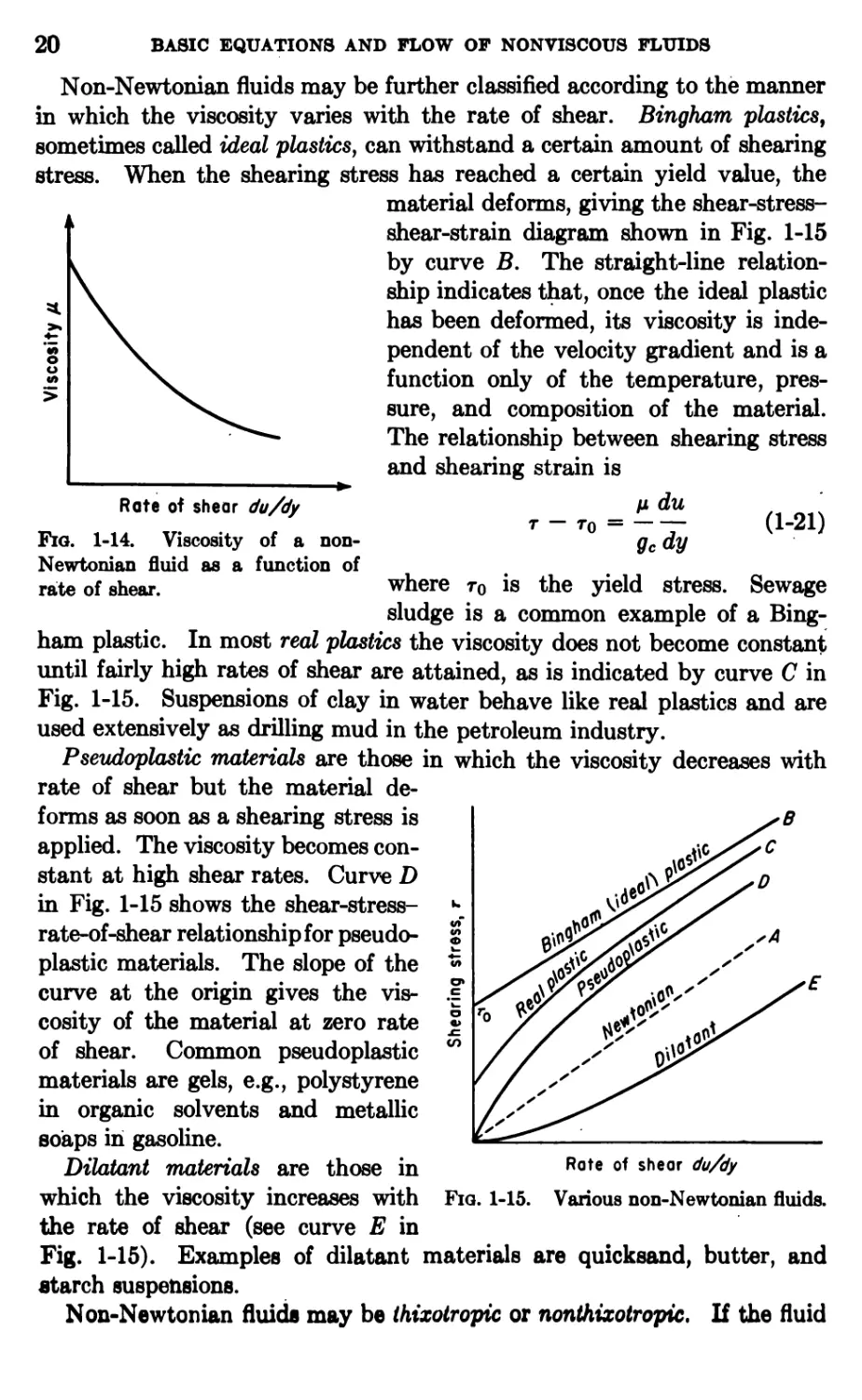
Non-Newtonian fluids may be further classified according to the manner
in which the viscosity varies with the rate of shear. Bingham plastics,
sometimes called ideal plasties, can withstand a certain amount of shearing
stress. When the shearing stress has reached a certain yield value, the
material deforms, giving the shear-stress-
shear-strain diagram shown in Fig. 1-15
by curve B. The straight-line
relationship indicates that, once the ideal plastic
has been deformed, its viscosity is
independent of the velocity gradient and is a
function only of the temperature,
pressure, and composition of the material.
The relationship between shearing stress
and shearing strain is
ix du '
r-r0 = -— (1-21)
gcdy
where r0 is the yield stress. Sewage
sludge is a common example of a
Bingham plastic. In most real plastics the viscosity does not become constant
until fairly high rates of shear are attained, as is indicated by curve C in
Fig. 1-15. Suspensions of clay in water behave like real plastics and are
used extensively as drilling mud in the petroleum industry.
Pseudoplastic materials are those in which the viscosity decreases with
rate of shear but the material
deforms as soon as a shearing stress is
applied. The viscosity becomes
constant at high shear rates. Curve D
in Fig. 1-15 shows the shear-stress-
rate-of-shear relationship for pseudo-
plastic materials. The slope of the
curve at the origin gives the
viscosity of the material at zero rate
of shear. Common pseudoplastic
materials are gels, e.g., polystyrene
in organic solvents and metallic
soaps in gasoline.
Dilatant materials are those in
which the viscosity increases with
the rate of shear (see curve E in
Fig. 1-15). Examples of dilatant materials are quicksand, butter, and
starch suspensions.
Non-Newtonian fluids may be thixotropic or nonthixotropic. If the fluid
Fig. 1-15.
Rate of shear du/dy
Various non-Newtonian fluids.
FLUIDS AND FLUID PROPERTIES
21
possesses some sort of structure which is broken down when it is subjected
to shear, then on removal of the shearing stress the viscosity, instead of
being the same as at zero rate of shear, will change with time as the fluid
builds up the structure it had prior to being deformed. If a thixotropic
fluid is tested in an apparatus in which the rate of shear can be increased
and then decreased, the relationship between the shear stress and the rate
Thixotroph
pseudoplastic
fluid
Thixotropic
f difatant
fluid
Rate of shear du/dy
Fig. 1-16. Thixotropic non-Newtonian fluids.
of shear will be found to be different when the stress is increasing than
when the stress is decreasing. Such curves for thixotropic pseudoplastic
and dilatant materials are illustrated in Fig. 1-16.
1-16. Units and Dimensions
The system of dimensions used throughout this text is a combination of
the two systems mass-length-time-temperature (m-L-t-T) and force-length-
time-temperature (F-L-t-T). The use of pounds force (lb/) and pounds
mass (lbm) is common in much engineering work. The conversion factor
between the two systems of dimensions is the gravitational constant gCy
which has dimensions mL/Ff.
BIBLIOGRAPHY
1. Bridgman, P. W.: Proc. Am. Acad. Arts. Sci., 60:141 (1923).
2. Bromley, L. A., and C. R. Wilke: Ind. Eng. Chem., 43:1641 (1951).
3. Can-, N. L., J. D. Parent, and R. E. Peck: Chem. Eng. Progr. Symposium Ser.,
[16] 61:91 (1955).
4. Eucken, A.: Physik. Z., 12:1101 (1911).
6. Gilliland, E. R.: Ind. Eng. Chem., 26:681 (1934).
6. Hirschfelder, J. O., R. B. Bird, and E. L. Spotz: Trans. ASME, 71:921 U949).
22 BASIC EQUATIONS AND FLOW OP NONVISCOUS FLUIDS
7. Hougen, O. A., and K. M. Watson: "Chemical Process Principles," John Wiley &
Sons, Inc., New York, 1947.
8. Kern, D. Q.: "Process Heat Transfer," McGraw-Hill Book Company, Inc., New
York, 1950.
9. Lenoir, J. M., W. A. Junk, and E. W. Comings: Chem. Eng. Progr., 49:539 (1953).
10. Lindsay, A. L., and L. A. Bromley: Ind. Eng. Chem., 42:1508 (1950).
11. Lyderson, A. L., R. A. Greekhom, and O. A. Hougen: Univ. Wisconsin Eng. Expt.
Sta. Rept. 4, October, 1955.
12. Lyderson, A. L.: Univ. Wisconsin Eng. Expt. Sta. Rept. 3, April, 1955.
13. Othmer, D. F., and R. Gilmont: Petroleum Refiner, 31(1) :107 (1952).
14. Palmer, G.: Ind. Eng. Chem., 40:89 (1948).
15. Perry, J. H.: "Chemical Engineers' Handbook," 3d ed., McGraw-Hill Book
Company, Inc., New York, 1950.
16. Uyehara, O. A., and K. M. Watson: Natl. Petroleum News Tech. Sec., 36:R764,
Oct. 4, 1944.
17. Wilke, C. R.: Chem. Eng. Progr., 46:218 (1949).
CHAPTER 2
THE DIFFERENTIAL EQUATIONS
OF FLUID FLOW
2-1 Introduction
Many physical problems that engineers must solve involve the
evaluation of an unknown physical quantity. Frequently this physical quantity
in a variable which is dependent on other physical quantities. The
solution of the problem involves the determination of a functional relationship
hotween the physical variables. In many cases, one is concerned with the
rates of change of the function with respect to the variables. Equations
involving an unknown function and its derivatives are differential equations.
In fluid flow there are several differential equations which result from
the application of various physical laws. In these equations the
independent variables are usually the space coordinates x, yy and z and time t. The
■Impendent variables are velocity, temperature, pressure, and properties of
I ho fluid. The important differential equations of fluid flow are:
1. The continuity equation, based on the law of conservation of mass
2. The momentum equation, based on Newton's second law of motion
3. The energy equation, based on the law of conservation of energy
2-2. The Continuity Equation for One-dimensional Flow
The continuity equation is the mathematical expression of the law of
j'ohHorvation of mass. Referring to Fig. 2-1, consider a fluid flowing parallel
In the x axis. The mass flow of fluid through a cubical element of space
liuving dimensions dx, dy, dz with its edges parallel to the x, y, z axes is
in ho determined. At the x face of the cube the fluid velocity and density
iiro, respectively, u and p. At the x + dx face the velocity and density
mo u + (du/dx) dx and p + (dp/dx) dxf where du/dx and dp/dx are the rate
ul ohange of the velocity and density with respect to x. In this system u
hihI p are the dependent variables, while x is an independent variable.
23
24 BASIC EQUATIONS AND FLOW OF NONVISCOUS FLUIDS
/
V
u
P
^/V
—^ !
dx
/\
dy J
/"
*■ X
«+#)*
*'
**&>
Fig. 2-1. One-dimensional flow through a differential element of space.
Since steady conditions do not necessarily exist, time is also an independent
variable.
A mass balance on the element is made for a differential time dt. The
mass input into the x face of the element in time dt is pu dy dz dt. The
mass output from the x + dx face in time dt is
/ dp \/ du \
[p -\ dx JI u -\ dxidydzdt
\ dx / \ dx /
which becomes, on neglecting the term containing (dx)2,
(
dp du \
pu + u — dx + p — dxjdydzdt
dx dx I
The accumulation of mass in the cube in time dt is related to the time rate
of change of density and is expressed as
dp
dt
dx dy dz dt
Making a mass balance on the cube as follows,
Input = output + accumulation
(2-D
(dp du \ dp
pu + u — dx + p — dx)dydzdt + - dx dy dz dt (2-2)
dx dx / dt
THE DIFFERENTIAL EQUATIONS OF FLUID FLOW 25
Eq. (2-2) may be simplified to
dp du dp
dx dx dt
The left side of Eq. (2-3) is an exact derivative, and the continuity
equation for one-dimensional flow becomes
- ^ = dJ. (24)
dx dt
Equation (2-4) is the differential equation expressing the law of
conservation of mass for a fluid flowing parallel to the x-coordinate axis in which
both the velocity and the density of the fluid are functions of x and t.
2-3. The Continuity Equation for Three-dimensional Flow
A similar analysis may be used to formulate the equation of continuity
for flow in three dimensions. In this analysis, however, it is convenient
to consider a point in a fluid where the velocity V may be represented by
three component velocities u, v, and w, each parallel, respectively, to the
x, y} and z axis of the rectangular coordinate system used, as illustrated
in Fig. 1-1 of Appendix I. The velocity V varies with time and position.
This variation with position may be represented by the individual
variation of the component velocities u, v, and w with respect to their individual
directions. A mass balance is made on the differential element of space,
but here, three directions of flow must be considered. The mass input
to the element in time dt is
pudydzdt (for the x direction) + pvdxdzdi (for the y direction)
+ pwdxdydt (for the z direction)
The mass output from the element in time dt is
( dp W du \
I p H dx I [ u -\ dx]dy dzdt (for the x direction)
\ dx / \ dx I
( dp \/ dv \
+ [p -\ dy J ( v H dyidxdzdt (for the y direction)
\ dy / \ dy I
( dp \( dw \
+ [p -\ dz JI w -\ dz]dxdydt (for the z direction)
V dz I \ dz /
The accumulation of mass in the cube in time dt is
dp
— dxdy dzdt
dt
Table 2-1. Fobhb of the Continuity Equation
Three-dimensional flow
Two-dimens-onal flow in
x and y direction
One-dimensional flow in
x direction
Unsteady state
Compressible fluid
d{pu) d{pv) d(pw) dp
dx dy dz dt
d{pu) d(pv) _ dp
dx dy dt
d(pu) dp
dx ™ Tt
Incompressible fluid
du dv . dw
1 1 = 0
dx dy dz
du dv
1 -0
dx dy
du
— - 0
dx
Steady state
Compressible fluid
djpu) djpv) d(pw) _
dx dy dz
d{pu) djpo) _o
dx dy
d(pu) jQ
dx ™
Incompressible fluid
du dv dw
1 1 -0
dx dy dz
du dv
1 -0
dx dy
dx
THE DIFFERENTIAL EQUATIONS OF FLUID FLOW 27
A mass balance on the cube gives, after simplification,
dp dp dp (du dv dw\ dp
-u v w p( 1 1 ) = — (2-5)
dx dy dz \dx dy dz/ dt
which may also be written as
d(pu) d(pv) d(pw) dp
-Z-l + -^-l + -^—L = _ JL (2-6)
dx dy dz dt
Equation (2-6) is the general continuity equation for three-dimensional
flow. It is a mathematical expression of the law of conservation of mass
and involves no assumptions. Using vector notation, t Eq. (2-6) may be
written
div (PV) = - ^ (2-7)
dt
All problems in fluid flow require that the continuity equation be satisfied.
If steady-state conditions prevail, all derivatives with respect to time are
zero, and Eq. (2-6) becomes
d(pu) d(pv) d(pw)
-^ + -^ + -^—^ = 0 (2-8)
dx dy dz
or div (PV) = 0 (2-9)
If a fluid is compressible, the density will vary in space, so Eq. (2-9) applies
for the steady-state flow of a compressible fluid. For the steady-state flow
of an incompressible fluid the density is constant, and the continuity
equation becomes
du dv dw
— + — + — = 0 (2-10)
dx dy dz
or divV = 0 (2-11)
Table 2-1 gives the forms of the continuity equation which apply to vari-
ou8 conditions of flow.
2-4. The Momentum Equations
Kvery particle of fluid at rest or in steady or accelerated motion obeys
Nmvton's second law of motion, which states that the time rate of change
t A description of vector notation used in this and subsequent chapters may be found
In Appendix I.
28 BASIC EQUATIONS AND PLOW OP NONVISCOUS FLUIDS
of momentum is equal to the external forces, i.e.,
and since mass is constant,
- (mu) = Fge (2-12)
at
du
m— = Fgc (2-13)
at
or (Mass) (acceleration) = external force (2-14)
The product of mass and acceleration is called inertial force. The
momentum equations of fluid flow are a mathematical expression of Newton's
second law applied to moving masses of fluid. The derivation of the
equations involves determining the inertial force of the flowing fluid in each
coordinate direction and equating it to the external forces acting on the
fluid. The three main external forces which may act on the fluid are field
forces (gravity forces), normal forces (pressure), and shear or tangential
forces (caused by the resistance of the fluid to deformation).
Inertial Forces. The momentum equations will be derived for the x
direction. Similar equations may be derived for the other two coordinate
directions, t Consider a point in a moving fluid where the velocity is V.
As pointed out in Sec. 2-3, this velocity may be represented by three
component velocities u, v, and w. In the general case of three-dimensional
unsteady flow these component velocities are functions of x, y, z, and t; i.e.,
for the x-coordinate direction
u = Fx{x,y,z,t) (2-15)
Taking the differential of each side of Eq. (2-15),
du du du du
du = —dx-\ dy -\ dz-\ dt (2-16)
dx dy dz dt
and dividing by dt,
du dudx dudy dudz du
+ —— + + — (2-17)
dt dx dt dy dt dz dt dt
Since u = dx/dtf v = dy/dt, w = dz/dt,
du du du du du
— = u— + v — + w— + — (2-18)
dt dx dy dz dt
du/dt is the acceleration in the x direction. The fluid in a cubical element
of space of size dx, dy, dz has this acceleration in the x direction. The
t More detailed derivations of the momentum equation are found in refs. 1, 8, and 4.
THE DIFFERENTIAL EQUATIONS OF FLUID FLOW 29
inertial force in the x direction is the product of the mass and the
acceleration; i.e., letting IF* be the inertial force in the x direction,
mdu
IF, = -- (2-19)
gc dt
Putting m — pdxdy dz and using Eq. (2-18),
p / du du du du\
IF* = — It* h v \-w \-—)dxdydz (2-20)
gc\ dx dy dz bit
Similar equations may be obtained for the inertial forces in the y and z
directions.
External Forces. 1. Field forces. If the fluid exists in a force field, such
as a gravitational or electrostatic field or both, then each particle of fluid
will have a potential energy which is a function of its position in the force
field. The force potential of the field is 121 and is defined as the energy
stored in a unit mass of fluid in moving it from one point to the other in
the force field. The force exerted on a unit mass is the rate of change of
12 with respect to distance. Therefore dto/dx is the force per unit mass
exerted on the fluid in the x direction, and similar derivatives hold for the
y and z directions. The field force exerted on the fluid in a spatial element
dxdydzin the x direction is
dtl
FF* = - p — dx dy dz (2-21)
dx
2. Normal and tangential forces. The state of stress at a point in a fluid
is completely defined by nine stress components,{ as follows:
px = normal stress in direction of x axis
rXy = tangential stress parallel to x plane and in direction of y axis
tVx = tangential stress parallel to y plane and in direction of x axis
pv = normal stress in direction of y axis
TVM = tangential stress parallel to y plane and in direction of z axis
t An example of a force field is the earth's gravitational field. If one considers a
massif fluid under the influence of gravity and selects some arbitrary plane where the
|K>tential energy of the fluid is>eero, then clearly the potential energy of the fluid varies
with the distance above thesarbitrary plane. Letting Z be the distance above the
arbitrary plane, the potential energy of the fluid per unit mass in terms of Z is gZ/ge. This
|K)tontial energy gZ/ge is themame.as the term 12 indicated above. Restricting changes
to those in the vertical direction, the gravitational force exerted on a unit mass is
( — ) • It becomes —ig/ge), which has dimensions of force per unit mass. The
dZ \ge/
foroo.acts vertically downward, whereas the positive direction of Z is vertically upward;
liniioe the negativetuign.
18ta, for example, ref. 4.
30 BASIC EQUATIONS AND PLOW OF NONVISCOUS FLUIDS
rzy = tangential stress parallel to z plane and in direction of y axis
pz = normal stress in direction of z axis
rzx = tangential stress parallel to z plane and in direction of x axis
rxz = tangential stress parallel to x plane and in direction of z axis
The first subscript on the shear-stress component refers to the plane parallel
to the stress, and the second subscript gives the direction in which the
stress acts.
p*+ir
dz 2
Fig. 2-2. External forces acting on the three positive faces of a small cubical element
in space.
dpx dx_
p* dx 2
dy 2 *rzx dz
dz 2
JPx dx
\/p**77T
'•144—
_ . *r„ dz
__^ /x + ~dF T
<>ryx dy
Fia. 2-8. External forouM acting in the x direction on a imall oubioul element in ipaoe.
THE DIFFERENTIAL EQUATIONS OF FLUID FLOW
31
Figure 2-2 shows all the stresses exerted on three positive faces of a
cubical element in space. In Fig. 2-3 all the stresses exerted on the
element are shown, but only those which act in the x direction are labeled.
Only three of the six shear stresses above are independent. This fact
may be demonstrated by reference to Fig. 2-4, which shows the cross
section of the fluid element of Fig. 2-3 at the plane 2 = 0.
<xy
*>/ dx
17^
L-dx
\\ 2
\
^=
~r
dy
2
J
\
■-
\*
dy
2
^L
ry* dy 2
dx
2
\ *r„ dx
y"* jx 2
\
*ryx d£
T**~ dy 2
Fig. 2-4. External forces which have a moment about the z axis.
The algebraic sum of the moments of forces about the z axis equals the
product of the mass, the square of the radius of gyration, and the angular
acceleration. Since the normal stresses and gravity forces act through
the center of the element, only the shear stresses have a moment about
the z axis. Thus, considering the counterclockwise direction to be positive,
(drXy dx
dx 2
drXy dx
dx 2
)dx
dydz —
(
dryx dy dryx dy\ dy
ryx H h Tyx : — )azdx —
dy 2 dy 2/ 2
= pdxdy dz (radius of gyration)2(angular acceleration) (2-22)
Therefore rxy — ryx = p(radius of gyration)2(angular acceleration) (2-23)
Am the size of the element approaches zero, the right side of Eq. (2-23)
Incomes zero if the angular acceleration is finite. Thus
Txy - ryx (2-24)
32 BASIC EQUATIONS AND FLOW OF NONVISCOUS FLUIDS
Similarly, it may be shown by taking moments about the x and y axis
respectively that
Tyz = Tzy (2-25)
Tzx = TXZ (2-26)
The summation of all the normal and tangential forces acting in the
x direction gives
(dpx dx dpx dx\
px -\ px -\ )dydz (on x plane)
dx 2 dx 2 /
/ dryxdy dryxdy\
+ I ryx + —— — - ryx + -— — )dxdz (on y plane)
\ dy 2 dy 2/
(drzx dz drzx dz\
rzx + —- — - rzx + —- — )dydx (on z plane) (2-27)
dz 2 dz 2/
On addition Eq. (2-27) becomes
/dpx dryx drzx\
SFX = (—+ —- + —)dxdydz (2-28)
\dx dy dz /
Application of Newton's Second Law. The application of Newton's second
law requires that the inertial force of the element of fluid be equal to the
external forces. Thus
IFX = FFX + SFX (2-29)
Combining Eqs. (2-20), (2-21), and (2-28),
p / du du du du\
— \u \- v h w 1 \dxdydz
gc\ dx dy dz dt/
dto (dpx dryx drzx\
= -p — dxdydz + [ 1 1 ) dx dy dz (2-30)
dx \dx dy dz /
Equation (2-30) is the mathematical expression of Newton's second law
of motion for the forces exerted on fluid moving through a cubical element
in space. Two similar equations may be derived for the y and z directions.
Relation between Shear Stress and Viscosity. As pointed out in Chap. 1,
the viscosity of a fluid is that property which offers resistance to shear,
and for Newtonian fluids the intensity of shear stress is a linear function of
the time rate of angular deformation. This linear function is used in Eq.
(2-30) to relate the shear stress to viscosity.
It is evident that the two-dimensional element shown in Fig. 2-5 is
undergoing angular deformation. The velocities at three corners of the
element are shown and are such that the elomont tends to assume the
THE DIFFERENTIAL EQUATIONS OF FLUID FLOW
33
Fig. 2-5. Fluid element in two dimensions showing velocities causing angular
deformation.
shape indicated by the broken lines. The angular velocity of the linear
element dx is
v + (dv/dx) dx — v dv
dx dx
The angular velocity of the linear element dy is — (du/dy). The
counterclockwise direction is considered positive. The net rate of angular
deformation of the element is the difference of the angular velocities of the elements
dx and dy.
dv ( du\ dv du
Rate of angular deformation = ( ——) = 1 (2-31)
dx \ dy/ dx dy
The relation between intensity of shear stress and viscosity is
li / dv du\
Tyz
*ZV
[i. (dw dv\
gc \dy dz/
(2-32)
ju /du dw\
Qc \dz dx)
The normal stresses pXt pVt and pt may be related to the viscosity in a
similar manner. The normal stress is proportional both to the rate of
linear deformation in the direction in which the normal stress acts and
34 BASIC EQUATIONS AND FLOW OP NONVISCOUS FLUIDS
to the rate of volume deformation of the element. For any fluid at rest
or in uniform motion the normal stresses are numerically equal to the
static pressure —P. The sign is negative since the static pressure of
the fluid is opposite to the direction of the normal stresses exerted on it.
For arbitrary motion of the fluid the normal stresses differ from — P by
an amount dependent on the rate of linear and volume deformation of
the fluid. Thus
2/x du X (du dv dw\
9c to Qc w dy dz /
Qc dx qc \dx dy
2/x dv X /du
Qc dy Qc \dx
-r^ <* i -- to dw\
vv= -p + -- + -(— + t + t) (W
dy dz/
2/x dw X (du dv dw\
Qc dz Qc \dx dy dz /
where du/dxy dv/dyy and dw/dz are the respective rates of linear
deformation in the x, y, and z directions. It is convenient to include the factor 2
in the second terms on the right-hand side of the equations. The last
term of Eq. (2-33) contains the rate of volume deformation du/dx + dv/dy
+ dw/dz. The proportionality constant X, which relates the normal stress
to the rate of volume deformation, is of the nature of a bulk modulus.
Adding Eq. (2-33),
/2/x 3X\ (du dv dw\
V* + p„+p*=-3P +(_ + -)(_ + - + — ) (2-34)
\Qc Qc/ \dx dy dz/
From Eqs. (1-5) (Appendix I) and (2-7)
{ du dv dw 1 Dp
dx dy dz p Dt
/2/x 3X\ 1 Dp
Thus Vx + w + Vz = -3P -(- + -)-— (*35)
\gc Qc/ p Dt
Equation (2-35) states that the average normal stress is different from
the static pressure by an amount proportional to the total derivative of
the density. It is assumed2 that the pressure is a function only of the
density and not of the rate of change of the density. This leads to the
requirement that the coefficient of the last term of Eq. (2-35) must be zero.
Thus
2m 3X
— + — - 0 (2-36)
Qc Qc
from which
x- -Hm
(2-37)
THE DIFFERENTIAL EQUATIONS OF FLUID FLOW • 35
i
The shear stresses and normal stresses are now expressed in terms of the
viscosity of the fluid. Combining Eqs. (2-30), (2-32), (2-33), and (2-37)
gives
p / du du du du\ dQ
-Im h v \- w 1 I dxdy dz = —p — dxdydz
ge \ dx dy dz dt / dx
\ d T 2/x du 2/x (du dv dw\ 1
+ — -P + ----^ (- + - + —)
idxl gc dx 3gc\dx dy dz/ J
d r /x (dv du\\ d f/x (du dw\\\
dy Lgc \dx dy/ J dzlgc\dz dx) J J
Equation (2-38) may be reduced to
du du du du dQ gcdP
u \- v \-w 1 = — gc
dx dy dz dt dx p dx
1 J2 d I" /du dv dw\]\ l[ d / du\ d / du\
~pl3^L \d^ dy ~dz/\) pLd^V ~dx) TyxTy)
d ( du\ d ( du\ d ( dv\ d ( dw\~]
dy
Written in vector notation, Eq. (2-39) becomes
du du du du dQ gc dP 2d
u \- v \- w 1 = — gc (/x div V)
dx dy dz dt dx p dx 3p dx
+
- div (/x grad u) + div f/x —j (2-40)
Equation (2-40) is the momentum equation for viscous flow for the x-coordi-
nate direction. Two similar equations may be derived for the y and z
directions. The momentum equations represent the mathematical
expression resulting from the application of Newton's second law of motion to
the arbitrary flow of a fluid, and they involve the relation of the shear and
normal stresses in the fluid to its viscosity.
Since Eq. (2-40) and the corresponding equations for the y and z
directions are much too complicated to be solved analytically, they must be
simplified. Any problem in fluid flow which involves the determination
of fluid velocity as a function of space and time requires the solution of
the momentum and continuity equations. In many problems it may be
more convenient to use coordinate systems other than the rectangular
system; e.g., in flow through circular tubes, cylindrical coordinates are most
convenient, and for flow past spheres, spherical coordinates may be used
Table 2-2. Momentum Equations for Various Conditions of Fluid Flow
L General equations (for
x direction
y direction
t direction
2. Viscosity constant:
x direction
y direction
* direction
3. Viscosity constant, dei
equations):
x direction
y direction
% direction
Newtonian fluids):
isity constant (Navier-Stokes
Dtt-
Dt
Dv
Dt =
Dw
Du
Dt "
Dv
Dt "
Dw
~Dt =
Du
Dt "
Dv _
Dt "
Dw
'Dt ~
dG
an
gedP 1 T2 d __
---0*divV) — div 0* grad t*)
P dx p Lo dx
0c dP K2 d
1 - — 0* div V) — div 0* grad v) ■
P By plSdy
— o"~(/*<^y V) — div (/»grad w)
p dz p L3 dz
-^^(Vu+iidivv1)
p ax V 3dx /
p dy V 3dy J
P dz \ Zdz J
p dx
-*? + '*
P d2/
p dZ
—(«£)]
-*(•£>]
-(«£)]
4. Zero Tncosfrr (Eater equations): 1
x direction
y direction
* direction
5. Steady state
6. Two-dimensional flow in x and y directions
7. One-dimensional flow in x direction
8. Steady laminar flow in a uniform horizontal circular
tube with axis parallel to x axis
Du dSl gedP
Dt ~ Qc dx p dx
Dv dQ geaP
Dt 9e ay P ay
Dw dG gedP
~Dt " "9c Yz ~ 7 dz
All derivatives with respect to time become zero
10 = 0, and all derivatives with respect to z become zero
w = 0, v — 0, and all derivatives with respect to y and z become zero
v — 0, t0 = 0 (cylindrical coordinates)
o--<^ + ,(i^ + g)
p ax Xr ar ar2/
THE DIFFERENTIAL EQUATIONS OF FLUID FLOW 39
are shown. The energy input to the element per unit time is
a
internal energy
d(upE) dx
UpE
}
dx
kinetio energy
+ -1 \pu(u2 + v2 + u?)-- [Pu(u2 + v2 + w2)] ^1
2gc I dx 2 J
pressure volume work heat oonduotion v
T d(Pu)dxl [dT d2Tdxl\
+ \Pu-^—- — -k\ -— \jdydz
L dx 2 J Idx dx2 2 J/
+ similar terms for y and z directions + q' dx dy dz + $ dx dy dz
where k = thermal conductivity of fluid
q' = time rate of energy generation (from chemical reaction) in fluid
per unit volume
$ = dissipation function
The dissipation function is defined as the time rate of energy dissipated
per unit volume because of the action of viscosity. The energy output
per unit time is
([
upE +
d(upE) dx
]
dx 2
If d dx)
+ — \9u{u2 + v2 + i*2) + - [pu(u2 + v2 + w2)]-\
2gc[ dx 2 J
T d(Pu)dx~\ [dT d2Tdx~\\
+ \Pu + -—-—\ - Jb — + -t— \)dydz
L dx 2 J Idx dx2 2 J/
+ similar terms for the y and z directions
The energy accumulated in the element consists of two parts, internal
energy and kinetic energy, i.e.,
{d( oETi Id 1
1 [p(u2 + v2 + w2)] \ dxdydz
dt 2gc dt I
Making an energy balance according to Eq. (2-1),
(d2T d2T d2T\ d(Pu) d(Pv) d(Pw) d(puE)
dy dz 2gc[dx dy
d 1 d(pE) 1 d
+ r IMu2 + v2 + i*3)] + -^ + — - [p(u2 + v2 + i^)] (»41)
6§ J dt 2g0dt
38 BASIC EQUATIONS AND PLOW OF NONVISCOUS FLUIDS
to best advantage. In subsequent chapters various types of fluid flow
are discussed, and in most cases the momentum and continuity equations
are presented. In Chap. 3 flow of nonviscous fluids, wherein the viscosity
may be assumed to be zero, is studied. In Chap. 4 and following chapters
flow of viscous fluids in closed conduits and past immersed bodies is
considered.
In many cases the nature of the flow is such that the equations may be
considerably simplified. Table 2-2 gives the momentum equations for a
variety of conditions of flow. When flow is one-dimensional in the x
direction, various terms in Eq. (2-40) become zero, and the two momentum
equations for the y and z directions are eliminated. For two-dimensional
flow, two momentum equations are required, and those terms involving
the coordinate direction in which no flow occurs become zero.
-dx
2-5. The Energy Equation for Three-dimensional Flow
When flow is nonisothermal, the temperature of the fluid is a dependent
variable which is a function of x, y, z, and t. Just as the continuity
equation is a mathematical expression of the law of conservation of mass and
gives the velocity distribution in space, the energy equation is a
mathematical expression for the law of conservation of energy and gives the
temperature distribution in space. In making an energy balance on a
spatial element of dimensions dx, dyf
| and dz, the following forms of energy
must be considered:
1. Internal, or intrinsic, energy of
the fluid E. This energy does not
include energy of position or energy
of motion.
2. Kinetic energy.
3. Pressure-volume energy.
4. Heat transferred by
conduction.
5. Energy of position or potential
energy.
6. Energy dissipated in the fluid
by viscous action.
7. Energy generated by chemical
reaction or electrical current.
In the following derivation of the
energy equation external forces and
potential energy are neglected. In
Fig. 2-6 is shown the cross section (at z = 0) of a cubical element. At
point (0,0) the various quantities required in making an energy balance
Intemol energy E
Temperature T
Pressure P
[Density p
dy
Fig. 2-6. Variables required in the
derivation of the energy equation. (All
quantities are considered to be a function
of xf y, z, and t.)
40 BASIC EQUATIONS AND FLOW OF NONVISCOUS FLUIDS
Differentiating the terms on the right side of Eq. (2-41) and making use
of the continuity equation (2-6) results in f
(d2T d2T d2T\
d(Pu) d(Pv) d(Pw) p D _ DE
= ^ + ^ + ^ + ^-(W2 + ^ + ^) + p— (2-42)
dx dy dz 2gcDt Dt
Equation (2-42) may be further simplified by considering the Euler
equations shown in item 4 of Table 2-2. Multiplying the first equation by u,
the second equation by v, and the third equation by w and adding the three
equations gives (neglecting field forces)
1 D 0 0 0 gc/ dP dP dP\
(u2 + v2 + u?) = --U — + v— + w — ) (2-43)
2Dt p \ dx dy dz/
but
/du dv dw\ dP dP dP
= P[ — + — + —) + u— + v— + w —
\dx dy dz/ dx dy dz
d(Pu) d(Pv) d(Pw)
dx dy dz \dx dy ' dz/ dx dy
(2-44)
Substituting Eq. (2-43) into (2-44) and putting the result into Eq. (2-42)
gives
DE /d2T d2T d2T\ (du dv dw\
"isr-K^+^+^)-pt+s+w+''+* <M5)
From Eq. (1-4)
DE „ DT
where Cv is the mean heat capacity at constant volume. Thus Eq. (2-45)
becomes
DT
PCV k V2T - Pdiv V + q' + $ (2-47)
The solution of Eq. (2-47) gives the temperature distribution in the
flowing fluid. Like the momentum equations, Eq. (2-47) is too complicated
to solve analytically and consequently is greatly simplified in most flow
problems.
t Note: The substantial derivative of w2, D(u2)/Dt is
d(u2) d(u*) d(u2) d(ua)
dt dx dy d§
THE DIFFERENTIAL EQUATIONS OF FLUID FLOW
41
For incompressible liquids Eq. (2-47) becomes, since div V = 0,
pCv k V2T + q' + * (2-48)
The dissipation function $ is of the following form:,_*
/du dv dw\2 [/du\2 /dv\2 /dw\2l
*—»'(5+i;+*)+*iy + (s)+(*)J
Kdw dv\2 (du dw\2 (dv du\2l
It is seen to be a function of the fluid viscosity and the linear deformation
of the fluid. It has a value of zero for nonviscous fluids. For fluids of
low viscosity and for velocities less than the sonic velocity, $ has a value
which is negligible compared to other terms in the equation. For
velocities above that of sound, $ is significant. It must also be considered in
lubrication problems involving high-viscosity fluids.
Another form of Eq. (2-47) may be obtained by utilizing the
relationship between Cv and Cp; i.e., for perfect gases
P
Cp-Cv (2-50)
PT
P
Thus CVT = CPT - - (2-51)
p
DT _ DT D /P\
Dt " P Dt Dt\p)
and Cv— = CP—-— (-) (2-52)
which becomes
From Eq. (2-5)
DT DT I DP PDp
Cv = CP + -o— • (2-53)
Dt P Dt p Dt p2 Dt
Dp /du dv dw\
JL= (_ + _ + _) (2-54)
Dt \dx dy dz/
Substituting Eqs. (2-53) and (2-54) into Eq. (2-47),
DT 0 DP
pCp ~Dt = k + ~Dt + ^ + * (2-55)
liquation (2-55) is the energy equation for perfect gases, and its solution
will give the temperature distribution as a function of x, y} z} and U
42 BASIC EQUATIONS AND PLOW OP NONVISCOUS FLUIDS
2-6. The Energy Equation for Steady Two-dimensional Flow
For flow past immersed bodies the energy equation for two-dimensional
flow is used to determine the temperature distribution in the flowing fluid.
The two-dimensional equation is approximately applicable for flow past
bodies of revolution, such as spheres, where axial symmetry prevails in
the direction of flow. For more precise results, however, the
three-dimensional equation should be used and converted to a form employing spherical
coordinates. For steady two-dimensional flow in the x and y directions
Eq. (2-55) becomes
/ dT dT\ /d2T d2T\ dP dP
A("S + -5)-*(i?+ v) + "^+"^ + ,' + * (M6)
Goldstein * points out that the term v(dP/dy) is negligible and $ can be
approximated by the term n(du/dy)2/gc. Thus, neglecting energy
generation g7, Eq. (2-56) becomes
/ dT dT\ /d2T d2T\ dP fx /du\2
°c'{u* + °lu)-k{7s + V) + u* + 7.W ("7)
Since the last two terms of Eq. (2-57) are usually negligible except above
the sonic velocity, for low-speed flows (subsonic) Eq. (2-57) becomes
/ dT dT\ /d2T d2T\
*("s+'*)-*(i?+v) •*>
Equation (2-58) is the common form of the two-dimensional energy
equation and applies for the following conditions:
(1) Perfect gases (for liquids replace Cp by Cv)
(2) Steady flow
(3) q' = 0
(4) $ negligible
(5) u(6P/dx) negligible.
2-7. The Energy Equation for Steady Flow in Circular Tubes
For steady, laminar flow in circular tubes Eq. (2-55) becomes (neglecting
the last three terms)
/ dT\ (b2T d2T d2T\
This equation is most conveniently handled by employing cylindrical
coordinates rather than rectangular coordinates (seo Fig. 4-8).
THE DIFFERENTIAL EQUATIONS OF FLUID FLOW 43
/ dT\ [d2T 1 d / dT\ 1 d2Tl
With symmetry about the axis of the tube the last term of Eq. (2-60)
becomes zero.
BIBLIOGRAPHY
1. Goldstein, S. (ed.): "Modern Developments in Fluid Dynamics," Oxford University
Press, London, 1938.
2. Kuethe, A. M., and J. D. Shetzer: "Foundations of Aerodynamics," John Wiley
& Sons, Inc., New York, 1950.
3. Lamb, H.: "Hydrodynamics," 6th ed., Cambridge University Press, London, 1932.
4. Streeter, V. L.: "Fluid Dynamics," 2d ed., McGraw-Hill Book Company, Inc., New
York, 1958.
CHAPTER 3
FLOW OF NONVISCOUS FLUIDS
3-1. Flow of Fluids with No Viscosity
This chapter deals with the flow of fluids having zero viscosity. To the
engineer accustomed to calculating friction losses and familiar with
velocity profiles and boundary layers, the value of relationships applying to
nonviscous flow may be questionable, but in a large number of fluid-flow
problems the effect of viscosity is insignificant compared to other quantities,
such as pressure, inertia force, and field force, with the result that it may
be neglected. This is particularly true of fluids having low viscosity, such
as water and the common gases.
The solution of any fluid-flow problem involves the determination of the
fluid velocity and fluid pressure as a function of time and space coordinates.
This solution can be greatly simplified if the fluid viscosity is assumed to
be zero. Typical problems where such an assumption is valid are in flow
over weirs, through orifices, in large tanks, in channel and duct entrances,
and in converging and diverging nozzles. In such problems the movement
of the main mass of fluid is of particular interest, and conditions
immediately adjacent to the solid boundary, where viscosity has a significant
effect, are not of interest.
In the following sections the classical approach to nonviscous flow is
presented. A number of examples are included to illustrate the
application of the various relationships considered.
3-2. The Equations of Motion for Nonviscous Fluids (Euler Equations)
The Euler equations of motion for three-dimensional nonviscous flow are
given in item 4 of Table 2-2. All the viscosity terms in the general
equations of motion have disappeared, leaving only the inertia terms and the
terms corresponding to field forces and normal forces.
du du du du dil g0 dP
— + u— + v— + w— - -qc - (3-1)
dt dx dy dz dx p dx
FLOW OF NONVISCOUS FLUIDS
45
dv dv dv dv d!2 gc dP
-+U — +V— + W- ge- — (3-2)
dt dx dy dz dy p by
dw dw dw dw dQ gc dP
hw \-v — + w—= -gc (3-3)
dt dx dy dz dz p dz
In addition the equation of continuity must be satisfied.
d(pu) d(pv) d(fyw) dp
_^Li + _^Z + _^_Z 1 (2-6)
dx dy dz dt
The number of unknowns in the above equations is five: u, v, w, P, p.
Since it is usually possible to express the density p in terms of the pressure
by means of an equation of state, the above four equations are sufficient
to solve for all unknowns. However, in the solution of the equations,
constants of integration appear which must be evaluated from the
boundary conditions in any specific problem.
3-3. Velocity Potential and Irrotational Flow
In integrating Eqs. (3-1) to (3-3) it is convenient to introduce a new
function 0, which is the velocity potential. The velocity potential in the
velocity field is analogous to, but not the same as, the force potential 12 in
the force field. Just as the derivative of 12 in any direction gives the force
acting on the fluid in that direction, the derivative of 4> in any direction
gives the velocity in that direction. Therefore
d<t>
-f = u (3-4)
dx
-^ = v (3-5)
9y
36
— = w (3-6)
dz
Substituting Eqs. (3-4) to (3-6) into Eq. (2-6) gives
/d2* d2* d2*\ dp dp dp dp Dp
— pi —--\ -\ J = u h v \- w = — (3-7)
9 W dy2 dz2) dx dy dz dt Dt
dy2 dz2/ dx dy
Thus, for incompressible fluids Eq. (3-7) becomes
d <f> d <f> d <f>
**-T7 + Z3 + 3-0 <«*>
46 BASIC EQUATIONS AND FLOW OF NONVISCOUS FLUIDS
Differentiating Eq. (3-4) with respect to y and Eq. (3-5) with respect to
x gives
d"d> OU
(3-9)
dy dx
d2<t>
dxdy
Subtracting Eq. (3-9) from (3-10),
dv du
du
dv
dx
= 0
dx dy
Similarly it may be shown that
(3-10)
(3-11)
(3-12)
(3-13)
The terms on the left of Eqs. (3-11) to (3-13) are the vorticity components.
It is shown below [Eq. (3-14)] that the vorticity components are twice
the rate of rotation of the fluid element. Physically these relations mean
du
— —
dz
dw
— -
dy
dw
- =
dx
dv
— — =
dz
= 0
= 0
u dx
Fig. 3-1. Velocities causing rotation of a fluid element.
that the fluid element has no rotation in space. Therefore the
assumption of a velocity potential as defined by Eqs. (3-4) to (3-6) requires
that the flow be irrotational. Referring to Fig. 3-1, the rate of rotation
of the dx element is
v + (dv/dx) dx — v dv
dx
— radians/seo
dx
FLOW OF NONVISCOUS FLUIDS 47
The rate of rotation of the dy element is
u + (du/dy) dy — u du
= radians/sec
dy dy
The counterclockwise direction is positive.
The net rate of rotation of the two-dimensional element is the average
of the sum of the rate of rotation of the dx and dy elements; i.e.,
1 /dv du\
-I ) = rate of rotation
2 \dx dy/
(3-14)
Therefore Eqs. (3-11) to (3-13) mean that there is zero angular velocity
of the fluid elements about their center. Since the fluid has zero viscosity,
no tangential or shear stresses may be applied to the fluid elements.
Pressure forces act through the center of the elements and can cause no
rotation; therefore no torque may be
applied to the fluid elements. If a fluid
element is initially at rest, it cannot
be set in rotation; if it is rotating, the
rotation cannot be changed.
The fact that flow is irrotational
does not preclude the possibility of
deformation of the fluid element. In
the flow of a nonviscous fluid between
convergent boundaries, the elements
of fluid deform as they flow through
the channel, but there is no rotation about the axis of the element. The
element in Fig. 3-2 is deformed in moving from B to C, but it has not
been rotated in space.
Fig. 3-2. Irrotational flow between
convergent boundaries.
3-4. Streamlines
A satisfactory pictorial representation of fluid flow, particularly
nonviscous flow, can be obtained by the use of streamlines. At every point in
npace the motion of the fluid can be indicated by means of a velocity
vector showing the direction and magnitude of the velocity. In place of
vectors, which are unwieldy, use is made of streamlines, which are lines drawn
tangent to the velocity vector at every point in space. For all points on
a utreamline the velocity vectors meet the streamline tangentially, and
therefore no fluid can cross the streamline. In Fig. 3-3 AB and CD are
two arbitrary streamlines. Considering the sections ab and cd between
them, tho input of fluid through ab equals the output through cd plus the
48
BASIC EQUATIONS AND PLOW OF NONVISCOUS FLUIDS
accumulation in the section abed. If the fluid is incompressible, the input
equals the output.
The components u, v, and w of the velocity V are the derivatives of
distance with respect to time; i.e.,
dx dy dz
u = — v = — w = —
dt dt dt
Since the same element of time is considered in each case,
dx dy dz
u v w
(3-15)
Equation (3-15) is the differential equation of the streamline in three-
dimensional flow.
3-5. The Stream Function for Two-dimensional Incompressible Flow
For two-dimensional flow, the streamlines can all be represented on a
two-dimensional plane. On the basis of the continuity equation and from
the nature of the streamlines a stream function ^ may be defined which is
related to the velocity of the fluid. In Fig. 3-3 let streamlines AB and CD
represent the stream functions fa and fa respectively. Considering a unit
Fig. 3-3. Streamlines and the derivation of the stream function.
thickness of fluid, fa — fa is defined as the volume rate of fluid flow
between the streamlines AB and CD. The streamline CfDf is a differential
distance away from CD, and the flow between streamlines CD and CD'
is d\f/. At a point 0 on CD the distance elements — dx and dy indicate the
PLOW OP NONVISCOUS FLUIDS
49
distance between CD and CD'. The velocity of the fluid at 0 is u and
v in the x and y directions respectively. Since no fluid crosses the
streamlines, the volume rate of flow across the element dy is u dyf and the volume
rate of flow across the element — dx is — v dx. This volume rate of flow
is d$ since flow is assumed incompressible. Thus
dip = u dy
= — vdx
Using partial derivatives, since ^ is a function of both x and yf
dy
= u (3-16)
j- = -v (3-17)
ox
Equations (3-16) and (3-17) define the stream function ^ for
two-dimensional incompressible flow. Physically, the stream function is the volume
rate of flow per unit distance normal to the plane of motion between a
streamline in a fluid and an arbitrary base streamline.
The definition of the stream function does not require that flow be ir-
rotational. However, if flow is irrotational, it may be shown that
d2+ d2+
7T + TS = ° <3"18)
dx2 dy2
3-6. Integration of Euler's Equations; Bernoulli's Equation
In order to integrate Eqs. (3-1) to (3-3) the velocity-potential equations
(3-4) to (3-6) and the equations of irrotational flow (3-11) to (3-13) are
used. Substituting these equations into Eq. (3-1) gives
d2<f> du dv dw dfl gc dP
+ u— + v— + w— + gc— + -— = 0 (3-19)
dt dx dx dx dx dx p dx
Equation (3-19) may be integrated with respect to x. The right side
becomes a function of y, z, and t. It cannot be a function of x because the
derivative with respect to x must be zero. Thus
d4> u2 + v2 + w2 gcP
-7 + r + QSl + — = Fl(y,z,t) (3-20)
dt 2 p
50 BASIC EQUATIONS AND FLOW OF NONVISCOUS FLUIDS
Similarly Eqs. (3-2) and (3-3) become, on integration,
d<t> u2 + v2 + w2 gcP
— + + gfi + — = F2(x,z,t) (3-21)
at
u2
u2
+ t? + w2
2
+ 1? + W2
d« u2 + y? + v? geP
— + z + 9Jl + — = F3(x,y,t) (3-22)
at & p
All the arbitrary functions of Eqs. (3-20) to (3-22) are equal; i.e.,
Fx(yAt) = F2(x,z,t) = F3(x,yft) (3-23)
Since Fif F2y and F3 are each functions of only two distance variables
but are all functions of t, the equality of Eq. (3-23) is satisfied if F\, F2y
and Fz are functions of t alone. The magnitude of the velocity vector V
may be expressed in terms of its components:
|V| = Vu2 + v2 + w2 (3-24)
Therefore |V|2 = u2 + v2 + t^ (3-25)
The final integrated form of the Euler equations is
d* « QcP
-± + V2 |V|2 + gSl + — = F4(t) (3-26)
at p
Equation (3-26) is Bernoulli1 s equation for unsteady flow. It considers the
rate of change of the velocity potential with respect to time, the magnitude
of the velocity of the fluid, the potential energy of the fluid, and the static
pressure. If flow is steady, Eq. (3-26) reduces to
lA IV |2 + gSt + — = const (3-27)
p
Dividing by gc gives
1 |V|2 P
- 1—L + 12 + - = const (3-28)
2 ge 9
If gravity is the only external force acting on the fluid, then the potential
energy per unit volume becomes
12 = — (3-29)
9c
where Z is the distance above some base plane where the potential energy
is zero. Substituting Eq. (3-29) into (3-28) gives the familiar form of
Bernoulli's equation for steady flow.
1 |V|2 gZ P t x
- —±- + — + - - const (3-30)
2 g0 9c p
FLOW OP NONVISCOUS FLUIDS
51
The dimension of each term in Eq. (3-30) is energy per unit mass.
Physically, the equation means that for steady, irrotational flow the sum of the
kinetic energy %(\V\2/gc)y the potential energy gZ/gc, and the pressure
energy P/p is the same at all points in space. For rotational flow, Eq.
(3-30) can be applied to a particular streamline, the constant having
different values for different streamlines [see also Eqs. (4-7) and (4-8)].
3-7. Two-dimensional, Irrotational, Incompressible Flow; the Flow Net
As pointed out in Sec. 3-3, irrotational flow implies the existence of a
velocity potential 0, defined by Eqs. (3-4) to (3-6), which, when introduced
into the continuity equation for two-dimensional incompressible flow, gives
d24> d2<f>
dx2 by2
In Sec. 3-5 it was shown that a stream function ^, defined by Eqs. (3-16)
and (3-17) for two-dimensional incompressible flow, satisfies Eq. (3-18) for
irrotational flow; i.e.,
dx2 by2
The determination of <f> and ^ for any physical problem involves the
solution of Eqs. (3-18) and (3-31). For two-dimensional motion, 4> and ^ are
both functions of x and y. The arbitrary constants resulting from the
solution of Eqs. (3-18) and (3-31) are determined from the boundary
conditions of the problem. Only one pattern of irrotational flow can exist
for a given fixed boundary.
The particular solution of Eqs. (3-18) and (3-31) for any problem will
yield <f> and yp as functions of x and y, which functions may be plotted on
the xy plane at constant values of 0 and ^. The result is a flow net
consisting of 4> curves and ^ curves, which form an orthogonal system in that
they intersect at right angles. In the limit, as the increments of 0 and ^
between the curves approach zero, the flow net becomes a network of
infinitesimal squares.
An example of a flow net is shown in Fig. 3-4, in which all lines intersect
at right angles. The lines of constant ^ represent the direction of the
velocity vector at any point. When ^ is obtained as a function of x and y,
the velocity of the fluid at every point may be obtained as a function of
x and y by Eqs. (3-16) and (3-17). Also
|V| - Vu2 + v> (3-32)
Hence the velocity at any point may be obtained in terms of x and y.
52 BASIC EQUATIONS AND FLOW OF NONVISCOUS FLUIDS
Once the velocity is known at every point, the pressure may be determined
by the application of Bernoulli's equation (3-30). The velocity
relationships existing as two-dimensional flow occurs in the xy plane of Fig. 3-4
may be derived by considering the square meshes abed and a'b'c'd' between
the two streamlines fo and ^4, the respective velocities at the center of
A
A
Sz
A
4 *z 3
*k
*,
*
*>
Fig. 3-4. The flow net.
each mesh being Vi and V2. Since no fluid crosses the streamlines fo and
^4, the amount of fluid flowing through abed is the same as through a'6'c'd'.
The volume rate of flow per unit distance perpendicular to the xy plane
is | Vi \ad for element abed and | V2 \a'd' for element a'6'c'd'. Thus
|Vx|ad= |V2|a'd'
or
jy>i
IVil
ad
ab
(3-33)
The last result of Eq. (3-33) comes from the fact that the.meshes are square.
The lines representing constant values of <f> indicate all pointB- in space
where the absolute velocity is the same.
FLOW OP NONVISCOUS FLUIDS
53
3-8. Examples of Two-dimensional, Irrotational, Incompressible Flow
In a majority of fluid-flow problems encountered in practice it is not
possible to assume that the viscosity of the fluid is zero, and hence the
Euler equations do not adequately describe the flow. There are instances
where irrotational flow is very nearly attained. Gas flow below the sonic
velocity is very nearly incompressible, and in cases where the viscous
effects are insignificant, one can assume irrotational flow and solve Eqs.
(3-18) and (3-31) in order to obtain the velocity pattern and pressure
pattern for the system. Instances where irrotational, incompressible flow
can be assumed without too much error are the discharge of fluids from
large reservoirs through small outlets, flow through small inlets into large
reservoirs, flow through converging and diverging sections of large two-
dimensional ducts, flow through sharp-edged orifices, flow over sharp-
crested weirs, and flow past pitot tubes.
3-9. Analytical Solution of Some Problems in Two-dimensional,
Incompressible, Irrotational Flow
In certain cases where the geometry of the system is quite simple it is
possible to obtain analytical solutions for \f/ and <f> in terms of x and y.
As shown in Appendix II, if a functional relationship exists between
complex numbers
<t> + i+ = Fx(x + iy) (3-34)
then the Cauchy-Riemann equations
d<f> d\P
T'T (8"35)
ox ay
d<t> ty
— = - — (3-36)
dy dx
result provided the derivative of the functional relationship is continuous
From the relations indicated in Eqs. (3-35) and (3-36) it may be shown that
Kqs. (3-18) and (3-31) for two-dimensional, incompressible, irrotational
How are satisfied.
When the complex variable <f> + fy is plotted on the <$ plane, the lines
of constant <f> and ^ will form a square-mesh flow net. A plot of <t>(x,y)
iind ^(x,y) on the xy plane will produce a network having characteristics
dependent on the functional relationship F\ in Eq. (3-34). The meshes
obtained on the xy plane will be square only if they are infinitesimal in
mjbo; however, all lines on the xy plane will intersect at right angles, and
hence the requirements of a flow net will be satisfied. A few examples
54 BASIC EQUATIONS AND PLOW OP NONVISCOUS FLUIDS
J
J
f
i
%
c
1
•
•
-»
•
/
U
•
-*• dt-0
-b. r .a- 9
"►jp-/
^ *
of functional relationships between 0 + i^ and x + iy are given below,
and the resulting flow nets are interpreted physically. A more detailed
discussion of these examples is
provided by Streeter.1
1. One-dimensional Flow of an
Infinite Fluid in the x Direction
4> + i+=U{x + iy) (3-37)
Since 0, ^, x, and y are all real,
<t> = Ux
+ =Uy
Plotting the flow net on the <W
plane and xy plane in Fig. 3-5 shows
that in both cases the net is made
up of square meshes.
The sides of the squares in the xy
plane are 1/U times the sides of the
squares in the <& plane. The flow
net shown on the xy plane depicts
the flow of an infinite fluid in the x
direction having a velocity £7.
d<t> d\f/
dx dy
velocity in x direction
d<f> fy
dy dx
velocity in y direction
Fig. 3-5. Flow net of an infinite fluid
flowing in the x direction. In irrotationaJ flow past solid
boundaries, since the boundary is always
a streamline, any streamline in the flow net may be replaced by a solid
boundary, and the flow net beyond the boundary will remain unchanged.
If two streamlines in Fig. 3-5 are replaced by solid boundaries, the flow
net will represent flow in a two-dimensional channel with parallel walls.
2. Flow along Two Inclined Planes. The form of the functional
relationship for flow along two inclined planes is
i
^ 1
• i
1
1 1
k 1
/
1
-te- df- 1
> J*
0 + if = a(x + iy)w,a 0 < a < 2t
(3-38)
where a is the enclosed angle between the two inclined planes. It is con-
FLOW OF NONVISCOUS FLUIDS
55
venient to represent both complex variables of Eq. (3-38) in polar form so
that the real and imaginary parts may be separated.
(3-39)
where R = V*2 + *2
r = Vjf + y2
From Eq. (3-39)
fle'e
_ aJ.ir/ae«(»/a)»i
R = arwla
0 = ^1
a
In the <t*p plane, when © varies from 0 to w (corresponding to the upper
half of the 4*p plane), the angle 6\ varies from 0 to a in the xy plane.
To obtain 4> and ^ as functions of x and y Eq. (3-38) may be expressed
as follows:
/ / TCv\ ^"0l\
4> + vp = arwla (cos h isin —) (3-40)
\ a at
from which <t> = ar*,a cos — (3-41)
a
+ = ar*/a sin— (3-42)
a
Example 3-1
An incompressible, nonviscous fluid is flowing along two planes inclined at an
angle of 45° with each other. At a point 5 ft from the intersection of the planes
the fluid in contact with the plane is flowing at a velocity of 5 ft/sec. Consider
one plane to coincide with the x axis and the intersection of the planes to be at
the point (0,0). Also assume that fluid flows in a positive direction along the x axis.
(a) Draw the flow net for this flow.
(6) Determine the velocity at the point (2, 0.5).
Solution
(a) From Eqs. (3-41) and (3-42), when a = x/4,
<f> = arA cos 40i
Nimilarly 4/ = ar* sin 40i
Hlnoe
cos 0i = —; - and sin0i =
y/x2 + y2 y/x* + y*
<t> = a(x4 - 6x V + j/4)
^ — 4a(x*y — xy*)
56 BASIC EQUATIONS AND PLOW OF NONVISCOUS FLUIDS
The flow net may be drawn from these relationships. From the statement of the
problem the value of a may be determined.
At point (5,0)
Thus
From which
u = ^ = a(4x3 - 12xy2)
ox
v = ^ = a(V - \2x*y)
u = 5 ft/sec
v = 0
5 = a4(5)3
a = Hoo = 0.01
The resulting flow net is indicated in Fig. 3-6.
{JiPAl ^ u-0.260ft/s9C
\V\*0.350 ft/sec
Fig. 3-6. Flow along two planes inclined at an angle of 45° to each other.
(6) The fluid velocity at the point (2, 0.5) may be calculated.
u = 0.01[(4)(2)8 - (12)(2)(0.5)2] = 0.260 ft/sec
v = 0.01[(4)(0.5)8 - (12)(2)2(0.5)] 0.235 ft/sec
Thus |V| - V(0.26)2 + (0.235)2 - 0.350 ft/sec
The direction of V is toward the x axis and makes an angle of 138° with the x axis
(Fig. 3-6).
FLOW OF NONVI8COU8 FLUIDS
57
3. Point Source or Sink in an Infinite Fluid. The function representing
a point source in an infinite fluid is
Q
* + ^ = —ln(x + ty) (3-43)
Ztt
where Q is the rate of fluid discharge from the point. Using polar
coordinates,
Since
thus
Therefore
2t
Q Q
= — In r H i0i
2ir 2ir
r= Vx2 + y2
y
di = tan -
X
Q
0 = — In Vx2 + y2
Ztt
& = — tan ' -
2t x
d« Q x
dx 2x x2 + j/2
_ dA-fL y
dy 2r x2 + y2
IVI = Vu2 + v2
(3-44)
or |V| = ^ * 2=^- (3-45)
The above results show that the magnitude of the velocity varies inversely
UN the radial distance from the point source. It is infinite at the source,
und the direction of the velocity is always radially outward from the source.
The flow net for a point source is shown in Fig. 3-7a, the velocity having a
direction away from the origin. A point sink in an infinite fluid has the
mime-shaped flow net, as indicated in Fig. 3-76, except that the direction
58
BASIC EQUATIONS AND PLOW OF NONVISCOUS FLUIDS
of all velocity vectors is radially toward the sink. The functional
relationship for a point sink is
Q
* + i+ = - — In (x + iy) (3-46)
2tt
(a) Point source {6) Point sink
Fig. 3-7. Examples of flow nets.
[c) Vortex
4. Combination of a Source and Sink. Consider a source located at x =
—a and a sink located at x = a. Fluid flows at a rate of Q volume units
per unit time per unit thickness from the source to the sink. The
functional relation for this flow situation is
Q . x + a + iy
<t> + w = — I11
2t x — a + iy
Using polar coordinates,
0 + t^ = — In
2ir r26^
(3-47)
(3-48)
where rx = V (x + a)2 + y2
r2 = V(x - a)2 + t/2
2/
0i = tan"1
x + a
y
62 = tan"1
x — a
From the above the absolute value of the velocity is
Qa
IVI =
Trrxr2
(3-49)
Stated physically, Eq. (3-49) means that the magnitude of the velocity
vector in the region about a source and Mink is proportional to th* volu-
FLOW OP NONVISCOUS FLUIDS
metric flow rate and one-half the distance between them and inversely
proportional to the radial distances from the source and sink. A flow net
of a source-and-sink combination is shown in Fig. 3-8.
Fig. 3-8. Flow net for a source and sink of equal strength.
Example 3-2
Two perforated pipes are mounted vertically in an infinitely large tank. The
pipes are situated so that the distance between them is 5 ft. Water discharges
from one at the rate of 10 ft3/(min)(ft of length) and enters the other at the same
rate. Assuming two-dimensional irrotational flow, calculate the magnitude of the
fluid velocity along a line joining the two pipes.
Solution
Equation (3-49) may be used to calculate the magnitude of the velocity vector
at any point on a line joining the two pipes.
Q = 10 ft3/(min)(ft of length)
a = 2.5 ft
At a point midway between the two pipes
ri = 2.5 ft
r2 = 2.5 ft
lirl d0)(2.5)
Thus
(t)(2.5)(2.5)
= 1.27 ft/min
Table 3-1 gives the magnitude of the velocity of the fluid as a function of the
distance from the source.
60 BASIC EQUATIONS AND FLOW OF NONVISOOUS FLUIDS
Table 3-1
Distance from
source, ft
0
0.5
1.0
1.5
2.0
2.5
3.0
3.5
4.0
4.5
5.0
|V|,
ft/min
00
3.53
1.99
1.51
1.33
1.27
1.33
1.51
1.99
3.53
oo
5. Vortex. If the function represented by Eq. (3-43) is modified as
follows:
Ti
0 + fy = — In (x + iy) (3-50)
2/TT
where r is the circulation, the resulting flow net (Fig. 3-7c) represents a
vortex. Vortex flow is represented by circular streamlines, and the
magnitude of the velocity varies inversely as the distance from the center of
the streamlines. Geometrically this flow net is the same as for a source
or sink except that for vortex flow the streamlines are circles, and the
equipotential lines are radial lines emanating from the origin. Since no
fluid can cross the streamlines, vortex flow means that fluid is circulating
about a point.
An analysis similar to that for a point source shows that for a vortex
|V| = -^ (3-51)
2irr
indicating that the magnitude of the velocity is inversely proportional to
the distance from the center of the streamlines.
6. Flow around an Infinitely Long Cylinder. For irrotational flow around
an infinitely long cylinder of radius r0, the function used to construct the
flow net is
0 + if = U (x + iy + -^—) (3-52)
\ x + xyf
where U is the velocity of the undisturbed fluid flowing in the x direction.
The axis of the cylinder coincides with the origin of the xy plane.
FLOW OF NONVISCOUS FLUIDS 61
Separating the real and imaginary parts of Eq. (3-52) gives
*-v'(1 + *T?) <"»>
The streamlines corresponding to ^ = 0 are the x axis and the boundaries
of the cylinder. Figure 3-9 shows a flow net around a cylinder. From
Eqs. (3-53) and (3-54)
2 2x2r02 I
d<t> f r0
+ y2 (*2 + j/2)2 J
(3-55)
d<t> -2r02xy
v = — =U , * (3-56)
dy (x2 + ^)2
Fig. 3-9. Flow net for uniform flow past a circular cylinder.
It is of interest to show how the velocity varies at the surface of the
cylinder. Since
r2 = x2 + y2
x = r cos 0i
and r = r0 at the surface of the cylinder
u = U(2 - 2 cos2 Si)
v = U(—2sm6i cosfli)
from which | V| = 2U sin 6X = 2U sin 6 6 = t - 6Y (3-57)
liquation (3-57) gives the magnitude of the fluid velocity at the surface of
the cylinder at any angle B\ measured in a positive direction from the
positive x axis. Thus the forward part of the cylinder, which is encountered
llrit by the fluid, corresponds to a value of $i = t.
62 BASIC EQUATIONS AND PLOW OF NONVISCOUS FLUIDS
Since sin 6 = sin (tt — 0i), Eq. (3-57) would be unchanged if the angle
6 were measured in a clockwise direction from the negative x axis, i.e.,
measured from the forward part of the cylinder.
Example 3-3
An infinitely long cylinder 3 in. in diameter is placed in a wind tunnel in which
air is flowing at the rate of 80 ft/sec. The air is at 60°F and 1 atm pressure.
Assuming incompressible, irrotational flow, determine (a) the magnitude of the air
velocity adjacent to the surface of the cylinder and (6) the pressure of the air
adjacent to the cylinder.
Solution
(a) Measuring the angle 6 from the forward point of the cylinder, Eq. (3-57) may
be used to determine the velocity at the cylinder surface. A tabulation of the
velocity as a function of 0 is shown in Table 3-2.
Table 3-2
*, deg,
measured from
forward point
0
30
60
90
120
150
180
Ve, ft/sec,
at surface of
cylinder
0
80
139
160
139
80
0
Pe -P,
lb//ft2
7.62
0
-15.24
-22.86
-15.24
0
7.62
(6) The pressure distribution over the cylinder may be determined by Bernoulli's
equation (3-30). Neglecting gravity forces, Eq. (3-30) becomes
1 t/2 P = 1 |V,|2 P9
2 ge 9 2 ge p
where V* and P$ are, respectively, the velocity and pressure at the angle 6 measured
from the forward point and U and P are the velocity and pressure of the undisturbed
air. At 60°F and 1 atm the density of air is 0.0764 lbm/ft8. Values of P9 - P are
tabulated in Table 3-2.
The pressure distribution over the surface of the cylinder may be
expressed in terms of 6 by means of Eq. (3-30).
/>#-P«-?-([/'- |V,|a)
FLOW OF NONVISCOUS FLUIDS 63
From Eq. (3-57)
Pe- P = — (C72 — 4C72 sin2 6)
2gc
pu2
Pe- P = (1-4 sin2 6) (3-58)
20c
At e = o, |v#| = o
pU2
Pe^>-P = — (3-59)
2gc
Equation (3-58) may be used to predict the pressure distribution over
the surface of the cylinder for nonviscous flow. It is also applicable for
the flow of viscous fluids up to a value of 6 = 60°. Equation (3-59)
expresses the impact pressure at the leading edge of the cylinder. The
impact pressure is the pressure resulting from the complete conversion of the
kinetic energy of the fluid into pressure energy.
3-10. Approximate Construction of a Flow Net
In most cases the geometry of the system under consideration is such
that an analytical solution of Eqs. (3-18) and (3-31) is extremely difficult,
if not impossible. In these instances the flow net may be constructed by
making use of the symmetry of the system and the fact that the fixed
boundaries are also streamlines. The various examples of flow nets
mentioned in Sec. 3-9 may be used to construct the flow net of a more
complicated system. For example, in the case of a fluid discharging from a large
tank through a small outlet one may consider that the outlet appears as
a point sink to the fluid a large distance from it, and the flow net will be
the same as for a point sink. Only in the vicinity of the outlet will the flow
net differ from that for a point sink. The flow net is constructed by first
drawing equally spaced streamlines, the number depending upon the
accuracy required. The equipotential lines (constant <t>) are then drawn at
right angles to the streamlines so that approximately square meshes are
obtained throughout the whole system. The equipotential lines are normal
to the solid boundaries.
The accuracy of construction may be checked by also drawing the
diagonals of the meshes, which should also form an orthogonal system of
curves.
Example 3-4
Water is flowing out of an infinitely large reservoir through a rounded outlet
having parallel sides 1 ft apart. The rounded portion of the outlet has a radius of
64 BASIC EQUATIONS AND PLOW OF NONVISCOUS FLUIDS
6 in. Velocity of flow in the outlet is 5 ft/sec. Assume flow is two-dimensional,
incompressible, and irrotational.
(a) Draw the flow net.
(b) Show how the velocity changes along the center line as the water flows from
the reservoir and through the outlet.
(c) Making use of Bernoulli's equation (3-30), show the pressure distribution
along the center line of the outlet.
Solution
(a) The streamlines are first drawn. Referring to Fig. 3-10, the distance between
the two boundaries of the outlet is divided into six equal spaces, and the streamlines
Ay By C, D, Ey Fy and G are indicated as parallel lines in the outlet.
The corresponding streamlines in the infinite fluid on the left of the figure are
A'y B'y C, D'y E'y F'y G'. Streamlines A'A and G'G coincide with the fixed
boundaries of the system. An infinite distance to the left of the outlet the fluid flows as if
the outlet were a point sink at 0. Consequently the flow net a large distance from
the outlet is the same as shown in Fig. 3-76 for a point sink, with all streamlines
pointing radially to the center of the outlet. These streamlines are shown as
*?
N D'
\
A'
\
\
\
\
^ V
-+B
f2 Stream tine tt
\ "£
tO 9\0 8
\ ^ \
V' A x
7 6 5A
>c \
f 3 2 t . „*•
-►/■ 1
Zf\
z \
^G
F' ^— \G'
Fig. 3-10. Flow net for flow through a rounded outlet (Example 3-4).
broken lines in Fig. 3-10. To draw the actual streamlines it is necessary to
construct smooth curves joining the radial streamlines A'y B't C, D', E', F'y G' to the
parallel lines A, B, C, D, Ey Fy G. Since A'A and G'G coincide with the boundary
and D'D is the central streamline, only B'B} C'Cf E'E} F'F need be estimated. The
equipotential lines are drawn so they intersect the streamlines at right angles. The
completed flow net is shown in Fig. 3-10 for the lower half of the outlet.
PLOW OF NONVISCOUS FLUIDS
65
(b) To obtain the velocity along the center D'D consider the points 1 to 12
(Fig. 3-10). The spacing between the streamlines or equipotential lines may be
used to give the velocity approximately midway between the lines. The velocity
Table 3-3
Points
1-2
2-3
3-4
4-5
6-6
6-7
7-8
8-9
9-10
10-11
11-12
Distance between
equipotential
lines on
streamline D'D, in.
2.0
2.0
2.0
2.05
2.10
2.50
2.80
3.30
4.70
6.20
9.1
Velocity on
streamline D'D at
midpoint between
equipotential lines, ft/sec
5.0
5.0
5.0
4.9
4.8
4.0
3.6
3.0
2.1
1.6
1.1
P - Pi-2
along
streamline
D'D, lb//ft2
0
0
0
0.96
1.90
8.72
11.70
15.50
20.0
21.8
23.2
in the outlet is 5 ft/sec. In Table 3-3 the distances between equipotential lines are
indicated, and the velocities midway between these lines are calculated from Eq.
(3-33).
The distance between equipotential lines at points 1 and 2 (where the velocity is
5 ft/sec) is 2.0 in. At points 6 and 7 the distance between equipotential lines is
2.5 in. Thus the velocity | Vc-71 midway between points 6 and 7 is, by Eq. (3-33),
,VM|-^-«fV-c
The direction of this velocity is the tangent streamline D'D. The velocity along
streamline D'D is plotted in Fig. 3-11.
(c) The pressure distribution along D'D is obtained from the velocity distribution
by means of Bernoulli's equation (3-30). Neglecting gravity forces, Eq. (3-30)
becomes
1 |Vl-2|2 Pl-2 = 1 |V|- P
2 ge 9 2 ge p
where V1-2 and P1-2 are the velocity and pressure, respectively, midway between
I mints 1 and 2 and V and P are the velocity and pressure at any other point in the
fluid. Therefore
P-PM-£(|VM|»-|V|»>
66 BASIC EQUATIONS AND FLOW OF NONVISCOUS FLUIDS
12 11 10 9 8 7654321
25
20
|^15
I
A 10
^w— —Tr*\—ill——
\ o I I I I I
1 1 I I ^wi I o l^>
I
3 -
.2?
|
2 >
Fig. 3-11. Velocity and pressure distribution along streamline D'D of Fig. 3-10.
This relation may be used to calculate the pressure along the streamline D'D. For
example,
|Ve.7| = 4 ft/sec
P«-7 — Pl-2 =
62.4
(2)(32.2)
8.7 lb//ft:
l(5)2 - (4)2
3-11. Separation
The solutions to the examples of Sees. 3-9 and 3-10 are based on irrota-
tional flow. Flow is usually rotational, but nevertheless the flow net
obtained for irrotational flow is very useful. If the fixed boundaries of the
system are parallel or converge so that the streamlines converge, the actual
flow will be very nearly irrotational except immediately adjacent to the
solid boundary. However, if the streamlines of a flow net diverge rapidly,
as they would for divergent boundaries, the actual flow will be quite
different from that indicated by a flow net; i.e., the assumption that the
limiting streamlines coincide with the fixed boundaries is not valid when
the boundaries are divergent. The flowing fluid tends to leave the
boundary whenever the streamlines are divergent. This is separation. The flow
net obtained for irrotational flow is very useful in determining regions
in a system where separation is likely to occur.
In the system shown in Fig. 3-10, as long as flow is from left to right, the
streamlines are convergent, and there is no tendency for separation; how-
FLOW OF NONVISCOUS FLUIDS
67
._qL_
[a) Rounded inlet
w
~-\&i
id) Sudden expansion
and contraction
ever, if flow is from right to left, the streamlines diverge, and separation
will occur. The region of separation for this type of inlet is shown in Fig.
3-12a. Separation also occurs during flow through abrupt contractions and
enlargements in conduits (Fig. 3-126), through abrupt bends (Fig. 3-12c),
and past bodies of revolution (Fig. 3-12d).
The region between the separated fluid and the solid boundary is in a
state of turbulent motion, a condition which causes a reduction of the
efficiency of flow. It is therefore
desirable to design boundaries which
have the least tendency to cause flow
separation. This is an important
factor in the design of airfoils. As
shown in Fig. 3-12d, there is
considerable tendency for separation to
occur during flow past a circular
cylinder because of the rapidly
diverging streamlines in the region
past the center of the cylinder. If
the cylinder were elliptical in shape,
the streamlines would diverge more
slowly, and the tendency for
separation would be reduced. It is
desirable to design the solid boundary so
that the actual flow agrees closely
with the flow net based on irrota-
tional flow.
The fact that streamlines diverge in a flow net means that there is a
tendency for separation to occur. Whether separation occurs or not
depends on the velocity, density, and viscosity of the fluid. For a given fluid,
separation will not occur until a certain velocity is reached.
O,'
ic) Abrupt bend (</) Circular cylinder
Fig. 3-12. Regions of separation (the
broken lines indicate approximately the
path of the separated fluid).
8-12. Stagnation Points
A stagnation point is any point in a fluid where the velocity is zero.
For two-dimensional, irrotational, incompressible flow, the conditions
required for the velocity to be zero are
u = — = 0
dx
d<f>
»« — = 0
dy
(3-60)
(3-61)
The stagnation pressure P9t is the pressure at the stagnation point and,
68 BASIC EQUATIONS AND FLOW OF NONVISCOUS FLUIDS
from Eq. (3-30), may be expressed in terms of P and V, the pressure and
velocity at any other point in the field.
p|V|2
P.t = P + ^-^ (3-62)
2gc
An example of a stagnation point is the leading edge or forward point of
a body immersed in a flowing fluid. Inspection of Eqs. (3-55) and (3-56)
shows that at the point x = —r0,y = 0 (the leading edge of the cylinder)
both u and v are zero; hence this is a stagnation point. The stagnation
pressure at this point is given by Eq. (3-59), which is equivalent to Eq. (3-62).
Example 3-5
An open tank car is 30 ft long, 8 ft wide, and 7 ft deep. It contains water to a
depth of 5 ft and is in a train traveling at 60 iniles/hr.
(a) Determine the slope of the surface of the liquid in the tank when the train
goes around a curve having a radius of 1,000 ft.
(b) What is the minimum length of time at constant deceleration in which the
train can stop without spilling the water?
Solution
In this problem the body of the fluid is being accelerated, so Eq. (3-1) reduces to
du _ d!2 gcdP
dt c dx p dx
In the case of rotation about an axis, the acceleration du/dt is directed toward the
center of rotation and is given by the relation
(angular velocity) 2(radius)
(a) The angular velocity of the tank car on the curve is
(60)(5,280)
(3,600)(1,000)
= 0.088 radian/sec
du
^ = -(0.088)2(1,000)
at
(Negative sign is used because acceleration is toward the center.) The slope of the
liquid surface is required. Along the surface P is constant, so dP/dx = 0. Letting
y be the height of the liquid surface above a datum plane of zero potential energy,
12 = ^
9c
_ du dy
Tbm' *-"'£
(Partial derivatives may be changed to total derivatives since du/dt - constant.)
FLOW OP NONVISCOUS FLUIDS
Therefore,
dy
dx
_ldu
gdt
(0.088)2(1,000)
32.2
0.240
which is the average slope of the liquid surface in the tank car.
(6) If the liquid is not to be spilled, the deceleration must be such that the
surface of the liquid just reaches the top edge of the car as shown.
Example 3-5
The slope of the surface dy/dx is 4/30. Along the surface (P = constant)
from which
du
— = acceleration = —
ot
du dy
di
(32.2)(4)
dt 9dx
30
= -4.29 ft/sec2
Thus the time to stop the train at 60 miles/hr (88 ft/sec) is
-88
-4.29
20.5 sec
Example 3-6
The pressure at the top of a natural gas well is 1,500 psia. The well contains
essentially pure methane and is 10,000 ft deep. The average temperature in the
well is 100°F. Compute the pressure at the bottom of the well by two methods:
(a) Using the average value of the compressibility factor and temperature.
(6) Using the average density qf the gas in the well.
Solution
The pressure at the bottom of the well may be obtained from
Eq. (3-1). (Take x — 0 at bottom of well and increasing as we
move up well.) Since the fluid is stationary, Eq. (3-1) becomes
c dx p dx
*—\P
In the earth's gravitational field
12-
xg
9c
x=0-
EXAMPLE 3-6
70 BASIC EQUATIONS AND FLOW OF NONVISCOT7S FLUIDS
(x = 0 is datum, or position of zero potential energy). Thus
P
Letting Po equal the pressure at x = 0 and P equal the pressure at x = x,
integration gives
Q~ JPn P
From Eq. (1-2)
Letting
where
Thus
JPo P
- - ZnRT
P
n =
29(Gr)
Gr = the gas gravity (air = 1)
1 _ RTZ 1
P
and
9c ho
29(Gr) P
p ZRT dP
29(Gr) P
Integrating, assuming average values of Z and T,
= 0
ZRT . P
-In —
0
from which
or
(a) For methane
ge 29(Gr)~P0
Po = 29(Gr) gx
P ZRT gc
_ _ T29(Gr)gl
p^Pexnzm:\x
Gr = i%9 = 0.552
Critical temperature = 343°R
Critical pressure = 45.8 atm
Assuming Z to be 0.90 (estimated from conditions at the top of the well),
2Q(Gr)gx = (29)(0.552)(32.2)(10,000) =
ZRTge (0.90)(1,543)(560)(32.2)
Thus Po - l,500e0206
= 1,845 psia
To check assumption of compressibility factor:
A 1,845 + 1,500 %a§70 .
Average pressure = -—- = 1,673 psia
Reduced pressure
2
1,673
From Fig. 1-3
(14.7)(45.8)
Reduced temperature - 8fl%48 - 1.63
Z-0.90
2.48
FLOW OF NONVISCOUS FLUIDS 71
This value checks with original assumption, so Po = 1,845 psia. The integration
may be carried out using an average density. Thus
gx P0 - P
Qe Pav
1 ZRT 1
Pav 29(Gr) Pav
(using average values of Z and T). Since
P -Po + P
F" 2~~
it may be shown that
1 + [29(Gr)g/2ZRTgc]x
r° M - [29(Gr)g/2ZRTge]x
(b) Again assuming Z = 0.90,
29(Gr)gx
- 0.103
_ (1,500)(1.103)
0~897 P
2ZA7V,
P
Methods (a) and (6) check.
BIBLIOGRAPHY
1. Streeter, V. L.: "Fluid Dynamics," 2d ed., McGraw-Hill Book Company, Inc., New
York, 1958.
PART II
THE FLOW OF VISCOUS FLUIDS
In the flow of all real, Newtonian fluids, the viscosity plays an important
role in determining the flow pattern and the energy requirements to move
the fluid. Indeed, a considerable portion of energy dissipated during fluid
flow results from the fact that the fluid has a finite viscosity. As pointed
out in Chap. 3, it is possible, in some instances, to neglect the viscous
terms in the Navier-Stokes equations and from the resulting Euler
equations to solve for the incompressible flow pattern and pressure distribution
for a particular system. The solutions of the Euler equations give accurate
flow patterns for certain types of boundaries, and the flow nets obtained
are useful in predicting points of stagnation and regions of separation in
the system.
As a nonviscous fluid flows past a solid boundary, the fluid immediately
adjacent to the boundary has a finite velocity determined by the conditions
of flow and the geometry of the boundaries. On the other hand, for the
flow of viscous fluids it is generally assumed that there is no slip between
the fluid and the solid boundary. In other words, as the fluid moves past
a solid boundary, the fluid immediately adjacent to the boundary has the
same velocity as the boundary. This assumption of no slip at the wall is
valid except for the flow of rarefied gases and for fluids which do not wet
the wall. The vicinity of the boundary is therefore a region where the
fluid velocity changes from that of the boundary to that of the main stream
of the fluid, and in this region velocity gradients exist in the fluid. As a
consequence, the flow of the fluid is rotational, and shear stresses are
present. This region of changing velocity is known as the boundary layer. The
boundary layer Extends from the solid boundary to the point in the fluid
at which the velocity gradient becomes zero.
Heat and mass transfer take place to fluids from solid boundaries. In
cither case heat or mass must pass through the boundary layer. The
manner of fluid flow in the boundary layer is important since it must be known
in order to predict rates of heat and mass transfer to or from the fluid.
In addition, the boundary layer is a region where energy is dissipated
74
THE PLOW OF VISCOUS FLUIDS
through viscous action, and the energy consumption in moving the fluid
can be predicted from information about the flow in the boundary layer.
The major portion of the remainder of this book is devoted to a
consideration of the flow of viscous, Newtonian fluids, velocity profiles in
boundary layers, friction losses during flow, and the relation of the rate of
heat transfer to the velocity profiles and friction losses. For the most part,
two main types of flow will be considered, conduit flow, or internal flow,
where the fluid completely fills a closed, stationary conduit, and immersed
flowj or external flow, where the fluid flows past a stationary immersed solid.
CHAPTER 4
LAMINAR FLOW IN CLOSED CONDUITS
4-1. Introduction
Nearly every operation of fluid transport, heat transfer, and mass
transfer involves the flow of viscous fluids in some form of a closed conduit.
The frictional resistance of fluids as they flow through pipes and fittings
and the rates of heat and mass transfer between fluids and pipe walls are
important quantities in the design of pipelines and equipment. A
complete knowledge of the mechanism of the flow of fluids in pipelines is basic
to the understanding of the processes which occur during the flow. In this
chapter laminar flow in several types of closed conduits is considered in
detail. Theoretical expressions are derived for the velocity distribution in
these conduits. Isothermal laminar-flow friction factors are derived, and
theoretical values are compared with those obtained experimentally.
4-2. The Energy Equation for a Steady-flow Process
The majority of processes involving flow in conduits are steady-flow
processes. The application of the law of conservation of energy to these
processes gives the so-called flow equation. Figure 4-1 shows a system
through which a fluid is flowing steadily between points 1 and 2. Between
these pointsj*energy may enter or leave the fluid. Assuming no
accumulation, the energy balance between points 1 and 2 is
mU22 mgZ2 mU2 mgZi
E2 + + -2-5 + P2V2 = E1 + + ^— + P1V1 + q
<*gc 9c <*9c Qc
where E « internal energy of fluid of mass m
m = mass of fluid
U «■ average velocity
Z - height above datum
P ■■ static pressure
75
(4-1)
76
THE FLOW OP VISCOUS FLUIDS
V = volume of mass m
q = energy in the form of heat added to fluid
w" = energy in the form of work done by fluid
The subscripts 1 and 2 refer to points 1 and 2 respectively. Equation (4-1)
P\
v i
IP,
Datum plane
Fig. 4-1. Steady-flow system.
may be expressed in various forms.6 Since H = E + PVt where H is the
enthalpy of the fluid,
/mU2\ (mgZ\
AH+ Al )+ Al-^-J = q-w" (4-2)
V olqc / \ gc I
When limiting internal energy to heat and compression effects, Eq. (4-1)
becomes
f TdS + A (—) + A (—) + f VdP = q-w" (4-3)
The flow of all viscous fluids is a process in which the irreversible dissipa-
n
tion of energy occurs. Thus / TdS, which is the increase in internal
energy of the fluid due to heat effects, is equal to the heat absorbed from
the surroundings plus all other energy dissipated into heat effects because
of such irreversibilities as friction; i.e.,
J TdS = q+ Iw (4-4)
where Iw is the lost work, i.e., energy that could have done work but was
dissipated in irreversibilities in the flowing material.
Combining Eqs. (4-3) and (4-4),
f2 /mU2\ /mgZ\
I VdP+ A I j + A (-M - -w" - to (4-5)
LAMINAR PLOW IN CLOSED CONDUITS
77
Equation (4-5) is expressed in terms of a unit mass of material by dividing
by m.
f*dP A(U*) A(gZ) . -
I 1 1 = — w — Iw (4-6)
J\ 9 <*Qc Qc
where p = m/V and w and Iw refer to a unit mass of fluid. Equations (4-1)
to (4-6) assume steady flow and neglect chemical, electrical, and surface
effects in defining the internal energy.
For the flow of an incompressible fluid and when w is zero, Eq. (4-6)
becomes
AP A(U2) g —
— + -^-^ + - AZ Iw (4-7)
p <*gc Qc
Bernoulli's equation (3-30) for the steady flow of an incompressible, non-
viscous fluid may be written as
AP A\V\2 g
— + -I-1 + - AZ = 0 (4-8)
9 2gc gc
There are two main differences between Eqs. (4-7) and (4-8). The
kinetic-energy term in Eq. (4-7) uses the average velocity of the fluid in
the conduit. Since the velocity varies across the conduit, the kinetic
energy of the whole stream is obtained by integration, and the value of a
is obtained in this way. For laminar flow in circular tubes a has a value
of 1 and for turbulent flow a value close to 2. In Eq. (4-8) the kinetic-
energy term uses the absolute value of the point velocity. Equation (4-7)
contains a dissipation term Iw not appearing in Eq. (4-8). The dissipation
term is due to the finite viscosity of the fluid and represents the energy
dissipated by fluid friction. The dimensions on the terms in Eq. (4-7) are
energy per unit mass (FL/m). It is usual to express Iw in the farm of a
pressure loss due to friction, i.e.,
'2 -dPf —
- = Iw (4-9)
f
where — dPf is the pressure decrease equivalent to the energy lost because
of friction. From Eqs. (4-7) and (4-9), for a conduit of uniform cross
section
AP g APf
— + - AZ (4-10)
9 9c 9
4-3. Conduit Flow and the Formation of the Boundary Layer
When a viscous fluid flows in a closed conduit, the boundary layer extends
from the wall to a point in the fluid where the velocity is a maximum.
The velocity gradient at this point of maximum velocity is zero.
78
THE PLOW OF VISCOUS FLUIDS
Entrance
Thickness of Edge of
boundary layer-j boundary layer -»
Fully developed
conduit flow z
a
Fig. 4-2. Formation of the boundary layer and velocity profiles at the entrance of a
circular tube.
The boundary layer does not form immediately at the entrance of the
conduit but builds up in the entrance region. At the point where the fluid
enters the conduit the boundary layer has zero thickness. The thickness
increases along the length of the conduit and eventually becomes constant
some distance from the entrance. Figure 4-2
illustrates the formation of the boundary layer in the
entrance section of a conduit. The fluid enters the
conduit at point a with a velocity of U. Velocity
profiles are shown at points a, 6, c, d, and e. At
point a the velocity is uniform across the section of
the conduit. At point e the boundary layer is
completely formed, and from this point onward it has
constant thickness. The dotted lines between a
and e indicate the edge of the boundary layer.
Beyond point e the influence of the entrance upon
the pattern of flow has disappeared and fully
developed conduit flow is said to exist.
4-4. Shearing Stresses in a Fluid Flowing Steadily
in a Circular Conduit
Shearing stresses are present in the boundary
layer. Since these stresses are exerted in a direction
opposite to the direction of flow, they represent a
force of resistance to the flow. When flow occurs
in a closed conduit, the shear stress at the wall rw
may be expressed in terms of —dP//dxf the
pressure loss due to friction.
Figure 4-3 shows a vertical conduit with fluid
flowing upward. The pressure at point 1 is P. At
point 2 distance dx downstream from point 1 the
pressure is P + dP. The shear forces rw acting
Fig. 4-3. Forces acting
on a differential element
of fluid flowing steadily
in a circular tube.
LAMINAR FLOW IN CLOSED CONDUITS
79
on the fluid at the wall are exerted in a direction opposite to the direction
of flow. For steady flow the summation of forces on the cylindrical
element must be zero.
pressure forces fluid weight shear forces
SF = irrJP - m-JiP + dP) -mrjdxp-- tir^T*dx = 0 (4-11)
9c
Simplifying Eq. (4-11) and dividing by p«rw2,
dP g 2rwdx , ^s
-dx - 0 (4-12)
P Qc pr*>
Substituting Eq. (4-10) (in its differential form instead of its integrated
form) into Eq. (4-12),
T" = 71T (4"13)
where rw is the shear stress on the fluid at the wall. Equation (4-13)
relates the shear stress to the radius of the tube and the pressure gradient
due to friction. At any arbitrary radius the shear stress in the fluid is t,
and by a similar force balance
r -dPf
2 dx r:
(4-14)
The results expressed by Eqs. (4-13) and (4-14) indicate that the shear
stresses in the fluid are related to the lost-work terms or friction losses.
Fig. 4-4. Shear-stress distribution in a fluid flowing in a circular tube.
These relationships may be used to calculate shear stresses when the
friction losses are known. Equation (4-14) shows that for steady flow in a
circular conduit the shear stress in the fluid is a linear function of the
distance from the axis of the tube. This linear distribution is shown in Fig. 4-4.
4-6. The Friction Factor
Numerous studies on the friction losses occurring during turbulent flow
have indicated that they are proportional to the kinetic energy of the fluid
80
THE PLOW OF VISCOUS FLUIDS
per unit volume pU2/2gc and the area Aw of the solid surface in contact
with the fluid. This is the basis of the definition of the friction factor.
Viscosity has been found to have but slight effect during turbulent flow.
The force of resistance F is expressed as
fpU2
F=J^—AW (4-15)
2gc
The quantity / is a proportionality factor. Rearranging Eq. (4-15),
F fpU2
— = — (4rU)
Aw 2gc
c Velocity U
Resisting force F ^ /— Area A*
Fig. 4-5. Resistance of a solid surface in a flowing fluid.
The resisting force is opposite to the direction of flow. F/Aw corresponds
to shear force at the wall rw (see Fig. 4-5.) Hence
fpU2
r, = ^— (4-17)
2gc
Combining Eqs. (4-17) and (4-13), replacing rw by dw/2t and solving for/,
Qcdw —dPf
2p\J2~dx
Equation (4-18) defines the Fanning friction factor for flow in circular
tubes. It is expressed in terms of the tube diameter, fluid density, fluid
velocity, and the pressure gradient equivalent to the frictional resistance
per unit length of tube.
From Eq. (4-18) the lost work due to friction may be determined in
terms of the friction factor. Rearranging Eq. (4-18),
-dPs 2fU2
- = -—dx (4-19)
p gcdw
Integrating Eq. (4-19),
/ 2 -dPf - ( 2 2fU2
/ = lw= -1—dx (4-20)
J\ p J\ gcdw
Substituting Eq. (4-20) into (4-6),
/ — + + -AZ«-tZ>-/ 2L_ dx (4.21)
J\ P olQc Qc J\ Qcdw
/= _^ (4_ig)
LAMINAR PLOW IN CLOSED CONDUITS
81
4-6. Other Expressions for the Friction Factor in Tubes
There are several definitions of friction factors for flow in conduits. The
friction factor originally defined by Blasius3 and used by Moody,16 Rouse,23
Brown,6 and others is four times the Fanning friction factor and will be
referred to as the Blasius friction factor fBf where
fs = J7W---L (4-22)
pU2 dx
Thus fB = 4/ (4-23)
Other writers define a friction factor which is twice the size of the Fanning
friction factor.
4-7. The Hydraulic Radius of a Conduit
Whenever fluid flow in noncircular conduits is considered, it is necessary
to determine some characteristic length term to use in the calculation of
the Reynolds number and the friction factor. For circular pipes it is the
diameter of the pipe, but for conduits having cross sections other than
circular a new length term must be defined. This length term is four times
the hydraulic radius, which is defined as
the ratio of the cross-sectional area of
the conduit to the wetted perimeter.
Figure 4-6 shows a noncircular conduit // Area A \^ Perimeter p
through which a fluid is flowing. The
pressure gradient due to friction along
the length of the conduit is —dP//dx.
The shear at the solid boundary of the „ ^ , . , .
, ., . ,, „ /a *n\ r* Fig. 4-6. Closed conduit of lr-
conduit is expressed by Eq. (4-17). Con- regular crog8 section
sidering a length of conduit dx and a
balance of forces like that used in deriving Eq. (4-11) and making use of
Eq. (4-10) results in
A(-dPf) = rwpdx (4-24)
where p is the wetted perimeter. Substituting (4-17) in (4-24) gives
fpU2
A (-dPf) = J-— p dx (4-25)
2gc
which, upon rearrangement, gives
82
THE FLOW OF VISCOUS FLUIDS
Equation (4-26) is the same as Eq. (4-18) except that the diameter dw has
been replaced by the term 4A/p, which is the equivalent diameter de of the
noncircular conduit. The expression A/p is the hydraulic radius rh. For
circular conduits the equivalent diameter is the diameter of the tube.
The above definition for the hydraulic radius and equivalent diameter is
suitable for conduits which have constant cross section; however, there are
conduits in which the cross-sectional area varies in a periodic manner with
the length, and for these three types of hydraulic radii have been defined,
namely,
maximum cross-sectional area
(nOnu* TT1 —- (4-27)
wetted perimeter
minimum cross-sectional area
(nOmin = — — (4-28)
wetted perimeter
volume of free space per unit length
and rv = -— (4-29)
area of wetted surface per unit length
The last term, rVf is the volumetric hydraulic radius. As before, the
equivalent diameter is four times the hydraulic radius.
I. LAMINAR FLOW IN CIRCULAR TUBES
4-8. Laminar and Turbulent Flow in Tubes
In 1883 Osborne Reynolds M published a series of papers describing his
experiments on the "circumstances which determine whether the motion
of water shall be direct or sinuous,
and of the law of resistance in
parallel channels." This classical
experiment consisted of injecting dye
into water flowing in glass tubes.
Figure 4-7 is a reproduction of the
flow patterns published by
Reynolds, showing that, under certain
conditions of velocity and tube
diameter, the streak of dye in the
^ fluid continued at the center of the
_ , w ~ , , , . „.,„. tube and flowed in a line parallel to
Fig. 4-7. Color bands in a fluid flowing xi • £ xi_ x i_ /-n- a m \
in a circular tube. [From 0. Reynolds, the aX1S °f the tube <Flg' 4"7a)'
Trans. Roy. Soc. {London), 174A:935 Under other conditions of velocity
(1883).] and diameter the color band was
distributed throughout the cross
section of the tube a short distance from the tip of the needle injecting the
dye (Fig. 4-76). When the tube was viewed by the light of an electric
£s
(*)
^
id)
&
i
LAMINAR PLOW IN CLOSED CONDUITS
83
spark, the mass of color was resolved into distinct curls, indicating rapidly
changing eddies having circular motion, as shown in Fig. 4-7c. Reynolds
determined critical velocities at which laminar (direct) flow changed into
turbulent (sinuous) flow and found that the critical velocity was
proportional to the kinematic viscosity of water and inversely proportional to the
diameter of the tube. Combining these two results leads to the equation
cv
tfcrit = — (4-30)
dw
where C7crit = critical velocity
v = kinematic viscosity
dw = tube ID
c = proportionality constant
The value of the constant c is between 1,900 and 2,000.
Equation (4-30) may be rearranged to give
v
The quantity on the left-hand side of Eq. (4-31) is dimensionless if
consistent units are used. This dimensionless group is the criterion for
determining whether laminar or turbulent flow is the stable form under given
conditions. Reynolds showed that, when dwU/v was less than 1,900, the
flow was laminar but when the value of the group became greater than
2,000, the flow was turbulent. This dimensionless group is known as the
Reynolds modulus or the Reynolds number and is usually written Re (or
A^Re)- It is useful because it is a dimensionless quantity and indicates the
manner of flow for any fluid in any size of pipe.
In laminar flow (Fig. 4-7a) the particles of fluid move in a direction
parallel to thetsolid boundaries, and there is no velocity component normal
to the axis of the conduit. In turbulent flow (Figs. 4-76 and c) there is
considerable mixing of the fluid during flow. A particle of fluid has an average
velocity parallel to the axis* of the conduit, but its motion is chaotic, and
it has instantaneous velocities both parallel and perpendicular to the axis.
The shear stresses in the fluid, which are due to the viscosity, tend to
stabilize the unidirectional motion of a fluid particle in flow, while inertia
forces, which are due to the weight and velocity of the fluid, tend to dis*
rupt the unidirectional flow. It is these forces which determine the exist-
once of laminar or turbulent flow in a system.
4-9. Velocity Profiles for Laminar Flow in Circular Tubes
Fully developed isothermal laminar flow of an incompressible fluid in a
horizontal tube whose axis coincides with the x axis of the rectangular
coordinate system may be dewritart by a simplified form of the equations
84
THE FLOW OP VISCOUS FLUIDS
shown in item 3 of Table 2-2. Since the fluid has no velocity components
normal to the axis of the tube, v and w are zero; flow is steady, so all
derivatives with respect to time become zero; the flow is fully developed, so du/dx
is zero. Under these conditions the differential equation for such flow is
gcdP /d2u d2u\
(4-32)
/ -r cos 0
2 - r sin ^
Fig. 4-8. Relation between cylindrical and rectangular coordinate systems.
It is convenient to express Eq. (4-32) in terms of cylindrical coordinates
xf r, 6 rather than rectangular coordinates x, y> z. The relation between
the two coordinate systems is shown in Fig. 4-8.
n gcdPM
0 = h v
p dx
/l du dzu 1 d2u\
Flow is symmetrical about the x axis, so the derivative with respect to 6
becomes zero. Equation (4-33) may be rewritten as
gcdP _v d / du\
p dx r dr\ dr)
(4-34)
Equation (4-34) is a second-order differential equation which may be solved
to obtain u in terms of r by integrating with respect to r holding x constant.
Two boundary conditions are necessary to evaluate the two arbitrary
constants appearing in the solution of a second-order differential equation.
These boundary conditions are as follows:
Atr = 0
du
dr
Atr
u
=
=
B
0
rw
0
axis of the tube
(velocity gradient is zero)
tube wall
(no slip at the wall)
LAMINAR PLOW IN CLOSED CONDUITS 85
Integrating Eq. (4-34) and introducing the boundary conditions gives
M=-TLT-0V'-r2> (445)
4/x ox
Equation (4-35) relates the point velocity at any radius to the viscosity,
the pressure gradient, and the radius of the tube. If the tube is not
horizontal, the point velocity is expressed by
4 \v dx u dx/
where x is measured along the axis of the pipe and Z is the elevation above
a datum plane. For a vertical pipe dZ/dx = 1.
The maximum point velocity Umax is obtained from Eq. (4-35) by letting
r = 0. Hence
Umax = --J- — **2 (4-37)
4/x dx
from which it will be seen that
-££-!= <«»
4/x dx rw2
Substituting Eq. (4-38) into (4-35), the point velocity is obtained as a
function of the maximum point velocity.
U = Umax(l "^) (4-39)
The average velocity is defined by
U = - = —- (4-40)
Q = _Q
A irru
where U = average velocity
Q = volumetric rate of flow of fluid in tube
A = cross-sectional area of tube
Q may be expressed in terms of the point velocity u by integration over
the (Toss section from r = 0 to r = rw. The incremental discharge at a
mdiuH r through an annular ring of thickness dr is
dQ = 2irrudr (4-41)
Hubitituting the value of u given in Eq. (4-39) and integrating from r = 0
In r ■ rwt
«-*"-/. T"UJ*—— (t42)
86
THE FLOW OF VISCOUS FLUIDS
/
The average velocity U may now be found from Eqs. (4-40) and (4-42).
U =
iru*
2wru
Thus, from Eqs. (4-39) and (4-43), the point velocity is
(4-43)
(4-44)
Equation (4-44) expresses the point velocity u at any radius r as a
function of the average velocity U and the tube radius rw. The form of the
equation indicates that the velocity profile is parabolic in shape. Figure
4-9 shows a velocity profile for incompressible, isothermal, laminar flow in
Fig. 4-9. Parabolic velocity distribution for isothermal, incompressible, laminar flow
in a circular tube.
circular tubes calculated from Eq. (4-44). Experimental investigations of
Senecal and Rothfus M and Ferrell, Richardson, and Beatty 10 have
essentially substantiated Eq. (4-44). Ferrell and coworkers studied the flow of
water and glycerol in a 3^-in.-ID glass tube. Point velocities were
measured in the region from 0.06 to 0.002 in. from the tube wall, and good
agreement with the parabolic velocity-distribution equation was obtained.
A dye-displacement technique was used to measure point velocities close
to the wall. Senecal and Rothfus measured the velocity distribution for
the isothermal flow of air in J4- and %-in.-ID smooth tubing. At
Reynolds numbers near 1,000 the measured velocity distribution agreed well
with Eq. (4-44). Departure from the parabolic distribution was observed
as a Reynolds number of 2,000 was approached. The results of these
investigations are shown in Fig. 4-10. The points represent experimental
data, while the curves are plots of Eq. (4-44).
Equation (4-43) has been verified experimentally by Stanton and Pan-
nellM for the flow of air and water in circular tubes and by Senecal and
Rothfus » for the flow of air. The latter two workeri found that in the
LAMINAR PLOW IN CLOSED CONDUITS 87
Distance from tube wall, inches
Km. 4-10. Comparison of experimental and theoretical velocity profiles for laminar
(low in circular tubes. Points represent experimental data; curves are plotted from
I0q. (4-44). (From V. E. Senecal, Ph.D. Thesis, Carnegie Institute of Technology, 1952.)
Iloynolds-number range from 500 to 2,000 the ratio of average velocity in
tho tube to maximum velocity at the center was 0.5 (Figs. 7-3 and 7-4).
4-10. Shear Stresses and Friction Factors for Laminar Flow in
Circular Tubes
For laminar flow the shear stress in a fluid is related to the viscosity by
IC<|. (1-12). For circular tubes, since r = rw — y, the shear stress on the
fluid at any radius r is
88
100
10
&
c
.o
S i.o
0.1
THE FLOW OF VISCOUS FLUIDS
Reynolds number dwU/r
1000
10,000
0.1
1 E
g. {4-52
I
')
^
I
Data of Stanton and Panne//2*]
e Thickoil
oAir
Data of Senecal ond Rothfus™
e Air
optc
^ #
■fP
•^'
•
3
O
u
rh
0.01 5
10 100 1000
Reynolds number dmllb
Fig. 4-11. Laminar-flow friction factors in circular tubes.
The shear stress exerted at the wall is
0.001
rw =
Prom Eq. (4-44)
gc \dr/r=r„
/du\ _ 4f7
\6V/r=r rw
Substituting Eq. (4-47) into (4-46),
rw =
4mC7
gcrw
(4-46)
(4-47)
(4-48)
Equation (4-48) gives the shear stress exerted at the wall for laminar flow
in terms of the viscosity, the average velocity, and the radius. Combining
LAMINAR FLOW IN CLOSED CONDUITS
89
Eqs. (4-13) and (4-48) and letting rw = dw/2, where dw is the inside
diameter of the tube, results in Poiseuille's equation l8 for laminar flow in tubes.
-dP, Z2nU
(4-49)
dx gdw
Equation (4-49) relates the pressure loss due to friction to the fluid
viscosity, the average velocity in the tube, and the tube diameter. From
Eq. (4-18)
-dPf 2fpU2
—L = -^— (4-50)
dx Qt/Av
Combining Eqs. (4-49) and (4-50),
32m£7 2/pU2
g<4m2 g<4u
Solving for /,
(4-51)
16M 16
f = j7r = r- (4-52)
dwUp Re
Equation (4-52) relates the friction factor to the Reynolds number for
laminar flow in circular tubes. The data of Stanton and Pannell26 and
Senecal and Rothfus M plotted on Fig. 4-11 show agreement with Eq. (4-52)
up to a Reynolds number of 2,000.
4-11. Nonisothermal Laminar Flow in Circular Tubes
It was assumed in the integration of Eq. (4-32) that the viscosity and
density of the fluid were constant. This is essentially true for isothermal,
incompressible flow. If the fluid is being heated or cooled, the properties
urn also variable, and Eq. (4-34) should be written considering these
facte >rH, namely, the variation of viscosity with temperature and the way in
which the tube-wall temperature varies with length.
For the heating of liquids during laminar flow in tubes, McAdams14
pointa out that the isothermal parabolic velocity profile is distorted and
fliittoned. This is due to the fact there is a radial temperature gradient in
Iho fluid. The high temperature near the wall causes a reduction in the
vlncoHity of the liquid, and the layers of fluid flow at a greater velocity.
('onvorsely, when the liquid is being cooled, the liquid near the wall has a
higher viscosity than that near central core, and the velocity profile be-
rnmoH more pointed than for isothermal laminar flow.
DeinHlor9 mathematically analyzed the nonisothermal laminar flow of
K»i*oh and liquid metals in a circular tube for constant rate of heat transfer
90
THE FLOW OP VISCOUS FLUIDS
if/a
2.25
2.00
1.75
1.50
1.25
1.00
0.75
0.50
0.25
n
i i
V5
"V7
^f/TS
^ 0
6\
—-i
0.2
0.4
0.6
r/rw
0.8
1.0
Fig. 4-12. Velocity distribution for laminar flow of the common gases in circular tubes.
(From R. G. Deissler, NACA TN 2410, July, 1951.)
along the tube. For gases the variation of viscosity, thermal conductivity,
and density were considered. Figure 4-12 shows the theoretical velocity
profiles obtained by Deissler for the common gases. The ratio u/U is
plotted versus r/rw at constant values of Tw/Tb, where Tw is the
temperature of the tube wall and Tb is the bulk temperature of the fluid. For
heating, Tw/Tb is greater than 1, and the velocity profile is pointed; while
for cooling, Tw/Tb is less than 1, and the profile is flattened. These results
agree with those of McAdams for liquids, since the viscosity of gases
increases with temperature. Figure 4-13 shows Deissler's analytical results
for liquid metals, which also agree with those of McAdams.
LAMINAR FLOW IN CLOSED CONDUITS 91
2.50
2.25
2.00
1.75
1.50
u/U 1.25
1.00
0.75
0.50
0.25
0
0 0.2 0.4 0.6 0.8 1.0 1.2
r/rw
Fio. 4-13. Velocity distribution for laminar flow of liquid metals in circular tubes.
(From R. G. Deissler, NACA TN 2410, July, 1951.)
n. LAMINAR FLOW IN ANNULI
4-12. Flow in Annuli
Flow in annuli is encountered in double-pipe heat exchangers, in which
ono fluid flows in the inner tube and the other flows in the annular space,
rtuch flow in the annular space may be either laminar or turbulent
depending on the Reynolds number. Theoretical equations may be derived for
the laminar-flow velocity profiles in annuli, but the geometry of the annu-
lui, although simple, makes the laminar-flow velocity-profile equation
somewhat more complicated than that for circular tubes.
Flow in two types of concentric annuli, plain annuity and modified annuli,
will be considered. Plain annuli consist of two smooth concentric tubes,
while modified annuli consist of an outer, smooth tube and an inner, con-
92
THE FLOW OF VISCOUS FLUIDS
centric, finned tube, the purpose of the fins on the outer surface of the
inner tube being to increase the surface area for heat transfer. The finned
tube may have either transverse or longitudinal fins.
4-13. Isothermal Laminar Flow in Plain Annuli
Figure 4-14 shows a cross section of a plain annulus consisting of an
outer tube with inside diameter d2 and an inner tube with outside diameter
d\. The respective radii of the tubes are r2 and r\. A velocity profile is
shown, with the velocity of the fluid at the boundaries of the annulus
assumed to be zero. At some point between the two walls of the annulus
Outer tube
Fig. 4-14. Cross section of a plain concentric annulus showing the velocity profile for
laminar flow.
the point velocity reaches a maximum value. Hence, in the derivation of
the velocity-profile equation for laminar flow, the following boundary con^
ditions apply:
At r = ri
u = 0
At r = r2
u = 0
At T = Tmax
U = ^mai
du
0
dr
The differential equation for laminar flow in horizontal annuli is the same
as that for circular tubes. The first integration of Eq. (4-34) gives
gcdPr2 du
= r hci
fjL dx 2 dr
(4-63)
LAMINAR FLOW IN CLOSED CONDUITS 93
By the boundary condition r = rmax, du/dr = 0, the constant Ci becomes
9c dP 2
rmax- Hence, substituting this value of cx in Eq. (4-53),
2/x dx
f^V-O-r? («4)
2/x ox or
Integration of Eq. (4-54) gives
gc dP /r2 2 \
— —-( — - rmax In r 1 = u + c2 (4-55)
2/x dx \2 /
At r = ri and r = r2 the point velocity u is zero, which gives the following
values of c2: 2
c2 = ^ — ( ^- - rLx In r2 ) (4-56)
2/x dx \ 2 /
or
2m ax V 2 /
From Eqs. (4-56) and (4-57) the value of rmax is determined in terms of rx
and r2.
r—V«mSm) (4"58)
Equation (4-58) is the theoretical position of the point of maximum velocity
for laminar flow in an annulus.
Combining Eqs. (4-55) and (4-56), one obtains the expression for the
point velocity in an annulus.
2\x dx \2 2
The average velocity is given by
fr%
I 2irru dr
Jri
u = ~= /, .„ (^°)
Q
A r(r22 - rx2)
Integration of Eq. (4-60) results in
U " " r T" <r»' + r>2 " 2r2"«) (^
O/i OX
liy dividing Eq. (4-59) by (4-61) the point velocity may then be expressed
l>y r22 - r2 - 2ri„ In (r2/r)
« " 2C/ r'+r' »> (4_62)
94
THE PLOW OF VISCOUS FLUIDS
Equation (4-62) is the relationship between the point velocity at any radius
r, the average velocity, and annulus dimensions, for laminar flow in an
annulus. It is a function of the radius of both tubes comprising the
annulus. As rx approaches zero, Eq. (4-62) becomes identical with Eq. (4-44).
A limited number of experimental data are available on laminar velocity
profiles in annuli. Rothfus21 determined velocity profiles for the laminar
H
3
sec
Velocity, ft/
«
1
0
0
7
111
°1
f
o
8/
1 0
0
Oft
0
rt=0.250in.
r2* 1.539 in.
Re = 1820
o Rothfus data
— EqX4-62)
9
o
U
«tl
3
1
)city, ft,
ro
£
1
n
o
o
rt = 1.000 in. 1
r2*1.539in. '
Re*1250
0.2 0.4 0.6 0.8 1.0 1.2 1.4 1.6 1.0
[a) Distance from axis of annulus, inches
1.2 14
1.6
Kb)
Fig. 4-15. Comparison of experimental and theoretical velocity profiles for laminar
flow in plain annuli. (Data from R. R. Rothfust Ph.D. Thesis, Carnegie Institute of
Technology, 1948.)
flow of air in two different annuli having the following dimensions: r2 =
1.539 in., rx = 0.250 in. and r2 = 1.539 in., rx = 1.000 in. Rothfus's
experimental data are shown in Fig. 4-15, where the point velocity u is plotted
versus the radius r. The curves were obtained by calculating the
theoretical point velocities from Eq. (4-62). Figure 4-15 shows that Eq. (4-62)
agrees closely with the experimental data obtained in the annulus in which
ri = 1.000 in. However, for the annulus in which rx = 0.250 in., neither
the profile nor the theoretical value of rmax shows good agreement with the
experimental data.
Prengle 1J> and Rothfus, Monrad, Sikchi, and Heideger M studied laminar
and turbulent flow in concentric annuli. Prengle's dye experiments
indicated that the laminar velocity profile agreed with Eq. (4-62) up to a
Reynolds number of about 700. [For annuli, the diameter term in the
Reynolds number is the equivalent diameter d2 — d\ calculated from Eq.
LAMINAR PLOW IN CLOSED CONDUITS
95
(4-27).] Above this Reynolds number the point of maximum velocity did
not agree with that predicted by Eq. (4-58). Rothfus et al.22 showed that,
for Reynolds numbers ranging from 900 to 1,700, rmax was greater than
that given by Eq. (4-58) while above a Reynolds number of 1,700 it was
less. When Reynolds numbers greater than 10,000 were attained, flow was
turbulent, and the point of maximum velocity agreed with that predicted
by Eq. (4-58).
4-14. Shear Stresses and Friction Factors for Laminar Flow in
Plain Annuli
The rate of shear in the fluid at any radius r during laminar flow in the
annulus is given by Eq. (4-45). Differentiating Eq. (4-62) with respect to
r gives
Bu 4C/(rL, - r2)
dr r(r22 + r,2 - 2rLx) '
From Eqs. (4-45) and (4-63) the shear stress t at any radius r is given by
9Ar22 + n2 - 2ri„)
for r < rmax (4-64)
W(r2 - HU
gcr(r22 + n* - 2r2n„)
letting r = rx and r2 in Eqs. (4-64) and (4-65), respectively, r\ and T2, the
shear stresses at the walls of the annulus, may be obtained. The ratio of
these two shear stresses is
2 = ^"-^ (4-66)
Equation (4-66) could also be derived by making a balance of forces on a
differential length dx of annular fluid, as was done in the derivation of Eq.
(4-13). Although Eq. (4-66) was derived above using relationships
applying to laminar flow alone, it also holds for turbulent flow in annuli.
Rothfus and coworkers22 measured shear stresses at the boundaries of two
annuli during turbulent flow. Their experimental results agree well with
those predicted by Eq. (4-66).
Considering a differential length dx of annular fluid between r\ and r2,
It may be shown that
~*Pf _ 2(Tar2 + rm)
dx r22 — ri2
96
THE PLOW OP VISCOUS FLUIDS
It also may be shown, by considering appropriate portions of the annular
fluid, that
-dPf _ 2r2r2
dx r22 - rLx
-dPf 2rxrx
and -^. = -;—-, (449)
t*x ' max ' 1
Substituting values of t\ and r2 obtained from Eqs. (4-64) and (4-65) into
Eq. (4-67) and replacing the radius terms with diameter terms gives
-dPf _ 32/iC/
~dx~~ " gc(d22 + dx2 - 2dLx) (4"70)
Equation (4-70) is Poiseuille's equation for laminar flow in plain annuli and
gives the pressure gradient due to friction as a function of the viscosity,
the average fluid viscosity, and the diameters of the tubes comprising the
annulus.
The equivalent diameter of a plain annulus is
4ir(d22 - dx2)
de L_' =d2-dx (4-71)
4x(d2 + d\)
From Eq. (4-26) a friction factor may be defined for annuli using the
equivalent diameter of Eq. (4-71).t
2pU2 dx
Combining Eqs. (4-72) and (4-70),
(d2 - dJpU d22 + dx2 - 2dLx
The first term on the right of Eq. (4-73) is the Reynolds number for the
annulus. Replacing dmax by th$ expression given for it in Eq. (4-58) (with
t The friction factor defined by Eq. (4-72) cannot be related to the wall stresses in
annuli as was done for circular tubes [see Eq. (4-17)]. Rothfus et al.B define two
friction factors for annuli as follows:
hpU2 f»U-
Ti - — T2
2gc 2g0
[see Eqs. (7-94) and (7-95)].
LAMINAR FLOW IN CLOSED CONDUITS
97
diameter replacing radius) and dividing both numerator and denominator
lfi /dA
(4-74)
byd22
where
*
Re \d2/
/dA (1 - dx/d2)2
W 1 + (di.
/d2)2 + {[1 MdiAWln (d,/d2)|
(4-75)
The function <t>(di/d2) denned in Eq. (4-75) has a value of unity at di/d2 = 0
for a circular tube and a value of 1.5 at di/d2 = 1 for parallel planes. In
Fig. 4-16 *(di/d2) is plotted versus di/d2. Equation (4-74) is compared
•*5"
1.3U
1.40
1.30
1 94
0.01
0.1
d</dz
1.0
Fig. 4-16. Value of ^(diAfc) as a function of di/cfe from Eq. (4-75).
with experimental data on laminar flow in annuli in Fig. 4-17, in which
J/$((i\/d2) is plotted versus the annulus Reynolds number. The straight
lino is Eq. (4-74). Values of di/d2 represented by the data range from
0.01(13 to 0.82. Fair agreement is obtained between the theoretical
equation and experimental data. An experimental study by Nootbar and Kint-
nor IT on annuli of small clearances did not show good agreement with Eq.
(4-74). With values of di/d2 of 0.64, 0.72, 0.82, and 0.91 these workers
obtained a value of <t>(di/d2) of 1.35, compared to a theoretical value of
1,4K to 1.50. They suggest that curvature of the tubes may have an effect
t.hut has been neglected in all work on laminar flow in annuli.
1
1 Q
• KnudsenandKatz (ft\dz/d^3.60
• Rothfus(2/)%dz/dr6./5
1 <> Rothfus{2t\dl/df1.54
• Carpenter, et al (6\dz/dy*t.33
• Krotz, et al i/2),dz/dt --1.591
o Krotz, et al {I2),dz/dr 1.241
• Broun {4\dz/df 2.97
° Atherton{1\dz/d.'-1.25
o Atnerton{1)tdz/dr2.20
D Atherton{1\dz/d^2J5
v
9
a
al
pi fN
\Eq. [4-74)
T ^^
^
liT\J I
li I i\J
i rw
I I [01
ll I III
— I
ggg
D fjj
YirH
11 llllll
IrN*
y ^
ps
o—\
Z3Ll
flj
al
I
£
I p\l J I I
—nnvTi
Hi
I I I I |<
ItmJtIu^
1 rmflK
m|p^
|4-e
—*
>•
=i»fe |
=sj
as
0.1
10
100
Reynolds number ( ^~*1 )U
1,000
OjOI
0.005
Fio. 4-17. Predicted and experimental friction factors for laminar flow in plain annulL
LAMINAR FLOW IN CLOSED CONDUITS
99
4-15. Laminar Flow in Modified Annuli Containing Transverse-finned
Tubes
There are indications that laminar flow in annuli containing transverse-
finned tubes can be treated similarly to laminar flow in plain annuli. By
injecting dye into the stream Knudsen and Katz u made visual studies of
laminar and turbulent flow in such modified annuli. In the region of
laminar flow the dye appeared as a filament for almost the whole length of the
annulus. No motion was observed in the space between the fins. This
indicated, as did subsequent friction-loss experiments on the same annuli,
that for laminar flow the modified annulus behaved like a plain annulus
containing a smooth inner core of the same diameter as the fins. A flow
pattern for laminar flow in a modified annulus containing a transverse-
finned tube is shown in Fig. 7-33.
m. LAMINAR FLOW IN NONCIRCULAR CONDUITS
4-16. Isothermal Laminar Flow between Infinite Parallel Planes
Isothermal laminar flow between two parallel planes of infinite extent is
described by the following differential equation:
dP
d*u
dx dyc2
(4-76)
The planes are oriented so that the mid-plane between them coincides with
the horizontal xz plane. Flow is in the positive x direction. If the two
planes are located a distance b apart, the boundary conditions for Eq.
(4-76) are as follows:
y~j
At ye = 0 '■ ~
du
0
dyc
b
Atye = -
u = 0
Fia. 4-18. Velocity profile for laminar flow between
infinite parallel planes.
Integrating Eq. (4-76) and introducing these boundary conditions gives
2/i dx
The average velocity U may be determined by integrating Eq. (4-77) be-
©"-*■]
(4-77)
100
THE PLOW OP VISCOUS FLUIDS
tween the limits ye = 0 and yc = 6/2 and dividing the result by b/2. Thus
Qc_ dP /b\2
Solving for w in Eqs. (4-77) and (4-78),
3U[ ye2 1
u 1 - -^r (4-79)
2 L (b/2)2l
The maximum point velocity occurs midway between the planes at ye = 0.
Hence
«max = — (4-80)
Equation (4-79) gives the point velocity between the two planes as a
function of the average velocity and the spacing of the planes. Equation (4-80)
shows that for laminar flow between parallel planes of infinite extent the
maximum velocity is 1.5 times the average velocity. A
velocity-distribution curve for laminar flow between parallel planes is shown in Fig. 4-18.
The shear stress on the fluid at any distance yc from the mid-point may
be obtained by differentiating Eq. (4-79) with respect to yc and making use
of Eq. (4-45) with r = yc.
r = \ (4-81)
0c(&/2)2
3/i U
rw (4-82)
Qc(W2)
The pressure loss due to friction is related to the shear at the wall by the
equation
—dPf tw
= —r (4-83)
dx 6/2 V }
Equation (4-83) is derived in the same way as Eq. (4-13). Combining
Eqs. (4-82) and (4-83),
-dPf 12/mU
—r1 = -TT (4-84)
dx gcbz
The equivalent diameter of two parallel planes located a distance b apart
is 26. Using this in the definition of the friction factor and the Reynolds
number results in
24M 24
'-IE-5 (**»
LAMINAR FLOW IN CLOSED CONDUITS
101
Equation (4-85) is the theoretical equation for the friction factor as a
function of the Reynolds number for laminar flow between infinite parallel
planes.
4-17. Laminar Flow in Noncircular Conduits
Equation (4-32) describes laminar flow in a rectangular conduit oriented
with its axis parallel to the horizontal x axis. Rearranging Eq. (4-32),
gc dP d2u d2u
I* dx dy2 dz2
(4-86)
Equation (4-86) is a partial differential equation, and its solution will give
u as a function of both y and z. If
the axis of the conduit coincides
with the x axis and the conduit has I
dimensions indicated in Fig. 4-19,
the boundary conditions for Eq.
(4-86) are as follows:
h— o/2—H
At z = ± - and
2
u = 0
„-±-
At y = 0 and 2 = 0
du du
dy dz
Timoshenko and Goodier27 have
given a general series solution of
Eq. (4-86) in the solving of the
analogous equation for torsion in
rectangular beams. This series
solution is
_i 2
Fig. 4-19. Dimensions of rectangular
conduits [Eq. (4-87)].
U
■*h°± £ ',.,«
*> dXn-l,3,5tt
[cosh (nwy/a) 1 n*z
1 V cos— (4-87)
cosh (nicb/2a) J a
Equation (4-87) shows that u is a function of both y and z and gives the
velocity profile for isothermal laminar flow in rectangular conduits. Clark
and Kays7 used a finite-difference approach and a relaxation technique to
102
THE PLOW OF VISCOUS FLUIDS
obtain an approximate solution of Eq. (4-86). The rectangular cross
section is divided up into a number of finite increments having dimensions
Ay by Az (see Fig. 4-20a). Equation (4-86) in finite-difference form becomes
ttm-l,n + Vl.n ~ 2tt,
(At/)2
m,n Wm,n-1 + ^m.n+l — 2tt,
(A*)5
*■•-*£ (4-88)
/x dx
The quantities wm_i,n, etc., are shown in Fig. 4-206. To solve Eq. (4-88)
Ay and Az are fixed, and, making use of the boundary conditions of the prob-
\a)
\F
1
Ay
/T7+2-
/77 + 1 ■
m-\
\um,n-\
um+\,n
\n
um-\,n
um,n+\ 1
id)
n-\
/7+1
/7+2
Fig. 4-20. Finite increments of rectangular conduit for solution of Eq. (4-88).
lem, i.e., zero velocity at the wall, values^of u are assumed. These values
are inserted in Eq. (4-88), and if this equation is not satisfied, new values
of u are used. Equation (4-88) is more conveniently solved if brought into
dimensionless form by dividing by —- —, where a is defined in Fig.
H dx
4-19. The solution obtained by the finite-difference method was found to
be sufficiently accurate by comparing it with the analytical solution
represented by Eq. (4-87).
Point velocities for laminar flow in other noncircular horizontal ducts
may be predicted by the following:
LAMINAR PLOW IN CLOSED CONDUITS
1. Right isosceles triangle (Fig. 4-21a):
dPgcf
u= 1
dx 2/x \
W? + v2) + zy--(z + y)
Aa2
(-D"
*3 £o (2n + l)3 sinh {[(2n + 1)t]/2)
" . (2n + l)iry (2n + 1)«
sinh cos
. (2n + 1)** (2n + 1)tj/
+ einn cos
])
(o) Right isosceles triangle (£) Equilateral triangle
[c) Ellipse
Fig. 4-21. Various noncircular conduits.
2. Equilateral triangle (Fig. 4-216):
dx 2m L 2a 27 J
3. Ellipse (Fig. 4-21c):
dP 0°l,2 , * a
U= _ _ (z2 + J/2) __
dx 4jti L a
a2-b2
+ 6!
(22-J/2)-
2a2b2 I
103
(4-89)
(4-90)
(4-91)
4-18. Friction Factors for Laminar Flow in Rectangular Conduits
The equivalent diameter of the rectangular conduit shown in Fig. 4-19 is
Aab
de =
(4-92)
2(o + b)
Cornish * and Lea and Tadros 13 derived a theoretical equation for laminar
flow in rectangular conduits expressing the friction factor as a function of
the Reynolds number and the conduit dimensions.
/a\ar 192 / x6 1 3rb \1 6.0
/(-) 1--= (tanh rtanh — + ...)-— (4-93)
\dj L ir8(6/o \ 2a 3* to /J Be
104 THE FLOW OF VISCOUS FLUIDS
Cornish studied laminar flow in a rectangular duct 0.404 by 1.178 cm
and obtained results substantiating Eq. (4-93).
Example 4-1
Schiller *4 studied laminar flow in a rectangular conduit measuring 7.9 by 27.8
mm. He reported that the relation between the friction factor and the Reynolds
number was/ = 16/Re. Using Eq. (4-93), calculate the relationship between the
friction factor and the Reynolds number for the conduit studied by Schiller and
compare the results with those obtained experimentally.
Solution
a = 7.9 mm
b = 27.8 mm
\ = 352
a (4)(7.9)(27.8) 12,lmm
d< = (2)(7.9 + 27.8) = 12-31 ^
©'-(&)■-"»
192 ^ -0.1786
x5(6/a) x5(3.52)
tanh^ = tanh(v)(3,52) = tanh 5.52 = 1.000
2a 2
192
TrWa)
Substituting in Eq. (4-93),
b('-*B-?'-S+-)-""
f(0.412)(0.821) = |H
fromwhich /-__g__.^
Fair agreement with Schiller's experimental results is obtained.
4-19. T^minar Flow in Other Noncircular Conduits
Nikuradse16 reported that for conduits of triangular and trapezoidal
cross section the friction factor for laminar flow may be obtained from
Eq. (4-52).
16
/ = — (4-52)
Re
The equivalent diameter used in determining the Reynolds number is
four times the ratio of the cross-sectional area to the wetted perimeter.
LAMINAR FLOW IN CLOSED CONDUITS
105
Nikuradse also found that the transition from laminar to turbulent flow
occurred at a Reynolds number of about 2,000.
BIBLIOGRAPHY
1. Atherton, D. H.: Trans. ASME, 48:145 (1926).
2. Badger, W. L., and J. T. Banchero: "Introduction to Chemical Engineering,"
McGraw-Hill Book Company, Inc., New York, 1955.
3. Blasius, H.: Z. Math. u. Phys., 66:1 (1908).
4. Braun, F. W.: Pressure Drop in Annuli Containing Plain and Transverse Fin Tubes,
M.S. Thesis, Oregon State College, 1950.
5. Brown, G. G., and associates: "Unit Operations," John Wiley & Sons, Inc., New
York, 1950.
6. Carpenter, R. G., A. P. Colburn, E. M. Schoenborn, and A. Wurster: Trans. AIChE,
42:165 (1946).
7. Clark, S. H., and W. M. Kays: Trans. ASME, 76:859 (1953).
8. Cornish, R. J.: Proc. Roy. Soc. (London), 120A:691 (1928).
9. Deissler, R. G.: NACA TN 2410, 1951.
10. Ferrell, J. K., F. M. Richardson, and K. O. Beatty: Ind. Eng. Chem.t 47:29 (1955).
11. Knudsen, J. G., and D. L. Katz: Chem. Eng. Progr., 46:490 (1950).
12. Kratz, A. P., H. J. Maclntire, and R. E. Gould: Univ. Illinois Eng. Expt. Sta.
Bull. 222, 1931.
13. Lea, F. C, and A. G. Tadros: Phil. Mag., 11:1235 (1931).
14. McAdams, W. H.: "Heat Transmission," 3d ed., McGraw-Hill Book Company, Inc.,
New York, 1954.
15. Moody, L. F.: Trans. ASME, 66:671 (1944).
16. Nikuradse, J.: Ing.-Arch., 1:306 (1930).
17. Nootbar, R. F., and R. C. Kintner: Proc. Midwest. Conf. Fluid Mechanics, 2nd
Conf., Ohio State University, 1952, p. 185.
18. Poiseuille, J. L. M.: Mhn. presenUes par divers savants Grangers d VAcad. Sci. Inst.
Nat. France, 9:433 (1846).
19. Prengle, R. S.: Ph.D. Dissertation, Department of Chemical Engineering, Carnegie
Institute of Technology, 1953.
20. Reynolds, O.: Trans. Roy. Soc. (London), 174A:935 (1883).
21. Rothfus, R. R.: Velocity Gradients and Friction in Concentric Annuli, Ph.D. Thesis,
Carnegie Institute of Technology, 1948.
22. Rothfus, R. R., C. C. Monrad, K. G. Sikchi, and W. J. Heideger: Ind. Eng. Chem.,
47:913 (1955).
23. Rouse, H.: "Elementary Mechanics of Fluids," John Wiley & Sons, Inc., New York,
1948. .
24. Schiller, L.: Z. angew. Math. u. Mech., 3:2 (1923).
25. Senecal, V. E., and R. R. Rothfus: Chem. Eng. Progr., 49:533 (1953).
26. Stanton, T. E., and J. R. Pannell: Trans. Roy. Soc. (London), 214A-.199 (1914).
27. Timoshenko, S. P., and J. N. Goodier: "Theory of Elasticity," 2d ed., McGraw-
Hill Book Company, Inc., New York, 1951.
28. Walker, W. H., W. K. Lewis, W. H. McAdams, and E. R. Gilliland: "Principles
of Chemical Engineering," 3d ed., McGraw-Hill Book Company, Inc., New York,
1037.
CHAPTER 5
TURBULENCE
6-1. Introduction
In this chapter turbulence is described qualitatively and to some extent
quantitatively. The intention is not to present a complete discussion of
turbulence but to give the reader a preliminary understanding of turbulence
so that he will be familiar with prevailing theories, experimental methods,
quantities involved, and application to fluid-flow problems.
Turbulence has been the concern of those interested in fluid mechanics
since Reynolds's w classical experiment showing that under certain
conditions flow in a pipe was direct, or streamlined, and that under other
conditions flow was turbulent, or sinuous. The term sinuous was applied because
the path of fluid particles in turbulent flow was observed to be sinusoidal
or irregular. The chaotic nature of fluid motion during turbulent flow has
prevented an exact quantitative description of it. Historically, there have
been two important theories of turbulence. The earliest theory, or
empirical theory, attempted to describe turbulence on the basis of the
temporal mean of the flow quantities. Although this theory was highly
successful in showing the effect of turbulence on the processes of momentum,
heat, and mass transfer, it assumes a mechanism of turbulence which is not
realistic. The second theory, or statistical theory of turbulence, considers
a more realistic mechanism of turbulent flow, and is based on a knowledge
of the fluctuations of the various flow quantities. The development of
high-speed electronic equipment has aided the study of turbulence
materially from a statistical standpoint.
The empirical theories of turbulence were developed during the period
from 1900 to 1915. The outstanding worker in the field at that time was
Ludwig Prandtl, whose mixing-length theory remained the most important
theory of turbulence until about 1935. At present the Prandtl mixing-
length theory finds extensive application in turbulent-flow problems where
only the temporal mean of the flow quantities is known. Investigators in
10fl
TURBULENCE
107
fluid mechanics from the time of Reynolds realized that a knowledge of the
fluctuations occurring during turbulent flow would add materially to the
understanding of turbulence. Reynolds2l modified the Navier-Stokes
momentum equations to include the fluctuation of the velocity.
In 1921 Taylor30 introduced the idea that the velocity of a fluid in
turbulent motion was a random continuous function of position and time.
He applied statistics to this random continuous function and in 1935
published his classic series of papers on the "Statistical Theory of
Turbulence/' 3l This represented a new approach to the understanding of
turbulence, not previously considered by many workers in the field. The
result of Taylor's statistical theory brought renewed effort in experimental
work. After 1935 numerous investigations to determine the velocity
fluctuations during turbulent flow were made. Such investigations have
continued, and today turbulent flow is studied in large wind tunnels with the
help of the most modern electronic measuring and control equipment.
Some of the prominent workers in the field of the statistical theory of
turbulence are von Kdrm&n, who also made important contributions to
PrandtFs mixing-length theory, Kolmogoroff, Burgers, Townsend, Dryden,
Batchelor, Lin, and Chandrasekhar. The literature on turbulent flow is
very extensive, and only a few of the important references will be
mentioned here. The reader is referred to them for a more complete
bibliography of turbulent flow.
6-2. Stability of Laminar Flow
The Reynolds experiment referred to in Sec. 4-8 showed that laminar
flow became unstable as the velocity of flow increased in a given tube. It
demonstrated that the transition from laminar to turbulent flow occurred
at a value of the Reynolds number in the neighborhood of 2,000. When
the Reynolds number was less than 2,000, flow was always laminar. The
transition to turbulent flow usually took place in the range of Reynolds
numbers from 2,000 to 13,000. There have been instances where laminar
flow has existed well above a Reynolds number of 2,000. This is effected
by minimizing all disturbances in the flow system.
The actual mechanism of transition from laminar to turbulent flow is
not well known. The Reynolds number represents a ratio of the inertia to
the viscous forces in the fluid. The viscous forces tend to stabilize laminar
How. At high Reynolds numbers the inertia forces predominate over the
vmcous forces, and turbulent flow results. With flow in circular tubes it
appears that the Reynolds number of 2,000 is the value below which
disturbances in the fluid will die out and not produce turbulence. However,
the fact that under special conditions laminar flow may be preserved at
highor Reynolds numbers indicates that turbulence may be caused by ex-
108
THE PLOW OP VISCOUS FLUIDS
ternal conditions. The absence of these external conditions allows laminar
flow to be maintained even though inertia forces are large.
A number of experimental and theoretical studies on the transition from
laminar to turbulent flow 3,6,11,13,14,18,19,22,29 have been made for flow over flat
plates and flow through circular tubes and between parallel planes. The
results for circular tubes have been substantially in agreement. Maurer l3
indicated that turbulence began at a Reynolds number of about 1,500.
Senecal and Rothfus w found that the major transition from laminar to
turbulent flow occurred at a Reynolds number of 2,100, with the remaining
transition being complete at about 2,800. Lindgren l2 claims that
transition continues up to Reynolds numbers of 3,300.
Gibson6 and Prengle and Rothfusl8 have made detailed studies of the
beginning of transition from laminar to turbulent flow in pipes. Gibson,
by means of a special entrance, observed the breakdown of a dye filament
at Reynolds numbers as high as 26,000. The dye filament broke down
first at a point about 0.6rw, where rw is the tube radius, from the axis of
the tube. It was suggested that transition to turbulent flow was related
to the energy distribution across the pipe, since for laminar flow the rate
of change of kinetic energy with radius is a maximum at r = 0.577rw.
Prengle and Rothfus observed that at Reynolds numbers as low as 932
departure from laminar behavior could be observed, and as the Reynolds
number increased, the region of turbulent flow spread outward toward the
wall of the pipe.
The experimental work of Davies and White3 on flow between parallel
planes indicated a critical Reynolds number of 2,000 (Re = 2bU/v, where
b is the spacing between the planes). They also showed that for the range
of Reynolds numbers from 280 to 1,800 small disturbances die out.
Theoretical studies of the stability of laminar flow have dealt mainly
with the effect of disturbances on the vorticity or rate of rotation of the
fluid elements. The components of vorticity in the x, y, and z directions
are shown in Eqs. (3-11) to (3-13). The vorticity is twice the rate of
rotation of the element about the respective axis [see Eq. (3-14)]. The nature
of the disturbances which cause transition differs according to the type of
flow taking place. For flow in conduits disturbances at the entrance are
generally thought to be sufficient to cause turbulent flow. The effect of
roughness is considered to be slight. Schiller23 found that roughness had
little effect on the critical Reynolds number and postulated, as Reynolds
did in 1883, that transition was a function of the magnitude of the other
disturbances, probably those due to the shape of the entrance. For flow
over immersed bodies the main source of disturbance is considered to be
TURBULENCE
109
the turbulence in the main stream. This has been shown experimentally
to have an effect on the transition to turbulence in the boundary layer.426
Most theoretical studies have dealt with flow over flat plates and between
parallel planes. Disturbances, whatever their nature, are considered to be
of a periodic nature, and the effects of the amplitude and frequency of the
disturbance have been considered separately.
One of the earliest theoretical investigations on the stability of laminar
flow was conducted by Rayleigh.19 He considered the condition of laminar
flow as an equilibrium condition which was subjected to periodic
disturbances of a given amplitude. He established the criterion that a
continuously increasing or decreasing vorticity in moving from the axis
represented a condition for stability. One of the more detailed theoretical works
is that by Lin,11 who determined the effect of the frequency of periodic
disturbances on the stability of laminar flow. Lin's work is a revision of
the mathematical theory of Tollmien34 and Schlichting.24 All these works
determine the effect of periodic disturbances on the stability of laminar
flow. Lin gives plots for flat plates and infinite parallel planes in which
curves relating the frequency of the disturbance to the Reynolds number
are shown. The results indicate a region in which the disturbances are
damped out and a region in which the disturbances are amplified. In 1947
Schubauer and Skramstad ffi detected periodic disturbances in the boundary
layer on a flat plate and essentially substantiated Lin's theoretical results.
For flow between parallel planes Lin's results predict a minimum Reynolds
number 2bU/v of about 21,200. Below this Reynolds number disturbances
of any frequency are damped. Thomas33 substantiates these results.
Meksyn and Stuart M showed the effect of the amplitude of the disturbances
on stability of flow between parallel planes. A plot of amplitude versus
Reynolds number gives a minimum Reynolds number of 11,600, below
which disturbances of all amplitudes die out. For disturbances of
infinitesimal amplitude the critical Reynolds number is 20,000. These results are
not in good agreement with the experimental critical Reynolds number of
2,000.
6-3. Definition of Various Velocity Terms
Turbulence is characterized by random, chaotic motion of fluid particles.
At any point in a three-dimensional turbulent fluid the velocity varies with
respect to both time and direction. The instantaneous velocities and
pressure are u%9 v», w», and p»-, while the time averages of these quantities are
u, vt wt P, where
110
THE PLOW OF VISCOUS FLUIDS
1 fl
-J U{dt = u
t Jo
1 fl
- I Vidt = v
t Jo
1 fl
-I W{dt = w
t Jo
1 fl
-I pidt = P
t Jo
(5-1)
At any particular instant the difference between m and u (v{ and vf W{ and
wf and pi and P) represents the amount of fluctuation of the instantaneous
quantity from the average quantity. The fluctuating components are u\ v'y
w'f and p'.
Ui = U + U'
= v + v'
= w + w'
= p + p'
(5-2)
From Eqs. (5-1) it is evident that
1 /•'
- / «' dt = u' = 0
tJo
1 f*
- v' dt = v' = 0
tJo
1 /■'
- / to' dt = w' = 0
tJo
1 /■'
-/ i/a-p'-o
I JO
The mean square of the velocity fluctuations is defined as
1 f —
- / u'2 dt = w'2
tJo
1 /"' —
- / t>'2 d< = «;'2
tJo
- / w'2 dt - to'8
tJo
(«)
(6-4)
TURBULENCE 111
The root mean square of the velocity fluctuations is V^, Vj*t Vtf*.
The turbulent shear components are
1 f* —
- / u'v' dt = uV
tj0
1 f
- / v'w' dt = v'w' (5-5)
t Jo
1 fl
- / u'w' dt = u'w'
tJo
When the mean flow is in the direction of the x axis, v and w are zero;
however, the quantities w75, i/2, w72, u'v'f v'w'y and u'w' are all finite.
6-4. Reynolds Equations for Incompressible Turbulent Flow
Even though flow is turbulent, the momentum equations are still
applicable if instantaneous values of the velocity and pressure are used.
Since the fluctuations are random and chaotic, it is evident that the
solution of the momentum equations for turbulent flow is impossible.
Reynolds modified the momentum equation by introducing the mean values
and fluctuating values of the flow quantities in place of the instantaneous
values. In doing so he assumed the fluctuations to be continuous functions
of time and space.
The momentum equation for the x direction for incompressible flow is
(neglecting field forces)
Dui Qc dpi
T7=~ -^+"VV- (5-6)
Dt p ox
For incompressible flow, since div V = 0,
Du{ dui d(u{2) d(utVi) diuflVi)
— + -^ + -^- + --^ (6-7)
Dt dt dx dy dz
Substituting Eq. (5-7) into Eq. (5-6) and collecting terms of like
derivatives gives
flu* gc dpi d ( dm \
dt p dx dx \ dx /
d ( dUi \ d ( dUi \
+ — I*- uti)i) + — [v- uxWi) (5-8)
dy\dy / dz\ dz I
Kach term of Eq. (5-8) is now considered separately. The instantaneous
112
THE FLOW OF VISCOUS FLUIDS
quantities are replaced by their equivalents as given in Eqs. (5-2). After
the differentiation is carried out, the fluctuating values of the quantities
are replaced by their mean valuels [these are zero by Eqs. (5-3)].
dU{ d du dur du
(u + u') = — + (5-9)
dt dt dt dt dt
dpi d dP dp' dP
Similarly — (P + p') + — = — (5-10)
dx dx dx dx dx
v u{2 = v— (u + u') - (u + u')2
dx dx
(du du'\
= v[ — + —) - u2 - 2uu' - u'2
\dx dx/
du « —«
2 /2
— v u — u
dx
dUi du
v uti>i = v uv — u'v'
dy dy
dUi du
v u#Vi = v uw — u'w'
dz dz
(5-11)
(5-12)
(5-13)
Similarly
Substituting Eqs. (5-9) to (5-13) into (5-8) and rearranging,
Du gcdP 0 dut2 du'v' du'w'
-— + vV2u (5-14)
Dt p dx dx dy dz
Similar equations may be obtained for the y and z directions. These are
the Reynolds momentum equations for incompressible turbulent flow.
Comparing Eq. (5-14) with (5-6), it is seen that the instantaneous quantities
in Eq. (5-6) have been replaced by mean quantities and that three additional
terms are present which involve the fluctuating components of the velocity.
6-5. The Reynolds Stresses
Multiplying each side of Eq. (5-14) by p gives
Du dP 0 dpu'2 dpu'v' dpu'w'
p—=-g— + fXV2u- — — (5-15)
Dt dx dx dy dz
The term ju V2u gives the stresses in the fluid due to the mean velocity u
and the molecular viscosity m- The last three terms on the right of Eq.
TURBULENCE
113
(5-15) give the stresses in the fluid due to the turbulent fluctuations. The
quantities — pu'2, —pu'v', and —pu'w' are called the Reynolds stresses or
eddy stresses. In al^ there are six independent Reynolds stresses: three
normal stresses, — pu'2f —p/2, and —pw®, and three shear stresses, —pu'v',
—pv'w't and —pu'w'.
5-6. Prandtl's Mixing-length Theory
The mixing-length theory arose out of early attempts by Prandtl and
von Kdrm&n to describe turbulent flow quantitatively. It was well known
that the friction loss occurring during turbulent flow was many times that
attributable to molecular viscosity alone. Prandtl1617 reasoned that the
high friction loss of turbulent flow was due to the exchange of momentum
between fluid particles. Consider two adjacent layers of fluid moving at
different velocities. If a particle of fluid moves from one layer to the other,
a momentum exchange between the two layers results. Slow particles
entering the faster layer act as a drag on it. Fast particles entering the
slower layer tend to speed it up. The result is the equivalent of shear
force between the two layers. Prandtl introduced the concept of mixing
Ungth} which he described physically as the distance a particle of fluid
(containing many molecules) moved
transverse to the mean flow before
it lost its identity and mingled with
other particles.
In Fig. 5-1 the curve represents a
portion of a turbulent velocity
profile with mean flow in the x direc- ^
tion. Hence v and w = 0. At
section (1) the mean velocity is u, and ^ « . , , ,
/rt\ j- j. 7 -x Fig. 5-1. Portion of turbulent-velocity-
at section (2), a distance I away, it profile curye showing the Prandtl mixing
is u + l(du/dy). At section (1) the iength.
fluctuating velocity in the x
direction is u'} and the fluctuating cross velocity is v' (in the y direction).
Prandtl defines the mixing length by the following equation:
du
u' = k— (5-16)
dy
That is, the x-direction fluctuating velocity is of the order of the difference
in the mean velocities of two layers separated by a distance U, where U is
the instantaneous mixing length. The turbulent shear stress between the
two layers due to momentum exchange is the instantaneous rate of
momentum transfer per unit area. The rate of masB exchange per unit area
{2)
114 THE PLOW OF VISCOUS FLUIDS
is pe/. Thus the turbulent shear stress on the fluid is
pv'k du
(rt)i — (5-17)
9c dy
where (rt)i is the instantaneous turbulent shear stress. Substituting Eq.
(5-16) into Eq. (5-17) gives an expression for the instantaneous turbulent
shear stress, i.e.,
(5-18)
(5-19)
9c
The shear stress given in Eq. (5-19) is the Reynolds shear stress defined in
Sec. 5-5. Prandtl also assumed that v' and u' were of the same order,
which results in the following expression for the mean turbulent shear stress:
(5-20)
The
mean
(rt)i
turbulent shear stress is
Tt =
pu'v'
9c
pu'v'
_ p / du\2
9c V dy)
9c \ dy)
where I is the mean mixing length.
5-7. Combination of Laminar and Turbulent Shear Stress; Eddy Viscosity
The total shear stress r on the fluid in Fig. 5-1 consists of a laminar and
a turbulent shear stress. The laminar portion is given by Eq. (1-12).
fjL du
r, = -- (5-21)
9c dy
Addition of Eqs. (5-20) and (5-21) gives the total shear stress.
H du p / du\2
T = Tl + Tt = -— + -(l — ) (5-22)
9c dy gc \ dy/
Rearranging Eq. (5-22),
du . du du
Tgc = »-+pl* — - (5-23)
dy dy dy
du
or rgc - Gu + EM) — (5-24)
dy
where Em = pl2(du/dy) and is defined as the eddy viscosity. It is
analogous to the molecular viscosity ju, since the product of eddy viscosity and
velocity gradient gives the turbulent shear stress. Equation (5-24) gives
TURBULENCE
115
the total shear stress on the fluid at any section as a function of the
molecular viscosity, the eddy viscosity, and the mean velocity gradient.
The mixing length is a function of the distance y from the wall, the exact
form of this function being unknown. Prandtl and von K&rm&a postulated
relationships between these quantities for turbulent flow in conduits and
developed equations for the turbulent velocity profile which agreed well
with experiment (see Chap. 7).
6-8. The Statistical Theory of Turbulence; Correlation Coefficients
The mixing-length theory was an attempt to describe turbulence
quantitatively. However, it is not realistic to consider discrete fluid particles
which retain their identity over a certain distance. If one could follow a
particle of fluid starting at a certain
point, it is probable that a
continuous mixing would be observed. The
particle loses.some of its identity as
soon as it moves an infinitesimal dis- u* 0k—\— f\r\f\/\. ^/\
tance from where it was originally *>r/me
observed. It follows that turbulent
motion is continuous, a condition |
which was assumed by Reynolds in FlG ^ Variation of the yelocity fluctu_
deriving the momentum equations ati0n with time,
for turbulent flow. The velocity is
everywhere continuous, and the derivatives of the velocity are
continuous. The idea of continuity may be illustrated by Fig. 5-2, where the x
direction of the velocity fluctuation at a given point is plotted as a
function of time.
In turbulent flow the velocity V of the fluid is a random, continuous
function of time and space. It is a random function because the
instantaneous value of V at any point cannot be predicted from the mean value
of the flow quantities. The values of V at any point are distributed
according to the laws of probability. If the instantaneous velocity is considered
to be the sum of a mean velocity and a fluctuating velocity, the
distribution of the fluctuating velocity follows the gaussian, or normal, distribution
curve shown in Fig. 5-3. This curve is a plot of the frequency of occurrence
of a fluctuating velocity versus the value of the fluctuating velocity. The
most frequent value of the fluctuating velocity is zero. The properties of
the normal distribution curves are such that 68.2 per cent of the fluctuating
velocities have values in the range —A to A; 95.5 per cent have values in
the range — 2A to 2A; and 99.7 per cent have values in the range — 3A to
3A. The value of A depends on the intensity of the turbulence, a term
which will be discussed in more detail in succeeding sections.
116
THE PLOW OP VISCOUS FLUIDS
This statistical concept of the distribution of the fluctuating quantities
avoids the difficulties associated with the mixing-length theory. Rather
than dealing with frequency distribution of the fluctuating quantities,
Taylor8031 introduced correlation coefficients between the quantities. A
correlation coefficient is defined in the following way:
UtU't + u
u'2
(5-25)
where ut is the fluctuating velocity at time t and ut+M is the fluctuating
velocity at a time At later. Equation (5-25) gives the relation between
-3A
-2A
Fig. 5-3.
flow.
-A 0 A
Value of fluctuating quantity
Curve showing gaussian distribution of fluctuating quantities in turbulent
the fluctuating velocities at different times. It gives the effect of ut on
Wf+Af. If At is zero, the coefficient is unity. As At becomes large, Rt
becomes zero, indicating the u[ has no effect on u't+u.
The correlation coefficient given in Eq. (5-25) takes the Lagrangian view
of flow: the paths of fluid particles are followed. Taylor also defined
correlation coefficients based on the Eulerian view, which involves the value of
the fluctuating quantity at two different points in space. For example, v!
may be measured at two different points in space. The correlation
coefficient Rxu> is the correlation between values of u' at two points separated
by a distance x in the direction of the x coordinate.
Rxu> =
U\U2
VWV^
(5-26)
where u\ and u2 are values of u' at points 1 and 2 separated by a distance x.
TURBULENCE
117
Similarly
_ U1U2
(5-27)
where u\ and i4 are values of u' at points 1 and 2 separated by a distance
y measured in the y direction. Also
Rzu' =
U\U2
VWV^
(5-28)
where u\ and w2 are values of u' at points 1 and 2 separated by a distance
z measured in the z direction. Similar correlation coefficients may be
defined for v' and w'.
s—;—*>•
UZ
/?VS "*"*
^^
y
i
"►<>2
"\
, » /
Ryu'
U\UZ
'" ^^ y
R' uv
V W
u w
Fig. 6-4. Correlation coefficients.
118
THE FLOW OF VISCOUS FLUIDS
At a given point correlation coefficients between u' and v', v' and w', and
u' and w' are denned as
(5-29)
(6-30)
(5-31)
Ru'v'
Rv'w'
r>
uV
" V^V^
vfw'
~ V^1 Vri*
u'w'
V7>
' W '
The correlation coefficients defined in Eqs. (5-26) to (5-31) are shown in
Fig. 5-4, along with sketches showing the velocities related by the
coefficients.
6-9. The Intensity of Turbulence
The intensity of turbulence is a measure of the magnitude of the velocity
fluctuations about the mean value. Itjias been pointed out that the
temporal mean values of the fluctuations u', v', and w' are all zero. However,
the root mean squares of the fluctuations VHP. V72. and Vr are finite
and are the components of the intensity of the fluctuations. The intensity
of turbulence is often expressed in terms of a percentage of the mean value;
i.e., it is given as 100Vw^/u, lOOV^A, lOOVlP/w.
In wind tunnels, where the mean flow is in the x direction and the
average velocity is U, the intensity of turbulence is expressed as 100V u,2/U.
6-10. The Scale of Turbulence
The scale of turbulence can be defined by means of the correlation
coefficients. PrandtFs mixing length may be considered as representing the
scale of turbulence. Using the correlation coefficients, the Lagrangian
scale of turbulence is defined as
lx = Vu'2 I Rt dt (5-32)
where Rt is defined by Eq. (5-25). Using the Eulerian view, the scale is
defined as
Ly = / Ry^ dy (5-33)
r
rjx = J RXu' dx
Jo
(6-34)
TURBULENCE
119
—pu'v' = —pRU'V'>
— pv'w' = —pRv'w'*
— pu'w' = —pRu'w'*
/tf*y
\Z7*\
^
/7*
fvP
/P
It is seen that the scale depends on which correlation coefficient is used.
Taylor31 points out that the length Lv may be considered as the average
size of the eddies in turbulent flow.
6-11. The Reynolds Shear Stresses in Terms of the Correlation Coefficients
The Reynolds, or eddy, shear stresses can be expressed in terms of the
correlation coefficients defined in Eqs. (5-29) to (5-31); i.e.,
(5-35)
(5-36)
(5-37)
6-12. Isotropic, Homogeneous Turbulence
Theoretical investigations on the statistical theory of turbulence are
Rroatly simplified by assuming isotropy and homogeneity. Isotropy is that
condition wherein the intensity components in all directions are equal.
This may be expressed by
V2 = V2 = tf* (5-38)
Likewise, regardless of the orientation of the coordinate axis in space, the
value of the quantities in Eq. (5-38) will always be the same. Isotropy
hImo means that the fluctuations are perfectly random, with the result that
(hero is no correlation between components of the fluctuation in different
directions; i.e.,
^V = 7w' = wV = 0 (5-39)
Homogeneity in turbulence means that the intensity components are not
ft function of position in space. The assumption of homogeneity does not
In id to so many simplifications as isotropy does. Likewise, it is difficult to
produce turbulent flow which is homogeneous, except over short distances.
Inotropic turbulence may be produced in the laboratory, but in many
problems of fluid flow isotropy does not exist. In turbulent flow in
boundary layers and in closed conduits the turbulence is not isotropic. There
iippours to be a tendency for turbulence to become isotropic. At the edge
of 1 ho boundary layer or at the axis of the conduit, where the mean velocity
lirmlinnt becomes zero, the turbulence is nearly isotropic.
In Iho laboratory isotropic turbulent flow may be produced in wind
lunnolH by passing the air stream through a wire grid or screen. Some
120
THE PLOW OP VISCOUS FLUIDS
distance downstream from the grid the irregularities due to the grid
disappear, and isotropic turbulence is nearly attained. Much of the experimental
work conducted since 1935 has been in flowing streams in which the
turbulence is isotropic. The results of these experimental investigations have
confirmed the predictions of the statistical theory of turbulence.
Prior to 1941 most theoretical studies concerned isotropic turbulence,
since isotropy permitted much simplification of the relationships. No
extensive work had been done on the more practical subject of nonisotropic
turbulejice. The application of the theories of isotropic turbulence to
nonisotropic turbulence was greatly aided in 1941 by the theory of locally
isotropic turbulence proposed by Kolmogoroff.8 Although the details of this
theory will not be considered here, its physical concepts will be mentioned
briefly (it has been described fully by Obukhoff and Yaglom16 and
Batchelor *)• The theory postulates that turbulent motion consists of
eddies of all possible scales. The scale defined in Eqs. (5-33) and (5-34)
is the mean scale. The motion of the large eddies produces smaller eddies,
which in turn produce yet smaller eddies. The process continues to the
smallest eddies. From the standpoint of energy dissipation, it is
postulated that the larger eddies lose their energy in forming smaller eddies and
that in the process very little energy is dissipated as heat. The motion of
the smallest eddies is laminar, and almost all their energy is dissipated as
heat because of the molecular viscosity of the fluid. Thus it is seen that
the energy dissipated by turbulent flow is dissipated mostly by smaller
eddies. Kolmogoroff also states that, although the large eddies of turbulent
flow may be nonisotropic, the smaller eddies are isotropic, so most of the
energy is thus dissipated in turbulence which is isotropic. This theory of
local isotropic turbulence permits the relationships derived for isotropic
turbulence to be applied to nonisotropic turbulence.
6-13. The Spectrum of Isotropic Turbulence
Considering turbulence to be made up of eddies of different size, the
total kinetic energy of the turbulent fluid may be considered to be
distributed among the eddies. The spectrum of turbulence gives the
distribution of kinetic energy among the eddies. It is convenient to express the
energy distribution in terms of frequency instead of in terms of eddy size.
At any point in isotropic turbulence the mean energy of the eddies is
proportional to u75. Taylor32 defined the one-dimensional spectrum function
F{n) dny where F{n) is the fraction of the total energy which is due to
frequencies between n and n + dn\ thus
>
F(n) dn - 1 (6-40)
L
TURBULENCE
121
Taylor's spectrum function is the Fourier transform of the correlation
functions given by Eqs. (6-26) to (5-28). He shows that for isotropic
turbulence the spectrum curve may be expressed by the equation
UF(n) _ 4
~lT " 1 + 4**n2Lx2/U2 (5^X)
where Lx is defined by Eq. (5-34) and U is the mean velocity of the
turbulent stream.
6-14. Turbulence Measurements; the Hot-wire Anemometer
There are numerous methods of determining point velocities of fluids in
space. Where flow is steady and not accompanied by turbulent
fluctuations, the pitot tube has proved useful for measuring velocities except in
the vicinity close to solid boundaries. In turbulent flow the pitot tube is
suitable for measuring only temporal mean velocities and does not react to
turbulent fluctuations. The most satisfactory instrument for measuring
turbulence and turbulent fluctuations is the hot-wire anemometer. This
instrument consists of an electrically heated platinum or tungsten resistance
wire mounted between two steel needles. The size of wire ordinarily used
ranges from 0.0001 to 0.0003 in. in diameter and 0.025 to 0.06 in. in length.
The wire is heated by passing a constant current through the wire, and heat
loss from the wire equals the heat generated in it by virtue of its electrical
rosistance. The heat loss from the wire is a function of its temperature,
the stream temperature, and the air velocity. It is given by the following
relationship, derived by King:7
q= (C1 + C2V^)(T-T0) (5-42)
where q = rate of heat loss from wire
T = wire temperature
Ta - air temperature
As the velocity of the air flowing across the wire fluctuates, the
temperature of the wire also fluctuates, and so does the wire resistance. Since
1 he wire current is constant, the emf across it fluctuates. Ideally, if there
were no lag in the wire, and if the emf were proportional to the velocity
fluctuations, the emf fluctuations would give a true picture of the variation
of the velocity with time on a cathode-ray oscilloscope. Actually, such a
picture is obtained only after suitable electronic equipment is employed to
oomponsate for wire lag and for nonlinear characteristics.
Various arrangements and methods of using hot wires have been
developed to measure turbulence. In addition, much specialized electronic
122
THE FLOW OP VISCOUS FLUIDS
equipment is employed along with the hot-wire anemometer to afford a
detailed analysis of the quantities which the hot wire measures. In the
present discussion various hot-wire arrangements will be described to
indicate what quantities they measure. No mention will be made of auxiliary
electronic equipment or of the mathematical relationships involved in
the measurement. For these, the reader is referred to more detailed
articles.2* 6'9-10
1. Measurement of Turbulence Intensity. The measurement of the
intensity of turbulence involves the determination of the rms of the x
component of the velocity fluctuation Vw'2, which is measured by inserting a
single hot wire in a turbulent stream perpendicular to the direction of the
mean flow. Such an arrangement is indicated in Fig. 5-5. A constant
curate an square
meter
Hot wire
J: u*u >
7
Hot wire /
supports
) Amplification
) and
1 compensation
Oscillograph
Fig. 5-5. Hot-wire arrangement for the measurement of turbulenoe intensity V u'2 an(^
percentage turbulence 100
u
rent is maintained in the wire by a Wheatstone bridge. When air is
flowing past the hot wire, velocity fluctuations cause fluctuations in the emf
across the bridge. This fluctuating emf is fed into an amplifier, the output
of which may be recorded on an oscillograph or measured by a meter
giving the rms values of the amplifier output.
The hot wire is sensitive to uf (x-direction fluctuations) but insensitive
to v' and w' (y- and z-component fluctuations). After suitable
compensation and correction, the instantaneous amplifier output is proportional to
The meter reading is then proportional to which is the
turbulence intensity. The percentage turbulence 100V u'2/U mpy also be
determined. The oscillograph record shows the variation of uf with time and
looks something like Fig. 5-2.
2. Measurement of Vr and \Zw'2. The y and z components of the
turbulence intensity are measured by means of a cross-wire anemometer,
which consists of two identical wires, one placed at a positive angle to the
wind and the other at a negative angle to the wind. The plane of the wires
is in the direction of mean flow. Such a probe is shown in Fig. 5-6, oriented
in the xy plane. If e\ and en are the instantaneous voltages (suitably
TURBULENCE 123
compensated) across wires I and II respectively, then the following
relationship holds:
Vtf* oc V(ei - en)2 (5-43)
Thus the y component of turbulence intensity Vv'2 may be obtained by
measuring the difference of the voltages on the two wires by an instrument
which gives rms readings. In order to obtain VV it is necessary to orient
the probe in the xz plane.
/ Hot wires
U » % J^O? Wire suPPOfts
Kin. 5-6. Arrangement of two hot wires in the form of a cross to measure V v'2 and
uV. Both wires lie in the xy plane.
The intensity of turbulence Vu'2 may also be measured by this
arrangement since
V^ oc V(ei + en)2 (5-44)
3. Measurement of Turbulent Shear Components u'vr and u'w'. The
determination of turbulent shear components is also carried out by the use of
l,lio cross wires described above and shown in Fig. 5-6. When they are
orionted in the xy plane,
JiVoc^-^ (5_45)
mid when oriented in the xz plane,
u'w' oc ei2 - en2 (5-46)
Hoparate mean-square meters may be used to read the rms voltages V e\2
mid V^i?, which may then be used to determine u'v' or u'w', depending
on the orientation of the hot-wire probe.
y
I*
Wire supports
Wire supports
I'm ft-7. Arrangement of two parallel hot wires to measure the correlation coefficient
Uyu' uimI tho ecale of turbulence Ly.
I. Measurement of the Correlation Coefficient Ryu* and the Scale of
Turbulence Ly. The correlation coefficient RyU' may be measured using two iden-
124
THE FLOW OF VISCOUS FLUIDS
tical hot wires parallel to each other and placed perpendicular to the
direction of mean flow, as shown in Fig. 5-7. If e\ and en are the properly
compensated voltages across wires I and II respectively, then
(ei + eii)2 - fa - eii)2
(ei + en)2 + (ei - en)2
Rv*' = ,_ , . xft . - .fl (5-47)
From Eq. (5-47) it is seen that it is necessary to read the rms of the sum
of the voltages of the two wires and the rms of the difference in the voltages
of the two wires. These two readings may be used to calculate Ryu>. To
calculate Ly, values of RyU' are plotted versus y (the distance between the
parallel wires), and the resulting curve is integrated from y = 0 to y = oo
according to Eq. (5-33).
5. Determination of the Energy Spectrum of Turbulence. The energy
spectrum of turbulence may be determined with a single hot-wire probe when
use is made of suitable filters and measuring equipment. The single hot
wire is placed in the stream perpendicular to the mean flow, as indicated
in Fig. 5-5. The probe is first connected to an amplifier which passes
voltages of all frequencies. Let the measured voltage be e. Then
^oc? (548)
A filter is now placed in the system so that voltages of frequencies from 0
to n are measured. All other frequencies above n do not pass through.
Let en be the voltage indicated by all frequencies between 0 and n. Then
w? oc ~7} (5-49)
where u% is the mean square of the velocities having frequencies between
0 and n.
For short periods of time the proportionality constants in Eqs. (5-48)
and (5-49) are the same, so
The ratio on the left side of Eq. (5-50) is the fraction of the total kinetic
energy which has frequencies between 0 and n. By varying n from low to
high values the energy spectrum may be determined.
6-15. Some Measurements of Intensity, Scale, and Energy Spectrum
of Turbulence
Since 1937 a large number of hot-wire-turbulence data have been
obtained. There has been extensive investigation of turbulent streams in
TURBULENCE
125
wind tunnels in which the turbulence is isotropic. Considerable effort,
however, has also been put forth in the study of turbulent boundary layers.
In this section some measurements of intensity, scale, and energy spectrum
of turbulence in wind tunnels are presented to show what types of data are
obtainable and to indicate the order of magnitude of these quantities in
turbulent streams.
Turbulence is produced in wind tunnels by passing the flowing stream
through square-mesh screens placed in the cross section of the tunnel. The
8
8
C
i
«>
o»
B
c
«>
o
•I*
1
<JJ^
• M * 1/4"
* M -- 1/2"
© M -- /*
© M * 31/4"
o M = 5"
• %
©
1)
40 80 120 160 200 240 280 320
Number of screen mesh distances downstream from screen,x/M
360
Kid. 6-8. Percentage turbulence downstream from turbulence-producing screens.
(From H. L. Dryden et at., NACA RepL 581, 1937.)
Intensity and scale of turbulence is a function both of the size of mesh
ojxming in the screen and of the wire diameter. Figure 5-8 shows the per-
cwntage turbulence 100Vu'2/U plotted versus x/M for a wind-tunnel
utroam ranging in velocity from 20 to 70 ft/sec. The term x/M gives the
number of mesh lengths downstream from the turbulence-producing
NcrtKUi, where x is the distance downstream from the screen and M is the
moHh size. The data shown were obtained by Dryden and coworkers,4
uning screens having mesh sizes of 34, 3^> 1, 334, and 5 in. in which the
ratio of wire size to mesh length was 0.2. The plot indicates that about
'JO mesh lengths from the screens the percentage turbulence is about 5 per
will, which means that the rms of the x component of velocity fluctuation
U fl |)or cent of the mean velocity U. The percentage turbulence decreases
i upldly and reaches a value of 0.8 per cent beyond 200 mesh lengths from
(lie loreen.
126
THE FLOW OF VISCOUS FLUIDS
1.2
1.0
g 0.8
© 0.6
c
o
| 0.4
o
o
0.2
<
L*o—^
/*
[ ,1-in. mesh screen
h //5-/n. mesh screen
<^l
-100 -80 -60
-40 -20 0 20 " 40
Cross stream separation of wires, mm
60
80 100
Fig. 6-9. Curves showing the correlation coefficient as a function of the separation
of two parallel hot wires. Air speed is 40 ft/sec. Measurements taken 40 mesh lengths
from the turbulence-producing screens. (From H. L. Dryden et al.f NACA Rept. 581,
1937.)
^ 0.6
^0.5
0.4
0.3
0.2
£ 0.1
o
-
g
o
1 e
_Q
O
o\oo o
O
fj
20
40
60
180
80 100 120 140 160
Number of mesh lengths from turbulence-producing screen,///J/
Fig. 5-10. Scale of turbulence behind a l-in.-mesh screen as a function of the distance
downstream from the screen. Air speed about 40 ft/sec. (From H. L. Dryden et cd.,
NACA Rept. 581, 1937.)
TURBULENCE
127
These workers also determined the scale of turbulence and the
correlation coefficient Ryu> for the same screens listed above. The correlation
coefficient was obtained using two parallel hot wires as described in Sec.
5-14. Figure 5-9 shows Ryu* plotted versus yt the distance between the two
wires. A symmetrical curve is obtained about y = 0. The correlation
coefficient has a value of unity at y = 0 and eventually becomes zero.
These curves of Rvu» versus y represent the statistical distribution of u'
along the y axis at any instant. They also represent the degree of
relationship between v! at y = 0 to u' at any other point along the y axis.
10
^
0.01
0.0001
k
I
21
s
Wk o
III- •
1
rm • f
rm © <l
rm ° c
rm UF
L
e<5
LT>i
• 1
•• M.
Air speed
5 ft/sec
70ft/sec
75ft/sec
i i i linn =
Reference curve
(n)
4
x 4r'n'L
4 j. i
U
2
rrt
r | |
%i
^
k
yjt=:
OJ001
OjOI 0.1
UF{n)/Lx
10
Fin. 5-11. The spectrum of turbulence in a wind tunnel 82 in. downstream from a
3-1 n.-mesh turbulence-producing screen. [From L. F. G. Simmons and C. Salter, Proc.
Hoy. Soc. (London), 166A:73 (1938).]
The scale of turbulence, defined by Eq. (5-33), is obtained by determining
the area under the curves in Fig. 5-9. Dryden and coworkers also
determined the variation of scale with distance downstream from the screen.
Those data are shown in Fig. 5-10 as a plot of Lv/M versus x/M for the
I -in. mesh size only. The scale increases downstream from the screen, indi-
I'litinK that the smaller eddies die out, leaving the larger ones.
The energy spectrum of isotropic turbulence is shown in Fig. 5-11, where
Ihti data of Simmons and Salter28 and Eq. (5-41) are plotted. These meas-
uromonts were made on a stream at a point 82 in. downstream from a
Nrrwn with 3-in. mesh. The data are plotted as UF(n)/Lx against nLx/U.
Tho reference curve is a plot of Eq. (5-41). This plot shows the relation
between F(n) and n, where F(n) is the fraction of the total turbulent
k luetic energy arising from frequencies between n and n + dn. This analy-
mU of turbulence is similar to that applied to light waves and is physically
128
THE PLOW OP VISCOUS FLUIDS
a consideration of the distribution of turbulence intensity (kinetic energy)
as a function of eddy size (frequency).
BIBLIOGRAPHY
1. Batchelor, G. K.: Proc. Cambridge Phil. Soc., 43:533 (1947).
2. Corrsin, S., and M. S. Uberoi: NACA Rept. 1040, 1951.
3. Davies, S. J., and C. M. White: Proc. Roy. Soc. (London), 119A:92 (1928).
4. Dryden, H. L., G. B. Schubauer, W. C. Mock, and H. K. Skramstad: NACA Rept.
581, 1937.
5. Dryden, H. L., and A. M. Kuethe: NACA Rept. 320, 1929.
6. Gibson, A. H.: Phil Mag., 16:637 (1933).
7. King, L. V.: Phil. Mag., 29:556 (1915).
8. Kolmogoroff, A. M.: Compt. rend. acad. sci. U.R.S.S., 80:301 (1941); 31:538 (1941);
32:16 (1941).
9. Kovasznay, L. S. G.: NACA TN 2839, 1953.
10. Laufer, J.: NACA Rept. 1174, 1954.
11. Lin, C. C: Quart. Appl. Math., 8(2):117, 3(3):218, 3(4):277 (1946).
12. Lindgren, E. R.: Arkiv Fysik, 7:293 (1953).
13. Maurer, E.: Z. Physik, 126:522 (1949).
14. Meksyn, D., and J. T. Stuart: Proc. Roy. Soc. (London), 208A:517 (1951).
15. Obukhoff, A. M., and A. M. Yaglom: Priklad. Matemat. i Mekh., 16:3 (1951); see
also NACA TM 1350, 1953.
16. Prandtl, L.: Z. angew. Math. u. Mech., 6:136 (1925); see also NACA TM 1231, 1949.
17. Prandtl, L.: Z. Ver. deut. Ing., 77:105 (1933); see also NACA TM 720, 1933.
18. Prengle, R. S., and R. R. Rothfus: Ind. Eng. Chem., 47:379 (1955).
19. Rayleigh, Lord: "Scientific Papers," vol. 1, p. 474, Cambridge University Press,
London, 1899; see also Proc. London Math. Soc., 11:57 (1880).
20. Reynolds, O.: Trans. Roy. Soc. (London), 174A:935 (1883).
21. Reynolds, O.: Trans. Roy. Soc. (London), 186A:123 (1895).
22. Schiller, L.: Proc. Intern. Congr. Appl. Mech., 3rd Congr., Stockholm, 1930, 1:226.
23. Schiller, L.: Z. angew. Math. u. Mech., 2:96 (1922).
24. Schlichting, H.: Nachr. Ges. Wiss. Gdttingen, Math.-physik. KL, 1938:181-208.
25. Schubauer, G. B., and H. K. Skramstad: J. Aeronaut. Sci., 14:69 (1947.)
26. Schubauer, G. B., and P. S. Klebanoff: NACA WR W-86 (formerly ARR 5K27.
March, 1946).
27. Senecal, V. E., and R. R. Rothfus: Chem. Eng. Progr., 49:533 (1953).
28. Simmons, L. F. G., and C. Salter: Proc. Roy. Soc. (London), 166A:73 (1938).
29. Squire, H. B.: Proc. Roy. Soc. (London), 142A:621 (1933).
30. Taylor, G. I.: Proc. London Math. Soc., 20:196 (1921).
31. Taylor, G. I.: Proc. Roy. Soc. (London), 161A:421 (I-IV)(1935).
32. Taylor, G. I.: Proc. Roy. Soc. (London), 164A-.476 (1938).
33. Thomas, L. H.: Phys. Rev., 86:812 (1952).
34. Tollmien, W.: Nachr. Ges. Wiss. GminaeOr Modh.-physiL KL, 1929:21-44; see also
NACA TM 609,1931.
CHAPTER 6
DIMENSIONAL ANALYSIS AND ITS APPLICATION
TO FLUID DYNAMICS
6-1. Dimensional Analysis in Engineering
Dimensional analysis is applied in all fields of engineering. Physical
processes may be described by^an^-equation among dimensional physical
quantities or variables^Fhfough dimensional analysis these quantities are
arranged in dimensionless groups. In applying dimensional analysis, it is
necessary that all the dimensional variables affecting the process be known.
The dimensionless groups obtained provide no information about the
mechanism of the process but aid in correlating experimental data and
developing functional relationships between dimensional variables. Also,
once the functional relationship is experimentally obtained between dimen-
HJonless groups, the effect of any dimensional factor may be determined.
This is particularly useful where it is difficult, experimentally, to change
Home variable. In this chapter the various methods of dimensional analy-
m« will be discussed, along with several applications to fluid-flow problems.
6-2. Geometric Similarity
The solid boundaries of any flow system may be adequately described
by a number of length dimensions L\t L2, L3, ..., Ln. If these lengths
are divided by Lit the system may be defined by Lif r2, r3f r\} ..., r'n,
whoro
, u
"~u
, u
• . . •
. £»
'-Li
129
130
THE FLOW OP VlSCOtTS FLUIDS
Ul
VI
Ui
Wi
un
VII
un
Wn
Geometric similarity exists between two solid systems if the ratios r2f r3,
..., rn are the same for each system.
6-3. Kinematic Similarity
Kinematic similarity refers to the motion occurring in the system and
considers the velocities existing. For kinematic similarity to exist in two
geometrically similar systems I and II, the velocities at the same relative
point in each system must be related as follows:
(6-1)
Likewise, the velocity gradients in each system will bear a similar
relationship to each other.
6-4. Dynamic Similarity
Dynamic similarity considers the relationship between the inertial,
normal, shear, and field forces acting in systems. In geometrically similar
systems dynamic similarity exists at the same relative point in each system
if
Inertia forcei inertia forcen
Viscous forcei viscous forcen
(6-2)
Inertia forcei inertia forcen
Gravity forcei gravity forcen
6-5. Dimensional Analysis
1. Historical. Dimensional analysis has been used in some form for a
long time, particularly in fluid flow. In 1850 Stokes8 showed that in
geometrically similar flow systems the Reynolds number could be used as a
criterion of dynamic similarity. Some time later Helmholtz4 obtained the
same result using the differential momentum equations of flow, a method
that has been well illustrated by Klinkenberg and Mooy.6 In 1899
Rayleigh7 first applied the method of dimensional analysis that is in
general use today. In 1914 Buckingham 2 stated the II theorem, which is
the basis of dimensional analysis. Several books 1-M on dimensional analy-
DIMENSIONAL ANALYSIS IN FLUID PLOW
131
sis have been published, and the reader is referred to them for a detailed
mathematical discussion of the subject.
2. Units and Dimensions. In dimensional analysis it is necessary to
determine the dimensions on physical quantities. The fundamental
dimensions of mass, length, time, and temperature are sufficient to express
the dimensions of any physical variable. Owing to the common
engineering practice of using the terms pound force (lb/) and pound mass (lbm), it
is usual to express the dimensions of variables in terms of the fundamental
quantities force, mass, length, time, and temperature. In dimensional
analysis, if this latter set of fundamental quantities is used, it is necessary
to include the conversion factor between poundal and pound force as an
additional dimensional quantity in the system. \
The introduction of the conversion factor gc is illustrated using Newton's
law for the weight of a body.
W = mg (6-3)
where g = acceleration of gravity
m = mass
W = weight or force exerted on body
For a unit mass, the weight is g units of force. In the English system,
where mass is in pounds mass, this unit of force becomes the poundal.
The unit of force called the pound force is the weight of a pound mass at
mm level and at 45° latitude, where g = 32.17 ft/sec2. Thus, 1 pound
force is 32.17 poundals. Since the dimensions on the poundal are
(lbm)(ft)/sec2, the conversion factor between pound force and poundal
becomes 32.17 (lbm)(ft)/(lb/)(sec2) and has the symbol gc. Thus, if weight
\h to be expressed in terms of pound force, Eq. (6-3) becomes
mg
W = — (6-4)
9c
3. Dimensional Homogeneity. The principle of dimensional homogeneity
applies to relationships between dimensional variables. An equation
containing dimensional variables is dimensionally homogeneous if each term
In the equation has the same dimensions. This may be stated alternatively
iim follows: a dimensionally homogeneous equation is valid irrespective of
tho fundamental units used in it. Consider Eq. (3-58) for the pressure
illntribution for nonviscous flow past a cylinder.
pu2
Pe- P = (1-4 sin2 6) (3-58)
20c
Tho dimensions on each quantity are as indicated in Table 6-1, showing
(hut the equation is dimensionally homogeneous.
132
THE PLOW OP VISCOUS FLUIDS
Table 6-1. Dimensions on Quantities in Eq. (3-58)
Quantity
p
U
9c
e
plPfac
P
Dimensions
m/Lz
Lit
mL/Ft2
None
F/L2
F/L2
4. Methods of Dimensional Analysis. There are three principal methods
of dimensional analysis, all of which yield identical results:
a. The Buckingham method
6. The Rayleigh method
c. The use of differential equations
The basis of all dimensional-analysis theory is Buckingham's theorem,2
which states that "if an equation is dimensionally homogeneous, it can be
reduced to a relationship among a complete set of dimensionless products."
This theorem has been proved mathematically by Langhaar.6
6-6. The Buckingham Method
Let Qi, ..., Qn be n dimensional variables upon which a given physical
process depends. Let r'2, ..., rn (see Sec. 6-2) be the dimensionless length
ratios required to geometrically describe the solid boundaries of the system.
The functional relation between all these variables may be expressed as
F1(Q1,Q2,...,Qn;r'2,...,O=0 (6-5)
If consideration is limited to geometrically similar systems, the relationship
becomes
F2(0i,02,...,0n) =0 (6-6)
Letting j be the number of fundamental dimensions (such as mass, length,
time, etc.) necessary to define the dimensions on Qu Q2t ..., Qnt and letting
i be the number of independent dimensionless products,
i = n - j (6-7)
Thus every dimensionally homogeneous equation such as Eq. (6-6) may be
reduced to
Fz(UuU29UZ9...9Ui) =0 (6-8)
where the dimensionless groups n are expressed as follows:
n! = 0io,026l-0/,0i+i
n2 = Q10»Q26»..Q/«Qi+a
n,-Q1o^..QA?>+,
DIMENSIONAL ANALYSIS IN FLUID PLOW 133
In Eq. (6-9) the dimensional quantities Q\f Q2t ..., Qj must, between
them, contain all the j fundamental dimensions. The exponents a\, ..., j\;
a2, ..., J2, etc., must be of such value that the iTs are dimensionless.
Example S-l
The force F exerted on a body immersed in a flowing fluid is a function of fluid
velocity Uf the fluid density p, the fluid viscosity ju, and a characteristic length of
the body L. Using Buckingham's method, determine the dimensionless groups in
which the dimensional variables may be arranged.
Solution
Table 6-2 shows the dimensions on all quantities.
Table 6-2. Dimensions on Quantities in Example 6-1
Quantity Dimensions
F F
P m/L3
U L/t
L L
fi m/Lt
ge mL/Ft2
n - 6 j - 4
i — n — j ■* 2
Selecting F, p, U, and L f as the four quantities which, between them, contain all
the fundamental dimensions, the dimensionless groups are
IIi = Fa^Uc'Ldin (6-10)
n2 = Fo^U^L^gc (6-11)
Rubstituting dimensions on the quantities in Eq. (6-10), the exponents must have
values such that
-(r.)"(i)^£
Is dimensionless. Hence
oi = 0
h + 1 = 0
-a - 1 = 0
-3&i + ci + di - 1 = 0
from which ai = 0
&x= -1
Ci= -1
<f,= -1
fTho quantities goloctod are the ones which one desires to have appear in each
dlmensionleii group.
134
THE FLOW OF VISCOUS FLUIDS
Similar handling of Eq. (6-11) gives
02 = 1
62= -1
c2 = -2
d2= -2
The two dimensionless groups obtained are
n2= *•
pU2L2
The variables of the system may be related by a functional relationship between
these two groups
Equation (6-12) may be interpreted by stating that for geometrically similar
systems there is a functional relationship between the group n/LUp, which is the
reciprocal of the Reynolds number, and Fgc/pU2L2, which is called the Euler number.
This also means that in two geometrically similar systems, if the Reynolds numbers
are the same, the Euler numbers will also be identical. The functional relationship
in Eq. (6-12) must, in most cases, be obtained by experiment.
6-7. The Rayleigh Method
In general terms, the Rayleigh method of dimensional analysis is
expressed as Q\ varies as Q2aQsbQ4c, etc. The dimensionless groups are
obtained by evaluating the exponents so that the relationship is dimensionally
homogeneous. Like powers of the quantities are grouped together to give
dimensionless groups.
Example 6-2
Use the Rayleigh method to make a dimensional analysis of the system considered
in Example 6-1. The dimensional quantities to be considered are F, p, U, L, ju, and
Solution
By Rayleigh's method
F oc paUhLcfjLdgc*
For the relationship to be dimensionally homogeneous paUbLcfxdge9 must have the
same dimensions as F; i.e., the expression
m\° /L\* /m\d /mL
<Sf&"(Sf(m
DIMENSIONAL ANALYSIS IN FLUID FLOW
135
has dimensions of F. Thus
For F -e = 1
For m a + d + e = 0
For L -3a + b + c- d + e = 0
For* -6-d-2e = 0
Since there are five unknowns and only four simultaneous equations, four of the
unknowns must be determined in terms of the fifth one. The four which are
determined must be on quantities which between them contain all the fundamental
dimensions. It is seen that to determine a, 6, c, and d in terms of e would be incorrect,
since a, bf c, and d are exponents on quantities which between them do not contain
all of the fundamental units (F does not appear on the dimensions of any of these
quantities). It is convenient to solve for a, 6, c, and e in terms of d. Thus
a= 1 - d
Therefore
or
F
pU2L2
6 =
c =
e =
= 2-d
= 2-d
= -1
oc p^-tU^tf-t^gr*
-G
<Up)
This result implies a functional relationship between Fgc/pU2L2 and n/LUp, a result
which is the same as that obtained in Example 6-1.
6-8. The Use of Differential Equations
The momentum equations (2-39) are differential equations describing the
motion of a fluid. Limiting consideration to incompressible fluids with
constant viscosity, the momentum equation for the x direction is
du du du du dQ gc dP fx /d2u d2u d2u\
|-u yv i-w—= -gc h-( 1 1 )
dt dx dy dz dx p dx p \dx2 dy2 dz2/
(6-13)
Kquation (6-13) is a dimensionally homogeneous equation, and division by
ono of the terms will yield dimensionless groups. Only the terms which
apply to the particular problem need be included in the dimensional analy-
mIm. The method of using differential equations to obtain dimensionless
UroupH is well illustrated by Klinkenberg and Mooy.6
Tho variables in Eq. (6-13) are velocity, length, field forces, static pres-
«un\ density, and viscosity. In making a dimensional analysis the
dimension of each term of the differential equation is expressed in terms of the
iihovo variables. The analysis is also restricted to geometrically similar
NyNtoms.
Table 6-3. Dimensionless Gboups Obtainable from the Momentum Equation
Type of flow
1. Flow of a nonviscous fluid in
space or past immersed bodies.
Gravitational effects absent
2. Flow of a nonviscous fluid
including gravitational effects.
Flow of liquid in open channel,
paths of jets, formation of
waves on liquid surfaces.
Viscosity and surface tension
neglected
Unsteady
state
term
du
~dt
U
t
Inertia
terms
du du du
dx dy dz
U*
L
*
*
v
^
V
Field forces
(gravity)
9
*
y> u*
Reciprocal of
Froude number
Static-pressure forces
_9cdP
p dx
9cP
pL
*
^ pip
Euler number
*
-» P9c
^ pip
Euler number
Viscous
forces
/&u d*t* d*u\
"\dx*+dy*+~dz*)
vU
Boundary
condition
(a) Wall shear
pL
it. For conduit flow ptes-
a pressure
of frictiooal re-
4. Acceleration of foodies of
liquids. Liquid has sero velocity
relative to its container
5. Settling of particles in fluids.
Fhiidiiation of granular beds.
S3 Viscosity of fluid not negligible
6. Local velocity of a viscous
fluid in the neighborhood of a
solid boundary
^W
>
IP
Reciprocal of
Froude number
^ plP *
Euler number
9cP/pL
U/t
^^ LUP
Reciprocal of
Reynolds number
Reciprocal of
Reynolds number
-»zfe
Reciprocal of
Reynolds number
-»
TwQe/p
IP
Table 6-3. Dimbnsionless Groups Obtainable from the Momentum Equation (Continued)
s
Type of flow
7. Formation of waves on a
liquid surface. Surface tension
not negligible. Breakup of
liquid jets under the influence
of gravity
Unsteady
state
term
du
dt
U
t
Inertia
terms
du du du
u h v h w —
dx dy dz
IP
L
*
V
S
V
v»
Field forces
(gravity)
dft
9
*
Reciprocal of
Froude number
Static-pressure forces
_9cdP
p dx
9cP
Viscous
forces
/d2u d2u d2u\
V W dy2 + dz2)
vU
L2
*
* LUP
Reciprocal of
Reynolds number
Boundary
condition
(6) Surface tension
*9c
pL*
*
» •*
* pIPL
Reciprocal of
Weber number
DIMENSIONAL ANALYSIS IN FLUID FLOW
139
Table 6-3 illustrates the use of the differential momentum equation in
determining dimensionless groups for a number of flow conditions. The
double-headed arrows indicate the terms which are the numerator, and the
single-headed arrows indicate the terms which are the denominator in
obtaining the dimensionless groups. The asterisks in the columns indicate
the terms of the differential equation which are important for the
particular flow conditions. The effects of solid boundaries and of liquid surfaces
are included in Table 6-3. At a solid boundary the shear force is rw. This
force per unit area must be divided by the mass of the fluid in order to get
the accelerative effect of the wall shear. The product of rwgc and area
gives force, while the product of density and volume gives mass. The
ratio of force to mass is acceleration. Hence the boundary condition shown
in Table 6-3 for solid surfaces is [rwgc (area)]/[p (volume)], which has
dimensions of Twgc/pL. Similarly, when liquid surfaces exist, the force of
surface tension at the boundary is important, and the boundary condition
is [<rgc (length)]/[p (volume)], which has dimensions agc/pL2, where a is the
surface tension in force per unit length.
Using differential equations for dimensional analysis has certain
advantages. In deriving a differential equation for a process there is little pos-
Hibility of neglecting some of the variables. Although the resulting
differential equation may be too complicated to solve, it is useful in obtaining
the dimensionless groups for the system. The physical significance of the
dimensionless groups is apparent by this method (see Sec. 6-11).
Example 6-3
As an example of the use of differential equations to obtain dimensionless groups*
the steady flow of a nonviscous fluid in the absence of gravitational effects will be
considered. One differential equation for this flow is:
du du du -gcdP ...
U— + V— + W— = —— — (6-14)
dx dy dz p dx
El i£
L pL
Tho dimensions of the terms using the variables of the system are shown below
Va\. (6-14). Dividing the right-hand term by the left-hand term gives the Euler
number
9cP/pL gcP
ipjr = W* (fl46)
Thin means that at the same relative position in geometrically similar systems the
Miller numbers are identical.
Example 6-4
I )fltormine the value of the Euler number for the flow of a nonviscous fluid past
mi Immersed cylinder. Show that it is the only dimensionless group concerned in
1.1 w nyfttem.
140 THE FLOW OF VISCOUS FLUIDS
Solution
The pressure distribution at the surface of a cylinder as a nonviscous
past it is
Pe-P = ^(l -4sin20)
*9c
Dividing by pU*/gc,
PeQc Pgc = 1 -4sinafl
pU* pU* 2
Solving for the Euler number,
PoQc Pgc 1 -4sinafl
pU* pU*+ 2
The first term on the left of Eq. (6-17) is constant, since it includes properties of the
undisturbed main stream. The second term is constant at any particular value of
0. Thus, for any value of 0, the Euler number is the same for geometrically similar
systems. The angle 0 is expressed in radians, which is actually a ratio of two
lengths, so the same values of 0 in similar systems correspond to the same relative
position.
It is seldom that an expression for the Euler number may be found analytically.
Whenever two or more dimensionless groups are involved, the relationship between
them will usually have to be determined experimentally.
6-9. The Use of Models
The dimensionless groups obtained by dimensional analysis may be used
to interpret the data obtained from experiments on models of full-sized
equipment. The models studied must be geometrically similar (see Sec.
6-2) to the full-scale prototype. If this condition is satisfied, any functional
relationship obtained between the dimensionless groups using the.model
data may be used on the full-scale equipment.
6-10. Further Examples
Several examples are included in this section illustrating the use of
models and showing the procedure when systems are not geometrically
similar.
Example 6-5
The inside of a circular pipe may be defined geometrically by three length terms,
inside diameter dw, length L, and wall roughness e. Let the resistance to flow be F.
Other variables which affect the resistance are density p, viscosity /*> and velocity
U. Make a dimensional analysis of these variables.
Solution
By Eq. (6-5)
Fi (^,P^^, £.^-) - 0 (6-18)
fluid flows
(3-58)
(6-16)
(6-17)
DIMENSIONAL ANALYSIS IN FLUID PLOW
141
For geometrically similar systems
F2(F, dw, U, p, /x, 9c) = 0 (6-19)
From Example 6-2, the dimensionless groups obtainable from the quantities are the
Reynolds number dwUp/n and the Euler number Fge/plPdw2. Since F is a force,
F/dw2 is equivalent to pressure, and the Euler number becomes AP gJpU2* There
are four dimensionless groups involving all the variables when geometric
similarity does not exist; i.e.,
F3 (^i^.^) = 0 (6-20)
V /x pu2 L e /
It is the practice in correlating resistance data for flow in pipelines to combine the
Euler group with the o\,/L ratio, thus giving the dimensionless term (AP gcdw)/pU2Lf
which, when divided by 2, is the friction factor/, i.e., for a horizontal pipe
APgcdy
S-WPL (M1)
Example 6-6 7
The mass m of drops formed by a liquid discharging by gravity from a vertical
tube is a function of tube diameter dW} liquid density p, surface tension <r, and the
acceleration of gravity g. The effect of viscosity is neglected. It is difficult to
determine the effect of surface tension on drop size. Make a dimensional analysis
using Rayleigh's method. In this way the effect of surface tension may be
determined by finding the effect of the dimensionless group that contains it.
Solution
By Rayleigh's method
m oc d^aYffc9
»(b)W(58'
has dimensions of m.
ForL a-3b-c + d + e = 0
For m b + e = 1
For F c - e = 0
For t -2d - 2e = 0
from which a = 3 — 2e
6 = 1-6
c = e
d= -e
ThU8 -a^3(^y
Two dimensionless groups are obtained:
142
THE PLOW OF VISCOUS FLUIDS
Experimental data may be obtained by varying p and dw and may be used to give
the relationship between the two groups. This relationship may be used to show
the effect of all the dimensional variables even though only two were varied in the
experiments. This procedure is satisfactory if the quantities which are varied have
a significant effect on the droplet size.
Example 6-7
A new type of heat exchanger has been designed for cooling water. No data exist
on the resistance to flow in such a heater. It is proposed to study a scale model of
the heat exchanger having a length ratio of 1:10 with the commercial prototype.
Flow in the prototype will be 200 gal/min of water at an average temperature of
120°F.
(a) What flow rate of air at 60°F and 1 atm pressure in the model will give flow
conditions similar to those in the prototype?
(b) If the pressure drop across the model for the flow rate obtained in (a) is 30 in.
H2O, what will be the pressure drop across the prototype?
Solution
For water at 120°F
v = 0.610 X 10⁻⁶ ft2/sec
p - 61.7 lbm/ft3
For air at 60°F
v = 1.58 X 10⁻⁴ ft2/sec
p = 0.0763 lbm/ft3
(a) For dynamic similarity to exist in both model and prototype the Reynolds
numbers must be equal. The quantities included in the Reynolds number are
tabulated in Table 6-4.
Table 6-4
Length
Volume rate of flow
Velocity
Kinematic viscosity
Reynolds number
Model
L
Q ft3/min
Q
L2
1.58 X 10"4 ft2/sec
L* 1.58 X 10"4
Prototype
10L
900
— = 26.8 ft3/min
26.8
100L2
0.610 X 10"6 ft2/sec
26.8 1
10L-—
100L* 0.610 X 10"B
DIMENSIONAL ANALYSIS IN FLUID PLOW
143
The Reynolds numbers are equal. Thus
(10)(26.8)(1.58 X 10⁻⁴)
e =
(100)(0.610 X 10"5)
= 69.4 ft3/min
The air flow rate in the model must be 69.4 ft3/min.
(6) If dynamic similarity exists between model and prototype, the Euler
numbers must be equal.
Table 6-5
Length
Pressure drop
Velocity
Density
Euler number
Model
L
30 in. H20
69.4
L2
0.0763 ltWft3
3tyc
0.0763(69.4/L2)2
Prototype
10L
AP
26.8
100L2
61.7 ltWft3
*Pgc
61.7(26.8/100L2)2
Since the Euler numbers are equal,
(30)(61.7)(26.8)2
AP =
(0.0763)(69.4)2(100):
- 0.36 in. H20
This will be the pressure drop across the prototype corresponding to the 30-in.
pressure drop across the model.
6-11. Significance of Dimensionless Groups
The use of the Buckingham and Rayleigh methods of dimensional
analysis will yield dimensionless groups, but their physical significance is not
evident. The use of differential equations allows one to interpret physically
tho dimensionless groups thus derived but still provides no information on
tho fundamental mechanism of the process. The Reynolds numbers
derived in Examples 6-1 and 6-2 have no obvious significance, but it is
apparent from item 3 of Table 6-3 that the Reynolds number represents the
ratio of viscous forces to inertia forces in the system. Similarly, the Euler
number is the ratio of pressure forces to inertia forces. Table 6-6 shows
the physical significance of the common dimensionless groups encountered
In fluid flow.
144 THE FLOW OF VISCOUS FLUIDS
Table 6-6. Physical Significance op Some Dimensionless Groups in Fluid Flow
Group
LUP
Pgc
IP
Lg
pULL
<rge
U
Uc
TwQc/p
V?
Name
Reynolds number (Re)
Euler number (Eu)
Froude number (Fr)
Weber number (We)
Mach number (Ma)
(u+y
Significance
Inertia forces
Viscous forces
Pressure forces
Inertia forces
Inertia forces
Gravity forces
Inertia forces
Surface-tension forces
Velocity
Sonic velocity
Wall shear forces
Inertia forces
6-12. Uses and Limitations of Dimensional Analysis
It has been pointed out that dimensional analysis gives no indications
of the fundamental mechanism of a process. This constitutes one of the
serious limitations of the method. Likewise, a dimensional analysis of any
process is invalid if any significant variable has been neglected. It is
extremely useful, however, in correlating experimental data, and there are
numerous relationships in the field of fluid flow and heat transfer which
bear out this fact. Even though no information is provided about the
fundamental mechanism, the groups obtained by means of dimensional
analysis are useful in any basic study of a process.
BIBLIOGRAPHY
1. Bridgman, P. W.: "Dimensional Analysis," Yale University Press, New Haven,
Conn., 1946.
2. Buckingham, E.: Phya. Rev., 4:345 (1914).
3. Duncan, W. J.: "Physical Similarity and Dimensional Analysis," Edward Arnold
& Co., London, 1953.
4. Helmholtz, H.: Charlotienburg Phyrik.-U'h. Reichaan$taltf Witt. AbhandL, 1:158
(1894).
DIMENSIONAL ANALYSIS IN FLUID PLOW 145
5. Klinkenberg, A., and H. H. Mooy: Chem. Eng. Progr., 44:17 (1948).
6. Langhaar, H. L.: "Dimensional Analysis and Theory of Models," John Wiley &
Sons, Inc., New York, 1951.
7. Rayleigh, Lord, Phil. Mag., 48:321 (1899).
8. Stokes, G. G.: "Mathematical and Physical Papers," vol. 3, p. 1, Cambridge
University Press, London, 1922; see also Trans. Cambridge Phil. Soc.t 9:8 (1856).
CHAPTER 7
TURBULENT FLOW IN CLOSED CONDUITS
7-1. Introduction
In Chap. 4 theoretical relationships were presented which predicted both
velocity profiles and friction factors for laminar flow in closed conduits.
Turbulent flow occurs much more frequently than laminar flow, but it
cannot beanalyzed satisfactorily from a theoretical standpoint. Relationships
for predicting mean point velocities have been derived using PrandtPs
mixing-length theories as a basis. These theories predict velocities quite
accurately, but they do not represent the physical case at certain points
in the stream. Some studies have been made with hot-wire anemometers
to determine mean velocity fluctuations, correlation coefficients, and the
spectrum of turbulence, but they have found limited application.
In the present chapter velocity distributions and friction factors for
turbulent flow in closed conduits are considered. For turbulent flow, the wall
roughness of the conduit influences both velocity distribution and the
friction factor. This is not the case in laminar flow. The effect of wall
roughness in circular tubes and annuli is considered also.
I. TURBULENT FLOW IN CIRCULAR TUBES
7-2. The Transition from Laminar to Turbulent Flow
Since turbulent flow in circular tubes is the type usually encountered in
practice, it has been studied extensively. Numerous velocity profilea have
been determined experimentally, and attempts have been made to
determines universal relationship to express the velocity distribution for flow
in tubes. The work of Stanton et al.,56 Nikuradse,34 Reichardt,46 Deissler,8
and Rothfus and Monrad61 has provided the data for the study of
turbulent flow in circular tubes.
The nature of the velocity profile in turbulent flow is quite different from
that in streamline flow. A comparison of the two profiles is shown in Fig.
146
TURBULENT PLOW IN CLOSED CONDUITS
147
7-1, in which the point velocity is plotted as a function of the tube
diameter. The open circles represent experimental data obtained by Nikuradse
for water flowing in a tube 0.394 in. in diameter. The average velocity is
Distance measured along tube diameter, cm
Fin. 7-1. Comparison of laminar and turbulent velocity profiles at the same average
velocity.
1.79 ft/sec, and the Reynolds number is 4,000. Ordinarily, laminar flow
will not exist at this Reynolds number except when all possible disturbances
have been eliminated. The velocity distribution curve for laminar flow
wan calculated from Eq. (4-44). The difference between the two velocity
profiles is considerable, although the average velocity in the tube is the
148
THE PLOW OF VISCOUS FLUIDS
same for both cases. The form of the laminar-flow profile is due to viscous
forces between adjacent layers of fluid. The interface between layers
diminishes toward the center of the
tube and causes the velocity to
change gradually. However, when
turbulence exists, most of the
velocity gradient occurs in the fluid
adjacent to the wall, where the fluid
retains some degree of streamline
motion. The profile in the center
core is almost flat, since in this
region the motion is turbulent and
inertia forces are high and have an
effect over the major portion of the
tube cross section.
Nikuradse determined the
velocity distribution for turbulent flow
in smooth circular tubes with
diameters of 1.0, 2.0, 3.0, 5.0, and 10.0 cm
and at Reynolds numbers ranging
from 4 X 10³ to 3.24 X 10⁶. Figure
7-2 is a plot of some of the
experimental velocity profiles obtained;
the distance from the axis r is
plotted versus the measured lineal
velocity u. The five curves shown
are velocity profiles determined in a
tube 1 cm in diameter and at values
of Reynolds numbers ranging from
4 X 10³ to 2.33 X 10⁴. All the
curves have the same general shape
and indicate a maximum velocity
at the center of the tube. There
are indications that the velocity
becomes zero at the tube wall, and in
all cases there is a very high
velocity gradient du/dy in the vicinity
of the tube wall.
r^
Lit*
LfLj*
\jb *t
| Re*4,
ft**
S^°
eoo
too
000
0.1 0.2 Q3 0.4
Distance from center, cm
0.5
Fig. 7-2. Velocity profiles for turbulent
flow in smooth circular tubes. (From
J. Nikuradse, VDI-Forschungsheft 356,
1932.)
In both laminar and turbulent flow in tubes the point of maximum
velocity is at the axis of the tube. Equation (4-43) represents a theoretical
relationship between the average velocity and the maximum velocity for
laminar flow and indicates that the average velocity is one-half of the
mftYimnm velocity. Figure 7-1 shows that for turbulent flow the ratio of
TURBULENT PLOW IN CLOSED CONDUITS
149
the average velocity to the maximum velocity is much greater than 0.5,
attaining a value slightly higher than 0.8.
Figure 7-3 is a plot of {//^max versus the Reynolds number showing the
data of Nikuradse u and Stanton and Pannell.67 Figure 7-4 is a similar
0.9
08
0.7
^|J
0.6
0.5
0.4
c
wm{
TIT
UL^fcQC
J^
o Nikuradse {34) {Water)
« Stanton and Pannell [57) [Water)
« Stanton and Pannell [57) {Air)
-J-U ' ' '
i Mill
10s
I04
to8
Reynolds number
I0«
107
Fig. 7-3. Variation of axial velocity with the Reynolds number for flow in smooth
circular tubes.
plot of the data of Senecal and Rothfus.65 In the laminar region (below
Re = 2,000) C//tWx has a value of 0.5, which is in agreement with Eq.
(4-43). At Reynolds numbers slightly greater than 2,000, U/umax increases
Hharply, reaching a value near 0.8 and thereafter increasing very slowly
i
0.8
0.7
0.6
0.5
o 0.500-in. tubing
• 0.750-in. tubing
t_
^A
^
1
-°—°—"iftfLli
$^
oUB^Ji W"Wlr
*&*
•€°
y+i
B°"
200
1,000 2,000
Reynolds number, dmU/*
10,000
Vm\. 7-4. Ratio of average to maximum velocity as a function of the Reynolds number
for transition flow in tubes. [From V. E. Senecal and R. R. Rothfus, Chem. Eng.
I'rogr., 49:688 (1968).]
150
THE PLOW OP VISCOUS FLUIDS
over the range of Reynolds numbers studied. Figure 7-3 provides a means
of determining the average velocity in pipelines by measuring the velocity
at the pipe axis. Using the measured value of Wmax, an approximate
Reynolds number may be calculated from which a value of U/v^^ may be
obtained from Fig. 7-3. From this a value of U may be calculated from
which a second Reynolds number is calculated. A second determination
of U/ttmax should be sufficient to give a correct average velocity.
Example 7-1
Air is flowing at 100°F in a circular duct having an ID of 12.0 in. A differential
manometer placed across a pitot tube reads 0.85 in. H20. A manometer also shows
that the pressure of the flowing air is 2.0 in. H20 above atmospheric pressure. The
barometer reads 29.43 in. Hg. Determine the mass rate of flow in the duct.
Solution
Applying Eq. (4-6) between points 1 and 2 in Fig. 7-5,
/,
1 P OLQc
since AZ, wy and Iw are zero. The pressure change is small between points 1 and 2,
Direction
of flow
Fig. 7-5. Example 7-1.
so average density may be used. At point 1 the velocity is Umax; at point 2 the
velocity is zero:
P2- Pi = 0.85 in. H20
Average air density = 0.0702 lbm/ft3
Viscosity of air at 100°F = 12.84 X 10"6 lbm/(ft)(sec)
Substituting in equation, taking a = 2,
(0.85 in.)(62.4 lbm/ft3)(32.2 ft/sec2)
(12 in./ft)(0.0702 lbTO/ft8)[32.2 (lbm)(ft)/(lb/)(sec2)]
Ujnax^ ft2/8ec2
(2)[32.2 (lbm)(ft)/(lb/)(ieca)]
- 0
TURBULENT PLOW IN CLOSED CONDUITS 151
giving
i^nax = 63.6 ft/sec
Now calculate the Reynolds number based on Um^.
v _ (Lum&xp _ (1 ft)(63.6 ft/sec)(0.0702 lbm/ft3) _ Afi
Rem« " —^— " 12.84 X 10-Mbm/(ft)(sec) " 3*48 X 10
At this Reynolds number, from Fig. 7-3
— = 0.855
Wmax
Thus U = (0.855)(63.6) = 54.5 ft/sec
(1)(54.5)(0.0702) _
**- 12.84X10- ~2-98xW
At this Reynolds number
JL = 0.85
Umax.
Thus U = (0.85)(63.6) = 54.1 ft/sec
This is the average velocity in the duct. The mass rate of air flow is
(j ft2) (54.1 ft/sec)(0.0702 lbm/ft3) = 2.98 lbm/sec
7-3. Prandtl's Power Law of Velocity Distribution in Tubes
The power law of velocity distribution for turbulent flow in circular
tubes represents one of the earliest attempts to correlate velocity data.
Nikuradse84 plotted his data as shown in the upper graph of Fig. 7-6,
where w/ttmax (the ratio of the point velocity at a position y from the wall
to the maximum velocity) is plotted versus y/rw (the ratio of the distance
from the wall to the radius of the tube). Such a plot succeeds in bringing
the extremities of the velocity-profile curves into coincidence; however, tl^e
middle portions of the curves are still separated, and it is obvious that such
a dimensionless plot is not universal in character.
The most extensive work on the study of turbulent velocity profiles was
done by Prandtl.89-40-48 By means of his theories it is possible to obtain
relationships which succeed in predicting turbulent velocity profiles quite
accurately.
Prandtl's ideas regarding the mechanism of fluid flow were associated
with the laws of resistance to flow. He postulated39 that during turbulent
(low the velocity of the fluid adjacent to wall was zero and that there was
a layer of fluid close to the wall which was in laminar motion. The existence
152
THE PLOW OF VISCOUS FLUIDS
of this laminar film has been widely accepted, although its actual presence
has not been detected experimentally with any degree of satisfaction. In
1920 Stanton et al.66 claimed to have measured the velocity profile in the
laminar layer adjacent to the pipe wall. Since the laminar layer is ex-
HI
1.0
0.9
0.8
0.7
0.6
0.5
0.4
0.3
0.1
•u
\4
t
1 /
/
1/
k
o
4/
¥
f
/
/
/
/
s
/
y
^•~~
Nikurodse's data
o Re--4%000
* Re = 23,300
* Re --725,000
o Re--3%240%000
0 0.1 0.2 0.3 0.4 0.5 0.6 0.7 0.8 0.9 1.(
/
1.0
0.9
0.8
0.7^
0.6
0.5
Tw
0.1
0.2 0.3 0.4 0.5 0.6 0.7 0.8 0.9 1.0
JL
Fig. 7-6. Turbulent-flow velocity profiles plotted on a dimensionless basis.
tremely thin, its detection by any velocity-measuring device is difficult,
particularly since the presence of the measuring equipment disturbs the
laminar layer. In 1949 Miller29 stated that the existence of the laminar
layer has not been proved and that he will question whether it exists until
conclusive proof is obtained. In this regard, however, it may be stated that
present theories of heat and mass transfer depend largely on the belief
that such a laminar film does exist, and their successful application
constitutes at least a partial proof that Prandtl's theory is correct.
TURBULENT FLOW IN CLOSED CONDUITS
153
If such a laminar layer is present, the only shearing force acting in this
layer would be a viscous force, in which case the velocity profile in the
neighborhood of the wall could be expressed by
/du\
\dy/y=0
^ (7-1)
Thus, knowing rW} which is related to the pressure loss due to friction
by Eq. (4-13), the velocity profile in the laminar layer can be obtained for
any flow and for any fluid. This can be done for both laminar and
turbulent flow, since in both types a laminar layer adjacent to the tube wall is
assumed.
For turbulent flow, however, at positions in the main stream beyond the
laminar layer the flow is turbulent, and the shear stress cannot be expressed
by Eq. (7-1). Prandtl41 derived a preliminary relationship for velocity
profiles in turbulent flow from Blasius'2 friction-factor equation for the flow
of fluids in tubes. The form of the relationship which Prandtl derived is
(7-2)
which is known as the power law for the velocity distribution in turbulent
flow. In order to test this law, Nikuradse's data u are plotted in Fig. 7-6
as log (u/umax) versus log (y/rw) for various values of the Reynolds
number. The slopes of the lines vary from a value of 1/7 at Re = 4 X 10³ to
1/10 at Re = 3.24 X 10⁶.
The Blasius friction-factor equation relates the friction factor to the
Reynolds number
/ = 0.079(Re)"" (7-3)
where / is the friction factor. Combining Eqs. (7-3) and (4-17) and noting
that dw = 2rw and Re = 2rwU/v,
— = 0.079 (_) (7-4)
From Eq. (7-4), since rWt gCt p, and v are constant,
U = wJ1 (7-5)
Hince the ratio of the average velocity to the maximum velocity is
approximately constant,
Umax = c2rw" (7-6)
Initiation (7-6) may be written to express the velocity at any radius r
u - ctr" (7-7)
154
THE PLOW OF VISCOUS FLUIDS
and since the distance from the tube wall y varies in the same way as the
radius r, Eq. (7-7) may be written
u = cm* (7-8)
Dividing Eq. (7-8) by Eq. (7-6) gives the power law for velocity distribution
Wmax \» 10/
(7-2)
It is evident from Fig. 7-6 that the velocity distribution in the turbulent
core can be expressed in some form of a power law. However, Eq. (7-2) is
based on Blasius' friction-factor equation (7-3), which is valid only up to
a Reynolds number of 100,000. It would be expected that Eq. (7-2) would
be valid up to this Reynolds number. The curves in Fig. 7-6 bear out this
conclusion.
7-4. Logarithmic Velocity-distribution Equations
A logarithmic velocity-distribution equation for turbulent flow in smooth
tubes was derived by Prandtl,43 using his mixing-length theory as a basis.
This theory was referred to in Sec. 5-6, where it was shown that
u du p / du\2
= -- + -(*-) (5-22)
Qc dy qc \ dy/
Qc dy gc \ dy,
where r is the shear stress at any distance y from the tube wall. The
turbulent portion of the shear stress is contained in the last term of Eq. (5-22).
If viscous shear is neglected,
Qc\ dy/
v-a i (7"9)
Qc \ dy/
This equation expresses the turbulent shear between any two layers of fluid
in terms of the Prandtl mixing length, the density, and the velocity
gradient. Expressing the shear at any point in terms of the shear at the wall
by the use of Eq. (4-14) gives the following equation, in which r/rw is
replaced by the the term 1 — y/rw:
Tv>
V rj gc\ dy)
du rwgc / y
from which I— = J—^- Jl - — (7-11)
dy \ p \ rw
The term \^rwgc/p appears frequently in analyzing velocity profiles. In
dimensional analysis of the problem (see Table 6-3) this term appeared in
TURBULENT FLOW IN CLOSED CONDUITS
155
One of the dimensionless groups obtained. It has dimensions of velocity
and is called the friction velocity or the shear velocity. It is given the
symbol u*.
u* = /-=^ (7-12)
The friction velocity is constant for a given set of flow conditions.
Prandtl proceeded to develop his velocity-distribution equation by
assuming that near the wall the term 1 — y/rw is very nearly equal to 1,
and thus from Eqs. (7-11) and (7-12) one obtains
du
u* = l— (7-13)
dy
It is further assumed that neither the viscosity nor the roughness of the
wall has any appreciable effect on the position being considered.
Therefore, for a point at the distance y from the wall there is no other
characteristic length than the distance y. Hence follows the relationship
where k is a
Integration
universal constant.
yields
u
1 =
Thus
du
dy
01*
Ky
, substituting Eq. (7-14)
u*
Ky
u
= — In y + c
K
into
(7-14)
(7-13),
(7-15)
(7-16)
The universal constant k was determined by Prandtl42 and Nikuradse34
from the data which the latter obtained on turbulent velocity profiles. The
constant was evaluated by means of Eqs. (7-11) and (7-15) and was found
to have a value of 0.4.
The eddy viscosity is defined in terms of the mixing length [see Eqs.
(6-23) and (5-24)] as
ndu
EM = pl2— (7-17)
dy
The eddy diffusivity of momentum cm is
EM 0du
*m = l2— (7-18)
P dy
Combining Eq. (7-14) with (7-18),
*m = *2y2^ (7-19)
dy
156
THE FLOW OF VISCOUS FLUIDS
By dimensional analysis, if it is assumed that «m is a function of y and
du/dy, one dimensionless group — is obtained. PrandtPs relation-
y2(du/dy)
ship given in Eq. (7-14) is equivalent to assuming a constant value k2 for
this dimensionless group.
The velocity distribution of Prandtl can be obtained by solving for the
constant of integration in Eq. (7-16) by making use of the boundary
condition that u = Umax at y = rw. [Note: This use of the boundary
condition is not entirely appropriate because Eq. (7-13) applies strictly to the
vicinity near the tube wall. However, the resulting velocity-distribution
equation represents experimental data very well.]
u = wmax + 2.5u* In — (7-20)
Equation (7-20) is known as the Prandtl velocity-distribution equation.
It is plotted in Fig. 7-7 as (^max — u)/u* versus y/rw and is compared with
the actual experimental data of Nikuradse.34
Von K&rm&n 19 obtained a different expression for the point velocity.
He shows l920 by his similarity theory that the turbulent shear stress is
r = /j2 ., 2.2 7-21)
gjtfu/dy2)2
K2(du/dy)3
(d'u/dy2)2
K(du/dy)
cPu/dy2
The result given in Eq. (7-22) could be obtained from dimensional analysis
by assuming *m to be a function of du/dy and d2u/dy2.
Substitution of Eq. (7-23) into Eq. (7-11) and subsequent integration
gives
»—+i*«[h(l-J^)+Jl-i] (7-24)
Conditions:
At y = 0
du
=00
dy
At!/ = rw
U = Wmax
from which «„ = ((At/A^a (7-22)
and from Eq. (7-18)
1 = "EzS <**>
The value of k is taken as 0.4. Equation (7-24) is plotted in Fig. 7-7.
TURBULENT FLOW IN CLOSED CONDUITS
157
10
9
8
7
o
0
4
3
2
i
0
i
1
\
Vi
\ >
^ Eg. (7-20) Prandtl (42)
^Eg.(7-24) vonKarman (19)
^Eg.(7-25)Wang(60)
Nikuradse's data (34)
o Re-4,000
• Re=3,240,000
^^^^ <
>
0.1
0.2
0.3
0.4
0.5
y/r*
0.6
0.7
08
0.9 1.0
Fig. 7-7. Comparison of the various velocity-distribution equations.
Wang80 has developed another velocity-distribution equation which
agrees with experimental data better than the equations of Prandtl or
von K&rm&n do. Wang develops an expression for the mixing length from
the actual velocity distribution, substitutes this expression into Eq. (7-11),
and, on integration and solving for the constant, derives the following
equation:
unu - u ( 1 + Vl - y/ru
= 2.5 (In
u* \ 1 -
- 0.572 In
Vl - y/rw
1 - y/rw + 1.75 Vl
2tan_1 Jl - —
y/rw + 1.53
1 - y/rw - 1.75\/1 - y/rw + 1.53
1.75VT
+ 1.14 tan
-l
y/rw
1.53 - (1 - y/rw)
) (7"!
25)
158
THE FLOW OF VISCOUS FLUIDS
Wang's equation is also plotted in Fig. 7-7. The agreement of Wang's
equation with the experimental data is very good. However, considering
its complexity, it is less useful than either Prandtl's or von KArm&n's
equation. In fact, the Prandtl equation agrees very well with the data, and its
simplicity makes it very convenient to use.
7-5. The Universal Velocity Distribution for Smooth Tubes
Equation (7-20) may be taken as a basis for the development of a still
more general equation for the velocity distribution in circular tubes. One
must consider the flow pattern in the vicinity of the wall, where both
laminar and turbulent flow exist, as
shown in Fig. 7-8. Although the
transition from laminar to turbulent
flow is gradual, it will be assumed
that the transition takes place at a
distance dx from the wall and that
beyond this point only fully
developed turbulence exists. Because the
velocity gradient is assumed to be
uniform throughout the laminar
layer, it can be expressed as
(du\ Ufi!
dy/y=hx hi
(7-26)
Since only viscous forces are acting
in the laminar layer, the shear at
the wall may be expressed in terms
| of the velocity and the viscosity,
giving
Fig. 7-8. Velocity distribution near the
wall of a smooth tube.
QcTw = M —
Equation (7-27) may be rearranged by using Eq. (7-12).
u*
dlU*
(7-27)
(7-28)
In Eq. (7-28) hxu*/v is a dimensionless quantity having the same form as
the Reynolds number. This equation states that the ratio of the velocity
at the edge of the laminar layer to the friction velocity is equal to some
modified Reynolds number. By letting u^ be a function of rWt p, ju, and 6\
the groups appearing in Eq. (7-28) could be obtained by dimensional
analysis. It is assumed that this ratio is constant for all turbulent flow in all
TURBULENT FLOW IN CLOSED CONDUITS
159
sizes of tubes. Thus Eq. (7-28) is a dimensionless equation, each side of
which is constant; i.e.,
-j c (7-29)
U* V
Rearranging Eq. (7-20) to
Umax .—_,!/ ,_ ^AV
—- + 2.5 In — (7-30)
u*
and substituting u = u^ and y = b\ gives
U«! Umax rwU*
c = — 2.51n-^- (7-31)
U* U* Cv
Collecting all the constant terms in a constant C\ results in
= cx + 2.51n (7-32)
Substituting Eq. (7-32) into (7-30) gives a dimensionless equation for the
turbulent velocity distribution in smooth circular tubes.
u yu*
— = Cl + 2.51n— (7-33)
U* V
The terms u/u* and u*y/v are dimensionless terms. The former is the
ratio of the point velocity to the friction velocity; the latter is a modified
Reynolds number involving the friction velocity, the distance from the
wall, and the kinematic viscosity of the fluid. Thus Eq. (7-33) may be
written
u+ = ex + 2.5 In y+ (7-34)
u
where u"1" = —
u*
yu*
IT =
V
Kquation (7-34) is the universal velocity-distribution equation for turbu-
Imit flow in circular tubes. The dimensionless groups u+ and y~*~ could
havo been obtained by dimensional analysis; however, a further
consideration of the mechanism of turbulent flow involving an assumption of the
variation of the mixing length [Eq. (7-14)] provided the functional
relationship between the dimensionless groups.
160
THE PLOW OP VISCOUS FLUIDS
Nikuradse M plotted his experimental data to obtain the constant in Eq.
(7-34). In Fig. 7-9 Nikuradse's experimental data are plotted, and the
value of c\ is 5.5 for curve I. Thus
u+ = 5.5 + 2.5 In y+ (7-35)
An investigation of Nikuradse's original data indicates that his calculated
values of y* are different by an amount equal to seven units from those
determined from tables containing his original data. It appears that
36
32
28
?d
err
20
u
16
12
o
4
0
J^
-3-
»—*''
Li>
V
'Hi
11II '
Mil /
>
I I II mJ
3+n
fill
i
i
i
/
f
111 11
'III
'III
1 III jfctf
Up
PI
<«*
Jsf
nTT
ILtfn
£&!*?""
MM
Ml
L
•Til
nnn
w
Jtfr
*mT
inn
* Nikuradse s shifted data
o Nikuradse s original data
—Ifr/v* A?r laminar sublayer
_*«
r
I-Curve obtained by Nikuradse[34)
R'Curve obtained by Deissler (8)
1 1 1 Mill 1 1 1 1 Mill 1
11 mini 11iiiiiii 11
nM
sffiRf
10
10*
103
104
/+
10D
Fig. 7-9. Experimental velocity-distribution data plotted as w+ versus y+. (From
J. Nikuradse, VDI-Forschungsheft 356, 1932.)
Nikuradse shifted his original data29 in order that his velocity-distribution
data near the wall of the tube would agree with PrandtPs laminar-sublayer
theory, which is represented on Fig. 7-9 by the broken curve. Both the
shifted and original data of Nikuradse are plotted in Fig. 7-9, and the
difference is apparent only at values of y+ less than 50.
Curve II in Fig. 7-9 represents the equation
,+ =
= 3.8 + 2.78 In y+
(7-36)
which was obtained by Deissler8 for the flow of air in a smooth circular
tube. Deissler investigated values of y+ up to 5,000. The difference
between curves I and II in the range of y+ from 30 to 5,000 is very small.
Since Nikuradse M investigated a very large range of y+t it appears that
the equation represented by curve I in Fig. 7-9 is probably the more
dependable over the whole range of y+.
Reichardt46 obtained some velocity-distribution data for flow in an open
channel, and, using his own results and Nikuradae's, he obtained the plot
TURBULENT PLOW IN CLOSED CONDUITS
161
in Fig. 7-10, which shows u+ as a function of y+ throughout the cross
section of the tube. The curve may be divided into three distinct parts.
In the region adjacent to the wall the fluid motion is laminar, according
to Prandtrs theory. Therefore, in this region
U+ = y+
(7-37)
The relation given in Eq. (7-37) for the laminar layer may be obtained
from Eq. (7-28), which was derived for the edge of the laminar layer but
applies throughout when di is replaced by y and u^ is replaced by u.
20
15
10
. Laminar
layer *
l<d
y
*zy*
t
L
f
R<
layer T
^
r
u+=-3.C
5+5.00 In
Turbuk
/aye
i^**
wt
r ~|
^jo&
Vm'\ 1 ' 1
\+* 5.5+25 toy*
i i 1
o Nikuradse
• Reichardt
iReichardt-Schuh
V*
10
20
50 100 200
500 1,000
Fio. 7-10. Universal velocity distribution for turbulent flow in circular tubes. (From
//. Reichardt, NACA TM 1047, 1943.)
Von KArmAn M analyzed the curve in Fig. 7-10 and found the extent of the
laminar boundary layer to be between y+ = 0 and y+ = 5. Between
;/* -■ 5 and y+ = 30 is a buffer layer, in which the relation between y+
iinri w+ can be expressed as a logarithmic relationship.
Thus the velocity distribution for the whole cross section of the circular
tube is expressed by the following three relationships:
,nminar layer:
y+ <5
(7-37)
162 THE PLOW OF VISCOUS FLUIDS
Buffer layer:
u+ = -3.05 + 5.0 In y+ 5 < y+ < 30 (7-38)
Turbulent core:
M+ = 5.5 + 2.5 In y+ y+ > 30 (7-35)
Equations (7-35), (7-37), and (7-38) may be used to calculate the
complete velocity profile for turbulent flow in smooth circular tubes.
7-6. Inconsistencies in the Universal Velocity-distribution Equations
It is apparent that experimental velocity data are in good agreement
with the curves given by Eqs. (7-35), (7-37), and (7-38). The
relationships, however, are not consistent with physical reality. The change from
laminar to turbulent motion is gradual, and the transition probably starts
at values of y* less than 5. It is therefore not correct to have three
different curves (u+ versus y^) representing the complete velocity
distribution when a single curve should be used. A second, more serious
inconsistency is the fact that at the axis of the tube Eq. (7-35) does not give a
zero velocity gradient. For this reason a velocity profile calculated from
Eqs. (7-35), (7-37), and (7-38) has an average velocity somewhat higher
than it should. Despite these inconsistencies, however, the universal
velocity-distribution equations have been used extensively in studying the
relation between momentum and heat transfer.
7-7. Improvements in the Universal Velocity-distribution Equations
Aware of the inconsistencies mentioned above, a number of workers have
developed relationships to avoid them if possible. Deissler6 developed a
single equation relating u+ to y+ up to y+ = 26. He derived an
expression for the velocity profile in the vicinity of the wall, neglecting the effect
of kinematic viscosity, i.e., assuming
€M = n2uy (7-39)
where n is a constant determined experimentally,
rnu+
1/V2W
+ 1 Jo
(7-40)
n (l/v^)e-[(nu+)2/21
The constant n has a value of 0.109.
A subsequent analysis by Deissler I0 taking the effect of kinematic
viscosity into account gives a relationship differing only slightly from Eq.
TURBULENT FLOW IN CLOSED CONDUITS
163
(7-40). For the turbulent core Deissler obtained Eq. (7-36). Equations
(7-36) and (7-40) are plotted in Fig. 7-11, along with Deissler's
experimental data. Equation (7-40) applies for 0 < y+ < 26, while Eq. (7-36)
applies for y+ > 26. Equation (7-40) is distinctive in that it represents
by a single curve the velocity distribution in the laminar layer and buffer
layer. It does not assume the existence of a laminar layer, but in the
limit as y+ approaches zero, Eq. (7-40) approaches Eq. (7-37), which would
indicate that laminar motion exists immediately adjacent to the pipe wall.
Nikuradse's velocity data were critically reanalyzed by Ross,47 who
considered only that part of Nikuradse's data which appeared most reliable.
He found that in the turbulent core in the region close to the wall (not
including the laminar layer and buffer layer) the equation
u+ = 5.6 + 5.6 log y+ (7-41)
best represented the data up to a value of y/rw = 0.13, while Eq. (7-24) with
k = 0.3 represented the data in the range 0.13 < y/rw < 1.0. Equations
(7-41) and (7-24) (with k = 0.30) are plotted in Fig. 7-12 as (t^ax - u)/u*
versus y/rw. In plotting Eq. (7-41), u = t^ax at a value of y/rw = 1.38.
This value was determined from Nikuradse's data. The resulting curve
shown in Fig. 7-12 agrees with velocity data very well and gives a zero
velocity gradient at the axis of the tube.
A study by Rothfus and Monrad6l indicates that u+ and y+ are not the
only dimensionless groups involved in a universal relationship, particularly
in the region just beyond the buffer layer. These workers obtained better
correlation of data by plotting w+(C//ttmax) versus y+iumtx/U). Pai *
derived an equation for the velocity distribution from the Reynolds
momentum equations (5-14). The theoretical relationship obtained is shown in
Eq. (7-42), the numerical constants of which were obtained from
experimental data.
14 /*«\2 /*«\32
= 1 - 0.204 (—) - 0.796 (—) (7-42)
Up to a value of r/rw = 0.9 Eq. (7-42) agrees with Nikuradse's u velocity
data for the flow of water in a tube at a Reynolds number of 3.24 X 10⁶.
Pai found that the following equation agreed with Nikuradse's data over
the whole tube cross section:
u /r\2 /r\32
= 1 - 0.204 (— ) - 0.250 (— J (7-43)
In view of the fact that Nikuradse's data in the vicinity of the wall are
quostionable, further investigation in this region to check Eq. (7-42) is
lUWOBsary.
164
THE PLOW OF VISCOUS FLUIDS
10,000
Fig. 7-11. Deissler's circular-tube velocity-distribution data. [From R. G. Deissler,
Trans. ASME, 73:101 (1951).]
12
10
Eq.\7-4I\
Ik
1 ^c
V\
Eq. [7-24) w
\ J
ith*=0.30
0.01
01
y/r*
1.0
Fig. 7-12. Proposed turbulent-core velocity-distribution curve for flow in circular tubes.
(From D. Row, Proc. Midwest. Conf. Fluid Mechanics, 3rd Con/., Univ. Minn., 1963,
p. 651.)
TURBULENT PLOW IN CLOSED CONDUITS
165
7-8. Effect of Variable Fluid Properties on Turbulent Velocity Profiles
The equations given above for turbulent-flow velocity profiles apply to
incompressible fluids in*the absence of heat transfer between fluid and
surroundings. Deissler6-7 showed that for adiabatic flow the effects of
compressibility on the velocity distribution were small up to the sonic velocity.
Deissler7 developed velocity-distribution relationships for the case of
heat transfer to the fluid flowing in a tube.. He considered only variation
of fluid viscosity and assumed density to be constant.
For gases in the region near the wall (0 < y+ < 26)
y+ = exp
I ) (1 - «u+) <** / exp f J (1 - «u+)-" du+
(7-44)
and in the turbulent core
y+ = ^ exp ( - — Vl - Wu+J (— Vl - om+ + 1J (7-45)
where n = 0.109
jc = 0.36
Ci = constant of integration evaluated at y^ = 26
co = dimensionless heat-transfer factor:
(a = (7-46)
d! = exponent giving relation of gas viscosity to temperature, i.e.,
T\d'
Equation (7-45) reduces to Eq. (7-36) for the case of no heat transfer (i.e.,
w = 0). Equations (7-44) and (7-45) are plotted in Fig. 7-13 for a gas
with d' = 0.68 and a Prandtl number Cpfx/k = 1.0. These curves are
applicable without great error to the common gases.7 In using Eqs. (7-44)
and (7-45) the fluid properties are evaluated at the tube-wall temperature.
For liquids 10 in the region near the wall (0 < y+ < 26)
Jo
dy+
/*//** + n2u+2/+ I 1 - exp I II
(7-48)
and for the turbulent core
1
u+ = Ci + - In y+ (7-49)
K
166
35
30
25
20
15
10
THE FLOW OF VISCOUS FLUIDS
^. Qw\rw9c//>w
Cp9crwTwAw
Eq {7-44)\
1
For y+y26, curves
are plotted from
Eq. {7-45)
'
v&
t
•ffl
wt
n a/= 11
]/\°'051
X\\ Hill
1 Mllll
1 \ n \\\
1 \K s^«4&J£\ 0005\ 1
fmjfefltfw
* \J 0.02
1 J aai
-ql Ml
'I'
10
10z
10*
10«
Fig. 7-13. Predicted effect of heat transfer on the velocity distribution for turbulent
flow of a gas having a Prandtl number of 1. All properties evaluated at Tw. (From
R. G. Deissler, NACA TN 2242, 1950.)
where n = 0.109
T \d'
' has values between —1 and —4 for liquids)
k = 0.36
Ci = constant evaluated at y+ = 26
7-9. Relation of u+ and y+ to the Friction Factor and Reynolds Number
The friction velocity is defined as
u>* = jrwgc
and the shear stress exerted on the wall is
fpU2
T„ = —
2fe
(7-12)
(4-17)
TURBULENT FLOW IN CLOSED CONDUITS
167
Combining Eqs. (4-17) and (7-12),
(7-50)
\ z
Thus from Eq. (7-34)
, u u/U
u+ = — -= (7-51)
u* Vf/2
Equation (7-51) provides a means of calculating the dimensionless
quantity u+ from the friction factor and the average velocity in the tube.
Likewise the relation
, yu* y Re If
V+ = — --7J5 (7-52)
v r«, 2 \2
allows the calculation of y+ from the Reynolds number and the friction
factor.
7-10. Velocity Distribution for Turbulent Flow in Rough Tubes
The internal surface of tubes is usually quite rough, especially after the
tubes have been in service for some time. Drawn tubing is considered to
be smooth when it is new. Standard pipe generally is quite rough, even
when new. Such boundary roughness is shown schematically in Fig. 7-14.
The average height of the roughness projections is expressed by the
quantity e, while the radius of the tube extends from the center of the tube to
the average distance of the wall. The relative roughness of the surface is
expressed by the relation e/rw. This dimensionless quantity must be
considered also when correlating friction and velocity data for turbulent flow
in tubes. For laminar flow the relative roughness has no effect on velocity
distribution or friction loss.
Nikuradse3236 studied artificially roughened pipes and determined
velocity profiles for values of rw/e from 15.0 to 507.0. The tubes were
artificially roughened by cementing sand grains of diameter e to the inside
surface.
The difference between velocity profiles in smooth tubes and rough tubes
is shown in Fig. 7-15, which is a plot of the point velocity u versus y/rw
for a constant volumetric flow rate in tubes having different surface
conditions.
In deriving a general correlation for velocity distribution in rough tubes
Prandtl41 modified Eq. (7-16) by replacing the distance from the wall y
with the relative roughness y/e, giving
u ly
— --ln- + Cl (7-53)
u* k e
168
THE FLOW OF VISCOUS FLUIDS
Fig. 7-14. Sketch of a rough pipe wall.
l.bUU
$ 1,000
<
E
u
"o
o
0
//
((
r
4
f*
r^
<z*-
**^
A-smooth
B~e/rw* 0.018
C-e/rw-0.058
c\
~a~\
£
1.0
Fig 7-15. Comparison of velocity
profiles in rough and smooth tubes.
Fig. 7-16. Experimental velocity-distribution data in rough tubes. (Data from
J. Nikuradse, VDI-Forachunasheft 361, 1933.)
TURBULENT FLOW IN CLOSED CONDUITS
169
In Fig. 7-16 Nikuradse's experimental velocity data are plotted in the
form u+ versus y/e. The data shown are for the turbulent core only. The
equation of the line is
u+ = 2.5 In - + 8.5 (7-54)
e
and this relationship fits the data quite well. Equation (7-54) indicates
that the value of k in Eq. (7-53) is 0.4, which is the same value as that
obtained by Nikuradse for turbulent flow through smooth tubes. The
relationship given in Eq. (7-54) may be used to calculate velocity distributions
in the turbulent core of rough tubes.
7-11. A Velocity-distribution Equation for Both Rough and Smooth Tubes
Rouse 62 derived a general equation to predict the velocity distribution
in the turbulent core for either rough or smooth tubes. The average
velocity may be expressed by the following equation:
j 2wru dr
Jo
U = - = ^—2 (7-55)
0
A 7T7Y
From Eq. (7-35) the point velocity u in smooth tubes is given by
(u*y\
5.5 + 2.5 In —J (7-56)
Combining Eqs. (7-55) and (7-56) and carrying out the integration between
the specified limits results in
U u*r
— = 2.5 In + 1.75 (7-57)
W* V
A similar procedure may be carried out for the velocity profiles in rough
pipes, and the result is
U rw
— = 2.5 In— + 4.75 (7-58)
u* e
By subtracting Eq. (7-57) from (7-35) or Eq. (7-58) from (7-54) one
obtains the following relationship in both cases:
V U
u+ = 2.5 In — + 3.75 + — (7-59)
rw u*
I lonce, using the average velocity, the equations become identical for both
nmooth and rough pipes. This provides evidence that the turbulence
mechanism is independent of the condition of the solid boundary.
170
THE PLOW OF VISCOUS FLUIDS
Fig. 7-17. Combined velocity distribution for both rough and smooth tubes plotted
according to Eq. (7-59).
^|*e
riQC
Uob
0.85
{J.OH
0.83
Oft?
0.81
| a80
0.79
0.78
0.77
0.76
0.75
0.74
o
A
| D
1 o
o
"1 •
TTTTT
rw/e*50>
rw/e=25i
rw/e= 12L
/-„/*= 6(
rw/e= 3t
rw/e* ti
basCL
7 1
p
9
1
?.6\
*> Op
Vr\^
1 l p
fctl pa a
HT
•^
►
•
-il
*Jol
jpp B IJ
Itrn
~T>JC |i
LI
■WW*
rrtSfci
nrm*
»
•o»
Ac
»*
*fti
±J
0
n-
r
a
h-
fi
pp
D=D-
n*
J
*^
c/U
•
fife
'S^fSra
J^Lkj
t4ti
J* 1 J
dfKJppgi
iJJJ
Tm
J«J
J4I
103
104 109
Reynolds number
10'
Fig. 7-18. Effect of the Reynolds number on axial velocity for flow in rough tubes.
(From J. Nikuradse, VDI-For8chung8heft 361, 1933.)
TURBULENT FLOW IN CLOSED CONDUITS
171
Equation (7-59) is plotted in Fig. 7-17, where u+ is plotted versus y/rw
for various values of the parameter U/u*. The parameter is constant
if the rate of flow in the pipe is constant. Figure 7-17 may be used for the
determination of point velocities for turbulent flow in either smooth or
rough tubes. The experimental data of Nikuradse3436 are included in Fig.
7-17 to show that Eq. (7-59) has experimental verification. The plot has
the advantage that when it is used to determine point velocities in rough
tubes, the magnitude of the wall roughness need not be known.
Nikuradse also presented data which related the value of U/um** to the
Reynolds number for the rough tubes he studied. These data are plotted
in Fig. 7-18, and the resulting curves, at various roughnesses, are useful
for determining the maximum velocity in rough pipes.
7-12. Friction Factors for Turbulent Flow in Smooth Tubes
It is shown by the dimensional analysis in Example 6-5 that for
geometrically similar systems the friction factor and Reynolds number are the
two dimensionless groups obtainable from the variables of the system.
When wall roughness has a significant effect, an additional dimensionless
group, the relative roughness, must be considered. All friction data for
turbulent flow in tubes have been correlated by plotting the friction factor
versus the Reynolds numbers for geometrically similar systems. Various
friction-factor-Reynolds-number relationships have been obtained, all of
which predict the friction factor with a fair degree of accuracy.
Some of the first friction data for turbulent flow in smooth tubes were
obtained by Reynolds;46 however, he determined the pressure gradient
along the tube due to friction and did not report friction factors.
Extensive data on various fluids and various sizes of tubes have been obtained
since Reynolds's experiments, and in 1913 Blasius2 analyzed all the data
and presented a correlation between the friction factor and the Reynolds
number. Most workers had investigated only a relatively short range of
Reynolds numbers, and the relation obtained was applicable only over the
range studied. Blasius suggested the following expression for the friction
factor:
/ = 0.079(Re)-" (7-3)
Equation (7-3) may be used to predict friction factors with excellent
accuracy for Reynolds numbers from 3,000 to 100,000. Subsequent
experiments covering wider ranges of Reynolds numbers have shown that the
Blamus equation does not predict friction factors accurately for Reynolds
numbers above 100,000.
In 1914 Stanton and Pannell67 conducted extensive experiments in which
they investigated the flow of air, water, and oil, covering a range of Reyn-
172
THE FLOW OF VISCOUS FLUIDS
olds numbers from 10 to 500,000. Following these workers, Nikuradse 84
conducted experiments on the flow of water in smooth pipes for Reynolds
numbers ranging from 4,000 to 3,240,000. The data of these investigators
are shown in Fig. 7-19, where the friction factor is plotted versus the
Reynolds number. For comparison, Eq. (7-3) is plotted as a broken line.
The deviation of the Blasius equation from the experimental data at values
of the Reynolds number greater than 100,000 is evident. By means of his
own data and those of Stanton and Pannell and other investigators
QOlr—«
I
.S
aooi
[~~I
l°U
ffF
>t-
%ifS
V
**
TT8
■ Data of Stanton and Pannell (57)
o Data of Nikuradse (34)
Blasius equation [£q.(7-3j]
^«LftA^
^T^«V*'
T T *
4X10³
I04
10*
dwU
106
3X10⁶
Reynolds number —y
Fig. 7-19. Friction factors for turbulent flow in smooth circular tubes.
Nikuradse obtained the following relationship between / and Re, which is
applicable over the whole range of Reynolds numbers investigated:
—f = 4.0 log (ReVf) - 0.40
(7-60)
Equation (7-60) is the friction-factor equation recommended for
determining friction factors in smooth tubes.
Von K&rm&n 19 derived a theoretical equation which had the same form
as Eq. (7-60) and differed only slightly from it in the value of the
constants. The universal velocity-distribution equation for the turbulent core
was used. The value of u* given in Eq. (7-50) was substituted in Eq.
(7-57), resulting in an expression relating the average velocity to the
friction factor and the tube radius.
-7= = 5.75 log
Vf/2
{*&)
+ 1.75
Equation (7-61) reduces to
1
Vf
= 4.06 log (Re Vf) -0.60
(7-61)
(7-62)
The difference between Eqs. (7-62) and (7-60) is small.
TURBULENT PLOW IN CLOSED CONDUITS
173
An empirical equation relating the friction factor and the Reynolds
number was presented by Drew et al.13
/ = 0.00140 + 0.125(Re)-°'32 (7-63)
Equation (7-63) is somewhat simpler than Nikuradse's equation and is
based on 1,310 experiments covering a Reynolds-number range from 3,000
to 3,000,000. The friction-factor plot based on this equation has been
used extensively for determining friction factors in smooth tubes.88*69
A simpler relationship between the Reynolds number and the friction
factor is given in Eq. (7-64). This relationship is used in heat-transfer
calculations which make use of the analogy between the transfer of
momentum and the transfer of heat.
/ = 0.046(Re)-°-2 (7-64)
Table 7-1. Comparison op the Friction-factor Equations at Various Values
of the Reynolds Number
Re
3,000
10,000
100,000
1,000,000
10,000,000
Eq. (7-3)
0.0107
0.00790
0.00443
0.00250
0.00140
Eq. (7-64)
0.00930
0.00730
0.0046
0.00289
0.00183
Eq. (7-60)
0.0109
0.00772
0.00448
0.00291
0.00204
Eq. (7-62)
0.0109
0.00774
0.00449
0.00292
0.00202
Eq. (7-63)
0.0110
0.00797
0.00456
0.00290
0.00218
In Table 7-1, Eqs. (7-3), (7-64), (7-60), (7-62), and (7-63) are compared
with each other at various Reynolds numbers. Good agreement is
obtained at Reynolds numbers less than 100,000, but at greater values of the
Reynolds number the Blasius equation deviates somewhat from the others.
The von Kdrm&n equation, which was derived from the
velocity-distribution equation, shows excellent agreement with Nikuradse's empirical
equation. Moody " and Rouse M have published friction-factor charts based on
Eq. (7-60).
7-13. Friction Factors for Turbulent Flow in Rough Tubes
In general, the friction factor for turbulent flow in circular conduits is a
function of two dimensionless quantities, the Reynolds number and the
relative roughness e/dw. For smooth tubes the relative roughness may be
noglected. Commercial pipe is usually quite rough, while glass tubing and
drawn-metal tubing are considered to be smooth. For rough tubes new
friction-factor equations are required which take into account the rough-
174
THE FLOW OF VISCOUS FLUIDS
ness e/dw. Drew and Genereaux 14 have given an equation representing
the bulk of the data on various types of commercial pipe made of various
materials. The data for all commercial pipe were quite scattered, and the
following equation represents average values:
1
V7
= 3.21og(ReV7) + 1.2
(7-65)
A number of investigators have studied the resistance to flow in rough
pipes. The method of investigation consists in producing some artificial
roughness on the inner surface. The degree of this artificial roughness is
thus known accurately, and the friction factors are found as a function of
the roughness. Schiller63 made rough pipes by cutting threads of varying
height and pitch in smooth pipes. He concluded that the Reynolds
number at which transition from laminar to turbulent flow occurred was
independent of the nature of the wall. Hopf 17 and Fromm 16 studied the
resistance to flow in rough channels in which the roughness was caused by
wire net, serrated zinc sheet, and corrugated steel. Hopf found that for
rough surfaces the friction factor in the region of flow well past the critical
point was independent of the Reynolds number. He expressed the friction
factor for rough surfaces as follows:
/ = 0.01 f — ) (7-66)
The experiments of these workers cover a number of roughness types
but only a narrow range of Reynolds numbers. Nikuradse36 undertook
the determination of friction factors along with his studies of the velocity
profiles in artificially roughened pipes. The range of values of rw/e covered
0.04
j> 0.01
c
o
0.001
IT
E^
mr^3
p[sj^(KK5B
SDCD
-y
• rw/ez50r
a rw/e*252
* rw/e-126
» rJ/es6Q
• rw/e-30
i 111
6
nn
B
jjjcswra*
It^**^^
W^
p—
m-ux*
'-«•»
«»
JUtt
^^
9(?0<"'oA
• 1 |i| 1 \i
l*X*XjHA4rlA(j
&M
103
104
105
106
Reynolds number
Fig. 7-20. Friction factors for flow in artificially roughened tubes. {From J. Nikuradse,
VDI-Forschungsheft 361, 1933.)
TURBULENT FLOW IN CLOSED CONDUITS
175
was from 15 to 507, while the Reynolds numbers varied from 1,000 to
1,000,000. The results Nikuradse obtained are shown in Fig. 7-20, where
the friction factor is plotted versus the Reynolds number. It is seen that
for each value of rw/e an individual friction-factor curve is obtained. The
transition from laminar to turbulent flow is unaffected by the roughness
of the pipe and occurs at the same point as in smooth tubes. In the
turbulent region of flow it is seen that each friction-factor curve eventually
becomes horizontal; i.e., the friction factor becomes independent of the
Reynolds number and dependent only on the roughness. This region of
horizontal friction-factor curves is referred to as the region of fully turbulent
flow. Von K&rm&n l9 determined the resistance equation for flow in rough
pipes in a manner similar to that used for smooth tubes. Substitution of
Eq. (7-50) into Eq. (7-58) gives Eq. (7-67), which is von K&rm&n's
theoretical equation relating the friction factor and the roughness in the region
of fully turbulent flow.
1 r
—r- = 4.06 log — + 3.36 (7-67)
Vf e
The corresponding equation which Nikuradse obtained experimentally is
-7= = 4 log — + 3.48 (7-68)
Vf e
Equations (7-67) and (7-68) are very nearly identical.
It is seen from Fig. 7-20 that the friction-factor curves for rough pipes
follow the smooth-tube friction-factor equation for a short range of
Reynolds numbers. Beyond this region there is a transition region to fully
turbulent flow.
For the transition region Colebrook 4 proposed the following empirical
equation:
^ = 4 log ^ + 3.48 - 4 log (l + 9.35 ^) (7-69)
In the transition region the friction factor is a function of both the
roughness rw/e and the Reynolds number. This equation applies to the
transition region up to a value of (rw/e)/ReVj = 0.005. At values greater
than this the flow is fully turbulent, and the friction factor is then
independent of the Reynolds number.
7-14. Complete Friction-factor Plot for Both Rough and Smooth Tubes
A summary of the equations available for the prediction of friction factors
for laminar and turbulent flow in both smooth and rough pipes is given
bolow.
176 THE PLOW OF VISCOUS FLUIDS
Laminar flow (smooth or rough pipe):
16
/ = — Re < 2,000
Re
Turbulent flow (smooth pipe):
(4-52)
-7= = 4.0 log (ReVf) - 0.40 Re > 3,000 (7-60)
V/
Fully turbulent flow (rough pipe):
rje
1 dw
—7= = 4 log — + 2.28 7=
Vf e ReV/
- > 0.005
and for transition flow
1 dw / da/e \
(7-70)
(7-71)
10s
Rtynoldi numbtr
Fm. 7-21. Complete frictioii-fuctor plot for both rough and Nmooth lubos.
TURBULENT PLOW IN CLOSED CONDUITS
177
Moody " and Rouse62 have presented identical friction-factor charts for
the determination of friction factors in either smooth or rough pipes. The
charts are based on Eq. (4-52) for laminar flow, Eq. (7-60) for turbulent
flow in smooth tubes, Eq. (7-70) for fully turbulent flow in rough pipes,
and Eq. (7-71) for the transition region, where the friction factor is a
function of both the roughness and the Reynolds number. A complete friction-
factor plot based on Moody's chart is given in Fig. 7-21, where the Fanning
Pipe diameter, feet, dw
04 Q6 25
0.07
0.06
005
0.04
0.035
0.03
0.025 •
"5.
.c
0»
0.02 £
0.018 I
0.016 I
J-0.014 1
o
o
k_
0.012 f
0.01
0009
0.008
300
0.1
UUD rrr
f\f\A III
KJXJ'f [ ■ | |
n ni I^L I
\J.\JD \^tf
nn? 1 1 1
^4 1
o.oi pmi
U.UOo L IX
0.006 Rkf
0.005 Hd
0004 ire
V.VVo
0002 Hi
t | TV
► 0.001
► 0.0008 ri~~f
0.0006 r~n
J 00005 rji
0.0004 rri
► l i i
: 0.0003 rri
II 1
{ 0.0002 pM
| | |
0.0001 r~H
0.00008 rri
0.00QP6 K<2
0.000|05ti£
0.00QP4 HH
VJ.OVOfJD |—p]
000002 H—
| l l
OjOOOyOI r~M
OXX>Qj0O8fTJ
OJOOOJD06 r-H
0.000p05j
Q2 03
^TNSL^k1"
J «VPi
K i°^\
XI *o>
rM °-
iSl' ' 1 T
TVfcr
T*'
K^,
Tv
\l
s_*»
W M
iN?5 •'
1 1 r&L
2 3 4
0.51 OBI
i L* * * i
■^k^/P/Vtfta
2 3 4
I ' 1 ' '
/V-LLLLLi
-Fft*/**/ II XI 1 1 11
1 ^ i ■' *n! I I 11
1 Wood l^ul.
1 S7t7ytf~p4-^L:
OnK/^vKJ
NJwvvQL
fc^vOSr^
^\r^
*- ifxx
if**' rsP
\5fc- • 1 1 IK
TXSs,1 V
r rs^iTs
\*f UlC ^^i
lxI 1 | 1 111
>^T^V | | | | | |
^WvTFB
XCL, 1 1 'a A \M 1 T
VYf"
1 1 111 Ps5
_ ' 1 1 1 1 II
R->
\« 1
Nr* 1
1S53
rK°'
m£n
5 6 8 10
1 | -5»X>lM
rr^Tr- i . ^^s
rnv^n ^
Ik* 1
20 30 40
56 810
I } ' ' ' 1
IN?
pif
Mk
si
|\|
1 1 nI 1 1 1
rL
FM1
IS?
v r
"^^Cliii-
20 1
i i 1
> ' 1
* i—
^
IK
n\
n4J
rV»
r
L
—L
J
1-
s
si
► 1
MmPS^B
** I^Jl*
1 V"> M
sJ f&l X
Ptl r^ *-
=fflb--t
| | | N^
frv3
1 80 1
§|U
<*SsK]
t^S"
Sffl
fe
h^v3*
200
60 100
Pipe diameter, inches, 4,
Fia. 7-22. Relative roughness of pipes made of different materials. [From L. F. Moody,
Trant. ASMS, 66:671 (1944).]
178
THE PLOW OP VISCOUS FLUIDS
friction factor is plotted versus the Reynolds number with relative
roughness dw/e as the parameter. Moody presented the chart shown in Fig. 7-22,
giving the roughness of commercial pipe as a function of the diameter.
Various materials are considered. From Fig. 7-22 it is possible to obtain
the value of the term dw/ef and then from Fig. 7-21 the friction factor may
be obtained at any Reynolds number.
7-15. Friction Factors for Nonisothermal Flow
The friction-factor plot of Fig. 7-21 may be used to obtain friction
factors for nonisothermal flow if the fluid properties are evaluated at a film
temperature which may be calculated from the bulk temperature of the
fluid Tb and the wall temperature Tw by the relation
Tf = 0A(Tw - Tb) + Tb (7-72)
Deissler and Eian9 showed that the effects of heat-transfer rate on the
friction factor are essentially eliminated by evaluating fluid properties at
the film temperature defined in Eq. (7-72).
7-16. Turbulence Measurements for Flow in Tubes
Turbulent flow in circular tubes has been studied with hot-wire
turbulence-measuring equipment to determine values of velocity fluctuations,
turbulent shear stresses, and the spectrum of turbulence. An
investigation by Laufer M covers the structure of turbulent pipe flow quite
thoroughly. Laufer used a hot-wire anemometer to measure velocity profiles,
the rms of the turbulent velocity fluctuations and V^u/2.
shear stresses expressed as u'v'/u*2f and turbulent energy spectra.
The general variations of the velocity fluctuations from the tube wail to
the axis are shown in Fig. 7-23 for air flowing in a 9.72-in.-ID tube at a
Reynolds number of 50,000. This plot shows Vv?/u*f V7*/u*t and
y/vP/u* as a function of y/rw. The velocity fluctuations u'y v'y and w'
are in the direction of the cylindrical coordinates x, r, and 6 respectively,
the tube axis coinciding with the x coordinate.
The rms velocity fluctuations approach zero at the pipe wall, reach
maximum values at y/rw = 0.02 to 0.2, then all decrease to the same value
at the tube axis. The terms Vu^/m*, V7*/u*t Vw^/u* all have
values slightly less than 0.8 at the tube axis, indicating that in this vicinity
the turbulence becomes isotropic. The axial component of the fluctuation
v u'2/u* has higher values than the others over the whole range of y/rw
from 0 to 1. The variation of the Reynolds shearing stress u'v'/u*2 from
TURBULENT FLOW IN CLOSED CONDUITS
179
2.4
2.2
2.0
1.8
2 1.6
S 1.4
1.2
1.0
0.8
Data of Laufer (26) for air
flowing in a 9.72"ID
tube at a Reynolds
number of 50,000
Fig. 7-23. Distribution of rms velocity fluctuation for turbulent flow in a circular
tube. (Data from J. Laufer, NACA Rept. 1174, 1954.)
tube wall to tube axis is shown in Fig. 7-24. The data points are those
obtained by Laufer26 for u'v'/u*2y while the curve is a plot of the equation
Equation (7-73) is a theoretical equation Pai87 derived using the Reynolds
aquations (5-14). The constants in Eq. (7-73) were evaluated by means
of Nikuradse's experimental velocity-distribution data at a Reynolds
number of 3.24 X 10⁶. Figure 7-24 shows that the turbulent shear stresses are
■tiro at the tube wall, reach a maximum value very close to the wall, then
decreuMo almost linearly to zero at the tube axis.
180
THE FLOW OF VISCOUS FLUIDS
0.9 r
-w 1 1 1
1 ^ Eq. (7-73) -Semiempiricol
equationofPat'{37)
0 0.2 0.4 0.6 0.8 1.0
y/rw
Fig. 7-24. Reynolds shearing stress for the flow of air in a circular tube.
Laufer's measurements of the turbulent energy spectrum for flow in
tubes show the same general distribution of turbulent kinetic energy as in
Fig. 5-11, particularly near the tube axis, where turbulence is nearly
isotropic.
7-17. Illustrative Problems
The following examples involve the use of some of the relationships
presented during the discussion of turbulent flow in tubes.
Example 7-2
In Example 7-1 the average velocity of the air flowing in a 12-in.-ID duct was
found to be 54.1 ft/sec. Consider the tube wall to be smooth.
(a) Using Eqs. (7-20), (7-24), and (7-35), calculate the fluid velocity at a point
3 in. from the tube wall.
(b) Calculate the thickness of the laminar layer.
(c) Using Eq. (7-37), calculate the velocity of the fluid at the edge of the laminar
layer.
(d) Using Eq. (7-40), calculate the value of j/+ for a value of u+ - 5. Compare
it with Eq. (7-37).
(e) Calculate the shear stress at the wall.
TURBULENT PLOW IN CLOSED CONDUITS
Solution
(a) Properties of air:
p = 0.0702 lb»/ft*
M = 12.84 X 10"« lbm/(ft)(sec).
Re-12
1,6 "12
54.1
00702 - 06X10'
12.84 X 10- ~ ~96 X 10
181
Umax = 63.6 (from Example 7-1)
The friction factor is calculated from Eq. (7-60).
-^ = 4.0 log (2.96 X 10⁶\/J) - 0.40
Vf
Solving for/ by trial and error,
f = 0.0036
From Eq. (7-50)
^ = C/^ = 54.1^§ = 2.30ft/seo
At a point 3 in. from the wall
^ = 0.5
rw
From Eq. (7-20)
u = 63.6 + (2.5)(2.30) In 0.5 = 59.6 ft/sec
From Eq. (7-24)
u = 63.6 + (2.5)(2.30)[ln (1 - Vo5) + y/§!> = 60.6 ft/a
By Eq. (7-52)
2.96 X 10⁶ /O0036
y+ = 0.5 -^-f yj-^j- = 3,150
By Eq. (7-35)
w+ = 5.5 + 2.5 In 3,150 = 25.8
from which u = (25.8)(2.30) = 59.3 ft/sec
Summary of calculated point velocities at y = 3.0 in.:
By Eq. (7-20) u = 59.6 ft/sec
By Eq. (7-24) u = 60.6 ft/sec
By Eq. (7-35) u = 59.3 ft/sec
(6) The laminar layer extends to a value of y+ = 5. Thus, letting $i = thick-
utM of laminar layer,
5i Re R 5i 2.96 X 10⁶ /O0036
r* 2 \2 ' 6 2 \ 2
giving h - 0.00477 in.
182 THE PLOW OF VISCOUS FLUIDS
(c) At u+ = 5
u = (5)(2.30) = 11.50 ft/sec
The velocity at the edge of the laminar layer is 11.50 ft/sec.
(d) Equation (7-40) may be rearranged by letting
\/2 x = nu+
then V2 dx = d(nu+)
1/Vi / e-*2 dx
80 y+ = n (l/vW)e-2
The integral may be evaluated from any standard table of integrals, with n =
0.109 and u+ = 5.0. Thus
y/2x = (5.0)(0.109) = 0.545
and x2 = 0.1485
1 /-0.646
-±= / e-*2 dx = 0.2796
Thus at u+ = 5
V^(0.2796)_
^ 0.109e-°1486
which is the value of y+ where u+ = 5.
(e) From Eq. (7-12)
from which
«"p (2.30ft/8ec)2(0.07021bm/ft»)
r" - IT = 32.2 objw/Ob/XW) = °-0115 lb//ft
Example 7-3
An 8-in.-ID cast-iron pipeline has been in service for 10 years. The maximum
water (at 60°F) flow rate possible in the line is 950 gal/min with the present pumps
and motors. Past experience with this type of pipe indicates that the relative
roughness is a function of time according to the relation
du, VdJo \ + 5/
where (e/dw)0 is the relative roughness of new cast-iron pipe and t is the time of
service in years.
(a) Calculate the velocity of the fluid at a point 1 in. from the pipe wall by Eqs.
(7-54) and (7-59).
(b) Calculate the pressure loss per 100 ft of horizontal pipe at the maximum
flow rate.
TURBULENT PLOW IN CLOSED CONDUITS 183
Solution
(a) From Fig. 7-22 for new 8-in.-ID cast-iron pipe
(e/djo = 0.00125
After 10 years of service
-f- = 0.00125(1 + i%) = 0.00375
Thus
e = (0.00375)(8) = 0.03 in.
a i -^ • 950 gal/min „ ^ „ ,
Average velocity in pipe = (60 ^^(7.48 gal/ft3)[(x/4)(H2)Mt^l = 6°6 ft/sec
For water at 60°F, the kinematic viscosity is 1.21 X 10"5 ft2/sec.
"* (12)(1.21 X 10-*) 6M X W
From Fig. 7-21 at dw/e = 267
Thus
By Eq. (7-54)
Thus
By Eq. (7-59)
/ = 0.0069
u* = 6.06 ^|^ = 0.354 ft/sec
w+ = 5 = 2-51nok + 8-5 = 17-27
w = (17.27)(0.354) = 6.11 ft/sec
6.06 \
and
u+ = 5.75 log H + (3.75 + |||) = 17.39
u = (17.39)(0.354) = 6.15 ft/sec
(6) By the energy equation for horizontal pipe and incompressible fluids
AP _ _ rm 2fU2dx
p Jo g<4w
(2)(0.0069)(6.06)2(100)(62.4)(12)
(32.2)(8)(144)
= -1.02psi
The pressure decrease per 100 ft of pipe is 1.02 psi.
Example 7-4
Natural gas (assume pure methane) is to be pumped through a 100-mile section
nf 40-ln.-ID pipeline at the rate of 1.5 X 108 ft3 per 24 hr measured at 60°F and
Ntaiwliird atmospheric pressure. The gas is to be at a pressure of 10 psig at the dis-
itlmrice end of the line. What is the gas pressure at the (beginning of the 100-mile
wutlon? The average temperature of the flowing gas is 60°F.
184 THE FLOW OF VISCOUS FLUIDS
Solution
For a differential length of pipe Eq. (4-21) becomes (assuming iD = 0 and
neglecting elevation effects)
dP UdU = 2fU2dx
9 Qc gedw
Multiplying by ge/2U2.
9c dP dU = _J_,
2oV2 ^2U dw
Letting w = the mass rate of flow,
w = pAU
°-s ^ «•-&
PA*gedP dU J
P
but - = ZnRT
9
where n = moles per unit mass = (
Gr = gas gravity (air = 1)
Hence P =
29(GV)P
ZRT
2Q(Gr)A2gJ>dP ,dU f
80 2w*ZRT ^2C7" dv™
Integrating over a length of pipe L, assuming Z, T, and / constant at average
values
2Q(.Gr)Aigc(Pii - P2») Vt fL
4w*ZRT * tfi <*«,
Neglecting In (U2/U1) and solving for w.
r29(gr).lVP1» - PficL.1*
W=[ 4ZRTfL J
and since A = xd*8/*.
. = p^^P^-P,2)^!*
11,7 L MZRTfL J
t This equation may be used to derive the Weymouth equation for gas flow in pipelines:
, To f(pi2 - P2*)dJ-\»
1.6156
Pol
Z(Gr)TfL
where Q — ft8 of gas per hour measured at To and Po, °R and psia
Pi, P2 — inlet and outlet pressure, respectively, psia
dw — pipe diameter, in.
T = temperature of flowing gas, °R
L — pipe length, miles
TURBULENT PLOW IN CLOSED CONDUITS 185
Volume of 1 lb mole of gas at 60°F, 1 atm pressure = 379 ft'
. ,_ (1.5 X 10«)(16) _„ ... .
w = mass rate of flow = (379)(24)(3)600) " 73.41bm/sec
Gravity of methane = !%9 = 0.552
Viscosity of methane at 60°F, 1 atm = 0.0108 centipoise
(4)(73.4)(12)
Reynolds number
From Fig. 7-21
Assuming Z = 1,
0r)(40)(0.0108)(0.000672)
3.87 X 106
= 0.0023
734 = r(29)(0.552)(ir2)(32.2)(P12 - PJ)(*%*)*-\*
L (64)(1)(1,543)(520)(0.0023)(100)(5,280) J
from which
(Pi2 - P22)H - 12,680
px2 _ p22 . 16a5 x 10«
P2 = 10 psig = 24.7 psia
P22 - [(24.7)(144)]2 - 12.7 X 10«
Pi2 = 160.5 X 10⁶ + 12.7 X 10⁶ - 173.2 X 10⁶
and Pi = 13,160 psf
= 91.4 psia
This is the pressure at the beginning of the 100-mile section. At this pressure
the compressibility factor is unity (Fig. 1-3), and the viscosity is essentially the
name as at atmospheric pressure (Fig. 1-10).
n. TURBULENT FLOW IN ANNULI
7-18. The Transition from Laminar to Turbulent Flow in Plain Annuli
Only limited investigation of the laminar-turbulent transition in plain
iinnuli has been made. The results of most friction-loss and velocity-dis-
Irihution experiments have indicated that transition occurs at a Reynolds
number (based on equivalent diameter) of about 2,000. However, the
I munition is gradual and covers a fairly wide range of Reynolds numbers.
Prongle and Rothfus44 made a detailed study of the transition in plain
annuli by injecting dye into the stream. Transition first occurred at the
point of maximum velocity. These workers defined a Reynolds number
186
THE FLOW OF VISCOUS FLUIDS
based on the point of maximum velocity, i.e.,
Re2 =
4rHUp
(7-74)
\ru =
2(r22 - rLx)
r2
(7-75)
where 4r# is the equivalent diameter of the portion of the annulus between
the outer tube and the point of maximum velocity, which is calculated
from Eq. (4-58). At values of Re2 near 700, deviations from laminar flow
occurred and became progressively greater up to values of Re2 about 2,2(50.
Above Re2 = 2,200, turbulent flow existed in the annuli studied.
7-19. Velocity Distribution for Turbulent Flow in Plain Annuli
Few studies have been made on the turbulent velocity profiles in annuli.
Rothfus4M9 determined point velocities for air flowing in turbulent flow in
1.6
1.4
1.2
S 1.0
^0.8
£ 0.6
0.4
0.2
n
I*
At
/1
\
/
L
>j£
• Calculated from eq. (4-62)
o Experimental data of Knudsen
and Katz (24)
Nonisothermal curve
V
l
1J
0.3 0.4 0.5 0.6 0.7 0.8 0.9 1.0
Distance from axis of annulus, inches
1.1 1.2
Fig. 7-25. Comparison of laminar and turbulent velocity profiles in plain annuli for
the same average velocity.
two different annuli. Knudsen and Katz M have also determined velocity
profiles in an annulus for water flowing both isothermally and with heat
being transferred through the inner wall of the annulus.
The difference between laminar and turbulent velocity profiles in annuli
is indicated in Fig. 7-25, where the open circleH represent experimental data
TURBULENT PLOW IN CLOSED CONDUITS
187
on the velocity profile for water flowing in an annulus for which r2 = 1.120
in. and rx =0.311 in. The Reynolds number is 9,190. The solid circles
represent calculated point velocities [from Eq. (4-62)] for laminar flow in
the same annulus at the same velocity. The value of rmax for both curves
is very nearly the same. The broken curve in Fig. 7-25 is the turbulent
velocity profile for the case where heat is being transferred through the
wall of the inner tube. The point of maximum velocity is shifted
somewhat for the nonisothermal profile. The experimental data of Knudsen
and Katz on water and of Rothfus on air are plotted in Fig. 7-26. These
investigators studied different annuli, and in order to plot all the curves
on the same basis the abscissa of the curves in Fig. 7-26 is y\/(r2 — r{)9
where y\ is the distance from the outer surface of the inner tube and r2 — T\
is the difference of the radii of the outer and the inner tube. This dimen-
sionless ratio varies from 0 to 1 for any annulus. The ordinate in Fig. 7-26
is the point velocity. Also shown is the point where the maximum velocity
dz/d< » 3.60 Re* 35700 Nonisothermal
0 0.1 0.2 0.3 0.4 0.5 0.6 0.7 0.8 0.9 1.0
Fig. 7-26. Experimental turbulent-flow velocity profiles in plain annuli.
would be if the flow were laminar. For each annulus the positions indi-
iwtod by the arrows represent the value of
V(r22 -r!2)/2 In (r2/n) - n
r2 - n
luttloulatod from Eq. (4-58)]. This is the point of maximum velocity for
188
THE PLOW OP VISCOUS FLUIDS
laminar flow in the annuli, and for all turbulent velocity profiles shown in
Fig. 7-26 the point of maximum velocity lies very close to the arrows.
However, these curves are only for values of r2/ri less than 6.5. The
turbulent velocity profile is very flat in the vicinity of the maximum
velocity, and experimental determination of rmax is quite difficult.
During the transition from laminar to turbulent flow, the point of
maximum velocity shifts from its position for laminar flow. However, for fully
turbulent flow its position is the same as for laminar flow. This shift during
the transition is shown in Fig. 7-27, which illustrates the data of Rothfus
1.1
1.0
5
vf 0.9
0.8
-*— —^4 9 9 ? \
° \ I t T I T
\ \ ° J I I I 111
I o I
2000
4000
6000
8000
10P00
Reynolds number Re2 s
Fig. 7-27. Dependence of the point of maximum velocity on the Reynolds number
for the transition region of flow in plain annuli. [Data from R. R. Rothfus, C. C. Monrad,
K. G. Sikchi, and W. J. Heideger, Ind. Eng. Chem.t 47:913 (1955).]
et al.60 The ratio of the observed value of r22 — r^ar to the calculated
value of r22 — r^ [from Eq. (4-58)] is plotted versus Re2 [see Eq. (7-74)].
It is important to know the position of the point of maximum velocity
since it is used to calculate shear stresses at both the inner and outer walls
of the annulus. The ratio of shear stresses at the inner and outer walls of
the annulus is given by Eq. (4-66).
ri r2{rliBX - rx2)
Using
gives
and
T2
-dPf
dx
T2 =
n(r22 - ri„)
2(r2r2 + Tirx)
^-r,2
r22 ~ rL. -dPf
2r2 dx
rL» - rx2 -dPf
2r,
dx
(4-66)
(4-67)
(7-76)
(7-77)
where rt and t2 are the shear stresses at the walls of the annulus.
TURBULENT FLOW IN CLOSED CONDUITS
189
Since the position of the point of maximum velocity is not midway
between the walls of the annulus, the velocity-distribution curve is not
symmetrical. It is convenient to iivide the velocity profile into an outer
portion, extending from the outer-tube wall to the point of maximum velocity,
and an inner portion, extending from the point of maximum velocity to the
wall of the inner tube. In dealing with quantities in the annulus the
subscript 1 refers to quantities at the inner wall or in the inner portion of the
velocity profile, and the subscript 2 refers to quantities at the outer wall or
in the outer portion of the profile.
For a given steady flow in an annulus r\ and r2 are constant. The
friction velocities for the inner and outer portion of the stream are, respectively,
*
U2 =
from which may be defined
vt
where U\f u2 = point velocities in inner and outer profiles respectively
yx = distance from inner tube
y2 = distance from outer tube
The experimental annular velocity data of Knudsen and Katz24 and
Hothfuu48 are plotted in Figs. 7-28 and 7-29. In Fig. 7-28 uf is plotted
vnrnu§ y2 for the outer portion of the velocity curve, and in Fig. 7-29
M|* \n plotted versus y£ for the inner portion of the velocity curve. For
value* of y2 greater than 30 the following equation represents most of the
ilttta of Knudsen and Katz:
!1L
u2
U2
^*2/i
"22/2
(7-78)
(7-79)
(7-80)
(7-81)
(7-82)
(7-83)
v£ - 6.1 log yt + 3.0
(7-84)
190
THE FLOW OF VISCOUS FLUIDS
26
9A
C.H
??
?0
18
16
»?14
12
10
8
6
4
2
0
o
tfi'n
■HD
,fi
A
)>c
t)i
ft
oJS?
fflf
•M
' 1 1
D
%
«T
N <^>
1 l**o't'
<^o
D
Id
<
°o
0
it ,
P T .. ^
u
-er
o
><■,
a
a
2_
C
1°
r 1
o
9
1 1 1
Hi
c
0
0
1 \T Q
ro-yi
1 D^D
aD
111°
0 _9*
Vki/b^
tew^T
!JkT1
x=rw
? v
U iff
Ujffl
Knudsen and Katz data-water (24)
9 Isothermal Re 39,200
• " 69,900
0 " 9,190
o Nonisothermal 26,900
o « 56,000
<> * S,J00
Rothfus* isothermal data on air {48)
* 1/2-in. core 5,670
0 * 21,450
*> 2-in. core 3.800
D » 14,400 \
1 1 1 Mill INI Mill
26
24
22
20
18
16
14
12
1.0
10
100
1,000
Fig. 7-28. Experimental velocity-distribution data for the outer portion of the annular
velocity profile.
In Fig. 7-29, where data for the inner portion of the velocity curve are
plotted, the bulk of the data of Knudsen and Katz can be represented by
the equation '
u{
+ _
= 4.41ogyi+ + 6.2
(7-85)
In this case considerably more scattering of the data is noted. Equation
(7-85) applies for the turbulent portion of the velocity-profile curve at
values of y£ greater than 40 (approximately). The data for the isothermal
profiles agree more closely with Eq. (7-85) than the data for the
nonisothermal profiles do. This is to be expected, since heat was being
transferred into the annulus through the inner tube, and it is probable that the
inner portion of the velocity-profile curve would be more affected by the
transference of heat. Equations (7-84) and (7-85) represent at least a
partial correlation of the turbulent-velocity data in annuli. Since very few
data are available, it is unlikely that these equations represent a final
correlation.
TURBULENT FLOW IN CLOSED CONDUITS
22
20
IB
16
14
+ 12
in
lU
8
6
4
2
0
°o0
<!
%°
Tl
<
to
0
J
o
n
H
UT
Dv&
1r
?
M
ii °
~*
\\<&.
•
oft/
1 #
fL*«
w4
$L
Tr
►
^
O 1
c
a
Co
>°^
>^e
g
o
a
0
<>\>
0
—O-r*
"U
•> w
T
d
D
J u
0 6 O
11 °
tt°
fl *JV
if
d
1 ^
o
J
o a
4^
^'
,LU«H
.
i '
I oil
Knudsen and Katz data-water (24)
9 Isothermal Re 39,200
• • 69,900
o • 9,190
o Nonisothermal 26,900
o • 56,000
<> • 9,360
Rothfus' isothermal data on air (46)
o 1/2-in. core 5,670
0 • 21,450
o 2-in.core 3,600
0 " 14,400 \
1 1 1 1 1 III 1 1 1 1 1 Mil
191
22
20
18
16
14
12
1.0
10
100
1,000
K
Fio. 7-29. Experimental velocity-distribution data for the inner portion of the annular
velocity profile.
Bailey * investigated the data of Knudsen and Katz and reported the
following relationships as holding within experimental error for the inner
and outer velocity profiles respectively:
and
Mmax ~ Ml = / nLx ~ r2 r{\
u* \ dax-r!2r/
--2.51n(l- 7)
Umax — ^2
(7-86)
(7-87)
In Fig. 7-30 these equations are represented by the straight line, and in the
intma figure the experimental velocity-profile data are plotted. There is
donmderable scattering of the data about the solid line. The data for the
niltor portion of the annulus, in general, correlate better with Eq. (7-87)
than the data for the inner portion correlate with Eq. (7-85).
A further attempt at correlating the velocity data in annuli is shown in
Klg. 7-31, in which the data of Knudsen and Katz are plotted as tt/wma*
vormiN y/ym*%, where ymftX is the distance from the point of maximum
velocity to the wall. The data are represented quite well by the following equa-
192
THE FLOW OF VISCOUS FLUIDS
14
13
12
11
10
o
8
7
6
5
4
3
2
i
n
n
»
A
\
i
—<
>
>
0
.
|-f-|
H
White symbols-outer profile
Block symbols-inner profile
o# Re-39,200 {isothermal)
° • Re-- 69,900 iisotbermol)
D • Re-- 9,190 {isothermal)
o « Re-26,900 [nonisothermof)
a ▲ Re-56,000 Knonisothermal)
n m Re- 9,380 [ponisothermal)
%\ ■
W*J
k. ■
>:&>
^S
»
1
c
0.01
0.1
1.0
r*-rl
iw^'-mm
z rm«
Fig. 7-30. Annular velocity-distribution data correlated according to Eqs. (7-86) and
(7-87). (From R. V. Bailey, Oak Ridge NaU. Lab., Tech. Div. Eng. Research Sec. ORNL
521, 1950.)
tions for the outer and inner profiles respectively:
_U2_ = r v* I0142
«max Uj/max^J
mi ^ , r_s_T
Wmax L(ymax)iJ
10.102
(7-88)
(7-89)
Experimentally it was found24 that tZ/^max had an average value of
0.876 =b 1.8 per cent. Thus Eqs. (7-88) and (7-89) could be expressed by
the following relationships, in which the average velocity U is used:
T V2 l0142 / r2-r \014a
u2 = l.UU\—^—\ = l.UUl— ) (7-90)
L(l/m«)aJ Va - rm„/
TURBULENT FLOW IN CLOSED CONDUITS
193
r 2/1 r102 / r-n \°102
ux = 1.14C7 = 1.14C7I —) (7-91)
L(2/max)lJ Vmax ~ T\J
There are indications that the above equations are not valid below
Reynolds numbers of 10,000. However, they do express quite adequately the
point velocity for both turbulent portions of the velocity-profile curve and
for both isothermal and nonisothermal flow.
1.0
0.6
Inner velocity profile
M>
•
-o
•o
-o
rt~L
few
0.1
0.2 „„., , 0.4 0.6 0.8 1.0
1.0
0j6
Outer velocity profile
k- -A-
-O-
0.1
0,2
/2/(/mo>c
Isothermol
•I
H
Nonisothermal
u
m
0.4
'* Re
39,200
69,900
9,190
26,900
56,000
9,380
0.6
0
a
•
-o
&
♦
0.8 1.0
Kio. 7-31.
(7-80).
Annular velocity-distribution data plotted according to Eqs. (7-88) and
It may be shown theoretically, as it was for turbulent flow in circular
tuhos, that for the laminar film in the vicinity of the wall of the annulus
y* - ut and y£ = u} for the inner and outer portions of the profile, re-
N|xwtively. Figures 7-28 and 7-29 indicate that this is true for values of
y \ and y£ up to 7. These conclusions are not too definite, since the impact
tuho used in determining the velocities was not calibrated, and there is
always some question regarding velocity data in the region close to the
wall, where there is a rapid change in velocity with radius.
7-90. Turbulent Velocity Distribution in Modified Annuli
Modified annuli which contain inner fin tubes are used as extended-sur-
fiwe heat exchangers. The purpose of increasing the surface area of the
Inner tube is to increase the rate of heat transfer in the annulus, and thus,
194
THE FLOW OF VISCOUS FLUIDS
for a given space occupied by the heat exchanger, a larger amount of heat
may be transferred. Some types of fin tubes have longitudinal fins parallel
to the axis of the tube; other types have fins in the form of flat, circular
disks mounted perpendicular to the axis of the tube. The latter are called
transverse-fin tubes. Very often the transverse fins are in the form of a
helix, and the tubes are called transverse-helical-fin tubes. Other types of
extended-surface tubes used in annuli are spine tubes, which have small
spines or needles closely spaced over the whole surface, and serrated-fin
tubes, which have transverse disk fins with segments cut from them, making
them approximately star-shaped.
Little investigation has been made of the mechanism of the flow of fluids
in modified annuli, although considerable work has been done on the study
of the pressure drop in such annuli. Knudsen 22 carried out a study of the
mechanism of flow in five modified annuli containing transverse-helical-fin
tubes. The investigation covered the determination of velocity profiles in
these annuli and the visual study of the flow patterns occurring in the
spaces between the fins with water flowing in the modified annulus. The
five different annuli studied by Knudsen are described dimensionally in
Table 7-2.
Table 7-2. Modified Annuli Studied by Knudsen t
Tube
no.
A
B
C
D
E
Fins
per
inch
3.98
8.12
4.19
5.85
8.02
Diam. at
base of
fins, in.
0.664
0.648
0.655
0.649
0.639
Diam.
of fins,
in.
1.050
1.031
1.241
1.295
1.319
Fin
spacing,
in.
0.222
0.098
0.214
0.146
0.102
Fin
height,
in.
0.193
0.191
0.293
0.323
0.341
Ratio of fin
spacing to
fin height
1.15
0.51
0.73
0.45
0.30
t J. G. Knudsen, Heat Transfer, Friction, and Velocity Gradients in Annuli
Containing Plain and Transverse Fin Tubes, Ph.D. Thesis, University of Michigan, 1949; J. G.
Knudsen and D. L. Katz, Chem. Eng. Progr., 46:490 (1950).
In an annulus with transverse fins on the inner tube the cross-sectional
area for flow varies. At a fin it is equal to ir(r22 — r/2), but between fins it
is equal to ir(r22 — rx2), where r/ is the outside radius of the fin and rx is the
root radius. Velocity profiles were studied only at the fins, i.e., at the points
of minimum cross section. Figure 7-32 shows the nine velocity profiles
obtained. In order to represent annuli of different dimensions on the same
basis the point velocity has been plotted as a function of yt/fa — r/).
TURBULENT FLOW IN CLOSED CONDUITS
195
0 0.1 0.2 0.3 0.4 0.5 0.6 0.7 Q8 Q9 1.0
ft rf
Fiu. 7-32. Turbulent-flow velocity profiles in modified annuli.
196
THE FLOW OF VISCOUS FLUIDS
All the velocity profiles shown in Fig. 7-32 have the same general shape.
The profile is unsymmetrical, and the point of maximum velocity lies closer
to the outer wall of the annulus than it would for a plain annulus
containing an inner tube of the same diameter as the fins.
Knudsen and Katz 23 made visual studies of the flow patterns occurring
in modified annuli. The investigation was carried out by injecting colored
'*': ll\
f l
l l l
\
■ l
(a) U = 0.09 ft/sec
Re = 632
(b) U = 0.211 ft/sec
Re = 1,480
1 * -, *
}
t
- '*: .
«*
l
(I
1 ' '
(c) U
Re
0.724 ft/sec
5,070
(d) U = 1.24 ft/sec
Re = 10,400
Fig. 7-33. Flow patterns in modified annuli. [From J. G. Knudsen and D. L. Katz,
Chem. Eng. Progr., 46:490 (1950).]
fluid into the flowing annular stream at a point just above the edge of the
fin. It was possible to see the path of the flowing fluid in the fin spaces.
This visual study was made both for laminar and turbulent flow and
covered a Reynolds-number range of 500 to 20,000.
In the region of laminar flow the dye appeared as a ribbon and
maintained this shape for almost the whole length of the annulus. For
turbulent flow there was considerable motion of the fluid between the fins.
Eddies appeared between the fins and were observed to rotate at a rate
which was a function of the velocity of fluid in the open cross section of
the annulus. Figure 7-33 shows a scries of flow patterns photographed for
TURBULENT FLOW IN CLOSED CONDUITS
197
tube A of Table 7-2. The laminar region of flow is depicted in Fig. 7-33a,
while in Fig. 7-336, c, and d turbulent flow is evident. The circular eddies
may be observed for turbulent flow. Sketches of flow patterns for all tubes
described in Table 7-2 are shown in Fig. 7-34, from which it can be seen
that the flow patterns change as the Reynolds number increases and that
[OlOJlOjOj
-* Direction of flow
IQJ IOJ Q
Tube A
Q
g m u
fude D
D
Tube E
1,000
2,000 4,000 6,000 8,00010,000
Reynolds number
20,000 30,000
Fig. 7-34. Sketches of flow patterns in modified annuli for the tubes described in
Table 7-2. [From J. G. Knudsen and D. L. Katz, Chem. Eng. Progr., 46:490 (I960).]
the fin spacing and the fin height have an effect on the type of flow pattern
which occurs between the fins.
The results depicted in Figs. 7-33 and 7-34 indicate that it is possible to
predict the flow patterns which occur between transverse fins during
turbulent flow. The prediction of the flow pattern is based on a dimensionless
quantity which is the ratio of the fin spacing to the fin height. For values
of this ratio between 1.15 and 0.73 the flow pattern is characterized by one
circular eddy between the fins, which becomes slightly elongated when the
ratio reaches a value near 0.73. When the ratio ranges from 0.51 to 0.45,
two circular eddies form between the fins, and they rotate in opposite
directions. When the ratio reaches a value of 0.31, a somewhat different
pattern is observed. In this case, a circular eddy forms at the outer edge
of the fin space, but in the space between this eddy and the tube wall no
iteady circular eddies are observed.
198
THE FLOW OP VISCOUS FLUIDS
7-21. Friction Factors in Plain Annuli
In order to describe an annulus geometrically, it is necessary to use the
diameters of both tubes making up the annulus. Thus it would be
expected that the friction factor is a function of the Reynolds number and
the diameter ratio d2/di, and this can be shown by dimensional analysis
when wall roughness is assumed to have no effect. Extensive investigation
has failed to produce a satisfactory relationship involving the diameter
ratio.
The friction factor for annuli is expressed by Eq. (4-72).
(d2 — di)gc —dPf
'—i^-ir <M2)
The Reynolds number for annuli is based on the equivalent diameter
d2 — d\.
A large number of experimental data have been obtained on turbulent
friction factors in annuli involving various diameter ratios, fluids, and
types of tube surfaces. Eq. (7-65) has been recommended for use with
annuli. Davis5 made a comprehensive study of all existing annular
friction-factor data and proposed the following equation:
/dJdx - IX"0-1
/( ' ) = 0.055(Re)-°-2 (7-92)
Davis's equation for turbulent annular friction factors involves the
diameter ratio d2/d\. Empirical correlations of most investigators express the
friction factor in terms of the Reynolds number alone. All data vary
considerably because some annuli investigated do not have tubes with smooth
surfaces. The average of most experimental results can be represented by
the following equation:
/ = 0.076(Re)-°-25 ' (7-93)
Experimental data deviate as much as 35 per cent from Eq. (7-93).
Equations (7-92) and (7-93) are proposed relationships for the turbulent
friction factors in smooth annuli. They are compared with each other in
Table 7-3 at Reynolds numbers of 3,000, 10,000, 100,000, and 1,000,000.
With the Davis equation, three diameter ratios are considered.
Table 7-3 indicates that the friction-factor equations agree quite well,
and they may be used to predict turbulent friction factors in smooth annuli.
Davis's equation shows that the effect of the diameter ratio is small at
values of d2/d\ greater than approximately 3. At low values of d2/d\ the
effect of the diameter ratio is large. Rothfus, Monrad, Sikchi, and Hei-
deger M defined inner- and outer-wall friction factors for annuli and corre-
TURBULENT FLOW IN CLOSED CONDUITS 196
Table 7-3. Comparison of Friction-factor Equations fob Annuli
Re
3,000
10,000
100,000
1,000,000
Eq. (7-92)
di/di = 1.5
0.00958
0.00745
0.00494
0.00292
d2/d! = 4
0.0108
0.00850
0.00535
0.00336
d2/dx = 7
0.0109
0.00860
0.00542
0.00341
Eq. (7-93)
0.0103
0.0076
0.00426
0.00239
lated friction-loss data over a Reynolds-number range from 10,000 to
45,000. The inner- and outer-wall friction factors are, respectively,
/i =
/2 =
2rige
2r2gc
(7-94)
(7-95)
These relationships are similar to Eq. (4-17).
Combining Eqs. (7-76) and (7-94),
U =
(r22 - rLx)ffc -dPf
r2PU2
dx
(7-96)
From Eq. (7-96) the pressure drop due to friction may be calculated when
/>, the dimensions of the annulus, the average velocity, and the fluid
density are known. Rothfus and coworkers report that for 10,000 < Re2 <
46,000 and for long annuli
1
Vh
= 4.0 log (Re2 V/2 ) - 0.40
(7-97)
whoro Re2 is the Reynolds number defined in Eq. (7-74). Since Eq. (7-97)
In the same as (7-60), the friction-factor curve for smooth tubes on Fig.
7-21 may be used to obtain /2 from Re2. For short annuli, entrance
condition* have a significant effect on the outer-wall friction factor. Equation
(7-07) applies for annuli in which L/(d2 — di) is greater than 250. At
vuluus of this ratio less than 250 plots are available to determine /2 (Sec.
U-7).
200
THE FLOW OF VISCOUS FLUIDS
7-22. Effect of Inner-tube Eccentricity in Plain Annuli
Deissler and Taylor u made a theoretical study of flow in eccentric and
concentric plain annuli and showed that the friction factor decreases as the
eccentricity of the annulus is increased. Figure 7-35 shows the results
reported by Deissler and Taylor, in which is plotted the friction factor versus
the Reynolds number at various eccentricities for an annulus with d2/^i
= 3.5. Experimental friction-loss data of Stein and others 68 on eccentric
1.0|
0.8
? 0.6
o
0.4
g 0.2
it •
0.1
i^5"^
™- — Friction fa
circular tui
Ea. {7-60
^^
ctor for
ie from
■■■^^
Per cent
eccentricity
5^a<2. 1
80
too
8 10
0.1 0.2 0.4 0.6 0.8 1 2 4
Reynolds number, Re x 10~5
Fig. 7-35. Predicted effect of eccentricity on the friction factor in plain annuli
(r2/ri = 3.5). (From R. G. Deissler and M. F. Taylor, NACA TN 3451, 1955.)
annuli agree approximately with Fig. 7-35. The per cent eccentricity is
defined as the per cent of annulus width by which the inner tube is eccentric.
Example 7-5 v
A double-tube heat exchanger consists of an inner tube 1.00 in. ID and an outer
tube 2.00 in. ID. Carbon tetrachloride at an average temperature of 120°F flows
in the annular space of the heat exchanger at a rate of 15 gal/min. The heat
exchanger is installed in a vertical position, and flow is downward.
(a) Determine the point of maximum velocity in the annulus.
(6) Calculate the lost work due to friction per pound mass of fluid per foot of
annulus (i) using Eq. (7-65) for the friction factor and (n) using Eq. (7-97) for the
friction factor.
(c) Determine the shear stress at the inner and outer wall of the annulus using
the friction factor calculated from Eq. (7-97).
Solution
For carbon tetrachloride at 120°F
p = 98.0 lbm/ft8
y. - 0.72 centipoiae
TURBULENT PLOW IN CLOSED CONDUITS 201
Equivalent diameter of annulus = 2.0 — 1.0 = 1.0 in.
Average liquid velocity in annul™ = (748)(^ff _ (1)2] = 2.04 ft/sec
Re (based on equivalent diameter) = ^ p^g^ " 3.44 X 10«
(a) The position of maximum velocity is calculated from Eq. (4-58).
\21n(l
- (0.5)2
v ' - 0.735 in.
.0/0.5)
The point of maximum velocity is 0.235 in. from the inner wall of the annulus.
(6) From Eq. (7-65) at Ite = 3.44 X 10⁴
/ = 0.0066
From Eq. (4-20), using the equivalent diameter of the annulus,
- _ (2)(o.(M)(2y)(i2) _ 0 0204 (ft)(lb/)/(lbm)(ft of length)
Re, [defined by Eq. (7-74)] = ^Z^"!^!^^
J H v n (1.0)(12)(0.72)(0.000672)
= 3.16 X 10
From Eq. (7-97)
/, = 0.0058
From Eq. (7-96) the lost work per foot of annulus is
— = 1 -dPf = (0.0058)(1.0)(2.04)2(12)
p dx [(1.0)2 - (0.735)2](32.2)
= 0.0197 (ft)(lb/)/(lbm)(ft of length)
Equations (7-65) and (7-97) give almost the same value of the lost work per foot
of annulus.
(c) In part (6)
U - 0.0058
From Eq. (7-95)
(0.0058)(98.0)(2.04)2 _
T2 (2K3^2) °-°367 lb//ft
This is the shear stress at the outer wall.
(0.0387)(1.0)[(0.735)» - (0.5)*]
Tl (0.5)[(1.0)>- (0.735)*] = 00465 1Vft
Thui ti - 0.0465 lb//ft2, which is the shear stress exerted at the inner wall of
the annulus.
202
THE FLOW OF VISCOUS FLUIDS
7-23. Friction Factors for Turbulent Flow in Annuli Containing
Transverse-fin Tubes
To describe the geometry of an annulus containing a transverse-fin tube
a number of dimensions are necessary, including the outside-tube diameter
d2, the inside-tube diameter, i.e., the root diameter d\, the fin diameter d/,
the fin height e, the fin spacing s, and the fin thickness. The friction factor
for such annuli is a function not only of the Reynolds number but also of
all the above dimensions.
There is no empirical relationship involving all these quantities which
will predict the friction factor in these modified annuli since existing
experimental data are not sufficiently extensive to show the effect of each
variable. Knudsen and Katz M determined the friction factors for water flowing
in the annuli containing the transverse-helical-fin tubes described in Table
7-2. A relatively small range of fin spacings was investigated, and the
diameter of the outside tube was not varied. Braun and Knudsen3
determined friction factors for similar annuli. They constructed fin tubes by
placing circular metal disks on a solid rod, the distance between the disks
being maintained by spacers, which also fitted the rod. In this way it was
possible to investigate a wide range of fin spacings. However, the diameter
of the outside tube was again held constant for all tests. Pressure-drop
data in annuli containing transverse-fin tubes indicate that a friction-factor
curve is obtained for each tube, and charts relating the friction factor and
the Reynolds number have been presented which are similar to the plot
obtained by Nikuradse35 in his study of rough pipes (Fig. 7-20).
The equivalent diameter of a modified annulus containing a transverse-fin
tube is difficult to determine because of the varying cross-sectional area.
Perhaps the best equivalent diameter would be the volumetric diameter
based on the volume of free flow per unit length and the wetted surface
per unit length. This volumetric diameter is four times the volumetric
hydraulic radius defined in Eq. (4-29). However, it is not readily
calculated. Knudsen and Katz have used as the equivalent diameter the
difference between the outside-tube diameter and the fin diameter, i.e., d2 — d/.
This is the equivalent diameter at the minimum cross section defined in
Eq. (4-28).
The friction-factor chart obtained by Braun and Knudsen3 on modified
annuli is shown in Fig. 7-36. The plot was obtained from cross plots of
the friction-factor-Reynolds-number chart. In Fig. 7-36 the friction factor
is plotted versus the dimensionless quantity (d2 — d/)/(d2 — dr) at
constant values of s/e, the ratio of fin spacing to fin height. Each set of curves
is for a constant Reynolds number. Figure 7-36 may be used to determine
the friction-factor curve for any annulus containing a transverse-fin tube.
For a given annulus the value of d/e and (cfo — df)/{dt — dr) may be easily
TURBULENT PLOW IN CLOSED CONDUITS
203
calculated, and from Fig. 7-36 the friction factors at the four given
Reynolds numbers may be obtained. The friction-factor-Reynolds-number
curve may then be drawn for the given annulus.
The fin thickness is not considered in Fig. 7-36, but its effect is assumed
to be negligible for the finned tubes investigated.
d2-dr
Vuk. 7-36. Friction factors in annuli containing transverse-fin tubes.
Ilrnun and J. 0. Knudsen, Chem. Eng, Ptoqt., 48:517 (1952).]
[From F. W.
204
THE FLOW OP VISCOUS FLUIDS
Winkel61 studied several kinds of modified annuli in which the inner
tube had rings on its surface. The clearance between the rings and the
outside tube was quite small. No general correlation can be obtained from
Winkers investigation, but his results may be of some use if annuli of this
type are encountered. A summary of Winkers work is given in Fig. 7-37.
Annulus tested
Laminar-flow
friction factor
Turbulent-flow
friction factor
Transition
Reynolds
number
ffij5(»-
Hi?
UlLte
/ = 24(Re)"
/ - O.llSOte)-0-2
2,000-2,700
I5A -H5I-
.inUtJximii^
/ - 15.4(Re)'
/ =» 0.165(Re)-°-2
500-700
AW
\^25-^toy-
Hctm
IT
/- lMCRe)"1
/ = 0.327(Re)-°-46
1,800
1
/ = 17.9(Re)-
/ = 2.24(Re)-°-646
1,600-5,000
/ = 13.7(Re)"
/ = 0.0935(Re)
-0.26
1,000-1,600
Fiq. 7-37. Friction factors in modified annuli. [From R. Winkel, Z. angew. Math,
u. Meeh., 8:251 (1923).]
TURBULENT FLOW IN CLOSED CONDUITS
205
The left column of Fig. 7-37 shows the annuli studied and their dimensions;
the second column gives the expressions for the laminar friction factors,
while the third column gives the expressions for the turbulent friction
factors. The fourth column gives the range of Reynolds numbers in which
transition from laminar to turbulent flow occurred and
in which the friction-factor formulas given in the second
and third columns do not apply. The turbulent
friction-factor equations shown in Fig. 7-37 apply for
Reynolds numbers up to 16,000. The equivalent
diameter used in the equations is the equivalent diameter
at the minimum cross section.
7-24. Friction Factors in Annuli Containing
Longitudinal-fin Tubes
Fig. 7-38. Cross
section of an an-
nulus containing a
longitudinal-fin
Friction factors in annuli containing longitudinal-fin tube,
tubes having a transverse cross section as shown in
Fig. 7-38 have been investigated by de Lorenzo and Anderson.27 They
recommend the friction-factor curve shown in Fig. 7-39, where the friction
factor is plotted versus the Reynolds number for both laminar and
turbulent flow. The equivalent diameter of annuli containing longitudinal-fin
tubes is four times the ratio of the free cross-sectional area to the wetted
perimeter.
u.o
0.1
aoi
nnK
10*
103 104
Reynolds number
105
Km. 7-80. Friction factors for annuli containing longitudinal-fin tubes. [From B.
4* Loremo and E. D. Anderson, Trans. ASMEt 67:697 (1945).]
206
THE PLOW OP VISCOUS FLUIDS
m. TURBULENT FLOW IN NONCIRCULAR CONDUITS
7-25. Velocity Distribution for Turbulent Flow between Infinite Parallel
Planes
Donch 12 and Nikuradse31 measured respective point velocities for the
turbulent flow of air and water between parallel planes. Goldstein l6
analyzed their data and obtained the following relationship for the turbulent
core:
!t:—Ki-&|-'»"
98)
where Um&x is the maximum velocity in the stream and u* is the friction
velocity.
26
25
24
23
22
21
20
** 19
18
17
16
15
13
12
o Nikuradse's data (J/)
• Donch s data (!2)
X
•»'
«aV
k VT
•
a\
^
• >
10
102
103
104
/+
Fig. 7-40. Velocity distribution for turbulent flow between parallel planes.
Donch's l2 and Nikuradse's3I velocity-distribution data are plotted in
Fig. 7-40 as u+ versus y+, where u+ = u/u* and y+ = yu*/v. The data
agree with the equation
u+ = 6.2 log y+ + 3.6 (7-99)
Schlinger and Sage64 report velocity-distribution data for flow between
parallel planes up to a value of y+ - 760. Their data agree with Eq. (7-99)
TURBULENT FLOW IN CLOSED CONDUITS
207
and also coincide quite well with the circular-tube equations (7-35) and
(7-36).
Laufer a studied turbulent flow between parallel planes, and by means
of a hot-wire anemometer he was able to obtain point velocities at values
of y+ as low as 2. His results for small values of y+ indicate the relation
u+ = y+ o < y+ < 5 (7-37)
Laufer's turbulent-core data lie considerably above those given by Eq.
(7-99).
Pai M used Reynolds's momentum equations (5-14) to derive the
following semiempirical velocity distribution relation:
— = 1 - 0.3293 (—) - 0.6707 ( —) (7-100)
<W W2/ W2/
where yc is the distance from the center line and b is the distance between
the planes. The exponents in Eq. (7-100) are determined from Laufer's
experimental data; the form of the relationship is determined from
theoretical considerations. Equation (7-100) applies over the whole distance
between the parallel planes.
7-26. Friction Factors for Turbulent Flow between Parallel Planes
The friction-factor-Reynolds-number relation for turbulent flow between
parallel planes is the same as that for circular tubes.
-7= = 4.0 log (ReVf) - 0.40 (7-60)
v/
bgc -dPf
where / = —
pU2 dx
2bU
Re =
V
b = spacing of the planes
7-27. Velocity Distribution for Turbulent Flow in Rectangular, Triangular,
and Trapezoidal Conduits
No extensive studies have been conducted on the velocity distribution in
iwmduitH having noncircular cross sections. The most thorough investiga-
Hmiim wero made by Prandtl42 and Nikuradse,33 who, in addition to deter-
MilhifiK point velocities in such conduits, also carried out visual studies of
Urn How patterns.
Right-angled triangle—unequal sides
Rectangle
Equilateral triangle
Right-angled isosceles triangle
Fig. 7-41. Point velocities in noncircular conduits. [From L. Prandtt, Proc. Intern. Conor. Appl. Mech., 2nd Conor., Zurich,
1927, p. 62; /. Nikuradse, In#.-Arch., 1:306 (1930).]
TURBULENT FLOW IN CLOSED CONDUITS
209
The velocity data Prandtl and Nikuradse obtained for water flowing in
noncircular conduits are shown in Fig. 7-41. The various conduits studied
are shown in cross section, and the experimentally determined velocities are
plotted. Lines joining points of equal velocity give the complete velocity
distribution.
Of considerable interest are the results of PrandtFs and Nikuradse's
visual studies of the flow patterns in these conduits. By injecting a milky
fluid at various points in the cross section the direction of flow at these
Right-angled triangle-unequal sides
Fig. 7-42. Secondary flow in noncircular conduits. [From L. Prandtl, Proc. Intern.
Congr. Appl. Mech., 2nd Congr., Zurich, 1927', p. 62; J. Nikuradse, Ing.-Arch., 1:300
(1930).]
points could be determined. It was found that there was flow toward the
corners of the conduit and away from the sides of the conduit. This
motion was superimposed on the longitudinal motion of the fluid particles.
The patterns of this secondary motion are reproduced in Fig. 7-42. The
tilTuct of the secondary flow on the lines of constant velocity is to transpose
Uioho lines in the direction of the secondary flow. Hence, in the corners
llwHO lines are pushed toward the corner, and in the vicinity of the wall
Uioy are pushed away from the wall.
7-28. Friction Factors for Turbulent Flow in Rectangular, Triangular, and
Trapezoidal Conduits
Kxperimental data on the pressure drop during turbulent flow in con-
ilultfl of noncircular cross section indicate that the Blasius equation (7-3)
will miitably predict friction factors from the point of transition to a Reyn-
ciIcIm number of 100,000.
/ - 0.079(Re)-* (7-3)
210
THE FLOW OF VISCOUS FLUIDS
-o- Nikuradse
-•- Schiller [Zeit angew. Mathu. Mech., 2:If if923)]
0.100
0.050
0.020
f 0.010
0.005
0.002
0.001
100 200 500 1J0OO 5,000 20,000 10Q.000
Re
2
Fig. 7-43. Turbulent-flow friction factors in noncircular conduits. [From J. Nikuradse,
Ing.-Arch., 1:306 (1930).]
>r" \
r^L
^P^l
c^^SLi
r^5
-^
^2
'0/&
\—-Log R\
0.01
I
E
0.00(
r^**»»
0
U— D
/
-C
in i
7-C
CT""«
tre c
angu
-60
i
due
fucf
flar
0
•»»
7-
du
•°tT
8.0
786
cf
-Q
9'
1"
— d
If
•id
X /.oo
146" x 36"
W
)p«2c
*B.°
3x10«
105
Reynolds number based on equivalent diameter
I0e
Fig. 7-44. Friction factors in rectangular, square, and circular ducts. [Data from
P. G. Huebscher, Heating-, Pipingt Air Conditioning, 19:127 (1947).]
TURBULENT PLOW IN CLOSED CONDUITS
211
Nikuradse33 determined friction factors for noncircular conduits, and his
data covering the laminar- and turbulent-flow regions are shown in Fig.
7-43. Nikuradse's results on all conduits may be reduced to Eq. (7-3).
Huebscher 18 reported turbulent friction-factor data for air flowing in
noncircular conduits in the Reynolds-number range from 20,000 to 500,000.
These data, shown in Fig. 7-44, agree better with Eq. (7-60) than with
Eq. (7-3). Lowdermilk and others28 also report that friction-factor data
for noncircular conduits can be correlated with Eq. (7-60). The same
workers also studied nonisothermal flow in noncircular ducts and found
that Eq. (7-60) could also be used to predict nonisothermal friction factors
if the fluid properties were evaluated at (Tw + 7W2, which is arithmetic
average of the wall and bulk temperatures.
BIBLIOGRAPHY
1. Bailey, R. V.: Oak Ridge Nail. Lab. Tech. Div. Eng. Research Sec., ORNL 521,1950.
2. Blasius, H.: Mitt. Forschungsarb. 131, pp. 1-40, 1913.
3. Braun, F. W., and J. G. Knudsen: Chem. Eng. Progr., 48:517 (1952).
4. Colebrook, C. F.: J. Inst. Civil Engrs. (London), 11:133 (1938-1939).
6. Davis, E. S.: Trans. ASME, 66:755 (1943).
6. Deissler, R. G.: NACA TN 2138, 1950.
7. Deissler, R. G.: NACA TN 2242, 1950.
8. Deissler, R. G.: Trans. ASME, 73:101 (1951).
9. Deissler, R. G., and C. S. Eian: NACA TN 2629, 1952.
10. Deissler, R. G.: NACA TN 3145, 1954.
11. Deissler, R. G., and M. F. Taylor: NACA TN 3451, 1955.
12. Donch, F.: VDI-Forschungsheft 282, 1926.
13. Drew, T. B., E. C. Koo, and W. H. McAdams: Trans. AIChE, 28:56 (1932).
14. Drew, T. B., and R. P. Genereaux: Trans. AIChE, 32:17 (1936).
15. Fromm, K.: Z. angew. Math. u. Mech., 3:339 (1923).
10. Goldstein, S.: Proc. Roy. Soc. (London), 159A:473 (1937).
17. Hopf, L.: Z. angew. Math. u. Mech., 3:329 (1923).
18. Huebscher, P. G.: Heating, Piping, Air Conditioning, 19:127 (1947).
19. Kdrman, T. von: NACA TM 611, 1931.
20. KArman, T. von: /. Aeronaut. Set., 1:1 (1934).
21. Karman, T. von: Trans. ASME, 61:705 (1939).
22. Knudsen, J. G.: Heat Transfer, Friction, and Velocity Gradients in Annuli
Containing Plain and Transverse Fin Tubes, Ph.D. Thesis, University of Michigan,
1949.
28. Knudsen, J. G., and D. L. Katz: Chem. Eng. Progr., 46:490 (1950).
24. Knudsen, J. G., and D. L. Katz: Proc. Midwest. Conf. Fluid Dynamics, 1st Con].,
Vniv. Illinois, 1950, p. 175.
2A. Laufer, J.: NACA Rept. 1053, 1951.
20. Laufer, J.: NACA Rept. 1174, 1954.
27. liorunzo, B. de, and E. D. Anderson: Trans. ASME, 67:697 (1945).
2N. lowdermilk, W. H., W. F. Weiland, and J. N. B. Livingood: NACA RM E53J07,
1954.
1MI. Mlllor, B.. Trans. ASME, 71:357 (1949).
HO. Moody, L. F.: Trans. ASME, 66:671 (1944).
212
THE FLOW OF VISCOUS FLUIDS
31. Nikuradse, J.: VDI-Forschungsheft 289, 1929.
32. Nikuradse, J.: Proc. Intern. Congr. Appl. Mech., 3rd Congr., Stockholm, 1930, 1:239.
33. Nikuradse, J.: Ing.-Arch., 1:306 (1930).
34. Nikuradse, J.: VDI-Forschungsheft 356, 1932.
36. Nikuradse, J.: VDI-Forschungsheft 361, 1933.
36. Pai, S. I.: /. Appl. Mechanics, 20:109 (1963).
37. Pai, S. I.: /. Franklin Inst., 266:337 (1963).
38. Perry, J. H.: "Chemical Engineers' Handbook," 3d ed., McGraw-Hill Book
Company, Inc., New York, 1950.
39. Prandtl, L.: Z. angew. Math. u. Mech., 1:431 (1921).
40. Prandtl, L.: Z. angew. Math. u. Mech., 6:136 (1925); see also NACA TM 1231,
1949.
41. Prandtl, L.: Ergeb. Aerodyn. VersuchanstaU Gottingen 3, p. 1, 1927.
42. Prandtl, L.: Proc. Intern. Congr. Appl. Mech., 2nd Congr., Zurich, 1927, p. 62.
43. Prandtl, L.: Z. Ver. deut. Ing., 77:105 (1933); see also NACA TM 720, 1933.
44. Prengle, R. S., and R. R. Rothfus: Ind. Eng. Chem., 47:379 (1955).
45. Reichardt, H.: NACA TM 1047, 1943.
46. Reynolds, O.: Trans. Roy. Soc. (London), 174A:935 (1883).
47. Ross, D.: Proc. Midwest. Conf. Fluid Mechanics, 3rd Conf., Univ. Minn., 1953, p. 651.
48. Rothfus, R. R.: Velocity Gradients and Friction in Concentric Annuli, Ph.D. Thesis,
Carnegie Institute of Technology, 1948.
49. Rothfus, R. R., C. C. Monrad, and V. E. Senecal: Ind. Eng. Chem., 42:2511 (1950).
50. Rothfus, R. R., C. C. Monrad, K. G. Sikchi, and W. J. Heideger: Ind. Eng. Chem.,
47:913 (1955).
51. Rothfus, R. R., and C. C. Monrad: Ind. Eng. Chem., 47:1144 (1955).
52. Rouse, H.: "Elementary Mechanics of Fluids," John Wiley & Sons, Inc., New
York, 1948.
53. Schiller, L.: Z. angew. Math. u. Mech., 3:2 (1923).
54. Schlinger, W. G., and B. H. Sage: Ind. Eng. Chem., 46:2636 (1953).
55. Senecal, V. E., and R. R. Rothfus: Chem. Eng. Progr., 49:533 (1953).
56. Stanton, T. E., D. Marshall, and C. N. Bryant: Proc. Roy. Soc. (London), 97A:413
(1920).
57. Stanton, T. E., and J. R. Pannell: Trans. Roy. Soc. (London), 214A-.199 (1914).
58. Stein, R. P., J. W. Hoopes, M. Markels, W. A. Selke, A. J. Bendler, and C. F.
Bonilla: Chem. Eng. Progr., Symposium Ser. [11], 60:115 (1954).
59. Walker, W. H., W. K. Lewis, W. H. McAdams, and E. R. Gilliland: "Principles of
Chemical Engineering," 3d ed., McGraw-Hill Book Company, Inc., New York,
1937.
60. Wang, Chi-teh: J. Appl. Mechanics, 68:A-85 (1946).
61. Winkel, R.: Z. angew. Math. u. Mech., 3:251 (1923).
CHAPTER 8
THE LAMINAR SUBLAYER
8-1. The Laminar-film Hypothesis
In early studies of the transfer of heat between a fluid flowing turbu-
lently and a smooth solid wall the idea was put forth that the heat flows
by conduction through a film immediately adjacent to the solid boundary.
This implies the existence of a layer of fluid which is in laminar motion.
It has been pointed out that the thickness of this laminar film could be
calculated from heat-transfer measurements on the basis that the distance
over which laminar flow occurs is exactly the same as the distance over
which the heat is transferred by molecular conduction. Miller,7 in a discus-
nion of the laminar-film hypothesis, states that this need not be the case.
PrandtFs9 two theories regarding the laminar film adjacent to a solid
boundary have been mentioned in Chap. 7. These theories are (1) that
Utn fluid touching the solid boundary has zero velocity with respect to the
wall and (2) that a layer of fluid adjacent to the solid boundary moves in
laminar motion. Miller pointed out that the experimental proof of such a
laminar layer was lacking. As a basis, he used the velocity-distribution
data available at that time and indicated that measured velocity gradients
adjacent to solid boundaries are different from those calculated from fric-
I Ion-lose data when the existence of laminar motion is assumed. From
Kijh. (4-46) and (4-17) the velocity gradient in the laminar layer may be
calculated from the relation
/du\ fPU2
( —) =— (8-D
\dy/ywmQ 2/i
In the following sections the difficulties associated with the detection of
it laminar boundary layer are discussed, and the significant studies on flow
adjacent to a solid boundary are mentioned.
218
214
THE FLOW OF VISCOUS FLUIDS
8-2. The Thickness of the Laminar Sublayer
It was shown in Chap. 7 that if laminar flow exists adjacent to the solid
boundary, the relation between u+ and y+ is
u+ = y+ (7-37)
Von K&rm&n determined that this relation holds up to a value of y+ = 5,
which implies that complete laminar flow exists up to this distance from
10"
r2
10"
r3
^
10"
10"
frr^~
sfr
*>-
10"
107
105 106
Reynolds number dwU/y
Fig. 8-1. Variation of the laminar-sublayer thickness with the Reynolds number \for
turbulent flow in tubes (based on y+ « 5 at the edge of the laminar layer).
the wall. Letting 5i be the thickness of the sublayer in which flow is
completely laminar and expressing y+ by Eq. (7-52),
Therefore
rw 2 \2
81 _ 5l _ 5 /^
2rw " dw " Re \ /
(8-2)
(8-3)
The relation between 8i/dw and the Reynolds number is shown in Fig.
8-1, where the curve represents Eq. (8-3). The friction factor in Eq. (8-3)
is calculated from Eq. (7-60). These results indicate that for turbulent
THE LAMINAR SUBLAYER
215
flow in tubes 5i is less than 1 per cent of the tube diameter at a Reynolds
number of 10,000 and decreases rapidly as the Reynolds number increases.
The actual thickness of the laminar sublayer is very small except for very
large pipes and low Reynolds numbers. It is extremely difficult to measure
a detailed velocity profile in this small distance.
The velocity at the edge of the laminar sublayer (at y+ = 5) may be
obtained from the relation
u£ =
Uy/f/2
= 5
or
U \2
(8-4)
(8-5)
where u^ is the velocity at y+ = 5. Equation (8-5) gives the ratio of the
velocity at the edge of the laminar sublayer to the average velocity in the
0.4,
0.3
X 0.21
0.1
mr^£
r^
3xl03
104
10*
10*
107
Reynolds number, dwU/r
Kio. 8-2. Variation of the velocity at the edge of the laminar sublayer with the Reynolds
number for turbulent flow in circular tubes (based on u+ = 5 at the edge of the laminar
Uynr).
plpu as a function of the friction factor, which, in turn, is a function of the
Hnynolds number. In Fig. 8-2, uiJU is plotted versus the Reynolds
number.
1-8. Measurement of Point Velocities near a Solid Boundary
Tho actual measurement of point velocities (time-average velocities)
11 ray bo carried out with a pitot tube or a hot-wire anemometer. Since
iwirh of these instruments must be of finite size, their very presence dis-
hirlm the flow to be measured. The hot-wire anemometer has been used
In a greater extent since the development of electronic accessory equipment
216
THE FLOW OP VISCOUS FLUIDS
to go with it. It has proved to be more useful than the pitot tube in
determining point velocities near solid boundaries. Laufer6 obtained very good
profiles near a solid wall using a hot-wire probe with a wire diameter of
0.00024 in.
Pitot tubes with very small openings have been used, but they are still
large compared to the probable thickness of the laminar sublayer. Stanton,
Marshall, and Bryantl4 used a pitot tube which was part of the pipe wall,
thereby obtaining pitot-tube openings as small as 0.001 in. Rothfus,
Monrad, and Senecall2 used a pitot tube having an opening 0.0015 by
0.024 in. However, the opening was in the side of hypodermic-needle
tubing, and in the vicinity of the wall the opening, became smaller as the
tube was moved out. In this way very small openings could be obtained.
Deissler l used a pitot tube having width of opening of 0.005 in. Most
pitot tubes which have been used have a width of opening almost as great
as the thickness of the laminar sublayer.
8-4. Disadvantages of the Pitot Tube in Measuring Velocities Close to a
Solid Wall
The impact pressure exerted when an incompressible fluid impinges on
a pitot-tube opening is a measure of the velocity at that point according
to the following relation, which was derived from Eq. (4-8):
pu2
Pi = — (8-6)
20c
where Pi is the impact pressure and is the difference between static
pressure of the stream and the static pressure at the impact-tube opening. As
the fluid impinges on the impact tube, its kinetic energy is converted to
pressure energy, and Eq. (8-6) holds for complete conversion. For actual
pitot tubes the right side of Eq. (8-6) is usually multiplied by a coefficient
of 0.98 or 0.99.
The opening of the pitot tube must be of finite size, and the point
velocity of the fluid will vary across the tube opening. Usually the velocity
calculated by means of Eq. (8-6) is considered to be at the center of the
tube opening. This is true if point velocities are being measured in the
turbulent portion of the flowing stream; however, when point velocities
are being measured near a solid boundary, Eq. (8-6) does not give an
accurate value of the velocity at the center of the pitot-tube opening.
Figure 8-3a shows an impact tube with a square opening of width b
placed in a turbulent stream so that the center of the tube opening is a
distance y0 from the solid boundary. The point velocity in the stream in
u « cy
(8-7)
THE LAMINAR SUBLAYER
217
The actual impact pressure (Pj)c corresponding to the point velocity at
the center of the tube opening is obtained from Eqs. (8-6) and (8-7).
(ft).-?**
20c
(8-8)
The impact pressure at any point in the pitot-tube opening is pc2y^/2gc.
The average pressure (P/)av over the tube opening is the measured pressure
and is expressed as
/.
V.+&/2
(cWp/2&«) dy
(Pj)c and (P/)av may be compared with each other only when the value of
yo is known relative to b. If y0 = 26, which means that the pitot tube is
[o) Impact tube in turbulent Kb) Impact tube in laminar
stream stream
Fig. 8-3. Pitot tube in a flowing stream.
(c) Circulation in impact
tube
relatively close to the solid boundary, (Pj)c and (P/)av are within 1 per
twnt of each other. Thus it may be assumed that a small pitot tube
measure* accurately the point velocity at the center of its opening when the
flow is turbulent.
Figure 8-36 shows the same pitot tube located very close to the solid
boundary, where the point velocity changes very rapidly, i.e.,
u = cy (8-10)
The actual impact pressure at the center of the tube opening is
2fe
(8-11)
218
THE FLOW OF VISCOUS FLUIDS
The pressure at any point in the tube opening is pc2y2/2ge.
t Vo+6/2
/ (6c2j/2p/2gc) dy
(Plhv ~2
lcV/ ^3
36 20c
[(»+D-(»-i)] (W2)
If the pitot tube is immediately adjacent to the solid wall, y0 = 6/2
(approximately), and from Eqs. (8-11) and (8-12) it may be shown that (P/)av
is 1.33 times as great as (P/)c. In this case the measured pressure (P/)av
actually corresponds to the point velocity at a position which is 58 per
cent of the distance 6 from the edge of the pitot tube.
Another complication which arises in the measurement of point
velocities close to a solid wall is illustrated in Fig. 8-3c. Because of the rapidly
changing pressure across the pitot-tube opening there is a possibility that
circulation will occur in the tube as indicated by the broken arrow; i.e.,
flow occurs from the high- to the low-pressure area. If this should happen,
the actual measured impact pressure would be greater than that given by
Eq. (8-12) and would correspond to a point velocity even farther out in
the stream and perhaps beyond the pitot tube.
Example 8-1
A smooth tube is 1.00 in. OD and has a wall thickness of 0.049 in. Benzene is
flowing in the tube at the rate of 2 gal/min. A pitot tube is located in the laminar
sublayer so that the pitot-tube opening is 0.005 by 0.005 in. The center of the pitot-
tube opening is 0.0025 in. from the wall. The benzene temperature is 80°F.
(a) Calculate the measured impact pressure.
(6) Calculate the velocity corresponding to the measured impact pressure.
(c) Calculate the velocity at the center of the pitot-tube opening.
Solution
141 144
Average velocity = —
At 80°F
7.48 I t I 0.902
0.902
= 1.0 ft/sec
Viscosity of benzene = 0.6 centipoise (Fig. 1-8)
Density of benzene = 7.25 lbm/gal (Fig. 1-2)
I 7.25 I 7.48
0.902 11.0
Re =
12 I I 0.6 I 0.000672
From Fig. 7-21
/ - 0.0077
= 1.01 X 10⁴
THE LAMINAR SUBLAYER
219
From Eq. (8-1)
1.0 I 1.0
/du\ _ 0.0077 |54.2
W
!//„_o 0.000672 I 0.6
= 10.35 X 10* ft/(sec)(ft)
= 86.3 ft/(sec)(in.)
(a) y0 = 0.0025 in.
b = 0.005 in.
b „
b
Vo + g - 0.005 in.
(»+*)■-
125 X 10
-»i
From Eq. (8-12)
= 86.3 I 86.3 I 54.2 1125 X 10"9
( /,av 3 10.0051 2 I 32.2
= 5.22 X 10"2 lb//ft2
(6) The velocity corresponding to 5.22 X 10 "2 lb//ft2 is
4
'(^XJO-MWBa.^
54.2
(c) At the center of the pitot-tube opening the point velocity is
(86.3)(0.0025) = 0.216 ft/sec
The velocity corresponding to the measured impact pressure is about 15 per cent
iibove the point velocity of the center of the pitot-tube opening. The calculations
neglect effects due to circulation, surface tension, or other disturbances.
8-5. Experimental Work on Velocity Distribution near Solid Boundaries
Home of the earliest work on velocity profiles close to solid boundaries
wan conducted by Stanton et al.,14 who studied the flow of air in a circular
tube and used a very small pitot tube, one side of which was the tube wall.
Velocities were measured with the center of the pitot-tube opening about
O.Ofi mm from the tube wall. Stanton and his associates calibrated this
pltot tube for the case when the flow was laminar in the main tube. They
obtained the calibration curve shown in Fig. 8-4, where the pitot-tube
n|xuiing is plotted versus the effective distance. The calibration assumes
that the laminar-flow velocity-distribution equation (4-44) is true. The
HTewtive distance means that the pressure measured at a certain pitot-tube
n|>miing oonesponds to a velocity at some effective distance from the wall.
220
THE PLOW OF VISCOUS FLUIDS
In Fig. 8-4 the effective distance becomes even greater than the pitot-tube
opening when the opening becomes very small. By means of this
calibration Stanton tentatively proved the existence of a laminar sublayer at the
tube wall.
Q3
E
e distance, n
P
Effectiv
P
n
**
a U-955 cm/sec
* U- 570 cm/sec
° U-370 cm/sec
Sf
^
r
Y*
Lrl^
r*
i^^
^
&
j^^
0.1 Q2 03
Pitot tube opening, mm
0.4
0.5
Fig. 8-4. Pitot-tube calibration. [From T. E. Stanton et al., Proc. Roy. Soc. (London),
97A:413 (1920).]
If the laminar flow exists at the tube wall, then Eq. (8-1) gives the
velocity distribution in this layer; i.e.,
fpU2
/du\ _ fpU
(8-1)
Thus, for any set of flow conditions, the velocity distribution may be
calculated in the laminar sublayer. Stanton did this for all his tests. He
then plotted his velocity-distribution data both with and without the
pitot-tube calibration. Figure 8-5 is a sketch of the type of curve
obtained, showing a plot of the point velocity versus the distance from the
wall. Curve I is the velocity distribution calculated for the laminar layer.
Curve II shows the measured velocity distribution plotted as the actual
distance from the center of the pitot tube versus the velocity. Curve III
is obtained using the pitot-tube calibration; it is a plot of the effective
distance versus the point velocity. Curve III is shifted to the right of curve
II and approaches curve I asymptotically. On the basis of this corrected
curve Stanton concluded that laminar flow exists in a layer of fluid adjacent
to the tube wall.
Other investigators have encountered the same difficulty with regard to
the determination of the point velocities in the laminar layer. It has been
shown (Fig. 7-9) how Nikuradse8 shifted his velocity data to conform with
THE LAMINAR SUBLAYER
221
1,500
1,000
500
0^
Curve without calibration
s / Curve with calibration
/Calculated curve
i i
the theory that laminar flow occurs near the tube wall. The data of
Reichardt10 shown in Fig. 7-10 indicate that he measured velocities in the
region where the flow is laminar.
Velocity-distribution studies using pitot tubes have been made by
Rothfus n and by Knudsen and Katz.4 Rothfus calibrated pitot tubes and
obtained a calibration similar to Stanton's. Rothfus was unable to come to
a definite conclusion regarding the existence of a laminar layer. Knudsen
and Katz measured velocity profiles
close to the tube walls of an annulus
but used an uncalibrated impact tube.
Velocity profiles were obtained close to
the wall by first determining curve I in
Fig. 8-5 for the particular flow
conditions under consideration. Then, since
curve III in Fig. 8-5 is very similar to
curve II, though shifted to the right,
Knudsen and Katz plotted their data
directly so that it would fit curve I and
thereby obtained velocity profiles near
the solid wall. Their studies also
indicated that laminar flow exists near
the tube wall. However, calculations
of heat-transfer coefficients from their
velocity data showed that the
thickness of the laminar layer which they
determined was too great.
Deissler l also obtained velocity data adjacent to the wall of smooth
pipe for air flowing at Reynolds numbers between 16,000 and 25,000. His
data extend to values of y+ as low as 2.0 and in the region 2.0 < y+ < 5.0
thu data agree well with Eqs. (7-37) and (7-40). To determine the position
of the pitot tube, the data for a number of velocity traverses were plotted
against the scale reading on the pitot-tube holder. All velocity curves
wore extrapolated to zero velocity, where all curves intersected. This
point corresponded to zero distance from the wall.
Using a pitot tube for low Reynolds numbers and a hot-wire anemometer
for high Reynolds numbers, Laufer 6«6 obtained velocity distributions in a
t.uho of 9.72 in. ID and in a rectangular duct 60 by 5 in. He measured
vnlorities in the vicinity of 0.0025 in. from the solid boundary and obtained
ilniaiknl data in the range of 2.0 < y+ < 5.0. Again the data agree well
with Kqs. (7-37) and (7-40).
In Fig. 8-0 Laufer's velocity-distribution data near the wall for air flow-
liiK In u circular tube are shown. The dashed line is calculated from friction-
luii measurements using Eq. (8-1) and assuming laminar flow in the sub-
CD 0.1 0.2
Distance from tube wall, mm
Fig. 8-5. Type of velocity profiles
obtained by Stanton et al. [From
T. E. Stanton et al., Proc. Roy. Soc.
(London), 97A:413 (1920).]
222
THE FLOW OP VISCOUS FLUIDS
layer. The measured velocity distribution adjacent to the wall indicates
that motion in the sublayer is laminar.
A dye-displacement technique for measuring velocity distribution near
solid boundaries was employed by Ferrell, Richardson, and Beatty,3 who
measured velocities within 0.002 in. of the tube wall for laminar flow and
obtained excellent agreement with Eq. (4-44). These authors indicate that
measurements closer to the wall could be obtained if molecular diffusion
0.7
0.6
0.5
g 0.4
^ 0.3
0.2
0.1
i
it
/
/
/
/ Z1
/jr
*' L p,,tc
r'^j
^1
- 1 1
. meosureir>entL.
5 fncw
Re
• 500,000
o 50,000
1
0.008
0.016 0.024
0.032
0.040
Fig. 8-6. Mean velocity distribution near the wall for air flowing in a 9.72-in.-ID
circular tube. (From J. Laufer, NACA Rept. 1174, 1954.) (Reynolds number is based
On Wmax.)
were reduced. It is suggested that the dye-displacement technique might
possibly be used for measuring velocity distribution during turbulent flow.
8-6. Visual Studies of the Laminar Sublayer
In a series of investigations Fage and Townend2 observed the motion of
small particles in a flowing fluid by means of an electron microscope. They
noted that the colloidal particles normally present in tap water were
suitable for observation. For turbulent flow in a tube the movement of these
particles was observed at a distance of 0.000025 in. from the wall. A
sketch given by Fage and Townend of the movement of the particles near
the wall is shown in Fig. 8-7. At this distance from the wall it was found
that there was no fluctuation of the particles in the radial direction; so the
flow was of a laminar type. However, the motion of the particles in the
laminar layer was sinuous, and no particle was observed to move in a
straight path.
Rothfus and Prengle " made a detailed study of the laminar-turbulent
THE LAMINAR SUBLAYER
223
Fio. 8-7. Movement of particles near a solid boundary observed under an electron
microscope. [From A. Fage and H. C. H. Toumend, Proc. Roy. Soc. (London),
186A:656 (1932).]
■i.u
0.1
OjOI
<
\
v
1 1 1 1— 1
III 1
Fully developed lamina
J
<
•
m
•
'X.
•
•
• Data of Rothfus and Ptengle {13) \
'TurbL
/Eq\
//en/ t
8-3)
low
1 ^^"i
i
i 1
0 2,000 4,000 6,000 8,000 10,000
Reynolds number, dwU/r
Kiel. 8-8. Variation of the laminar-sublayer thickness with the Reynolds number for
flow in oiroular tubes. [Data from R. R. Rothfu$ and R, S. Prengk, Ind. Eng. Chem.,
Mll088 (1953).]
224
THE FLOW OF VISCOUS FLUIDS
transition in tubes by studying the behavior of a thin filament of dye and
were able to measure the thickness of the laminar sublayer from the
behavior of the dye adjacent to the wall. Their results are plotted in Fig.
8-8, where b\/dw is plotted versus the Reynolds number. When h\/dw is
0.5, flow is completely laminar in the tube. These results also indicate
that departure from laminar flow may occur at a Reynolds number of
about 1,000, which is considerably below the 2,000 where the transition from
laminar to turbulent flow is usually assumed to take place.
8-7. The Possibility of the Existence of the Laminar Sublayer
The difficulties encountered in the detection of a laminar sublayer have
been mentioned. Early investigations on velocity distribution near solid
boundaries and extensive work on heat transfer between solid surfaces and
turbulent fluids provided evidence for a laminar layer but did not prove
its existence. More recent work of Deissler, Laufer, Rothfus, and Ferrell
et al., using fine pitot tubes, hot-wire anemometers, and dye techniques,
have provided velocity data nearer the wall than ever before. The results
of these workers are additional evidence to support the theory that a
laminar sublayer exists adjacent to the wall, provided that all their
calibration procedures are correct.
On the theoretical side, the approach made by Deissler l appears to be
the most realistic. Basing his analysis on the assumption that in the
vicinity of the wall
CM = n2uy (7-39)
he obtained the equation
rnu+
1/V2W e-l(nu+)'/2J d(nu+)
V+ = n (l/v^)e-[(nu+)8/21 (7'4a)
where n — 0.109 as determined experimentally. As y+ approaches zero,
it becomes equal to u+, which indicates that laminar motion exists as the
wall is approached.
It is probably best to think of the laminar sublayer from the statistical
standpoint. All investigations of velocity distribution near solid
boundaries have involved the measurement of temporal-mean velocities. The
effect of turbulent velocity fluctuations has not been determined. It is
likely that the laminar sublayer is a layer having the most probable
thickness of y+ in the vicinity of 5.0, and it is reasonable to expect that the
thickness would, in some instances, be nearly zero (y+ < 1.0) or relatively
large (y+ up to 10.0). The instantaneous thickness of the laminar sublayer
is probably a function of time in the same way that turbulent velocity
THE LAMINAR SUBLAYER
225
fluctuations are a function of time. From this point of view, the laminar
sublayer is not an entity apart from the turbulent core but exists in
conjunction with it, and a continuous transition from one to the other occurs.
The location of this transition is a fluctuating quantity, which varies with
time.
BIBLIOGRAPHY
1. Deissler, R. G.: NACA TN 2138, 1950.
2. Fage, A., and H. C. H. Townend: Proc. Roy. Soc. (London), 136A:656 (1932).
3. Ferrell, J. K., F. M. Richardson, and K. O. Beatty: Ind. Eng. Chem., 47:29 (1955).
4. Knudsen, J. G., and D. L. Katz: Proc. Midwest Conf. Fluid Dynamics, 1st Conf.,
Univ. Illinois, 1950, p. 175.
5. Laufer, J.: NACA Rept. 1053, 1951.
6. Laufer, J.: NACA Rept. 1174, 1954.
7. Miller, B.: Trans. ASME, 71:357, 1949.
8. Nikuradse, J.:VDI-Forschungsheft35G, 1932.
9. Prandtl, L.: Z. angew. Math. u. Mech., 1:431 (1921).
10. Reichardt, H.: NACA TM 1047, 1943.
11. Rothfus, R. R.: Velocity Gradients and Friction in Concentric Annuli, Ph.D. Thesis,
Carnegie Institute of Technology, 1948.
12. Rothfus, R. R., C. C. Monrad, and V. E. Senecal: Ind. Eng. Chem., 42:2511 (1950).
13. Rothfus, R. R., and R. S. Prengle: Ind. Eng. Chem., 44:1683 (1952).
14. Stanton, T. E., D. Marshall, and C. N. Bryant: Proc. Roy. Soc. (London), 97A:413
(1920).
CHAPTER 9
FLOW IN THE ENTRANCE SECTION OF
CLOSED CONDUITS
9-1. Introduction
In previous chapters considerations of flow of Newtonian fluids in tubes,
annuli, and other conduits have assumed that the flow pattern depended
only on the fluid properties and the boundary of the system and not on
the prior history of the fluid. In laboratory apparatus and in much
commercial equipment the dynamics of flow in the entrance section depends
on disturbances created before or at the entrance. Such disturbances in
the flow are dissipated as the fluid flows through the equipment. The
reliability of standard coefficients for orifice meters is known to be
dependent on the absence of upstream disturbances, and recommended
installations call for a straight tube length at least 50 diameters ahead of the
orifice. Straightening vanes, in the form of bundles of small tubes, are
often inserted in the conduit in order to dampen the disturbances which
may be present.
When a fluid enters a conduit, the boundary layer begins forming at the
entrance. The fully developed velocity profile exists after the edge of the
boundary layer coincides with the axis of the duct. The fluid-dynamical
conditions at the entrance of the conduit greatly influence the length
required for the fully developed velocity profile to form. The entrance to a
conduit involves either a sudden expansion or contraction in the
cross-sectional area of flow, and for this reason the configuration of the entrance is
an important consideration in studying the flow downstream. When the
rate is such that the fully developed flow will be laminar, the configuration
of the conduit entrance has slight effect on the subsequent flow. For this
case, flow will usually be laminar in the boundary layer even though the
entering fluid may be turbulent. When the fully developed flow is
turbulent in the conduit, the configuration of the entrance is of prime importance
in determining the dynamics of flow downstream. If the entrance is
abrupt, the boundary layer will probably be turbulent from the beginning.
226
FLOW IN THE ENTRANCE SECTION OP CLOSED CONDUITS 227
If the entrance is rounded, the boundary layer may be laminar
immediately beyond the entrance and then become turbulent some distance
downstream. Figure 9-1 illustrates schematically the formation of the boundary
layer at the entrance to a circular tube. In Fig. 9-la flow is laminar in the
boundary layer and in the tube. In Fig. 9-16 flow is turbulent in the tube
(a) Completely laminar boundary layer
(6) Completely turbulent boundary layer
r^r
^-Z
{c) Partially laminar and partially turbulent
boundary layer
Fig. 9-1. Formation of boundary layers at the entrance to smooth circular tubes.
and in the whole boundary layer. In Fig. 9-lc, which illustrates a rounded
entrance, flow is turbulent in the tube but is first laminar and then
turbulent in the boundary layer.
In considering flow in the entrance section of conduits, two entrance
lengths are involved, the length required for the velocity profile to develop
and the length required for the shear stress at the wall to reach its fully
developed value. As the fluid enters the conduit, the velocity gradient at
the wall is theoretically infinite. In a relatively short distance the velocity
profile adjacent to the wall will have developed to a steady value.
Formation of the fully developed velocity profile, however, requires a considerable
length.
228
THE FLOW OP VISCOUS FLUIDS
9-2. Velocity Distribution for Laminar Flow at the Entrance of a Pipe
It is commonly assumed that the velocity profiles in the inlet section
following a sharp-edged entrance have the form shown in Fig. 4-2. The
profile is flat at the entrance. The boundary layer increases in thickness,
but the central core beyond the boundary layer maintains its flat profile and
is accelerated in order to satisfy the continuity equation. The various
theoretical analyses of laminar flow in entrance sections have been based on the
assumption that the fully developed velocity profile forms in this manner.
Schiller10 predicted theoretically that
Le
— = 0.02875Re (9-1)
dw
where Le is the axial distance from the entrance required for a fully
developed parabolic velocity profile [as given by Eq. (4-44)] to form. Prandtl
and Tietjens8 indicate that the velocity profile is developed in a length
given by
— = 0.05Re (9-2)
dw
Langhaar's8 analysis of laminar flow at the entrance of a circular tube
produced useful relationships. He solved the momentum equations,
linearizing them by assuming that the acceleration of the fluid along the conduit
was a function of x alone (where the conduit axis coincides with the x axis).
Langhaar shows that
— = 0.0575Re (9-3)
dw
where Le is now the length required for the center-line velocity to reach 99
per cent of its fully developed value. This result is in fair agreement with
Eq. (9-2).
The following relation given by Langhaar permits the calculation of the
complete laminar velocity profile in the entrance section of a tube:
u_ = Ip[<t>(x)] - Io[<t>(x)r/rw]
U~ J2[«(s)]
where Zo and I2 are modified Bessel functions of the first kind and are
functions of x. Values of <t>(x) are given in Table 9-1 as a function of
(x/dw)/Re, and these are also plotted in Fig. 9-2.
Example 9-1
A fluid is flowing in a 2.1-in.-ID tube at a Reynolds number of 1,000. Using
Eq. (9-4), calculate the complete velocity profile a distance 7H in. from the entrance
PLOW IN THE ENTRANCE SECTION OP CLOSED CONDUITS 229
of the tube. Plot the velocity profile as r/rw versus u/ U, and compare with the fully
developed laminar velocity profile as calculated by Eq. (4-44).
Solution
x = 7.5 in.
dw = 2.1 in.
1,000
6.0
Table 9-1. Values of ^(x) to Use in Eq. (9-4) f
<t>(x)
20.0
11.0
8.0
6.0
5.0
4.0
3.0
2.5
2.0
1.4
1.0
0.6
0.4
x/dw
~Re~
0.000205
0.00083
0.001805
0.003575
0.00535
0.00838
0.01373
0.01788
0.02368
0.0341
0.04488
0.06198
0.0760
fH. L. Langhaar, Trans. ASME, 64:A-55 (1942).
0.0001 Q001 0.01 0.1
fit
Flo. 9-2. The function *(x) to be used in Eq. (9-4). [ResvUa from H. L. Langhaar,
Tratf. ASME, 64:A-55 (1942).]
Thus
From Fig. 9-2
Re
x/dw
Re
4(x)
230 THE PLOW OP VISCOUS FLUIDS
From any standard table of Bessel functions
7o(6.0) = 67.234
72(6.0) = 46.787
At various values of r/rW} I0(6.0r/rw) is determined, and u/U is calculated from
Eq. (9-4).
At r/r„ - 0.95
From Eq. (9-4)
u
U
(6.0)(0.95) = 5.70
7o(5.70) = 51.17
67.23 - 51.17
= 0.344
46.787
The results are tabulated in Table 9-2 and plotted in Fig. 9-3.
Table 9-2
T
Tv>
1.0
0.95
0.90
0.85
0.80
0.75
0.70
0.65
0.60
0.55
0.50
0.40
0.30
0.20
0.10
0
'•(-)
\Ty>)
67.23
51.17
39.01
29.79
22.79
17.48
13.44
10.70
8.03
6.24
4.88
3.05
1.99
1.39
1.09
1.0
u
U
Eq. (9-4)
0
0.344
0.604
0.779
0.949
1.065
1.150
1.210
1.268
1.304
1.337
1.372
1.397
1.408
1.413
1.415
Fully
developed flow
Eq. (4-44)
0
0.195
0.38
0.555
0.72
0.875
1.02
1.155
1.28
1.345
1.50
1.68
1.82
1.92
1.98
2.0
Figure 9-4 shows the development of the velocity at the axis of the tube
as determined theoretically by Langhaar. Here Um^/U is plotted versus
(x/d„)/Re.
PLOW IN THE ENTRANCE SECTION OP CLOSED CONDUITS 231
1.2
1.0
0.8
f 0.6
Tube o
i
^^-Portiolly developed profile calculated from Eq.{9-4) 1
X'\
Fully developed \
profile calculated
from Eg. {4-44)
0.4
0.2
0 0.2 0,4 0.6 0.8 1.0 1.2 1.4 1.6 1.8 2.0
u/U
Fig. 9-3. Partially developed and fully developed velocity profiles in circular tubes
(Re = 1,000; partially developed profile is 3.57 diameters from the tube entrance).
2.01
1.8
i l6
1.4
1.2
1.0
0 0.01 0.02 0.03 0.04 0.05 0.06 0.07 008
x/dw
Re
Kid. 0-4. Development of axial velocity for laminar flow in the entrance of a circular
tub*. [Results from H. L. Langhaar, Trans. ASME, 64:A-55 (1942).]
232
THE PLOW OP VISCOUS FLUIDS
9-3. Friction Factors for Laminar Flow in the Inlet Section of a Circular
Tube
The friction factor for laminar flow in the entrance section of circular
conduits has been determined by Langhaar,6 whose theoretical results are
shown in Table 9-3 and by curve I of Fig. 9-5, in which f&v(x/dw) is plotted
Table 9-3. Analytical Results of Langhaar f
x/dw
Re
0.000205
0.00083
0.001805
0.003575
0.00535
0.00838
0.01373
0.01788
0.02368
0.0341
0.04488
0.06198
0.0760
'•-©
0.0530
0.0965
0.1413
0.2075
0.2605
0.340
0.461
0.547
0.659
0.845
1.028
1.308
1.538
2(-AP)?c
pU* *
1.2122
1.3866
1.5732
1.8300
2.0442
2.3614
2.8474
3.1898
3.6354
4.3840
5.1146
6.2326
7.1478
f H. L. Langhaar, Trans. ASME, 64:A-55 (1942).
t When flow is not horizontal, replace (—AP)/p by (—AP)/p — AZ(g/gc).
versus (x/d„)/Re. The friction factor /BV is the average friction factor
over the length of conduit from x = 0 to x = x, thus:
\dj
2pU2
(9-6)
where — AP/ is the pressure loss due to friction over the length from 0 to x.
Curve IV in Fig. 9-5 shows the variation of (-AP gc)/(pU2/2) f with
(x/dw)/Re as determined theoretically by Langhaar, where AP is the
difference between the pressure at point x in the conduit and the pressure in
the reservoir where the velocity is zero. Beyond the transition region, i.e.,
for (x/dw)/Re > 0.1, Langhaar showed that
-APgc 64(x/<U
pU2/2
Re
+ 2.28
(9-6) t
t See second footnote in Table 9-3.
FLOW IN THE ENTRANCE SECTION OP CLOSED CONDUITS 233
0.0001 0.001 0.01 Q1
xfow
Re
Fig. 9-5. Average friction factors for laminar flow in the entrance region of a circular
tube.
where AP is now the difference between the pressure at the end of the
capillary and the pressure in the reservoir of fluid before the capillary.
Equation (9-6) is the relationship used to calculate viscosity from
measurements made on a capillary viscometer. When (x/d^J/Re is less than 0.01,
an exit loss correction must be made.f
Example 9-2
One means of determining the radius of the capillary tube in a capillary viscometer
is to determine the time of efflux for a certain quantity of a liquid of known density
and viscosity.
In one calibration test the amount of liquid discharged from the capillary was
9 in.'/min. The capillary was located at the bottom of a vertical cylindrical
chamber. During the test the average height of liquid above the exit of the capillary was
f An energy balance between the reservoir and the exit of the capillary gives
AP AZg 2/ftVl^a; U2
P Qc 9<4w Qc
where lP/ge is the exit loss for laminar flow (recommended by J. H. Perry, "Chemical
Engineers Handbook/' p. 388, McGraw-Hill Book Company, Inc., New York, 1050).
Thin equation reduces to
U*/2grl p Qc J *■
whero AP and AZ are differences in pressure and elevation between a point beyond
the exit of the capillary and a point in the reservoir.
234 THE PLOW OP VISCOUS FLUIDS
1 ft, and the pressure above the liquid in the chamber was 150 psia. The capillary
was 0.5 in. long. The liquid had a viscosity of 56 centipoises and a density of 59.1
lbm/ft3. Calculate the diameter of the capillary tube.
Solution
It will be assumed that Eq. (9-6) is applicable (this assumption must be checked).
Letting du> = capillary diameter,
_ (9)(4) UIXIO-
(60)(l,728)W(dttJ) dj "/SeC
-AP = 150 psi
-AZ = 1 ft
Tta _^_M£ = (±lg^) + 1=367
P 9c 59.1
2(7C / AP AZg\ (2) (32.2) (367) (<k)4
/ AP AZg\ =
t/2 V p ge / (1.11 X 10"4)2
- 1.918 X 10¹²£r4
x/dv, (0.5)(rfu,)2(56)(6.72 X 10"4)
Re (12)(dw)(rfu,)(l.ll X 10"4)(59.1)
= 0.238
The above result justifies the assumption made at the beginning of the solution.
Substituting in Eq. (9-6),
(1.918 X 10¹²)(d„,)4 = (64)(0.238) + 2.28
= 17.51
Thus dw* = 9.13 X 10"12
dw = 1.74 X 10⁻³ ft
= 0.0209 in.
The capillary diameter is 0.0209 in. '
Curve II of Fig. 9-5 represents the experimental results of Kline and
Shapiro,4 which are expressed by the relation
Y±)-8.485 J^
\dj \ Re
x/dw _ x/dw .
1— io-5 < -LJ? < io-3 (9-7)
Re Rs
For comparison, curve III in Fig. 9-5 is included to show how the
friction factor is affected by the entrance. Curve III shows what the value
of the friction factor would be if fully developed laminar flow existed at
the entrance. It is based on Eq. (4-52) and represents the relation
\dj
16(x/dw)
-IT- ^
PLOW IN THE ENTRANCE SECTION OP CLOSED CONDUITS 235
The comparison shows that the friction factor in the entrance section is
considerably higher than that for fully developed flow. This is due to
two factors, namely, the very high velocity gradients which exist at the
tube entrance and the fact that the core of fluid beyond the boundary
layer is being accelerated in accordance with the continuity equation.
9-4. Turbulent Velocity Profiles in the Entrance Section of Circular Tubes
When a fluid enters a tube at such a rate that the fully developed flow
will be turbulent in the tube, the entrance configuration and turbulence of
1.4
l2N^
1.0
*1*
I
0.4
02
Ui-
— K«
Ratio of distance
from entrance
to diameter
x/dw
o/OO
x 46
a t.5
H^
fe-
>
"*-«
^
\
SJ
\
\
J
1
0.2
0.4
0.6
Radius
0.8
1.0
Inside tube radius' rw
Fig. 9-6. Turbulent velocity profiles for flow through a tube with rounded entrance
at various distances from the entrance. Reynolds number — 46,000. (From R. G.
Deissler, NACA TN 2138, 1950.)
the entering stream are factors which determine the magnitude of the
entrance length. No general relationship is available to predict the distance
required for a fully developed turbulent velocity profile. In general, a
greater distance is required for a rounded entrance than for a sharp-edged
entrance,8 since in the former the initial portion of the boundary layer is
laminar and a laminar boundary layer increases in thickness more slowly
than a turbulent one.
236
THE PLOW OP VISCOUS FLUIDS
For turbulent flow at Reynolds numbers greater than 10,000, Schiller
and Kirsten u observed that entrance lengths greater than 50 tube
diameters were generally necessary for the formation of a fully developed
turbulent velocity profile. These workers used a rounded entrance, as did
Deissler,1 who obtained the velocity profiles reproduced in Fig. 9-6. Three
profiles are shown for the flow of air in a 0.87-in.-ID tube at a Reynolds
number of 46,000. The velocity profiles were measured at 1.5, 46, and 103
diameters downstream from the entrance. The results indicate that a
distance of more than 50 diameters is needed to form the fully developed
profile.
9-5. Turbulent Friction Factors for Flow in the Entrance Section of
Circular Tubes
For turbulent flow the distance required for the local friction factor to
equal the fully developed friction factor is considerably less than that re-
. i
III "^
c£|cvj
0.07
0.06
Q05
004
003
002
Q01
II
\
1
v^-
10X10
3
30
Wool
0 2 4 6 8 10 12 14 16 18 20
x/dw
Fig. 9-7. Predicted local static-pressure gradient in the entrance of a circular tube.
(From R. G. Deissler, NACA TN 3016, 1953.)
quired for the development of the velocity profile. Figure 9-7 shows
Deissler's2 predicted static-pressure gradient
q4w / 1 dP g dZ\
2U2 \ pdx gc dx/
for a tube as a function of the distance from the entrance. The curves were
FLOW IN THE ENTRANCE SECTION OP CLOSED CONDUITS 237
derived assuming a completely turbulent boundary layer beginning at the
tube entrance and show that at a distance of about 10 diameters from the
entrance the static-pressure gradient becomes constant. This constant
value is equal to the fully developed friction factor in the tube [given by Eq.
(7-60)]. Figure 9-8 shows Deissler's predicted values of the local wall
shear stress. It is seen that the term 2rwgc/pU2, which is the local friction
<*L
^
1
jj*
o
o
o
*^
g
■?
*^
o
Loc
0.04
0.03
002
0.01
°,
i\
It
Re\ |
Mjpo\
\2Q0\
10
x/dw
12
14 16 18 20
Fig. 9-8. Predicted wall shear stress in the entrance section of a circular tube. {From
R. G. Deissler, NACA TN 3016, 1953.)
factor, becomes constant in a distance of about 6 diameters, indicating that
the velocity profile adjacent to the wall becomes established in a very
short distance. At positions close to the entrance the static-pressure
gradient, since it includes the kinetic-energy effect due to the formation of the
0.07
0.06
g 0.05
r"N~l
<
**\& 0.04
. ! 0.03
*
CM
^ 0.02
Q01
0
»
^=a
Re
/Ox/0*
—?/?
YY
2A
Hod\
10 12
x/d*
14
16 18
20
Kid. 9-9. Predicted static-pressure drop in the entrance section of a circular tube.
(From H. 0. Deissler, NACA TN 3016, 1953.)
238 THE FLOW OF VISCOUS FLUIDS
velocity profile, is higher than 2rwgc/pU2. Figure 9-9 shows a plot of
g4w ( AP AZg\
—— ( 1 as a function of x/dW) where — AP is the pressure
2U2x \ p fife /
drop and — AZ the drop in elevation between x = 0 and x = x.
Latzko 3«7 predicted the entrance length required for the friction factor
to become constant as follows:
— = 0.623(Re)* (9-9)
dw
which appears to agree with Deissler's theoretical results.
Example 9-3
Compare the static-pressure drop over the first foot of a pipe with that over 1 ft
of pipe 100 diameters from the entrance.
Flow conditions:
Re = 100,000
Tube diameter: 3-in.-ID smooth tubing
Fluid: water at 60°F
Solution
Let (—AP)oo be the pressure drop per foot at a point 100 diameters from the
entrance. At Re = 100,000
/ = 0.00448
From Eq. (4-21)
(AP), = -2fU*
P gcdw
from which
(~ty* - °-00448
Let (—AP)i be the pressure drop for the first foot of pipe. '
x 1
- =4
dw 0.25
From Fig. 9-9
For x = 1 and Z = 0
^ri-APh_AZii= 0(X)8
2lPx Ip ge J
2lPxl p
2plP
= 0.008
onH (~^)i _ 0008 _ , 7Q
md (=AJ% " 0^0448 " 1<79
The pressure drop over the first foot of pipe is 1.8 times the pressure drop over 1 ft
of pipe after the velocity profile is fully developed.
PLOW IN THE ENTRANCE SECTION OP CLOSED CONDUITS 239
9-6. Effect of Entrance Geometry on Turbulent Velocity Profiles in
Circular Tubes
The influence of entrance configuration on turbulent velocity profiles was
observed by Knudsen and Katz.5 The entrance configuration was varied,
and the effect on the velocity profile was determined. The velocity profile
for water flowing in a circular tube was determined at 44 diameters from
the entrance, and the point velocity, instead of being a maximum at the
axis of the tube, was found to be a maximum some distance from the axis.
The types of velocity profiles obtained are shown in Fig. 9-10, along with
a cross section of the tube and entrance. The fluid entered the tube through
Impact
tube
. o Entronce I
j * Entronce II
0.8 0.6 0.4 0.2 0
Distance from axis of tube, inches
Fig. 9-10. Effect of entrance configuration on velocity profiles in circular tubes. (From
J. G. Knudsen and D. L. Katz, unpublished work.)
an enlarged section, the purpose of which was to distribute the fluid
evenly. However, a tapered plug in the enlarged section protruded nearly
to the tube entrance, so that, as the fluid entered the tube, it flowed first
over the plug. The effect was to reduce the velocity of the fluid at the
lube axis, and this effect was still evident 44 diameters downstream. The
open circles in Fig. 9-10 represent data obtained when the end of the plug
was even with the tube entrance, and the triangles represent data obtained
when the end of the plug protruded only slightly into the enlarged section.
There is a difference in the two curves, indicating that the velocity profile
wu8 affected by the entrance disturbances.
240 THE PLOW OP VISCOUS FLUIDS
9-7. Turbulent Friction Factors in the Inlet Section of Concentric Annuli
The effect of the entrance conditions on the shear stress on the outer
wall of a concentric annulus is depicted very well in Fig. 9-11, which
shows the results of Rothfus, Monrad, Sikchi, and Heideger.9 The ratio
3.5
3.0
2.5
I 2-°
Is
1.5
1.0
05
0
— I
D
o I
C\
d^
/ery
on
5
u
s.
^\
Ion
nuli
0
9-
K
,
xS
)0
Curve Re2
o 5,000
b 9,000
c 25,000
d 45,000
*»«*.
IS
)0
)
2<
DO
25
)0
<
X
—
0
°\
\
<
\
A
V
CV
d =
/ery
on
e
"n
lor
null
>0
^v
^
ig-
1(
X)
Curve Re2
o 5,000
b 9,000
c 25,000
d 45,000
^
r^«.
150
ib)
200
250
dz-ds
Fig. 9-11. The variation of shear stress on the outer wall of a plain annulus as a function
of distance from the entrance, (a) High turbulence; (b) low turbulence. [From R. R.
Rothfus, C. C. Monrad, K. G. Sikchi, and W. J. Heideger, Ind. Eng. Chem., 47:913
(1955).]
(r2)x-x/(T2)x=» is plotted versus x/(d2 — di). Figure 9-1 la shows results
when the entering fluid has high turbulence, and Fig. 9-116 is for low
turbulence in the entering stream. It is noted that the ratio (t2)x=x/(t2)x-oo
does not approach unity until values of x/(d2 — di) of 200 and above are
reached.
9-8. Laminar Velocity Profiles in the Entrance Section of Parallel Planes
Sparrow 13 studied laminar flow in the inlet section of two parallel planes.
He assumed that the velocity in the boundary layer was expressed by the
relation
u y /y\2
--2--(-) (,,,0)
PLOW IN THE ENTRANCE SECTION OP CLOSED CONDUITS 241
where u« = velocity at edge of boundary layer
8 = thickness of boundary layer
y = distance from wall where velocity is u (see Fig. 9-12)
The following approximate relationships were obtained:
dx _ 362 (us - U)(9u6 - 7U)
d^~4to i? (9-11)
and - = 1.5(l J
b \ uj
(9-12)
where b is the distance between the parallel planes. Equation (9-11)
relates the velocity u* at the edge of the boundary layer to the distance x
from the entrance. This is a first-order differential equation which must
be integrated. Equation (9-12) gives the thickness of the boundary layer
*■+- \
^1 L>li
u
"1
t
'
i
r
Fig. 9-12. Development of velocity profile for laminar flow between parallel planes.
once Ui is known from Eq. (9-11). When both 5 and m are known, the
velocity profile in the boundary layer may be obtained from Eq. (9-10).
Rearranging Eq. (9-11) and integrating,
x/2b _ 3 fuslu(u6/U- l)(9m/ff- 7) us
Re " Wi (u6/U)2 ~U
d - (9-13)
where Re = 2bU/v. Equation (9-13) has been integrated graphically, and
the results are shown in Fig. 9-13, where (x/2b)/Re is plotted against ui/U
from ui/U = 1 up to a value of ub/U = 1.5. At this value fully developed
laminar flow is established. At ui/U = 1.5, (x/26)/Re has a value of
0.00648, thus giving
Le
— = 0.00648Re (9-14)
where L, is the length required for a fully developed laminar velocity
profile to form between two parallel planes.
242
THE FLOW OP VISCOUS FLUIDS
II*
60
10
ni
1.0
1.2 1.3
1.4
1.5
Pig. 9-13. Variation of velocity at edge of boundary layer as a function of distance
from the entrance to two parallel planes [obtained from the integration of Eq. (9-13)].
Equations (9-11) and (9-12) give velocity profiles in the entrance section
between parallel planes which agree fairly well with the experimental
results of Schlichtingl2 except at relatively large values of (x/26)/Re.
Schlichting's result gives an entrance length almost twice that predicted
by Eq. (9-14).
9-9. Turbulent Friction Factors and Velocity Profiles in the Entrance
Section of Two Parallel Planes
It is probable that the distance required for the formation of a fully
developed velocity profile between parallel planes is similar to that for
circular tubes, i.e., about 50 equivalent diameters from the entrance.
The wall shear stress and pressure drop in the entrance section of parallel
planes have been predicted by Deissler2 and are shown in Figs. 9-14 and
9-15.
PLOW IN THE ENTRANCE SECTION OP CLOSED CONDUITS
0.04
0.03
243
\0.02
0.01
I
I
Is
^-^,
A
-10^
<10h
30
M>
inn
my_
aw
6 6
*/de
10
12
14
Fig. 9-14. Predicted wall shear stress in the entrance section between two parallel
planes. (From R. G. Deissler, NACA TN 3016, 1953.)
0.07
0.06
, 0.05
i 0.04
XT
0.03
0.02
0.01
1
\
\
\
1
\
V
IV
\
\
\
^
^=»
Re
~/0xf0z
30
SO
100
6
x/d.
10
12
Fio. 9-15. Predicted static-pressure drop in the entrance section between two parallel
planes. (From R. G. Deissler, NACA TN 3016, 1953.)
244
THE FLOW OF VISCOUS FLUIDS
Example 9-4
Air is flowing through a bank of flat parallel plates at a Reynolds number of
1,000. The plates have negligible thickness and are spaced 0.125 in. apart. They
act as cooling fins on a hot-water radiator. Determine the length of flow
required for the formation of a fully developed velocity profile. Calculate the velocity
profile at x = L«/3, where L« is the entrance length.
Solution
From Eq. (9-14)
b = 0.125 in.
Le
from which
At x = 1.62/3 = 0.54 in.
(2)(0.125)
Le = 1.62 in
= (0.00648)(1,000)
From Fig. 9-13.
From Eq. (9-12)
Givine
x/2b = 0.54/0.250
Re 1,000
= 0.00216
V-v
-'•8('-is)-°-
337
6 = (0.337)(0.125) = 0M22 in.
The point velocity is calculated from Eq. (9-10) as u/ui for various values of y/8.
Results are tabulated in Table 9-4 and plotted in Fig. 9-16.
Table 9-4
y
6/2
0
0.135
0.271
0.407
0.541
0.675
y
b
0
0.2
0.4
0.6
0.8
1.0 (edge of
boundary layer)
yf in.
0
0.00845
0.0169
0.0254
0.0338
0.0422
u
u9
0
0.36
0.64
0.84
0.96
1.00
u
U
0
0.464
0.825
1.082
1.239
1.29
PLOW IN THE ENTRANCE SECTION OF CLOSED CONDUITS
1.0 r
0.8
245
b/Z
0.6
0.4
Q2
Center line
0.2
0.4
0.6 0.8
u/U
1.0
1.2
1.4
Fig. 9-16. Partially developed laminar velocity profile between parallel planes
calculated from Example 9-4 (Re = 1,000; profile calculated for a value of x/2b = 2.16).
BIBLIOGRAPHY
1. Deissler, R. G.: NACA TN 2138, 1950.
2. Deissler, R. G.: NACA TN 3016, 1953.
3. Deissler, R. G.: Trans. ASME, 77:1221 (1955).
4. Kline, S. J., and A. H. Shapiro: NACA TN 3048, 1953.
5. Knudsen, J. G., and D. L. Katz: unpublished work.
6. Langhaar, H. L.: Trans. ASME, 64-.A-55 (1942).
7. Latzko, H.: Z. angew. Math. u. Mech., 1:268 (1921).
8. Prandtl, L., and O. Tietjens: "Hydro- und Aeromechanik," vol. 2, p. 28, Springer-
Verlag OHG, Berlin, 1931.
9. Rothfus, R. R., C. C. Monrad, K. G. Sikchi, and W. J. Heideger: Ind. Eng. Chem.,
47:913 (1955).
10. Schiller, L.: Z. angew. Math. u. Mech., 2:96 (1922).
11. Schiller, L., and H. Kirsten: Z. tech. Phys., 10:268 (1929).
12. Schlichting, H.: Z. angew. Math. u. Mech., 14:368 (1934).
13. Sparrow, E. M.: NACA TN 3331, 1955.
CHAPTER 10
FLOW OF INCOMPRESSIBLE FLUIDS PAST
IMMERSED BODIES
10-1. The Boundary Layer on Immersed Bodies
Flow past immersed bodies differs from flow in closed conduits in that
the fluid is considered to have no outside boundaries. Prior to
encountering an immersed body the undisturbed fluid has uniform mean velocity in
the x direction and zero mean velocity in the y and z directions. The
flowing stream is usually turbulent. As the fluid flows past the immersed
body, a boundary layer forms adjacent to the solid surface. This type of
flow is encountered in the flight of aircraft through the atmosphere. Flow
around solid objects is not only important in aerodynamics but also of
interest in the process industries. In the shell side of tubular heat
exchangers flow takes place parallel and perpendicular to circular cylinders.
The transfer of heat from extended surfaces depends on the flow of fluids
past flat surfaces. Numerous industrial processes depend on the fluidiza-
tion of granular solids, and the mechanism of fluid flow past the particles
governs the rates of heat and mass transfer.
The formation of $ boundary layer on a flat plate is shown schematically
in Fig. 10-1. The undisturbed fluid has a velocity U in the x direction.
2
S
A
Fig. 10-1. Formation of a boundary layer on a flat plate.
The fluid in contact with the surface is assumed to have zero velocity, and
frictional (viscous) resistance retards the moving fluid in a thin layer near
246
INCOMPRESSIBLE PLOW PAST IMMERSED BODIES
247
the wall. The boundary layer extends from the surface, where the velocity
is zero, to the point where the velocity is that of the undisturbed main
stream. Theoretically, the edge of the boundary layer is an infinite
distance from the wall. However, most of the velocity change occurs in a
very small distance. Usually the edge of the boundary layer is defined as
the point at which the velocity reaches some fraction of the velocity in the
undisturbed stream. The thickness 6 of the boundary layer is variable
along the surface and is zero at the leading edge. The broken line in Fig.
10-1 indicates the edge of the boundary layer. The thickness is measured
normal to the surface.
10-2. Equations of Two-dimensional Flow in the Boundary Layer
The complete momentum equations of flow in two dimensions are given
in Table 2-2, items 3 and 6, for an incompressible fluid with constant
viscosity.
du du du dQ gcdP /d2u d2u\
— + "-+»-= - 9o— - -— + v(— + —) (10-1)
dt dx dy dx p dx \dx2 dy*/
dv dv dv dQ gcdP (d2v d2v\
Jt + UTX + V7y=-9°Ty--pTy + VX& + tf) (1°"2)
These equations were considerably simplified by Prandtl ** on the basis
that frictional effects of viscosity are important only in the immediate
vicinity of the surface and can be considered negligible beyond this thin
layer of fluid. The simplifications obtained by Prandtl's order-of-magni-
tiido analysis of the terms in Eqs. (10-1) and (10-2) are summarized below, f
(1) Flow is steady, i.e., du/dt = 0, dv/dt = 0. This is strictly
applicable for laminar flow but applies to turbulent flow if mean velocities
are considered.
(2) The boundary layer is thin compared to the distance measured
from the leading edge.
(3) As a result of (2), d2u/dx2 is much smaller than d^/dy2.
(4) The velocity v (in the y direction) is much smaller than the
velocity u (in the x direction), so all terms in Eq. (10-2) which involve
v are of such an order of magnitude that they may be neglected.
(5) dP/dy ~ 0. The pressure across the boundary layer is assumed
constant.
(0) The field force fi is neglected.
t Kor a detailed order-of-magnitude analysis of Eqs. (10-1) and (10-2) see ref. 48 or
itif. 2 of Chap. 2.
248
THE PLOW OP VISCOUS FLUIDS
The simplified two-dimensional equation of motion becomes
du du qc dP u d2u
dx dy p dx p dy*
In addition, the two-dimensional continuity equation for an
incompressible fluid describes the law of conservation of mass in the boundary layer,
i.e.,
du dv
— + — = 0 (104)
dx dy
Equation (10-3) is the simplified momentum equation for the boundary
layer. It is applicable for flow past flat or curved surfaces. For two-
dimensional flow along a curved surface, the distance x for Eq. (10-3) is
measured along the surface from the leading edge, and y is measured
normal to the curved surface.
The number of unknowns in Eqs. (10-3) and (10-4) is three, u, v9 and
dP/dx. If dP/dx is specified, the two equations are sufficient to give u
and v as functions of x and y.
10-3. Local and Total Drag Coefficients for Flow over Immersed Bodies
As a solid body moves through a fluid, resistance is encountered by the
body, and, conversely, as a fluid flows past a solid body, the fluid
encounters resistance. This resistance to the movement of a solid in a fluid
is known as drag, and it is caused by the shear stresses exerted in the
boundary layer of the fluid next to the solid surface. If the boundary
layer is completely laminar in character, the shear forces are viscous alone,
while if the boundary layer is turbulent, the resistance results from velocity
fluctuations of the fluid in the boundary layer. Drag is an energy loss,
and, if caused by stresses in the boundary layer, it is surface drag.
However, as will be seen in the discussion of the mechanism of flow around
cylinders, separation of the boundary layer occurs, and the fluid
immediately behind the solid body is in turbulent motion. This turbulent wake
results in loss of energy in addition to that lost because of surface drag.
The energy loss due to the turbulent wake is form drag and is a function
of the form or shape of the body past which, the fluid is flowing.
The coefficient of friction, or the coefficient of drag, for flow past solid
bodies is defined in the same way as the friction factor for circular tubes; i.e.,
F = J— (10-5)
2gc
where F is the force of resistance exerted on the solid body by the fluid
INCOMPRESSIBLE FLOW PAST IMMERSED BODIES
249
flowing past it and Aw is the wetted area of the immersed body. Another
drag coefficient for flow past solid bodies is defined as follows:
„ fDpU2AP
F = — (10-6)
2gc
where Ap is the projected area of the body on a plane normal to the
direction of flow. It is necessary to distinguish between these two drag
coefficients. The coefficient / is based on the wetted area and applies mainly
for flat plates and thin streamlined struts, while the
coefficient /d is based on the projected area of the U
body and applies for cylinders and bodies of
revolution. When the force is calculated from the coeffi- V,
cient of drag, it includes both the surface drag and the
form drag. p dx *\
The local coefficient of drag/' is obtained from a «„ 1AO ™ .,,,
i 11 ri !•• i f r i riQ.i\3-z. rima now-
knowledge of the conditions at the surface of the ^ over element of
body. In Fig. 10-2 an element of a solid surface of solid surface.
width dz and length dx is shown. The shear at the
Hurface of this element is rw, so that the force acting on the element is
tw dz dx. This force may be expressed in the same way as the total force
in Eq. (10-5) by making use of the local drag coefficient.
pU2
tw dx dz = /' dx dz (10-7)
20c
This equation expresses the point-resisting force in terms of the local drag
coefficient and the average velocity in the main stream. The total force
F acting on a surface of length L and width z is
Jo ^o
, dx dz (10-8)
From Eqs. (10-5), (10-7), and (10-8) it may be shown (assuming/' to be
Independent of z) that
z (L 1 fL
/-— / f'dx = - f'dx (10-9)
Aw Jo Li Jq
liquation (10-9) gives the relation between the local drag coefficient and
Ihti total drag coefficient when there is no separation of the boundary
liiynr from the surface of the immersed body. If separation occurs, the
lo(ul drag coefficient will also include form drag, which cannot be taken
Into account by the integral on the right of Eq. (10-9).
250
THE PLOW OP VISCOUS FLUIDS
I. FLOW PAST FLAT PLATES
10-4. Blasius' Exact Solution for the Laminar Boundary Layer on a Flat
Plate
The simplest example of flow past immersed bodies is the flow past a
thin, flat plate oriented parallel to the direction of flow. The flow in the
forward portion of the boundary layer is laminar, even though the
mainstream flow may be turbulent. The length of the boundary layer in which
laminar flow exists depends on the main-stream turbulence and mean
velocity, the distance from the leading edge, and the kinematic viscosity of
the fluid.
Blasius 1 obtained an exact solution of Eqs. (10-3) and (10-4) for the
laminar boundary layer on a flat plate immersed in a fluid with uniform
velocity. At the edge of the boundary layer the velocity is U.
Substituting this in Eq. (10-3) (since the momentum equation applies over the
whole thickness of the boundary layer) gives
dU dU gcdP txd2U
U — +v—= -y-l—+*— (10-10)
dx dy p dx p dy'
Since U is the velocity in the x direction only and does not vary in the y
direction, rT ^
SU gc dP
U— = -y-— (10-11)
dx p dx
Substituting Eq. (10-11) in (10-3),
du du dU p.d2u
dx dy dx p dy6
For flow past a thin, flat plate in a uniform stream, the velocities at the
edge of the boundary layer and in the undisturbed stream are identical.
Thus, since U is independent of x,
dU
— = 0 (10-13)
dx
du du a d2U
Thus uT + vT = -^i (10"14)
dx dy p dy'
Equation (10-14) and the continuity equation
du dv
-+- = 0 (10-4)
dx dy
are two partial differential equations describing laminar flow past a thin,
flat plate. Since Eq. (10-14) is a third-order ■equation, three boundary
INCOMPRESSIBLE FLOW PAST IMMERSED BODIES
251
conditions must be specified in order to obtain a particular solution for u
and v in terms of x and y. These boundary conditions are as follows:
At y = 0 surface of plate
u = 0
t; = 0
At y = oo edge of boundary layer
u = U
Blasius' solution of Eqs. (10-14) and (10-4) involves the introduction of
the stream function ^, defined by Eqs. (3-16) and (3-17),
— = u (3-16)
dy
^--v (3-17)
dx
which satisfies the two-dimensional continuity equation (10-4).
Equation (10-14) is reduced to an ordinary differential equation by
defining a variable t\ which is a function of x and y and a function <t> which is
a function of t\ alone. The variable iy is defined by
1-J( —) (10-15)
2 \/xx/
and the function <t> is defined by
+ = (^ ) <t> (10-16)
Without showing the details of the mathematics involved, Eqs. (10-15)
itnd (10-16) may be used to obtain the following expressions for the terms
appearing in Eq. (10-14):
u = -<t>f (10-17)
du Uri
— -<t>" (10-18)
dx Ax
dy 4 \/xx
d2u _ U C/p
dy2 8 fix
du U /Up\A
dy 4 \ixx/
<f>'" (10-20)
V~2\~j) (* *J (1°"21)
252 THE PLOW OP VISCOUS FLUIDS
where <£', 0", <f>"' are first, second, and third total derivatives of <t> with
respect to 17.
Substituting Eqs. (10-17) to (10-21) into Eq. (10-14) gives
0'" + ^0" = 0 (10-22)
Equation (10-22) is a nonlinear ordinary differential equation of third
order. The boundary conditions for Eq. (10-22) are as follows:
At 17 = 0 corresponding to y = 0
0 = 0
+' = 0
At 17 = 00 corresponding to y = 00
0' = 2
The above three boundary conditions are sufficient to permit a solution
of Eq. (10-22).
No solution in closed form has been found for Eq. (10-22). A series
solution is obtainable, however. The function <f> is expanded in a Taylor
series.
* = Co + Cm + C2 - + -J- + • • • (10-23)
Differentiating Eq. (10-23) with respect to ij,
2C2r, 3C3ij2 4C4i/3
Since 0 and </>' are zero at 17 = 0, C0 and C\ must be zero. The series values
of </>, 0", and <£'" are substituted in Eq. (10-22), and like powers of 17 are
collected, giving
\2! 2!/
C8 + C41 + I — + — )ij2 + - -=0 (10-25)
Since q may have values from zero to infinity, the coefficients of q must be
zero. So
C3 = 0
C4 = 0
^ + ^ = 0
2! 2!
All constants that are not zero may be expressed in terms of C2, which
results in
C2v2 C2V HC2V 375C2*vn
<f> = 1 1 (10-26)
2! 5! 8! 11! K '
INCOMPRESSIBLE FLOW PAST IMMERSED BODIES 253
Equation (10-26) is a series solution of Eq. (10-22), and it satisfies the
boundary condition at t\ = 0. The third boundary condition, i.e., at
V — °°, <t>' = 2, is used to evaluate C2. Using numerical methods,
Goldstein 19 obtained a value of 1.32824 for C2. Table 10-1 shows the values of
Kiel. 10-8. Values of <t>, <f>\ 4", and u/U obtained from the solution of Eq. (10-22).
4, 4>', 0" as functions of 17 determined by Howarth,26 which are more accu'
mlo than the values originally given by Blasius.1 Values of u/U from Eq.
(10-17) are also included. From the quantities in Table 10-1, the flow
iMimlitinns at any x and y may be obtained. In Fig. 10-3, 0, 0', and 0"
urn plotted versus 17 to show graphically how these functions vary.
254 THE FLOW OP VISCOUS FLUIDS
Table 10-1. Values of 4>, 4>\ 4>", and u/U for Flow past a TmN, Flat Plate f
V
0
0.2
0.4
0.6
0.8
1.0
1.2
1.4
1.6
1.8
2.0
2.2
2.4
2.6
2.8
3.0
3.2
3.4
3.6
3.8
4>
0
0.0266
0.1061
0.2380
0.4203
0.6500
0.9223
1.2310
1.5691
1.9295
2.3058
2.6924
3.0853
3.4819
3.8803
4.2796
4.6794
5.0793
5.4793
5.8792
*'
0
0.2655
0.5294
0.7876
1.0336
1.2596
1.4580
1.6230
1.7522
1.8466
1.9110
1.9518
1.9756
1.9885
1.9950
1.9980
1.9992
1.9998
2.0000
2.0000
*"
1.32824
1.3260
1.3096
1.2664
1.1867
1.0670
0.9124
0.7360
0.5565
0.3924
0.2570
0.1558
0.0875
0.0454
0.0217
0.0096
0.0039
0.0015
0.0005
0.0002
u
U
0
0.1328
0.2647
0.3938
0.5168
0.6298
0.7290
0.8115
0.8761
0.9233
0.9555
0.9759
0.9878
0.9943
0.9915
0.9990
0.9996
0.9999
1.0000
1.0000
t From L. Howarth, Proc. Roy. Soc. (London), 164A:547 (1938).
Example 10-1
A thin, flat plate is immersed in a stream of air at atmospheric pressure flowing
at a velocity of 20 ft/sec. Air temperature is 60°F. At a point 6 in. from the
leading edge determine the distance from the plate at which the point velocity is half
the main-stream velocity. At this point calculate v and du/dy.
Solution
At 60°F
Kinematic viscosity of air = 1.58 X 10 ~4 ft2/sec
Density of air = 0.0765 lbm/ft3
When x = 6 in., it is required to determine the value of y for u/U = 0.5. From
either Table 10-1 or Fig. 10-3, when u/U = 0.5,
and <t> = 0.4
<t>f = 1.0
0" - 1.20
Thus
Giving
INCOMPRESSIBLE PLOW PAST IMMERSED BODIES
(20)(12)
255
it
(6)(1.58 X 10"4)
y = 3.1 X 10"3 ft
- 0.0372 in.
d = °-78
From Eq. (10-19)
du _ 20 r
"" 4 t(
(20)(12)
by 4 L(6)(1.58 X 10"4)
= 3.02 X 10³ sec"1
20
From Eq. (10-21)
. = \ [(20)d-58 X 10-)(12)]y78)(L0) _ a4] = 0 Q151 ft/gec
The conditions at the point x = 6 in., y = 0.0372 in. are shown in Fig. 10-4.
a* 20
0.04 h
0.03
ft/sec
0.02 h
0.01
¥=0.0151ft/sec
K6.0t0.0372) u*10 ft/sec
0 1 2 3 4 5 6 7
x, inches
Fig. 10-4. Results of Example 10-1.
10-5. Von KArmfin's Integral Momentum Equation
Von KArm&n29 analyzed the flow in the boundary layer, and using New-
ton'n Hocond law he derived an integral relationship for the velocity
distribution in the boundary layer. He considered a two-dimensional region
of fluid including the boundary layer and having a differential length dx.
In thiH region the total rate of increase of momentum is equal in both
inunnitudo and direction to the forces acting on the boundaries of the
millon. The relationship derived by von KArmdn may also be obtained
by Integrating Eqs. (10-3) and (10-4) directly with respect to y between
I ho limitH y - 0 and y — Bt where 6 is large enough to include the boundary
luyor. Equations (10-3) and (10-4) become
256
THE FLOW OP VISCOUS FLUIDS
f1 du f* du f' gedP f*d2u
/ u — dy + v — dy= -- — dy + v — dy (10-27)
Jo dx Jo dy Jo p dx J0 dy"
Jo ox Jo
dy = 0
(10-28)
The integration of Eqs. (10-27) and (10-28) is carried out holding x
constant. The boundary conditions are as follows (see Fig. 10-5):
Aty = 0
u = 0
v = 0
du _ rwgc
dy n
My = 8
u= U
V = Vfi
du
— = 0
dy
y
at the solid surface
at edge of boundary layer
VB I Edge of boundary layer
Pig. 10-5. Boundary conditions for derivation of von Karman's integral momentum
equation.
Equation (10-28) becomes
/.
du
— */+Mo = 0
o ox
giving
v*
Ch du
Jo dx
dy
(10-29)
(10-30)
On integration, Eq. (10-27) becomes
-V2 u2dy + [uv]j>- u-.dy- -—— + v\-\ (10-31)
dx Jo Jo dy p dx IdyJo
INCOMPRESSIBLE PLOW PAST IMMERSED BODIES 257
Introducing the boundary conditions gives
d fh 0 /* dv BgcdP rwgc
— y2u2dy+Uv8-u — dy - — (10-32)
dx J0 Jo ty p dx p
Substituting Eqs. (10-11), (10-28), and (10-30) into (10-32),
d fh o fhdu> fh &* W rwgc
— M u2dy-U — dy+u — dy = 8U — (10-33)
dx Jq Jo dx Jo dx dx p
/ b * rb «\ rb dT] r (1
y2\ u2dy-U— I udy + — y2\ u2dy = 6U — (10-34)
Jo dx Jo dx Jq dx p
or
d
dx
and collecting like terms,
d fh 0 d [* dU rwgc
— / u2dy - U— / udy = BU — (10-35)
dx Jq dx Jq dx p
Equation (10-35) may be rearranged to the following form on the basis
that U is a function of x and not of y:
Twgc d fh dU fh
-52 = _ / U(U -u)dy + — / (U -u)dy (10-36)
p dx Jq dx Jq
P
which is the same as
Twgc d 0f*uU-u dU f*U-u
— = -u2 TT—Fr-dy + -ru —Fr-dy (1°-37)
p dx Jq U U dx Jo U
Equations (10-36) and (10-37) are von Kdrmdn's integral momentum
equations for the boundary layer. They express the shear at the wall rwasa
function of the point the velocity in the boundary layer u and the velocity
ill. the edge of the boundary layer [7. In order to solve Eq. (10-36) the
point velocity must be known as a function of y.
For a flat plate in parallel flow, U is constant, and Eq. (10-36) becomes
rwgc d f6
-=i = — / u(U -u)dy (10-38)
p dx Jo
which is von K&rm&n's integral momentum equation for the boundary
lityor on a flat plate.
10-6. The Boundary-layer Thickness from Blasius' Solution
A« pointed out previously, the thickness of the boundary layer is theo-
rntlutilly infinite, and one of the boundary conditions for Blasius7 solution
U at an infinite distance from the wall. It is usual to define the boundary-
258 THE PLOW OP VISCOUS FLUIDS
layer thickness 5 as the normal distance from the wall where the point
velocity is within 1 per cent of the main-stream velocity. Thus 5 is the
value of y where u/U = 0.99. From Table 10-1, when u/U = 0.99, rj has
a value of 2.48. Thus
which is rearranged to
8 (Uy_
2 W
2.48 (10-39)
4.96
x/RtTx
(10-40)
where Rex is the local Reynolds number Ux/v based on the distance from
the leading edge of the plate.
10-7. Pohlhausen's Analysis of the Laminar Boundary Layer on a Flat
Plate
Pohlhausen ** used von Kdrmdn's integral equation for a flat plate [Eq.
(10-38)] to obtain expressions for the velocity profile and laminar boundary-
layer thickness. He assumed three different forms of the velocity-profile
curve,
u = ClV + (V (10-41)
u = ClV + (V (10-42)
u = ClV + C2V2 + C3ys + C4y* (10-43)
Equation (10-38) will be used with Eq. (10-41) to derive expressions for
the velocity profile and boundary-layer thickness. For Eq. (10-41) the
boundary conditions are
At j/ = 0
u = 0
Aty = S
u= U
du
0
From the conditions, Ci and C2 may
and Eq. (10-41) becomes
u
U
Ci =
c2 =
= 1.5*
&
be evalual
U
1.5 —
S
U
-i©'
(10-44)
INCOMPRESSIBLE FLOW PAST IMMERSED BODIES 259
The shear stress at the wall (tw at y = 0) is determined from Eq. (10-44)
by differentiating with respect to y and setting y = 0:
(10-45)
(10-46)
• *l-J.\. W/V • '*)*] (,,M7)
Integration of Eq. (10-47) with respect to y gives
l.5Uv d
thus
Substituting Eqs.
1.517*
1 /du\ 1.5
U\dy/y=0~ 5
rwQc Uv
= 1.5 —
p i
. (10-44) and (10-46) into Eq. (10-38),
L\m['n*-*.\(,-
1*4.
. =-(11%4ot/2«) (10-48)
5 dx
Since t/ and v are constant, the variables x and £ may be separated and
the result integrated with respect to x.
(1.5)(840>
-— dx = Sd5 (10-49)
11717
(1.5)(840)i« S2
and -—-— + C (10-50)
117C7 2
Introducing the boundary condition 5 = 0 at x = 0, the constant of
integration becomes zero. Thus
, (2)(1.5)(840) vx
a2 = —— -— (10-51)
117 U
«>r a = 4.64 (—J (10-52)
By substituting Eq. (10-52) in Eq. (10-44) the velocity distribution in
lorms of y and x is obtained.
u 1.5 y 1 y3
H = TM V»x/U ~ (2)(4.64)3 Wvx/Uf
IO(|iiutions (10-52) and (10-53) are, respectively, the boundary-layer-thick-
iwmi and velocity-profile equations obtained from von Karman's integral
i«( Illations by assuming the velocity profile to be of the form given by Eq.
(10-41). The laminar-boundary-layer thickness obtained by the Blasius
260
THE FLOW OP VISCOUS FLUIDS
Table 10-2. Properties of the Laminar Boundary Layer on a Flat Plate as
Determined by Various Methods
Form of
velocity-
profile
curve
Blasius-How-
arth solution
Eq. (10-41)
Eq. (10-42)
Eq. (10-43)
Boundary-
layer
thickness
6 4.96
x \/Re^
5 4.64
x VUe~x
6 5.5
x y/fie~x
6 _ 5.83
x y/Rex
Displacement
thickness
5* 1.721
x y/Re~x
8* 1.740
x VRe~x
5* 1.833
x y/jtex
5* 1.749
x \/Re^
Drag coefficient
Local
/'
/'
r
r
0.664
0.648
\/R<£
0.727
0.686
Total
1.328
1.296
1.454
" Vr^
1.372
solution and by Pohlhausen [using Eqs. (10-41) to (10-43)] is shown in
Table 10-2. In Fig. 10-6 the velocity profiles as given by the Blasius
solution and by Eq. (10-53) are compared.
a>
Local v
1.0
t 0.8
velo
1 0.6
c
1 0.4
n
0
Blasius solution^
\W^E<I W-53) |
0 1 2 3 4* 5
Fig. 10-6. Comparison of Blasius' solution with Eq. (10-53) for the laminar velocity
distribution for flow over a flat plate in parallel flow.
INCOMPRESSIBLE FLOW PAST IMMERSED BODIES 261
10-8. The Displacement Thickness
A common term used in describing boundary layers is the displacement
thickness 5*, which is defined by the relation
5<
-ro-i)
dy
(10-54)
Referring to Fig. 10-7, 8* is that thickness which makes area 1 equal to
area 2 so that area 1 + 3 equals area 2 + 3; i.e., the displacement thick-
Fiq. 10-7. Illustration of the displacement thickness.
ness is the thickness that a layer of fluid (area 1+3) would have if it had
the same integrated velocity defect as the actual boundary layer (area
2 + 3). If the velocity profile is of the form given by Eq. (10-41),
••-/'('-"H?)*
s* =
3$
From Eq. (10-62)
8* = 1.740
(9)*
(10-55)
(10-56)
(10-57)
Table 10-2 gives values of the displacement thickness on a flat plate
calculated from the various velocity-profile equations.
THE FLOW OF VISCOUS FLUIDS
—11.00
0.75
1.00
0.75
+1.00
0.75
1.00
0.75
1.00
0.75
0.50
0.25
Fig. 10-8. Velocity distribution in the laminar boundary layer on a flat plate. (From
J. M. Burgers, Proc. Intern. Congr. Appl. Medu, 1st Congr., Delft, 1924, P- 113.)
INCOMPRESSIBLE FLOW PAST IMMERSED BODIES 263
10-9. Experimental Laminar Velocity Profiles on Flat Plates
A considerable number of investigations of laminar velocity profiles on
flat plates parallel to the flowing stream have been carried out, and the
majority of the results agree well with the Blasius solution of the boundary
layer. Burgers 2 determined velocity profiles for air flowing over smooth
plates having lengths varying from 22 to 125 cm. The velocity distribution
near the surface of these plates was measured at various values of x and
L ^ L,
y/W */W
Fig. 10-9. Velocity distribution in the laminar boundary layer on a flat plate. (From
M. Hansen, NACA TM 585, 1930.)
for various velocities. Burgers's data are shown in Fig. 10-8, where u/U
is plotted versus y/y/vx/U. The solid curve represents the velocity
distribution given by Eq. (10-42). It appears that Blasius* solution or Eq.
(10-53) would fit the data better. Figure 10-9 depicts some data obtained
by Hansen 21 for both thin and thick plates. The reference curve is Blasius'
Holution. The data for the thick plate lie somewhat above the curve, while
for the thin plate good agreement is obtained. Figure 10-10 shows some
velocity-distribution data obtained by Dhawan.6 The laminar-flow data
agree with Blasius7 predicted curve. Figure 10-10 also shows the velocity
profile for a turbulent boundary layer at a value of Rex = 2.19 X 10⁵.
This turbulent boundary layer was obtained by providing a disturbance
at the leading edge of the plate.
264
THE PLOW OP VISCOUS FLUIDS
1.11
1.0
0.9
0.8
0.7
U.0
n5
KJ.D
Q3
Q2
0.1
0
,
4
i
i
1
i
i
1
f m
i •
• 8
1 -j
f v
1 /
•V
%l
/
•
°7
•4
9
•
£-H"
,--^
»*•"'"
——j
Laminar boundary layer
• Rex--9.47xt04] J
o Rex- 212*lO?\xs28.5cm |
• Rex--3.02 * W5 >
• Rex=6.24xf05 x-59cm A
—— Blasius solution
Turbulent boundary layer |
-—Rex = 2.19*10* J
Boundary layer tripped at
leading edge of plate
1 1 1 1
J
'1»
Fig. 10-10. Velocity profiles in the boundary layer on a flat plate.
NACA TN 2567, 1952.)
(From S. Dhawan,
10-10. Flow near the Leading Edge of a Flat Plate
The Blasius solution for the laminar boundary layer on a flat plate is
restricted to positions relatively far from the leading edge. Since, in
regions close to the leading edge, conditions (2) and (4) of Sec. 10-2 are
not attained, the simplified differential equation (10-3) is not applicable.
It is necessary to use the complete momentum equations (10-1) and (10-2)
to analyze flow in the vicinity of the leading edge of the plate. Carrier and
Lin 8 have made a study of such flow.
10-11. Drag Coefficients for Laminar Flow past a Flat Plate
The shear stress at the surface of the plate is
/du\
r„ffc = Ml —J
(10-58)
INCOMPRESSIBLE FLOW PAST IMMERSED BODIES
265
Combining Eq. (10-58) with Eq. (10-7), which defines the local coefficient
of friction /',
2m /du\
/' = -^(-j (10-59)
The velocity gradient at the surface du/dy may be determined from Eq.
(10-19) and the value of 0" at y = 0. From Table 10-1, 0" = 1.328 at
y = 0. Thus, from Eq. (10-19),
Kdy/y=jQ 4 V/xx
Substituting Eq. (10-60) into Eq. (10-59),
/du\ U/Up\H
(-) =t( — ) L328 (10-60)
0.664 0.664
Using Eq. (10-9) to obtain the total drag coefficient for a plate of length L,
?L 0.664
from which
1 fL 0.6_
/ = 7 / —?=^i=dx (10-62)
LJq y/x
1 328
/ 7= 2 X 10⁴ < ReL < 5 X 10⁶ (10-63)
vRcl
where ReL = UL/v is the total Reynolds number for flow over the flat
plate of length L. Equations (10-61) and (10-63) are the drag coefficients
predicted by the Blasius solution.
Drag coefficients on flat plates may be determined experimentally by
three methods. The total drag coeflBcient may be obtained by measuring
the force exerted on a plate in parallel flow and calculating the total drag
coefficient by Eq. (10-5). Errors are involved in this method, since the
plates must be of finite width, and care must be taken to eliminate these
edge effects. All relationships so far derived apply to flat plates of infinite
span. Local drag coefficients may be obtained from the measured velocity
distribution adjacent to the surface of the plate, or the local shear stress
may be measured directly by determining the force exerted on a small
movable element of surface. The latter method has proved satisfactory
for determining local coefficients of friction.
Figure 10-11 shows some experimental values of the local drag coefficient
determined by Dhawan,6 who measured wall friction directly. The
experimental data (including some obtained from velocity-profile measurements)
agree with Eq. (10-61).
266
THE FLOW OP VISCOUS FLUIDS
aoi
2
%
8 0.001
5
•o
l
0.0001
k^
sBlosh
JSSOt
/t/bi
jJ9
1
^^
• From profile measurements
° Direct skin-friction
measurements x- 28.6cm
r*Direc
meos
r SKin-rn
urements
i
won
x-56cm
1 1 1
EqAW-7
•^
5)
KH
10"
4 . • |0.
Re*
4 « 6106
Fio. 10-11. Local drag coefficients for flow past a flat plate. (From S. Dhawan, NACA
TN 2567, 1952.)
0.8
% 0.1
£
0.01
—1 1 1 1 11II 1
o Data of Jonour, [26)
\lfgM0-64) f'-2.90Re'L°6°
P^
I l l 41/
Blosius
\\\ f3P
1IIrm\ns
Vfei
v*
9QT
v*
^
^hR
rfko
r^°
Do
s
s
L
10
100 1,000
Total Reynolds number, ReL
5,000
Fio. 10-12. Total drag coefficients for flow parallel to flat plates at low Reynold!
numbers, (From Z. Janour, NACA TM 1816, 1951.)
INCOMPRESSIBLE FLOW PAST IMMERSED BODIES
267
Janour * obtained total drag coefficients for flat plates for very low
Reynolds numbers and reported values of / higher than those given by
Eq. (10-63) for the Reynolds-number range from 10 to 3,000. In this range
/ = 2.90(ReL)~°60 10 < ReL < 3,000 (10-64)
The Reynolds-number range for which Eq. (10-63) holds is from 2 X 10⁴
to 5 X 10⁵. At this upper value of the Reynolds number the boundary
layer becomes turbulent. Janour suggests the following correction for edge
effects:
3.2/xL[7
^edge = 10 < ReL < 3,000 (10-65)
Qc
where Fedge is the force of resistance of the two edges of the plate which
are parallel to the direction of flow. Janour's experimental data are shown
in Fig. 10-12, where the total drag coefficient (corrected for edge effects) is
plotted versus the Reynolds number. Equations (10-63) and (10-64) are
plotted for comparison.
Drag coefficients at very low Reynolds numbers have been determined
by Janssen,27 who solved Eqs. (10-1) and (10-4) by means of an analogue
computer. The results are shown in Table 10-3, where values of the total
drag coefficient are shown as a function of the Reynolds number.
Table 10-3. Total Drag Coefficients for Flow past Flat Plates at Low
Reynolds Numbers f
Rcl
0.1
1.0
10.0
/
22.22
2.80
0.57
t From E. Janssen, "Heat Transfer and Fluid Mechanics Institute, Preprints of
Papers," p. 173, Stanford University Press, Stanford, Calif., 1956.
Example 10-2
The flat plate in Example 10-1 is 2 ft square. What force is exerted on it?
(Neglect edge effects.)
Solution
_lu __mm__
From Eq. (10-63)
,_ 1-328 0.0Q264
\/25.3 X 104
The force exerted on the plate is calculated from Eq. (10-5) considering both sides
In the area term.
(0.00264)(0.0765)(20)»(2)(2)(2) _ AA, ,,.
F (2)(32^j °-01 lb/
268
THE FLOW OP VISCOUS FLUIDS
Example 10-3
For the flat plate in Example 10-1 determine the boundary-layer thickness and
the local drag coefficient at a distance 1 ft from the leading edge.
Solution
At x = 1 ft
Rer =
From Eq. (10-61)
(D(20)
1.58 X 10"4
0.664
Vl-27 X 106
= 1.27 X 105
= 0.00186
This is the local drag coefficient 1 ft from the leading edge.
From Eq. (10-40)
i— "2_- 0.0139
x y/\21 X 106
When x = 1 ft,
5 = 0.0139 ft
= 0.167 in.
This is the boundary-layer thickness 1 ft from the leading edge.
10-12. The Transition from Laminar to Turbulent Flow on a Flat Plate
In the vicinity of the sharp leading edge of a flat plate, flow in the
boundary layer is laminar, even though the fluid in the main stream is
turbulent. As the laminar boundary layer increases in thickness, it
becomes unstable, and flow becomes turbulent. Figure 10-13 is a schematic
a
/■"""V.
1 °
r* Laminar
*
. of
\
i
> i
\
\
\
A Transition
0
i
—
Laminar
.sublayer
o' 1
-* Turbulent ***
Fio. 10-13. Schematic sketch of laminar and turbulent boundary layers on a flat plate.
representation of the change from a laminar boundary layer to a turbulent
boundary layer. For a certain distance along the plate a laminar zone
exists, while beyond is a short transition region followed by the turbulent
zone. The broken line ao! represents the outer edge of the laminar
boundary layer, while a'b is the outer edge of the turbulent boundary layer. It
INCOMPRESSIBLE FLOW PAST IMMERSED BODIES 269
is assumed that a laminar sublayer exists adjacent to the wall for the
turbulent boundary layer, so laminar flow always exists between the broken line
aa'cd and the surface of the plate.
The region of transition is marked by an increase in the wall shear stress
and a change in the form of the velocity-distribution curve. The boundary-
layer thickness increases much more rapidly in the turbulent zone than in
the laminar zone. A turbulent and laminar velocity profile are shown in
Fig. 10-10, and a series of velocity profiles in the transition region is shown
in Fig. 10-14. These profiles, obtained by Schubauer and Klebanoff,62 were
fll
U
jrfR
^3=«—
S |IT
■ • —-
x,ft
o 525
* 5.75
a 6.25
• 675
• 7.50
* 8.00
0 0.1 0.2 0.3 0.4 0.5 0.6 0.7
/, in.
Fig. 10-14. Mean velocity profiles in the transition region on a flat plate. U — 80 ft/
sec; free-stream turbulence — 0.03 per cent. (From G. B. Schubauer and P. S. Klebanoff,
NACA TN 3489, 1955.)
measured on a flat plate at distances from 5.25 to 8.00 ft from the leading
edge, which correspond to approximate values of Rex from 2.6 X 10° to
4 X 10°. The changing form of the velocity profile and rapid increase in
boundary-layer thickness and wall shear stress are evident. The curve for
x - 5.25 ft is for the laminar boundary layer, while at x = 8.0 ft the
boundary layer is completely turbulent. Investigation with a hot-wire
anemometer in the transition region showed that part of the time flow
was laminar and part of the time it was turbulent. The fraction of the
time when the flow was turbulent increased with increasing x and became
unity at g — 8 ft.
The various changes that occur in boundary layers in the transition zone
have been used to determine the point of transition. The increase in wall
270
THE PLOW OP VISCOUS FLUIDS
shear stress has been detected by hot-wire anemometers, pitot tubes, and
direct wall-friction measurements.652'66 Turbulence in the boundary layer
has been detected by volatile chemicals on the wall or by injection of
smoke or gas at the surface of the plate.4*746 The transition zone may
also be determined by measurement of the boundary-layer thickness.
Hansen21 determined the transition zone by plotting the quantity h/y/vx/U
versus Rex, as shown in Fig. 10-15.
For the laminar boundary layer
h/\/vx/U is constant. The break
at a local Reynolds number of about
3 X 10⁵ is the point of transition to
a turbulent boundary layer.
fe
16
14
12
10
81
6
41
2
fr ftVI
V
f o
0
)
o
sr <
o 7
> o
1
2
E
tn I
2 O
O —
% X
8*
Transition
zone
Laminar
region
Turbulent
^region
4 6 8
Re^xICT5
10 12
0.1 0.2 0.3
Per cent turbulence
0.4
Fig. 10-15. Variation of boundary-
layer thickness with local Reynolds
number for flow over flat plates. (From
M. Hansen, NACA TM 585, 1930.)
Fig. 10-16. Effect of main-stream
turbulence on transition on a flat plate. (From
G. B. Schubauer and H. K. Skramstad,
NACA Rept. 909, 1948.)
The transition from a laminar to a turbulent boundary layer is affected
by the roughness of the surface of the flat plate and the percentage
turbulence of the main stream. For a smooth, flat plate with a sharp leading
edge transition may occur at Reynolds numbers from 105 to 3 X 10°.
Dry den7 reported transition Reynolds numbers of 1.1 X 10° for a
turbulence of 0.5 per cent and 1 X 10⁵ for a turbulence of 3 per cent. Hansen's
result (transition at Rex = 3 X 10⁵) indicates that the turbulence was
between 1 and 2 per cent for the plates he studied. The transition-region
velocity profiles shown in Fig. 10-14 were measured for a free-stream
turbulence of 0.03 per cent, and the transition zone extends from Rex = 3 X 10°
to 4 X 10°. Comparable values of the transition Reynolds number are
shown in Fig. 10-16, where Rex is plotted versus the percentage
turbulence. These curves were obtained by Schubauer and Skramstad.63 The
region below the curves corresponds to laminar flow, the transition zone is
between the curves, and the turbulent zone lies above. The transition
from laminar to turbulent flow is a sudden phenomenon, but the point of
INCOMPRESSIBLE FLOW PAST IMMERSED BODIES 271
transition oscillates over the range of Reynolds numbers included in the
transition region in Fig. 10-16. For flow of a turbulent stream past a flat
plate transition may usually be considered to occur at a local Reynolds
number of 5 X 10⁵ if no information is available regarding the percentage
turbulence of the free stream.
10-13. Means of Artificially Controlling the Laminar-Turbulent Transition
on Flat Plates
The position of the laminar-turbulent transition on a flat plate may be
moved either upstream or downstream in a number of ways. If the
leading edge of the plate contains an irregularity to disturb the flow,6 the
boundary layer may be turbulent for the whole length of the plate. If the
surface of the plate is rough, the transition will occur closer to the leading
edge than for a smooth plate. Transition also occurs at a smaller value of
Rex if the plate is heated, and a similar effect is noted if flow occurs against
a positive pressure gradient (dP/dx positive).36
A common means of preventing transition to turbulent flow is to make
the surface of the plate porous and to provide suction so that some of the
fluid flows into the pores of the plate. This introduces new conditions in
the solution of the boundary-layer equations, since at the surface the y
component of velocity v is not zero but depends on the rate of flow into
the porous surface.
10-14. Turbulent Boundary Layer on a Smooth, Flat Plate:
Velocity Distribution
Velocity profiles in turbulent boundary layers have been obtained by
van der Hegge-Zijnen,24 Burgers,2 and Hansen.21 Figure 10-17 is a plot of
log u versus log y for some data obtained by van der Hegge-Zijnen for air
flowing over a plate at a point 59.1 in. from the leading edge of the plate.
The laminar, transition, and turbulent zones in the boundary layer are
indicated. Some plots obtained by Hansen are reproduced in Fig. 10-18,
and experimental data obtained by Burgers are shown in Fig. 10-19. The
insert in Fig. 10-18 gives the dimensions of the plate studied.
Using the same method as that used for circular tubes, von K&rm&n M
determined the form of the velocity-profile equation for the turbulent
portion of the boundary layer. At any point x on the plate the relationship
between the point velocity u and the distance from the plate y is given by
This is the power law for the velocity distribution over flat plates. The
272
THE FLOW OP VISCOUS FLUIDS
data of van der Hegge-Zijnen u (Fig. 10-17) indicate that for the turbulent
portion of the boundary layer the velocity is proportional to y to the 0.146
* 0.0005 0.001 0.01 0.1
Distance from surface, inches
Fig. 10-17. Turbulent-boundary-layer velocity distribution on a flat plate. (From
B. G. van der Hegge-Zijnen, Thesis, Delft, 1924.)
power, which is in good agreement with Eq. (10-66). Hansen's data (Fig.
10-18) indicate that the exponent on the term y/h varies from 0.186 to
0.198, while the exponent given by Burgers's data (Fig. 10-19) varies from
0.15 to 0.18. Although velocity-distribution data for the turbulent bound-
0.1 0.15 0.2 0.4 0j6 0B 1.0
Fig. 10-18. Turbulent-boundary-layer velocity distribution on a flat plate. (From
M. Hansen, NACA TM 685, 1930.)
ary layer obey some exponential law, it is not the one-seventh-power law
of von KArmAn. The exponent appears to lie in the range 0.15 to 0.20
||M \lf\ s s-M-n
4 6TTT9 ffl <S&t£l
* 6 6 cM H * -U „ J
ftllllll Ku 1 1 IrT 1 1 1 1 HI tL 1—1—
M-yl | 11 1 ffl 1 I si ViT —
Hll111111\| | 1 HlMTnl u 1 1~H
till 111
lllfllllllN 11\ 11111 \J-4h—1—|—1
1111
for R To 1
y 111
lllllilllll In 11 vJMil ill 11 1
P 1 I Nt
1 11 ItllW llll IrLl
cJ
09t/ujo 'n
6^r
6%
278
274 THE FLOW OP VISCOUS FLUIDS
and to depend on the velocity in the main stream and the type of plate
over which the fluid is flowing.
The fact that the majority of the experimental data on the velocity
profile in the turbulent boundary layer not do follow the one-seventh-power
30
28
26
24
22
18
16
14
12
,w1 1.5 2.0 2.5 3.0 3.5 4.0
toQyu*/v
Fig. 10-20. Velocity distribution for the turbulent boundary layer on a flat plate
plotted as u+ versus y+. (From F. SchuUz-Grunaw, NACA TM 986, 1941.)
law of von Kdrm&n led Falkner ie to propose a new formula, which agrees
very well with most experimental data, especially At high Reynolds
numbers.
It is seen that the exponent}/} has been changed to %. Hansen's21 data
for the velocity profile on smooth plates indicate a better agreement with
Eq. (10-67) than with Eq. (10-66).
o x-0.5 meters
• x=/.0 "
« jt=/.5 •
x x-2.5 »
• x-3.2 "
e x*3.9 »
+ x=5.3 "
i
j
/+
J
f
r
i
•
O 4
X A
• /
/
•
INCOMPRESSIBLE PLOW PAST IMMERSED BODIES 275
Schultz-Grunow55 correlated turbulent-boundary-layer data by plotting
the dimensionless groups u+ = u/u* versus y+ = yu*/v, where u* =
y/TwQc/p- A plot of his results is shown in Fig. 10-20, where the straight
line represents the equation
u+ = 5.93 log y+ + 4.07 (10-68)
At values of y+ greater than 400 all the data deviate from Eq. (10-68).
Schultz-Grunow recommends, on the basis of experimental work of Kempf ,M
that Eq. (7-35) be used in the range 10 < y+ < 400 for the velocity
distribution in the turbulent boundary layer. This is the equation for the
velocity distribution in the turbulent core for flow in a circular tube.
u+ = 5.5 + 2.5 In y+ (7-35)
There appear to be three zones in the turbulent boundary layer of a flat
plate. The laminar sublayer is adjacent to the surface and extends from
y+ = 0 to y+ = 10. For the laminar sublayer
u+ = y+ (7-37)
There is a zone from y+ = 10 to y+ = 400 where Eq. (7-35) represents
the relationship between u+ and y+ and from a value of y+ = 400 to the
edge of the boundary layer Eq. (10-67) probably best represents the
velocity distribution. Klebanoff31 has described the portion of the boundary
layer beyond y+ = 400 as a region characterized by intermittency, which
means that the thickness of the boundary layer varies with time because
of turbulence fluctuations in the boundary layer and in the main stream.
10-15. Turbulent Boundary Layer on a Smooth, Flat Plate:
Boundary-layer Thickness and Drag Coefficients
The thickness of the turbulent boundary layer is calculated from the
Blasius friction equation (7-3) for the friction factors in circular tubes.
/ = 0.079(Re)-* (7-3)
From Eq. (7-3) von K&rm&n M expressed the shear stress at the surface of
the plate as
pU2 ( v \*
rw = 0.0228 — I —) (10-69)
gc \Ud/
Combining Eq. (10-69) with the integral equation (10-38), one obtains
i) dy = 0.0228C/2 (-—) (10-70)
d f*
— u(U - u)
dxJo
Bubstituting for the value of u given by Eq. (10-66) and integrating gives
276
THE PLOW OP VISCOUS FLUIDS
an expression relating the boundary-layer thickness to the local Reynolds
number and the distance from the leading edge of the plate.
- = 0.376(Re*)-H 5 X 10⁵ < Re, < 107
(10-71)
Equation (10-71) is valid in the local-Reynolds-number range 5 X 10⁵ <
Re* < 107 since Eq. (10-66) is valid in this range. For local Reynolds
numbers above 6.5 X 10° Falkner 16 recommends the relation
- = 0.1285(Ites)
x
-Yi
(10-72)
A numerical comparison of Eqs. (10-71) and (10-72) is shown in Table 10-4.
Table 10-4. Comparison op Equations for Calculating Turbulent-boundary-
layer Thickness on Flat Plates
Reynolds
number
Rex
104
10*
106
107
108
8
X
By Eq. (10-72)
0.0343
0.0284
0.0178
0.0129
0.0093
By Eq. (10-71)
0.0598
0.0376
0.0238
0.0149
0.0102
Substituting Eq. (10-71) into Eq. (10-69),
ge L [/(0.376a;) J
pU2[
= 0.0228 — ■
Qc L
r
from which
2rwgc
7^
and from Eq. (10-7)
= 0.0585(R*x)~H
/' = 0.0585(Re«)-M
(10-73)
(10-74)
(10-75)
Equation (10-75) gives the local drag coefficient for the turbulent boundary
layer. Upon carrying out the integration indicated in Eq. (10-9), the total
coefficient of friction is obtained.
/ - 0.074(ReL)-* 5 X 10⁸ < Ret < 107
(10-76)
INCOMPRESSIBLE FLOW PAST IMMERSED BODIES
277
A number of other relationships for local and total drag coefficients have
been derived for turbulent boundary layers on flat plates. In the high-
Reynolds-number range Falkner recommends the relations
/' = 0.0262(Re*r* (10-77)
and / = 0.0306(ReL)"~* 6.5 X 10⁵ < ReL < 108 (10-78)
Schlichting tt derived an expression for the turbulent drag coefficient
using von Kdrm&n's momentum equation (10-38) and the
logarithmic-distribution law [Eq. (7-35)] and obtained the semiempirical relation
0.455
Prandtl45 suggested that an amount equivalent to 1,700/Rez, be
subtracted from the right side of Eqs. (10-76) and (10-79) to account for the
laminar boundary layer on the front part of the plate. The Prandtl-
Schlichting equation for the drag coefficient makes use of this correction; i.e.,
0.455 C
(log ReL)258 ~ R^
/ - „ - ^2.58 " — (10-8°)
where the factor C is a function of the Reynolds number of transition as
shown in Table 10-5.
Table 10-6. Values op C to Be Used in Eq. (10-80)
Reynolds number
of transition
3 X 10⁶
5X 10⁶
106
3 X 10⁸
C
1,050
1,700
3,300
8,700
Schultz-Grunow M derived the following relations for the local and total
drag coeflBcients for flow on flat plates based on velocity distributions he
measured:
0.370
0.427
/ = 7Z1Z 10 < BfiL < 109 (10-82)
(-0.407 +log ReL)2M
ICquations (10-76), (10-78), (10-79), and (10-82) are relationships giving
tho total drag coefficient for turbulent flow on a flat plate. These
equations are compared in Table 10-6, where the drag coefficient predicted by
278
THE FLOW OP VISCOUS FLUIDS
each is shown for several Reynolds numbers. Equations (10-79) and
(10-82) agree well over the whole Reynolds-number range and are
recommended where precise values of the drag coefficient are required.
Table 10-6. Comparison of Drag-coefficient Equations for Turbulent Flow
over Flat Plates
ReL
106
106
107
108
109
Predicted /
Eq. (10-76)
0.0074
0.00466
0.00296
0.00186
0.00117
Eq. (10-78)
0.00692
0.00426
0.00306
0.00220
0.00169
Eq. (10-79)
0.00712
0.00446
0.00299
0.00214
0.00167
Eq. (10-82)
0.00762
0.00464
0.00294
0.00204
0.00146
Equation (10-63) (for the laminar boundary layer), Eq. (10-80) (with
C = 1,700), and Eq. (10-79) are plotted in Fig. 10-21. Data of Kempf,80
Wieselsberger,62 and Falkner 16 are included.
0.1
2 aoi
1
0.001
Lan
v'nar re±
JJ rr"^
lion, Eq. (
mil
11 IN
o
Data presented by Falkner (16)
• Wieselsberger's data (62)
f£:
'■/Tart
63)]
I ' ' ' '
||_
iu/ent region, Eq. (
kill* l i in
Tnr^
JitK
mL^
**
nsi
• LI
*&4
Ml
Hon re
|
10-79) -
I III
yiL.
fflr1-
gion, Eq.
mi
1 III
(/
0-80)
ff|J*1*K«
"J^«ilLl|
10*
105
108
106 107
Re* = UL/*
Fig. 10-21. Total drag coefficients for flow parallel to flat plates.
»•
Example 10-4
Air at 60°F and 1 atm pressure is flowing parallel to a flat plate which is 4 ft
square. The air velocity is 100 ft/sec. Calculate (a) the boundary-layer thickness
18 in. from the leading edge, (6) the total drag coefficient, and (c) the drag force on
the plate.
INCOMPRESSIBLE PLOW PAST IMMERSED BODIES 279
Solution
For air at 60°F
(a) At x - 18 in.
From Eq. (10-71)
v = 1.58 X 10 "4 ft2/sec
p = 0.0765 lbm/ft3
_ (1.5)(100) _Q10xlQa
R6x " 1.58 X 10-* " 9-49 X 10
- = (0.376)(9.49 X 10⁵)"* = 0.0240
x
5 = (1.5)(0.0240) = 0.036 ft
- 0.432 in.
This is the boundary-layer thickness at x = 18 in.
By Eq. (10-80), with C - 1,700.
, = 0-455 1J00 = ft ^^
1 [log (2.53 X 10⁶)]2-58 2.53 X 10⁶ U,UU^
(c) From Eq. (10-5) the total drag force exerted on the plate is
(0.00306)(0.0765)(100)2(4)(4)(2)
(2)(32.2)
= 1.16 lb,
10-16. The Admissible Roughness of Flat Plates
The admissible roughness of a flat plate is the roughness above which
an increase in drag coefficient over that for a smooth plate would occur.
A plate with a surface roughness below the admissible roughness may be
considered hydraulically smooth. Schlichting 49 recommends the following
rotation for the determination of the admissible roughness:
= 102 (10-83)
V
where eadmu» is the admissible height of the roughness projections.
10-17. Turbulent Flow past Thin, Rough Plates
A small amount of work has been done on the determination of velocity
profiles in the boundary layer for air flowing over rough plates. Van der
lloKKO-Zijnen M studied velocity profiles on a plate having small quadri-
liitoral pyramids on its surface and measuring 189.5 by 50 cm. The
projections on the surface were described as quadrilateral pyramids arranged
280
THE FLOW OP VISCOUS FLUIDS
-6.5mm
V.
in vertical and horizontal rows. The mean height was 1.7 mm, and the
spacing was 6.5 mm in the longitudinal direction and 6.33 mm in the
transverse direction. Both the tops of
l7rnm the projections and the valleys were
slightly rounded. Figure 10-22
shows a longitudinal cross section
of this waffle plate investigated by
van der Hegge-Zijnen. Velocity
profiles were determined at values
of x from 25 to 175 cm and at values
of the average velocity from 811 to
3,200 cm/sec. A plot of the data
obtained at values of x = 175 cm and x = 25 cm is shown in Fig. 10-23.
At values of y greater than 0.50 cm the points lie approximately on a
straight line. Van der Hegge-Zijnen investigated the possibility that the
velocity in the boundary layer could be represented by the formula
u = yn (10-84)
The results of his experiments are summarized in Table 10-7, where mean
values of the exponent n are tabulated as a function of x. At each value
of x the value of n increases slightly with increasing velocity in the main
100r
Fig. 10-22. Longitudinal cross section of
a rough plate. [From B. G. van der Hegge-
Zijnen, Verhandel. Koninkl. Akad. Weten-
schap. Amsterdam Afdeel. Natuurh., 31:
499 (1928).]
0.1 1.0
Distance from surface, cm
Fig. 10-23. Velocity distribution in the boundary layer on a rough plate. [From
B. G. van der Hegge-Zijnen, Verhandel. Koninkl. Akad. Wetenechap. Amsterdam Afdeel,
NatuurK 31:499 (1928).]
INCOMPRESSIBLE FLOW PAST IMMERSED BODIES 281
stream. The average deviation given in Table 10-7 is the average
deviation (from the average value) of the observed values of n at each velocity.
It is seen that, as x increases, n decreases, indicating, according to van der
Hegge-Zijnen, that perhaps the turbulent boundary layer was not fully
developed at low values of x. Above x = 100 cm n becomes constant at
about 0.25.
Table 10-7. Values of n [in Eq. (10-84)] Obtained bt van der Hegge-Zijnen f
Distance
from leading
edge of
plate, cm
15
20
25
37.5
50
62.5
75
87.5
100
125
150
175
Average
of n
0.35
0.35
0.36
0.31
0.33
0.30
0.27
0.28
0.29
0.26
0.25
0.25
Average
deviation of observed
values of n from
average value
0.025
0.015
0.011
0.010
0.009
0.012
0.002
0.003
0.006
0.010
0.004
0.005
f B. G. van der Hegge-Zijnen, Verhandei. Koninkl. Akad. Wetenschap. Amsterdam
Afdeel. Natuurk., 31:499 (1928).
Hansen 2l also made a study of the velocity profiles over rough plates
and determined the value of the exponent n. No measurements are
available on the roughness projections on the plates used by Hansen. He reported
that for plates having a wavy surface the value of n varied from 0.189 to
0.11)4, increasing slightly as the velocity of the main stream increased. For
u mirface with a few shallow indentations the value varied from 0.215 to
0.233, and for a plate having well-defined projections on its surface the
valuo of n was from 0.284 to 0.325. These results are somewhat in
agreement with those of van der Hegge-Zijnen.
Van der Hegge-Zijnen derived the following formula for determining the
thickness of the turbulent boundary layer on the surface of a rough plate:
5 - 0.259 (- J e(l - 0.00059x) x < 175 cm (10-85)
Tho quantities x, e, and 6 are measured in centimeters.
282
THE PLOW OP VISCOUS FLUIDS
He also measured the thickness of the boundary layer over the plate
and compared the measured value with that calculated from Eq. (10-85).
This equation expresses the thickness of the boundary layer as a function
of the distance from the leading edge x and the average height of the
roughness projections e. Table 10-8 shows the calculated and experimental
values of 5 on a rough plate. The agreement between the experimental
boundary-layer thickness and the calculated value is very good. Equation
(10-85) indicates that the boundary-layer thickness is independent of the
velocity in the main stream. Van der Hegge-Zijnen found experimentally
that the boundary-layer thickness decreased somewhat as the velocity
increased, the thickness decreasing about 20 per cent as the velocity
increased from 800 to 3,200 cm/sec.
Table 10-8. Values of Boundary-layer Thickness as Calculated and as
Observed Experimentally for Flow past Rough Plates
Distance
from leading
edge of
plate, cm
25
50
75
100
125
150
175
Thickness of boundary layer
Obtained
experimentally
S, cm
1.11
1.84
2.63
3.01
3.69
3.80
3.72
Obtained from
Eq. (10-85) for
e = 1.7 mm
1.21
1.89
2.44
2.92
3.32
3.70
4.03
10-18. Drag Coefficients for Turbulent Flow past Rough Plates
For a plate with a roughness below the admissible roughness any of the
smooth-plate relationships may be used to calculate the drag coefficient.
Schlichting49 indicates that when the dimensionless group Ue/v is above
2,000, the drag coefficient for rough plates is a function of the roughness
only and not of the Reynolds number. This drag coefficient is givon by the
relation
(T\ — 2.o t
1.89 + 1.62 log -J 102 < - < 106 (10-86)
Ue
— > 2,000
V
INCOMPRESSIBLE FLOW PAST IMMERSED BODIES 283
H. FLOW NORMAL TO TWO-DIMENSIONAL BODIES
10-19. The Boundary Layer on Two-dimensional Bodies
PrandtPs momentum equations for the boundary layer are
du du gcdP nd2u
dx dy p dx p dy2
du dv
— + — = 0 (104)
dx dy
gcdP
For flow over a flat plate the term was neglected because the
p dx
velocity at the edge of the boundary layer was independent of x. When
flow takes place normal to thick bodies such as cylinders, air foils, and
wedges, the velocity at the edge of the boundary layer is a function of x,
9c dP
and in solving Eqs. (10-3) and (10-4) the term must be considered.
p dx
When fluid flows past a two-dimensional body (say a cylinder), the fluid
is accelerated as it passes over the forward portion of the body and is then
decelerated after it passes the thickest part of the body. This is responsible
for the phenomenon known as separation of the boundary layer.
Separation of the boundary layer occurs at the point on the body where
the pressure gradient is zero. In Fig. 10-24 a section of a cylinder with
fluid flowing past it is shown. The boundary-layer thickness increases
Fig. 10-24. Schematic sketch of a boundary layer on a circular cylinder.
with the distance in the direction of flow. The fluid in the main stream
flowing past the cylinder is accelerated as a result of going around the
cylinder, and the acceleration (increase in kinetic energy) is accompanied
by a decrease in the pressure (dP/dx is negative). However, as the fluid
284
THE FLOW OF VISCOUS FLUIDS
in the main stream goes past the cylinder, the expanding cross section of
flow on the right side of Fig. 10-24 requires a deceleration of the fluid and
a corresponding increase in the pressure; i.e., dP/dx is positive. The
boundary layer is thus flowing against an adverse pressure gradient as it
moves around the cylinder, which results in a marked change in the
velocity profile in the boundary layer. In order to maintain flow in the direction
of the adverse pressure gradient, the boundary layer separates from the
solid surface and continues in space.
Actually, the point of separation is a stagnation point. The velocity
gradient du/dy at the surface is zero. At any point on the surface of the
cylinder before separation u = 0 and v = 0, so, from Eq. (10-3),
/dP /x d2u\
(—--—5) (10-87)
\dx gc dr/j,„o
Equation (10-87) indicates that for a change in sign of dP/dx the term
d^/dy2 changes in sign, so that the velocity-profile curve exhibits a point
of inflection.
The above results are presented schematically in Fig. 10-24. The broken
lines represent the limits of the boundary layer on a cylinder immersed in
a flowing fluid. Various velocity profiles are drawn in this layer.
Separation is shown to take place where (du/dy) y=Q = 0. The velocity-profile
curve has a point of inflection as it crosses the inner limit of the separated
boundary layer.
Actual separation of fluid as it flows around a cylinder has been observed
experimentally by studying flow patterns. In Fig. 10-25, consisting of a
series of photographs obtained by Tietjens69 for fluid flowing past a
cylinder at various Reynolds numbers, the separation of the boundary layer
can be easily seen, and the disturbance in the fluid downstream from the
cylinder is indicated. At the point of separation of the boundary layer
from the surface of the cylinder the velocity gradient at the surface is zero
or nearly zero. Beyond the point of separation the fluid is flowing in the
direction opposite to that in the main stream. The broken line aa' (Fig.
10-24) is the edge of the separated boundary layer and is the point where
the reverse flow under the boundary layer changes to forward flow in the
boundary layer. Thus the area behind the cylinder is an area of disturbed
flow, being characterized by eddies which may be clearly seen in Fig. 10-25.
The area of disturbance beyond the cylinder is the turbulent wake, which,
as will be shown in a later section, dissipates a large amount of energy.
The Reynolds number for fluids flowing past immersed cylinders is
expressed as d0U/v, where d0 is the outside diameter of the cylinder, U is
the velocity in the main stream, and v is the kinematic viscosity of the
fluid.
INCOMPRESSIBLE FLOW PAST IMMERSED BODIES 285
r - — .
-*-"
\* ' ■**
- -"
/* "
- ^ -
«-.
' ***
^ ^~
^ . ^4^^^^;' 1
Mm*~ <5&£*t
' .. ^ *<S^
^y * *•*- -V-CV
' ;*■• .v. v*~* ^
^ 4? J,* **
1 > ^ ^
\ ,
^ ■■.>-£■.
- -*^\.-* .
■ '.U-* ' ;iC
, ,»
(a) Reo = 0.25
(d) Re0 = 9.0
1 "*"
"we
'?»*. *"'
'
>N "... 4 '
-.-,
•*"' >;
' l
1 • ><
1 +*■
—-
j ~ jfrr
yt •***'* v " 1
" * - -»j
**** " •*' .**' *»+-^~~
i£.<-£y ■ ^'t - \
^ v Ta*
(6) Re0 = 0.65
(e) Re0 = 250
(c) Rco = 2.0
.-/
*;
*. ' "* -*';. "'
*'«'<■ jv'
^.V ;•
7 ' . * J
^.*.; ,■, *- t
: '- "??'':
"*.'*^*/V "v* *',,">"*>>,r . I
v- '-v;.V;: ;*■ ■■(' .^"*.
:'•' SI'S
^Vfcv.
(/) Reo = 250
I'm 10 2.r>. Flow pat-terns for How past circular cylinders. {From 0. J. Tietjens,
/Vim-. Intern. Congr. Appl. Mcch., 3rd Congr., Stockholm, 1930, vol. 1, p. 331.)
286
THE FLOW OP VISCOUS FLUIDS
10-20. Comments on the Solution of the Two-dimensional
Boundary-layer Equation
The solution of Eqs. (10-3) and (10-4) requires a knowledge of the term
dP/dx. Since Eq. (10-3) applies over the whole boundary layer, a relation
similar to Eq. (10-11) may be obtained for the pressure gradient; i.e.,
p dx-\ dx\
where Um&x is the velocity at the edge of the boundary layer. Equations
(10-3) and (10-4) are then rewritten for two-dimensional bodies as follows:
du du dum&x /x d2u
"—+"- = <W -P- + ~—2 (10"89)
dxi dy dX\ p dy6
du dv
— + — = 0 (10-90)
dx\ dy
where X\ is the distance measured from the forward point of stagnation of
the body and y is the distance measured normal to the surface of the body.
These quantities are illustrated in Fig.
iboUodor*lal,er 10-26. Only in the case of the flat plate
/09- are x and X\ identical, the quantity x
being the distance measured in the
direction of the x axis in the rectangular
coordinate system.
The following methods are employed in
Fig. 10-26. Definition of dis- solving Eqs. (10-89) and (10-90):
tances xx and y for Eq. (10-89). 1- Assume a velocity distribution in the
boundary layer and use the von Kdrmdn
integral equation. This method was employed by Pohlhausen 43 and later
refined by Dryden.8 Their results agree well with experiment.
. 2. Assume a relation for the variation of Wmax with x\. It has been found
that if the relation
Wmax = CXXn' (10-91)
is assumed, Eq. (10-89) may be reduced to an ordinary nonlinear
differential equation which may be solved. Falkner and Skan 17 used this method
to determine the velocity distribution on the forward portion of a circular
cylinder.
3. Assume that the velocity at the edge of the boundary layer varies
the same as if the flow were irrotational. For a circular cylinder the veloc-
INCOMPRESSIBLE FLOW PAST IMMERSED BODIES 287
ity at the edge of the boundary layer would then be expressed by Eq.
(3-57):
|V| = 2t/sin0 (3-57)
where | V| is the absolute value of the velocity at the edge of the boundary
layer. Since | V| has direction parallel to the surface of the cylinder, it
corresponds to Wmax, the velocity at the edge of the boundary layer. Thus
Umax = 2f7 sin 6 (10-92)
Meksyn 39 used this method to obtain an expression for the laminar
boundary layer on cylindrical and elliptical cylinders and on spheres.
10-21. The Solution of Eq. (10-89) Assuming um&x = cxxn'
If the velocity at the edge of the boundary layer is assumed to vary
according to Eq. (10-91), it is possible to reduce Eq. (10-89) to an ordinary
nonlinear differential equation. Denning the stream function ^ as in Eqs.
(3-16) and (3-17), (also replacing x by Xi) satisfies the continuity equation^
Defining the functions
and * = ( —— ) <t> (10-94)
\1 + u p /
where 0 is a function of rji only, and Xi and y are measured according to
Fig. 10-26. Equation (10-89) becomes
0'" + 0"0 + \(1 - <f>'2) = 0 (10-95)
2n'
where X = ——: (10-96)
1 + n
Kquation (10-95) is an ordinary nonlinear differential equation. This
equation was solved numerically by Hartree,22 and the solution is tabulated in
Table 10-9, where values of <£"(0) and <t>' are given for various values of
rji and X. This table may be used to calculate velocity profiles and local
coefficients of friction for flow over any immersed body provided the value
of n' is known. The velocity profile and local coefficient of friction are
calculated from the relations [derived from Eqs. (10-93) and (10-94)]
— = <t>f (10-97)
Wmax
■A-w) (1M3)
pospenencncnen ju »*. ju j*. ju po oo po w co
*■ io b bo b »u to o bo b »u to b be b »^ to b
» jo to to to — j- j
> b *»u to b bo b 1
op p op op op ©
*co bo ^ b en »u bo to ►- b
'Op;
• S oo <
pp p p p o o o c
CD (D C C (D 0D
od *a e» co t- **
) m CO Cn
pop
00 ^ ^
fc oo oo
» o o o
» Cn bi lu
o p o <
03 00 tO i
— I— i£ <
ssssssisss
o o o o o
■>b
o o o o o
8S2888:
h- O O O O O O OOOOOOOOOO
:^ss:
> © © ©
!§'§M
> CO **J »
pop
H S lU
o o c o c
o o © o o
989.8 £
h- © © © © © OOOOOOOOOO
> O O $ O O 00 I
i o oo >^ en a a '
• pop
• ^ b b
' 55 co 55
: © S to
O O O
2! jfe '*•
o» oo i—
o p o
bo to to
•* "2 **
o o o o o
o o o c o
' £§28
t*.ooaoiKoocO'*Jco**
H- © © © ©
o o o o o o o
ill
iiiii
p p p
fe'Sfe
poo
bo ^ b
o o o o o o
§§Ii!
p p p p p
Jo to h-» I— !— <
* to n- tO Cn <
o o o o o
"""bo
i£2:
h- © © o ppppppp
pop
8E 2
o o o o o o o
o o o
lu bo <
SqDM*O*>0iMMa BtOtOCnH-h-QoSjODCni O iR m S S S 00
o o o o o
o o o o o
5 5181
h- © © OOOOOOOOOO
!8S8£838S 281
>ooS*:5E£5£- en !-5
O O O O O O O
O O O
g k si
£St8
o o o o o
bo to to to h-
8S$82
s co S So oo
p p p p p
h- O O O O
o o p p j
8 §11!
> o p p o o
•2 88si
o o o
2 28
o o o
b b« *.
til
o o o o o
lu bo bo to '
o o o o o
^ooSiooodcocoi
pop
o o o o
fb 'co to
00 00 h-
p p o
'co 'co
o o o o o o o
288 sSotsSl
o o p
b b en
8S3
o o o o o
o o o o o
M M M O O
h- O O
0 o o o <
1 S2S I !
ppoopoooo
!88i
o o o o o
§3 ft fe S3 2
h- h- CO t* ■»*
tO O) S M M
p p p p p
io m m b b
en co CO 5 ©
*- © © © p a p p p p
>ooooooooo
o o o o o
Cn Cn *. *. CO
m ioa g *
oo to to © en
o o o o o
So **° £ 8 8
S8888
» a a oi oi oi oi oi
. is b o> a *. *»» b
* !k w b bo b *> io b
i to to to
> b *> to
MMMMI
b bo b *> i
p p p
b bo ^
p p p p p p p
b b '*■ co to ►- b
'pppppppp
> p p p
1 CO CO CO
:g|§
P P P P
P P
s
p p p p p p p
tU CO <
i— «Q to oo
j- p P P P P P P
» p P P
i bb b
i oo *< a
» <K © to
> to p h-
p p p p
p p
^ b
o» oo
I 51 E *. *- 0» (
p p p
p p p
poop
pppppppp pppppppp
> ?£ «5 ?B £ cpcococpcocoqpqo**** a a oi ^.
iiiii isilsiiilsi iiii
p p
— o
S
p p p
lu lu co
p p p p
MM Q O
5 to S 8
^pppppp pppp
> co co co
pppp
b cp co oo
£ £ 5J *.
£ co *. oo
p P
> p p p
I *> CO
pppp
CntO<I<IcO00GI='O(
M O O O O O PPPP
P P P P <
<o b b op i
p P P <
> p p P P
. CO tO h- P
*- p p p p ppppp poooo pppppppppp
> CD CD 00 '
i acd mi
I MM<0 I
o» k* 5»
• * ? § i
CO •— Cn Cn CO 0» <
h- P P P
iiii
OO 00 Oi
pppppppppp
2 2 odoSoDMacooS
coo oaiaio^sts^So]
p p p
go Vi v*
OOP
Soa
p p p
$ '°i h
PPPP
CO tO h- Q
h- p p
• p p p p p p p
t <o <o io
p p
s
P P P
P P P P P P P
IllsSsigs li£gisi§g
h- p o pppppppp
p p
' CD CO CO CO CO CO 00
> p p p
1 S* £ o?
i Oi iS S
PPPP
1 g '5 8
290 THE FLOW OP VISCOUS FLUIDS
The flow on the forward portion of sharp-edged wedges, circular
cylinders, and parabolic cylinders closely follows the relation
Umax = CXin' (10-91)
For circular and parabolic cylinders n' has a value of unity over a large
part of the front. For sharp-edged wedges
n' = —— (10-99)
t — a
where 2a is the angle of the wedge (see Fig. 10-27).
r0fite ioyer
Fig. 10-27. Flow past a two-dimensional wedge.
10-22. The Pressure Distribution for Flow over Circular Cylinders
The sketch in Fig. 10-28 serves to define the various terms concerned
with the boundary layer formed on cylinders. The broken line represents
the edge of the boundary layer of thickness 6. The conditions in the
undisturbed stream are given by the velocity U and the pressure P. The
outer edge of the boundary layer is the point where du/dy becomes zero.
Fig. 10-28. Definition of terms for flow past cylinders.
The velocity at this point is Um&^; it differs from the main-stream velocity
and varies with the angle 0, which indicates positions on the surface of the
cylinder in relation to the leading edge. The static pressure P$ in the
boundary layer is constant across the thickness of the boundary layer.
Since flow in the main stream is considered irrotational, Bernoulli's steady-
INCOMPRESSIBLE FLOW PAST IMMERSED BODIES 291
flow equation may be applied between the main stream and the edge of
the boundary layer thus
Pu2
Pe +
Solving for «,„„,
2ffc
-<
P-Pe
f>U2/2gc
f 1
(10-100)
(10-101)
Therefore, from Eq. (10-101), the velocity at the edge of the boundary-
layer Mom* may be calculated from the pressure distribution over the
cylinder. When the effect of fluid viscosity can be neglected, the pressure
distribution over the surface of the cylinder is given by Eq. (3-58), which is
rearranged as
^L*-l-W. (10-102)
Thorn,68 Green,20 and Fage and Falkner M have obtained data on the
distribution of the static pressure at the surface of a cylinder in a stream of
60 120
Angles
Fig. 10-29. Pressure distribution for air flow past circular cylinders.
air. Figure 10-29 shows the data of these workers plotted as (Pe — P)/
(P$ — P)$-o t versus 0. Up to a value of 6 = 60° all curves nearly
coincide regardless of Reynolds number. Likewise, Eq. (10-102) is obeyed
t <P# - P)#-o - pU*/*0c
292
THE PLOW OP VISCOUS FLUIDS
well for values of 6 up to 45°. Therefore Eq. (10-102) or Fig. 10-29 may
be used to calculate the velocity at the edge of the boundary layer by
means of Eq. (10-101). Green verified Eq. (10-101) as shown in Fig. 10-30,
where measured values of i^az are plotted with values of Wmax calculated
16
1.4
1.2
1.0
J|* 0.8
Q6
Q2
0
Cylinder diam. 6 in
if'JO ft/sec
Ref94,300
-*- Calculated from Eq. (10-10/)
o Experimentalpoints
10 20 30
40
$
50 60 70 80
Fig. 10-30. Experimental and calculated values of Umax for the boundary layer on a
circular cylinder. (From J. J. Green, Brit. Aeronaut. Research Comm. R. & M. 1313,
1930.)
from Eq. (10-101). The points were obtained experimentally, while the
curve is a plot of Eq. (10-101) using the pressure distributions shown in
Fig. 10-29.
10-23. Separation of the Boundary Layer on a Cylinder
The actual point of separation cannot be predicted from the conditions
of flow in the main stream. It is influenced by the type of wind tunnel in
which the cylinder is located and also by the history of the main stream
before it comes in contact with the cylinder. The Reynolds number also
affects the point of separation, as does the condition of the surface of the
cylinder itself. Fage 13 studied visually the flow around a cylinder and
determined the approximate values of 6 where separation occurred. He
also made measurements of the velocity gradient at the surface and deter-
INCOMPRESSIBLE FLOW PAST IMMERSED BODIES 293
mined the point where it was zero. These results are summarized in Table
10-10.
Table 10-10. Points of Boundary-layer Separation for Air Flowing past a
Circular Cylinder f
Main-stream
velocity, ft/sec
22.0
26.9
39.2
67.9
71.4
Value of 0
Where
du
dy
79.6
84.6
84.8-89.8
Near 94.8
Near 94.8
Where
separation is observed
visually
Near 84.6
94.6
Near 94.8
Near 104.8
Near 104.8
t From A. Fage, Brit. Aeronaut. Research Comm. R. & M. 1179, 1928.
10-24. The Laminar Boundary Layer on Single Circular Cylinders
A number of investigators have measured velocity distributions in the
laminar boundary layer on a circular cylinder. The results of the
investigations of Thom M and Green *° are shown in Fig. 10-31. The circles show
their experimental data, while the solid curves are predicted velocity
profiles obtained from a numerical solution of Eqs. (10-89) and (10-90). In
the curves shown in Fig. 10-31 it is seen that the boundary-layer thickness
increases rapidly over the forward portion of the cylinder up to a value of
0 — 50° and thence increases more slowly up to a value of 6 = 90°. As
seen in Table 10-10, separation of the boundary layer takes place in the
vicinity of B = 90°.
The velocity distribution in the boundary layer on the forward portion
of a circular cylinder may be predicted by assuming that n' in Eq. (10-91)
in unity. This is true over the forward part of the cylinder. Thus, from
Kq. (10-96), X is also unity. Therefore values of 0' may be obtained from
Table 10-9 for X = 1, and w/wmax may be calculated. The value of Umax
for the particular point in question may be calculated from Eq. (10-101).
Meksyn M presented a more accurate solution for the laminar boundary
layer on a circular cylinder, assuming that the pressure at the surface of
the cylinder could be predicted from the relationships for irrotational flow.
He also made correction for the region near the point of separation. The
s
Cylinder diameter- 6 inches
Air velocity-30 ft/sec
o Experiment by Green (20)
—Calculated by Green (20)
O — cm roo— csjro o
O. Q Q Q Q Q
Odd O d O
,- CM ro *• o — CM ro *• in <0
§0 Q Q Q O. O O O Q
OOO O O O d d O
Distance from surface of cylinder, inches
t 1
V
'
i
6-30° V
i__i r
9
J
J
t^j
?
V
7<S
*•-
0
ffie?-
6-50°
'
1
1
f
A
»
1
|
4
1
1
f
►•
A"'
/|
• *=70°
—i— i—
o
/
/
I
/
/
/
'
9
/
f
o'
t
/
'
6=90°
i_j
,'
*+
—0
Cylinderdiameter'4.5inches
Airvelocity-12.3ft/sec
—©—Experimentby Thom{J58i
Calculated by Thorn (58)\
•
1
. .
1 1
.
1 1
O - W K) t
O O Q O
d d o o
O - CVI IO
Q Q Q
OOO
O - cm ro
9 Q P
d o o
<T O CM ^- t£> 00 OCM^'<0COOCM^'<0COO
§0 Q O O O O. Q O —.—.—. — —. c\i
dodo' doodoooooo
Distance from surface of cylinder, inches
Fig. 10-31. Laminar-boundary-layer velocity profiles on circular cylinders. (Data from J. J. Green, Brit.
Aeronaut. Research Comm. R. & M. 1313, 1930; A. Thorn, Bnt. Aeronaut. Research Comm. R. & M. 1176, 1928.)
INCOMPRESSIBLE FLOW PAST IMMERSED BODIES
295
relationships given below apply up to the point of separation. Meksyn
defines the following quantities:
Xi = -
cos (180° - B)
sin2 [(180° - 0)/2]
2
(10-103)
12
= 2r0 + ( r0 + y + -^— J cos (180° - 6) (10-104)
\ r0 + yt
= J - (—J 2 sin (180° - d) 1 y (10-105)
The equation for the velocity profile at any angle 6 is
- = tf>'[2 sin (180° - 6)]
(10-106)
where <£' is the derivative of 4> with respect to iy2.
Table 10-9 may also be used in calculating the velocity profile from
Meksyn's solution. Given the angle where the point velocity is to be
determined, Xi may be calculated. The value of iy2 may be calculated from
the flow condition, the angle, and the value of y (measured normal to the
cylinder), y is calculated from y, r0, and 0. When Xi and iy2 have been
determined, <t>f is obtained from Table 10-9. This value of <t> is substituted
in Eq. (10-106) to determine u/U.
Example 10-6
Calculate the velocity at a radial distance of 0.0025 in. from the surface of a
cylinder at a point 30° from the leading edge. The cylinder is 6 in. in diameter,
the velocity of the air in the main stream is 30 ft/sec, and the Reynolds number is
04 300.
(a) Use Eqs. (10-91) with n' = 1, (10-93), (10-96), and (10-97).
(6) Use Eqs. (10-103) to (10-106).
Solution
(a) From Fig. 10-30, at 6 =
So
At*-30°
= 30°
^max
u
^max
Kinematic viscosity of air
Xi
= 0.91
= (30)(0.91)
(0.5)(30)
94,300
= 1.57 in
- 0.131 ft
= 27.3 ft/sec
1.59 X 10"4
296 THE PLOW OP VISCOUS FLUIDS
By Eq. (10-93)
n mo* / 97 s
= 0.238
By Eq. (10-96)
0.0025 /
771 = —12—V;
27.3
12 \(1.59X 10"4)(0.131)
From Table 10-9, at X = 1 and iyi = 0.238
0' = 0.266
Thus u = (0.266)(27.3) - 7.27 ft/sec
(6) From Eq. (10-103)
cos 150°
sin2 75°
X.- -^^ = 0.928
7 - (2)(3) + (3 + 0.0025 + g^) cos 150° - 0.800 in.
From Eq. (10-105)
*?2
= 0.0025 H
(2)(12) \(1.
(2)(30)(12)
(2 sin 150°) =0.247
.59 X 10"4)(0.800)
From Table 10-9, at iy2 - 0.247 and Xi = 0.928
<f>' = 0.266
Thus u = (30)(0.266)(2 sin 150°) = 7.98 ft/sec
The point velocities calculated by the two methods are within 10 per cent of each
other.
10-25. The Laminar Boundary Layer on Single Elliptical Cylinders
When a fluid passes over an elliptical cylinder, the phenomena are
similar to those observed when it passes over a circular cylinder. The leading
edge of the ellipse is the point of
U
"Boundary
^lq/er
Reverse
flow
stagnation, and from this point the
boundary layer builds up and finally
separates from the surface. Figure
10-32 is a sketch of an elliptical
cylinder with a major axis of 2rx
and a minor axis of 2r0. The
cylinder is oriented so that the major axis
is parallel to the direction of net
flow in the main stream, thus making one end of the major axis a point of
stagnation. The broken line shows the limits of the boundary layer and
its separation from the surface. Positions on the surface of the cylinder
are measured along the surface from the stagnation point and are given
the symbol x\. A position on the surface may also be designated by tho
Fig. 10-32. Definition of terms for flow
past elliptical cylinders.
INCOMPRESSIBLE FLOW PAST IMMERSED BODIES 297
angle which is made by a straight line through the point and the axis of
the cylinder. Measured from the trailing edge of the ellipse, the angle
is 0i, and measured from the leading edge of the ellipse, it is 0. Thus
6 + 0x = 180°.
Tietjens 59 obtained flow patterns of a fluid flowing across an immersed
elliptical cylinder. Photographs of these flow patterns are reproduced in
Fig. 10-33 for four different Reynolds numbers. At higher values of the
(a) Re0 = 0.3 (c) Re0 = 3.3
(b) lteo = 1.3 (d) Re0 = 150
In; I0-3U. Flow patterns for flow past elliptical cylinders. (From 0. J. Tietjens,
I'inc Intern. C<mgr. Appl. Mech., 3rd Congr.y Stockholm, 1930, vol. 1., p. 331.)
I{<vholds number the disturbance downstream from the ellipse increases,
Inil it is not so great as in the case of circular cylinders. The Reynolds
iniimI mm- for flow past an ellipse where the major axis is parallel to the flow
im expressed as 2r{)l <I v.
Srhubnuer '»' made extensive measurements of the point velocities in the
boundary layer formed on an elliptical cylinder with a major axis of 11.78
in and minor axis of 3.<)X in. Point velocities were also determined in the
298
THE PLOW OP VISCOUS FLUIDS
separated boundary layer. Figure 10-34 shows plots of Schubauer's data
for values of xt of 0.180, 1.097, and 1.457 in. He found that the point of
boundary-layer separation was at approximately 0i = 60° (0 = 120°).
Meksyn39 obtained a solution for the velocity distribution in the
boundary layer on an elliptical cylinder, and the equations are similar to those
he gave for circular cylinders. The solid line shown in Fig. 10-34
represents Meksyn's predicted velocity distribution.
© Observed by Schubauer (5/)
1.4r
Fig. 10-34. Velocity profiles for flow past elliptical cylinders. [From D. Meksyn,
Proc. Roy. Soc. (London), 192A:645 (1948), and G. B. Schubauer, NACA Rept. 527,
1935.]
Meksyn introduces elliptic coordinates { and d\, which can be expressed
in terms of the major and minor axes of the ellipse. The angle 6X is
measured from the trailing edge of the ellipse, while { can be expressed in terms
of r0 and rx as follows:
cosh £ = , ll « (10-107)
and
sinh { =
TO •
(10-108)
The following quantities are defined in terms of the flow conditions, 0\, and {:
J'A /cosh 2{ - cos 2B1\-XA
V3
-mc-
-J e* sin $i
y (10-109)
7l = vrf — r02 e*(l + cosh £ cos 0i)
(cosh 2$ - 1) cos 6i
X2= -
(cosh 2£ - cos 20i) sin2 0i/2
(10-110)
(10-111)
INCOMPRESSIBLE FLOW PAST IMMERSED BODIES
299
The relationship for calculating the point velocity at the position being
considered is
u /cosh 2£ - cos 20A~'H t
-=(^ "— J ^sin*! (10-112)
where <t>f is the derivative of <t> with respect to i?3.
The above equation may be solved by the use of Table 10-9 in the same
manner as Eq. (10-106).
10-26. The Drag of Cylinders Immersed in a Flowing Fluid
The drag of two-dimensional cylinders immersed in a flowing fluid is
much greater than that of a flat plate. This fact is due to the separation
of the boundary layers on two-dimensional bodies and the subsequent
formation of a turbulent wake behind the body. The local and total drag
coefficients are given by Eqs. (10-6) and (10-7), which are rearranged as
F 2gc
<° - Tr7* (,<wl3)
r = -z£ (io-ii4)
where the area AP is the projected area of the cylinder on a plane normal
to the direction of flow. The local coefficient of friction is related to the
shear stress at the surface, which, in turn, can be calculated from the
velocity gradient at the surface. This quantity can be calculated from
Eq. (10-98) if the value of n' in Eq. (10-91) is known. Meksyn39 derived
the following expression for the local coefficient of friction on circular
cylinders:
/ v \H . 180° - 6 180 - 6
r = 16 (—-) *"(0) sin2 cos — (10-115)
\2ro(// 2 2
Equation (10-115) predicts local friction coefficients on circular
cylinders which agree well with measured values. The equation is valid up to
tho point of separation, which occurs theoretically when the velocity
gradient (and hence/') is zero. By Eq. (10-115) separation occurs at 0 = 95°
(approximately). Fage and Falkner 14 measured values of the local
coefficient of friction on a circular cylinder. Their results are shown in Fig.
10-35.
Total drag coefficients for flow past cylinders have been obtained by
Wioselsberger,61 who studied a range of Reynolds numbers from 5 to 106.
The effect of the length-to-diameter ratio of the cylinder was also studied.
300
THE PLOW OP VISCOUS FLUIDS
10
x 5
i
14
'Y^
u*
Vi
r
\#*
0
\^Re0=!.06x/05
L—/
?e0=2J2x/05
Re^1.66xW5
50
100
130
e
Fig. 10-35. Local coefficients of friction on circular cylinders. (From A. Fage and
V. M. Falkner, Brit. Aeronaut. Research Coram. R. & M. 1369, 1931.)
The results of the work are shown in Fig. 10-36. The two curves shown
are for different diameter-to-length ratios, the top curve being for a diam-
eter-to-Jength ratio of l:oo and the lower curve being for a ratio of 1:5.
2.0
1.0
hS>
L Wieselsberger
\\ \\ 'Pin
3
^^*^4>-
s data 16/)
|oM b "" -
L • Circular cylinder {Length/diameter-co)
\ © Circular cylinder {Length/diameter-5)
1 I Elliptical cylii
H Streamlined c
ider{/:3){Rouse{47)p
ylinder {t:3){Rouse {47
.247)
)Pl 247) >
—Moj°
Nkl/|
n\X\-
ilXL^
^
3
4]\\\\\
"Wftfl
TV Ml
0.1
102 103 104 105 106
dQU
Reynolds number, ——
Fig. 10-36. Drag coefficients for flow past circular cylinders at high Reynolds numbers.
Wieselsberger investigated cylinders having diameters varying from 0.05
to 300 mm, and individual curves were obtained for each
length-to-diameter ratio. The effect of this ratio is shown in Table 10-11.
Lamb M developed an expression for the coefficient of drag for flow past
circular cylinders when no separation of the boundary layer occurs, in
INCOMPRESSIBLE PLOW PAST IMMERSED BODIES 301
Table 10-11. Effect of the Lenqth-to-diameteb Ratio for Flow past Cibculab
Cylinders f
(Reo = 88,000)
Length
Diameter
00
40
20
10
5
3
2
1
Drag coefficient
Sd
1.2
0.98
0.92
0.82
0.74
0.74
0.68
0.63
t C. Wieaelsberger, Ergeb. Aerodyn. Vertuchanstalt OWingen 2, p. 22, 1923.
which case the resistance is due only to viscous drag:
8x
/z> =
Re0 < 0.5
(10-116)
Re0(2.002 - In Reo)
This expression applies only for low Reynolds numbers and is plotted as a
broken line in Fig. 10-37, where drag coefficients for low flow rates are
plotted versus the Reynolds number. The circles on the figure represent
Wieselsberger's experimental data.
100
£ 10
?
4«
flr~
I I l 1
III
II! I
o Wieselsberger's data (61) Mill
Lamb's equation [^c7.(/^-//^)] h+4-H
°TsL
0.1
10
100
dQU
Rtynolds number, ~^—
Fio. 10-87. Drag coefficients for flow past oiroular oylinders at low Reynolds numbers.
302
THE FLOW OF VISCOUS FLUIDS
Table 10-12. Drag Coefficients fob Flow Normal to
Two-dimensional Ctlindebs t
Direction of flow
do, in.
d\, in.
r
do
Id
Range of Reo
12.00
4.00
1.00
12.00
4.00
1.00
1.00
104-2 X 10⁶
12.00
4.00
1.00
6.00
2.00
0.50
1.6
2 X 10⁵-
8 X 10⁵
6.00
2.00
0.50
12.00
4.00
1.00
0.6
104-5 X 10⁴
do
I
ii
VA
12.00
4.00
1.00
6.00
2.00
0.50
0.021
0.021
0.021
2.2
2 X 10⁴-106
12.00
6.00
0.083
1.9
1.6 X 10⁵-
6 X 10⁵
12.00
4.00
6.00
2.00
0.250
0.250
1.6
3 X 10⁴-
2 X 10⁶
t From K. Delany and N. E. Sorenson, NACA TN 3038, 1953.
INCOMPRESSIBLE FLOW PAST IMMERSED BODIES 303
Table 10-12. Drag Coefficients fob Flow Normal to
Two-dimensional Ctlindebs (Continued)
Direction of flow
I
do
1
\
I
<f0
I
r
U 1 •
* j\
Y 1
V* H - '
1 »\
1
4
i
'€
/
i\ 7
a, »
>
^0
do, in.
12.00
4.00
1.00
12.00
12.00
1.00
6.00
2.00
0.50
6.00
6.00
2.00
12.00
4.00
1.00
12.00
12.00
4.00
16.97
5.66
1.41
16.97
16.97
5.66
di, in.
12.00
4.00
1.00
12.00
12.00
1.00
12.00
4.00
1.00
12.00
12.00
4.00
6.00
2.00
0.50
6.00
6.00
2.00
16.97
5.66
1.41
16.97
16.97
5.66
r
do
0.021
0.021
0.021
0.167
0.333
0.333
0.042
0.042
0.042
0.167
0.500
0.500
0.021
0.021
0.021
0.083
0.167
0.167
0.015
0.015
0.015
0.118
0.235
0.235
fD
2.0
1.2
1.0
1.4
0.7
0.4
1.8
1.7
1.7
1.5
1.5
1.5
Range of Reo
2 X 10*-
2.8 X 10⁶
3 X 10⁵-106
5 X 10*-
4 X 10⁶
1.8 X 10*-
7 X 10⁶
105-5 X 10⁵
105-106
2 X 10*-
4 X 10⁶
2 X 10⁵
10M X 105
2 X 10*-
2 X 10⁶
2 X 10⁵-106
4 X 10*-
2 X 10⁵
Critical Reo
1.4 X 10⁶
5.6 X 10⁶
8X 10⁵
5 X 10⁶
6 X 10⁵
6 X 10⁵
304
THE PLOW OP VISCOUS FLUIDS
Table 10-12. Drag Coefficients for Flow Normal to
Two-dimensional Cylinders (Continued)
Direction of flow
Kv?
* Q\ ■"
]
<*0
I
*
rf iV »'
do, in.
6.00
2.00
0.50
6.00
6.00
1 2.00
12.00
4.00
1.00
12.00
12.00
4.00
12.00
4.00
1.00
12.00
12.00
4.00
di, in.
12.00
4.00
1.00
12.00
12.00
4.00
12.00
4.00
1.00
12.00
12.00
4.00
12.00
4.00
1.00
12.00
12.00
4.00
r
do
0.042
0.042
0.042
0.167
0.333
0.333
0.021
0.021
0.021
0.083
0.250
0.250
0.021
0.021
0.021
0.083
0.250
0.250
Sd
1.1
1.1
1.1
1.2
1.3
1.1
2.0
1.9
1.3
Range of Reo
10*-106
8 X 10*-
5 X 10⁵
2 X 10*-
2 X 10⁵
5 X 10*-106
1.8 X 10⁵-
106
4 X 10*-
2 X10⁵
10*-106
2 X 10⁵-106
2 X 10*-
3 X10⁶
Critical Reo
4 X 10⁵
6 X 10*
4 X 10* v
Finn 18 studied the drag of a circular cylinder at Reynolds numbers from
0.05 to 5.0 and obtained agreement with Eq. (10-116) up to a Reynolds
number of 1.0.
The resistance provided by an elliptical cylinder and a streamlined body,
such as a strut or an airfoil, is considerably less than that provided by a
circular cylinder. Streamlining the rear portion of a solid body results in
reducing the turbulent wake behind the body, thus leading to a reduction
of the drag coefficient for these solid bodies. Curve I in Fig. 10-36 is a
plot given by Rouse *7 for the drag coefficient/d over an elliptical cylinder.
INCOMPRESSIBLE FLOW PAST IMMERSED BODIES 305
Curve II is a plot of fa versus Re0 for a streamlined strut. The range of
Reynolds numbers covered by curves I and II in Fig. 10-36 is small, but
the curves serve to indicate the relative values of the drag coeflBcients for
bodies of various shapes.
Delany and Sorenson5 conducted an extensive investigation on the
resistance of cylinders of various shapes placed with axis normal to a flowing
stream of air. They studied cylindrical, elliptical, square, rectangular, and
triangular cylinders and determined the effect of rounding the*sharp edges
of the square, rectangular, and triangular cylinders. Their results are
tabulated in Table 10-12, where the drag coefficient is given for a range of
Reynolds numbers. In this range the drag coefficient is within about 10
per cent of the value given in Table 10-12. The critical Reynolds numbers
(see Sec. 10-27) are also tabulated to show when the laminar boundary
layer becomes turbulent.
10-27. The Transition from Laminar to Turbulent Flow on Cylinders
The flow of fluids over two-dimensional circular cylinders can
conveniently be divided into three regimes. At low Reynolds numbers (less than
Re0 = 0.5) flow is laminar over almost the whole cylinder, and the only
resistance to flow is due to viscous surface friction, little energy being
dissipated in a turbulent wake. As the Reynolds numbers increase from 0.5,
the drag coefficient becomes relatively constant and remains so over a
fairly wide range of Reynolds numbers. This regime of flow, in which the
drag coefficient is constant, is characterized by laminar flow over the
forward portion of the cylinder and a fairly wide turbulent wake behind the
cylinder. The boundary layer is laminar up to the point of separation.
For circular cylinders the drag coefficient is constant over an approximate
range of Reynolds numbers from 103 to 105.
The third regime of flow begins at the point where the drag coefficient
decreases rapidly to a value less than one-half of its previous constant
value. At this point flow in the boundary layer changes from laminar to
turbulent. Beyond this point of rapid decrease the drag coefficient is again
almost constant with respect to the Reynolds number. The critical
Reynolds number is the Reynolds number at which transition from laminar to
turbulent flow in the boundary layer occurs.
The critical Reynolds number is greatly influenced by the intensity of
turbulence of the main stream. This fact was evident in the case of flow
over flat plates where transition took place at Reynolds numbers between
10fl and 3 X 10°. For flow over circular cylinders, Fage 12 reported a criti-
cal-Ileynolds-number range of 1.05 X 10⁵ to 2.60 X 10⁵ for a stream with
2.2 per cent turbulence and 4.8 X 10⁴ to 1.48 X 10⁵ with 5.3 per cent
turbulence. The effect of intensity and scale of turbulence on the position of
306
THE PLOW OF VISCOUS FLUIDS
laminar-turbulent transition on an elliptical cylinder is shown by the curve
in Fig. 10-38, which was obtained by Schubauer.50 In this figure, the
r0\H . /==
— I is plotted versus Xi/r0 where vu/U is the
quantity
turbulence intensity, Lx is the scale [defined by Eq. (5-34)], r0 is one-half
the minor axis of the elliptical cylinder, and X\ is the distance measured
along the surface from the leading edge to the point where transition occurs.
ion
b
"<7>
1 1.4
"o
O
1 ,rt
Q01 Q02 Q03 Q04 Q05 Q06 Q07
#GT
Fig. 10-38. Effect of main-stream turbulence intensity and scale on boundary-layer
transition on an elliptical cylinder. (From G. B. Schvbauer, NACA Rept. 652, 1939.)
The sharp decrease in the drag coefficient that occurs at the transition
point is due to the displacement of the point of separation toward the
trailing edge of the cylinder. This has the effect of reducing the size of the
turbulent wake and thus reducing the drag coefficient. The shear stress
at the wall for the turbulent boundary layer is much greater than for the
laminar boundary layer; however, the contribution of surface friction to the
total drag coefficient is small compared to the contribution of the turbulent
wake. Therefore, any reduction in the size of the wake has the effect of
materially reducing the drag coefficient.
m. FLOW PAST BODIES OF REVOLUTION: SPHERES, ELLIPSOIDS, DISKS
10-28. The Three-dimensional Boundary-layer Equation for Bodies
of Revolution
When flow takes place past an immersed body of revolution such as a
sphere, the motion of the fluid near the surface of the body is
three-dimensional with respect to a rectangular coordinate system. However, such
flow is symmetrical about the axis of the body. Millikan 40 derived the
boundary-layer equations for such axially symmetrical flow over blunt-
nosed bodies of revolution. They are as follows:
INCOMPRESSIBLE FLOW PAST IMMERSED BODIES 307
The momentum equation:
du
du
gcdP
u h v—= h v
dxi dy p dx\ \dy
/d2u 1 dr du\
\dy2 r dy by)
The continuity equation:
d(ru) d(rv)
+ ^— = 0
dxi
dy
(10-117)
(10-118)
where xx = distance measured from the leading edge of body
y = distance measured normal to surface of body
r = radius of transverse cross section at point (xlyy)
At the surface (y = 0) the transverse cross section of the body has a
radius rt. The radius of curvature
at any point is designated as rc.
These quantities are illustrated in
Fig. 10-39. Equations (10-117) and
(10-118) are based on the
assumption that y is small compared to rc
and 8 is small compared to r. This
is true except in the vicinity of the
leading edge, where r approaches
zero. For the two-dimensional case,
r is infinite, so Eqs. (10-117) and
(10-118) become identical with Eqs.
(10-89) and (10-90).
Solution of Eqs. (10-117) and
(10-118) will yield expressions for
the velocity profile in the boundary layer, the boundary thickness, and the
local drag coefficients. Unfortunately, however, Eqs. (10-117) and (10-118)
can be solved only in special cases. The alternative method of determining
boundary-layer thickness and local drag coefficient has been to use an
integral momentum equation similar to the one for two-dimensional flow [Eq.
(10-38)]. Millikan ^ derived the following three-dimensional integral
momentum equation from Eqs. (10-117) and (10-118):
d fh 9 d f6
— / u* dy - um&x — udy
dxi Jo oxi Jo
( / u2 dy - wmax / u dy ) = 6wB
rt dxi Vo Jo /
Fig. 10-39. Definition of terms for flow
past spheres.
+
du*
dXi
-TJ± (1(Mio)
p
To solve Eq. (10-119) the following must be known or assumed:
1. The form of the velocity profile in the boundary layer. Usually the
form of the profile is assumed.
308
THE FLOW OF VISCOUS FLUIDS
2. The variation of the static pressure along the surface of the body.
This will give dv^^Jdxi by the use of Eq. (10-88). In solving Eq. (10-119)
either the experimental pressure distribution or the pressure distribution
for irrotational flow past the body is used.
3. The variation of rt with respect to x\. This is known when the shape
of the body is specified.
10-29. The Pressure Distribution for Flow past a Sphere
As pointed out above, it is necessary to know the pressure distribution
over an immersed body of revolution if Eq. (10-119) is to be solved. For
the flow of a nonviscous fluid past a sphere it may be shown by methods
presented in Chap. 3 that the pressure distribution is given by the relation
^zf-^= l-%sin20 (10-120)
where 6 = angle measured from forward stagnation point of sphere
Pe = static pressure at angle 0
P = static pressure of undisturbed stream
From Bernoulli's equation (3-27)
^^ = 1.50 sin 0 (10-121)
The pressure distribution for the flow of air past spheres was determined
experimentally by Fage.11 His data for three Reynolds numbers are shown
in Fig. 10-40, where (Pe — P)/(pU2/2gc) is plotted versus 0. Up to a value
of 0 = 60° the three curves are close together. Separation takes place in
the range 80° < 0 < 100°.
Tomotika60 reported an empirical equation for tWx, the velocity at the
edge of the boundary layer, using measured pressure distributions.
= 1.500 - O.364O203 - O.O2466805 0 < 80° (10-122)
U
where 0 is in radians. Equations (10-120) and (10-122) are also plotted in
Fig. 10-40. At Reynolds numbers below the critical Eq. (10-122) predicts
the pressure distribution, while at Reynolds numbers above the critical
Eq. (10-121) predicts the pressure distribution. Both equations apply up
to 0 = 80°.
INCOMPRESSIBLE PLOW PAST IMMERSED BODIES
309
160 180
Fig. 10-40. Pressure distribution for flow past spheres. (From A. Fage, Brit. Aeronaut.
Research Comm. R. & M. 1766, 1937.)
10-30. The Laminar Boundary Layer on a Sphere
Tomotika60 solved Eq. (10-119) by assuming that the velocity
distribution in the laminar boundary layer could be represented by the relation
u = cxy + c2y2 + csyz + c4y4
(10-123)
He obtained the following equation for the laminar-boundary-layer thick-
neiifti:
310
THE FLOW OF VISCOUS FLUIDS
u a(a2) u us1 d2unuix
= 4>i(D) 4>2(D) cot 9 — + <h(D)
w0 W
and
*i(J» =
<h(P) =
+»(D) =
D =
dumijde Uv
7,257.6 - 1,336.2Z> + 37.92D2 + 0.8Z>3
213.12 - 5.76D - D2
426.24D - 3.84D2 - 0.4Z>3
213.12 - 5.76D - D2
3.84 + 0-8D
213.12 - 5.76© - D2
S2 3Mm«
r0v d0
dB2
(10-124)
(10-125)
(10-126)
(10-127)
(10-1.28)
A graphical solution of Eq. (10-124) is given in Fig. 10-41, in which the
"theoretical" curve is based on the values of «„„ given by Eq. (10-121)
50
40
30
as'
r0r
20
10
1
3
<flt
&
\/
10 20 30 40 50 60 70 80
Angle from stagnation point,^
90 100 110
Fig. 10-41. Boundary-layer thickness on a sphere. (From S. Tomotika, Brit. Aeronaut.
Research Comm. R. & M. 1678, 1935.)
and the "actual" curve is based on values of Wmax given by the empirical
relation [Eq. (10-122)]. The actual curve may be used to predict the
laminar-boundary-layer thickness on the surface of a sphere up to 6 = 80°.
Millikan40 solved Eq. (10-119) assuming a parabolic velocity profile in
the laminar boundary layer, such as given by Eq. (10-42). He gives the
INCOMPRESSIBLE FLOW PAST IMMERSED BODIES 311
following general equation for the thickness of the laminar boundary on
the forward portion of a body of revolution:
^-T-^ / "maxr*2d*i (10-129)
Example 10-6
Using the equation derived by Millikan for the thickness of the laminar boundary
layer on a body of revolution, calculate the laminar-boundary-layer thickness on a
<*i/
^1
V/f
A\ \rde
r* AT
0>
■ angle from stagnation
point in radians
x< = r0s
rt - r0sin^
u
Fig. 10-42. Quantities used in Examples 10-6 and 10-7.
sphere of radius ro in a fluid flowing with a velocity of U. Use the value of Umax
given by Eq. (10-121), and determine 82U/vr0 as a function of 6.
Solution
From Fig. 10-42, when 6 is in radians,
Xi = T(fi
and ft = r0 sin 6
From Eq. (10-121)
Umax = 1.517 sin 6
Substituting the above into Eq. (10-129) results in
82U 20 ie
vr{ sinu0./o
which may be integrated graphically or analytically to give 82U/vr0 as a function
of*.
10-31. Drag Coefficients for Bodies of Revolution
Various bodies of revolution are shown in Fig. 10-43. The radius in the
piano normal to the direction of flow is r0, and the Reynolds number for
the flow is doU/v, where do ■ 2r0. The projected area of the body is *t02.
312
THE FLOW OP VISCOUS FLUIDS
The over-all length of the body in the direction of flow is L, and the ratio
2r0/L is the diameter-to-length ratio.
Disc
Sphere
Ellipsoid- minor mis
normal to flow
Ellipsoid-major
axis normal to
flow
Fig. 10-43. Bodies of revolution.
Streamlined snap*
The drag on a sphere moving very slowly in a viscous fluid was
determined by Stokes. In this case, the boundary layer does not separate from
the sphere, and the force of resistance by Stokes7 equation is
F =
SirdonU
(10-130)
Oseen42 has proposed the following relation for the flow of a viscous fluid
past a sphere:
SirdnuU
F (1 + ^6Reo) (10-131)
From Eq. (10-6) the total drag coefficient given by Stokes' equation is
24
Re0 < 1.0
while Oseen's equation gives
24
Sd = —- (1 + KeReo) Re0 < 2.0
Reo
(10-132)
(10-133)
Equations (10-132) and (10-133) apply for the motion of spheres in an
infinite fluid, the effects of neighboring walls being negligible. Ladenburg M
proposed the following relation for the drag coefficient for flow past a sphere
in a cylinder of diameter dw:
Sd
1 + 2A(d0/dw)
24
Re0
(10-134)
In Fig. 10-44 some experimental data of Liebster M giving drag coefficients
for spheres at low Reynolds numbers are plotted. Equations (10-132) and
(10-133) are plotted as broken curves. Oseen's equation agrees with the
experimental data up to a Reynolds number of 2.0, whereas Stokes1 equa-
INCOMPRESSIBLE FLOW PAST IMMERSED BODIES
313
tion is good only up to a Reynolds number of 1.0. The solid circles in Fig.
10-44 represent Liebster's u data for the movement of spheres in cylinders.
These points are values of /d/[1 + 2A(do/dw)] plotted versus the Reynolds
number, and they agree fairly well with Stokes7 equation.
Drag coefficients for bodies of revolution at Reynolds numbers higher
than those covered in Fig. 10-44 can be obtained from Fig. 10-45, where
1,000
H^
kk ioo
CSJ
v$>
10
*-Eqs.W-t32)
\ and
V, W-134)
\
Doto of Webster {34)
° £ {Sphere in infinite
fluid)
fn
• Q-r—- {Sphere in o
^Eq.{t0-f33)
IV
^
0.01 0.1 1.0 10
dJJ
Reynolds number, -y-
100
Fig. 10-44. Drag coefficients for flow past spheres at low Reynolds numbers.
Wieselsberger's data61 on disks, spheres, and ellipsoids are plotted. The
two ellipsoids Wieselsberger studied had diameter-to-length ratios 2r0/L
of 1.33 and 0.67, respectively.
The actual effect of the diameter-to-length ratio is indicated in a plot of
fi) versus Re0 presented by Miiller41 and shown in Fig. 10-46. Only a
Hmall range of Reynolds numbers is covered, but the plot serves to indicate
that for ellipsoids the coefficient of drag decreases with decreasing values
of 2r0/L. As the value of 2r0/L decreases, the body becomes more
streamlined, and consequently the resistance to the flow of fluids becomes less.
The two lower curves of Fig. 10-46 compare the drag coefficient of an
ellipsoid having 2r0/L = 0.333 with an airship hull having a value of
2r{)/L = 0.166. The drag coefficients for these two bodies are very nearly
the same. The upper curve of Fig. 10-46 shows the coefficient of drag for
dinks for which 2r0/L is infinite.
Local coefficients of friction on spheres may be predicted by a relation-
fthip derived by Meksyn M that is valid up to 6 = 80°.
^'-eV~3(^uf*"m^
180° - e 180° - e
2
•cos-
(10-135)
314 THE PLOW OP VISCOUS FLUIDS
1.4
1.2
1.0
:oefficien
p
00
£ 0.6
0.4
0.2
n
i
i
i i i i
TTTT 1
1 1
_ • Discs-30,60,151,400mm
1 1 1 1
Hinm
o Spheres-18,6Zf,80,99L6\142t282.5 mm diom.
a Ellipsoid ( A g
\
\ -*lj00K
"kLfro—
'TIT
I
M
^irT
• • - • —•_
f 1 ■
«
Wm
tTiT
r^
>otf
nrrr
°Tm
-til
—1—nr~
P
In *
tW
si)
«^
i ^
I
\
1
\
«* Mill
n
t MM
H°irnt
1 l^^hTTI mi
10*
'°3 ,o4 w
Reynolds number, -y-
10s
106
Fig. 10-45. Drag coefficients for flow past bodies of revolution. (From C. Wieselsherger,
Ergeb. Aerodyn. VersuchanstaU Gottingen 2, p. 22, 1923.)
1.10
0.60
0.40
0.20
n
I I I 1 1 -P
V
>
<
>
/
^r
S
L
V
r\
'Disc
m\ i i i i i i i i
"Ellipsoid (4:3)
TTTT
—Sphere (1:1
-Ellipsoid
(3:4)
ii i i i
/Ellipsoid (1:3)
—
1 1 1
'Airship model (1:6)
Fig. 10-46. Drag coefficients for flow past bodies of revolution. (From W. Midler,
"Mathemati8che Str&mungslehre" Springer-Verlag OHO, Berlin, 1928.)
INCOMPRESSIBLE FLOW PAST IMMERSED BODIES
315
Equation (10-135) may be solved using Table 10-9, determining ^"(0) for
any specified value of Xi [defined in Eq. (10-103)]. Fage's n experimental
values of/' for spheres are shown in Fig. 10-47.
Fig. 10-47. Local coefficients of friction for flow past spheres. {From A. Fage, Brit,
Aeronaut. Research Comm. R. & M. 1766, 1937.)
Example 10-7
For a Reynolds number of 157,000 calculate the drag coefficient for a sphere from
the pressure distribution given in Fig. 10-40 and the local coefficients of friction
given in Fig. 10-47.
Solution
It is necessary to consider separately the forces due to pressure and the forces
due to viscous shear stresses.
Force due to pressure. Considering a differential element of area subtended by an
angle dB (see Fig. 10-42), the force exerted in the direction of flow is given by
^pressure = (ft - P)^Tt &ft = (ft - P)w dfo)2
where P$ is the pressure at the angle 6 and 2Trt drt is the projected area of the
differential element of surface.
pressure = Aft - PW d(sin2 6)
Jo
Hut the drag coefficient due to pressure is defined by
Thus
-I
2pc
P, -P
rf(sin^)
Jo pUV2gr
- 0.464
(evaluated by graphical integration from values obtained from Fig. 10-40).
316 THE FLOW OF VISCOUS FLUIDS
Force due to shear stress at the surface. Considering the same differential element,
the force exerted in the direction of flow due to surface shear stress is
d/^shear = (T„,2irr*ro dff) sin 6
where 2irrtr0 dd is the area of the differential element of spherical surface and rw is
the shear stress at the surface.
Since rt = r0 sin 0,
fthear - / 2nT02Ttr SU12 6 dd
Jo
The drag coefficient due to shear at the surface is defined as
„ _ /Bhearpt72W
So /8hear = 2/*^sin20<J0
(evaluated from Fig. 10-47).
The total drag coefficient is
= 2/7 si
Jo
= 0.009
pU2
sm26dB
/pre-ure + /.hear = 0.464 + 0.009
= 0.473
This value agrees well with Fig. 10-45.
10-32. Transition from Laminar to Turbulent Flow on Bodies
of Revolution
Phenomena similar to those on two-dimensional cylinders are observed
on bodies of revolution when transition from laminar to turbulent flbw
occurs. The point of boundary-layer separation moves downstream, and a
sharp decrease in the drag coefficient is observed. For spheres, the drag
coefficient remains between 0.4 and 0.5 for Reynolds numbers from 103 to
105. When transition occurs, the drag coefficient drops rapidly to a value
in the vicinity of 0.2 and remains relatively constant thereafter.
The critical Reynolds number, i.e., the Reynolds number where the drag
coefficient decreases, is influenced by the turbulence of the main stream
flowing past the body. In fact, a drag-coefficient-Reynolds-number curve
in the transition region is obtained for each percentage turbulence of the
main stream. Of the numerous investigations of the effect of turbulence
on the critical Reynolds numbers of spheres, the work of Dryden, Schu-
bauer, Mock, and Skramstad 10 results in good correlation of the factors
INCOMPRESSIBLE FLOW PAST IMMERSED BODIES
317
*_
>b 4
V>
•
\o
^
Data of Dryden et a/. UO)
o 5-in. sphere
^\*
• 8-m.
\*P
sphere
O
f
o
12
14
16
24
26
28
18 20 22
Critical Reynolds number xlO-4
Fig. 10-48. Effect of turbulence on the critical Reynolds number for flow past spheres.
(From H. L. Dryden et al.t NACA Rept. 581, 1937.)
o
o
w*
2.0
*5 1.0
o
^p o
o^
o Data of Dryden [9)
\. c
00
o
<
) 1
12
14
26 28
16 18 20 22 24
Critical Reynolds number x 10~4
Flo. 10-49. Effect of turbulence intensity on the critical Reynolds number for flow
pMt spheres. (From H. L. Dryden, NACA Rept. 392, 1931.)
318
THE FLOW OF VISCOUS FLUIDS
involved. These workers showed that the critical Reynolds number is
related to the dimensionless term ——- Ijrj 9 where y/uP/U is the
intensity of turbulence and Lx is the scale of turbulence. Figure 10-48 shows
the effect of turbulence on critical Reynolds numbers for spheres. In this
plot the experimental data were obtained for spheres of two diameters.
All empirical data, however, may be represented by a single curve. The
critical Reynolds number plotted in Fig. 10-48 is the Reynolds number
where the drag coefficient has a value of 0.3.
Some useful results for spheres obtained by Dryden9 are shown in Fig.
10-49, where the critical Reynolds number (where fa = 0.3) is plotted
versus the percentage turbulence of the main stream. These results may
be used to predict approximate critical Reynolds numbers for spheres or,
conversely, to predict the percentage turbulence of the stream flowing past
the sphere.
10-33. Two- and Three-dimensional Turbulent Boundary Layers
Turbulent boundary layers on circular cylinders and bodies of revolution
are much more difficult to analyze than the laminar boundary layer. In
solving the integral momentum equation (10-119) for laminar flow it is
necessary to assume the form of the laminar velocity profile. This
assumption allows the calculation of the shear stress at the wall. When solving
Eq. (10-119) for the turbulent boundary layer, an assumption must also
be made regarding the shear stress at the surface of the body. Another
difficulty arises in that the actual position of the turbulent boundary layer
is unknown. Transition from laminar to turbulent flow on cylinders and
bodies of revolution is accompanied by the sharp decrease in the drag
coefficient as indicated in Figs. 10-36 and 10-45. However, this does not
mean that the boundary layer is completely turbulent. Presumably it will
be laminar over the forward portion of the body, the point of transition
from laminar to turbulent boundary layer moving toward the leading edge
as the Reynolds numbers increase above the critical value.
Millikan,40 Mager,36 and Tetervin and Lin 57 have solved the integral
momentum equation for the turbulent boundary layer on cylinders and
bodies of revolution. Millikan assumes that the turbulent velocity profile
follows the one-seventh-power law and that the shear stress at the wall
varies in the same manner as on a flat plate. Tetervin and Lin assume
that the turbulent velocity profiler follows some power law and employ
experimental values of the wall shear stress to obtain a general solution to
the integral momentum equation for turbulent two- and three-dimensional
boundary layers.
INCOMPRESSIBLE FLOW7 PAST IMMERSED RODIES 319
IV. FLOW PAST FLAT PLATES—NORMAL AND INCLINED TO THE STREAM
10-34. Manner of Flow of a Fluid Impinging on a Flat Plate
As fluid flows past a flat plate placed normal to the direction of flow, a
boundary layer forms on the plate and separates at the edges. The flow
is characterized by a turbulent wake behind the plate which is always
■ °
#*•'• '■ <
\u/*i-
\* .;:,■■■
i. ^ '
,V.^ ;«?**' * * ".
**;:>V v ■. . . *.;/• .;.*
(a) Reo
~7 ^
■'' , .„ v-r' -"
';■■ ■ • ?^ ' ? s ^
*'<.'■>*!■ *
->■■,- />**■
.*'*»■
"fc"'' X -:'
.:x v'^
1 """
{b) Re0
y.
t
.'- '*S;
,*> 1
* i; ^ 1
, '*■'.<&. 1
•*• $&\
^■^'"V'M
= 0.03
**.
*\v
s<4- x
■■ - .** ^
^■'»v- * ^
\' v'*v ..r,
'\^:;*.. -*
" 1
». "■«^v^. 1
" ^ '"~" 1
« —..*. *"*■
v%y "?-■■■'!
■'■ .v
'^i^-'^l
■y^* / . ■ «*■ 1
^">^..
= 0.25
•^ 1
; '
L^^. .• '•
■>"N .^ ■: .-'
N sV > -
' ^ ^V^^ :•
•'' <:"/;r. ' "',
(d) Re() = 1.3
*f
v.
h'*":-
*
v-** ' '
(e) Reo = 4.0
N.
(r) Re„ - ().(i.r>
V ■
-:' <Z
>y
l
l
r ■ "f" ; *i ■* - ■ *"-**•
"**. ■ l "^'v11*^^!*- """"
-iSr • _
(/) Reo = 10.0
I i., 10 ;»0 l-'luw luillerns for m fluid ini|iiiiKiiiK "ii :i ll.it pl.iie. (From (). ./. Tietjeris,
/'mm- //»/<///. r •##/#!//-. .■!/»/»/. Mn'h., .in/ Conyr., Shrklurtm, HMO, vol. I, />• 331.)
320
THE FLOW OP VISCOUS FLUIDS
about as wide as the plate itself. Flow patterns for fluids flowing past flat
plates placed normal to the direction of flow obtained by Tietjens59 are
shown in Fig. 10-50. The photographs in this figure are for various
Reynolds numbers.
10-35. The Drag of Flat Plates Normal and Inclined to the Stream
For flow at Reynolds numbers above 1,000 the drag coefficient of a flat
plate normal or inclined to the stream is constant and independent of the
Reynolds number. Schubauer and Dryden M reported drag coefficients for
a flat plate placed normal to a flowing stream. They also showed the effect
3.0- ■ ■ ■ ■ ■ ■ ■
o
i£
^1 2.0
oT
o
I i.o
"c
«>
o
£
0I 1 1 1 1 1 1 1
1.26 127 1.28 1.29 1.30 1.31 1.32 1.33
Drag coefficient, £
Fig. 10-51. Effect of percentage turbulence on the drag coefficient for flow normal
to a flat plate. (From G. B. Schubauer and H. L. Dryden, NACA Rept. 546, 1936.)
of turbulence in the main stream on the drag coefficient. Figure 10-51 is
a plot of fo versus percentage turbulence for flow past a plate placed
normal to flow. The circles represent the data of Schubauer and Dryden.
Fage and Johansen 15 determined drag coefficients for a flat plate
inclined at various angles to the flowing stream. The results are shown in
Fig. 10-52, where the drag coefficient fo is plotted versus the angle of
incidence, which is the angle the flat plate makes with the flowing stream.
Except for a small decrease near an angle of incidence of 15°, the drag
coefficient increases as the angle increases up to 90°. The drag coefficient
for an angle of 90° is about 20 per cent below the values obtained by
Schubauer and Dryden. Figures 10-51 and 10-52 may be used to predict
drag coefficients for flat plates normal or inclined to the direction of flow
of the fluid.
o Data of Schubauer ondDryden (54) o,
o/o
o ^r
INCOMPRESSIBLE FLOW PAST IMMERSED BODIES 321
1.2
1.0
s?
fc
c
eff
8
Drag
OB
Q6
0.4
Plate inclined
to flow
Ur >?Analeof\
incidence^
i i i
0.2
0 10 20 30 40 50 60 70 80 90
Angle of incidence
Fig. 10-52. Drag coefficients for flow past inclined flat plates. [Data from A. Fage
and F. C. Johansen, Proc. Roy. Soc. (London), 116A:170 (1927).]
BIBLIOGRAPHY
1. Blasius, H.: Z. Math. u. Phys., 56:1 (1908).
2. Burgers, J. M.: Proc. Intern. Congr. Appl. Mech., 1st Congr., Delft, 1924, P- 113.
3. Carrier, G. F., and C. C. Lin: Quart. Appl. Math., 6:63 (1948).
4. Charters, A. C, Jr.: NACA TN 891, 1943.
5. Delany, K., and N. E. Sorenson: NACA TN 3038, 1953.
6. Dhawan, S.: NACA TN 2567, 1952.
7. Dryden, H. L.: NACA Rept. 562, 1936.
8. Dryden, H. L.: NACA Rept. 497, 1934.
9. Dryden, H. L.: NACA Rept. 392, 1931.
10. Dryden, H. L., G. B. Schubauer, W. C. Mock, and H. K. Skramstad: NACA Rept.
581, 1937.
11. Fage, A.: Brit. Aeronaut. Research Comm. R. & M. 1766, 1937.
12. Fage, A.: Brit. Aeronaut. Research Comm. R. & M. 1765, 1937.
18. Fage, A.: Brit. Aeronaut. Research Comm. R. <fe M. 1179, 1928.
14. Fage, A., and V. M. Falkner: Brit Aeronaut. Research Comm. R. <fe M. 1369, 1931.
15. Fage, A., and F. C. Johansen: Proc. Roy. Soc. (London), 116A:170 (1927).
10. Falkner, V. M.: Aircraft Eng., 16:65 (1943).
17. Falkner, V. M., and S. W. Skan: Brit. Aeronaut. Research Comm. R. <fe M. 1314,1930.
18. Finn, R. K.: J. Appl. Phys., 24:771 (1953).
It). Goldstein, S. (ed.): "Modern Developments in Fluid Dynamics," Oxford University
Press, London, 1938.
30. Green, J. J.: Brit. Aeronaut. Research Comm. R. & M. 1313, 1930.
21. Hansen, M.: NACA TM 585, 1930.
92. Hartree, D. R.: Proc. Cambridge Phil. Soc., 88:223 (1937).
2M. Hegge-Zijnen, B. G. van der: Verhandel. Koninkl. Akad. Wetenschap. Amsterdam
Afdeel. Natuurk., 81:499 (1928).
94. Hegge-Zijnen, B. G. van der: Measurements of the Velocity Distribution in the
Moundary Layer along a Plane Surface, Thesis, Delft, 1924.
9fl, Howarth, L.: Proc. Roy. Soc. (London), 164A:547 (1938).
9tt, Junour, Z.: NACA TM 1316, 1951.
322
THE FLOW OP VISCOUS FLUIDS
27. Janssen, E.: "Heat Transfer and Fluid Mechanics Institute, Preprints of Papers,"
p. 173, Stanford University Press, Stanford, Calif., 1956.
28. Karman, T. von: NACA TM 1092, 1946.
29. Karman, T. von: Z. angew. Math. u. Mech., 1:233 (1921).
30. Kempf, G.: "Neue Ergebnisse der Widerstandsforschung," Werft, Reederei, Hafen,
p. 234,1929.
31. Klebanoff, P. S.: NACA TN 3178, 1954.
32. Ladenburg, R.: Ann. Physik, 23:447, 1907.
33. Lamb, H.: Phil. Mag., 21:112 (1911).
34. Liebster, H.: Ann. Physik, 82:541 (1927).
35. Liepmann, H. W., and G. H. Fila: NACA TN 1196, 1947.
36. Mager, A.: NACA Rept. 1067, 1952.
37. Main-Smith, J. D.: Brit. Aeronaut. Research Comm. R. & M. 2755, 1954.
38. Meksyn, D.: Proc. Roy. Soc. (London), 194A:218 (1948).
39. Meksyn, D.: Proc. Roy. Soc. (London), 192A:545 (1948).
40. Millikan, C. B.: Trans. ASME, 64:APM-3, 1932.
41. Miiller, W.: "Mathematische StrOmungslehre," Springer-Verlag OHG, Berlin, 1928.
42. Oseen, C. W.: Arkiv. Mat. Astron. Fysik, 6:75 (1910); 9:1 (1913).
43. Pohlhausen, K.: Z. angew. Math. u. Mech., 1:252 (1921).
44. Prandtl, L.: NACA TM 452, 1928.
45. Prandtl, L.: Ergeb. Aerodyn. VersuchanstaU Gottingen, 3, p. 1, 1927.
46. Preston, J. H., and N. E. Sweeting: Brit. Aeronaut. Research Comm. R. & M. 2014,
1947
47. Rouse, H.: "Elementary Mechanics of Fluids," John Wiley & Sons, Inc., New York,
1948.
48. Schlichting, H.: "Boundary Layer Theory," McGraw-Hill Book Company, Inc.,
New York, 1955.
49. Schlichting, H.: NACA TM 1218, 1949.
50. Schubauer, G. B.: NACA Rept. 652, 1939.
51. Schubauer, G. B.: NACA Rept. 527, 1935.
52. Schubauer, G. B., and P. S. Klebanoff: NACA TN 3489, 1955.
53. Schubauer, G. B., and H. K. Skramstad: NACA Rept. 909, 1948.
54. Schubauer, G. B., and H. L. Dry den: NACA Rept. 546, 1936.
55. Schuhz-Grunow, F.: NACA TM 986, 1941.
56. Simmons, L. F. G., and A. F. C. Brown: Brit. Aeronaut. Research Comm. R. & M+
1547, 1934.
57. Tetervin, N., and C. C. Lin: NACA Rept. 1046, 1951.
58. Thorn, A.: Brit. Aeronaut. Research Comm. R. & M. 1176, 1928.
59. Tietjens, O. J.: Proc. Intern. Congr. Appl. Mech., 3rd Congr. Stockholm, 1930,
vol. 1, p. 331.
60. Tomotika, S.: Brit. Aeronaut. Research Comm. R. & M. 1678, 1935.
61. Wieselsberger, C: Ergeb. Aerodyn. VersuchanstaU Gottingen 2, p. 22, 1923.
62. Wieselsberger, C: Ergeb. Aerodyn. VersuchanstaU Gottingen 1, p. 120, 1923.
CHAPTER 11
FLOW IN THE SHELL SIDE OF MULTITUBE
HEAT EXCHANGERS
11-1. Introduction
The flow of fluids in the shell side of multitube heat exchangers is a
combination of immersed flow and conduit flow. As far as the heat-exchanger
tubes are concerned, they are immersed in the fluid flowing in the shell.
The heat-exchanger shell itself is actually a closed conduit with fluid
flowing in it. The effect of the shell on the dynamics of flow in it is probably
very small, since a large portion of the free space in the shell is occupied
by the tubes. Such dimensions as tube shape, tube size, tube spacing, and
tube configuration are the main variables affecting the mechanism of flow
in heat-exchanger shells.
In this chapter flow in heat-exchanger shells is discussed from two
standpoints. First, the flow of fluid normal to banks of tubes is considered.
In most gas and air heaters, such as automobile radiators and room heaters,
the gas flows perpendicular to a bank of tubes carrying the hot fluid. In
this case, the cross section of the heat exchanger perpendicular to the gas
flow is usually rectangular. The second type to be considered is flow in
multitube, baffled heat exchangers. In these the shell-side fluid is caused,
by means of a baffle arrangement, to flow both perpendicular and parallel
to the tubes. The purpose of the baffles is to prevent the formation of
stagnant areas in the heat exchanger.
11-2. Tube Arrangements
It \h usual, in the construction of multitube heat exchangers, to arrange
llm tubes in rows. The rows of tubes perpendicular to the flowing stream
are called transverse rows; the rows parallel to the flow are called longitudi-
nul rows.
333
324
THE FLOW OF VISCOUS FLUIDS
There are two ways of arranging tubes in tube banks:
1. In the in-line arrangement, shown in Fig. ll-lo, the tubes in adjacent
transverse rows are in line with each other in the direction of flow of the
fluid. The center-to-center distance between tubes in adjacent transverse
rows is the longitudinal pitch Sl- The center-to-center distance
between the longitudinal rows is the transverse pitch St. Both Sl and St
y0 0 0 0 }0 0 0 0
0 0t0 0
0 0
'b 0
0 0f00
Direction of flow
(a) In-line arrangement
Fig. 11-1.
Direction of flow
(&) Staggered arrangement
Tube arrangements.
are shown in Fig. 11-la for the in-line arrangement. There are two types
of in-line arrangements:
a. Square in-line arrangement, in which Sl = St-
b. Rectangular in-line arrangement, in which Sl < St or Sl > St-
For the in-line arrangements the minimum cross section presented to the
flowing stream is the distance between the longitudinal rows St — d0f where
d0 is the outside diameter of the tubes.
2. The staggered arrangement is shown in Fig. 11-16. The tubes in
adjacent transverse rows are not in line with the direction of flow of the fluid.
The distance St is the center-to-center spacing of tubes in the transverse
rows, while Sl is the center-to-center spacing of transverse rows. The
center-to-center distance between the tubes in adjacent transverse rows is
£>L, which is related to Sl and St by
S'r
=^fy
(li-D
There are two types of staggered tube arrangements:
a. Staggered triangular arrangement, in which St < £>L or St > <Sf,.
When St < &lj the minimum cross section of flow is St — d0, while if
St > &l> the minimum cross section of flow is fix — d0- The staggered
FLOW IN THE SHELL SIDE OP HEAT EXCHANGERS 325
square arrangement is a special case of the staggered triangular
arrangement in which Si, = Sr/y/2.
b. The staggered equilateral-triangular arrangement, in which £>L = St*
11-3. Flow Patterns for Flow Perpendicular to Banks of Tubes
As might be expected, flow perpendicular to a cylindrical tube in a bank
of tubes is similar to flow past a single cylinder in an infinite fluid. A
boundary layer forms on the forward portion of the cylinder and ultimately
separates from the surface, producing a turbulent wake behind the cylinder.
(<7)
OOOO
oooo
oooo
oooo
oooo
1.5 dioms. x 2.6 dioms.
(*)
oooo
o o o
oooo
o o o
oooo
o o o
oooo
2.6 diams. x 1.3diams.
id)
o o o
o o o
o o o
o o o
o o o
o o o
'SSSSSSS/ff ///////// /
2.0 dioms. x 2.6 did
[f)
ooooo
oooo
ooooo
oooo
ooooo
o
o
o
o
o
o
777?
ms.
1.5 diams. x 1.3 diams.
(c)
oooo
oooo
oooo
oooo
oooo
oooo
2.0 diams. x 1.8 diam
Iff)
6o°o6
°o°o°
°o°o°
0608°
crcro
[a
')
o
o
o
o
o
o
s. 2j
1.5 diams. x 1.0 diams.
Fia. 11-2. Banks of tubes studied by Wallis. [From R. P.
423 (1034).]
O
O
O
O
O
O
O
O
O
o
o
o
0 diams. x 3.4 die
o
o
o
o
o
o
•77777,
ims.
cz> cz> cz>
2.0 diams. x 2.1 diams.
Wallis, Engineering, 148:
The presence of adjacent cylinders, however, affects the thickness and
velocity distribution in the boundary layer. The nature of the turbulent
wake is determined to a large extent by the tube arrangement. Drag
coefficients for individual tubes in a tube bank will be affected by surrounding
tubes and will thus be different from those for a single tube with no tubes
■urrounding it. It is usual in measuring the resistance to flow across tube
hanks to determine the drag of rows of tubes rather than to determine drag
cm efficients for individual tubes.
Wallis lB studied visually the flow of fluids perpendicular to tube banks
by ohMTving the motion of fine aluminum powder placed on the surface
of water flowing perpendicular to the tubes. The axes of the tubes were
326
THE FLOW OF VISCOUS FLUIDS
,>V .; *£
*' -'A>,
V . "
{ \ V . 'M
'■■■■" 'ii ■
v..
ik.-* ■„ ■"■■ . ■' ■' ■*■
■>:■■
v.„^'
■* - ■ *-; ^ *
. /** ,. ?*•,. - * -* * ■■■
A "«' - ' *\ -.. . -*■ */ *■ i "^^,
>**? V ■
i.C
Fig. 11-3. Flow patterns for flow past tuhr li:uik.s.
FLOW IN THE SHELL SIDE OF HEAT EXCHANGERS 327
V*V">
* ■■'-'
-- :-lVi
■ * : V*.!
1 ■*•
■:'?r*y
'4. *
* »
. >;v
■a*
»
>.,; ^ ^
m6$);'
^.y '_
*
\ .
\
\l>',om /■'. /'. WaUis, Engineering, 148:423 (11)34).j
328
THE PLOW OP VISCOUS FLUIDS
vertical. After a number of trials, Wallis was able to obtain some good
photographs of the flow patterns which occurred as the water flowed through
the tube bank. He studied the tube groupings depicted in Fig. 11-2, i.e.,
four different in-line arrangements, three different staggered arrangements,
and one staggered arrangement in which the tubes are elliptical in section.
The designation given for the distances between the tubes in Fig. 11-2 is
based on the tube diameter. For example, in Fig. 11-2, the designation
"1.5 diams. X 2.6 diams." means that St is 1.5do and Sl is 2.6do, where do
is the diameter of the tubes. For the arrangement of the elliptical tubes in
Fig. 11-2 the designation "2.0 diams. X 2.1 diams.,, means that St is 2.0
times the minor axis of the ellipse and Sl is 2.1 times the minor axis of the
ellipse, where St and Sl are again center-to-center distances.
The flow patterns for the in-line arrangements in Fig. 11-2 are shown in
Fig. 11-3. They are all similar. The patterns around the tubes in the first
transverse row are similar to the patterns shown in Fig. 10-25 for flow
around a single circular cylinder. The separation of the boundary layer
and the turbulent wake behind the tubes are evident. However, it appears
that the turbulent wake continues to the next tube in the next transverse
row, and only a very thin boundary layer forms on that tube. The spaces
between the tubes in all transverse rows contain a turbulent wake, while
in the unobstructed space between the longitudinal rows there is no
evidence of excessive eddying or turbulence. Figure 11-3 gives the flow
patterns observed by Wallis for the staggered tube arrangements shown in
Fig. 11-2. When the tubes are widely spaced, a turbulent wake occurs
behind each tube and extends nearly up to the next tube, which is two
transverse rows away. However, a boundary layer is formed on the forward
part of each tube in the bundle, and separation of this boundary layer
takes place. For the closely spaced staggered arrangements (Fig. 11-3)
the turbulent wake behind each tube is considerably reduced. With these
spacings the tubes are placed so that they are not in the turbulent wake
of the tubes immediately upstream, with the result that energy
dissipation is likely to be reduced. The only place where there is a large
turbulent wake is behind the last transverse row of tubes. The flow pattern
for the elliptical tubes is shown in Fig. 11-3. With this arrangement there
is still less evidence of turbulent-wake formation than in the case of the
circular tubes, and thus the energy loss due to flow past a bank of elliptical
tubes should be less than with circular tubes.
11-4. Flow in Baffled Heat Exchangers
Commercial multitube heat exchangers contain baffles to guide the fluid
through the equipment and to prevent stagnant regions from forming.
The baffles are of various types, each type producing a different kind of
PLOW IN THE SHELL SIDE OF HEAT EXCHANGERS 329
flow pattern in the shell of the heat exchanger. The common forms of
baffles installed in heat exchangers are as follows.
1. Orifice baffles (Fig. 11-4) extend through the cross section of the shell.
The holes for the tubes are considerably larger than the tube, and the fluid
flows through this annular orifice at each point where the tube passes
through the baffle. The arrows in Fig. 11-4 indicate the general direction
of fluid flow; it is mainly parallel to the tubes, but a small amount of cross-
flow occurs.
2. Disk-and-doughnut baffles are shown in Fig. 11-5. This arrangement
consists of disks and doughnuts, or annular rings, placed alternately along
l
y
1
y
i
x
3:
x
zc
X
IE
XT—
x
x
X
3:
j^_
—x—
x
X
X
X
T
"~k
—1
1
A
A
Fig. 11-4. Orifice baffles.
Fig. 11-5. Disk-and-doughnut baffles.
the length of the tube bundle. Since the clearance between the baffle
and the tubes where they go through the baffle is small, most of the flow
takes place parallel to the tubes, as indicated by the arrows. A greater
portion of the tube bank is subjected to crossflow with this baffle
arrangement than with orifice baffles.
3. Segmental baffles are the type most frequently found in commercial
heat exchangers (see Fig. 11-6). The segmental baffle is a segment of a
Fig. 11-6. Segmental
circle and is installed in the tube bundle in such a way that the fluid flows
back and forth across the tube bank. The arrows in Fig. 11-6 indicate the
K<meral direction of fluid flow through a tube bundle containing segmental
hufflaH. In general, the segmental baffles cause more crossflow than any
other type of baffle. In the typical heat exchanger containing segmental
baffles a large portion of the tubes have fluid flowing perpendicular to them.
330
THE FLOW OF VISCOUS FLUIDS
The shaded areas in Fig. 11-7 indicate the approximate regions where flow
is parallel to the tube in a tube bundle containing segmental baffles.
Areo of parallel flow,
vBaffle^.
Fig. 11-7. Areas of parallel flow in a heat exchanger with segmental baffles.
The amount of crossflow and extent of stagnant regions in a heat
exchanger containing segmental baffles depends on the baffle spacing, the size
of opening between baffle and shell, and the amount of baffle overlap.
BAFFLE SPACING
.3 ' '- ' '
a
f
ri
x
<
CO
>1
*» r
Fig. 11-8. Flow patterns for flow past two-dimensional baffles. (From A. Y. Gunter,
H. R. Sennstrom, and S. Kopp, paper 47-A-103, presented at the annual meeting of the
ASME, Atlantic City, N.J., 1947.)
PLOW IN THE SHELL SlDE Otf HEAT EXCHANGERS 331
Gunter, Sennstrom, and Kopp8 obtained photographs of the flow
pattern of a fluid flowing past segmental baffles of different heights and
spacing. They observed the motion of fine aluminum powder on the surface
of a fluid flowing through a two-dimensional system of baffles. The series
of photographs in Fig. ll-8€shows the flow patterns obtained for five
different baffle spacings and five positions of the baffles relative to each other
(baffle overlap), giving twenty-five different systems investigated. Flow
of the fluid is from the left.
The edge of each baffle is a point of separation of the boundary layer from
the baffle. A turbulent wake extends behind each baffle, increasing in
size as the baffle spacing increases.
However, the main path of the fluid,
as indicated by smooth streamlines,
takes up a considerable portion of
the space between the baffles. The
dark areas in the photographs,
particularly in the corners at the base
of the baffle, are evidence of regions
of stagnation, where the
heat-transfer surface is probably very
ineffective. In general, areas of
stagnation are reduced by close baffle
Hpacing and large baffle overlap.
The photographs also indicate that
the major portion of the flow is
across the tubes.
For convenience in construction it is necessary that commercial baffled
huat exchangers have clearance both between the tubes and the baffles
and between the baffles and the shell. These clearances should be as
nmall as possible, but often they are of considerable magnitude, and their
nffect on the flow in the heat exchanger must be taken into account. Since
the clearances allow leakage of fluid past the baffles, the effectiveness of
tho baffles is reduced. Tinker's 14 representation of the flow of the fluid
Ntream through the shell side of a commercial heat exchanger containing
wKmcntal baffles is shown in Fig. 11-9. It is seen that the stream approach'
lug a particular baffle can be divided into four parts:
1. Stream A, which flows through the tube holes in the baffles
2. Stream B, which flows across the bank, through the baffle opening or
window, across the tube bank, and so on through the exchanger
3. St roam E> which flows between the baffles and the shell and which
U an annular stroam of thickness equal to the clearance between the baffles
mid tho Hhell
4. Stream C, which is a bypass or recirculating stream between streams
II anil E
Fig. 11-9. Fluid streams through heat-
exchanger shell. {From T. Tinker,
"Proceedings of the General Discussion on Heat
Transfer" Institution of Mechanical
Engineers, London, and American Society of
Mechanical Engineers, New York, 1951,
p. 89.)
332
THE FLOW OP VISCOUS FLUIDS
It is apparent that stream B should constitute as large a fraction as
possible of the total flow. If all clearances were zero, stream B could
conceivably be 100 per cent of the total flow. Evidently, as much as possible
should be done to reduce streams C and E, since neither one is effective in
transferring heat to or from the tubes. The effect of stream A is unknown.
The fact that it goes through the baffle holes and thereby contacts the tubes
at a relatively high velocity indicates that it may contribute to the
effectiveness of heat transfer in the heat exchanger.
11-5. The Equivalent Diameter of Banks of Tubes
A number of diameter terms are used in friction-factor and Reynolds-
number calculations for flow across banks of tubes. The dimensions by
which a bank of tubes is described are as follows:
1. Tube diameter d0
2. Spacing of longitudinal rows St
3. Spacing of transverse rows Sl
4. Distance between tubes in adjacent transverse rows £>L
5. Number of transverse rows of tubes Nt
6. Dimensions of shell
Many investigators have used either the tube diameter d0 or the
clearance between tubes in transverse rows dc = St — d0 as the length term
to be used in the Reynolds number. A correlation of friction data must
then involve dimensionless groups containing the other variables, Sl, &l>
Nt, and shell dimensions. Other investigators have defined equivalent
diameters which include all of the dimensional variables of the tube bank
in an effort to obtain a correlation of data involving a minimum number
of dimensionless groups.
A common equivalent diameter for tube banks is that based on the free
cross-sectional area and the wetted perimeter, i.e.,
(4) (free cross-sectional area)
d< = — ff . .. t (11-2)
wetted perimeter
Considering the shaded portions in Fig. 11-10, de may be given as
STSL - Td02/±
de = 4 j (11-3)
too
The volumetric equivalent diameter is defined as
free volume in tube bank
For large banks of bare tubes d, and dv are essentially equal, but for small
FLOW IN THE SHELL SIDE OF HEAT EXCHANGERS
333
I—$•—1
In-line
Staggered
Fig. 11-10. Method of calculating de for tube banks.
banks of bare tubes and banks of finned tubes they are not. Kays, London,
and Lo13 defined an equivalent diameter based on the minimum free area
of flow perpendicular to the flowing stream and on the length of the tube
bank. This equivalent diameter is similar to the volumetric diameter and
is expressed as
, (4) (minimum area of flow)(L)
dv = (11-5)
heat-transfer area in exchanger
where L is the effective flow length of the tube bank and is defined as
L = NTSL (11-6)
For the staggered arrangement the minimum area of flow is determined
from St if St is less than £>L and from Si, if St is greater than Si,.
The velocity used in the calculation of the Reynolds number is that
through the minimum area of flow. The mass velocity through the
minimum area is Gm^m/LPt). In Table 11-1 the various diameter terms
described above are defined and the corresponding Reynolds number shown.
11-6. Definition of Friction Factors for Tube Banks
Various friction factors are defined for flow across banks of tubes. The
definitions more or less consider the various dimensions of the system.
The usual friction factor for tube banks is defined as
Jtb =
2(-APf)gcP 1
AG2
N'
(11-7)
where N' is the number of major restrictions encountered in flow through
the tube bank. For all in-line arrangements and for staggered
arrangements where St is less than Si,
N' - NT
(11-8)
334 THE FLOW OP VISCOUS FLUIDS
Table 11-1. Diameter Terms Used for Tube Banks
Term
Tube diameter
Tube clearance
Equivalent diameter
Volumetric equivalent
diameter
Modified volumetric
equivalent diameter
Symbol and definition
do
de
de
dv
*
■■ St — do
(4) (free cross-sectional area)
wetted perimeter
_ STSL - *do2/4:
A free volume in tube bank
as 4
exposed surface area of tubes
(4) (minimum area of flow)(iV>£L)
heat-transfer area in exchanger
Reynolds number
doGmax
Reo =
■r, dcGmajL
Rec
_ deffmsx.
Re =
_ dvGmux.
Re„ =
where Nt is the number of transverse rows. For staggered arrangements
where St is greater than Si,
N> = NT - 1 (11-9)
The friction factor denned by Eq. (11-7) has been used in recent
correlations of Bergelin et al.* Chilton and Genereaux4 defined the following
friction factor:
2(-APf)gePdv
From Eq. (11-6)
Thus, when N' = NT,
fco =
2(-APf)gcP 1 dv
4GLx NTSL
dv
fco = Stb
Sl
(11-11)
(11-12)
Gunter and Shaw7 defined the following friction factors for tube banks
For in-line arrangements:
2( - AP/)(/cp dv /St\oa /ST^ °-8
/<«» = 4-
4GL
\dj W
(11-13)
PLOW IN THE SHELL SIDE OP HEAT EXCHANGERS 335
For staggered arrangements:
a-^S©"©" ™
As before, it may be shown that, when N' = Nt,
dv /St\°* /St\0-6
dv /St\oa /St\°-6
Kays, London, and Lo l3 defined the friction factor
-M
2(-AP/)g<lpd;
/sl = —; — (H-17)
and when N' = Nt
fKL=fTB~^ (H-18)
11-7. Friction Factors for Laminar Flow across Banks of Tubes
When a fluid flows across a tube bank in such a way that little or no
separation of the boundary layer occurs on the individual tubes, the flow is
considered laminar in nature. All frictional resistance associated with
Much flow is viscous resistance. The friction factor is inversely proportional
to the Reynolds number in this regime of flow. Laminar flow exists up
to a value of Re„ = 100.
There has been extensive investigation of flow across banks of tubes for
both laminar and turbulent flow. This work is important since friction
factors for flow across banks of tubes have been used to predict the
friction losses in commercial heat exchangers.14 A study of laminar flow across
tube banks has been conducted by Bergelin and coworkers,1,2 who studied
laminar crossflow for seven different tube arrangements and obtained the
following expression for the friction factor:
/pb\n 70 /doV'6
*»t)-is:(s) B*<WB (U-19)
Sm/d0 = 1.25 or 1.50
whoro Sm - St for in-line arrangements and Sm = St or £>L, whichever ia
Miiiillar, for staggered arrangements. The viscosity correction is used when
Mow jh nonisothermal, where M6 is viscosity of the fluid at the average bulk
Inmperature and nw is the fluid vitwosity at the tube-wall temperature.
336
THE FLOW OF VISCOUS FLUIDS
The exponent n is given by the relation
n = 0.57(Ret,)-°25 Re, < 300 (11-20)
The empirical relationship of Eq. (11-19) is restricted to two values of
Sm/do, 1.25 and 1.50.
Chilton and Genereaux4 recommend the following equation for laminar
flow across banks of tubes:
26.5
fco = — (11-21)
Re„
Gunter and Shaw7 reviewed a large amount of data on crossflow in tube
banks and reported the relations
180
fos or f'GS = — (11-22)
Re„
For predicting friction factors for laminar flow across tube banks Eq.
(11-19) is recommended if 1.25 < Sm/d0 < 1.50. Outside this range of
Sm/do Eq. (11-22) is recommended. Equation (11-21) gives friction
factors which are low.
Example 11-1
A tube bank has the following dimensions:
d0 = 0.375 in.
Nt = 10 transverse rowB
N' = 10
St = l%2 in.
S'L = % in. = Sm
SL = lH2 in.
d* = 0.0225 ft
L - 0.338 ft
Tube length = 6 in.
Minimum free area of flow = 0.0254 ft2
Number of tubes in transverse row = 7
Tube arrangement: staggered, equilateral triangle
Oil is flowing across this tube bank at a mass velocity (based on minimum flow
area) of 241,000 lbm/(hr)(ft2), giving a value of Re, = 45.3. Calculate the value
of -APf from Eqs. (11-19), (11-21), and (11-22). The density of the oil is 53.29
lbm/ft3.
Solution
By Eq. (11-19)
_ 70 r(0.375)(32)-|'-*
(The experimental value otfTB is 1.06.)
PLOW IN THE SHELL SIDE OP HEAT EXCHANGERS 337
From Eq. (11-7)
_ (1.08)(2)(241,000)*(10) 2
~APf = (32.2)(3,600)>(53.29) ' MA lb//ft
/"■S-"*
, (0.586)(2)(241,000)2(0.338) =
7 (32.2)(3,600)2(53.29)(0.0225) 7/
Us " 4^3 "" 397
By Eq. (11-21)
By Eq. (11-10)
By Eq. (11-22)
By Eq. (11-14)
(3.97)(241,000)2 0.338 /0.0225\°-«=
7 (2)(32.2)(3,600)2(53.29) 0.0225 V0.0391/ 7/
Equation (11-19) gives results intermediate between those of Eqs. (11-21) and
(11-22).
11-8. Transition Flow across Tube Banks
Extensive investigation of the friction loss for flow across tube banks
indicates that transition to turbulent flow occurs at a value of Re„ in the
neighborhood of 100. The transition region extends over a fairly wide
Reynolds-number range. Bergelin, Brown, and Doberstein l determined
friction factors in the transition region of flow for five different tube arrange-
ments. Their results are reproduced in Fig. 11-11, where Jtb ( — I is
plotted versus Reo, the Reynolds number based on the tube diameter d0-
These authors specify the transition region to be in the range 200 < Re0
< 5,000. For staggered tube arrangements transition is characterized by
a smooth friction-factor curve, while for in-line arrangements an
irregularity is noted in the curve much the same as for closed conduits. This
fact indicates that the transition process for staggered arrangements
differs from that for in-line arrangements.
Figure 11-12 is a plot of Jkl [defined by Eq. (11-17)] versus Re', showing
data obtained by Kays, London, and Lo l3 for seven different banks of
tubes. The banks contained tubes 9.75 in. long and had 13 to 26 transverse
rows and 10 to 20 tubes per row. Six staggered arrangements and one
in-line arrangement are represented in Fig. 11-12. Again the transition
curve for the in-line arrangement is different from that for the staggered
arrangement. Figures 11-11 and 11-12 may be used to predict friction
factors for transition flow across banks of tubes.
338 THE FLOW OP VISCOUS FLUIDS
Transition zone \— — —*■
10 20 40 102 200 103 104
Fig. 11-11. Smoothed curves of friction and heat-transfer factors for tube banks.
{From 0. P. Bergelin, G. A. Brown, and S. C. Doberstein, Trans. ASME, 74:953 (1952).]
11-9. Turbulent Flow across Tube Banks
Several relationships for predicting friction factors for flow across banks
of tubes have been developed from a large number of experimental data
on tube banks of various dimensions. Chilton and Genereaux4 propose
the following relationships:
For staggered arrangements:
Stb = 0.75(Rec)-° 2 (11-23)
For in-line arrangements:
Stb = 0.33(Rec)-°2 (11-24)
(For both arrangements 100 < Re, < 20,000.)
FLOW IN THE SHELL SIDE OP HEAT EXCHANGERS 339
Arrangement
Staggered
H
ii
H
H
H
In-line
Symbol
a
a
o
o
•
O
X
Curve
A
B
C
D
E
F
6
</0,ia
0.375
0.375
0.375
0.375
0.375
0.375
0.250
Sr, in.
0.4688
0.5625
0.5625
0.750
0.9375
0.4688
0.3125
SL, in.
0.4688
0.375
0.5625
0.375
0.2813
0.5625
0.375
4/, ft.
0.0125
0.0196
0.0298
0.0327
0.0271
0.0256
0.0166
0.2
0.1
0.02
^*"S
-^fr4
1 1 1
W^s^L^
iTrr^
s
iU^U^-*
III X
ill
r*"^
^
F£=UJJI
—)
•-K^fcEfeL.
1 ^v
200
103
104
3x10⁴
R/.^£max_
"e*^ 77
Fig. 11-12. Friction factors for flow across tube banks. [Data from W. M. Kays,
A. L. London, and R. K. Lo, Trans. ASME, 76:387 (1954).]
In Eqs. (11-23) and (11-24) Rec is based on the clearance between tubes in
transverse rows (see Table 11-1).
Grimison6 gave a complete friction-factor plot for flow across tube banks
based on the friction-factor data from numerous tube banks. Jakob9
Htudied the same data as Grimison and obtained the following equations
for the friction factor:
For the staggered arrangement:
For in-line arrangements:
Stb = (Reo)"015 [o.044 +
O.OS(SL/do)
(11-25)
(11-26)
(Sr/do' - i)0.«+(i.iM,/sL>_
(For both arrangements 5,000 < Reo < 40,000.)
(lunter and Shaw' reviewed the available friction-factor data for both
plain and extended-surface tube banks and recommended the following
I'ululionship for both types of surface:
340
THE PLOW OP VISCOUS FLUIDS
For both arrangements:
f08 0Tf0S = 1.92(Rev)-°'U5
(For bare tubes, 500 < Rev < 200,000)
(For extended surfaces, 100 < Re„ < 20,000)
(11-27)
Example 11-2
Given the two tube banks described in Table 11-2, determine the pressure drop
due to friction at values of Re„ = 2,000 and 40,000 by means of Eqs. (11-23) to
(11-27).
Table 11-2
Dimensions,
ft
do
ST
Sl
&
d„
de
L
N'
Tube bank
No. 1 staggered
0.0313
0.0391
0.0338
0.0391
0.0225
0.0078
0.338
10
No. 2 in-line
0.0313
0.0393
0.0391
0.0308
0.0078
0.391
10
Solution
For tube bank 1, at Re, = 2,000
By Eq. (11-23)
jtb = (0.75)(693)-°-2 = 0.202
From Eq. (11-7)
-AP/(yep_(0.202)(4)(10)
GLx 2
4.04
Similar calculations may be made for each bank and each Reynolds number.
The results are shown in Table 11-3.
FLOW IN THE SHELL SIDE OF HEAT EXCHANGERS 341
Table 11-3
Tube Bank No. 1
2,000
40,000
Rec - 693
Reo = 2,780
Rec = 13,900
Re0 = 55,600
Stb [Eq. (11-23)] - 0.202
Stb [Eq. (11-25)] - 0.212
fbs [Eq. (11-27)] - 0.638
Stb [Eq. (11-23)] - 0.111
Stb [Eq. (11-25)] = 0.131
fbs [Eq. (11-27)] = 0.413
4.04
4.24
3.84
2.22
2.62
2.49
Tube Bank No. 2
2,000
40,000
Rec - 507
Reo - 2,030
Rec - 10,100
Reo -40,600
Stb [Eq. (11-24)] - 0.0948
Stb [Eq. (11-26)] - 0.215
Sgs [Eq. (11-27)] « 0.638
Stb [Eq. (11-24)] = 0.0515
Stb [Eq. (11-26)] - 0.137
Sgs [Eq. (11-27)] - 0.413
1.90
4.30
3.67
1.03
2.74
2.37
For the staggered arrangements comparable values of ( — AP/ flrcp)/Gma*
are obtained by all friction-factor equations. For in-line arrangements the
equations of Jakob and Gunter and Shaw agree fairly well in predicting
friction loss. For design purposes use of either Jakob's equations (11-25)
and (11-26) or Gunter and Shaw's equation is recommended to predict
friction loss for turbulent flow past banks of tubes. When flow is non-
isothermal, an additional term is included to account for the variation in
the viscosity of the fluid. The right sides of Eqs. (11-7), (11-10), (11-13),
and (11-14) are multiplied by the term (nb/nw)0A*.
11-10. Turbulent Flow across Banks of Tubes Having Noncircular
Cross Section
There has been little investigation of flow past banks of tubes of non-
circular cross section. Streamlined, rather than circular, tubes in a tube
bank would offer much less resistance to flow and therefore should be more
affective in transferring heat from the standpoint of power required per
342
THE FLOW OP VISCOUS FLUIDS
unit of heat transferred. Joyner and Palmer 10 determined friction factors
for tube banks containing streamlined tubes and showed that certain
shapes of tube were superior to round tubes from the standpoint of power
consumption. Since obvious difficulties arise in the construction of heat
exchangers containing noncircular tubes, little has been done
commercially along this line. Joyner and Palmer found that the friction loss for
flow across banks of noncircular tubes could be expressed by the relation
2(-APf)gcPde
4G* L
dG \-0-2
(11-28)
where de is the equivalent diameter defined in Table 11-1, i.e., four times
Table 11-4. Tube Banks of Streamlined Tubes Studied bt Jotner and Palmer f
(All staggered arrangements)
Tube shape and size
> Direction of flow
dc
do
Value of
c t to be
used in
Eq. (11-28)
Range of
d/lr*
0.5
1.0
1.5
2.4
0.049
0.063
1.5 X 10*-6 X 10⁴
2.5 X 10M.5 X 106
t.66"4
0.5
1.0
1.5
0.033
0.045
0.055
1.5 X 10⁴-4.5 X 10⁴
2.9 X 10⁴-105
1.5 X 10⁴-9 X 10⁴
de, in.
0.83
1.66
2.49
0.039
1.5 X 10⁴-7 X 10⁴
0.83
1.66
2.49
0.047
104-7 X 10⁴
t From U. T. Joyner and C. B. Palmer, NACA WR L-609 (formerly ARR,
January, 1943).
t For all runs the average value of c is 0.049.
PLOW IN THE SHELL SIDE OP HEAT EXCHANGERS 343
the free cross-sectional area divided by the wetted perimeter, and c is a
coefficient dependent on tube shape and tube spacing. The tubes studied
by Joyner and Palmer and the values of c to be used in Eq. (11-28) are given
in Table 11-4. Only staggered arrangements were studied, and the
clearance between tubes in adjacent rows was one-half the clearance dc between
tubes in transverse rows. These authors report that tubes shaped like
the third diagram in Table 11-4 are best suited for use in tube banks on
the basis of heat transfer and consistently low friction factor.
11-11. Flow across Banks of Fin Tubes and Tubes with
Extended Surfaces
Tube banks made up of fin tubes are even more complicated
geometrically than banks of smooth tubes. A type of tube bank often encountered
is the radiator-core type, made up of a bank of tubes held together by
continuous fins placed close to each other, as shown in Fig. 11-13. Fluid flow
Pl>
Continuous -&■ -Lf—.
fin , ' '
(a) Rodiotor core
' Circular fin Tube
Rectongular fin. Tube.
(b) Circulor fin tube \c) Rectongulor fin tube
Flo. 11-13. Typed of tube banks with extended surfaces.
344
THE PLOW OP VISCOUS FLUIDS
through these tube banks takes place perpendicular to the tubes and parallel
to the fins. Other tube banks are made up of fin tubes each carrying its
own fins. The fins may be either circular or rectangular, as shown in the
cross section in Fig. 11-13.
Gunter and Shaw7 studied the existing pressure-drop data for crossflow
of fluids across banks of fin tubes in an attempt to obtain a correlation for
2xl02 tO3 4x10³ 104
Maximum air velocity, f pm
Fig. 11-14. Friction losses for air flow across banks of transverse-fin tubes. (From D.
L. Kaiz et al., Univ. Mich. Eng. Research Inst. Rept. on Project M592, August, 1952.)
all types of surfaces. They recommend Eq. (11-22) for laminar flow across
banks of fin tubes and Eq. (11-27) for turbulent flow. Turbulent flow
exists at Reynolds numbers Rev greater than 100.
Katz et al.11 correlated a considerable amount of data for air flowing
across banks of transverse-fin tubes. The data were from some thirty
different units, and twenty-seven different types of fin tubes were encoun-
PLOW IN THE SHELL SIDE OP HEAT EXCHANGERS 345
tered. Most tube-bank units consisted of tubes on equilateral-triangular
pitch. The frontal-face area varied from 0.605 to 480 ft2, and the
number of transverse rows of tubes ranged from 1 to 8. The number of tubes
per transverse row varied from 3 to 23.
The correlation these investigators obtained for air is shown in Fig. 11-14,
where the product of the pressure drop in inches of water per row and the
Arrangement
In-line
In-line
In-line
In-line
Symbol
A
X
•
o
Curve
A
B
C
D
Pin
diam.jn.
0.04
0.04
0.125
0.031
STt in.
Q125
0.12
0.375
0.062
SL/in.
0.125
0.096
0.250
0.062
Pin
length, in.
0.24
0.281
0.875
0.718
0.2
0.1
'*
0.03
^
1^
"*-x-
-X—
-4—
,*-""
-Ai
-X
_£
—
-L
,—
)
xr
*T
+ »-»-*
4 U u **
H ■ • *
*-*A-
m
^-+
—ft
c
100
1.000
1Q000
Re© :
doGm
Flo. 11-15. Friction factors for flow in pin-fin heat exchangers. {From W. M. Kays,
Stanford Univ. Dept. Mech. Eng. Tech. Rept. 19, Navy Contract N6-onr-251 Task Order
II, August, 1053.)
equivalent diameter of the tube bank is plotted versus the maximum lineal
velocity of air through the unit. The equivalent diameter for a fin-tube
unit is defined as follows:
d«a =
12
(!)
(11-29)
The various curves shown in Fig. 11-14 represent constant values of the
parameter Kf = iV/d//dr0,2, which is a function of the dimensions of the
lln tube. In calculating Kf and deq (in feet), d/, dr, and St are all in inches.
Kays lf reported friction factors for the flow of fluids through pin-fin
hnat exchangers, which consist of parallel, flat heating (or cooling) surfaces
ninnooted by cylindrical pins arranged in an orderly pattern. Friction
fantorB obtained by Kays for four pin-fin heat exchangers are plotted
In Fig. 11-15, where/xl is plotted versus Reo. The pins are arranged in
linn with the flow and range from 0.031 to 0.125 in. in diameter and 0.24
In 0,88 in. in length. Dimensional data for each heat exchanger are given
346
THE PLOW OP VISCOUS FLUIDS
on Fig. 11-15. In calculating the value of <tv [for Eq. (11-17)] the area to
be used is all the wetted area in the heat exchanger.
11-12. Friction Losses in Commercial Baffled Tubular Heat Exchangers
It is most important from a practical standpoint to be able to predict
friction losses for flow through commercial heat exchangers. However,
because of the complicated geometry of such systems, few good
relationships exist for the accurate calculation of friction losses. One of the main
difficulties involved in such a calculation is in the determination of the
amount of fluid which recirculates or flows through clearances between
baffles and tubes (see Fig. 11-9). If all baffles could be installed without
appreciable clearance, consideration could be confined to friction losses
for crossflow and friction losses through baffle openings or baffle windows.
The most complete relation for predicting friction losses in commercial
heat exchangers was devised by Tinker,14 who took into consideration all
the various clearances involved in a heat exchanger. The relation depends
on an accurate knowledge of friction factors for flow across banks of tubes
as well as the friction loss for flow through the baffle windows. Tinker
compared his predicted-friction-loss equation with a large number of
experimental data and obtained fair agreement, although considerable
scattering of the data occurred. For a detailed consideration of Tinker's
equation, the reader is referred to the original article.
Donohue6 proposed equations for predicting friction loss for flow in heat
exchangers. He considered only crossflow and flow through the baffle
window and neglected any flow which might occur through baffle
clearances. For the baffle-window loss the suggested equation is
2.9GW
sp.gr. X 101
where ( — AP/)W = friction loss through baffle window, lb//in.2
Gw = mass velocity through window, lbm/(hr)(ft2)
sp.gr. = specific gravity of fluid
Donohue proposes the following equations for the crossflow friction loss:
Laminar flow, Reo < 100:
2(-AP,W 1 15
}TB 4GL, AT, (Sr/do - l)W?ma*/M)
Turbulent flow, 500 < Re0 < 30,000:
2(-AP/)gcpJ_ = OT5
JTB 4GL, AT, (Sr/do - l)°-\d0GmM°-> K )
(-AP,)W= ' , (11-30)
FLOW IN THE SHELL SIDE OF HEAT EXCHANGERS 34?
where Ni is the number of tube rows traversed by the fluid in crossflow
in going from one baffle window to the next (see Fig. 11-16 for illustration
of the baffle window and the definition of iVi). The term — AP/ is the
friction loss for the crossflow in one baffle space. The total friction loss for
crossflow in a heat exchanger is the value of — AP/ as determined by Eqs.
(11-31) and (11-32) multiplied by the number of baffle spaces.
Williams and Katz l6 conducted a study of heat transfer and friction
losses in small baffled heat exchangers containing both plain and fin tubes.
Fio. 11-16. Illustration of the baffle window and the number of tube rows between
the baffle windows.
They obtained relationships of the same form as given by Eqs. (11-31)
and (11-32) for the crossflow of fluid in the heat-exchanger tube bank.
The results of these workers and dimensional data on the heat exchangers
Htudied are summarized in Table 11-5. Fluids used in the heat exchangers
Table 11-5. Friction Factors for Crossflow in Baffled Heat Exchangers f
Tube
O.D.,
in.
Main tubes
0.7 A1
0.504
(MUI
Kliuied tubes f
().78fl
(MM
0,0110
Root
diameter,
in.
0.689
0.878
0.520
Fins
per
in.
18.42
19.38
18.10
Fin
height,
in.
0.048
0.054
0.060
Tube
spacing, X
0.94
0.625
0.750
0.94
0.625
0.750
Shell
I.D.,
in.
7.97
7.97
6.01
7.97
7.97
6.01
Number of
segmental
baffles
9
9
11
9
9
11
Stb
Laminar flow
Reo < 100
100 (Reo)-1
230 (Reo)-1
430 (Reo)-1
100 (Reo)-1
130 (Reo)-1
160 (Reo)""1
Turbulent flow
Reo >7500
1.51 (Reo)"02
3.0 (Reo)-0-2
3.6 (Reo)"0,2
1.51 (Reo)"02
2.0 (Reo)-0"2
1.75 (Reo)"02
Value of c
to be used
in Eq.
(17-90)
0.356
0.302
0.400
0.255
0.205
0.324
t From R. B. Williams and D. L. Kats, Tram. ASMS, 74:1307 (1952).
t All tubs arrangements are equilateral triangular. Tube lengths are 46.64 in.
I For finned tubes the effective diameter is taken as that of a plain tube having the same inside
illaiustsr and the same weight of metal as the finned tube. This effective diameter is used in the oal-
iMilatlun uf Res.
348
THE FLOW OP VISCOUS FLUIDS
were water, glycerin, and oil. The friction factors shown in Table 11-5
are somewhat higher than those predicted by Eqs. (11-31) and (11-32).
In a commercial heat exchanger the measured friction loss for flow across
the tubes is generally lower than that predicted by any of the crossflow-
friction-factor equations. This phenomenon, which was observed by Dono-
hue,5 is due to the fact that part of the total flow goes through the baffle
clearances.
BIBLIOGRAPHY
1. Bergelin, O. P., G. A. Brown, and S. C. Doberstein: Trans. ASME, 74:953 (1952).
2. Bergelin, O. P., A. P. Colburn, and H. L. Hull: Univ. Delaware Eng. Expt. Sta. Bull.
2, 1950.
3. Bergelin, O. P., G. A. Brown, H. L. Hull, and F. W. Sullivan: Trans. ASME, 72:881
(1950).
4. Chilton, T. H., and R. P. Genereaux: Trans. AIChE, 29:161 (1933).
5. Donohue, D. A.: Ind. Eng. Chem., 41:2499 (1949).
6. Grimison, E. D.: Trans. ASME, 69:583 (1937).
7. Gunter, A. Y., and W. A. Shaw: Trans. ASME, 67:643 (1945).
8. Gunter, A. Y., H. R. Sennstrom, and S. Kopp: A Study of Flow Patterns in Baffled
Heat Exchangers, paper 47-A-103, presented at the annual meeting of the ASME,
Atlantic City, N.J., 1947.
9. Jakob, M.: Trans. ASME, 60:381 (1938).
10. Joyner, U. T., and C. B. Palmer: NACA WR L-609 (formerly ARR, January, 1943).
11. Katz, D. L., E. H. Young, R. B. Williams, G. Balekjian, and R. P. Williamson:
Correlation of Heat Transfer and Pressure Drop for Air Flowing across Banks of
Finned Tubes, Univ. Mich. Eng. Research Inst. Rept. on Project M592, August, 1952.
12. Kays, W. M.: Stanford Univ. Dept. Mech. Eng. Tech. Rept. 19, Navy Contract
N6-onr-251 Task Order 6, August, 1953.
13. Kays, W. M., A. L. London, and R. K. Lo: Trans. ASME, 76:387 (1954).
14. Tinker, T.: "Proceedings of the General Discussion on Heat Transfer," Institution
of Mechanical Engineers, London, and American Society of Mechanical Engineers,
New York, 1951, pp. 89, 97, 110.
15. Wallis, R. P.: Engineering, 148:423 (1934).
16. Williams, R. B., and D. L. Katz: Trans. ASME, 74:1307 (1952).
PART III
CONVECTION HEAT TRANSFER
The transfer of energy in the form of heat is an operation frequently
encountered in all phases of engineering work. In virtually every process,
whether it is electrical, mechanical, chemical, or atomic, heat transfer is
involved either by one or all of the three modes of transfer: conduction,
convection, or radiation. In many cases the engineer must design
equipment which will economically remove or add as much heat as possible from
a given process, while in other cases the converse is desirable, i.e.,
economically preventing heat from being transferred. All three modes of heat
transfer are important industrially, and each finds application under
certain operating conditions.
Conduction of heat in a solid occurs under the influence of a temperature
gradient, and the transfer is affected by an exchange of vibrational kinetic
energy between the individual molecules. Pure conduction in liquids and
gases seldom occurs because of the difficulty of preventing the molecules
from moving under the influence of density differences. The transfer of
hoat through a fluid flowing in laminar motion is considered to be largely
l>y conduction. The differential equation giving the temperature as a
function of distance and time for three-dimensional heat conduction in a solid
or Htationary fluid is obtainable from the energy equation (2-48) by letting
all velocities be zero.
Heat transfer by radiation is significant at high temperatures. Energy
U omitted by matter at high temperatures, and this energy, upon striking
another body, may be absorbed, reflected, or transmitted. The portion of
tin* energy that is absorbed is transformed, in most cases, into heat. If a
hot und a cold body are so arranged that some of the energy emitted from
I lie hot body strikes the cold body, there will be a net interchange of energy
I mtwuon the two. The energy will manifest itself by increasing the tempera-
I uro of the cold body. An equilibrium will be reached, in which the energy
lo*t by each body will equal the energy gained.
Tho transfer of heat between a solid surface and a fluid flowing past the
Hurfuco ia one of the most common means of heating and cooling fluids.
840
350
CONVECTION HEAT TRANSFER
Convection heat transfer is the transfer of heat from one point in a fluid
to another point by actual movement of fluid particles. If the movement
is brought about by density differences, the heat is transferred by natural
convection; if the movement is created by actually pumping the fluid, the
heat is then transferred by forced convection.
Convection heat transfer is significantly affected by the mechanics of
fluid flow occurring adjacent to the solid surface. The following chapters
are devoted to a consideration of forced-convection heat transfer between
fluids and closed conduits, between fluids and immersed bodies, and in
multitube heat exchangers. The mechanism of forced-convection heat
transfer is described, and theoretical and empirical relationships are
presented which predict heat-transfer coefficients for the various systems
considered. The analogy between momentum transfer and heat transfer is
discussed, and consideration is given to the relation between heat transfer
and friction loss. Also treated is heat transfer with liquid metals, which
has attained considerable importance, particularly in connection with
nuclear power plants.
CHAPTER 12
THE CONVECTION-HEAT-TRANSFER
COEFFICIENT. DIMENSIONAL ANALYSIS
IN CONVECTION HEAT TRANSFER
12-1. Heat Transfer between a Solid Wall and a Turbulent-flowing Fluid
Since forced-convection heat transfer is brought about by the movement
of fluids and the mixing of the fluid particles, the mechanism of fluid flow
must be known in order to understand the mechanism of heat transfer and
to explain phenomena occurring during the process. For heat transfer
to take place, the temperature of the conduit wall must be different from
the temperature of the fluid. The flow patterns of the fluid particles
flowing past a solid wall are sketched in Fig. 12-1. Immediately adjacent to
Fig. 12-1. Motion of a fluid flowing past a solid boundary.
the wall is a layer of fluid which is either in laminar flow cr approaches it.
Id this layer there is no mixing of the fluid. The edge of the laminar layer
in indicated in the sketch by wavy arrows, and beyond them is the
turbulent core, in which circular arrows represent the eddies of turbulent flow.
The layer of fluid immediately adjacent to the wall will be at the same
temperature as the wall. Since there is no mixing of the fluid in the
laminar layer, heat must be transferred by conduction through this layer.
If heat is being transferred from the wall to the fluid, the temperature at
I he edge of the laminar layer will be less than the wall temperature but
Kieater than the temperature in the turbulent fluid. In the turbulent core
the particles have a circular, eddying motion, and the eddies sweep the edge
of the laminar layer and probably penetrate it, taking with them into the
3131
352
CONVECTION HEAT TRANSFER
turbulent core fluid which is at a higher temperature than the fluid in the
core. The hotter fluid is rapidly mixed with the colder fluid in the turbulent
core, the result being that heat is rapidly transferred from the edge of the
laminar layer to the center of the stream. In his visual studies of turbulent
flow Reynolds2 found that the colored band mixed very quickly with the
fluid as soon as it was injected into the stream, and it was not possible to
detect an uncolored laminar region adjacent to the wall. When heat
transfer occurs during turbulent flow, the temperature drop across the turbulent
core is small, while the temperature drop across the laminar layer is quite
large. Since the rate of heat transfer is proportional to the temperature
drop and inversely proportional to the thermal resistance of the material
through which heat is flowing, it is apparent that the laminar layer provides
the greatest resistance to heat flow, while the turbulent core provides very
little resistance to heat flow.
12-2. The Convection-heat-transfer Coefficient
The rate of heat transfer from a solid wall to a fluid flowing past it is
proportional to the area of the surface and the temperature difference
between the solid and the fluid; i.e.,
dqw oc ATdAw (12-1)
where dqw is the heat-transfer rate from a small element of surface dAw
and AT7 is the temperature difference between the surface and the fluid.
The definition of AT differs according to whether the heat transfer takes
place during flow in a conduit or flow past an immersed body.
-*• Temperature
Tw T Tc
Fig. 12-2. Schematic temperature profile for cooling a fluid flowing in a closed conduit.
For fully developed conduit flow the temperature profile in the fluid for
cooling is shown schematically in Fig. 12-2. The proportionality shown in
Eq. (12-1) may be expressed as
dqw = h dAw (Tw - Th) (12-2)
where dAw is the wetted area of a differential element dx of conduit length
DIMENSIONAL ANALYSIS IN HEAT TRANSFER
353
and T\> is the bulk temperature of the fluid, i.e., the temperature obtained
by thorough mixing of the fluid, t The term h is the proportionality factor
and is defined as the local convection-heat-transfer coefficient. It is also
called the film coefficient of heat transfer, since in turbulent flow the
laminar film adjacent to the wall provides most of the resistance to heat transfer.
In many cases of heat transfer in ducts the coefficient varies along the
length, and a mean value must be used. The mean value of the coefficient
hmis
1 ih
hm = - / hdx (12-3)
L Jo
and the mean rate of heat transfer per unit area over the length L is
Y~ = hm(Tw - r6),.m. (12-4)
where qw/Aw is the mean rate of heat transfer per unit area over the length
L and (Tw — Tb)\.m. is the logarithmic mean temperature difference
between the wall and the fluid.
Another mean heat-transfer coefficient frequently used is based on the
arithmetic mean temperature difference between the wall and the fluid; i.e.,
Y~ = K.m.(Tw - r6)a.m. (12-5)
When heat transfer takes place during flow over immersed bodies, the
temperature profile has the form shown schematically in Fig. 12-3. At
Temperature profile Edge of thermal
Ve,ocity, U llZytayer ^JJS^ *""
Temperature, T^
> 7® ^ V-i-"f Boundary-layer thickness
Fig. 12-3. Temperature profile for flow over an immersed body.
the surface of the solid the fluid is at the temperature of the surface. Some
distance from the surface the fluid is at the temperature T^ of the
undisturbed stream. Thus the local convection-heat-transfer coefficient is
defined by the relation
dqw = h dAw (Tw - 71,) (12-6)
The region over which the fluid temperature changes from that of the wall
fin the experimental determination of heat-transfer coefficients the bulk temperature
of t\w fluid leaving the heated section of a conduit is obtained by passing the fluid through
mixing chamber* before measuring its temperature.
354
CONVECTION HEAT TRANSFER
to that of the undisturbed main stream is the thermal boundary layer, the
thickness of which is designated by A.
Equation (12-2) [or Eq. (12-6)] may be rearranged into an OhmVlaw
type of relation
potential difference
Resistance = —
flux
1 Tw - Th
h dqw/dAw
(12-7)
and the reciprocal of the heat-transfer coefficient becomes equivalent to a
resistance to heat transfer. For turbulent flow past solid surfaces this
resistance to heat transfer is made up of the resistance of the laminar
sublayer, the buffer layer, and the turbulent core.
12-3. Relation of the Heat-transfer Coefficient to the Temperature
Gradient at the Surface
The local convection-heat-transfer coefficient may be related to the
temperature gradient in the fluid at the surface of the solid. Considering
Fig. 12-2, the rate of heat transfer dqw to the fluid through the area dAw
is given by Eq. (12-2). This amount of heat must pass through the
surface of area dAw into the fluid by pure conduction, assuming that laminar
flow exists adjacent to the wall. Therefore, considering y as defined in
Fig. 12-2, from Eq. (1-9)
dqw = -kdAw (—) (12-8)
\dy/yss0
Combining Eqs. (12-2) and (12-8),
k /dT\
Tw- Th W/i/-o
Equation (12-9) relates the heat-transfer coefficient to the thermal
conductivity of the fluid, the temperature gradient at the wall, and the
temperature difference between wall and fluid for heat transfer in closed conduits.
For flow past immersed bodies
k /dT\
Tw- ^ \dy~)v=0 (1
12-4. Application of Dimensional Analysis to Heat Transfer
The local heat-transfer coefficient is a function of the physical properties
of the fluid which is flowing past the surface. In addition, the mechanism
of fluid flow also has a significant effect on the coefficient. Such physical
DIMENSIONAL ANALYSIS IN HEAT TRANSFER
355
properties as fluid density, viscosity, heat capacity, and thermal
conductivity are considered to have an effect on the heat-transfer coefficient, as
do the dimensional variables required for geometrical description of the
system and the point where the local heat-transfer coefficient is being
considered. The dimensional variables include diameter (or equivalent
diameter) of closed conduits and distance from entrance or leading edge. The
flow property to be considered is the fluid velocity (average velocity in a
closed conduit or undisturbed main-stream velocity for flow past immersed
bodies). Heat-transfer data and convection-heat-transfer coefficients have
been correlated by means of dimensionless groups derived from the above-
mentioned variables.
Example 12-1
The convection-heat-transfer coefficient for turbulent flow in a circular tube is a
function of the following variables: tube diameter dw, distance from tube entrance
xf fluid velocity Uf viscosity /z, density p, heat capacity at constant pressure Cp,
and thermal conductivity k. Using Buckingham's method as described in Chap.
6, determine the dimensionless groups by which the variables of the system may be
arranged.
Solution
The quantities to be considered and their dimensions are tabulated below [x is
not included since it will appear in x/dw as one of the dimensionless groups (see
Sec. 6-2)].
Quantity
k
dw
U
/*
h
cP
p
n
i
= 7
= n •
3
-J
Dimensions
mL/tzT
L
L/t
m/Lt
m/tzT
L2/t2T
m/Lz
- 4
= 3
Three independent dimensionless groups are obtainable. Since j = 4, four
variables are selected which between them contain the four fundamental quantities,
mass, length, time, and temperature. Selecting dw, U, /x, and k, the three groups
III = dwalUblnelkdlp
n2 = dJ"U*ik«k**h
n3 = dwa*UbYzkd*Cp
and since IIi, n2, and II3 are dimensionless,
0,-1
6,-1
C- -1
di-0
at — 1
6,-0
ct - 0
d,- -1
at = 0
6,-0
c,-1
d, - -1
356 CONVECTION HEAT TRANSFER
from which II i = —— (Reynolds number)
M
II2 = -jp (Nusselt number)
IIa = -^- (Prandtl number)
k
For fully developed turbulent flow in a circular tube the data may be
correlated by the three dimensionless groups obtained in the above example
if the variables considered are the only ones affecting the heat-transfer
coefficient. Most heat-transfer data have been correlated empirically using
these groups. However, the fact that the fluid temperature varies across
the section of the conduit requires other refinements to be included in the
correlation. One that is commonly used is the dimensionless group Hb/Pw,
where nb is the viscosity of the fluid at the bulk temperature and pw is the
viscosity of the fluid at the wall temperature. Other improvements in
empirical correlations involve evaluating the fluid properties at the so-
called film temperature, which is the arithmetic average between the bulk
temperature and the wall temperature.
12-5. Use of the Energy Equation to Obtain Dimensionless Groups in
Heat Transfer
Using the methods of Klinkenberg and Mooy * described in Sec. 6-8, it
is possible to obtain the dimensionless groups in heat transfer from the
energy equation. Neglecting heat generation q' and dissipation $, the
energy equation for three-dimensional motion becomes
dT dT dT dT k (d2T d2T d2T\
— + u— + v— + w— = — (—- + _+_) (12-11)
dt dx dy dz Cpp\dx2 dy2 dz21
Equation (12-11) is dimensionally homogeneous, and division by one of
the terms will yield dimensionless groups. Table 12-1, which is similar to
Table 6-3, shows the various dimensionless groups obtainable from Eq.
(12-11).
12-6. The Physical Significance of Dimensionless Groups in
Heat Transfer
The physical significance of the dimensionless groups appearing in forced-
convection heat transfer may be determined from Table 12-1. Of particular
interest, however, are the Nusselt group (hdw/k for tubes) and the Prandtl
group Cp/x/fc, the significance of which is not evident from Table 12-1.
Table 12-1. Ddcensionless Groups Obtainable from the Energy Equation
8
Conduction in solids or stationary
fluids
Heat transfer during fluid flow in
closed conduits or past immersed
bodies
Unsteady-
state
term
ar
at
T
t
Convection terms
aT . aT aT
u h v— -f- w —
ax ay dz
UT
L
CppUL
k <C
Peclet number »
(Reynolds)(Prandtl)
Conduction terms
k /a2T a2T a2T\
k T
CppL2
k t
CrplS
Fourier number
Boundary condition
Heat-transfer coefficient
hT
CppL
h
" CppU
Nusselt
Stanton number » _ . ■
Peclet
hL
* k
Nusselt number
358
CONVECTION HEAT TRANSFER
Considering heat transfer in tubes, and multiplying each side of Eq.
(12-9) by djk,
Mw dw /dT\
Nu = T=_r—F\*) (12"12)
also
Nu =
dw dqu
k dAw Tw - Th
(12-13)
The term on the right of Eq. (12-12) may be considered as the ratio
of the temperature gradient at the wall to the temperature gradient
(Tw — Tb)/dw across the fluid in the pipe. This is equal to the Nusselt
number.
Table 12-2. Significance of Some Dimensionless Groups in Convection
Heat Transfer
Group
hL
k
Cpti
k
CppUL
k
h
CppU
M6
Mw
dw* dw
PeriorPe-
g—p(Ta-TJ
Natural
convection
Name
of group
Nusselt (Nu)
Prandtl (Pr)
Peclet (Pe)
Stanton (St)
Viscosity ratio
Graetz (Gz
or Gz')
Grashof (Gr)
Significance
Ratio of temperature gradients [see Eq.
(12-12)]
Molecular diffusivity of momentum
Molecular diffusivity of heat
Heat transfer by convection
Heat transfer by conduction
Wall heat-transfer rate
Heat transfer by convection
Viscosity of fluid at bulk temperature
Viscosity of fluid at wall temperature
Same as Peclet number except effect of
dw/L considered (entrance regions)
(Buoyancy forces) (inertia force)
. (Viscous forces)2
DIMENSIONAL ANALYSIS IN HEAT TRANSFER
359
The Prandtl number may be obtained as follows:
CPn [kip v
Pr = — = —— = - (12-14)
k k/Cpp a
where v is the kinematic viscosity of the fluid or the molecular diffusivity
of momentum and a is the molecular diffusivity of heat. The Prandtl
number is the ratio two molecular diffusivities, that of momentum to that
of heat.
Table 12-2 shows various dimensionless groups which are of importance
in heat transfer by convection and their significance.
12-7. Comment on the Grashof Group in Natural Convection
When heat transfer takes place by natural convection, movement of the
fluid occurs because of density differences brought about by temperature
gradients. Therefore, the variation of density with temperature as
represented by the coefficient of thermal expansion 0 is an important factor in
natural convection. The rate of natural-convection heat transfer is also
determined by the magnitude of the temperature difference Tw — T^
between the wall and the fluid. The Grashof group contains these variables.
Example 12-2
The natural-convection heat-transfer coefficient on a hot vertical plate immersed
In a cold fluid is a function of the following variables:
Quantity
0
Tw — T^
X
k
cP
9
/*
Q
Dimensions
\/T
T
L
mL/t3T
L2/t2T
m/I?
m/Lt
L/t2
I )ntormine the dimensionless groups into which the variables of the system may be
in1 ranged.
Solution
My Buckingham's method five dimensionless groups are obtainable from the
vuiifihlee:
111 - -jp (Prandtl number)
360 CONVECTION HEAT TRANSFER
hx
n2 = ~r (Nusselt number)
k
n, = #r. -
■r.)
The Grashof number used in correlating natural-convection data is the product
of lis, n4, and lis.
BIBLIOGRAPHY
1. Klinkenberg, A., and H. H. Mooy: Chem. Eng. Progr., 44:17 (1948).
2. Reynolds, O.: Trans. Roy. Soc. (London), 174A:935 (1883).
CHAPTER 13
HEAT TRANSFER DURING LAMINAR FLOW
IN CLOSED CONDUITS
13-1. Heat Transfer during Laminar Flow
When heat transfer occurs during laminar flow of a fluid, the transfer
through the fluid is by conduction alone. No mixing of the fluid, like that
occurring during turbulent flow, takes place. In practice it is difficult to
obtain truly laminar flow during heat transfer except in very small
passages. Natural convection currents are usually present, and under these
conditions conduction alone is not the only mode of heat transfer to be
considered.
In the present chapter heat transfer during laminar flow in closed
conduits is analyzed theoretically, and the analytical results are compared with
Home of the experimental data available. It is possible, since turbulence
in absent, to set up the continuity, momentum, and energy differential
equations for a given system. With the application of the appropriate
boundary conditions, the solution of these equations will give the
temperature and velocity at any point in the conduit. The results may be expressed
in terms of the heat-transfer coefficient or, if preferable, the Nusselt number.
11 should be emphasized that the boundary conditions have a significant
effect on the analytical results. The two extreme cases ordinarily
considered in studies of this sort are that of uniform wall temperature along the
whole length of the duct and that of uniform rate of heat transfer along
I he length of the duct. Other cases frequently considered are linear
variation of the wall temperature along the tube and linear increase of the axial
temperature of the fluid along the tube. These four conditions are shown
m'hematically in Fig. 13-1. The determination of the arbitrary constants
it|ipearing in the solution of the differential equation involves the
application of one of these four conditions. Analytical investigation of laminar
I mat transfer also involves a consideration of the hydrodynamical condi-
! Inn exiting in the conduit. The heat transfer may be taking place at the
entrance) to the conduit, where the velocity profile is also developing, or
801
362
CONVECTION HEAT TRANSFER
it may take place far from the entrance, where the laminar velocity profile
is fully developed. It is also possible to consider laminar heat transfer
during slug flow, in which a uniform velocity profile is assumed. The
He at tronsfer begins
^
e
(a) Heot tronsfer begins ot entrance.
Velocity profile developing.
He at transfer begins
id) Slug flow ossumed.
Heat transfer begins
wr-m
Fig. 13-1. Various boundary conditions
used in analytical heat-transfer studies.
(c) Velocity profile fully developed
when heot tronsfer begins.
Fig. 13-2. Various hydrodynamical
conditions existing in a duct when heat
transfer begins.
various types of hydrodynamical conditions to be considered during
laminar-flow heat transfer are shown in Fig. 13-2.
Combining the conditions of Fig. 13-2 with those of Fig. 13-1, it is seen
that there are twelve possible combinations of boundary conditions and
hydrodynamical conditions. Not all of these have been investigated, and
in this chapter only a few will be discussed to indicate the limits for each
set of conditions.
LAMINAR-FLOW HEAT TRANSFER IN CLOSED CONDUITS 363
13-2. The Differential Equations for Laminar-flow Heat Transfer in a
Closed Conduit
Considering a horizontal conduit with flow taking place in the x
direction, the momentum and continuity differential equations become
du du du gcdP (d2u d2u d2u\
dx dy dz p dx \dar dy' dz'/
du dv dw
1 1 = 0 for incompressible fluids (2-10)
dx dy dz
Neglecting temperature effects due to viscous friction,
dT dT dT k /d'2T d2T d2T\
u — + v — +w— = ( —r + -^ + —v) (13-2)
dx dy dz CpP \dx2 dy2 dz2 J
Eqs. (13-1) and (13-2) apply at any cross section of the conduit; however,
when fully developed laminar flow exists in a uniform conduit, Eqs. (13-1)
and (13-2) reduce to Eqs. (4-32) and (2-59) respectively.
I. LAMINAR-FLOW HEAT TRANSFER IN CIRCULAR TUBES
13-3. The Leveque Solution
One of the simplest solutions for the laminar-flow heat-transfer coefficient
in circular tubes is that of Leveque.19 The analysis applies directly to
laminar-flow heat transfer on a flat plate, but the results may be easily applied
Main streom
Velocity, U * , ^ u^Velocity profile, u=cy
Temperature, Tm T
tL
£.
♦*
Fig. 13-3. Conditions for the Leveque solution.
lo circular tubes (for this reason it is presented here, rather than in Chap.
17). The Leveque solution sets up the problem mathematically and yields
u Notation in the region near the wall. The temperature distribution along
I ho lube and the heat-transfer coefficient may be readily calculated from
I ho notation.
ConHidcr a fluid flowing over a surface under the following conditions
(noo Fig. 13-3):
(1) The fluid properties are constant.
(2) The surface temperature is uniform at Tw.
364 CONVECTION HEAT TRANSFER
(3) The undisturbed-fluid temperature is T^.
(4) Heat transfer is due to conduction alone.
(5) The velocity of the fluid is
u = cy, v = 0, w = 0
where y = direction outward normal to surface
u = velocity in z direction
c = constant
v = y-direction velocity
w = 2-direction velocity
The fluid temperature T is a function of x and y. For small values of y,
d2T/dx2 <<< d2T/dy2. Also —- may be considered negligible.
dz£
Eq. (13-2) becomes
dT d2T
— = a—-
dx by2
k
<%— = «—£ (1*3)
where a =
CpP
Conditions:
Atx = 0
y>0
T=T„
Atx > 0
y = 0
r= tw
Equation (13-3) may be transformed to an ordinary differential equation
by introducing a new variable X, where
Then Eq. (13-3) becomes
Conditions:
AtX = 0
T = T„
AtX = oo
T= Tm
d2T , dT
LAMINAR-rLOW HEAT TRANSFER IN CLOSED CONDUITS 365
Equation (13-5) has the following solution, in which the boundary
conditions have been introduced:
T - Tw 1 /x _
= / e~x dX (13-6)
T„ - Tw 0.893 J0
The temperature T is now expressed as a function of x and y (since X
is a function of x and y). The integral shown on the right-hand side of
Eq. (13-6) has been evaluated2 through the use of a series. Several values
of it are shown in Table 13-1.
(Xe-x*dXi
Jo
Lx<-xtdX x 1Vj
Table 13-1. Values of the Integral
Jo
~'dX
0.0
0.05
0.10
0.15
0.20
0.25
0.30
0.35
0.40
0.45
0.50
0.55
0.60
0.65
0.70
0.75
0.80
0.85
0.90
0.95
1.0
0
0.0600
0.1000
0.1500
0.1996
0.2490
0.2980
0.3463
0.3937
0.4400
0.4849
0.5282
0.5695
0.6087
0.6454
0.6796
0.7110
0.7395
0.7651
0.7877
0.8075
1.05
1.10
1.15
1.20
1.25
1.30
1.35
1.40
1.45
1.50
1.55
1.60
1.65
1.70
1.75
1.80
1.85
1.90
1.95
2.00
0.8246
0.8390
0.8510
0.8609
0.8689
0.8752
0.8801
0.8838
0.8866
0.8886
0.8901
0.8911
0.8918
0.8922
0.8925
0.8927
0.8928
0.8929
0.8929
0.8930
f For a more complete table refer to M. Abramowitz, /. Math, and Phys., 30:162
(1951).
Equation (13-6) may be used to determine the heat-transfer coefficient
aa a function of x. From Eq. (12-10)
k /dT\
Alio at constant x — - —- — (13-7)
dT
~dy
T — T
6T dX
" dX~dy
366
CONVECTION HEAT TRANSFER
From Eq. (13-4)
From Eq. (13-6)
dX / c \*
dy \9axJ
dT Too — Tw _x
dX 0.893
(13-8)
(13-9)
(The derivative of an integral with respect to the upper limit is the
integrand.) Thus
dT = T„- Tw _v. / c \H
dy 0.893
Therefore, since X = 0 when y = 0,
■■*(-)
e-x*i ) (13-10)
/dT\ _T«-TW/ c\*
\dy)y=0~ 0.893 \9ax)
Substituting Eq. (13-11) into (12-10) gives
k ( c \H
h = ( ) (13-12)
0.893 \9ax/
hx x / c \H
or Nux = — = ( ) (13-13)
k 0.893 \9ax/
where Nux is the local Nusselt number on the surface a distance x from the
leading edge. Equation (13-13) expresses the local Nusselt number as a
function of x, the thermal diffusivity of the fluid, and c, the slope of the
velocity profile at the surface.
Equation (13-12) may be modified to give the Nusselt number in the
entrance region of a circular tube. If it is assumed that the velocity
distribution in the laminar boundary layer in the entrance of a circular tube
may be expressed by Eq. (4-44), i.e.,
u = 2lj\l - (—) 1 (4-44)
/du\ -4C7
and ( —) = (4-47)
\dr/r=ry, rw
Since r = rw — y (13-14)
du du t
then — = * (13-15)
dr dy
fThe partial derivatives are used here. Total derivatives would be correct also
since u is a function only of y in this case.
LAMINAR-FLOW HEAT TRANSFER IN CLOSED CONDUITS 367
/du\ 4C7
so ( —) =— (13-16)
This is the value of c which may be used in Eq. (13-12).
Substituting Eq. (13-16) in (13-12),
h ( 1 (13-17)
0.893 \9rwax/
4C7 \H
(13-18)
hdw dw / 4C7 \
and = I 1
fc 0.893 \9rwax/
which simplifies to
Nu = 1.077(Pe)H (—) 100 < Pe — < 5,000 (13-19)
\x / x
Equation (13-19) is the Leveque solution for the Nusselt number for
laminar flow in the entrance region of a circular tube. It is based on the
assumption that the velocity gradient at the wall has a value given by Eq.
(13-16). This assumption is not true at the immediate entrance to the
tube, where the velocity gradient is infinite; however, the velocity profile
at the wall develops rapidly, and the gradient soon approaches that given
by Eq. (13-16). In general, Eq. (13-19) is applicable in the range 100 <
Pe(dw/x) < 5,000, and in this region it agrees with empirical data.
Example 13-1
Determine the range of length-to-diameter ratios over which Eq. (13-19) may be
UMed to predict the laminar-flow Nusselt number for a fluid with a Prandtl number
of 1.0 and at a Reynolds number of 1,000.
Solution
Since Pe = RePr,
Pe = (1,000)(1.0) = 1,000
Thus, from the range given with Eq. (13-19),
100 < 1,000—< 5,000
x
or, nolving for x,
10d«, > x > 0.2dw
Therefore, when Pe - 1,000, Eq. (13-19) may be applied between a point H
diameter to a point 10 diameters downstream from the entrance.
368
CONVECTION HEAT TRANSFER
13-4. The Classical Graetz Problem; Velocity Profile Fully Developed
One of the earliest analyses of laminar-flow heat transfer in tubes was
made by Graetz9 in 1885; it has been thoroughly described by Drew7
and Jakob.11 The analysis has been extended to include a variety of
boundary conditions.
The conditions of the classical Graetz problem for laminar-flow heat
transfer in circular tubes (see Fig. 13-4) are as follows:
(1) The fluid properties are constant.
(2) The laminar parabolic velocity profile is assumed to be established
before heating or cooling of the fluid.
(3) At x = 0 the temperature of the tube wall changes from T^ to
Tw and is uniform at this value for x > 0. T^ is the fluid
temperature as it enters the heating or cooling section.
Heat transfer begins at x=0
,TW = constant for x>0
Average velocity, U
Temperature, T^
for x<0
1
Velocity profile
fully developed
s:
3 1
Fig. 13-4. Boundary conditions for the classical Graetz solution.
Since the parabolic velocity profile is fully developed, the momentum and
continuity equations are satisfied by
--^['-©l
(4-44)
Rewriting the energy equation (13-2) in terms of cylindrical coordinates,
assuming radial symmetry and neglecting d2T/dx2,
dT k Tl d / dT\l
dx Cpplrdr\ dr/]
Combining Eqs. (4-44) and (13-20),
„r,_(i.Yi»!:.i.ri»(r5:
L \rj J dx Cr,plrdr\ dr
I)
>r/.
(13-20)
(13-21)
LAMINAR-PLOW HEAT TRANSFER IN CLOSED CONDUITS 369
Boundary conditions:
At x = 0 at any r
Atz > 0
r = rw
T = Tw
Solution of Eq. (13-21) gives T as a function of x and r. Introduction of
the above boundary conditions will give a particular solution of Eq. (13-21)
and permit the evaluation of the arbitrary constants appearing in the
solution. This partial differential equation is solved by assuming that T — Tw
is the product of two functions, one which is a function of x and the other
a function of r. The solution takes the form of an infinite series as follows:
—— = £ cn<t>n (-) exp P w (13-22)
- T* n,o V«,/ Pe
where cn are coefficients, <t>n(r/rw) are functions of r/rw determined by the
boundary conditions, and 0n2 are exponents determined by the boundary
conditions.
Detailed solutions of Eq. (13-22) are given by Jakob n and Sellars,
Tribus, and Klein.26 Graetz originally evaluated the first three values of
fn and 0n and the first three functions <t>o(r/rw)y <t>i(r/rw)f and <t>2(r/rw).
Abramowitz * obtained very accurate values of the first five cn coefficients,
while Schenk and Dumore24 reported the first five values of the
coefficients and exponents of the terms in the series solution. Sellars, Tribus,
and Klein26 made a valuable contribution to the classical Graetz solution
by reporting the first ten values of cn and 0n2.
The solution to Eq. (13-21) will not be considered in detail, but it is
summarized in Table 13-2, and the practical results of the solution are
expressed in equation form. The local Nusselt number for laminar flow in
nircular tubes predicted by the Graetz solution is
n^ Cn<t>'n(l) -Pn\x/rw)
X, exp
n,0 2 H Pe
Nu = — ■ —,— (13-23)
2 2^ —— exP
n«0
2/3n2 Pe
whore the individual terms in the series may be obtained from Table 13-2.
370 CONVECTION HEAT TRANSFER
Table 13-2. Summary of Solution of Eq. (13-21) f
Equation
Boundary conditions
Solution
where
for r small
for r medium
far r close to rw
dx Cpp
x - 0 all r T - T„
x>0 r = rw T - Tw
T-T. w^° /r\ -fin\x/rw)
/3W - 4n + «
c„ - (-ir(2.84606)/3n-*
*(=)-'•(£)
*n (£) = >te
cos WPJZ}<r/rJ Vl - (r/r.)* + (fc/2) sin"1 (r/r„) - t/4]
fl - (r/r»)2]*
-©-v2-a^i<-"^[^('-a,>])
N £-2-exp^pr-
U "v^nd) -ft,2(zA«.)
22:-—j-exp p-
n-0 2(S»* fe
_ f^ll _ 1.0128ft.-*
tFrom J. R. Sellars, M. Tribus, and J. S. Klein, Trans. ASME, 78:441 (1956);
M. Jakob, "Heat Transfer," vol. 1, John Wiley & Sons, Inc., New York, 1949.
LAMINAR-rLOW HEAT TRANSFER IN CLOSED CONDUITS
Table 13-2. Summary of Solution op Eq. (13-21) (Continued)
371
n
0
1
2
3
4
5
6
7
8
9
fin
2.667
6.667
10.667
14.667
18.667
22.667
26.667
30.667
34.667
38.667
a 2
fin
7.113
44.49
113.8
215.1
348.5
513.8
711.1
940.5
1202
1495
Cn
+1.480
-0.8035
+0.5873
-0.4750
+0.4044
-0.3553
+0.3189
-0.2905
+0.2677
-0.2489
-cn*;(i)
2
0.7303
0.5381
0.4601
0.4137
0.3818
0.3579
0.3390
0.3236
0.3106
0.2995
r
rw
0
0.1
0.2
0.3
0.4
0.5
0.6
0.7
0.8
0.9
1.0
*©
1
0.9818
0.9290
0.8456
0.7382
0.6147
0.4833
0.3506
0.2244
0.1069
0
*©
1
0.8923
0.6067
0.2367
-0.1062
-0.3399
-0.4317
-0.3985
-0.3051
-0.1637
0
*■(£)
1
0.753
0.206
-0.290
-0.407
-0.204
0.104
0.278
0.278
0.144
0
Hausen 10 proposed the following equation as representing the Graetz
nolution for constant wall temperature and parabolic velocity distribution.
This equation is for the mean Nusselt number over a length of pipe x.
—i
whare
Num = 3.66 +
Num - ——
0.0668[(sAU/Pe]
1 + 0.04[(*/dw)/Pe]-*
for circular tubes
(13-24)
(13-25)
Tho mean Nusselt number is useful in calculating the total heat transferred
nvur a given length of pipe by Eq. (12-4).
372
CONVECTION HEAT TRANSFER
Equation (13-23) may be used to evaluate the Nusselt number for fully
developed laminar flow in a circular tube as a function of the distance from
the beginning of the heat-transfer section. Application of Eq. (13-23)
requires the use of a large number of tenns when (x/r^/Te is small. For this
case Sellars, Tribus, and Klein 25 propose the relation
Nu
—esr
x/rw
Pe
<0.01
(13-26)
which is essentially the same as that obtained by the Leveque solution
shown in Eq. (13-19).
From Eq. (13-23) the value of the Nusselt number as (x/rw)/Pe becomes
large is
Nuw = 3.656 — > 0.25 (13-27)
Pe
where Nu^ is the asymptotic value of the Nusselt number when (x/rw)/Pe
100,
£
2
I
8
o
10
*
~-_
.*»'
L«|i
jftt=
Mil
nu
Extende
Uniform
1 llr*"**
dt
net
.^.
>roetz
W=
1 1II
nu
solution
f EqMJ-
P
ii.ii
28
^Leveque solution
J
LW
.U3-m
llll 1
L
m
LLU
j Cons font wall temperature
\ Eq\13-23)
III
|[|
llll
1 11
10
102 103
Pe
x/dw
104
109
Fig. 13-5. Local Nusselt number for laminar flow in tubes. Velocity profile fully
developed.
becomes greater than 0.25. Equation (13-23) is plotted in Fig. 13-5 in the
range 0.0001 < (x/d„,)/Pe < 1.0.
13-5. Extension of the Graetz Problem; Velocity Profile Fully Developed
Sellars, Tribus, and Klein *• provided a useful extension of the classical
Graetz solution by considering boundary conditions other than constant
wall temperature. Their results are given below, and the reader is referred
to the original article for details of the mathematical solution.
LAMINAR-FLOW HEAT TRANSFER IN CLOSED CONDUITS
373
Case 1. Constant'Wall'heat Flux. The differential equation (13-21) is
applicable. The boundary conditions are (see Fig. 13-1)
ktx = 0
T=T„
at any r
At all x
qw
— = const
dTb
dx
= const
The Nusselt number is
Nu
1
where:
fflxO
exp {l-pm2(x/rw)]/Fe}
AnXC-O
m
0
1
2
ft*2
26.64
84.62
176.40
-^(-O
8.864 X 10"3
2.062 X 10"3
9.435 X 10"4
For small values of (x/rw)fPe
Nu
= I639(-K-)
x/rw
~Pe~
<0.01
For large values of (x/rw)/Pe
Nu., = 4.364
x/rw
Pe
>0.25
(13-28)
(13-29)
(13-30)
Rquation (13-28) is plotted in Fig. 13-5.
Cote 2, Linear Wall Temperature. The differential equation (13-21) is
applicable. The boundary conditions are
At x — 0 for any r
T - T.
Atx > 0
r — rv
T - Tw
Tm> — Tm - ex where c - const
374
CONVECTION HEAT TRANSFER
The Nusselt number becomes
»rrcn«'(l) -A.a(*/r.)
^ + 4E-—^exp _
Nu ^J*= * (13_3i)
88/ , /^^'(l) ~l8n2(x/rw)
8^68 + 8L ^ri"exP—^—
For small values of (x/rw)fPe
/x/rwX~* x/rw
Nu = 2.035 (—- J —— < 0.01 (13-32)
For large values of (x/rw)/Fe
NUoo = 4.364 —- > 0.5 (13-33)
Pe ~~
The limiting Nusselt number for case 2 is the same as for case 1;
however, for the former the limiting Nusselt number is reached when (x/rw)/Fe
= 0.5, while in the latter it is reached when (x/rw)/Fe = 0.25. This means
that the thermal entrance length (at constant Peclet number) for constant
wall temperature (case 1) is one-half the thermal entrance length for linear
wall temperature (case 2). The thermal entrance length is that distance
from the beginning of heat transfer at which the Nusselt number becomes
independent of length.
13-6. Laminar-flow Heat Transfer; Velocity Profile Developing
Since heat transfer often occurs near the actual entrance of a tube, the
velocity profile is not parabolic but is developing. The Graetz solutions
based on the parabolic velocity distribution are not valid in these
circumstances. This problem was considered by Kays,13 who obtained a numerical
solution of Eq. (13-20) in which the laminar velocity profile was assumed
to develop according to the relation derived by Langhaar 18 [see Eq. (9-4)].
Kays showed that his numerical solution was valid by solving Eq. (13-20)
for constant wall temperature and assuming the velocity profile to be
parabolic. His results agree with the classical Graetz solution.
Kays considered three boundary conditions:
(1) Constant wall temperature (Pr = 0.7)
(2) Constant heat input (Pr = 0.7)
(3) Constant temperature difference (Pr = 0.7)
The results of the numerical solution are shown in Figs. 13-6 and 13-7.
In Fig. 13-6 values of the local Nusselt number hdw/k are plotted versus
(x/dw)/Pe for the three boundary conditions. Experimental data of Kroll1T
LAMINAR-FLOW HEAT TRANSFER IN CLOSED CONDUITS 375
100
5
10
p*
"^
1 •
iii
r~~i
1 '
m 1
1
i—i
i—i
Mnaiyncai resuirs or nays \u\. veioary pror/ie
developing [Pr-0.7)
Classical Graetz solution \Eq\13-23)\
o Data of Kroll {17)
1 1 1 11
^Uniform heat flux
'^«
*5
»*•
y
r^
**k*L
I
Constant temperature difference
H-\ 1 1—i I l I ii
LJJ [
Hi^^Con*
j | ^~^^^i
?font wall tempera!
£u
£Mw
*«
ure
•]■[-
i 1 1 i pi
0.001
Oj01
0.1
*/dw
Pe
1.0
Kig. 13-6. Local Nusselt numbers for laminar flow in the entrance of a tube (Pr *= 0.7).
100
I l l ll 1 1—I—l Mill 1 r-
Kays {13) analytical results. Velocity profile
developing KPr-07)
o Data reported by Kays {14)
Classical Graetz solution [fa. {13-24)]
0,00f
*/d„
Pe
hit. 13-7. Mean Nusselt numbers for laminar flow in the entrance of a tube (Pr = 0.7).
376
CONVECTION HEAT TRANSFER
are included, indicating good agreement with the numerical solution.
Equation (13-23), the classical Graetz solution, is shown in Fig. 13-6 for
comparison. Figure 13-7 is a plot of the mean Nusselt number over a length
of tube x versus (x/dw)/Pe for two of the boundary conditions considered
by Kays. Experimental data reported by Kays M are shown in Fig. 13-7.
Good agreement with the numerical solution is indicated.
Kays also reported relationships for the mean and local Nusselt
numbers for the boundary conditions he studied. These relationships are
summarized below.
1. Constant wall temperature (Pr = 0.7):
0.104[(x/dtg)/Pe]^1
1 + 0.016[(z/dw)/Pe]
2. Constant temperature difference (Pr = 0.7):
Num = 3.66 + , , 'AA<l,JxmlH)i8 (13-34)
O.lOKxAU/Per1
Num = 4.36 + ., (13-35)
1 + 0.016Kx/dw)/Pe]-°-8
3. Constant heat input (Pr = 0.7):
Nu = 4.36 + \^__^—J (13_36)
1 + 0.001 l[(x/dw)/Fe]-1
Equations (13-34) to (13-36) may be used to predict Nusselt numbers for
laminar flow in the entrance section of circular tubes. They are strictly
applicable to the flow of air or the common gases since they were derived
for a fluid with a Prandtl number of 0.7.
13-7. Empirical Correlation of Laminar-flow Heat-transfer Data
Experimental laminar-flow heat-transfer data are not plentiful; nor have
all the available data been obtained under conditions for which analytical
solutions are available, i.e., constant wall temperature, constant heat input,
etc. Another difficulty encountered in comparing analytical and empirical
results is that of variable fluid properties. Most theoretical work assumes
constant fluid properties, but in practice the assumption is valid only in
the limit where temperature differences approach zero. In dealing with
experimental data the further question arises of whether natural convection
plays a significant role in the heat transfer. Some experimental results are
shown in Figs. 13-6 and 13-7, and relatively good agreement with
theoretical work is obtained.
Boehm 8 studied the laminar-flow heat transfer for the cooling of oil in
a tube. The heat transfer was studied after the velocity profile was estate
LAMINAR-FLOW HEAT TRANSFER IN CLOSED CONDUITS 377
lished, and Nusselt numbers based on the arithmetic mean temperature
difference were determined over a section having a length-to-diameter ratio
x/dw of 124. Since the data were obtained at essentially constant wall
temperature, they may be compared with classical Graetz solution. Figure
13-8 is a plot of Nua.m. versus (x/dw)/Pe, where Nua .m. ~~ "'a.m.
dw/k, in
which Aa.m. is defined by Eq. (12-5). Boehm's data fall much below the
curve for Eq. (13-24) and agree quite well with a curve for cooling obtained
by Kraussold.16 Kraussold's curve for heating lies above that for cooling.
Nusselt's M laminar-flow data for air are plotted on Fig. 13-8. They were
40
30
20
10
^
X
*
\
k^
*.,
<
^J4a>
JkL]
Taft
mr
aussold (16) (heating)
Mil 1 1 1 l 1
1 1 1 1 1
\vX-Kraussold (16) (cc
5sl i i i i i
"ChU 1 III
rBl? ^
1 ?H °
no
o
L/dm=150
ii 11 i
Mil 1
wling) L/dw * /
|U«
TTTTT1T'" 1
~1
n
Trm
o Data of Boehm \6) on oil [T|
• Data of Nusselt (22) on o/'rUl
| II
'50 1 1
^fffi
1-24)
10"
10"
10"2
x/dw
Pe
10"
1.0
Fig. 13-8. Mean Nusselt numbers for fully developed laminar flow in tubes.
obtained at fairly high values of (x/d„)/Pe and fall close to Eq. (13-24).
The following equation, proposed by Sieder and Tate,26 is also plotted
on Fig. 13-8:
NU..„.-..86(—) (-) (13-37,
(Properties evaluated at bulk temperature)
where Mb is the viscosity of the fluid at its arithmetic mean bulk tempera-
l.iiro. Equation (13-37) gives Nusselt numbers somewhat higher than the
analytical Graetz solution.
Thfl relatively poor agreement of experimental data with theoretical
nmiiltM in probably due to natural-convection effects, which are difficult to
eliminate.
378
CONVECTION HEAT TRANSFER
13-8. The Effect of Variable Fluid Properties and Natural Convection
The effect of variable fluid properties is manifested in two ways. The
velocity profile is no longer parabolic but becomes either more pointed
or more blunt, depending on how the viscosity changes with temperature.
The work of Deissler6 in analyzing the effect on laminar-flow velocity
profiles has already been mentioned (Sec. 4-11 and Figs. 4-12 and 4-13).
Natural convection also occurs, mainly because of variation in the fluid
density. The natural-convection effect is most noticeable during laminar
flow in vertical tubes.
Martinelli and Boelter20 studied laminar-flow heat transfer in vertical
tubes and proposed the relation
IjOi
0.9
0.8
0.7
0.6
0.5
0.4|
0.3
0.2
0.1
/GrPrV
NuB.m. = 1.75FlA/Gzam. + 0.0722F2 (—-)
Conditions:
0.84
(13-38)
V
0.4 0.8 1.2 1.6
*-Nua.m./Gza.m.
2J0
Fig. 13-9. Factors F\ and Fi to be used
in Eq. (13-38). [From R. C. MartineUi
and L. M. K. Boelter, Univ. Calif.
(Berkeley) Pubis. Eng., 5:23 (1942).]
(1) Gza.m. determined using
fluid properties at
arithmetic mean bulk
temperature.
(2) Gr and Pr evaluated at
tube-wall temperature.
(3) Temperature difference in
Gr is Tw — Too, the initial
temperature difference.
(4) Applies to heating with
upward flow and cooling
with downward flow.
(5) For cooling with upward
flow and heating with
downward flow change
+0.0722 to -0.0722.
Equation (13-38) may be used to
predict Nusselt numbers for laminar
flow in vertical tubes. Although it
is an empirical equation, it has the
same form as an analytical
relationship derived by Martinelli and
Boelter. The functions Fx and F2
are given in Fig. 13-9.
d I
z
6
S 10
1 «M|
rTTT7 "TTTT
\\\\^--o
L*
Wp
j ] ]
HI yfl ||
TUT"
l^?7=<w*tol/a^
lifting!
fflr
IlllU^tiHH
10*
10
Hill III
UN Mir.
UUM«>"
IE
ntin
/ [_[_
1111 /
\\\\s,
im/Pz.
A
TTTTT
m
z6rPt'^l
ILL
15
10
102
103
104
105 1
10
10z
103
104
ss
10
mi1 "rrn
111]/1* LL
llllks
tSE\4Sl4
\\XwO
m
IU
I/'11
JjZ&tO7- Rr-Prlri // \ ~
Tftr u
TtnffiS
V*Wf±Lm.
10
102
103
Graetz number, ^-(PeJy1
104
102
10
105 1
mi1 ' 'ii
WW^/o II
INIH-fp,u LL
|r
LffBr^
ffflr
ffl
ffijL
llll /
-pm
mS
BUr
JJ44—^—
/
IO?--GrPrWJC\ S
ffl
1
1
J
p^
~JTF
s
ss
i ii
IF
?4tiini
10
10z
I03
Graetz number, -j"5*'"/1
104
10s
Fig. 13-10. Predicted Nusselt numbers for laminar flow in tubes showing effect of free convection and variable viscosity. [From R. L. Pig-
ford, Chem. Ertg. Progr. Symposium Ser., [17] 51:79 (1965).]
380 CONVECTION HEAT TRANSFER
Pigford28 has given charts (Fig. 13-10) for prediction of laminar-flow
Nusselt numbers based on a theoretical analysis. The charts are a plot
of Nua.m. versus Gza.m. for various values of Gr?r/(L/dw). Each chart
is at a constant value of uw/uaCi so that the effect of viscosity variation
of the fluid is considered.
A tentative correlation for laminar flow in horizontal tubes is given by
Eubank and Proctor.8
/mA014 b//GrPr\0-75
Nua.m. ( —) = 1.75 */Gza.m. + 0.04 ( —-1 (13-39)
\Hb/ \ \x/dw/h
Conditions:
(1) Applies for laminar-flow heat transfer in circular tubes.
(2) Gza.m., Gr, and Pr evaluated at arithmetic mean bulk temperature.
(3) Temperature difference in Gr is arithmetic mean temperature
difference.
Example 13-2
Oil at 70°F is flowing upward through a vertical J^-in.-OD 16 BWG copper tube.
After a sufficient calming section the temperature of the tube wall is maintained at
212°F. What length of tube (from the start of heating) is required for a 20°F
rise in the oil temperature? The oil flow rate is 300 lb/hr.
Properties of oil:
Thermal conductivity: 0.085 Btu/(hr)(ft2)(°F)/ft
Specific gravity: 1.0
Heat capacity: 0.5 Btu/(lbm)(°F)
Viscosity at
70°F: 25 centipoises
80°F: 20 centipoises
90°F: 15 centipoises
212°F: 3 centipoises
Solution
Average bulk temperature of oil = 80°F
Tube ID = 0.370 in.
_ (4)(300)(12)
(ir)(0.370)(20)(2.42)
_ (0.5)(20)(2.42) _
0.085
Pe.= 7.30 X 10⁴
(Pe)* = 41.7
f20\014
<£)- (!) - -
LAMINAR-FLOW HEAT TRANSFER IN CLOSED CONDUITS
From Eq. (13-37)
Nuft.m. = (1.86)(41.7) (y) "(1.304) = 101 (^)*
= (0.085)(101) /^\H= 8.59 MA*
B'm" dw \ x) dto \x )
AT... = (212-70)+ (212-90) _ „,
q = K.m.Td„xAT..m = (300)(0.5)(20)
. (300)(0.5)(20) 7.24
381
'•1
Therefore
from which
and
giving
Td^(132) d„x
7.24 _ 8.59 MA*
dt*£ ^u> \ x /
(^)* = 0.0364
— = 0.0069
x = 54 in.
= 4.5 ft
The length may also be calculated using Eq. (13-24). Assuming the average
bulk temperature to be 80°F,
Pe = 7.30 X 10⁴
Assuming a length of 54 in.,
Pe _ 7.30 X 10⁴
x/dw 54/0.370
From Eq. (13-24)
= 500
Nu„- 3.66 +}°^™L= 13.16
giving
Thus
giving
ATi.m.
1 + 0.04(500) *
(13.16)(0.085)(12)
0.370
(212 - 70) - (212 - 90)
In [(212 - 70)/(212 - 90)1
(36.3)Qr)(0.370)(:r)(132)
= 36.3 Btu/(hr)(ft2)(°F)
132
12
= 3,000
x - 6.45 ft
- 77 in.
Thin does not check with original assumption of x. Further trials give x = 98
In, Equation (13-24) predicts a much longer length than Eq. (13-37) largely be-
382
CONVECTION HEAT TRANSFER
cause the viscosity ratio is neglected in Eq. (13-24). If the viscosity ratio is
considered, Eq. (13-24) predicts a length of 62 in.
n. LAMINAR-FLOW HEAT TRANSFER IN ANNULI
13-9. Theoretical and Empirical Relationships for Laminar-flow Heat
Transfer in Annuli
Little theoretical work has been done on laminar-flow heat transfer in
annuli compared with that done on circular tubes. The relatively
complicated form of the laminar velocity profile [Eq. (4-62)] makes the solution
of Eq. (13-20) difficult.
Jakob and Rees l2 derived theoretical relationships for the temperature
difference between the two walls of the annulus. They also gave
relationships for the heat-transfer coefficient based on this temperature
difference.
There have been analytical investigations of annular laminar-flow heat
transfer assuming a uniform velocity profile (slug flow). Trefethen M
obtained the following relation for the limiting Nusselt number for such slug
flow:
/XT N ^2 ~~ dl)
(Nu,)« = :
k
= 8(d,/d! - l)[tf»/di)a - l]2
4(d2/di)4 In (d2/di) - 3(d2/di)4 + 4(d2/d02 - 1
where the heat is transferred through the inner tube of the annulus. If
heat is transferred through the outer tube, the positions of d2 and d\ should
be reversed in Eq. (13-40). Values of (Nu,)* as a function of d2/di are
given in Table 13-3.
Table 13-3. Values of the Limiting Nusselt Number for Slug Flow in Annuli
(Constant rate of heat input; inside tube heated)
di
di
1.00
2.00
3.00
3.59
4.00
5.00
11.00
21.00
101.00
(Nu.).
6.00
6.36
6.93
7.32
7.57
8.21
11.91
17.50
50.80
LAMINAR-FLOW HEAT TRANSFER IN CLOSED CONDUITS 383
The empirical equation usually recommended is that obtained by Chen,
Hawkins, and Solberg,4 who studied laminar-flow heat transfer from the
inner wall in four annuli with diameter ratios d2/d\ ranging from 1.09 to
2.0. The Nusselt number based on the arithmetic mean heat transfer
coefficient and the equivalent diameter may be predicted from the following
relation:
Nua.m. = 1.02(Re)045(Pr)05p) (|) (^j (Gr)005
200 < Re < 2,000 (13-41)
(Re based on de)
where /*& is the viscosity at the arithmetic mean bulk temperature of
the fluid and mi is the viscosity at the temperature T\ of the inner wall
of the annulus. Other properties are evaluated at the bulk temperature of
the fluid.
m. LAMINAR-FLOW HEAT TRANSFER IN NONCIRCULAR DUCTS
13-10. The Graetz Problem for Infinite Parallel Planes; Velocity
Profile Developed
When heat transfer takes place during fully developed laminar flow
bet-ween infinite parallel planes with both planes heated (or cooled), the
differential equation for the temperature of the fluid is
T (Vc\^dT k d2T
1.517 1 - (-T-) — = * (13-42)
L V&/2/ J dx CpP dyc2
whore b is the spacing of the planes and yc is the distance measured normal
to the mid-plane. Solution of Eq. (13-42) with appropriate boundary
conditions will give T as a function of x and yc. Sellars, Tribus, and Klein26
nolvod Eq. (13-42) for two boundary conditions:
(1) Constant wall temperature:
Atx = 0
T = ^ for all yc
At x > 0
b
T - Tw - const
384
CONVECTION HEAT TRANSFER
(2) Uniform heat flux:
for all yc
At x
T
At x
Vc
qw
= 0
= r.
>o
b
= ±-
2
= const
(A uniform heat flux means that dTb/dx is constant for constant fluid
properties.)
These workers reported series solutions for the temperature and the local
rate of heat transfer, and the results are applicable to laminar-flow heat
transfer between parallel planes and in flat rectangular ducts.
Norris and Streid21 proposed the following relations for laminar-flow
heat transfer in flat ducts for the case of constant wall temperatures:
/x/de\-H x/de
Nua.m. = 1.85 (—-) -— < 0.0005 (13-43)
\ Pe / Pe
/x/de\-H x/de
Num = 1.85 (-— ) -—< 0.014 (13-44)
\ Pe / Pe
Nux = 7.60 — > 0.014 (13-45)
These relations are the results of a theoretical study of laminar-flow heat
transfer between parallel planes and may be applied to predict Nusselt
numbers for laminar flow in flat rectangular ducts with heat being
transferred through all sides which are all at the same uniform temperature.
13-11. The Graetz Problem for Rectangular, Square, and Triangular
Ducts; Fully Developed Velocity Profile; All Sides Heated
The differential equation for laminar-flow heat transfer in a rectangular
duct is
dT k /d2T d2T\
In this equation flow is in the x direction, and the cross section of the
duct is parallel to the yz plane. The solution of Eq. (13-46) to give T as
a function of xy yy and z requires a knowledge of the fully developed laminar
velocity profile in the rectangular duct. This profile is given by Eq. (4-87),
which, because of its complicated nature, prevents an analytical solution of
LAMINAR-FLOW HEAT TRANSFER IN CLOSED CONDUITS 385
Table 13-4. Limiting Nusselt Numbers for Laminar-flow Heat Transfer in
Noncirculab Ducts t
Equilateral triangle
Values of a/b for rectangles:
1 (square)
0.713
0.500
0.333
0.25
0 (parallel planes)
Nu*
Constant wall
temperature
2.89
3.39
7.60
Uniform
heat flux
3.00
3.63
3.78
4.11
4.77
5.35
8.24
t From S. H. Clark and W. M. Kays, Trans. ASME, 75:859 (1953).
10 r
f 6
Cons
I I
KM
vV'
font wo
% I
—!—
I
Jniform
II tempt
heat f/i
vature'
±
a 1
/*
7—
0 0.2 0.4 0.6 0.8 1.0
a/b
Kin, 18-11. Limiting Nusselt number for laminar flow in rectangular ducts. [From 8.
II Clark and W. M. Kays, Tram. ASME, 75:859 (1958).]
386
CONVECTION HEAT TRANSFER
Eq. (13-46). Clark and Kays 6 solved Eq. (13-46) numerically and
determined values of the limiting Nusselt number for two boundary conditions,
uniform wall temperature and uniform heat flux. Their results are shown
in Table 13-4. Figure 13-11 is a plot of Nux versus a/b, where a and 6 are
defined by Fig. 4-19. The Nusselt numbers given in Table 13-4 apply for
very long ducts. Clark and Kays indicate fair agreement of these
predicted Nusselt numbers with measured values.
13-12. Laminar-flow Heat Transfer in Flat Ducts; Velocity
Profile Developing
The problem of laminar heat transfer in the entrance section of flat ducts
has been analyzed by Sparrow.27 The flat ducts considered were
approximately two parallel planes with heat being transferred through each plane.
Sparrow solved the equation
dT dT k d2T
u 1- v— = -
dx dy Cpp dy2
(13-47)
by getting it in integral form [see Eq. 17-6)] and assuming that the velocity
profile develops according to Eq. (9-13) (see Sec. 9-8). Sparrow's
analytical results may be represented by the following equation:
0.664(Gz') * / /PrV*
NUw = (Pr)^ V * + 7'3 (g?) °01 " Pr ~ 2 (13"48)
The function Fi is plotted in Fig. 13-12.
than 2.0 the following relationship holds:
For Prandtl numbers greater
Nu„
(Pr)w V
/Pr\*
1 + 627fe)
(13-49)
to
IX)
0.7
11
—^4
0J01
1.0
0.1
Prandtl number
Fig. 13-12. Value of factor Fx to be used in Eq. (13-48).
30
LAMINAR-PLOW HEAT TRANSFER IN CLOSED CONDUITS 38?
In Eqs. (13-48) and (13-49) Gz' = Pe(d«/x), and Pe and Num are based on
the equivalent diameter of infinite parallel planes, which is twice the
spacing of the planes. Equations (13-48) and (13-49) are plotted in Fig. 13-13
for 100 < Gz' < 100,000 and for Prandtl numbers of 0.01, 1, and 10.
The curve labeled "parabolic velocity profile" is plotted from results of
Norris and Streid,21 whose investigation assumed the velocity profile to be
fully developed. The upper curve labeled "slug flow" gives the Nusselt
number as a function of Gz' when the velocity is assumed uniform across
the duct.
In Fig. 13-13 the effect of the Prandtl number on heat transfer in the
entrance region of a duct is clearly shown. As the Prandtl number
approaches zero, the Nusselt number approaches that predicted by assuming
103
102
10
v*K&
MM 1 rHH
LWffl
\rioi;r
oi'c .el**': 11iTTTl
so*6
10
10Z
10*
104
105
Gz -
Pe
x/de
V\ik, 13-13. Predicted mean Nusselt numbers for laminar flow between parallel planes.
(From E. M. Sparrow, NACA TN 3331, 1955.)
fling flow, and, conversely, when the Prandtl number becomes very large,
Mia Nusselt number approaches that obtained when the velocity profile is
fully developed (parabolic). This fact is utilized in predicting rates of heat
Imnafar with liquid metals, which have a very low Prandtl number. A
rwiiionable value for the Nusselt number for such fluids may be obtained
liy WMiuming slug flow in the duct. This will be considered more fully in
('Imp. 16.
388
CONVECTION HEAT TRANSFER
13-13. Empirical Relationship for Laminar-flow Heat Transfer in
Rectangular Ducts
As with circular tubes, laminar-flow heat-transfer data for rectangular
ducts are scarce. Kays and Clark 16 have published data obtained in the
study of radiator cores in which the air passages were rectangular ducts.
The following tentative empirical relationships obtained from the data
should be applicable to rectangular ducts that are geometrically similar
to the ones studied. The relations apply for air only.
1. For uniform wall temperature:
Nua.m
= 1 +
/ a\ Pe
(0.003 + 0.039 -) 500 < Re < 2,000 (13-50)
\ 6/ x/de
Nuoo \ b/ x/d(
2. For uniform heat flux
NUa.m
Pr « 0.7
Nu«
= 1 +
/ a\ Pe
(0.003 + 0.019 -) 500< Re < 2,000 (13-51)
\ 6/ x/de
Pr « 0.7
Equations (13-50) and (13-51) are based on data obtained on a square duct
0.18 by 0.18 in. with x/de = 100 and a rectangular duct 0.151 by 0.395 in.
with x/de = 55. All tests were made on air. The value of Nu^ may be
obtained from Fig. 13-11 for various values of a/6.
Example 13-3
The cross section of an air heater consists of a large number of small rectangular
ducts having inside measurements of 0.2 by 0.4 in. The length of each duct is 4
in. The walls of the ducts are maintained at 150°F. Air at 70°F flows through
the heater at a superficial mass velocity of 2,600 lbm/(hr)(ft2). The cross-sectional
area of the rectangular ducts is 85 per cent of the total cross-sectional area of the
radiator. Determine the temperature rise of the air flowing through the radiator.
Solution
Assume that the average bulk temperature of air is 85°F. At this temperature
H = 0.0180 centipoise
Pr = 0.71
k = 0.0155 Btu/(hr)(ft2)(°F)/ft
Cp = 0.24 Btu/(lbm)(°F)
Equivalent diameter of duct = if^0' .^l = 0.267 in.
(2)(0.2 + 0.4)
Re =
0.267
12
^l I- -1,560
0.85 ! 0.0180 I 2.42
Pe (1,560)(0.71)
x/d. 4/0.267
LAMINAR-PLOW HEAT TRANSFER IN CLOSED CONDUITS 389,
From Eq. (13-50)
Nu..m./Nu. = 1 + [0.003 + (2»?)] (74) = 2.67
From Fig. 13-11
Nu^ = 3.4
Thus Nua.m. = (3.4)(2.67) - 9.08
*-- - (908)n75K12) - «* BtuAhrKft^-F)
In each duct (letting T2 be the exit temperature),
^ (2,600)(0.2)(0.4)(0.24)(gT2 - 70)
Q (0.85)(144)
^ (6.33)(1.2)(4) (150 - 70) + (150 - T2)
144 2
from which (0.408)(T2 - 70) = (0.211) (ll5 - y)
giving
T2 = 103°F
The air leaves the heater at 103°F.
BIBLIOGRAPHY
1. Abramowitz, M.: J. Math, and Phys., 32:184 (1953).
2. Abramowitz, M.: J. Math, and Phys., 30:162 (1951).
8. Boehm, J.: Wdrme, 66:143 (1943).
4. Chen, C. Y., G. A. Hawkins, and H. L. Solberg: Trans. ASME, 68:99 (1946).
5. Clark, S. H., and W. M. Kays: Trans. ASME, 75:859 (1953).
6. Deissler, R. G.: NACA TN 2410, 1951.
7. Drew, T. B.: Trans. AIChE, 26:26 (1931).
8. Eubank, O. C, and W. S. Proctor: S.M. Thesis, Department of Chemical
Engineering, Massachusetts Institute of Technology, 1951.
0. Graetz, L.: Ann. Phys. u. Chem., 25:337 (1885).
10. Hausen, H.: Verfahrenstechnik Beih. Z. Ver. deut. Ing. 4, p. 91, 1943.
11. Jakob, M.: "Heat Transfer," vol. 1, John Wiley & Sons, Inc., New York, 1949.
12. Jakob, M., and K. A. Rees: Trans. AIChE, 37:619 (1941).
18. Kays, W. M.: Trans. ASME, 77:1265 (1955).
14. Kays, W. M.: Stanford Univ. Dept. Mech. Eng. Tech. Rept. 14, Navy Contract
N6-onr-251 Task Order 6, June 15, 1951.
I A. Kays, W. M., and S. H. Clark: Stanford Univ. Dept. Mech. Eng. Tech. Rept. 17,
Navy Contract N6-onr-251 Task Order 6, Aug. 15, 1953.
10, Kraussold, H.: VDI-Forschungsheft 351, 1931.
17, Kroll, C. L.: Heat Transfer and Pressure Drop for Air Flowing in Small Tubes,
Hc.D. Thesis, Department of Chemical Engineering, Massachusetts Institute of
Technology, 1951.
IN. Langhaar, H. L.: Trans. ASME, 64:A-55 (1942).
10. Leveque, J.: Ann. mines, [12] 13:201, 805, 381 (1928).
20. Martinelli, R. C, and L. M. K. Boelter: Univ. Calif. (Berkeley) PvbU. Eng., 5:23
(1942).
390
CONVECTION HEAT TRANSFER
21. Norris, R. H., and D. D. Streid: Trans. ASME, 62:525 (1940).
22. Nusselt, H.: Habilitationsschrift, Dresden, 1909.
23. Pigford, R. L.: Chem. Eng. Progr. Symposium Ser., [17] 51:79 (1955).
24. Schenk, J., and J. M. Dumore: Appl. Set. Research, 4A:39 (1953).
25. Sellars, J. R., M. Tribus, and J. S. Klein: Trans. ASME, 78:441 (1956).
26. Sieder, E. N., and G. E. Tate: Ind. Eng. Chem., 28:1429 (1936).
27. Sparrow, E. M.: NACA TN 3331, 1955.
28. Trefethen, L. M.: "Proceedings of the General Discussion on Heat Transfer,"
Institution of Mechanical Engineers, London, and American Society of Mechanical
Engineers, New York, 1951, p. 436.
CHAPTER 14
TURBULENT-FLOW HEAT TRANSFER IN CLOSED
CONDUITS. EMPIRICAL CORRELATIONS FOR
HIGH-PRANDTL-NUMBER FLUIDS
14-1. Introduction
The transfer of heat to or from fluids flowing turbulently in closed
conduits is one of the most important modes of industrial heat transfer.
Virtually all industrial heat-transfer equipment contains closed conduits,
usually circular tubes, through which either the hot or cold fluid flows. It is
not surprising that empirical correlations for turbulent-flow heat transfer
in tubes were developed quite early or that they have constantly been
modified and improved as experimental methods have become refined and
industrial needs have grown.
The complicated nature of turbulent flow prevents an analytical approach
to the problem like that which can be made for laminar flow. The energy
oquation is applicable both for turbulent flow and laminar flow. In
turbulent flow, however, heat is transferred by convection as well as conduction,
and a knowledge of the turbulent velocity fluctuations is required to
obtain a solution of the energy equation. Nevertheless, various studies on
the basic mechanism of turbulent heat transfer have continued
throughout the years, so that in addition to empirical correlations (which say
nothing about mechanism) there are theoretical and semiempirical relation-
nl»ipH based on fundamental knowledge of the processes occurring. The
latter are considered in detail in Chap. 15. In the present chapter the more
Important empirical correlations of turbulent heat-transfer data in closed
onnduits are presented. The relationships given apply for fluids with a
I'runritl number greater than 0.7.
ICarly experimental work on turbulent heat transfer in tubes was mainly
mi air and water, covering a Prandtl-number range of 0.7 to 10.0. Later
NhidioH were made on various high-viscosity oils having Prandtl numbers
intending up to 1,000. Since most of the work was conducted using
moderate temperature differences between the conduit wall and the fluid, the
391
392
CONVECTION HEAT TRANSFER
empirical correlations which were developed were applicable to these
conditions. In recent years new heat-transfer media and heat transfer at
extremely high temperature differences have required modification of existing
relationships and the development of new correlations.
Among these new media the liquid metals are of importance. This group
of fluids is characterized by very low Prandtl numbers (of the order of
0.01). Heat transfer with liquid metals is considered separately in Chap.
16.
14-2. Methods of Correlating Heat-transfer Data
The empirical correlations of turbulent heat-transfer data for closed
conduits have been obtained using the dimensionless groups described in Chap.
12. Of these, the Nusselt, Reynolds, and Prandtl numbers have been used
most frequently. However, other groups, namely, the Peclet and Stanton
numbers, which are derived from the above-mentioned three, have also
been used. It was seen in Chap. 13 that the Nusselt number and Peclet
number RePr and the diameter-to-length ratio are sufficient for correlating
laminar-flow heat-transfer data in the absence of natural-convection effects.
For turbulent-flow heat transfer, however, these two groups are not
sufficient.
The two common forms of equations relating these dimensionless groups
for turbulent-flow heat transfer are
■®
Nu = Cl(Re)n>(Pr)n* I —) (14-1)'
■©"
St = c2(Re)n«(Pr)n* ( — J (14-2)
where Ci and c2 are constants and ni, ..., n6 are exponents.
Both equations are equivalent, but Eq. (14-2) has certain advantages
for correlating experimental data. The mean heat-transfer coefficient for
a circular tube of length L may be calculated from the relation
M^LKr* - r6)i.m. = -7^ gc^t* - Tbl) (14-3)
4
where Tbl and T^ are, respectively, the inlet and outlet bulk temperature
of the fluid. From Eq. (14-3) the Nusselt and Stanton numbers become
dw2 GCP Tbt - Tbl
Num = (14-4)
4L k (Tw-Tb)lmm.
4L (r. - r6),.m :
TURBULENT-FLOW HEAT TRANSFER IN CONDUITS 393
The Stanton number may be determined without knowing or taking into
account the physical properties of the fluid. In calculating the Nusselt
number, one must include the mass velocity, the heat capacity, and the
thermal conductivity. An error in any one of these is therefore included in
the Nusselt number. Another advantage of correlating data by Eq. (14-2)
is the fact that, at constant Prandtl number, the Stanton number varies
as (Re)""0,2, while the Nusselt number varies as (Re)0,8. Equation (14-1)
requires a greater range of ordinates.
14-3. The Effect of Temperature Difference on Turbulent Heat Transfer
If fluid properties were constant, the use of Eqs. (14-1) and (14-2) to
correlate data would be quite simple. However, the temperature of the
fluid not only varies across the section of the conduit but also along the
length of the conduit. Since physical properties change with
temperature, there is always the problem of which temperatures to use for
evaluating the properties. In early work, where temperature differences were low
and only air and water were studied, the bulk temperature of the fluid was
Huitable for evaluation of all fluid properties. With heat transfer with oils,
in which the viscosity varies greatly with temperature, it was necessary to
use an additional dimensionless group m&/mu> to obtain satisfactory
correlation of data. Recently it has become common practice to evaluate all fluid
properties at a so-called film temperature rather than using a viscosity-ratio
correction. The usual film temperature for evaluating properties is
To.5 = \ (14-6)
l.u., it is the arithmetic average of the wall and bulk temperatures. Among
tho various other film temperatures which have been defined are
Toa = Tb + 0A(Tw - Tb) (14-7)
T0.* = Tb + 0.6(Ttt, - Tb) (14-8)
'Phono have also been used frequently in correlating data.
394
CONVECTION HEAT TRANSFER
I. TURBULENT-FLOW HEAT TRANSFER IN CIRCULAR TUBES
14-4. Fully Developed Turbulent Flow; Moderate
Temperature Difference
A large number of turbulent heat-transfer data had been obtained by
various investigators up to 1936. Most of these data were correlated by
three equations. Dittus and Boelter9 proposed the equation
en—(T)rm;
Conditions:
(1) Fluid properties evaluated at arithmetic mean bulk temperature
(2) Re > 10,000
(3) 0.7 < Pr < 100
(4) n = 0.4 for heating, 0.3 for cooling
(5) L/dw > 60
Colburn 6 obtained the following equation, in which the Stanton group
is used instead of the Nusselt group:
(±) (Sat)* = 0.023 fief* (14-10,
Conditions:
(1) Fluid properties, except Cp in Stanton group, evaluated at film
temperature T0,5 [Eq. (14-6)]
(2) Re > 10,000
(3) 0.7 < Pr < 160
(4) L/dw > 60
Equations (14-9) and (14-10) are not applicable for fluids with very high
Prandtl numbers. Sieder and Tate w proposed an equation which is
applicable to fluids whose viscosity changes greatly for small temperature
changes.
Conditions:
(1) Fluid properties evaluated at bulk temperature (except fiw)
(2) Re > 10,000
(3) 0.7 < Pr < 16,700
(4) L/dw > 60
t Sieder and Tate employed a constant of 0.027. Drexel and McAdams 10 obtained
a constant of 0.021 for air. The constant of 0.023 is considered satisfactory tc correletf
most available data.
TURBULENT-PLOW HEAT TRANSFER IN CONDUITS 395
The curves shown in Fig. 14-1 are recommended for determining heat-
transfer coefficients in circular tubes for all regions of flow and for fluids
with Prandtl numbers greater than 0.7. For values of the Reynolds num-
JO2 I05 I04 K)5 I06 J0T
Reynolds number/—£—J
Fia. 14-1. Recommended curves for determining heat-transfer coefficients in circular
tubes.
ber less than 2,000 Eq. (13-37) is plotted at various values of the diameter-
to-length ratio. For values of the Reynolds number greater than 10,000,
the single curve represents Eq. (14-11).
14-5. Additional Correlations of Turbulent-flow Heat-transfer Data
1. Air at High Temperatures and High AT7. Humble, Lowdermilk, and
Desmon 14 studied the transfer of heat to air flowing in a smooth circular
tube by investigating various entrance configurations, tube lengths, and
tube-wall temperatures. They obtained the empirical relationship
« -c.034m'm°'(i.y (u.12)
\ « / 7*0.5 \ M / 7*0.5 \ « /7*0.5 \dw/
Conditions:
(1) Fluid properties evaluated at film temperature [Eq. (14-6)]
(2) 10,000 < Re < 500,000
(3) 30 < L/dw < 120
(4) 600 < Tw < 3050°R
(5) 0.8 < Tw/Th < 3.5
Mquution (14-12) was substantiated by Weiland and Lowdermilk.2*
2. Water at High Pressures and Temperatures, Kaufman and Hender-
Hoti lfl studied heat transfer to water at high pressures (200 and 2,000 psig)
mid high temperatures (up to 560°F) and found that Eq. (14-0) satisfac-
396
CONVECTION HEAT TRANSFER
torily represented the data up to Reynolds numbers of 106. Kaufman and
Isley 16 studied heat transfer to water at gauge pressures up to 200 in. Hg
flowing in a tube with L/dw = 50. For horizontal flow and flow up or
down in a vertical tube these authors obtained the equation
Conditions:
(1) Fluid properties evaluated at bulk temperature
(2) 10,000 < Re < 50,000
(3) L/dw = 50
Equation (14-13) was checked by Grele and Gedeon.11
. 3. Molten Sodium Hydroxide. Heat-transfer coefficients for heating
molten sodium hydroxide flowing in a tube with L/dw = 100 were found
by Grele and Gedeon u to be about 20 per cent above those predicted by
Eq.(14-9).
14-6. Heat Transfer in Tubes Containing Turbulence Promoters
The major resistance to heat transfer between solid boundaries and
turbulent fluids is the laminar sublayer adjacent to the wall. The
resistance of this laminar layer is proportional to its thickness, and any
reduction of the thickness will result in a comparable increase in the rate of heat
transfer between the wall and the fluid.
One means of reducing the thickness of the laminar layer is by
increasing the intensity and scale of the turbulence of the flowing stream. This is
done by placing turbulence promoters, usually spiral wires or strips, in
the conduit. They have the effect of increasing not only the rate of heat
transfer but also the resistance to flow; so actually the heat transferred per
unit of power expended may not be changed.
Studies of the effect of turbulence promoters on the rate of heat transfer
have been made by Royds,24 Seigel,26 and Colburn and King,6 who showed
that turbulence promoters materially increase the rate of heat transfer.
A variety of turbulence promoters were investigated, and Fig. 14-2 shows
SeigeFs results. Here the heat-transfer coefficient for water flowing in a
%-in.-OD copper tube is plotted against the flow rate in gallons per minute.
All tubes containing turbulence promoters have considerably higher heat-
transfer coefficients than the empty tube. These results are in no way
general, but they serve to indicate at least semiquantitatively the effect
of turbulence promoters on heat transfer.
Another means of increasing turbulence of the flowing stream is by
vibrations or pulsations. Martinelli and Boelter30 have studied the effect ot
TURBULENT-FLOW HEAT TRANSFER IN CONDUITS 397
800
700
CM
£ 600
s
I 500
S
s
" 400
«5
c
s
I 300
I
200
100
3/8'wovy
1 /W
K
Jx/^
—i i 11in
. 12 go. spiral wire\
3/8*'pitch II
}
-^Twisted strips,
0,02"thick, II
^>7^ 1 Mill
TrpAto turbulence promoteA
III I uiil!!
0.1
1.0
Water flow rate, gal/min
10.0
Fig. 14-2. Effect of turbulence promoters on rates of heat transfer in circular tubes.
|From L. G. Seigel, Heating, Piping, Air Conditioning, 18:111 (June, 1946).]
2.0
i
1.5
«5
«»
| 1.0
I
Q5
X .—-
***
*
o
*a
8
A
X
O
-*\
A |
X
8
x Series E cooling
a Series H he o ting
o Series I heoting
1.0 1.1 1.2 1.3 1.4
Pulsotion rotlo
1.5
1.6
I'hi, 14-8. Kffect of pulsations on heat-transfer coefficients in circular tubes. [From
F H. Wut and A. T. Taylor, Chem. Eng. Progr., 48:39 (1952).]
398
CONVECTION HEAT TRANSFER
vibrations on heat transfer from a cylinder. West and Taylor w determined
heat-transfer coefficients for turbulent flow of water inside tubes to which
water was supplied by a reciprocating pump. The pulsations from the
pump brought about a considerable increase in the heat-transfer coefficient
over that predicted by Eq. (14-9). The results of West and Taylor are
shown in Fig. 14-3, where the ratio of observed to predicted [from Eq.
(14-9)] heat-transfer coefficients is plotted versus the pulsation ratio. The
pulses from the reciprocating pump were partially damped by an air
chamber on the discharge side of the pump. The pulsation ratio is defined as the
ratio of the maximum volume to the minimum volume of air in the air
chamber over the cycle of one pulsation. Figure 14-3 clearly shows the
increase in heat-transfer coefficients due to pulsation, the maximum
increase occurring at a pulsation ratio of about 1.4.
14-7. Turbulent Heat Transfer in Rough Tubes
The condition of the surface in contact with the fluid affects the heat-
transfer coefficient for turbulent flow. The heat-transfer coefficient for a
rough surface is higher than for a smooth surface because the roughness
projections on the surface disturb the laminar layer. If the roughness
elements are of a sufficient height to project beyond the laminar layer and
into the turbulent core, there will be a turbulent wake behind each
element. This wake will disturb the laminar film, and the turbulent eddies
from the wake will penetrate it. The result is a reduction of the resistance
of the laminar film to heat transfer and likewise an increase in the heat-
transfer coefficient. No general correlation showing the effect of wall
roughness on the heat-transfer coefficient exists. There have been
investigations in which one type of wall roughness was studied, but the results
cannot be used to predict heat-transfer coefficients for other types of wall
roughness.
Cope 7 made a study of the relation between heat transfer and friction
loss in rough circular pipes. The pipes investigated were roughened by
cutting both left-hand and right-hand threads in them, so that the
surface was actually covered by small pyramids. Heat-transfer coefficients
and friction factors in these roughened tubes are shown in Fig. 14-4, where
the friction factor and the dimensionless term Nu\/Pr are both plotted
versus the Reynolds number. The data indicate that the rate of heat
transfer is proportional to the roughness of the tubes. Cope reported,
however, that smooth pipes are more efficient than rough pipes when
compared on the basis of the amount of heat transferred per unit of power used
to pump the fluid through the pipe. The turbulent wake which formed
behind each pyramid on the surface contributed less to the increase in heat
transfer than to the increase in energy dissipation. ^
TURBULENT-FLOW HEAT TRANSFER IN CONDUITS
399
1,000
Nu VpT
100
50'
0J04,
)
s
s
f%\
Sa
o
A
K
%J^
rw/e~-
G
7.94
rw/e~-44£
0.01
aoos1-^
Reynolds number
Pia. 14-4. Heat-transfer coefficients and friction losses in rough pipes. [From W. F.
Cope, Proc. Inst. Mech. Engrs. (London), 145:99 (1941).]
A more general correlation dealing with wall roughness is given by Sams,25
who investigated heat transfer from tubes with square threads on their
Innor walls. The experimental data could be represented within ±15 per
ount by the relation
(b±) _ 0.040 M) (*>) (14-14)
Conditions:
(1) dw ■■ inside diameter of pipe
(2) Properties evaluated at r0.fl [Eq. (14-6)]
400
CONVECTION HEAT TRANSFER
(3)u; = l/v^72
where///2 = 0.0036 (^)°'8(^)
s = thread spacing
W = thread thickness
e = thread height
(4) 500 < dwu*/v < 2 X 10⁴
1.70
14-8. Turbulent Heat Transfer at the Entrance to a Circular Tube
The empirical equations previously given in this chapter apply [with
the exception of Eq. (14-12)] where both the velocity and temperature
2.0
1.0
—
D
- <o
ft/
to*
s£*
0.5
1.0
10
100
x/dw
Fia. 14-5. Local heat-transfer coefficients in the entrance section of a tube for turbulent
flow. (From 7. T. Aladyev, NACA TM 1356, 1954.)
profiles are fully developed. They can generally be used to predict the
mean heat-transfer coefficient in a pipe in which L/dw is greater than 60.
They cannot be used to predict coefficients in the entrance section of tubes.
2.0
1.0'
F
rTTT
/6jtf4-l
^JT^^^****^
0.5
10
10
100
L/dw
Fig. 14-6. Mean heat-transfer coefficients in the entrance section of a tube for turbulent
flow. (From /. T. Aladyev, NACA TM 1356, 1954.) *
TURBULENT-PLOW HEAT TRANSFER IN CONDUITS 401
There has been a considerable amount of investigation of mean and local
turbulent heat-transfer coefficients in entrance regions of tubes; however,
few general correlations showing the effect of entrance conditions on the
heat-transfer coefficient exist. Stanton 28 showed that mean heat-transfer
coefficients in tubes were the same between values of L/dw from 30 to 60.
Nusselt28 studied the effect of entrance length and recommended
introducing the factor (L/du,)-0054, so that the resultant equation for the heat-
transfer coefficient becomes
eft—■CtT^:©
, -0.054
10 < L/dw < 400 (14-15)
Equation (14-15) has been used extensively for predicting heat-transfer
coefficients in entrance sections.
Aladyev l measured local and mean heat-transfer coefficients for water
flowing in the entrance region of a circular tube in which both the velocity
and temperature profiles were developing. The tube wall was essentially
at a constant temperature. Aladyev's results are shown in Fig. 14-5, where
the ratio h/h^ is plotted versus x/dw at constant values of the Reynolds
number, and in Fig. 14-6, where the ratio of hm/h^ is plotted versus L/dw.
1000
100
10
f\L
l"n
~~~Slonp of-Of 1 1 1 111
J if l_i 1
2oo\itf\
)oo\
-11
-*&IW
aM
-/<jt±y
1 \to\ ||
o.t
10
L/dw
100
l''ici. 14-7. Predicted moan Nusselt number as a function of L/du,. (Pr « 0.73; uniform
ln'ttt flux; uniform initial velocity and temperature profiles.) (From A. G. Deissler,
NACA 7W3010. 1953.)
402
CONVECTION HEAT TRANSFER
Aladyev's work covers a Reynolds-number range from 104 to 105, the curves
for Re = 106 being extrapolated. The curves in Figs. 14-5 and 14-6
indicate that the local coefficient h is constant 40 diameters from the entrance
and the mean coefficient hm is constant 50 diameters from the entrance.
Deissler8 has presented analytical results for predicting heat-transfer
coefficients in circular tubes. Figure 14-7 shows the predicted curve Deissler
obtained, indicating the variation of the mean Nusselt number Num with
L/dw at various Reynolds numbers. Conditions for Fig. 14-7 are constant
Table 14-1. Values of Fi to Use in Eq. (14-16) t
Entrance
^
•*
^
-A
*
^1
Entrance^
Entrance**.
——-%,
—3
rn
i
_—_—. _ i ^
l_J
•—|
i 1
Description
Bellmouth
Bellmouth with screen
Short calming section with
sharp-edged entrance
Long calming section with
sharp-edged entrance
45°-angle-bend entrance
90°-angle-bend entrance
1-in. square-edged orifice
entrance
1.5-in. square-edged orifice
entrance
Fi
0.7
1.2
3 (approx.)
1.4
5 (approx.)
7 (approx.)
16 (approx.)
7 (approx.)
t From L. M. K. Boelter, G. Young, and H. W. Iverson, NACA TN 1451, 1948. h
TURBULENT-FLOW HEAT TRANSFER IN CONDUITS 403
heat input, velocity and temperature profile developing, and Prandtl
number = 0.73; i.e., the curves apply for air. The broken lines in Fig. 14-7 are
drawn at a slope of —0.1, indicating a basis for the empirical equation
obtained by Humble et al.14 [Eq. (14-12)]. Deissler's results show that the
mean Nusselt number becomes essentially constant at values of L/dw > 30.
Boelter, Young, and Iverson 2 studied the effect of entrance
configuration on heat-transfer coefficients in circular tubes. They investigated the
heat transfer to air in the entrance section of a tube in which the wall
temperature was essentially constant and recommend the following equation:
hm dw L
r-H?i7 — > 5 (14-16)
/loo Li aw
where experimental values of Fi are given in Table 14-1 for the various
types of entrance section illustrated. The results for the bellmouth entrance
are substantially in agreement with the results obtained by Deissler.
H. TURBULENT-FLOW HEAT TRANSFER IN ANNULI
14-9. Turbulent Heat Transfer in Smooth Annuli
The heat-transfer coefficient for a fluid flowing in a smooth annulus with
heat flowing through the inner tube wall is expressed by equations similar
to those used for circular tubes. An additional term is included, however,
to account for the geometry of the system, and it is usually some function
of the diameter of the tubes making up the annulus. Wiegand31 studied
a large number of annular-heat-transfer data and recommended the
following relationship for predicting heat-transfer coefficients for flow in
annuli:
Conditions:
(1) Properties evaluated at bulk temperature
(2) de = d2 - dx
(3) Re > 104
Monrad and Pelton22 recommend the following equation, which gives re-
millH very close to Eq. (14-17) and is subject to the same conditions:
/hmde\ /deG\°* /Cpn\* /d2\05*
Huhnoquent experimental results of Miller, Byrnes, and Benforado21 are
■ubitantially in agreement with Eq. (14-17). These workers found that
404
CONVECTION HEAT TRANSFER
the velocity profile was established in 20 equivalent diameters and the
Nusselt number was constant 4 equivalent diameters from the annulus
entrance.
14-10. Turbulent-flow Heat Transfer in Annuli Containing Finned Tubes
1. Transverse-finned Tubes. Knudsen and Katz 17 determined heat-
transfer coefficients for water flowing in annuli containing transverse-
helical-finned tubes. They obtained a relation similar to Eq. (14-9), but
additional terms defining the dimensions of the finned tubes are included.
The following equation applies for fin-height-fin-spacing ratios e/s from 1
to 2 and was determined for the finned tubes described in Table 7-2.
1 < - < 2 (14-19)
s
The equivalent diameter used in Eq. (14-19) is d2 — df. A finned tube
with a value of e/s = 3 gave heat-transfer coefficients somewhat higher
than those predicted by Eq. (14-19), probably as a result of extensive
turbulence which was observed visually in the fin space of this particular
tube.
The finned tubes studied by Knudsen and Katz were compared with
each other on the basis of heat transferred per unit of power required to
pump the fluid through the annulus. The results indicated that there is
an optimum fin height and fin spacing. Some finned tubes investigated
were more economical than others from the standpoint of heat transferred
per unit of power.
2. Spined Tubes. Hobson and Weber 13 investigated the rate of heat
transfer between air and three different spined tubes in annuli. In all,
eight different annuli were studied, and these workers obtained the relation
LZL-1\ = 0.001681 ) (-M 4,000 < Re < 40,000 (14-20)
de = d% — df
3. Longitudinal-finned Tubes. Gunter and Shaw 12 and de Lorenzo and
Anderson 18 conducted studies of heat transfer in annuli containing
longitudinal-finned tubes and presented their results in graphical form. The
outstanding feature of their work is the comparison of continuous and non-
continuous longitudinal fins. The noncontinuous fins have higher heat-
transfer coefficients since a thick boundary layer cannot form on them, and
they promote turbulence of the annular stream. *
TURBULENT-FLOW HEAT TRANSFER IN CONDUITS
405
Clark and Winston4 give the curve shown in Fig. 14-8 to predict heat-
transfer coefficients in annuli containing longitudinal-finned tubes. In
this figure the term St(Pr)*(/*u>/M&)0'14 is plotted versus Re\ZirL/pf where
the Reynolds number is based on the equivalent diameter dey defined in
Table 11-1, L is the heated length of the finned tube, and p is the wetted
air
csj|m
£ 0.01
0.002
Fia. 14-8. Rates of heat transfer in annuli containing longitudinal-finned tubes.
L. Clark and R. E. Winston, Chem. Eng. Progr., 51:147 (1955).]
[From
perimeter of the channel between two longitudinal fins. Beyond a value
of Rey/vL/p of 60,000, Eq. (14-11) is recommended with dw replaced by de.
III. TURBULENT HEAT TRANSFER IN NONCIRCULAR DUCTS
14-11. Turbulent Flow in Smooth Noncircular Ducts
The work of Drexel and McAdams 10 and Boelter, Sanders, and Romie •
Indicates that for moderate temperature differences Eq. (14-9) or (14-10)
with dw replaced by de may be used to predict turbulent heat-transfer
coefficients in noncircular ducts. Boelter et al. found that local
heat-transfer coefficients became constant about 30 equivalent diameters from the
nut ranee.
For heat transfer at high temperature differences Lowdermilk, Weiland,
and Livingood l9 obtained the following relation for air flowing in square,
rooUngular, and triangular ducts:
,0.8 /n ..\0.4
(14-21)
(**) . 0.023 (tff (5sf
406
CONVECTION HEAT TRANSFER
Conditions:
(1) Properties evaluated at film temperature [Eq. (14-6)]
(2) L/de > 57
(3) Re > 10,000
For values of L/de less than 57 these workers recommend Eq. (14-12)
with dw replaced by de.
BIBLIOGRAPHY
1. Aladyev, I. TV. NACA TM 1356, 1954.
2. Boelter, L. M. K., G. Young, and H. W. Ivereon: NACA TN 1451, 1948.
3. Boelter, L. M. K., V. D. Sanders, and F. E. Romie: NACA TN 2524, 1951.
4. Clark, L., and R. E. Winston: Chem. Eng. Progr., 51:147 (1955).
5. Colburn, A. P.: Trans. AIChE, 29:174 (1933).
6. Colburn, A. P., and W. J. King: Trans. AIChE, 26:166 (1931).
7. Cope, W. F.: Proc. Inst. Mech. Engrs. (London), 145:99 (1941).
8. Deissler, R. G.: NACA TN 3016, 1953.
9. Dittus, F. W., and L. M. K. Boelter: Univ. Calif. (Berkeley) Pubis. Eng., 2:443 (1930).
10. Drexel, R. E., and W. H. McAdams: NACA WR W-108 (formerly ARR 4F28,
February, 1945).
11. Grele, M. D., and L. Gedeon: NACA RM E52L09, 1953.
12. Gunter, A. Y., and W. A. Shaw: Trans. ASME, 64:795 (1942).
13. Hobson, M., and J. H. Weber: Ind. Eng. Chem., 46:2290 (1954).
14. Humble, L. V., W. H. Lowdermilk, and L. G. Desmon: NACA Rept. 1020, 1951.
15. Kaufman, S. J., and F. D. Isley: NACA RM E50G31, 1950.
16. Kaufman, S. J., and R. W. Henderson: NACA RM E51I18, 1951.
17. Knudsen, J. G., and D. L. Katz: Chem. Eng. Progr., 46:490 (1950).
18. Lorenzo, B. de, and E. D. Anderson: Trans. ASME, 67:697 (1945).
19. Lowdermilk, W. H., W. F. Weiland, and J. N. B. Livingood: NACA RM E53J07,
1954.
20. Martinelli, R. C, and L. M. K. Boelter: Proc. Intern. Congr. AppL. Mech., 5th Congr.,
Cambridge, Mass., 1988, p. 578.
21. Miller, P., J. J. Byrnes, and D. M. Benforado: J. AIChE, 1:501 (1955).
22. Monrad, C. C, and J. F. Pelton: Trans. AIChE, 38:593 (1942).
23. Nusselt, W.: Z. Ver. dent. Ing., 61:685 (1917).
24. Royds, R.: "Heat Transmission by Radiation, Conduction, and Convection,"
Constable & Co., Ltd., London, 1921.
25. Sams, E. W.: NACA RM E52D17, 1952.
26. Seigel, L. G.: Heating, Piping, Air Conditioning, 18:111, June (1946).
27. Sieder, E. N., and G. E. Tate: Ind. Eng. Chem., 28:1429 (1936).
28. Stanton, T. E.: Trans. Roy. Soc. (London), 190A.67 (1897).
29. Weiland, W. F., and W. H. Lowdermilk: NACA RM E53E04, 1953.
30. West, F. B., and A. T. Taylor: Chem. Eng. Progr., 48:39 (1952).
31. Wiegand, J. H.: Discussion of- Paper by McMillen and Larson, Tram. AIChB,
41:147 (1945).
CHAPTER 15
THE ANALOGY BETWEEN MOMENTUM
AND HEAT TRANSFER
16-1. The Relation between Forced-convection Heat Transfer and
Friction
When heat is transferred between a solid and a turbulent fluid, it has
been observed that the heat-transfer rate may be increased by supplying
more energy to the pump handling the fluid. From the results indicated
in Chaps. 7 and 14 for turbulent flow in smooth circular tubes (considering
only velocity as variable)
and
-AP/ oc Uus (approx.)
h oc U°'B (approx.)
Profile with
no turbulence
promoter^ /y
■' Profile with
^^ ^ turbulence
+^~~"~'' promoter
Therefore — AP/ and h increase with increased velocity.
The role of turbulence promoters in increasing heat-transfer coefficients
I mm been discussed in Sec. 14-6. The presence of baffles or spirals in tubes
increases the turbulence of the
turbulent core and thereby reduces the
nIToctive thermal resistance of the
litminar layer. The turbulence pro-
inotorH, however, increase the
friction loss for flow through the tube,
mii tho increase in heat transfer has
I Minn brought about only by
supplying more energy to the pump.
Tho increase in friction loss is mani-
Um\m\ by an increase in both the
wnll nhriir stress and the velocity gradient at the wall. The increase in
into of hcuit transfer shows up as an increase in the temperature gradient
Ml l.hn wall. Thus the increase in wall shear stress (skin friction) is accom-
pimlcMl by an increase in rate of heat transfer. The qualitative effect of
luibulenoo promoters is shown in Fig. 15-1.
407
Fia. 15-1. Effect of turbulence promoters
on the temperature profile adjacent to the
wall of a tube.
408
CONVECTION HEAT TRANSFER
Most of the experimental studies of the effect of turbulence promoters
on the rate of heat transfer have shown that the actual heat transference
per unit of pumping power expended is less for tubes with turbulence
promoters than for tubes without them. Similar results have been obtained
for heat transfer in rough pipe (see Sec. 14-7). From an economic
standpoint, turbulence promoters or rough pipes are not recommended. Heat-
transfer equipment is a capital investment to be paid for over a period of
18
. 14
5io
A
X
S
*
c'
n
Row 1
*4
i
1 |
*6
1 i
i
10
1
oi6
12
A^
b
Row
°2
x -
7
4
b—-=4f
\—Z02m—H I
4 6 8 10
Moss velocity, lb/(hr)(ft2)xi0"3
Fio. 15-2. Effect of tube shape on heat transfer in tube banks. [From C. C. Winding,
Ind. Eng. Chem., 30:942 (1938).]
time, and increased pumping costs include both extra equipment and
increased operating expenses. Thus, the increase in energy required when
the turbulence promoter is used soon costs more than the saving in heat-
transfer equipment.
Winding M investigated the rates of heat transfer from banks of
staggered tubes and determined the influence of tube shape on the heat-transfer
coefficient. The curves in Fig. 15-2 depict Winding's data plotted as the
over-all heat-transfer coefficient versus the mass velocity of the fluid
through the tube bank. The over-all coefficients for the third, fourth,
fifth, and sixth rows of circular tubes are shown on the upper plot of Fig.
15-2, while the lower plot shows the coefficients for the streamlined tubes.
At low mass velocities the heat-transfer coefficient is nearly the same fqr
THE ANALOGY BETWEEN MOMENTUM AND HEAT TRANSFER 409
streamlined as for circular tubes, while at high mass velocities the coefficient
is about 5 per cent higher for circular tubes. The pressure drop across
circular tubes would be much greater than across streamlined tubes; so the
latter would be the more economical for carrying out heat transfer. The
saving in power is achieved not by increasing turbulence and subsequently
increasing the heat transfer but by decreasing only that turbulence which
was useless for heat transfer. The turbulent wake does not help heat
transfer for the row of tubes behind which it is formed.
Knudsen and Katz u studied the heat transfer from helical-fin tubes in
an annulus. The turbulence between the fins of such fin tubes is
illustrated in Fig. 7-33, which is a flow pattern obtained by these workers.
Various fin tubes were compared with each other on the basis of heat
transferred per unit of power needed to force the fluid through the annulus.
The results indicated that there is an optimum fin height and fin spacing
from the standpoint of heat transfer. Some fin tubes were more efficient
and others were less efficient than smooth tubes. The investigation showed,
however, that a certain increase in turbulence due to roughness was
beneficial. For some fin tubes turbulent eddies appeared to move the fluid
particles away from the heat-transfer surface, while for other tubes this was
not true.
These experimental results indicate that an increase in turbulence will
bring about an increase in heat transfer, but often an increase in energy
loss also occurs, with the result that less heat is transferred per unit of
power consumed. If power is not a serious economic factor in a
heat-transfer process, then greater heat transfer may be accomplished by the use of
turbulence promoters or rough surfaces. However, if power is an economic
factor, any increase in turbulence should be more effective in increasing
the rate of heat transfer than it is in increasing the energy loss.
16-2. Historical Background of the Analogy between Momentum and
Heat Transfer
Ah pointed out above, a relation exists between heat transfer and skin
friction. The determination of this relationship, both theoretically and
experimentally, has been the concern of many investigators in the field of
fluid flow and heat transfer. A thorough knowledge of the relationship
would allow prediction of rates of heat transfer from friction-loss data.
Itoynolds,21 in 1874, was one of the first scientists to recognize the
existence of a relationship between heat transfer and skin friction. He did con-
Alilnrable theoretical work on the subject and obtained a simple
relationship between the two processes. In 1910 Prandtl18 did further theoretical
work on the relationship and refined Reynolds's formula. Much of the
work for the next twenty years was of an experimental nature. Numerous
410
CONVECTION HEAT TRANSFER
data on heat transfer and friction losses in systems were obtained and used
in an attempt to verify the formulas developed by Reynolds and Prandtl.
In 1933 Colburn2 presented ./-factor correlations, which represented the
empirical relationship between fluid flow and heat transfer. Since that
time, most heat-transfer and fluid-flow data have been correlated
empirically using the j factor. In 1939 von K&rm&n 10 analyzed the turbulent
heat-transfer and momentum-transfer processes occurring in tubes and
proposed a relationship that considerably modified PrandtFs. After 1945 the
theoretical studies of turbulent heat and momentum transfer increased
rapidly. Some of the notable investigations are those of Martinelli,16
Seban and Shimazaki,24 Deissler,4 and Lyon.14
16-3. Comparison of Turbulent Transfer Processes in Circular Tubes
When turbulent flow occurs in circular tubes, momentum is transferred
between layers of fluid. This momentum transfer manifests itself as fric-
tional resistance and at the wall of the tube is expressed as tw, the shear
stress at the wall, which is equivalent to the time rate of momentum
transfer per unit area at the wall. Heat and mass transfer may occur during
Table 15-1. Comparison of Turbulent Transfer Processes in Circular Tubes
Quantity transferred
Unit for molecular
transfer
Coefficients
Driving force
Rate of transfer as a
function of gradients
at the wall
Rate of transfer in
terms of coefficients
Momentum
transfer
Momentum tw
Viscosity n
Fanning friction
factor /
Velocity
difference U
- - - (?)
Heat
transfer
Heat^
Aw
Thermal
conductivity k
Heat-transfer
coefficient h
Temperature
difference AT
Aw \dj//y_0
T"h*T
Mass
transfer
Mass-r-^
Aw
Diffusivity D
Mass-transfer
coefficient km
Concentration
difference Acm
?= - -*> (-)
Aw \ dy /y-0
— - km ACm
THE ANALOGY BETWEEN MOMENTUM AND HEAT TRANSFER 411
turbulent flow, taking place by virtue of a temperature or concentration
difference, respectively, between the wall and the fluid. Table 15-1 shows
a comparison between the processes of momentum, mass, and heat transfer
during fluid flow. Included in the table are driving potentials, quantities
transferred, and rates of transfer. For momentum transfer, the driving
force is the average velocity of the fluid £7, which is the average relative
velocity of the fluid with respect to the tube wall.
16-4. Definition of the Analogy between Momentum and Heat Transfer
The analogy between momentum and heat transfer is best defined by a
statement of Reynolds's theory.21 According to this theory, the movement
of heat between a surface and a fluid follows the same laws as the movement
of momentum between the surface and a fluid, whether by conduction or
Movable
ptot$ —*
Plate temperature 7J
Stationary
plate
yelocity ond
"temperature profile
Plate temperature Tw
Stationary
plate
Movable
plate
Fin. 15-3. The analogy between
momentum transfer and heat transfer for
laminar flow.
Fia. 15-4. Velocity and temperature
profile for laminar motion between a
stationary and movable plate (see Fig. 15-3).
convection (radiation is neglected). The similarity of the equations
describing the three transfer processes is obvious in Table 15-1, and, at least
for molecular transfer, the laws governing the movements are the same.
If Reynolds's theory is correct, and if, in fact, heat and momentum transfer
follow the same laws, it will be possible to predict rates of heat transfer
from rates of momentum transfer and to predict temperature profiles from
velocity profiles.
Koynolds's theory states that the analogy between heat and momentum
IranHfer applies both for laminar and turbulent flow. This is most easily
demonstrated by considering the laminar motion of a fluid between two
parallel plates of which one is stationary and the other moves at a velocity
u i. The stationary plate is maintained at a temperature Tw and the
moving plate at a temperature T\ (see Fig. 15-3). The velocity profile and
Munpurature profile between the two plates are identical when compared
412
CONVECTION HEAT TRANSFER
on a relative basis. This is illustrated by Fig. 15-4, showing u/ui and
(T — Tw)/(Ti — Tw) plotted versus y, where y is the distance from the
stationary plate, u is the velocity at y} and T is the temperature at y.
The ratios u/ux and (T — TW)/(T\ — Tw) are zero when y = 0; they vary
linearly with y and have a value of unity at the moving plate. For this
case, the laws governing momentum and heat transfer are the same. From
the plot given in Fig. 15-4 both rates of heat transfer and momentum
transfer may be calculated if the viscosity and thermal conductivity of the fluid
are known.
Rayleigh 20 pointed out that Reynolds's theory was true for laminar flow,
as demonstrated above, but indicated that there is question regarding its
*|#
1.0
0.8
0.6
0.4|
02
H
O^S"*"
-*— Velocity profile
• Temperature
rw - 2.44 cm
U = 542 cm/sec
Tb*24.8°C
Re ~-I7J 00 \
uid - air
0.2
0.4 0.6
y/r*
0.8
1.0
Fia. 15-5. Velocity and temperature profiles for turbulent flow in a circular tube.
(Data from J. R. PanneU, Brit. Aeronaut. Research Comm. R. & M. 243m, 1916.)
application to turbulent flow. Stanton w indicated in an appendix to Ray-
leigh's article that the theory was applicable to turbulent flow as well as
to laminar flow if time-average values of velocity and temperature are
used. To substantiate this, he presents some data of Pannell's 17 for
turbulent heat transfer in a smooth tube. These data are shown in Fig. 15-5,
where w/umax and (Tw — T)/(TW — Tc) are plotted versus y/rw for air
flowing in a tube at a Reynolds number of 17,300. The two profiles are
nearly coincident, indicating that, for air, the laws governing momentum
and heat transfer are the same. It is shown in following sections that,
since temperature and velocity profiles are the same only for fluids having
a Prandtl number of unity, this group must be considered when predicting
heat-transfer rates from friction data.
The analogy between heat and momentum transfer may be shown by
considering the mathematical equations describing the two processes. In
THE ANALOGY BETWEEN MOMENTUM AND HEAT TRANSFER 413
Sec. 5-6 it was shown that the total shear stress at a point in a turbulent
fluid is composed of a laminar and a turbulent portion, where
n du
Tl = - —
gcdy
(5-21)
Tt =
pu'v'
9c
(5-19)
where the term pu'v'/gc is the mean turbulent shear stress. Prandtl19
expressed this turbulent shear stress in terms of the mixing length in such a
way that the total shear could be expressed as
which becomes
du du du
rgc = M — + pl — —
dy dy dy
du
rgc = (m + Em ) —
dy
(5-23)
(5-24)
where Em is the eddy viscosity. Dividing Eq. (5-24) by the density p,
rgc . , du
— = (y + *m ) —
P dy
(15-1)
where €m is the eddy diffusivity of momentum and is related to the Prandtl
mixing length by
0du
*m = 12— (15-2)
dy
A similar analysis may be applied to the transfer of heat across a
turbulent stream. The sketch in Fig. 15-6 shows two sections of a fluid in
turbulent motion, the distance between these two sections being Z, the Prandtl
mixing length. At section 1 the mean
velocity is u, and the mean
temperature is T. At section 2 the velocity
mid temperature are u + l(du/dy) and
T + l{dT/dy). The rate of turbulent
heat transfer per unit area is the
product of the mass flow in the y direction
mid the temperature difference between
tho two sections.
<£);
-f) - -C^l^- (16-3)
Fig. 15-6. Two sections in a flowing
fluid at a different velocity and
temperature.
414
CONVECTION HEAT TRANSFER
Prandtl assumes v' to be of the order of l{du/dy) (see Sec. 5-6). Thus Eq,
(15-3) becomes
q \ 0dudT
(£)
*\ = -CpPP-— (1M)
Combining the turbulent heat transfer with that due to conduction, the
total rate of heat transfer becomes
a / du\ dT
•f = -(k + CpPl2-)— (15-5)
AQ \ dy/ dy
and dividing by Cpp,
which becomes
/ k du\ dT
= - ( +l2 —)— (15-6)
CppAq \Cpp dy/ dy
q dT
= " (a + eH) — (15-7)
CppAq dy
where «# is the eddy diffusivity of heat and is related to the Prandtl mixing
length by
0du
*h = 12— (15-8)
dy
Equations (15-2) and (15-8) indicate that en and €m are equal. This
results from the various assumptions Prandtl made in the analysis. He
assumed that the mixing length for heat transfer is the same as the mixing
length for momentum transfer; i.e., a particle of fluid travels the same
distance before losing its identity and before attaining a different
temperature. Under these conditions, a true analogy exists between momentum
and heat transfer for turbulent flow.
The use of the analogy between momentum transfer and heat transfer
for predicting heat transfer from momentum transfer depends on the
relationship between en and cat- Most investigators assume them to be equal,
as Prandtl did; however, recent experimental work has shown they are
not equal. Therefore, a general relationship between en and eM is needed
so that the analogy between heat transfer and momentum transfer will be
most useful. Experimental values of €# and cat are presented in a
subsequent section.
For mass transfer a relationship similar to that for heat transfer may be
derived using the molecular diffusivity of mass D, the eddy diffusivity of
mass €m, and the concentration gradient dcm/dy; i.e.,
An* dy
THE ANALOGY BETWEEN MOMENTUM AND HEAT TRANSFER 415
16-5. The Momentum and Energy Equations for Turbulent Flow
in Circular Tubes
The Reynolds momentum equations for three-dimensional flow of a
turbulent fluid were derived in Sec. 5-4, using a rectangular coordinate
system. For steady flow in a circular tube in which the mean radial velocity
is zero the Reynolds momentum equations (when cylindrical coordinates
are used) reduce to
gcdP v d ( du\ Id
p dx r dr \ dr/ r dr
where vf is the turbulent velocity fluctuation in the x direction and v' is
the fluctuation in the radial direction. The last term of Eq. (15-10)
represents the turbulent shear in the fluid.
By methods similar to those used in Sec. 5-4 the three-dimensional
energy equation may be modified to include both velocity and temperature
fluctuations (see Prob. 1 of Chap. 5). For steady turbulent flow in a tube
the energy equation becomes
dT a d / dT\ Id
u— = -T(r — ) - --{rv'T) (15-11)
dx r or \ or / r dr
Utilizing the concept of the Prandtl mixing length and the eddy diffusivities,
Eqs. (15-10) and (15-11) may be written as
gcdP 1 d f dul
p dx r dr L dr J
dT 1 d T dTl
u— = -— \r(a+eH) — \ (15-13)
dx r dr L dr J
Tho simultaneous solution of Eqs. (15-12) and (15-13), with the
appropriate boundary conditions, will give the velocity and temperature
distribution in the pipe. The solution involves knowing values of €m and en as a
function of the radius. From Eqs. (4-13) and (4-17) and (4-21) for a hori-
lontal tube
gcdP gcdPf 2rwgc /iCi/ix
-— = — = (15-14)
p ox p ox prw
Tlmi Eq. (15-12) becomes
2rwgc 1 d f dul
---r r(* + ur)-r (15-15)
prw r dr I dr J
416 CONVECTION HEAT TRANSFER
and integrating with respect to r from r = 0 to r = r, Eq. (15-15) becomes
But from Eq. (4-14)
TwQcT _
T = Tw
("
r
+
du
cm) —
dr
(15-16)
(4-14)
rgc du
— = -(y+eM)- (15-17)
p dr
and since y = rw — r and dy = — dr,
tqc du
— =(v+*m)- (15-1)
P cfy
In Eq. (15-13) the term u(dT/dx) may be expressed in terms of the rate
of heat transfer at radius r. Considering an annular element of fluid of
Fig. 15-7. Differential element for energy balance in Eq. (15-18).
length dx, as shown in Fig. 15-7, an energy balance may be made as follows:
Input = output + accumulation (2-1)
qr + — dr = qr + [2irr dr Cppu — ) dx (15-18)
dr \ dx/
dT 1 dqr
from which u — = (15-19)
dx 2irrCppdx dr
where qr is the rate of heat transfer at radius r. Thus Eq. (15-13) becomes
1 dqr 1 d T dTl
= "- \r(a + eH) — (15-20)
2irrCpPdx dr r dr L dr J
Integrating Eq. (15-20) from 0 to r (qr = 0 at r = 0),
qr dT
= («+€*)— (15-21)
2irrCpp dx dr
THE ANALOGY BETWEEN MOMENTUM AND HEAT TRANSFER 417
Since 2irr dx = Ar, the area for radial flow of heat
qr dT
77V " <« + €") "J" (15-22>
CppAr dr
qr dT
CppAr dy
(15-23)
Equation (15-23) is the same as Eq. (15-7). Equations (15-1) and (15-23)
are used in the various analogies between heat transfer and momentum
transfer to predict rates of heat transfer from friction losses and velocity
profiles.
16-6. The Reynolds Analogy
In 1874 Reynolds21 postulated that the laws governing momentum and
heat transfer were the same. In 1883 he22 discovered the laws of friction
resistance for turbulent flow in conduits and was thereby able to express
the analogy between heat transfer and momentum transfer in mathematical
form.
Consider a fluid flowing in a pipe of length L, the walls of which are
maintained at a constant temperature Tw (see Fig. 15-8). The fluid enters at
\4m\
Velocity U
►
Temperature
■^t
Bulk temperature I
I Velocity U
STemperature Tb
Constant wall temperature Tw
Fia. 16-8. Definition of terms for the derivation of the Reynolds analogy for turbulent
flow in a circular tube.
a temperature Tbx and leaves at T^. Considering a differential element
of length dx, the temperature of the fluid is Tb, and the friction loss over
thin differential length of pipe is expressed as
gc -dPf 2fU2
dx
(15-24)
letting the mass rate of flow through the pipe be m, Eq. (15-24) is
rearranged as follows:
*dj -dP, *da*2fUP
ge mU (16-25)
dx
4m d„
418
CONVECTION HEAT TRANSFER
In Eq. (15-25) the left-hand term is the rate of momentum transfer per
unit length of pipe. The term mU is the momentum of the fluid with
respect to the tube wall. According to Reynolds's theory, mCp dTb/dx may
be substituted for (irdw2/4;)gc(—dPf)/dx, and mCp(Tw — Tb) may be
substituted for mU, where mCp dTb/dx is the rate of heat transfer per unit
length of pipe and mCp(Tw — Tb) is the sensible heat in the fluid using the
tube-wall temperature as a basis; Eq. (15-25) becomes
dTb vdw2 2fUP
mCp = —- mCp(Tw - Tb) (15-26)
dx 4m dw
Since m = (vdw2/4)pU, Eq. (15-26) becomes
dTb 2/
= — dx (15-27)
Tw — Tb dt
Integrating Eq. (15-27) between Tb = T&, and Tb = Tb% and between
x = 0mdx = L,
In _ = — (15-28)
The result expressed by Eq. (15-28) relates the temperature change in the.
fluid to the friction factor, the tube length, tube diameter, tube-wall
temperature, and fluid inlet temperature. The outlet temperature can be
calculated from the friction factor, and the heat-transfer coefficient need not
be considered. Stanton M was one of the first investigators to attempt to
verify the Reynolds analogy with experimental data. He measured rates
of heat transfer to water flowing in tubes. A plot of Stanton's data is shown
in Fig. 15-9, where In [(Tw - Tbl)/(TW - T^)] is plotted against 2fL/dw.
The values of the friction factor were not reported by Stanton but are
determined from Stanton's data, using Fig. 7-21. The straight line is a
plot of Eq. (15-28), and the experimental data (open circles) do not agree
well with this line.
An expression for the heat-transfer coefficient and Nusselt number may
also be obtained from the Reynolds analogy. A heat balance on the
element of length dx in Fig. 15-8 may be expressed as
— UCpP dTb = hirdw(Tw - Tb) dx (15-29)
4
Combining Eqs. (15-27) and (15-29) and solving for h gives
h = - UCpP (15-30)
h f
or = St = - (16-31)
UCvP 2 v
THE ANALOGY BETWEEN MOMENTUM AND HEAT TRANSFER
419
2fL
1.1
1.0
0.9
0.8
0.7
0.6
0.5
0.4
0.3
02
0.1
o<fe <
o o
°o'.2
,5'£a8V
*&*
° Stanton's data
plotted according to
Reynolds'analogy -
Eg.[t5-28)
• Stanton's data
plotted according to
Prandtis analogy-
fgA/5-48)
0.3
0.4
05
In
£8
Kki. 15-9. 'The Reynolds and Prandtl analogies for water flowing in tubes. [Data
from T. E. Stanton, Tram. Boy. Soc. {London), 190A:67 (1897).]
Equation (15-30) may be expressed in another way to show the Reynolds
analogy. Multiplying each side by U and replacing h by qv/[Aw(Tw — Tb)]
IKq. (12-2)],
q»u f .,
(16-32)
A^T,, - Tb) 2
and from Eqe. (7-12) and (7-50)
= - U2CpP
«-#-J
Thus Eq. (15-32) becomes
Cpp(Tw — Tb)
U
(15-33)
Qw/Aw rwgc/p
whlah is another way of expressing the Reynolds analogy. The Reynolds
420
CONVECTION HEAT TRANSFER
analogy predicts that the Stanton number is one-half the Fanning friction
factor. Since
Nu
St = =-=- (15-34)
RePr
the Nusselt number becomes
Nu = - RePr
2
(15-35)
or, when the Prandtl number is unity,
Nu = - Re
2
(15-36)
Equation (15-36) gives the Nusselt number as predicted by the Reynolds
analogy. It agrees well with turbulent heat-transfer data on fluids which
have a Prandtl number close to 1. For mass transfer the Reynolds analogy
gives the relation
-^ = -Re (15-37)
D 2
which also agrees best with data on systems where the Schmidt number
fi/pD is close to 1.
Tube wall
at temperature
16-7. The Prandtl Analogy
The Reynolds analogy does not take into account the velocity
distribution across the tube. In 1910 Prandtl18 extended Reynolds's work by
considering the velocity distribution
velocity profile in the laminar sublayer and obtained
a relationship which involved the
ratio of the average velocity to the
velocity at the edge of the laminar
sublayer.
The sketch in Fig. 15-10 shows
the velocity profile adjacent to the
tube wall. The thickness of the
laminar sublayer is $i, and the
velocity at the edge of the laminar
layer is ub\. The temperature of
the wall is Tw, and the temperature of the fluid at the edge of the
laminar layer is T8i. In the laminar sublayer *H and eM are both zero, and
they are assumed to be equal in the turbulent core. Equations (15-1) and
(15-23) are used.
Fia. 15-10.
at the edge
^Temperature T$
ifJ/elocity ug
I 1
v^-Edge of laminar sublayer
Velocity and temperature
of the laminar sublayer.
THE ANALOGY BETWEEN MOMENTUM AND HEAT TRANSFER 421
TQC du
— -(*+«) — (15-1)
P dy
qr dT
- - (« + «*) — (15-23)
ArCpp dy
Integrating these equations from y = 0 to y = $1 («# = €j* = 0 and also
at 2/ = 0, t = tw, and gr/Ar = Qw/^w),
u>> , rwgcf^dy
which become
^o P Jo v
yrifl AwCvp Jn a
(15-38)
(15-39)
u8l = (15-40)
P"
Tw - Th = -p-i- (15-41)
Combining Eqs. (15-40) and (15-41),
u^pv AwCpp
(Tw - Th) (15-42)
Twgc<x qw
Applying the Reynolds analogy for the turbulent core [Eq. (15-33)],
(U — Ui,)p AwCvp
t^^c qw
Eliminating T*x between Eqs. (15-42) and (15-43),
[U + uSl(Pr -1)]-?- = ^It {rw _ Tb) (1M4)
where Pr = v/a. Introducing
, / TwQc
UtL^^l and h =
2 p 4tt(rtt - n)
gives
U + utl(Pi - 1) _ CpP
tf2(//2) A
(16-45)
A //2
from which = St (15-46)
CpPU 1 + (m,/tO(Pr - 1) l '
ICquation (15-46) predicts the Stanton number from the friction factor, the
422 CONVECTION HEAT TRANSFER
Prandtl number, and the ratio v*x/U. It reduces to Eq. (15-31) when the
Prandtl number is unity. From Eq. (8-5) the velocity at the edge of the
laminar sublayer is
U \2
(8-5)
Thus Eq. (15-46) becomes, after replacing St by Nu/RePr,
(//2)RePr
Nu = -=. (15-47)
1 + 5Vf/2(Pr - 1)
Equation (15-47) is the relation obtained by PrandtPs analogy taking the
thickness of the laminar sublayer into consideration. From Eqs. (15-29)
and (15-47) it may be shown that
, Tw - Tbl 2/L 1
In — - = - — (15-48)
Tw - TV dw 1 + 5\/f72(Pr - 1)
Stanton's M data are calculated to obtain values of the right-hand side of
Eq. (15-48). The data (solid circles) are plotted in Fig. 15-9 and show good
agreement with the straight line, which represents Eq. (15-48).
For mass transfer PrandtPs analogy becomes
kmdw = (//2)ReSc
D 1 + 5v?/2(Sc - 1)
where Sc is the Schmidt number i*/pD.
Example 16-1
Estimate the temperature rise for water flowing in a heat-exchanger tube 10 ft
long, 1.000 in. OD with a 16 BWG wall. The water flows at the rate of 15 gal/min
and enters the tube at a temperature of 60°F. Neglect entrance effects and use the
properties of water evaluated at the arithmetic average bulk temperature. The
tube-wall temperature is 212°F.
Solution
Kinematic viscosity of water at 60°F
v = 1.21 X 10"5 ft2/sec
Pr = 7.5
Tube ID = 0.870 in.
15 I I 144
Water velocity =
60 I 7.48 I (0.870)2
4
— = 8.10 ft/sec
0.870 I 8.10 I A RW ^A
THE ANALOGY BETWEEN MOMENTUM AND HEAT TRANSFER 423
From Fig. 7-21
f = 0.0051 yj£ = 0.0505
From Eq. (15-48)
. 212-60 (2)(0.0051)(10)(12) 1
m - —
212 - 7V 0.870 1 + (5)(0.0505)(7.5 - 1)
= 0.532
from which T^ = 122°F
fin -A-122
Average water temperature = - = 91 °F
v = 0.82 X 10"6 ft2/sec
Pr = 5.5
0.870 I 8.10 I „, ,^
* = 12 1 0.82 1 10- = 71 X 104
f = 0.0048 yj£ = 0.049
212 - 60 (2)(0.0048)(10)(12) 1
In
212 - 7V, 0.870 1 + (5)(0.049)(5.5 - 1)
= 0.630
from which
Tbi = 131°F
Further calculation gives a value for T^ of 132°F.
From Eq. (14-9) the value of the Nusselt number may be calculated at the
average bulk temperature.
. , . 60+132
Average temperature = = 96 F
From Eq. (14-9)
h = 1780 Btu/(hr)(ft2)(°F)
With this value of h the value of T^ may also be calculated.
t ,. , , Tw — Tbx hirdwL
from which m^—^ = —
Th„. in 212-«> - (1780)Qr)(10)(0.870) _
1 nU" m 212 - T* " (15)(8.33)(1)(60)(12) " UM1
giving
T^ - 123°F
Prandtl's analogy predicts a higher temperature rise in the tube than Eq. (14-9)
(loan by about 14 per cent.
424
CONVECTION HEAT TRANSFER
16-8. The von K&rm&n Analogy
Von K&rmdn 10 obtained a further improvement of PrandtPs analogy
by integrating Eqs. (15-1) and (15-23) and making use of the universal
velocity distribution shown in Fig. 7-10. The resulting equation for the
Nusselt number is
(//2)RePr
Nu = = -^— (15-50)
1 + 5v7/2{Pr - 1 + In [1 + %(Pr - 1)]}
16-9. Colburn's Analogy; The j Factor
A useful empirical means of correlating convection-heat-transfer data and
showing the relationship to the friction factor was developed by Colburn,2
who proposed thej factor. The correlation of heat-transfer data obtained
by Colburn has been mentioned [Eq. (14-10)].
fh\(C+\* mtmW" (u.10)
\GCp/b \ k JTo,5 \ M /T0.6
When the right side of Eq. (14-10) is compared with Eq. (7-64), it is seen
to be equivalent to one-half the friction factor; i.e.,
where Jh is the j factor for heat transfer and is the product of the Stanton
number and the Prandtl number to the two-thirds power.
Since St = Nu/RePr, Eq. (15-51) may be written
Nu = -Re(Pr)* (15-52)
For mass transfer one obtains
^ = ^Re(Sc)« (15-53)
Colburn investigated a large number of convection-heat-transfer and
pressure-drop data and found that a correlation in the form of Eq. (15-51) was
obtainable, thus making it possible to predict the heat-transfer coefficient
from the friction factor. A graphical comparison of Eqs. (15-36), (15-47),
(15-50), (15-52), and (14-11) is shown in Fig. 15-11, where the Nusselt
number is plotted versus the Reynolds number at constant values of the
Prandtl number. The top curves of Fig. 15-11 are for a Prandtl number
of 10.0 and the lower curves for a Prandtl number of 0.01. When the
THE ANALOGY BETWEEN MOMENTUM AND HEAT TRANSFER 425
10*
10<
10s
10
10*
^
fy
b^=
r~*^
,4
*
y*-
ii
AM
M
f
^H1
HI i
■H-H Prandtl equation \Eq\15-47\—7
von K
Co/but
| 111 Siedei
WW teyK
\\\\ yy.
WWV
\KY\y
m>^
iflr >
IN '
im
ll
^'
llljx
orman equation \tq{fo-50l—^
77 equation [Eq\15-52^ 0
'-Tate equation \Eq\l4-1t\—0
Ms equation [Eq\15-36\ \
Pr=t0.0
=
y
'
>\\\
/VN
\
\\&
m
TTT
M
rHi ^
1 Ss
'/
\VC' j>
ntf '
ftlr
mK
[in
1 111/
Hti/
i=
7^
^
/
/*
V
/
V
/
v 1 Mill
^ J
sNN 1 tfH
JMrffU
Jrr\ [M
n\W]\
\A\
\a
A
: I
litiffl
^ i^n
M
<
v-Sieoer-/ore equanon \cq. \ih-ij)\ ryj]
^-Co/bum equation \fq [15-52] QT]
v-von Karmon equation \Eq[15-50\ fttl
^-Prandtl equation \Eq [15-47] \\X\
Pr--aoi mi
10*
106
107
Reynolds number
hti, 16-11. Comparison of various analogies between heat transfer and momentum
Lmnifiir.
426
CONVECTION HEAT TRANSFER
Prandtl number is unity, all equations become identical. All equations
agree well at high Prandtl numbers. At low Prandtl numbers there is wide
divergence of the various equations, those of Prandtl and von K&rm&n
giving much lower values of the Nusselt number. These results would
indicate that for fluids with a high Prandtl number the empirical equations
satisfactorily predict the heat-transfer coefficient. For low-Prandtl-num-
ber fluids the large difference between the theoretical and empirical
equations suggests that the present empirical relationships are not suitable.
New equations have been developed for predicting heat-transfer coefficients
for such fluids.
16-10. The Martinelli Analogy; Uniform Heat Flux
In 1947 Martinelli16 presented a thorough analysis of turbulent-flow heat
transfer in circular tubes. He emphasized the calculation of Nusselt
numbers for liquid metals but presented relationships which apply to all fluids
at all Reynolds numbers. The conditions of flow and heat transfer for
which Martinelli developed relationships are as follows:
(1) Velocity and temperature profiles are fully developed. There are
no entrance effects.
(2) The fluid properties are independent of temperature.
(3) There is uniform heat flux along the tube wall.
Starting with Eqs. (15-1) and (15-23),
rgc du
— =(y+eM)- (15-1)
P dy
a. dT
= ~(a+eH) — (15-23)
CppAr dy
The shear at any point y is related to the shear at the wall by
t = —tw (4-14)
Tin
and, since r = rw — y7
/ v\
I tw (15-54)
■o-a
Martinelli assumes the same linear distribution for the rate of heat
transfer across the tube as exists for the shear; thus
THE ANALOGY BETWEEN MOMENTUM AND HEAT TRANSFER 427
Equations (15-1) and (15-23) become
!i*(1_I.)-(F+w)*! (15-56)
P \ rj ay
Jt_(, _£)__,. + „>* (1M7)
CppAw \ rw/ ay
The Nusselt number may be calculated from the temperature
distribution by Eq. (12-12).
hdw dw /dT\
Nu = — = —(—1 (12-12)
k Tw-Tb \dy/y=0
The temperature distribution as a function of y is obtained by integrating
Eq. (15-57). To carry out this integration en must be known as a function
of y. Martinelli assumed that €# was proportional to €m and determined
€m from Eq. (15-56), using the universal velocity distribution given in
Fig. 7-10 and described by Eqs. (7-35), (7-37), and (7-38).
The important relationships derived by Martinelli are as follows:
1. Temperature distribution:
a. Laminar sublayer (0 < y~*~ < 5):
^Pr^
Tw - T m y\
1 w J- c
(h / (h \ Re [f
— Pr+ln(l + 5 — PrJ + O.SFjln— -
*m \ <m J 60 V2
(15-58)
where yi is the value of y at y+ = 5.
b. Buffer layer (5 < y+ < 30):
Tw-T
Tw-Te «£
r. Turbulent core y+ > 30:
an L w \yi /J
Pr + In ( 1 + 5 — Pr ) + 0.5Fj In — /-
V €M ) 60 \2
(15-59)
Tu, - T
* U) "" •* 0
W \ tM I 60 \2rw
^Pr + mfx + S^pA + O.SF.ln^ f-
*m \ it ) 60 \2
(15-60)
428
CONVECTION HEAT TRANSFER
2. Heat-transfer coefficient:
Nu =
€H JfTw-Tc
eM \2TW- Tb
RePr
5\ — Pr + ln(\ + 5 — PA + 0.5F! In— -]
(15-61)
where values of Fi and (Tw — Tb)/(TW — Tc) are given in Tables 15-2
and 15-3. The calculations to determine Ft and (Tw - Th)/(TW - Tc)
are given in detail by Martinelli. The values of Fx given in Table 15-2
apply for en/^M equal to unity.
Table 15-2. Values of Fi to Be Used in Eq. (15-61) t
^
\ Re
Pe \
102
108
104
106
106
104
0.18
0.65
0.92
0.99
1.00
106
0.098
0.45
0.83
0.985
1.00
106
0.052
0.29
0.65
0.980
1.00
fFrom W. H. McAdams, "Heat Transmission," McGraw-Hill Book Company, Inc.,
New York, 1954.
T — Th
Table 15-3. Values of -^ —- to Be Used in Eq. (15-61) t
Tw — T r
\
\Re
Pr \
\
0
lO"4
10"8
lO"2
lO"1
1.0
10
102
108
104
0.564
0.568
0.570
0.589
0.692
0.865
0.958
0.992
1.00
106
0.558
0.560
0.572
0.639
0.761
0.877
0.962
0.993
1.00
106
0.553
0.565
0.627
0.738
0.823
0.897
0.963
0.993
1.00
107
0.550
0.617
0.728
0.813
0.864
0.912
0.966
0.994
1.00
t From W. H. McAdams, "Heat Transmission," McGraw-Hill Book Company, Ino.,
New York, 1954.
THE ANALOGY BETWEEN MOMENTUM AND HEAT TRANSFER 429
104 105 106 107
Reynolds number
Flo. 15-12. Comparison of the Martinelli, Colburn, and von K&rm&n analogies.
Equations (15-58) to (15-60) may be used to calculate the temperature
ill«tribution for any value of Prandtl number and Reynolds number.
ICquation (15-61) may be used in conjunction with Tables 15-1 and 15-2
to predict the Nusselt number. All the above equations depend on the
vaIuo of €h/*m, which, lacking actual experimental data, is usually taken
km unity. In deriving these relationships, Martinelli assumed *h/*m to be
Independent of the distance from the wall. This assumption is now known
to ho incorrect. Figure 15-12 shows a comparison of Martinelli's analogy
|K<|, (15-61) for *h/*m - 1], von KArmAn's analogy [Eq. (15-50)], and
(lollmrn's analogy [Eq. (15-52)] at Prandtl numbers of 1 and 0.01.
430
CONVECTION HEAT TRANSFER
16-11. Seban and Shimazaki's Analogy; Constant Wall Temperature
Seban and Shimazaki24 made an analysis similar to that of Martinelli
for turbulent flow in circular tubes. They did not, however, assume a
linear radial distribution of heat flux, as Martinelli did [see Eqs. (15-55)
and (15-57)], and they considered the case of constant wall temperature.
They determined the radial temperature distribution by solving Eq. (15-13)
after obtaining an expression for the term dT/dx. Differentiating the
expression (Tw — T)/(TW — Tb) with respect to x (this derivative is assumed
to be zero since the temperature profile is considered to be fully developed;
i.e., entrance effects are absent),
d /Tw- T\ _ 1 / dT\ _ Tw-T /dTw _ dTb\ _
dx \TW - Th) ~ Tw- Tb\ dx) (Tw - Tb)2 \~d7 ~d7/ "
(15-62)
Since the wall temperature is constant, dTw/dx = 0; therefore
dT _ Tw- T dTb
dx~ Tw- Tb dx
Substituting Eq. (15-63) into Eq. (15-13),
Tw - T dTb
(15-63)
Tw - Tb dx
1 d T dTl
= _ \r(a+€H) \ (15^4)
r or L drJ
Seban and Shimazaki integrated Eq. (15-64) twice to get the radial
temperature distribution and the Nusselt number. Their results are
summarized below. Two functions of r/rw are obtained.
/ r \ / r/r» u Tw- T r r
Mr)-/ Tit ¥7d7 (15-65)
Vw/ Jo {r/r^tH + a)/v rw
The temperature distribution becomes
Ttt - Te «2(1)
and the Nusselt number
= 1 - " (15-67)
Pr
Nu = —— (1WJ8)
92U)
To solve the above equation the temperature distribution is first calcu-
THE ANALOGY BETWEEN MOMENTUM AND HEAT TRANSFER 431
lated using Martinelli's equations (15-58) to (15-60). This distribution
is used in Eq. (15-65) to evaluate <t>\(r/rw), which, in turn, is used in Eq.
(15-66) to get 02(rAu>). The temperature distribution is then calculated
from Eq. (15-67), this distribution is put back in Eq. (15-65), and the
procedure is repeated to obtain another temperature distribution. This
iterative process is continued until the calculated temperature distribution does
not change. The Nusselt number is then calculated from Eq. (15-68).
16-12. Lyon's Analogy; Uniform Heat Flux
Lyon 14 derived relationships for the Nusselt number using the analogy
between heat transfer and momentum transfer for the case of uniform
heat flux. In deriving his relationship, Lyon made the following
assumptions:
(1) Velocity and temperature profiles are fully developed. There are
no end effects.
(2) Steady state exists. There are no changes in temperature or
velocity over a reasonable length of time in a given position in a given
fluid. The rapid fluctuations in these conditions due to eddying
or molecular movement still exist, and allowance for such
fluctuations is made in the usual definitions of eddy diffusivity,
viscosity, and thermal conductivity.
(3) At any point in the tube all properties and quantities are in radial
symmetry.
(4) Fluid properties are independent of temperature.
(5) The heat flux at the wall of the tube qw/Aw is uniform along the
length of the tube. On this basis dT/dx and dTb/dx are constant
and assumed equal to each other.
Strictly speaking, the above conditions are met only in the limiting case
of no heat transfer. However, in sections where temperature changes of
the heated or cooled fluid are small and where the temperature difference
between the tube wall and the fluid remains approximately constant, the
conditions are fulfilled to the degree required to permit useful application
of the results.
The following derivation is based on the work of Lyon.14 The heat-
transfer coefficient is defined as
Qw
h = (15-69)
AW(TW -Tb)
The sketch in Fig. 15-13 shows a circular tube of unit length with flow
Inking place through the tube. The heat flow through the wall per unit
lime is qw. In Eq. (15-69) all quantities are easily determined except the
moan flow temperature, or bulk temperature, Tb. Determination of this
432
CONVECTION HEAT TRANSFER
temperature requires the use of the velocity distribution and the analogy
between heat transfer and momentum transfer.
'AreoAm
Fig. 15-13. Unit length of tube in which fluid is flowing and heat transfer is taking
place.
By a heat balance, qw is equated to the heat accumulated in the fluid in
flowing through the unit length of the tube.
2rm dTb
Qw = *Tw ULpp——
ax
(15-70)
The area Aw equals 2irrw. Substituting these quantities in Eq. (15-69),
Trw2UCpP(dTb/dx) rwUCpP(dTb/dx)
h =
2mw{Tw - Tb)
2(TW - Tb)
(15-71)
The temperature Tb is defined as the bulk temperature of the fluid, i.e.,
the temperature that would be measured if all liquid flowing through a
Temperature T
Fig. 15-14. Definition of terms for the derivation of Lyon's analogy.
section were thoroughly mixed. Referring to the right-hand sketch of Fig,
15-14, the amount of fluid flowing through an element of width drr is
2itrTUT drr, where tt and ut are the radius and velocity, respectively, and
THE ANALOGY BETWEEN MOMENTUM AND HEAT TRANSFER 433
the temperature of the fluid is T. Therefore, the bulk temperature of the
fluid is
(2vrTUr drr)T
L
Tb = -2-; (16-72)
/
2vrrUr dfr
o
Subtracting each side of Eq. (15-72) from Tw results in
/:
2*ttut(Tw - T) drT
Tw-Th = — ; (15-73)
2ttTtUt drr
Jo
On integration the denominator becomes irrw2U, thus resulting in
/ rw
2 I irrTuT(Tw - T) drT
Jo
Tw — Tk =
irr W2U
I 1 Tt Ut Tr
= 2/ —-(Ta-T)d- (15-74)
Jo rw U rw
A new set of conditions may now be developed independently. At a
radius rq (left-hand sketch of Fig. 15-14) the radial heat flux is q and the
total conductivity, including molecular and eddy conductivities, is K.
dT q
^ *■ - w (,"5)
Equation (15-75) is a conductivity equation, which, upon integration
between the limits r = rw and r = rT, gives
Tw-T=( V-^drq (15-76)
JrT L'KTqK
Just as Eq. (15-70) gives the heat flow at the tube wall by an expression for
tho temperature rise in the entire tube, so a similar relationship may be
wt up for the heat flow to a cylinder of radius rq within the tube. The
difference lies in the necessity for finding an expression for the mean
velocity in the cylinder of radius rq. This mean velocity may be expressed as
/
2vru dr
° J— (15-77)
Ttq
434 CONVECTION HEAT TRANSFER
Thus the heat transferred into a cylinder of radius rq becomes
■/:
TQ
2vru dr
dT J
q = *rq2Cpp — - (15-78)
ox vrq
Substituting Eq. (15-78) into (15-76),
Cpp(dT/dx) / ' 2irru dr
frw Jo
Tw-T= —— drq (15-79)
JrT 2vrqK
Equation (15-79) expresses the temperature distribution across the tube.
Substituting this equation into Eq. (15-74) and putting the resulting
relationship into Eq. (15-71) gives an expression for the heat-transfer
coefficient in terms of the radius, the point velocity, and the total conductivity,
as shown in Eq. (15-80). In obtaining Eq. (15-80), dT/dx is assumed equal
to dTb/dx.
r U
h = (15-80)
I rudr
f rrnr,r»Jo V *
./o rw U \JrT rqK / rw
Multiplying each side of Eq. (15-80) by 2rw/k results in an expression for
the Nusselt number in terms of the radius, point velocity, and
conductivity.
Nu= 7rr (15-81)
Ta'Tw
rrq'rw
1 h
(r/rw)(u/U) d(r/rw)
(r0/rw)(K/k)
2, , ,
'0 ' w U LJ TTlrw
The following dimensionless terms are defined:
u
u
ut
~U
r
rw
rT
= V
= VT
= B
= RQ
= Rj,
(16-82)
(16-83)
(16-84)
(15-86)
(16-86)
THE ANALOGY BETWEEN MOMENTUM AND HEAT TRANSFER 435
The quantities Rt, Rq, and R are different variables. Thus, substituting
Eqs. (15-82) to (15-86) in Eq. (15-81) and rearranging the integrals gives
Nn = —— (15-87)
/ dRdRqdRT
J0 Rg(K/k)
which is equivalent to
1
Nu —5 -9 (15-88)
WRTdR)
/„ Rg(K/k)
l[ —^— —dBg
Jo BJF'" '
The equality of the integrals in Eqs. (15-87) and (15-88) may be shown.
If h and ^3 are triple integrals expressed as
/ D,rn^dRdR<>dRr t15"89)
. -iT JO Rq(K/k)
and
/ — dRdRTdRq (15-90)
. J Jo Rq{K/k) 9
then the first integration of each gives, respectively,
Jo Jri
4>{RryRq) dRq dRT (15-91)
jRt
and U = J J ° 4>(Rr,Rq) dRr dRq (15-92)
Jo Jo
where *(«r,«,) = p/ar/M / RVdR (15-93)
Rq(K/k) Jo
+(RTyRq) represents a surface in space, and J3 and J3 represent a solid
volume under this surface. The limits of the second integration of J3 are from
Itq - Rt to Rq = 1. These limits are illustrated in Fig. 15-15 (top), which
ulso shows the limits of the third integration of J3 from RT = 0 to Rt = 1.
The area thus covered by these two integrations of 73 is the triangle BOA,
utid the surface $(RT,Rq) is integrated over this area.
The second integration of Z's ifl from Rt - 0 to Rt = Rq, and the third
Integration is from Rq - 0 to Rq - 1, as shown in Fig. 15-15 (bottom).
436
CONVECTION HEAT TRANSFER
«
n
-II
z
1 ♦*?
A\ '
~ Limit nq-f
Limit Rq~0
(o)
**
1
o
1
^1
A'
V/WS/MM
•\^y
/*'
/
~ Limit Rg-f
Limit Rq-0
U>) RT
Fia. 15-15. Sketch to show limits of
integration of Eqs. (15-87) and (15-88).
The area covered by the two
integrations of tz is the triangle B'OA'}
which is the same as the triangle
BOA in Fig. 15-15 (top). Thus,
h = &
(15-94)
The integral 1$ is then equivalent
to the integral in Eq. (15-88).
Equation (15-88) must be
integrated in order to determine the
Nusselt number. The velocity
distribution is generally assumed to
be of the form indicated by Fig.
7-10, and integrations are carried
out graphically. Values of the
total conductivity are determined
by methods described in Sec.
15-14.
16-13. Comparison of Martinelli's, Seban and Shimazaki's, and Lyon's
Equations for the Nusselt Number
A comparison of the Nusselt number as calculated by Martinelli's
equation (15-61), Seban and Shimazaki's equation (15-68), and Lyon's equation
(15-88) is shown in Table 15-4.
Table 15-4. Nusselt Number Calculated from Eqs. (15-61), (15-68), and (15-88)
Uh = *m)
Pr
1.0
0.1
0.01
Reynolds
number
10,000
100,000
1,000,000
10,000
100,000
1,000,000
10,000
100,000
1,000,000
Eq. (15-61)
(Martinelli)
uniform heat flux
u = U
36.7
217.0
1,416.0
14.0
53.0
271.0
7.97
14.50
48.7
Eq. (15-68)
(Seban and Shimazaki)
constant wall temp.
u variable
35.4
209.0
1,360.0
11.9
46.0
256.0
5.97
11.6
43.1
Eq. (15-88)
(Lyon)
uniform heat flux
u variable
15.0
53.0
265.0
8.0
13.7
45.0
THE ANALOGY BETWEEN MOMENTUM AND HEAT TRANSFER
437
16-14. The Calculation of Eddy Diffusivities and Total Conductivities
The eddy diffusivity of momentum may be calculated from Eq. (15-56)
if the velocity profile is known.
P
(-3-
du
(» + *u) —
dy
Solving for €m and introducing the relation u*2 = rwgc/p,
u*2(l - y/rw)
CM =
From the relations
du/dy
_ yu* _ y Re If
~~~7~ " 7W~~2 \2
one obtains
from which
Combining Eq
and from Eq.
+ u
u*
u*dy
dy^ =
V
, du
du* = —
u*
du+ v du
dy+ u*2 dy
s. (15-98) and (15-95),
(7-52)
*m _ 1 - y/rw
v du+/dy+
eM_ 1^2/+/[(Re/2)V^2]
du+/dy~*
- 1
(15-56)
(15-95)
(7-52)
(7-51)
(15-96)
(15-97)
(15-98)
(15-99)
(15-100)
The eddy diffusivity of momentum may be calculated from Eq. (15-100).
It is the usual practice to calculate eddy diffusivities of momentum from
the universal velocity distribution equations; i.e.,
w+ = y+
y+ <5
m+ - -3.05 + 5.0 In y+ 5 < y+ < 30
u+ - 5.5 + 2.5 In y+ y+ > 30
(7-37)
(7-38)
(7-35)
438
CONVECTION HEAT TRANSFER
30
20
10
/Scale changes
1
i
1/
8
4/
T
"S
\
\
L \
Y
\
\
300
200
100
0 002 0.04 0.06 0.08 01 02 03 0.4 0.5 06 0.7 0.8 0.9 1.0
/Air
Fia. 15-16. Values of cm/v for turbulent flow in tubes calculated from Eq. (15-100).
Equation (15-100) is plotted in Fig. 15-16 for Reynolds numbers of 104
and 105.
The total conductivity K, which appears in Eq. (15-88), is made up of
the molecular conductivity and the eddy conductivity of heat.
Since Eh = Cpp€Hy
which may be rearranged to
K = k + EH
K = k + CpP€H
K €H
- = 1 + — Pr
k v
(15-101)
(15-102)
(15-103)
Equation (15-103) gives the ratio of the total conductivity to the
molecular conductivity. If en is known as a function of €m, Eq. (15-100) may be
used to obtain values of «#. In calculating Nusselt numbers en and e^
are usually assumed equal.
THE ANALOGY BETWEEN MOMENTUM AND HEAT TRANSFER 439
16-15. Experimental Values of Eddy Diffusivities
Obviously, the equations making use of the analogy between momentum
and heat transfer require the relation between en and €m to be known if
results are to be accurate. To simplify calculations *h/*m is taken to be
unity in most work; however,
experimental investigation has shown
*h/*m to vary between 1.0 and 1.6.
Isakoff and Drew9 determined 3
values of €m and en for the
turbulent flow of mercury in a circular
tube. Temperature and velocity £
profiles were measured, and values ^
of the eddy diffusivities were cal- *£ 2
X
U.UUO
0.0 0*f
<0
<f 0.003
if
£
w |* 0.002
0.001
r\
i
1
'"
X
0.2
0.4 0.6
r*
0.8 1.0
\^Wall
i
I
/
U
1
1
\I
o
[~€H
\ rM
<
Center line —n
1.0 0.8
0.6 0.4
0.2
Fia. 15-17. Experimental values of eddy
diffusivities. (From S. E. Isakoff and
T. B. Drew, "Proceedings of the General
Discussion on Heat Transfer" Institution
of Mechanical Engineers, London, and
A merican Society of Mechanical Engineers,
New York, 1951, p. 405.)
Fig. 15-18. Experimental values of eddy
diffusivities of heat and momentum for
air flowing between parallel planes.
Reynolds number = 9,390. [From F.
Page, W. G. ScMinger, D. K. Breaux,
and B< H. Sage, Ind. Eng. Chem., 44:424
(1952).]
ciliated from these data. The results of the work are plotted in Fig. 15-17.
The ratio *h/*m is a function not only of the Reynolds number but of the
position in the cross section of the pipe.
Similar results were obtained by Page, Schlinger, Breaux, and Sage,16
who measured velocity and temperature profiles for air flowing between
two parallel plates. Figure 15-18 is a plot representing one test they
carried out. It shows a plot of both «# and cat as a function of the position in
tho stream. Both diffusivities reach a maximum value. Throughout the
whole cross section €// is greater than €m> The ratio *m/ch as determined
440 CONVECTION HEAT TRANSFER
,''"
.'-''
7*
1
J>*..?>3450 _
Re*36.660 __
Re-18,220
1.0 0.9 0.8 07 06 0.5 04 03 02 0.1 0
yc/W2)
Fia. 15-19. Value of cm/ch for air flow between parallel planes. [Data from F. Page
et al, Ind. Eng. Chem.} 44:424 (1952).]
by Page et al. for air is shown in Fig. 15-19 for three different Reynolds
numbers.
Deissler6 proposed the following semiempirical equation for the ratio
— = nPe[l - 6"(1/nPe)] (15-104)
where n is determined experimentally to be 0.000153. Using Eq. (15-104),
Deissler predicted Nusselt numbers for liquid metals which agree well
with experimental values (see Sec. 16-8).
16-16. Effect of Prandtl Number on Temperature Distribution in a Tube
The integration of Eq. (15-13) gives the temperature of the fluid as a
function of the radius. When the radial temperature distribution is
obtained, the heat-transfer coefficient may be calculated from the
temperature gradient at the wall, just as the friction factor may be calculated from
the velocity gradient at the wall.
The temperature distribution for turbulent flow in tubes is a function
of the Reynolds number and the Prandtl number, as indicated by Mar-
tinelli's equations (15-58) to (15-60). The temperature profile across the
section of a tube as calculated from Martinelli's equations is plotted in
Fig. 15-20 for a Reynolds number of 10,000 and for Prandtl numbers of
10.0, 1.0, and 0.01. The line for Pr = 1.0 in Fig. 15-20 is also the velocity
profile, u/umaxj calculated from Eqs. (7-35), (7-37), and (7-38) for a
Reynolds number of 10,000. When the Prandtl number is unity, the velocity
THE ANALOGY BETWEEN MOMENTUM AND HEAT TRANSFER 441
1.0
0.8
J I °6
K*
04 ft
0.2
1/
/
/
1
H
££0
£^v
cf
ft
V
/
\
Temperature
^profile and
velocity profit* "
Re--/O,000
0.2
0.4
0.6
08
1.0
Fig. 15-20. Effect of Prandtl number on temperature profile for turbulent flow in
circular tubes. Calculated from Eqs. (15-58) to (15-60).
1.0
(X8
0.6
Skv»
«
0.4
0.2
I 4
/
/c
4
a
*'i
S/f
^
=*r-i
—— Temperature profile calculated I
from Martinetli analogy for
uniform heat flux
^^>— Temperature profile meosured |
by Seban and
for constant»
Pr*0.7
Re* 10,400
Shimazoki (25) 1
oil temperature \
0.2
0.4 . 0.6
y/r*
0.8
1.0
Kiu. 15-21. Comparison of measured and calculated temperature profiles in circular
tubes.
442
CONVECTION HEAT TRANSFER
and temperature profiles are the same when plotted on a dimensionless
basis, as in Fig. 15-20. The effect of the Prandtl number on the
temperature distribution is clearly indicated in the figure.
Seban and Shimazakitt measured temperature profiles for air flowing in
a circular tube in which the wall temperature was constant. The
experimental data they reported are plotted in Fig. 15-21 for a Reynolds number
of 10,400. The temperature profile as calculated from Eqs. (15-58) to
(15-60) for a Prandtl number of 0.7 is shown. The difference between
Martinelli's temperature profile and Seban and Shimazaki's result is due
to two factors:
1. Martinelli's profile is based on en = cm-
2. Martinelli's profile is based on uniform heat flux, and Seban and
Shimazaki's data were obtained for the case of constant wall
temperature.
16-17. Limitation of Equations Which Determine the Nusselt Number
from Velocity Data
The various equations which have been given for calculating the Nusselt
number from the velocity distribution, in addition to being restricted to
the conditions for which they were derived, cannot be solved without
1. A knowledge of eH/eM, which is generally assumed to be equal to 1,
although experimental data have been obtained which indicate that it may
have values considerably different from 1, depending on the flow
conditions.
2. An accurate relationship between w+ and i/+.
In the laminar layer adjacent to the wall the total conductivity is equal
to the molecular conductivity of the fluid. The integral in Eq. (15-88) is
composed of three separate integrals, each representing a certain region in
the cross section of the stream, these regions being the laminar, buffer, and
turbulent layers. Thus, letting 7^ represent the integral in Eq. (15-88),
the three separate integrals may be expressed
Is = III + Ibl + Itl (15-105)
where III is the integral over the laminar layer integrated over the limits
Rq = 1 and the value of Rq at the edge of the laminar layer, Ibl is the
integral evaluated over the buffer layer, having limits from the value of Rq
at the edge of the laminar layer to the value of Rq at the edge of the buffer
layer, and Itl is the integral evaluated for the turbulent core over the
limits of the value of Rq at the edge of the buffer layer to the value of Rq at
the center of the pipe, i.e., at Rq = 0.
When the Prandtl number is large, the total conductivity is much greater
THE ANALOGY BETWEEN MOMENTUM AND HEAT TRANSFER 443
than the molecular conductivity in the turbulent portion of the stream.
Hence III, the contribution of the laminar layer to the heat-transfer
coefficient, is large. It is necessary to know the limits of integration of III
very accurately in order to obtain accurate values of the heat-transfer
coefficient. However, owing to the difficulty of measuring the thickness
of the laminar layer, it is not possible to determine the value of III with
any degree of accuracy. Thus, equations which relate the heat-transfer
coefficient to the velocity distribution are not suitable for fluids having a
Prandtl number greater than 1.
On the other hand, if the Prandtl number is small, indicating that the
thermal conductivity is large, the contribution of the integrals Ibl and
Itl to the complete integral is large compared to that of the integral III,
so that the thickness of the laminar layer is relatively unimportant. The
various equations for calculating heat-transfer coefficients from velocity-
distribution data have found extensive application for fluids having a low
Prandtl number, and they have been used as a basis for developing simple
relationships between the heat-transfer coefficient and the flow conditions.
16-18. Deissler's Analysis; Fluid Properties Variable
Work on the calculation of temperature profiles and heat-transfer
coefficients for turbulent flow in tubes has been done by Deissler.6'8 The
theoretical analyses have covered both high- and low-Prandtl-number fluids
and have also taken into consideration the effect of variable fluid properties.
The conditions of Deissler's analysis are as follows:
(1) Velocity and temperature profiles fully developed; no entrance
effects
(2) eH = eM
(3) Prandtl number and heat capacity independent of temperature
The equations which are integrated to give the temperature and velocity
distribution are
tqc du
— -(*+«)- (15-1)
P dy
a. dT
= -(a+eH) — (15-23)
CppAr dy
The distinguishing feature of Deissler's work is his assumption of the value
of the eddy diffusivity of momentum. In the region close to the wall he
assumes
tM - n2uy y+ < 26 (15-106)
444
CONVECTION HEAT TRANSFER
and for the turbulent core he assumes the von Karman relation
, (du/dy)3
«-^«w? *>x <I6-,07)
Experimental values of n are 0.109 and of k are 0.36.
The velocity distributions Deissler obtained by integrating Eq. (15-1)
are discussed in Sec. 7-8, Eqs. (7-44), (7-45), (7-48), and (7-49). In
deriving them, the viscosity is assumed to be a function of temperature
according to Eq. (7-47) for gases or the relation following Eq. (7-49) for liquids.
The analytical heat-transfer results obtained by Deissler are
summarized below.
1. Gases:8
T
and -^ = <H. "" (15-109)
i u
2r$Pr
Nu — (15-108)
Tg~
u*rw
where rz =
V
(All properties evaluated at tube-wall temperature)
\ u+{r+ - y+)
J_o
/ W [u+(r+ - y+)/(l - WT+)] dy+
Jo
where w is defined by Eq. (7-46), and
oA tJ
For gases with a Prandtl number of 1 the predicted temperature
distribution plotted as T+ versus y+ is the same as the generalized velocity
distribution given in Fig. 7-13. For air (Pr = 0.73) the generalized temperature
distribution predicted by Deissler is shown in Fig. 15-22.
Deissler also shows that when the fluid properties are evaluated at the
film temperature T0A [see Eq. (14-7)], the Nusselt number is independent
of the rate of heat addition. For air with a Prandtl number of 0.73, the
predicted relation between Num and Re is shown in Fig. 15-23. Deissler's
experimental data on the heating of air, which are included, show good
THE ANALOGY BETWEEN MOMENTUM AND HEAT TRANSFER 445
30
25
^ 20
i 15
to
1
r\
lo LU
xt0.0l|
J-0.02
Jr 0.03
^a- U.U't
A 0.05
10
100
1,000
J9crwfa
10,000
Fig. 15-22. Predicted temperature distribution for the heating of gases by forced
convection in a circular tube. (From R. G. Deissler, NACA TN 2629, 1952.)
800
Num 100
1001
II "r
II f •▼
» 'm' >t
o 0.006-0.009 1.1-1.2
* 0.014-0015 1.2-1.4
o 0.022-0.0k
\v
>e 1.5-1.9
—^
I
A
L*r
w
k\
.4
Jp
F1
^
r
4
a.
^
1
11 i
II * s *
a
1/
if
i
\ \
i—i
r-i
J Oflu i/.i/«/ ^
p*
f
^
r
r
10,000
Re
100P00
600P00
Fio. 15-23. Mean Nusselt numbers for heating gases in circular tubes (properties
ivaluated at Tq.a). (From R. Q. Deisaler, NACA TN 2629, 1952.)
446
CONVECTION HEAT TRANSFER
100
80
Hk* 60
i
H*
40
20
l~~
ft
(/$-//
f)ft—y>
-+
i
1 \EqAt5-ff2)^
\\\\ —
1 1 llllll
1 •'I 1
-\a002\
Ao 1111
ArOJ002\
~W Mil
10
100
1000
10,000
Fia. 15-24. Predicted temperature distribution for the heating and cooling of liquids
in a circular tube. Velocity profile fully developed; Pr = 10.0; m/a4c = (T/TW)~~A.
(From R. G. Deissler, NACA TN 3145, 1954.)
agreement with theoretical results. The approximate equation of the
predicted line for Re > 20,000 is
Num = 0.0185(Re)0'8
(Properties evaluated at T0A)
(15-110)
This compares favorably with Eq. (14-9) with the Prandtl number taken
as 0.73.
2. Liquids:
Deissler6 predicts the temperature distribution for liquids to be
a. Fory < 26:
T+ _ fv+_ djl
Jo 1/Pr + n2u+y+(l - exp {-n2u+y+/(»/,*„)]
(Properties evaluated at tube-wall temperature)
b. For y+ > 26:
7T+ = c1 + -lny+
K
where — = (—) = (1 - wT+)d'
iiw \TW/
n = 0.109
d = constant evaluated at y+ = 26
x - 0.36
(15-111)
(15-112)
THE ANALOGY BETWEEN MOMENTUM AND HEAT TRANSFER 447
Equation (15-111), which gives the temperature distribution up to y+ = 26,
must be solved in conjunction with Eq. (7-48).
The Nusselt number for heat transfer to liquids is calculated from Eq.
(15-108) (for constant properties).
2r+Pr
Nu = —— (15-108)
where T£ =
f " T+u+{r+ - y+) dy+
./o
f*
J u+(r£ - y+) dy+
Jo
Figure 15-24 shows Deissler's predicted temperature distribution for a
liquid with Pr = 10.0 and a viscosity variation /x/mu> = (T/Tw)~*.
Example 16-2
Calculate the Nusselt number for water flowing in a 2-in.-ID smooth pipe at a
Reynolds number of 30,000. The water temperature is 60°F.
(a) Use Martinelli's equation (15-61).
(6) Use Lyon's equation (15-88) and use the velocity distribution given by Eqs.
(7-35), (7-37), and (7-38).
(c) Use Eq. (14-11).
Solution
At Re = 30,000
/ = 0.00585 (from Fig. 7-21)
2
Re\lJ- = 1,620
00585 - 0.0542
At60°F
v - 1.218 X 10"6 ft2/sec
Pr = 7.74
P3- ^OOOXmS X 10->)(12) _ 2 lg5
aw Z
Pe - RePr - (7.74)(30,000) - 2.32 X 10*
(a) MartinelWs solution. From Tables 15-1 and 15-2
Fi = 0.99
448 CONVECTION HEAT TRANSFER
Substituting in Eq. (15-61) (with €# = €m),
(0.0542)(1.065)(2.32 X 10⁶)
Nu =
(5) {7.74 + In [1 + (5)(7.74)] + (0.5)(0.99) In [(3 X 10⁴)(0.0542)/C0]|
13,400
_ one
(5)(7.74 + 3.68 + 1.63)
(6) By Lyon's method Eq. (15-88) must be integrated.
1
Nu =
>(CRVdRy
2/
Jo
o R„(K/k)
dRa
€m/v is calculated from Eq. (15-100). For 0 < y+
Therefore
From Eq. (15-103)
V
U+ = y +
du+
1 - y+/(l,620/2)
1
<5
1«
f-
For 5 < y+ <30
u+= -3.05+ 5.00 In y+
du+ = 5.00
dy+ y+
eM y+U - 2/+/810)
5
- 1
and f - 1 + 7.74 [*+(1 ~f /810> - l]
For 30 > y+ > 810 (tube axis)
u+ = 5.5 + 2.5 In y+
du+ = 2.5
dy+ y+
€m _ y+(l - y+/810)
v 2.5
«n
si§§SS38£S
OOOCn^COfcOH*©
WHHOOM^COHOOO^O<Cn^COMHO
£8!?2 8 3SSS£S2
oooooooooooooooooo
H- CO M 00 CO <
CO 00 Cn M Cn •
CO CO CO CO CO CO CO CO CO CO
MOOOOgcOcOcOcOcOcO
h-h-h-h-OOOOOOOO O O O O O O
*0 h- h- O CO M M
CO i£ 00 rffc. CO 35 ^
M fcD ** ^ " •
OOOOOOOOOOOOOOOOOO
OCnCO^MOScOMt— COMMCni-'Mi
McOOCnMCnOCnfcDCO
OOOOOOOOOOOOOOOOOO
fe
$£
►fc ►£ ►£ ►£ ►£ ^ ►£
co cO co co co co cO
OOOOt0WHMW00tn^M$>Cn00
OOOOOOOOOOOOOOOOOO
§2 fi £ "M N N N *£ ■£*?'£'£ ■£ *£ *£ *£
fcO^MCOOOH-OiH-OCOC»COfcO^H-H-CO
h"cJ8o!Uwmhooooooooo
M h (n Cn ^ h
W bO H
OiMCnM^.i-'CnCOOiOOCnfcO
CO fcO CO
COMuiMOCntOH
C^HHCiwWCnOOCnMOOOOOH
O^cOcOCn^OOM^^i^cOcOcOcOcO
MMtOMi-'t— MM^O&COcOcpcOcO
CnMCnCOM^COCnOMQO
OOOOOOOOOOOOOOOOOO
Q 9 9 9 9 Q o o b o <5 w w to io m w
©OQQOOh^h-iIOi^cO^^i^i^^
32
fcO
H- CO CO CO M . -
Cn Cn f h M W h
fcO
450
CONVECTION HEAT TRANSFER
0.8
0.7
0.6
0.5
0.4
0.3
0.2
0.1
| Scale[changes^
\l
L
o
Q
minmininmininin mo
o'o'oddddooo
Fia. 15-25. Plot of RV versus R for Example 15-2.
0.002
£
0.001
1$
in m in in m m m m m mo
0>cor*». <£>m*-ro cm—. o
ddoodod dod
Fig. 15-26. Plot of (f*9RVdlt\2/[Rq(K/k)\ versus Rq for Example 15-2.
THE ANALOGY BETWEEN MOMENTUM AND HEAT TRANSFER 451
To express R in terms of y+
fi-JL-1-1.
= 1- y+
= l-*+
(Re/2)v7/2
Ml
810
To express V in terms of u+
u m+m* u+V\/f/2 ^ If
v = v'-u TT- - u+\2 - 00542w+
The various quantities for the integration of Eq. (15-88) are shown in Table
15-5. In Fig. 15-25 RV is plotted versus R, and integration of the resulting curve
,Rq
gives values of / RV dR. These values are then used to calculate values of
Jo
(f RV dR) /[Rq(K/k)]} which is plotted versus Rq in Fig. 15-26. Integration
of the curve in Fig. 15-26 from Rq = 0 to Rq = 1 gives
L
>(/. RVdR)
BjLK/k)
Substituting in Eq. (15-88),
dR„ = 2.70 X 10
—8
NU " 2(2.7 X 10-') - m
The value calculated by Lyon's equation is about 10 per cent below that
calculated by MartinehTs method,
(c) By Eq. (14-11), assuming nb/nw = 1,
Nu = (0.023)(30,000)° 8(7.74)* = 174
Values of the Nusselt number obtained in parts (a), (6), and (c) compare well
with each other.
16-19. Lyon's Analogy for Heat Transfer in Smooth Annuli
Theoretical equations for the calculation of heat-transfer coefficients in
unnuli are not so numerous as for circular tubes. This is due to the fact
that the velocity distribution for circular tubes is well known, except in
the region immediately adjacent to the wall. Only a few
velocity-distribution data are available for annuli, some work having been done by Roth-
fus " and Knudsen and Katz.12
452
CONVECTION HEAT TRANSFER
Following the procedure Lyon used for circular tubes, Knudsen and Katz
developed an analogous equation for calculating the heat-transfer coefficient
in annuli.
(r22 - n2)2tf2
h = — — (16-113)
r*
I rudr
A /'• (rTK
4rx / rTuT \ —
Jry Jr* TaK
drq drT
Bailey l also derived the same equation for the heat-transfer coefficient
in annuli but proceeded further, to include dimensionless quantities so that
the coefficient could be expressed in terms of the fluid properties, the
velocity distribution, and the diameter ratio of the annulus. Bailey defined the
quantity R, where R = (r — ri)/(r2 — rx), so that, when r = rx, R = 0,
and when r = r2, R = 1. Also, dr = dR/(r2 — rx). Substituting these
values into Eq. (15-113) results in the following expression for the Nusselt
number:
XT (r22 ~ ri2)2 ,1C11/Ix
Nu = (15-114)
r [rVdR
f f tJr
2(r2-r1)2r1/ rTVT / ' x dRqdRr
Jo Jo rq(K/k)
The same difficulty is encountered in the solution of Eq. (15-114) as in
that of (15-88); i.e., for fluids having large Prandtl numbers it is necessary
to know the thickness of the laminar layer very accurately, and existing
data for this region in annuli are even less definite than the corresponding
data for circular tubes. Another difficulty is encountered in the solution
of Eq. (15-114) because the integration must be carried out over the whole
profile in the annular space. This requires an accurate knowledge of the
position of maximum velocity.
For circular tubes the conductivity ratio K/k may be obtained from
Eq. (15-103).
K eH
-= 1 + —Pr (15-103)
k
v
The shear at any point on the outer and inner portions of the annular
velocity profile may be obtained from Eqs. (4-68), (4-69), and (4-72).
\ p /2 2 r(r2 - rx)
and (±)-u*l!^ZjL (16.116)
\ p /i 2 r(r2 - rx)
THE ANALOGY BETWEEN MOMENTUM AND HEAT TRANSFER 453
where the subscript 1 refers to the inner portion of the velocity profile and
the subscript 2 refers to the outer portion. Equations (15-115) and (15-
116) give the shear at any point on the annular velocity profile. From
these two relationships and Eq. (15-1) it may be shown that
/•\ , r/j^ - *~)/fr, - r,)1 . ,
\vh I2vr (du/dy)2 J
(du/dy)
and (—\ = \fU (rLx ~ V(r2 ~ ri)1 -
Kv/x L2vr (du/dy)x J
(15-118)
Equations (15-117) and (15-118) may be used to determine the value of
K/kmEq. (15-114).
Equation (15-114) has been evaluated for water flowing in an annulus
by means of the velocity distributions obtained by Knudsen and Katz.12*18
Since water has a relatively large Prandtl number, it is necessary to know
the thickness of the laminar layer adjacent to the wall. This thickness was
calculated from the turbulent-velocity-distribution equation given by Eqs.
(7-90) and (7-91). It may also be shown from Eqs. (4-64), (4-65), (15-115),
and (15-116) that the velocity in the laminar layer may be expressed as
/C/2r22-rLx /1K11ft,
u2 = ; 2/2 (15-119)
2v r2(r2 - n)
/f/2dax-r!2
and ux = — 2/i (15-120)
2v r\(r2 — ri)
Assuming that no buffer zone exists, the velocity at the edge of the laminar
layer given by the turbulent-core equations is the same as the velocity given
by the laminar-layer equations. Hence, equating Eqs. (7-91) and (15-120)
and solving for yu the calculated thickness of the laminar layer is obtained.
Equation (15-114) was solved using this calculated value of the laminar-
layer thickness, and it was also solved using one-half of the calculated
thickness.
It is found that the value of K/k calculated from Eq. (15-103) has
maximum values on either side of the point of maximum velocity and becomes
»oro at the point of maximum velocity. This is probably not true
physically, so that values of K/k in the region of the point of maximum velocity
are determined by linear interpolation between the two maximum points, f
The sketch given in Fig. 15-27 illustrates this procedure, where K/k is
plotted against the radius. The solid line represents calculated values of
t Little error U involved in this assumption.
454
CONVECTION HEAT TRANSFER
Radius
Fig. 15-27. Value of K/k for smooth concentric annuli.
K/k. The broken line represents assumed values of K/k which were used
in the solution of Eq. (15-114).
Table 15-6 shows the results obtained from solving Eq. (15-114) for water
flowing in an annulus. \
Table 15-6. Calculated Nusselt Numbers for Water Flowing in an Annulus
(ri =0.311 in.; r2 = 1.120 in.)
Reynolds
number
9,190
35,700
69,900
Velocity, ft/
sec
1.032
2.93
4.91
Friction
factor
0.00882
0.00652
0.0058
Prandtl
number
10.0
7.28
6.10
Calculated
laminar-
layer
thickness,
in.
0.0268
0.0092
0.0052
Calculated Nusselt number
Using
calculated
laminar-
layer
thickness
47
146
227
Using
one-half of
calculated
laminar-
layer
thickness
84
234
394
Using
Eq.
(14-17)
121
323
507
All the Nusselt numbers calculated by means of Eq. (15-114) are lower
than those predicted by the empirical equation (14-17), indicating that
the laminar-layer thicknesses used in solving Eq. (15-114) were too great.
It is reasonable to assume that the thickness calculated by Eqs. (7-91)
and (15-120) would be too great, since the process involves the
extrapolation of both the laminar profile and the turbulent profile into the buffer
zone. It appears from the results given in Table 15-6 that the actual
thickness of the laminar layer is about one-third the calculated value given in
the table. Considering the small thicknesses involved, however, the
results given in the table are reasonable.
THE ANALOGY BETWEEN MOMENTUM AND HEAT TRANSFER 455
BIBLIOGRAPHY
1. Bailey, R. V.: Oak Ridge Nail. Lab. Tech. Div. Eng. Research Sec. ORNL 521, 1950.
2. Colburn, A. P.: Trans. AIChE, 29:174 (1933).
3. Deissler, R. G.: NACA TN 2138, 1950.
4. Deissler, R. G.: Trans. ASME, 73:101 (1951).
5. Deissler, R. G.: NACA RM E52F05, 1952.
6. Deissler, R. G.: NACA TN 3145, 1954.
7. Deissler, R. G.: NACA Rept. 1210, 1955.
8. Deissler, R. G., and C. S. Eian: NACA TN 2629, 1952.
9. Isakoff, S. E., and T. B. Drew: "Proceedings of the General Discussion on Heat
Transfer/' Institution of Mechanical Engineers, London, and American Society of
Mechanical Engineers, New York, 1951, p. 405.
10. Karman, T. von: Trans. ASME, 61:705 (1939).
11. Knudsen, J. G., and D. L. Katz: Chem. Eng. Progr., 46:490 (1950).
12. Knudsen, J. G., and D. L. Katz: Proc. Midwest. Conf. Fluid Dynamics, 1st Conf.,
Univ. Illinois, 1950, p. 175.
13. Knudsen, J. G., and D. L. Katz: unpublished work.
14. Lyon, R. N.: Chem. Eng. Progr., 47:75 (1951).
15. Martinelli, R. C: Trans. ASME, 69:947 (1947).
16. Page, F., W. G. Schlinger, D. K. Breaux, and B. H. Sage: Ind. Eng. Chem., 44:424
(1952).
17. Pannell, J. R.: Brit. Aeronaut. Research Comm. R. <fc M. 243ii, 1916.
18. Prandtl, L.: Physik. Z., 11:1072 (1910).
19. Prandtl, L.: Z. angew. Math. u. Mech., 5:136 (1925); see also NACA TM 1231, 1949.
20. Rayleigh, Lord: Brit. Aeronaut. Research Comm. R. & M. 497, 1917.
21. Reynolds, O.: Proc. Manchester Lit. Phil. Soc., 14:7 (1874).
22. Reynolds, O.: Trans. Roy. Soc. (London), 174A:935 (1883).
28. Rothfus, R. R., C. C. Monrad, and V. E. Senecal: Ind. Eng. Chem., 42:2511 (1950).
24. Seban, R. A., and T. T. Shimazaki: Trans. ASME, 73:803 (1951).
2A. Seban, R. A., and T. T. Shimazaki: "Proceedings of the General Discussion on Heat
Transfer," Institution of Mechanical Engineers, London, and American Society of
Mechanical Engineers, New York, 1951, p. 122.
2(1. Stanton, T. E.: Trans. Roy. Soc. (London), 190A-.67 (1897).
27. Htanton, T. E.: Brit. Aeronaut. Research Comm. R. & M. 497, appendix, 1917.
23. Winding, C. C: Ind. Eng. Chem., 30:942 (1938).
CHAPTER 16
HEAT TRANSFER WITH LIQUID METALS
16-1. Liquid Metals as Heat-transfer Media
In recent years there has been a growing interest in the use of
low-melting metals as heat-transfer media. Liquid metals have had limited
application in the field of heat transfer for a number of years, but developments
in handling and metering liquid metals and their suitability for
high-temperature, high-heat-flux applications have led to a considerable amount
of theoretical and empirical investigation in this field. Liquid metals have
been used extensively to cool valves in aircraft engines. Power generation
using mercury instead of water as the working fluid in boilers has been
carried out commercially since 1922. Small quantities of liquid metals
have found numerous applications in research work as heat-transfer media.
The present interest in liquid metals in the field of heat transfer stems from
their use in atomic reactors. In this application large quantities of heat
must be removed rapidly at very high temperatures and at relatively low
temperature differences. Under these conditions liquid metals have
certain advantages over water at high pressure.
The common low-melting metals which have proved suitable for heat-
transfer purposes are lithium, sodium, potassium, mercury, bismuth, and
lead. In addition, sodium-potassium and lead-bismuth alloys have received
considerable attention. In the present chapter some of the theoretical and
experimental investigations on liquid metals are discussed. The purpose
is to show the differences between liquid-metal heat transfer (low Prandtl
number) and heat transfer with the common gases and liquids (high
Prandtl number). In Chaps. 12 to 15 consideration has been restricted
mainly to high-Prandtl-number fluids.
It is beyond the scope of this discussion to cover all the work, both
theoretical and experimental, that has been done recently on liquid-metal
heat transfer. (For a complete discussion of liquid metals see refs. 7 and
13.) A thorough summary of experimental investigations of liquid-metal
heat transfer is given by Lubarsky and Kaufman.11
AJta
Table 16-1. Physical Properties of Some Common Low-melting-point Metals
Metal
Melting
point,
°F
Normal
boiling
point, °F
perature, °F
Density,
lbm/ft8
Viscosity.
lbm/(ft)(sec)
Heat
capacity,
Btu/(lbm)(°F)
Thermal
conductivity,
Btu/(hr)(ft2)(°F)/ft
Bismuth
Xead
Lithium
Mercury
Potassium
Sodium
Sodium-Potassium, 22% Na
56% Na
Lead-Bismuth, 44.5% Pb
520
621
354
-38.0
147
208
66.2
12
257
2691
3159
2403
675
1400
1621
1518
1443
600
1400
700
1300
400
1800
50
600
300
1300
400
1300
200
1400
200
1400
550
1200
625
591
658
633
31.6
27.6
847
802
50.4
42.1
56.3
48.6
53.0
43.1
55.4
46.2
646
614
.0!)
.53
.61
.92
.40
.28
.07
.58
.25
.09
.29
.12
.330
.0981
0.390
0.108
1.18
0.772
0.0345
0.0393
0.038
.037
.0
.0
.033
.032
.19
.18
0.32
0.30
0.226
0.211
0.270
0.249
0.035
0.
1.
1.
0.
0.
0.
0.
9.5
9.0
9.3
8.6
22.0
4.7
8.1
26
19
46
34
14
14.8
16.7
6.20
458
CONVECTION HEAT TRANSFER
16-2. Properties of Liquid Metals
With liquid metals, as with other fluids, the density, viscosity, thermal
conductivity, and specific gravity are the properties to consider in heat
transfer. Liquid metals are unique among fluids because of their high
thermal conductivity and consequently low Prandtl number. Their
viscosity is comparable to that of water. A summary of the properties of
the common liquid metals used for heat-transfer purposes is given in Table
16-1. Complete information on physical properties is available elsewhere.13
16-3. Advantages and Disadvantages of Liquid Metals as
Heat-transfer Media
One major advantage of liquid metals as heat-transfer media is the fact
that they are liquid over a wide temperature range. An inspection of Table
16-1 shows that for the metals listed the difference between the normal
boiling point and the melting point is greater than 1000°F (except for
mercury) and may be over 2000°F. This extremely wide temperature
range is possible at pressures up to 1 atm. If water is used as a
heat-transfer medium, the total pressure must be as high as 3,000 psi to ensure that
the water will remain liquid over a temperature range of about 650°F. The
liquid metals can also be used at very high temperatures. An additional
advantage of liquid metals is their high heat-transfer coefficient; thus very
high heat fluxes, such as are necessary in atomic reactors, may be handled.
The main disadvantage of using liquid metals for heat-transfer purposes
is the difficulty of handling them, but techniques have been developed
which virtually eliminate this disadvantage. Sodium and
sodium-potassium alloys, which have the most desirable properties because of their high
heat-transfer capacity and low pumping power, are dangerous to handle,
especially if pumping and storing equipment should fail. They react
violently with water and chlorinated hydrocarbons, and they also ignite in
air at elevated temperatures. Even from the handling standpoint, liquid
metals possess some advantages over other liquids, one being the fact that
electromagnetic pumps and metering equipment may be used conveniently.
Such equipment has no moving parts and is superior to conventional
equipment from this standpoint.
I. LIQUID-METAL HEAT TRANSFER IN CIRCULAR TUBES
16-4. Laminar-flow Heat Transfer with Liquid Metals
Very few empirical data exist on heat transfer during laminar flow of
liquid metals in circular tubes. It is generally stated 18 that the
relationships derived in Chap. 13 for laminar flow in tubes are suitable for liquid
HEAT TRANSFER WITH LIQUID METALS
459
metals as well as for other fluids. Results in Sec. 13-4 indicated that
limiting Nusselt numbers Nu^ were 3.66 for constant wall temperature and
4.36 for uniform heat flux and uniform wall-temperature gradient. These
limiting Nusselt numbers are presumed to apply for liquid metals also.
Johnson, Hartnett, and Clabaugh9 measured Nusselt numbers for
mercury and the lead-bismuth eutectic during laminar and transition flow in
circular tubes and obtained Nusselt numbers considerably below the
limiting value of 4.36 predicted in Chap. 13. The solid curve shown in Fig.
16-1 represents the data of Johnson, Hartnett, and Clabaugh within ±20
1 1 v 1
Limiting Nussult number
for laminar ilow^
/i
ai
eSU/TS Or
id Clabt
vunnsu
lugh (9)
nt nurin
err,
20 40 60 80 100 120 140 160
Peclet number
Fia. 16-1. Heat transfer for laminar and transition flow of liquid metals in circular
tubes.
per cent. The data cover a range of Peclet numbers between 25 and 150,
with Reynolds numbers ranging from 1,000 to 10,000. The laminar range
is at Peclet numbers below 40, and the measured Nusselt numbers here are
much below the theoretical value of 4.36 indicated by the broken line.
These investigators could find no reason (such as oxide or gaseous films
on the pipe wall or nonwetting of the wall by the molten metal) to account
for the low values of Nusselt number obtained.
16-5. The Analogy between Momentum and Heat Transfer Applied to
Liquid Metals in Turbulent Flow
When engineers began designing heat-exchange equipment for use with
liquid metals, the usual empirical equations for predicting heat-transfer
cm efficients were found to be unsuitable. Such relationships as Eqs. (14-9)
to (14rl 1) were developed for fluids with Prandtl numbers greater than
0.7. These equations do not apply for fluids with Prandtl numbers of the
order of 0.001 to 0.1, which is in the range for most liquid metals.
The effect of low Prandtl number on the Nusselt number is shown in
Fig. 15-11, where the von K&rm&n, Colburn, and Prandtl analogies are
460
CONVECTION HEAT TRANSFER
compared with Eq. (14-11). The von K&rm&n analogy predicts Nusselt
numbers (for Pr = 0.01) much lower than Colburn's analogy or Eq.
(14-11). It also predicts Nusselt numbers much closer to those measured
experimentally for liquid metals. Consequently, there has been extensive
application of the analogies between heat transfer and momentum
transfer, particularly those of Martinelli, Lyon, and Seban and Shimazaki, to
turbulent liquid-metal heat transfer in circular tubes.
16-6. Lyon's Analogy Applied to Liquid-metal Heat Transfer; Uniform
Heat Flux
The various relationships given in Chap. 15 for predicting Nusselt
numbers from velocity-distribution data are well suited for application to liquid
metals. Since liquid metals have a high thermal conductivity, the total
conductivity in turbulent flow (molecular conductivity + eddy conductiv-\
ity) is nearly equal to the molecular conductivity. In other words, the eddy
conductivity does not become so large (relatively) as it does for fluids like
water (see Example 15-2). The following example will illustrate these
statements.
Example 16-1
Calculate the Nusselt number for liquid sodium flowing in a 2-in.-ID smooth
pipe at a Reynolds number of 30,000. The metal temperature is 1300°F.
(a) Use Martinelli's analogy (Table 15-4).
(6) Use Lyon's equation (15-88).
Solution
From Example 15-2
yj£ = 0.0542 Re^ = 1,620
At 1300°F, from Table 16-1,
Pr = 0.0038
Pe = PrRe = (30,000)(0.0038) = 114
(a) MartineUi'8 solution. From Table 15-4 by graphical interpolation
Nu = 8.1
(b) By Lyon's method Eq. (15-88) must be integrated.
1
Nu =
(Rq v 2
r» (/. RVdR)
RAK/k)
2( ""„,„,» ' tit.
Jo
The quantities for the integration of this equation are computed as in Example
15-2 and are tabulated in Table 16-2.
ivr
OB *J
58
§§§ssgs;s
OOOCn*.w*OH-©
8S
S
8*
MOMCOCOCTJ^COCO
OOOOOOOOOOOOOOOOOO
M 00 CO CO CO CO CO
Cn M CJJ ft M 00 00
S S3 £ 3
ft o 00 ft
lspll
h-oooOOOOOOOOOOOOOO
Hi Hi O CO M M
fc 31 § f g 3 3 g g ;g g g £
OOOOOOOOOOOOOOOOOO
h * '^ (» '^ ^1 ft W !► M M M M h h O
MftC©MoCOMgOC7iOM£.
-_ -_ ^ CO M CO ©
Cn MCnOi Cn W CO
OOOOOOOOOOOOOOOOOO
oQOOOftMOOOO&OOCOcOcOcOcOcOcO
H^QMt^COHCnOOCOOHHHHHH
SOMofcOOOCOMOOCOMoit^ftOOCOcO
OOOOM WhM WOOOtt M ttnOO
OOOOOOOOOOOOOOOOOO
I CO M$ CO H
oMCnOft^COtOo©©©©©©©©©
8 Cn (O Q fcD o CO CO CO CK o
i^CTlftl-'ftO^MMCO
M o Cn Cn £t o
*0MOOOOfcDO^Mt3M
oooooooooooooooooo
^fcOCnftoOftOOOtOCOCOCnftMOO
Oft5l&>CnCni£tfk.O©00©ft©COM
OOOOOOOOOOOOOOOOOO
CO I
to <
J=J £ £2
CO <
fcdfcdfcdtdfcdtOtsSM
©COCCOh^hh
462
CONVECTION HEAT TRANSFER
fRi \ 2
In Fig. 16-2 (f RV dRJ /[Rq(K/k)\ is plotted versus Rq, and the area under
the curve is determined between Rq = 0 and Rq = 1.
From this graphical integration
A( RVdR)
I D/y/IN dRq = 0.0568
«•(«/*)
Thus, from Eq. (15-88),
Nu =
1
= 8.80
(2)(0.0568)
This value agrees well with that predicted by Martinelli's equation.
I
U.Z
0.1
n
Scale changes^
0 0.1 0.2 03 0.4 Q5 0.6 0.7 OB 0.9
Rq
1.0
Fia. 15-2. Plot of (j 9RVdRY/[Rq(K/k)] versus Rq for Example 15-1.
It is interesting to note the values of K/k in Table 16-2 and compare
them with the values of K/k calculated for water in Table 15-5. For the
liquid sodium considered in Table 16-2 the total conductivity K is never
more than 1.3 times as great as the thermal conductivity fc, which means
that molecular heat transfer is predominant throughout the cross section
of the tube. For this reason, the laminar boundary thickness is not
important, since the resistance of the laminar layer is only a small fraction of
the total resistance to heat transfer. In Table 15-5 for water the value of
K is as much as 600 times the value of fc. In this case the thickness of the
laminar layer is important, since it offers the major portion of the total
resistance to heat transfer.
HEAT TRANSFER WITH LIQUID METALS
463
Equation (15-88) may be used to calculate the Nusselt numbers for slug
flow of liquid metals in tubes. In slug flow the velocity profile is uniform,
and hence V becomes unity. Assuming K = k (a valid assumption, as
indicated by Table 16-2), Eq. (15-88) becomes
(NO* = 7-7^ ~* (16-1)
Jo
¥9—dB«
which upon integration gives a value of (Nua)x as follows:
(Nu.). = 8.0 (16-2)
Equation (16-2) gives the value of the Nusselt number for slug flow of fluids
in which total conductivity can be assumed equal to the molecular
conductivity.
Lyon 12 used Eq. (15-88) to develop a relatively simple expression for
predicting Nusselt numbers for heat transfer with liquid metals. He
integrated Eq. (15-88) using Nikuradse's16 velocity-distribution data for
smooth tubes. Assuming K = k, Lyon obtained Nusselt numbers between
6.84 and 7.15 in the range of Reynolds numbers investigated by Nikuradse.
On the basis of these results, Lyon proposed the following equation for
predicting Nusselt numbers for liquid metals:
Num = 7 + 0.025(Pe)0-8 (16-3)
Conditions:
(1) Properties evaluated at bulk temperature
(2) Pe > 100
(3) L/dw > 60
(4) Uniform heat flux
Kquation (16-3) is recommended for calculating Nusselt numbers for
sodium-potassium alloys (see Sec. 16-9).
16-7. Seban and Shimazaki's Equation; Constant Wall Temperature
Hoban and Shimazaki18 proposed an equation for predicting Nusselt
numbers for liquid metals. This relation was obtained from their analytical
nc |uations (15-65) to (15-68). For low-Prandtl-number fluids, with heat
I.riuiMfor taking place at constant wall temperature, these authors propose
I hn relation
Num - 5.0 + 0.025(Pe)08 (16-4)
464
CONVECTION HEAT TRANSFER
Conditions:
(1) Properties evaluated at bulk temperature
(2) Pe > 100
(3) L/dw > 60
(4) Constant wall temperature
The difference between the conditions of constant wall temperature and
uniform heat flux is evident in Eqs. (16-3) and (16-4) (also compared in
Table 15-4). For low Peclet numbers, lower Nusselt numbers are
obtainable with constant wall temperature than with uniform heat flux. At high
Peclet numbers there is little difference between the two conditions.
16-8. Deissler's Equation for Liquid Metals
Deissler2 proposed a relation for predicting Nusselt numbers for liquid
metals based on the assumptions indicated in Eqs. (15-106) and (15-107)
and taking the relation between en and €m to be
— = nPe[l - e-(1/nPe)] (15-104)
CM
where n = 0.000153. Deissler's analytical results can be represented very
closely by the equation
Num = 6.3 + 0.000222(Pe)1-3 (16-5)
This equation agrees favorably with a large number of heat-transfer data
on liquid metals.
16-9. Experimental Heat-transfer Data on Liquid Metals and Comparison
with Analytical Results
1. Uniform Heat Flux. Considerable experimental work has been done
on the determination of heat-transfer coefficients for liquid metals, most of
it being on sodium-potassium alloys, mercury, and lead-bismuth alloys.
In general, the empirical data for sodium-potassium alloys agree well with
Lycn's equation (16-3) for uniform heat flux. Most of the experimental
coefficients on mercury and lead-bismuth alloys are considerably below
those predicted by Lyon's equation, and an empirical relationship is
recommended for these liquid metals. A thorough review of the available
experimental data on liquid-metal heat transfer is given by Lubarsky and
Kaufman.11
Lyon measured over-all heat-transfer coefficients in a double-tube heat
exchanger with sodium-potassium alloy (50 per cent sodium) as both the
hot and cold fluids. He also predicted over-all coefficients from Eq. (16-3)
HEAT TRANSFER WITH LIQUID METALS
465
I
E
2
40
30
20h
10
1 Calculated from Eq.( 16-3)
1 o Data ot Werner,King,ond
h Tidboll(22)
^r"
^
_.
o*
e
_o
M
—rr
Logf&^n
5_
100
200 300400
1,000 2,000 4,000
Peclet number
Fig. 16-3. Nusselt number as a function of Peclet number for the turbulent flow of
liquid metals in circular tubes.
for circular tubes and from Eq. (16-10) for annuli. Reasonable agreement
is obtained between predicted and measured over-all coefficients. Werner,
King, and Tidballw report heat-transfer coefficients for sodium-potassium
alloys flowing in circular tubes; their data are shown in Fig. 16-3. The
experimental data compare favorably with the solid line, which represents
Eq. (16-3).
In Fig. 16-4 the experimental data of Johnson, Hartnett, and Clabaugh8
on the lead-bismuth eutectic and of Trefethen M on mercury are plotted.
40
—. *0
r~
L " *
fc •
, «■* •■■
- - 8.
-* 8g
tfr*
%J#
■■ i
,^
—
c
X
*•
0
° x* 0J&8&
r" °
* uara <
° Do tot
t/7\ ji i
\tf) on
^
#<
*
ff
*
&
i
-'■
$\
i
\
if Trefethen {20) on mercury
>f Johnson, Hortnett, and Clabaugh
lead-bismuth eutectic
10 ^F5^
too
1,000
Peclet number
10,000
Jfiu. 10-4. Liquid-metal beat transfer in circular tubos. Uniform heat flux.
466
CONVECTION HEAT TRANSFER
Most available experimental data on mercury and lead-bismuth alloys agree
with those of the above workers. The broken line represents Lyon's
equation (16-3), and is seen to lie somewhat above the experimental points.
The solid line represents the empirical relation recommended by Lubarsky
and Kaufman.11 nA
Num = 0.625(Pe)0'4 (16-6)
Conditions:
(1) Properties evaluated at bulk temperature
(2) 102 < Pe < 104
(3) Uniform heat input
(4) L/dw > 60
2. Uniform Wall Temperature. Several investigations of heat transfer
with liquid metals have been carried out under conditions of constant walk
10
9
8
7
J 5
|4
I*
1.5
J^
A
* A ,
A A
A
X
I
X
* X X
X * K
1 .
A A
A
4 A
A
A *
* * X
X* *
* X
XX Xx
XX X
X *
X
X
A
A
A
*-&
A
A
*X
\
X *X
ll6U^
£2^1
Q
X
X X
r
X
X
8>
C
ft0
0
n
—*V 1
o"
Data of Doody and Younger [4) as 1
reevaluated by Lubarsky and Kaufman (//)
a Mercury with sodium added
x Pure mercury
O (yl
mi
iiuan
?rcut
y
oae
',"
nu ruye \j i mm
100 200 300 400 1,000 2,000
Peclet number
Fia. 15-5. LiquiJ-metal heat transfer in circular tubes. Constant wall temperature.
temperature. Gilliland, Musser, and Page6 measured heat-transfer
coefficients for mercury flowing in a circular tube surrounded by condensing
steam. Doody and Younger4 studied heat transfer to mercury and
mercury-sodium using hot water as a heating medium, which represents a
condition between uniform heat flux and constant wall temperature. The
experimental data of these workers are plotted in Fig. 16-5. The curve
represents Eq. (16-4), which is Seban and Shimazaki's theoretical
equation for heat transfer to liquid metals at constant wall temperature. The
data of Gilliland et al. fall below the curve, while those of Doody and
HEAT TRANSFER WITH LIQUID METALS
467
Younger for mercury-sodium alloys come near the curve. The data of the
latter workers for pure mercury fall much below that for mercury-sodium-
alloy solutions. They attribute the low heat-transfer coefficients of pure
mercury to the fact that the fluid does not wet the tube wall.
16-10. The Effect of Wetting in Liquid-metal Heat Transfer
Experimental liquid-metal heat-transfer coefficients vary widely. Most
data on sodium and sodium-potassium alloys agree well with Lyon's
theoretical equation (16-3). On the other hand, data on mercury and lead-
bismuth alloys fall considerably below Lyon's equation. Many
investigators have attributed the low coefficients of mercury and the lead-bismuth
alloys to the fact that, since these metals do not wet the surface, there is
a contact resistance which is measured along with the heat-transfer
coefficient. The data on these metals are therefore greatly influenced by the
condition of the tube wall.
It is not yet established definitely whether this wetting or nonwetting
effect is the complete cause of the wide variation of data. Many
investigators claim to have observed a physical effect of wetting. The data of
Doody and Younger shown in Fig. 16-5 indicate much higher coefficients
for mercury-sodium alloys, which wet the wall, than for mercury, which
does not wet the wall. On the other hand, an almost equal number of
investigators report no difference between wetting and nonwetting metals.
Figures 16-6 and 16-7 are plots of data obtained by Lubarsky 10 and Strom-
quist,19 respectively. The former studied heat transfer with the lead-
bismuth eutectic with and without magnesium, which was used as a wetting
agent. Some small difference can be seen between the wetting and
nonwetting data. Similar results were obtained by Stromquist, who
investigated heat transfer with mercury with and without sodium as a wetting
agent.
Other factors besides the wetting effect have been suggested as possible
reasons for the wide variation of data, e.g., gas entrainment, insulating gas
layer, and oxide films. Johnson, Hartnett, and Clabaugh9 report that
those factors do not account for the low observed heat-transfer coefficients
in laminar flow.
MacDonald and Quittenton 14 attribute the wide scattering of liquid-
motal heat-transfer data to gas entrainment in the fluid. They studied
limit transfer with liquid sodium and observed a large variation in the
limit-transfer coefficient at the same conditions of temperature and flow
ratn. Their experimental equipment was designed in such a way that there
wum a definite possibility of entraining varying amounts of argon gas in
Out liquid sodium. They report that gas concentrations as low as 0.1 per
otnt (by volume) produced marked reductions in heat-transfer rates.
468
CONVECTION HEAT TRANSFER
20i
1.0
3
C
•• 9
<o
<o
1 8
7
y
•
•
o •
•
i
%
o
o
6
0 °[^^° °
a • 0-*°» °
• • • Data of L
1 o #
• Wetting dot
eutectic witt
o Nonwetting
bismuth eut
o ~ u
o Head-bismuth
i 004% Mg\
data Uead-
ectic)
o
o
X
700 103 3X10³
Peclet number.
Fia. 16-6. Liquid-metal heat transfer in circular tubes under wetting and nonwetting
conditions. (Results from B. Lubarsky, NACA RM E51G02, 1951.)
50
10
tg
ggg
D*>
o
^
f
-m
Til rO«-
PM—o"35"
«L
T u
? 1 1 oMercut
1 1 1 • 5b^«//»
—tfr
«
0
o
o
y (nonwetting)
? omo/gom (wetting)
•d^T
n i 4
0
U>1
1
1
102
10*
Peclet number
104
3X10⁴
Fig. 16-7. Liquid-metal heat transfer in circular tubes under wetting and nonwetting
conditions. (Results from W. K. Stromquist, USAEC Tech. Inform. Service ORO-98,
March, 1953.)
HEAT TRANSFER WITH LIQUID METALS
16-11. Liquid-metal Heat Transfer in Entrance Regions; Velocity and
Temperature Profile Developing
The theoretical and empirical equations presented above for the
prediction of liquid-metal heat-transfer coefficients apply to long tubes with values
of L/dw greater than 60. Many of the experimental data have been
obtained on long tubes, and no extensive data are available on the local
coefficients in the entrance region or on average coefficients in the entrance
region. Poppendiek and Harrison 16 mathematically analyzed liquid-metal
heat transfer in the entrance section of a circular tube. They propose the
following equations for the local and mean Nusselt numbers respectively:
Nu =
Num =
1
n+1 l1/(n+2)/^ dA1/(n+2)
T[(n + 3)/(n + 2)] l_21-*(n + 2)
f n+1 V"n™ / dw\
k=oTMj] (*t) (16-7)
r n+i ]1/(B+2)/rcrfA
(n + l)r[(» + 3)/(n + 2)] L21~"(n + 2) J \ ° h)
n + 2 f »+l l1/(B+2)/ dA1/("+2)
(16-8)
where Num is the mean Nusselt number over a length of tube L. Equations
(16-7) and (16-8) are based on a velocity distribution which follows a power
law, and n is the exponent in the power-law expression. The value of n
is Yi for turbulent flow in circular tubes. The solid line in Fig. 16-8 is a
901
80
70
60
Num
50
40
30
20
o Experimental data of Harrison {$)
o
o <?>
o
1 2
°*
"oa3
p
o
o o,
°oo o
o
o
0
o
o ^»
G
o
o
j$&
>
o
8^
o
<b o °
o
1,000 2,000 1000
4,000
5,000
Fia. 10-8. Liquid-metal heat transfer in the entrance region of a circular tube. (From
W. B. Harmon, Oak Ridge Nail. Lab. Reactor Exptl. Eng. Div. ORNL 915, 1954.)
470
CONVECTION HEAT TRANSFER
plot of Eq. (16-8). The data points represent the results obtained by
Harrison6 on heat transfer with mercury. The experimental results agree
reasonably well with the theoretical line. Harrison also obtained data on
sodium, but, because of nonwetting conditions, they were very erratic.
Nu
Nu„
2.6
2.0
*r\
i
I
\
Re=105,PrsO.Ol
8 , 12
x/dw
16
20
Fia. 16-9. Liquid-metal heat transfer in the entrance region of a circular tube.
(From R. G. Deissler, NACA TN 3016, 1953.)
An analysis of liquid-metal heat transfer in entrance regions was carried
out by Deissler,8 whose results for a Prandtl number of 0.01 and a
Reynolds number of 105 are shown by the curve in Fig. 16-9, in which Nu/Nu*
is plotted versus x/dw.
H. LIQUID-METAL HEAT TRANSFER IN ANNULI AND BETWEEN PARALLEL
PLANES
16-12. Analytical and Experimental Results of Liquid-metal Heat
Transfer in Annuli and between Parallel Planes
As with liquid-metal heat transfer in circular tubes,_Eqs. (15-113) and
(15-114) may be simplified by assuming slug flow (V = 1) and taking
K = fc. Under these conditions the Nusselt number may be expressed by
Eq. (13-40), which was derived by Trefethen21 and Bailey.1
(Nu,)a =
h(d2 — d{)
8(d2/d1 - l)[(d2/di)2 - l]2
4(d2/d!)4 In (daM) - 3(d2M)4 - 4(d2/dx)2 - 1
(13-40)
Table 13-3 gives values of (Nu,)^ as a function of d2/di.
Seban17 developed an expression for liquid-metal heat transfer between
parallel plates with heat transferred through one plate only. This
relationship is recommended for use with annuli when d2/di is less than 1.4.
Num = 5.8 + 0.020(Pe)0-8 (16-9)
HEAT TRANSFER WITH LIQUID METALS
471
Conditions:
(1) Pe > 50
(2) Num and Pe based on equivalent diameter of system
(3) Applies for parallel plates with heat transfer through one side or
annuli with d2/di < 1.4
(4) Uniform heat flux
(5) Sodium, potassium, and their alloys
Werner, King, and Tidball22 developed an equation for liquid-metal
heat transfer in annuli which applies a correction of 0.70(d2/di)0,53 to the
circular-tube equation (16-3).
(d \0*53
—) [7.0 + 0.025(Pe)0'8] (16-10)
The conditions are the same as for Eq. (16-9), but (16-10) applies to
annuli only. This correction to the circular-tube equation to predict heat-
15
10
£ 6
Z 5
§
«
•
o^
o <
• % °<
to ©•
^^ *•»
»
<
*>~*
o
E> en°
ft?
J.*«»"
<
^ ^»
Oo
►
»
«•*•*
o
o
Q
> (
o
o o^
■> ^^^
Eq, U6-11)
• Lubarsky's 'wetting data UO) [Lead- \
6
bism
Lube
(Leo
•Eq.
uth i
frsky
d-bt
16-
1 '
7//0}
's m
smu
9)
■
' Wl\
th t
>h a04% Mg
vetting data 1
i/toy)
)
10]
200 1000
Peclet number
Fiq. 16-10. Liquid-metal heat transfer in annuli.
2,000
1 ninHfer coefficients for annuli is suggested by the fact that Eq. (14-18)
for annuli is obtained by multiplying Eq. (14-9), for circular tubes, by the
fuutor 0.87(da/di)OM.
472
CONVECTION HEAT TRANSFER
Lubarsky 10 obtained heat-transfer data on a double-pipe heat exchanger
using the lead-bismuth eutectic as both the hot and cold fluid. He also
studied the effect of wetting by adding 0.04 per cent magnesium to the
eutectic. The results are shown in Fig. 16-10 for both the wetting and
nonwetting tests. Little difference is detectable between the two sets of
data, both being satisfactorily represented by the relation
Num = 3.80 + 0.0133(Pe)08 (16-11)
which is shown as a solid curve. Equation (16-9) is also plotted in Fig.
16-10 and lies somewhat above Lubarsky's data. Equation (16-9) is
recommended for sodium-potassium alloys and Eq. (16-11) for mercury and the
lead-bismuth eutectic. Equation (16-11) also represents Lubarsky's
circular-tube data satisfactorily (see Fig. 16-6). \
BIBLIOGRAPHY
1. Bailey, R. V.: Oak Ridge Natl. Lab. Tech. Div. Eng. Research Sec. ORNL 521, 1950.
2. Deissler, R. G.: NACA RM E52F05, 1952.
3. Deissler, R. G.: NACA TN 3016, 1953.
4. Doody, T. C, and A. H. Younger: Chem. Eng. Progr. Symposium Ser., [5] 49:33
(1953).
5. Gilliland, E. R., R. J. Musser, and W. R. Page: "Proceedings of the General
Discussion on Heat Transfer," Institution of Mechanical Engineers, London, and
American Society of Mechanical Engineers, New York, 1951, p. 402.
6. Harrison, W. B.: Oak Ridge NaU. Lab. Reactor Exptl. Eng. Div. ORNL 915, 1954.
7. Jackson, C. B. (ed.): "Liquid Metals Handbook, Sodium and NaK Supplement,"
3d ed., USAEC and U.S. Dept. of the Navy, Washington, D.C., 1955.
8. Johnson, H. A., J. P. Hartnett, and W. J. Clabaugh: Trans. ASME, 75:1191 (1953).
9. Johnson, H. A., J. P. Hartnett, and W. J. Clabaugh: paper 53-A-188, presented at
annual meeting of the ASME, New York, 1953.
10. Lubarsky, B.: NACA RM E51G02, 1951.
11. Lubarsky, B., and S. J. Kaufman: NACA TN 333d, 1955.
12. Lyon, R. N.: Chem. Eng. Progr., 47:75 (1951).
13. Lyon, R. N. (ed.): "Liquid Metals Handbook," 2d ed., USAEC and U.S. Dept. of
the Navy, Washington, D.C., 1952.
14. MacDonald, W. C, and R. C. Quittenton: Chem. Eng. Progr. Symposium Ser.t
[9] 50:59 (1954).
15. Nikuradse, J.: VDI-Forschungsheft 356, 1932.
16. Poppendiek, H. F., and W. B. Harrison: Chem. Eng. Progr. Symposium Ser.t [17)
51:49 (1955).
17. Seban, R. A.: Trans. ASME, 72:789 (1950).
18. Seban, R. A., and T. T. Shimazaki: Trans. ASME, 73:803 (1951).
19. Stromquist, W. K: USAEC Tech. Inform. Service ORO-93, March, 1953.
20. Trefethen, L. M.: USAEC Tech. Inform. Service NP1788, July 1, 1950.
21. Trefethen, L. M.: "Proceedings of the General Discussion on Heat Transfer,"
Institution of Mechanical Engineers, London, and American Society of Mechanical
Engineers, New York, 1951, p. 436.
22. Werner, R. C, E. C. King, and R. A. Tidball: paper presented at annual meeting
of the AIChE, Pittsburgh, Pa., Dec. 5, 1949.
CHAPTER 17
HEAT TRANSFER DURING INCOMPRESSIBLE FLOW
PAST IMMERSED BODIES
17-1. The Thermal Boundary Layer
When fluids flow past immersed bodies, such as plates, cylinders, and
spheres, heat is often transferred between the boundary and the fluid.
This transfer of heat must take place through the hydrodynamical
boundary layer which forms on the immersed object (see Sec. 10-1). For heat
Edge of hydrodynamic Edge of thermal
boundary layer. /boundary layer
Edge of hydrodynamic
boundary layers
Edge of thermal
boundary layer
(?) Heot tronsfer begins ot leoding edge
Fia. 17-1. Thermal and hydrodynamical boundary layers on a flat plate.
(£)Heot tronsfer begins some
distance from leoding edge
transfer to take place the temperature of the immersed body must be
different from that of the flowing fluid. As the fluid flows past the immersed
Holid, a hydrodynamical boundary layer, as well as a thermal boundary
layer, forms. In the thermal boundary layer the fluid temperature at the
Molid surface equals that of the surface. On moving away from the surface,
the fluid temperature changes and becomes equal to the temperature of
the undisturbed stream at the edge of the thermal boundary layer. The
thickness of the thermal boundary layer may be different from that of the
hydrodynamical boundary layer, and it starts at the point where the heat
triiiiMfor starts. The thermal and hydrodynamical boundary layers on a flat
pliitu are shown schematically in Fig. 17-1. In Fig. 17-la the heat transfer
HlartH at the leading edge of the plate, while in Fig. 17-lb the heat transfer
heginM a distance x0 from the leading edge.
478
474
CONVECTION HEAT TRANSFER
17-2. The Equations of Two-dimensional Flow and Heat Transfer in the
Boundary Layer; Fluid Properties Constant
The momentum and continuity equations for two-dimensional flow past
immersed bodies are
du du gc dP /jl d2u
dx dy p dx p dyz
"- + *>-= --—+ -T7 (1(W)
du dv
— + - = 0 (10-4)
dx ay
The two-dimensional energy equation (neglecting viscous friction) is ,
/ dT dT\ (d2T d2T\
In the boundary layer d2T/dx2 is much less than d2T/dy2, and so it may be
neglected. Equation (2-58) becomes
dT dT d2T
h v— = a—-
dx dy dy2.
u— + v— = a— (17-1)
where a = k/Cpp, the thermal diffusivity.
Equations (10-3), (10-4), and (17-1) are based on the assumption that
the fluid properties are independent of temperature. Solution of Eqs. (10-3)
and (10-4) gives the velocity distribution in the hydrodynamical boundary
layer. Equation (17-1) may then be solved to give the temperature
distribution in the thermal boundary layer; i.e., it gives the temperature T
as a function of the space coordinates x and y.
17-3. The Integral Energy Equation
In Sec. 10-5 the two-dimensional momentum and continuity equations
(10-3) and (10-4) were integrated to give von K&rm&n's integral momentum
equation. In a similar way, the energy equation (17-1) may be integrated
to give the integral energy equation.
Equation (17-1) is considered to be valid throughout the thickness A
of the thermal boundary layer, and it is integrated from y = 0 to y = A,
giving
fL dT fL dT f*d2T
/ u — dy+ v — dy = a —rdy (17-2)
Jo dx Jq dy J0 dy2
HEAT TRANSFER FROM IMMERSED BODIES 475
Equation (17-2) becomes
d rA f*du A r* dv
- uTdy- —Tdy+lvT)£- T-dy
dxj0 Jo dx Jo dy
\dy/v
From the continuity equation (10-4) and the conditions
Aty = 0
v = 0
Aty = A
r*du
»- -/ Tdy
Jo dx
Eq. (17-3) becomes
-/ uTdy- T — dy-T* —dy+ T — dy= -<*( — )
dxj0 Jo dx Jo dx J0 dx \dy/
(17^3)
which reduces to
(17-4)
^- f uTdy -T„-?- [ udy= -a (^-) (17-5)
dxj0 dxj0 \dy/yesiQ
The temperature T^ of the undisturbed stream is independent of x, so Eq.
(17-5) becomes
- u{T-T„)dy= -<*( — ) (17-6)
dxj0 \dy/yssiQ
Equation (17-6) is the integral energy equation. It may be integrated
only if T — ^ is known as a function of y. The resulting integration will
Kive the boundary-layer thickness as a function of x and will yield the local
hoat-transfer coefficient as a function of x.
The local heat-transfer coefficient for flow past immersed bodies is defined
by Eq. (12-10)
k /dT\
A= ( —) (12-10)
Tw-T„\dy/ymmo
from which - ( — J - 7 (Tw - T„) (17-7)
\dy/u
h
— 1
<dy/ymt0 k
476 CONVECTION HEAT TRANSFER
Substituting Eq. (17-7) into Eq. (17-6),
^ f u(T- TJ dy = — (Tw - r.) (17-8)
ox Jo Cpp
When Tw is independent of x, and dividing each side by U, the
mainstream velocity (also independent of x), the Stanton number becomes
h d fL u T - T*
= St = — / dy (17-9)
CpPU dxJo UTW-T„
Equation (17-9) gives the local Stanton number, which may be evaluated
when u/U and (T — T^)/{TW — T*) are known as a function of y. \
I. LAMINAR FLOW PARALLEL TO FLAT PLATES
17-4. Pohlhausen's Solution; Constant Wall Temperature
The case of heat transfer from an isothermal flat plate has been studied
analytically by Pohlhausen,39 who solved the energy equation (17-1) to
obtain the temperature distribution in the boundary layer as well as the local
heat-transfer coefficient on the plate.
The momentum and continuity equations (10-3) and (10-4) have been
solved by Blasius2 (Sec. 10-4), and Pohlhausen used Blasius, solution to
solve the energy equation.
Consider a fluid with velocity U and temperature T^ flowing past a flat
plate maintained at a temperature Tw (see Fig. 17-2). The temperature
Main stream
Velocity*U
Temperature ■ Tm
T(xfy) • Temperature in thermal boundary
layer
^^Ptote at uniform temperature, T0
Fia. 17-2. Boundary conditions for Pohlhausen's solution.
T of the fluid at any point beyond the leading edge of the plate is a function
of x and y and is related to these independent variables through the energy
equation
dT dT d2T
u— + v a— (17-1)
dx dy dy2
HEAT TRANSFER FROM IMMERSED BODIES
with boundary conditions
all x
477
Aty = 0
T= Tw
At y = oo
Atx = 0
all x
all 2/
In Blasius' solution for the velocity distribution in the laminar boundary
layer on a flat plate the following variables were defined (see Sec. 10-4):
2\i*x)
. r^i
V p /
*
from which were obtained
u = — <f>'
2
-i©"*-*'
Defining the dimensionless temperature ratio
Tw-T
T =
(10-15)
(10-16)
(10-17)
(10-21)
(17-10)
T — T
and making use of Eqs. (10-15) to (10-17) and (10-21), Eq. (17-1) becomes
d2f dT
_ + Pr0—= 0
drf drj
(17-11)
with boundary conditions
At if = 0
f = 0
At 7? = 00
r = i
Kquation (17-11) is an ordinary, linear differential equation which may be
oaaily solved. Letting T' — dT/d% Eq. (17-11) becomes
h Pr«f' - 0
drj
(17-12)
478 CONVECTION HEAT TRANSFER
which rearranges to
dT
— = -Pr*dn (17-13)
Integrating,
In T' = -Pr [ <t>dri + Ci (17-14)
Jo
or T' = — = C2 exp f - Pr J 4> drA (17-15)
Integration of Eq. (17-15) gives
[fB = C2 / exp (-Frf <l> drA dv (17-16)
Introducing the boundary conditions gives the value of C2:
C2 = — (17-17)
/ exp f —Pr / 4> drj 1 dt\
So the complete solution of Eq. (17-11) with boundary conditions inserted is
/ exp f — Pr/ ^dr\\dr\
f = i±—± \-— (17-18)
/ exp f —Pr / <t>di)\ drj
Equation (17-18) gives the temperature distribution in the boundary layer
as a function of the Prandtl number and of 77, which is a function of x and
y. The values of </> in Eq. (17-18) may be obtained from Table 10-1. Pohl-
hausen has tabulated values of the integral / exp f — Pr / </> drj J drj\
as a function of the Prandtl number. Values of the integral are tabulated
in Table 17-1.
It will be seen from Eqs. (17-15) and (17-17) that
©,_- c> - [/> (-pr/„ ♦ *) *r <i7-i9)
From the definition of T and r, [Eqs. (10-15) and (17-10)],
(dT/dy)v-0 1 (dT/dy)v_o
\d»j/ii-o
dij/,-o (dv/dv)v^o Tw-T»H(Up/vx)H
(17-20)
HEAT TRANSFER FROM IMMERSED BODIES
479
Table 17-1. Values of i exp ( — Pr / </> dij J dt\ and the Local Nusselt
Number for Pohlhausen's Flat-plate Solution
Pr
0.001
0.01
0.1
0.6
0.7
0.8
0.9
1.0
1.1
7.0
10.0
15.0
[f6XP
(-Frj tdr^dr,]
0.0346
0.103
0.280
0.552
0.585
0.614
0.640
0.664
0.687
1.29
1.46
1.67
Nux
(Re*)*
0.0173
0.0516
0.140
0.276
0.292
0.307
0.320
0.332
0.343
0.695
0.730
0.835
NuL
(Rei,)*
0.0346
0.103
0.280
0.552
0.585
0.614
0.640
0.664
0.687
1.29
1.46
1.67
v—o
—1
(12-10)
(17-21)
(17-22)
From Eq. (12-10),
H k—C-T)
Tw - T. \dy/v=0
and the local Nusselt number Nux is
hx x /dT\
Nux = ( —)
ft Tw-T* \dy/
Combining Eqs. (17-19) to (17-21),
Conditions:
(1) Rex < 300,000
(2) Fluid properties evaluated 14 at 0.58(7\„ - 7^) + T„
Equation (17-22) gives the predicted local Nusselt number for laminar flow
over a flat plate. The value of the integral in Eq. (17-22) is given in Table
17-1. Also tabulated are values of Nux/(Rex)H as a function of the Prandtl
number. Heat-transfer coefficients may be calculated from these quantities.
The average heat-transfer coefficient for a plate of length L is
i rL
Am-- / hdx (17-23)
480 CONVECTIOK HEAT TRANSFER
Thus from Eqs. (17-22) and (17-23)
bk = NuL = (—) [^ exp (-PrJ'* *l) *l] (17-24)
The values of Nul/(Rcl)h given in Table 17-1 may be used to calculate
average Nusselt numbers for laminar flow over flat plates. \
17-5. Solution of the Integral Energy Equation; Constant
Wall Temperature
A solution for the thermal-boundary-layer thickness, temperature
distribution, and local Nusselt number may be obtained using the integral
energy equation (17-6). This solution involves the assumption of the form
of the temperature and velocity profiles. In solving von K&rm&n's integral
momentum equation for the hydrodynamical boundary layer the velocity
distribution was assumed to be of the form
The temperature distribution is assumed to be of the same form.
Tw-T y l/y\3
Since ^ ^ - 1 - *~_ (17-26)
T-T* y l/y\3
£■- 1-1.5- + -(-) (17-27)
Tw - T, A 2 W
Substituting Eqs. (10-44) and (17-27) into (17-6),
■ir „ 1 /.A 3
Tw
T
Tw
T
—
r.
r„
r.
r„
From Eq. (17-27)
\d3//1/_o axio L ' * 2W
x[i-i5I+Kl)3]rfy (i7-28)
/3T\ 1.5(TW - TJ
( —) = (17-29)
Integrating Eq. (17-28) and making use of Eq. (17-29),
1.5a(Tw - TJ
= U(TW - TJ - [5(%0f* - %80f4)] (17-30)
OX
HEAT TRANSFER FROM IMMERSED BODIES
481
where f is the ratio of the two boundary-layer thicknesses A/6. It is
assumed that A/5 is less than unity, so the term i^sof4 n^y be neglected.
It will be seen later that A/5 is always less than unity if the Prandtl
number is greater than 1. Equation (17-30) becomes
UA d 9
«-— -(f2*) (17-31)
10 dx
Carrying out the differentiation in Eq. (17-31) and noting that A = f 5,
U ( _ db 9 9 df\
10 \ dx dx/
which becomes, after substituting Eq. (10-49) for 8(d6/dx) and Eq. (10-51)
for 52,
1^3(f3 + 4xf2^) = ^; (17^88)
The ratio x${3 may be considered to be unity, so Eq. (17-33) becomes
d(?) 1
? + %x^-+ = - (17*4)
dx Pr
Equation (17-34) is a first-order linear differential equation the solution of
which gives f3 as a function of x. The boundary conditions on Eq. (17-34)
are:
At x = x0 starting point of heat transfer
f = 0
The solution of Eq. (17-34) is given by Eckert M thus
H-^t'-OT (IM5)
If x0 = 0,
A
8 (Pr)*
(17*6)
It will be recalled that the analysis was based on the presumption that A/5
Iiuh a value less than 1. From Eq. (17-36) this is seen to be true if the
Prundtl number is greater than unity. Equation (17-36) gives the relation
but ween the thickness of the hydrodynamical boundary layer and the
thermal boundary layer. For high-Prandtl-number fluids A is less than 5.
For gases with Prandtl number as low as 0.6, A is only 1.19 times as great
an A, and Eq. (17-30) is valid for this case; it is not valid for the liquid
482
CONVECTION HEAT TRANSFER
metals, which have low Prandtl numbers. From the definition of the local
Nusselt number given by Eq. (17-21) and from Eq. (17-29)
Nux =
1.5z
But from Eq. (10-52)
• - 4.64(9)
Thus from Eq. (17-36) (with x0 = 0)
X
4.64 /vx\*
" (Fr)*\u)
(17-37)
(10-52)
(17-38)
Equation (17-38) may be used to calculate the thickness of the thermal
boundary layer. Substituting Eq. (17-38) into (17-37),
Conditions:
Nux = 0.324(Rex)H(Pr)*
(17-39)
(1) Rex < 300,000
(2) Pr > 0.6
(3) Fluid properties evaluated at 0.58(TM, - T*) + T*
(4) Heating starts at leading edge
Equation (17-39) may be used to calculate local Nusselt numbers for
laminar flow past flat plates. It is derived by means of the integral energy
equation, the form of the temperature and velocity profiles being assumed.
2.0
1.0
0.2
0.1
ijj Eq.{17-22\
"Eq\l7-39) |
Yay(3/) H4j
solution rtti
0.1
1.0
10
100
Prandtl number
Fia. 17-3. Nusselt numbers for laminar flow over flat plates.
If heat transfer starts at a distance x0 from the leading edge, Eq. (17-39)
becomes
, ^•-"■324(Ee.)H(Pr)H|i ' <„_„)
HEAT TRANSFER FROM IMMERSED BODIES 483
From Eqs. (17-23) and (17-39) the mean Nusselt number for a plate of
length L is
NuL = 0.648(ReL)*(Pr)* (17-41)
Two relationships are now available for predicting local Nusselt
numbers for laminar flow on flat plates, namely, Eqs. (17-22) and (17-39).
They are compared graphically in Fig. 17-3, where Nux/(Rex)H is plotted
versus the Prandtl number. At Prandtl numbers greater than 0.6 both
relationships agree well with each other, and either one may be used.
Below Prandtl numbers of 0.6 Eq. (17-39) is not valid, and therefore Eq.
(17-22) must be used.
Example 17-1
A thin copper cooling fin is 2 in. square, and its temperature is essentially uniform
at 180°F. Air at 60°F flows parallel to the fin at a velocity of 40 ft/sec. Pressure
is atmospheric.
(a) Determine the temperature gradient at the surface and the local rate of heat
transfer at the center of the fin.
(6) Determine the total rate of heat transfer from the fin.
(c) Determine the thermal-boundary-layer thickness for a point at the center of
the fin.
Solution
Use fluid properties evaluated at 0.58(77w - T„) + T„ = 130°F.
Pr = 0.70
v - 1.98 X 10"4 ft2/sec
k = 0.0165 Btu/(hr)(ft2)(°F)/ft
(a) At the center of the fin
*■ - ~k\ i£ 1 io- - 1M x 104
From Eq. (17-39)
Nux = (O.324)(1.09 X 104)*(0.70)* = 37.4
* = (37-4)(0.0165)(12) _ JM Btu/(hr)( W)
The local rate of heat transfer is
h(T„ - TJ = (7.42)(180 - 60) = 890 Btu/(hr)(ft2)
From Eq. (12-8)
-0.0165 (--) = 890
fdT\
uivinir
©._„-- o£--*-™
which ii the temperature gradient at the surface.
484 . CONVECTION HEAT TRANSFER
Prom Eq. (17-41)
NuL = (0.648)(3.36 X 10*)*(0.70)H = 105.2
giving
A. = (105-2)(°o0165)(12) = 10.4 Btu/(hr)(ft>)(»F)
The rate of heat loss from the whole plate is
(10.4)(180 - 60)(2)(2)(2)
144
(c) From Eq. (17-38)
A 4.64
= 69.4 Btu/hr
x (Pr)*(Itex)*
4.64
= 0.0401
(0.70) H(1.69 X 10⁴)*
Thus, when x = 1 in.,
A = 0.0401 in.
which is the thickness of the thermal boundary layer at the center of the plate.
Example 17-2
Compare the rate of heat transfer from six individual fins similar to that described
in Example 17-1 and from one fin 2 by 12 in. oriented with the long side parallel
to the flow.
Solution
From Example 17-1 the rate of heat transfer from a single small fin is 69.4 Btu/hr.
Thus for six identical fins the rate of heat transfer is 416 Btu/hr. For a single fin
2 by 12 in.
12 I 40 I
** —irl 1* I w- °202xio»
From Eq. (17-41)
NuL = (0.648)(2.02 X 10*)*(0.70)* = 258
^ = (2^2165)(12) = 4.26Btu/(hr)(ft^F)
Rate of heat transfer = (4-26)(180-^)(2)(12)(2) = m ^
A much higher rate of heat transfer is obtained using a number of small fins than
using one long fin of equal area.
HEAT TRANSFER FROM IMMERSED BODIES
485
17-6. Laminar Flow over Flat Plates; Wall Temperature Variable
The case of laminar-flow heat transfer from a flat plate with wall
temperature variable is considered in Sec. 17-16, where the general case of two-
dimensional flow and heat transfer is discussed.
H. TURBULENT FLOW PARALLEL TO FLAT PLATES
17-7. Solution of the Integral Energy Equation; Constant
Wall Temperature
The integral energy equation may be used to determine the local Nusselt
number for turbulent flow parallel to flat plates. To solve this equation
the temperature and velocity profiles are assumed to have the same form.
This assumption is, in effect, an application of the Reynolds analogy **
(see Sec. 15-6). The velocity distribution is assumed to be of the form
given by Eq. (10-66).
5"(i) <1M6)
Thus the temperature distribution is assumed to be
Tm-T (y\»
For fluids with Prandtl numbers close to unity A/ 8 may also be assumed
to be unity. Thus, substituting Eqs. (17-42) and (10-66) into (17-9),
and carrying out the integration
h 7 d8
but from Eq. (10-71)
CpPU 72 dx
(17-44)
- = 0.376(Rex)-H (10-71)
x
c^-™m)iH0] (17-45)
which becomes
h ( „. \w
= 0.0292 ( ) (17-46)
CpPU \UpxJ K '
mid Hince the Prandtl number is unity,
Nu. - 0.0292(Re„)* (17-47)
486
CONVECTION HEAT TRANSFER
Conditions:
(1) Boundary layer turbulent over whole plate
(2) Pr = 1
(3) Heat transfer takes place over whole plate
(4) Fluid properties evaluated 14 at
O.lPr + 40
r°°" Pr+72 (5P--r-) /
Equation (17-47) gives the local Nusselt number for turbulent flow parallel
to flat plates as a function of the local Reynolds number. The average
Nusselt number on a plate of length L is
NuL = 0.0366(ReL)H (17-48)
The conditions are the same as for Eq. (17-47).
17-8. The Prandtl Analogy Applied to Flat Plates; Constant
Wall Temperature
For fluids which have Prandtl numbers much greater than 1, Eqs. (17-47)
and (17-48) are not applicable. The resistance of the laminar sublayer
must be considered, and PrandtPs
analogy 41 may be applied to determine an
expression for the local Nusselt number.
In Fig. 17-4 the approximate
temperature distribution on a flat plate is shown.
r —-^ * The temperature distribution is approxi-
VM///#&M////////////////m mately linear throughout the laminar
sublayer, which has a thickness h\. At the
Fig. 17-4. Approximate turbulent edge 0f the laminar sublayer the velocity
temperature profile over a flat plate . , th tpmDpraturp ^ m Thp
for the derivation of the Prandtl " u*v*™ ™e temperature is lSl. ihe
analogy. Prandtl analogy, which was denved for
circular tubes, is equally applicable for
flat plates if Tb is replaced by TV Thus Eq. (15-44) becomes
P • [U + uSl(Pr - 1)] = ^^ (Tw - TJ (17-49)
TwQc Qu
Introducing from Eq. (10-69) rwgc/p = 0.0228U2(v/U8)* and from Eq.
(12-6) h = qJ[Aw(Tw - TJ],
U + uSl(Pr- 1) CpP
0.0228U2(v/U8)y* h
(17-50)
HEAT TRANSFER FROM IMMERSED BODIES 487
Replacing S by Eq. (10-71),
h 0.0292(Re*)-M
CpPU 1 + (uSl/U)(Pr - 1)
Eckert M reports that
(17-51)
— = 1.3(Pr)-M(Rex)-Mo (17-52)
h Nu*
Since
CpPU RexPr
Equation (17-51) becomes
0.0292(Rex)HPr
NU* —^ (17-53)
1 + (WC/)(Pr - 1)
Conditions:
(1) Turbulent boundary layer starts at leading edge
(2) Heat transfer starts at leading edge
(3) Properties evaluated at14
O.lPr + 40
r°°" Pr + 72 (T«-Tw)
(4) Pr > 1.0
Equation (17-53) may be used to calculate local Nusselt numbers for
turbulent flow parallel to flat plates.
17-9. The Colbum Analogy Applied to Flat Plates; Constant
Wall Temperature
The Colburn analogy may be easily applied for turbulent flow parallel
to flat plates. Defining the heat-transfer j factor as
h /CPn\H
and equating jn to one-half the local drag coefficient [which is given as a
function of Rex in Eq. (10-75)],
h /Cpn\H
— (-^)-0.028^,)- (17-55)
from whioh Nu. - 0.0292(Re,)H(Fr)« (17-56)
488 CONVECTION HEAT TRANSFER
Conditions:
(1) Pr > 0.6
(2) Heat transfer and turbulent boundary layer start at leading edge
(3) Fluid properties evaluated at14
0.1Pr + 40
To°" Pr + 72 ^-^
From Eq. (17-56) the average Nusselt number for a plate of length L is
NuL = 0.0366(ReL)*(Pr)* (17-57)
Example 17-3
The leading edge of the cooling fin in Example 17-1 is rough, so that the boundary
layer is completely turbulent. Determine the rate of heat transfer from the fin.
Solution
From Eq. (17-57)
NuL = (0.0366)(3.36 X 10⁴)*(Pr)* = 136
^ = (136)(0.0165)(12) = 135Btu/(hr)(ft8)(OF)
Rate of heat loss = (^(ISO - 60)(2)(2)(2) = ^
144
The rate of heat loss for laminar flow was 69.4 Btu/hr. At larger values of Bbl
the difiference between the heat transferred for laminar flow and for turbulent flow
is much greater than shown in this example.
17-10. Combined Laminar and Turbulent Flow Parallel to a Flat Plate
Equations (17-47), (17-53), and (17-56) are valid if the turbulent
boundary layer begins at the leading edge of the flat plate. If both a
laminar and a turbulent boundary layer exist on the plate, a correction must
be applied to the above-mentioned relationships. Eckert14 reported the
following relationships for the average Nusselt number in cases where the
laminar boundary layer must be considered:
1. For transition Reynolds number of 105:
NuL = 0.0366(Pr)*[(ReL)* - 4,200] (17-58)
2. For transition Reynolds number of 5 X 10⁵:
NuL = 0.0366(Pr)*[(ReL)>* - 23,100] (17-59)
HEAT TRANSFER FROM IMMERSED BODIES
489
17-11. Effect of Unheated Starting Length
The relationships for the local Nusselt number given by Eqs. (17-47),
(17-53), and (17-56) are applicable only if the heat transfer takes place
over the entire plate. A correction
must be made if the forward
portion of the plate is unheated for a
distance of x0 from the leading edge. UT T»\
This situation is illustrated sche- —
matically in Fig. 17-5. At the point
i Plate^
x = x0 there is essentially a step- ^ x .
wise change in temperature. For „
^ ,, , , , , . m Fig. 17-5. Flat plate with a step wis d
x < x0 the plate temperature is r.f temperature change at a point ^ from
and for x > x0 the plate tempera- the leading edge,
ture is Tw.
Rubesin * developed an analytical expression for the local Nusselt
number on a plate having such a stepwise surface-temperature discontinuity.
Nux = 0.0292(Rex)*(Pr)* 1 - I -j (17-60)
where x0 is the point where the stepwise discontinuity in temperature
occurs. Equation (17-60) has been substantiated experimentally by Scesa
and Sauer,47 who studied heat transfer from plates at values of x0/L of
0.104, 0.208, 0.316, and 0.528. Step increases in the temperature of the
plate surface were 10 and 22°F. The last term of Eq. (17-60) represents the
correction for unheated starting lengths. Scesa and Levy * presented an
analytical relationship to account for the unheated portion of the plate.
This relationship gives local Nusselt numbers somewhat higher than those
predicted by Eq. (17-60).
17-12. Experimental Heat-transfer Data for Laminar and Turbulent Flow
past Flat Plates
There has been considerable investigation of heat transfer during
laminar and turbulent flow parallel to flat plates. Many of the data have been
obtained for the case where the plate temperature is a constant. The more
important investigations are those of Juerges,24 Slegel and Hawkins,63 and
Klias.16 The data of these workers cover both the laminar and turbulent
How regimes, although most of the observations were made on the latter.
Thc» data essentially confirm Eq. (17-41) for completely laminar flow and
Kcj. (17-57) for completely turbulent flow. These equations are shown in
490
CONVECTION HEAT TRANSFER
104
103
3*
>
«?
1
It nu
Nusse
10
"~°~~ UQiO or o/6(jei ana nawi\ins\u*j i
a- Data of Pormolee and Huebscher[37)
L°3^
4
A
1
L 1 v
'^
i i wy\ i
A
A
CO;
* 7 1 1
J-*1
^nf
I | I [>FFFH
1 <t\ J*l MM
&
Af*
ttl r f,° ""
-L' LiO^'
V*
>f1
(>1
.<*
J
104 105 10* 107
Reynolds number, HeL
Fia. 17-6. Total Nusselt numbers for the flow of air parallel to flat plates (constant
plate temperature).
Fig. 17-6, where Nul is plotted versus Rez, for a Prandtl number of 0.7.
Experimental data are included.
Drake 12 investigated heat transfer to air from a plate having variable
surface temperature. His measured Nusselt numbers agree with those
predicted by Eq. (17-57), and his results indicate that for air and higher-
Prandtl-number fluids the local Nusselt number is not affected by the
temperature variation of the plate surface. A large effect might be noted,
however, for low-Prandtl-number fluids, such as the liquid metals.
17-13. Nusselt Numbers for Turbulent Flow past Rough Plates
There has been little investigation of heat transfer from rough plates.
Stanton and Booth w could find no effect of surface roughness on the rate
of heat transfer from a plate. If the surface roughness is less than the
admissible roughness [see Eq. (10-83)], the plate may be considered smooth.
HEAT TRANSFER FROM IMMERSED BODIES
491
4 6 8 10 12
Distance from leoding edge of plate, inches
Fig. 17-7. Effect of turbulence promoters on the local heat-transfer coefficient for air
flowing parallel to a flat plate. (From L. M. K. Boelter et <d., NACA TN 2517, 1951.)
and Eqs. (17-47), (17-53), and (17-56) may be used. If the roughness is
greater than the admissible roughness, the total drag coefficient may be
determined from Eq. (10-86), and Colburn's analogy can be employed to
determine an approximate heat-transfer coefficient.
17-14. Effect of Turbulence Promoters on Flat Plates
Boelter and coworkers3 determined local heat-transfer coefficients on a
Hat plate containing turbulence promoters, which were vertical strips affixed
to the plate at 1-in. intervals. Strips }£ and % in. high were studied.
These investigators found that the local heat-transfer coefficient on the
pliite increased by as much as 200 per cent, the increase being also a
function of the width of the duct in which the plate was located. They found
that the local heat-transfer coefficient was approximately constant beyond a
point 2 in. from the leading edge. The %-in. turbulence promoters brought
492
CONVECTION HEAT TRANSFER
about an increase of about 30 per cent in the local coefficient over that
for the J^-in. promoters. Figure 17-7 is a plot of some data obtained by
Boelter and coworkers on the effect of turbulence promoters on flat plates.
From the standpoint of power consumed per unit of heat transferred the
plate with turbulence promoters offers no advantage over a smooth flat
plate.
m. HEAT TRANSFER DURING FLOW NORMAL TO TWO-DIMENSIONAL"
BODIES
17-15. The Two-dimensional Momentum and Energy Equations
When heat transfer takes place during flow past two-dimensional bodies,
such as cylinders or airfoils, the velocity distribution and temperature
distribution in the boundary layer are obtained by the simultaneous solution
of the continuity, momentum, and energy equations, which are as follows:
1. Momentum:
2. Continuity:
3. Energy:
bu bu bumax nd2u
U—+V— = "max— + -—«
dxi by dxi p by1
bu bv
— + 0
dXi by
bT bT k b2T
bXi by Cpp by2
(10-89)
(10-90)
(17-61)
where X\ is defined in Fig. 10-26.
By means of the several methods described in Sec. 10-20, Eqs. (10-89) and
(10-90) may be solved to give the velocity distribution in the laminar
boundary layer. The velocities obtained from the solution of Eqs. (10-89) and
(10-90) may be used in Eq. (17-61) to obtain the temperature distribution
in the boundary layer. In Sec. 17-4 the analytical solution of Eqs. (10-89),
(10-90), and (17-61) is described for the case of a flat plate at constant wall
temperature. Of much greater interest is the solution of these equations
for flow past any two-dimensional immersed body with any arbitrary
surface-temperature distribution. Since the introduction of the electronic
digital computer and other high-speed computational methods it has
been possible to obtain such a solution of these three differential equations.
Important analytical investigations have been those of Chapman and
Rubesin,6 Levy,81 Klein and Tribus,28 Seban,60 and Levy and Seban.82
Chapman and Rubesin6 solved the case for which the
surface-temperature distribution is arbitrary (in the form of a polynomial) and tho
pressure gradient umMX(bum%x/bxi) in the direction of flow is zero. The latter
HEAT TRANSFER PROM IMMERSED BODIES
493
condition gives the solution of Eqs. (10-89) and (10-90) in the form of
Blasius' solution (see Sec. 10-4). These workers' results are readily
applicable to practical cases. Seban60 solved Eqs. (10-89), (10-90), and (17-
61) for the general case of arbitrary free-stream velocity and surface-
temperature distribution. Klein and Tribus M presented an excellent
review of the analytical work done on forced-convection heat transfer from
nonisothermal surfaces. In addition, they provided solutions for the case
where the surface temperature contains discontinuities, e.g., those which
would be present if heating elements in the form of wires or strips were
imbedded in the surface. Levy81 dealt with the problem of heat transfer
from two-dimensional bodies where the velocity um&x and surface
temperature Tw are power functions. His solution,31 which is described in more
detail in the following section, is applicable to flow over the forward part
of cylinders and wedges and reduces to Pohlhausen's solution for flow
over flat plates.
17-16. Levy's Solution for Heat Transfer from Two-dimensional Bodies
Levy's solution for forced-convection heat transfer from two-dimensional
bodies is based on the following variation of the velocity at the edge of the
boundary layer and surface temperature:
Wmax = CXl1' (10-91)
Tw - ^ = Ax!m' (17-62)
where c and A are constants.
By defining the stream function \f/ according to Eqs. (3-16) and (3-17) and
defining the functions 771 and </> according to Eqs. (10-93) and (10-94) the
momentum equation was transformed to the ordinary differential equation
0'" + 4>"4> + X(l - 0'2) = 0 (10-95)
2n'
where X = (10-96)
1 + n
and ^ is a function of 171 only. The energy equation (17-61) may be
transformed into
d2T dT
—- + 0Pr Pr(2 - \)m'<t>'T = 0 (17-63)
dm drji
T — T
where T = — (17-10)
Tho Holution of Eqs. (10-95) and (17-63) gives the boundary-layer velocity
and temperature profile respectively. These equations may be solved
494
CONVECTION HEAT TRANSFER
analytically for only two cases: that for which mf = 0 (constant surface
temperature) and that for which (2 — X)ra' = — 1. For all other cases
they must be solved by numerical methods, which give only approximate
results. Levy solved Eqs. (10-95) and (17-63) numerically for various
values of X and m and considers his results to be in error by not more than 4
per cent. He shows a number of temperature-distribution curves and
reports values of the temperature gradient at the surface. The latter
quantity is required in determining local heat-transfer coefficients on the two-
dimensional body by means of the relationship
-(dT/dVl)m=0 NuXl
/ — = —;= (17-64)
y/2 - X \/ReXl
Values of (dT/drji)m=0 reported by Levy are shown in Table 17-2 for
X = 0, Table 17-3 for X = 1, and Table 17-4 for X = 1.6. For flow parallel
/dT\
Table 17-2. Values of (—) for X — 0 (Flat Plate) t
\di7i/,1_o
m' \
-0.50
-0.25
0
0.25
0.50
1.00
2.00
3.00
4.00
0.7
0
-0.4065
-0.4989
-0.5690
-0.6746
-0.8218
-0.9296
-1.017
2.0
0
-0.3789
-0.5822
-0.7130
-0.8112
-0.9593
-1.165
-1.316
-1.437
10.0
0
-0.6257
-0.9863
-1.210
-1.377
-1.625
-1.965
-2.211
-2.406
20.0
0
-0.7668
-1.230
-1.513
-1.721
-2.024
-2.445
-2.741
-2.974
tFrom S. Levy, / Aeronaut. Sci.t 19:341 (1952).
to a flat plate X = 0, and for flow over the forward portion of a circular or
elliptical cylinder X = 1. Various values of the Prandtl number and of m!
are shown in the tables. The data in these tables may be used to calculate
local Nusselt numbers and local heat-transfer coefficients by means of Eq.
(17-64). In Fig. 17-8 values of Nux,/\/ReXl are plotted versus m! for a
Prandtl number of 0.70 (air at moderate temperatures). When m' = 0,
the surface temperature is constant. Levy's solution for m' = 0 and X = 0
agrees with Eqs. (17-22) and (17-39) for laminar-flow heat transfer on a
flat plate as shown in Fig. 17-3.
HEAT TRANSFER FROM IMMERSED BODIES
/dT\
Table 17-3. Values of i —) for X = 1 f
\o»n/in-o
Pr
m'
0
75
50
25
25
50
1.00
00
40
00
00
0.7
0
-0.1755
4093
4879
5535
6094
7033
8461
-0.9567
-1.048
1.0
0
-0.2001
-0.4708
-0.5603
-0.6345
-0.6979
-0.8116
-0.9647
-1.089
-1.192
5.0
-1.011
-1.141
-1.251
-1.432
-1.795
-1.914
-2.086
t From S. Levy, /. Aeronaut. Sri., 19:341 (1952).
Table 17-4. Values of
KdnJ
ill-O
for X = 1.6 t
\v Pr
-2.50
-1.50
-0.50
0.00
0.25
0.50
1.00
2.00
3.00
4.00
0.7
0
-0.2687
-0.4413
-0.5062
-0.5353
-0.5626
-0.6120
-0.6975
-0.7692
-0.8315
1.0
0
-0.3101
-0.5085
-0.5828
-0.6161
-0.6468
-0.7031
-0.7995
-0.8808
-0.9512
5.0
0
-0.5587
-0.9303
-1.064
-1.122
-1.176
-1.275
-1.442
-1.581
-1.701
10.0
0
-0.7005
-1.186
-1.357
-1.432
-1.501
-1.626
-1.836
-2.010
-2.159
t From 8. Levy, J. Aeronaut. Set., 19:341 (1952).
496 CONVECTION HEAT TRANSFER
J.4
1.2
1.0
|/ 0.8
i 0.6
0.4
0.2
0
-3-2-101234
m'
Pia. 17-8. Levy's solution for laminar-flow heat transfer from immersed bodies
(Pr = 0.7). [From S. Levy, J. Aeronaut. Sci., 19:341 (1952).]
17-17. Local Heat-transfer Coefficients for Flow past Circular Cylinders;
Experimental Values
Considerable experimental work has been done on heat transfer between
a circular cylinder and a fluid flowing perpendicular to its axis. Although
a large amount of the investigation has been on the determination of
average heat-transfer coefficients, there has been rather extensive study of local
heat-transfer coefficients on cylinders, which have been correlated, at least
semiquantitatively, with the mechanism of flow which exists.
As might be expected, the local heat-transfer coefficient at tlie stagnation
point of cylinders is fairly high. It decreases with increasing distance from
the stagnation point and would continue to do so if it were not for the
occurrence of transition from a laminar to a turbulent boundary layer or the
separation of the boundary layer. In the following discussion the effect of
these factors on the local heat-transfer coefficient is noted.
1. Low-Reynolds-number Range (20 < Re0 < 500). There has been little
investigation of local coefficients on cylinders in the low-Reynolds-number
range. The major experimental contribution is the work of Eckert and
Soehngen,16 who studied the flow of air past heated cylinders at Reynolds
numbers d0U/v ranging from 20 to 500. They determined local heat-
transfer coefficients and also reported a correlation between the average
HEAT TRANSFER FROM IMMERSED BODIES 497
Nusselt number hmdo/k on the cylinder and the Reynolds number. Figure
17-9 is a plot of the local Nusselt number hd0/k versus 0, the angle measured
from the stagnation point for three of the Reynolds numbers studied by
Eckert and Soehngen. These curves demonstrate the variation of the local
Nusselt number over the cylindrical surface. At the low Reynolds
numbers for which the curves are drawn the minimum occurs between 120 and
22
20
18
16
£h 14
i
I 12
z
1 to
! e
6
4
2
~0 20 40 60 80 100 120 140 160 180
Angle from forward stagnation point, 0, degrees
Fig. 17-9. Local Nusselt numbers for the flow of air past cylinders at low Reynolds
numbers. [From E. R. G. Eckert and E. Soehngen, Trans. ASME, 74:343 (1952).]
130° from the forward point of stagnation. Beyond the minimum, the local
Nusselt number rises slightly to the trailing edge (0 = 180°). The highest
rate of heat transfer is obtained on the forward stagnation point.
2. High-Reynolds-numbers Range (Reo > 1,000). The most extensive
investigations of local heat-transfer coefficients on cylinders at relatively
high Reynolds numbers are those of Lorisch,88 Krujilin,80 Schmidt and
Wenner,49 Comings, Clapp, and Taylor,9 Giedt,18'19 and Zapp.61 All the
uhovo'studies, except that of Giedt in 1949, were restricted to cylinders
with isothermal surfaces. The work of Comings, Clapp, and Taylor, Zapp,
and Giedt considered the effect of turbulence on local coefficients.
The manner in which the local hoat-transfer coefficient varies over the
L*4
Reo
91—1
jcJ J
498
CONVECTION HEAT TRANSFER
cylindrical surface changes drastically as the Reynolds number is increased
up to and beyond the critical value. When the turbulence of the main
stream is low (about 1 per cent), the plot of local Nusselt number versus the
angle measured from the forward stagnation point has much the same shape
as the curves shown in Fig. 17-9 for low Reynolds numbers. A series of
0l 1 1 1 1 1 1 1 1 1
0 20 40 60 80 100 120 140 160 180
Angle from forward stagnation point, 0, degrees
Fia. 17-10. Local Nusselt numbers for air flowing past circular cylinders. [Results
from W. H. Giedt, Trans. ASME, 71:375 (1949); G. M. Zapp, M.S. Thesis, Oregon
State College, 1950.]
curves obtained by Zapp at Reynolds numbers of 39,000, 71,500, and
110,000 is shown in Fig. 17-10. All curves have minimum values at 0 slightly
greater than 80°, which is about at the point of separation of the boundary
layer. Beyond the minimum point, the curves rise, reaching^values of the
Nusselt number at the trailing edge which are higher than those at the
forward stagnation point. The curves obtained by Zapp in Fig. 17-10 were for
a main-stream turbulence intensity of 0.9 per cent. The upper curve in Fig.
17-10 was obtained by Giedt (probably near the same percentage
turbulence) for a Reynolds number of 219,000. The shape of this curve is
considerably different from the lower three. It contains two minimum points,
and between them is a maximum point that is much higher than the local
HEAT TRANSFER FROM IMMERSED BODIES
499
Nusselt number at the forward point of stagnation. The first minimum
in the local-Nusselt-number curve (at about 95°) is thought to be due to
the transition from a laminar boundary layer to a turbulent boundary
layer. At this transition the wall shear stress also begins to increase. The
second minimum (at about 140°) is thought to lie where the boundary layer
separates, since this minimum coincides with the point of zero shear stress
at the surface (see Fig. 10-35). A Reynolds number of 219,000 is in the
vicinity of the abrupt drop in the total drag coefficient, this drop being
caused by the transition from a laminar to a turbulent boundary layer (see
Sec. 10-27).
Martinelli, Guibert, Morrin, and Boelter36 studied the data of Schmidt
and Wenner and proposed the following empirical equation for predicting
the local Nusselt number on a cylinder up to 6 = 80°:
_.,14(Prr(_) [,_(_)] (1M5)
For air with a Prandtl number of 0.74 Eq. (17-65) becomes
Nu = l.Ol(Reo)0-5 [l - (£) ] (17-66)
Conditions:
(1) 6 measured in degrees
(2) 0 < 6 < 80°
(3) Main-stream turbulence less than I per cent
Equations (17-65) and (17-66) may be used to calculate local Nusselt
numbers on cylinders.
17-18. The Effect of Turbulence Intensity on Local Heat-transfer
Coefficients on Circular Cylinders
Comings, Clapp, and Taylor9 studied the effect of the intensity of
turbulence of the main stream on heat transfer from a cylinder. In the relatively
low range of Reynolds numbers that was studied (400 to 20,000) these
workers found no large effect of turbulence intensity on heat-transfer rates.
Average heat-transfer coefficients on the cylinder at turbulence levels above
7 per cent were somewhat higher than those obtained at levels below 3
per cent, the difference being greater at higher Reynolds numbers. Figure
17-11 is a plot of the mean Nusselt number as a function of percentage
turbulence for a Reynolds number of 5,800. Most of the 30 per cent
increase in Nusselt number occurs at a turbulence intensity between 2 and
4 per cent.
500
CONVECTION HEAT TRANSFER
50
45
U
5S40
30,
<9^
o
o
^0
o-
o
/te0 * 5,800
Air temperature, 80°-90°F
Surface temperature, 212°F
o
o
8 10 12 14
Per cent turbulence
16
18
20 22
Fia. 17-11. Effect of turbulence intensity on the rate of heat transfer for air flowing
past a circular cylinder. [From E. W. Comings et al., Ind. Eng. Chem., 40:1076 (1948).]
The results obtained by Zapp 61 and Giedt19 on the effect of turbulence
intensity are essentially the same; both investigated relatively high
Reynolds numbers. The results obtained by Zapp are shown in Fig. 17-12,
which is a plot of the local Nusselt number versus 0 at a Reynolds number
of 39,000 and at turbulence intensities of 0.9, 3, and 11.5 per cent, and in
300
*
6
200
-o- 09% turbulence
-*- 3.0% turbulence
-*-115% turbulence
Reynolds number - 39,000
20 40 60 80 100 120 140
Angle from forward stagnation point, 0, degrees
160 180
Fia. 17-12. Effect of percentage turbulence on local Nusselt number for air flowing
past a circular cylinder, Reo = 39,000. (From G. M. Zapp, M.S. Thesis, Oregon State
College, 1950.)
HEAT TRANSFER FROM IMMERSED BODIES
501
Fig. 17-13, which is a similar plot for a Reynolds number of 110,000. The
effect of increased turbulence level is to increase the local heat-transfer
coefficient over most of the cylinder and to bring about transition from
a laminar to a turbulent boundary layer at much lower Reynolds numbers.
In Fig. 17-12 the turbulence level of 11.5 per cent was sufficient to cause
the formation of a turbulent boundary layer even at the relatively low
Reynolds number of 39,000. The presence of the turbulent boundary
layer is indicated by the fact that the curve for the 11.5 per cent turbulence
contains two minimum points.
Reynolds number - 110,000
0 20 40 60 80 100 120 140 160 180
Angle from forward stagnation point, 0, degrees
Fig. 17-13. Effect of percentage turbulence on local Nusselt number for air flowing
past a circular cylinder, Reo = 110,000. (From G. M. Zapp, M.S. Thesis, Oregon State
College, 1950.)
17-19. The Effect of a Single Roughness Element on the
Cylindrical Surface
Schmidt and Wenner49 determined the effect of a single 1.5-mm-diameter
wire on the surface of a 100-mm-diameter cylinder. The wire was placed
77.5° from the forward point of stagnation. The effect of the wire is shown
Hchematically in Fig. 17-14. At the point where the wire is located on the
Hurface a maximum in the curve occurs, on either side of which are two
minimum points. The wire evidently causes transition from laminar to
turbulent flow. The over-all effect of the wire was a slight increase in the
average heat-transfer coefficient on the cylinder.
502
CONVECTION HEAT TRANSFER
0 30 60 90 120 150 180
Angle from forward stagnation point, .0, degrees
Fia. 17-14. Effect of an interference wire on the rate of heat transfer from a cylinder
to air. (From E. Schmidt and K. Wenner, NACA TM 1050, 1943.)
17-20. Local Nusselt Numbers at the Forward Point of Stagnation of
Circular Cylinders
The local Nusselt number at the forward point of stagnation (0 = 0)
of a circular cylinder immersed in an air stream was given by Goldstein * as
Nu*_0 = 1.14(Pr)0-4(Re0)0-5 (17-67)
and for air with Pr = 0.74
Nu*=o = l.OlVR^ (17-68)
Equation (17-68) is plotted as a solid line in Fig. 17-15, and it shows good
agreement with the experimental data of Eckert and Soehngen,16 Zapp,61
Giedt,18 and Schmidt and Wenner.49 Robinson and Han tt studied heat
HEAT TRANSFER FROM IMMERSED BODIES
503
transfer to circular cylinders in ducts to find the effect of duct size. They
recommend the use of an additional factor y/\ + d0/b, by which the right
side of Eq. (17-68) should be multiplied. The term b is the duct width,
and as it increases indefinitely the term y/\ + d0/b becomes zero.
1,000
x Data of Eckert and Soehngen (15)
*DotaofGiedt(18)
• Data of Schmidt and Wenner (49)
° Data of Zapp (6f), 0.9% turbulence
* Data of Zapp (61), 3.0% turbulence
f Data of Zapp (61), 11.5% turbulence
10
10z
103
10*
10*
Reynolds number, Re0
Fia. 17-15. Local Nusselt number at the forward stagnation point for the flow of air
past circular cylinders.
Example 17-4
From Fig. 17-10 the local Nusselt number at a point 30° from the forward
stagnation point is 316 for an air Reynolds number d0U/v of 110,000. Compare this
value with that predicted by Levy's solution. Assume constant surface
temperature K = 0 in Eq. (17-62)].
Solution
On the forward portion of a cylinder
n' « 1 [in Eq. (10-91)]
Therefore from Eq. (10-96)
2n'
From Table 17-3, for X = 1, m' = 0, Pr = 0.7,
From Eq. (17-64)
(f) =-°-4
-7FTT " °-48
\/Uxi/v
»i ii the distance measured from the forward stagnation point.
xx - rtf - —
504
Thus
When
and
CONVECTION HEAT TRANSFER
hdo/k 0.488\/2
y/UdJ~v y/6
0 = 30° = x/6 radians
Udo/v = 110,000
hdo (0.488)(\/2 )(\/6 )(\/l 10,000)
k yfk
= 316
The value of the Nusselt number predicted by Levy's solution agrees with the
measured value.
17-21. Average Nusselt Numbers on Circular Cylinders
Extensive data are available on average Nusselt numbers for flow past
circular cylinders. Much of the work has been done with air, the Reynolds
numbers investigated for this fluid ranging from 1.0 to 4 X 10⁵. Cylinders
ranging from 0.0004 in. diameter (fine wires) to 3.25 in. diameter have
been studied. McAdams M gives a good summary of the various work that
has been done on heat transfer from circular cylinders. He recommends the
correlation reported by Hilpert M as being most reliable and representative
of most of the available data for circular cylinders. Some of the data,
however, do not agree with Hilpert's correlation. Douglas and Churchill"
reanalyzed the data studied by McAdams and suggest that some of the data
failed to correlate with Hilpert's curve because of the high temperature
differences involved. They recalculated the data, using the physical
properties determined at the film temperature 0.5(7^ + TJ). In McAdams's
plot the density in the Reynolds number is evaluated at the free-stream
temperature instead of the film temperature. The relation for predicting
the average heat-transfer coefficient for gases flowing past cylinders is
Conditions:
/Uo\ = JdoUP\n
(17-69)
(1) All fluid properties evaluated at T0,5 = 0.5(7^ + TJ
(2) Applies for gases and liquids
(3) Turbulence intensity 1 to 2 per cent ,
(4) Values of c and n are as given in Table 17-5
To consider the effect of duct width, the factor c should be multiplied by
Vl + do/b. Equation (17-69) is plotted in Fig. 17-16, which also includes
the data of Zapp,61 Schmidt and Wenner,49 Giedt,18 and Comings, Clapp,
and Taylor.9 The data of Zapp and of Comings, Clapp, and Taylor clearly
HEAT TRANSFER FROM IMMERSED BODIES
505
Table 17-5
/<kUP\
1-4
4r40
•40-4,000
4,000-40,000
40,000-250,000
n
0.330
0.385
0.466
0.618
0.805
c
For gases
0.891
0.821
0.615
0.174
0.0239
For liquids
0.989(Pr)*
0.911(Pr)*
0.683(Pr)*
0.193(Pr)*
0.0266(Pr)*
show the effect of turbulence intensity on the average Nusselt number. At
low turbulence intensities the data of all the above-mentioned investigators
agree with the curve representing Eq. (17-69).
800
i
XJ
E
g 100
20
f + Data of Comings, C/app, and Taylor (9), 1-3% turbulence
[ x Data of Comings, Clapp, and Taylor, 7-18% Jurtm
[ o Data of Zapp [61) ,0.9 % turbulence
ho Data of Zapp, 3.0% turbulence
L* Data of Zapp, 11.5% turbulence
a Data of Schmidt and Wenner (49)
• Data of Giedt (18) <
Eq.(17-69)\,
+
k
\ft\
>
* * _s
+ <r
f
\\\l
1 w\
'III
lence
III •>
> 111 ^j*
*/*
7~~1
103
10«
105
5x10*
Re0
Fig. 17-16. Mean Nusselt numbers for the flow of air past circular cylinders.
Churchill and Brier7 studied heat transfer from cylinders at very high
temperature differences and propose the following relationship for
predicting the average Nusselt number:
Num = 0.60(Pr)^(Re0)H(roo/rtt,)012 (17-70>
Conditions:
(1) All fluid properties evaluated at bulk temperature
(2) 300 < Rao < 2,260
506
CONVECTION HEAT TRANSFER
Their data correlate well with Eq. (17-69) when the fluid properties are
evaluated at the film temperature.
17-22. Local Heat-transfer Coefficients for Flow past
Elliptical Cylinders
Local heat-transfer coefficients on elliptical cylinders with flow parallel
to the major axis and for the case of uniform heat flux have been studied
by Seban and Drake51 and Drake, Seban, Doughty, and Levy.13 The
latter investigators studied an elliptical cylinder with axi^ ratio of 1:3. The
0 0.1 0.2 0.3 0.4 0.5 0.6 0.7 0.8 0.9
Relotive distance along ellipse, xK/ds
Fia. 17-17. Local Nusselt numbers for air flowing past an elliptical cylinder. [From
R. M. Drake et al., Trans. ASME, 76:1291 (1953).]
experimental results obtained are shown in Fig. 17-17, where (hdi/k)/
yjd\ U/v is plotted versus £i/di, where dx is the axis parallel to the flow
and xi is measured from the forward stagnation point. The experimental
curve shown in Fig. 17-17 agrees well with the curve predicted by Seban *°
up to Xi/di = 0.4. At the point of separation (xi/di = 0.9) the
experimental curve is about 20 per cent above the predicted value of the
coefficient. As the ratio of the axes of the cylinder becomes greater thap 3:1, it
behaves more like a flat plate, and the flat-plate equations may be used
to predict approximate local coefficients on elliptical cylinders except in
the vicinity of the leading edge. At the forward stagnation point the
following approximate relationship holds for gases:
T-"(-) 07-7.)
HEAT TRANSFER PROM IMMERSED BODIES
507
17-23. Local Heat-transfer Coefficients on Streamlined Cylinders
Martinelli et al.86 recommend the following procedure for calculating
local heat-transfer coefficients on streamlined cylinders. The forward
portion is assumed to be a circular cylinder, and the trailing portion is assumed
Circular
cylinder
Flat plate
Fia. 17-18. Approximation of an airfoil so that Eqs. (17-39) and (17-65) may be
used to predict local rates of heat transfer.
to be a flat plate, as shown in Fig. 17-18. Equation (17-65) is recommended
for the forward portion.
For the trailing portion of the streamlined cylinder Eq. (17-39) is
recommended for laminar flow
Nux = 0.324(Rex)H(Pr)H (17-39)
and Eq. (17-56) for the turbulent boundary layer
Nux = 0.0292(Rex)*(Pr)* (17-56)
The distance x is measured from the forward stagnation point along
the surface of the streamlined cylinder.
17-24. Average Nusselt Numbers on Cylinders of Noncircular
Cross Section
Eckert14 reports the empirical results of Hilpert M for average Nusselt
numbers on cylinders of noncircular cross section. The form of the
relationship for air is
/ma _/*wy (IM9)
V k 'To.5 \ M STo.5
Conditions:
(1) Applies for gases only
(2) Fluid properties evaluated at 0.5(TW + T*)
(3) Values of c and n are as given in Table 17-6
508
CONVECTION HEAT TRANSFER
Table 17-6
Cross section
T
4>
doUp
5 X lOMO6
5 X lOMO5
5 X lOMO6
5 X ltf-l.W X 104
1.95 X 10M06
0.0921
0.222
0.138
0.144
0.0347
0.675
0.588
0.638
0.638
0.782
IV. HEAT TRANSFER DURING FLOW PAST SPHERES
17-26. Transfer Processes on Spheres
There has been considerable interest in heat-, momentum-, and mass-
transfer processes on spheres. In many operations, such as spray drying,
humidification, and water cooling, heat and mass transfer occur
simultaneously at the surface of a sphere or particle. Such simultaneous heat
and mass transfer also occurs at the surface of a solid catalyst pellet on
which a chemical reaction is occurring in either the liquid or gas phase.
Liquid-liquid extraction involves mass transfer at the surface of spheral
droplets of the discontinuous phase. The heat- and mass-transfer processes
occurring in beds of fluidized catalyst take place at the surface of spheres or
particles.
Much of the experimental work on spheres has involved the study of
mass-transfer rates, particularly evaporation, from the surface. As a result,
most of the data, including those obtained on heat transfer, have been
correlated using Colburn's ^-factor analogy.
HEAT TRANSFER FROM IMMERSED BODIES
509
17-26. Local Heat-transfer Coefficients on Spheres
Very little has been done either theoretically or experimentally on the
determination of local heat-transfer coefficients on spheres. Carey 6
determined local heat-transfer coefficients for air flowing past spheres at
Reynolds numbers from 44,000 to 150,000. He compared his experimental
results with theoretical relationships in which many simplifying
assumptions had been made. A plot of the local coefficients measured by Carey
0 20 40 60 80 100 120 140 160 180
Angle from forward stagnation point, 0, degrees
Fig. 17-19. Local heat-transfer coefficients for air flowing past a sphere. [From J. R.
Carey, Trans. ASME, 75:483 (1953).]
is shown in Fig. 17-19 for two Reynolds numbers, 44,000 and 150,000. At
all Reynolds numbers Carey observed a minimum at 6 = 105°. Between
$ = 105 and 120° the coefficient rises abruptly and then rises more slowly
between 120 and 180°. The region between 90 and 120° is the region of
transition and separation.
Carey correlated his data on local coefficients by plotting Nu/\/Re0
versus 0, and curve I of Fig. 17-20 represents the correlation for values of 0
from 0 to 105°. Curve II of Fig. 17-20 is a curve predicted from the
theoretical equation derived by Pohlhausen m
hb
— = 0.765 (17-72)
k
where 6 is the thickness of the laminar boundary layer on the forward
510
CONVECTION HEAT TRANSFER
portion of the sphere. Values of 8 may be determined from the
"experimental" curve of Fig. 10-41. The theoretical curve in Fig. 17-20 is
somewhat below the line representing Carey's experimental values.
0.7
0.6
0.5
0.4
0.3
0.2
0.1
«£
>_
\
$&
&A
0.4
0.3
lb
0.2
3iR
20
40 60 80 100 120 140
Angle from forword stagnation point, degrees
160 18i
8-1
Fia. 17-20. Heat transfer for the flow of air past spheres. [From J. R. Carey, Trans.
ASME, 75:483 (1953).]
Curve III of Fig. 17-20 shows the empirical relation between Nu/(Re0)0,59
and 6 for values of 0 between 120 and 180°. Curves I and III are
recommended for predicting local heat-transfer coefficients for the flow of air
past spheres.
Use of the Reynolds analogy for relating the local heat- or mass-transfer
coefficient to the local coefficient of friction does not appear possible for
the case of spheres, i.e., the following do not apply.
(17-73)
(17-74)
At the forward point of stagnation /' is zero but neither h nor km are
zero. The variation of h or km is much different from /' up to a value of
6 = 50°. There has been some success, however, in relating mean heat-
transfer coefficients on a sphere to a mean value of the coefficient of
friction through the Reynolds analogy. (See Sec. 17-29.)
h
cpPu
Km
u
r
2
/'
2
HEAT TRANSFER FROM IMMERSED BODIES
511
17-27. Local Heat-transfer Coefficients at the Forward Stagnation
Point of Spheres
Carey measured local heat-transfer coefficients at the stagnation point
of spheres and obtained the following empirical relationship:
Nu*«o = 0.37(Reo)0'53 44,000 < Re0 < 150,000 (17-75)
17-28. Average Heat-transfer Coefficients on Spheres
Extensive experimental work has been done on both mass and heat
transfer from spheres in order to determine average coefficients.
A general correlation obtained by Froessling 17 on the rates of
evaporation of water drops appears to be the best available for predicting heat-
and mass-transfer coefficients for spheres. This correlation is:
1. For heat transfer:
2. For mass transfer:
~D~)
Conditions:
(1) 1 < Re0 < 70,000
(2) 0.6 < Pr < 400
(3) 0.6 < Sc < 400
(4) Dilute solutions
Ranz42 compared the data of Froessling,17 Maisel and Sherwood,84 and
Ranz and Marshall ** on mass transfer and those of Kramers w on heat
transfer and found Eqs. (17-76) and (17-77) to be representative of the
experimental data. Equation (17-76) is plotted as the solid curve in Fig.
17-21 (curve I), where Num is shown as a function of (Pr)^Re0. The data
points shown on the graph represent the heat-transfer results of Kramers w
for oil, water, and air and those of Tang, Duncan, and Schweyer M for air.
Kramers's studies covered a Prandtl-number range of 0.7 to 380. His data
may be represented by the relation
Num - 2.0 + 1.3(Pr)015 + 0.66(Pr)°-31(Re0)0-5 (17-78)
2.0 + 0.60(Pr)*(Re0)H (17-76)
= 2.0 + 0.60(Sc)*(Re0)H (17-77)
512
CONVECTION HEAT TRANSFER
100
I
10
1
1
J
<
"I
i-fnML
1 1 1 1 1 M 1 | | I | I
i Data of Kramers (29)
> Data of Tang, Duncan, and Schweyer{56)
Jb
~~H 4
l4nt
\ °l p
'III
n't i
S^t
J1H5 "w
^ l°l
^
g **>
D
c
III ^
IJW^
1 | |
W
°n
p| 11
k\T
>f
■^
?>ffl
10
100
1,000
Pr2/3Re0
Fig. 17-21. Mean Nusselt numbers for flow past spheres.
.10,000
Equation (17-78) is recommended by Kramers for the range 10 < Re0 <
105. Tang, Duncan, and Schweyer M obtained the following relation from
their data:
Ki
CppU Re0 VRt%
3.10 0.55
+
(17-79)
Conditions:
(1) 50 < Re0 < 1,000
(2) Applicable to gases (Pr = 0.7)
Curve II represents a correlation obtained by Carey6 for heat transfer
from spheres to air. It is expressed by the following relation:
Num = 0.69VRe^
(17^80)
Conditions:
(1) 40,000 < Re0 < 150,000
(2) Pr = 0.7 (gases)
Equation (17-80) is essentially the same as the correlation obtained by
Yuge M for a Reynolds-number range from 6.5 X 10² to 1.3 X 10⁵.
Equation (17-76) is the best one to use (for the complete Reynolds-number
range) for the prediction of average Nusselt numbers for flow of fluids past
spheres.
HEAT TRANSFER FROM IMMER8ED BODIES
513
17-29. Use of Reynolds' Analogy for Predicting Average Heat-transfer
Coefficients on Spheres
Tang, Duncan, and Schweyer M made use of Reynolds' analogy to derive
a relationship for predicting average heatoransfer coefficients on spheres.
The Reynolds analogy is expressed by
h f
or
CpPU
hm
Pr = 1
= — Pr = 1
2
fin
2
(17-73)
(17-81)
where fm is the average value of the local coefficient of friction; i.e.,
i',dA
A-
(17^82)
where A = the area of the sphere. These workers solved Millikan's
equation (10-119) using the pressure distribution over the cylinder as given in
Fig. 10-40 for Re0 = 157,200 (below critical) and from the solution obtained
1.0
0.1
.3
0.01
0.001
v
>
"X
e3
I I I I
nJ/,
m
p Curve obtaint
L by Reynolds
\ analogy
rfc
W7'84)\
Experimental curve
m—
^
?s
llll
Ill
I III
[Eq.U7-79)] \\\\\\
1—TtipkP
10
100
1,000
1QQ00
Re0
Fiq. 17-22. Heat transfer from spheres. Comparison of experimental results with
those) obtainable from the Reynolds analogy. (Based on the work of Y. S. Tang, J. M.
Duncan, and H. E. Schweyer, NACA TN 2867, 1953.)
514
CONVECTION HEAT TRANSFER
values of/' up to the point of separation (8 = 86°). Beyond the point of
separation the local coefficient of friction is small, and the value of fm
from 6 = 86° to 6 = 180° was considered to be 5 per cent of the value of
fm from 6 = 0° to 0 = 86°. The value of fm obtained by these
calculations is
fm = 1.32/Vr^ (17-83)
Substituting Eq. (17-83) into (17-81),
Sim = -^zz = 0.66/Vr^ Pr = 1 (17-84)
Cppu
Equation (17-84) gives the relation between the average Stanton number
and the Reynolds number using the Reynolds analogy. Figure 17-22 shows
plots of Eqs. (17-79), the empirical equation obtained by Tang, Duncan,
and Schweyer, and Eq. (17-84), which was derived using the Reynolds
analogy based on the average value of the local coefficient of friction.
The equations agree well with each other in the Reynolds-number range
from 200 to 10,000.
V. HEAT TRANSFER ON THE SHELL SIDE OF TUBULAR HEAT EXCHANGERS
17-30. Nusselt Numbers for Flow across Banks of Circular Tubes
As pointed out in Sec. 11-1, most room heaters and radiators are so
arranged so that the air to be heated flows perpendicular to a bank of tubes.
A large portion of the flow in baffled heat exchangers is perpendicular to
the tubes. For this reason it is necessary to be able to predict heat-transfer
coefficients for flow across tube banks.
One of the earliest and simplest correlations of heat-transfer data for
flow across banks of staggered tubes was proposed by Colburn.8
(b±) _„,(«=)"(£*)" (17-85)
where h&v is the average heat-transfer coefficient for the tube bank.
Conditions:
(1) 10 < Re0 < 40,000
(2) Mass velocity Gmax is based on the minimum free-flow area
(3) Fluid properties evaluated at 0.5(TW + T&)
(4) Staggered tube arrangement
(5) Ten or more rows of tubes
Equation (17-85) represents the simplest correlation of heat-transfer data
HEAT TRANSFER FROM IMMERSED BODIES
515
for flow across banks of tubes. It is based on the pertinent data available
up to 1933. In 1937 Pierson38 and Huge M investigated the heat-transfer
characteristics of a large number of tube banks. Grimison 21 correlated the
data obtained by these workers and gave an equation of the form
——) = c ( ) 2,000 < Reo < 40,000 (17-86)
Equation (17-86) is applicable for banks having 10 or more transverse
rows of tubes. The values of c and n for the heating of air are given in
Table 17-7. For fluids other than air the factor c should be multiplied by
Table 17-7. Values of c and n to Be Used in Eq. (17-86) for Banks of Tubes
Containing More than Ten Transverse Rows t
Arrangement
Staggered
In-line
\ Sr/do
SL/do \
0.6
0.9
1.0
1.125
1.250
1.50
2.0
3.0
1.25
1.50
2.0
3.0
1.25
c
0.518
0.451
0.404
0.310
0.348
0.367
0.418
0.290
n
0.556
0.568
0.572
0.592
0.592
0.586
0.570
0.601
1.50
c
0.497
0.505
0.460
0.416
0.356
0.275
0.250
0.299
0.357
n
0.558
0.554
0.562
0.568
0.580
0.608
0.620
0.602
0.584
2.0
c
0.446
0.478
0.519
0.452
0.482
0.440
0.100
0.101
0.229
0.374
n
0.571
0.565
0.556
0.568
0.556
0.562
0.704
0.702
0.632
0.581
3.0
c
0.213
0.401
0.518
0.522
0.488
0.449
0.421
0.0633
0.0678
0.198
0.286
n
0.636
0.581
0.560
0.562
0.568
0.570
0.574
0.752
0.744
0.648
0.608
t From E. D. Grimison, Trans. ASME, 59:583 (1937).
1.13(Pr)H. Nusselt numbers predicted by Eq. (17-86) are somewhat
higher than those predicted by Eq. (17-85). Equation (17-86) is
recommended for predicting heat-transfer coefficients for turbulent flow past tube
hanks.
Snyder64 measured average heat-transfer coefficients on individual tubes
in a bank of staggered tubes for which SlM) = Sr/do = 1.8. He
determined average heat-transfer coefficients for each tube row and obtained a
correlation in the form of Eq. (17-86) for air, the values of the c and n
516
CONVECTION HEAT TRANSFER
Table 17-8. Values op c and n to Be Used in Eq. (17-86) According to
Snyder's Correlation f
(8,000 < Re0 < 20,000; ^ - ^ = 1.8^
Tube row
1
2
8
4
6
6
7
8
9
10
n
0.588
0.608
0.638
0.640
0.654
0.640
0.625
0.624
0.622
0.620
c
0.200
0.190
0.162
0.169
0.150
0.178
0.207
0.213
0.216
0.223
t From N. W. Snyder, Chem. Eng. Progr. Symposium Ser., [5] 49:11 (1953).
0.04
t^K
*
<a
k
li
>
"^
Q_
<n
0.01
0j006
A -*-
B-+-
C —°-
0—o-
E ——
F —o—
G -x-
d0l in.
0.375
0.375
0.375
0.375
0.375
0.375
0.250
Sr, in.
6.4688
0.5625
0.5625
0.750
0.9375
0.4688
0.3125
SL, in.
0.4688
0.375
0.5625
0.375
0.2813
0.5625
0.375
'r'.ft
0.0125
0.0196
0.0298
0.0327
0.0271
0.0256
0.0166
Staggered
Staggered
Staggered
Staggered
Staggered
Staggered
In-line
W#W£K
1 IH^^T^H'-JJ r^*^i
Hi———r^ddb^*
Mill m\
^ v
^^3
EtR
^?>v
ffifR
300
1,000
Reynolds number, Re, s
10,000
dlGm
Fig. 17-23. Heat-transfer coefficients for flow across banks of circular tubes. [Data
from W. M. Kays et al.t Trans. ASME, 76:387 (1954).]
HEAT TRANSFER PROM IMMERSED BODIES
517
\flow\
being given in Table 17-8. These values may be used to predict average
Nusselt numbers for each row of tubes. For fluids other than air multiply
cby 1.13(Pr)*.
For the laminar and transition region of flow across banks of tubes
experimental results have been reported by Bergelin, Brown, and Doberstein *
and Kays, London, and Lo.27 The results of the former group are shown in
the lower part of Fig. 11-11,
where (Kv/CPGmta)(Pr)^w/^)0^
is plotted versus Re0 in the range
from 10 to 4,000. Curves are shown
for three staggered and two in-line
arrangements, and these are
recommended for predicting heat-transfer
coefficients in tube banks of similar
dimensions. The experimental
results of Kays, London, and Lo are
shown in Fig. 17-23 for six different
staggered arrangements and one
inline arrangement (see Sec. 11-8).
In this figure (KY/CpGmaji)(Pr)H is
plotted versus Re'„. These curves
may also be used to predict heat-
transfer coefficients for laminar and
transition flow across tube banks.
lo o ® o o o
I00900J
p o ® o o o
I O O ® O O {
p o ® o o ol
k o o 9 o o 4
180
160
140
I 120
1 100
17-31. Local Heat-transfer
Coefficients on Tubes in Tube
Banks
80
60
40
20
4>£ 1
-jr=/Q300\
fk
\T\n
A
n
M
Row
4th
5th
40 80
120
Robinson and Han tt and
Thompson, Scott, Laird, and Holden57 have
reported measurements of local heat-
transfer coefficients on tubes in a
tube bank. The latter group
obtained coefficients on a single tube
in each transverse row of a bank
containing six transverse rows.
Their results are shown in Fig. 17-
24, where the local Nusselt number
on each tube is plotted versus the
angle from the forward stagnation
point. All curves shown were obtained at a Reynolds number (d0Up/nf
where U is the superficial air velocity) of 18,300. A sketch shows the tube
160
Angle from forward stagnation
point, 0, degrees
Fia. 17-24. Variation of heat transfer
around tubes in a tube bank. (Data from
A. S. T. Thompson et al., "Proceedings of
the General Discussion on Heat Transfer/*
Institution of Mechanical Engineers,
London, and American Society of Mechanical
Engineers, New York, 1951, p. 177.)
518
CONVECTION HEAT TRANSFER
bank and the single tubes which were studied. All curves are similar in
shape, the curve for the first row being more nearly like the curves obtained
for flow past single circular cylinders (see Fig. 17-10). The local Nusselt
numbers for tubes in the second row are generally higher than those in
the first row. This is undoubtedly due to the turbulence caused by the
first row. The local coefficients for tubes in the third and succeeding rows
progressively decrease, becoming nearly constant (except at the forward
stagnation point) for rows five and six. It appears that the second and
third rows are most affected by the turbulence created by the first row.
17-32. Average Nusselt Numbers on Single Tubes in a Tube Bank
Snyder54 measured average heat-transfer coefficients on a single tube for
air flowing across a bank of staggered tubes. His results are in general
agreement with those of Thompson et al. which are described above.
Ih
<l
9
.O
3
C
o
l_
q>
.0
E
3
C
+-
sse
3
z
q>
o
q>
>
<
80
70
60
50
40
30
20
10
0
—7^
rfAvet
Cy/h
'oje M
ider at
1 1 1
Results of Snyder {54)
/ Re**if0.000
jsselt n
fie0't
1
for sin
Eq\17
g/e Cir
-69)
culor
■—A
123456789 10
Tube row
Fig. 17-25. Variation of average Nusselt number on tubes for crossflow of air through
a tube bank. [Results from N. W. Snyder, Chem. Eng. Progr. Symposium Ser., [5]
49:11 (1953).]
Snyder's results for a Reynolds number (Re0 based on maximum mass
velocity) of 10,000 are shown in Fig. 17-25, where hmdo/k is plotted versus the
number of the tube row (hm is the average heat-transfer coefficient on the
tube). The average Nusselt number increases up to the third row, de-
HEAT TRANSFER FROM IMMERSED BODIES
519
creases slightly, and then remains essentially constant beyond the fifth
row. The value of the average Nusselt number beyond the fifth row is
about 80 per cent over that existing at the first row. Figure 17-25 shows
clearly the effect of the front rows of tubes on the succeeding rows.
200i
^ 100
60
30'
n
o '
0
J
<!> <
Log.
o
N
o<k
^T i
r\
o 8
o
<
0
O OJ
ljys&£-£
^o3^
\sr°rt °o
oo °
o
(8
o n"
V*
0
. <9»
o
w
r
o
Jo
s$r*°
o
0
1.5 x10²
4X10*
103
4x10
Maximum air velocity, fpm
Fig. 17-26. Heat transfer to air flowing across banks of finned tubes. (From D. L.
Katz et al., Univ. Mich. Eng. Research Inst. Rept. on Project M592, August, 1952.)
10<
>
1.5 X10³
o
1 mti2*>o
hSrofP
¥* so
*\
08
<v
° A
B "
<
^
►
>ojj8ff
p*1
o
o
o
o 9
5 o
1
©eg
iSr
0
o>(
0
o
o
j»o
o o
n
o
$
o
tf
1
o
*b
u0<*'
r6
0
o
DO*
p~
p
10D
3x10*
10*
^tq ^mox
Fig. 17-27. Generalized correlation for heat transfer from banks of finned tubes
(From D. L. Kaiz et al.f Univ. Mich. Eng. Research Inst. Rept. on Project M592, August,
1052.)
520
CONVECTION HEAT TRANSFER
17-33. Heat Transfer for Flow across Banks of Finned Tubes
Katz et al.25 correlated the heat-transfer data for air flowing across banks
of transverse-finned tubes. Their results are plotted in Fig. 17-26 for air,
and a generalized correlation for all fluids is given in Fig. 17-27. Figure
17-26 shows the group (haJSr/d^iN/d/)0'5 plotted versus the maximum
air velocity Umax through the finned tube bank. The heat-transfer coeffi-
Arrangement
In-line
In-Jine
In-line
In-line
Symbol
A
X
•
o
Curve
A
B
C
D
Pin
diam.,in.
0.04
.0.04
0.125
0.031
STt In.
0.125
0.12
0.375
0.062
5*,in.
0.125
0.096
0.250
0.062
Pin
length, in
0.24
0.281
0.875
0.718
ao2
2
0.01
lke
0004
^x^
**x^
*^
^x.
T
p
^"*^
■oL
*n«
'^L
c
10Z
Re,
103
104
Fig. 17-28. Heat transfer in pin-fin heat exchangers. {Data from W, M. Kays, Stanford
Univ. Dept. Mech. Eng. Tech. Rept. 19, Navy Contract N6-onr-251, Task Order 6, August,
1953.)
cient is a function of the tube pitch, root diameter, fin diameter, and
number of fins per inch. The generalized correlation shown in Fig. 17-27 is a
plot of (Aavd«ff/fc)(Pr)~H versus deqGmax/iJLy where deq is defined by Eq.
(11-29).
An investigation of heat transfer in pin-fin heat exchangers (see Sec.
11-11) was reported by Kays.26 A plot of the group (Aav/CrpGmax)(Pr)^
versus Reo (based on d0 and Gmax) is shown in Fig. 17-28 for four different
arrangements of the pins in the exchangers. The curves in Fig. 17-28 may
be used to predict heat-transfer rates in such heat exchangers.
17-34. Heat-transfer Coefficients on the Shell Side of Heat Exchanger!
The most extensive analysis of momentum and heat transfer on the
shell side of baffled heat exchangers has been carried out by Tinker,68 whose
analysis includes a consideration of the effects of dimensional characteris-
HEAT TRANSFER FROM IMMERSED BODIES
521
tics and mechanical clearances on shell-side performance. The reader is
referred to the original articles for details concerning Tinker's work.
A correlation of shell-side heat-transfer coefficients was proposed by
Donohue,10 based on data he obtained as well as that of Short62 and
Bowman.4 The following equations are recommended:
1. For unbaffled heat exchangers:
-^ = 0.128d,°-6(-^) (Pr)H( —) 100 <de-^-< 20,000
(17-87)
where de is defined in Table 11-1 and must be expressed in inches and Gu is
the mass velocity in the unbaffled exchanger based on the free-flow area.
2. For disk-and-doughnut baffles:
h&ydo
(j ri \ 0.6 / \ 0.14
^f) (Pr)*(-^) (17^8)
k \ n / \nw/
where de is in inches
Ge = y/GwGc
Gw = mass velocity through baffle window
Gc = crossflow mass velocity based on flow area at diameter of shell
3. For segmental baffles:
Kvd0 MAX06 u./MftX014
-^ = 0.25 I -°-^J (Pr)^f —) (17-89)
For Eqs. (17-87) to (17-89) the fluid properties (except nw) are
evaluated at the bulk temperature of the fluid. These relationships are
recommended for predicting shell-side heat-transfer coefficients in commercial
heat exchangers.
Williams and Katz M investigated shell-side heat-transfer coefficients in
baffled heat exchangers containing plain and finned tubes. They obtained
a heat-transfer correlation in the form of Eq. (17-89).
^-°- = c I —J (Pr)* I —) Reo > 200 (17-90)
Values of c are given in Table 11-5 for six different tube banks. Equation
(17-90) is recommended for baffled heat exchangers containing transverse-
finned tubes.
BIBLIOGRAPHY
1. Bergelin, O. P., G. A. Brown, and S. C. Doberetein: Trans. ASME, 74:953 (1952).
2. Blasius, H.: Z. Math. u. Phys., 66:1 (1908).
8. Boelter, L. M. K., Q. Young, M. L. Greenfield, V. D. Sanders, and M. Morgan:
NACA TN 2517. 1951.
522
CONVECTION HEAT TRANSFER
4. Bowman, R. A.: ASME Misc. Paper 28, p. 75, 1936.
5. Carey, J. R.: Trans. ASME, 75:483 (1953).
6. Chapman, D. R., and M. W. Rubesin: J. Aeronaut. Sci., 16:547 (1949).
7. Churchill, S. W., and J. C. Brier: Chem. Eng. Progr. Symposium Ser., [17] 51:57
(1955).
8. Colburn, A. P.: Trans. AIChE, 29:174 (1933).
9. Comings, E. W.. J. T. Clapp, and J. F. Taylor: Ind. Eng. Chem., 40:1076 (1948).
10. Donohue, D. A.: Ind. Eng. Chem., 41:2499 (1949).
11. Douglas, W. J. M., and S. W. Churchill: Heat Transfer Symposium, AIChE
National Meeting, Louisville, Ky., 1955, Preprint 16.
12. Drake, R. M.: J. Appl. Mechanics, 16:1 (1949).
13. Drake, R. M., R. A. Seban, D. L. Doughty, and S. Levy: Trans. ASME, 75:1291
(1953).
14. Eckert, E. R. G.: "Introduction to the Transfer of Heat and Mass," McGraw-Hill
Book Company, Inc., New York, 1950.
15. Eckert, E. R. G., and E. Soehngen: Trans. ASME, 74:343 (1952).
16. Elias, F.: Abhandl. Aerodyn. Inst. Tech. Hochschule Aachen 9, 1930; see also NACA
TM 614, 1931.
17. Froessling, N.: Gerlands Beitr. Geophys., 52:170 (1938).
18. Giedt, W. H.: Trans. ASME, 71:375 (1949).
19. Giedt, W. H.: J. Aeronaut. Sci.t 18:725 (1951).
20. Goldstein, S. (ed.): "Modern Developments in Fluid Dynamics," vol. 1, Oxford
University Press, London, 1938.
21. Grimison, E. D.: Trans. ASME, 59:583 (1937).
22. Hilpert, R.: Forsch. Gebiete Ingenieurw., 4:215 (1933).
23. Huge, E. C: Trans. ASME, 59:573 (1937).
24. Juerges, W.: Gesundh.-Ing.t Reihe I, Beiheft 19, p. 1, 1924.
25. Katz, D. L., E. H. Young, R. B. Williams, G. Balekjian, and R. P. Williamson:
Correlation of Heat Transfer and Pressure Drop for Air Flowing across Banks of
Finned Tubes, Univ. Mich. Eng. Research Inst. Rept. on Project M592, August, 1952.
26. Kays, W. M.: Stanford Univ. Dept. Mech. Eng. Tech. Rept. 19, Navy Contract
N6-onr-251, Task Order 6, August, 1953.
27. Kays, W. M., A. L. London, and R. K. Lo: Trans. ASME, 76:387 (1954).
28. Klein, J., and M. Tribus: Forced Convection from Nonisothermal Surfaces, Univ.
Mich. Eng. Research Inst. Rept. on Project M992-B, August, 1952.
29. Kramers, H.: Physica, 12:61 (1946).
30. Krujilin, G. J.: Tech. Phys. U.S.S.R., 5:289 (1938).
31. Levy, S.: J. Aeronaut. Sci., 19:341 (1952).
32. Levy, S., and R. A. Seban: J. Appl. Mechanics, 20:415 (1953).
33. Lorisch, W.: VDI-Forschungsheft 322, 1929.
34. Maisel, D. S., and T. K. Sherwood: Chem. Eng. Progr., 46:131 (1950).
35. Martinelli, R. C, A. G. Guibert, E. H. Morrin, and L. M. K. Boelter: NACA WR
W-14 (formerly ARR, March, 1943).
36. McAdams, W. H.: "Heat Transmission," 3d ed., McGraw-Hill Book Company,
Inc., New York, 1954.
37. Parmalee, G. V., and R. G. Huebscher: Heating, Piping, Air Conditioning, 19:115
(Aug., 1947).
38. Pierson, O. L.: Trans. ASME, 59:563 (1937).
39. Pohlhausen, E.: Z. angew. Math. u. Mech., 1:115 (1921).
40. Pohlhausen, K.: Z. angew. Math. u. Mech., 1:252 (1921).
41. Prandtl, L.: Physik. Z., 11:1072 (1910).
42. Ram, W. £.: Chem. Eng. Progr., 48:247 (1952).
HEAT TRANSFER PROM IMMERSED BODIES
523
43. Ranz, W. E., and W. R. Marshall: Chem. Eng. Progr., 48:141 (1952).
44. Reynolds, O.: Proc. Manchester Lit. Phil. Soc., 14:7 (1874).
45. Robinson, W., and L. S. Han: Proc. Midwest. Conf. Fluid Mechanics, 2nd Conf.,
Ohio State University, 1952, p. 349.
46. Rubesin, M. W.: An Analytical Investigation of Convective Heat Transfer from a
Flat Plate Having a Stepwise Discontinuous Surface Temperature, M.S. Thesis,
University of California, 1947; see also NACA TN 2345, 1951.
47. Scesa, S., and F. M. Sauer: Trans. ASME, 74:1251 (1952).
48. Scesa, S., and S. Levy: Trans. ASME, 76:279 (1954).
49. Schmidt, E., and K. Wenner: Forsch. Gebiete Ingenieurw., 12(2):65 (1941); see also
NACA TM 1050, 1943.
50. Seban, R. A.: University Calif. (Berkeley) Inst. Eng. Research Rept. 12, ser. 2, 1950.
51. Seban, R. A., and R. M. Drake: Trans. ASME, 75:235 (1953).
52. Short, B. E.: Univ. Texas Publ. 4324, pp. 1-55, 1943.
53. Slegel, L. G., and G. A. Hawkins: Purdue Univ. Eng. Bull. Research Ser. 97, 1946.
54. Snyder, N. W.: Chem. Eng. Progr. Symposium Ser., [5] 49:11 (1953).
55. Stanton, T. E., and H. C. Booth: British Aeronaut. Research Comm. R. & M. 271,
1917.
56. Tang, Y. S., J. M. Duncan, and H. E. Schweyer: NACA TN 2867, 1953.
57. Thompson, A. S. T., A. W. Scott, A. M. Laird, and H. S. Holden: "Proceedings
of the General Discussion on Heat Transfer," Institution of Mechanical Engineers,
London, and American Society of Mechanical Engineers, New York, 1951, p. 177.
58. Tinker, T.: "Proceedings of the General Discussion on Heat Transfer," Institution
of Mechanical Engineers, London, and American Society of Mechanical Engineers,
New York, 1951, pp. 89, 97, 110.
59. Williams, R. B., and D. L. Katz: Trans. ASME, 74:1307 (1952).
60. Yuge, T.: Repts. Inst. High Speed Mechanics, 5(49):175 (1955).
61. Zapp, G. M.: The Effect of Turbulence on Local Heat Transfer Coefficients around
a Cylinder Normal to an Air Stream, M.S. Thesis, Oregon State College, 1950.
APPENDIX I
MATHEMATICAL TERMS AND VECTOR NOTATION
1-1. Vectors and Scalars
The physical quantities appearing in problems are either vectors or scalars.
Scalar quantities, such as density, viscosity, thermal conductivity, energy, etc.,
are represented by a number which signifies their magnitude. Scalar quantities
can be either dimensional or dimensionless. Vector quantities are those quantities
which are not completely described by magnitude alone. A velocity having a
magnitude of 10 ft/sec is not completely described until its direction is also specified.
Other vector quantities occurring in physical problems are acceleration and force.
1-2. The Velocity Vector
In dealing with the arbitrary motion of fluid in space one is concerned with the
velocity of the fluid at various points. This velocity is represented by the velocity
Fia. 1-1. Components of an arbitrary velocity vector.
vector V in Fig. 1-1. As shown, the velocity V is equivalent to three components
of magnitude, u, v, and w, normal to each other and in the direction of the x, yy
and * coordinates respectively; i.e.,
V = lu + jv + Jew
where lt J, and £ are unit vectors.
525
d-1)
526 APPENDIX I
1-3. The Derivative of a Vector
The derivative of a vector is equivalent to the derivative of the components of
the vector and is also a vector quantity. For example, taking the partial derivative
of each side of Eq. (1-1) with respect to x gives
dV d , , , r v du , . dv , T dw . x N /x rtN
-r- = T-(lu+jv + kw) = l]T+J *- + *-*- (a vector) (1-2)
1-4. The Divergence of a Vector
The divergence div V of the vector V is defined as the scalar product of the two
vectors V and i(d/dx) + j(d/dy) + k(d/dz). The scalar product of two vectors
results in a scalar quantity.
where p is a scalar. Carrying out the differentiation in Eq. (1-4),
where Dp/Dt is the substantial derivative of p with respect to t (see Sec. 1-8).
1-5. The Derivative of the Divergence of a Vector
The derivative of the divergence of a vector is equal to the divergence of the
derivative of the vector. The result is a scalar quantity.
_ d2u d2v d2w
dx2 dx dy dx dz
,. /. du . dv T dw\
= divf (M)
1-6. The Gradient of a Scalar
The gradient is a term applied to the operation on scalar quantities which consist*
of multiplying the scalar by the vector 1(6/dx) +j(d/dy) + k(d/dz). The result
is a vector quantity; i.e.,
MATHEMATICAL TERMS AND VECTOR NOTATION 527
^-('s+^+^'-'s+^+^s (avector) (I"7)
1-7. The Laplacian of a Scalar
The Laplacian of a scalar is the operation on a scalar with the quantity d2/dx2 +
d2/dy2 + d2/dz2, which is generally called the Laplacian operator V2. The
Laplacian operation on a scalar also gives a scalar quantity. The Laplacian operation
is equivalent to the divergence of the gradient of a scalar.
_2 _ d2u d2u d2u
= div grad u
mdu , _du , r du\
~dz)
(d , d , T d\ / du , du , T <
d2u d2u d2u
1-8. The Total Differential and Total Derivative
In Fig. 1-1 the component of V in the x direction is u. In the arbitrary motion
of a fluid
u = Ffay^t) (1-9)
For a differential change of dx, dy, dz, and dt the total change in u is du, which is the
total differential denned as
du du du du
du = —dx + —dy + —dz + —dt (MO)
dx dy y dz dt v '
However, in moving the distances dx, dy, dz there has been a certain elapsed time
dt\ or one might consider that x, y, and z are also functions of t. Dividing Eq.
(1-10) by dt results in
du _dudx dudy dudz du
It'^lt'^d^'di^'dz'li^'di ( }
dx/dty dy/dty and dz/dt are respectively u, v, and w, the components of the velocity
V. Thus
du du , du , du , du
*-ute + v3y- + wTz + m (W2)
du/dt is the total derivative of u with respect to t and represents the total
acceleration of the fluid due to changes of velocity in both space and time. The total
derivative is often given the symbol Du/Dt. Following are two more examples of total
derivatives:
APPENDIX n
COMPLEX NUMBERS AND CONFORMAL MAPPING
II-l. Complex Numbers
The quantity x + iy is a complex number, where x and y are real numbers and
i is yj — 1. A complex number consists of two parts; a real part given by x and an
imaginary part given by iy. Complex numbers may be represented graphically
on two-dimensional rectangular graph paper. The x axis represents the real axis
and the y axis represents the imaginary axis. The two-dimensional plane of the
/
i
Real axis
Imoginory axis
jr„y,/)
/ i
/ i
/ i
/ !
i >
Fia. II-l. Graphical representation of the complex number x + iy.
graph is the complex plane. Figure II-l shows the graphical representation of the
complex number x + iy} the point (x,y) representing the complex number.
An alternative expression for complex numbers is
r(cos 0i + i sin 0i)
where r is the radial distance from the origin of the x and y coordinates and 6\ if
the angle made with the x axis.
COMPLEX NUMBERS AND CONFORMAL MAPPING
529
r = y/x2 + y2
x = r cos 0i
y = r sin 0\
(II-D
(H-2)
aw)
In the above expression r cos B\ is the real part, and ri sin 0i is the imaginary part.
It may be shown by expansion into series that
Kcos 0i + i sin 0i) = rei$l
(H-4)
The right side of Eq. (II-4) is the exponential expression for a complex number.
The operations of addition, subtraction, multiplication, and division of complex
numbers follow the usual rules of real numbers. Table II-l shows the results of
carrying out these operations.
Table II-l. Operations with Complex Numbers
Operation
Addition
Subtraction
Multiplication
Division
Powers of
numbers
Algebraic representation
x\ + iy\ + X2 + iyi
(xi + iyi) - (X2 + iy2)
(xi + iyi)(x2 +iyi)
ne^r*"*
x\ + iyi
xi + iyi
(* + iy)n
(rete*)n
Result
x\ + xi + i(y\ + yi)
(xi - x2) + i(yi - yt)
x\x* - y\Wi. + iixiyt + x2yi)
W('i+''>
x\xi + ym i(y\xi - xm)
X22 + y£ X22 + 2/22
Tl g»(*i-*2)
x» + inx»-iy - nJ^ZJ± xn-2y2 +...
2!
rnein0i
II-2. Functions of Complex Variables
Consider two complex numbers </> + vty and x + iy such that
4> + i+ = Fx(x + iy) (II-5)
In these complex numbers </>, yfr, x, and y are all real variables. The functional
relationship given in Eq. (II-5) also requires that</>, ^, x, and y be related; i.e.,
* - <K*,2/) and if - Mz,y).
Let w - 0 + t* (II-6)
and . * - * + iy (II-7)
530
Differentiating
From Eqs.
APPENDIX n
w with respect to x,
m
(II-6) and (II-7)
Substituting Eqs.
Differentiating
From Eqs,
dw
~dx~
dw
~dx~~
dz
dx
dwdz
dz dx
dx dx
1
(II-9) and (11-10) into (II-8),
dw
dz
w with respect to yt
. (II-6) and (II-7)
dw
dy
dw _
~oy ~
dz
dy
d<t> .#
dx dx
_ dwdz
dz dy
d<f> .df
dy dy
■■ i
Substituting Eqs. (11-14) and (11-13) into (11-12),
(H-8)
(H-9)
(11-10)
(11-11)
(11-12)
(11-13)
(H-14)
dw _ 13^ ty = d+ _ {d^ (11-15)
dz % dy dy dy dy
(H-17)
Thus, combining Eqs. (11-11) and (11-15),
dx dx dy dy
Equating the real and imaginary parts of Eq. (11-16),
&/> = ty
dx dy
d$=_fy
dy dx
Equations (11-17) are known as the Cauchy-Riemann equations. Any functional
relationship defined throughout a region, such as the function described in Eq.
(II-5), satisfies Eqs. (11-17) provided all partial derivatives are continuous.
II-3. Conformal Mapping
The complex number </> + i\p may be represented graphically on the ty complex
plane just as x + iy is represented on the xy complex plane (see Fig. II-l). If a
functional relationship exists between </> + i\p and x + iy, i.e.,
<t> + ty - Fx(x + iy) (II-5)
COMPLEX NUMBERS AND CONFORMAL MAPPING 531
then for every point on the 4*1/ plane there will be a corresponding point on the xy
plane, the position of the point depending upon the functional relationship in Eq.
(II-5). This is most easily illustrated if one considers a line at constant 4> on the
<f*p plane. In Fig. II-2a the vertical line labeled fa represents a constant value of
</>. Corresponding to this line will be a line on the xy plane, the shape of which is
determined by the functional relationship between the two complex numbers. This
line is labeled fa on the xy plane shown in Fig. 11-26. Similarly the line fa on the
44s plane corresponds to the curve fa on the xy plane, as is also the case for the lines
labeled fa and fa. In Fig. II-2a the lines fa and fa intersect the lines fa and fa
* +i *2
•f'
4?
*\
A
D
m
B
C
[a) Plot on 4>^ plone (£) Plot on xy plane
Fig. II-2. Illustration of conformal mapping.
forming the square ABCD. In Fig. 11-26 the lines intersect to form the mesh
ABCD; i.e., the square ABCD on the <t»p plane has been mapped onto the xy plane
as the mesh ABCD. This process is conformal mapping. The lines of constant
<t> and \p on the <& plane all intersect at right angles and form a grid of square meshes.
The corresponding lines mapped onto the xy plane also intersect at right angles
and form a grid of meshes which are square if they are infinitesimal in size.
As an example of conformal mapping consider that the functional relationship
of Eq. (II-5) is as follows:
4> + ty = (x + iyf (11-18)
or 4> + ty = x2 - y2 + 2ixy (11-19)
Equating the real and imaginary parts of Eq. (11-19),
<t> = x2 - y2 (11-20)
* = 2xy (11-21)
Equations (11-20) and (11-21) may now be used for conformal mapping. For
example, the line corresponding to 0 = 1 on the ^ plane will map into the curve
y - ±y/x2 — 1 on the xy plane. Figure II-3 shows the results of the conformal
mapping.
532
APPENDIX II
rr
1
1
1
•7 t - * "»
„. 1 II II II
>- -e- -e- -e- -e-
1 1 1 1 .i. - A
0/= 3
y - c
Fia. II-3. Conformal map of the function <t> + ty ■■ (x 4- ty)*.
II-4. The Application of Conformal Mapping to Nonviscous Fluid Flow
Differentiating the first of Eqs. (11-17) with respect to x and the second with
respect to y and adding the results gives
*-* + dy2
dx2
(11-22)
Likewise differentiating the first of Eqs. (11-17) with respect to y and the second
with respect to x and subtracting, one obtains
dx2 + dy2 U
(11-23)
= v
(H-24)
Equations (11-22) and (11-23) are the differential equations describing
two-dimensional, incompressible, nonviscous flow of fluids, where </> is the velocity potential
and \f/ is the stream function. <f> and \p are defined as follows:
d<t>
Vx = U
dy
dy
34/
— = -v
ox
The above relationships also satisfy the Cauchy-Riemann conditions.
Therefore, the constant <f> lines shown in Fig. II-3 (either on the <j»p plane or the
xy plane) may be considered to be the equipotential lines, or lines of constant
velocity, in the flowing fluid. Also, the lines of constant \p may be considered to be
streamlines in the flowing fluid. The system of intersecting lines on the xy plane
in Fig. II-3 satisfies all the conditions of a flow net in that all the lines intersect at
right angles and the meshes are approximately square. The meshes would be square
if the lines were located an infinitesimal distance apart.
In systems where flow takes place past solid boundaries, the limiting streamline
coincides with the shape of the solid boundary. This fact is helpful in interpreting
flow nets which have been obtained by conformal mapping.
COMPLEX NUMBERS AND CONPORMAL MAPPING 533
This may be illustrated by the use of Fig. II-3. The conformal mapping of the
net on the <f»p plane to that on the xy plane was a purely mathematical procedure.
No thought was given to any physical significance of the nets thus obtained. On
the (ty plane the line corresponding to ^ = 0 is the <f> axis. On the xy plane (referring
to Fig. II-3) the line corresponding to \fr = 0 is the positive x and y axis. This line
may be considered to be the solid boundaries of a flow system. Hence the flow net
shown on the xy plane of Fig. II-3 describes the ideal flow along two planes which
intersect each other at right angles. Similarly, the streamline corresponding to
\f/ = I could have been considered to be the solid boundary of the system, and the
flow net then would represent the flow past a two-dimensional solid having a shape
corresponding to the curve for \p = 1 on the xy plane.
The use of conformal mapping in ideal-fluid flow problems then consists of
determining the functional relationship between </> + fy and x + xy such that a streamline
or streamlines mapped on the xy plane coincide with the solid boundaries of the given
system. Mathematically, what has been obtained is a solution of the differential
equations of ideal-fluid flow [Eqs. (11-22) and (11-23)]. The boundary conditions
are obtained from the shape of the solid surfaces past which flow is taking place.
APPENDIX III
TABLE OF NOMENCLATURE
The fundamental dimensions are represented by the following letters:
F = force L « length
m = mass t = time
T — temperature
Symbol
A
A
*Nn
a
a
b
C, Co, Ch
cv
c, co, ci,
..., cn
Cm
D
D
D/Dt
Meaning
Constant
Cross-sectional area; APt projected area of immersed body
perpendicular to direction of flow; Aqi area through which rate of
heat transfer is q; ATf area through which rate of heat transfer
is qr; Aw, area of surface in contact with fluid; area of wall
Area through which rate of mass transfer is Nm
Constant
Length of short side of rectangular duct; dimensions on noncircu-
lar ducts shown in Fig. 4-21
Distance between parallel planes; length of long side of
rectangular duct; dimensions on noncircular ducts shown in Fig. 4-21
Constant or coefficient
Heat capacity at constant pressure
Heat capacity at constant volume
Constant or coefficient
Concentration
Quantity denned by Eq. (10-128)
Molecular diffusivity of mass
Substantial or total derivative with respect to t
Dimensions
Variable
L2
L2
Variable
L
L
Variable
FL/mT
FL/mT
Variable
m/Lz
None
L2/t
\/t
534
TABLE OP NOMENCLATURE
535
Meaning
Diameter; do, sphere or cylinder diameter; projected diameter of
immersed bodies perpendicular to direction of flowing fluid; d\,
outside diameter of inner tube of annulus; d% inside diameter
of outer tube of annulus; dc, clearance between tubes in
transverse rows; de, equivalent diameter of closed conduit [Eq.
(11-2)]; dgq, equivalent diameter of bank of finned tubes denned
by Eq. (11-29); df, fin diameter; dmax, diameter of annulus
where maximum point velocity occurs; dTf root diameter of
finned tube; c^, volumetric equivalent diameter denned by Eq.
(11-4); d'v, modified volumetric equivalent diameter denned by
Eq. (11-5); dw, inside diameter of circular tube
Exponent giving relation of gas or liquid viscosity to temperature
Divergence of a vector
Internal energy
2.718, base of natural logarithms
Fin height; height of roughness projections; height of threads;
todmiBB, admissible roughness [Eq. (10-83)]
Voltage across hot-wire anemometer
Denotes 2.718 raised to a certain exponent
Force; /''edge, force of resistance due to edges of flat plate
Function or coefficient
Field force
Fraction of total turbulent energy due to frequencies between n
and n + dn
Friction factor for flow in closed conduits; drag coefficient [defined
by Eq. (10-5)] for flow over immersed bodies; /i, /2, friction
factors for inner and outer walls of annulus, respectively, as denned
by Eqs. (7-94) and (7-95); /', local drag coefficient or
skin-friction coefficient denned by Eq. (10-7); /m, mean value of local
drag coefficient over immersed body; /av, average friction
factor for finite length of tube; /#, Blasius friction factor denned
by Eq. (4-22) ;fco, friction factor for tube banks denned by Eq.
(11-10);/d, drag coefficient for immersed bodies defined by
Eq. (10-6); //, friction factor defined after Eq. (14-14); fas, fas*
friction factor for tube banks defined by Eqs. (11-13) and
(11-14); JKLy friction factor for tube banks denned by Eq.
(11-17); /tb, friction factor for tube banks denned by Eq.
(11-7) \?TBy friction factor for tube banks defined by Eq. (11-31)
Mass velocity; Gc, crossflow mass velocity in heat exchangers
based on minimum flow area at shell diameter; Ge, geometric
mean mass velocity \ZGcGu>'t Gmax, maximum mass velocity
through tube banks; Gu, mass velocity in unbaffled heat
exchanger based on free-flow area; Gw, mass velocity through
bafflo window based on free-flow area
536 appendix in
Symbol |
Gr
9
9c
grad
H
k
h
h,I*
Ibl
IF
i
i
I
Jo
i
3
3H
K
K'
k
£
km
L
I
In
log
Iw
Iw
M
M
m
Meaning
Gas gravity
Acceleration of gravity
Gravitational constant
Gradient of a scalar
Enthalpy; AHV, latent heat of vaporization
Local heat-transfer coefficient defined by Eq. (12-2); fta.m.,
arithmetic mean heat-transfer coefficient [Eq. (12-5)]; h&v, average
heat-transfer coefficient for shell side of a tube bank; hm, mean
heat-transfer coefficient [Eqs. (12-3) and (12-4)]; mean heat-
transfer coefficient on immersed bodies; h*» local heat-transfer
coefficient a long distance from an entrance
Bessel function of the first kind of order zero; 12, Bessel
function of the first kind of order two
Triple integral
Triple integral over buffer layer; III, triple integral over laminar
sublayer; Itl, triple integral over turbulent core
Inertial force
Imaginary number, \/ — l
Number of independent dimensionless groups
Unit vector in x direction
Bessel function of the first kind of order zero; J%, Bessel
function of the first kind of order one-third
Number of fundamental dimensions
Unit vector in the y direction
j factor for heat transfer defined by Eq. (15-51)
Total conductivity of heat
Njdf/dr0'2, parameter defined in Fig. 11-14
Thermal conductivity
Unit vector in 2 direction
Mass-transfer coefficient
Tube length; plate length; length of immersed body; heat-transfer
length; flow length of a tube bank; Iq, Z*, etc., length
dimensions; L6, entrance length required for development of
velocity profile; Lx, Lyy scale of turbulence defined by Eqs. (5-33)
and (5-34)
Time-average Prandtl mixing length; Z», instantaneous Prandtl
mixing length; h, scale of turbulence defined by Eq. (5-32)
Logarithm to base e
Logarithm to base 10
Energy lost because of friction
Energy lost because of friction per unit mass of flowing fluid
Molecular weight
Mesh size of turbulence-producing screen
Mass
Dimensions
None
L/e
mL/Ft*
FL/m
F/UT
F
None
F/tT
F/tT
L/t
L
L
FL
FL/m
m/m
L
m
TABLE OF NOMENCLATURE
537
Symbol
m
m!
Ni
Nf
Nm
NT
Nw
N'
n
n
n
n
n
n'
P
Pr
V
V'
Pi
V*
Pv
Vn
Q
Qh ft.
Qs,...
q'
R
R
Rt
Meaning
Mass rate of flow
Exponent showing variation of surface temperature of immersed
body [Eq. (17-62)]
Number of tube rows traversed between baffle windows (Fig.
11-16)
Number of fins per inch on a transverse-finned tube
Rate of mass transfer
Number of transverse rows of tubes
Rate of mass transfer at the wall
Number of major restrictions in flow through a tube bank
Constant or exponent used in velocity-distribution equations
Exponent
Frequency
Moles per unit mass
Number of dimensional variables
Exponent showing variation of umax on immersed body [Eq.
(10-91)]
Static pressure; AP, increase in static pressure over a finite length
of conduit; Po, reference pressure; — AP/, pressure decrease
equivalent to energy loss due to friction; (—AP/)W, friction loss
through baffle window; Pi, impact pressure; (Pj)av, average or
measured impact pressure; (P/)c, impact pressure at center of
pi tot-tube opening; Pat, stagnation pressure; P$, static
pressure at the angle $; Pc, critical pressure
Reduced pressure
Perimeter
Fluctuating component of static pressure
Instantaneous static pressure
Normal stress in the x direction
Normal stress in the y direction
Normal stress in the z direction
Volumetric rate of flow
Dimensional variable
Heat absorbed by flowing fluid; rate of heat transfer through area
Aq; qr, rate of heat transfer at radius r; qw, rate of heat
transfer at a solid boundary
Rate of energy generation in a fluid or solid
Gas constant
Ratio of radii as given by Eq. (15-84); Rq, Rt, ratios of radii
defined by Eqs. (15-85) and (15-86)
Correlation coefficient defined by Eq. (5-25); Rxu', Ryu', Rtu',
Ru'v't Rv'w', Ru'w'i correlation coefficients denned by Eqs. (5-26)
to (5-31)
Dimensions
m/t
L-1
m/t
m/t
m/m
F/L*
None
L
F/L2
F/L2
F/L2
F/L2
F/L2
Lz/t
Variable
FL/t
F/LH
FL/mT
None
538
APPENDIX III
Radial distance from axis or center; radius of transverse section
at point (xi,y) above surface of a body of revolution (Fig. 10-
39); r0, outside tube radius; radius of circular cylinder; radius of
bodies of revolution measured normal to direction of fluid flow;
one-half the minor axis of ellipse; n, outside radius of inner tube
of annul us; r<i, inside radius of outer tube of annulus; rc, radius
of curvature (Fig. 10-39); r/, outside radius of fin; rjy, hydraulic
radius of annulus denned by Eq. (7-75); (rfc)max, hydraulic
radius at maximum cross section; (rh)min, hydraulic radius at
minimum cross section; rmax, radius where maximum point
velocity occurs in annulus; rq, radius where rate of heat transfer
is q\ tt, radius where temperature of flowing fluid is T; rt, radius
of body of revolution at any transverse cross section (Fig.
10-39); rv, volumetric hydraulic radius; rw, inside radius of
circular tube
Dimensionless length ratios
Dimensionless radius rwu*/p
Entropy
Distance between tubes in longitudinal rows; S'L, distance
between tubes in adjacent transverse rows (staggered
arrangement) ; Sm, minimum center-to-center spacing of adjacent tubes
in a tube bank; St, distance between tubes in transverse rows
External forces
Fin spacing; thread spacing
Specific gravity
Absolute temperature; To, reference temperature; ro.4, TVs, TVe,
film temperatures defined by Eqs. (14-6) to (14-8); T\,
temperature of inner wall of annulus; T^, temperature of
undisturbed flowing stream; temperature of fluid at entrance to
conduit; Ta, air temperature; Tb, normal boiling point; Tb,
bulk temperature of fluid; Tc, critical temperature; Tc,
temperature at tube axis; T/, film temperature defined by Eq.
(7-72); (Tw — Tb)\.m., logarithmic mean temperature difference
between conduit wall and flowing fluid; Tw, temperature of
wall or at boundary between a solid and a fluid; Tsv
temperature at edge of laminar sublayer
Dimensionless temperature defined by Eq. (17-10); T\ df/dy
Dimensionless temperature (l/o>)(l — T/Tw)
Dimensionless temperature (l/o>)(l— Tb/Tw)
Time
Time-average velocity of undisturbed flowing stream; average
velocity in a closed conduit; t/crit, velocity at transition from
laminar to turbulent flow in a conduit; £/max, maximum
velocity through tube bank
TABLE OF NOMENCLATURE
539
Symbol
u
u*
u+
V
V
VC
V
V
W
w
w
w
w"
ti>
X
X
Meaning
Time-average velocity in x direction; u\, point velocity in inner
portion of annular velocity profile; W2, point velocity in outer
portion of annular velocity profile; u\ fluctuating component of
velocity in x direction; u', mean value of the velocity
fluctuation; Vu'2, rms of velocity fluctuation; u'v', u'w\ and v'w',
turbulent shear components; uif instantaneous velocity in the x
direction; Umax, time-average maximum point velocity; point
velocity at edge of boundary layer; ut, time-average point
velocity where temperature is T; m, point velocity at a
distance 6 from a solid boundary; u< velocity at edge of laminar
sublayer
Friction velocity defined by Eq. (7-12); u\, U2, friction velocity
for inner and outer portions of annular velocity profile,
respectively, defined by Eqs. (7-78) and (7-79); Uf, friction velocity
for flow in rough pipes defined after Eq. (14-14)
Dimensionless velocity parameter u/u*; uf, uf, dimensionless
velocity parameter for inner and outer portions respectively of
annular velocity profile [Eqs. (7-80) and (7-81)]
Volume of mass m
Velocity vector; V$, velocity vector at angle $
Critical molal volume; Vm, molal volume
Dimensionless quantity defined by Eq. (15-82); VT,
dimensionless quantity defined by Eq. (15-83)
Time-average velocity in y direction; v\ fluctuating velocity in
y direction; w7, mean value of velocity fluctuation; Vd'2, rms
of velocity fluctuation; t>», instantaneous velocity in y
direction; vt, value of v at a distance 6 from a solid boundary
Weight
Thread thickness
Complex number
Time-average velocity in z direction; w\ fluctuating velocity in
the z direction; w\ mean value of velocity fluctuation; V^'2,
rms of velocity fluctuation; w%t instantaneous velocity in z
direction
Work done by fluid on surroundings
Work done per unit mass of fluid
Quantity defined by Eq. (13-4)
Cartesian coordinate; distance from leading edge of a flat plate;
distance from entrance of closed conduit; xo, distance from
leading edge of flat plate where heat transfer starts; x\y distance
measured along surface from forward stagnation point of an
immersed body
Dimensions
\L/t
L/t
None
L8
L/t
Lz/m
None
L/t
F
L
L/t
FL
FL/m
None
L
540
APPENDIX HI
Symbol
y
y+
z
z
z
Meaning
Cartesian coordinate; distance measured normal to solid
boundary; yo, distance of center of impact tube opening from wall;
yi, distance from inner wall of annul us; y^ distance from outer
wall of annulus; yc, distance measured normal to center line
between two parallel planes; (?/max)i, distance from inner wall of
annulus to point of maximum velocity; (ymax)2, distance from
outer wall of annulus to point of maximum velocity
Dimensionless distance yu*/v\ yf, y£, dimensionless distances
for annuli denned by Eqs. (7-82) and (7-83)
Vertical distance above a datum plane
Complex number
Cartesian coordinate; width of immersed flat plate
Dimensions
L
None
L
L
Greek Symbols
a
a
a
fi
fin
T
r
7
A
A
6
EE
Ea/
«J5T
f
V
e
e
Angle between two intersecting planes; half the angle of a wedge
Thermal diffusivity k/Cpp
Factor in kinetic-energy term to correct for velocity distribution
Coefficient of thermal expansion
Coefficients in Graetz solution [Eq. (13-22)]
Gamma function
Circulation
Quantity defined by Eq. (10-104); 71, quantity defined by Eq.
(10-110)
Final value minus initial value; increase
Thickness of thermal boundary layer
Thickness of hydrodynamical boundary layer; 5i, thickness of
laminar sublayer; 5*, displacement thickness defined by Eq.
(10-54)
Eddy conductivity of heat
Eddy viscosity
Eddy diffusivity of heat; cm, eddy diffusivity of momentum; em,
eddy diffusivity of mass
Ratio of thermal-boundary-layer thickness to hydrodynamical-
boundary-layer thickness A/5
Function defined by Eq. (10-15); 171, 172, 173, functions defined by
Eqs. (10-93), (10-105), and (10-109) respectively
Polar coordinate for definition of complex numbers
Angle measured from forward stagnation point; cylindrical
coordinate; 0i, angle measured from trailing edge of ellipse or
cylinder; elliptical coordinate; polar coordinate for definition of
complex numbers; $2, polar coordinate for definition of
complex numbers
None
L2/t
None
i/r
L2/t
L
L
L
F/tT
m/Lt
L2/t
None
None
None
TABLE OF NOMENCLATURE
541
Symbol
*
X
X
M
V
I
n
X
p
<r
T
*
0
^, ^0, <t>l,
...,*n
*
G
a>
Meaning
Universal constant appearing in velocity-distribution equations
Bulk modulus of viscosity
Quantity defined by Eq. (10-96); Xi, X2, quantities defined by
Eqs. (10-103) and (10-111) respectively
Viscosity; mi, viscosity at temperature T\\ w>, viscosity at
temperature Tb; lie, viscosity at critical point; Mu>, viscosity at
temperature Tw; Moo, viscosity at temperature T*
Kinematic viscosity
Elliptical coordinate [Eqs. (10-107) and (10-108))
Dimensionless group
3.1416
Density
Surface tension
Shear stress in a flowing fluid; to, yield stress for a plastic; n, T2,
shear stresses at inner and outer walls respectively, of an an-
nulus; tj, laminar shear stress or shear stress due to molecular
viscosity; r*, time-average turbulent shear stress; (r<)t-,
instantaneous turbulent shear stress; rWf shear stress at boundary
between a fluid and a solid; Txy, ryx, rys, Tjy, rfX, rXf, shear
stresses (first subscript refers to plane parallel to stress, and
last subscript gives direction of stress)
Viscous-dissipation function
Velocity potential
Function; <t>\ 4>'\ etc., first, second, and higher derivatives of the
function <t>; <t>(0), <t>(l), value of <t> when independent variable
has values of 0 and 1 respectively
Stream function
Force potential
Dimensionless heat-transfer factor defined by Eq. (7-46)
Dimensions
None
m/Lt
None
m/U
L2/t
None
None
m/L*
F/L
F/l?
F/LH
L*/t
L2/t
FL/m
Miscellaneous symbols
V2
Z
Absolute value
Laplacian operator
Compressibility factor
Dimensionless groups
Eu
Fr
Gr
Euler number APgc/pU2
Froude number iP/Lg
Grashof number (djfgfi AT)//*1
542
APPENDIX IH
Dimension less groups (Continued)
Graetz number irFe/(4z/dw); Gz', modified Graetz number Fe/(x/dw) or Fe/(x/de);
Gza.m., Graetz number based on fluid properties evaluated at arithmetic mean
bulk temperature of fluid
Nusselt number based on local heat-transfer coefficient hdw/k, hde/kt hdo/k, etc.;
Nuoo, asymptotic value of Nusselt number; Nua.m., Nusselt number based on
arithmetic mean heat-transfer coefficient hA.m.; Nul, total Nusselt number for
a flat plate ?imL/k; Num, mean Nusselt number based on mean heat-transfer
coefficient hm\ Nu,, Nusselt number for slug flow; (Nu,)*, asymptotic value of
Nu,; Nu*, local Nusselt number hx/k; NuXl, local Nusselt number on immersed
body hxi/k; Nu^-o, value of the local Nusselt number hdo/k at forward
stagnation point
Peclet number RePr
Prandtl number Cpii/k
Reynolds number dwUp/n; Reynolds number based on equivalent diameter
defined in Eqs. (11-2) and (11-3); Remax, Reynolds number in circular tubes based
on maximum velocity; Rec, Reo, Rev, Re0, Reynolds number based on dCy do,
d„, dv respectively (for tube banks all Reynolds numbers use GmajL); Re2,
Reynolds number for annuli defined by Eq. (7-74); Rei,, total Reynolds number on a
flat plate LU/v; Rex, local Reynolds number on a flat plate xU/v; ReXl, local
Reynolds number for immersed body XiU/p
Schmidt number n/pD
Stanton number based on local heat-transfer coefficient h/CpG; Stm, Stanton
number based on mean heat-transfer coefficient hm/CpG
Weber number pU2L/<rqc
PROBLEMS
CHAPTER 1
1-1. Castor oil at 59°F fills the space between two parallel horizontal plates which are
Y% in. apart. If the upper plate moves with a velocity of 5 ft/sec and the lower one is
stationary, what is the shear stress in the oil?
1-2. A long vertical cylinder 3.00 in. in diameter slides concentrically inside a fixed
tube having a diameter of 3.02 in. The uniform annular space between tube and
cylinder is filled with water at 59°F. Assuming a linear velocity distribution, what is the
resistance to motion at a relative velocity of 3 ft/sec for a 6-in. length of cylinder? What
would be the resistance if the fluid were SAE 30 oil at 59 °F?
1-3. Two concentric cylinders are 10.00 in. long and have diameters 4.52 and 4.50 in.
What is the viscosity of a liquid which produces a torque of 0.45 ft-lb/ upon the inner
cylinder when the outer one rotates at the rate of 128 rpm? What would the radial
spacing of the cylinders have to be to give the same torque speed ratio with carbon
tetrachloride at 50°F? Mercury at 60°F? Pure glycerin at 80°F?
1-4. A viscometer consists of two concentric cylinders. The inner stationary
cylinder has an outside diameter of 12.00 in. and a length of 6.00 in. The outer cylinder has
an inside diameter of 12.10 in. In determining the viscosity of a fluid at constant
temperature, the following data were obtained:
Outer Torque on
cylinder, inner cylinder,
rpm ft-lb/
0 0
10 0.25
20 0.43
30 0.58
40 0.70
50 0.82
(a) Show from the above data that the fluid is non-Newtonian.
(6) Plot the viscosity [in (lbm)/(ft)(hr)] as a function of the rate of shear. ,
(c) Determine the viscosity at zero rate of shear by two methods.
(d) What type of non-Newtonian fluid is being investigated?
1-6. A flat circular disk is separated from a flat stationary surface by a layer of oil
0.01 in. thick. The disk is 6 in. in diameter. Determine the power input to the shaft
rotating the disk as a function of the rotational speed. The viscosity of the oil is 100
centipoises.
1-6. A crankshaft on an automobile is 2.000 in. in diameter. The connecting rod
bearing on the shaft if 2.005 in. in diameter and 1.50 in. long. The bearing is lubricated with
543
544
PROBLEMS
SAE 10 oil, and the temperature of the bearing is at 235°F. The oil is distributed evenly
between the shaft and the bearing. How much heat must be removed per hour so that
the bearing remains at a constant temperature? The shaft is rotating at 2,500 rpm.
Viscosity of SAE 10 oil at 235°F is 4.5 centipoises.
1-7. A 3- by 3-in. circular piston has a stroke of 4 in. The clearance between the
piston and cylinder wall is 0.001 in. and can be assumed to be uniform. If oil (viscosity =
5 centipoises) is to be used as a lubricant, what is the maximum crankshaft rpm if the
heat load at the cylinder wall cannot exceed 15,000 Btu/hr?
CHAPTER 2
2-1. For steady laminar flow in a circular tube with axis parallel to the x axis, v — 0
and w = 0. Derive Eq. (8) of Table 2-2 from Eq. (3) (x direction) of the same table.
Make use of the relationship between cartesian (x,y,z) and cylindrical (x,r,6) coordinates
x — x
y — r cos 0
z — rsinfl
2-2. Derive Eq. (2-60) from Eq. (2-59).
2-8. A two-dimensional velocity field is described by
u - 2xy2
v - 2x2y
Under what flow condition does this satisfy the equation of continuity?
2-4. A three-dimensional velocity field is described by
u — xyz
v - -y
w = — %yz2 + i
(a) Under what flow condition is the equation of continuity satisfied?
(6) Determine an expression for the absolute value of the velocity in space,
(c) What are the magnitude and direction of the velocity at points (0,0,0), (1,2,3), and
(-4,5,1)?
2-5. The temperature in a material is given by the relationship
T - (x2y + sy2)10
where x and y are in units of feet and T is the temperature (°F).
(a) Obtain the equation for the isotherm passing through the point (1,2).
(6) Plot the equation obtained in (a) for 0.5 < x < 5.
(c) What is the rate of heat conduction in the x direction and y direction at the point
(1,2) if the material is water?
(d) Could this temperature field exist in a solid material?
2-6. The velocity u in a two-dimensional field for an incompressible fluid is
expressed as:
u - 3x2y + j/3
(a) Use the continuity equation to determine v.
PROBLEMS
545
(b) In the determination of v, a constant of integration appears. Can this constant
of integration be a function of x?
(c) Assuming the constant of integration to be zero, obtain the equation for the
constant velocity line passing through the point (3,4).
(d) Draw the velocity vectors at points (0,0), (1,2), (—3,4), (3,4).
CHAPTER 3
8-1. The velocity in a two-dimensional velocity field for an incompressible fluid is
expressed as
u = x2y - 2x - V-
xz
v = — + 2y - xy2
(a) Is the equation of continuity satisfied?
(6) Is the flow irrotational?
(c) Determine the magnitude of the velocity at points (0,0), (1,1), (2,2).
8-2. A stream function is given by the equation
* - xz - 3y*
(a) What are the magnitude and direction of the velocity at points (0,0), (2,3), (—3,6)?
(6) Draw the streamlines corresponding to ^ — 0, 1, 2, 3, and 4.
3-8. The velocity potential and stream function for a flow system are given by
x — 4> + e* cos $
y = }[/ + e* sin ^
Draw the flow net for this set of equations and suggest the solid boundaries that
would give this type of flow net.
8-4. A point source in a two-dimensional infinite body of water supplies water at the
rate of 20 ft8/(sec) (ft). Calculate the speed of the water at distances 1, 5, and 10 ft
from the source. The gauge pressure 1 ft from the source is 200 lb//ft2. What is the
pressure 10 ft from the source?
8-5. A point source discharges water into a tank at the rate of 50 ft8/(min)(ft). The
tank is 40 ft long and 20 ft wide. The point source is located at the middle of one end
of the tank and a point sink is located at the middle of the other end. Draw the flow
net for this flow.
3-6. A very large rectangular tank is divided into two parts by a vertical partition.
The partition contains a vertical slot 2 in. wide and 5 ft long. Water at 60 °F flows
through the slot at the rate of 25 ft3/sec. Assume two-dimensional, incompressible,
nonviscous flow.
(a) Draw the flow net for the flow through the orifice. Make a full-scale drawing and
let the distance between the streamlines in the orifice be 0.2 in.
(6) What is the fluid velocity at a point 4 in. from the orifice? One foot from the
orifice?
(c) The vapor pressure of water at 60 °F is 0.26 psia. What minimum pressure at a
point 1 ft from the orifice is required so that the water in the orifice will not vaporize?
3-7. Water is flowing through an open rectangular channel at 20 ft/sec. The channel
is circular with a radius of 50 ft. The channel is 2 ft wide. The constant flow rate is
2,000,000 gal/hr. Determine the minimum height of the sides of the channel.
546
PROBLEMS
3-8. Compare the shape of the surface of a liquid in a cylindrical tank 3 ft in diameter
when (a) the tank is rotated at 100 rpm and (6) the tank contains an agitator which
rotates at 100 rpm. (In the latter case assume that the velocity of the fluid varies inversely
as the distance from the center of the tank. Assume also that the fluid in contact with
the 2-in.-diameter shaft of the agitator has the same velocity as the shaft.)
3-9. An airplane traveling 400 miles/hr goes into a turn of 14,700-ft radius banking
30°. What is the slope of the gasoline in its tank with respect to the bottom of the tank?
3-10. A parabolic reflector, whose cross section can be represented by y = 2x2, is to be
coated by centrifugation. What would be the optimum speed of rotation for a uniform
coat?
3-11. The velocity potential and stream function of a flow system are given by
x = -<t> + In V<t>2 + *2
V = — if + tan l -
Draw the flow net for this system and suggest the solid boundaries that would give
this type of flow net.
3-12. Construct the flow net for flow along two planes intersecting at an angle of 135°
3-13. Given the following data on a gas well:
Wellhead pressure 2600 psia
Depth of well 7500 ft
Gas gravity 0.744 (Air = 1)
Pseudocritical pressure 663.8 psia
Pseudocritical temperature 385.6°R
Depth, ft Temperature, °F
0 77
2000 144
4000 174
6000 206
7500 228
Compute the pressure at the bottom of the well by two methods:
(a) Using average values for the temperature and compressibility factor.
(6) Using an average well-fluid density.
3-14. Derive the barometric formula
p'p^(-m)
RTgc,
where P = barometric pressure at a height Z above sea level
Po = barometric pressure at sea level
R = gas constant per unit mass of air
T = absolute temperature
What assumptions are involved in deriving this formula?
3-15. When the barometer at sea level is normal determine the pressure at an
altitude of 10,000 ft when the temperature of the atmosphere varies as follows:
r°F = 59 - 0.00365?
where Z is the height above sea level.
PROBLEMS
547
8-16. Metal cylinders 6 in. high are cast by a method of centrifugal casting. The
molten metal is put into a mold and the mold is rotated so that the molten metal assumes
the shape of a cylinder. At what rate must the mold be rotated in order that the inside
diameter of a cylinder will vary not more than 0.010 in. from top to bottom? The
average inside diameter of the cylinders is 3 in. The molten metal has a density of 8.7 g/cd
and a viscosity of 2.5 centipoises.
8-17. A vertical cylindrical tank 2 ft in diameter and 4 ft deep contains water to a
depth of 2 ft and oil (specific gravity = 0.86) to a depth of 1 ft. At what speed can the
tank be rotated so the oil just reaches the top rim of the tank? At this speed what will
be the pressure at the center of the bottom of the tank?
8-18. Water is flowing at the rate of 1 ft3 /(sec) (ft) in a two-dimensional duct having
parallel boundaries 5.00 in. apart. An orifice having a width of 2.50 in. is in the duct.
Draw the flow net for the flow through the orifice. Plot the pressure profile along the
center streamline for the flow across the orifice and compare this with the pressure profile
actually obtained for flow across such a sharp-edged circular orifice in a pipeline. Water
temperature is 60°F. [See H. Judd, Trans. ASME, 88:331 (1916).)
CHAPTER 4
4-1. Show that the average kinetic energy per unit mass of a fluid in laminar flow
in a circular tube is lP/gc where U is the average velocity. Perform this calculation for
laminar flow in an annulus.
4-2. For laminar flow in a circular tube, determine the point in the cross section of
the tube where the rate of change of the kinetic energy is a maximum.
4-8. Pure glycerin at 150°F is flowing from a tank through a 2-in. schedule 40 pipe.
The pipe is vertical and connected to the bottom of the tank. The pressure in the tank is
atmospheric and the depth of liquid in the tank is 3 ft. Assume Re = 1,000.
(a) Determine the static pressure in the pipe a distance of 30 ft from the pipe entrance.
(6) What is the difference in static pressure between two points in the pipe located
a distance 30 ft apart?
(c) What is the friction loss over 30 ft of pipe:
(1) in terms of energy loss per lbm of fluid?
(2) in terms of pressure loss?
(d) Is the pressure loss due to friction between two points equal to the difference in
static pressure between the same two points? Explain.
4-4. The joints in a pipeline are of the bell and spigot type as shown in the
accompanying illustration. After the joint was sealed and in operation, a crack developed in
6/n
Sealing ^3jn^
moterial^r—-x
1 ^=k^
?//7
Prob. 4-4.
k
the sealing material. This crack was He in- wide and extended the length of the joint.
The line is carrying crude oil (viscosity «■ 150 centipoises, specific gravity — 1.0) at a
pressure of 80 psig. Estimate the loss of oil through the craok. Neglect entrance
effects.
548
PROBLEMS
4-5. A tank contains water at 50°F. A capillary tube 24 in. long with a bore of He
in. is mounted horizontally on the tank a distance of 5 ft below the water surface. How
long will it take for the water surface to fall 2 ft? The tank has a cross-sectional area
of 2 ft2.
4-6. Oil is flowing in a 4-in. schedule 40 steel pipeline. The oil flow rate is 18,000
bbl/day. Given the following data:
Average properties of oil:
Viscosity 300 centipoises
Density 1.09 g/cc
Heat capacity 0.5 Btu/(lbro)(°F)
Properties of steel:
Heat capacity 6 cal/(mole)(°C)
(a) Determine the temperature rise in the oil per mile of pipeline if the line is
completely insulated. The temperature, of the
0~~yWKKM—0 pipe wall is always the same as that of
J ^H the oil.
x ^^H (6) Determine the heat loss in Btu/hr
i^^U per 100 ft of pipe if flow is isothermal.
-^—B 0-7--1 1 0 4-7. Ferrell, Richardson, and Beatty
[Ind. Eng. Chem., 47:29 (1955)] used a
dye-displacement technique to measure
the velocity distribution for laminar flow
in a tube. A tube is filled with liquid
containing dye up to a point O-O. Clear
liquid fills the tube above this point.
Laminar flow is started and the
thickness y of the dye solution at point B-B
Pbob. 4-7. is determined with a
spectrophotometer.
Typical data which might be obtained from such an experiment are tabulated below
for the flow of water in a 0.500-in.-ID tube at an average velocity of 0.280 ft/sec. The
distance between points 0-0 and B-B is 2.19 ft.
ime from start
of flow, sec
102.0
83.0
70.5
62.6
55.0
50.0
39.2
28.5
21.2
15.3
10.2
Dye thick
ness, in.
0.005
0.006
0.007
0.008
0.009
0.010
0.013
0.018
0.024
0.034
0.055
Compare the velocity profile obtained from this experimental data with that predicted
for laminar flow by Eq. (4-44).
PROBLEMS
549
4-8. A fluid flows downward in a 2-in. schedule 40 vertical pipeline at an average
velocity of 3 ft/sec. The fluid has a density of 1.1 g/cc. A differential manometer is
connected to taps in the pipeline located a distance of 30 ft apart. The heavy fluid in
the manometer is mercury and the manometer lines and space above the mercury are
filled with the fluid which flows in the pipe. The reading on the manometer is 1.2 in.
A sample of fluid flowing in the pipe is tested in a viscosimeter made up of two concentric
cylinders 10 in. high and having diameters of 4.52 and 4.50 in. A torque of 0.45 ft/lb/
is produced on the inner cylinder when the outer cylinder is rotated at the rate of 128
rpm.
(a) Determine if the above data are consistent.
(6) What would have been the manometer reading if flow had been upward? Explain.
4-9. From Eqs. (4-87) and (4-93) estimate the maximum point velocity at the center
of a rectangular conduit which is 2 by 3 in. (inside measurement) and in which water
at 60 °F flows with a Reynolds number of 1,000. The Reynolds number is expressed as
deU/v where de is defined by Eq. (4-92).
4-10. A continuous reactor supplies polystyrene for devolatilization at a rate of 630
lbm/day. The polystyrene (specific gravity = 0.906, viscosity at given flow rate —
4,000 poises) flows through a 2-in. standard steel pipeline from the reactor to the de-
volatilizer. The line is 16 ft long. The absolute pressure in the devolatilizer is 2 mm
of Hg and the surface of the polystyrene in the reactor is 10 ft above the surface in the
devolatilizer.
(a) Calculate the friction factor.
(6) Determine the pressure loss due to friction.
(c) Determine the pressure at the surface of the polystyrene in the reactor.
4-11. A fine steel wire 0.01 in. in diameter is located along the axis of a l-in.-ID tube.
Oil (kinematic viscosity = 200 centistokes, specific gravity = 0.85) flows in this annulus
at a Reynolds number of 1,500 based on equivalent diameter.
(a) Plot the laminar velocity profile across the cross section of the annulus.
(6) Determine the friction factor. (Neglect entrance effects.)
(c) If the wire is 10 ft long, determine the tensile force exerted on one end of it by
virtue of the shear stresses at its surface.
4-12. A crude-oil pipeline 20 miles long delivers 5,000 bbl/day. The pressure drop
over the line is 500 psi. To increase the capacity a parallel pipeline is installed over the
last 12 miles. This line is the same size as the original. Both ends of the pipeline are at
the same elevation and laminar flow may be assumed. Find the total discharge rate
under the new conditions, assuming the same pressure drop of 500 psi.
4-13. Oil with a specific gravity of 1.1 and viscosity of 450 centipoises is flowing
through a 4-in.-ID pipeline at the rate of 1,500 bbl/day. The static pressure at station
A is 1,000 psig. Determine the static pressure* at station B which is 5,000 ft away and
at an elevation which is 100 ft lower than that of A.
CHAPTER 5
6-1. By methods similar to those used in Sec. 5-4, modify the energy equation [Eq.
(2-55)] to include the fluctuation of both the velocity and the temperature terms.
Assume q' - * - DP/Dt - 0.
CHAPTER 6
6-1. The looal velocity u of an incompressible fluid flowing steadily past a solid
surface if a function of Ut p, m, rtfl y, x, where y is the distance from the surface where the
550
PROBLEMS
velocity u exists and x is the distance measured in the direction of flow from the leading
edge or entrance of the system. Group these variables into dimensionless quantities.
From the groups derived obtain the groups u/u* and yu*/v where u* = -\Au>0c/p. Also
make the dimensional analysis for the case where the entrance effect is negligible (i.e, x
has no effect).
6-2. In studying the disintegration of horizontal liquid jets in a stationary
surrounding medium, the variables considered are jet diameter, length of jet from discharge to
breakup, jet velocity, surface tension, viscosity and density of liquid comprising the
jet, and viscosity and density of the surrounding medium. Arrange these variables in
dimensionless groups both considering and neglecting gravitational forces.
6-3. It is proposed to study a fuel-injection nozzle for a furnace by means of a model
one-tenth the size of the prototype. The prototype nozzle will discharge 100 lbm/hr of
fuel oil having a viscosity of 4 X 10 ~6 (lb/) (sec)/ft2, a surface tension of 0.002 lb//ft,
and a density of 1.06 g/ml. Fuel temperature is 60°F. The liquid jet will discharge into
air essentially at 60°F. The model will also discharge fuel oil into air at 60°F and 1
atm pressure.
(a) What flow rate should be used in the model to simulate actual flow conditions?
(b) At the flow rate in (a) the liquid jet formed by the model is 8.5 in. long from nozzle
outlet to breakup. What length of jet might be expected in the prototype? [Note:
Experimental results on nozzles indicate that the group (L/dw)/\/We is a function of
the jet Reynolds number, where L is the jet length, dw is the iet diameter, and We is the
Weber number, pU*dw/gc<T.\ Neglect gravity forces.
6-4. Models are used to study the power requirements of mixers. In mixers
containing baffles the surface of the fluid remains almost level and the power required is a
function of impeller diameter, impeller speed, fluid density, and fluid viscosity. When the
mixer is not baffled the liquid surface does not remain level but forms a vortex owing to
its rotation. In this case, the power is also a function of the acceleration of gravity.
Derive the dimensionless groups for both baffled and unbaffled mixers.
A baffled paddle mixer is to be studied with a model one-tenth the size of the
prototype. What speed of paddle rotation in the model will correspond to 100 rpm in the
prototype? The fluid in the model is the same density, and is one-quarter the viscosity
of the fluid in the prototype. When dynamic similarity exists between model and
prototype, what is the ratio between power consumption in the model and that in the
prototype?
6-6. In analyzing turbulent flow in tubes Prandtl and von Ka>man obtained
relationships for the eddy diffusivity of momentum cm where cm = Em/p [see Eq. (7-18)].
Prandtl assumed that cm is a function of y and du/dy while von Karman assumed that
cm is a function of du/dy and <Pu/dy2, where y is the distance from the solid
boundary, and u is the point velocity at this location. By means of dimensional analysis
derive the dimensionless groups resulting from each of these assumptions. (See L.
Prandtl, NACA TM 720, 1933, and T. von Karman, NACA TM 611, 1931.)
6-6. The performance of a lubricating oil ring depends on the following variables:
Q = oil delivered in volume per unit time
dw = the inside diameter of the ring
N ■■ shaft speed, revolutions per minute
n = oil viscosity
p = oil density
a = surface tension of the oil (force per unit length)
Determine the dimensionless groups in which these variables may be arranged.
6-7. The mass of drops formed by a liquid discharging slowly into air from a vertical
thin-walled tube is considered to be a function of the tube diameter, fluid density, ao-
PROBLEMS
551
celeration of gravity, the radius of the tube, and the surface tension of the liquid against
air. The following data were obtained for water at 15°C.
Tube
diameter, in.
0.088
0.134
0.191
0.200
0.256
0.354
0.383
0.406
0.459
0.521
0.523
0.566
0.584
Mass of
drop, g
0.0375
0.0526
0.0712
0.0755
0.0923
0.1151
0.1362
0.1461
0.1703
0.1969
0.2023
0.2210
0.2339
Estimate the size of drop formed by pure benzene at 20°C when discharged from a tube
0.15 in. in diameter.
6-8. The drag on a torpedo is being studied by using a model in a wind tunnel at a
scale of 1:20. What wind velocity should be used in the wind tunnel if the torpedo speed
is 10 knots per hour? To what prototype resistance would a model resistance of 10 lb/
correspond? Temperature is 60°F.
CHAPTER 7
7-1. A sucrose solution containing 40 wt % sucrose at 20°C flows in a smooth 6.00-in.-
ID level pipe 1,000 ft long. The specific gravity of the sucrose solution is 1.25 and the
viscosity is 6.0 centipoises. If the average velocity in the pipe is 10 ft /sec calculate:
(a) Friction factor.
(6) Velocity gradient at the wall.
(c) Shear at the wall.
(d) Friction velocity.
(e) Thickness of the laminar layer.
(J) The complete velocity profile and plot.
(g) U/umax and compare with the value given on Fig. 7-3.
7-2. Do parts (a), (d), (/), and (g) of Prob. 7-1 using dw/e = 100. In the case of (g),
compare the value of U/umax obtained with that given by Fig. 7-18.
7-3. A 2-in.-ID horizontal pipeline is carrying gasoline (specific gravity — 0.69,
viscosity = 0.6 centipoise). The flow rate is 40 gal/min. The difference in pressure
between two points 100 ft apart is 1.3 psi.
(a) Estimate the relative roughness of the pipe.
(6) Draw the velocity profile in the pipe. On the same plot draw the velocity profile
for the same flow rate, assuming the pipe to be smooth.
(c) For each velocity profile drawn in (6) determine the average velocity by
integration. Compare this with the true average velocity. Explain any difference.
(d) What is the power required for pumping per hundred feet of pipe? Compare this
with the power required if the pipe were smooth.
552
PROBLEMS
7-4. Air at 1 atm pressure is flowing in a 2-in.-ID smooth tube. At a section in the
tube the velocity is 50 ft/sec and the temperature is 150°F. Draw the velocity profile
across this cross section of the tube for the following cases:
(a) Adiabatic flow. Tube-wall temperature is 150°F.
(6) Air being heated. Tube-wall temperature is 250°F and local rate of heat transfer
is 1500 Btu/ChrXft2).
(c) Air being cooled. Tube-wall temperature is 50°F and local rate of heat transfer
is 1500 Btu/ChrXft2).
7-5. A new water main 12.0 in. in diameter carries water at 60°F. The rate of flow is
5 ft/sec. The water main is made of cast iron.
(a) Determine the Fanning friction factor.
(6) What is the point velocity at a distance of 3 in. from the pipe wall?
(c) What is the power required to overcome friction in 10 miles of water main?
7-6. Assuming rmax may be obtained from Eq. (4-58), plot the ratio ti/t2 as a
function of r\/rt for flow in concentric annuli.
7-7. What reading in inches of water would be given by a pitot tube inserted, at the
center of a length of straight pipe conveying air at 70°F psig above normal barometer,
and at an average velocity of 10 ft/sec?
7-8. Hydrogen from a catalytic reforming unit is pumped a distance of 175 miles to
a petrochemical plant through a 24-in.-ID steel pipeline at a rate of 50,000,000 standard
ft'/day. The gas is delivered to the pump at 25 psig and is to be at 100 psig when it
reaches the petrochemical plant What power is required for pumping? The average
pipeline temperature is 70 °F. If the flow is adiabatic, estimate the temperature change
in the gas as it flows the 175 miles. Consider the pipe wall to be always the same
temperature as the gas and the wall thickness to be 1 in.
7-9. A horizontal annulus consists of two concentric tubes. The inner tube has an
OD of 1.00 in. and the outer tube has an ID of 2.00 in. The inner tube is movable and
H 10ft H
Pbob. 7-9.
suspended on frictionless packing. The outer tube is stationary. Calculate the force F if
(a) Water at 60°F flows in the annulus at the rate of 15 gal/min.
(6) Air at 60 °F is flowing in the annulus with an average velocity 5 times the average
velocity of the water in (a).
7-10. Calculate the force F exerted on the outer tube for Prob. 7-9 if the inner tube
of the annulus is stationary and the outer tube is suspended on frictionless packing.
7-11. Calculate the velocity gradient at each wall of the annulus for parts (a) and (6)
of Prob. 7-9.
7-12. Water at 60°F is flowing in a smooth 6-in.-ID pipe. At what point in the pipe
is the velocity equal to the average stream velocity? Calculate using:
(a) Re - 100,000
(6) Re - 10,000
7-13. Water at 60°F flows through a section of horizontal 6-in.-ID pipe J^ mile long.
Static pressure is 120 psig at one end and 75 psig at the other end. Flow is 50,000 gal/hr.
Calculate:
(a) the friction loss
(b) the friction factor
(c) the friction velocity
(d) the shear stress at the pipe wall
PROBLEMS
553
7-14. Water at 60°F flows through a section of 12-in.-ID pipeline 1,000 ft long running
from elevation 300 to 270 ft. A pressure gauge at elevation 300 reads 40.5 psig and one at
elevation 270 reads 50 psig. Flow is 5 ft3/sec. Calculate:
(a) the friction loss
(b) the shear stress at the pipe wall
(c) the shear stress 3 in. from the pipe wall
(d) the friction factor
(e) the friction velocity
7-15. A natural-gas line 23.5 in. ID and 156.56 miles long is transporting 226,178,000
standard ft8 of gas per 24 hr with a pressure drop of 742.4 to 354.4 psia. The gas is
measured at 60 °F and 14.735 psia. The gas gravity is 0.600 and the viscosity is 126
micropoises at 750 psia and 113 micropoises at 350 psia at the flowing temperature of
65 °F. The critical temperature of the gas is 361 °R and the critical pressure is 672 psia.
Calculate the gas flow and compare it with the observed gas flow. (Note: The
compressibility factor of the gas is 0.940 at 360 psia and 0.875 at 760 psia.)
7-16. A city is considering the installation of 10 miles of water main. It is found that
if water flows at a velocity of 5 ft/sec in this water main, the pipe diameter must be 8.0
in. for the desired amount of water to be delivered. The water is at a temperature of
60°F.
Cast-iron pipe with 8.0 in. ID costs $1.50 per foot while standard wrought-iron pipe
with 8.0 in. ID costs $2.50 per foot. The cast-iron pipe must be replaced after 8 years of
service, and the wrought-iron pipe must be replaced after 10 years' service; hence the
initial investment must be written off in either 8 or 10 years, depending on whether cast-
iron or wrought-iron pipe is used. With both types of pipe the roughness (value of e)
may be considered to be 1.25 times the roughness when the pipe is new and may be
considered constant at this value over the period the pipe is in service.
Determine which pipe would be most economical to install. The cost of power for
overcoming friction is 2 cents per hp-hr.
7-17. Gases from a copper-smelting operation contain 7.0 per cent SO2 (remainder is
assumed to be air). They flow to a Cottrel precipitator through a rectangular duct
6 ft by 1 ft and 500 ft long. Gauge pressure at the exit of the duct is 2 in. of water.
Gas temperature may be assumed to be 150 °F over the whole length of the duct.
Volume of gas flowing is 22,500 ft8/min at 60 °F and 1 atm pressure. The barometer is
normal.
(a) Estimate the pressure of the gases at the entrance to the duct.
(b) Assuming the duct to consist of two parallel planes 1 ft apart, draw the velocity
profile between the planes.
(c) Using the assumption in (6) calculate the shear stress at the wall.
7-18. At the Eemano power development in Northern British Columbia water is
supplied to the turbines by an 11-ft-diameter steel-lined circular tube. This tube is 10
miles long. The entrance to the tube is at the bottom of an artificial lake. The surface
of the lake is 2,600 ft above the exit of the tube. Consider the tube to be smooth. The
flow rate is 2,000 ft3 of water per second. Water temperature is 60 °F.
(a) Determine the static pressure before a valve placed at the exit of the tube.
(b) What is the thickness of the laminar sublayer?
(c) What is the shear at the wall?
(d) What is the velocity gradient at the wall?
7-19. Field tests on a 15-in. cast-iron water main indicate that the wall roughness has
increased to 0.005 ft after many years of service. If the main now carries a flow of 8
ft8/sec, what increase in flow at the same power input would result from replacing the
line with a new cant-iron pipe of the same diameter? The line is horizontal and water
temperature if 00 °F,
654
PROBLEMS
7-20. Two double-pipe heat exchangers contain finned tubes. Exchanger A
contains a transverse finned tube which has 5 fins per inch. The root diameter of the fin
is 0.75 in. and the fin diameter is 1.75 in. Exchanger B contains a longitudinal finned
tube. This tube is 0.75 in. OD and contains 20 longitudinal fins lA in. high on its surface.
The effective heat-transfer length in each exchanger is 10 ft. The outside surface area
of each tube is essentially the same. The outer tube of each exchanger is 2.50 in. ID,
and 350 lb,»/hr of air at 1 atm pressure and average temperature of 100 °F flows in the
annular space of each exchanger. What must be the ratio of heat-transfer coefficients
in the heat exchangers so that they are equivalent when compared on the basis of heat
transferred per unit of pumping power?
CHAPTER 8
8-1. (a) What rate of water flow (at 60°F) would be necessary in a 5-ft-diameter pipe
such that the laminar sublayer was on the order of 0.5 in. thick?
(6) A pitot tube with an opening 0.05 by 0.05 in. is inserted into the laminar
sublayer for the flow described in (a). Plot the measured impact pressure (psi) when the
center of the opening is 0.45, 0.40, 0.35, 0.30, 0.25, 0.20, 0.15, 0.10, and 0.05 in. from the
wall.
(c) If the measured impact pressure calculated in (6) is measured by a differential
manometer containing carbon tetrachloride under water, what reading of the manometer
would be obtained for the various positions of the pitot tube?
8-2. For a pitot tube with a circular opening determine the ratio of the measured
average impact pressure to the impact pressure at the center of the opening. The pitot
tube is placed in the laminar sublayer adjacent to the pipe wall such that the center of
the opening is located a distance a from the wall where a is the radius of the pitot-tube
opening.
8-3. Water at 60 °F is flowing at the rate of 2,000 gal/min in a smooth pipe 5 ft in
diameter. A pitot tube with a square opening 0.02 by 0.02 in. is inserted in the flowing
stream. The impact pressure (static pressure at pitot-tube opening minus static pressure
of flowing stream) is measured with the center of the pitot tube located 0.05,0.04,0.03,
0.02, and 0.01 in. from the wall. On the same graph, plot the following as a function of
the distance of the center of the pitot-tube opening from the tube wall:
(a) Measured impact pressure (psi).
(b) Velocity corresponding to the measured impact pressure in (a).
(c) The velocity in the laminar sublayer calculated from Eq. (7-37).
8-4. Solve Prob. 8-3 for air at 60°F and 1 atm pressure flowing in the pipe at the same
Reynolds number as the water.
8-5. Solve Prob. 8-3 for mercury at 60°F flowing in the pipe at the same Reynolds
number as the water. For mercury at 60°F, m = 1.65 centipoises and p = 13.56 g/cc.
8-6. Solve Prob. 8-3 for an oil flowing in the pipe at the same Reynolds number ai
the water. Viscosity of the oil is 100 centipoises and density is 1.10 g/cc.
CHAPTER 9
9-1. Estimate the amount of oil (m « 150 centipoises, p — 60 Ibm/ft8) which wtmld bn
lost through a hole V% in. in diameter in the wall of a 6-in. schedule 80 pipe. The statio
pressure in the pipeline is 400 psig.
PROBLEMS
555
9-2. The amount of SAE 10 oil at 60 °F coming from a hole H in. in diameter in a
pipe wall has been measured and found to be 1 gal/min. The pipe is 4 in., schedule 40.
Determine the static pressure in the pipeline both considering and neglecting entrance
effects.
9-3. A capillary viscometer is used to determine the viscosity of glycerin. The
capillary is 0.05 in. in diameter and 0.5 in. long. It is connected to the bottom of a vertical
cylindrical chamber 2 in. in diameter. At 20°C the viscosity of glycerin is 1,410 centi-
poises and the specific gravity is 1.263 (20°/20°C). Determine the time required for 10
g of glycerin to be discharged from the capillary when the pressure in the cylinder is 200
psia and the height of glycerin above the entrance of the capillary is 10 in.
9-4. A capillary viscometer is used to measure the viscosity of a certain grade of
lubricating oil. The capillary is 0.04 in. in diameter and 0.75 in. long. It is connected to
the bottom of a vertical cylindrical chamber 3 in. in diameter. The chamber is filled
to a height of 12 in. and is under 100 psia pressure. The specific gravity of the oil is 0.94.
If it takes 4.00 sec for 10 cc of oil to be forced through the capillary, what is the viscosity
of the oil?
9-5. Two static-pressure taps in a horizontal 2-in. schedule 40 pipe are located 1 in.
from the entrance and 25 in. from the entrance, respectively. For water at 60°F flowing
at Reynolds numbers of 10,000 and 100,000, determine the difference in static pressure
between these points. Compare these with the pressure drop calculated by neglecting
entrance effects. Consider the pipe to be smooth, i.e., e/du, = 0.
9-6. An annulus is made up of an outer tube 1.649 in. ID and an inner tube 1.000 in.
OD. Carbon tetrachloride at 70°F is flowing in the annulus at a value of Re2 of 25,000.
Plot the shear stress at the outer wall of the annulus as a function of distance from the
entrance for both low and high turbulence streams. Also, for both cases, determine the
pressure drop between two pressure taps located 10 in. and 100 in. from the entrance to
the horizontal annulus.
9-7. A plate fin radiator consists of flat cooling surfaces connected by fins of metal
such that the cross section of flow consists of a number of small rectangles. The size
Prob. 9-7.
of the rectangles is 0.15 in. by 0.40 in. The radiator is 3 in. thick. Assuming that the
curves in Figs. 9-8 and 9-9 apply for rectangles with dw replaced by de, determine the
pressure drop in inches of water for air at 100 °F flowing through the radiator at a mass
velocity of 15,000 lbm/(hr)(ft2). The entering air is at atmospheric pressure.
9-8. Kreith and Eisenstadt {Trans. ASME, 79:1070 (1957)] studied the flow of air
through short capillaries. They measured the pressure drop across a plate containing
50 holes. The plate was placed in a pipe. The cross-sectional area of the pipe was much
larger than the area of the holes. The pressure difference was determined across static
pressure taps installed in the pipe wall. A small portion of the data obtained by these
workers is shown below.
556
PROBLEMS
Hole
diameter,
in.
0.030
0.0312
0.0138
0.0312
0.0312
Plate
thickness,
in.
He
X
He
y*.
H
Pressure
loss across
plate
inH20t
0.052
0.70
0.92
0.170
0.485
Air-flow rate in
pipe, ft8/min,
at 790 mm Hg
and 100°F
0.136
0.585
0.114
0.204
0.290
t Pressure difference between upstream reservoir and end of capillary.
Determine whether these data are in agreement with pressure losses predicted from
Langhaar's theory.
9-9. A small sieve plate column is being used to humidify air. Air flows upward
through the column, bubbling through water on the plates and leaving the column at
the top at a pressure of 1 atm. Estimate the air pressure at the bottom of the column
described below.
Column diameter 1.83 in.
No. of sieve plates 5
Plate thickness He in.
Height of liquid on plate 1 in.
Hole diameter He in.
No. of holes 140
Air-flow rate 10 ft3/min (at 60°F, 1 atm)
Average column temperature 80 °F
CHAPTER 10
10-1. Air is flowing in a wind tunnel at a velocity of 23 ft/sec. The temperature is
60°F and the pressure is atmospheric. A flat plate is immersed in the flowing air parallel
to the direction of flow.
(a) Determine the length of the flat plate if the boundary layer over the complete
length of the plate is laminar.
(6) Calculate the boundary-layer thickness at a point 4 in. from the leading edge of
the plate.
(c) Calculate the local drag coefficient at a point 4 in. from the leading edge of the
plate.
(d) Calculate the total force exerted on the plate using the length of the plate
calculated in (a). Give this force in terms of pounds per foot of plate width.
10-2. Determine the following quantities at a value of Rex = 100,000:
(a) The boundary-layer thickness.
(b) The local drag coefficient.
(c) The total drag coefficient (for plate length of 2x).
(d) The velocity gradient at the surface.
(e) The velocity profile (plot u versus y).
PROBLEMS
55T
Consider the following cases of flow over a smooth flat plate:
Air at 100 °F at a main-stream velocity of 60 ft/sec.
Water at 60 °F at a main-stream velocity of 10 ft/sec.
Oil (viscosity - 100 centipoises, density - 58 lWft8) at a main-stream
velocity of 3 ft/sec.
Mercury (viscosity - 1.21 centipoises, density = 845 lbm/ft3) at a
mainstream velocity of 1 ft/sec.
10-3. Estimate the drag force exerted on the sides of a building 50 by 100 ft and 50
ft high, by a wind of 25 miles/hr blowing in a direction parallel to the sides of the build-
(1)
(2)
(3)
(4)
Wind
25mph
Prob. 10-3.
ing. Neglect end effects. The temperature is 70°F. Barometer is normal. What is
the total wind load on the building?
10-4. A refinery finds that its waste water contains 1 per cent by volume of oil in the
form of droplets ranging in size from 0.010 to 0.042 cm in diameter. The oil has a density
of 0.92 g/cc. An engineer proposes that the water be dumped into a ditch of rectangular
cross section, 8 ft wide and 4 ft deep, and be discharged through a skimming mechanism
which removes all the oil that rises to the top. How far down the ditch should the
skimmer be placed to remove all the oil droplets? The waste water amounts to 1,500,000
gal/hr.
10-5. A petroleum engineer in the field must estimate the viscosity of the crude oil
from a new well. He has no equipment for measuring viscosity, but finds that a
spherical pebble falls through the oil at a rate of 2 cm/sec. The pebble is 0.35 in. in diameter.
Specific gravity of the oil is assumed to be 1 and the specific gravity of the rock is 2.5.
Estimate the viscosity of the oil.
10-6. A rough estimate of the power required for paddle-type agitators may be
obtained through the use of the drag coefficient for a fluid impinging on a flat plate at
b
arQ-A
d0
Prob. 10-6.
Reynolds numbers greater than 5 X 10⁸. Determine an expression for the power
number pgo/nWp for a paddle agitator of diameter do with paddles of the size shown.
558
PROBLEMS
In the power number, p is the power per paddle, n is the rate of rotation in revolutions
per second, and p is the density. The quantities a and b are constants giving the size of
the paddle.
Estimate the power required for a six-paddle agitator for:
b = 0.1667
a -0.5
r0 = 2 f t
p = 1.2 g/cc
n = 120 rpm
10-7. Compare the drag force exerted on a smooth flat plate with that on a plate of
the same size covered with sand grains 0.04 in. in diameter. The plates measure 1 by
1 ft and are immersed in air (at atmospheric pressure and 60°F) flowing at 100 ft/sec.
10-8. Air flows upward in a 12-in.-diameter pipe at an average velocity of 5.00 ft/sec.
Calculate and plot against diameter, the diameter of a silica particle which will have a
settling velocity equal to the air velocity. Make reasonable assumptions for missing
data.
10-9. Dust is removed from air in a Cottrell precipitator made from two horizontal
charged metal plates which are arranged parallel to each other to form a narrow channel
of depth equal to b. A charged dust particle which is carried into the space between
the plates by means of an air stream falls toward the lower plate at a constant velocity.
The particle is carried forward through the space between the plates at the velocity of
the gas stream which is in laminar flow. In order for the precipitator to remove all the
dust, the plates must be made long enough for the smallest dust particle to settle from
the leading edge of the upper plate to the bottom plate before it is carried out of the
channel. If the mean air velocity is 0.5 ft/sec in a channel which is 0.5 in. deep, how long
must the channel be for a spherical particle 10 microns in diameter to settle? An
electrostatic field exerting a force which is ten times gravity is applied. Assume air at 1 atra
pressure and 100 °F.
10-10. An impact tube is to be used in an attempt to measure velocity and velocity
distributions in a large vessel (30 to 40 ft in diameter) such as the regenerator in a fluid
catalytic cracker. It has been decided to build a multiple-opening impact tube for this
*i^
Manometer f-—~—:_-_-_-_-.*? .<£>4> Ml
leads «~!^--=-#J-<i>A 1iP
^""---i-r-,, y \) *
Head of impact tube #4
Prob. 10-10.
purpose. The tube is to be constructed from l-in.-OD bar stock. Six small, equally
spaced impact openings are to be located in a plane perpendicular to the axis of the
cylinder. A separate static-pressure tap is also to be constructed to permit the
measurement of the velocity head. The velocity head is measured by a differential manometer.
In order to calibrate the unit it is inserted to the center of a 15-in. line carrying 12,000
lbm of water/min at 60 °F. The ring of impact openings is placed at the exact center of
the pipe with one of the openings facing directly upstream. A differential pressure of
2.0 in. of water was read on the gauge when this tap was in use.
(a) Calculate the operational coefficient of this impact tube.
(b) If opening 2 is placed directly upstream, what is the reading (differential pressure)
at taps 1 and 3?
PROBLEMS
559
(c) If the impact tube is placed in the large vessel with tap 1 facing directly down
(vertical) and readings of 0.0 in. and 1.10 in. of water are found on taps 1 and 2
respectively, what is the velocity of the material in the vessel at this point and what is its
direction? Assume the density of the material in the vessel is 115 lbm/ft3.
10-11. A person is towed across a smooth lake on a 2- by 6-ft horizontal surfboard.
Assuming the rider stands vertically, estimate how fast he is moving if the boat pulls
with a force of 12 lb/. Perform the calculation for (a) both sides submerged; (6) one
side submerged. Water temperature is 50°F.
10-12. A counter-current washing column is to be operated with water flowing upward
at a velocity of 2 ft /sec. If the packing is to be glass spheres, what is the size of the
smallest sphere allowable so that no spheres will be carried out of the bed? Assume glass
density is 150 ltWft3.
10-13. (a) Estimate the wind load on a spherical tank having a capacity of 50,000
gal for wind velocities of 20, 40, and 60 miles/hr.
(6) For each wind velocity in (a) determine the thickness of the boundary layer and
plot the velocity profile across the boundary layer at a point 45° from the forward point
of stagnation.
(c) For each wind velocity in (a), determine the pressure at the surface of the tank at
a point 45° from the forward point of stagnation. Assume normal barometer and an air
temperature of 50 °F.
10-14. A weather balloon 6 ft in diameter and containing helium is released at sea
level. At all times the helium is at the same temperature as the surrounding air, and
the pressure in the balloon is always 2 mm of mercury greater than that of the
surroundings. The balloon and its load weigh 2000 g. How long will it take the balloon
to reach an altitude of 10,000 ft? Atmospheric pressure and temperature are as follows:
Altitude, ft
0
2,500
5,000
7,500
10,000
Temperature, °F
59
42
23
Pressure, mm
760
693
630
574
523
10-15. A circular cylinder 3 in. in diameter is immersed in air flowing at 60 ft/sec.
The air is at 1 atm pressure and 60 °F.
(a) Plot the pressure at the surface of the cylinder as a function of the angle
measured from the forward point of stagnation assuming incompressible nonviscous flow.
Compare the curves obtained with those shown in Fig. 10-29.
(b) Plot- the thickness of the boundary layer on the cylinder as a function of the angle
measured from the forward stagnation point.
(c) At positions 30° and 60° from the forward stagnation point, calculate the local
velocity in the boundary layer at a distance halfway through the boundary layer.
(d) What drag force will be exerted on this cylinder per foot of length?
10-16. A water tower consists of a tank supported above the ground. The tank is
15 ft in diameter and 20 ft high. What is the horizontal force exerted on the tank by
a wind of 50 miles/hr? The barometer is normal and air temperature is 50 °F.
560 PROBLEMS
10-17. An agitator is constructed as shown below.
Central
Shaft
(a) Estimate the power required for rotation when this agitator is rotated in water
at 60 °F such that the Reynolds number for the spheres is 2 X 10⁶. Neglect the
resistance of the arms supporting the spheres.
(6) Estimate the power required when the rate of rotation is doubled and the sphere
Reynolds number is 4 X 10⁶.
(c) Estimate the power required when the agitator is rotated at the same rate as in
(a) but the diameter of the spheres is doubled.
CHAPTER 11
11-1. Air at a superficial velocity of 40 ft/sec is flowing across a tube bank
consisting of l-in.-OD tubes spaced on 2-in. centers. The temperature is 60°F and the air is
at atmospheric pressure. The tube bank contains 15 transverse rows of tubes.
(a) Calculate the pressure drop across the bank for equilateral triangular arrangement
of tubes. Use Eqs. (11-23), (11-25), and (11-27) and compare.
(b) Calculate the pressure drop across the bank for square in-line arrangement of
tubes. Use Eqs. (11-24), (11-26), and (11-27) and compare.
(c) Calculate the pressure drop considering each tube as a cylinder immersed in a
flowing fluid, and obtain drag coefficients as given by Fig. 10-36. In calculating the
pressure drop by this method use (1) the superficial velocity as the main-stream
velocity and (2) the maximum velocity as the main-stream velocity. Compare the results
with those obtained in (a) and (6).
11-2. Compare the pressure drop across the following two tube banks for air (at 60 °F,
1 atm pressure) flowing at a superficial velocity of 40 ft/sec.
(a) Circular tubes: 1-in. OD; equilateral triangular arrangement on 2-in. centers;
15 transverse rows.
(6) Elliptical tubes: minor axis 1 in., major axis 2 in., triangular arrangement; 1-in.
clearance between tubes in transverse rows, }/i-\n. clearance between tubes in adjacent
transverse rows; 10 transverse rows.
11-3. Compare the pressure drop across the following two tube banks for air (at 60°Ff
1 atm pressure) flowing at a superficial velocity of 40 ft/sec.
(a) Circular tubes: 1-in. OD; equilateral triangular arrangement on 2-in. centers; 16
transverse rows.
(6) Transverse-finned tubes: 1-in. root diameter, 2-in. fin diameter, 7 fins per inch;
equilateral triangular spacing on 2-in. centers; 15 transverse rows.
PROBLEMS
561
CHAPTER 13
18-1. A fluid is flowing at a steady rate with laminar motion through a tube whose
walls are kept at constant temperature by means of a steam jacket. Owing to a slight
variation of viscosity with temperature, however, the velocity distribution is not
parabolic as it is for isothermal flow, but is practically flat and will be considered the same
for all points in the pipe. The heat capacity and thermal conductivity may be
considered constant. Transfer of heat by conduction parallel to the axis of the pipe may be
assumed to be negligible.
(a) Develop an expression in terms of the size of the pipe and velocity and physical
properties of the fluid for calculating the temperature rise in passing through
the tube.
(6) Also develop an expression for the local Nusselt number in terms of the variables
of the system.
18-2. Solve Prob. 13-1 for flow between infinite parallel planes. Compare the results
with the curve labeled "slug flow" in Fig. 13-13.
18-8. Use the Leveque solution to determine the mass-transfer Nusselt number
kmdu>/D for mass transfer from the wall in the entrance to a circular tube.
13-4. Water at 68°F flows into a l-in.-ID circular tube at the rate of 200 lbm/hr.
(a) A section of the tube 9 in. long is heated so that the wall temperature is 200°F.
Estimate the bulk temperature of the water leaving the heated section.
(6) A 9-in. section of the tube is replaced by a tube of solid sodium chloride. What
will be the bulk concentration of the water stream leaving the section? The solubility
of NaCl in water at 68°F is 36 g per 100 cm3 of solution. The diffusivity of NaCl in water
is 1.26 X 10"6 cmVsec.
13-5. Dry air at 96°F enters a 2-in.-ID wetted-wall column at the rate of 8 lbm/hr.
The column is 10 in. long and the wall temperature is constant at 55°F at all times.
Estimate the temperature and humidity of the air leaving the column. What would
the humidity and temperature be if the 2-in.-ID column were replaced by sixteen }£-
in.-ID columns?
13-6. Plot the radial temperature distribution at a cross section 5 in. from the entrance
of a l-in.-ID tube, in which water at 100°F is flowing at the rate of 200 lbm/hr. Tube
wall temperature is 200 °F.
13-7. Calculate the mean Nusselt number for water flowing in a ^-in.-ID tube 30
in. long. The water flows at a rate of 10 lbm/hr and has an average temperature of 180°F.
Compare the results obtained by Eq. (13-24) and Fig. 13-10. Assume that the Grashof
number is essentially zero.
13-8. Crude oil is to be heated from 65 to 95 °F in a shell-and-tube heat exchanger.
The oil flow rate (through the tubes) is 100,000 lbm/hr. The tubes are 0.5-in.-OD 16
BWG and the tube wall is at 200°F. If the exchanger should be no longer than 10 ft,
estimate the number of tube passes if (a) there are 20 tubes per pass; (6) there are 10
tubes per pass. Use the following properties for the oil.
Specific gravity 1.1
Specific heat 0.5
Viscosity
At 80°F 100 centipoises
At 200°F 10 centipoises
Thermal conductivity 0.08 Btu/(hr)(ft2)(°F)/ft
Estimate the power required to pump the oil through the tube side of the exchanger.
562
PROBLEMS
18-9. The viscosity of an oil as a function of temperature is given below.
Temperature, °F
50
75
100
125
150
175
200
Viscosity, centipoises
105
75
52
35
24
15
10
Specific gravity = 1.1
Thermal conductivity = 0.08 Btu/(hr)(ft2)(°F)/ft
Specific heat = 0.5
This oil at 50°F flows in a l-in.-ID tube at the rate of 6,000 ltWhr. After a suitable
calming length the tube wall is maintained at a temperature of 200°F. Estimate the
length of heating required for the flow to become turbulent.
13-10. Air enters a small circular duct 1.0 in. ID at the rate of 4 ltWhr. Compare
the mean heat-transfer coefficient in a heated length of 10 in. as calculated by two
methods.
(a) Assume the velocity profile fully developed at beginning of heating.
(6) Assume a uniform velocity profile at beginning of heating. Assume constant wall
temperature, and air at 70°F, 1 atm pressure.
13-11. An air heater consists of fins placed between two heated plates maintained at
200°F. The ducts for the flow of the air consist of rectangular channels. The fins are
made of 16 BWG copper and are 3 by 6 in., and there are eight fins per inch. Assuming
Heated plate
Air flow
Prob. 13-11.
100 per cent fin efficiency, calculate the temperature of the air leaving the heater. Air
is supplied at the rate of 150 lbm/hr at 70°F and 1 atm pressure. Other dimensions are
shown in the sketch.
CHAPTER 14
14-1. Water at 100°F is flowing in a 2-in.-ID tube at a Reynolds number of 100,000.
Determine the mean heat-transfer coefficient in this tube for each of the entrances shown
in Table 14-1. Consider tube lengths of 1, 5, and 10 ft. For each entrance, at what
length is the coefficient within 5 per cent of that for an infinite length?
PROBLEMS
563
14-2. Determine the heat-transfer coefficients for the finned tubes in the two annuli
and for the flow conditions described in Prob. 7-20. From the results of this problem
and those of Prob. 7-20, which heat exchanger appears to be most economical assuming
that both cost the same to purchase and install?
CHAPTER 15
16-1. Apply Colburn's analogy to heat transfer from the inner tube in an annulus
using Eq. (7-97). Compare values of the group (hm/CpG)(Cpn/k)H as predicted by the
analogy with those predicted by Eq. (14-18).
16-2. An annulus is made up of an inner tube 1 in. OD and an outer tube 2 in. ID.
A 2-ft section of the inner tube is replaced with a tube of solid sodium chloride. Water
at 80 °F flows through the annulus at an average velocity of 4 ft /sec. Neglecting entrance
effects, estimate the concentration of sodium chloride in the water as it leaves the
annulus. As in Prob. 15-1 use Colburn's analogy to calculate the mass transfer.;' factor
15-3. In the annulus in Prob. 15-2 a 2-ft section of the inner tube is replaced by a
porous material which may be kept wet with water at 55°F. Dry air at 95 °F, 1 atm
pressure, enters the annulus at the rate of 200 lbm/hr. Estimate the humidity of the air
leaving the annulus.
15-4. Use Prandtl's analogy to predict the amount of evaporation from a wetted-wall
column 2 in. ID and 4 ft long. Air is supplied at the rate of 200 lbm/hr. It enters dry
at 100°F and 1 atm pressure. The water on the walls of the column is at the adiabatic
saturation temperature (57°F). Using Prandtl's analogy, also estimate the temperature
of the air leaving the column. Do these results indicate that the column operates
adiabatically?
15-5. Solve Prob. 15-4 using von Karm&n's analogy.
15-6. Water at 60°F is flowing in a 2-in.-ID smooth tube at a velocity of 10 ft/sec.
Calculate the ratio of the total conductivity of heat to the molecular conductivity of
heat at a point in the turbulent core 0.50 in. from the tube wall. Assume that the flow
is steady and unaffected by any entrance disturbance. In the turbulent core the velocity
distribution may be obtained from Eq. (7-35). State any assumptions made in carrying
out the calculations.
15-7. Plot the following quantities as a function of radius for flow in a 2-in.-ID
smooth tube:
(a) Eddy viscosity
(6) Total viscosity
(c) Eddy diffusivity of momentum
(d) Ratio of total conductivity of heat to molecular conductivity of heat (assume
tH ■ €Af).
Consider the following flow conditions:
(1) 30 gal/min of water at 60°F
(2) 700 lbm/hr of air at 60°F, 1 atm pressure
(3) 70,000 lbm/hr of crude oil [specific gravity — 1.1, specific heat = 0.5,
viscosity = 20 centipoises, thermal conductivity = 0.08 Btu/(hr)(°F)(ft2)/ft]
(4) 3,000 lbm/hr of liquid sodium at 1300°F (see Table 16-1)
15-8. In Martinelli's equation (15-61) for predicting the Nusselt number, the three
terms in the denominator correspond respectively to the resistance of the laminar layer,
buffer layer, and turbulent core. Express these resistances in terms of percentages of
564
PROBLEMS
the total for the following cases of flow in a l-in.-ID tube. The Reynolds number is
100,000 in each case. Evaluate fluid properties at the bulk temperature.
Fluid
(a) Water
(6) Air
(c) Liquid sodium. .*
Bulk
temperature, °F
150
60 (1 atm)
1300
Tube-wall
temperature, °F
250
150
700
15-9. Compute the Stanton number for each of the three cases in Prob. 15-8. Use
Martinelli's analogy and compare with results obtained from relationships presented in
Chaps. 14 and 16.
15-10. Using Eqs. (15-58), (15-59), and (15-60), draw the temperature profile showing
the radial temperature distribution (Tw — T^/iT^ — Tc) as a function of tube radius
for each of the three cases given in Prob. 15-8. From the information given in Prob. 15-8
compute the value of Tc in each case. From the temperature profile obtained predict
the Nusselt number for each case from Eq. (12-12).
15-11. For high-Prandtl-number fluids the prediction of the heat-transfer coefficient
from the velocity distribution depends on knowing the thickness of the laminar sublayer.
Show this with Lyon's equation (15-88) for water at 100 °F flowing in a l-in.-ID tube at
a Reynolds number of 50,000. Consider values of y+ = 4.0, 5.0, 6.0, and 7.0 for
thicknesses of the laminar sublayer.
15-12. For water at 100°F flowing at a Reynolds number of 100,000 in a 2-in.-ID tube
plot the total conductivity of heat as a function of radius. Calculate the total
conductivity by two methods, (a) Assume ej?/eAf = 1. (6) Use values of ejy/eAf from Fig. 15-17.
15-13. Using Lyon's equation (15-88) compute the Nusselt number for both cases
considered in Prob. 15-12.
15-14. For cases (b) and (c) described in Prob. 7-4 estimate the temperature at the
axis of the tube.
CHAPTER 16
16-1. Liquid sodium at 400°F flows through a 0.28-in.-ID smooth stainless-steel tube
at the rate of 1,40*) lbm/hr.
(a) Using the velocity-distribution equations determine the velocity at the center.
(b) At a point halfway between the wall and center of the tube determine e\f/v and
K/k where K is the total conductivity of heat. Assume e# = «m •
16-2. In an experimental program to determine the heat-transfer characteristics of
molten lead-bismuth eutectic, a steel tube (0.750 in. OD and 0.652 in. ID) is electrically
heated by nichrome wire wound uniformly around the tube. Estimate the tube-wall
temperatures that might be expected to occur for the following two cases:
Flow rate, lbm/hr
Temperature of liquid entering heating section, °F
Net electrical heat flux, Btu/(hr)(ft2)
Length of heating section, ft
(a)
2,000
300
2,000
4
(b)
20,000
600
12,000
4
PROBLEMS
565
16-3. A steam-heated shell-and-tube heat exchanger is to be designed to heat sodium-
potassium alloy (56 per cent Na) from 200 to 400 °F. Saturated steam at 500 psia is
available to supply the shell side of the exchanger. Use %-in.-ID 16 BWG stainless-
steel tubes. Flow rate of liquid metal is 10,000 lbm/hr. Consider a mass velocity in
each tube of about 400,000 lbm/(hr)(ft2). Determine the number of tube passes, tube
length, and the friction loss on the tube side of the exchanger. Assume a
steam-condensing coefficient of 2000 Btu/(hr)(ft2)(°F).
16-4. An insulated double-pipe heat exchanger is made up of an outer stainless-steel
tube 1.5 in. OD, 10 BWG wall, and an inner tube 0.75 in. OD, 16 BWG wall. Sodium-
potassium alloy (56 per cent sodium) flows countercurrently at the same rate (2,000
lbm/hr) in both the inner tube and the annulus. The liquid metal flowing in the inner
tube enters at 1000°F and leaves at 600°F. That entering the annulus enters at 200°F
and leaves at 600 °F. What is the length of double-pipe heat exchanger required? What
are the power requirements to pump each fluid through the horizontal heat exchanger?
CHAPTER 17
17-1. A plate 6 in. long is immersed in a flowing stream. The total Reynolds number
is 100,000. Plot the local heat-transfer coefficient, the thickness of the thermal boundary
layer, the thickness of the hydrodynamical boundary layer, and the local Nusselt
number as a function of the distance from the leading edge for the following cases:
(a) Water at 60°F; plate temperature 150°F.
(6) Air at 60°F, 1 atm; plate temperature 212°F.
(c) Oil at 60°F, specific gravity 1.1, specific heat 0.5, viscosity 20 centipoises, thermal
conductivity, 0.08 Btu/(hr)(ft2)(°F)/ft; plate temperature 200°F.
(d) Liquid sodium at 500°F; plate temperature 1000°F.
For each of the above cases determine the total Nusselt number hmL/k.
17-2. A 10-ft double-pipe heat exchanger contains an outer tube 2.50 in. ID and an
inner longitudinal-finned tube with 20 fins. The fins are lA in. high and are placed on a
tube 0.75 in. OD. For air flowing at 500 lbm/hr,
compare the heat-transfer coefficient in this exchanger with
that obtained if the fins were discontinuous and were
each considered to be a thin plate J£ by 3 in.
Consider that a turbulent boundary layer exists on each
plate. The air is at atmospheric pressure and at an
average temperature of 95 °F.
17-3. A tank contains 300 gal of a solution with the
following properties:
1.0
1.0
10 centipoises
0.4 Btu/(hr)(ft2)(°F)/ft
It is proposed to heat this solution by means of an
electrically heated agitator which has cylin Irica! paddles.
The paddles are cylinders 1 in. in diameter and 1 ft
long mounted on a central shaft 4 in. in diameter.
The paddles are maintained at a temperature of 300°F.
Estimate the time required to heat the solution trom 60 to 250°F. The agitator rotates
at 60 rpm and there are a total of oight paddles. Assume complete mixing of the
solution at all times. Estimate also the power required to rotate the agitator. What
contribution does this power input make in raising the fluid temperature?
Specific gravity
Specific heat
Viscosity
Thermal conductivity
Prob. 17-3.
566
PROBLEMS
17-4. A 1-ft-square thin plate of solid sodium chloride is immersed in a stream of
water flowing at 6 ft/sec. The plate is oriented parallel to the direction of flow.
Temperature of the liquid and the plate is 100°F. At what rate is the plate losing salt
(a) if the boundary layer is completely laminar on the plate?
(6) if the boundary layer is completely turbulent on the plate?
17-5. A wet plate 1 ft square is oriented parallel to a stream of dry air flowing at
100 ft/sec. The air is at 1 atm pressure and 100 °F. Determine the rate of evaporation
from the plate for
(a) a completely laminar boundary layer
(6) a completely turbulent boundary layer
Consider the cases where the plate is maintained at 100 °F and the case where the
plate is at a temperature of 57°F (the adiabatic saturation temperature of the air). In
the latter case, determine how much heat is transferred to the plate and compare it with
the amount of heat required to evaporate the water from the plate.
17-6. From Levy's solution, plot the local Nusselt number hdo/k as a function of the
angle (up to 80°) measured from the forward stagnation point for air (Pr = 0.7) flowing
past a cylinder at Reynolds numbers of 23,244, 597,39,000, 71,500,110,000, and 219,000.
Assume constant surface temperature. Compare the results with those in Figs. 17-9
and 17-10. Explain any major discrepancies.
17-7. A sharp-edged wedge is placed in an air stream flowing at 50 ft /sec. The angle
of the wedge is 20°. The air is at 1 atm pressure and 70 °F. Show how the local Nusselt
number hx\/k varies over the first foot of the wedge where
(a) the surface temperature is constant
(6) the surface temperature is proportional to the distance from the leading edge, i.e.,
Tw - T* = Axi [i.e., ro' = 1 in Eq. (17-62)]
17-8. Estimate the rate at which a \b-xn.. sphere of naphthalene will sublime when
immersed in an air stream flowing at 40, 60, 100, and 150 ft /sec. Air is at 1 atm pressure
and 70°F. The naphthalene may also be considered to be at 70°F.
17-9. Estimate the distance a spherical drop of water originally Y% in. in diameter
must fall in quiet dry air at 100°F in order to reduce its volume by 50 per cent. The drop
always falls at its terminal velocity and its temperature is 57°F.
17-10. A tube bank consists of l-in.-OD tubes spaced on 2-in. centers in an equilateral
triangular arrangement. Air (at 1 atm pressure and 100 °F average temperature) flows
across the tube bank at a superficial velocity of 30 ft/sec. There are 10 transverse rows
of tubes. Determine the heat-transfer coefficient for this tube bank
(a) by Eq. (17-86)
(6) by Eq. (17-69). In using this equation use both the superficial velocity and the
maximum velocity in the determination of the Reynolds number. Compare the results.
Tube-wall temperature may be taken as 220 °F.
17-11. A rough plate 1 ft by 1 ft is covered with sand grains 0.04 in. in diameter. Air
(1 atm pressure, 60 °F) flows parallel to the plate. Estimate the mean heat-transfer
coefficient for this plate. Compare it with the heat-transfer coefficient for a smooth plato
of the same size. Consider an air velocity of 100 ft/sec.
INDEX
Acceleration of bodies of fluids, 68
Admissible roughness, 279
Analogy between momentum and heat
transfer, 407-454, 459-464
applied to liquid metals, 459-464
Colburn's, 424, 487-488
definition of, 411-412
Deissler's, 443-447, 464, 470
history of, 409-410
limitations, 442-443
Lyon's, 431-436, 447-454, 460-463
Martinelli's, 426-429
Prandtl's, 420-423, 486-487
Reynolds, 417-420, 513-514
limitations, 420
Seban and Shimazaki's, 430
von Karman, 424
Angular deformation, 33
Bernoulli's equation, 50, 77
derivation from Euler equations, 50
relation to flow equation, 77
for steady flow, 50
for uttteady flow, 50
BlasiusTlat-piate boundary-layer solution,
250-255
Boundary layer, 73, 246-321, 473-474
on a circular cylinder, 293-296
formation in entrance regions, 77-78,
226-227, 240-241
on immersed bodies, 246-247
separation, 283-284, 292-293
on a sphere, 309-311
thermal, 473-474
thickness, 481-482
thickness, 257-258, 275-276, 281-282,
481-482
Cauohy-Riemann equations, 53, 530, 532
Colburn's analogy, 424, 487-488
Columns of gas, 69
pressure in, 69-71
Complex numbers, 528-530
functions of, 529-530
Cauchy-Riemann equations, 53, 530,
532
operations with, 529
representation, 528-529
use in conformal mapping, 530-533
Compressibility, 7
of gases, 7-8
of liquids, 7
Compressibility factor, 7-8
at critical point, 7
Conduit flow, 74, 77-78
fully developed, 78
Conformal mapping, 530-533
application to fluid flow, 532-533
use of complex numbers in, 531
Conservation, of energy, 23, 38
of mass, 23
Continuity equation, 23-27
forms of, 26
for one-dimensional flow, 23, 250
derivation, 23-25
for three-dimensional flow, 25, 307
derivation, 25-27
for two-dimensional flow, 26, 283, 474,
492
Correlation coefficients, 115-118
related to Reynolds stresses, 119
Deissler's analogy, 443-447, 464
for gases, 444
for liquid metals, 464, 470
entrance regions, 469 -470
for liquids, 446
Density, 5-6
of gases, 7
of liquids, 6-7
568
INDEX
Differential equations, of fluid flow, 23
continuity equation, 23-27
energy equation, 38-43
momentum equations, 27-38
Diffusion coefficient, of gases, 18
of liquids, 19
Dimensional analysis, 129-144, 354-360
in engineering, 129
in fluid flow, 129-144
in heat transfer, 354-360
history of, 130
limitations, 144
methods of, 132
Buckingham, 132, 355
Rayleigh, 134
use of differential equations, 135-139,
356-357
and use of models, 140, 142
uses, 144
Dimensional homogeneity, 131
Dimensionless groups, 143-144, 356-358
significance of, in fluid flow, 143-144
in heat transfer, 356-358
Displacement thickness, 260-261
for laminar flow past plates, 260
Dissipation function, 39, 41
approximate, for two-dimensional flow,
42
Divergence of a vector, 526
Drag coefficient, for bodies of revolution,
311-315
for circular cylinders, 299-301
definition of, 248-249
for elliptical cylinders, 300
for flat plates, 264-268
laminar flow, 264-268
turbulent flow, 275-279, 282
for inclined flat plates, 320-321
effect on, of angle of inclination, 321
of main-stream turbulence, 320
local, 249
relation to shear stress, 249
for noncircular cylinders, 302-305
total, 248-249
relation to local coefficient, 249
Dye-displacement technique, 86, 222
Dynamic similarity, 130
Eddy diffusivity, of heat, 414
calculation of, 438
experimental values, 439-440
Eddy diftusivity, relation of, to eddy
diffusivity of momentum, 414, 439-440
u» Prandtl mixing length, 414
of mass, 414
at momentum, 155, 413
calculation of, 437
experimental values, 439-440
relation of, to eddy diffusivity of heat,
413, 439-440
to Prandtl mixing length, 155, 413
Eddy stresses, 113, 179-180
Eddy viscosity, 114, 155, 413
Energy equation, 38-43
derivation of, 38-43
for flow past immersed bodies, 474,
492
integral form, 474r-476
solution for flow past flat plates, 480-
487
for laminar flow, in circular tubes, 42
in ducts, 363
for steady two-dimensional flow, 42
for perfect gases, 42
for three-dimensional flow, 40
for incompressible liquids, 41
for perfect gases, 41
for turbulent flow in ducts, 414, 417
Energy generation in fluids, 39
Entrance length, 226-227
Entrance regions, 226-245, 363-389, 400-
403, 469-470
flow in, 226-245
heat transfer in, 363-389, 400-402, 469-
470
Equation of state, 7, 45
perfect gases, 7
real gases, 7
Equivalent diameter, 82
of modified annuli, 202
of plain annuli, 96, 186
of rectangular ducts, 103
of tube banks, 332-344
Euler equations, 37, 44
integration of, 49-50
Euler number, 134, 136, 139, 144
External forces, 28
types, 28
Field forces, force potential, 29
Film temperature, 178, 211, 898
Finite-difference equation, 102
INDEX
569
Finned tubes, longitudinal, 194, 205, 404
in annuli, 205
friction factors, 205
heat-transfer coefficients, 404
transverse, 194^197, 202-205, 404
in annuli, 194^197
flow patterns, 196-197
friction factors, 202-205
heat-transfer coefficients, 404
velocity distribution, 195
in tube banks, 34&-34S, 519-520
friction factors, 343-345
heat-transfer coefficients, 514-520
in tubular heat exchangers, 347, 521
Flow, in entrance sections of ducts, 226-245
formation of boundary layer, 226-227,
240-241
friction factor, 232-243
annuli, 240
laminar flow in tubes, 232-235
parallel planes, 242-243
turbulent flow in tubes, 236-238
heat-transfer coefficients, 363-389,
40<M03, 469-470
laminar flow, in noncircular ducts,
383-389
in tubes, 363-382
liquid metals, 469-470
turbulent flow in tubes, 400-402
velocity distribution (see Velocity
distribution)
of fluids with zero viscosity, 44-71
applications, 44
past circular cylinders, 60
laminar, 285-296, 299-301, 496-506
nonviscous, 60
flow net for, 61
pressure at cylinder surface, 63
velocity at cylinder surface, Gl
turbulent, 300, 305-306
past immersed bodies, 246-321, 473-514
flat plates, 250-282, 476-492
inclined, 319-321
of revolution, 306-318, 508-514
two-dimensional, 283-306, 492-508
along two inclined planes, nonviscous,
54^56
flow net for, 56
Flow equation, 75-77
forms of, 77, 80
for an incompressible fluid, 77
relation to Bernoulli's equation, 77
Flow net, 51, 53-66, 532-533
analytical solution for, 53-63
approximate construction, 63-66
characteristics of, 51
Flow pattern*, 196-197, 285, 297, 319,
325-323, 330, 351
Fluid dynamics, 3
Fluid kinematics, 3
Fluid aphonics, 3
Fluid proparties, 1
Force potential, 29
Forced-convection heat transfer, 350
Forces on a fluid, 3, 28, 29
Form drag, 248
Friction factor, 79
in annuli entrances, 240
Blasius, 81
in entrance to parallel planes, 242-243
Fanning, 80
relation to wall shear stress, 8C^4tb
for laminar flow, in modifiea annuli,
99 /
in noncircular ducts, 103-105
between parallel planes, 100
in plain annuli, 96-98
across tube banks, 335-337
in tubes, 87-89
in tube entrances, 232-238
laminar flow, 232-235
turbulent flow, 236-238
for turbulent flow, in annuli, 198-205
effect at inner tube eccentricity,
200
of inner and outer wall, 199
modified, 202-205
plain, 198-200
in noncircular ducts, 209-211
between parallel planes, 207
across tube banks, 337-346
circular tubes, 337-341
finned tubes, 343-346
noncircular tubes, 341-343
in tubes, 171-178
nonisothermal flow, 178
rough, 173-178
smooth, 171-173, 175-178
(See also Turbulent flow)
Friction velocity, 155
for plain annuli, 189
relation to friction factor, 166
for tubes, 155
Froude number, 186-137, 144
570
INDEX
Gas flow in pipelines, 183-185
Geometric similarity, 129-130
Gradient of a scalar, 526
Graetz number, 358, 379
Graetz problem, 368-374, 384-386
Grashof number, 358-360
Heat capacity, at constant pressure, 9
at constant volume, 9
of gases, 9-10
of liquids, 9-10
Heat-transfer coefficient, 352
definition of, 352-354
relation of, to Nusselt number, 358
to wall-temperature gradient, 354
Hot-wire anemometer, 121-124, 215-216,
221
Hydraulic radius, 81-82
volumetric, 82
Ideal fluid, 19
Inertia] forces, 28-29
Integral energy equation, 474^476, 480-
483, 485-486
Integral momentum equation, 255-257,
258-259, 307
Intensity of turbulence, 118, 125
effect of, on drag coefficients, 320
on entrance length, 240
on heat transfer, 499-501
on transition, 270, 306
in tubes, 179
Internal flow, 74
Irrotational flow, 45-47
j factor, 424
Kinematic similarity, 130
Kinematic viscosity, 12
Laminar-film hypothesis, 213-225
Laminar flow, in circular tubes, 82-91,
363-382, 458
differential equation for, 84
friction factor in entrance, 232-235
friction factors, 89
maximum Reynolds number for, 83
nonisothermal, 89-91
Laminar flow, in circular tubes, Nusselt
numbers, 363-382
asymptotic, 372, 374
effect on, of natural convection,
37&-380
of variable properties, 378-380
experimental data, 376-377
Graetz solution, 368-372
extended, 372-374
Leveque solution, 363-368
liquid metals, 458
with velocity profile developing,
374r-376
(See also Nusselt number)
shear stresses in fluid, 87-88 .
stability of, 82-83, 107-108
velocity distribution, 83-87, 89-91
velocity profile in entrances, 228-231
in closed conduits, 75-105
in modified annuli, 99, 196
in noncircular conduits, 101-105, 383-
389
differential equation, 101
friction factors, 103-105
Nusselt numbers, 383-389
asymptotic values, 385, 388
Graetz solution, 383-386
with velocity profile developing,
386-387
velocity distribution, 101-103
between parallel planes, 99-101
differential equation for, 99
friction factors, 100
shear stresses in fluid, 100
Nusselt numbers, 383-384, 386-387
Graetz problem, 383
shear stresses in fluid, 100
stability of, 107-109
velocity distribution, 99
point of maximum velocity, 100
velocity profile in entrance, 240-242
past bodies of revolution, 306-316, 509-
514
boundary-layer thickness, 310-311
local drag coefficients, 313-315
momentum equation for, 307
Nusselt number for spheres, 509-514
average values, 511-514
local values, 509-510
from Reynolds analogy, 513-514
at stagnation point, 511
pressure distribution, 308-309
INDEX
571
Laminar flow, past bodies of revolution,
total drag coefficients, 311-316
velocity distribution on spheres, 309
past flat plates, 250-268, 476-485
Blasius solution, 250-255
boundary layer thickness, 257-260
displacement thickness, 260-261
drag coefficients, 264-268
Nusselt numbers, 476-485
Levy's solution, 49^-496
Pohlhausen's solution, 476-480
solution of integral energy equation,
480-483
solution with integral momentum
equation, 258-260
velocity distribution, 253, 258-260,
262-264
past two-dimensional bodies, 283-305,
492-508
flow patterns, 285, 297, 319
local drag coefficients on circular
cylinders, 299-300
Nusselt numbers, 493-508
average, on circular cylinders, 504-
506
on noncircular cylinders, 507-508
effect on, of roughness, 501
of turbulence, 499-501
Levy's solution, 493-496
local values, 496-499, 506-507
at stagnation point, 502-503
pressure distribution on circular
cylinders, 290-292
total drag coefficients, on circular
cylinders, 290-292
effect of length to diameter ratio,
301
on elliptical cylinders, 300
on noncircular cylinders, 302-305
velocity distribution, on circular
cylinders, 287-290, 293-296
on elliptical cylinders, 298-299
in plain annuli, 91-98, 382-383
differential equation for, 92
friction factors for, 96-98
Nusselt numbers, 382-383
asymptotic values, 382
shear stress in fluid, 95-96
velocity distribution, 92-93
point of maximum velocity, 93
aoross tube banks, 335-337
friotion factors, 886-887
Laminar-flow heat transfer in ducts, 361-
389
mode of transfer, 361
Laminar sublayer, 152-153, 161-162, 213-
225
experimental determination, 219-224
flow patterns in, 223
statistical nature, 224-225
theory, 213
thickness, 214-215
velocity at edge, 215
velocity distribution, 152, 161-162, 193,
207
Laplacian of a scalar, 527
Liquid metals, 456-472
as heat-transfer media, 456
advantages, 458
Nusselt numbers, 458-472
effect of wetting, 467-468, 471
in entrance region, 469-470
laminar flow in tubes, 458-459
turbulent flow, in annuli, 470-471
between parallel planes, 470-471
in tubes, 459-470
properties, 457-458
Lost work, 76
relation of, to friction factor, 80
to heat effects, 76
to pressure loss, 77
Lyon's analogy, 431-436, 447-454, 460-
463
Mach number, 144
Martinelli's analogy, 426-429, 436
Mass and weight relation, 131
Mass transfer, 410
Mass-transfer Nusselt number, 420, 422,
424
Mixing length, 113
instantaneous, 113
mean, 114
Prandtl, 114, 154, 415
relation df, to eddy diffusivity, 155, 413-
414
to eddy viscosity, 114, 155
Mixing-length theory of Prandtl, 106, 113-
114, 146, 154
Modes of heat transfer, 349
Molecular-transport properties of fluids,
heat, 11
mass, 11
572
INDEX
Molecular-transport properties of fluids,
momentum, 11
Momentum equations, 27-38
derivation, 27-38
for flow, past spheres, 307
integral form, 307
past two-dimensional bodies, 28£
solution, 286-290, 293-296
forms of, 36-37
Euler equations, 37, 44
Navier-Stokes equations, 36
reduction to integral equations, 255-
257
for turbulent flow in ducts, 415-416
two-dimensional, 247
simplified, 247-248
Momentum transfer, 12, 113, 407-454
Multitube heat exchangers, 323-348
baffle types, 329-330
flow in, 328-332
flow patterns, 325-331
effect of clearances, 331
friction factors, 346-347
heat-transfer coefficients, 520-521
tube arrangements, 323-324
Natural convection, 358, 359-360
effect on laminar-flow heat transfer,
378-380
Navier-Stokes equations, 36, 73, 107
Newtonian coefficient of viscosity, 12
Newtonian fluids, types, 19
Newton's second law of motion, 3, 12, 35,
131
Non-Newtonian fluids, 19
types, 20-21
Normal stresses, 33
relation to viscosity, 33-34
Nusselt number, 356-358
by analogy, Colburn, 424
Deissler's, 443-447
Lyon's, 431-436, 447-454, 460-463
Martinelli's, 426-429
Prandtl's, 420-423
Reynolds', 417-420
Seban and Shimazaki's, 430
von Karman's, 424
effect on, of pulsations, 397
of temperature, 394^396
of temperature difference, 393, 395
of turbulence promoters, 396-398
Nusselt number, effect on, of wall
roughness, 398-400
empirical equations, 394-396
in entrance regions, 400-403, 469-470
for laminar flow, in ducts, 361-389
annuli, 382-383
asymptotic value, 372-374, 382,
384,388
circular tubes, 367-382
noncircular ducts, 383-389
past flat plates, 476-485
Levy's solution, 493-496
Pohlhausen's solution, 476-480
solution of integral energy equation,
480-483
paot spheres, 509-514
average values, 511-514
local values, 509-510
from Reynolds analogy, 513-514
at stagnation point, 511
past two-dimensional bodies, 493-508
average, on circular cylinders, 504-
506
on noncircular cylinders, 507-508
effect on, of roughness, 501
of turbulence, 499-501
Levy's solution, 493-496
local values, 496-499, 506-507
at stagnation point, 502-503
liquid metals, 459-470
for multitube heat exchangers, 520-
521
with finned tubes, 521
significance of, 358
for turbulent flow, in ducts, 394-406
annuli, 403-404
circular tubes, 394-403
modified annuli, 404-405
noncircular ducts, 405-406
past flat plates, 485-492
from Colburn's analogy, 487-488
effect on, of roughness, 490-491
of turbulence promoters, 491
of unheated starting length, 489
from integral energy equation, 485-
486
from Prandtl's analogy, 486-487
across tube banks, 514-520
average values, 514-517
for finned tubes, 519-520
around individual tubes, 517-518
on individual tubea, 518-519
INDEX
573
Peclet number, 358
Pin-fin heat exchangers, 345-340, 520
friction factors, 345-346
heat-transfer coefficients, 520
Pitot tube, 215-221
calibration, 219-221
limitations, 216-219
Point of maximum velocity, 148, 192
position, 148, 188
relation to average velocity, 149, 170,
192
Point sink, 57-58
combined with point source, 58
nonviscous flow in, 57-58
flow net for, 58
Point source, 57-58
combined with point sink, 58
nonviscous flow in, 57
flow net for, 58
Poiseuille's equation, 89
for parallel planes, 100
for plain annuli, 96
for tubes, 89
Prandtl analogy, 420-423, 486-487
Prandtl laminar-layer theory, 152-153,
161, 213
Prandtl mixing length, 113-114, 154, 415
relation to eddy viscosity, 114, 155
Prandtl number, 356
effect of, on temperature profile, 440-442
on thermal boundary-layer thickness,
482
significance of, 358-359
PrandtPs mixing-length theory, 106, 113-
115, 146, 154
PrandtPs simplified momentum equation,
248,283
Pressure distribution during flow, over
cylinders, 290-292
past spheres, 308-309
Rate of rotation of fluid elements, relation
to velocity potential, 46
Real fluids, 19
Relation between heat transfer and
friction, 407-409
Relative roughness of pipe walla, 177
Reynolds analogy, 417-420, 513-514
for heat transfer, 417-420
limitation*, 420
for man transfer, 420
Reynolds analogy, for Nusselt number on
spheres, 513-514
Reynolds experiment, 82, 107
Reynolds momentum equations, 111-112,
207
Reynolds number, 82, 137-139, 144, 356
Reynolds stresses, 112
for flow in tubes, 178-180
related to correlation coefficients, 119
Rotational flow, 73
Roughness of commercial pipe, 177
Scalars, 525
gradient of, 526
Laplacian of, 527
Scale of turbulence, 118, 126
effect on transition, 306, 316-317
Separation, 66-67
of boundary layer, 283-284
effect on heat transfer, 496-502
on elliptical cylinder, 296-297
position on circular cylinder, 292-293
prediction from flow net, 66
Shear stresses, in fluids, 29
during flow in circular tube, 78
variation with radius, 79
laminar, 114
for laminar flow, between parallel
planes, 100
in plain annuli, 95-96
in tubes, 87-88
relation to viscosity, 11,12,32-33,114
turbulent, 114, 154
at solid boundary, 78
during flow in circular tube, 78
relation of, to friction factor, 80
to friction loss, 79
at walls of annuli, 95, 188, 240
Specific gravity, 5-6
Spectrum of isotropic turbulence, 120,127
Spined tubes, 404
Stability of laminar flow, 107-109
Stagnation point, 67
heat-transfer coefficients at, 502-503,
511
Stagnation pressure, 67
Stanton number, 357-358, 392, 418, 421
State of stress in a fluid, 29
States of matter, 4
Stream function, 48-49, 251, 287
equations, 48
574
INDEX
Stream function, relation to streamlines,
48
for two-dimensional, incompressible flow,
48
Streamlines, 47
differential equation, 48
Surface drag, 248
Surface tension, 11
Systems of dimensions, 21, 131
Tangential forces, 29
Thermal boundary layer, 473-474
temperature distribution, 478, 480, 493-
494
thickness on flat plates, 481-482
effect of Prandtl number, 482
Thermal conductivity, 16
eddy, 438
of gaseous mixtures, 16
of gases, 16—17
of liquid mixtures, 18
of liquids, 17-18
molecular, 16
total, 433, 438
calculation of, 438
units, 16
Thermal expansion of liquids, 6
Thixotropy, 20
Total conductivity of heat, 433
calculation, 438
Total derivative, 527
Transfer processes, 3, 410
comparison of, 410
on spheres, 508
Transition from laminar to turbulent flow,
82-83, 107
in annuli, 185-186
on bodies of revolution, 316-317
on cylinders, 305-306
effect of roughness on, 175
on flat plates, 268-271
in heat exchangers, 337-338
mechanism, 107-109
in tubes, 146
Tube arrangements, 323-325
equivalent diameter of tube banks, 332-
334
pitch, longitudinal, 324
transverse, 324
Tube banks, 323-347, 408, 514-520
equivalent diameter, 332-334
Tube banks, friction factor, 333-345
definition of, 333-335
effect of tube shape, 341-343
values of, 335-343
heat transfer with, 408, 514-520
effect of tube shape, 408
Turbulence, 106-128
effect on heat transfer, 499-501
empirical theory, 106
homogeneous, 119
intensity (see Intensity of turbulence)
isotropic, 119
production of, 119
spectrum of, 120, 127
nonisotropic, 120
scale, 118, 126
statistical theory, 107, 115-118
correlation coefficients, 115-118, 126
Turbulence measuring equipment, 122-124
Turbulence promoters, 396-398, 407-409,
491
effect on temperature profile, 407
Turbulent-energy spectrum, 120, 127
for flow in circular tubes, 180
Turbulent flow, 82-83, 106-128
in annuli, 185-205, 240, 403-405
friction factor (see Friction factor)
Nusselt numbers, 403-405
liquid metals, 470-472
by Lyon's analogy, 451-454
modified annuli, 404-405
plain annuli, 403-404
transition, 185
velocity distribution, 186-195
for modified annuli, 193-195
for plain annuli, 186-193
in circular tubes, 82-83, 146-185, 394-
403, 415-436, 443-451, 459-470
friction factors, 171-178
in entrance, 236-238
nonisothermal flow, 178
for rough tubes, 173-178
for smooth tubes, 171-173, 175-178
Nusselt numbers (see Nusselt
number)
transition, 82-83, 146
turbulent-energy spectrum, 180
turbulent shear stress, 178-180
velocity distribution, 146-171
comparison with laminar flow, 147
effect on, of roughness, 167-169
of variable properties, 165-166
INDEX
575
Turbulent flow, in circular tubes, velocity
distribution, equation for rough
and smooth pipe, 169-171
logarithmic equations, 154-158
power-law relationships, 151-154
universal equation, 158-162
improvements, 162
inconsistencies, 162-164
velocity fluctuations, 178-180
velocity profile in entrance, 235, 239
effect of entrance geometry, 239
in modified annuli, 193-197, 202-205,
404-405
flow patterns, 196-197
friction factors, 202-205
Nusselt numbers, 404-405
velocity distribution, 193-195
in noncircular ducts, 206-211, 240-243,
405-406, 470
flow patterns, 209
friction factors, 207, 209-211
in entrance, 242-243
Nusselt number, 405-406, 470
liquid metals, 470-472
velocity distribution, 206-209
velocity profile in entiance, 241-242
past bodies of revolution, 316-318
drag coefficients, 314
transition from laminar flow, 316-318
effect of mainstream turbulence,
317-318
past flat plates, 268-282, 485-492
boundary-layer thickness, 275-276,
281-282
drag coefficients, 276-279, 282
effect of roughness, 282
Nusselt numbers (see Nusselt number)
transition from laminar flow, 268-
271
controlling, 271
detection, 270
velocity profiles during, 269
velocity distribution in boundary
layer, 271-275, 279-282
rough plate, 279-282
smooth plate, 271-275
past inclined flat plates, 319-321
drag coefficients, 320-321
effect on, of angle of inclination,
320-321
of mainstream turbulence, 320
flow pattern*, 819
Turbulent flow, past two-dimensional
bodies, 305-306
Nusselt numbers, 498-502
effect of turbulence intensity, 499-
501
pressure distribution, 290-292
transition from laminar flow, 305-306
effect of, on drag coefficient, 301,
306
on separation of boundary layer,
305
effect of mainstream turbulence on,
305-306
total drag coefficients, 300
quantities in, 109-111
Reynolds equations for, 111-112
Reynolds stresses for, 112
across tube banks, 337-346, 514-520
flow patterns, 325-328
friction factors, 337-346
circular tubes, 337-341
finned tubes, 343-346
noncircular tubes, 341-343
Nusselt numbers (see Nusselt number)
transition from laminar flow, 337-338
Turbulent-flow heat transfer in ducts, 391
method of correlating data, 392-393
Turbulent shear stresses, 112-113
for flow in tubes, 178-180
Turbulent transfer processes, comparison,
410
Turbulent velocity fluctuations, 110
for flow in tubes, 178-179
Two-dimensional, irrotational, nonviscous,
incompressible flow, 51-68
analytical solution, 53-63
in combined source and sink, 58
equations for, 51
examples, 53
flow nets for, 53-66
of infinite fluid, 54
past a circular cylinder, 60-63
to a sink, 57
from a source, 57
along two inclined planes, 54
in a vortex, 58-60
Types of fluids, 19-21
Vapor pressure, 5
Vector, 525
derivative of, 526
576
INDEX
Vector, divergence of, 526
unit, 525
Vector notation, 27, 35, 525-527
Velocities in turbulent flow, 109-111
fluctuating, 110
mean-square, 110
root-mean-square, 111
instantaneous, 109-110
time average, 109
Velocity components, 28, 525
Velocity distribution, in boundary layers,
246
circular cylinders, 287-290, 293-296
elliptical cylinders, 297-299
flat plates, 250-257, 259-260, 262-
264, 269, 271-275, 279-282
spheres, 309
in duct entrances, 77-78, 226-227
laminar flow, between parallel planes,
240-242
in tubes, 228-231
turbulent flow, between parallel
planes, 242-243.
in tubes, 235, 239
effect of entrance geometry, 239
for laminar flow in ducts, 82
circular tubes, 83-87
experimental, 87
nonisothermal, 89-91
theoretical, 86
noncircular ducts, 101-103
parallel planes, 99-100
plain annuli, 92-95
in rough pipe, 165-169
for turbulent flow, in annuli, 185-195
comparison with laminar profile,
186
modified, 193-195
flow pattern, 196-197
plain, 186-193
logarithmic equation, 189-191
power-law equation, 191-193
Velocity distribution, for turbulent flow,
in annuli, position of maximum
velocity, 187-188
in circular tubes (see Turbulent flow)
between infinite parallel planes, 206-
207
in noncircular ducts, 206-210
flow patterns, 209
secondary flow, 209
Velocity measurement near solid wall, 215-
222
Velocity measuring devices, 121, 215-
216
calibration of pi tot tube, 219-221
dye displacement, 222
hot-wire anemometer, 122, 215
limitations of pitot tube, 216
Velocity potential, 45-47
relation to fluid rotation, 46
Velocity vector, components, 525
Viscosity, 12-16
at critical point, 13
eddy, 114, 155
of gaseous mixtures, 16
of gases, 13-14
generalized reduced, 13, 15
of liquid mixtures, 16
of liquids, 13-14
molecular, 12
relation to momentum transfer, 12-13,
410
units, 12
von Karmdn analogy, 424
von Karmdn integral momentum equation,
255-257
Vortex, 60
flow net for, 58-60
Vorticity components, 46
Weber number, 138, 144
Wetting effect of liquid metals, 467