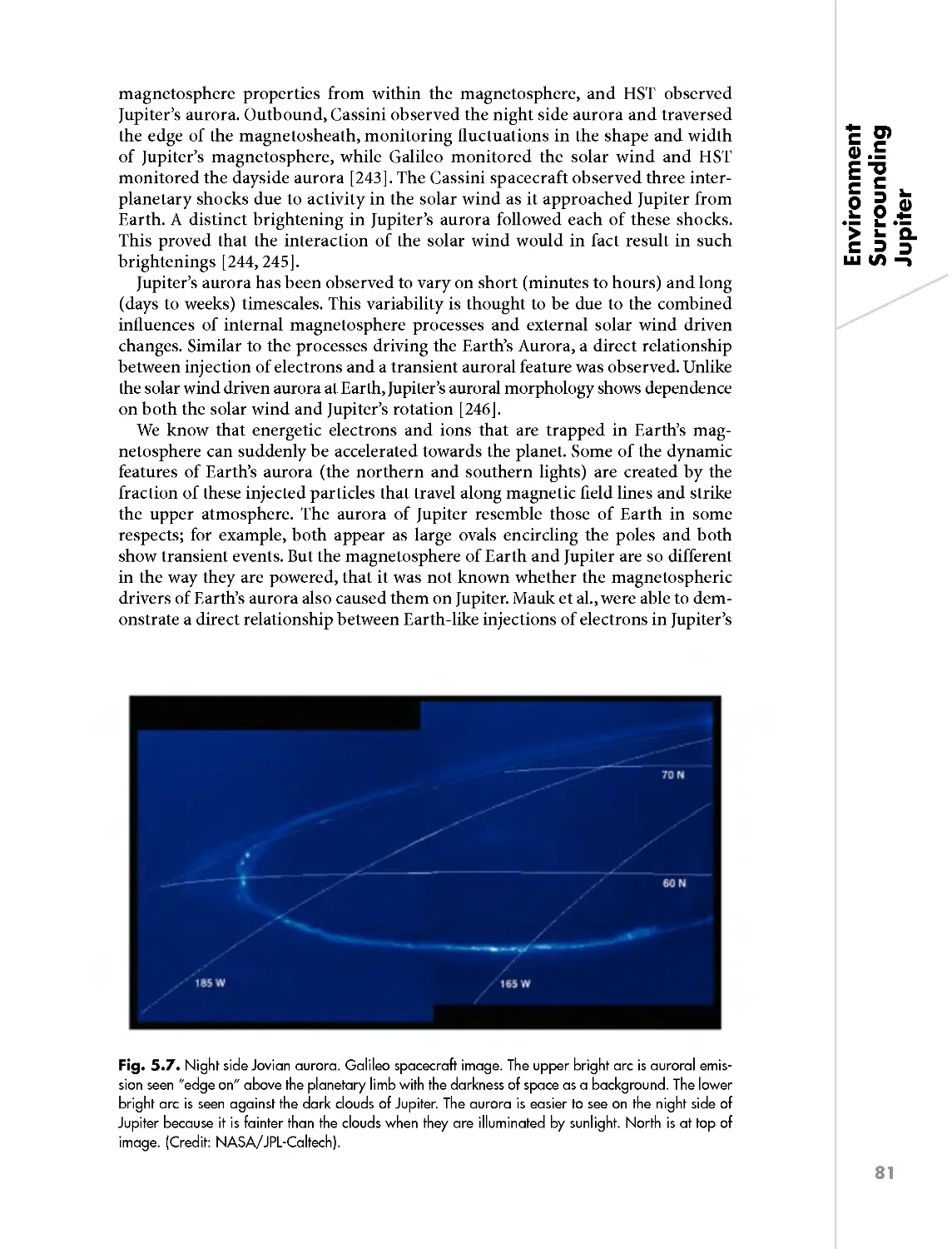
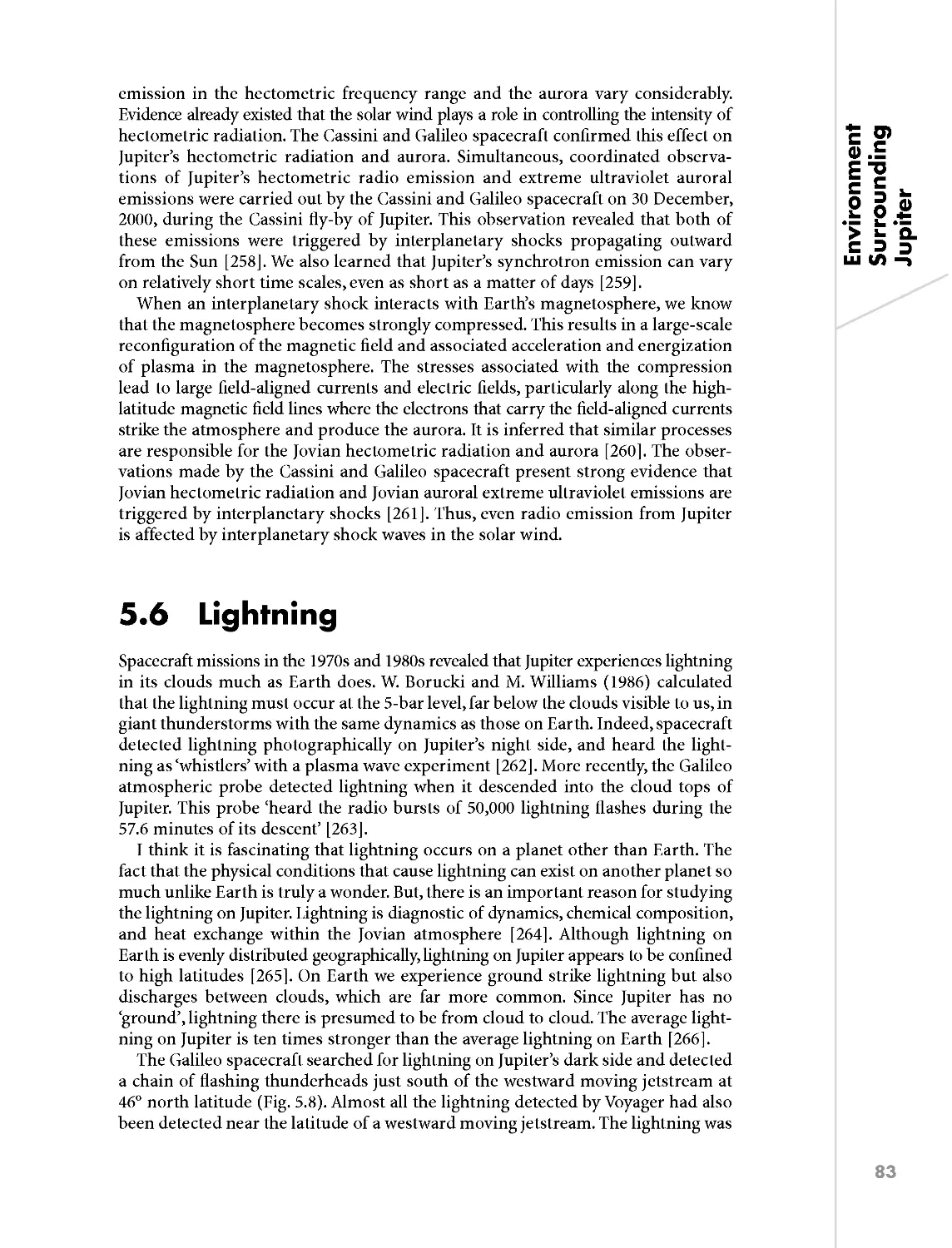
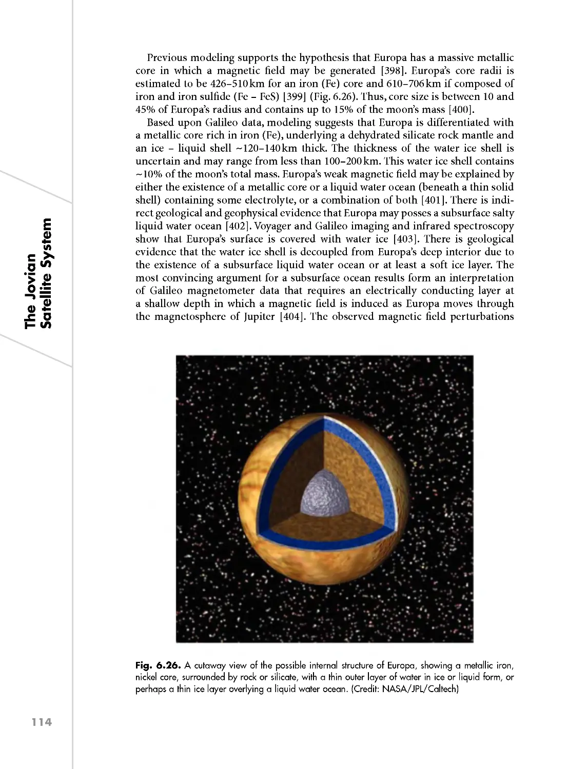
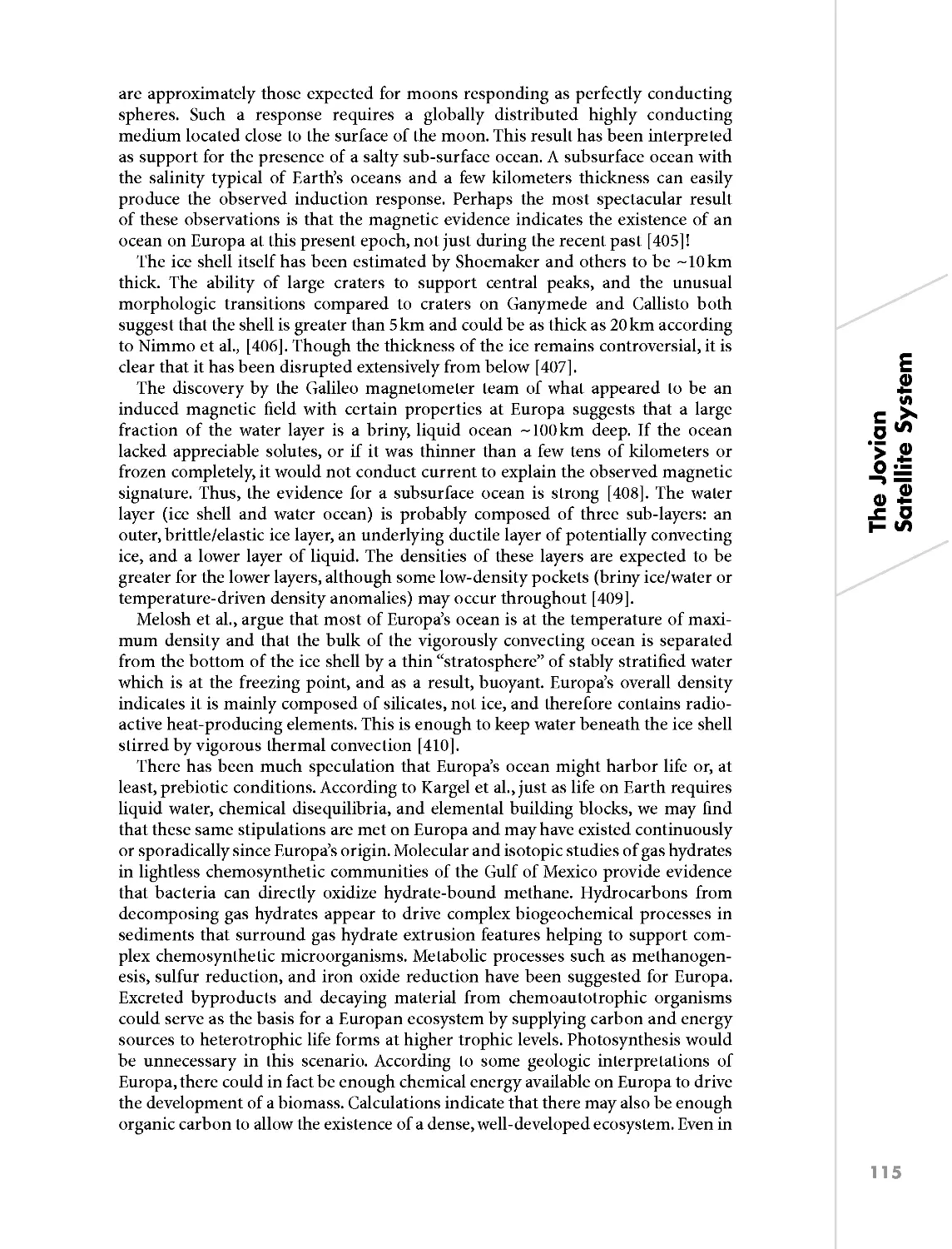
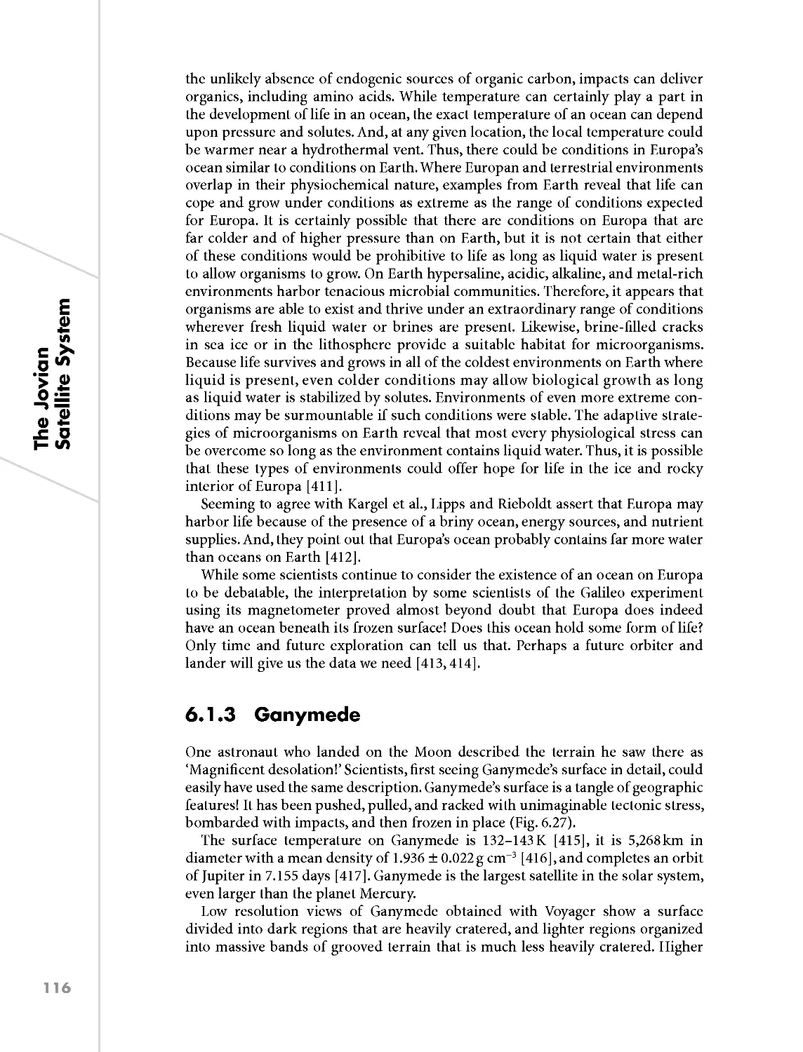
/


Текст
Jupiter
and How to Observe I1
John W. Mmnully
Q Springer
Astronomers’ Observing Guides
Other Titles in This Series
Star Clusters and How to Observe Them
Mark Allison
Saturn and How to Observe it
Iulius Benton
Nebulae and How to Observe Them
Steven Coe
The Moon and How to Observe It
Peter Grego
Venus and Mercury and How to Observe Them
Peter Grego
Supernovae and How to Observe Them
Martin Mobberley
Total Solar Eclipses and How to Observe Them
Martin Mobberley
Double & Multiple Stars and How to Observe Them
Iarnes Mullaney
The Herschel Objects, and How to Observe Them
Iarnes Mullaney
Galaxies and How to Observe Them
Wolfgang Steinicke 264 Richard Iakiel
John W. McAna11y
JUPITER
and How to
Observe It
@ Springer
John W. McAnally
USA
cpajohnm@aol.com
Series Editor
Dr. Mike Inglis BSc, MSc, PhD.
Fellow of the Royal Astronomical Society
Suffolk County Community College, New York, USA
inglism@sunysuffolk.edu
British Library Cataloguing in Publication Data
A catalogue record for this book is available from the British Library
Library of Congress Control Number: 2007932968
Astronomers’ Observing Guides Series ISSN 1611-7360
ISBN: 978- 1 —85233—750—6 e—ISBN: 978- l—84628—727—5
Printed on acid—free paper
© Springer—Verlag London Limited 2008
Apart from any fair dealing for the purposes of research or private study, or criticism or review,
as permitted under the Copyright, Designs and Patents Act 1988, this publication may only be reproduced,
stored or transmitted, in any form or by any means, with the prior permission in writing of the publishers,
or in the case of reprographic reproduction in accordance with the terms of licences issued by the
Copyright Licensing Agency. Enquiries concerning reproduction outside those terms should be sent to
the publishers.
The use of registered names, trademarks, etc. in this publication does not imply, even in the absence of
a specific statement, that such names are exempt from the relevant laws and regulations and therefore
free for general use.
The publisher makes no representation, express or implied, with regard to the accuracy of the
information contained in this book and cannot accept any legal responsibility or liability for any errors
or omissions that may be made.
987654321
Springer Science+Business Media
springer.com
In memory ofmyfather and mother, ]ohn R. McAnally, ]r., and Margaret
McAnally. I am eternally gratefulfor their love and encouragement.
And in memory ofmy mother-in-law, Mary Dicorte, who always asked how the
book was coming along. I will miss herprayers, love, and kind ways.
And to my wife, Rose Ann, for her infinite love and patience.
Acknowledgments
As with any endeavor of this magnitude, I owe much to friends and colleagues.
I wish to thank all of my fellow amateur astronomers who have so graciously
contributed images for the illustrations in this book, including Donald C. Parker,
Ed Grafton, P. Clay Sherrod, Eric Ng, Damian Peach, Christopher Go, Cristian
Fattinnanzi, Brady Richardson, Trudy LeDoux, and Dave Eisfeldt.
I am also grateful to the editor Mike Inglis and to the publishers at Springer for
the invitation to write this book, and for their patience in allowing the time
I believe was necessary to make it a good one.
I greatly appreciate my colleagues, the staff of the Association of Lunar and
Planetary Observers, for their support and friendship. Likewise, my friends in
the Central Texas Astronomical Society have given me great moral support and
encouragement.
Finally, I am deeply grateful to Amy Simon-Miller, Glenn Orton, and Scott C.
Sheppard for their assistance in gathering papers and materials, and for many,
many useful discussions. Their support and friendship has been invaluable to me.
Author contact information:
By e-mail: cpajohnm@aol.com
or
through the Web site of
The Association of Lunar and Planetary Observers
\ Acknowledgements
vii
Contents
Secfionl
Chapter 1
Chapter 2
Chapter 3
Chapter 4
Chapter 5
Acknowledgments . . . . . . . . . . . . . . . . . . . . . . . . . . . . . . . . . . . . . . .
Introduction . . . . . . . . . . . . . . . . . . . . . . . . . . . . . . . . . . . . . . . . . . . .
The Earliest Observations . . . . . . . . . . . . . . . . . . . . . . . . . . . . . . . .
1.1 Known to the Ancients . . . . . . . . . . . . . . . . . . . . . . . . . . . . . . .
1.2 Galileo Galilei and Discovery of the Galilean
Moons . . . . . . . . . . . . . . . . . . . . . . . . . . . . . . . . . . . . . . . . . . . . .
1.3 Cassini and the Great Red Spot . . . . . . . . . . . . . . . . . . . . . . .
1.4 In Good Company . . . . . . . . . . . . . . . . . . . . . . . . . . . . . . . . . .
]upiter’s Place in the Solar System . . . . . . . . . . . . . . . . . . . . . . . . .
2.1 Physical Characteristics . . . . . . . . . . . . . . . . . . . . . . . . . . . . . .
2.2 A System of Basic Terminology and
Nomenclature . . . . . . . . . . . . . . . . . . . . . . . . . . . . . . . . . . . . . .
The Physical Appearance of the Planet . . . . . . . . . . . . . . . . . . . . .
3.1 Common Visual Markings . . . . . . . . . . . . . . . . . . . . . . . . . . . .
3.2 Winds and let Streams in the Atmosphere . . . . . . . . . . . . . .
3.3 Color in Iupiter’s Belts and Zones . . . . . . . . . . . . . . . . . . . . .
3.4 Summary . . . . . . . . . . . . . . . . . . . . . . . . . . . . . . . . . . . . . . . . . .
Color, Chemical Composition of the Planet,
and Vertical Structure of the Atmosphere . . . . . . . . . . . . . . . . . . .
4.1 Color . . . . . . . . . . . . . . . . . . . . . . . . . . . . . . . . . . . . . . . . . . . . . .
4.2 The Chemical Composition . . . . . . . . . . . . . . . . . . . . . . . . . . .
4.3 The Vertical Structure of Iupiter’s Atmosphere . . . . . . . . . .
The Electromagnetic Environment Surrounding
Iupiter . . . . . . . . . . . . . . . . . . . . . . . . . . . . . . . . . . . . . . . . . . . . . . . . . .
5.1 The Magnetosphere and Magnetic Field . . . . . . . . . . . . . . . .
5.2 The Io Cloud and Torus . . . . . . . . . . . . . . . . . . . . . . . . . . . . . .
5.3 Radiation Belts . . . . . . . . . . . . . . . . . . . . . . . . . . . . . . . . . . . . .
5.4 Aurora . . . . . . . . . . . . . . . . . . . . . . . . . . . . . . . . . . . . . . . . . . . . .
5.5 Radio Emission . . . . . . . . . . . . . . . . . . . . . . . . . . . . . . . . . . . . .
5.6 Lightning . . . . . . . . . . . . . . . . . . . . . . . . . . . . . . . . . . . . . . . . . .
5.7 The Io Flux Tube and Magnetic Footprints on
Iupiter . . . . . . . . . . . . . . . . . . . . . . . . . . . . . . . . . . . . . . . . . . . . .
vii
12
12
45
47
48
50
50
64
66
69
69
76
78
78
82
83
86
\Contents \
ix
/ Contents /
Chapter 6
Secfionll
Chapter 7
Chapter 8
Chapter 9
5.8 X-Ray Emission from Iupiter and Its Environ . . . . . . . . . . 88
5.9 Summary . . . . . . . . . . . . . . . . . . . . . . . . . . . . . . . . . . . . . . . . . 89
The Iovian Satellite System . . . . . . . . . . . . . . . . . . . . . . . . . . . . . . . . 91
6.1 The Galilean Moons of Iupiter . . . . . . . . . . . . . . . . . . . . . . . 91
6.2 The Lesser Moons . . . . . . . . . . . . . . . . . . . . . . . . . . . . . . . . . . 130
6.3 The Rings of Iupiter . . . . . . . . . . . . . . . . . . . . . . . . . . . . . . . . 138
6.4 Trojans and Comets . . . . . . . . . . . . . . . . . . . . . . . . . . . . . . . . 142
How to Observe the Planet Jupiter
Introduction . . . . . . . . . . . . . . . . . . . . . . . . . . . . . . . . . . . . . . . . . . . . 147
Equipment . . . . . . . . . . . . . . . . . . . . . . . . . . . . . . . . . . . . . . . . . . . . . . 149
7.1 Telescopes . . . . . . . . . . . . . . . . . . . . . . . . . . . . . . . . . . . . . . . . 149
7.2 Eyepieces . . . . . . . . . . . . . . . . . . . . . . . . . . . . . . . . . . . . . . . . . 155
7.3 Filters . . . . . . . . . . . . . . . . . . . . . . . . . . . . . . . . . . . . . . . . . . . . 156
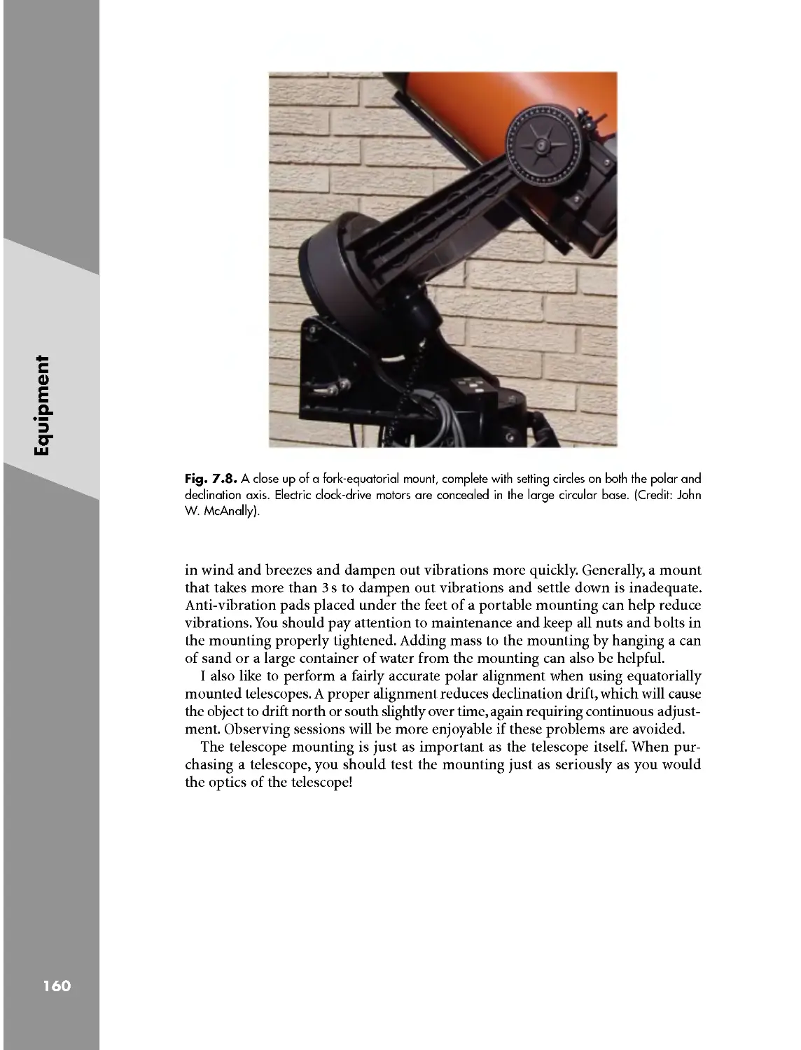
7.4 Mountings . . . . . . . . . . . . . . . . . . . . . . . . . . . . . . . . . . . . . . . . 158
Sky Conditions . . . . . . . . . . . . . . . . . . . . . . . . . . . . . . . . . . . . . . . . . . 161
8.1 Seeing . . . . . . . . . . . . . . . . . . . . . . . . . . . . . . . . . . . . . . . . . . . . 161
8.2 Transparency . . . . . . . . . . . . . . . . . . . . . . . . . . . . . . . . . . . . . . 162
8.3 Learning about Weather . . . . . . . . . . . . . . . . . . . . . . . . . . . . 163
Making a Record . . . . . . . . . . . . . . . . . . . . . . . . . . . . . . . . . . . . . . . . . 165
9.1 Making a Drawing of Iupiter . . . . . . . . . . . . . . . . . . . . . . . . 165
9.2 The Full Disk Drawing . . . . . . . . . . . . . . . . . . . . . . . . . . . . . . 166
9.3 The Strip Sketch . . . . . . . . . . . . . . . . . . . . . . . . . . . . . . . . . . . 170
9.4 Intensity Estimates . . . . . . . . . . . . . . . . . . . . . . . . . . . . . . . . . 172
9.5 Central Meridian Transit Timings . . . . . . . . . . . . . . . . . . . . 175
9.6 Drift Charts . . . . . . . . . . . . . . . . . . . . . . . . . . . . . . . . . . . . . . . 176
9.7 Observation and Estimates of Color . . . . . . . . . . . . . . . . . . 178
9.8 The Use of Photography to Study Iupiter . . . . . . . . . . . . . . 179
9.9 CCD Imaging . . . . . . . . . . . . . . . . . . . . . . . . . . . . . . . . . . . . . . 180
9.10 Imaging with Webcams . . . . . . . . . . . . . . . . . . . . . . . . . . . . . 182
9.11 Making use of CCD and Webcam Images . . . . . . . . . . . . . . 188
9.12 Measurement of Latitude . . . . . . . . . . . . . . . . . . . . . . . . . . . 190
9.13 Keeping a Record: The Logbook . . . . . . . . . . . . . . . . . . . . . 192
9.14 Reporting . . . . . . . . . . . . . . . . . . . . . . . . . . . . . . . . . . . . . . . . . 194
9.15 Amateur Organizations . . . . . . . . . . . . . . . . . . . . . . . . . . . . . 195
Conclusion . . . . . . . . . . . . . . . . . . . . . . . . . . . . . . . . . . . . . . . . . . . . . . 197
References . . . . . . . . . . . . . . . . . . . . . . . . . . . . . . . . . . . . . . . . . . . . . . 198
Index . . . . . . . . . . . . . . . . . . . . . . . . . . . . . . . . . . . . . . . . . . . . . . . . . . . 215
Introduction
Jupiter and How to Observe It
Welcome to a wonderful pastime! Observing the planets and learning something
about them is an activity that anyone can do. I often liken amateur astronomy to
the game of golf. Anyone can take up the sport. You can spend lots of money for
equipment or you can be more frugal. You can participate at any level you wish and
you can start when you are young and continue until you are old, all of your life at
any age! However, amateur astronomers have one great advantage; we don’t have to
complain about our golf scores! My interest in astronomy began in the 1960s, not
in science class but in reading class. We read a story in the eighth grade about the
Hale 200-in. telescope on Mount Palomar, and how George Hale raised the money
so it could be built. I am not sure what happened, but something in me just clicked
and I knew that somehow I had to get into astronomy. My parents were poor, so my
first telescope was inexpensive, small and hopelessly inadequate; yet, I remember
going out with it every clear night. Later in high school I purchased a telescope that
was still small but much better optically, and my views became much more clear.
The planets especially have always fascinated me with their bright appearance and
motion against the background stars. Whether observing visually or taking images
through a telescope,I continue to be intrigued by what can be seen on their sur-
faces,by what changes and what stays the same!
In writing this book it is my hope that after reading it the beginner, who is just
starting out, will acquire enough knowledge from it to be able to go to the telescope
and make a meaningful observation the very first time. The methods and proce-
dures described are not, for the most part, overwhelming or difficult; they simply
require patience, care, and attention to detail. I believe the advanced amateur will
also find enough here to be challenging, especially the more advanced procedures
of imaging and reducing and reporting real data that is scientifically valuable.
I have tried to follow a logical approach. As with any new endeavor, it is important
to understand terminology and scientific notation about the subject to be studied,
before the study is undertaken. Speaking the language is important and I have
tried to make ‘Iupiter speak’ a little less daunting. It can also be helpful to have an
understanding of the subject’s past history and to think about what might occur
in the future.
\ Introduction
/ Introduction
Section I of this book will discuss much of what we already know about Iupiter,
and will hopefully provide a good grounding in the planet in preparation for
Sect. II. Section II will discuss in some detail how to observe the planet, record
data in a meaningful way, and report it. There is so much about Iupiter to know
and understand. My own lifetime journey through this learning process has been
a most enjoyable experience. I hope you enjoy yours. Every night can be a new
adventure!
Iohn W. McAnally
Assistant Coordinator for Transit Timings
Iupiter Section
Association of Lunar and Planetary Observers
2124 Wooded Acres
Waco, Texas 76710
cpajohnm@aol.com
Section I
Chapter 1
The Earliest
Observations
'I.'I Known to the Ancients
Iupiter is so bright in the night sky that it can easily be seen with the naked eye;
in fact, among the planets, only Venus can shine brighter. Being so bright it was
known to man long before the invention of the telescope. Ancient civilizations
around the world knew of its wanderings and made attempts to predict its behav-
ior against the stars. In mythology, Iupiter was the chief god of the Romans. The
Greeks referred to Iupiter as Zeus. I can imagine that even prehistoric man would
have noticed Iupiter, shining so bright against the other star-like bodies. We can
think of Iupiter as our chief planet in the solar system. As we’ll see, we might not
even exist without this giant planet!
1.2 Galileo Galilei and Discovery
of the Galilean Moons
Galileo Galilei was perhaps the first person to effectively use a telescope to explore
the heavens, and is credited with being the first person to use a telescope to look
at Iupiter. In Ianuary 1610 he noticed three star-like objects lined up in a row in
Iupiter’s equatorial plane (he eventually discovered a forth one). This alignment
apparently aroused his deep curiosity and he eventually came to the conclusion
that they must be in orbit around Iupiter! What a discovery! Seeing that another
planet had bodies in orbit ab out itself, and knowing of the problems with the orbital
theories of the time, Galileo came to the further conclusion that the Earth must not
be the center of the motions that were observed in the universe. Having previously
been encouraged in his other scientific studies by the Church in Rome, Galileo
made his findings known to the Pope. Much to his disappointment, the Church
soon took exception to his assertions that Earth was not the center of the universe and
forbade him to continue his research or to even discuss it openly. He was subse-
quently placed under house arrest. Of course, we now know that Galileo was correct,
but at the time Iupiter presented him with what was truly a life-threatening situation!
These four moons are now known as the ‘Galilean moons’.
The Earliest
Observations
The Earliest
Observations
'l.3 Cassini and the Great Red Spot
After Galileo, as the quality of lenses and telescopes improved, observers began
to detect markings on Iupiter’s surface. In 1665, Giovanni Dominico Cassini dis-
covered a “permanent spot” on Iupiter and followed it on and off for several years.
Cassini also discovered Iupiter’s equatorial current, the flattening of its poles, and
its limb darkening. Later, when the Great Red Spot was recognized in 1879, it was
suggested that this was a rediscovery of Cassini’s spot. However, there is really no
empirical evidence to support this, and we must be careful not to state this as fact
[1]-
As the years went by and telescopes and lenses continued to improve, more and
more discoveries were made regarding Iupiter. Many of the people making these
discoveries would be considered amateurs today. However, these amateurs were
serious, dedicated, careful observers. And as we will see, there continues to be room
in astronomy for amateurs today, and perhaps more so than ever!
1.4 In Good Company
The amateurs of to day are in very good company with many notable observers who
have led the way before us such as Bertrand Peek, Hargreaves, Phillips,Molesworth,
and Elmer Reese; and with contemporaries of today such as Miyazaki, Don Parker,
Phillip Budine, Iohn Rogers, Walter Haas, Olivarez, and many, many others. If not
for these observers, the visual record of Iupiter would be sparse indeed. We can
take pride in helping to continue the works of so many wonderful amateurs.
The telescopes and related equipment are better than ever. I can only imagine
what Bertrand Peek would have given for a good web cam or CCD camera! How
much easier our work is compared to theirs; yet, we can only hope to measure up
to their discipline, their persistence, and their attention to detail!
So, from Galileo to today many years have gone by and yet, Iupiter still begs to
be observed! What will we discover next year, and the next, and the next?
Chapter 2
Jupiter's Place
in the Solar System
Whether our study of Iupiter is casual or serious, it will be helpful to understand
some basic facts about the planet, including simple nomenclature. This knowledge
will help us in our own study, and it will allow us to understand what others say
and write about the planet. As I have found over the years, there is always some-
thing new and exciting to learn, something new to be discovered and revealed, but
we must understand the language.
So, where does Iupiter stand in the scheme of things? Our solar system is com-
prised of many bodies, large and small. We were taught about the nine planets
in school, and their order in distance from the Sun. Recently, the International
Astronomical Union changed the classification of Pluto, and it is no longer offi-
cially classified as a planet in the simple sense. Now we have eight planets and all
manner of other bodies.
2.1 Physical Characteristics
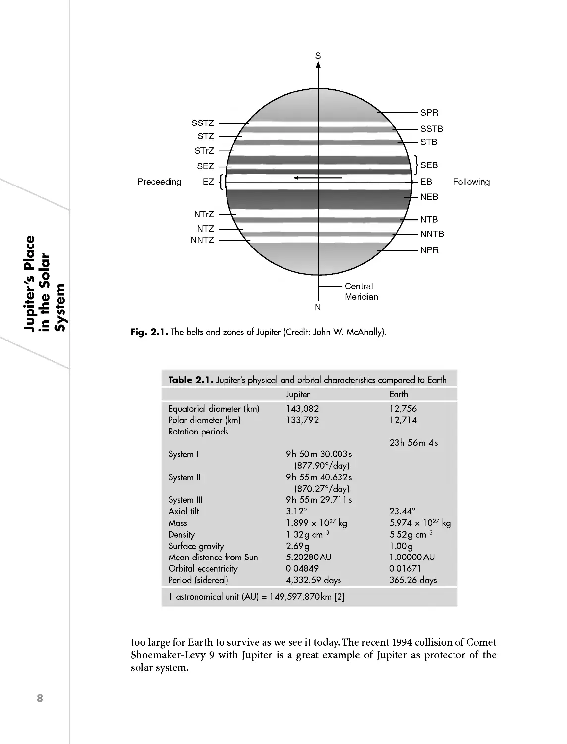
Iupiter displays a series of bright zones and darker belts, generally running paral-
lel to its equator. Figure 2.1 illustrates the globe of Iupiter with the belts and zones
that are usually visible. Not all features will be visible at all times, as belts and zones
are prone to brighten, darken, become larger or smaller, or even disappear from
time to time.
Iupiter is the fifth planet from the Sun. It is a gas giant, having no surface as
we think of on Earth. Its volume is so large, that if it were a hollow sphere, all the
other planets would fit easily inside with room to spare. Even mighty Saturn is only
about one-third its mass. However, Iupiter’s density is so low that if there were a
water ocean large enough, Iupiter would float on its surface!
Iupiter’s large mass is of extreme importance to the solar system and especially
to Earth. Iupiter’s mass perturbs the orbit of nearly every planet in our solar system. It
also influences the orbits of smaller bodies that come into the inner solar system
from the Kuiper Belt and the Ort Cloud. Iupiter’s mass and strong gravitational
influence has a tendency to either sweep up small bodies that cross its orbit, or to
eject them from the solar system entirely. This solar system ‘vacuum cleaner’ made
it possible for Earth to survive long enough for life to form and evolve. Without
this protection, the bombardment of Earth would occur too frequently by bodies
Jupiter's Place
in the Solar
System
Jupiter's Place
in the Solar
System
A
SPR
SSTB
STB
STrZ
sEz }SEB
Preceeding EZ { EB Following
NEB
NTrZ NTB
NTZ
NNTZ NNTB
NPR
Central
Meridian
N
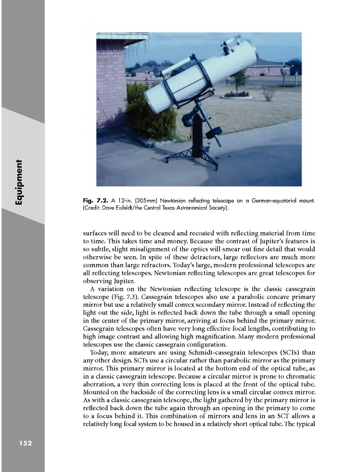
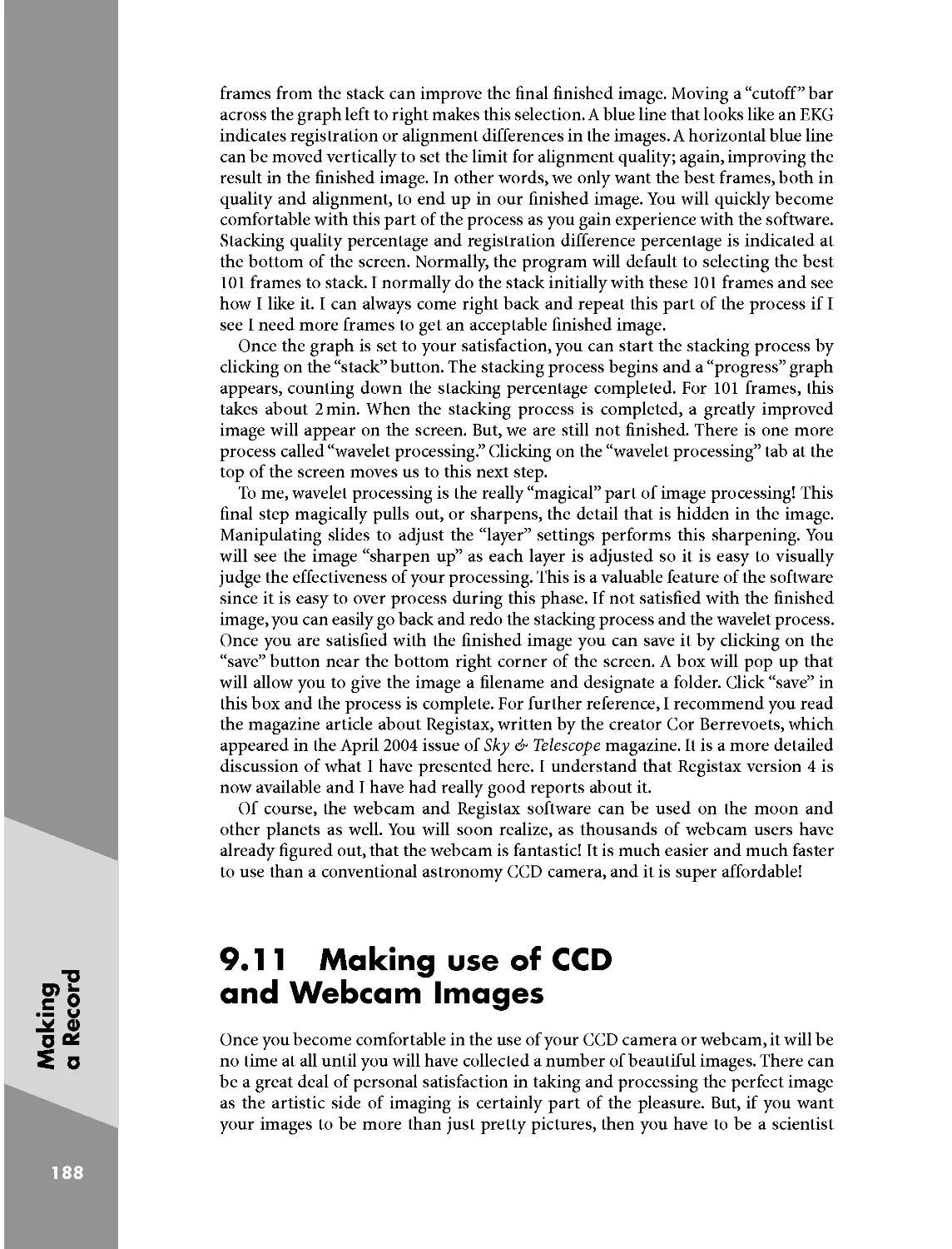
Fig. 2.1. The bells and zones of Jupiler (Credil: John W. McAnally).
Table 2.1. Jupiler's physical and orbilal characlerislics compared lo Earlh
Jupiler Earlh
Equalorial diameler (km) 143,082 12,756
Polar diameler (km) 133,792 12,714
Rolalion periods
23h 56 m 4 s
Syslem I 9h 50m 30.003s
(877.90°/day)
Syslem ll 9h 55m 40.632s
(870.27°/day)
Syslem Ill 9h 55m 29.711 5
Axial lill 3.12° 23.44°
Mass 1.899 X 1027 kg 5.974 X 1027 kg
Density 1.32g cm‘3 5.52g cm‘3
Surface gravity 2.69g 1.00g
Mean dislance from Sun 5.20280AU 1 .00000AU
Orbilal eccenlricily 0.04849 0.01671
Period (sidereal) 4,332.59 days 365.26 days
1 aslronomical unil (AU) = 149,597,870 km [2]
too large for Earth to survive as we see it today. The recent 1994 collision of Comet
Shoemaker-Levy 9 with Iupiter is a great example of Iupiter as protector of the
solar system.
Iupiter exhibits differential rotation; that is, different latitudes of the planet
have different rotation rates. Generally, System I includes the latitudes from the
north edge of the south equatorial belt, all of the equatorial zone, to the south
edge of the north equatorial belt. System I also includes the south edge of the
north temperate belt. System II includes the rest of the planet. Since amateurs in
the past have observed Iupiter in visible wavelengths, it has been common practice
for them to refer to System I and II. Professional astronomers have generally
used a third rotation system, System III. The System III rotation rate is related
to a radio source on Iupiter that rotates with the planet at a specific rate. Since
these three rotation rates are different, we must designate which system we are
referring to when we speak of longitudinal positions on Iupiter. Depending upon
the latitude at which a feature appears on Iupiter, amateurs refer to System I or
II longitude. This usage will become more apparent in the section of this book
dealing with transit timings. Table 2.1 summarizes Iupiter’s physical data and
orbital characteristics.
2.2 A System of Basic Terminology
ancl Nomenclature
Like most sciences, planetary astronomy comprises a language of special terms
and nomenclature. Understanding those associated with Iupiter will facilitate our
discussions and explanations, since this scientific shorthand can actually help to
keep our discussions simple and unambiguous. Years ago,A.L.PO. Iupiter Section
Coordinator Phil Budine suggested a simple, straightforward system that we can
still use today. There are abbreviations for the terms and nomenclature of dark
and bright features, and for the belts and zones; so, some of the more common
terms and abbreviations are shown in Tables 2.2 and 2.3. Various dark and bright
features can be seen in the belts and zones at any given time. Some of the features
most often seen are illustrated in Table 2.4. These illustrations are modeled after
illustrations used by past A.L.PO. Iupiter Recorder Phillip Budine.
A simple example can help us understand how we put this terminology into
use. Figure 2.2 shows a large condensation, or barge, on the north edge of the
north equatorial belt. This feature would be described as, ‘Dc L cond N edge
NEB’; which literally means ‘dark center, large condensation, north edge, north
equatorial belt.’ So,you see how in simple, straightforward notation we have com-
pletely described the feature and where it resides. If we were describing a bright
feature we would use the designation ‘W’, instead of ‘D’. Later, when we discuss
central meridian transit timings, you will see how we combine this description
with the longitudinal position of the feature to turn this kind of observation into
real, meaningful data.
As we will see in Sect. II of this book, your observations are only valuable if
they are properly recorded and notated. The system of nomenclature presented
here should allow anyone to accomplish this task. Organizations such as The
Association of Lunar and Planetary Observers (A.L.PO.) and the British
Astronomical Association (BAA) have standard observing forms that the observer
can use to record observations. Many other organizations around the world also
have standardized forms. Standardized observations greatly facilitate the gathering
Jupiter's Place
in the Solar
System
/
Jupiter's Place
in the Solar
System
‘I0
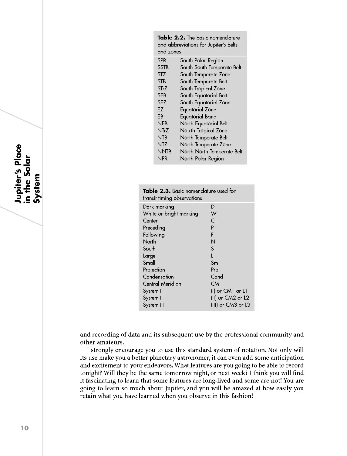
Table 2.2. The basic nomenclature
and abbreviations for Jupiter's bells
and zones
SPR South Polar Region
SSTB South South Temperate Belt
STZ South Temperate Zone
STB South Temperate Belt
STrZ South Tropical Zone
SEB South Equatorial Belt
SEZ South Equatorial Zone
EZ Equatorial Zone
EB Equatorial Band
NEB North Equatorial Belt
NTrZ No rth Tropical Zone
NTB North Temperate Belt
NTZ North Temperate Zone
NNTB North North Temperate Belt
NPR North Polar Region
Table 2.3. Basic nomenclature used for
transit timing observations
Dark marking
White or bright marking
Center
Preceding
Following
North
South
Large
Small
Projection Pro]
Condensation Cond
Central Meridian CM
System I (I) or CMl or Ll
System II (II) or CM2 or L2
System III (III) or CM3 or L3
(3/)I—(/uz-n-ongg
and recording of data and its subsequent use by the professional community and
other amateurs.
I strongly encourage you to use this standard system of notation. Not only will
its use make you a better planetary astronomer, it can even add some anticipation
and excitement to your endeavors. What features are you going to be able to record
tonight? Will they be the same tomorrow night, or next week? I think you will find
it fascinating to learn that some features are long-lived and some are not! You are
going to learn so much about Iupiter, and you will be amazed at how easily you
retain what you have learned when you observe in this fashion!
Table 2.4. Basic nomenclature for dark and bright teatures commonly seen on Jupiter (Credit:
John W. McAnally)
Nodule Notch
l
l
Condensation Rod
ll
ll
Elongated condensation (Barge) Festoon Gap
E ..:_.. ;
Dark section of belt Looping festoon Veil (shading)
O T
Low projection Oval Column
Tall projection Bay Rift
From standard nomenclature proposed by Phillip W. Budine.
S
SEB
EZ
P F
NEB
NTrZ
NTB
NTZ
I
Center large condensation
north edge of NEB
Fig. 2.2. Example of a large condensation depicted on the northern edge of Jupiter's North
Equatorial Belt (Credit: John W. McAnally).
Jupiter's Place
the Solar
System
-0
.§g
Ill
2%’
=3
0
_=D.
|—<
‘I2
of the Planet
Chapter 3
The Physical Appearance
of the Planet
The disk of Iupiter presents a variety of features that can be observed by an
amateur astronomer with modest equipment. Features both obvious and subtle
await the eager observer. Indeed, Iupiter is often referred to as “the amateurs’
planet”, due in part to its enormous size and angular diameter that makes it easy
to observe. The use of CCD cameras and web cams by many amateurs today is
becoming more commonplace, with excellent images being obtained showing
great detail. It is the physical appearance of the planet and ease of observation that
first attracts most of us. In this chapter we will deal with the physical structure,
characteristics, and phenomenon that can be observed visually and by imaging; in
other words, those things that anyone, including an amateur with a telescope, can
see. Specifically, we will examine non-vertical structure in Iupiter’s clouds, winds,
jet streams, and color.
The observation of features on the surface of Iupiter, or rather in its cloud tops,
and the observation of changes in the longitudinal and latitudinal positions of
features, and the determination of the movement of features with regard to the
speed of various currents and the appearance and reappearance of other phenomena,
has been a mainstay of amateur observations since the beginning of recorded
observations more than 150 years ago. While there is much to Iupiter amateurs
cannot observe directly, these things we can see. Amateurs today continue this
wonderful tradition of observational astronomy.
3.1 Common Visual Markings
Although we should never approach the observation of Iupiter with any precon-
ceived notion of what maybe seen, it can be useful to have an understanding of the
type of features that may be present at any given time. The bright ovals, eddies, and
condensations are evidence of great turmoil and chaos in the visible atmosphere
of Iupiter. Features seen in Iupiter’s cloud tops are not stationary, and maybe short
or long lived. Knowing this, I think the observation of these features is all the more
tantalizing. You may wish to review the figures and tables in Chap. 2 again while
studying this chapter.
Generally, the planet is made up of clouds that have organized themselves into
dark belts and bright zones, due mainly to the rapid rotation of the planet. The belts
and zones are defined by powerful jet streams that are permanent winds blowing
eastward or westward. Dark spots and bright ovals are storms that drift eastward
or westward at slower rates. The rapid rotation of the planet causes all motions to
be channeled along lines of latitude; thus the belts and zones run east and west. See
Fig. 2.1 in Chap 2,which depicts the placement of belts and zones and nomenclature.
3.1.1 The Polar Regions
To the visual observer, the polar-regions most often present a gray, dusky appear-
ance, absent specific features. Indeed, during the apparitions of 2000-2001 and
2001-2002, most visual observers reported no features at all. A few observers
using large instruments with exceptional image contrast reported an occasional
small, bright oval near the latitude of the NNTB or SSTB. However, these sight-
ings were never widely observed and thus, difficult to confirm. Occasionally there
is an exception to the inactivity usually noted in the polar-regions, as reported
during October 1997. During that apparition, several independent observers
observed faint dusky markings, slightly more intense than the surrounding
region. Among those observers, I was able to observe one feature well enough to
make one set of transit timings. This occurred on the night of October 26, 1997
U.T. (Fig. 3.1). Quoting from my own observing log,“The NPR is also exceedingly
Preceeding Following
N
1997 Oct 26 / 1:20 K.T.
L2: 333°
L2°
DP, shading, NPR, Just N of NNTB - 333°
DP, shading, NPR, Just N of NNTB - 343°
Fig. 3.1. A full disk drawing of Jupiter showing the shading or veil in the north polar region of
Jupiter on October 26, l997 (Credit: John W. McAnally).
\
The Physical
Appearance
of the Planet
‘I3
/
The Physical
Appearance
of the Planet
14
faint. A dusky patch or mottling is seen by me for the first time at the southern
edge of the NPR (these had previously [recently] been reported by others). This
mottling was very distinct and unmistakable! It was fairly extended in longitude.
It was seen clearly enough that I was able to make a CM transit timing of the
preceding and following edge. This may be the first measurement (CM transit
timing of such a feature, at least during this apparition) reported to A.L.P.O. (this
observation was made in integrated light). The mottling was also seen in green
(W56) light. Not seen in yellow (W12) light.” Alas, the feature disappeared and
was not observed again. However, their existence was confirmed beyond doubt
when these dusky markings were captured in a few CCD images, coinciding with
the longitudinal position observed by me and several other observers. These
dusky markings were first seen visually and later also confirmed by CCD imag-
ing. A fine example that visual observations are still of value.
Often, the polar-regions seem to spread their gray appearance all the way to
the NTZ or the STZ. Occasionally, however, subtle, lighter zones can be made
out, divided by thin, grayish belts barely seen. Observing the often too subtle
NNNTB and NNTB, their southern counterparts, and intervening zones, is
extremely difficult. Consequently it is very difficult to collect current, useful
data on the drift rates and wind currents in these regions. Occasions have been
rare in which any useful transit timings have been obtained from the polar-
regions. However, when bright or dark features present themselves in these
belts and zones for long enough, the observations that can be obtained are of
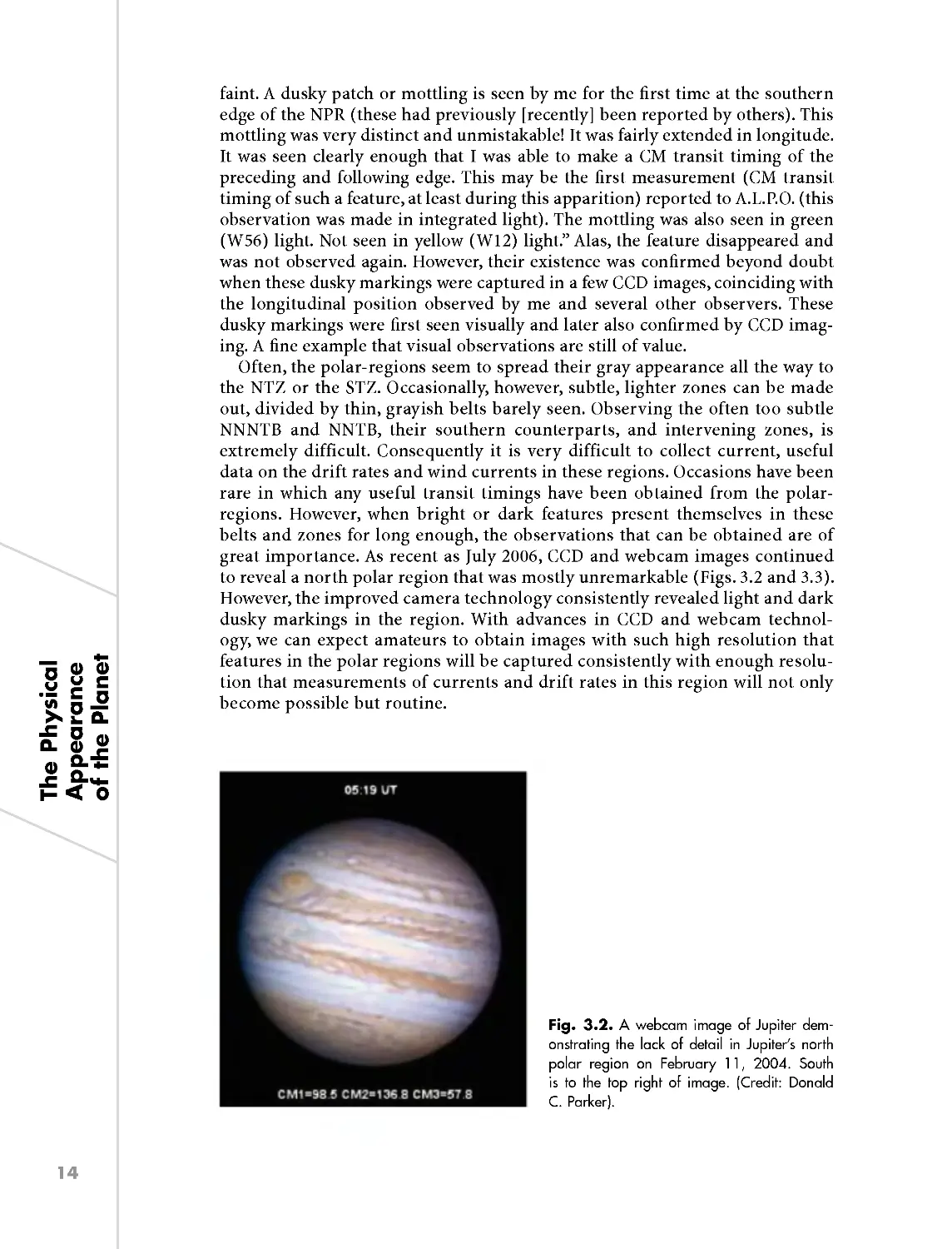
great importance. As recent as Iuly 2006, CCD and webcam images continued
to reveal a north polar region that was mostly unremarkable (Figs. 3.2 and 3.3).
However, the improved camera technology consistently revealed light and dark
dusky markings in the region. With advances in CCD and webcam technol-
ogy, we can expect amateurs to obtain images with such high resolution that
features in the polar regions will be captured consistently with enough resolu-
tion that measurements of currents and drift rates in this region will not only
become possible but routine.
Fig. 3.2. A webcam image of Jupiter dem-
onstrating the lack of detail in Jupiter's north
polar region on February H, 2004. South
is to the top right of image. (Credit: Donald
C. Parker).
Fig. 3.3. A webcam image showing a little
more activity in Jupiter's north polar region,
although the region is still unremarkable, on
April 12, 2006. South is to the top right of
image. (Credit: Donald C. Parker).
3.1.2 The North-North Temperate Region
The North—North Temperate Region generally extends from 57° North to 35°
North latitude. As mentioned, the North—North Temperate belt (NNTB) can
be difficult to observe and is not always present (Fig. 3.4). However, when the
belt is present, it is important to note its width and intensity. There may also
be seen the occasional projection on its southern edge. Although these are
rare, if present, careful observations and transit timings can yield valuable
data concerning drift rates and wind currents. During the 2000-2001 appari-
tion, a remarkable, dark segment appeared in the NNTB (Fig. 3.5). In fact, a
disk drawing of Iupiter on August 2, 2000 shows this dark segment quite well.
Similarly, CCD images by David Moore, 1. Ikemura, Peach, Maurizio Di Sciullo,
Antonio Cidadao, and others around the world also captured this dark seg-
ment. Observers continued to detect this segment in CCD images in early 2002,
although the segment was fading and not near the intensity of 2000-2001. By
April 2002, images by Don Parker revealed a NNTB segment that was broken
and spread out. Thus, the feature was long-lived and yielded very useful data
concerning the drift rate and wind speeds in this belt. It measured 10—15° in
longitudinal length when first seen. Features such as this are very rare in the
NNTB. This one presented a wonderful opportunity to check recent data about
currents against that collected in prior years with Earth based telescopes and
against wind speed data collected during the Voyager series. Often, the NNTB
goes wanting for such data! This feature was extensively imaged by amateurs
using CCD cameras but was also widely observed visually. The feature lasted
for over 14 months. The NNTB was unremarkable from Iune 2002 to May 2004
(Fig. 3.6). However, in April 2006 imagers detected a bright oval and a little red
spot (LRS) in the NNTZ. Portions of the NNTB were also seen, reddish-brown
in color.
\
The Physical
Appearance
of the Planet
‘I5
/
The Physical
Appearance
of the Planet
‘I6
Fig. 3.4. An image of Jupiter showing a
fairly dark NTB, and a discontinuous NNTB
on September 30, 1998. Note the narrow NEB
and bright Mid-SEB Outbreak running down
the middle of the SEB. South is up. (Credit:
Donald C. Parker).
Fig. 3.5. Jupiter on August 30, 2000. Note the
dark segment of the NNTB and that the remain-
der of the NNTB is discontinuous or absent.
South is up. (Credit: Donald C. Parker).
3.1.3 The North Temperate Region
The North Temperate Region extends from latitude 35° North to 23° North. While
the polar-regions are often disappointing, the North Temperate Belt (NTB) contains
a class of feature all its own. To the casual observer, the NTB usually presents the
appearance of an otherwise featureless, thin, grayish or reddish-gray belt slightly
more intense than the neighboring polar region. However, closer scrutiny reveals
otherwise. The belt can be continuous, fragmented, or completely absent. During
the 2000-2001 and 2001-2002 apparitions, the NTB was reported by most observers
to have a reddish-brown coloration mixed in with the gray tone (Fig. 3.7). I have
Fig. 3.6. Jupiter on February 10, 2004. During
the 2004 apparition both the NTB and NNTB
disappeared from Jupiter's disk. Notice the
prominent bluish-gray features on the NEBn
and the faint bluish band in the NTrZ. South is
up. (Credit: Donald C. Parker).
Fig. 3.7. Jupiter showing a moderately
intense GRS and NTB. CCD image taken
November 28, 2000. South is up. (Credit: Ed
Gratton).
observed on more than one occasion that the coloration and intensity of some
segments of the belt resemble the appearance of the north equatorial belt. The belt
is also often observed to be inconsistent in its width. In the most recent apparitions,
some observers have noted that segments of the belt are often split, or double, and
that its intensity can vary greatly.
During the 1999 apparition, the NTB was prominent and continuous. However,
the belt can also be absent. By 2001, some segments of the NTB had become
rather faint. Indeed, by December 2001, images taken by Ed Grafton revealed
segments of the NTB that were mostly gray in coloration and as light in intensity
as the north polar region. By Ianuary and February 2002, images by Ed Grafton,
Maurizio Di Sciulla, and Donald Parker revealed that, while some segments of the
\
The Physical
Appearance
of the Planet
17
/
The Physical
Appearance
/
of the Planet
NTB were the normal, reddish brown color, much of it had taken on this fainter,
gray appearance. By December 2002, images by Parker revealed that the NTB
had mostly vanished with only a few remaining dark segments scattered around
the planet. On February 22, 2003 a CCD image taken by Eric Ng of Hong Kong,
revealed a short segment of NTB, 20° long, near System 2 longitude 320°. By May 3,
2003 a CCD image by Christophe Pellier revealed a very short, faint segment of
the NTB near System 2 longitude 140° (Fig. 3.8). I saw no remnants of the NTB in
CCD images after that date. The NTB continues to be absent through Iuly 2006.
This gives Iupiter the appearance of having a bright alabaster zone stretching
from the north edge of the NEB to the NPR with only a faint, bluish gray north
tropical band south of the NTB’s normal position. In some high-resolution CCD
images, a faint bluish-gray band can also be made out in the north temperate
zone (NTZ). Do not mistake these bands for remnants of these two belts, as they
are not (Fig. 3.6). According to Peek [3] and Rogers, NTB fadings normally last
for periods from 8-13 years [4]. As recent as February 2007, the NTB was absent.
However, that began to change in late March and by April 27, 2007, the NTB was
almost completely restored. We must be always alert because sometimes events
really do happen just this quickly!
Some of the most interesting, visual features of the NTB may be the so-called
rapid moving spots (RMS) that are sometimes present. According to Peek, “in 1880
there appeared for the first time in Iupiter’s recorded history an outbreak of dark
spots at the south edge of the NTB that displayed the shortest rotation periods that
had ever been observed on Iupiter” [5]. The drift rates of the RMS are incredibly
fast. These spots are seen on the southern edge of the NTB (NTBs) when present
and may reside within the NTBs prograding jet stream. This jet stream is the fastest
jet stream on the planet. The RMS may also be associated with the NTBs jet stream
outbreaks. These outbreaks appear to have had periods of 10 years in the past and
more recently 5 years [6]. Although a few suspicious features were observed during
the 2000-2001 and 2001-2002 apparitions, the last notable outbreak of RMS seen
visually seems to have occurred in 1997. In that year, several spots were recorded
and observed throughout the apparition. These 1997 RMS had a drift rate of —56
to —57° per 30 days. These spots appear to have been associated with the North
Temperate Current C (NTC C). NTB outbreaks may also result in the appearance
of white spots or ovals.
Fig. 3.8. A highly detailed webcam image
of Jupiter taken on January 5, 2003. Note the
discontinuous, fragmented NTB and narrow
NEB. The EZ appears to be very disturbed and
south temperate oval BA is seen on the STBs.
South is up. (Credit: Ed Grafton).
In addition to observations of the RMS, the NTB can also fade, and it can exhibit
a shift in latitude. Dark spots and streaks can also appear on the north edge
(NTBn) of the NTB from time to time [7]. During the 2000-2001 and 2001-2002
apparitions, several dark condensations could be observed on the NTBn. A few
observers even detected faint gray festoons streaming away from some of these
dark condensations, stretching into the brighter NTZ. Occasionally, a bright oval
could be seen on the NTBn, intruding noticeably into the NTB. These features were
easily seen in the better amateur CCD images.
Separating the NTB and the NNTB is the NTZ. The NTZ can exhibit some
interesting features worth monitoring by amateurs. On many occasions the NTZ
simply appears dusky gray, approaching the bland appearance of the polar-
regions with no distinctive markings. At other times it can appear much
brighter, being a distinct divide between the NTB and NNTB. During the
2000-2001 apparition, the NTZ was described as almost alabaster by many
observers. Indeed, the zone rivaled the north tropical zone in brightness,
appearing brighter than the north tropical zone to many observers. During
the apparition of 2001-2002, several segments of the NTZ were observed to be
rather dusky in appearance while the remainder of the zone was bright. These
dusky segments may be caused by the absence of bright, high altitude clouds at
these longitudes. Changes such as these in the appearance of a zone are worth
careful monitoring and should certainly be reported. During 2006, the NTZ was
very bright with no obvious activity.
3.1.4 North Tropical Region
The North Tropical Region generally extends from 23° North to 9° North latitude.
The north tropical region of Iupiter displays some of the most active and vivid
features of the planet. In my experience, more amateur observations are made of this
region than any other, rivaled only by the region of the Great Red Spot (GRS).
The north tropical zone (NTrZ) lies between the NTB and the north equatorial
belt (NEB). This zone usually exhibits a bright, alabaster appearance, very similar
in brightness to the usual bright appearance of the equatorial zone (EZ.) This
was the case during the 2000-2001 and 2001-2002 apparitions. However, during
2003 the NTrZ was brighter than the EZ, due to the coloration event in the EZ. By
March 2004, disturbances in the EZ continued to make the EZ dimmer than the
NTrZ. Often, low projections can be seen on the southern edge of the NTB (NTBs)
extending into the NTrZ. Several dark projections were seen during the 2000-2001
and 2001-2002 apparitions and were followed reliably for several months, yielding
good drift rate data. During 2006, the NTrZ was again one of the brightest zones on
the planet, brighter than the EZ and absent any notable features.
The North Tropical Current (NTC) controls all the visible features in the NTrZ and
the northern edge of the North Equatorial Belt (NEBn). Although there are variations
in the speed of the current, it applies to all major spots whether bright or dark [8].
Sometimes a thin bluish band can be seen running through the NTrZ longitudi-
nally. This North Tropical Band is not easily seen visually, but was present during
the 2002-2003 and 2003-2004 apparitions as revealed by CCD images (Fig. 3.6).
Even in the CCD images, the band was very subtle and not visible the entire apparition.
This band has come and gone several times during Iupiter’s recent history. It was
evident during 2006, spanning the circumference of the planet.
\
The Physical
Appearance
of the Planet
‘I9
/
The Physical
Appearance
of the Planet
20
On a CCD image taken by Don Parker on 2004 Iuly 14, the NTrZ was one of the
brightest zones on the planet, even out shining the EZ which had a dusky, yellow-
ochre appearance over most of its width.
The North Equatorial Belt (NEB) is home to some of the most obvious and reliable
features on the planet. During most apparitions, condensations, barges, festoons,
ovals, and projections can be seen in the belt or on its edges. While many of the
belts and zones on Iupiter are low in intensity, the NEB is often one of the three
darkest features of the planet. During the apparitions of 2000-2001 and 2001-2002
the belt generally appeared solid and wide with a reddish brown coloration reported
by most observers (Fig. 3.9).
Dark condensations of oval shape, large and small, can often be seen on the north-
ern edge of the belt. The larger condensations are referred to as barges and seem to
be most conspicuous when the NEBn has receded slightly, as though leaving these
condensations in its place. The condensations are most often described as reddish-
brown in color, a darker version of the NEB. Barges were very prominent during the
1997 and 1998 apparitions,with several being seen at different longitudes around the
planet. During the 1999 apparition, the northern edge of the NEB receded at several
locations around the planet, giving the NEB a very narrow appearance at these loca-
tions. This further gave the NEBn the appearance of being undulating and wavy, or
of having bright bays protruding into the NEBn from the NTrZ. Dark condensations
were noted at several places around the planet on the NEBn (Fig. 3.10).
During the 2000-2001 and 2001-2002 apparitions, the barges were much less
conspicuous, with smaller condensations in their place. Even the smaller conden-
sations were not so prominent during 2000-2001. However, during 2001-2002,
something unusual occurred. During that apparition several barges, similar to
those often seen on the NEBn, were discovered in the middle of the NEB at several
positions around the planet (Fig. 3.11)! Several of these barges were prominent
enough to be seen visually throughout the apparition. During one recent apparition,
two of these mid-NEB condensations were reliably observed by CCD imaging.
Over time, they drifted together and merged. I had the privilege of observing several
of these mid-NEB barges on a night of good seeing with the 36-inch telescope at
McDonald Observatory in Texas during the fall of 2001. The rich, reddish-brown
Fig. 3.9. A CCD image of Jupiter, taken on
October 29, 2000 revealing a wealth of detail.
Surviving south temperate oval BA is seen on
the STBs followed by darker material. The SEB
is split by a bright SEZ. The EZ is undergoing
a coloration event, with only the south most
portion remaining bright. The NEB is broad,
and the NTB is also very intense, both with a
strong reddish-brown color. Notice the long,
bright rift running through the NEB. A small,
rare bright oval can be seen in the NPR. South
is up. (Credit: Donald C. Parker).
Fig. 3.10. Jupiter on September 30, 1998.
Note how narrow the NEB was in 1998 com-
pared to 2000 (previous image). Also note
the mid-SEB Outbreak in the SEB. South is up.
(Credit: Donald C. Parker).
Fig. 3.1 'I. A CCD image of Jupiter taken on
Januaryl , 2001 . Note the two dark condensa-
tions or barges imbedded in the middle of the
NEB, with a bright oval between them. Most
otten we see these condensations on the north-
ern edge of the NEB. Also note the split SEB
with very little coloration. South is up. (Credit:
P. Clay Sherrod).
coloration of the barges was beautiful to behold! The dark condensations or spots
are cyclonic as observed by spacecraft [9].
By 2002 and continuing into 2003, the NEB had returned to its more normal
broad appearance with an even NEBn. The dark condensations, or barges, seen in
the late 1990s were for the most part absent during 2002. In place of barges along
the NEBn, during the 2001-2002 apparition, at least four small white ovals were
seen at the edge of, or just barely imbedded in, the northern edge of the NEB at
various locations around the planet. By March 2004, these ovals had disappeared.
Instead, the NEB was again narrowing at several positions around the planet. By
March 2004, neither white ovals nor dark condensations, nor barges, were seen on
the NEBn, except for the long-lived white spot “Z”, seen on the edge of the NEBn.
The NTrZ was so bright, that white spot “Z” was exceedingly difficult to make out
visually, and even difficult to distinguish in many CCD images. The NEBn was very
uneven and undulating. In many places, it presented a ragged appearance on the
northern edge of the belt,with the reddish-brown dark material of the belt broken
up by the bright, white clouds of the NTrZ.
\
The Physical
Appearance
of the Planet
21
/
The Physical
Appearance
/
22
of the Planet
White ovals of the NEB are anticyclonic [10] and can sometimes be seen on or
near the NEBn. When the northern edge of the NEB is receded, the ovals may appear
completely in the NTrZ. At other times the white ovals can be seen to protrude into
the northern edge of the NEB, forming a bay or large notch in it. Occasionally, a
white oval may be seen completely within the northern edge of the NEB, perfectly
surrounded by the coloration of the NEB itself. This gives a striking appearance and
is often referred to as a “porthole.” The long-lived white oval, designated oval “Z,”
has been observed for some time on the NEBn. This oval was widely observed and
reported during the 2001-2002 apparition. Again, features as prominent as this
allow long-term observations and provide a good means for determining drift rates
at the latitude occupied. Four small, but very bright and prominent ovals were also
seen during the 2001-2002 apparition embedded in the NEBn at different locations
around the planet. These smaller ovals were prominently absent during the five
previous apparitions. Their appearance was a very interesting addition to the belt.
Although none of these small ovals were seen or reported visually, they were fol-
lowed consistently in CCD images for several months of the apparition. The small
ovals have now been seen with some frequency in following apparitions now that
CCD and webcams are producing images with ever improving resolution.
Although during many apparitions we become used to seeing the NEB as some-
what wide and solid, bright rifts can occasionally be seen running through the
belt. Such was the case in 2000-2001 (Figs. 3.5 and 3.9) and even more so during
the 2001-2002 apparition. During these two apparitions, many bright rifts were
detected on CCD images. Several of these rifts were prominent enough to be seen
visually, and I observed several with an 8-inch reflector. The rifts usually extended
for some distance around the planet, with lengths of 20—30° not uncommon. Some
of the rifts were so visually stunning as to give the NEB the appearance of being split
into a north and south component along some segments of the belt. Rifts generally
are white spots or streaks with varying shapes near the middle of the belt. They are
usually oriented from south-preceding (Sp) to north-following (Nf), sheared as it
were by a velocity gradient. During 2004, bright rifts were again prominent running
through the NEB (Fig. 3.12). During March of that year, rifts were so prominent in a
segment of the NEB as to make the belt appear faded when viewed visually through
an eyepiece. Bright rifts can change in shape and length over short periods of time.
Fig. 3.12. Jupiter on March 6, 2004. This
webcam image reveals a bright rift running
through the middle of the NEB for quite some
distance. Note the low contrast of the GRS on
the following limb compared to the SEB. Four
small ovals are prominent in the SSTZ in this
image. The NTB and NNTB are still absent.
South is up. (Credit: Donald C. Parker).
Although the NEB does not go through distinct jet stream outbreaks like other
belts, it can exhibit variations in its activities in addition to those already cited [11].
Although the color of the belt is generally always reddish-brown to grayish-brown
the northern edges have been known to occasionally appear yellowish. The NEB
can undergo latitude shifts. Over recorded history, while the southern edge of the
belt has been fairly stable, the north edge has varied greatly, especially during the late
1800s to early 1900s. During the 2000 through 2002 apparitions, some segments
of the NEB became rather narrow, with the northern edge retreating significantly.
And, while the NEB is normally not subject to fading as the SEB can be, it has gone
through fadings and revivals (restoration of the belt) in the mid-19th century and
early-20th century [12].
During 2006, the NEB was again broad, and was about as dark as the SEB. The
northern edge of the NEB was relatively smooth, without large undulations or
bays. Long-lived white oval Z was well seen. There were also other smaller ovals,
similar to the ones often found in the SSTB, seen embedded in the northern edge of
the NEB. These small ovals were difficult to see visually, but were quite prominent
in good CCD/webcam images. To me the color of the NEB was a distinct reddish-
brown. There were a few darker reddish-brown barges seen in the middle of the
NEB at various locations around the planet. There were also distinct bright rifts
running longitudinally through the NEB, with a prominent one centered near 89°
System II, on an image taken by Donald Parker on 15 Iuly, 2006. This bright rift was
at least 50° in longitudinal length and could be seen visually. The bright rift ran
through the NEB and its preceding end opened into the EZ at 307° System I
(Fig. 3.13). The rift, residing near the southern edge of the NEB, caused the southern
edge of the NEB to appear uneven. There were many grayish-blue projections on
Fig. 3.13. A webcam image of Jupiter on July 16, 2006. Note once again a bright rift running
through the NEB. A distinctly reddened south temperate oval BA is in conjunction with the GRS. The
EZ is very disturbed and the festoons on the NEBs are very prominent. The NTB and NNTB have still
not returned. South is up. (Credit: Donald C. Parker).
\
The Physical
Appearance
of the Planet
23
/
The Physical
Appearance
of the Planet
24
the southern edge of the NEB during 2006, and these projections were quite
prominent. Unlike some apparitions, these projections often formed beautiful
festoons trailing off into the EZ. The bases of most of these festoons were broad
and dark, easily seen visually.
3.1.5 Equatorial Region
The Equatorial Region extends from 9° north to 9° south. Another prominent feature
almost always seen with the NEB are the dark, bluish-gray projections on the
southern edge of the NEB (NEBs), often with bluish-gray festoons trailing away
from the projection into the Equatorial Zone. I have found that, even when the seeing
is much less than perfect, most amateurs can observe and record these projections
and festoons on the southern edge of the NEB (NEBs) with some reliability. Along
with the barges of the NEBn and the GRS, these projections are among the most
consistently observed features on the planet. The bluish-gray projections seen on
the southern edge of the NEB move with the North Equatorial Current.
It seems during every apparition, several of these NEBs bluish-gray projections
and festoons can be observed around the planet. Peek noted during one apparition
that it was almost certain that, during a single hour of observation, at least one
dark projection from the southern edge of the NEB would be recorded passing
Iupiter’s central meridian as the planet rotated on its axis [13]. Today, I still find
this to be true on almost any night of observation. The dark projections are gen-
erally features that catch the eye immediately. According to Peek, they take many
forms, from tiny humps or short spikes, to large elongated masses or streaks. The
humps and spikes are often the points of departure of gray wisps or festoons, some
of them most delicate and some quite conspicuous, that seem to issue forth from
the south edge of the NEB and look as if they were dispersing like smoke in the
Equatorial Zone [14]. I have had the pleasure of noting this wonderful appearance
for myself on many occasions. During one observation that particularly stands
out, Iupiter was at opposition and at its closest to Earth,with the seeing being near
perfect. On that night, not only could several festoons be easily made out; but, so
much detail could be seen inside the festoons, they appeared to have been braided!
Most often, the seeing is not that good. During the apparitions of 1997, 1998, and
1999, festoons were very prominent and easily seen visually (Fig. 3.14). However,
by 2002, the festoons had become thin and faint, and much more difficult to make
out. Even their appearance in CCD images was remarkably unspectacular! By 2004,
the festoons were becoming darker again and not quite so thin; thus, much easier
to make out visually. Some of the bluish-gray projections, while not trailing promi-
nently into the EZ, did display large, intense bases. That is to say, you could see a
large, long bluish-gray feature lying on the southern edge of the NEB. This often
gave the projection the appearance of a bluish-gray plateau, some nearly the length
of the GRS itself, and quite easy to see (Fig. 3.15). Peek described this effect as “dark
masses and streaks strikingly conspicuous and rectangular in outline” [15]. To an
inexperienced or infrequent observer, these changes might not be so apparent.
To this day, no one ever described these bluish-gray NEBs features as poetically
as Bertrand. M. Peek. Peek wrote,“The dark projections are generally features that
catch the eye immediately. They take many forms, from tiny humps or short spikes
to large elongated masses or streaks. The humps and spikes are often the points of
Fig. 3.14. In 1998, the bluish-gray pro-
iections and festoons were very prominent
on the NEBs. Also note the fragmented,
discontinuous STB. Jupiter on November
23, 1998. (Credit: Donald C. Parker).
Fig. 3.15. Prominent bluish-gray 'plateaus'
on Jupiter's NEBs. Note the narrow NEB with
a bright rift. The GRS has a very small, intense
orange center. Jupiter on May 22, 2004.
South is up. (Credit: Donald C. Parker).
departure of gray wisps or festoons, some of them most delicate and some quite
conspicuous, that seem to issue from the S. edge of the belt and look as if they were
dispersing like smoke in the Equatorial Zone. Frequently, however, they do not
simply vanish but curve round (no apparent motion is implied by these attempts
at simile) and return to the belt, almost certainly reaching it at a point where
another projection appears. Sometimes a wisp will curve right over one projection
and return to the second one following its point of departure. Quite often one of
them will fork into both preceding and following directions; this may lead to the
formation of a series of gray arches with light, or even bright, central regions, the
whole presenting a most fascinating spectacle, and any such light oval area may
contain a bright nucleus, which, however, is seldom to be found near its center but
The Physical
1-
8%’
=0
ga
30
&£
<"6
25
/
The Physical
Appearance
of the Planet
26
more probably fairly close to the belt near one of its ends. If a projection has been
by-passed by one of the curving wisps, the enclosed light area will not, of course,
be elliptical but will assume a shape resembling that of a kidney bean [16].”
While these bluish-gray features, or festoons, are almost always present, the
shape and characteristic of each individual feature can be subject to change over
short periods of time. This morphology is of great interest. Peek observed in 1941
a projection that grew enormously in just 2 days [17]. Shapes and sizes of the
features are so prone to change that it can be difficult to keep track of them reliably.
Certainly, from one week to the next, these projections can change in shape to the
point that an observer who does not carefully track them will have trouble reliably
identifying the same feature the next week. From 1959 to 1964, the Association of
Lunar and Planetary Observers (A.L.P.O.) made a special effort to follow these
features close to solar conjunction. Thus, during that time it was possible to track
and recover individual features from one apparition into the next, proving that
they could exist for long periods of time. However, in recent history these projec-
tions and festoons have not been so reliably followed.
The probe from the Galileo spacecraft actually descended through one of these
bluish-gray features and detected a lower than expected level of water vapor [18].
But, to the visual observer, they appear as dark features, trailing back into the
Equatorial Zone (EZ). Often, bright ovals are seen immediately following these
festoons, seemingly imbedded in the hook of the festoons themselves. The vertical
structure of these bluish-gray features is quite fascinating and will be further dis-
cussed in Chap. 4.
To the untrained observer, the equatorial zone (EZ) can appear quite uneventful.
Yet, there is actually much to watch for here. During 1999, the EZ was very active
with projections and festoons from the NEBs intruding prominently into the zone.
On November 25, 1999 I noticed that the EZ was actually darker than the north
polar region (NPR) and almost as dark as the south polar region (SPR). On August
05, 2000 it was noted by many observers, and confirmed on CCD images, that the EZ
was greatly disturbed, giving the EZ an overall dusky appearance, such that the
south tropical zone (STrZ) was actually the brightest zone on the planet (Fig. 3.16).
These disturbances can be seen from time to time.
Visually, the EZ most often appears as the brightest feature on the planet, cream
or alabaster in color. This was the case during the apparitions of 2000—2001,2001—2002,
2002-2003, and 2003-2004. However, there are exceptions. Closer examination
usually reveals there is more going on here. During Iupiter’s history, the EZ has
occasionally taken on a darker, yellow-ochre to brownish color, or sometimes a
dusky appearance as the EZ undergoes a coloration event. Sometimes this effect
can be subtle.
During the 1999-2000 apparition the EZ was bright and the festoons coming
off the NEBs were very intense and prominent. Several of these festoons could be
seen at various locations around the planet. The space between these festoons was
generally bright and alabaster in color. However, by September 2001 the festoons
were no longer so intense and the color of the EZ had begun to change. During
2000-2001 the EZ underwent a coloration event that would last beyond 2004.
By September 2001, the EZ coloration event gave a curious appearance to the
planet. Compared to 1999, the decline of the projections and festoons gave a
somewhat “clean” appearance to the EZ. These normally prominent features were
conspicuous by their lack of intensity! The EZ had taken on a yellowish to yellow-
ochre coloration for fully three-quarters of the distance from the NEBs to the SEBn.
Fig. 3.16. Jupiter with a very disturbed EZ. The NTB is prominent with a couple of small projections
on the southern edge. The northern edge of the NEB is withdrawn and undulating, and the SEB is
split into two components. One of the Galilean moons is casting a shadow on Jupiter's globe. August
5, 2000. South is up. (Credit: Donald C. Parker).
Fig. 3.17. A low intensity GRS followed
by a faded SEB. Note the coloration event
in the northern two-thirds of the EZ. Jupiter
on January 15, 2003. South is up. (Credit:
P. Clay Sherrod).
During this time, due to much turbulence following the GRS, the SEB following
the GRS for several degrees had faded (Fig. 3.17). The GRS itself had also declined
in intensity. This fading of the SEB and GRS, and the dusky appearance of the EZ,
combined with the coloration of the EZ, made it difficult to make out visually where
the GRS/RSH ended and the SEB began! For several degrees following the GRS, the
EZ was actually more intense than the SEB! It was still quite easy to discern the GRS
against the SEB in CCD images. However, as late as December 2002 the GRS and
\
The Physical
Appearance
of the Planet
27
/
The Physical
Appearance
of the Planet
28
SEB following it were still faded. During the 2002-2003 apparition the northern
three-quarters of the equatorial zone continued to display a light yellow-ochre
coloration. A CCD image by Eric Ng taken on May 01, 2003 revealed an EZ that was
almost entirely colored with a pronounced yellow-ochre appearance (Fig. 3.18).
Only the very southern edge of the EZ was bright, like a thin bright line extend-
ing all around the planet just north of the SEB. By 2004, the NEBs projections and
festoons were again easily seen. These features, along with the continued coloration
of the EZ, and the absence of the NTB and NNTB gave the appearance of the NTrZ
and NTZ being the brightest regions of the planet.
Sometimes the EZ will display an equatorial band (EB). The EB is most often
seen as a thin, bluish-gray band or line running through the length of the EZ. It
is not always present, and when present it may be broken or discontinuous. Often,
when the EB is present at the same time as the bluish-gray projections of the NEBs,
the projections will be seen to loop into the EZ and tie into the EB (Fig. 3.19).
During 2006, the projections and festoons trailing into the EZ were so prominent
as to give the EZ a dusky appearance visually. The festoons trailed back into a
bluish-gray equatorial band (EB). The area between the EB and the northern edge
of the SEB was very bright, easily contrasted against the duskiness of the rest of
the EZ. Many of the bluish- gray projections/festoons were accompanied by a bright
oval, or porthole, following the projection and tucked u next to it. Some of these
were bright enough to see visually. The festoons, portholes, and the various shad-
ings of gray gave the EZ a very stormy appearance, especially visually through an
eyepiece. Because of this, the NTrZ and the STrZ both appeared brighter than the
EZ (Fig. 3.19).
In the SEBn, especially near the longitude of the GRS, extensive turbulence can
be witnessed for several degrees of longitude preceding and following the GRS, as
just mentioned. This turbulence is especially prominent following the GRS, where
Fig. 3.18. Jupiter on May 1, 2003. Notice the yellow-ochre coloration of the northern two-thirds
of the EZ. The NTrZ was the brightest zone on Jupiter at this time. Webcam image with south up.
(Credit: Eric Ng).
Fig. 3.19. Jupiter with prominent testoons trailing into the EZ. Notice at this late date the NTB and
NNTB are still absent. August 18, 2006. South is up. (Credit: Donald C. Parker).
Fig. 3.20. Jupiter on March 8, 2003. Note
the wake following the GRS causing a dis-
turbed SEB. South is up. (Credit: Ed Gratton).
white ovals can appear in the south equatorial belt (SEB) (Fig. 3.20). These bright
ovals can often be seen trailing back from the GRS toward the following side of the
planet for several degrees of longitude. This bright area of continuous turbulence
can vary in intensity, but is usually easy to make out against the usually darker,
reddish-brown color of the SEB itself.
Sometimes, small bright ovals can be seen in the SEB near its northern edge
preceding the GRS. There have been several instances of small, bright ovals in the
\
The Physical
Appearance
of the Planet
29
/
The Physical
Appearance
of the Planet
30
SEBn that have approached and passed north of the GRS, sometimes being caught
up in the currents surrounding the GRS and swirling around the edge of the GRS
into the middle of the SEB. Sometimes these bright spots will actually appear to
enter into the GRS itself, offering an opportunity to track the anti-cyclonic behav-
ior inside the GRS. This phenomenon was well observed on CCD images of Iupiter
taken during September and October 2002.
3.1.6 The South Tropical Region
The South Tropical Region extends from latitude 9° south to 27° south. The South
Tropical Region is considered by some to be the most interesting region of the
planet. This is no doubt due to the fact that the GRS resides in this region, situated
on and actually protruding into the southern edge of the SEB.
The South Tropical Zone lies just south of the SEB, between the SEB and the
South Temperate Belt (STB). This zone, like other zones on the planet, normally
displays a bright cream or alabaster appearance. Sometimes shadings can be seen
in the zone, and disturbances and dislocations can also be seen from time to time.
Markings in this zone are often difficult to see visually although easily detected by
CCD or web cam imaging.
A further discussion of the SEB is appropriate here, as this is where many of
the cyclical events on Iupiter occur. In addition to being the home of the GRS, the
South Tropical Region is home to the famous SEB fadings, SEB Revivals, partial
fadings, mid-SEB outbreaks, South Tropical Disturbances (STrDists), and South
Tropical Dislocations.
The SEB is often wide and dark like the North Equatorial Belt. Sometimes the
SEB is slightly wider. Normally, the SEB displays a reddish-brown color, just as
the NEB does. At times, the SEB can split into two parts, a northern and southern
component. When this occurs, the bright zone between these two components is
referred to as the SEB zone (SEBZ). In November 1998 the SEB was a solid belt at
longitude 292° System 2, with a very narrow belt of turbulent white clouds run-
ning along the northern edge of the belt. However, at 236° System 2 in September
1998 the northern half of the SEB was very bright, with turbulent white clouds.
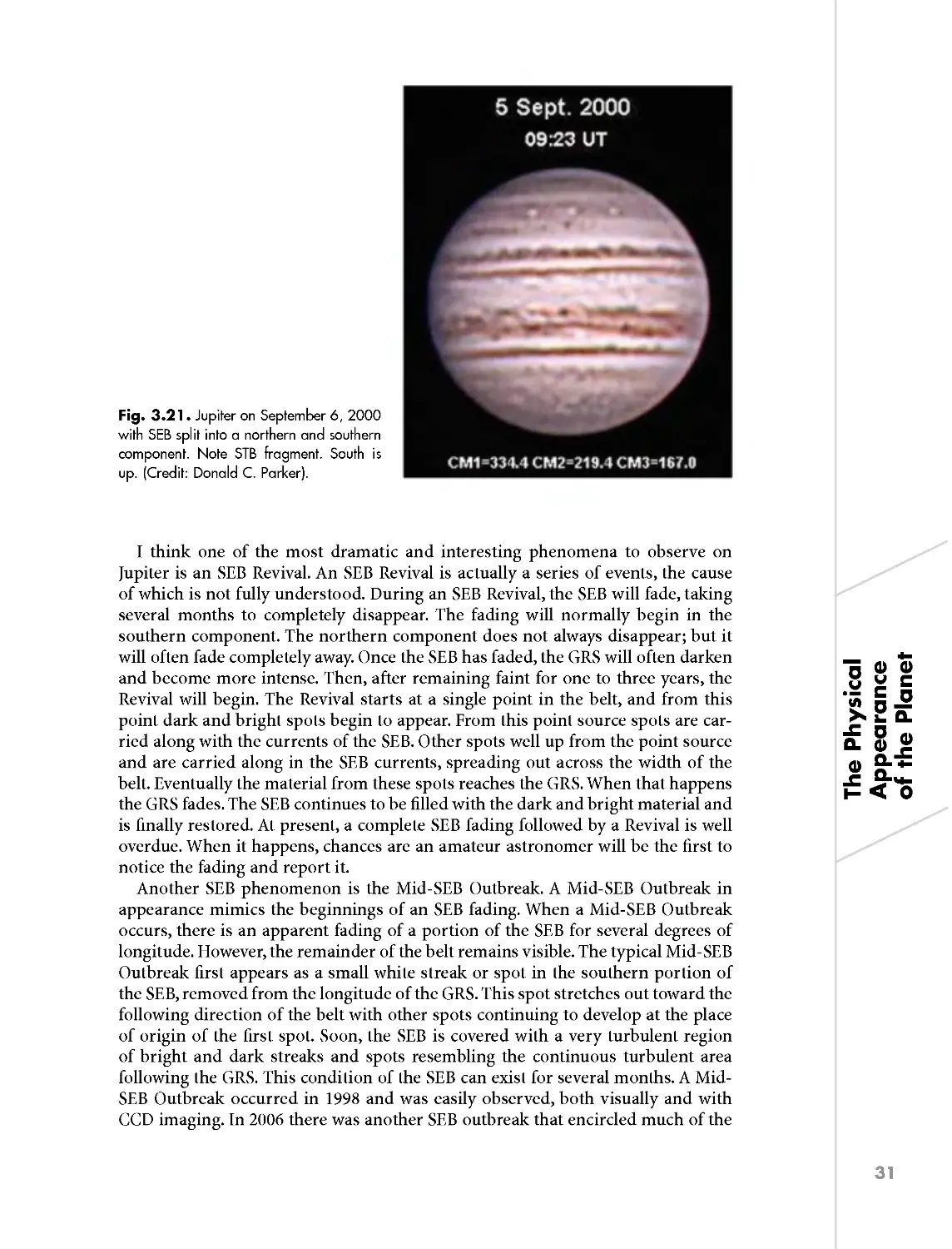
Later, during September 2000, Iupiter’s SEB was split into two components, with
the northern component, SEBZ, and southern component occupying the width of
a normal, solid SEB (Fig. 3.21). The southern edge of the SEB (SEBs) was uneven,
with bright bays protruding into the southern edge. Through February 2002 and
beyond, the SEB continued to be divided into this double component. Although
faint, in May 2002 the northern and southern components displayed a slight reddish-
brown color, with the northern component the darker of the two. By February
2003, the SEB was again solid along most of its length, except for the usual bright,
turbulent region following the GRS. During 2006, the SEB was again broad with a
general reddish-brown color. As usual, there was much bright turbulence following
the GRS. In April 2006, there was a really large white oval in the wake of turbulence
following the GRS.
Although the SEB does not form large condensations or barges like the NEB
does, sometimes small, reddish condensations or spots can form on or near the
southern edge of the SEB. These very tiny versions of the GRS, while sometimes
difficult to make out visually in a small telescope, can provide us with an opportunity
to track the drift rate and currents at this latitude of the planet.
Fig. 3.21. Jupiter on September 6, 2000
with SEB split into a northern and southern
component. Note STB fragment. South is
up. (Credit: Donald C. Parker).
I think one of the most dramatic and interesting phenomena to observe on
Iupiter is an SEB Revival. An SEB Revival is actually a series of events, the cause
of which is not fully understood. During an SEB Revival, the SEB will fade, taking
several months to completely disappear. The fading will normally begin in the
southern component. The northern component does not always disappear; but it
will often fade completely away. Once the SEB has faded, the GRS will often darken
and become more intense. Then, after remaining faint for one to three years, the
Revival will begin. The Revival starts at a single point in the belt, and from this
point dark and bright spots begin to appear. From this point source spots are car-
ried along with the currents of the SEB. Other spots well up from the point source
and are carried along in the SEB currents, spreading out across the width of the
belt. Eventually the material from these spots reaches the GRS. When that happens
the GRS fades. The SEB continues to be filled with the dark and bright material and
is finally restored. At present, a complete SEB fading followed by a Revival is well
overdue. When it happens, chances are an amateur astronomer will be the first to
notice the fading and report it.
Another SEB phenomenon is the Mid-SEB Outbreak. A Mid-SEB Outbreak in
appearance mimics the beginnings of an SEB fading. When a Mid-SEB Outbreak
occurs, there is an apparent fading of a portion of the SEB for several degrees of
longitude. However, the remainder of the belt remains visible. The typical Mid-SEB
Outbreak first appears as a small white streak or spot in the southern portion of
the SEB, removed from the longitude of the GRS. This spot stretches out toward the
following direction of the belt with other spots continuing to develop at the place
of origin of the first spot. Soon, the SEB is covered with a very turbulent region
of bright and dark streaks and spots resembling the continuous turbulent area
following the GRS. This condition of the SEB can exist for several months. A Mid-
SEB Outbreak occurred in 1998 and was easily observed, both visually and with
CCD imaging. In 2006 there was another SEB outbreak that encircled much of the
\
The Physical
Appearance
of the Planet
31
/
The Physical
Appearance
of the Planet
32
planet. As it progressed around the planet, it gave the SEB the appearance of being
split into two components, a northern and southern component (Fig. 3.22).
The STrDist is another interesting phenomenon. Rogers describes a STrDist as
“a coherent sector of shading and disturbance that spans the South Tropical Zone
(STrZ) [19]”. This zone resides between the SEB and the STB. The disturbance is
characterized by a dark coloration or shading in the STrZ. This dark coloration is
initially short in length, concave on the following and preceding ends, and usually
bounded on each end by a small white oval. Often, the disturbance begins near the
preceding edge of the GRS. The Disturbance normally fades when the SEB fades
prior to a SEB Revival. Disturbances normally last several months [20].
South Tropical Dislocations are also seen in the STrZ. A South Tropical
Dislocation occurs when a faded section of the STB passes the GRS. When this
happens the STrZ preceding the GRS darkens, so that the normal pattern of belts
and zones is reversed [21]. According to Rogers, in the 1970s a sector of the STB
turned white, and since then this ‘STB Fade’ has repeatedly induced structures like
STrDists preceding the GRS, giving rise to a dislocation of the normal pattern of
alternating belts and zones. Moving with the South Temperate Current this STB
Fade passes the GRS every two years. On some of these passages, it has induced a
darkening of the STrZ on the preceding side of the GRS, usually in the form of a
South Tropical Band although additional shading may be present. The term ‘South
Tropical Dislocation’ has been applied to this combination of the white STB and
dark STrZ, and also to the remarkable suite of structures that develop from it [22].
Although the STB itself in recent years has often been difficult to make out visually,
including any STrDist, the dislocation is fascinating and valuable to observe. CCD
and webcam images normally show these events quite well.
Fig. 3.22. Jupiter with a prominent Mid-SEB Outbreak underway on March 2, 2006. South is up.
(Credit: Donald C. Parker).
3.1.7 The Great Red Spot
The GRS is no doubt the most recognizable feature on the planet. It is embedded
in the southern edge of the SEB and is nestled between wind jets to the north and
south [23]. It is an anti-cyclonic storm, rotating in a counter clock-wise direction,
not too dissimilar from hurricanes on Earth, only incomprehensibly larger (Fig. 3.23).
According to Schmude, the longitudinal length of the GRS was 23,000 km during
the 1992-1993 apparition. Since Earth is 12,756 km in diameter, almost two of them
could fit inside the GRS! The GRS varies in color and shape with time. Sometimes,
the GRS is a vibrant red against a cream-colored background [24]. At other times,
such as is apparent during South Equatorial Disturbances, the spot seems to fade
and blend into its surroundings [25]. Although the GRS can be quite dark, since
1997 it has been rather faint, with a color of salmon-pink or light orange reported
by most observers instead of deep red. As a consequence, the GRS has been difficult
to observe in recent years, especially by amateurs new to Iupiter observing. Of late
the GRS has been in the shape of an oval, or ellipse. During some past apparitions,
the preceding and following ends of the GRS were more pointed.
A dark, oval spot near the latitude of the present day GRS was first observed by I-D
Cassini and others beginning in 1665 [26]. Observed for a long, long time, there is
some conjecture as to whether or not this weather system has persisted for over 350
years [27]. Indeed the system currently identified as the GRS can only be tentatively
traced back to circa 1830, 120 years after the last sighting of Cassini’s spot [28]. In
1878, the present day GRS was observed to be a deep,brick-red color [29]. Since that
time, the GRS has often been very faint or totally faded. The mostly cloud-free area
around the GRS is traditionally called the GRS “hollow” [30], or simply Red Spot
Hollow. The Red Spot Hollow (RSH) marks the position of the GRS when the GRS is
faded. The Hollow protrudes distinctly into the southern edge of the SEB.
From apparition to apparition, the color of the GRS can change noticeably. In
fact, past changes in the STrZ and SEB have demonstrated that the GRS and its
surroundings can change on very short time scales of less than five months [31].
Historical notes about the physical appearance of the GRS and its surroundings
also indicate variability of both very short and long time-scales [32]. In general,
the GRS is never “geranium” red, nor completely white [33], but no obvious peri-
odic color trend is evident. It is observed, however, that when the GRS “ingests”
smaller white vortices, the northern portion or the so-called “eyelid” of the GRS
does whiten [34]. Occasional brightening in the northern part of the spot, is often
associated with the ingestion of smaller eddies that are sheared apart inside the
storm or with interaction with the South Tropical Zone [35].
Fig. 3.23. Jupiter's Great Red Spot. Note
the darker condensation in the center of the
GRS and the overall salmon-orange color,
surrounded by a slightly darker collar of
material. The GRS is nestled into the Red
Spot Hollow. A bright gap can be seen
north of the GRS, between the GRS and the
southern edge of the SEB. Bright turbulence
can be seen in the wake following the GRS.
South is up. (Credit: Ed Grafton).
\
The Physical
Appearance
of the Planet
33
/
The Physical
Appearance
of the Planet
34
During the 2000-2001 apparition, the GRS was faint, with a darker condensation
in its very center (Fig. 3.23). This dark center was difficult to observe visually, but
it was easily made out in CCD images. The GRS was bordered on its southern edge
by a thin gray line. Sometimes, small white spots can be seen entering the GRS.
When this happens we have an opportunity to monitor the circulation inside the
GRS itself. According to Schmude, during the 2001-2002 apparition, the GRS was
reported to have no color or a faint orange-pink color [36]. By the beginning of
the 2003-2004 apparition, many observers were reporting a slight darkening of the
GRS with a slightly more intense pink color. This appearance continued through
2006, with the GRS displaying a moderately intense orange-salmon color, and a
darker condensation in its center.
In the past, small dark condensations have also been observed to circulate around
the GRS, leading to the conclusion that the GRS is a vortex. These observations
helped to identify the circulating currents inside the GRS. During the apparition of
1965-1966 a dark spot was observed on the north edge of the STB that approached
the GRS in decreasing longitude. Upon reaching the GRS it continued to pass the GRS
on the south side of the GRS. After reaching the preceding side of the GRS it did not
pass it, but continued around the GRS to the northern side of the GRS and returned
to the following end of the GRS. The spot was photographed by Elmer Reese and B. A.
Smith of the New Mexico State University Observatory, and observed by them from
December 1965 to Ianuary 1966. The spot circulated completely around the GRS in 9
days [37]. This observation was a significant contribution by amateurs. The Voyager
spacecraft also acquired images of spots that allowed scientists to further study these
currents. Dark spots were observed as recently as the 2001-2002 apparition [38].
To say we do not know everything we would like to know about the GRS is an
understatement! We do not possess a complete understanding of the cause of many
of the phenomena seen on the planet nor do we know with certainty when events
will occur or reoccur. However, we do know that certain events seem to follow others.
For example, the GRS alternates between periods when it is dark and faint. When
SEB Fades occur, the GRS often darkens, only to fade again during an SEB Revival
as the SEB is restored to its normal appearance. As this is written, a complete SEB
Fading is long overdue on Iupiter. The observation of such an event is of great impor-
tance and some diligent amateur will probably be the first to note the start of such
an event. When it happens, will the GRS darken as it has done in the past? And how
much time will pass before the SEB Revival begins? Any inconsistency from previous
patterns might indicate a change in ]upiter’s weather patterns. Regardless, any new
behavior would be of extreme importance to the professional community.
The size of the GRS has been changing over the years. According to Simon-
Miller et al. the latitudinal extent, or north—south distance, of the GRS has
remained constant, with ground based observations from 1880 to 1970 indicating a
latitudinal length of 11° i 1°. This was consistent with Voyager data indicating
a measured latitudinal extent of ~12,000 km [39]. However, the length of the GRS,
longitudinally, has been diminishing over the years. In 1882, the GRS had a length
of 34°. Until 1920, its length remained 30°, but since then it has never been as long
again [40]. It has been known since the early 1900s [41] that the GRS is shrinking
in apparent longitudinal extent.
If the latitudinal extent of the storm is thus assumed to be constant, the aspect
ratio can be plotted for the older observations, indicating that the GRS is indeed
becoming more round in appearance [42]. The system currently has an aspect ratio
of about 1.6 and, obeying the historical trend, the GRS should become round by
the year 2080, although that is not a stable configuration [43]. Simon-Miller, et al.
found a longitudinal shrinkage rate for the GRS of —0.193° per year. At this present
shrinkage rate, the GRS would be approximately round by the year 2040 [44].
The accuracy of any measurement of the length of the GRS is dependent upon
the observer’s ability to accurately identify the preceding and following edge of the
system. This may seem straightforward but is not necessarily so. Poor seeing can
undermine ones ability to see fine detail and transit timings under poor conditions
can induce error into the timing. Likewise, measurements of longitude taken from
CCD or webcam images can also suffer. Crisp, focused images of high resolution
are needed to get accurate and reliable measurements. Sometimes the preceding
and following edge of the GRS can be mistaken for the preceding and following
edge of the Red Spot Hollow, even when measuring CCD or webcam images. Prior
to the advent of CCD cameras and webcams, measurements of the GRS could only
be made with the use of filar micrometers or central meridian transit timings,
to be discussed later in this book. In spite of the inherent inaccuracies, multiple
measurements by a large number of observers are desirable, and can average out
the errors of measurement.
To illustrate the shrinking of the GRS over the years, we can review the historical
record. The difficulty of measurement is illustrated by the results reported by various
observers and researchers. All longitudes are given in System 2. Well known Iupiter
observer Elmer I. Reese determined a length of 24.4° i 1° during the 1962-1963
apparition [45]. During the 1968-1969 apparition Phillip Budine reported a length
of 23° [46]. Giancarlo Favero et al.. reported 22.9° i 0.5° in October 1975 [47]. Phillip
Budine reported a length of 20° during the apparition of 1967-1968 [48]. A length
of 23° was reported by Phillip Budine in 1983 [49]. A length of 19° was reported by
Phillip Budine for the 1985-1986 apparition [50]. For the 1986-1987 apparition Budine
determined a length of 22° early in the apparition, and 25° late in the apparition
[51]. Richard Schmude reported 23.6° i 1° during February 1989 [52],while Lehman
et al. determined a mean length of 20° for the 1989-1990 apparition [53]. Schmude
determined a length of 25.5° i 3° for the 1989-1990 apparition [54]. According to
Lehman and McAnally, during the apparition of 1998-1999, the GRS presented itself
as a much smaller feature inside the RSH. The GRS proper was determined to be
only 10° in length, while the RSH was 25° in length [55]. Using only high quality CCD
and webcam images in which the preceding and following edge of the GRS could be
accurately identified, I measured the length of the GRS to be 19° in November 1999,
17° in September 2000, 20° in September 2001, 17.5° in Ianuary 2002, and 17° in late
Ianuary 2003. During the 2003-2004 apparition I determined the mean length of the
GRS to be 17° in longitude. During 2006, I measured the length of the GRS to be 16°.
Observations and measurements of the GRS by astronomers, including amateurs,
will continue to be very important.
Sometimes the GRS presents a curious appearance, not quite filling the entire
space occupied by the red spot hollow (RSH). This appearance has been noted
during several recent apparitions. One such apparition, the 1998-1999 one, has
already been mentioned above. In a CCD image taken by Donald Parker on
September 04, 2000 a salmon-orange colored GRS was nestled in the southern
two-thirds of a bright RSH. The bay of the RSH protruded significantly into the SEB,
with bright material filling a large gap between the southern edge of the GRS
and the northern edge of the SEB. The GRS and RSH again presented this kind
of appearance in a CCD image taken by Maurizio Di Sciullo on Ianuary 12, 2002
in an image taken by Eric Ng on Ianuary 28, 2003 in an image taken by Tan Wei
\
The Physical
Appearance
of the Planet
35
/
The Physical
Appearance
of the Planet
36
Leong on February 23, 2003 an image by Cristian Fattinnanzi on April 02, 2004
and on webcam images taken by Parker on May 06, 2004 and 22. Sometimes the
color in the GRS can appear to be concentrated into a small area inside the GRS
itself, giving the GRS an even smaller appearance. This was the case on a CCD
image taken by G. Kiss on November 18, 2001 when the color of the GRS was
concentrated into an ellipse in the southern half of the GRS. This effect was again
seen in a CCD image taken by Parker on Ianuary 21, 2002. In all the images cited
above, an even darker concentration of color was seen in the center of the GRS,
giving the appearance of a dark spot inside the GRS! This has been a common
appearance in recent years. By April 2004, images by Fattinnanzi, Parker, and others
revealed a GRS in which the color again filled the entire ellipse of the spot; how-
ever, the dark center remained.
The source of color for the GRS is not understood. However, it appears that
Iupiter’s visible color is contained in the tropospheric haze [56], which is an
extended, colored, tropospheric haze denser than that seen on the rest of the
planet, and reaching higher in altitude than most other locations on the planet
[57]. Spacecraft missions have confirmed that the GRS has the vertical characteristic
of a tilted pancake [58].
Much about the GRS is left unanswered, such as what created it, what main-
tains it, what colors it, and why there is no counterpart to it in Iupiter’s northern
hemisphere. And so, we do not know everything we would like to know about the
GRS by a lot! One of my favorite endeavors is to keep a record of the changing
appearance of the GRS. Certainly the GRS will continue to attract the attention of
amateurs and professionals alike.
3.1.8 The South Temperate Region
The South Temperate Region generally extends from latitude 27° south to 37°
south. In the past, this region has displayed some of the most interesting features
on the planet.
The STB can be thought of as the southern counter part to the NTB. Like the NTB,
it is a relatively narrow belt and usually not nearly as dark as the SEB. Its coloration
is often described as gray, but I often note a touch of reddish-brown in the belt also.
During the apparitions of 2001, 2002, and 2003, the STB was faint and some segments
of the belt were totally faded, or at best, broken and fragmented (Fig. 3.21). Visually,
features in this belt can be difficult to observe, as often the contrast between the belt
and the surrounding zones can be very subtle. But, on occasion, a feature of some
prominence can be seen. This belt can be continuous,broken into segments, or faded
and completely absent. Dark spots have been observed here as well as bright ovals.
According to Rogers, the STB was always quite distinct, at least until the 1980s [59].
However, since 1997 I have found the STB to be very subtle and difficult to observe
visually. When seen, the STB has often been a narrow, faint gray belt, broken and
discontinuous.
In 1998, the STB immediately following the longitude of the GRS presented a
mottled but otherwise continuous appearance. By 1999, many segments of the STB
were quite faded. In 2002, the STB was so faded as to be mostly absent, punctuated
by short, darker segments in a few locations around the planet. By the end of 2002,
the belt was so faded as to make it difficult visually to distinguish the STB from the
northern edge of the SPR, since the South—South Temperate Belt (SSTB) was also
very faint or absent. This condition continued into 2003. However, in 2003 a dark
segment, approximately 50° long, was seen for many months. This dark segment was
so prominent as to be easily seen visually in telescopes as small as 8-inches aperture.
CCD images revealed that this segment was not solid, but composed of a string of
condensations close together. In February 2003, this dark segment was positioned
immediately south of the GRS, giving the impression of an eyebrow over the GRS
(Fig. 3.24). The appearance of this segment allowed transit timings and longitude
measurements to be made, providing a welcome opportunity to track the drift rate
at this latitude. By Iuly 2004, the STB was again presenting a mostly continuous, thin,
although faint belt around most of the planet. I found this to be so even visually in
an 8-inch telescope. Some segments of the belt continued to be faded. In 2006 the
STB was absent or at least very difficult to see around most of the planet, being most
easily seen following south temperate oval (STO) BA. In some locations where the
STB was faded, a very light remnant could sometimes be made out.
As mentioned, short dark segments and condensations or “spots” may occa-
sionally be present in the STB. As recent as 2003, a very short, dark segment or
condensation was observed on the southern edge of the STB (STBs). This segment
was followed for several months, and was seen visually as well as being detected
on CCD and webcam images. A darker segment was seen for a short distance
following oval BA during 2006. Segments and spots like this are not seen during
every apparition. However, one of the most prominent spots ever seen in the STB
appeared in 1998.
The South Temperate Dark Spot of 1998 was a fascinating feature to observe.
While there is evidence of this spot on CCD images by Miyazaki in 1997, the spot
did not come to notoriety until 1998 (Fig. 3.25). As the Assistant-Coordinator for
Transit Timings of the A.L.P.O. Iupiter Section, I first received a report of the spot
on 1998 Iune 20 from Harry Pulley, who had observed the spot and recorded a
transit timing on that date. The spot was subsequently observed and reported by
other observers over the next several weeks and I initially determined the spot
had a drift rate of —5° per 30 days. On Iuly 22, 1998 I issued an alert message from
A.L.P.O. via the Internet and gave this feature the provisional name of STB Dark
Spot #1. Visually, the spot appeared as a very small dark spot, like a pencil spot on
Fig. 3.24. Dark segment of the STB,
giving the appearance of an 'eyebrow'
south of the GRS on February 18,
2003. The STB is discontinuous. The
NEB is narrow and the NTB is absent.
Note the five bright ovals in the SSTB.
Note also the coloration of the north-
ern two-thirds of the EZ. South is up.
(Credit: Ed Grafton).
\
The Physical
Appearance
of the Planet
37
/
The Physical
Appearance
of the Planet
38
Fig. 3.25. Jupiter on August 3, 1998 and
the South Temperate Dark Spot of l 998. Also
seen is STB Dark Spot #2, an elongated spot
following close behind. Two major ground
telescopes and the Galileo spacecraft made
investigations of the 'dark spot’. South is up.
(Credit: Donald C. Parker).
a page, almost as dark as a moon shadow. Being so small, the spot was difficult to
see visually, but once found it seemed to jump out at the observer. The visual effect
was remarkable.
After Iuly 14, 1998 the drift rate of the spot increased to —15° per 30 days,
prompting me to issue another alert message. This second message caught the
attention of Dr. Glenn Orton, of the let Propulsion Laboratory, who requested
additional information. Dr. Orton was one of the Galileo Spacecraft Mission
Interdisciplinary Scientists. Dr. Orton and I began corresponding on a regular
basis. From the date the first alert message was issued until the end of the 1998-1999
apparition, the spot was observed continuously around the world. In fact, world-
wide participation was so intense that there were few occasions that a transit of the
spot was not observed at least twice a week! There was tremendous cooperation,
especially among amateurs; and the interest by the professional community was a
great example of professional-amateur cooperation!
On September 21, 1998 I issued another alert over the Internet announcing a
second dark feature had been seen in the STB. This feature was given the pro-
visional name of STB Dark Spot #2. Dr. Orton informed me that a decision had
been made in the professional community to examine Dark Spot #1 more closely.
It was Dr. Orton’s intention to observe Iupiter at 5-um with the NASA Infrared
Telescope Facility (IRTF) Telescope and Near Infrared Camera (NSFCAM) from
Mauna Kea for three full nights starting on or about September 27, 1998. At the
same time, Dr. Terry Martin was to observe from Palomar Observatory using a
middle-infrared camera and a spectrometer. Dr. Orton anticipated they would also
capture the feature with 27-um observations made with the Galileo Spacecraft
Photo-Polarimeter-Radiometer (PPR) sequence on Galileo’s orbit number 17 [60].
Dr. Orton later informed me that all three observations were successful. You can
imagine how excited we were in the amateur community, having contributed to the
professional interest in this feature that led to the allocation of observing time with
such important resources!
These observations revealed that the feature was not a spot at all, but a hole in
Iupiter’s cloud tops. The “spot” was bright at 5-um (the infrared). Since infrared
detectors detect warmth, this brightness indicated the spot was a warm feature. In
other words, we were detecting the warmer temperature below Iupiter’s cloud tops
escaping up through this hole. In visible light, this hole was dark, since we were
seeing through it to lower cloud decks.
This “spot” was observed for two apparitions with great success, and caught the
attention of amateurs and professionals alike. Not only was this an exciting fea-
ture to observe and record, the international cooperation that ensued was a great
accomplishment for astronomers [61]. When features like these are seen, Iupiter
observers are presented with an opportunity to monitor the drift rates in this belt
with great accuracy.
The features most prominently seen on the STB are white ovals [62]. Many of
these ovals are quite small and difficult to observe visually due to the low contrast
of the ovals against the zones on either side of the belt. The most famous STO today
is the larger oval BA (Fig. 3.26).
Oval BA is the loan survivor of three ovals that originated in the South Temperate
Zone (STZ) between 1939 and 1940 [63]. The history of these ovals is quite fascinating,
and the eventual demise of two of them presented astronomers, professional and
amateur alike, with an adventure in observational astronomy we shall not soon forget.
The three STOs began their existence as bright sections of the STZ. During
1939-1940, three bright segments or spots appeared in Iupiter’s south temperate
region. The spots rapidly contracted during the 1940s to form three large white
ovals by 1950, eventually shrinking to sizes of ~ 10,000 km by the 1990s. During
their lifetimes, the ovals demonstrated wandering motions (movement in longi-
tude), with ‘mutual close approaches without mergers’ [64].
Fig. 3.26. The bright South Temperate Oval 'BA' in the STB near Jupiter's central meridian on April
22, 2005. Note how the color of oval 'BA' is very close to that of the neighboring zones on this date.
A small bright oval is in the SSTB just south of 'BA'. South is up. (Credit: Damian Peach).
\
The Physical
Appearance
of the Planet
39
/
The Physical
Appearance
of the Planet
40
According to Rogers, the three ‘proto ovals’ appeared when the STZ became sub-
divided by the gradual appearance of three dark features, which initially appeared
either as dusky sections of the zone or as segments of a south component of the STB.
These dark features expanded longitudinally until they confined the three
intervening bright sectors of the STZ into gradually contracting ovals. Elmer Reese
had originally named the dark segments AB, CD, and EF. Subsequently, the bright
ovals formed between them became known as BC, DE, and FA [65]. The STOs are
anticyclonic like the GRS, rotating counterclockwise.
Voyager images in 1979 revealed the STOs to be anticyclonic vortices similar
dynamically to the GRS. In 1998, two of the ovals BC and DE merged into a larger
one, later designated BE, while Iupiter was too close to the Sun to be observed [66].
At the beginning of the 1998-1999 apparition, it was discovered that one of the
three ovals was missing! Apparently, something unexpected happened while Iupiter
was at conjunction, hidden from view behind the sun. The answer to this did not
come immediately. Dr. Reta Beebe of NMSU and the International Iupiter Watch
(IIW) contacted me seeking the longitudinal positions of the two surviving ovals.
I had just assumed the duties of the Assistant Coordinator for Transit Timings of
the A.L.P.O. Iupiter Section in 1997 and had the responsibility of keeping track
of the positions of features in Iupiter’s visible atmosphere. Dr. Beebe’s intention
was to use the Hubble Space Telescope (HST) to study the remaining ovals. In her
words, no one was sure whether an oval had simply faded or two had merged.
Eventually it was decided that the most likely scenario was that ovals BC and DE
had indeed merged. The merged oval was renamed BE.
Previously the three ovals had drifted close to each other on many occasions,
only to drift apart again. Often, smaller intervening cyclonic ovals were present,
separating the larger anticyclonic ovals. It was always assumed that the dynamics
of these systems would simply cause the three large ovals to bounce off of each
other should they come together. News that two of the ovals had actually merged
stunned Iupiter scientists.
As the 1999-2000 apparition began, the possibility of another STO merger, this
time between ovals BE and FA, again presented itself. On April 30, 1999 the separa-
tion between the ovals’ centers was only 18°. From April 30, 1999 to November 20,
1999 the distance between BE and FA varied in a dance that would see them drift
closer together only to drift further apart again. The ovals drew closer then drifted
apart several times. By November 20, 1999 the ovals were at or approaching conjunc-
tion with the GRS. Astronomers wondered if the passing of the GRS would change
the ovals’ drift rates. The ovals continued their dance of drifting closer together and
then farther apart, but closing the overall distance over time. By Ianuary 2000, CCD
images by the Pic du Midi Observatory revealed that a cyclonic cell between the two
ovals had disappeared, which could make it easier for the two ovals to collide and
merge (Sanchez-Lavega personal communication). On February 8, 2000 the ovals
centers were measured as 12° apart. More significantly, the following edge of BE
and the preceding edge of FA were only 5° apart! At this time as a staff member of
the A.L.P.O., I issued an alert over the Internet, receiving immediate response from
astronomers at IPL and Cornell University. By March 17, 2000 the ovals were in
contact with each other but undisturbed. From this time forward, events developed
rapidly. On March 19 and 20, 2000 oval BE shifted northward with FA overtaking it.
Indeed, infrared images from the Infrared Telescope Facility (IRTF) on Mauna Kea,
showed the bright methane cloud-caps over the ovals rotating around each other. On
March 21 and 23, 2000 CCD images showed BE was disrupted. By April 7, 2000 CCD
images showed BE/FA as a single object, very diffuse [67].
And so, during a three week period beginning in March 2000, ovals FA and BE
completed their merger in the south temperate region. The merger took place
when the ovals were southeast of the GRS, and after the disappearance of a smaller
clockwise rotating oval that had been between them. The high altitude oval clouds
of ovals BE and FA demonstrated counter clockwise rotation around each other,
then merged and began shrinking. The interaction of deeper clouds did not show
mutual rotation [68].
Prior to the merger of the two remaining ovals BE and FA, HST images revealed
that oval BE had a diameter of ~9,000 km and oval FA had a diameter ~7,700 km.
Situated between them was a smaller oval, designated O1. Oval O1 had a diameter
of ~5,000km. In latitude, oval BE was located at —32.7°, oval FA at —33.6°, and
smaller oval O1 was at —31°, or south of both STOs. Oval O1 was first observed in
May 1998 and was similar to one observed between ovals BC and DE before they
merged in 1998 [69].
Close interactions between these three vortices (BE, FA, and O1) began in
November 1999 when the ovals passed the GRS. At that time oval O1 began a
southward migration, moving from latitude —31° to —36°,“moving along an arc of
35° that encircled oval BE in the anticyclonic (counter clockwise) sense”, according
to Sanchez-LaVega et al. Oval O1 moved from the cyclonic region to the adjacent
anticyclonic (counter clockwise) one [70].
It would appear that the removal of oval O1 allowed ovals BE and FA to interact
directly. According to Sanchez-LaVega et al. “as the ovals approached each other,
BE moved with a velocity of u = 0.6 ms”, whereas FA decreased its velocity from
u = 1.6 ms’1 in Ianuary 2000 to u = 0.9 ms’1 in early March 2000.” On March 17,
2000 FA pushed BE northward by ~3.2° (4,000 km) as observed at high altitudes.
Then on March 21, 2000 the pair began an anticyclonic (counter clockwise) orbit
about each other. By April 3, 2000 the ovals had merged, and by April 14, 2000 had
decreased in size to a compact state [71].
At middle and lower levels (altitudes) the interaction was a little different, and
the first interaction occurred March 12-15, 2000. Between April 7 and 14, 2000 new
oval BA was still forming with a double nucleus of 5° separation still seen. Later,
on September 2, 2000 the area of BA was determined to be ~70% of the sum of the
areas of BE and FA [72].
According to Sanchez-LaVega et al. the orbiting action observed in oval O1 and
in ovals FA and BE can be explained by the presence of a velocity field induced by
the vortices on each other. The observed interactions consisted of well-known
phenomena that had been observed and predicted by models in computer simulations.
It appears that most interactions of smaller scale spots observed in Iupiter lead to
mergers. However, prior to 1998 the three STOs had always just bounced off of each
other. In spite of their long history as separate objects, the two remaining STOs
had collided and merged together. So, after 60 years the three ovals have finally
coalesced into one vortex [73]. As of this writing, the surviving oval BA continues
to thrive. With the last of the two STOs having merged, the remaining oval became
known as oval BA [74, 75]. Like the GRS, oval BA is a huge counter-clockwise rotating
vortice. Oval BA is still visible today, being especially well seen in CCD imaging.
Visually, this oval can be difficult to make out due to its low contrast, especially if
the dark collar of material that often surrounds it is absent.
\
The Physical
Appearance
of the Planet
41
/
The Physical
Appearance
of the Planet
42
Amateur and professional astronomers alike kept faithful watch over STO BA
during the 2000-2001 apparition. In October 2000, oval BA presented a large,
bright object. However, with a faded and broken STB, oval BA was often difficult
to make out visually. A CCD image taken by Donald Parker on October 5, 2000
revealed a large oval BA surrounded by a collar of dark material, and trailed for
a short distance by a dark segment of the STB. Without this dark material, BA
would have been difficult to see even on CCD images, due to low contrast with
the rest of the south temperate region. I used this dark segment of the STB to
help pinpoint the following edge of oval BA when observing visually. However,
by December 2001 the dark collar of material surrounding oval BA had almost
vanished, leaving the contrast between the oval and its surroundings so subtle as
to make it near impossible to visually make out the oval. Only low intensity dark
material following the oval in the STB made it possible to see it at all. Even on
CCD images by Ed Grafton in December 2001 and Maurizio Di Sciulla in Ianuary
2002, the low contrast of oval BA was startling. Eventually, some of the dark collar
material returned. A CCD image by Eric Ng taken on February 22, 2003 revealed
an oval surrounded by dark material, although oval BA itself was rather dusky
and subdued, contributing to low contrast. By March 2004, oval BA was once
again easier to see due to dark material surrounding it on its south, preceding,
and following edge. CCD images by Rolando Chavez, Cristian Fattinnanzi, and
Parker reveal this quite well.
Since they first appeared in 1939-1940, the STOs contracted and continued
to contract during their lifespan. The three ovals were of different lengths lon-
gitudinally, with FA being the most diminutive of the three before the demise
began. In the 1980s, ovals BC and DE were 8—9° in length while oval FA was 5°
in length [76]. On March 11, 2004 I measured the length of surviving oval BA as
7°. The morphology, intensity, and drift rate of STO BA continues to be of great
interest to Iupiter observers. Could the GRS have gone through the same process
somewhere in its history? Keeping an eye on the behavior and condition of oval
BA will be a valuable contribution that amateur astronomers can make, possibly
for years to come.
Fig. 3.27. Jupiter on July 3, 2006. South
Temperate Oval 'BA' has turned red. Note how
the color of 'BA' is very similar to that of the
GRS. South is up. (Credit: Christopher (30).
With great surprise, oval BA changed color in late 2005 and became noticeably
red in early 2006 (Fig. 3.27). Many amateurs began to refer to the oval as “Red Spot,
Ir.”I prefer to continue referring to this feature as oval BA, since this is what it truly
is and because we need to preserve the continuity of our observational record. This
change in the oval’s color was first noted and reported by amateur astronomers,
and by April 2006 professional astronomers had made a detailed study and analy-
sis of this event. This historic change will be more fully discussed in Chap. 4.
It seems to me that, compared to the NTB, the STB is a much more active
belt with a greater variety of features. What will the future hold? Only future
observations will reveal how many ovals, spots, and belt fadings will appear. And
what about oval BA? How long will it survive? Forever? That now seems unlikely.
However, with no other large ovals to collide with, is there anything there to dis-
rupt it? The south temperate region will continue to be one of the most important
regions of the planet to patrol.
3.1.9 The South-South Temperate Region
The South—South Temperate Region generally extends from latitude 37° south to
53° south. Lying just south of the STB is the STZ, and just south of that is the SSTB.
The south—south temperate region is exceedingly difficult to observe visually. To
most observers this region appears as varying intensities of gray, with very few
features that can be made out. Sometimes a dim, gray SSTB can be seen. Most often
it is actually difficult to distinguish this belt, or the South South Temperate Zone
(SSTZ) for that matter, from the northern edge of the SPR. Like the STB, the SSTB
is a very narrow belt with a light gray coloration. While features here are difficult to
observe visually, CCD imaging by amateurs has been quite successful. Normally,
a number of small, bright ovals can be seen here, being of great interest to astrono-
mers (Fig. 3.28). These ovals can provide our only chance to monitor the drift rates
at this latitude. Unlike the much larger STO BA, these south STOs are quite small
and of especially low contrast. Many visual observers have never seen one. Images
with CCD cameras and webcams usually reveal them easily, as they stand out
against the slightly darker gray coloration of the SSTB and SSTZ. Examination of
CCD images during recent apparitions suggests that there are always six or more of
these ovals each apparition. These ovals are of relatively small size, however, I did
measure one oval as 5° in length on a CCD image taken by Cristian Fattinnanzi on
April 02, 2004. Several ovals were seen, quite bright against the dusky, gray SSTZ.
During 2006, several small bright ovals were again observed, being very prominent
in CCD/webcam images (Fig. 3.28).
Like the NPR, the SPR often presents little that can be seen by amateurs, even with
CCD cameras and webcams. Sometimes imaging can reveal very subtle, thin faint
bands and barely noticeable zones marked only by very subtle shading differences.
Sometimes small bright ovals are seen. Features that might offer a chance to track
currents in this region are short-lived or very difficult to see. I did note during the
2003-2004 apparition what might be described as a very small south polar hood of
bluish-gray color, which was also noticeable on CCD images (Fig. 3.29). However, the
remarkable work by amateurs using CCDs and webcams caught many features that
were of great interest. In fact, the SPR turned out to be much more active than the
NPR! Small bright ovals that turned out to be long-lived were seen in the SPR at 60°
south latitude, and another one was seen in the south—south—south temperate
\
The Physical
Appearance
of the Planet
43
/
The Physical
Appearance
of the Planet
44
Fig. 3.28. Four very bright small ovals are seen in the SSTB of Jupiter in this webcam image taken
on April 2, 2004. The GRS can be seen emerging from the following limb of the planet. A prominent
bluish-gray plateau with a trailing festoon can be seen on the south edge of the NEB. The northern
edge of the NEB is very uneven. South is up. (Credit: Cristian Fattinnanzi).
Fig. 3.29. Jupiter with a very quiet SPR on
February 10, 2004. Note the absence of any
remarkable features in the region. By contrast,
the EZ is very busy with prominent blue-gray
features projecting into it from the southern
edge of the NEB. Also note the subtle, yellow-
ochre coloration of the northern two-thirds
of the EZ. South is up. (Credit: Donald C.
Parker).
current (SSSTC) at 50° south latitude. As technology advances and more tools
become available to amateurs, the future may allow amateurs to do even more useful
work in this region.
Hopefully, the past history we have studied here makes it clear that over a
relatively short number of years, Iupiter can exhibit distinct and substantial
changes in appearance. If you pay attention, you will never find Iupiter to be a
boring planet!
3.2 Winds and Jet Streams
in the Atmosphere
Features seen in Iupiter’s atmosphere are not stationary,but drift with the currents
and jet streams they are associated with. While the study of Iupiter’s atmospheric
dynamics is a whole discipline in itself, some understanding of Iupiter’s atmos-
pheric systems can aid the amateur in the study of Iupiter. When the drift rate of a
certain feature is known along with its apparent latitudinal position, its association
with a particular jet stream or current can be specified with some certainty. This
knowledge will allow a prediction of its future position over time, allowing for the
recovery and identification of the feature with some certainty following the end of
an apparition or following a period of bad weather when there has been a lapse in
observations. In more than one instance, the determination of the type of feature
in a belt or zone was finally settled only after its drift rate had been determined and
compared with historical data for the region being observed.
There are a number of currents and jet streams in Iupiter’s atmosphere, some
of which can only be observed by spacecraft. Here we will concentrate only on
the ones that can be monitored visually. Following is a discussion of various jet
streams and currents after Rogers, 1995 (Fig. 3.30).
The currents that can be monitored by visual observers fall into three categories.
There is the great equatorial current, which encompasses the entire equatorial
region. This current pro-grades, or moves in increasing longitude, at 7—8° per day,
relative to System II. There are the nine slow currents, which govern most of the
visible features outside the equatorial region, and have speeds of no more than 1°
per day. And, there are the jet streams on the edges of certain belts, only observed
SSTB ' t .
STB: STBS Jet
SEBs jet
SEC <:—
Preceeding Following
NEC <——
NTBs jet NEB" jet
NTC-B .
NTB
NNTBS Jet NNTlgriejiet
N
Fig. 3.30. A simplified depiction of the currents and jet streams on Jupiter, indicating the direction
of flow in Jupitefs atmosphere. South is up. (Credit: John W. McAnc:lly otter Rogers i995).
The Physical
1-
8%’
=0
ga
30
&£
<"6
45
/
The Physical
Appearance
of the Planet
46
during infrequent outbreaks of small dark spots, which have speeds of several
degrees per day [77].
The jet streams are detectable from Earth only when they are disturbed by distinct
spot outbreaks. All the larger features move with the slow currents [78].
3.2.1 The Slow Currents
The slow currents had all been detected and recorded by 1901 (Table 3.1). Since
that time, they have shown only temporary Variations in speed. The cause for the
difference in speed of the nine currents is not known. The speeds do not seem to
be related to the types of features that are carried along by them, nor to any jet
streams around them [79].
A Variety of features can be seen in these slow currents, including bright and dark
spots, medium and large spots, and cyclonic and anti-cyclonic spots. Regardless of
the feature seen, they all seem to move in the same slow current. In some latitudes,
either bright spots or dark spots are more common [80]. All latitudes of the planet
present something of interest because of the Variety of features and the currents
Table 3.1. Jupiter's jet streams and slow currents: latitudes and speeds
Latitude range u Change in longitude
Jetstream B” (m s“) System || (° per 30 days)
SSSSTBn 53.4°S +36.3 -129
SSSTBn 43.6°S +42.1 -125
SSTBn 36.5°S +31.6 -88
STBs 32.6°S -20.8 +42
STBn 27—29°S +44.3 -1 10
SEBs 20.0°S -56.6 +1 17
SEC 7°S +1 28 -276
NEC 5-8°N +103 -224
NEBn 17.6°N -24.3 +45
NTBs 23.8°N +163 -375
NTBn 31 .6°N -32 +69
NNTBs 35.6°N +34.5 -94
NNTBn 39.5°N -14.8 +31
NNNTBs 43°N +21.8 -68
NNNNTBs 48.2°N +28.5 -94
NNNNNTBs 56.6°N +14.1 -59
Current
SSSTC 45—52°S +0.1 1 1.9 -8.3
SSTC 38—42°S +6.6 1 0.7 -25.1
STC 29—35°S +7.5 to 1.5 -26 to -12
STropC 13—25°S -3.6 (11.0) -0.1 (12.3)
NTropC 14-22°N +0.5 (12.5) -9.1 (15.4)
NTC 25-34°N -10.6 (11.8) +17.0 (14.2)
NNTC 37—42°N -2.9 (11.2) -0.3 (13.2)
NNNTC 44-47°N +2.5 (11.4) -15.2 (14.1)
NNNNTC 49-55°N -2.9 (10.9) +1.4 (12.8)
B” represents zenographic latitude; u (m s“) represents speed in meters per second in
System |||. (After Rogers 1995.)
with which they are involved. All features may not be present during each appari-
tion, but there will be enough variety to maintain the serious observer’s interest.
Patience and attention to detail will enable the observer to gather significant data
about the present condition of these currents.
The uniformity of the slow currents is important because bright and dark spots
are now known to have opposite circulations, and actually lie on opposite sides
of the retrograding jet stream, which are commonly deflected around them. The
larger spots are therefore embedded in waves on the retrograding jet streams. The
slow-current features observed from Earth are mostly large bright ovals or dark
condensations of sizes comparable to the distances between jet streams [81].
3.2.2 The Jet Streams
Iupiter’s jet streams are not too dissimilar to the jet streams on Earth. Both are fast
moving currents. However, the jet streams on Iupiter appear to be more stable in
latitudinal position that Earth’s jet stream, which can vary in latitudinal position
by a significant distance. Iupiter also has many more jet streams than Earth. These
jet streams create some of the most exciting phenomenon in Iupiter’s atmosphere.
Certainly, over the years I have enjoyed watching the fast changing positions of
features in these jet streams.
The fastest jet stream on the planet, which resides on the southern edge of the
NTBs, was discovered during an outbreak of spots in 1880. Three other rapid currents
on the SEBs, STBn, and NNTBs, were discovered during outbreaks in the 1920s.
The fifth jet stream to be discovered from Earth, the SSTBn, was observed in 1988
[82].
Our view from Earth is selective, since the jet streams are only detectable during
outbreaks. For the five jet streams that have been observed from Earth, latitudes
and speeds determined by spacecraft agree with those determined from Earth. The
latitudes of the jet streams, except for one, have not changed significantly over the
period of Earth-based observations [83]. There are several other jet streams that
have only been observed from spacecraft. However, for the five detectable from
Earth, amateurs, especially with CCD and webcam imaging, can monitor and
contribute significant drift rate data.
3.3 Color in Jupiter's Belts and Zones
Observation of color in Iupiter’s belts and zones can be an aesthetically pleasing
endeavor. Unfortunately, it also is one that can be very scientifically frustrating.
Not only is contrast very subtle between features in Iupiter’s cloud tops, but the
determination of color by the human eye is difficult to quantify and fraught with
subjectivity. Peek noted that the visual appreciation of color is such an individual
affair that it can hardly be expected to furnish scientific data reliable enough to
be used with confidence as a satisfactory basis for theoretical investigation [84].
Using the human eye, observers can only judge color in a relative and subjective
manner, even if they are wise to possible instrumental and atmospheric illusions
[85]. Nevertheless, I almost always make note of color in the record of observation
when observing Iupiter.
\
The Physical
Appearance
of the Planet
47
/
The Physical
Appearance
of the Planet
48
A number of hurdles present themselves when attempting to observe the color
of a celestial object from Earth. The type of telescope and optics is very important,
and a reflector used in combination with high quality eyepieces is usually the better
choice since it will minimize the effect of chromatic aberration.
Earth’s atmosphere, or more specifically atmospheric dispersion, is a major
source of trouble. Earth’s atmosphere introduces chromatic effects that at low altitude
are considerable and are particularly apt to vitiate color estimates in the case of a
belted planet like Iupiter. The greater density of the air near the ground, compared
with that at higher altitudes, not only brings about the well known effects of refrac-
tion but also causes the image of a point source, like a star, to appear as a short
vertical spectrum with the violet at its upper and the red at its lower end. Under
telescopic magnification this is especially noticeable, and in the case of a planet
whose upper limb (lower in the telescopic image) may be seen edged in blue,while
the lower limb has a reddish border. For a belted planet like Iupiter with bright
zones,blue and red light will spill over from the edges of the bright zones and color
the edges of the adjacent darker belts [86].
The use of color filters of known wavelength transmission can eliminate the
subjectivity in determination of color. It can be noted that when observing Iupiter
with a blue filter, the GRS appears darker, as the red light is not transmitted.
Likewise, the GRS will appear bright when observed with a red filter. Filters can
be used visually, or with photography and CCD and webcam imaging. Filters of
known transmission are very useful scientifically and more will be discussed about
their use later.
When describing color on Iupiter, it is probably wise to avoid thinking in absolute
terms. The GRS is not red but reddish or reddish-brown, or salmon-orange, or
pinkish. The belts are not brown or gray, but instead reddish-brown or grayish.
There are shades of gray, shades of browns or ochre, colors tending toward some-
thing; however, there are no absolutes.
One of the most intriguing methods for removing subjectivity from the obser-
vation of color is put forth by Dr. Iulius Benton. Benton is the Coordinator of the
Saturn Section of the Association of Lunar and Planetary Observers. Visually made
absolute color estimates should be carried out by comparing ‘the planet’ with a
satisfactory color standard, according to Benton. Estimates of absolute color have
to be made with instruments in integrated light (no filter). The A.L.P.O. Saturn
Section has carefully investigated a suitable color standard, and it employs some
500 colored paper wedges for comparative use. One should have normal color
vision for this type of work, and the color standard should (ideally) be illuminated
by a tungsten lamp filtered with a Wratten 78 (W78) color filter [87].
In spite of the difficulties in determination of color, it continues to be important
for observers of Iupiter to study and characterize color, including the patterns of
change in coloration and intensity.
3.4 Summary
Some features may be seen to occur only in certain belts or zones. Features may
be present during one apparition and absent the next. Some may be seldom seen,
while others are almost always present. CCD images can reveal features difficult to
make out with the unaided eye; or, even those that usually cannot be seen at all.
Some of Iupiter’s features are so subtle that I know several experienced observers
who have never made them out visually. It is important for the observer of Iupiter
not to be disappointed if certain features seen previously are absent at a later date.
Certainly, the absence of a feature, or type of feature, may turn out to be an impor-
tant piece of data. Approach the planet with objectivity, without expectations, and
every observation will be a new discovery. You will never be disappointed.
The Physical
1-
8%’
=0
ga
30
&£
<"6
49
r/
cg k
E52
03'-U
£'—Z
U30-
£9.03
_°E£
OOH-
UUO
/
50
Chapter 4
Color, Chemical
Composition of the
Planet, and Vertical
Structure of the
Atmosphere
There is much about Iupiter that is not readily apparent to the amateur astronomer
gazing through a small telescope in visible light. We can argue whether an under-
standing of such things should not simply be the domain of professional astrono-
mers. Regardless, I believe well-rounded amateurs will want to learn as much as
possible, and thus will appreciate the study of the planet all the more.
4.1 Color
Previously, we discussed the observation of Iupiter’s colors. But, what causes the
color in Iupiter’s atmosphere? As we might surmise, that explanation is not so
easily forthcoming. The different colors represent clouds with different composi-
tions and different vertical structures [88]. The understanding of color in Iupiter’s
atmosphere is dependent upon some basic understanding of atmosphere. So, first,
let us try to understand some basic principles about atmospheric structure.
Iupiter’s atmosphere is divided into four main layers. These layers are the tropo-
sphere, stratosphere, thermosphere, and ionosphere (Fig. 4.1). The boundaries of
the troposphere and stratosphere are determined by atmospheric pressure and
temperature, both of which are interrelated, as temperature changes with height
in atmosphere.
Iupiter emits almost twice as much heat as it receives from the Sun. This heat is
emitted upward as infrared radiation. As this heat is radiated upward, it drives the
changes in Iupiter’s weather. Similar to Earth, temperatures in Iupiter’s atmosphere
change with altitude. Unlike Earth, Iupiter has no hard surface that we can see. On
Earth we measure altitude from ‘sea level.’ Iupiter has no sea level, so here scientists
make an assumption. On Earth we measure pressure in bars. Iupiter scientists use
the same scale of measurement and assume that 1 bar is sea level for Iupiter. So that
1 bar of pressure is the same as an altitude of zero.
I I I I I I
— 3,000
net
.7 _ Ionosphere I
10 Thermosphere _ , — — ’ J
_ _ , — — ‘ — 600
10-6 — ' ’ ’ T
10‘5 — — 300
10-4 —
E A
Q — 200 g
9 10-3 — 0
3 E
In '4:
9 7:
0.
10-2 _ Stratosphere
— 100
10-1 - ¢— Tropapause
4- Visible cloud tops
1 _ — 0
Troposphere
10 _ — -100
102 I I I I I _3oo
0 200 400 600 800 1000 1200
Temperature (‘’K)
Fig. 4.1. A simplified model of the vertical structure of Jupiter's atmosphere, demonstrating how
temperature and pressure vary with height. (Adapted from Rogers I995.) [89].
On Earth, the lowest atmospheric layer is the troposphere, and so it is with
Iupiter. On Iupiter, the troposphere extends from some low level to an altitude
corresponding to the lowest temperature in Iupiter’s atmosphere. This point is
referred to as the tropopause; that is, the altitude at which the troposphere stops.
Beyond the tropopause is the stratosphere. So, the tropopause is the boundary
between the troposphere and the stratosphere. The tropopause is also described
as the layer at which temperature stops decreasing. From the tropopause the
temperature again rises into the stratosphere. So, at the tropopause, a tempera-
ture inversion occurs. Temperature increases with altitude above the tropopause.
The next boundary layer is the stratopause. According to Amy Simon-Miller, “the
stratopause occurs when the temperature stops increasing and begins to decrease
Color, Chemical
:3
Igg
30.
9.0
EE
Ou-
U0
5'I
1/
cg k
E52
03'-U
£'—Z
U30-
£9.03
_°E£
OOH-
UUO
/
52
again. So, the physical thickness and height of each layer is determined entirely by
temperature.” (Simon-Miller personal communication.)
Like Earth, the clouds that we see occur in the troposphere. In the lower tropo-
sphere, convection is the main method of moving the heat upward. In the upper
troposphere, thermal radiation also plays a part. At the tropopause, convection
almost stops [90]. Clouds generally cannot exist above the tropopause, except for
the case in which strong convection causes the clouds to overshoot the tropopause
a little and protrude into the stratosphere. The clouds in the troposphere are optically
thick. We see the tops of the clouds illuminated by sunlight but we cannot see into
the clouds. The cloud tops of the zones are generally higher than the cloud tops of
the belts (Simon-Miller personal communication).
The stratosphere lies above the tropopause. In the stratosphere, heat is carried
upward by thermal radiation, and there is no convection [91]. Temperature rises in
the stratosphere with altitude. While the troposphere has distinct clouds,by contrast
the stratosphere is composed of thin gases, sometimes interspersed or overcast
with thin hazes or aerosols. Aerosols are small particles suspended in a gas. These
gases are practically transparent, or optically thin. In the stratosphere, heat is
absorbed from the Sun and from the radiation of Iupiter’s own heat below. The
stratosphere attempts to reradiate this heat upwards. However, the gases here are
so thin, they cannot radiate heat away as rapidly as can be done at lower altitudes
[92]. Thus, above the tropopause, temperature again rises with altitude, instead of
falling as it does from ‘sea level’ up to the tropopause. At zero (0) altitude or 1 bar, the
atmospheric temperature is ~165 K. The temperature at the tropopause is 105 K at
a level of 100-160 mbar. The temperature at the upper stratosphere reaches about
170 K at 1mbar. Here the temperature stabilizes until the thermosphere is reached
at which point the temperature literally takes off! Beyond the stratosphere, the
temperature in the thermosphere can reach between 850 and 1,300 K [93].
The ionosphere is defined as the upper layer of the atmosphere where there are
many free ions and electrons. Hydrogen molecules are disassociated and ionized
by solar ultraviolet radiation, and by electrons and ions raining down from the
magnetosphere. The ionosphere extends several thousand kilometers above the
molecular atmosphere. Here electrons can reach temperatures of 1,000—1,300 K.
The thermosphere is defined as the upper layer of the atmosphere that is very hot.
Here the neutral gas, 1,500—2,000 km above the cloud tops, can reach temperatures
of 1,100 (i200) K. The thermosphere overlaps with the ionosphere [94].
We might suspect that color depends upon chemical composition; however, this
is not necessarily the case. We refer to any agents that affect the shape of the reflec-
tion spectrum at continuum wavelengths in the extended visible spectrum from
about 0.4 to 1].Lm as chromophores [95]. To the question of color, spectra have
not given any answers. Most potential colored substances (chromophores) do not
produce distinct spectral lines, just very broad bands. Spectra of visible light show
hardly any difference between the belts and zones [96]. All the major compounds
predicted to form clouds in Iupiter’s atmosphere are chemically simple and would
be white. According to Rogers (1995), the main candidates for colored substances
are alkali metals, ammonium hydrosulphide, sulphur, phosphorus, and organic
polymers [97]. However, the constituent that causes the variations in the color of
Iupiter’s clouds is unknown [98].
Simon-Miller et al., (2001) performed radiative transfer analysis using data
taken by the Galileo spacecraft Solid State Imager (SSI) during its nominal mis-
sion (December 1995 to December 1997). The objective was to use the methane
band at 727nm and 889nm, and color sensitivities at 410 and 756nm to identify
the vertical position of cloud absorption that leads to coloration. For this analysis,
Simon-Miller et al., (2001) selected areas in the EZ, NEB, the GRS, a cyclonic and
anti-cyclonic oval, and a bluish-gray, 5-um equatorial hotspot.
It is believed that Iupiter’s visible cloud structure is dominated by hazes in
the stable stratified upper troposphere and stratosphere, and by condensate
clouds of ammonia, ammonium hydrosulfide, and water at deeper levels (Fig. 4.2)
[100]. West et al. (1986), have presented an interpretation of their observations.
Historically, belts and zones have been thought to be regions of downwelling and
upwelling, respectively, and therefore are expected to have cloud decks of differing
densities and elevations (Fig. 4.3). This idea was supported somewhat by the visible
differences in coloration, with belts being reddish and generally darker. Color dif-
ferences could arise either because (a) the clouds in belts are older and covered
by a reddening agent (e.g., photochemical smog that has rained down or sunlight
processing of the cloud particles), with less overturning than is seen in the zones,
or (b) because they are deeper in the atmosphere, allowing sublimation of the
overlying ammonia ice rime on a core of redder material [103]. Neither of these
speculations has yet been verified, because of a lack of detailed information about
vertical motions and about the distribution of cloud and coloring with height and
latitude [104].
Altitude Pressure Temperature
(km) (bars) (°K)
- 0.1
+40 -
‘ 105 Tropopause
Violet-absorbing
+30 ‘ _ 0'2 haze
- 120
+20 ‘ — 0.4 NH3
_ OB _ 140 clouds
+10 -
- 0.8
o — — 1.0 ' 16°
— 1.2
- 180
-10 - - 1.5 }NH4sH
- 200 clouds
_20 _ 2.0
- 220
_30 _
_ 3'0 240
4° - $33.
' 4'0 — 260
_50 _
- 280
Fig. 4.2. A simplified model of cloud structure on Jupiter. (Adapted from Rogers l995.) [99].
” \
cg k
E52
2*-o
U30-
::D.¢l3
_°E£
OOH-
UUO
\
53
1/
cg k
E52
03'-U
£'—Z
U30-
£9.03
_°E£
OOH-
UUO
/
54
Great
Altitude Pressure Temperature Bright Dark Bright Dark red
(krn) (bars) (°K) zone belt zone belt spot
- 0.1
+40 ' — 105 Violet-
absorbing
+30 — -0.2 haze
— 120
+20 - -0.4 NH3
cloud
+10 _ —o_6 140
_ 0'8 160
0 _ - 1.0
_ 1'2 180
-10 _ _ 1'5 NH SH
_ 4
— 2_0 200 cloud
_20 _
- 220
_30 _
— 3.0
— 240 H20
-40 - cloud
' 4'0 — 260
_50 _
— 280
Fig 4.3. Model and cross section of Jupitei’s cloud structure, showing direction of convection flow,
height, pressure, and temperature. (Adapted from Rogers 1995 and Benton 2005.) [101 , 102].
One theory is that hazes, or smog and aerosols in the stratosphere rain down and
are deposited on the upper levels of clouds in the troposphere. We have smog on
Earth, much of which is man-made. But, on Iupiter according to Amy Simon-Miller,
“In Iupiter’s case we likely have incident sunlight/ultraviolet radiation interacting
with the aerosols and gases to make hydrocarbon smog. The small particles would
then rain down toward the clouds. We are actually seeing the majority of the colored
substance above the clouds in a thick hazy layer. The clouds underneath can be white
as new ammonia ice wells up and the clouds overturn. In the locations where the
clouds shoot higher from convection, they are whiter, since we are looking through
less haze and seeing the fresh clouds.” (Simon-Miller personal communication.)
According to Simon-Miller et al. (2001), the main differences between the belts
and zones, if these areas are assumed to be typical, lies in the color of the tropo-
spheric hazes and the optical depth of the variable cloud sheet. In all cases, the
cloud sheet at the base of the tropospheric haze shows no evidence of coloration
[105]. This generally agrees with the findings of West et al. (1896), and Simon-
Miller et al. (2000), who find the majority of the coloration is likely to be in diffuse
particles above the thick cloud deck. If white ammonia ice crystals are mixed in
this layer, the color differences between belts and zones could be entirely due to the
proportion of ammonia ice in the mix or riming the colored particles [106].
In the belts, the higher pressure of a thinner cloud sheet, and thicker, redder
haze could be produced by downwelling and convergence in cyclonic sheer zones,
evaporating the ices in the haze and clouds and increasing the layer thickness of
tropospheric haze. A few fresh white clouds are forced up by convective events to
replenish the layers as smog likely falls out from above to color them. In zones,
small wisps of color could be formed in a similar manner, with weak cyclonic
events temporarily evaporating the tropospheric hazes as they subside in the
otherwise upwelling, and therefore brighter, surroundings [107].
In the case of the EZ, where a color gradient can sometimes be seen between the
northern (EZn) and southern (EZs) sections of the zone (as mentioned previously),
there may be an indication that a riming or mixing of ice with the haze caused the
EZs to appear whiter than the EZn [108].
The Great Red Spot has its own internal energy driving it and the height and
temperature arguments we use to explain color on the rest of the planet do not
apply to it! (Simon-Miller, personal communication October 25, 2004). The Great
Red Spot has been studied in detail with spacecraft imaging to determine its
thermal structure, dynamics, color, and composition [109] (Fig. 4.4). Infrared data
suggest that the GRS has a higher, colder cap of haze than other regions [110], and
color studies indicate a difference in its color from other red regions [111]. Using
data from the Galileo spacecraft SSIduring its nominal mission from December
1995 to December 1997, Simon-Miller et al. (2001), observed that the central core
of the GRS was the reddest in color and may be caused by a different coloring agent
than other regions on the planet [112]. Indeed, amateur ground based observations
have revealed this same appearance. During the 2003-2004 apparition, the center
of the GRS gave a distinct dark red condensation appearance at the core in many
amateur CCD images. During the nominal mission, the cloud sheet was found to
be quite thick at various locations within the GRS. The pressure results confirmed
that the cloud sheet is higher (lower in pressure) in the north than in the south,
Fig. 4.4. Comparison of The Great Red Spot at Four different Wavelengths. These images show
the appearance of the GRS in violet light (41 5nm, upper left), infrared light (757nm, upper right),
and infrared light in both a weak (732 nm, lower left) and a strong (886 nm, lower right) methane
absorption band. Reflected sunlight at each of these wavelengths penetrates to different depths and
is scattered or absorbed by different atmospheric constituents before detection by the Galileo space-
craft. (Credit: Courtesy NASA/JPL-Caltech).
” \
cg k
E52
2*-o
U30-
::D.¢D
_°E£
OOH-
UUO
\
55
i/
cg k
E52
03'-U
£'—Z
U30-
£9.03
_°E£
OOH-
UUO
/
56
and is higher in the east than in the west, yielding an overall tilt as predicted.
Other studies have previously implied that the GRS is tilted. Indeed, some have
described the GRS as a tilted pancake! NW and SE regions of the GRS contained
cloud sheets at about the same pressure, but differed substantially in haze struc-
ture. The tropospheric hazes for both bright and dark locations in the GRS were
more-blue absorbing than those seen in the belt regions. The core locations also
required redder stratospheric hazes, when modeled, than seen anywhere else on
the planet, consistent with the possibility of a second differing coloring agent in
the GRS [113].
It is common to see darker,bluish-gray features on the southern edge of the NEB
at visible wavelengths (Fig. 4.5). For years we have referred to them as projections
or the bases of festoons. It has been observed that the larger, dark patches are
very warm at wavelengths of Sum, indicating that these are actually areas of thin
clouds, allowing the warmth beneath to be detected in the infrared. These bluish-
gray NEBs features are often referred to as 5-um hotspots [114].
These dark bluish-gray features are regions of suspected strong downwelling,
which clear out clouds and hazes allowing 5-um radiation to escape from below
[115] (Fig. 4.6). We see down into this hole, thus the darker appearance. David M.
Harland states that an infrared hotspot is actually a hole in the ammonia clouds
through which energy at a wavelength of Sum can readily escape. It appears dark
at visual wavelengths because there is no ammonia to reflect sunlight [116]. Thus,
it would appear that these dark areas, rather than being a feature, would instead be
the absence of features, or clearings in the clouds. A hotspot appears bright in the
FOLLOWING PRECEEDING
S
Fig. 4.5. A Galileo Spacecraft Image of an Equatorial Hotspot on Jupiter. These spacecraft images
cover an area 34,000l<m by ll,OOOl<m. The top mosaic combines the violet and near-infrared
continuum filter images to create an image similar to how Jupiter would appear to human eyes. The
bottom mosaic used galileo's three near-infrared wavelengths (displayed in red, green, and blue) to
show variations in cloud height and thickness. Bluish clouds are high and thin, reddish clouds are
low, and white clouds are high and thick. The dark blue hotspot in the center is a hole in the deep
cloud with an overlying thin haze. North is to the top. (Credit: Courtesy NASA/JPL-Caltech).
FOLLOWING PRECEEDING
S
Fig. 4.6. Wind patterns in JupiteI’s equatorial region and equatorial hotspot. Jupiter's atmospheric
circulation is dominated by alternating jets of east/west (zonal) winds. The bands have different
widths and wind speeds but have remained constant as long as telescopes and spacecraft have
measured them. The top half of this Galileo spacecraft image lies within JupiteI’s NEB, a westward
(left) current. The bottom half shows part of the equatorial zone, a fast moving eastward current. The
dark region near the center is an equatorial "hotspot”. The clouds near the hotspot are the fastest
moving features in the image, moving at ~l 00m s“, or 224 miles per hour. The arrows show the
winds measured by an observer moving eastward (right) at the speed of the hotspot, as though the
hotspot is stationary while the rest of the planet moves around it. There is little cloud motion away
from the hotspot, consistent with the idea that dry air is converging over this region and sinking,
maintaining the cloud-free nature of the hotspot. North is at the top. (Credit: NASA/JPL-Caltech).
infrared because heat from the interior is leaking out through a hole in the upper
layers of cloud [117]. These hotspots were a high priority for the Galileo spacecraft
team [118].
The Galileo Probe descended through one of these “spots” and found little evidence
of the ammonia cloud layer, only slight evidence for a cloud near the typical
ammonium hydrosulfide cloud level, and no distinct water cloud [119]. Galileo
data combined with that from the probe confirmed that these features mark where
cold dry air is converging and being forced to descend. The hotspot examined by
Galileo resided in an easterly jet stream. In effect, the prevailing eastward flow was
pouring straight down the hole, maintaining its form [120] (Fig. 4.7). Galileo data
indicated that the humidity in the vicinity of the hot spot through which the probe
descended ranged from 0.02 to 10% with the lowest value in the center [121]. This
explains why the probe detected less water molecules than expected. As the hot gas
rises from the deep interior, the various volatiles precipitate out as rain. As the dry
air “turns over” at the top of the atmosphere, the winds converge and descend. By
this point, there are no volatiles left to condense to form clouds, so a dry clearing
is created. Then, as the cold air descends, the pressure rises and it is heated again.
According to Glenn Orton, “these dry spots may grow and diminish, but they
return in the same places, possibly because of the circulation patterns” [122].
” \
cg k
E52
2*-o
U30-
::D.¢D
_°E£
OOH-
UUO
\
57
i/
cg k
E52
03'-U
£'—Z
U30-
£9.03
_°E£
OOH-
UUO
/
58
Fig. 4.7. Three dimensional visualization of Jupiter's equatorial region. An equatorial "hotspot”,
a hole in the bright, reflective, equatorial cloud layer where warmer thermal emission from JupiteI’s
deep atmosphere can pass through. Dry air may be converging and sinking over these regions. The
bright clouds to the right of the hotspot may be examples of upwelling moist air and condensation.
This is a view from between cloud layers and above the streaks in the lower cloud leading toward the
hotspot. The cloud streaks end near the hotspot, consistent with the idea that clouds traveling along
these streaks descend and evaporate as they approach the hotspot. View is to northeast. (Credit:
Courtesy NASA/JPL-Caltech).
Thus, this hotspot that the probe descended into was a relatively clear and dry
area. Eight to ten somewhat evenly spaced hotspots are present at this latitude at
any given time; located at the boundary between the northern part of the equatorial
zone and the southern edge of the northern equatorial belt, between 6° and 8° N. All
the hotspots move as a group with a velocity near 103 m per second with respect
to System III, at the time of the probe entry. The hotspots are also associated with
accompanying equatorial plumes; optically thick cloud features which are believed
to be regions of strong convection [123].
The 5-um hotspots lie in the jet at the boundary between the equatorial zone
and the north equatorial belt (NEB), a shear zone believed to be a region of general
downwelling air [124]. Not all bluish-gray features are hotspots, but all hot spots
are bluish- gray features.
Where the probe entered Iupiter’s atmosphere there was no evidence of a
deep-water cloud. The favored explanation is that the probe entry hot spot was
an extremely dry downdraft [125]. The analysis of Orton et al., of the vertical
structure of hotspots is that there is a two-layer cloud structure (as opposed to
the normal three-layer one). There is, ( 1) an upper tropospheric cloud layer above
450 mbar probably consisting of ammonia ice particles less than 1-um in size with
significant opacity in the visible, becoming optically thin in the near-infrared and
negligible at mid-infrared wavelengths. (2) A tropospheric cloud below the 1 bar
level, probably ammonia hydrosulphide, with small optical depth, S 1.0 at 4.78 um.
The normal third layer of distinct water clouds is absent. According to Orton et al.,
comparisons with regions to the north and south of hotspots are consistent with
the interpretation that hotspots are regions of reduced cloud opacity, possibly
because of a dry downdraft. A thicker cloud of possibly brighter particles in
the upper troposphere is required to satisfy the highly reflective cloud features
in the visible, as well as particles of size greater than ~3 pm to satisfy the opacity
in the mid-infrared. In other words, the high, bright cloud material that must be
surrounding the hotspot is absent from within the hotspot itself. Thus, the hotspot
is a region of reduced cloud opacity, because of the dry downdraft [126]. Thus,
an infrared, or 5].Lm, hot spot is actually a hole in the ammonia clouds through
which energy at 5].Lm can readily escape. It appears dark at visual wavelengths
because there is no ammonia to reflect sunlight. We can assume that, had the probe
descended into any other region of Iupiter’s atmosphere, it would have detected
more water, and that the ‘typical’ atmosphere of Iupiter is, in fact, wetter.
Five micrometer hotspots have a lifecycle. The Galileo probe entered Iupiter’s
atmosphere on December 7, 1995. Hotspots were being monitored preceding the
arrival of the probe, and the expected probe entry site (PES) had been determined
long before. During the months preceding the probe’s arrival, the morphology of
this PES was quite interesting. In September 1995 the PES hotspot apparently had
merged with another hotspot and then split again soon after. At the beginning
of what Orton et al., referred to as what might be called the beginning of its ‘life
cycle’, between October 3 and 13, 1995, the hotspot reemerged as a small ‘wedge
shape’ evolving into a larger ‘comma’ shape, with a bright but small round core
and a small ‘tail’. Then a transient filament-like morphology appeared, after which
it evolved into a ‘mature phase’, when the spot covered an area a few degrees in
longitude and had a tail tilted approximately 30°. Subsequently, it reached its most
intense state, flattened and expanded enormously. The PES remained in this flat
morphology until between November 1995 and Iuly 1996. Following this, it began
its life cycle again assuming a small wedge shape, followed by a comma shape. It
skipped the mature phase then began again as a small feature in December 1996.
By August 1997 it had evolved into a mature phase, and began once again to break
up again shortly thereafter [127].
A study spanning more than three years was made of the longitudinal locations,
morphology, and evolution of 5-um hotspots using the Infrared Telescope Facility-
National Science Foundation Camera (IRTF-NSFCAM). This three-year period
included the date of the Galileo probe entry. According to Orton et al., an analysis
of the data shows that within periods of several months to a year, there are eight or
nine longitudinal areas with high likelihood of containing a 5-um hotspot. These
areas drift together (approximately at the same rate) with respect to System III at a
rate that changes only slowly in time, and they are quasi-evenly spaced, suggesting
a wave feature [128].
Ortiz et al., observed that the number of hotspots is actually almost always
higher than 10 or 11. They also observed that there might be different wave modes,
or wave numbers, which move at slightly different speeds. This could explain why
individual hotspots seem to move a little faster than others. Although their mor-
phology is complex, most hotspots seem to show a mature phase in which they are
larger, with a hot narrow festoon extending south and westward from the eastern
most edge, tilted about 30°. More observations are needed to provide a complete
correlation, if one exists, between the 5-um hotspots and the bluish-gray festoons
we see visually [129].
” \
cg k
E52
2*-o
U30-
::D.¢D
_°E£
OOH-
UUO
\
59
r/
cg k
E52
03'-U
£'—Z
U30-
£9.03
_°E£
OOH-
UUO
/
60
It had been thought that these features formed at random longitudes around the
planet, but a closer inspection of the data revealed that this was not true once an
appropriate drift rate was chosen. Ortiz et al., concluded that both the pattern and
observed speeds were consistent with a Rossby wave [130].
Ortiz, define a hotspot as a region in Iupiter’s atmosphere whose equivalent
brightness temperature at 4.8 um is greater than 240 K at nadir viewing. The
hotspots extend from the southern edge of the NEBs and into the equatorial zone
(EZ). They are not referred to as NEB or EZ hotspots, but by their central latitude,
that is 6.5° N planetocentric [131].
High-resolution red and near-infrared images reveal that regions of exactly the
same morphology as the hotspots at 4.8 um are very dark visually. However, not
all the dark features seen in the red and near infrared are bright at 4.8 um. Thus,
while every hotspot is associated with a bluish-gray feature, not every bluish-gray
feature (festoon) is associated with a hotspot [132]. According to Orton, all of the
bluish-gray features are warm, even if slightly so, in the infrared; however, as Ortiz
writes, not every bluish-gray feature would be classified as a hotspot (Orton, per-
sonal communication, August 2005).
Long-term observations of the NEBs bluish-gray features (the visible festoons)
reveal that their drift rates and locations show similarities to the 5-um hotspots; that
is, their quasi-periodic, but often symmetric, spacing in longitude as well as their time
variable numbers around the full circumference of the planet. According to Rogers
(1995), and the data of other organizations, these ‘dark NEBs projections’ often have
lifetimes of months with a faded feature reappearing in the same location [133].
We have previously discussed the physical appearance of these features (festo ons)
as seen visually in amateur instruments and how during one period the A.L.P.O.
made a special effort to follow the festoons from one apparition into the next.
I think it would be a wonderful project for amateurs to repeat that endeavor on a
more continued basis with the goal of tracking the morphology just described.
These bluish-gray features appear “bright” at 5 pm, that is to say, in the infrared.
Since infrared senses differences in temperature, we know they are hot spots. Since
Earth’s atmosphere shields us from infrared wavelengths, work in the infrared
must be done at high altitude. Orton has gathered his data with the NASA infrared
telescope on Mauna Kea, Hawaii. While infrared work is still much the domain of
the professional astronomer, how far off in the future can amateur instrumentation
and capabilities be?
While we often see extended features in Iupiter’s belts and zones that are somewhat
dark, true condensed, independent spots that are truly dark are rare in ]upiter’s
atmosphere. We have already had some discussion of the South Temperate Dark Spot
of 1998. It was one of the darkest spots ever seen (Fig. 4.8). The Galileo spacecraft was
used to examine this spot. Data indicated that the spot was warmer than the environ-
ment in which it resided. The warm cloud-free conditions indicated it was a region
where dry upper atmosphere gas flow had converged, made a hole in the cloud as it
was forced to descend, and warmed as its density increased [134].
The 1998 Dark Spot (South Temperate Dark Spot of 1998) was unlike the cloud-free
hotspot into which the probe had descended. According to Dr. Glenn Orton, IPL,
both appear warm at Sum, but the dark spot was truly warmer than its surroundings,
whereas the ‘5-um hotspots’ actually appear to be the same temperature as their
surroundings [135].
There is also a distinct color contrast. The 5-um hotspots, festoons as we see
them, are normally colored a dark blue-gray. The 1998 Dark Spot was spectacularly
Fig. 4.8. The South Temperate Dark Spot of 1998 as Imaged by the Galileo spacecratt. The single
arrow in the upper image, which is a map of Jovian temperatures, identities a warm area that is
further identified with the "black spot”, shown in the visible light image of the middle image. The spot
may be the result of a downward spiraling wind that blows away high clouds and reveals deeper,
very dark cloud layers. The bottom image is a thermal radiation image sensitive to cloud-top tem-
peratures. The warm temperatures and cloud-tree conditions imply that this feature is a region where
dry upper-atmospheric gas is being torced to converge, is warmed up and then torced to descend,
clearing out clouds. (Credit: NASA/JPL-Caltech).
black. Visually when I observed the spot, it was incredibly small, yet almost as
black as a moon shadow.
In late 2005, the remaining white south temperate oval BA changed color and
became noticeably red in early 2006. I think this was quite unexpected by the astro-
nomical community, and proved to be of great interest to professional astronomers.
Oval BA is the remnant of three long-lived white ovals that formed in the 1930s
south of the GRS. The previous two surviving ovals, BE and FA collided and merged
” \
cg k
E52
2*-o
U30-
::D.¢D
_°E£
OOH-
UUO
\
6'I
1/
cg k
E52
03'-U
£'—Z
U30-
£9.03
_°E£
OOH-
UUO
/
62
in April 2000 (Fig. 4.9). Oval BA had always displayed an off-white or dusky-white
appearance, but images obtained by amateur astronomers in late 2005 caught the
oval displaying a tawny appearance. Images taken in December 2005 revealed that
oval BA was red for the first time in its history. This was confirmed by further imaging
in early 2006 [136] (Fig. 4.10).
According to Simon-Miller et al., Hubble Space Telescope (HST) images from
1998 to 1996, and additional Galileo spacecraft data from 1997, indicated that
oval BA was similar to the rest of Iupiter’s white zone regions with high, optically
thick, white clouds and haze. In contrast, the darker belt regions appeared to be
comprised of deeper white clouds covered with a thick, blue-wavelength, absorbing
(or scattering) haze. This haze is actually widespread, but appears darkest in loca-
tions with the deepest clouds, allowing for the longest path length through the
haze. As previously mentioned, the GRS with its high, thick, colored clouds differs
from Iupiter’s other anticyclonic regions and ovals. A separate coloring agent is
required to explain its color. This coloring agent may be material that is dredged
up from deep within the atmosphere in the upwelling central region of the GRS’
strong, high-pressure system. Neither the coloring agents in the belts nor the
FOLLOWING PRECEEDING
S
Fig. 4.9. JupiteI’s Long-Lived South Temperate White Ovals in False Color. Anticyclonic (coun-
terclockwise) ovals BE and FA as imaged by the Galileo spacecraft. Note the cyclonic (clockwise)
intervening balloon shaped vortex between them. When this smaller oval disappeared the two larger
ones merged. In this false-color image, light blue clouds are high and thin, reddish clouds are deep,
and white clouds are high and thick. The clouds and haze over the large white ovals BE and FA are
high, extending into JupiteI’s stratosphere. North is at the top. (Credit: NASA/JPL-Caltech).
Fig. 4.10. South Temperate Oval BA in
Conjunction with the Great Red Spot. The
Great Red Spot on July 15, 2006 with a
dark center. Note the collar of gray material
bordering the GRs on its southern edge. South
Temperate Oval BA, just to the south, has
also taken on a reddish color, very similar in
intensity to the GRS. (Credit: Courtesy Donald
C. Parker).
suspected second coloring agent in the GRS has ever been conclusively identified.
If there is a second coloring agent in the GRS, it is unclear whether it is produced at
some depth or if it is caused by the UV irradiation of lofted material over the GRS.
Since cyclonic systems can also be red, it would appear that something from depth
should be responsible or at least a contributor to the reddening. This material from
depth might be always red or it may turn red over short exposure to UV photons
[137]. The compound NH 4SH could be a possibility, since it turns red in only a few
hours when exposed to UV photons (Simon-Miller, personal communication).
Images taken by HST on April 8, April 16, and April 24, 2006 indicated that oval
BA was now clearly red. However, white clouds seen in the methane-band images
indicated that the color was not caused by a longer path length through colored
haze, nor was it a clearing out of haze and clouds. This was further evidence of a
second coloring agent [138]. There have been other, short-lived, storms that are
cyclonic that have taken on red coloration. When they are super red, they seem
to be free of any overlying haze, indicating big holes in the upper hazes. Again,
this is a good argument that there is something from below that can be quite red
(Simon-Miller, personal communication). The presence of a second coloring agent
in both oval BA and the GRS indicated that the storm had likely intensified and
was isolating material in much the same manner as the GRS. A comparison of rota-
tional velocities measured by the Voyager and Galileo spacecraft, and later by the
Cassini spacecraft and the HST shows increased vorticity. This increased vorticity
could provide the mechanism for dredging material from some depth, allowing the
darkening of oval BA. Thus, this normally white storm appears to have intensified
to become more like the GRS [139]. Future observations of oval BA may lead to
clues that will finally unlock the mystery into the red color of the GRS and other
ovals. Certainly, amateurs with CCD and web cams will play an important role in
this research.
There have been entire studies devoted to determining the cause of Iupiter’s
color, and there are theories that have gained support among scientists. However,
most are unproven. While we are fairly sure that the white clouds of the zones are
made of ammonia ice [140], the most fundamental questions about Iupiter, such as
what colors its clouds, have yet to be answered [141].
In summary, we believe that color on Iupiter does not depend upon chemical
composition. Potential color substances, agents that affect the shape of the reflec-
tion spectrum, are referred to as chromophores. Astronomers believe that Iupiter’s
visible cloud structure is dominated by hazes in the upper troposphere and the
stratosphere, and by condensate clouds of ammonia, ammonium hydrosulfide,
and water at deeper levels. The hazes in the upper troposphere and stratosphere
may interact with ultraviolet light, producing hydrocarbon smog that rains down,
coloring the cloud tops in the troposphere. The distinct clouds in the troposphere
that reside at different depths, may also affect the visual appearance of color.
Ammonia ice clouds that well up to higher altitudes due to convection will appear
white. The core of the GRS is the reddest of all areas on the planet. A coloring agent,
different from the rest of the planet, may be responsible for the redness of the GRS.
And the bluish-gray 5-um hot-spots of the NEBs are not colored at all, but result
from the absence of ammonia clouds.
Hopefully the preceding discussion, though somewhat complicated, will help
us understand the difficulties involved in understanding color in Iupiter’s atmos-
phere. And, while the techniques discussed at present might be the realm of the
professional, it should be noted that many amateurs today are imaging Iupiter
” \
cg k
E52
2*-o
U30-
::D.¢D
_°E£
OOH-
UUO
\
1/
cg k
E52
03'-U
£'—Z
U30-
£9.03
_°E£
OOH-
UUO
/
64
in methane and other wavelengths. Imaging in different wavelengths provides
valuable clues to the height and structure of the clouds. And who knows, with
the advances being made in instrumentation available to amateurs today, more
and more areas of study will cease to be the sole realm of the professional. Some
understanding of these disciplines now can prepare amateurs for their participa-
tion in the future.
4.2 The Chemical Composition
As mentioned previously, spectra of Iupiter’s clouds have not provided many
answers regarding the chemical composition of the planet, and all of the major
compounds predicted to form clouds are chemically simple and would appear
white. However, because of Iupiter’s size and mass, it is expected to have retained
chemical elements similar to the cosmic proportions when it formed — that is,
the proportions found in the Sun and the interstellar gas [142]. Therefore, as we
understand the formation of our solar system, we would expect hydrogen and
helium to make up the greatest part of Iupiter’s mass, or 99%. The hydrogen-
dominated atmosphere is chemically ‘reducing’ — that is, the other elements should
exist mostly as hydrogen compounds [143]. Over the years ground based, and more
recently, spacecraft observations have contributed significantly to our knowledge
of Iupiter’s chemistry. We know that different elements exist in Iupiter’s clouds
at different levels or bars of pressure, since their formation could only occur at
specific pressures. Therefore, as different wavebands are emitted from different
depths, a spectral line reveals the concentration of a gas at and above the corre-
sponding depth at that wavelength [144] . We shall see later how this property helps
to characterize the vertical structure of Iupiter’s atmosphere.
The first molecules that were discovered on Iupiter were methane and ammonia.
Rupert Wildt (1931, 1932) identified them from several absorption bands that had
long been known in the red-light spectrum [145]. After the Voyager spacecraft
missions, and prior to the Galileo era, we knew that the following molecules were
present in Iupiter’s atmosphere [146].
Methane (CH 4) is the most abundant gas after hydrogen and helium. It exists at
all levels of the atmosphere [147].
Ammonia (NH3) is the next most abundant,existing at 1 bar or deeper. Ammonia
levels seem to be affected by Iupiter’s weather. For example, there is less ammonia in
the belts than in the zones. This pattern is consistent with the theory that belts are
regions of sinking gas or downwelling, and the ammonia poor gas drawn down
from higher altitudes explains why the ammonia clouds are lower and thinner in
the belts [148].
Water (H20) is much less abundant than ammonia. There is none at 1 Bar and
only a little at ~4 Bars [149].
Hydrogen sulfide (H28) has not been definitely detected, but it is expected to be
present deeper, below the clouds [150].
Phosphene (PH3), germane (GeH4), and arsine (ASH3) ( Noll and colleagues,
1990), have been detected in proportions similar to those which are predicted from
cosmic abundances. Since they should be unstable in the troposphere, their pres-
ence may be due to updrafts from much deeper levels. However, so far there is no
definite sign of variations in their abundances between the belts and zones [151].
Carbon monoxide (CO) is even more surprising as it is an oxidized compound
that must be unstable in reducing atmospheres. However, the observations show it
to be well mixed throughout the troposphere. Therefore, it must also be brought up
from deeper regions [152]. According to Lewis and Fegley (1984), the abundances
of phosphene, germane, and carbon monoxide can all be explained by updrafts
from the level of Iupiter’s atmosphere where the temperature is ~800—1,300 K, a
depth well below any direct probing [153].
Hydrogen cyanide (H CN) was first definitely detected by Tokunaga and colleagues
(1981), and is not in chemical equilibrium. Its origin is uncertain, its most likely
source being photochemical (light-induced) reactions in the upper troposphere [154].
Acetylene (C2H2) and ethane (C2H6) have also been detected, but in infrared emission,
indicating they are in the stratosphere. It is believed that acetylene and ethane are
produced photo-chemically by irradiation of methane in the stratosphere [155].
Since the Voyager missions, the Galileo spacecraft has orbited Iupiter and the
Cassini spacecraft has made its historic flyby on its way out to Saturn. As a result of
these two missions, we now have evidence of additional molecules. We also know
that the origins of these gas molecules are linked to internal thermo-chemistry,
photo-chemistry, and impactor chemistry; and these processes are now more fully
understood with respect to Iupiter.
According to Kunde et al., “down in the deep atmosphere where pressures
and temperatures are high, Iupiter’s thermo-chemical furnace processes the
approximately solar elemental composition by converting H (hydrogen) atoms
into molecular forms (H2) and reactive atoms (e.g., C, N, and 0 [carbon, nitrogen,
and oxygen]) into saturated hydrides (methane, CH 4; ammonia, NH3; water, H20).
Convection transports these molecules upward into the cooler regions, where
H20, NH 4SH, and NH3 condense to form clouds” [156]. Thus, Iupiter is a very good
example of thermo-chemical processes.
Photo-chemistry relates to the changing of molecules due to the interaction of
UV photons with molecules in Iupiter’s upper atmosphere, or bombardment of the
surfaces of asteroids and meteors by solar UV.
The composite infrared spectrometer (CIRS) on board the Cassini spacecraft
also detected two new hydrocarbon species in Iupiter’s stratosphere, the methyl
radical CH3 and diacetylene C4H2. Both of these elements contribute to Iupiter’s
stratospheric photo-chemistry. They were detected in Iupiter’s north and south
auroral infrared hotspots [157]. The polar auroral stratosphere is driven by the
deposit of energetic magnetospheric electrons and ions that heats the atmosphere,
enhances the abundances of some hydrocarbons by ion-induced chemistry, and
increases the visibility of all stratospheric species in the thermal infrared by elevating
the ambient temperatures. CIRS measurements of Iovian auroral regions show
that the emissions of many hydrocarbons within the auroral infrared hotspots are
enhanced compared to the surrounding ambient polar atmosphere; that is, there
is a distinct difference in temperature and/or composition between the hotspot
relative to its surroundings [158].
Impactor chemistry relates to the influence of chemical composition by external
sources of material. The most dramatic illustration of this was the multiple impacts
of comet Shoemaker-Levy 9 (SL9) into Iupiter in Iuly 1994. CIRS observed spatial
distributions of carbon dioxide and hydrogen cyanide and both are considered to
be by products of the SL9 impacts. SL9 injected large quantities of nitrogen, oxygen,
and sulfur bearing molecules into Iupiter’s stratosphere. Substantial amounts of
hydrogen cyanide, carbon monoxide, and carbon monosulfide were produced in
” \
cg k
E52
2*-o
U30-
::D.¢D
_°E£
OOH-
UUO
\
1/
cg k
E52
03'-U
£'—Z
U30-
£9.03
_°E£
OOH-
UUO
/
66
the resultant shock chemistry and subsequent photo-chemistry. Carbon dioxide
was then produced from the photo-chemical evolution of CO and H20 [159].
The probe from the Galileo spacecraft made in situ measurements as it descended
into Iupiter’s cloud tops. The probe helped to determine that the helium abundance
in Iupiter’s atmosphere was in fact very close to what was expected, just under 25%
of the solar value. By contrast, the abundances of methane, ammonia, and sulfur
exceeded the solar abundances, which implies that the infall of small bodies such
as comets into Iupiter has played an important roll in the planet’s evolution. Also,
argon,krypton, and xenon were found to be in much greater abundance than solar
values, two to three times what was expected, meaning that Iupiter did not form
solely from the solar nebula [160].
Now, with our more complete understanding of Iupiter’s chemical composition,
we know of these additional molecules in Iupiter’s atmosphere: Hydrogen (H2),
Methyl radical (CH3), Ethylene (CZH4), Methylacetylene (CSH4), Benzene (C6H6),
Diacetylene (C4H2), Carbon dioxide (CO2), and the isotopes Deuterated hydrogen
(HD), Monodeuterated methane (CHSD), Isotopic methane (BCH4), Isotopic ethane
(BCZH6), Isotopic ammonia (15NH3), and tropospheric ices Water ice (H20 I”), and
Ammonia ice (NH3 1“) [161] (Kunde et al., supporting online information, pp 12-13,
Science 2004). Also, argon, krypton, and xenon [162].
4.3 The Vertical Structure
of Jupiter's Atmosphere
Unlike the physical or visual appearance of Iupiter where observations of changes
in the longitudinal and latitudinal positions of features has long been an area in
which amateurs have been able to participate, observations of Iupiter’s vertical
structure, at least at the time of this writing, have not. Indeed, even the ability
of the professional astronomer to pierce deeply the cloud tops of Iupiter is still
severely restricted, as we shall see. However, as amateurs we should seek to under-
stand that knowledge which is available and the processes by which such data is
acquired and reduced.
With an understanding of the abundances of elements in Iupiter’s atmosphere,
and knowing the profile of temperature and pressure with altitude, it is possible to
predict the levels at which clouds of various types should form [163]. The depth to
which a sensing instrument can view depends upon the opacity of the gas, which
is dependent upon the chemical composition. Different gases condense at different
temperatures and pressures, both of which increase with depth [164]. Figure 4.1
depicts a simplified model of the vertical structure of Iupiter’s atmosphere.
Iohn S. Lewis (1969) first developed the cloud model presently accepted by
Iupiter scientists. Lewis predicted three main cloud layers: ammonia ices at the
highest level (0.3—0.7 bars), ammonium hydrosulphide below it (NH4SH; 2 bars),
and water deeper still (5-6 bars) [165]. Water will condense as it rises within
Iupiter’s atmosphere and passes through the 4-bar pressure zone. Ammonia con-
denses at much colder temperatures, and higher in the atmosphere at ~0.7 bars.
But, since Iupiter’s atmosphere is not cold enough to condense methane, it remains
in the gaseous state [166]. The water clouds could include an upper layer of ice
crystals and a lower layer of water droplets, like on Earth. The water is not pure,
but would have a lot of ammonia dissolved into it (Fig. 4.2). According to Carlson
and colleagues (1988), the ammonia clouds are like thick cirrus and are unlikely to
precipitate anything. However, the thick water—ammonia clouds below them will
probably produce rain [168].
Because the methane is well mixed, and because it has convenient spectral
absorption features, it can be used as a ‘tracer’ for determining the vertical distri-
bution of clouds of other elements. This is why professionals today are so excited
that amateurs are now able to image Iupiter in methane wavelengths. The atmos-
pheric pressure of a cloud can be inferred from images taken in the near infrared.
Knowing the pressure of a cloud allows us to infer its depth, and knowing its depth
allows us to infer its chemical composition. This is because clouds of various types
will only form at specific pressures and temperatures. Or, considering this from
another point of view, if an observation identifies a cloud of ammonia on Iupiter
for example, then we would know the depth of the cloud and its temperature. An
image taken at a wavelength which is strongly absorbed by methane can penetrate no
deeper than 1 bar; a wavelength which is less strongly absorbed can penetrate
a little deeper; and a wavelength which methane does not absorb will penetrate to
about 8 bars. If we make assumptions about opacity, then such imagery can be
processed to infer the pressure, and thus the depth, at which a feature resides. By
‘stacking’ the three images it is possible to infer the vertical structure of a specific
cloud [169]. This is very useful information.
With a simplified model we can portray the vertical cloud structure of Iupiter’s
belts and zones, and the convective flow (Fig. 4.3). Note the relative altitudes of the
clouds and hazes in the belts and zones. Also note that the top of the GRS resides
at the highest altitude.
It may surprise those new to observing Iupiter that we are not able to penetrate
very deep into Iupiter’s atmosphere with our instruments. Remember, the clouds of
the troposphere are optically thick, and we only see the tops of clouds illuminated
by sunlight. The stratosphere has lower densities and is mainly gases and aerosols,
and is optically thin. In fact, the stratosphere is invisible visually. According to
Simon-Miller, the stratospheric haze is also virtually impossible to see, except in
the UV, where it is usually featureless, though some features are occasionally seen.
(Simon-Miller personal communication). Certainly, getting down to 4 or 5 bars is
just scratching the surface. So, what might exist deeper in the planet?
To infer the structure of Iupiter far below the clouds, we must turn to theoretical
physics, using what information is available on the behavior of hydrogen and
helium at extreme temperatures and pressures [170]. The current accepted theories
and models seem to agree on the following main features (Fig. 4.11). Below the vis-
ible clouds exists a deep atmosphere/ ocean of molecular hydrogen. At the higher
altitudes (lower pressure) the hydrogen exists as a gas, but lower down, ~1,000 km
below the cloud tops at thousands of bars of pressure, this hydrogen gas turns
into a hot liquid [171]. Even further down, at a depth of 15,000—25,000 km below
the cloud tops at temperatures over 15,000 K, at a pressure of 2-4 million bars we
should find a mantle of metallic hydrogen [172]. And finally, at the very center of
the planet, at a pressure approaching 1,006 million bars and a temperature over
35,000 K, there should exist a rocky core. At this pressure and temperature, most of
the planet’s metals should have sunk into this core [173].
Iupiter’s interior generates extreme heat. What causes this tremendous heat?
Earth’s weather is driven by heat absorbed from the Sun. However, Iupiter’s
weather is driven more by its own internal heat than from solar heat. Spacecraft
” \
cg k
E52
2*-o
U30-
::D.¢D
_°E£
OOH-
UUO
\
3 ..
E58
03'-U
£'—Z
U30-
£9.03
_°E£
OOH-
Q00
68
Atmosphere
\
Rocky
co re
/
Mantle
of
metallic
hydrogen
Fig. 4.1 'I. A simplified model of Jupiler's inlerior. (Courlesy John W. McAnolly).
observations have determined that Iupiter actually emits 1.67 times more heat
than it absorbs from the Sun [174].
Iupiter radiates the heat from its very hot interior. The prime candidate for this
heat is primordial and gravitational heat since the planet has not finished cooling
and contracting since it formed. Or, alternatively the heat could be caused by con-
traction of the planet at 1mm per year [175].
Although amateurs cannot directly observe the chemistry, pressure, and tem-
peratures that drive the activity in Iupiter’s atmosphere, a basic understanding
of these mechanisms can help us appreciate even more the visible features we
observe. By understanding the processes that create the features we see, we gain
an insight into the planet not perceived by visual observations alone. To me, every
aspect of the study of Iupiter is fascinating. But, the understanding of pressure and
temperature and how they affect cloud structure has new meaning for amateurs.
We have discussed how methane, ammonia, and other elements exist at various
pressures and temperature, and how observing at specific wavelengths can provide
information concerning the vertical structure of the clouds. Today, the ability
of amateurs to observe at anything other than visible and methane wavelengths
is limited. However, advances are being made. In recent years, more than just a
handful of amateurs are observing in the methane band. Recently when I sent an
amateur’s CCD image of Iupiter in methane to Dr. Reta Beebe at New Mexico State
University, she remarked to me, “Now, this is very useful!” (Beebe, personal com-
munication). Methane is only the beginning. Thus, an understanding of Iupiter’s
atmospheric structure becomes even more important. Surely in this century, with
technology advancing so rapidly, amateurs will find more and more wavelengths
at their disposal. I think before the century is over, amateurs will be doing what
professionals are doing today.
Chapter 5
The Electromagnetic
Environment
Surrounding Jupiter
There is more to Iupiter than meets the eye, at least the amateur’s eye in the visible
spectrum, such as its electromagnetic environment. Iupiter’s electromagnetic
environment is a fascinating aspect of the planet and a basic understanding of this
environment will make you a more knowledgeable amateur astronomer.
5.1 The Mognetosphere
and Magnetic Field
Iupiter is encased in its own magnetosphere as Earth is, with one big exception.
Iupiter’s magnetosphere is big, really big. According to Harland, “Iupiter’s mag-
netosphere is the largest discreet structure in the solar system. It is millions of
kilometers across and tens of millions of kilometers long. In fact, if it could be seen
by the naked eye, it would appear larger than the Moon in our night sky — it would
span 1.5°, compared to 0.5° for the Moon” [176]. Hill describes it as approximately
20 solar diameters wide and several astronomical units in length (Fig. 5.1) [177].
Now that is an enormous structure!
In attempting to comprehend the great size of Iupiter’s magnetosphere, we can
express it as a multiple of Iupiter’s radius. Iupiter’s radius is measured from its
center to its “surface”; R] represents one Iupiter radii, or 71,400 km. The distance
from Iupiter’s center to the bow shock can be 100R]. Iupiter’s magnetotail can
stretch to a radius of 150—200R . Iupiter’s magnetosphere is so large because it is
inflated by hot plasma and by the centrifugal force of the cooler co-rotating plasma
sheet, to be discussed.
The magnetosphere is divided into three zones (Fig. 5.2). The outer zone is the
most rarified and its shape and structure are variable. The middle zone contains an
equatorial sheet of plasma that co-rotates with the planet’s magnetic field. The inner
zone contains the Io torus, the densest part of the magnetosphere. The structure of
the magnetosphere can be further described as consisting of several parts. Its outer
boundary is formed by its interaction with the solar wind — that tenuous magnetic
field and plasma that streams outward from the Sun. The solar wind wraps itself
around the sunward side of ]upiter’s magnetosphere, spilling around the planet as
Environment
Surrounding
Jupiter
69
Environment
Surrounding
Jupiter
70
Solar wind
Magneto sheath
f
‘‘’’—f 50 100 150 200
3”” <— : : : :
ward ,' R J
1: lo Torus Plasma Sheet
Z 1
I
I
I‘ Magneto pause
.'
. *9»
Solar wlnd .'
'99’ 1, ll BOW Shock
0
Q_ I
i’ .'
E’ I
fr:
E I
.45 I
5 I
<0:
I S
Fig. 5.1. A model of Jupilefs mognelosphere (Ailer Rogers 1995 [178]).
. Y\
Solar wlnd “aw flea‘
*1 e“oQV\ wag “
60
A _ — - ' ‘ ' - ~ . .
. ‘ ‘ ~ ia\l
,v ~. Ma9r\9‘°
// lo Torus “fix \\
ll: ‘ _ _ _ _ ‘ 10:0‘ \“ 7
I \ 9\a5‘“
RJ
\
I
I I
Zone 4 I I
l
l
Sun , , ,
' 200 300
Ward 250 150', -1. ‘"3-'1<:)o
‘ ‘\ sheet ,1 '1
\
‘ \ ‘ ’ u M _
. _ . - agneto tall
Ma9”e1° Pause
Solar wind
Bowshock Magneto Sheam
Fig. 5.2. A model of Jupilefs mognelosphere - looking down from above lhe Jovian norlh pole
(Ailer Rogers 1995 [179]).
it is deflected. This sharp boundary is called the ‘magnetopause’. Plasma in the
solar wind is sharply deflected as it approaches the magnetopause, creating
a ‘bow shock’. The area between the bow shock and the magnetopause is called the
‘magnetosheath’ [180]. We know that the distance of these boundaries from Iupiter
varies with the strength of the solar wind,which also varies over time [181].
The pressure balance at the magnetopause determines the size of a magneto-
sphere. The internal pressure is sustained by the planet’s magnetic field and the
plasma (hot ionized gas) trapped inside the field. The external pressure is provided
by the solar wind — a fully ionized stream of plasma that flows continually, but
variably, outwards from the Sun. The wind is highly supersonic, and its pressure
variations tend to steepen into shock waves as they move away from the Sun.
These interplanetary shocks produce sudden compressions and expansions of
magnetospheres [182].
In 1995 as the Galileo spacecraft approached Iupiter, scientists eagerly awaited
the detection of the magnetosphere by the spacecraft. The magnetosphere was
finally detected by the spacecraft’s magnetometer when a lull in the solar wind
allowed Iupiter’s magnetosphere to balloon outward. The bow shock of the mag-
netosphere actually washed back and forth over the spacecraft several times
between November 16 and November 26, 1995 [183]. Thus, this single-spacecraft
event demonstrates that Iupiter’s magnetopause moves inward or outward in
response to the pressure of the solar wind.
At Earth, multiple-spacecraft observations have been used to understand how
this motion occurs, since this type of observation can give us a snapshot view of a
transient event in progress [184]. According to Fairfield and Sibeck et al., variations
in the size of Earth’s magnetosphere have been reported for decades, some 1,821
observations [185].
At Iupiter, fewer but similar observations have been made with Pioneer and
Voyager data, and it is well recognized that the magnetopause distance should be
controlled, at least in part, by the pressure of the solar wind [186].
The Cassini and Galileo spacecraft obtained simultaneous observations during
December 2000 and Ianuary 2001. The Cassini spacecraft was on its way to Saturn,
and the Galileo spacecraft was in orbit around Iupiter at the same time. Scientists
took advantage of the Cassini flyby, centered on December 30, 2000, while Galileo
was still in its extended orbital mission around Iupiter. As Cassini approached
the vicinity of Iupiter, it first encountered Iupiter’s bow shock on December 28,
2000. Cassini would actually encounter the bow shock numerous times. The data
indicate that Cassini actually encounters Iupiter’s bow shock at least 16 times
between December 28, 2000, and Ianuary 20, 2001, as the pressure of the solar
wind increased and the bow shock washed back and forth over the spacecraft
[187]. During this encounter with Iupiter, Galileo was well sunward of Cassini. An
analysis of the data taken by the two spacecraft indicate that the magnetopause
was in a state of transition from a significantly inflated size at Cassini to a large but
nominal size at Galileo. Based on the distance between the two spacecraft and the
solar wind pressure, it would take some 5 hours for the pressure front to propagate
from the position of Galileo to that of Cassini. Hence, there was clear evidence
of a region of increasing pressure moving from Galileo to Cassini’s position on
timescales similar to what would be expected for a region of increased pressure
in the solar wind [188]. Thus, we see that Iupiter’s magnetosphere is a constantly
changing structure on a scale and timetable we can scarcely imagine, due to the
influences of the solar wind.
Environment
Surrounding
Jupiter
7'I
Environment
Surrounding
Jupiter
72
Although a vacuum by our everyday standards, ]upiter’s magnetosphere contains
rarified plasma — that is, gas dissociated into positively charged ions and negatively
charged electrons. Even larger than the magnetosphere is a rarefied nebula of
sodium atoms that envelops the entire Iovian system. Several spacecraft missions
have reported the presence of large numbers of energetic ions and electrons
surrounding Iupiter. Apparently, relativistic electrons are detectable for several
astronomical units from the planet. Energetic neutral particles have also been
detected, neither the mass nor charge state of which can be determined, and so are
labeled energetic neutral atoms. Images have also shown the presence of sodium as
a trace element. The Cassini spacecraft discovered a fast and hot atmospheric neutral
wind extending more than 0.5 astronomical units from Iupiter, and the presence
of energetic neutral atoms accelerated by the electric field in the solar wind. It
is thought that these atoms originate in volcanic gases from the moon I0, and
undergo significant changes through a number of electromagnetic interactions,
then escape Iupiter’s magnetosphere into the Iovian environment. This ‘nebula’
extends outward from Iupiter over hundreds of Iovian radii [189].
We are going to use the term ‘plasma’ a lot, so we should understand what
plasma is. Plasma is highly ionized gas, consisting of almost equal numbers of free
electrons and positive ions. The plasma sheet is low-energy plasma, largely concen-
trated within a few planetary radii of the equatorial plane, distributed throughout
the magnetosphere throughout which concentrated electric currents flow [190].
Because it is made up of low-density ionized gas, plasma is a very good electrical
conductor with properties that are strongly affected by electric and magnetic
fields. Individual ions and electrons interact with one another by both emission
and absorption of low-frequency ‘waves’. Plasma waves occur both as electrostatic
oscillations - which are similar to sound waves — and as electromagnetic waves.
Such waves are induced by instabilities within the plasma [191].
The magnetosphere owes its existence to Iupiter’s magnetic field. Like that of
Earth, Iupiter’s magnetosphere consists of plasma populations that are mostly confined
to certain regions of the magnetic field and are mostly pulled around with it as
the planet rotates. In Iupiter’s radiation belts, the trapped particles are ten times
more energetic than those in the magnetic belts of Earth, and many times more
abundant. Iupiter’s magnetosphere contains an internal source of material in
the volcanic activity of the moon I0 [192]. I0 is an important source of material for the
magnetosphere and most of the particles in the magnetosphere come from Io.
The energy of the magnetosphere comes from Iupiter’s rotation. Ions and electrons
are initially energized as they are spun up to co-rotation by the magnetic field into
the Io torus. The magnetosphere is very dynamic. The magnetic equator is offset 10°
to the equatorial equator. The magnetic field itself is not fully symmetrical (Fig. 5.3)
but generally can be described as a dipole, tilted 9.6° to the rotation axis [194].
Therefore, being tilted the magnetosphere wobbles as it is whirled around by the
planet’s rotation. So, when viewed from a stationary point, it oscillates and twists.
The outer fringe is affected by gusts from the solar wind and can change on a time
scale of hours. There are also changes in the Io torus from year to year, perhaps due
to changes in the moon’s volcanic activity.
According to Rogers, the magnetic fields can be pictured as ‘lines of force’ like
elastic cables running through space, anchored in the rotating planet. As the magnetic
fields are stronger near the poles, the lines of force are closer together, the field
lines converging towards the magnetic poles. Consequently, the field can be
described as a magnetic bottle, and this is why it can accumulate plasma in the
Q
N 8
-9
:5
C
5:”
C) Si
NEB Physical equator
———————————— __) ~1o°
SEB Magnetic $55.33;
Fig. 5.3. A simplified view of Jupiter's offset, tilled magnelic poles, magnetic field lines, and auroral
ovals. (After Rogers 1995 [l 93]).
form of high-energy ‘radiation belts’, both around Iupiter and around Earth [195].
We can imagine magnetic field lines by remembering how iron filings behave in
the vicinity of a simple magnet. Remember the experiment in school? The teacher
places a magnet on a table, and then pours iron filings around it. The iron filings
organize themselves around the magnet in the shape of, and along the magnetic
field lines of, the magnetic field running through the north and south poles of the
magnet. The magnetic field lines of a planet behave and look much the same way.
The field itself probably originates deep within Iupiter. It is suspected that the
field originates from ‘dynamo’ circulation deep inside Iupiter, within the outer shell
of the hypothesized metallic hydrogen that is thought to make up the mantle of
the planet. Like Iupiter, the magnetic field rotates, but with a rotation period of 9 h
55min and 29.71 s. This rotation period is defined as System III, which is also the
rotation period that coincides with radio bursts from the planet that are synchro-
nized to particular orbital positions of the moon I0 [196]. The axis of rotation of
the magnetic field is tilted 9.6° from Iupiter’s polar axis and it is offset 0.12 R] (R1
is one Iupiter radius) from Iupiter’s center. System III is not to be confused with
System I and System II rotation periods.
Of course, the existence and scale of Iupiter’s magnetosphere was known from
Earth based radio observations. But the exact intensities of the magnetic field and
particle populations, and the detailed structure and true overall extent could not
Environment
Surrounding
Jupiter
73
Environment
Surrounding
Jupiter
74
be accurately discerned until the spacecraft flybys of the 1970s and 1980s. Over
time, various spacecraft examining different regions of the magnetosphere have
provided a better understanding of the magnetosphere, showing how much the
structure changes over time, and revealing the importance of the moon Io as a
source of material (Fig. 5.4) [197]. By the end of the Pioneer/Voyager era, we knew
the following ( 1) An electric current of more than a million amperes flows along
the magnetic flux tube linking Iupiter and I0. (2) A doughnut-shaped torus con-
taining sulfur and oxygen ions surrounds Iupiter at the orbit of Io. This torus
emits ultraviolet light, has temperatures of up to 100,000 K, and is populated by
more than 1,000 electrons cm‘3. A region of ‘cold’ (i.e., forced to rotate with the
magnetic field) plasma exists between Io’s orbit and the planet. It has larger than
expected amounts of sulfur, sulfur dioxide, and oxygen, all probably derived
from Io’s volcanic eruptions. (3) The Sun-facing magnetopause (outer edge of the
magnetosphere where the solar wind meets the magnetosphere) responds rapidly
to changing solar wind pressure, varying from less than 50 Iupiter radii to more
than 100 Iupiter radii from the planet’s center. (4) A region of ‘hot’ (i.e., not forced
to rotate with the magnetosphere) plasma exists in the outer magnetosphere.
It consists primarily of hydrogen, oxygen, and sulfur ions. (5) Iupiter emits low
frequency radio waves (wavelengths of one to several kilometers). The amount of
radiation is strongly latitude-dependent. (6) There exists a complex interaction
between the magnetosphere and the moon Ganymede. This results in deviations
from a smooth magnetic field and charged particle distributions that extend up
to 200,000 km from the satellite. (7) About 25 Iupiter radii behind the planet, the
character of the magnetosphere changes from the ‘closed’ magnetic lines to an
extended magnetotail without line closure. This occurs as a result of downstream
interaction with the solar wind. (8) Iupiter’s magnetotail extends to the orbit of
Saturn - more than 700 million km ‘downwind’ of Iupiter [199].
For perhaps the first time, the simultaneous observations by Cassini and Galileo
gave scientists a glimpse of the actual shape and curvature of the bow shock and
magnetopause when the spacecraft were 100 Iovian radii apart, with Galileo sunward
of Cassini and outbound from Iupiter on its 29th orbit [200]. The Cassini flyby of
Iupiter offered an unprecedented opportunity, since Galileo was still in orbit about
Auroral
oval
Sodium
cloud
lo flux tube N
Solar wind
Fig. 5.4. A simplified view of lhe Io Torus, lhe Io Flux Tube, Sodium Cloud, Plasma sheel, and Polar
Aurora. (Afler Rogers 1995 [l 98]).
the planet. As Cassini approached, one spacecraft characterized the solar wind, the
other sensing the response of the Iovian magnetosphere. Later, as the relative positions
of the two spacecraft changed, the roles reversed. For a short time both spacecraft
were in the magnetosphere. The two spacecraft obtained data that showed the Iovian
magnetosphere being compressed as a result of an inter-planetary shockwave, gen-
erated by the Sun, that impinged upon it [201]. As Cassini was inbound in situ (i.e,
in the environment of Iupiter), it made measurements of the upstream solar wind
conditions while Galileo was deep in the magnetosphere. Later, when Cassini was
outbound moving past Iupiter, the roles reversed as Galileo was out in the solar wind
and while Cassini crossed in and out of the magnetosheath [202].
Iupiter’s interaction with the solar wind is not passive by any means. Its inter-
action is actually very active, and its magnetosphere leaves a distinct impression
on the solar wind, even far upstream. The volcanoes of the moon Io supply heavy
ions of mostly oxygenated sulfur to Iupiter’s magnetosphere. According to Hill,
once in the magnetosphere, these ions are energized and can escape magnetic
confinement if they are neutralized through charge-exchange interactions. These
energetic neutral atoms form a planetary wind that can actually move upstream
against the solar wind. These ions are not coupled to the solar wind because they
are not charged. Eventually, these energetic neutral atoms are re-ionized and do
become part of the solar wind. However, because the solar wind is mainly com-
posed of hydrogen like the Sun, the heavy ions retain the distinctive signature of
their origins in the volcanoes of Io; thus, providing clear evidence of the Iovian
magnetosphere’s impact on the solar wind [203].
Remember that the magnetosphere is composed of the outer zone, the middle
zone, and the inner zone (Fig. 5.2). The magnetic field in the outer magnetosphere is
weak and variable on timescales of an hour or less, especially near the magnetopause.
However, the plasma here is very rarefied and hot. Iust inside the magnetopause it is
the hottest thermal population known anywhere in the solar system (even the Sun),
at 300-400 million Kelvin. However, the particles are very sparse. It is the pressure
of this super hot plasma, and not the magnetosphere, that actually holds back the
solar wind [204]. As the solar wind encounters the magnetosphere it is deflected
around the planet. The magnetosphere is compressed on the sunward side, and as
the solar wind slips around it, the magnetosphere is drawn out into a long tail. This
magnetotail is quite long and can be 150—200R . The “tail” can break off and travel
“downwind” from the planet in the solar wind. Pioneer 10 and Voyager 2 encountered
pieces that had broken off as far out as the vicinity of Saturn’s orbit. The orbit of the
Galileo spacecraft was maneuvered so that the spacecraft could explore the magne-
totail, which it passed through at a distance of 143 R] [205].
The middle zone extends from the Io plasma torus out to a distance of ~30—50R .
This part of the magnetosphere is dominated by the plasma sheet which is ~5R
thick [206]. According to Harland, the Galileo spacecraft demonstrated that the
disk-like plasma sheet extends at least 100 R from Io’s torus from which it derives,
and that the thickness of the undulating disk varies significantly from one 10-h
rotation to the next [207]. The plasma sheet is approximately equatorial and
co-rotating although not exactly so. The plasma sheet is hot, although not nearly
as hot as the hot plasma in the outer zone. Thus we refer to the plasma sheet as the
‘cooler plasma.’ I0 and its neutral atomic cloud supply the Io plasma torus, which
diffuses outward to form the plasma sheet. The composition of this denser but
cooler plasma sheet is dominated by sulfur and oxygen from Io. In fact, most of
the particles of the magnetosphere come from Io. The Io torus is the densest part
Environment
Surrounding
Jupiter
75
Environment
Surrounding
Jupiter
76
of the magnetosphere and occupies a space starting at ~5.5R] and extending to 8R]
[208]. By comparison, the orbital radius of I0 is 5.9 R].
The inner zone extends from 5.5R to 1.5R . This region is dominated by
Iupiter’s intrinsic magnetic field. Here the total plasma density decreases but the
highest energy particles reach their peak intensities [209]. In fact, inside the inner
zone a human would receive a lethal dose of radiation in less than a minute.
To review, Iupiter’s magnetosphere is basically composed of three zones. On
the sunward side, the outer zone starts at the magnetopause and extends inward
toward Iupiter to ~50 R]. The middle zone extends from the outer zone inward to
the Io torus at 8R]. The inner zone is dominated by the Io torus, which extends
from 8R] to 5.5R.
To further understand the structure of the magnetosphere, it can be helpful to
examine the many parts of the magnetosphere as though we were in a spacecraft
traveling to Iupiter from the direction of the Sun.
As we travel along with the solar wind, we find that we are suddenly compressed
with other particles as we approach the vicinity of Iupiter. Here a bow shock develops.
As we pass through the bow shock, we enter a relatively thin region called the
magnetosheath. Soon, we cross an imaginary line called the magnetopause where
the solar wind actually meets the magnetosphere and is deflected around and past
the planet. We are now in the rarified plasma known as the outer zone. Next, we
reach the equatorial, co-rotating plasma sheet of the middle zone. Finally, we reach
the inner zone and the Io torus. Leaving this, we move back into the middle zone
followed by the outer zone. These zones are somewhat stretched out on the side
away from the Sun. And finally, we move into the magnetotail, which is the mag-
netosphere on the side away from the Sun that is drawn out by the solar wind.
According to Rogers, the magnetotail starts ~150R from the planet, where plasma
breaks away from the co-rotating plasma sheet and flows down the tail [210]. Since
the magnetotail has been detected all the way to the vicinity of Saturn,we see from
our travel that Iupiter’s magnetosphere truly is an enormous structure!
5.2 The lo Cloud and Torus
The core of the magnetosphere, its densest part, and the source of most of its
plasma, is the Io torus [211]. Indeed, Io itself plays a significant role in Iupiter’s
magnetosphere, as it is believed that most of the particles in the magnetosphere
come from Io. Lou Frank of the University of Iowa says the Io torus is the “beating
heart of the Iovian Magnetosphere [212].” Material is transported from Io to the
torus in neutral atomic form via a cloud of neutral atoms that is localized around
Io itself [213].
This sodium cloud surrounding Io was actually discovered from Earth by
Brown in 1972, being detected by the optical emission from the sodium atoms in
it. Other atoms are also present in the cloud and these atoms come from I0 [214].
It was previously known that the Io torus contained sulfur, oxygen, sodium, and
potassium. In 1999, astronomers at Kitt Peak National Observatory in Arizona
announced that the torus also contained chlorine [215]. The Io atomic cloud is
localized around I0 and is generally elongated in a shape resembling that of a
banana (Fig. 5.4) [216]. While I0 and the atomic cloud orbit Iupiter at 17km s’1, the
plasma sheet co-rotates at 74km s’1, overtaking the cloud. Of course the atoms in
the cloud are also in orbit around Iupiter. Those that diffuse inward toward Iupiter
orbit faster and those that diffuse outward orbit slower. As the co-rotating plasma
overtakes the cloud, impacts cause atoms to split into ions and electrons that can
then be captured by the plasma sheet where they eventually migrate out into the
magnetosphere [217].
If you imagine a giant tire inner tube encircling Iupiter’s waist, or perhaps a
really big doughnut, you get a pretty good picture of the Io plasma torus. The
torus resides at 5—8R], co-rotating with the magnetic field. Io passes through the
torus only twice per orbit around Iupiter, since the torus is tilted 7° to the orbit
of I0 [218]. The torus is not a physically hard, impenetrable structure. It is not
to be confused with Iupiter’s gossamer rings. Rather it is a torus of ionized gas,
i.e., a plasma, a halo that extends all the way around Io’s orbit [219]. Pioneer 10
discovered the torus in 1973 when the spacecraft detected its ultraviolet emission.
Later in 1979, Voyager determined the full extent of the torus [220]. The Pioneer
10, Voyager 1, and Ulysses spacecraft have all traveled through the torus. More
recently the Galileo spacecraft has penetrated the torus. As a result, we know there
are three concentric parts of the torus. There is a cold, inner torus at 5.0-5.6 R],
inside Io’s orbit. It receives only 2% of the plasma from I0 [221]. There is the torus
peak at 5.7R], just inside the orbit of Io. This is the sharp boundary between the
cold inner torus and the warm outer torus [222]. And there is the warm outer
torus that resides at 5.9-7.5 R], at and outside Io’s orbit. The outer torus is the main
Fig. 5.5. Active volcanic plumes on Io. This Galileo spacecraft image shows two volcanic plumes on
Io. One plume was captured on the bright limb of the moon over a caldera named Pi//an Patera. This
plume is 140 km (86 miles) high. The second plume is seen near the terminator (boundary between
night and day) and is called Prometheus. The shadow of the 75 km (45 mile) high airborne plume
can be seen extending to the right of the eruption vent. The vent is near the center of the bright and
dark rings. North is toward the top of the image. (Credit: NASA/JPL-Caltech).
Environment
Surrounding
Jupiter
77
Environment
Surrounding
Jupiter
78
pool of plasma that gradually diffuses outward. As it does, it gains energy from the
magnetic field and from the hot plasma that surrounds it [223].
There is a distinct outer boundary to the plasma torus where it comes up against
the plasma sheet of the middle magnetosphere. From 7.5—9R the plasma density
falls off sharply and the temperature increases dramatically, fivefold [224].
We do not fully understand all the mechanisms that maintain the torus. It had
been thought that neutral atoms were sputtering from the surface crust of Io as they
were being bombarded by charged particles circulating in ]upiter’s magnetosphere.
But the more likely process became evident only when volcanic plumes were spotted
on Io’s limb (Fig. 5.5). The Voyager spacecraft saw ultraviolet emission from ionized
oxygen and from both single and doubly ionized sulfur in the torus. Apparently,
the plasma density is related to Io’s volcanic activity [225]. By the time the Galileo
spacecraft was into its mission, scientists had concluded that this is in fact the case.
The Iovian magnetic field snatches away and then progressively accelerates away the
ionized material ejected from I0 [226].
Although the low escape velocity on Io allows the volcanic plumes to rise to
several hundred kilometers in altitude, the eruptions do not occur with enough
velocity to launch particles into Iupiter’s magnetosphere. Instead, particles in
the plumes become positively or negatively charged, making them susceptible to
Iupiter’s magnetic field,which grabs them into the magnetosphere. These particles
form the doughnut shaped torus [227].
5.3 Radiation Belts
Like Earth, Iupiter possesses a system of radiation belts that function in much the
same way. However, it was not known initially whether the radiation belt was a
single belt or multiple belts.
The Galileo atmospheric probe carried an energetic particle instrument used
to measure the fluxes of electrons, protons, helium nuclei, and heavy ions in the
electromagnetic environment. Once the probe was inside Io’s orbit, it started its
energetic particles sampling. Scientists had expected the region inside the orbit
of Iupiter’s rings to be quiet. However, at a distance from Iupiter of 50,000 km, the
probe detected a belt of intense radiation with a particle density ten times stronger
than Earth’s Van Allen Belts! The radiation intensities measured by the probe on
its way in clearly indicated the presence of two distinct radiation belts, the inner of
which had not been previously known [228].
5.4 Aurora
Like Earth, Iupiter forms spectacular auroras. More specifically, auroras are seen
near and around Iupiter’s poles, and occur in much the same fashion as they do
on Earth. Aurora form an oval around each magnetic pole, where ions or electrons
from the magnetosphere stream down into the ionosphere. These particles come
from the Io orbital plasma cloud and beyond (Fig. 5.6). The aurora oval roughly
marks the ring of the magnetic field lines that intersect Io’s orbit and often has
hotspots inside it [229].
Fig. 5.6. False color aurora. A false color composite of Galileo spacecraft images of Jupiter's
northern aurora on the night side of the planet. The glow is caused by electrically charged particles
impinging on the atmosphere from above. The particles travel along Jupiter's magnetic field lines,
which are nearly vertical at this latitude. The auroral arc marks the boundary between the "closed”
field lines that are attached to the planet at both ends and the "open” field lines that extend out into
planetary space. The colored background is light scattered from Jupiter's bright cresent. (Credit:
NASA/JPL-Caltech).
The existence of Iovian auroral activity was first inferred from the particles and
fields data collected by the Pioneer probes. The International Ultraviolet Explorer
spacecraft, launched in 1978, made the first direct observations. The Galileo space-
craft later searched for auroral activity on the dark side of the planet, using its
ultraviolet spectrometer [230]. Iupiter’s auroras are best detected at far-ultraviolet
wavelengths,where atoms and molecules of hydrogen radiate. These emissions can
only be detected outside Earth’s atmosphere. Consequently, the spacecraft mis-
sions of the 1970s and 1980s first detected the aurora in Iupiter’s cloud tops, with
the Earth orbiting observatory Copernicus being the first. Iupiter’s aurora can also
be detected from the Hubble Space Telescope (HST), as was first done in 1992 [231],
and with modern infrared technology from ground based Earth instruments.
Several research groups have made infrared images of Iupiter’s aurora [232]. Earth
Environment
Surrounding
Jupiter
79
Environment
Surrounding
Jupiter
80
orbiting spacecraft have also detected X-ray emissions coming from Iupiter’s
aurora regions [233]. The aurora can also be detected from Earth in the infrared
at 3.5 mm. In far ultraviolet and infrared, the auroral oval can be detected in both
the day and night side [234]. Auroral activity is concentrated in the oval ribbons,
one around each magnetic pole [235]. It is thought that ‘hazy clouds’ are produced
directly beneath auroral activity [236].
Iupiter’s aurora is the most powerful in the solar system. The main features
being the main oval, or footprint, that generally co-rotates with the planet, and
a region of patchy, diffuse emission inside the oval on Iupiter’s dusky side [237].
Iupiter’s aurora is powered largely by energy extracted from planetary rotation,
although there also seems to be a contribution from the solar wind. This contrasts with
Earth’s aurora, which is generated through the interaction of the solar wind
with Earth’s magnetosphere [238].
There is evidence that the auroral activity on Iupiter can flare and then subside
rapidly. During a two hour period on September 21, 1999 the HST was used to
make four imaging runs of Iupiter’s northern far-ultraviolet aurora using HST’s
Imaging Spectrograph (STIS) in time-tagged mode. During a 4-min segment of the
2-h imaging run, a dramatic, rapidly intensifying, flare-like auroral emission was
detected on Iupiter. The event began as a small ‘pinpoint’ emission near 167° System
III longitude and 63° north latitude, which rose rapidly in intensity and became
a structure several thousand kilometers across. The event apparently reached its
maximum intensity in approximately 70 s, and then began to decrease in intensity
and size. This entire sequence happened inside the four-minute segment. During
this flare event, other auroral emissions remained virtually unchanged in both
intensity and morphology. This flare event occurred within a region of fainter
more diffuse emissions inside the main auroral oval [239].
The portion of the flare poleward of the main oval demonstrates that it is linked
by magnetic field lines to a region of the magnetosphere lying at distances greater
than 30 R] on Iupiter’s dayside. An analytical model indicates that the flare maps
to a longitudinally extended region located at distances between 40 and 60R] in
the morning sector. Therefore, it can be assumed that the flare was triggered by a
disturbance in this region of the magnetosphere [240]. Calculations based upon
measurements taken by the Advanced Composition Explorer spacecraft at the Earth
L1 Langrarian position, indicates a series of sharp rises in the solar-wind dynamic
pressure at the orbit of Iupiter near the time that the flare was observed [241].
We have already discussed the effect of the solar wind on the shape and size of
the Iovian magnetosphere. We have also discussed the effect of the solar wind on
changes in the intensity of auroral emissions. It is speculated that a sharp jump
in the solar-wind dynamic pressure at Iupiter’s dayside magnetopause produced
the disturbance that manifested itself in the polar-cap flare. Solar-wind conditions
at the time of the flare were not unusual, suggesting that such flares, if triggered
by changes in the solar-wind pressure, may not be uncommon. The response of
Earth’s aurora to solar-wind dynamic pressure pulses are evidenced by rapid global
brightenings associated with the passing of interplanetary shocks, and as smaller
scale transient auroral events. Similar events may be at work at Iupiter [242].
During the Cassini spacecraft flyby of Iupiter, as Cassini was enroute to Saturn,
scientists took advantage of the encounter to take data on Iupiter’s auroral activity. In
order to correlate changes in the intensity and morphology of Iupiter’s aurora
with the state of the solar wind, Cassini carried out a coordinated observation
campaign with the HST and the Galileo spacecraft in orbit around the planet.
Inbound, Cassini monitored the state of the solar wind, Galileo observed
magnetosphere properties from within the magnetosphere, and HST observed
Iupiter’s aurora. Outbound, Cassini observed the night side aurora and traversed
the edge of the magnetosheath, monitoring fluctuations in the shape and width
of Iupiter’s magnetosphere, while Galileo monitored the solar wind and HST
monitored the dayside aurora [243]. The Cassini spacecraft observed three inter-
planetary shocks due to activity in the solar wind as it approached Iupiter from
Earth. A distinct brightening in Iupiter’s aurora followed each of these shocks.
This proved that the interaction of the solar wind would in fact result in such
brightenings [244, 245].
Iupiter’s aurora has been observed to vary on short (minutes to hours) and long
(days to weeks) timescales. This variability is thought to be due to the combined
influences of internal magnetosphere processes and external solar wind driven
changes. Similar to the processes driving the Earth’s Aurora, a direct relationship
between injection of electrons and a transient auroral feature was observed. Unlike
the solar wind driven aurora at Earth, Iupiter’s auroral morphology shows dependence
on both the solar wind and Iupiter’s rotation [246].
We know that energetic electrons and ions that are trapped in Earth’s mag-
netosphere can suddenly be accelerated towards the planet. Some of the dynamic
features of Earth’s aurora (the northern and southern lights) are created by the
fraction of these injected particles that travel along magnetic field lines and strike
the upper atmosphere. The aurora of Iupiter resemble those of Earth in some
respects; for example, both appear as large ovals encircling the poles and both
show transient events. But the magnetosphere of Earth and Iupiter are so different
in the way they are powered, that it was not known whether the magnetospheric
drivers of Earth’s aurora also caused them on Iupiter. Mauk et al.,were able to dem-
onstrate a direct relationship between Earth-like injections of electrons in Iupiter’s
Fig. 5.7. Night side Jovian aurora. Galileo spacecraft image. The upper bright arc is auroral emis-
sion seen "edge on” above the planetary limb with the darkness of space as a background. The lower
bright arc is seen against the dark clouds of Jupiter. The aurora is easier to see on the night side of
Jupiter because it is fainter than the clouds when they are illuminated by sunlight. North is at top of
image. (Credit: NASA/JPL-Caltech).
Environment
Surrounding
Jupiter
Environment
Surrounding
Jupiter
82
magnetosphere and a transient auroral feature in Iupiter’s polar region. The
discovery of Earth-like charged particle injections within Iupiter’s magnetosphere
is surprising because Iupiter’s magnetosphere is powered mostly from the inside
by the rapid but steady planetary rotation rather than from the outside by the vari-
able solar wind. Mauk et al., took advantage of the Cassini flyby in late 2000 and
early 2001, and the joint Cassini, Galileo, HST observation campaign and discov-
ered the previously unknown role of injection in generating auroral emissions at
Iupiter [247]. According to Scott Bolton, a member of the Galileo spacecraft plasma
spectrometer team, the auroral arc on Iupiter is thin and patchy, contrary to those
on Earth. Iupiter’s auroral arc is estimated to occur between 300 and 600 km above
the 1 bar reference level [248].
Three of Iupiter’s moons, Io, Ganymede, and Europa, each produce a very
distinct auroral “footprint” at Iupiter (Fig. 5.7) . The footprint of I0 is by far the
brightest, since its volcanic activity puts heavy ions into the Iovian magneto-
sphere [249, 250]. These footprints will be more fully discussed in the sections
on The Io Flux Tube and Magnetic Footprints on Iupiter.
5.5 Radio Emission
Radio emissions from Iupiter provided the first clues that the planet had a strong
magnetic field and a large magnetosphere [251]. Iupiter is a very strong radio
source, especially at a wavelength of 30—0.6 MHZ. Radiation in the radio part of the
spectrum was first detected from Iupiter in the 1950s. Soon it was discovered that
the radio bursts seemed to happen when certain longitudes were near Iupiter’s
central meridian. However, these radio bursts did not appear to be associated with
any physical feature seen on Iupiter. Finally, in 1964 E. K. Biggs realized that they
corresponded to particular orbital positions of the moon Io. Once again we see the
strong influence of Io on Iupiter’s electromagnetic environment [252].
These 30—0.6 MHZ emissions are known as decametric emissions, and are only one
of four classes of radio emission. We know that these decametric radio waves are
“synchrotron radiation that spiral around the magnetic field lines” [253] . Synchrotron
radio emission is produced when electrons are trapped in a magnetic field. The other
three emissions are decimetric, millimetric, and kilometric emissions.
Decimetric emission is detected at wavelengths between 10 cm and several
meters. These come from the inner magnetosphere at 1.3-3 R], and appear strong-
est at 1.5 R]. This is the highest energy part of the radiation belts [254].
Millimetric emission is part of the thermal spectrum of Iupiter’s atmosphere,
detected at wavelengths up to 10 cm [255].
Kilometric emission can only be detected from space, and this emission from
Iupiter was not discovered until Voyager reached the Iovian system [256].
There is evidence that Iupiter’s radio emissions and aurora are controlled by
the solar wind. Radio emission in wavelengths of 0.3-3 MHZ is often referred to
as hectometric radiation. Research by Gurnett et al., [257] indicates that the emissions
are triggered by interplanetary shock propagating outward from the Sun. The
same electrons that produce the hectometric emission also produce aurora. Thus,
aurorae are also controlled by the interplanetary shock in the solar wind. It is
believed that Iupiter’s radio emissions are generated along high-latitude magnetic
field lines by the same electrons that produce Iupiter’s aurora, and both the radio
emission in the hectometric frequency range and the aurora vary considerably.
Evidence already existed that the solar wind plays a role in controlling the intensity of
hectometric radiation. The Cassini and Galileo spacecraft confirmed this effect on
Iupiter’s hectometric radiation and aurora. Simultaneous, coordinated observa-
tions of Iupiter’s hectometric radio emission and extreme ultraviolet auroral
emissions were carried out by the Cassini and Galileo spacecraft on 30 December,
2000, during the Cassini fly-by of Iupiter. This observation revealed that both of
these emissions were triggered by interplanetary shocks propagating outward
from the Sun [258]. We also learned that Iupiter’s synchrotron emission can vary
on relatively short time scales, even as short as a matter of days [259].
When an interplanetary shock interacts with Earth’s magnetosphere, we know
that the magnetosphere becomes strongly compressed. This results in a large-scale
reconfiguration of the magnetic field and associated acceleration and energization
of plasma in the magnetosphere. The stresses associated with the compression
lead to large field-aligned currents and electric fields, particularly along the high-
latitude magnetic field lines where the electrons that carry the field-aligned currents
strike the atmosphere and produce the aurora. It is inferred that similar processes
are responsible for the Iovian hectometric radiation and aurora [260]. The obser-
vations made by the Cassini and Galileo spacecraft present strong evidence that
Iovian hectometric radiation and Iovian auroral extreme ultraviolet emissions are
triggered by interplanetary shocks [261]. Thus, even radio emission from Iupiter
is affected by interplanetary shock waves in the solar wind.
5.6 Lightning
Spacecraft missions in the 1970s and 1980s revealed that Iupiter experiences lightning
in its clouds much as Earth does. W. Borucki and M. Williams (1986) calculated
that the lightning must occur at the 5-bar level, far below the clouds visible to us, in
giant thunderstorms with the same dynamics as those on Earth. Indeed, spacecraft
detected lightning photographically on Iupiter’s night side, and heard the light-
ning as ‘whistlers’ with a plasma wave experiment [262]. More recently, the Galileo
atmospheric probe detected lightning when it descended into the cloud tops of
Iupiter. This probe ‘heard the radio bursts of 50,000 lightning flashes during the
57.6 minutes of its descent’ [263].
I think it is fascinating that lightning occurs on a planet other than Earth. The
fact that the physical conditions that cause lightning can exist on another planet so
much unlike Earth is truly a wonder. But, there is an important reason for studying
the lightning on Iupiter. Lightning is diagnostic of dynamics, chemical composition,
and heat exchange within the Iovian atmosphere [264]. Although lightning on
Earth is evenly distributed geographically, lightning on Iupiter appears to be confined
to high latitudes [265]. On Earth we experience ground strike lightning but also
discharges between clouds, which are far more common. Since Iupiter has no
‘ground’, lightning there is presumed to be from cloud to cloud. The average light-
ning on Iupiter is ten times stronger than the average lightning on Earth [266].
The Galileo spacecraft searched for lightning on Iupiter’s dark side and detected
a chain of flashing thunderheads just south of the westward moving jetstream at
46° north latitude (Fig. 5.8). Almost all the lightning detected by Voyager had also
been detected near the latitude of a westward moving jetstream. The lightning was
Environment
Surrounding
Jupiter
83
Environment
Surrounding
Jupiter
84
Fig. 5.8. Changing Lightning Storms on Jupiter. Galileo spacecraft images showing lightning storms
in three different locations on Jupiter's night side. Each panel shows multiple lightning strikes, coming
from different parts of the storm. The lightning originates in Jupiter's water cloud, which is 50-75 km
(30-45 miles) below the ammonia cloud. The latter acts as a translucent screen, diffusing the light
over an area proportionate to the depth of the lightning. The lightning strikes are hundreds of times
brighter than lightning on Earth. The bottom row shows the same three storms as the top row, but the
bottom-row images were taken two minutes later. The panels are 8,000 km on a side. North is at the
top of the picture. (Credit: NASA/JPL-Caltech).
flashing far below the visible ammonia cloud deck that was acting like a translucent
screen, diffusing the light upward. The apparent width of the flash could be used
as an indicator to infer its depth of 75 km, a depth that would be consistent with
water clouds [267]. Previously, the Voyager observations determined that Iupiter’s
lightning occurred at a depth of ~5 bar in water clouds [268].
Voyager observed that the Great Red Spot (GRS) spawned a series of rapidly
expanding white clouds resembling large thunderheads, which were carried away
by the prevailing jetstream. Indeed, a telescope of just 6-in. aperture can reveal the
large bright wake on the following side of the GRS. Later, the Galileo spacecraft
detected lightning in these GRS-following ‘thunderheads’ and confirmed they are
intensely convective features. Galileo made multi-filter observations of a cloud in
one of these amorphous cyclonic regions, and the observation of lightning was
consistent with this observation (Fig. 5.9). Multiple lightning strikes confirmed
that this was a site of moist convection in the saturated environment at a depth of
75 km. The bright cloud Galileo observed resembled a site of convective upswelling
in Earth’s atmosphere [269]. As Cassini passed Iupiter on its way out to Saturn, it
also made observations of Iovian lightning. Its observations of lightning in the Hot
line of the lightning spectrum also suggested that the lightning Cassini observed
was at depths of more than 5 bars in the atmosphere [270]. We know there is great
turbulence following the GRS. The most interesting lightning seen by the Galileo
50
48
46
44
Planetocentric Latitude
42
40
18 16 14 12 10
West Longitude
Fig. 5.9. Jovian Lightning and the Daytime Storm. A Galileo spacecraft image of a convective
storm (left panel) and the associated lightning (right panels) in JupiteI’s atmosphere. The left image
shows the daytime view. The right images show the area highlighted (box) in the dayside view as it
appeared i 10 min later during the night. Multiple lightning strikes are visible in the nightside images,
which were taken 3min and 38s apart. The bright, cloudy area in the dayside view is similar in
appearance to a region of upwelling in Earth's atmosphere. The dark, clear region to the west (left)
appears similar to a region of downwelling in Earth's atmosphere. (Credit: NASA/JPL-Caltech).
spacecraft occurred in the GRS wake. Apparently, this region of unusually strong
turbulent eddies in the atmospheric flow is favorable for unusually strong light-
ning. One of the four storms observed by Cassini resided in the turbulent wake of
the GRS [271].
Iupiter’s lightning appears to occur in clusters, also called storms (Fig. 5.10). The
Galileo spacecraft observed multiple flashes in these storms and that the storms
are separated by large distances. Most of the storms observed by Galileo occur
in cyclonic shear zones. The only exceptions are the storms between 40° and 50°
north, which seem to be clustered near the center of westward jets [272]. Both the
Voyager and Galileo spacecraft observed considerably fewer storms in the south-
ern hemisphere of Iupiter.
Since lightning on Iupiter is expected to occur in water clouds, lighting deeper
than 5 bars suggests that the water clouds themselves exist deeper than 5 bars on
Iupiter. Thus, we see demonstrated the benefit of observing Iupiter’s lightning, as
no other investigative technique can observe much below the 5 bar level on Iupiter.
To support water clouds at depths more than 5 bars and the corresponding temper-
ature associated with that depth, water abundance in the deep Iovian atmosphere
should be more than 1X solar abundances [273, 274].
The Cassini spacecraft observed four lightning spots on Iupiter as it passed by,
and these were correlated with four unusually bright, small (~1,000km in size)
Environment
Surrounding
Jupiter
85
Environment
Surrounding
Jupiter
86
Fig. 5.10. Water Cloud Thunderstorm
on Jupiter. A false color image of a
convective thunderstorm northwest of
the GRS taken by the Galileo space-
craft. The white cloud in the center
is a tall, thick cloud l,OOOl<m (620
miles) across, standing 25 km (15 miles)
higher than the surrounding clouds.
(Credit: NASA/California Institute of
Technology/ Cornell University).
clouds that Cassini had previously observed a few hours earlier on the day side.
Apparently the bright, small clouds are quite rare, with only a few on the planet at
any given time. Visible and near infrared (IR) spectra suggested that these clouds
were dense, vertically extended, and contained unusually large particles. This is also
typical of terrestrial (Earth bound) thunderstorms [275]. Lightning in the Voyager 2
observations were not always correlated with small bright clouds. Because Cassini at
the distance it passed could observe very few and only the most powerful lightning
storms, the correlation of the clouds with Cassini lightning may suggest that only the
most powerful thunderstorms with bright lightning will penetrate the troposphere
up to the levels where they are easily observable in reflected light [276]. The Cassini
observations also confirmed the Voyager conclusions that Iovian thunderstorms may
generate lightning even when the clouds do not extend to the top of the troposphere
and expose themselves as bright clouds. Such deep storms may develop the high tops
several hours or even days after or before the deep thunderstorm stage, or they may
remain at deep levels through their whole life span [277].
We can now be fairly certain that Iovian lightning occurs from cloud to cloud
discharge, as most lightning occurs on Earth, and that Iovian lightning occurs in
water clouds. The Iovian lightning gives us an indication of the depth of water
clouds on Iupiter and, by estimating the temperature at these depths allows us to
make an estimate of the Iovian water abundance ratio compared to the solar ratio.
We have learned much from the spacecraft missions mentioned above; yet,we have
so much to learn about Iovian lightning and the mechanisms that drive it.
5.7 The to Flux Tube and Magnetic
Footprints on Jupiter
As we have discussed, Iupiter and its moon, Io, are strongly linked in an electro-
magnetic fashion. One of the examples of this connection is a phenomenon called
“the Io flux-tube.” I0 is electrically linked to Iupiter by a pair of “flux-tubes” that
run down the magnetic field lines in Iupiter’s polar regions [278].
The Io flux tube is a fascinating feature of Iupiter’s electromagnetic environment
and Iohn Rogers explains it very well. According to Rogers,“As the plasma-filled
magnetic field sweeps past Io, it induces an electrical potential across Io which
drives an electric current, either through its body, or more likely, through its
ionosphere. Plasma sweeping past Io tends to be entrained to the orbital speed
of I0 and accelerated north or south into this current, which becomes a so-called
‘flux tube’ of particles running along the magnetic field lines that intersect Io.
The flux tube is actually guided by a wave that propagates from Io along the
field lines, called an ‘Alfven wave’. On the side of the flux tube toward Iupiter,
electrons stream away from Io toward the ionosphere, and ions stream in the
opposite direction. On the side away from Iupiter, the directions are reversed”
(Fig. 5.4) [279].
I0 also leaves a magnetic footprint on Iupiter’s upper atmosphere. This foot-
print appears as a spot of ultraviolet emission that remains fixed underneath Io’s
position as Iupiter rotates. We know that the magnetic footprint of Io extends
much further than the immediate vicinity of the Io flux tube interaction with
Iupiter [280]. There is also faint, persistent, far-ultraviolet emission from the
footprints of Ganymede and Europa. The emissions of the magnetic footprints
of Io, Ganymede, and Europa were detected in ultraviolet images taken with the
HST Space Telescope Imaging Spectrograph (STIS). The fact that these footprints
are associated with the respective Iovian moons was established by observ-
ing that the footprint remains stationary under its moon as Iupiter rotates.
Ganymede’s footprint appears distinctly brighter that Europa’s, and Io’s is the
brightest of all [281, 282].
The emission of each footprint persists for several hours downstream. That
is, the ultraviolet emission signature gives the appearance of a comet, with the
footprint stationary under its moon being the head, and the fading downstream
emission being the tail [283]. Harland describes the auroral footprints as ‘having
comet-like tails’ because the charged particles continue to excite Iupiter’s atmos-
phere for some time after Io has passed overhead. Of course, we understand that
it is Iupiter that rotates so rapidly under the moon as the moon slowly orbits
(Fig. 5.7) [284].
There is a tremendous amount of energy in the Io flux-tubes. On December 7,
1995, the Galileo spacecraft flew past Io on its way into orbit around Iupiter. As it
passed Io, the spacecraft detected bi-directional electron flows aligned with the
Iovian magnetic field lines. This was the first in situ observation of the Io flux
tubes. The flow of particles was equivalent to an electric current of several millions
amps and an overall deposit of energy into Iupiter’s atmosphere of a trillion watts;
the most powerful direct current in the solar system! That is incredible energy of
which the human mind can hardly comprehend! This energy generated the auroral
emissions that appear as footprints in the ultraviolet, as it strikes the Iovian atmos-
phere [285].“Io’s downstream emission extends for at least 100° in longitude along the
magnetic footprint of Io’s orbit”. Clarke et al., believe this implies active processes
that persist for a few hours after Iupiter’s magnetic field has swept past Io. Clarke
et al., conclude that these downstream emissions are produced by high-energy
charged particles that precipitate into Iupiter’s atmosphere from the plasma torus
downstream from Io, a process that continues at a declining rate for several hours
after Io has passed [286]. These footprints are evident at both Iovian poles, as is
the auroral polar hoods, discussed previously. The exact cause of these emissions
is not fully understood.
Environment
Surrounding
Jupiter
87
Environment
Surrounding
Jupiter
5.8 X-Ray Emission from Jupiter
and Its Environ
Next to our Sun, Iupiter is the strongest and most interesting X-ray source within
our solar system. Observations with the Chandra X-ray Observatory (CXO) and
the XMM-Newton Observatory revealed that Iupiter’s environment is a rich source
of X-rays and that the structure is very complicated. There appear to be four
distinct sources of X-ray emission (1) the high-latitude auroral zones, or polar
auroral zones on Iupiter; (2) the disk of Iupiter; (3) the Io plasma torus; (4) and
the Galilean moons [287].
Elsner et al., explain the production of X-rays as: “A number of interactions among
electrons, protons, ions, neutral atoms, and electromagnetic fields lead to the production
of X-rays. One of the simplest is the interaction between an electron and proton or
ion leading to the emission of a photon. The electron begins and ends unbound to
the heavy positively charged particle. This process is called bremsstrahlung and leads
to broadband continuum emission. For sufficiently energetic electrons, the spectrum
can peak in the X-ray band or at higher frequencies” [288].
X-ray emission in Iupiter’s auroral regions is attributed to charge-exchange
between energetic ions and neutral atoms high in the polar atmosphere. X-ray
emission from Iupiter’s moons may result from the energetic ions incident on their
surfaces ionizing and exciting neutral surface atoms leading to fluorescent K-shell
line emission [289]. High spatial resolution observations of < 1 arcsec of Iupiter
with the CXO in 2000 found that most of the auroral X-rays were located in small
high-latitude regions, and in the north were confined to longitudes between 160°
and 180° System 3, and in latitude between 60° and 70°. This correlated strongly
with the Iovian magnetic field and mapped along magnetic field lines to distances
greater than 30 Iupiter radii (RI) from the planet. CXO observations in 2003 of the
southern hemisphere found auroral emissions to be more extended in longitude
than in the north, but still tied to magnetic field lines. Astronomers conclude that
the X-ray auroral emission regions reside well within the ultraviolet (UV) auroral
oval (discussed earlier). Typically the auroral regions emit ~0.5—1.0 GW in soft
X-rays [290].
Gladstone et al., call this concentration of auroral X-rays a “pulsating auroral X-ray
hot spot.” Comparison of Chandra X-ray emission mapping with simultaneous
(December 18, 2000) far-ultraviolet images obtained by the HST imaging
spectrograph revealed that the northern auroral X-rays are concentrated in a “hot
spot” within the main ultraviolet auroral oval at high magnetic latitudes. Gladstone
et al., agree with Elsner et al., that the hot spot is located at ~60—70° north
latitude and ~160—190° system III longitude. No southern latitude hot spot has
been detected, but that may be due simply to the poor viewing geometry of the
southern polar cap during these observations [291].
Astronomers have also concluded that the emission from the auroral region is
variable. Short, seconds to minutes, UV flares have been observed to be accompanied
by an X-ray flare, with the location of the X-ray flare slightly offset from the loca-
tion of the UV flare. An unexpected observation of a ~40-min periodic oscillation
in the X-ray emission from Iupiter’s northern auroral zone was detected by the
CXO in December 2000. Surprisingly, the February 2003 CXO observations did
not find a 40-min oscillation. However, CXO did detect variability on a timescale
from 10 to 100 min. In February 2002, the Ulysses spacecraft observed 40-minute
oscillations that were correlated with periodic radio bursts from Iupiter. Although
at the time of the 2003 CXO observations, the Ulysses radio observations did not
detect periodic 40-min oscillations, but did detect variations on timescales similar
to that in the X-ray emission [292]. Astronomers do not yet fully understand the
relationship of X-ray emissions to other forms of emission.
Astronomers have also established beyond a doubt that the bright X-ray emission
from the Iovian polar-regions is line emission, not a continuum, and is likely
caused by charge exchange between energetic highly-stripped heavy ions and neutral
atoms in ]upiter’s upper atmosphere [293]. According to Elsner et al., the CXO X-ray
spectrum for the northern region of Iupiter indicates strong evidence that one of
the major constituents of the incoming ion stream is highly ionized oxygen. There
must be at least one other major constituent to account for the line emission. The
two strongest candidates are highly ionized sulfur and highly ionized carbon.
Sulfur would favor a magnetospheric origin while carbon would favor a solar origin.
The CXO data seem to favor sulfur. However, XMM-Newton spacecraft data from
April 2003 seems to favor carbon. Astronomers have not been able to arrive at a
conclusion [294].
The planetary disk of Iupiter seems to be awash in X-ray emission. CXO data
indicates Iupiter’s X-ray emission appears to be a featureless disk illuminated by
solar X-rays [295], or from a combination of reflected and fluoresced solar X-rays
[296]. This seems to be a rather simple picture, but astronomers continue to inves-
tigate other possible causes of X-ray emission from Iupiter’s disk.
The Io Plasma Torus is also an emitter of X-rays. According to Elsner et al., CXO
observations in November 1999 and December 2000 detected a faint diffuse source
of soft X-rays from the region of the Io plasma torus. Apparently, knowledge of the
spatial structure in X-rays and X-ray spectra of the Io plasma torus are limited by
its faintness. So far, Na, Cl, S, and 0 ions and possibly protons, have been detected
in the Io plasma torus X-ray spectrum [297].
X-ray emissions have also been observed from the Galilean moons, and how
these emissions occur is of great interest to astronomers. In 1999 and 2000, the
CXO detected X-ray emission from the Galilean moons, specifically X-ray emissions
from I0 and Europa. The estimated power of the emission from Io was ZMW, and
3 MW for Europa. X-ray emission from Callisto is suspected but was not detected
by CXO, apparently occurring below the spacecraft’s sensitivity level during the
observation. According to Elsner et al.,“the X-ray emissions from Europa are best
explained by energetic H, S, and 0 ion bombardment of the icy surface with sub-
sequent fluorescent emission from the deposition of energetic particle energy in
the top 10 um of the surface” [298].
Thus, the environment of Iupiter is a rich, diverse source of X-ray emission.
While our knowledge of Iovian X-ray emission is limited, perhaps future space-
craft missions in orbit around Iupiter making in situ observations will eventually
yield the data astronomers long for, as advocated by Elsner et al. [299].
5.9 Summary
As we now understand, there is so much more to Iupiter and the Iovian system
than can be seen in visible wavelengths. The electromagnetic environment of
Iupiter is one of the largest, most complicated structures in the solar system.
Environment
Surrounding
Jupiter
89
Environment
Surrounding
Jupiter
90
And although the study of Iupiter’s electromagnetic environment is presently the
domain of professional astronomers, an understanding of this environment gives
us a more complete picture of what is going on with Iupiter. And who knows, can
the day be far off when amateurs will be making these observations, or at least
mining the data collected by others? The availability of technology is advancing
fast, so stay tuned.
Chapter 6
The Jovian Satellite
System
Iupiter is practically its own solar system, only lacking its own heat source,
like the Sun. And yet, the tidal forces it exerts does result in some heat related
phenomena in some of its larger moons. In addition to the four large Galilean
moons, Iupiter also has a family of smaller regular moons and irregular moons.
In fact, as of November 27, 2006 there were 63 known moons of Iupiter (Scott
Sheppard, personal communication). Iupiter has a ring system, undetected until
the spacecraft missions of the 1970s. There is also a family of asteroids known
as Trojans, and a Iupiter family of comets. As we will see, Iupiter has substantial
gravitational influence in our solar system.
6.1 The Galilean Means of Jupiter
Galileo first discovered Iupiter’s four largest moons when he observed Iupiter with
a telescope on Ianuary 7, 1610. These four largest moons are named Ganymede,
Europa, Callisto, and I0. Of course, now we know these ‘Galilean’ moons are
interesting little worlds in their own right. Perhaps ‘little’ is an inappropriate
description, since Ganymede, Callisto, and I0 are each larger in diameter than
Earth’s Moon.
Albedo markings were detected on all the Galilean moons with large telescopes
and good seeing long before the spacecraft missions of the 1970s, although great
detail was never detected and the observations were always suspect. The Voyager
spacecraft missions detected a wealth of detail on the surfaces of these moons,
along with other kinds of data. The Galileo spacecraft mission that followed
provided even greater detail and a new cache of data that scientists will be studying
for years. Yet, there are many interesting phenomena that amateurs can observe
with modest telescopes. Since the Galilean moons orbit Iupiter in its equatorial
plane, ground based telescopes can observe transits of the moons in front of the
planet. And, we can observe the shadows of these moons on Iupiter’s surface,
appearing ink black against Iupiter’s bright cloud tops. We can observe eclipses
of the moons as they disappear and reappear in and out of Iupiter’s shadow. We
can also observe occultations of the moons by Iupiter, as they disappear behind
the limb of the planet and reappear on the other side. About every six years, when
the Iovian system is edge-on to Earth, we can see the moons occult and eclipse
each other. Mutual occultations of the moons offer one of the only chances to
\
The Jovian
Satellite System
91
/
The Jovian
Satellite System
92
detect color differences between the moons. Schedules for all of these events can
be found at various scientific web sites and in schedules published monthly in Sky
and Telescope and Astronomy magazines. And, with the great advances in CCD
cameras and web cams, now even experienced amateurs are capturing images of
Iupiter’s moons that show amazingly detailed albedo markings. Yes, it can be very
rewarding to observe Iupiter and its moons and to show them to a person for the
first time. The movement of the moons in relation to Iupiter can be detected in a
relatively short period.
The orbits of the Galilean moons are eccentric, or non-circular. The Galilean
moons deform the others orbits, while Iupiter’s tidal forces try to circularize them.
I0 is most affected by this tug of war since it is closest in to Iupiter. The effect of all
of this is to cause tidal heating of I0 and Europa [300].
6.1.1 to
I0 is a fascinating world! We have already seen in Chap. 5 that I0 is a major polluter
of the Iovian environment. Mainly due to volcanic activity, Io creates clouds
of neutral atoms, sheds dust, deposits sulfur on the surfaces of its neighboring
moons, and supplies charged particles to the Io torus. Indeed, the Galileo space-
craft detected significant variability in the concentrations of dust and charged
particles from one spacecraft orbit to another, probably due to varying intensi-
ties of volcanic activity [301]. What a busy moon! As we shall see, Io displays
some of the most intriguing volcanic related activity in the solar system [302]!
Astronomers were greatly surprised when the first close look at Io revealed that its
surface was devoid of craters (Fig. 6.1)! We now know that this is due to the great
geologic activity on this moon and the constant resurfacing of its surface. Much
new data was collected during the Galileo era and scientists have delved into it to
further our understanding of Io. Galileo was launched in October 1989 and ended
by plummeting into Iupiter in September 2003.
Io’s diameter is 3,642.6 km [303] and it is so close to Iupiter that it completes
an orbit around its parent in just 1.769 days [304]! It has a mean density of
Fig. 6.1. High Resolution Global View of
lo by the Galileo Spacecraft. I0 is the most
volcanic body in the solar system. Its surface
reveals rugged mountains, layer materi-
als forming plateaus, and many irregular
depressions called volcanic calderas.
Several of the dark, flow-like features corre-
spond to hot spots, and may be active lava
flows. There are no impact craters seen,
as volcanism covers the surface with new
deposits more rapidly than impacts from
comets and asteroids can occur. (Credit:
NASA/ JPL/ University of Arizona/PIRL)
3.5294 i 0.0013g cm‘3 [305]. The tidal force of Iupiter acting on Io melts its
interior, drives its volcanoes, covers its surface with sulfur, provides all the
wonderful colors on its surface, and spits out a transient atmosphere of sulfur
and sodium that makes its way into the Io torus cloud [306]. Yes, due to the
tidal forces caused by its close proximity to Iupiter, I0 is a tortured world. Io’s
surface is pockmarked with calderas, lava lakes, and plumes. Its volcanic activi-
ties are not evidenced so much by pyroclastic clouds, like volcanoes on Earth,
but rather geysers similar to “Old faithful” in that they are concentrated and
powerful. These ‘geysers’ are referred to officially as ‘plumes’ on I0, and they are
not ordinary by any sense of the word (Fig. 6.2).
However,volcanic eruptions are not the only event on Io. During a 5-year period,
the Galileo spacecraft recorded 82 surface changes on Io, from various processes
[307]. I0 is so close to Iupiter that differential gravity has distorted the moon’s
shape. The surface of the hemisphere that faces Iupiter forms a 100-m tall bulge
[308]. Io’s atmosphere is tenuous at best. Being composed of S02, its atmosphere
can reach 10-7 bar at midday or under volcanic plumes, but is completely frozen
out at night. Surface temperature on Io can range from 120—130K at midday to
60-90 K at midnight [309].
The plumes on Io are fascinating. During the Galileo spacecraft mission, two types
of plumes were observed. These two types of plumes are categorized based upon
their size and the colors of their deposits, or fallout. According to Geissler et al.,
Fig. 6.2. Active volcanic plumes on Io. The Galileo spacecraft capture two active plumes on Io. One
plume is clearly seen on the bright limb, or edge, of the moon. This plume is 140 km (86 miles) high.
Prometheus, the second plume is, is seen near the terminator. The shadow of the 75-km high plume
can be seen extending to the right of the eruption vent. The vent is near the center of the bright and
dark rings. (Credit: NASA/JPL/Caltech)
\
The Jovian
Satellite System
93
/
The Jovian
Satellite System
94
smaller plumes produce circular rings averaging 150-200 km in radius that are yellow
or white in color. Evidence indicates that these plumes are the most numerous ones
and normally coat their surroundings with frosts of fine- grained S02. The repeated
eruptions of these smaller plumes are most likely significant contributors to Io’s
resurfacing rate. Larger plumes are much less numerous, but produce orange or
red sulfur rich rings, oval in shape, that typically range in diameter from 500 to
550 km (Fig. 6.3). The larger plumes probably account for most of the dust ejection.
Both types of plumes can occur as a single episode, or can be somewhat continu-
ous over a period of time [310]. It is theorized that the two classes of plumes are
driven by different volatiles. The smaller plumes are powered by the explosive
volatilization of S02. These plumes contain silicate ash and or sulfur compounds
that cause the discoloration of the resulting deposits. The larger plumes prob-
ably contain significant quantities of sulfur, evidenced by extensive red or orange
deposits [311]. According to Harland, Susan Kieffer’s comprehensive analysis and
model showed that sulfur dioxide at a depth of several kilometers would be heated
to 1,400K upon direct contact with silicate lava. Once boiled under pressure, the
gaseous sulfur dioxide would force open pre-existing cracks in the crust and vent
explosively upon reaching the surface [312].
Galileo observed four volcanic eruptions that were described as explosive [313].
Some of the larger plumes can be truly spectacular. A plume seen by the Galileo
spacecraft over the volcano Tvashtar in late 2000,rose ~400 km high [314] (Fig. 6.4)!
Galileo later detected an even larger plume that rose ~500 km over a feature provi-
sionally named Thor. Apparently these plumes rise so high because of the intensity
of their eruption and Io’s low surface gravity. The Galileo spacecraft may have actu-
ally flown through the plume of Thor, since the Galileo Plasma Subsystem detected
S02 near closest approach at this time [315]. Due to the great height of these plumes,
Fig. 6.3. Arizona-sized Io eruption. The right frame was captured by the Galileo spacecraft five
months after it captured the left one. During this time a new dark spot 400 km in diameter, roughly
the size of Arizona, developed in the right half of the frame around a valcanic center named Pi//an
Patera. (Credit: NASA/ JPL/ University of Arizon/PIRL)
Fig. 6.4. Eruption at Tvashtar Catena on Io imaged by the Galileo spacecraft. This pair of images
captures a dynamic eruption at Tvashtar Catena, a chain of volcanic bowls on Io. A change has
occurred in the location of hot lava over a period of a few months in 1999 and early 2000. This style
of volcanism on Io is unpredictable and short-lived. (Credit: NASA/JPL/University of Arizona/PIRL)
a large surface area can be affected. Late in its mission, Galileo detected a large
plume deposit ring south of the Karei area. The interior radius of this ring was
415km, and its exterior radius averaged 690 km. The area covered by the deposit
was almost 933,000km2 [316]!
As noted, plumes can occur on a continuous basis. Both Voyagers 1 and 2
observed prominent plumes coming from a feature known as Masubi. During the
Galileo mission, distinct surface changes were noted since the Voyager observa-
tions, and Galileo observed two distinct eruptions that produced prominent rings
around Masubi. The first eruption occurred between orbits 9 and 10, leaving a
prominent dark ring. However, by the next observation on orbit 11, the rings had
begun to fade. Eight months later, on orbit 15, the rings had completely disappeared.
So, the rings from the fallout can be quite short-lived [317].
The most prolific plume on Io appears to be from the feature known as
Prometheus. This most persistently active plume was observed by both Voyagers
1 and 2, and by the Galileo spacecraft on every favorable encounter. According to
Geissler et al., Prometheus produces a dusty plume 50-150 km high that deposits a
bright ring of S02 ~250 km in diameter, as well as fainter rings both interior and
exterior to the bright ring. The center of the bright ring had migrated 85 km to the
west since the Voyager encounters. The plume apparently derives from the distal
end of lava flows issuing from a fissure, and these flows had grown in length since
Voyager. The plume either moved along with the flow, or another plume developed
in a different place along the flow (Fig. 6.5). We see that not only can activity occur
continuously, but it can also move around contributing further to the surface
changes on I0 [318].
Another continuous plume is one associated with Pele, having been first
observed by Voyager 1. Due to its consistent high-temperature thermal emission,
giant plume, and enormous red ring, Pele is one of Io’s most distinctive plumes
(Fig. 6.6). The Hubble Space Telescope detected plumes here in 1998, 1996, and
\
The Jovian
Satellite System
95
/
The Jovian
Satellite System
96
Fig. 6.5. Sources of Volcanic Plumes Near Prometheus. Prometheus is the "Old Faithful” ot |o's
many active volcanoes. A plume has been seen here everytime the viewing conditions were favorable
for the Voyager and Galileo spacecratt. However, the location of the vent that is the source of the
plume is still a mystery. The lava flow extends 90 km from the source. Bright patches probably com-
posed of sulfur dioxide can be seen in several places along the tlow's margins. Galileo spacecratt
image. (Credit: NASA/JPL/University ot Arizona/PIRL)
Fig. 6.6. A Voyager 1 image taken in March 1979 looking straight down at Pele, one of |o's
most active plumes. The heart-shaped feature is where the material in the plume falls to the surface.
(Credit: NASA/JPL/Caltech)
1997. Even the Cassini spacecraft detected a plume over Pele as it passed Iupiter
on its way to Saturn [319]. Of the total resurfacing caused by plume activity Pele,
because of its size and activity, accounts for over 40% of it. While some areas of
Io, such as that around Pele, were resurfaced continually, much of Io remained
unchanged during the course of the Galileo mission. Approximately 83% of Io’s
visible surface never changed during the Galileo era [320].
While evidence suggests that plumes normally eject S02 and sulfur, evidence
has also been found of silicate deposits. In fact, taking images with red, green,
and violet filters, Galileo detected deposits of S02, sulfur, and silicate [321]. In Iuly
1997, the Galileo spacecraft found a 200 km tall plume rising from Pillan Patera.
Later, a gray colored plume deposit was seen around Pillan, indicating the ejected
material had been mostly silicate, not just sulfur [322]. Some plume deposits are
irregular in shape, while others such as those from Prometheus, produce well-
defined rings [323].
Although the giant plumes do not contribute much to the resurfacing of Io,
Scientists believe that they contribute significantly to the escape of dust from
Io into the Iovian environment because of the high velocity at which the dust is
ejected. And, even though the plumes are tenuous, they easily supply enough mass
to account for the flux of dust escaping Io. These plumes provide a connection
between the geologic activity on the surface of the moon and the flux of materials
into space. Plumes eject dust and gas directly and help to sustain the tenuous
atmosphere that is eroded by impacting charged particles [324]. The repeated
eruptions of smaller S02 dominated plumes do contribute significantly to Io’s
resurfacing rate [325]. The majority of eruptions deposit materials that can reach
distances between 50 and 350km. A much smaller class of giant eruptions can
deposit materials as far away as 350-800 km.
Ultimately, Galileo data allowed scientists to conclude that there are two distinct
types of plumes. Smaller plumes produce near-circular rings typically 150-200 km
in radius, white or yellow in color, that can be contaminated with silicates, and
that frequently coat their surroundings with frosts of fine-grained S02. Galileo
observed a much smaller number of larger plumes, which produced oval orange
or red, sulfur rich rings with maximum radii in the north—south direction that
typically range in radius from 500-550 km [326].
While plumes may be the most exciting events on Io, surface changes are also
caused by other events. Numerous small-scale changes have been documented
using Voyager and Galileo spacecraft data. Many paterae were seen to brighten
or darken during the Galileo mission. 0ne assumption is that these changes were
caused by thermal activity, heating the surfaces of the paterae, causing the existing
S02, a bright substance, to sublimate away. Another assumption is that the thermal
activity heated the S02 surrounding the paterae, causing it to liquify the ice, allowing
it to flow onto the paterae floor flooding and brightening it. Or that fresh lava flowed
from the interior due to thermal heating, darkening the surface of the paterae with
new material [327] (Fig. 6.7). High resolution imaging of Amirani showed that new
lavas covered an area ~620 km2 during a 134-day interval. The lavas apparently
erupted from 23 separate locations across flow fields. Lava flows were also detected
at Prometheus and numerous other locations. Scientists believe the Galileo data
revealed the overturning of lava lakes, evidenced by the eruption of fresh lava onto
surfaces already covered by lava. Thus,we see three main classes of surface changes:
volcanic plume deposits, patera color or albedo changes, and S02 seepage [328].
\
The Jovian
Satellite System
97
/
The Jovian
Satellite System
98
Fig. 6.7. The Galileo spacecratt caught Tvashtar Catena in active eruption on the surface of lo in
November 1999. The molten lava was so hot that it saturated, or over-exposed, Galileo's camera.
The lava appears to be producing fountains up to l .5l<m above the surface! Several other lava flows
can be seen on the floors of the calderas, with the darkest flows probably the most recent. (Credit:
NASA/JPL/University of Arizona/PIRL)
Even from a single site, eruption styles can be diverse. During the Galileo
mission, Ishtar Catemz exhibited many eruption styles, including a curtain of
lava fountains, extensive surface flows, and a ~400 km high plume. These events
occurred over a relatively short period of time, ~13 months [329].
After the Voyager missions, it was thought that most of the volcanic flows were
due to sulfur flows. However, with the Galileo mission scientists began to realize
that the temperatures of flows were so high that they had to be silicate based.
Many of the flows observed were too hot to be sulfur based, since sulfur would
vaporize at ~700 K. Galileo measured a lava flow at Prometheus at 1,100 K that had
to be silicate rich [330]. On the other hand, Emakong Patera is surrounded by lava
flows that are notable for being yellow-white. It is thought that this lava flow had
been moderately hot sulfurous lava rather than very hot silicate. So, there is till
evidence for sulfur flows,but silicate now seems to be more prominent [331]. One
important result of the Galileo mission is that Io’s paterae appear to be persistent
lakes of lava [332].
During the Galileo era episodic brightenings that have been interpreted to
be S02 seepage occurred at several locations around Io; specifically at Haemus
Montes, Zal Montes, Dorian Montez, and the plateau to the north of Pillan Patera.
These are regions with pronounced topography adjacent to active volcanic centers
[333]. A brightening of a bright halo around Haemus Mons apparently occurred
between Voyager 2 and Galileo’s first orbit around Iupiter. This brightening was
attributed to possible S02 seepage from the base of the massif [334].
There were also many smaller-scale changes in color or albedo that were
confined to patera surfaces; such as those located at Gish Bar, Itzammz, Camaxtli,
Kamimzri, Reiden, Pillan, Dazhbog, and Amaterasu. Most of these locations are
recognized hot spots, and in some cases the paterae later produced major eruptions
that changed the surrounding surfaces for hundreds of kilometers [335]! Often, Io’s
volcanoes give notice they are about to erupt by a darkening of their caldera. Such
events are common on Io, along with patera brightenings and color changes. This
may signify transient heating within a caldera [336].
As with Earth,lava flows on Io can be associated with extremely high temperatures,
and there may be a correlation between extremely high temperature and plume
activity. There have been four well documented eruptions with temperatures exceed-
ing 1,400K on Io: Pillan, Masubi, Pele, and Surt. We can probably assume there
have been many other events simply not caught by Galileo or other observational
means. Scientists believe that such high temperatures may indicate the presence of
lava fountaining, which is driven by volatiles that also produce large plumes in Io’s
tenuous atmosphere [337]. Galileo observed a spectacular eruption at Tvashtar, an
eruption occurring along a ~25 km long fissure that produced a fire-fountain of lava
reaching 1km in height! This eruption was also observed from Earth with the IRTF
and Keck AO systems. These ground based observations helped establish the ~36 h
duration and 1,300—1,900 K temperature of the fire-fountain event [338].
The most surprising thing learned during the Galileo mission may be that there
were only a small number of volcanic centers that visibly altered their surround-
ings. Out of over 100 active volcanoes and 450 paterae considered young and
potentially active, only 28 produced noticeable surface changes more than a few
tens of kilometers in extent. Few of the high temperature thermal events detected
by Galileo were accompanied by plume events, and even the powerful eruptions of
Loki left no visible mark on the surrounding terrain [339] (Fig. 6.8).
Mass wasting processes act on Io; slumping and landslides occur in close prox-
imity to each other, thus there is spatial variations in material properties over
distances of several kilometers (Fig. 6.9). However, even though there is a lot of
evidence for mass wasting events, the floors of paterae lying close to mountains are
relatively free of debris. Thus, the rate of volcanic resurfacing seems to dominate
[340]. Apparently, I0 is so volcanically active that it is resurfaced at a rate of ~1 cm
per year [341, 342]. In fact, I0 is the most active known planetary body in terms of
luminosity and resurfacing rate, even more active than the Earth [343]!
Io’s volcanic activity does not tend to build mountains or domes and in fact there
are few mountains or mountain ranges on Io. We do not see the mountain building
associated with plate tectonics as we see on Earth. But Io does have mountains. One
of them is Haemus Mons, a ~10 km high mountain surrounded by a bright halo of
S02 [344]. At its base, Haemus Mons appears to span 200 km [345].
Io’s mountains are isolated, stand alone, and do not appear to form mountains
ranges (Fig. 6.10). Thus, they do not appear to be the result of large-scale techton-
ism as on Earth. Io’s mountains are interesting because they rise directly off the
plains without foothills. Their origin is a mystery, since sulfur does not have the
strength to form peaks [346]. Galileo images show its mountains to be collapsing
under their own weight. They must therefore be a relatively recent creation [347].
Paul Schenk and Mark Bulmer, using stereo images taken by Voyager in 1979,
postulate that mountains like Euboea Mons are individually faulted and uplifted
blocks of crustal material [348] (Fig. 6.11). The mountains are massifs that could
\
The Jovian
Satellite System
99
/
The Jovian
Satellite System
‘I00
Fig. 6.8. A Galileo spacecratt image showing active volcanic centers on Io. Loki Patera is the
large, dark horsehoe shaped teature close to the terminator toward the south pole of the moon.
The big, reddish-orange ring in the lower right is formed by material deposited from the eruption
of Pele, |o's largest volcanic plume. North is at the top of the picture. (Credit: NASA/JPL/University
ot Arizona/PIRL)
Fig. 6.9. Slumping Clitt on Io. The Galileo spacecratt caught this image of a mountain named
Te/egonus Mensa on Io showing outward slumping. The clitt is slumping due to gravity. The sun
illuminates the surface from the upper right. (Credit: NASA/JPL/University ot Arizona/PIRL)
Fig. 6.10. A Galileo spacecratt image reveals details around a peak named Tohil Mons, which
rises 5.4 km above |o's surface. Few of |o's mountains actually appear to be volcanoes. However, the
shape of the pit directly to the east of Tohi/'5 peak suggests a volcanic origin. (Credit: NASA/JPL/
University of Arizona/PIRL)
have been upthrusted recently — thus they are not necessarily ancient. The underlying
structure of the mountains appears to be rigid silicate blocks. These blocks are
probably thrust upward and then tilt. The angular mountains appear to be younger
than the rounded ones. There may be structural relationships between mountains
and calderas on Io. The absolute ages of Io’s mountains are unknown [349].
High-resolution images taken by Galileo also reveal unexplained ridges on other-
wise flat terrain. Some sites of ridge formation can be attributed to down-slope
motion of loose material. But, this cannot explain the ridges seen on plains that
are relatively flat. These ridges are similar to dunes on Earth and Mars. Earth and
Mars have atmospheres with enough density to allow particle transport and thus
dune formation. But the atmospheric pressure on I0 is too low to do this. Io’s winds
cannot transport particles to form dunes [350].
These ridge, or dune-like, features are quite common on Io, since 28% of the
Galileo high-resolution images show them. The regions with abundant ridges are
rich in volatiles, dominated by S02. Thus, it is speculated that the presence of a
blanket of volatiles is necessary for ridge formation [351]. Therefore, since Io lacks
an atmosphere with enough density, scientists conclude that the formation of these
ridges is consistent with formation from tidal flexing of Io by Iupiter, in the pres-
ence of a substantial volatile rich deposit on the surface [352].
Previous modeling supported the hypothesis that Io has a massive metallic core
in which a magnetic field may be produced [353]. With the Galileo flyby of Io, the
moment of inertia could be determined, allowing the model of Io’s interior to be
\
The Jovian
Satellite System
101
/
The Jovian
Satellite System
‘I02
Fig. 6.1 'I. Mountains of lo. The Galileo spacecratt caught this image of mountains of lo. The
mountain just left of center in the image is Akm (l3,000tt) high, and the small peak to the left is
l.5l<m (5,000tt) high. These mountains seem to be in the process of callapsing. (Credit: NASA/JPL/
University of Arizona/PIRL)
Fig. 6.12. This is a cutaway view of the possible internal structure of lo. The moon has a metallic
iron, nickel core. The core is surrounded by a rock or silicate shell, which extends all the way to the
surface. (Credit: NASA/JPL/Caltech)
refined. The low Value that resulted from the flyby indicates that Io possesses a two-
layer structure, with a metallic core most likely of iron and iron-sulfide, enclosed
by a partially molten silicate mantle, over which there is a Volcanically active
crust, or lithosphere (Fig. 6.12). The Galileo data suggested that the core would be
36-52% of the moon’s radius [354]. I0 is so hot that its silicate lithosphere is Very
thin, and the magma is never Very far from its surface [355].
6.1.2 Europa
Europa is the second closest Galilean moon to Iupiter, with an orbital period
of 3.551 days [356]. It is the smallest of the Galilean moons with a diameter of
3,130km and a mean density of 2.989 i 0.046 [357]. Europa is intriguing for a
number of reasons, not the least of which is that it may have a liquid ocean beneath
its surface that scientists think might harbor some form of life!
The surface temperature on Europa is 120-131 K [358] and its atmosphere is
tenuous, at best. The materials present on the surface are the products of radiation
transformations, cryovolcanism, impact and gardening events that have occurred
over time. Chemical alteration of the ice has been shown to produce condensed
hydrogen peroxide within some icy surface regions. An atmosphere composed
mostly of atomic and molecular hydrogen with some atomic and molecular
oxygen from radiation processing of surface ice has also been detected [359].
As early as 1994, the Hubble Space Telescope had detected oxygen emissions
from Europa [360]. The Cassini spacecraft Ultraviolet Imaging Spectrograph
(UVIS) showed the presence of an extended oxygen atmosphere in addition to
a bound molecular oxygen atmosphere. The UVIS observations also indicated
the presence of atomic hydrogen and possibly other elements. Europa’s water ice
surface undergoes charged particle bombardment. This erodes the surface due to
‘sputtering’ and to a lesser extent sublimation. ‘Sputtering’ produces hydrogen and
oxygen. The hydrogen is lost to space leaving the oxygen behind, thus the thin,
bound oxygen predominant atmosphere and escaping hydrogen [361]. A torus of
energetic neutral atoms has also been associated with Europa [362].
The surface of Europa has been characterized as ‘billiard ball’ smooth (Fig. 6.13).
There is so little topographical relief that the vertical range of its surface is confined
to a few hundred meters. Europa is covered with surface ice and though relatively
Fig. 6.13. This color composite view shows a view of the moon Europa in natural color (left) and
in enhanced color (right). The bright white and bluish part of Europa's surface is composed mostly of
water ice. The brownish, mottled regions on the right side of the moon may be covered by hydrated
salts and an unknown red component. The yellowish mottled terrain on the left side is caused by
some other unknown component. North is to the top of the image. (Credit: NASA/JPL/University of
Arizona/PIRL)
\
The Jovian
Satellite System
‘I03
The Jovian
Satellite System
104
smooth, this surface presents albedo, color, and texture variations [363]. This
surface ice is thought by some to be a mixture of salt brines [364].
At low resolution, the surface can be classified into two main terrain types,
ridged plains and mottled terrain. High-resolution Galileo images reveal that
the mottled terrain consists predominantly of chaos regions. There is debate
regarding the mechanisms that form these features, but the most popular model is
that convection in the underlying ice shell deforms the surface, producing chaos
regions, pits, and domes [365].
Figueredo and Greeley actually identify five principal terrain types: plains,
bands, ridges, chaos, and crater materials. These are thought to result from
tectonic fracturing and lineament building, cryovolcanic reworking of surface
units with possible emplacement of sub-surface materials, and impact cratering
[366] (Fig. 6.14). Miyamoto, et al., describe additional surface features as domes,
platforms, irregular uplifts, and disrupted micro-chaos regions. Some of these
features show positive elevations reaching 100—200m or more, and have surface tex-
tures bearing no relation to the surrounding terrain, These features appear to have
obscured and spread over the pre-existing surface as a viscous flow; that is, as though
there has been a fluid emplacement of ice or slush on the surface. These features are
rarely disrupted by tectonic structures such as ridges and must therefore be some of
the youngest features on Europa’s surface [367].
Four types of plain are seen. ‘Undifferentiated plains’ are smooth, gradational with
adjacent terrain, and are cut by numerous linear features. ‘Bright plains’ are located
towards high latitudes, and are crisscrossed by a variety of linear features. ‘Dark
Fig. 6.14. The Galileo spacecratt caught this southern hemisphere image of Europa in February
1997, showing the southern extent of the "wedges” region, an area of extensive disruption. South of
the wedges, the eastern extent of the Agenor Linea is also visible. Thera and Thrace Macula are the
dark irregular features southeast of Agenor Linea. North is to the top. (Credit: NASA/JPL/Caltech)
plains’ resemble the light plains but are darker. ‘Fractured plains’ give the appearance
of being shattered and bear curved gray streaks and numerous brown spots [368].
The various linear features are what stand out when first looking at Europa.
The ‘triple bands’ comprise a bright stripe, possibly a ridge, running down a dark
band (Fig. 6.15). They run for thousands of kilometers but rarely exceed 15km
wide. They often start or end near dark circular spots, or brown mottled terrain.
These may be caused by stresses induced by the moon’s orbital eccentricity. The
‘dark wedges’ that are seen can be 300 km long and may be 25km wide at the open
end. Since they cut across older features, they appear to be the result of fractures,
splitting and spreading the surface ice, with the gaps being subsequently refilled
with slush that froze again [369] (Fig. 6.16).
Ridges are by far the most common linear feature on Europa. A double ridge
feature consists of a central trough bounded by a ridge pair. In some instances,
double ridges taper and continue as single ridges, troughs, or fractures. Single
ridges are usually smaller than there double counterparts and form relatively
short segments [370]. There are examples of linear features and ridges that show
evidence of filling in or flooding, specifically swamping of preexisting ridges and
grooves by a fluid that has erupted onto the surface. This is the first evidence
of ice flows on any of the Galilean moons [371]. Another exciting discovery
were features that scientists referred to as ‘icebergs.’ Galileo revealed that some
of Europa’s surface had been fractured into polygonal ‘rafts’ of ice that were
individually 3-6 km across (Fig. 6.17). The chaos around these features was
stained brown, suggesting the presence of minerals of endogenic origin. Scientist
Ron Greeley said the blocks of ice were “similar to those seen on Earth’s polar seas
Fig. 6.15. This high-resolution image of Europa taken by the Galileo spacecraft shows a dark,
relatively smooth region at the lower right corner that may be a place where warm ice has welled
up from below. The image also shows two prominent ridges that have different characteristics; the
youngest ridge runs from left to top right and is about 5km wide. The ridge has two bright, raised
rims and a central valley. It overlies, and therefore must be younger than, a second ridge running
from top to bottom on the left side of the image. (Credit: NASA/JPL/Caltech)
\
The Jovian
Satellite System
‘I05
/
The Jovian
Satellite System
‘I06
Fig. 6.16. Europa wedge region. A Galileo spacecratt image showing crustal separation, with the
dark bands being areas where the icy crust has completely pulled apart. Dark material has welled
up from below and tilled the void created by this separation. (Credit: NASA/JPL/Caltech)
Fig. 6.17. This image, taken by the Galileo spacecratt, reveals the ice-rich crust of Europa. Crustal
plates up to l3l<m (8 miles) across have broken apart and "ratted” into new positions. (Credit:
NASA/ JPL/ Arizona State University)
during springtime thaws.” According to Paul Geissler the motion of the ice rafts
could not be explained by convection in ice; only a fluid medium could account
for such rotation and tilting. According to Michael Carr, the rafts had been clearly
caught up in a strong current in a fluid medium,which was almost certainly water.
Because they had been floating, they were true icebergs and most of their bulk
would have been below the water level, just like on Earth (Fig. 6.18). Thus, we see
strong evidence for some kind of liquid ocean. Carr believes the icebergs provide
the proof that Europa had to have had liquid water exposed at the surface at some
time in its past [372] (Fig. 6.19).
Fig. 6.18. This mosaic of images taken by the Galileo spacecratt reveals ridges, plains, and
mountains on Europa. There are hundreds of ridges that cut across each other, indicating multiple
episodes of ridge tormation either by volcanic or tectonic activity within the ice. There are also
numerous isolated mountains or ”massits”. Irregular shaped areas where the ice appears to be lower
than the surrounding plains may be related to the "chaos” areas of iceberg-like teatures. (Credit:
NASA/ JPL/ Arizona State University)
Fig. 6.19. A very high resolution Galileo spacecratt image of the Conamara Chaos region on
Europa. Icy plates have been broken apart and moved around laterally. There are corrugated
plateaus ending in icy clitts over lOOm high. (Credit: NASA/JPL/Caltech)
\
The Jovian
Satellite System
107
/
The Jovian
Satellite System
‘I08
Bands are generally linear, curvilinear, or cycloidal features,with sharp parallel to
subparallel margins. The interior of smooth bands consists of either very subdued
ridges and troughs or material with little or no structure. It is common that the
material forming the bands has a relatively lower albedo than the surrounding
plains. Smooth bands are interpreted as regions of crustal extension in which the
low relief and lack of internal structure can be due to small-scale fracturing or the
emplacement of infilling material [373] (Fig. 6.20).
‘Cycloids’ are chains of scalloped lines linked arc-to-arc at their cusps, extending
over the icy plains for hundreds of kilometers. Evidently, the cuspate form is the
result of pressure on the underside of the thin ice shell induced by diurnal tides in
the enclosed ocean. This caused Europa’s ice shell to flex. Iupiter’s immense gravity
caused the ice to bulge, cyclically, over the period of an orbit. Once the tidal force
exceeded the tensile strength of the ice, it began to crack. The crack propagated
relatively slowly across the ever-changing stress field, following a curved path.
As soon as the stress subsided, the fracture halted. Later, when the stress built up
again, the crack restarted,but it did so along a new curve, and so on. This tidal cycle
occurs about every 85 h. The distinctive scalloped appearance resulted from the fact
that successive curved fractures shared cusps. The creation of these cycloids could
Fig. 6.20. This mosaic of Galileo images shows chaos and gray bands crossing Europa. The icy
crust has been broken apart revealing a darker underlying material. The smooth gray band is an
area where the crust has been fractured, separated, and filled in with material from the interior.
Obviously, the moon has been subjected to intense geological deformation. (Credit: NASA/JPL/
Caltech)
only happen if the tidal bulge could slide freely over the interior, implying there is
a deep ocean separating the thin icy shell from the underlying silicate lithosphere.
There is apparently no evidence that these cycloids are still being formed. The
absence of new formation does not mean there is no longer a liquid ocean. It may
simply mean that the icy crust has finally become thick enough that the stresses
cannot overcome its tensile strength to fracture and create the cycloids. However,
some scientists believe we should still be seeing current activity if a liquid ocean
still exists. Obviously, if a new cycloid had been observed in the process of forma-
tion, it would be evidence that the ocean tides were still active [374]. According to
Lee et al., cycloidal cracks are probably the most important among Europa’s surface
features for proving a subsurface liquid ocean, since the tidal stress that produces
them can only approach the ice failure strength if an ocean is present [375].
‘Chaos’ features can be described as materials that form irregular areas containing
blocks or polygons of preexisting crustal material,with other intervening material
that appears to lie at the same or a lower level than the surrounding plains [376]
(Fig. 6.21). Chaos regions seem to be most simply explained by melt-through events.
A natural explanation is that the Chaos regions represent areas where deep, warm
ocean waters have come into contact with the overlying ice. Partial melt-through
events, which should be more common, may also allow disruption of the surface
ice and formation of Chaos [377]. According to Greenberg et al., 18% of the surface
of Europa is fresh appearing chaos while another 4% appears as slightly modified
chaos. There is much more older chaotic terrain that is overprinted by tectonic
structures. This chaos suggests that the effects of having liquid water under a very
thin ice shell have dominated Europan geology. Chaos regions are widespread on
Europa, and widespread chaos regions suggest that there has been occasional zero
shell thickness [378]. Like craters, chaos areas may have been formed continuously
over at least the entire geological age of the surface, leaving only the most recent
Fig. 6.21. This Galileo spacecraft view of chaotic terrain on Europa shows an area where the icy
surface has been broken into many separate plates that have moved laterally and rotated. The plates
are surrounded by a topographically lower matrix that may have been emplaced by water, slush, or
warm flowing ice, which rose up from below the surface. One of the plates is seen as a flat, lineated
area in the upper portion of the image. (Credit: NASA/JPL/Caltech)
The Jovian
Satellite System
‘I09
/
The Jovian
Satellite System
110
chaos in recognizable form. Chaos may also have formed concurrently with ridge
formation, as a long-term process [379].
Cryovolcanism is the eruption of liquid or vapor phases of water or other
volatiles that would be frozen solid at the normal temperatures of an icy satellite’s
surface. Cryovolcanism has apparently resurfaced broad areas of Europa by
disruption, displacement, and reworking of crustal ice [380] (Fig. 6.22).
There are craters on Europa’s surface, but very few of them. The rarity of large
impact craters suggests a geologically young surface, perhaps due to widespread
resurfacing processes already alluded to [381]. The craters seem to fall into two
categories. One type, referred to as ‘palimpsests’ are 100 km across with concentric
fractures and low surface relief, as though the impact was later filled in. This ‘filling
in’ leaves a very shallow crater or one that is almost not there. The second class
consists of about a dozen craters with diameters of ~25 km (Fig. 6.23). The ice was
probably thin at the time of impact. One crater in particular, Pwyll Crater, displays
fantastically bright ejecta rays. These bright rays are fresh fine water-ice particles
that were ejected and painted streaks for thousands of kilometers.
The bright rays indicate a very young crater. The lack of craters overall suggests
that Europa’s surface is relatively young [382]. According to Moore et al., Europa’s
craters appear to be anomalously shallow compared to similarly sized craters on
other solid-surface bodies, which may be due to post-impact isostatic adjustment
[383]. Thus, if there is a subsurface liquid water layer on Europa, the overlying
ice must be thick enough that ~3—6 km deep craters do not penetrate completely
[384]. Ruiz believes that analysis of size and depth of the largest impact structures
suggests that these features were formed in an icy shell at least ~19—25km thick
[385]. Even the largest impact feature, Tyre, transported material to the surface from
Fig. 6.22. A wide-field image of a portion of Europa's icy surface, revealing ridges, plateaus, and
patches of smooth, low-lying darker materials. Note the absence of craters, indicating this region
is composed of a young surface material, suggesting that Cryovolcanism has resurfaced the region.
(Credit: NASA/JPL/Arizona State University)
Fig. 6.23. This enhanced color image from the Galileo spacecratt is of a young impact crater
named Pwy//, a feature that is about 26 km in diameter. Pwyll is thought to be one of the youngest
features on Europa. The bright white ejecta rays extend in all directions for over a thousand kilometers
from the impact site. (Credit: NASA/JPL/University of Arizona/PIRL)
a depth not greater than ~4km deep. And, Pwyll and Mammmm transported
material from a depth not greater than ~2km [386]. Many crater floors lie at the
same general elevation as the surrounding terrain beyond the continuous ejecta
blanket, as opposed to being lower than surrounding terrain due to the excavation
of the impact. This is true for craters Cilix and Mammmm and may be a result of
fluid fill in or isostatic adjustment following the impact [387]. Europa’s larger craters,
Cilix, Maeve, and Pwyll appear to exhibit central peaks, or central peak complexes.
Cilix displays an elongated central peak complex surrounded by a flat crater floor,
terrace walls, a circular rim, and reddish brown continuous ejecta blanket. The
central peak complex is composed of two prominent massifs. Both massifs exhibit
~300 m relief, and is located in the center of the crater floor. The crater floor reveals
only a few tens of meters relief and is mottled by a number of sub-kilometer reddish-
brown patches [388]. Unlike the Moon or Mars, the central peaks of Europa’s largest
craters rise well above the surrounding crater rim. In the case of Pwyll, the central
peak rises ~800m above the crater floor, or ~300m above the average rim height.
By contrast, central peaks rising above rims are rare for the Moon and Mars [389].
\
The Jovian
Satellite System
/
The Jovian
Satellite System
112
Shoemaker estimated Europa’s crater retention age as 30 Myr for craters less than
10km, and found that the cratering record is consistent with a 10-km-thick ice crust
overlying a liquid ocean [390]. There are ~150 impact craters less than 1km across
and these craters show no evidence of degradation by tectonic activity, again sug-
gesting a decline in geologic processes on Europa, and that impact cratering was
one of the last geologic processes to have occurred [391] (Fig. 6.24).
Impact into ice does not produce exactly the same effect as an impact into
a silicate solid. Consequently, most craters on Europa are dissimilar to craters
seen on Earth’s Moon. Likewise, impact into solid ice produces an effect different
from an impact into a low-viscosity material. Impact simulations suggest that the
Europan features Callinish and Tyre would not be produced by impact into a solid
ice target, but might be explained by impact into an ice layer of order of 10km
thick overlying a low-viscosity material [392]. It is believed that Tyre is a relatively
recent cratering event [393].
It is important to understand the order in which resurfacing events have
occurred on Europa. It is believed that tectonic resurfacing dominates the early
formation of background plains by the intricate superposition of lineaments, the
opening of wide bands with infilling of inter-plate gaps, and the buildup of ridges
and ridge complexes along prominent fractures in the ice. Due to the lack of craters
being overprinted by lineaments, it is thought that tectonic resurfacing decreased
rapidly after ridged plains formation (Fig. 6.25). Later, the degree of cryogenic
resurfacing increased with time. The transition from tectonic to cryogenic
dominated resurfacing may be attributed to the gradual thickening of Europa’s
cryosphere. The evolution from a brittle ice shell to a thicker one would cause a
decrease in fracturing or the melt through of sub-surface material due to tidal and
endogenic processes; fracturing and plate displacements decreasing with time as
the shell thickened [394].
Fig. 6.24. This Galileo spacecratt image shows the Conamara Chaos region, revealing craters that
range in size from 30m to over 450 m. The large number of craters seen here is unusual for Europa.
This section of Conamara Chaos lies inside a bright ray of material that was ejected from the large
impact crater Pwy//. The presence of craters within the bright ray suggests that many are secondaries
which formed from the impact of chunks of material that were thrown out by the enormous energy
of the impact which formed Pwy//. (Credit: NASA/JPL/Caltech)
Fig. 6.25. The Galileo spacecratt imaged this ancient impact basin on Europa. The "bulls-
eye”pattern appears to be a T40-km wide impact scar that formed as the surface fractured minutes
atter a mountain-sized asteroid or comet slammed into the moon. This color composite represents
a series of events. The earliest event was the impact that formed the Tyre structure. The impact was
followed by the formation of the reddish lines superposed on Trye, the red color indicating areas
that are probably a dirty water ice mixture. The fine blue-green lines are ridges that formed atter the
crater from west to east. (Credit: NASA/JPL/University of Arizona/PIRL)
The resurfacing of Europa did not occur as discreet events, but rather more
likely as a continuous process, or stages. The first stage involved the sequence of
formation and deformation of the background plains, a complex process. Tectonic
processes were predominant at this stage, far outweighing cryovolcanism or impact
cratering. The early second stage was probably entirely dominated by tectonic
resurfacing. Tectonic processes also dominated the late second stage, when several
sets of lineaments with very consistent orientation developed. During the third
stage, resurfacing was primarily cryovolcanic and involved the formation of chaos
and subdued pitted plains. The fourth resurfacing stage on the trailing hemisphere
of Europa involved the development of the last sets of lineaments and the cryovol-
canic formation of some chaos at middle southern latitudes. Lineaments include
ridges and ridge complexes. On the trailing hemisphere the final events include
the opening of linear and slightly cuspate regional fractures, and the formation of
impact craters and associated ejecta deposits. On the leading hemisphere, the final
stage involves the development of cuspate smooth bands and double ridges at high
latitudes [395].
Even though the resurfacing process changed from tectonic-dominated processes
to cryovolcanic-dominated processes, the transition appears to have been gradual,
with both processes coexisting at most times but in varying degrees [396]. Kargel
et al., believe that all of these features, their relationships, and their ages indicate
that the crust of Europa has been completely resurfaced in the recent geological
history [397].
The Jovian
Satellite System
113
/
The Jovian
Satellite System
114
Previous modeling supports the hypothesis that Europa has a massive metallic
core in which a magnetic field may be generated [398]. Europa’s core radii is
estimated to be 426-510 km for an iron (Fe) core and 610-706 km if composed of
iron and iron sulfide (Fe — FeS) [399] (Fig. 6.26). Thus, core size is between 10 and
45% of Europa’s radius and contains up to 15% of the moon’s mass [400].
Based upon Galileo data, modeling suggests that Europa is differentiated with
a metallic core rich in iron (Fe), underlying a dehydrated silicate rock mantle and
an ice — liquid shell ~120—140 km thick. The thickness of the water ice shell is
uncertain and may range from less than 100-200 km. This water ice shell contains
~10% of the moon’s total mass. Europa’s weak magnetic field may be explained by
either the existence of a metallic core or a liquid water ocean (beneath a thin solid
shell) containing some electrolyte, or a combination of both [401]. There is indi-
rect geological and geophysical evidence that Europa may posses a subsurface salty
liquid water ocean [402]. Voyager and Galileo imaging and infrared spectroscopy
show that Europa’s surface is covered with water ice [403]. There is geological
evidence that the water ice shell is decoupled from Europa’s deep interior due to
the existence of a subsurface liquid water ocean or at least a soft ice layer. The
most convincing argument for a subsurface ocean results form an interpretation
of Galileo magnetometer data that requires an electrically conducting layer at
a shallow depth in which a magnetic field is induced as Europa moves through
the magnetosphere of Iupiter [404]. The observed magnetic field perturbations
Fig. 6.26. A cutaway view of the possible internal structure of Europa, showing a metallic iron,
nickel core, surrounded by rock or silicate, with a thin outer layer of water in ice or liquid form, or
perhaps a thin ice layer overlying a liquid water ocean. (Credit: NASA/JPL/Caltech)
are approximately those expected for moons responding as perfectly conducting
spheres. Such a response requires a globally distributed highly conducting
medium located close to the surface of the moon. This result has been interpreted
as support for the presence of a salty sub-surface ocean. A subsurface ocean with
the salinity typical of Earth’s oceans and a few kilometers thickness can easily
produce the observed induction response. Perhaps the most spectacular result
of these observations is that the magnetic evidence indicates the existence of an
ocean on Europa at this present epoch, not just during the recent past [405]!
The ice shell itself has been estimated by Shoemaker and others to be ~10 km
thick. The ability of large craters to support central peaks, and the unusual
morphologic transitions compared to craters on Ganymede and Callisto both
suggest that the shell is greater than 5km and could be as thick as 20km according
to Nimmo et al., [406]. Though the thickness of the ice remains controversial, it is
clear that it has been disrupted extensively from below [407].
The discovery by the Galileo magnetometer team of what appeared to be an
induced magnetic field with certain properties at Europa suggests that a large
fraction of the water layer is a briny, liquid ocean ~100km deep. If the ocean
lacked appreciable solutes, or if it was thinner than a few tens of kilometers or
frozen completely, it would not conduct current to explain the observed magnetic
signature. Thus, the evidence for a subsurface ocean is strong [408]. The water
layer (ice shell and water ocean) is probably composed of three sub-layers: an
outer, brittle/elastic ice layer, an underlying ductile layer of potentially convecting
ice, and a lower layer of liquid. The densities of these layers are expected to be
greater for the lower layers, although some low-density pockets (briny ice/water or
temperature-driven density anomalies) may occur throughout [409].
Melosh et al., argue that most of Europa’s ocean is at the temperature of maxi-
mum density and that the bulk of the vigorously convecting ocean is separated
from the bottom of the ice shell by a thin “stratosphere” of stably stratified water
which is at the freezing point, and as a result, buoyant. Europa’s overall density
indicates it is mainly composed of silicates, not ice, and therefore contains radio-
active heat-producing elements. This is enough to keep water beneath the ice shell
stirred by vigorous thermal convection [410].
There has been much speculation that Europa’s ocean might harbor life or, at
least, prebiotic conditions. According to Kargel et al., just as life on Earth requires
liquid water, chemical disequilibria, and elemental building blocks, we may find
that these same stipulations are met on Europa and may have existed continuously
or sporadically since Europa’s origin. Molecular and isotopic studies of gas hydrates
in lightless chemosynthetic communities of the Gulf of Mexico provide evidence
that bacteria can directly oxidize hydrate-bound methane. Hydrocarbons from
decomposing gas hydrates appear to drive complex biogeochemical processes in
sediments that surround gas hydrate extrusion features helping to support com-
plex chemosynthetic microorganisms. Metabolic processes such as methanogen-
esis, sulfur reduction, and iron oxide reduction have been suggested for Europa.
Excreted byproducts and decaying material from chemoautotrophic organisms
could serve as the basis for a Europan ecosystem by supplying carbon and energy
sources to heterotrophic life forms at higher trophic levels. Photosynthesis would
be unnecessary in this scenario. According to some geologic interpretations of
Europa, there could in fact be enough chemical energy available on Europa to drive
the development of a biomass. Calculations indicate that there may also be enough
organic carbon to allow the existence of a dense,well-developed ecosystem. Even in
\
The Jovian
Satellite System
115
The Jovian
Satellite System
116
the unlikely absence of endogenic sources of organic carbon, impacts can deliver
organics, including amino acids. While temperature can certainly play a part in
the development of life in an ocean, the exact temperature of an ocean can depend
upon pressure and solutes. And, at any given location, the local temperature could
be warmer near a hydrothermal vent. Thus, there could be conditions in Europa’s
ocean similar to conditions on Earth. Where Europan and terrestrial environments
overlap in their physiochemical nature, examples from Earth reveal that life can
cope and grow under conditions as extreme as the range of conditions expected
for Europa. It is certainly possible that there are conditions on Europa that are
far colder and of higher pressure than on Earth, but it is not certain that either
of these conditions would be prohibitive to life as long as liquid water is present
to allow organisms to grow. On Earth hypersaline, acidic, alkaline, and metal-rich
environments harbor tenacious microbial communities. Therefore, it appears that
organisms are able to exist and thrive under an extraordinary range of conditions
wherever fresh liquid water or brines are present. Likewise, brine-filled cracks
in sea ice or in the lithosphere provide a suitable habitat for microorganisms.
Because life survives and grows in all of the coldest environments on Earth where
liquid is present, even colder conditions may allow biological growth as long
as liquid water is stabilized by solutes. Environments of even more extreme con-
ditions may be surmountable if such conditions were stable. The adaptive strate-
gies of microorganisms on Earth reveal that most every physiological stress can
be overcome so long as the environment contains liquid water. Thus, it is possible
that these types of environments could offer hope for life in the ice and rocky
interior of Europa [411].
Seeming to agree with Kargel et al., Lipps and Rieboldt assert that Europa may
harbor life because of the presence of a briny ocean, energy sources, and nutrient
supplies. And, they point out that Europa’s ocean probably contains far more water
than oceans on Earth [412].
While some scientists continue to consider the existence of an ocean on Europa
to be debatable, the interpretation by some scientists of the Galileo experiment
using its magnetometer proved almost beyond doubt that Europa does indeed
have an ocean beneath its frozen surface! Does this ocean hold some form of life?
Only time and future exploration can tell us that. Perhaps a future orbiter and
lander will give us the data we need [413, 414].
6.1 .3 Ganymede
One astronaut who landed on the Moon described the terrain he saw there as
‘Magnificent desolation!’ Scientists, first seeing Ganymede’s surface in detail, could
easily have used the same description. Ganymede’s surface is a tangle of geographic
features! It has been pushed, pulled, and racked with unimaginable tectonic stress,
bombarded with impacts, and then frozen in place (Fig. 6.27).
The surface temperature on Ganymede is 132-143 K [415], it is 5,268 km in
diameter with a mean density of 1.936 i 0.022 g cm’3 [416], and completes an orbit
of Iupiter in 7.155 days [417]. Ganymede is the largest satellite in the solar system,
even larger than the planet Mercury.
Low resolution views of Ganymede obtained with Voyager show a surface
divided into dark regions that are heavily cratered, and lighter regions organized
into massive bands of grooved terrain that is much less heavily cratered. Higher
Fig. 6.27. A Galileo spacecratt view of Ganymede in natural color. The dark areas are the older,
more heavily cratered regions and the light areas are younger tectonically deformed regions. The
brownish-gray color is due to mixtures of rocky materials and ice. Bright spots are geologically recent
impact craters and their ejecta. North is to the top of the picture. (Credit: NASA/JPL/Caltech)
resolution images, particularly those from the Galileo spacecraft, reveal craters
with bright and dark ejecta in the darker regions (Fig. 6.28).
The lighter grooved terrain is found to have parallel alternating grooves and
ridges running for hundreds of kilometers. The troughs and crests of these are
separated by 5—10km horizontally and several hundred meters vertically. The
grooves and ridges appear to be bundled into formations referred to as ‘lineations’.
These lineations can be seen in some places to cut across one another, suggest-
ing a very complex tectonic process (Fig. 6.29). This terrain can include small
hills. In certain areas there is smooth terrain that might be the result of melting
of the grooved terrain from below, or the result of cryovolcanism. Upon close
examination it is easy to see that the grooved terrain cuts into the dark cratered
terrain, indicating that the dark terrain is older. A good example of Ganymede’s
dark terrain is a region named Galileo Regio (Fig. 6.30). Galileo Regio is a large
oval area ~2,800—3,200 km in diameter [418]. This feature had been seen by early
telescopic observers; Dollfus and others making sketches of albedo markings.
More recently even amateur astronomers, with modern 10-in. telescopes utilizing
CCD cameras and webcams, are capturing these albedo features!
While the light, grooved terrain certainly presents evidence of tectonism, Galileo
discovered the affects of tectonic activity in the darker regions as well. The dark
terrain of Nicholson Regio is intensely fractured by tectonic forces, and one large
crater was seen to have been torn apart [419].
The Jovian
Satellite System
117
/
The Jovian
Satellite System
Fig. 6.28. A Galileo spacecraft view of the bright, rayed crater Osiris on Ganymede. North is to
the bottom of the image. (Credit: NASA/JPL/Caltech)
Another dark region is Marius Regio. Marius Regio is a large area that lies near
Galileo Regio. This combined area is of great interest because the two regios are
separated by a sulci named Uruk Sulcus (Fig. 6.31). The separation of the two
regios appears to have been the result of some form of plate tectonics [420]. Crustal
spreading may be responsible for the formation of Uruk Sulcus [421].
About 65% of the surface area of Ganymede consists of bright terrain with
relatively low crater populations. Most of this bright terrain is heavily grooved.
These tectonically resurfaced areas generally show numerous triangular ridges
and troughs, probably resulting from tilt-block normal faulting, resulting in the
destruction of pre-existing surface forms. The eccentricity of Ganymede’s early
orbit may have been high enough in the past that tidal heating and flexing drove
internal activity such that the internal heating aided the formation of bright terrain
[422]. Many of the grooves probably formed at different times, during different
deformational episodes, responding to different stress fields [423]. Pappalardo
et al., made an initial analysis of Galileo images taken of the Uruk Sulcus area.
Ridges and grooves are widespread in this region, with the terrain described as
‘parallel ridged terrain’. The tectonic activity in the region is multifaceted. In
addition to tilt block normal faulting, evidence is also found for horst and graben
faulting, strike-slip deformation, high extensional strain, domino-style normal
faulting, and horizontal shear and transtension. In Uruk Sulcus, spacing of ridges
and troughs is ~8 km, with crest-to-trough height differences usually 300—400m
and as great as 700 m, with terracing apparent on some of the ridge walls [424].
Pappalardo et al., conclude there is abundant evidence that tilt-block-style normal
faulting, horst-and-graben style normal faulting, and strike-slip deformation has
modified pre-existing terrain through destruction of the older surfaces [425].
Fig. 6.29. Ridges, grooves, craters, and the relatively smooth areas in Uruk Sulcus on Ganymede
were captured in this image by the Galileo spacecratt. The patterns of ridges and grooves indicate
that extension (pulling apart) and shear (horizontal sliding) have both shaped the icy landscape.
(Credit: NASA/JPL/Caltech)
The dark regions make up ~35% of the surface of Ganymede. Its geologic
history is different from that of the bright areas. As alluded to, the dark terrain
is covered with widespread, heavy cratering (Fig. 6.32). It is also faulted, to some
extent. In the dark regions we see cratering, hummocky-hilly terrain, palimpsests,
furrows, faults and fractures, knobs and massifs, furrow rims, and low-albedo
plains. The geologic processes thought to have occurred in Galileo Regio in
particular include tectonic deformation, mass wasting, sublimation, resurfacing
by impact ejecta, and possible cryovolcanism and isostatic adjustment. However,
scientists have not found unequivocal evidence for cryovolcanism within the dark
regions; no features that may be source vents have been found. Impact cratering
is a significant process within the dark regions of Ganymede. Galileo Regio is the
largest contiguous region of dark terrain on Ganymede [426]. It is thought that the
darker coloration of these regions consists of a thin, low albedo veneer overlying a
\
The Jovian
Satellite System
119
/
C)
II-
">1
C
.2 "’
3 2
% % Fig. 6.30. This region of Galileo Regio contains ancient impact craters revealing the great age of
E "6 the terrain. Galileo spacecratt images. (Credit: NASA/JPL/Caltech)
I— III
/
Fig. 6.31. A high-resolution mosaic of the Uruk Sulcus region on Ganymede, taken by the Galileo
spacecratt. Note the parallel ridges and troughs. (Credit: NASA/JPL/Caltech)
cleaner substrate that contains small amounts of admixed dark meteoritic material
[427]. By contrast, the low-lying ice of sulci is relatively clean.
There is significant impact cratering on Ganymede, indicating that Ganymede
suffered its fair share of the effects of the ‘Great Bombardment’ period (Fig. 6.33).
Most of the impacts appear to have occurred early in Ganymede’s history. This is
evident from the fact that most of the cratering evidence is contained in the dark
‘I20
Fig. 6.32. A portion of the Galileo Regio region on Ganymede, revealing the heavily cratered
dark terrain that makes up about half of the surface of this moon. Some craters are cut by numerous
fractures, showing that the ancient crust was highly deformed early in Ganymede's history. A Galileo
spacecratt image. (Credit: NASA/JPL/Caltech)
Fig. 6.33. The Galileo spacecratt reveals that the grooved terrain of Ganymede's Nippur Sulcus is
composed of ridges and troughs spaced l-2 km apart. A few broad ridges have smaller ridges on
top of them. A l2l<m crater is superimposed on these ridges. (Credit: NASA/JPL/Brown University)
regions of the surface, with the grooved terrain having resurfaced the moon in
a later period. Yet, there are a number of impact crater features in these grooved
areas, indicating that some of the impacts occurred after the grooves appeared.
Relatively speaking, Ganymede is much more heavily cratered than Europa, but
not nearly so as Callisto.
\
The Jovian
Satellite System
121
/
The Jovian
Satellite System
‘I22
Craters on Ganymede do not behave the same as craters on our Moon or on
Mars. For example, many of the craters on the Moon, large and small, show deep
excavations with crater rims and central peaks. On Ganymede, as craters increase
in diameter, the floors become shallower, and the crater rims less prominent; in
other words, they become flatter with size. There are many examples of craters on
Ganymede that are so shallow as to almost disappear. These features are referred to
as ‘palimpsests’ and some of them are 400 km in diameter (Fig. 6.34). Palimpsests
consist of four surface units: central plains, an unoriented massif facie, a concen-
tric massif facie, and outer deposits. Deposits represent fluidized impact ejecta
[428]. ‘Palimpsests’ account for a large portion of the surface and thus must have
originated in Ganymede’s early history. During this time Ganymede’s surface was
probably not as firm as it is now, and would have been able to flow over time and
soften the relief of the crater. Or, alternately, the larger impacts were able to pen-
etrate to the slush below at the time, allowing fluid to flood the crater floor.
There are young craters with brilliant ejecta ray systems that occur in both
the dark regions and the light, grooved terrain (Fig. 6.35). The most conspicuous
of these is named Osiris. This crater is 150km in diameter with rays extending
1,000+ km [429]. Like our Moon, there is also evidence of some large impacts on
Ganymede. There are several relics of multiple-ringed basins on Ganymede, with the
largest of these being Gilgamesh in the southern hemisphere. Gilgamesh has a 150 km
wide central depression, and an outermost ring with a 225km radius [430].
The Galileo spacecraft detected a thin ionosphere, suggesting that Ganymede
had a tenuous atmosphere. The Hubble Space Telescope had detected a tenuous
oxygen atmosphere. Galileo also detected the presence of a magnetic field around
Ganymede. This was also evidence for conditions allowing polar-aurorae. As it
turns out, the prerequisites for an auroral display are a magnetic field, circulating
charged particles, and a tenuous atmosphere. Ganymede has about 50% water ice
on its surface. Apparently, both Europa and Ganymede release oxygen by
Fig. 6.34. A small portion of Galileo Regio showing the light-colored palimpsest of Memphis
Facula. Although smooth in appearance, surprisingly the 340-km wide feature originated as the site
of a massive impact. This Galileo spacecraft image reveals that the crater walls have slumped, the
floor has risen isostatically, and the remaining topography has been smoothed out by slush. (Credit:
NASA/JPL/Caltech)
Fig. 6.35. The Galileo spacecratt caught this image of the dark-floored crater Khensu on
Ganymede. Khensu possesses an unusually dark floor and a bright eiecta blanket. The dark compo-
nent may be residual material from the impactor, or it may be that the impactor punched through the
bright surface to reveal a dark layer beneath. (Credit: NASA/JPL/Brown University)
dissociation of water ice exposed on the surface. Hydrogen atoms are knocked
off the surface by bombardment from charged particles. This process is called
‘sputtering’. Because the hydrogen is lighter than oxygen, it leaks to space, leaving
the oxygen behind. This type of atmosphere is very, very thin [431].
There is no sign of current cryovolcanism on Ganymede’s surface [432]. In fact,
the observations by the Galileo spacecraft provide little evidence for cryovolcanism
on Ganymede; yet, Galileo did make a more detailed investigation of a suspicious
region first seen by Voyager. Galileo confirmed the appearance of a feature in
Sippar Sulcus, indicating a series of fluid eruptions creating a flow that appears
to have eroded into the icy surface creating its own ‘caldera’ [433] (Fig. 6.36). So,
while a few isolated cryovolcanic flow features have been discovered, there is little
evidence for widespread volcanic landforms on Ganymede [434].
Ganymede is strongly differentiated. Previous modeling supports the hypothesis
that Ganymede has an outer shell composed of various ice solid phases and a
massive metallic core in which a magnetic field might be generated (Fig. 6.37). As a
result of the Galileo spacecraft mission, the magnetic field has been confirmed and
Ganymede is the first satellite found to have its own magnetosphere [435]. Not only
does Ganymede posses its own intrinsic magnetic field (not an induced one), it also
has its own magnetosphere, one that deflects Iupiter’s magnetosphere! The core
size of Ganymede ranges from 25 to 33% of its surface radius. The thickness of the
silicate mantle above the core varies between 900 and 1,100 km [436]. Spectroscopic
data suggests that ice is the major component on Ganymede’s surface. Its mean
density suggests that Ganymede’s interior consists of approximately 60% silicate
rock plus metal and 40% volatile ices by mass.
Its moment of inertia factor is the smallest measured value for any solid body in
the Solar System and indicates a strong concentration of mass towards its center
\
The Jovian
Satellite System
‘I23
/
The Jovian
Satellite System
124
Fig. 6.36. The Sippar Sulcus area on Ganymede contains curvilinear and arcuate scarps or clitts.
These features appear to be depressions that might be sources for water ice volcanism thought to
form the bright grooved terrain on Ganymede. This structure is the best candidate seen for an icy
volcanic lava flow on Ganymede. The morphology of this structure suggests the possibility of volcanic
eruptions creating a channel and flow, and cutting down into the surface. (Credit: NASA/JPL/Brown
University)
Fig. 6.37. This cut-out model represents the probable internal structure of Ganymede. Ganymede's
surface is rich in water ice. The Galileo spacecratt confirmed that the moon is highly ditterentiated,
with a rock and iron core overlain by a deep layer of warm sott ice, capped by a thin cold rigid
ice crust. Data suggests that a dense metallic iron core exists at the center of the rock core. (Credit:
NASA/JPL/Caltech)
[437]. According to Iohn Anderson of IPL, ‘the Galileo data showed clearly that
Ganymede was differentiated into a core and a mantle, that there was a 800 km
thick layer of warm ice beneath a warped and faulted ice crust, an equally thick
mantle of rock, and an iron core.’ It was not clear whether the metallic core was
pure iron or a mixture of iron and iron sulfide [438].
There is indirect geological and geophysical evidence that Ganymede may posses
a subsurface salty liquid water ocean [439]. Ganymede possesses an intrinsic
magnetic field and the most likely source is dynamo action in a liquid Fe—FeS core.
It has therefore been concluded that Ganymede’s interior should have an iron-rich
core surrounded by a silicate rock mantle and by an outer shell of ice. The ice shell
is suggested to be ~800 km thick and the core may have a radius of between 400
and 1,300 km. Interpretations of magnetic data from Galileo passes of Ganymede
have suggested the presence of a conducting layer at a depth between 170 and
460 km in which a magnetic field is being induced. This suggests that Ganymede,
just like Europa and Callisto, may have a subsurface ocean. However, it must be
noted that the magnetic data can also be fitted with models that do not require
a subsurface ocean [440]. The melting temperature of ice will be significantly
reduced by small amounts of salts and/ or incorporated volatiles such as methane
and ammonia. If these elements are present, they could contribute to the liquidity
of the ice, further enhancing the chance of Ganymede currently having a liquid
ocean below its surface [441].
6.1.4 Callisto
Being the Galilean moon furthest from Iupiter, Callisto completes an orbit about
its parent in 16.689 days [442]. It has a surface temperature of 142—157K [443],
a diameter of 4,820.6i3.0 km with no detectable deviation from sphericity, and
a density of (1,834.4i3.4) kg m’3 [444]. It is the second largest Galilean moon.
Callisto has the lowest surface brightness of the four Galilean moons, although it
is brighter than Earth’s Moon (Fig. 6.38).
Spectral data clearly show that the surface of Callisto is covered by water ice.
Its surface is evenly distributed dark, heavily cratered terrain, lacking volcanic or
tectonic landforms. Callisto’s low albedo also indicates the presence of non-icy
components on its surface [445]. Of interest, small craters less than 3 km in diameter
occur less frequently on Callisto than on Ganymede (Fig. 6.39). This suggests the
presence of an erosional process at scales smaller than 1km such as sublimation of
surface ices, CO2 degassing, or the existence of more volatile ammonia ice [446]. The
surface of Callisto is the oldest among the Galilean satellites, and its largest craters
are hundreds of kilometers in diameter. Its main features were probably formed
during heavy bombardment [447].
Magnetic field data from the Galileo spacecraft suggests that Callisto has a
magnetic field that may be induced by interaction with Iupiter’s magnetic field. An
internal conducting layer, such as a subsurface ocean of at least 10km thickness with
the salinity of terrestrial saltwater, could explain this. If it exists, the subsurface
ocean is probably at great depth since there is no outward sign of any internal
activity affecting the surface [448]. The observed magnetic field perturbations are
approximately those expected for moons responding as perfectly conducting spheres.
Such a response requires a globally distributed highly conducting medium located
close to the surface of the moon. This result has been interpreted as support for the
\
The Jovian
Satellite System
125
/
The Jovian
Satellite System
126
Fig. 6.38. An image of Callisto by the Voyager 2 spacecratt. The surface of Callisto is the most
heavily cratered of the Galilean moons. The bright areas are ejecta thrown out from relatively young
impact craters. (Credit: NASA/JPL/Caltech)
presence of a salty subsurface ocean. A subsurface ocean with the salinity typical
of Earth’s oceans and a few kilometers thickness can easily produce the observed
induction response. Perhaps the most spectacular result of these observations is
that the magnetic evidence indicates the existence of an ocean on Callisto at this
present epoch, not just during the recent past [449]! Modeling also supports the
hypothesis that Callisto may have an internal liquid water ocean [450].
The surface of Callisto is very old and shows no evidence of extensive resurfacing.
Unlike Ganymede, Callisto does not show areas of grooved terrain, probably due
to its undifferentiated state and the lack of significant tidal stress from Iupiter
[451]. The surface of Callisto is heavily cratered, more so than Ganymede, with
craters and more craters everywhere we look (Fig. 6.40). Some scientists have
characterized its surface as boring, especially compared to the other Galilean
moons, and its craters show very little evidence of any kind of significant erosion
that would be caused by tectonic activity or cryovolcansim.
Unlike the other Galilean moons, there is no convincing evidence of volcanism
of any kind. This lack of erosion can possibly be attributed to the fact that Calliso
is at a greater distance from Iupiter than the other three moons, and therefore does
not suffer from tidal heating, nor from the orbital resonances that the other moons
impose on each other [452]. The monotony of its surface is broken by a fair number
of large, multiple-ringed, impact basins. This indicates that Callisto suffered from
asteroid related bombardment [453] (Fig. 6.41). The largest and most outstand-
ing feature on its surface is the Valhalla multiple-ringed impact basin. Valhalla
is comprised of a smooth central plain ~600 km in diameter and a series of rings
extending to a radius of ~2,000 km [454]!
Fig. 6.39. Craters on Callisto as imaged by the Galileo spacecratt. Notice the dark, mobile blanket
of dust-like material that seems to cover everything on Callisto. Some crater walls show movement
of this material. While the moon has a significant number of large craters, it seems to lack a related
number of small craters. While the dust-like material would fill in some small craters on the slopes of
larger ones, it is not clear what process would erase the others. (Credit: NASA/JPL/Caltech)
In many places, the surface of Callisto gives the appearance of having been
dusted in a dark powder. Whatever this dusty material is, it has the effect
of softening the features of many of the craters on Callisto’s surface [455].
Although not extensively resurfaced, there is some evidence of degradation of
many of Callisto’s craters. Landslides, slumping, and crater rim failure is seen
in many areas [456, 457] (Fig. 6.42). There are some small ‘smooth’ areas sug-
gestive of cryovolcanic resurfacing; however, there is no definitive evidence
of this. There is quite a lot of evidence of other processes that have degraded
Callisto’s surface, such as sublimation-driven landform modification and mass
wasting or slumping [458].
Like Ganymede, ‘palimpsests’ are evident on the surface of Callisto. Palimpsests
are large, circular, low relief impact scars, and consist of four surface units: central
plains, unoriented massif facies, concentric massif facies, and outer deposits.
Palimpsest deposits represent fluidized impact ejecta rather than cryovolcanic
deposits or ancient crater interiors [459]. Palimpsests give the impression of large
craters that are almost not there.
The Jovian
Satellite System
127
/
The Jovian
Satellite System
‘I28
Fig. 6.40. Another portion of Callisto's surface imaged by the Galileo spacecratt. Note the varied
landscape and the many features that are almost completely filled in by the dust-like material on the
moon's surface. (Credit: NASA/JPL/Caltech)
Callisto possesses an exosphere. The ultraviolet spectrometer on board Galileo
detected hydrogen atoms escaping from Callisto, and scientists determined that
oxygen was therefore being disassociated from water molecules in the crust as a
result of bombardment from solar ultraviolet radiation! The infrared spectrometer
also found evidence of carbon dioxide frost and even gaseous carbon dioxide.
According to Robert Carlson, Callisto’s atmosphere is so tenuous that the carbon
dioxide molecules drift around without bumping into one another. Callisto is not
able to retain this atmosphere because ultraviolet radiation from the Sun breaks
the molecules down into ions and electrons that are then swept away by Iupiter’s
magnetic field. It may be that carbon dioxide is periodically vented from the
surface [460]. Otherwise, Callisto has no significant atmosphere.
There is indirect geological and geophysical evidence that Callisto may posses
a subsurface salty liquid water ocean [461]. Callisto possesses one of the oldest
known surfaces in the Solar system. Being the furthest from Iupiter of the Galilean
moons, Callisto is not tortured by the tidal forces that can contribute to constant
upheaval and resurfacing, and therefore avoided an internal heating process. The
moment of inertia determined by the Galileo spacecraft suggests that Callisto has
only a partially differentiated interior (Fig. 6.43). That is, it does not posses a distinct
Fig. 6.41. A Voyager spacecratt image of the Valhalla multiple-ringed structure on Callisto. This
feature consists of a light floored central basin some 300 km in diameter surrounded by at least eight
discontinuous rhythmically spaced ridges. The rings are indicative of the moon's low density and
probable low internal strength. (Credit: NASA/JPL/Caltech)
separate core and separate mantle,but ice and rock incompletely separated. Callisto
is believed to have avoided differentiation through large-scale melting but may be
incompletely differentiated through the convective gradual unmixing of two solid
components, ice and metal-rich rock. It is not clear whether this unmixing process
is still ongoing or has been arrested. Magnetic field data returned by Galileo sug-
gests that Callisto has a conducting layer at a depth of not more than a few 100 km
in which a magnetic field is induced. The simplest explanation for this observation
calls for a subsurface ocean or layers of partially molten ice. Spectroscopic data
suggests that ice is the major component on Callisto’s surface. Its density suggests
that Callisto contains approximately equal shares of rock/iron and ice [462, 463].
The source of heat that would keep a subsurface ocean from freezing completely on
Callisto is probably radiogenic. Also, any salt in the ice or slush will act as a natural
antifreeze. A salt mixture no more concentrated than the oceans on Earth would be
enough to explain the magnetic field data collected by Galileo [464].
Kruskov and Kronrod suggested a six-layer, partially differentiated interior
structure for Callisto, consisting of the following shells: (1) an outer water—ice
envelope; (2) an intermediate water—ice mantle, which is subdivided into three
reservoirs and composed of a mixture of high-pressure ices and rock material
(dry silicates and/or hydrous silicates + Fe—FeS alloy); and (3) a central iron rock
\
The Jovian
Satellite System
‘I29
/
The Jovian
Satellite System
‘I30
Fig. 6.42. A Galileo spacecratt image revealing large landslide deposits within two large impact
craters. The two landslides are about 3km in length and occurred when material in the crater walls
failed under gravity. These deposits are interesting because they traveled several kilometers from
the crater wall in the absence of an atmosphere or other fluids that might have lubricated the flow.
(Credit: NASA/JPL/Arizona State University)
ice-free core made up of a mixture of rock material and iron sulfide alloy [465].
Callisto does not display any non-impact related tectonic features [466].
So, of the four Galilean moons, Callisto has the oldest undisturbed surface and
is the most stable. It may have a subsurface ocean that still exists today. And, unlike
the other Galilean moons, it shows no sign of any kind of volcanism.
6.2 The Lesser Moons
Iupiter possesses 63 moons or satellites as of this writing, including a large number
of smaller ones (Scott S. Sheppard, personal communication). Some of these small
satellites reside in prograde orbits, and others reside in retrograde orbits (Table 6.1).
Satellites that orbit in the same direction as the planet’s rotation are prograde, and
those that orbit opposite the direction of the planet’s rotation are retrograde. Some
Fig. 6.43. An artist's concept of the interior of Callisto, depicting a salty ocean beneath an icy
crust. Prior to Galileo, scientists thought Callisto was relatively inactive. Callisto's cratered surtace
lies at the top of an ice layer. Immediately beneath the ice, the blue band represents the possible
ocean whose depth must exceed lOl<m. The mottled interior is composed of ice and rock. (Credit:
NASA/JPL/Caltech)
satellites have small, circular orbits with low inclinations, and the others have Very
large, Very elongated orbits with high inclinations (Fig. 6.44).
6.2.1 The Regular Satellites
The category of regular satellites includes the Galilean moons previously discussed.
The other regular satellites are Very small bodies that have small circular orbits
and low inclinations. Besides the four Galilean moons there are four inner regular
satellites or moons. These are Metis 44km, Adrastea 16 km,Amalthea 168 km, and
Thebe 98km (Fig. 6.45). All of the regular satellites probably formed in the early
circumjovian disk of gas and dust around Iupiter during Iupiter’s formation. All
regular satellites have prograde orbits (Fig. 6.46).
6.2.2 The Irregular Satellites
There are a large number of irregular satellites orbiting Iupiter. Irregular satel-
lites orbit Iupiter in Very large orbits, with large inclinations and eccentricities,
especially compared to the regular satellites [467] (Fig. 6.47). Some irregular
satellites have prograde orbits and others have retrograde orbits. These bodies
\
The Jovian
Satellite System
131
_ooN V 02 TNN ammo o_N.o No? ooo._m_._m 2 _ooN\m mnE_E._oI xxx
oooN V N.m_ N.NN m.mN0 0NN.o ow: ooowo T _N 2 oooN\m mv_x_om._oI __xx
mooN N 02 m.mN o.oN0 mNN.o ow: ooo.%o. —N 5 mooN\m mEm:§ ._x
_ooN V N? m.NN MNNO oNN.o ma: ooo.o§.om Na —ooN\m ocobt. x_xx
_ooN m N.0_ w.NN vomo NmN.o $3 oooaamom E _ooN\m 9_Eo.m ___xxx
_ooN N 02 TMN 0.NNO _wN.o 33 ooo._Nn_oN 2 _ooN\m w_mo£._O >xxx
_ooN N m.0_ TMN Nomm VVTO we: oooaomf O: _ooN\m o__o%m >_xxx
m._o_:mo._.__ o_oo._mo.:o~_ ov_:o:<
mooN m 0.m_ o.mN $3 omV.o V. _m ooo.%o.2 ofl mooN\m 8:8 _>._x
._o_:mo._.__ o_oo._mo._n_ oQ._oU
oooN V 2: V.NN oxmm wVN.o om.wN ooowmmf _: oooN\m
moi wk o.o_ 0.2 oamm N _m.o m0.oN ooo. —Vn_ : Sum __>
mm? mm m. : N.w_ N.omN N _ To om.wN ooox K. : oo£_mx._ X
Voml of Tm w.V_ 0.omN No To omxm ooo. —0V_ : o__oE_I _>
E2 2 02 N.oN o.oVN V0 To OVKN ooowo T : owm._ ___x
m._o_:mo._.__ o_oo._mo._n_ o__oE_I
oooN 0 V.V_ o. _N o.om_ NVN.o wo.mV oooxomx Z oooN\m o.m_Em;._. ___>x
._o_:mo._.__ o_oo._mo._n_ ofi_Eo;._.
o :: _Nw.V x mm 00.2 Bo.o Boo oommww; o.m___oU >_
o _0_ NON.m x 0V 0 Tn _oo.o Nu To ootomo; wwmEx:oO ___
o _0_ NN Tm x mm mmm ooo.o $3. 8 T K0 8_o5m __
o :: MVQM x on R; ooo.o omo.o oow. —NV o_ _
m:om___oO
«K3 8 x 0.2 mod w _o.o E3 8% _NN mjwfi. >_x
Now_ mm: x TV_ om.o mood ammo ooV_ :: ow£_oE< >
«K3 2 x D: one Noo.o Rod oomwfl o2mo\__o< >x
«K3 VV x mK_ one _oo.o _No.o oo TwN— m:m<4 _>x
m._o_:mw._ ._m::_ __oEm
._oo> REV: EOE. m9: 732 o C Ttv: :o:o:m_mon_\oEoZ
35 I wo_._mn_ _ 0
Awhommwgm .U zoum ;_wm._U. 90$ o=__2om ._w=m3 . _..0 0_A.u._.
Emzmxm w=__o=om
:u_>o_. 9....
‘I32
Emzmxm w=__o=om
:u_>o_. 9....
=oo::::oU.
mooN N N.0_ N.mN wxmm 0 _m.o moi ooo\oVm\VN m Z mooN\m o:m__xU ___>._x
003 N N.V_ w.oN ma? mwN.o _KV_ ooo_No TVN Z Ra (m wo;._.____oU __>x
mooN V Q2 m.NN m. ZK NmV.o $2 89 zaam Z mooN\m wwwo< _._x
mooN m of w.NN flown wNm.o mm? oooxvqmm 2 oooN\m w:oEmmoI x_xxx
V KL mm 0. : «.2 m.VNm omN.o $2 oooamqmm 8_o=_m x_
oooN 0 of N. _N ma? _NV.o mm? ooodowam 2 oooN\m m=_ucmo<4 x_x
moi mm 02 Q2 owom ooV.o V. _m_ oooemamm wo;Q_mon_ ___>
_ooN N V.0_ o.mN 02$ N _m.o o. _m_ oooxwtmm 2 —ooN\m o_9_8_m _>xxx
_ooN V V.m_ o.NN m.NmK Vmm.o am? oooamqmm Z _ooN\m 00:22.4 ___>xx
_ooN m _.0_ NNN MNK mKN.o no? ooowowam VZ _ooN\m ¢eo_ob.m __xxx
mooN V o.0_ CNN 38 B _.o 35 ooqmow _N OZ mooN\m mv___oI >._x
m._o_:mo._.__ o_oo._mo.:o~_ oo;Q_mon_
mooN N w.0_ Nmm m.VmK VON.o mam: oooawoem _ Z mooN\m e9_u___ov_ >_._x
mooN V of CNN V.0Vm NnN.o 32 89 ZVQMN Z mooN\m o_8_e_.m __>._x
oooN m «.2 m. _N o.m§ mVN.o N.m0_ oooawnmm NZ oooN\m 9_»_8_ ___xx
mm? 0V M. _ _ oK_ m.Nom mmN.o 32 oooeotmm mE._oU _x
oooN m V.m_ 0. _N N.Nmm NmN.o Na: ooqoonmm Z oooN\m 2omxo._. xx
oooN m o.0_ w.NN Oman 00N.o 32 ooqfimmm VZ oooN\m wEo:_._m_ >xx
_ooN m —.0— n.NN No? VON.o _.mo— 89 _mN\mN _Z _ooN\m o£_< _xxx
oooN V a? m.NN mmfi oVN.o N.m0— ooox _N\mN OZ oooN\m wo:om_ _>xx
_ooN N V.o_ o.mN mamm o0N.o o.m2 ooofimam 2 _ooN\m o_ov_ __>xxx
oooN V N? m.NN wmfi _mN.o N.m0_ ooqfi TMN OZ oooN\m m:ow_o;U _xx
_ooN N 92 N.mN min Rowe _.m0_ oooaaoam OZ _ooN\m oo£_mon_ ___>xxx
NooN m V.o_ w.NN omfi omN.o o.m2 ooq _mo_NN Z NooN\m w;u._< ___._x
m._o_:mo._.__ o_oo._mo.:o~_ oE._oU
Em: wN N.N_ 3: m.o 3 VVN.o $3 ooodnq —N mv_:o:< __x
oooN m 3: m. _N m. 50 0 _m.o V.oV_ oooaoq _N Z oooN\m 2mouo_ >_xx
mooN N V.0_ m.mN 3% _NN.o V. 5 oooao T _N NNZ mooN\m mo:_x_o;._. __._x
oooN N of N. _N 030 omN.o o.oV— oooNV T _N Z oooN\m ov__w_xo._n_ __>xx
‘I33
+._0._0nE9_m .m :0um xm9.SOU+
x._o>0um__0 +0 ._09A 9:. I ._0o>
U030 9: +0 ._9m_.:0_+0 9:. I mN_m
.0030 9: +0 w+02_:m0_.: mS_0£0 9:. I I
20:04:. +0030 9: +0 o_02_:m0_.: _0u:Q0 9:. I m0_.:
§_o_2 +0::0._0 :0::_0>m._ 0:0 ._0+ 9:: 9:. I +00_._mn_
b_u_.::muum :09: 9:. I m_
:0:0:__u:_ :09: 9:. I _
m_x0 ._0_0_.:.__.:9 :09: 9:. I <
mooN N n.0+ 0.mN 5%: 80o N.oV+ oonmmoem MNZ mooN\m
mooN N n.0+ Nmm m. :K Vmm.o o.N0+ ooqoowam 0 Z mooN\m
mooN N m.0+ V.mN M000 0 + +.o m.0V+ ooqoomom w Z mooN\m
mooN N m.0+ V.mN m.o% 8 +.o n.m0+ ooqoooam N Z mooN\m
mooN N m.0+ m.mN imam onN.o 0.wV+ ooqooq +N 0 Z mooN\m
mooN N w.0+ m.mN V.w00 o+ +.o w.oV+ ooqoooam m Z mooN\m
mooN N n.0+ 0.mN mxom NNN.o o.oV+ ooqooowm V Z mooN\m
mooN + NN+ o.mN nmmm «Koo w.mV+ omtmoof N Z mooN\m
mooN N n.0+ 0.mN oxen V +N.o +.V0+ oooéumem 0 Z mooN\m
mooN + NN+ NMN o.mw0 o0N.o m.V0+ ow0_ +VV:NN «Z mooN\m
mooN V 0.m+ V.NN Km: 0 +N.o o.m0+ ow +:Vwo:VN 2 mooN\m
mooN N V.0+ o.mN N.mNm VoN.o o.VV+ oNoNmN_mN VZ mooN\m
mooN N 0.0+ V.mN o.Vom +VN.o n.mV+ mwwammaz MZ mooN\m
mooN N 0.0+ N.mN mama owno m. +m+ o zxomnwm NZ mooN\m
09:0: 9: 0. .0» mooN :_ +0w._m>0um_+0 mm=__90m §_o_2
._0o> :.:v: +m0_.:+ m0_.: +9A0_0+ 0 C :.:v: :0:0:m_mon_\9:0Z
35 I +00_._mn_ _ 0
+_o9E::0u+ . _..0 036...
Emzmxm 9___90m
:0_>o_. 0;...
134
4x10⁷ I I I I I I I I I I I I I I I
2x10⁷
(km)
0
—2x1o7
—4X1O7 I I I I I I I I I I I I I I
—4x1o7 —2x1o7 0 2x10⁷
(km)
4x10⁷
Fig. 6.44. A diagram depicting the orbits of JupiteI’s known satellites. (Credit: Scott C. Sheppard)
Fig. 6.45. Galileo spacecratt images showing the tour small, irregular shaped moons that orbit
Jupiter in the zone between the planet's ring and larger Galilean satellites. Shown in correct relative
size and from left to right, arranged in order of increasing distance from Jupiter, are Metis, Adrastea,
Amalthea, and Thebe. (Credit: NASA/JPL/Cornell University)
are Very small. Because of their small size and orbital characteristics, they are
believed to be objects that were captured from orbits around the sun during the
early formation of Iupiter [468]. Himalia is the largest irregular satellite, having
\
The Jovian
Satellite System
‘I35
/
The Jovian
Satellite System
‘I36
2 X10⁶ I I I I I I I I I I I I I I I I I I I I I I I I I I I I I I I I I I I I I I I
1 X10⁶ _— ....................... ‘I L
E 3 .'«"5*"_3~§“.‘. 3
— I I I I —
5 0 : :
-1 x10⁶ _— ......................... -- -
_ I I I I I I I I I I I I I I I I I.--I-I-I-I-I.-II---I.-ll I I I I I I I I I I I I I I I I _
—2><106 —1><106 0 1X10⁶ 2><106
(km)
Fig. 6.46. A diagram depicting the orbits of the known Jovian regular satellites. These satellites
have small, circular orbits and low inclinations. (Credit: Scott C. Sheppard)
a diameter ~150km. This little moon was discovered by Perrine in 1904. There
appear to be two distinct prograde groups of satellites and at least three retrograde
groups. The groups suggest that these satellites are the result of the breakup from
collision of multiple parent bodies. Breakup could be the result of impact with
interplanetary bodies, primarily comets, or by collision with other satellites. Each
retrograde group contains one large object (with a radius > 14km) along with
several smaller ones (with a radius < 4km). Outside of these distinct groups, there
are many satellites with diameters of just 2km. Recent surveys predict that Iupiter
should be surrounded by ~100 rocky satellites with diameters larger than ~1 km
[469].
Evidence from physical observations of these satellites is limited, but we know
that their colors range from neutral, the color of the Sun, to moderately red. The
satellites lack the ultra-red material found on the Centaurs and Kuiper Belt Objects.
The retrograde satellites are systematically redder than the prograde satellites,
suggesting that the retrograde satellites are fragments of a D-type body while the
prograde satellites result from the breakup of a C-type body [470]. However, while
Fig. 6.47. A diagram depicting the orbits of the Jovian irregular satellites. Irregular satellites have
large orbits, inclinations, and eccentricities. These are probably objects captured during the early
formation of Jupiter. (Credit: Scott C. Sheppard)
the colors of irregular satellites are very similar to C, P, and D-type carbonaceous
outer main belt asteroids, the spectra of Iupiter’s irregular satellites are consistent
with C-type asteroids [471]. Evidence for oxidized iron in phyllosilicates has been
found in an absorption feature in the spectra of the moon Himalia [472].
While the regular satellites,with their circular, non-eccentric orbits are expected
to exist in permanent orbits around Iupiter, the irregular satellites must be
considered temporarily captured. In fact there are several examples of comets that
are in temporary capture orbits around Iupiter, and others that scientists expect
to be captured in the next 100 years. The most famous example of a temporarily
captured satellite is comet Shoemaker-Levy 9 (SL9), which dramatically crashed
into Iupiter in 1994. SL9 was probably in orbit around Iupiter for decades to a
century. Had it not collided with Iupiter it would eventually have been ejected
by the planet, either to orbit the Sun as a short period comet or to leave the solar
system completely [473].
\
The Jovian
Satellite System
137
/
The Jovian
Satellite System
‘I38
6.3 The Rings of Jupiter
I remember being fascinated as a young boy that the planet Saturn possessed a
ring system. As I grew up through high school and even into college, that fascina-
tion remained with me. As I look back now, I realize it never occurred to me and
perhaps to no one else, that we would one day use the phrase ‘The Rings of Iupiter’!
How times have changed. The discovery that other planets have rings should be the
ultimate lesson for us in expecting the unexpected, especially in astronomy!
Iupiter was not the first planet after Saturn to enter the family of ringed planets.
That honor actually fell to the planet Uranus when, on March 10, 1977 teams led by
Iames L. Elliot and Robert L. Mills observed the stellar occultation of the star SAO
158687 by Uranus. An analysis of the premature, unexpected dip in brightness of the
star led to the conclusion that Uranus possessed rings. Subsequent to this discovery,
the Voyager 1 spacecraft confirmed the existence of rings around Iupiter in March
1979 [474]. The Uranus rings were imaged for the first time when Voyager 2 encoun-
tered the planet. Finally, in Voyager 2 images taken on August 11, 1989 ring arcs
were seen orbiting the planet Neptune. Where previous occultation observations
of Neptune had failed to be conclusive, Voyager images confirmed the existence of
Neptune’s rings [475]. Thus, all four gas giant planets were found to have rings, and
each planet’s rings were found to be different from that of the others.
Iupiter’s rings are organized into three main components; a cloud-like halo, a
main ring, and a faint, gossamer ring [476] (Fig. 6.48). Iupiter’s rings are optically
thin, and contain large numbers of dust-sized particles [477]. Because of the way
Fig. 6.48. A schematic cut-away view of the components of Jupiter's ring system showing the
geometry of the rings in relation to Jupiter and the small inner satellites, which are the source of the
dust that forms the rings. (Credit: NASA/JPL/Cornell University)
incident light is scattered by particles in the ring, the ‘main’ ring is thought to
contain a significant population of micron-sized particles, ranging from micron-
size to tens of micron-size [478]. Modeling suggests that ring particles drift inward
towards Iupiter and are eventually lost to the planet’s atmosphere [479]. Both
gravitational and magnetic forces are thought to control the ring system [480].
Evidence of Iupiter’s rings was first obtained by particle flux measurements
made by the Pioneer 10 and 11 spacecraft. Conclusive proof was not obtained
until the Voyager 1 spacecraft imaged the main ring in March 1979. Voyager 2 took
additional images and revealed the hint of a broad ring outside of the main ring,
now known as the gossamer ring. A wider, more diffuse halo ring was also detected
orbiting interior to the main ring [481]. The Galileo spacecraft later confirmed
the existence of the outer gossamer ring [482, 483]. Three small inner moons were
also discovered during the Voyager encounter with Iupiter. These moons are called
Thebes, Adrastea, and Metis [484, 485]. These inner moons, along with the inner
moon Amalthea, not only supply the material for the rings, but also shepherd and
help define the limits of the rings. The ring neighborhood where Iupiter’s ring
resides also contains several small lumpy satellites, or “collisional shards” as Burns
refers to them [486].
The halo ring is the innermost component of the ring system and is a cloud of
fine particles that bloom vertically at the main ring’s inner boundary and contin-
ues with decreasing intensity toward the planet and vertically [487]. The halo ring
extends from ~92,000 to ~122,500 km outward from Iupiter [488] (Fig. 6.49). The
halo is caused by interaction with Iupiter’s magnetic field, and is thought to be
composed of fine dust grains that have been dragged inward from the main ring
until they are excited vertically. It has a height of ~20,000 km [489—493].
Fig. 6.49. Two images of Jupiter's rings, taken by the Galileo spacecraft. Different brightness scales
accent different parts of the ring system. The ring system has three main parts - a flat main ring; a
halo inside the main ring shaped like a double-convex lens; and the gossamer ring outside the main
ring. In the top view, a faint mist of particles is seen above and below the main ring. This "halo”
is unusual in planetary rings, and is caused by electromagnetic forces pushing the smallest grains,
which carry electric charges, out of the ring plane. (Credit: NASA/JPL/Cornell University)
\
The Jovian
Satellite System
‘I39
/
The Jovian
Satellite System
‘I40
The main ring is the brightest and easiest ring to detect. It was seen clearly in
Voyager images and later in ground based images [494]. According to Brooks et
al., the main ring is thought to extend 6,500—7,000 km [495]. Ockert-Bell et al.,
suggest a width of ~6,440 km, spanning a distance of 122,500-128,940 km [496].
Cassini observations placed an upper limit on the rings thickness at 80 km
[497]. The main ring possesses a sharp outer boundary and a diffuse inner
one. The Galileo spacecraft also revealed that the ring displays a phenomenon
known as the Metis notch, which is located near the outer boundary of the
ring. The location of the Metis notch suggests a relationship with that moon,
although the relationship is not fully understood. Perhaps it has something to
do with the manner in which the moon shepherds material in the ring. The
Metis notch appears as a significant decrease in brightness of the ring in the
vicinity of Metis’ orbit, which is bounded on its outer edge by a bright annu-
lus of ring material. Galileo also found bright patches in the main ring whose
origin is not understood. These bright patches may be debris generated by
smaller, less energetic collisions [498, 499]. The Cassini spacecraft saw possible
1,000 km-scale azimuthal clumps within the ring, and ruled out the possibility
that they could be previously undetected moons. A possible explanation is that
they are simply slight density variations at that vicinity of the ring, a simple
clumping of material. Or they may be no more than a natural consequence of
a long line-of-sight [500]. The Galileo spacecraft also observed a diffuse and
vertically extended cloud of material, reminiscent of the halo, above and below
the main ring [501]. It is believed that particles for the main ring come from
the small moons Adrastea and Metis, with Adrastea thought to be the primary
source of material. Adrastea’s orbit lies just outside the outer edge of the main
ring. The orbit of Metis lies just 1,000 km inside Adrastea. Outside of Metis, the
brightness of the main ring drops off very quickly.
There is some further asymmetry in the ring brightness that is not fully
explained. Among the possible explanations for this is that asymmetry may arise
from elongated ring particles oriented along a particular axis. Another is that it
may be related to the magnetic field. Or, it may be due to localized enhancement
in the number of ring particles. Another explanation may be the generation of
debris from collisions or from an impact into a ring parent body by an external
impactor. However, because of the expected effect of shearing in the rings, the
origin for this material would require a more recent impact event and thus, this
asymmetry might be a localized short term material-producing impact event.
Light-scattering studies suggest that the ring parent-bodies are concentrated
near the outer edge of the main ring, in the outer most ~2,000 km of the ring
[502]. Parent bodies probably make up a majority of the ring system’s mass,
but a much smaller fraction of it surface area. Dynamical arguments suggest
that parent-bodies are the collisional remnants of a fragmented satellite [503].
In November 2002, the Galileo spacecraft observed a series of flashes near the
moon Amalthea. It is believed that these flashes represent sunlight reflected from
7 to 9 small moonlets located within ~3,000 km of Amalthea. Analysis indicates
that these small bodies are between 0.5m to several tens of km in diameter. In
September 2003 Galileo detected a single additional body. It is suggested that
these small bodies are a part of a discrete rocky ring embedded within Iupiter’s
gossamer ring [504].
The gossamer ring is the outer most member of the ring system. The gossamer
ring has two components: one extends from the exterior of the main ring
128,940km to just inside Amalthea’s orbit at 181,366km and the other extends
Fig. 6.50. A schematic depicting the structure of JupiteI’s main and gossamer rings. The top panel
shows that the main ring (red) is formed mostly from meteoroid impact debris kicked up from the
innermost moons, Metis (m) and Adrastea (a). Since both satellites orbit in paths not inclined to
Jupiter's equator, the main ring appears as a narrow line. The Middle panel shows the ettect of dust
ejected from the satellite Amalthea (A), responsible for producing one of the two moon components
of the gossamer ring. Amalthea's orbit is inclined to JupiteI’s plane, and at ditterent times the satel-
lite's vertical position can range anywhere between the two extreme limits shown. Dust ejected from
Amalthea (orange) produces a ring whose thickness equals Amalthea's vertical positions beyond
Jupiter's equatorial plane. The lower panel shows the additional ettect of dust ejected from Thebe (T),
which makes up the second component (shown in green) of the gossamer ring. The two positions
shown represent the maximum projections of Thebe trom Jupiter's equatorial plane. This component
of the gossamer ring is thicker than the Amalthea dust component because Thebe's orbit is more
inclined than that of Amalthea. (Credit: NASA/JPL/Cornell University)
from the exterior of the main ring out to just inside Thebes orbit at 221,888 km
(Fig. 6.50). Very faint material can be detected out beyond the orbit of Thebes
where it finally blends into the background at 250,000 km [505].
The Jovian
Satellite System
141
/
The Jovian
Satellite System
142
The moons Thebes and Amalthea are believed to be the source of the material
in the translucent gossamer ring. These inner moons are heavily cratered by
interplanetary meteor impacts and it is the dust from these impacts that sustain
the rings. There are many clues that support this conclusion. Among them is
the fact that the structure of the outer gossamer ring comprises two rings, one
embedded within the other! The orbits of Amalthea and Thebes are slightly
inclined to Iupiter’s equatorial plane. The outer gossamer rings are also slightly
inclined to Iupiter’s equatorial plane and the two ring components are even tilted
at an angle to one another!
Ockert-Bell et al., refer to the innermost gossamer ring as the Amalthea ring,
and the other as the Thebe ring. The outermost material beyond Thebe is simply
referred to as the gossamer extension. The thickness of the Amalthea ring is thought
to be < 4,000 km, and the Thebe ring is thought to be > 8,000 km across vertically
[506]. The thickness of these rings seems to be connected to their corresponding
moon and the elevation each moon reaches above and below the planet’s equato-
rial plane. Amalthea and Thebes exhibit epicyclic latitudinal oscillations that carry
them above and below Iupiter’s equatorial plane and, as material is lost from the
surface of these moons, it is deposited in the gossamer rings [507].
In addition to observations by the Voyager, Galileo, and Cassini spacecraft,
Earth based observations have been carried out by the Palomar 5-m telescope
and the IRTF telescope, the Keck 10-m telescope, and the Hubble Space Telescope.
These observations indicate that the material in the rings is very red in color. This
red color comes from both the intrinsic color of the large bodies, and the red
light preferentially scattered by the dust. The observations also indicate that the
particles in the ring are both non-spherical small particles of sizes up to tens of
microns and perhaps mm- to km-size large bodies. This non-spherical aspect fits
with the effects of impacts and collisions between bodies [508].
The rings have been observed from Earth with professional size instruments
in visible, near infrared, and infrared wavelengths. To my knowledge no amateur
with amateur equipment has yet managed to image Iupiter’s ring system. However,
with the advancement in equipment and telescopes that are becoming available to
amateurs, how long will it be before this happens? My own astronomical society
possesses an advanced 0.6-m instrument and I know of other organizations that
possess larger ones. Surely, this observation will not continue to be the domain of
professionals forever.
6.4 Trojans and Comets
6.4.1 Troians
Iupiter is such a massive planet that it controls its own family of asteroids. These
bodies are known as Trojans and reside in Trojan clouds located at or near Iupiter’s
lagrangian points L4 and L5 (Fig. 6.51). The lagrangian points are locations along
Iupiter’s orbit where the gravitational attraction from the Sun and Iupiter are bal-
anced. Trojans have diameters < 300 km, yet their numbers are so great that they
number as many objects as contained in the main asteroid belt located between the
orbits of Mars and Iupiter.
_ L4 _
Sun Jupiter _
(AU)
O
I
_2 _ _
_ L5 _
(AU)
Fig. 6.51. A simplified view of the Trojan asteroid clouds at JupiteI’s L4 and L5 Lagrangian points.
These clouds are composed of small bodies with diameters < 300 km. The gravitational attraction
from the Sun and Jupiter are balanced near these areas, allowing the objects to have stable orbits
over the age of the Solar system. The dashed circle around Jupiter shows its Hill sphere, or the area
where Jupiter's gravity dominates that of the Sun. This Hill sphere is the area in which all of Jupiter's
satellites are found. (Credit: Scott C. Sheppard)
6.4.2 Jupiter Family Comets
Iupiter also has great influence over comets that fall in toward the Sun. Short period
comets, having orbital periods <20 years and low inclinations, are controlled by
Iupiter. Short period comets are thought to originate from the Kuiper Belt. From
time to time, the orbits of these objects may be jostled due to collisions or gravi-
tational affects, altering their orbits and sending them on a new path in toward
the Sun. The new orbit of the comet will cross the orbit of Iupiter, allowing gravi-
tational interaction. Over time, the comet’s orbit will gradually change until it is
either thrown out of the solar system or it collides with a planet or the Sun. The
most spectacular example of a planetary collision in our lifetime was that of comet
Shoemaker-Levy 9, which crashed into Iupiter in 1994 (Fig. 6.52).
\
The Jovian
Satellite System
‘I43
/
The Jovian
Satellite System
144
Fig. 6.52. A series of images showing the blemishes from the impact of Comet Shoemaker-Levy 9.
These impact features were easily seen in amateur telescopes. (Credit: Donald Parker)
Section II
How to Observe the
Planet Jupiter
Section II will discuss what truly excites us and gives us the greatest pleasure, the
observation of the planet itself. We will discuss equipment, the types of observa-
tions, keeping a record, and reporting.
Introduction
Amateurs have contributed to the observational record of Iupiter for years and
years. The official reports of the British Astronomical Association go back at least
114 years, to 1891. Individual reports by amateurs can be traced back even further
than that to 1869, and Rogers (1995) shows sketches as far back as 1831. The
Association of Lunar and Planetary Observers can claim organized records begin-
ning in 1947, the year the organization was formed; and certainly individual A. L.P.O.
members were making serious observations even before then. Organizations in
Europe and the Orient have also made serious contributions to the observation of
Iupiter. The amateur and professional Iupiter astronomers of today stand in awe
of observers like T. E. R. Phillips, P. B. Molesworth, Antoniadi, F. I. Hargreaves,
Bertrand M. Peek, Walter H. Haas, Elmer I. Reese, T. Sato, A. W. Heath, I. Dragresco,
and many, many others. If the accomplishments of the scientists of the past are due
in part because they stood on the shoulders of those who came before them, it is
all the more true for those of us who observe and study Iupiter today. The truth
is, without the observational records of amateurs, we would not have a continuous
record of the physical appearance of Iupiter, since professional astronomers are
often busy elsewhere. Even in this ultra-modern, high-tech world, amateur obser-
vations will continue be important to the study of this giant planet.
Since the professional community never seems to get enough observing time on
the world’s professional instruments, they need the observations of amateurs to fill
the void in their own observations or even to be the basis of their research. Serious
amateurs make careful, standardized observations that can be measured statistically.
Professional astronomers need the data amateurs collect. We used to say that, although
amateurs did not have equipment that was as sophisticated as the professional
astronomer, the amateur’s data, carefully recorded, is still valuable. Well, that statement
is still true except for the part about sophistication. Larger, better telescopes are
becoming more affordable and more sophisticated. Instrumentation, such as CCD
Observe the
Planet Jupiter
0
i
3
o
:I:
o
i
3
o
1:
Observe the
Planet Jupiter
cameras, are no longer only within reach of professionals, and even really large
instruments are becoming available to amateurs as amateur organizations find
ways to build sophisticated observatories.
So, what are the observations that amateurs can make? Actually, there are many
types of observations that amateurs can perform. These observations include disk
drawings, strip sketches, intensity estimates, central meridian transit timings and
the construction of drift charts, measurements of latitude, observations of color,
stellar occultations, eclipses and transits of the Galilean moons, CCD and webcam
imaging, measurements of images, and photometry of Iupiter and its Galilean
moons. To the beginner this list must seem unbelievable; can amateurs really do all
of this? Yes, they can and we’ll discuss each in turn. We’ll also discuss the different
types of telescopes, advantages or disadvantages of each type, eyepieces and filters,
and other helpful pieces of equipment.
Chapter 7
Equipment
Any serious observing program will benefit from equipment that is up to the task.
The quality of equipment used should be the best the observer can afford. For
planetary work, some designs are better than others, and some should be avoided
if at all possible. Here we will discuss what is available and the advantages and
disadvantages of each choice.
7.1 Telescopes
To make meaningful observations of Iupiter, you will need access to an adequate
telescope. There’s the big question! What is an adequate telescope? What type
of telescope is best? What is the minimum size telescope required? Many observ-
ers prefer refractors, others prefer Newtonian reflectors, many astronomers make
meaningful observations with Schmidt-cassegrains, and some with exotic types. It
is easy to understand why the beginner could be easily confused.
I believe that a refractor of at least 4-in. aperture or a reflector of at least 6-in.
aperture is the minimum size needed to engage in serious observations of Iupiter.
Telescopes of smaller size will not provide enough resolution. The term resolution
refers to the ability of a telescope to resolve small details. In no other activity is it
more important, that a good big one is better than a good little one. In planetary
observing, size can give you an advantage. Normally, the larger the aperture of the
telescope lens, the better its resolving power. The resolving power of a telescope
can be stated in terms of the Dawes limit. The Dawes limit is expressed by the
formula:
,, _ 4.56
“P 7’
where sep” stands for the minimum separation in seconds of arc at which two
stars of equal magnitude can be observed as two distinct objects separate from
each other, in a telescope of a given aperture. The Dawes factor is 4.56, and d
represents the diameter of the telescope lens or mirror in inches. So, the larger
the telescope, the greater its ability to resolve two stars that are close together; the
bigger the aperture, the smaller the separation that can be observed. Once, one of
my professional astronomer friends informed me he had requested time on one of
the Keck 10-m telescopes for a Iupiter observing run. The reason he wanted it was
not its light gathering ability but its resolving power. Of course, resolution can be
adversely affected by poor seeing and by optics of poor quality. Seldom will any
telescope achieve the theoretical limit of resolution (Table 7.1). Some nights the
seeing can be so poor that no telescope, regardless the aperture, would produce
acceptable results. But on those nights when seeing is great, a larger telescope will
gather more light, allow more magnification, and show more fine detail.
The contrast of features on Iupiter is very subtle; therefore, the desirable telescope
for observing Iupiter is one that forms a sharp image with high image contrast.
Most astronomers would argue that of all types, the refracting telescope does this
best. Refractors make an image by focusing light through a clear lens. The lens is
mounted in a lens cell at the front of a tube and light is brought to a focus at the
lower end of the tube where an eyepiece or other instrument is attached. A refracting
telescope that is well made is a dependable instrument (Fig. 7.1) requiring relatively
little maintenance compared to reflecting telescopes. Refractors provide high
image contrast since there is no obstruction in the light path as with traditional
reflecting telescopes. Observers using high quality refractors have made some of
the best planetary drawings I have seen.
However, refractors of large aperture are expensive to make. The objective
lenses of early refractors were plagued with a certain amount of chromatic
aberration. Because of this chromatic aberration, red and blue fringing was
often seen around the edges of bright objects. This caused the color rendition of
planets and bright stars to be somewhat unreliable in refractors. In years past,
refracting lenses had to be constructed with long focal lengths to eliminate as
much chromatic aberration as possible. This resulted in refracting telescopes
with focal ratios of f/ 15 or higher. Really large refractors had optical tubes of
great length and weight, requiring large mounts to support them and large struc-
tures to house them. Consequently, the 40-in. Yerkes refractor was the largest and
the last of the large refractors to be made. Amateurs generally do not have such
large instruments; but a 6-in. f/ 15 refractor still requires a lot of space to use and
is not so easily transported.
Recently, especially in the last few years, manufacturers have overcome most
of the problems inherent in refracting lenses. Modern high quality refractors use
lenses made of special glass that are carefully ground by computerized machines
to shorter focal lengths. Modern lenses are able to accurately focus all the different
Table 7.1 . Resolution of telescopes
according to Dawes’ limit
Resolution
Aperture (seconds of arc)
6cm (2.4in.) 2.2
8cm (3.1 in.) l.5
l0cm (l2.0in.) 1.2
l5cm (6.0in.) 0.8
20.3cm (8.0in.) 0.6
25cm (l0.0in.) 0.5
32cm (l2.5in.) 0.4
40cm (l6.0in.) 0.3
(After Sherrod l98l [5l0].)
Fig. 7.1. A typical refracting telescope on o German-equoloriol mount. (Credit: Brody Richardson).
wavelengths of light into crisp, color accurate images. These developments have
made the refracting telescope more affordable and more compact. Today, many
observers are selecting refracting telescopes as their telescope of choice.
Next to the refractor, a long-focus Newtonian reflecting telescope (Fig. 7.2)
produces the best image contrast. To many observers, a 6-in. f/8 Newtonian
reflector offers as much image contrast as a 4-in. f/ 15 refractor. These reflectors
use a parabolic shaped mirror, located at the lower end of the tube, to collect and
bring light to a focus near the upper end of the optical tube. Because the glass
for a mirror does not have to be as optically pure as a refracting lens, mirrors
are easier and less expensive to make. Also, mirrors can be more easily ground
to shorter focal lengths. As a result, the cost per inch of aperture is usually much
lower for a reflecting telescope than for a refractor. And, because mirrors are
much easier to grind accurately than refracting lenses, the mirror can be formed
into a perfect parabolic shape so that every wavelength of light can be brought to
the same focal point. This virtually eliminates chromatic aberration in a reflect-
ing telescope. With shorter focal lengths, reflectors can be made shorter and
lighter, the mounts do not have to be as large as refractors, and reflectors can be
housed in smaller shelters. Consequently, even modestly large reflectors can be
transportable. One drawback of reflecting telescopes is that they require more
maintenance than refractors. The mirror for a reflecting telescope is mounted in
a mirror cell that is itself mounted to the optical tube. To bring the focused image
to an eyepiece, a secondary optical flat mirror set at a 45° angle is used at the
upper end of the optical tube to divert the light path out the side of the tube to an
eyepiece or other instrument. The two mirrors in this system must be perfectly
collimated and aligned to produce a usable image. Periodically, these mirrors will
require adjustment to keep the telescope in good working order. Also, the mirror
Fig. 7.2. A 12-in. (305mm) Newtonian reflecting telescope on a German-equatorial mount.
(Credit: Dave Eisteldt/the Central Texas Astronomical Society).
surfaces will need to be cleaned and recoated with reflecting material from time
to time. This takes time and money. Because the contrast of Iupiter’s features is
so subtle, slight misalignment of the optics will smear out fine detail that would
otherwise be seen. In spite of these detractors, large reflectors are much more
common than large refractors. Today’s large, modern professional telescopes are
all reflecting telescopes. Newtonian reflecting telescopes are great telescopes for
observing Iupiter.
A variation on the Newtonian reflecting telescope is the classic cassegrain
telescope (Fig. 7.3). Cassegrain telescopes also use a parabolic concave primary
mirror but use a relatively small convex secondary mirror. Instead of reflecting the
light out the side, light is reflected back down the tube through a small opening
in the center of the primary mirror, arriving at focus behind the primary mirror.
Cassegrain telescopes often have very long effective focal lengths, contributing to
high image contrast and allowing high magnification. Many modern professional
telescopes use the classic cassegrain configuration.
Today, more amateurs are using Schmidt-cassegrain telescopes (SCTs) than
any other design. SCTs use a circular rather than parabolic mirror as the primary
mirror. This primary mirror is located at the bottom end of the optical tube, as
in a classic cassegrain telescope. Because a circular mirror is prone to chromatic
aberration, a very thin correcting lens is placed at the front of the optical tube.
Mounted on the backside of the correcting lens is a small circular convex mirror.
As with a classic cassegrain telescope, the light gathered by the primary mirror is
reflected back down the tube again through an opening in the primary to come
to a focus behind it. This combination of mirrors and lens in an SCT allows a
relatively long focal system to be housed in a relatively short optical tube. The typical
Fig. 7.3. The author behind a 24-in. (0.61 m) classic cassegrain reflecting telescope, a 2-ton profes-
sional instrument in a professional observatory owned by an amateur organization. (Credit: Trudy
LeDoux/ the Central Texas Astronomical Society).
8-in. f/ 10 SCT (Fig. 7.4) with a focal length of 80-in. can be contained in an optical
tube only 22-in. long! This explains the popularity of the SCT; it is compact,
relatively light, and easily transported! Several of my professional astronomer
friends use these portable instruments on field expeditions. With an effective
f/ 10 focal length, the SCT is a very good general-purpose telescope. However,
the SCT is the least desirable telescope design for planetary observing. The com-
pound lens design of the SCT requires a large secondary mirror. In an 8-in.f/10
SCT, this secondary mirror is 2.75-in. in diameter, causing a 35% obstruction of
the primary mirror. This large secondary mirror causes a significant reduction in
image contrast compared to refractors and Newtonian reflectors. For this reason,
the SCT is not as good for visual observing. However, the SCT seems to perform
as well as other telescope designs when used with CCD cameras or webcams
for planetary imaging. Another problem with SCTs is image shift. Unlike other
telescope designs, most commercially manufactured SCTs achieve focus by mov-
ing the primary mirror forward and backward in the optical tube. The mirror
actually slides on an inner tube and is adjusted by turning a focus knob with a
jack-screw that engages the primary mirror assembly. There must be a certain
amount of play in this mounting so that the mirror can move without binding.
If the amount of play is excessive the observer will notice a sideways shift of
the image as the focus is changed. This image shift, while often slightly present
in other telescope designs due to tolerances in the eyepiece rack and pinion
focusing mechanism, can be very annoying in an SCT that is poorly assembled.
I have experienced such large image shift in some SCTs that the primary mirror,
when viewing near the horizon, has shifted enough off center as to no longer be
Fig. 7.4. An 8-in. (203 mm) Schmidt-cassegrain reflecting telescope on o fork-equotoriol mount and
tripod. (Credit: John W. McAnolly).
adequately collimated! It would be very gratifying if commercial manufacturers
would take pride in their product and truly eliminate this deficiency. In spite off
its shortcomings, the SCT will remain popular. In its defense,I have made a high
number of serious observations of Iupiter using an SCT. With care and patience,
an observer using a Schmidt-cassegrain can produce fine results.
There are other types of telescopes, most of which are variations on the
types already discussed. These other types include Maksutov, off-axis reflectors,
Maksutov-Newtonians, Schmidt-Newtonians, binocular telescopes and others.
To summarize, the best telescope is one that produces a sharp image with high
image contrast. This would favor refractors and long focal length (f/8 or longer)
Newtonian reflectors. Size matters, and high resolution and high magnifications
require large aperture. Therefore, a 4-in. refractor or 6-in. reflector is the minimum
size for serious work. The optics of any telescope should be accurately aligned and
collimated, since subtle features can be missed with a poorly working optical sys-
tem. Finally, never put off an observing program for lack of the “perfect” telescope.
Make the best observation you can with the instrument you have. In reality, the
perfect telescope is one the observer uses well.
7.2 Eyepieces
The performance of the most modest telescope can be improved by using a really
good eyepiece. Good eyepieces are important to planetary observing, since the
observer is often using high magnification trying to see subtle surface markings.
Thanks to modern manufacturing, there is a wide selection of very fine eyepieces
to choose from today with a broad range of prices (Fig. 7.5). The eyepiece is one
piece of equipment that the observer should not be too thrifty about. You should
invest as much as you can in a couple of really good eyepieces. They can make all
the difference.
To observe Iupiter, you should have a modest number of eyepieces to produce
a range of magnifications. A good Barlow lens should also be included. Beginners
often attempt to use too much magnification when observing Iupiter, thinking
bigger is better. Experienced observers find this not to be true. Although, Iupiter
is large and bright, it does not tolerate high magnification well — the image tends
to go soft quickly. A good rule of thumb is not to exceed magnification of 40x per
inch of aperture. With poor seeing, even that limit may not be attainable. With 8-
in. telescopes, I rarely use more than 200x when observing Iupiter, even on nights
of steady seeing. I have had observing sessions in which I achieved 325x usable
magnification with my 8in., but those nights have been rare. With Iupiter, try to go
light on the magnification. You will learn from experience what you can achieve
with your own setup.
As with telescope selection, arguments can arise over the choice of eyepiece
design. An eyepiece used for observing the planets should be one capable of
Fig. 7.5. An assortment of eyepieces, both orthoscopic and pléssl, and 0 X2 borlow lens. (Credit:
John W. McAnc:||y).
producing tack sharp images. This normally dictates a multiple-element design;
that is one that uses several lenses mounted in combination inside the eyepiece
barrel. Planets are bright objects. Therefore, the eyepiece should have proper coat-
ings to eliminate stray reflections and ghosting. Modern coatings actually increase
light transmission through the eyepiece and contribute toward high image con-
trast. The field end of the eyepiece barrel should be threaded to receive eyepiece
filters, to be discussed later.
My all time favorite type of eyepiece for planetary observing is the orthoscopic
design. This eyepiece is a 4-element design. Orthoscopic eyepieces perform well at
very high magnification, and produce a sharp image over almost the entire field
of view. Their shortcoming is that they do not produce a very wide field of view,
so they are not well suited for other types of observing. But, this is not a problem
in planetary observing. Unfortunately, I do not see many offerings of orthoscopic
eyepieces on the market today. A good used one can be a prized possession.
Perhaps the next favored eyepiece design is the plossl eyepiece. Certainly today
this seems to be the most popular design, manufactured by many companies. The
plossl eyepiece also uses a 4-element lens, but combines the lenses differently than
an orthoscopic lens. Being very popular, plossl eyepieces are plentiful and come
in a wide range of prices. These eyepieces have a fairly wide field of view and
produce sharp images to the edge of the field, both at low power and high power.
Plossl eyepieces are very good general-purpose eyepieces and also function well
for close double star observing. Most of the eyepieces in my eyepiece box are plossl
eyepieces. Here too, you should spend as much as you can afford on a quality eye-
piece with good coatings.
Another common eyepiece type is the Kellner. Kellner eyepieces use a 3-element
lens design. While Kellners perform well at low power for wide field viewing, they
suffer more at high power than the previously mentioned designs. I do not use
Kellner eyepieces for planetary viewing or other high power uses.
There are also multi-element designs using six or more elements in the eyepiece.
These are usually eyepieces producing ultra-wide fields of view. They are also very
expensive and I am not convinced they are any more useful for planetary work
than orthoscopic or plossl eyepieces. Generally, this expense can be avoided.
There are other less expensive designs, many of which are 2-element lenses.
These are poor for planetary viewing and should be avoided.
Although I prefer orthoscopic and plossl eyepieces for planetary observing,
the observer can make up his own mind by trying various designs, especially the
multi-element ones if so desired. Whatever eyepiece is used, it should be kept clean
and free of smudges, and the lens elements should be held securely in place inside
the eyepiece barrel.
7.3 Filters
Planetary observing is one endeavor in which the use of colored filters of specific
wavelengths can be quite useful. We have previously discussed the fact that certain
features on Iupiter tend to display certain colors, such as the bluish-gray festoons
of the southern edge of the North Equatorial Belt, the redness of the Great Red
Spot, or the reddish-brown coloration of the equatorial belts themselves. Filters
can help us see these features.
Contrast and color differences between features on Iupiter are very subtle and
especially difficult to detect by the inexperienced observer. Color filters (Fig. 7.6)
can increase this contrast and help with the accurate determination of a feature’s
color. Filters can also help steady an image, especially when the seeing is poor or
when attempting to view at a low elevation, such as near the horizon. An image
that is unsteady or “boiling” due to poor seeing can be impossible to observe. Since
different wavelengths of light are refracted, or bent differently as they pass through
our atmosphere, the use of a filter to restrict the wavelength passing through to our
eyes can improve this situation.
I strongly advocate the use of filters in planetary observing. This is a personal
choice and some observers believe that filters reduce too much the brightness of
the image. However, I believe most serious observers today would agree with me.
So, how do filters do what they do? A colored filter of the proper density will
block all frequencies of light except for the one for which it is made to pass
through. Simply stated, a red filter will filter out all wavelengths of light except the
red wavelength, passing through the red light. Blue filters block all but blue light,
and so on. We can take advantage of the transmission properties of these filters. For
example, when observing a planet, the effect of a red filter is to make red features
appear bright and other wavelengths to appear darker. The wavelength of the filter
used determines which colors will appear darker. In general, to increase the contrast
of a feature you want to observe, use a filter opposite the color of the feature. For
example, to increase the contrast of a blue feature, use a red filter. In this manner, filters
also assist with the identification of features. For example, if a feature becomes
darker when viewed through a red filter, then the feature probably trends toward
blue wavelengths. And, if it appears brighter through a red filter, then the feature
Fig. 7.6. An assortment of color filters, each mounted in a ring made to screw into the base of an
eyepiece, shown for comparison. (Credit: John W. McAna||y).
is probably red in color. This is a much more objective way to confirm the color of
a feature, as opposed to viewing in integrated light since different observers can
perceive color differently. For example, if you find it difficult to discern where the
preceding and following edges of the GRS are, try using a blue filter.
Red filters, such as Wratten 21 (light orange-red), 23 (light red), or 25 (red) can
assist in the identification of blue features such as the projections, festoons, and
the bluish-gray features on the southern edge of the North Equatorial Belt. Red
filters can also help you see really subtle features, like the south temperate oval BA,
especially when a collar of bluish-gray material surrounds the oval.
Blue filters, such as Wratten 82A (light blue), 80A (medium blue), or 38A (blue)
can be used to enhance red features, such as the Great Red Spot and the reddish-
brown equatorial belts themselves. Since blue filters enhance, or darken, the equatorial
belts, they help increase the contrast of bright features imbedded in the belts such
as bright ovals and rifts. This is especially helpful when trying to accurately identify
and measure the preceding and following ends of a rift or when measuring the
length of a large bright oval.
I like to use yellow filters such as Wratten 12 (medium yellow) and 8 (light yellow)
to observe the polar regions. Many veils and shadings have been observed in yel-
low light. South temperate oval BA can often be enhanced using the Wratten 8 filter,
to distinguish it against an otherwise grayish background. I especially like the
Wratten 8 filter as a general-purpose contrast enhancer. For me, this filter seems to
increase overall contrast gently without washing out the more subtle features.
I have also used green filters effectively. Wratten 11 (yellow green), 56 (light green),
and 58 (green) will also enhance red and brown features.
Filters are usually threaded so they can be screwed into the field end of the
eyepiece barrel. As with eyepieces, filters should be of good quality, squarely and
securely mounted in their mountings, and optically flat on both surfaces. Filters
should be kept clean of lint, dirt, and smudges so as not to obstruct the fine detail
you are attempting to observe.
Again, there are varied opinions about filters, and the you should experiment to
see which filters work best for you. Depending upon observing conditions, observing
without a filter can sometimes prove to be the best choice.
7.4 Mountings
Mountings for astronomical telescopes come in various designs. These include
alt-azimuth mounts, dobsonian mounts, german-equatorial mounts, and fork
equatorial mounts. Regardless of the type, the mounting for the telescope should
be sturdy enough to stabilize the telescope and hold it rigidly for viewing. Nothing
is more frustrating than a good telescope on a poor mount that allows the telescope
to vibrate and wiggle at the lightest touch. With such a mounting the image will
never appear still enough for serious observing and the effort may as well be aban-
doned. Be wary of cheap, inadequate mountings.
I have observed with many different types of telescopes mounted on various
mountings. Serious work can be performed with any type as long as it supports the
telescope adequately. However, I strongly prefer equatorially mounted telescopes
that are motor driven or other types that can be programmed to follow Earth’s
rotation. While an alt-azimuth, dobsonian, or hand driven equatorial mount can
be moved by hand to place the object in the field of view, this is less than satisfactory.
The continuous interaction with the telescope to keep up with the planet, espe-
cially when using high magnification, is tiring and consumes valuable observing
time and hinders concentration. Equatorial mountings allow the telescope to rotate
with the rotation of the earth and keep an object in the telescope field of view while
moving around only one axis. The declination axis allows the telescope to move
in the north—south direction, and the polar axis allows the telescope to move in
the east—west direction. The polar axis is aligned with Earth’s polar axis. The two
main types of equatorial mountings are German-equatorial mountings (Fig. 7.7)
and fork-equatorial mountings (Fig. 7.8). I also prefer mountings that are equipped
with electronic slow motion controls so the planet can be easily centered in the field
of view without touching the telescope by hand. Sometimes it is desirable to sweep
the planet back and forth ever so slightly while viewing to help the eye detect
subtle features. This sweeping is easily performed with no vibration transmitted
to the telescope when using slow-motion controls. This technique is also effective
for finding what I refer to as the “sweet spot” in the field of view. This varies with
eyepiece and eye from observer to observer.
Mountings that are overbuilt are preferred over ones that are much too small.
This may seem like an obvious statement,but heavier mounts perform much better
Fig. 7.7. A strong German-equatorial mount on a portable pier, made to carry a heavy telescope.
The counter weight shown weighs over 50lbs. (Credit: Dave Eisfeldt/the Central Texas Astronomical
Society).
Fig. 7.8. A close up of a fork-equatorial mount, complete with setting circles on both the polar and
declination axis. Electric clock-drive motors are concealed in the large circular base. (Credit: John
W. McAnally).
in wind and breezes and dampen out Vibrations more quickly. Generally, a mount
that takes more than 3 s to dampen out Vibrations and settle down is inadequate.
Anti-Vibration pads placed under the feet of a portable mounting can help reduce
Vibrations. You should pay attention to maintenance and keep all nuts and bolts in
the mounting properly tightened. Adding mass to the mounting by hanging a can
of sand or a large container of water from the mounting can also be helpful.
I also like to perform a fairly accurate polar alignment when using equatorially
mounted telescopes. A proper alignment reduces declination drift, which will cause
the object to drift north or south slightly over time, again requiring continuous adjust-
ment. Observing sessions will be more enjoyable if these problems are avoided.
The telescope mounting is just as important as the telescope itself. When pur-
chasing a telescope, you should test the mounting just as seriously as you would
the optics of the telescope!
Chapter 8
Sky Conditions
8.1 Seeing
As astronomers we are always concerned with “seeing”. The term “seeing” refers
to how still the air is. When we look at a planet or other astronomical object, we
look up through layers of Earth’s atmosphere. This atmosphere is always moving.
Light from the planet or star enters the atmosphere on its way to our eyes and
is affected by these layers of atmosphere, which bends the light slightly in dif-
ferent directions as it travels toward us. This bending of light causes starlight to
“twinkle” and the image of a planet to dance around and “boil” in our eyepieces.
Have you ever noticed on a clear winter night after a relatively warm day, how the
stars twinkle so vigorously? If you look at a bright star through a telescope on a
night like that, you will notice how the star is not still at all. In fact, it may seem
to bubble and roil, giving off sparkles of different colors. That is an example of
poor seeing. If you were observing a pair of very close double stars, you might
not be able to separate the two because they are so stirred up! Such poor seeing
also affects planetary observing. Under the same conditions, the image of Iupiter
in your eyepiece may appear to ‘boil’ and will not hold still no matter what you
do. Of course, what is happening is radiative cooling. During the warm day the
Earth absorbs heat. Then, when the Sun sets, this heat begins to radiate into the
air as we cool down. These rising air currents also contribute to unsteadiness in
the atmosphere.
Dr. Iulius Benton gives a more formal definition of ‘seeing’. According to Benton,
“Astronomical seeing is the result of a number of very slight differences in the
refractive index of air from one point to another, and such variations are directly
related to density differences, normally associated with temperature gradients
from one location to another. The observed effect of such random atmospheric
deviations is an irregular distortion and motion of the image [511].” It is difficult
to make a serious observation of Iupiter that will produce good data or images
when seeing is poor.
Organizations like the A.L.P.O., B.A.A., and others have established arbitrary
scales to estimate the seeing conditions during an observation. The A.L.P.O. uses a
scale of 0-10 to indicate seeing conditions. Basically, the scale runs from 0, which
is the worst possible seeing, to 10 which is perfect. Few of us ever see perfect seeing
conditions. The A.L.P.O. scale gives some guidelines for these different levels of
seeing and when useful work can be performed:
1. 0; the worst possible seeing, the image is completely unsteady and no fine detail
can be made out.
2. 2-4; the whole disk moves with little detail made out.
3. 5; the planet’s disk is stationary but boils, as though viewing the image through
a moving liquid (Benton). Some fine detail can be intermittently seen.
4. 6-9; the planetary disk is stationary with little scintillation and fine detail can
be made out.
5. 10; perfect seeing. The image is perfectly still. Smaller features normally not seen
are easily made out.
Normally, a serious observation under high magnification should not be attempted
unless the seeing is at least “5” or better.
Although poor seeing may be difficult to overcome, there are steps we can
take to make sure we avoid conditions that would make seeing worse. We have
just discussed that as heat rises, currents are put into motion that cause seeing
to deteriorate. We want to avoid observing from locations that contribute to this
problem. Keep in mind that stone, concrete, brick walls, and patios are all struc-
tures that act like a heat sink, storing up heat during a sunny day and radiating
it away long into the night. Therefore, you should avoid setting up a telescope on
a brick or concrete patio, or next to a building or street. Certainly do not set up
a telescope on a concrete driveway or sidewalk, and try to avoid observing over
rooftops or fireplace chimneys. As you see, with a little thought, some of this
becomes common sense. If observing from inside a shelter, such as an observa-
tory dome or roll-off roof facility, the temperature inside the shelter should not
be different from the temperature outside. If observing from a dome in which
the air inside the dome is warm from the day’s heating, air will rise through the
dome opening for hours until equalized. Have you ever gazed over a barrel of
burning leaves at something in the distance? Remember how wavy everything
was in your field of view. The heated dome will produce the same effect. Shelters
should always be opened early enough prior to observing so the temperature
inside can equalize with the outside air (Fig. 8.1). Large fans to move air during
the day may be needed to help with this problem. Even outdoors, we often find
that seeing improves as the night wears on and things cool down. I have often
found the best seeing for observing Iupiter occurs after 2:00 A.M.
And so, we are not only concerned with the observing environment up high in
Earth’s atmosphere, but also the immediate environment around our telescope. Even
telescope design can play an important part in “seeing”. A refractor or a closed tube
reflector like a Schmidt-cassegrain that has been stored indoors during the day will
take considerably more time to cool down than a Newtonian reflector whose optical
tube is an open truss system. With the closed tube, wavy air currents inside the tube
can result in poor seeing until the tube cools down. Poor seeing not only affects visual
observations, but photography and imaging as well, which we will discuss later.
8.2 Transparency
The other major atmospheric condition that astronomers worry about is
“transparency”. “Transparency” is a very descriptive term that simply refers
to how clear the sky is. Most observers measure transparency by simply using
Fig. 8.1. The professional observatory of the Central Texas Astronomical Society. Notice the hood
on the side that conceals a large exhaust fan. One on each side of the building helps to minimize
the buildup of heat inside the dome during the day. (Credit: John W. McAnally)
the stellar magnitude scale, and this is a system of measurement advocated by
the A.L.P.O.
A measure of transparency simply states the limiting magnitude that can be
seen in the immediate vicinity of the object being observed, absent light pollution.
In other words, transparency indicates clear sky or clouds in varying degrees. For
example, if during an observation under dark skies sixth magnitude stars can be
seen, then we say the transparency was six. If only third magnitude stars could be
seen in the vicinity of the object being observed, we would say the transparency was
three, and so on. When observing from a light polluted area, you will need to make a
judgement as to what the transparency would be if you were under a dark sky. And
so again, the use and application of the transparency scale is common sense.
Along with transparency, other conditions that have an affect on our observa-
tions would be the presence of haze, water vapor in the air, or wind. Transparency
could be quite good under each of these conditions, but our ability to make a good
observation could still be degraded. Recording this type of information is impor-
tant, as we will see later in this book.
8.3 Learning about Weather
How many times have you experienced a wonderful afternoon and, thinking the
night would be good for observing, set up your equipment only to discover the
seeing conditions were horrible? Or, having had a clear day, find clouds rolling in
just minutes after darkness? I have experienced this disappointment more times
than I care to remember. Too often it seems to happen when I have planned a very
important, once in a lifetime, observation. What can we do about this dastardly
state of affairs? Sadly, often is the case we can do nothing at all. But sometimes
we could have averted disappointment if we simply understood better our own
weather. More specifically, I am referring to cause and effect in weather.
Now, it is not my intention to turn you into an expert weather forecaster; we’ll
leave that to the professional weather people to attempt. However there are some
phenomena each of us can better understand and make use of.
I have already mentioned the cooling that occurs at night after a warm day. This
problem is especially pronounced when the day has been cloudy, followed by a
very clear night with no cloud cover. We can almost predict without fail that, for at
least several hours into the night, the seeing will be horrible in spite of the perfect
transparency. An opposite condition can also occur. Sometimes, after a front has
moved through the area following a rainfall clearing the sky, the seeing conditions
can be superb.
Many of my colleagues and I have discovered that a slight haze in the sky can
actually result is very good seeing in which the planet’s disk is surprisingly still,
resulting in an effect opposite that of radiative cooling. Of course, some of the finer
planetary detail can be obscured if the haze is too thick. Regardless, try observing
under these conditions the next time you have a chance. One way to do this is to
observe when there are intermittent clouds present. The planet’s disk will peri-
odically disappear into this haze, then cloud, and back into view again. You will
be surprised to find that what you thought was a useless night produced some of
your better observations. You can study books about weather and pay attention to
how different weather conditions affect the seeing in your area. Keep a log of your
local conditions and try to remember when a weather change has resulted in good
observing conditions.
Chapter 9
Making Cl Record
At some point, if you are like most amateur astronomers, you will want to record
what you are seeing through your telescope. The desire to record all the wonderful
things you can see is almost irresistible, but how? Many of you will first try to draw
what you see. Then you’ll wonder if your simple film camera can do the trick. Finally,
after some searching around, you’ll discover the more sophisticated imaging devices
available today. So, how do you get started? Well, that is our next discussion.
9.1 Making a Drawing of Jupiter
If you wish to make a serious study of Iupiter you should observe it as often as
possible. Only when you stay abreast of conditions on the planet can you hope to
recognize a subtle change when it occurs. If you observe only occasionally you will
never know whether something you see has any significance. Nor will you know
when an event began or how long it has run.
Drawing or sketching what you see while looking through a telescope is the
oldest and simplest method of making a record of the observation. Even today,
in this high tech world, the eye as detector and paper and pencil as recorder is a
simple, inexpensive valuable method available to everyone. Not necessarily to be
outdone by CCD cameras, modern observers with very high acuity of vision like
Carlos Hernandez, Iohn Rogers, Claus Benninghoven, and Stephen Iames O’Meara
can accurately record amazing detail with just their eyes and a telescope of good
quality. Indeed, during the era of photographic film, the eye was always able to
see more planetary detail than film could capture. Studying Iupiter by making a
drawing has another attribute. The process of drawing the planet will make you a
better observer; it trains the eye to see fine detail. It trains the mind to remember
what has been seen. Somehow, the simple act of drawing what we see puts us on a
higher intellectual plane. Even if you feel that you are not skilled at drawing, you
should give it a try. In fact, there are techniques that can help even the beginner.
And remember, not only is it pleasurable to record what we see, we are also trying
to make a record that has scientific value.
The drawing of Iupiter should present the planet in the normal configuration
as seen through an astronomical telescope, inverted with the south pole at the
top. This is easily done in Newtonian reflectors. However, refractors and Schmidt-
cassegrains often come supplied with star diagonals that make it easier for the
observer to view objects near the zenith. Use of these star diagonals will insert an
extra reflection, an odd number of reflections, into the light path of the telescope.
The effect of this is to give a view in which south is down and east and west are
reversed. You should avoid using star diagonals and make the drawing the proper
way, so that south is at the top. If you insist on using a star diagonal, then the
observing form should prominently note this use and indicate north, south, east,
and west on the drawing as seen through the star diagonal.
We must remember that a drawing is not a photograph or digital image. It is
therefore subjective,being what we perceive with our eyes and our mind, and what
we record with our hand. Consequently, as observers we must make an honest
attempt to record only what is truly seen, and draw only the amount of detail we
can see. We must never record what we think we see or, more importantly, what
we want to see or think should have been seen. A dishonest observation will be
found out and the integrity of the observer will be destroyed. In science, the loss of
integrity is very difficult to restore. Sometimes, it is acceptable to record a feature
that is “suspected”, and this condition should be prominently noted in the data. In
spite of the inability of film to capture fine detail, one of its advantages was that it
was an objective, unbiased means of capturing the appearance of the planet. We
will discuss the use of film later.
There are two basic types of drawings, a full disk drawing and a strip sketch.
9.2 The Full Disk Drawing
In making a full disk drawing, the process should be completed in a series of logical
steps.First, use a preprinted observing form that has ]upiter’s oblate outline already
recorded (Fig. 9.1). There is no scientific value in practicing to draw the perfect disk,
and your observing time can be better spent drawing details anyway. The B.A.A and
A.L.P.O. have observing forms that anyone can obtain and use. Forms can be repro-
duced onto heavier drawing paper that will hold up better under nighttime dewing
and the inevitable erasures. These forms also provide a place to record data about
the observation such as time, weather, seeing and transparency, telescope, eyepieces,
filters used, and observing location. All of this information is important to give
credibility to the observation. A selection of good artist pencils in various grades of
lead are also helpful, as will be a good paper stump for smearing, and a good artist’s
or architect’s eraser for erasing cleanly.
To begin the drawing, you should first observe the planet for several minutes,
noting the features that are present. Be patient, use different magnifications and
different filters, and see how the planet is going to perform for you. By all means,
get into a comfortable viewing position (Fig. 9.2). Prepare yourself for an adventure!
Because Iupiter rotates so rapidly upon its axis, it is obvious in just 20min that
features are moving across the disk as the planet rotates! Therefore, it is imperative
that a drawing of Iupiter be completed in 20 min or less. This task seems daunting,
but it can be done. If a drawing takes more than 20min, the placement of features
can be skewed and inaccurate.
With form in hand begin the drawing by first sketching in the positions of the
north and south equatorial belts. Accurately placing these belts on the drawing is
critical and can be a little tricky. Poor placement can adversely affect the subsequent
placement of other features during the remainder of the drawing. Bertrand Peek
commented on this critical placement of the belts and wrote,“. . .for it is essential
that in making a drawing the conspicuous markings should be used as fiducial
points, to which the fainter detail can be related. The author (Peek) confesses that
Association of Lunar and Planetary Observers
Jupiter Section Observing Form
Intensity Estimates
Date (U.T.): Begin (U.T.): End (U.T.):
Name: Observing site:
Address:
Te|escope:jf/jun. /cm ; RL / RR / SC Magnification:
Filters: Seeing: (1-10) jor (I - V):
Transparency:j(c|ear / haze / int. clouds) E-mail (optional):
No. Time .T. S I ll Remarks
Notes
(Continue on back if needed)
Fig. 9.1. An observing form used to make a full disk drawing of Jupiter and record intensity
estimates and the transit times of features as they rotate past the central meridian. (Credit: the
Association of Lunar and Planetary Observers).
he has always hesitated to embark upon the making of a drawing of Iupiter, unless
there has been to hand a fairly recent series of latitude measurements that will
ensure his placing at least the four main belts at there correct distances from the
centre of the disk. Some draughtsmen have a personal tendency to place objects
too far from the centre of a planet, others to concentrate them there; so it is wise to
resort to any legitimate means of attaining reasonable accuracy [512].”
Fig. 9.2. The author at telescope during early evening, making a full disk drawing and recording
transit timings. (Credit: John W. McAnally).
I have often used an eyepiece with a graduated reticle pattern to measure the
disk of Iupiter and note the placement of the belts in relation to the reticle pat-
tern. To do this, first measure the planet from pole to pole, noting the number of
graduations over that distance. Transfer this number of graduations onto one of
the observing forms. Next, lightly sketch in the positions of the belts in relation
to that reticle pattern. Finally, go back to the eyepiece with the observing form
and make sure you are satisfied with your placement of the belts. This form can
now serve as a master form to lightly sketch in the belts on future observing
forms. Usually, these measurements are good for several months. The measure-
ment of the planet with the reticle pattern eyepiece can be performed several
times during the apparition. Once the belts have been accurately placed on the
form, other large features should be sketched in relation to each other. The shad-
ings of these features, dark and light, can be partially completed.
Next, smaller features that can be seen should be drawn in relation to the
positions of the larger features. By this time, you should be nearing the end of
the 20-min period. During the time spent so far, you may have viewed through
red, green, and blue filters.
Finally, more detail of all features already drawn can be added, including an
accurate representation of the darkness or brightness of the feature.
In the remaining couple of minutes, compare the drawing to the telescope view
making sure the drawing is accurate. Make note of the ending time of the drawing
in universal time. Recording this time is very important.
Now, you can relax and record the other data needed for the observation
(Fig. 9.3). Every drawing must record some standard information about the
observation you made. For example, the A.L.P.O. observing form records the
following information:
1. The name of the observer.
2. The location the observation was made from and the address (contact infor-
mation) of the observer.
3. The date and time of the observation in Universal Time. Because your data
may be of interest to astronomers all over the world, it is important to record
this date and time in a manner that will not be confusing since people from
different countries record dates in different formats. So, I always spell out the
month, etc., like this: 2004August05/ 12:15 U.T. Remember that the date must
also conform to universal time.
. The type of telescope and its aperture.
. The magnifications used during the observation.
. Filters used, if any.
. The seeing and transparency.
. The beginning and end time of the observation in universal time.
\DO0\]O\U'1>-l>
. The longitude of the planet’s central meridian at the end of the observation/
drawing.
10. And space to record other information about observing conditions such as the
presence of haze,wind, intermittent clouds, and any other descriptive informa-
tion the observer feels may be necessary to help the reader fully understand the
ob servation/ drawing.
To the beginner this probably seems like an enormous amount of data to record
for a drawing that was completed in just 20min. But the truth is, without this
information the drawing you just made is almost worthless. Next to the accuracy
of your drawing, this information is the most important part of the observation.
It allows the observation to become part of the historical record of Iupiter, and it
allows other scientists to evaluate the data for themselves, a very important part
of the scientific method. It also allows others to form an opinion about the cred-
ibility of the observation. An observation made under favorable conditions with
adequate equipment is certainly more believable than one made under impossible
conditions with a telescope that is too small to reveal the features recorded. So by
all means, record the required information for your observation so that others will
be able to rely upon your work.
As we will see, regardless of the type of observation or imaging you perform this
information will be required of you.
Association of Lunar and Planetary Observers
Jupiter Section Observing Form
T
T 6
L g
m
3
2 7
2 5
Intensity Estimates
Date (U.T.): 2000 Nov 28 Begin (U.T.): 4:52 End (U.T.): 5:12
Name: John W Mcauall Observing site:
Address:
Telescope: s r/ 10 / cm ; RL / RR /@ Magnification: 163x, 200x, 254x
Filters: W8, W21, W80A Seeing: (1-10) 7 or (I - V):
Transparency: 6 / haze/ int. clouds) E-mail (optional):
No Time (U.T.) Remarks
102 0406 base
l03 0409 DP GRS
l04 0455 DF GRS
105 0505 base
106 0634
Notes
NEB & SEB - Reddish brown
NTB - Gra with hi11t of Reddish brown
GRS - Light orange salmon
NPR & SPR - Light gra
EZ - Brightest zone
(Continue on back if needed)
Fig. 9.3. A completed full disk drawing with related information. (Credit: John W. McAnally).
9.3 The Strip Sketch
The strip sketch shares many of the same characteristics of the full disk drawing, but
differs in one important respect (Fig. 9.4). In making a disk drawing, the observer
concentrates on a relatively narrow range of latitude, and does not draw the full
disk. As such, a strip sketch allows you to concentrate in more detail on a particular
Association of Lunar and Planetary Observers
Jupiter Section Strip Map
Date (U.T.): Begin (U.T.): End (U.T.):
Name: Observing site:
Address:
Te|escope:jf/jun. /cm. ; RL / RR/SC Magnification:
Filters: Seeing: (1-10) jor (I - V):
Transparency:j(c|ear/ haze / int. clouds) E-mail (optional):
No_ Time .T. S em I Remarks
Fig. 9.4. An observing form for making a strip sketch of Jupiter and for recording transit timings.
(Credit: the Association of Lunar and Planetary Observers).
part of Iupiter’s disk, since you are not devoting Valuable observing and drawing
time to the whole planet.
For example, a strip sketch might be done that only records a section of Iupiter
from the latitude just south of the South Equatorial Belt to just north of the North
Fig. 9.5. A wonderful strip sketch of a portion ofJupiter made by Clay Sherrod. Note the longitudinal
data provided and the labeling of the belts and zones. (Credit: P. Clay Sherrod).
Equatorial Belt. It can span the entire width of the planet or a shorter segment. If
desired, the strip sketch can be even more restricted than this, covering only the
Great Red Spot (GRS) and its immediate surroundings, for example, allowing you
to concentrate on this in great detail. Phillip Budine refers to these as sectional
sketches, covering only a short longitudinal section of the planet. Or, the strip
sketch can be kept going for hours, making a continuous record of the planet as
it rotates during the night. When this latter method is adopted, the sketch can be
done in conjunction with central meridian transit timings, to be discussed later,
and tied to the sketch by annotating features with their longitude. In recent times,
Claus Benninghoven and Clay Sherrod have demonstrated great skill in making
strip sketches, rivaling information recorded by CCD cameras (Figs. 9.5-9.7).
To start a strip sketch, all the rules discussed in making a full disk drawing
should be followed. Limit the observation to no more than 20min for the section
being drawn, recording the large features first, then drawing in the smaller features
in relation to the larger ones. Finally, check the accuracy of your sketch with the
view in your telescope. The A.L.P.O. also provides a form for the strip sketch. The
same data mentioned above for a full disk drawing should also be recorded for a
strip sketch.
9.4 Intensity Estimates
When completing a drawing of Iupiter, observers can also makes estimates of the
intensity of the features recorded. While the value of a drawing is its ability to
provide a visual record of the planet’s appearance, intensity estimates provide a
source of data that can actually be quantified. This is very important data that the
amateur can collect. Professionals find this data, collected over time, to be valuable
to their own research.
Observing forms can also provide a place to record intensity estimates (Fig. 9.1).
The observing form used by the A.L.P.O. provides a separate disk on its form next
Fig. 9.6. More amazing strip sketches of Jupiter by Clay Sherrod. Note the spectacular detail he
has recorded! (Credit: P. Clay Sherrod).
Fig. 9.7. Jupiter's Great Red Spot and surrounding area, captured in a strip sketch by Clay Sherrod.
Note that Clay made transit timings of the preceding edge, center, and following edge of the GRS.
(Credit: P. Clay Sherrod).
to the disk provided for drawing the planet. Intensity generally refers to the relative
darkness or brightness of a feature. The A.L.P.O. uses a numerical scale to indicate
the relative intensity of features seen.
The A.L.P.O. intensity scale is a numbered scale from 0 to 10, with 0 indicating
the darkest feature and 10 the brightest. Many years ago, Phillip Budine stated
these intensity values as:
10 Unusually brilliant zone
9 Extremely brilliant zone
8 Very bright zone
7 Bright zone
6 Slightly shaded zone
5 Dull zone
4 Dusky polar belt
3 Dark belt
2 Very dark belt
1 Extremely dark belt
0 Black, shadow of a planet
With the use of this scale, you can estimate the relative brightness of belts and
zones and individual features, such as condensations, festoons, and bright ovals
(Fig. 9.3).
With experience, you can estimate the intensity of features with good accuracy.
The ability to make intensity estimates certainly improves with practice but might
appear intimidating to the beginner, who might have difficulty getting started. In
my own experience I have found, at least during recent apparitions, the general
overall intensity of the North Equatorial Belt (NEB) to be 3, with the relative
brightness of the North Tropical Zone to be 7. Condensations along the north edge
of the NEB to be 2, and bright ovals imbedded in the NEB to be 7.5-8, and so on.
You should not approach these intensity estimates with any preconceived notion,
but my description here can provide an idea of the process.
The application of the scale is certainly subjective, and one observer might
estimate the intensity of a feature to be slightly brighter than another observer.
However, with practice, you can learn to be consistent in the application of the
scale as you become familiar with the appearance of the planet. In spite of this
subjectivity, the intensity scale is a much more quantitative and accurate method
than simple word descriptions, which can be rather vague or ambiguous at best.
This quantitative scale has another major advantage; it can be statistically analyzed
over time. And, in spite of the subjectivity, the effect of personal bias can be mini-
mized when intensity estimates by a large number of observers during the same
apparition are included in the statistical analysis.
9.5 Central Meridian Transit Timings
Of all the visual observing programs, the central meridian transit timing is the
most valuable observation the amateur can make. The data produced by central
meridian (CM) transit timings is extremely important to the professional community
because, above all other amateur endeavors, it contributes to the understanding of
Iovian wind currents, jet streams, and weather. Here, the amateur truly makes a
meaningful contribution.
When properly performed, CM transit timings result in data that provides the
longitudinal position of features in Iupiter’s cloud tops. By recording the positions of
features over time, the speed of wind currents and jet streams at various latitudes
can be determined. All that is needed is a steady telescope, an accurate timepiece,
patience, and dedication. The transit timing is easily accomplished but requires an
understanding of some basic principles.
The Central Meridian is an imaginary line that runs from Iupiter’s north pole to
its south pole, evenly dividing the planet (Fig. 2.1). Like the Earth, Iupiter is divided
into 360° of east—west longitude. By referring to an ephemeris, it is possible to
determine, for any given minute, the longitude that happens to be on ]upiter’s central
meridian at a given time. For any feature observed on the CM, if we determine the
longitude of the CM, we also determine the longitude of the feature itself at that
date and time. Simple enough!
Some advanced amateurs may use a filar micrometer that is available to them
to mark the central meridian. However this expensive piece of equipment is really
not necessary. For years I have made this measurement with nothing more than my
eyes. I simply make a visual estimation of the CM noting the crossing of features
over my imaginary line. With practice, it is possible to become quite good at this,
and it is always satisfying to see your timings in agreement with other observers
around the world!
Of course, noting the crossing of a feature across the CM is also a bit subjective.
An observer might be uncertain and delay the marking of the transit for several
minutes, in error. What then may be done to minimize this problem? Phillip
Budine, past A.L.P.O. Iupiter Section Coordinator, recommends what I refer to as
“the three minute rule.” Simply put, the human eye may perceive an object to be
on the CM for up to 3 min. In making your transit timing, if you note the minute
at which the feature first appears to be on the CM, and then note the time that the
feature is obviously no longer on the CM, then an average of these two times will
usually prove to be the best estimate of the transit. I have used this “three minute
rule” extensively and it has always produced reliable results. The goal is to note the
transit to the nearest minute. Therefore, a timepiece or some other means of noting
time to the nearest 30 s, such as the time signals on a short-wave radio, is required.
When using my watch, I always set it first to the time signals on the short-wave.
Of course, the timing just made must be recorded, and the forms used for making
sketches can also provide a place for this. The A.L.P.O. forms have a place to record
this data. Once again, Universal Time should be used to record the time and date of
the transit. The feature’s longitude, either in System I or System II as appropriate,
should also be recorded. As noted previously in this book, visually Iupiter has two
systems of rotation, System I and System II.
A clear, straightforward description of the feature observed should also be
recorded. Phillip Budine developed a system of nomenclature that is remarkable in
its accuracy and simplicity. This system of nomenclature was discussed in Chap. 2 of
this book. This method of notation, when properly used, will provide an abbreviated,
yet accurate description of the feature, including its location among the belts and
zones of the planet (Figs. 2.2 and 2.3). For example, the center of a dark condensa-
tion observed to transit the CM on the northern edge of the North Equatorial Belt
would be described as: Dc, sm cond., n edge NEB. Similarly, the center of a bright oval
observed in the center of the South Temperate Belt would be described as: Wc,
oval, center STB. And therefore, the descriptions used would include D for dark,
W for white, p for preceding end, c for center, and f for following end. Along with
these notations would be recorded the System I or II longitude of the feature and the
Universal Time of the transit. The System I or II longitude can be determined and
entered onto the observing form at a later time, when the ephemeris is consulted.
An ephemeris can be obtained from any number of sources today, including a web
site maintained by the let Propulsion Laboratory. Also, there are computer programs
available that can yield the CM longitude when the date and time in Universal Time
is entered.
I have spent many a wonderful night behind a telescope watching Iupiter rotate,
recording transit timings for hour upon hour. I find it very satisfying to collect data
that I know is valuable to the study of Iupiter. And there is the sense of the hunt,
waiting for the next feature to appear from around the following limb of the planet.
There is always the anticipation of what may appear next!
9.6 Drift Charts
After recording a series of central meridian transit timings, it will be useful to plot
these positions on a chart so that the drift rates of features can be determined. A
drift chart also helps us see how features behave in relation to each other and it
helps us predict their future behavior and position. Thus, the “drift chart”becomes
a valuable part of the scientific record for an apparition. A drift chart is also
referred to as a “drift line graph.”
To complete a drift chart by hand, the longitudes of features are entered on the
chart against the dates of observation. We normally find the chart to be most easily
interpreted when the date is represented by the vertical axis and longitude
is represented on the horizontal axis. Almost any graph paper purchased at an
office supply store will suffice. The graph paper should have enough graduations so
that it is relatively easy to plot longitude along the top margin of the paper to the
nearest degree, even when interpolating between lines. Running vertically, down
the left margin of the paper, a distance of about two inches per month normally
provides enough room to accurately represent the days of the month. With a little
practice, setting up the graph becomes an easy task. Since the apparition will run
for several months, continuation pages will be necessary. You can also use software
programs to make measurements of images. Iupos is a piece of software with
amazing capabilities that is easily located by searching the Internet.
A typically plotted drift chart is illustrated (Fig. 9.8). Here we see that features
drift in decreasing longitude with time, giving the plot the appearance of a slanted
line. Sometimes features can drift at inconsistent rates or may pause altogether
for a short period of time, or they may speed up. It is therefore desirable to have
enough observations so we can have confidence in the chart being produced. A
chart with too few observations may be suspect, especially if the results seem to
indicate a varying drift rate. With too few observations you cannot be certain if
the feature is really speeding up or slowing down, or if there is simply error in the
CM timings themselves. A large number of observations will tend to cancel out
random errors in timings. As illustrated, I like to plot the observations in the form
Fig. 9.8. A drift chart created by the author to reduce transit timing data. This one depicts a
conjunction of the GRS and South Temperate Ovals BE and FA. Note how the drift rates of the ovals
changed as they approached and then passed the GRS. (Credit: John W. McAna||y).
of a scatter diagram, then using a least squares solution, construct a line through
the plots to interpret the drift rate of the feature. I feel it is important to plot all of
the timings since this adds to the credibility of the graph by allowing the reader
to see the raw data that was collected and how it was interpreted. Presenting the
data in this visual way is simple and straightforward, allowing anyone reading the
graph to judge the deviation in the observations and to access the adequacy of
the number of plots recorded. In the past, some observers have been criticized for
not allowing all the plots to be seen, simply showing the interpreted drift line by
itself, inadvertently precluding any scrutiny of the work. I believe it is more desirable
and credible to plot all the observations, as shown. The illustration (Fig. 9.8) shows
oval BA, a bright oval, overtaking and passing the GRS, a dark feature.
Since Iupiter is divided into System I and System II rotation rates, it is helpful
to have several graphs to present like features together. For example, one chart
might present the plots for features in the latitude from the middle of the South
Equatorial Belt to the South —South Temperate Belt (SSTB) (System II), or for the
region of the southern edge of the North Equatorial Belt to the northern edge of
the South Equatorial Belt (System I), and so on. I normally subdivide the plot of
features even more than this, to avoid overcrowding on the charts. One of the most
fascinating behaviors to observe and measure is that of the GRS, south temperate
oval BA, and the smaller ovals of the SSTB. In recent years, the GRS has been rela-
tively stationary and plots of oval BA will show oval BA overtaking and passing
the GRS. The drift rate of oval BA is affected by the GRS when it passes and this
is easily seen when plotted on the drift chart. Likewise, the behavior of the SSTB
ovals is also fascinating. But, more importantly, the data being collected is very
important. I have previously related the story of the South Temperate Dark Spot of
1998. Transit timings plotted on a drift chart alerted us to what turned out to be a
new, significant feature.
I also like to prepare a table displaying the dates of the transit timings, the
longitudes, and the names of the observers to be published along with the drift
chart. When research is published it is accepted procedure to disclose how the
observations were made, the instruments used, and the data that was collected
in arriving at the findings. Again, I believe publishing the data in this way helps
provide complete disclosure to the astronomy community.
Once the transits have been plotted on the drift chart, it is possible to calculate
the rotation rates of the feature located at that latitude, thus allowing the speeds of
currents and jet streams to be determined for the apparition. This data, gathered
from apparition to apparition, allows patterns of behavior to be determined. With
this information, scientists can create computer models to analyze atmospheric
conditions on Iupiter.
9.7 Observation and Estimates
of Color
In Chap. 3 we discussed the observation of color in Iupiter’s atmosphere and I
encourage the reading of that section again. We discussed how subjective and inaccu-
rate the observation of color can be and how some of our predecessors, pillars of
the amateur astronomical community, have dealt with the subject. In spite of the
difficulties,I must admit I consider the study of color in Iupiter’s atmosphere to be
one of the most pleasurable and intriguing parts of my passion for the planet.
The contrast of colors in Iupiter’s atmosphere is very subtle. You may have
particular difficulty discerning from among the different shades of gray, brown,
alabaster, and ochre; and we have already discussed how the GRS isn’t so red after
all, at least at the present time! So, if the determination of color is so difficult and
subjective, of what use is the endeavor?
I believe that, as with drawing the planet, the study of color trains the eye to see.
It improves our skills and makes us a better observer. It will train the careful, honest
observer to be all the more mindful of the integrity of his observation. Over time, the
observation of color in a consistent manner can provide useful data regarding trends
in ]upiter’s atmosphere. We have referred to “coloration events” in Iupiter’s Equatorial
Zone. We have discussed the fadings and “Revivals” of the South Equatorial Belt and
the subsequent increase and decrease in intensity of the GRS. Belts fade and are
restored. All of these events are impossible to discuss without introducing some
discussion of color. The great history of Iupiter is replete with the discussion of color
by past observers. It is as though the discussion of color in ]upiter’s atmosphere is
ingrained in the human spirit and we should not deny it to ourselves.
It is my practice to record the color of Iupiter’s belts, zones, and other individual
features on the Iupiter observing form. I generally make this determination while
I am making intensity estimates. I find that estimates of color, as with intensity
estimates, are best performed at lower powers of magnification in integrated light;
that is, without the use of color filters. With a Celestron C8 I usually do this at a
magnification not exceeding 175x. With a 12-in. instrument I would use a higher
power. Excessive magnification causes the image to be dimmer, and the color to
be more diffused or diluted. The intensity of the color needs to be strong enough
that your eye can make a reasonable estimate of its tint and intensity. I also like to
record this information in the descriptive notes of my observing log, a log that I
keep for all of my astronomy observations, including the non-planetary ones. As
subjective as it is, we never know when our record of color will turn out to be the
most important piece of information recorded on a given night.
9.8 The Use of Photography
to Study Jupiter
Every serious observer of Iupiter will eventually be drawn to the fascination of
photography and a desire to record the appearance of the planet in a more objective
manner. When I was a boy, I imagined the day when I would possess that special
35mm camera with which I would be able capture the stars and the planets on film.
Since then I have done just that, and what I have learned has been somewhat frus-
trating. I know this must sound surprising and disappointing to those of you who
have reached that same, magical stage in your astronomy life, but it is true.
Although film as a recording medium is completely objective, it does have its
own shortcomings. It seems the “seeing” we discussed earlier plays havoc with film
photography, especially when attempting to capture fine detail in small, planetary
features. Older textbooks can be found that show photographs of Iupiter, Saturn, and
Mars taken with the 5-m (200-in.) Hale Telescope at Mount Palomar on photographic
plates that were available at the time. While these photographs reveal the larger, more
obvious albedo features, the human eye was able to see much more detail just looking
through an eyepiece in a smaller telescope. The Palomar photographs suffered from
the effects of “seeing”.
Unlike deep sky photography of stellar and nebulous objects in which the
camera can be placed at the prime focus of the telescope, planetary photography
requires some amount of “eyepiece projection”, so that the image falling on the
photographic film is large enough for the film to record planetary detail with
satisfactory resolution. To achieve this projection, an eyepiece is placed in front
of the camera, using a tele-extender between the camera and eyepiece so that the
camera’s film plane is some distance from the eyepiece, thus projecting an enlarged
image on the film. Iupiter is a bright object and we normally do not have much dif-
ficulty observing it visually at moderately high magnifications. But when the image
is enlarged to project onto film, the act of enlarging the image spreads out its light
and also reduces its brightness. This dimming requires us to lengthen the exposure
time to capture an acceptably bright image on the film. And there’s the rub. When
we lengthen the exposure time, we give the effects of poor seeing a chance to blur
our photographic image. The exposure time required to capture an enlarged image
of Iupiter can range from 1 to 3 s, and perhaps longer. During the 3 s or more of
exposure, the waviness of the currents in the air smears the fine detail that we want
to record. There are modern, fast films available that can reduce exposure time,but
normally the faster the film the coarser the grain of the emulsion. This coarseness
will reduce the film’s ability to record fine detail.
Donald Parker,world-renowned amateur planetary imager, used film successfully
into the late 1960s before the advent of CCD cameras. Don produced some of the
best film based photographs of the planets taken up to that time and yet, he was
not able to capture all that could be seen with the human eye.
Astrophotography with film has always been an exciting endeavor for me, and
every amateur astronomer should give it a try. I have seen some surprisingly good
film images taken of Iupiter by a few amateurs with near perfect seeing conditions.
But be prepared for disappointment and a lot of darkroom work trying to improve
contrast in the final print to squeeze out as much detail as possible. There are many
good books on the subject and you should certainly have a few of them in your
own library. Remember that the same information recorded when a drawing is
made of Iupiter should also be recorded for the photograph, including information
about the film, camera, and exposure.
Fortunately, technology marches on and advancements have led to a solution
for the problems with planetary photography through the use of CCD cameras
and web cams.
9.9 CCD Imaging
For the amateur astronomer, the development of the affordable CCD camera
has been as important to the advancement of our science as big telescopes and
high-speed photographic films were to astronomers of ages past. According
to one professional astronomer whose specialty is instrumentation, the CCD
camera is allowing amateurs to do scientific work that is as good or better than
the work professionals were doing as recently as the 1970s.
There are numerous books available today on the subject of CCD imaging, written
by real experts that discuss CCD imaging in great detail. So many books have been
written by such smart people, that I would refer you to them and their knowledge
of CCD imaging. One of the best books is one in the Series of Patrick Moore books,
edited by David Ratledge titled The Art and Science of CCD Astronomy. Several
talented CCD imagers contributed to the book and I highly recommend it. You can
learn more from them than I can teach you in the few pages available here. However,
it will serve us well to discuss the advantages of CCD imaging over film and the
results that can be attained.
Like film, a CCD image is an absolutely objective record of the physical appear-
ance of Iupiter and the placement of its features. The placement of its features;
this is important! A CCD camera is so sensitive that it can capture an image in
a fraction of the exposure time required for film, effectively freezing the image.
Consequently, a CCD image suffers far less from the effects of “seeing” than film
does. At best, film captures 3—5% of the light that lands on it. By contrast, a CCD
chip captures 30-50% of the light that strikes it, a tremendous gain in light gathering
ability [513].
The term “CCD” stands for charge coupled device. A CCD is a silicon chip.
Originally developed as a storage device, it was discovered that a silicon chip is
sensitive to light. And whereas a silicon chip is normally encased in a black plastic
case to keep light out, a CCD chip is made with a window opening on its top to let
light in. Silicon is sensitive to the visible and near infrared part of the spectrum. It is
sensitive in the sense that it will convert incident light (photons) into an electric charge
(electrons). The active light-exposure part of the CCD is divided into photosites or
pixels in a matrix of rows and columns. Each photosite converts light (photons) into
electrons and stores them until the end of the exposure. The number of photons
produced is proportional to the light intensity. These photosites actually count the
electrons that are produced when photons strike them. The chip takes the place
of film in the camera. The rest of the CCD camera comprises electronic devices
to record and digitize the signal, plus a cooling system to keep it cool [514]. The
electronic video camera or still camera that you have at home contains a small CCD
chip, maybe just 1/8-inch square. The Hubble Space Telescope uses one that is quite
sophisticated and large. A local amateur observatory here owns an astronomy CCD
camera with a chip 1-in. square. As you would expect, cameras with larger chips
are more expensive. So far, most astronomy CCD cameras do not have chips as big
as 35 mm film negatives, but those size chips are now available. Consequently, they
cannot capture a field of view as large as film. However, for planetary imaging, we
don’t care. A small chip can work well for us.
Astronomy CCD cameras do not have a camera lens. Rather, the camera is fitted
with a barrel similar to an eyepiece and is placed into the eyepiece holder of the tel-
escope, much like a 35mm camera body is attached to a telescope for prime focus
or eyepiece projection photography. Like a film camera, a CCD camera can be used
for long exposures or short ones. Thus, CCD cameras are suited for faint, deep sky
work as well as planetary imaging.
As books on CCD cameras will point out, it is important to match pixel size with
the image scale produced by your telescope. Once the image is taken, there is then the
problem of processing the image in your computer to bring out detail in the finished
image. Don Parker points out that, even though the raw CCD image requires further
processing, computer work has many advantages over the long hours astrophotogra-
phers used to spend in the darkroom with funny lights and chemicals!
Because CCD cameras are so much more sensitive than film, exposure times for
planetary imaging are greatly reduced. Instead of several seconds for film, a CCD
image can be obtained with exposures of 1 s or less, improving the ability to freeze
the image. Most CCD cameras take only black and white images. To obtain color,
separate exposures must be taken through red, green, and blue filters. Then the
three images must be combined in a computer by using image-processing software.
Because these images are going to be combined or stacked, it is important to obtain
the three exposures without too much delay between images. Remember, Iupiter
rotates rapidly. Therefore, CCD cameras with fast download times are advantageous.
With the advent of software that will automatically align and stack images, many
CCD imagers today take several images, tens if not hundreds, and stack them
together. This stacking and aligning of multiple images accomplishes a couple of
important things. Stacking multiple images increases the density of the image,which
leads to an image of higher contrast and resolution. Some of the CCD images of
Iupiter being produced today by skilled amateurs are of Voyager Spacecraft quality!
Absolutely superb imaging showing great detail! Some amateur CCD images have
even captured surface features on Iupiter’s moons Ganymede and I0.
While CCD cameras are much more affordable today, the really good ones are
still quite expensive. An adequate camera will cost at least several hundred dollars,
and a really good one will cost several thousand. It is a wonderful research tool for
those who can afford one.
9.10 Imaging with Webcams
The advancement of affordable CCD cameras has been a real boost to amateur
astronomers who can afford them. And just when it appeared things could not get
better, another, much more affordable camera has come along to help the rest of us.
The little, inconspicuous webcam, has finally put digital planetary imaging within
reach of every amateur astronomer today! Of note, the recent close apparition of
Mars was the most imaged apparition of that planet ever, due mainly to the avail-
ability of quality webcams. The astronomy world has never seen anything like it!
Since a webcam is within affordable reach of almost every amateur today, we will
discuss webcam imaging in some detail.
Webcams, when first introduced, were intended for use with computers, to send
live communication over the Internet. We could talk with and see our friends and
relatives at the same time. The webcam produces live, streaming video images. It
wasn’t long until some industrious amateurs figured out how to use webcams for
astronomy to capture images of bright objects, namely planets. Today, many webcam
manufacturers provide software to allow webcams to be used to capture images
through a telescope. My personal favorite is the Phillips ToUCam Pro webcam
(Fig. 9.9). This camera can be obtained with the proper software and a screw in barrel
so the camera can be inserted into the eyepiece holder of a telescope (Fig. 9.10).
The really wonderful news about webcams is that they produce a color image
and are extremely affordable, especially when compared to CCD cameras. Mine
cost less than $300, including the software and eyepiece barrel! And they are plenty
sensitive enough for planetary imaging.
Webcams use a small CCD chip, about 1/4 in. or smaller to collect an image. This
image is an avi. file. With the software provided, this stream of images is broken
Fig. 9.9. A Phillips ToU Cam Pro webcam, used to capture images of the moon and planets. (Credit:
John W. McAnally).
Fig. 9.10. A webcam mounted into the eyepiece holder of a telescope ready for imaging. A 2x
barlow lens is inserted between the telescope and tne camera to increase the focal length to {/20
(Credit: John W. McAnally).
down into individual frames, and the frames are counted. A shutter speed can
be specified for the exposure, and gain and contrast can also be adjusted for the
camera. The gain and exposure time controls the brightness of the image being
captured. I most often use a gain setting of 50-75% and a shutter speed of 1/25 to
1/50 s. With this setup, even my 8-in. telescope has produced surprisingly detailed
images of Iupiter.
Fig. 9.11. The authors webcam imaging setup, including webcam, laptop computer, telescope,
portable electric power source for the telescope clock drive, and the all important logbook for record-
ing the imaging data. (Credit: John W. McAnally).
With the webcam hooked up to my laptop computer (Fig. 9.11), hundreds of
frames can be captured in just a few seconds. It is not unusual for me to capture 500
frames in 30-40 s. Webcams can even be used on really large (Fig. 9.12) telescopes!
The individual raw images reveal a surprising amount of detail, but need to be
processed to really bring out the full potential in the final image. The frames must
be aligned and stacked. Fortunately, software is available to do just that, and the
best part is, the software is free!
There is a variety of software available that will align and stack images. The one
I prefer is called Registax. This is amazing software, written by Dutch amateur
astronomer Cor Berrevoets, and then offered by him to the world for free [515].
What a wonderful gift to the world of astronomy! The software can be obtained
from the maker over the Internet and comes with complete instructions. It is very
easy to use. The website is http://aberrator.astronomynet/registax/.
To take images with a webcam, set up your telescope as you would for visual
observing. While I have seen webcams used successfully with dobsonian mounted
reflectors that did not track with the Earth’s rotation, I prefer to use an equatori-
ally mounted telescope. I also perform a reasonable polar alignment. However,
I do not take as much time aligning as I would for a one-hour deep sky exposure.
Fig. 9.12. The webcam can be used in any size telescope. Here the author installs his webcam into
the eyepiece port of a 2-ton, 24-in. (0.61 m) professional classic cassegrain. (Credit: Trudy LeDoux/
the Central Texas Astronomical Society).
A reasonably close alignment is good enough. A webcam can record images that
can be stacked with a less than perfectly aligned telescope. HoweVer,I prefer a good
polar alignment because it will reduce declination drift, allowing the telescope to
keep the image centered without frequent adjustment. I prefer the image stay in
the center of the field of View at least 10min before I have to center again. This
way, the aligning and stacking program does not have to work so hard making the
alignment. Remember, we are trying to capture images that are as crisp as possible.
So, exercise a little patience here in setting up the telescope. It is also important to
setup the telescope far enough in advance of the imaging run so the telescope can
settle down to the outside air temperature. Air currents inside the telescope tube
will degrade the images you capture. I often set up my telescope outside prior to
having dinner. That usually allows enough time.
Using one of my telescopes, an 8-in., f/ 10 Schmidt-cassegrain, let’s go through a
typical imaging run. I plug the webcam into my laptop that also runs the imaging
software. After setting up the telescope so it can settle down, and polar aligning it, I
locate Iupiter in the telescope field of View with a low power eyepiece of about 80X.
Then I insert the webcam. Usually, the image will be out of focus. Patience is needed
here since the out of focus image will appear faint on the computer screen against
the background sky and may be difficult to make out. With a little practice, you will
learn which direction to adjust the focus to begin bringing the image into focus on
the screen. As soon as I have an image of Iupiter on my computer screen, I use the
slow-motion controls on my telescope to finish centering the image. Now I finish
focusing. This can be tricky, because touching the telescope to adjust the focus also
causes the image to dance on the computer screen. Once I am near focus, I begin
moving the focus ever so slightly, past focus one way, then the other, until I have
bracketed the focus and I know it is as good as I can make it. It is a good idea to
use vibration-damping pads under the telescope’s tripod feet when a tripod is used.
An electric focusing control can also be a handy tool, since that allows you to avoid
touching the telescope. A breeze or wind can also play havoc with an imaging run.
At this point, the telescope is still working at f/ 10. At f/ 10 the image in the camera
is big enough to capture the larger features on Iupiter’s disk. But, we want even
more detail. Now that Iupiter is in focus and centered in the field of view, I remove
the camera and insert a 2X Barlow lens into the telescope in front of the camera
so that the telescope is working at f/20. Now I have a much larger image and even
smaller features can be captured. I have often captured the small SSTB ovals with
this configuration. Some amateurs take images at f/40 and capture some incredible
detail. But remember, the focusing and other issues become more difficult as the
image size increases. But it can be worth the effort, especially when the seeing is
especially good. Once a sharp focus is achieved, the camera controls can be set.
Clicking on “options” allows access to “properties”. Click “properties” and the
“video properties” screen needed to setup the camera for imaging appears. On
the “image control” screen I normally set frame rate to “25”, “brightness” to about
25%,“gamma” to about 45%,“saturation” to about 50%, and “auto exposure” to off.
On the “camera controls” screen I set “white balance” to auto. Then I set the “shut-
ter speed” between 1/25 and 1/50 s, depending upon the seeing condition, and I set
“gain”, from low to high at 50-75%. The computer displays a live view of Iupiter on
the screen. When these controls are properly set, you can easily make out Iupiter’s
belts and zones on the computer screen. If you make the image too bright, the
image you capture will be washed out and you will not be able to process it properly.
Likewise, the image cannot be too faint. These pointers will get you started,but you
should experiment to see what settings work best with your telescope.
Now it is time to take the stream of images. After closing out the “video properties”
screen, click on “file” and “set capture file” will appear. Clicking “set capture file”
allows you to designate the file your image will be saved to. I like to incorporate the
date into the file name. This can help you organize your data base of images later.
Once the file has been designated you can go back and click on “capture”. Then
click “start capture”. Then click “OK” and the camera will start recording and the
frame counter will show the number of images being taken. The video avi files will
quickly take up a lot of memory. You will want to capture an adequate number of
frames so that you have enough to align and stack; however, after a point, additional
frames do not gain you very much. I like to take at least 500 frames. You can stop
the picture taking process at any time manually by clicking the stop button, or you
can set a time limit. I like to set a limit of 30 s. This time limit usually results in
about 500 frames. Now I have an avi file that is between 300 and 400 MB.
After performing several imaging runs, the images will need to be processed.
Sometimes I do this at the telescope while I am waiting for Iupiter to rotate and
present a new view. This way, I can also make sure my camera settings are working
for the seeing conditions, etc. Or, the images can be processed at any later date, at
my convenience. The processing software Registax is a wonderful program that is
extremely easy to use. The raw images often capture more detail than the observer
could draw accurately by hand but they do not reveal the detail that is hidden
within them. The Registax processing software will work magic on these images!
Registax is an easy program to use. Many of the applications used in this software
are the same as those used to align, stack, and process CCD images. The raw avi
file frames are run through these applications to produce the final detailed image.
It is possible to over process images. However, Registax allows you to monitor the
progress of the processing and steps can be repeated and changed prior to saving
the final image. With practice, you can become skilled with the application of this
software in a short amount of time.
Once Registax is up and running, you will go to the file folder, as with any file,
and locate your raw image file. Clicking on “select input” allows you to go to your
file folder to select the raw image to be processed. Click on the image file you want
to process. Then click “open”. Now the raw image appears on the screen. Once
Registax has the image loaded the processing can begin. You can process all the
frames in the avi file or you can select a range of images by checking the “Show
frame list”. Once the list appears, designate the frames you want to include in the
processing. Remember, we need enough frames to get a good, dense image with
enough contrast and resolution. Normally I set the processing area to 512 pixels.
Set the “alignment box pixels” to a number large enough to allow the alignment
box to completely surround Iupiter’s disk on the screen. Normally I set the alignment
box pixels to 256. A white cross will appear on the screen. Move this cross to a
feature on Iupiter you can make out, such as a bright spot or a festoon; then click
the left button on the mouse. This will cause the “Aligning” screen to appear. Now
you have successfully designated an alignment reference point on Iupiter’s disk
and you are ready to set up the alignment parameters. An FFT spectrum box will
appear along with a “registration properties” box will appear along with the image
screen. Also, various values will appear on the “aligning” screen that you will need
to set. Under “Optimizing options” I normally set “Optimize until” to 1%,“Search
area” to 2 pixels, and “Lower quality” to 80%. Under “Tracking options” I check
“Track object”. Under the other “Options” I check the “Alignment filter” and set it
to 5 pixels. I set “Quality filter band” to start 2 and width 5. I check “use contrast”,
and I set “resample” to 2.0 and “Bell”. I check “Auto-Optimization” and “Fast optimize”.
The other settings I leave blank. Now you are ready to align your images. Click
the “align” button. Once the frames are aligned the program will “optimize” them.
The “registration properties” box display will show the process of this step and
indicate the frame order with best quality first and indicate graphically how close
the alignment actually is. It takes my laptop about 12min to align and optimize
550 frames with the settings I use. This aligning process does what is says; it takes
all of the frames you have selected and, regardless of where they appeared in the
camera’s field of view, the software “picks them up and moves them so they are in
the same position on each frame”, using features seen on the planet itself to make
the alignment. At least, that is how I visualize the process. After the aligning process
is completed, the stacking process can be started.
To start the stacking process, just click on the tab labeled “Stacking” at the top
of the computer screen. The stacking page will appear, displaying Iupiter’s image
along with a “Stackgraph”. The stacking process does just what it says, it stacks or
digitally adds all the images together. I think you begin to see the benefit of the
procedures the Registax software is performing. Aligning and stacking multiple
images will average out imperfections in the individual images. Plus, the weak color
and contrast in single images is improved by adding several images together.
The “Stackgraph” is used to select the frames that will be stacked together. This
graph represents the frames in order of quality, indicating high to low with a
horizontal red line running across the top of the graph. This graph line tells you
where the quality of the individual frames falls off. Eliminating the lower quality
frames from the stack can improve the final finished image. Moving a “cutoff” bar
across the graph left to right makes this selection. A blue line that looks like an EKG
indicates registration or alignment differences in the images. A horizontal blue line
can be moved vertically to set the limit for alignment quality; again, improving the
result in the finished image. In other words, we only want the best frames, both in
quality and alignment, to end up in our finished image. You will quickly become
comfortable with this part of the process as you gain experience with the software.
Stacking quality percentage and registration difference percentage is indicated at
the bottom of the screen. Normally, the program will default to selecting the best
101 frames to stack. I normally do the stack initially with these 101 frames and see
how I like it. I can always come right back and repeat this part of the process if I
see I need more frames to get an acceptable finished image.
Once the graph is set to your satisfaction, you can start the stacking process by
clicking on the “stack” button. The stacking process begins and a “progress” graph
appears, counting down the stacking percentage completed. For 101 frames, this
takes about 2min. When the stacking process is completed, a greatly improved
image will appear on the screen. But, we are still not finished. There is one more
process called “wavelet processing.” Clicking on the “wavelet processing” tab at the
top of the screen moves us to this next step.
To me, wavelet processing is the really “magical” part of image processing! This
final step magically pulls out, or sharpens, the detail that is hidden in the image.
Manipulating slides to adjust the “layer” settings performs this sharpening. You
will see the image “sharpen up” as each layer is adjusted so it is easy to visually
judge the effectiveness of your processing. This is a valuable feature of the software
since it is easy to over process during this phase. If not satisfied with the finished
image, you can easily go back and redo the stacking process and the wavelet process.
Once you are satisfied with the finished image you can save it by clicking on the
“save” button near the bottom right corner of the screen. A box will pop up that
will allow you to give the image a filename and designate a folder. Click “save” in
this box and the process is complete. For further reference, I recommend you read
the magazine article about Registax, written by the creator Cor Berrevoets, which
appeared in the April 2004 issue of Sky 694 Telescope magazine. It is a more detailed
discussion of what I have presented here. I understand that Registax version 4 is
now available and I have had really good reports about it.
Of course, the webcam and Registax software can be used on the moon and
other planets as well. You will soon realize, as thousands of webcam users have
already figured out, that the webcam is fantastic! It is much easier and much faster
to use than a conventional astronomy CCD camera, and it is super affordable!
9.1 ‘I Making use of CCD
and Webcam Images
Once you become comfortable in the use of your CCD camera or webcam, it will be
no time at all until you will have collected a number of beautiful images. There can
be a great deal of personal satisfaction in taking and processing the perfect image
as the artistic side of imaging is certainly part of the pleasure. But, if you want
your images to be more than just pretty pictures, then you have to be a scientist
and make them mean something. Of course, that is the major focus of this book,
to encourage the reader to study Iupiter and add something to our knowledge
of the planet. Certainly, your images will become part of the historical record of
the physical appearance of the planet; but there is more to be gleaned from these
images. For your images to be truly worth something scientifically, they will need
to be measured to determine the position of features seen on Iupiter’s disk.
Previously we discussed the use of central meridian transit timings to determine
the longitudinal position of features seen on ]upiter’s disk. Measuring CCD and
webcam images has the same goal, to keep track of features over time. The longitude
of features can be scaled from the planet’s disk, using the images from webcams and
CCD cameras.
Using a fan shaped device described in Rogers [516] (Fig. 9.13), it is relatively
easy to determine longitude of any feature seen on the disk if the longitude of the
central meridian is known for Iupiter at the time the image was taken. Once again,
it is important to record all the pertinent information regarding the image just like
we do for a disk drawing or transit timing. The imager should record the date and
time to the nearest minute in Universal Time, the telescope size and focal ratio,
seeing conditions, transparency, and the location of the observer. Additionally,
information should be recorded regarding image processing, including the camera
used, filters if any, integration times, number of frames and frame speed, and any
other information that will help the user of your images understand how they were
produced. This data gives credibility to your image and makes it useful. For exam-
ple, without the date and time the image is almost useless for science.
L //77b
<x\>"-’\
/ \\
60° 30° 20° 10° 0° 10° 20° 30° 60°
Fig. 9.13. A measuring device used to scale the longitude of features on a CCD or webcam image.
(Credit: John Rogers, 1995).
Knowing the central meridian of Iupiter in your image, Roger’s device is used
to scale the longitude of features seen on either side of the central meridian. The
image can be examined on your computer screen or you can print it out onto
paper. To use the device, place it onto Iupiter’s image with the outer rays of the fan
on the left and right limb of the planet at the latitude of the belt or zone containing
the feature you wish to scale. With the disk of Iupiter oriented so south is at the
top, place the fan over Iupiter so that the widest opening of the fan is up if measuring
features in Iupiter’s northern hemisphere, and place it with the widest part of the
fan down if measuring Iupiter’s southern hemisphere. Each division in the fan
represents 10° of longitude. With Iupiter oriented so that South is up, longitude on
Iupiter will increase from left to right, or from the preceding side to the following
side. So, a feature that is to the left of Iupiter’s central meridian will have a lower
longitude than the central meridian, and so on. I have used this device with great
success, achieving an accuracy of one to two degrees with my measurements.
Measuring is not difficult; it just requires patience and attention to detail. Even old
film photographs of Iupiter can be measured using the Rogers device as long as
you know what the central meridian is for Iupiter on that photo.
The longitudinal positions of features should be recorded on the transit form
previously discussed, in the same manner as a central meridian transit timing
using the same nomenclature to describe the objects measured. We have already
discussed the value of recording the longitudinal position of features over time. This
is one of the most important contributions the amateur astronomer can make.
CCD and webcam images have a great advantage over central meridian transit
timings in that the images are not subjective and the measurements are not prone
to timing errors, as transit timings can be. Images can also be used as a record of
color and intensity, but care must be taken not to over process or to increase the
contrast too much during processing. Color can also be skewed if care is not taken
in the application of filters and color processing. Imagers should strive for a finished
image that shows great detail but that is as natural as possible. One imager that has
excelled at this is Ed Grafton of Houston, Texas. Much can be learned from his work.
It is exceptional. To keep myself honest in my own image processing, I make regular
visual observations of Iupiter so I know how the planet is supposed to look. Besides,
as exciting as imaging can be, still nothing compares to seeing the planet visually in
the eyepiece of a telescope.
9.12 Measurement of Latitude
As part of the long-term study of Iupiter, the observation of latitude is also important
to our understanding of the behavior of the planet. We know from measurements
over time what the normal latitude boundaries of Iupiter’s belts and zones are, we
know the normal latitude of Iupiter’s currents and jet streams, and we know that
these latitudinal positions can vary. While the measurement of latitude is not consid-
ered by many observers to be as easily performed as measurements of longitude, it is
an area of study that amateurs are certainly capable of participating in.
During the 1800s and until about 1950, measurements of latitude could only
be made visually with telescopes equipped with filar micrometers. These were
precision measuring devices that were very expensive and not often available
to amateur astronomers. The procedure for using a filar micrometer is fully
discussed in Peek [517]. In order for filar micrometer latitude measurements
to be useful, great care and precision must be exercised in making the measure-
ment. Furthermore, the telescope used must be equatorially mounted on a very
stable mounting that is driven to compensate for the Earth’s rotation. Otherwise,
the image in the eyepiece will bounce around hopelessly, making an accurate
measurement impossible and unreliable.
Fortunately, the procedure for making latitude measurements can also be
applied to high-resolution photographs, and this has been the case since about
1948 [S18]. Photographs of high resolution are required, since any blurring of the
image makes it difficult to make measurements with precision.
The advent of CCD and webcam imaging has finally made it possible for astron-
omers, including amateurs, to make measurements of latitude from images with
true accuracy. Once again, CCD cameras and webcams are making it possible for
amateurs to perform scientific work that is of professional quality. Today I am not
aware of very many amateurs who use filar micrometers.
Once the raw measurements have been taken, usually from images today, they
must be reduced. On Earth, we refer to latitude as geographical or geocentric. On
Iupiter, the corresponding latitudes are named ‘zenographical’ and ‘Zenocentric’
after the Ionic genitive of the Greek ‘Zeus’ [519]. Some astronomers use the terms
‘planetographical’ and ‘planetocentric’. Peek [S20], Rogers [521], and Schmude
[523] discuss the methods for doing this. In order to calculate the latitude from
measurements, the following steps must be performed (Fig. 9.14). Measure the
distance from the feature from the south pole, s, and the polar radius, r. Calculate
(r—s)/ r. Call this sin 0, and solve for 0. The next thing we have to determine is
Iupiter’s apparent tilt, which we designate 5’. Most almanacs give the Earth’s Zeno-
centric latitude 5 (or DE), but we need Iupiter’s tilt, and so we must solve for 5’.
5’ is derived by: tan 5’= 1.07tan 5 (1.07 is the ratio of Iupiter’s polar and equatorial
diameters, and is recently actually determined to be 1.0694.) Now we can calculate
the “mean latitude” /3’, which is: /3’: 0 + 5’. To summarize:
/3’ = sin’1 B + 5’.
r
Because Iupiter is oblate and not a perfect sphere, there are two other definitions of
latitude, and /3’will need to be converted into one of them (Fig. 9.14). Zenocentric
latitude ([3) is the angle subtended at the planet’s center between the feature and
N
Earth Jupiter
Fig. 9.14. A diagram illustrating the measurement of latitude. (Credit: John Rogers, 1995).
the equator. Zenographic latitude (/3”) is the angle between the polar axis and the
local horizon.
We can convert between the two having determined their tangents:
tan /3”: 1.07 tan /3’ or tan /3’: l.07 tan /3”.
If Iupiter were a perfect sphere, /3’ and /3” would be identical, but on Iupiter they
are not and can differ by as much as 4°.
For the purpose of making latitude measurements of Iupiter’s features, we nor-
mally want to determine latitude like we would perceive it on Iupiter’s “surface”.
Thus, we normally want to determine zenographic latitude, /3”.
Richard Schmude [524] expresses these calculations in a slightly different math-
ematical form. First compute 0, as:
Sin 0 = (5-11) / (s + n)
where s and n are the distances between the feature and the south and north pole
at the polar limb. These distances are measured with a ruler in millimeters. If 0 is
negative, then the feature is south of the equator, and if 0 is positive, the feature is
north of the equator. Since 0 represents latitude on Iupiter as though Iupiter were
spherical, we must solve for the other calculations of latitude using the following
equations:
inv tan[1.0694 >< tan [inv.sin (0) + 1.0694D]] zenographic
inv tan[1.9351 >< tan [inv.sin (0) + 1.0694D]] zenographic
inv sin 0 + 1.0694D mean,
where D is the sub-Earth latitude on Iupiter. This quantity D can be found in the
Astronomical Almanac [525].
In order to perform accurate measurements of latitude, the images used must
be of high resolution. Images in which the boundaries of belts and zones are ill
defined, or in which bright and dark spots appear indistinct, will result in measure-
ments of which the margin of error is too great, as an accuracy of measurement
within one degree is desired. The amateur astronomer who can make latitude
measurements with the desired accuracy can certainly consider himself to be a
more advanced amateur.
9.13 Keeping a Record: The Logbook
Most of us find it relatively easy to remember the date and circumstance surround-
ing the individual pictures taken over the years in the family photo album. Family
pictures are, well, familiar to us. We know the people in them, or we remember in
great detail the family vacation they depict. Family pictures represent familiar sur-
roundings. The collecting of scientific data, or the making of astronomical images
or sketches is a totally different situation. It is not nearly so easy to remember the
circumstance surrounding these; and frankly, it is not very scientific or reliable to
work from memory. As emphasized previously, a drawing or image for which no
basic information is recorded is practically worthless.
We should record basic information regarding date, time, instrument used, and
weather conditions for each observation of course; but, it is also most beneficial to
assemble this data in some logical, organized manner.
For me, one of the best ways to keep an organized record is the use of a logbook.
Keeping as logbook is a natural thing to do. I have kept one since 1967. My logbook
is not a fancy, leather bound book; it is a simple, spiral bound notebook. I have
filled up several of these over the years, and when one is completed it is relatively
easy to go buy another one and keep going.
I use my logbook for all of my observations, not just the planetary observations.
And so for me, it is also a nice history of what I have been up to. When I am observ-
ing Iupiter or any planet, I start the entry for the night with very basic information.
This includes the day of the week, the date in local time, and my location. Yes,I enter
the local date, and I note the time zone and whether it is standard time or daylight
saving time. Later, I will note the date in universal time. I use local time along with
universal time because I like to look back and be reminded of the local conditions,
the time of night, the conditions, and so on. I also make a general remark about the
weather conditions, cold or hot, windy or still, light haze or clear, and whether our
moon is bright or absent. I also record when an observation previously anticipated
could not be performed because the weather deteriorated. Some of these notations
are more nostalgic than scientific, but I like to record them. Truthfully, you can
record anything you want to. I usually mention the names of people who may have
observed with me, such as friends or family. And,I have on occasion asked distin-
guished friends and acquaintances to autograph my logbook on that night’s pages. I
also record what my intentions are for the night, for example to observe Iupiter.
As you can see, my logbook is a very personal record. It is a record containing not
only data that was carefully and scientifically recorded, but also one that I enjoy
going back to and reading over again. There are many pleasant memories in my
logbooks.
After the general comments, I record more serious information, such as the
type and size of telescope to be used and camera equipment, if any. For Iupiter,
before I begin a sketch or imaging run, I take the time to observe visually for
several minutes. I then enter into my logbook a description of Iupiter’s general
appearance. At this time I may also make and record my intensity estimates
of Iupiter’s belts, zones, and other features. I also make note of the seeing and
transparency, and the magnification and filters used for this phase of my obser-
vation. Finally, I am ready to proceed with the more demanding observations of
the evening. Each type of observation, whether visual transit timings or webcam
imaging, has its own set of information that needs to be recorded in a careful,
systematic manner.
For visual transit timings, the very best example of data recording is the typical
notebook entry made by Walter Haas. Walter Haas is the founder of the Association
of Lunar and Planetary Observers and has been an indefatigable observer of
Iupiter. I remember one apparition in which Walter recorded over 1,600 individual
transit timings! My notebook entries for Iupiter are modeled after Walter Haas.
First I enter information regarding the size and type of telescope used and the
observing location, such as city and state, etc. Then,working from left to right,I set
up the rest of my notebook page to record the following information:
1. The number of my transit timing. (I keep track of my transit timings by number-
ing them in order from the beginning of the apparition to the end of the appari-
tion. I do not start the numbering over each night.)
2. A description of the feature observed in transit, in the notation previously dis-
cussed.
3. The time of the transit, to the nearest minute, in universal time.
4. The longitude, usually determined later by referencing an ephemeris, with the
column subdivided into two smaller columns, one for System I, and the other
for System II.
5. And finally I record information regarding the magnification and filters used,
seeing, and transparency.
After I am finished recording transits for the night,I record any other descriptive
notes that I feel will further describe the observations.
Imaging runs with a CCD camera or webcam require their own special data. For
webcam imaging,I enter the following information, from left to right:
1. The image number, in order, for the night.
2. The end time, in universal time, for the imaging run.
3. The number of frames accumulated.
4. Total elapsed time for the imaging run.
5. The exposure setting.
6. The gain setting.
7. The f/ratio setup;f/10,f/20, etc.
8. The seeing.
9. The transparency.
I leave space between these entries so I can enter any other information I feel is
necessary; and also so I can come back later and write a comment regarding how
the finished image came out, after Registax processing. I also leave room to note
the file name.
The use of the logbook is plain common sense. Once you record the necessary
data for each type of observation, you can record anything you want or find inter-
esting. It can be the journal of your astronomical life. Get into the habit of always
keeping a logbook. Since you are taking the time to go out with equipment and
look at the planets or stars anyway, you may as well make a record of it. You never
know when the insignificant observation made the night before turns out to be
something of great importance, and you are the only one that saw it.
9. 'I 4 Reporting
The goal of scientific research is publication. The work of the most brilliant scientist
will come to nothing if others do not know about it. There are professional publi-
cations, journals that regularly publish the works of professional scientists. These
journals are discriminating publications that require peer review and acceptance by
a committee of scientists before the research work can be accepted for publication.
The point is, getting work published is a difficult thing, and it is meant to be. The
reputation of the journal, the institution, not to mention the scientist and the science
itself, is at risk and can be irreparably harmed by bad science. Professional scientists
make their living doing their science. Their careers depend upon acceptance and
publication. But at least professional scientists have publications in which they can
be published.
Amateurs also have venues in which their work can be recognized. The work of
some amateur astronomers is of such high quality that professional astronomers
will often incorporate it into their own research. The amateur may be honored, in
some cases, by having his name listed with the authors of the publication. Or, the
amateur may be credited in the dedication segment of the book or publication, or in
some other manner. The American Astronomical Society (AAS), an organization
that limits its membership to professional astronomers or other scientists in closely
related fields, has undertaken an effort to foster collaboration between the professional
and amateur astronomy community, recognizing the potential of amateurs to contribute
to science. The Division for Planetary Scientists, a sub-group of the AAS, has long
recognized the potential of amateurs to contribute to the work they do. There have
been many occasions in which professional papers on Iupiter have incorporated data
gathered by members of the British Astronomical Association (BAA), the Association
of Lunar and Planetary Observers (A.L.PO.), and other organizations. I myself have
received telephone calls and e-mail messages from scientists seeking transit data I
have accumulated for A.L.PO. These are certainly exhilarating experiences for any
amateur scientist.
In a sense, amateurs have a great advantage over the professional astronomer.
We can work at our own pace. We can observe with our own instruments anytime
we choose, not having to wait for telescope time. Most of us make our living in
other jobs and professions, so we are not encumbered with fund raising to do our
science. In short, amateurs have a lot of freedom. If we want to do astronomy just
for fun, we can!
But astronomy is the one remaining science that also offers the amateur a chance
to make a meaningful contribution. If the amateur wants to do serious science, he
can. As we have seen, improvements in equipment and affordability are making it
possible for the serious amateur to do many of the things that used to be the realm
of the professional astronomer.
We have already discussed the kinds of observations that amateurs can perform,
many of which require only modest equipment and attention to detail. So when the
amateur has collected his data, what does he do with it?
9.15 Amateur Organizations
Today in this hobby and science of astronomy, and especially in planetary observ-
ing, we are blessed with a number of very good, accessible amateur organizations
that cultivate amateurs and provide a place for them to learn and share their
observations. Many organizations have web sites with practice aids, discussion
groups, and leaders available to help the beginner launch an observational career,
whether the career is intended to be casual or serious. Information regarding vari-
ous organizations will be provided in Chap. 9 of this book. You should not fail to
explore these organizations. There are also many astronomy societies and clubs
and you may be fortunate to find one in your locale. Ioining a club and visiting
with its members provides an excellent opportunity to learn more ab out all aspects
of astronomy. I have always found club members more than willing to share their
special knowledge with the beginner.
Surprisingly, there are many amateur organizations that are eager to receive the
data and observations collected by careful amateurs. Many of these organizations
also have training programs that will help the novice who wants to become more
serious about his science. The Association of Lunar and Planetary Observers, the
British Astronomical Association, and other organizations in Europe and the Orient
all provide venues for the amateur to contribute and publish his work. These organi-
zations, although composed of amateurs, maintain high standards of work. The
reputation of these amateur organizations is as valuable to them as the professional
community’s is to it. And knowing this, professionals often turn to these amateur
organizations for assistance. During a recent Iupiter apparition, professional
astronomers called upon the amateur community to conduct world wide, round the
clock imaging of Iupiter during opposition, so that a complete record of ]upiter’s
physical appearance could be made. This mission was very successful, and united the
amateur and professional communities like nothing else could.
Amateur organizations maintain their own publications, and seek to publish on a
regular schedule. Almost any amateur who does good science can submit his work.
The A. L.P.O. publishes the Iournal of the Association of Lunar & Planetary Observers
The Strolling Astronomer on a quarterly basis. The BAA and other organizations
have similar publications. The work of these organizations is impressive and very
professional.
Serious amateur organizations take great pride in what they do and zealously
guard their reputations. These amateur organizations are typically membership
organizations whose members do not participate in astronomy as a way of making
a living, but rather participate for the love of the hobby and science. Yet, they want
their work to be taken seriously and strive for the highest possible standards in
their observations and data. The standards must be high if their work is to amount
to anything. Although there are many high quality organizations around the world,
I am most familiar with two of them, the British Astronomical Association (BAA)
and the Association of Lunar and Planetary Observers (A.L.P.O.).
The contact information for the BAA is:
British Astronomical association
Burlington House
London
UK
W1] ODU
http://www.britastro.org
The contact information for the A.L.P.O. is:
Matthew Will
A.L.P.O. Membership Secretary
P.O. Box 13456
Springfield, Illinois 62791-3456
http://www.lpl.arizona.edu/alpo
Certainly, we can and often do participate in astronomy just for fun, just for the
beautiful sights we see in a telescope. But think about this; if you are going to take
the time to haul all of that equipment outdoors anyway, why not do something
serious with it. Make an observation that means something, record it properly, and
report it to the appropriate organization. It could be you making the next meaningful
contribution to this science of astronomy.
Conclusion
What do We do Now?
A college professor Iknew, speaking to a group of college students upon the occasion
of their graduation, remarked, “Graduates,I have taught you everything you know;
but, I have not taught you everything I know! Your work has only begun!”
How true that statement is for all of us. If you are new to observing Iupiter, what
you have just read in this book may comprise your total knowledge about the
planet. But your learning experience has only just begun. There is so much more
to learn and new discoveries are waiting for someone to discover them! I think
that is where the fun is; just a few more degrees of rotation, a few more degrees of
longitude and new, different, ever changing features wait to be seen and recorded.
Tonight, tomorrow night, next week, next month, next year; what does the future
hold? Only a practiced observer will be able to discern the changing surface of
Iupiter!
The observations of amateurs will continue to be important in maintaining
the history of the physical appearance of Iupiter. At present there is no spacecraft
in orbit around the planet. The New Horizons Spacecraft took images of Iupiter
as it flew past a few months ago on its way out to Pluto, but now it too is beyond
the giant planet. So once again only Earth based instruments will be able to keep
watch. Now it is up to us.
Whether you observe for fun or seek to make a serious contribution, the pastime
of Iupiter watching offers something for everyone. So, get off the couch, grab your
telescope and head outside. Your adventure starts at sundown!
Conclusion
197
References
198
References
l\)l\)l\)l\)>—t >—«>—a>—a>—a>—a>—a>—a>—4>—A
.“"’!\”.“.°.‘° .°°.\‘.°‘E~":4>E*"!\”.“.°‘°°°\‘°‘i~"*4‘.°"\”-‘
24.
25.
26.
27.
28.
29.
30.
The Giant Planetjupiter, I. H. Rogers, Cambridge University Press 1995, p. 6
The Giant Planetjupiter, I. H. Rogers, Cambridge University Press 1995, p. 4
The Planet jupiter, B. M. Peek, Faber and Faber, Ltd., 2nd edition Patrick Moore 1981, p. 83
The Giant Planetjupiter, I. H. Rogers, Cambridge University Press 1995, p. 105
The Planet jupiter, B. M. Peek, Faber and Faber, Ltd., 2nd edition Patrick Moore 1981, p. 83
The Giant Planetjupiter, I. H. Rogers, Cambridge University Press 1995, p. 106
The Giant Planetjupiter, I. H. Rogers, Cambridge University Press 1995, p. 106
The Giant Planetjupiter, I. H. Rogers, Cambridge University Press 1995, p. 116
The Giant Planetjupiter, I. H. Rogers, Cambridge University Press 1995, p. 118
The Giant Planetjupiter, I. H. Rogers, Cambridge University Press 1995, p. 118
The Giant Planetjupiter, I. H. Rogers, Cambridge University Press 1995, p. 123
The Giant Planet Iupiter, I. H. Rogers, Cambridge University Press 1995, p. 127
The Planet jupiter, B. M. Peek, Faber and Faber, Ltd., 2nd edition Patrick Moore 1981, p. 88
The Planet jupiter, B. M. Peek, Faber and Faber, Ltd., 2nd edition Patrick Moore 1981, p. 94
The Planet jupiter, B. M. Peek, Faber and Faber, Ltd., 2nd edition Patrick Moore 1981, p. 94
The Planet jupiter, B. M. Peek, Faber and Faber, Ltd., 2nd edition Patrick Moore 1981, p. 94
The Planet jupiter, B. M. Peek, Faber and Faber, Ltd., 2nd edition Patrick Moore 1981, p. 95
jupiter Odyssey: the Story of NASA’s Galileo Mission, D. M. Harland, Springer/Praxis
2000, pp. 121,122
The Giant Planetjupiter, I. H. Rogers, Cambridge University Press 1995, p. 160
The Giant Planetjupiter, I. H. Rogers, Cambridge University Press 1995, p. 197
The Giant Planetjupiter, I. H. Rogers, Cambridge University Press 1995, p. 160
The Giant Planetjupiter, I. H. Rogers, Cambridge University Press 1995, p.205
“New Observational Results Concerning Iupiter’s Great Red Spot”, A. A. Simon—Miller,
P. I. Gierasch, R. F. Beebe, B. Conrath, F. M. Flasar, R. K. Achterburg, and Cassini CIRS
Team. Icarus 2002,158, p.254
“New Observational Results Concerning Iupiter’s Great Red Spot”, A. A. Simon—Miller,
P. I. Gierasch, R. F. Beebe, B. Conrath, F. M. Flasar, R. K. Achterburg, and Cassini CIRS
Team. Icarus 2002,158, p.250
“New Observational Results Concerning Iupiter’s Great Red Spot”, A. A. Simon—Miller,
P. I. Gierasch, R. F. Beebe, B. Conrath, F. M. Flasar, R. K. Achterburg, and Cassini CIRS
Team. Icarus 2002,158, p.250
The Giant Planetjupiter, I. H. Rogers, Cambridge University Press 1995, p. 188.
“New Observational Results Concerning Iupiter’s Great Red Spot”, A. A. Simon—Miller,
P. I. Gierasch, R. F. Beebe, B. Conrath, F. M. Flasar, R. K. Achterburg, and Cassini CIRS
Team. Icarus 2002,158, p.249
“New Observational Results Concerning Iupiter’s Great Red Spot”, A. A. Simon—Miller,
P. I. Gierasch, R. F. Beebe, B. Conrath, F. M. Flasar, R. K. Achterburg, and Cassini CIRS
Team. Icarus 2002,158, pp. 249, 250
The Giant Planetjupiter, I. H. Rogers, Cambridge University Press 1995, p. 189
“New Observational Results Concerning Iupiter’s Great Red Spot”, A. A. Simon—Miller,
P. I. Gierasch, R. F. Beebe, B. Conrath, F. M. Flasar, R. K. Achterburg, and Cassini CIRS
Team. Icarus 2002,158, p.250
“New Observational Results Concerning Iupiter’s Great Red Spot”, A. A. Simon—Miller,
P. I. Gierasch, R. F. Beebe, B. Conrath, F. M. Flasar, R. K. Achterburg, and Cassini CIRS
Team. Icarus 2002,158, p.250
32.
33.
34.
35.
36.
37.
38.
39.
40.
41.
42.
43.
44.
45.
46.
47.
48.
49.
50.
52.
53.
54.
55.
56.
57.
58.
59.
60.
62.
63.
“New Observational Results Concerning Iupiter’s Great Red Spot”,A. A. Simon—Miller,
P. I. Gierasch, R. F. Beebe, B. Conrath, F. M. Flasar, R. K. Achterburg, and Cassini CIRS
Team. Icarus 2002, 158, p. 250
The Planet Iupiter, B. M. Peek, Faber and Faber, Ltd., 2nd edition Patrick Moore 1981,
pp. 138, 139
“New Observational Results Concerning Iupiter’s Great Red Spot”,A. A. Simon—Miller,
P. I. Gierasch, R. F. Beebe, B. Conrath, F. M. Flasar, R. K. Achterburg, and Cassini CIRS
Team. Icarus 2002, 158, p. 251
“New Observational Results Concerning Iupiter’s Great Red Spot”,A. A. Simon—Miller,
P. I. Gierasch, R. F. Beebe, B. Conrath, F. M. Flasar, R. K. Achterburg, and Cassini CIRS
Team. Icarus 2002, 158, p. 250
R. Schmude, IALPO Spring 2003, p. 26
P. Budine, IALPO February 1971, p. 198
R. Schmude, IALPO Spring 2003, p. 41
“New Observational Results Concerning Iupiter’s Great Red Spot”,A. A. Simon—Miller,
P. I. Gierasch, R. F. Beebe, B. Conrath, F. M. Flasar, R. K. Achterburg, and Cassini CIRS
Team. Icarus 2002, 158, p. 250
The Giant Planetjupiter, I. H. Rogers, Cambridge University Press 1995, p. 191
“New Observational Results Concerning Iupiter’s Great Red Spot”,A. A. Simon—Miller,
P. I. Gierasch, R. F. Beebe, B. Conrath, F. M. Flasar, R. K. Achterburg, and Cassini CIRS
Team. Icarus 2002, 158, p. 251
“New Observational Results Concerning Iupiter’s Great Red Spot”,A. A. Simon—Miller,
P. I. Gierasch, R. F. Beebe, B. Conrath, F. M. Flasar, R. K. Achterburg, and Cassini CIRS
Team. Icarus 2002, 158, p. 251
“New Observational Results Concerning Iupiter’s Great Red Spot”,A. A. Simon—Miller,
P. I. Gierasch, R. F. Beebe, B. Conrath, F. M. Flasar, R. K. Achterburg, and Cassini CIRS
Team. Icarus 2002, 158, p. 264
“New Observational Results Concerning Iupiter’s Great Red Spot”,A. A. Simon—Miller,
P. I. Gierasch, R. F. Beebe, B. Conrath, F. M. Flasar, R. K. Achterburg, and Cassini CIRS
Team. Icarus 2002, 158, p. 253
E. Reese, IALPO November 1963, p. 142
P. Budine. IALPO May 1974, p. 230
Favero et al. IALPO Iuly 1978, p. 97
P. Budine, IALPO Iune 1973, p. 83
P. Budine, IALPO Ianuary 1986, p. 97
P. Budine, IALPO February 1990, p. 2
P. Budine, IALPO August 1997, p. 164
R. Schmude, IALPO Iuly 1989, p. 124
D. Lehman et al. IALPO April 1999, p. 52
R. Schmude, IALPO September 1991, p. 113
D. Lehman and I. W. McAnally, IALPO October 1998, p. 164
“New Observational Results Concerning Iupiter’s Great Red Spot”, A. A. Simon—Miller,
P. I. Gierasch, R. F. Beebe, B. Conrath, F. M. Flasar, R. K. Achterburg, and Cassini CIRS
Team. Icarus 2002, 158, p. 263
“New Observational Results Concerning Iupiter’s Great Red Spot”, A. A. Simon—Miller,
P. I. Gierasch, R. F. Beebe, B. Conrath, F. M. Flasar, R. K. Achterburg, and Cassini CIRS
Team. Icarus 2002, 158, p.263
“New Observational Results Concerning Iupiter’s Great Red Spot”, A. A. Simon—Miller,
P. I. Gierasch, R. F. Beebe, B. Conrath, F. M. Flasar, R. K. Achterburg, and Cassini CIRS
Team. Icarus 2002, 158, p. 249
The Giant Planetjupiter, I. H. Rogers, Cambridge University Press 1995, p. 220
I. W. McAnally, IALPO Iuly 1999, pp. 108-111
I. W. McAnally, IALPO Iuly 1999, pp. 108-111
The Giant Planetjupiter, I. H. Rogers, Cambridge University Press 1995, p.220
The Giant Planetjupiter, I. H. Rogers, Cambridge University Press 1995, p. 223
References
‘I99
References
200
64.
65.
66.
67.
68.
69.
70.
72.
73.
74.
75.
76.
77.
78.
79.
80.
82.
83.
84.
85.
86.
87.
88.
89.
90.
92.
93.
94.
95.
96.
97.
“The Merger of Two Giant Anticyclones in the Atmosphere of ]upiter”,A. Sanchez—Lavega,
G. S. Orton, R. Morales, I. Lecacheux, F. Colas, B. Fisher, P. Fukumura—Sawada, W. Golisch,
D. Griep, C. Kaminski, K. Baines, K. Rages, and R. West. Icarus 2001, 149, p. 492
The Giant Planet jupiter, I. H. Rogers, Cambridge University Press 1995, p. 223
“The Merger of Two Giant Anticyclones in the Atmosphere of ]upiter”,A. Sanchez—Lavega,
G. S. Orton, R. Morales, I. Lecacheux, F. Colas, B. Fisher, P. Fukumura—Sawada, W. Golisch,
D. Griep, C. Kaminski, K. Baines, K. Rages, and R. West. Icarus 2001, 149, p. 492.
I. W. McAnally, unpublished report, July 2000
“The Merger of Two Giant Anticyclones in the Atmosphere of Jupiter”, A. Sanchez—Lavega,
G. S. Orton, R. Morales, I. Lecacheux, F. Colas, B. Fisher, P. Fukumura—Sawada, W. Golisch,
D. Griep, C. Kaminski, K. Baines, K. Rages, and R. West. Icarus 2001, 149, p. 492
“The Merger of Two Giant Anticyclones in the Atmosphere of ]upiter”,A. Sanchez—Lavega,
G. S. Orton, R. Morales, I. Lecacheux, F. Colas, B. Fisher, P. Fukumura—Sawada, W. Golisch,
D. Griep, C. Kaminski, K. Baines, K. Rages, and R. West. Icarus 2001, 149, p. 492
“The Merger of Two Giant Anticyclones in the Atmosphere of ]upiter”,A. Sanchez—Lavega,
G. S. Orton, R. Morales, I. Lecacheux, F. Colas, B. Fisher, P. Fukumura—Sawada, W. Golisch,
D. Griep, C. Kaminski, K. Baines, K. Rages, and R. West. Icarus 2001, 149, pp. 492-494
“The Merger of Two Giant Anticyclones in the Atmosphere of ]upiter”,A. Sanchez—Lavega,
G. S. Orton, R. Morales, I. Lecacheux, F. Colas, B. Fisher, P. Fukumura—Sawada, W. Golisch,
D. Griep, C. Kaminski, K. Baines, K. Rages, and R. West. Icarus 2001, 149, p. 494
“The Merger of Two Giant Anticyclones in the Atmosphere of ]upiter”,A. Sanchez—Lavega,
G. S. Orton, R. Morales, I. Lecacheux, F. Colas, B. Fisher, P. Fukumura—Sawada, W. Golisch,
D. Griep, C. Kaminski, K. Baines, K. Rages, and R. West. Icarus 2001, 149, p. 494
“The Merger of Two Giant Anticyclones in the Atmosphere of ]upiter”,A. Sanchez—Lavega,
G. S. Orton, R. Morales, I. Lecacheux, F. Colas, B. Fisher, P. Fukumura—Sawada, W. Golisch,
D. Griep, C. Kaminski, K. Baines, K. Rages, and R. West. Icarus 2001, 149, p. 494
I. W. McAnally, unpublished report, July 2000
“The Merger of Two Giant Anticyclones in the Atmosphere of ]upiter”,A. Sanchez—Lavega,
G. S. Orton, R. Morales, I. Lecacheux, F. Colas, B. Fisher, P. Fukumura—Sawada, W. Golisch,
D. Griep, C. Kaminski, K. Baines, K. Rages, and R. West. Icarus 2001, 149, p. 494
The Giant Planet jupiter, I. H. Rogers, Cambridge University Press 1995, p. 224
The Giant Planet jupiter, I. H. Rogers, Cambridge University Press 1995, p. 45
The Giant Planet jupiter, I. H. Rogers, Cambridge University Press 1995, p. 45
The Giant Planet jupiter, I. H. Rogers, Cambridge University Press 1995, p. 48
The Giant Planet jupiter, I. H. Rogers, Cambridge University Press 1995, p. 48
The Giant Planet jupiter, I. H. Rogers, Cambridge University Press 1995, p. 48
The Giant Planet jupiter, I. H. Rogers, Cambridge University Press 1995, p. 49
The Giant Planet jupiter, I. H. Rogers, Cambridge University Press 1995, p. 49
The Planet jupiter, B. M. Peek, Faber and Faber, Ltd., 2nd edition Patrick Moore 1981, p. 43
The Giant Planet jupiter, I. H. Rogers, Cambridge University Press 1995, p. 59
The Planet jupiter, B. M. Peek, Faber and Faber, Ltd., 2nd edition Patrick Moore 1981, pp. 41, 42
Visual Observations of the Planet Saturn and its Satellites: Theory and Methods, the
A.L.P.O. Saturn Handbook, I. L. Benton, ]r., Associates in Astronomy 1995, 7th revised
edition, p. 64
The Giant Planet jupiter, I. H. Rogers, Cambridge University Press 1995, p. 59
The Giant Planet jupiter, I. H. Rogers, Cambridge University Press 1995, p. 70
The Giant Planet jupiter, I. H. Rogers, Cambridge University Press 1995, p. 70
The Giant Planet jupiter, I. H. Rogers, Cambridge University Press 1995, p. 70
The Giant Planet jupiter, I. H. Rogers, Cambridge University Press 1995, p. 70
The Giant Planet jupiter, I. H. Rogers, Cambridge University Press 1995, p. 70
The Giant Planet jupiter, I. H. Rogers, Cambridge University Press 1995, p. 289
“An HST Study of Iovian Chromophores”,A.A. Simon—Miller, D. Banfield, and P. I. Gierasch.
Icarus 2001, 149, p. 94
The Giant Planet jupiter, I. H. Rogers, Cambridge University Press 1995, p. 280
The Giant Planetjupiter, I. H. Rogers, Cambridge University Press 1995, p.280
98.
99.
100.
101.
102.
103.
104.
106.
107.
108.
109.
110.
111.
112.
113.
114.
115.
116.
117.
118.
119.
120.
121.
122.
123.
124.
125.
126.
127.
128.
“An HST Study of Iovian Chromophores”, A. A. Simon—Miller, D. Banfield, and P. I.
Gierasch. Icarus 2001, 149, p. 94
The Giant Planetjupiter, I. H. Rogers, Cambridge University Press 1995, p. 70
“Color and the Vertical Structure in Iupiter’s Belts, Zones, and Weather
Systems”, A. A. Simon—Miller, D. Banfield, and P. I. Gierasch. Icarus 2001, 154, p. 459
The Giant Planetjupiter, I. H. Rogers, Cambridge University Press 1995, p. 78
Saturn and How to Observe It, I. L. Benton, Ir., Springer 2005, p. 16
“Color and the Vertical Structure in Iupiter’s Belts, Zones, and Weather
Systems”, A. A. Simon—Miller, D. Banfield, and P. I. Gierasch. Icarus 2001, 154, p.459
“Color and the Vertical Structure in Iupiter’s Belts, Zones, and Weather
Systems”, A. A. Simon—Miller, D. Banfield, and P. I. Gierasch. Icarus 2001, 154, p.459
“Color and the Vertical Structure in Iupiter’s Belts, Zones, and Weather
Systems”, A. A. Simon—Miller, D. Banfield, and P. I. Gierasch. Icarus 2001, 154, p. 464
“Color and the Vertical Structure in Iupiter’s Belts, Zones, and Weather
Systems”, A. A. Simon—Miller, D. Banfield, and P. I. Gierasch. Icarus 2001, 154, p.464
“Color and the Vertical Structure in Iupiter’s Belts, Zones, and Weather
Systems”, A. A. Simon—Miller, D. Banfield, and P. I. Gierasch. Icarus 2001, 154, p. 466
“Color and the Vertical Structure in Iupiter’s Belts, Zones, and Weather
Systems”, A. A. Simon—Miller, D. Banfield, and P. I. Gierasch. Icarus 2001, 154,
p. 466
“Color and the Vertical Structure in Iupiter’s Belts, Zones, and Weather Systems”,
A. A. Simon—Miller, D. Banfield, and P. I. Gierasch. Icarus 2001, 154, p. 467
“Color and the Vertical Structure in Iupiter’s Belts, Zones, and Weather Systems”,
A. A. Simon—Miller, D. Banfield, and P. I. Gierasch. Icarus 2001, 154, p.467
“Color and the Vertical Structure in Iupiter’s Belts, Zones, and Weather Systems”,
A. A. Simon—Miller, D. Banfield, and P. I. Gierasch. Icarus 2001, 154, p.467
“Color and the Vertical Structure in Iupiter’s Belts, Zones, and Weather Systems”,
A. A. Simon—Miller, D. Banfield, and P. I. Gierasch. Icarus 2001, 154, p.467
“Color and the Vertical Structure in Iupiter’s Belts, Zones, and Weather Systems”,
A. A. Simon—Miller, D. Banfield, and P. I. Gierasch. Icarus 2001, 154, pp. 467, 468
The Giant Planetjupiter, I. H. Rogers, Cambridge University Press 1995, p. 68
“Color and the Vertical Structure in Iupiter’s Belts, Zones, and Weather
Systems”, A. A. Simon—Miller, D. Banfield, and P. I. Gierasch. Icarus 2001, 154, p. 469
]upiter Odyssey, D. M. Harland, Springer/Praxis 2000, p. 259
]upiter Odyssey, D. M. Harland, Springer/Praxis 2000, p.259
]upiter Odyssey, D. M. Harland, Springer/Praxis 2000, p. 258
“Color and the Vertical Structure in Iupiter’s Belts, Zones, and Weather
Systems”, A. A. Simon—Miller, D. Banfield, and P. I. Gierasch. Icarus 2001, 154, p.469
]upiter Odyssey, D. M. Harland, Springer/Praxis 2000, pp. 259-260
]upiter Odyssey, D. M. Harland, Springer/Praxis 2000, p. 260
]upiter Odyssey, D. M. Harland, Springer/Praxis 2000, p.260
“Characteristics of the Galileo Probe Entry Site from Earth—Based Remote Sensing
Observations”, G. S. Orton et al.]ournal of Geophysical Research 1998, 103, p. 22,792
“Characteristics of the Galileo Probe Entry Site from Earth—Based Remote Sensing
Observations”, G. S. Orton et al.]ournal of Geophysical Research 1998, 103, p. 22,808
“Characteristics of the Galileo Probe Entry Site from Earth—Based Remote Sensing
Observations”, G. S. Orton et al.]ournal of Geophysical Research 1998, 103, p. 22,808
“Characteristics of the Galileo Probe Entry Site from Earth—Based Remote Sensing
Observations”, G. S. Orton et al.]ournal of Geophysical Research 1998, 103, p. 22,812
“Characteristics of the Galileo Probe Entry Site from Earth—Based Remote
Sensing Observations”, Glenn S. Orton et al.]ournal ofGeophysical Research 1998,
103, p. 22,792
“Characteristics of the Galileo Probe entry Site from Earth—Based Remote Sensing
Observations”, G. S. Orton et al. journal of Geophysical Research 1998, 103,
p. 23,051
References
201
References
202
129.
130.
131.
132.
133.
134.
135.
136.
137.
138.
139.
140.
141.
142.
143.
144.
145.
146.
147.
148.
149.
150.
151.
152.
153.
154.
155.
156.
157.
158.
159.
160.
161.
162.
“Evolution and Persistence of 5—um Hot Spots at the Galileo Probe Entry Latitude”,
I. L. Ortiz, G. S. Orton,A. I. Friedson, S. T. Stewart, B. M. Fisher, and I. R. Spencer.journal
ofGeophysical Research 1998, 103, p. 23,063
“Evolution and Persistence of 5—um Hot Spots at the Galileo Probe Entry Latitude”,
I. L. Ortiz, G. S. Orton,A. I. Friedson, S. T. Stewart, B. M. Fisher, and I. R. Spencer.journal
ofGeophysical Research 1998,103, p. 23,051
“Evolution and Persistence of 5—um Hot Spots at the Galileo Probe Entry Latitude”,
I. L. Ortiz, G. S. Orton, A. I. Friedson, S. T. Stewart, B. M. Fisher, and I. R. Spencer.
journal of Geophysical Research 1998, 103, p. 23,058
“Evolution and Persistence of 5—um Hot Spots at the Galileo Probe Entry Latitude”,
I. L. Ortiz, G. S. Orton, A. I. Friedson, S. T. Stewart, B. M. Fisher, and I. R. Spencer.
journal of Geophysical Research 1998, 103, p. 23,059
“Evolution and Persistence of 5—um Hot Spots at the Galileo Probe Entry Latitude”,
I. L. Ortiz, G. S. Orton, A. I. Friedson, S. T. Stewart, B. M. Fisher, and I. R. Spencer.
journal of Geophysical Research 1998, 103, p. 23,060
jupiter Odyssey, D. M. Harland, Springer/Praxis 2000, p. 278
jupiter Odyssey, D. M. Harland, Springer/Praxis 2000, p. 279
“Iupiter’s White Oval Turns Red”, A. A. Simon—Miller, N. I. Chanover, G. S. Orton,
M. Sussman, I. G. Tsavaris, and E. Karkoschka. Icarus 2006, 185, p. 558
“Iupiter’s White Oval Turns Red”, A. A. Simon—Miller, N. I. Chanover, G. S. Orton,
M. Sussman, I. G. Tsavaris, and E. Karkoschka. Icarus 2006, 185, p. 559
“Iupiter’s White Oval Turns Red”, A. A. Simon—Miller, N. I. Chanover, G. S. Orton,
M. Sussman, I. G. Tsavaris, and E. Karkoschka. Icarus 2006, 185, p.559
“Iupiter’s White Oval Turns Red”, A. A. Simon—Miller, N. I. Chanover, G. S. Orton,
M. Sussman, I. G. Tsavaris, and E. Karkoschka. Icarus 2006, 185, p. 560
The Giant Planetjupiter, I. H. Rogers, Cambridge University Press 1995, p. 59
“An HST Study of Iovian Chromophores”, A. A. Simon—Miller, D. Banfield, and P. I.
Gierasch. Icarus 2001, 149, p. 104
The Giant Planetjupiter, I. H. Rogers, Cambridge University Press 1995, p. 277
The Giant Planetjupiter, I. H. Rogers, Cambridge University Press 1995, p.277
The Giant Planetjupiter, I. H. Rogers, Cambridge University Press 1995, p. 276
The Giant Planetjupiter, I. H. Rogers, Cambridge University Press 1995, p.277
The Giant Planetjupiter, I. H. Rogers, Cambridge University Press 1995, p.277
The Giant Planetjupiter, I. H. Rogers, Cambridge University Press 1995, p.277
The Giant Planetjupiter, I. H. Rogers, Cambridge University Press 1995, p.278
The Giant Planetjupiter, I. H. Rogers, Cambridge University Press 1995, p.279
The Giant Planetjupiter, I. H. Rogers, Cambridge University Press 1995, p.279
The Giant Planetjupiter, I. H. Rogers, Cambridge University Press 1995, p.279
The Giant Planetjupiter, I. H. Rogers, Cambridge University Press 1995, p. 279
The Giant Planetjupiter, I. H. Rogers, Cambridge University Press 1995, p.279
The Giant Planetjupiter, I. H. Rogers, Cambridge University Press 1995, p.279
The Giant Planetjupiter, I. H. Rogers, Cambridge University Press 1995, p.279
“Iupiter’s Atmospheric Composition from the Cassini Thermal Infrared Spectrometer
EXperiment”,V. G. Kunde et al. Science 2004, 305, p. 1,582
“Iupiter’s Atmospheric Composition from the Cassini Thermal Infrared Spectrometer
EXperiment”,V. G. Kunde et al. Science 2004, 305, p. 1,582
“Iupiter’s Atmospheric Composition from the Cassini Thermal Infrared Spectrometer
EXperiment”,V. G. Kunde et al. Science 2004, 305, pp. 1,582, 1,585
“Iupiter’s Atmospheric Composition from the Cassini Thermal Infrared Spectrometer
EXperiment”,V. G. Kunde et al. Science 2004, 305, pp. 1,583, 1,584
jupiter Odyssey, David M. Harland, Springer/Praxis 2000, pp. 115, 116
“Iupiter’s Atmospheric Composition from the Cassini Thermal Infrared Spectrometer
EXperiment”,V. G. Kunde et al. Science 2004, 305, (supporting on—line information,
pp. 12-13.)
jupiter Odyssey, D. M. Harland, Springer/Praxis 2000, p. 116
163.
164.
165.
166.
167.
168.
169.
170.
171.
172.
173.
174.
175.
176.
177.
178.
179.
180.
181.
182.
183.
184.
185.
186.
187.
188.
189.
190.
191.
192.
193.
194.
195.
196.
197.
198.
199.
200.
201.
202.
203.
204.
205.
206.
207.
208.
209.
210.
211.
212.
The Giant Planetjupiter, I. H. Rogers, Cambridge University Press 1995, p. 279
jupiter Odyssey, D. M. Harland, Springer/Praxis 2000, p. 249
The Giant Planetjupiter, I. H. Rogers, Cambridge University Press 1995, p. 280
jupiter Odyssey, D. M. Harland, Springer/Praxis 2000, p. 249
The Giant Planetjupiter, I. H. Rogers, Cambridge University Press 1995, p.280
The Giant Planetjupiter, I. H. Rogers, Cambridge University Press 1995, p.280
jupiter Odyssey, D. M. Harland, Springer/Praxis 2000, p. 249
The Giant Planetjupiter, I. H. Rogers, Cambridge University Press 1995, p. 282
The Giant Planetjupiter, I. H. Rogers, Cambridge University Press 1995, p.282
The Giant Planetjupiter, I. H. Rogers, Cambridge University Press 1995, p.282
The Giant Planetjupiter, I. H. Rogers, Cambridge University Press 1995, p.282
The Giant Planetjupiter, I. H. Rogers, Cambridge University Press 1995, p. 66
The Giant Planetjupiter, I. H. Rogers, Cambridge University Press 1995, p. 283
jupiter Odyssey, D. M. Harland, Springer/Praxis 2000, p. 97
“Magnetic Moments at Iupiter”, T. W. Hill. Nature 2002, 415, p. 965
The Giant Planetjupiter, I. H. Rogers, Cambridge University Press 1995, p. 292
The Giant Planetjupiter, I. H. Rogers, Cambridge University Press 1995, p.292
The Giant Planetjupiter, I. H. Rogers, Cambridge University Press 1995, p. 294
The Giant Planetjupiter, I. H. Rogers, Cambridge University Press 1995, p.294
“Magnetic Moments at Iupiter”, T. W. Hill. Nature 2002, 415, p. 965
jupiter Odyssey, D. M. Harland, Springer/Praxis 2000, p. 96
“The Dusk Flank of Iupiter’s Magnetosphere”,W. S. Kurth et al. Nature 2002, 415, p. 991
“The Dusk Flank of Iupiter’s Magnetosphere”,W. S. Kurth et al. Nature 2002, 415, p. 993
“The Dusk Flank of Iupiter’s Magnetosphere”,W. S. Kurth et al. Nature 2002, 415, p. 993
“The Dusk Flank of Iupiter’s Magnetosphere”, W. S. Kurth et al. Nature 2002, 415,
pp. 992, 993
“The Dusk Flank of Iupiter’s Magnetosphere”,W. S. Kurth et al. Nature 2002, 415, pp. 992
“A Nebula of Gases from Io Surrounding Iupiter”, S. M. Krinigis et al. Nature 2002,
415, p. 994
jupiter Odyssey, D. M. Harland, Springer/Praxis 2000, pp. 408, 409
jupiter Odyssey, D. M. Harland, Springer/Praxis 2000, pp. 36, 37
The Giant Planetjupiter, I. H. Rogers, Cambridge University Press 1995, p.294
The Giant Planetjupiter, I. H. Rogers, Cambridge University Press 1995, p.294
The Giant Planetjupiter, I. H. Rogers, Cambridge University Press 1995, p.294
The Giant Planetjupiter, I. H. Rogers, Cambridge University Press 1995, p. 293
The Giant Planetjupiter, I. H. Rogers, Cambridge University Press 1995, p. 298
The Giant Planetjupiter, I. H. Rogers, Cambridge University Press 1995, p.294
The Giant Planetjupiter, I. H. Rogers, Cambridge University Press 1995, pp. 298, 303
Neptune: the Planet, Rings, and Satellites, E. D. Miner and R. R. Wessen, Springer/
Praxis 2002, pp. 111-114
“The Dusk Flank of Iupiter’s Magnetosphere”,W. S. Kurth et al. Nature 2002, 415, pp. 992
“The Cassini—Huygens Flyby of Iupiter”, C. I. Hansen, S. I. Bolton, D. L. Matson, L. I.
Spilker, and I. —P. Lebreton. Icarus 2004, 172, p. 1
“The Cassini—Huygens Flyby of Iupiter”, C. I. Hansen, S. I. Bolton, D. L. Matson, L. I.
Spilker, and I. —P. Lebreton. Icarus 2004, 172, p. 4
“Magnetic Moments at Iupiter”, T. W. Hill. Nature 2002, 415, p. 966
The Giant Planetjupiter, I. H. Rogers, Cambridge University Press 1995, p. 303
jupiter Odyssey, D. M. Harland, Springer/Praxis 2000, p. 270
The Giant Planetjupiter, I. H. Rogers, Cambridge University Press 1995, p. 302
jupiter Odyssey, D. M. Harland, Springer/Praxis 2000, p. 271
The Giant Planetjupiter, I. H. Rogers, Cambridge University Press 1995, p. 302
The Giant Planetjupiter, I. H. Rogers, Cambridge University Press 1995, p. 295
The Giant Planetjupiter, I. H. Rogers, Cambridge University Press 1995, p. 302
The Giant Planetjupiter, I. H. Rogers, Cambridge University Press 1995, p. 303
jupiter Odyssey, D. M. Harland, Springer/Praxis 2000, pp. 101, 102
References
203
References
204
213.
214.
215.
216.
217.
218.
219.
220.
221.
222.
223.
224.
225.
226.
227.
228.
229.
230.
231.
232.
233.
234.
235.
236.
237.
238.
239.
240.
241.
242.
243.
244.
245.
246.
247.
248.
249.
250.
251.
252.
253.
254.
255.
256.
257.
258.
The Giant Planetjupiter, I. H. Rogers, Cambridge University Press 1995, p.303
The Giant Planetjupiter, I. H. Rogers, Cambridge University Press 1995, p.303
jupiter Odyssey, D. M. Harland, Springer/Praxis 2000, p. 322
The Giant Planetjupiter, I. H. Rogers, Cambridge University Press 1995, p. 303
The Giant Planetjupiter, I. H. Rogers, Cambridge University Press 1995, p.303
The Giant Planetjupiter, I. H. Rogers, Cambridge University Press 1995, p.303
jupiter Odyssey, D. M. Harland, Springer/Praxis 2000, p. 101
The Giant Planetjupiter, I. H. Rogers, Cambridge University Press 1995, p. 303
The Giant Planetjupiter, I. H. Rogers, Cambridge University Press 1995, p. 303
The Giant Planetjupiter, I. H. Rogers, Cambridge University Press 1995, p. 305
The Giant Planetjupiter, I. H. Rogers, Cambridge University Press 1995, p. 306
The Giant Planetjupiter, I. H. Rogers, Cambridge University Press 1995, pp. 306, 307
jupiter Odyssey, D. M. Harland, Springer/Praxis 2000, p. 101
jupiter Odyssey, D. M. Harland, Springer/Praxis 2000, p. 332
jupiter Odyssey, D. M. Harland, Springer/Praxis 2000, pp. 101, 102
jupiter Odyssey, D. M. Harland, Springer/Praxis 2000, pp. 112, 113
The Giant Planetjupiter, I. H. Rogers, Cambridge University Press 1995, p.288
jupiter Odyssey, D. M. Harland, Springer/Praxis 2000, p.257
The Giant Planetjupiter, I. H. Rogers, Cambridge University Press 1995, p.288
The Giant Planetjupiter, I. H. Rogers, Cambridge University Press 1995, p.288
The Giant Planetjupiter, I. H. Rogers, Cambridge University Press 1995, pp. 288-289
The Giant Planetjupiter, I. H. Rogers, Cambridge University Press 1995, p. 288
jupiter Odyssey, D. M. Harland, Springer/Praxis 2000, p. 257
jupiter Odyssey, D. M. Harland, Springer/Praxis 2000, p. 272
“An Auroral Flare at Iupiter”, I. H. Waite, Ir. et al. Nature 2001, 410, p. 787
“An Auroral Flare at Iupiter”, I. H. Waite, Ir. et al. Nature 2001, 410, p. 787
“An Auroral Flare at Iupiter”, I. H. Waite, Ir. et al. Nature 2001, 410, p. 787
“An Auroral Flare at Iupiter”, I. H. Waite, Ir. et al. Nature 2001, 410, p. 788
“An Auroral Flare at Iupiter”, I. H. Waite, Ir. et al. Nature 2001, 410, pp. 788-789
“An Auroral Flare at Iupiter”, I. H. Waite, Ir. et al. Nature 2001, 410, p. 787
“The Cassini—Huygens Flyby of Iupiter”, C. I. Hansen, S. I. Bolton, D. L. Matson, L. I.
Spilker, and I.—P. Lebreton. Icarus 2004, 172, p.4
“Magnetic Moments at Iupiter”, T. W. Hill. Nature 2002, 415, p. 966
“Auroral Structures at Iupiter and Earth”, T. W. Hill. Advances in Space Research 2004,
33, pp. 2021, 2025
“The Cassini—Huygens Flyby of Iupiter”, C. I. Hansen, S. I. Bolton, D. L. Matson, L. I.
Spilker, and I.—P. Lebreton. Icarus 2004, 172, p.4
“Transient Aurora on Iupiter from Injections of Magnetospheric Electrons”, I. Mauk,
I. T. Clarke, D. Grodent, I. H. Waite, Ir., C. P. Paranicas, and D. I. Williams. Nature 2002,
415, p. 1003
jupiter Odyssey, D. M. Harland, Springer/Praxis 2000, p. 272
“Magnetic Moments at Iupiter”, T. W. Hill. Nature 2002, 415, p. 966
“Auroral Structures at Iupiter and Earth”, T. W. Hill. Advances in Space Research 2004,
33, p. 2030
“Control of Iupiter’s Radio Emission and Aurorae by the Solar Wind”, D. A. Gurnet
et al. Nature 2002, 415, p. 985
The Giant Planetjupiter, I. H. Rogers, Cambridge University Press 1995, p. 298
The Giant Planetjupiter, I. H. Rogers, Cambridge University Press 1995, p. 299
The Giant Planetjupiter, I. H. Rogers, Cambridge University Press 1995, p.298
The Giant Planetjupiter, I. H. Rogers, Cambridge University Press 1995, p.299
The Giant Planetjupiter, I. H. Rogers, Cambridge University Press 1995, p.299
“Control of Iupiter’s Radio Emission and Aurorae by the Solar Wind”, D. A. Gurnet
et al. Nature 2002, 415, p.985
“Control of Iupiter’s Radio Emission and Aurorae by the Solar Wind”, D. A. Gurnet
et al. Nature 2002, 415, p.985
259
260
26L
262.
263
264.
265
266
261
268
269
270
27L
272
273
274
275
276
271
278
279
280
28L
282
283
284
285
286
281
288
289
290
“Control of ]upiter’s Radio Emission and Aurorae by the Solar Wind”, D. A. Gurnet
etaLIhUure2002,415,p.989
“Control of ]upiter’s Radio Emission and Aurorae by the Solar Wind”, D. A. Gurnet
etaLIhHure2002,415,pp.986—988
“Control of ]upiter’s Radio Emission and Aurorae by the Solar Wind”, D. A. Gurnet
etaLIhUure2002,415,p.986
The Giant Planetjupiter, I. H. Rogers, Cambridge University Press 1995, p. 287
jupiter Odyssey, D. M. Harland, Springer/Praxis 2000, p. 124
“Lightning on Jupiter Observed in the H“ Line by the Cassini Imaging Science
Subsystem”, U. A. Dyudina et al. Icarus 2004, 172, p. 24
jupiter Odyssey, D. M. Harland, Springer/Praxis 2000, p. 124
jupiter Odyssey, D. M. Harland, Springer/Praxis 2000, p. 124
jupiter Odyssey, D. M. Harland, Springer/Praxis 2000, pp. 257, 258
“Galileo Images of Lightning on Jupiter”, B. Little et al. Icarus 1999, 142, p. 318
jupiter Odyssey, D. M. Harland, Springer/Praxis 2000, p. 273
“Lightning on Jupiter Observed in the H“ Line by the Cassini Imaging Science
Subsystem”, U. A. Dyudina et al. Icarus 2004, 172, p. 25
“Lightning on Jupiter Observed in the H“ Line by the Cassini Imaging Science
Subsystem”, U. A. Dyudina et al. Icarus 2004, 172, p. 32
“Galileo Images of Lightning on Jupiter”, B. Little et al. Icarus 1999, 142, pp. 313, 314
“Lightning on Jupiter Observed in the H“ Line by the Cassini Imaging Science
Subsystem”, U. A. Dyudina et al. Icarus 2004, 172, p. 32
“Galileo Images of Lightning on Jupiter”, B. Little et al. Icarus 1999, 142, p. 306
“Lightning on Jupiter Observed in the H“ Line by the Cassini Imaging Science
Subsystem”, U. A. Dyudina et al. Icarus 2004, 172, p. 32
“Lightning on Jupiter Observed in the H“ Line by the Cassini Imaging Science
Subsystem”, U. A. Dyudina et al. Icarus 2004, 172, p. 32
“Lightning on Jupiter Observed in the H“ Line by the Cassini Imaging Science
Subsystem”, U. A. Dyudina et al. Icarus 2004, 172, pp. 33, 34
jupiter Odyssey, D. M. Harland, Springer/Praxis 2000, p. 298
The Giant Planetjupiter, I. H. Rogers, Cambridge University Press 1995, p. 307
“Ultraviolet emissions from the Magnetic Footprints of Io, Ganymede, and Europa
on Jupiter”, I. T. Clarke et al. Nature 2002, 415, p. 997
“Ultraviolet emissions from the Magnetic Footprints of Io, Ganymede, and Europa
on Jupiter”, I. T. Clarke et al. Nature 2002, 415, p. 997
“Auroral Structures at Jupiter and Earth”, T. W. Hill. Advances in Space Research 2004,
33, p. 2030
“Ultraviolet emissions from the Magnetic Footprints of Io, Ganymede, and Europa
on Jupiter”, I. T. Clarke et al. Nature 2002, 415, p. 997
jupiter Odyssey, D. M. Harland, Springer/Praxis 2000, p. 273
jupiter Odyssey, D. M. Harland, Springer/Praxis 2000, p.298
“Ultraviolet emissions from the Magnetic Footprints of Io, Ganymede, and Europa
on Jupiter”, I. T. Clarke et al. Nature 2002, 415, p. 999
“Simultaneous Chandra X ray, Hubble Space Telescope Ultraviolet, and Ulysses Radio
Observations of ]upiter’s Aurora”, R. F. Elsner et al. journal of Geophysical Research
2005,ll0,p.4l7
“Simultaneous Chandra X ray, Hubble Space Telescope Ultraviolet, and Ulysses Radio
Observations of ]upiter’s Aurora”, R. F. Elsner et al. journal of Geophysical Research
2005,ll0,p.4l8
“Simultaneous Chandra X ray, Hubble Space Telescope Ultraviolet, and Ulysses Radio
Observations of ]upiter’s Aurora”, R. F. Elsner et al. journal of Geophysical Research
2005,ll0,p.4l8
“Simultaneous Chandra X ray, Hubble Space Telescope Ultraviolet, and Ulysses Radio
Observations of ]upiter’s Aurora”, R. F. Elsner et al. journal of Geophysical Research
2005,ll0,p.4l9
References
205
References
206
29L
292
293
29&
295
29&
291
29&
299
300
30L
302
303
30%
305
306
301
30&
309
310
31L
312
313
314
315
31&
“A Pulsating Auroral X—ray Hot Spot on jupiter”, G. R. Gladstone et al. Nature 2002,
415, p. 1000
“Simultaneous Chandra X ray, Hubble Space Telescope Ultraviolet, and Ulysses Radio
Observations of ]upiter’s Aurora”, R. F. Elsner et al. journal of Geophysical Research
2005,110,p.419
“Simultaneous Chandra X ray, Hubble Space Telescope Ultraviolet, and Ulysses Radio
Observations of ]upiter’s Aurora”, R. F. Elsner et al. journal of Geophysical Research
2005,110,p.419
“Simultaneous Chandra X ray, Hubble Space Telescope Ultraviolet, and Ulysses Radio
Observations of ]upiter’s Aurora”, R. F. Elsner et al. journal of Geophysical Research
2005, 110, pp. 419-420
“Simultaneous Chandra X ray, Hubble Space Telescope Ultraviolet, and Ulysses Radio
Observations of ]upiter’s Aurora”, R. F. Elsner et al. journal of Geophysical Research
2005,110,p.420
“A Pulsating Auroral X—ray Hot Spot on jupiter”, G. R. Gladstone et al. Nature 2002,
415, p. 1,000
“Simultaneous Chandra X ray, Hubble Space Telescope Ultraviolet, and Ulysses Radio
Observations of ]upiter’s Aurora”, R. F. Elsner et al. journal of Geophysical Research
2005,110,p.421
“Simultaneous Chandra X ray, Hubble Space Telescope Ultraviolet, and Ulysses Radio
Observations of ]upiter’s Aurora”, R. F. Elsner et al. journal of Geophysical Research
2005,110,p.422
“Simultaneous Chandra X ray, Hubble Space Telescope Ultraviolet, and Ulysses Radio
Observations of ]upiter’s Aurora”, R. F. Elsner et al. journal of Geophysical Research
2005,110,p.426
The Giant Planetjupiter, I. H. Rogers, Cambridge University Press 1995, pp. 334-336
“Surface Changes on Io During the Galileo Mission”, P. Geissler, A. McEwen, C. Phillips,
L. Keszthelyi, and I. Spencer. Icarus 2004, 169, p. 30
“Surface Changes on Io During the Galileo Mission”, P. Geissler, A. McEwen, C. Phillips,
L. Keszthelyi, and I. Spencer. Icarus 2004, 169, p.29
“Core Sizes and Internal Structure of Earth’s and ]upiter’s Satellites”, O. L. Kuskov and
V.A.Kronrod.Icarus2001,151,p.221
“Implications from Galileo Observations on the Interior Structure and Chemistry
of the Galilean Satellites”, F. Sohl, T. Spohn, D. Breuer, and K. Nagel. Icarus 2002,157,
p.105
“Core Sizes and Internal Structure of Earth’s and ]upiter’s Satellites”, O. L. Kuskov and
V.A.Kronrod.Icarus2001,151,p.221
The Giant Planetjupiter, I. H. Rogers, Cambridge University Press 1995, p. 337
“Surface Changes on Io During the Galileo Mission”, P Geissler, A. McEwen, C. Phillips,
L.Keszfl1ehd,and].SpenceLIcarus2004,169,pp.30,32—34
jupiter Odyssey, D. M. Harland, Springer/Praxis 2000, p. 291
The Giant Planetjupiter, I. H. Rogers, Cambridge University Press 1995, pp. 357, 358
“Surface Changes on Io During the Galileo Mission”, P Geissler,A. McEwen, C. Phillips,
L. Keszthelyi, and I. Spencer. Icarus 2004, 169, p.29
“Surface Changes on Io During the Galileo Mission”, P Geissler,A. McEwen, C. Phillips,
L. Keszthelyi, and I. Spencer. Icarus 2004, 169, p. 59
jupiter Odyssey, D. M. Harland, Springer/Praxis 2000, pp. 297-298
“Surface Changes on Io During the Galileo Mission”, P Geissler,A. McEwen, C. Phillips,
L. Keszthelyi, and I. Spencer. Icarus 2004, 169, p.29
“The Final Galileo SS1 Observations of lo: Orbits G28 — 133”, E. P. Turtle et al. Icarus
2004,169,p.6
“The Final Galileo SS1 Observations of lo: Orbits G28 — 133”, E. P. Turtle et al. Icarus
2004,169,p.8
“Surface Changes on Io During the Galileo Mission”, P. Geissler, A. McEwen, C. Phillips,
L. Keszthelyi, and I. Spencer. Icarus 2004, 169, p. 31
317.
318.
319.
320.
321.
322.
323.
324.
325.
326.
327.
328.
329.
330.
331.
332.
333.
334.
335.
336.
337.
338.
339.
340.
341.
342.
343.
344.
345.
346.
347.
“Surface Changes on Io During the Galileo Mission”, P. Geissler, A. McEwen,
C. Phillips, L. Keszthelyi, and I. Spencer. Icarus 2004, 169, pp. 36, 37
“Surface Changes on Io During the Galileo Mission”, Paul Geissler, Alfred McEwen,
Cynthia Phillips, Laszlo Keszthelyi, and Iohn Spencer. Icarus 2004, 169, p. 44
“Surface Changes on Io During the Galileo Mission”, P. Geissler, A. McEwen,
C. Phillips, L. Keszthelyi, and I. Spencer. Icarus 2004, 169, p. 51
“Surface Changes on Io During the Galileo Mission”, P. Geissler, A. McEwen,
C. Phillips, L. Keszthelyi, and I. Spencer. Icarus 2004, 169, p. 59
“Surface Changes on Io During the Galileo Mission”, P. Geissler, A. McEwen,
C. Phillips, L. Keszthelyi, and I. Spencer. Icarus 2004, 169, p. 31
Iupiter Odyssey, David M. Harland, Springer/Praxis 2000, pp. 314, 315
“Surface Changes on Io During the Galileo Mission”, P. Geissler, A. McEwen,
C. Phillips, L. Keszthelyi, and I. Spencer. Icarus 2004, 169, p. 58
“Surface Changes on Io During the Galileo Mission”, P. Geissler, A. McEwen,
C. Phillips, L. Keszthelyi, and I Spencer. Icarus 2004, 169, pp. 29, 61
“Surface Changes on Io During the Galileo Mission”, P. Geissler, A. McEwen,
C. Phillips, L. Keszthelyi, and I. Spencer. Icarus 2004, 169, p. 62
“Surface Changes on Io During the Galileo Mission”, P. Geissler, A. McEwen,
C. Phillips, L. Keszthelyi, and I. Spencer. Icarus 2004, 169, p. 62
“Surface Changes on Io During the Galileo Mission”, P. Geissler, A. McEwen,
C. Phillips, L. Keszthelyi, and I. Spencer. Icarus 2004, 169, pp. 56, 57
“Surface Changes on Io During the Galileo Mission”, P. Geissler, A. McEwen,
C. Phillips, L. Keszthelyi, and I. Spencer. Icarus 2004, 169, p. 62
“The Final Galileo SS1 Observations of 1o: Orbits G28 — 133”, E. P. Turtle et al. Icarus
2004, 169, pp. 3, 24
Iupiter Odyssey, D. M. Harland, Springer/Praxis 2000, p. 341
Iupiter Odyssey, D. M. Harland, Springer/Praxis 2000, p. 349
“The Final Galileo SS1 Observations of 1o: Orbits G28 — 133”, E. P. Turtle et al. Icarus
2004,169, p. 24
“Surface Changes on Io During the Galileo Mission”, P. Geissler, A. McEwen, C. Phillips,
L. Keszthelyi, and I. Spencer. Icarus 2004, 169, p. 58
“Surface Changes on Io During the Galileo Mission”, P. Geissler, A. McEwen, C. Phillips,
L. Keszthelyi, and I. Spencer. Icarus 2004, 169, p. 37
“Surface Changes on Io During the Galileo Mission”, P. Geissler, A. McEwen, C. Phillips,
L. Keszthelyi, and I. Spencer. Icarus 2004, 169, p. 58
“Surface Changes on Io During the Galileo Mission”, P. Geissler, A. McEwen, C. Phillips,
L. Keszthelyi, and I. Spencer. Icarus 2004, 169, p. 53
“Surface Changes on Io During the Galileo Mission”, P. Geissler, A. McEwen, C. Phillips,
L. Keszthelyi, and I. Spencer. Icarus 2004, 169, p. 61
“Surface Changes on Io During the Galileo Mission”, P. Geissler, A. McEwen, C. Phillips,
L. Keszthelyi, and I. Spencer. Icarus 2004, 169, p. 41
“Surface Changes on Io During the Galileo Mission”, P. Geissler, A. McEwen, C. Phillips,
L. Keszthelyi, and I. Spencer. Icarus 2004, 169, p. 61
“The Final Galileo SS1 Observations of 1o: Orbits G28 — 133”, E. P. Turtle et al. Icarus
2004,169, p. 3
Iupiter Odyssey, D. M. Harland, Springer/Praxis 2000, p. 346
“Ridges and Tidal Stress on Io”, G. D. Bart, E. P. Turtle, W. L. Iaeger, L. P. Keszthelyi,
and R. Greenberg. Icarus 2004, 169, p. 123
“Implications from Galileo Observations on the Interior Structure and Chemistry of the
Galilean Satellites”, F. Sohl, T. Spohn, D. Breuer, and K. Nagel. Icarus 2002, 157, p. 104
“Surface Changes on Io During the Galileo Mission”, P. Geissler,A. McEwen, C. Phillips,
L. Keszthelyi, and I. Spencer. Icarus 2004, 169, p. 61
Iupiter Odyssey, D. M. Harland, Springer/Praxis 2000, p. 294
Iupiter Odyssey, D. M. Harland, Springer/Praxis 2000, pp. 345, 348
Iupiter Odyssey, D. M. Harland, Springer/Praxis 2000, pp. 347, 348
References
207
References
208
348.
349.
350.
351.
352.
353.
354.
355.
356.
357.
358.
359.
360.
361.
362.
363.
364.
365.
366.
367.
368.
369.
370.
371.
372.
373.
374.
375.
376.
377.
378.
379.
380.
Iupiter Odyssey, D. M. Harland, Springer/Praxis 2000, p. 345
Iupiter Odyssey, D. M. Harland, Springer/Praxis 2000, pp. 347, 353
“Ridges and Tidal Stress on Io”, G. D. Bart, E. P. Turtle, W. L. Iaeger, L. P. Keszthelyi,
and R. Greenberg. Icarus 2004,169, pp. 111,113
“Ridges and Tidal Stress on Io”, G. D. Bart, E. P. Turtle, W. L. Iaeger, L. P. Keszthelyi,
and R. Greenberg. Icarus 2004, 169, p. 124
“Ridges and Tidal Stress on Io”, G. D. Bart, E. P. Turtle, W. L. Iaeger, L. P. Keszthelyi,
and R. Greenberg. Icarus 2004, 169, p. 125
“Core Sizes and Internal Structure of Earth’s and Iupiter’s Satellites”, O. L. Kuskov and
V. A. Kronrod. Icarus 2001,151, p. 204
Iupiter Odyssey, D. M. Harland, Springer/Praxis 2000, p. 300
Iupiter Odyssey, D. M. Harland, Springer/Praxis 2000, pp. 297, 318, 319, 335
“Implications from Galileo Observations on the Interior Structure and Chemistry of the
Galilean Satellites”, F. Sohl, T. Spohn, D. Breuer, and K. Nagel. Icarus 2002, 157, p. 105
“Core Sizes and Internal Structure of Earth’s and Iupiter’s Satellites”, O. L. Kuskov and
V. A. Kronrod. Icarus 2001,151, p. 221
The Giant Planetjupiter, I. H. Rogers, Cambridge University Press 1995, p. 331
“The Chemical Nature of Europa Surface Material and the Relation to a Subsurface
Ocean”, T. M. Orlando, T. B. McCord, and G. A. Grieves. Icarus 2005, 177, p. 529
Iupiter Odyssey, D. M. Harland, Springer/Praxis 2000, p. 196
“Cassini UVIS Observations of Europa’s Oxygen Atmosphere and Torus”, C. I. Hansen,
D. E. Shemansky, and A.R. Hendrix. Icarus 2005, 176, pp. 305, 306, 313
“Cassini UVIS Observations of Europa’s Oxygen Atmosphere and Torus”, C. I. Hansen,
D. E. Shemansky, and A.R. Hendrix. Icarus 2005, 176, p. 305
Iupiter Odyssey, D. M. Harland, Springer/Praxis 2000, p. 183
“The Chemical Nature of Europa Surface Material and the Relation to a Subsurface
Ocean”, T. M. Orlando, T. B. McCord, and G. A. Grieves. Icarus 2005, 177, p. 532
“Effects of Plasticity on Convection in an Ice Shell: Implications for Europa”, A. P
Showman and L. Han. Icarus 2005, 177, pp. 425, 426
“Resurfacing History of Europa from Pole—to—Pole Geological Mapping”, P H. Figueredo
and R. Greeley. Icarus 2004, 167, p. 287
“Putative Ice Flows on Europa: Geometric Patterns and Relation to Topography
Collectively Constrain Material Properties and Effusion Rates”, H. Miyamoto, G. Mitri,
A. P. Showman, and I. M. Dohm. Icarus 2005, 177, pp. 413, 414
Iupiter Odyssey, D. M. Harland, Springer/Praxis 2000, p. 183
Iupiter Odyssey, D. M. Harland, Springer/Praxis 2000, p. 185
“Resurfacing History of Europa from Pole—to—Pole Geological Mapping”, P H. Figueredo
and R. Greeley. Icarus 2004, 167, p. 282
Iupiter Odyssey, D. M. Harland, Springer/Praxis 2000, p. 189
Iupiter Odyssey, D. M. Harland, Springer/Praxis 2000, pp. 198, 199
“Resurfacing History of Europa from Pole—to—Pole Geological Mapping”, P. H. Figueredo
and R. Greeley. Icarus 2004, 167, p. 292
Iupiter Odyssey, D. M. Harland, Springer/Praxis 2000, pp. 230-231, 232
“Mechanics of Tidally Driven Fractures in Europa’s Ice Shell”, S. Lee, R. T. Pappalardo,
and N. C. Makris. Icarus 2005, 177, p. 368
“Resurfacing History of Europa from Pole—to—Pole Geological Mapping”, P. H. Figueredo
and R. Greeley. Icarus 2004, 167, p. 289
“The Temperature of Europa’s Subsurface Water Ocean”, H. I. Melosh,A. G. Ekholm,
A. P. Showman, and R. D. Lorenz. Icarus 2004, 168, p. 500
“Chaos on Europa”, R. Greenberg, G.V. Hoppa, B. R. Tufts, P Geissler, and I. Riley. Icarus
1999,141, pp. 263, 269
“Chaos on Europa”, R. Greenberg, G.V. Hoppa, B. R. Tufts, P Geissler, and I. Riley. Icarus
1999,141, pp. 283, 284
“Resurfacing History of Europa from Pole—to—Pole Geological Mapping”, P. H. Figueredo
and R. Greeley. Icarus 2004, 167, p.287
381.
382.
383.
384.
385.
386.
387.
388.
389.
390.
391.
392.
393.
394.
395.
396.
397.
398.
399.
400.
401.
402.
403.
404.
405.
406.
407.
“Resurfacing History of Europa from Pole—to—Pole Geological Mapping”, P. H. Figueredo
and R. Greeley. Icarus 2004, 167, p. 287
Iupiter Odyssey, D. M. Harland, Springer/Praxis 2000, pp. 185, 192
“Impact Features on Europa: Results of the Galileo Europa Mission (GEM)”, I. M. Moore
et al. Icarus 2001, 151, p. 95
“Impact Features on Europa: Results of the Galileo Europa Mission (GEM)”, I. M. Moore
et al. Icarus 2001,151, p. 97
“The Heat Flow of Europa”, I. Ruiz. Icarus 2005, 177, p. 438
“Impact Features on Europa: Results of the Galileo Europa Mission (GEM)”, I. M. Moore
et al. Icarus 2001,151, p.109
“Impact Features on Europa: Results of the Galileo Europa Mission (GEM)”, I. M. Moore
et al. Icarus 2001,151, pp. 98, 99
“Impact Features on Europa: Results of the Galileo Europa Mission (GEM)”, Ieffrey
M. Moore et al. Icarus 2001,151, pp. 97, 98
“Impact Features on Europa: Results of the Galileo Europa Mission (GEM)”, I. M. Moore
et al. Icarus 2001,151, p.107
“Europa’s Crust and Ocean: Origin, Composition, and the Prospects for Life”, I. S. Kargel
et al. Icarus 2000,148, p. 226
“Europa’s Icy Shell: Past and Present State, and Future Exploration”, F. Nimmo et al.
Icarus 2005, 177, p. 294
“Impact Features on Europa: Results of the Galileo Europa Mission (GEM)”, I. M. Moore
et al. Icarus 2001,151, p. 95
“Impact Features on Europa: Results of the Galileo Europa Mission (GEM)”, I. M. Moore
et al. Icarus 2001,151, p.110
“Resurfacing History of Europa from Pole—to—Pole Geological Mapping”, P. H. Figueredo
and R. Greeley. Icarus 2004, 167, pp. 287, 306
“Resurfacing History of Europa from Pole—to—Pole Geological Mapping”, P. H. Figueredo
and R. Greeley. Icarus 2004, 167, pp. 299, 305
“Resurfacing History of Europa from Pole—to—Pole Geological Mapping”, P. H. Figueredo
and R. Greeley. Icarus 2004, 167, p.305
“Europa’s Crust and Ocean: Origin, Composition, and the Prospects for Life”, I. S. Kargel
et al. Icarus 2000, 148, p. 249
“Core Sizes and Internal Structure of Earth’s and Iupiter’s Satellites”, O. L. Kuskov and
V. A. Kronrod. Icarus 2001,151, p. 204
“Core Sizes and Internal Structure of Earth’s and Iupiter’s Satellites”, O. L. Kuskov and
V. A. Kronrod. Icarus 2001,151, p. 216
“Implications from Galileo Observations on the Interior Structure and Chemistry
of the Galilean Satellites”, F. Sohl, T. Spohn, D. Breuer, and K. Nagel. Icarus 2002,157,
pp. 104, 118
“Implications from Galileo Observations on the Interior Structure and Chemistry
of the Galilean Satellites”, F. Sohl, T. Spohn, D. Breuer, and K. Nagel. Icarus 2002,
157, pp. 104, 110, 118
“Core Sizes and Internal Structure of Earth’s and Iupiter’s Satellites”, O. L. Kuskov and
V. A. Kronrod. Icarus 2001,151, p. 214
“Implications from Galileo Observations on the Interior Structure and Chemistry of the
Galilean Satellites”, F. Sohl, T. Spohn, D. Breuer, and K. Nagel. Icarus 2002, 157, p. 105
“Implications from Galileo Observations on the Interior Structure and Chemistry of the
Galilean Satellites”, F. Sohl, T. Spohn, D. Breuer, and K. Nagel. Icarus 2002, 157, p. 105
“Subsurface Oceans on Europa and Callisto: Constraints from Galileo Magnetometer
Observations”, C. Zimmer and K. K. Khurana. Icarus 2000, 147, p. 239
“Europa’s Icy Shell: Past and Present State, and Future Exploration”, F. Nimmo et al.
Icarus 2005,177, p.294
“The Chemical Nature of Europa Surface Material and the Relation to a Subsurface
Ocean”, T. M. Orlando, T. B. McCord, and G. A. Grieves. Icarus 2005, 177, p. 529
References
209
References
210
408.
409.
410.
411.
412.
413.
414.
415.
416.
417.
418.
419.
420.
421.
422.
423.
424.
425.
426.
427.
428.
429.
430.
431.
432.
433.
434.
435.
436.
437.
438.
439.
“Europa’s Crust and Ocean: Origin, Composition, and the Prospects for Life”, I. S. Kargel
et al. Icarus 2000, 148, p. 228
“The Great Thickness Debate: Ice shell Thickness Models for Europa and Comparisons
with Estimates Based on Flexure at Ridges”, S. E. Billings and S. A. Katterhorn. Icarus
2005, 177, p. 397
“The Temperature of Europa’s Subsurface Water Ocean”, H. I. Melosh,A. G. Ekholm,
A. P. Showman, and R. D. Lorenz. Icarus 2004, 168, p. 498
“Europa’s Crust and Ocean: Origin, Composition, and the Prospects for Life”, I. S. Kargel
et al. Icarus 2000,148, pp. 251-253, 256
“Habitats and Taphonomy of Europa”, I. H. Lipps and S. Rieboldt. Icarus 2005, 177, p. 515
]upz'ter Odyssey, D. M. Harland, Springer/Praxis 2000, p. 242
“Internal Structure of Europa and Callisto”, O. L. Kuskov and V. A. Kronrod. Icarus
2005, 177, p. 559
The Giant Planetjupiter, I. H. Rogers, Cambridge University Press 1995, p. 331
“Core Sizes and Internal Structure of Earth’s and Iupiter’s Satellites”, O. L. Kuskov and
V. A. Kronrod. Icarus 2001,151, p. 221
“Implications from Galileo Observations on the Interior Structure and Chemistry of the
Galilean Satellites”, F. Sohl, T. Spohn, D. Breuer, and K. Nagel. Icarus 2002, 157, p. 105
]upz'ter Odyssey, D. M. Harland, Springer/Praxis 2000, p. 133
]upz'ter Odyssey, D. M. Harland, Springer/Praxis 2000, p. 152
]upz'ter Odyssey, D. M. Harland, Springer/Praxis 2000, p. 134
“Formation of Grooved Terrain on Ganymede: Extensional Instability Mediated by
Cold, Superplastic Creep”,A. I. Dombard and W. B. McKinnon. Icarus 2001, 154, p. 321
“On the Resurfacing of Ganymede by Liquid — Water Volcanism”, A. P. Showman,
I. Mosqueira, and I. W. Head III. Icarus 2004, 172, pp. 625, 626, 628
“Formation of Ganymede Grooved Terrain by Sequential Extensional Episodes:
Implications of Galileo Observations for Regional Stratigraphy”, G. C. Collins. I. W.
Head, and R. T. Pappalardo. Icarus 1998, 135, p. 346
“Grooved Terrain on Ganymede: First Results from Galileo High—Resolution Imaging”,
R. T. Pappalardo et al. Icarus 1998, 135, pp. 276-278
“Grooved Terrain on Ganymede: First Results from Galileo High—Resolution Imaging”,
R. T. Pappalardo et al. Icarus 1998, 135, p. 300
“Dark Terrain on Ganymede: Geological Mapping and Interpretation of Galileo Regio
at High Resolution”, L. M. Prockter et al. Icarus 1998, 135, pp. 317, 318, 329, 338
“Dark Terrain on Ganymede: Geological Mapping and Interpretation of Galileo
Regio at High Resolution”, Louise M. Prockter et al. Icarus 1998, 135, p. 342
“Morphology and Origin of Palimpsests on Ganymede Based on Galileo Observations”,
K. B. Iones, I. W. Head III, R. T. Pappalardo, and I. M. Moore. Icarus 2003, 164, p. 197
The Giant Planetjupiter, I. H. Rogers, Cambridge University Press 1995, p. 375
]upz'ter Odyssey, D. M. Harland, Springer/Praxis 2000, p. 134
]upz'ter Odyssey, D. M. Harland, Springer/Praxis 2000, pp. 142, 143
]upz'ter Odyssey, D. M. Harland, Springer/Praxis 2000, p. 150
jupiter Odyssey, D. M. Harland, Springer/Praxis 2000, p. 159
“On the Resurfacing of Ganymede by Liquid — Water Volcanism”, A. P. Showman,
I. Mosqueira, and I. W. Head III. Icarus 2004, 172, p. 626
“Core Sizes and Internal Structure of Earth’s and Iupiter’s Satellites”, O. L. Kuskov and
V. A. Kronrod. Icarus 2001,151, pp. 204, 214
“Implications from Galileo Observations on the Interior Structure and Chemistry of the
Galilean Satellites”, F. Sohl, T. Spohn, D. Breuer, and K. Nagel. Icarus 2002, 157, p. 104
“Implications from Galileo Observations on the Interior Structure and Chemistry of
the Galilean Satellites”, F. Sohl, T. Spohn, D. Breuer, and K. Nagel. Icarus 2002, 157,
pp. 104, 106
]upz'ter Odyssey, D. M. Harland, Springer/Praxis 2000, p. 150
“Core Sizes and Internal Structure of Earth’s and Iupiter’s Satellites”, O. L. Kuskov and
V. A. Kronrod. Icarus 2001,151, p.214
440.
441.
442.
443.
444.
445.
446.
447.
448.
449.
450.
451.
452.
453.
454.
455.
456.
457.
458.
459.
460.
461.
462.
463.
464.
465.
466.
467.
468.
469.
“Implications from Galileo Observations on the Interior Structure and Chemistry of the
Galilean Satellites”, F. Sohl, T. Spohn, D. Breuer, and K. Nagel. Icarus 2002, 157, p. 106
“Subsurface Oceans and Deep Interiors of Medium—Sized Outer Planet Satellites and Large
Trans—Neptunian Objects”, H. Hussmann, F. Sohl, and T. Spohn. Icarus 2006, 185, p. 258
“Implications from Galileo Observations on the Interior Structure and Chemistry of the
Galilean Satellites”, F. Sohl, T. Spohn, D. Breuer, and K. Nagel. Icarus 2002, 157, p. 105
The Giant Planetjupiter, I. H. Rogers, Cambridge University Press 1995, p. 331
“Shape,Mean Radius, Gravity Field, and Interior Structure of Callisto”, I. D.Anderson,
R. A. Iacobson, and T. P. McElrath. Icarus 2001, 153, pp. 157, 158
“Internal Structure of Europa and Callisto”, O. L. Kuskov and V. A. Kronrod. Icarus
2005, 177, p. 551
“Implications from Galileo Observations on the Interior Structure and Chemistry of the
Galilean Satellites”, F. Sohl, T. Spohn, D. Breuer, and K. Nagel. Icarus 2002, 157, p. 106
“Internal Structure of Europa and Callisto”, O. L. Kuskov and V. A. Kronrod. Icarus
2005, 177, p. 551
“Implications from Galileo Observations on the Interior Structure and Chemistry of the
Galilean Satellites”, F. Sohl, T. Spohn, D. Breuer, and K. Nagel. Icarus 2002, 157, p. 106
“Subsurface Oceans on Europa and Callisto: Constraints from Galileo Magnetometer
Observations”, C. Zimmer and K. K. Khurana. Icarus 2000, 147, p. 239
“Internal Structure of Europa and Callisto”, O. L. Kuskov and V. A. Kronrod. Icarus
2005, 177, p. 550
“Formation of Ganymede Grooved Terrain by Sequential Extensional Episodes:
Implications of Galileo Observations for Regional Stratigraphy”, G. C. Collins, I. W. Head,
and R, T. Pappalardo. Icarus 1998, 135, p. 358
jupiter Odyssey, D. M. Harland, Springer/Praxis 2000, p. 166
jupiter Odyssey, D. M. Harland, Springer/Praxis 2000, p. 171
jupiter Odyssey, D. M. Harland, Springer/Praxis 2000, p. 165
jupiter Odyssey, D. M. Harland, Springer/Praxis 2000, p. 168
jupiter Odyssey, D. M. Harland, Springer/Praxis 2000, p. 177
“Galileo Views of the Geology of Callisto”, R. Greeley, I. E. Klemaszewski, R. Wagner
and the Galileo Imaging Team. Planetary and Space Science 2000, 48, p. 829
“Galileo Views of the Geology of Callisto”, R. Greeley, I. E. Klemaszewski, R. Wagner
and the Galileo Imaging Team. Planetary and Space Science 2000, 48, p.829
“Morphology and Origin of Palimpsests on Ganymede Based on Galileo Observations”,
K. B. Iones, I. W. Head III, R. T. Pappalardo, and I. M. Moore. Icarus 2003, 164, p. 197
jupiter Odyssey, D. M. Harland, Springer/Praxis 2000, p. 178
“Core Sizes and Internal Structure of Earth’s and Iupiter’s Satellites”, O. L. Kuskov and
V. A. Kronrod. Icarus 2001,151, p. 214
“Implications from Galileo Observations on the Interior Structure and Chemistry of
the Galilean Satellites”, F. Sohl, T. Spohn, D. Breuer, and K. Nagel. Icarus 2002, 157,
pp. 104, 1 17
“Shape,Mean Radius, Gravity Field, and Interior Structure of Callisto”,I. D.Anderson,
R. A. Iacobson, and T. P. McElrath. Icarus 2001, 153, p. 160
jupiter Odyssey, D. M. Harland, Springer/Praxis 2000, p. 180
“Internal Structure of Europa and Callisto”, O. L. Kuskov and V. A. Kronrod. Icarus
2005, 177, p. 563
“Formation of Ganymede Grooved Terrain by Sequential Extensional Episodes:
Implications of Galileo Observations for Regional Stratigraphy”, G. C. Collins. I. W.
Head, and R. T. Pappalardo. Icarus 1998, 135, p. 345
jupiter: The Planet, Satellites, and Magnetosphere, D. C. Iewett, S. Sheppard, and C. Porco.
Cambridge University Press 2004, Chapter 12, p. 1
“An Abundant Population of Small Irregular Satellites Around Iupiter”, S. S. Sheppard
and D. C. Iewiit. Nature 2003, 423, p. 261
“An Abundant Population of Small Irregular Satellites Around Iupiter”, S. S. Sheppard
and D. C. Iewiit. Nature 2003, 423, p.261
References
211
References
212
470.
471.
472.
473.
474.
475.
476.
477.
478.
479.
480.
481.
482.
483.
484.
485.
486.
487.
488.
489.
490.
491.
492.
493.
]upiter: The Planet, Satellites, and Magnetosphere, D. C. Iewett, S. Sheppard, and C. Porco.
Cambridge University Press 2004, Chapter 12, p. 6
“Outer Irregular Satellites of the Planets and their Relationship with Asteroids,
Comets, and Kuiper Belt Objects”, S. C. Sheppard. Asteroids, Comets, Meteors:
Proceedings IAU Symposium No. 229, 2005, pp. 327-329
“Outer Irregular Satellites of the Planets and their Relationship with Asteroids,
Comets, and Kuiper Belt Objects”, S. C. Sheppard. Asteroids, Comets, Meteors:
Proceedings IAU Symposium No. 229, 2005, p. 328
]upiter: The Planet, Satellites, and Magnetosphere, D. C. Iewett, S. Sheppard, and C. Porco.
Cambridge University Press 2004, Chapter 12, pp. 8, 9
Neptune: the Planet, Rings, and Satellites, E. D. Miner and R. R. Wessen. Springer/Praxis
2002, pp. 28,238
Neptune: the Planet, Rings, and Satellites, E. D. Miner and R. R. Wessen. Springer/Praxis
2002, p. 174
“The Structure of Iupiter’s Ring System as Revealed by the Galileo Imaging
Experiment”, M. E. Ockert—Bell, I. A. Burns, 1. I. Daubar, P. C. Thomas, and I. Veverka.
Icarus 1999,138, p. 188
“The Size Distribution of Iupiter’s Main Ring from Galileo Imaging and Spectroscopy”,
S. M. Brooks, L. W. Esposito, M. R. Showalter, and H. B. Throop. Icarus 2004, 170, p. 35
“The Size Distribution of Iupiter’s Main Ring from Galileo Imaging and
Spectroscopy”, S. M. Brooks, L. W. Esposito, M. R. Showalter, and H. B. Throop.
Icarus 2004, 170, pp. 43, 44
“The Size Distribution of Iupiter’s Main Ring from Galileo Imaging and
Spectroscopy”, S. M. Brooks, L. W. Esposito, M. R. Showalter, and H. B. Throop.
Icarus 2004,170, pp. 50, 51, 52, 54, 55
“Galileo NIMS Near—Infrared Observations ofIupiter’s Ring System”,S. McMuldroch,
S. H. Pilorz, G. E. Danielson, and the NIMS Science Team. Icarus 2000, 146, p. 2
“The Size Distribution of Iupiter’s Main Ring from Galileo Imaging and Spectroscopy”,
S. M. Brooks, L. W. Esposito, M. R. Showalter, and H. B. Throop. Icarus 2004, 170, p. 36
]upiter Odyssey, D. M. Harland, Springer/Praxis 2000, p. 286
“The Size Distribution of Iupiter’s Main Ring from Galileo Imaging and Spectroscopy”,
S. M. Brooks, L. W. Esposito, M. R. Showalter, and H. B. Throop. Icarus 2004, 170, p. 36
“The Structure of Iupiter’s Ring System as Revealed by the Galileo Imaging
Experiment”, M. E. Ockert—Bell, I. A. Burns, 1. I. Daubar, P. C. Thomas, and I. Veverka.
Icarus 1999,138,p. 189
]upiter Odyssey, D. M. Harland, Springer/Praxis 2000, p. 283
“The Structure of Iupiter’s Ring System as Revealed by the Galileo Imaging
Experiment”, M. E. Ockert—Bell, I. A. Burns, 1. I. Daubar, P. C. Thomas, and I. Veverka. Icarus
1999,138,p.189
“The Structure of Iupiter’s Ring System as Revealed by the Galileo Imaging
Experiment”, M. E. Ockert—Bell, I. A. Burns, 1. I. Daubar, P. C. Thomas, and I. Veverka. Icarus
1999,138,p.189
“The Structure of Iupiter’s Ring System as Revealed by the Galileo Imaging
Experiment”, M. E. Ockert—Bell, I. A. Burns, 1. I. Daubar, P. C. Thomas, and I. Veverka. Icarus
1999,138,p.188
“Galileo NIMS Near—Infrared Observations ofIupiter’s Ring System”, S. McMuldroch,
S. H. Pilorz, G. E. Danielson, and the NIMS Science Team. Icarus 2000, 146, p. 2
“The Structure of Iupiter’s Ring System as Revealed by the Galileo Imaging
Experiment”, M. E. Ockert—Bell, I. A. Burns, 1. I. Daubar, Peter C. Thomas, and Ioseph
Veverka. Icarus 1999, 138, pp. 207, 208
“Galileo NIMS Near—Infrared Observations of Iupiter’s Ring System”, S. McMuldroch, S.
H. Pilorz, G. Edward Danielson, and the NIMS Science Team. Icarus 2000, 146, p. 10
]upiter Odyssey, D. M. Harland, Springer/Praxis 2000, pp. 284-288
“The Iovian Rings: New Results Derived from Cassini, Galileo, Voyager, and Earth-
based Observations”, H. B. Throop, C. C. Porco, R. A. West, I. A. Burns, M. R.
Showalter, and P. D. Nicholson. Icarus 2004, 172, p. 67
494.
495.
496.
497.
498.
499.
500.
501.
502.
503.
504.
505.
506.
507.
508.
509.
510.
511.
512.
513.
514.
515.
“The Structure of Iupiter’s Ring System as Revealed by the Galileo Imaging
Experiment”, M. E. Ockert—Bell, I. A. Burns, I. I. Daubar, P. C. Thomas, and I. Veverka. Icarus
I999, l38,p. 189
“The Size Distribution of Iupiter’s Main Ring from Galileo Imaging and Spectroscopy”,
S. M. Brooks, L. W. Esposito, M. R. Showalter, and H. B. Throop. Icarus 2004, 170, p. 39
“The Structure of Iupiter’s Ring System as Revealed by the Galileo Imaging
Experiment”, M. E. Ockert—Bell, I. A. Burns, I. I. Daubar, P. C. Thomas, and I. Veverka. Icarus
I999, l38,p. 196
“The Iovian Rings: New Results Derived from Cassini, Galileo,Voyager, and Earth—based
Observations”, H. B. Throop, C. C. Porco, R. A. West, I. A. Burns, M. R. Showalter, and
P. D. Nicholson. Icarus 2004, 172, p. 59
“The Size Distribution of Iupiter’s Main Ring from Galileo Imaging and Spectroscopy”,
S. M. Brooks, L. W. Esposito, M. R. Showalter, and H. B. Throop. Icarus 2004,170,
pp. 36-38, 55
“The Structure of Iupiter’s Ring System as Revealedby the Galileo Imaging Experiment”,
M. E. Ockert—Bell, I. A. Burns, I. I. Daubar, P. C. Thomas, and I. Veverka. Icarus 1999,
138, p. 196
“The Iovian Rings: New Results Derived from Cassini, Galileo,Voyager, and Earth—based
Observations”, H. B. Throop, C. C. Porco, R. A. West, I. A. Burns, M. R. Showalter, and
P. D. Nicholson. Icarus 2004, 172, pp. 59, 69
“The Structure of Iupiter’s Ring System as Revealed by the Galileo Imaging
Experiment”, M. E. Ockert—Bell, I. A. Burns, I. I. Daubar, P C. Thomas, and I. Veverka. Icarus
I999, l38,p. 196
“The Size Distribution of Iupiter’s Main Ring from Galileo Imaging and Spectroscopy”,
S. M. Brooks, L. W. Esposito, M. R. Showalter, and H. B. Throop. Icarus 2004,170,
pp. 50-52, 54
“The Iovian Rings: New Results Derived from Cassini, Galileo,Voyager, and Earth—based
Observations”, H. B. Throop, C. C. Porco, R. A. West, I. A. Burns, M. R. Showalter, and
P. D. Nicholson. Icarus 2004, 172, pp. 59, 60
“The Galileo Star Scanner Observations of Amalthea”, P. D. Fieseler et al. Icarus 2004,
169, p. 390
“The Structure of Iupiter’s Ring System as Revealed by the Galileo Imaging
Experiment”, M. E. Ockert—Bell, I. A. Burns, I. I. Daubar, P C. Thomas, and I. Veverka. Icarus
I999, l38,p. 188
“The Structure of Iupiter’s Ring System as Revealed by the Galileo Imaging
Experiment”, M. E. Ockert—Bell, I. A. Burns, I. I. Daubar, P C. Thomas, and I. Veverka. Icarus
I999, l38,p. 203
“The Structure of Iupiter’s Ring System as Revealed by the Galileo Imaging
Experiment”, M. E. Ockert—Bell, I. A. Burns, I. I. Daubar, P. C. Thomas, and I. Veverka.
Icarus 1999,138, pp. 206, 207
“The Iovian Rings: New Results Derived from Cassini, Galileo,Voyager, and Earth—based
Observations”, H. B. Throop, C. C. Porco, R. A. West, I. A. Burns, M. R. Showalter, and
P. D. Nicholson. Icarus 2004, 172, pp. 70-72, 75
The Giant Planetjupiter, I. H. Rogers, Cambridge University Press 1995, p. 402
A Complete Manual ofAmateur Astronomy, C. P. Sherrod, Prentice—Hall, Inc., 1981, p. 9
Visual Observations of the Planet Saturn and its Satellites: Theory and Methods, I. L.
Benton, Ir., Associates in Astronomy 1985, p. 35
The Planet jupiter, B. M. Peek, Faber and Faber,Ltd., 2nd edition Patrick Moore 1981, p. 39
Digital Astrophotography: the State of the Art, D. Ratledge, (editor). Springer—Verlag
London Limited 2005, p. 2
Digital Astrophotography: the State of the Art, David Ratledge, (editor). Springer-
Verlag London Limited 2005, pp. 2, 3
“Processing Webcam Images with Registax”, Cor Berrevoets. Sky and Telescope 2004,
107, pp. 130-165
References
213
References
214
516.
517.
518.
519.
520.
521.
522.
523.
524.
525.
The Giant Planetjupiter, I. H. Rogers. Cambridge University Press 1995, p. 391
The Planetjupiter, B. M. Peek, Faber and Faber, Ltd., 2nd edition Patrick Moore 1981,
pp. 45-50
The Giant Planetjupiter, I. H. Rogers. Cambridge University Press 1995, p. 396
The Planet ]upiter,B. M. Peek, Faber and Faber, Ltd., 2nd edition Patrick Moore 1981, p. 49
The Planetjupiter, B. M. Peek, Faber and Faber, Ltd., 2nd edition Patrick Moore 1981,
pp. 45-50
The Giant Planetjupiter, I. H. Rogers. Cambridge University Press 1995, p. 396
The Giant Planetjupiter, I. H. Rogers. Cambridge University Press 1995, p. 397
jupiter Observer’s Handbook, R. Schmude, Ir. The Astronomica League 2004, pp. 6-7
jupiter Observer’s Handbook, R. Schmude, Ir. The Astronomica League 2004, pp. 6-7
jupiter Observer’s Handbook, R. Schmude, Ir. The Astronomica League 2004, pp. 6-7
Index
Aerosols, 52, 54
Amateur organizations, 195, 196
Association of Lunar and Planetary
Observers, 147, 195, 196
Asteroids, 142
Atmosphere, 48, 161
Belts, 7, 8, 48, 52, 54
British Astronomical Association,
147, 196
Callisto, 121, 125-130
—atmosphere, 128, 130
—core,129,130
—craters,125,126,127,130,131
—crust, 128, 131
—cryovolcanism, 127
—density,125,129
—diameter, 125
—dust, 127, 128
—ejecta rays, 126
—exosphere, 128
—ice,125,129,130,131
—interior, 128, 131
—liquid ocean, 125, 128, 130, 131
—magnetic field, 125, 129
—mantle, 129
—mass wasting, 127
—multiple ringed-basins, 126, 129
—orbit, 125
—palimpsests, 127
—ridges, 129
—tectonic activity, 125, 130
—temperature, 125
—volcanic activity, 125,
126, 130
Cassegrain,152,153,185
Cassini, Giovanni Dominico, 6, 33
CCD, CCD imaging, 180-182
Central meridian, 8, 175
Central meridian transit timings,
175, 176
Chromophores, 52, 63
Color filters, 48
Color, observation and estimates,
178, 179
Comets, 143, 144
Drawing Iupiter, 165-175
—full disk drawing, 166-170
—strip sketch, 170-172, 173, 174
Drift charts, 176-178
Eclipses, 91
Electromagnetic environment,
69-90
Europa,87,103—116,121,122,125
—atmosphere, 103
—bands,104,108,112
—chaos,104,105,107,108,109,113
—core, 114
—craters, 104, 109, 110, 111, 112,
113, 115
—crust, 113
—cryogenic, cryovolcanism, 110,
112, 113
—cycloids, 108, 109
—density, 103, 115
—diameter, 103
—ejecta rays, 110, 111, 112
—ice,103,104,105,106,108,109,
110,112,113,114,115
—interior, 114
—life, 115, 116
—linear features, 104, 105
—liquid ocean, 103, 107, 109, 114,
115, 116
—magnetic field, 114, 115
—mass, 114
—mountains, 107
—orbit, 103
—palimpsests, 110
—plains,104,107,109,112
—ridges,104,105,107,109,
112, 113
—stratosphere, 115
—surface, 103, 104
—tectonic activity, 107, 112, 113
—temperature, 103
—torus, 103
—water, 106
—wedges,104,106
Eyepieces, 155, 156
Filters, 156-158
Galilean moons, 91-130
Galileo Galilei, 5
Galileo probe, 26, 57, 59, 66, 78, 83
Ganymede, 74, 87, 116-125
—atmosphere, 122, 123
—aurora, 122
—core,123,124,125
—craters,117,119,120,121,
122, 123
—cryovolcanism, 117, 119, 123, 124
—density,116,123
—diameter, 116
—ejecta rays, 117, 122, 123
—faulting, 118, 119
—grooves,117,118,119,121,122,
124
—lineations, 117
—liquid ocean, 125
—ice,117,120,122,123,124,125
—interior, 123, 124, 125
—ionosphere, 122
—lava, 124
—magnetic field, 122, 125
—magnetosphere, 123
—mantle, 123, 125
—mass, 123
—multiple ringed-basins, 122
—orbit, 116
—palimpsests, 122
—ridges, 117, 118, 119, 120, 121
—surface, 116
—tectonic activity, 117
—temperature, 116
—volcanic activity, 123
Great Red Spot, 6, 33-36, 84
Hazes, 52, 53, 54, 61, 63
Impactor chemistry, 65
Intensity estimates, 172-175
Interplanetary shocks, shock waves,
71, 75
10, 72, 74, 75, 87, 92-102
—atmosphere, 93,101
—clouds, 92
— core, 101
—craters, 92
Index
215
Index
216
1o(C0ntinued)
—density, 92
—diameter, 92
—dust, 97
—eruptions, 94, 95, 97, 98, 99,100
—interior, 102
—ionosphere, 87
—lava, 95, 96, 97, 98, 99
—lava lakes, 97
—magnetic field, 101, 128
—mass wasting, 99
—mountains, 99, 100, 101, 102
—orbit, 92
—plate tectonics, 99
—plumes, 77, 78, 93, 94, 95, 96, 97,
98, 99, 100
—resurfacing, 97, 99
—ridges, 101
—silicate, 97, 98, 102
—sulfur, 92, 93, 94, 97, 98, 99
—sulfur rings, 94, 95, 97, 100
—temperature, 93, 99
—tidal flexing, 101
—torus, 69, 70, 74, 75, 76-78, 89,
92, 93
—volcanic activity, 92, 93, 94, 99,
100, 101, 102
—volcanic gases, 72
Iupiter
—atmosphere, 45, 50-64,
66-68, 87
—aurora, 78-82, 83, 88
—auroral footprint, 82, 87
—auroral ovals, 74, 78
—axial tilt, 8
—barges, 20
—bow shock, 69, 70, 71, 74
—chemical composition, 52, 63,
64-66, 67
—clouds, 12, 50, 52-54, 57, 59, 63,
64, 66, 67, 80, 84, 86
—cold plasma, 74
—color, 36, 47-48, 50-64
—core, 67, 68
—density, 8
—diameter, 8
—differential rotation, 9
—distance from Sun, 8
—equatorial band, 28
—equatorial region, 24-30, 58
—equatorial zone, 19, 20, 24, 25,
26, 55, 58
—equatorial zone coloration
event, 26
—festoons, 24, 26, 28, 56, 59, 60
—Great Red Spot (GRS), 27, 29, 30,
31, 32, 33-36, 37, 40, 41, 42, 55, 56,
62, 63, 84
—hot plasma, 70, 74
—hotspots, 56-61
—inner zone, 69, 75
—1o flux tube, 74, 86-87
—ionosphere, 50, 52, 78
—infrared radiation, infrared,
50, 60
—lightning, 83-86
—magnetic field, 69, 72, 73, 78, 79,
81, 82, 83, 86, 88,139,140
—magnetic footprints, 86-87
—magnetic flux tube, 74
—magnetopause, 70, 71, 74, 75
—magnetosheath, 70, 71, 75, 81
—magnetosphere, 52, 69-76, 78, 80,
81, 82, 83
—magnetotail, 69, 70, 74, 75
—mantle, 67, 68, 73
—mass, 8
—middle zone, 69, 75
—mid-SEB outbreak, 30, 31
—north equatorial belt, 20, 30,
56, 58
—north equatorial current, 24
—north north temperate belt, 47
—north north temperate region, 15
—north polar region, 13-14, 26, 43
—north temperate belt, 16-19, 36,
43, 47
—north temperate region, 16-19
—north temperate zone, 19
—north tropical band, 19
—north tropical current, 19
—north tropical region, 19-24
—north tropical zone, 28
—outer zone, 69, 75
—orbital characteristics, 8
—OVal BA, 39, 41, 42, 43, 61-63
—OVal BC, 40, 42
—Oval BE, 40, 41, 61
—OVal DE, 40, 42
—Oval FA, 40, 41, 42, 61
—physical characteristics, 8
—plasma, plasma sheet, 69, 72, 75,
76-77, 78, 87, 89
—plateau, 24
—projections, 23-26, 56, 60
—porthole, 22, 28
—radiation belts, 72, 73, 78
—radio emission, 82-83
—radius, 69
—rain, 57, 63, 67
—rapid moving spots, 18
—Red Spot, ]r., 43
—Red Spot Hollow, 33, 35
—rifts, 22
—rotation periods, 8
—SEB fadings, 30, 31, 34
—SEB Revival, 30, 31, 34
—SEB zone, 30
—sodium cloud, 74
—south equatorial belt, 28, 29, 30,
31, 33, 36, 47
—south equatorial disturbance, 33
—south polar region, 26, 36, 43
—south south south temperate
current, 43-44
—south south temperate belt, 36,
43, 47
—south south temperate ovals, 43
—south south temperate region,
43-44
—south south temperate zone, 43
—south temperate belt, 32, 34, 36,
37, 39, 42, 43, 47
—south temperate current, 32
—South Temperate Dark Spot of
1998, 37-39, 60
—south temperate oval, 37, 39-43
—south temperate zone, 39, 43
—south temperate region, 36-43
—south tropical band, 32
—south tropical dislocation, 30, 32
—south tropical disturbance, 30, 32
—south tropical region, 30-32
—south tropical zone, 26, 28, 32, 33
—STB fade, 32
—storms, 13, 33, 63, 85, 86
—stratop ause, 51
—stratosphere, 50, 63, 65, 67
—stratospheric haze, 56
—surface gravity, 8
—system 1, 8,9
—system 11, 8,9
—system 111, 8,9
—temperature, 50, 52-54, 67
—thermosphere, 50, 52
—torus, 74, 87, 89
—trop op ause, 51
—troposphere, 50, 51, 63, 67, 86
—tropospheric cloud, 58
—tropospheric haze, 36, 54, 56
—vortex, vortice, 34, 41
—white ovals, 22
—white spot “Z”, 21
—wind and jet streams, 13, 23, 33,
45-47, 57, 84
—X-ray emissions, 80, 88-89
Kuiper Belt, 7
Moons of Iupiter, 130-137
—Adrastea,131,135,140,141
—Amalthea,131,135,140,141,142
—craters, 142
—inner satellites, 138, 139, 142
—irregular satellites, 131,
135, 137
—O1‘bitS,130,131,135,136,137
—Metis,131,135,140,141
—prograde, 130, 131, 136
—regular satellites, 131
—retrograde,130,136
—Thebe,131,135,141,142
Mountings, 158-160
—alt-azimuth, 158
—declination axis, 159
—dobsonian, 158
—fork-equatorial,154,158,159,160
—german-equatorial, 151, 152,
158, 159
—polar axis, 159
Newtonian reflector, 151, 152
Occultations, 91
Ort Cloud, 7
Peek, Bertrand M., 24
Photochemical smog, 53
Photo-chemistry, 65
Photography, 179
—eyepiece projection, 180
—fi_lm, 179
Planetary wind, 75
Plasma, 71, 72, 75, 83
Pressure, 55, 66
Record keeping, 192-194
Refractor, 149-151
Reporting, 194, 195
Ring system, 91, 138-142
—duSt, 138,139,141,142
—gossamer ring, 138, 139, 140,
141, 142
—halo ring, 138, 139, 140
—main ring, 138, 139, 140, 141
—Metis notch, 140
Romans, 5
Schmidt-cassegrain, 152-154
Seeing, 150, 161, 162, 163,
164, 179
—sca.le, 161, 162
Shoemaker-Levy 9 comet, 65, 137,
143, 144
Smog, 54, 63
Solar wind, 69, 70, 71, 72, 74, 75, 80,
81, 82, 83
Spectra, spectrum, 48, 52, 63
Synchrotron radiation, 82, 83
Telescopes, 149-154
—cassegrain,152,153
—chromatic aberration, 150, 151, 152
—Dawes limit, 149
—fork-equatorial mounting, 154
—german -equatorial mounting,
151, 152
—image contrast, 150, 151, 153
—Newtonian reflecting telescope,
151, 152
—refractors, 149-151
—res olution, 149, 150
—Schmidt- cassegrain, 152-154
Terminology and nomenclature, 9-11
—barge, 9
—bay, 11
—centra.l meridian, 8, 9
—column, 11
—condensation, 9
—festoon, 11
—following, 10
—gap, 11
—looping festo on, 11
—nodule, 11
—notch, 11
—oVa.l, 11
—preceding, 10
—projection, 10
—rift, 11
—rod, 11
—shading, 11
—veil, 11
Thermo-chemical furnace, 65
Transits, 91
Transit timings, 175, 176
Transparency, 162, 163, 164
—s cale, 163
Trojans, 91,142,143
Weather, 163, 164
Webcams, imaging with webcams,
182-188
—data measurement and analysis,
188-192
—processing images, 186-188
—Registax software, 184, 186-188
Zeus, 5
Zones, 7, 8, 48, 52, 54
Index
217