/


Текст
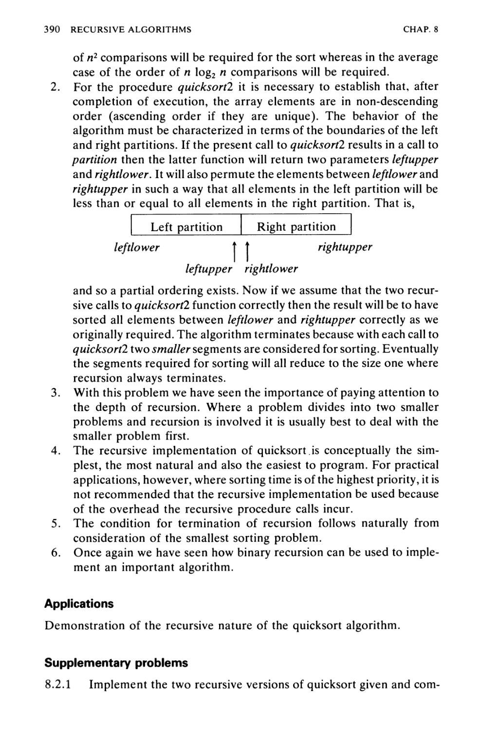
R.G.Dromey
How to Solve it
by Computer
PRENTICE-HALL
INTERNATIONAL
SERIES IN
COMPUTER
SCIENCE CA.R. HOARE SERIES EDITOR
HOW TO SOLVE IT
BY COMPUTER
by
R. G. DROMEY
Department of Computing Science
The University of Wollongong
ENGLEWOOD CLIFFS, NEW JERSEY LONDON NEW DELHI
SINGAPORE SYDNEY TOKYO TORONTO WELLINGTON
Library of Congress Cataloging in Publication Data
DROMEY, R. G., 1946-
How to Solve it by Computer.
Bibliography: p.
Includes index
1. Mathematics—Data processing
2. Problem solving—Data processing
2. Electronic digital computers—Programming
I. Title.
QA76.95.D76 519.4 81-19164
ISBN 0-13-433995-9 AACR2
ISBN 0-13-434001-9 (pbk.)
British Library Cataloging in Publication Data
DROMEY, R. G.
How to Solve it by Computer.
1. Algorithms
I. Title
511'.8 QA9.58
ISBN 0-13-433995-9
ISBN 0-13-434001-9 (pbk)
© 1982 by PRENTICE-HALL INTERNATIONAL, INC., London
© 1982 by PRENTICE-HALL INC., Englewood Cliffs, N.J. 07632
All rights reserved. No part of this publication may be reproduced,
stored in a retrieval system, or transmitted, in any form or by any
means, electronic, mechanical, photocopying, recording or otherwise,
without the prior permission of the publisher.
ISBN 0-13-1433^5^
ISBN 0-13-14314001-=) -CPBK>
PRENTICE-HALL INTERNATIONAL, INC., London
PRENTICE-HALL OF AUSTRALIA PTY. LTD., Sydney
PRENTICE-HALL CANADA, INC., Toronto
PRENTICE-HALL OF INDIA PRIVATE LTD., New Delhi
PRENTICE-HALL OF JAPAN, INC., Tokyo
PRENTICE-HALL OF SOUTHEAST ASIA PTE., LTD., Singapore
PRENTICE-HALL, INC., Englewood Cliffs, New Jersey
WHITEHALL BOOKS LIMITED, Wellington, New Zealand
Printed in the United States of America
10 987654321
This book is dedicated to
George Polya
We learn most when
We have to invent
Piaget
CONTENTS
PREFACE xiii
ACKNOWLEDGEMENTS xxi
1 INTRODUCTION TO COMPUTER PROBLEM-SOLVING 1
1.1 Introduction 1
1.2 The Problem-solving Aspect 3
1.3 Top-down Design 7
1.4 Implementation of Algorithms 14
1.5 Program Verification 19
1.6 The Efficiency of Algorithms 29
1.7 The Analysis of Algorithms 33
Bibliography 39
2 FUNDAMENTAL ALGORITHMS 42
Introduction 42
Algorithm 2.1 Exchanging the Values of Two Variables 43
Algorithm 2.2 Counting 47
Algorithm 2.3 Summation of a Set of Numbers 51
Algorithm 2.4 Factorial Computation 56
Algorithm 2.5 Sine Function Computation 60
Algorithm 2.6 Generation of the Fibonacci Sequence 64
Algorithm 2.7 Reversing the Digits of an Integer 69
Algorithm 2.8 Base Conversion 74
Algorithm 2.9 Character to Number Conversion 80
Bibliography 84
ix
x CONTENTS
3 FACTORING METHODS 85
Introduction 85
Algorithm 3.1 Finding the Square Root of a Number 86
Algorithm 3.2 The Smallest Divisor of an Integer 92
Algorithm 3.3 The Greatest Common Divisor of Two
Integers 97
Algorithm 3.4 Generating Prime Numbers 105
Algorithm 3.5 Computing the Prime Factors of an Integer 116
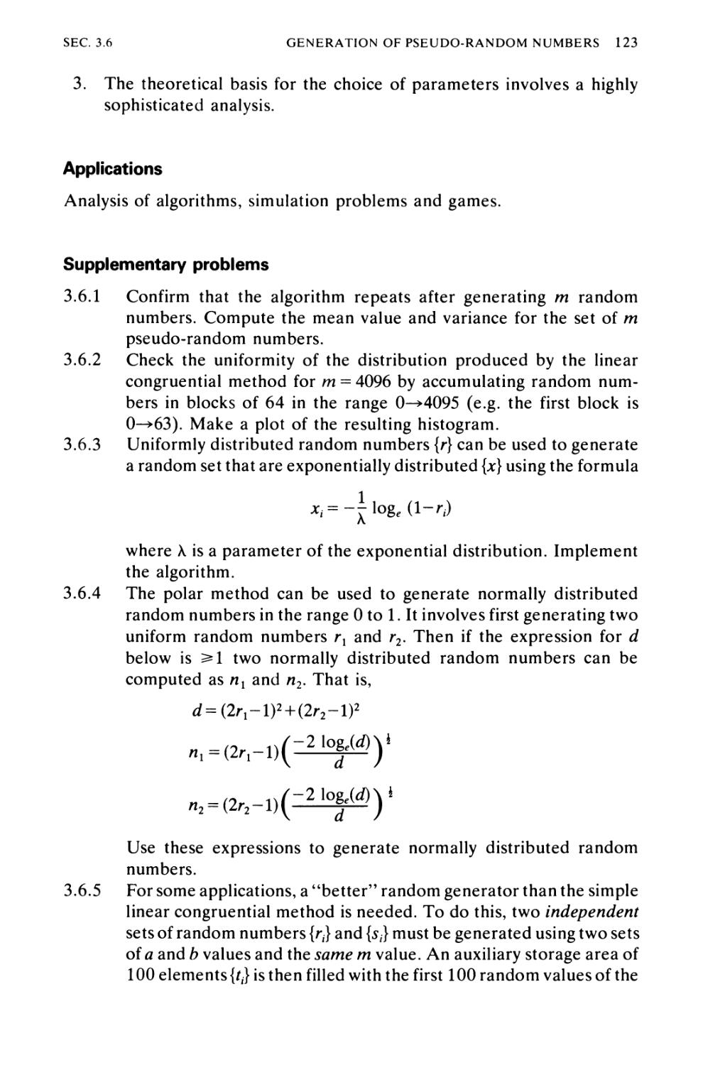
Algorithm 3.6 Generation of Pseudo-random Numbers 120
Algorithm 3.7 Raising a Number to a Large Power 124
Algorithm 3.8 Computing the Azth Fibonacci Number 132
Bibliography 138
4 ARRAY TECHNIQUES 139
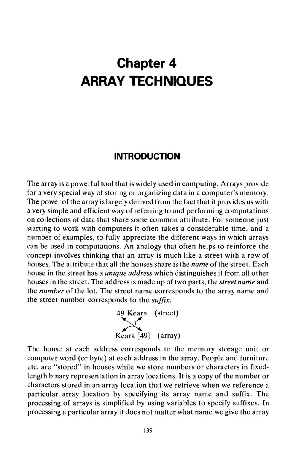
Introduction 139
Algorithm 4.1 Array Order Reversal 140
Algorithm 4.2 Array Counting or Histogramming 144
Algorithm 4.3 Finding the Maximum Number in a Set 147
Algorithm 4.4 Removal of Duplicates from an Ordered
Array 152
Algorithm 4.5 Partitioning an Array 156
Algorithm 4.6 Finding the kth Smallest Element 166
Algorithm 4.7 Longest Monotone Subsequence 174
Bibliography 180
5 MERGING, SORTING AND SEARCHING 181
Introduction 181
Algorithm 5.1 The Two-way Merge 182
Algorithm 5.2 Sorting by Selection 192
Algorithm 5.3 Sorting by Exchange 198
Algorithm 5.4 Sorting by Insertion 204
Algorithm 5.5 Sorting by Diminishing Increment 209
Algorithm 5.6 Sorting by Partitioning 216
Algorithm 5.7 Binary Search 227
Algorithm 5.8 Hash Searching 237
Bibliography 246
6 TEXT PROCESSING AND PATTERN SEARCHING 248
Introduction 248
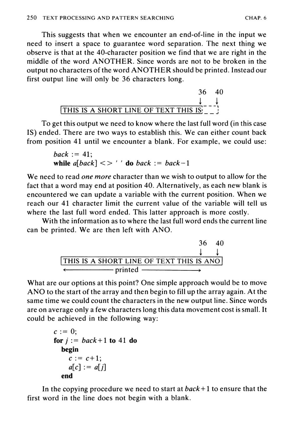
Algorithm 6.1 Text Line Length Adjustment 249
Algorithm 6.2 Left and Right Justification of Text 256
Algorithm 6.3 Keyword Searching in Text 267
Algorithm 6.4 Text Line Editing 274
Algorithm 6.5 Linear Pattern Search 282
Algorithm 6.6 Sublinear Pattern Search 293
Bibliography 303
CONTENTS xi
7 DYNAMIC DATA STRUCTURE ALGORITHMS 304
Introduction 304
Algorithm 7.1 Stack Operations 306
Algorithm 7.2 Queue Addition and Deletion 314
Algorithm 7.3 Linked List Search 325
Algorithm 7.4 Linked List Insertion and Deletion 331
Algorithm 7.5 Binary Tree Search 342
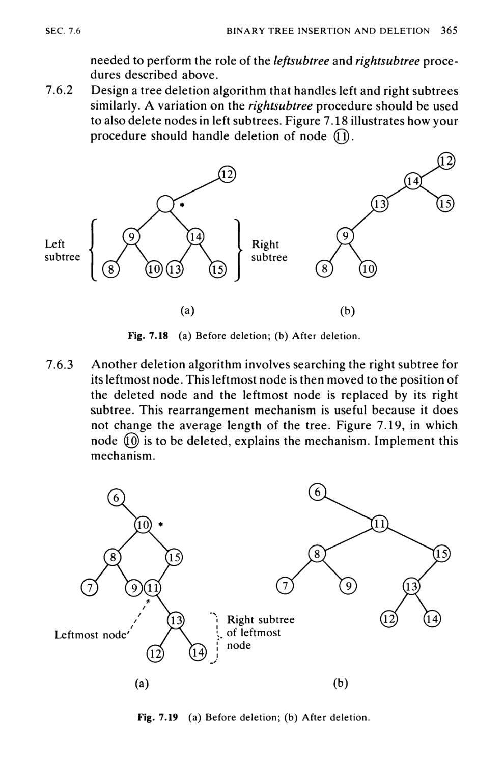
Algorithm 7.6 Binary Tree Insertion and Deletion 349
Bibliography 366
8 RECURSIVE ALGORITHMS 367
Introduction 367
Algorithm 8.1 Binary Tree Traversal 373
Algorithm 8.2 Recursive Quicksort 383
Algorithm 8.3 Towers of Hanoi Problem 391
Algorithm 8.4 Sample Generation 404
Algorithm 8.5 Combination Generation 414
Algorithm 8.6 Permutation Generation 422
Bibliography 433
INDEX 435
PREFACE
The inspiration for this book has come from the classic work of Polya on
general and mathematical problem-solving. As in mathematics, many
beginners in computing science stumble not because they have difficulty
with learning a programming language but rather because they are ill-
prepared to handle the problem-solving aspects of the discipline.
Unfortunately, the school system seems to concentrate on training people to answer
questions and remember facts but not to really solve problems.
In response to this situation, it was felt there was a definite need for a
book written in the spirit of Polya's work, but translated into the computing
science context. Much of Polya's work is relevant in the new context but,
with computing problems, because of their general requirements for
iterative or recursive solutions, another dimension is added to the problem-
solving process.
If we can develop problem-solving skills and couple them with top-
down design principles, we are well on the way to becoming competent at
algorithm design and program implementation. Emphasis in the book has
been placed on presenting strategies that we might employ to "discover"
efficient, well-structured computer algorithms. Throughout, a conscious
effort has been made to convey something of the flavor of either a personal
dialogue or an instructor-student dialogue that might take place in the
solution of a problem. This style of presentation coupled with a carefully
chosen set of examples, should make the book attractive to a wide range of
readers.
The student embarking on a first course in Pascal should find that the
material provides a lot of useful guidance in separating the tasks of learning
how to develop computer algorithms and of then implementing them in a
programming language like Pascal. Too often, the end is confused with the
Xlll
xiv PREFACE
means. A good way to work with the book for self-study is to read only as
much as you need to get started on a problem. Then, when you have
developed your own solution, compare it with the one given and consciously
reflect on the strategies that were helpful or hindersome in tackling the
problem. As Yohe1 has rightly pointed out "programming [computer
problem-solving] is an art [and] as in all art forms, each individual must
develop a style which seems natural and genuine."
Instructors should also find the style of presentation very useful as
lecture material as it can be used to provide the cues for a balanced amount
of instructor-class dialogue. The author has found students receptive and
responsive to lectures presented in this style.
The home-computer hobbyist wishing to develop his or her problem-
solving and programming skills without any formal lectures should find the
completeness of presentation of the various algorithms a very valuable
supplement to any introductory Pascal text. It is hoped that even some of the
more advanced algorithms have been rendered more accessible to beginners
than is usually the case.
The material presented, although elementary for the most part,
contains some examples and topics which should be of sufficient interest and
challenge to spark, in the beginning student, the enthusiasm for computing
that we so often see in students who have begun to master their subject.
Readers are urged not to accept passively the algorithm solutions given.
Wherever it is possible and practical, the reader should strive for his or her
own simpler or better algorithms. As always, the limitations of space have
meant that some topics and examples of importance have either had to be
omitted or limited in scope. To some degree the discussions and
supplementary problems that accompany each algorithm are intended to compensate
for this. The problem sets have been carefully designed to test, reinforce, and
extend the reader's understanding of the strategies and concepts presented.
Readers are therefore strongly urged to attempt a considerable proportion
of these problems.
Each chapter starts off with a discussion of relatively simple, graded
examples, that are usually related in some fairly direct way. Towards the
middle and end of each chapter, the examples are somewhat more involved.
A good way to work with the book is to only consider the more fundamental
algorithms in each chapter at a first reading. This should allow the necessary
build-up of background needed to study in detail some of the more advanced
algorithms at a later stage.
The chapters are approximately ordered in increasing order of
conceptual difficulty as usually experienced by students. The first chapter intro-
t J. M. Yohe, "An overview of programming practices", Comp. Surv., 6, 221-46
(1974).
PREFACE xv
duces the core aspects of computer problem-solving and algorithm design.
At a first reading the last half of the chapter can be skimmed through. Where
possible, the ideas are reinforced with examples. The problem-solving
discussion tries to come to grips with the sort of things we can do when we are
stuck with a problem. The important topic of program verification is
presented in a way that should be relatively easy for the reader to grasp and
apply at least to simple algorithms. Examples are used to convey something
of the flavor of a probabilistic analysis of an algorithm.
The second chapter concentrates on developing the skill for formulating
iterative solutions to problems—a skill we are likely to have had little
experience with before an encounter with computers. Several problems are
also considered which should allow us to come to a practical understanding
of how computers represent and manipulate information. The problem of
conversion from one representation to another is also addressed. The
algorithms in this chapter are all treated as if we were faced with the task of
discovering them for the first time. Since our aim is to foster skill in computer
problem-solving, this method of presentation would seem to be appropriate
from a pedagogical standpoint. Algorithms in the other chapters are also
discussed in this style.
In the third chapter, we consider a number of problems that have their
origin in number theory. These algorithms require an extension of the
iterative techniques developed in the first chapter. Because of their nature,
most of these problems can be solved in a number of ways and can differ
widely in their computational cost. Confronting the question of efficiency
adds an extra dimension to the problem-solving process. We set out to
"discover" these algorithms as if for the first time.
Array-processing algorithms are considered in detail in Chapter 4.
Facility with the use of arrays needs to be developed as soon as we have
understood and are able to use iteration in the development of algorithms.
Arrays, when coupled with iteration, provide us with a very powerful means
of performing computations on collections of data that share some common
attribute. Strategies for the efficient processing of array information raise
some interesting problem-solving issues. The algorithms discussed are
intended to address at least some of the more important of these issues.
Once arrays and iteration have been covered, we have the necessary
tools to consider merging, sorting and searching algorithms. These topics are
discussed in Chapter 5. The need to organize and subsequently efficiently
search large volumes of information is central in computing science. A
number of the most well-known internal sorting and searching algorithms
are considered. An attempt is made to provide the settings that would allow
us to "discover" these algorithms.
The sixth chapter on text and string processing represents a diversion
from the earlier emphasis on "numeric" computing. The nature and organ-
xvi PREFACE
ization of character information raises some important new problem-solving
issues. The demands for efficiency once again lead to the consideration of
some interesting algorithms that are very different from those reviewed in
earlier chapters. The algorithms in this chapter emphasize the need to
develop the skill of recognizing the essentials of a problem without being
confused or misled by extraneous detail. "Discovering" some of these
algorithms provides an interesting test-bed for us to apply some of the
problem-solving skills we should have absorbed after covering the first five
chapters.
Chapter 7 is devoted to the fundamental algorithms for maintaining and
searching the primary dynamic data structures (i.e. stacks, queues, lists, and
binary trees). The issues in this chapter arise mostly at the implementation
level and with the use of pointers.
In the final chapter, the topic of recursion is introduced. A recursive call
is presented as an extension of the conventional subprocedure call. The
simplest form of recursion, linear recursion, is only briefly treated because
the view is taken that there are almost always simple iterative schemes that
can be found for performing what amounts to linear recursion. Furthermore,
linear recursion does little to either convey anything of the power of
recursion or to really deepen our understanding of the mechanism. The same
cannot usually be said for problems involving either binary recursion or the
more general non-linear recursion. Algorithms that belong to both these
classes are discussed in detail, with special emphasis being placed on
recognizing their underlying similarities and deepening our understanding of
recursion mechanisms.
As a concluding remark about the book, if the author were to hope that
this work may achieve anything, it would be that it stimulated students and
others to embark on a journey of discovering things for themselves!
A SUGGESTION FOR INSTRUCTORS
"...any idea or problem or body of knowledge can be
presented in a form simple enough so that any particular
learner can understand it in a recognizable form."
—Bruner.
In comparison with most other human intellectual activities, computing is in
its infancy despite the progress we seem to have made in such a short time.
Because the demand for computers and people with computing skills is so
great in our rapidly changing world, we have not had time to sit back and
A SUGGESTION FOR INSTRUCTORS xvii
reflect on the best way to convey the "computing concept" on a wide scale.
In time, computing will mature and evolve as a well-understood discipline
with clear and well-defined methods for introducing the subject to
beginners—but that is in the future. For the present, because we are not in this
happy situation, it is most prudent to look to other mature disciplines for
guidance on how we should introduce computing to beginners. Assuming we
want to have the highest possible success rate in introducing computing to
students (a situation which clearly at present does not prevail) and that we
want to teach computing on the widest possible scale, then the most obvious
discipline to turn to is that of learning to read and write.
Educators have mastered the process of teaching people to read and
write to the extent that these skills are able to be transmitted on a very wide
scale, efficiently, and with a very high rate of success. Putting aside the
various methods within the learning-to-read-and-write discipline we see that
there are some fundamental principles acknowledged by all methods that
are highly relevant to teaching computing.
In teaching people to read and write a very substantial time (years in
fact) is devoted to reading. Only after such preparation is it considered
appropriate that they should attempt to write stories or essays, or books, etc.
In fact, even before people attempt to learn to read they undergo several
years of listening to language, speaking, and being "read to". Clearly, in
learning a language, the ultimate goal is to be able to verbalize and write
fluently in that language. Similarly in computing the goal is to be able to
program (or design and implement algorithms) effectively. In learning to
read and write it has long been recognized that reading is easier and that it
must precede writing by a considerable margin of time to allow the
assimilation of enough models and constructs of text to make writing possible.
In teaching computing we seem to have overlooked or neglected what
corresponds to the reading stage in the process of learning to read and write.
To put it strongly, asking people to design and write programs early on in
their computing experience is like expecting that they be able to competently
write essays before they have learned to read or even to write short
sentences—it is expecting just too much of a lot of people. It also probably
explains why many otherwise very able people just don't get started in
computing.
What we are therefore proposing is that in teaching computing we
should draw as much as we can from the learning-to-read-and-write analogy.
This means that we must be able to provide the beginning student with his or
her "reading experience" in computing before embarking on the more
difficult computer problem-solving tasks which require considerably more
creative effort, discipline, and technical skill.
At this point it is important to recognize that the "reading experience"
cannot be gained by sitting down with a book of programs and attempting to
xviii PREFACE
"read" them. The problem with this approach is that program instructions as
written on a piece of paper are a static representation of a computer
algorithm. As such they do not very fluently convey anything of the dynamic
aspect of computer algorithms and programs.
It can be argued that it is important to have a clear and in-depth
understanding of the dynamic character of programs before attempting
algorithm design and program implementation. What is needed is a practical
and economical method of giving students their "reading experience" in
computing. To gain this experience the students need to "see" programs
written in a high level language executing. Traditionally, all the student sees
is the output printed on the terminal or line printer and prompts by the
program when it requires input from the terminal. This level of "seeing" a
program execute is unsatisfactory for beginners because it conveys very little
about the program's flow of control or about the effects of individual and
groups of program statements. What we need is much more explicit
demonstrations of what is happening in a program that causes it to produce the
outputs that it does. A far more transparent way to do this is to place before
the student on a terminal the text of the program being executed and then to
trace the execution on the displayed program while at the same time
dynamically updating on the screen the changes in program variables as they are
made and related to steps in the displayed program. This dynamic method of
studying algorithms can greatly assist the student in acquiring a level of
understanding necessary to design and implement his or her own algorithms.
The facilities and software tools needed to adequately demonstrate
execution of a program in this way are relatively economical to provide. All
that is needed is a terminal with cursor addressing facilities and a small set of
software tools (several hundred lines of code) that can be inserted into the
program being studied to make its execution "visible" on the screen. Only
one procedure call per statement of the program being studied is needed to
operate it in a visible mode (this software is available from the author). The
display software is transparent to the user. The appropriate tools allow us to
see a program execute in single-step mode while monitoring the changes in
variables as they are dynamically displayed on the screen. The student can
cause the program to execute the next statement at each stage by simply
pressing a single key (e.g. the RETURN) on the terminal.
As an example, the screen layout for "visible" execution of a selection
sorting procedure in Pascal is as illustrated in Fig. 1. The next statement to be
executed at each stage is tracked by having an arrow that can be moved from
statement to statement on the procedure text displayed on the screen. A
more complete description of the software is given elsewhere.1
t R. G. Dromey, Before Programming—On Teaching Introductory Computing,
Technical Report No. 81/6, Dept. of Computing Science, University of Wollon-
gong(1981).
A SUGGESTION FOR INSTRUCTORS xix
I :
J '
procedure selectionsort(a\nelements\ n:integer);
var i {index for sorted part}, j {index for unsorted part},
p {position of minimum}, min {minimum in unsorted part}: integer;
begin
for / := 1 to n-\ do
begin
min := a[i\\
P '= i;
for j : = i+l to n do
if a[j]< min then
begin
min := a[j];
P '•= j
end;
a[p] := a[i\\
a[i] := min
end
end
array: 12 4 56 67 9 23 45
* J
condition: a[j] < min :
true
1
2
a[i] :
a[j] :
12
4
P '
n :
1
8
dp]:
min :
12
4
Fig. 1 Screen layout for visible program execution.
The cause-and-effect nature of what is displayed when executing
programs in this manner (automatic single-step mode) can accomplish a number
of things.
(1) Most importantly, it provides a good understanding of the dynamic
nature of algorithms—an essential prerequisite if students are to later
design and implement their own algorithms.
(2) It gives a deep insight into the basic laws of composition of computer
algorithms (sequence, selection, iteration, and modularity).
(3) It is a useful vehicle for helping students to learn various programming
constructs. Actually observing constructs being used within different
programming contexts and linking these constructs to changes in the
values of variables and conditions gives the student the necessary
concrete demonstrations that will enable him or her to master the use
of these constructs.
(4) It conveys in a very vivid fashion the workings of a particular algorithm.
For example, the selection sort algorithm when visibly executed
conveys the difficult concept of how we can have one loop executing within
another loop. It also highlights the difference between subscripted
variables and subscripts.
XX PREFACE
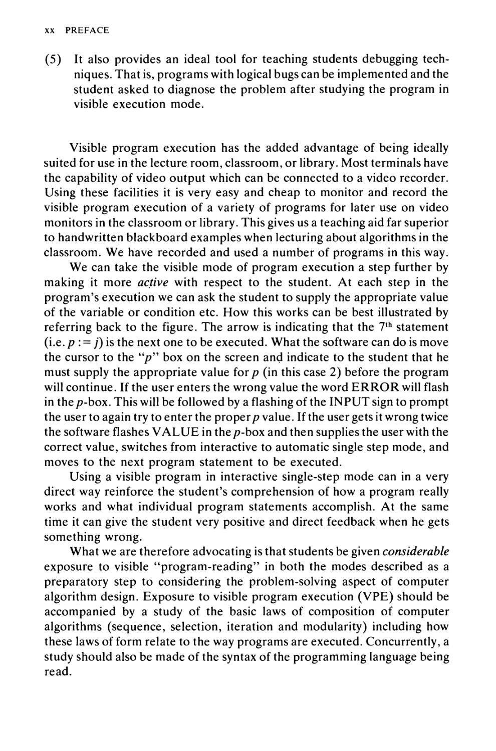
(5) It also provides an ideal tool for teaching students debugging
techniques. That is, programs with logical bugs can be implemented and the
student asked to diagnose the problem after studying the program in
visible execution mode.
Visible program execution has the added advantage of being ideally
suited for use in the lecture room, classroom, or library. Most terminals have
the capability of video output which can be connected to a video recorder.
Using these facilities it is very easy and cheap to monitor and record the
visible program execution of a variety of programs for later use on video
monitors in the classroom or library. This gives us a teaching aid far superior
to handwritten blackboard examples when lecturing about algorithms in the
classroom. We have recorded and used a number of programs in this way.
We can take the visible mode of program execution a step further by
making it more active with respect to the student. At each step in the
program's execution we can ask the student to supply the appropriate value
of the variable or condition etc. How this works can be best illustrated by
referring back to the figure. The arrow is indicating that the 7th statement
(i.e. p : = j) is the next one to be executed. What the software can do is move
the cursor to the "/?" box on the screen and indicate to the student that he
must supply the appropriate value for/? (in this case 2) before the program
will continue. If the user enters the wrong value the word ERROR will flash
in the /?-box. This will be followed by a flashing of the INPUT sign to prompt
the user to again try to enter the proper/? value. If the user gets it wrong twice
the software flashes VALUE in the/?-box and then supplies the user with the
correct value, switches from interactive to automatic single step mode, and
moves to the next program statement to be executed.
Using a visible program in interactive single-step mode can in a very
direct way reinforce the student's comprehension of how a program really
works and what individual program statements accomplish. At the same
time it can give the student very positive and direct feedback when he gets
something wrong.
What we are therefore advocating is that students be given considerable
exposure to visible "program-reading" in both the modes described as a
preparatory step to considering the problem-solving aspect of computer
algorithm design. Exposure to visible program execution (VPE) should be
accompanied by a study of the basic laws of composition of computer
algorithms (sequence, selection, iteration and modularity) including how
these laws of form relate to the way programs are executed. Concurrently, a
study should also be made of the syntax of the programming language being
read.
ACKNOWLEDGEMENTS
The inspiration for the approach taken in this book grew out of an
admiration for George Polya's classic works on problem-solving. During the
summer and autumn of 1980, I had the pleasure of spending a number of
afternoons chatting with Professor and Mrs. Polya.
The influence of Polya's work and that of the pioneers of the discipline
of computing science, E. W. Dijkstra, R. W. Floyd, C. A. R. Hoare, D. E.
Knuth, and N. Wirth, is freely acknowledged. There is also a strong influence
of Jeff Rohl's work in the last chapter on recursion.
I sincerely appreciate the guidance and encouragement given to me by
Professor Hoare, Henry Hirschberg, Ron Decent, and my reviewers.
I am also grateful to the University of Wollongong and Stanford
University for the use of their facilities.
A number of people have generously given helpful comments and
support during the preparation of the manuscript. I would particularly like to
thank Tom Bailey, Miranda Baker, Harold Brown, Bruce Buchanan, Ann
Cartwright, John Farmer, Tony Guttman, Joan Hutchinson, Leanne Koring,
Donald Knuth, Rosalyn Maloney, Richard Miller, Ross Nealon, Jurg
Nievergelt, Richard Patis, Ian Pirie, Juris Reinfelds, Tom Richards, Michael
Shepanksi, Stanley Smerin and Natesa Sridharan and my students at
Wollongong.
The understanding and encouragement throughout this whole project
that I have received from my wife Aziza is deeply appreciated.
Finally, I wish to extend my deepest gratitude to Bronwyn James for her
loyalty and untiring and able support in the preparation and typing of the
manuscript.
xxi
Chapter 1
INTRODUCTION TO COMPUTER
PROBLEM-SOLVING
1.1 INTRODUCTION
Computer problem-solving can be summed up in one word—it is demand-
ing\ It is an intricate process requiring much thought, careful planning,
logical precision, persistence, and attention to detail. At the same time it can
be a challenging, exciting, and satisfying experience with considerable room
for personal creativity and expression. If computer problem-solving is
approached in this spirit then the chances of success are greatly amplified. In
the discussion which follows in this introductory chapter we will attempt to
lay the foundations for our study of computer problem-solving.
1.1.1 Programs and algorithms
The vehicle for the computer solution to a problem is a set of explicit and
unambiguous instructions expressed in a programming language. This set of
instructions is called a program. A program may also be thought of as an
algorithm expressed in a programming language. An algorithm therefore
corresponds to a solution to a problem that is independent of any
programming language.
To obtain the computer solution to a problem once we have the
program we usually have to supply the program with input or data. The program
then takes this input and manipulates it according to its instructions and
eventually produces an output which represents the computer solution to the
problem. The realization of the computer output is but the last step in a very
long chain of events that have led up to the computer solution to the
problem.
l
2 COMPUTER PROBLEM-SOLVING
CHAP. 1
Our goal in this work is to study in depth the process of algorithm design
with particular emphasis on the problem-solving aspects of the task. There
are many definitions of an algorithm. The following definition is appropriate
in computing science. An algorithm consists of a set of explicit and
unambiguous finite steps which, when carried out for a given set of initial
conditions, produce the corresponding output and terminate in a finite time.
1.1.2 Requirements for solving problems by computer
From time to time in our everyday activities, we employ algorithms to solve
problems. For example, to look up someone's telephone number in a
telephone directory we need to employ an algorithm. Tasks such as this are
usually performed automatically without any thought to the complex
underlying mechanism needed to effectively conduct the search. It therefore
comes as somewhat of a surprise to us when developing computer algorithms
that the solution must be specified with such logical precision and in such
detail. After studying even a small sample of computer problems it soon
becomes obvious that the conscious depth of understanding needed to design
effective computer algorithms is far greater than we are likely to encounter
in almost any other problem-solving situation.
Let us reflect for a moment on the telephone directory look-up
problem. A telephone directory quite often contains hundreds of thousands of
names and telephone numbers yet we have little trouble finding the desired
telephone number we are seeking. We might therefore ask why do we have
so little difficulty with a problem of seemingly great size? The answer is
simple. We quite naturally take advantage of the order in the directory to
quickly eliminate large sections of the list and home in on the desired name
and number. We would never contemplate looking up the telephone number
of J. R. Nash by starting at page 1 and examining each name in turn until we
finally come to Nash's name and telephone number. Nor are we likely to
contemplate looking up the name of the person whose number is 2987533.
To conduct such a search, there is no way in which we can take advantage of
the order in the directory and so we are faced with the prospect of doing a
number-by-number search starting at page 1. If, on the other hand, we had a
list of telephone numbers and names ordered by telephone number rather
than name, the task would be straightforward. What these examples serve to
emphasize is the important influence of the data organization on the
performance of algorithms. Only when a data structure is symbiotically linked with
an algorithm can we expect high performance. Before considering these and
other aspects of algorithm design we need to address the topic of problem-
solving in some detail.
SEC. 1.2
THE PROBLEM-SOLVING ASPECT 3
1.2 THE PROBLEM-SOLVING ASPECT
It is widely recognized that problem-solving is a creative process which
largely defies systematization and mechanization. This may not sound very
encouraging to the would-be problem-solver. To balance this, most people,
during their schooling, acquire at least a modest set of problem-solving skills
which they may or may not be aware of.
Even if one is not naturally skilled at problem-solving there are a
number of steps that can be taken to raise the level of one's performance. It is
not implied or intended that the suggestions in what follows are in any way a
recipe for problem-solving. The plain fact of the matter is that there is no
universal method. Different strategies appear to work for different people.
Within this context, then, where can we begin to say anything useful
about computer problem-solving? We must start from the premise that
computer problem-solving is about understanding.
1.2.1 Problem definition phase
Success in solving any problem is only possible after we have made the effort
to come to terms with or understand the problem at hand. We cannot hope to
make useful progress in solving a problem until we fully understand what it is
we are trying to solve. This preliminary investigation may be thought of as
the problem definition phase. In other words, what we must do during this
phase is work out what must be done rather than how to do it. That is, we
must try to extract from the problem statement (which is often quite
imprecise and maybe even ambiguous) a set of precisely defined tasks.
Inexperienced problem-solvers too often gallop ahead with how they are going to
solve the problem only to find that they are either solving the wrong problem
or they are solving just a very special case of what is actually required. In
short, a lot of care should be taken in working out precisely what must be
done. The development of algorithms for finding the square root (algorithm
3.1) and the greatest common divisor (algorithm 3.3) are good illustrations
of how important it is to carefully define the problem. Then, from the
definitions, we are led in a natural way to algorithm designs for these two
problems.
1.2.2 Getting started on a problem
There are many ways to solve most problems and also many solutions to
most problems. This situation does not make the job of problem-solving
easy. When confronted with many possible lines of attack it is usually
4 COMPUTER PROBLEM-SOLVING
CHAP. 1
difficult to recognize quickly which paths are likely to be fruitless and which
paths may be productive.
Perhaps the more common situation for people just starting to come to
grips with the computer solution to problems is that they just do not have any
idea where to start on the problem, even after the problem definition phase.
When confronted with this situation, what can we do? A block often occurs
at this point because people become concerned with details of the
implementation before they have completely understood or worked out an
implementation-independent solution. The best advice here is not to be too
concerned about detail. That can come later when the complexity of the
problem as a whole has been brought under control. The old computer
proverb1 which says "the sooner you start coding your program the longer it
is going to take" is usually painfully true.
1.2.3 The use of specific examples
A useful strategy when we are stuck is to use some props or heuristics (i.e.
rules of thumb) to try to get a start with the problem. An approach that often
allows us to make a start on a problem is to pick a specific example of the
general problem we wish to solve and try to work out the mechanism that will
allow us to solve this particular problem (e.g. if you want to find the
maximum in a set of numbers, choose a particular set of numbers and work
out the mechanism for finding the maximum in this set—see for example
algorithm 4.3). It is usually much easier to work out the details of a solution
to a specific problem because the relationship between the mechanism and
the particular problem is more clearly defined. Furthermore, a specific
problem often forces us to focus on details that are not so apparent when the
problem is considered abstractly. Geometrical or schematic diagrams
representing certain aspects of the problem can be usefully employed in many
instances (see, for example, algorithm 3.3).
This approach of focusing on a particular problem can often give us the
foothold we need for making a start on the solution to the general problem.
The method should, however, not be abused. It is very easy to fall into the
trap of thinking that the solution to a specific problem or a specific class of
problems is also a solution to the general problem. Sometimes this happens
but we should always be very wary of making such an assumption.
Ideally, the specifications for our particular problem need to be
examined very carefully to try to establish whether or not the proposed
algorithm can meet those requirements. If the full specifications are difficult
to formulate sometimes a well-chosen set of test cases can give us a degree of
t H. F. Ledgard, Programming Proverbs, Hayden, Rochelle Park, N.J., 1975.
SEC. 1.2
THE PROBLEM-SOLVING ASPECT 5
confidence in the generality of our solution. However, nothing less than a
complete proof of correctness of our algorithm is entirely satisfactory. We
will discuss this matter in more detail a little later.
1.2.4 Similarities among problems
We have already seen that one way to make a start on a problem is by
considering a specific example. Another thing that we should always try to
do is bring as much past experience as possible to bear on the current
problem. In this respect it is important to see if there are any similarities
between the current problem and other problems that we have solved or we
have seen solved. Once we have had a little experience in computer
problem-solving it is unlikely that a new problem will be completely
divorced from other problems we have seen. A good habit therefore is to
always make an effort to be aware of the similarities among problems. The
more experience one has the more/tools and techniques one can bring to
bear in tackling a given problem. The contribution of experience to our
ability to solve problems is not always helpful. In fact, sometimes it blocks us
from discovering a desirable or better solution to a problem. A classic case of
experience blocking progress was Einstein's discovery of relativity. For a
considerable time before Einstein made his discovery the scientists of the
day had the necessary facts that could have led them to relativity but it is
almost certain that their experience blocked them from even contemplating
such a proposal—Newton's theory was correct and that was all there was to
it! On this point it is therefore probably best to place only cautious reliance
on past experience. In trying to get a better solution to a problem, sometimes
too much study of the existing solution or a similar problem forces us down
the same reasoning path (which may not be the best) and to the same dead
end. In trying to get a better solution to a problem, it is usually wise, in the
first instance at least, to try to independently solve the problem. We then give
ourselves a better chance of not falling into the same traps as our
predecessors. In the final analysis, every problem must be considered on its merits.
A skill that it is important to try to develop in problem-solving is the
ability to view a problem from a variety of angles. One must be able to
metaphorically turn a problem upside down, inside out, sideways,
backwards, forwards and so on. Once one has developed this skill it should be
possible to get started on any problem.
1.2.5 Working backwards from the solution
There are still other things we can try when we do not know where to start on
a problem. We can, for example, in some cases assume that we already have
6 COMPUTER PROBLEM-SOLVING
CHAP. 1
the solution to the problem and then try to work backwards to the starting
conditions. Even a guess at the solution to the problem may be enough to
give us a foothold to start on the problem. (See, for example, the square root
problem—algorithm 3.1). Whatever attempts that we make to get started on
a problem we should write down as we go along the various steps and
explorations made. This can be important in allowing us to systematize our
investigations and avoid duplication of effort. Another practice that helps us
develop our problem-solving skills is, once we have solved a problem, to
consciously reflect back on the way we went about discovering the solution.
This can help us significantly. The most crucial thing of all in developing
problem-solving skills is practice. Piaget summed this up very nicely with the
statement that "we learn most when we have to invent."
1.2.6 General problem-solving strategies
There are a number of general and powerful computational strategies that
are repeatedly used in various guises in computing science. Often it is
possible to phrase a problem in terms of one of these strategies and achieve
very considerable gains in computational efficiency.
Probably the most widely known and most often used of these principles
is the divide-and-conquer strategy. The basic idea with divide-and-conquer is
to divide the original problem into two or more subproblems which can
hopefully be solved more efficiently by the same technique. If it is possible to
proceed with this splitting into smaller and smaller subproblems we will
eventually reach the stage where the subproblems are small enough to be
solved without further splitting. This way of breaking down the solution to a
problem has found wide application in particular with sorting, selection, and
searching algorithms. We will see later in Chapter 5 when we consider the
binary search algorithm how applying this strategy to an ordered data set
results in an algorithm that needs to make only log2AZ rather than n
comparisons to locate a given item in an ordered list n elements long. When this
principle is used in sorting algorithms, the number of comparisons can be
reduced from the order of n2 steps to n log2AZ steps, a substantial gain
particularly for large n. The same idea can be applied to file comparison and
in many other instances to give substantial gains in computational efficiency.
It is not absolutely necessary for divide-and-conquer to always exactly halve
the problem size. The algorithm used in Chapter 4 to find the k{h smallest
element repeatedly reduces the size of the problem. Although it does not
divide the problem in half at each step it has very good average performance.
It is also possible to apply the divide-and-conquer strategy essentially in
reverse to some problems. The resulting binary doubling strategy can give
the same sort of gains in computational efficiency. We will consider in
Chapter 3 how this complementary technique can be used to advantage to
SEC. 1.3
TOP-DOWN DESIGN 7
raise a number to a large power and to calculate the nth Fibonacci number.
With this doubling strategy we need to express the next term n to be
computed in terms of the current term which is usually a function of n/2 in
order to avoid the need to generate intermediate terms.
Another general problem-solving strategy that we will briefly consider
is that of dynamic programming. This method is used most often when we
have to build up a solution to a problem via a sequence of intermediate steps.
The monotone subsequence problem in Chapter 4 uses a variant of the
dynamic programming method. This method relies on the idea that a good
solution to a large problem can sometimes be built up from good or optimal
solutions to smaller problems. This type of strategy is particularly relevant
for many optimization problems that one frequently encounters in
operations research. The techniques of greedy search, backtracking and branch-
and-bound evaluations are all variations on the basic dynamic programming
idea. They all tend to guide a computation in such a way that the minimum
amount of effort is expended on exploring solutions that have been
established to be suboptimal. There are still other general computational
strategies that we could consider but because they are usually associated
with more advanced algorithms we will not proceed further in this direction.
1.3 TOP-DOWN DESIGN
The primary goal in computer problem-solving is an algorithm which is
capable of being implemented as a correct and efficient computer program.
In our discussion leading up to the consideration of algorithm design we have
been mostly concerned with the very broad aspects of problem-solving. We
now need to consider those aspects of problem-solving and algorithm design
which are closer to the algorithm implementation.
Once we have defined the problem to be solved and we have at least a
vague idea of how to solve it, we can begin to bring to bear powerful
techniques for designing algorithms. The key to being able to successfully
design algorithms lies in being able to manage the inherent complexity of
most problems that require computer solution. People as problem-solvers
are only able to focus on, and comprehend at one time, a very limited span of
logic or instructions. A technique for algorithm design that tries to
accommodate this human limitation is known as top-down design or stepwise
refinement.
Top-down design is a strategy that we can apply to take the solution of a
computer problem from a vague outline to a precisely defined algorithm and
program implementation. Top-down design provides us with a way of
handling the inherent logical complexity and detail frequently encountered in
8 COMPUTER PROBLEM-SOLVING
CHAP. 1
computer algorithms. It allows us to build our solutions to a problem in a
stepwise fashion. In this way, specific and complex details of the
implementation are encountered only at the stage when we have done sufficient
groundwork on the overall structure and relationships among the various
parts of the problem.
1.3.1 Breaking a problem into subproblems
Before we can apply top-down design to a problem we must first do the
problem-solving groundwork that gives us at least the broadest of outlines of
a solution. Sometimes this might demand a lengthy and creative
investigation into the problem while at other times the problem description may in
itself provide the necessary starting point for top-down design. The general
outline may consist of a single statement or a set of statements. Top-down
design suggests that we take the general statements that we have about the
solution, one at a time, and break them down into a set of more precisely
defined subtasks. These subtasks should more accurately describe how the
final goal is to be reached. With each splitting of a task into subtasks it is
essential that the way in which the subtasks need to interact with each other
be precisely defined. Only in this way is it possible to preserve the overall
structure of the solution to the problem. Preservation of the overall structure
in the solution to a problem is important both for making the algorithm
comprehensible and also for making it possible to prove the correctness of
the solution. The process of repeatedly breaking a task down into subtasks
and then each subtask into still smaller subtasks must continue until we
eventually end up with subtasks that can be implemented as program
statements. For most algorithms we only need to go down to two or three levels
although obviously for large software projects this is not true. The larger and
more complex the problem, the more it will need to be broken down to
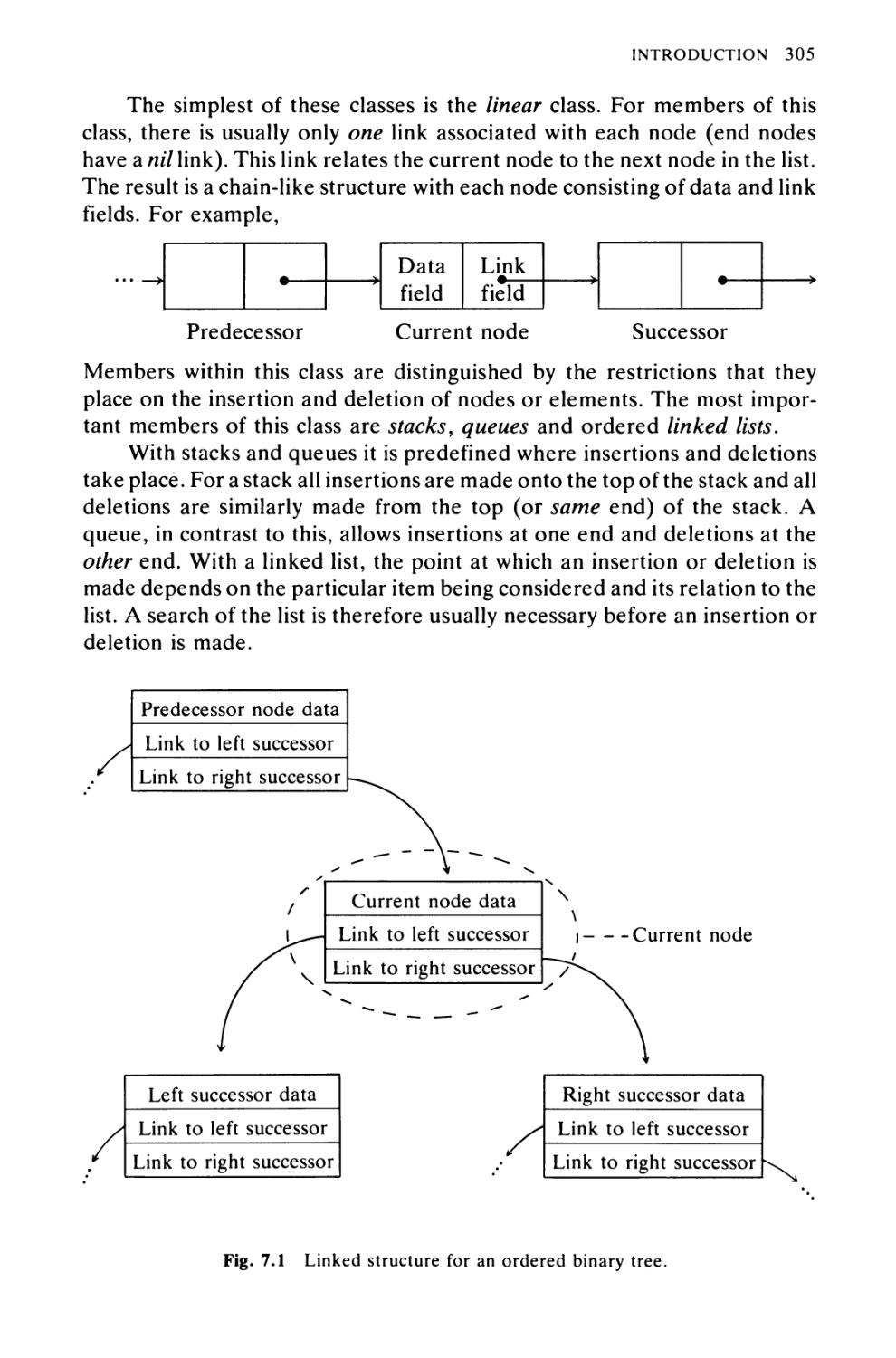
be made tractable. A schematic breakdown of a problem is shown in
Fig. 1.1.
The process of breaking down the solution to a problem into subtasks in
the manner described results in an implementable set of subtasks that fit
quite naturally into block-structured languages like Pascal and Algol. There
can therefore be a smooth and natural interface between the stepwise-
refined algorithm and the final program implementation—a highly desirable
situation for keeping the implementation task as simple as possible.
1.3.2 Choice of a suitable data structure
One of the most important decisions we have to make in formulating
computer solutions to problems is the choice of appropriate data structures.
SEC. 1.3
TOP-DOWN DESIGN 9
General outline
Input conditions
Output requirements
Body of algorithm
Subtask 1
Subtask 3
Subtask 2
Subtask la
Subtask 2a
Fig. 1.1 Schematic breakdown of a problem into subtasks as employed in top-down design.
All programs operate on data and consequently the way the data is
organized can have a profound effect on every aspect of the final solution. In
particular, an inappropriate choice of data structure often leads to clumsy,
inefficient, and difficult implementations. On the other hand, an appropriate
choice usually leads to a simple, transparent, and efficient implementation.
There is no hard and fast rule that tells us at what stage in the
development of an algorithm we need to make decisions about the associated data
structures. With some problems the data structure may need to be
considered at the very outset of our problem-solving explorations before the
top-down design, while in other problems it may be postponed until we are
well advanced with the details of the implementation. In other cases still, it
can be refined as the algorithm is developed.
The key to effectively solving many problems really comes down to
making appropriate choices about the associated data structures. Data
structures and algorithms are usually intimately linked to one another. A small
change in data organization can have a significant influence on the algorithm
required to solve the problem. It is not easy to formulate any generally
applicable rules that say for this class of problem this choice of data structure
10 COMPUTER PROBLEM-SOLVING
CHAP. 1
is appropriate. Unfortunately with regard to data structures each problem
must be considered on its merits.
The sort of things we must however be aware of in setting up data
structures are such questions as:
(1) How can intermediate results be arranged to allow fast access to
information that will reduce the amount of computation required at a
later stage?
(2) Can the data structure be easily searched?
(3) Can the data structure be easily updated?
(4) Does the data structure provide a way of recovering an earlier state in
the computation?
(5) Does the data structure involve the excessive use of storage?
(6) Is it possible to impose some data structure on a problem that is not
initially apparent?
(7) Can the problem be formulated in terms of one of the common data
structures (e.g. array, set, queue, stack, tree, graph, list)?
These considerations are seemingly general but they give the flavor of the
sort of things we need to be asking as we proceed with the development of an
algorithm.
1.3.3 Construction of loops
In moving from general statements about the implementation towards sub-
tasks that can be realized as computations, almost invariably we are led to a
series of iterative constructs, or loops, and structures that are conditionally
executed. These structures, together with input/output statements,
computable expressions, and assignments, make up the heart of program
implementations.
At the time when a subtask has been refined to something that can be
realized as an iterative construct, we can make the task of implementing the
loop easier by being aware of the essential structure of all loops. To construct
any loop we must take into account three things, the initial conditions that
need to apply before the loop begins to execute, the invariant relation that
must apply after each iteration of the loop, and the conditions under which
the iterative process must terminate.
In constructing loops people often have trouble in getting the initial
conditions correct and in getting the loop to execute the right number
SEC. 1.3
TOP-DOWN DESIGN 11
of times rather than one too few or one too many times. For most
problems there is a straightforward process that can be applied to avoid these
errors.
1.3.4 Establishing initial conditions for loops
To establish the initial conditions for a loop, a usually effective strategy is to
set the loop variables to the values that they would have to assume in order to
solve the smallest problem associated with the loop. Typically the number of
iterations n that must be made by a loop are in the range O^i^n. The
smallest problem usually corresponds to the case where i either equals 0 or i
equals 1. Algorithms 2.2. and 4.3 illustrate both these situations. To bring
this point home let us suppose that we wish to sum a set of numbers in
an array using an iterative construct. The loop variables are i the array and
loop index, and s the variable for accumulating the sum of the array
elements.
The smallest problem in this case corresponds to the sum of zero
numbers. The sum of zero numbers is zero and so the initial values of i and s
must be:
r solution for n = 0
1.3.5 Finding the iterative construct
Once we have the conditions for solving the smallest problem the next step is
to try to extend it to the next smallest problem (in this case when i = 1). That
is we want to build on the solution to the problem for i = 0 to get the solution
for / = 1.
The solution for n = 1 is:
solution for n = 1
This solution for n = 1 can be built from the solution for n = 0 using the values
for i and s when n = 0 and the two expressions
, rn \ generalized solution for n>0
s := s+a[i] J °
The same two steps can be used to extend the solution from when n = 1 to
when n — 2 and so on. These two steps will in general extend the solution
i := 1
5 :=*[!]
12 COMPUTER PROBLEM-SOLVING
CHAP. 1
from the (/- l)th case to the ith case (where j>1). They can therefore be used
as the basis of our iterative construct for solving the problem for n^\.
• ._ n- ] initialization conditions
. _ (I. f f°r 1°°P and solution to
' * summing problem when n = 0
while i<n do
begin
/ := i+l;
s := s+a\i\
end
solution of the
array summation
problem for n^\
\ solution to summation
problem for n^O
The process we have gone through to construct the loop is very similar to that
of mathematical induction. We will consider these ideas more closely when
proof of correctness and invariant relations are discussed.
The other consideration for constructing loops is concerned with the
setting up of the termination conditions.
1.3.6 Termination of loops
There are a number of ways in which loops can be terminated. In general the
termination conditions are dictated by the nature of the problem. The
simplest condition for terminating a loop occurs when it is known in advance
how many iterations need to be made. In these circumstances we can use
directly the termination facilities built into programming languages. For
example in Pascal the for-loop can be used for such computations:
for / : = 1 to n do
begin
end
This loop terminates unconditionally after n iterations.
A second way in which loops can terminate is when some conditional
expression becomes false. An example is:
while (*>0) and (*<10) do
begin
end
With loops of this type it cannot be directly determined in advance how
many iterations there will be before the loop will terminate. In fact there is
SEC. 1.3
TOP-DOWN DESIGN 13
no guarantee that loops of this type will terminate at all. In these
circumstances the responsibility for making sure that the loop will terminate rests
with the algorithm designer. If the model for the computation is
straightforward it may be a simple matter to guarantee termination (e.g. in our example
above if x is changed with each iteration in either a monotonically increasing
or decreasing fashion, then eventually the conditional expression (x>0) and
(x<10) will become false. There are loops of this kind where it is very
difficult to prove that termination is guaranteed. Algorithm 3.1 (for
computing square roots) contains a loop that is typical for this type of termination.
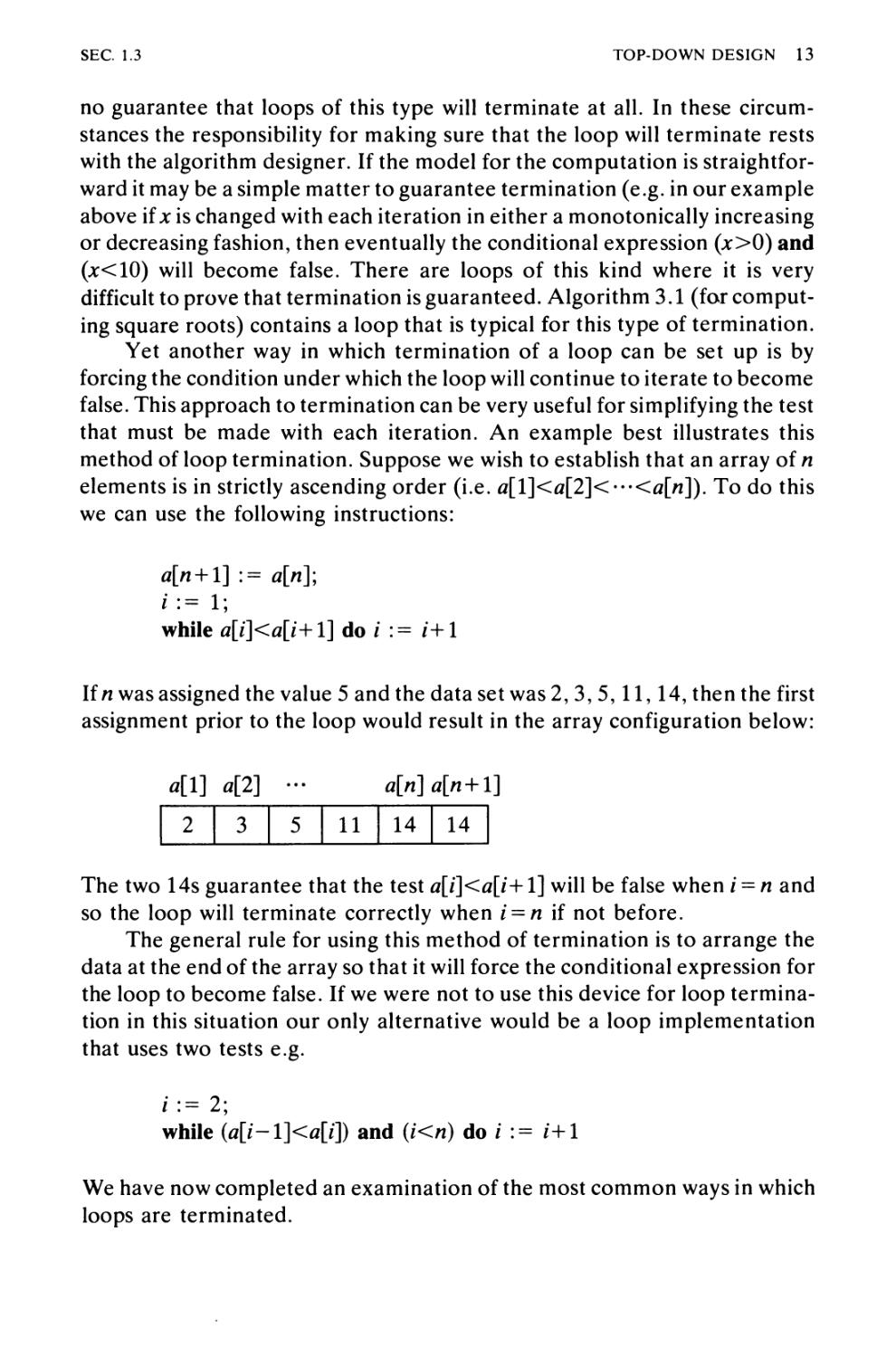
Yet another way in which termination of a loop can be set up is by
forcing the condition under which the loop will continue to iterate to become
false. This approach to termination can be very useful for simplifying the test
that must be made with each iteration. An example best illustrates this
method of loop termination. Suppose we wish to establish that an array of n
elements is in strictly ascending order (i.e. a[l]<a[2]<~'<a[n]). To do this
we can use the following instructions:
tf|>z + l] := a[n];
i:= 1;
while fl|7]<0[/+l] do / := i+l
If n was assigned the value 5 and the data set was 2, 3, 5,11,14, then the first
assignment prior to the loop would result in the array configuration below:
a[l] a[2] ••■ a[n]a[n + l]
2 | 3
5
11
14
14
The two 14s guarantee that the test a[i]<a[i+1] will be false when i = n and
so the loop will terminate correctly when i — n if not before.
The general rule for using this method of termination is to arrange the
data at the end of the array so that it will force the conditional expression for
the loop to become false. If we were not to use this device for loop
termination in this situation our only alternative would be a loop implementation
that uses two tests e.g.
i := 2;
while (a[i-l]<a[i]) and (i<n) do i := i+\
We have now completed an examination of the most common ways in which
loops are terminated.
14 COMPUTER PROBLEM-SOLVING
CHAP. 1
1.4 IMPLEMENTATION OF ALGORITHMS
The implementation of an algorithm that has been properly designed in a
top-down fashion should be an almost mechanical process. There are,
however, a number of points that should be remembered.
If an algorithm has been properly designed the path of execution should
flow in a straight line from top to bottom. It is important that the program
implementation adheres to this top-to-bottom rule. Programs (and
subprograms) implemented in this way are usually much easier to understand and
debug. They are also usually much easier to modify should the need arise
because the relationships between various parts of the program are much
more apparent.
1.4.1 Use of procedures to emphasize modularity
To assist with both the development of the implementation and the
readability of the main program it is usually helpful to modularize the program along
the lines that follow naturally from the top-down design. This practice allows
us to implement a set of independent procedures to perform specific and
well-defined tasks. For example, if as part of an algorithm it is required to
sort an array, then a specific independent procedure should be used for the
sort. In applying modularization in an implementation one thing to watch is
that the process is not taken too far, to a point at which the implementation
again becomes difficult to read because of the fragmentation. When it is
necessary to implement somewhat larger software projects a good strategy is
to first complete the overall design in a top-down fashion. The mechanism
for the main program can then be implemented with calls to the various
procedures that will be needed in the final implementation. In the first phase
of the implementation, before we have implemented any of the procedures,
we can just place a write statement in the skeleton procedures which simply
writes out the procedure's name when it is called; for example,
procedure sort]
begin
writeln{'sort called')
end
This practice allows us to test the mechanism of the main program at an early
stage and implement and test the procedures one by one. When a new
procedure has been implemented we simply substitute it for its "dummy"
procedure.
SEC. 1.4
IMPLEMENTATION OF ALGORITHMS 15
1.4.2 Choice of variable names
Another implementation detail that can make programs more meaningful
and easier to understand is to choose appropriate variable and constant
names. For example, if we have to make manipulations on days of the week
we are much better off using the variable day rather than the single letter a or
some other variable. This practice tends to make programs much more
self-documenting. In addition, each variable should only have one role in a
given program. A clear definition of all variables and constants at the start of
each procedure can also be very helpful.
1.4.3 Documentation of programs
Another useful documenting practice that can be employed in Pascal in
particular is to associate a brief but accurate comment with each begin
statement used. This is appropriate because begin statements usually signal
that some modular part of the computation is about to follow. A related part
of program documentation is the information that the program presents to
the user during the execution phase. A good programming practice is to
always write programs so that they can be executed and used by other people
unfamiliar with the workings and input requirements of the program. This
means that the program must specify during execution exactly what
responses (and their format) it requires from the user. Considerable care
should be taken to avoid ambiguities in these specifications. They should be
concise but accurately specify what is required. Also the program should
"catch" incorrect responses to its requests and inform the user in an
appropriate manner.
1.4.4 Debugging programs
In implementing an algorithm it is always necessary to carry out a number of
tests to ensure that the program is behaving correctly according to its
specifications. Even with small programs it is likely that there will be logical
errors that do not show up in the compilation phase.
To make the task of detecting logical errors somewhat easier it is a good
idea to build into the program a set of statements that will print out
information at strategic points in the computation. These statements that print out
additional information to the desired output can be made conditionally
executable. If we do this then the need to remove these statements at the
time when we are satisfied with the program becomes unnecessary. The
simplest way to implement this debugging tool is to have a Boolean variable
(e.g. debug) which is set to true when the verbose debugging output for the
16 COMPUTER PROBLEM-SOLVING
CHAP. 1
program is required. Each debugging output can then be parenthesized in
the following way:
if debug then
begin
writeln(...)
end
The actual task of trying to find logical errors in programs can be a very
testing and frustrating experience. There are no foolproof methods for
debugging but there are some steps we can take to ease the burden of the
process. Probably the best advice is to always work the program through by
hand before ever attempting to execute it. If done systematically and
thoroughly this should catch most errors. A way to do this is to check each
module or isolated task one by one for typical input conditions.
The simplest way to do this is to draw up a two-dimensional table
consisting of steps executed against all the variables used in the section of
program under consideration. We must then execute the statements in the
section one by one and update our table of variables as each variable is
changed. If the process we are modelling is a loop it is usually only necessary
to check the first couple of iterations and the last couple of iterations before
termination.
As an example of this, consider the table we could draw up for the
binary search procedure (algorithm 5.7).
The essential steps in the procedure are:
lower := 1; upper := n\
while lower<upper do
begin
middle := (lower+upper) div 2;
if x>a[middle] then
lower := middle+1
else
upper := middle
end;
found := (x = a[lower])
For the search value x and the array a[l.. n] where * = 44 and n = 15 we may
have:
Initial 41]
configuration
lo
10
r
wer
12
20
23
27
30
31
mi
39
t
ddlt
42
0
44
45
49
57
i
63
1
Uf.
*[15]
701
\
)per
SEC. 1.4 IMPLEMENTATION OF ALGORITHMS 17
Then the associated execution table is given by Table 1.1.
Table 1.1 Stepwise execution table for binary search.
Iteration no.
Initially
1
2
3
4
lower
1
9
9
9
10
middle
—
8
12
10
9
upper
15
15
12
10
10
lower < upper
true
true
true
true
false
a[middle\
—
39
49
44
42
x > a[middle]
—
true
false
false
true
NOTE: The values of variables associated with each iteration apply after the
iteration has been completed.
If we get to the stage where our program is executing but producing
incorrect results (e.g. it might be a sort routine that places most, but not all,
elements in order) the best idea is to first use a debugging trace to print out
strategic information. The next step is to follow the program through by
hand in a stepwise fashion checking against the computer's debugging
output as we go. Whenever we embark on a debugging procedure of this kind we
should be careful to ensure that we follow in a straight line along the path of
execution. It is usually a wasted effort to assume that some things work and
only start a systematic study of the algorithm halfway through the execution
path. A good rule to follow when debugging is not to assume anything.
1.4.5 Program testing
In attempting to test whether or not a program will handle all variations of
the problem it was designed to solve we must make every effort to be sure
that it will cope with the limiting and unusual cases. Some of the things we
might check are whether the program solves the smallest possible problem,
whether it handles the case when all data values are the same, and so on.
Unusual cases like these are usually the ones that can cause a program to
falter.
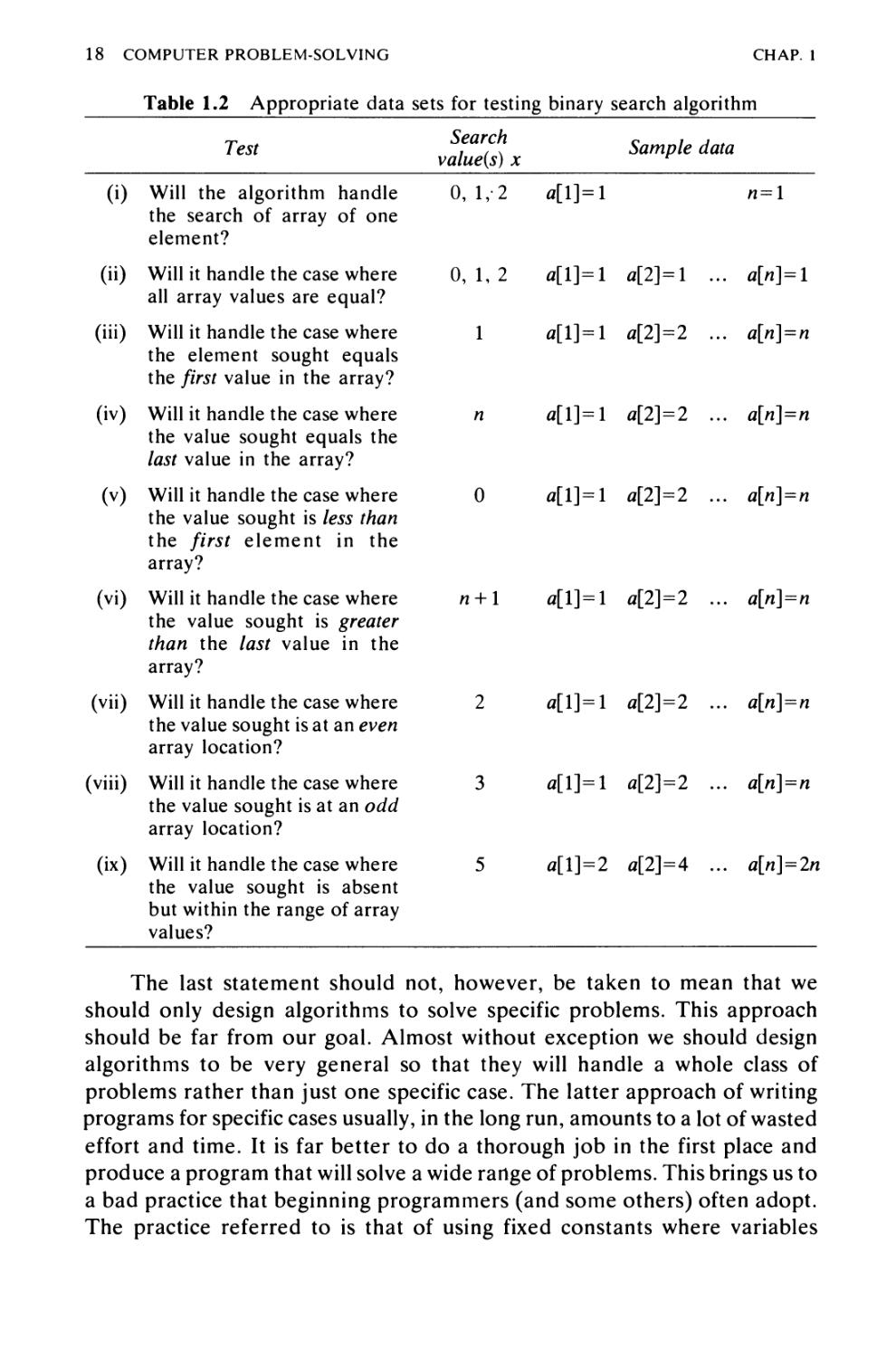
As an example, consider the testing we would need for the binary search
algorithm (i.e. algorithm 5.7). Appropriate data sets and tests are given in
Table 1.2.
It is often not possible or necessary to write programs that handle all
input conditions that may be supplied for a given problem. Wherever
possible programs should be accompanied by input and output assertions as
described in the section on program verification. Although it is not always
practical to implement programs that can handle all possible input
conditions we should always strive to build into a program mechanisms that allow
it to gracefully and informatively respond to the user when it receives input
conditions it was not designed to handle.
18 COMPUTER PROBLEM-SOLVING CHAP. 1
Table 1.2 Appropriate data sets for testing binary search algorithm
^ VaZ(sU Sample data
(i) Will the algorithm handle 0, 1, 2 a[l]=l n=\
the search of array of one
element?
(ii)
(iii)
(iv)
(v)
(vi)
(vii)
(viii)
(ix)
Will it handle the case where
all array values are equal?
Will it handle the case where
the element sought equals
the first value in the array?
Will it handle the case where
the value sought equals the
last value in the array?
Will it handle the case where
the value sought is less than
the first element in the
array?
Will it handle the case where
the value sought is greater
than the last value in the
array?
Will it handle the case where
the value sought is at an even
array location?
Will it handle the case where
the value sought is at an odd
array location?
Will it handle the case where
the value sought is absent
but within the range of array
values?
0, 1, 2
1
n
0
rc + 1
2
3
5
a[\}=\
*[1] = 1
*[1]=1
*[1]=1
41]= 1
a[\}= 1
a[l]= 1
a[l]=2
a[2]=l .,
a[2]=2 .,
a[2]=2 .
a[2]=2 .,
a[2]=2 .
a[2]=2 .
a[2]=2 .
a[2]=4 .
.. a[n]=l
.. a[n] = n
.. a[n]=n
.. a[n]=n
.. a[n]=n
.. a[n]=n
.. a[n]=n
.. a[n]=2n
The last statement should not, however, be taken to mean that we
should only design algorithms to solve specific problems. This approach
should be far from our goal. Almost without exception we should design
algorithms to be very general so that they will handle a whole class of
problems rather than just one specific case. The latter approach of writing
programs for specific cases usually, in the long run, amounts to a lot of wasted
effort and time. It is far better to do a thorough job in the first place and
produce a program that will solve a wide range of problems. This brings us to
a bad practice that beginning programmers (and some others) often adopt.
The practice referred to is that of using fixed constants where variables
SEC. 1.5
PROGRAM VERIFICATION 19
should be used. For example, we should not use statements of the form
while /<100do
The 100 should always be replaced by a variable, i.e.
while i<n do
A good rule to follow is that fixed numeric constants should only be used in
programs for things like the number of months in a year, and so on. Pascal
provides for the use of constant declarations.
The considerations we have made concerning the implementation of
algorithms leads us to other very important topics concerning just what we
mean by a good solution to a problem and, secondly, the question of what
actually constitutes a correct program.
1.5 PROGRAM VERIFICATION
The cost of development of computing software has become a major
expense in the application of computers. Experience in working with
computer systems has led to the observation that generally more than half of all
programming effort and resources is spent in correcting errors in programs
and carrying out modification of programs. As larger and more complex
programs are developed, both these tasks become harder and more time-
consuming. In some specialized military, space, and medical applications,
program correctness can be a matter of life and death. This suggests two
things. Firstly, that considerable savings in the time for program
modification should be possible if more care is put into the creation of clearly written
code at the time of program development. We have already seen that
top-down design can serve as a very useful aid in the writing of programs that
are readable and able to be understood at both superficial and detailed levels
of implementaion.
The other problem of being able to develop correct as well as clear code
also requires the application of a systematic procedure. Proving even simple
programs correct turns out to be a far from easy task. It is not simply a matter
of testing a program's behavior under the influence of a variety of input
conditions to prove its correctness. This approach to demonstrating a
program's correctness may, in some cases, show up errors but it cannot
guarantee their absence. It is this weakness in such an approach that makes it
necessary to resort to a method of program verification that is based on
sound mathematical principles.
20 COMPUTER PROBLEM-SOLVING
CHAP. 1
Program verification refers to the application of mathematical proof
techniques to establish that the results obtained by the execution of a
program with arbitrary inputs are in accord with formally defined output
specifications.
Although we have only now come to consider this aspect of algorithm
design, it is not meant to imply that this process should be carried out after
the complete development of the algorithm. In fact, a far better strategy is to
develop the proof in a top-down fashion along with the top-down
development of the algorithm. That is, we start out by proving the correctness of the
very basic structure of the algorithm at an abstract or superficial level. Then
as abstract tasks are replaced by more specific mechanisms, it is necessary to
ensure that these refinements do not alter the correctness of the more
abstract level. This process is repeated until we get down to the specific
program steps.
1.5.1 Computer model for program execution
To pursue this goal of program verification, we must fully appreciate what
happens when a program is executed under the influence of given input
conditions. What is important in this respect is the execution path that is
followed for the given input conditions. A program may have a variety of
execution paths leading to successful termination. For a given set of input
conditions only one of these paths will be followed (although obviously some
paths may share common subpaths for different inputs). The written
algorithm implementation therefore defines a whole set of execution paths.
The progress of a computation from specific input conditions through to
termination can be thought of as a sequence of transitions from one
computation state to another. Each state, including the initial state, is defined by the
values of all variables at the corresponding point in time. A state transition
and progress towards completion is made by changing the value of a variable
followed by a transfer of control to the next instruction on the current
execution path. As well as instructions that change the computation state
there are also other instructions that simply make tests on the current state.
These tests are used to bring about a change in the sequential flow of
execution. This model for program execution provides us with a foundation
on which to construct correctness proofs of algorithms.
1.5.2 Input and output assertions
The very first step that needs to be taken in order to prove a program correct
is to provide a formal statement of its specifications in terms of the variables
that it employs. The formal statement has two parts, an input assertion and
SEC. 1.5
PROGRAM VERIFICATION 21
an output assertion which can be expressed in logic notation as predicates
that describe the state of the executing program's variables. The input
assertion should specify any constraints that have been placed on the values
of the input variables used by the program (e.g. an input variable d may play
the role of a divisor in the program. Clearly d cannot have the value 0. The
input assertion is therefore d <> 0). When there are no restrictions on the
values of the input variables the input assertion is given the logical value true.
The output assertion must specify symbolically the results that the program is
expected to produce for input data that satisfies the input assertion (e.g. if a
program is designed to calculate the quotient q and remainder r resulting
from the division of x by y then the output assertion can be written as:
{x = q*y + r)/\(r<y)
where the symbol "A" represents the logical connective "and".
1.5.3 Implications and symbolic execution
The problem of actually verifying a program can be formulated as a set of
implications which must be shown to be logically true. These implications
have the general form:
where the logical connective "3" is read as "implies". P is termed the
assumption and Q the conclusion. The associated truth table defining
implication is given in Table 1.3.
Table 1.3 Truth table defining implication
p
true
true
false
false
Q
true
false
true
false
P^Q
true
false
true
true
In order to show that these implications or propositions are logically
true, it is necessary to take into account the effects of executing the program
for arbitrary inputs that satisfy the input assertion. A relatively
straightforward way to do this is to use the technique of symbolic execution. With
symbolic execution, all input data values are replaced by symbolic values and
all arithmetic operations on numbers translate into algebraic manipulation
of symbolic expressions. As an example, consider the following program
segment labelled with input and output assertions:
22 COMPUTER PROBLEM-SOLVING
CHAP. 1
A readln(x,y)\
{assert: true}
x := x-y;
y := x+y;
x := y-*
# {asserf x = yOAy = *0}
where *0 and yO refer to the initial values of x and y respectively.
Table 1.4 Normal and symbolic execution for exchange mechanism
Step Normal execution Symbolic execution
input values: x = 3 y = 1 input values: x = a y = /3
1 * := *->> => * = 3-l = 2 x := x-y ^> x = a-/3
2 y : = *+>> =>y = 2 + l = 3 >>:= *+>> => y = (a-/3)+j3 = a
3 jc := y-jc => a: = 3-2 = 1 x := y-x => jc = ((a-j3)+j3)-(a-/3) = j3
Both normal execution and symbolic execution, shown in Table 1.4, indicate
that the values of x and y are exchanged.
Symbolic execution enables us to transform the verification procedure
into proving that the input assertion with symbolic values substituted for all
input variables implies the output assertion with final symbolic values
substituted for all variables. A proposition phrased in this way is referred to as a
verification condition (VQ over the program segment from the input
assertion to the output assertion.
To proceed with the verification procedure it is usually necessary to set
up a number of intermediate verification conditions between the input and
output assertions. Taken to the limit this involves carrying out the
verification procedure statement by statement. For practical purposes it is, however,
usually sufficient to only consider verification conditions for blocks of a
program as marked by straight-line segments, branching segments, and loop
segments. We will adopt the convention that VC(A — B) refers to the
verification condition over the program segment from A to B. We will now consider
the verification of each of these basic segment types in turn.
1.5.4 Verification of straight-line program segments
The best way to illustrate the verification procedure is by example. Our
exchange mechanism mentioned above will serve as an example of a
straight-line program segment.
SEC 1.5
PROGRAM VERIFICATION 23
The verification condition for this program segment is:
VC(A - E): true 3 {x = yOAy = xO}
On substitution of the initial and final values of all variables, we get:
VC(A-B): truezD ((a-p)+P)-(a-p)) = pA(a-p)+P) = a
The conclusion part of the verification condition can be simplified to yield
p = (3 and a = a which is clearly true and so the implication is true.
1.5.5 Verification of program segments with branches
To handle program segments that contain branches it is necessary to set up
and prove verification conditions for each branch separately. As an example,
consider the following program segment that ensures that x is less than or
equal to y.
readln{x,y)\
A {assert PA: true}
if x>y then
begin
t:= x;
x := y\
y: = t
end
B {assert PB\ ((x<=y)A(x = xOAy =yO))\/(x = yOAy = xO)}
In general, the propositions that must be proved for the basic if construct
are:
PAACAz>PB
PAA~CAz>PB
where CA is the branch condition.
The two verification conditions needed in this case are given below,
where the initial values of x and y are respectively a and p
VC(A-(t)~B): true Aa>pz>((a^p)A(p = aAa = /3))V(0 = pAa = a)
Since a>(3 is true and the second part of the conclusion (i.e. a = aA(3 = (3) is
true, the verification condition for the true path is true.
The verification condition for the false path is:
VC(A-(f)-B): true A~(a>p)z>((a^p)A(a = aAp = j3))V(a = pAp = a)
Since ~(a>/3)3 (a^/3) and the conclusion (a = aA(3 = /3) is true the
verification condition for the false path is true. It follows that the labelled program
segment (A-B) is true. Case statements can be treated similarly.
24 COMPUTER PROBLEM-SOLVING
CHAP. 1
1.5.6 Verification of program segments with loops
There are problems with trying to verify loop segments directly by symbolic
execution because the number of iterations required is usually arbitrary. To
overcome this problem, a special kind of assertion called a loop invariant
must be employed. A loop invariant should be a property (predicate) that
captures the progressive computational role of the loop while at the same
time remaining true before and after each loop traversal irrespective of how
many times the loop is executed. Once the loop invariant is established,
there are several steps that must be taken to verify the loop segment. To
understand this loop verification procedure, we will use the following
single-loop program structure as our model.
A {input assertion PA}
straight-line program segment
B {loop invariant IB}
while loop-condition do
begin
loop-free program segment
end
C {output assertion Pc}
(a) The first step that must be taken is to show that the loop invariant is
true initially, before the loop is entered. This can be done by setting up
a verification condition VC(A-B) for the program segment from A to
B. That is, the input assertion, together with any changes to variables
caused by the segment A - B, must imply that the loop invariant is true.
We can use symbolic execution to carry out this verification step. That
is, we must show PazdIb.
(b) The second part of verifying a loop involves showing that the loop
invariant is still true after the segment of program within the loop has
been executed. To do this we can set up a verification condition
VC(B-B). This involves showing that the loop invariant with initial
values of variables set, together with the condition for loop execution
CB, implies the truth of the loop invariant with final values of variables,
i.e.
/flACp/fl
Symbolic execution can also be used to verify this step.
SEC. 1.5
PROGRAM VERIFICATION 25
(c) As a final step in verifying a loop segment, it is necessary to show that
the invariant, together with the negation of the loop-entry condition,
implies the assertion that applies on exiting from the loop. The
verification condition in this case for our basic loop structure will be VC(B~ C).
The corresponding proposition will be:
IBA~CB=>PC
A better understanding of the application of the loop verification
technique can be gained by studying a specific example. Consider the
following program segment which can be used to compute factorial.
A {assert PA: n>=0}
i := 0;
fact: = 1;
B {invariant IB: fact=i\Ai^n}
while i<n do
begin
/ := /+1;
fact := i*fact
end
C {assert Pc: fact = n\}
Assume the input value of n isy and the current values of/ and fact are a and
p respectively. Using symbolic execution we can show that the associated
verification conditions that must be proved are:
1. VC(A-B):PA=>IB
: y^0=>l = 0!A0^y
Now 1 = 0! is true by definition and y^Oz^O^y is trivially true and so the
verification condition VC(A-B) is true.
2. VC(B-B) : IB/\CBz>IB
: p = a\Aa^yAa<yz>(a+ 1)0 = (a+1)!A(a+ l)^y
Since fi = a\
we have (a+l)/3 = (a+l)a! = (a+l)!=(a+l)a! by definition
and so j3 = a!z>(a+l))3 = (a+l)! is true.
Also a^yAa<yz>a<y
and so (a+l)^y for integer a and y.
It follows that the verification condition VC(B-B) is true.
3. VC{B-Q:IBA~CBz>Pc
: p = alAa^yA ~(a<y)3/3 = y!
Since ~(a<y)Da^y
then a^yAa^yz>a = y
and so because a = y it follows that p = a\zip = y\ is true
and so the verification condition VC(B-Q is true.
26 COMPUTER PROBLEM-SOLVING
CHAP. 1
Since the verification conditions for all three program segments are correct,
the complete program segment is said to be partially correct.
What the verification method we have described gives us is only a proof
of partial correctness, with the implication that if the algorithm terminates
the result produced will be correct. For programs that contain loops we are
therefore left with the separate but necessary task of proving that the
program terminates in order to establish total correctness.
Before considering in detail a method for proof of termination, we will
consider setting up the verification conditions for a program example that
employs an array.
1.5.7 Verification of program segments that employ arrays
The idea of symbolic execution developed in the preceding sections can be
extended to some of the simpler examples that employ arrays although it
now becomes necessary to account for the symbolic values of all array
elements. As an example of verification of a program segment containing an
array we will set up the verification conditions for a program that finds the
position of the smallest element in the array.
The program annotated with assertions may take the following form:
A {assert PA: n^l}
i := 1;
p:= 1;
B {invariant IB\ (l^i^n)A(l^p^i)A(a[p]^a[l], a[2], ..., a[i])}
while i<n do
begin
i := i+l;
if tf[/]<tf[p] then p := i
end
C {assert Pc: (l^p^n)A(a[p]^a[l], a[2], ..., a[n])}
where we have used the shorthand convention that:
a[p]^a[l], a[2], ..., a[n]^a[p]^a[l]Aa[p]^a[2]A ••• Aa[p]^a[n]
Assuming that the initial values of a[l], a[2],..., a[n] are respectively al9
a2, ...,a„,and that the initial value of n is 5, we can use symbolic execution to
check the verification conditions:
VC(A-B): S^lzKl^l^SJAU^l^DAa^a!
With i and/7 having initial values of (3 and y respectively, the verification
conditions for the two paths through the loop are:
SEC. 1.5
PROGRAM VERIFICATION 27
VC(B-(t)-B): (1^^5)A(l^y^)A(ar^a1, a2, ..., ap)Ap<5/\afi+l<ay
z)(l^j8+1^8)A(l^i8+l^i8+l)Aa/B+1^a1, a2, ..., a^+1
VC(B-(fl-B): (1^^5)A(l^y^)A(ar^a1, a2, ..., a,)
Aj8<SA-(a^o^)
3(1^8+l^S)A(ls^j8+l)A (ay^«i, a2, ..., a^)
VC(B-C): (l^/3^8)A(l^y^/3)A(a^a,, a2, ..., afi)A~(P<S)
=>(l^y^8)A(ay^al5 a2, ..., as)
The example above should give some flavor of how programs with
arrays may be treated. We will now return to consideration of the problem of
proving program termination.
1.5.8 Proof of termination
To prove that a program terminates, it is necessary to show that it
accomplishes its stated objective in a finite number of steps. This amounts to
showing that every loop in the program terminates in a finite number of
steps. In many instances, proof of termination follows directly from the
properties of the various iterative constructs. Consider, for example, the
for-loop below:
for i : = 1 to n do
begin
end
When n is positive and finite this is guaranteed to terminate because, with
each iteration, the number of steps to the termination condition being
satisfied is reduced by at least one. This reduction can only be carried out a
finite number of times and so the loop must terminate.
There are obviously loops for which the proof of termination is much
more subtle and elusive. One of two situations usually prevails in such
circumstances. When there is no single variable that is monotonically
progressing towards the termination condition, we often find that an arithmetic
combination of two (or more) variables makes progress towards termination
with each iteration.
If the termination characteristic of the program is not of this type, it
usually remains to show that there is some property of the data (perhaps a
sentinel) that will guarantee termination.
More formally, the problem of proving loop termination can often be
approached by associating another expression, in addition to the loop
invariant, with each loop. The expression, e, should be chosen to be a
function of the variables used in the loop. It should always be non-negative
and it must be shown to decrease in value with each loop iteration. If these
28 COMPUTER PROBLEM-SOLVING
CHAP. 1
criteria are satisfied, the loop must terminate. Proof of termination can
therefore be reduced to establishing the truth of the following termination
conditions.
(i) Referring back to our generalized loop structure we must show that the
truth of the loop invariant IB, together with condition for loop
execution CB, implies that the value of the expression e is greater than zero.
That is,
TC1(B): IBACB^e >0
The condition e^O becomes an invariant of the loop.
In some instances, the invariant used for establishing partial
correctness is not sufficient for use in a proof of termination. This problem
can be overcome by attaching additional conditions (derived from
earlier assertions) to the invariant,
(ii) The second proposition that must be proven is to show that the loop
invariant IB, together with the condition for loop execution, CB, implies
that the value e() of the expression before execution is strictly greater
than its value e after loop execution, i.e. for a loop B
TC2(B-B): /flACp(e0>e)A(e^0)
The final value of e can be obtained by symbolic execution of the
statements in the loop.
Once these two propositions have been shown to be true, we can
immediately conclude that the repetition process is finite since e can only be
decreased a finite number of times while remaining positive as required by
TC1(B). The considerations of termination for repeat.. until loops follow a
similar line of reasoning.
A proof of termination for the quotient/remainder program given
below will now be outlined.
begin
A {assert PA: (x^0)A(y>0)}
r := x\q := 0;
B {invariant IB\ r^0Ax = y*q + r}
while y^r do
begin
r := r—y\
q := q + \
end
C {assert Pc: (x = y*q + r)A(0^r<y)}
SEC. 1.6
THE EFFICIENCY OF ALGORITHMS 29
To prove termination for this program segment we will use:
e = r+y
In order to establish the first termination condition, we will need to attach
the additional condition y>0 from PA to the invariant IB. We then have
TC1(B): (r^0)A(x = y*q+r)A(y>0)A(y^r)z>(r+y>0)
Now
(r^0)A(y>0)z>(r+y>0)
and so TC1(B) can be shown to be true.
Assuming that x, y, r and q respectively have the symbolic values a, /3, y,
and 5 on entering the loop, then for TC2(B-B) we have:
TCl(B-B): (y^O)A(a = /3*5+y)A(/3>0)A(/3^y)3y+/3>(y-/3)+/3
where
e0 = y+p and € = (y-p)+p
which can easily be shown to be true and so the proof of termination is
complete.
Once both partial correctness and termination have been established,
the proof is complete. To embark on detailed formal proofs of programs
requires a considerable degree of mathematical maturity and experience.
The length and detail of such proofs is usually considerably greater than the
size of the original program text. In the discussions which follow, we will
therefore only attempt to annotate programs with relevant assertions.
1.6 THE EFFICIENCY OF ALGORITHMS
Efficiency considerations for algorithms are inherently tied in with the
design, implementation, and analysis of algorithms. Every algorithm must
use up some of a computer's resources to complete its task. The resources
most relevant in relation to efficiency are central processor time (CPU time)
and internal memory. Because of the high cost of computing resources it is
always desirable to design algorithms that are economical in the use of CPU
time and memory. This is an easy statement to make but one that is often
difficult to follow either because of bad design habits, or the inherent
complexity of the problem, or both. As with most other aspects of algorithm
design, there is no recipe for designing efficient algorithms. Despite there
30 COMPUTER PROBLEM-SOLVING
CHAP. 1
being some generalities each problem has its own characteristics which
demand specific responses to solve the problem efficiently. Within the
framework of this last statement we will try to make a few suggestions that
can sometimes be useful in designing efficient algorithms.
1.6.1 Redundant computations
Most of the inefficiencies that creep into the implementation of algorithms
come about because redundant computations are made or unnecessary
storage is used. The effects of redundant computations are most serious
when they are embedded within a loop that must be executed many times.
The most common mistake using loops is to repeatedly recalculate part of an
expression that remains constant throughout the entire execution phase of
the loop. The example below illustrates this point:
x := 0;
for i : = 1 to n do
begin
x := *+0.01;
y := (a*a*a+c)*x*x+b*b*x\
writeln ('x = ' , x,'y = ' ,y)
end
This loop does twice the number of multiplications necessary to
complete the computation. The unnecessary multiplications and additions can be
removed by precomputing two other constants a3c and b2 before executing
the loop:
a3c := a*a*a+c\
b2 := b*b\
x := 0;
for i : = 1 to n do
begin
x := Jt+0.01;
y := a3c*x*x+b2*x\
writeln {'x = \x,'y = ' ,y)
end
The savings in this instance are not all that significant but there are
many other situations where they are much more significant. It is always
most important to strive to eliminate redundancies in the innermost loops of
computations as these inefficiencies can be most costly.
SEC. 1.6
THE EFFICIENCY OF ALGORITHMS 31
1.6.2 Referencing array elements
If care is not exercised redundant computations can also easily creep into
array processing. Consider, for example, the two versions of an algorithm for
finding the maximum and its position in an array.
Version (1)
p:= 1;
for i : = 2 to n do
if tf[/]>tf[jp] then p := i;
max := a[p]
Version (2)
p:= 1;
max := a[l]\
for i : = 2 to n do
if a[i]>max then
begin
max := a[i];
P • = i
end
The version (2) implementation would normally be preferred because the
conditional test (i.e. a[i]>max) which is the dominant instruction is more
efficient to perform than the corresponding test in version (1). It is more
efficient because to use the variable max only one memory reference
instruction is required, whereas to use the variable a[p] requires two memory
references and an addition operation to locate the correct value for use in the
test. Also in version (2), introduction of the variable max makes it clearer
what task is to be accomplished.
1.6.3 Inefficiency due to late termination
Another place inefficiencies can come into an implementation is where
considerably more tests are done than are required to solve the problem at
hand. This type of inefficiency can be best illustrated by example. Suppose
we had to linear search an alphabetically ordered list of names for some
particular name. An inefficient implementation in this instance would be
one where all names were examined even if the point in the list was reached
where it was known that the name could not occur later (e.g. suppose we
were looking for the name MOORE, then, as soon as we had encountered a
name that occurred alphabetically later than MOORE, e.g. MORRIS, there
32 COMPUTER PROBLEM-SOLVING
CHAP. 1
would be no need to proceed further). The inefficient implementation could
have the form:
1. while name sought <> current name and no end-of-file do
(a) get next name from list.
A more efficient implementation would be:
1. while name sought > current name and not end-of-file do
(a) get next name from list.
2. test if current name is equal to name sought.
The same sort of inefficiency can be built into the bubblesort algorithm
(algorithm 5.3) if care is not taken with the implementation. This can happen
if the inner loop that drives the exchange mechanism always goes the full
length of the array. For example,
for i : = 1 to n — 1
for; := 1 to n-\
if a[j]>a[j+1] then "exchange a\j] with tf[/+l]"
With this sorting mechanism, after the /!h iteration, the last i values in the
array will be in sorted order. Thus, for any given / the inner loop should not
proceed beyond n-i. The loop structure will then be:
for / := 1 to n-\
for; := 1 to n-i
if a[j]>a[j+1] then "exchange a\J] with tf[/+l]"
The lesson to be learned from this is that we should always try to take
advantage of any order or structure in a problem.
1.6.4 Early detection of desired output conditions
The bubblesort also provides us with an example of another related type of
inefficiency involving termination. It sometimes happens, due to the nature
of the input data, that the algorithm establishes the desired output condition
before the general conditions for termination have been met. For example, a
bubblesort might be used to sort a set of data that is already almost in sorted
order. When this happens it is very likely that the algorithm will have the
data in sorted order long before the loop termination conditions are met. It is
therefore desirable to terminate the sort as soon as it is established that the
data is already sorted. To do this all we need to do is check whether there
SEC. 1.7
THE ANALYSIS OF ALGORITHMS 33
have been any exchanges in the current pass of the inner loop. If there have
been no exchanges in the current pass the data must be sorted and so early
termination can be applied (a check of algorithm 5.3 reveals how this is
implemented for the bubblesort). In general, we must include additional
steps and tests to detect the conditions for early termination. However, if
they can be kept inexpensive (as in the bubblesort) then it is worth including
them. That is, when early termination is possible, we always have to trade
tests and maybe even storage to bring about the early termination.
1.6.5 Trading storage for efficiency gains
A trade between storage and efficiency is often used to improve the
performance of an algorithm. What usually happens in this type of tradeoff is that
we precompute or save some intermediate results and avoid having to do a
lot of unnecessary testing and computation later on. (See for example the
longest monotone subsequence problem—algorithm 4.7.)
One strategy that it sometimes used to try to speed up an algorithm is to
implement it using the least number of loops. While this is usually possible,
inevitably it makes programs much harder to read and debug. It is therefore
usually better to stick to the rule of having one loop do one job just as we
have one variable doing one job. When a more efficient solution to a
problem is required it is far better to try to improve the algorithm rather than
resorting to "programming tricks" that tend to obscure what is being done.
A clear implementation of a better algorithm is to be preferred to a "tricky"
implementation of an algorithm that is not as good. We are now left with the
task of trying to measure the efficiency of algorithms.
1.7 THE ANALYSIS OF ALGORITHMS
There are usually many ways to solve any given problem. In computing, as in
most efforts of human endeavor, we are generally concerned with "good"
solutions to problems. This raises certain questions as to just what do we
mean by a "good" solution to a problem? In algorithm design "good" has
both qualitative and quantitative aspects. There are often certain esthetic
and personal aspects to this but, on a more practical level, we are usually
interested in a solution that is economical in the use of computing and human
resources. Among other things, good algorithms usually possess the
following qualitites and capabilities:
34 COMPUTER PROBLEM-SOLVING
CHAP. 1
1. They are simple but powerful and general solutions.
2. They can be easily understood by others, that is, the implementation is
clear and concise without being "tricky".
3. They can be easily modified if necessary.
4. They are correct for clearly defined situations.
5. They are able to be understood on a number of levels.
6. They are economical in the use of computer time, computer storage
and peripherals.
7. They are documented well enough to be used by others who do not
have a detailed knowledge of their inner workings.
8. They are not dependent on being run on a particular computer.
9. They are able to be used as a subprocedure for other problems.
10. The solution is pleasing and satisfying to its designer—a product that
the designer feels proud to have created.
These qualitative aspects of a good algorithm are very important but it is
also necessary to try to provide some quantitative measures to complete the
evaluation of "goodness" of an algorithm. Quantitative measures are
valuable in that they can give us a way of directly predicting the performance of
an algorithm and of comparing the relative performance of two or more
algorithms that are intended to solve the same problem. This can be
important because the use of an algorithm that is more efficient means a saving in
computing resources which translates into a saving in time and money.
1.7.1 Computational complexity
To make a quantitative measure of an algorithm's performance it is
necessary to set up a computational model that reflects its behavior under
specified input conditions. This model must capture the essence of the
computation while at the same time it must be divorced from any
programming language.
We are therefore required to characterize an algorithm's performance
in terms of the size (usually n) of the problem being solved. Obviously, more
computing resources are needed to solve larger problems in the same class.
The important question that we must settle is, how does the cost of solving the
problem vary as n increases? Our first response to this question might be
that as n increases then so does the cost in the same manner (e.g. a problem
for n = 200 takes twice as long as a problem for n = 100). While this linear
dependence on n is true for some simple algorithms in general the behavior
with n follows some other completely different pattern. At the lower end of
the scale we have algorithms with logarithmic (or better) dependence on n,
while at the higher end of the scale we have algorithms with an exponential
SEC. 1.7
THE ANALYSIS OF ALGORITHMS 35
dependence on n. With increasing n the relative difference in the cost of a
computation is enormous for these two extremes. Table 1.5 illustrates the
comparative cost for a range of n values.
Table 1.5 Computational cost as a function of problem size for a range of
computational complexities
\og2n
1
3.322
6.644
9.966
13.287
n
2
10
102
103
104
n \og2n
2
33.22
664.4
9966.0
132,877
n2
4
102
104
106
108
n3
8
103
106
109
1012
2"
4
>103
>>1025
>>10250
>>1025()0
What is obvious from this table is that we can solve only very small
problems with an algorithm that exhibits exponential behavior. Even
assuming that a computer can do about one million operations per second, an
exponential algorithm with n = 100 would take immeasurably longer than
the existence of the earth to terminate. At the other extreme, for an
algorithm with logarithmic dependence on n, a problem with n = 104 would
require only 13 steps which amounts to about 13 microseconds of computer
time. These examples emphasize how important it is to have an
understanding of the way in which algorithms behave as a function of the problem size.
What can also come out of analyzing algorithms is a theoretical model of the
inherent computational complexity of particular problems.
In deciding how to characterize the behavior of an algorithm as a
function of the size of the problem n, we must study the mechanism very
carefully to decide just what constitutes the dominant mechanism. It may be
the number of times a particular arithmetic (or other) expression is
evaluated, or the number of comparisons or exchanges that must be made as n
grows. For example, comparisons, exchanges, and moves characterize most
sorting algorithms. The number of comparisons usually dominates so we use
comparisons in our computational model for sorting algorithms.
1.7.2 The order notation
A standard notation has been developed to represent functions which bound
the computing time for algorithms. It is an order notation and it is usually
referred to as the O-notation. An algorithm in which the dominant
mechanism is executed en1 times for c, a constant, and n the problem size, is said to
have an order n2 complexity which is written as 0(n2). Formally, a function
g(n) is 0(f(n)) provided there is a constant c for which the relationship
g(n)^cf(n)
36 COMPUTER PROBLEM-SOLVING
CHAP. 1
holds for all values of n that are finite and positive. With these conventions
we have a means of characterizing the asymptotic complexity of an algorithm
and hence of determining the size of problems that it can solve using a
conventional sequential computer. We can write the above relationship in
the form:
lim 4r^ = c where c is not equal to zero
A2->oo f(n) M
As an example, suppose we have an algorithm that requires (3n2+6tt + 3)
comparisons to complete its task. According to the convention just outlined
we have:
g(n) = 3n2+6n + 3 and lim ^±6n±3 = 3
° n->oo n2
It follows that this particular algorithm has an asymptotic complexity of
0(n2). In using this methodology to decide upon the superiority of one
algorithm over another we need to pay careful attention to the constants of
proportionality. It can happen that an algorithm with a higher asymptotic
complexity has a very small constant of proportionality and hence for some
particular range of n it will give better performance than an algorithm with
lower complexity and a higher proportionality constant.
1.7.3 Worst and average case behavior
In analyzing any given algorithm there are two measures of performance
that are usually considered. These are the worst and average case behavior of
the algorithm. These two measures can be applied to both the time and space
complexity of an algorithm. The worst case complexity for a given problem
size n corresponds to the maximum complexity encountered among all
problems of size n. Determination of the worst case complexity for many
algorithms is relatively straightforward. We choose a set of input conditions
that force the algorithm to make the least possible progress towards its final
goal at each step.
In many practical applications it is much more important to have a
measure of the expected complexity of a given algorithm rather than the
worst case behavior. The expected complexity gives a measure of the
behavior of the algorithm averaged over all possible problems of size n. In
comparing two algorithms to solve a given problem, we would generally opt
in preference for the algorithm that has the lower expected complexity.
Unfortunately, setting up a computational model to characterize the average
behavior often involves very complex and sophisticated combinatorial
analyses.
SEC. 1.7
THE ANALYSIS OF ALGORITHMS 37
1.7.4 Probabilistic average case analysis
As a simple example, suppose we wish to characterize the behavior of an
algorithm that linearly searches an ordered list of elements for some value x.
1
2
...
n
In the worst case it will be necessary for the algorithm to examine alln values
in the list before terminating.
The average case situation is somewhat different. For a probabilistic
average case analysis it is generally assumed that all possible points of
termination are equally likely, i.e. the probability that x will be found at
position 1 is l/n, and at position 2 is l/n, and so on. The average search cost
is therefore the sum of all possible search costs each multiplied by their
associated probability. For example, if n = 5 we would have:
average search cost =1/5 (1 + 2+3 + 4+5) = 3
Noting that 1+2+3+ ••• +n = n(n+l)/2 (i.e. from Gauss' formula) then in
the general case we have:
average search cost = —(— (az + 1)) =
rt+1
As a second, slightly more complicated example, let us consider the
average case analysis for the binary search procedure described in algorithm
5.7. What we wish to establish in this analysis is the average number of
iterations of the search loop that are required before the algorithm
terminates in a successful search. This analysis will correspond only to the first
binary search implementation proposed in algorithm 5.7 which terminates
as soon as the search value is found. The associated binary search tree for an
array of size 15 is given in Fig. 1.2.
Referring to the tree we see that 1 element can be found with 1
comparison, 2 elements with 2 comparisons, 4 elements with 3 comparisons,
and so on, i.e. sum over all possible elements = 1 + 2+2+3 + 3 + 3 + 3 + 4+ •••.
In the general case, 2' elements require /+1 comparisons. Now assuming that
all items present in the array are equally likely to be retrieved (i.e. their
probability of retrieval is l/n), then the average search cost is again just the
sum over all possible search costs, each multiplied by their associated
probability. That is,t
Llog2n]
l V l
average search cost = - 2* (*+l)x2' = —
f Llog2"J
2^ ix2l+n\
t Where [J is used to indicate that [log2«J is the greatest integer less than or equal to
\og2n (it is referred to as "Floor" \og2n), and £ is the mathematical summation
symbol.
38 COMPUTER PROBLEM-SOLVING
CHAP. 1
c
o
•c
a
E
o
c
o
a
E
o
o
Fig. 1.2 Binary decision tree for a set of 15 elements.
BIBLIOGRAPHY 39
This formula is exact only when n is one less than a power of two. Some
calculus is needed to evaluate the sum:
Llog2"J
s= V ;x2'
i=0
We may recognize that this sum is a geometric progression and we know that
in general:
xk+1-l
\+x+x2+ ••• +xk = -—r1
x-l
We may also note that:
/x2'=^ (2*<)
ax x=2
It follows that to compute our sum we can take the derivative of
(xk+l~l)/(x-l) multiplied by 2 and evaluated at x = 2 where A; = [log2AzJ.
When this is done we get:
Llog2"J
s= ]!T /x2' = (az+1) (Llog2AzJ-l) + 2
i=0
And, after substituting for the sum in our average search cost expression, we
find:
average search cost = - ' *• ^2 •*—^ U°g2^J for large n.
This example illustrates that even for a relatively simple example, a degree
of mathematical sophistication is required to carry out the analysis. We now
have some of the tools necessary to embark on a study of algorithm design.
BIBLIOGRAPHY
Problem-solving
The classic book on problem-solving is Polya's How to Solve It (1971), which was first
published in the 1940s. This book is highly recommended to all embarking on
computer problem-solving. Polya's other works on mathematical problem-solving
contain a wealth of useful hints and exercises. Gardiner's Aha\ Insight is also a
delightful book. The other references listed also contain important ideas on
problem-solving.
40 COMPUTER PROBLEM-SOLVING
CHAP. 1
1. Gardiner, M., Aha\ Insight, Freeman, N.Y., 1978.
2. Polya, G., How to Solve It, Princeton University Press, Princeton, N.J., 1971.
3. Polya, G., Mathematical Discovery: On Understanding, Learning and Teaching
Problem-Solving, Vols I and II, Wiley, N.Y., 1962.
4. Polya, G., Mathematics and Plausible Reasoning, Vols I and II, Princeton
University Press, Princeton, N.J., 1954.
5. Watkins, R. P., Computer Problem-Solving, Wiley, Hong Kong, 1974.
6. Wickelgren, W. A., How to Solve Problems: Elements of a Theory of Problems
and Problem-Solving, Freeman, S.F., 1974.
Top-down design
The references in this section provide a valuable scholarly treatment of structured
programming.
1. Alagic, S. and M. A. Arbib, The Design of Well-Structured and Correct
Programs, Springer-Verlag, N.Y., 1978.
2. Dahl, O.-J., E. W. Dijkstra and C. A. R. Hoare, Structured Programming,
Academic Press, N.Y., 1972.
3. Dijkstra, E. W., A Discipline of Programming, Prentice-Hall, Englewood
Cliffs, N.J., 1976.
4. Wirth, N., "Program development by stepwise refinement", Comm. ACM, 14,
221-7, 1971.
5. Wirth, N., Systematic Programming: An Introduction, Prentice-Hall,
Englewood Cliffs, N.J., 1973.
Program verification
The references in this section represent some of the most important and influential
contributions to the discipline of computing science. The article by Kidman (1978)
provides a very good tutorial introduction to program verification for beginners. The
paper by Wegbreit (1977) also provides important guidelines. The original and most
influential contributions to the field of program verification were made by Floyd
(1967) and Hoare (1969).
1. Elspas, B., K. N. Levitt, R. J. Waldinger and A. Waksman, "An assessment of
techniques for proving program correctness", Comp. Surv., 4, 97-147, 1972.
2. Floyd, R. W., "Assigning meanings to programs", in Proc. Symp. in Appl.
Math., Mathematical Aspects of Computer Science, ed. J. T. Schwartz, Am.
Math. Soc, Vol. 19, pp. 19-32, 1967.
3. Dijkstra, E. W., A Discipline of Programming, Prentice-Hall, Englewood
Cliffs, N.J., 1976.
4. Hantler, S. L. and J. C. King, "An introduction to proving the correctness of
programs", Comp. Surv., 18, 331-53, 1976.
5. Hoare, C. A. R., "An axiomatic basis for computer programming", Comm.
ACM, 12, 576-80, 1969.
6. Kidman, B. P., "An introduction to program verification", Proc. Sth Australian
Comp. Conf., Canberra, Vol. 2, 877-902, 1978.
BIBLIOGRAPHY 41
7. Linden, T. A., "A summary of progress toward proving program correctness",
Fall Joint Computer Conf, Vol. 41, Part 1, 201-11, 1972.
8. Manna, Z., Mathematical Theory of Computation, McGraw-Hill, N.Y., 1974.
9. Ramamoorthy, C. V. and R. T. Yeh, Tutorial: Software Methodology, IEEE
Computer Society, Chicago, 1978.
10. Wegbreit, B., "Constructive methods in program verification", IEEE Trans.
Soft. Eng., SE-3, 193-209, 1977.
Design and analysis of algorithms
The contribution of Knuth (1969, 1972) has been singularly outstanding in this field.
The book by Aho et al. (1974) is also an important contribution.
1. Aho, A. V., J. E. Hopcroft and J. D. Ullman, The Design and Analysis of
Computer Algorithms, Addison-Wesley, Reading, Mass., 1974.
2. Goodman, S. E. and S. T. Hedetniemi, Introduction to the Design and Analysis
of Algorithms, McGraw-Hill, N.Y., 1977.
3. Guttmann, A. J., Programming and Algorithms, Heinemann, London, 1977.
4. Knuth, D. E., The Art of Computer Programming, Vol. 1: Fundamental
Algorithms, Addison-Wesley, Reading, Mass., 1969.
5. Knuth, D. E., "Mathematical analysis of algorithms", Proceedings IFIP
Congress, Ljubljana, 135-143, 1972.
6. Maly, K. and A. R. Hanson, Fundamentals of Computing Science, Prentice-
Hall, Englewood Cliffs, N.J., 1978.
Chapter 2
FUNDAMENTAL ALGORITHMS
INTRODUCTION
The computer has come close to reaching the status of a universal machine
because of its unique ability to perform an almost infinite range of tasks. It
combines versatility with lightning speed. What comes as a surprise in this
context is that only a very small number of basic instructions are used to
perform all computations. At the most fundamental level a computer has
instructions for storing information, for performing arithmetic, and
comparing information. There are also instructions for cqnfrolling the way a
computation is performed. These very basic instructions are used to ultimately
build the more powerful and complex instructions that we find as primitives
in the high level programming languages like Pascal. At the programming
language level the same thing happens. Once again, a few computational
mechanisms are used to build much larger computational procedures. It is
the latter fundamental mechanisms along with considerations of computer
information representation that we will examine in this chapter.
One of the most widely used of these fundamental mechanisms is that
for interchanging the values associated with two variables. In particular, this
operation is widely used in many sorting algorithms. The idea of counting is
also an essential part of many more elaborate computational procedures. An
extension of the counting idea forms the basis of the often-used mechanism
for summing a set of data.
Seemingly, an unlimited number of problems can be expressed in a way
that allows them to be solved by repeating a very basic mechanism over and
over. For example, a set of n numbers can be summed by simply adding
successive numbers from the set to an accumulating sum (see algorithm 2.3).
The basic mechanism that is used in the iterative or repetitive process must
cause changes in the variables and/or information considered by the
mechanism. Only in this way cian progress be made towards termination of
42
SEC. 2.1
EXCHANGING THE VALUES OF TWO VARIABLES 43
the iterative process which is always conditionally terminated.
In implementing computer solutions to problems, probably the most
important skill that we need to develop is the ability to phrase problems in a
way that will allow an iterative solution to be formulated. Unfortunately, for
most of us, before our first encounter with computer problem-solving we
have had little experience (at the conscious level, at least) of formulating
iterative solutions to problems. Time and again in our early programming
days we are confronted by simple problems that we can solve very easily (e.g.
like picking the maximum number in a set) but for which we have great
difficulty in formulating an iterative solution. This happens because we can
solve many problems without explicitly formulating or understanding the
method used to obtain the solution. When dealing with computers, we are
not granted such a luxury. Once we have grasped the idea of "thinking
iteratively (and also recursively)", we start to place ourselves in a position
where we can formulate computer solutions to otherwise very complex
problems.
Another foundation that we must build early in our computing days, is
an understanding of the way in which computers represent and manipulate
information. In particular, we must appreciate the differences between
number and character representations of information and how to
manipulate and convert between the various representations.
Only after we have digested the essence of these fundamental concepts
are we in a position to tackle the more involved aspects of computer
problem-solving.
Algorithm 2.1
EXCHANGING THE VALUES OF TWO VARIABLES
Problem
Given two variables, a and b, exchange the values assigned to them.
Algorithm development
The problem of interchanging the values associated with two variables
involves a very fundamental mechanism that occurs in many sorting and data
manipulation algorithms. To define the problem more clearly we will
examine a specific example.
44 FUNDAMENTAL ALGORITHMS
CHAP. 2
Consider that the variables a and b are assigned values as outlined
below. That is,
Starting configuration
a b
111
463
This means that memory cell or variable a contains the value 721, and
memory cell or variable b contains the value 463. Our task is to replace the
contents of a with 463, and the contents of b with 721. In other words we
want to end up with the configuration below:
Target configuration
a b
463
721
To change the value of a variable we can use the assignment operator.
Because we want a to assume the value currently belonging to b, and b the
value belonging to a we could perhaps make the exchange with the following
assignments:
a:=b; (1)
b:=a (2)
where ": = " is the assignment operator. In (1) ": = " causes the value stored
in memory cell b to be copied into memory cell a.
Let us work through these two steps to make sure they have the desired
effect.
We started out with the configuration
a b
111
463
then after execution of the assignment a: = b we have
a b
463
463
The assignment (1) has changed the value of a but has left the value of b
untouched. Checking with our target configuration we see that a has
assumed the value 463 as required. So far so good! We must also check on b.
When the assignment step (2) i.e. b: = a is made after executing step (1) we
end up with:
a b
463
463
SEC. 2.1
EXCHANGING THE VALUES OF TWO VARIABLES 45
In executing step (2) a is not changed while b takes on the value that currently
belongs to a. The configuration that we have ended up with does not
represent the solution we are seeking. The problem arises because in making
the assignment:
a := b
we have lost the value that originally belonged to a (i.e. 721 has been lost). It
is this value that we want b to finally assume. Our problem must therefore be
stated more carefully as:
new value of a := old value of b\
new value of b := old value of a
What we have done with our present proposal is to make the assignment
new value of b := new value of a
In other words when we execute step (2) we are not using the value a that will
make things work correctly—because a has already changed.
To solve this exchange problem we need to find a way of not destroying
"the old value of a" when we make the assignment
a := b
A way to do this is to introduce a temporary variable t and copy the original
value of a into this variable before executing step (1). The steps to do this
are:
t:= a;
a:= b
After these two steps we have
a t b
463
721
463
We are better off than last time because now we still have the old value of a
stored in t. It is this value that we need for assignment to b. We can therefore
make the assignment
b := t
After execution of this step we have:
463
721
721
Rechecking with our target configuration we see that a and b have now been
interchanged as required.
The exchange procedure can now be outlined.
46 FUNDAMENTAL ALGORITHMS
CHAP. 2
Algorithm description
1. Save the original value of a in t.
2. Assign to a the original value of b.
3. Assign to b the original value of a that is stored in f.
The exchange mechanism as a programming tool is most usefully
implemented as a procedure that accepts two variables and returns their
exchanged values.
Pascal implementation
procedure exchange (var a,b: integer);
var t: integer;
begin {save the original value of a then exchange a and b)
{assert: a=aOAb=bO}
t : = a;
a := b;
b :=t
{assert: a=bOAb=aO}
end
Notes on design
1. The use of an intermediate temporary variable allows the exchange of
two variables to proceed correctly.
2. This example emphasizes that at any stage in a computation a variable
always assumes the value dictated by the most recent assignment made
to that variable.
3. Working through the mechanism with a particular example can be a
useful way of detecting design faults.
4. A more common application of exchange involves two array elements
(e.g. a[i] and a\f\). The steps for such an exchange are:
t:= a\i\\
a[i\:=a\j}\
a\j] := t
Applications
Sorting algorithms.
Supplementary problems
2.1.1 Given two glasses marked A and B. Glass^4 isfullof raspberry drink
and glass B is full of lemonade. Suggest a way of exchanging the
contents of glasses A and B.
SEC 2.2
COUNTING 47
2.1.2 Design an algorithm that makes the following exchanges:
The arrows indicate that b is to assume the value of a, c the value of
b, and so on.
2.1.3 Design an algorithm that makes the following exchanges:
2.1.4 Given two variables of integer type a and b, exhange their values
without using a third temporary variable.
2.1.5 What happens when the arguments given to the procedure exhange
are i and a\i\l
Algorithm 2.2
COUNTING
Problem
Given a set of n students' examination marks (in the range 0 to 100) make a
count of the number of students that passed the examination. A pass is
awarded for all marks of 50 and above.
Algorithm development
Counting mechanisms are very frequently used in computer algorithms.
Generally a count must be made of the number of items in a set which
possess some particular property or which satisfy some particular condition
or conditions. This class of problems is typified by the "examination marks"
problem.
As a starting point for developing a computer algorithm for this
problem we can consider how we might solve a particular example by hand.
Suppose that we are given the set of marks
55, 42, 77, 63, 29, 57, 89
To make a count of the passes for this set we can start at the left, examine the
first mark (i.e. 55), see if it is ^50, and remember that one student has
passed so far. The second mark is then examined and no adjustment is made
to the count. When we arrive at the third mark we see it is ^50 and so we add
one to our previous count. The process continues in a similar manner until all
marks have been tested.
48 FUNDAMENTAL ALGORITHMS
CHAP. 2
Order in
which marks
are
examined
55
42
77
63
29
57
89
In more detail we have:
Marks Counting details for passes
previous count = 0 current count = 1
previous count = 1 current count = 1
previous count = 1 current count = 2
previous count = 2 current count = 3
previous count = 3 current count = 3
previous count = 3 current count = 4
previous count = 4 current count = 5
.-. Number of students passed = 5
After each mark has been processed the current count reflects the
number of students that have passed in the marks list so far encountered.
We must now ask, how can the counting be achieved? From our
example above we see that every time we need to increase the count we build
on the previous value. That is,
current count = previous count +1
When, for example, we arrive at mark 57, we have
previous count = 3
Currentjcount therefore becomes 4. Similarly when we get to the next mark
(i.e. 89) the current count oi A must assume the role of previous count. This
means that whenever a new current count is generated it must then assume
the role oi previous count before the next mark is considered. The two steps
in this process can be represented by
current count : = previous_count+1 (1)
previous count := current count (2)
These two steps can be repeatedly applied to obtain the count required.
In conjunction with the conditional test and input of the next mark we
execute step (1), followed by step (2), followed by step (1), followed by step
(2) and so on.
Because of the way in which previous count is employed in step (1) we
can substitute the expression for previous jcount in step (2) into step (1) to
obtain the simpler expression
current count : = current count +1
t r
(new value) (old value)
The current count on the RHS (right-hand side) of the expression assumes
the role oi previous count. As this statement involves an assignment rather
than an equality (which would be impossible) it is a valid computer state-
SEC. 2.2
COUNTING 49
ment. What it describes is the fact that the new value of current count is
obtained by adding 1 to the old value of currentjcount.
Viewing the mechanism in this way makes it clear that the existence of
the variable previous count in its own right is unnecessary. As a result we
have a simpler counting mechanism.
The essential steps in our pass-counting algorithm can therefore be
summarized as:
while less then n marks have been examined do
(a) read next mark,
(b) if current mark satisfies pass requirement then add one to count.
Before any marks have been examined the count must have the value zero.
To complete the algorithm the input of the marks and the output of the
number of passes must be included. The detailed algorithm is then as
described below.
Algorithm description
1. Prompt then read the number of marks to be processed.
2. Initialize count to zero.
3 While there are still marks to be processed repeatedly do
(a) read next mark,
(b) if it is a pass (i.e. ^50) then add one to count.
4. Write out total number of passes.
Pascal implementation
program passcount (input, output)',
const passmark = 50;
var count {contains number of passes on termination),
i {current number of marks processed},
m {current mark),
n {total number of marks to be processed): integer;
begin {count the number of passes (>=50) in a set of marks)
writeln ('enter a number of marks n on a separate line followed by the
marks')',
readln (n)-,
{assert: n>=0)
count := 0;
/ := 0;
{invariant: count = number of marks in the first i read that
are > = passmark Ai = <n)
while i<n do
50 FUNDAMENTAL ALGORITHMS
CHAP. 2
begin {read next mark, test it for pass and update count if necessary)
i : = /+1;
read (m);
if eoln (input) then read In)
if m>=passmark then count := count+ 1
end;
{assert: count = number of passes in the set of n marks read}
writeln ('number of passes =', count)
end.
Notes on design
1. Initially, and each time through the loop, the variable count represents
the number of passes so far encountered. On termination (when i = n)
count represents the total number of passes in the set. Because i is
incremented by 1 with each iteration, eventually the condition i<n will
be violated and the loop will terminate.
2. It was possible to use substitution to improve on the original solution to
the problem. The simplest and most efficient solution to a problem is
usually the best all-round solution.
3. An end-of-line test is included to handle multiple lines of data.
Applications
All forms of counting.
Supplementary problems
2.2.1 Modify the algorithm above so that marks are read until an end-of-
file is encountered. For this set of marks determine the total number
of marks, the number of passes, and the percentage pass rate.
2.2.2 Design an algorithm that reads a list of numbers and makes a count
of the number of negatives and the number of non-negative
members in the set.
2.2.3 You are given the problem described above. However, assume that
your program is to start out with the variable count initialized to the
total number of students n. On termination, the value of count
should again represent the number of students that passed the
examination. If there were more passes than fails, why would this
implementation be better than the original one?
SEC. 2.3
SUMMATION OF A SET OF NUMBERS 51
Algorithm 2.3
SUMMATION OF A SET OF NUMBERS
Problem
Given a set of n numbers design an algorithm that adds these numbers and
returns the resultant sum. Assume n is greater than or equal to zero.
Algorithm development
One of the most fundamental things that we are likely to do with a computer
is to add a set of n numbers. When confronted with this problem in the
absence of a computer we simply write the numbers down one under the
other and start adding up the right-hand column. For example, consider the
addition of 421, 583 and 714.
421
583
714
In designing a computer algorithm to perform this task we must take a
somewhat different approach. The computer has a built-in device which
accepts two numbers to be added, performs the addition, and returns the
sum of the two numbers (see Fig. 2.1). In designing an algorithm to add a set
of numbers a primary concern is the mechanism for the addition process. We
will concentrate first on this aspect of the problem before looking at the
overall design.
First
number (^4)
Second
number (B)
Computer's
arithmetic
unit
Sum of two
numbers (A + B)
Fig. 2.1 Schematic mechanism for computer's addition process.
52 FUNDAMENTAL ALGORITHMS
CHAP. 2
The simplest way that we can instruct the computer's arithmetic unit to
add a set of numbers is to write down an expression that specifies the
addition we wish to be performed. For our three numbers mentioned
previously we could write
s := 421 + 583+714 (1)
The assignment operator causes the value resulting from the evaluation
of the right-hand side of statement (1) to be placed in the memory cell
allocated to the variable s.
Expression (1) will add three specific numbers as required.
Unfortunately it is capable of doing little else. Suppose we wanted to sum three other
numbers. For this task we would need a new program statement.
It would therefore seem reasonable that all constants in expression (1)
could be replaced by variables. We would then have
s := a+b + c (2)
Expression (2) adds any three numbers provided they have been
previously assigned as values or contents of a, b, and c respectively. Expression
(2) as the basis of a program for adding numbers is more general and more
useful than expression (1). It still has a serious deficiency—it can only add
sets of three numbers.
A fundamental goal in designing algorithms and implementing
programs is to make the programs general enough so that they will successfully
handle a wide variety of input conditions. That is, we want a program that
will add any n numbers where n can take on a wide range of values.
The approach we need to take to formulate an algorithm to add n
numbers in a computer is different from what we would do conventionally to
solve the problem. Conventionally we could write the general equation
(3)
(4\ (Reminder: 2 is the
mathematical
summation operator)
We could also write a computer program statement somewhat like equation
(3) to add our n numbers but this is not very practical because we want to be
able to change n (we may want to use the program to sum a different sized set
of numbers). We must therefore look for a better mechanism more in
keeping with the way a computer is naturally designed to do things. Several
facts about computers are relevant for our current problem. Firstly,
computers are well suited to do repetitive things. Secondly, the computer's adding
device is designed so that it can only add two numbers at a time. We might
therefore ask how we can formulate an algorithm for the addition of n
numbers that makes best use of these facts.
s = (al + a2+a3+ ••• +an)
n
or equivalently s = \ at
SEC. 2.3
SUMMATION OF A SET OF NUMBERS 53
One way to do this that takes note of the fact that the computer adds two
numbers at a time is to start by adding the first two numbers ax and a2. That is,
s := ax + a2 (1)
We could then proceed by adding a3 to the s computed in step (1).
s . = c-j-fl (2) (cf. counting statement
3 V ' in algorithm 2.2)
In a similar manner:
s := s+a4
s := s+a5
(3, ...9n-l)
From step (2) onwards we are actually repeating the same process over and
over—the only difference is that values of a and s change with each step. For
general ith step we have
s := 5+a/+1 (i)
This general step can be placed in a loop to iteratively generate the sum of n
numbers.
The algorithm we want to develop for summing n numbers should
perform correctly for all values of n greater than or equal to 0 (i.e. n^O). It
must therefore work correctly for the sum of zero (n = 0) and the sum of 1
(n= 1) numbers. This means the step (1) we have used is not appropriate.
However, if we replace /+1 in the general step (i), by i and substitute / = 1 we
get:
s := s+0! (1')
The step (T) will be correct provided s := 0 before this step is executed.
It follows that all sums for n^\ can be generated iteratively. The instance
where n = 0 is a special case which cannot be generated iteratively. The sum
of zero numbers is zero and so we can generate the first sum directly by the
assignment
s := 0
The core of the algorithm for summing n numbers therefore involves a
special step followed by a set of n iterative steps. That is,
1. Compute first sum (5 = 0) as special case.
2. Build each of the n remaining sums from its predecessor by an iterative
process.
3. Write out the sum of n numbers.
54 FUNDAMENTAL ALGORITHMS
CHAP. 2
The only other considerations involve the input of n, the number of numbers
to be summed, and the input of successive numbers with each iterative step.
Our complete algorithm can now be outlined.
Algorithm description
1. Prompt and read in the number of numbers to be summed.
2. Initialize sum for zero numbers.
3. While less than n numbers have been summed repeatedly do
(a) read in next number,
(b) compute current sum by adding the number read to the most
recent sum.
4. Write out sum of n numbers.
Pascal implementationf
program sum (input, output);t
var / {summing loop index],
n {number of numbers to be summed}: integer;
a {current number to be summed},
s {sum of n numbers on termination}: real;
begin {computes sum of n real numbers for n>=0}
write/n (input n on a separate fine, followed by the numbers to be
summed');
readln (n);
{assert: n>=0}
i : = 0;
s := 0.0;
{invariant: s =sum of first i numbers readAi=<n}
while i<n do
begin {calculate successive partial sums}
i := /+1;
read (a);
if eoln (input) then readln;
s := s+a
end;
{assert: s =sum of n numbers read}
write/n ('sum of n = ', n, ' numbers = ', s)
end.
t See (7) in Notes on design (next section).
X A while-loop has been used to emphasize iteration and termination. A for-loop could
equally well have been used.
SEC. 2.3
SUMMATION OF A SET OF NUMBERS 55
Notes on design
1. To sum n numbers (/i— 1) additions must be performed. The present
algorithm has used n additions instead to allow a simpler and cleaner
implementation.
2. Initially, and each time through the loop, the sum s reflects the sum of
the first i numbers read. On termination (when i = n) s will represent
the sum of n numbers. Because i is incremented by 1 with each iteration
eventually the condition i<n will be violated and the loop will
terminate.
3. The design employed makes no consideration of the accuracy of the
resultant sum or the finite size of numbers that can be accurately
represented in the computer. An algorithm that minimizes errors in
summation does so by adding, at each stage, the two smallest numbers
remaining.
4. Observe that only general algorithms should be implemented as
programs. A program parameterized to solve just one problem is usually a
wasted effort.
5. The obvious or direct solution to the problem is considerably different
to the computer solution. The requirement of flexibility imposes this
difference on the computer solution.
6. Consideration of the problem at its lowest limit (i.e. n = 0) leads to a
mechanism that can be extended to larger values of n by simple
repetition. This is a very common device in computer algorithm design.
7. A program that reads and sums n numbers is not a very useful
programming tool. A much more practical implementation is a function
that returns the sum of an array of n numbers. That is,
function asum(\ar a:nelements\n:integer):real;
var sum {the partial sum),
/: integer;
begin {compute the sum of n real array elements (n^O)}
sum : = 0.0;
for i : = 1 to n do
sum := sum+a\i\\
asum := sum
end
Applications
Average calculations, variance and least squares calculations.
56 FUNDAMENTAL ALGORITHMS
CHAP. 2
Supplementary problems
2.3.1 Design an algorithm to compute the average of n numbers.
2.3.2 Redesign the algorithm so that it only needs to perform n~\
additions to sum n numbers.
2.3.3 Design an algorithm to compute the sum of the squares of n
numbers. That is,
s =
2 w
2.3.4 The harmonic mean defined by
H=
1=1
is sometimes used as a mean of central tendency. Develop an
algorithm to compute the harmonic mean of n data values.
2.3.5 Develop an algorithm to compute the sums for the first n terms
(n^O) of the following series:
(a) 5=1 + 2+3+ —
(b) 5=1 + 3+5+ •••
(c) 5 = 2+4+6+ —
(d) 5=1 + 1/2+1/3+ •••
2.3.6 Generate the first n terms of the sequence
1 2 4 8 16 32 -
without using multiplication.
2.3.7 Develop an algorithm that prints out n values of the sequence
1-11-11-1 -
2.3.8 Develop an algorithm to compute the sum of the first n terms (n^l)
of the series
5=1-3 + 5-7+9--
Algorithm 2.4
FACTORIAL COMPUTATION
Problem
Given a number n, compute n factorial (written as n\) where n^O.
Algorithm development
We can start the development of this algorithm by examining the definition
SEC. 2.4
FACTORIAL COMPUTATION 57
of n\. We are given that
az! = 1x2x3x ••• x(n-l)xn for n^l
and by definition
0!=1
In formulating our design for this problem we need to keep in mind that
the computer's arithmetic unit can only multiply two numbers at a time.
Applying the factorial definition we get
0! = 1
l! = lxl
2! = lx2
3! = lx2x3
4! = lx2x3x4
We see that 4! contains all the factors of 3!. The only difference is the
inclusion of the number 4. We can generalize this by observing that n\ can
always be obtained from (n-1)! by simply multiplying it by n (for n^ 1). That
is,
n\ = nx(n-l)\ for n^\
Using this definition we can write the first few factorials as:
l! = lxO!
2! = 2xl!
3! = 3x2!
4! = 4x3!
If we start with p = 0! = 1 we can rewrite the first few steps in computing n\
as:
p:=l (1) =0!
p := p*\ 1 =1!
p:= p*3 I K -«+iJ =3,
p := p*A J =4!
From step (2) onwards we are actually repeating the same process over and
over. For the general (i+l)th step we have
p:=p*i (i+l)
This general step can be placed in a loop to iteratively generate n\. This
allows us to take advantage of the fact that the computer's arithmetic unit
can only multiply two numbers at a time.
In many ways this problem is very much like the problem of summing a
set of n numbers (algorithm 2.3). In the summation problem we performed a
58 FUNDAMENTAL ALGORITHMS
CHAP. 2
set of additions, whereas in this problem we need to generate a set of
products. It follows from the general (/+l)th step that all factorials for n^\
can be generated iteratively. The instance where n = 0 is a special case which
must be accounted for directly by the assignment
p := 1 (by definition of 0!)
The central part of the algorithm for computing n\ therefore involves a
special initial step followed by n iterative steps.
1. Treat 0! as a special case (p := 1).
2. Build each of the n remaining products/? from its predecessor by an
iterative process.
3. Write out the value of n factorial.
Algorithm description
1. Establish n, the factorial required where n^O.
2. Set product p for 0! (special case). Also set product count to zero.
3. While less than n products have been calculated repeatedly do
(a) increment product count,
(b) compute the ith product p by multiplying i by the most recent
product.
4. Return the result n\.
This algorithm is most usefully implemented as a function that accepts as
input a number n and returns as output the value of n\. In the Pascal
implementation p has been replaced by the variable factor.
Pascal implementation
function nfactorial (n : integer): integer;
var / {loop index representing ith factorial): integer;
factor {/!}:integer;
begin {computes and returns n! for n > = 0}
{assert:n> = 0}
factor := 1;
{invariant : factor=/'! after the ith iteration Ai = <n}
for / : = to n do
factor : = / * factor;
nfactorial := factor
{assert: nfactorial =n\}
end
SEC. 2.4
FACTORIAL COMPUTATION 59
Notes on design
1. The algorithm uses n multiplications to compute n\. There is in fact a
more efficient algorithm that computes n\ in essentially log2AZ steps.
(See note 5 below).
2. After the /th time through the loop the value of factor is /!. This
condition holds for all i. On termination (when i = n) factor will
correspond to n\. Because i is incremented by 1 with each iteration,
eventually the condition i = n will be reached and the loop will terminate. The
algorithm performs correctly for all n^O. However, no consideration is
given to the finite size of numbers that can be represented in the
computer.
3. Careful definition of the problem and examination of some specific
examples is central to the development of the algorithm. The simplest
problem leads to a generalization that forms the basis of the algorithm.
4. The idea of accumulating products is very similar to that of
accumulating sums (see algorithm 2.3).
5. A more efficient mechanism is based on the fact that it is possible to
express n\ in terms of (n/2)\. In principle, the mechanism is similar to
that used in calculating the n{h Fibonacci number (ref. A. Shamir,
"Factoring numbers in 0(log n) arithmetic steps," Inf. Proc. Letts., 8
28-31, 1979). See also algorithm 3.8.
Applications
Probability, statistical and mathematical computations.
Supplementary problems
2.4.1 For a given n, design an algorithm to compute l/n\.
2.4.2 For a given x and a given n, design an algorithm to compute xn/nl.
2.4.3 Design an algorithm to determine whether or not a number n is a
factorial number.
2.4.4 Design an algorithm which, given some integer n, finds the largest
factorial number present as a factor in n.
2.4.5 Design an algorithm to simulate multiplication by addition. Your
program should accept as input two integers (they may be zero,
positive, or negative).
2.4.6 The binomial theorem of basic algebra indicates that the coefficient
nCr of the rth power of x in the expansion of (x+l)n is given by
n n\
Cr = r\(n-r)\
60 FUNDAMENTAL ALGORITHMS
CHAP. 2
Design an algorithm that evaluates all coefficients of x for a given
value of n.
Algorithm 2.5
SINE FUNCTION COMPUTATION
Problem
Design an algorithm to evaluate the function sin(x) as defined by the infinite
series expansion
. . v X X3 X5 X\
sinW=Try!+--^ + -
Algorithm development
This problem embodies some of the techniques we have seen in earlier
algorithms. Studying the expression for sin (x) we see that powers and
factorials following the sequence
1,3,5,7,...
are required. We can easily generate this odd sequence by starting with 1 and
successively adding 2. Our other problem is to compute the general term
xl/i\ which can be expressed as
J?=fxfxfx...x4 for i>1
i\ 1 2 3 i
The function we need to compute this will involve the following steps:
fp ■= i;
;:=0;
while j<i do
begin
fp := fp*x/j
end
The algorithm can be completed by implementing the additions and
subtractions and making the appropriate termination. With this approach each term
(i.e. x'/il) is computed by starting at the smallest ; value and working
upwards. In calculating n\ we used the efficient approach of calculating each
term from its predecessor. The question this raises is can we do the same with
the present problem? To explore this possibility we can examine the overlap
for some specific terms of the series. For example,
SEC. 2.5
SINE FUNCTION COMPUTATION 61
x3 xxxxx _ x2 ir
3!~3x2xl " 3x2 Tl
i = 3
x5 xxxxxxxxx _x?_
5!~5x4x3x2xl ~ 5x4 3!
X1 XXxXxXxXxXxXx X2 X5
7!~7x6x5x4x3x2xl~ 7x6 5!
"Ti I'
/=7
Each of the terms;t2/(3x2), x2/(5x4), x2/(7x6), ... can be described by the
general term:
lifi[) for 1 = 3,5,7,...
Therefore to generate consecutive terms of the sine series we can use
x2
current ith term = tt^—t. x (previous term)
To get the terms to alternate in sign we can use the device employed in
problem 2.3.8. Repeatedly executing
sign := - sign
will generate alternating positive and negative terms. This can be
incorporated directly into our term expression. The initial conditions are therefore
tsin = x;
term := x\
i := 1
The ith term and summation which can be generated iteratively from their
predecessors are:
/ := i + 2;
term := —term*x*x/(i*(i—l));
tsin = tsin + term
We now have an effective iterative mechanism for generating successive
terms of the sine function. The only other consideration is how to terminate
the algorithm.
Clearly we can only evaluate sin (x) to a finite number of terms. An
important consideration here is the desired accuracy we require for sin (x).
Because x is in the range —1=^*^1 we can see that the contribution from
higher terms quickly becomes very small. For example the 4th term (i.e.
x7/7\) makes a contribution of less than 0.0002. In circumstances like this a
useful way to bring about termination is to fix an acceptable error level (e.g.
lxlO-6) and generate successive terms until the contribution of the current
term is less than the acceptable error. A detailed error analysis of the
62 FUNDAMENTAL ALGORITHMS
CHAP. 2
problem confirms that this is an acceptable termination condition. Because
the terms alternate in sign we will have to use the absolute error term value
for the termination test.
The overall strategy for our sine function algorithm can be summarized
as follows.
Algorithm description
1. Set up initial conditions for the first term that cannot be computed
iteratively.
2. While the absolute value of current term is greater than the acceptable
error do
(a) identify the current ith term,
(b) generate current term from its predecessor,
(c) add current term with the appropriate sign to the accumulated
sum for the sine function.
Since the sine expression involves the calculation of a single value it is best
implemented as a function.
Pascal implementation
function sin ix: real): real;
const error = 1.0e-6;
var / {variable to generate sequence 1 3 5 7}: integer;
x2 {x squared),
term {current sum of terms - eventually approximates sin}: real;
begin {function returns sin ix) with an accuracy of = <error}
{assert:-1.0 = <x = <'\.0}
term := x;
tsin := x;
/ := 1;
x2 := x *x;
{invariant: after the jth iteration, i = 2/ +1 Ate/777 = (-1 )]j * (xf/) / /!
Atsin is sum of first (y.+1) terms}
while abs (term)>error do
begin {generate and accumulate successive terms of sine
expression}
i := / + 2;
term := -term * x2 / (/ * (/-1));
tsin := tsin + term
end;
sin := tsin
{assert: sin-sine {x)Aabs (term) = <error}
end
SEC. 2.5
SINE FUNCTION COMPUTATION 63
Notes on design
1. The number of loop iterations for this algorithm is a function of the
error requirements. For an error of less than 10"6 only 5 terms need to
be evaluated. This accuracy will suffice for most practical applications.
The cost of generating successive terms of the series is constant. This is
more favorable than the original design where the cost of generating
successive terms was proportional to the position of the terms in the
series (i.e. later terms required more computation).
2. Before, and throughout the iterative process, at the yth pass (; is not
explicitly defined) term represents the ;th term in the sine series
expansion and tsin contains the appropriately signed summation of the first;
terms in the series expansion. The invariant restrictions on the
variables tsin and term hold for all ;^1. We can be confident that the
algorithm will terminate because for the chosen x range (i.e. -1=^*^1)
the absolute value of term is a strictly decreasing function. It will
therefore eventually become less than the set error level. In this
discussion we have not considered contributions from round-off
errors.
3. The number of multiplications is reduced by precomputing the x*x
term.
4. This algorithm embodies the same basic mechanism that is applied in
the factorial and summation algorithms. The only differences involve
choice of initial conditions, choice of iterative terms, and choice of
termination conditions.
5. Where it is appropriate, generation of each term from its predecessor
usually leads to the simplest and most efficient implementation for a
problem. It is therefore usually worth putting in the extra effort to see if
terms can be generated from their predecessors. Specific examples are
good for this purpose.
6. Take particular note of the way the alternating sign effect is achieved
and also of the way termination is brought about.
Applications
Mathematical and statistical computations.
Supplementary problems
2.5.1 Design an algorithm to find the sum of the first n terms of the series
/5 = 0! + l!+2! + 3!+ - +n\ (n^O)
64 FUNDAMENTAL ALGORITHMS
CHAP. 2
2.5.2 The exponential growth constant e is characterized by the
expression
1 1 11
e = 1 1 V •••
0! 1! 2! 3!
Devise an algorithm to compute e to n terms.
2.5.3 Design an algorithm to evaluate the function cos (x) as defined by
the infinite series expansion
y-2 y4 y6
The acceptable error for the computation is 10-6.
Algorithm 2.6
GENERATION OF THE FIBONACCI SEQUENCE
Problem
Generate and print the first n terms of the Fibonacci sequence where n^l.
The first few terms are:
0, 1, 1, 2,3, 5, 8, 13, ...
Each term beyond the first two is derived from the sum of its two nearest
predecessors.
Algorithm development
From the definition we are given that:
new term = preceding term-)-term before preceding term
The last sentence of the problem statement suggests we may be able to use
the definition to generate consecutive terms (apart from the first two)
iteratively.
Let us define:
a as the term before the preceding term
b as the preceding term
c new term
Then to start with we have:
a := 0 first Fibonacci number
b := 1 second Fibonacci number
and c := a+b third Fibonacci number (from definition)
SEC. 2.6
GENERATION OF FIBONACCI SEQUENCE 65
When the new term c has been generated we have the third Fibonacci
number. To generate the fourth, or next Fibonacci number, we need to apply
the same definition again. Before we can make this next computation we
need to make some adjustments. The fourth Fibonacci number is derived
from the sum of the second and third Fibonacci numbers. With regard to the
definition the second Fibonacci number has the role of the term before the
preceding term and the third Fibonacci number has the role oi"the preceding
term". Therefore, before making the next (i.e. the fourth) computation we
must ensure that:
(a) new term (i.e. the third) assumes the role of the preceding term,
(b) and what is currently the preceding term must assume the role of the
term before the preceding term.
That is,
a := 0 [1] term before preceding term
b : = 1 [2] preceding term
c := a+b [3] new term
a := b [4] term before preceding term becomes
preceding term
b := c [5] preceding term becomes new term
After making step [5] we are in a position where we can use the definition to
generate the next Fibonacci number. A way to do this is to loop back to step
[3]. Further investigation of steps [3]—>[5] indicates they can be placed in a
loop to iteratively generate Fibonacci numbers (for n>2). The essential
mechanism we could use is:
a := 0;
b:= 1;
i:=2;
while i<n do
begin
i := i+l;
c := a+b\
a := b\
b:= c
end
Before leaving off this discussion we should ask can any improvements be
made to our algorithm? With the mechanism we have, as each new term c is
computed, the term before the preceding term, a, loses its relevance to the
calculation of the next Fibonacci number. To restore its relevance we made
the assignment
a := b
66 FUNDAMENTAL ALGORITHMS
CHAP. 2
We know that at all times only two numbers are relevant to the generation of
the next Fibonacci number. In our computation, however, we have
introduced a third variable, c. What we can therefore attempt to do is keep the
two variables a and b always relevant. Because the first Fibonacci number
becomes irrelevant as soon as the third Fibonacci is computed we can start
with:
a := 0; [1]
b := 1; [2]
a := a+b [3] (this keeps a relevant to generate the next
Fibonacci number)
If we iterate on step [3] to generate successive Fibonacci numbers we run
into trouble because we are not changing b. However, after step [3] we know
the next (i.e. fourth) Fibonacci number can be generated using
next := a+b [4] (fourth Fibonacci number)
So we need to ask where is the fault in our reasoning? When we do step [4],
the old value of b, as defined by step [2], loses its relevance. To keep b
relevant at step [4] we can make the assignment:
b := a+b
The first four steps then become
a := 0; [1]
b := 1; [2]
a := a+b; [3]
b := a+b [4]
After step [4] we find that a and b as defined are correct for generating
the fifth Fibonacci number. At this point the old a value becomes irrelevant.
Working through several more steps confirms that we can safely iterate on
steps [3] and [4] to generate the required sequence. Because the algorithm
generates Fibonacci numbers in pairs care must be taken to write out exactly
n numbers. The easiest way to do this is to keep the output one step behind
the generation phase.
The complete algorithm description can now be given.
Algorithm description
1. Prompt and read n, the number of Fibonacci numbers to be generated.
2. Assign first two Fibonacci numbers a and b.
3. Initialize count of number generated.
4. While less than n Fibonacci numbers have been generated do
(a) write out next two Fibonacci numbers;
SEC. 2.6
GENERATION OF FIBONACCI SEQUENCE 67
(b) generate next Fibonacci number keeping a relevant;
(c) generate next Fibonacci number from most recent pair keeping b
relevant for next computation;
(d) update count of number of Fibonacci numbers generated, /.
5. If n even then write out last two Fibonacci numbers else write out
second last Fibonacci number.
Pascal implementation
program Fibonacci (input output);
var a {Fibonacci number variable},
b {Fibonacci number variable},
i {number of Fibonacci numbers generated},
n {number of Fibonacci numbers to be generated}: integer;
begin {generate each Fibonacci number from the sum of its two
predecessors}
a : = 0;
b : = 1;
/ := 2;
write/n (enter n the number of Fibonacci numbers to be
generated');
readln (n);
{assert: n>0}
{invariant: after jth iteration i =2j + 2/\first i Fib. numbers have
been generated Aa = (/-1 )th Fib. no. Ab =ith Fib. no.
A/=<A7 + 1}
while i<n do
begin
write/n (a, b);
a := a+b;
b := a+b;
i := i + 2
end;
if /=n then write/n (a, b) else write/n (a)
{assert: first n Fibonacci numbers generated and written out}
end.
Notes on design
1. To generate n Fibonacci numbers essentially n steps are required. The
algorithm functions correctly for all values of n^l.
2. Throughout the computation the variables a and b always contain the
two most recently generated Fibonacci numbers. Therefore, whenever
an addition is made to generate the next Fibonacci number, the
requirements for that number to be a Fibonacci number are always
satisfied. Because / is increased with each iteration the condition i<n
will eventually be violated and the algorithm will terminate.
68 FUNDAMENTAL ALGORITHMS
CHAP. 2
3. The second algorithm is more efficient than the first algorithm because
it makes only one assignment per Fibonacci number generated. The
first algorithm makes three assignments per Fibonacci number
generated.
4. With the present algorithm Fibonacci numbers are generated in pairs.
When n is odd one more number will be generated than is required. It
will not, however, be printed. This is a small sacrifice for the other
gains.
5. A more advanced algorithm that can calculate the nxh Fibonacci
number in log2rc steps will be discussed in algorithm (3.8).
Applications
The Fibonacci sequence has practical applications in botany, electrical
network theory, sorting and searching.
Supplementary problems
2.6.1 Implement the Fibonacci algorithm as a function that accepts as
input two consecutive Fibonacci numbers and returns as output the
next Fibonacci number.
2.6.2 The first few numbers of the Lucas sequence which is a variation on
the Fibonacci sequence are:
1 3 4 7 11 18 29 ...
Design an algorithm to generate the Lucas sequence.
2.6.3 Given a = 0, 6=1, and c = 1 are the first three numbers of some
sequence. All other numbers in the sequence are generated from
the sum of their three most recent predecessors. Design an
algorithm to generate this sequence.
2.6.4 Given that two numbers d and e are suspected of being consecutive
members of the Fibonacci sequence design an algorithm that will
refute or confirm this conjecture.
2.6.5 The ascending sequence of all reduced fractions between 0 and 1
which have denominators ^n is called the Farey series of order n.
The Farey series of order 5 is:
H 1 1 1 n 1 1 H
15435253451
Denoting this series by
Xq Xi X2
Jo 7i Ji
SEC. 2.7
REVERSING THE DIGITS OF AN INTEGER 69
it can be shown that
*o = 0 y0 = l xx = \ yx = n
and in general for k^\
x -|(y*+")| v _x
xk + 2 I ^ I xk + l xk
v _i(y*+")l v _v
where [#J is the greatest integer less than or equal to q.
Design an algorithm to generate the Farey series for a given n. (See
D. E. Knuth, The Art of Computer Programming, Vol. 1,
Fundamental Algorithms, Addison-Wesley, Reading, Mass., p. 157,
1969.)
2.6.6 Generate the sequence where each member is the sum of adjacent
factorials, i.e.
/3=l! + 0!
/4 = 2! + l!
/5 = 3! + 2!
Note that by definition 0!= 1.
Algorithm 2.7
REVERSING THE DIGITS OF AN INTEGER
Problem
Design an algorithm that accepts a positive integer and reverses the order of
its digits.
Algorithm development
Digit reversal is a technique that is sometimes used in computing to remove
bias from a set of numbers. It is important in some fast information-retrieval
algorithms. A specific example clearly defines the relationship of the input to
the desired output. For example,
Input: 27953
Output: 35972
70 FUNDAMENTAL ALGORITHMS CHAP. 2
Although we might not know at this stage exactly how we are going to make
this reversal one thing is clear—we are going to need to access individual
digits of the input number. As a starting point we will concentrate on this
aspect of the procedure. The number 27953 is actually
2xl04+7xl03 + 9xl02+5xl0+3
To access the individual digits it is probably going to be easiest to start at one
end of the number and work through to the other end. The question is at
which end should we start? Because other than visually it is not easy to tell
how many digits there are in the input number it will be best to try to
establish the identity of the least significant digit (i.e. the rightmost digit). To
do this we need to effectively "chop off" the least significant digit in the
number. In other words we want to end up with 2795 with the 3 removed and
identified.
We can get the number 2795 by integer division of the original number
by 10
i.e. 27953 div 10-»2795
This chops off the 3 but does not allow us to save it. However, 3 is the
remainder that results from dividing 27953 by 10. To get this remainder we
can use the mod function. That is,
27953 mod 10-^3
Therefore if we apply the following two steps
r := n mod 10 (l)=>(r=3)
n := n div 10 (2)=>(w = 2795)
we get the digit 3, and the new number 2795. Applying the same two steps to
the new value of n we can obtain the 5 digit. We now have a mechanism for
iteratively accessing the individual digits of the input number.
Our next major concern is to carry out the digit reversal. When we apply
our digit extraction procedure to the first two digits we acquire first the 3 and
then 5. In the final output they appear as:
3 followed by 5 (or 35)
If the original number was 53 then we could obtain its reverse by first
extracting the 3, multiplying it by 10, and then adding 5 to give 35. That is,
3x10+5^35
The last three digits of the input number are 953. They appear in the
"reversed" number as 359. Therefore at the stage when we have the 35 and
then extract the 9 we can obtain the sequence 359 by multiplying 35 by 10
and adding 9. That is,
SEC. 2.7
REVERSING THE DIGITS OF AN INTEGER 71
35x10+9^359
Similarly
359x10+7^3597
and
3597x10+2^35972
The last number obtained from the multiplication and addition process
is the "digit-reversed" integer we have been seeking. On closely examining
the digit extraction, and the reversal process, it is evident that they both
involve a set of steps that can be performed iteratively.
We must now find a mechanism for building up the "reversed" integer
digit by digit. Let us assume that the variable dreverse is to be used to build
the reversed integer. At each stage in building the reversed integer its
previous value is used in conjunction with the most recently extracted digit.
Rewriting the multiplication and addition process we have just
described in terms of the variable dreverse we get
Iteration Value of dreverse
[1] dreverse := dreverse* 10+3 3
[2] dreverse := dreverse*10+5 35
[3] dreverse := dreverse*10+9 359
Therefore to build the reversed integer we can use the construct:
dreverse := (previous value of dreverse)*lO
+ (most recently extracted rightmost digit)
The variable dreverse can be used on both sides of this expression. For the
value of dreverse to be correct (i.e. dreverse = 3) after the first iteration it
must initially be zero. This initialization step for dreverse is also needed to
ensure that the algorithm functions correctly when the input number to be
reversed is zero.
What we have not established yet is under what conditions should the
iterative process terminate. The termination condition must in some way be
related to the number of digits in the input integer. In fact as soon as all digits
have been extracted and processed termination should apply. With each
iteration the number of digits in the number being reversed is reduced by
one, yielding the sequence shown in Table 2.1. Accumulative integer
division of the "number being reversed" by 10 produces the sequence 27953,
2795, 279, .... In our example, when the integer division process is applied
for a 5th time a zero results since 2 is less than 10. Since at this point in the
computation the "reversed" number has been fully constructed we can use
the zero result to terminate the iterative process.
72 FUNDAMENTAL ALGORITHMS
CHAP. 2
Table 2.1 Steps in digit reversal
Number being reversed
27953
2795
279
27
2
Reversed number being constructed
3
35
359
3597
35972
Step
[11
[2]
T31
Kl
[5]
The central steps in our digit reversal algorithm are:
1. While there are still digits in the number being reversed do
(a) extract the righmost digit from the number being reversed and
append this digit to the right-hand end of the current reversed
number representation;
(b) remove the rightmost digit from the number being reversed.
When we include input and output considerations and details on
initialization and termination we arrive at the following algorithm description.
Algorithm description
1. Establish n, the positive integer to be reversed.
2. Set the initial condition for the reversed integer dreverse.
3. While the integer being reversed is greater than zero do
(a) use the remainder function to extract the rightmost digit of the
number being reversed;
(b) increase the previous reversed integer representation dreverse by
a factor of 10 and add to it the most recently extracted digit to give
the current dreverse value;
(c) use integer division by 10 to remove the rightmost digit from the
number being reversed.
This algorithm is most suitably implemented as a function which accepts as
input the integer to be reversed and returns as output the integer with its
digits reversed.
Pascal implementation
function dreverse (n: integer): integer;
var reverse: integer;
begin {reverse the order of the digits of a positive integer}
{assert: n> = 0/\n contains k digits a(1), a(2), a(3),..., a(k)}
reverse : = 0;
SEC. 2.7
REVERSING THE DIGITS OF AN INTEGER 73
{invariant: after jth iteration, n =a(1), a(2), a(3), ... a(k-j)A
reverse =a{k), a(£-1), ..., a(£-y +1)}
while A7>0 do
begin
reverse := reverse * 10 + A7 mod 10;
n := n div 10
end;
{assert: reverse =a(k), a(£ -1), ..., a(1)}
dreverse := reverse
end
Notes on design
1. The number of steps to reverse the digits in an integer is directly
proportional to the number of digits in the integer.
2. After the ith time through the loop (i is not explicitly defined in the
algorithm) the variable dreverse contains the i leftmost digits in the
reversed integer. This condition remains invariant for all /. Also after i
iterations the variable n is reduced by i digits. On termination when n
has been reduced to zero digits the variable dreverse will contain the
same number of digits as the input integer. The algorithm will
terminate because the variable n is reduced by one more digit with each
iteration. The algorithm performs correctly for all values of n^O.
3. In this design we see once again how a complete solution to a problem
is built iteratively from a succession of partial solutions. This is the
fundamental design framework for many algorithms.
4. In designing this algorithm we have implicitly been working back from
the solution to the starting point. This idea of working backwards is a
very powerful and important concept in computing science which we
will exploit much more explicitly in the design of more advanced
algorithms.
5. A specific example helps to lead us to a method for building the
reversed representation.
Applications
Hashing and information retrieval, data base applications.
Supplementary problems
2.7.1 Design an algorithm that counts the number of digits in an integer.
2.7.2 Design an algorithm to sum the digits in an integer.
2.7.3 Design an algorithm that reads in a set of n single digits and converts
them into a single decimal integer. For example, the algorithm
should convert the set of 5 digits {2,7,4,9,3} to the integer 27493.
74 FUNDAMENTAL ALGORITHMS
CHAP. 2
Algorithm 2.8
BASE CONVERSION
Problem
Convert a decimal integer to its corresponding octal representation.
Algorithm development
Frequently in computing it is necessary to convert a decimal number to the
binary, octal or hexadecimal number systems. To design an algorithm for
such conversions we need to understand clearly what the base change
entails.
Because initially we probably have no firm ideas on the mechanism for
base conversion we will begin with some groundwork. We can start by trying
to come to terms with exactly what is a decimal number and an octal number.
For this exploration we can look at some specific examples.
The decimal (i.e. base 10) number 275 by its representation, is seen to
consist of:
5 units 5x1
7 tens 7x10
2 hundreds 2x100
275
The decimal system uses the ten digits 0,1,2,3, ..., 9 to represent numbers.
The actual position of each digit in a number determines its value.
Similar conventions apply for the octal (or base 8) number system. The
octal system uses only the eight digits 0,1,2,3,..., 7 to represent numbers. In
the octal system the position of each digit determines its value in a similar
(but different) way to the decimal system. Taking a few steps ahead for the
purposes of illustration it can be shown that the octal representation of the
decimal number 275 is 423. The octal number consists of:
3 units 3x1
2 eights 2x8
4 sixty-fours 4x64
275 decimal
As another illustration in contrast to the decimal number 275 (written as
27510) the octal number 275 (written as 2758) consists of:
SEC. 2.8
BASE CONVERSION 75
5 units
7 eights
2 sixty-fours
5x1
7x8
2x64
189 decimal
We can see that 2758 is much smaller in magnitude than 2751().
With this groundwork complete we can now return to our base
conversion problem. We have learned that in changing the base of a number we are
not in any way changing the magnitude of the number but rather we are
changing the way the number is represented.
As a starting point we will consider the conversion of a particular
decimal number to its octal representation. This will hopefully reveal much
of the mechanics of the algorithm we are seeking.
Consider that we wish to convert the decimal number 93 to its octal
representation. We know that 93 is made up of 3 units and 9 tens. In diagram
form we have:
9 C
< Tens > 5: <
0
10
20
30
40
50
60
70
9093 100
93 decimal
The corresponding octal number will need to be divided up into "blocks" of
units, eights, sixty-fours and so on, rather than units, tens, hundreds and so
on. Using a diagram for the octal representation we get:
3 8 16
4
2
1
- Sixty-four —
4 32 40
_9 n
48
rtq
56
—><—
64
3 C
-Eights * |
72 80 88 9
^
From our diagram we can see that when we divide 93 decimal up into blocks
of eight there are 5 units left over at the end. Our octal representation must
therefore be of the form ...5. In dividing 9310upinto blocks of eight we also
discover that there are 11 blocks of eight (i.e. 11x8 = 88) present in 9310. At
this stage we might be tempted to write down 115 as our octal representation
of 9310. There is a problem with this, however, because 11 is not a valid octal
digit (the only octal digits that we can use are 0,1,2,3, ..., 7). We might
76 FUNDAMENTAL ALGORITHMS
CHAP. 2
therefore ask where do we go from here? With only eight digits the
maximum number of eights we can represent is 7. Remembering our previous
examples we know that sixty-fours can be used in the representation. In fact
8 eights can (and must) be represented as 1 sixty-four. It follows that 11
eights can be represented as 1 sixty-four and 3 eights. Applying the
positional conventions we have encountered earlier we can conclude that the
octal representation of 93 decimal is 135.
The octal number 135 consists of
5 units 5x1
3 eights 3x8
1 sixty-four 1x64
93 decimal
Using a diagram we have arrived at the octal representation for 9310. What
we must now do is translate what was done with the diagram into an
algorithm. Integer division of 93 by 8 will tell us how many eights are in 9310;
that is,
93 div 8^11 eights
The number of sixty-fours in 9310 must also be found. This involves breaking
the 11 eights into 1 sixty-four and 3 eights. To be systematic about the
process we should first find the units, then the eights, then the sixty-fours,
and then the five-hundred-and-twelves and so on. We have
93 units—> 11 eights and 5 units
11 eights—»1 sixty-four and 3 eights
1 sixty-four—>0 five-hundred-and-twelves and 1 sixty-four
We can now more explicitly identify the base conversion mechanism
8 I 93 1
8 1 11 1 5 remainder
8 | 1 | 3 remainder
I 0~| 1 remainder
In changing a decimal number to its octal representation we start by dividing
the decimal number by 8. The remainder of this operation is the least
significant digit (i.e. 5) of the octal representation. The quotient (i.e. 11) is
then taken and divided by 8. The remainder of this operation is the second
least significant digit of the octal representation. The process of dividing the
quotient and using the remainder as the next least significant digit of the
octal representation continues until a zero quotient is encountered. This
situation marks the fact that there are no higher order digits in the octal
representation (in the example above a zero quotient after 3 divisions by 8
SEC. 2.8
BASE CONVERSION 77
indicates that there are no five-hundred-and-twelves in our original number
93—this is clearly true).
We now have the essentials for implementing our base conversion
algorithm. It involves an iterative process where successive octal digits are
derived as remainders from a sequence of quotients, each of which is in turn
derived from its predecessor by division by 8. More specifically starting with
q := 93 we have
q := q div 8=># := 11 with remainder 5 [1]
q := q div 8=># := 1 with remainder 3 [2]
q := q div 8=># := 0 with remainder 1 [3]
To get both the quotient q and the remainder r at each step we will need to
employ both the integer division and remainder functions. For the general ith
step we will need
r := q mod 8=>remainder
q := q div 8=>reduced quotient
As we have already established, the iterative process needs to be terminated
as soon as a zero quotient is encountered. The initial value of the quotient q
should be the original decimal value of the number to be converted to octal.
The essential steps in the algorithm are:
1. Initialize the quotient q to the decimal number to be converted.
2. Derive the octal digits iteratively using a succession of remainder and
quotient computations on consecutive quotient values. Terminate the
process when a zero quotient is encountered.
The algorithm should be implemented so that it will also handle
conversions other than decimal to octal (e.g. decimal to binary, decimal to ternary).
To allow this the inputs to the algorithm should be the new base required and
the decimal number to be converted. For convenience of output the digits of
the new representation should be stored in an array and written out only
after the loop has terminated. Incorporating these refinements we get the
following detailed algorithm.
Algorithm description
1. Establish the newbase and initialize the quotient q to the decimal
number to be converted.
2. Set the new digit count ndigit to zero.
3. Repeatedly
(a) compute the next most significant digit (i.e. octal) from the
current quotient q as the remainder r after division by newbase,
78 FUNDAMENTAL ALGORITHMS
CHAP. 2
(b) convert r to appropriate ascii value,t
(c) increment new digit count ndigit and store r in output array
new rep,
(d) compute the next quotient q from its predecessor using integer
division by newbase
until the quotient is zero.
A character array is used is for output to accommodate newbase values of
more than 10 (see notes 5 and 6).
Pascal implementation
procedure basechange(n,newbase: integer); J
var / {index for new digit output array},
ascii {ascii value for current digits},f
ndigit {current counter of new digits computed},
q {current quotient},
r {current digit for newbase representation},
zero {ascii value of zero character}', integer;
newrep: array[1..100] of char {output array}',
begin {changes base of integer from decimal to any base < = 36}
{assert: n>0A2 = <newbase = <36}
zero : = ord(0);
q := n;
ndigit := 0;
{invariant: after the ndigitth iteration, q=n div [newbase]ndigit)
Anewrep[1..ndigit] contains the ndigit least significant digits
of n in newbase in reverse order A r contains ndigit least
significant digit}
repeat
r := q mod newbase;
ndigit : = ndigit + 1;
ascii := zero+r;
if ascii>ord ('9') then ascii : = ascii+ 1)
newrep[ndigit] := chr {ascii);
q : = q div newbase
until <7 = 0;
{assert: newrep[1..ndigit] contains the ndigit representation of n in the
base newbase in reverse order}
writeln (Base ', newbase, ' representation of ', n, 'is ');
for / : = ndigit downto 1 do
write (newrep[i]);
writeln
end
t See algorithm 2.9 for explanation of ascii.
t The parameters n and newbase should be checked for range requirements by the calling
procedure.
SEC. 2.8
BASE CONVERSION 79
Notes on design
1. The number of steps in this algorithm is a function of the newbase, and
the magnitude of the integer n. More specifically the number of steps is
proportional to x, where x is the smallest integer satisfying the
condition n<(newbase)x.
2. Throughout the iterative process after the ndigitxh iteration the ndigit
rightmost digits of the newbase representation have been computed.
This condition remains invariant throughout the iterative process. On
termination the ndigit digits have been computed. After each iteration
r contains the ndigit digit in the new base representation as measured
from the right. Since newbase is an integer greater than one and the
integer division is performed on q with each iteration q will be
decreased until q = 0. Termination is therefore ensured. The algorithm
functions correctly for all storable integers greater than or equal to
zero. If the output contains more digits than can be printed on a line
then an error will occur.
3. In designing this algorithm a clear understanding of the nature of the
data we are working with is essential. Specific examples help to lead us
to the required iterative construct and the appropriate termination
condition.
4. Once again in this algorithm we see the general framework of
establishing an initial condition and then building the solution iteratively from a
succession of predecessors.
5. The algorithm will not handle newbase values of more than 36 (i.e. ten
digits plus 26 alphabetic characters) because of lack of suitable
characters for representing digits.
6. The algorithm relies on the fact that the alphabetic characters follow
seven characters after the character 9 as in the ascii (American
Standard Code for Information Interchange) character set.
7. The algorithm could be made more general by providing for the input
numbers to be in any base up to 36.
Applications
Interpretation of stored computer data and instructions.
Supplementary problems
2.8.1 Modify the algorithm to incorporate the generalization suggested in
note (7).
2.8.2 Design an algorithm that converts binary numbers to octal.
2.8.3 Design an algorithm to convert binary numbers to decimal.
80 FUNDAMENTAL ALGORITHMS
CHAP. 2
2.8.4 Design an algorithm that accepts as input a decimal number and
converts it to the binary-coded decimal (bed) representation. In the
bed scheme each digit is represented by a 4-bit binary code.
2.8.5 Design an algorithm that accepts as input a decimal fraction and
converts it to the corresponding binary fraction of a fixed accuracy
(e.g. 0.62510 = 0.1012=lx2-1 + 0x2-2 + lx2-3).
Algorithm 2.9
CHARACTER TO NUMBER CONVERSION
Problem
Given the character representation of an integer convert it to its
conventional decimal format.
Algorithm development
Before we embark on a solution to this conversion problem, we must fully
appreciate the difference between the character representation of an integer
and its conventional number representation.
The number of different characters needed to represent textual and
string information is relatively small. The upper and lower case alphabetic
characters, the ten digits, and various punctuation and control characters
make up only about one hundred different characters. In contrast to this, the
range of different integers (and real numbers) that are needed may extend
into the millions, the billions and even further. To obtain unique
representations for such a large span of numbers requires a considerable amount of
"space" to store each individual number. Numbers are represented in the
computer in binary positional notation using just the 0 and 1 digits. As an
example, let us examine the binary and decimal positional representations
for the decimal number 221.
decimal notation =2xl02 + 2xl01-f lxl0° = 221
binary notation ^Ix27+lx26 + 0x25 + lx24+ Ix23+lx22 + 0x21 + lx2°
^11011101
Comparing the two representations for 221, we see that only 3 decimal digits
are needed to represent 221 whereas 8 binary digits are used. To represent
one billion, we need 10 decimal digits and about 32 binary digits or bits. The
SEC. 2.9
CHARACTER TO NUMBER CONVERSION 81
fundamental unit or computer word size for storing numbers is usually one of
16, 32, 36, 60 or 64 bits. Since only 7 or 8 bits (8 bits are called a byte) are all
that is needed to distinguish among the hundred or so characters that we are
likely to need (i.e. 28 = 256) it is therefore very wasteful of computer
memory to store only one character in the basic storage unit for numbers.
The solution is therefore to pack several characters into each computer
word. For example, on 32-bit computers we find that four 8-bit characters
are usually stored in each computer word.
To make this packing possible it has been necessary to assign fixed 8-bit
codes to the one hundred or so characters. One of the most widely used of
these coding systems is called the American Standard Code for Information
Interchange or ascii code. Some examples from this system are shown in
Table 2.2.
Table 2.2 Ascii character codes and their decimal equivalents
iracter
0
1
2
3
A
B
C
a
b
8-bit code
00110000
00110001
00110010
00110011
oioobooi
01000010
01000011
ono'oooi
01100010
Decimal
48
49
50
51
65
66
67
97
98
Note that the decimal digits, 0,1, 2, 3,..., 9, are also assigned 8-bit character
code values. Because of this it is convenient in many applications to
represent numbers as sequences of characters. For example, we might represent a
date by a string of characters; for example,
23 April 1984
With representations like this there are times when it is necessary to do
conventional arithmetic calculations on the numbers represented as
sequences of 8-bit characters. In our example above the 23 does not have the
value of 2 tens and 3 units but rather there are the decimal values 50 and 51
in successive 8-bit bytes. We cannot do the arithmetic operations directly on
the character code representations because the corresponding binary
representation does not conform to the standard binary positional notation used
to represent numbers in the computer. Our only alternative in such
circumstances is to convert the number from its character representation to its
82 FUNDAMENTAL ALGORITHMS
CHAP. 2
conventional number internal representation. This brings us back to our
original character-to-number conversion problem.
Our task is therefore to accept as input a character representation of a
number containing a known number of characters and make the conversion
to the conventional decimal representation*. To do this it will be necessary to
use our knowledge of the particular character code being employed. In this
example, we will choose to work with the ascii code. Fortunately, most
programming languages including Pascal provide some additional functions
to make tasks like this relatively straightforward to perform.
Suppose as an example we wanted to convert the four-character
sequence 1984 to the decimal number 1984. The representation we start out
with is
19 8 4 characters
\ \ i i
49
57
56
52
To make the conversion, the 49 will need to be converted to 1000, the 57 to
900, the 56 to 80 and the 52 to 4 units. To get the appropriate decimal digit in
each case we have had to subtract 48 (the ascii value of character 0) from the
ascii value of each character. Pascal makes this job easier by providing a
function called ord which accepts an 8-bit character as its argument and
returns as output its corresponding decimal (in our case ascii) value, e.g. the
statement
x := ord{'9')
will assign to x the decimal value 57. In our example, to get the decimal digits
we will need to subtract ord('0') from the ascii values of each of the
characters in the sequence.
Having progressed this far, our next step is to use the digits to construct
the corresponding decimal number. The character sequence will need to be
processed one character at a time to obtain the decimal digits. What we must
now work out is how each digit is to be converted to make its appropriate
contribution to the decimal number we are seeking. If we start processing the
characters from the left, when we encounter the "1" it is not immediately
obvious what power of ten it should be multiplied by after the ascii
conversion. However, by the time we have encountered a second character in the
sequence we know it should be multiplied by at least 10. And, at the time we
have encountered the third character, we know the second digit should have
been multiplied by 10 and the first digit multiplied by 100. What this
suggests is that we can proceed using essentially the same mechanism as we
used in algorithm 2.7 to build up the required integer. That is, for our
example of 1984,
SEC. 2.9
CHARACTER TO NUMBER CONVERSION 83
1^1 -* 1
9-^1x10+9 -> 19
8^19x10+8 -* 198
4^198x10+4 ^1984
All that is left now is to work out the details of the mechanism for
implementing this process. The "shifting-to-the-left" mechanism can be obtained at
each step by multiplying the previous decimal value by 10 and adding in the
current decimal digit. Details of our implementation can now be outlined. It
is assumed that the length of the character string has been determined and
that a check has been made to confirm that the string represents a positive
integer.
Algorithm description
1. Establish the character string for conversion to decimal and its length
n.
2. Initialize decimal value to zero.
3. Set baseO value to the ascii or ordinal value of '0'.
4. While less than n characters have been examined do
(a) convert next character to corresponding decimal digit,
(b) shift current decimal value to the left one digit and add in digit for
current character,
5. Return decimal integer corresponding to input character
representation.
Pascal implementation
function chrtodec (string: nelements; n: integer): integer;
var / {index for count of characters converted},
dec {used to build converted decimal integer),
baseO {ascii or ordinal value of character 0 }: integer;
begin {converts character string integer representation to decimal}
{assert: n> = 0Astring[1..n] represents a non-negative number}
dec := 0;
baseO := ord ('0');
{invariant: after the ith iteration, dec contains the i leftmost digits
of the string in integer form Ai = <n}
for / : = 1 to n do
dec := dec * 10 + ord (string[i])-base0;
{assert: dec contains the integer representation of the n digits in string}
chrtodec := dec
end
84 FUNDAMENTAL ALGORITHMS
CHAP. 2
Notes on design
1. The number of steps to perform the conversion of the character
representation of an integer to decimal is directly proportional to n, the
number of characters in the original representation.
2. After the i{h time through the loop the first i characters of the string
representation will be converted to digits. Also after i iterations, the
variable dec will contain the i leftmost digits of the decimal
representation with the leftmost digit multiplied by 10'"1, the next digit by 10'~2
and the rightmost of the i digits multiplied by 10°. Termination of the
for-loop is guaranteed after n iterations. This algorithm does not
handle real numbers nor does it protect against the situation where the
string being converted will cause integer overflow.
Applications
Business applications, tape processing.
Supplementary problems
2.9.1 Design an algorithm that will handle conversions to decimal where
the input character string may contain a decimal point.
2.9.2 Design an algorithm to convert a decimal representation for a
number to the corresponding character string representation.
2.9.3 Given that all ascii codes are less than 128, design an algorithm that
reads a given set of data and decides whether or not it may contain
decimal data.
BIBLIOGRAPHY
Most of the algorithms in this chapter are covered in introductory texts. Bartee
(1977) provides a detailed discussion on number systems.
1. Bartee, T. C, Digital Computer Fundamentals, 4th edn, McGraw-Hill, Tokyo,
1977.
Chapter 3
FACTORING METHODS
INTRODUCTION
Throughout the long history of mathematics dating as far back as the early
Greeks, the theory of numbers in general, and factoring methods in
particular, has been extensively studied. Up until more recent times these studies
were for the most part carried out purely for interest's sake.
With the development of computers an understanding of these
techniques has begun to be important for very practical reasons as well as their
theoretical interest. Many of the algorithms developed long before the
advent of computers are now very much a part of important computer
applications.
Prime numbers, for example, are used in a number of applications.
Recently developed methods for encrypting text to make its contents
obscure to any outside observer rely on the fact that the product of two very
large primes (more than 100 digits each) is effectively impossible to factorize
in an acceptable time with known factoring methods. The best known
factoring algorithms rely upon the use of greatest common divisors and
related techniques. Prime numbers also play a role in fast methods for
information retrieval that employ hashing algorithms (hashing is discussed
in Chapter 5). With some hashing schemes it turns out to be appropriate to
choose table sizes that are prime numbers. In encryption algorithms, as well
as working with large primes, there is a need to raise numbers to large
powers by efficient means. In this chapter we will consider a technique for
this purpose.
Random numbers are extensively used in many simulation studies. The
method for random number generation that we will consider has evolved
from theoretical developments in the theory of congruences.
85
86 FACTORING METHODS
CHAP. 3
Algorithm 3.1
FINDING THE SQUARE ROOT OF A NUMBER
Problem
Given a number m devise an algorithm to compute its square root.
Algorithm development
When initially confronted with the problem of designing an algorithm to
compute square roots, we may be at a loss as to just where to start. In these
circumstances we need to be really sure of what is meant by "the square root
of a number". Taking some specific examples, we know that the square root
of 4 is 2, the square root of 9 is 3, and the square root of 16 is 4 and so on.
That is,
2x2 = 4
3x3 = 9
4x4=16
From these examples we can conclude that in the general case the square
root az, of another number m must satisfy the equation
nxn = m (1)
If we are still unsure as to what to do next, we can take a guess at the
square root and then use equation (1) to check whether or not we have
guessed correctly. Suppose, for example, we do not know the square root of
36. We might guess that 9 could be its square root. Using equation (1) to
check our guess we find that 9x9=81 which is greater than 36. Our guess of
9 is too high so we might next try 8. For example, 8x8 = 64 which is still
greater than 36 but closer than our original guess.
The investigation we have made suggests that we could adopt the
following systematic approach to solve the problem.
1. Choose a number n less than the number m we want the square root of.
2. Square n and if it is greater than m decrease n by 1 and repeat step 2,
else go to step 3.
3. When the square of our guess at the square root is less than m we can
start increasing n by 0.1 until we again compute a guess greater than m.
At this point, we start decreasing our guess by 0.01 and so on until we
have computed the square root we require to the desired accuracy.
SEC. 3.1
FINDING THE SQUARE ROOT OF A NUMBER 87
Diagramatically, we can see in Fig. 3.1 how this algorithm approaches the
desired solution.
Deviation
from
desired
solution
Desired square
root
Number of iterations
Fig. 3.1 Oscillating convergence to square root.
Studying our algorithm carefully, we observe that the number of
iterations it requires depends critically on how good our initial guess is (e.g. if m is
10,000 and our initial guess n is 500 we will need over 400 iterations before
we start to converge rapidly on the square root). This observation raises the
question, can we derive a quicker way of homing in on the square root that is
not so critically dependent on our initial guess?
To try to make progress towards a better algorithm, let us again return
to the problem of finding the square root of 36. In choosing 9 as our initial
guess, we found that
92 = 81 which is greater than 36.
We know from equation (1) that the 9 should divide into 36 to give a
quotient of 9 if it is truly the square root. Instead 9 divides into 36 to give 4.
Had we initially chosen 4 as our square root candidate, we would have found
42 = 16 which is less than 36.
From this we can see that when we choose a square root candidate that is too
large, we can readily derive from it another candidate that is too small. The
larger the guess is that is too large, the correspondingly smaller will be the
guess that is too small. In other words, the 9 and the 4 tend to cancel out each
other by deviating from the square m in opposite directions. Thus,
Square
Square Root
The square root of 36 must lie somewhere between 9, which is too big, and 4,
which is too small. Taking the average of 9 and 4:
88 FACTORING METHODS
CHAP. 3
(9+4)
= 6.5
gives us an estimate "in between" 9 and 4. This new estimate may again be
either greater than 36, equal to, or less than 36. We find that 6.52 = 42.25
which is greater than 36. Dividing this new value into 36:
J36
6.5
= 5.53
we see that it again has a complementary value (i.e. 5.53) that is less than 36.
Thus,
Square
Square Root
81
42.25
36 - -
30.5809
16
greater
than 36
9
6.5
7?
less 5.53
1 than 36 4
We now have two estimates of the square root, one on either side, that are
closer than our first two estimates.
We can proceed to get an even better estimate of the square root by
averaging these two most recent guesses:
(6.5 + 5.53)/2 = 6.015
where 6.0152 = 36.6025 which is only slightly greater than the square we are
seeking. Although we have not proved it, we may suspect that the strategy of
averaging complementary estimates of the square root will converge very
rapidly to the desired result even for bad initial estimates. At this stage we
should do some mathematical analysis to confirm the validity of this strategy
(see Notes on design). However, we will assume that it is a good strategy and
proceed with the development of the algorithm.
Our first task now is to clarify the averaging rule that we intend to use to
generate successively better approximations to the desired square root. To
work this out, let us return to the "square root of 36 problem". As our initial
guess gl we chose 9. We then proceeded to average this guess with its
complementary value (36/9 = 4). In the general case, the complementary
value is given by
complementary value := —
Our next step was to get an improved estimate of the square root, g2, by
averaging gl and its complementary value (i.e. (9+36/9)/2 = 6.5). We can
therefore write the expression for g2 in the general case as
g2 := (gl+(m/gl))/2
SEC. 3.1
FINDING THE SQUARE ROOT OF A NUMBER 89
We should now be able to use this expression as the basis of our square root
finding algorithm.
In our example for finding the square root of 36, we began with gl = 9
and established that g2 = 6.5. We then repeated the averaging process.
However, now 6.5 (i.e. g2) assumed the role that previously belonged to gl
in order to compute an even better estimate. We can achieve this repetitive
interchanging of roles by setting up the following loop
r~\2 := (gl+m/gl))/2;
This loop will give us progressively better approximations g2 to the square
root of m.
A question that still remains open is how are we to terminate the
iterative process? We seem to have no way of knowing in advance how many
iterations will be needed in the general case to calculate an acceptable value
for a given square root. We are therefore going to need some other criterion
for stopping the iterative process. We know that with successive iterations
our algorithm produces closer and closer approximations to the square root.
For example, for our square root of 36 problem, we have the sequence
9-* 6.5-* 6.015 -> ...
As the iterations increase, we can expect that the differences between the
square roots estimated with successive iterations will become progressively
smaller. We can therefore terminate the algorithm when the difference
between gl and g2 becomes less than some fixed error (e.g. 0.0001 might be
an acceptable error). We cannot be sure in advance whether or not g2 will be
progressively larger or smaller than gl. To be safe, the absolute difference
between gl and g2 should be used as our termination criterion.
The only other question that remains open is just how should we choose
our initial guess? Our considerations so far tell us that in one sense it does not
matter much what initial guess we make since the balancing mechanism of
our algorithm will ensure that we fairly rapidly converge on an acceptable
square root. We might therefore be tempted to choose the number m itself or
perhaps ra/2 as our initial guess and leave it at that (see Notes on design).
Our square root algorithm can now be described in detail.
Algorithm description
1. Establish ra the number whose square root is required and the
termination condition error e.
2. Set the initial guess g2 to ra/2.
3. Repeatedly
(a) let gl assume the role of g2,
90 FACTORING METHODS
CHAP. 3
(b) generate a better estimate g2 of the square root using the
averaging formula,
until the absolute difference between gl and g2 is less than error e.
4. Return the estimated square root g2.
Pascal implementation
function sqroot(m,error: real): real;
var gl {previous estimate of square root},
g2 {current estimate of square root}: real;
begin {estimates square root of number m}
{assert: m>0Ag1 =m/2}
g2 := m/2;
{invar/ant: \g2 * g2-m\ = <\g1 * gl -m\Ag1>0Ag2>0}
repeat
gi .= g2;
g2 := ig1+m/g1)/2
until abs(g1-g2)<error;
{assert: \g2 * g2-m\ = <\g1 * gl -m\A\g1 -g2\<error}
sqroot : = g2
end
Notes on design
1. It is not easy to show how many iterations are needed to find the square
root to a given accuracy in the general case. We can, however, show
relatively simply that the method converges rapidly. At the n{h step we
have
gn = s-e
where s is the desired square root of m and e is the corresponding error
term. Making this substitution in our averaging formula, we get
m
'•♦1 = (('-')+F7))/s
and with m — s1 and for e small we get
and so
8n+l=s-e+2s
8n+l §n 2s
SEC. 3.1
FINDING THE SQUARE ROOT OF A NUMBER 91
The quadratic term confirms that the method will converge rapidly to
the desired result. Also the relative erroren= | 1 — (gn/\/m)\ decreases
rapidly since en+l = en2/2.
2. After inspecting the averaging formula, we conclude that in the limit
when gl = \Jm our formula yields
g2 = (gl+r^/2 = (gl+gl)/2 = gl
The method therefore shows in principle convergence to the desired
limit. To establish that the algorithm terminates we must show that the
absolute difference between successive iterations is strictly decreasing
to the limit. This follows directly from the fact that the algorithm shows
quadratic convergence.
3. In this design, we have applied a feedback principle. That is, we keep
making corrections to our estimate in a way dependent on how much
the previous solution deviated from the desired result. The more
drastic the deviation the more drastic the correction. This is a very
important principle.
4. A specific example has given us the clues we need to set up a general
model.
5. The formula we have developed for computing the square root can be
derived alternatively from Newton's formula.
x = x+&±
n+l n /'(*„)
6. To compute the nxh root (i.e. where x" = m) we can use
^=(("-1)*,+^))/*
7. It is possible to set up a polynomial expression that will give optimum
starting values for gl (see E. G. Maursund, "Optimal starting values
for Newton-Raphson calculation of vV\ Communications ACM, 10,
430-2 (1967)). The square root function in a computer system may be
used thousands of times in a day. In such circumstances it would be
worthwhile using some mathematical knowledge to find an improved
algorithm. For such an often-used routine, the extra cost or research
will probably pay for itself time and time again.
Supplementary problems
3.1.1 Implement the square-root-finding algorithm that was
originally proposed.
92 FACTORING METHODS
CHAP. 3
3.1.2 The geometric mean is used to measure central tendency. It is
defined as
G.M.= \/(xiXx2xx3x — xx„)
Develop an algorithm to input n numbers and compute their
geometric mean.
3.1.3 Design an algorithm that finds the integer whose square is closest to
but greater than the integer number input as data.
3.1.4 Design and implement an algorithm to iteratively compute the
reciprocal of a number.
Algorithm 3.2
THE SMALLEST DIVISOR OF AN INTEGER
Problem
Given an integer n devise an algorithm that will find its smallest exact divisor
other than one.
Algorithm development
Taken at face value, this problem seems to be rather trivial. We can take the
set of numbers 2, 3,4, ..., az and divide each one in turn intoAZ. As soon as we
encounter a number in the set that exactly divides into n our algorithm can
terminate as we must have found the smallest exact divisor of n. This is all
very straightforward. The question that remains, however, is can we design a
more efficient algorithm?
As a starting point for this investigation, let us work out and examine
the complete set of divisors for some particular number. Choosing the
number 36 as our example, we find that its complete set of divisors is
{2, 3, 4, 6, 9, 12, 18}
We know that an exact divisor of a number divides into that number leaving
no remainder. For the exact divisor 4 of 36, we have:
36
444444444
123456789
SEC. 3.2
SMALLEST DIVISOR OF AN INTEGER 93
That is, there are exactly 9 fours in 36. It also follows that the bigger number
9 also divides exactly into 36. That is,
9
and 36
^ -* 4
4x9
1
Similarly, if we choose the divisor 3, we find that it tells us that there is a
bigger number 12 that is also an exact divisor of 36. From this discussion we
can draw the conclusion that exact divisors of a number must be paired.
Clearly, in this example we would not have to consider either 9 or 12 as
potential candidates for being the smallest divisor because both are linked
with another smaller divisor. For our complete set of divisors of 36, we see
that:
(i.e. f- 18)
Smaller factor
2
3
4
6
Bigger factor
is linked with 18
is linked with 12
is linked with 9
is linked with 6
From this set, we can see that the smallest divisor (2) is linked with the
largest divisor (18), the second smallest divisor (3) is linked with the second
biggest divisor (12) and so on. Following this line of reasoning through we
can see that our algorithm can safely terminate when we have a pair of
factors that correspond to
(a) the biggest smaller factor s,
(b) the smallest bigger factor b.
Or, in other words, we want an s and b that satisfy
sxb = n
and for which s is less than b. The crossover point and limiting value must
occur when s = b, i.e. when
sxs = n
It follows that it is not necessary to look for smallest divisors of n that are
greater than the square root of n.
This consideration is particularly relevant if we are likely to have to deal
with large prime numbers (a prime number is an integer that is only exactly
divisible by 1 and by itself).
94 FACTORING METHODS
CHAP. 3
What this square root limit allows us to do is stop the search for a valid
exact divisor much earlier than we would otherwise be able to if the number
we were considering was a prime number (e.g. for the prime number 127 our
algorithm can terminate after only 10 iterations).
Before being completely satisfied with our new design, we should once
again ask are there any other improvements we can make? The set of
divisors that we would now consider are all integers up to \/(n). For the
prime number 127, the divisors we would consider are
2, 3,4, 5, 6, 7, 8, 9, 10, 11
We know that all even numbers are divisible by 2. It follows that if the
number we are testing is not divisible by 2 then it certainly will not be
divisible by 4, 6, 8, 10, .... And so if the number we are testing is odd, we
need only consider odd numbers as potential smallest divisor candidates (i.e.
we need only consider 3, 5, 7, 9, ... ).
In fact, consideration of odd numbers is more than we need to do. We
will not pursue this latter "improvement" here as it is related to the more
challenging problem of generating prime numbers, which we will consider
later.
The overall strategy for our algorithm can now be summarized:
1. If the number n is even, then the smallest divisor is 2
else
(a) compute the square root r of n,
(b) while no exact divisor less than square root of n do
(b.l) test next divisor in sequence 3, 5, 7, ....
All that is left to do now is work out the implementation details. The
divisors to test can be generated by starting d at 3 and using
d:= d+2
To determine whether or not a number is an exact divisor of another
number, we can check if there is any remainder after division. For this we can
use the mod function. If n mod d= 0 then d is an exact divisor of n.
The two conditions for termination can be applied directly. It is possible
that our algorithm may terminate when either or both of the conditions
n mod d=0 and d^r apply. An additional test is therefore needed after
termination to check whether or not n does in fact have an exact divisor. We
can now proceed with the detailed description of the algorithm.
Algorithm description
1. Establish n the integer whose smallest divisor is required.
SEC 3.2
SMALLEST DIVISOR OF AN INTEGER 95
If n is not odd then return 2 as the smallest divisor
else
(a) compute r the square root of n,
(b) initialize divisor d to 3,
(c) while not an exact divisor and square root limit not reached do
(c.l) generate next member in odd sequence d,
(d) if current odd value d is an exact divisor
then return it as the exact divisor of n
else return 1 as the smallest divisor of n.
Pascal implementation
function sdivisor (n: integer): integer;
var d {current divisor and member of odd sequence),
r {integer less than or equal to square root of n}\ integer;
begin {finds the smallest exact divisor of an integer n, returns 1 // n
prime}
{assert: n>0}
if not odd(n) then
sdivisor := 2
else
begin {terminate search for smallest divisor at sqrt (n)}
r := trunc(sqrt(n));
d : = 3;
{invariant: d = <r +1 Ano odd integer in [3..d - 2] exactly
divides n}
while (A7 mod d< >0) and (d<r) do d := d + 2)
{assert: d is smallest exact divisor of n Ad = <r\/(d = <r+ 1)Aa7
is prime}
if n mod d = 0 then
sdivisor := d
else
sdivisor : = 1
end
end
Notes on design
1. The algorithm takes at most \\/n\/2 (i.e. strictly the largest integer less
than or equal to (\/n)/2) iterations to determine the smallest divisor of
a number n. If n is even, no iterations are performed.
2. After the ith iteration of the while-loop, the first / members of the odd
sequence 3, 5, 7, 9, ... will have been tested for exact division into n.
Also after the i,h iteration it will be established that the ith member of
the sequence 3, 5, 7, ... is the smallest exact divisor of n or that the
96
FACTORING METHODS
CHAP. 3
smallest exact divisor of n is not among the first i members of the odd
sequence. The algorithm is guaranteed to terminate because with each
iteration, d is incremented by 2 and so eventually the condition d^r
will be satisfied.
3. We observe that, as is usually the case, the mbst obvious solution to a
problem is not the best. When designing algorithms we should always
keep this thought in mind.
4. Consideration of a specific example tells us a lot about the design
although we should always be watchful that we have not picked some
special case.
5. We should always be on the lookout for doing unnecessary steps in our
algorithms (e.g. it is no good considering even numbers as divisor
candidates when the input number n is odd). Even our algorithm as it
stands considers unnecessary candidates (e.g. 9, 15, ...). Ideally, we
should consider only prime numbers as divisor candidates but this is a
difficult problem in itself (see algorithm 3.4).
6. It is possible with extra assignments to terminate the while-loop with a
single test. This usually results in a more efficient implementation. In
the present problem, the gains, if any, will be marginal. Notice that
there is no need to assign n mod d to a variable. We would not,
however, use (d^sqrt(n)) as a termination condition because
recomputing sqrt(n) after each iteration is costly and unnecessary.
7. Dijkstra also gives an interesting and efficient method for finding the
smallest prime factor of a large number (see E. Dijkstra, A Discipline
of Programming, Prentice-Hall, Englewood Cliffs, N.J., p. 143,1976).
Applications
Allocation problems.
Supplementary problems
3.2.1 Modify the algorithm so that the square root of n does not need to be
explicitly computed.
3.2.2 Design an algorithm to produce a list of all exact divisors of a given
positive integer n.
3.2.3 Design and implement an algorithm that finds the smallest positive
integer that has n or more divisors.
3.2.4 For the integers in the range 1 to 100 find the number that has the
most divisors.
3.2.5 It is possible to improve the efficiency of our smallest divisor
algorithm by generating a sequence of ds that excludes multiples of
SEC. 3.3
THE GREATEST COMMON DIVISOR OF TWO INTEGERS 97
3 as well as multiples of 2. Implement an algorithm that includes this
refinement.
3.2.6 An algorithm due to Fermat can be used to find the largest factor/
(less than or equal to \fn) of an odd integer. Fermat established that
the following relations hold for n.
n=fxg with/=%
n = x2—y2 with 0^y<x^n
wherex = L(/+g)/2J, y = [(g~f)/2\
The algorithm can be implemented by introducing two auxiliary
variables x' and y' such that
x' = 2x+\
y' = 2y + \
The odd values that these two variables can assume are:
x': 2|VazJ + 1, 2|VazJ + 3, 2|\/fiJ + 5, ...
/: 1, 3, 5, 7, ...
Noting that successive squares can be generated by summing the
odd sequence, the error e (initially set to [|_VazJ2-az]) when positive
is reduced by subtracting successive y' values until it is made zero or
negative, and, when negative it is reduced by adding successive x'
values. This process terminates when e = 0. At this point the factor/
can be found from
f=[{x'-y')/2\
Implement Fermat's algorithm.
Algorithm 3.3
THE GREATEST COMMON DIVISOR OF TWO INTEGERS
Problem
Given two positive non-zero integers n and m design an algorithm for finding
their greatest common divisor (usually abbreviated as gcd).
Algorithm development
When initially confronted with this problem, we see that it is somewhat
different from other problems we have probably encountered. The difficult
98 FACTORING METHODS
CHAP. 3
aspect of the problem involves the relationship between the divisors of two
numbers. Our first step might therefore be to break the problem down and
find all the divisors of the two integers n and m independently. Once we have
these two lists of divisors we soon realize that what we must do is select the
largest element common to both lists.'This element must be the greatest
common divisor for the two integers n and m.
We may expect that this algorithm will be relatively time consuming for
large values of n and m because of the tedious step of having to generate all
factors of two integers.
It was the Greek philosopher, Euclid, who more than 2000 years ago
first published a better way to solve this problem. The algorithm published,
which has come to be known as Euclid's algorithm, was probably invented by
a predecessor of Euclid's called Eudorus. The ancient Chinese also
discovered this algorithm.
To embark on our search for a better algorithm, a good place to start is
with a careful look at just what is the greatest common divisor of two
integers. The gcd of two integers is the largest integer that will divide exactly
into the two integers with no remainder. We can build up to the common
divisor of two integers by first considering an exact divisor of a single integer.
An exact divisor of a number is another smaller number that divides the
original number up into a set of equal parts. For example, the divisor 5
divides the number 30 up into 6 equal parts. Diagrammatically this can be
represented as:
0 5 10 15 20 25 30
Pl
Pi
Pi
Pa
P5
P6
P1=P2=P3 = P4=P5=P6
Now let us extend this idea and representation to two integers, 30 and 18,
whose gcd x we may be seeking. Studying Fig. 3.2, we see that for the
common divisor situation both n and m can be thought of as being divided up
into segments of size x. When the two blocks for n and m are aligned from the
left, the section AB of n must match the full length of m. The number n,
however, exceeds m by the length BC. The question is, what can we say
about the segment BC? Ux is going to be an exact divisor of both n and m and
if AB is exactly divided by x, then so too must BC be exactly divided up into
segments of size x.
Having made this observation, our next problem is to try to work out
how to find the largest of the common divisors that n and m may share.
Considering the simpler problem first, we know that the greatest divisor of a
single number is the number itself (e.g. the greatest exact divisor of 30 is 30).
SEC. 3.3 THE GREATEST COMMON DIVISOR OF TWO INTEGERS 99
A EC
mmmm
-* X ► -* X ►^ X ►
18
m\
^ x ►
^ p segments of ► ^ q segments of ►
size x size x
Fig. 3.2 Schematic representation of the gcd problem.
For our example, we have:
(a) the greatest divisor of 30 is 30;
(b) the greatest divisor of 18 is 18.
Our problem is to find the greatest common divisor of two numbers rather
than one number. Clearly no number greater than 18 can be a candidate for
the gcd because it will not divide exactly into 18. We can in fact generalize
this statement to say that the gcd of two numbers cannot be bigger than the
smaller of the two numbers. The next question we might ask is, can the gcd of
two numbers be equal to the smaller of those two numbers (this is not true in
the case of 18 and 30 but if we were considering 12 and 36 we would find that
12 is the gcd)? We can therefore conclude that the smaller of the two
numbers n and m must be the upper limit for the gcd.
We must now decide how to continue when the smaller of the two
numbers n and m is not their gcd.
To try to answer this question let us return to our specific problem of
trying to find the gcd of 18 and 30. We have the situation shown in Fig. 3.3.
The other piece of information available to us is that the segment BC will
need to be exactly divided by the gcd. And since 18 is not the gcd the number
x we are seeking must be less than 18 and it must exactly divide into the
segment BC. The biggest number that exactly divides into BC must be 12
since BC is itself 12. If 12 is to be the gcd of 18 and 30 it will have to divide
exactly into both 18 and 30. In taking this step, we have actually reduced our
original problem to the smaller gcd problem involving 12 and 18, as shown in
Fig. 3.4.
100 FACTORING METHODS
CHAP. 3
18
30
mii
B
18
-common
part
Fig. 3.3 Schematic representation of gcd problem showing common part.
18
^
1W
^
12 (gcd of 12 and 18 will
k^
««
part
^
oe gca or 15 ana sv)
Fig. 3.4 Smaller gcd problem to be solved.
Applying a similar argument to our smaller problem, we discover that
since 12 is not a divisor of 18, we are going to end up with a still smaller
problem to consider. That is, we have the situation shown in Fig. 3.5. With
this latter problem, the smaller of the two numbers 6 and 12 (i.e. 6) is an
exact divisor of 12. Once this condition is reached we have established the
gcd for the current problem and hence also for our original problem.
We can now summarize our basic strategy for computing the gcd of two
numbers:
1. Divide the larger of the two numbers by the smaller number.
2. If the smaller number exactly divides into the larger number
then the smaller number is the gcd
else remove from the larger number the part common to the smaller
number and repeat the whole procedure with the new pair of
numbers.
SEC. 3.3
THE GREATEST COMMON DIVISOR OF TWO INTEGERS 101
12
™$
gcd (18, 30) = gcd (12, 18) = gcd (6, 12)
Fig. 3.5 A still smaller gcd problem to be solved.
Our task now is to work out the details for implementing and terminating the
gcd mechanism. First let us consider how to establish if the smaller number
exactly divides into the larger number. Exact division can be detected by
there being no remainder after integer division. The mod function allows us
to compute the remainder resulting from an integer division. We can use:
r : = n mod m
provided we had initially ensured that n^m. If r is zero, then m is the gcd. If r
is not zero, then as it happens it corresponds to the "non-common" part
between n and m. (E.g. 30 mod 18 = 12.) It is therefore our good fortune that
the mod function gives us just the part of n we need for solving the new
smaller gcd problem. Furthermore, r by definition must be smaller than m.
What we need to do now is set up our iterative construct using the mod
function. To try to formulate this construct, let us return to our gcd (18, 30)
problem.
For our specific example we have:
r : = 30 mod 18=12
r : = 18 mod 12= 6
r := 12 mod 6= 0
step (1)
step (2)
step (3)
"the gcd"
Our example suggests that with each reduction in the problem size the
smaller integer assumes the role of the larger integer and the remainder
assumes the role of the smaller integer.
The reduction in problem size and role changing steps are carried out
repeatedly. Our example therefore suggests that the gcd mechanism can be
captured iteratively with a loop of the form:
102 FACTORING METHODS
CHAP. 3
while gcd not found do
(a) get remainder by dividing the larger integer by the smaller integer;
(b) let the smaller integer assume the role of the larger integer;
(c) let the remainder assume the role of the smaller integer.
Now we must decide in detail how the loop should terminate. Our
earlier discussion established that the current divisor will be the gcd when it
divides exactly into the integer that is the larger (or equal) member of the
pair. The exact division will correspond to a zero remainder. It follows that
we can use this condition to terminate the loop. For example:
while non-zero remainder do
"continue search for gcd".
Examining the mechanism we have constructed a little more carefully
we see that there are two things we have not considered. Firstly, when the
termination condition is tested on entering the loop we will not have
computed any remainder. One way to overcome this would be to compute the
remainder for the original pair of integers before entering the loop. That is,
1. compute remainder for original pair of integers.
2. while non-zero remainder do
"continue search for gcd".
We see that with this mechanism, since the remainder has to be computed at
least once, we have a situation where termination could be tested after first
passing through the loop once. This suggests that a simpler mechanism in this
case would be:
repeatedly
"search for gcd"
until zero remainder.
The other consideration we must attend to is that when the original pair
of integers is passed to the loop we do not know which is the larger. A way
around this problem would be to exchange the two integers before entering
the loop if their roles are wrongly assigned. This looks clumsy so let's see
what goes wrong if we fail to make this change before entering the loop. For
our earlier example, if we enter the loop with
r := 18 mod 30
the remainder becomes 18, the larger integer becomes 30, and the smaller
integer becomes 18. What has happened is that the roles of the larger and
smaller integers have been interchanged, which amounts to the exchange we
SEC. 3.3 THE GREATEST COMMON DIVISOR OF TWO INTEGERS 103
had originally intended. It follows that we need not concern ourselves with
the problem of deciding which of the input pair of integers is the larger.
A final point to consider is, which variable will contain the gcd when the
mechanism terminates? Referring back to our earlier description of the
mechanism we see that in the final iteration before termination, the smaller
integer which is the gcd gets assigned the role of the larger integer. Noting
this fact we can now describe our algorithm in detail.
Algorithm description
1. Establish the two positive non-zero integers smaller and larger whose
gcd is being sought.
2. Repeatedly
(a) get the remainder from dividing the larger integer by the smaller
integer;
(b) let the smaller integer assume the role of the larger integer;
(c) let the remainder assume the role of the divisor
until a zero remainder is obtained.
3. Return the gcd of the original pair of integers.
Pascal implementation
function gcd(n,m: integer): integer;
var r {remainder after integer division of n by m}: integer;
begin {computes the greatest common divisor for two positive
non-zero integers}
{assert: n>0Am>0}
repeat
{compute next gcd candidate and associated remainder}
r := n mod at?;
n := m;
m := r
until r = 0;
{assert: n =gcd of original pair n, and m}
gcd := n
end
Notes on design
1. The number of iterations required by the gcd algorithm is highly
dependent on the input data and whether or not the two integers have a
common divisor greater than 1. A "worst-case" type situation occurs
when the original pair of integers are adjacent Fibonacci numbers.
Then successive remainders follow the Fibonacci sequence down to
104 FACTORING METHODS
CHAP. 3
zero. The number of iterations is therefore bounded by the number of
terms in the Fibonacci sequence up to the point that includes the
original pair of integers. If N is the smallest Fibonacci number greater
than the larger of n and m, then it can be shown that there will be
|"log<I)(\/(5Ar))]-2 iterations where <S> = 0.5(1+ \/5).
2. The algorithm we have implemented, although logically tidy, is not
easy to prove correct because it does not have a suitable invariant
relation that holds throughout the computation. If we make the
necessary changes to allow our loop to take the form:
repeat
n := m;
m := r;
r := n mod m
until r : = 0
we will get an algorithm that is easier to prove correct. Starting with
m:= a and r: = b (where a and b are the original pair of numbers whose
gcd is sought) we will have the following invariant relation:
gcd(AZ, ra) = gcd(tf, b)Ar^0
On termination, we will have
ra = gcd(Az, ra) = gcd(tf, b)/\r=0
We can conclude that the algorithm terminates because n mod m is
always less than m and so r is strictly decreasing and so eventually the
condition r=0 will be met.
3. We observe that the solution to the gcd problem is brought about by
taking a problem and breaking it down into a smaller problem that can
be solved by the same mechanism. We will see later that this is a very
powerful technique that usually suggests the use of recursion.
4. Definitions play an important role in solving this problem.
5. Simple diagrams are often helpful in discovering algorithms as we have
observed with this problem.
Applications
Reducing a fraction to its lowest terms.
Supplementary problems
3.3.1 Implement a gcd algorithm that uses a while-loop rather than a
repeat-loop.
SEC. 3.4
GENERATING PRIME NUMBERS 105
3.3.2 Design a gcd algorithm that does not use either division or mod
functions.
3.3.3 Design an algorithm that will find the gcd of n positive non-zero
integers.
3.3.4 If the two integers whose gcd is sought may contain multiples of two,
then a better way to proceed is by first reducing each of the integers
by their common multiples of two, taking into account their
contribution to the gcd. When one integer contains multiples of two it is
best to remove these contributions before proceeding with the
standard gcd mechanism. Try to incorporate these ideas into a more
efficient gcd algorithm.
3.3.5 Design an algorithm to find all common prime divisors of two
numbers. (Hint: Algorithm 3.5 may be useful).
3.3.6 It is well known that adjacent Fibonacci numbers do not share a
common divisor greater than 1 (they are relatively prime). Design
an algorithm that tests this observation for the first n integers.
3.3.7 Design an algorithm to compute the smallest common multiple
(scm) of two non-zero positive integers n and/?. The scm is defined
as the smallest integer m such that n and p divide exactly into m.
3.3.8 Design an algorithm to compute the smallest common divisor other
than one of two positive non-zero integers.
3.3.9 Given the two fractions a/b and c/d, design an algorithm that
computes their sum in terms of the smallest common denominator.
Algorithm 3.4
GENERATING PRIME NUMBERS
Problem
Design an algorithm to establish all the primes in the first n positive integers.
Algorithm development
The efficient generation of prime numbers is an open problem. We will
consider here the more restricted problem of generating all primes in the
first n integers. A prime number is a positive integer that is exactly divisible
only by 1 and itself. The first few primes are:
2 3 5 7 11 13 17 19 23 29 31 37 ...
106 FACTORING METHODS
CHAP. 3
All primes apart from 2 are odd.
As a starting point in developing our prime number generator let us
explore how we can establish whether or not a particular number is a prime
number. To do this we can pick a particular example (i.e. the number 13).
The definition of a prime number gives Us the start we need. We know that if
the number we are testing is prime it will have no exact divisors other than 1
and itself. This suggests that to determine whether or not 13 is prime we need
to divide it in turn by the set of numbers 2, 3, 4, 5, ... , 12. If any of these
numbers divide into 13 without remainder we will know it cannot be prime.
Therefore to test 13 for primality, eleven calls to the mod function are
required. It is easy to see that as n grows, the cost of making these divisions
and tests is going to get very expensive. We must therefore look for ways of
improving the efficiency of our algorithm. A little thought reveals that there
are several avenues open to us. Firstly, we can try to keep to a minimum the
number of numbers that we have to test for primality and secondly we can try
to improve the efficiency of testing a number for primality.
Following up the first suggestion, we know that apart from 2 we do not
need to examine any of the even numbers. Starting x at 1 and using the
increment
x := x+2
gives us the sequence of numbers
3, 5, 7, 9, 11, 13, 15, 17, ...
For large n this still leaves us with a large set of numbers to consider. So far
we have eliminated numbers divisible by 2. Can we extend this to eliminating
numbers divisible by 3, 5, and so on? To explore this idea let us first write
down the odd sequence with the multiples of 3 removed. We have:
3 5 7 11 13 17 19 23 25 29...
224242424...
Beyond 5 we have the alternating sequence of differences 2,4. This
alternating difference sequence should be able to be generated. We will not dwell on
it here but it is easy to see that the construct below with dx initially 4
dx := abs(dx—6)
has the desired behavior. This device will allow us to eliminate two-thirds of
the numbers from consideration as potential prime numbers candidates.
We might now ask can we eliminate multiples of 5 in a similar manner?
SEC. 3.4
GENERATING PRIME NUMBERS 107
The answer is yes but it would be slightly more involved. This line of attack
does not seem as though it is going to be very fruitful. What we do see from
this however is that one way to generate prime numbers is to simply write
down the list of all integers then cross out multiples of 2, 3, 5, 7, 11, and so
on.
(a) 2 3/5/7/9 0 11 j£ 13 1/ 15 1/ 17 yg 19
multiples of 2 crossed out
(b) 2 3 5 7 / 11 13 y6 17 19
multiples of 3 crossed out
i
(c) 2 3 5 7 11 13 17 19
At stage (c) in this instance we are left with all prime numbers less than
20. If we start out with a much larger list and successively cross out multiples
of 2, 3, 5, 7, 11, ... the numbers that are not crossed out will be prime
numbers. This idea for generating primes dates back to the early Greek
mathematician, Eratosthenes and is usually referred to as the "sieve of
Eratosthenes".
There is a problem in implementing this method directly if it is
necessary to generate a large number of primes. Storage proportional to the span
of integers up to n may be required.
Further investigation of the "crossing out" mechanism indicates that for
large n most elements are crossed out a number of times (e.g. 15 is crossed
out twice because it is a multiple of 3 and also a multiple of 5).
These observations suggest that it is worth while trying to see if there is
any way in which we can cut down on the amount of storage and testing
needed to find a set of primes.
We have previously seen that to determine that 13 is a prime it would
need to be divided by the set of numbers 2, 3, 4, ... , 11, 12. Studying this
mechanism carefully and noting how the search for the smallest divisor of a
number was terminated (algorithm 3.2) we can see that it is not necessary to
test divisors beyond [\/l3J. If a number* has an exact divisor then there will
have to be a factor less than or equal to \/x. (See the reasoning in algorithm
3.2 for an explanation of this.) For large x termination of the divisor testing
at \/x will be a relatively efficient operation (e.g. when x is approximately
1000, division by only the primes up to 31 is all that is needed to test x for
primality—this involves only 10 divisions). Division by composite numbers
is never needed because if a composite number is an exact divisor, this
implies that a smaller prime factor of the composite has already been an
exact divisor.
108 FACTORING METHODS
CHAP. 3
At this stage we can propose a basic structure for our algorithm:
while x<n do
begin
(a) generate next x using the construct dx := abs(dx~6),
(b) test whether x is prime using all primes ^\/x,
(c) if a prime is found that is less than \/n then store it for
later testing against larger x values.
end
To test all integers up to n for primality we will need to retain all primes up to
Every time a new x is brought up for testing we will need to ensure that
we have the appropriate set of primes to divide into x.
Working through some examples we find:
x range prime divisors required
2^*<9 2
9^<25 2, 3
25^*<49 2, 3, 5
49^*<121 2, 3, 5, 7
Our method for generating x values excludes all multiples of 2 and 3.
Therefore our method for generating x values will produce only primes for
values of x less than 25. As soon as* reaches 25 the divisor 5 will need to be
used in the prime test. We can then proceed until x reaches 49 at which stage
7 must be included as a divisor and so on.
Starting out with
p[l]:= 2;/>[2]:=3;M3]:= 5;
and plimsq := 25; limit := 3
we can include the following conditional statement before testing each x
value for primality
if x> = plimsq then
begin
limit := limit+\\
plimsq := sqr(p[limit])
end
It is only necessary to increase limit by 1 with this test because the difference
between the squares of adjacent primes is always greater than 4, the largest
increment that is made in x.
There would appear to be a risk here that we may run out of primes to
test against x as it gets very large. To avoid this risk we could ensure that the
SEC. 3.4
GENERATING PRIME NUMBERS 109
program terminates if we run out of divisors to test for primality. To make
things easier we will use a result from number theory that tells us that:
P[i]<p[i-iy
This condition is sufficient to ensure that we will never run out of divisors.
Once we have established the proper set of prime divisors we need to test a
given x, the next step is to actually test x for primality. For this purpose we
can use a loop that successively tests all the prime divisors with indices less
than limit against x.
Some thought reveals there are two conditions under which this loop
should terminate:
1. an exact divisor of x has been found—so it cannot be prime;
2. we have reached the divisor with index one less than limit.
Using the mod function to test for exact division and using the remainder
rem to set the Boolean condition prime we get:
; := 3; prime := true\
while prime and (j<limit) do
begin
rem := x mod /?[;];
prime := rem <> 0;
end
We may anticipate that this loop will be heavily used for large values of n and
so in a practical implementation it would be better to reduce the two loop
tests to a single test by removing the test j<limit. This can be done by
temporarily replacing the element in p[limit] with a sentinel equal to x and
making a test on; outside the loop. This is left as an exercise for the reader.
All that is now needed is a test to see if the prime-testing loop
established that x is prime. If it is, then, providing x is less than \Jn it is saved,
otherwise it can be written out directly.
The central part of our more detailed algorithm then has the form below
assuming limit, dx, and plimsq have been appropriately initialized.
while x<n do
begin
dx := abs{dx—6)\
x := x+dx\
if limit^i then
if x^plimsq then
begin {include next prime as divisor}
110 FACTORING METHODS
CHAP. 3
limit := limit+1;
if limit^i then
plimsq := sqr(p[limit\)
end;
/ := 3;
prime := true]
while prime and (j<limit) do
begin {test next number x for primality)
rem := x mod /?[;];
prime := rem <> 0;
end
if prime then "write out x and save if necessary"
end
We now have the basis of a workable algorithm for finding primes. For large
n a lot of time will be spent in the inner loop doing costly divisions (in the
mod function). We, might therefore ask is there any way we can alleviate this
division testing? What we get from any division test is either a zero or a
non-zero integer. A non-zero remainder tells us that the particular prime
being used is not an exact divisor of x. Its value also tells us the next value in
the x range where the current divisor p[k] will be an exact divisor. For
example:
*
^
rem
^
;«
M
T t
Previous x Current 1
for which x >
p[k] was an 1
exact di
visor
(
r
^ext x for
•vhich p[k] will
:>e an exact
Jivisor
Processed
Not yet
processed
We can use this information to "cross out" in advance the next value of x
divisible byp[k]. To do this another array out[l. .\/n] will be needed to store
values crossed out in advance. The crossing out is done by
nxtout := p[k]~ rem)
out[nxtout] := false
The idea will then be to check the array out before testing a given number for
primality. If it is already "crossed out" no prime testing need be done. An
investigation and testing of this idea shows that it will allow us to cut down by
a factor of 4 or 5 the number of numbers that have to be tested for primality.
SEC. 3.4
GENERATING PRIME NUMBERS 111
This sounds like a useful refinement. Unfortunately whenever a prime x is
encountered all prime divisors less than \/x must be tested against it. For
large n establishing the primes by this method is going to be computationally
costly.
It may therefore be better to go back to the sieve of Eratosthenes and
see if there is anything we can do about its large storage cost. The advantage
that the sieve method has is that it does not involve any costly divisions to
establish the primes. To generate all the primes up to n we need to cross out
all multiples less than n of all the primes less than or equal to \fn. We want to
do this using considerably less than a storage cost of n. The question is how
can we achieve a useful reduction in storage? Our sieve algorithm as
originally proposed needs to generate multiples of the primes 5, 7, 11, ..., \/n in
storage of size n. For example, for 5 we have the multiples
5, 10, 15, 20, 25, 30, 35, ...
With this set we notice that every second multiple is even and so it
cannot be a prime candidate. Each new member of the "multiple-of-5"
sequence is generated by adding the original prime on to the previous
accumulated multiples of 5. The same condition applies for all multiple
sequences. Using n storage locations for n<49 we only need to cross out
multiples of 3 and 5. For this example we have:
-multiples of 3
3|5|7|9|ll|l3|l5|l7|l9|2l|23|25|27|29|31 33 35 37 39|4l|43|45|47
^multiples of 5
The numbers that have not been crossed out are prime. What we do with the
sieve method is cross out all the multiples in advance and then make a single
pass through the array and pick out the numbers not crossed out.
It is apparent that once we have "crossed out" the 9 the space that 3, 5,
7, 9 occupy is no longer needed because at that time we will know all primes
less than 9. A similar argument applies when we discover the 15 has been
crossed out. This suggests if we can in some way do our crossing out in a
localized fashion we may not have to pay such a high storage cost. We know
that for n<49 we only need to consider multiples of 3 and 5 (assuming
multiples of 2 are automatically neglected). We would only need space for
two variables in this instance if we could generate all the multiples of 3 and 5
in consecutive order; e.g., 3x3, 3x5, 3x7, 5x5, 3x9, ... A way in which we
can do this is to have a variable x (as in the previous method) which assumes
all possible odd values. Whenever x is incremented what we must do is
112 FACTORING METHODS
CHAP. 3
increment the multiples of 3 and/or 5 while they are less than x. The next
step is then to check if the current multiples of 3 and 5 are equal to x. If
neither multiple is equal to x then x must be prime. In the general case this
check will need to be made with the multiples of all primes less than or equal
to |V*J.
If limit marks the index of the largest prime less than or equal to [\/x\
then our prime test for the current value of x will be
while prime and (j<limit) do
begin
while multiple[j]<x do multiple[j] := multiple[j]+p[j]*2m,
prime := x <> multiple [;];
end
Where the array multiple contains at each stage the multiples of all primes
=^L\/*J. 2 */?[&] is used rather than/?[A;J to avoid generating even-numbered
multiple candidates. This less expensive method of prime testing can replace
the prime testing by division used in our previous algorithm. Because of the
way the array multiple is used a new prime is not added to the multiple list
until its square has been reached. The new prime multiple can be included by
the test
if limit^i then
if x^ plimsq then
begin
multiple[limit] := plimsq;
limit := limit+\\
if limit^i then
plimsq := sqr(p\limit\)
end
With these changes to the previous algorithm we now have a method for
generating primes that avoids the division test but achieves the same result.
The cost has been additional storage to store the multiples of the primes less
than \/n. Our detailed algorithm is now given below.
Algorithm description
1. Initialize and write out the first 3 primes. Also initialize the square of
the 3rd prime.
2. Initialize x to 5.
3. While x less than n do
(a) get next x value excluding multiples of 2 and 3;
(b) if not past end of multiples list then
SEC. 3.4
GENERATING PRIME NUMBERS 113
(b.l) if x^ square of largest prime then
(l.a) include next prime multiple as its square,
(l.b) update square by squaring next prime >\fx\
(c) while have not established x is non-prime with valid prime
multiples do
(c.l) while current prime multiple is less than x, increment by
current prime value doubled,
(c.2) do prime test by comparing x with current multiple;
(d) if current x prime then
(d.l) write out x and if it is less than \fn store it.
Pascal implementation
procedure primes (n: integer);
const A7p = 100;
var multiple: array[1..A7p] of integer; {multiples of primes}
p: array[1..A7p] of integer; {primes up to sqrt (n)}
i {index for primes saved},
j {index of primes and multiple array},
limit {upper index for primes less than sqrt(x)},
plimsq {square of largest prime included so far},
rootn {truncated sqrt(n)},
dx {increment either 2 or A to avoid multiples of 3},
x {current candidate for prime test}: integer;
prime: boolean;
begin
{assert: A7>1}
p[1] := 2;p[2] := 3; p[3] := 5;/:= 3;
if n < 5 then for j : = 1 to (n +1) div 2 do writeln (p[/])
else
begin
fory := 1 to 3 do writeln (p[/]);
x := 5; plimsq := 25; limit : = 3; dx := 2;
rootn := trunc(sqrt(n)Y,
{invariant: after current iteration all primes in [2..x] have been
written out Ax = < n + 2}
whilex<n do
begin {test x for primality}
x := x+dx)
dx := abs(dx-6);
if limit <=i then
if x > = plimsq then
begin
multiple[limit] := plimsq;
limit : = limit + 1;
if limit <=i then
plimsq := sqr(p[limit])
end;
114 FACTORING METHODS
CHAP 3
prime : = true)
y:=3;
{invariant: after jth iteration x not divisible by primes
p[1 ../ - 1 ]Ay =<limitAx <p[limit] * p[limit]}
while prime and (J < limit) do
begin {test x by comparing with all multiples of primes}
while mult/ple[j]<x do
multip/e{J] := muftipfe[j]+p[j] * 2;
prime : = x<>multiple[j];
end;
{assert: (y = ///77/f Ax/s p/vVrce) V (y = < //m/f Ax not prime)}
if p/7>77e then
begin
w/7te/A?(x);
if x<=rootn then
begin
/ := / + 1;
p[/] :=x
end
end
end
end
{assert: all primes in range [2..n + 2] have been written out}
end
Notes on design
1. There are approximately n/\ogen primes in the first n positive integers.
The analysis of the final algorithm is rather complex and so we will not
pursue it here. Essentially (n3/2/\og ] n) additions are required to
establish the primes in the first n integers.
2. After the current pass through the outermost while-loop the value x
has been tested for primality and all elements of the array in positions
less than j (excluding positions 1 and 2) are greater than or equal to x.
Also after the current pass, x is less thanplimsq. The variablepnrae will
be true after the current pass if jc is prime, otherwise it will be false. In
the inner while-loop for prime-testing after they,h step the first (y-1)
elements of multiple will be ^x and the variable prime will be true if
none of the first y—1 primes are multiples or exact divisors of x. The
innermost while-loop maintains the invariant relation that multi-
ple[j]^x after the (y-l)lh pass through the prime-test loop.
The outermost loop will terminate because the difference
between x and n decreases by at least 2 with each pass through the
outermost loop.
The prime-test loop will terminate because the difference
between/ and limit decreases by 1 with each pass through this loop. The
innermost while-loop involving multiples will terminate because
SEC 3.4
GENERATING PRIME NUMBERS 115
multiple[j] is incremented by 2 */?[;] a positive integer with each
iteration and so eventually its termination condition will be met. Since all
loops terminate the whole process will terminate. The mechanism will
function correctly for values of n>\. The fact that n may exceed the
word size or that the array limits may be exceeded has not been
allowed for.
3. In this problem we have seen how a gain in computational efficiency is
made by using additional storage. Divisions are generally costly and so
in computation-bound applications an attempt should be made to limit
them.
4. Most of the computation time for this problem is spent in the prime-
testing loop. Every effort should therefore be made to keep this loop as
simple and efficient as possible. In practice it would be better to use a
single conditional test on the prime-testing loop (see discussion).
Supplementary problems
3.4.1 At the cost of some additional storage the prime-testing loop can be
simplified and speeded up. This involves moving the step for
updating the multiple array outside this loop. Try to modify the algorithm
to incorporate this refinement.
3.4.2 It is possible to implement a sieving algorithm which crosses out
each composite (non-prime) number exactly once rather than a
number of times. The algorithm is based on the idea that any
non-prime x can be written as x = pkq where k^ 1 and q is a prime
^/?. Try to implement this algorithm (ref. D. Gries and J. Misra, "A
linear sieve algorithm for finding prime numbers", Comm. ACM,
21, 999-1003 (1978)).
3.4.3 Another interesting sequence of numbers is produced by starting
out with the list of all integers 1, 2, 3, ..., n. From this list every
second number is removed to produce a new list. From the new list
every third number is removed to give yet another list. Every fourth
number is removed from this list and so the process continues. The
numbers that remain after this process are called the lucky numbers.
The first seven lucky numbers are 1, 3, 7, 9, 13, 15, 21, ... . Design
an algorithm to list the lucky numbers in the first n integers.
3.4.4 The largest known primes are called the Mersenne primes. They are
of the form 2P-1 where p is prime. A test called Lucas' test can be
used to check whether a number of this form is prime. The test can
be stated as follows. If/?>2 then 2P — 1 is prime only if/p_2 = 0 where
the sequence / can be generated using
/o = 4,//+1 = (/?-2) mod(2'-l).
Design an algorithm to generate the Mersenne primes in the first n
integers.
116 FACTORING METHODS
CHAP. 3
Algorithm 3.5
COMPUTING THE PRIME FACTORS OF AN INTEGER
Problem
Every integer can be expressed as a product of prime numbers. Design an
algorithm to compute all the prime factors of an integer n.
Algorithm development
Examination of our problem statement suggests that
n=f{xf2xf3 •" xfk where n>\ and/^/2^ ••• ^fk
The elements/i,^, ...,/* are all prime numbers. Applying this definition to
some specific examples we get:
8=2x2x2
12 = 2x2x3
18 = 2x3x3
20 = 2x2x5
60 = 2x2x3x5
An approach to solving this factorization problem that immediately comes
to mind is to start with the divisor 2 and repeatedly reduce n by a factor of 2
until 2 is no longer an exact divisor. We then try 3 as a divisor and again
repeat the reduction process and so on until n has been reduced to 1.
Consider the case when n = 60.
Marking with an asterisk the unsuccessful attempts to divide, we have
2 2 2 3 3 4 5
60 30 15* 15 5* 5* 5 1
We can make several observations from this example. Firstly, 2 is the only
even number that we need to try. In fact if we pay careful attention to our
original definition we will see that only prime numbers should be considered
as candidate divisors. Our present approach is going to test a lot of
unnecessary divisors. From this we can begin to see that generation of a set of prime
numbers should be an integral part of our algorithm. From our earlier work
on primes and smallest divisors (algorithms 3.2 and 3.4) we know that all
prime factors of n must be less than or equal to \fn. This suggests that we
should perhaps produce a list of primes up to \/n before going through the
process of trying to establish the prime factors of n. Further thought reveals
that there is a flaw in this strategy which comes about because prime factors
SEC. 3.5
COMPUTING THE PRIME FACTORS OF AN INTEGER 117
may occur in multiples in the factorization we are seeking. A consequence of
this is that in precomputing all the primes up to \Jn we may end up
computing a lot more primes than are needed as divisors for the current
problem. (As an extreme example if n were 1024 we would calculate primes
up to 32 whereas in fact the largest prime factor of 1024 is only 2.)
A better and more economical strategy is therefore to only compute
prime divisors as they are needed. For this purpose we can include a
modified version of the sieve of Eratosthenes that we developed earlier. As
in our earlier algorithm as soon as we have discovered n is prime we can
terminate. At this stage let us review the progress we have made. The
top-level description of the central part of our algorithm is:
while "it has not been established that n is prime" do
begin
(a) if nxtprime is divisor of n then save nxtprime as a factor and
reduce n by nxtprime
else get next prime,
(b) try nxtprime as a divisor of n.
end
We now must work out how the "not prime" test for our outer loop should
be implemented. The technique we employed earlier was to use integer
division and test for zero remainder. Once again this idea is applicable. We
also know that as soon the prime divisor we are using in our test becomes
greater than \/n the process can terminate.
Initially when the prime divisors we are using are much less than \/n we
know that the testing must continue. In carrying out this process we want to
avoid having to calculate the square root of n repeatedly. Each time we make
the division:
n div nxtprime (e.g. 60 div 2)
we know the process must continue until the quotient q resulting from this
division is less than nxtprime.
At this point we will have:
(nxtprime)2 >n
which will indicate that n is prime. The conditions for it not yet being
established that n is prime are therefore:
(a) exact division (i.e. r := n div nxtprime = 0),
(b) quotient greater than divisor (i.e. q := n mod nxtprime>nxtprime).
The truth of either condition is sufficient to require that the test be repeated
again.
118 FACTORING METHODS
CHAP. 3
Now we need to explore how the algorithm will terminate. If we follow
the factorization process through for a number of examples we discover that
there are two ways in which the algorithm can terminate. One way for
termination is where n is eventually reduced to 1. This can happen when the
largest prime factor is present more than once (e.g. as in the case of 18 where
the factors are 2x3x3). The other possible situation is where we terminate
with a prime factor that only occurs once (e.g. the factors of 70 are 2x5x7).
In this instance we have a termination condition where n is >1. Therefore,
after our loop terminates we must check which termination condition applies
and adjust the prime factors accordingly.
The only other considerations are the initialization conditions and the
dynamic generation of primes as required. Since we have already considered
the prime number generation problem before we will assume there is a
function available which when given a particular prime as an argument
returns the next prime. The sieve of Eratosthenes can be readily adapted for
this purpose and in the present example we will assume that the procedure
eratosthenes which returns nxtprime is available. The prime factorization
algorithm can now be given in detail.
Algorithm description
1. Establish n the number whose prime factors are sought.
2. Compute the remainder r and quotient q for the first prime
nxtprime = 2.
3. While it is not established that n is prime do
(a) if nxtprime is an exact divisor of n then
(a.l) save nxtprime as a factor/,
(a.2) reduce n by nxtprime,
else
(a'.l) get next biggest prime from sieve of Eratosthenes,
(b) compute next quotient q and remainder r for current value of n
and current prime divisor nxtprime.
4. If n is greater than 1 then
add n to list as a prime factor /.
5. Return the prime factors/of the original number n.
Pascal implementation
procedure primefactors (varf: nelements; var/: integer; n\ integer);
var
q {quotient of n div nxtprime},
r {remainder of n div nxtprime),
nxtprime {next prime divisor to be tested}: integer;
d: array[1..100] of integer; {multiples array for sieve)
SEC. 3.5
COMPUTING THE PRIME FACTORS OF AN INTEGER 119
begin {computes the prime factors f of n by division by successive
primes}
{assert: A7>1}
nxtprime := 2;
q := n'div nxtprime)
r := n mod nxtprime',
i : = 0;
{invariant', after current iteration f [1../] will contain all prime factors
(including repeats)<nxtprime
Aone or more contributions of nxtprime if it is a factor}
while (r = 0) or (q>nxtprime) do
begin {record factor if exact divisor or get next prime}
if r = 0 then
begin {exact divisor so save prime factor and reduce n}
i := / + 1;
f[i] := nxtprime;
n : = q
end
else eratosthenses(dfnxtprime)', {get next prime}
q := n divnxtprime',
r : = n mod nxtprime
end;
if A7>1 then
begin {n is a prime factor}
/ : = / +1;
f[i]:=n
end
{assert: f[1J] will contain all prime factors (including repeats) of
original n}
end
Notes on design
1. The computational cost for this algorithm can be divided into two
parts. The part for generating the prime divisors (which we have
considered before) and the part for computing the prime factors. In the
worst case (when n is prime) of the order of \fn steps will be needed to
compute the prime factors of n. Average behavior is not easy to
characterize.
2. The condition that remains invariant for the prime factoring loop is
after an iteration with the divisor nxtprime all prime factors less than
nxtprime will have been established. At the same time n will have been
reduced at least by the product of all its prime factors (including
multiples) less than nxtprime. On termination the condition that (nd\\
nxtprime^nxtprime) must hold. The algorithm must eventually
terminate because with each iteration either n is decreased or nxtprime is
increased. Both these changes have the effect of reducing the ratio of n
to nxtprime until eventually the condition q>nxtprime no longer holds.
120 FACTORING METHODS
CHAP. 3
3. The algorithm we have developed here, although correct, is only
suitable for numbers with 6 or less digits. Beyond this it starts to
become computationally expensive and so more sophisticated
factoring algorithms are needed. As a final comment a practical method (i.e.
one that is economical in both space and time) for factoring very large
numbers has yet to be developed. Modern encryption algorithms rely
on this fact.
4. If this algorithm were to be used on a routine basis, a better strategy
would be to precompute a table of primes once rather than generating
the primes as required.
5. Knuth gives a practical method for factoring large numbers {The Art of
Computer Programming, Vol. 2, pp. 347-9).
Applications
Factoring numbers with up to six digits.
Supplementary problems
3.5.1 Implement a version of the prime factorization algorithm that
incorporates a sieve of Eratosthenes procedure.
3.5.2 Implement a prime factorization algorithm that eliminates only
multiples of 2, 3 and 5 as divisors and compare it with 3.5.1 in terms
of the number of divisions made.
3.5.3 Amicable numbers are pairs of numbers each of whose divisors add
to the other number. {Note: 1 is included as a divisor but the
numbers are not included as their own divisors.) Design and
implement an algorithm that tests whether a given pair of numbers are
amicable numbers.
3.5.4 A perfect number is one whose divisors add up to the number.
Design and implement an algorithm that prints all perfect numbers
between 1 and 500.
Algorithm 3.6
GENERATION OF PSEUDO-RANDOM NUMBERS
Problem
Use the linear congruential method to generate a uniform set of
pseudorandom numbers.
SEC. 3.6
GENERATION OF PSEUDO-RANDOM NUMBERS 121
Algorithm development
Random number generators are frequently used in computing science for
among other things, testing and analysing the behavior of algorithms. A
sequence of random numbers should exhibit the following behavior.
1. The sequence should appear as though each number had occurred by
chance.
2. Each number should have a specified probability of falling within a
given range.
The approach generally taken in computing science for random number
generation is to simulate random processes by deterministically producing a
sequence of numbers that appear to exhibit random behavior. These
sequences are predictable in advance and for this reason they are usually
referred to as pseudo-random sequences. There are many methods for
generating pseudo-random numbers. Perhaps the most widely used of these
algorithms is the linear congruential method. When this method is
appropriately parameterized it will generate pseudo-random sequences that, for
practical purposes, satisfy statistical criteria required of uniformly
distributed random variables. In a uniform distribution each possible number is
equally probable.
The implementation of the linear congruential method is very
straightforward. Successive members of the linear congruential sequence {x} are
generated using the expression:
xn+l = (ax„ + b) mod m for n^O
where the parameters a, b, m, and x0 must be carefully chosen in advance
according to certain criteria. The parameters a, b, and m are referred to as
the multiplier, increment, and modulus respectively. Knuth {The Art of
Computer Programming, Vol. 2, pp.9-157) gives an excellent theoretical
basis for the choice of these parameters. These results can be summarized as
follows:
All parameters should be integers greater than or equal to zero and m should
be greater than x0, a, and b.
Parameter x0
The parameter x0 can be chosen arbitrarily within the range 0=^^0<m-
Parameter m
The value of m should be greater than or equal to the length of the random
sequence required. In addition it must be possible to do the computation
(a*x+b) mod m without roundoff.
122 FACTORING METHODS
CHAP. 3
Parameter a
The choice of a depends on the choice of m. If m is a power of 2 then a should
satisfy the condition:
a mod 8 = 5
If m is a power of 10, then a should be chosen such that:
a mod 200 = 21
Further requirements on a are that it should be larger than \/m and less than
m-\Jm, (a-l) should be a multiple of every prime dividing into ra, and if m
is a multiple of 4 then (a-l) should also be a multiple of 4. These conditions,
together with the requirement that b should be relatively prime to m are
needed to guarantee that the sequence has a period of ra.
Parameter b
The constant b should be odd and not a multiple of 5.
When a, b, and ra are chosen according to the conditions outlined above
a sequence of ra pseudo-random numbers in the range 0 to (m-1) can be
generated before the sequence begins to repeat. A Pascal implementation of
the linear congruential method is given below for an ra value of 4096.
Pascal implementation
procedure random (varx: integer);
var
a {multiplier},
b {increment},
m {modulus}: integer;
begin {generates pseudo-random numbers x by the linear
congruential method}
m := 4096;
{assert: 0 = <x=<A77-1}
b := 853;
a := 109;
x := (a * x+b) mod m
{assert: 0 = <x=<A77-1}
end
Notes on design
1. The linear congruential method is a simple, efficient and practical
method for generating pseudo-random numbers.
2. A uniform distribution of pseudo-random numbers can be used as a
basis for generating other distributions such as the normal and
exponential distributions.
SEC. 3.6
GENERATION OF PSEUDO-RANDOM NUMBERS 123
3. The theoretical basis for the choice of parameters involves a highly
sophisticated analysis.
Applications
Analysis of algorithms, simulation problems and games.
Supplementary problems
3.6.1 Confirm that the algorithm repeats after generating m random
numbers. Compute the mean value and variance for the set of m
pseudo-random numbers.
3.6.2 Check the uniformity of the distribution produced by the linear
congruential method for m = 4096 by accumulating random
numbers in blocks of 64 in the range 0—»4095 (e.g. the first block is
0—»63). Make a plot of the resulting histogram.
3.6.3 Uniformly distributed random numbers {/*} can be used to generate
a random set that are exponentially distributed {x} using the formula
*,-=-£ log, (1-r,-)
where X is a parameter of the exponential distribution. Implement
the algorithm.
3.6.4 The polar method can be used to generate normally distributed
random numbers in the range 0 to 1. It involves first generating two
uniform random numbers rl and r2. Then if the expression for d
below is ^1 two normally distributed random numbers can be
computed as nx and n2. That is,
d=(2r1-l)2 + (2r2-l)2
„l=(2ri-1)(^<*)'
Use these expressions to generate normally distributed random
numbers.
3.6.5 For some applications, a "better" random generator than the simple
linear congruential method is needed. To do this, two independent
sets of random numbers {r,} and {s,} must be generated using two sets
of a and b values and the same m value. An auxiliary storage area of
100 elements {f,} is then filled with the first 100 random values of the
124 FACTORING METHODS
CHAP. 3
sequence {r}. Having carried out this initialization step we can then
generate successively pairs of random numbers r, and st. To output
the ith "better" random number, we use s, and the modulus m to
compute an index; to the table f[1...100], i.e.
j=[\00si/m\
The ith "better" random number is then found at position t[j]. After
t[j] has been referenced it is replaced by the current ri value.
Implement this "better" random number generator. (Ref. M. O. Mac-
Laren and G. Marsaglia, "Uniform random number generators",
J. ACM, 12, 83-9, (1965)).
Algorithm 3.7
RAISING A NUMBER TO A LARGE POWER
Problem
Given some integer*, compute the value of xn where n is a positive integer
considerably greater than 1.
Algorithm development
Evaluating the expression
p = xn
where x and n are given is a straightforward task. A simple method of
evaluation is to repeatedly multiply an accumulating product p by x for n
iterations, for example,
p:= 1
for i := 1 to n do p := p*x
In most cases, evaluating xn in this way is satisfactory. There are, however,
occasions (e.g. as in a recently published encryption algorithm) where it is
necessary to strive for higher efficiencies in evaluating the power of some
integer. Let us therefore concern ourselves with trying to discover a more
efficient algorithm for power evaluation.
It is not obvious where to start in designing a more efficient algorithm
for evaluating xn. In these circumstances it is probably best to study how a
specific example is evaluated using the first algorithm to see if this will help
us to get started.
Consider the evaluation of *10. In our stepwise approach we have:
SEC. 3.7
RAISING A NUMBER TO A LARGE POWER 125
Pl =Xl =X
p2 =x2 =x xx
p3 =x3 =x2xx
p4 = x4 =x3xx
PlO==^ == X XX
Studying these steps carefully, we see that x is increasing by one power at
each step. In trying to evaluate x10 more efficiently, what are we really trying
to do? To evaluate x10 more efficiently implies that we will need to take fewer
steps to complete the task. The question is just how can we do this? Looking
back at our example, we see that we could have generated x4 by simply
multiplying x2 by itself, for example,
x4 = x2xx2
This requiresywsf one multiplication rather than the two multiplications used
in our example above. In terms of power addition we have 2+2 = 4
compared with 2+1 + 1 = 4. This new way of evaluating x4 may provide the lead
we need so we should investigate further along these lines. In one sense,
what this most recent example tells us is that we will have solved our problem
in the most efficient way when we discover the set of numbers that add to 10
in the least number of steps. (Remember, multiplication in this instance
translates into the addition of powers).
Some sets of numbers that add up to 10 are:
8+2=10
7+3=10
6+4=10
5 + 5=10
4+4+2=10
What we observe is that whichever one of these possibilities we choose we
are going to be faced with a smaller power evaluation problem that needs to
be solved efficiently. Also since adding three numbers is not going to be as
efficient as adding two numbers, our "best" solution to the problem is not
likely to come from adding sets like 4+4+2. This leads us to the question as
to what is the pair of numbers that we can choose to add to 10 that leaves us
with the smallest smaller power evaluation problem?
Suppose we choose 8 and 2 as our pair of powers to generate x10 (i.e.
*8x;t2 = ;t10). If we made this choice we would need to generate xs which is
already close to*10 before we could complete the task. Putting it another way,
we need to ask what is the "smallest" pair of numbers that we can choose that
add up to 10? The answer to this question has to be two 5s. For example,
5+5=10
126 FACTORING METHODS
CHAP. 3
All other combinations, e.g. 6+4, etc., leave us with a larger smaller power
evaluation problem to solve (in this case x6). That is, for our current power
evaluation problem, once we have generated x5 we can go directly to x10 by
simply multiplying x5 by itself.
Our next concern is to try to work out how to compute x5 efficiently.
Again we can try the power-halving approach. Unfortunately, half of 5 is 2.5
which is not an integral power. Our only useful alternative in this case is to
generate x5 by squaring x2 to give x4 and then multiplying that result by x. For
example,
x5 = x2xx2xx
The steps to compute x10 are therefore:
X2 —X XX
x4 =x2xx2
x5 =x4xx
xl0 = x5xx5
With this scheme we have used only four rather than nine multiplications to
evaluate x10. On this basis, it would be reasonable to expect that for larger
powers the savings would be much greater.
We are still quite a long way from coming to terms with the
implementation of this algorithm, so let us consider another example to see what
generalizations we can make. Consider the case of evaluating*23. In working
out the steps required to compute *10 we actually started with the final power
and worked backwards. We can try the same idea with this second example.
x23 = x22xx
X2i=xnxxu
xn=xl0xx
Xl0 = X5 XX5
X5 = X4 XX
X4 =X2 XX2
X2 =X XX
Here we can see that only 7 multiplications have been required to raise a
number to the power 23. We can also see after studying these last two
examples that a definite pattern has evolved.
At each stage in the power generation process, one of two conditions
apply:
(a) Where we have an odd power it must have been generated from the
power that is one less (e.g. x23 =x22xx).
(b) Where we have an even power, it can be computed from a power that is
half its size (e.g. *22 = *11x*11).
SEC. 3.7
RAISING A NUMBER TO A LARGE POWER 127
These last two statements capture the essence of the algorithm. This means
that our algorithm will need to be in two parts:
1. a part that determines the multiplication strategy, and
2. a second part that actually does the power evaluation.
To map out the multiplication procedure, we can start with the power
required and determine whether it is even or odd. The next step is to
integer-divide the current power by 2 and repeat the even/odd
determination procedure. From our two examples we can see that this whole process
must be continued until 2 is reached. The even/odd information can be
recorded in an array by storing a 1 for odd and a 0 for even powers.
For our second example we would have:
X™
xu
X5
X2
X1
41] = 1
42] = 1
43] =1
44] = 0
45] = 1
To carry out the second part of the algorithm (i.e. the power
evaluation), we need to work forwards rather than backwards. This implies that we
must start with the highest element in the d array (in our example d[4]) and
work back down to d[l].
Starting out with our product p equal to 1 we can proceed with the
power evaluation using the following rule:
if the current d array element is zero then
(a) we simply square the current power product /?,
else
(a') we square the current product p and multiply by x to generate an
odd power.
For the evaluation of x23 the steps are:
45]= 1 =>/?
44] = 0=>/?
43]= 1 =>/?
42]= 1 =>/?
41] = 1 =>/?
= pxpxx
= pxp
= pxpxx
=pxpxx
= pxpxx
(lxlx*)
(xxx)
(x2xx2xx)
(x5xx5xx)
(^"x^xjc)
= x
= x2
= x5
= XU
=*23
From our earlier work on base conversion (Chapter 2) we may recognize
that repeated division of the power n by 2 has the effect of computing its
binary representation. Since efficient power evaluation is based on the
binary representation of the power we may ask can it be done directly rather
128 FACTORING METHODS
CHAP. 3
than after deriving the binary representation? If we could proceed in this
way there would be no need to save the multiplication strategy for later use.
To try to discover if a direct approach is viable we can return to our
earlier example and its binary representation:
2310= 10111
Our original scheme builds up the power by left-shifting the most significant
digits, i.e. we have:
1 x
10 x2
101 x5
1011 x11
10111 x23
With this scheme the contributions of the most significant digits are
incorporated first. In contrast, derivation of the binary representation of the
power gives us the binary digits in the order from the least significant to the
most significant. The question we may therefore ask is, can the power
evaluation also take place in this order? Referring to the binary
representation for x23 we see that it can be written as
X23 = XlX2X4X16
where
Ix2° + lx21 + lx22+0x23 + lx24 = 23
which suggests that power evaluation can be coupled directly with the
derivation of the binary representation of the power n.
For our example we will need to be able to consecutively generate the
powers
jc1, x2, x4, and x16
as successive binary digits are established.
Each of these powers can be generated by multiplying its predecessor by
itself: for example,
x4 = x2xx2
Notice that xs is missing from the list but it still must be computed when the 0
binary digit is established if x16 is to be obtained at the next step. Studying our
example once again more thoroughly we see that power evaluation involves
the following steps.
1. Successive generation of numbers of the power sequence x, x2, x4, xs,
x16, ...
SEC 3.7
RAISING A NUMBER TO A LARGE POWER 129
2. Inclusion of the current power member into the accumulated product
when the corresponding binary digit is one.
Table 3.1 summarizes the power evaluation for x23 by our new proposal.
Table 3.1 Power evaluation by doubling strategy for x23
Binary digit Power sequence Accumulated product
1 x x
1 x2 x2 xx =x3
1 x4 x4 xx3 = x7
0 xs —
1 x™ xl6xx7=x23
The test n mod 2=1 can be used to check if the next most significant binary
digit is one. If the accumulated product is labelled product and successive
members of the power sequence are labelled psequence then to include the
current power sequence member into the accumulated product we can use
the following standard form:
product := productx psequence
The variable product will need to be initially set to 1 to allow for the case
where the power n is zero. The power sequence variablepsequence will need
to be initialized to x, the number that is to be raised to the power n. The
initialization steps are therefore:
product := 1;
psequence := x
With successive iterations the power value of psequence will need to be
doubled. This step can be accomplished using:
psequence := psequencexpsequence
The other step that must take place with each iteration is that n must be
divided by 2. For example,
n : = n div 2
The algorithm will need to terminate when n is reduced to zero.
We now have all the details needed to describe the power evaluation
algorithm in full.
Algorithm description
1. Establish n, the integer power, and x the integer to be raised to the
power n.
130 FACTORING METHODS
CHAP. 3
2. Initialize the power sequence and product variable for the zero power
case.
3. While the power n is greater than zero do
(a) if next most significant binary digit of power n is one then
(a. 1) multiply accumulated product by current power sequence
value;
(b) reduce power n by a factor of two using integer division;
(c) get next power sequence member by multiplying current value by
itself.
4. Return x raised to the power n.
Pascal implementation
function power(x, n: integer): integer;
var product {current accumulated product eventually contains result},
psequence {current power sequence value}', integer;
begin {computes x raised to the power n using doubling strategy}
{assert: x>0An> = 0An0 = n}
product := 1;
psequence := x;
{invariant: product * [psequence) \n=x\nOAn> = 0}
while A7>0 do
begin {incorporate power for next most significant binary digit if
not zero}
if (A7 mod 2) = 1 then
product := product * psequence;
n := n div 2;
psequence : = psequence * psequence
end;
{assert: product =x\nO}
power : = product
end
Notes on design
1. Multiplications of the order of |"log2/t] are needed to raise x to the
power n. This method of power evaluation, although not optimum for
all values of n, is an efficient method for large values of n.
2. The while-loop generates the binary representation of the integer n for
all values of n>0. After the ith iteration the / rightmost bits of the binary
representation of n have been generated and x has been raised to a
power equal to the value of these i rightmost bits. At the same time n
SEC. 3.7
RAISING A NUMBER TO A LARGE POWER 131
has been reduced by 2'. The algorithm terminates because with each
iteration n is reduced and so eventually the condition n>0 will be false.
The algorithm will function correctly for all values of n^O. For
large values of n the value of xn will quickly exceed the limits of most
computers' integer wordsize representations. No attempt has been
made in the current algorithm to protect against this possibility.
Obviously an extended representation using arrays or modular arithmetic
is needed in such circumstances. Functionally, however, the above
method of power evaluation can be used.
3. Our original doubling method is not as attractive as the final algorithm
because it requires separate array storage.
4. A specific example has been very helpful in isolating the mechanism
for power evaluation.
5. In this algorithm, we see that a divide-and-conquer strategy is applied.
The original problem is solved by repeatedly solving a problem half its
size. This idea is applied recursively. This divide-and-conquer strategy
as is often the case leads to a balanced and efficient algorithm.
Applications
Encryption (secret coding of information), and testing for non-primality of
numbers.
Supplementary problems
3.7.1 Design an algorithm for power evaluation that is built upon a base 3
strategy rather than the current base 2 method. Compare the results
for this new method with the current algorithm.
3.7.2 Design a complete precision power evaluation algorithm for values
of xn that may exceed the computer's integer representation limit.
3.7.3 It is sometimes important to establish that a number is not a prime.
To do this we can use a result that follows from the work of Fermat.
It is possible to show that for all prime numbers except 2, the
following condition holds:
2P _1 mod/?=l
This test can be performed in the order of log2(/?) steps. Design an
algorithm to test a number for non-primality. For simplicity, choose
a prime such that 2pl does not exceed your computer's integer word
size representation limit.
132 FACTORING METHODS
CHAP. 3
Algorithm 3.8
COMPUTING THE //th FIBONACCI NUMBER
Problem
Given a number n generate the nxh member of the Fibonacci sequence.
Algorithm development
Remembering back to algorithm (2.6) we are given that the nxh member of
the Fibonacci sequence /„ is defined recursively as follows:
/i = 0
/2=1
fn=fn-l+fn-2 fom>2
We have previously seen how this definition can be used in conjunction with
an iterative construct to generate Fibonacci numbers. What we are
concerned with here is whether or not there is a more efficient way of generating
the Azth Fibonacci number rather than the complete sequence of n Fibonacci
numbers. It sometimes happens when one member of a set is required the
job can be done more efficiently than generating the (n-l) predecessors. For
example, in algorithm (3.7) we saw how this principle was very effectively
applied. That is, we were able to raise a number to the nlh power, not by
generating its (n — l) predecessors but instead by generating only of the order
of log2AZ of its predecessors. What we are interested in here is whether or not
we can apply this divide-and-conquer strategy to our current problem. In the
power generation problem, our task was straightforward because the
relationship between powers of i and the powers of 2/ was simple and easily
defined (e.g. x6 = x3xx3).
In our present problem we are not sure whether such a "doubling
relationship" exists. To explore this possibility let us write down the first few
members of the Fibonacci sequence.
Fibonacci 01 x 23 5 8132134
number
index 12 3 4 5 6 7 8 9 10
To pick an example let us see if the 8th Fibonacci number can be related to
the 4th Fibonacci number. We have:
/8=13
SEC. 3.8
COMPUTING THE nxh FIBONACCI NUMBER 133
The relationship is:
/8 = 6x/4+l
Trying this relationship out with f10 and f5 we discover that it does not
generalize. We may suspect that no doubling relationship exists between just
two Fibonacci numbers. The next thing we can try is some combination of
two Fibonacci numbers to generate the "doubled" Fibonacci number. This
might have more chance of success since in the original scheme for
generating Fibonacci numbers, two numbers are used to generate the next. Let us
therefore try to write/8 in terms of only/4 and/5. To do this we will need to
use the original definition for the sequence. That is,
ft=ft+fs = (fs+ti+fs (substituting for /6)
fs=fl+f6=[(fs+f<)+fs)+f5+f<
collecting terms we get:
/8 = 3/5+2/4 = 3x3 + 2x2=13
Since f5 = 3 and f4 = 2 the last expression suggests:
/8=/5+/4
Checking with /10, /5 and /6 to see if the formula generalizes, we get
/.o=/26+/l = 52+32 = 34
Without going into a detailed proof, we might be satisfied that in general:
Jin ~~ Jn+\ *Jn
Further checks with the sequence confirm this expression.
We are almost there, or are we? Looking back at our algorithm
for computing powers, we found that on occasions, to get the optimum final
solution, we sometimes had to multiply by just x to take into account odd
powers. We might expect that the same idea will have to carry through to our
current problem. That is, we will need to have on hand the Fibonacci number
hn+\ as weH as tne Fibonacci number f2n to extend the process. To generate
the /2/1+1 Fibonacci number we need f2n and f2n-i'.
J2n + 1 =J2n+f2n-l
The problem is we do not have/2„_! and so we are not much better off. We are
therefore going to need to try to generate/9 from/5 and/4. Applying the same
substitution method as we used to establish:
f2n=fl+l+tt (for/I>l)
134 FACTORING METHODS
CHAP. 3
we finally get, after some substitution and checking:
/2n + l=2/„/n + 1+/„2+1 (forfl^l)
To double the next time,/^ and/2„+1 assume the role originally assigned to/„
and/n+1 respectively. We now have the basis of a method for generating the
nth Fibonacci number in a similar manner to raising x to the power n as in
algorithm (3.7).
In this case our algoirthm will need to be in two parts:
1. a part that determines the doubling strategy by generating the binary
representation of n, and
2. a second part that actually computes the nth Fibonacci number
according to the doubling strategy.
We now need to work through some examples to see just how these
doubling formulas can be applied. To start with, we can generate the binary
representation of n using the method in algorithm 3.7. Let us consider n = 10
(Table 3.2).
Table 3.2
Pair of Fibonacci „., , D.
numbers needed Fibonacci number Binary representation
(fioJn) ___—>/io 41] = 0
(Ss, Se) -^^m—* fs 42] = 1
(Si, fs) -—^H——* Si 43]=o
(SiJi)^ " /i 44] =1
Notice that "doubling" (SiJ^) only gives us (fAJ5). However, to generate
the next "doubled" pair (Si0,Sn) we need the pair (/s,^). Fortunately we can
simply use the standard formula to generate/6 (i.e./6=/5+/4).
Consider another example where n= 13 (Table 3.3).
Table 3.3
Pair of Fibonacci
numbers needed
(fu
(ft,
(fl,
(fu
,/.4>
fi)—-^Z
w-^:
h)-—
Fibonacci number
___ »/»
*h
__— *h
h
Binary representation
41] = i
42] = o
43] =1
44] =1
After studying these two examples carefully, it becomes clear how the
binary representation can be used to generate the Fibonacci number we
require.
We always start out with the pair (Si, Si) and to generate the required
Fibonacci number we will always need to make one less doubling step (/—1)
SEC. 3.8
COMPUTING THE n{h FIBONACCI NUMBER 135
than there are binary digits / in the representation of n (e.g. the binary
representation of n=\3 is 1011 and hence 4-1 = 3 doubling steps are
required). The binary digit that is always accounted for by the initial
conditions is always the most significant digit (e.g. for n = 13 it is d[4]) when n has
been reduced to 1. We can eliminate this digit by stopping generating binary
digits one step earlier.
Considering our example for n = 13, we must start by applying the
doubling rule to the pair (fu /2). This yields the pair (f2, /3). Before we can
proceed, we need the pair (f3if4) which we can derive directly from the pair
(/2,/3) by applying the standard formula/^ =fk+fk-\-1° general, whenever
the corresponding binary digit (in this case d[3]) is odd, we need to carry out
the doubling process and then extend the sequence by one before doubling
again.
If we use fn andfnpl for the Fibonacci numbers/„ and/„+1 respectively
and f2n andf2npl forf2n and/2„+1 we will have the initial doubling steps:
fin := fn*fn+fnpl*fnpl;
flnp\ := 2*fn*fnpl+fnpl*fnpl
and then the following reassignments in preparation for the next doubling
step:
fn := f2npl;
fnpl := f2nplJrf2n (extension by 1)
At this point the variables/h andfnpl are correctly assigned to allow the next
doubling step to be taken.
Returning to our example, once we have the pair (/3, /4) we get the next
pair (f69f7) just by doubling. The zero for d[2] tells us that we can use the pair
(A* fi) directly for the next doubling step without having to extend the
sequence by 1.
Using the variables fn, fnpl, f2n,f2npl again, we have in this case first
the initially doubling steps as before: that is,
f2n := fn*fn+fnpl*fnpl;
f2npl := 2*fn*fnpl+fnpl*fnpl
and then the following reassignments in preparation for the next doubling
step:
fn:=f2n;
fnpl := flnpl
At this point the variables/h andfnpl are correctly assigned to allow the next
doubling step to be taken. In the actual implementation, since the square of
fnpl occurs twice, it is more efficient to precompute it.
The doubling step is common to both the case when d[k] = 0 and
136 FACTORING METHODS
CHAP. 3
d[k] = 1. It can therefore be put before the two possible reassignment cases.
The reassignments in preparation for the next doubling can then be made
conditional on the value of the current binary digit. Noting these facts the
detailed description of our algorithm can now be given. The method used for
establishing the binary representation for n is exactly the same as that used in
algorithm 3.7.
Algorithm description
1. Establish n, indicating the nth Fibonacci number is required.
2. Derive the binary representation of n by repeated division by 2 and
store representation in array d[l..i—1].
3. Initialize the first two members of the doubling sequence.
4. Stepping down from the (i-l)th most significant digit in the binary
representation of n to 1 do
(a) use current pair of Fibonacci numbers/„ and/„+1 to generate the
pair/2„ and/2„+1,
(b) if current binary digit d[k] is zero
then make the reassignments to/„ and/„+1
else extend sequence by 1 number and then make the
reassignments to/„ and fn+l.
5. Return the nth Fibonacci number /„.
Pascal implementation
function nfib (n: integer): integer;
var d: array [1..100] of integer; {array containing binary digits}
fn {the nth fibonacci number - on termination contains final result),
f2n {the 2nth fibonacci number),
fnpl {the (n +1 )th fibonacci number),
f2npl {the (2a7 +1 )th fibonacci number),
/'{binary digit count less 1 of n and index for binary array),
k {index for array of binary digits),
sqfnpl {square of the (n +1 )f/? fibonacci number): integer;
begin {generate the nth fibonacci number by repeated doubling)
{assert: n>0/\n has =< 100 digits in its binary representation)
i := 0;
{invariant: after the ith iteration the i least significant bits of binary
representation of original n stored in c/[/..1]}
while n > 1 do
begin {generate binary digits for n without the most significant
digit)
/ : = / +1;
if odd{n) then d[f\ := 1 else d[i] := 0;
n := n div 2
end;
SEC. 3.8
COMPUTING THE «th FIBONACCI NUMBER 137
fn : = 0;
fnpl : = 1;
{invariant: after current iteration fn=fibonacci number
corresponding to i-k + 1 leftmost bits of binary representation
ofn}
for k : = / downto 1 do
begin {generate the 2n and (2n +1 )th fibonacci numbers from
the nth and (rc +1 (#7}
sqfnpl : = fnpl * fnpl)
f2n := fn * fn + sqfnpl;
f2npl := 2 * fn * fnpl + sqfnpl;
if cf[/r]=0 then
begin {reassign nth and (n +1 )th ready for next doubling
phase}
fn := f2n;
fnpl : = f2npl
end
else
begin {extend sequence by one and reassign nth and
fn :=f2npl;
fnpl := f2npl + f2n
end
end;
{assert: fn =the nth fibonacci number}
nfib := fn
end
Notes on design
1. For a given value of n the algorithm requires of the order of log2 n steps
to compute the nxh Fibonacci number.
2. The while-loop generates the binary representation of n for values of n
greater than 1. After the ith iteration, the i rightmost bits of the binary
representation of n have been generated. On termination, when n = 1
all but the leftmost significant digit of the binary representation of n
has been generated.
After the ;th iteration of the for-loop (; is not explicitly defined) a
Fibonacci number fn has been generated which corresponds to the
(;'+1) leftmost binary digits of az. On termination when j = i and k = 1
the variable fn corresponds to the nth Fibonacci number.
The while-loop terminates because n follows a strictly decreasing
sequence to 1 due to the repeated division by 2. By definition, the
for-loop will also terminate.
The algorithm will function correctly for all values of n^\. For
large values of n the value of fn will quickly exceed the limits of most
computers' integer word size representations. No attempt has been
made in the current algorithm to protect against this possibility.
138 FACTORING METHODS CHAP. 3
3. In this problem we have been able to carry over a design that we
learned about in the previous algorithm.
4. The algorithm in itself is not all that useful. The technique that it
illustrates however is very important.
5. In this problem we were able to make progress by having a goal (i.e. a
way in which we wanted to try to compute the nxh Fibonacci number)
and then using a specific example to invent the formula we needed to
achieve the goal.
6. Notice that to save on multiplications it is preferable to precompute
//i+i-
Supplementary problems
3.8.1 Develop a recursive implementation that incorporates the ideas
above for calculating the nxh Fibonacci number. Compare the
performance of the recursive method with the iterative solution.
3.8.2 What sequence of pairs of Fibonacci numbers would be needed to
compute the 23rd Fibonacci number using the present algorithm?
3.8.3 It is possible to multiply two numbersx and y by repeatedly halving
y (i.e. integer division) when it is even and reducing it by 1 when it is
odd. Wheny is odd the current value of x is accumulated. Wheny is
even, x is doubled. Implement this multiplication algorithm. {Note:
Doubling and halving operations correspond to "shift" operations
which are very efficient on most computers.)
3.8.4 It is possible to compute n\ in 0(log2 n) steps. Try to develop such an
algorithm for computing n\ (Ref. A. Shamir, "Factoring numbers in
0(log n) arithmetic steps", Inf. Proc. Letts., 8, 28-31 (1979)).
BIBLIOGRAPHY
Most of the algorithms in this chapter are covered in introductory computing texts.
Knuth (1969) provides a detailed discussion on factoring methods.
1. Knuth, D. E., The Art of Computer Programming, Vol. 2: Seminumerical
Algorithms, Addison-Wesley, Reading, Mass., 1969.
Chapter 4
ARRAY TECHNIQUES
INTRODUCTION
The array is a powerful tool that is widely used in computing. Arrays provide
for a very special way of storing or organizing data in a computer's memory.
The power of the array is largely derived from the fact that it provides us with
a very simple and efficient way of referring to and performing computations
on collections of data that share some common attribute. For someone just
starting to work with computers it often takes a considerable time, and a
number of examples, to fully appreciate the different ways in which arrays
can be used in computations. An analogy that often helps to reinforce the
concept involves thinking that an array is much like a street with a row of
houses. The attribute that all the houses share is the name of the street. Each
house in the street has a unique address which distinguishes it from all other
houses in the street. The address is made up of two parts, the street name and
the number of the lot. The street name corresponds to the array name and
the street number corresponds to the suffix.
49 Keara (street)
x
Keara [49] (array)
The house at each address corresponds to the memory storage unit or
computer word (or byte) at each address in the array. People and furniture
etc. are "stored" in houses while we store numbers or characters in fixed-
length binary representation in array locations. It is a copy of the number or
characters stored in an array location that we retrieve when we reference a
particular array location by specifying its array name and suffix. The
processing of arrays is simplified by using variables to specify suffixes. In
processing a particular array it does not matter what name we give the array
139
140 ARRAY TECHNIQUES
CHAP. 4
suffix—it is only the suffix value which determines which array
location is referenced (i.e. if the variables/and; both have the value 49 then the
references a[i] and a[j] both reference the same array location which is
449]).
The concept of a one-dimensional array which we have been
considering extends in a natural way to multidimensional arrays.
Arrays play an integral part in many computer algorithms. They
simplify the implementation of algorithms that must perform the same
computations on collections of data. Furthermore, employment of arrays often
leads to implementations that are more efficient than they would otherwise
be.
The contents of array locations can be changed and used in conditional
expressions etc. in the same way as single variables. Also the suffix can be
the result of a computation as well as a single variable (e.g., tf[2*/+l] and
a[j—l] are valid references to array locations provided the resulting suffix is
within the array bounds).
The most important basic ways in which we change the contents of an
array location are by direct computation and assignment, by exchange of the
contents of two array locations, and by counting. In the algorithms which
follow we will examine a variety of basic array techniques and applications.
We will also see in later chapters how arrays are used to simulate stacks and
queues and other important data structures. Non-linear data structures such
as trees and graphs can also be maintained using one-dimensional and
two-dimensional arrays.
In more advanced computer applications arrays can be used to build
and simulate finite state automata.
Algorithm 4.1
ARRAY ORDER REVERSAL
Problem
Rearrange the elements in an array so that they appear in reverse order.
Algorithm development
The problem of reversing the order of an array of numbers appears to be
completely straightforward. Whilst this is essentially true, some care and
thought must go into implementing the algorithm.
SEC. 4.1
ARRAY ORDER REVERSAL 141
We can start the design of this algorithm by careful examination of the
elements of an array before and after it has been reversed; for example,
1
2
3
4
5
6
7
before reversal
7654321
after reversal
What we observe from our diagram is that the first element ends up in
the last position. The second element ends up in the second last position and
so on. Carrying this process through we get the following set of exchanges:
array a[\. .n]
l l R 1 l
ll2!^!4!^!6!7!
■
' f f ti
In terms of suffixes the exchanges are:
step [1]
step [2]
step [3]
step [4]
a[l]<=>a[7]
a[2]<=>a[6]
a[3]<=>a[5]
a[4]<=>a[4]
there is no exchange here
Examining the effects of these exchanges we discover that after step [3]
the array is completely reversed. We see that with each step the suffixes on
the left are increasing by one while at the same time the suffixes on the right
are decreasing by one. In setting up our algorithm we need a pair of suffixes
that model this increasing-decreasing behavior. Our increasing suffix can be
the variable / which is simply incremented by one with each step.
For our decreasing suffix we might try [n-i] since this decreases by 1
with each increase in /by 1. The problem with this suggestion is that when
/= 1 we find that [n-i] is equal to n-\ rather than n as we require for our
exchange. We can correct this by adding 1. The suffix [az-/+1] can then be
used as our decreasing suffix. With these suffixes we have
i n-i+1
1 7-1+1=7
2 7-2+1=6
3 7-3+1=5
4 7-4+1=4
142 ARRAY TECHNIQUES
CHAP. 4
Each exchange (cf. algorithm 2.1) can be achieved by a mechanism of
the form
t:=a[l];
a[i] := a[n-i+l]\
a[n-i+l] := t
The only other aspect of the algorithm that we need to consider is the
range that i can assume for a given n. Studying our original array it is clear
that only 3 exchanges are needed to reverse arrays with either 6 or 7
elements. Consideration of further examples leads us to the generalization
that the number of exchanges r to reverse the order of an array is always the
nearest integer that is less than or equal half the magnitude of n. Our
algorithm now follows directly from the above results and discussion.
Algorithm description
1. Establish the array a\\. .n] of n elements to be reversed.
2. Compute r the number of exchanges needed to reverse the array.
3. While there are still pairs of array elements to be exchanged
(a) exchange the ith element with the [n — i + l]th element.
4. Return the reversed array.
The algorithm can be suitably implemented as a procedure that accepts
as input the array to be reversed and returns as output the reversed array.
Pascal implementation
procedure reverse (var a: nelements; n: integer);
var / {increasing index for array},
r {number of exchanges required}: integer;
t {temporary variable needed for exchange}: real;
begin {reverses an array of n elements}
{assert: A7>OAa[1] = a7, a[2] = a2,...,a|/7] = a(A7)}
r := n div 2;
{invariant: 1=</ = <|fl/2JAa[1] = 3(n), a[2] = a{n-1),...,
a[/] = a(n-/ + 1),
a[/ + 1] = a(/ + 1), a[n-i] = a(n-i), a[n-/ + 1] = a(/)f ..., a[A?] = a/}
for / : = 1 to r do
begin {exchange next pair}
t:=a[i\,
a[i] := a[A7-/ + 1];
a[A?-/ + 1] := t
end
{assert: a[1] = a(A7)/ a[2] = a(A7-1)/.../a[A7-1] = a2, a[A7] = a/}
end
SEC. 4.1
ARRAY ORDER REVERSAL 143
Notes on design
1. To reverse an array of n elements [n/2\ exchanges are required.
2. There are r=[n/2\ pairs of elements in an array of n elements. To
reverse an array of n elements r pairs of elements must be exchanged.
After the jth iteration (for / in the range 1^/^r) the first i pairs of
elements have been interchanged. This relation remains invariant. The
Ith pair consists of the ith element and the (Az-/+l)th element. The
algorithm will terminate because with each iteration i is advanced by 1
so eventually r pairs will have been exchanged.
3. In practice where array elements need to be accessed in reverse order it
is usually not necessary to actually reverse the order of the array
elements. Instead simply using a standard decreasing subscript device
like (az-/+ 1) will do the job. Alternatively, with appropriate
initialization, ; := y-1 can be used.
4. An example makes it easier to establish how many pairs of exchanges
are required in general for both even and odd array sizes.
5. To exchange a pair of array elements the same technique is employed
as is used for exchanging a pair of single variables.
6. There is a simpler algorithm for array reversal that starts out with two
indices, j = 0 and; = Az + l. With each iteration i is increased and j is
decreased for /<;.
Applications
Vector and matrix processing.
Supplementary problems
4.1.1 What happens if the exchange process continues for n steps rather
than |/i/2J steps?
4.1.2 Implement the array reversal algorithm suggested in note 6.
4.1.3 Design an algorithm that places the kth element of an array in
position 1, the (k + l)th element in position 2, etc. The original 1st
element is placed at (n — k + 1) and so on.
4.1.4 Design an algorithm that rearranges the elements of an array so that
all those originally stored at odd suffixes are placed before those at
even suffixes. For example, the set
1
2
3
4
5
6
7
8
would be transformed to
1
3
5
7
2
4
6
8
144 ARRAY TECHNIQUES
CHAP. 4
Algorithm 4.2
ARRAY COUNTING OR HISTOGRAMMING
Problem
Given a set of n students' examination marks (in the range 0 to 100) make a
count of the number of students that obtained each possible mark.
Algorithm development
This problem embodies the same principle as algorithm 2.2 where we had to
make a count of the number of students that passed an examination. What
we are required to do in this case is obtain the distribution of a set of marks.
This problem is typical of frequency counting problems. One approach we
could take is to set up 101 variables CO CI, C2, ..., C100 each corresponding
to a particular mark. The counting strategy we could then employ might be
as follows:
while less than n marks have been examined do
(a)
(bO)
(bl)
(b2)
(b3)
get next mark m,
if m = 0 then CO
if m = l then CI
if m = 2 then C2
if ra = 3 then C3
= C0+1;
= Cl + 1;
= C2+1;
= C3 + 1;
(blOO) if m= 100 then C100 := C100+1.
The difficulty with this approach is that we need to make 101 tests (only
one of which is successful) just to update the count for one particular mark.
Furthermore our program is very long. It therefore seems that there should
be an easier way to solve the problem.
To begin the search for a better solution let us consider first how we
might solve the problem without a computer. An approach we could take is
illustrated by the following diagram:
* *
I I f"
50 55 60
It involves taking a piece of graph paper or dividing plain paper up into slots
each of which can be identified with a particular mark value. The next step is
to examine each mark, and, depending on its value, we place a star in the
SEC. 4.2
ARRAY COUNTING OR HISTOGRAMMING 145
corresponding mark's slot. If we applied this step to all marks when the task
was completed the number of stars associated with each slot would represent
the mark's count for that particular mark.
The method we have outlined is certainly.a workable hand solution. The
question we must now ask is can we use these ideas in developing a useful
computer solution to the problem? In the method we have proposed it is not
necessary to compare each mark with all possible marks' values. Instead, the
value of a particular mark leads us directly to the particular slot that must be
updated. This one-step procedure for each mark would certainly be very
attractive if it could be carried across to the computer algorithm.
It is at this point that we need to recognize that an array can be usefully
employed in the solution to our problem. We can very easily set up an array
with 101 locations, each location corresponding to a particular mark value.
For example,
a[0] a[l] 4100]
t t t
mark mark mark
0 1 ••• 100
If we store in each array location the count of the number of students that
obtained that mark we will have the required solution to the problem (e.g. if
15 students obtained the mark 57, then we will have the number 15 in
location 57 when all marks have been examined).
What we must now consider is just how the count for each array location
is achieved. In setting up our mechanism we want to try to incorporate the
one-step procedure that was possible in the hand solution. Initially we can
consider what happens when a particular mark is encountered. Suppose the
current mark to be counted is 57. In using the array for counting we must at
this stage add one to the count stored in location 57. For this step we can use
the actual mark's value (i.e. 57) to reference the array location that we wish
to update. That is, the mark's value can be employed as an array suffix.
Because it is necessary to add one to the previous count in location 57, we
will need a statement of the form:
new count in location 57 := previous count in location 57+1
Since location a[57] must play both the "previous count" and "new count"
roles, we can write
457] := «[57]+1
or for the general mark m we can write
a[m] := a[m]+l
146 ARRAY TECHNIQUES
CHAP. 4
This last statement can form the basis of our marks-counting algorithm. By
using the mark value to address the appropriate array location, we have
modelled the direct update method of the hand solution.
To complete the algorithm, all that is necessary is to include details for
the input of the marks and the output of the marks frequency distribution.
Prior to beginning the counting process the array must have all its elements
set to zero. The details of the algorithm are then as given below.
Algorithm description
1. Prompt and read in n the number of marks to be processed.
2. Initialize all elements of the counting array a[0.. 100] to zero.
3. While there are still marks to be processed, repeatedly do
(a) read next mark m,
(b) add one to the count in location m in the counting array.
4. Write out the marks frequency count distribution.
Pascal implementation
program histogram (input, output);
var / {current number of marks processed},
m {current mark),
n {number of marks to be processed}: integer;
a: array [0..100] of integer;
begin {compute marks frequency distribution}
writeln (enter number of marks n on a separate line followed by
marks')',
readln (n);
for/ := 1 to 100 do a[i] : = 0;
{assert: n> = 0Aall a[0..100] are set to 0}
{invariant: when i marks read, for j in range 0 = </ = < 100, all a[j]
will represent the number of marks j in the first i read/\i = <n}
for / : = 1 to n do
begin {read next mark and update appropriate array elements}
read (m);
if eoln (input) then readln',
{assert: m in range 0 = <A77=<100}
a[m] := a[m]+1
end;
{assert: when n marks read, for j in range 0 = </ = < 100, all a[/]
will represent the number of marks j in the set}
for/ := 0 to 100 do
begin
write (a[/]);
if / mod 8 = 0 then writeln
end
end.
SEC. 4.3
FINDING THE MAXIMUM NUMBER IN A SET 147
Notes on design
1. Essentially n steps are required to generate the frequency histogram
for a set of n marks.
2. After i iterations the ;th element in the a array will contain an integer
representing the number of marks; encountered in the first i marks.
This relation holds for all; in the range O^/^lOO and for all / in the
range l^i^n. On termination, when i = n, all array elements will
reflect the appropriate marks' counts for the complete set. It follows
from the definition of the for-loop that both loops terminate.
3. The idea of indexing by value is important in many algorithms because
of its efficiency.
Applications
Statistical analyses.
Supplementary problems
4.2.1 Modify the algorithm above so that a histogram is obtained only for
each ten percentile range (e.g. 0—>10%, 11—»20%, ...) rather than
for each individual mark.
4.2.2 It is required to generate a histogram distribution for a set of daily
average temperatures recorded in Antarctica. The temperatures are
integer values in the range -40°C to +5°C. Design an algorithm to
input n such temperatures and produce the appropriate
distribution.
4.2.3 Modify the marks algorithm so that the mean and the median mark
for the set are obtained. The median mark is that mark for which
essentially half the candidates received that mark or some smaller
mark.
Algorithm 4.3
FINDING THE MAXIMUM NUMBER IN A SET
Problem
Find the maximum number in a set of n numbers.
Algorithm development
Before we begin to work on the algorithm for finding the maximum we need
148 ARRAY TECHNIQUES
CHAP. 4
to have a clear idea of the definition of a maximum. After consideration we
can conclude that the maximum is that number which is greater than or equal
to all other numbers in the set. This definition accommodates the fact that
the maximum may not be unique. It also implies that the maximum is only
defined for sets of one or more elements.
To start on the algorithm development for this problem let us examine a
particular set of numbers. For example,
8
6
5
15
7
19
21
6
13
After studying this example we can conclude that all numbers need to be
examined to establish the maximum. A second conclusion is that comparison
of the relative magnitude of numbers must be made.
Before proceeding with our algorithm let us consider how we solve the
problem in the absence of a computer. When we are given a short list of
numbers and asked to find the maximum we simply scan the list and supply
the answer. For the list above we will quickly be able to respond that 21 is the
maximum. The mechanism we "seem" to apply is to scan the numbers and
select one which we "feel" is bigger than the rest. We then rescan the
numbers to check the validity of our assumption. If we encounter a larger
number we rescan the set comparing the numbers with our new candidate.
The process is repeated until we are satisfied with our choice. For short lists
this whole process is so fast that we are not usually aware of the details of the
mechanism we use.
For longer lists (perhaps of a thousand or more numbers) it is not nearly
so easy to apply the strategy we have outlined. Instead we need to simplify
and systematize our approach to prevent the problem from becoming
beyond our capabilities.
The simplest and most systematic way to examine every item in a list is
to start at the beginning of the list and work through, number by number,
until the end of the list is reached. It is not going to be enough just to examine
each item. At each step a comparison is needed.
Imagine for a moment that we are given the task of finding the
maximum among one thousand numbers by having them flashed up on a screen
one at a time. This task is close to the problem that must be solved to
implement the computer algorithm. When the first number appears on the
screen we have no way of knowing whether or not it is the maximum. In this
situation the best that we can do is write it down as our temporary candidate
for the maximum. Having made the decision to write down the first number
we must now decide what to do when the second number appears on the
screen. Three situations are possible:
1. the second number can be less than our temporary candidate for the
maximum;
SEC. 4.3
FINDING THE MAXIMUM NUMBER IN A SET 149
2. the second number can be equal to our temporary candidate for the
maximum;
3. the second number can be greater than our temporary candidate for the
maximum.
If situations (1) or (2) apply our temporary candidate for the maximum
is still valid and so there is no need to change it. In these circumstances we
can simply go ahead and compare the third number with our temporary
maximum which we will call max.
However, if the second number is greater than our temporary
maximum, we must cross out our original temporary maximum and write down
the second number as the new temporary maximum. We then move on and
compare the third number with the new temporary maximum. The whole
process will need to continue until all elements in the set have been
examined. As larger values are encountered they assume the role of the
temporary maximum. At the time when all numbers have been examined the
temporary maximum that is written down is the maximum for the complete
set. This strategy can form the basis of our computer algorithm.
As with most algorithms we must take care in getting the starting
conditions correct. We can use an iterative procedure to examine all the
elements in the set (we will assume they are actually in an array). Our initial
proposal might therefore be:
1. While all array elements not examined do
(a) if the current array element > temporary maximum then
update the temporary maximum.
When we start out we realize there is a problem with this proposal.
There is no temporary maximum at the time when the first element is
considered so no valid comparison with the first element can be made. We
must therefore look for a way around this problem. Remembering back to
our numbers-on-a-screen example we see that when the first number
appeared we immediately, without comparison, considered it as the
temporary maximum. We can apply the same idea to our algorithm by initially
setting the temporary maximum variable max to the first array element. This
corresponds to solving the smallest problem. All other elements can be
examined iteratively and comparisons can be made with a valid temporary
maximum. With these modifications to our initial approach we have the
essentials for our maximum-finding algorithm.
Algorithm description
1. Establish an array «[1..az] of n elements where n^l.
2. Set temporary maximum max to first array element.
150 ARRAY TECHNIQUES CHAP. 4
3. While less than n array elements have been considered do
(a) if next element greater than current maximum max then
assign it to max.
4. Return maximum max for the array of n elements.
This algorithm can be implemented as a function that accepts as input
an array of length n and returns as output max, the maximum value in the
array of n numbers.
Pascal implementation
function amax (a: ne/ements; n: integer): real;
var / {array index}: integer;
max {current maximum}: real;
begin {find the maximum in an array of n numbers}
{assert: n>0}
i := 1;
max : = a[/];
{invariant: max is maximum in a[1../]A/ = <A7}
for / : = 2 to n do
if a[i]>max then max := a[/];
{assert: max is maximum in a[]..n]}
amax := max
end
Notes on design
1. The number of comparisons needed to find the maximum in an array of
n elements is n — 1.
2. For all i in the range l^i^n when i elements have been examined the
variable max is greater than or equal to all elements in the range 1 to /.
This relation remains invariant throughout the computation. On
termination when i = n the variable max contains the maximum value for
the complete set. The algorithm will terminate because with each
iteration the variable i is incremented by 1 and so eventually the
condition when i — n is reached. The algorithm will function correctly
for values of n^\.
3. A way of establishing the initializing step is to consider the smallest
possible problem that can be solved by the algorithm. In this case the
smallest problem is that of finding the maximum in an array of one
number (i.e. n = 1). This problem can only be solved by direct assign-
SEC. 4.3
FINDING THE MAXIMUM NUMBER IN A SET 151
ment of the max variable. With the initial step established larger
problems (i.e. n>\) can be solved by iteration.
4. Sometimes algorithms to find the maximum are initialized by setting
max = 0. Setting max initially to any fixed constant is bad programming
practice (e.g. the program would fail if all values were negative and
max was initialized to zero).
5. The generalization of this problem involves finding the k{h smallest
element in an array. We will consider this problem later.
Applications
Plotting, scaling, sorting.
Supplementary problems
4.3.1 Design an algorithm to find the minimum in an array.
4.3.2 Design an algorithm to find the number of times the maximum
occurs in an array of n elements. Only one pass through the array
should be made.
4.3.3 Design an algorithm to find the maximum in a set and the position
(a) where it first occurs;
(b) where it last occurs.
4.3.4 Design an algorithm to find the maximum absolute difference
between adjacent pairs of elements in an array of n elements.
4.3.5 Design an algorithm to find the second largest value in an array of n
elements.
4.3.6 Find the position of a number x (if it occurs) in an array of n
elements.
4.3.7 Design an algorithm for finding the maximum in a set by comparing
each number with all other numbers. Your algorithm should
terminate when it finds a number that is greater than or equal to all other
numbers. What happens when you look for the most efficient
implementation of this method?
4.3.8 Design an algorithm to find the minimum, the maximum, and how
many times they both occur in an array of n elements.
4.3.9 The minimum and maximum in an array of size n can be found using
(3/2)w comparisons instead of In comparisons by considering the
elements in pairs and comparing the larger element of the pair
against the current maximum and the smaller element of the pair
against the current minimum. Implement this algorithm.
152 ARRAY TECHNIQUES
CHAP. 4
Algorithm 4.4
REMOVAL OF DUPLICATES FROM AN ORDERED ARRAY
Problem
Remove all duplicates from an ordered array and contract the array
accordingly.
Algorithm development
As a starting point for this design let us focus on a specific example so that we
have a clear idea of exactly what is required.
12 3 4 5 6 7 8 9 10 11 12 13
Before duplicate removal
2
2
8
15
23
23
23
23
26
29
30
32
32
1
2
8
15
23
26
29
30
32
After a brief examination of the array we will be able to produce the
contracted array below:
2 3 4 5 6 7 8
After duplicate removal
Having seen what our goal is we must now discover a suitable
mechanism for the process. Comparing the two arrays we see that all elements, apart
from the first, have shifted their positions in the array. In other words, each
unique element in the original array has been moved as far to the left as
possible.
Whatever mechanism we finally decide upon is going to need to be built
around the detection of duplicates in the original data. A duplicate pair is
identified when two adjacent elements are equal in value. With each
comparison, only two situations are possible:
1. a pair of duplicates has been encountered;
2. the two elements are different.
It is fairly obvious that these two situations will always need to be
treated differently. To try to understand this, consider what happens when
the four 23s are encountered.
SEC. 4.4
REMOVAL OF DUPLICATES 153
We have:
15 23 23 23 23 26
[4] [5] [6] [7] [8]
When the 15 is compared with 23 (step [4]) the 23 is the most recent unique
element encountered and so it should be moved as far to the left as possible.
At the next step, two 23s are compared. Since the 23 has already been
accounted for in the previous step, the only action we must take is to move to
the next pair. Once again, two 23s are compared and so again all we can do is
move to the next step. At step [8] 26 is compared with 23. Here the 26 is the
most recently encountered unique element. It must therefore be
appropriately relocated in the array.
Study of our example reveals that the position in the array where each
most recently encountered unique element must be located is determined at
each instance by the number of unique elements met so far. In the case of the
26, it is the fifth unique element and so it must accordingly be placed in
position 5. This suggests the use of a counter, the value of which at each
instance reflects the number of unique elements encountered to date. If i is
the position where the most recently encountered unique element is found
and j is the count of the number of unique elements to date, then an
assignment of the form:
a[j] := a[i]
will model the contraction mechanism.
For example, when the 26 is encountered and recorded as the next
unique element, we have the configuration below:
5 9
15
23
23
23
23
23
26
t t
/ i
Summarizing the basic steps so far in our mechanism we have:
while all adjacent pairs of elements have not been compared do
(a) if they are not equal, shift the rightmost element in the next pair to the
array position determined by the current unique element count.
Having established the basic mechanism, we need to work out details of
the initialization process. After studying our example, we can conclude that
154 ARRAY TECHNIQUES
CHAP. 4
the first array element will always remain untouched. To accommodate the
fact that the first two elements may be identical, the comparison process will
need to start by comparing the first two elements. To do this we have two
initialization choices:
1. /:= 1
a[i] = a[i+1] ? (comparison)
2. i:=2
a[i— 1] = a[i] ? (comparison)
When we consider how the algorithm must terminate, we discover that
the second alternative is better because it allows the algorithm to terminate
directly when i is equal to n, the number of elements in the original array.
We may have noticed in exploring the problem that if there are no
duplicates in the array, then the repeated assignment
a[j] := a[i]
is unnecessary because all elements are already in their correct place. Even if
duplicates are present in an array it is only necessary to start shifting
elements after the first duplicate is encountered. How can these situations
best be accommodated? One way is to compare pairs of elements until a
duplicate is encountered. For this we can use a loop of the form
while a[i—i]<>a[i] do i := j+1
When a duplicate is encountered, the unique element count will be i—1. The
variable ; should be set to this value.
There is a problem of termination with this loop if there are no
duplicates in the array. The easiest way around this problem is to force the loop to
terminate by including the test i<n.
We can now describe our algorithm in more detail.
Algorithm description
1. Establish the array a[l. .n] of n elements.
2. Set loop index i to 2 to allow correct termination.
3. Compare successive pairs of elements until a duplicate is encountered
then set unique element count;.
4. While all pairs have not been examined do
(a) if next pair not duplicates then
(a.l) add one to unique element count;,
(a.2) move later element of pair to array position determined
by the unique element count;.
SEC. 4.4
REMOVAL OF DUPLICATES 155
Pascal implementation
procedure duplicates (vara: ne/ements; var n: integer);
var / {at all times / -1 is equal to the number of pairs examined},
j {current count of the number of unique elements encountered}:
integer;
begin {deletes duplicates from an ordered array}
{assert: n > 1 Aelements a[1..n]in non-descending order}
i : = 2;
while (a[/-1]oa[/]) and (i<n) do/ := /+1;
if a[/-1]oa[/] then / := /+1;
{assert: i> = 2Aa[1..i-1]unique/\in ascending order}
y :=/-1;
{invariant: after the ith iteration j< =i -1 A/ = <n +1 Athere are no
equal adjacent pairs in the set a[1..y]}
while i<n do
begin {examine next pair}
/ : = / + 1;
if a[/'-1]oa[/] then
begin {shift latest unique element to unique count position}
y : = y + i;
*[/]:= a[/]
end
end;
{assert: there are no equal adjacent pairs in a[1..y]}
n : = j
end
Notes on design
1. To delete duplicates from an array of n elements (n — l) comparisons
are required. The number of data movements (i.e. a[j]: = a[i]
instructions) required is at best 0 and at worst (n-2). In general it will be
somewhere between these two extremes.
2. At the end of each iteration, the variable j represents the number of
unique elements encountered in examining the first (i-l) pairs of
elements. They unique elements encountered are located in the firsty
locations of the array. On termination when i = n or n+1 the value of y
will represent the number of unique elements in the original input data.
The algorithm will terminate because the variable i advances by one
towards n with each iteration. The algorithm will function correctly for
values of n>\. In the case when all elements are unique the second
while-loop is not entered.
3. It may be conceptually convenient in this algorithm to think of the
original data set as a source array and the final data set with duplicates
removed as the target data set.
156 ARRAY TECHNIQUES CHAP. 4
4. A specific example is useful in developing the algorithm.
5. Inclusion of the first while-loop prevents unnecessary data movement
operations.
Applications
Data compression and text processing problems.
Supplementary problems
4.4.1 Remove from an ordered array all numbers that occur more than
once.
4.4.2 Delete from an ordered array all elements that occur more than k
times.
4.4.3 Give an example of an array configuration that will lead to (n—2),
data movement operations.
4.4.4 Design an algorithm for storing an ordered array that has many
duplicates. It can be assumed there are no negative array elements.
4.4.5 Given a large ordered array that may contain many elements that
are multiply occurring (it may be assumed that on average when an
element is multiply occurring it will occur many times). Devise an
adaptive duplicate deletion algorithm that is more efficient than the
above algorithm for this particular type of data.
Algorithm 4.5
PARTITIONING AN ARRAY
Problem
Given a randomly ordered array,of az elements, partition the elements into
two subsets such that elements =^;t are in one subset and elements >x are in
the other subset.
Algorithm development
This problem is relevant to some sorting and median finding algorithms. To
try to focus on what must be done, we can consider a particular example.
Given the random data set below, we are asked to partition it into two
subsets, one containing elements ^17 and the other containing elements
>17.
SEC. 4.5
PARTITIONING AN ARRAY 157
«[i]
410]
28
26
25
11
16
12
24
29
6
10
Top end of array
Clearly we need to be able to separate the two subsets. To do this, we
could put those elements >17 at the top end (the high suffix end) of the
array and those ^17 at the bottom of the array.
One straightforward way of making this transfer is to sort the array into
ascending order. When we do this we get the configuration below.
P
i
6
10
11
12
16
24
25
26
28
29
=17-
->17-
After sorting we can easily find the location that partitions the elements
into the two subsets we require.
With this solution to the problem, we have actually ordered the two
subsets in addition to separating them. In our original statement of the
problem it was not required that the elements be ordered. For our example
the configuration below:
P
i
12
6
10
11
16
28
24
29
26
25
=17
>17
would equally well have satisfied the requirements of the problem. Notice in
this data set that while the data is still partitioned into two subsets the
elements are no longer ordered. Sorting of data is usually a costly operation.
We might therefore suspect that there may be a simpler, less costly solution
to the problem than our original proposal.
If sorting does not seem necessary, we might therefore ask what other
alternatives do we have? To try to come to terms with this, let us re-examine
and compare the original random set and the "unordered" solution to the
problem.
Random set
28
26
25
11
16
12
24
29
6
10
P
i
12
6
10
11
16
28
24
29
26
25
A partitioned
solution
:17-
•>17
158 ARRAY TECHNIQUES
CHAP. 4
Comparing these two data sets, we see that elements at the left-hand
end >17 must be moved to the right-hand end of the partitioning point /?.
Elements ^17 that are to the left of/? need not be moved because they
are already in their proper partition. This saving will result in fewer exchanges
being required than in the sort method. When we are initially presented with
the random set we do not know how many elements are ^17. One way to
overcome this would be to make a pass through the array counting all values
=^17. Once we know the value of/? we can then make another pass through
the array. This time when we encounter a value >17 on the left side of/? we
must move it to the right of/?. For example, the 28 could be placed where the
12 is and the 12 could be placed in the 28's original position. This idea can be
extended and so we end up with the steps illustrated below.
28 | 26
P
25
11
16
12
24
29
6
10
Whenever we encounter a value on the left that must be moved to the
right partition, we simply search for the next value on the right that has to be
moved to the left partition and exchange them. When we reach/? by moving
from the left all the exchanges needed will have been made.
This proposal is much more efficient than the method involving sorting
as now only two passes need to be made through the array.
Before settling on this partitioning method we should explore whether
or not the partitioning might be possible with just one rather than two passes
through the data set. In the first pass through the data set, in our most recent
proposal, no partitioning or exchanging takes place because we do not know
where the two partitions will eventually split.
Studying the random set again more closely we observe that the 28
could safely be exchanged with the 10 without knowing where the final
partition will be. That is,
I I
28
26
25
11
16
12
24
29
6
10
Similarly the 26 could be exchanged with the 6. What this exploration is
starting to suggest is that we can move in from both ends. When we do this we
are actually "growing" both the left and right partitions towards the middle.
That is
SEC. 4.5
PARTITIONING AN ARRAY 159
Left partition
(growing to the
right) -*
Right partition
(growing to the
*- left)
If we continue this "pincer" process, the two partitions will eventually
meet and when they do we will have the desired partition for our complete
data set. Working completely through our example above, we get:
-
|
28
26
I I
25
11
16
12
24
29
6
10
Random set
With these exchanges we end up with the partitioned set below:
P
i
10
6
12
11
16
25
24
29
26
28
It can be seen that this approach enables us to partition the data by making
just one pass rather than two passes through the array. We might therefore
propose the following basic partitioning mechanism:
while the two partitions have not met do
(a) extend the left and right partitions inwards exchanging any wrongly
placed pairs in the process.
Having worked out the basic mechanism, we must now turn our
attention to the details of the algorithm.
The first consideration is to model the "moving inwards" process.
Movement inwards from the left can proceed until we encounter an element
larger than the partitioning value x (in the above example x = 17). This can
be accomplished by a loop of the form:
while tf[/]^;t do i := i+l
Movement inwards from the right can proceed until we encounter an
element smaller than or equal to x\ for this we can use a decreasing loop:
while a[j]>x do ; := ;-l
The starting value for i must be 1 and the starting value for; must be n, the
number of elements in the array. As soon as both loops have terminated we
160 ARRAY TECHNIQUES
CHAP. 4
have detected an element at position /, that must be moved to the right
partition, and an element at;, that must be moved to the left partition.
*'= 1 a[i]>x fl[/N* j = n
Left partition
Elements still to
be partitioned
Right partition
' j
At this point the i,h and;'lh elements can be exchanged. For the exchange
we can use the standard technique:
t:= a[i];
a[i] := a[j\,
a[j] : = t
After the exchange we can start the "moving inwards" process again at
positions (i+l) and (;-l).
The only other implementation considerations we need to make involve
termination of the loops. Only when the two partitions meet do we need to
terminate the "pincer" process. That is, the main loop should progress only
while the i index is less than the ; index. That is,
while /<; do
(a) move i and; towards each other exchanging any wrongly placed pairs in
the process.
Incorporating the ideas for moving inwards and exchanging wrongly
placed pairs we get:
while /<; do
begin
while tf[/]^;t do i := i+l;
while a[j]>x do; := ;-l;
a[i] := a[j]\
a[j] := t\
i := i+l;
end
With this loop structure we see that because of the way i and; are changed
after each exchange, they can cross over when the two partitions meet. It
follows that we can end up with the configuration shown below:
1 ; i n
a[l../']=£* ...
... a[i. .n]>x
SEC. 4.5
PARTITIONING AN ARRAY 161
The index; will therefore indicate the upper limit for the left partition. At
this point we may feel that the development is complete. However, because
there are two loops that can change i and; within our main loop we need to
investigate further how any special cases may influence the conditions for
termination of all three loops. There are several possible configurations that
can apply when the two partitions are about to meet.
Case 1
Before termination
After termination
Case 2
Before termination
After termination
1
i
5
6
6
5
)
1
i>j
5
i
5
6
7
1
)
6
x = 6
i<]
x = 6 i = j
x = 6
i<)
x = 6 j<i
)
There is a problem here because i, and; cross over before the last exchange is
made. This will lead to incorrect partitioning of the array. We will come back
to this problem again when we have looked at the other cases.
Case 3
Before termination
After termination
Case 4
Before termination
After termination
1
i
5
J
5
i
5
J
1
i
1
)
1
5
x = 6
i<J
x = 6 j>i
x = 6 i<j
x = 6 j>i
) i
162 ARRAY TECHNIQUES
CHAP. 4
As in case 2, there are problems in case 4 as i and; can cross over before
the last exchange is made.
At this point let us attempt to solve the problem that is raised by cases 2
and 4. Clearly, from our examples, it is only safe to make an exchange when
i^j. One way to prevent the wrong partitioning would therefore be to
include the test
if i^j then
"exchange a[i] and #[;]"
The problem with this extra test is that it is included to cope with just two
special cases. Is there any other way around the problem? Our problem
arises in cases 2 and 4 because the elements are already correctly placed
before the last exchange is made. We already have the condition
while i<j do
in our main outer loop but it does not prevent the exchange from taking
place. We might therefore ask can it be used to prevent the exchange in cases
2 and 4?
Re-examining the basic mechanism of the main loop we see that the
following basic steps are repeated over and over:
1. move towards middle from the left and right;
2. exchange wrongly partitioned pair;
1. move towards middle from left and right;
2. exchange wrongly partitioned pair;
1.
2.
If the loop condition were to prevent the exchange it would need to
come directly before the exchange. That is,
while i<j do
begin
t:= a\i\\
a[f] := t\
i := i+l;
while a[i]^x do i := /+1;
while a[j]>x do ; := y-1
end
There is a problem with this because the first time through the main loop we
do not know whether a[i] and a[j] should be automatically exchanged since
SEC. 4.5
PARTITIONING AN ARRAY 163
there has been no initial move inwards from the left and right to establish
that an exchange is necessary. Again looking at the basic mechanism we see
that the easiest and cleanest way around this problem is to take the very first
"move towards the middle from the left and right" outside the loop as an
initializing step and precondition for entering the loop. We then get:
while tf[/]^* do i := j+1;
while a[j]>x do; := ;-l;
while i<j do
begin
f.= a[i\;
a[i] := «[/];
a[j] := t;
i := i+l;
while a[i]^x do / := i+l;
while a[j]>x do ; := ;-l
end
Re-examining our four test cases again we see that there are no longer any
difficulties with crossover. There is still a problem with this implementation
because we have not allowed for the fact that x could be either greater than
or less than all the elements. In both these cases one of the initializing-step
loops can cause a reference to an out-of-bounds array location. Our only
alternative is to include bounds checks on the / and; indices in the first two
loops. They will then become:
while (a[i]^x) and (/<;) do i := i+l;
while (a[j]>x) and (/<;') do; := ;-l
When x is greater than or equal to all the array values these two loops will
terminate with i = j = n and all a\\. J]^x. In the other case where x is less
than all the array elements, these two loops will terminate with / = ;= 1. In
this case, to be strictly correct; should have the value 0. To cover this case we
need to include the following statement:
if a[j]>x then ; := ;-l
Our development of the algorithm is now complete.
Algorithm description
1. Establish the array a[\. .n] and the partitioning value x.
2. Move the two partitions towards each other until a wrongly placed pair
of elements is encountered. Allow for special cases of x being outside
the range of array values.
164 ARRAY TECHNIQUES
CHAP. 4
3. While the two partitions have not met or crossed over do
(a) exchange the wrongly partitioned pair and extend both partitions
inwards by one element;
(b) extend left partition while elements less than or equal to x;
(c) extend the right partition while elements are greater than x.
4. Return the partitioning index p and the partitioned array.
Pascal implementation
procedurexpartition (vara: nelements) n: integer; varp: integer; x:
real);
var / {current upper boundary for values in partition = <x},
j {current lower boundary for values in partition >x}: integer;
t {temporary variable for exchange}: real;
begin {partition array into two subsets (1) elements = <x
(2) e/ements>x}
{assert: n>0}
i := 1;/ := n;.
while (/</) and (a[/]<=x) do / := / + 1;
while (/</) and (a[/]>x) do/ :=/-1;
if a[/]>x then/ : = /-1;
{invariant: after the ith iteration a[1../-1]=<xAa[/ + 1..A7]>x
A/ = <A7 + 1A/> = 0A/ = </ + 1}
while/</ do
begin {exchange current pair that are in wrong positions}
t:=a[i\,
a[/]:=a[/];
a\j]:=t;
{move inwards past the two exchanged values}
i := / + 1;
/:=/-i;
{extend lower partition}
while a[/] < =x do / : = / +1;
{extend upper partition}
whilea[/]>x do/ :=/-1
end;
{assert: a [1../-1] = <xAa[/ + 1..A7]>xA/>/}
p : = /
end
Notes on design
1. To partition an array into two subsets at most (n+2) comparisons of the
form tf[/]^;t and a[j]>x must be made. The number of exchanges
required can vary between 0 and [n/2\ depending on the distribution of
the array elements. If a sorting method had been used for partitioning,
SEC. 4.5
PARTITIONING AN ARRAY 165
of the order of n\og2n (written 0(n\og2n)) comparisons would have
been required.
2. After each iteration the first (i-l) elements in the array are =^;t and the
last (n-j) elements are >x. The variables i and ; are increased and
decreased respectively in such a way that these two relations hold. The
outer while-loop will terminate because with each iteration the
distance between i and; is decreased by at least 2 because the statements
i := /+1 and; := 1 are executed at least once.
3. In designing an algorithm, do not do more than is required. Sorted
partitions are not needed to solve the problem.
4. In the final design the problem is solved by only moving data when it is
absolutely necessary. This is a sound algorithm design principle.
5. The final design is superior to the second design because it achieves the
partitioning more efficiently without knowledge of the partition
location. The lesson from this is do not bother to compute unnecessary
information.
6. The idea of working inwards from both ends of the array gives the
algorithm balance.
7. If there are a lot of duplicates, some unnecessary exchanges are made.
Applications
Sorting, statistical classification.
Supplementary problems
4.5.1 Another simple but less efficient way to partition the data is to apply
the following rules with each iteration:
(a) if fl[/]^jt then increase /;
(b) otherwise if a[j]>x then decrease ;;
(c) if neither of the above conditions apply then exchange a[i] and
a[f] and increase / and decrease ;.
Implement this algorithm. (Ref. J. Reynolds, The Craft of
Programming, Prentice-Hall, London, 1981, p. 126.)
4.5.2 Design an algorithm to extract the subset of values in a randomly
ordered array that are within a specific range. What we want is:
values =ss
range
values ^
Modify the selection sort (algorithm 5.2) so that it sorts all values
166 ARRAY TECHNIQUES
CHAP. 4
less than x. Varying x randomly, compare this algorithm with the
partitioning algorithm.
4.5.3 The problem of the Dutch national flag involves starting out with a
row of n buckets, i.e. bucket[l.. n], each bucket containing a single
pebble that is either red, white or blue.
The task is to arrange the pebbles so that all reds occur before
all whites which in turn occur before all blue pebbles. Design and
implement an algorithm to solve the Dutch national flag problem.
(See E. W. Dijkstra, A Discipline of Programming, Prentice-Hall,
Englewood Cliffs, N.J., 1976, p.lll.)
Algorithm 4.6
FINDING THE £<h SMALLEST ELEMENT
Problem
Given a randomly ordered array of n elements determine the kth smallest
element in the set.
Algorithm development
We have already seen an algorithm for finding the largest value in a set. The
current problem is a generalization of this problem. As we saw in the
partitioning problem (algorithm 4.5), one way to find the kth smallest
element would be to simply sort the elements and then pick the kxh value. We
may, however, suspect that this problem could be treated in a similar fashion
to the partitioning problem. In the partitioning problem, we knew in
advance the value x about which the array was to be partitioned but we did
not know how many values were to be partitioned on either side of x. The
current problem represents the complementary situation where we are given
how the array is to be partitioned but we do not know in advance the value of
x (i.e. the kth smallest value).
The partitioning algorithm can only partition data into two subsets
when it has in advance the value about which the two subsets are to be
partitioned. The question is, then, how can we apply the partitioning
algorithm to the current problem without knowing in advance the klh
smallest value?
Since we have no idea in advance what the kxh smallest value is, we might
therefore be tempted to choose a value x at random from the array and
SEC. 4.6
FINDING THE fcth SMALLEST ELEMENT 167
partition the array about x. The variables / and u are initially assigned to the
bounds of the array. For example,
B-
subsets*
subset^x
1=1
V
u = n
Unless we are very lucky we will not pick the kth smallest value with our
random guess. However, the value x will cause the original data set to be
divided into two smaller subsets. The kth smallest value will have to be in one
or the other of these two subsets A and B. If, for example, the kth smallest
value is in subset B (i.e. in the subset with elements ^x) then we can
completely disregard subset A and start trying to find the kth smallest value in
subset B. The easiest way to do this is to replace / by /' and start searching for
the kxh smallest value again in the smaller subset B. If we repeatedly apply
this partitioning process to smaller and smaller subsets that contain the kxh
smallest value we will eventually obtain the desired result.
The two cases where further processing is required are:
1. kxh smallest in subset ^x:
kth smallest in this subset
/
; i
-kxh position
Here we set / := i and repeat the partitioning process for the new limits
of / and u.
2. kth smallest in subset =^;t:
kth smallest in this subset
/
kth position.
J
Here we set u : = ; and repeat the partitioning process for the new limits
of u and /. By examining the values of i and ; on termination of the
partitioning loop we know which subset contains the kxh smallest value and
hence which limit must be updated. The two tests we can use are
if j<k then / := i;
if i>k then u := j
The partitioning process need only continue while l<u. The variables i and;
will need to be reset to the adjusted limits / and u before beginning each new
partitioning phase.
168 ARRAY TECHNIQUES
CHAP. 4
The basic mechanism may therefore take the form:
while l<u do
(a) choose some value x about which to partition the array,
(b) partition the array into two partitions marked by i and ;,
(c) update limits using the tests
if j<k then / := i
if i>k then u := j
What we must now decide is how x should be selected. Since the algorithm is
designed for random data it should not matter which array element is
assigned to x. It is therefore tempting to select as our guess at the kth smallest
value the element stored in the kth position simply because it allows the
special case of sorted data to be handled most efficiently. What are the
implications of this choice? If the partitions do not meet at k (i.e. further
partitioning is necessary) then a different value will need to be moved there
for selection in the next partitioning pass. Before considering this detail let
us consider the partitioning process. The strategy developed in algorithm 4.5
should be applicable (perhaps in some modified form) to the present
problem. The difference we may anticipate at this stage is that x will be selected
using
x := a[k]
rather than having x with a given value as in the earlier problem. Unlike in
the partitioning problem, because x is selected from the array, we should be
able to avoid the complications caused by the fact that it could be outside the
bounds of the array. In the "moving-inwards" process the loop
while a[j]>x do ; := ;'—1
is guaranteed to stop because it must eventually run into x. There is,
however, a problem with
while a[i]= <x do i : = j+1
because it will not stop on encountering the array value equal to x. Can we
prevent this? The answer is yes, if we change the ^ to a < sign, for example,
while a[i]<x do i := j + 1
What are the implications of this? A careful examination of some examples
reveals that it has no serious effect on the partitioning process other than
causing array values equal to x to be swapped (perhaps unnecessarily), i.e.
we may have values equal to x in either or both partitions after a partitioning
pass. This does not present any difficulties with regard to our overall
strategy. Furthermore, a side-effect of changing tf[/]=^;t to a[i]<x is to
guarantee that the value at position k is moved with each partitioning pass
SEC 4.6
FINDING THE kxh SMALLEST ELEMENT 169
that does not result in termination of the algorithm. This fits in nicely with
our earlier requirement on the occupancy of a[k]. In detail, if the /-loop
passes the kth position, then a smaller value than the current guess (i.e.
x = a[k]) from the righthand side will be placed in the kth position. The fact
that the /-loop has reached the k{h position first can only mean that the
current kth smallest choice is too large and so it needs to be replaced by a
smaller guess. The complementary argument applies if the;-loop reaches the
kth position first.
A further examination of the details for updating / and u suggests that
changes are needed to handle the case where / and; both reach k in the same
pass. The easiest way out of this problem is to allow the loop to make an extra
iteration. Filling in the details, and making the modifications we have
outlined, the central part of our partitioning algorithm can take the form:
while l<u do
begin {make next partitioning pass}
i := /;; := u\
x := a[k]\
while a[i]<x do / := j'+l;
while a[j]>x do; := ;-l;
while i^j do
begin {exchange and extend partitions}
t:= a[i];
a[i] := a[j];
a[j] := t;
i := i+l;
while a[i]<x do / := i+l;
while a[j]>x do; := ;+l
end;
if j<k then / := /;
if i>k then u := j
end
At this point we have a useful mechanism for finding the kth smallest
element. How well this algorithm performs depends on how lucky we are
with our choices of x at each partitioning stage. For example, if x is much too
small, we may end up with the two partitions meeting at the far left, a long
way from the kth position. For example,
[l]-> k H>]
x too small
1=1 i=j w=1000
t_
two partitions meet here
170 ARRAY TECHNIQUES
CHAP. 4
With n = 1000, k = 500 and if i and ; meet at position 20, then with our
current choice of x we have only reduced the problem size from / := 1,
u = 1000 to /= 21, u = 1000. So in effect we have had to pay the price of a
large number of comparisons with very little gain or reduction in the
problem size. We might therefore ask, is there a way in which we can do anything
about having made a bad guess x at the kxh value? What we need is a way of
being able to detect as soon as possible that we have made a bad guess at the
kth smallest value. If we can do this we should be able to cut down on
comparisons that are not very fruitful. Studying our diagram above we see
that as soon as the; index passes k on its way to meeting up with i we know
that our choice of x must have been too small. Similarly, the complementary
argument indicates that as soon as i passes k on its way to meeting with ; we
know that our choice of x must have been too big.
Therefore, in the first case (when i meets; at a position less than k) we
can stop the "pincer" process when;<A: rather than when />;'. The saving in
making this early termination is illustrated in Fig. 4.1. A similar argument
can be made for the other case when i meets; at a position greater than k.
Using this approach we are able to stop making comparisons and exchanges
as soon as we have detected that our current choice of x is not the kth smallest
value.
Elements
- ^* -
Elements ^x
k
^x
Savings in comparisons
and exchanges here
x
^x
Old
New
-T
This part not examined for
current x value
Partitions would
have met here
Fig. 4.1 Partitioning with early termination.
To implement this alternative method of termination, we need two
tests, one checking whether i has passed k and a second to check whether;
has passed k. We can use:
while (i^k) and (j^k) do ...
Once again we must consider what happens in terms of exchanges when one
of the partitions reaches the kth position. Using the configuration:
250 292 300
x = 292
SEC. 4.6
FINDING THE kxh SMALLEST ELEMENT 171
We are better off this time than with the earlier algorithm because it is no
longer possible for the two while-loops to cause i and ; to cross over before
the last exchange in the current iteration of the outer partition loop. This is
because x is always kept between the i and ; positions. The conditional test
controlling exchanges:
if i^j then "exchange"
becomes unnecessary. We now, therefore, have a simpler and more efficient
algorithm. The detailed description of our final algorithm is given below.
Algorithm description
1. Establish a[\ . .n] and the requirement that the k{h smallest element is
sought.
2. While the left and right partitions do not overlap do
(a) choose a[k] as the current partitioning value x\
(b) set i to the upper limit / of the left partition;
(c) set; to the lower limit u of the right partition;
(d) while i has not advanced beyond k and; is greater than or equal to
A: do
(d.l) extend the left partition while #[/]<*;
(d.2) extend the right partition while x<a[j];
(d.3) exchange a[i] with a[j]\
(d.4) extend i by 1 and reduce ; by 1;
(e) if k{h smallest in left partition, update upper limit u of left
partition;
(f) if kth smallest in right partition, update lower limit / of right
partition.
3. Return the partitioned array with elements ^a[k] in the first k
positions in the array.
Pascal implementation
procedure kselect (var a: nelements; k, n: integer);
var / {temporary extension of left partition for current guess at kth
smallest element x},
j {temporary extension of right partition for current guess at kth
smallest element x},
I {upper limit for left partition},
u {lower limit for right partition) integer;
x {current guess at kth element in array},
t {temporary variable used to exchange a[i] with a[/]}: real;
begin {finds kth smallest element in array a. on termination kth
smallest is in position k}
172 ARRAY TECHNIQUES
CHAP. 4
{assert: n>0A1 =<k = <n}
/:= 1;
u : = n;
{invariant: all a[1../-1] = <a// a[i/ + 1..A7]A/ = <* + 1 A*-1 =«v}
while/< i/ do
begin {using new estimate of kth smallest x try to extend left
and right partitions}
i := /;
J := w,
x := a[k\,
{invariant: all a[/../-1] = <a// a[/ + 1..i/]A/ = </r + 1 f\j>=k-1
A1 =</r = <A7}
while U<=k) and (/>=£) do
begin {extend left and right partitions as far as possible, then
exchange}
while a[i] <xdo / : = / +1;
whilex<a[/] do/ :=/-1;
f :=a[/];
a[/] :=a[/];
a[/] :=f;
/ : = / +1;
y: = y-1
end;
{update limits of left and right positions as required}
if/<£ then / := /;
if i>k then u : = j
end
{assert: all a[1..^] = <a// a[£..A7]}
end
Notes on design
1. The algorithm must make at least (n + 1) comparisons to find the kth
smallest among n elements. This occurs when the kth smallest element
has been chosen as the initial partitioning value. In the worst case
where a search is made for the median m (i.e. m = [n+1] div 2) and the
problem space is reduced by 1 with each pass then (n/2+1)
(az/2+2)/2 = (az + 2) (az + 4)/8 comparisons are required. This result
follows from the summation formula where the sum 5^ of 1 + 2+ ••• +# is
Sq = q(q+1)/2. In the average case (which is rather difficult to analyze)
about 3/t comparisons are required to find the median. For k very small
relative to n the number of comparisons is on average less than In. In
the limit when k= 1 on average close to AZ+l + logeAZ comparisons are
required. We will not consider the exchanges required here but it
should be noted that the final algorithm makes considerably fewer
exchanges than the earlier version of the algorithm.
SEC. 4.6
FINDING THE kth SMALLEST ELEMENT 173
2. The detailed proof of correctness of this algorithm is rather lengthy.
We will only summarize the most important details. To do this we need
to characterize the behavior of the four variables, /, w, /, and;. After
each pass through the outermost while-loop, all elements in positions
a[l], a[2] ,... , a[i—1] are less than or equal to x and all elements in
positions a[u+1], a[u+1], ... , a[n] are greater than or equal to x. On
termination, the elements a[i], a[2], ... , tf[A;-l] are less than or equal
to x = a[k] and elements £i[fc+l], a[k+2], ... , a[n] are greater than or
equal to x = a[k]. After each pass through the loop "while (i^k) and
(;>&) do" all elements in positions a[l], a[2],..., a[i—1] are less than or
equal to x and all elements in positions a[j+l], a[j+2]9 ... , a[ri] are
greater than or equal to the current x = a[k] value. On termination of
the outer loop, j=k—1 and i = k+l and the above condition remains
invariant. The exchange does not alter the invariant relations for i and
;. The innermost while-loops terminate because x is in a[1..ai] and
between a[i] and a[j]. The loop "while i^k..." terminates because with
each iteration i increases towards k by at least 1 and; decreases towards
k by at least 1. The outermost while-loop terminates because with each
iteration either i is incremented by at least 1 and; is decremented by at
least 1.
3. We have seen two useful algorithms developed for finding in general
the kth smallest element in a random set (and in particular the median
of a random set). The final algorithm is better for several reasons. It
only persists with a given guess x at the kxh smallest element as long as is
essential. As soon as it is known x is incorrect, a new x is considered.
This idea saves on both exchanges and comparisons (in particular when
k is small relative to n). The mechanism is simpler because it is not
necessary to guard against making exchanges as in the earlier
algorithm.
4. In this problem the strategy of setting out with a large problem and
quickly reducing it to smaller and smaller problems is effectively
applied.
Applications
Finding the median and finding percentiles.
Supplementary problems
4.6.1 Implement and compare the two algorithms given for varying k
values relative to n. For the comparison measure the number of
174 ARRAY TECHNIQUES
CHAP. 4
exchanges in each case. Use a random number generator to produce
suitable data sets.
4.6.2 For very small values of k relative to n (i.e. for k< 10 and large n) it is
possible to design a more efficient algorithm using the following
idea. At each stage in the algorithm the largest element in the first k
values is exchanged with progressively smaller values in the set
a[k+1], a[k+2], ..., a[n]. Design and implement this algorithm and
compare it with the algorithm above for very small k relative to n.
4.6.3 If the first k elements in the array are maintained as a heap or a tree
data structure, we get a more efficient version of algorithm 4.6.2.
Implementation of this algorithm involves some rather
sophisticated concepts.
4.6.4 The algorithm we have described can be improved by using a
sampling method. The idea is to use say a 1 % sample and find the kxh
smallest as the estimate of x (ref. R. W. Floyd and R. L. Rivest,
"Expected time bounds for selection," Comm. ACM, 18,165-172,
1975). Implement and test this approach.
Algorithm 4.7
LONGEST MONOTONE SUBSEQUENCE
Problem
Given a set of n distinct numbers, find the length of the longest monotone
increasing subsequence.
Algorithm development
A monotone increasing subsequence is a subset of numbers which are strictly
increasing from left to right. This definition does not require that the
numbers be adjacent in the original set or that the longest sequence is unique. For
example in the set below:
1
2
9
4
7
3
11
8
14
6
the sequence 1, 2, 4, 7, 11, 14, is a monotone increasing subsequence. The
task at hand is to find the longest such subsequence for a given sequence of
integers.
Although it is not too difficult by eye to pick out monotone increasing
subsequences, implementation of a systematic procedure seems somewhat
more challenging.
SEC. 4.7
LONGEST MONOTONE SUBSEQUENCE 175
To try to make a start on developing an algorithm, let us examine more
carefully the subsequence we have selected and its relation to the complete
sequence. Our subsequence is again:
1 2 4 7 11 14
In deriving this subsequence we notice that there are many other monotone
increasing subsequences present in the data:
1 2 9
1 2
2 9
12 3 6
Our task in solving this problem involves being able to "recognize"
monotone increasing subsequences and, having done so, being able to
decide which is the longest. From the subsequences we have examined, we
notice that they have no unique starting point and no unique ending point
and, also more than one subsequence may start and end at the same point.
(For example, we have discovered that two monotone subsequences 1, 2, 9
and 2, 9 end with a 9.) The longest subsequence that can end with 9 is of
length 3. Our problem is that we do not know where the longest subsequence
ends.
These observations suggest that we will need to have a systematic way of
generating and examining subsequences in order to make progress in finding
the longest monotone increasing subsequence. We know that the longest
subsequence must end with one particular number in the original sequence.
At the same time we might suspect that the task of finding the longest
subsequence that ends at a particular point might be easier to solve than our
original problem. If we can first solve this smaller problem for all possible
points of termination (i.e. for the longest subsequences terminating at each
position in the array), we should be able to select from this set the solution to
our original problem.
In order to try to develop an algorithm for finding the longest
subsequence terminating at a particular point, we can return to our specific
example. Let us suppose that we wish to determine the longest monotone
increasing subsequence ending at position 6.
To start with we will write down the lengths of the first five longest
subsequences by inspection and then we will try to work out a suitable
mechanism.
index
sequence
sequence lengths
1
1
1
2
2
2
3
9
3
4
4
3
5
7
4
6
3
176 ARRAY TECHNIQUES
CHAP. 4
In carrying out these steps we notice that each sequence must be of length at
least one. Also we see that the subsequence terminating at position 4 (i.e. 1,
2, 4) can only be of length 3. To work this out we had to disregard the 9.
From this we can see that there is no point in considering values larger than
the terminating value (in this case 4) in determining the length of the longest
sequence ending with a 4. Applying this observation to the longest sequence
ending at position 6, we determine that this sequence must be:
1 2 3
which is of length 3. This sequence is made up of the subsequence
terminating at position 2 and the element in position 6. What this suggests is that to
determine the longest subsequence terminating at position 6, we need to
examine all the other subsequences terminating before 6 and see if the 3 can
be added to the end of these subsequences. For example, we have:
1
1
1
1
1
Sequence
3
2 3
2 9 3
2 4 3
2 4 7
3
Valid/not
V
V
X
X
X
valid
Old
sequence length
1
2
3
3
4
The subsequences that do not maintain the monotone increasing criterion
are marked with crosses.
To implement this process of extending the earlier subsequences we
need to have access to the lengths of all preceding subsequences. The longest
new extended subsequence terminating at position 6 must be derived from the
longest earlier subsequence to which the element in position 6 can be
appended. The same process can be used to determine the longest
subsequence ending in position 7 and so on.
We now have the basis of a method for finding the longest monotone
increasing subsequence, that is,
1. For each subsequence termination position do
(a) append the current element onto the longest of the preceding
subsequences that allows the monotone increasing criterion to be
maintained.
We will need two loops to implement this process, one to examine each new
termination position, and a second to examine all preceding subsequences.
A basic structure we can use for an array «[1..az] is:
for i : = 2 to n do
begin
(a) for; := 1 to i-1 do
SEC. 4.7
LONGEST MONOTONE SUBSEQUENCE 177
begin
(a.l) "find the longest monotone increasing subsequence
in the set a[\.. i-l] terminated by a value <#[/]"
end
(b) "append the i,h element to the appropriate preceding
monotone increasing subsequence and update the maximum
subsequence to date as necessary"
end
The outer loop must start at j = 2 so that there can always be a valid
predecessor. The inner loop must examine all elements that precede the
current ith element (i.e. a[l..i-l]).
To find the longest monotone increasing subsequence within the inner
loop, we need to exclude elements larger than the latest element being
considered, a[i]. If last is set to a[i] this can be achieved by the test:
if a[j]<last then
"see if length of ;th sequence is longest encountered to date"
Another simple conditional test is needed to detect and retain the length of
the longest sequence encountered. The append operation simply involves
storing the length of the longest monotone increasing subsequence
terminating at the /th position. A separate array b\\ .. n] can be used for this purpose.
We have now worked out essentially all the details of our algorithm.
Before proceeding, we should ask is there any way in which we can improve
the efficiency of our algorithm? A lot of time is spent in the inner loop going
over and over the same set of data. What we need to do is see if there is any
way in which we can cut down on the number of steps made in the inner loop.
It would seem desirable to examine the preceding subsequences in the order
from longest to shortest. The problem with this is that it would probably
require sorting the predecessors by length which in itself is a costly operation
(see Notes on design).
What other alternatives do we have? Our algorithm, as it stands, does
keep track of the longest monotone increasing subsequence encountered to
date. Provided we have the position where this longest subsequence
terminates, we can test directly to see if the latest element can be appended onto
the longest subsequence. If it can, there is no need to go through the inner
loop at all. Placing this test before the inner loop will considerably improve
the efficiency of our algorithm particularly if the longest monotone
increasing subsequence is quite long in relation to the total length of the sequence.
In the instance where the sequence to be examined is in ascending order, the
algorithm will take of the order of n operations rather than of the order of n2
operations. In many applications, the longest subsequence will be
considerable in size, so this refinement to our algorithm will be very useful. Our
algorithm can now be described in detail.
178 ARRAY TECHNIQUES
CHAP. 4
Algorithm description:
1. Establish the data set «[1..az] of n elements.
2. Set initial conditions for subsequence terminating in the first position.
3. For the remaining (n — 1) positions in the array do
(a) if current element less than maximum in the longest previous set
then
(a.l) locate position and value of maximum among the
predecessors;
(a.2) update position and length of maximum if required;
else update length, position of maximum and the maximum
length so far.
4. Return length of longest monotone increasing subsequence.
Pascal implementation
procedure monotone (a: ne/ements; n: integer; var maxlength:
integer);
var
length: array [1..100] of integer;
/ {index for current terminating subsequence},
j {index for predecessors of current terminating subsequence},
maxj {length of current longest predecessor subsequence},
pmax {position of current longest monotone increasing
subsequence}: integer;
current {current element to be appended to appropriate preceding
subsequence}: real;
begin {find longest monotone increasing subsequence}
{assert: n>0}
length [1] := 1;
pmax := 1;
maxlength := 1;
{invariant: after ith iteration length[1..i] are lengths of Imss ending
at a[1../]A1 =<i = <nAmaxlength = length of Imss in first i
positions Apmax is where it terminates}
for / : = 2 to a? do
begin {append current element to its longest valid predecessor
subsequence}
current := a[/];
if current <a[pmax] then
begin {search for longest predecessor subsequence}
maxj := 1;
{invariant: after jth iteration maxj = length of Imss in a[1..y]
terminating in a value less than a[/]A/ = </-1}
for/ := 2 to/-1 do
begin {reject subsequence with too large a terminator}
if a[j]<current then
SEC. 4.7
LONGEST MONOTONE SUBSEQUENCE 179
begin
if maxj</ength[j] then maxj := /ength[j]
end
end;
length[i] := maxj + '\m,
if length[i~\> maxlength then
begin {save length and position of longest subsequence
to date)
maxlength : = maxlength + 1;
pmax := /
end
end
else
begin {append directly to longest predecessor}
maxlength : = maxlength +1;
length [/'] := maxlength;
pmax := /
end
end,
{assert: maxlength = length of Imss in a[1..n]Apmax is where it
terminates}
end
Notes on design
1. In the worst case (for a sequence in descending order) the algorithm
will examine data elements \n(n-\)+n = \n(n +1) times. In the best
case when the data is in ascending order, essentially n tests will be made
on the data. On average the number of tests will fall somewhere
between these two extremes. The longer the longest monotone
increasing subsequence, the more comparisons the test guarding the inner
loop will save. In contrast to the final implementation, our first
proposal would always involve examination of \n(n-\) data elements.
2. After the ith step in the outer loop the longest subsequences
terminating with the first i elements will have been determined. Also, after the
Ith step the termination position and length of the longest monotone
increasing sequence among the first i elements will be established. In
the inner loop after the ;th step, the longest subsequence terminating
with a value less than a[i] will be established.
3. In the development of this algorithm small specific examples play an
important role.
4. The idea of breaking a large problem down into a set of smaller simpler
problems is a valuable strategy in designing algorithms.
5. In this design we have seen how it is always important to try to make
the best use of a given piece of information (i.e. we have used
knowledge of the longest subsequence to date to improve the efficiency of
180 ARRAY TECHNIQUES CHAP. 4
our algorithm).
6. Because it is more efficient to reference a single variable than an
indexed variable, the current term a[i] (which is referenced frequently)
has been assigned to a single variable current.
7. With an additional n storage elements, it is possible to implement a
more efficient algorithm for this problem by linking together all
elements with sequences of the same length. We can then easily examine
sequences in order from the largest to the smallest.
Applications
Studying random sequences, file comparison.
Supplementary problems
4.7.1 Implement the first design that was proposed for finding the longest
monotone increasing subsequence.
4.7.2 Compare the performance of the algorithm in 4.7.1 with the
algorithm above for
(a) random data,
(b) data with a long monotone increasing subsequence (say 0.5n).
4.7.3 Design and implement an algorithm that prints out the longest
monotone increasing subsequence for a given set of data.
4.7.4 Design and implement an algorithm that determines the length of
the longest monotone (it may be either increasing or decreasing)
subsequence.
4.7.5 Design and implement an algorithm that uses the suggestion in
note 7.
BIBLIOGRAPHY
Most of the algorithms in this chapter can be found in introductory computing texts.
1. Hoare, C. A. R., "Proof of a program: FIND", Comm. ACM, 14, 39-45,
(1971).
Chapter 5
MERGING, SORTING AND SEARCHING
INTRODUCTION
The related activities of sorting, searching and merging are central to many
computer applications. Sorting alone has been said to account for more than
30% of all computer time spent.
Sorting and merging provide us with a means of organizing information
to facilitate the retrieval of specific data. Searching methods are designed to
take advantage of the organization of information and thereby reduce the
amount of effort to either locate a particular item or to establish that it is not
present in a data set.
Sorting algorithms arrange items in a set according to a predefined
ordering relation. The two most common types of data are string
information and numerical information. The ordering relation for numeric data
simply involves arranging items in sequence from smallest to largest (or vice
versa) such that each item is less than or equal to its immediate successor.
This ordering is referred to as non-descending order. The items in the set
below have been arranged in non-descending numeric order.
{7, 11, 13, 16, 16, 19, 23}
Sorted string information is generally arranged in standard lexicographical
or dictionary order. The following list has been arranged in dictionary order
{a, abacus, above, be, become, beyond}
Because of its economic importance, the problem of sorting has been
extensively studied both from theoretical and practical standpoints. As a result,
there are numerous algorithms available for sorting information. Sorting
algorithms usually fall into one of two classes:
1. The simpler and less sophisticated algorithms are characterized by the
fact that they require of the order of n2 comparisons (i.e. 0(n2)) to sort
n items.
181
182 MERGING, SORTING AND SEARCHING
CHAP. 5
2. The advanced sorting algorithms take of the order of n log2 n (i.e.
0(n log2Az)) comparisons to sort n items of data. Algorithms within this
set come close to the optimum possible performance for sorting
random data.
It is instructive to compare n2 and n log2 n as a function of n. Table 5.1 makes
this comparison for various values of n.
Table 5.1 A comparison of sorting algorithm complexities
as a function of n
n
10
100
1,000
10,000
n2
100
10,000
1,000,000
100,000,000
n log2 n
33.2
664.4
9,966
132,877
n2/n log2 n
3.01
15.05
100.34
752.58
Clearly, as n becomes larger the advanced methods establish their
superiority over the simpler methods. The n2ln\og2n ratio emphasizes this
difference with increasing n.
The advanced methods gain their superiority because of their ability to
exchange values over large distances in the early stages of the sort. It can be
shown that, on average, for random data, items need to be moved a distance
of about n/3. The simpler and less efficient methods tend to only move items
over small distances and consequently they end up having to make many
more moves before the final ordering is achieved.
No one sorting method is best for all applications. Performances of the
various methods depend on parameters like the size of the data set, the
degree of relative order already present in the data, the distribution of values
of the items, and the amount of information associated with each item. For
example, if the data is almost in sorted order, the bubblesort (which is
normally the least efficient for random data) can give better performance
than one of the advanced methods.
In this chapter we will examine a variety of the simple and more
advanced sorting algorithms. We will do this in an attempt to get a better
overall picture of the wide variety of techniques that can be used to
manipulate data in a computer.
Algorithm 5.1
THE TWO-WAY MERGE
Problem
Merge two arrays of integers, both with their elements in ascending order,
into a single ordered array.
SEC. 5.1
THE TWO-WAY MERGE 183
Algorithm development
Merging two or more sets of data is a task that is frequently performed in
computing. It is simpler than sorting because it is possible to take advantage
of the partial order in the data.
Examination of two ordered arrays should help us to discover the
essentials of a suitable merging procedure.
Consider the two arrays:
a:
b:
15
18
42
51
8
11
16
17
m elements
44
58
71
74
n elements
A little thought reveals that the merged result should be as indicated below.
The origins (array a or b) are written above each element in the c array.
c:
b
8
b
11
a
15
b
16
b
17
a
18
a
42
b
44
a
51
b
58
b
71
b
74
(n+m)
elements
What can we learn from this example? The most obvious thing we see is that
c is longer than either a or b. In fact c must contain a number of elements
corresponding to the sum of the elements in a and b (i.e. n + m). Another
thing that comes from this example is that to construct c it is necessary to
examine all elements in a and b. The example also indicates that to achieve
the merge a mechanism is needed for appropriately selecting elements from
a and b. To maintain order in placing elements into c it will be necessary to
make comparisons in some way between the elements in a and the elements
in b.
To see how this might be done let us consider the smallest merging
problem (that of merging two elements).
To merge the two one-element arrays all we need to do is select the
smaller of the a and b elements and place it in c. The larger element is then
placed into c. Consider the example below:
a:
15
8
The 8 is less than 15 and so it must go into c[l] first. The 15 is then placed in
c[2] to give:
c:
8
15
We should be able to make a similar start to our larger problem of merging m
and n elements. The comparison between a[l] and b[l] allows us to set c[l].
184 MERGING, SORTING AND SEARCHING
CHAP. 5
; ther
a:
b:
c:
i have:
15
18
42
8
11
16
8
After the 8 has been placed in c[l] we need a way of deciding which element
must be placed next in the c array. In our two-element merge the 15 was
placed next in c. However, with our larger example placing 15 in c[2] will
leave the 11 out of order. It follows that to place the next element in c we
must compare the next element in b (i.e. 11) with the 15 and then place the
smaller of these into c.
We can now start to see what is happening. In the general case the next
element to be placed into c is always going to be the smaller of the first
elements in the "unmerged" parts of arrays a and b.
After the second comparison (i.e. tf[l]<fo[2]?) we have Fig. 5.1(a), and
by repeating the process (i.e. comparing a[l] and b[3]) we obtain Fig. 5.1(b).
To keep track of the start of the "yet-to-be-merged" parts of both the a and b
arrays two index pointers * and; will be needed. At the outset they must both
have the value 1. As an element is selected from either a or b the appropriate
pointer must be incremented by 1. This ensures that i and; are always kept
pointing at the respective first elements of the yet-to-be-merged parts of
both arrays. The only other pointer needed is one that keeps track of the
number of elements placed in the merged array to date. This pointer,
denoted k, is simply incremented by 1 with each new element added to the c
array.
If we follow the step-by-step merging process that we began above we
eventually get to the situation shown in Fig. 5.1(c).
When we run out of elements to be merged in one of the arrays we can
no longer make comparisons between elements in the two arrays. We must
therefore have a way of detecting when one of the arrays runs out. Which
array runs out first depends on the particular data set.
One approach we can take with this problem is to include tests to detect
when either array runs out. As soon as this phase of the, merge is completed
another mechanism takes over which copies the yet-to-be-merged elements
into the c array. An overall structure we could use is:
1. while (i^m) and (j^n) do
(a) compare a[i] and b[j] then merge the smaller member of the pair
into c array,
(b) update appropriate pointers,
SEC. 5.1
THE TWO-WAY MERGE 185
2. if i<m then
(a) copy rest of a array into c,
else
(a') copy rest of b array into c.
A careful study of this proposal reveals that it results in a rather clumsy
implementation. It is therefore worthwhile looking to see if there are any
simpler alternatives.
b:
c:
//////////////////////////,
15
18
i=l
8
11
42
f////////////////
16
7 = 3
8
11
Segment of array
^ still to be merged
k = 3
(a) Merge of first two elements.
b:
15
'////////////////////,
18
i=l
8
11
42
'///////////////
16
7 = 3
8
11
15
(b)
15
18
42
51
Merge c
no more elements to
_be merged
b:
8
11
16
17
44
'//////////>
58
71
74
elements still to
_be merged
11
15
16
17
U
42
44
51 ...
(c) State of merge after a array exhausted.
Fig. 5.1
186 MERGING, SORTING AND SEARCHING
CHAP. 5
A place to start on this new line of attack is with the segment that had to
be copied in our example. Studying this we see that the largest value from the
a and b arrays ends up as the last value to be merged into the c array. What
does this observation suggest? If for a moment we imagined that the largest
value on the end of the a array were a 74 then the merge would progress in
such a way that completion of c would occur when the ends of both a and b
were reached. That is,
a:
b:
15
18
42
51
the largest value in the two arrays
8
11
16
17
44
58
71
74
This observation gives us the clue we need to set up a simpler merging
mechanism. If we ensure that the largest element in the two arrays is present
on the ends of both arrays then the last two elements to be merged must be
the last element in the a array and the last element in the b array. With this
situation guaranteed we no longer have to worry about which array runs out
first. We simply continue the merging process until (n + m) elements have
been inserted in the c array.
The central part of this implementation could be:
if a[m]<b[n] then tf[ra+l] := b[n] else fo|>z + l] := a[m\\
i:= 1;
7':= 1;
nm := n + m;
for k : = 1 to nm do
begin {merge next element)
if a[i]<b[j] then
begin
c[k] := a[il
i := i+l
end
else
begin
4k] := &[/];
end
end
This latest proposal although a clean simple implementation can in
certain circumstances do considerably more comparisons than are
necessary.
In the algorithms above, have we made best use of the information
available? Since we have access to the last elements of both arrays it is easy to
determine in advance which array will be completed first in the merge and
SEC. 5.1
THE TWO-WAY MERGE 187
which array will need to be copied after the merge. With these facts
established we should be able to reduce the tests in the while-loop from two to one
and at the same time cut down on the number of comparisons. A comparison
between a[m] and b[n] will establish which array finishes merging first.
41]
a[m]b[l] b[n]
We would then have:
if a[m]^b[n] then
(a) "merge all of a with fo"
(b) "copy rest of V
else
(a') "merge all of b with a"
(b') "copy rest of a"
A single procedure mergecopy can be used to implement these merging and
copying steps. The merge and the copying operations can also be
implemented as separate procedures. In the merging process it is possible
that the two arrays do not overlap. When this happens the a and b data sets
should be copied one after the other. After determining which array finishes
merging first it is then a simple matter to determine if there is overlap
between the two arrays. A comparison of the last element of the array that
finishes merging first with the first element of the other array will establish
whether or not there is overlap. For example if a ends first we can use:
if a[m]^b[l] then
(a)
(b)
else
(a')
(b')
copy array a
copy array b
merge all of a with b
copy the rest of b
The details of the actual merge are very similar to our second proposal
except that now the process only continues until all the m values of the a
array have been merged (when a terminates first in the merge). The copying
mechanism involves the direct copying from one array to another.
Algorithm description
(1) procedure merge
1. Establish the arrays a\\ . . ra] and b\\ . .ri\.
2. If last a element less than or equal to last b element then
(a) merge all of a with b,
188 MERGING, SORTING AND SEARCHING
CHAP. 5
(b) copy rest of b,
else
(a') merge all of b with a,
(b') copy rest of a.
3. Return the merged result c[l..w + m].
(2) procedure mergecopy
1. Establish the arrays a[\ . .m] and b[\ . .n] with a[m]^b[n].
2. If last element of a less than or equal to first element of b then
(a) copy all of a into first m elements of c,
(b) copy all of b into c starting at ra+1,
else
(a') merge all of a with b into c,
(b') copy rest of b into c starting at position just past where merge
finished.
(3) procedure shortmerge
1. Establish the arrays a[l..m] and b[l..n] with a[m]^b[n].
2. While all of a array still not merged do
(a) if current a element less than or equal to current b element then
(a.l) copy current a into the current c position,
(a.2) advance pointer to next position in a array,
else
(a'.l) copy current b into the current c position,
(a'.2) advance pointer to next position in b array;
(b) advance pointer for c array by one.
(4) procedure copy
1. Establish the arrays b[\. .n] and c[l. .n+m\
and also establish where copying is to begin in b (i.e. at j)
and where copying is to begin in c (i.e. at k).
2. While the end of the b array is still not reached do
(a) copy element from current position in b to current position in c;
(b) advance pointer; to next position in b\
(c) advance pointer k to next position in c.
Pascal implementation
procedure copy(yar b\ ne/ements; var c: npmelements) j,n: integer;
var/r: integer);
var / {index for sect/on of b array to be copied): integer;
begin {copy sequence b\j..n] into merged output)
{assert: k=kO)
SEC. 5.1
THE TWO-WAY MERGE 189
{invariant: c[kO]=b\f]Ac[kO + 1]=b\j+ 1]A....c[*-1]=6[/]A1 = <*0
A 1 = </=<A7 A *\=<j=<n Ak0 = <k=<m+n + 1}
for / : = j to n do
begin
c[k]:=b[i];
k : = *+1
end
{assert: c[kO]=b[j]Ac[kO + 1]=b[j + 1].~hc[k -1]=b[n]}
end;
procedureshortmerge(vara,b: nelements; varc: npmelements; m:
integer; var j,k: integer);
var / {index for the a array that Is being merged}: integer;
begin {merges all of a array with b array elements <a[m]}
{assert: m>0An>0Aa[1..m] orderedA6[1 ..n] ordered]
i := 1;
{invariant: after ith iteration a[1../-1] merged with £[1..y-1] and
stored in c[1..£-1] ordered Ai = <m + 1 Aj = <n + 1 A
£ = <A77+A7+1}
while i< = m do
begin
if a[i]<=b\j] then
begin
c[k]:=a[i];
i : = /+1
end
else
begin
c[k]:=b\j];
y :=y + i
end;
* :=*+1
end
{assert: c[1..k -1] ordered A it is made up of only a[1..A77] and
6[1..y-1] elements Ak = <m+n + *\ Ay = <A7 + 1}
end
procedure mergecopy(yar a,b: nelements; var c: npmelements; m,n:
integer);
var / {first position in a array},
j {current position in b array},
k {current position in merged array - initially 1}: integer;
begin {merges a[1..A77] with 6[1..A7]}
{assert: m>0An>0Aa[1..m] orderedAb[1..n] ordered}
i:= V.j := V,k:= 1;
if a[m]<=b[i] then
begin {two sequences do not overlap so copy instead of merge}
copyiia,c,i,m,k);
copy\b,c,j,n,k)
end
190 MERGING, SORTING AND SEARCHING
CHAP. 5
else
begin {merge all of a with b then copy rest of b)
shortmerge\d,b,c,m,jfk\,
copy\b,c,j,n,k)
end
{assert: c[1..A77 +n] orderedMt is made up of only a[1..A77] and
i>[1..A7] elements)
end
procedure merge(var a,b\ ne/ements; var c: npmelements; m,n\
integer);
begin {merges the arrays a[1..A77] and 6[1..A7] to give c[1..A77 +n]
taking advantage of which array is used up first in merge}
if a[m]< = b[n] then
mergecopy(p,b,c,m,n)
else
mergecopy\b,a,c,n,m)
end
Notes on design
1. For two input arrays of sizes m and n the number of comparisons vary
from 2 to {n + m +1) to complete the task. When there is no overlap of
the ranges of the two arrays the minimum situation applies.
2. In considering the behavior of this algorithm we will focus on the
procedure shortmerge. On completion of the ith step of the while-loop
the first (i-l) elements will have been merged with the first (;-l)
elements of the b array. The number of merged elements after the /th
step will be i+j—2. The first k—\ elements after the ith step will be in
non-descending order. The loop terminates because with each
iteration either i or; is incremented and since it is guaranteed that there
exists a j such that a[m]^b[j] before shortmerge is called a condition
will eventually be established that i will be incremented beyond m.
3. The final design we have come up with has resulted in a seemingly
more complicated implementation than for the two earlier proposals.
Although this may be true the actual mechanism for the final algorithm
is simpler and cleaner. Furthermore, it uses all the information at hand
to the best advantage. Unnecessary comparisons are avoided when the
two arrays do not overlap.
4. Consideration of the smallest merging problem gives us a reference
point for isolating the basic merging mechanism.
5. The present algorithm is not suitable for merging data sets whose
lengths are not known in advance as is often the case when files have to
be merged. In that case a modification of the first algorithm must be
used.
SEC. 5.1
THE TWO-WAY MERGE 191
6. When the sizes of the two data sets are known in advance it is possible
to use only two arrays to complete the merge.
Applications
Sorting, tape sorting, data processing.
Supplementary problems
5.1.1 Implement the first merging algorithm that was developed.
5.1.2 Design and implement a merging algorithm that reads the data sets
from two files of unknown length. Use end-of-file tests to detect the
ends of the data sets.
5.1.3 Design and implement a merging algorithm that uses only two
arrays. It can be assumed that the sizes of the two data sets are
known in advance. An interesting way to do this is to place the array
with the biggest element so that it fills up the output (merged) array.
The following diagram illustrates the idea (the b array has the
largest element).
1 m
I a array
1 ra+1 n+m
I I 7 I Output array and
b array : r L
1 ' ' temporary storage for b
This simplifies the merge because when the merging of a is
completed the remaining elements of b will be in place.
5.1.4 Design an algorithm for merging three arrays.
5.1.5 In the special case where it is necessary to "merge" two files of m
and n elements (where m = 1 and n is large) the problem is best
solved by binary search. It is also possible to show that conditions
for merging are "best" when m = n. Noting these facts it is possible
to implement a merging algorithm that couples a binary search with
a normal merging operation in a way that allows the best features of
both to be retained. This can be done by imagining that the larger of
the two data sets is divided up into blocks equal to the size of the
smaller data set. For example,
1 | a[\..m\
<- 2' ->
1 1 I 1 I b[l..n]
192 MERGING, SORTING AND SEARCHING
CHAP. 5
where the blocksize is 2' and t— [log2 (n/m)\. The merge then starts
by moving backwards in steps of size 2' through b[\ .. n] until the last
element in m is established to be within a given block of size 2'. The
last element of a[l..m] can then be merged with the block in t
comparisons using a binary search. The process then repeats for
a[m — 1]. Implement this algorithm. (See F. W. Hwang and S. Lin,
"A simple algorithm for merging two disjoint linearly ordered data
sets", SIAM J. Computing, 1, 31-39 (1972).)
Algorithm 5.2
SORTING BY SELECTION
Problem
Given a randomly ordered set of n integers, sort them into non-descending
order using the selection sort.
Algorithm development
An important idea in sorting of data is to use a selection method to achieve
the desired ordering. In its simplest form at each stage in the ordering
process, the next smallest value must be found and placed in order.
Consider the unsorted array:
a[l]«[2]a[3]
a[8]
20
35 | 18
8
14
41
3
39
unsorted array
What we are attempting to do is to develop a mechanism that converts the
unsorted array to the ordered configuration below:
sorted array
Comparing the sorted and unsorted arrays we see that one way to start off
the sorting process would be to perform the following two steps:
a[l]a[2]
3
8
14
18
20
35
39
a[8]
41
1. Find the smallest element in the unsorted array;
2. Place the smallest element in position a[l].
r
i
20
35
18
8
.14
41
3
39
SEC. 5.2
SORTING BY SELECTION 193
The following construct can be used to find the smallest element:
min := a\\\\
for ; : = 2 to n do
if a[j]<min then min := a[j]
Then the assignment below can be used to put the minimum in position a[i],
a[l] := min
Performing these two steps on the unsorted array we get:
3
35
18
8
14
41
3
39
By applying these two steps we have certainly managed to get the 3 into
position a[l] but in doing so we have lost the 20 that was there originally.
Also we now have two 3s in the array whereas we started out initially with
just one. To avoid these problems we will obviously have to proceed
somewhat differently. Before placing the 3 in position a[l] we will need to save the
value (i.e. the 20) that is already there. A simple way to save it would be to
store it in a temporary variable (e.g. t := a[l] would save it).
The next question is what can we do with the 20 once the 3 has been
stored in position tf[l]? We need to put it back in the array but the question
is, where? If we put it in position 2 we are not much better off because then
we need to find a place for the 35. A careful examination of the situation,
shown in Fig. 5.2, reveals that we can in fact put it back in the position where
we found the smallest value. The 3 still in that position has already been
relocated so no information is lost.
i 1
20
35
18
8
1
*[1] a[2]
3
Y//A
35
18
8
14
41
3
t
14
41
20
39
a[n]
39
Sorted <-
part
of
array
■ Unsorted part of-
array
IM3 Sorted
Before exchange
After exchange
Fig. 5.2 Basic selection and exchange mechanism.
To achieve these two changes we need a mechanism that not only finds
the minimum but also remembers the array location where the minimum is
194 MERGING, SORTING AND SEARCHING
CHAP. 5
currently stored. That is every time the minimum is updated we must save its
position. This step can be added to our previous code:
min := a\\\\
p:= 1;
for ; : = 2 to n do
if a[j]<min then
begin
min := a\_j]\
P '= J
end
The 20 and the 3 can then be swapped using the following statements (note
the 3 is saved in the temporary variable min) which will need to be placed
outside the loop for finding the minimum.
a[p] := £i[l]; {puts 20 in array position p}
a[l] := min
We now have a mechanism that "sorts" one element but what we need is a
mechanism that will allow us to sort n elements. The same strategy can be
applied to find and place the second smallest element in its proper order. To
find the second smallest element we will need to start looking in the array at
position 2 because if we start at position 1 we would again find the 3 which
would be of no help. The steps we need are therefore:
min := a[2]m,
p:=2;
for ; : = 3 to n do
if a[j]<min then ...
We can extend this process for finding the 3rd smallest, the 4th smallest, and
so on. A conceptually simple way to think about the process is to consider
that at each stage the array is divided into an unsorted part and a sorted part.
The selection mechanism then involves repeatedly extending the sorted part
by one element by finding the next smallest element in the unsorted part of
the array and placing it on the end of the sorted array. That is,
while all elements in the array are not yet sorted do
(a) find the position /?, and value a[p], of the smallest element left in the
unsorted array;
(b) exchange the element in a[p] with the element in the first position in the
unsorted part of the array.
Before actually considering the details of the implementation see Fig. 5.3,
where the complete sort for our example is shown.
SEC. 5.2
SORTING BY SELECTION 195
r~
20
35
18
8
14
41
"1
3
39
17773
3
i
35
18
1
8
14
41
20
39
// / / /
3
8
18
35
14
41
20
39
'// / / / / /
3
8
14
35
1
18
41
20
39
I t
;///;/;; /\
r
3 8 14 18 35 41 20 39
I I
I 1
'///////////
3
8
14
18
20
41
35
39
J
'//////////////.
3
8
14
18
20
35
i
1
41
39
WZA
Sorted
i=l
i = 2
i = 3
i = 4
i = 5
i = 6
I \
/////// ;///////////////
3
8
14
18
20
35
39
41
i = 7
Fig. 5.3 Sorting by the selection method.
Notice that we only need to go through the unsorted part of the array
n-l (i.e. in this case 7) times because as soon as n-l elements have been put
in order the nth element must by definition be the largest and so by default it
must be in order.
To progressively place elements in the sorted array a loop is needed to
repeatedly find the smallest element in the remaining unsorted array.
196 MERGING, SORTING AND SEARCHING
CHAP. 5
The mechanism we can use for this purpose is:
for i=l to n-\ do
begin
"find and (by exchange) place the ixh smallest element in order"
end
Our development is now complete.
Algorithm description
1. Establish the array a[l.. n] of n elements.
2. While there are still elements in the unsorted part of the array do
(a) find the minimum min and its location p in the unsorted part of
the array a[i. .ri\\
(b) exchange the minimum min in the unsorted part of the array with
the first element a[i] in the unsorted array.
Pascal implementation
procedureselectionsort(vara: nelements; n: integer);
var / {first element in unsorted part of array},
j {index for unsorted part of array},
p {position of minimum in unsorted part of array},
min {current minimum in unsorted part of array}: integer;
begin {sorts array a[1..A7] into non-descending order using selection
method}
{assert: n>0M = 0}
{invariant: a[1../] sortedAa// a[1../] = <a// a[i+*\..n}
for / : = 1 to n -1 do
begin {find minimum in unsorted part of array and exchange it
with a[i]}
{assert: 1=<i = <n-1Aj = i}
min : = a[/];
P := /;
{invariant: min=<all a[Lj~\/\i = <n -1 A/ = <j = <n
Ai = <p=<j Amin=a\p]}
for/ := /+1 ton do
if a\j']<min then
begin {update current minimum in unsorted part of array}
min := a\j\,
p :=j
end;
{assert: min=<all a[i..n~\Amin =a\p]}
SEC. 5.2
SORTING BY SELECTION 197
a\p] :=a[/];
a[/] := min
end
{assert: a[1..A7] sorted in non-descending order A a permutation
of original data set}
end
Notes on design
1. In analyzing the selection sort algorithm there are three parameters
that are important: the number of comparisons made, the number of
exchanges made, and the number of times the minimum is updated.
The first time through the inner loop n — 1 comparisons are made, the
second time n — 2, the third time n — 3, and finally 1 comparison is made.
The number of comparisons is therefore always:
azc = (az-1) + (az-2) + (az-3)+ ... + l = w(w-l)/2
(by Gauss' formula)
The number of exchanges is always (n-1) because it is equal to the
number of times the outer loop is executed. Calculation of the number
of times the minimum is updated involves a more detailed analysis
since it is dependent on the data distribution. On average it can be
shown that there are (n loge n + cri) updates required for random data.
2. After the ith step of the outer loop the first / values a\\.. /] have been
placed in non-descending order (i.e. tf[l]^tf[2]^ ••• ^fl[i]). Also after
the ith step all elements with subscripts >i (i.e. a[i+l. .n]) are greater
than or equal to the first i elements. After the ;th step of the inner loop
the position p and value min of the smallest element among a[i../] has
been determined. On termination of this loop the position and value of
the smallest element among a[i. .n] is determined. By definition both
for-loops terminate and so the algorithm terminates.
3. Of the simple sorting algorithms the selection sort is one of the best
because it keeps to a minimum the number of exchanges made. This
can be important if there is a significant amount of data associated with
each element.
4. In this design we saw how a complete algorithm is built by first
designing an algorithm to solve the simplest problem. Once this is done
it can be generalized to provide the complete solution.
5. The number of comparisons required by the selection sort can be
reduced by considering elements in pairs and finding the minimum and
maximum at the same time. Some care must be taken in implementing
this algorithm.
198 MERGING, SORTING AND SEARCHING CHAP. 5
6. There are more sophisticated and efficient ways of carrying out the
selection process. We will examine some of these later.
Applications
Sorting only small amounts of data—much more efficient methods are used
for large data sets.
Supplementary problems
5.2.1 Sort an array into descending order.
5.2.2 Implement a selection sort that removes duplicates during the
sorting process.
5.2.3 Implement an algorithm that incorporates the idea in note 5, and
work out the relative number of comparisons it makes.
5.2.4 Count the number of minimum updates the selection sort requires
for sorted, reverse order, and random data.
5.2.5 The selection sort can be modified so that it will terminate as soon as
it is established that the data set is sorted. This is done by counting
the number of times the minimum is updated in each selection pass.
It also involves some other changes. Implement this algorithm.
5.2.6 Implement a function that examines an array and returns the
Boolean value sorted which is true if the array is in non-descending
order and false otherwise.
Algorithm 5.3
SORTING BY EXCHANGE
Problem
Given a randomly ordered set of n numbers sort them into non-descending
order using an exchange method.
Algorithm development
Almost all sorting methods rely on exchanging data to achieve the desired
ordering. The method we will now consider relies heavily on an exchange
mechanism. Suppose we start out with the following random data set:
SEC. 5.3
SORTING BY EXCHANGE 199
q[iM2] ... oM
30
12
18
8
14
41
3
39 |
t_J
With the data as it stands there is very little order present. What we are
always looking for in sorting is a way of increasing the order in the array. We
notice that the first two elements are "out of order" in the sense that no
matter what the final sorted configuration 30 will need to appear later than
12. If the 30 and 12 are interchanged we will have in a sense "increased the
order" in the data. This leads to the configuration below:
a[\]a[2]a[3]
12
30
18
8
14
41
3
39
t_f
After examining the new configuration we see that the order in the data can
be increased further by now comparing and swapping the second and third
elements. With this new change we get the configuration
12
18
30
8
14
41
3
39
The investigation we have made suggests that the order in the array can be
increased using the following steps:
1. For all adjacent pairs in the array do
(a) if the current pair of elements is not in non-descending order then
exchange the two elements.
After applying this idea to all adjacent pairs in our current data set we get the
configuration below:
12
18
8
14
30
3
39
41
On studying the mechanism carefully we see that it guarantees that the
biggest element 41 will be forced into the last position in the array. In effect
the last element is at this stage "sorted". The array is still far from being
sorted.
If we start at the beginning and apply the same mechanism again we will
be able to guarantee that the second biggest value (i.e. 39) will be in the
second last position in the array. In the second pass through the array there is
no need to involve the last element in comparison of adjacent pairs because
it is already in its correct place. By the same reasoning, when a third pass is
made through the data the last two elements are in their correct place and so
they need not be involved in the comparison-exchange phase.
200 MERGING, SORTING AND SEARCHING
CHAP. 5
The repeated exchange method we have been developing guarantees
that with each pass through the data one additional element is sorted. Since
there are n elements in the data this implies that (n-1) passes (of decreasing
length) must be made through the array to complete the sort. It is evident
that (n-1) passes rather than n passes are required because by definition
once (n-1) values have been sorted the nth value must be in its correct place
(in this instance it would be the first element). Combining these observations
with our earlier mechanism for comparing and exchanging adjacent pairs the
overall structure of our algorithm becomes:
for i := 1 to n-1 do
begin
(a) for all unsorted adjacent pairs do
(a.l) if current pair not in non-descending order then
exchange the two elements
end
This mechanism is applied to our original data set in Fig. 5.4.
Our final consideration is to fill in details of inner loop to ensure that it
only operates on the "unsorted" part of the array. Adjacent pairs can be
compared using a test of the form
if a[j]>a[j+1] then "exchange pair"
Our major concern here is that the index does not intrude into the sorted
array. Since the upper limit of the (;+l) index for each pass is directly a
function of the number of passes, and hence the i value, the upper limit for
the inner loop will need to be n-i. A check for the first pass (when i= 1)
confirms this. In this case for the last adjacent pair when; = Az —1 the index
;+1 will be equal to n as required. For the complete example we have worked
through we see that the array is already sorted by the time i has reached 6.
It is not hard to imagine, because of the nature of this sorting algorithm,
that for many data sets the array will be completely ordered well before i
reaches n — 1. Can we take advantage of this? To do this we need some
criterion for deciding when the array is completely sorted. To try to work this
out let us consider what happens when our algorithm is given an array that is
completely sorted. In that case we see that no exchanges are made. A
relatively easy way to solve our problem is therefore to check whether or not
any exchanges have been made in the current pass. If there have been no
exchanges, then it follows that all elements in the unsorted part of the array
must already be in ascending (or more strictly, non-descending) order. An
indicator sorted that is set to true before the current pass and which is then set
to false if an exchange is made will do the job. An additional test will then be
needed after each pass to see if sorted is still true. This alters our outermost
loop test.
SEC. 5.3
SORTING BY EXCHANGE 201
^
Sorted
30
12
18
8
14
41
3
12
18
8
14
30
3
12
8
14
18
3
8
12
14
3
8
12
3
8
3
3
^ 3
8
12
14
18
30
39
39
///A
41
'/////A
39
41
//////
30
39
//\
41
/'///////////a
18
30
39
41
///////////////A
14
18
30
39
41
w/////////////
12
14
18
30
39
41
V//////////A
8
12
14
18
30
39
41
/-value = number of passes
Original data
i=l
i = 2
i = 3
i = 4
i = 5
i = 6
i=l (sorted)
Fig. 5.4 Sorting by exchange.
There are still other refinements that we can make to this algorithm but
we will leave these as supplementary problems.
Algorithm description
1. Establish the array a[l. .n] of n elements.
2. While the array is still not sorted do
(a) set the order indicator sorted to true;
(b) for all adjacent pairs of elements in the unsorted part of the array
do
(b.l) if current adjacent pair not in non-descending order
then
(l.a) exchange the elements of the pair,
(l.b) set sorted to false.
3. Return the sorted array.
202 MERGING, SORTING AND SEARCHING
CHAP. 5
Pascal implementation
procedure bubb/esort (var a: ne/ements; n: integer);
var / {index for number of passes through the array},
j {Index for unsorted part of array},
t {temporary variable used in exchange}: integer;
sorted {if true after current pass then array sorted}: boolean;
begin {sorts array a[\..n] into non-descending order by exchange
method}
{assert: n>0}
sorted := false;
/ :=0;
{invariant: after ith iteration i = <nAa[n-i+1..n] ordered Kail
a[1..A7-/] = <a// a[A7-/+1..A7]V(/<A7Aa[1..A? -/] ordp^dA
a[n-i + 1..A7] orderedAall a[\..n -/] = <a// a[n -/+ \..n])}
while (/<A7) and (not sorted) do
begin {make next pass through unsorted part of array}
sorted := true;
i := /+1;
{invariant: after jth iteration j=<n- i Aall a[1../] = <a\j +1 ]}
for y : = 1 to n - i do
if aD']>a|)'+1] then
begin {exchange pair and indicate another pass required}
t :=a\j\,
a\j]:=a\j+M
a|>'+1] := t;
sorted := false
end
{assert: all a[1..A7 -i] = <a[n -/+1]}
end
{assert: a[1..A7] sorted in non-descending order A a permutation
of original data set}
end
Notes on design
1. The relevant parameters for analyzing this algorithm are the number of
comparisons and number of exchanges made. The minimum number
of comparisons is (n-l) when the data is already sorted. The maximum
number of comparisons occur when (n-l) passesare made. In this case
n(n-l)/2 comparisons are made.
If the array is already sorted zero exchanges are made. In the
worst case there are as many exchanges as there are comparisons, i.e.
n(n-l)/2 exchanges are required. In the average case n(n-\)/A
exchanges are made.
SEC. 5.3
SORTING BY EXCHANGE 203
2. After the ith iteration, all a[n-i+1.. n] are sorted and all a[l.. n-i] are
less than or equal to a[n — i+1]. In addition, the inner loop may
establish thattffl. .Az-/]are sorted with/<Az. For the inner loop, after the;th
iteration the a[j+l] element will be greater than or equal to all
elements in a[l..;']. Termination of the while-loop is guaranteed because i
increases by 1 with each iteration and the for-loop must, by definition,
always terminate.
3. A weakness of this algorithm is that it relies more heavily on exchanges
than most other sorting methods. Since exchanges are relatively time-
consuming, this characteristic makes the method very costly for sorting
large random data sets. There is, however, one instance where a
bubblesort (as it is usually called) can be efficient. If a data set has only
a small percentage of elements out of order a bubblesort may require
only a small number of exchanges and comparisons.
4. Examination of the intermediate configurations for the sample data set
suggests that the algorithm lacks balance and symmetry. While large
data elements make rapid progress to the right end of the array small
values make only slow progress to the left end of the array (e.g., note
the progress of the 3 in the example above). This problem can be
alleviated by alternating the directions in which passes are made
through the data.
Applications
Only for sorting data in which a small percentage of elements are out of
order.
Supplementary problems
5.3.1 Use a count of the number of comparisons and exchanges made to
compare the selection sort and bubblesort for random data.
5.3.2 Implement a version of the bubblesort that builds up the sorted
array from smallest to largest rather than as in the present
algorithm.
5.3.3 Design and implement an algorithm that incorporates the
suggestion in note 4 above.
5.3.4 Design and implement a modified bubblesort that incorporates
exchanges in the reverse direction of fixed length.
5.3.5 Try to design a less efficient bubblesort than the present algorithm.
204 MERGING, SORTING AND SEARCHING
CHAP. 5
Algorithm 5.4
SORTING BY INSERTION
Problem
Given a randomly ordered set of n numbers sort them into non-descending
order using an insertion method.
Algorithm development
Sorting by insertion is one of the more obvious and natural ways to sort
information. It approximates quite closely the ordering procedure that card
players often use. Central to this algorithm is the idea of building up the
complete solution by inserting an element from the unordered part into the
current partially ordered solution, extending it by one element. This
mechanism is suggestive of a selection sort where we selected the smallest
element in the unordered part and placed it on the end of the sorted part.
We have:
ordered part
unordered part
1 n
A simple, systematic, and alternative way we could choose the next item to
be inserted is to always pick the first element in the unordered part (i.e. x in
our example). We then need to appropriately insert x into the ordered part
and, in the process, extend the ordered section by one element. Diagram-
matically what we want to do is illustrated in Fig. 5.5.
Elements to
be moved
all*?*
yvxv*
1
1
-Ordered part—><-
- Ordered part -
(extended by 1)
Unordered part ■
X
all>*
- Unordered part -
(decreased by 1)
Before insertion
After insertion
Fig. 5.5 Mechanism for insertion.
SEC. 5.4
SORTING BY INSERTION 205
Initially the whole array is in an unordered state. For this starting
condition x will need to be the second element and a[l] the "ordered part".
The ordered part is extended by first inserting the second element, then the
third element, and so on. At this stage the outline for our insertion sort
algorithm is:
for / : = 2 to n do
begin
(a) choose next element for insertion (x := a[i])
(b) insert x into the ordered part of the array
end
To make room for x to be inserted all elements greater than x need to be
moved up by one place (shaded area in Fig. 5.5). Starting with ; := i the
following steps will allow us to move backwards through the array and
accomplish the task.
while x<a[j—1] do
begin
end
As soon as we have established that x is greater than or equal a[j— 1] the loop
will terminate and we will know that x must be placed in position a[j] to
satisfy the non-descending order requirements. There is a problem of
termination with this loop when x happens to be less than all the elements
a[l..i—i]. In this instance our loop will cause the suffix a[0] to be
referenced. We must therefore protect against this problem. One way around the
problem would be to include a check on the ; suffix using
while x<a[j-l] and ;>2 do
This is going to mean a more costly test that will have to be executed very
frequently. Another approach we can take to terminate the loop correctly is
to temporarily place x as a sentinel at either a[0] or a[l] which will force the
loop to terminate. This is rather untidy programming. We may therefore ask,
is there any other cleaner alternative? Our concern is always that we may
want to insert an element that is smaller than the element that at each stage
occupies position a\\\. If the minimum element were in position a[l] we
would have no concern about the insertion mechanism terminating. This
suggests that the easiest way to overcome our problem is to find the
minimum and put it in place before starting the insertion process. Once the
minimum is put in place the first two elements must be ordered and so we can
start by inserting the third element. To test our design, Fig. 5.6 shows this
mechanism applied to a specific example.
206 MERGING, SORTING AND SEARCHING
CHAP. 5
Ordered
20
'//;
3
35
18
8
14
41
3
39
35
18
i
///////.
3
35
|
8
14
41
20
39
18
8
4
v/////////,
3
18
Y//////.
3
8
35
14
41
20
39
8
14
I
////
18
///<
35
41
20
39
14
v//////
3
8
///////
14
18
(//<
35
41
20
39
n
41
20
1
y/ ///////// //// // / //
3
8
14
18
35
41
y/////.
3
8
//////////
14
18
20
39
20
39
i
///////
35
41
39
y//
3
/////////////////
8
14
18
20
35
///////
39
41
Minimum selected
i = 3
i = 4
i = 5
i = 6
i = 7
i = 8
Sorted
Fig. 5.6 Sorting by insertion.
Our complete algorithm can now be described. There are several ways
of improving this basic insertion sort algorithm. These suggestions will be
given in the supplementary problems.
Algorithm description
1. Establish the array a[l.. n] of n elements.
2. Find the minimum and put it in place to act as sentinel.
SEC. 5.4
SORTING BY INSERTION 207
3. While there are still elements to be inserted in the ordered part do
(a) select next element x to be inserted;
(b) while x is less than preceding element do
(b.l) move preceding element up one position,
(b.2) extend search back one element further;
(c) insert x at current position.
Pascal implementation
procedure insertionsort(var a: nelements; n: integer);
var / {increasing index of number of elements ordered at each stage},
j {decreasing index used in search for insertion position},
first {smallest element in array},
p {original position of smallest element},
x {current element to be inserted}: integer;
begin {sorts array a[1..A7] into non-descending order using insertion
method}
{assert: A7>0A/ = 1}
{find minimum to act as sentinal}
first := a[1]; p := 1;
for / : = 2 to n do
if a[i]< first then
begin
first : = a[/];
p := i
end;
a[p]:=a[1];
a[1] := first;
{invariant: 1 = < / = < n Aa [ 1../] ordered}
for / : = 3 to n do
begin {insert ith element — note a[1] is a sentinal}
x := a[/];
j :=/;
{invariant: 1 =</ = </Ax =<a|/./]}
whilex<a[/-1] do
begin {search for insertion position and move up elements}
a\j]'.= aV-n
y :=y-1
end;
{assert: 1 = </Ax = <a|y +1../]}
{insert x in order}
a\j] := x
end
{assert: a[1..A7] sorted in non-descending order and a
permutation of original data}
end
208 MERGING, SORTING AND SEARCHING
CHAP. 5
Notes on design
1. In analyzing the insertion sort two parameters are important. They are
the number of comparisons (i.e. x<a[j-l]) made and secondly the
number of array elements that need to be moved or shifted. The inner
while-loop must be executed at least once for each i value. It follows
that at least [In — 3) comparisons must be made. At the other extreme
at most (i —1) comparisons must be made for each i value. Using the
standard summation formula we can show that in the worst case
(*±*±)
comparisons will be required. Usually the average case behavior is of
more interest. Assuming that on average (j + l)/2 comparisons are
needed before x can be inserted each time it can be shown that
/az2+6az-12\
comparisons are required. The performance of the algorithm is
therefore 0(n2). Similar arguments can be used to compute the number of
move operations.
2. The condition remaining invariant in the outer loop is that after the ith
iteration the first i values in the array have been placed in non-
descending order (i.e. tf[l]=^tf[2]^ • • • ^a[i]). After the nth iteration the
array is completely sorted. On completion of the iteration with index;
of the inner while-loop it is established that the subset of elements
a[j../] are all **x where l^/'^i. The algorithm functions correctly for
all values of n^l. By definition the for-loop will terminate.
Termination of the inner loop is guaranteed because the loop index is strictly
decreasing and the minimum in a[l] guarantees that the condition
x<a[j—l] will eventually be false.
3. The insertion sort is usually regarded as the best of the n2 algorithms
for sorting small random data sets.
4. The design for this algorithm has been arrived at by first working out
the mechanism for insertion in an array of size n = 2. Generalization to
larger-sized problems is then straightforward.
5. There is a cleaner way to do an insertion sort that involves a slight
increase in loop overhead. This involves searching for the position of
insertion from the beginning of the array each time. The central part of
the insertion sort will then have the form:
for i : = 2 to n do
begin {search for x's position then insert it}
j := 1; x := a[i\\
SEC. 5.5
SORTING BY DIMINISHING INCREMENT 209
while x>a[j] do ; : = ;+1;
for A; := i down to; + l do a[k] := a[k—l]\
a[j] := x
end
Applications
Where there are relatively small data sets. It is sometimes used for this
purpose in the more advanced quicksort algorithm (algorithm 5.6).
Supplementary problems
5.4.1 Compare the selection sort and insertion sort for random data. Use
the number of moves and the number of comparisons to make the
comparative study.
5.4.2 A small saving can be made with the insertion sort by using a
method that does other than selection of the next element for
insertion. Try to incorporate this suggestion.
5.4.3 A saving on both comparisons and moves can be made by inserting
more than one element into the ordered part with successive passes.
Design such an algorithm that functions by inserting two elements
with each pass through the outermost loop.
5.4.4 The algorithm we have produced takes no advantage of the fact the
elements in positions #[1../] are ordered. Use a binary search to
speed up the location of the insertion position (see algorithm 5.7).
5.4.5 Modify the insertion sort so that it is more balanced. To do this allow
insertions at both ends of the array. You may also wish to include an
exchange mechanism to speed up the algorithm even further.
5.4.6 The position of the last insertion can be "remembered" and
employed when inserting the next element. Implement a version of
the insertion sort that incorporates this idea.
Algorithm 5.5
SORTING BY DIMINISHING INCREMENT
Problem
Given a randomly ordered set of n numbers sort them into non-descending
order using Shell's diminishing increment insertion method.
210 MERGING, SORTING AND SEARCHING
CHAP. 5
Algorithm development
A comparison of random and sorted data sets indicates that for an array of
size n, elements need to travel on average a distance of about n/3 places.
This observation suggests that progress towards the final sorted order will be
quicker if elements are compared and moved initially over longer rather
than shorter distances. This strategy has the effect (on average) of placing
each element closer to its final position earlier in sort. The worst case for this
strategy will be when elements are compared and moved over only a distance
of one (as in the bubblesort).
We now come to the question of how to implement this idea. A method
is needed that initially moves elements over long distances then, as the sort
progresses, the distance over which elements are compared and moved is
decreased. One strategy for an array of size n is to start by comparing
elements over a distance of n/2 and then successively over the distances
n/4, n/S, az/16, ..., 1.
Consider what happens when the n/2 idea is applied to the data set
below.
Original data
1 1
20
35
18
1 1
8
14
,
41
3
39
After comparisons and exchanges over the distance n/2 we have n/2 chains
of length two that are "sorted".
r
T
T
i
14
35
3
8
20
41
18
39
n/2—sorted
L
±
±
J
The next step is to compare elements over a distance n/4 and thus
produce two sorted chains of length 4.
n/4—sorted
3
8
14
35
18
39
20
41
Notice that after the n/4 sort the "amount of disorder" in the array is
relatively small.
The final step is to form a single sorted chain of length 8 by comparing
and sorting elements distance 1 apart.
3
8
14
18
20
35
39
41
n/S—sorted
Since the relative disorder in the array is small towards the end of the sort
(i.e. when we are n/S—sorting in this case) we should choose as our method
SEC. 5.5
SORTING BY DIMINISHING INCREMENT 211
for sorting the chains an algorithm that is efficient for sorting partially
ordered data. We have already seen that the insertion sort and bubblesort
are effective for sorting partially ordered data. The insertion sort should be
better because it does not rely so heavily on exchanges. The next question to
ask is will the insertion sort be appropriate in the earlier stages of the sort
where we are concerned with sorting many shorter chains? Since initially the
chains are short we might also expect the insertion sort to work well in these
circumstances.
Our next and most important consideration is to work out how to apply
an insertion sort to the various chains. The overall structure of our algorithm
must allow us to apply insertion sorts over the following distances: n/2, n/4,
n/S, ..., 1. We can implement this as follows:
inc := n\
while inc>\ do
begin
(a) inc := inc div 2;
(b) "Insertion sort all chains with increment of size inc"
end
The next steps in the development are to establish first how many chains
are to be sorted for each increment gap and then to work out how to access
the individual chains for insertion sorting. A careful study of our example
reveals that the number of chains to be sorted for each increment size is
always equal to the increment itself (i.e. equal to inc). We can therefore
expand our algorithm to:
inc := n\
while inc>\ do
begin
(a) inc := inc div 2;
(b) for ; : = 1 to inc do
begin
"Insertion sort current chain with increment of size
mc"
end
end
Now comes the crucial stage of dovetailing the insertion sort into the
algorithm. (See algorithm 5.4 for a full description of the insertion sort.)
In the standard implementation the first element that we try to insert is
the second element in the array. In the present context for each chain to be
sorted it will need to be the second element in the chain. The position of the
second element k of each of the chains is given by:
k := j+inc
212 MERGING, SORTING AND SEARCHING
CHAP. 5
Successive members of each chain beginning with ; can be found using:
k := k + inc
until k exceeds n, the number of elements in the array.
With these refinements we get:
inc : = n\
while inc>\
begin
inc := inc div 2;
for ; : = 1 to inc do
begin
k := /+mc;
while k^n do
begin
x := #[&];
"Find insertion position current for *"
a[current] := *;
A; := k + inc
end
end
end
A sentinel was used in our earlier implementation of the insertion sort.
In the present case we do not have a single location (i.e. a[l]) where all
chains to be sorted terminate. This complicates the issue of trying to use a
sentinel to terminate the insertion mechanism. In doing the insertion we
must place x (equal to a[k]) at its "sorted" position in the chain. Starting
with:
current := k
the first element to be compared with x is at position previous, where:
previous := current—inc
Successively earlier members of the chain can be found using:
previous := previous-inc
In our earlier algorithm we used the following loop construct to do the
insertion:
while x<a[previous] do
Because of the problem with sentinels we need another way of terminating
this loop. If previous is repeatedly decremented by inc it will eventually fall
below j which marks the start of the current chain being insertion-sorted.
SEC. 5.5
SORTING BY DIMINISHING INCREMENT 213
Therefore we should only try to do an insertion while:
previous^ j
We may be tempted to write the required condition as:
while (previous^}) and (x<a[previous]) do
While this seems perfectly reasonable there are problems with such a Pascal
implementation because the loop-condition evaluation does not stop as soon
as it is discovered the first condition (previous^]) is not true. As a result it is
possible for the test x<a[previous] to be made when previous is out of
bounds. A way to get around this problem is to place the test in the loop and
use a flag (i.e. inserted) to indicate whether or not the test x<a[previous] is
true or false.
The loop condition then becomes:
while (previous^]) and not (inserted) do
Making the actual insertion is then done as in our earlier implementation. At
each stage in the iterative process we need to keep track of the current and
previous members of the present sort chain. Each time before previous is
decreased by inc the variable current will need to assume its role. This
compares with the use of a[j] and a[j— 1] in the original insertion sort
algorithm. We are now ready to summarize the complete implementation
details. The algorithm we have developed is usually referred to as a shellsort
after its inventor D. Shell.
Algorithm description
1. Establish the array a[l.. n] of n elements.
2. Set the increment size inc to n.
3. While the increment size is greater than one do
(a) decrease inc by a factor of 2;
(b) for all the inc chains to be sorted at gaps of inc do
(b. 1) determine position k of second member of current chain,
(b.2) while end of current chain not reached do
(2.a) use insertion mechanism to put x = a[k] in place,
(2.b) move up current chain one by increasing k by inc.
Pascal implementation
procedure shellsort (vara: nelements; n: integer);
var Inc {stepsize at which elements are to be sorted),
current (position in chain where x is finally inserted),
214 MERGING, SORTING AND SEARCHING
CHAP. 5
previous {index of element currently being compared with x},
j {index for lowest element in current chain being sorted},
k {index of current element being inserted},
x {current value to be inserted}: integer;
inserted {is true when insertion can be made}: boolean;
begin {uses a diminishing increment modification to insertion sort}
{assert: n>0}
inc := n;
{invariant: n>=inc>=1 Aafter each iteration all inc chains with
displacement inc are ordered}
while inol do
begin {do insertion sorts with diminishing increments}
inc := inc div 2;
{invariant: 1 = </ = <inc Aafter jth iteration first j chains with
displacement inc are ordered}
for/ := 1 to/nc do
begin {sort all chains for current interval inc}
k := j+inc;
{invariant: 1=<j = <incA1=<inc = <nAk = <n
Aa\j] = <a\j+inc] = <a\j + 2*inc] = <....=<a[k-inc]}
while k< = n do
begin {step through all members of current chain}
inserted := false;
x := a[k];
current := k;
previous := current-inc;
{invariant: j<current = <kAx <a[current]
= <a[current+inc] =<... =<a[k]}
while [previous >=/) and (not inserted) do
begin {locate position and perform insertion of x}
if x <a[previous] then
begin {move chain member up one position}
a[current] := a[previous];
current := previous;
previous : = previous - inc
end
else
inserted := true
end;
{assert: x =<a[current + inc] =<a[current + 2 *inc~\
= <..=<a[k]}
a[current] := x;
k := k-\-inc
end
end
end
{assert: a[1..A7] sorted in non-descending order A a permutation
of original data set}
end
SEC. 5.5
SORTING BY DIMINISHING INCREMENT 215
Notes on design
1. The analysis of shellsort has proven to be a very difficult problem. It
can be shown that there are better choices of the decrement sequence
than n/2, n/4, n/S, ..., 1. For the sequence of decrements, 2P-1, ...,
31,15,7,3,1 the number of comparisons and moves is proportional to
n1-2. This is obviously clearly superior to the earlier sorting methods we
have considered. At the same time it is not as good as the advanced
sorting methods that require of the order of n log2 n comparisons.
2. The condition remaining invariant for the outermost while-loop of
shellsort is that after each iteration all chains (there are inc of them at
each stage) whose elements are separated by inc places have been
insertion sorted. After theyth step of the next inner for-loop the first;
chains (with increments of inc) have been insertion sorted. For the next
inner while-loop (i.e. while k^n) after the iteration involving k the
element at position k has been ordered appropriately in its chain. With
the innermost while-loop after the iteration involving the index
previous it is either established that the current element can be inserted in
position current or that all elements in the current chain including
a[previous] are greater than x. All these elements have been moved
one position in preparation for the eventual insertion of x in the chain.
The outer loop eventually terminates because inc is reduced by a
factor of 2 with each pass. By definition the for-loop terminates. The
while-loop for stepping through the current chain terminates because k
is increased by inc with each pass. Finally, the innermost while-loop
will terminate because previous is reduced by inc with each pass.
3. In this design an attempt has been made to move elements further
earlier on in the sort in order to end up with a faster overall algorithm.
4. The development of this algorithm is slightly more complex than other
sorts we have seen. As an example it brings home the importance of
good clean top-down design.
Applications
Works well on sorting large data sets but there are more advanced methods
with even better performance.
Supplementary problems
5.5.1 Use a measure of comparisons and moves to compare the shellsort
with a standard insertion sort. Use random data for the test.
216 MERGING, SORTING AND SEARCHING
CHAP. 5
5.5.2 Compare the performance of shellsort implementations that use
respectively the sequence of decrements n/2, n/4, n/S, ..., 1 and
2P-1, ..., 31, 15, 7, 3, 1. Use random data sets and use the number
of comparisons and moves as a measure.
5.5.3 Implement a version of shellsort that incorporates a bubblesort in
place of the insertion sort. Compare the performance of this
implementation with that of the algorithm that incorporates an
insertion sort.
5.5.4 Design an algorithm that compares a random and sorted array and
establishes the average distance that elements must travel in moving
from random to sorted order.
5.5.5 Modify the shellsort so that the test "previous^}" is not needed in
the innermost while-loop.
5.5.6 A cleaner version of shellsort can be obtained by altering the end
from which the insertion is made at each step. This involves a slight
modification of the idea suggested in note 5 of algorithm 5.4.
Incorporate this idea into shellsort.
Algorithm 5.6
SORTING BY PARTITIONING
Problem
Given a randomly ordered set of n numbers, sort them into non-descending
order using Hoare's partitioning method.
Algorithm development
The shellsort algorithm introduced us to the idea that data must be moved
over large distances in the early stages of a sort if it is to be an efficient
algorithm. There is a simpler and more effective way of doing this than the
strategy employed in shellsort (algorithm 5.5). Discovering a simpler and
more powerful mechanism is probably something that would elude many of
us even knowing that it existed. Let us, however, attempt the creative step by
considering the sort of questions that we could ask that may lead us in the
right direction.
Our initial response to the idea of moving data over long distances
might be to ask what is the maximum distance over which we can move data?
The answer to this question is that we could exchange the first and the last
elements if they were out of order. Similarly, we could then exchange the
second, and second last elements if they were out of order, and so on.
SEC. 5.6
SORTING BY PARTITIONING 217
Applying this mechanism to the unsorted array listed below:
Unsorted array
we end
20
35
18
8
14
41
3
39
up with the new configuration:
20
3
18
8
14
41
35
39
Having made this first pass through the array we must now ask, how next to
proceed? The first pass has provided us with a set of ordered pairs. One way
to proceed might be to try to extend these pairs into larger ordered segments.
Exploring this idea we find that it comes down to a merging operation and so
loses the characteristic of exchanging data over large distances. Moving in
from both ends at first sight seems like a good idea but simply exchanging
pairs when they are out of order is not much help. What appears to be wrong
with this strategy is that we have not reduced the size of the problem to be
solved in any easily recognizable way. We therefore have two alternatives,
we can either change the way in which we process the elements, or we can
change the criterion used to exchange pairs of elements. If we decided to
pursue the latter course we will need to find an alternative criterion for
swapping pairs of elements. What other criteria are there? This seems to be a
hard problem to decide abstractly so let us refer back to our original data set
to see if we can find any clues there.
Examining the data set carefully, we see that when the first and last
elements are compared (i.e. the 20 and the 39) no exchange takes place.
However, the 20 is the third largest element and so it should really be moved
to the righthand end of the array as quickly as possible. There would be no
point in exchanging the 20 with the 39 but it would make a lot of sense to
exchange the 20 with the small value 3 in the seventh position in the array.
What does this approach suggest? It has led us to the idea that it is probably a
good strategy to move the big elements to the righthand end as quickly as
possible and at the same time to move the smaller elements to the lefthand
end of the array. Our problem is then to decide which elements are big and
which elements are small in the general case. Reflecting for a moment we
realize that this problem does not have a general solution—we seem to be
stuck! The only possibility left is to take a guess at the element that might
allow us to distinguish between the big and the small elements. Ideally, after
the first pass through the data, we would like to have all big elements in the
right half of the array and all small elements in the left half of the array. This
amounts to partitioning the array into two subsets. For example,
Partition of all
"small" elements
Partition of all
"large" elements
218 MERGING, SORTING AND SEARCHING
CHAP. 5
We must now decide how to achieve this partitioning process. Following our
earlier discussion, the only possibility is to use an element from the array.
This raises the question, is partitioning the array compatible with exchanging
data over large distances in the early stages of the sort? To try to answer this
question, as a test case we can choose 18 as the partitioning value, since it is
the fourth largest of the eight values. Carrying out this step the first thing we
discover is that 20 should be in the partition for larger elements rather than
in the partition for smaller elements. That is,
20
35
18
8
14
41
3
39
t
Should be in partition
for large elements
t
Should be in partition
for small elements
If 20 is in the wrong partition it implies that there must be a small element
that is wrongly placed in the other partition. To make progress in
partitioning the array, we need to place 20 in the partition for larger elements. The
only satisfactory way to do this is to "make room" for it in the partition of
larger elements by finding a "small" element in that partition and
exchanging the pair. The 3 in position 7 is a candidate for this transfer of data. If we
move into the array from the right looking for small elements, and in from
the left looking for large elements (where large and small are relative to 18),
we will have a way of partitioning the array, and, at the same time,
exchanging data over large distances as we had originally set out to do. At this point
we may recognize that the first partitioning method considered in the
discussion of algorithm 4.6 can be easily adapted to the present situation.
Recapitulating, the basic steps in the partitioning algorithm were:
1. Extend the two partitions inwards until a wrongly partitioned pair is
encountered.
2. While the two partitions have not crossed
(a) exchange the wrongly partitioned pair;
(b) extend the two partitions inwards again until another wrongly
partitioned pair is encountered.
Applying this idea to the sample data set given above we get:
3
14
8
18
35
41
20
39
t /
Partition for
/
Partition for
smaller elements larger elements
all ^18 all ^18
SEC. 5.6
SORTING BY PARTITIONING 219
The partitioning method discussed in algorithm 4.6 can take as many as
n+2 comparisons to partition n elements. This can be improved by replacing
the loop test i^j by the test i<j~\. For this new implementation, when
termination occurs with i=j-l it is then necessary to perform an extra
exchange outside the loop.
Unlike our earlier proposal, the smaller elements are now completely
separated from the larger elements. How can this result be exploited? We
now have two partitions whose values can be treated independently. That is,
if we sort the first three values and then later sort the last five values, the
whole array will be completely ordered. In sorting these two partitions, we
want to again try to adhere to the idea of exchanging data over large
distances. Since the two partitions are independent, we can treat them as two
smaller problems that can be solved in a manner similar to the original
problem. Although for small data sets (like the one we have been
considering) this looks clumsy, we can imagine that for much larger sets it will provide
an efficient way of transferring data over large distances.
What we must now establish is how this partitioning idea and
transferring of data over large distances fits in with our goal for sorting the data. To
investigate this relationship, we can again apply the partitioning process to
the two partitions derived from the original data set. To make it easier to
understand the mechanism we can consider a choice of partitioning elements
that allows us to divide the two partitions in half. (That is, we can choose 8
for the left partition and 35 for the right partition.) When the partitioning
mechanism is applied to these partitions with 8 and 35 as the partitioning
elements we get:
3
8
14
18
20
41
35
39
12 3 4 partitions
Notice that from this example that an exchange should be made when we
encounter elements greater than or equal to our partitioning value. We will
come back to this later.
Examining the results of these latest partitioning steps, we see that there
are now four partitions. We notice that these partitions are partially ordered
(i.e. the elements in the first partition are smaller than the elements in the
second partition which are in turn smaller than the elements in the third
partition and so on. If the partitions of size 2 and 3 are again trivially
partitioned it will result in the array being sorted. What we have learned
from this consideration is that repeated partitioning gives us a way of moving
data over long distances and, at the same time, when the process is taken to
the limit, it leads to the complete data set being sorted. We have therefore
220 MERGING, SORTING AND SEARCHING
CHAP. 5
discovered that repeated partitioning can be used for sorting. Our task now
is to work out how to implement this mechanism. Before doing this we can
summarize our progress with the algorithm. The basic mechanism we have
evolved is:
while all partitions not reduced to size one do
(a) choose next partition to be processed;
(b) select a new partitioning value from the current partition;
(c) partition the current partition into two smaller partially ordered sets.
There are two major issues that must now be resolved. Firstly, we must find a
suitable method for selecting the partitioning values. Our earlier discussion
led us to the conclusion that the best we would be able to do was "guess" a
suitable partitioning value. On average, if the data is random, we may expect
that this approach will give reasonable results. The simplest strategy for
selecting the partitioning value is to always use the first value in the partition.
A little thought reveals that this choice will be a poor one when the data is
already sorted and when it is in reverse order. The best way to accommodate
these cases is to use the value in the middle of the partition. This strategy will
not alter the performance for random data but it will result in much better
performance for the more common special cases we have mentioned. If
lower and upper specify the array limits for a given partition then the index
middle for the middle element can be computed by averaging the two limits
(see algorithm 5.7):
middle := (lower + upper) div 2
In our earlier example we saw how the original data was divided initially into
two partitions that needed to be processed further. Because only one
partition at a time can be considered for further partitioning, it will be necessary
to save information on the bounds of the other partition so that it can be
partitioned later. For example,
Left partition Right partition
/ \ /
Process first Need to save bounds of
this partition so that it
can be processed later
Further consideration of the repeated partitioning mechanism suggests that
we will have to save the bounds for a large number (rather than just one) of
the partitions as the process extends to smaller and smaller partitions. The
easiest way to do this is to store these in an array (it really functions as a
stack—see Chapter 7). This raises the question of how much extra storage
SEC. 5.6
SORTING BY PARTITIONING 221
needs to be allocated for this array. To answer this we will need to look at the
worst possible partitioning situation. In the worst case, we could end up with
only one element in the smaller partition each time. This situation would
result in the need to store the bounds for n — 1 partitions if we were sorting n
elements. The associated cost would be 2(n — 1) array locations. To ensure
that our algorithm will handle all cases correctly, it seems that we will need to
include the 2(n-l) extra locations. This is a costly increase in storage and so
we should see if there is any way of reducing it. To do this we will need to take
a closer look at the worst case situation where we have assumed that the
bounds for partitions of size 1 must be stored away each time. That is,
\ / \
Larger partition—to be Partition of size
partitioned next 1—saved for later
processing
The problem arises here because we always (unknowingly) keep selecting
the larger partition to be processed next. If instead for this case we could
control the situation so that the smaller partition was processed next, then
only two locations would be needed to save the larger partition bounds for
later processing. This improvement comes about because "partitioning" the
partition of size 1 leads to no extra partitions being generated before the
larger partition is again processed. With this strategy, the situation above is
no longer the worst case. The worst case will now apply when the "biggest"
smaller partition is processed next at each stage. The biggest smaller
partition is half the size of the current partition. If we start out with an array of size
n to be sorted, it can be halved log2 n times before a partition of size 1 is
reached. Therefore, if we adopt the strategy of always processing the smaller
partition next we will only need additional storage proportional to log2 n.
This is much more acceptable even for very large n. (That is, we will only
need about twenty locations of partition storage to process an array of
2000.) A simple test that determines where the partitions meet relative to
the middle can decide which is the larger partition. That is,
if partitions meet to the left of the middle then
"process left partition and save right's limits"
else
"process right partition and save left's limits"
We can now again summarize the steps in our algorithm and
incorporate the details of the refinements we have just made.
222 MERGING, SORTING AND SEARCHING
CHAP. 5
while all partitions have not been reduced to size 1 do
(a) choose the smaller partition to be processed next;
(b) select the element in the middle of the partition as the partitioning
value;
(c) partition the current partition into two partially ordered sets;
(d) save the larger of the partitions from step (c) for later processing.
At this point in our development, the thing that is not very clear is how the
algorithm is going to terminate. In our earlier discussion we established that
when the partitioning process is repeatedly applied, we eventually end up
with a single element to be "partitioned". In concert with this process of
reducing the partition size to 1, the larger of the two partitions is being
"stacked" away for later processing. Figure 5.7 illustrates the partitioning
mechanism and the "stacking away" of the larger partition in each case.
When a partition of size 1 has been reached we have no alternative
other than to start the partitioning process on the partition that has most
recently been stored away. To do this we must remove its limits from the top
of the stack.
For our example it will require that segment h. .c is partitioned next.
Our task is to ensure that all partitions have been reduced to size 1. When all
partitions have been reduced to size 1 there will be no limits left on the stack
for further processing. We can use this condition to terminate the repeated
partitioning mechanism. The mechanism can start with the limits for the
complete array on the stack. We then proceed with repeated partitioning
until the stack is empty. This can be signalled by maintaining a pointer to the
"top-of-the-stack". When this array index is zero it will indicate that all
partitions have been reduced to size 1. We will see later (algorithm 8.2) in
the recursive implementation of quicksort how Pascal implicitly and
automatically implements the stack mechanism.
Stage
01
HI
0
cd
a e f c
fghc
a. .c<d. .b
f. .c<a..e
d..b\
/. .g<h. x and /. .g = size 1
Stack at each stage
4op of stack
m
a.
d.
.e
.b
h.
a.
d.
.c
.e
.b
HI
Fig. 5.7 Stack mechanism to save partition limits for later processing.
SEC. 5.6
SORTING BY PARTITIONING 223
We have now explored the problem sufficiently to be able to provide a
detailed description of the algorithm. Details of the partitioning mechanism
follow from algorithm 4.6.
Algorithm description
1. Establish array a[l. .n] to be sorted.
2. Place upper and lower limits for array on the stack and initialize
pointer to top of stack.
3. While stack is not empty do
(a) remove upper and lower limits of array segment from top of
stack;
(b) while current segment not reduced to size 1 do
(b.l) select middle element of array segment from stack;
(b.2) partition the current segment into two with respect to the
current middle value;1
(b.3) save the limits of the larger partition on the stack of later
processing and do setup to process the smaller partition
next if it contains more than one element.
Pascal implementation
procedure quicksort (war a: ne/ements; n,stacksize: integer);
var left {upper limit of left partition a[1..left~\},
right {lower limit of right partition a[right..n]},
newleft {upper limit of extended left partition},
newright {lower limit of extended right partition},
middle {middle index of current partition},
mguess {current guess at median},
temp {temporary variable used for exchange},
stacktop {current top of stack}: integer;
stack: array[1.. 100] of integer;
begin {sort by repeated partitioning of smallest available partition}
{assert: n>0}
stacktop := 2;
stack[l] := 1;
stack[2] := n;
{invariant: 1=<i,p Alfs = <n Afor all unsorted partitions defined on
stack for which j<k we have all a[1..y] = <a// a[k..l]Afor all ordered
partitions currently in array for which p <r we have all a[p..q]
= <a[r..s] Astacktop > = 0}
t A detailed treatment of the partitioning mechanism has been given previously in
the text and in the discussion for algorithm 4.6. For reasons of efficiency the
partitioning procedure has been included directly into the quicksort algorithm
rather than via a procedure call.
224 MERGING, SORTING AND SEARCHING
CHAP. 5
while stacktop>0 do
begin {partition until all partitions reduced to size one}
right := stack[stacktop];
left : = stack[stacktop -1 ];
stacktop := stacktop-2;
{invariant: all a[stack[stacktop -*\]..left -*\ =<a/l a[left..right]
= <a/l a[right + 1..stack[stacktop]]/\left = <rightAlimits for first
and third positions all stacked}
while left<right do
begin {partition the current segment according to mguess}
newleft := left;
newright := right;
middle := (left + right) div 2;
mguess := a[middle];
while a[newleft]<mguess do newleft := newleft + 1;
while mguess<a[newright] do newright := newright-};
{invariant: all a[/eft..new/eft-1] = <a// a[newright +1..right]}
while newleft < newright -1 do
begin {exchange wrongly partitioned pair and then extend
both segments}
temp := a[new/eft];
a[newleft] := a[newright];
a[newright] := temp;
new/eft : = new/eft + 1;
newright := newright-};
while a[new/eft]<mguess do newleft : = newleft +1;
while mguess <a[newright] do newright := newright
end;
if newleft < = newright then
begin {allow for case where two partitions do not
cross-over}
if new/eft < newright then
begin {exchange}
temp := a[new/eft];
a[new/eft] := a[newright];
a[newright] := temp
end;
new/eft : = newleft + 1;
newright := newright -1
end;
if newright < middle then
begin {set up to process smaller left partition next}
stack[stacktop +1] := new/eft;
stacktop : = stacktop + 2;
stack[stacktop] := right;
right := newright
end
else
begin {set up to process smaller right partition next}
SEC. 5.6
SORTING BY PARTITIONING 225
stack[stacktop + 1] : = left)
stacktop : = stacktop + 2;
stack[stacktop] := newright;
left := newleft
end
end
end
{assert: a[1..A7] sorted in non-descending order Aa permutation of
the original data set}
end
Notes on design
1. The quicksort algorithm is recognized as probably the most efficient of
the internal sorting algorithms. It gains its efficiency by keeping the
number of data movement operations small. Detailed analysis of the
algorithm shows that the comparison step dominates. In the average
case, of the order of n log2 n comparisons are made for an array of n
elements. The worst case, where the largest (or smallest) element is
always selected as the partitioning value, results in of the order of n2
comparisons.
2. For the partitioning part of the implementation, after each iteration
we have that a[left. .newleft-l]^mguess and a[newright+\..
right\^mguess. With each pass through the "while left<right-\ do"
loop all elements in the range a[\.. left-1] are less than or equal to all
elements in range a[left..n]. Similarly, all elements in the range
a[right+\. .n] are greater than or equal to all elements in the range
a[\ .. right] and left^right+1 and right^left-1. After each iteration of
the stack loop "while stacktop>0 do", the top of the stack will contain
the limits for the smallest array segment to date that is yet to be
partitioned if the stack is not empty. With each iteration of the
partitioning loop either newleft or newright is changed by at least one and so
this loop will terminate. It follows that the "while left<right do" will
also terminate because left and right are determined by newleft and
newright. Termination of the outermost loop which depends on the
stack being empty is harder to understand. Informally, we can use the
following argument to explain how termination comes about.
Repeated partitioning results in smaller and smaller partition limits being
placed on the stack until eventually we end up with a partition of size
one. At this point, partitioning ceases and the smallest available
partition left on the stack is removed and processed. Since all partitions
considered are eventually reduced to size one and there are only at
most n such partitions we may expect that the removal-from-the-stack
operation will guarantee that the algorithm will eventually terminate.
226
MERGING, SORTING AND SEARCHING
CHAP. 5
3. The quicksort algorithm has a number of attractive attributes. It has
the advantage over most other 0(n log2 n) algorithms in that it only
moves elements when it is absolutely necessary. (That is, it can be said
that it achieves its goal by applying the principle of least effort—a
powerful and elegant strategy.) This can be important where large
amounts of data have to be moved around. (In some cases this can be
avoided by swapping pointers rather than the actual data.)
4. The algorithm possesses the highly desirable characteristic of
exchanging data over large distances early in the sorting process.
5. The quicksort algorithm is not superior to some of the other 0(n2)
algorithms when it comes to sorting small data sets (—12). The
algorithm can therefore be speeded up by incorporating an insertion
sort into the mechanism. Whenever the algorithm reduces a partition
to less than say 12 elements it can be insertion-sorted instead of being
partitioned further.
6. Quicksort is by nature a recursive algorithm. As we will see in Chapter
8 it has a very simple recursive implementation.
7. Notice that when all elements to be "sorted" are equal, quicksort does
a lot of unnecessary exchanges.
Applications
Internal sorting of large data sets.
Supplementary problems
5.6.1 The number of comparisons required by quicksort can be reduced
by a few percent by using the median of three elements whenever a
new guess at the median is required. A simple way to do this is to
always select the median of the first, middle, and end values in the
array segment being partitioned. Implement this refinement and
compare it with the original version using the number of
comparisons as a measure.
5.6.2 It was mentioned earlier (in note 5) that quicksort can be speeded
up by using an insertion sort whenever a segment less than about
twelve elements needs to be sorted. Incorporate this suggestion.
5.6.3 The suggestion in the previous problem can result in a considerable
overhead for the procedure calls to the insertion sort. An alternative
and more effective approach is to postpone the insertion sorting
until after all partitions have been reduced to a size of less than 12.
Implement this version and devise suitable tests to compare it with
the 5.6.2 implementation.
SEC. 5.7
BINARY SEARCH 227
5.6.4 A significant saving in comparisons can be made by initially placing
the partitioning value selected into the first location of the range to
be partitioned and proceeding with the partitioning from the second
position. Implement this modification.
Algorithm 5.7
BINARY SEARCH
Problem
Given an element x and a set of data that is in strictly ascending numerical
order find whether or not x is present in the set.
Algorithm development
The problem of searching an ordered list such as a dictionary or telephone
directory occurs frequently in computing.
Before pursuing the computer solution to such problems it is useful to
draw upon our non-computing experience of searching ordered data. For
this purpose consider how we use the telephone directory to look up
someone's number (perhaps Mr J. K. Smith's number). One way to find his
number would be to start at page 1 of the telephone book and progress
through page-by-page until we are successful. Personal experience tells us
that this method is far too slow and that instead we use a completely different
approach to solve the problem. The fact is that we have no trouble in quickly
locating a particular person's telephone number in a directory of over a
million names. The question is how do we manage this?
In looking for Mr Smith's number we certainly do not start looking near
the front of the directory. Instead we would probably open the directory at a
page somewhere more than two-thirds of the way through. We would then
glance at the name at the top of the page we had opened and decide from this
whether or not we had gone too far. From our current position, depending
on the name we haa encountered, we would apply the same strategy again
although most probably on a smaller scale. In this way moving backwards
and forwards we would very quickly home in on the page containing the
name we were seeking. What we are doing in this search process is discarding
from further consideration as quickly as possible large portions of the
directory. In fact we are applying what is commonly known as an
interpolation search method. It is possible to formulate such a strategy as a computer
228 MERGING, SORTING AND SEARCHING
CHAP. 5
algorithm but for the present we will concentrate on a somewhat different
approach which is more general in that it will yield a very good performance
independently of the distribution of the ordered data.
The above strategy at first sight seems somewhat difficult to formalize
into a computer algorithm. What we need is a method that allows us to
quickly eliminate large portions of the data and systematically home in on
the relevant area.
It is easy to see that in all cases the value in the set that we are seeking is
either in the first half of the list or the second half of the list (it may also be the
middle value in the set). For example,
1 njl n
t t
Either in Or in
this half this half
We can establish the relevant half by comparing the value sought with the
value in the middle of the set. This single test will eliminate half of the values
in the set from further consideration. Now we have a problem only half the
size of the original problem. Suppose it is established that the value we are
seeking is in the second half of the list (e.g. somewhere between the (n/l)xh
value and the nxh value).
njl 3n/4 n
t t
Either in Or in
this half this half
Once again, it is either in the first half or the second half of this reduced set.
By examining first the n/1 value and then the 3n/4 value we have been able
to eliminate from further consideration essentially three quarters of the
values in the original data set in just two comparisons. We can continue to
apply this idea of reducing our problem by half at each comparison until we
encounter the value we are seeking or until we establish that it is not present
in the set. With the telephone directory problem, the latter task is just as
easily accomplished. We can expect the same situation to apply to our
computer algorithm.
The halving strategy that we have been considering is one of the most
widely used methods in computing science. It is commonly known as the
divide-and-conquer strategy. The corresponding searching method we are
starting to develop is known as the binary search algorithm.
At this stage we have the general strategy:
SEC. 5.7
BINARY SEARCH 229
repeatedly
"examine middle value of remaining data and on the basis of this
comparison eliminate half of the remaining data set"
until (the value is found or it is established that it is not present)
Let us now consider a specific example in order to try to find the details of the
algorithm needed for implementation.
*[1] «m 415]
101 12
20
23
27
30
31
39 |42
44
45
49
57
63
70
t t t
lower middle upper
Suppose we are required to search an array of 15 ordered elements to
establish if * = 44 is present and, if so, the position that it occupies in the
array. We start by examining the middle value in the array. If the array
contains an even number of values it will not strictly have a middle value. To
get the middle value of an array of size n we can try:
middle := n div 2
for n = 15 this yields middle = 7 which is not strictly the middle. If we add 1
before carrying out the division we get
middle := (n + 1) d\\ 2 = S (the middle)
This gives a[middle] = a[S] = 39. Since the value we are seeking (i.e. 44) is
greater than 39 it must be somewhere in the range a[9]... a[15]. That is, a[9]
becomes the lower limit of where 44 could be. That is, lower := middle+\.
We then have:
a[9]
42
44
45
a[12]
49
57
63
a[15]
70
t t t
lower middle upper
To calculate the middle index this time we can subtract 8 from 15 (i.e., the
amount discarded) to give 7 the number of values remaining. We can then
divide it by 2 to give 3 which can be added to 9 to give 12. This approach is
somewhat involved. Studying the upper and lower index values we see that if
we add them and divide by 2 we end up with 12. Tests on several other values
confirm that this method of calculating the middle works in the general case,
e.g.
middle := (lower+upper) div 2
When a[12] is examined it is established that 44 is less than a[12]. It follows
230 MERGING, SORTING AND SEARCHING
CHAP. 5
that 44 (if it is present) must be in the range a[9] ... a[ll]. Accordingly the
upper limit becomes one less than the middle value, i.e.
upper := middle—1
We then have:
a[9] a[ll]
42
44
45
t t t
lower middle upper
From this we see that with each comparison either the lower limit is
increased or the upper limit is decreased.
With the next comparison we find the value we are seeking and its
position in the array. That is, in just 3 comparisons we have located the value
we wanted. It can be seen that an additional comparison would have been
required if the value we had been seeking were either 42 or 45.
Our algorithm must handle the situation where the value we are seeking
is not present in the array. When the value we are seeking is present the
algorithm terminates when the current middle value is equal to the value
sought. Clearly this test can never be true when the value sought is not present.
Some other condition must therefore be included to guarantee that the
algorithm will terminate.
To investigate termination when the value is not present consider what
happens when we are searching for 43 rather than 44. The procedure
progresses as before until we get the configuration below:
a[9] 411]
42
44
45
t t t
lower middle upper
At this stage we find that 43 is less than the middle value and we have:
upper := middle—!
This leads to the situation where lower= upper = middle (i.e. they are
all 9).
a[9] 411]
42
44
45
r
lower (i.e. lower = 9
middle middle = 9
upper upper = 9)
SEC. 5.7
BINARY SEARCH 231
The next comparison of 43 with a[middle] = a[9] tells us the value we are
seeking is above the middle value. We therefore get
lower : = middled 1 = 10
We then have lower = 10 and upper = 9. That is, lower and upper have
crossed over. Another investigation in searching for 45 indicates that lower
once again becomes greater than upper. When the value we are seeking is
present lower may become greater than upper but only when the value
sought is found. Since all unsuccessful searches eventually pass through the
stage when upper = lower = middle (because of the way in which middle is
calculated) we can use the condition
lower> upper
in conjunction with the equality test of the array value with the value sought
to terminate our algorithm. Before leaving off this discussion, we should be
sure that the algorithm terminates when the value we are seeking is less than
the first value a[l] or greater than the last value a[n].
A further check for the special case when there is only one element in
the array confirms that the algorithm functions correctly and also terminates
as required. At this stage we have the following algorithm.
1. Establish ordered array size n and the value sought x.
2. Establish the ordered data set a[\. .ri].
3. Set upper and lower limits.
4. Repeatedly
(a) calculate middle position of remaining array;
(b) if value sought is greater than middle value
then adjust lower limit to one greater than middle,
else adjust upper limit to one less than middle
until value sought is found or lower becomes greater than upper.
5. Set found accordingly.
The Pascal implementation is
procedure binsch (var a.nelements; az,*: integer; var middle.integer;
var found: boolean);
var lower, {lower limit}
upper {upper limit}:integer;
begin
lower := 1;
upper := n\
repeat
middle := {lower + upper) div 2;
if x > a[middle] then
lower := middle + 1
232 MERGING, SORTING AND SEARCHING
CHAP. 5
else
upper : = middle — 1
until (a[middle] = x) or (lower>upper);
found := (a[middle] = x)
end
The termination condition for the algorithm above is somewhat clumsy.
Furthermore, it is difficult to prove the algorithm is correct. It is, therefore,
useful to investigate whether or not there is a more straightforward
implementation. In any particular search the test whether the current middle
value (i.e. a[middle]) is equal to the value sought usually applies only within
one step of where the algorithm would otherwise terminate (see the binary
decision tree for an explanation). This means that if the algorithm can be
formulated to terminate with a single condition it will lead to a more elegant
and also a more efficient solution.
Careful examination of our original algorithm indicates that we cannot
simply remove the test a[middle] = x as this leads to instances where the
algorithm will not terminate correctly. The problem arises because it is
possible to move past a successful match.
To obtain a better solution to the problem we must therefore maintain
conditions that prevent this bypass. A way to do this is to ensure that upper
and lower home in on the target termination position in such a way that they
do not cross over or move past the match condition.
In other words, if x is present in the array, we want the following
condition to hold after each iteration:
a[lo wer] ^x ^ a[ upper]
It follows that lower and upper will need to be changed in such a way as to
guarantee this condition ifx is present. If we can do this, we should be able to
find a suitable termination condition involving just lower and upper. Our
starting configuration will be:
| I | I I I array a[lower.. upper]
t t t
lower middle upper
Beginning with:
middle := (lower+upper) div 2
we can make the following conditional test in an effort to bring upper and
lower closer together:
x>a[middle]
If this condition is true then x must be in the range a[middle+l.. upper] if it is
SEC. 5.7
BINARY SEARCH 233
present in the array. It follows that with this condition true, we can make the
assignment:
lower := middle+1
On the other hand if this condition is not true (i.e. therefore x^a[middle]) x
must be in the range a[lower.. middle] if it is present in the array. The
variable upper can therefore be reassigned as:
upper := middle
(Note that the assignment upper := middle—1 is not made because the test
x>a[middle] is not strong enough to discount the possibility that
a[middle] = x.)
We are now left with the question of deciding how this mechanism can
be terminated. The mechanism by which lower and upper are changed is such
that if the element x is present either one of them could reach an array
element equal to x first. If upper descends to an array value equal to x first,
then lower must increase until this element is reached from below. The
complementary situation will apply if lower reaches an array element equal
to x first. These two situations suggest that the termination condition:
lower = upper
is probably the most appropriate if x is present.
The fact that lower is set to (middle+1) rather than just middle
guarantees that lower will be increased after each pass through the loop where lower
is reassigned.
The guarantee that upper is decreased each time through the loop that it
is reassigned is more subtle since it is always assigned to the current middle
value. The truncation caused by the integer division, i.e.
middle := (lower + upper) div 2
ensures that the middle value is always less than the current upper value
(except when upper = lower). For example,
middle = (2+4) div 2 = 3<4
middle = (2+3) div 2 = 2<3
Because middle is decreased in this way, it follows that upper will also be
decreased whenever it is reassigned.
At this point we should also check the special cases when x is not present
to ensure that the algorithm always terminates correctly. The most
important special cases are:
1. there is only one element in the array;
2. x is less than the first element in the array;
234 MERGING, SORTING AND SEARCHING
CHAP. 5
3. x is greater than the last element in the array;
4. x is in the range a[l. .n] but is absent from the array.
A check of these cases reveals that the algorithm terminates correctly when
the element x is not present in the array. We can now, therefore, give a
detailed description of our algorithm.
Algorithm description
1. Establish the array a[\. .az], and the value sought x.
2. Assign the upper and lower variables to the array limits.
3. While lower<upper do
(a) compute the middle position of remaining array segment to be
searched,
(b) if the value sought is greater than current middle value then
(b.l) adjust lower limit accordingly
else
(b'.l) adjust upper limit accordingly.
4. If the array element at lower position is equal to the value sought then
(a) return found
else
(a') return not found.
Pascal implementation
procedure binarysearch(var a: ne/ements; n,x: integer; var found:
boolean);
var lower {lower limit of array segment still to be searched},
upper {upper limit of array segment still to be searched},
middle {middle of array segment still to be searched}: integer;
begin {binary searches array a[1..w] for element x}
{assert: n >0Aa[1..A7] sorted in ascending order Aexists k such that
1 = <k = <nAx=a[k] if x is present}
lower := 1;
upper := n;
{invariant: fower>='\/\upper = <n Ax in a[lower..upper] if present}
while lower < upper do
begin {increase lower and decrease upper keeping x in range if
present}
middle := (lower + upper) div 2;
if x >a[middfe] then
lower : = middle + 1
else
upper := middle
end;
SEC. 5.7
BINARY SEARCH 235
{assert: lower = upper =k/\x=a[k] if x in a[1..A?]}
found := {a[/ower]=x)
end
Notes on design
1. The binary search algorithm in general offers a much more efficient
alternative than the linear search algorithm. Its performance can best
be understood in terms of a binary search tree. For an array of 15 items,
the tree has the form shown in Fig. 5.8.
From this tree it can be seen that at most 4 comparisons are
needed. In general no more than [log2 azJ + 1 comparisons are required.
This means that even for an array of one million entries only about
twenty comparisons would be required. By comparison, a linear search
requires on average n/2 comparisons.
Fig. 5.8 Binary decision tree for binary search algorithm.
2. With each iteration, if jc is present in the array, lower will be increased
and upper will be decreased in such a way that the condition:
a[lower]^x^a[upper] and lower^upper
remains true. Termination will occur when lower = upper and hence if
x is present we will have
a[lower] = x = a[upper]
236 MERGING, SORTING AND SEARCHING
CHAP. 5
3. There have been many implementations of the binary search algorithm
(see, for example, B. Kidman, "Understanding the binary search",
Aust. Comp. /., 13, 7-12 (1981); N. Wirth, Algorithms + Data
Structures = Programs, Prentice-Hall, 1976).
Most of them are either more complicated, or they possess what
might be regarded as unusual initialization and termination conditions
that tend to make them harder to understand.
Supplementary problems
5.7.1 Design and implement versions of the binary search that have the
following loop structures:
(a) while lower<upper+l do
(b) while lower<upper—\ do
5.7.2 Implement versions of the binary search that make the following
paired changes to lower and upper.
(a) lower := middle+l \
upper := middle—1 J
(b) lower := middle \
upper := middle J
5.7.3 Implement a binary search algorithm that calculates the middle
using \(lower+upper)/2].
5.7.4 A variation on the basic binary algorithm involves not centering the
algorithm around the lower and upper limits. Instead, two alternate
parameters are maintained, one that points to the middle of the
array segment still to be searched, and a second marking the half
width of that segment. A binary search algorithm that uses this
approach is referred to as a uniform binary search. Design and
implement a uniform binary search.
5.7.5 Develop an algorithm that uses a random number generator which
always generates random numbers in the range lower.. .upper. In
each instance the random number generated should take on the role
of middle in the above algorithms. Compare the performance of this
algorithm with the binary search algorithm in terms of the number
of comparisons made.
5.7.6 A searching method that uses linear interpolation can give fast
retrieval when the ordered data set is relatively evenly distributed
over its range of possible values. With this method, the magnitude of
the value x we are seeking is used to determine which element of the
array we should next compare with x. When lower and upper are the
current limits of the array segment left to be searched we can
SEC. 5.8
HASH SEARCHING 237
examine next the element that is approximately a distance
/ x-a[lower] \ , . .
I -r 1—ri —11 x(upper-lower-l)
\alupper\-allower\/ rr
above the current value of lower. Implement an interpolation search
and compare its performance with the log2 n performance of the
binary search. Use a uniform random number generator to produce
the array a. Note that this array will need to be sorted.
Algorithm 5.8
HASH SEARCHING
Problem
Design and implement a hash searching algorithm.
Algorithm development
It usually comes as a surprise to most people when they learn for the first
time that there exists a searching method that is on average considerably
faster than a binary search and which often only has to examine one or two
items before terminating successfully. Having been told that such a method
exists, let us consider how we might go about trying to discover this
seemingly mysterious super-fast searching algorithm.
To make a start on our task let us take a specific data set and see what we
can do with it. To simplify the problem let us first focus on the task of finding
the position of a number in an array.
«[i] m «[i5]
10
12
20
23
27
30
31
39 |42
44
45
49
53
57
60
Suppose we were to focus on finding the 44 (in the more usual context it
would be some information associated with the 44 that we would be
seeking). Our earlier experience with the binary search illustrated how we could
take advantage of the order in an array of size n to locate an item in about
log2 n steps. Exploitation of order just does not seem to be a strong enough
criterion to locate items much faster than this. The almost unbelievable
aspect of the faster method is the statement that "it usually only has to look
at one, two or three items before terminating successfully". To try to make
progress let us focus on the extreme case where it only examines one item
before terminating. When first confronted with this idea it seems to be
impossible—how could we possibly find one item in a thousand first time?
238 MERGING, SORTING AND SEARCHING
CHAP. 5
To find the 44 in our example we would have to somehow go "magically" to
location 10 first. There does not seem to be any characteristic that 44
possesses that would indicate that it was stored in location 10. All we know
about 44 is its magnitude. We seem to have come to a dead end! How could
44's magnitude be of any help in locating its position in the array in just one
step? Reflecting on this for a while, we come to the conclusion that only if the
number AA were stored in array location AA would be able to find it in one
step. Although the idea of storing each number in the array location dictated
by its magnitude would allow us to locate it or detect its absence in one step,
it does not seem practical for general use. For example, suppose we wanted
to store and rapidly search a set of 15 telephone numbers each of seven
digits, e.g. 4971667. With the present scheme, this number would have to be
stored at array location 4971667. Any array with such an enormous number
of locations just to store and search for 15 numbers does not seem worth it.
Before abandoning the idea of looking for a better method let us take one
last look at the "progress" we have made. To make things easier let us return
to our earlier example. We have a set of 15 numbers between 10 and 60. We
could store and search for these elements in an array of size 60 and achieve a
one-step retrieval. The problem with this is that in the general case this
would mean that too much space would have to be used. This leads to the
question, can we apply the same retrieval principles using a smaller storage
space?
One response to this last question would be that we might proceed by
"normalizing" the data. This would amount to applying a transformation to
each number before we search for it (i.e. 60 could be transformed so that it
becomes 15, 20 becomes 5 and so on, by doing an integer division by 4 and
rounding to the nearest integer). When we apply this normalizing
transformation to our sample data set and round to the nearest integer we discover
that some values share the same index in the range 1 to 15 while other indices
in this range are not used. Therefore, we see that by reducing the array size
from the magnitude range (60) to the occupancy range (15) we have
introduced the possibility of multiple occupancy. Clearly the less we reduce the
range the less will be the risk of multiple occupancy or collisions as they are
usually called.
This proposal that we have made seems to only half-solve our problem.
The normalized set of values would be:
12 3 4 5 6 7
9 10 11 12 13 14 15
1 3 |
5
6
7
8
10
11
12
13
14
15
{10, 12}
t t t
{20} {23} {27}
t t t
{39} {49}
t
{57}
{30, 31} {42, 44, 45} {53} {60}
SEC. 5.8
HASH SEARCHING 239
It is easy to imagine situations where this normalizing scheme will introduce
even more severe collision situations (i.e. suppose the largest value was
much bigger than all other values in the set). These observations suggest that
our normalizing approach is probably not the best one to take.
Our most recent observations leave us with the question, is there any
alternative presearch transformation that we can apply to our original data?
What we desire of such a transformation is that for our particular example it
produces values in the range 1—>15 and that it is not badly affected by
irregularities in the distribution of the original data. One such alternative
transformation would be to compute the values of the original set modulo 15
and add 1 (we will assume that the numbers to be stored are all positive).
Applying this transformation (which is usually referred to as hashing) to our
original data set we get:
1 2 3 4 5 6 7 8 9 10 11 12 13 14 15
30
31
49
20
23
39
10
12
44
t t t
{45, 60} {53} {27, 42, 57}
This result is a little disappointing as there are still nearly as many collisions.
We are, however, better off with this method because it can accommodate
irregularities in the distribution better.
We made an observation earlier that the more we try to "compress" a
data set the more likely it is that there will be collisions. To test out this
observation let us see if we can reduce the number of collisions by choosing
to use an array with say 19 locations rather than 15 (i.e. we will calculate our
numbers modulo 19 rather than 15 and drop the plus one). In most
circumstances we would be prepared to concede the use of 20% extra storage if it
would give us very fast retrieval with very few collisions.
0 1 2 3 4 5 6 7 8 9 10 11 12 13 14 15 16 17 18
57
20
60
23
44
45
27
10
30
12
53
ft t t
{39} {42} {49}{31}
Once again there are a number of collisions but this time there are no
multiple collisions. Studying this table we see that 11 of the 15 values have
been stored such that they can be retrieved in a single step. We are therefore
left with the question of what to do about the collisions? If we can find a
method of storing the values that collided so that they too can be retrieved
quickly then we should end up with an algorithm that has a high average
retrieval efficiency. To study this problem let us return to our example.
240 MERGING, SORTING AND SEARCHING
CHAP. 5
The situation as it stands is that there are a number of "free" locations in
the array which could be used to store the four elements that made collisions.
We may therefore ask the question for each individual element—where is
the best place to store this element? For example, we can ask where is the
best place to store the 31 which collided with the element in location 12.
Studying this particular case we see that if 31 is placed in location 13 then we
would be able to locate it in two steps. The way we could do this would be to
compute:
31 mod 19—>location 12
We would then examine the element in location 12 and discover that it is not
31. Having made this discovery we could move to the next position in the
array (i.e. position 13) and discover the 31. We must now ask can we
generalize this idea? As another example we can ask where should the 49 be
placed? If position 13 is occupied by 31 then we have the choiceof placing it
either in position 14 or position 9 as these are the two closest locations. While
position 9 might seem the more attractive location to place 49, we see that
there are problems because in the general case we will not know in what
direction to search. Position 14 therefore seems the best place to store the
49. We can then always use the rule of searching forward (modulo the table
size) when we do not find the element we are seeking at the hashed location.
From this discussion we can conclude that collisions can be resolved by
storing the "collided" element in the next available forward location.
Applying this idea to our particular set we get
0 1 2 3 4 5 6 7 8 9 10 11 12 13 14 15 16 17 18
57
20
39
60
23
42
44
45
27
10
30
12
31
49
53
The elements that made collisions are underlined. The tail of each
arrow indicates where an element that collided should have been stored.
Before proceeding further let us try to assess the average number of steps to
retrieve an element from this table assuming all elements are likely to be
retrieved with equal probability.
We have:
(a) 11 elements located in 1 step
(b) 3 elements located in 2 steps
(c) _J. element located in_4 steps
11 21
Therefore, for this configuration an element will be located in — 1.4 steps on
average. This seems very promising, particularly if such performance
extends to the general case. Rather than pursue this verification here, we will
SEC. 5.8
HASH SEARCHING 241
assume it to be true and continue with the development of a hash searching
algorithm that will match our proposed storage scheme.
To make things simpler, we will assume that the goal is to construct a
hash searching function that simply returns the position of the search key (a
number) in the hash table. (As we remarked earlier, in practice we would not
be interested just in the position of a key but rather in the information
associated with the key—i.e. we might need to locate a person's address by
doing a hash search using his/her name.)
Our discussion thus far suggests that the steps in locating an item in the
table should be relatively straightforward. Our method for resolving
collisions requires that we perform the following basic steps:
1. Derive a hash value modulo the table size from the search key.
2. If the key not at hash value index in array then
(a) perform a forward linear search from current position in the array
modulo the array size.
For a search item key and a table size n we can accomplish step (1) using:
position := key mod n
We can then use a test of the form:
if table[positiori\ <> key then ...
to decide whether key is located at the index position in the array table.
To complete the development of the algorithm all that remains is to
work out the details of the search. In constructing the forward search all we
need do is examine successive positions in the table taking note that the
index will need to "wrap-around" when it gets to the end of the array (see
Fig. 5.9).
We can use the mod function to accomplish the wrap-around, that is,
position := (positional) mod n
position (start search here)
/
1
\
\
0
.-»_-»--»_
1
End search here
1
--»-
• -»-
-*-
(n
-»-
-
-
\
V
Wrap-around of position index
Fig. 5.9 Collision resolution mechanism for hashing scheme.
242 MERGING, SORTING AND SEARCHING
CHAP. 5
The final consideration is to work out the details for terminating the search.
Several things are relevant in this respect.
To make the search as efficient as possible we must stop it either as soon
as we have located the key or as soon as we know that the key is not in the
table. A test of the form:
if table[position] = key then ...
will allow us to identify the presence of key in the table. It will not, however,
enable us to detect its absence. To establish a good "absence-test" let us
return to our earlier example. Suppose that we were to conduct a search in
the table for "25" which is not present. The first step would be:
position := 25 mod 19 = 6.
We discover that it is not in position 6 and then start searching positions 7,
8, ... In performing this search we find that at position 9 a "blank" is
encountered rather than another number. What does this imply?
A blank suggests an available position at which to store a number.
Furthermore, because of the way keys are inserted in the table it tells us 25
could not be inserted anywhere past position 9—remember the collision
resolution rule we proposed, "insert the key in the first available location".
The first encounter with an unoccupied location can therefore be used to
signal the end-condition for an unsuccessful search. If we are storing
numbers it will not be convenient to mark unoccupied locations with a blank. In
practice the value we use to safely signal an unoccupied location will depend
on the nature of the keys and the way the table is employed. We will
therefore avoid the issue by choosing to use a variable empty that is passed as
a parameter to the procedure. The test we can then use will have the form:
if table[position] = empty then ...
We might now propose the following search:
while key not found and current position not empty do
(a) move to next location modulo table size.
This seems to satisfy our requirements. However, when we study the
termination conditions carefully we find that we have overlooked the possibility
that the table could be full and the key may not be present. In that case we
have a potentially infinite loop. How can we avoid this? Referring back to
Fig. 5.9, we discover that as soon as we arrive back at the position at which
we started we will know that the key is not present. An extra test seems
to be needed. We now have established three ways in which the search can
terminate:
1. successfully on finding the key;
SEC. 5.8
HASH SEARCHING 243
2. unsuccessfully at an empty location;
3. unsuccessfully with a full table.
The need to test these three conditions as each new position is examined
seems rather clumsy. We might, therefore, ask is there a way to reduce the
number of tests? Our earlier use of sentinels for terminating a search may be
relevant. Following this line of reasoning we see that the first and third tests
can be combined. We can force the search to be successful after examining all
elements in the table. The way we can do this is by temporarily storing the
key in the table at the original hashed position after discovering that the
value there does not match the search key. The original value can then be
restored after the search is complete. A Boolean variable active which is set
to false on either finding the key or on finding an empty location can be used
to terminate the search loop. A separate Boolean variable found can be used
to distinguish between the termination conditions. This variable should not
be set when the key is found only after a complete search of the table.
Our development of the algorithm is now complete.
Algorithm description
1. Establish the hash table to be searched, the key sought, the empty
condition value, and the table size.
2. Compute hash index for key modulo the table size.
3. Set Boolean variables to terminate search.
4. If key located at index position then
(a) set conditions for termination
else
(a) set sentinel to handle full table condition.
5. While no termination condition satisfied do
(a) compute next index modulo table size;
(b) if key found at current position then
(b.l) set termination conditions and indicate found if valid
else
(b'.l) if table position empty then signal termination.
6. Remove sentinel and restore table.
7. Return result of search.
Pascal implementation
procedure hashsearch(yar table: nelements) var position: integer;
var found: boolean; tabfesize,empty,key-.integer);
var temp {temporary storage for value at position start},
start {hash value index to table}: integer;
active {if true continue search of table}: boolean;
244 MERGING, SORTING AND SEARCHING
CHAP. 5
begin {uses hashing technique to search table for key)
{assert: tab/esize>0}
active := true; found := false)
start : = key mod tablesize;
position := start;
if table[start] =key then
begin {key found at hash position}
active := false;
found := true;
temp := tab/e[start]
end
else
begin {set up sentinel to terminate on full table}
temp := tab/e[start];
table[start] : = key
end;
{invariant: key not equal to values table[start.. {position -1) mod
tablesize]Anumber of values checked = <tablesize +1}
while active do
begin {linear search table from position start for key}
position := {position +1) mod tablesize;
if table[position]=key then
begin {found key -make sure not just termination}
active := false;
if position < > start then found := true
end
else
if tab/e[position] = empty then active := false
end;
table[start] := temp
{assert: {table[position]=key Apositionostart Afound=true\J
(complete table searched A found' = false)}
end
Notes on design
1. The performance of the hash searching algorithm can be characterized
by the number of items in the table that need to be examined before
termination. This performance is a function of the fraction of occupied
locations (called the load factor a). It can be shown, after making
certain statistical assumptions, that on average [l + (l/(l-a))]/2
locations will need to be examined in a successful search (e.g. for a table
that is 80% full this will be fewer than three locations irrespective of
table size). The cost of making an unsuccessful search is more
expensive. On average [l + (l/(l-a)2)]/2 locations must be examined before
encountering an empty location (e.g. for a table that is 80% full, this
will amount to 13 locations).
SEC. 5.8
HASH SEARCHING 245
2. To characterize the behavior of the hash search, we need to focus on
the search loop. After each iteration, it will be established that key is
not in the locations from start to position or that key occurs at the table
location position, or if the current position is empty that key is not in
the table. The algorithm will terminate because with each iteration of
the search loop,position will be increased by one modulo the table size.
Therefore, eventually the sentinel will be encountered. This will bring
about termination if it has not happened earlier due to a match or an
empty location.
3. In solving this problem, it was useful to focus on an ideal but
impractical solution. We were then able to move from this situation to a more
practical implementation that retained much of the flavor and
desirable properties of the original approach.
4. It would be desirable if the cost of unsuccessful searches was less
expensive on average. One way to achieve this is to insert the keys into
the table in increasing numerical (or alphabetical) order. For example,
consider the five keys 16, 18, 25, 26, 29 inserted in numerical order
into the table below of size 5.
0 12 3 4
25
16
26
18
29
If we were to search for 17 which hashes to position 2, we can stop the
search immediately because there is a key there that occurs
numerically later than 17. This stopping rule applies in general for tables
constructed using an ordering method. The average number of
locations that must be examined for an unsuccessful search is then identical
to that for a successful search.
5. In most (but not all) practical applications, hash tables are not allowed
to fill beyond about 80% because of the sharp deterioration in
performance beyond this level.
6. The hashing method we have described suffers from the fact that there
is a tendency for the keys that are inserted latest to cluster around the
keys that were inserted without collision. A way to minimize this is to
apply what is known as the linear quotient method. The idea is to use
the remainder of division by the table size (which must be prime) as the
first probe of the table. The quotient is then used as the stepsize to make
subsequent probes of the table (if linear probing). With this method, all
table values are examined before repetition if the table size is prime.
Applications
Fast retrieval from both small and large tables.
246 MERGING, SORTING AND SEARCHING
CHAP. 5
Supplementary problems
5.8.1 Extend the hashing algorithm given so that it will work with words
rather than numbers. One way to "hash" a word is to take the sum of
the collating sequence values for the characters in the word (e.g.
a = l, b = 2, c = 3, ... —the word ace will have the hash value
1 + 3 + 5 = 9).
5.8.2 Modify the hashing algorithm given so that it searches a table in
which the words have been inserted in alphabetical order (see note 4
above).
5.8.3 It is not always convenient or possible to insert items into a hash
table in order as required in the previous problem. An alternative
approach that achieves the same effect is to proceed as follows when
inserting a new element x. If x hashes to location k and the value
there occurs alphabetically later than x, then interchange the roles
of x and table[k] and repeat the process until an empty location is
found. This has the effect of letting x take precedence in ordering
over keys that were inserted earlier but occur alphabetically later.
5.8.4 Implement the linear quotient hashing method described in note 6
and compare its performance with the algorithm above for a load
factor of 80%. Use a random number generator to provide the key
set. Make tests for sets of both successful and unsuccessful searches.
5.8.5 Make a plot of load factor versus search cost (successful and
unsuccessful) for load factors in the range 50% to 95% at 5% intervals
(a) using the formulas given in note 1, and
(b) by doing a simulation with random numbers.
5.8.6 Use random numbers to fill a table to 80% and do a profile of the
number of values that were at their hash position, at their hash
position + 1, at their hash position + 2 and so on.
5.8.7 If items are retrieved from a hash table with unequal frequencies a
gradual speed-up in retrieval can be obtained by shifting each item
as it is retrieved one position closer to its original hash position by
performing an exchange. Implement this hash search method.
BIBLIOGRAPHY
Wirth (1976) gives an important treatment of sorting methods. Knuth (1973) gives
the most comprehensive treatment of sorting and searching algorithms. The survey
of Martin (1971) is also very readable and informative.
BIBLIOGRAPHY 247
1. Aho, A. V., J. E. Hopcroft and J. D. Ullman, The Design and Analysis of
Algorithms, Addison-Wesley, Reading, Mass., 1974.
2. Knuth, D. E., The Art of Computer Programming, Vol. 3: Sorting and
Searching, Addison-Wesley, Reading, Mass., 1973.
3. Knuth, D. E., "Algorithms", Sci. Am., 237 (4), 63-80 (1977).
4. Lorin, H., Sorting and Sort Systems, Addison-Wesley, Reading, Mass., 1975.
5. Martin, W. A., "Sorting", Comp. Surv., 3, 147-74 (1971).
6. Price, C. E., "Table look-up techniques", Comp. Surv. 3, 49-65 (1971).
7. Wirth, N., Algorithms + Data Structures = Programs, Prentice-Hall,
Englewood Cliffs, N.J., 1976.
Chapter 6
TEXT PROCESSING AND PATTERN
SEARCHING
INTRODUCTION
It has long been recognized that computers are well equipped to perform
other than numeric computations. A consequence of this has been the
ever-increasing application of computers to the processing of textual
information. The nature of textual data as opposed to numerical data forces us to
adopt a whole range of new computational strategies and algorithms that are
appreciably different from those we have needed for dealing with numeric
problems. The basic unit is now a character rather than a number.
Our major concerns in processing text are centered around either
manipulation and movement of characters or searching for patterns or
words. The first two algorithms we will consider in this chapter convey
something of the flavor of text manipulation as it is applied to computer
document preparation. The mechanisms for manipulation of text are usually
straightforward, although considerable attention must be paid to details and
the structure of the text.
Perhaps the single most important part of text processing is centered
around the search for particular patterns within the text. The large volumes
of text that might have to be processed, and the frequency with which text
searches must be conducted, underlines the need for efficient search
algorithms. The last half of this chapter is devoted to a study of text and
pattern searching algorithms. These algorithms demonstrate the importance
of paying attention to the text structure and the information at hand when
considering designs.
248
SEC. 6.1
TEXT LINE LENGTH ADJUSTMENT 249
Algorithm 6.1
TEXT LINE LENGTH ADJUSTMENT
Problem
Given a set of lines of text of arbitrary length, reformat the text so that no
lines of more than n characters (e.g. 40) are printed. In each output line the
maximum number of words that occupy less than or n characters, should be
printed and no word should extend across two lines. Paragraphs should also
remain indented.
Algorithm development
Let us start thinking about the design for this problem by trying to isolate the
basic mechanisms. We could begin by reading text until we have read n
characters. The words completed at this point can then be printed. We must
remember that the input lines may contain less than n, n itself, or more than n
characters.
Consider diagramatically what is involved when the process is
beginning. In this case assume that the required n is 40 characters.
eoln n = 40 characters
, I _- i
first f [THIS IS A SHORT LINE OF TEXT| J
two I t coin
input 28 i
lines I I THIS IS ANOTHER RATHER SOMEWHAT LONGER LINE|
Let us start by reading 40 characters from the input and placing them in an
array.
28 36 az = 40
I I I
[this is a short line of text this is ano"!
What this suggests is that when we reach the end of the first line and our
character count has not yet reached n = 40 we are going to need to start
reading from the next line. After we have placed 28 characters in our array
we have reached the end of the first input line. We can then start reading
from the second line to make our quota up to 40 characters. If we place the
first character of the second input line in position 29 we will end up with:
... OFTEXTTHIS ...
250 TEXT PROCESSING AND PATTERN SEARCHING
CHAP. 6
This suggests that when we encounter an end-of-line in the input we
need to insert a space to guarantee word separation. The next thing we
observe is that at the 40-character position we find that we are right in the
middle of the word ANOTHER. Since words are not to be broken in the
output no characters of the word ANOTHER should be printed. Instead our
first output line will only be 36 characters long.
36 40
t 4 i
[THIS IS A SHORT LINE OF TEXT THIS IS; ;
To get this output we need to know where the last full word (in this case
IS) ended. There are two ways to establish this. We can either count back
from position 41 until we encounter a blank. For example, we could use:
back := 41;
while a[back] <> ' ' do back := back-1
We need to read one more character than we wish to output to allow for the
fact that a word may end at position 40. Alternatively, as each new blank is
encountered we can update a variable with the current position. When we
reach our 41 character limit the current value of the variable will tell us
where the last full word ended. This latter approach is more costly.
With the information as to where the last full word ends the current line
can be printed. We are then left with ANO.
36 40
( I I
[THIS IS A SHORT LINE OF TEXT THIS IS ANO]
< printed >
What are our options at this point? One simple approach would be to move
ANO to the start of the array and then begin to fill up the array again. At the
same time we could count the characters in the new output line. Since words
are on average only a few characters long this data movement cost is small. It
could be achieved in the following way:
c: = 0;
for; := back+\ to 41 do
begin
c := c+1;
a[c] := a[j]
end
In the copying procedure we need to start at back+\ to ensure that the
first word in the line does not begin with a blank.
SEC 6.1
TEXT LINE LENGTH ADJUSTMENT 251
Always in problems of this nature we must make sure that the algorithm
will terminate correctly. What are the possibilities here? The most likely
thing that will happen is that we will end up with a partly filled line at the
stage when we encounter the end-of-file. The algorithm as we have
developed it so far only prints out full lines. We must, therefore, include
steps that will print out any partially filled line after the end-of-file has been
encountered.
The algorithm we have developed may be considered as a line-centered
approach to the problem. The overall strategy can now be summarized.
1. While not at end-of-file do
(a) fill up output line;
(b) write out output line up to the last full word;
(c) move any partial word at end of output line to the beginning of
line.
2. Write out any partially filled line.
In our algorithm when a word does not completely fit on a line it must be
printed on the next line. Thus, whenever there is a word to be printed there is
always the question "can it be printed on the current line or rather must it go
to the next line?" These observations suggest that it may be fruitful to
consider a word-oriented approach to the problem. One way to pursue this
approach is to read words one at a time. When a given word has been read,
one of two situations may prevail:
1. The word can be printed on the current line because the character
count does not exceed the line length limit.
2. The line length limit is exceeded and so the word must be printed on
the next line.
The preceding discussion suggests the following very straightforward
strategy:
1. While not at end-of-file do
(a) read next word from input;
(b) if the line length limit is not exceeded then
(b.l ) print word on the current line
else
(b'.l) move to next line and print current word.
Comparing this new mechanism with our original proposal it is easy to
see that we now have a clearer, cleaner and simpler algorithm. We can
252 TEXT PROCESSING AND PATTERN SEARCHING
CHAP. 6
therefore proceed with the refinement of our new algorithm as there does
not seem to be any other workable alternative. In the process we should
make sure that our method will handle punctuation and leave any
paragraphs present in the original text indented (tabs will not be considered).
After examining a variety of text we come to the conclusion that,
conventionally, words are either separated by one or more spaces and/or a
new line character(s). Any punctuation which generally follows on directly
at the end of words need not be distinguished from the words. These
observations make our task easier.
The input phase can proceed character-by-character. If the current
character is neither a space nor an end-of-line it can simply be added to the
current word array. As each word is built, a character count will need to be
made. Remember back to our earlier discussion, if it is an end-of-line
character it will need to be replaced by a space.
With these refinements our input mechanism becomes:
1. While not end-of-file do
(a) read and store next character;
(b) if character is a space then
output current word on appropriate line.
To determine which line the current word is to be printed on, we need to
add the current word (plus its trailing blank) length wordcnt to the current
line length linecnt. If the line length limit is not exceeded the current word
can be written out directly and then we can prepare to accept the next word
as input. On the other hand, if the current word causes the line length limit to
be exceeded, we will need to move to the next line before writing out the
current word. After the current word has been written out on the new line,
the character count for the new line will have to be the length of the word just
written out.
The only difference between the two word-output situations is that in
the instance when the line limit is exceeded the output must be preceded by a
move-to-the-next line and a reset of the character count on the new line. The
steps needed for output of the current word are therefore:
(a) if line length limit exceeded then
(a.l) move to the next line;
(a.2) reset character count on new line linecnt;
(b) write out current word plus its trailing space;
(c) zero character count for word ready for input of next word.
Recalling our original specifications we require that the algorithm will
leave paragraphs present in the original text still indented in the reformatted
SEC. 6.1
TEXT LINE LENGTH ADJUSTMENT 253
output. We know that a new paragraph is indicated by one or more blanks at
the start of a line. The question is how can we distinguish between multiple
blanks embedded in the text and a new paragraph? A little thought reveals
that the new paragraph must follow on directly after encountering an end-
of-line. We should therefore be able to use the condition of an end-of-line,
eol, followed by a space to detect the start of a new paragraph. (We will
assume that the original text has been preprocessed such that only new
paragraphs have leading spaces.) Our paragraph test and following action
will then be:
if end-of-line true followed by single space then
(a) move to next line,
(b) reset character count for new line.
For this test to be workable we will need to "turn-on" an end-of-line flag eol
at the time when we encounter the end-of-line condition. Since the condition
for a new paragraph involves the combination of a new line followed by a
space it will be necessary to set the flag after the paragraph check to avoid
getting a new paragraph when a space precedes the end-of-line character. In
adopting this strategy we will need to make use of the fact that the character
returned in Pascal when we try to read a new line is a space. We will also need
to remember to "turn-off" the new line flag as soon as we have begun
printing words on the new line. The complete algorithm can now be
described.
Algorithm descriptiont
1. Establish the line length limit limit and add one to it to allow for a
space.
2. Initialize word and line character counts to zero and end-of-line flag to
false.
3. While not end-of-file do
(a) read and store next character;
(b) if character is a space then
(b.l) if a new paragraph then
(l.a) move to next line and reset character count for
new line,
t The unlikely situation where a word is longer than the line length will cause such
words to be written out, exceeding the line length limit. It has also been assumed
that there are no end-of-line hyphens. They would produce an unwanted space in
each case.
254 TEXT PROCESSING AND PATTERN SEARCHING CHAP. 6
(b.2) add current word length to current line length,
(b.3) if current word causes line length limit to be exceeded
then
(3.a) move to next line and set line length to current
word length,
(b.4) write out current word and its trailing space and
reinitialize character count,
(b.5) turn off end-of-input-line flag,
(b.6) if at end-of-input-line then
(6.a) set end-of-input-line flag and move to next input
line.
Pascal implementation
procedure textformat(limit: integer);
var / {index for word array},
linecnt {count of characters on current line},
wordcnt {count of characters in current word}: integer;
chr {current character},
space {the space character}: char;
eol {flag to mark end of line condition}: boolean;
word: array[1..30] of char; {storage for current word}
begin {reformats text so no line more than limit long and no broken
words}
{assert: all words less than 31 characters A limit > = maximum
wordlength in text}
wordcnt := 0; linecnt : = 0; eol := false; space := ' ';
limit := limit + 1;
{invariant: after current character read, all lines with maximum
number of whole words =< linecnt will have been printed A all
complete words read and identified will have been printed}
while not eol(input) do
begin {process character by character using space to signal
end-of-word}
read (chr)\
wordcnt := wordcnt +1;
word[wordcnt] := chr,
if chr = space then
begin {possible end of current word}
if eol and (wordcnt = 1) then
begin {a new paragraph detected in original text}
writeln;
linecnt := 0
end;
linecnt := linecnt + wordcnt;
if linecnt > limit then
begin {line length limit exceeded so move to next
output line}
SEC. 6.1
TEXT LINE LENGTH ADJUSTMENT 255
write In;
linecnt := wordcnt
end;
{write out current word}
for / : = 1 to wordcnt do
write (word[i]);
wordcnt := 0;
eol := false;
if eoln (input) then
begin {set end-of-input-line flag to detect new
paragraph}
eol := true;
read/n
end
end
end;
{assert: complete text reformatted and printed such that no line
contains more than limit characters and each line has the
maximum number of complete words packed on the line}
writeln
end
Notes on design
1. The cost of reformatting text is linearly dependent on the number of
characters in the original text.
2. At the point when the;th character in the original text has been read all
completed words in the first; characters will have been output
according to the reformatting requirements established by the variable limit.
Also all paragraphs within the first; characters will have been indented
as in the original text. All lines that have been printed when the /h
character is reached will be of length less than or equal to limit
characters. On each line of output the maximum number of words consistent
with the line length limit will be printed. With each iteration another
character is read from the file and so eventually the end-of-file
condition will be met and the loop will terminate.
3. Focusing on the output of words rather than the output of lines of text
leads to a clearer and simpler algorithm. We should always be on the
lookout for the most fundamental mechanism that will accomplish the
task we wish to perform.
4. Notice that the present algorithm handles punctuation and multiple
spaces in the text in a straightforward manner. We may imagine that
there are length zero words between multiple spaces.
5. Comparing the final design with the earlier method we can see that we
have managed to set up simpler initialization and termination
conditions.
6. A diagram, although helpful in solving this problem, has tended to
256 TEXT PROCESSING AND PATTERN SEARCHING
CHAP. 6
influence us to focus on a line-oriented rather than a word-oriented
solution to the problem.
Applications
Text processing, report writing and file management.
Supplementary problems
6.1.1 Modify the algorithm so that it removes multiple blanks other than
those at the start of new paragraphs.
6.1.2 The algorithm we have developed may not reproduce the original
text if the output was used as input. This would happen because if
there was a space at the end of an input line it would be turned into
two spaces in the reformatted output. Modify the algorithm so that it
overcomes this problem.
6.1.3 Design an algorithm that reads and left justifies lines of text (as
required in our algorithm). The beginning of each new paragraph
should not be left justified. Note each new paragraph can be
assumed to start with an upper case letter and be preceded by
multiple blanks.
6.1.4 Design an algorithm that reads lines of text, reformats it and writes
it out in pages of two columns (each forty characters wide)
separated by a 10-space gap. The first column of the output should
correspond to the first half of the input text page and the second
column to the second half of the input text page. Each output page
should contain 40 lines of text.
6.1.5 Implement the first text-formatting design proposed. Try to avoid
the need for shifting word fragments after the current line is printed.
Algorithm 6.2
LEFT AND RIGHT JUSTIFICATION OF TEXT
Problem
Design and implement a procedure that will left and right justify text in a way
that avoids splitting words and leaves paragraphs indented. An attempt
should also be made to distribute the additional blanks as evenly as possible
in the justified line.
SEC. 6.2
LEFT AND RIGHT JUSTIFICATION 257
Algorithm development
Books and computer-prepared documents are almost always left and right
justified. What this means is that all lines have a fixed length with the first
word on the line always starting in a fixed position (except when there is a
new paragraph) and the last word also finishing in another fixed position. As
an example, suppose the problem statement above was to be left and right
justified. We might have:
Design and implement a procedure
that will left and right justify text in
a way that avoids splitting words and
leaves paragraphs indented. An attempt
t r
fixed starting fixed finishing
position position
The fixed line length is achieved by inserting additional spaces between
words. One point which this example raises that we had not considered
before is the need to allow the fixed line length to be considerably shorter or
longer than the average line length of the unformatted text. This suggests
that in some cases before left and right justification can begin, considerable
rearrangement of the text will be necessary. Studying our example above
more carefully, we come to the conclusion that a line can only be left and
right justified when the unformatted line is less than or equal to the fixed
length required. It seems, therefore, that the formatting procedure will need
to take place in two steps:
(a) rearrange the text so that line lengths do not exceed the fixed output
line length;
(b) left and right justify the reformatted text lines.
Essentially the requirements of the first step are fulfilled by the procedure
developed in algorithm 6.1. So our task reduces to that of taking the output
of the procedure in algorithm 6.1 and running it through the left-and-right-
justification procedure. In fact the process can be made even simpler. As
procedure textformat produces a line of text it can directly call our new
procedure to complete the justification. This will require only several small
changes to the original procedure textformat. These changes are left as an
exercise for the reader.
In what follows we will concentrate on the left and right justification
procedure under the assumption that the input to this procedure is a line of
text that is smaller or equal to the length of the required left and right
justified output. Our problem is now one of "evenly" distributing the extra
spaces among the words in the input line. To make the task easier we will
258 TEXT PROCESSING AND PATTERN SEARCHING
CHAP. 6
assume that the input line has only one space separating words and there are
no added spaces at the end of the line. It is straightforward to alter the
formatting procedure so that it guarantees that this condition holds in the
output. We will also assume that any punctuation in the text either directly
precedes or directly follows words with no intervening spaces.
To make a start on the insertion of spaces we can consider several
examples in order to try to understand what is involved. On reflecting about
the problem we come to the conclusion that for any particular line one of
four possible situations may prevail.
1. The line is already of the correct length and so no processing is required
(zero spaces to be added).
2. The number of extra spaces needed to expand the current line to the
required length is equal to the number of spaces already present in the
line. In this case it is simply a matter of adding one space to each
existing space.
3. The number of spaces to be added is greater than the existing number
of spaces in the line.
4. The number of spaces to be added is less than the existing number of
spaces.
Since the first two cases are straightforward we can concentrate on examples
where situations (3) and (4) apply. As an example of case (3) suppose we
need to add 10 extra spaces to a line which originally possesses only 7 spaces.
12 3 4 5 6 7
| 111111 II I 1 1 1 I 1 1 InPut nne
Our task is to evenly distribute the 10 extra spaces among the 7 placement
positions. Dividing 10 by 7 we discover that ideally V/i spaces should be
added to each existing space. Obviously this is not a great help since we can
only add an integral number of spaces to each existing space. Because there
are more spaces to be added than there are existing positions, a first step
would be to add one space to each position. This will certainly satisfy our
criterion for evenness and leave us with only three additional spaces (10-7)
to be accounted for. As soon as there are less spaces to be added than there
are available positions, situation (4) prevails. Now our problem is to add less
than one space to each existing position.
At this point we could add one more space to each of the first three
positions. If we adopt this strategy then the overall appearance of the output
text will tend to become lopsided. We must, therefore, find a way of more
evenly distributing these extra spaces among the 7 positions. The sort of
thing we would like is if there was one space to be added then it would be
SEC. 6.2
LEFT AND RIGHT JUSTIFICATION 259
added to the middle space. If there were two spaces to be added then the first
would be positioned one-third of the way across and the second, two-thirds
of the way across. When this approach is coupled with the varying word sizes
and input line lengths, the additional spaces will tend to blend into the
background. Returning to our example, where we need to distribute 3 spaces
over 7 positions, we have:
1
2
3
4
t
5
6
7
extra spaces
In this particular case the "best" result would probably correspond to the
extra spaces being added after words 2, 4 and 6.
Before trying to work out a mechanism we had better look at another
example (e.g. distributing 4 additional spaces among 7 positions).
1
2
3
4
5
6
7
extra spaces
By "eye", it would seem "best" to distribute the extra spaces in this case
after words 1, 3, 5 and 7. What we now need to do is develop a mechanism
that can distribute spaces in this way. Notice in both cases there is a gap of
two between consecutive extra spaces. In the first case where we need to add
3 spaces to 7 positions we can calculate that ideally we should add one space
to every 2*/3 (i.e. 1/z) positions. This is closer to 2 than anything else so adding
the extra spaces after every second word (i.e. 2, 4, 6) would appear to be a
reasonable strategy. In the second case, where 4 extra spaces need to be
added to the line, we find that ideally we should add one space every V/a
positions. Once again, every second position would seem to be the closest we
can get. Applying this we get the sequence 2, 4, 6, 8. There is a problem here
because the last extra space does not fit within our set of 7 even though 2
seems to be the most suitable increment. In the "hand" solution we used the
sequence 1, 3, 5, 7 which again uses an increment of 2 but has its starting
position shifted back one position. The last two templates are the same
except for their starting positions. The most recent observations raise at least
two points. Firstly, the chosen starting position can influence whether or not
the required set of spaces can be added. Secondly, there is no guarantee that
for a given increment it will be possible to add the required number of
260 TEXT PROCESSING AND PATTERN SEARCHING
CHAP. 6
spaces. Our algorithm will need to accommodate both these points.
Assuming that we are convinced that a "template" method is a good
way to distribute extra spaces evenly let us now try to establish a suitable
starting position for the general case where we already know the template
increment delta. In our example with delta = 2 we see that the template could
be positioned starting at space 1 or space 2. In the general case, a start
anywhere between 1 and delta would be possible. The question to ask now is
which starting position would give us the most balanced distribution of extra
spaces?
A starting position next of:
next : = delta div 2
will give us good balance since it is the "average" of the possible range.
However, next will be zero when delta is one because of the integer division.
We can allow for this situation by using:
next := (delta+1) div 2
There remains the second problem of what to do if our chosen template and
starting position does not allow us to expand the line to the desired width.
(For example, our template/starting-position combination may have
allowed us to add 5 spaces whereas in fact 7 spaces need to be added to
produce the desired output line length. Once the 5 spaces have been added
there still remains the problem of evenly distributing the remaining 2
spaces.) If this situation prevails after adding the spaces according to the
template we will have a smaller problem to solve. This smaller problem
should be solvable by exactly the same mechanism. This possibility of
repetition in distributing the extra spaces suggests that two loops may be
needed—one to distribute the extra spaces according to the current template
and a second to repeat the process for other templates as necessary. The
central part of our mechanism could be:
while still extra spaces to distribute do
(a) compute current template increment and starting position according to
current extra space count,
(b) distribute extra spaces guided by template and reduce the extra space
count accordingly in the process.
Now that we have evolved a mechanism that will handle the case where there
are fewer extra spaces than available positions for placing them, we need to
ask how this can be fitted in with the rest of the mechanism. Comparing cases
(3) and (4) it is clear that we are effectively using a template mechanism in
case (3) also. We may not, therefore, need to treat case (3) as a special case.
By choosing an increment of one and a starting position of one, our mechan-
SEC. 6.2
LEFT AND RIGHT JUSTIFICATION 261
ism will allow us to add a space to every existing space. It may happen,
however, that we need to add more than one space to each existing space
(e.g. we may want to distribute 9 spaces over 4 positions). To accommodate
this case a variable spaceblock can be used to indicate the number of spaces
to be added to each position with the current template pass. Where there are
extraspaces extra spaces to be added to nspaces positions we have:
spaceblock : = extraspaces div nspaces
Following our earlier argument, the template increment delta will be
calculated using:
delta := round(nspaces/extraspaces)
There is a problem with using this in the case where nspaces is less than
extraspaces as it would be possible for delta to be set to zero. An additional
test:
if delta = 0 then delta : = 1
is therefore needed to catch this situation.
Having established the mechanics of the procedure for distributing the
extra spaces to achieve left and right justification our next task is to build the
rest of the mechanism around these steps.
Before we can start to add the extra spaces, we must determine the
number of positions in the line where spaces can be added. Under the
assumption that there is only one space separating each word this amounts to
counting the number of spaces in the line. In adopting this procedure we
have forgotten that there will be a number of leading spaces at the start of a
new paragraph. Therefore, before counting the spaces on a given line we
need to step past any leading spaces. As a precaution, we should also check
for spaces on the end of the line.
The steps will be:
1. Remove spaces from beginning and end of line.
2. Zero space count.
3. While still more characters in line do
(a) if current character a space then
(a.l) add one to space count.
There now remains the problem of actually adding the extra spaces if it
is possible to do so. The mechanism we have developed may need to make
one or more passes through the data. When we consider the idea of stepping
through the line and adding spaces according to the current template we see
that problems start to arise. The problems begin as soon as there is a chance
262 TEXT PROCESSING AND PATTERN SEARCHING
CHAP. 6
that more than one pass through the line might be needed to obtain the
distribution we want. It is the introduction of the multiple spaces that is going
to cause the problem. What other alternatives do we have? One approach
would be to completely determine where all the extra spaces need to be
added before trying to add them to the line. An array equal in length to the
number of positions in the line where spaces could be added would serve the
purpose. We could then use this array to store the number of extra spaces
that would need to be added to each existing space. A still better idea is to
put single spaces in this array at the time when we are doing the space count.
This will then solve the initialization problem when consecutive lines are to
be processed. In the case where 10 extra spaces were to be added to 7
existing positions we would end up with the following values in our space
count array.
12 3 4 5 6 7
2323232
Where only 3 extra spaces were to be added to 7 positions we would have:
12 3 4 5 6 7
1
2
1
2
1
2
1
Additions to the table can be made iteratively for each template using the
values next and delta as determined earlier, i.e.
1. While not past end-of-line do
(a) add space block at current template position;
(b) move to next template position.
This loop may cause more spaces to be added than are needed. An extra
condition that ensures we do not add more spaces than necessary should
therefore be included. Decrementing and testing the extra space count will
do the job.
Our only remaining task is to use the space count table or array to
produce the left and right justified output. Following our earlier discussion,
we will need to step through the line character-by-character. Whenever we
encounter a space in the line we will need to refer to the space count table to
decide how many extra spaces (if any) must be added at the current location.
If we are to actually write out the left and right justified line as it is processed
one of two things can happen as each character is considered. If the character
is not a space then it can be written out directly otherwise the table will need
to be used to decide how many spaces are to be written before moving to the
next word. The index to the array will need to be incremented by one as each
SEC. 6.2
LEFT AND RIGHT JUSTIFICATION 263
new space is encountered. In this procedure we have not catered for the
leading spaces at the start of new paragraphs. This can be handled at the time
when the initial space count for the line is being made. If start is where the
first alphabetic character on the line begins we can use:
For from start to end of line do
(a) if next character a space then
(a.l) move to next position in space count table
(a.2) write out the number of spaces as determined by the space
count table
else
(a'.l) write out current text character.
The complete description of our left and right justification algorithm is
described below.
Algorithm description
1. Establish line to be justified, its current (old) length and the
justification (new) length.
2. Include test to see if it can be justified.
3. Initialize space count and alphabetic start of line.
4. While current character a space do
(a) shift to next character;
(b) increment alphabetic start to line;
(c) write out a space.
5. For from alphabetic start to end of line do
(a) if current character a space then
(a.l) increment space count,
(a.2) set current position in space count table to 1.
6. Remove any spaces from end of line.
7. Determine the extra spaces to be added from new and old line lengths.
8. While still extra spaces to add and possible to do so do
(a) compute current template increment from space count and extra
spaces count (use rounded values);
(b) if increment zero then set to 1 since more extras than spaces;
(c) if extra spaces greater than space count then
(c. 1) determine space block using extra spaces and space count
else
(c'.l) set space block size to 1;
(d) determine starting position for template;
(e) while not end-of-line and still spaces to add do
(e.l) add space block to current template position,
264 TEXT PROCESSING AND PATTERN SEARCHING CHAP. 6
(e.2) move to next position in template,
(e.3) decrement extra space count by space block size.
9. For from start to end-of-line do
(a) if next character a space then
(a.l) move to next position in space count table,
(a.2) write out number of spaces as per space count table
else
(a'.l) write out current character.
10. Finish off with an end-of-line.
Pascal implementation
procedure leftrightjustify(line: nchars; oldlength,newlength: integer);
const tsize = 40;
var delta {increment for current template},
extraspaces {number of extra spaces to complete justification},
j {index for writing out spaces},
/'space {index for space count template},
nspaces {number of spaces in input line},
next {current position in template array},
position {current position in line},
start {position of first non-space in line},
spaceblock {number of spaces to be added to current template}:
integer;
space {the space character}: char;
template: array[1..te/ze] of integer;
begin {right and left justifies a line of text to newlength by blank fill}
if old length > newlength then
writeln (line too long - cannot left and right justify')
else
begin {line can be left and right justified}
space := ' '; start := 1;
while (line[start]= space) and (start < = oldlength) do
begin {allow for new paragraph with leading blanks}
start : = start +1;
write (space)
end;
nspaces := 0;
if start < = oldlength then
while line[oldlength]= space do oldlength := oldlength -1;
{assert: all leading A all trailing spaces removed from line A
nspaces = 0}
{invariant: start = <position =<oldlength A after current
iteration A nspaces equals count of all spaces in range
line['\..position]}
for position : = start to oldlength do
if line[position]= space then
SEC. 6.2
LEFT AND RIGHT JUSTIFICATION 265
begin {count spaces and initialize space count template}
nspaces : = nspaces + 1;
template[nspaces] := 1
end;
extraspaces := newlength - oldlength;
{invariant: extraspaces = number of spaces still to be added to
line}
while (extraspaces >0) and (nspaces >0) do
begin {set up temp/ate according to current space count}
delta := round (nspaces /extraspaces);
if delta = 0 then delta : = 1;
if extraspaces > nspaces then
spaceb/ock : = extraspaces div nspaces
else
spaceblock := 1;
nexf : = (cfe/te + 1) div 2;
{invariant: after current iteration extraspaces = number of
spaces still to be added to line A spaceblock spaces to be
added after (next - delta) word A 1 = < next = < nspaces +
delta A delta >=1}
while (next<=nspaces) and (extraspaces>0) do
begin {designate space position for current temp/ate
size}
template[next] := template[next]+spaceblock;
next := next + delta;
extraspaces := extraspaces - spaceblock
end
end;
ispace := 0;
for position : = start to oldlength do
if line[position]= space then
begin {w/v'te exfra spaces if any at current location}
ispace : = ispace + 1;
for/ := 1 to template[ispace] do
write (space)
end
else
write (line[position ]);
writeln
end
{assert: current line left and right justified to length newlength}
end
Notes on design
1. The three iterative phases in this algorithm, the space count, the
template construction and the output of the justified line of text all
show linear behavior. The output phase which may dominate when the
266 TEXT PROCESSING AND PATTERN SEARCHING
CHAP. 6
output length is much greater than the input length is linear with
respect to the output length.
2. There are several loops whose behavior we need to consider. The first
is the loop that reads past leading spaces at the start of a new
paragraph. After the current iteration of this loop, the first (start-l) spaces
on the line will have been written. For the space-counting loop after the
current iteration the first position spaces in the line will have been
checked for space identity. Also after the current iteration the space
count in the first position characters will be nspaces (excluding leading
spaces). The first nspaces positions in the template array will contain
ones.
After each iteration of the outer space template construction loop,
the number of extra spaces remaining to be inserted will be extra-
spaces. The template with increment size delta will have been
constructed at the end of the current iteration. It will have been positioned
starting at the (delta+l)di\ 2 space. For the inner template
construction loop after the current iteration blocks of spaces of size spaceblock
will have been added to the first {next—delta) space positions of the
template according to the current increment delta starting at
(delta+l)d\\ 2. The number of spaces remaining to be inserted after
the current iteration will be extraspaces.
With regard to the outer for-loop for writing out the justified line
after the current iteration the first position characters in the old line
will have been written out together with all inserted and original spaces
needed to follow the first ispace words on the current line. After the
current iteration of the inner for-loop the first; spaces will have been
written after the ispace word on the current line.
With regard to termination, the first while-loop terminates
because with each iteration another character on the line will have
been considered. The for-loop for counting spaces will by definition
terminate. The inner while-loop needed to construct the template will
terminate because with each iteration next is increased by at least one
since delta is always ^1. With each iteration of the outer template
construction loop, the inner template construction loop (which
terminates) will be entered and it will always reduce the extra spaces to
be added. It follows that the outer loop terminates. The other loops all
terminate by definition of the for-loop and so the complete algorithm
terminates since all its loops terminate.
3. In this problem we have seen how what were initially thought to be
special cases of the mechanism could with some careful planning be
incorporated into the general mechanism.
4. By using an extra table that stored space positions it would be possible
to significantly improve the efficiency of the expansion loop.
SEC. 6.3
KEYWORD SEARCHING 267
5. The algorithm handles correctly the case where there is only one word
on a line.
6. The algorithm is made simpler by not adding the extra spaces until
their complete distribution is known.
7. It is possible to design more sophisticated left and right justification
algorithms that produce a more aesthetically pleasing output.
Applications
Document preparation—limited application.
Supplementary problems
6.2.1 Modify the current algorithm so that while it adheres to the basic
template distribution idea, it does not add multiple extra spaces to a
location before there has been one extra space added to each
location.
6.2.2 Incorporate the suggestion in note 4.
6.2.3 Implement a version of the algorithm that passes the left and right
justified line back to the calling procedure.
6.2.4 Include tests in the current algorithm to ensure that the line is not
expanded if more than twice the number of existing spaces must be
added to the line.
6.2.5 Design and implement a simpler justification algorithm that does
not require the use of a space table.
6.2.6 Design and implement an algorithm that reverses the justification
process by removing multiple blanks. Paragraph indentations
should be preserved.
6.2.7 Design and implement a left and right justification algorithm that
inserts extra spaces after the longest word first, then after the second
longest word and so on. In your implementation, by making certain
assumptions, try to avoid having to do a sort. This approach usually
produces an aesthetically more pleasing output.
Algorithm 6.3
KEYWORD SEARCHING IN TEXT
Problem
Count the number of times a particular word occurs in a given text.
268 TEXT PROCESSING AND PATTERN SEARCHING
CHAP. 6
Algorithm development
The text searching problem and related variations of it are commonly
encountered in computing. To give an example, we may wish to determine
whether or not the word SENTENCE occurs in the text:
THIS IS A SENTENCE OF TEXT
Solving this problem visually is something we do very easily without being
conscious in any way of the mechanism we apply. To design a computer
algorithm we are going to need to be considerably more explicit. As a
starting point we will need to compare in some way the characters in the
word with the characters in the text.
To examine text in a computer we are essentially limited to examining it
one character at a time. We therefore need a way of deciding when a match
has been made.
Perhaps before starting on this line of attack, we should have a clear
idea of exactly what we mean by a word and a text. Observation of any piece
of text shows us that a word is a consecutive sequence of alphabetic
characters. A word in a text may be preceded and followed by one or more
non-alphabetic characters (e.g. space(s), punctuation marks, end-of-line
characters, end-of-file characters). Closer examination shows that the first
word is a special case in that it may or may not be preceded by one or more
non-alphabetic characters. It follows from the definition of a word that a text
is a sequence of words separated by non-alphabetic characters.
We are now in a better position to define what we mean by a match of
two words. Two words can be said to match when they agree character-for-
character from the first to the last character. It follows that if the number of
character-for-character matches is equal to the length of both the word
sought and the text word then we have a match. For example,
...SENTENCE ... (text word—length = 8)
$ match . . | match
SENTENCE (word sought—length = 8)
number of character-for-character matches (i.e. $) is 8.
A mismatch between two words must therefore mean that the two
words are not the same character-for-character or in other words the number
of character-for-character matches is less than the length of the two words.
We need to be a little careful here because for example the word SENT
matches the word SENTENCE but we cannot say that there is a word-
match. We will come back to this question a little later. Having worked out
the important definitions that are relevant to this problem we must now try
to consider how we can implement the text searching algorithm.
SEC. 6.3
KEYWORD SEARCHING 269
Since we must at all times have access to the word we are seeking in the
text we will need to store it in an array. In searching for the word
SENTENCE we can store it in the first eight locations of an array called word.
Our task will then be to examine all the words in the text and see if each one
in turn matches the word SENTENCE. We can do this by examining first the
first word in the text, and then the second word in the text, and so on until we
come to the end of the text.
Let us consider first the case where there is a match between the first
character of the text and the first character of the word. The next step can be
to compare the second character of the text with the second character of the
word (we must take care that our algorithm will handle one-letter words). To
do this we can read the next character and shift a pointer i for the word array
to the second position in the array. For example, we have
read(chr)
s
E
N
T
t
/ = 2
We must then compare the chr just read with word[2]. If the character
chr is an "E" the matching process can continue by incrementing / reading
the next chr and so on. If / gets to 9 (for our example above) we will know
that a match of the word pattern has been made.
Every time it is established that the pattern sought has been completely
matched, we will need to take additional steps to decide whether or not the
pattern is a word rather than a substring of a word. Remembering our
definitions we can do this by checking'whether the pattern is both preceded
and followed by a non-alphabetic character.
The central part of our overall strategy is now:
1. Set i to first position in word.
2. While not end-of-file do
(a) read next text character;
(b) if current text character matches /th character in word then
(b.l) extend partial match i by one;
(b.2) if a pattern match then
see if word match also and take appropriate action
else
deal with mismatch situation.
In reading the text we must take into account end-of-lines.
We are left with the problems of checking the word-match condition
270 TEXT PROCESSING AND PATTERN SEARCHING
CHAP. 6
and dealing with mismatches. From our earlier discussion, we know that, in
general, words are preceded by and followed by non-alphabetic characters.
WORD
\ /
non-alphabetic
It is easy enough after the pattern-match condition has been met to establish
whether or not the next character is alphabetic by simply making the set test
chr in alphabet
provided alphabet has been established as the set of alphabetical characters.
The task of checking the character that precedes the current pattern is
not so easy. Somehow we must find a way to remember the character that
precedes the pattern. Characters are eligible to precede a word only when
they do not match the current character in the word—that is, when a
mismatch condition applies. This suggests that whenever we get a mismatch
we should save the current text character in case it is needed later to decide
whether or not there has been a word-match. The "saved" character will not
be changed during a pattern match since it is only changed when a mismatch
occurs.
The other step that must be taken when a mismatch occurs is to reset the
pointer for the word array so that it again points at the first character. The
steps to be taken when a mismatch occurs are therefore:
else {mismatch}
(a) save current text character as pre,
(b) reset word array pointer to first position.
To handle the case where the very first word is not preceded by a non-
alphabetic character we must initialize the variable pre for the character
preceding the pattern to a non-alphabetic character. Also the word array
pointer should be initialized to one.
In our discussion we have not followed through on what must be done
when a word-match is established. It turns out that this situation is very
similar to the mismatch case. However, now the character that follows the
matched word must assume the role of the character that precedes the next
word. The pointer for the word array will also need to be reset to one. And,
finally, the match count will need to be updated. We then have:
if word-match then
(a) increment match count by one,
SEC. 6.3
KEYWORD SEARCHING 271
(b) set pre to most recent character read,
(c) reset pointer i to first of word array.
The complete algorithm for word searching can now be given.
Algorithm description
1. Establish the word and wordlength wlength of the search-word.
2. Initialize the match-count nmatches, set preceding character and set
pointer for word array /to 1.
3. While not at end-of-file do
(a) while not end-of-line do
(a.l) read next character;
(a.2) if current text character chr matches ith character in word
then
(2.a) extend partial match /by 1,
(2.b) if a word-pattern match then
(b.l) read next character post,
(b.2) if preceding and following character not
alphabetic then
(2.a) update match count nmatches,
(b.3) reinitialize pointer to word array /,
(b.4) save following character post as preceding
character
else
(2' .a) save current text character as preceding character
for match,
(2'.b) reset word array pointer / to first position;
(b) read past end-of-line.
4. Return word-match count nmatches.
The implementation has been designed to handle only lower-case alphabetic
characters.
Pascal implementation
procedure wordsearch(word\ nchars; wlength: integer; var
nmatches: integer);
type letters = 'a'.,'z;
var / {position in search word array}: integer;
chr {current text character},
pre {candidate for character preceding current word},
post {candidate for character following current word}: char;
alphabet: set of letters;
272 TEXT PROCESSING AND PATTERN SEARCHING
CHAP. 6
begin {counts the number of times a word occurs in a given text}
{assert: w/ength>0}
alphabet := ['a'./z'];
pre :='';/:= 1;
while not eof(input) do
begin {read and process next character}
{invariant: (i = <wlength A /asf(/-1) characters read in text
match word [1../-1]) V (a wordmatch A / = 1) A
nmatches = number of word matches in first (/ -1) characters
read}
while not eo/n (input) do
begin
read(chr);
if chr = word[i] then
begin {see if partial match is now complete}
i :=/ + 1;
if i>wlength then
begin
read (post);
if (not (pre in alphabet)) and (not (posf in
alphabet)) then
begin {a wo/tf match}
nmatches : = nmatches +1;
end
/ := 1;
pre : = post
end
end
else
begin {a mismatch}
pre := chr;
i := 1
end
end;
readln;
end
{assert: nmatches = number of times word found in text}
end
Notes on design
1. The dominant instruction for this algorithm will be the comparison of
the current text character with the current word character. The number
of times this test is made is equal to the number of characters in the text
being searched.
2. At the stage in the search when the first; characters have been read and
processed all text words that completely match the search word in the
first; characters will have been counted. After each iteration, the value
of the variable i will indicate that the preceding i-\ characters in the
SEC. 6.3
KEYWORD SEARCHING 273
text match the first j-1 characters in the search word if a partial
matching situation prevails. With each iteration, the variable pre is
assigned to a character that is potentially a preceding character for the
next word to be matched. At the completion of the current iteration the
variable post is either undefined or is assigned to the text character
located directly after the current pattern match. The algorithm
terminates because with each iteration another character is read and so
eventually an end-of-file will be reached.
3. The present algorithm uses a very simple mechanism for the dominant
part of the computation.
4. The algorithm can be used to search for prefixes and suffixes of words
but it will not handle the general pattern searching problem even
though it is based on a pattern-match preceding the word match. For
example, the present algorithm will not record a match in searching for
the pattern abcabdabc in the text ab cab cab dab c.
5. At the cost of specialization, we have developed an algorithm with
linear worst-case behavior rather than the quadratic worst-case
behavior that is possible for the corresponding pattern matching
algorithm.
6. In trying to solve this problem, it is useful to start by considering the
smallest problem, that of searching a single word of text. In the
implementation we have relied upon the fact that Pascal returns a
blank when an end-of-line character is encountered.
7. It is possible to implement significantly more efficient algorithms for
solving both the current problem and also the more general pattern
matching problem.
Applications
Limited text searching.
Supplementary problems
6.3.1 Modify this algorithm so that it will terminate on finding the first
complete word-match.
6.3.2 Design and implement a word-searching algorithm that on finding a
mismatch with the current word simply reads characters to the start
of the next word before attempting a match again.
6.3.3 Design and implement an algorithm that searches a text and saves
the word that provides the best partial match (other than a complete
match) with the search word.
6.3.4 Design and implement an algorithm that prints a list of all words in
the text that contain the search word as a prefix.
274 TEXT PROCESSING AND PATTERN SEARCHING
CHAP. 6
Algorithm 6.4
TEXT LINE EDITING
Problem
Design and implement an algorithm that will search a line of text for a
particular pattern or substring. Should the pattern be found it is to be
replaced by another given pattern.
Algorithm development
The need to replace one string by another occurs very frequently in program
and documentation preparation. Viewed at its simplest level, the underlying
task is to replace all occurrences on a line of a particular pattern by another
pattern. The mechanism for the hand solution to such a problem is very
straightforward, i.e. suppose we want to replace wrong by right in the line
below:
the two wrongs in this line are wrong (original)
All we need to do is examine the line, find the pattern wrong to be changed
and replace it with the new pattern right. For our example, we would get:
the two rights in this line are right (edited line)
Our preliminary investigation suggests that there are two phases to the
text editing problem. The first stage involves locating the pattern to be
replaced and the second stage involves the actual replacement with the new
pattern.
The task should be easier if we take advantage of the natural way the
problem divides in designing our algorithm. It is, therefore, probably best to
work initially on the search. In our earlier discussion on keyword searching
in text the point was made that the searching method we proposed would not
handle cases like searching for the pattern abcabdabc in the text abcabcab-
dabc. In our text editing algorithm we want to be able to handle such cases. A
good place to start on our algorithm might therefore be with an examination
of the problem we have just posed.
We have:
abcabdabc (pattern)
abc abcabdabc (text)
t
mismatch
SEC. 6.4
TEXT LINE EDITING 275
Our earlier searching algorithm, when confronted with this problem, would
proceed with the match up to the sixth character in the text and pattern.
Then, having encountered a mismatch, it would continue by comparing the
seventh character in the text with the first character in the pattern. In
adopting this strategy the chance of making a match for our present example
is lost. It can be seen that the problem arises because after recovering from
the mismatch we have proceeded to compare the first character of the
pattern with the seventh character in the text. Had we instead recovered
from the mismatch by comparing the first character in the pattern with the
second character in the text and so on the match we require would not have
been missed.
The mechanism we are trying to implement can be thought of as
positioning the start of the pattern at the first character in the text, the second
character in the text, and so on. At each position the degree of match between
the pattern and the text must be determined. In this way there will be no risk
of missing a match. In our example above there are only four positions at
which we can locate the pattern relative to the text. They are:
Positions
(i)
(2)
(3)
(4)
abcabcabdabc
abcabdabc
abcabdabc
abcabdabc
abcabdabc
(text)
mismatch
mismatch
mismatch
match
The central part of our pattern searching strategy is therefore:
while there are still positions in the text to place the pattern do
(a) "locate" pattern at next position in text;
(b) see if there is a complete match at current text position.
From the way the pattern lengthpatlength and the text size textlength interact
we can conclude that there are:
textlength -patlength +1
positions at which the pattern can be placed in the text.
Having placed the pattern at a given position i in the text, the next step is
to examine the extent of the match at the particular text position /. To do this
we need to be able to step through the consecutive characters in the pattern
and at the same time we need to be able to look ahead in the text. To try to
establish the required matching mechanism let us return to our earlier
example and consider the case where the pattern is positioned starting at the
fourth text position. The variable; can be used to characterize the extent of
the match.
276 TEXT PROCESSING AND PATTERN SEARCHING
CHAP. 6
1 = 4 i'=12
1 1
abcabcabdabc (text)
abcabdabc (pattern)
t t
;=1 ;=9
In determining the extent of the match at position four we want the text and
pattern indices to jointly follow the sequences below:
text pattern displacement
4 1 3
5 2 3
6 3 3
12 9 3
As it happens, the sequence for the text is displaced by /—1 relative to the
pattern sequence. We can accommodate this displacement in our
comparison by using:
if pattern[j] = txt[i+j-l] then "extend the match"
Incrementing; will serve to extend the match. In fact a loop that extends over
the pattern length but will stop on a mismatch will do the job.
We now have a way of making the match between the pattern and the
text but as yet we do not have a way of deciding when a complete match has
been made or what to do when a mismatch occurs. Referring again to our
example, we see that the simplest way to test for a match is to check whether;
has advanced beyond the pattern length (in our example above, if; were to
reach 10 we would know there was a complete match at the current text
position). The test we would apply is:
if j>patlength then
"a complete match so carry out the edit operation"
The mismatch situation which is likely to be the more common situation
clearly does not require that any editing be done. Examination of the first
pattern position for our example makes it clear what has to be done in a
mismatch situation.
i=l mismatch
1 1
abcabcabdabc (text)
abcabdabc (pattern)
t
; = 6
SEC. 6.4
TEXT LINE EDITING 277
In this example, before we can test for a match with the start of pattern
located at position 2 the pointer for the pattern; will need to be reset to one.
This most recent investigation suggests that the matching mechanism is
simpler than we had originally supposed. Whenever we compare a text
character and a pattern character one of two situations prevails—the pair of
characters either match or there is a mismatch. If there is a match then we are
obliged to make an additional test to see if the complete match situation has
been established. Once we see the problem in this light the need for a
separate matching loop disappears. Our central searching strategy has now
evolved to:
while i^textlength- patlength + \ do
(a) if pattern[j] = txt[i+j-1] then
(a.l) increase ; by one,
(a.2) if a complete match then perform edit
else
(a'.l) reset pattern pointer ;,
(a'.2) move pattern to next text position by incrementing /.
We have now reached the point where we can successfully search for and
detect a pattern match in the text. The task that remains is to formulate the
editing step.
To start on this problem, let us refer back to our original example in
which we replaced wrong by right. It is apparent that in general the edited
line will be made up of some parts in common with the original line. In our
example the common parts are underlined.
the two wrongs in this line are wrong (original)
the two rights in this line are right (edited)
In the general case, we cannot expect that the input and edited lines will be of
the same length because the original pattern and its replacement may be
different in length. This suggests that it will probably be easiest to create a
new copy of the common parts in producing the edited line. Our editing step
will therefore involve a sequence of copying and pattern replacement steps
with replacement taking place when the searching algorithm finds a
complete match and copying prevailing otherwise. So in producing the edited
line we must either copy from the original line or from the replacement
pattern. The copying from the original line will therefore need to proceed
hand-in-hand with the search. The question that must be answered is, how
can we integrate the copying operation into the search? It is apparent that
whenever there is a mismatch and a corresponding shift of pattern relative to
the text, copying can take place. In the case where a character match is made,
it is not so apparent what should be done. Examining this situation more
carefully we see that / will only be increased when a complete match is made
278 TEXT PROCESSING AND PATTERN SEARCHING
CHAP. 6
and so in the partial-match situation no copying will be needed. A
complete-match signals the need to copy not from the original line but
instead from the substitute pattern. So, in fact the two copying situations that
we must deal with are well defined:
(a) When a mismatch copy from the original line.
(b) When a complete match copy from new pattern.
Let us consider the mismatch copy first. One proposal for the copy might be:
newtext[i] := txt[i]
This, however, does not take into account that the new line will grow at a
different rate if the old and new patterns are different in length. The pattern
position variable i will still be appropriate but a new variable k which can
grow at a different rate will be needed for the edited line. The copy in the
mismatch situation will then be of the form:
newtext[k] := txt[i]
When we encounter a complete match we need to copy in a complete
pattern rather than a single character as this corresponds to the edit
situation. The new pattern newpattern must be inserted directly after where the
last character has been inserted in the edited line of text (i.e. after position
k). Since a number of characters need to be copied, the best way to do it will
be with a loop. That is,
for / : = 1 to newpatlength do
begin
k := k + \\
newtext[k] := newpattern\l\
end
Once the pattern is copied, we will need to move past the text positions
occupied by the old pattern. We can do this by incrementing i by the old
pattern length
i := i+patlength
At this point we will also need to reset the pointer for the search pattern.
We have now established an editing mechanism that will replace a
pattern located anywhere and any number of times in the line to be edited.
We have also set up a mechanism to copy from the original text line.
Examining this mechanism closely we see that it can fail to copy the last few
characters from the text because of the smaller value of the positioning index
relative to the number of characters in the original text. We must, therefore,
insert steps to copy these "leftover" characters. That is,
SEC. 6.4
TEXT LINE EDITING 279
while i^textlength do
begin
k := k+U
nextext[k] := txt[i];
i := H-l
end
Once these editing requirements are incorporated into our pattern searching
scheme we will have the complete algorithm.
Algorithm description
1. Establish the textline, the search pattern, and the replacement pattern
and their associated lengths in characters.
2. Set initial values for the position in the old text, the new text, and the
search pattern.
3. While all pattern positions in the text have not been examined do
(a) if current text and pattern characters match then
(a.l) extend indices to next pattern/text character pair,
(a.2) if a complete match then
(2.a) copy new pattern into current position in edited
line,
(2.b) move past old pattern in text,
(2.c) reset pointer for search pattern
else
(a'. 1) copy current text character to next position in edited text,
(a'.2) reset search pattern pointer,
(a'.3) move pattern to next text position.
4. Copy the leftover characters in the original text line.
5. Return the edited line of text.
Pascal implementation
procedure textedit (yar text,newtext: nchars; var pattern,newpattern:
nchars; var newtextlength: integer; textlength,patlength,newpatlength\
integer);
var / {position of start of search pattern in text};
j {pointer for search pattern and displacement for current text
position},
k {current number of characters in the edited text line},
I {index for newpattern}: integer;
begin {searches for and replaces pattern by newpattern in text
returning edited line newtext}
280 TEXT PROCESSING AND PATTERN SEARCHING
CHAP. 6
{assert: textlength,patlength,newtextlength,newpatlength >0}
/ := 1;/ := 1;* := 0;
{invariant: i = <j = < patlength +1 A newtext[1 ..k] established A
i(j = < patlength A lasty-1 characters in text match pattern^..y-1])
V(/' = 1 A text[i..i+patlength] replaced by newpattern in newtext))}
while / < = textlength -patlength +1 do
begin
if texf[/+/-1]=p3tte/77[/] then
begin{a pattern and text character match}
y : = /+!;
if />patlength then
begin {a complete pattern match has been made}
for / : = 1 to newpatlength do
begin {cop/ new pattern to edited line}
k := k + V,
newtext[k] := newpattern[l]
end;
/ := / + patlength;
j:= 1
end
end
else
begin {a mismatch so copy current text character to edited
line and reset}
k := * + 1;
nextext[k] := text[i];
i := / + 1;
/:= 1
end
end;
while / < = textlength do
begin {copy left over characters from text to edited line}
k :=* + 1;
newtext[k] := text[i\,
i :=/ + 1
end;
{assert: newtext[1..k] represents edited text with all
non-overlapping occurrences of pattern replaced by newpattern}
newtextlength := k
end
Notes on design
1. The dominant instruction in this algorithm is the comparison of the
current text character with the current pattern character. The pattern
searching algorithm by itself has potentially quadratic worst-case
behavior since the number of comparisons is slightly less than the
product of the pattern and text lengths. The present algorithm makes
considerably fewer comparisons because of the shift made when a
pattern match is established. The worst-case situation for a given
SEC 6.4
TEXT LINE EDITING 281
pattern length is when there are no complete matches but a maximum
number of partial matches (e.g. suppose we were searching for aaab in
the text aaaaaaaaaaaa...). The average behavior of the algorithm
should be close to linear in the text length.
2. At the stage in the search when the pattern has been placed in the first i
positions in the text, all patterns in the text in the first i characters that
completely match the search pattern will have been found and replaced
by the new pattern. After each iteration the value of the variable ; will
indicate that the previous;—1 characters in the text starting at i match
the first/"—1 characters in the search pattern if either a partial match or
a mismatch situation prevails. After an iteration in which a complete
match situation exists, ; will be set to 1. After each iteration the
variable k represents the current number of characters in the edited
text line. At the end of each iteration, either i has remained constant
and ; has increased or i has increased and ; has been reset to 1. The
variable; can increase under constant /only until it exceedspatlength at
which time i increases. So, although the loop variable i does not
increase with each iteration, there will always only be a finite number
(i.e. patlength) of non-productive iterations before i is again increased
towards the termination limit. It follows that the main loop will
terminate as will the two minor copying loops.
3. This algorithm handles the case when the pattern is longer than the
text.
4. Viewing the problem as one of placing the pattern at a sequence of text
positions simplifies the design.
5. In editing the line of text we have assumed that overlap need not be
considered by stepping past matched text when an edit has been
performed. In some applications this assumption may not be
appropriate.
6. Much more efficient pattern searching algorithms exist as we shall see
later in the chapter.
Applications
Limited text editing.
Supplementary problems
6.4.1 Implement a version of the current pattern searching algorithm that
counts the number of times a given pattern occurs in a text. Your
implementation should accommodate the fact that the search
pattern may have repeating subsegments.
282 TEXT PROCESSING AND PATTERN SEARCHING
CHAP. 6
6.4.2 Design and implement an algorithm that will remove all
occurrences of a particular pattern from a text.
6.4.3 Using English text and patterns determine the average behavior of
the pattern searching algorithm in 6.4.1
6.4.4 Try to implement a pattern searching algorithm that has linear
rather than quadratic worst-case behavior.
6.4.5 Given two ordered sets of numbers A and B, determine whether or
not the set A is contained within the set B.
6.4.6 Implement an algorithm that prints all patterns that are the same
length as the search pattern but which may or may not differ from
the pattern by one character.
Algorithm 6.5
LINEAR PATTERN SEARCH
Problem
Design and implement a pattern searching algorithm with a performance
that is linearly dependent on the length of the string or text being searched.
A count should be made of the number of times the search pattern occurs in
the string.
Algorithm development
We have already seen a simple pattern matching algorithm used in the text
editing problem (algorithm 6.4). The simple algorithm exhibits close to
linear behavior for applications like searching English text. That is, the
number of character comparisons made is only slightly more than the length
of the text. The efficiency of this algorithm can, however, deteriorate
seriously in other applications where much smaller alphabets are considered.
And, in the worst possible case, the number of character comparisons will
only be slightly less than the product of the string and search-pattern lengths.
It is, therefore, desirable to have a pattern searching algorithm with a
performance that is always linearly dependent on the string length no matter
what alphabet size prevails.
To make a start on the more efficient pattern searching algorithm, let us
first examine the simple pattern matching algorithm more closely.
abcabdabc (search pattern)
abcabcabdabc... (string being searched)
t
mismatch
SEC. 6.5
LINEAR PATTERN SEARCH 283
In our example, the match between the pattern and the string proceeds until
we get a mismatch with the d and the c in the sixth position. When this
happens with the simple pattern matching algorithm, the matching resumes
by comparing the second character in the string with the first character in the
search pattern. In making this step we need to re-examine characters in the
string that we have already looked at before. It is this repeated
reexamination of string characters that contributes to the inefficiency of the
simple pattern searching algorithm. Our task is to set up a pattern searching
algorithm such that it is never necessary to re-examine earlier characters in
the string when a mismatch occurs.
In conducting the simple pattern search, the idea was to "place" the
pattern sought at consecutive positions in the text and in each case establish
the extent of the match. Referring back to our example, we can see that the
problem arises when we get a partial match. If we are not to re-examine any
earlier characters in the text we need to find a way of using the information
gained in making the mismatch. Let us look again more closely at our
example to try to discover if there is an alternative course of action after the
mismatch at position 6.
abcabdabc (search pattern)
abcabcabdabc... (string being searched)
t
mismatch
To explore this we can place the pattern at consecutive positions
relative to the string. For example,
Position mismatch position
i
abcabc... (string)
(2) abcab... (pattern)
(3) abca... (pattern)
(4) abc... (pattern)
From the example, for the positions already examined in the partial match at
string position one, it can be seen that the second and third positions offer no
possibility of a match. The fourth position offers a possibility of a match
because the fourth string character matches the first pattern character and so
on. Having discovered that the pattern may be able to make a match starting
at a position (the fourth) earlier than the mismatch position (i.e. the sixth
position) we must try to understand what this means. Examining our sample
string closely, we see that the reason that a match can start before the
mismatch position is because the beginning of the string is repeated before
the mismatch. It is this partial match with the repeated part of the pattern
that prevents us from resuming the search directly after the mismatch by
comparing the first character in the pattern with the seventh character in the
284 TEXT PROCESSING AND PATTERN SEARCHING
CHAP. 6
string. We must now ask what have we learned from this observation that
might allow us not to re-examine any of the earlier string characters?
If we are going to avoid any re-examination of the earlier string
characters then, directly after the mismatch at the sixth character, either the sixth or
the seventh character will have to be involved. We have also established that
it is not appropriate to compare the first pattern character with the seventh
string character as this might result in us missing a match. The question now
arises, is there any way out of this dilemma? Looking once more at our
example with the pattern placed in various positions we see that it would be
valid to compare the third character in the pattern with the sixth character in
the string as this would introduce no risk of missing a possible match with the
pattern positioned starting at the fourth character.
mismatch position
i
abcabc... (string)
abc... (pattern)
I
•— smaller partial match already established
In making this new comparison what we have done is taken note of the
smaller partial match that exists between the pattern and the string when the
mismatch happens at the sixth character in the string. In adopting this
strategy, we have been able to avoid looking at any of the characters in the
string that precede the mismatch position.
We now know that we can avoid having to step back in the string by
taking note of smaller partial matches that may exist at the time when we
encounter a mismatch. Our next job is to refine and develop this idea. In our
example above, the smaller partial match that exists when the mismatch
occurs is ab. If we are going to use the idea we have just developed, we need a
way of establishing the appropriate smaller partial match (if any) that will
exist when a mismatch occurs at each possible position in the pattern. Our
method for developing this will need to be independent of the string being
searched and so we are only left with establishing these partial matches from
the pattern itself. To discover this let us look more closely at another pattern.
abcabcacab
If we get a mismatch between the first character in the pattern and the
current string character, we can compare the first character in the pattern
with the next character in the string (see Fig. 6.1(a)). If, however, the first
pattern character matches with the string and it is followed by a mismatch
(Fig. 6.1(b)), we can once again compare the first character in the pattern
with the next character in the string.
SEC. 6.5
LINEAR PATTERN SEARCH 285
As a further example, suppose the first five characters in the pattern are
matched at the current location in the string and there is a mismatch at the
sixth character. (See Fig. 6.1(c).)
current situation
abcabcacab
. . .ba. . .
t
mismatch
next step
abcabcacab (pattern shifted forward one place)
. . . ba . . . (string)
(a) Mismatch at first character in pattern.
current situation
abcabcacab (pattern)
a * a . . . (string)
t
mismatch
(where "*" is any character other than "b")
next step
abcabcacab (pattern)
a * a . . . (string)
(b) Mismatch at second character in pattern.
current situation
abcabcacab (pattern)
. . .abcab*. . . (string)
t
mismatch
(where "*" is any character other than "c")
next step
abcabcacab (pattern)
. . .abcab*. . . (string)
(c) Mismatch at sixth character in pattern.
(pattern)
(string)
Fig. 6.1
286 TEXT PROCESSING AND PATTERN SEARCHING
CHAP. 6
In this latest situation, after taking into account the mismatch at the
sixth character, the extent of the match may actually be two because of the
way in which ab is repeated in the pattern. It follows that we can continue the
match by comparing the third character in the pattern with the sixth
character (as shown) in the string. Notice in this case we have not advanced in the
string at the time of making the next comparison.
Table 6.1 gives the smaller partial matches that will exist when the
current mismatch occurs.
Table 6.1 Smaller partial match table
123456789 10
abcabcacab
0001234012
To establish these smaller partial matches needed to recover from a
mismatch situation, we need to model the process we have just developed by
hand. This amounts to taking one copy of the pattern and considering it as a
fixed string. The other copy of the pattern is then located at positions relative
to the first copy. Whenever a partial match is established (as for example,
starting at the fourth position), the positions that are part of the partial
match (i.e. 5,6, and 7 in our example) are then not considered as positions to
look for partial matches. The reason for this is that they could only
potentially provide smaller partial matches than the one that has already been
established. A little thought reveals that we need to always consider the
largest partial matches to avoid missing complete matches when recovering
from mismatches.
We can summarize the procedure for establishing all the partial matches
as follows:
while all partial matches for the pattern have yet to be established do
(a) continue the match from the current starting position and save partial
match details along the way until a mismatch occurs;
(b) if a mismatch has occurred then
(b.l) record zero partial match for the current position,
(b.2) reset count to consider partial match at the next position.
Having worked out how to derive the partial match information needed for
our linear search algorithm, let us try to develop a searching algorithm that
uses it.
At the outset it seems fairly clear that we will need to handle the match
and mismatch situations between the pattern and the string differently.
Mismatch
position
Pattern
Smaller
partial match
SEC. 6.5
LINEAR PATTERN SEARCH 287
Basically, what we must do is consider "placing" the pattern relative to the
string as dictated by the partial matches, complete matches, and mismatches
that occur. Our basic strategy might be:
while all potential match positions not considered do
(a) if current string and pattern characters match then
(a.l) extend partial match
else
(a'.l) deal with mismatch situation,
To extend the partial match we will need a mechanism that moves to the next
positions in both the string and pattern. Accompanying this increase we will
need a test for complete matches. This can simply be a test of the form:
if partial match index exceeds pattern length then
"a complete match is established".
Whenever this condition is satisfied we will need to count the match. There is
also the question of how to "recover" from a complete match. We have so far
only considered how to recover from mismatches. Studying the table for our
earlier example, we see that the extent of the partial match will be ab... or in
other words the first two characters of the pattern when the complete match
is established. It follows that the recovery from the complete match will not
need to be handled differently from mismatch recoveries.
Now comes the question of how we are to use the partial match table to
recover from a mismatch. In our preliminary discussion on deriving the
partial matches, we found that not all mismatch situations were treated
identically. They divide into two types, those where the earlier partial match
is zero, and those where there is a finite partial match when the mismatch
occurs. In the latter case there is no movement forward in the string when the
rematch commences whereas in the zero partial match situation it is simply a
matter of advancing one character in the string and comparing it with the
first character in the search pattern. The zero partial match is indicated in the
table directly by a zero element and so this situation is easy to detect. To
decide on the details of the mechanism needed to recover from a mismatch
when we have a non-zero partial match to continue with let us consider a
specific case.
Suppose that we wish to recover from a mismatch at the seventh
character with our pattern used earlier. In this case the partial match on
recovery is abc and so the fourth character in the pattern will need to be
compared with the current string character at the next step. Examining
Table 6.1, we can see that the value at the sixth position (the one directly
before the mismatch) provides us with the recovery partial match. If the
288 TEXT PROCESSING AND PATTERN SEARCHING
CHAP. 6
partial match table is called recover and the variable match gives the position
in the pattern when the mismatch occurs then the statement below gives us
the new position in the pattern.
match := recover[match — l]+l
The "1" needs to be added to the recovery value because it is the next
character in the pattern beyond the current partial match that should be
compared with the current string character. The mechanism needed to
handle the mismatch condition is therefore:
if zero partial match then
(a) move to next character in string
(b) and reset pattern pointer to beginning
else
match := recover[match -1]+1.
Recovery from the complete match is handled similarly. In the
implementation a separate procedure can be used for the recovery.
In setting up the partial match table the first position is not set as it
corresponds to zero displacement. The index of the recovery can assume
values of zero as well as one and so both these positions should have a zero
value recorded.
We are now in a position to describe in detail the algorithms for setting
up the recover table and conducting the linear search.
Algorithm description
Description for both the search algorithm and the recovery setup algorithm
are given in this section.
(1) The partial-match table setup algorithm
1. Establish the search pattern.
2. Set initial displacement between the pattern and itself to one.
3. Initialize the zero and first positions in the partial match array to zero.
4. While all positions of pattern relative to itself not considered do
(a) if current pattern and displaced pattern character pairs match
then
(a.l) save current degree of partial match,
(a.2) move to next position in pattern and the displaced
pattern
else
(a'.l) a mismatch so set partial match to zero,
SEC. 6.5
LINEAR PATTERN SEARCH 289
(a'.2) reset pointer to start of displaced pattern,
(a'.3) move the start of the displaced pattern to the next
available position.
5. Return the partial match table.
(2) The linear pattern searching algorithm
1. Establish the pattern to be searched for and the string in which it is to
be sought together with the lengths of the pattern and the string.
2. Set initial values for start of pattern and string and zero the match
count.
3. While all appropriate pattern positions in the string have not been
examined do
(a) if current string and pattern characters match then
(a.l) extend indices to next pattern/string pair,
(a.2) if a complete match then
(2.a) update complete match count,
(2.b) reset recovery position from the partial match
table
else
(a'.l) reset recovery position from the partial match table.
4. Return count of the number of complete matches of the pattern in the
string.
(3) The procedure for recovering from mismatches and complete matches
1. Establish the partial match table, the current position in string and
position in pattern.
2. If no smaller partial match then
(a) move to next position in string,
(b) return to start of pattern
else
(a') recover from mismatch or complete match by using table to set
new smaller partial match for current position in string.
3. Return smaller partial match and current pattern position.
Pascal implementation
procedure kmpsearch (pattern: nchars; string: nchars; var recover:
ntchars) var nmatches', integer; pat/ength, slength: integer);
var position {current position in string},
match {one more than extent of current partial match}: integer;
procedure restart (recover: ntchars; var match, position: integer);
290 TEXT PROCESSING AND PATTERN SEARCHING
CHAP. 6
begin {uses partial match table to recover from mismatches and
complete matches}
{assert: mismatch or complete match A match = position in pattern
A position = position in string}
match : = recover[match -1 ] +1;
if match = 1 then
{no smaller partial match so move to next position and restart}
position : = position +1
{assert: (match -1) = smaller partial match A match = position in
pattern A position = position in string}
end;
procedurepartialmatch (pattern: nchars; var recover: ntchars;
patlength: integer);
var position {current starting position of displaced pattern},
match {one more than extent of current partial match}: integer;
begin {sets up partial match table used by linear pattern search}
{assert: patlength >0}
position := 2; match : = 1;
recover[0] := 0; recover^] : = 0;
{invariant: pattern^..match -1] matches pattern [position - match
+ Imposition -1] A recover[position -1] = match -1 A
position =< patlength +1}
while position < = patlength do
begin
if pattern [position ] = pattern [match ] then
begin
recover[position] := match;
match : = match +1;
position : = position +1
end
else
begin
recover[position] := 0;
match := 1;
position : = position +1
end
end
{assert: complete partial match table recover[0..patlength]
constructed}
end;
begin {pattern search algorithm - uses partial match table to achieve
linearity}
partialmatch (pattern,recover,patlength);
{assert: partial match table constructed A patlength, s/ength >0}
position : = 1; match : = 1;
SEC. 6.5
LINEAR PATTERN SEARCH 291
{invariant: (match =<pat/ength A string[position -match
+ 1..position -1] matches pattern[1 ..match -1]) V (a pattern match
A nmatches = number of overlapping matches in first position -1
characters of string)}
while position <=slength do
begin {see if current partial match can be extended}
if pattern[match]=string[position] then
begin {extend match and test for complete match}
match : = match +1;
position : = position +1;
if match >patlength then
begin {count and recover from complete match}
nmatches : = nmatches +1;
restart (recover, match, position)
end
end
else {recover from mismatch}
restart (recover, match, position)
end
{assert: nmatches = number of times pattern found in string}
end
Notes on design
1. In the algorithm for constructing the partial match table, the dominant
step is the character comparison between the pattern and the displaced
pattern. This is executed only (ra-1) times for a pattern of length ra.
The algorithm is therefore linearly dependent on the length of the
pattern.
With the searching algorithm, once again the character
comparison step dominates. The number of times it is executed is determined
by the rate at which match and position increase towards the string end.
Since for a string of length n there can be at most n shifts forward made
either by the pattern or in the string, then at most In comparisons could
be made. The search algorithm therefore has linear or O(n)
performance.
2. For the partial match procedure, after the iteration for a given value of
position the smaller partial matches for the first (position -1) values in
the recover table will be established. On termination when position
exceeds patlength the complete recover table will have been built.
Also after the iteration with the current value of position the first
(position -1) characters will have been compared with the displaced
pattern.
After the iteration with the current value of match it will remain
invariant that the first (match -1) characters of the displaced pattern
match the fixed pattern, starting at (position -1) in the fixed pattern
292 TEXT PROCESSING AND PATTERN SEARCHING
CHAP. 6
and extending backwards (match -1) positions. The algorithm
terminates because with each iteration position is advanced by one and so
eventually it will exceed patlength.
In the search algorithm, at the point when the first position
characters have been considered, all patterns in the string in the first position
characters that completely match the search pattern will have been
counted. This will be reflected by the value of nmatches. The same
argument that was applied to match in the partial match algorithm is
relevant for the search algorithm. The argument in note 1 confirms that
the algorithm will terminate after at most In steps for a string of length n.
3. Specific examples have been very helpful in uncovering the rather
elusive and subtle observations needed to solve this problem.
4. The algorithm performs correctly for patterns of length one.
5. Even in our algorithm as it stands, we have let a number of
inefficiencies creep in for the sake of clarity and simplicity. For example, the
recover table should have the "+1" built directly into it.
6. The recovery function we have developed, although probably the
easiest to understand, is not one that minimizes the number of
comparisons made by the algorithm. For example, notice when we have:
abcabc ...
and a mismatch occurs at the sixth position, there is no point
"recovering" at the third position as this also is destined to give a mismatch.
7. It is possible by constructing an appropriate finite state machine to
develop a version of this algorithm that examines each string character
only once.
8. The algorithm we have implemented is a variation on the algorithm
due to Knuth, Morris and Pratt (see D. E. Knuth, J. H. Morris and
V. R. Pratt, "Fast pattern matching in strings", SI AM J. Computing, 6,
323-50 (1977)).
9. Aho and Corasick give a very elegant application and implementation
of the Knuth, Morris and Pratt algorithm (see A. V. Aho and M. J.
Corasick, "Efficient string matching: an aid to bibliographic search",
Comm. ACM., 18, 333-40 (1975)).
10. Bailey and Dromey give a sublinear pattern searching algorithm for
strings from small alphabets (see T. A. Bailey and R. G. Dromey "Fast
string searching by finding subkeys in subtext", Inf. Proc. Letts., 11,
130-3 (1980)).
Applications
Pattern searching in small alphabet systems and multiple keyword searching
in text.
SEC. 6.6
SUBLINEAR PATTERN SEARCH 293
Supplementary problems
6.5.1 In many applications failure to match with the first character in the
pattern will dominate. Try to restructure the algorithm so that it can
take advantage of this fact.
6.5.2 Try to construct a better recovery function based on the observation
in note 6.
6.5.3 It is possible to implement a much cleaner and more efficient
version of the algorithm that does not need to distinguish between
zero-match and partial-match recovery states. To do this, a second
table delta made up of zeroes and ones appropriately placed can be
used. The variable position will then be updated using
position := positions-delta[match-l]
Modify the partial match algorithm so that it appropriately
generates the delta table and make changes to the search algorithm so that
it takes advantage of the delta table.
6.5.4 Using the ideas present in the linear search algorithm, try to develop
a sublinear search algorithm that is dominated by a mechanism that
needs to examine only every kth character in the string. The value of
k should be considerably less than half the search pattern length.
(See T. A. Bailey and R. G. Dromey, "Fast string searching by
finding subkeys in subtext," Inf. Proc. Letts., 11, 130-3 (1980).)
Algorithm 6.6
SUBLINEAR PATTERN SEARCH
Problem
Design and implement an algorithm that will efficiently search a given text
for a particular keyword or pattern and record the number of times the
keyword or pattern is found.
Algorithm development
In looking for the keyword SENTENCE in the text
THIS IS A RATHER SLOW ATTACK AT TEXT...
one approach that we can take may proceed as follows. Test if the first
character in the word matches the first character in the text (e.g. compare S
and T). If they do not match, compare the first character in the word with the
294 TEXT PROCESSING AND PATTERN SEARCHING
CHAP. 6
second character in the text (e.g. compare S and H) and so on. When the first
character in the word matches the current character in text (e.g. S of
SENTENCE matches S of SLOW) we then compare the second character in
the word with the next character in the text (in this case E with L) and so on.
It is straightforward to see how this idea can be extended to give complete-
word matches. The question we need to ask at this stage is "is there a better
way of implementing a text searching algorithm?" In the method described
we appear to be doing a lot of unnecessary work but at the same time it is
difficult to see that there might be other alternatives.
In the example above we started off by seeing if the word SENTENCE
could start at the first character in the text, that is,
THIS IS A RATHER SLOW... (text)
SENTENCE (word)
If the word SENTENCE were to start at the first character in the text then
the first character would have had to be an S. In addition the second
character would have had to be an E, ..., and the eight character an E.
Since the word SENTENCE does not start at the first character in the
text we may ask "where next could the word SENTENCE start?" Looking
carefully at the structure of the word and the text we conclude that it could
not possibly start until after the eighth character. This is so because the
eighth character is a blank and there is no blank in the word SENTENCE (see
Fig. 6.2).
1
i
THIS IS A RATHER SLOW . . .
SENTENCE (not possible)
SENTENCE
SENTENCE
SENTENCE
SENTENCE
SENTENCE
SENTENCE
SENTENCE
SENTENCE (possible)
Fig. 6.2 Next starting positions of pattern SENTENCE for given text.
We could just as easily have established that SENTENCE did not start
in character position 1 by comparing first the last character in the word
against the eighth character in the text. In doing so we would have
encountered the blank character which is not in the word SENTENCE. Since a
SEC. 6.6
SUBLINEAR PATTERN SEARCH 295
blank is not in the word SENTENCE we can try the same strategy again, that
is, we can look next at where the last character in SENTENCE could be (e.g.
in character position 16 in the text).
For example,
® ©
i i
THIS IS A RATHER SLOW...
S ENTENCE
t
16th character
If SENTENCE were to end at character position 16 then the 16th text
character would need to be an E. Instead we find an R which again is not in
the word SENTENCE. This means that the next place that the word
SENTENCE could end is at text position 24.
For example,
® © ©
i i i
THIS IS A RATHER SLOW ATTACK AT TEXT...
t
24th character
At text position 24 we encounter a T. This is not an E so SENTENCE cannot
end at position 24. The question is where is the next possible position that
the word SENTENCE could end? This case is somewhat different to the last
two cases because Tis contained in the word SENTENCE. It is possible that
the T just encountered in the text may belong to the word SENTENCE. That
is, we could have the word SENTENCE fitted into the text as follows:
©
1
...SLOW ATTACK AT...
S ENTENCE
t t
24th 28th character
To check out if the T at position 24 really does belong to the word
SENTENCE we could again look at the position where the last character of the
word would be expected (in this case character 28). At position 28 we
encounter a K instead of an E. From this we can conclude that the T at
position 24 did not really belong to the word SENTENCE. Furthermore, we
can take another jump of 8 from position 28 because K is not in the word
SENTENCE. Let us at this stage recap our progress through the text.
296 TEXT PROCESSING AND PATTERN SEARCHING
CHAP. 6
© © © © ©
Using the strategy of always checking to see next where the last
character of the word sought could possibly be we have ended up only examining
five characters (as marked) out of 36 (that is, we have needed to do matches
against less than 15% of the text characters). This is a big improvement over
the scheme that involves matching every character in the text.
From the discussion and the example above we might predict that in
many cases only a small fraction of the characters in a text would need to be
examined in searching for some keyword or pattern. Once we have realized
this point we are more than half way to designing an efficient pattern
searching algorithm.
Let us now try to use the results that have come out of our discussion in
order to design an efficient implementation.
What we have learned so far can be summarized as follows:
1. It is a good idea to focus on the last character in the word or pattern
rather than the first character.
2. If a text character is encountered that is not in the keyword we are
seeking then we can skip a number of characters equal to the word
length before again looking for the last character.
3. If at any stage we encounter a character that is present in the word then
we next skip to the position where the last character in the word would
be if the present text character really belonged to the word sought (e.g.
the situation at position 24 above). We will see how multiple characters
are handled later.
Using these observations we want to try to build a mechanism that allows us
to skip as far as possible at each instance subject to the constraint that there
must be no risk of bypassing a keyword match.
Our basic overall strategy for the central part of our algorithm is
therefore:
while not at end-of-text do
(a) if current text character indicates not at end-of-word then
(a.l) skip to position indicated by identity of current text character
else
(a'.l) match backwards character-by-character in the text and the
pattern,
(a'.2) if match complete then
add one to pattern match count.
SEC. 6.6
SUBLINEAR PATTERN SEARCH 297
We can conclude from the above discussion that one of three basic
situations applies when we are at any location in the text:
1. the text character hit is not present in the keyword;
2. the character hit is present in the keyword;
3. the character hit is the same as the last character in the keyword.
We have already dealt with the first situation, so let us examine the other two
cases in more detail.
Consider that we are searching for the pattern SEPTEMBER and that
we have just hit the text character T.
For example:
S E PTEMBER
???T?????
I t
(pattern)
(text)
Examination of SEPTEMBER tells us that we can safely make a jump of five
characters past T without risk. If an R is not found with the latest jump then
T cannot have been part of the .. T R fragment of SEPTEMBER.
Therefore, skipping could continue in accordance with the identity of the new
character encountered. Similarly we can arrive at the following skip list:
encounter
}>
5?
??
,
,,
,,
S then skip 8
E ,
P ,
T ,
M ,
B ,
R ,
, „ (7, 4, or 1)?
, „ 6
, „ 5
, „ 3
, „ 2
, „ o?
At this stage there is a problem about what to do when we hit an E or an R.
We see that there are three possible skips associated with E.
For example,
S E PTEMBER
We must therefore decide whether a jump of 7, 4, or 1 is appropriate.
The situation we have is:
? ? E ? ? ? . .X
S E PTEMBER
S E PTEMBER
S E PTEMBER
(text)
case (1) skip 1
case (2) skip 4
case (3) skip 7
298 TEXT PROCESSING AND PATTERN SEARCHING
CHAP. 6
Now if we skipped 7 and really case (1) applied when we encountered an X
which is not in SEPTEMBER we would continue. Remembering that we
want no risk of missing a keyword match we must conclude that the following
rule should apply. When a character in the text is encountered that occurs
multiply in the keyword always make the smallest skip associated with that
character—this guarantees there will be no chance of missing a keyword
match (in the example above on encountering an E a skip of 1 would be
made).
The other situation that we must consider is what to do when we
encounter a text character that is the same as the last character in the
keyword? There is no way we can skip forward without risking missing a
match. Our only alternative is to start matching backwards until we match
the keyword or until we get a mismatch. After the backward matching has
terminated we need to again resume forward matching.
If the last character occurs only once in the keyword, then a skip can be
made equivalent to the length of the word. If the last character occurs more
than once in the keyword as in the word SESSIONS then a skip from the
latest occurrence of the multiple character (in this case 4) must always be
made.
We can now be specific about the skips associated with all the letters in
SEPTEMBER.
For example,
8 16 5 13 2 19 — skips
SEPTEMBER — characters
To be able to use this skip information in a search we need to be able to
access it quickly. That is, whenever we see an E we want to know
immediately that the length of the skip we can make is 1. One way to do this would
be to have an array with 26 slots with slot 1 corresponding to the skip for A,
slot 2 corresponding to the skip for B, and so on. The procedure would then
be that whenever we encountered a B we would look in slot 2 and get the skip
associated with B and so on. An even better way to do this is to use the
numeric value of each character directly as an index into the array that
contains the skip values (e.g. using the ascii character set for our example
above, location 65 (i.e. A) would contain 9, location 66 would contain 2, and
so on).
To derive the skip table we can start by filling all locations with a skip
equal to the keyword length. We can then proceed to modify the table for
those characters contained in the keyword by starting at the leftmost
character and moving right. In this case we place, at the array location
corresponding to the key value, the skip required to reach the last character in the
keyword. This can be implemented in the following way if the array word
contains the keyword characters.
SEC. 6.6
SUBLINEAR PATTERN SEARCH 299
for / : = 1 to w length -1 do
begin
p := ord{word\i\)\
skip[p] := wlength-i
end;
p := ord(word[wlength]);
skip[p] := skip[p]
Notice that any multiple characters will get the smallest skip associated with
that character in the word. The skip associated with the last character in the
word is made negative to make it easy to detect when a backward match
needs to be pursued.
Our next consideration is to establish how the skip table is to be used in
conducting the search. We know the process starts by examining the
character at location wlength in the text (e.g. suppose i = wlength). The next step
has to be to identify the numeric value of the text character at position i. To
do this we can use:
nxt := ord(txt[i])
The value nxt then becomes the index to the skip table. If the corresponding
skip table value is positive, we are not at the end of the word, so we can move
on to the character at position
i := i+skip[nxi]
Otherwise if the skip table value is negative, we have hit the last character
and so we must do some "backmatching".
The actual matching process needs only to be a straightforward
character by character process. We can now summarize the steps in the algorithm.
Algorithm description
1. Establish the word and text to be searched.
2. Set up the skip table.
3. Set keyword match count to zero.
4. Set character position i to keyword length.
5. While current character position < textlength do
(a) get numeric value nxt of current character at position /,
(b) index into skip table at position nxt,
(c) if skip value for current character is greater than 0, then
(c.l) increase current position by skip value
else
(c'.l) backwards-match text and word,
(c'.2) if match made update match count,
300 TEXT PROCESSING AND PATTERN SEARCHING
CHAP. 6
(c'.3) recover from mismatch.
6. Return match count.
Pascal implementation
procedure quicksearch (textword: tc; tiength, wiength: integer; var
nmatches: integer);
const asize = 127;
type
asc// = array[0..127] of integer;
var / {index for text search},
j {index for matching backwards in text},
k {index for matching backwards in word},
nxt {ordinal value of current character}: integer;
match {if true when k = 0 then a word match}: boolean;
skip: ascii;
begin {set up skip table}
{assert: wiength >0 A tiength >0 A wiength =< tiength A text and
pattern ascii}
setskips (word, skip, wiength, asize);
{assert: skip table established for the search pattern word}
nmatches := 0;
/ := wiength',
{invariant: i points to next place where pattern word could end A
wiength = < / = < tiength + wiength A nmatches = number of times
word matched in first i characters}
while i< = tiength do
begin {use skip table to drive search for pattern}
nxt := ord(text[i]);
if skip[nxt]>0 then
/ := / + skip[nxt]
else
begin {maybe at end of word so match backwards}
{assert: last character in word found in text}
k : = wiength -1
match := true;
{invariant: word[k + *\..wiength] matches text[j +1../] A
k> = 0 A/> = 0 A i = <tlength}
while (k>0) and (match =true) do
begin
if text[/] = word[k] then
begin {move back one character in word and text}
y :=y-i;
k :=*-1
end
else
match := false
end;
SEC. 6.6
SUBLINEAR PATTERN SEARCH 301
{assert: (k = 0 A match = true) V (k>0 A match = false)
if A773to/7 = true then nmatches : = nmatches +1;
{recover allowing for negative skips}
i := /-s£/p[r/xf]
end
end
{assert: nmatches = number of times word found in text}
end
procedure setskips (word: tc; var skip: ascii; wlength, asize: integer);
var / {index for skip table array},
j {index for characters in search word},
p {ascii value of current character in word}: integer;
begin {set skips associated with all characters in alphabet}
{assert: wlength >0}
for / : = 0 to asize do
skip[i] := wlength;
{assert: j = 0 A all ascii characters given skip length of wlength}
{invariant: skip table adjusted according to first j characters in
word}
for/ := 1 to wlength -1 do
begin {use ascii as index for skip table}
p := ord(word[/]);
skip[p] := wlength-j
end;
{assign negative skip to last character to differentiate from others}
p := ord(word[w/ength]);
skip[p] := -skip[p]
end
Notes on design
1. Calculating the average case behavior for this algorithm is difficult
because of its dependence on the probability distributions of the text
and the word or pattern sought. In the best case when none of the
characters in the pattern of length m are in the text of length n we can
expect n/m character comparisons. This is the lower bound on the
number of comparisons. Because of the way in which the matching
backwards has been implemented in the worst case we would expect
O(nm) comparisons. We can compute the expected number of
comparisons for a search in a given text if we know the probabilities of all
characters in the alphabet used in text. In this instance we have:
No. of comparisons =
lsjXPj
where sy is the skip associated with the ;th alphabetic character for the
302 TEXT PROCESSING AND PATTERN SEARCHING
CHAP. 6
given pattern or word being sought and p} is its probability of
occurrence. This estimation can be corrected further by multiplying the
number of comparisons by the probability of the last character in the
word. This gives a first order correction for the number of backward
matches. With the inclusion of this correction we find that the above
formula gives very accurate results for English text. In most cases it is
relatively close to n/m.
2. For the searching algorithm, after the ith character has been examined
all complete matches of the pattern with the text will have been
established and nmatches will represent the count of such matches at all
times. The skip associated with the ith character will be greater than
zero if the ith character is not the last character in the word. If the last
occurrence of the /th text character is at the kxh position in the search
pattern of length m then a skip of (m — k) will be made. If at the ith text
character a match is made with the last pattern character then while the
word and text characters match a move backwards of one character in
both is made. The algorithm terminates because with each iteration of
the outermost loop a positive step through the text is made. The inner
matching loop also terminates because with each iteration progress is
made toward either establishing a match or a mismatch.
3. In the algorithm an attempt is made to make the best use of the
information gained at each step. (We could, however, make better use
of the backmatching.)
4. What seems the obvious way to tackle the problem (i.e. by matching
the first characters first) can only lead to an inefficient algorithm.
5. Table-driven algorithms (as in this case) are often very efficient.
6. The algorithm is more general than a word matching algorithm. It may
be more correctly classified as a pattern matching algorithm.
7. The algorithm is only set to work with ascii characters of the case of the
input keyword.
Applications
Text editors, pattern matching, keyword searching.
Supplementary problems
6.6.1 Design a main program that calls the procedure quicksearch. The
main program should be able to read and search successive blocks of
text.
6.6.2 Test out the above procedure by counting the number of
comparisons it has to make for words of various lengths (try lengths of 5, 10,
15).
BIBLIOGRAPHY 303
6.6.3 Modify the procedure quicksearch so that the table indexing on
characters is replaced by the use of sets.
6.6.4 A different approach to fast text searching is to step through the text
in skips equal to the word length. As soon as we get a mismatch in
trying to match the word sought we skip to the start of the next word.
To do this it is necessary to build the "skip-to-the-next-word" links
into the text. For example,
UTHIS IS A1_6SENTENCE TO BE6SKI P0 SEARCHED
A "0" is used to indicate an end of line. In conducting this
preprocessing it is often prudent to skip over small words (which we are
usually not interested in searching for). When words of three
characters or less are ignored it is only necessary to examine about
10-20% of the text characters in conducting a search. The
performance of this new algorithm will therefore frequently compare very
favorably with the algorithm we have just developed.
Design the necessary preprocessing and searching algorithms.
6.6.5 Another fast text searching algorithm involves stepping through the
text and examining only every mth character (where m is the search
pattern length) and then taking appropriate action to confirm the
match when text characters are encountered that belong to the
pattern. (See C. Lakos and A. Sale, "Is disciplined programming
transferable?", Aust. Comp. /., 10, 87-93 (1978).)
Implement this algorithm.
BIBLIOGRAPHY
Wirth (1973) provides one of the few introductory treatments of text processing.
Aho et al. (1974) gives a more advanced treatment. The other references cover
variations on the pattern searching algorithms at the end of the chapter.
1. Aho, A. V., J. E. Hopcroft and J. D. Ullman, The Design and Analysis of
Computer Algorithms, chapter 9, Addison-Wesley, Reading, Mass., 1974.
2. Aho, A. V. and M. J. Corasick, "Efficient string matching: an aid to
bibliographic search", Comm. ACM, 18, 333-40 (1975).
3. Bailey, T. A. and R. G. Dromey, "Fast string searching by finding subkeys in
subtext", Inf. Proc. Letts., 11, 130-3 (1980).
4. Boyer, R. S. and J. S. Moore, "A fast string searching algorithm", Comm.
ACM, 20, 762-72 (1977).
5. Knuth, D. E., J. H. Morris and V. R. Pratt, "Fast pattern matching in strings",
SIAMJ. Comp., 6, 322-50 (1977).
6. Lakos, C. and A. Sale, "Is disciplined programming transferable?" Aust.
Comp J., 10, 87-93 (1978).
7. Wirth, N., Systematic Programming: An Introduction, chapter 14, Prentice-
Hall, Englewood Cliffs, N.J. 1973.
Chapter 7
DYNAMIC DATA STRUCTURE
ALGORITHMS
INTRODUCTION
The need for flexible and efficient methods for storing, manipulating and
accessing large amounts of information is central in computing science. To
meet this demand a variety of very powerful methods for storing information
have evolved. These various data structures or information structures are
accompanied by a set of equally powerful algorithms that can be used for
their access and manipulation.
Up until now the only data structure we have been concerned with has
been the array. The data structures we will now consider are different in that
they use storage or memory dynamically. The amount of storage used at any
time is therefore directly proportional to the amount of information stored at
that stage of the computation. With these structures it becomes possible to
allocate new storage when it is needed and to discard old storage when it is
not needed during the progress of a computation. In contrast, with arrays, a
fixed amount of storage must be preallocated and remain throughout the
execution of the program. An array is therefore described as a static data
structure. The set and record data structures as used in Pascal also come
under the heading of static data structures. As we will see these static data
structures have a role to play in the creation of dynamic data structures.
Typically a record, set or array forms the basic unit of storage for a dynamic
data structure. These basic units of storage are usually referred to as nodes
(or elements or items) of the data structure. These nodes are interrelated or
linked in some way to form the data structure. The linkage information for a
particular node is contained within that node. It is the structure imposed on
the data by the linkages which characterizes a given data structure. The
possibilities for linkage fall into three classes, linear, hierarchical or
treelike, and network (or graph-like in a mathematical sense) structures. The
linkages are referred to as links, pointers, or references.
304
INTRODUCTION 305
The simplest of these classes is the linear class. For members of this
class, there is usually only one link associated with each node (end nodes
have a nil link). This link relates the current node to the next node in the list.
The result is a chain-like structure with each node consisting of data and link
fields. For example,
Prede
cessor
Data
field
Link
field
Current node
Successor
Members within this class are distinguished by the restrictions that they
place on the insertion and deletion of nodes or elements. The most
important members of this class are stacks, queues and ordered linked lists.
With stacks and queues it is predefined where insertions and deletions
take place. For a stack all insertions are made onto the top of the stack and all
deletions are similarly made from the top (or same end) of the stack. A
queue, in contrast to this, allows insertions at one end and deletions at the
other end. With a linked list, the point at which an insertion or deletion is
made depends on the particular item being considered and its relation to the
list. A search of the list is therefore usually necessary before an insertion or
deletion is made.
Predecessor node data
Link to left successor
Link to right successor [
Current node data
Link to left successor
Link to right successor
Current node
Left successor data
Link to left successor
Link to right successor
Right successor data
Link to left successor
Link to right successor
Fig. 7.1 Linked structure for an ordered binary tree.
306 DYNAMIC DATA STRUCTURE ALGORITHMS
CHAP. 7
Among the hierarchical class of dynamic data structures, probably the
most widely used structure is the ordered binary tree structure. This structure
differs from the linear structures in that although nodes can have one
predecessor (or ancestor, if we refer to the family tree analogy) they may
have as many as two successors. Thus each node contains data and the links
to its two successors (see Fig. 7.1). The binary tree structure is a recursive^
data structure. What this means is that it is possible to define a tree of a given
size in terms of two smaller trees which exhibit the tree-like property. This
recursive nature of trees has important implications in relation to the
algorithms that are used to process trees. Frequently, recursive algorithms
are naturally suited for processing recursively defined tree structures. A
feature of the tree data structure is that it allows very fast access of
information and efficient insertions and deletions. As with the linked lists, a search of
the tree nodes is usually necessary before an insertion or deletion can be
made.
The most complicated of the three classes of data structures that we
have mentioned are the networks or, as they are more commonly called, the
graphs. A graph is really a generalization of the tree structure which allows
loops. The difference comes about because each node of a graph may have
more than one predecessor and more than one successor (in some cases, no
distinction is made between predecessors and successors). The operations of
searching, insertion and deletion are not usually so important for graphs.
Instead, with graphs, we are usually concerned with constructing paths
through the graph that link the nodes in some special way. With graphs it is
possible for there to be a "distance" associated with the links between pairs
of nodes. In the present chapter we will concern ourselves only with linked
lists, stacks, queues and binary trees. The various algorithms associated with
graphs have their place in the company of a more advanced study.
Algorithm 7.1
STACK OPERATIONS
Problem
Implement two procedures, one for adding items to a stack and the second
for removing items from a stack.
t See Chapter 8.
SEC. 7.1
STACK OPERATIONS 307
Algorithm development
Most of us are familiar with the way some office work-piles operate. As items
of work are received they are stacked on top of one another on a desk. Then,
as time permits, a member of the office staff removes the item that is
currently on top of the stack and attends to it. The two possible operations on
the office stack are illustrated in Figs. 7.2 and 7.3.
Top of stack ■
Top of stack
(a)
Most recently received item
(current next item to get processed)
- Current earliest item received
(current last item to get processed)
Most recently received item
(current next item to get processed)
(b)
Fig. 7.2 Adding to a stack (pushing): (a) Before pushing item 5; (b) After pushing item 5.
In computing science there are many instances (e.g. handling procedure
calls, recursion, compiling) where we need to model mechanisms that
function in a very similar manner to our office work-pile. A stack in computing is
considered to be an ordered list of zero or more elements which allows
insertions and deletions at only one end called the top. A stack pointer is
used to record, at all times, the location of the top of the stack. (A deletion
cannot be made from an empty stack.)
308 DYNAMIC DATA STRUCTURE ALGORITHMS
CHAP. 7
Top of stack
-Most recently received item
(current next item to get processed)
-Current earliest item received
(current last item to get processed)
Top of stack
(a)
Most recently received item
(current next item to get processed)
(b)
Fig. 7.3 Removing from a stack (popping): (a) Before popping item 5; (b) After popping
item 5.
From the description given, an array seems well suited to model the
stack mechanisms. Consider how we might use an array to model a stack.
Pushing an item onto the stack is going to correspond to adding another
element to the array. For the sake of simplicity let us consider that we want to
create a stack of integers.
The push will involve:
stackpointer := stackpointer+l;
stack[stackpointer] := item
In making the push we have neglected a check to see whether or not the stack
has room for another item. After incorporating this check, the Pascal
implementation of a stack push will be as described below (we have
neglected a written description for this procedure and those that follow because of
the simplicity of the steps involved).
SEC. 7.1
STACK OPERATIONS 309
procedure push (var stack.nelements; var stackpointerAnteger;
item ,maxsize: integer);
begin {pushes items onto an array stack}
if stackpointer<maxsize then
begin {push item onto stack]
stackpointer := stackpointer+\\
stack[stackpointer] := item
end
else
write In (' stack o verflo w')
end
Popping an item off the top of the stack is handled just as simply as the
push. It amounts to removing an element from the array. The central steps
are:
item := stack[stackpointer]\
stackpointer := stackpointer—1
This time we do not need a check to see if there is overflow but rather a test
must be made to see if there is an item on the stack that can be removed. A
zero value for the stackpointer will signal this underflow if our array stack has
the range [1.. maxsize]. The Pascal implementation for popping from a stack
is therefore as described below.
procedure pop (var stack.nelements; var item,stackpointer Anteger)',
begin {pops items from an array stack)
if stackpointer>0 then
begin {pop item off top of stack}
item := stack[stackpointer\\
stackpointer := stackpointer— 1
end
else
writeln('stack underflow')
end
We notice in this procedure that when an item is "removed" from the top of
the stack it still remains in the array. However, because of the way in which
the stack pointer is used, it is no longer part of the current stack. These
observations highlight a weakness in using an array to implement a stack.
Typically in the way in which stacks are used, they may grow and shrink
rather dramatically during the course of execution of a program.
Furthermore, it is sometimes necessary to store large amounts of information in each
stack element. As a consequence, stacks can potentially use up large
amounts of storage.
310 DYNAMIC DATA STRUCTURE ALGORITHMS
CHAP. 7
With the array implementation of a stack it is necessary to preallocate
the maximum stack size at the time of implementing the program. A much
more desirable way to use a stack would be to have it only take up as much
space as there were items on the stack at each point in time during the
execution. A number of programming languages, including Pascal, can
accommodate this type of dynamic storage allocation. In adopting this latter
approach, we are implementing the stack in a way that naturally takes
advantage of its dynamic nature.
To proceed with the dynamic stack implementation we will need to take
advantage of language dependent facilities for handling dynamic storage
allocation. In Pascal, this amounts to using the pointer mechanism coupled
with a linked list structure. To do this we can set up a chain of records. Each
record will need an information storage part info and a linkage part link that
points back to its predecessor in the chain. The structure will be:
pointer
info.n
link.n
info.n-1 \link.n-l\—> > \ info.I
nil
The type declarations that will be needed to implement this data
structure are:
type stackpointer = tstackelement]
stackelement = record
info : integer;
link : stackpointer
end
The inclusion of the pointer field of type stackpointer in each record of type
stackelement allows us to set up a linked list of records. The other declaration
needed is the pointer variable pointer which must be of type stackpointer.
This can be set up by a standard variable declaration in the calling procedure.
In principle, the new mechanisms for pushing and popping elements on
and off the stack are like the array versions but now extra steps are needed to
maintain the linkage and create and remove records.
To try to understand the linkage procedure let us examine what
happens as the first several items are pushed onto the stack. Initially, before any
items have been pushed onto the stack, the pointer will not be pointing to
anything. This case can be signalled explicitly by the initialization:
pointer := nil
This will be the value of the pointer before the first record is pushed. When
the first record is created, it will include the first link component of the stack.
We must decide how this link is assigned to maintain the stack. Now that we
have a record on the stack, the pointer will need to point to this record and
the record itself (which is the bottom of the stack) will point "nowhere".
SEC. 7.1
STACK OPERATIONS 311
We will have:
second
first
nil
pointer —>| first | nil
When a second item is pushed on the stack we will get:
pointer
So, as each new component is pushed onto the stack, the pointer will need to
be updated to point to it and the link for the new component will need to
point to what was previously the top of the stack. The assignments will be:
link := pointer
pointer : = newelement
To actually create the new component a call will need to be made to the
Pascal procedure new. The clearest way to make references to the new
component is via Pascal's with statement.
To pop an element off the top of the stack we must essentially "reverse"
the process we have just described.
We start out with:
pointer
second
first
nil
first
nil
and want to end up with:
pointer
This involves resetting the pointer to the top of the stack so that it points to
the element pointed to by the element on top of the stack. The data on top of
the stack must also be collected and the top element removed using Pascal's
dispose function. The assignment to update the pointer will be:
pointer := link
Once again the implementation can be done using a with statement. To test
for an empty stack we will now need to check for a nil pointer. The detailed
descriptions of the linked list implementations of the push and pop
operations can now be given.
Algorithm description
(1) Pushing an item onto a stack
1. Establish data to be pushed onto stack.
312 DYNAMIC DATA STRUCTURE ALGORITHMS
CHAP. 7
2. Create new record and store data.
3. Establish link from new element back to its successor.
4. Update pointer to top of stack.
(2) Popping an item off top of a stack
1. If stack not empty then
(a) get pointer to top element,
(b) retrieve data from top of stack,
(c) reset top of stack pointer to successor of top element,
(d) remove top element from stack
else
(a') write stack underflow.
2. Return data from top of stack.
Pascal implementation1
procedure push (data: integer; var pointer, stackpointer)',
var newelement {pointer to new element created): stackpointer,
begin {pushes data onto top of stack}
{assert: pointer points to top of stack}
new (newelement);
with newelement] do
begin
info := data;
link : = pointer
end;
pointer := newelement
{assert: newelement pushed onto stack A pointer points to top of
stack}
end
procedure pop (var data: integer; var pointer: stackpointer);
var topelement {pointer to pop element on stack}: stackpointer;
begin {pops data off top of stack}
{assert: pointer points to top of stack}
if pointer < >nil then
begin
topelement : = pointer;
with topelement] do
t It is assumed that stackpointer and pointer have been declared as described in the
discussion.
SEC 7.1
STACK OPERATIONS 313
begin
data := info;
pointer := link
end;
dispose (topelement)
end
{assert: top element removed from stack A pointer points to new
top of stack}
else
writeln(stack underflow')
end
Notes on design
1. Stack operations involve essentially one compound step and as such
their time complexity is of little interest. With regard to storage
efficiency the linked implementation is better because it only uses as much
storage as there are elements on the stack. In contrast to the array
implementation, storage for the maximum anticipated stack size is
committed throughout execution of the program.
2. The condition that remains invariant for both the push and pop
operations is that after a transaction the stackpointer is adjusted so that it
once again points to the top of the stack.
3. The linked implementation of the stack operations is more in keeping
with the dynamic nature of the stack.
4. No upper limit on stack size needs to be explicitly defined in the linked
implementation although it is conceivable that the stack size allocated
by the system could overflow.
Applications
Parameter tracking and passing with procedure calls, compilers, recursion.
Supplementary problems
7.1.1 Implement the main program that would supply and receive data
from the push and pop procedures.
7.1.2 Design and implement a procedure that accepts as input a character
string that represents an arithmetic expression, for example,
y := (a+b))*(c+d)/((x*y)/(w+z)
and determines whether or not it is well-formed. By well-formed it is
meant that the parentheses should be properly balanced according
314 DYNAMIC DATA STRUCTURE ALGORITHMS
CHAP. 7
to standard algebraic conventions (note that the expression above
has an equal number of left and right parentheses but it is not
well-formed).
7.1.3 It is sometimes necessary to perform stack operations with variable
length strings. Implement push and pop procedures that manipulate
such strings stored on a stack consisting of a fixed length character
array.
7.1.4 Design and implement procedures that maintain two stacks within
one array.
Algorithm 7.2
QUEUE ADDITION AND DELETION
Problem
Design and implement procedures that maintain a queue that can be subject
to insertions and deletions.
Algorithm development
We often need to model processes similar to what we observe in a canteen
queue. In this queue, when someone gets served everyone moves up one
place. Newcomers always take their place at the rear of the queue. For
example, the job scheduler in an operating system needs to maintain a queue
of program requests.
Before starting on the design for this problem we need a clear idea of
what is meant by a queue in the computing science context. A queue is
defined to be a linear list in which all insertions are made at one end (the
rear) and all deletions are made at the other end (the front). Queues are
therefore used to store data that needs to be processed in the order of its
arrival.
Schematically, we have:
Current front Current rear
of queue | I of queue
el
e2
e3
e4
e5
e6 e7
t t
All deletions at front All insertions at rear
{i.e. el is first candidate! f i.e. next element is tol
to be removed. J \ be added after e7 J
SEC. 7.2
QUEUE ADDITION AND DELETION 315
To model a queue in a computer we will need a suitable data structure.
The definition and example suggest that an array may be what we need. Let
us explore this idea with another example. We will start out with an empty
queue which corresponds to an array with no active elements.
123456789
| I I I I I I | I | Empty queue = empty array
The obvious place to add the first queue element el is in the first array
location.
123456789
el
The second element el (providing el has not been deleted) can go in the
second array location.
123456789
el
e2
In adding elements to the rear of the queue what we are concerned with
is knowing at each stage where the next element must be added. One way to
do this would be to start at the front of the queue and step through the
elements until we find an empty location. As the queue gets longer, this
process becomes more and more inefficient. A closer examination of the
problem reveals that we can keep track of where the end of the queue is by
simply employing a variable whose value always marks the rear of the queue.
With this suggestion, inserting an element at the end of the queue involves
two steps:
1. updating the rear marker;
2. placing the new element in the location pointed to by the rear marker.
Our ideas on queue insertion seem practical so let us move on and see
how queue deletion should be treated. If we start with the configuration
below:
rear
12 3 4 5 1
el
el
e3
e4
e5
e6
then the first element to be deleted will be el. We can achieve this deletion
by moving each element one position closer to the front and adjusting the
rear. That is,
316 DYNAMIC DATA STRUCTURE ALGORITHMS
CHAP. 7
12 3 4 5
e2 e3 e4\ e5 e6\ e6
r
rear
With this mechanism we are going to need to change the position of
every remaining element in the queue each time the first element is deleted.
As the queue gets longer this will become a relatively costly step. We might
therefore ask, is there another less costly approach? In posing this question
what we are really asking is whether there is a way of maintaining a queue
without having to move all the elements each time the front element is
removed.
After examining our example closely, we see that if the elements
themselves are not to be moved then the only other alternative is to move the
front of the queue. A variable with a complementary role to that of rear will
do the job. So, for our example, after deletion of the first element, we would
have:
12 3 4 5 6
M
e2
e3
e4
e5
e6
t
front
t
rear
We now have mechanisms for queue insertion and deletion. As more
insertions and deletions are made the current queue entries are going to be
displaced further and further to the right (towards the high suffix end) of the
array. To give an example, initially we might have the following queue
parameters:
front = 1
rear=25
q length = 25 (q length = rear—front +1)
and some considerable time later after a number of insertions and deletions:
front = 87
rear =102
q length =16
These examples imply that over a long period of time we may be faced with a
very high storage cost. This excessive use of storage is obviously going to
make our current proposal unacceptable for practical use. Ideally it would be
desirable to have to commit only an amount of storage equal to the maxi-
SEC. 7.2
QUEUE ADDITION AND DELETION 317
mum anticipated queue length. This goal seems reasonable since in many
applications, because of the way insertions and deletions compete, the queue
length is relatively stable. From our earlier example it is clear that a queue
can be maintained within an array greater than or equal to its maximum
length by shifting the elements as we had originally proposed. The question
that remains is, can we do it without having to move all the elements after
each deletion? One idea might be to wait until rear reaches the end of the
array and then move all elements as far to the front as possible. This is
certainly a lot better than the previous proposal of shifting every time.
Before the shift we might have:
1 2 3
7 8 9
X
X
X
XIX
e6
e7
e8
e9
array length = 9
deleted
t
front
t
rear
With this configuration there is no more room for insertions at the end of the
array but now the first 5 locations have become free. We can, therefore, shift
e6 to position 1, e7 to position 2 and so on. The problem with this is that it still
involves a lot of shifting. So, now we need to ask the question once again, are
there any better alternatives? Since the space at the front of the array is now
free we could certainly store elO in position 1, but what impact would this
have on maintaining continuity of our queue? If we were to do this it would
mean that the rear was in front o/the front of the queue. That is,
1 2 3
5 6
8
elO
X
X
X
X
e6
e7
e8
e9
t
rear
t
front
This arrangement seems rather peculiar. Let us see what happens when we
try to insert another element, ell. Applying our earlier idea for insertion we
get:
123456789
elO
ell
X
X
X
e6
e7
e8
e9
t
rear
t
front
Peculiar as our arrangement seems, it appears to be allowing us to maintain a
queue provided we take the end of the array into account properly. We see
that eventually, after more insertions and deletions, we will get the
configuration again where the front is no longer behind the rear:
318 DYNAMIC DATA STRUCTURE ALGORITHMS
CHAP. 7
123456789
elo\ell\el2\el3\el4\el5
>W
t t
front rear
And so what we have is a queue that can wrap-around in an array. It is
referred to as a circular queue. The process is stable for insertions and
deletions as long as the queue size never exceeds the array size chosen to
maintain the queue. To maintain our queue every time we make either an
insertion or deletion we will need to check whether the rear or front markers
are going to exceed the array size. Whenever this happens the corresponding
marker will need to be reset to 1.
Having worked out our basic mechanism for maintaining a queue in an
array, our next task is to take a closer look at the design of the insertion and
deletion algorithms. Examining our queue data structure carefully we see
that a number of conditions can apply when we want to make the next
insertion:
1. the queue can be empty;
2. the queue can be already full;
3. the end of the array has been reached prior to the insertion;
4. none of the above conditions apply (the most likely case).
We might anticipate that at least some of these cases will involve other than
direct insertion in the next location. An important case that we must detect is
when an attempt is made to insert into a full queue. From our previous
examples it would seem that the easiest way to do this would be to check if
the front and rear markers are equal. However, as soon as we start to think
about implementing this we realize that there is going to be a whole range of
situations where the queue only contains one element which will have the
condition front = rear. For example,
front = 6
i
... deleted...
el5
... deleted ...
t
rear = 6
We are therefore going to need some other way of distinguishing between a
queue with one element and a full queue. To make the problem simpler and
easier to understand let us look at the smallest queue array (i.e. the queue
has maximum length 1) to see if we can distinguish between it being full or
empty. The difference between the two situations involves only one element
so it may be easier to see what is happening.
SEC. 7.2
QUEUE ADDITION AND DELETION 319
1
Queue array of length 1
front = ? rear = ?
Normally when an insertion is made rear is increased by one and the element
is placed in the queue. If we were to apply this rule in the present case rear
would need to have been initially set to zero. There is then the question of
what to do about the front initially and after deletion. Only two possibilities
exist for our one element array. The marker front can only be either 0 or 1
before the insertion. If we choose front = 1 initially we have:
Before insertion
1
front = 1 rear = 0 Queue empty
After insertion
1
I el | {rear := rear+\)
front= 1 rear= 1 Queue full
At this point we have distinguished between full and empty. Let us see what
happens now when we delete an element. This involves increasing front by
one but since it takes us beyond the end of the array it must be reset to the
start of the array. There is a problem here because the start and end of the
array are at the same position and so once again, on deletion in this way, we
would end up with
After deletion
1
\yjk\ {front : = fronts 1}
front = 1 rear= 1 Queue empty
This contradicts the earlier situation. Because of this problem let us look at
the other alternative starting out with/r<9m = 0.
Before insertion
1
front = 0 rear=0 Queue empty
320 DYNAMIC DATA STRUCTURE ALGORITHMS
CHAP. 7
After insertion
el
front = 0 rear = 1
Now let us once again try to do a deletion.
After deletion
{rear := rear+l}
Queue full
m
front = 1 rear = 1
{front : = fronts 1}
Queue empty
The empty state after deletion is now different from the full state. Also in
comparing the empty case after deletion with the empty case before insertion
we see that in both cases when the queue is empty the front and the rear are
equal. Now that we have a mechanism that will work for queues of maximum
length one, our next task is to see if we can generalize it to work for
potentially larger queues.
As a first step in this direction, consider the case where we have only a
single element left in the array of length greater than 1.
Before deletion
1
deleted
el5
deleted
Queue not empty
After the deletion (which will include/r<9AU: = front+1) we want the relation
front = rear to hold to indicate that the queue is empty. So, if before the
deletion we have:
front = 4
and
rear = 5
we will obtain the desired condition on deletion. This is analogous to the
situation for our array of length 1.
After deletion
1 5 9
Queue empty
el5
front = 5, rear =5
With this configuration, if we try to make another deletion we will know that
we must not do so because front = rear.
SEC 7.2
QUEUE ADDITION AND DELETION 321
The steps for deletion will be:
if front = rear then
"queue is empty so cannot delete"
else
"advance front ensuring it stays within array bounds"
To ensure front stays within bounds as soon as it exceeds arraylength it
should be reset to one. That is,
front := front+\\
\i front> array length then
front := 1
We now have to investigate whether or not the full case can be
generalized in a similar manner. Our conditions for specifying an empty queue
require that front is one step before the first element in the queue and the
rear marks the last element in the queue. Consider the full queue below,
where we have applied these criteria:
Queue full
1
e5
2
e6
3
e7
4
e8
5
e9
6
el
7
e2
8
e3
9
e4
front = 5, rear =5
We again run into problems because front and rear are equal. This
corresponds to the condition we have been trying to use to signal an empty queue.
Also, if we apply the mechanism of queue addition with this configuration
we will overwrite the first queue element. What we want is for the front and
rear not to be equal when the queue is full. That is, rear would have to be 4
when the queue was full. That is,
Queue full?
1
e5
2
e6
3
e7
4
e8
5
e9
6
el
1
e2
8
e3
9
e4
rear = 4
\
front = 5
If this configuration is to correspond to a "full" queue then we will only
be able to store 8 elements in 9 positions. Now when we have the
configuration below:
1
e5
2
e6
3
e7
4
e8
5
6
el
1
e2
8
e3
9
e4
Queue full
rear = 4
front = 5
322 DYNAMIC DATA STRUCTURE ALGORITHMS
CHAP. 7
and we try to add another element we first extend the rear by one and then
test to see if the queue is full. Under these conditions front = rear will
indicate the queue is full.
The steps for adding an element to the rear of the queue will therefore
be:
1. Advance rear ensuring it does not go out of array bounds
2. If front = rear then
(2.a) queue full so take appropriate action
else
(2'.a) add new element to rear of queue.
We can ensure that rear stays within the array bounds by using a similar
mechanism to that required for confining front. If the queue is full, rear
should be reset to its former value so as not to confuse the full and empty
states. In making this adjustment we need to take into account the array
bounds. That is,
if queue full then
(a) write message queue full;
(b) rear := rear— 1;
(c) if rear=0 then rear := arraylength.
The step (c) is needed to handle the case below:
Before readjustment
of rear
1 2 3
5 6 7 8 9
el
e2
e3
e4
e5
e6
e7
e8
front = 1 rear = 1
After readjustment
of rear
123456789
el
e2
e3
e4
e5
e6
e7
e8
Queue full
Queue full
front = 1 rear = 9
The descriptions for queue insertion and deletion will now be outlined.
It will be assumed that front and rear are both one when the queue is initially
empty.
SEC. 7.2
QUEUE ADDITION AND DELETION 323
Algorithm descriptions
(1) Queue insertion
1. Establish the queue, data for insertion, array length, front, and
rear.
2. Advance the rear according to mechanism for keeping it within
array bounds.
3. If front not equal to rear then
(3.a) insert data at next available position in queue
else
(3.a') queue is full so write out full signal,
(3.b') restore rear marker to its previous value taking into
account array bounds.
4. Return updated queue and its adjusted rear pointer.
(2) Queue deletion
1. Establish queue, arraylength, front and rear markers.
2. If front not equal to rear then
(2.a) advance front according to mechanism for keeping it
within array bounds,
(2.b) remove element from front of queue
else
(2.a') queue empty so write out empty message.
3. Return updated queue, the element off the front of the queue and
the adjusted front marker.
Pascal implementation
procedure qinsert (var queue: nelements) var rear: integer;
data,arraylength,front: integer);
begin {inserts data at rear of circular queue—rear points to last
element}
{assert: rear points to end of queue A 1 =<rear = <arraylength}
rear : = rear +1;
if rear•>arraylength then
rear := 1;
if front<>rear then
queue[rear] := data
{assert: element added to rear of queue A rear points to end of
queue A 1 =<rear = <arraylength}
else
begin {queue full so signal and readjust rear to previous value}
writeln(queue full—cannot insert');
rear := rear-1;
324 DYNAMIC DATA STRUCTURE ALGORITHMS
CHAP. 7
if rear = 0 then
rear := arraylength
end
end
procedure qdelete (var queue: nelements; var data,front\ integer;
arraylength,rear: integer);
begin {deletes elements from front of queue—front precedes first
element]
{assert: front pointer precedes first element A
1 =<front = <array/ength}
if front<>rear then
begin {remove front element}
front : = front +1;
if front >arraylength then
front := 1;
data := queue[front]
end
{assert: element removed from front of queue A front pointer
precedes first element A 1 =< front = < array length}
else
writeln (queue empty—cannot delete)
end
Notes on design
1. Queue operations involve essentially one compound step and so their
time complexity is of little interest.
2. The condition that remains invariant for both queue insertion and
deletion operations is that after a transaction the rear marker again
points to the last element in the queue and the front marker points to
the position just preceding the first queue element. If the queue is
empty this condition is still signalled by front equals rear after an
attempted deletion. Also, if the queue is full this condition is still
signalled by front and rear after an attempted insertion.
3. With the present implementation one array location must always be
kept free (e.g. only a maximum of 9 queue elements can be maintained
in an array size of 10). It is possible to implement algorithms for queue
insertion and deletion that allow all elements of the array to be
occupied when the queue-full condition applies. The penalty for this is
extra tests during insertion and deletion.
4. As we have observed in note 3, we can often trade storage for a more
efficient implementation.
5. Consideration of the smallest queue problem gives us some useful
insights for solving the general problem.
SEC. 7.3
LINKED LIST SEARCH 325
6. An alternative way to keep front and rear within the array bounds
would be to use an increment of the form
front : = (front +1) mod arraylength
7. In the present discussion we have not considered the linked list
implementation of a queue. In some applications this implementation
would be appropriate. In principle it is also simpler to utilize. This
implementation is left as an exercise for the reader.
Applications
Simulation problems, job scheduling.
Supplementary problems
7.2.1 Modify the present algorithm so that the mod function is used to
keep front and rear within the array bounds. Care should be taken in
specifying the array bounds for this implementation (see note 6).
7.2.2 Design and implement queue insertion and deletion algorithms that
allow all array elements to be occupied when the queue.is full (see
note 3).
7.2.3 Choose a queue of initial size n, then use a random number
generator to simulate insertions and deletions (e.g. 0<0.5 => addition,
0.5^ 1.0 => deletion) and determine what is the minimum array size
that will support this queue without causing overflow.
7.2.4 A dequeue is a linear list that allows insertions and deletions at both
ends. Implement procedures for maintaining a dequeue.
7.2.5 Implement a queue as a linked linear list such that it only occupies
an amount of space proportional to the current queue size. (See
algorithms 7.1, 7.3 and 7.4.)
Algorithm 7.3
LINKED LIST SEARCH
Problem
Design and implement an algorithm to search a linear ordered linked list for
a given alphabetic key or name.
326 DYNAMIC DATA STRUCTURE ALGORITHMS
CHAP. 7
Algorithm development
With the stack and queue data structures it is always clear in advance exactly
where the current item should be retrieved from or inserted. This favorable
situation does not prevail when it is necessary to perform insertions and
deletions on linear linked lists. Before we can carry out such operations with
an ordered linked list we must first carry out a search of the list to establish
the position where the change must be made. It is this problem that we wish
to consider in the present discussion. We will need such a search algorithm
later when we come to discuss linked list insertion and deletion operations.
Before starting on the algorithm design let us consider an example that
defines the problem we wish to solve. Suppose we have a long alphabetically
ordered list of names as shown in Table 7.1 and that we wish to insert the
name DAVID.
Table 7.1 Insertion into an alphabetically ordered list.
Location Name
1 AARONS
2 ADAMS
3 DANIEL ^_ DAVID needs to be
4 DROVER *~ inserted here.
5 ENGEL
6 FRY
7 GRAY
The task that must be performed before the insertion can be made is to
locate exactly where DAVID should be inserted. After examining the
names' list above we quickly respond that DAVID needs to be inserted
between DANIEL and DROVER. At-this point, we will not concern
ourselves with how the insertion (or deletion) is made but rather we will
concentrate on developing the accompanying search algorithm for a linked
list structure. In deciding where DAVID should be inserted, what we have
had to do is search the list until we have either found a name that comes
alphabetically later (in the insertion case) or until we have found a matching
name (in the deletion case). On the assumption that the list is ordered there
will be no need to search further in either case. The central part of our search
algorithm will therefore be:
1. While current search name comes alphabetically after current list
name do
(a) move to next name in the list.
SEC. 7.3
LINKED LIST SEARCH 327
This algorithm does not take into account that the search name may come
after the last name in the list and as such it is potentially infinite—we will
need to take this into account later. Our development so far has been
straightforward and the problem would be almost solved if we only had to
search a linear list rather than a linked linear list.
The motivation for maintaining an ordered set of names as a linked list
arises because it allows for efficient insertion and deletion of names while
still retaining the alphabetical order. As we will see later this is certainly not
true for a list of names stored as a linear array.
At this point, we are ready to consider the linked list representation of
an ordered list and the accompanying search algorithm. In the linked list
data structure each record or name has an appended pointer field that points
to the location of the next record in logical (usually alphabetical) order in the
list. From this definition we can see that there no longer has to be a direct
correspondence between the way the names are arranged physically and
their logical order. It is this relaxation of the relationship between physical
and logical order that makes it possible to do efficient insertions and
deletions. The difference is illustrated in Fig. 7.4.
listhead
AARONS
ADAMS
DANIEL
•-K"" UKUVtK •--4-.,*
DAVID | *_[/--»
Physical order—left to right
Logical order—as indicated by pointers or links
Fig. 7.4 Difference between physical and logical order for a linked list.
In conducting a search of a linked list we must follow the logical order
rather than the physical order. The search of an ordered list like the one we
have just described must begin at the first list element in logicial order. If all
list nodes have the structure:
listnode = record
listname : nameformat;
next : listpointer
end
then we will need to use the linkage information next to proceed along the list
(i.e. if the search cannot be terminated at the first element). This will simply
328 DYNAMIC DATA STRUCTURE ALGORITHMS
CHAP. 7
amount to assigning the pointer value next in the current node to the current
node pointer, i.e.
current := next
If we step through the logical order of the list in this manner we will
eventually arrive at the desired position corresponding to the place where
the search name either exists or is able to be inserted. Assuming the search
has terminated we must now ask what information must be passed back to
the calling procedure to allow an amendment to the list or to indicate
whether the name is present or not? A Boolean variable notfound which is
set to true when the search procedure is called and which may subsequently
be set to false can be used to terminate the search. In our search, at the time
of termination, we will have a pointer to the current node. That is,
The insertion situation:
(to insert DAVID)
DANIEL
DROVER
( current
The match or deletion situation:
(to match or delete DAVID)
DANIEL
DAVID
( current Y
In both situations, the pointer to the current node is actually the information
stored in the "DANIEL node". To make either an insertion or a deletion the
pointer information stored in the "DANIEL node" is going to have to be
changed (i.e. in the insertion case DANIEL'S pointer would have to point to
the DAVID node rather than the DROVER node). Our search mechanism
should therefore always keep around the pointer to the previous node which
can be returned to the calling procedure when the search terminates. This
can be done (assuming the with statement is used) using the following steps
at each node before moving on to the next node:
previous := current',
current := next
The only other consideration that must be made relates to the
termination problem that we had mentioned earlier. Our search mechanism needs to
SEC 7.3
LINKED LIST SEARCH 329
be able to handle the case where the name we are searching for is
alphabetically beyond the end of the list (e.g. the last name in the list might be
WILSON and the search name ZELMAN). Since the last name in the list has
no successor its pointer points to "nowhere". This situation is signalled by
setting the pointer field to nil. If WILSON were the last name in the list we
would have:
WATSON
WILSON
nil
The search loop should therefore terminate either on reaching the search
name's position (virtual or real) or on encountering a nil pointer. A special
pointer to the start of the list listhead will need to be supplied to the search
procedure. To accommodate the case where the search name occurs before
the first name in the list the pointer to the previous node will need to be
initialized to nil. Our algorithm can now be detailed.
Algorithm description
1. Establish search name, and the pointer to the start of the list.
2. Initialize previous node pointer to nil and set flag for continuing the
search to true and current pointer to start of list.
3. While search can logically proceed and not at end of list do
(a) if search name alphabetically less than current list name then
(a.l) set condition for terminating search
else
(a'.l) set previous node pointer to current node pointer,
(a' .2) adjust current node pointer so that it points to next node.
4. Establish whether or not search name found.
5. Return previous and current node pointers and found status.
Pascal implementation
Before giving the search procedure the type declarations needed in the
calling procedure will be given. It will be assumed that names are no more
than 20 characters. The declarations are:
const namesize = 20;
type nameformat = packed array [1.. names ize] of char;
listpointer = t listnode;
listnode= record
listname : nameformat;
next : listpointer
end;
330 DYNAMIC DATA STRUCTURE ALGORITHMS
CHAP. 7
procedure listsearch(searchname\ nameformat; var current,previous:
listpointer; listhead'. listpointer; var found: boolean);
var notfound {if true indicates next node must be examined):
boolean;
begin {searches ordered linked list for the presence of searchname}
{assert: listhead points to head of list]
previous := nil; notfound := true; current := listhead;
found := false;
{invar/ant: searchname occurs alphabetically after name at,
previous node if previous node <> nil}
while notfound and (current<>nil) do
with current] do
if searchname <=listname then
notfound := false
else
begin {move pointers to next node}
previous := current;
current := next
end;
{assert: searchname is equal to or occurs before the name
at current node if it exists}
if current<>nil then
\i searchname = current].listname then found := true
else found : = false
end
Notes on design
1. The cost of the ordered list search is proportional to the number of
nodes that have to be examined before the search terminates. Over a
large number of trials, if the search has equal probability of stopping at
each node, then on average half the list will need to be searched. In the
worst case all nodes will need to be examined. (See analysis in first
chapter.)
2. At the end of each iteration of the search loop, it will be established
that all names in nodes preceding the current node occur in dictionary
order before the search name. The pointers previous and current will
point respectively to the current node and the next node after the
current iteration. The Boolean variable notfound will remain true
unless the search name has been found or bypassed. The loop will
terminate because eventually (if not before) the condition current = nil
will be true when the end of the list is reached. The other termination
condition where the search name matches or occurs alphabetically
later than the current list name will usually force termination before
the end of the list is reached.
3. A refinement to the current search algorithm would involve using a
sentinel to bring about termination of the search when the search name
SEC. 7.4 LINKED LIST INSERTION AND DELETION 331
was beyond the end of the list. This would involve linking the last node
to the sentinel which can be set equal to the searchname. When this is
done the test:
current < > nil
can be dropped and replaced by a single test outside the loop to
establish whether the name or the sentinel has been found.
4. The search algorithm we have constructed can be used in conjunction
with list insertion and deletion procedures because it establishes the
information that is needed for these list amendments.
5. The binary search algorithm cannot be used to search the linked list
even though it is ordered because the correspondence between
physical and logical order does not exist. It follows that the linked list
structure commits us to a sequential search. Other storage alternatives
(i.e. trees) should be considered if it is anticipated that the list will be
very long.
Applications
Maintaining short linked lists.
Supplementary problems
7.3.1 Modify the list searching algorithm so that it will search a list that
cannot be assumed to be ordered.
7.3.2 Design a list searching algorithm that incorporates a sentinel (see
note 3).
7.3.3 Design and implement a list searching algorithm that uses arrays for
both the names and the pointers.
7.3.4 Design and implement an algorithm that accepts as input an ordered
list of search names. The task required is to establish and report the
absence or presence of these search names in a second much longer
ordered list.
Algorithm 7.4
LINKED LIST INSERTION AND DELETION
Problem
Design and implement procedures for inserting and deleting elements from
a linear ordered linked list.
332 DYNAMIC DATA STRUCTURE ALGORITHMS
CHAP. 7
Algorithm development
We have already encountered the idea (in the preceding algorithm) that
linked lists are efficient for maintaining the logical order of data sets that are
subject to frequent insertions and deletions. Let us try to understand why
linked lists exhibit this efficiency before proceeding with the insertion and
deletion algorithms.
Location Name
1 AARONS
2 ADAMS
3 BORDEN
4 CLOVER
5 DANIEL (we wish to insert
6 DROVER^ DAVID here)
100 ZELMAN
(a)
Location Name
1 AARONS
2 ADAMS
3 BORDEN
4 CLOVER
5 DANIEL
6 DAVID
7 DROVER
101 ZELMAN
(b)
Fig. 7.5 Inserting an element into an ordered list: (a) Before insertion of DAVID; (b) After
insertion of DAVID.
As an example of the type of problem that we are likely to encounter,
suppose that we have an alphabetically ordered list of surnames. The tasks
that we need to consider are inserting an element into this list in a way that
preserves the order and deleting an element from the list. For example,
suppose that we wish to insert DAVID into the list shown in Fig. 7.5(a). We
could represent this list in the computer by using an array of names. We see
in Fig. 7.5(b) that to insert DAVID into this array all elements occurring
alphabetically "later" than DAVID would need to be moved down one
place in the array. For an array of names, the amount of data needing to be
(has been inserted)
all moved down
one place
SEC. 7.4
LINKED LIST INSERTION AND DELETION 333
moved quickly becomes excessive as the size of the list grows. It follows that
use of an array in this way is obviously not suitable for maintaining a list of
names that is subject to frequent insertions and deletions. On average with
such an arrangement, we could expect to have to shift half the elements in
the list with each amendment.
Physical
Location
1
2
3
4
5
6
100
101
Name
AARONS
ADAMS
BORDEN
CLOVER
DANIEL
DROVER
ZELMAN
DAVID
Link
2
3
4
5
6 *-
7 <-
m
m
(physical location of logical
successor)
previous node
current node (where logical
search stops)
nil
logical successor of DANIEL
(a)
Physical
Location
1
2
3
4
5
6
100
101
Name
AARONS
ADAMS
BORDEN
CLOVER
DANIEL
DROVER
ZELMAN
DAVID
Link
2
3
4
5
[Toll
7
nil
0
(b)
(physical location of logical
successor)
Fig. 7.6 Inserting an element into a linked ordered list: (a) Physical insertion of DAVID;
(b) Logical insertion of DAVID.
Clearly if we are to maintain an ordered list that is subject to frequent
insertions and deletions we need to minimize the amount of data movement.
The most desirable situation in this context would be not to move any of the
names at all when a name is either inserted or deleted. We can certainly store
DAVID after ZELMAN at the end of the list without having to move any of
the other list members. If we do this, however, the list is no longer in
alphabetical order. What we are looking for at this point is a mechanism that
334 DYNAMIC DATA STRUCTURE ALGORITHMS
CHAP. 7
allows us to physically place inserted items at the end of the list while at the
same time retaining the logical order of the list. A way we can do this is to
associate with each name a link field which at all times points to the physical
location of its logical successor in the list. Once this is done the physical order
loses its relevance. If we start out with the configuration in Fig. 7.6(a) then
the steps to logically insert DAVID are shown in Fig. 7.6(b).
After the logical insertion of DAVID we see that DANIEL's link points
to the physical location of DAVID and DAVID's link points to the physical
location of DROVER. The insertion of a new element has only involved a
very small change to the existing list structure. A linked structure therefore
allows insertions and deletions at low cost.
(previous node)
I
DANIEL
(current node) (search terminated here)
1
DROVER
DAVID
(to be logically inserted
between DANIEL and DROVER)
(a)
DANIEL
DAVID
DROVER
(b)
Fig. 7.7 Inserting an element into the middle of a linked list: (a) Before insertion; (b) After
insertion.
We could use arrays to implement the linked list data structure but it
turns out to be more practical and economical in the use of storage to use
records and pointers. With the latter approach, it is only necessary to commit
as much storage as there are nodes presently in the list, whereas with the
array implementation we need to preallocate a fixed amount of storage.
Our task now is to consider the insertion and deletion mechanism using
pointers. As we have already seen, before we can make a change (insertion
or deletion) to a list we have to find the appropriate place in the list where the
changes are needed. The list searching procedure in algorithm 7.3 can be
used to find the place where either the insertion or the deletion is needed.
SEC. 7.4
LINKED LIST INSERTION AND DELETION 335
There are therefore two steps to insert (or delete) an element:
1. Search the list in logical order until a name is found that does not come
before (in dictionary order) the name to be inserted.
2. Insert the name (or delete it).
The search has been considered before, so we can proceed with the
development of the insertion and deletion mechanisms.
To avoid confusion we can consider the list insertion process first. Using
our previous example, the list structure before and after insertion of DAVID
is given in Figs. 7.7(a) and (b) respectively. To make the insertion, the
previous node's pointer (DANIEL's) must be amended to point to the
inserted node (DAVID) and the inserted node's pointer must point to what
was the node at the time when the search for DAVID's place of insertion
terminated. The pointer changes are therefore:
previous node pointer : = inserted node location
inserted node pointer : = current node location
(previous node)
( current node J
AARONS
* ADAMS
G
listhead
AARDVARK
{node to be inserted}
(a)
C
listhead
AARONS
ADAMS
AARDVARK
(b)
Fig. 7.8 Inserting an element before the first element in a linked list: (a)Before insertion;
(b) After insertion.
336 DYNAMIC DATA STRUCTURE ALGORITHMS
CHAP. 7
These steps will need to be preceded by the creation of a node. This can be
done using Pascal's new function. When we check this mechanism on some
examples we see that it works correctly in the general case. We need to be
sure also that it will work correctly when an item is inserted before the first
element, after the last element and as the first element in the list.
The case where the inserted node is to be placed before the first element
in the list is given in Fig. 7.8. We see that insertion before the first node
requires that the listhead pointer has to be updated since there is no previous
node pointer. Insertion in front of the first node will therefore need to be
treated specially. To do this we must detect when such an insertion is
required. Our list searching algorithm should somehow supply the
information we need. When we terminate the search at the first node we see that the
current node pointer will be pointing to the listhead. We can therefore
employ the following test and pointer update:
if previous node pointer is equal to nil then
(a) adjust listhead to point to newly inserted node.
The inserted node's pointer will point to its successor as in the usual
case. Having dealt with this special case we should also look at the other two
special cases mentioned above. When we do this with examples and
diagrams we discover that they fit within the pattern of the general mechanism.
The steps for updating the pointers when a new node is inserted (taking
into account the special case) are therefore:
1. Adjust pointer of inserted node so that it points to its successor.
2. If previous node pointer not pointing to listhead then
(a) adjust previous node's pointer so that it points to the inserted
node
else
(a') adjust listhead to point to newly inserted node.
We are now ready to fully describe the search and insertion steps but we
will postpone this description until we have considered the case of deleting
an element from the list.
In principle we might imagine that the same sort of adjustments are
needed for deletion as for insertion. To try to discover what is involved let us
consider some specific examples of deletion. Suppose that we wish to delete
DAVID from the list. Referring to Fig. 7.9 we see that the previous node's
pointer (D ANIEL's) must be amended to point to the successor of the node
being deleted, that is,
previous node pointer : = deleted node's pointer
SEC. 7.4
LINKED LIST INSERTION AND DELETION
337
(previous node) ( current node J
1 _J
DANIEL
DAVID
DROVER
(a)
(previous node]
I
DANIEL
DAVID
DROVER
must be disposed of
(b)
Fig. 7.9 Deleting an element from the middle of a linked list: (a) Before deletion; (b) After
deletion.
There will also need to be a step to reclaim the storage occupied by the
deleted node. Pascal's dispose function can be used for this purpose.
As with the insertion we should also consider the unusual cases of
deletion, i.e. deletion of the first element, deletion of the last element and
deletion from a single element list. The diagrams relevant for deleting the
first element are given in Fig. 7.10.
In this special case it is the listhead pointer that must be updated rather
than the previous node pointer. This case must therefore be detected as
special and treated accordingly, that is,
1. If previous node pointer not pointing to nil then
(a) adjust previous node's pointer so that it points to successor of
deleted node
else
(a') adjust listhead to point to successor of the deleted node (i.e. the
new first node of list).
Investigation of the other two unusual cases indicates that they do not need
to be treated specially.
We are now ready for the complete descriptions of the insertion and
deletion procedures.
338 DYNAMIC DATA STRUCTURE ALGORITHMS
CHAP. 7
(previous node)
AARONS
( current node J
AARONS
(a)
(previous node) ( current node J
f listhead J
ADAMS
ADAMS
must be disposed of
(b)
Fig. 7.10 Deleting the first element from a linked list: (a) Before deletion; (b) After
deletion.
Algorithm descriptions
(1) Linked list insertion
1. Establish the name to be inserted and the pointer to the head of the
list.
2. Initialize previous node to nil and current node pointer to head of
list.
3. Search list for the insertion position of the name to be inserted and
return pointers to their logical predecessor and successor nodes.
4. Create new node.
5. Store the name to be inserted in the new-node (inserted node).
6. Adjust inserted node's pointer so that it points to its logical
successor.
7. If not inserting new name at front of list then
(a) adjust previous node's pointer so it points to inserted node,
else
(a') adjust head of list pointer so that it points to inserted node at
head of list.
8. Return updated list and listhead.
SEC. 7.4
LINKED LIST INSERTION AND DELETION 339
(2) Linked list deletion
1. Establish the name to be deleted and the pointer to the head of the
list.
2. Initialize the previous node pointer to nil and the current node
pointer to the head of the list.
3. Search list for name to be deleted and return pointers to their
logical predecessor and the node itself (if found).
4. If name to be deleted found then
(a) if node to be deleted not head of list then
(a.l) set previous node's pointer to point to the successor
of the node to be deleted
else
(a'.l) set listhead pointer to point to the successor of the
node to be deleted;
(b) dispose of the node to be deleted
else
(a') write out that the name cannot be deleted.
5. Return updated list and listhead.
Pascal implementation
The record description needed in the calling procedure is:
const namesize = 20;
type nameformat = packed array[1. .namesize] of char;
listpointer = | listnode;
listnode- record
listname : nameformat;
next : listpointer
end;
(1) Linked list insertion
procedure fistinsert (newname: nameformat; var listhead:
listpointer);
var previous {pointer to previous node},
current {pointer to current node},
newnode {pointer to new node to be inserted}: listpointer;
found: boolean; {true if newname found}
begin
{assert: listhead points to head of list}
previous : = nil; current : = listhead;
fistsearch (newname, current, previous, listhead, found);
340 DYNAMIC DATA STRUCTURE ALGORITHMS
CHAP. 7
{assert: newname occurs alphabetically earlier than name at
current node if list not empty)
new(newnode)',
newnode\.listname : = newname)
if previous < >nil then
begin
newnode\.next := previous].next;
previous].next := newnode
end
else
begin
newnode].next := listhead;
listhead : = newnode
end
{assert: node containing newname inserted in list in alphabetical
order}
end
(2) Linked list deletion
procedure listdelete (o/dname: nameformat; var listhead: listpointer);
var previous {pointer to previous node},
current {pointer to current node}: listpointer,
found {true if name for deletion {o/dname) found}: boolean;
begin
{assert: listhead points to head of list}
previous : = nil; current : = listhead;
listsearch (oldname, current, previous, listhead, found);
{assert: o/dname is equal to or occurs before name at current node
if a name present}
if found then
begin
if previous < >nil then
previous].next := current].next
else
listhead := current].next;
dispose (current)
end
{assert: node containing oldname removed from list and links
restored}
else
writeln('not present—cannot delete, o/dname)
end
Notes on design
1. The linked list insertion and deletion algorithms are dominated by the
list search. The cost of the search is proportional to the list length
requiring half the list to be searched on average and a complete list
search in the worst case.
SEC. 7.4
LINKED LIST INSERTION AND DELETION 341
The correctness of these algorithms rests on the correctness of the
search algorithm. Both the insertion and deletion algorithms perform
operations on lists that maintain the logical order of the list as
determined by the associated pointer set.
Applications
Maintaining relatively small ordered lists that are subject to frequent
insertions and deletions.
Supplementary problems
7.4.1 Design and implement an algorithm that inserts items on the end of
a list. Your algorithm should not have to search the list to perform
the insertion.
7.4.2 Design and implement list insertion and deletion algorithms that
use arrays to store both the names and the pointers. Unused (either
initially unused or deleted) storage should be maintained as a free
list. That is, all unused storage should be linked together in a list.
When a new item is deleted it is placed on the end of the freelist and
when a new item is inserted the space should be taken from the end
of the freelist.
7.4.3 Design and implement an algorithm that will merge two ordered
linked lists.
7.4.4 In some applications, particular information needs to be retrieved
from a list with a much higher frequency than other information.
Under these conditions the best way to arrange the list is to put the
most frequently retrieved item at the head of the list, the second
most frequently retrieved item in the second position and so on. The
appropriate order is often not known in advance. To make a list
progress towards the appropriate order whenever an item is
retrieved it can be exchanged with its predecessor. Under this
scheme the most frequently retrieved items eventually migrate to
the front of the list. Design algorithms that search and maintain such
a linked list.
7.4.5 Another way of performing the task described in 7.4.4 is to always
move an item to the head of the list after it is retrieved. Design and
implement algorithms that search and maintain a linked list in this
form.
7.4.6 Following the theme of the previous two problems include a
frequency of retrieval parameter in each node and only shift an item
higher in the list when it has a higher frequency of retrieval than its
predecessor. The retrieval parameter should be kept up to date.
342 DYNAMIC DATA STRUCTURE ALGORITHMS
CHAP. 7
7.4.7 Design and implement an algorithm that performs insertions and
deletions on a doubly linked list. In a doubly linked list each node
has two pointers (except at the head and tail), one to its successor
and one to its predecessor. (This allows for list traversal in both
backward and forward directions.)
Algorithm 7.5
BINARY TREE SEARCH
Problem
Design and implement an algorithm to search an ordered binary tree for a
given alphabetic key or name.
Algorithm development
We have seen previously in discussing the binary search algorithm
(algorithm 5.7) how information can be very efficiently retrieved from an
ordered array. The only difficulty with such a data structure is that it is very
costly to maintain if insertions and deletions need to be made frequently.
The linked list data structure (algorithms 7.3 and 7.4) avoids this difficulty
but, in doing so, it will only allow a sequential search rather than the much
more efficient binary search. Since sequential searching is costly,
particularly for long lists, it is highly desirable to have a data structure which allows
efficient insertions and deletions but which also can be searched very
efficiently. Fortunately, there is a linked data structure that enables us to do this.
We saw previously that the binary search algorithm (algorithm 5.7) was
very efficient in searching an ordered array because the search mechanism
treated the ordered data as though it were organized as a binary tree. In this
context, an ordered array with n elements translates into a search in which at
most |_log2rtJ elements must be examined to locate any element. That is, the
search mechanism superimposes an imaginary tree on the ordered file. The
alternative to this arrangement is to explicitly construct the tree using a set of
links or pointers. See Fig. 7.11.
To explicitly construct the data structure corresponding to the
superimposed binary search tree we can see that each node in the tree will need to
have two links or pointers associated with it, one pointing to the root of its
left subtree and the second pointing to the root of its right subtree. This is
shown in Fig. 7.12.
SEC. 7.5
BINARY TREE SEARCH 343
AARONS
ADAMS
DANIEL
DROVER
ENGEL
FRY
GRAY
(a)
DANIEL
ENGEL
FRY
GRAY
(b)
Fig. 7.11 (a) Ordered data; (b) Corresponding binary search tree.
left subtree
ADAMS
AARONS
root of binary tree
right subtree
Fig. 7.12 An ordered binary tree with associated pointers.
344 DYNAMIC DATA STRUCTURE ALGORITHMS
CHAP. 7
The tree structure we have created is an ordered binary tree. At this
point it is worth defining an ordered binary tree. An ordered binary tree is a
finite set of nodes which is either empty or consists of a root node as the
ancestor of two disjoint binary trees called the left subtree and the right
subtree of the root. Any node of the left subtree when compared with any
node of the right subtree satisfies the ordering relation (e.g. alphabetical or
numerical) of the tree. The left or right subtree at any level may be empty.
We might ask, what can be gained by representing the data in this way?
Before trying to answer this we should think back to the linked list structure.
There we saw that the advantage of the linked structure over the ordered
structure was that it allowed easy insertion and deletion with only small
changes to the data structure. As we will see later, insertions and deletions
using an ordered binary tree are also efficient and relatively straightforward
to perform.
Our present concern is with developing an algorithm that will search the
linked binary tree representation we have just described. Suppose that we
wish to search the ordered binary tree for the name DANIEL.
We might expect there would be considerable similarities between the
binary search algorithm for an ordered data set and the search of a linked
binary tree. If we were to binary search our ordered set of names for the
name DANIEL we would start by comparing the middle name in the set
DROVER with DANIEL. With regard to our ordered binary tree, this is
equivalent to comparing the search name DANIEL with the name at the
root of the binary tree. The comparison of the two names in the binary search
case tells us that DANIEL must be in the first half of the list of names. The
middle name ADAMS in the first half of the list is therefore examined next.
Equivalently, with our ordered binary tree, we must examine the name
ADAMS at the root of the left subtree. To locate this name instead of using a
computation (as in the binary search) we employ the left pointer stored in
root node since it points to the root of the left subtree. Assuming the
appropriate node definition has been made and that we are within the
bounds of a with statement the step will involve:
current := left
The steps in our search for DANIEL are:
DANIEL<DROVER=>move to left subtree (root ADAMS)
DANIEL> ADAMS=>move to right subtree (root DANIEL)
DANIEL = DANIEL=>terminate search
Whether we branch into the left or right subtree at any point in the
search will depend on the name stored at the current node and the name
being searched for; that is,
SEC. 7.5
BINARY TREE SEARCH 345
if name in node comes alphabetically after search name then
(a) move to root of left subtree
else
(a') move to root of right subtree.
These steps give us a way of traversing the tree in the desired manner but
they do not give us any way of stopping either when the name sought has
been located or when the search has been unsuccessful. It follows that the
compound statement above should only be executed when it is established
that there is no match at the current node.
We will then have:
if match at current node then
(a) terminate search
else
(a') move to appropriate left or right subtree.
We also need to allow for the case where the search is unsuccessful. To see
what must be done in this case, consider that we were searching for DAVID
which is not stored in our tree. Following the links through for DAVID, we
see that we would eventually get to the name DANIEL, at which point we
would decide that DAVID was in DANIEL's right subtree. However,
DANIEL has no right subtree. For nodes that have no successor a nil is
placed in the pointer field and is used to indicate that a node does not have a
successor. The search must therefore continue until we find a match with the
search name or until we encounter a node with a nil pointer on the linked
path we are pursuing.
Because we intend to use our tree search algorithm as part of tree
insertion and deletion algorithms, we should also maintain a pointer to the
previous node. The reason for this will become clearer later on, but for now it
will suffice to say that these operations are similar to the list insertion and
deletion operations which required a pointer to the previous node to be kept.
A statement of the form:
previous := current
that is performed before the current node variable is updated will save the
required information. We have now established how the information needed
for insertion and deletion can be obtained. The one remaining task is to
establish whether or not the search key was found.
We have already seen that there are two ways in which our search loop
can terminate, either by finding a match or by coming to the end of a path in
the tree. Our task is, therefore, to determine the way the search terminated
346 DYNAMIC DATA STRUCTURE ALGORITHMS
CHAP. 7
in the current instance. This brings us back to the question of how to
terminate when a match is made. Until a match has been made the search
remains in a "not found" state which suggests we should continue if there is
still an allowable path to follow. However, as soon as a match is made, the
search reverts to a "found" state. We can capture this mechanism by using a
notfound Boolean variable which remains true until a match is made. A test
of the status of this variable after the search has terminated will enable us to
determine whether or not the search has been successful. We can use:
found := not(notfound)
The development of the ordered binary tree search is now complete.
Algorithm description
1. Establish the search key and the pointer to the root of the tree.
2. Set the not found state and make the current node pointer point to the
root and the previous node pointer to nil.
3. While search key not found and there is still a valid path to follow in the
tree do
(a) if search key is not found at the current node then
(a.l) save pointer to current node in previous node pointer,
(a.2) if search key is in the left subtree then
(2.a) adjust current node pointer to point to the root of
left subtree
else
(2' .a) adjust current node pointer to point to the root of
the right subtree
else
(a'.l) make the not found condition false to signal termination
of the search.
4. Establish whether or not search key found.
5. Return pointers to the previous node, the current node, and a variable
indicating whether or not the search was successful.
Pascal implementation
The record declaration needed in the calling procedure is
const namesize = 20;
type name format = packed array [1. .names ize] of char;
treepointer- \treenode\
SEC. 7.5
BINARY TREE SEARCH 347
treenode = record
treename : nameformat',
left : treepointer;
right : treepointer
end;
procedure treesearch (searchname: nameformat', var current,
previous: treepointer; root: treepointer; var found: boolean);
var notfound {if false indicates search must terminate): boolean;
begin {searches an ordered linked binary tree for the presence of
searchname)
{assert: root points to root of tree)
previous := nil; current := root; notfound := true;
{invariant: after current iteration if searchname were (or is) present
it would be in subtree with root current node and predecessor
previous node)
while notfound and (current<>nil) do
with current] do
if searchname < > treename then
begin {save previous node and proceed to appropriate
subtree)
previous := current;
if treename > searchname then
current := left
else
current := right
end
else
notfound := false;
{assert: searchname found at current node V could be inserted in
subtree of previous node)
found : = not notfound
end
Notes on design
1. The cost of the ordered binary tree search is proportional to the
number of nodes that have to be examined before the search
terminates. The number of nodes that need to be searched depends on the
structure of the tree. In the worst possible case (where only all right
pointers were linked or all left pointers were linked) the tree structure
can degenerate into a linked linear list then on average half the nodes
would need to be examined. What is of more interest to us is the search
length for an "average" tree structure. One way to determine this
parameter is to consider trees that have been formed from randomly
348 DYNAMIC DATA STRUCTURE ALGORITHMS
CHAP. 7
arranged data of size n. It is then necessary to average the search for all
data items over the resulting n\ trees. The analysis is rather involved
but it leads to the prediction that on average slightly less than 2 loge n
nodes will need to be examined. This compares with the [log2 n\ in the
binary search and perfectly balanced tree cases.
2. At the end of each iteration of the search loop it will be established that
the search name is at the current node (if it is present) or it is in the
subtree whose root is the current node. The pointer current will point to
the next node to be examined and the pointer previous will point to the
node that has most recently been examined. The Boolean variable
notfound will remain true after each iteration unless the searchname is
found. The loop will terminate because eventually (if not before) the
condition current = nil will be true when there are no further branches
in the tree to follow. The other termination condition where the
searchname matches the treename may force an earlier termination of
the loop.
3. In structure this algorithm has similarities with the linked list search
and the binary search algorithm.
4. The search algorithm we have constructed can be used in conjunction
with tree insertion and tree deletion procedures.
5. A refinement similar to that suggested for the list search can slightly
improve the efficiency of the search. This would involve creating a
sentinel node and ensuring that all nodes are linked to this node when
their paths terminate. For most applications such a refinement is
hardly worthwhile.
6. Various methods for traversing an ordered binary tree will be
discussed in the next chapter on recursion.
Applications
Maintaining a large file of items that is subject to frequent searches,
insertions and deletions.
Supplementary problems
7.5.1 Design and implement a tree searching algorithm that uses arrays
for the names and the left and right pointer sets.
7.5.2 Implement a tree search algorithm that employs a sentinel as
described in note 5. Assume that the tree has been set up so that the
sentinel node exists but has not been set.
7.5.3 Design a tree search algorithm that adds one to a counter stored in
each node as it is encountered during a search.
SEC. 7.6
BINARY TREE INSERTION AND DELETION 349
7.5.4 Design and implement an algorithm that will search a tree structure
that may have more than two nodes emanating from each node. As
part of the design it will be necessary to construct a suitable data
structure for storing such trees.
Algorithm 7.6
BINARY TREE INSERTION AND DELETION
Problem
Design and implement procedures for inserting and deleting elements from
a linked ordered binary tree.
ADAMS
DROVER
root of tree
AARONS
DANIEL
ENGEL
GRAY
i 1
► ' DAVID '
I -I
I • I
I 1
I
•
(to be inserted)
Fig. 7.13 Insertion into an ordered binary tree.
350 DYNAMIC DATA STRUCTURE ALGORITHMS
CHAP. 7
Algorithm development
After having considered the insertion and deletion procedures for linked
lists we may anticipate that the corresponding binary tree operations will
have a similar flavor. That is, we might expect to have to first do a search and
then adjust some pointers to perform either an insertion or a deletion. The
nature of the tree structure is, however, likely to stop the algorithms from
being the same as the list algorithms.
As we did with the list problem let us first deal with the tree insertion
mechanism. To make a start on this, consider the situation where we wish to
insert the name DAVID in the ordered binary tree shown in Fig. 7.13.
The first question we must answer before we can do the insertion is
where in the tree should DAVID be placed? We could arbitrarily place it in
different positions and test if the relation for an ordered binary tree was
satisfied. This approach seems rather arbitrary and likely to be time
consuming. We might, therefore, anticipate that there is a better way to tackle the
problem. Our experience with ordered binary trees up to date has involved
searching for a name already present in the tree. That is, we know how to
search a binary tree to either locate a name or establish that it is not present.
Our next question might be, can this help us in any way? We could certainly
search the tree for DAVID, but how would this help? When we do this our
search follows the pattern:
DAVID < DROVER
DAVID > ADAMS
DAVID > DANIEL
move to left subtree (root ADAMS)
move to right subtree (root DANIEL)
move to right subtree (root nil so terminate)
In this case our search terminates unsuccessfully because DAVID is not
present but if DAVID had been positioned at the root of DANIEL'S right
subtree then the search would have been successful. Thus indirectly the
search has answered our question about where to place DAVID—that is, the
inserted item must be placed in the position where the tree search algorithm
would expect to find it if it were present. Therefore, the first part of the tree
insertion involves a search to find where in the tree the new item is to be
inserted. Referring back to our tree searching algorithm, we see that for our
example, the pointer previous will be pointing to DANIEL'S node and the
current value will be nil when the search terminates. That is,
current = nil
DANIEL
Before DAVID is inserted
SEC. 7.6
BINARY TREE INSERTION AND DELETION 351
To insert DAVID it will need to be placed at the root of DANIEL's right
subtree. This will involve setting the previous node's (i.e. DANIEL's) right
pointer so that it points to the new DAVID node. That is,
DANIEL
After DAVID is inserted
DAVID
At this point we are ready to summarize the basic steps in the mechanism:
1. find where new name is to be placed in tree by searching for it,
2. create a new node and store in it the name to be inserted. Since it has no
subtrees its left and right pointers will be nil',
3. adjust the previous node's pointer so that it points to the node to be
inserted.
The search mechanism has been discussed in detail before and so we do not
need to consider it further other than to assume that the treesearch
procedure developed in algorithm 7.5 can be used. Creation of the new node and
the storage mechanism is also straightforward. We are, therefore, only left
with the problem of adjusting the previous node's pointer. Examining our
searching mechanism again we see that at the point when the search
terminates (assuming the name is not already present) the only information we
have is a pointer to the previous node and a current node value of nil. Before
we can make the insertion we need to know whether the new node is to be
inserted in the previous node's left or right subtree. However, the
information has been lost during the search. That is, for our example we are
effectively at the previous node DANIEL and we must decide whether
DAVID should be placed in its left or right subtree. A simple order test using
the previous node's name and the name to be inserted will resolve the
situation and allow us to update the appropriate pointer, i.e. within the
context of the previous node we can apply the step:
if treename>newname then
(a) insert newname in left subtree by updating left pointer of previous
node
else
(a') insert in right subtree by updating right pointer of previous node.
352 DYNAMIC DATA STRUCTURE ALGORITHMS
CHAP. 7
In the situation where the tree is initially empty we do not apply these steps
but instead we must update the root pointer so that it points to the newly
inserted node.
We can now give a full description of our tree insertion algorithm.
Before moving on to this description we will consider in detail the tree
deletion algorithm.
The fact that a node to be deleted from a binary tree may be linked to
left and right subtrees suggests that the deletion mechanism may be more
complicated than insertion. At the outset we should therefore take the
trouble to consider all environments in which deletion of a node might be
required. These are shown in Fig. 7.14, where in each case the node to be
deleted is marked with an asterisk (*).
If we have to treat the seemingly large number of environments for
deletion as all special cases our algorithm is going to be very complex. Our
goal in this context must therefore be a general algorithm for deletion in
which there are as/lew special cases as possible. We must therefore begin to
look for similarities rather than differences among the various cases (e.g.
cases (a), (b), (c) and (d) of Fig. 7.14 all involve deletion of the root node).
One approach we could take would be to try to deal with the simplest
cases first and attempt to group them together. This may work but it is
usually easier to design an algorithm that will handle the most complex case
in the hope that this will encompass the simpler cases. For this reason, let us
start by examining case (1) where we intend to delete the node marked with a
12. As a first step in this direction, let us remove all links involving node 12.
We are left with:
®Predecessor of deleted node
Right subtree of
deleted node
Our tree is now broken into three subtrees. What we must decide is how
these subtrees can be linked together in a way that allows the new tree to
conform to the definition of an ordered binary tree. When dealing with
ordered linked lists it was simply a matter of linking the predecessor of the
deleted node to its successor. In the binary tree case, there is one.
"predecessor" (or ancestor) node (i.e.® in our example) as with the lists but now there
are two successor nodes (i.e. @ and @). After examining the situation we
see that both the subtree with root (|0) and the subtree with root © are
candidates for being the new right subtree of®. At this point it does not
seem to matter which of these subtrees we link to®. Let us, therefore, link
®to ©.
Left subtree of
deleted node
SEC. 7.6
BINARY TREE INSERTION AND DELETION 353
(a) @.* (b)
(c)
(d)
(e)
(f)
(g)
(h)
(i) (10)
.9]
(J)
12 *
(k)
Node to be deleted
Fig. 7.14 Cases for tree deletion.
354 DYNAMIC DATA STRUCTURE ALGORITHMS
CHAP. 7
Now comes the question of what to do with the subtree whose root is 10 . It
cannot take up the position as left subtree of(8) as this violates the definition
of an ordered binary tree (see algorithm 7.5 for the definition). The only
possible nodes left to attach this subtree to are therefore (y), (G), (f7), and
@. An examination of all these possibilities reveals that the only suitable
role for this subtree will be as the left subtree of node (J3). All the other
possibilities violate the definition of an ordered binary tree. The new tree
after deletion of node (O) therefore, should have the form:
The two linkages needed to restore the tree are marked with heavy lines.
What we must now try to do is extract some generality from this
example. To do this we must compare the tree before and after deletion of
node (Q). From this comparison we can conclude that the following steps
must take place:
if a node in a right subtree has to be deleted then
(a) link the predecessor node of the deleted node to the right subtree of the
deleted node;
(b) link the left subtree of the deleted node to the leftmost node in the
subtree resulting from step (a).
The leftmost position mentioned in step (b) is the only place to put the left
subtree of the deleted node that does not violate the definition of an ordered
binary tree. This is shown in block diagram form in Fig. 7.15.
SEC. 7.6
BINARY TREE INSERTION AND DELETION 355
Predecessor
of deleted
node
Right subtree
of deleted
node
Left subtree
of deleted
node
"** — Link made at
leftmost node
of right subtree
Fig. 7.15 Schematic representation of deletion of a node from a right subtree.
(a')
Predecessor
of deleted
node
Before deletion ' After deletion
(no right subtree)
Left subtree
of deleted
node
(b')
Predecessor
of deleted
node
Before deletion"* After deletion
(no left subtree)''
Right subtree
of deleted
node
(C)
®
Before deletion After deletion
(no left or right
subtrees)
Predecessor
of deleted
node
Fig. 7.16 Other cases for deletion from a right subtree.
356 DYNAMIC DATA STRUCTURE ALGORITHMS
CHAP. 7
Looking back to our set of diagrams we see that the variations on the
current scheme for deleting from the right subtree are:
(a') The deleted node may have no right subtree.
(b') The deleted node may have no left subtree.
(c') The deleted node may have no left or right subtrees.
The corresponding diagrams for these cases are given in Fig. 7.16. Note that
incase (c')the right link of @ will need to have the value nil on termination.
Case (a') looks as though it may cause problems. We will postpone this
consideration until a little later when we have worked out the details for the
more general case where there are left and right subtrees of the deleted
node.
To begin working on the deletion mechanism let us reconsider our
situation at the time when the node to be deleted has been located by the
treesearch procedure. At that point the only information we have is a pair of
pointers to the previous node and the current node (i.e. the one to be
deleted). We must now ask, is this all the information needed to put the tree
back together after deletion of the current node? After studying our
previous example we see that we have enough information to link the predecessor
of the deleted node to the right subtree of the deleted node (if it exists). The
statement:
if previous < > nil then
previous] .right := current] .right
else
root := current] .right
will enable us to perform this task allowing for root = current. Figure 7.17
shows this in terms of pointers. We do not at this stage, however, have
enough information to link the left subtree of the deleted node to the
leftmost node of the right subtree of the deleted node (refer to situation (1) in
the aforementioned set of examples). The thing that stops us from making
this link directly is that we do not know the identity of the leftmost node in
the right subtree of the deleted node. Referring to our earlier example we
have:
Leftmost node ^_^ / >v /
in right subtree ^~"*(}J) QJ)Qj)
Our task is to find the leftmost node in this right subtree of the node to be
deleted. To move into this right subtree a statement of the following form is
needed:
I Right subtree of
deleted node
SEC. 7.6
BINARY TREE INSERTION AND DELETION 357
newcurrent := current] .right
After this assignment newcurrent will point to the root of the right subtree.
Previous
w
Current
Previous
•
Current
(a)
Right subtree
(b)
Right subtree
Fig. 7.17 (a) Before deletion; (b) After deletion.
To actually find the leftmost node of this subtree, we can start at the root and
follow down the successive left links until we encounter a node with a nil left
link—this is the leftmost node in the right subtree (i.e. (JJ) in our example).
The steps we will need to perform the search for the leftmost node in the
right subtree are:
1. Get pointer to root of right subtree and save it.
2. While current pointer not nil do
(a) save current pointer,
(b) set current pointer to its left link.
We need to save the current pointer before resetting it to prevent the pointer
to the leftmost node from being set to nil when the search loop terminates.
Our procedure will also need to take into account that the loop may not be
executed at all (i.e. the node to be deleted may not have a right subtree).
Once we have a pointer to the leftmost node of the right subtree it is
simply a matter of linking this node's left pointer to the root of the left
358 DYNAMIC DATA STRUCTURE ALGORITHMS
CHAP. 7
subtree of the deleted node, i.e. \l new previous points to the leftmost node in
the right subtree we will have (provided current node is not the root node in
which case root := current] .left)
newprevious] .left := current] .left
We discovered earlier when considering case (a') that the step we have just
described should not be performed when the deleted node has no right
subtree. This situation can be detected by a check whether current] .right is
nil. When this situation prevails we need to place the left subtree of the
deleted node as the right subtree of the node preceding the deleted node. We
can do this using
previous] .right := current] .left
provided current is not root in which case root becomes current] .left. Refer
back to case (a') for the appropriate diagram.
We have now established a mechanism to delete a node from a right
subtree. Our mechanism will account for the case where the node for
deletion has no right subtree and where it has both left and right subtrees. It
is a simple task to establish that the other cases fit within our general
framework.
Having considered all the possibilities for deleting a node from a right
subtree, our next task is to consider all the cases for deleting a node from a
left subtree. In starting to consider this new problem, we soon come to
realize that it can be treated as the "mirror image" of the problem we have
just solved. Some further deliberation reveals that simply replacing right by
left and vice versa everywhere in our previous discussion will give us a
mechanism for deleting an element from a left subtree.
We now have mechanisms for deleting elements from either right or left
subtrees. The only task remaining is to specify the procedure that allows us
to first find the node to be deleted and then appropriately call either the
procedure for deleting an element from a left or right subtree. The algorithm
follows directly from this description.
We are now at a stage where we can fully describe all the procedures
that we have developed in this discussion.
Algorithm description
(1) Binary tree insertion
1. Establish the name to be inserted and the pointer to the root of the
tree.
2. Find where new name is to be placed in tree using treesearch.
7.6
BINARY TREE INSERTION AND DELETION 359
3. Create a new node and store in it the name to be inserted. At the
time of insertion this new node will have no subtrees so its left and
right pointers must be set to nil.
4. If tree is not initially empty then
(a) if tree name comes alphabetically later than newname then
(a.l) adjust previous node's left pointer so that it points to
the new node
else
(a'.l) adjust previous node's right pointer so that it points
to the new node,
else
(a') adjust root pointer to point to new node.
5. Return the updated tree and its root pointer.
Binary tree deletion
1. Establish the name to be deleted and the pointer to the root of the
tree.
2. Search tree for name to be deleted and return pointers to the name
to be deleted and its predecessor if it is present.
3. If node to be deleted is found then
(a) if node to be deleted is in the left subtree then
(a. 1) invoke procedure for deleting node from left subtree
else
(a'.l) invoke procedure for deleting node from right
subtree,
else
(a') report name to be deleted was not present.
4. Return tree from which node has been deleted (if present).
Deletion from right subtree
1. Establish pointers to the current node to be deleted, its predecessor
(or ancestor), and the root of the tree.
2. Link the predecessor node of the current node to its right subtree.
3. Get pointer to the root of the right subtree of the current node and
set it as the new current node pointer.
4. Find leftmost node in right subtree by following down a set of left
links until a nil is encountered.
t Deletion from the left subtree is identical to the above procedure if the words left
and right are interchanged in the description above.
360 DYNAMIC DATA STRUCTURE ALGORITHMS
CHAP. 7
5. If the node to be deleted has a right subtree then
(a) make the left subtree of'the node to be deleted into the left
subtree of the leftmost node in the right subtree and adjust
root if necessary
else
(a') make the left subtree of the node to be deleted become the
right subtree of the predecessor of the node to be deleted and
adjust root if necessary.
6. Dispose of the deleted node.
7. Return the tree from which the node has been deleted (if present).
Pascal implementation
(1) Binary tree insertion
procedure treeinsert(newname\ nameformat; var root: treepointer);
var current {pointer to current node},
previous {pointer to node above current node},
newnode {pointer to newly inserted node}', treepointer,
found {if true means name already present so no insertion}:
boolean;
begin
{assert: root points to root of tree}
treesearch (newname, current, previous, root, found))
if not (found) then
begin
{assert: previous node is predecessor node for newname to be
inserted if tree not empty}
new(newnode);
with newnode] do
begin
treename := newname;
left := nil;
right := nil
end;
if root<>nil then
with previous] do
if treename > newname then
left := newnode
else
right := newnode
else
root := newnode
end
{assert: previous node linked to newnode containing inserted
newname maintaining ordered binary tree}
else
writeln ( The name ', newname, ' is already present')
end
.6
BINARY TREE INSERTION AND DELETION 361
Binary tree deletion
procedure treedelete (o/dname: nameformat; var root: treepointer);
var current {pointer to the node to be deleted},
previous (pointer to the ancestor of node to be deleted}:
treepointer)
found {true if name to be deleted is in tree}: boolean;
begin
{assert: root points to root of tree}
treesearch (oldname, current, previous, root, found);
if found then
{assert: current node points to node containing oldname}
if previous < >nil then
if oldname <previous].treename then
leftsubtree (current,previous,root)
else
rightsubtree (current,previous,root)
else
rightsubtree (current,previous,root)
{assert: o/dname removed from tree and links restored to
maintain ordered binary tree}
else
writeln (The name, oldname, is not present in tree)
end
Deletion from right subtree1
procedure rightsubtree (current,previous: treepointer; var root:
treepointer);
var newcurrent {pointer to leftmost node examined so far in right
subtree},
newprevious {finally contains pointer to leftmost node in right
subtree}: treepointer;
begin {removes current node from binary tree—current node has a
"smaller'' ancestor}
{assert: root points to root of tree}
newprevious := previous;
newcurrent := current}.right;
{link predecessor node of the current node to its right subtree}
if previous < >nil then
previous}.right := current].right
else
root := current].right;
{assert: newcurrent points to root of right subtree of current node}
{invariant: newcurrent points to leftmost node examined so far in
right subtree of current node A newprevious points to its
predecessor}
t The procedure for deletion from the left subtree has exactly the same form as the
procedure rightsubtree. To convert this procedure to the procedure left subtree the
roles of left and right must be exchanged.
362 DYNAMIC DATA STRUCTURE ALGORITHMS
CHAP. 7
while newcurrentonil do
begin {find leftmost node in right subtree of predecessor node}
newprevious := newcurrent;
newcurrent := newcurrent]. left
end;
if current].right<>nil then
{left subtree of current node becomes left subtree of leftmost
node in right subtree}
if newprevious < >nil then
newprevious].left := current].left
else
root := current].left
else
{no right subtree so left subtree becomes right subtree of
predecessor node}
if previous < >nil then
previous].right := current].left
else
root := current].left;
dispose (current)
{assert: current node removed and links restored to maintain
ordered binary tree}
end
Notes on design
1. The cost of ordered binary tree insertion and deletion is proportional
to the number of nodes that need to be examined before the insertion
or deletion can be made. It follows that the discussion of performance
will take the same path as that given in note 1 of the treesearch
algorithm (algorithm 7.5). We might therefore expect on average for a
randomly constructed tree with n nodes that approximately 2 \ogen
nodes will need to be examined.
2. In the discussion of the behavior of the tree insertion and tree deletion
algorithms, we will not consider the treesearch algorithm since its
behavior has been characterized in algorithm 7.5. The adjustments to
the tree made by the tree insertion algorithm depend on the pointer
previous passed to this procedure by the treesearch procedure. If the
tree is empty before insertion then the root is set to point to the newly
inserted node. If the tree is not initially empty then the procedure will
use the information stored in the would-be ancestor of the new node to
decide whether the new node should be placed in either the left or right
subtree of its ancestor. The changes made to the tree made by the
rightsubtree deletion algorithm depend on the values of the previous
and current pointers returned by the treesearch procedure. We can
SEC. 7.6
BINARY TREE INSERTION AND DELETION 363
characterize the behavior of the iterative process used in this
procedure in the following way. After each iteration, the pointer newprevi-
ous will point to the leftmost node in the right subtree of the node to be
deleted that has been examined so far. The pointer newcurrent will
point to the node at the root of the left subtree of the node pointed to
by newprevious. On termination newprevious will point to the leftmost
node in the right subtree of the node to be deleted.
On termination of the algorithm if the tree only contained the
node to be deleted then the root pointer will be set to nil. If the root
node has been deleted then the new root of the tree will be the root of
the right subtree. If a leaf node has been deleted (i.e. a node with m'/left
and right subtrees) then the predecessor node will have a nil pointer
where it previously had a pointer to the leaf node that was deleted. If an
internal node has been deleted (i.e. a node with left and right subtrees)
then the right pointer of the predecessor will be changed to point to the
root of the right subtree of the deleted node. The left subtree of the
deleted node will become the left subtree of the leftmost node in the
right subtree of the deleted node. If the deleted node has no right
subtree then the left subtree of the deleted node will assume the role of
the right subtree of the predecessor of the deleted node. The behavior
of the leftsubtree procedure can be described similarly to the rightsub-
tree procedure.
The behavior of the treedelete procedure is governed by the
behavior of the treesearch antf leftsubtree and rightsubtree
procedures.
The treeinsert procedure terminates because the treesearch
procedure terminates. It consists of a linear sequence of steps and so it must
terminate. The treedelete and leftsubtree and rightsubtree procedures
terminate for similar reasons. The loop in rightsubtree terminates
because with each iteration a new node is examined and so because the
tree is finite eventually a node will be found that has a nil pointer. This
will force termination of the loop.
3. In the preceding discussion we have considered one insertion and one
deletion algorithm for ordered binary trees. Also we have only
considered one possible representation for ordered binary trees. As we
might expect there are a number of other algorithms and
representations that can be used for these operations. We will cover some of these
other algorithms in the notes on design and supplementary problems.
4. In the present algorithm for tree deletion we have tried to take
advantage of the symmetry in the problem. As a result we have ended up with
separate procedures for deleting nodes from left and right subtrees.
The limitations of Pascal and the data structure chosen do not make it
364 DYNAMIC DATA STRUCTURE ALGORITHMS
CHAP. 7
very easy to pass information in such a way as to use the same
procedure for left and right subtree deletions. Most other algorithms for
deletion exhibit asymmetry with respect to deletion from left and right
subtrees. This difference in operation can over a period of time
introduce additional asymmetry into the existing tree structure which is
usually undesirable.
5. A separate procedure has been used for locating the position of
insertion and the node to be deleted. Because the insertion and deletion
processes both involve an initial search phase which is separate to the
manipulation of the tree nodes, it is therefore reasonable to use a
separate procedure for the search.
6. The tree insertion and deletion algorithms can be implemented quite
elegantly using recursion. The recursive algorithms do, however, tend
to hide (from the beginner, at least) some of the subtleties of the
mechanisms of tree insertion and deletion (see Chapter 8 for'a
discussion on recursion).
7. The algorithm for tree insertion can be used for sorting of data. To
actually retrieve the items from the tree in "sorted" order it is
necessary to traverse the tree in a particular order. What is called an inorder
traversal of the tree is necessary to retrieve the items from an ordered
binary tree in sorted order. Tree traversal algorithms (including
inorder traversal) are discussed in the next chapter on recursion.
8. There is a risk with the tree insertion and deletion algorithms described
that the tree will have a depth considerably greater than log2AZ for n
nodes stored. To avoid this risk tree insertion and deletion algorithms
that incorporate a balancing mechanism have been developed. These
mechanisms which are the logical extension of the insertion and
deletion algorithms we have described allow insertion and deletion with
0(log2Az) steps even in the worst case. The basic idea behind balancing
is to ensure for every node that the height of its left and right subtrees
differ by at most one.
Applications
To maintain large amounts of information which must be able to be changed
easily and searched quickly—e.g. airline reservations.
Supplementary problems
7.6.1 Design and implement tree insertion and deletion algorithms that
use arrays for the names and left and right pointer sets. A linked free
list should be used to keep track of unused storage. You should be
able to design your algorithm such that only one procedure is
SEC. 7.6
BINARY TREE INSERTION AND DELETION 365
needed to perform the role of the leftsubtree and rightsubtree
procedures described above.
7.6.2 Design a tree deletion algorithm that handles left and right subtrees
similarly. A variation on the rightsubtree procedure should be used
to also delete nodes in left subtrees. Figure 7.18 illustrates how your
procedure should handle deletion of node (fi).
(a) (b)
Fig. 7.18 (a) Before deletion; (b) After deletion.
7.6.3 Another deletion algorithm involves searching the right subtree for
its leftmost node. This leftmost node is then moved to the position of
the deleted node and the leftmost node is replaced by its right
subtree. This rearrangement mechanism is useful because it does
not change the average length of the tree. Figure 7.19, in which
node @ is to be deleted, explains the mechanism. Implement this
mechanism.
(a) (b)
Fig. 7.19 (a) Before deletion; (b) After deletion.
366 DYNAMIC DATA STRUCTURE ALGORITHMS
CHAP. 7
7.6.4 Design and implement an algorithm that will convert a general
multiway tree (each node may have more than two successors) to
the corresponding ordered binary tree.
BIBLIOGRAPHY
There are numerous excellent texts on data structures. Wirth (1976), Gotlieb (1978)
and Hoare (1972) provide important treatments of the subject as does Knuth (1973).
1. Berztiss, A. T., Data Structures: Theory and Practice, Academic Press, N.Y.
1975.
2. D'Imperio, M. E., "Data structures and their representation in storage", Ann.
Rev. in Automatic Programming, 5, 1-75 (1969).
3. Gotlieb, C. C. and L. R. Gotlieb, Data Types and Structures, Prentice-Hall,
Englewood Cliffs, N.J., 1978.
4. Hoare, C. A. R., "Notes on data structuring" in O.-J. Dahl, E. W. Dijkstra and
C. A. R. Hoare, Structured Programming, Academic Press, N.Y., 1972.
5. Horowitz, E. and S. Sahni, Fundamentals of Data Structures, Comp. Sci. Press,
Woodland Hills, Calif., 1976.
6. Knuth, D. E., The Art of Computer Programming, Vol. 1: Fundamental
Algorithms, 2nd ed., Addison-Wesley, Reading, Mass., 1969.
7. Knuth, D. E., The Art of Computer Programming, Vol. 3: Sorting and
Searching, Addison-Wesley, Reading, Mass., 1973.
8. Lewis, T. G. and M. Z. Smith, Applying Data Structures, Houghton Mifflin,
Boston, Mass., 1976.
9. Nievergelt, J., "Binary search trees and file organizations", Comp. Surv., 6,
195-207 (1974).
10. Page, E. S. and L. B. Wilson, Information Representation and Manipulation in a
Computer, Cambridge University Press, London, 1973.
11. Tremblay, J. P. and P. C. Sorensen, An Introduction to Data Structures with
Applications, McGraw-Hill, N.Y., 1976.
12. Wirth, N., Algorithms + Data Structures = Programs, Prentice-Hall,
Englewood Cliffs, N.J., 1976.
Chapter 8
RECURSIVE ALGORITHMS
INTRODUCTION
Recursion is a programming technique with a completely different flavor to
the methods we have encountered in earlier discussions. In a number of the
problems we have discussed in previous chapters, we have found it useful to
call other procedure(s) or function(s) within the body of the main procedure.
For example,
procedure external^ ... )
begin
internal^ ... ) <— Call to a second procedure internal within the
: body of procedure external (note that proce-
end dure internal may itself call other procedures
and so on)
Under these conditions the statements in procedure external are executed
according to the flow of control in the procedure as influenced by the input
conditions or data. At the point in procedure external where the call to
procedure internal is encountered, execution of procedure external is
suspended. As soon as procedure external is suspended, procedure internal
starts to execute. Procedure internal continues until it terminates. Directly
after termination of procedure internal, procedure external resumes
execution where it left off, taking into account any changes to its variables that the
call to internal may have brought about. Even if procedure internal itself calls
another procedure innermost within the body of its statements, the sequence
of execution of the whole process involving the three "nested" procedures
follows in a natural order, i.e. for this new example:
1. external executes until a call to internal is encountered at which point
procedure external suspends execution.
367
368 RECURSIVE ALGORITHMS
CHAP. 8
2. With external suspended, procedure internal starts to execute and
continues until it encounters a call to procedure innermost at which
point internal also suspends execution (i.e. now both external and
internal are suspended).
3. With both external and internal suspended, procedure innermost
begins to execute and continues execution until it reaches termination.
4. At the point when innermost terminates, the procedure internal
resumes where it left off. (At this stage innermost has terminated and
external is still suspended.) Procedure internal then continues until it
comes to termination.
5. With both innermost and internal terminated, the main procedure
resumes from where it left off at the call to internal and proceeds until it
too comes to termination at which point the whole process comes to
termination.
The whole process we have described is relatively straightforward and
easy to use. Another rather simplified way to view the complete process is to
imagine that each procedure call is replaced by the set of statements that
make up the procedure. The result is an expanded version of the main
procedure in which the called procedures appear to form a nested structure.
For our previous example, the "imagined" expansion of procedure external
would take the form shown in Fig. 8.1.
procedure external
begin
1 call to internal
end
(a)
(b)
Fig. 8.1 (a) Original main procedure; (b) Expanded view.
We have now laid the foundations we need to allow us to introduce the
ideas of recursion and recursive procedures (and recursive functions).
procedure external
begin
start of internal
start of innermost
end of innermost
end of internal
end
b
a
INTRODUCTION 369
A special case of one procedure calling another procedure (or function)
is where the original procedure calls itself rather than some other procedure.
Algorithms that are implemented in this way are said to be recursive. It is
possible to break up the class of recursive algorithms into several important
subclasses as described below.
Linear recursion
The simplest type of recursive algorithm is that in which only one internal
recursive call is made within the body of the procedure (or function).
Recursive algorithms of this type are said to be linear. Many linear recursive
algorithms fit within the following general framework (although the order of
the steps may change).
procedure linear( ... )
begin
if "termination condition satisfied" then
(a) return some value(s)
else
begin
(a') perform some action(s)
(b') make a further recursive call to linear
end
end
For this type of procedure, the last recursive call made before the
termination condition is met is the earliest call to terminate. The following
mechanism tree illustrates this idea. The nodes refer to recursive calls.
Linear recursion
t
Order in which
recursive calls
terminate
linear
Original call
i
Order in which
recursive calls
are made
i
Final call
Depth of
recursion = 4
Probably the simplest and most often quoted examples involving linear
recursion are the factorial and greatest common divisor computations.
Linear recursive algorithms follow directly from their recursive definitions.
Several possible implementations are:
370 RECURSIVE ALGORITHMS
CHAP. 8
function nfactorial(n: integer): integer;
begin
if n = 0 then
nfactorial := 1
else
nfactorial := n * nfactorial(n-l)
end
procedure fact(n:integer;- var nfactorial:integer);
var t : integer;
begin
if n = 0 then
nfactorial := 1
else
begin
fact(n-l, t)\
nfactorial := n * t
end
end
function gcd(n, m:integer):integer;
begin
if m = 0 then
gcd := n
else
gcd := gcd(m, n mod m)
end
As we have seen in earlier chapters, both the factorial and greatest common
divisor computations have simple efficient iterative solutions. We will
therefore not dwell on these examples. To be sure that the examples are
understood, the reader should carry out the hand calculations for these functions
for several specific inputs.
A final remark is in order regarding linear recursion. With linear
recursive algorithms, there is usually a much greater risk of incurring a large
depth of recursion (e.g. copying a long list recursively). Each recursive call
requires the saving of an additional set of parameters, local variables, and
links. Therefore, potentially, a linear recursive algorithm can be much more
expensive in its use of memory than simple iterative solutions. This overhead
tends to also make linear recursive algorithms slower than their slightly less
concise iterative counterparts. When we move away from linear recursion
the space-cost argument against recursion usually becomes much less
relevant.
INTRODUCTION 371
Binary recursion
The next increase in sophistication with the use of recursion is found in the
mechanism called binary recursion. Binary recursion is a special case of the
more general non-linear recursion. Because of its wide application and
importance in computing science, it is relevant to discuss binary recursion
separately. An algorithm that makes two internal recursive calls to itself is
said to employ binary recursion. Many problems in computing science fit
within this framework. A problem is solved by first breaking it down into two
smaller problems that are each in turn solved by being broken into two still
smaller problems, and so on recursively. A number of problems that involve
recursively defined data structures (e.g. binary trees) are solved most simply
and naturally using binary recursion. In the first half of this chapter, we will
consider in detail several algorithms involving binary recursion. A
commonly used structure for algorithms employing binary recursion is given
below. For a given implementation the order of the various steps and details
may change.
procedure binary( ... )
begin
if termination condition met then
(a) perform some action(s) and/or return some value
else
begin
(a') perform some action(s)
(b') make a recursive call to binary that solves one of the two
smaller problems
(c') make another recursive call to binary to solve the other
smaller problem
end
end
A very simple example of binary recursion involves recursive
computation of the Fibonacci sequence. As for our linear examples, the iterative
solution is simpler and more efficient. However, as we will see later, iterative
solutions to solve problems involving binary recursion are often much more
complicated and require the use of stacks. We will also see later that it is
usually easiest to interpret binary recursion in terms of a binary mechanism
tree.
Non-linear recursion
Non-linear recursion is widely used in computing science. When an
algorithm uses a number of internal recursive calls within the body of the
372 RECURSIVE ALGORITHMS
CHAP. 8
procedure then the procedure is said to involve non-linear recursion. In
these systems, multiple internal recursive calls are usually generated by
placing a single recursive call within a loop. In the second half of this chapter
we will discuss in detail several non-linear recursive algorithms. A general
framework is given below which fits many non-linear recursive algorithms.
procedure nonlinear^ ... )
begin
for ; : = k to n do
begin
(a) perform some action(s)
(b) if "termination condition not met" then
(b.l) make a further recursive call to nonlinear
else
(b'.l) "perform some action(s)
end
end
As for binary recursion, these mechanisms are best understood in terms of
tree-like structures.
Mutual recursion
Yet another more unusual type of recursion is called mutual recursion. With
this type of recursion, a procedure calls itself indirectly via another
procedure that calls itself indirectly via the first procedure. In a sense the two (or
more) procedures are interlocked together. A simple but typical model for
mutual recursion is given below.
procedure mutual( ... )
begin
internal call to another
end
procedure another^ ... )
begin
internal call to mutual
end
There are many variations on this basic theme; Pascal compilers use
recursive descent which is a form of mutual recursion. We will choose not to
consider mutual recursion further in this chapter.
SEC. 8.1
BINARY TREE TRAVERSAL 373
What we are likely to discover in our first encounter with recursion, is
that the difficulty in understanding it lies in trying to get, at one time, an
overall picture of what is happening and in what order it is happening. Once
we can overcome this with diagrams etc. the whole concept becomes a lot
clearer and easier to use. We will not deal with all aspects of recursion but
rather we will concentrate on simpler and related examples in an effort to
bring home the more fundamental aspects of the topic.
Problems like factorial and the gcd algorithm are not considered in
detail (although they are often used as examples elsewhere) because they do
little to convey the real flavor and power of recursion.
Algorithm 8.1
BINARY TREE TRAVERSAL
Problem
Design recursive procedures for inorder, preorder, and postorder traversal
of an ordered binary tree.
Algorithm development
There are many ways in which we can systematically examine all the nodes of
an ordered binary tree exactly once. Several of these methods of traversal
are important because of the order that they superimpose on the data stored
in the tree. In an earlier discussion (Chapter 7) we saw a way for storing a set
of names in a binary tree such that any given name could be retrieved in
0(log2Az) steps on average. A task that we may often wish to perform with
this data would be to print out the names in alphabetical or lexical order. To
try to understand how we might do this let us consider the example shown in
Fig. 8.2. The lexical order for this set of names is:
AARONS, ADAMS, DANIEL, DROVER, ENGEL, FRY, GRAY.
When the names stored in an ordered binary tree are printed in lexical order
it is said that an inorder traversal of the nodes of the tree has been performed.
The information that we have on hand before beginning to print out the
names is just a pointer to the root node (i.e. the node containing DROVER).
At this point we have a dilemma because DROVER obviously cannot be
printed first. Our only alternative since we cannot print this node initially is
to "save" it (or a pointer to it) to avoid having to consider the root node
again (remember our earlier restriction of wishing to examine each node in
the tree only once). After examining our tree diagram we see that all the
374 RECURSIVE ALGORITHMS
CHAP. 8
root of tree
Fig. 8.2 An ordered binary tree.
names that come alphabetically after DROVER are in its right subtree. The
basic situation that we have is shown in Fig. 8.3. From this, we can infer that
all the nodes in the left subtree will have to be printed before printing the
root name. All nodes in the right subtree will need to be printed after the root
name. The printing order is therefore:
1. Print all names in left subtree of root.
2. Print the name at the root.
3. Print all names in right subtree of root.
Left subtree
containing all
names that come
before name at
root of tree
Right subtree
containing all
names that come
after name at
root of tree
Fig. 8.3 Schematic subtree representation of an ordered binary tree.
Referring back to our example, we discover that when we move to the
left subtree of the root we encounter a node with the name ADAMS which
still cannot be printed first. The name ADAMS should however be printed
SEC. 8.1
BINARY TREE TRAVERSAL 375
before the root name DROVER. The question that now arises is what
should we do on encountering a second name ADAMS which should not be
printed yet? Our only alternative once again is to store it and look in the left
subtree whose root is ADAMS. Examining this situation more carefully we
discover that what we should do (as far as printing is concerned) when we are
at the node containing ADAMS is essentially the same as what we needed to
do when we were at DROVER. That is, when we arrive at the node
containing ADAMS we must go through the process of printing all the
members of its left subtree, then ADAMS, and then all members of
ADAMS' right subtree. This sequence of steps suggests that recursion can be
used to perform the task since as we move from the root to the left subtree
and so on we are actually applying the same process over and over. If we can
formulate the problem recursively, we should be able to avoid having to
explicitly save names that we encounter before it is their turn to be printed.
In our earlier discussion, we found that the steps involved in printing the
names in lexical order were:
1. Traverse and print all names in left subtree;
2. Print name at root of tree;
3. Traverse and print all names in right subtree.
To construct our recursive procedure we will need to refine steps (1) and (3)
and to work out the conditions for termination of a recursive call. To begin
the printing process by considering the left subtree we can make the
subtree's root the root of the tree to which we again apply steps (1) through (3).
This amounts to making a recursive call to our original 3-step procedure. If
our recursive procedure is called inorder then a recursive call of the form:
inorder{current\ .left)
will allow us to descend to the root of the left subtree. Similarly, a recursive
call of the form:
inorder(current\ .right)
will allow us to descend to the root of the right subtree of the current node.
The steps that we have in our recursive call to inorder are:
1. inorder{current\. left);
2. write name at current node;
3. inorder {cur rent\. right).
We can see that a series of recursive calls must be made to take us down the
left subtree until we encounter the name AARONS—the first name to be
printed. When we reach the node containing AARONS and try to apply the
three steps:
376 RECURSIVE ALGORITHMS
CHAP. 8
1. Traverse and print the names in AARONS' left subtree;
2. Print the name AARONS;
3. Traverse and print the names in AARONS' right subtree,
we find that the node containing AARONS has no left subtree because its
left pointer is nil. It follows that whenever we try to process a tree (or
subtree) whose root is nil the recursive process must terminate. Taking into
account that the root of AARONS' right subtree is also nil we see that all
that should happen when we try to process the subtree with root AARONS
is:
1. No left subtree so terminate recursion in left branch.
2. Print the root of the subtree AARONS.
3. No right subtree so terminate recursion in right branch.
The overall result of visiting the node containing AARONS is simply to print
the name AARONS as we require. The three steps in the recursive
procedure can therefore be guarded with a statement of the form:
if root of current subtree not nil then
(a) proceed with recursive 3-step procedure.
We now have a complete formulation of our recursive procedure for
printing the names of an ordered binary tree in lexical or alphabetical order.
This corresponds to an inorder traversal of the nodes of the tree.
Before we are completely satisfied that we have formulated our
algorithm correctly, we should trace through a small example very carefully.
The result of doing this trace for the example we considered earlier at the
start of the discussion is shown in Fig. 8.4.
In implementing recursive algorithms we should always pay attention to
the potential depth of recursion for our problem. If it is possible that the
depth of recursion can be large in relation to the problem size then we should
look for an iterative solution to the problem or try to change the recursive
implementation to reduce the upper bound on the depth of recursion. The
reason for this is that there can be costly storage overhead when dealing with
large problems. For our present problem, provided care has been taken in
building the tree, the depth of recursion should only be of the order log2 n for
a tree with n nodes.
Before giving the complete description for the inorder traversal
method, we need to consider the preorder and postorder traversal methods.
The two other methods for binary tree traversal that we wish to consider
differ in the order in which they visit the root node and its left and right
subtrees.
SEC. 8.1
BINARY TREE TRAVERSAL 377
inorder
DROVER
initial call
r-inorder DROVER —left
Inorder ADAMS —left
r-inorder AARONS —left
Recursion terminates
^write "AARONS"
'—inorder AARONS —right Recursion terminates
I—write "ADAMS"
'—inorder | ADAMS | —right
—left Recursion terminates
i—inorder
DANIEL
-write "DANIEL"
-inorder | DANIEL | —right Recursion terminates
-write "DROVER"
-inorder DROVER —right
r-inorder FRY —left
inorder ENGEL —left
-write "ENGEL"
^-inorder FRY —right
-inorder
GRAY
r—write "GRAY"
1—inorder
GRAY
—left
-right
Recursion terminates
-inorder | ENGEL | —right Recursion terminates
-write "FRY"
Recursion terminates
Recursion terminates
Fig. 8.4 Trace for inorder tree traversal.
378 RECURSIVE ALGORITHMS
CHAP. 8
For preorder traversal, the order in which the root node and its left and
right subtrees are visited is:
1. Visit root and print name.
2. Visit left subtree.
3. Visit right subtree.
Like the inorder traversal, this process and the postorder traversal below are
both recursive.
For postorder traversal, the order in which the root node and its left and
right subtrees are visited is:
1. Visit left subtree.
2. Visit right subtree.
3. Visit root and print name.
Both the preorder and postorder traversals are important in relation to the
computer evaluation of arithmetic expressions which can be considered to
have the form of a binary tree. The internal or branch nodes of the binary
tree contain the operators and the leaf nodes contain the variables and
constants.
Traversing the binary tree representation of an arithmetic expression in
postorder results in a representation of the expression (called reverse polish
or postfix notation) in which each operator follows its pair of operands. The
latter representation is very convenient for evaluating such expressions
using a stack. We will not pursue further the development of the preorder
and postorder procedures since their recursive implementations follow
directly from the definitions and have a form that is closely similar to the
inorder procedure.
Before leaving off this discussion, it is instructive to compare the three
methods of traversal we have considered to be sure that we have a firm
understanding of their differences. If we look back at our binary tree of
names, we see inorder traversal corresponds to the order in which we
encounter the nodes when we move from left to right across the page.
Another way to think about this and the other methods of traversal is to
imagine that the tree is a solid structure and that we start at the root and
make a traversal around the perimeter of the tree moving first to the left
subtree as shown in Fig. 8.5. (The path followed is marked with a dashed
line.)
Now if we imagine that each node in the tree may have three spokes
(two horizontal and one vertically down) protruding from it as indicated in
Fig. 8.6, then we have a very easy way of seeing the difference between
inorder, preorder and postorder traversals. The order in which our dashed
path crosses the vertical spoke of each node corresponds to inorder traversal.
SEC. 8.1
BINARY TREE TRAVERSAL 379
Fig. 8.5 Tree traversal path.
Similarly, the order in which the dashed path crosses the left spoke of each
node corresponds to preorder traversal, and the order in which the path
crosses the right spoke of each node gives us postorder traversal.
The three different orders for the set of names in our original example
are shown below:
Inorder traversal:
AARONS, ADAMS, DANIEL, DROVER, ENGEL, FRY, GRAY
Preorder traversal:
DROVER, ADAMS, AARONS, DANIEL, FRY, ENGEL, GRAY
Postorder traversal:
AARONS, DANIEL, ADAMS, ENGEL, GRAY, FRY, DROVER.
Preorder <-
-> Postorder
Inorder
Fig. 8.6 Scheme for distinguishing among preorder, inorder and postorder traversal.
380 RECURSIVE ALGORITHMS
CHAP. 8
Algorithm description
(1) Procedure for inorder traversal of an ordered binary tree1^
1. Establish current node (initially the root of the tree).
2. If current node not nil then
(a) recursively do an inorder traversal of the left subtree of the
current node;
(b) print the name at the current node;
(c) recursively do an inorder traversal of the right subtree of the
current node.
Pascal implementation
(1) Inorder traversal
procedure Inorder (current: treepointer)',
begin
if current < >nil then
begin
inorder(current], left))
{assert: names in all nodes in left subtree of current node have
been printed in lexical order)
writeln (current], treename);
{assert: name in current node printed}
inorder(current]. right)
{assert: names in all nodes in right subtree of current node
have been printed in lexical order}
end
end
(2) Preorder traversal
procedure preorder (current: treepointer);
begin
if current<>nil then
begin
writeln (current], treename);
{assert: name in current node printed}
preorder(current].left\,
{assert: names in all nodes in left subtree of current node have
been printed in preorder order}
preorder (current], right)
{assert: names in all nodes in right subtree of current node
have been printed in preorder order}
end
end
t The descriptions for the preorder and postorder traversals differ from the current
procedure only in their arrangement of (a), (b) and (c) in step 2 above. They have
therefore not been included.
SEC. 8.1
BINARY TREE TRAVERSAL 381
(3) Postorder traversal
procedure postorder (current: treepointer);
begin
if current<>nil then
begin
postorder(current], left)',
{assert: names in all nodes in left subtree of current node have
been printed in postorder order}
postorder (current], right);
{assert: names in all nodes in right subtree of current node
have been printed in postorder order}
writeln (current], treename)
{assert: name in current node printed}
end
end
Notes on design
1. The performance of the inorder, preorder and postorder traversal
algorithms is directly proportional to the number of nodes in the tree.
The number of recursive calls made is probably the best measure to
use. For an ordered binary tree with n nodes there will be (2az+ 1) calls
to each of the recursive procedures with the present implementation.
2. With the inorder procedure, it is necessary to establish that it prints
first all names in the left subtree, then the name at the current node and
then all elements in the right subtree. To try to characterize the
behavior of this procedure, let us consider the case where the current
call to inorder does not invoke any further internal recursive calls to
inorder. This implies that we are dealing with a leaf node since only
when current] .left and current] .right are nil will there be no internal
recursion. In this case, the two internal calls to inorder will have no
effect. As a result, the current name (i.e. the name at the leaf node) will
be printed as required. Now if we assume that the internal calls to
inorder result in the names in the left and right subtrees being printed
correctly, then the current call to inorder will result in all names being
printed correctly in the left subtree, then the name at the current node
being printed, and then the names in the right subtree being correctly
printed. Therefore the tree that encompasses the left and right subtrees
will also be correctly printed. This argument can form the basis for a
formal inductive proof of the procedure. Each recursive call to inorder
results in a move to a lower level of the tree and since we know that
recursion always terminates at the leaf nodes we may loosely conclude
that the algorithm will terminate. The preorder and postorder
procedures may be considered similarly.
3. If non-recursive implementations for these traversal algorithms were
382 RECURSIVE ALGORITHMS
CHAP. 8
to be made then it would be necessary to explicitly save on a stack
information relating to nodes that have been visited but not printed.
The result is a seemingly much more complex and less transparent
implementation in each case.
4. In situations where a stack is needed it is usually better to use a
recursive implementation for the problem.
5. We notice in the present implementation that there are always two
fruitless procedure calls on each leaf node. This can be costly since
there are always more leaf nodes than internal nodes. We can avoid
these redundant calls by stopping the recursion one step earlier. To do
this we must include an explicit, but computationally cheap, test for
leaf nodes. The changes will be:
begin
notleaf: = (current] .left < > nil) or (current] .right < > nil)
if notleaf then
begin
if (current].left <> nil) then inorder(current\.left);
writeln(current\ .treename);
if (current].right <> nil) then inorder(current\.right)
end
else
writeln(current\ .treename)
end
If we use this implementation, a separate test outside the procedure
will be needed to be sure that the procedure is not called to print a tree
with no nodes.
6. We have used binary recursion to solve this problem.
Applications
Maintenance of large stores of information, evaluation of arithmetic
expressions.
Supplementary problems
8.1.1 Design a non-recursive algorithm for inorder traversal of an
ordered binary tree.
8.1.2 Design a recursive procedure for counting the number of nodes in
an ordered binary tree.
8.1.3 Design a recursive procedure that counts the number of leaf nodes
in an ordered binary tree.
SEC. 8.2
RECURSIVE QUICKSORT 383
8.1.4 Design and implement recursive tree insertion and tree deletion
algorithms.
8.1.5 Design an algorithm that uses an ordered binary tree to sort a set of
names. Once the tree has been created, print out the sorted result.
8.1.6 A binary tree can be traversed without either directly using a stack
or employing recursion. This can be done by traversing the tree in
triple order which is defined by the following steps (each node is
visited 3 times):
Triple order mechanism
1. visit current node
2. traverse its left subtree
3. visit current node
4. traverse its right subtree
5. visit current node.
If we ensure each nil pointer is replaced by a reflexive pointer to the
node itself the pointer adjustments given below can be used in a
simple iterative scheme to traverse the tree in triple order. The
algorithm can terminate when current = nil.
Pointer adjustments for triple order traversal
next := current] .left;
current] .left := current] .right;
current].right : = previous;
previous := current;
current := next.
Implement this method of tree traversal (see B. Dwyer, "Simple
algorithms for traversing a tree without an auxiliary stack", Inf.
Proc. Letts., 2, 143-5 (1974)).
Algorithm 8.2
RECURSIVE QUICKSORT
Problem
Design and implement a recursive version of the quicksort sorting algorithm.
Algorithm development
We have already seen in our earlier discussion of the quicksort algorithm
(algorithm 5.6) that it uses a divide-and-conquer strategy. The original set of
384 RECURSIVE ALGORITHMS
CHAP. 8
data is first separated into two "partitions" as shown in Fig. 8.7. After the
separation, all elements in the first {rightlower-!) positions (left partition)
will be less than or equal to all elements in positions (leftupper+1) through n
(the right partition). After this first step, the same partitioning mechanism is
then applied to both of the smaller partitions (i.e. a[l.. leftupper] and a[right-
lower.. n\. The partitioning of smaller and smaller segments continues until
we end up with segments of size one. At this point, following from our earlier
discussion of quicksort, the array will be completely sorted.
What we recognize in this mechanism is that essentially the same
process is being repeatedly applied to smaller and smaller problems. The
mechanism is therefore recursive in nature. Having made this observation,
let us write down the basic steps that are being repeated and then try to
develop a recursive algorithm for the problem. The basic steps are:
1. Partition the data into left and right partitions provided there is more
than one element in the current set.
2. Repeat the partitioning process for the left partition.
3. Repeat the partitioning process for the right partition.
To construct our recursive procedure, we must refine these steps and work
out details on how the recursion can be terminated.
rightlo wer = leftlo wer leftupper = rightupper
i i
Original data
leftlo wer = 1 rightupper = n
(a)
leftupper rightlower
I
Left partition
I
Right partition
leftlower rightupper
(b)
Fig. 8.7 (a) Before separation; (b) After separation.
With regard to the partitioning mechanism, we can use the partitioning
method described in algorithm 5.6. The first step in our recursive quicksort
can therefore be a procedure call of the form:
partition(ay leftlower, rightupper, leftupper, rightlower)
We will not discuss the partitioning mechanism further here other than to say
that rightlower and leftupper will define the limits of the right and left
SEC. 8.2
RECURSIVE QUICKSORT 385
segments after the partition call. The values of leftlower, leftupper, right-
lower and rightupper follow from our original algorithm.
Now let us consider steps (2) and (3). To repeat the partitioning process
for the left partition we can make a recursive call to our original 3-step
procedure. If our recursive procedure is called quicksort! then a call of the
form:
quicksort!(a, leftlower, leftupper)
will allow us to sort the left partition. Similarly, a recursive call of the form
quicksort2(a, rightlower, rightupper)
will allow us to sort the right partition.
The task that remains is to work out the condition for termination. We
would expect termination to be related to the smallest segment that needs to
be partitioned. If recursive calls to quicksort! are made with smaller and
smaller partitions, eventually a call will be made with a segment of size one.
From our earlier discussion on partitioning we recognize that it is not
meaningful to try to partition a one-element segment. Furthermore, at this
stage, there is no point in making new recursive calls to quicksort! since
there will no longer be any left and right partitions to operate on. We can
therefore conclude that a call to a one-element segment should result in
termination of the recursion. The body of the recursive process should be
guarded by a test to see if the current segment contains more than one
element. Since in the call to quicksort! the lower and upper limits of the
segment are defined we can use the test:
if "segment contains more than one element" then
(a) partition into left and right partitions,
(b) quicksort! left partition,
(c) quicksort! right partition.
Because rightupper will be greater than leftlower when a segment contains
more than one element the test can take the form:
if leftlower<rightupper then
(a) continue with body of recursive procedure
The detailed Pascal implementation of our quicksort! algorithm follows
directly from our discussion:
procedure quicksort!(\ar a.nelements; leftlower,
rightupper.integer);
var leftupper {upper limit of left segment},
rightlower {lower limit of right segment}:integer;
386 RECURSIVE ALGORITHMS
CHAP. 8
begin
if leftlower<rightupper then
begin
partition(a, leftlower, rightupper, leftupper, rightlower)',
quicksort2(a, leftlower, leftupper);
quicksort2(a, rightlower, rightupper)
end
end
Once again we have used binary recursion to solve a problem. At this point it
is worth tracing through a small example, Fig. 8.8, to be sure that we fully
understand the mechanism and are convinced that it is correct. The partition
being operated on in the current call to quicksort! is "boxed". The two
partitions generated from the current call to partition are underlined. Each
call is parenthesized with three linked bars. Note that because partitioning
stops on the partitioning element 18 in the first instance it can be excluded
because it is already in place.
We notice from this example that there is a considerable build up of
partitions to be sorted later. We should, therefore, investigate what is the
maximum possible depth of recursion as it may result in a very large storage
overhead. In the worst possible case, each call to partition with a segment of
n elements will result in a left partition of (n-1) and a right partition of one
which is saved away to be dealt with later. As a result of this, the depth of
recursion can grow to size (n—1). This will result in a very considerable
storage overhead for large n. In our stack implementation of the algorithm
we got around this problem by always sorting the smaller partition first. The
maximum size for the stack was then only log2AZ when n elements were to be
sorted. This follows since the biggest smaller problem with each successive
call is \n. There can be at most log2Az calls before the stack again decreases.
We should be able tocarry this idea across to our recursive implementtion to
limit the depth of recursion to log2AZ. There are only two situations that we
have to deal with:
1. The left partition is smaller than the right partition in which case it
should be sorted first.
2. The right partition is equal to or smaller than the left partition in which
case it should be sorted first.
These two situations can be accommodated by preceding the recursive calls
with a test that decides the order in which the left and right partitions should
be sorted. That is,
if left partition smaller than right partition then
(a) sort left partition first,
SEC. 8.2
RECURSIVE QUICKSORT 387
(b) then sort right partition
else
(a') sort right partition first,
(b') then sort left partition
quicksort{ |20 35 8 18 14 41 3 391 ) Initial call
(\3 14 8] 18 f35 41 20 39]) Result of first call to partition
-quicksort2( [3 14 8[ 18 [35 41 20 29])
-([3 8] [14] 18 [35 41 20 39]) Result of second call to pardon
-quicksort2([3 8] \u\ 18 [35 41 20 39]) Recursion
terminates
-quicksort (\3~~s\ 14 18 [35 41 20 39])
r-([3][8] 14 18 [35 41 20 39])
i-quicksort2([r]{S\ 14 18 [35 41 20 39]) Recursion
terminates
^-quicksort ({3} 8 14 18 [35 41 20 39]) Recursion
terminates
^-quicksort(3 8 14 18 135 41 20 391 )
.—(3 8 14 18 [35 39 20] [41])
Y—quicksort{3 8 14 18 [35 39 20] [4l]) Recursion terminates
\—quicksort(3 8 14 18 [35 39 2(J1 41 )
r-(3 8 14 18 [35 20] [39] 41)
\—quicksort (3 8 14 18 [35 20] [39) 41) Recursion
terminates
^—quicksort(3 8 14 18 [35 20 [ 39 41) Recursion
terminates
-(3 8 14 18 [20] [35] 39 41)
|—quicksort^ 8 14 18 [20] [35] 39 41) Recursion
terminates
i—quicksort (3 8 14 18 [20j 35 39 41) Recursion
terminates
Fig. 8.8 Trace for recursive quicksort.
388 RECURSIVE ALGORITHMS
CHAP. 8
The complete description of our recursive implementation of quicksort! can
now be given.
Algorithm description
1. Establish the array of elements to be sorted and the upper and lower
limits for the current segment to be sorted.
2. If the current segment contains more than one element then
(a) partition the current segment into two smaller segments such that
all elements in the left segment are less than or equal to all
elements in the right segment;
(b) if left segment smaller than the right segment then
(b.l) recursively quicksort! the smaller left segment,
(b.2) recursively quicksort! the larger right segment
else
(b'.l) recursively quicksort! the smaller right segment,
(b'.2) recursively quicksort! the larger left segment.
Pascal implementation
procedure partition (vara: nelements; l,u: integer; var//: integer);
var£ {index of partitioning element),
t {temporary variable for exchange),
x {guess at median -used for partitioning): integer;
begin {partition segment a[/..u] into segments a [/../] and a[i..u]
aboutx)
{assert: / = <u)
k := (/ + 6/)div2;
x :=a[k];
i := /;
j : = u;
while a[/] <x do /':=/+1;
while x<a[y] do/ : = /-1;
{invariant: / = </ A all a[/../-1] = <x Aj = <u A x=<all a[/ + 1..i/]}
while /</-1 do
begin {exchange wrongly partitioned pair and then extend both
partitions)
t:=a[i\,
a[/] := a[/];
a\f]:=V,
i := / + 1;
/: = /-i;
whilea[/]<x do/ := / + 1;
while x <a[/] do / : = / -1
end;
if /<=/ then
begin
if/</ then
SEC. 8.2
RECURSIVE QUICKSORT 389
begin
t:=a[i];
a[/]:=a|y];
a\j]:=t
end;
/ := / + 1;
/: = /-!
end
{assert: j<i A all a[/../-1] = <a// a[/ + 1..i/]}
end
procedure quicksort(var a: nelements; leftlower, rightupper:
integer);
var leftupper, {upper limit of left segment}
rightlower {lower limit of right segment): integer;
begin {proceed with sort if segment contains more than one
element)
if leftlower < rightupper then
begin {partition current into two smaller segments)
partition (a, leftlower, rightupper, leftupper, rightlower);
{assert: leftlower<rightlower A all a[leftlower..
leftupper] = <all a[rightlower.. rightupper^
if (leftupper-leftlower)<(rightupper-rightlower) then
begin {sort the smaller left segment first)
quicksort2(a, leftlower, leftupper);
{assert: a[leftlower.. leftupper] sorted in non-descending
order)
quicksort (a, righ/ower, rightupper)
{assert: a[right/ower.. rightupper] sorted in non-descending
order)
end
else
begin {sort smaller right segment first)
quicksort (a, righlower, rightupper);
{assert: a[rightlower.. rightupper] sorted in
non-descending order)
quicksort (a, leftlower, leftupper)
{assert: a[leftlower.. leftupper] sorted in non-descending
order)
end
end
end
Notes on design
1. In terms of comparisons and exchanges, the performance of the
recursive implementation of quicksort is the same as the stack
implementation. (See discussion with algorithm 5.6.) In the worst case, of the order
390
RECURSIVE ALGORITHMS
CHAP. 8
of n2 comparisons will be required for the sort whereas in the average
case of the order of n log2 n comparisons will be required.
2. For the procedure quicksort! it is necessary to establish that, after
completion of execution, the array elements are in non-descending
order (ascending order if they are unique). The behavior of the
algorithm must be characterized in terms of the boundaries of the left
and right partitions. If the present call to quicksort! results in a call to
partition then the latter function will return two parameters leftupper
and rightlower. It will also permute the elements between leftlower and
rightupper in such a way that all elements in the left partition will be
less than or equal to all elements in the right partition. That is,
| Left partition | Right partition |
leftlower t t rightupper
leftupper rightlower
and so a partial ordering exists. Now if we assume that the two
recursive calls to quicksort! function correctly then the result will be to have
sorted all elements between leftlower and rightupper correctly as we
originally required. The algorithm terminates because with each call to
quicksort! two smaller segments are considered for sorting. Eventually
the segments required for sorting will all reduce to the size one where
recursion always terminates.
3. With this problem we have seen the importance of paying attention to
the depth of recursion. Where a problem divides into two smaller
problems and recursion is involved it is usually best to deal with the
smaller problem first.
4. The recursive implementation of quicksort.is conceptually the
simplest, the most natural and also the easiest to program. For practical
applications, however, where sorting time is of the highest priority, it is
not recommended that the recursive implementation be used because
of the overhead the recursive procedure calls incur.
5. The condition for termination of recursion follows naturally from
consideration of the smallest sorting problem.
6. Once again we have seen how binary recursion can be used to
implement an important algorithm.
Applications
Demonstration of the recursive nature of the quicksort algorithm.
Supplementary problems
8.2.1 Implement the two recursive versions of quicksort given and com-
SEC. 8.3
TOWERS OF HANOI PROBLEM 391
pare the maximum depth of recursion they require for random data.
8.2.2 Compare the execution time differences for the two recursive
implementations for:
(a) a data set yielding worst-case performance,
(b) random data.
8.2.3 Compare the execution time differences for the better recursive and
stack implementations of quicksort on your particular computer.
8.2.4 Modify the quicksort! algorithm so that it generates a histogram of
the frequency of calls made for segment sizes in the range 1 to n.
What conclusions can you draw from this profile?
8.2.5 A modified recursive quicksort can be implemented based on the
final partitioning mechanism used in algorithm 4.6. This
partitioning mechanism at each call breaks a segment into three parts as
shown below:
/
I
)
m
r
<— =^;t —»<— mixed —><— ^x —>
The basic structure of the algorithm is:
procedure threesort (var a: nelements; /, r: integer);
if l<r then
begin
partition (a, I, r, i, j, m);
threesort (a, /, i);
threesort (a, j, ra-1);
threesort (a, m, r);
threemerge {a, /, /,;, m, r)
end
where the procedure threemerge merges the three segments after
they have been sorted. Implement this algorithm.
Algorithm 8.3
TOWERS OF HANOI PROBLEM
Problem
Design and implement a recursive algorithm to solve the Towers of Hanoi
problem for one or more disks.
392 RECURSIVE ALGORITHMS
CHAP. 8
Algorithm development
An ancient Brahmin tale has it that the life of the universe is defined in terms
of the time it will take a group of monks (working continuously) to move a
set of 64 gold disks, all of different diameters, from one pole to another.
There are specific rules about how the transfer should be done. These rules
make the project far from trivial and also a very "long-term" project, to put
it mildly. The rules are:
1. Only one disk may be moved at a time.
2. A third pole may be used for temporary storage of disks.
3. No disk should ever be placed on top of a disk of smaller diameter.
4. The disks are arranged on the original pole initially with the largest
disk on the bottom, the second largest disk on top of it, and so on. The
smallest disk ends up being on top of the stack.
originpole
sparepole
(a)
finalpole
originpole
sparepole
(b)
finalpole
Fig. 8.9 A six disk Tower of Hanoi problem: (a) Initial configuration; (b) Required final
configuration.
SEC. 8.3
TOWERS OF HANOI PROBLEM 393
The problem as defined is known as the Towers of Hanoi problem (see
Fig. 8.9).
When we start to play around with this problem, we soon realize that it
is far from easy even for the case where only 6 disks have to be moved from
the originpole to the finalpole (in fact this case requires at least 63 disk
transfers). If you have not at this stage attempted to solve the problem even
for as few as 4 disks, it is instructive to do so just to get some feel for what is
involved.
After having made these preliminary explorations with the problem, we
are usually left with the feeling that it is difficult to explain, to say the least. A
computer solution to the problem seems to be a long way off. The other
response we are likely to have to the problem is that we suspect that there
must be a systematic way to solve it. Our task therefore, is to try to discover a
systematic method for specifying how the disk transfers should be made. To
do this we will consider the case where 6 disks have to be moved from the
originpole to the finalpole.
/
/
/
originpole
sparepole
(a)
\
\
finalpole
originpole
sparepole
(b)
finalpole
Fig. 8.10 (a) Configuration before transfer of biggest disk; (b) Configuration after transfer
of biggest disk.
394 RECURSIVE ALGORITHMS
CHAP. 8
Our earlier experience with the problem has probably been that it is
very easy to get bogged down in detail and lose sight of a possible
mechanism. With this in mind, we might ask the question, what would constitute real
progress towards our final goal? A response might be that we would have
progressed if we could get a configuration where the largest disk (6, as
numbered here) had been moved to the finalpole. Before we would be able
to do this we would need to remove all the other disks! This prompts a
second question—where could the disks on top of the largest disk be placed
without breaking the rules given? They obviously cannot be distributed
between the sparepole and the finalpole and they cannot all be on the
finalpole. The only place for them all would be on the sparepole.
The corresponding configuration is shown in Fig. 8.10(a). Only when
this configuration prevails can we transfer the biggest disk from the origin-
pole to the finalpole. (Figure 8.10(b)).
If we can find a way of legally moving the five smallest disks to the
sparepole then we will be able to transfer the biggest disk from the originpole
to the finalpole. Let us now reassess this new situation. We have made some
progress ( with assumptions) in that the biggest disk is where we want it but
there are still 5 other disks in the wrong place.
N
originpole
sparepole
finalpole
originpole sparepole finalpole
Fig. 8.11 Transfer of second biggest disk to finalpole.
SEC. 8.3
TOWERS OF HANOI PROBLEM 395
To make further progress the second largest disk (disk 5) which is
currently at the bottom of the sparepole will need to be placed on top of the
largest disk on the finalpole. Following the same line of reasoning as we used
before, the four smallest disks on top of disk 5 will need to be moved
temporarily onto the originpole. When this has been done disk 5 can be
moved from the sparepole to the finalpole. This second step again rests on
the assumption that we have a way to transfer the four smallest disks from
the sparepole to the originpole. The steps involved are shown in Fig. 8.11.
Reassessing the situation again, we see that now the two largest disks
are where we want them and the four others are on the originpole. After
studying this most recent configuration carefully, we recognize that it
corresponds to essentially the same problem we started out with. The only
difference is that now 4 rather than 6 disks need to be moved from the initial
to the finalpole. The observation we can make at this point is that a basic
mechanism is being applied to smaller and smaller subproblems of the
original problem. This suggests that we may be able to solve the problem
recursively. The assumptions (e.g. that at the first step we can get the 5
smallest disks onto the sparepole) may end up "being taken care of" in the
recursion.
In a recursive solution to a problem, we often expect to be able to apply
the same procedure to a problem one size smaller. For our situation, the
problem of size 4 is similar to the problem of size 6. We seem to somehow
have bypassed the problem of size 5, or have we? Let us take another closer
look at the problem of size 5. What we recognize on looking back at the latter
step is that it too is really analogous to the problem of size 6. The only
difference is that the roles of the sparepole and the originpole have been
interchanged. This is encouraging because we are now beginning to see the
relationship between a problem of a given size and the problem of the next
size down. It is this relationship we will need to fully understand if we are
going to be able to construct a recursive algorithm for the problem.
At this point, let us try to apply what we have learned to write down the
basic steps of the algorithm in terms of the same problem that is one size
smaller.
If, in general, there are ndisks to be transferred then our initial problem
is to:
transfer ndisks from the originpole to the finalpole
In terms of a problem with (ndisks—1) disks the mechanism will involve
the steps shown in Fig. 8.12. (Compare with Fig. 8.10 which relates the
problem of size 6 to the problem of size 5.)
What we recognize from this description is that both steps (a) and (c)
involve the solution of problems one smaller in size than the original
problem. We might ask how should these two smaller problems be solved? Our
396 RECURSIVE ALGORITHMS
CHAP. 8
a.
4N
F^
.5b
o
&■
F^
175
I
"*3
a
.5b
•*
3T
C
a:
Ah
a
4*
v.
O
&■
F^
o
.1-
.5
a:
■a-
1>
4N
a.
1>
■Si
o
"X3
Fig. 8.12 (a) Transfer ndisks-l from the originpole to the sparepole; (b) Transfer the one
remaining disk from the originpole to the finalpole; (c) Transfer the ndisks-l from
the sparepole to the finalpole.
SEC. 8.3
TOWERS OF HANOI PROBLEM 397
response to this might be that there does not seem to be anything inherently
different in solving each of these problems in terms of yet two other
problems one smaller in size. It is in this way that recursion can come into the
mechanism.
When we have progressed this far with the development of a mechanism
and there are still some lingering uncertainties in our mind as to whether the
mechanism will solve the problem, we can resort to a diagram. In fact, it is
always good practice when developing recursive algorithms to try to draw a
diagram to explain the mechanism. Examining our earlier examples, we see
that a model that naturally describes our recursive procedure is a binary tree.
Once again we are dealing with binary recursion. Consider the tree for
solving the problem of size 4 shown in Fig. 8.13. The problem of size 4 splits
into two problems of size 3, which in turn each split into two problems of size
2, etc.
Original problem
Height of binary
tree is 4
Subproblems
Fig. 8.13 Binary tree illustrating mechanism for solving a Towers of Hanoi problem of
size 4.
The root of the tree corresponds to the original problem that must be
solved. We can imagine that at each node a transfer is made. For a given
node, the left subtree represents transferring all the smaller disks from on top
of it. The right subtree represents transferring all the smaller disks back on
top of the current disk after it has itself been transferred. (For example, the
left subtree of node 4 represents the mechanism for transferring the 3, 2, and
1 disks off disk 4, and the right subtree of 4 represents transferring the same
disks back onto disk 4 after it has been moved to the finalpole). The leaves of
the tree all correspond to problems of size one. It is not possible to
meaningfully split a problem of size one into two smaller problems. This gives us a
clue as to how the recursion should be terminated. We will come back to the
problem of termination a little later.
From the preceding discussion we can see that recursion provides us
with a way of postponing the solution to a large problem until smaller and
easier problems are solved. At each stage of the solution, the simple transfer
398 RECURSIVE ALGORITHMS
CHAP. 8
step builds the solution towards its final goal. The network of parameter
passing ensures that each smaller problem is properly related to the bigger
problems that must be solved, and ultimately to the original problem we set
out to solve.
Our binary tree diagram actually tells us all we need to know about the
order in which transfers are made as well as the order in which they are
proposed. The order in which transfers are made is exactly the same as the
order in which nodes are printed in the inorder traversal of a binary tree (see
algorithm 8.1). In fact, it is easiest to think of the Towers of Hanoi problem
as inorder traversal of an ordered binary tree. When all the details are
stripped away the underlying mechanisms are the same.
Consideration of the tree model for the mechanism has given us a better
insight into the nature of the problem and also a clue as to how we might
handle termination. The task that remains is to refine the recursive
mechanism we have proposed and to incorporate the termination condition.
In setting up the procedure calls for the recursive procedure what is
important is going to be the order in which the parameters identifying the
three poles are specified. The order is important because within the subprob-
lems we have seen that the originpole, sparepole, and finalpole play different
roles to that defined by the original problem.
Let us start by defining the original procedure call. If the recursive
procedure is called towershanoi and the number of disks to be transferred is
ndisks then the call can have the form:
towershanoi(ndisks, originpole, sparepole, finalpole)
We can now establish the procedure calls for the subproblems with reference
to the original procedure call.
The first recursive call in the body of the procedure involves
transferring (ndisks-1) disks from the originpole to the sparepole. For this problem,
the role of the finalpole and the sparepole are interchanged. Noting this fact
the procedure call for step (a) will be:
towers hanoi(ndisks—I, originpole, finalpole, sparepole)
Step (b) which involves the transfer of a single disk from the current
originpole to the current finalpole can be handled by a call to a procedure
named transferdisk that accepts as input two parameters, originpole and
finalpole. The call can take the form:
transferdisk(originpole, finalpole)
We will postpone the discussion on this procedure until after consideration
of the second internal recursive call to towershanoi. Referring back to our
diagrams and to our description of step (c) we observe that what remains to
be done to solve the problem of size ndisks is to transfer (ndisks-\) disks
SEC. 8.3
TOWERS OF HANOI PROBLEM 399
from the sparepole to the finalpole. This time the roles of the originpole and
the sparepole are interchanged. The procedure call will therefore have the
form:
towershanoi(ndisks—l, sparepole, originpole, finalpole)
The transferdisk procedure has two input parameters, the originpole and the
finalpole both of which can assume three possible labels. The easiest way to
define these labels is to declare a pole data type, for example,
type pole = {origin, spare, final)
The transferdisk procedure then only needs two case statements, one to
identify and print out the originpole label and a second to identify and print
out the finalpole label. The constructs can have the form:
case originpole of
origin : write('origin-pole to');
spare : write('spare-pole to');
The only consideration left to deal with relates to termination. We saw
earlier in our discussion with the tree model for the problem that recursion
proceeds until we get to a problem of size 1 which involves a direct transfer.
If recursion were to proceed further, it would imply that a problem with zero
disks were to be solved. We can therefore proceed with recursion until a
problem of size zero occurs. The body of the recursive procedure can be
guarded by a statement of the form:
if ndisks>0 then
"proceed with recursion"
The Pascal implementation may then be:
procedure towershanoi(ndisks:integer; originpole, sparepole, final-
pole .pole)',
begin
if ndisks>0 then
begin
towershanoi(ndisks—l, originpole, finalpole, sparepole)',
transferdisk(originpole, finalpole);
towershanoi(ndisks—l, sparepole, originpole, finalpole)
end
end
We notice when the problem reduces to size 1 there are two internal calls to
towershanoi that achieve nothing. Because there will usually be a large
number of problems of size 1 involved in any Towers of Hanoi problem it is a
400 RECURSIVE ALGORITHMS
CHAP. 8
better strategy to halt the recursion one step earlier. To do this the guard will
need to be changed to:
if ndisks>\ then
"proceed with recursion"
With this change the direct transfer for the problem of size 1 will need to be
handled separately. That is,
if ndisks>\ then
"proceed with recursion"
else
transferdisk{originpole, finalpole)
This modification eliminates the redundant calls for problems of size 1.
A complete description of the algorithm can now be given.
Algorithm description
(1) Towers of Hanoi procedure
1. Establish the number of disks to be transferred, the originpole, the
sparepole, and the finalpole.
2. If current problem involves transfer of more than one disk then
(a) recursively call function to transfer all disks except the
bottom disk from the current originpole to the sparepole,
(b) transfer the bottom disk from the originpole to the finalpole,
(c) recursively call function to transfer all disks from the
sparepole to the finalpole
else
(a') transfer current disk from the originpole to the finalpole.
(2) Transfer disk procedure
1. Establish the current originpole and finalpole labels.
2. Determine the identity of the current originpole label.
3. Write out the label for the current originpole.
4. Determine the identity of the current finalpole label.
5. Write out the label for the current finalpole indicating that the
transfer has been made to this pole.
Pascal implementation1
procedure towers(ndisks: integer);
type pole = (origin,spare,final))
t The calling procedure should also check to see that ndisks is at least one to avoid
infinite recursion.
SEC. 8.3
TOWERS OF HANOI PROBLEM 401
procedure transferdisk(originpole, fina/po/e: pole)',
begin {simulate transfer of disk from current originpole to current
final pole}
case originpole of
origin: write (' origin-pole to ');
spare: write ('spare-pole to ');
final: write (final-pole to ')
end;
case finalpole of
origin: write/n('origin-pole');
spare: writeln ('spare-pole');
final: writeln ('final-pole')
end
end;
procedure towershanoi(ndisks: integer; originpole, sparepole,
finalpole: pole)',
begin {solves the towers of hanoi for ndisks disks)
if ndisks >1 then
begin {solve current problem by first solving next smallest
problem}
towershanoi (ndisks -*\, originpole, finalpole, sparepole)',
{assert: (ndisks -1) transferred from originpole to sparepole
according to rules)
transferdisk(originpole, finalpole)',
{assert: disk transferred from originpole to finalpole}
towershanoi (ndisks -1, sparepole, originpole, finalpole)
{assert: (ndisks -1) transferred from sparepole to finalpole}
end
else
transferdisk (originpole, fina/po/e)
{assert: disk transferred from originpole to finalpole)
end;
begin {towers}
towershanoi(ndisks,origin,spare,final)
end
Notes on design
1. The performance of the towershanoi procedure can be measured in
terms of the number of transfers needed to move all disks from the
originpole to the finalpole. The easiest way to count these transfers is to
refer to our tree model for the algorithm. The number of transfers
needed to solve a given problem corresponds to the number of nodes in
the appropriate complete ordered binary tree. A problem with n disks
corresponds to a tree of height n (where n is the number of levels in the
tree). A tree of height n has 2n — \ nodes. It follows that the number of
402 RECURSIVE ALGORITHMS
CHAP. 8
transfers required is an exponential function of the number of disks to
be transferred. It is interesting to refer back to the task to be carried out
by the monks. Their job was to transfer 64 disks. The number of
transfers for them is 264 -1 which is 18,446,744,073,709,551,615
— a task that is sure to take a long time at any rate of progress.
2. The characterization of the behaviot of the towershanoi procedure can
be done in terms very similar to that used to describe the inorder tree
traversal algorithm (algorithm 8.1) as it too involves binary recursion.
The only real difference is that instead of printing names at each node
as during inorder traversal, a disk transfer is made. The reader is
therefore referred to the Notes on design section of algorithm 8.1
3. In developing this algorithm, we have seen how looking at partial
solutions to a problem can guide us to a simple but powerful general
solution. Looking at what would constitute the smallest amount of
positive progress to solving a problem is often useful.
4. In solving this problem we have done so by decomposing the original
problem into two smaller problems which are solved recursively and
then combined to solve the original problem. This problem-solving
strategy which is known as the decomposition principle is widely used
for solving combinatorial problems.
5. Another way of looking at this problem is to say that recursion has
allowed us to postpone the solution of a large problem until a group of
other smaller problems has been solved.
6. We have seen how it is often useful to construct a diagram to model our
algorithm's behavior. In this example it has told us a lot about the
mechanism and also about termination of the algorithm.
7. With recursion, we usually have several choices for termination.
Compare the two Pascal implementations given in terms of the procedure
calls they make. This is left as an exercise for the reader.
8. This example helped us to discover the underlying relationship
between the Towers of Hanoi algorithm and inorder tree traversal.
9. This algorithm does not in itself have a practical application other than
perhaps measuring the life of the universe. It does, however, provide us
with an important illustration of how recursion can be used to make a
seemingly otherwise difficult problem easy to solve. (It so happens
that there is also a simple iterative solution—see P. Buneman and
L. Levy, 'The Towers of Hanoi Problem", Inf. Proc. Letts. 10, 243
(1980)).
10. The depth of recursion is at most n for solving a problem that involves
the transfer of n disks.
11. Notice that every alternate move consists of a transfer of the smallest
disk from one pole to another. If we imagine the three poles to be in a
SEC. 8.3
TOWERS OF HANOI PROBLEM 403
circle, and that they are numbered, smallest to largest as 1, 2, 3, ..., n
then all those disks with odd numbers rotate in one direction and all
even-numbered disks rotate in the other direction. This observation
can form the basis of an iterative solution.
Supplementary problems
8.3.1 Implement a version of the towershanoi procedure that uses three
arrays each of n elements to solve the problem for n disks. If the
disks are labelled 1 through n with the largest diameter disks being n,
the contents of the three arrays after each transfer should reflect the
corresponding status of the 3 poles. Incorporate a suitable printout
that reflects the status of the poles after each transfer.
8.3.2 Incorporate a rectangle (or disk) plotting routine into the algorithm
so that the disks and poles are suitably printed after each transfer. A
typical plot might be
8.3.3 Design an algorithm for solving the Towers of Hanoi problem that
does not employ recursion (see notes 9 and 11).
8.3.4 Design an algorithm that solves the Towers of Hanoi problem
where there are n disks and k = |"\/(2az)] poles. For this configuration
your algorithm should exhibit linear rather than exponential
behavior. Recursion is not necessary to solve this problem.
Reference
W. W. R. Ball, Mathematical Recreations and Essays (11th edn), Macmillan, N.Y.,
1967.
404 RECURSIVE ALGORITHMS
CHAP. 8
Algorithm 8.4
SAMPLE GENERATION
Problem
Design an algorithm that generates all permutations of the first n integers
taken rata time and allowing unrestricted repetitions. This is sometimes
referred to as sample generation. The values of n and r must be greater than
zero.
Algorithm development
The problem of generating permutations with unrestricted repetitions is
probably the simplest of the combinatorial problems. Our interest in the
problem arises not because of the combinatorics involved but because it
represents a problem that does not have a simple obvious general iterative
solution. An example will make this clear. Suppose n refers to the first 5
integers and they are to be sampled 3 at a time (i.e. r = 3). The first few, and
last unrestricted permutations of this set, are listed in Fig. 8.14.
As an aside, it is worth noting that if the integers are restricted to 0 and
1, then for a given r the set of permutations with restricted repetitions will
correspond to the r-bit binary representations of the first 2r integers
(including zero).
column (2j
column (l) *
* column (Y)
There are nr = 53= 125
different permutations in
this set.
5 5 5 J
Fig. 8.14 Permutations with unrestricted repetitions for n = 5 and r— 3.
After studying Fig. 8.14 carefully, we see that each of the three (r)
columns can assume all of the 5 (n) values. Furthermore, since the values in
SEC. 8.4
SAMPLE GENERATION 405
the third column extend over their complete range for each change in the
second column, we can conclude that this particular problem could be solved
with three nested loops of the form:
for / : = 1 to 5 do
for ; : = 1 to 5 do
for k : = 1 to 5 do
"write out i, ; and k values";
A check of this mechanism confirms that it will solve our particular problem.
However, if we wished to generate an unrestricted repetition permutation
set of different size (i.e. of different r value) we would be in trouble. It is easy
to see that the number of nested loops must be equal to the r value. This
creates a problem if we are to construct a general algorithm that will work for
any r value. The reason there is a problem is because our programming
languages do not allow us to easily write programs that have a variable
number of nested loops. Simply executing one loop that encloses another
loop does not look promising. If we are to make any progress with the
problem we will need to look to some other mechanism for generating this
permutation set. Somehow we will need to focus on the loop count variables.
Before starting on an alternative approach, let us examine more
carefully the proposed solution to the specific problem that we discussed earlier.
There are several things that this proposed solution suggests. Firstly, the role
of each of the nested loops appears to be the same. All each loop must do is
generate an index in the range 1 to 5 (in the general case, the range would be
1 to n). Secondly, a new permutation is available only after a change of index
has been made in the innermost loop. For example, the first permutation is
available only after we have moved from the outermost loop to the
innermost loop. Each loop contributes a single integer to the first permutation and
also to all the other permutations. What we see happening is that the solution
to a large problem is being built up by solving and combining a set of
solutions to other smaller problems each of which can be solved in a similar
way.
To try to make some headway with this problem, let us concentrate on
solving first the smallest problem—that of generating the set of values in the
first column of the set. A simple loop ranging from 1 to n will solve this
problem. The first step towards a solution to the general problem might
therefore take the form:
for / : = 1 to n do
begin
"solve the remaining smaller problems in a similar fashion"
end
406 RECURSIVE ALGORITHMS
CHAP. 8
To generate the integers for the second column, we again need a loop that
extends over the range 1 to n. To solve our particular problem it must extend
over the range 1 to n for each value of the first loop. Therefore, for each
iteration of the first loop we must solve a problem that is essentially the same
as that for the first loop. It is at this point that we must recognize that the
process we have described is really a recursive process. If the original process
calls itself once with each iteration we will have solved our permutation
generation problem for two columns. In a similar manner if each of the
secondary calls initiates another set of calls we will have solved the problem
for three columns. It is easy to see that this mechanism will allow us to deal
with the general case of r columns. Basic steps in our mechanism might
therefore be:
while all indices for current column not generated do
(a) generate next index for current column,
(b) repeat the same index generation process for the next column.
These steps seem to embody much of what we need to solve our problem
recursively. Our mechanism as it stands includes no details relating to
termination and output of the permutations.
Output was brought about in our original mechanism by simply printing
the current loop indices after each change in the innermost loop. A similar
approach with our recursive algorithm does not seem possible because of the
localized influence of loop variables. What, therefore, is an alternative that
will allow us to pass information about the status of the computation to the
other column values? Our only choice must be to store the column values in
an array. There is then the question of how the array should be used to store
the column values. Our response will probably be that the only practical
solution is to associate each array element with one column of the
permutation set. So now, instead of generating loop indices, we will need to keep our
array elements appropriately updated. To ensure that the array element
associated with the kxh column column[k] takes on its appropriate set of
values we can insert the following statement in the main loop of our
mechanism:
column[k] := column[k]+l
Before entering the loop column[k] will need to be initialized to zero. If we
give our recursive procedure the name sample and include the refinements
suggested above we will have:
procedure sample( ? )
begin
SEC. 8.4
SAMPLE GENERATION 407
column[k] := 0;
while column[k]<n do
begin
column[k] := column[k]+l',
sample{ ? )
end
end
We are now left with the task of deciding what parameters should be
passed to our procedure both externally and in the recursive call. Also, we
need to establish the mechanism for termination and the point at which a
new permutation is available for printing. A study of the mechanism we have
created suggests that k must play a role as a parameter because it identifies
the current column that is being updated. The variable k can therefore be
included in the original parameter list for the procedure. The internal
recursive call to sample is intended to deal with the next column. In terms of A:
this is the (&+l)th column. Therefore, k+\ can be a parameter for the
internal call. The parameters n and r do not change so they can be stored in
the calling procedure. It will also be easiest to store the array in the calling
procedure.
To try to work out the details about when each new permutation is
available and when termination should be enforced, let us first return to our
original nested-loop algorithm. If we can work out the details from it about
when each combination is available, we may be able to carry this over to the
equivalent situation for the recursive algorithm. We see that with the
iterative solution, a new permutation is available only after the rightmost
(innermost) loop or rth column of the permutation set has been updated. We must
now ask, what is the equivalent situation for our recursive algorithm? Our
recursive algorithm can only make updates to the rth column when
k = r
This suggests that when k is equal to r we should be able to output the first r
elements of the column array as the current permutation. If we are a little
uncertain about this we should attempt to draw a diagram that tries to
capture the mechanism we have outlined. To do this we can refer to the 5U3
problem discussed earlier. (U stands for permutation with unrestricted
repetitions.) The first call to our procedure for this problem generates five
first column values. Associated with each of these first column values is a set
of five second column values. And, in turn, associated with each second
column value is a set of five third column values. This suggests a tree-like
structure. Part of our mechanism tree for the 5U3 problem is shown in Fig.
8.15. Each of the permutations with unrestricted repetitions can be found by
408 RECURSIVE ALGORITHMS
Fig. 8.15 Part of mechanism tree for 5U3 problem.
SEC. 8.4
SAMPLE GENERATION 409
tracing a path from the root down through the tree to the leaf nodes. This
diagram confirms that when we are at the rth column (i.e. at the 3rd column or
leaf node, in this case) a new permutation will be available. Our algorithm
can be imagined to make an inorder traversal of the nodes of this tree (see
the discussion in algorithm 8.1 for an explanation of tree traversal).
Our discussion suggests that whenever k = r we will be able to print the
next permutation. We can therefore insert the following statements in the
loop of our procedure after updating the column[k] value:
if k = r then
begin
for ; : = 1 to r do
write(column[j]);
writeln
end
We are now only left with the problem of termination. In the general case,
we only need to generate permutations of values for r columns. Our
recursive algorithm is structured such that while it is generating the values for the
current column it initiates calls to the procedure to generate the values for
the next column. It follows that when we are at the rth column (i.e. when
k = r) there are no further columns to consider and so there should be no
further calls to greater depths of recursion. This ties in nicely with our
printing of permutations whenever k = r. In fact, when k — r, instead of doing
a further recursive call at the next level we can simply output the current
permutation.
To reinforce our understanding of this algorithm, we can work through
the first few cycles for the 5U3 problem. It is useful to relate these steps to the
mechanism tree. (See Figs. 8.15 and 8.16.)
The procedure can be started with k = 1 and all elements of the column
array should be set to zero. The complete description of the algorithm is
given below.
Algorithm description
1. Establish positive non-zero set size, permutation size, and array for
storing permutations. Also establish index to current column of per-
mutaion set.
2. Initialize current column value to zero.
3. While current column index less than set size do
(a) increase current column value by one,
(b) if current column index not at final column then
(b. 1) recursively call procedure to generate all the next column
values associated with current column value
else
(b'.l) new permutation available in array so write it out.
410 RECURSIVE ALGORITHMS
CHAP. 8
sample (k = 1 |0 0 0[ )
(k=l 1 0 01 )
-sample (k = 2 |1 0 0| )
(* = 2
1 1 0
-sample (jfc = 3 |l 1 0[ )
(k = 3
1 1 1
(* = 3 1 1 2| )
(k = 3 11 1 3 I )
(k = 3
1 1 4
(k = 3
-sample (k = 2
1 1 5
1 1 5
(k=2 12 5 )
sample (k = 3 \ 1 2 5 | )
(k = 3
1 2 1
(k = 3 |1 2 2| )
(* = 3 |1 2 3[ )
(k = 3 |1 2 4| )
(k = 3
1 2 5
—sample (k = 2 |l 2 5| )
First level-one call
First level-two call
First level-three call
1st permutation printed
2nd permutation printed
3rd permutation printed
4th permutation printed
5th permutation printed
Second level-two call
Second level-three call
6th permutation printed
7th permutation printed
8th permutation printed
9th permutation printed
10th permutation printed
Third level-two call
(k = 2 |l 3 5| )
Fig. 8.16 Trace for sample set generation for 5U3 problem.
SEC. 8.4
SAMPLE GENERATION 411
Pascal implementation
procedure sampleset(n,r\ integer);
var column: array[1..20] of integer;
k: integer;
procedure sample(k: integer);
vary {index for printing permutations): integer;
begin {recursively generates all permutations with unrestricted
repetitions for the first n integers taken r at a time. The permutations
are generated in lexical order)
{assert: n>0 A r>0 A r = <n A 1 =<k = <r]
co/umn[k] := 0;
{invariant: after ith iteration column[1..k-'\]=c1, c2, ..
co/umn[k]=i A columns column[k + 1..r] have assumed all possible
values [1../7] with unrestricted repetitions and been printed when
k=r A / = <A7 A all column values in [I../7] A 1 =<k = <r)
while column[k]<n do
begin {generate next value for current column)
co/umn[k] := column[k] + 1m,
if k<r then
{generate subsequent column values associated with current
column value)
sample(k + '\)
else
begin {next permutation available - write it out)
for/ := 1 tor do
write (column [/']);
writeln
end
end
{assert: all permutations beginning with d, c2, ..., c(k-*\) have
been generated)
end;
begin {sampleset}
k:= 1;
sample (k)
end
Notes on design
1. The number of times the conditional test in the loop is executed gives
us a measure of the time complexity of this algorithm (this is equal to
the number of nodes in our mechanism tree). For our particular
example when n = 5 and r = 3 there were 5 choices for the first column.
Associated with each of these 5 choices there were 5 choices for the
RECURSIVE ALGORITHMS CHAP. 8
second column which comes to n2 values for the first two columns. In
general, when there are r columns the conditional test will be executed
nr times. The algorithm therefore exhibits exponential behavior. The
depth of recursion is r.
To characterize the behavior of this procedure involving non-linear
recursion, let us consider first the case where the call is made to
sample(k+l). If we assume that this call does not alter the elements in
the first k columns and that it generates all appropriate permutations
for column[k+l] through r, then we can consider in detail the case
where the call is made to sample(k). When the current call to sample
does not invoke any further internal recursive calls, our assumptions
must be correct. In the general case, where the call is made to sam-
ple(k), admitting the assumptions associated with the call to sam-
ple(k+l), the present call will leave the elements in column[l. .k-1]
untouched since they are not referenced in the body of the procedure.
Furthermore, the present call ensures that all permutations of col-
umn[k.. n] are produced correctly because all possible choices of
column[k] are made. After each choice, a recursive call to sample(k + l)
is invoked. This argument can form the basis of a formal inductive
proof of the procedure. Each recursive call to sample results in a move
to a higher column and it terminates at k = r\n each case. We can
therefore loosely conclude that the algorithm terminates.
Notice with this algorithm how the solution to a large problem is built
up by solving a succession of smaller inter-related problems.
The impractical iterative solution to a specific problem was helpful in
guiding us to a general recursive solution to the problem. To get a
better understanding of what is needed for a recursive solution, it is
often useful to explore an impractical iterative solution as a
preliminary step. From such explorations, one can often discover details about
termination, loop limits and the depth of recursion required.
When a solution to a problem appears to demand a variable number of
nested loops, it is usually advisable to see if it is possible to solve the
problem using non-linear recursion. Using the approach we have
described, a set of r nested loops has been replaced by a recursive
procedure that calls itself r times. Many problems can be solved in this
way.
In the procedure sample, we have chosen to include only the variable k
as a parameter for reasons of efficiency. To handle the details of the
initialization, sample has been embedded in another procedure. It
allows a simpler procedure call by the user. This practice has been
adopted for the remaining algorithms in the chapter which suffer from
the same problem.
SEC. 8.4
SAMPLE GENERATION 413
Applications
Combinatorics, generation of sequences of numbers with a given base,
simulations.
Supplementary problems
8.4.1 Implement a recursive algorithm that generates the nUr
permutations with unrestricted repetitions in reverse lexical order.
8.4.2 As it happens in this particular problem, it is possible to construct a
simple iterative solution if one adopts the mechanism for converting
numbers from base 10 to base r. Try to implement this simple
iterative solution to the problem.
8.4.3 Another simple (although not so efficient) way to generate these
permutations in lexical order is to start with the permutations
{1, 1, 1, ..., 1}. The next permutation in each case is generated by
scanning the current permutation from right to left until we
encounter an element that has not attained its maximum value. This
element is incremented by one, and all elements to the right of it are
reset to their lowest allowable values and so the process repeats.
Implement this algorithm.
8.4.4 Design an algorithm that accepts as input a given permutation of the
nUr set and returns as output
(a) the permutation that directly precedes it,
(b) the permutation that directly follows it in lexical order.
8.4.5 Make a modification to the permutation generation algorithm so
that it only prints those permutations that add up to a given value 5.
A separate loop to do the summing should not be used.
8.4.6 When our algorithm is used to generate the first 2n binary integers
we notice that much of the time more than one binary digit must be
changed in going from one integer to the next. Another approach to
generating this set (not in lexical order) is to arrange the
computation so that only one binary digit is changed in going from one
representation to the next. The way this is done is as follows. The
digit that must be changed to generate the kth binary representation
from the (k—l)th representation is equal to one plus the power of the
largest power of 2 that exactly divides k. The algorithm should start
with all binary digits set to zero. Implement this algorithm. These
representations are called gray codes.
414 RECURSIVE ALGORITHMS
CHAP. 8
Algorithm 8.5
COMBINATION GENERATION
Problem
Design an algorithm that generates all combinations of the first n integers
taken rata time where n and r are greater than or equal to 1.
Algorithm development
There are many occasions in computing science and probability theory
applications where we want to know the number of possible ways (written
nCr) for choosing a subset of r objects from a set of n objects. In other
instances, we want to explicitly identify each of these combinations. We will
concern ourselves with the latter problem. The algorithm we will develop is
useful in solving a variety of other problems. To simplify the argument let us
concentrate on developing an algorithm that will generate all combinations
of the first n integers taken rata time.
To get a feel for what is involved let us consider a specific example,
perhaps that of generating all combinations of size 3 using the first 5 integers.
Note that when dealing with combinations (as opposed to permutations) of
objects, order plays no part. For example, the sequences {1, 2, 3}, {2, 1, 3}
and {3, 1, 2} all represent a single combination. To avoid unnecessary
computation it will be highly desirable that we generate only one
representation of each combination. It is not very difficult to show that the ten
combinations of the first five integers taken three at a time are:
1111112 2 2 3
2223343344
3454554555
After studying this example carefully, we may conclude that the set of
combinations can be generated using three nested loops. The outermost
loop will handle the first column of integers, the middle loop the middle
column and the innermost loop the righthand column. We can get the limits
for each loop by observing the starting and ending integer in each column.
The central part of our algorithm for generating combinations of size 3
from the first 5 integers may therefore have the form:
for a : = 1 to 3 do
for b := 2 to 4 do
for c : = 3 to 5 do
writeln(a,b,c);
SEC. 8.5
COMBINATION GENERATION 415
When we check out this mechanism we discover that our lower loop limits
are not correct (e.g. one of the "combinations'' generated would be {3,2,3}).
After studying our example again more carefully we conclude that the
"b-loop" must always start at one more than the current tf-value. Similarly,
the "c-loop" must always start at one more than the current b-value. With
these changes we get:
for a : = 1 to 3 do
for b := a+1 to 4 do
for c := fo + 1 to 5 do
writeln(a,b,c)',
A check of this mechanism confirms that it solves the 5C3 problem.
Unfortunately, the mechanism we have created solves only one particular problem.
For example, to solve the problem 6C4 we would need/bwr nested loops (one
for each column) and a different set of loop limits. Implementation of a
program with a variable number of nested loops would seem to be
impractical just as we had found with the previous algorithm. We must therefore ask,
is there any other path open to us?
Before trying to embark on a new path, let us examine the mechanism
we have proposed to see if there is anything we can learn from it. One thing
we notice is that it is only after a change is made in the innermost loop that a
new combination is written out. For each value of a the variables b and c take
on a range of values. Similarly, for each combination of a and b the variable c
takes on a range of values.
What this mechanism suggests is that a solution to a large problem is
created by solving a succession of smaller problems in such a way that the
solution of each of the smaller problems depends on its predecessor. In our
search for a more practical combination-generation algorithm let us
concentrate first on the smallest problem—that of generating the elements in the
first column for the general case. The initial thing that we must establish is
the range of values for the first column. From our previous example and
other simple examples, we can establish that in general the first column can
assume (n—r+1) values. We can write down a loop to generate these values
as before. The inner loops have been replaced by a general statement.
for a := 1 to n-r+1 do
begin
"solve the remaining smaller problems in a similar manner"
end.
The question that this raises is, how can we solve "the remaining smaller
problems in a similar manner"? To generate the range of values in the
second column, we need a loop that generates integers in the range 2 to
AZ-r+2. As we discovered earlier in the 5C3 example, it is not simply a matter
416 RECURSIVE ALGORITHMS
CHAP. 8
of generating integers in this range. The key to solving the problem must lie
in the way the numbers in the second column are related to the numbers in
the first column. Studying our earlier example, we see that for each value of
the first column, the numbers in the second column always start at one more
than this value and extend to their upper limit. From this we can conclude
that the values in the second column could be generated by a loop similar to
our original loop but with the upper limit increased by one and the lower
limit always starting at one more than the current value for the first column.
The problem for the second column can therefore be solved in a similar way
to the first column. Combining the results for the first and second columns
will take us a step closer to solving the general problem. It is this similarity of
each of the smaller problems to one another that suggests that it might be
fruitful to use recursion.
Originally, we had proposed that each new nested loop would look after
the generation of another column of the values required for the combination
set. Viewing the problem as a recursive one, we might anticipate that a
recursive call in the body of the main loop could achieve the same effect. If
our original procedure is called combinations then we might have:
procedure combinations(lowervalue, upperlimit)
begin
for a := lowervalue to upperlimit do
combinations(a +1, upperlimit-^-1)
end.
This skeleton recursive procedure seems to embody much of what we need
to solve our problem recursively. It does not, however, address the problems
of termination and output of combinations. In our original mechanism, we
used loop indices to give us the combinations we were seeking. It would
appear that this is not possible with our recursive algorithm because of the
localized effect of the loop variables. Our only choice mustbe to store the
column values in an array as we did in the previous algorithm. These values
can then be accessed by any recursive call. Again we can associate each array
element with one column of the combination set. If we adopt this strategy,
our task then becomes one of ensuring that at each step in the computation,
all the array elements are appropriately assigned and updated. Provided this
is done correctly, it will then be only a matter of printing out the array
elements as each new combination is generated.
At this point, as well as introducing an array, we will need to express our
algorithm somehow in terms of the n and r values used to define the
combination set we are seeking.
Reassessing the situation, the lower limit for the loop will now be
determined by the current value of the array element corresponding to the
SEC. 8.5
COMBINATION GENERATION 417
preceding column. If the array column is used to store column values of the
column set then the starting value for the kxh column in the current situation
will be:
column[k] := column[k-l]+l
Having established and related the lower limit of column[k] to the current
value in the previous column, we are then free to increment column[k] to its
upper limit. Our earlier discussion showed that the upper limit for the first
column was n—r+1. Further examination of our earlier example and other
examples shows that the upper limit for the second column will be AZ-r+2,
the upper limit for the third column will be n—r+3 and so on. Generalizing
this, we would expect that the upper limit for the kxh column is:
n — r+k
We have now defined the upper and lower limits for the kxh column. The
lower limit has been properly related to the current value of the previous
column and the upper limit has been related to n and r. Our next task is to try
to build these ideas into our basic recursive framework.
The role of our original loop mechanism was to ensure that the current
column (i.e. loop index) value took on the appropriate range of values. In the
present context, this translates into the current array value assuming the
appropriate set of values. To increment the value of the kxh column we can
use:
column[k] := column[k]-\-1
Using this idea and relating the lower limit to the previous column, the loop
written generally will have the form:
procedure combinations^ ? )
begin
column[k] := column[k-\\\
while column[k]<n-r+k do
begin
column[k] := column[k]+l\
combinations^ ? )
end
end
We must now decide what parameters should be passed to our
procedure. Studying the text of our procedure, it becomes clear that the variable k
must play an important part as it defines the column we are currently
operating on, k, and the column we must operate on next, i.e. column (&+1).
418 RECURSIVE ALGORITHMS
CHAP. 8
This suggests that our original procedure call should be in terms of A: and the
recursive procedure call should involve (&+1). The other variables, n, r, and
the array column can be referenced from the calling procedure.
Having settled most of the details of the recursive aspects of the
mechanism we are left with the problems of termination and output of
combinations.
Using a line of reasoning similar to that used in the previous algorithm,
we see that our recursive algorithm only makes an update to the r,h column
when:
k = r
This suggests that when k is equal to r we should be able to output the first r
elements of the column array as the current combination. Referring to the
5C3 problem discussed earlier, the first call to our procedure for this problem
generates three first column values. Associated with each of these first
column values is a set of second column values. And, in turn, associated with
each second column value, is a set of third column values. This suggests a
tree-like structure. Following this line of reasoning through, the mechanism
tree for the 5C3 problem will have the form shown in Fig. 8.17. Each of the
combinations can be found to be tracing a path from the root down through
the tree to the leaf nodes. This diagram confirms that whenever we are at the
rth column (i.e. at the 3rd column or leaf nodes in this case) a new combination
will be available. Our algorithm essentially makes an inorder traversal of the
tree (see the discussion in algorithm 8.1 for explanation of tree traversal).
Fig. 8.17 Mechanism tree for the 5C3 problem.
Our preceding discussion has led us to the conclusion that whenever
k = r a new combination will be available for printing. To print the current
combination we can use:
SEC. 8.5
COMBINATION GENERATION 419
if k = r then
begin
for j : = 1 to r do
write(column[j]);
writeln
end
These steps can be inserted directly after the point where the k{h column is
updated.
Our only concern now is to deal with the problem of termination. In the
general case, we only need to generate combinations of values for r columns.
Our recursive algorithm is structured such that while it is generating the
values for the current column it initiates calls to the procedure to generate
the corresponding values for the next column. It follows that when we are at
the rth column (i.e. when k = r) there are no further columns to consider and
so there should be no further calls to greater depths of recursion. This ties in
nicely with our output of combinations when k = r. In fact when k = r,
instead of doing a further recursive call at the next level we simply output the
current combination. Compare this with the previous algorithm.
The whole recursive process can be started by a call to the procedure
with k set to 1. When k = l the column[0] element is referenced. This
element should be initialized to zero. The complete description for the
algorithm can now be given.
Algorithm description
1. Establish positive non-zero set size, combination size, and array for
storing combinations. Also establish index to current column of
combination set.
2. Initialize current column value to current value of previous column.
3. While current column value is less than its upper limit do
(a) increase current column value by one;
(b) if current column not final column then
(b. 1) recursively call procedure to generate all the next column
values associated with the current column value
else
(b'.l) new combination available in array so write it out.
Pascal implementation
procedure combinationset(n,r\ integer);
var column: array[0 .. 20] of integer;
k: integer;
420 RECURSIVE ALGORITHMS
CHAP. 8
procedure combinations (k: integer);
vary {index for printing combinations}: integer;
begin {recursively generates all combinations of first n integers r at a
time in lexical order)
{assert: n>0 A r>0 A r = <n A 1 =<k = <r A column[0] = 0}
column[k] : = column[k -1 ];
{invariant: after the ith iteration column^ .. £-1]=c7, c2, ...,
c(k-*\)f\ d <c2 .. <column[k] A column[k] = column[k-'\]+i A
column[k] = <n-r+k A column[k +1 .. r] have assumed all
possible values in [co/umn[k] + 1 .. n] such that column[k]<
co/umn[k +1 ]<.. column[r]}
while column[k]<n -r+k do
begin {generate next value for the current column)
co/umn[k] : = column[k] +1;
if k<r then
{generate subsequent column values associated with the
current column)
combinations (k +1)
else
begin {next combination available - write it out)
for/ := 1 tor do
write (column [/]);
writeln
end
end
{assert: all combinations beginning with d, c2, ..., c(/r-1) have
been generated)
end;
begin {combinationset}
co/umn[0] := 0;
k := 1;
combinations (k)
end
Notes on design
1. The number of times the conditional test in the loop is executed gives
us a measure of the time complexity of this algorithm (this is equal to
the number of nodes in our mechanism tree). Referring to the tree for
our 5C3 example, we see that there are 5Q leaf nodes, 4C2 nodes the
next level up and only 3Q nodes at the top level. In this case, there are
therefore 5C3+4C2+3Cl = 19 nodes. In the general case, there will be
r
2 n~i+1Cr.i+1 nodes.
The depth of recursion is r.
SEC. 8.5
COMBINATION GENERATION 421
2. To characterize the behavior of this non-linear recursive procedure, let
us consider first the case where the call is made to combinations(k+1).
If we assume that this call does not alter the elements in the first k
columns and that it generates all appropriate combinations for
columns k+\ through r then we can consider the case where the call is
made to combinations(k). When the current call to combinations does
not invoke any further internal recursive calls our assumptions must be
correct. In the general case, where the call is made to combinations(k),
admitting the assumptions associated with the call to combina-
tions(k+\), the present call will leave the elements in column[0. .k-l]
untouched since they are not referenced in the body of the procedure.
Furthermore, the present call ensures that all combinations of col-
umn[k..n] are produced correctly because all possible choices of
column[k] are made. After each choice a recursive call to combina-
tions{k+\) is invoked. This argument can form the basis of a formal
inductive proof of the procedure. Each recursive call to combinations
results in a move to a higher column and it terminates at k = r in each
case. We can loosely conclude that the algorithm terminates.
3. Notice with this algorithm, like the preceding one, how the solution to
a larger problem is built up by solving a succession of inter-related
smaller problems.
4. The impractical iterative solution to a specific problem was helpful in
guiding us to a general recursive solution to the problem.
5. A set of r nested loops can be replaced by a recursive procedure that
calls itself r times. Many problems can be solved in this way.
6. In the implementation, we have chosen to include only the variable k as
a parameter for reasons of efficiency.
Applications
Combinatorics, applications of probability theory.
Supplementary problems
8.5.1 Modify the given algorithm so that it prints out all combinations up
to r at a time in lexical order.
8.5.2 Implement a recursive algorithm that generates the nCr
combinations in reverse lexical order.
8.5.3 Design a combination generation algorithm that accepts as input a
set of n characters and produces as output all combinations of size r
of these characters.
422 RECURSIVE ALGORITHMS
CHAP. 8
8.5.4 Another simple way to generate combinations in lexical order is to
start with the combination {1, 2, 3, ..., r}. The next combination in
each case is generated by scanning the current combination from
right to left until we encounter an element that has not attained its
maximum value. This element is incremented by one, and all
elements to the right of it are set to their lowest allowable values and so
the process repeats. Implement this combination generation
algorithm and compare its performance with our original algorithm.
8.5.5 Design an algorithm that accepts as input a given combination of the
nCr set and returns as output the next combination in lexical order.
8.5.6 In many instances, the algorithm we have produced must change
more than one element in going from one combination to the next.
Try to design a combination generation algorithm that only needs to
make one change in going from one combination to the next. (Ref.
P. J. Chase, "Combinations of m out of n objects", Comm. ACM,
13, 368 (1970).)
Algorithm 8.6
PERMUTATION GENERATION
Problem
Design an algorithm that generates all permutations of the first n integers
taken rata time where n and r are greater than or equal to 1.
Algorithm development
As we shall see, the problem of permutation generation shares some of the
characteristics of the last two problems. It also possesses other aspects which
should help to deepen our understanding of recursion. As with our previous
two problems, we will concentrate on dealing with the problem expressed in
terms of integers. Related problems for other than integers can be handled
similarly.
To make a start with the problem we can consider a specific example
involving the generation of all permutations of the first 5 integers taken 3 at a
time. Unlike the combinations' situation, order is important and so
sequences like {1, 2, 3}, {2, 1, 3} and {3, 1, 2} all represent distinct permutations.
SEC. 8.6
PERMUTATION GENERATION 423
Some of the permutations of the first 5 integers taken 3 at a time are:
1 1 1 1 1 1 ... 5 5
222333... 44
345245... 23
Studying our example carefully, we see that each of the three (r) columns can
assume all of the 5 (n) values as in algorithm 8.4. However, within a given
permutation, no value may occur in more than one column (i.e. no
repetitions are allowed). In the combination generation problem too, no
repetitions were allowed. We should therefore see if this approach can be used
here.
Unfortunately, when we try to solve the permutation generation
problem in the same way as the combination generation problem we run into
trouble. The problem arises because the integers within a given permutation
need not be ordered. (For example, {1, 3, 2} is a perfectly acceptable
permutation.
It may be worthwhile trying to phrase the problem in terms of a simple
but impractical nested loop structure. Such an exploration may provide us
with the clues we need to solve the problem. At this point there are three
things we have discovered about permutation sets. Firstly, each column must
be able to take on all of the first n integer values. Secondly, the integers in a
permutation need not be ordered and, thirdly, there must be no repetitions
within a given permutation. Our work in algorithm 8.4 gave us a simple
nested-loop structure for ensuring that each column assumed all the values
in the range 1 to n. Three loops were needed to solve the 5U3 problem. We
therefore might expect to be able to use three loops to solve the 5P3 problem.
If we were to do this we would need some method for deciding that no
integer was repeated in each permutation printed. Applying this restriction,
the algorithm needed to solve the 5P3 problem might be:
for / : = 1 to 5 do
for ; : = 1 to 5 do
for k : = 1 to 5 do
if "there are no duplicates among /,;, and fc" then
"print out /,;', and k as next permutation"
Our experience with the last two algorithms has shown us that a set of r
nested loops can often be replaced by a recursive procedure that calls itself to
depth r. We might therefore be encouraged to try to formulate a recursive
solution to the present problem. The explorations we have made so far
suggest that we may tentatively describe the required algorithm as follows:
424 RECURSIVE ALGORITHMS
CHAP. 8
for / : = 1 to n do
begin
"solve the remaining smaller problems similarly ensuring that
there are no duplicates."
end
This mechanism will handle the generation of the values in the first column.
To generate the range of values in the second column, we once again need a
loop that generates integers in the range 1 to n. The generation of integers
for the second column is accompanied by a restriction. No second column
value can be the same as its first column value. Extending this argument to the
third column we see that although all integers in the range 1 to n are potential
candidates, no third column value can be equal to either the first or second
column values of the current permutation. The same argument applies to
subsequent columns. We must now face up to the problem of generating
these restricted column values. We might envisage using a collection of
complicated if-statements or a loop to do the job but these methods look as
though they will be unwieldy. We therefore need to look for a simple way of
remembering what the current situation is in the columns that precede the
current column. What would be preferable is a single test to see if the current
integer is eligible for use in the current column. The question that remains is,
can we construct a one step test to decide the eligibility of the current integer
in the permutation being generated? Since the test must not involve a series
of comparisons the issue is, in what other way can we remember what
integers have been used already? Our only alternative seems to be to use an
array to store those integers that have been used. The question now is, can an
array be compatible with making a single eligiblity test? Our answer to this
must be yes, provided we make the test by indexing. This will involve several
things. When integer / has been employed in a column we will need to mark
accordingly the ith position in our "remembering" array as it is used. At any
given time we can then test if a given integer k has already been used by
seeing if the array location at k has been marked. A Boolean array can be
used for this purpose.
Having overcome the problem of deciding what integers are eligible for
a particular column, we see that the problem that remains to be solved is
almost the same as that for generating permutations with unrestricted
repetitions (algorithm 8.4). We can therefore summarize our progress with the
following outline for a permutation generation algorithm:
for / : = 1 to n do
if integer i is eligible for the current column k then
(a) mark ith integer as no longer eligible for subsequent columns,
(b) save i as current column value,
SEC. 8.6
PERMUTATION GENERATION 425
(c) recursively generate values for the remaining columns for the
current permutation.
Studying this mechanism carefully, we see that it has a flaw because as soon
as the first permutation has been generated all of the first n integers will have
been marked as ineligible. To try to work out how to correct this, let us
consider a specific example. Suppose the first permutation generated for
n = 4 is:
12 3 4
The next permutation will be:
12 4 3
To derive the second permutation from the first, both the 3rd and 4th column
values need to be changed with the third column value being changed//rsf. If
this is to work out the 4 must be eligible for selection as the third column
value. This can only happen if it has previously been removed from the
not-eligible set. We must work out how to incorporate this removal
operation into our algorithm. Studying our algorithm, we see that the value of the
loop index is marked as "not eligible" before the recursive call is made
because this information must be carried through to later calls for the current
permutation. It follows that after the recursive step has terminated, the
current loop index is no longer needed in the "not eligible" set. At this point
the index value needs to be removed so that it may be eligible for use in a
later (or earlier) column for the next permutation. With this addition to our
algorithm it should function correctly. The step to be added to the loop is:
(d) remove current index i from the "not eligible" set
The Boolean values true and false can be used to mark and remove values
from the not-eligible set.
At this point we have done enough development to be able to describe
our algorithm. We will give the Pascal implementation as we might already
have some reservations about the efficiency of the. algorithm we have
produced because with each recursive call the range 1 to n must be considered.
procedure lperm(\ar &:integer);
var /:integer;
begin
for i : = 1 to n do
if available[i] then
begin
column[k] := i;
available[i] :- false]
426 RECURSIVE ALGORITHMS
CHAP. 8
if k<r then
lperm(k + l)
else
"write out current permutation";
available[i] := true
end
end
The permutations are stored in the array column and the Boolean array
available is used to mark which integers are no longer available. They must
all be made available initially. The algorithm we have constructed produces
the permutation set in lexical order. Studying this mechanism carefully, we
observe that the dominant instruction is the test to see if the integer i is
currently available for selection. The test will have to be made nr times which
is usually much greater than the number of permutations in the set, nPr.
From the observations we have just made, we are led to the question,
how can we improve the performance of our algorithm? What we need to do
is find a way of reducing the cost of generating each new permutation. To try
to discover a method let us again focus on the steps for going from the first to
the second permutation for n = 4
12 3 4 (first permutation)
12 4 3 (second permutation)
These two permutations only differ in the order of their last two elements.
Our present algorithm must execute the test
if available[i] then ...
four times to go from the first to the second permutation.
This seems rather excessive since the two permutations only differ in the
order of their last two elements. We might therefore ask, is there a simpler
mechanism that would allow us to go from the first to the second
permutation? The answer is yes, all we need to do is exchange the last two elements of
the first permutation.
We also see from this example that exchanging any pair of elements in
the set will give us another permutation. This suggests that we may be able to
construct a more efficient permutation generation algorithm that is based on
exchanging pairs of elements. If we are to base our algorithm on exchanging
pairs of elements, we will need to do it systematically to avoid missing any
permutations and also to avoid generating duplicates.
The question that we must face up to is, how can we systematically
generate permutations using exchanges? Our earlier experience for related
problems suggests that a good way to proceed might be by building up the
solution column by column. We might therefore be hopeful of constructing
SEC. 8.6
PERMUTATION GENERATION 427
an algorithm with at least some of the framework of our earlier proposal. We
know, for example, that the first column must assume all values in the range
1 to n. Once the first column value is chosen we are left with only n-\
choices for the second column value. Furthermore, once the first and second
column values are chosen we are left with only n — 2 choices for the third
column and so on.
For example, for the 5P3 case when we have the first two columns set as
below:
3
1
then the possible choices for the third column are:
{2, 4, 5}
That is, we could have:
3 1 2
3 1 4
3 1 5
This example suggests that at any given time our n integers are divided into
two sets, the set that has been already chosen and the current unchosen set.
Our earlier algorithm used a Boolean array to distinguish between the
chosen and unchosen sets. What we are now seeking is a more efficient way
to distinguish between these two sets. If we can find a more efficient way of
maintaining the two sets we should end up with a more efficient algorithm.
Some thought reveals that one possibility would be to simply keep the k
chosen values in the first k locations of the array and the remaining n-k
values in the remaining n-k locations. Our task, then, to generate a new
permutation will involve exchanging values back and forth between the
chosen and unchosen sets, i.e. schematically our mechanism will involve
-Exchange
Chosen
Next
Unchosen set
Having progressed this far, let us again try to write the simple but impractical
nested loop structure for the 5P3 problem and then try to proceed from there.
Our discussion suggests that three nested loops will be needed to generate a
three-column permutation set. In choosing the values for a given column,
probably the best way to do it systematically is to choose them consecutively
from the unchosen set. Having established these choices we might propose
the following loop structure:
428 RECURSIVE ALGORITHMS
CHAP. 8
for i : = 1 to 5 do
for ; : = 2 to 5 do
for k : = 3 to 5 do
begin
column[l] := column [/];
column[2] := column [;];
column[3] := column [&];
end
Studying this mechanism we discover that while it might at first glance
appear to do the job we want, it has some flaws and inefficiencies. While
column[l] can take on all its values, column[2] and column[3] are prevented
from assuming #// values. For example, suppose we start out with 1, 2, ..., 5
in the first five array locations when column[l] assumes the value 2 our
mechanism does not place the 1 into the unchosen set. At this point our
mechanism produces:
1 2
t
2
^
3
4
5 |
j
Currently Unchosen
chosen segment
which means that column[2] is prevented from assuming the value 1.
Instead, at this point we want the configuration below.
2
1
3
4
5
How can we achieve this configuration? A straightforward approach is to
exchange the first column value with the i,h column value. Extending this idea
we see that the second column value should be exchanged with the;th column
value and so on. Furthermore, since i does not change in the two innermost
loops, the exchange between column[l] and column[i] should take place
outside these two loops.
In our earlier implementation, we found that it was necessary to reverse
the process of eligibility. We might expect a similar situation to apply with
our new algorithm. Once a value has been selected and finished with for a
given column, it needs to be returned to its original position so that it can be
selected for other columns. It follows that the exchange process must be
reversed. Our nested-loop solution for the 5P3 problem will therefore have
the form:
for i : = 1 to 5 do
(a) exchange the 1st and ith column values,
(b) for; := 2 to 5 do
SEC. 8.6
PERMUTATION GENERATION 429
(b.l) exchange the 2nd and/h column values,
(b.2) for k := 3 to 5 do
(2.a) exchange the 3rd and kxh column values,
(2.b) write out current permutation,
(2.c) exchange the kth and 3rd column values,
(b.3) exchange the ;th and 2nd column values,
(c) exchange the ith and 1st column values.
A check of this mechanism confirms that it will perform the task we require.
Our next task is therefore to formulate it as a general recursive algorithm.
Studying our nested-loop mechanism we see that essentially the same
process is repeated with each loop. The common steps associated with each loop
are:
1. While all available values for current column not selected do
(a) exchange ;th available value with current column value,
(b) repeat the process for the remaining columns,
(c) exchange the current column value with the ;th available value.
If we regard step (b) of this mechanism as a recursive step, then these steps
embody much of what is needed to solve the problem recursively. We now
must address the problems of termination and output of the permutations.
Further investigation of our mechanism confirms that it is structurally
similar to our original proposal and so termination and output of
permutations can be handled similarly. The marking of eligibility and non-eligibility
of a given integer has been replaced by an exchange and its reversal. The test
for eligibility has been replaced by adjusting the loop index so that it will
always select from the currently unchosen or eligible set.
With the addition of the termination and output steps, formulation of
our new algorithm is complete and so it can be described in detail.
Algorithm description
1. Establish set size, permutation size, and array for storing permutations
(it must be equal in length to the set size rather than the permutation
size). Also establish index to current column of permutation set.
2. While all available values for current column not selected do
(a) exchange/11 value from unchosen set with current column value,
(b) if current column index not at final column then
(b. 1) recursively call procedure to generate all the next column
values associated with the current representation for all
columns up to the current column,
430 RECURSIVE ALGORITHMS
CHAP. 8
else
(b'.l) new permutation available so write it out,
(c) reverse the exchange made in step (a).
Pascal implementation
procedure permutationset(n,r: integer);
var column: array[1..20] of integer;
k: integer;
procedure permutations (k: integer);
var / {index for printing permutations},
j {index for selecting values from the unchosen set},
temp {temporary variable used in exchange}: integer;
begin {recursively generates all permutations of the first n integers
taken r at a time. The permutations are not in lexical order}
{assert: n>0 A r>0 A r = <n A 1 =<k = <r A
co/umn[1..n] = c1,c2,...c(n) A d,c2,.. all in [1../?]}
{invariant: after jth iteration column^., k-1] = c7\c2,...,c[k-1)
where d,c2,... uniquely chosen from set [1 .. a?] leaving n -k + 1
unchosen values in co/umn[k .. n] A all permutations of column
[k ..n] generated in which column[k] = c(j) A k = <j = <n}
for/ := k to n do
begin {select all available values for the current column}
temp := column[k];
column[k] := co/umn{j];
column{j] := temp;
if k<r then
{generate subsequent column values}
permutations (k +1)
else
begin {next permutation available - write it out}
for / : = 1 to r do
write [column[i]);
write/n
end;
temp := column[k];
column[k] := column\j\,
column{J] := temp
end
{assert: all permutations beginning with d,c2,...,c{k-4\) have
been generated}
end;
beg\n{permutationset}
for k : = 1 to n do
co/umn[k] := k\
k:= 1;
permutations (k)
end
SEC. 8.6
PERMUTATION GENERATION 431
Notes on design
1. When we study the mechanism tree for this algorithm we see that its
time complexity is proportional to n\/(n — r)\. The tree for 4P3 has the
form given in Fig. 8.18. The number of leaf nodes is 4x 3 x 2 = 24 which
corresponds to the number of permutations of 4 elements taken 3 at a
time.
Fig. 8.18 Mechanism tree for the 4P3 problem.
2. We can characterize the behavior of this algorithm using arguments
very similar to those used in characterizing the previous two
algorithms. This is left as an exercise for the reader.
3. In studying our final implementation we notice that it has some built-
in inefficiencies. Notice that the first time through the loop at each
level k=j and so making an exchange is unnecessary. Also setting
temp := column[k] inside the loop is redundant because k does not
change within the loop.
4. A common problem involving permutations is to generate all
permutations of n objects taken n at a time. When our algorithm is applied to
this problem, we see that it will make some unnecessary steps because
it proceeds to the situation where k = r = n. We only really need to
proceed to the situation where k — n — \ because after the first n — \
elements have been chosen, the nxh element is completely determined.
5. Our final implementation, although more efficient than our earlier
proposal, has only been able to gain this efficiency by sacrificing lexical
output of the permutations. It may be added that there are currently
about forty different algorithms that have been proposed for
generating permutations. Our proposal is certainly not the most efficient but it
does illustrate a rather general computational structure that can be
applied to a wide range of problems.
432 RECURSIVE ALGORITHMS
CHAP. 8
6. Note that algorithms for generating permutations in lexical order are
inherently less efficient than other algorithms because they must often
use more than one exchange to go from one permutation to the next.
7. In solving this problem once again we have seen how the final solution
has been built from the solution of simpler problems. Starting with the
simplest problem leads us in a natural way to the idea of using chosen
and unchosen sets. Once we have made this discovery it is then only a
matter of working out the mechanics for maintaining these two sets.
The simple nested loop model was helpful in this regard.
8. With our final algorithm, there are two exchanges in the body of the
loop. We might suspect that it is possible to formulate an algorithm that
requires only one exchange in the body of the loop. In fact we can make
a simple change to our algorithm to produce a more efficient
implementation for computing the n\ permutations of the first n
integers. All we need do is include a test before the recursivecall that will
allow us to exchange the/th and kxh elements if (n — k) is odd or exchange
the n{h and kth elements if (n — k) is even.
Applications
Combinatorial problems, simulation.
Supplementary problems
8.6.1 Modify the algorithm given to incorporate the improvements
suggested in note 3.
8.6.2 Implement a recursive algorithm to compute the n\ permutations of
the first n integers. In your implementation, the internal recursive
call should be of the form permutations(n-l) rather than permuta-
tions(k+l) as we have used in the present algorithm.
8.6.3 Design an algorithm that accepts as input a given permutation of the
ten digits and returns as output the next permutation in the set in
lexical order. As an example, if we have:
current permutation is: 7901638542
then the next permutation is: 7901642358
As a hint, note that the last four digits in the current permutation are
in descending order.
8.6.4 Design a recursive algorithm for generating permutations in lexical
order that is based on the mechanism used to solve problem 8.6.3.
BIBLIOGRAPHY 433
8.6.5 Implement the suggestion made in note 8 and compare the number
of exchanges for this new implementation with the original and the
results from problem 8.6.3.
BIBLIOGRAPHY
Rohl (1979) provides one of the best introductory treatments of recursion. Rohl's
other papers and Wirth (1976) give a detailed introduction to recursion. Sedgewick
(1977) gives a comprehensive survey of permutation generation methods.
1. Alagic, S. and M. A. Arbib, The Design of Well-Structured and Correct
Programs, Springer-Verlag, N.Y., 1978.
2. Barron, D. W., Recursive Techniques in Programming, American Elsevier,
N.Y., 1968.
3. Buneman, P. and L. Levy, "The Towers of Hanoi Problem", Inf. Proc. Letts.,
10, 243-4 (1980).
4. Hayes, P. J., "A note on the Towers of Hanoi Problem", Comp. J. 20, 282-5
(1977).
5. Rohl, J. S. in "Why Recursion?" in Proceedings of the Symposium on Language
Design and Programming Methodology (Sydney), ed. J. Tobias, 71-83, 1979.
6. Rohl, J. S., "Recursion as an alternative to back-tracking and non-deterministic
programming", pp. 177-89 in Programming Language Systems, eds. M. C.
Newey, R. B. Stanton and G. C. Wolfendale, A.N.U. Press, Canberra, 1978.
7. Rohl, J. S., "Programming improvements to Fike's algorithm for generating
permutations", Comp. J., 19, 150-9 (1976).
8. Sedgewick, R., "Permutation generation methods", Comp. Surv., 9, 137-64
(1977).
9. Wirth, N., Algorithms+Data Structures = Programs, Prentice-Hall, Engle-
wood Cliffs, N.J., 1976.
INDEX
accumulated product; 129
accumulating products; 59, 61
accumulating sum; 61
addition mechanism; 51, 53
Aho, A. V; 41, 247, 292,303
Alagic,S.;433
algorithm; xiii, 2
behavior; 35
capabilities; 34
generality; 52
implementation; 14
performance; 34
qualities; 34
sequences; 106
amicable numbers; 120
analysis; 33
Arbib, M. A.; 433
arrays; xiv, 139
counting; 144,145
merging; 182
order reversal; 140-142
partitioning; 156, 218, 384
partitioning algorithm; 163, 388
referencing; 31
searching; 342
subscripts; 139
ascii; 79
ascii character codes; 81
ascii values; 82
assertion; 17
assignment; 44
assumption; 21
asymptotic complexity; 36
average behavior; 36-37
average computation; 56
backtracking; 7
Bailey, T A.; 292
Ball, WW R.; 403
Barron, D. W; 433
Bartee, TC; 84
base conversion; 74-75
base conversion algorithm; 78
Berztiss, A. T; 366
binary; 74
coded decimal; 80
decision tree; 38
doubling; 6-7
insertion sort; 209
merging; 191
numbers; 99
recursion; 371, 380-382, 389,
397, 400
representation; 80,127,134, 404
search; 6,16-17,18,191, 209, 227,
331, 342, 344
436 INDEX
binary (cont'd)
algorithm; 231, 234
analysis; 37-39
tree; 235, 371
tree; 306, 343, 397
deletion; 349, 353
deletion algorithm; 360
insertion; 349
insertion algorithm; 360
search; 342, 351
search algorithm; 346
traversal; 373, 383
binomial theorem; 59
bit; 80
blank-fill of text; 257
Boyer and Moore algorithm; 293,
300
Boyer, R. S.; 303
branch-and-bound; 7
Bruner, J.; xvi
bubblesort; 32-33,182,198, 210
bubblesort algorithm; 202
Buneman, P.; 402, 433
byte; 71
C
character conversion; 80
character conversion algorithm; 83
character representation; 80-82
circular queue; 318
combination generation; 414, 423
combination generation algorithm;
419
combinatorics; 404
comparisons; 35
compiler; 372
computation state; 20
computational
complexity; 34-39
cost; 35
efficiency; 6
model; 34-35
computer problem-solving; xiii
conclusion; 21
congruences; 85
Corasick, M. J.; 292, 303
cosine series; 64
counting; 145
mechanism; 47-48
procedure; 49-50
D
data compression; 156
data structure; 2, 304
data structure choices; 8-9
debugging; 15-16
deletion from a binary tree; 349
deletion from a list; 331
deletion from a queue; 323
dequeue; 325
digit reversal algorithm; 72
digit reversal; 69
Dijkstra, E.;40, 96,166
dispose function; 337
distance function for sorting; 210
divide-and-conquer strategy; 131,
132,228,383
divide-and-conquering in sorting;
220
document preparation; 249, 256
documentation; 15
doubling method; 131
doubling strategy; 7,134
doubly linked list; 342
Dromey, R. G.; xviii, 292
duplicate removal; 152
duplicate removal algorithm; 155
Dutch national flag problem; 166
dynamic data structures; 304
dynamic programming; 7
dynamic stack algorithms; 312
dynamic storage allocation; 336
E
editing text; 274
efficiency; 29, 33
Einstein, A.; 5
encryption; 85,120
Eratosthenes; 117-118
INDEX 437
Eratosthenes sieve; 107, 111
errors; 15
Euclid's algorithm; 98
Eudorus; 98
examination-marks problem; 47,
144
exchange; 22, 47,160,194,198, 427
mechanism; 43
of array elements; 46,194
procedure; 46
sort; 198
algorithm; 202
expected complexity; 36-37
exponential dependence; 35
exponential distribution; 123
Gauss' formula; 37,197
gcd algorithm; 103,370
geometric mean; 92
geometric progression; 39
good algorithm characteristics;
33-34
Gotlieb, L. R.; 366
Gottlieb, C. C; 366
graph; 306
graphs; 140
gray codes; 413
greatest common divisor; 97
greatest common divisor algorithm;
370
greedy search; 7
Gries, D.; 115
factorial; 57, 60
algorithm; 25, 58, 370
computation; 138
factoring; 59
factoring methods; 85,138
factorization; 116
Farey series; 68-69
fast retrieval; 245
fast string searching; 292, 293
fast text searching; 303
feedback; 91
Fermat's algorithm; 97
Fermat's primality test; 131
Fibonacci
algorithm; 65, 67-68
number algorithm; 65-68,136
numbers; 7, 59,103,132
doubling strategy; 133
sequence; 64, 371
finite state automata; 140
Floyd, R. W;40,174
for-loop; 12
frequency counting; 144
Gardiner, M; 39
H
harmonic mean; 56
hash searching; 237
hash table construction; 245
hashing; 85, 237
algorithm; 243
words; 246
Hayes, P. J.; 433
heuristics; 4
hexadecimal; 74
histogramming; 144,147
Hoare, C. A. R.; 40,180, 216, 366
Hopcroft,J. E.;247, 303
Horowitz, E.; 366
Hwang, FW; 192
I
implications; 21
imput assertions; 20-21
indexing by value; 145, 238, 299
induction; 11-12
inefficiences; 30
information structures; 304
inorder traversal; 373, 398
inorder traversal algorithm; 380
438 INDEX
input; xiii
insertion; 204, 209
in a list; 331
in a queue; 323
into a binary tree; 349
sort; 204, 209, 226
algorithm; 207, 208
integer division; 70, 77
interpolation search; 236
invariant; 104
invariant relations; 11
iteration; 10
iterative constructs; 11
iterative process; 53, 57-58, 61,
71,77
J
justification of text; 256
K
L
Lakos, C; 303
late termination; 31-32
Ledgard, H. E; 4
left and right justification; 257
left and right justification
algorithm; 264
Levy, L.; 402, 433
Lewis, T. G.; 366
Lin, S; 192
line editing; 274
linear
congruential method; 121
list search; 326
pattern search; 282
quotient hashing; 245
recursion; 369
search; 37
linked
binary tree; 344
list deletion; 331
algorithm; 340
list insertion; 326, 331
algorithm; 338-339
list search; 325
lists; 305, 342
links; 304
list
searching; 32, 325, 334
searching algorithm; 329
storage; 334
load factor for hashing; 244
logarithm dependence; 35
logical errors; 15
logical order of data; 332
longest monotone subsequence; 174
longest monotone subsequence
algorithm; 178
loop construction; 10-11
loop initialization; 11
loop invariants; 11, 24, 27-29
loop termination; 12, 27, 31-33, 61,
71, 77, 89,102,154, 205, 213
loops; 10, 24
Lorin, H.; 247
Lucas sequence; 68
lucky numbers; 115
M
MacLaren, M. O.; 124
marks problem; 144
Marsaglia, G.; 124
Martin, W A.; 246
mathematical analysis; 37-39
Maursund, E. G.; 91
keyword searching; 267, 282, 292,
293
keyword searching algorithm; 271,
300
Kidman, B. P.; 40, 236
Knuth, D. E.; 41, 69,120,121,138,
246,292,303,366
Knuth-Morris-Pratt algorithm; 289
kth smallest element; 166
kth smallest element algorithm; 169
INDEX 439
maximum; 147
maximum finding; 31,147
algorithm; 26,150
fast method; 151
mechanism tree for combinations;
418
mechanism tree for permutations;
408,431
median; 147,156, 226
median finding algorithm; 169-171
merging; 181
algorithm; 184,188
with binary search; 191
with sentinels; 186
with two arrays; 191
Mersenne primes; 115
minimum finding; 193
mismatch; 268
Misra, J.; 115
mod function; 94,109
modularity; 14
monotone subsequence; 7,174
Moore, J. S.; 303
Morris,! H.; 292, 303
multiple keyword searching; 292
multiplication by addition; 59
mutual recursion; 372
N
new function; 336
Newton's formula; 91
Nievergelt, J.; 366
nil; 305
nodes; 304
non-descending order; 181
non-linear recursion; 371, 404
non-linear recursion algorithm; 411,
419
O
O-notation; 35
octal; 74
odd sequence; 60
ord\ 82
order checking; 13
order notation; 35
ordered binary tree; 306, 343, 354
deletion; 349
insertion; 349
traversal; 373
ordered list search; 326
ordering relation; 181
output; xiii
output assertions; 20-21
P
Page, E. S.; 366
partial correctness; 26, 29
partition sort; 216
partition termination termination;
170
partitioning; 156,166, 384
algorithm; 163,165,169, 388
an array; 156
with early termination; 170
pattern matching; 269, 276
pattern searching; 248, 282
pattern searching algorithm; 289,
300
percentile finding algorithm; 169
perfect numbers; 120
permutation generation; 413, 422
algorithm; 411, 425, 430
by exchange; 427
in lexical order; 425
permutations with unrestricted
repetitions; 404
Piaget, J.;5
pointers; 304, 311,346
polar method; 123
Polya, G.; xiii, 39-40
pop;309
positional representation; 74
postorder traversal; 373
postorder traversal algorithm; 381
power evaluation; 124
power evaluation algorithm; 130
Pratt, V.R.; 292, 303
440 INDEX
prefix searching; 273
preorder traversal; 373
preorder traversal algorithm; 380
Price, C. E.; 247
primality test; 108,131
prime factorization algorithm; 119
prime factors; 116
prime number generation; 107,113,
115
prime numbers; 85,105
probabilistic average case; 37
problem
definition; 3, 59
solving; xiv, 3, 39-40
experience; 5
strategies; 6-7
procedures; 14
procedure stubs; 14
program; xiii
documentation; 15
errors; 15
execution model; 20
modification; 19
segments; 23
testing; 17,18
verification; 19-29,40
proof of correctness; 19-29
proof of termination; 26-29
propositions; 21, 23, 28
pseudo-random numbers; 120
push; 308
R
random number algorithm; 122-124
random numbers; 85,120
record; 304
recursion; xvi, 367
binary; 371
linear; 369
mutual; 372
non-linear; 371
recursive
algorithms; 367
data structures; 306
descent; 372
quicksort; 383
algorithm; 385, 389
sorting; 226, 384
tree traversal; 373
reducing a fraction; 104
redundant computations; 30
references; 304
reformatting text; 249
relatively prime; 105
remainder; 70, 77
removal of duplicates; 152
Reynolds, J.; 165
right justification of text; 256
Rivest, R. L.; 174
Rohl,J. S.;433
queue addition; 314
queue addition algorithm; 323
queue deletion; 314
queue deletion algorithm; 323
queues; 140, 305
quicksearch; 293
quicksearch algorithm; 300
quicksort; 209, 216, 383
quicksort algorithm; 223, 389
quotient; 77
quotient-remainder; 28
Sahni, S.; 366
Sale, A.; 303
sample generation; 404
sample set generation; 411
searching; 2, 32,181, 237, 248, 326
a tree; 342
an array; 342
ordered data; 227
strings; 282
text; 267
Sedgewick, R.; 433
selection
algorithm; 169-170
problem; 166
INDEX 441
selection (cont'd)
sort; xvi-xx, 192
algorithm; 196
sentinels; 13,186, 205, 212, 243
sequence; 60
sequence generation; 56
sequential search; 325
sequential search algorithm; 329
series summation; 56
set; 304
shaker sort; 203
Shamir, A.; 138
Shell, D.; 213
shellsort; 209
shellsort algorithm; 213
sign alternation; 61
sine computation; 62
sine series; 60
smallest divisor; 92
smallest divisor algorithm; 95
Smith, M. Z.; 366
Sorensen, P. C; 366
sorting; xix, 6,156,181, 383
algorithm complexities; 182
by diminishig increment; 209
by exchange; 198
by insertion; 204
by partitioning; 216
by recursion; 384
by selection; 192
distance; 210
partially ordered data; 203, 211
small data sets; 208
square root; 86, 93
square root algorithm; 90
stack; 220, 371, 382
algorithms; 312
-array implementation; 309
-dynamic implementation; 310
operations; 306
pointer; 307
pop algorithm; 309
push;308
algorithm; 309
stacks; 140, 305
state transitions; 20
static data structures; 304
stepwise refinement; 7-8
string
editing algorithm; 279
matching; 276
searching; 282
searching algorithm; 289, 300
sublinear pattern search; 293
sublinear pattern searching
algorithm; 300
subproblems; 8
subscripts; 139
subsequence; 174
subtrees; 342
summing algorithm; 54-55
summing numbers; 11-12, 51-54
symbolic execution; 21
symmetry; 203
T
table look-up; 237
tape merge; 184
teaching computing; xvi-xx
temporary variables; 45-46
termination; 27, 31, 94
termination conditions; 28
testing; 6
text
editing algorithm; 279
justification; 256
line editing; 274
processing; 248
reformatting; 249
algorithm; 254, 264
searching; 248, 267, 293
algorithm; 271, 303
top-down design; 7-8, 40
total correctness; 26
Towers of Hanoi algorithm; 400
Towers of Hanoi problem; 392
traversal of binary trees; 373
tree
deletion; 349, 353, 360
insertion; 349, 360
searching; 342, 351, 362
algorithm; 346
442 INDEX
tree (cont'd)
traversal; 373, 383
trees; 140, 306
treesort; 383
Tremblay, J. P.; 366
two-way merge; 182
U
Ullman,J. D.; 247, 303
V
variable names; 15
variable exchange; 46
verification; 19
verification conditions; 22-29
video output; xx
visible program execution; xviii-xix
W
while-loop; 12
Wilson, L. B.; 366
Wirth, N.; 236, 246, 303, 366, 433
word matching; 270
word searching; 267
word searching algorithm; 271
worst case complexity; 36-37
Y
Yohe, J. M.; xiv