THIRD
EDITION
• ata tructures
; ' ro • le
olvin • sin •
4
\
\
TM
I
\
\
ARK ALLEN WEISS

fData Structures &
Problem Solving
i j Using Java
mark alien weiss
florida international university
PEARSON
Addison
Wesley
Boston San Francisco New York
London Toronto Sydney Tokyo Singapore Madrid
Mexico City Munich Paris Cape Town Hong Kong Montreal

Senior Acquisitions Editor Michael Hirsch
Production Supervisor Marilyn Lloyd
Production and Editorial Services Gillian Hall and Juliet Silveri
Copyeditor Penelope Hull
Proofreader Holly McLean-Aldis
Marketing Manager Michelle Brown
Marketing Assistant Jake Zavracky
Cover Design Supervisor Joyce Cosentino Wells
Cover Design Night & Day Design
Prepress Buyer Caroline Fell
Cover Image © 2004 Photodisc
Access the latest information about Addison-Wesley titles from our World Wide Web site:
http://www.aw-bc.com/computing
Many of the designations used by manufacturers and sellers to distinguish their products
are claimed as trademarks. Where those designations appear in this book, and Addison-
Wesley was aware of a trademark claim, the designations have been printed in initial caps
or all caps.
The programs and applications presented in this book have been included for their
instructional value. They have been tested with care, but are not guaranteed for any particular
purpose. The publisher does not offer any warranties or representations, nor does it accept
any liabilities with respect to the programs or applications.
Library of Congress Cataloging-in-Publication Data
Weiss, Mark Allen.
Data structures and problem solving using Java / Mark Allen Weiss.-- 3rd ed.
p. cm.
Includes bibliographical references and index.
ISBN 0-321-32213-4
1. Java (Computer program language) 2. Data structures (Computer science)
3. Problem solving-Data processing. I. Title.
QA76.73.J38W45 2005
005.13'3-dc22
2004031048
For information on obtaining permission for use of material in this work, please submit a
written request to Pearson Education, Inc., Rights and Contracts Department, 75 Arlington
Street, Suite 300, Boston, MA 02116 or fax your request to (617) 848-7047.
Copyright © 2006 by Pearson Education, Inc.
All rights reserved. No part of this publication may be reproduced, stored in a retrieval
system, or transmitted, in any form or by any means, electronic, mechanical,
photocopying, recording, or otherwise, without the prior written permission of the publisher. Printed
in the United States of America.
12345678910- HT-070605

To the love of my life, Jill.

preface
■ his book is designed for a two-semester sequence in computer science,
beginning with what is typically known as Data Structures and continuing
with advanced data structures and algorithm analysis. It is appropriate for the
courses from both the two-course and three-course sequences in "B.l
Introductory Tracks," as outlined in the final report of the Computing Curricula
2001 project (CC2001)—a joint undertaking of the ACM and the IEEE.
The content of the Data Structures course has been evolving for some
time. Although there is some general consensus concerning topic coverage,
considerable disagreement still exists over the details. One uniformly
accepted topic is principles of software development, most notably the
concepts of encapsulation and information hiding. Algorithmically, all Data
Structures courses tend to include an introduction to running-time analysis,
recursion, basic sorting algorithms, and elementary data structures. Many
universities offer an advanced course that covers topics in data structures,
algorithms, and running-time analysis at a higher level. The material in this text
has been designed for use in both levels of courses, thus eliminating the need
to purchase a second textbook.
Although the most passionate debates in Data Structures revolve around
the choice of a programming language, other fundamental choices need to be
made:
■ Whether to introduce object-oriented design or object-based
design early
■ The level of mathematical rigor

■ The appropriate balance between the implementation of data
structures and their use
■ Programming details related to the language chosen (for instance,
should GUIs be used early)
My goal in writing this text was to provide a practical introduction to data
structures and algorithms from the viewpoint of abstract thinking and
problem solving. I tried to cover all the important details concerning the data
structures, their analyses, and their Java implementations, while staying away
from data structures that are theoretically interesting but not widely used. It is
impossible to cover all the different data structures, including their uses and
the analysis, described in this text in a single course. So I designed the
textbook to allow instructors flexibility in topic coverage. The instructor will need
to decide on an appropriate balance between practice and theory and then
choose the topics that best fit the course. As I discuss later in this Preface, I
organized the text to minimize dependencies among the various chapters.
a unique approach
My basic premise is that software development tools in all languages come
with large libraries, and many data structures are part of these libraries. I
envision an eventual shift in emphasis of data structures courses from
implementation to use. In this book I take a unique approach by separating
the data structures into their specification and subsequent implementation
and taking advantage of an already existing data structures library, the Java
Collections API.
A subset of the Collections API suitable for most applications is discussed
in a single chapter (Chapter 6) in Part Two. Part Two also covers basic
analysis techniques, recursion, and sorting. Part Three contains a host of
applications that use the Collections API's data structures. Implementation of the
Collections API is not shown until Part Four, once the data structures have
already been used. Because the Collections API is part of Java students can
design large projects early on, using existing software components.
Despite the central use of the Collections API in this text, it is neither a
book on the Collections API nor a primer on implementing the Collections
API specifically; it remains a book that emphasizes data structures and basic
problem-solving techniques. Of course, the general techniques used in the
design of data structures are applicable to the implementation of the
Collections API, so several chapters in Part Four include Collections API implemen-

preface vii
tations. However, instructors can choose the simpler implementations in Part
Four that do not discuss the Collections API protocol. Chapter 6, which
presents the Collections API, is essential to understanding the code in Part Three.
I attempted to use only the basic parts of the Collections API.
Many instructors will prefer a more traditional approach in which each
data structure is defined, implemented, and then used. Because there is no
dependency between material in Parts Three and Four, a traditional course can
easily be taught from this book.
prerequisites
Students using this book should have knowledge of either an object-oriented
or procedural programming language. Knowledge of basic features, including
primitive data types, operators, control structures, functions (methods), and
input and output (but not necessarily arrays and classes) is assumed.
Students who have taken a first course using C++ or Java may find the first
four chapters "light" reading in some places. However, other parts are definitely
"heavy" with Java details that may not have been covered in introductory courses.
Students who have had a first course in another language should begin at
Chapter 1 and proceed slowly. If a student would like to use a Java reference
book as well, some recommendations are given in Chapter 1, pages 3-25.
Knowledge of discrete math is helpful but is not an absolute prerequisite.
Several mathematical proofs are presented, but the more complex proofs are
preceded by a brief math review. Chapters 7 and 19-24 require some degree
of mathematical sophistication. The instructor may easily elect to skip
mathematical aspects of the proofs by presenting only the results. All proofs in the
text are clearly marked and are separate from the body of the text.
summary of changes in
the third edition
1. The code was completely rewritten to use generics, which were
introduced in Java 5. The code also makes significant use of the
enhanced for loop and autoboxing.
2. In Java 5, the priority queue is now part of the standard Collections
API. This change is reflected in the discussion in Chapter 21 and in
some of the code in Part Three.

viii preface
Chapter 4 contains new material discussing covariant arrays (and
newly added covariant return types), as well as a primer on writing
generic classes.
Java
This textbook presents material using the Java programming language. Java is
a relatively new language that is often examined in comparison with C++.
Java offers many benefits, and programmers often view Java as a safer, more
portable, and easier-to-use language than C++.
The use of Java requires that some decisions be made when writing a
textbook. Some of the decisions made are as follows:
1. The minimum required compiler is Java 5. Please make sure you are
using a compiler that is Java 5-compatible.
2. GUIs are not emphasized. Although GUIs are a nice feature in Java,
they seem to be an implementation detail rather than a core Data
Structures topic. We do not use Swing in the text, but because many
instructors may prefer to do so, a brief introduction to Swing is
provided in Appendix B.
3. Applets are not emphasized. Applets use GUIs. Further, the focus of
the course is on data structures, rather than language features.
Instructors who would like to discuss applets will need to supplement this
text with a Java reference.
4. Inner classes are used. Inner classes are used primarily in the
implementation of the Collections API, and can be avoided by instructors
who prefer to do so.
5. The concept of a pointer is discussed when reference variables are
introduced. Java does not have a pointer type. Instead, it has a
reference type. However, pointers have traditionally been an important
Data Structures topic that needs to be introduced. I illustrate the
concept of pointers in other languages when discussing reference
variables.
6. Threads are not discussed. Some members of the CS community
argue that multithreaded computing should become a core topic in the
introductory programming sequence. Although it is possible that this
will happen in the future, few introductory programming courses
discuss this difficult topic.

preface ix
Java 5 adds some features that we have opted not to use. Some of these
features include
■ Static imports, not used because in my opinion it actually makes the
code harder to read.
■ Enumerated types, not used because there were few places to declare
public enumerated types that would be usable by clients. In the few
possible places, it did not seem to help the code's readability.
■ Simplified I/O, not used because I view the standard I/O structure as a
teaching opportunity for discussing the decorator pattern.
text organization
In this text I introduce Java and object-oriented programming (particularly
abstraction) in Part One. I discuss primitive types, reference types, and some
of the predefined classes and exceptions before proceeding to the design of
classes and inheritance.
In Part Two, I discuss Big-Oh and algorithmic paradigms, including
recursion and randomization. An entire chapter is devoted to sorting, and a
separate chapter contains a description of basic data structures. I use the
Collections API to present the interfaces and running times of the data structures.
At this point in the text, the instructor may take several approaches to present
the remaining material, including the following two.
1. Discuss the corresponding implementations (either the Collections
API versions or the simpler versions) in Part Four as each data
structure is described. The instructor can ask students to extend the classes
in various ways, as suggested in the exercises.
2. Show how each Collections API class is used and cover
implementation at a later point in the course. The case studies in Part Three can
be used to support this approach. As complete implementations are
available on every modern Java compiler, the instructor can use the
Collections API in programming projects. Details on using this
approach are given shortly.
Part Five describes advanced data structures such as splay trees, pairing
heaps, and the disjoint set data structure, which can be covered if time permits
or, more likely, in a follow-up course.

chapter-by-chapter text organization
Part One consists of four chapters that describe the basics of Java used
throughout the text. Chapter 1 describes primitive types and illustrates how to
write basic programs in Java. Chapter 2 discusses reference types and
illustrates the general concept of a pointer—even though Java does not have
pointers—so that students learn this important Data Structures topic. Several of the
basic reference types (strings, arrays, files, and string tokenizers) are
illustrated, and the use of exceptions is discussed. Chapter 3 continues this
discussion by describing how a class is implemented. Chapter 4 illustrates the use of
inheritance in designing hierarchies (including exception classes and I/O) and
generic components. Material on design patterns, including the wrapper,
adapter, decorator patterns can be found in Part One.
Part Two focuses on the basic algorithms and building blocks. In Chapter
5 a complete discussion of time complexity and Big-Oh notation is provided.
Binary search is also discussed and analyzed. Chapter 6 is crucial because it
covers the Collections API and argues intuitively what the running time of the
supported operations should be for each data structure. (The implementation
of these data structures, in both Collections API-style and a simplified
version, is not provided until Part Four). This chapter also introduces the iterator
pattern as well as nested, local, and anonymous classes. Inner classes are
deferred until Part Four, where they are discussed as an implementation
technique. Chapter 7 describes recursion by first introducing the notion of proof
by induction. It also discusses divide-and-conquer, dynamic programming,
and backtracking. A section describes several recursive numerical algorithms
that are used to implement the RSA cryptosystem. For many students, the
material in the second half of Chapter 7 is more suitable for a follow-up
course. Chapter 8 describes, codes, and analyzes several basic sorting
algorithms, including the insertion sort, Shellsort, mergesort, and quicksort, as
well as indirect sorting. It also proves the classic lower bound for sorting and
discusses the related problems of selection. Finally, Chapter 9 is a short
chapter that discusses random numbers, including their generation and use in
randomized algorithms.
Part Three provides several case studies, and each chapter is organized
around a general theme. Chapter 10 illustrates several important techniques
by examining games. Chapter 11 discusses the use of stacks in computer
languages by examining an algorithm to check for balanced symbols and the
classic operator precedence parsing algorithm. Complete implementations
with code are provided for both algorithms. Chapter 12 discusses the basic
utilities of file compression and cross-reference generation, and provides a
complete implementation of both. Chapter 13 broadly examines simulation by

preface xi
looking at one problem that can be viewed as a simulation and then at the
more classic event-driven simulation. Finally, Chapter 14 illustrates how data
structures are used to implement several shortest path algorithms efficiently
for graphs.
Part Four presents the data structure implementations. Chapter 15
discusses inner classes as an implementation technique and illustrates their use
in the Array List implementation. In the remaining chapters of Part Four,
implementations that use simple protocols (insert, find, remove variations) are
provided. In some cases, Collections API implementations that tend to use
more complicated Java syntax (in addition to being complex because of their
large set of required operations) are presented. Some mathematics is used in
this part, especially in Chapters 19-21, and can be skipped at the discretion of
the instructor. Chapter 16 provides implementations for both stacks and
queues. First these data structures are implemented using an expanding array,
then they are implemented using linked lists. The Collections API versions are
discussed at the end of the chapter. General linked lists are described in
Chapter 17. Singly linked lists are illustrated with a simple protocol, and the more
complex Collections API version that uses doubly linked lists is provided at
the end of the chapter. Chapter 18 describes trees and illustrates the basic
traversal schemes. Chapter 19 is a detailed chapter that provides several
implementations of binary search trees. Initially, the basic binary search tree is
shown, and then a binary search tree that supports order statistics is derived.
AVL trees are discussed but not implemented, but the more practical red-
black trees and AA-trees are implemented. Then the Collections API TreeSet
and TreeMap are implemented. Finally, the B-tree is examined. Chapter 20
discusses hash tables and implements the quadratic probing scheme as part of
HashSet and HashMap, after examination of a simpler alternative. Chapter 21
describes the binary heap and examines heapsort and external sorting. There
is now a priority queue in the Java 5 Collections API, so we implement the
standard version.
Part Five contains material suitable for use in a more advanced course or
for general reference. The algorithms are accessible even at the first-year
level. However, for completeness, sophisticated mathematical analyses that
are almost certainly beyond the reach of a first-year student were included.
Chapter 22 describes the splay tree, which is a binary search tree that seems to
perform extremely well in practice and is competitive with the binary heap in
some applications that require priority queues. Chapter 23 describes priority
queues that support merging operations and provides an implementation of
the pairing heap. Finally, Chapter 24 examines the classic disjoint set data
structure.

The appendices contain additional Java reference material. Appendix A
lists the operators and their precedence. Appendix B has material on Swing,
and Appendix C describes the bitwise operators used in Chapter 12.
chapter dependencies
Generally speaking, most chapters are independent of each other. However,
the following are some of the notable dependencies.
■ Part One {Tour of Java): The first four chapters should be covered in
their entirety in sequence first, prior to continuing on to the rest of the
text.
■ Chapter 5 {Algorithm Analysis): This chapter should be covered prior
to Chapters 6 and 8. Recursion (Chapter 7) can be covered prior to
this chapter, but the instructor will have to gloss over some details
about avoiding inefficient recursion.
■ Chapter 6 {The Collections API): This chapter can be covered prior to
or in conjunction with material in Part Three or Four.
■ Chapter 7 {Recursion): The material in Sections 7.1-7.3 should be
covered prior to discussing recursive sorting algorithms, trees, the
Tic-Tac-Toe case study, and shortest-path algorithms. Material such
as the RSA cryptosystem, dynamic programming, and backtracking
(unless Tic-Tac-Toe is discussed) is otherwise optional.
■ Chapter 8 {Sorting Algorithms): This chapter should follow Chapters
5 and 7. However, it is possible to cover Shellsort without Chapters 5
and 7. Shellsort is not recursive (hence there is no need for Chapter
7), and a rigorous analysis of its running time is too complex and is
not covered in the book (hence there is little need for Chapter 5).
■ Chapter 15 {Inner Classes and Implementations of ArrayLists):
This material should precede the discussion of the Collections API
implementations.
■ Chapters 16 and 17 {Stacks and Queues/Linked Lists): These chapters
may be covered in either order. However, I prefer to cover Chapter 16
first because I believe that it presents a simpler example of linked
lists.
■ Chapters 18 and 19 {Trees/Binary Search Trees): These chapters can
be covered in either order or simultaneously.

preface xiii
separate entities
The other chapters have little or no dependencies:
■ Chapter 9 {Randomization): The material on random numbers can be
covered at any point as needed.
■ Part Three {Applications): Chapters 10-14 can be covered in
conjunction with or after the Collections API (in Chapter 6) and in
roughly any order. There are a few references to earlier chapters.
These include Section 10.2 (Tic-Tac-Toe), which refers to a
discussion in Section 7.7, and Section 12.2 (cross-reference generation),
which refers to similar lexical analysis code in Section 11.1 (balanced
symbol checking).
■ Chapters 20 and 21 {Hash Tables/A Priority Queue): These chapters
can be covered at any point.
■ Part Five {Advanced Data Structures): The material in Chapters
22-24 is self-contained and is typically covered in a follow-up course.
mathematics
I have attempted to provide mathematical rigor for use in Data Structures
courses that emphasize theory and for follow-up courses that require more
analysis. However, this material stands out from the main text in the form of
separate theorems and, in some cases, separate sections or subsections. Thus
it can be skipped by instructors in courses that deemphasize theory.
In all cases, the proof of a theorem is not necessary to the understanding
of the theorem's meaning. This is another illustration of the separation of an
interface (the theorem statement) from its implementation (the proof). Some
inherently mathematical material, such as Section 7.4 {Numerical
Applications of Recursion), can be skipped without affecting comprehension of the
rest of the chapter.
course organization
A crucial issue in teaching the course is deciding how the materials in Parts
Two-Four are to be used. The material in Part One should be covered in
depth, and the student should write one or two programs that illustrate the

design, implementation, testing of classes and generic classes, and perhaps
object-oriented design, using inheritance. Chapter 5 discusses Big-Oh
notation. An exercise in which the student writes a short program and compares
the running time with an analysis can be given to test comprehension.
In the separation approach, the key concept of Chapter 6 is that different
data structures support different access schemes with different efficiency. Any
case study (except the Tic-Tac-Toe example that uses recursion) can be used
to illustrate the applications of the data structures. In this way, the student can
see the data structure and how it is used but not how it is efficiently
implemented. This is truly a separation. Viewing things this way will greatly
enhance the ability of students to think abstractly. Students can also provide
simple implementations of some of the Collections API components (some
suggestions are given in the exercises in Chapter 6) and see the difference
between efficient data structure implementations in the existing Collections
API and inefficient data structure implementations that they will write.
Students can also be asked to extend the case study, but again, they are not
required to know any of the details of the data structures.
Efficient implementation of the data structures can be discussed
afterward, and recursion can be introduced whenever the instructor feels it is
appropriate, provided it is prior to binary search trees. The details of sorting
can be discussed at any time after recursion. At this point, the course can
continue by using the same case studies and experimenting with modifications to
the implementations of the data structures. For instance, the student can
experiment with various forms of balanced binary search trees.
Instructors who opt for a more traditional approach can simply discuss a
case study in Part Three after discussing a data structure implementation in
Part Four. Again, the book's chapters are designed to be as independent of
each other as possible.
exercises
Exercises come in various flavors; I have provided four varieties. The basic In
Short exercise asks a simple question or requires hand-drawn simulations of
an algorithm described in the text. The In Theory section asks questions that
either require mathematical analysis or asks for theoretically interesting
solutions to problems. The In Practice section contains simple programming
questions, including questions about syntax or particularly tricky lines of
code. Finally, the Programming Projects section contains ideas for extended
assignments.

pedagogical features
■ Margin notes are used to highlight important topics.
■ The Key Concepts section lists important terms along with definitions
and page references.
■ The Common Errors section at the end of each chapter provides a list
of commonly made errors.
■ References for further reading are provided at the end of most chapters.
supplements
A variety of supplemental materials are available for this text. The following
resources are available at http://www.aw-bc.com/cssupport for all readers of this
textbook:
■ Source code files from the book. (The On the Internet section at the
end of each chapter lists the filenames for the chapter's code.)
■ PowerPoint slides of all figures in the book.
In addition, the following supplements are available to qualified instructors.
To access them, visit http://www.aw-bc.com/computing and search our catalog by
title for Data Structures and Problem Solving Using Java. Once on the
catalog page for this book, select the link to Instructor Resources.
■ Instructor's Guide that illustrates several approaches to the material.
It includes samples of test questions, assignments, and syllabi.
Answers to select exercises are also provided.
acknowledgments
Many, many people have helped me in the preparation of this book. Many
have already been acknowledged in the prior edition and the related C++
version. Others, too numerous to list, have sent e-mail messages and pointed out
errors or inconsistencies in explanations that I have tried to fix in this edition.
For this edition, I would like to thank all of the folks at Addison-Wesley:
my editor Michael Hirsch, project editors Juliet Silveri and Gillian Hall, and

xvi preface
Michelle Brown in marketing. Thanks also go to the copyeditor Penelope
Hull, to the proofreader Holly McLean-Aldis, and to Joyce Wells for an
outstanding cover design.
Some of the material in this text is adapted from my textbook Efficient C
Programming: A Practical Approach (Prentice Hall, 1995) and is used with
permission of the publisher. I have included end-of-chapter references where
appropriate.
My World Wide Web page, http://www.cs.fiu.edu/~weiss, will contain
updated source code, an errata list, and a link for receiving bug reports.
M.A.W.
Miami, Florida

contents
part one Tour of Jawa
chapter 1
1.1
1.2
1.3
1.4
1.5
primitive java
the general environment 4
the first program 5
1.2.1 comments 5
1.2.2 mai n 6
1.2.3 terminal output 6
primitive types 6
1.3.1 the primitive types 6
1.3.2 constants 7
1.3.3 declaration and initialization of primitive types
1.3.4 terminal input and output 8
basic operators 8
1.4.1 assignment operators 9
1.4.2 binary arithmetic operators 10
1.4.3 unary operators 10
1.4.4 type conversions 10
conditional statements 11
1.5.1 relational and equality operators 11
1.5.2 logical operators 12
1.5.3 the if statement 13
1.5.4 the while statement 14
1.5.5 the for statement 14
1.5.6 the do statement 15

xviii contents
1.5.7 break and continue 16
1.5.8 the switch statement 17
1.5.9 the conditional operator 17
1.6 methods 18
1.6.1 overloading of method names 19
1.6.2 storage classes 20
summary 20
key concepts 20
common errors 22
on the internet 23
exercises 23
references 25
reference types
2.1 what is a reference? 27
2.2 basics of objects and references 30
2.2.1 the dot operator (.) 30
2.2.2 declaration of objects 30
2.2.3 garbage collection 31
2.2.4 the meaning of = 32
2.2.5 parameter passing 33
2.2.6 the meaning of == 33
2.2.7 no operator overloading for objects 34
2.3 strings 35
2.3.1 basics of string manipulation 35
2.3.2 string concatenation 35
2.3.3 comparing strings 36
2.3.4 other String methods 36
2.3.5 converting other types to strings 37
2.4 arrays 37
2.4.1 declaration, assignment, and methods 38
2.4.2 dynamic array expansion 40
2.4.3 ArrayList 43
2.4.4 multidimensional arrays 45
2.4.5 command-line arguments 46
2.4.6 enhanced for loop 46

contents xix
2.5 exception handling 48
2.5.1 processing exceptions 48
2.5.2 the finally clause 48
2.5.3 common exceptions 50
2.5.4 the throw and throws clauses 51
2.6 input and output 51
2.6.1 basic stream operations 52
2.6.2 the StringTokenizer type 53
2.6.3 sequential files 55
summary 58
key concepts 58
common errors 60
on the internet 60
exercises 61
references 62
chapter 3
' objects and classes
3.1
3.2
3.3
3,4
3,5
what is object-oriented programming? 63
a simple example 65
javadoc 67
basic methods 70
34-1
constructors 70
mutators and accessors 70
output and toString 72
equals 72
man n 72
static fields and methods 72
additional constructs 73
3.5.1 the this reference 73
the thi s shorthand for constructors 74
the instanceof operator 74
instance members versus static members
static fields and methods 75
static initializers 77
34-2
34-3
344
34-5
34.6
3.5.2
3-5.3
3-54
3-5.5
3.5.6
75

xx contents
3.6 packages 78
3.6.1 the import directive 78
3-6.2 the package statement 80
3.6.3 the CLASSPATH environment variable 81
3.6.4 package visibility rules 82
3.7 a design pattern: composite (pair) 82
summarf 83
kef concepts 84
common errors 87
on the internet 87
exercises 88
references 91
4,1 what is inheritance? 94
4.1.1 creating new classes 94
4-1-2 type compatibility 99
4.1.3 dynamic dispatch and polymorphism 100
4-1-4 inheritance hierarchies 101
4.1.5 visibility rules 101
4-1.6 the constructor and super 102
4.1.7 final methods and classes 103
4-1-8 overriding a method 105
4-1-9 type compatibility revisited 105
4-1-10 compatibility of array types 108
41.11 covariant return types 108
4.2 designing hierarchies 109
42.1 abstract methods and classes 110
4.3 multiple inheritance 114
4.4 the interface 115
441 specifying an interface 115
442 implementing an interface 116
443 multiple interfaces 117
444 interfaces are abstract classes 117
4.5 fundamental inheritance in java 118
45-1 the Object class 118

contents xxi
4.6
4.7
4.8
4.9
4.5.2 the hierarchy of exceptions 119
4.5.3 i/o: the decorator pattern 120
implementing generic components using inheritance 124
4.6.1 using Object for genericity 124
4.6.2 wrappers for primitive types 125
4.6.3 autoboxing/unboxing 127
4.6.4 adapters: changing an interface 128
4.6.5 using interface types for genericity 129
implementing generic components using java 1.5 generics 131
4.7.1 simple generic classes and interfaces 131
wildcards with bounds 132
4.7.2
47.3
4.74
47.5
4.7.6
generic static methods 133
type bounds 134
type erasure 135
restrictions on generics 136
the functor (function objects)
4.8.1 nested classes 142
4.8.2 local classes 143
4.8.3 anonymous classes 144
4.8.4 nested classes and generics
dynamic dispatch details 146
summary 149
key concepts 150
common errors 152
on the internet 153
exercises 154
references 160
137
145
chapter 5
part two Algorithms and
Building Blocks
algorithm analysis
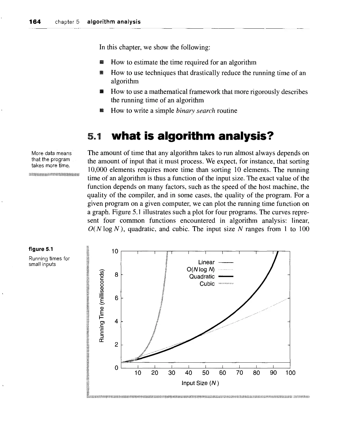
5.1 what is algorithm analysis? 164
5.2 examples of algorithm running times 168

5.3 the maximum contiguous subsequence sum problem 169
5.3.1 the obvious 0(/V3) algorithm 170
5.3.2 an improved 0(N2) algorithm 173
5.3.3 a linear algorithm 173
5.4 general big-oh rules 177
5.5 the logarithm 181
5.6 static searching problem 183
5.6.1 sequential search 183
5.6.2 binary search 184
5.6.3 interpolation search 187
5.7 checking an algorithm analysis 188
5.8 limitations of big-oh analysis 189
summary 190
key concepts 190
common errors 191
on the internet 192
exercises 192
references 199
chapter 6 the collections api
6.1 introduction 202
6.2 the iterator pattern 203
6.2.1 basic iterator design 204
6.2.2 inheritance-based iterators and factories 206
6.3 collections api: containers and iterators 208
6.3.1 the Collection interface 209
6.3.2 Iterator interface 212
6.4 generic algorithms 214
6.4.1 Comparator function objects 215
6.4.2 the Collections class 215
6.4.3 binary search 218
6.4.4 sorting 218
6.5 the List interface 220
6.5.1 the Listlterator interface 221
6.5.2 LinkedList class 223

contents xxiii
6.6
8,7
stacks and queues 225
6.6.1 stacks 225
6.6.2 stacks and computer languages 226
6.6.3 queues 227
6.6.4 stacks and queues in the collections api 228
228
the TreeSet class
the HashSet class
239
sets
6.7.1
6.7.2
6.8 maps 236
6.9 priority queues
summary 243
kef concepts 244
common errors 245
on the internet 245
exercises 246
references 249
229
231
chapter 7
recursion
7.1 what is recursion? 252
7.2 background: proofs by mathematical induction 253
7.3 basic recursion 255
7.3.1 printing numbers in any base 257
7.3.2 why it works 259
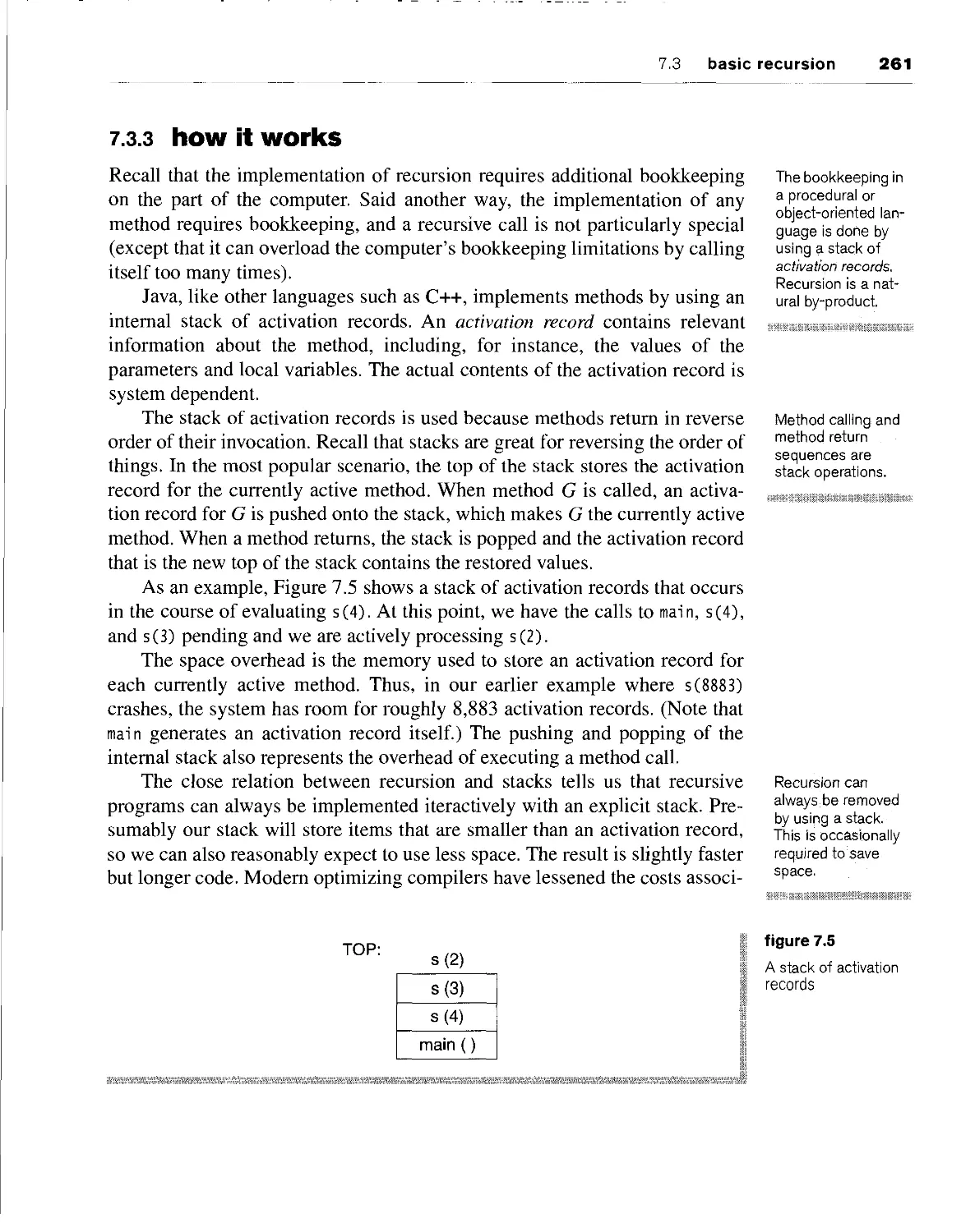
7.3.3 how it works 261
7.3.4 too much recursion can be dangerous 262
7.3.5 preview of trees 263
7.3.6 additional examples 264
7.4 numerical applications 269
7.4.1 modular arithmetic 269
7.4.2 modular exponentiation 270
7.4.3 greatest common divisor and multiplicative inverses 272
7.4.4 the rsa cryptosystem 275
7.5 divide-and-conquer algorithms 277
7.5.1 the maximum contiguous subsequence sum problem 278
7.5.2 analysis of a basic divide-and-conquer recurrence 281
7.5.3 a general upper bound for divide-and-conquer running times 285

XXiv contents
7.6 dynamic programming 287
7.7 backtracking 291
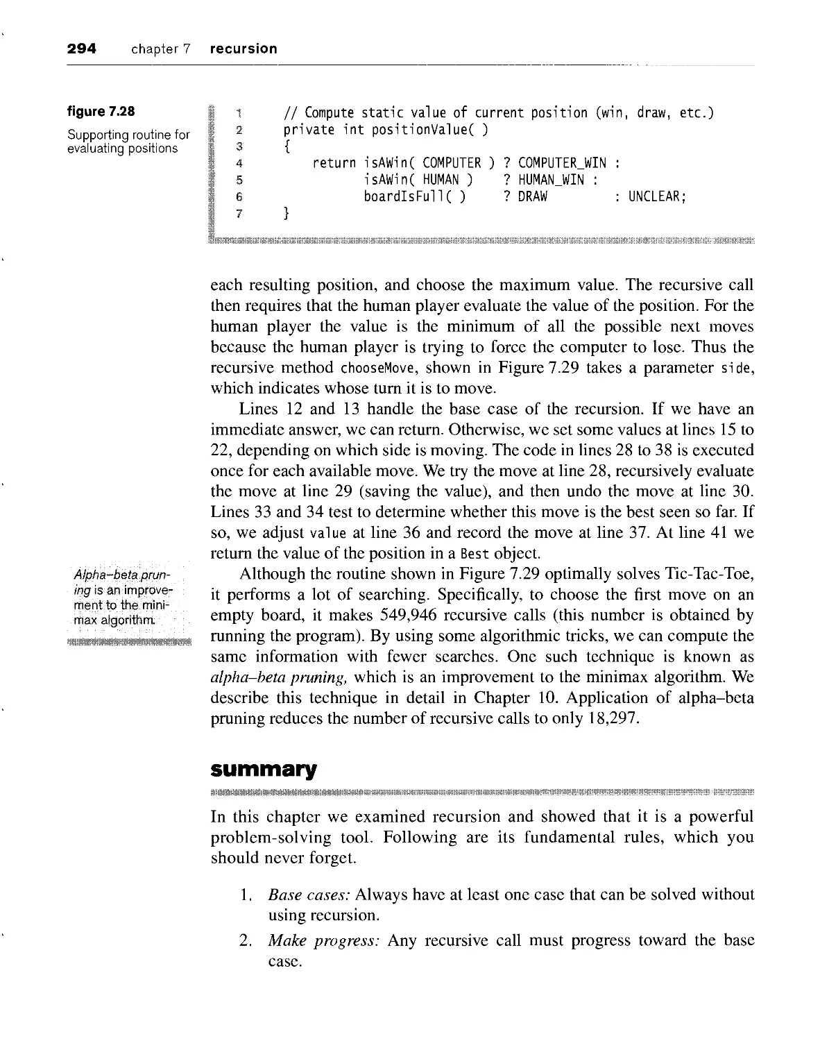
summary 294
key concepts 296
common errors 297
on the Internet 297
exercises 298
references 302
chapter 8
sorting algorithms
8.1
8.3
8.4
why is sorting important? 304
preliminaries 305
analysis of the insertion sort and other simple sorts 305
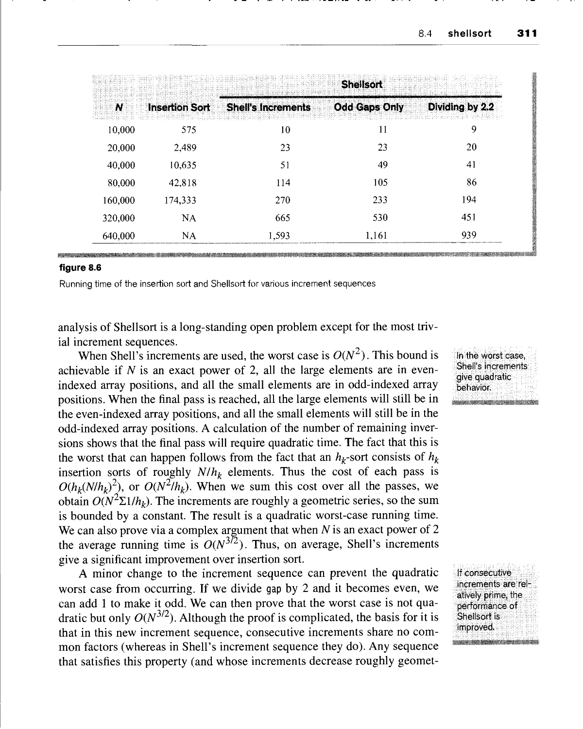
shellsort 309
8.4.1 performance of shellsort 310
8.5 mergesort 313
8.5.1 linear-time merging of sorted arrays 313
8.5.2 the mergesort algorithm 315
8.6 quicksort 316
8.6.1 the quicksort algorithm 317
8.6.2 analysis of quicksort 320
8.6.3 picking the pivot 323
8.6.4 a partitioning strategy 325
8.6.5 keys equal to the pivot 327
8.6.6 median-of-three partitioning 327
8.6.7 small arrays 328
8.6.8 Java quicksort routine 329
8.7 quickselect 331
8.8 a lower bound for sorting 332
summary 334
key concepts 335
common errors 336
on the internet 336
exercises 336
references 341

contents XXV
chapter 9
randomization
9.1 why do we need random numbers? 343
9.2 random number generators 344
9.3 nonuniform random numbers 349
9.4 generating a random permutation 353
9.5 randomized algorithms 354
9.6 randomized primality testing 357
summary 360
key concepts 360
common errors 361
on the internet 362
exercises 362
references 364
part three Applications
chapter 10 fun and games
10.1 word search puzzles 367
10.1.1 theory 368
10.1.2 Java implementation 369
10.2 the game of tic-tac-toe 373
10.2.1 alpha-beta pruning 374
10.2.2 transposition tables 377
10.2.3 computer chess 381
summary 384
key concepts 384
common errors 384
on the internet 384
exercises 385
references 387

XXVi contents
11.1 balanced-symbol checker 389
11.1.1 basic algorithm 390
11.1.2 implementation 391
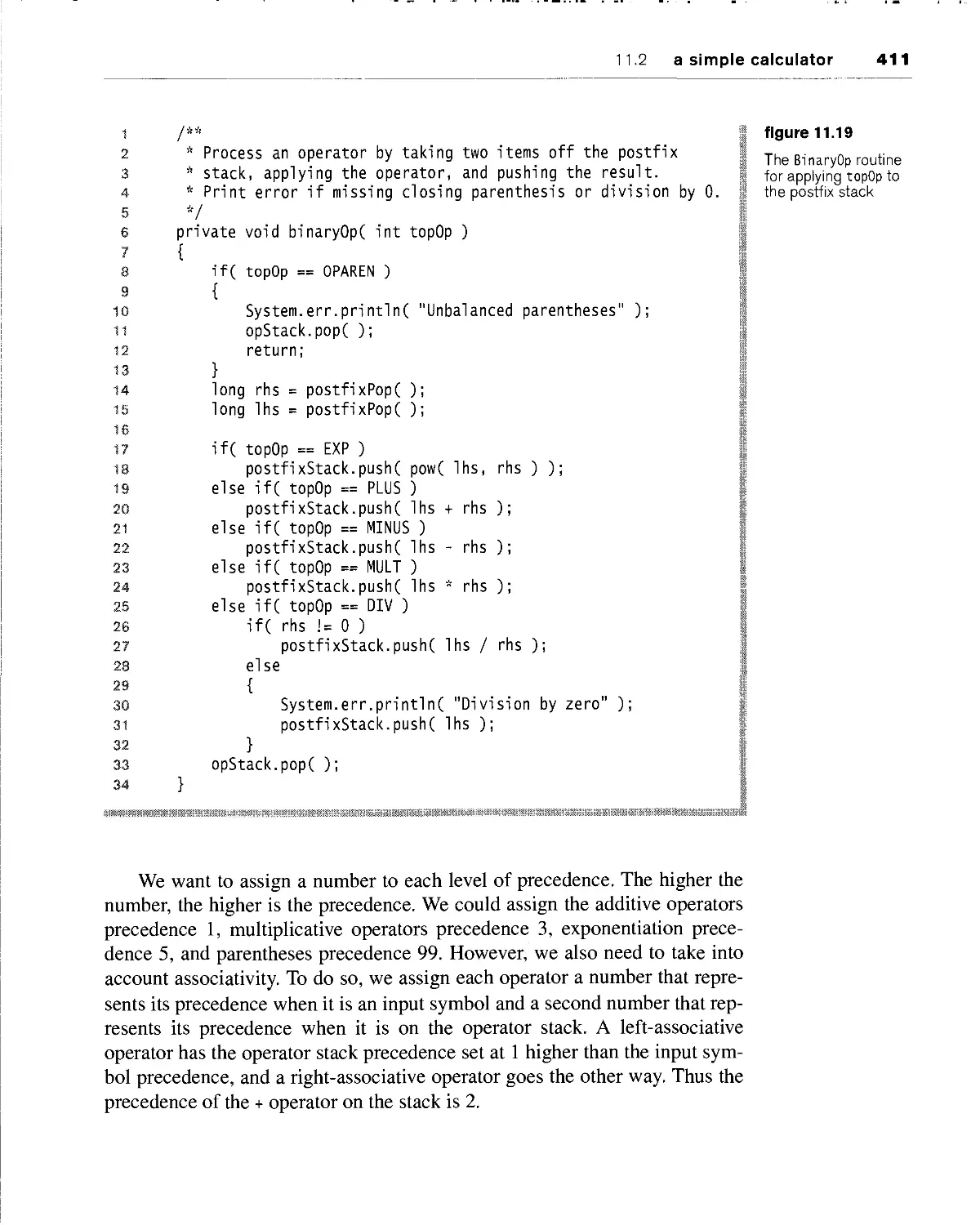
11.2 a simple calculator 400
11.2.1 postfix machines 402
11.2.2 infix to postfix conversion 403
11.2.3 implementation 405
11.2.4 expression trees 414
summary 415
kef concepts 416
common errors 416
on the internet 417
exercises 417
references 418
12.1 file compression 420
12.1.1 prefix codes 421
12.1.2 huffman's algorithm 423
12.1.3 implementation 425
12.2 a cross-reference generator 441
12.2.1 basic ideas 441
12.2.2 Java implementation 441
summarf 445
key concepts 446
common errors 446
on the internet 446
exercises 446
references 450
13.1 the josephus problem 451
13.1.1 the simple solution 453

contents xxvii
13,1.2 a more efficient algorithm 453
13.2 event-driven simulation 457
13.2.1 basic ideas 457
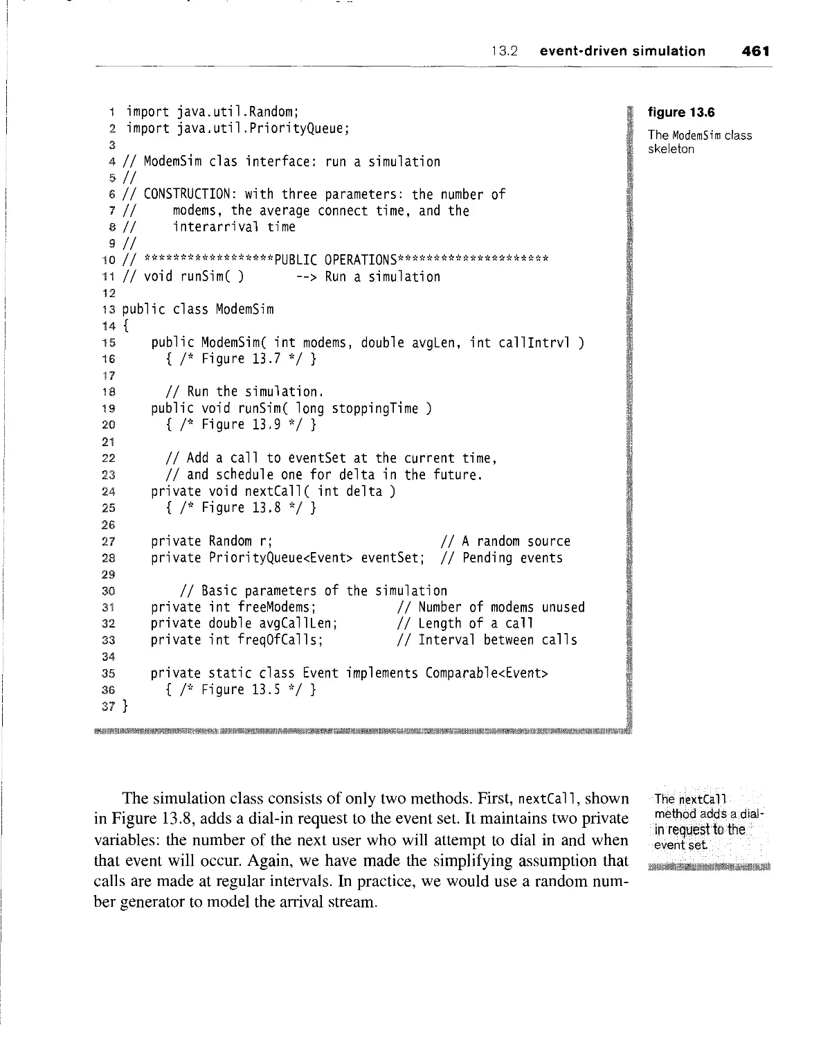
13.2.2 example: a modem bank simulation 458
summary 466
kef concepts 466
common errors 467
on the Internet 467
exercises 467
chapter 14 graphs and paths
14.1 definitions 472
14.1.1 representation 474
14.2 unweighted shortest-path problem 483
14.2.1 theory 483
14.2.2 Java implementation 489
14.3 positive-weighted, shortest-path problem 489
14.3.1 theory: dijkstra's algorithm 490
14.3.2 Java implementation 494
14.4 negative-weighted, shortest-path problem 496
14.4.1 theory 496
14.4.2 Java implementation 497
14.5 path problems in acyclic graphs 499
14.5.1 topological sorting 499
14.5.2 theory of the acyclic shortest-path algorithm 501
14.5.3 Java implementation 501
14.5.4 an application: critical-path analysis 504
summary 506
key concepts 507
common errors 508
on the internet 509
exercises 509
references 513

xxviii contents
part four Implementations
Mii!^^
15.1 iterators and nested classes 518
15.2 iterators and inner classes 520
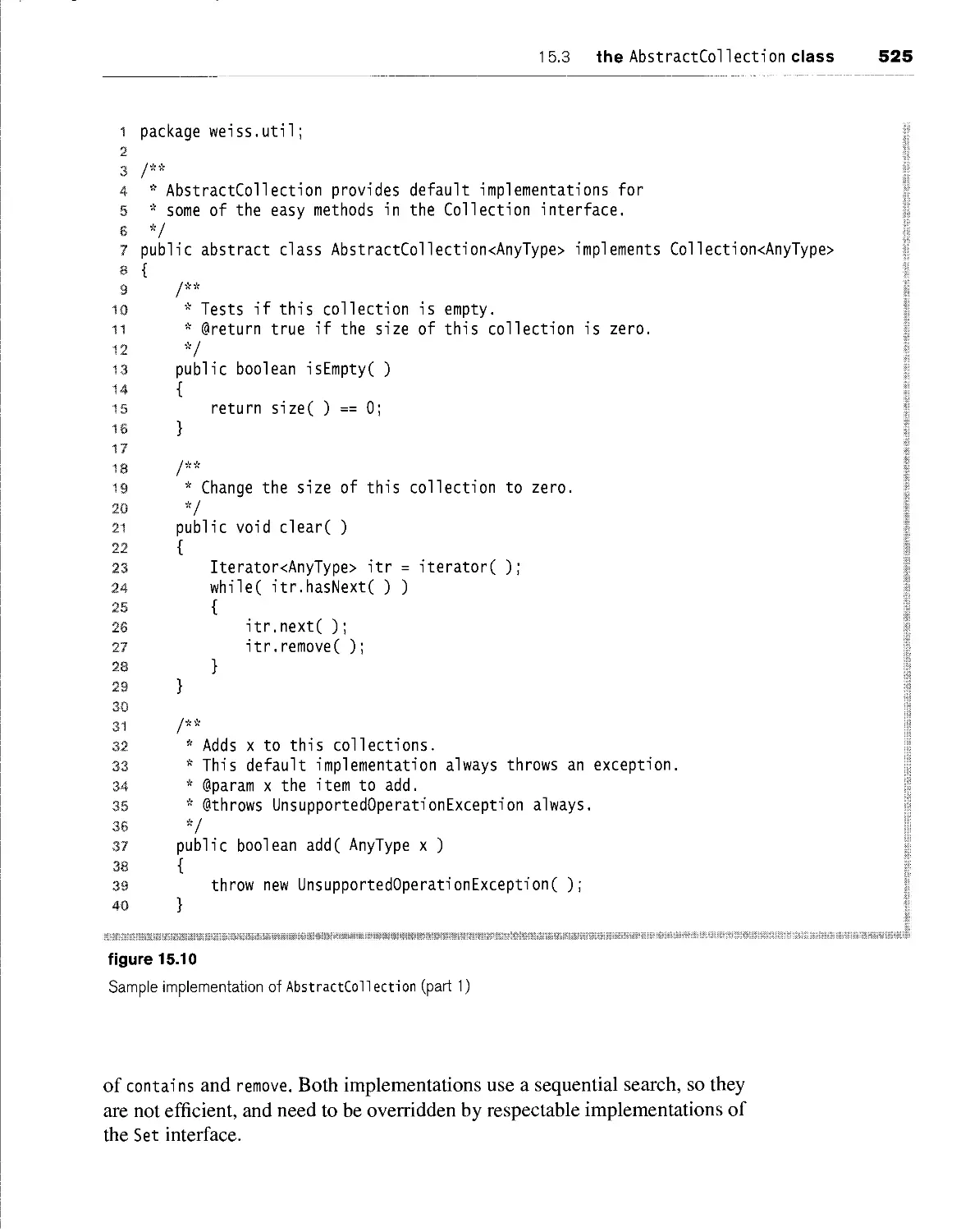
15.3 the AbstractCollection class 524
15.4 StringBuilder 528
15.5 implementation of ArrayList with an iterator 529
summary 534
key concepts 535
common errors 535
on the internet 535
exercises 535
§||;if|t|i^
^ff; »>,U.:^T
16.1 dynamic array implementations 539
16.1.1 stacks 540
16.1.2 queues 544
16.2 linked list implementations 549
16.2.1 stacks 550
16.2.2 queues 553
16.3 comparison of the two methods 557
16.4 the Java.util .Stack class 557
16.5 double-ended queues 559
summarf 559
kef concepts 559
common errors 559
on the internet 559
exercises 560

contents xxix
\<$*pt4%;'ff:
' linked lists
17.1 basic ideas 563
17.1.1 header nodes 565
17.1.2 iterator classes 566
17.2 java implementation 568
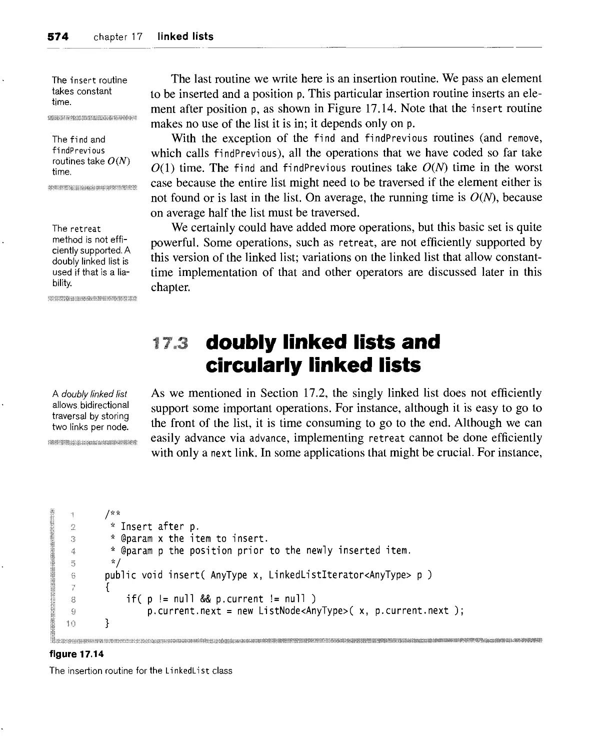
17.3 doubly linked lists and circularly linked lists 574
17.4 sorted linked lists 577
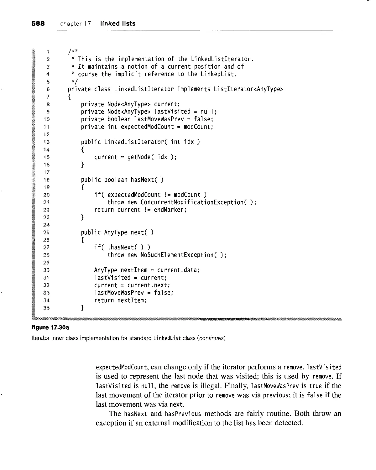
17.5 implementing the collections api Li nkedList class 579
summary 590
kef concepts 590
common errors 591
on the internet 591
exercises 591
Siiftpl § 11 f:!;! t:: i ^tre^is:
18.1 general trees 595
18.1.1 definitions 596
18.1.2 implementation 597
18.1.3 an application: file systems 598
18.2 binary trees 602
18.3 recursion and trees 609
18.4 tree traversal: iterator classes 611
18.4.1 postorder traversal 615
18.4.2 inorder traversal 619
18.4.3 preorder traversal 619
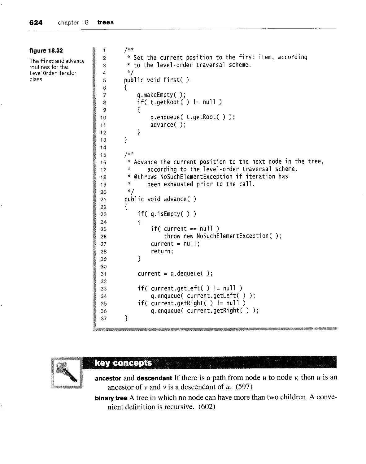
18.4.4 level-order traversals 622
summary 623
kef concepts 624
common errors 625
on the internet 626
exercises 626

XXX contents
chapter 19 ' binary' search trees
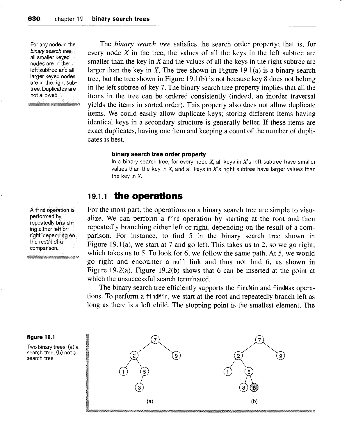
19.1 basic ideas 629
19.1.1 the operations 630
19.1.2 Java implementation 632
19.2 order statistics 639
19.2.1 Java implementation 640
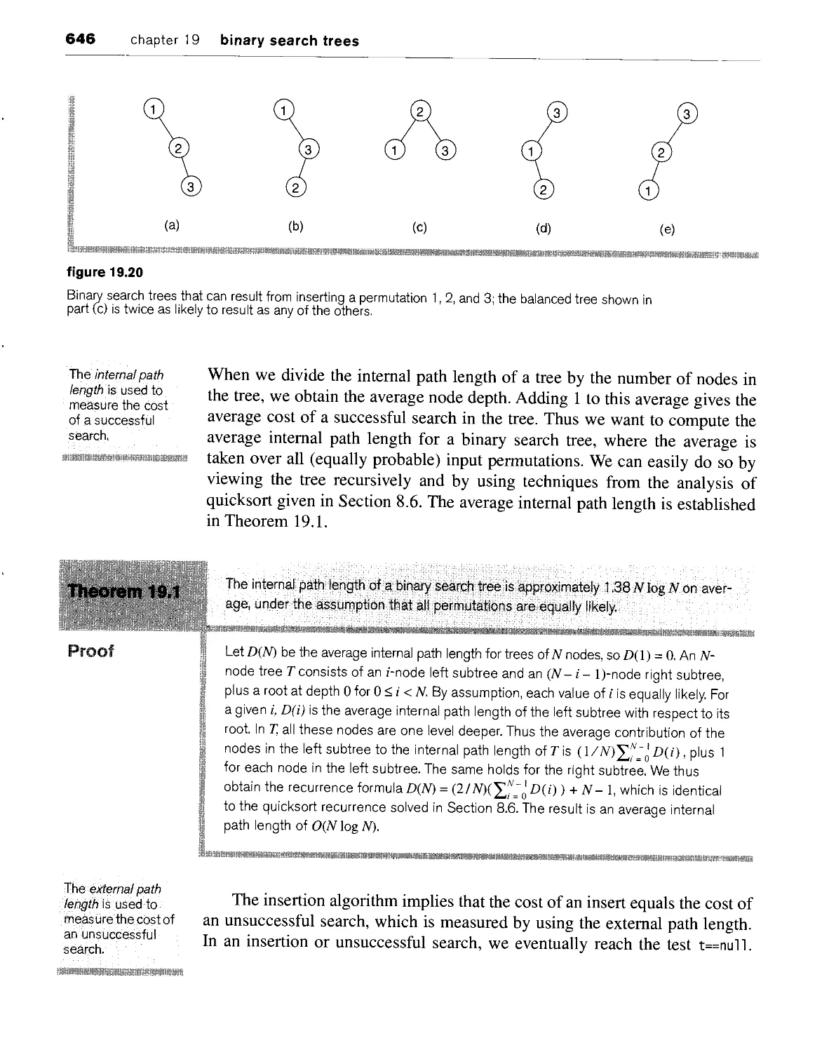
19.3 analysis of binary search tree operations 644
19.4 avl trees 648
19.4.1 properties 649
19.4.2 single rotation 651
19.4.3 double rotation 654
19.4.4 summary of avl insertion 656
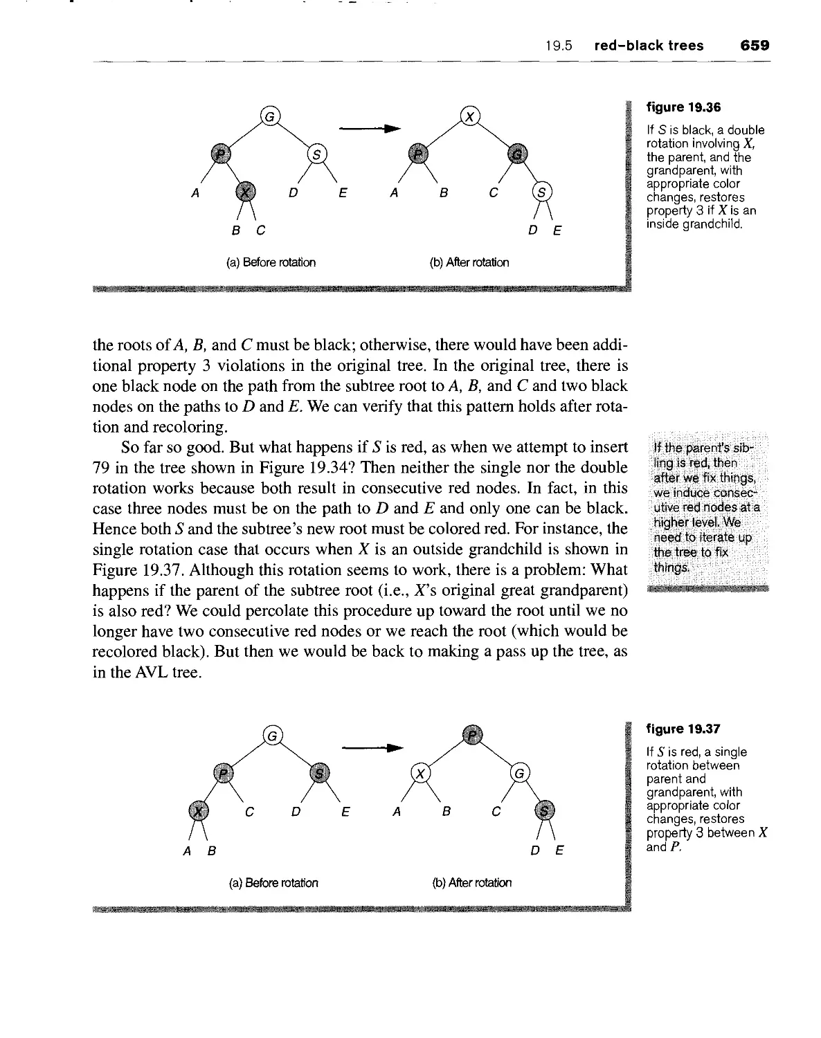
19.5 red-black wees 657
19.5.1 bottom-up insertion 658
19.5.2 top-down red-black trees 660
i9'5-3 Java implementation 661
19.5.4 top-down deletion 668
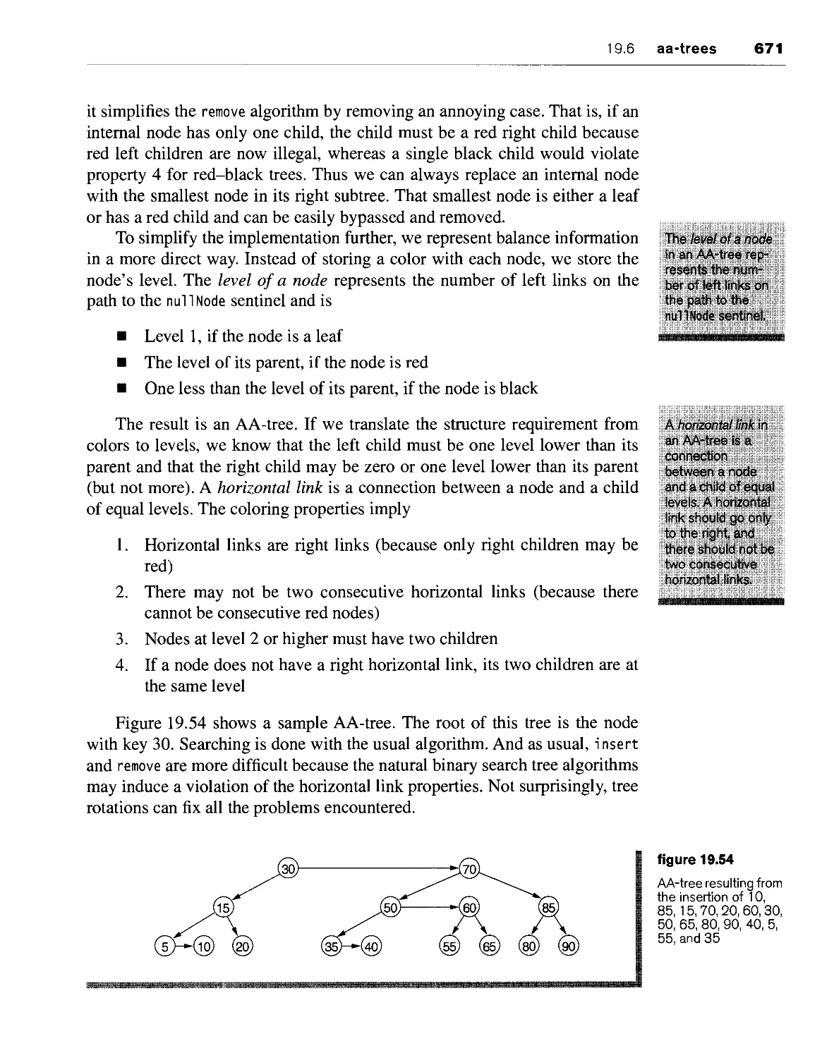
19.6 aa-trees 670
19.6.1 insertion 672
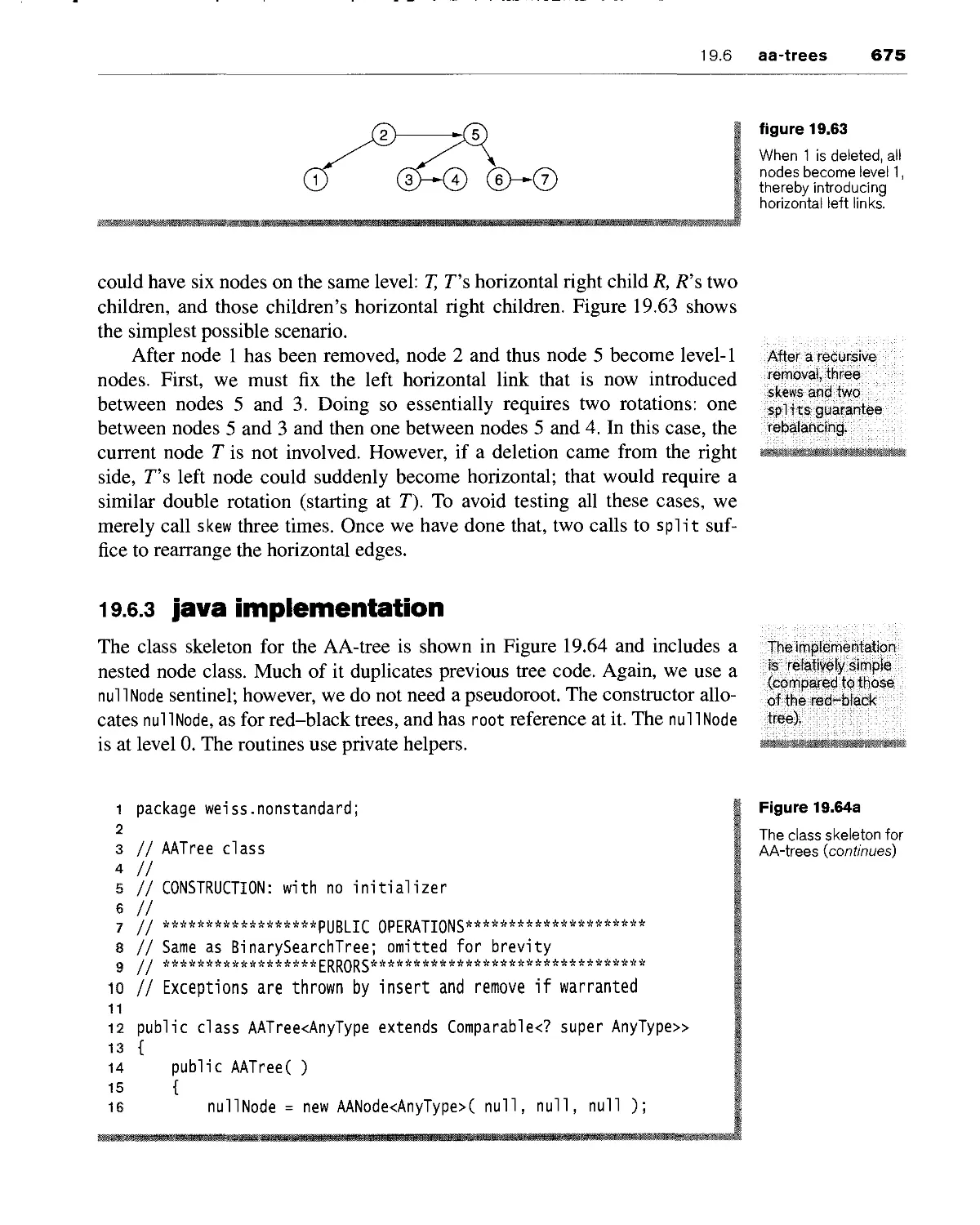
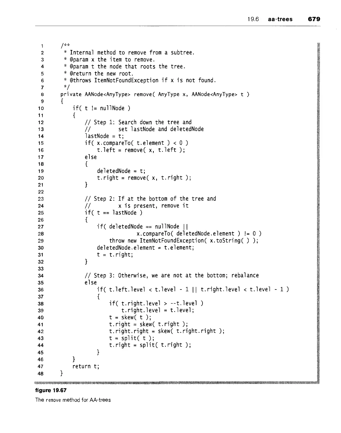
19.6.2 deletion 674
19.6.3 Java implementation 675
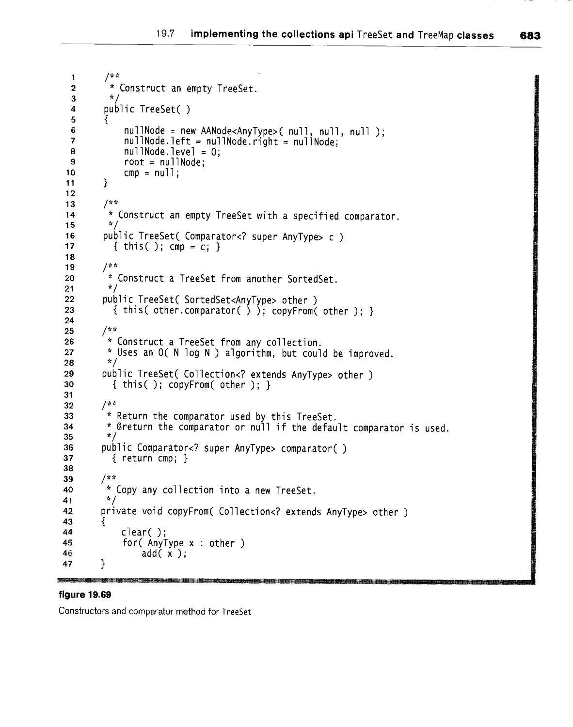
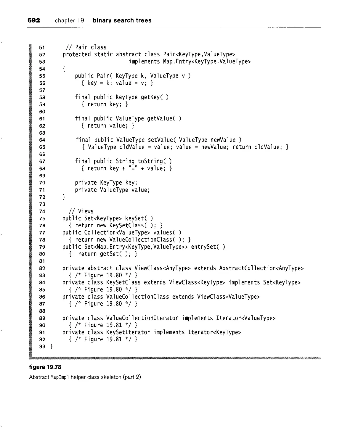
19.7 implementing the collections api TreeSet and
TreeMap classes 680
19.8 b-trees 698
summary 704
key concepts 705
common errors 706
on the internet 706
exercises 707
references 709
chapter 20 hash tables
20.1 basic ideas 714
20.2 hash function 715

contents
XXXI
20.3 linear probing 717
20.3.1 naive analysis of linear probing 719
20.3.2 what really happens: primary clustering 720
20.3.3 analysis of the f i nd operation 721
20.4 quadratic probing 723
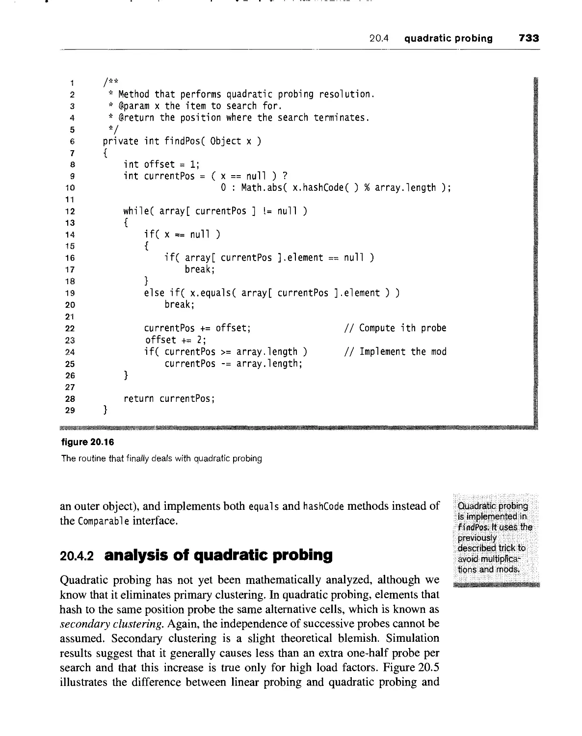
20.4.1 Java implementation 727
20.4.2 analysis of quadratic probing 733
20.5 separate chaining hashing 736
20.6 hash tables versus binary search trees 737
20.7 hashing applications 737
summary 738
key concepts 738
common errors 739
on the internet 740
exercises 740
references 742
chapter 21 a priority queue: the binary heap
21.1 basic ideas 746
21.1.1 structure property 746
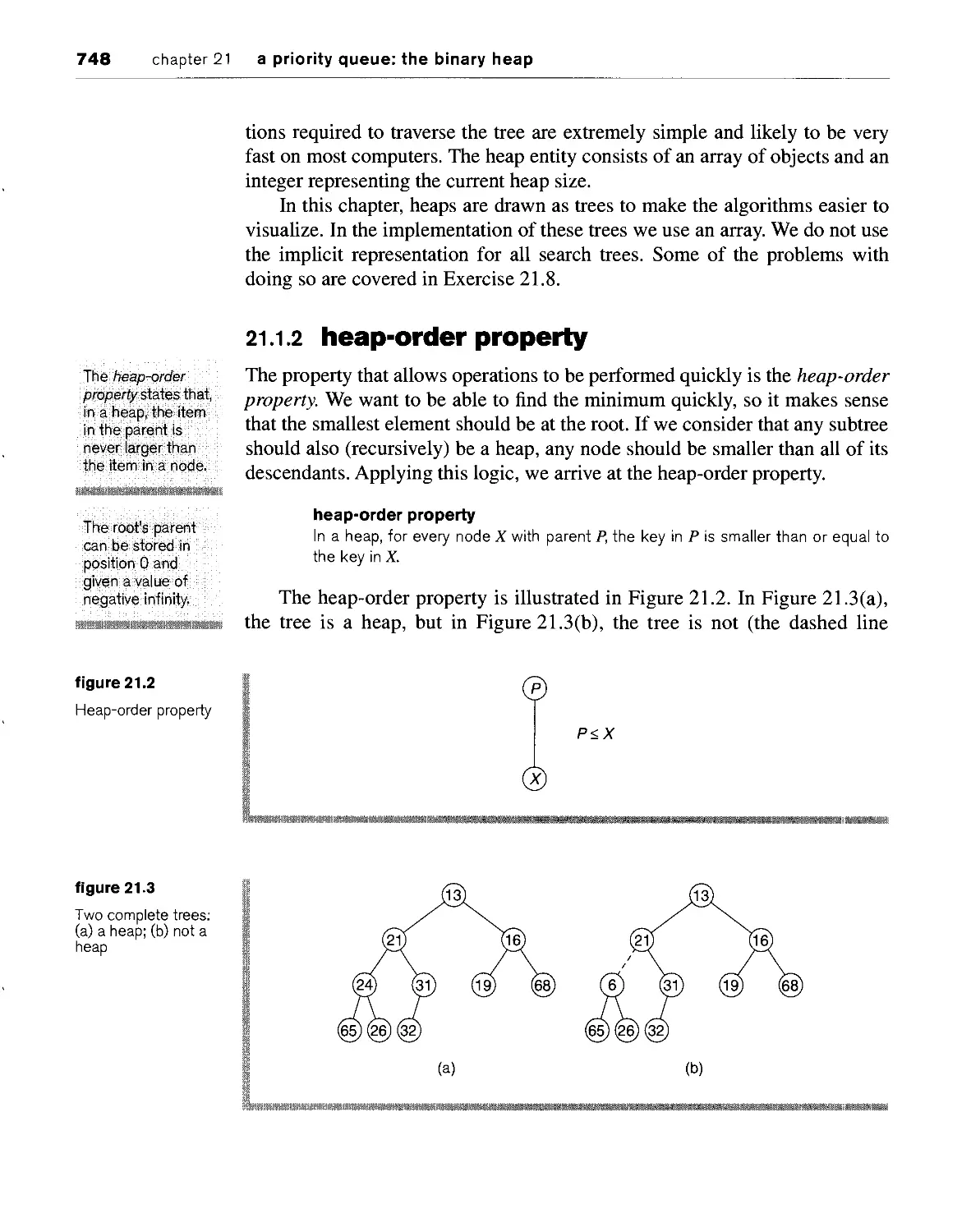
21.1.2 heap-order property 748
21.1.3 allowed operations 749
21.2 implementation of the basic operations 752
21.2.1 insertion 752
21.2.2 the deleteMin operation 754
21.3 the buildHeap operation: linear-time heap construction 756
21.4 advanced operations: decreaseKey and merge 761
21.5 internal sorting: heapsort 761
21.6 external sorting 764
21.6.1 why we need new algorithms 764
21.6.2 model for external sorting 765
21.6.3 the simple algorithm 765
21.6.4 multiway merge 767
21.6.5 polyphase merge 768
21.6.6 replacement selection 770

xxxii
contents
summary 771
key concepts 772
common errors 772
on the Internet 773
exercises 773
references 777
part five Adwamcecl Data
Structures
illiisiisp^l/p^lii
T.mmimmmmmammm
782
self-adjustment and amortized analysis
22.1.1 amortized time bounds 783
22.1.2 a simple self-adjusting strategy (that does not work) 783
22.2 the basic bottom-up splay tree 785
22.3 basic splay tree operations 788
22.4 analysis of bottom-up splaying 789
22.4.1 proof of the splaying bound 792
22.5 top-down splay trees 795
22.6 implementation of top-down splay trees 798
22.7 comparison of the splay tree with other search trees 803
summary 804
kef concepts 804
common errors 805
on the internet 805
exercises 805
references 806
illilll^
".*
23.1 the skew heap 809
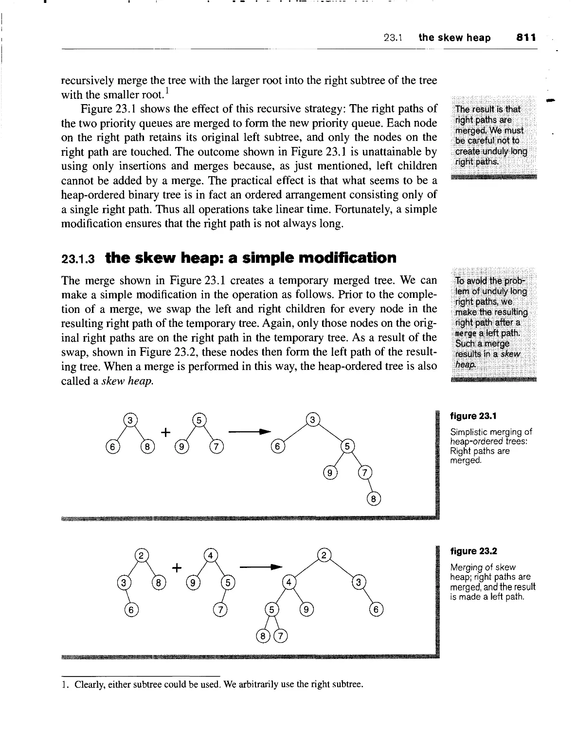
23.1.1 merging is fundamental 810
23.1.2 simplistic merging of heap-ordered trees 810
"- ''■*•■' ?,

contents xxxiii
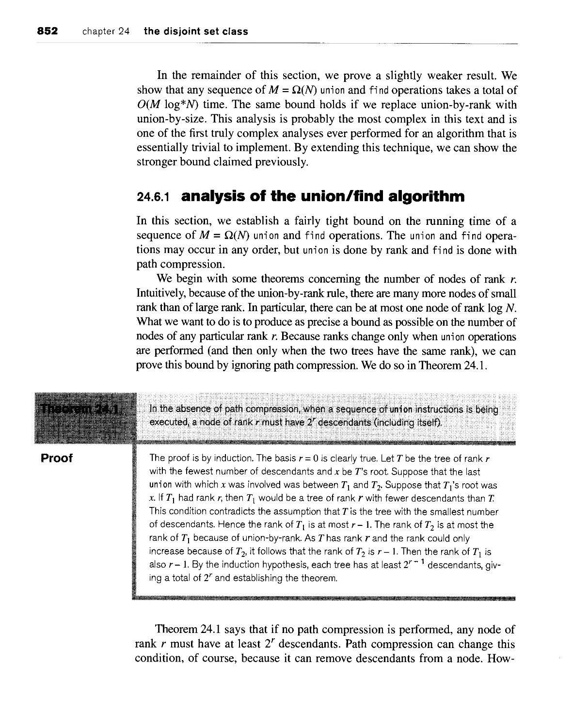
23.1.3 the skew heap: a simple modification 811
23.1.4 analysis of the skew heap 812
23.2 the pairing heap 814
23.2.1 pairing heap operations 815
23.2.2 implementation of the pairing heap 816
23.2.3 application: dijkstra's shortest weighted path algorithm 822
summary 826
key concepts 826
common errors 826
on the internet 827
exercises 827
references 828
chapter 24 the disjoint set class
24.1 equivalence relations 832
24.2 dynamic equivalence and applications 832
24.2.1 application: generating mazes 833
24.2.2 application: minimum spanning trees 836
24.2.3 application: the nearest common ancestor problem 839
24.3 the quick-find algorithm 842
24.4 the quick-union algorithm 843
24.4.1 smart union algorithms 845
24.4.2 path compression 847
24.5 Java implementation 848
24.6 worst case for union-by-rank and path compression 851
24.6.1 analysis of the union/find algorithm 852
summary 859
kef concepts 859
common errors 860
on the internet 860
exercises 861
references 863

xxxiv contents
W^i^^W^k^M&^&M,
fSilS^ilX^B; £': graphical user interfaces
B.I the abstract window toolkit and swing 868
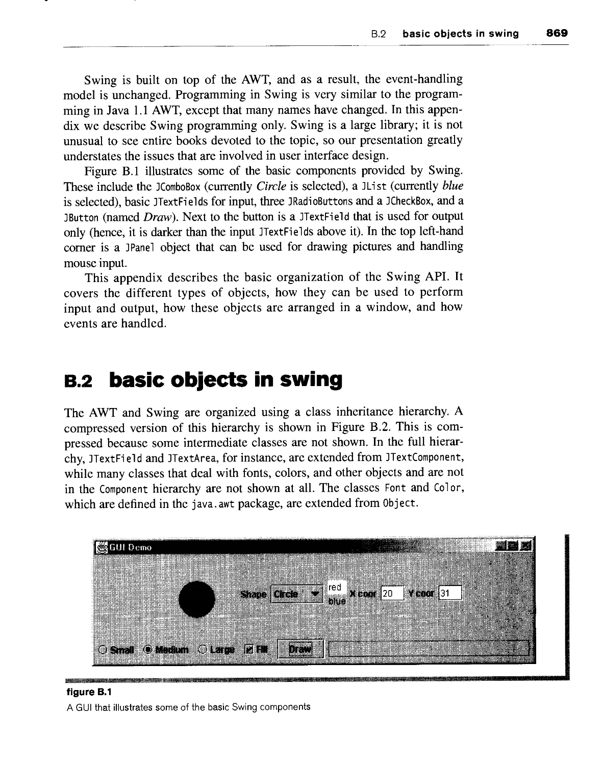
B.2 basic objects in swing 869
B.2.1 Component 870
B.2.2 Container 871
B.2.3 top-level containers 871
B.2.4 ] Panel 872
B.2.5 important i/o components 874
B.3 basic principles 878
B.3.1 layout managers 879
B.3.2 graphics 883
B.3.3 events 885
B.3.4 event handling: adapters and anonymous inner classes 887
B.3.5 summary: putting the pieces together 889
B.3.6 is this everything i need to know about swing? 890
summary 891
kef concepts 891
common errors 893
on the internet 894
exercises 894
references 895
^^ll^g^^^^^j^^iC^^-^f^.:^ :|||pM^^^j|j||^^|9|^y|i)^|||j^^:
index

Tour of Java
chapter 1 primitive Java
chapter 2 reference types
chapter 3 objects and classes
chapter 4 inheritance

primitive Java
I he primary focus of this book is problem-solving techniques that allow
the construction of sophisticated, time-efficient programs. Nearly all of the
material discussed is applicable in any programming language. Some would
argue that a broad pseudocode description of these techniques could suffice to
demonstrate concepts. However, we believe that working with live code is
vitally important.
There is no shortage of programming languages available. This text uses
Java, which is popular both academically and commercially. In the first four
chapters, we discuss the features of Java that are used throughout the book.
Unused features and technicalities are not covered. Those looking for deeper
Java information will find it in the many Java books that are available.
We begin by discussing the part of the language that mirrors a 1970s
programming language such as Pascal or C. This includes primitive types, basic
operations, conditional and looping constructs, and the Java equivalent of functions.
In this chapter, we will see
■ Some of the basics of Java, including simple lexical elements
■ The Java primitive types, including some of the operations that
primitive-typed variables can perform

4 chapter 1 primitive Java
■ How conditional statements and loop constructs are implemented in
Java
■ An introduction to the static method—the Java equivalent of the
function and procedure that is used in non-object-oriented languages
javac compiles
.Java files and
generates .class files
containing
bytecode. Java
invokes the Java
interpreter (which is
also known as the
Virtual Machine).
1.1 the general environment
How are Java application programs entered, compiled, and run? The answer,
of course, depends on the particular platform that hosts the Java compiler.
Java source code resides in files whose names end with the .Java suffix.
The local compiler, javac, compiles the program and generates .class files,
which contain bytecode. Java bytecodes represent the portable intermediate
language that is interpreted by running the Java interpreter, java. The
interpreter is also known as the Virtual Machine.
For Java programs, input can come from one of many places:
■ The terminal, whose input is denoted as standard input
■ Additional parameters in the invocation of the Virtual Machine—
command-line arguments
■ A GUI component
■ A file
Command-line arguments are particularly important for specifying
program options. They are discussed in Section 2.4.5. Java provides mechanisms
to read and write files. This is discussed briefly in Section 2.6.3 and in more
detail in Section 4.5.3 as an example of the decorator pattern. Many
operating systems provide an alternative known as file redirection, in which the
operating system arranges to take input from (or send output to) a file in a
manner that is transparent to the running program. On Unix (and also from an
MS/DOS window), for instance, the command
java Program < inputfile > outputfile
automatically arranges things so that any terminal reads are redirected to
come from i nputf i 1 e and terminal writes are redirected to go to outputfi 1 e.

1.2 the first program 5
1.2 the first program
Let us begin by examining the simple Java program shown in Figure 1.1. This
program prints a short phrase to the terminal. Note the line numbers shown on the
left of the code are not part of the program. They are supplied for easy reference.
Place the program in the source file FirstProgram.java and then compile
and run it. Note that the name of the source file must match the name of the
class (shown on line 4), including case conventions. If you are using the JDK,
the commands are
javac FirstProgram.java
java FirstProgram
1.2.1 comments
Java has three forms of comments. The first form, which is inherited from C,
begins with the token /* and ends with */. Here is an example:
/* This is a
two-line comment */
Comments do not nest.
The second form, which is inherited from C++, begins with the token //.
There is no ending token. Rather, the comment extends to the end of the line.
This is shown on lines 1 and 2 in Figure 1.1.
The third form begins with /** instead of /*. This form can be used to
provide information to the javadoc utility, which will generate documentation
from comments. This form is discussed in Section 3.3.
Comments make
code easier for
humans to read.
Java has three
forms of comments.
1 // First program
2 // MW, 5/1/05
3
4 public class FirstProgram
5 {
6 public static void main( String [ ] args )
7 {
8 System.out.println( "Is there anybody out there?" );
9 }
10 }
figure 1.1
A simple first program
1. If you are using Sun's JDK, javac and java are used directly. Otherwise, in a typical
interactive development environment (IDE), such as JCreator, these commands are executed
behind the scenes on your behalf.

6 chapter 1 primitive Java
Comments exist to make code easier for humans to read. These humans
include other programmers who may have to modify or use your code, as well
as yourself. A well-commented program is a sign of a good programmer.
When the program
is run, the special
method main is
invoked.
1.2.2 main
A Java program consists of a collection of interacting classes, which contain
methods. The Java equivalent of the function or procedure is the static
method, which is described in Section 1.6. When any program is run, the
special static method man n is invoked. Line 6 of Figure 1.1 shows that the static
method man n is invoked, possibly with command-line arguments. The
parameter types of main and the void return type shown are required.
1.2.3 terminal output
println is used to The program in Figure 1.1 consists of a single statement, shown on line 8.
perform output. println is the primary output mechanism in Java. Here, a constant string is
placed on the standard output stream System.out by applying a println
method. Input and output is discussed in more detail in Section 2.6. For now
we mention only that the same syntax is used to perform output for any entity,
whether that entity is an integer, floating point, string, or some other type.
i .3 primitive types
Java defines eight primitive types. It also allows the programmer great
flexibility to define new types of objects, called classes. However, primitive types
and user-defined types have important differences in Java. In this section, we
examine the primitive types and the basic operations that can be performed on
them.
Java's primitive
types are integer,
floating-point,
Boolean, and character.
The Unicode
standard contains over
30,000 distinct
coded characters
covering the
principal written
languages.
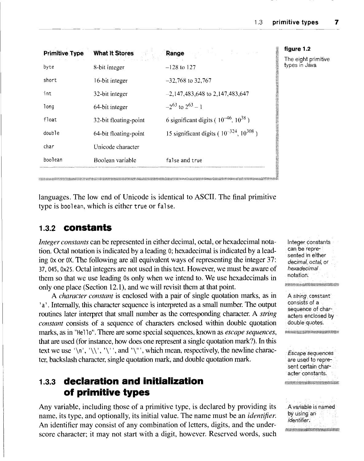
1.3.1 the primitive types
Java has eight primitive types, shown in Figure 1.2. The most common is the
integer, which is specified by the keyword i nt. Unlike with many other
languages, the range of integers is not machine-dependent. Rather, it is the same
in any Java implementation, regardless of the underlying computer
architecture. Java also allows entities of types byte, short, and long. These are known
as integral types. Floating-point numbers are represented by the types float
and double, double has more significant digits, so use of it is recommended
over use of float. The char type is used to represent single characters. A char
occupies 16 bits to represent the Unicode standard. The Unicode standard
contains over 30,000 distinct coded characters covering the principal written

1.3 primitive types 7
Primitive Type
byte
short
int
long
float
double
char
boolean
What It Stores
8-bit integer
16-bit integer
32-bit integer
64-bit integer
32-bit floating-point
64-bit floating-point
Unicode character
Boolean variable
Range
-128 to 127
-32,768 to 32,767
-2,147,483,648 to 2,147,483,647
-263 to 263 - 1
6 significant digits ( lfT46, 1038 )
15 significant digits ( 1(T324, 10308 )
false and true
figure 1.2
The eight primitive
types in Java
languages. The low end of Unicode is identical to ASCII. The final primitive
type is bool ean, which is either true or fal se.
1.3.2 constants
Integer constants can be represented in either decimal, octal, or hexadecimal
notation. Octal notation is indicated by a leading 0; hexadecimal is indicated by a
leading Ox or OX. The following are all equivalent ways of representing the integer 37:
37, 045, 0x25. Octal integers are not used in this text. However, we must be aware of
them so that we use leading 0s only when we intend to. We use hexadecimals in
only one place (Section 12.1), and we will revisit them at that point.
A character constant is enclosed with a pair of single quotation marks, as in
'a'. Internally, this character sequence is interpreted as a small number. The output
routines later interpret that small number as the corresponding character. A string
constant consists of a sequence of characters enclosed within double quotation
marks, as in "Hello". There are some special sequences, known as escape sequences,
that are used (for instance, how does one represent a single quotation mark?). In this
text we use ' \n', ' \\', ' \ ", and ' \"', which mean, respectively, the newline
character, backslash character, single quotation mark, and double quotation mark.
1.3.3 declaration and initialization
of primitive types
Any variable, including those of a primitive type, is declared by providing its
name, its type, and optionally, its initial value. The name must be an identifier.
An identifier may consist of any combination of letters, digits, and the
underscore character; it may not start with a digit, however. Reserved words, such
Integer constants
can be
represented in either
decimal, octal, or
hexadecimal
notation.
A string constant
consists of a
sequence of
characters enclosed by
double quotes.
Escape sequences
are used to
represent certain
character constants.
A variable is named
by using an
identifier.

8 chapter 1 primitive Java
as int, are not allowed. Although it is legal to do so, you should not reuse
identifier names that are already visibly used (for example, do not use mai n as
the name of an entity).
Java is case- Java is case-sensitive, meaning that Age and age are different identifiers.
sensitive. -phis text uses the following convention for naming variables: All variables
sA^i*- *■-.-.--,'. start wjt^ a iowercase letter and new words start with an uppercase letter. An
example is the identifier minimumWage.
Here are some examples of declarations:
int num3; // Default initialization
double minimumWage = 4.50; // Standard initialization
int x = 0, numl = 0; // Two entities are declared
int num2 = numl;
A variable should be declared near its first use. As will be shown, the
placement of a declaration determines its scope and meaning.
1.3.4 terminal input and output
Basic formatted terminal I/O is accomplished by readLine and pn'ntln. The
standard input stream is System.in, and the standard output stream is
System.out.
The basic mechanism for formatted I/O uses the Stri ng type, which is
discussed in Section 2.3. For output, + combines two Stri ngs. If the second
argument is not a String, a temporary String is created for it if it is a primitive
type. These conversions to String can also be defined for objects (Section
3.4.3). For input, things are complicated: we must associate a BufferedReader
object with System.in. Then a String is read and can be parsed. A more
detailed discussion of I/O, including a treatment of formatted files, is in
Section 2.6.
1.4 basic operators
This section describes some of the operators available in Java. These
operators are used to form expressions. A constant or entity by itself is an
expression, as are combinations of constants and variables with operators. An
expression followed by a semicolon is a simple statement. In Section 1.5, we
examine other types of statements, which introduce additional operators.

1.4 basic operators 9
1.4.1 assignment operators
A simple Java program that illustrates a few operators is shown in Figure 1.3.
The basic assignment operator is the equals sign. For example, on line 16 the
variable a is assigned the value of the variable c (which at that point is 6).
Subsequent changes to the value of c do not affect a. Assignment operators can be
chained, as in z=y=x=0.
Another assignment operator is the +=, whose use is illustrated on line 18
of the figure. The += operator adds the value on the right-hand side (of the +=
operator) to the variable on the left-hand side. Thus, in the figure, c is
incremented from its value of 6 before line 18, to a value of 14.
Java provides various other assignment operators, such as -=, *=, and /=,
which alter the variable on the left-hand side of the operator via subtraction,
multiplication, and division, respectively.
Java provides a
host of assignment
operators,
including =, +=,
-=, *», and /=.
1
2
3
4
5
6
7
8
9
10
11
12
13
14
15
16
17
18
19
20
21
22
23
24
25
26
27
pu
{
}
blic class OperatorTest
// Program to illustrate basic operators
// The output is as follows:
//use
// 6 8 6
// 6 8 14
// 22 8 14
// 24 10 33
public static void main( String [ ] args )
{
int a = 12, b = 8, c = 6;
System.out.println( a + " " + b + " " +
a = c;
System.out.printing a + " " + b + " " +
c += b;
System.out.print!n( a + " " + b + " " +
a = b + c;
System.out.print!n( a + " " + b + " " +
a++;
++b;
c = a++ + ++b;
System.out.print!n( a + " " + b + " " +
}
c );
c );
c );
c );
c );
figure 1.3
Program that
illustrates operators

10 chapter 1 primitive Java
1.4.2 binary arithmetic operators
Java provides
several binary
arithmetic operators,
including +, -, *,
/, and %.
Line 20 in Figure 1.3 illustrates one of the binary arithmetic operators that
are typical of all programming languages: the addition operator (+). The +
operator causes the values of b and c to be added together; b and c remain
unchanged. The resulting value is assigned to a. Other arithmetic operators
typically used in Java are -,*,/, and %, which are used, respectively, for
subtraction, multiplication, division, and remainder. Integer division returns only
the integral part and discards any remainder.
As is typical, addition and subtraction have the same precedence, and this
precedence is lower than the precedence of the group consisting of the
multiplication, division, and mod operators; thus 1+2*3 evaluates to 7. All of these
operators associate from left to right (so 3-2-2 evaluates to -1). All operators
have precedence and associativity. The complete table of operators is in
Appendix .
Several unary
operators are defined,
including -.
Autoincrement and
autodecrement add
1 and subtract 1,
respectively. The
operators for doing
this are ++ and --.
There are two
forms of
incrementing and
decrementing: prefix and
postfix.
1.4.3 unary operators
In addition to binary arithmetic operators, which require two operands, Java
provides unary operators, which require only one operand. The most familiar
of these is the unary minus, which evaluates to the negative of its operand.
Thus -x returns the negative of x.
Java also provides the autoincrement operator to add 1 to a variable-
denoted by ++ — and the autodecrement operator to subtract 1 from a
variable—denoted by --. The most benign use of this feature is shown on lines
22 and 23 of Figure 1.3. In both lines, the autoincrement operator ++ adds 1
to the value of the variable. In Java, however, an operator applied to an
expression yields an expression that has a value. Although it is guaranteed
that the variable will be incremented before the execution of the next
statement, the question arises: What is the value of the autoincrement expression
if it is used in a larger expression?
In this case, the placement of the ++ is crucial. The semantics of ++x is that
the value of the expression is the new value of x. This is called the prefix
increment. In contrast, x++ means the value of the expression is the original value of
x. This is called the postfix increment. This feature is shown in line 24 of
Figure 1.3. a and b are both incremented by 1, and c is obtained by adding the
original value of a to the incremented value of b.
The type conversion
operator is used to
generate a
temporary entity of a new
type.
1.4.4 type conversions
The type conversion operator is used to generate a temporary entity of a new
type. Consider, for instance,

1.5 conditional statements 11
double quotient;
int x = 6;
int y = 10;
quotient = x / y; // Probably wrong!
The first operation is the division, and since x and y are both integers, the result is
integer division, and we obtain 0. Integer 0 is then implicitly converted to a doubl e
so that it can be assigned to quotient. But we had intended quotient to be assigned
0.6. The solution is to generate a temporary variable for either x or y so that the
division is performed using the rules for double. This would be done as follows:
quotient = ( double ) x / y;
Note that neither x nor y are changed. An unnamed temporary is created, and
its value is used for the division. The type conversion operator has higher
precedence than division does, so x is type-converted and then the division is
performed (rather than the conversion coming after the division of two i nts being
performed).
1.5 conditional statements
This section examines statements that affect the flow of control: conditional
statements and loops. As a consequence, new operators are introduced.
1.5.1 relational and equality operators
The basic test that we can perform on primitive types is the comparison. This
is done using the equality and inequality operators, as well as the relational
operators (less than, greater than, and so on).
In Java, the equality operators are == and !=. For example,
leftExpr==rightExpr
evaluates to true if leftExpr and rightExpr are equal; otherwise, it evaluates to
false. Similarly,
leftExprUrightExpr
evaluates to true if leftExpr and rightExpr are not equal and to false
otherwise.
The relational operators are <, <=, >, and >=. These have natural meanings
for the built-in types. The relational operators have higher precedence than the
equality operators. Both have lower precedence than the arithmetic operators
In Java, the
equality operators
are == and !=.
The relational
operators are <, <=.
>, and >=.

12 chapter 1 primitive Java
but higher precedence than the assignment operators, so the use of
parentheses is frequently unnecessary. All of these operators associate from left to
right, but this fact is useless: In the expression a<b<6, for example, the first <
generates a bool ean and the second is illegal because < is not defined for bool -
eans. The next section describes the correct way to perform this test.
Java provides
logical operators that
are used to
simulate the Boolean
algebra concepts of
AND, OR, and NOT.
The corresponding
operators are &&, 11,
and !.
Short-circuit
evaluation means that if
the result of a
logical operator can be
determined
by examining the
first expression,
then the second
expression is not
evaluated.
1.5.2 logical operators
Java provides logical operators that are used to simulate the Boolean algebra
concepts of AND, OR, and NOT. These are sometimes known as conjunction,
disjunction, and negation, respectively, whose corresponding operators are &&,
11, and !. The test in the previous section is properly implemented as a<b &&
b<6. The precedence of conjunction and disjunction is sufficiently low that
parentheses are not needed. && has higher precedence than 11, while ! is
grouped with other unary operators (and is thus highest of the three). The
operands and results for the logical operators are boolean. Figure 1.4 shows
the result of applying the logical operators for all possible inputs.
One important rule is that && and 11 are short-circuit evaluation operations.
Short-circuit evaluation means that if the result can be determined by examining
the first expression, then the second expression is not evaluated. For instance, in
x != 0 && 1/x != 3
if x is 0, then the first half is f al se. Automatically the result of the AND must
be f al se, so the second half is not evaluated. This is a good thing because
division-by-zero would give erroneous behavior. Short-circuit evaluation allows
us to not have to worry about dividing by zero.
figure 1.4
Result of logical
operators
x
false
false
true
true
y
false
true
false
true
x && y
false
false
false
true
x II y
false
true
true
true
!x
true
true
false
false
2. There are (extremely) rare cases in which it is preferable to not short-circuit. In such cases,
the & and | operators with bool ean arguments guarantee that both arguments are evaluated,
even if the result of the operation can be determined from the first argument.

15 conditional statements 13
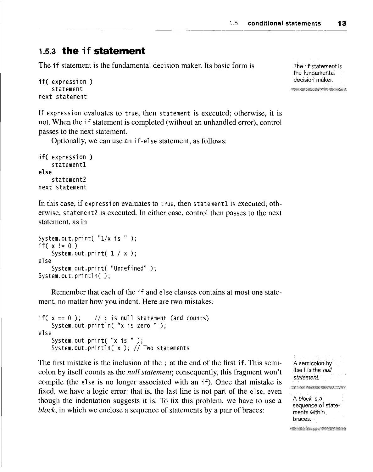
1.5.3 the if statement
The i f statement is the fundamental decision maker. Its basic form is The if statement is
the fundamental
if( expression ) decisionmaker.
statement
next statement
If expression evaluates to true, then statement is executed; otherwise, it is
not. When the i f statement is completed (without an unhandled error), control
passes to the next statement.
Optionally, we can use an if-else statement, as follows:
if( expression )
statementl
else
statement2
next statement
In this case, if expression evaluates to true, then statementl is executed;
otherwise, statement2 is executed. In either case, control then passes to the next
statement, as in
System.out.print( "1/x is " );
if( x != 0 )
System.out.print( 1 / x );
else
System.out.print( "Undefined" );
System.out.println( );
Remember that each of the if and el se clauses contains at most one
statement, no matter how you indent. Here are two mistakes:
if( x == 0 ); // ; is null statement (and counts)
System.out.println( "x is zero " );
else
System.out.print( "x is " );
System.out.println( x ); // Two statements
The first mistake is the inclusion of the ; at the end of the first i f. This
semicolon by itself counts as the null statement; consequently, this fragment won't
compile (the else is no longer associated with an if). Once that mistake is
fixed, we have a logic error: that is, the last line is not part of the else, even
though the indentation suggests it is. To fix this problem, we have to use a
block, in which we enclose a sequence of statements by a pair of braces:
A semicolon by
itself is the null
statement.
A block is a
sequence of
statements within
braces.

14 chapter 1 primitive Java
if( x == 0 )
System.out.println( "x is zero" );
else
{
System.out.print( "x is " );
System.out.println( x );
}
The if statement can itself be the target of an if or else clause, as can
other control statements discussed later in this section. In the case of nested
if-else statements, an else matches the innermost dangling if. It may be
necessary to add braces if that is not the intended meaning.
The while
statement is one of
three basic forms
of looping.
1.5.4 the while statement
Java provides three basic forms of looping: the whi 1 e statement, for statement,
and do statement. The syntax for the whi le statement is
while( expression )
statement
next statement
Note that like the i f statement, there is no semicolon in the syntax. If one is
present, it will be taken as the null statement.
While expression is true, statement is executed; then expression is
reevaluated. If expression is initially false, then statement will never be executed.
Generally, statement does something that can potentially alter the value of
expression; otherwise, the loop could be infinite. When the while loop
terminates (normally), control resumes at the next statement.
The for statement
is a looping
construct that is used
primarily for simple
iteration.
1.5.5 the for statement
The while statement is sufficient to express all repetition. Even so, Java
provides two other forms of looping: the for statement and the do statement. The
for statement is used primarily for iteration. Its syntax is
for( initialization; test; update )
statement
next statement
Here, initialization, test, and update are all expressions, and all three are
optional. If test is not provided, it defaults to true. There is no semicolon
after the closing parenthesis.
The for statement is executed by first performing the initialization.
Then, while test is true, the following two actions occur: statement is per-

1.5 conditional statements 15
formed, and then update is performed. If i ni ti al ization and update are
omitted, then the for statement behaves exactly like a while statement. The
advantage of a for statement is clarity in that for variables that count (or
iterate), the for statement makes it much easier to see what the range of the
counter is. The following fragment prints the first 100 positive integers:
for( int i = 1; i <= 100; i++ )
System.out.printlnC i );
This fragment illustrates the common technique of declaring a counter in the
initialization portion of the loop. This counter's scope extends only inside the loop.
Both initialization and update may use a comma to allow multiple
expressions. The following fragment illustrates this idiom:
for( i = 0, sum = 0; i <= n; i++, sum += n )
System.out.println( i + "\t" + sum );
Loops nest in the same way as if statements. For instance, we can find all
pairs of small numbers whose sum equals their product (such as 2 and 2,
whose sum and product are both 4):
for( int i = 1; i <= 10; i++ )
for( int j = 1; j <= 10; j++ )
if( i + j == i * j )
System.out.println( i + ", " + j );
As we will see, however, when we nest loops we can easily create
programs whose running times grow quickly.
Java 5 adds an "enhanced" for loop. We discuss this addition in Section
2.4 and Chapter 6.
1.5.6 the do statement
The while statement repeatedly performs a test. If the test is true, it then
executes an embedded statement. However, if the initial test is false, the
embedded statement is never executed. In some cases, however, we would like to
guarantee that the embedded statement is executed at least once. This is done
using the do statement. The do statement is identical to the while statement,
except that the test is performed after the embedded statement. The syntax is
do
statement
while( expression );
next statement
The do statement is
a looping construct
that guarantees the
loop is executed at
least once.

16 chapter 1 primitive Java
Notice that the do statement includes a semicolon. A typical use of the do
statement is shown in the following pseudocode fragment:
do
{
Prompt user;
Read value;
} while( value is no good );
The do statement is by far the least frequently used of the three looping
constructs. However, when we have to do something at least once, and for
some reason a for loop is inappropriate, then the do statement is the method of
choice.
The break
statement exits the
innermost loop or
switch statement.
The labeled break
statement exits
from a nested loop.
1.5.7 break and continue
The for and while statements provide for termination before the start of a
repeated statement. The do statement allows termination after execution of a
repeated statement. Occasionally, we would like to terminate execution in the
middle of a repeated (compound) statement. The break statement, which is the
keyword break followed by a semicolon, can be used to achieve this.
Typically, an if statement would precede the break, as in
while(
{
)
if( something )
break;
}
The break statement exits the innermost loop only (it is also used in
conjunction with the switch statement, described in the next section). If there are several
loops that need exiting, the break will not work, and most likely you have poorly
designed code. Even so, Java provides a labeled break statement. In the labeled
break statement, a loop is labeled, and then a break statement can be applied to the
loop, regardless of how many other loops are nested. Here is an example:
outer:
while( ... )
{
while( ... )
if( disaster )
break outer; // Go to after outer
}
// Control passes here after outer loop is exited

1.5 conditional statements 17
Occasionally, we want to give up on the current iteration of a loop and go
on to the next iteration. This can be handled by using a continue statement.
Like the break statement, the continue statement includes a semicolon and
applies to the innermost loop only. The following fragment prints the first 100
integers, with the exception of those divisible by 10:
for( int 1 = 1; i <= 100; i++ )
{
if( i % 10 == 0 )
continue;
System.out.println( i );
}
Of course, in this example, there are alternatives to the continue statement. However,
conti nue is commonly used to avoid complicated i f-el se patterns inside loops.
The continue
statement goes to the
next iteration of the
innermost loop.
1.5.8 the switch statement
The switch statement is used to select among several small integer (or character)
values. It consists of an expression and a block. The block contains a sequence of
statements and a collection of labels, which represent possible values of the
expression. All the labels must be distinct compile-time constants. An optional
default label, if present, matches any unrepresented label. If there is no
applicable case for the swi tch expression, the swi tch statement is over; otherwise, control
passes to the appropriate label and all statements from that point on are executed.
A break statement may be used to force early termination of the switch and is
almost always used to separate logically distinct cases. An example of the typical
structure is shown in Figure 1.5.
The switch
statement is used to
select among
several small integer
(or character)
values.
1.5.9 the conditional operator
The conditional operator ?: is used as a shorthand for simple if-else
statements. The general form is
testExpr ? yesExpr ; noExpr
testExpr is evaluated first, followed by either yesExpr or noExpr, producing
the result of the entire expression. yesExpr is evaluated if testExpr is true;
otherwise, noExpr is evaluated. The precedence of the conditional operator is
just above that of the assignment operators. This allows us to avoid using
parentheses when assigning the result of the conditional operator to a
variable. As an example, the minimum of x and y is assigned to mi nVal as follows:
The conditional
operator 7: is used
as a shorthand for
simple if-else
statements.
'- » ^J«S8%S«rs(~»t9*iS ass*
minVal
x <=
y;

18 chapter 1 primitive Java
figure 1.5
Layout of a swi tch
statement
1
2
3
4
5
6
7
8
9
10
11
12
13
14
15
16
17
18
19
20
21
22
switch( someCharacter )
{
case '(':
case '[':
case '{':
// Code to
break;
case ')':
case ']';
case '}':
// Code to
break;
case '\n';
// Code to
break;
default:
// Code to
break;
}
process opening symbols
process closing symbols
handle newline character
handle other cases
1.6 methods
A method is similar
to a function in
other languages.
The method header
consists of the
name, return type,
and parameter list.
The method
declaration includes the
body.
A public static
method is the
equivalent of a
"C-style"
global function.
In call-by-value, the
actual arguments
are copied into the
formal parameters.
Variables are
passed using call-
by-value.
What is known as a function or procedure in other languages is called a
method in Java. A more complete treatment of methods is provided in Chapter
3. This section presents some of the basics for writing functions, such as mai n,
in a non-object-oriented manner (as would be encountered in a language such
as C) so that we can write some simple programs.
A method header consists of a name, a (possibly empty) list of
parameters, and a return type. The actual code to implement the method, sometimes
called the method body, is formally a block. A method declaration consists of
a header plus the body. An example of a method declaration and a mai n routine
that uses it is shown in Figure 1.6.
By prefacing each method with the words public static, we can mimic the
C-style global function. Although declaring a method as static is a useful
technique in some instances, it should not be overused, since in general we do
not want to use Java to write "C-style" code. We will discuss the more typical
use of static in Section 3.5.
The method name is an identifier. The parameter list consists of zero or
more formal parameters, each with a specified type. When a method is called,
the actual arguments are sent into the formal parameters using normal assign-

1.6 methods 19
1 public class MinTest
2 {
3 public static void main( String [ ] args )
4 {
5 int a = 3;
6 int b = 7;
?
8 System.out.println( min( a, b ) );
9 }
10
11 // Method declaration
12 public static int min( int x, int y )
13 {
14 return x < y ? x : y;
15 }
16 }
ment. This means primitive types are passed using call-by-value parameter
passing only. The actual arguments cannot be altered by the function. As with
most modern programming languages, method declarations may be arranged
in any order.
The return statement is used to return a value to the caller. If the return
type is void, then no value is returned, and return; should be used.
1.6.1 overloading of method names
Suppose we need to write a routine that returns the maximum of three i nts. A
reasonable method header would be
int max( int a, int b, int c )
In some languages, this may be unacceptable if max is already declared. For
instance, we may also have
int max( int a, int b )
Java allows the overloading of method names. This means that several
methods may have the same name and be declared in the same class scope as
long as their signatures (that is, their parameter list types) differ. When a call
to max is made, the compiler can deduce which of the intended meanings
should be applied based on the actual argument types. Two signatures may
have the same number of parameters, as long as at least one of the parameter
list types differs.
figure 1.6
Illustration of method
declaration and calls
The return
statement is used to
return a value to
the caller.
Overbading of a
method name
means that several
methods may have
the same name as
long as their
parameter list types
differ.
wmwmmmmMsimtiimmmm

20 chapter 1 primitive Java
static final
variables are
constants.
Note that the return type is not included in the signature. This means it is
illegal to have two methods in the same class scope whose only difference is
the return type. Methods in different class scopes may have the same names,
signatures, and even return types; this is discussed in Chapter 3.
1.6.2 storage classes
Entities that are declared inside the body of a method are local variables and
can be accessed by name only within the method body. These entities are
created when the method body is executed and disappear when the method body
terminates.
A variable declared outside the body of a method is global to the class. It
is similar to global variables in other languages if the word static is used
(which is likely to be required so as to make the entity accessible by static
methods). If both stati c and fi nal are used, they are global symbolic
constants. As an example,
static final double PI = 3.1415926535897932;
Note the use of the common convention of naming symbolic constants
entirely in uppercase. If several words form the identifier name, they are
separated by the underscore character, as in MAX_INT_VALUE.
If the word stati c is omitted, then the variable (or constant) has a
different meaning, which is discussed in Section 3.4.6.
summary
This chapter discussed the primitive features of Java, such as primitive types,
operators, conditional and looping statements, and methods that are found in
almost any language.
Any nontrivial program will require the use of nonprimitive types, called
reference types, which are discussed in the next chapter.
*\
key concepts
assignment operators In Java, used to alter the value of a variable. These
operators include =, +=, -=, *=, and /=. (9)
autoincrement (++) and autodecrement (--) operators Operators that add and
subtract 1, respectively. There are two forms of incrementing and
decrementing prefix and postfix. (10)

key concepts 21
binary arithmetic operators Used to perform basic arithmetic. Java provides
several, including +, -, *, /, and %. (10)
block A sequence of statements within braces. (13)
break statement A statement that exits the innermost loop or swi tch statement.
(16)
bytecode Portable intermediate code generated by the Java compiler. (4)
call-by-value The Java parameter-passing mechanism whereby the actual
argument is copied into the formal parameter. (18)
comments Make code easier for humans to read but have no semantic
meaning. Java has three forms of comments. (5)
conditional operator (?:) An operator that is used in an expression as a
shorthand for simple if-else statements. (17)
continue statement A statement that goes to the next iteration of the innermost
loop. (17)
do statement A looping construct that guarantees the loop is executed at least
once. (15)
equality operators In Java, == and != are used to compare two values; they
return either true or false (as appropriate). (11)
escape sequence Used to represent certain character constants. (7)
for statement A looping construct used primarily for simple iteration. (14)
identifier Used to name a variable or method. (7)
if statement The fundamental decision maker. (13)
integral types byte, char, short, int, and long. (6)
java The Java interpreter, which processes bytecodes. (4)
javac The Java compiler; generates bytecodes. (4)
labeled break statement A break statement used to exit from nested loops. (16)
logical operators &&, 11, and !, used to simulate the Boolean algebra concepts
of AND, OR, and NOT. (12)
main The special method that is invoked when the program is run. (6)
method The Java equivalent of a function. (18)
method declaration Consists of the method header and body. (18)
method header Consists of the name, return type, and parameter list. (18)
null statement A statement that consists of a semicolon by itself. (13)
octal and hexadecimal integer constants Integer constants can be represented in
either decimal, octal, or hexadecimal notation. Octal notation is indicated
by a leading 0; hexadecimal is indicated by a leading Ox or OX. (7)
overloading of a method name The action of allowing several methods to have
the same name as long as their parameter list types differ. (19)

primitive Java
primitive types In Java, integer, floating-point, Boolean, and character. (6)
relational operators In Java, <, <=, >, and >= are used to decide which of two
values is smaller or larger; they return true or fal se. (11)
return statement A statement used to return information to the caller. (19)
short-circuit evaluation The process whereby if the result of a logical operator
can be determined by examining the first expression, then the second
expression is not evaluated. (12)
signature The combination of the method name and the parameter list types.
The return type is not part of the signature. (18)
standard input The terminal, unless redirected. There are also streams for
standard output and standard error. (4)
static final entity A global constant. (20)
static method Occasionally used to mimic C-style functions; discussed more
fully in Section 3.5. (18)
string constant A constant that consists of a sequence of characters enclosed
by double quotes. (7)
switch statement A statement used to select among several small integral values.
(17)
type conversion operator An operator used to generate an unnamed temporary
variable of a new type. (10)
unary operators Require one operand. Several unary operators are denned,
including unary minus (-) and the autoincrement and autodecrement
operators (++ and --). (10)
Unicode International character set that contains over 30,000 distinct
characters covering the principle written languages. (6)
while statement The most basic form of looping. (14)
Virtual Machine The bytecode interpreter. (4)
' r-^:..^:^:^-y^X'^:'^i M^^^^^^Y^''^'
1. Adding unnecessary semicolons gives logical errors because the
semicolon by itself is the null statement. This means that an unintended
semicolon immediately following a for, while, or if statement is very likely to go
undetected and will break your program.
2. At compile time, the Java compiler is required to detect all instances in
which a method that is supposed to return a value fails to do so.
Occasionally, it provides a false alarm, and you have to rearrange code.
3. A leading 0 makes an integer constant octal when seen as a token in
source code. So 037 is equivalent to decimal 31.

exercises 23
4. Use && and 11 for logical operations; & and | do not short-circuit.
5. The el se clause matches the closest dangling i f. It is common to forget to
include the braces needed to match the else to a distant dangling if.
6. When a switch statement is used, it is common to forget the break
statement between logical cases. If it is forgotten, control passes through to the
next case; generally, this is not the desired behavior.
7. Escape sequences begin with the backslash \, not the forward slash /.
8. Mismatched braces may give misleading answers. Use Balance, described
in Section 11.1, to check if this is the cause of a compiler error message.
9. The name of the Java source file must match the name of the class being
compiled.
Following are the available files for this chapter. Everything is self-contained,
and nothing is used later in the text.
FirstProgram.java The first program, as shown in Figure 1.1.
OperatorTestjava Demonstration of various operators, as shown in
Figure 1.3.
MinTestjava Illustration of methods, as shown in Figure 1.6.
1.1 What extensions are used for Java source and compiled files?
1.2 Describe the three kinds of comments used in Java programs.
1.3 What are the eight primitive types in Java?
1.4 What is the difference between the * and *= operators?
1.5 Explain the difference between the prefix and postfix increment
operators.
1.6 Describe the three types of loops in Java.
1.7 Describe all the uses of a break statement. What is a labeled break
statement?
1.8 What does the conti nue statement do?
1.9 What is method overloading?
1.10 Describe call-by-value.

chapter 1 primitive Java
IN THEORY
1.11 Let b have the value of 5 and c have the value of 8. What is the value
of a, b, and c after each line of the following program fragment:
a = b++ + C++;
a = b++ + ++c;
a = ++b + C++;
a = ++b + ++c;
1.12 What is the result of true && false || true?
1.13 For the following, give an example in which the for loop on the left is
not equivalent to the whi 1 e loop on the right:
for( init; test;
{
statements
}
update )
init;
while( test )
{
statements
update;
}
1.14 For the following program, what are the possible outputs?
public class WhatlsX
{
public static void f( int x )
{ /* body unknown */ }
public static void main( String [ ] args )
{
int x = 0;
f( x );
System.out.println( x );
}
}
IN PRACTICE
1.15 Write a while statement that is equivalent to the following for
fragment. Why would this be useful?
for( ; ; )
statement
1.16 Write a program to generate the addition and multiplication tables for
single-digit numbers (the table that elementary school students are
accustomed to seeing).
1.17 Write two static methods. The first should return the maximum of three
integers, and the second should return the maximum of four integers.

references 25
1.18 Write a static method that takes a year as a parameter and returns true
if the year is a leap year, and f al se otherwise.
PROGRAMMING PROJECTS
1.19 Write a program to determine all pairs of positive integers, (a, b),
such that a<b< 1000 and (a2 + b2 + 1 )/(ab) is an integer.
1.20 Write a method that prints the representation of its integer parameter
as a Roman numeral. Thus, if the parameter is 1998, the output is
MCMXCVIII.
1.21 Suppose you want to print out numbers in brackets, formatted as
follows: [1] [2] [3], and so on. Write a method that takes two parameters:
howMany and lineLength. The method should print out line numbers
from 1 to howMany in the previous format, but it should not output
more than 1 i neLength characters on any one line. It should not start a [
unless it can fit the corresponding ].
1.22 In the following decimal arithmetic puzzle, each of the ten different
letters is assigned a digit. Write a program that finds all possible
solutions (one of which is shown).
MARK A=l W=2 N=3 R=4 E=5 9147
+ ALLEN L=6 K=7 1=8 M=9 S=0 + 16653
WEISS 25800
Some of the C-style material in this chapter is taken from [5]. The complete
Java language specification may be found in [2]. Introductory Java books
include [1], [3] and [4].
1. G. Cornell and C. S. Horstmann, Core Java 2 Volumes I and 2, 7th ed.,
Prentice Hall, Upper Saddle River, NJ, 2005.
2. J. Gosling, B. Joy, and G. Steele, The Java Language Specification, 2nd
ed., Addison-Wesley, Reading, MA, 2000.
3. J. Lewis and W Loftus, Java Software Solutions: Java 1.4 Edition,
Addison-Wesley, Boston, MA, 2005.
4. W. Savitch, Java: An Introduction to Computer Science & Programming,
3rd ed., Prentice Hall, Upper Saddle River, NJ, 2004.
5. M. A. Weiss, Efficient C Programming: A Practical Approach, Prentice
Hall, Upper Saddle River, NJ, 1995.

reference types
^^hapter 1 examined the Java primitive types. All types that are not one of
the eight primitive types are reference types, including important entities such
as strings, arrays, and file streams.
In this chapter, we will see
■ What a reference type and value is
■ How reference types differ from primitive types
■ Examples of reference types, including strings, arrays, and streams
■ How exceptions are used to signal erroneous behavior
2.1 what is a reference?
Chapter 1 described the eight primitive types, along with some of the
operations that these types can perform. All other types in Java are reference types,
including strings, arrays, and file streams. So what is a reference? A reference
variable (often abbreviated as simply reference) in Java is a variable that
somehow stores the memory address where an object resides.

28 chapter 2 reference types
As an example, in Figure 2.1 are two objects of type Point. It happens, by
chance, that these objects are stored in memory locations 1000 and 1024,
respectively. For these two objects, there are three references: pointl, point2,
and point3. pointl and point3 both reference the object stored at memory
location 1000; point2 references the object stored at memory location 1024.
Both pointl and point3 store the value 1000, while point2 stores the value
1024. Note that the actual locations, such as 1000 and 1024, are assigned by
the runtime system at its discretion (when it finds available memory). Thus
these values are not useful externally as numbers. However, the fact that
pointl and point3 store identical values is useful: It means they are
referencing the same object.
A reference will always store the memory address where some object is
residing, unless it is not currently referencing any object. In this case, it will
store the null reference, null. Java does not allow references to primitive
variables.
There are two broad categories of operations that can be applied to
reference variables. One allows us to examine or manipulate the reference value.
For instance, if we change the stored value of pointl (which is 1000), we
could have it reference another object. We can also compare poi ntl and poi nt3
and determine if they are referencing the same object. The other category of
operations applies to the object being referenced; perhaps we could examine
or change the internal state of one of the Poi nt objects. For instance, we could
examine some of Poi nt's x and y coordinates.
Before we describe what can be done with references, let us see what is
not allowed. Consider the expression pointl*point2. Since the stored values of
pointl and point2 are 1000 and 1024, respectively, their product would be
1024000. However, this is a meaningless calculation that could not have any
possible use. Reference variables store addresses, and there is no logical
meaning that can be associated with multiplying two addresses.
figure 2.1
An illustration of a
reference. The Point
object stored at
memory location
1000 is referenced
by both pointl and
point3. The Point
object stored at
memory location
1024 is referenced
by point2. The
memory locations
where the variables
are stored are
arbitrary.
1000
1024
3200
3600
5124
(0,0)
(5,12)
point2 =
pointl =
point3 =
1024
1000
1000
(at 1024)
point3

2.1 what is a reference? 29
Similarly, pointl++ has no Java meaning; it suggests that pointl—1000—
should be increased to 1001, but in that case it might not be referencing a
valid Point object. Many languages (e.g., C++) define the pointer, which
behaves like a reference variable. However, pointers in C++ are much more
dangerous because arithmetic on stored addresses is allowed. Thus, in C++,
poi ntl++ has a meaning. Because C++ allows pointers to primitive types, one
must be careful to distinguish between arithmetic on addresses and arithmetic
on the objects being referenced. This is done by explicitly dereferencing the
pointer. In practice, C++'s unsafe pointers tend to cause numerous
programming errors.
Some operations are performed on references themselves, while other
operations are performed on the objects being referenced. In Java, the only
operators that are allowed for reference types (with one exception made for
Strings) are assignment via = and equality comparison via == or !=.
Figure 2.2 illustrates the assignment operator for reference variables. By
assigning point3 the stored value of point2, we have poi nt3 reference the same
object that point2 was referencing. Now, point2==point3 is true because poi nt2
and point3 both store 1024 and thus reference the same object. pointl!=point2
is also true because pointl and point2 reference different objects.
The other category of operations deals with the object that is being
referenced. There are only three basic actions that can be done:
1. Apply a type conversion (Section 1.4.4).
2. Access an internal field or call a method via the dot operator (.)
(Section 2.2.1).
3. Use the i nstanceof operator to verify that the stored object is of
a certain type (Section 3.5.3).
The next section illustrates in more detail the common reference operations.
1000
1024
3200
3600
5124
(0,0)
(5,12)
point2 =
pointl =
point3 =
1024
1000
1024
(at 1024)
point3
figure 2.2
The result of
point3=point2:
point3 now
references the
same object as
point2.

30 chapter 2 reference types
2.2 basics of objects and references
In Java, an object is In Java, an object is an instance of any of the nonprimitive types. Objects are
an instance of any treated differently from primitive types. Primitive types, as already shown, are
of the nonpnmitive ,. . , , . , , ,, ■ ■■ ■ ,,
types handled by value, meaning that the values assumed by the primitive variables
*v..-..-.v.~-v..*>-....-• = are stored in those variables and copied from primitive variable to primitive
variable during assignments. As shown in Section 2.1, reference variables
store references to objects. The actual object is stored somewhere in memory,
and the reference variable stores the object's memory address. Thus a
reference variable simply represents a name for that part of memory. This means
that primitive variables and reference variables behave differently. This
section examines these differences in more detail and illustrates the operations
that are allowed for reference variables.
2.2.1 the dot operator (.)
The dot operator (.) is used to select a method that is applied to an object. For
instance, suppose we have an object of type Circle that defines an area
method. If theCi rcl e references a Ci rcl e, then we can compute the area of the
referenced Ci rcle (and save it to a variable of type double) by doing this:
double theArea = theCircle.area( );
It is possible that theCi rcl e stores the nul 1 reference. In this case, applying the
dot operator will generate a NullPointerException when the program runs.
Generally, this will cause abnormal termination.
The dot operator can also be used to access individual components of an
object, provided arrangements have been made to allow internal components
to be viewable. Chapter 3 discusses how these arrangements are made.
Chapter 3 also explains why it is generally preferable to not allow direct access of
individual components.
2.2.2 declaration of objects
We have already seen the syntax for declaring primitive variables. For objects,
there is an important difference. When we declare a reference variable, we are
simply providing a name that can be used to reference an object that is stored in
memory. However, the declaration by itself does not provide that object. For
example, suppose there is an object of type Button that we want to add into an
existing Panel p, using the method add (all this is provided in the Java library).
Consider the statements

2.2 basics of objects and references 31
Button b; // b may reference a Button object
b.setLabelC "No" ); // Label the button b refers to "No"
p.add( b ); // and add it to Panel p
All seems well with these statements until we remember that b is the name of
some Button object but no Button has been created yet. As a result, after the
declaration of b the value stored by the reference variable b is nul 1, meaning b
is not yet referring to a valid Button object. Consequently, the second line is
illegal because we are attempting to alter an object that does not exist. In this
scenario, the compiler will probably detect the error, stating that "b is
uninitialized." In other cases, the compiler will not notice, and a run-time error will
result in the cryptic NullPointerException error message.
The (only common) way to allocate an object is to use the new keyword.
new is used to construct an object. One way to do this is as follows:
Button b;
b = new Button( );
b.setLabel( "No" );
p.add( b );
// b may reference a Button object
// Now b refers to an allocated object
// Label the Button b refers to "No"
// and add it to Panel p
Note that parentheses are required after the object name.
It is also possible to combine the declaration and object construction, as in
Button b = new Button( );
b.setLabelC "No" ); // Label the Button b refers to "No"
p.add( b ); // and add it to Panel p
Many objects can also be constructed with initial values. For instance, it
happens that the Button can be constructed with a String that specifies the
label:
Button b = new Button( "No" );
p.add( b ); // Add it to Panel p
When a reference
type is declared, no
object is allocated.
At that point, the
reference is to null.
To create the
object, use new.
The new keyword is
used to construct
an object
Parentheses are
required when new
is used.
The construction
can specify an
initial state of the
object
2.2.3 garbage collection
Since all objects must be constructed, we might expect that when they are no
longer needed, we must explicitly destroy them. In Java, when a constructed
object is no longer referenced by any object variable, the memory it consumes
will automatically be reclaimed and therefore be made available. This
technique is known as garbage collection.
The runtime system (i.e., the Java Virtual Machine) guarantees that as
long as it is possible to access an object by a reference, or a chain of
references, the object will never be reclaimed. Once the object is unreachable by a
Java uses garbage
collection. With
garbage collection,
unreferenced
memory is
automatically reclaimed.

32 chapter 2 reference types
chain of references, it can be reclaimed at the discretion of the runtime system
if memory is low. It is possible that if memory does not run low, the virtual
machine will not attempt to reclaim these objects.
Ihs and rhs stand
for left-hand side
and right-hand side,
respectively.
For objects,«is a
reference
assignment, rather than
an object copy.
2.2.4 the meaning of =
Suppose we have two primitive variables Ihs and rhs where Ihs and rhs stand for
left-hand side and right-hand side, respectively. Then the assignment statement
Ihs = rhs;
has a simple meaning: The value stored in rhs is copied to the primitive
variable Ihs. Subsequent changes to either Ihs or rhs do not affect the other.
For objects, the meaning of = is the same: Stored values are copied. If 1 hs
and rhs are references (of compatible types), then after the assignment
statement, Ihs will refer to the same object that rhs does. Here, what is being
copied is an address. The object that Ihs used to refer to is no longer referred to
by Ihs. If Ihs was the only reference to that object, then that object is now
unreferenced and subject to garbage collection. Note that the objects are not
copied.
Here are some examples. First, suppose we want two Button objects. Then
suppose we try to obtain them first by creating noButton. Then we attempt to
create yesButton by modifying noButton as follows:
Button noButton = new Button( "No" );
Button yesButton = noButton;
yesButton. setLabeK "Yes" );
p.add( noButton );
p.add( yesButton );
This does not work because only one Button object has been constructed. Thus
the second statement simply states that yesButton is now another name for the
constructed Button at line 1. That constructed Button is now known by two
names. On line 3, the constructed Button has its label changed to Yes, but this
means that the single Button object, known by two names, is now labeled Yes.
The last two lines add that Button object to the Panel p twice.
The fact that yesButton never referred to its own object is immaterial in
this example. The problem is the assignment. Consider
Button noButton = new Button( "No" );
Button yesButton = new ButtonC );
yesButton = noButton;
yesButton.setLabeK "Yes" );
p.add( noButton );
p.add( yesButton );

2.2 basics of objects and references
33
The consequences are the same. Here, there are two Button objects that have
been constructed. At the end of the sequence, the first object is being
referenced by both noButton and yesButton, while the second object is unreferenced.
At first glance, the fact that objects cannot be copied seems like a severe
limitation. Actually, it is not, although this does take a little getting used to.
(Some objects do need to be copied. For those, if a clone method is available,
it should be used. However, clone is not used in this text.)
2.2.5 parameter passing
Because of call-by-value, the actual arguments are sent into the formal
parameters using normal assignment. If the parameter is a reference type, then we
know that normal assignment means that the formal parameter now references
the same object as does the actual argument. Any method applied to the
formal parameter is thus also being applied to the actual argument. In other
languages, this is known as call-by-reference parameter passing. Using this
terminology for Java would be somewhat misleading because it implies that
the parameter passing is different. In reality, the parameter passing has not
changed; rather, it is the parameters that have changed, from nonreference
types to reference types.
As an example, suppose we pass yesButton as a parameter to the
clearButton routine that is defined as follows:
Call-by-value
means that for
reference types, the
formal parameter
references the
same object as
does the actual
argument.
public static void clearButton( Button b )
{
b.setLabeK "No" );
b = null;
}
Then, as Figure 2.3 shows, b references the same object as yesButton, and
changes made to the state of this object by methods invoked through b will be
seen when clearButton returns. Changes to the value of b (i.e., which object it
references) will not have any affect on yesButton.
2.2.6 the meaning of ==
For primitive types, == is true if the stored values are identical. For reference
types, its meaning is different but is perfectly consistent with the previous
discussion.
Two reference types are equal via == if they refer to the same stored object
(or they are both null). Consider, for example, the following:
For reference
types, == is true
only if the two
references reference
the same object.

34 chapter 2 reference types
figure 2.3
The result of call-by-
value, (a) b is a copy
of yesButton; (b) after
b.setLabelC'No"):
changes to the state
of the object
referenced by b are
reflected in the object
referenced by
yesButton because
these are the same
object; (c) after
b=null: change to the
value of b does not
affect the value of
yesButton; (d) after
the method returns, b
is out of scope.
(a)
(b)
(c)
(d)
Button a = new Button( "Yes" );
Button b = new Button( "Yes" );
Button c = b;
The equals method
can be used to test
whether two
references reference
objects that have
identical states.
Here, we have two objects. The first is known by the name a, and the second is
known by two names: b and c. b==c is true. However, even though a and b are
referencing objects that seem to have the same value, a==b is false, since they
reference different objects. Similar rules apply for !=.
Sometimes it is important to know if the states of the objects being
referenced are identical. All objects can be compared by using equals, but for many
objects (including Button) equals returns false unless the two references are
referencing the same object (in other words, for some objects equals is no
more than the == test). We will see an example of where equal s is useful when
the String type is discussed in Section 2.3.
2.2.7 no operator overloading for objects
Except for the single exception described in the next section, new operators,
such as +, -, *, and / cannot be defined to work for objects. Thus there is no <
operator available for any object. Instead, a named method, such as lessThan,
must be defined for this task.

2.3 strings 35
2.3 strings
Strings in Java are handled with the String reference type. The language does
make it appear that the Stri ng type is a primitive type because it provides the +
and += operators for concatenation. However, this is the only reference type
for which any operator overloading is allowed. Otherwise, the Stri ng behaves
like any other reference type.
The String behaves
like a reference
type.
2.3.1 basics of string manipulation
There are two fundamental rules about a String object. First, with the
exception of the concatenation operators, it behaves like an object. Second, the
String is immutable. This means that once a String object is constructed, its
contents may not be changed.
Because a String is immutable, it is always safe to use the = operator with
it. Thus a String may be declared as follows:
String empty = "";
String message = "Hello";
String repeat = message;
After these declarations, there are two String objects. The first is the empty
string, which is referenced by empty. The second is the String "Hello" which
is referenced by both message and repeat. For most objects, being referenced
by both message and repeat could be a problem. However, because Strings
are immutable, the sharing of String objects is safe, as well as efficient. The
only way to change the value that the string repeat refers to is to construct a
new String and have repeat reference it. This has no effect on the String that
message references.
Strings are
immutable; that is, a
String object will
not be changed.
2.3.2 string concatenation
Java does not allow operator overloading for reference types. However, a
special language exemption is granted for string concatenation.
The operator +, when at least one operand is a String, performs
concatenation. The result is a reference to a newly constructed String object. For
example,
"this" + " that" // Generates "this that"
"abc" + 5 // Generates "abc5"
5 + "abc" // Generates "5abc"
// Generates "abc"
String
concatenation is performed
with + (and +»).

36 chapter 2 reference types
Single-character strings should not be replaced with character constants;
Exercise 2.6 asks you to show why. Note that operator + is left-associative,
and thus
1 + ( 2 + "a"
)
// Generates "al2"
// Generates "3a"
// Generates "12a"
Also, operator += is provided for the String. The effect of str+=exp is the
same as str=str+exp. Specifically, this means that str will reference the newly
constructed String generated by str+exp.
Use equals and
compareTo to
perform string
comparison.
2.3.3 comparing strings
Since the basic assignment operator works for Strings, it is tempting to
assume that the relational and equality operators also work. This is not true.
In accordance with the ban on operator overloading, relational operators
(<, >, <=, and >=) are not defined for the String type. Further, == and != have the
typical meaning for reference variables. For two String objects lhs and rhs,
for example, lhs==rhs is true only if lhs and rhs refer to the same String
object. Thus, if they refer to different objects that have identical contents,
lhs==rhs is false. Similar logic applies for !=.
To compare two String objects for equality, we use the equals method.
lhs.equals(rhs) is true if lhs and rhs reference Strings that store identical
values.
A more general test can be performed with the compareTo method.
lhs. compareTo (rhs) compares two String objects, lhs and rhs. It returns a
negative number, zero, or a positive number, depending on whether lhs is
lexicographically less than, equal to, or greater than rhs, respectively.
Use length, charAt,
and substring to
compute string
length, get a single
character, and get
a substring,
respectively.
2.3.4 other String methods
The length of a String object (an empty string has length zero) can be
obtained with the method length. Since length is a method, parentheses are
required.
Two methods are defined to access individual characters in a String. The
method charAt gets a single character by specifying a position (the first
position is position 0). The method substring returns a reference to a newly
constructed String. The call is made by specifying the starting point and the first
nonincluded position.
Here is an example of these three methods:

2.4 arrays 37
String greeting = "hello";
int len = greeting.length( ); // len is 5
char ch = greeting.charAt( 1 ); // ch is 'e'
String sub = greeting.substring( 2, 4 ); // sub is "11"
2.3.5 converting other types to strings
String concatenation provides a lazy way to convert any primitive to a String.
For instance, ""+45.3 returns the newly constructed String "45.3". There are
also methods to do this directly.
The method toString can be used to convert any primitive type to a
String. As an example, Integer.toString(45) returns a reference to the newly
constructed String "45". All reference types also provide an implementation
of toString of varying quality. In fact, when operator + has only one String
argument, the nonString argument is converted to a String by automatically
applying an appropriate toStri ng. For the integer types, an alternative form of
Integer. toString allows the specification of a radix. Thus
System.out.println( "55 in base 2: " + Integer.toString( 55, 2 ) );
prints out the binary representation of 55.
The int value that is represented by a String can be obtained by calling
the method Integer.parselnt. This method generates an exception if the
String does not represent an int. Exceptions are discussed in Section 2.5.
Similar ideas work for a doubles. Here are some examples:
toString converts
primitive types (and
objects) to Strings.
int x = Integer.parselnt( "75" );
double y = Double.parseDouble( "3.14" );
2.4 arrays
An aggregate is a collection of entities stored in one unit. An array is the
basic mechanism for storing a collection of identically typed entities. In Java
the array is not a primitive type. Instead, it behaves very much like an object.
Thus many of the rules for objects also apply to arrays.
Each entity in the array can be accessed via the array indexing operator
[]. We say that the [] operator indexes the array, meaning that it specifies
which object is to be accessed. Unlike C and C++, bounds-checking is
performed automatically.
In Java, arrays are always indexed starting at zero. Thus an array a of
three items stores a [0], a [1], and a [2]. The number of items that can be stored
An array stores a
collection of
identically typed entities.
The array indexing
operator []
provides access to any
object in the array.

38 chapter 2 reference types
Arrays are indexed
starting at zero. The
number of items
stored in the array is
obtained by the
length field. No
parentheses are
used.
To allocate an array,
use new.
in an array a can always be obtained by a. length. Note that there are no
parentheses. A typical array loop would use
for( int i = 0; i < a.length; i++ )
2.4.1 declaration, assignment, and methods
An array is an object, so when the array declaration
int [ ] arrayl;
is given, no memory is yet allocated to store the array, arrayl is simply a name
(reference) for an array, and at this point is nul 1. To have 100 i nts, for
example, we use new:
arrayl = new int [ 100 ];
Now arrayl references an array of 100 ints.
There are other ways to declare arrays. For instance, in some contexts
int [ ] array2 = new int [ 100 ];
is acceptable. Also, initializer lists can be used, as in C or C++, to specify
initial values. In the next example, an array of four i nts is allocated and then
referenced by array3.
int [ ] array3 = { 3, 4, 10, 6 };
The brackets can go either before or after the array name. Placing them before
makes it easier to see that the name is an array type, so that is the style used
here. Declaring an array of reference types (rather than primitive types) uses
the same syntax. Note, however, that when we allocate an array of reference
types, each reference initially stores a nul 1 reference. Each also must be set to
reference a constructed object. For instance, an array of five buttons is
constructed as
Button [ ] arrayOfButtons;
arrayOfButtons = new Button [ 5 ];
for( int i = 0; i < arrayOfButtons.length; i++ )
arrayOfButtons[ i ] = new Button( );
Figure 2.4 illustrates the use of arrays in Java. The program in Figure 2.4
repeatedly chooses numbers between 1 and 100, inclusive. The output is the
number of times that each number has occurred. The import directive at line 1
will be discussed in Section 3.6.1.

2.4 arrays 39
1
2
3
4
5
6
7
8
9
10
11
12
13
14
15
16
17
18
19
21
22
23
26
import Java.util.Random;
public class RandomNumbers
{
// Generate random numbers (from 1-100)
// Print number of occurrences of each number
public static final int DIFF_NUMBERS = 100;
public static final int TOTAL.NUMBERS = 1000000;
public static void main( String [ ] args )
{
// Create array; initialize to 0s
int [ ] numbers = new int [ DIFF_NUMBERS + 1 ];
for( int i = 0; i < numbers.length; i++ )
numbers[ i ] = 0;
Random r = new Random( );
// Generate the numbers
for( int i = 0; i < T0TAL_NUMBERS; i++ )
numbers[ r.nextlnt( DIFF_NUMBERS ) + 1 ]++;
// Output the summary
for( int i = 1; i <= DIFF_NUMBERS; i++ )
System.out.println( i + ": " + numbers[ i ] );
figure 2.4
Simple demonstration
of arrays
Line 14 declares an array of integers that count the occurrences of each
number. Because arrays are indexed starting at zero, the +1 is crucial if we
want to access the item in position DIFFERENT_NUMBERS. Without it we would
have an array whose indexible range was 0 to 99, and thus any access to index
100 would be out-of-bounds. The loop at lines 15 and 16 initializes the array
entries to zero; this is actually unnecessary, since by default, array elements
are initialized to zero for primitive and nul 1 for references.
The rest of the program is relatively straightforward. It uses the Random
object defined in the Java.util library (hence the import directive at line 1).
The nextlnt method repeatedly gives a (somewhat) random number in the
range that includes zero but stops at one less than the parameter to nextlnt;
thus by adding 1, we get a number in the desired range. The results are output
at lines 25 and 26.
Since an array is a reference type, = does not copy arrays. Instead, if lhs
and rhs are arrays, the effect of
Always be sure to
declare the correct
array size. Off-by-
one errors are
common.

40 chapter 2 reference types
The contents of an
array are passed by
reference.
int [ ] lhs
int [ ] rhs
lhs = rhs;
new int [ 100 ];
new int [ 100 ];
is that the array object that was referenced by rhs is now also referenced by
lhs. Thus changing rhs[0] also changes lhs[0]. (To make lhs an independent
copy of rhs, one could use the clone method, but often making complete
copies is not really needed.)
Finally, an array can be used as a parameter to a method. The rules follow
logically from our understanding that an array name is a reference. Suppose
we have a method methodCall that accepts one array of int as its parameter.
The caller/callee views are
methodCall( actualArray ); // method call
void methodCall( int [ ] formalArray ) // method declaration
In accordance with the parameter-passing conventions for Java reference
types, formalArray references the same array object as actualArray. Thus
formalArray[i] accesses actual Array [i]. This means that if the method modifies
any element in the array, the modifications will be observable after the
method execution has completed. Also note that a statement such as
formalArray = new int [ 20 ];
has no effect on actualArray. Finally, since array names are simply references,
they can be returned.
Dynamic array
expansion allows us
to allocate
arbitrary-sized arrays
and make them
larger if needed.
2.4.2 dynamic array expansion
Suppose we want to read a sequence of numbers and store them in an array
for processing. The fundamental property of an array requires us to declare a
size so that the compiler can allocate the correct amount of memory. Also, we
must make this declaration prior to the first access of the array. If we have no
idea how many items to expect, then it is difficult to make a reasonable choice
for the array size. This section shows how to expand arrays if the initial size is
too small. This technique is called dynamic array expansion and allows us to
allocate arbitrary-sized arrays and make them larger or smaller as the program
runs.
The allocation method for arrays that we have seen thus far is
int [ ] arr = new int[ 10 ];
Suppose that we decide, after the declarations, that we really need 12 ints
instead of 10. In this case, we can use the following maneuver, which is
illustrated in Figure 2.5:

2.4 arrays 41
arr
arr
original
arr
original
arr
original
_
(a)
fb')
v-v
(c)
figure 2.5
Array expansion,
internally: (a) At the
starting point, arr
represents 10
integers; (b) after
step 1, original
represents the same
10 integers; (c) after
steps 2 and 3, arr
represents 12
integers, the first 10
of which are copied
from original; and
(d) after step 4, the
10 integers are
available for
reclamation.
(d)
int [ ] original = arr;
arr = new int [ 12 ];
for( int i =0; i < 10; i++ )
arr[ i ] = original [ i ];
original = null;
// 1. Save reference to arr
// 2. Have arr reference more memory
// 3. Copy the old data over
// 4. Unreference original array
A moment's thought will convince you that this is an expensive
operation. This is because we copy all of the elements from original back to arr.
If, for instance, this array expansion is in response to reading input, it
would be inefficient to reexpand every time we read a few elements. Thus
when array expansion is implemented, we always make it some
multiplicative constant times as large. For instance, we might expand it to be twice as
large. In this way, when we expand the array from N items to 2N items, the
cost of the N copies can be apportioned over the next N items that can be
inserted into the array without an expansion.
To make things more concrete, Figures 2.6 and 2.7 show a program that
reads an unlimited number of strings from the standard input and stores the
result in a dynamically expanding array. An empty line is used to signal the
end of input. (The minimal I/O details used here are not important for this
example and are discussed in Section 2.6.) The resize routine performs the
array expansion (or shrinking), returning a reference to the new array.
Similarly, the method getStrings returns (a reference to) the array where it will
reside.
Always expand the
array to a size that
is some
multiplicative constant times
as large. Doubling
is a good choice.

42 chapter 2 reference types
figure2.6 1 import java.io.InputStreamReader;
Code to read an 2 import Java.io.BufferedReader;
unlimited number of 3 import Java. io.IOException;
Strings and output 4
them (parti) 5 public class ReadStrings
8 {
7 // Read an unlimited number of Strings; return a String [ ]
8 // The minimal I/O details used here are not important for
9 // this example and are discussed in Section 2.6.
0 public static String [ ] getStrings( )
1 {
2 BufferedReader in = new BufferedReader( new
3 InputStreamReader( System.in ) );
4 String [ ] array = new String[ 5 ];
5 String oneLine;
6 int itemsRead = 0;
?
8 System.out.println( "Enter strings, one per line; " );
9 System.out.println( "Terminate with empty line: " );
0
1 try
2 {
3 while( ( oneLine = in.readLine( ) ) != null &&
4 !oneLine.equals( "" ) )
5 {
6 if( itemsRead == array.length )
? array = resize( array, array.length * 2 );
array[ itemsRead++ ] = oneLine;
}
■0 }
1 catch( IOException e )
2 {
3 System.out.println( "Early abort of read." );
4 }
5
■6 return resize( array, itemsRead );
? }
At the start of getStri ngs, i temsRead is set to 0 and we start with an initial
five-element array. We repeatedly read new items at line 23. If the array is full,
as indicated by a successful test at line 26, then the array is expanded by
calling resize. Lines 42 to 48 perform the array expansion using the exact
strategy outlined previously. At line 28, the actual input item is assigned to the
array and the number of items read is incremented. If an error occurs on input,
we simply stop processing. Finally, at line 36 we shrink the array to match the
number of items read prior to returning.

2.4 arrays 43
38
39
40
41
42
43
44
45
46
47
48
49
50
51
52
54
55
58
57
// Resize a String[ ] array; return new array
public static String [ ] resize( String [ ] array,
int newSize )
{
String [ ] original = array;
int numToCopy = Math.min( original .length, newSize );
array = new String[ newSize ];
for( int i = 0; i < numToCopy; i++ )
array[ i ]= original [ i ];
return array;
}
public static void main( String [ ] args )
{
String [ ] array = getStrings( );
for( int i = 0; i < array.length; i++ )
System.out.println( array[ i ] );
}
figure 2.7
Code to read an
unlimited number of
Strings and output
them (part 2)
2.4.3 ArrayList
The technique used in Section 2.4.2 is so common that the Java library
contains an ArrayList type with built-in functionality to mimic it. The basic idea
is that an ArrayList maintains not only a size, but also a capacity; the capacity
is the amount of memory that it has reserved. The capacity of the ArrayLi st is
really an internal detail, not something that you need worry about.
The add method increases the size by one, and adds a new item into the
array at the appropriate position. This is a trivial operation if capacity has not
been reached. If it has, the capacity is automatically expanded, using the
strategy described in Section 2.4.2. The ArrayLi st is initialized with a size of 0.
Because indexing via [] is reserved only for primitive arrays, much as
was the case for Strings, we have to use a method to access the ArrayList
items. The get method returns the object at a specified index, and the set
method can be used to change the value of a reference at a specified index; get
thus behaves like the charAt method. We will be describing the
implementation details of ArrayList at several points in the text, and eventually write our
own version.
The code in Figure 2.8 shows how add is used in getStrings; it is clearly
much simpler than the getStrings function in Section 2.4.2. As shown at line
23, the ArrayList specifies the type of objects that it stores. Only the
specified type can be added to the ArrayList; other types will cause a compile-
The ArrayList is
used for expanding
arrays.
The add method
increases the size
by 1 and adds a
new item to the
array at the
appropriate position,
expanding capacity
if needed.

44 chapter 2 reference types
1 import java.io.InputStreamReader;
2 import java.io.BufferedReader;
3 import java.io.IOException;
4
5 import Java.util.ArrayList;
6
7 public class ReadStringsWithArrayList
8 {
public static void main( String [ ] args )
{
ArrayList array = getStringsC );
for( int i = 0; i < array.size( ); i++ )
System.out.println( array.get( i ) );
}
// Read an unlimited number of Strings; return an ArrayList
// The minimal I/O details used here are not important for
// this example and are discussed in Section 2.6.
public static ArrayList getStrings( )
{
BufferedReader in = new BufferedReader( new
InputStreamReader( System.in ) );
ArrayList<String> array = new ArrayList<String>( );
String oneLine;
System.out.println( "Enter any number of strings, one per line; " );
System.out.println( "Terminate with empty line: " );
try
{
while( ( oneLine = in.readLineC ) ) I= null &&
!oneLine.equals( "" ) )
array.add( oneLine );
}
catch( IOException e )
{
System.out.println( "Early abort of read" );
}
System.out.println( "Done reading" );
return array;
figure 2.8
Code to read an unlimited number of Strings and output them, using an ArrayList
*
1
>
i
J:
L
*
8
a
*
J
i
1
1
1
I
*
4
1
1
1
1
i
1
1
9
10
11
12
13
14
15
16
17
18
19
20
21
22
23
24
25
26
27
28
29
30
31
32
33
34
35
36
37
38
39
40
41
42
43 }

2.4 arrays 45
time error. It is important to mention, however, that only objects (which are
accessed by reference variables) can be added into an ArrayList. The eight
primitive types cannot. However, there is an easy workaround for that,
which we will discuss in Section 4.6.2.
The specification of the type is a feature added in Java 5 known as
generics. Prior to Java 5, the ArrayList did not specify the type of objects,
and any type could be added to the ArrayList. For backward compatibility,
failure to specify the type of objects in the ArrayList declaration is still
allowed, but its use will generate a warning because it removes the ability of
the compiler to detect type mismatches, forcing those errors to be detected
much later by the Virtual Machine when the program is actually run.
Sections 4.6 and 4.8 describe both the old style and the new style.
2.4.4 multidimensional arrays
Sometimes arrays need to be accessed by more than one index. A common
example of this is a matrix. A multidimensional array is an array that is
accessed by more than one index. It is allocated by specifying the size of its
indices, and each element is accessed by placing each index in its own pair of
brackets. As an example, the declaration
A multidimensional
array is an array
that is accessed by
more than one
index,
int [ ][ ] x = new int[ 2 ][ 3 ];
defines the two-dimensional array x, with the first index (representing the
number of rows) ranging from 0 to 1 and the second index (the number of
columns) ranging from 0 to 2 (for a total of six i nts). Six memory locations are
set aside for these i nts.
In the example above, the two-dimensional array is actually an array of
arrays. As such, the number of rows is x.length, which is 2. The number of
columns is x[0]. 1 ength or x[1]. length, both of which are 3.
Figure 2.9 illustrates how to print the contents of a two-dimensional array.
The code works not only for rectangular two-dimensional arrays, but also for
ragged two-dimensional arrays, in which the number of columns varies from
row to row. This is easily handled by using m[i] .length at line 11 to represent
the number of columns in row i. We also handle the possibility that a row
might be null (which is different than length 0), with the test at line 7. The
man n routine illustrates the declaration of two-dimensional arrays for the case
where initial values are known. It is simply an extension of the
one-dimensional case discussed in Section 2.4.1. Array a is a straightforward rectangular
matrix, array b has a null row, and array c is ragged.

46 chapter 2 reference types
figure 2.9
Printing a two-
dimensional array
1
2
3
4
5
6
7
8
9
10
11
12
13
14
15
16
1/
18
19
20
21
22
23
24
25
26
27
28
public
{
pu
{
}
pu
{
}
}
class MatrixDemo
blic static void printMatrix( int [ ][ ] m ]
for( int i = 0; i < m.length; i++ )
{
if( m[ i ] == null )
System.out.println( "(null)" );
else
{
for( int j = 0; j < m[i].length; ;
System.out.print( m[ i ][ j ]
System.out.println( );
}
}
blic static void main( String [ ] args )
int [ ][ ] a = { { 1, 2 }, { 3, 4 }, { 5,
int [ ][ ] b = { { 1, 2 }, null, { 5, 6 }
int [ ][ ] c = { { 1, 2 }, { 3, 4, 5 }, {
System.out.println( "a: " ); printMatrix(
System.out.println( "b: " ); printMatrix(
System.out.println( "c: " ); printMatrix(
++ )
+ " " );
6 } };
};
6 } };
a );
b );
c );
Command-line
arguments are
available by
examining the
parameter to mai n.
2.4.5 command-line arguments
Command-line arguments are available by examining the parameter to main.
The array of strings represents the additional command-line arguments. For
instance, when the program is invoked,
Java Echo this that
args[0] references the String "this" and args[l] references the String "that".
Thus the program in Figure 2.10 mimics the standard echo command.
2.4.6 enhanced for loop
Java 5 adds new syntax that allows you to access each element in an array or
ArrayList, without the need for array indexes. Its syntax is

2.4 arrays 47
1 public class Echo
2 {
// List the command-line arguments
public static void main( String [ ] args )
{
for( int i = 0; i < args.length - 1; i++ )
System.out.print( args[ i ] + " " );
if( args.length != 0 )
System.out.println( args[ args.length - 1 ] );
else
System.out.println( "No arguments to echo" );
3
4
5
6
7
8
9
10
11
12
13 }
}
figure 2.10
The echo command
for( type var
statement
collection )
Inside statement, var represents the current element in the iteration. For
instance, to print out the elements in arr, which has type String[], we can
write:
for( String val : arr )
System.out.println( val );
The same code works unchanged if arr has type ArrayList<String>, which is a
perk because without the enhanced for loop, the looping code must be
rewritten when the type switches from an array to an Array Li st.
The enhanced for loop has some limitations. First, in many applications
you must have the index, especially if making changes to the array (or
ArrayList) values. Second, the enhanced for loop is useful only if you are
accessing every item, in sequential order. If one item is to be excluded, you
should use the standard for loop. Examples of loops that are not easily
rewritten using an enhanced loop include
for( int i = 0; i < arrl.length; i++ )
arrl[ i ] = 0;
for( int i = 0; i < args.length - 1; i++ )
System.out.print!n( args[ i ] + " " );
In addition to allowing iteration through arrays and ArrayLists, the enhanced
for loop can be used in other types of collections. This use is discussed in
Chapter 6.

48 chapter 2 reference types
Exceptions are
used to handle
exceptional
occurrences such
as errors.
2.5 exception handling
Exceptions are objects that store information and are transmitted outside the
normal return sequence. They are propagated back through the calling
sequence until some routine catches the exception. At that point, the
information stored in the object can be extracted to provide error handling. Such
information will always include details about where the exception was
created. The other important piece of information is the type of the exception
object. For instance, it is clear that the basic problem is a bad index when an
ArraylndexOutBoundsException is propagated. Exceptions are used to signal
exceptional occurrences such as errors.
A try block
encloses code that
might generate an
exception.
A catch block
processes an
exception.
2.5.1 processing exceptions
The code in Figure 2.11 illustrates the use of exceptions. Code that might
result in the propagation of an exception is enclosed in a try block. The try
block extends from lines 17 to 21. Immediately following the try block are
the exception handlers. This part of the code is jumped to only if an exception
is raised; at the point the exception is raised, the try block in which it came
from is considered terminated. Each catch block is attempted in order until a
matching handler is found. An IOException is generated by readLine if some
unexpected error occurs, and a NumberFormatException is generated by parselnt
if oneLine is not convertible to an int.
The code in the catch block—in this case line 23 or 25—is executed if the
appropriate exception is matched. Then the catch block and the try/catch
sequence is considered terminated. A meaningful message is printed from
the exception object e. Alternatively, additional processing and more detailed
error messages could be given.
The finally clause
is always executed
prior to completion
of a block,
regardless of exceptions.
2.5.2 the finally clause
Some objects that are created in a try block must be cleaned up. For instance,
files that are opened in the try block may need to be closed prior to leaving
the try block. One problem with this is that if an exception object is thrown
during execution of the try block, the cleanup might be omitted because the
exception will cause an immediate break from the try block. Although we can
place the cleanup immediately after the last catch clause, this works only if
1. Note that both try and catch require a block and not simply a single statement. Thus braces
are not optional. To save space, we often place simple catch clauses on a single line with
their braces, indented two additional spaces, rather than use three lines. Later in the text we
will use this style for one-line methods.

2.5 exception handling 49
1 import java.io.BufferedReader; figure2.ll
2 import java.io.InputStreamReader; Simple program to
3 import java.io.IOException; illustrate exceptions
5 public class DivideByTwo
8 {
? public static void main( String [ ] args )
8 {
3 // BufferedReader is discussed in Section 2.6
10 BufferedReader in = new BufferedReader( new
11 InputStreamReader( System.in ) );
12 int x;
13 String oneLine;
14
15 System.out.println( "Enter an integer: " );
18 try
1? {
18 oneLine = in.readLine( );
19 x = Integer.parselnt( oneLine );
20 System.out.println( "Half of x is " + ( x / 2 ) );
21 }
22 catch( IOException e )
23 { System.out.println( e ); }
24 catch( NumberFormatException e )
25 { System.out.println( e ); }
26 }
2? }
the exception is caught by one of the catch clauses. And this may be difficult
to guarantee.
The finally clause that may follow the last catch block (or the try block,
if there are no catch blocks) is used in this situation. The finally clause
consists of the keyword finally followed by the finally block. There are three
basic scenarios.
1. If the try block executes without exception, control passes to
the fi nal ly block. This is true even if the try block exits prior to
the last statement via a return, break, or continue.
2. If an uncaught exception is encountered inside the try block,
control passes to the finally block. Then, after executing the
finally block, the exception propagates.
3. If a caught exception is encountered in the try block, control
passes to the appropriate catch block. Then, after executing the
catch block, the finally block is executed.

50 chapter 2 reference types
2.5.3 common exceptions
Runtime
exceptions do not have to
be handled.
Checked
exceptions must be
handled or listed in a
throws clause.
Errors are
unrecoverable exceptions.
There are several types of standard exceptions in Java. The standard
runtime exceptions include events such as integer divide-by-zero and illegal
array access. Since these events can happen virtually anywhere, it would
be overly burdensome to require exception handlers for them. If a catch
block is provided, these exceptions behave like any other exception. If a
catch block is not provided for a standard exception, and a standard
exception is thrown, then it propagates as usual, possibly past main. In this case,
it causes an abnormal program termination, with an error message. Some
of the common standard runtime exceptions are shown in Figure 2.12.
Generally speaking, these are programming errors and should not be
caught. A notable violation of this principle is NumberFormatException, but
NullPointerException is more typical.
Most exceptions are of the standard checked exception variety. If a
method is called that might either directly or indirectly throw a standard
checked exception, then the programmer must either provide a catch block
for it, or explicitly indicate that the exception is to be propagated by use
of a throws clause in the method declaration. Note that eventually it should
be handled because it is terrible style for main to have a throws
clause. Some of the common standard checked exceptions are shown in
Figure 2.13.
Errors are virtual machine problems. OutOfMemoryError is the most
common error. Others include Internal Error and the infamous UnknownError, in
which the virtual machine has decided that it is in trouble, does not know
why, but does not want to continue. Generally speaking, an Error is
unrecoverable and should not be caught.
figure 2.12
Common standard
runtime exceptions
Standard Runtime Exception
ArithmeticException
NumberFormatException
IndexOutOfBoundsException
NegativeArraySizeException
NullPointerException
SecurityException
Meaning
Overflow or integer division by zero.
Illegal conversion of String to numeric type.
Illegal index into an array or Stri ng.
Attempt to create a negative-length array.
Illegal attempt to use a null reference.
Run-time security violation.

2.6 input and output 51
Standard Checked Exception
java.i'o.EOFException
Java.io.Fi1eNotFoundException
java.io.IOException
InterruptedException
Meaning
End-of-file before completion of input.
File not found to open.
Includes most I/O exceptions.
Thrown by the Thread. si eep method.
figure 2.13
Common standard
checked exceptions
2.5.4 the throw and throws clauses
The programmer can generate an exception by use of the throw clause. For The throw clause is
instance, we can create and then throw an Ari thmeti cExcepti on object by used *,°tnrow an
exception.
throw new ArithmeticException( "Divide by zero" );
Since the intent is to signal to the caller that there is a problem, you
should never throw an exception only to catch it a few lines later in the same
scope. In other words, do not place a throw clause in a try block and then
handle it immediately in the corresponding catch block. Instead, let it leave
unhandled, and pass the exception up to the caller. Otherwise, you are using
exceptions as a cheap goto statement, which is not good programming and is
certainly not what an exception—signaling an exceptional occurrence—is to
be used for.
Java allows programmers to create their own exception types. Details on
creating and throwing user-defined exceptions are provided in Chapter 4.
As mentioned earlier, standard checked exceptions must either be caught or
explicitly propagated to the calling routine, but they should, as a last resort,
eventually be handled in mai n. To do the latter, the method that is unwilling to catch the
exception must indicate, via a throws clause, which exceptions it may propagate.
The throws clause is attached at the end of the method header. Figure 2.14
illustrates a method that propagates any lOExceptions that it encounters; these must
eventually be caught in main (since we will not place a throws clause in main).
The throws clause
indicates
propagated exceptions.
2.6 input and output
Input and output (I/O) in Java is achieved through the use of the j ava. i o
package. The types in the I/O package are all prefixed with java.io, including, as

52 chapter 2 reference types
figure 2.14
Illustration of the
throws clause
1
2
3
4
5
6
7
8
9
10
11
12
13
14
15
16
17
18
19
20
21
import
public
{
pu
{
}
pu
{
}
Java.io.lOException;
class ThrowDemo
blic static void processFile( String toFile )
throws lOException
// Omitted implementation propagates all
// thrown IOExceptions back to the caller
blic static void main( String [ ] args )
for( String fileName : args )
{
try
{ processFile( fileName ); }
catch( lOException e )
{ System.err.println( e ); }
}
we have seen, Java.io.lOException. The import directive allows you to avoid
using complete names. For instance, with
import Java.io.lOException;
you can use lOException as a shorthand for java.io.lOException at the top of
your code. (Many common types, such as String and Math, do not require
import directives, as they are automatically visible by the shorthands by virtue
of being in java.lang.)
The Java library is very sophisticated and has a host of options. Here, we
examine only the most basic uses, concentrating entirely on formatted I/O. In
Section 4.5.3, we will discuss the design of the library.
2.6.1 basic stream operations
Like many languages, Java uses the notion of streams for I/O. To perform I/O
to the terminal, a file, or over the Internet, the programmer creates an
associated stream. Once that is done, all I/O commands are directed to that stream.
A programmer defines a stream for each I/O target (for instance, each file
requiring input or output).

2.6 input and output 53
Three streams are predefined for terminal I/O: System.in, the standard
input; System.out, the standard output; and System.err, the standard error.
As already mentioned, the print and println methods are used for
formatted output. Any type can be converted to a String suitable for printing by
calling its toStn'ng method; in many cases, this is done automatically.
Unlike with C and C++, which have an enormous number of formatting
options, output in Java is done almost exclusively by String concatenation,
with no built-in formatting.
A simple method for reading formatted input is to read a single line into a
String object using readLine. The readline method reads until it encounters a
line terminator or end of file. The characters that are read, minus the line
terminator (if read), are returned as a newly constructed String. To use readLine,
we must first construct a BufferedReader object from an InputStreamReader
object that is itself constructed from System.in. This was illustrated in
Figure 2.11 at lines 10 and 11.
If an immediate end of file is encountered, then null is returned. If a read
error occurs for some reason other than end of file, then some IOException is
generated. Note that the IOException, which is a standard checked exception,
must eventually be caught. In many instances, the IOException is allowed to
propagate back to a catch block in the main method; this technique was
illustrated in Figure 2.14.
The predefined
streams are
System, in,
System.out, and
System, err.
BufferedReader is
used for line-at-a-
time input.
2.6.2 the StringTokenizer type
Recall that to read a single primitive type, such as an int, we use readLine to
read the line as a String and then apply a method to generate the primitive
type from the String. For int, we can use parselnt.
Sometimes we have several items on a line. For instance, suppose each
line has two ints. Java provides the StringTokenizer type to separate a String
into tokens. To use it by its shortened name, provide the import directive
import java.util.StringTokenizer;
Use of the string tokenizer is illustrated in Figure 2.15. First, at line 25,
we construct a StringTokenizer object by providing the String representing
the line of input. The countTokens method, shown on line 26, will provide the
number of tokens in the String; in this example, this should be two, or else
the input is in error. Then the nextToken method returns the next token as a
String. This method throws NoSuchElementException if there is no token, but
this is a runtime exception and does not have to be caught. At lines 31 and
32, we use nextToken followed by parselnt to obtain an int. All errors,
StringTokenizer
is used to extract
delimited
substrings from a large
string.

54 chapter 2 reference types
figure2.15 1 import java.io.InputStreamReader;
Programthat 2 imPort Java.io.BufferedReader;
demonstrates the 3 import java.io.IOException;
string tokenizer 4 import Java.util.Stn'ngTokem'zer;
5
8 public class MaxTest
7 {
public static void main( String [ ] args )
9 {
io BufferedReader in = new BufferedReader( new
11 InputStreamReader( System.in ) );
12
13 String oneLine;
14 Stn'ngTokem'zer str;
is int x;
16 int y;
1?
18 System.out.pn'ntln( "Enter 2 ints on one line: " );
19 try
20 {
21 oneLine = in.readl_ine( );
22 if( oneLine == null )
23 return;
24
25 str = new StringTokenizer( oneLine );
26 if( str.countTokens( ) != 2 )
27 {
28 System.out.pn'ntln( "Error: need two ints" );
29 return;
30 }
31 x = Integer.parselnt( str.nextToken( ) );
32 y = Integer.parselnt( str.nextToken( ) );
33 System.out.println( "Max: " + Math.max( x, y ) );
34 }
35 catch( IOException e )
38 { System.err.println( "Unexpected 10 error" ); }
37 catch( NumberFormatException e )
38 { System.err.println( "Error: need two ints" ); }
33 }
40 }
including the failure to provide exactly two tokens, are handled in the catch
blocks.
By default, tokens are separated by white space. The Stn'ngTokem'zer can
be constructed to recognize other characters as delimiters and to include these
delimiters as tokens.

2.6 input and output 55
2.6.3 sequential files
One of the basic rules of Java is that what works for terminal I/O also works FineReader is used
for files. To deal with a file, we do not construct a BufferedReader object from for file input
an InputStreamReader. Instead, we construct it from a FineReader object, which
itself can be constructed by providing a filename.
An example that illustrates these basic ideas is shown in Figure 2.16. Here,
we have a program that will list the contents of the text files that are specified
as command-line arguments. The mai n routine simply steps through the
command-line arguments, passing each one to listFile. In listFile, we construct
the FineReader object at line 24, and then use it to construct a BufferedReader
object—fi'leln—at line 25. At that point, reading is identical to what we have
already seen.
After we are done with the file, we must close it; otherwise, we could
eventually run out of streams. Note that this cannot be done at the end of the
try block, since an exception could cause a premature exit from the block.
Thus we close the file in a finally block, which is guaranteed to be started
whether there are no exceptions, handled exceptions, or unhandled
exceptions. The code to handle the close is complex because
1. f 11 eln must be declared outside of the try block in order to be
visible in the f i nal 1 y block.
2. f i 1 eln must be initialized to nul 1 to avoid compiler complaints
about a possible uninitialized variable.
3. Prior to calling close, we must check that fi'leln is not null to
avoid generating a NullPointerException (fi'leln would be null
if the file was not found, resulting in an IOException prior to its
assignment).
4. cl ose might itself throw a checked exception, and it requires a
try/catch block.
Formatted file output is similar to file input. FileWriter, PrintWn'ter, and FileWriter is used
println replace FineReader, BufferedReader, and readLi'ne, respectively. Figure for file output
2.17 illustrates a program that double-spaces files that are specified on the
command line (the resulting files are placed in a file with a .ds extension).
This description of Java I/O, while enough to do basic formatted I/O,
hides an interesting object-oriented design that is discussed in more detail in
Section 4.5.3.

56 chapter 2 reference types
figure2.16 1 import java.io.FileReader;
Program to list 2 imPort Java.io.BufferedReader
contents of a file 3 import java.io.IOException;
4
5 public class ListFiles
6 {
7 public static void main( String [ ] args )
8 {
9 if( args.length == 0 )
10 System.out.println( "No files specified" );
11 for( String fileName : args )
12 listFile( fileName );
13 }
14
15 public static void listFile( String fileName )
16 {
17 FileReader theFile;
18 BufferedReader fileln = null;
19 String oneLine;
20
21 System.out.pn'ntln( "FILE: " + fileName );
22 try
23 {
24 theFile = new FileReader( fileName );
25 fileln = new BufferedReader( theFile );
26 while( ( oneLine = fileln.readLine( ) ) != null
2? System.out.print!n( oneLine );
28 }
29 catch( IOException e )
30 { System.out.print!n( e ); }
31 finally
32 {
33 // Close the stream
34 try
35 {
36 if(fileln != null )
37 fileln.close( );
38 }
39 catch( IOException e )
40 { }
41 }
42 }
43 }

2.6 input and output 57
1
2
3
4
5
6
7
8
9
10 {
11
12
13
14
15
16
17
18
19
20
21
22
23
24
25
26
27
28
29
30
31
32
33
34
35
36
37
38
39
40
41
42
43
44
45
46
47
48
49
// Double space files specified on command line.
import j
import j
import j
import j
import j
ava.i
ava. i
ava. i
ava. i
o. FineReader;
o.BufferedReader;
o.FileWriter;
o.PrintWriter;
figure 2.17
A program to
double-space files
ava.io.IOException;
public class DoubleSpace
ic static void main( String [ ] args )
publi
{
}
for( String fileName : args )
doubleSpace( fileName );
public static void doubleSpace( String fileName )
{
PrintWriter fileOut = null;
BufferedReader fileln = null;
try
{
fileln = new BufferedReader(
new FileReader( fileName ) );
fileOut = new PrintWriter(
new FileWriter( fileName + ".ds" ) );
String oneLine;
while( ( oneLine = fileln.readLine( ) ) != null )
fileOut.print!n( oneLine + "\n" );
}
catch( IOException e )
{ e.printStackTrace( ); }
fi
{
nally
try
{
if( fileOut
fileOut
if( fileln
fileln.
!= null )
close( );
= null )
:lose( );
}
catch( IOException e )
{ e.printStackTrace( ); }

2 reference types
summary
This chapter examined reference types. A reference is a variable that stores
either the memory address where an object resides or the special reference
null. Only objects may be referenced; any object can be referenced by several
reference variables. When two references are compared via ==, the result is
true if both references refer to the same object. Similarly, = makes a reference
variable reference another object. Only a few other operations are available.
The most significant is the dot operator, which allows the selection of an
object's method or access of its internal data.
Because there are only eight primitive types, virtually everything of
consequence in Java is an object and is accessed by a reference. This includes
Strings, arrays, exception objects, data and file streams, and a string tokenizer.
The String is a special reference type because + and += can be used for
concatenation. Otherwise, a String is like any other reference; equals is required to
test if the contents of two Strings are identical. An array is a collection of
identically typed values. The array is indexed starting at 0, and index range checking
is guaranteed to be performed. Arrays can be expanded dynamically by using
new to allocate a larger amount of memory and then copying over individual
elements. This process is done automatically by the ArrayList.
Exceptions are used to signal exceptional events. An exception is signaled
by the throw clause; it is propagated until handled by a catch block that is
associated with a try block. Except for the run-time exceptions and errors, each
method must signal the exceptions that it might propagate by using a throws list.
StringTokenizers are used to parse a String into other Strings. Typically,
they are used in conjunction with other input routines. Input is handled by
BufferedReader, InputStreamReader, and FileReader objects.
The next chapter shows how to design new types by defining a class.
aggregate A collection of objects stored in one unit. (37)
array Stores a collection of identically typed objects. (37)
array indexing operator [] Provides access to any element in the array. (37)
ArrayList Stores a collection of objects in array-like format, with easy
expansion via the add method. (43)
BufferedReader Used for line-at-a-time input. (53)
call-by-reference In many programming languages, means that the formal
parameter is a reference to the actual argument. This is the natural effect
achieved in Java when call-by-value is used on reference types. (33)

key concepts 59
catch block Used to process an exception. (48)
checked exception Must be either caught or explicitly allowed to propagate by
a throws clause. (50)
command-line argument Accessed by a parameter to man n. (46)
construction For objects, is performed via the new keyword. (31)
dot member operator (.) Allows access to each member of an object. (30)
dynamic array expansion Allows us to make arrays larger if needed. (40)
enhanced for loop Added in Java 5, allows iteration through a collection of
items. (46)
equal s Used to test if the values stored in two objects are the same. (34)
Error An unrecoverable exception. (50)
exception Used to handle exception occurrences, such as errors. (48)
FileReader Used for file input. (55)
FileWriter Used for file output. (55)
finally clause Always executed prior to exiting a try/catch sequence. (48)
garbage collection Automatic reclaiming of unreferenced memory. (31)
immutable Object whose state cannot change. Specifically, Strings are
immutable. (35)
input and output (I/O) Achieved through the use of the java.io package. (51)
java.io Package that is used for nontrivial I/O. (51)
length field Used to determine the size of an array. (38)
length method Used to determine the length of a string. (36)
lhs and rhs Stand for left-hand side and right-hand side, respectively. (32)
multidimensional array An array that is accessed by more than one index. (45)
new Used to construct an object. (31)
null reference The value of an object reference that does not refer to any
object. (28)
NullPointerException Generated when attempting to apply a method to a null
reference. (31)
object A nonprimitive entity. (30)
reference type Any type that is not a primitive type. (30)
runtime exception Does not have to be handled. Examples include
ArithmeticException and NullPointerException. (50)
String A special object used to store a collection of characters. (35)
string concatenation Performed with + and += operators. (35)
StringTokenizer Used to extract delimited Strings from a single String. Found
in the java.util package. (53)

60 chapter 2 reference types
System.in, System.out, and System.err The predefined I/O streams. (53)
throw clause Used to throw an exception. (51)
throws clause Indicates that a method might propagate an exception. (51)
toString method Converts a primitive type or object to a Stri ng. (37)
try block Encloses code that might generate an exception. (48)
%
common errors
1. For reference types and arrays, = does not make a copy of object values.
Instead, it copies addresses.
2. For reference types and strings, equal s should be used instead of == to test
if two objects have identical states.
3. Off-by-one errors are common in all languages.
4. Reference types are initialized to nul 1 by default. No object is constructed
without calling new. An "uninitialized reference variable" or Null Pointer-
Exception indicates that you forgot to allocate the object.
5. In Java, arrays are indexed from 0 to N-l, where N is the array size.
However, range checking is performed, so an out-of-bounds array access is
detected at run time.
6. Two-dimensional arrays are indexed as A[i ] [ j], not A[i, j].
7. Checked exceptions must either be caught or explicitly allowed to
propagate with a throws clause.
8. Use " " and not ' ' for outputting a blank.
i^:
$lc
\ 't'?;•>*.'
Following are the available files for this chapter. Everything is self-contained,
and nothing is used later in the text.
RandomNumbers.java Contains the code for the example in Figure 2.4.
ReadStrings.java Contains the code for the example in Figures 2.6
and 2.7.
ReadStrings With ArrayList.j ava
Contains the code for the example in Figure 2.8.
Contains the code for the example in Figure 2.9.
Contains the code for the example in
Figure 2.10.
Illustrates the enhanced for loop.
MatrixDemo.java
Echo.java
ForEachDemo.j ava

exercises 61
DivideBy Two.j ava
MaxTestjava
ListFiles.java
DoubleSpace.j ava
Contains the code for the example in Figure 2.11.
Contains the code for the example in Figure 2.15.
Contains the code for the example in Figure 2.16.
Contains the code for the example in Figure 2.17.
exercises
IN SHORT
^
2.1 List the major differences between reference types and primitive
types.
2.2 List five operations that can be applied to a reference type.
2.3 What are the differences between an array and ArrayList?
2.4 Describe how exceptions work in Java.
2.5 List the basic operations that can be performed on Strings.
IN THEORY
2.6 If x and y have the values of 5 and 7, respectively, what is output by
the following?
System.out.println( x + '
System.out.println( x + "
+ y );
+ y );
IN PRACTICE
2.7 A checksum is the 32-bit integer that is the sum of the Unicode
characters in a file (we allow silent overflow, but silent overflow is
unlikely if all the characters are ASCII). Two identical files have the
same checksum. Write a program to compute the checksum of a file
that is supplied as a command-line argument.
2.8 Modify the program in Figure 2.16 so that if no command-line
arguments are given, then the standard input is used.
2.9 Write a method that returns true if String strl is a prefix of String
str2. Do not use any of the general string searching routines except
charAt.
2.10 Write a routine that prints the total length of the Stri ngs in a Stri ng []
passed as a parameter. Your routine must work unchanged if the
parameter is changed to an ArrayLi st<Stri ng>.

62 chapter 2 reference types
2.11 What is wrong with this code?
public static void resize( int [ ] arr )
{
int [ ] old = arr;
arr = new int[ old.length * 2 + 1 ];
}
for( int i = 0; i < old.length; i++ )
arr[ i ] = old[ i ];
2.12 Implement a split method that returns an array of String containing
the tokens of the String. The tokens are specified in the exact same
way as in the StringTokenizer constructor. The method signature for
split is
public static String [ ] split( String str, String tokens )
PROGRAMMING PROJECTS
2.13 Write a program that outputs the number of characters, words, and
lines in the files that are supplied as command-line arguments.
2.14 In Java, floating-point divide-by-zero is legal and does not result in an
exception (instead, it gives a representation of infinity, negative
infinity, or a special not-a-number symbol).
a. Verify the above description by performing some floating-point
divisions.
b. Write a static di vi de method that takes two parameters and returns
their quotient. If the dividend is 0.0, throw an Ari thmeti cExcepti on.
Is a throws clause needed?
c. Write a main program that calls divide and catches the
Ari thmeti cExcepti on. In which method should the catch clause be
placed?
2.15 Implement a text file copy program. Include a test to make sure that
the source and destination files are different.
2.16 Each line of a file contains a name (as a string) and an age (as an integer).
a. Write a program that outputs the oldest person; in case of ties,
output any person.
b. Write a program that outputs the oldest person; in case of ties,
output all oldest people (Hint: Maintain the current group of
oldest people in an ArrayLi st).
4
references
More information can be found in the references at the end of Chapter 1.

objects and classes
I his chapter begins the discussion of object-oriented programming. A
fundamental component of object-oriented programming is the specification,
implementation, and use of objects. In Chapter 2, we saw several examples of objects,
including strings and files, that are part of the mandatory Java library. We also
saw that these objects have an internal state that can be manipulated by applying
the dot operator to select a method. In Java, the state and functionality of an
object is given by defining a class. An object is then an instance of a class.
In this chapter, we will see
■ How Java uses the class to achieve encapsulation and information
hiding
■ How classes are implemented and automatically documented
■ How classes are grouped into packages
3.1 what is object-oriented
programming?
Object-oriented programming emerged as the dominant paradigm of the mid-
1990s. In this section we discuss some of the things that Java provides in the way

64 chapter 3 objects and classes
Objects are
entities that have
structure and state.
Each object defines
operations that may
access or
manipulate that state.
An object is an
atomic unit: Its
parts cannot be
dissected by the
general users of
the object.
Information hiding
makes
implementation details,
including components of
an object,
inaccessible.
Encapsulation is
the grouping of
data and the
operations that apply to
them to form an
aggregate, while
hiding the
implementation of the
aggregate.
of object-oriented support and mention some of the principles of object-oriented
programming.
At the heart of object-oriented programming is the object. An object is a
data type that has structure and state. Each object defines operations that
may access or manipulate that state. As we have already seen, in Java an
object is distinguished from a primitive type, but this is a particular feature
of Java rather than the object-oriented paradigm. In addition to performing
general operations, we can do the following:
■ Create new objects, possibly with initialization
■ Copy or test for equality
■ Perform I/O on these objects
Also, we view the object as an atomic unit that the user ought not to
dissect. Most of us would not even think of fiddling around with the bits that
represent a floating-point number, and we would find it completely
ridiculous to try to increment some floating-point object by altering its internal
representation ourselves.
The atomicity principle is known as information hiding. The user does
not get direct access to the parts of the object or their implementations; they
can be accessed only indirectly by methods supplied with the object. We can
view each object as coming with the warning, "Do not open—no user-
serviceable parts inside." In real life, most people who try to fix things that
have such a warning wind up doing more harm than good. In this respect,
programming mimics the real world. The grouping of data and the
operations that apply to them to form an aggregate, while hiding implementation
details of the aggregate, is known as encapsulation.
An important goal of object-oriented programming is to support code
reuse. Just as engineers use components over and over in their designs,
programmers should be able to reuse objects rather than repeatedly reimple-
menting them. When we have an implementation of the exact object that we
need to use, reuse is a simple matter. The challenge is to use an existing
object when the object that is needed is not an exact match but is merely
very similar.
Object-oriented languages provide several mechanisms to support this
goal. One is the use of generic code. If the implementation is identical
except for the basic type of the object, there is no need to completely rewrite
code: Instead, we write the code generically so that it works for any type.
For instance, the logic used to sort an array of objects is independent of the
types of objects being sorted, so a generic algorithm could be used.

3.2 a simple example 65
The inheritance mechanism allows us to extend the functionality of an object.
In other words, we can create new types with restricted (or extended) properties of
the original type. Inheritance goes a long way toward our goal of code reuse.
Another important object-oriented principle is polymorphism. A
polymorphic reference type can reference objects of several different types. When
methods are applied to the polymorphic type, the operation that is appropriate
to the actual referenced object is automatically selected. In Java, this is
implemented as part of inheritance. Polymorphism allows us to implement classes
that share common logic. As is discussed in Chapter 4, this is illustrated in the
Java libraries. The use of inheritance to create these hierarchies distinguishes
object-oriented programming from the simpler object-based programming.
In Java, generic algorithms are implemented as part of inheritance.
Chapter 4 discusses inheritance and polymorphism. In this chapter, we describe
how Java uses classes to achieve encapsulation and information hiding.
An object in Java is an instance of a class. A class is similar to a C
structure or Pascal/Ada record, except that there are two important enhancements.
First, members can be both functions and data, known as methods and fields,
respectively. Second, the visibility of these members can be restricted.
Because methods that manipulate the object's state are members of the class,
they are accessed by the dot member operator, just like the fields. In object-
oriented terminology, when we make a call to a method we are passing a
message to the object. Types discussed in Chapter 2, such as String, ArrayList,
StringTokenizer, and FineReader, are all classes implemented in the Java library.
A class in Java
consists of fields
that store data and
methods that are
applied to
instances of the
class.
3.2 a simple example
Recall that when you are designing the class, it is important to be able to hide
internal details from the class user. This is done in two ways. First, the class
can define functionality as class members, called methods. Some of these
methods describe how an instance of the structure is created and initialized,
how equality tests are performed, and how output is performed. Other
methods would be specific to the particular structure. The idea is that the internal
data fields that represent an object's state should not be manipulated directly
by the class user but instead should be manipulated only through use of the
methods. This idea can be strengthened by hiding members from the user. To
do this, we can specify that they be stored in a private section. The compiler
will enforce the rule that members in the private section are inaccessible by
methods that are not in the class of the object. Generally speaking, all data
members should be private.
Functionality is
supplied as
additional members;
these methods
manipulate the
object's state.

66 chapter 3 objects and classes
Public members
are visible to non-
class routines;
private members are
not.
Members that are
declared private
are not visible to
nonclass routines.
A field is a member
that stores data; a
method is a
member that performs
an action.
Figure 3.1 illustrates a class declaration for an IntCell object.1 The
declaration consists of two parts: public and private. Public members represent the
portion that is visible to the user of the object. Since we expect to hide data,
generally only methods and constants would be placed in the public section.
In our example, we have methods that read from and write to the IntCell
object. The private section contains the data; this is invisible to the user of the
object. The storedVal ue member must be accessed through the publicly visible
routines read and wri te; it cannot be accessed directly by man n. Another way of
viewing this is shown in Figure 3.2.
Figure 3.3 shows how IntCell objects are used. Since read and write are
members of the IntCell class, they are accessed by using the dot member
operator. The storedValue member could also be accessed by using the dot
member operator, but since it is private, the access at line 14 would be illegal
if it were not commented out.
Here is a summary of the terminology. The class defines members, which
may be either fields (data) or methods (functions). The methods can act on the
fields and may call other methods. The visibility modifier public means that the
member is accessible to anyone via the dot operator. The visibility modifier
pri vate means that the member is accessible only by other methods of this class.
figure 3.1
A complete
declaration of an
IntCell class
1
2
3
4
5
8
7
8
9
10
11
12
13
//
//
//
pu
{
}
IntCell class
int read( ) --> Returns the stored value
void write( int x ) --> x is stored
blic class IntCell
// Public methods
public int read( ) { return storedValue; }
public void write( int x ) { storedValue = x; }
// Private internal data representation
private int storedValue;
figure 3.2
IntCell members:
read and write are
accessible, but
storedValue is hidden.
! read | \ write |
storedValue
1. Public classes must be placed in files of the same name. Thus IntCell must be in file
IntCell.java. We will discuss the meaning of publ ic at line 5 when we talk about packages.

3.3 javadoc 67
1 // Exercise the IntCell class
2
3 public class TestlntCell
4 {
public static void main( String [ ] args )
{
IntCell m = new IntCell( );
5
6
7
8
9
10
11
12
13
14
15
16 }
m.write( 5 );
System.out.println( "Cell contents: " + m.read( ) );
// The next line would be illegal if uncommented
// because storedValue is a private member
// m.storedValue = 0;
}
figure 3.3
A simple test routine
to show how IntCell
objects are accessed
With no visibility modifier, we have package-visible access, which is discussed in
Section 3.6.4. There is also a fourth modifier known as protected, which is
discussed in Chapter 4.
3.3 javadoc
When designing a class, the class specification represents the class design and
tells us what can be done to an object. The implementation represents the
internals of how this is accomplished. As far as the class user is concerned, these
internal details are not important. In many cases, the implementation
represents proprietary information that the class designer may not wish to share.
However, the specification must be shared; otherwise, the class is unusable.
In many languages, the simultaneous sharing of the specification and
hiding of the implementation is accomplished by placing the specification and
implementation in separate source files. For instance, C++ has the class
interface, which is placed in a . h file and a class implementation, which is in a . cpp
file. In the . h file, the class interface restates the methods (by providing
method headers) that are implemented by the class.
Java takes a different approach. It is easy to see that a list of the methods in a
class, with signatures and return types, can be automatically documented from the
implementation. Java uses this idea: The program javadoc, which comes with all
Java systems, can be run to automatically generate documentation for classes. The
output of javadoc is a set of HTML files that can be viewed or printed with a
browser.
The class
specification describes what
can be done to an
object The
implementation
represents the internals
of how the
specifications are met
The javadoc
program automatically
generates
documentation for
classes.

68 chapter 3 objects and classes
javadoc tags
include #author,
tparam, Oreturn,
and ©throws. They
are used in
javadoc comments,
! - ?&^.~yf?&-~~
The Java implementation file can also add javadoc comments that begin
with the comment starter token /**. Those comments are automatically added in
a uniform and consistent manner to the documentation produced by javadoc.
There also are several special tags that can be included in the javadoc
comments. Some of these are ©author, ©param, ©return, and ©throws. Figure 3.4 illustrates
the use of the javadoc commenting features for the IntCell class. At line 3, the
©author tag is used. This tag must precede the class definition. Line 10 illustrates
the use of the ©return tag, line 19 the ©param tag. These tags must appear prior to a
method declaration. The first token that follows the ©param tag is the parameter
name. The ©throws tag is not shown, but it has the same syntax as ©param.
Some of the output that results from running javadoc is shown in
Figure 3.5. Run javadoc by supplying the name (including the .Java
extension) of the source file.
The output of javadoc is purely commentary except for the method headers.
The compiler does not check that these comments are implemented. Nonetheless,
the importance of proper documentation of classes can never be overstated,
javadoc makes the task of generating well-formatted documentation easier.
figure 3.4
The IntCell
declaration with
javadoc comments
1
2
3
4
5
6
7
8
9
10
11
12
13
14
15
16
17
18
19
20
21
22
23
24
25
26
27
7!
4
*
pu
{
}
A class for simulating an integer memory cell
©author Mark A. Weiss
7
iblic class IntCell
/**
* Get the stored value.
* ©return the stored value.
V
public int read( )
{
return storedValue;
}
/**
* Store a value.
* ©param x the number to store.
V
public void write( int x )
{
storedValue = x;
}
private int storedValue;

3.3 javadoc 69
3 : Uass IntLetl - Mieiosolt Internet Explorer
File £d* View go Favorites fcjelp
&v*
JDJXJ
. Links
"3
Overview Package
Tree Deprecated Index Help
KWCuHSB HBCTClASS
SUMMAW: WNEB ITHi.0 ICQMSTB IMtTMOO
0ETAH.: nao ICON STB |MOHOO
Class IntCeO
java.lancr. Object
I
-t—XatC«ll
public class IirfCefl.
extends javajtag.Gbject
A class for simtiklittg on integer memory cell
Constructor Summary
Method Summary
sut
Get the stared "value.
saitfi(int x)
Stop; a value
Method] iahtriled ft»m class jara. fang. Object
clone, equals, finalize, getClass, hasfciCode, notify, notifyAU,
toString, wait, wait, wait
! Constructor Detail
ZJ
figure 3.5
javadoc output for Figure 3.4 (partial output)

70 chapter 3 objects and classes
A constructor tells
how an object is
declared and
initialized.
The default
constructor is a
member-by-member
application of a
default initialization.
3.4 basic methods
Some methods are common to all classes. This section discusses mutators,
accessors, and three special methods: the constructors, toString, and equals.
Also discussed is man n.
3.4.1 constructors
As mentioned earlier, a basic property of objects is that they can be defined,
possibly with initialization. In Java, the method that controls how an object is
created and initialized is the constructor. Because of overloading, a class may
define multiple constructors.
If no constructor is provided, as in the case for the IntCell class in
Figure 3.1, a default constructor is generated that initializes each data member
using the normal defaults. This means that primitive fields are initialized to
zero and reference fields are initialized to the null reference. (These defaults
can be replaced by inline field initialization, which is executed prior to
execution of constructor bodies.) Thus, in the case of IntCell, the storedValue
component is 0.
To write a constructor, we provide a method that has the same name as the
class and no return type (it is crucial that the return type is omitted; a common
error is placing void as a return type, resulting in the declaration of a method
that is not a constructor). In Figure 3.6, there are two constructors: one begins
at line 7 and the other at line 15. Using these constructors, we can construct
Date objects in either of the following ways:
Date dl = new Date( );
Date d2 = new Date( 4, 15, 2005 );
Note that once a constructor is written, a default zero-parameter
constructor is no longer generated. If you want one, you have to write it. Thus the
constructor at line 7 is required in order to allow construction of the object that dl
references.
A method that
examines but does
not change the
state of an object
is an accessor. A
method that
changes the state
is a mutator.
3.4.2 mutators and accessors
Class fields are typically declared private. Thus they cannot be directly
accessed by nonclass routines. Sometimes, however, we would like to
examine the value of a field. We may even want to change it.
One alternative for doing this is to declare the fields public. This is
typically a poor choice, however, because it violates information-hiding
principles. Instead, we can provide methods to examine and change each
field. A method that examines but does not change the state of an object is

3.4 basic methods 71
1 // Minimal Date class that illustrates some Dava features figure3.6
2 // No error checks or javadoc comments A minimal Date class
3 that illustrates
4 public class Date constructors and the
_ r equals and toStn'ng
'• . . _, methods
6 // Zero-parameter constructor
7 public Date( )
8 {
9 month = 1;
10 day = 1;
11 year = 2002;
12 }
13
14 // Three-parameter constructor
15 public Date( int theMonth, int theDay, int theYear )
16 {
17 month = theMonth;
18 day = theDay;
19 year = theYear;
20 }
21
22 // Return true if two equal values
23 public boolean equals( Object rhs )
24 {
25 if( ! ( rhs instanceof Date ) )
26 return false;
27 Date rhDate = ( Date ) rhs;
28 return rhDate.month == month && rhDate.day == day &&
29 rhDate.year == year;
30 }
31
32 // Conversion to String
33 public String toString( )
34 {
35 return month + "/" + day + "/" + year;
38 }
37
38 // Fields
39 private int month;
40 private int day;
41 private int year;
42 }
an accessor. A method that changes the state is a mutator (because it
mutates the state of the object).
Special cases of accessors and mutators examine only a single field.
These accessors typically have names beginning with get, such as getMonth,
while these mutators typically have names beginning with set, such as
setMonth.

72 chapter 3 objects and classes
The advantage of using a mutator is that the mutator can ensure that
changes in the state of the object are consistent. Thus a mutator that changes
the day field in a Date object can make sure that only legal dates result.
The toString
method can be
provided, ft returns a
String based on
the object state.
3.4.3 output and toString
Typically, we want to output the state of an object using print. This is done by
writing the class method toString. This method returns a String suitable for
output. As an example, Figure 3.6 shows a bare-bones implementation of the
toString method for the Date class.
The equals method
can be provided to
test if two
references are referring
to the same value.
The parameter to
equals is of type
Object.
3.4.4 equals
The equal s method is used to test if two objects represent the same value. The
signature is always
public boolean equals( Object rhs )
Notice that the parameter is of reference type Object rather than the class type
(the reason for this is discussed in Chapter 4). Typically, the equals method for
class ClassName is implemented to return true only if rhs is an instance of
ClassName, and after the conversion to ClassName, all the primitive fields are
equal (via ==) and all the reference fields are equal (via member-by-member
application of equals).
An example of how equals is implemented is provided in Figure 3.6 for
the Date class. The instanceof operator is discussed in Section 3.5.3.
3.4.5 main
When the Java command is issued to start the interpreter, the mai n method in
the class file referenced by the Java command is called. Thus each class can
have its own main method, without problem. This makes it easy to test the
basic functionality of individual classes. However, although functionality can
be tested, placing mai n in the class gives mai n more visibility than would be
allowed in general. Thus calls from mai n to nonpublic methods will succeed in
the test, even though they will be illegal in a more general setting.
A static method is a
method that does
not need a
controlling object.
3.4.6 static fields and methods
A static method is a method that does not need a controlling object, and thus
is typically called by supplying a class name instead of the controlling object.
The most common static method is main. Other static methods are found in
the Integer and Math classes. Examples are the methods Integer.parselnt,

3.5 additional constructs 73
Math.sin, and Math.max. Access to a static method uses the same visibility rules
as do static fields. These methods mimic global functions found in non-
object-oriented languages.
Recall from Chapter 1 that some fields of the class use the modifier
static. Specifically, in conjunction with the keyword final, we have constants.
Without the word final, we have static fields, which have another meaning,
and another use of static methods, both of which are discussed in Section
3.5.5.
3.5 additional constructs
Three additional keywords are this, instanceof, and static. The keyword this
has several uses in Java; two are discussed in this section. The keyword
instanceof also has several general uses; it is used here to ensure that a
type-conversion can succeed. Likewise, static has several uses. We have already discussed
static methods. This section covers the static field and static initializer.
3.5.1 the this reference
The first use of this is as a reference to the current object. Think of the
this reference as a homing device that, at any instant in time, tells you
where you are. An important use of the this reference is in handling the
special case of self-assignment. An example of this use is a program that
copies one file to another. A normal algorithm begins by truncating the
target file to zero length. If no check is performed to make sure the source
and target file are indeed different, then the source file will be truncated—
hardly a desirable feature. When dealing with two objects, one of which is
written and one of which is read, we first should check for this special
case, which is known as aliasing.
For a second example, suppose we have a class Account that has a
method finalTransfer. This method moves all the money from one account
into another. In principle, this is an easy routine to write:
// Transfer all money from rhs to current account
public void finalTransfer( Account rhs )
{
dollars += rhs.dollars;
rhs.dollars = 0;
}
this is a reference
to the current
object. It can be
used to send the
current object, as a
unit, to some other
method.
Aliasing is a
special case that
occurs when the
same object
appears in more
than one role.

74 chapter 3 objects and classes
this can be used to
make a call to
another
constructor In the same
class.
However, consider the result:
Account accountl;
Account account2;
account2 = accountl;
accountl.finalTransfer( account2 );
Since we are transferring money between the same account, there should be
no change in the account. However, the last statement in f i nalTransf er assures
that the account will be empty. One way to avoid this is to use an alias test:
// Transfer all money from rhs to current account
public void finalTransfer( Account rhs )
{
if( this == rhs ) // Alias test
return;
dollars += rhs.dollars;
rhs.dollars = 0;
}
3.5.2 the this shorthand for constructors
Many classes have multiple constructors that behave similarly. We can use
thi s inside a constructor to call one of the other class constructors. An
alternative to the zero-parameter Date constructor in Figure 3.6 would be
public Date( )
{
this( 1, 1, 2005 ); // Call the 3-param constructor
}
More complicated uses are possible, but the call to this must be the first
statement in the constructor; thereafter more statements may follow.
The instanceof
operator is used to
test if an expression
is an instance of
some class.
3.5.3 the instanceof operator
The i nstanceof operator performs a runtime test. The result of
exp instanceof ClassName
is true if exp is an instanceof ClassName, and false otherwise. If exp is null, the
result is always false. The instanceof operator is typically used prior to
performing a type conversion and is true if the type conversion can succeed.

3 5 additional constructs 75
3.5.4 instance members versus static members
Fields and methods declared with the keyword stati c are static members. If they
are declared without the keyword stati c, we will refer to them as instance
members. The next subsection explains the distinction between instance and static
members.
Instance members
are fields or
methods declared
without the static
modifier.
3.5.5 static fields and methods
Static fields are used when we have a variable that all the members of some
class need to share. Typically, this is a symbolic constant, but it need not be.
When a class variable is declared static, only one instance of the variable is
ever created. It is not part of any instance of the class. Instead, it behaves like
a single global variable but with the scope of the class. In other words, in the
declaration
Static fields are
essentially global
variables with class
scope.
public class Sample
{
private int x;
private static int y;
}
each Sampl e object stores its own x, but there is only one shared y.
A common use of a static field is as a constant. For instance, the class
Integer defines the field MAXJ/ALUE as
public static final int MAXJ/ALUE = 2147483647;
If this constant was not a static field, then each instance of an Integer would
have a data field named MAXJ/ALUE, thus wasting space and initialization time.
Instead, there is only a single variable named MAXJ/ALUE. It can be accessed by
any of the Integer methods by using the identifier MAXJ/ALUE. It can also be
accessed via an Integer object obj using obj .MAXJ/ALUE, as would any field.
Note that this is allowed only because MAXJ/ALUE is public. Finally, MAXJ/ALUE
can be accessed by using the class name as Integer.MAXJ/ALUE (again
allowable because it is public). This would not be allowed for a nonstatic field. The
last form is preferable, because it communicates to the reader that the field is
indeed a static field. Another example of a static field is the constant Math. PI.
Even without the final qualifier, static fields are still useful. Figure 3.7
illustrates a typical example. Here we want to construct Ticket objects, giving
each ticket a unique serial number. In order to do this, we have to have some
way of keeping track of all the previously used serial numbers; this is clearly
shared data, and not part of any one Ti cket object.

76 chapter 3 objects and classes
figure 3.7
The Ticket class: an
example of static
fields and methods
1
2
3
4
5
6
7
8
9
10
11
12
13
14
15
16
17
18
19
20
21
24
28
2?
28
29
30
31
32
33
34
35
36
37
38
39
40
41
43
44
45
16
class Ticket
{
public Ticket( )
}
System.out.println( "Calling constructor" );
serialNumber = ++ticketCount;
public int getSerial( )
return serialNumber;
ublic String toString( )
return "Ticket #" + getSerial( );
public static int getTicketCount( )
return ticketCount;
private int serialNumber;
private static int ticketCount = 0;
class TestTicket
{
public static void main( String [ ] args )
{
Ticket tl;
Ticket t2;
System.out.println( "Ticket count is " +
Ticket.getTicketCount( ) );
tl = new Ticket( );
t2 = new Ticket( );
System.out.println( "Ticket count is " +
Ticket.getTicketCount( ) );
System.out.println( tl.getSerial( ) );
System.out.println( t2.getSerial( ) );

3.5 additional constructs 77
Each Ticket object will have its instance member serialNumber; this is
instance data because each instance of Ticket has its own serialNumber field.
All Ticket objects will share the variable ticketCount, which denotes the
number of Ticket objects that have been created. This variable is part of the class,
rather than object-specific, so it is declared static. There is only one
ticketCount, whether there is 1 Ticket, 10 Tickets, or even no Ticket objects.
The last point—that the static data exists even before any instances of the
class are created—is important, because it means the static data cannot be
initialized in constructors. One way of doing the initialization is inline, when the
field is declared. More complex initialization is described in Section 3.5.6.
In Figure 3.7, we can now see that construction of Ticket objects is done
by using ticketCount as the serial number, and incrementing ticketCount. We
also provide a static method, getTicketCount, that returns the number of
tickets. Because it is static, it can be invoked without providing an object
reference, as shown on lines 36 and 41. The call on line 41 could have been made
using either tl or t2, though many argue that invoking a static method using
an object reference is poor style, and we would never do so in this text.
However, it is significant that the call on line 36 clearly could not be made through
an object reference, since at this point there are no valid Ticket objects. This is
why it is important for getTicketCount to be declared as a static method; if it
was declared as an instance method, it could only be called through an object
reference.
When a method is declared as a static method, there is no implicit this
reference. As such, it cannot access instance data or call instance methods,
without providing an object reference. In other words, from inside
getTicketCount, unqualified access of serialNumber would imply this.serialNumber, but
since there is no this, the compiler will issue an error message. Thus, a non-
static field, which is part of each instance of the class, can be accessed by a
static class method only if a controlling object is provided.
A static field is
shared by all
(possibly zero)
instances of the
class.
Astatic method
has no implicit
this reference, and
can be invoked
without an object
reference.
3.5.6 static initializers
Static fields are initialized when the class is loaded. Occasionally, we need a
complex initialization. For instance, suppose we need a static array that stores
the square roots of the first 100 integers. It would be best to have these values
computed automatically. One possibility is to provide a static method and
require the programmer to call it prior to using the array.
An alternative is the static initializer. An example is shown in Figure 3.8.
There, the static initializer extends from lines 5 to 9. The simplest use of the
static initializer places initialization code for the static fields in a block that is
preceded by the keyword stati c. The static initializer must follow the
declaration of the static member.
A static initializer is
a block of code that
is used to initialize
static fields.
,-t*. i "i .»-.

78 chapter 3 objects and classes
figure 3.8
An example of a
static initializer
1 public class Squares
2 {
3 private static double [ ] squareRoots = new doublet 100 ];
5
8
7
8
9
10
M }
static
{
for( int i =0; i < squareRoots.length; i++ )
squareRoots[ i ] = Math.sqrt( ( double ) i );
}
// Rest of class
A package is used
to organize a
collection of classes,
3.6 packages
Packages are used to organize similar classes. Each package consists of a set
of classes. Two classes in the same package have slightly fewer visibility
restrictions among themselves than they would if they were in different
packages.
Java provides several predefined packages, including java.io, java.lang,
and java.util. The java.lang package includes the classes Integer, Math, String,
and System, among others. Some of the classes in the java.util package are
Date, Random, and StringTokenizer. Package java.io is used for I/O and includes
the various stream classes seen in Section 2.6.
Class C in package p is specified as p.C. For instance, we can have a Date
object constructed with the current time and date as an initial state using
java.util.Date today = new java.util.Date( );
Note that by including a package name, we avoid conflicts with identically named
classes in other packages (such as our own Date class). Also, observe the typical
naming convention: Class names are capitalized and package names are not.
The import directive
is used to provide a
shorthand for a fully
qualified class
name.
3.6.1 the import directive
Using a full package and class name can be burdensome. To avoid this, use
the import directive. There are two forms of the import directive that allow the
programmer to specify a class without prefixing it with the package name.
import packageName.ClassName;
import packageName.*;

3.6 packages 79
In the first form, ClassName may be used as a shorthand for a fully qualified
class name. In the second, all classes in a package may be abbreviated with
the corresponding class name.
For example, with the import directives
import Java.util.Date;
import java.io.*;
we may use
Date today = new Date( );
FileReader theFile = new FileReader( name );
Using the import directive saves typing. And since the most typing is
saved by using the second form, you will see that form used often. There are
two disadvantages to import directives. First, the shorthand makes it hard to
tell, by reading the code, which class is being used when there are a host of
import directives. Also, the second form may allow shorthands for unintended
classes and introduce naming conflicts that will need to be resolved by fully
qualified class names.
Suppose we use
Careless use of the
import directive can
introduce naming
conflicts.
import Java.util.*; // Library package
import weiss.util.*; // User-defined package
with the intention of importing the Java.util .Random class and a package that
we have written ourselves. Then, if we have our own Random class in
weiss.util, the import directive will generate a conflict with weiss.util.Random
and will need to be fully qualified. Furthermore, if we are using a class in one
of these packages, by reading the code we will not know whether it originated
from the library package or our own package. We would have avoided these
problems if we had used the form
import Java.util.Random;
and for this reason, we use the first form only in the text and avoid "wildcard"
import directives.
The import directives must appear prior to the beginning of a class
declaration. We saw an example of this in Figure 2.16. Also, the entire package
Java, lang is automatically imported. This is why we may use shorthands such
as Math.max, Integer.parselnt, System.out, and so on.
java.lang.*
is automatically
imported.

80 chapter 3 objects and classes
In versions of Java prior to Java 5, static members such as Math.max and
Integer.MAX_VALUE could not be shortened to simply max and MAX_VALUE.
Programmers who made heavy use of the math library had long hoped for a
generalization of the import directive that would allow methods such as sin, cos,
tan to be used rather than the more verbose Math.sin, Math.cos, Math.tan. In
Java 5, this feature was added to the language via the static import directive.
The static import directive allows static members (methods and fields) to be
accessed without explicitly providing the class name. The static import
directive has two forms: the single member import, and the wildcard import. Thus,
import static Java.lang.Math.*;
import static Java.lang.Integer.MAX_VALUE;
allows the programmer to write max instead of Math.max, PI instead of Math.PI,
and MAX_VALUE instead of Integer.MAX_VALUE.
The package
statement indicates that
a class is part of a
package. It must
precede the class
definition.
3.6.2 the package statement
To indicate that a class is part of a package, we must do two things. First, we
must include the package statement as the first line, prior to the class
definition. Second, we must place the code in an appropriate subdirectory.
In this text, we use the two packages shown in Figure 3.9. Other
programs, including test programs and the application programs in Part Three of
this book, are stand-alone classes and not part of a package.
An example of how the package statement is used is shown in Figure 3.10.
Here, we have the static method longPause that simply sleeps for a billion
milliseconds (approximately two weeks). This method is useful because when some
integrated environments run console applications from inside their environments,
they close the output console as soon as the program terminates. This can make
it hard to see the output. 1 ongPause keeps the console from closing in this situation.
figure 3.9
Packages defined in
this text
Package
weiss.util
Use
A reimplementation of a subset of the j ava. uti 1 package
containing various data structures.
weiss.nonstandard Various data structures, in a simplified form, using
nonstandard conventions that are different from Java.uti 1.

3.6 packages 81
1
2
3
4
5
6
7
a
9
10
11
12
package weiss.nonstandard;
pu
{
}
blic class Exiting
// Suspend current program for a long time
public static void longPause( )
{
try
{ Thread.sleep( 1000000000 ); }
catch( InterruptedException e ) { }
}
figure 3.10
A class Exiting with a
single static method,
which is part of the
package
weiss. nonstandard
3.6.3 the CLASSPATH environment variable
Packages are searched for in locations that are named in the CLASSPATH
variable. What does this mean? Here are possible settings for CLASSPATH, first for a
Windows system and second for a Unix system:
SET CLASSPATH=.;C:\bookcode\
setenv CLASSPATH .:$HOME/bookcode/
The CLASSPATH
variable specifies files
and directories that
should be searched
to find classes.
In both cases, the CLASSPATH variable lists directories (or jar files ) that
contain the package's class files. For instance, if your CLASSPATH is corrupted,
you will not be able to run even the most trivial program because the current
directory will not be found.
A class in package p must be in a directory p that will be found by
searching through the CLASSPATH list; each . in the package name represents
a subdirectory. Starting with Java 1.2, the current directory (directory .) is
always scanned if CLASSPATH is not set at all, so if you are working from a
single main directory, you can simply create subdirectories in it and not
set CLASSPATH. Most likely, however, you'll want to create a separate
Java subdirectory and then create package subdirectories in there. You
would then augment the CLASSPATH variable to include . and the Java
subdirectory. This was done in the previous Unix declaration when we added
SHOME/bookcode/ to the CLASSPATH. Inside the bookcode directory, you create a
subdirectory named weiss, and in that subdirectory, util and nonstandard.
In the nonstandard subdirectory, you place the code for the Exiting class.
A class in package
p must be in a
directory p that will
be found by
searching through
the CLASSPATH list.
2. Ajar file is basically a compressed archive (like a zip file) with extra files containing Java-
specific information. The jar tool, supplied with the JDK, can be used to create and expand
jar files.

82 chapter 3 objects and classes
An application, written in any directory at all, can then use the longPause
method either by issuing
weiss.nonstandard.Exiting.longPause( );
or simply using Exiting.longPause, if an appropriate import directive is
provided.
Fields with no
visibility modifiers are
package visible,
meaning that they
are visible only to
other classes in the
same package.
Non-public classes
are visible only to
other classes in the
same package.
3.6.4 package visibility rules
Packages have several important visibility rules. First, if no visibility modifier
is specified for a field, then the field is package visible. This means that it is
visible only to other classes in the same package. This is more visible than
private (which is invisible even to other classes in the same package) but less
visible than publ i c (which is visible to nonpackage classes, too).
Second, only public classes of a package may be used outside the
package. That is why we have often used the public qualifier prior to class. Classes
may not be declared private. Package-visible access extends to classes, too.
If a class is not declared publ i c, then it may be accessed by other classes in the
same package only; this is a package-visible class. In Part IV, we will see that
package-visible classes can be used without violating information-hiding
principles. Thus there are some cases in which package-visible classes can be
very useful.
All classes that are not part of a package but are reachable through the
CLASS PATH variable are considered part of the same default package. As a
result, package-visible applies between all of them. This is why visibility is
not affected if the public modifier is omitted from nonpackage classes.
However, this is poor use of package-visible member access. We use it only to
place several classes in one file, because that tends to make examining and
printing the examples easier. Since a public class must be in a file of the same
name, there can be only one public class per file.
3.7 a design pattern: composite (pair)
Although software design and programming are often difficult challenges,
many experienced software engineers will argue that software engineering
really has only a relatively small set of basic problems. Perhaps this is an
understatement, but it is true that many basic problems are seen over and over
3. This applies to top-level classes shown so far; later we will see nested and inner classes,
which may be declared private.

summary 83
in software projects. Software engineers who are familiar with these
problems, and in particular, the efforts of other programmers in solving these
problems, have the advantage of not needing to "reinvent the wheel."
The idea of a design pattern is to document a problem and its solution so
that others can take advantage of the collective experience of the entire
software engineering community. Writing a pattern is much like writing a recipe
for a cookbook; many common patterns have been written and, rather than
expending energy reinventing the wheel, these patterns can be used to write
better programs. Thus a design pattern describes a problem that occurs over
and over in software engineering, and then describes the solution in a
sufficiently generic manner as to be applicable in a wide variety of contexts.
Throughout the text we will discuss several problems that often arise in a
design, and a typical solution that is employed to solve the problem. We start
with the following simple problem.
In most languages, a function can return only a single object. What do we
do if we need to return two or more things? The easiest way to do this is to
combine the objects into a single object using either an array or a class. The
most common situation in which multiple objects need to be returned is the
case of two objects. So a common design pattern is to return the two objects
as a pair. This is the composite pattern.
In addition to the situation described above, pairs are useful for
implementing maps and dictionaries. In both these abstractions, we maintain key-
value pairs: The pairs are added into the map or dictionary, and then we
search for a key, returning its value. One common way to implement a map is
to use a set. In a set, we have a collection of items, and search for a match. If
the items are pairs, and the match criterion is based exclusively on the key
component of the pair, then it is easy to write a class that constructs a map on
the basis of a set. We will see this idea explored in more detail in Chapter 19.
A design pattern
describes a
problem that occurs
over and over in
software
engineering, and then
describes the
solution in a
sufficiently generic
manner as to be
applicable in a wide
variety of contexts.
A common design
pattern is to return
two objects as a
pair.
Pairs are useful for
implementing key-
value pairs in maps
and dictionaries.
summary
■BIB
This chapter described the Java class and package constructs. The class is the
Java mechanism that is used to create new reference types; the package is
used to group related classes. For each class, we can
■ Define the construction of objects
■ Provide for information hiding and atomicity
■ Define methods to manipulate the objects
The class consists of two parts: the specification and the
implementation. The specification tells the user of the class what the class does; the
implementation does it. The implementation frequently contains proprietary

3 objects and classes
code and in some cases is distributed only as a .class file. The specification,
however, is public knowledge. In Java, a specification that lists the class
methods can be generated from the implementation by using javadoc.
Information-hiding can be enforced by using the private keyword.
Initialization of objects is controlled by the constructors, and the components of the
object can be examined and changed by accessor and mutator methods,
respectively. Figure 3.11 illustrates many of these concepts, as applied to a
simplified version of ArrayList. This class, StringArrayList, supports add, get,
and size. A more complete version that includes set, remove, and clear is in the
online code.
The features discussed in this chapter implement the fundamental aspects
of object-based programming. The next chapter discusses inheritance, which
is central to object-oriented programming.
accessor A method that examines an object but does not change its state. (70)
aliasing A special case that occurs when the same object appears in more than
one role. (73)
atomic unit In reference to an object, its parts cannot be dissected by the
general users of the object. (64)
class Consists of fields and methods that are applied to instances of the class
(65)
class specification Describes the functionality, but not the implementation. (67)
CLASSPATH variable Specifies directories and files that should be searched to
find classes. (81)
composite The pattern in which we store two or more objects in one entity
(83)
constructor Tells how an object is declared and initialized. The default
constructor is a member-by-member default initialization, with primitive
fields initialized to zero and reference fields initialized to null. (70)
design pattern Describes a problem that occurs over and over in software
engineering, and then describes the solution in a sufficiently generic
manner as to be applicable in a wide variety of contexts. (83)
encapsulation The grouping of data and the operations that apply to them to
form an aggregate while hiding the implementation of the aggregate. (64)
equal s method Can be implemented to test if two objects represent the same
value. The formal parameter is always of type Object. (72)
field A class member that stores data. (66)

key concepts 85
1 /** figure 3.11
2 * The StringArrayList implements a growable array of Strings. l Simplified
3 * Insertions are always done at the end. StringArrayList with
4 * / add, get, and size
5 public class StringArrayList
6 {
7 /**
8 * Returns the number of items in this collection.
9 * ©return the number of items in this collection.
10 */
11 public int size( )
12 {
13 return theSize;
14 }
15
16 /**
17 * Returns the item at position idx.
18 * @param idx the index to search in.
19 * ©throws ArraylndexOutOfBoundsException if index is bad.
20 */
21 public String get( int idx )
23 if( idx < 0 || idx >= size( ) )
24 throw new ArrayIndexOutOfBoundsException( );
25 return theltems[ idx ];
26 }
27
28 /**
29 * Adds an item to this collection at the end.
30 * @param x any object.
31 * ©return true (as per java.util.ArrayList).
32 */
33 public boolean add( String x ) *
34 {
35 if( theltems.length == size( ) ) :
36 {
37 String [ ] old = theltems;
38 theltems = new String[ theltems.length * 2 + 1 ];
39 for( int i = 0; i < size( ); i++ ) \
40 theltems[ i ] = old[ i ];
41 }
42
43 theltems[ theSize++ ] = x; '-.
44 return true;
45 }
46 ?
4? private static final int INIT_CAPACITY = 10;
48
49 private int theSize = 0; ;
50 private String [ ] theltems = new String[ INIT_CAPACITY ]; •
51 }

86 chapter 3 objects and classes
implementation Represents the internals of how the specifications are met. As
far as the class user is concerned, the implementation is not important.
(67)
import directive Used to provide a shorthand for a fully qualified class name.
Java 5 adds the static import that allows a shorthand for a static member.
(78)
information hiding Makes implementation details, including components of an
object, inaccessible. (64)
instance members Members declared without the static modifier. (75)
instanceof operator Tests if an expression is an instance of a class. (74)
javadoc Automatically generates documentation for classes. (67)
javadoc tag Includes ©author, ©param, ©return, and ©throws. Used inside of
javadoc comments. (68)
method A function supplied as a member that, if not static, operates on an
instance of the class. (65)
mutator A method that changes the state of the object. (70)
object An entity that has structure and state and defines operations that may
access or manipulate that state. An instance of a class. (64)
object-based programming Uses the encapsulation and information-hiding
features of objects but does not use inheritance. (65)
object-oriented programming Distinguished from object-based programming
by the use of inheritance to form hierarchies of classes. (63)
package Used to organize a collection of classes. (78)
package statement Indicates that a class is a member of a package. Must
precede the class definition. (80)
package-visible access Members that have no visibility modifiers are only
accessible to methods in classes in the same package. (82)
package-visible class A class that is not public and is accessible only to other
classes in the same package. (82)
pair The composite pattern with two objects. (82)
private A member that is not visible to nonclass methods. (66)
public A member that is visible to nonclass methods. (66)
static field A field that is shared by all instances of a class. (77)
static initializer A block of code that is used to initialize static fields. (77)
static method A method that has no implicit this reference and thus can be
invoked without a controlling object reference. (77)
this constructor call Used to make a call to another constructor in the same
class. (74)

on the internet 87
this reference A reference to the current object. It can be used to send the
current object, as a unit, to some other method. (73)
toString method Returns a String based on the object state. (72)
common errors
6.
7.
Private members cannot be accessed outside of the class. Remember that,
by default, class members are package visible: They are visible only
within the package.
Use public class instead of class unless you are writing a throw-away
helper class.
The formal parameter to equals must be of type Object. Otherwise,
although the program will compile, there are cases in which a default
equals (that simply mimics ==) will be used instead.
Static methods cannot access nonstatic members without a controlling
object.
Classes that are part of a package must be placed in an identically named
directory that is reachable from the CLASSPATH.
thi s is a final reference and may not be altered.
Constructors do not have return types. If you write a "constructor" with
return type void, you have actually written a method with the same name
as the class, but this is NOT a constructor.
0
on the internet
Following are the files that are available:
TestlntCell.java
IntCell.java
Date.java
Exiting.java
Ticketjava
Squares.java
Contains a mai n that tests IntCel 1, shown in
Figure 3.3.
Contains the IntCel 1 class, shown in Figure 3.4.
The output of javadoc can also be found as
IntCell.html.
Contains the Date class, shown in Figure 3.6.
Contains the longPause method, shown in Figure 3.10
and found in package weiss.nonstandard.
Contains the Ti cket static member example in
Figure 3.7.
Contains the static initializer sample code in
Figure 3.8.
*

88 chapter 3 objects and classes
%
StringArrayListjava Contains a more complete version of
Stn'ngArrayList code in Figure 3.11.
ReadStringsWithStringArrayListjava
Contains a test program for StringArrayList.
IN SHORT
3.1 What is information hiding? What is encapsulation? How does Java
support these concepts?
3.2 Explain the public and private sections of the class.
3.3 Describe the role of the constructor.
3.4 If a class provides no constructor, what is the result?
3.5 Explain the uses of thi s in Java.
3.6 What is package-visible access?
3.7 For a class CI assName, how is output performed?
3.8 Give the two types of import directive forms that allow 1 ongPause to be
used without providing the weiss.util package name.
3.9 What is a design pattern?
3.10 For the code in Figure 3.12, which resides entirely in one file,
a. Line 17 is illegal, even though line 18 is legal. Explain why.
b. Which of lines 20 to 24 are legal and which are not? Explain why.
IN THEORY
3.11 A class provides a single private constructor. Why would this be
useful?
3.12 Suppose that the main method in Figure 3.3 was part of the IntCell
class.
a. Would the program still work?
b. Could the commented-out line in main be uncommented without
generating an error?
IN PRACTICE
3.13 A combination lock has the following basic properties: the
combination (a sequence of three numbers) is hidden; the lock can be opened
by providing the combination; and the combination can be changed,

exercises 89
1
2
3
4
5
6
7
8
9
10
11
12
13
14
15
16
1?
18
19
20
21
22
23
24
25
26
cl
{
}
cl
{
}
ass Person
public static final int NO_SSN = -i;
private int SSN = 0;
String name = null;
ass TestPerson
private Person p = new Person( );
public static void main( String [ ] args
{
Person q = new Person( );
System.out.print!n( p );
System.out.print!n( q );
System.out.println( q.NO_SSN );
System.out.print!n( q.SSN );
System.out.println( q.name );
System.out.println( Person.NO_SSN );
System.out.println( Person.SSN );
}
)
//
//
//
//
//
//
//
illegal
legal
7
7
7
7
7
figure 3.12
Code for
Exercise 3.10
but only by someone who knows the current combination. Design a
class with public methods open and changeCombo and private data fields
that store the combination. The combination should be set in the
constructor.
3.14 Wildcard import directives are dangerous because ambiguities and
other surprises can be introduced. Recall that both Java.awt.List and
java.util .List are classes. Starting with the code in Figure 3.13:
a. Compile the code; you should get an ambiguity.
b. Add an import directive to explicitly use Java.awt.List. The code
should now compile and run.
c. Uncomment the local List class and remove the import directive
you just added. The code should compile and run.
d. Recomment the local List, reverting back to the situation at the
start. Recompile to see the surprising result. What happens if you
add the explicit import directive from step (b)?

90 chapter 3 objects and classes
1 import java.util .*;
2 import java.awt.*;
3
4 class List // COMMENT OUT THIS CLASS TO START EXPERIMENT
5 {
6 public String toString( ) { return "My List!!"; }
7 }
8
9 class WildCardlsBad
0 {
1 public static void main( String [ ] args )
2 {
3 System.out.println( new List( ) ) ;
4 }
5 }
PROGRAMMING PROJECTS
3.15 Write a class that supports rational numbers. The fields should be two
long variables, one each that stores the numerator and denominator.
Store the rational number in reduced form, with the denominator
always nonnegative. Provide a reasonable set of constructors; the
methods add, subtract, multiply, and divide; as well as toString, equals, and
compareTo (that behaves like the one in the String class). Make sure that
toString correctly handles the case in which the denominator is zero.
3.16 Implement a simple Date class. You should be able to represent any date
from January 1, 1800, to December 31, 2500; subtract two dates;
increment a date by a number of days; and compare two dates using both
equal s and compareTo. A Date is represented internally as the number of
days since some starting time, which, here, is the start of 1800. This
makes all methods except for construction and toString trivial.
The rule for leap years is a year is a leap year if it is divisible by 4 and
not divisible by 100 unless it is also divisible by 400. Thus 1800, 1900,
and 2100 are not leap years, but 2000 is. The constructor must check the
validity of the date, as must toString. The Date could be bad if an
increment or subtraction operator caused it to go out of range.
Once you have decided on the specifications, you can do an
implementation. The difficult part is converting between the internal and
external representations of a date. What follows is a possible algorithm.
Set up two arrays that are static fields. The first array, daysTi 11 Fi rst-
Of Month, will contain the number of days until the first of each month in a
nonleap year. Thus it contains 0, 31, 59, 90, and so on. The second array,
day sTi 11 ] an 1, will contain the number of days until the first of each year,
figure 3.13
Code for Exercise
3.14 illustrates why
wildcard imports are
bad,

references 91
starting with firstYear. Thus it contains 0, 365, 730, 1095, 1460, 1826,
and so on because 1800 is not a leap year, but 1804 is. You should have
your program initialize this array once using a static initializer. You can
then use the array to convert from the internal representation to the
external representation.
3.17 Implement a Complex number class. Recall that a complex number
consists of a real part and an imaginary part. Support the same operations as
the Rational class, when meaningful (for instance, compareTo is not
meaningful). Add accessor methods to extract the real and imaginary parts.
3.18 Implement a complete IntType class that supports a reasonable set of
constructors, add, subtract, multiply, divide, equals, compareTo, and
toString. Maintain an IntType as a sufficiently large array. For this class,
the difficult operation is division, followed closely by multiplication.
r©T©r©ii cgs
More information on classes can be found in the references at the end of
Chapter 1. The classic reference on design patterns is [1]. This book describes
23 standard patterns, some of which we will discuss later.
1. E. Gamma, R. Helm, R. Johnson, and J. Vlissides, Elements of Reusable
Object-Oriented Software, Addison-Wesley, Reading, MA, 1995.
h

inheritance
A
i^^k.s mentioned in Chapter 3, an important goal of object-oriented
programming is code reuse. Just as engineers use components over and over in
their designs, programmers should be able to reuse objects rather than
repeatedly reimplement them. In an object-oriented programming language, the
fundamental mechanism for code reuse is inheritance. Inheritance allows us
to extend the functionality of an object. In other words, we can create new
types with restricted (or extended) properties of the original type, in effect
forming a hierarchy of classes.
Inheritance is more than simply code reuse, however. By using
inheritance correctly, it enables the programmer to more easily maintain and update
code, both of which are essential in large commercial applications.
Understanding of the use of inheritance is essential in order to write significant Java
programs, and it is also used by Java to implement generic methods and
classes.
In this chapter, we will see
■ General principles of inheritance, including polymorphism
■ How inheritance is implemented in Java

94 chapter 4 inheritance
■ How a collection of classes can be derived from a single abstract
class
■ The interface, which is a special kind of a class
■ How Java implements generic programming using inheritance
■ How Java 5 implements generic programming using generic classes
4.1 what is inheritance?
Inheritance is the fundamental object-oriented principle that is used to reuse
code among related classes. Inheritance models the IS-A relationship. In an
IS-A relationship, we say the derived class is a (variation of the) base class.
For example, a Circle IS-A Shape and a Car IS-A Vehicle. However, an Ellipse
IS-NOT-A Circle. Inheritance relationships form hierarchies. For instance, we
can extend Car to other classes, since a ForeignCar IS-A Car (and pays tariffs)
and a DomesticCar IS-A Car (and does not pay tariffs), and so on.
Another type of relationship is a HAS-A (or IS-COMPOSED-OF)
relationship. This type of relationship does not possess the properties that would
be natural in an inheritance hierarchy. An example of a HAS-A relationship is
that a car HAS-A steering wheel. HAS-A relationships should not be modeled
by inheritance. Instead, they should use the technique of composition, in
which the components are simply made private data fields.
As we will see in forthcoming chapters, the Java language itself makes
extensive use of inheritance in implementing its class libraries.
4.1.1 creating new classes
Our inheritance discussion will center around an example. Figure 4.1 shows a
typical class. The Person class is used to store information about a person; in
our case we have private data that includes the name, age, address, and phone
number, along with some public methods that can access and perhaps change
this information. We can imagine that in reality, this class is significantly
more complex, storing perhaps 30 data fields with 100 methods.
Now suppose we want to have a Student class or an Empl oyee class or both.
Imagine that a Student is similar to a Person, with the addition of only a few
extra data members and methods. In our simple example, imagine that the
difference is that a Student adds a gpa field and a getCPA accessor. Similarly,
imagine that the Employee has all of the same components as a Person but also
has a sal ary field and methods to manipulate the salary.
In an IS-A
relationship, we say the
derived class is a
(variation of the)
base class.
In a HAS-A
relationship, we say the
derived class has a
(instance of the)
base class.
Composition is used to
model HAS-A
relationships.

4.1 what is inheritance? 95
1
2
3
4
5
6
7
8
9
10
11
12
13
14
15
16
17
18
19
20
21
22
23
24
25
26
27
28
29
30
31
32
class Person
{
public Person( String n, int ag, String ad, String p )
{ name = n; age = ag; address = ad; phone = p; }
public String toString( )
{ return getName( ) + " " + getAge( ) + " "
+ getPhoneNumber( ); }
public String getName( )
{ return name; }
public int getAge( )
{ return age; }
public String getAddress( )
{ return address; }
public String getPhoneNumber( )
{ return phone; }
public void setAddress( String newAddress )
{ address = newAddress; }
public void setPhoneNumber( String newPhone )
{ phone = newPhone; }
private String name;
private int age;
private String address;
private String phone;
figure 4.1
The Person class
stores name, age,
address, and phone
number.
One option in designing these classes is the classic copy-and-paste: We
copy the Person class, change the name of the class and constructors, and then
add the new stuff. This strategy is illustrated in Figure 4.2.
Copy-and-paste is a weak design option, fraught with significant
liabilities. First, there is the problem that if you copy garbage, you wind up with
more garbage. This makes it very hard to fix programming errors that are
detected, especially when they are detected late.
Second is the related issue of maintenance and versioning. Suppose we decide
in the second version that it is better to store names in last name, first name format,
rather than as a single field. Or perhaps it is better to store addresses using a special
Address class. In order to maintain consistency, these should be done for all classes.
Using copy-and-paste, these design changes have to be done in numerous places.

96 chapter 4 inheritance
copy-and-paste.
figure4.2 t class Student
The Student class 2 {
stores name, age, 3 public Student( String n, int ag, String ad, String p,
address, phone 4 double g )
"™^fnrlS)avia 5 t name = n; age = ag; address = ad; phone = p; gpa = g; }
6
? public String toString( )
8 { return getName( ) + " " + getAge( ) + " "
9 + getPhoneNumber( ) + " " + getCPA( ); }
10
11 public String getName( )
12 { return name; }
13
14 public int getAge( )
15 { return age; }
18
17 public String getAddress( )
18 { return address; }
19
20 public String getPhoneNumber( )
21 { return phone; }
22
23 public void setAddress( String newAddress )
24 { address = newAddress; }
25
26 public void setPhoneNumber( String newPhone )
27 { phone = newPhone; }
28
29 public double getCPA( )
30 { return gpa; }
31
32 private String name;
33 private int age;
34 private String address;
35 private String phone;
36 private double gpa
37 }
Third, and more subtle, is the fact that using copy-and-paste, Person,
Student, and Employee are three separate entities with zero relationship
between each other, in spite of their similarities. So, for instance, if we have a
routine that accepted a Person as a parameter, we could not send in a Student.
We would thus have to copy and paste all of those routines to make them work
for these new types.
Inheritance solves all three of these problems. Using inheritance, we would
say that a Student IS-A Person. We would then specify the changes that a Student
has relative to Person. There are only three types of changes that are allowed:

4.1 what is inheritance? 97
1. Student can add new fields (e.g., gpa).
2. Student can add new methods (e.g., getCPA).
3. Student can override existing methods (e.g., toString).
Two changes are specifically not allowed because they would violate the
notion of an IS-A relationship:
1. Student cannot remove fields.
2. Student cannot remove methods.
Finally, the new class must specify its own constructors; this is likely to
involve some syntax that we will discuss in Section 4.1.6.
Figure 4.3 shows the Student class. The data layout for the Person and
Student classes is shown in Figure 4.4. It illustrates that the memory footprint
of any Student object includes all fields that would be contained in a Person
i class Student extends Person
2 {
public Student( String n, int ag, String ad, String p,
double g )
{
/* OOPS! Need some syntax; see Section 4.1.6 */
gpa = g; }
3
4
5
6
7
8
9
10
11
12
13
14
15
16
17 }
public String toString( )
{ return getName( ) + " " + getAge( ) + " "
+ getPhoneNumber( ) + " " + getCPA( ); }
public double getCPA( )
{ return gpa; }
private double gpa;
figure 4.3
Inheritance used to
create Student class
Person Class
Student Class
name
address
age
phone
name
address
age
phone
gpa
figure 4.4
Memory layout with
inheritance. Light
shading indicates
fields that are private,
and accessible only by
methods of the class.
Dark shading in the
Student class
indicates fields that
are not accessible in
the Student class but
are nonetheless
present.

98 chapter 4 inheritance
Inheritance allows
us to derive classes
from a base class
without disturbing
the implementation
of the base class.
The extends clause
is used to declare
that a class is
derived from
another class.
object. However, because those fields are declared private by Person, they are
not accessible by Student class methods. That is why the constructor is
problematic at this point: We cannot touch the data fields in any Student method
and instead can only manipulate the inherited private fields by using public
Person methods. Of course, we could make the inherited fields public, but that
would generally be a terrible design decision. It would embolden the imple-
mentors of the Student and Employee classes to access the inherited fields
directly. If that was done, and modifications such as a change in the Person's
data representation of the name or address were made to the Person class, we
would now have to track down all of the dependencies, which would bring us
back to the copy-and-paste liabilities.
As we can see, except for the constructors, the code is relatively simple.
We have added one data field, added one new method, and overridden an
existing method. Internally, we have memory for all of the inherited fields,
and we also have implementations of all original methods that have not been
overridden. The amount of new code we have to write for Student would be
roughly the same, regardless of how small or large the Person class was, and
we have the benefit of direct code reuse and easy maintenance. Observe also
that we have done so without disturbing the implementation of the existing
class.
Let us summarize the syntax so far. A derived class inherits all the
properties of a base class. It can then add data members, override methods, and add
new methods. Each derived class is a completely new class. A typical layout
for inheritance is shown in Figure 4.5 and uses an extends clause. An extends
clause declares that a class is derived from another class. A derived class
extends a base class. Here is a brief description of a derived class:
■ Generally all data is private, so we add additional data fields in the
derived class by specifying them in the private section.
figure 4.5
The general layout
of inheritance
public class Derived extends Base
{
// Any members that are not listed are inherited unchanged
// except for constructor.
// public members
// Constructor(s) if default is not acceptable
// Base methods whose definitions are to change in Derived
// Additional public methods
// private members
// Additional data fields (generally private)
// Additional private methods

4.1 what is inheritance? 99
■ Any base class methods that are not specified in the derived class are
inherited unchanged, with the exception of the constructor. The
special case of the constructor is discussed in Section 4.1.6.
■ Any base class method that is declared in the derived class's public
section is overridden. The new definition will be applied to objects of
the derived class.
■ Public base class methods may not be overridden in the private
section of the derived class, because that would be tantamount to
removing methods and would violate the IS-A relationship.
■ Additional methods can be added in the derived class.
4.1.2 type compatibility
The direct code reuse described in the preceding paragraph is a significant
gain. However, the more significant gain is indirect code reuse. This gain
comes from the fact that a Student IS-A Person and an Employee IS-A Person.
Because a Student IS-A Person, a Student object can be accessed by a
Person reference. The following code is thus legal:
Student s = new Student( "Doe", 26, "1 Main St",
"202-555-1212", 4.0 );
Person p = s;
System.out.println( "Age is " + p.getAge( ) );
This is legal because the static type (i.e., compile-time type) of p is Person.
Thus p may reference any object that IS-A Person, and any method that we
invoke through the p reference is guaranteed to make sense, since once a
method is defined for Person, it cannot be removed by a derived class.
You might ask why this is a big deal. The reason is that this applies not
only to assignment, but also to parameter passing. A method whose formal
parameter is a Person can receive anything that IS-A Person, including Student
and Employee.
So consider the following code written in any class:
public static boolean is01der( Person pi, Person p2 )
{
return pl.getAge( ) > p2.getAge( );
}
A derived class
inherits all data
members from the
base class and may
add more data
members.
The derived class
inherits all
methods from the base
class. It may accept
or redefine them.
It also can define
new methods.
Each derived class
is a completely new
class that
nonetheless has some
compatibility with
the class from
which it was
derived.
Consider the following declarations, in which constructor arguments are
missing to save space:
Person p = new Person( ... );
Student s = new Student( ... );
Employee e = new Employee( ... );

100 chapter 4 inheritance
The single isOlder routine can be used for all of the following calls:
is01der(p,p), is01der(s,s), is01der(e,e), is01der(p,e), is01der(p,s),
is01der(s,p), is01der(s,e), isOlder(e.p), is01der(e,s).
All in all, we now have leveraged one non-class routine to work for nine
different cases. In fact there is no limit to the amount of reuse this gets us. As soon as
we use inheritance to add a fourth class into the hierarchy, we now have 4 times 4,
or 16 different methods, without changing isOlder at all! The reuse is even more
significant if a method were to take three Person references as parameters. And
imagine the huge code reuse if a method takes an array of Person references.
Thus, for many people, the type compatibility of derived classes with
their base classes is the most important thing about inheritance because it
leads to massive indirect code reuse. And as isOlder illustrates, it also makes it
very easy to add in new types that automatically work with existing methods.
A polymorphic
variable can reference
objects of several
different types.
When operations
are applied to the
polymorphic
variable, the operation
appropriate to the
referenced object
is automatically
selected.
4.1.3 dynamic dispatch and polymorphism
There is the issue of overriding methods: If the type of the reference and the
class of the object being referenced (in the example above, these are Person
and Student, respectively) disagree, and they have different implementations,
whose implementation is to be used?
As an example, consider the following fragment:
Student s = new Student( "Joe", 26, "1 Main St",
"202-555-1212", 4.0 );
Employee e = new Employee( "Boss", 42, "4 Main St.",
"203-555-1212", 100000.0 );
Person p = null;
if( getTodaysDay( ).equals( "Tuesday" ) )
P = s;
else
P = e;
System.out.println( "Person is " + p.toString( ) );
Here the static type of p is Person. When we run the program, the dynamic
type (i.e., the type of the object actually being referenced) will be either
Student or Employee. It is impossible to deduce the dynamic type until the
program runs. Naturally, however, we would want the dynamic type to be used,
and that is what happens in Java. When this code fragment is run, the toStri ng
method that is used will be the one appropriate for the dynamic type of the
controlling object reference.
This is an important object-oriented principle known as polymorphism.
A reference variable that is polymorphic can reference objects of several
different types. When operations are applied to the reference, the operation
that is appropriate to the actual referenced object is automatically selected.

4.1 what is inheritance? 101
All reference types are polymorphic in Java. This is also known as dynamic
dispatch or late binding (or sometimes dynamic binding).
A derived class is type-compatible with its base class, meaning that a
reference variable of the base class type may reference an object of the derived
class, but not vice versa. Sibling classes (that is, classes derived from a
common class) are not type-compatible.
4.1.4 inheritance hierarchies
As mentioned earlier, the use of inheritance typically generates a hierarchy of
classes. Figure 4.6 illustrates a possible Person hierarchy. Notice that Faculty
is indirectly, rather than directly, derived from Person—so faculty are people
too! This fact is transparent to the user of the classes because IS-A
relationships are transitive. In other words, if X IS-A Fand Y IS-A Z, then X IS-A Z.
The Person hierarchy illustrates the typical design issues of factoring out
commonalities into base classes and then specializing in the derived classes. In
this hierarchy, we say that the derived class is a subclass of the base class and
the base class is a superclass of the derived class. These relationships are
transitive, and furthermore, the instanceof operator works with subclasses. Thus
ifobj is of type Undergrad (and not null), then obj instanceof Person is true.
IfX IS-A KthenX
is a subclass of Y
and Y is a
superclass of X. These
relationships are
transitive.
4.1.5 visibility rules
We know that any member that is declared with private visibility is accessible
only to methods of the class. Thus as we have seen, any private members in
the base class are not accessible to the derived class.
Student
Undergrad
Graduate
figure 4.6
The Person hierarchy
-: . .Lr ■#, ^--*v^«

102 chapter 4 inheritance
A protected class
member is visible to
the derived class
and also classes in
the same package.
Occasionally we want the derived class to have access to the base class
members. There are two basic options. The first is to use either public or package visible
access (if the base and derived classes are in the same package), as appropriate.
However, this allows access by other classes in addition to derived classes.
If we want to restrict access to only derived classes, we can make
members protected. A protected class member is visible to methods in a derived
class and also methods in classes in the same package, but not to anyone
else.1 Declaring data members as protected or public violates the spirit of
encapsulation and information hiding and is generally done only as a matter
of programming expediency. Typically, a better alternative is to write accessor
and mutator methods. However, if a protected declaration allows you to avoid
convoluted code, then it is not unreasonable to use it. In this text, protected
data members are used for precisely this reason. Protected methods are also
used in this text. This allows a derived class to inherit an internal method
without making it accessible outside the class hierarchy. Notice that in toy
code, in which all classes are in the default unnamed package, protected
members are visible.
If no constructor is
written, then a
single zero-parameter
default constructor
is generated that
calls the base class
zero-parameter
constructor for the
inherited portion,
and then applies
the default
initialization for any
additional data fields.
4.1.6 the constructor and super
Each derived class should define its constructors. If no constructor is written,
then a single zero-parameter default constructor is generated. This constructor
will call the base class zero-parameter constructor for the inherited portion
and then apply the default initialization for any additional data fields
(meaning 0 for primitive types, and nul 1 for reference types).
Constructing a derived class object by first constructing the inherited
portion is standard practice. In fact, it is done by default, even if an explicit
derived class constructor is given. This is natural because the encapsulation
The rule for protected visibility is quite complex. A protected member of class B is visible to
all methods in any classes that are in the same package as B. It is also visible to methods in
any class D that is in a different package than B if D extends B, but only if accessed through a
reference that is type-compatible with D (including an implicit or explicit thi s). Specifically,
it is NOT VISIBLE in class D if accessed through a reference of type B. The following
example illustrates this.
1 class Demo extends java.io.FilterlnputStream
2 { // FilterlnputStream has protected data field named in
3 public void foo( )
4 {
5 java.io.FilterlnputStream b = this; // legal
6 System.out.println( in ); // legal
7 System.out.println( this.in ); // legal
8 System.out.printing b.in ); // illegal
9 }
10 }

4.1 what is inheritance?
103
viewpoint tells us that the inherited portion is a single entity, and the base
class constructor tells us how to initialize this single entity.
Base class constructors can be explicitly called by using the method super.
Thus the default constructor for a derived class is in reality
public DerivecK )
{
super( );
}
The super method can be called with parameters that match a base class
constructor. As an example, Figure 4.7 illustrates the implementation of the
Student constructor.
The super method can be used only as the first line of a constructor. If it is
not provided, then an automatic call to super with no parameters is generated.
super is used to call
the base class
constructor.
4.1.7 final methods and classes
As described earlier, the derived class either overrides or accepts the base
class methods. In many cases, it is clear that a particular base class method
should be invariant over the hierarchy, meaning that a derived class should not
override it. In this case, we can declare that the method is f i nal and cannot be
overridden.
Declaring invariant methods final is not only good programming
practice. It also can lead to more efficient code. It is good programming practice
because in addition to declaring your intentions to the reader of the program
and documentation, you prevent the accidental overriding of a method that
should not be overridden.
A final method is
invariant over the
inheritance
hierarchy and may not be
overridden.
1 class Student extends Person
2 {
public Student( String n, int ag, String ad, String p,
double g )
{ super( n, ag, ad, p ); gpa = g; }
3
4
5
6
7
8
9
10 }
// toString and getAge omitted
private double gpa;
figure 4.7
A constructor for new
class Student; uses
super
*■ -f^--^'. '&*--

104 chapter 4 inheritance
To see why using f i nal may make for more efficient code, suppose base class
Base declares a final method f and suppose Derived extends Base. Consider the
routine
void doIt( Base obj )
{
obj.fC );
}
Since f is a final method, it does not matter whether obj actually
references a Base or Derived object; the definition of f is invariant, so we know
what f does. As a result, a compile-time decision, rather than a run-time
decision, could be made to resolve the method call. This is known as static
binding. Because binding is done during compilation rather than at run
time, the program should run faster. Whether this is noticeable would
depend on how many times we avoid making the run-time decision while
executing the program.
A corollary to this observation is that if f is a trivial method, such as a
single field accessor, and is declared f i nal, the compiler could replace the call to
f with its inline definition. Thus the method call would be replaced by a single
line that accesses a data field, thereby saving time. If f is not declared f i nal,
then this is impossible, since obj could be referencing a derived class object,
for which the definition of f could be different. Static methods are not final
methods, but have no controlling object and thus are resolved at compile time
using static binding.
Similar to the final method is the final class. A final class cannot be
extended. As a result, all of its methods are automatically final methods. As an
example, the String class is a final class. Notice that the fact that a class has
only final methods does not imply that it is a final class. Final classes are also
known as leaf classes because in the inheritance hierarchy, which resembles a
tree, final classes are at the fringes, like leaves.
In the Person class, the trivial accessors and mutators (those starting with
get and set) are good candidates for final methods, and they are declared as
such in the online code.
2. In the preceding two paragraphs, we say that static binding and inline optimizations "could
be" done because although compile-time decisions would appear to make sense, Section
8.4.3.3 of the language specification makes clear that inline optimizations for trivial final
methods can be done, but this optimization must be done by the virtual machine at run time,
rather than the compiler at compile time. This ensures that dependent classes do not get out
of sync as a result of the optimization.
Static binding could
be used when the
method is invariant
over the inheritance
hierarchy.
Static methods
have no controlling
object and thus are
resolved at
compile time using
static binding.
A final class may
not be extended. A
fea/c/assisafinal
class.

4.1 what is inheritance? 105
4.1.8 overriding a method
Methods in the base class are overridden in the derived class by simply
providing a derived class method with the same signature.3 The derived class
method must have the same return type and may not add exceptions to the
th rows list.4 The derived class may not reduce visibility, as that would violate
the spirit of an IS-A relationship. Thus you may not override a public method
with a package-visible method.
Sometimes the derived class method wants to invoke the base class
method. Typically, this is known as partial overriding. That is, we want to do
what the base class does, plus a little more, rather than doing something
entirely different. Calls to a base class method can be accomplished by using
super. Here is an example:
public class Workaholic extends Worker
{
public void doWork( )
{
super.doWork( ); // Work like a Worker
drinkCoffee( ); // Take a break
super.doWork( ); // Work like a Worker some more
}
}
A more typical example is the overriding of standard methods, such as
toString. Figure 4.8 illustrates this use in the Student and Employee classes.
4.1.9 type compatibility revisited
Figure 4.9 illustrates the typical use of polymorphism with arrays. At line 17,
we create an array of four Person references, which will each be initialized to
null. The values of these references can be set at lines 19 to 24, and we know
that all the assignments are legal because of the ability of a base type
reference to refer to objects of a derived type.
The printAll routine simply steps through the array and calls the toString
method, using dynamic dispatch. The test at line 7 is important because, as we
have seen, some of the array references could be nul 1.
The derived class
method must have
the same return
type and signature
and may not add
exceptions to the
throws list.
Partial overriding
involves calling a
base class method
by using super.
If a different signature is used, you simply have overloaded the method, and now there are
two methods with different signatures available for the compiler to choose from.
Java 5 loosens this requirement and allows the return type of the derived class's method to
be slightly different as long as it is "compatible." The new rule is discussed in Section
4.1.11.

106 chapter 4 inheritance
figure4.8 1 class Student extends Person
The complete Student 2 {
and Employee classes, 3 public Student( String n, int ag, String ad, String p,
using both torms ot 4 double g )
super 5 { super( n, ag, ad, p ); gpa = g; }
8
? public String toString( )
8 { return super.toString( ) + getGPA( ); }
9
10 public double getGPA( )
11 { return gpa; }
12
13 private double gpa;
14 }
15
!6 class Employee extends Person
I7 {
is public Employee( String n, int ag, String ad,
19 String p, double s )
30 { super( n, ag, ad, p ); salary = s; }
a i
?? public String toString( )
23 { return super.toString( ) + " $" + getSalary( ); }
24
25 public double getSalary( )
26 { return salary; }
27
28 public void raise( double percentRaise )
29 { salary *= ( 1 + percentRaise ); }
30
31 private double salary;
32 }
In the example, suppose that prior to completing the printing, we want to
give p[3]—which we know is an employee—a raise? Since p[3] is an Employee,
it might seem that
p[3].raise( 0.04 );
would be legal. But it is not. The problem is that the static type of p[3] is a
Person, and raise is not defined for Person. At compile time, only (visible) members
of the static type of the reference can appear to the right of the dot operator.
We can change the static type by using a cast:
((Employee) p[3]).raise( 0.04 );
The above code makes the static type of the reference to the left of the dot
operator an Employee. If this is impossible (for instance, p[3] is in a completely

4.1 what is inheritance? 107
1
2
3
4
5
6
7
8
9
10
11
12
13
14
15
16
17
18
19
20
21
22
23
24
25
26
27
28
cl
{
}
ass
pu
{
}
PersonDemo
blic static void printAll( Person [ ] arr )
for( int i = 0; i < arr.length; i++ )
{
if( arr[ i ] != null )
{
System.out.print( "[" + i + "] " );
System.out.println( arr[ i ].toString( ) )
}
}
public static void main( String [ ] args )
{
Pe
}
rson [ ] p = new Person[ 4 ];
p[0] = new Person( "joe", 25, "New York",
"212-555-1212" );
p[l] = new Student( "jill", 27, "Chicago",
"312-555-1212", 4.0 );
p[3] = new Employee( "bob", 29, "Boston",
"617-555-1212", 100000.0 );
printAllC p );
figure 4.9
An illustration of
polymorphism with
arrays
different hierarchy), the compiler will complain. If it is possible for the cast to
make sense, the program will compile, and so the above code will
successfully give a 4% raise to p[3]. This construct, in which we change the static
type of an expression from a base class to a class farther down in the
inheritance hierarchy is known as a downcast.
What if p[3] was not an Employee? For instance, what if we used the following?
((Employee) p[l]).raise( 0.04 ); // p[l] is a Student
In that case the program would compile, but the Virtual Machine would throw a
ClassCastException, which is a run-time exception that signals a programming
error. Casts are always double-checked at run time to ensure that the
programmer (or a malicious hacker) is not trying to subvert Java's strong typing system.
The safe way of doing these types of calls is to use i nstanceof first:
A downcast is a
cast down the
inheritance
hierarchy. Casts are
always verified at
runtime by the
Virtual Machine
if( p[3] instanceof Employee )
((Employee) p[3]).raise( 0.04 );

108 chapter 4 inheritance
4.1.10 compatibility of array types
Arrays of
subclasses are type-
compatible with
arrays of
superclasses. This is
known as
covariant arrays.
If an incompatible
type is inserted into
the array, the Virtual
Machine will throw
an ArrayStore-
Exception.
One of the difficulties in language design is how to handle inheritance for
aggregate types. In our example, we know that Employee IS-A Person. But is it
true that Employee[] IS-A Person[]? In other words, if a routine is written to
accept Person[] as a parameter, can we pass an Employee[] as an argument?
At first glance, this seems like a no-brainer, and Employee[] should be
type-compatible with Person[]. However, this issue is trickier than it seems.
Suppose that in addition to Employee, Student IS-A Person. Suppose the
Employee[] is type-compatible with Person[]. Then consider this sequence of
assignments:
Person[] arr = new Employee[ 5 ]; // compiles: arrays are compatible
arr[ 0 ] = new Student( ... ); // compiles: Student IS-A Person
Both assignments compile, yet arr[0] is actually a referencing an Employee,
and Student IS-NOT-A Employee. Thus we have type confusion. The runtime
system cannot throw a ClassCastException since there is no cast.
The easiest way to avoid this problem is to specify that the arrays are not
type-compatible. However, in Java the arrays are type-compatible. This is
known as a covariant array type. Each array keeps track of the type of object
it is allowed to store. If an incompatible type is inserted into the array, the
Virtual Machine will throw an ArrayStoreException.
In Java 5, the
subclass method's
return type only
needs to be type-
compatible with
(i.e., it may be a
subclass of) the
superclass
method's return
type. This is known
as a covariant
return type.
4.1.11 covariant return types
Prior to Java 5, when a method was overridden, the subclass method was
required to have the same return type as the superclass method. Java 5
relaxes this rule. In Java 5, the subclass method's return type only needs to
be type-compatible with (i.e., it may be a subclass of) the superclass
method's return type. This is known as a covariant return type. As an
example, suppose class Person has a makeCopy method
public Person makeCopy( );
that returns a copy of the Person. Prior to Java 5, if class Employee overrode this
method, the return type would have to be Person. In Java 5, the method may be
overridden as
public Employee makeCopy( );

4.2 designing hierarchies 109
4.2 designing hierarchies
Suppose we have a Circle class, and for any non-null Circle c, c.area()
returns the area of Ci rcle c. Additionally, suppose we have a Rectangle class,
and for any non-null Rectangle r, r.area() returns the area of Rectangle r.
Possibly we have other classes such as Ellipse, Triangle, and Square, all with area
methods. Suppose we have an array that contains references to these objects,
and we want to compute the total area of all the objects. Since they all have an
area method for all classes, polymorphism is an attractive option, yielding
code such as the following:
public static totalArea( WhatType [ ] arr )
{
double total = 0.0;
for( int i = 0; i < arr.length; i++ )
if( arr[ i ] != null )
total += arr[ i ].area( );
}
return total;
For this code to work, we need to decide the type declaration for WhatType.
None of Ci rcl e, Rectangl e, etc., will work, since there is no IS-A relationship. Thus
we need to define a type, say Shape, such that Circle IS-A Shape, Rectangle IS-A
Shape, etc. A possible hierarchy is illustrated in Figure 4.10. Additionally, in order
for arr[i] .area() to make sense, area must be a method available for Shape.
figure 4.10
The hierarchy of
shapes used in an
inheritance example

110 chapter 4 inheritance
figure4.11 ^ public class Shape
A possible Shape class 2 i
3 public double area( )
4 {
5 return -1;
6 }
7 }
This suggests a class for Shape, as shown in Figure 4.11. Once we have the
Shape class, we can provide others, as shown in Figure 4.12. These classes also
include a perimeter method. Observe that Square reuses code inherited from
Rectangle.
The code in Figure 4.12, with classes that extend the simple Shape class in
Figure 4.11 that returns -1 for area, can now be used polymorphically, as
shown in Figure 4.13.
Too many A huge benefit of this design is that we can add a new class to the hierar-
lnstanceof opera- chy without disturbing implementations. For instance, suppose we want to
tors is a symptom ,, • , • , • .,, , , • , ,
of poor object- add triangles into the mix. All we need to do is have Triangle extend Shape,
oriented design. override area appropriately, and now Triangle objects can be included in any
Shape [] object. Observe that this involves the following:
■ NO CHANGES to the Shape class
■ NO CHANGES to the Ci rcl e, Rectangl e, or Square classes
■ NO CHANGES to the total Area method
making it difficult to break existing code in the process of adding new code. Notice
also the lack of any i nstanceof tests, which is typical of good polymorphic code.
4.2.1 abstract methods and classes
Although the code in the previous example works, improvements are
possible in the Shape class written in Figure 4.11. Notice that the Shape class itself,
and the area method in particular, are placeholders; The Shape's area method
is never intended to be called directly. It is there so that the compiler and
run-time system can conspire to use dynamic dispatch and call an
appropriate area method. In fact, examining main, we see that Shape objects
themselves are not supposed to be created either. The class exists simply as a
common superclass for the others.
5. Declaring a private Shape constructor DOES NOT solve the second problem: The
constructor is needed by the subclasses.

4.2 designing hierarchies 111
1 public class Circle extends Shape figure4.12
2 I Circle, Rectangle, and
3 public Circle( double rad ) Square classes
4 { radius = rad; }
5
6 public double area( )
7 { return Math.PI * radius * radius; }
8
9 public double perimeter( )
10 { return 2 * Math.PI * radius; }
11
12 public String toString( )
13 { return "Circle: " + radius; }
14
15 private double radius;
16 }
17
18 public class Rectangle extends Shape
19 {
20 public Rectangle( double len, double wid )
21 { length = len; width = wid; }
23 public double area( )
24 { return length * width; }
25
26 public double perimeter( )
27 { return 2 * ( length + width ); }
28
29 public String toString( )
30 { return "Rectangle: " + length + " " + width; }
31
32 public double getLength( )
33 { return length; }
34
35 public double getWidth( )
36 { return width; }
37
38 private double length;
39 private double width;
40 }
41
42 public class Square extends Rectangle
43 {
44 public Square( double side )
45 { super( side, side ); }
46
47 public String toString( )
48 { return "Square: " + getLength( ); }
49 }

112 chapter 4 inheritance
figure 4.13
A sample program
that uses the shape
hierarchy
*J
:1
-■A
?2
23
24
?S
27
?8
2$
class ShapeDemo
{
public static double totalArea( Shape [ ] arr )
{
double total = 0;
for( Shape s : arr )
if( s != null )
total += s.area( );
}
return total;
public static void printAll( Shape [ ] arr )
{
for( Shape s : arr )
System.out.print!n( s );
}
public static void main( String [ ] args )
{
Shape [ ] a = { new Circle( 2.0 ),
new Rectangle( 1.0, 3.0 ),
null, new Square( 2.0 ) };
System.out.println( "Total area = " + totalArea( a ) );
printAlK a );
Abstract methods
and classes
represent placeholders.
The programmer has attempted to signal that calling Shape's area is an
error by returning -1, which is an obviously impossible area. But this is a
value that might be ignored. Furthermore, this is a value that will be returned
if, when extending Shape, area is not overridden. This failure to override could
occur because of a typographical error: An Area function is written instead of
area, making it difficult to track down the error at run time.
A better solution for area is to throw a runtime exception (a good one is
UnsupportedOperationException) in the Shape class. This is preferable to
returning -1 because the exception will not be ignored.
However, even that solution resolves the problem at runtime. It would be
better to have syntax that explicitly states that area is a placeholder and does
not need any implementation at all, and that further, Shape is a placeholder
class and cannot be constructed, even though it may declare constructors, and
will have a default constructor if none are declared. If this syntax were avail-

4.2 designing hierarchies 113
able, then the compiler could, at compile time, declare as illegal any attempts
to construct a Shape instance. It could also declare as illegal any classes, such
as Triangle, for which there are attempts to construct instances, even though
area has not been overridden. This exactly describes abstract methods and
abstract classes.
An abstract method is a method that declares functionality that all derived
class objects must eventually implement. In other words, it says what these
objects can do. However, it does not provide a default implementation.
Instead, each object must provide its own implementation.
A class that has at least one abstract method is an abstract class. Java
requires that all abstract classes explicitly be declared as such. When a
derived class fails to override an abstract method with an implementation, the
method remains abstract in the derived class. As a result, if a class that is not
intended to be abstract fails to override an abstract method, the compiler will
detect the inconsistency and report an error.
An example of how we can make Shape abstract is shown in Figure 4.14.
No changes are required to any of the other code in Figures 4.12 and 4.13.
Observe that an abstract class can have methods that are not abstract, as is the
case with semi perimeter.
An abstract class can also declare both static and instance fields. Like
nonabstract classes, these fields would typically be private, and the
instance fields would be initialized by constructors. Although abstract
classes cannot be created, these constructors will be called when the
derived classes use super. In a more extensive example, the Shape class
could include the coordinates of the object's extremities, which would be
set by constructors, and it could provide implementation of methods, such
as positionOf, that are independent of the actual type of object; positionOf
would be a final method.
As mentioned earlier, the existence of at least one abstract method makes
the base class abstract and disallows creation of it. Thus a Shape object cannot
itself be created; only the derived objects can. However, as usual, a Shape vari-
An abstract method
has no meaningful
definition and is
thus always defined
in the derived class.
Aciasswithatleast
one abstract
method must be an
abstract class,
public abstract class Shape
{
public abstract double area( );
public abstract double perimeter( );
public double semiperimeter( )
{ return perimeter( ) / 2; }
figure 4.14
An abstract Shape
class. Figures 4.12
and 4.13 are
unchanged.

114 chapter 4 inheritance
able can reference any concrete derived object, such as a Circle or Rectangle.
Thus
Shape a, b;
a = new Circle( 3.0 );
b = new Shape( );
// Legal
// Illegal
Before continuing, let us summarize the four types of class methods:
1. Final methods. The virtual machine may choose at run time to
perform inline optimization, thus avoiding dynamic dispatch. We use a
final method only when the method is invariant over the inheritance
hierarchy (that is, when the method is never redefined).
2. Abstract methods. Overriding is resolved at run time. The base class
provides no implementation and is abstract. The absence of a default
requires either that the derived classes provide an implementation or
that the classes themselves be abstract.
3. Static methods. Overridding is resolved at compile time because there
is no controlling object.
4. Other methods. Overriding is resolved at run time. The base class
provides a default implementation that may be either overridden by
the derived classes or accepted unchanged by the derived classes.
Multiple inheritance
is used to derive a
class from several
base classes. Java
does not allow
multiple inheritance.
4.3 multiple inheritance
All the inheritance examples seen so far derived one class from a single base
class. In multiple inheritance, a class may be derived from more than one base
class. For instance, we may have a Student class and an Employee class. A
StudentEmployee could then be derived from both classes.
Although multiple inheritance sounds attractive, and some languages
(including C++) support it, it is wrought with subtleties that make design
difficult. For instance, the two base classes may contain two methods that have
the same signature but different implementations. Alternatively, they may
have two identically named fields. Which one should be used?
For example, suppose that in the previous StudentEmployee example, Person
is a class with data field name and method toString. Suppose, too, that Student
extends Person and overrides toString to include the year of graduation.
Further, suppose that Employee extends Person but does not override toString;
instead, it declares that it is f i nal.

■ i I I ..-..., ._ , . _.
4.4 the interface 115
1. Since StudentEmployee inherits the data members from both Student
and Employee, do we get two copies of name?
2. If StudentEmployee does not override toString, which toString method
should be used?
When many classes are involved, the problems are even larger. It appears,
however, that the typical multiple inheritance problems can be traced to
conflicting implementations or conflicting data fields. As a result, Java does not
allow multiple inheritance. Instead, it provides an alternative known as the
interface.
4.4 the interface
The interface in Java is the ultimate abstract class. It consists of public abstract
methods and public static final fields, only.
A class is said to implement the interface if it provides definitions for all
of the abstract methods in the interface. A class that implements the
interface behaves as if it had extended an abstract class specified by the
interface.
In principle, the main difference between an interface and an abstract
class is that although both provide a specification of what the subclasses
must do, the interface is not allowed to provide any implementation details
either in the form of data fields or implemented methods. The practical
effect of this is that multiple interfaces do not suffer the same potential
problems as multiple inheritance because we cannot have conflicting
implementations. Thus, while a class may extend only one other class, it may
implement more than one interface.
4.4.1 specifying an interface
Syntactically, virtually nothing is easier than specifying an interface. The
interface looks like a class declaration, except that it uses the keyword interface. It
consists of a listing of the methods that must be implemented. An example is
the Comparable interface, shown in Figure 4.15, which is part of the standard
Java, lang package, starting with Java 1.2. The code shown in Figure 4.15
represents the interface prior to enhancements done in Java 5. Nonetheless, code
that is based on Java 1.4 and earlier versions of the Comparable interface will
continue to compile in Java 5. We discuss the Java 5 version of Comparable in
The interface is an
abstract class that
contains no
implementation details.
aMHHMUMtMMHMHE

116 chapter 4 inheritance
figure 4.15
The Comparable
interface
(pre-Java 5)
1 package java.lang;
2
3 public interface Comparable
4 {
5 int compareTo( Object other );
6 }
Section 4.7. This section discusses the simpler version of Comparable before
Java 5.
The Comparable interface specifies one method that every subclass
must implement: compareTo, which behaves like the String compareTo
method. In fact, String implements precisely this interface. Note that we
do not have to specify that these methods are public and abstract. Since
these modifiers are required for interface methods, they can and usually
are omitted.
The implements
clause is used to
declare that a class
implements an
interface. The class
must implement all
interface methods
or it remains
abstract
4.4.2 implementing an interface
A class implements an interface by
1. Declaring that it implements the interface
2. Defining implementations for all the interface methods
An example is shown in Figure 4.16. Here, we complete the Shape class,
which we used in Section 4.2.
Line 1 shows that when implementing an interface, we use implements
instead of extends. Shape is abstract because it has abstract methods; if it did
not, it would not need to be declared abstract. We can provide any methods
that we want, but we must provide at least those listed in the interface. The
interface is implemented at lines 6 to 17. Notice that we must implement the
exact method specified in the interface. Thus these methods take Object as a
parameter, instead of Shape or Comparable.
A class that implements an interface can be extended if it is not final. The
extended class automatically implements the interface. Thus, Ci rcl e automatically
implements Comparable, and it has inherited the compareTo method from Shape.
A class that implements an interface may still extend one other class. The
extends clause must precede the implements clause.

4.4 the interface 117
1 public abstract class Shape implements Comparable
2 {
public abstract double area( );
public abstract double perimeter( );
3
4
5
6
7
8
9
10
11
12
13
14
15
16
17
18
19
20
21 }
public int compareTo( Object rhs )
{
Shape other = (Shape) rhs;
double diff = area( ) - other.area( );
if( diff == 0 )
return 0;
else if( diff < 0 )
return -1;
else
return 1;
}
public double semiperimeter( )
{ return perimeter( ) / 2; }
figure 4.16
The Shape class (final
version), which
implements the
Comparable interface
4.4.3 multiple Interfaces
As we mentioned earlier, a class may implement multiple interfaces. The
syntax for doing so is simple. A class implements multiple interfaces by
1. Listing the interfaces (comma separated) that it implements
2. Defining implementations for all of the interface methods
The interface is the ultimate in abstract classes and represents an elegant
solution to the multiple inheritance problem.
4.4.4 interfaces are abstract classes
Because an interface is an abstract class, all the rules of inheritance apply.
Specifically,
1. The IS-A relationship holds. If class C implements interface /,
then C IS-A I and is type-compatible with /. If a class C
implements interfaces I], I2, and ^3, then C IS-A I], C IS-A I2, and CIS-
A 73, and is type-compatible with /j, I2, and 73.

inheritance
2. The instanceof operator can be used to determine if a reference is
type-compatible with an interface.
3. When a class implements an interface method, it may not reduce
visibility. Since all interface methods are public, all implementations must be
public.
4. When a class implements an interface method, it may not add checked
exceptions to the throws list. If a class implements multiple interfaces in
which the same method occurs with a different th rows list, the throws list
of the implementation may list only checked exceptions that are in the
intersection of the throws lists of the interface methods.
5. When a class implements an interface method, it must implement the
exact signature (not including the throws list); otherwise, it inherits an
abstract version of the interface method and has provided a non-
abstract overloaded, but different, method.
6. A class may not implement two interfaces that contain a method with
the same signature and incompatible return types, since it would be
impossible to provide both methods in one class.
7. If a class fails to implement any methods in an interface, it must be
declared abstract.
8. Interfaces can extend other interfaces (including multiple interfaces).
4.5 fundamental inheritance in Java
Two important places where inheritance is used in Java are the Object class
and the hierarchy of exceptions.
4.5.1 the Object class
Java specifies that if a class does not extend another class, then it implicitly
extends the class Object (defined in java.lang). As a result, every class is
either a direct or indirect subclass of Object.
The Object class contains several methods, and since it is not abstract, all
have implementations. The most commonly used method is toString, which
we have already seen. If toStn'ng is not written for a class, an implementation
is provided that concatenates the name of the class, an @, and the class's "hash
code."
Other important methods are equals and the hashCode, which we will
discuss in more detail in Chapter 6, and a set of somewhat tricky methods that
advanced Java programmers need to know about.

4.5 fundamental inheritance in Java 119
4.5.2 the hierarchy of exceptions
As described in Section 2.5, there are several types of exceptions. The root of
the hierarchy, a portion of which is shown in Figure 4.17, is Throwable, which
defines a set of printStackTrace methods, provides a toString implementation,
a pair of constructors, and little else. The hierarchy is split off into Error,
RuntimeException, and checked exceptions. A checked exception is any
Exception that is not a RuntimeException. For the most part, each new class
extends another exception class, providing only a pair of constructors. It is
possible to provide more, but none of the standard exceptions bother to do so.
In weiss.util, we implement three of the standard java.util exceptions. One
such implementation, which shows that new exception classes typically
provide little more than constructors, is shown in Figure 4.18.
OutOfMemoryError
Internal Error
UnknownError
RuntimeException
java.io.IOException
java.io.FileNotFoundException
NullPointerException
ArraylndexOutOfBoundsException
ArithmeticException
UnsupportedOperationException
NoSuchMethodException
InvalidArgumentException
java.uti1.NoSuchElementException
Java.util.ConcurrentModifi cationException
java.util.EmptyStackException
ClassCastException
figure 4.17
The hierarchy of
exceptions (partial
list)

120 chapter 4 inheritance
figure 4.18
NoSuchElementException,
implemented in
weiss.util
1
2
3
4
5
6
7
8
9
10
11
12
13
14
15
16
1?
18
19
20
21
22
package weiss.util;
pu
{
}
iblic class NoSuchElementException extends Run
/**
* Constructs a NoSuchElementException with
* no detail message.
V
public NoSuchElementException( )
{
}
/*
* Constructs a NoSuchElementException with
* a detail message.
* @param msg the detail message.
V
public NoSuchElementException( String msg )
{
super( msg );
}
4.5.3 i/o: the decorator pattern
I/O in Java looks fairly complex to use but works nicely for doing I/O with
different sources, such as the terminal, files, and Internet sockets. Because it is designed
to be extensible, there are lots of classes—over 50 in all. It is cumbersome to use
for trivial tasks; for instance, reading a number from the terminal requires
substantial work.
Input is done through the use of stream classes. Because Java was
designed for Internet programming, most of the I/O centers around byte-
oriented reading and writing.
Byte-oriented I/O is done with stream classes that extend InputStream or
OutputStream. InputStream and OutputStream are abstract classes and not
interfaces, so there is no such thing as a stream open for both input and output.
These classes declare an abstract read and write method for single-byte I/O,
respectively, and also a small set of concrete methods such as cl ose and block
I/O (which can be implemented in terms of calls to single-byte I/O).
Examples of these classes include FilelnputStream and FileOutputStream, as well as
the hidden SocketlnputStream and SocketOutputStream. (The socket streams are
produced by methods that return an object statically typed as InputStream or
OutputStream.)

4.5 fundamental inheritance in Java 121
Character-oriented I/O is done with classes that extend the abstract
classes Reader and Writer. These also contain read and write methods. There
are not as many Reader and Writer classes as InputStream and OutputStream
classes.
However, this is not a problem, because of the InputStreamReader and
OutputStreamWriter classes. These are called bridges because they cross over
from the Stream to Reader and Writer hierarchies. An InputStreamReader is
constructed with any InputStream and creates an object that IS-A Reader. For
instance, we can create a Reader for files using
InputStream fis = new FileInputStream( "foo.txt" );
Reader fin = new InputStreamReader( fis );
It happens that there is a FineReader convenience class that does this
already; Figure 4.19 provides a plausible implementation.
From a Reader, we can do limited I/O; the read method returns one
character. If we want to read one line instead, we need a class called BufferedReader.
Like other Reader objects, a BufferedReader is constructed from any other
Reader, but it provides both buffering and a readLi ne method. Thus, continuing
the previous example,
BufferedReader bin = new BufferedReader( fin );
Wrapping an InputStream inside an InputStreamReader inside a BufferedReader
works for any InputStream, including System.in or sockets. Figure4.20, which
duplicates Figure 2.15, illustrates the use of this pattern to read two numbers from
the standard input.
The wrapping idea is an example of a commonly used Java design
pattern, which we will see again in Section 4.6.2.
Similar to the BufferedReader is the PrintWriter, which allows us to do
println operations.
The OutputStream hierarchy includes several wrappers, such as DataOutput-
Stream,ObjectOutputStream, and GZIPOutputStream.
DataOutputStream allows us to write primitives in binary form (rather than
human-readable text form); for instance, a call to writelnt writes the 4 bytes
InputStreamReader
and
OutputStreamWriter classes are
bridges that allow
the programmer to
cross over from
the Stream to
Reader and Writer
hierarchies.
1 class FileReader extends InputStreamReader
2 {
3 public FileReader( String name ) throws FileNotFoundException
4 { super( new FileInputStream( name ) ); }
5 }
figure 4.19
The FileReader
convenience class

122 chapter 4 inheritance
figure 4.20
A program that
demonstrates the
wrapping of streams
and readers
1 import java.io.InputStreamReader;
2 import java.io.BufferedReader;
3 import java.io.IOException;
4
5 import java.util.StringTokenizer;
6
7 public class MaxTest
8 {
9 public static void main( String [ ] args)
10 {
1 BufferedReader in = new BufferedReader( new
InputStreamReader( System.in ) );
2
3
4
5
6
7
8
9
20
21
22
23
24
26
27
28
29
30
31
32
33
34
35
36
37
38
39
40
41 }
String oneLine;
StringTokenizer str;
int x;
int y;
System.out.println( "Enter 2 ints on one line: " );
try
{
oneLine = in.readLine( );
if( oneLine == null )
return;
str = new StringTokenizer( oneLine );
if( str.countTokens( ) != 2 )
{
System.out.println( "Error: need two ints" );
return;
}
x = Integer.parselnt( str.nextToken( ) );
y = Integer.parselnt( str.nextToken( ) );
System.out.println( "Max: " + Math.max( x, y ) );
}
catch( IOException e )
{ System.err.println( "Unexpected 10 error" ); }
catch( NumberFormatException e )
{ System.err.println( "Error: need two ints" ); }
that represent a 32-bit integer. Writing data that way avoids conversions to
text form, resulting in time and (sometimes) space savings. ObjectOutputStream
allows us to write an entire object including all its components, its
component's components, etc., to a stream. The object and all its components must

4.5 fundamental inheritance in Java 123
implement the Serealizable interface. There are no methods in the interface;
one must simply declare that a class is serializable. The GZIPOutputStream
wraps an OutputStream and compresses the writes prior to sending it to the
OutputStream. In addition, there is a BufferedOutputStream class. Similar
wrappers are found on the InputStream side. As an example, suppose we have an
array of serializable Person objects. We can write the objects, as a unit,
compressed as follows:
Person [ ] p = getPersons( ); // populate the array
FileOutputStream fout = new FileOutputStream( "people.gzip" );
BufferedOutputStream bout = new BufferedOutputStream( fout );
GZIPOutputStream gout = new GZIPOutputStream( bout );
ObjectOutputStream oout = new ObjectOutputStream( gout );
oout.writeObject( p );
oout.close( );
Later on, we could read everything back:
FilelnputStream fin = new FileInputStream( "people.gzip" );
BufferedlnputStream bin = new BufferedInputStream( fin );
GZIPInputStream gin = new GZIPInputStream( bin );
ObjectlnputStream oin = new ObjectInputStream( gin );
Person [ ] p = (Person[ ]) oin.readObject( );
oin.close( );
The online code expands this example by having each Person store a name, a
birth date, and the two Person objects that represent the parents.
The idea of nesting wrappers in order to add functionality is known as
the decorator pattern. By doing this, we have numerous small classes that
are combined to provide a powerful interface. Without this pattern, each
different I/O source would have to have functionality for compression,
serialization, character, and byte I/O, and so on. With the pattern, each
source is only responsible for minimal, basic I/O, and then the extra
features are added on by the decorators.
The idea of nesting
wrappers in order
to add functionality
is known as the
decorator pattern.
6. The reason for this is that serialization, by default, is insecure. When an object is written out
in an ObjectOutputStream, the format is well known, so its private members can be read by a
malicious user. Similarly, when an object is read back in, the data on the input stream is not
checked for correctness, so it is possible to read a corrupt object. There are advanced
techniques that can be used to ensure security and integrity when serialization is used, but that is
beyond the scope of this text. The designers of the serialization library felt that serialization
should not be the default because correct use requires knowledge of these issues, and so
they placed a small roadblock in the way.

124 chapter 4 inheritance
Generic
programming allows us to
implement type-
independent logic.
In Java, genericity
is obtained by using
inheritance.
4.6 implementing generic
components using inheritance
Recall that an important goal of object-oriented programming is the support
of code reuse. An important mechanism that supports this goal is the generic
mechanism: If the implementation is identical except for the basic type of the
object, a generic implementation can be used to describe the basic
functionality. For instance, a method can be written to sort an array of items; the logic is
independent of the types of objects being sorted, so a generic method could be
used.
Unlike many of the newer languages (such as C++, which uses templates
to implement generic programming), before version 1.5 Java did not support
generic implementations directly. Instead, generic programming was
implemented using the basic concepts of inheritance. This section describes how
generic methods and classes can be implemented in Java using the basic
principles of inheritance.
Direct support for generic methods and classes was announced by Sun in
June 2001 as a future language addition. Finally, in late 2004, Java 5 was
released and provided support for generic methods and classes. However,
using generic classes requires an understanding of the pre-Java 5 idioms for
generic programming. As a result, an understanding of how inheritance is
used to implement generic programs is essential, even in Java 5.
4.6.1 using Object for genericity
The basic idea in Java is that we can implement a generic class by using an
appropriate superclass, such as Object.
Consider the IntCell class shown in Figure 3.2. Recall that the IntCell
supports the read and write methods. We can, in principle, make this a generic
MemoryCell class that stores any type of Object by replacing instances of int
with Object. The resulting MemoryCell class is shown in Figure 4.21.
There are two details that must be considered when we use this strategy.
The first is illustrated in Figure 4.22, which depicts a man n that writes a "37" to
a MemoryCel 1 object and then reads from the MemoryCel 1 object. To access a
specific method of the object we must downcast to the correct type. (Of course in
this example, we do not need the downcast, since we are simply invoking the
toString method at line 9, and this can be done for any object.)
A second important detail is that primitive types cannot be used. Only
reference types are compatible with Object. A standard workaround to this
problem is discussed momentarily.

4.6 implementing generic components using inheritance 125
1 // MemoryCell class
2 // Object read( )
3 // void writeC Object x )
4
5 public class MemoryCell
6 {
// Public methods
public Object read( )
7
8
9
10
11
12
13 }
-> Returns the stored value
-> x is stored
{ return storedValue; }
public void write( Object x ) { storedValue = x; }
// Private internal data representation
private Object storedValue;
figure 4.21
A generic MemoryCell
class (pre-Java 5)
1 public class TestMemoryCell
2 {
public static void main( String [ ] args )
{
MemoryCell m = new MemoryCell( );
3
4
5
6
7
8
9
10
11 }
figure 4.22
Using the generic
MemoryCell class
(pre-Java 5)
m.write( "37" );
String val = (String) m.read( );
System.out.println( "Contents are: " + val );
MemoryCell is a fairly small example. A larger example that is typical of
generic code reuse, Figure 4.23 shows a simplified generic Array List class as
it would be written before Java 5; the online code fills in some additional
methods.
4.6.2 wrappers for primitive types
When we implement algorithms, often we run into a language typing
problem: We have an object of one type, but the language syntax requires an object
of a different type.

126 chapter 4 inheritance
figure 4.23 1 /**
A simplified ArrayLi st, 2 * The SirtipleArrayList implements a growable array of Object,
with add, get, and size' 3 * Insertions are always done at the end.
(pre-Java 5) 4 */
5 public class SirtipleArrayList
8 {
? /**
8 * Returns the number of items in this collection.
9 * ©return the number of items in this collection.
10 */
11 public int size( )
12 {
13 return theSize;
14 }
15
18 /**
17 * Returns the item at position idx.
18 * @param idx the index to search in.
19 * ©throws ArraylndexOutOfBoundsException if index is bad.
20 */
21 public Object get( int idx )
22 {
23 if( idx < 0 || idx >= size( ) )
24 throw new ArrayIndexOutOfBoundsException( );
25 return theltems[ idx ];
26 }
27
28 /**
29 * Adds an item at the end of this collection.
30 * @param x any object.
31 * ©return true (as per java.util.ArrayList).
32 */
33 public boolean add( Object x )
34 {
35 if( theltems.length == size( ) )
36 {
37 Object [ ] old = theltems;
38 theltems = new Object[ theltems.length * 2 + 1 ];
39 for( int i = 0; i < size( ); i++ )
40 theltems[ i ] = old[ i ];
41 }
42
43 theltems[ theSize++ ] = x;
44 return true;
45 }
46
47 private static final int IN INCAPACITY = 10;
48
49 private int theSize = 0;
so private Object [ ] theltems = new Object[ INIT_CAPACITY ];
51 }

4.6 implementing generic components using inheritance 127
This technique illustrates the basic theme of a wrapper class. One typical
use is to store a primitive type, and add operations that the primitive type
either does not support or does not support correctly. A second example was
seen in the I/O system, in which a wrapper stores a reference to an object and
forwards requests to the object, embellishing the result somehow (for
instance, with buffering or compression). A similar concept is an adapter
class (in fact, wrapper and adapter are often used interchangeably). An
adapter class is typically used when the interface of a class is not exactly what
is needed, and provides a wrapping effect, while changing the interface.
In Java, we have already seen that although every reference type is
compatible with Object, the eight primitive types are not. As a result, Java provides
a wrapper class for each of the eight primitive types. For instance, the wrapper
for the int type is Integer. Each wrapper object is immutable (meaning its
state can never change), stores one primitive value that is set when the object
is constructed, and provides a method to retrieve the value. The wrapper
classes also contain a host of static utility methods.
As an example, Figure 4.24 shows how we can use the Java 5 ArrayList to
store integers. Note carefully that we cannot use ArrayList<int>.
A wrapper class
stores an entity
(the wrapee) and
adds operations
that the original
type does not
support correctly. An
adapter class Is
used when the
interface of a class
is not exactly what
is needed.
4.6.3 autoboxing/unboxing
The code in Figure 4.24 is annoying to write because using the wrapper class
requires creation of an Integer object prior to the call to add, and then the
extraction of the int value from the Integer, using the intValue method. Prior
to Java 1.4, this is required because if an int is passed in a place where an
Integer object is required, the compiler will generate an error message, and if
the result of an Integer object is assigned to an int, the compiler will generate
an error message. This resulting code in Figure 4.24 accurately reflects the
1 import Java.util.ArrayList;
2
3 public class BoxingDemo
4 {
public static void main( String [ ] args )
{
ArrayList<Integer> arr = new ArrayList<Integer>( );
5
6
7
8
9
10
11
12
13
14 }
arr.add( new Integer( 46 ) );
Integer wrapperVal = arr.get( 0 );
int val = wrapperVal .intValue( );
System.out.println( "Position 0: " + val );
| figure 4.24
An illustration of the
Integer wrapper class
using Java 5 generic
ArrayList
?_f**~ &^°»~t ,^ r®Fvr-*w*?x*tt!*se?^fc

128 chapter 4 inheritance
distinction between primitive types and reference types, yet, it does not
cleanly express the programmer's intent of storing ints in the collection.
Java 5 rectifies this situation. If an i nt is passed in a place where an
Integer is required, the compiler will insert a call to the Integer constructor behind
the scenes. This is known as auto-boxing. And if an Integer is passed in a
place where an int is required, the compiler will insert a call to the intValue
method behind the scenes. This is known as auto-unboxing. Similar behavior
occurs for the seven other primitive/wrapper pairs. Figure 4.25 illustrates the
use of autoboxing and unboxing. Note that the entities referenced in the
ArrayList are still Integer objects; int cannot be substituted for Integer in the
Array Li st instantiations.
The adapter
pattern is used to
change the
interface of an existing
class to conform to
another.
4.6.4 adapters: changing an interface
The adapter pattern is used to change the interface of an existing class to
conform to another. Sometimes it is used to provide a simpler interface, either
with fewer methods or easier-to-use methods. Other times it is used simply to
change some method names. In either case, the implementation technique is
similar.
We have already seen one example of an adapter: the bridge classes
InputStreamReader and OutputStreamWriter that convert byte-oriented streams
into character-oriented streams.
As another example, our MemoryCell class in Section 4.6.1 uses read and
write. But what if we wanted the interface to use get and put instead? There
are two reasonable alternatives. One is to cut and paste a completely new
class. The other is to use composition, in which we design a new class that
wraps the behavior of an existing class.
figure 4.25
Autoboxing and
unboxing
1 import Java.util.ArrayList;
3 public class BoxingOemo
4 {
public static void main( String [ ] args )
{
ArrayList<Integer> arr = new ArrayList<Integer>( );
5
6
7
8
9
10
11
12
13 }
arr.add( 46 );
int val = arr.get( 0 );
System.out.println( "Position 0: " + val );

4.6 implementing generic components using inheritance 129
1 // A class for simulating a memory cell.
2 public class StorageCell
3 {
4 public Object get( )
5 { return m.read( ); }
6
7 public void put( Object x )
8 { m.write( x ); }
9
10 private MemoryCell m = new MemoryCell( );
11 }
We use this technique to implement the new class, StorageCell, in
Figure 4.26. Its methods are implemented by calls to the wrapped MemoryCell.
It is tempting to use inheritance instead of composition, but inheritance
supplements the interface (i.e., it adds additional methods, but leaves the
originals). If that is the appropriate behavior, then indeed inheritance may be
preferable to composition.
4.6.5 using interface types for genericity
Using Object as a generic type works only if the operations that are being
performed can be expressed using only methods available in the Object class.
Consider, for example, the problem of finding the maximum item in an
array of items. The basic code is type-independent, but it does require the
ability to compare any two objects and decide which is larger and which is
smaller. Thus we cannot simply find the maximum of an array of Object—we
need more information. The simplest idea would be to find the maximum of
an array of Comparable. To determine order, we can use the compareTo method
that we know must be available for all Comparables. The code to do this is
shown in Figure 4.27.
It is important to mention a few caveats. First, only objects that
implement the Comparable interface can be passed as elements of the Comparable
array. Objects that have a compareTo method but do not declare that they
implement Comparable are not Comparable, and do not have the requisite IS-A
relationship.
Second, if the Comparable array were to have two objects that are
incompatible (e.g., a String and a Shape), the compareTo method would throw a
ClassCastException. This is the expected (indeed, required) behavior.
figure 4.26
An adapter class that
changes the
MemoryCell interface
to use get and put

130 chapter 4 inheritance
figure 4.27
A generic findMax
routine, with demo
using shapes and
strings (pre-Java 5)
1
3
4
5
8
?
8
9
10
11
12
13
14
15
16
17
18
13
20
21
22
23
24
25
2S
27
28
29
30
31
32
cl
{
}
ass
l\
V
FindMaxDemo
M1?
' Return max item in a.
' Precondition: a.length > 0
7
public static Comparable findMax( Comparable [ ] a )
{
}
/''
i
i
int maxlndex = 0;
for( int i = 1; i < a.length; i++ )
if( a[ i ].compareTo( a[ maxlndex ] ) > 0 )
maxlndex = i;
return a[ maxlndex ];
' Test findMax on Shape and String objects.
7
public static void main( String [ ] args )
{
}
Shape [ ] shl = { new Circle( 2.0 ),
new Square( 3.0 ),
new Rectangle( 3.0, 4.0 ) };
String [ ] stl = { "Joe", "Bob", "Bill", "Zeke" };
System.out.println( findMax( shl ) );
System.out.printing findMax( stl ) );
Third, as before, primitives cannot be passed as Comparables, but the
wrappers work because they implement the Comparable interface.
Fourth, it is not required that the interface be a standard library interface.
Finally, this solution does not always work, because it might be
impossible to declare that a class implements a needed interface. For instance, the
class might be a library class, while the interface is a user-defined interface.
And if the class is final, we can't even create a new class. Section 4.8 offers
another solution for this problem, which is the function object. The function
object uses interfaces also, and is perhaps one of the central themes
encountered in the Java library.

4.7 implementing generic components using Java 5 generics 131
4.7 implementing generic components
using Java 5 generics
We have already seen that Java 5 supports generic classes and that these
classes are easy to use. However, writing generic classes requires a little more
work. In this section, we illustrate the basics of how generic classes and
methods are written. We do not attempt to cover all the constructs of the language,
which are quite complex and sometimes tricky. Instead, we show the syntax
and idioms that are used throughout this book.
4.7.1 simple generic classes and interfaces
Figure 4.28 shows a generic version of the MemoryCell class previously
depicted in Figure 4.21. Here, we have changed the name to Cenen'cMemoryCell
because neither class is in a package and thus the names cannot be the same.
When a generic class is specified, the class declaration includes one or
more type parameters enclosed in angle brackets <> after the class name. Line
1 shows that the Cenen'cMemoryCell takes one type parameter. In this instance,
there are no explicit restrictions on the type parameter, so the user can create
types such as Genen'cMemoryCell<Stn'ng> and GenericMemoryCell<Integer> but
not CenericMemoryCell<int>. Inside the Cenen'cMemoryCell class declaration, we
can declare fields of the generic type and methods that use the generic type as
a parameter or return type.
Interfaces can also be declared as generic. For example, prior to Java 5 the
Comparable interface was not generic, and its compareTo method took an Object
as the parameter. As a result, any reference variable passed to the compareTo
method would compile, even if the variable was not a sensible type, and only
When a generic
class is specified,
the class
declaration includes one or
more type
parameters, enclosed in
angle brackets <>
after the class
name.
Interfaces can also
be declared as
generic.
1 public class GenericMemoryCell<AnyType>
2 {
3 public AnyType read( )
4 { return storedValue; }
5 public void write( AnyType x )
6 { storedValue = x; }
7
8 private AnyType storedValue;
9 }
figure 4.28
Generic
implementation of the
MemoryCell class

132 chapter 4 inheritance
at runtime would the error be reported as a ClassCastException. In Java 5, the
Comparable class is generic, as shown in Figure 4.29. The String class, for
instance, now implements Comparabl e<Stri ng> and has a compareTo method that
takes a Stri ng as a parameter. By making the class generic, many of the errors
that were previously only reported at runtime become compile-time errors.
Generic collections
are not covariant.
Wildcards are used
to express
subclasses (or
superclasses) of
parameter types,
4.7.2 wildcards with bounds
In Figure 4.13 we saw a static method that computes the total area in an array
of Shapes. Suppose we want to rewrite the method so that it works with a
parameter that is ArrayList<Shape>. Because of the enhanced for loop, the code
should be identical, and the resulting code is shown in Figure 4.30. If we pass
an ArrayList<Shape>, the code works. However, what happens if we pass an
ArrayList<Square>? The answer depends on whether an ArrayList<Square> IS-A
ArrayList<Shape>. Recall from Section 4.1.10 that the technical term for this is
whether we have covariance.
In Java, as we mentioned in Section 4.1.10, arrays are covariant. So
Square [] IS-A Shape []. On the one hand, consistency would suggest that if
arrays are covariant, then collections should be covariant too. On the other
hand, as we saw in Section 4.1.10, the covariance of arrays leads to code that
compiles but then generates a runtime exception (an ArrayStoreException).
Because the entire reason to have generics is to generate compiler errors
rather than runtime exceptions for type mismatches, generic collections are
not covariant. As a result, we cannot pass an ArrayList<Square> as a parameter
to the method in Figure 4.30.
What we are left with is that generics (and the generic collections) are
not covariant (which makes sense) but arrays are. Without additional syntax,
users would tend to avoid collections because the lack of covariance makes
the code less flexible.
Java 5 makes up for this with wildcards. Wildcards are used to express
subclasses (or superclasses) of parameter types. Figure 4.31 illustrates the
use of wildcards with a bound to write a total Area method that takes as
parameter an ArrayList<T>, where T IS-A Shape. Thus, ArrayList<Shape> and
ArrayList<Square> are both acceptable parameters. Wildcards can also be
figure 4.29
Comparable interface,
Java 5 version which
is generic
1 package java.lang;
2
3 public interface Comparable<AnyType>
4 {
5 public int compareTo( AnyType other );
6 }

4.7 implementing generic components using Java 5 generics 133
1 public static double totalArea( ArrayList<Shape> arr )
2 {
3 double total = 0;
4
5 for( Shape s : arr )
6 if( s != null )
? total += s.area( );
8
9 return total;
10 }
1 public static double totalArea( ArrayList<? extends Shape> arr )
2 {
3 double total = 0;
4
5 for( Shape s : arr )
6 if( s != null )
7 total += s.area( );
8
9 return total;
10 }
used without a bound (in which case extends Object is presumed) or with
super instead of extends (to express superclass rather than subclass); there
are also some other syntax uses that we do not discuss here.
4.7.3 generic static methods
In some sense, the total Area method in Figure 4.31 is generic, since it works
for different types. But there is no specific type parameter list, as was done in
the GenericMemoryCell class declaration. Sometimes the specific type is
important perhaps because one of the following reasons apply:
1. The type is used as the return type
2. The type is used in more than one parameter type
3. The type is used to declare a local variable
If so, then an explicit generic method with type parameters must be declared.
For instance, Figure 4.32 illustrates a generic static method that performs
a sequential search for value x in array arr. By using a generic method instead
of a nongeneric method that uses Object as the parameter types, we can get
compile-time errors if searching for an Appl e in an array of Shapes.
figure 4.30
total Area method that
does not work if
passed an
ArrayList<Square>
i
t
figure 4.31
total Area method
revised with wildcards
that works if passed
an ArrayList<Square>
The generic
method looks much
tike the generic
class in that the
type parameter list
uses the same
syntax. The type list in
a generic method
precedes the return
type.

134 chapter 4 inheritance
figure 4.32
Generic static method
to search an array
public static <AnyType>
boolean contains( AnyType [ ] arr, AnyType x )
{
for( AnyType val : arr )
if( x.equals( val ) )
return true;
return false;
The type bound is
specified inside the
angle brackets <>.
The generic method looks much like the generic class in that the type
parameter list uses the same syntax. The type parameters in a generic method
precede the return type.
4.7.4 type bounds
Suppose we want to write a fi ndMax routine. Consider the code in Figure 4.33.
This code cannot work because the compiler cannot prove that the call to
compareTo at line 6 is valid; compareTo is guaranteed to exist only if AnyType is
Cotnparabl e. We can solve this problem by using a type bound. The type bound
is specified inside the angle brackets <>, and it specifies properties that the
parameter types must have. A naive attempt is to rewrite the signature as
public static <AnyType extends Cotnparable> ...
This is naive because as we know, the Comparable interface is now generic.
Although this code would compile, a better attempt would be
public static <AnyType extends Cotnparable<AnyType» ...
figure 4.33
Generic static method
to find largest element
in an array that does
not work
1 public static <AnyType> AnyType findMax( AnyType [ ] a )
2 {
int tnaxlndex = 0;
3
4
5
6
7
8
9
10 }
for( int i = 1; i < a.length; i++ )
if( a[ i ] .cotnpareTo( a[ tnaxlndex ] ) > 0 )
tnaxlndex = i;
return a[ tnaxlndex ];

4.7 implementing generic components using Java 5 generics 135
However, this attempt is not satisfactory. To see the problem, suppose
Shape implements Comparable<Shape>. Suppose Square extends Shape. Then all
we know is that Square implements Comparable<Shape>. Thus, a Square IS-A
Comparable<Shape>, but it IS-NOT-A Comparable<Square>!
As a result, what we need to say is that AnyType IS-A Comparable<T> where
T is a superclass of AnyType. Since we do not need to know the exact type T, we
can use a wildcard. The resulting signature is
public static <AnyType extends Comparable<? super AnyType»
Figure 4.34 shows the implementation of findMax. The compiler will
accept arrays of types T only such that T implements the Comparable<S>
interface, where T IS-A S. Certainly the bounds declaration looks like a mess.
Fortunately, we won't see anything more complicated than this idiom.
4.7.5 type erasure
Generic types, for the most part, are constructs in the Java language but not in
the Virtual Machine. Generic classes are converted by the compiler to non-
generic classes by a process known as type erasure. The simplified version of
what happens is that the compiler generates a raw class with the same name
as the generic class with the type parameters removed. The type variables are
replaced with their bounds, and when calls are made to generic methods that
have an erased return type, casts are inserted automatically. If a generic class
is used without a type parameter, the raw class is used.
One important consequence of type erasure is that the generated code is
not much different than the code that programmers have been writing before
generics and in fact is not any faster. The significant benefit is that the
programmer does not have to place casts in the code, and the compiler will do
significant type checking.
Generic classes are
converted by the
compiler to non-
generic classes by
a process known as
type erasure.
Generics do not
make the code
faster. They do
make the code
more type-safe at
compile time.
1 public static <AnyType extends Comparable<? super AnyType»
2 AnyType findMax( AnyType [ ] a )
3 {
int maxlndex = 0;
4
5
6
7
8
9
10
11 }
for( int i = 1; i < a.length; i++ )
if( a[ i ].compareTo( a[ maxlndex ] ) > 0 )
maxlndex = i;
return a[ maxlndex ];
figure 4.34
Generic static method
to find largest element
in an array. Illustrates
a bounds on the type
parameter

136 chapter 4 inheritance
Primitive types
cannot be used for a
type parameter.
instanceof tests
and typecasts work
only with the raw
type.
4.7.6 restrictions on generics
There are numerous restrictions on generic types. Every one of the restrictions
listed here is required because of type erasure.
primitive types
Primitive types cannot be used for a type parameter. Thus ArrayList<int> is
illegal. You must use wrapper classes.
instanceoftests
instanceof tests and typecasts work only with the raw type. In the following
code
ArrayList<Integer> listl = new ArrayList<Integer>( );
listl.addC 4 );
Object list2 = listl;
ArrayList<String> list2 = (ArrayList<String>) list;
String s = list2.get( 0 );
the typecast succeeds at runtime since all types are ArrayList. Eventually, a
runtime error results at the last line because the call to get tries to return a
Stri ng but cannot. As a result, the typecast will generate a warning, and a
corresponding instanceof test is illegal.
Static methods and
fields cannot refer
to the class's type
variables. Static
fields are shared
among the
class's generic
instantiations.
static contexts
In a generic class, static methods and fields cannot refer to the class's type
variables since after erasure, there are no type variables. Further, since there is
really only one raw class, static fields are shared among the class's generic
instantiations.
instantiation of generic types
It is illegal to create an instance of a generic type. If T is a type variable, the
statement
T obj = new T( );
// Right-hand side is illegal
It is illegal to
create an instance
of a generic type.
It is illegal to
create an array of a
generic type.
is illegal. T is replaced by its bounds, which could be Object (or even an
abstract class), so the call to new cannot make sense.
generic array objects
It is illegal to create an array of a generic type. If T is a type variable, the
statement
T [ ] arr = new T[ 10 ]; // Right-hand side is illegal

4.8 the functor (function objects) 137
is illegal. T would be replaced by its bounds, which would probably be Object,
and then the cast (generated by type erasure) to T[] would fail because
Object[] IS-NOT-A T[]. Figure 4.35 shows a generic version of SimpleArrayList
previously seen in Figure 4.23. The only tricky part is the code at line 38.
Because we cannot create arrays of generic objects, we must create an array
of Object and then use a typecast. This typecast will generate a compiler
warning about an unchecked type conversion. It is impossible to implement the
generic collection classes with arrays without getting this warning. If clients
want their code to compile without warnings, they should use only generic
collection types, not generic array types.
arrays of parameterized types
Instantiation of arrays of parameterized types is illegal. Consider the follow- Instantiation of
ing code: arrays of parame-
ArrayList<String> [ ] arrl = new ArrayList<String>[ 10 ];
ArrayList<Double> 1st = new ArrayList<Double>( ); lst.add( 4.5 );
Object [ ] arr2 = arrl;
arr2[ 0 ] = 1st;
String s = arrl[ 0 ].get( 0 );
Normally, we would expect that the assignment at line 4, which has the wrong
type, would generate an ArrayStoreException. However, after type erasure, the
array type is ArrayList[], and the object added to the array is ArrayList, so
there is no ArrayStoreException. Thus, this code has no casts, yet it will
eventually generate a ClassCastException at line 5, which is exactly the situation
that generics are supposed to avoid.
4.3 the functor (function objects)
In Sections 4.6 and 4.7, we saw how interfaces can be used to write generic
algorithms. As an example, the method in Figure 4.34 can be used to find the
maximum item in an array.
However, the findMax method has an important limitation. That is, it
works only for objects that implement the Comparabl e interface and are able
to provide compareTo as the basis for all comparison decisions. There are
many situations in which this is not feasible. As an example, consider the
SimpleRectangle class in Figure 4.36.
The SimpleRectangle class does not have a compareTo function, and
consequently cannot implement the Comparabl e interface. The main reason for this is
that because there are many plausible alternatives, it is difficult to decide on a
terized types is
illegal.

138 chapter 4 inheritance
figure 4.35 1 /**
SimpieArrayListclass 2 * The CenericSimpleArrayList implements a growable array,
using generics 3 * Insertions are always done at the end.
4 */
5 public class GenericSimpleArrayl_ist<AnyType>
6 {
7 /**
8 * Returns the number of items in this collection.
9 * ©return the number of items in this collection.
10 */
11 public int size( )
12 {
13 return theSize;
14 }
15
16 /**
1? * Returns the item at position idx.
18 * @param idx the index to search in.
19 * ©throws ArraylndexOutOfBoundsException if index is bad.
20 */
21 public AnyType get( int idx )
22 {
23 if( idx < 0 || idx >= size( ) )
24 throw new ArrayIndexOutOfBoundsException( );
25 return theltems[ idx ];
26 }
27
28 /**
28 * Adds an item at the end of this collection.
30 * @param x any object.
31 * ©return true.
32 */
33 public boolean add( AnyType x )
34 {
35 if( theltems.length == size( ) )
38 {
37 AnyType [ ] old = theltems;
38 theltems = (AnyType [])new Object[size( )*2 + 1];
39 for( int i = 0; i < size( ); i++ )
40 theltems [ i ] = old[ i ];
41 }
42
43 theltems[ theSize++ ] = x;
44 return true;
45 }
46
4? private static final int INIT_CAPACITY = 10;
48
49 private int theSize;
50 private AnyType [ ] theltems;
51 }

4.8 the functor (function objects) 139
//
pu
{
A simple rectangle class,
blic class SimpleRectangle
public SimpleRectangle( int 1, int w )
{ length = 1; width = w; }
public int getl_ength( )
{ return length; }
public int getWidth( )
{ return width; }
public String toString( )
{ return "Rectangle " + getLength( ) +
+ getWidth( ); }
private int length;
private int width;
by "
figure 4.36
The SimpleRectangle
class, which does not
implement the
Comparable interface
good meaning for compareTo. We could base the comparison on area, perimeter,
length, width, and so on. Once we write compareTo, we are stuck with it. What if
we want to have findMax work with several different comparison alternatives?
The solution to the problem is to pass the comparison function as a
second parameter to findMax, and have findMax use the comparison function
instead of assuming the existence of compareTo. Thus findMax will now have
two parameters: an array of Object of an arbitrary type (which need not have
compareTo defined), and a comparison function.
The main issue left is how to pass the comparison function. Some
languages allow parameters to be functions. However, this solution often has
efficiency problems and is not available in all object-oriented languages.
Java does not allow functions to be passed as parameters; we can only pass
primitive values and references. So we appear not to have a way of passing a
function.
However, recall that an object consists of data and functions. So we can
embed the function in an object and pass a reference to it. Indeed, this idea
works in all object-oriented languages. The object is called a. function object,
and is sometimes also called a functor.
The function object often contains no data. The class simply contains a
single method, with a given name, that is specified by the generic algorithm
(in this case, f i ndMax). An instance of the class is then passed to the algorithm,
which in turn calls the single method of the function object. We can design
different comparison functions by simply declaring new classes. Each new
class contains a different implementation of the agreed-upon single method.
Functor \s another
name for a
function object.
The function object
class contains a
method specified
by the generic
algorithm. An
instance of the
class is passed to
the algorithm.

140 chapter 4 inheritance
In Java, to implement this idiom we use inheritance, and specifically we
make use of interfaces. The interface is used to declare the signature of the
agreed-upon function. As an example, Figure 4.37 shows the Comparator
interface, which is part of the standard java.util package. Recall that to illustrate
how the Java library is implemented, we will reimplement a portion of
java.util as weiss.util. Before Java 5, this class was not generic.
The interface says that any (nonabstract) class that claims to be a
Comparator must provide an implementation of the compare method; thus any
object that is an instance of such a class has a compare method that it can call.
Using this interface, we can now pass a Comparator as the second
parameter to findMax. If this Comparator is cmp, we can safely make the call
cmp.compare(ol,o2) to compare any two objects as needed. A wildcard is
used in the Comparator parameter to indicate that the Comparator knows how
to compare objects that are the same type or supertypes of those in the
array. It is up to the caller of findMax to pass an appropriately implemented
instance of Comparator as the actual argument.
An example is shown in Figure 4.38. findMax now takes two parameters.
The second parameter is the function object. As shown on line 11, findMax
expects that the function object implements a method named compare, and it
must do so, since it implements the Comparator interface.
Once findMax is written, it can be called in main. To do so, we need to
pass to findMax an array of SimpleRectangle objects and a function object that
implements the Comparator interface. We implement OrderRectByWidth, a new
class that contains the required compare method. The compare method returns
an integer indicating if the first rectangle is less than, equal to, or greater than
" 1 package weiss.util;
:. 2
3 /**
4 * Comparator function object interface.
i 5 */
: 6 public interface Comparator<AnyType>
-. ^ i
'i a /**
49 * Return the result of comparing lhs and rhs.
; 10 * ©param lhs first object.
: 11 * ©param rhs second object.
£ 12 * ©return < 0 if lhs is less than rhs,
13 * 0 if lhs is equal to rhs,
? 14 * > 0 if lhs is greater than rhs.
I 15 */
i 16 int compare( AnyType lhs, AnyType rhs );
"; 1? }
J
figure 4.37
The Comparator
interface, originally
defined in java.util
and rewritten for the
weiss.util package

4.8 the functor (function objects) 141
1 public class Utils figure4.38
2 l The generic findMax
3 // Generic findMax with a function object. algorithm, using a
4 // Precondition: a.length > 0. function object
5 public static <AnyType> AnyType
6 findMax( AnyType [ ] a, Comparators? super AnyType> cmp )
? {
8 int maxlndex = 0;
9
10 for( int i = 1; i < a.length; i++ )
11 if( cmp.compare( a[ i ], a[ maxlndex ] ) > 0 )
12 maxlndex = i;
13
14 return a[ maxlndex ];
15 }
16 }
the second rectangle on the basis of widths, mai n simply passes an instance
of OrderRectByWidth to findMax. Both main and OrderRectByWidth are shown in
Figure 4.39. Observe that the OrderRectByWidth object has no data members.
This is usually true of function objects.
1 class OrderRectByWidth implements Comparator<SimpleRectangle> figure4.39
2 I An example of a
3 public int compare( SimpleRectangle rl, SimpleRectangle r2 ) function object
4 { return( rl.getWidthO - r2.getWidth() ); }
5 }
6
7 public class CompareTest
8 {
9 public static void main( String [ ] args )
0 {
1 SimpleRectangle [ ] rects = new SimpleRectangle[ 4 ];
2 rects[ 0 ] = new SimpleRectangle( 1, 10 );
3 rects[ 1 ] = new SimpleRectangle( 20, 1 );
4 rects[ 2 ] = new SimpleRectangle( 4, 6 );
5 rects[ 3 ] = new SimpleRectangle( 5, 5 );
7 System.out.println( "MAX WIDTH: "+
8 Utils.findMax( rects, new 0rderRectByWidth( ) ) );
9
20
7. The trick of implementing compare by subtracting works for ints as long as both are the
same sign. Otherwise, there is a possibility of overflow.

142 chapter 4 inheritance
The function object technique is an illustration of a pattern that we see
over and over again, not just in Java, but in any language that has objects. In
Java, this pattern is used over and over and over again and represents perhaps
the single dominant idiomatic use of interfaces.
A nested class is a
class declaration
that is placed inside
another class
declaration—the outer
class—using the
keyword stati c.
A nested class is a
part of the outer
class and can be
declared with a
visibility specifier. All
outer class
members are visible to
the nested class's
methods.
4.8.1 nested classes
Generally speaking, when we write a class, we expect, or at least hope, for it
to be useful in many contexts, not just the particular application that is being
worked on.
An annoying feature of the function object pattern, especially in Java, is the
fact that because it is used so often, it results in the creation of numerous small
classes, that each contain one method, that are used perhaps only once in a
program, and that have limited applicability outside of the current application.
This is annoying for at least two reasons. First, we might have dozens of
function object classes. If they are public, by rule they are scattered in
separate files. If they are package visible, they might all be in the same file, but we
still have to scroll up and down to find their definitions, which is likely to be
far removed from the one or perhaps two places in the entire program where
they are instantiated as function objects. It would be preferable if each
function object class could be declared as close as possible to its instantiation.
Second, once a name is used, it cannot be reused in the package without
possibilities of name collisions. Although packages solve some namespace
problems, they do not solve them all, especially when the same class name is used
twice in the default package.
With a nested class, we can solve some of these problems. A nested class
is a class declaration that is placed inside another class declaration—the outer
class—using the keyword static. A nested class is considered a member of
the outer class. As a result, it can be public, private, package visible, or
protected, and depending on the visibility, may or may not be accessible by
methods that are not part of the outer class. Typically, it is private and thus
inaccessible from outside the outer class. Also, because a nested class is a
member of the outer class, its methods can access private static members of
the outer class, and can access private instance members when given a
reference to an outer object.
Figure 4.40 illustrates the use of a nested class in conjunction with the
function object pattern. The static in front of the nested class declaration of
OrderRectByWidth is essential; without it, we have an inner class, which
behaves differently and is discussed later in this text (in Chapter 15).
Occasionally, a nested class is public. In Figure 4.40, if OrderRectByWidth
was declared public, the class CompareTestlnnerl.OrderRectByWidth could be
used from outside of the CompareTestlnnerl class.

4.8 the functor (function objects) 143
1 import Java.util.Comparator;
2
3 class CompareTestlnnerl
4 {
private static class OrderRectByWidth implements Comparator<SimpleRectangle>
{
public int compare( SimpleRectangle rl, SimpleRectangle r2 )
{ return rl.getWidth( ) - r2.getWidth( ); }
}
5
6
7
8
9
10
11
12
13
14
15
16
17
18
19
20
21
22 }
public static void main( String [ ] args )
{
SimpleRectangle [ ] rects = new SimpleRectangle[ 4 ];
rects[ 0 ] = new SimpleRectangle( 1, 10 );
rects[ 1 ] = new SimpleRectangle( 20, 1 );
rects[ 2 ] = new SimpleRectangle( 4, 6 );
rects[ 3 ] = new SimpleRectangle( 5, 5 );
System.out.println( "MAX WIDTH: " +
Utils.findMax( rects, new OrderRectByWidth( ) ) );
^4* *■%$ -* r?
- "_ -x "i ~v~
„ ^st* ■>*■«", J^ifsrt tt j^**3? *3*BS«r»3iA5 IW.VN?i|S6PB^IP8«PWSWW^
figure 4.40
Using a nested class to hide the OrderRectByWidth class declaration
4.8.2 local classes
In addition to allowing class declarations inside of classes, Java also allows
class declarations inside of methods. These classes are called local classes.
This is illustrated in Figure 4.41.
Note that when a class is declared inside a method, it cannot be declared
private or static. However, the class is visible only inside of the method in
which it was declared. This makes it easier to write the class right before its
first (perhaps only) use and avoid pollution of namespaces.
An advantage of declaring a class inside of a method is that the class's
methods (in this case, compare) has access to local variables of the function
that are declared prior to the class. This can be important in some
applications. There is a technical rule: In order to access local variables, the variables
must be declared f i nal. We will not be using these types of classes in the text.
Java also allows
class declarations
inside of methods.
Such classes are
known as local
classes and may
not be declared
with either a
visibility modif ier or the
static modifier.

144 chapter 4 inheritance
1
3
5
6
7
8
9
10
11
12
13
14
15
16
17
18
19
20
class CompareTestInner2
{
public static void mann( String [ ] args )
{
SimpleRectangle [ ] rects = new SimpleRectangle[ 4 ];
rects[ 0 ] = new SimpleRectangle( 1, 10 );
rects[ 1 ] = new SimpleRectangle( 20, 1 );
rects[ 2 ] = new SimpleRectangle( 4, 6 );
rects[ 3 ] = new SimpleRectangle( 5, 5 );
class OrderRectByWidth implements Comparator<SimpleRectangle>
{
public int compare( SimpleRectangle rl, SimpleRectangle r2 )
{ return rl.getWidth( ) - r2.getWidth( ); }
}
System.out.println( "MAX WIDTH: " +
Utils.findMax( rects, new OrderRectByWidth( ) ) );
}
}
figure 4.41
Using a local class to hide the OrderRectByWidth class declaration further
An anonymous
class is a class that
has no name.
Anonymous classes
introduce
significant language
complications.
Anonymous classes
are often used to
implement function
objects.
4.8.3 anonymous classes
One might suspect that by placing a class immediately before the line of code
in which it is used, we have declared the class as close as possible to its use.
However, in Java, we can do even better.
Figure 4.42 illustrates the anonymous inner class. An anonymous class is
a class that has no name. The syntax is that instead of writing new Inner(), and
providing the implementation of Inner as a named class, we write new
InterfaceO, and then provide the implementation of the interface (everything
from the opening to closing brace) immediately after the new expression.
Instead of implementing an interface anonymously, it is also possible to
extend a class anonymously, providing only the overridden methods.
The syntax looks very daunting, but after a while, one gets used to it. It
complicates the language significantly, because the anonymous class is a
class. As an example of the complications that are introduced, since the name
of a constructor is the name of a class, how does one define a constructor for
an anonymous class? The answer is that you cannot do so.
The anonymous class is in practice very useful, and its use is often seen as
part of the function object pattern in conjunction with event handling in user
interfaces. In event handling, the programmer is required to specify, in a
function, what happens when certain events occur.

4.8 the functor (function objects) 145
1 class CompareTestInner3
2 {
3 public static void main( String [ ] args )
4 {
5 SimpleRectangle [ ] rects = new SimpleRectangle[ 4 ];
6 rects[ 0 ] = new SimpleRectangle( 1, 10 );
7 rects[ 1 ] = new SimpleRectangle( 20, 1 );
a rects[ 2 ] = new SimpleRectangle( 4, 6 );
9 rects[ 3 ] = new SimpleRectangle( 5, 5 );
10
11 System.out.println( "MAX WIDTH: " +
12 Utils.findMax( rects, new Comparator<SimpleRectangle>( )
13 {
14 public int compare( SimpleRectangle rl, SimpleRectangle r2 )
15 { return rl.getWidth( ) - r2.getWidth( ); }
18 }
1? ) );
18 }
19 }
figure 4.42
Using an anonymous class to implement the function object
4.8.4 nested classes and generics
When a nested class is declared inside a generic class, the nested class cannot
refer to the parameter types of the generic outer class. However, the nested
class can itself be generic and can reuse the parameter type names of the
generic outer class. Examples of syntax include the following:
class Outer<AnyType>
{
public static class Inner<AnyType>
{
}
public static class Otherlnner
{
// cannot use AnyType here
}
}
Outer.Inner<String> il = new Outer.Inner<String>( );
Outer.Otherlnner i2 = new Outer.0therlnner( );
Notice that in the declarations of i 1 and i 2, Outer has no parameter types.

146 chapter 4 inheritance
Dynamic dispatch
is not important for
static, final, or
private methods.
In Java, the
parameters to a method
are always deduced
statical ly, at compile
time.
Static overloading
means that the
parameters to a
method are always
deduced statically,
at compile time.
Dynamic dispatch
means that once
the signature of an
instance method is
ascertained, the
class of the method
can be determined
at run time based
on the dynamic
type of the invoking
object.
4.9 dynamic dispatch details
A common myth is that all methods and all parameters are bound at run time.
This is not true. First, there are some cases in which dynamic dispatch is never
used or is not an issue:
■ Static methods, regardless of how the method is invoked
■ Final methods
■ Private methods (since they are invoked only from inside the class
and are thus implicitly final)
In other scenarios, dynamic dispatch is meaningfully used. But what
exactly does dynamic dispatch mean?
Dynamic dispatch means that the method that is appropriate for the object
being operated on is the one that is used. However, it does not mean that the
absolute best match is performed for all parameters. Specifically, in Java, the
parameters to a method are always deduced statically, at compile time.
For a concrete example, consider the code in Figure 4.43. In the whichFoo
method, a call is made to foo. But which foo is called? We expect the answer
to depend on the run-time types of argl and arg2.
Because parameters are always matched at compile time, it does not
matter what type arg2 is actually referencing. The foo that is matched will be
public void foo( Base x )
The only issue is whether the Base or Derived version is used. That is the
decision that is made at run time, when the object that argl references is
known.
The precise methodology used is that the compiler deduces, at compile
time, the best signature, based on the static types of the parameters and the
methods that are available for the static type of the controlling reference. At
that point, the signature of the method is set. This step is called static
overloading. The only remaining issue is which class's version of that method is
used. This is done by having the Virtual Machine deduce the runtime type of
this object. Once the runtime type is known, the Virtual Machine walks up
the inheritance hierarchy, looking for the last overridden version of the
method; this is the first method of the appropriate signature that the Virtual
Machine finds as it walks up toward Object. This second step is called
dynamic dispatch.
8. If no such method is found, perhaps because only part of the program was recompiled, then
the Virtual Machine throws a NoSuchMethodException.

4.9 dynamic dispatch details 147
1 class Base
2 {
}
public void foo( Base x )
{ System.out.println( "Base.Base" ); }
public void foo( Derived x )
{ System.out.println( "Base.Derived" ); }
figure 4.43
An illustration of static
binding for
parameters
10 class Derived extends Base
11 {
public void foo( Base x )
{ System.out.println( "Derived.Base" ); }
public void foo( Derived x )
{ System.out.println( "Derived.Derived" ); }
12
13
14
15
16
17 }
18
19 class StaticParamsDemo
20 {
public static void whichFoo( Base argl, Base arg2 )
{
// It is guaranteed that we will call foo( Base )
// Only issue is which class's version of foo( Base )
// is called; the dynamic type of argl is used
// to decide.
argl.foo( arg2 );
21
22
23
24
25
26
27
28
29
30
31
32
33
34
35
36
37
38
39
40 }
}
public static void main( String [] args )
{
Base b = new Base( );
Derived d = new DerivedC );
whichFoo( b, b )
whichFoo( b, d )
whichFoo( d, b )
whichFoo( d, d )
Static overloading can lead to subtle errors when a method that is
supposed to be overridden is instead overloaded. Figure 4.44 illustrates a
common programming error that occurs when implementing the equals method.
The equal s method is defined in class Object and is intended to return true
if two objects have identical states. It takes an Object as a parameter, and the

148 chapter 4 inheritance
figure 4.44
An illustration of
overloading equals
instead of overriding
equals. Here, the call
to the sameVal returns
false!
1
2
3
4
5
8
7
8
9
10
11
12
13
14
15
16
I?
18
19
20
>1
>3
>4
25
»6
n
»8
»9
SO
final class SomeClass
{
public SomeClass( int i )
{ id = i; }
public boolean sameVal( Object other )
{ return other instanceof SomeClass i
equals( other ); }
}
/**
* This is a bad implementation!
* other has the wrong type, so this does
* not override Object's equals.
V
public boolean equals( SomeClass other )
{ return other != null && id == other.id; }
private int id;
class BadEqualsDemo
{
public static void main( String [ ] args )
{
SomeClass objl = new SomeClass( 4 );
SomeClass obj2 = new SomeClass( 4 );
System.out.println( objl.equals( obj2 ) ); // true
System.out.print!n( objl.sameVal( obj2 ) ); // false
Object provides a default implementation that returns true only if the two
objects are the same. In other words, in class Object, the implementation of
equals is roughly
public boolean equals( Object other )
{ return this == other; }
When overridding equals, the parameter must be of type Object;
otherwise, overloading is being done. In Figure 4.44, equals is not overridden;
instead it is (unintentionally) overloaded. As a result, the call to sameVal will
return false, which appears surprising, since the call to equals returns true
and sameVal calls equals.
The problem is that the call in sameVal is this, equals (other). The static
type of this is SomeClass. In SomeClass, there are two versions of equals: the
listed equals that takes a SomeClass as a parameter, and the inherited equals

summary 149
that takes an Object. The static type of the parameter (other) is Object, so the
best match is the equals that takes an Object. At run time, the virtual machine
searches for that equals, and finds the one in class Object. And since this and
other are different objects, the equals method in class Object returns false.
Thus, equals must be written to take an Object as a parameter, and
typically a downcast will be required after a verification that the type is
appropriate. One way of doing that is to use an i nstanceof test, but that is safe only for
final classes. Overriding equals is actually fairly tricky in the presence of
inheritance, and is discussed in Section 6.7.
summary
i H £-"t-"^> -rpsfSY ?*=*!». *-~ n \>i *H*^- ^t^^^
Inheritance is a powerful feature that is an essential part of object-oriented
programming and Java. It allows us to abstract functionality into abstract base
classes and have derived classes implement and expand on that functionality.
Several types of methods can be specified in the base class, as illustrated in
Figure 4.45.
The most abstract class, in which no implementation is allowed, is the
interface. The interface lists methods that must be implemented by a derived
class. The derived class must both implement all of these methods (or itself be
abstract) and specify, via the implements clause, that it is implementing the
interface. Multiple interfaces may be implemented by a class, thus providing a
simpler alternative to multiple inheritance.
Finally, inheritance allows us to easily write generic methods and classes
that work for a wide range of generic types. This will typically involve using a
significant amount of casting. Java 5 adds generic classes and methods that
Method
final
abstract
static
Other
Overloading
Comments
Potentially inlined Invariant over the inheritance hierarchy (method
is never redefined).
Runtime Base class provides no implementation and is
abstract. Derived class must provide an
implementation.
Compile time No controlling object.
Runtime Base class provides a default implementation that
may be either overridden by the derived classes or
accepted unchanged by the derived classes.
figure 4.45
Four types of class
methods
&' ,-^p-t Vq j.1
.."k^ "J* * * * ~~
*V*'*« t#* ^,V*!fft«'s^FESNr $

150 chapter 4 inheritance
hide the casting. Interfaces are also widely used for generic components, and
to implement the function object pattern.
This chapter concludes the first part of the text, which provided an
overview of Java and object-oriented programming. We will now go on to look at
algorithms and the building blocks of problem solving.
abstract class A class that cannot be constructed but serves to specify
functionality of derived classes. (113)
abstract method A method that has no meaningful definition and is thus
always defined in the derived class. (113)
adapter A class that is typically used when the interface of another class is not
exactly what is needed. The adapter provides a wrapping effect, while
changing the interface. (127)
anonymous class A class that has no name and is useful for implementing
short function objects. (144)
base class The class on which the inheritance is based. (98)
boxing Creating an instance of a wrapper class to store a primitive type. In
Java 5, this is done automatically. (127)
composition Preferred mechanism to inheritance when an IS-A relationship
does not hold. Instead, we say that an object of class B is composed of an
object of class A (and other objects). (94)
covariant arrays In Java, arrays are covariant, meaning that Deri ved[] is type
compatible with Base[], (108)
covariant return type Overriding the return type with a subtype. This is
allowed starting in Java 5. (108)
decorator pattern The pattern that involves the combining of several wrappers
in order to add functionality. (123)
derived class A completely new class that nonetheless has some compatibility
with the class from which it was derived. (98)
dynamic dispatch A runtime decision to apply the method corresponding to
the actual referenced object. (100)
extends clause A clause used to declare that a new class is a subclass of
another class. (98)
final class A class that may not be extended. (104)
final method A method that may not be overridden and is invariant over the
inheritance hierarchy. Static binding is used for final methods. (103)

key concepts 151
function object An object passed to a generic function with the intention of
having its single method used by the generic function. (139)
functor A function object. (139)
generic classes Added in Java 5, allows classes to specify type parameters and
avoid significant amounts of typecasting. (131)
generic programming Used to implement type-independent logic. (124)
HAS-A relationship A relationship in which the derived class has a (instance of
the) base class. (94)
implements clause A clause used to declare that a class implements the
methods of an interface. (116)
inheritance The process whereby we may derive a class from a base class
without disturbing the implementation of the base class. Also allows the
design of class hierarchies, such as Throwable and InputStream. (98)
interface A special kind of abstract class that contains no implementation
details. (115)
IS-A relationship A relationship in which the derived class is a (variation of
the) base class. (94)
leaf class A final class. (104)
local class A class inside a method, declared with no visibility modifier. (143)
multiple inheritance The process of deriving a class from several base classes.
Multiple inheritance is not allowed in Java. However, the alternative,
multiple interfaces, is allowed. (114)
nested class A class inside a class, declared with the static modifier. (142)
partial overriding The act of augmenting a base class method to perform
additional, but not entirely different, tasks. (105)
polymorphism The ability of a reference variable to reference objects of
several different types. When operations are applied to the variable, the
operation that is appropriate to the actual referenced object is automatically
selected. (100)
protected class member Accessible by the derived class and classes in the
same package. (102)
raw type A class with the generic type parameters removed. (136)
static binding The decision on which class's version of a method to use is
made at compile time. Is only used for static, final, or private methods.
(104)
static overloading The first step for deducing the method that will be used. In
this step, the static types of the parameters are used to deduce the
signature of the method that will be invoked. Static overloading is always used.
(146)

152 chapter 4 inheritance
subclass/superclass relationships If X IS-A Y, then X is a subclass of Y and Y
is a superclass of X. These relationships are transitive. (94)
super constructor call A call to the base class constructor. (103)
super object An object used in partial overloading to apply a base class
method. (105)
type bounds Specifies properties that type parameters must satisfy. (134)
type erasure The process by which generic classes are rewritten as nongeneric
classes. (135)
type parameters The parameters enclosed in angle brackets <> in a generic
class or method declaration. (135)
unboxing Creating a primitive type from an instance of a wrapper class. In
Java 5, this is done automatically. (127)
wildcard types A ? as a type parameter; allows any type (possibly with
bounds). (134)
wrapper A class that is used to store another type, and add operations that the
primitive type either does not support or does not support correctly. (127)
1. Private members of a base class are not visible in the derived class.
2. Objects of an abstract class cannot be constructed.
3. If the derived class fails to implement any inherited abstract method,
then the derived class becomes abstract. If this was not intended, a
compiler error will result.
4. Final methods may not be overridden. Final classes may not be
extended.
5. Static methods use static binding, even if they are overridden in a
derived class.
6. Java uses static overloading and always selects the signature of an
overloaded method at compile time.
7. In a derived class, the inherited base class members should only be
initialized as an aggregate by using the super method. If these members are
public or protected, they may later be read or assigned to individually.
8. When you send a function object as a parameter, you must send a
constructed object, and not simply the name of the class.
9. Overusing anonymous classes is a common error.
10. The throws list for a method in a derived class cannot be redefined to
throw an exception not thrown in the base class. Return types must also
match.

on the internet 153
11. When a method is overridden, it is illegal to reduce its visibility. This is
also true when implementing interface methods, which by definition are
always public.
on the internet
All the chapter code is available online. Some of the code was presented in
stages; for those classes, only one final version is provided.
PersonDemo.java
Shape.java
Circle.java
Square.java
Rectangle .Java
ShapeDemo.java
The Person hierarchy and test program.
The abstract Shape class.
The Ci rcle class.
The Square class.
The Rectangle class.
A test program for the Shape example.
DecoratorDemo.java
MemoryCell.java
TestMemoryCell.java
SimpleArrayListjava
NoSuchElementException.java
The exception class in Figure 4.18. This is
part of weiss.util.
ConcurrentModificationExceptionjavaand
EmptyStackException.java are also online.
An illustration of the decorator pattern,
including buffering, compression, and
serialization.
The Memory Cell class in Figure 4.21.
The test program for the memory cell class
shown in Figure 4.22.
The generic simplified Array Li st class in
Figure 4.23, with some additional methods.
A test program is provided in
ReadStringsWithSimpleArrayList.java.
Primitive WrapperDemo.java
Demonstrates the use of the Integer class, as
shown in Figure 4.24.
Illustrates autoboxing and unboxing, as
shown in Figure 4.25.
The StorageCell adapter as shown in
Figure 4.26, and a test program.
The findMax generic algorithm in Figure 4.27.
GenericMemoryCell.java Illustrates the CenericMemoryCell class, in
Figure 4.28, updated to use Java 5 generics.
TestGenericMemoryCell.java tests the
class.
BoxingDemo.java
StorageCellDemo.java
FindMaxDemo.java
'4fc

154 chapter 4 inheritance
GenericSimpleArrayList.java
The generic simplified ArrayList class in
Figure 4.35, with some additional methods.
A test program is provided in ReadStrings-
WithGenericSimpIeArrayListjava.
GenericFindMaxDemo.java
Illustrates the generic findMax method in
Figure 4.34.
Contains the SimpleRectangle class in
Figure 4.36.
The Comparator interface in Figure 4.37.
Illustrates the function object, with no nested
classes, as shown in Figure 4.39.
Illustrates the function object, with a nested
class, as shown in Figure 4.40.
Illustrates the function object, with a local
class, as shown in Figure 4.41.
CompareTestInner3.java Illustrates the function object, with an
anonymous class, as shown in Figure 4.42.
The demonstration of static overloading and
dynamic dispatch shown in Figure 4.43.
Illustrates the consequences of overloading
instead of overriding equals, as shown in
Figure 4.44.
SimpIeRectangle.java
Comparator.java
CompareTest.java
CompareTestlnnerl.java
CompareTestInner2.java
StaticParamsDemo.java
BadEqualsDemo.java
%
IN SHORT
4.1 What members of an inherited class can be used in the derived class?
What members become public for users of the derived class?
4.2 What is composition?
4.3 Explain polymorphism. Explain dynamic dispatch. When is dynamic
dispatch not used?
4.4 What is autoboxing and unboxing?
4.5 What is a final method?
4.6 Consider the program to test visibility in Figure 4.46.
a. Which accesses are illegal?
b. Make main a method in Base. Which accesses are illegal?
c. Make main a method in Derived. Which accesses are illegal?

exercises 155
1 public class Base
2 {
3 public int bPublic;
4 protected int bProtect;
5 private int bPrivate;
6 // Public methods omitted
7 }
8
9 public class Derived extends Base
10 {
1 public int dPublic;
2 private int dPrivate;
3 // Public methods omitted
4 }
5
6 public class Tester
7 {
public static void main( String [ ] args )
{
Base b = new Base( );
Derived d = new Derived( );
8
9
20
21
22
23
24
25
26
27 }
System.out.println( b.bPublic + " " + b.bProtect +
+ b.bPrivate + " " + d.dPublic +
+ d.dPrivate );
rr rr
rr m
figure 4.46
A program to test
visibility
d. How do these answers change if protected is removed from line 4?
e. Write a three-parameter constructor for Base. Then write a five-
parameter constructor for Derived.
f. The class Derived consists of five integers. Which are accessible
to the class Derived?
g. A method in the class Derived is passed a Base object. Which of
the Base object members can the Derived class access?
4.7 What is the difference between a final class and other classes? Why
are final classes used?
4.8 What is an abstract method? What is an abstract class?
4.9 What is an interface? How does the interface differ from an abstract
class? What members may be in an interface?
4.10 Explain the design of the Java I/O library. Include a class hierarchy
picture for all the classes described in Section 4.5.3.
4.11 How were generic algorithms implemented in Java before Java 5?
How are they implemented in Java 5?

156 chapter 4 inheritance
4.12 Explain the adapter and wrapper patterns. How do they differ?
4.13 What are two common ways to implement adapters? What are the
trade-offs between these implementation methods? Describe how
function objects are implemented in Java.
4.14 What is a local class? What is an anonymous class?
4.15 What is type erasure? What restrictions on generic classes are a
consequence of type erasure? What is a raw class?
4.16 Explain the Java rules for covariance for arrays and generic
collections. What are wildcards and type bounds and how do they attempt
to make the covariance rules appear the same?
IN THEORY
4.17 A local class can access local variables that are declared in that
method (prior to the class). Show that if this is allowed, it is possible
for an instance of the local class to access the value of the local
variable, even after the method has terminated. (For this reason, the
compiler will insist that these variables are marked f i nal.)
4.18 This exercise explores how Java performs dynamic dispatch, and also
why trivial final methods may not be inlined at compile time. Place
each of the classes in Figure 4.47 in its own file.
a. Compile CIass2 and run the program. What is the output?
b. What is the exact signature (including return type) of the getX
method that is deduced at compile time at line 14?
figure4.47 t public class Classl
The classes for 2 i
Exercise 4.18 3 public static int x = 5;
4
5 public final String getX( )
6 { return "" + x + 12; }
? }
8
9 public class Class2
10 {
11 public static void main( String [ ] args )
12 {
13 Classl obj = new Classic );
14 System.out.println( obj.getX( ) );
15 }
16 }

exercises 157
c. Change the getX routine at line 5 to return an int; remove the ""
from the body at line 6, and recompile Class2. What is the
output?
d. What is the exact signature (including return type) of the getX
method that is now deduced at compile time at line 14?
e. Change CI as si back to its original, but recompile CI as si only.
What is the result of running the program?
f. What would the result have been had the compiler been allowed
to perform inline optimization?
4.19 In each of the following code fragments, find any errors and any
unnecessary casts.
a. Base [ ] arr = new Base [ 2 ];
arr[ 0 ] = arr[ 1 ] = new Derived( );
Derived x = (Derived) arr[ 0 ];
Derived y = ( (Derived[])arr )[ 0 ];
b. Derived [ ] arr = new Derived [ 2 ];
arr[ 0 ] = arr[ 1 ] = new Derived( );
Base x = arr[ 0 ];
Base y = ( (Base[])arr )[ 0 ];
c. Base [ ] arr = new Derived [ 2 ];
arr[ 0 ] = arr[ 1 ] = new Derived( );
Derived x = (Derived) arr[ 0 ];
Derived y = ( (Derived[])arr )[ 0 ];
d. Base [ ] arr = new Derived [ 2 ];
arr[ 0 ] = arr[ 1 ] = new Base( );
IN PRACTICE
4.20 Write a generic copy routine that moves elements from one array to
another identically sized and compatible array.
4.21 Write generic methods mi n and max, each of which accepts two
parameters and returns the smaller and larger, respectively. Then use those
methods on the String type.
4.22 Write generic method min, which accepts an array and returns the
smallest item. Then use the method on the Stri ng type.
4.23 Write generic method max2, which accepts an array and returns an
array of length two representing the two largest items in the array.
The input array should be unchanged. Then use this method on the
String type.

158 chapter 4 inheritance
4.24 Write generic method sort, which accepts an array and rearranges the
array in nondecreasing sorted order. Test your method on both String
and Shape.
4.25 For the Shape example, modify the constructors in the hierarchy to
throw an InvalidArgumentException when the parameters are negative.
4.26 Modify the Person class so that it can use findMax to obtain the
alphabetically last person.
4.27 A SingleBuffer supports get and put: The SingleBuffer stores a single
item and an indication whether the SingleBuffer is logically empty. A
put may be applied only to an empty buffer, and it inserts an item into
the buffer. A get may be applied only to a nonempty buffer, and it
deletes and returns the contents of the buffer. Write a generic class to
implement SingleBuffer. Define an exception to signal errors.
4.28 A SortedArrayLi st stores a collection. It is similar to ArrayLi st, except
that add will place the item in the correct sorted order instead of at the
end (however, at this point it will be difficult for you to use
inheritance). Implement a separate SortedArrayLi st class that supports add,
get, remove, and size.
4.29 This exercise asks you to write a generic countMatches method. Your
method will take two parameters. The first parameter is an array of
int. The second parameter is a function object that returns a Boolean.
a. Give a declaration for an interface that expresses the requisite
function object.
b. countMatches returns the number of array items for which the
function object returns true. Implement countMatches.
c. Test countMatches by writing a function object, EqualsZero, that
implements your interface to accept one parameter and returns
true if the parameter is equal to zero. Use an Equal sZero function
object to test countMatches.
4.30 Although the function objects we have looked at store no data, this is
not a requirement. Reuse the interface in Exercise 4.29(a).
a. Write a function object Equal sK. Equal sK contains one data
member (k). Equal sK is constructed with a single parameter (the default
is zero) that is used to initialize k. Its method returns true if the
parameter is equal to k.
b. Use Equal sK to test countMatches in Exercise 4.29 (c).

PROGRAMMING PROJECTS
4.31 Rewrite the Shape hierarchy to store the area as a data member and have it
computed by the Shape constructor. The constructors in the derived
classes should compute an area and pass the result to the super method.
Make area a final method that returns only the value of this data member.
4.32 Add the concept of a position to the Shape hierarchy by including
coordinates as data members. Then add a distance method.
4.33 Write an abstract class for Date and its derived class GregorianDate.
4.34 Implement a tax payer hierarchy that consists of a Taxpayer interface
and the classes SinglePayer and MarriedPayer that implement the
interface.
4.35 Implement a gzip and gunzip program that performs compression and
uncompression of files.
4.36 A book consists of an author, title, and ISBN number (all of which
can never change once the book is created).
A library book is a book that also contains a due date and the
current holder of the book, which is either a Stri ng representing a person
who has checked the book out or null if the book is currently not
checked out. Both the due date and holder of the book can change
over time.
A library contains library books and supports the following
operations:
1. Add a library book to the library.
2. Check out a library book by specifying its ISBN number and
new holder and the due date.
3. Determine the current holder of a library book given its ISBN
number.
a. Write two interfaces: Book and LibraryBook that abstract the
functionality described above.
b. Write a library class that includes the three methods specified. In
implementing the Library class, you should maintain the library
books in an ArrayList. You may assume that there are never any
requests to add duplicate books.

160 chapter 4 inheritance
The following books describe the general principles of object-oriented
software development:
1. G. Booch, Object-Oriented Design and Analysis with Applications
(Second Edition), Benjamin Cummings, Redwood City, CA, 1994.
2. T. Budd, Understanding Object-Oriented Programming With Java,
Addison-Wesley, Boston, MA, 2001.
3. D. de Champeaux, D. Lea, and P. Faure, Object-Oriented System
Development, Addison-Wesley, Reading, MA, 1993.
4. I. Jacobson, M. Christerson, P. Jonsson, and G. Overgaard, Object-
Oriented Software Engineering: A Use Case Driven Approach (revised
fourth printing), Addison-Wesley, Reading, MA, 1992.
5. B. Meyer, Object-Oriented Software Construction, Prentice Hall, Engle-
wood Cliffs, NJ, 1988.
II

Algorithms
and Building
Blocks
chapter 5 algorithm analysis
chapter 6 the collections api
chapter 7 recursion
chapter 8 sorting algorithms
chapter 9 randomization

algorithm analysis
■n Part One we examined how object-oriented programming can help in the
design and implementation of large systems. We did not examine
performance issues. Generally, we use a computer because we need to process a
large amount of data. When we run a program on large amounts of input, we
must be certain that the program terminates within a reasonable amount of
time. Although the amount of running time is somewhat dependent on the
programming language we use, and to a smaller extent the methodology we
use (such as procedural versus object-oriented), often those factors are
unchangeable constants of the design. Even so, the running time is most
strongly correlated with the choice of algorithms.
An algorithm is a clearly specified set of instructions the computer will
follow to solve a problem. Once an algorithm is given for a problem and
determined to be correct, the next step is to determine the amount of
resources, such as time and space, that the algorithm will require. This step is
called algorithm analysis. An algorithm that requires several gigabytes of
main memory is not useful for most current machines, even if it is completely
correct.

164 chapter 5 algorithm analysis
In this chapter, we show the following:
■ How to estimate the time required for an algorithm
■ How to use techniques that drastically reduce the running time of an
algorithm
■ How to use a mathematical framework that more rigorously describes
the running time of an algorithm
■ How to write a simple binary search routine
More data means
that the program
takes more time.
5.1 what is algorithm analysis?
The amount of time that any algorithm takes to run almost always depends on
the amount of input that it must process. We expect, for instance, that sorting
10,000 elements requires more time than sorting 10 elements. The running
time of an algorithm is thus a function of the input size. The exact value of the
function depends on many factors, such as the speed of the host machine, the
quality of the compiler, and in some cases, the quality of the program. For a
given program on a given computer, we can plot the running time function on
a graph. Figure 5.1 illustrates such a plot for four programs. The curves
represent four common functions encountered in algorithm analysis: linear,
0(N log N), quadratic, and cubic. The input size N ranges from 1 to 100
figure 5.1
Running times for
small inputs
10
w
C
o
o
</)
I
Linear
0(/Vlog N)
Quadratic
Cubic
10 20 30
40 50 60
Input Size (N)
70 80 90 100

5 1 what is algorithm analysis? 165
items, and the running times range from 0 to 10 milliseconds. A quick glance
at Figure 5.1 and its companion, Figure 5.2, suggests that the linear, 0(A^ log
N), quadratic, and cubic curves represent running times in order of decreasing
preference.
An example is the problem of downloading a file over the Internet. Suppose
there is an initial 2-sec delay (to set up a connection), after which the download
proceeds at 1.6 K/sec. Then if the file is N kilobytes, the time to download is
described by the formula T(N) = N/l.6 + 2. This is a linear function.
Downloading an 80K file takes approximately 52 sec, whereas downloading a
file twice as large (160K) takes about 102 sec, or roughly twice as long. This
property, in which time essentially is directly proportional to amount of input,
is the signature of a linear algorithm, which is the most efficient algorithm. In
contrast, as these first two graphs show, some of the nonlinear algorithms lead
to large running times. For instance, the linear algorithm is much more efficient
than the cubic algorithm.
In this chapter we address several important questions:
Of the common
functions
encountered in algorithm
analysis, linear
represents the most
efficient algorithm.
■ Is it always important to be on the most efficient curve?
■ How much better is one curve than another?
■ How do you decide which curve a particular algorithm lies on?
■ How do you design algorithms that avoid being on less-efficient
curves?
w
T3
C
o
o
</)
E
C
'c
c
D
rr
0.4
0.2
Linear
0(/Vlog N)
Quadratic
Cubic
_u
=t=
±
j_
_L
1000 2000 3000
4000 5000 6000 7000
Input Size (N)
8000 9000 10000
figure 5.2
Running times for
moderate inputs

166 chapter 5 algorithm analysis
The growth rate of
a function is most
important when N
is sufficiently large.
Big-Oh notation is
used to capture the
most dominant
term in a function.
A cubic function is a function whose dominant term is some constant
times N3. As an example, ION3 + N2 + 40N + 80 is a cubic function.
Similarly, a quadratic function has a dominant term that is some constant times
N2, and a linear function has a dominant term that is some constant times N.
The expression 0( N log N) represents a function whose dominant term is N
times the logarithm of N. The logarithm is a slowly growing function; for
instance, the logarithm of 1,000,000 (with the typical base 2) is only 20. The
logarithm grows more slowly than a square or cube (or any) root. We discuss
the logarithm in more depth in Section 5.5.
Either of two functions may be smaller than the other at any given point, so
claiming, for instance, that F(N) <G(N) does not make sense. Instead, we
measure the functions' rates of growth. This is justified for three reasons. First, for cubic
functions such as the one shown in Figure 5.2, when N is 1,000 the value of the
cubic function is almost entirely determined by the cubic term. In the function
\0N3 + N2 + 40N + S0, for N = 1,000, the value of the function is
10,001,040,080, of which 10,000,000,000 is due to the ION3 term. If we were to
use only the cubic term to estimate the entire function, an error of about 0.01 percent
would result. For sufficiently large N, the value of a function is largely determined
by its dominant term (the meaning of the term sufficiently large varies by function).
The second reason we measure the functions' growth rates is that the
exact value of the leading constant of the dominant term is not meaningful
across different machines (although the relative values of the leading constant
for identically growing functions might be). For instance, the quality of the
compiler could have a large influence on the leading constant. The third
reason is that small values of N generally are not important. For N = 20,
Figure 5.1 shows that all algorithms terminate within 5 ms. The difference
between the best and worst algorithm is less than a blink of the eye.
We use Big-Oh notation to capture the most dominant term in a function
and to represent the growth rate. For instance, the running time of a quadratic
algorithm is specified as 0(N2) (pronounced "order en-squared"). Big-Oh
notation also allows us to establish a relative order among functions by
comparing dominant terms. We discuss Big-Oh notation more formally in Section 5.4.
For small values of N (for instance, those less than 40), Figure 5.1 shows
that one curve may be initially better than another, which doesn't hold for
larger values of N. For example, initially the quadratic curve is better than the
0{ N log N) curve, but as N gets sufficiently large, the quadratic algorithm
loses its advantage. For small amounts of input, making comparisons between
functions is difficult because leading constants become very significant. The
function N + 2,500 is larger than N2 when N is less than 50. Eventually, the
linear function is always less than the quadratic function. Most important, for
small input sizes the running times are generally inconsequential, so we need
not worry about them. For instance, Figure 5.1 shows that when N is less than

5.1 what is algorithm analysis? 167
25, all four algorithms run in less than 10 ms. Consequently, when input sizes
are very small, a good rule of thumb is to use the simplest algorithm.
Figure 5.2 clearly demonstrates the differences between the various
curves for large input sizes. A linear algorithm solves a problem of size
10,000 in a small fraction of a second. The 0{ N log N) algorithm uses
roughly 10 times as much time. Note that the actual time differences depend
on the constants involved and thus might be more or less. Depending on these
constants, an 0(N \og N) algorithm might be faster than a linear algorithm
for fairly large input sizes. For equally complex algorithms, however, linear
algorithms tend to win out over 0( N log N) algorithms.
This relationship is not true, however, for the quadratic and cubic algorithms.
Quadratic algorithms are almost always impractical when the input size is more
than a few thousand, and cubic algorithms are impractical for input sizes as small as
a few hundred. For instance, it is impractical to use a naive sorting algorithm for
100,000 items, because most simple sorting algorithms (such as bubble sort and
selection sort) are quadratic algorithms. The sorting algorithms discussed in Chapter
8 run in subquadratic time—that is, better than 0{N2) —thus making sorting large
arrays practical.
The most striking feature of these curves is that the quadratic and cubic
algorithms are not competitive with the others for reasonably large inputs. We
can code the quadratic algorithm in highly efficient machine language and do a
poor job coding the linear algorithm, and the quadratic algorithm will still lose
badly. Even the most clever programming tricks cannot make an inefficient
algorithm fast. Thus, before we waste effort attempting to optimize code, we
need to optimize the algorithm. Figure 5.3 arranges functions that commonly
describe algorithm running times in order of increasing growth rate.
Quadratic
algorithms are
impractical for input sizes
exceeding a few
thousand.
Cubic algorithms
are impractical for
input sires as small
as a few hundred.
Function
c
log A'
log2/V
N
N\o%N
N2
N3
2N
Name
Constant
Logarithmic
Log-squared
Linear
NlogN
Quadratic
Cubic
Exponential
figure 5.3
Functions in order of
increasing growth rate

168 chapter 5 algorithm analysis
5.2 examples of algorithm
running times
In this section we examine three problems. We also sketch possible solutions and
determine what kind of running times the algorithms will exhibit, without
providing detailed programs. The goal in this section is to provide you with some
intuition about algorithm analysis. In Section 5.3 we provide more details on the
process, and in Section 5.4 we formally approach an algorithm analysis problem.
We look at the following problems in this section:
minimum element in an array
Given an array of N items, find the smallest item.
closest points in the plane
Given N points in a plane (that is, an x-y coordinate system), find the pair of points
that are closest together.
colinear points in the plane
Given N points in a plane (that is, an x-y coordinate system), determine if any three
form a straight line.
The minimum element problem is fundamental in computer science. It
can be solved as follows:
1. Maintain a variable mi n that stores the minimum element.
2. Initialize mi n to the first element.
3. Make a sequential scan through the array and update mi n as appropriate.
The running time of this algorithm will be O(N), or linear, because we will
repeat a fixed amount of work for each element in the array. A linear
algorithm is as good as we can hope for. This is because we have to examine every
element in the array, a process that requires linear time.
The closest points problem is a fundamental problem in graphics that can
be solved as follows:
1. Calculate the distance between each pair of points.
2. Retain the minimum distance.
This calculation is expensive, however, because there are N(N - l)/2 pairs
of points.1 Thus there are roughly N2 pairs of points. Examining all these
1. Each of N points can be paired with N - 1 points for a total of N(N - 1) pairs. However,
this pairing double-counts pairs A, B and B, A, so we must divide by 2.

5 3 the maximum contiguous subsequence sum problem 169
pairs and finding the minimum distance among them takes quadratic time. A
better algorithm runs in 0( N log N) time and works by avoiding the
computation of all distances. There is also an algorithm that is expected to take
O(N) time. These last two algorithms use subtle observations to provide
faster results and are beyond the scope of this text.
The colinear points problem is important for many graphics algorithms.
The reason is that the existence of colinear points introduces a degenerate
case that requires special handling. It can be directly solved by enumerating
all groups of three points. This solution is even more computationally
expensive than that for the closest points problem because the number of different
groups of three points is N(N - 1 )(N - 2)/6 (using reasoning similar to that
used for the closest points problem). This result tells us that the direct
approach will yield a cubic algorithm. There is also a more clever strategy
(also beyond the scope of this text) that solves the problem in quadratic time
(and further improvement is an area of continuously active research).
In Section 5.3 we look at a problem that illustrates the differences among
linear, quadratic, and cubic algorithms. We also show how the performance of
these algorithms compares to a mathematical prediction. Finally, after
discussing the basic ideas, we examine Big-Oh notation more formally.
5.3 the maximum contiguous
subsequence sum problem
In this section, we consider the following problem:
maximum contiguous subsequence sum problem
Given (possibly negative) integers At,A2, ■ ■■,AN, find (and identify the sequence
corresponding to) the maximum value of^Jk=.Ak. The maximum contiguous
subsequence sum is zero if all the integers are negative.
As an example, if the input is {-2, 11, -4, 13, -5, 2}, then the answer is 20,
which represents the contiguous subsequence encompassing items 2 through
4 (shown in boldface type). As a second example, for the input { 1, -3, 4, -2,
-1, 6 }, the answer is 7 for the subsequence encompassing the last four items.
In Java, arrays begin at zero, so a Java program would represent the input
as a sequence A0 to AN_,. This is a programming detail and not part of the
algorithm design.
Before the discussion of the algorithms for this problem, we need to
comment on the degenerate case in which all input integers are negative. The
problem statement gives a maximum contiguous subsequence sum of 0 for this case.
One might wonder why we do this, rather than just returning the largest (that is,
Programming
details are
considered after the
algorithm design.
Always consider
emptiness.

170 chapter 5 algorithm analysis
There are lots of
drastically different
algorithms (in terms
of efficiency) that
can be used to
solve the maximum
contiguous
subsequence sum
problem.
the smallest in magnitude) negative integer in the input. The reason is that the
empty subsequence, consisting of zero integers, is also a subsequence, and its
sum is clearly 0. Because the empty subsequence is contiguous, there is always
a contiguous subsequence whose sum is 0. This result is analogous to the empty
set being a subset of any set. Be aware that emptiness is always a possibility and
that in many instances it is not a special case at all.
The maximum contiguous subsequence sum problem is interesting
mainly because there are so many algorithms to solve it—and the
performance of these algorithms varies drastically. In this section, we discuss three
such algorithms. The first is an obvious exhaustive search algorithm, but it is
very inefficient. The second is an improvement on the first, which is
accomplished by a simple observation. The third is a very efficient, but not obvious,
algorithm. We prove that its running time is linear.
In Chapter 7 we present a fourth algorithm, which has 0{ N log N)
running time. That algorithm is not as efficient as the linear algorithm, but it is
much more efficient than the other two. It is also typical of the kinds of
algorithms that result in 0( N log N) running times. The graphs shown in Figures
5.1 and 5.2 are representative of these four algorithms.
A brute force
algorithm is generally
the least efficient
but simplest
method to code.
5.3.1 the obvious OflV3) algorithm
The simplest algorithm is a direct exhaustive search, or a brute force
algorithm, as shown in Figure 5.4. Lines 9 and 10 control a pair of loops that
iterate over all possible subsequences. For each possible subsequence, the value
of its sum is computed at lines 12 to 15. If that sum is the best sum
encountered, we update the value of maxSum, which is eventually returned at line 25.
Two ints—seqStart and seqEnd (which are static class fields)—are also
updated whenever a new best sequence is encountered.
The direct exhaustive search algorithm has the merit of extreme
simplicity; the less complex an algorithm is, the more likely it is to be programmed
correctly. However, exhaustive search algorithms are usually not as efficient
as possible. In the remainder of this section we show that the running time of
the algorithm is cubic. We count the number of times (as a function of the
input size) the expressions in Figure 5.4 are evaluated. We require only a Big-
Oh result, so once we have found a dominant term, we can ignore lower order
terms and leading constants.
The running time of the algorithm is entirely dominated by the innermost
for loop in lines 14 and 15. Four expressions there are repeatedly executed:
1. The initialization k = i
2. The test k <= j
3. The increment thisSum += a[ k ]
4. The adjustment k++

5 3 the maximum contiguous subsequence sum problem 171
1
2
3
4
5
6
7
8
9
10
11
12
13
14
15
18
1?
18
19
20
21
22
24
25
28
/**
* Cubic maximum contiguous subsequence sum algorithm.
* seqStart and seqEnd represent the actual best sequence.
V
public static int maxSubsequenceSum( int [ ] a )
{
int maxSum = 0;
for( int i = 0; i < a.length; i++ )
for( int ] = i; j < a.length; j++ )
{
int thisSum = 0;
for( int k = i; k <- j; k++ )
thisSum += a[ k ];
if( thisSum > maxSum )
{
maxSum = thisSum;
seqStart = i;
seqEnd = j;
}
return maxSum;
figure 5.4
A cubic maximum
contiguous
subsequence sum
algorithm
The number of times expression 3 is executed makes it the dominant term
among the four expressions. Note that each initialization is accompanied by at
least one test. We are ignoring constants, so we may disregard the cost of the
initializations; the initializations cannot be the single dominating cost of the
algorithm. Because the test given by expression 2 is unsuccessful exactly once
per loop, the number of unsuccessful tests performed by expression 2 is
exactly equal to the number of initializations. Consequently, it is not
dominant. The number of successful tests at expression 2, the number of
increments performed by expression 3, and the number of adjustments at
expression 4 are all identical. Thus the number of increments (i.e., the number
of times that line 15 is executed) is a dominant measure of the work
performed in the innermost loop.
The number of times line 15 is executed is exactly equal to the number of
ordered triplets (i, j, k) that satisfy \<i<k< j<N ? The reason is that the
index z' runs over the entire array, j runs from i to the end of the array, and k
runs from i to j. A quick and dirty estimate is that the number of triplets is
A mathematical
analysis is used to
count the number
of times that
certain statements are
executed.
2. In Java, the indices run from 0 to N -
simplify the analysis.
, We have used the algorithmic equivalent 1 to N to

chapter 5 algorithm analysis
somewhat less than N x N x N, or N3, because ;', j, and k can each assume
one of N values. The additional restriction i<k<j reduces this number. A
precise calculation is somewhat difficult to obtain and is performed in
Theorem 5.1.
The most important part of Theorem 5.1 is not the proof, but rather the
result. There are two ways to evaluate the number of triplets. One is to
evaluate the sum ^= : ^N= ^Jk = jl. We could evaluate this sum inside out (see
Exercise 5.9). Instead, we will use an alternative.
Theorem 5.1 The number of integer-ordered triplets (i, j, k) that satisfy \<i<k<i<N is
iV(A'+l)(A' + 2)/6.
Proof
Place the following N +2 balls in a box: N balls numbered 1 to N, one unnumbered
red ball, and one unnumbered blue ball. Remove three balls from the box. If a red ball
is drawn, number it as the lowest of the numbered balls drawn. If a blue ball is drawn,
number it as the highest of the numbered balls drawn. Notice that if we draw both a
red and blue ball, then the effect is to have three balls identically numbered. Order
the three balls. Each such order corresponds to a triplet solution to the equation in
Theorem 5.1, The number of possible orders is the number of distinct ways to draw
three balls without replacement from a collection of N +2 balls. This is similar to the
problem of selecting three points from a group of A'that we evaluated in Section 5.2,
so we immediately obtain the stated result.
We do not need
precise
calculations for a Big-Oh
estimate. In many
cases, we can use
the simple rule of
multiplying the size
of all the nested
loops. Note
carefully that
consecutive loops do not
multiply.
The result of Theorem 5.1 is that the innermost for loop accounts for
cubic running time. The remaining work in the algorithm is inconsequential
because it is done, at most, once per iteration of the inner loop. Put another
way, the cost of lines 17 to 22 is inconsequential because that part of the code
is done only as often as the initialization of the inner for loop, rather than as
often as the repeated body of the inner for loop. Consequently, the algorithm
is 0(N3),
The previous combinatorial argument allows us to obtain precise
calculations on the number of iterations in the inner loop. For a Big-Oh calculation,
this is not really necessary; we need to know only that the leading term is
some constant times yv3. Looking at the algorithm, we see a loop that is
potentially of size N inside a loop that is potentially of size N inside another
loop that is potentially of size N. This configuration tells us that the triple loop
has the potential for N X N X N iterations. This potential is only about six
times higher than what our precise calculation of what actually occurs.
Constants are ignored anyway, so we can adopt the general rule that, when we
have nested loops, we should multiply the cost of the innermost statement by

5.3 the maximum contiguous subsequence sum problem
173
the size of each loop in the nest to obtain an upper bound. In most cases, the
upper bound will not be a gross overestimate.3 Thus a program with three
nested loops, each running sequentially through large portions of an array, is
likely to exhibit 0(N3) behavior. Note that three consecutive (nonnested)
loops exhibit linear behavior; it is nesting that leads to a combinatoric
explosion. Consequently, to improve the algorithm, we need to remove a loop.
5.3.2 an improved 0(JV2) algorithm
When we can remove a nested loop from the algorithm, we generally lower the
running time. How do we remove a loop? Obviously, we cannot always do so.
However, the previous algorithm has many unnecessary computations. The
inefficiency that the improved algorithm corrects is the unduly expensive computation
in the inner for loop in Figure 5.4. The improved algorithm makes use of the fact
that ~^Jk = Ak = Aj + ^Jk'=\Ak. In other words, suppose we have just calculated
the sum for the subsequence i,..., j - 1 . Then computing the sum for the
subsequence i, ..., j should not take long because we need only one more addition.
However, the cubic algorithm throws away this information. If we use this
observation, we obtain the improved algorithm shown in Figure 5.5. We have two
rather than three nested loops, and the running time is 0(N2).
When we remove a
nested loop from
an algorithm, we
generally lower the
running time.
5.3.3 a linear algorithm
To move from a quadratic algorithm to a linear algorithm, we need to remove
yet another loop. However, unlike the reduction illustrated in Figures 5.4 and
5.5, where loop removal was simple, getting rid of another loop is not so easy.
The problem is that the quadratic algorithm is still an exhaustive search; that
is, we are trying all possible subsequences. The only difference between the
quadratic and cubic algorithms is that the cost of testing each successive
subsequence is a constant 0(1) instead of linear 0(N). Because a quadratic
number of subsequences are possible, the only way we can attain a subqua-
dratic bound is to find a clever way to eliminate from consideration a large
number of subsequences, without actually computing their sum and testing to
see if that sum is a new maximum. This section shows how this is done.
First, we eliminate a large number of possible subsequences from
consideration. Let Ajj be the subsequence encompassing elements from i toy, and
let Stj be its sum.
If we remove
another loop, we
have a linear
algorithm.
The algorithm is
tricky. It uses a
clever observation
to step quickly over
large numbers of
subsequences that
cannot be the best.
3. Exercise 5.16 illustrates a case in which the multiplication of loop sizes yields an
overestimate in the Big-Oh result.

174 chapter 5 algorithm analysis
figure 5.5
A quadratic maximum
contiguous
subsequence sum
algorithm
1
2
3
4
5
8
7
8
9
10
12
13
14
15
16
17
18
19
20
21
22
23
24
28
27
* Quadratic maximum contiguous subsequence sum algorithm.
* seqStart and seqEnd represent the actual best sequence.
V
public static int maxSubsequenceSum( int [ ] a )
{
int maxSum = 0;
for( int i = 0; i < a.length; i++ )
{
int thisSum = 0;
for( int j = i; j < a.length; j++ )
{
thisSum += a[ j ];
if( thisSum > maxSum )
{
maxSum = thisSum;
seqStart = i;
seqEnd = j;
}
return maxSum;
Theorem 5.2 ^etAhj be any sequence with Shj< 0. If q>j, then AUq is not the maximum
contiguous subsequence.
Proof
The sum eft As elements from /to q is the sum of yl's elements from /toy added to
the sum eft As elements from /+ 1 to a. Thus we have S, „ = S, ,■ + S,. , „, Because
S;j<0, we know that Sic/ <S/+ L,r Thus Aiq is not a maximum contiguous
subsequence.
An illustration of the sums generated by i, j, and q is shown on the first
two lines in Figure 5.6. Theorem 5.2 demonstrates that we can avoid
examining several subsequences by including an additional test: If thisSum is less
than 0, we can break from the inner loop in Figure 5.5. Intuitively, if a
subsequence's sum is negative, then it cannot be part of the maximum contiguous
subsequence. The reason is that we can get a larger contiguous subsequence

5.3 the maximum contiguous subsequence sum problem 175
/'
i i
<0
+ 1 c,
s/+1,g
<Sj+ 1, q
figure 5.6
The subsequences
used in Theorem 5.2
by not including it. This observation by itself is not sufficient to reduce the
running time below quadratic. A similar observation also holds: All
contiguous subsequences that border the maximum contiguous subsequence must
have negative (or 0) sums (otherwise, we would include them). This
observation also does not reduce the running time to below quadratic. However, a
third observation, illustrated in Figure 5.7, does, and we formalize it with
Theorem 5.3.
For any i, let AUI be the first sequence, with 5,,<0. Then, for any i£p<j and
p<q, Ap q either is not a maximum contiguous subsequence or is equal to an
already seen maximum contiguous subsequence
If p = i, then Theorem 5.2 applies. Otherwise, as in Theorem 5.2, we have
Siq = S,-W)_ ] + Spq. Since j is the lowest index for which SLj < 0 , it follows that
Sjp__] >0.Thus Sp q <Sj q. If q> j (shown on the left-hand side in Figure 5.7), then
Theorem 5.2 implies that AL is not a maximum contiguous subsequence, so neither
is A . Otherwise, as shown on the right-hand side in Figure 5.7, the subsequence
Ap has a sum equal to, at most, that of the already seen subsequence Ajq.
Theorem 5.3
Proof
/
i i+1 <i
he,
>=0
<=si} q
p-1 p
>=0
p-1 p
Q J
<=£■
figure 5.7
The subsequences
used in Theorem 5.3.
The sequence from p
to q has a sum that is,
at most, that of the
subsequence from /to
q. On the left-hand
side, the sequence
from i to q is itself not
the maximum (by
Theorem 5.2). On the
right-hand side, the
sequence from /to q
has already been
seen.

176 chapter 5 algorithm analysis
figure 5.8
A linear maximum
contiguous
subsequence sum
algorithm
1
2
3
4
5
6
7
8
9
10
11
12
13
14
15
16
1?
18
19
20
21
22
23
24
25
26
27
28
l\
PL
{
}
■ Linear maximum contiguous subsequence sum algorithm.
•' seqStart and seqEnd represent the actual best sequence.
7
iblic
int
int
for
{
}
static int maximumSubsequenceSum( int [ ] a )
maxSum = 0;
thisSum = 0;
( int i = 0, j = 0; j < a.length; j++ )
thisSum += a[ j ];
if( thisSum > maxSum )
{
maxSum = thisSum;
seqStart = i;
seqEnd = j;
}
else if( thisSum < 0 )
{
i = j + 1;
thisSum = 0;
}
return maxSum;
If we detect a
negative sum, we can
move i all the way
past/
If an algorithm is
complex, a
correctness proof is
required.
Theorem 5.3 tells us that, when a negative subsequence is detected, not
only can we break the inner loop, but also we can advance i to j+1. Figure 5.8
shows that we can rewrite the algorithm using only a single loop. Clearly, the
running time of this algorithm is linear: At each step in the loop, we advance
j, so the loop iterates at most TV times. The correctness of this algorithm is
much less obvious than for the previous algorithms, which is typical. That is,
algorithms that use the structure of a problem to beat an exhaustive search
generally require some sort of correctness proof. We proved that the algorithm
(although not the resulting Java program) is correct using a short
mathematical argument. The purpose is not to make the discussion entirely
mathematical, but rather to give a flavor of the techniques that might be required in
advanced work.

54 general big-oh rules 177
5.4 general big-oh rules
Now that we have the basic ideas of algorithm analysis, we can adopt a
slightly more formal approach. In this section, we outline the general rules for
using Big-Oh notation. Although we use Big-Oh notation almost exclusively
throughout this text, we also define three other types of algorithm notation
that are related to Big-Oh and used occasionally later on in the text.
definition: (Big-Oh) T(N) is 0(F(N)) if there are positive constants c and N0
such that T(N)<cF(N) whenN>Na.
definition: (Big-Omega) T(N) is Cl(F(N)) if there are positive constants c
and N0 such that T(N)>cF(N) when N>N0.
definition: (Big-Theta) T(N) is @{F(N)) if and only if T(N) is 0(F(N)) and
T(N) is Q(F(N)).
definition: (Little-Oh) T(N) is o(F(N)) if and only if T(N) is 0(F(N)) and
T(N) is not B(F(N)).
The first definition, Big-Oh notation, states that there is a point N0 such
that for all values of N that are past this point, T(N) is bounded by some
multiple of F( N). This is the sufficiently large N mentioned earlier. Thus, if
the running time T(N) of an algorithm is 0(N2), then, ignoring constants,
we are guaranteeing that at some point we can bound the running time by a
quadratic function. Notice that if the true running time is linear, then the
statement that the running time is 0(N2) is technically correct because the
inequality holds. However, O(N) would be the more precise claim.
If we use the traditional inequality operators to compare growth rates,
then the first definition says that the growth rate of T( N) is less than or equal
to that of F( N).
The second definition, T(N) = Q(F(N)), called Big-Omega, says that
the growth rate of T(N) is greater than or equal to that of F(N). For
instance, we might say that any algorithm that works by examining every
possible subsequence in the maximum subsequence sum problem must take
Q(N2) time because a quadratic number of subsequences are possible. This
is a lower-bound argument that is used in more advanced analysis. Later in the
text, we will see one example of this argument and demonstrate that any
general-purpose sorting algorithm requires Q.(N log N) time.
The third definition, T(N) = Q(F(N)) , called Big-Theta, says that the
growth rate of T(N) equals the growth rate of F(N). For instance, the
maximum subsequence algorithm shown in Figure 5.5 runs in Q(N2) time. In
other words, the running time is bounded by a quadratic function, and this
Big-Oh is similar to
less than or equal
to, when growth
rates are being
considered.
Big-Omega is
similar to greater than
or equal to, when
growth rates are
being considered.
Big-Theta is similar
to equal to, when
growth rates are
being considered.

178 chapter 5 algorithm analysis
Little-Oh is similar
to less than, when
growth rates are
being considered.
Throw out leading
constants, lower-
order terms, and
relational symbols
when using Big-Oh.
A worst-case
bound is a
guarantee over all inputs
of some size.
bound cannot be improved because it is also lower-bounded by another
quadratic function. When we use Big-Theta notation, we are providing not only
an upper bound on an algorithm but also assurances that the analysis that
leads to the upper bound is as good (tight) as possible. In spite of the
additional precision offered by Big-Theta, however, Big-Oh is more commonly
used, except by researchers in the algorithm analysis field.
The final definition, T(N) = o(F(N)), called Little-Oh, says that the
growth rate of T( N) is strictly less than the growth rate of F( N). This
function is different from Big-Oh because Big-Oh allows the possibility that the
growth rates are the same. For instance, if the running time of an algorithm is
o(N2), then it is guaranteed to be growing at a slower rate than quadratic
(that is, it is a subquadrcitic algorithm). Thus a bound of o(N2) is a better
bound than Q(N2). Figure 5.9 summarizes these four definitions.
A couple of stylistic notes are in order. First, including constants or low-
order terms inside a Big-Oh is bad style. Do not say T(N) = 0(2N2) or
T(N) = 0(N2 + N). In both cases, the correct form is T(N) = 0(N2).
Second, in any analysis that requires a Big-Oh answer, all sorts of shortcuts
are possible. Lower-order terms, leading constants, and relational symbols are
all thrown away.
Now that the mathematics have formalized, we can relate it to the analysis
of algorithms. The most basic rule is that the running time of a loop is at most
the running time of the statements inside the loop (including tests) times the
number of iterations. As shown earlier, the initialization and testing of the
loop condition is usually no more dominant than are the statements
encompassing the body of the loop.
The running time of statements inside a group of nested loops is the running
time of the statements (including tests in the innermost loop) multiplied by the sizes
of all the loops. The running time of a sequence of consecutive loops is equal to the
running time of the dominant loop. The time difference between a nested loop in
which both indices run from 1 to N and two consecutive loops that are not nested but
figure 5.9
Meanings of the
various growth
functions
Mathematical Expression
T(N) = 0(F(N))
T(N) = Q(F(N))
T(N) = &(F(N))
T(N) = o(F(N))
Relative Rates of Growth
Growth of T(N) is < growth of F(N) .
Growth of T(N) is 2 growth of F(N) .
Growth of T(N) is = growth of F(N).
Growth of T(N) is < growth of F(N).

5.4 general big-on rules 179
run over the same indices is the same as the space difference between a
two-dimensional array and two one-dimensional arrays. The first case is quadratic. The second
case is linear because N+N is 2N, which is still O(N). Occasionally, this simple
rule can overestimate the running time, but in most cases it does not. Even if it does,
Big-Oh does not guarantee an exact asymptotic answer—just an upper bound.
The analyses we have performed thus far involved use of a worst-case bound,
which is a guarantee over all inputs of some size. Another form of analysis is the
average-case bound, in which the running time is measured as an average over all
of the possible inputs of size N. The average might differ from the worst case if,
for example, a conditional statement that depends on the particular input causes
an early exit from a loop. We discuss average-case bounds in more detail in
Section 5.8. For now, simply note that the fact that one algorithm has a better worst-
case bound than another algorithm implies nothing about their relative average-
case bounds. However, in many cases average-case and worst-case bounds are
closely correlated. When they are not, the bounds are treated separately.
The last Big-Oh item we examine is how the running time grows for each
type of curve, as illustrated in Figures 5.1 and 5.2. We want a more
quantitative answer to this question: If an algorithm takes T(N) time to solve a
problem of size N, how long does it take to solve a larger problem? For instance,
how long does it take to solve a problem when there is 10 times as much
input? The answers are shown in Figure 5.10. However, we want to answer
the question without running the program and hope our analytical answers
will agree with the observed behavior.
We begin by examining the cubic algorithm. We assume that the
running time is reasonably approximated by T(N)= cN3. Consequently,
7\10A0 = c{ 10/V)3. Mathematical manipulation yields
In an average-case
bound, the running
time is measured
as an average over
all of the possible
inputs of size N.
T(10N) = lOOOcN3 = 1000T(N)
N
10
100
1,000
10,000
100,000
Figure 5.4
0(N})
0.000009
0.0025X0
2.281013
NA
NA
Figure 5.5
OiN2)
0.000004
0.000109
0.010203
1.2329
135
Figure 7.20
0(N log N)
0.000006
0.000045
0.000485
0.005712
0.064618
Figure 5.8
O(N)
0.000003
0.000006
0.000031
0.000317
0.003206
figure 5.10
Observed running
times (in seconds) for
various maximum
contiguous
subsequence sum
algorithms

180 chapter 5 algorithm analysis
If the size of the
input increases by
a factor of/ the
running time of a
cubic program
increases by a
factor of roughly/3.
If the size of the
input increases by
a factor of/ the
running time of a
quadratic program
increases by a
factor of roughly/2.
If the size of the
input increases by
a factor of/ then
the running time of
a linear program
also increases by a
factor of/ This is
the preferred
running time for an
algorithm.
Thus the running time of a cubic program increases by a factor of 1,000
(assuming N is sufficiently large) when the amount of input is increased by a
factor of 10. This relationship is roughly confirmed by the increase in running
time from N= 100 to 1,000 shown in Figure 5.10. Recall that we do not
expect an exact answer—just a reasonable approximation. We would also
expect that for N= 10,000, the running time would increase another 1,000-
fold. The result would be that a cubic algorithm requires roughly 35 minutes
of computation time. In general, if the amount of the input increases by a
factor off, then the cubic algorithm's running time increases by a factor of /3.
We can perform similar calculations for quadratic and linear algorithms.
For the quadratic algorithm, we assume that T(N) = cN2. It follows that
T(\0N) = c(l0N)2. When we expand, we obtain
T(\0N) = lOOcN2 = 100T(N)
So when the input size increases by a factor of 10, the running time of a
quadratic program increases by a factor of approximately 100. This relationship
is also confirmed in Figure 5.10. In general, an/-fold increase in input size
yields an / 2-fold increase in running time for a quadratic algorithm.
Finally, for a linear algorithm, a similar calculation shows that a 10-fold
increase in input size results in a 10-fold increase in running time. Again, this
relationship has been confirmed experimentally in Figure 5.10. Note,
however, that for a linear program, the term sufficiently large means a somewhat
higher input size than for the other programs. The reason is the overhead of
0.000003 sec that is used in all cases. For a linear program, this term is still
significant for moderate input sizes.
The analysis used here does not work when there are logarithmic terms.
When an 0(N log N) algorithm is presented with 10 times as much input, the
running time increases by a factor slightly larger than 10. Specifically, we
have r( ION) = c(10A01og( 10AO . When we expand, we obtain
7X10AO = 10cJVlog(10A0 = 10cJVlogJV+ 10cJVlogl0 = \0T(N) + c'N
Here c' = lOcloglO. As Ngets very large, the ratio T(10N)/T(N) gets closer
and closer to 10 because c'N/T(N)~ (\0\og\0)/\ogN gets smaller and
smaller with increasing N. Consequently, if the algorithm is competitive with
a linear algorithm for very large N, it is likely to remain competitive for
slightly larger N.
Does all this mean that quadratic and cubic algorithms are useless? The
answer is no. In some cases, the most efficient algorithms known are quadratic or
cubic. In others, the most efficient algorithm is even worse (exponential).
Furthermore, when the amount of input is small, any algorithm will do. Frequently the
algorithms that are not asymptotically efficient are nonetheless easy to program.
For small inputs, that is the way to go. Finally, a good way to test a complex lin-

5.5 the logarithm 181
ear algorithm is to compare its output with an exhaustive search algorithm. In
Section 5.8 we discuss some other limitations of the Big-Oh model.
5.5 the logarithm
The list of typical growth rate functions includes several entries containing
the logarithm. A logarithm is the exponent that indicates the power to which a
number (the base) is raised to produce a given number. In this section we look
in more detail at the mathematics behind the logarithm. In Section 5.6 we
show its use in a simple algorithm.
We begin with the formal definition and then follow with more intuitive
viewpoints.
definition: For any B, N > 0, \ogBN = K if BK = N.
In this definition, B is the base of the logarithm. In computer science,
when the base is omitted, it defaults to 2, which is natural for several reasons,
as we show later in the chapter. We will prove one mathematical theorem,
Theorem 5.4, to show that, as far as Big-Oh notation is concerned, the base is
unimportant, and also to show how relations that involve logarithms can be
derived.
The base does not matter. For any constant B > 1, \ogBN = 0(log N). Theorem 5.4
Let \ogBN = K. Then BK = N. Let C = logfl . Then 2C = B . Thus ; Proof
BK = (2C)K = N. Hence, we have2CK = N, which implies that
log N = CK =C \ogBN . Therefore \ogBN = (logiV)/(logfl), thus completing the
proof.
In the rest of the text, we use base 2 logarithms exclusively. An important fact
about the logarithm is that it grows slowly. Because 2 = 1,024, log 1,024 = 10.
Additional calculations show that the logarithm of 1,000,000 is roughly 20, and
the logarithm of 1,000,000,000 is only 30. Consequently, performance of an
0{ NlogN) algorithm is much closer to a linear 0( N) algorithm than to a
quadratic 0(N2) algorithm for even moderately large amounts of input. Before we
look at a realistic algorithm whose running time includes the logarithm, let us
look at a few examples of how the logarithm comes into play.
The logarithm of N
(to the base 2) is
the value X such
that 2 raised to the
power of X equals
N. By default, the
base of the
logarithm is 2.

182 chapter 5 algorithm analysis
The number of bits
required to
represent numbers is
logarithmic.
The repeated
doubling principle holds
that, starting at 1,
we can repeatedly
double only
logarithmically many
times until we
reach N.
The repeated
halving principle holds
that, starting at N,
we can halve only
logarithmically
many times.
This process is
used to obtain
logarithmic routines
for searching.
The Mh harmonic
number is the sum
of the reciprocals
of the first N
positive integers. The
growth rate of the
harmonic number is
logarithmic.
bits in a binary number
How many bits are required to represent TV consecutive integers?
A 16-bit short integer represents the 65,536 integers in the range -32,768 to
32,767. In general, B bits are sufficient to represent 2B different integers.
Thus the number of bits B required to represent N consecutive integers
satisfies the equation 2s > N. Hence, we obtain B > log N, so the minimum
number of bits is [log N~\. (Here [X~\ is the ceiling function and represents the
smallest integer that is at least as large as X. The corresponding floor function
\_X] represents the largest integer that is at least as small as X.)
repeated doubling
Starting from X = 1, how many times should X be doubled before it is at least as
large as N?
Suppose we start with $ 1 and double it every year. How long would it take to
save a million dollars? In this case, after 1 year we would have $2; after 2
years, $4; after 3 years, $8 and so on. In general, after K years we would have
2K dollars, so we want to find the smallest K satisfying 2K > N. This is the
same equation as before, so K = [log N~\. After 20 years, we would have
over a million dollars. The repeated doubling principle holds that, starting
from 1, we can repeatedly double only [log N~\ times until we reach N.
repeated halving
Starting from X = N, if N is repeatedly halved, how many iterations must be applied
to make N smaller than or equal to 1 ?
If the division rounds up to the nearest integer (or is real, not integer,
division), we have the same problem as with repeated doubling, except that we
are going in the opposite direction. Once again the answer is [ log N~\
iterations. If the division rounds down, the answer is |Jog N]. We can show the
difference by starting with X = 3. Two divisions are necessary, unless the
division rounds down, in which case only one is needed.
Many of the algorithms examined in this text will have logarithms,
introduced because of the repeated halving principle, which holds that, starting at
N, we can halve only logarithmically many times. In other words, an
algorithm is 0(log N) if it takes constant (0(1)) time to cut the problem size by
a constant fraction (which is usually ^). This condition follows directly from
the fact that there will be 0(log N) iterations of the loop. Any constant
fraction will do because the fraction is reflected in the base of the logarithm, and
Theorem 5.4 tells us that the base does not matter.
All of the remaining occurrences of logarithms are introduced (either
directly or indirectly) by applying Theorem 5.5. This theorem concerns the
Mh harmonic number, which is the sum of the reciprocals of the first N
positive integers, and states that the Mh harmonic number, HN, satisfies

5.6 static searching problem 183
HN = ©(log N). The proof uses calculus, but you do not need to understand the
proof to use the theorem.
Let HN = ][^= 1/r. Then HN = G(log N). A more precise estimate is
\nN + 0.577.'
The intuition of the proof is that a discrete sum is well approximated by the
(continuous) integral. The proof uses a construction to show that the sum HN can be
bounded above and below by f^r , with appropriate limits. Details are left as Exercise
5.18.
Theorem 5.5
Proof
The next section shows how the repeated halving principle leads to an
efficient searching algorithm.
5.6 static searching problem
An important use of computers is looking up data. If the data are not allowed
to change (e.g., it is stored on a CD-ROM), we say that the data are static. A
static search accesses data that are never altered. The static searching problem
is naturally formulated as follows.
static searching problem
Given an integer X and an array A, return the position of X \r\A or an indication that
it is not present. If X occurs more than once, return any occurrence. The array A is
never altered.
An example of static searching is looking up a person in the telephone
book. The efficiency of a static searching algorithm depends on whether the
array being searched is sorted. In the case of the telephone book, searching by
name is fast, but searching by phone number is hopeless (for humans). In this
section, we examine some solutions to the static searching problem.
5.6.1 sequential search
When the input array is not sorted, we have little choice but to do a linear
sequential search, which steps through the array sequentially until a match is
found. The complexity of the algorithm is analyzed in three ways. First, we
provide the cost of an unsuccessful search. Then, we give the worst-case cost
of a successful search. Finally, we find the average cost of a successful search.
A sequential search
steps through the
data sequentially
until a match is
found.

184 chapter 5
algorithm analysis
A sequential search
is linear.
Analyzing successful and unsuccessful searches separately is typical.
Unsuccessful searches usually are more time consuming than are successful
searches (just think about the last time you lost something in your house). For
sequential searching, the analysis is straightforward.
An unsuccessful search requires the examination of every item in the
array, so the time will be O(N). In the worst case, a successful search, too,
requires the examination of every item in the array because we might not find
a match until the last item. Thus the worst-case running time for a successful
search is also linear. On average, however, we search only half of the array.
That is, for every successful search in position i, there is a corresponding
successful search in position N - 1 - i (assuming we start numbering from 0).
However, N/2 is still O(N). As mentioned earlier in the chapter, all these
Big-Oh terms should correctly be Big-Theta terms. However, the use of Big-
Oh is more popular.
If the input array is
sorted, we can use
the binary search,
which we perform
from the middle of
the array rather
than the end.
The binary search
is logarithmic
because the search
range is halved in
each iteration.
5.6.2 binary search
If the input array has been sorted, we have an alternative to the sequential
search, the binary search, which is performed from the middle of the array
rather than the end. We keep track of low and high, which delimit the portion
of the array in which an item, if present, must reside. Initially, the range is
from 0 to N- 1 . If low is larger than high, we know that the item is not
present, so we return N0T_F0UND. Otherwise, we let mid be the halfway point of
the range (rounding down if the range has an even number of elements) and
compare the item we are searching for with the item in position mid. If we find
a match, we are done and can return. If the item we are searching for is less
than the item in position mid, then it must reside in the range low to mid-1. If it
is greater, then it must reside in the range mid+1 to high. In Figure 5.11, lines
17 to 20 alter the possible range, essentially cutting it in half. By the repeated
halving principle, we know that the number of iterations will be 0(log N).
For an unsuccessful search, the number of iterations in the loop is
Llog N] + 1 . The reason is that we halve the range in each iteration (rounding
down if the range has an odd number of elements); we add 1 because the final
range encompasses zero elements. For a successful search, the worst case is
[log N] iterations because in the worst case we get down to a range of only one
element. The average case is only one iteration better because half of the elements
require the worst case for their search, a quarter of the elements save one iteration,
and only one in 2' elements will save i iterations from the worst case. The
mathematics involves computing the weighted average by calculating the sum of a finite
series. The bottom line, however, is that the running time for each search is
0(log N). In Exercise 5.20, you are asked to complete the calculation.

5 6 static searching problem 185
1
2
3
4
5
6
7
8
9
10
11
12
13
14
15
16
17
18
19
20
21
22
24
25
26
/**
* Performs the standard binary search
* using two comparisons per level.
* ©return index where item is found, or NOT_FOUND.
V
public static <AnyType extends Comparable<? super AnyType»
int binarySearch( AnyType [ ] a, AnyType x )
int low = 0;
int high = a.length - 1;
int mid;
while( low <= high )
{
mid = ( low + high ) / 2;
if( a[ mid ].compareTo( x ) < 0 )
low = mid + 1;
else if( a[ mid ].compareTo( x ) > 0 )
high = mid - 1;
else
return mid;
}
return NOT_FOUND; // NOT_FOUND = -1
figure 5.11
Basic binary search
that uses three-way
comparisons
For reasonably large values of N, the binary search outperforms the
sequential search. For instance, if N is 1,000, then on average a successful
sequential search requires about 500 comparisons. The average binary search,
using the previous formula, requires |Jog N] - 1, or eight iterations for a
successful search. Each iteration uses 1.5 comparisons on average (sometimes
1; other times, 2), so the total is 12 comparisons for a successful search. The
binary search wins by even more in the worst case or when searches are
unsuccessful.
If we want to make the binary search even faster, we need to make the
inner loop tighter. A possible strategy is to remove the (implicit) test for a
successful search from that inner loop and shrink the range down to one item in
all cases. Then we can use a single test outside of the loop to determine if the
item is in the array or cannot be found, as shown in Figure 5.12. If the item we
are searching for in Figure 5.12 is not larger than the item in the mid position,
then it is in the range that includes the mid position. When we break the loop,
the subrange is 1, and we can test to see whether we have a match.
Optimizing the
binary search can
cut the number of
comparisons
roughly in half.

186 chapter 5 algorithm analysis
figure 5.12 l /**
Binary search using 2 * Performs the standard binary search
two-way comparisons 3 * using one comparison per level.
4 * ©return index where item is found of N0T_F0UND.
*/
5 public static <AnyType extends Comparable<? super AnyType»
' int binarySearch( AnyType [ ] a, AnyType x )
3 {
J if( a.length == 0 )
:o return N0T_FOUND;
11
12 int low = 0;
13 int high = a.length - 1;
14 int mid;
'.5
i6 while( low < high )
17 {
18 mid = ( low + high ) / 2;
19
20 if( a[ mid ].compareTo( x ) < 0 )
21 low = mid + 1;
?2 else
23 high = mid;
24 }
25
28 if( a[ low ].compareTo( x ) == 0 )
27 return low;
28
29 return NOT FOUND;
In the revised algorithm, the number of iterations is always UogAfJ
because we always shrink the range in half, possibly by rounding down. Thus,
the number of comparisons used is always [log N] + 1.
Binary search is surprisingly tricky to code. Exercise 5.6 illustrates some
common errors.
Notice that for small N, such as values smaller than 6, the binary search might
not be worth using. It uses roughly the same number of comparisons for a typical
successful search, but it has the overhead of line 18 in each iteration. Indeed, the
last few iterations of the binary search progress slowly. One can adopt a hybrid
strategy in which the binary search loop terminates when the range is small and
applies a sequential scan to finish. Similarly, people search a phone book nonse-
quentially. Once they have narrowed the range to a column, they perform a
sequential scan. The scan of a telephone book is not sequential, but it also is not a
binary search. Instead it is more like the algorithm discussed in the next section.

5.6 static searching proble
5.6.3 interpolation search
The binary search is very fast at searching a sorted static array. In fact, it is so fast
that we would rarely use anything else. A static searching method that is sometimes
faster, however, is an interpolation search, which has better Big-Oh performance
on average than binary search but has limited practicality and a bad worst case. For
an interpolation search to be practical, two assumptions must be satisfied:
1. Each access must be very expensive compared to a typical
instruction. For example, the array might be on a disk instead of in memory,
and each comparison requires a disk access.
2. The data must not only be sorted, it must also be fairly uniformly
distributed. For example, a phone book is fairly uniformly distributed. If the
input items are {1, 2,4, 8, 16, ... }, the distribution is not uniform.
These assumptions are quite restrictive, so you might never use an
interpolation search. But it is interesting to see that there is more than one way to
solve a problem and that no algorithm, not even the classic binary search, is
the best in all situations.
The interpolation search requires that we spend more time to make an
accurate guess regarding where the item might be. The binary search always
uses the midpoint. However, searching for Hank Aaron in the middle of the
phone book would be silly; somewhere near the start clearly would be more
appropriate. Thus, instead of mid, we use next to indicate the next item that we
will try to access.
Here's an example of what might work well. Suppose that the range
contains 1,000 items, the low item in the range is 1,000, the high item in the range
is 1,000,000, and we are searching for an item of value 12,000. If the items
are uniformly distributed, then we expect to find a match somewhere near the
twelfth item. The applicable formula is
next = low +
a[low] ,, . . , ..
x (high - low - 1)
a[high] -a[low]
The subtraction of 1 is a technical adjustment that has been shown to perform well
in practice. Clearly, this calculation is more costly than the binary search
calculation. It involves an extra division (the division by 2 in the binary search is really
just a bit shift, just as dividing by 10 is easy for humans), multiplication, and four
subtractions. These calculations need to be done using floating-point operations.
One iteration may be slower than the complete binary search. However, if the cost
of these calculations is insignificant when compared to the cost of accessing an
item, speed is immaterial; we care only about the number of iterations.

188 chapter 5
algorithm analysis
Interpolation search
has a better Big-Oh
bound on average
than does binary
search, but has
limited practicality and
a bad worst case.
In the worst case, where data is not uniformly distributed, the running
time could be linear and every item might be examined. In Exercise 5.19 you
are asked to construct such a case. However, if we assume that the items are
reasonably distributed, as with a phone book, the average number of
comparisons has been shown to be 0{ log log/V). In other words, we apply the
logarithm twice in succession. For N = 4 billion, log N is about 32 and log log N
is roughly 5. Of course, there are some hidden constants in the Big-Oh
notation, but the extra logarithm can lower the number of iterations considerably,
so long as a bad case does not crop up. Proving the result rigorously, however,
is quite complicated.
5.7 checking an algorithm analysis
Once we have performed an algorithm analysis, we want to determine
whether it is correct and as good as we can possibly make it. One way to do
this is to code the program and see if the empirically observed running time
matches the running time predicted by the analysis.
When N increases by a factor of 10, the running time goes up by a factor
of 10 for linear programs, 100 for quadratic programs, and 1,000 for cubic
programs. Programs that run in 0( N log N) take slightly more than 10 times
as long to run under the same circumstances. These increases can be hard to
spot if the lower-order terms have relatively large coefficients and N is not
large enough. An example is the jump from N = 10 to N = 100 in the running
time for the various implementations of the maximum contiguous
subsequence sum problem. Differentiating linear programs from 0( N log N)
programs, based purely on empirical evidence, also can be very difficult.
Another commonly used trick to verify that some program is 0(F( N))
is to compute the values T(N)/F(N) for a range of N (usually spaced out by
factors of 2), where T( N) is the empirically observed running time. If F(/V)
is a tight answer for the running time, then the computed values converge to a
positive constant. If F(N) is an overestimate, the values converge to zero. If
F(N) is an underestimate, and hence wrong, the values diverge.
As an example, suppose that we write a program to perform N random
searches using the binary search algorithm. Since each search is logarithmic,
we expect the total running time of the program to be 0(N log N).
Figure 5.13 shows the actual observed running time for the routine for various
input sizes on a real (but extremely slow) computer. The last column is most
likely the converging column and thus confirms our analysis, whereas the
increasing numbers for T/N suggest that 0( N) is an underestimate, and the
quickly decreasing values for T/N2 suggest that 0(N2) is an overestimate.

5.8 limitations of big-oh analysis 189
Note in particular that we do not have definitive convergence. One
problem is that the clock that we used to time the program ticks only every 10 ms.
Note also that there is not a great difference between O(N) and 0( N log N).
Certainly an 0( N log N) algorithm is much closer to being linear than being
quadratic.
5.8 limitations of big-oh analysis
Big-Oh analysis is a very effective tool, but it does have limitations. As already
mentioned, its use is not appropriate for small amounts of input. For small
amounts of input, use the simplest algorithm. Also, for a particular algorithm, the
constant implied by the Big-Oh may be too large to be practical. For example, if
one algorithm's running time is governed by the formula 2/V log N and another
has a running time of 10CKW, then the first algorithm would most likely be better,
even though its growth rate is larger. Large constants can come into play when an
algorithm is excessively complex. They also come into play because our analysis
disregards constants and thus cannot differentiate between things like memory
access (which is cheap) and disk access (which typically is many thousand times
more expensive). Our analysis assumes infinite memory, but in applications
involving large data sets, lack of sufficient memory can be a severe problem.
Sometimes, even when constants and lower-order terms are considered,
the analysis is shown empirically to be an overestimate. In this case, the
analysis needs to be tightened (usually by a clever observation). Or the average-
Worst-case is
sometimes
uncommon and can be
safely ignored. At
other times, it is
very common and
cannot be ignored,
N
10,000
20,000
40,000
80,000
160,000
320,000
640,000
CPU Time T
(milliseconds)
100
200
440
930
1,960
4,170
8,770
T/N
0.01000000
0.01000000
0.01100000
0,01162500
0,01225000
0,01303125
0,01370313
T/N2
0.00000100
0.00000050
0.00000027
0.00000015
0.00000008
0.00000004
0,00000002
T/(A/logN)
0,00075257
0.00069990
0.00071953
0.00071373
0.00070860
0.00071257
0.00071046
figure 5.13
Empirical running time
for N binary searches
in an AHtem
array

190 chapter 5 algorithm analysis
Average-case
analysis is almost
always much more
difficult than worst-
case analysis.
case running time bound may be significantly less than the worst-case running
time bound, and so no improvement in the bound is possible. For many
complicated algorithms the worst-case bound is achievable by some bad input, but
in practice it is usually an overestimate. Two examples are the sorting
algorithms Shellsort and quicksort (both described in Chapter 8).
However, worst-case bounds are usually easier to obtain than their average-
case counterparts. For example, a mathematical analysis of the average-case
running time of Shellsort has not been obtained. Sometimes, merely defining what
average means is difficult. We use a worst-case analysis because it is expedient
and also because, in most instances, the worst-case analysis is very meaningful. In
the course of performing the analysis, we frequently can tell whether it will apply
to the average case.
summary
In this chapter we introduced algorithm analysis and showed that algorithmic
decisions generally influence the running time of a program much more than
programming tricks do. We also showed the huge difference between the
running times for quadratic and linear programs and illustrated that cubic
algorithms are, for the most part, unsatisfactory. We examined an algorithm that
could be viewed as the basis for our first data structure. The binary search
efficiently supports static operations (i.e., searching but not updating), thereby
providing a logarithmic worst-case search. Later in the text we examine
dynamic data structures that efficiently support updates (both insertion and
deletion).
In Chapter 6 we discuss some of the data structures and algorithms
included in Java's Collections API. We also look at some applications of data
structures and discuss their efficiency.
"\
key concepts
average-case bound Measurement of running time as an average over all the
possible inputs of size N. (179)
Big-Oh The notation used to capture the most dominant term in a function; it
is similar to less than or equal to when growth rates are being considered.
(166)
Big-Omega The notation similar to greater than or equal to when growth rates
are being considered. (177)
Big-Theta The notation similar to equal to when growth rates are being
considered. (177)

common errors
binary search The search method used if the input array has been sorted and is
performed from the middle rather than the end. The binary search is
logarithmic because the search range is halved in each iteration. (184)
harmonic numbers The Mh harmonic number is the sum of the reciprocals of
the first N positive integers. The growth rate of the harmonic numbers is
logarithmic. (182)
interpolation search A static searching algorithm that has better Big-Oh
performance on average than binary search but has limited practicality and a
bad worst case. (188)
linear time algorithm An algorithm that causes the running time to grow as
0( N). If the size of the input increases by a factor off then the running
time also increases by a factor off. It is the preferred running time for an
algorithm. (180)
Little-Oh The notation similar to less than when growth rates are being
considered. (178)
logarithm The exponent that indicates the power to which a number is raised
to produce a given number. For example, the logarithm of N (to the base
2) is the value X such that 2 raised to the power of X equals N. (181)
repeated-doubling principle Holds that, starting at 1, repeated doubling can
occur only logarithmically many times until we reach N. (182)
repeated-halving principle Holds that, starting at N, repeated halving can occur
only logarithmically many times until we reach 1. This process is used to
obtain logarithmic routines for searching. (182)
sequential search A linear search method that steps through an array until a
match is found. (184)
static search Accesses data that is never altered. (183)
subquadratic An algorithm whose running time is strictly slower than
quadratic, which can be written as o(N2). (178)
worst-case bound A guarantee over all inputs of some size. (178)
sizes. For consecutive loops, it is not.
2. Do not just blindly count the number of loops. A pair of nested loops that
each run from 1 to N2 accounts for 0(N4) time.
3. Do not write expressions such as 0(2N2) or 0(N2 + N). Only the
dominant term, with the leading constant removed, is needed.

192 chapter 5 algorithm analysis
4. Use equalities with Big-Oh, Big-Omega, and so on. Writing that the
running time is > 0( N2) makes no sense because Big-Oh is an upper bound.
Do not write that the running time is < 0(N2); if the intention is to say
that the running time is strictly less than quadratic, use Little-Oh notation.
5. Use Big-Omega, not Big-Oh, to express a lower bound.
6. Use the logarithm to describe the running time for a problem solved by
halving its size in constant time. If it takes more than constant time to
halve the problem, the logarithm does not apply.
7. The base (if it is a constant) of the logarithm is irrelevant for the purposes
of Big-Oh. To include it is an error.
on the internet
The three maximum contiguous subsequence sum algorithms, as well as a
fourth taken from Section 7.5, are available, along with a main that conducts
the timing tests.
MaxSumTestjava
BinarySearch.java
Contains four algorithms for the maximum
subsequence sum problem.
Contains the binary search shown in Figure 5.11.
The code in Figure 5.12 is not provided, but a
similar version that is part of the Collections API and
is implemented in Figure 6.15 is in Arrays.java as
part of weiss.util.
&*
%:,:^.
^
'■■.-..,..■ ■•..,■-■ -■■...:■.■ 7 % - ■»,«;$.■■ ■<»:-5>j-'.i- ,!p*.-'<.'■>*:*■'--.:£■ ■
IN SHORT
5.1 Balls are drawn from a box as specified in Theorem 5.1 in the
combinations given in (a) - (d). What are the corresponding values of i, j,
and£?
a. Red, 5, 6
b. Blue, 5, 6
c. Blue, 3, Red
d. 6, 5, Red
5.2 Why isn't an implementation based solely on Theorem 5.2 sufficient
to obtain a subquadratic running time for the maximum contiguous
subsequence sum problem?

exercises 193
5.3 Suppose r,(AO = 0(F(N)) and T2(N) = 0(F(N)). Which of
the following are true?
a. r,(A0 + r2(A0 = 0(F(N))
b. Tl(N)-T2(N) = 0(F(N))
c. T[(N)/T2(N)= 0(1)
d. r,(AO = 0{T2{N))
5.4 Group the following into equivalent Big-Oh functions:
x2, x, x^+x, x2-x, and (x /(jt-1)).
5.5 Programs A and B are analyzed and are found to have worst-case
running times no greater than 15(W log N and N2, respectively. Answer
the following questions, if possible.
a. Which program has the better guarantee on the running time for
large values of N(N> 10,000)?
b. Which program has the better guarantee on the running time for
small values of N (N < 100)?
c. Which program will run faster on average forN= 1,000?
d. Can program B run faster than program A on all possible inputs?
5.6 For the binary search routine in Figure 5.11, show the consequences
of the following replacement code fragments:
a. Line 13: using the test low < high
b. Line 15: assigning mid = low + high / 2
c. Line 18: assigning low = mid
d. Line 20: assigning high = mid
IN THEORY
5.7 For the typical algorithms that you use to perform calculations by
hand, determine the running time to
a. Add two JV-digit integers
b. Multiply two JV-digit integers
c. Divide two JV-digit integers
5.8 In terms of N, what is the running time of the following algorithm to
compute XN:
public static double power( double x, int n )
{
double result = 1.0;
for( int i = 0; i < n; i++ )
result *= x;
return result;
}

194 chapter 5 algorithm analysis
5.9 Directly evaluate the triple summation that precedes Theorem 5.1.
Verify that the answers are identical.
5.10 For the quadratic algorithm for the maximum contiguous
subsequence sum problem, determine precisely how many times the
innermost statement is executed.
5.11 An algorithm takes 0.5 ms for input size 100. How long will it take
for input size 500 (assuming that low-order terms are negligible) if
the running time is
a. linear
b. 0(N log N)
c. quadratic
d. cubic
5.12 An algorithm takes 0.5 ms for input size 100. How large a problem
can be solved in 1 minute (assuming that low-order terms are
negligible) if the running time is
a. linear
b. 0(N\ogN)
c. quadratic
d. cubic
5.13 Complete Figure 5.10 with estimates for the running times that were
too long to simulate. Interpolate the running times for all four
algorithms and estimate the time required to compute the maximum
contiguous subsequence sum of 10,000,000 numbers. What assumptions
have you made?
5.14 Order the following functions by growth rate: N, JN, N]-5, N2,
NlogN, AHoglogN, N\og2N, N\og(N2), 2/N, 2N, 2Ni2, 37,
JV3, and N2\ogN. Indicate which functions grow at the same rate.
5.15 For each of the following program fragments, do the following:
a. Give a Big-Oh analysis of the running time.
b. Implement the code and run for several values of N.
c. Compare your analysis with the actual running times.
// Fragment 1
for( int i = 0; i < n; i++ )
sum++;
// Fragment 2
for( int i = 0; i < n; i += 2 )
sum++;

exercises
// Fragment 3
for( int i = 0; i < n; i++ )
for( int j = 0; j < n; j++ )
sum++;
// Fragment 4
for( int i = 0; i < n; i++ )
sum++;
for( int j = 0; j < n; j++ )
sum++;
// Fragment 5
for( int i = 0; i < n; i++ )
for( int j = 0; j < n * n; j++ )
sum++;
// Fragment 6
for( int i = 0; i < n; i++ )
for( int j = 0; j < i; j++ )
sum++;
// Fragment 7
for( int i = 0; i < n; i++ )
for( int j = 0; j < n * n; j++ )
for( int k = 0; k < j; k++ )
sum++;
// Fragment 8
for( int i = 1; i < n; i = i * 2 )
sum++;
5.16 Occasionally, multiplying the sizes of nested loops can give an
overestimate for the Big-Oh running time. This result happens when an
innermost loop is infrequently executed. Repeat Exercise 5.15 for the
following program fragment:
for( int i = 1; i <= n; i++ )
for( int j = 1; j <= i * i; j++ )
if( j % i == 0 )
for( int k = 0; k < j; k++ )
sum++;
5.17 In a court case, a judge cited a city for contempt and ordered a fine of
$2 for the first day. Each subsequent day, until the city followed the
judge's order, the fine was squared (that is, the fine progressed as
follows: $2, $4, $16, $256, $65536, . . . ).
a. What would be the fine on day N!
b. How many days would it take for the fine to reach D dollars (a
Big-Oh answer will do)?

196 chapter 5 algorithm analysis
5.18
dx
Prove Theorem 5.5. Hint: Show that Y^ - < [N. —. Then show a sim-
ilar lower bound.
5.19 Construct an example whereby an interpolation search examines
every element in the input array.
5.20 Analyze the cost of an average successful search for the binary search
algorithm in Figure 5.11.
5.21 Consider the following method, whose implementation is shown:
// Precondition: m represents matrix with N rows, N columns
// in each row, elements are increasing
// in each column, elements are increasing
// Postcondition: returns true if some element in m stores val;
// returns false otherwise
public static boolean contains( int [ ] [ ] m, int val )
{
int N = m.length;
for( int r = 0; r < N; r++ )
for( int c = 0; c < N; C++ )
if( m[ r ][ c ] == val )
return true;
return false;
}
An example of a matrix that satisfies the stated precondition is
int [ ] [ ] ml = { { 4, 6, 8 },
{ 5, 9, 11 },
{ 7, 11, 14 } };
a. What is the running time of contai ns?
b. Suppose it takes 4 seconds to run contains on a 100-by-100
matrix. Assuming that low-order terms are negligible, how long
will it take to run contains on a 400-by-400 matrix?
c. Suppose contains is rewritten so that the algorithm performs a
binary search on each row, returning true if any of the row-
searches succeed, and false otherwise. What is the running time
of this revised version of contains?
5.22 Method hasTwoTrueVal ues returns true if at least two values in an array
of Booleans are true. Provide the Big-Oh running time for all three
implementations proposed.

exercises 197
// Version 1
public boolean hasTwoTrueValues( boolean [ ] arr )
{
int count = 0;
for( int i = 0; i < arr.length; i++ )
if( arr[ i ] )
count++;
return count >= 2;
}
// Version 2
public boolean hasTwoTrueValues( boolean [ ] arr )
{
for( int i = 0; i < arr.length; i++ )
for( int j = i + 1; j < arr.length; j++ )
if( arr[ i ] && arr[ j ] )
return true;
return false;
}
// Version 3
public boolean hasTwoTrueValues( boolean [ ] arr )
{
for( int i = 0; i < arr.length; i++ )
if( arr[ i ] )
for( int j = i + 1; j < arr.length; j++ )
if( arr[ j ] )
return true;
return false;
}
IN PRACTICE
5.23 Give an efficient algorithm to determine whether an integer / exists
such that A, = / in an array of increasing integers. What is the
running time of your algorithm?
5.24 A prime number has no factors besides 1 and itself. Do the following:
a. Write a program to determine if a positive integer N is prime. In
terms of N, what is the worst-case running time of your program?
b. Let B equal the number of bits in the binary representation of N.
What is the value of Bl
c. In terms of B, what is the worst-case running time of your program?
d. Compare the running times to determine if a 20-bit number and a
40-bit number are prime.

198 chapter 5 algorithm analysis
5.25 An important problem in numerical analysis is to find a solution to
the equation F(X) = 0 for some arbitrary F. If the function is
continuous and has two points low and high such that F(low) and
F( high) have opposite signs, then a root must exist between low and
high and can be found by either a binary search or an interpolation
search. Write a function that takes as parameters F, low, and high and
solves for a zero. What must you do to ensure termination?
5.26 A majority element in an array A of size N is an element that appears
more than N/2 times (thus there is at most one such element). For
example, the array
3, 3, 4, 2, 4, 4, 2, 4, 4
has a majority element (4), whereas the array
3, 3, 4, 2, 4, 4, 2, 4
does not. Give an algorithm to find a majority element if one exists, or
reports that one does not. What is the running time of your algorithm?
(Hint: There is an O(N) solution.)
5.27 The input is an N x N matrix of numbers that is already in memory.
Each individual row is increasing from left to right. Each individual
column is increasing from top to bottom. Give an O(N) worst-case
algorithm that decides if a number X is in the matrix.
5.28 Design efficient algorithms that take an array of positive numbers a,
and determine
a. The maximum value of a[ j] +a[i ], for j > i
b. The maximum value of a[j]-a[i], for j > i
c. The maximum value of a[ j] *a[i ], for j > i
d. The maximum value of a [ j ] / a [ i ], for j > i
PROGRAMMING PROJECTS
5.29 The Sieve of Eratosthenes is a method used to compute all primes less
than N. Begin by making a table of integers 2 to N. Find the smallest
integer, i, that is not crossed out. Then print i and cross out /, 2i, 3i,
.... When / > Jn , the algorithm terminates. The running time has
been shown to be 0( JVloglogAO . Write a program to implement the
Sieve and verify the running time claim. How difficult is it to
differentiate the running time from 0( N) and 0( N log N)?
5.30 The equation A5 + B5 + C5 + D5 + E5 = F5 has exactly one integral
solution that satisfies 0<A<B<C<D<E<F<15. Write a
program to find the solution. Hint: First, precompute all values of Xs

references 199
and store them in an array. Then, for each tuple (A, B, C, D, E), you
only need to verify that some F exists in the array. (There are several
ways to check for F, one of which is to use a binary search to check
for F. Other methods might prove to be more efficient.)
5.31 Implement the maximum contiguous subsequence sum algorithms to
obtain data equivalent to the data in Figure 5.10. Compile the
programs with the highest optimization settings.
references
The maximum contiguous subsequence sum problem is from [5]. References
[4], [5], and [6] show how to optimize programs for speed. Interpolation
search was first suggested in [14] and was analyzed in [13]. References [1],
[8], and [17] provide a more rigorous treatment of algorithm analysis. The
three-part series [10], [11], and [12], newly updated, remains the foremost
reference work on the topic. The mathematical background required for more
advanced algorithm analysis is provided by [2], [3], [7], [15], and [16]. An
especially good book for advanced analysis is [9].
1. A. V. Aho, J. E. Hopcroft, and J. D. Ullman, The Design and Analysis of
Computer Algorithms, Addison-Wesley, Reading, MA, 1974.
2. M. O. Albertson and J. P. Hutchinson, Discrete Mathematics with
Algorithms, John Wiley & Sons, New York, 1988.
3. Z. Bavel, Math Companion for Computer Science, Reston Publishing
Company, Reston, VA, 1982.
4. J. L. Bentley, Writing Efficient Programs, Prentice-Hall, Englewood
Cliffs, NJ, 1982.
5. J. L. Bentley, Programming Pearls, Addison-Wesley, Reading, MA, 1986.
6. J. L. Bentley, More Programming Pearls, Addison-Wesley, Reading, MA,
1988.
7. R. A. Brualdi, Introductory Combinatorics, North-Holland, New York,
1977.
8. T. H. Cormen, C. E. Leiserson, R. L. Rivest, and C. Stein, Introduction to
Algorithms, 2d ed., MIT Press, Cambridge, MA, 2002.
9. R. L. Graham, D. E. Knuth, and O. Patashnik, Concrete Mathematics,
Addison-Wesley, Reading, MA, 1989.
10. D. E. Knuth, The Art of Computer Programming, Vol. 1: Fundamental
Algorithms, 3d ed., Addison-Wesley, Reading, MA, 1997.

200 chapter 5 algorithm analysis
11. D. E. Knuth, The Art of Computer Programming, Vol. 2: Seminumerical
Algorithms, 3d ed., Addison-Wesley, Reading, MA, 1997.
12. D. E. Knuth, The Art of Computer Programming, Vol. 3: Sorting and
Searching, 2d ed., Addison-Wesley, Reading, MA, 1998.
13. Y. Pearl, A. Itai, and H. Avni, "Interpolation Search - A log log N Search,"
Communications of the ACM 21 (1978), 550-554.
14. W. W. Peterson, "Addressing for Random Storage," IBM Journal of
Research and Development 1 (1957), 131-132.
15. F. S. Roberts, Applied Combinatorics, Prentice Hall, Englewood Cliffs,
NJ, 1984.
16. A. Tucker, Applied Combinatorics, 2d ed., John Wiley & Sons, New York,
1984.
17. M. A. Weiss, Data Structures and Algorithm Analysis in Java, Addison-
Wesley, Reading, MA, 1999.

the collections api
any algorithms require the use of a proper representation of data to
achieve efficiency. This representation and the operations that are allowed for
it are known as a data structure. Each data structure allows arbitrary insertion
but differs in how it allows access to members in the group. Some data
structures allow arbitrary access and deletions, whereas others impose restrictions,
such as allowing access to only the most recently or least recently inserted
item in the group.
As part of Java, a supporting library known as the Collections API is
provided. Most of the Collections API resides in Java, util. This API provides a
collection of data structures. It also provides some generic algorithms, such as
sorting. The Collections API makes heavy use of inheritance.
Our primary goal is to describe, in general terms, some examples and
applications of data structures. Our secondary goal is to describe the basics of
the Collections API, so that we can use it in Part Three. We do not discuss the
theory behind an efficient Collections API implementation until Part Four, at
which point we provide simplified implementations of some core Collections
API components. But delaying the discussion of the Collections API's
implementation until after we use it is not a problem. We do not need to know how
something is implemented so long as we know that it is implemented.
M

202 chapter 6
the collections api
In this chapter, we show
■ Common data structures, their allowed operations, and their running times
■ Some applications of the data structures
a The organization of the Collections API, and its integration with the
rest of the language
introduction
A data structure is
a representation of
data and the
operations allowed on
that data.
Data structures
allow us to achieve
component reuse.
The Collections
API is the one
library for data
structures and
algorithms that is
guaranteed to be
available.
Data structures allow us to achieve an important object-oriented
programming goal: component reuse. The data structures described in this section
(and implemented later, in Part Four) have recurring uses. When each data
structure has been implemented once, it can be used over and over in
various applications.
A data structure is a representation of data and the operations allowed on
that data. Many, but by no means all, of the common data structures store a
collection of objects and then provide methods to add a new object to, remove
an existing object from, or access a contained object in the collection.
In this chapter, we examine some of the fundamental data structures and
their applications. Using a high-level protocol, we describe typical operations
that are usually supported by the data structures and briefly describe their
uses. When possible, we give an estimate of the cost of implementing these
operations efficiently. This estimate is often based on analogy with
non-computer applications of the data structure. Our high-level protocol usually
supports only a core set of basic operations. Later, when describing the basics of
how the data structures can be implemented (in general there are multiple
competing ideas), we can more easily focus on language-independent
algorithmic details if we restrict the set of operations to a minimum core set.
As an example, Figure 6.1 illustrates a generic protocol that many data
structures tend to follow. We do not actually use this protocol directly in any
code. However, an inheritance-based hierarchy of data structures could use
this class as a starting point.
Then we give a description of the Collections API interface that is
provided for these data structures. By no means does the Collections API
represent the best way of doing things. However, it represents the one library for
data structures and algorithms guaranteed to be available. Its use also
illustrates some of the core issues that must be dealt with once the theory is taken
care of.
We defer consideration of efficient implementation of data structures to Part
IV. At that point we will provide, as part of package wei ss. nonstandard, some com-

6.2 the iterator pattern 203
1 package weiss.nonstandard;
2
3 // SimpleContainer protocol
4 public interface SimpleContainer<AnyType>
5 {
6 void insert( AnyType x );
7 void remove( AnyType x );
8 AnyType find( AnyType x );
3
10 boolean isEmpty( );
11 void make Empty( );
12 }
peting implementations for data structures that follow the simple protocols
developed in this chapter. We will also provide one implementation for the basic
Collections API components described in the chapter, in package wei ss. uti 1. Thus
we are separating the interface of the Collections API (that is, what it does, which
we describe in the chapter) from its implementation (that is, how it is done, which
we describe in Part Four). This approach—the separation of the interface and
implementation—is part of the object-oriented paradigm. The user of the data
structure needs to see only the available operations, not the implementation.
Recall this is the encapsulation and information-hiding part of object-oriented
programming.
The rest of this chapter is organized as follows: First, we discuss the
basics of the iterator pattern, which is used throughout the Collections API.
Then we discuss the interface for containers and iterators in the Collections
API. Next we describe some Collections API algorithms, and finally, we
examine some other data structures many of which are supported in the
Collections API.
6.2 the iterator pattern
The Collections API makes heavy use of a common technique known as the
iterator pattern. So before we begin our discussion of the Collections API, we
examine the ideas behind the iterator pattern.
Consider the problem of printing the elements in a collection. Typically,
the collection is an array, so assuming that the object v is an array, its contents
are easily printed with code like the following:
1. The enhanced for loop added in Java 5 is simply additional syntax. The compiler expands
the enhanced for loop to obtain the code shown here.
figure 6.1
A generic protocol for
many data structures
An iterator object
controls iteration
of a collection.
'miffsmmmmmmmm

204 chapter 6 the collections api
When we program
to an interface, we
write code that
uses the most
abstract methods.
These methods
will be applied to
the actual
concrete types.
for( int i = 0; i < v.length; i++ )
System.out.println( v[ i ] );
In this loop, i is an iterator object, because it is the object that is used to
control the iteration. However, using the integer i as an iterator constrains the
design: We can only store the collection in an array-like structure. A more
flexible alternative is to design an iterator class that encapsulates a position
inside of a collection. The iterator class provides methods to step through the
collection.
The key is the concept of programming to an interface: We want the code
that performs access of the container to be as independent of the type of the
container as possible. This is done by using only methods that are common to
all containers and their iterators.
There are many different possible iterator designs. If we replace i nt i
with Iterator-Type itr, then the loop on page 204 expresses
for( itr = v.first( ); itr.isValid( ); itr.advance( ) )
System.out.pn'ntln( itr.getData( ) );
This suggests an iterator class that contains methods such as isValid, advance,
getData, and so on.
We describe two designs, outside the Collections API context, that lead to
the Collections API iterator design. We discuss the specifics of the Collections
iterators in Section 6.3.2, deferring implementations to Part IV.
iterator returns
an appropriate
iterator for the
collection,
6.2.1 basic iterator design
The first iterator design uses only three methods. The container class is
required to provide an iterator method, iterator returns an appropriate
iterator for the collection. The iterator class has only two methods, hasNext and
next. hasNext returns true if the iteration has not yet been exhausted, next
returns the next item in the collection (and in the process, advances the
current position). This iterator interface is similar to the interface provided in the
Collections API.
To illustrate the implementation of this design, we outline the collection
class and provide an iterator class, MyContainer and MyContainerlterator,
respectively. Their use is shown in Figure 6.2. The data members and iterator
method for MyContainer are written in Figure 6.3. To simplify matters, we omit
the constructors, and methods such as add, size, etc. The ArrayList class from
earlier chapters can be reused to provide an implementation of these methods.
We also avoid use of generics for now.

6 2 the iterator pattern 205
10
11
12
public static void main( String [ ] args )
{
MyContainer v = new MyContainer( );
v.add( "3" );
v.add( "2" );
System.out.println( "Container contents:
MyContainerlterator itr = v.iterator( );
while( itr.hasNext( ) )
System.out.pn'ntln( itr.next( ) );
);
figure 6.2
A main method, to
illustrate iterator
design 1
1 package weiss.ds;
3 public class MyContainer
4 {
5 Object [ ] items;
6 int size;
9
10
11
12 }
public MyContainerlterator iterator( )
{ return new MyContainerIterator( this ); }
// Other methods
figure 6.3
The MyContai ner class,
design 1
The iterator method in class MyContainer simply returns a new iterator;
notice that the iterator must have information about the container that it is
iterating over. Thus the iterator is constructed with a reference to the MyContainer.
Figure 6.4 shows the MyContainerlterator. The iterator keeps a variable
(current) that represents the current position in the container, and a reference
to the container. The implementation of the constructor and two methods is
straightforward. The constructor initializes the container reference, hasNext
simply compares the current position with the container size, and next uses
the current position to index the array (and then advances the current
position).
A limitation of this iterator design is the relatively limited interface. Observe
that it is impossible to reset the iterator back to the beginning, and that the next
method couples access of an item with advancing. The next, hasNext design is
what is used in the Java Collections API; many people feel that the API should
have provided a more flexible iterator. It is certainly possible to put more function-
The iterator is
constructed with a
reference to the
container that it
iterates over.
The better design
would put more
functionality in the
iterator.

206 chapter 6 the collections api
figure 6.4
Implementation of the
MyContainerlterator,
design 1
// An iterator class that steps through a MyContainer.
package weiss.ds;
public class MyContainerlterator
{
private int current = 0;
private MyContainer container;
MyContainerIterator( MyContainer c )
{ container = c; }
public boolean hasNext( )
{ return current < container.size; }
public Object next( )
{ return container.items[ current++ ]; }
ality in the iterator, while leaving the MyContainer class implementation completely
unchanged. On the other hand, doing so illustrates no new principles.
Note that in the implementation of MyContainer, the data members items and
size are package visible, rather than being private. This unfortunate relaxation
of the usual privacy of data members is necessary because these data members
need to be accessed by MyContainerlterator. Similarly, the MyContainerlterator
constructor is package visible, so that it can be called by MyContainer.
An inheritance-
based iteration
scheme defines an
iterator interface.
Clients program to
this interface.
6.2.2 inheritance-based iterators and factories
The iterator designed so far manages to abstract the concept of iteration into
an iterator class. This is good, because it means that if the collection changes
from an array-based collection to something else, the basic code such as lines
10 and 11 in Figure 6.2 does not need to change.
While this is a significant improvement, changes from an array-based
collection to something else require that we change all the declarations of the
iterator. For instance, in Figure 6.2, we would need to change line 9. We
discuss an alternative in this section.
Our basic idea is to define an interface Iterator. Corresponding to each
different kind of container is an iterator that implements the Iterator protocol.
In our example, this gives three classes: MyContainer, Iterator, and
MyContainerlterator. The relationship that holds is MyContainerlterator IS-A Iterator. The
reason we do this is that each container can now create an appropriate iterator,
but pass it back as an abstract Iterator.

6.2 the iterator pattern 207
Figure 6.5 shows MyContainer. In the revised MyContainer, the iterator
method returns a reference to an Iterator object; the actual type turns out to
be a MyContainerlterator. Since MyContainerlterator IS-A Iterator, this is safe
to do.
Because iterator creates and returns a new Iterator object, whose actual
type is unknown, it is commonly known as a factory method. The iterator
interface, which serves simply to establish the protocol by which all
subclasses of Iterator can be accessed, is shown in Figure 6.6. There are only
two changes to the implementation of MyContainerlterator, shown in
Figure 6.7 and both changes are at line 5. First, the impl ements clause has been
added. Second, MyContainerlterator no longer needs to be a public class.
Figure 6.8 demonstrates how the inheritance-based iterators are used. At
line 9, we see the declaration of itr: It is now a reference to an Iterator.
Nowhere in main is there any mention of the actual MyContainerlterator type.
The fact that a MyContainerlterator exists is not used by any clients of the
MyContainer class. This is a very slick design and illustrates nicely the idea of
hiding an implementation and programming to an interface. The
implementation can be made even slicker by use of nested classes, and a Java feature
known as inner classes. Those implementation details are deferred until
Chapter 15.
A factory method
creates a new
concrete instance
but returns it using
a reference to the
interface type.
Nowhere in main is
there any mention
of the actual
iterator type.
i package weiss.ds;
3 public class MyContainer
4 {
s Object [ ] items;
e int size;
9
10
11
12 }
public Iterator iterator( )
{ return new MyContainerIterator( this ); }
// Other methods not shown.
figure 6.5
The MyContai ner class,
design 2
i package weiss.ds;
3 public interface Iterator
4 {
s boolean hasNext( );
6 Object next( );
7 }
figure 6.6
The Iterator
interface, design 2

208 chapter 6 the collections api
figure 6.7
Implementation of the
MyContainerlterator,
design 2
10
17
// An iterator class that steps through a MyContainer.
package weiss.ds;
class MyContainerlterator implements Iterator
{
private int current = 0;
private MyContainer container;
MyContainerIterator( MyContainer c )
{ container = c; }
public boolean hasNext( )
{ return current < container.size; }
public Object next( )
{ return container.iterns[ current++ ]; }
figure 6.8
A main method, to
illustrate iterator
design 2
S
3
10
11
12
public static void main( String [ ] args )
{
MyContainer v = new MyContainer( );
v.add( "3" );
v.add( "2" );
System.out.println( "Container contents: " );
Iterator itr = v.iterator( );
while( itr.hasNext( ) )
System.out.println( itr.next( ) );
6.3 collections api:
containers and iterators
This section describes the basics of the Collections API iterators and how they
interact with containers. We know that an iterator is an object that is used to
traverse a collection of objects. In the Collections API such a collection is
abstracted by the Collection interface, and the iterator is abstracted by the
Iterator interface.
The Collections API iterators are somewhat inflexible, in that they
provide few operations. These iterators use an inheritance model described in
Section 6.2.2.

6.3 collections api: containers and iterators 209
6.3.1 the Collection interface
The Collection interface represents a group of objects, known as its elements.
Some implementations, such as lists, are unordered; others, such as sets and
maps, may be ordered. Some implementations allow duplicates; others do not.
Starting with Java 5, the Collection interface and the entire Collections API
make use of generics. All containers support the following operations.
boolean isEmpty( )
Returns true if the container contains no elements and fal se otherwise.
int size( )
Returns the number of elements in the container.
boolean add( AnyType x )
Adds item x to the container. Returns true if this operation succeeds and
false otherwise (e.g., if the container does not allow duplicates and x is
already in the container).
boolean contains( Object x )
Returns true if x is in the container and false otherwise.
boolean remove( Object x )
Removes item x from the container. Returns true if x was removed and fal se
otherwise.
void clear( )
Makes the container empty.
Object [ ] toArrayC )
<OtherType> OtherType [ ] toArray ( OtherType [ ] arr )
Returns an array that contains references to all items in the container.
java.util.Iterator<AnyType> iterator( )
Returns an Iterator that can be used to begin traversing all locations in the
container.
Because Collection is generic, it allows objects of only a specific type
(AnyType) to be in the collection. Thus, the parameter to add is AnyType. The
parameter to contains and remove should be AnyType also; however, for
backward compatibility it is Object. Certainly, if contai ns or remove are called with
a parameter that is not of type AnyType, the return value will be fal se.
The method toArray returns an array that contains references to the items
that are in the collection. In some cases, it can be faster to manipulate this
array than to use an iterator to manipulate the collection; however, the cost of
The Collection
interface
represents a group of
objects, known as
its elements.

210 chapter 6 the collections api
doing so is extra space. The most common place where using the array would
be useful is when the collection is being accessed several times or via nested
loops. If the array is being accessed only once, sequentially, it is unlikely that
using toArray will make things faster; it can make things slower while also
costing extra space.
One version of toArray returns the array in a type that is Object[]. The
other version allows the user to specify the exact type of the array by passing a
parameter containing the array (thus avoiding the costs of casting during the
subsequent manipulation). If the array is not large enough, a sufficiently large
array is returned instead; however, this should never be needed. The following
snippet shows how to obtain an array from a Collection<String> coll:
String [ ] theStrings = new Stri ng [ coll.size( ) ];
coll.toArray( theStrings );
At this point, the array can be manipulated via normal array indexing. The
one-parameter version of toArray is generally the one that you would want to
use because the runtime costs of casting are avoided.
Finally, the iterator method returns an Iterator<AnyType>, which can be
used to traverse the collection.
Figure 6.9 illustrates a specification of the Collection interface. The
actual Collection interface in java.util contains some additional methods,
but we will be content with this subset. By convention, all implementations
supply both a zero-parameter constructor that creates an empty collection
and a constructor that creates a collection that refers to the same elements as
another collection. This is basically a shallow-copy of a collection.
However, there is no syntax in the language that forces the implementation of
these constructors.
The Collection interface extends I terable, which means that the enhanced
for loop can be applied to it. Recall that the Iterable interface requires the
implementation of an iterator method that returns a java.util .Iterator. The
compiler will expand the enhanced for loop with appropriate calls to methods
in java.util .Iterator. At line 41, we see the iterator method required by the
Iterable interface. However, we remark that we are taking advantage of cova-
riant return types (Section 4.8), because the return type for the iterator
method at line 41 is actually weiss.util .Iterator, which is our own class that
extends java.util .Iterator, and is shown in Section 6.3.2.
The Collections API also codifies the notion of an optional interface
method. For instance, suppose we want an immutable collection: Once it is
constructed, its state should never change. An immutable collection appears
incompatible with Collection, since add and remove do not make sense for
immutable collections.

6.3 collections api: containers and iterators 211
1 package weiss.util;
2
3 /**
4 * Collection interface; the root of all 1.5 collections.
5 */
6 public interface Collection<AnyType> extends Iterab1e<AnyType>, java.io.Serializable
? {
8 /**
9 * Returns the number of items in this collection.
10 */
11 int size( );
12
13 /**
14 * Tests if this collection is empty.
15 */
16 boolean isEmpty( );
17
18 /**
19 * Tests if some item is in this collection.
20 */
21 boolean contains( Object x );
22
23 /**
24 * Adds an item to this collection.
25 */
26 boolean add( AnyType x );
27
28 /*-"
29 * Removes an item from this collection.
30 */
31 boolean remove( Object x );
32
33 /**
34 * Change the size of this collection to zero.
35 */
36 void clear( );
3?
38 /**
39 * Obtains an Iterator object used to traverse the collection.
40 */
41 Iterator<AnyType> iterator( );
42
43 /**
44 * Obtains a primitive array view of the collection.
45 */
46 Object [ ] toArray( );
47
48 /**
49 * Obtains a primitive array view of the collection.
50 */
51 <OtherType> OtherType [ ] toArray( OtherType [ ] arr );
52 }
figure 6.9
A sample specification of the Collection interface

212 chapter 6 the collections api
An iterator is an
object that allows
us to iterate
through all objects
in a collection.
However, there is an existing loophole: Although the implementor of the
immutable collection must implement add and remove, there is no rule that says
these methods must do anything. Instead, the implementor can simply throw a
run-time UnsupportedOperationException. In doing so, the implementor has
technically implemented the interface, while not really providing add and remove.
By convention, interface methods that document that they are optional
can be implemented in this manner. If the implementation chooses not to
implement an optional method, then it should document that fact. It is up to
the client user of the API to verify that the method is implemented by
consulting the documentation, and if the client ignores the documentation and calls
the method anyway, the run-time UnsupportedOperationException is thrown,
signifying a programming error.
Optional methods are somewhat controversial, but they do not represent
any new language additions. They are simply a convention.
We will eventually implement all methods. The most interesting of these
methods is iterator, which is a factory method that creates and returns an
Iterator object. The operations that can be performed by an Iterator are
described in Section 6.3.2.
6.3.2 Iterator interface
As described in Section 6.2, an iterator is an object that allows us to iterate
through all objects in a collection. The technique of using an iterator class was
discussed in the context of read-only vectors in Section 6.2.
The Iterator interface in the Collections API is small and contains only
three methods:
boolean hasNext( )
Returns true if there are more items to view in this iteration.
AnyType next( )
Returns a reference to the next object not yet seen by this iterator. The object
becomes seen, and thus advances the iterator.
void remove( )
Removes the last item viewed by next. This can be called only once between
calls to next.
The Iterator
interface contains only
three methods:
next, hasNext, and
remove.
Each collection defines its own implementation of the Iterator interface,
in a class that is invisible to users of the Java, util package.
The iterators also expect a stable container. An important problem that
occurs in the design of containers and iterators is to decide what happens if the
state of a container is modified while an iteration is in progress. The Collections

6.3 collections api: containers and iterators 213
API takes a strict view: Any external structural modification of the container
(adds, removes, and so on) will result in a ConcurrentModificationException by
the iterator methods when one of the methods is called. In other words, if we
have an iterator, and then an object is added to the container, and then we invoke
the next method on the iterator, the iterator will detect that it is now invalid, and
an exception will be thrown by next.
This means that it is impossible to remove an object from a container
when we have seen it via an iterator, without invalidating the iterator. This is
one reason why there is a remove method in the iterator class. Calling the
iterator remove causes the last seen object to be removed from the container. It
invalidates all other iterators that are viewing this container, but not the
iterator that performed the remove. It is also likely to be more efficient than the
container's remove method, at least for some collections. However, remove cannot
be called twice in a row. Furthermore, remove preserves the semantics of next
and hasNext, because the next unseen item in the iteration remains the same.
This version of remove is listed as an optional method, so the programmer
needs to check that it is implemented. The design of remove has been criticized
as poor, but we will use it at one point in the text.
Figure 6.10 provides a sample specification of the Iterator interface.
(Our iterator class extends the standard java.util version in order to allow
The Iterator
methods throw an
exception if its
container has
been structurally
modified.
1 package weiss.util;
2
3 /**
4 * Iterator interface.
5 */
6 public interface Iterator<AnyType> extends java.util .Iterator<AnyType>
7 {
9
10
11
12
13
14
15
16
1?
18
19
20
21
23 }
* Tests if there are items not yet iterated over.
V
boolean hasNext( );
/**
* Obtains the next (as yet unseen) item in the collection.
V
AnyType next( );
/**
* Remove the last item returned by next.
* Can only be called once after next.
V
void remove( );
figure 6.10
A sample specification of Iterator

214 chapter 6
the collections api
figure 6.11
Print the contents of
any Collection.
i // Print the contents of Collection c (using iterator directly)
2 public static <AnyType> void printCollection( Collection<AnyType> c )
3 {
4 Iterator<AnyType> itr = c.iterator( );
5 while( itr.hasNext( ) )
6 System.out.print( itr.next( )+"");
? System.out.println( );
8 }
9
io // Print the contents of Collection c (using enhanced for loop)
11 public static <AnyType> void printCollection( Collection<AnyType> c )
12 {
for( AnyType val : c )
System.out.print( val + " " );
System.out.println( );
the enhanced for loop to work.) As an example of using the Iterator, the
routines in Figure 6.11 print each element in any container. If the container
is an ordered set, its elements are output in sorted order. The first
implementation uses an iterator directly, and the second implementation uses an
enhanced for loop. The enhanced for loop is simply a compiler substitution.
The compiler, in effect, generates the first version (with Java.util.Iterator)
from the second.
The Collections
class contains a set
of static methods
that operate on
Collection objects.
The material in
Section 4.8 is an
essential
prerequisite to this section.
generic algorithms
The Collections API provides a few general purpose algorithms that operate
on all of the containers. These are static methods in the Collections class (note
that this is a different class than the Collection interface). There are also some
static methods in the Arrays class that manipulate arrays (sorting, searching,
etc.). Most of those methods are overloaded—a generic version, and once for
each of the primitive types (except boolean).
We examine only a few of the algorithms, with the intention of showing
the general ideas that pervade the Collections API, while documenting the
specific algorithms that will be used in Part Three.
Some of the algorithms make use of function objects. Consequently, the
material in Section 4.8 is an essential prerequisite to this section.

6 4 generic algorithms 215
6.4.1 Comparator function objects
Many Collections API classes and routines require the ability to order objects.
There are two ways to do this. One possibility is that the objects implement the
Comparable interface and provide a compareTo method. The other possibility is that
the comparison function is embedded as the compare method in an object that
implements the Comparator interface. Comparator is defined in java.util; a sample
implementation was shown in Figure 4.37 and is repeated in Figure 6.12.
6.4.2 the Collections class
Although we will not make use of the Collections class in this text, it has two
methods that are thematic of how generic algorithms for the Collections API
are written. We write these methods in the Collections class implementation
that spans Figures 6.13 and 6.14.
Figure 6.13 begins by illustrating the common technique of declaring a
private constructor in classes that contain only static methods. This prevents
instantiation of the class. It continues by providing the reverseOrder method.
This is a factory method that returns a Comparator that provides the reverse of
the natural ordering for Comparable objects. The returned object, created at
line 20, is an instance of the ReverseComparator class written in lines 23 to 29.
In the ReverseComparator class, we use the compareTo method. This is an exam-
1 package weiss.util;
2
3 /**
4 * Comparator function object interface.
5 */
6 public interface Comparator<AnyType>
7 {
8 /**
s * Return the result of comparing lhs and rhs.
to * @param lhs first object.
11 * @param rhs second object.
12 * ©return < 0 if lhs is less than rhs,
13 * 0 if lhs is equal to rhs,
14 * > 0 if lhs is greater than rhs.
15 * ©throws ClassCastException if objects cannot be compared.
16 */
17 int compare( AnyType lhs, AnyType rhs ) throws ClassCastException;
18 }
figure 6.12
The Comparator interface, originally defined in java.util and rewritten for the weiss.util package
reverseOrder is a
factory method
that creates a
Comparator
representing the
reverse natural
order.

216 chapter 6 the collections api
1 package weiss.util;
3 /**
4 * Instanceless class contains static methods that operate on collections.
5 */
6 public class Collections
7 {
3 private Collections( )
9 {
0 }
1
2 /*
3 * Returns a comparator that imposes the reverse of the
4 * default ordering on a collection of objects that
5 * implement the Comparable interface.
* ©return the comparator.
V
<: public static <AnyType> Comparator<AnyType> reverseOrder( )
{
0 return new ReverseComparator<AnyType>( );
■1 }
2
3 private static class ReverseComparator<AnyType> implements Comparator<AnyType>
4 {
5 public int compare( AnyType lhs, AnyType rhs )
6 {
7 return - ((Comparable)lhs).compareTo( rhs );
8 }
9 }
0
1 static class DefaultComparator<AnyType extends Comparable<? super AnyType»
2 implements Comparator<AnyType>
3 {
4 public int compare( AnyType lhs, AnyType rhs )
5 {
6 return lhs.compareTo( rhs );
7 }
8 }
figure 6.13
The Collections class (part 1): private constructor and reverseOrder
pie of the type of code that might be implemented with an anonymous class.
We have a similar declaration for the default comparator; since the standard
API does not provide a public method to return this, we declare our method
to be package-visible.
Figure 6.14 illustrates the max method, which returns the largest
element in any Collection. The one-parameter max calls the two-parameter max

6.4 generic algorithms 217
33 /**
40 * Returns the maximum object in the collection,
41 * using default ordering
42 * @param coll the collection.
43 * ©return the maximum object.
44 * ©throws NoSuchElementException if coll is empty.
45 * ©throws ClassCastException if objects in collection
46 * cannot be compared.
4? */
48 public static <AnyType extends Object & Comparable<? super AnyType»
49 AnyType max( Collections extends AnyType> coll )
50 {
si return max( coll, new DefaultComparator<AnyType>( ) );
52 }
w
54 /**
55 * Returns the maximum object in the collection.
56 * ©param coll the collection.
57 * ©param cmp the comparator.
58 * ©return the maximum object.
59 - ©throws NoSuchElementException if coll is empty.
60 * ©throws ClassCastException if objects in collection
61 * cannot be compared.
62 */
63 public static <AnyType>
64 AnyType max( Collection^ extends AnyType> coll, Comparator? super AnyType> cmp )
85 {
56 if( coll .size( ) == 0 )
6? throw new NoSuchElementException( );
68
69 Iterator<? extends AnyType> itr = coll.iterator( );
70 AnyType maxValue = itr.next( );
71
72 while( itr.hasNext( ) );
73 {
?4 AnyType current = itr.next( );
75 if( cmp.compare( current, maxValue ) > 0 )
76 maxValue = current;
77 }
80
}
return maxValue;
figure 6.14
The Collections class (part 2): max
by supplying the default comparator. The funky syntax in the type
parameter list is used to ensure that the type erasure of max generates Object

218 chapter 6 the collections api
(rather than Comparable). This is important because earlier versions of Java
used Object as the return type, and we want to ensure backward compat-
ability. The two-parameter max combines the iterator pattern with the
function object pattern to step through the collection, and at line 75 uses calls
to the function object to update the maximum item.
binarySearch uses
binary search and
returns the index
of the matched
item or a negative
number if the item
is not found,
6.4.3 binary search
The Collections API implementation of the binary search is the static method
Arrays.binarySearch. There are actually seven overloaded versions—one for
each of the primitive types except boolean, plus two more overloaded versions
that work on Objects (one works with a comparator, one uses the default
comparator). We will implement the Object versions (using generics); the other
seven are mindless copy-and-paste.
As usual, for binary search the array must be sorted; if it is not, the results
are undefined (verifying that the array is sorted would destroy the logarithmic
time bound for the operation).
If the search for the item is successful, the index of the match is returned. If
the search is unsuccessful, we determine the first position that contains a larger
item, add 1 to this position, and then return the negative of the value. Thus, the
return value is always negative, because it is at most -1 (which occurs if the item
we are searching for is smaller than all other items) and is at least -a.length-1
(which occurs if the item we are searching for is larger than all other items).
The implementation is shown in Figure 6.15. As was the case for the max
routines, the two-parameter binarySearch calls the three-parameter binarySearch
(see lines 17 and 18). The three-parameter binary search routine mirrors the
implementation in Figure 5.12. In Java 5, the two-parameter version does not
use generics. Instead, all types are Object. But our generic implementation
seems to make more sense. The three-parameter version is generic in Java 5.
We use the binarySearch method in Section 10.1.
The Arrays class
contains a set of
static methods
that operate on
arrays.
6.4.4 sorting
The Collections API provides a set of overloaded sort methods in the Arrays
class. Simply pass an array of primitives, or an array of Objects that
implement Comparable, or an array of Objects and a Comparator. We have not provided
a sort method in our Arrays class.
void sort( Object [ ] arr )
Rearranges the elements in the array to be in sorted order, using the natural
order.

6 4 generic algorithms 219
1 package weiss.util;
2
3 /**
4 * Instanceless class that contains static methods
5 * to manipulate arrays.
6 */
7 public class Arrays
8 {
9 private Arrays( ) { }
10
11 /**
12 * Search sorted array arr using default comparator
13 */
14 public static <AnyType extends Comparable<? super AnyType» int
15 binarySearch( AnyType [ ] arr, AnyType x )
16 {
17 return binarySearch( arr, x,
18 new Collections.DefaultComparator<AnyType>( ) );
13 }
20
21 /**
22 * Performs a search on sorted array arr using a comparator.
23 * If arr is not sorted, results are undefined.
24 * @param arr the array to search.
25 * @param x the object to search for.
26 * @param cmp the comparator.
27 * ©return if x is found, returns the index where it is found.
28 * otherwise, the return value is a negative number equal
29 * to -( p + 1 ), where p is the first position greater
30 * than x. This can range from -1 down to -(arr.length+1).
31 * ©throws ClassCastException if items are not comparable.
32 */
33 public static <AnyType> int
34 binarySearch( AnyType [ ] arr, AnyType x, Comparator? super AnyType> cmp )
35 {
38 int low = 0, mid = 0;
37 int high = arr.length;
38
33 while( low < high )
40 {
41 mid = ( low + high ) / 2;
42 if( cmp.compare( x, arr[ mid ] ) > 0 )
43 low = mid + 1;
44 else
45 high = mid;
46 }
47 if( low == arr.length || cmp.compare( x, arr[ low ] ) != 0 )
48 return - ( low + 1 );
49 return low;
50 }
51 }
figure 6.15
Implementation of the binarySearch method in Arrays class

220 chapter 6 the collections api
void sort( Object [ ] arr, Comparator cmp )
Rearranges the elements in the array to be in sorted order, using the order
specified by the comparator.
In Java 5, these methods have been written as generic methods. The generic
sorting algorithms are required to run in 0( N log N) time.
the List interface
A list is a
collection of items in
which the items
have a position.
The List interface
extends the
Collection
interface and abstracts
the notion of a
position.
A list is a collection of items in which the items have a position. The most obvious
example of a list is an array. In an array, items are placed in position 0, 1, etc.
The List interface extends the Collection interface and abstracts the
notion of a position. The interface in Java, util adds numerous methods to the
Collection interface. We are content to add the three shown in Figure 6.16.
The first two methods are get and set, which are similar to the methods
that we have already seen in ArrayList. The third method returns a more
flexible iterator, the Listlterator.
figure 6.16
A sample List
interface
package weiss.util;
/**
* List interface. Contains much less than Java.util
V
public interface List<AnyType> extends Collection<AnyType>
{
AnyType get( int idx );
AnyType set( int idx, AnyType newVal );
10
n
1 9
/*
23 }
Obtains a Listlterator object used to traverse
* the collection bidirectionally.
* ©return an iterator positioned
* prior to the requested element.
* @param pos the index to start the iterator.
* Use size() to do complete reverse traversal,
* Use 0 to do complete forward traversal.
* ©throws IndexOutOfBoundsException if pos is not
* between 0 and size(), inclusive.
V
ListIterator<AnyType> listIterator( int pos );

6.5 the List interface 221
6.5.1 the Listlterator interface
As shown in Figure 6.17, Listlterator is just like an Iterator, except that it
is bidirectional. Thus we can both advance and retreat. Because of this, the
listlterator factory method that creates it must be given a value that is
logically equal to the number of elements that have already been visited in the
forward direction. If this value is zero, the Listlterator is initialized at the
front, just like an Iterator. If this value is the size of the List, the iterator is
initialized to have processed all elements in the forward direction. Thus in
this state, hasNext returns false, but we can use has Previous and previous to
traverse the list in reverse.
Figure 6.18 illustrates that we can use itrl to traverse a list in the forward
direction, and then once we reach the end, we can traverse the list backwards. It also
illustrates itr2, which is positioned at the end, and simply processes the ArrayList in
reverse. Finally, it shows the enhanced for loop.
Listlterator is a
bidirectional
version of Iterator.
i package weiss.util;
2
3 /**
4 * Listlterator interface for List interface.
5 "/
6 public interface ListIterator<AnyType> extends Iterator<AnyType>
? {
8 /**
9 * Tests if there are more items in the collection
10 " when iterating in reverse.
it * ©return true if there are more items in the collection
12 * when traversing in reverse.
13 */
14 boolean hasPrevious( );
/**
* Obtains the previous item in the collection.
* ©return the previous (as yet unseen) item in the collection
* when traversing in reverse.
*/
16
1?
18
19
20
21
22
23
24
25
28
27
AnyType previous( );
/*,
* Remove the last item returned by next or previous.
* Can only be called once after next or previous.
V
void remove( );
figure 6.17
A sample
Listlterator
interface

222 chapter 6 the collections api
1 import java.util.ArrayList;
2 import java.util.Listlterator;
3
4 class TestArrayList
5 {
8 public static void main( String [ ] args )
7 {
8 ArrayList<Integer> 1st = new ArrayList<Integer>( );
9 lst.add( 2 ); lst.add( 4 );
0 ListIterator<Integer> itrl = lst.listIterator( 0 );
1 ListIterator<Integer> itr2 = lst.listIterator( lst.size( ) );
2
3 System.out.print( "Forward: " );
4 while( itrl.hasNext( ) )
5 System.out.print( itrl.next( ) + " " );
6 System.out.println( );
7
3 System.out.print( "Backward: " );
9 while( itrl.hasPrevious( ) )
:0 System.out.print( itrl.previous( ) + "");
:i System.out.println( );
:2
13 System.out.print( "Backward: " );
:4 while( itr2.hasPrevious( ) )
\5 System.out.print( itr2.previous( ) + "");
:6 System.out.println( );
\8 System.out.print( "Forward: ");
:9 for( Integer x : 1st )
io System.out.print( x + " " );
:1 System.out.println( );
;2 }
;3 }
figure 6.18
A sample program that illustrates bidirectional iteration
One difficulty with the Listlterator is that the semantics for remove must
change slightly. The new semantics are that remove deletes from the List the
last object returned as a result of calling either next or previous, and remove can
only be called once between calls to either next or previous. To override the
javadoc output that is generated for remove, remove is listed in the Listlterator
interface.

6.5 the List interface
223
6.5.2 LinkedList class
There are two basic Li st implementations in the Collections API. One
implementation is the ArrayList, which we have already seen. The other is a
LinkedList, which stores items internally in a different manner than ArrayList,
yielding performance trade-offs. A third version is Vector, which is like
ArrayList, but is from an older library, and is present mostly for compatibility
with legacy (old) code. Using Vector is no longer in vogue.
The ArrayList may be appropriate if insertions are performed only at the
high end of the array (using add), for the reasons discussed in Section 2.4.3. The
ArrayList doubles the internal array capacity if an insertion at the high end
would exceed the internal capacity. Although this gives good Big-Oh
performance, especially if we add a constructor that allows the caller to suggest initial
capacity for the internal array, the ArrayLi st is a poor choice if insertions are not
made at the end, because then we must move items out of the way.
In a linked list, we store items noncontiguously rather than in the
usual contiguous array. To do this, we store each object in a node that
contains the object and a reference to the next node in the list, as shown in
Figure 6.19. In this scenario, we maintain references to both the first and
last node in the list.
To be more concrete, a typical node looks like this:
class ListNode
{
Object data; // Some element
ListNode next;
}
The LinkedList
class implements
a linked list
The linked list is
used to avoid large
amounts of data
movement. It
stores items with
an additional one
reference per item
overhead.
At any point, we can add a new last item x by doing this;
last.next = new ListNode( ); // Attach a new ListNode
last = last.next; // Adjust last
last.data = x; // Place x in the node
last.next = null; // It's the last; adjust next
AO
A1
A2
A3
figure 6.19
A simple linked list
' first
last

224 chapter 6 the collections api
The basic
tradeoff between
ArrayList and
LinkedList is that
get is not efficient
for LinkedList,
while insertion and
removal from the
middle of a
container is more
efficiently supported
by the LinkedList.
Access to the list
is done through an
iterator class.
Now an arbitrary item can no longer be found in one access. Instead, we must
scan down the list. This is similar to the difference between accessing an item on a
compact disk (one access) or a tape (sequential). While this may appear to make
linked lists less attractive than arrays, they still have advantages. First, an insertion
into the middle of the list does not require moving all of the items that follow the
insertion point. Data movement is very expensive in practice, and the linked list
allows insertion with only a constant number of assignment statements.
Comparing ArrayList and LinkedList, we see that insertions and deletions
toward the middle of the sequence are inefficient in the ArrayList but may be
efficient for a LinkedList. However, an ArrayList allows direct access by the
index, but a LinkedList should not. It happens that in the Collections API, get
and set are part of the List interface, so LinkedList supports these operations,
but does so very slowly. Thus, the LinkedList can always be used unless
efficient indexing is needed. The ArrayList may still be a better choice if
insertions occur only at the end.
To access items in the list, we need a reference to the corresponding node,
rather than an index. The reference to the node would typically be hidden
inside an iterator class.
Because LinkedList performs adds and removes more efficiently, it has
more operations than the ArrayList. Some of the additional operations
available for Li nkedLi st are the following:
void addLast( AnyType element )
Appends element at the end of this LinkedList.
void addFirst( AnyType element )
Appends el ement to the front of this Li nkedLi st.
AnyType getFirst( )
AnyType element( )
Returns the first element in this Li nkedLi st. el ement was added in Java 5.
AnyType getLast( )
Returns the last element in this Li nkedLi st.
AnyType removeFirst( )
AnyType remove( )
Removes and returns the first element from this LinkedList. remove was
added in Java 5.
AnyType removeLast( )
Removes and returns the last element from this Li nkedLi st.
We implement the Li nkedLi st class in Part Four.

6.6 stacks and queues 225
6.6 stacks and queues
In this section, we describe two containers: the stack and queue. In principle, both
have very simple interfaces (but not in the Collections API) and very efficient
implementations. Even so, as we will see, they are very useful data structures.
6.6.1 stacks
A stack is a data structure in which access is restricted to the most recently
inserted item. It behaves very much like the common stack of bills, stack of
plates, or stack of newspapers. The last item added to the stack is placed on
the top and is easily accessible, whereas items that have been in the stack for a
while are more difficult to access. Thus the stack is appropriate if we expect to
access only the top item; all other items are inaccessible.
In a stack, the three natural operations of insert, remove, and find are
renamed push, pop, and top. These basic operations are illustrated in Figure 6.20.
The interface shown in Figure 6.21 illustrates the typical protocol. It is
similar to the protocol previously seen in Figure 6.1. By pushing items and
then popping them, we can use the stack to reverse the order of things.
Each stack operation should take a constant amount of time, independent of
the number of items in the stack. By analogy, finding today's newspaper in a stack
of newspapers is fast, no matter how deep the stack is. However, arbitrary access in
a stack is not efficiently supported, so we do not list it as an option in the protocol.
What makes the stack useful are the many applications for which we need to
access only the most recently inserted item. An important use of stacks is in
compiler design.
A stack restricts
access to the most
recently inserted
item.
Stack operations
take a constant
amount of time.
push
pop, top
figure 6.20
The stack model:
Input to a stack is by
push, output is by top,
and deletion is by pop.
Stack

226 chapter 6
the collections api
figure 6.21
Protocol for the stack
// Stack protocol
package weiss.nonstandard;
public interface Stack<AnyType>
{
void push( AnyType x ); // insert
void pop( ); // remove
AnyType top( ); // find
AnyType topAndPop( ); // find + remove
boolean isEmpty( );
void makeEmpty( );
A stack can be
used to check for
unbalanced
symbols.
6.6.2 stacks and computer languages
Compilers check your programs for syntax errors. Often, however, a lack of
one symbol (e.g., a missing comment-ender */ or }) causes the compiler to
spill out a hundred lines of diagnostics without identifying the real error; this
is especially true when using anonymous classes.
A useful tool in this situation is a program that checks whether everything
is balanced, that is, every { corresponds to a }, every [ to a ], and so on. The
sequence [()] is legal but [(]) is not—so simply counting the numbers of
each symbol is insufficient. (Assume for now that we are processing only a
sequence of tokens and will not worry about problems such as the character
constant ' {' not needing a matching '}'.)
A stack is useful for checking unbalanced symbols because we know that
when a closing symbol such as ) is seen, it matches the most recently seen
unclosed (. Therefore, by placing opening symbols on a stack, we can easily check
that a closing symbol makes sense. Specifically, we have the following algorithm.
1. Make an empty stack.
2. Read symbols until the end of the file.
a. If the token is an opening symbol, push it onto the stack.
b. If it is a closing symbol and if the stack is empty, report an error.
c. Otherwise, pop the stack. If the symbol popped is not the
corresponding opening symbol, report an error.
3. At the end of the file, if the stack is not empty, report an error.

6.6 stacks and queues 227
In Section 11.1 we will develop this algorithm to work for (almost) all
Java programs. Details include error reporting, and processing of comments,
strings, and character constants, as well as escape sequences.
The algorithm to check balanced symbols suggests a way to implement
method calls. The problem is that, when a call is made to a new method, all
the variables local to the calling method need to be saved by the system;
otherwise, the new method would overwrite the calling routine's variables.
Furthermore, the current location in the calling routine must be saved so that the
new method knows where to go after it is done. The reason that this problem
is similar to balancing symbols is because a method call and a method return
are essentially the same as an open parenthesis and a closed parenthesis, so
the same ideas should apply. This indeed is the case: As discussed in Section
7.3, the stack is used to implement method calls in most programming
languages.
A final important application of the stack is the evaluation of expressions
in computer languages. In the expression 1+2*3, we see that at the point that
the * is encountered, we have already read the operator + and the operands 1
and 2. Does * operate on 2, or 1+2? Precedence rules tell us that * operates on
2, which is the most recently seen operand. After the 3 is seen, we can evaluate
2*3 as 6 and then apply the + operator. This process suggests that operands and
intermediate results should be saved on a stack. It also suggests that the
operators be saved on the stack (since the + is held until the higher precedence * is
evaluated). An algorithm that uses this strategy is operator precedence
parsing, and is described in Section 11.2.
The stack is used
to implement
method calls in
most
programming languages.
The operator
precedence parsing
algorithm uses a
stack to evaluate
expressions.
6.6.3 queues
Another simple data structure is the queue, which restricts access to the least
recently inserted item. In many cases being able to find and/or remove the
most-recently inserted item is important. But in an equal number of cases, it is
not only unimportant, it is actually the wrong thing to do. In a multiprocessing
system, for example, when jobs are submitted to a printer, we expect the least
recent or most senior job to be printed first. This order is not only fair but it is
also required to guarantee that the first job does not wait forever. Thus you can
expect to find printer queues on all large systems.
The basic operations supported by queues are the following:
The queue
restricts access to
the least recently
inserted item.
■ enqueue, or insertion at the back of the line
■ dequeue, or removal of the item from the front of the line
■ getFront, or access of the item at the front of the line

228 chapter 6 the collections api
Queue operations
take a constant
amount of time.
Figure 6.22 illustrates these queue operations. Historically, dequeue and
getFront have been combined into one operation; we do this by having dequeue
return a reference to the item that it has removed.
Because the queue operations and the stack operations are restricted
similarly, we expect that they should also take a constant amount of time per
query. This is indeed the case. All of the basic queue operations take 0( 1)
time. We will see several applications of queues in the case studies.
The Collections
API provides a
Stack class but no
queue class. Java
5 adds a Queue
interface.
6.6.4 stacks and queues in the collections api
The Collections API provides a Stack class but no queue class. The Stack
methods are push, pop, and peek. However, the Stack class extends Vector and
is slower than it needs to be; like Vector, its use is no longer in vogue and can
be replaced with List operations. Before Java 1.4, the only java.util support
for queue operations was to use a LinkedList (e.g., addLast, removeFirst, and
getFirst). Java 5 adds a Queue interface, part of which is shown in Figure
6.23. However, we still must use LinkedList methods. The new methods are
add, remove, and element.
sets
A Set contains no
duplicates.
The SortedSet is an
ordered container.
It allows no
duplicates.
A Set is a container that contains no duplicates. It supports all of the
Collection methods. Figure 6.24 illustrates that the interface does little more
than declare a type.
A SortedSet is a Set that maintains (internally) its items in sorted order.
Objects that are added into the SortedSet must either be comparable, or a
Comparator has to be provided when the container is instantiated. A SortedSet
supports all of the Set methods, but its iterator is guaranteed to step through
items in its sorted order. The SortedSet also allows us to find the smallest
and largest item. The interface for our subset of SortedSet is shown in
Figure 6.25.
figure 6.22
The queue model:
Input is by enqueue,
output is by getFront,
and deletion is by
dequeue.
enqueue dequeue
► Queue ►
getFront

6.7 sets 229
i package weiss.util;
3 /**
4 * Queue interface.
5 */
6 public interface Queue<AnyType> extends Collection<AnyType>
7 {
8 /**
9 * Returns but does not remove the item at the "front"
10 * of the queue.
11 * @return the front item of null if the queue is empty.
12 * @throws NoSuchElementException if the queue is empty.
13 */
14 AnyType element( );
15
16 /**
i? * Returns and removes the item at the "front"
is * of the queue.
is * @return the front item.
20 * @throws NoSuchElementException if the queue is empty.
2! */
22 AnyType remove( );
figure 6.23
Possible Queue
interface
1 package weiss.util;
2
3 /**
4 * Set interface.
5 */
6 public interface Set<AnyType> extends Collection<AnyType>
7 {
8 }
figure 6.24
Possible Set
implementation
6.7.1 the TreeSet class
The SortedSet is implemented by a TreeSet. The underlying implementation
of the TreeSet is a balanced-binary search tree and is discussed in Chapter 19.
By default, ordering uses the default comparator. An alternate ordering
can be specified by providing a comparator to the constructor. As an example,
Figure 6.26 illustrates how a SortedSet that stores strings is constructed. The
call to printCollection will output elements in decreasing sorted order.
The SortedSet, like all Sets, does not allow duplicates. Two items are
considered equal if the comparator's compare method returns 0.
Trie TreeSet is an
implementation of
SortedSet.

230 chapter 6 the collections api
figure 6.25
Possible SortedSet
interface
3
10
11
12
13
14
15
16
17
18
19
20
21
22
23
24
2S
26
2?
28
package weiss.util;
/**
* SortedSet interface.
V
public interface SortedSet<AnyType> extends Set<AnyType>
{
/**
* Return the comparator used by this SortedSet.
* @return the comparator or null if the
* default comparator is used.
V
Comparator? super AnyType> comparator( );
/**
* Find the smallest item in the set.
* ©return the smallest item.
* ©throws NoSuchElementException if the set is empty.
V
AnyType first( );
/**
* Find the largest item in the set.
* ©return the largest item.
* ©throws NoSuchElementException if the set is empty.
V
AnyType last( );
public static void main( String [] args )
{
Set<String> s = new TreeSet<String>( Collections.reverseOrder( ) );
s.add( "joe" );
}
s.add( "bob" );
s.add( "hal" );
printCollection( s );
// Figure 6.11
figure 6.26
An illustration of the TreeSet, using reverse order
In Section 5.6, we examined the static searching problem and saw that if
the items are presented to us in sorted order, then we can support the find
operation in logarithmic worst-case time. This is static searching because,
once we are presented with the items, we cannot add or remove items. The
SortedSet allows us to add and remove items.

6.7 sets 231
We are hoping that the worst-case cost of the contains, add, and remove
operations is 0(log N) because that would match the bound obtained for the
static binary search. Unfortunately, for the simplest implementation of the
TreeSet, this is not the case. The average case is logarithmic, but the worst
case is 0{ N) and occurs quite frequently. However, by applying some
algorithmic tricks, we can obtain a more complex structure that does indeed have
0(log N) cost per operation. The Collections API TreeSet is guaranteed to
have this performance, and in Chapter 19, we discuss how to obtain it using
the binary search tree and its variants, and provide an implementation of the
TreeSet, with an iterator.
We mention in closing that although we can find the smallest and largest
item in a SortedSet in 0(log N) time, finding the Kth smallest item, where K
is a parameter, is not supported in the Collections API. However, it is possible
to perform this operation in 0(log N) time, while preserving the running
time of the other operations, if we do more work.
We can also use a
binary search tree
to access the Kth
smallest item in
logarithmic time.
6.7.2 the HashSet class
In addition to the TreeSet, the Collections API provides a HashSet class that
implements the Set interface. The HashSet differs from the TreeSet in that it
cannot be used to enumerate items in sorted order, nor can it be used to obtain
the smallest or largest item. Indeed, the items in the HashSet do not have to be
comparable in any way. This means that the HashSet is less powerful than the
TreeSet. If being able to enumerate the items in a Set in sorted order is not
important, then it is often preferable to use the HashSet because not having to
maintain sorted order allows the HashSet to obtain faster performance. To do
so, elements placed in the HashSet must provide hints to the HashSet
algorithms. This is done by having each element implement a special hashCode
method; we describe this method later in this subsection.
Figure 6.27 illustrates the use of the HashSet. It is guaranteed that if we
iterate through the entire HashSet, we will see each item once, but the order
The HashSet
implements the Set
interface. It does
not require a
comparator.
i public static void main( String [] args )
2 {
3 Set<String> s = new HashSet<String>( );
4 s.add( "joe" );
5 s.add( "bob" );
6 s.add( "hal" );
7 printCollection( s ); // Figure 6.11
figure 6.27
An illustration of the
HashSet, where items
are output in some
order

232 chapter 6 the collections api
that the items are visited is unknown. It is almost certain that the order will
not be the same as the order of insertion, nor will it be any kind of sorted
order.
Like all Sets, the HashSet does not allow duplicates. Two items are
considered equal if the equals method says so. Thus, any object that is inserted into
the HashSet must have a properly overridden equals method.
Recall that in Section 4.9, we discussed that it is essential that equals is
overridden (by providing a new version that takes an Object as parameter)
rather than overloaded.
equals must be
symmetric; this is
tricky when
inheritance is involved.
Solution 1 is to not
override equals
below the base
class. Solution 2 is
to require
identically typed objects
using getClass.
The hashCode
method must be
overridden, if
equals is
overridden, or the HashSet
will not work.
implementing equals and hashCode
Overriding equals is very tricky when inheritance is involved. The contract for
equals states that if p and q are not null, p.equals(q) should return the same value
as q.equals(p). This does not occur in Figure 6.28. In that example, clearly
b.equals(c) returns true, as expected, a.equals(b) also returns true, because
BaseClass's equals method is used, and that only compares the x components.
However, b.equals(a) returns false, because DerivedClass's equals method is used,
and the i nstanceof test will fail (a is not an instance of Deri vedCl ass) at line 29.
There are two standard solutions to this problem. One is to make the
equals method final in BaseClass. This avoids the problem of conflicting
equals. The other solution is to strengthen the equals test to require that the
types are identical, and not simply compatible, since the one-way
compatibility is what breaks equals. In this example, a BaseClass and DerivedCl ass object
would never be declared equal. Figure 6.29 shows a correct implementation.
Line 8 contains the idiomatic test. getClass returns a special object of type
Class (note the capital C) that represents information about any object's class.
getClass is a final method in the Object class. If when invoked on two different
objects it returns the same Class instance, then the two objects have identical
types.
When using a HashSet, we must also override the special hashCode method
that is specified in Object; hashCode returns an int. Think of hashCode as
providing a trusted hint of where the items are stored. If the hint is wrong, the
item is not found, so if two objects are equal, they should provide identical
hints. The contract for hashCode is that if two objects are declared equal by
the equals method, then the hashCode method must return the same value for
them. If this contract is violated, the HashSet will fail to find objects, even if
equals declares that there is a match. If equals declares the objects are not
equal, the hashCode method should return a different value for them, but this
is not required. However, it is very beneficial for HashSet performance if
hashCode rarely produces identical results for unequal objects. How hashCode
and HashSet interact is discussed in Chapter 20.

6.7 sets 233
7
8
9
10
11
12
13
14
15
16
1?
18
13
20
21
22
2j
24
25
28
2?
23
30
31
32
3-3
34
36
37
38
33
40
41
42
44
45
46
47
48
49
50
51
class BaseClass
{
public BaseClass( int i )
{ x = i; }
public boolean equals( Object rhs )
{
// This is the wrong test (ok if final class)
if( !( rhs instanceof BaseClass ) )
return false;
return x == ( (BaseClass) rhs ).x;
}
private int x;
class DerivedClass extends BaseClass
{
public DerivedClass( int i, int j )
{
super( i );
y = j;
}
public boolean equals( Object rhs )
{
// This is the wrong test.
if( !( rhs instanceof DerivedClass ) )
return false;
return super.equals( rhs ) &&
y == ( (DerivedClass) rhs ).y;
}
private int y;
public class EqualsWithlnheritance
{
public static void main( String [ ] args )
{
BaseClass a = new BaseClass( 5 );
DerivedClass b = new DerivedClass( 5, 8 );
DerivedClass c = new DerivedClass( 5, 8 );
figure 6.28
An illustration of a
broken implementation
of equals
System.out.println( "b.equals(c)
System.out.println( "a.equals(b)
System.out.println( "b.equals(a)
" + b.equals( c ) )
" + a.equals( b ) )
" + b.equals( a ) )

234 chapter 6 the collections api
figure6.29 1 class BaseClass
Correct
2 {
implementation of 3 public BaseClass( int i )
equals 4 { X = i; }
}
public boolean equals( Object rhs )
{
if( rhs == null || getClass( ) != rhs.getClass( ) )
return false;
return x == ( (BaseClass) rhs ).x;
}
private int x;
class DerivedClass extends BaseClass
■■- {
public DerivedClass( int i, int j )
{
super( i );
2 y = j;
3 }
. 4
5 public boolean equals( Object rhs )
■6 {
? // Class test not needed; getClassO is done
:8 // in superclass equals
."9 return super.equals( rhs ) &&
o y == ( (DerivedClass) rhs ).y;
'1 }
: 2
•^ private int y;
Figure 6.30 illustrates a SimpleStudent class in which two SimpleStudents
are equal if they have the same name (and are both SimpleStudents). This
could be overridden using the techniques in Figure 6.29 as needed, or this
method could be declared final. If it was declared final, then the test that is
present allows only two identically typed SimpleStudents to be declared equal.
If, with a final equals, we replace the test at line 40 with an instanceof test,
then any two objects in the hierarchy can be declared equal if their names
match.
The hashCode method at lines 47 and 48 simply uses the hashCode of the
name field. Thus if two SimpleStudent objects have the same name (as declared
by equals) they will have the same hashCode, since, presumably, the implemen-
tors of String honored the contract for hashCode.

6.7 sets 235
// duplicate
1 /**
2 * Test program for HashSet.
3 */
4 class IteratorTest
5 {
6 public static void main( String [ ] args )
7 i
a List<SimpleStudent> studl = new ArrayList<SimpleStudent>( );
9 studl.add( new SimpleStudent( "Bob", 0 ) );
10 studl.add( new SimpleStudent( "Joe", 1 ) );
ii studl.add( new SimpleStudent( "Bob", 2 ) );
1.2
is //Will only have 2 items, if hashCode is
14 // implemented. Otherwise will have 3 because
is // duplicate will not be detected.
16 Set<SimpleStudent> stud2 = new HashSet<SimpleStudent>( studl );
i?
is printCollection( studl ); // Bob Joe Bob (unspecified order)
19 printCollection( stud2 ); // Two items in unspecified order
20 }
21 }
22
23 / * *
24 * Illustrates use of hashCode/equals for a user-defined class.
25 * Students are ordered on basis of name only.
2f3 */
27 class SimpleStudent implements Comparable<SimpleStudent>
28 {
29 String name;
30 int id;
31
32 public SimpleStudent( String n, int i )
33 { name = n; id = i; }
34
35 public String toString( )
36 { return name + " " + id; }
37
38 public boolean equals( Object rhs )
39 {
40 if( rhs == null || getClass( ) != rhs.getClass( ) )
41 return false;
42
43 SimpleStudent other = (SimpleStudent) rhs;
44 return name.equals( other.name );
45 }
46
4? public int hashCode( )
48 { return name.hashCode( ); }
43 }
figure 6.30
Illustrates the equals and hashCode methods for use in HashSet

236 chapter 6
the collections api
The accompanying test program is part of a larger test that illustrates all
the basic containers. Observe that if hashCode is unimplemented, all three
SimpleStudent objects will be added to the HashSet because the duplicate will
not be detected.
It turns out that on average, the HashSet operations can be performed in
constant time. This seems like an astounding result because it means that the
cost of a single HashSet operation does not depend on whether the HashSet
contains 10 items or 10,000 items. The theory behind the HashSet is
fascinating and is described in Chapter 20.
A Map is used to
store a collection
of entries that
consists of keys
and their values.
The Map maps keys
to values.
6.8 maps
A Map is used to store a collection of entries that consists of keys and their
values. The Map maps keys to values. Keys must be unique, but several keys can
map to the same value. Thus, values need not be unique. There is a SortedMap
interface that maintains the map logically in key-sorted order.
Not surprisingly, there are two implementations: the HashMap and TreeMap.
The HashMap does not keep keys in sorted order, whereas the TreeMap does. For
simplicity, we do not implement the SortedMap interface but we do implement
HashMap and TreeMap.
The Map can be implemented as a Set instantiated with a pair (see Section
3.7), whose comparator or equals/hashCode implementation refers only to the
key. The Map interface does not extend Collection; instead it exists on its own.
A sample interface that contains the most important methods is shown in
Figures 6.31 and 6.32.
Most of the methods have intuitive semantics, put is used to add a key/
value pair, remove is used to remove a key/value pair (only the key is
specified), and get returns the value associated with a key. null values are allowed,
which complicates issues for get, because the return value from get will not
distinguish between a failed search and a successful search that returns null
for the value. containsKey can be used if null values are known to be in the
map.
The Map interface does not provide an iterator method or class. Instead it
returns a Collection that can be used to view the contents of the map.
The keySet method gives a Collection that contains all the keys. Since
duplicate keys are not allowed, the result of keySet is a Set, for which we can
obtain an iterator. If the Map is a SortedMap, the Set is a SortedSet.
Similarly, the values method returns a Collection that contains all the
values. This really is a Collection, since duplicate values are allowed.

6.8 maps
1 package weiss.util; figure6.31
T /*.<. A sample Map
3 / interface (part 1)
4 * Map interface.
5 * A map stores key/value pairs.
6 * In our implementations, duplicate keys are not allowed.
7 */
3 public interface Map<KeyType,ValueType> extends java.io.Senalizable
9 {
10 /**
11 * Returns the number of keys in this map.
12 */
13 int size( );
14
15 /**
16 * Tests if this map is empty.
17 */
18 boolean isEmpty( );
19
20 /**
21 * Tests if this map contains a given key.
22 */
23 boolean containsKey( KeyType key );
24
25 /**
26 * Returns the value that matches the key or null
2? * if the key is not found. Since null values are allowed,
28 * checking if the return value is null may not be a
as * safe way to ascertain if the key is present in the map.
30 */
31 ValueType get( KeyType key );
32
3 j /
34 * Adds the key/value pair to the map, overriding the
35 * original value if the key was already present.
36 * Returns the old value associated with the key, or
37 * null if the key was not present prior to this call.
38 */
39 ValueType put( KeyType key, ValueType value );
40
41 /**
42 * Removes the key and its value from the map.
43 * Returns the previous value associated with the key,
44 * or null if the key was not present prior to this call.
45 */
a" ValueType remove( KeyType key );

238 chapter 6 the collections api
/**
* Removes all key/value pairs from the map.
V
void clear( );
/**
* Returns the keys in the map.
V
Set<KeyType> keySet( );
* Returns the values in the map. There may be duplicates.
V
Collection<ValueType> values( );
/**
* Return a set of Map.Entry objects corresponding to
* the key/value pairs in the map.
V
Set<Entry<KeyType,ValueType» entrySet( );
/**
* Interface used to access the key/value pairs in a map.
* From a map, use entrySetO .iterator to obtain an iterator
* over a Set of pairs. The nextO method of this iterator
* yields objects of type Map.Entry<KeyType,ValueType>.
V
public interface Entry<KeyType,ValueType> extends java.io.Serializable
{
/**
* Returns this pair's key.
V
KeyType getKey( );
/**
* Returns this pair's value.
7
ValueType getValue( );
/**
* Change this pair's value.
* ©return the old value associated with this pair.
7
ValueType setValue( ValueType newValue );
}
}
figure 6.32
A sample Map interface (part 2)

6.9 priority queues 239
Finally, the entrySet method returns a collection of key/value pairs.
Again, this is a Set, because the pairs must have different keys, The objects in
the Set returned by the entrySet are pairs; there must be a type that represents
key/value pairs. This is specified by the Entry interface that is nested in the Map
interface. Thus the type of object that is in the entrySet is Map. Entry.
Figure 6.33 illustrates the use of the Map with a TreeMap. An empty map is
created at line 23 and then populated with a series of put calls at lines 25 to
29, The last call to put simply replaces a value with "unlisted". Lines 31 and
32 print the result of a call to get, which is used to obtain the value for the key
"Dane Doe". More interesting is the printMap routine that spans lines 8 to 19.
In printMap, at line 12, we obtain a Set containing Map.Entry pairs. From
the Set, we can use an enhanced for loop to view the Map.Entrys, and we can
obtain the key and value information using getKey and getValue, as shown on
lines 16 and 17.
Returning to main, we see that keySet returns a set of keys (at line 37) that
can be printed at line 38 by calling printCollection (in Figure 6.11); similarly
at lines 41 and 42, values returns a collection of values that can be printed.
More interesting, the key set and value collection are views of the map, so
changes to the map are immediately reflected in the key set and value
collection, and removals from the key set or value set become removals from the
underlying map. Thus line 44 removes not only the key from the key set but
also the associated entry from the map. Similarly, line 45 removes an entry
from the map. Thus the printing at line 49 reflects a map with two entries
removed.
Map.Entry
abstracts the
notion of a pair in
the map.
KeySet, values, and
entrySet return
views.
6.9 priority queues
Although jobs sent to a printer are generally placed on a queue, that might not
always be the best thing to do. For instance, one job might be particularly
important, so we might want to allow that job to be run as soon as the printer
is available. Conversely, when the printer finishes a job, and several 1-page
jobs and one 100-page job are waiting, it might be reasonable to print the long
job last, even if it is not the last job submitted. (Unfortunately, most systems
do not do this, which can be particularly annoying at times.)
Similarly, in a multiuser environment the operating system scheduler
must decide which of several processes to run. Generally, a process is allowed
to run only for a fixed period of time. A poor algorithm for such a procedure
involves use of a queue. Jobs are initially placed at the end of the queue. The
scheduler repeatedly takes the first job from the queue, runs it until either it
The priority queue
supports access of
the minimum item
only.

240 chapter 6 the collections api
1 import java.util .Map;
?, import java.util .TreeMap;
3 import java.util.Set;
5 import java.util.Collection;
3
3 public class MapDemo
f {
i public static <KeyType,ValueType>
J void printMap( String msg, Map<KeyType,ValueType> m )
3 {
1 System,out.println( msg + ";" );
<2 Set<Map.Entry<KeyType,ValueType» entries = m.entrySet( );
•J
'4 for( Map,Entry<KeyType,ValueType> thisPair : entries )
{
6 System,out,print( thisPai r.getKey( ) + ": " );
"i System.out,println( thisPair,getValue( ) );
'a }
«9 }
'•0
'i public static void main( String [ ] args )
{
-'3 Map<String,String> phonel = new TreeMap<String,String>( );
•5 phonel,put( "Dohn Doe", "212-555-1212" );
■H phonel,put( "Dane Doe", "312-555-1212" );
•i phonel.put( "Holly Doe", "213-555-1212" );
,8 phonel.put( "Susan Doe", "617-555-1212" );
•"9 phonel.put( "Dane Doe", "unlisted" );
-3
-i System.out.println( "phonel.get(\"Dane Doe\"): " +
ia phonel.get( "Dane Doe" ) );
-3 System.out.println( "\nThe map is: " );
-4 printMap( "phonel", phonel );
s
-6 System.out.println( "\nThe keys are: " );
"7 Set<String> keys = phonel.keySet( );
i3 printCollection( keys );
. 9
•o System.out.println( "\nThe values are: " );
1 Collection<String> values = phonel.values( );
"2 printCollection( values );
;3
-4 keys.remove( "Dohn Doe" );
..5 values.remove( "unlisted" );
;? System.out.println( "After Dohn Doe and 1 unlisted are removed" );
13 System.out.printing "\nThe map is: " );
3 printMap( "phonel", phonel );
'3 }
M }
figure 6.33
An illustration using the Map interface

6,9 priority queues 241
finishes or its time limit is up, and places it at the end of the queue if it does
not finish. Generally, this strategy is not appropriate because short jobs must
wait and thus seem to take a long time to run. Clearly, users who are running
an editor should not see a visible delay in the echoing of typed characters.
Thus short jobs (that is, those using fewer resources) should have precedence
over jobs that have already consumed large amounts of resources.
Furthermore, some resource-intensive jobs, such as jobs run by the system
administrator, might be important and should also have precedence.
If we give each job a number to measure its priority, then the smaller
number (pages printed, resources used) tends to indicate greater importance.
Thus we want to be able to access the smallest item in a collection of items
and remove it from the collection. To do so, we use the findMin and deleteMin
operations. The data structure that supports these operations is the priority
queue and supports access of the minimum item only. Figure 6.34 illustrates
the basic priority queue operations.
Although the priority queue is a fundamental data structure, before Java 5
there was no implementation of it in the Collections API. A SortedSet was not
sufficient because it is important for a priority queue to allow duplicate items.
In Java 5, the PriorityQueue is a class that implements the Queue interface.
Thus insert, findMin, and deleteMin are expressed via calls to add, element, and
remove. The PriorityQueue can be constructed either with no parameters, a
comparator, or another compatible collection. Throughout the text, we often use the
terms insert, findMin, and deleteMin to describe the priority queue methods.
Figure 6.35 illustrates the use of the priority queue.
As the priority queue supports only the deleteMin and findMin operations,
we might expect performance that is a compromise between the constant-time
queue and the logarithmic time set. Indeed, this is the case. The basic priority
queue supports all operations in logarithmic worst-case time, uses only an
array, supports insertion in constant average time, is simple to implement, and
is known as a binary heap. This structure is one of the most elegant data
structures known. In Chapter 21, we provide details on the implementation of the
binary heap. An alternate implementation that supports an additional
The binary heap
implements the
priority queue in
logarithmic time
per operation with
little extra space.
insert
figure 6.34
The priority queue
model; Only the
minimum element is
accessible,

242 chapter 6 the collections api
figure 6.35
A routine to
demonstrate the
PriorityQueue
3
I
'3
U
14
! i
3 'I
import java.util .PriorityQueue;
public class PriorityQueueDemo
{
public static <AnyType extends Comparable<? super AnyType»
void dumpPQ( String msg, PriorityQueue<AnyType> pq )
{
System.out.println( msg + ":" );
while( !pq.isEmpty( ) )
System.out.println( pq.remove( ) );
}
// Do some inserts and removes (done in dumpPQ).
public static void main( String [ ] args )
{
PriorityQueue<Integer> minPQ = new PriorityQueue<Integer>( );
S3
20
?A
• 4
minPQ.add( 4 )
minPQ.add( 3 )
minPQ.add( 5 )
dumpPQ( "minPQ", minPQ );
An important use
of priority queues
is event-driven
simulation.
-1H3W~e$£*.t-*3 ^ -
decreaseKey operation is the pairing heap, described in Chapter 23. Because
there are many efficient implementations of priority queues, it is unfortunate
that the library designers did not choose to make PriorityQueue an interface.
Nonetheless, the PriorityQueue implementation in Java 5 is sufficient for most
priority queue applications.
An important application of the priority queue is event-driven simulation.
Consider, for example, a system such as a bank in which customers arrive and wait in
line until one of K tellers is available. Customer arrival is governed by a probability
distribution function, as is the service time (the amount of time it takes a teller to
provide complete service to one customer). We are interested in statistics such as
how long on average a customer has to wait or how long a line might be.
With certain probability distributions and values of K, we can compute
these statistics exactly. However, as K gets larger, the analysis becomes
considerably more difficult, so the use of a computer to simulate the operation
of the bank is appealing. In this way, the bank's officers can determine how
many tellers are needed to ensure reasonably smooth service. An event-driven
simulation consists of processing events. The two events here are (1) a cus-

summary 243
tomer arriving and (2) a customer departing, thus freeing up a teller. At any
point we have a collection of events waiting to happen. To run the simulation,
we need to determine the next event; this is the event whose time of
occurrence is minimum. Hence, we use a priority queue that extracts the event of
minimum time to process the event list efficiently. We present a complete
discussion and implementation of event-driven simulation in Section 13.2.
summary
In this chapter, we examined the basic data structures that will be used
throughout the book. We provided generic protocols and explained what the
running time should be for each data structure. We also described the interface
provided by the Collections API. In later chapters, we show how these data
structures are used and eventually give an implementation of each data
structure that meets the time bounds we have claimed here. Figure 6.36
summarizes the results that will be obtained for the generic insert, find, and remove
sequence of operations.
Chapter 7 describes an important problem-solving tool known as
recursion. Recursion allows many problems to be efficiently solved with short
algorithms and is central to the efficient implementation of a sorting
algorithm and several data structures.
Data
Structure
Stack
Queue
List
Tree Set
Hash Set
Priority
Queue
Access
Most recent only, pop, 0( 1)
Least recent only, dequeue, 0( 1)
Any item
Any item by name or rank, 0(log
Any item by name, 0( 1)
findMin, 0(1),
deleteMin, 0(\og N )
N)
Comments
Very very fast
Very very fast
O(N)
Average case easy to do; worst case requires effort
Average case
insert is 0( 1) on average, 0(\og N ) worst case
figure 6.36
A summary of some data structures

chapter 6
the collections api
Arrays Contains a set of static methods that operate on arrays. (218)
binary heap Implements the priority queue in logarithmic time per operation
using an array. (241)
binary search tree A data structure that supports insertion, removal, and
searching. We can also use it to access the ATth smallest item. The cost is
logarithmic average-case time for a simple implementation and
logarithmic worst-case time for a more careful implementation. (231)
Collection An interface that represents a group of objects, known as its
elements. (209)
Collections A class that contains a set of static methods that operate on
Collection objects. (214)
data structure A representation of data and the operations allowed on that
data, permitting component reuse. (202)
factory method A method that creates new concrete instances but returns them
using a reference to an abstract class. (207)
hashCode A method used by HashSet that must be overridden for objects if the
object's equals method is overridden. (232)
HashMap The Collections API implementation of a Map with unordered keys. (236)
HashSet The Collections API implementation of an (unordered) Set. (231)
iterator An object that allows access to elements in a container. (212)
Iterator The Collections API interface that specifies the protocol for a
unidirectional iterator. (212)
list A collection of items in which the items have a position. (220)
List The Collections API interface that specifies the protocol for a list. (220)
Listlterator The Collections API interface that provides bidirectional iteration.
(221)
linked list A data structure that is used to avoid large amounts of data
movement. It uses a small amount of extra space per item. (223)
LinkedList The Collections API class that implements a linked list. (223)
Map The Collections API interface that abstracts a collection of pairs
consisting of keys and their values and maps keys to values. (236)
Map.Entry Abstracts the idea of a pair in a map. (239)
operator precedence parsing An algorithm that uses a stack to evaluate
expressions. (227)
priority queue A data structure that supports access of the minimum item only.
(239)

on the internet 245
programming to an interface The technique of using classes by writing in
terms of the most abstract interface. Attempts to hide even the name of the
concrete class that is being operated on. (207)
queue A data structure that restricts access to the least recently inserted item.
(227)
Set The Collections API interface that abstracts a collection with no
duplicates. (228)
SortedSet The Collections API interface that abstracts a sorted set with no
duplicates. (228)
stack A data structure that restricts access to the most recently inserted item.
(225)
TreeMap The Collections API implementation of a Map with ordered keys. (236)
TreeSet The Collections API implementation of a SortedSet. (229)
common errors
Do not worry about low-level optimizations until after you have
concentrated on basic design and algorithmic issues.
When you send a function object as a parameter, you must send a
constructed object, and not simply the name of the class.
When using a Map, if you are not sure if a key is in the map, you may need
to use contai nsKey rather than checking the result of get.
A priority queue is not a queue. It just sounds like it is.
on the internet
There is lots of code in this chapter. Test code is in the root directory,
nonstandard protocols are in package weiss.nonstandard, and everything else is in
package weiss.util.
Collection.java
Iterator.java
Collections.java
Arrays.java
List.java
Listlterator.java
TestArrayListjava
Contains the code in Figure 6.9.
Contains the code in Figure 6.10.
Contains the code in Figures 6.13 and 6.14.
Contains the code in Figure 6.15.
Contains the code in Figure 6.16.
Contains the code in Figure 6.17.
Illustrates the ArrayList, as in Figure 6.18.

246 chapter 6 the collections api
Setjava Contains the code in Figure 6.24. The online
code contains an extra method that is not part of
Java 1.2.
Stack.java Contains the nonstandard protocol in
Figure 6.21.
UnderflowException.java
Contains a nonstandard exception.
Queue.java Contains the standard interface in Figure 6.23.
SortedSet.java Contains the code in Figure 6.25.
TreeSetDemo.java Contains the code in Figures 6.11 and 6.26.
IteratorTestjava Contains the code that illustrates all the iterators,
including code in Figures 6.11, 6.27, and 6.30.
EqualsWithlnheritance.java
Contains the code in Figures 6.28 and 6.29,
combined as one.
Map.java Contains the code in Figures 6.31 and 6.32.
MapDemo.java Contains the code in Figure 6.33.
PriorityQueueDemo.java
Contains the code in Figure 6.35.
Si>3& ,N SHORT
6.1 Show the results of the following sequence: add (4), add(8), add(l),
add(6), remove(), and remove () when the add and remove operations
correspond to the basic operations in the following:
a. Stack
b. Queue
c. Priority queue
IN THEORY
6.2 Consider the following method, whose implementation is not shown:
// Precondition: Collection c represents a Collection of
// other Collections.
// c is not null; none of the collections are null
// str is not null
// Postcondition: returns the number of occurrences of
// String str in c.
public static
int count( Collection<Collection<String» c, String str )

exercises 247
a. Provide an implementation of count.
b. Assume that Col 1 ecti on c contains N collections and that each of
those collections contains N objects. What is the running time of
count, as written in part (a)?
c. Suppose it takes 2 milliseconds to run count when N (specified) is
100. Assuming low-order terms are negligible, how long will it
take to run count when N is 300?
6.3 Can all of the following be supported in logarithmic time: insert,
deleteMin, deleteMax, findMin, and findMax?
6.4 Which of the data structures in Figure 6.36 lead to sorting algorithms
that could run in less than quadratic time (by inserting all items into
the data structure and then removing them in order)?
6.5 Show that the following operations can be supported in constant time
simultaneously: push, pop, and findMin. Note that deleteMin is not part
of the repertoire. Hint: Maintain two stacks—one to store items and
the other to store minimums as they occur.
6.6 A double-ended queue supports insertions and deletions at both the
front and end of the line. What is the running time per operation?
IN PRACTICE
6.7 Write a routine that uses the Collections API to print out the items in
any Collection in reverse order. Do not use a Listlterator.
6.8 Show how to implement a stack efficiently by using a List as a data
member.
6.9 Show how to implement a queue efficiently by using a Li st as a data
member.
PROGRAMMING PROJECTS
6.10 A queue can be implemented by using an array and maintaining the
current size. The queue elements are stored in consecutive array
positions, with the front item always in position 0. Note that this is not the
most efficient method. Do the following:
a. Describe the algorithms for getFront, enqueue, and dequeue.
b. What is the Big-Oh running time for each of getFront, enqueue,
and dequeue using these algorithms?
c. Write an implementation that uses these algorithms using the
protocol in Figure 6.23.

248
chapter 6 the collections api
6.11 The operations that are supported by the SortedSet can also be
implemented by using an array and maintaining the current size. The array
elements are stored in sorted order in consecutive array positions. Thus
contains can be implemented by a binary search. Do the following:
a. Describe the algorithms for add and remove.
b. What is the running time for these algorithms?
c. Write an implementation that uses these algorithms, using the
protocol in Figure 6.1.
d. Write an implementation that uses these algorithms, using the
standard SortedSet protocol.
6.12 A priority queue can be implemented by using a sorted array (as in
Exercise 6.11). Do the following:
a. Describe the algorithms for findMin, deleteMin, and insert.
b. What is the Big-Oh running time for each of findMin, deleteMin,
and insert using these algorithms?
c. Write an implementation that uses these algorithms.
6.13 A priority queue can be implemented by storing items in an unsorted
array and inserting items in the next available location. Do the
following:
a. Describe the algorithms for fi ndMi n, del eteMi n, and i nse rt.
b. What is the Big-Oh running time for each of findMin, deleteMin,
and insert using these algorithms?
c. Write an implementation that uses these algorithms.
6.14 By adding an extra data member to the priority queue class in
Exercise 6.13, you can implement both insert and findMin in constant
time. The extra data member maintains the array position where the
minimum is stored. However, deleteMin is still expensive. Do the
following:
a. Describe the algorithms for i nsert, fi ndMi n, and del eteMi n.
b. What is the Big-Oh running time for del eteMi n?
c. Write an implementation that uses these algorithms.
6.15 By maintaining the invariant that the elements in the priority queue
are sorted in nonincreasing order (that is, the largest item is first, the
smallest is last), you can implement both findMin and deleteMin in
constant time. However, insert is expensive. Do the following:
a. Describe the algorithms for insert, findMin, and deleteMin.
b. What is the Big-Oh running time for insert?
c. Write an implementation that uses these algorithms.

references 249
6.16 A double-ended priority queue allows access to both the minimum
and maximum elements. In other words, all of the following are
supported: findMin, deleteMin, findMax, and deleteMax. Do the following:
a. Describe the algorithms for insert, findMin, deleteMin, findMax,
and deleteMax.
b. What is the Big-Oh running time for each of findMin, deleteMin,
findMax, deleteMax, and insert using these algorithms?
c. Write an implementation that uses these algorithms.
6.17 A median heap supports the following operations: insert, findKth,
and removeKth. The last two find and remove, respectively, the Kth
smallest element (where k is a parameter). The simplest
implementation maintains the data in sorted order. Do the following:
a. Describe the algorithms that can be used to support median heap
operations.
b. What is the Big-Oh running time for each of the basic operations
using these algorithms?
c. Write an implementation that uses these algorithms.
6.18 Write a program that reads strings from input and outputs them
sorted, by length, shortest string first. If a subset of input strings has
the same length, your program should output them in alphabetical
order.
6.19 Col lections, fill takes a List and a value, and places val ue in all
positions in the list. Implement fi 11.
6.20 Collections, reverse takes a List and reverses its contents. Implement
reverse.
6.21 Write a method that removes every other element in a Li st. Your
routine should run in linear time and use constant extra space if the List
is a LinkedList.
6.22 Write a method that takes a Map<String,String> as a parameter and
returns a new Map<String,String> in which keys and values are
swapped. Throw an exception if there are duplicate values in the map
that is passed as a parameter.
references
References for the theory that underlies these data structures are provided in
Part Four. The Collections API is described in most recent Java books (see the
references in Chapter 1).
k.

recursion
A
^^k. method that is partially defined in terms of itself is called recursive.
Like many languages, Java supports recursive methods. Recursion, which is
the use of recursive methods, is a powerful programming tool that in many
cases can yield both short and efficient algorithms. In this chapter we explore
how recursion works, thus providing some insight into its variations,
limitations, and uses. We begin our discussion of recursion by examining the
mathematical principle on which it is based: mathematical induction. Then we give
examples of simple recursive methods and prove that they generate correct
answers.
In this chapter, we show
■ The four basic rules of recursion
■ Numerical applications of recursion, leading to implementation of an
encryption algorithm
■ A general technique called divide and conquer
■ A general technique called dynamic programming, which is similar to
recursion but uses tables instead of recursive method calls
■ A general technique called backtracking, which amounts to a careful
exhaustive search

252 chapter 7 recursion
7.1 what is recursion?
A recursive method
is a method that
directly or
indirectly makes a call
to itself.
A recursive method is a method that either directly or indirectly makes a call to
itself. This action may seem to be circular logic: How can a method F solve a
problem by calling itself? The key is that the method F calls itself on a
different, generally simpler, instance. The following are some examples.
■ Files on a computer are generally stored in directories. Users may
create subdirectories that store more files and directories. Suppose
that we want to examine every file in a directory D, including all files
in all subdirectories (and subsubdirectories, and so on). We do so by
recursively examining every file in each subdirectory and then
examining all files in the directory D (discussed in Chapter 18).
■ Suppose that we have a large dictionary. Words in dictionaries are
defined in terms of other words. When we look up the meaning of a
word, we might not always understand the definition, so we might
have to look up words in the definition. Likewise, we might not
understand some of those, so we might have to continue this search
for a while. As the dictionary is finite, eventually either we come to a
point where we understand all the words in some definition (and thus
understand that definition and can retrace our path through the other
definitions), we find that the definitions are circular and that we are
stuck, or some word we need to understand is not defined in the
dictionary. Our recursive strategy to understand words is as follows: If
we know the meaning of a word, we are done; otherwise, we look the
word up in the dictionary. If we understand all the words in the
definition, we are done. Otherwise, we figure out what the definition means
by recursively looking up the words that we do not know. This
procedure terminates if the dictionary is well defined, but it can loop
indefinitely if a word is circularly defined.
■ Computer languages are frequently defined recursively. For instance,
an arithmetic expression is an object, or a parenthesized expression,
or two expressions added to each other, and so on.
Recursion is a powerful problem-solving tool. Many algorithms are most
easily expressed in a recursive formulation. Furthermore, the most efficient solutions
to many problems are based on this natural recursive formulation. But you must
be careful not to create circular logic that would result in infinite loops.
In this chapter we discuss the general conditions that must be satisfied by
recursive algorithms and give several practical examples. It shows that
sometimes algorithms that are naturally expressed recursively must be rewritten
without recursion.

7.2 background: proofs by mathematical induction 253
7.2 background: proofs by
mathematical induction
In this section we discuss proof by mathematical induction. (Throughout this
chapter we omit the word mathematical when describing this technique.)
Induction is commonly used to establish theorems that hold for positive
integers. We start by proving a simple theorem, Theorem 7.1. This particular
theorem can be easily established by using other methods, but often a proof by
induction is the simplest mechanism.
Induction is an
important proof
technique used to
establish theorems
that hold for
positive integers.
For any integer N> 1, the sum of the first N integers, given by
£f=1i = 1+2+ -+JV, equals N(AT+l)/2.
Theorem 7.1
Obviously, the theorem is true for N = 1 because both the left-hand and right-
hand sides evaluate to 1. Further checking shows that it is true for 2 < N < 10.
However, the fact that the theorem holds for all N that are easy to check by hand
does not imply that it holds for all N. Consider, for instance, numbers of the form
22* + 1 . The first five numbers (corresponding to 0 < k < 4) are 3, 5, 17, 257,
and 65,537. These numbers are all prime. Indeed, at one time mathematicians
conjectured that all numbers of this form are prime. That is not the case. We can
easily check by computer that 225+ 1 = 641 x 6,700,417. In fact, no other
prime of the form 22* + 1 is known.
A proof by induction is carried out in two steps. First, as we have just
done, we show that the theorem is true for the smallest cases. We then show
that if the theorem is true for the first few cases, it can be extended to include
the next case. For instance, we show that a theorem that is true for all
\<N<k must be true for 1 < N < k + 1. Once we have shown how to extend
the range of true cases, we have shown that it is true for all cases. The reason
is that we can extend the range of true cases indefinitely. We use this
technique to prove Theorem 7.1.
A proof by
induction shows that the
theorem is true for
some simple cases
and then shows
how to extend the
range of true cases
indefinitely.
hii^^mwxmmwtm^imx ~c?
Clearly, the theorem is true for N = 1. Suppose that the theorem is true for all
1 <JV<A:.Then
Proof of
Theorem 7.1
r;
(*+l)+I*=l
(7.1)
(continued on next page)

254 chapter 7 recursion
Proof of
Theorem 7.1
continued from previous page)
3y assumption, the theorem is true fork, so we may replace the sum on the right-
iand side of Equation 7.1 with k(k + 1)/2 , obtaining
£*!!'■ = (k+\) + {k{k+\)/2) (7.2)
Ogebraic manipulation of the right-hand side of Equation 7.2 now yields
X*:!' = (*+l)(* + 2)/2
'his result confirms the theorem for the case k + 1 . Thus by induction, the theorem is
'ue for all integers N>\.
In a proof by
induction, the basis is the
easy case that can
be shown by hand.
The inductive
hypothesis
assumes that the
theorem is true for
some arbitrary case
and that, under this
assumption, it is
true for the next
case.
Why does this constitute a proof? First, the theorem is true for N = 1,
which is called the basis. We can view it as being the basis for our belief that
the theorem is true in general. In a proof by induction, the basis is the easy
case that can be shown by hand. Once we have established the basis, we use
inductive hypothesis to assume that the theorem is true for some arbitrary k and
that, under this assumption, if the theorem is true for k, then it is true for k + 1.
In our case, we know that the theorem is true for the basis A^ = 1, so we know
that it also is true for N - 2. Because it is true for N = 2, it must be true for N =
3. And as it is true for N = 3, it must be true for N = 4. Extending this logic, we
know that the theorem is true for every positive integer beginning with N=l.
Let us apply proof by induction to a second problem, which is not quite as
simple as the first. First, we examine the sequence of numbers l2, 22 - l2,
32-22+ l2, 42-32 + 22- l2, 52-42 + 32-22+ l2, and so on. Each
member represents the sum of the first N squares, with alternating signs. The
sequence evaluates to 1, 3, 6, 10, and 15. Thus, in general, the sum seems to
be equal to the sum of the first N integers, which, as we know from Theorem
7.1, would be N(N + 1 )/2. Theorem 7.2 proves this result.
Proof
The sum £('= v(-l)A'-<72 = N*-(N- 1)2 + (7V-2)2- ••• is N(N+ l)/2.
The proof is by induction.
Basis: Clearly, the theorem is true for A" = 1 .
(continued on next page)

7.3 basic recursion 255
{continued from previous page)
Inductive hypothesis: First we assume that the theorem is true for A::
£.,(-!)*-'/> = *(*±I).
Then we must show that it is true for k + 1 , namely, that
L'=*+1(-i)*+1-f<2 = (*±I^)
We write
If we rewrite the right-hand side of Equation 7.3, we obtain
I'.^iC-1)**1-''-2 = (k+\y-(k2-(k-\)2 + --)
and a substitution yields
X!.*^-1)**1-''2 = (*+i)2-(Xl.*(-1)*-''2)
Proof of
Theorem 7.2
(7.3)
(7.4)
If we apply the inductive hypothesis, then we can replace the summation on the right-
hand side of Equation 7.4, obtaining
X'-*+i(-1)*+1"'72 = (k + \)2 - k(k + \)/2 (7.5)
Simple algebraic manipulation of the right-hand side of Equation 7.5 then yields
X,,-*+i(-1)*+1-'''2 = (*+l)(*+2)/2
which establishes the theorem for TV = k + 1 . Thus, by induction, the theorem is true
for all N>\.
7.3 basic recursion
Proofs by induction show us that, if we know that a statement is true for a
smallest case and can show that one case implies the next case, then we know
the statement is true for all cases.
Sometimes mathematical functions are defined recursively. For instance,
let S(N) be the sum of the first N integers. Then 5(1) = 1, and we can write
S(N) = S(N- 1) + N. Here we have defined the function 5 in terms of a smaller
instance of itself. The recursive definition of S(N) is virtually identical to the
A recursive method
is defined in terms
of a smaller
instance of itself.
There must be
some base case
that can be
computed without
recursion.

256 chapter 7 recursion
The base case is an
instance that can
be solved without
recursion. Any
recursive call must
make progress
toward a base case.
closed form S(N) = N(N + l)/2, with the exception that the recursive
definition is only defined for positive integers and is less directly computable.
Sometimes writing a formula recursively is easier than writing it in closed
form. Figure 7.1 shows a straightforward implementation of the recursive
function. If AT = 1, we have the basis, for which we know that 5(1) = 1. We
take care of this case at lines 4 and 5. Otherwise, we follow the recursive
definition 5(A0 = S(N - 1) + N precisely at line 7. It is hard to imagine that we
could implement the recursive method any more simply than this, so the
natural question is, does it actually work?
The answer, except as noted shortly, is that this routine works. Let us
examine how the call to s(4) is evaluated. When the call to s(4) is made, the
test at line 4 fails. We then execute line 7, where we evaluate s(3). Like any
other method, this evaluation requires a call to s. In that call we get to line 4,
where the test fails; thus we go to line 7. At this point we call s(2). Again, we
call s, and now n is 2. The test at line 4 still fails, so we call s(l) at line 7. Now
we have n equal to 1, so s(l) returns 1. At this point s(2) can continue, adding
the return value from s(l) to 2; thus s(2) returns 3. Now s(3) continues,
adding the value of 3 returned by s(2) to n, which is 3; thus s(3) returns 6. This
result enables completion of the call to s(4), which finally returns 10.
Note that, although s seems to be calling itself, in reality it is calling a
clone of itself. That clone is simply another method with different parameters.
At any instant only one clone is active; the rest are pending. It is the
computer's job, not yours, to handle all the bookkeeping. If there were too much
bookkeeping even for the computer, then it would be time to worry. We
discuss these details later in the chapter.
A base case is an instance that can be solved without recursion. Any
recursive call must progress toward the base case in order to terminate
eventually. We thus have our first two (of four) fundamental rules of recursion.
1. Base case: Always have at least one case that can be solved without
using recursion.
2. Make progress: Any recursive call must progress toward a base case.
figure 7.1
Recursive evaluation
of the sum of the first
N integers
// Evaluate the sum of the first n integers
public static long s( int n )
{
if( n == 1 )
return 1;
else
return s( n - 1 ) + n;

7.3 basic recursion 257
Our recursive evaluation routine does have a few problems. One is the call
s(0), for which the method behaves poorly. This behavior is natural because
the recursive definition of 5(A0 does not allow for N < 1. We can fix this
problem by extending the definition of 5(A0 to include N=0. Because there are no
numbers to add in this case, a natural value for 5(0) would be 0. This value
makes sense because the recursive definition can apply for 5(1), as 5(0) + 1 is
1. To implement this change, we just replace 1 with 0 on lines 4 and 5.
Negative N also causes errors, but this problem can be fixed in a similar manner
(and is left for you to do as Exercise 7.2).
A second problem is that if the parameter n is large, but not so large that
the answer does not fit in an int, the program can crash or hang. Our system,
for instance, cannot handle N > 8,882. The reason is that, as we have shown,
the implementation of recursion requires some bookkeeping to keep track of
the pending recursive calls, and for sufficiently long chains of recursion, the
computer simply runs out of memory. We explain this condition in more detail
later in the chapter. This routine also is somewhat more time consuming than
an equivalent loop because the bookkeeping also uses some time.
Needless to say, this particular example does not demonstrate the best use
of recursion because the problem is so easy to solve without recursion. Most
of the good uses of recursion do not exhaust the computer's memory and are
only slightly more time consuming than nonrecursive implementations.
However, recursion almost always leads to more compact code.
7.3.1 printing numbers in any base
A good example of how recursion simplifies the coding of routines is number
printing. Suppose that we want to print out a nonnegative number N in
decimal form but that we do not have a number output function available.
However, we can print out one digit at a time. Consider, for instance, how we
would print the number 1369. First we would need to print 1, then 3, then 6,
and then 9. The problem is that obtaining the first digit is a bit sloppy: Given a
number n, we need a loop to determine the first digit of n. In contrast is the last
digit, which is immediately available as n%10 (which is n for n less than 10).
Recursion provides a nifty solution. To print out 1369, we print out 136,
followed by the last digit, 9. As we have mentioned, printing out the last digit
using the % operator is easy. Printing out all but the number represented by
eliminating the last digit also is easy, because it is the same problem as
printing out n/10. Thus, it can be done by a recursive call.
1. A call to s(-l) is made, and the program eventually crashes because there are too many
pending recursive calls. The recursive calls are not progressing toward a base case.

258 chapter 7 recursion
Failure to progress
means that the
program does not
work.
The code shown in Figure 7.2 implements this printing routine. If n is smaller
than 10, line 6 is not executed and only the one digit n%10 is printed; otherwise, all
but the last digit are printed recursively and then the last digit is printed.
Note how we have a base case (n is a one-digit integer), and because the
recursive problem has one less digit, all recursive calls progress toward the
base case. Thus we have satisfied the first two fundamental rules of recursion.
To make our printing routine useful, we can extend it to print in any base
between 2 and 16.2 This modification is shown in Figure 7.3.
We introduced a Stri ng to make the printing of a through f easier. Each digit is
now output by indexing to the DIGIT_TABLE string. The printlnt routine is not
robust. If base is larger than 16, the index to DIGIT_TABLE could be out of bounds. If
base is 0, an arithmetic error results when division by 0 is attempted at line 8.
The most interesting error occurs when base is 1. Then the recursive
call at line 8 fails to make progress because the two parameters to the
recursive call are identical to the original call. Thus the system makes
recursive calls until it eventually runs out of bookkeeping space (and exits
less than gracefully).
figure 7.2
A recursive routine for
printing Win decimal
form
1 // Print n in base 10, recursively.
2 // Precondition: n >= 0.
3 public static void pn'ntDecimal ( long n )
4 {
s if( n >= 10 )
6 printDecimal( n / 10 );
7 System.out.pn'nt( (char) ('0' + ( n % 10 ) ) );
s }
figure 7.3
A recursive routine for
printing Win any base
1 private static final String DIGITJTABLE = "0123456789abcdef";
2
3 // Print n in any base, recursively.
4 // Precondition: n >= 0, base is valid.
5 public static void printlnt( long n, int base )
6 {
7 if( n >= base )
8 printlnt( n / base, base );
3 System.out.print( DIGIT_TABLE.charAt( (int) ( n % base ) ) );
io }
2. Java's toString method can take any base, but many languages do not have this built-in
capability.

7.3 basic recursion 259
1 public final class Printlnt
2 {
private static final String DIGIT_TABLE = "0123456789abcdef";
private static final int MAX_BASE = DIGIT_TABLE.length( );
3
4
5
8
7
8
9
10
11
12
13
14
15
16
17
18
19
20
21
24
25
26
28
29
30 }
// Print n in any base, recursively
// Precondition: n >= 0, 2 <= base <= MAX_BASE
private static void printIntRec( long n, int base )
{
if( n >= base )
printIntRec( n / base, base );
System.out.print( DIGIT_TABLE.charAt( (int) ( n % base ) ) );
}
// Driver routine
public static void printlnt( long n, int base )
{
if( base <= 1 11 base > MAXJASE )
System.err.printing "Cannot print in base " + base );
else
{
if( n < 0 )
{
n = -n;
System.out.print( "-" );
}
printlntRecC n, base );
}
}
figure 7.4
A robust number-
printing program
We can make the routine more robust by adding an explicit test for base.
The problem with this strategy is that the test would be executed during each
of the recursive calls to printlnt, not just during the first call. Once base is
valid in the first call, to retest it is silly because it does not change in the
course of the recursion and thus must still be valid. One way to avoid this
inefficiency is to set up a driver routine. A driver routine tests the validity of
base and then calls the recursive routine, as shown in Figure 7.4. The use of
driver routines for recursive programs is a common technique.
A driver routine
tests the validity of
the first call and
then calls the
recursive routine.
7.3.2 why it works
In Theorem 7.3 we show, somewhat rigorously, that the printDecimal
algorithm works. Our goal is to verify that the algorithm is correct, so the proof is
based on the assumption that we have made no syntax errors.

260 chapter 7 recursion
,^®°f^ ^"zL The al9orithm printDecimal shown in Figure 7.2 correctly prints n in base 10.
Proof Si Let k be the number of digits in n. The proof is by induction on k.
Basis: If k = 1 , then no recursive call is made, and line 7 correctly outputs the one
digit of n.
Inductive Hypothesis: Assume that printDecimal works correctly for all A>1 digit
integers. We show that this assumption implies correctness for any k + 1 digit
integer n. Because k > 1 , the if statement at line 5 is satisfied for a k + 1 digit integer n.
By the inductive hypothesis, the recursive call at line 6 prints the first k digits of n.
Then line 7 prints the final digit. Thus if any k digit integer can be printed, then so can
a k+] digit integer. By induction, we conclude that printDecimal works for all k, and
thus all n.
Recursive
algorithms can be
proven correct with
mathematical
induction.
The third
fundamental rule of
recursion: Always
assume that the
recursive call
works. Use this rule
to design your
algorithms.
The proof of Theorem 7.3 illustrates an important principle. When
designing a recursive algorithm, we can always assume that the recursive calls
work (if they progress toward the base case) because, when a proof is
performed, this assumption is used as the inductive hypothesis.
At first glance such an assumption seems strange. However, recall that we
always assume that method calls work, and thus the assumption that the
recursive call works is really no different. Like any method, a recursive routine
needs to combine solutions from calls to other methods to obtain a solution.
However, other methods may include easier instances of the original method.
This observation leads us to the third fundamental rule of recursion.
3. "You gotta believe": Always assume that the recursive call works.
Rule 3 tells us that when we design a recursive method, we do not have to
attempt to trace the possibly long path of recursive calls. As we showed
earlier, this task can be daunting and tends to make the design and verification
more difficult. A good use of recursion makes such a trace almost impossible
to understand. Intuitively, we are letting the computer handle the bookkeeping
that, were we to do ourselves, would result in much longer code.
This principle is so important that we state it again: Always assume that
the recursive call works.

7.3 basic recursion 261
7.3.3 how it works
Recall that the implementation of recursion requires additional bookkeeping
on the part of the computer. Said another way, the implementation of any
method requires bookkeeping, and a recursive call is not particularly special
(except that it can overload the computer's bookkeeping limitations by calling
itself too many times).
Java, like other languages such as C++, implements methods by using an
internal stack of activation records. An activation record contains relevant
information about the method, including, for instance, the values of the
parameters and local variables. The actual contents of the activation record is
system dependent.
The stack of activation records is used because methods return in reverse
order of their invocation. Recall that stacks are great for reversing the order of
things. In the most popular scenario, the top of the stack stores the activation
record for the currently active method. When method G is called, an
activation record for G is pushed onto the stack, which makes G the currently active
method. When a method returns, the stack is popped and the activation record
that is the new top of the stack contains the restored values.
As an example, Figure 7.5 shows a stack of activation records that occurs
in the course of evaluating s(4). At this point, we have the calls to main, s(4),
and s(3) pending and we are actively processing s(2).
The space overhead is the memory used to store an activation record for
each currently active method. Thus, in our earlier example where s(8883)
crashes, the system has room for roughly 8,883 activation records. (Note that
main generates an activation record itself.) The pushing and popping of the
internal stack also represents the overhead of executing a method call.
The close relation between recursion and stacks tells us that recursive
programs can always be implemented iteractively with an explicit stack.
Presumably our stack will store items that are smaller than an activation record,
so we can also reasonably expect to use less space. The result is slightly faster
but longer code. Modern optimizing compilers have lessened the costs associ-
The bookkeeping in
a procedural or
object-oriented
language is done by
using a stack of
activation records.
Recursion is a
natural by-product.
Method calling and
method return
sequences are
stack operations.
Recursion can
always be removed
by using a stack.
This is occasionally
required to save
space.
TOP:
s(2)
s(3)
s(4)
main ()
figure 7.5
A stack of activation
records

262 chapter 7 recursion
Do not use
recursion as a
substitute for a simple
loop.
The ;'th Fibonacci
number is the sum
of the two previous
Fibonacci numbers.
Do not do
redundant work
recursively; the program
will be incredibly
inefficient.
ated with recursion to such a degree that, for the purposes of speed, removing
recursion from an application that uses it well is rarely worthwhile.
7.3.4 too much recursion can be dangerous
In this text we give many examples of the power of recursion. However,
before we look at those examples, you should recognize that recursion is not
always appropriate. For instance, the use of recursion in Figure 7.1 is poor
because a loop would do just as well. A practical liability is that the overhead
of the recursive call takes time and limits the value of n for which the program
is correct. A good rule of thumb is that you should never use recursion as a
substitute for a simple loop.
A much more serious problem is illustrated by an attempt to calculate the
Fibonacci numbers recursively. The Fibonacci numbers F0, F,,...,F, are
defined as follows: F0 = 0 and F, = 1 ; the ith Fibonacci number equals the
sum of the (j'th - 1) and (ith - 2) Fibonacci numbers; thus Ft = Fi_i+Fi_2.
From this definition we can determine that the series of Fibonacci numbers
continues: 1, 2, 3, 5, 8, 13, 21, 34, 55, 89, ....
The Fibonacci numbers have an incredible number of properties, which
seem always to crop up. In fact, one journal, The Fibonacci Quarterly, exists
solely for the purpose of publishing theorems involving the Fibonacci
numbers. For instance, the sum of the squares of two consecutive Fibonacci
numbers is another Fibonacci number. The sum of the first N Fibonacci numbers is
one less than FN + 2 (see Exercise 7.9 for some other interesting identities).
Because the Fibonacci numbers are recursively defined, writing a
recursive routine to determine FN seems natural. This recursive routine, shown in
Figure 7.6, works but has a serious problem. On our relatively fast machine, it
takes nearly a minute to compute F40, an absurd amount of time considering
that the basic calculation requires only 39 additions.
The underlying problem is that this recursive routine performs redundant
calculations. To compute fib(n), we recursively compute fib(n-l). When the
recursive call returns, we compute fib(n-2) by using another recursive call.
figure 7.6
A recursive routine for
Fibonacci numbers: A
bad idea
i // Compute the Nth Fibonacci number.
2 // Bad algorithm.
3 public static long fib( int n )
4 {
5 if( n <= 1 )
6 return n;
? else
8 return fib( n - 1 ) + fib( n - 2 );
9 }

7.3 basic recursion 263
figure 7.7
A trace of the
recursive calculation
of the Fibonacci
numbers
But we have already computed fib(n-2) in the process of computing fib(n-l),
so the call to fib(n-2) is a wasted, redundant calculation. In effect, we make
two calls to fib(n-2) instead of only one.
Normally, making two method calls instead of one would only double
the running time of a program. However, here it is worse than that: Each call to
fib(n-l) and each call to fib(n-2) makes a call to fib(n-3); thus there are actually
three calls to fib(n-3). In fact, it keeps getting worse: Each call to fib(n-2) or
fib(n-3) results in acall to fib(n-4), so there are five calls to fib(n-4). Thus we get
a compounding effect: Each recursive call does more and more redundant work.
Let C{N) be the number of calls to f i b made during the evaluation of f i b(n).
Clearly C(0) = C(l) = 1 call. For N> 2, we call fib(n), plus all the calls needed to
evaluate fib(n-l) and fib(n-2) recursively and independently. Thus
C(N) = C(N- 1) + C(N- 2) + 1 . By induction, we can easily verify that for
N> 3 the solution to this recurrence is C(N) = FN+2 + FN_i~l. Thus the number
of recursive calls is larger than the Fibonacci number we are trying to compute,
and it is exponential. For N = 40, F4Q = 102,334,155, and the total number of
recursive calls is more than 300,000,000. No wonder the program takes forever.
The explosive growth of the number of recursive calls is illustrated in Figure 7.7.
This example illustrates the fourth and final basic rule of recursion.
4. Compound interest rule: Never duplicate work by solving the same
instance of a problem in separate recursive calls.
7.3.5 preview of trees
The tree is a fundamental structure in computer science. Almost all operating
systems store files in trees or tree-like structures. Trees are also used in
compiler design, text processing, and searching algorithms. We discuss trees in
detail in Chapters 18 and 19. We also make use of trees in Sections 11.2.4
(expression trees) and 12.1 (Huffman codes).
One definition of the tree is recursive: Either a tree is empty or it consists
of a root and zero or more nonempty subtrees T{,T2, ..., Tk, each of whose
roots are connected by an edge from the root, as illustrated in Figure 7.8. In
The recursive
routine fib is
exponential.
The fourth
fundamental rule of
recursion: Never
duplicate work by
solving the same
instance of a
problem in separate
recursive calls.

264 chapter 7
recursion
figure 7.8
A tree viewed
recursively
A free consists of a
set of nodes and a
set of directed
edges that connect
them.
Parents and
children are naturally
defined. A directed
edge connects the
parent to the child.
A leaf has no
children.
certain instances (most notably, the binary trees discussed in Chapter 18), we
may allow some of the subtrees to be empty.
Nonrecursively, then, a tree consists of a set of nodes and a set of directed
edges that connect pairs of nodes. Throughout this text we consider only
rooted trees. A rooted tree has the following properties.
■ One node is distinguished as the root.
■ Every node c, except the root, is connected by an edge from exactly
one other node p. Node p is c's parent, and c is one of p's children.
■ A unique path traverses from the root to each node. The number of
edges that must be followed is the path length.
Parents and children are naturally defined. A directed edge connects the parent
to the child.
Figure 7.9 illustrates a tree. The root node is A: As children are B, C, D,
and E. Because A is the root, it has no parent; all other nodes have parents. For
instance, S's parent is A. A node that has no children is called a leaf. The
leaves in this tree are C, F, G, H, I, and K. The length of the path from A to K
is 3 (edges); the length of the path from A to A is 0 (edges).
7.3.6 additional examples
Perhaps the best way to understand recursion is to consider examples. In this
section, we look at four more examples of recursion. The first two are easily
implemented nonrecursively, but the last two show off some of the power of
recursion.

7.3 basic recursion 265
figure 7.9
A tree
factorials
Recall that N\ is the product of the first N integers. Thus we can express N\ as
N times {N- 1)!. Combined with the base case 1! = 1, this information
immediately provides all that we need for a recursive implementation. It is
shown in Figure 7.10.
binary search
In Section 5.6.2 we described the binary search. Recall that in a binary search, we
perform a search in a sorted array A by examining the middle element. If we have a
match, we are done. Otherwise, if the item being searched for is smaller than the
middle element, we search in the subarray that is to the left of the middle element.
Otherwise, we search in the subarray that is to the right of the middle element. This
procedure presumes that the subarray is not empty; if it is, the item is not found.
This description translates directly into the recursive method shown in
Figure 7.11. The code illustrates a thematic technique in which the public
driver routine makes an initial call to a recursive routine and passes on the
return value. Here, the driver sets the low and high points of the subarray,
namely, 0 and a.length-1.
In the recursive method, the base case at lines 18 and 19 handles an empty
subarray. Otherwise, we follow the description given previously by making a
1
2
3
4
5
8
?
8
// Evaluate n!
PL
{
}
blic static long factorial( int n )
if( n <= 1 ) // base case
return 1;
else
return n * factorial ( n - 1 );
figure 7.10
Recursive
implementation of the
factorial method

266
chapter 7 recursion
268
chapter 7 recursion
figure 7.14
(a) A fractal star
outline drawn by the
code shown in
Figure 7.15; (b) The
same star immediately
before the last square
is added
(a)
(b)
As with the previous example, the method drawFractal uses a Java library
routine. In this case, fi 11 Rect draws a rectangle; its upper left-hand corner and
dimensions must be specified. The code is shown in Figure 7.15. The
parameters to drawFractal include the center of the fractal and the overall dimension.
From this, we can compute, at line 5, the size of the large central square. After
figure 7.15
Code for drawing the
fractal star outline
shown in Figure 7.14
1
2
3
4
5
8
7
8
9
10
11
12
13
14
15
16
17
18
19
20
21
24
// Draw picture in Figure 7.14.
void drawFractal( Graphics g, int xCenter,
int yCenter, int boundingDim )
{
int side = boundingDim / 2;
if( side < 1 )
return;
// Compute corners,
int left = xCenter - side / 2
int top = yCenter - side / 2
int right =
int bottom
xCenter + side / 2
yCenter + side / 2
// Recursively draw four quadrants.
drawFractal( g, left, top, boundingDim / 2 );
drawFractal( g, left, bottom, boundingDim / 2 );
drawFractal( g, right, top, boundingDim / 2 );
drawFractal( g, right, bottom, boundingDim / 2 );
// Draw central square, overlapping quadrants.
g.fillRect( left, top, right - left, bottom - top );

7.4 numerical applications 269
handling the base case at lines 7 and 8, we compute the boundaries of the
central rectangle. We can then draw the four miniature fractals at lines 17 to 20.
Finally, we draw the central square at line 23. Note that this square must be
drawn after the recursive calls. Otherwise, we obtain a different picture (in
Exercise 7.26, you are asked to describe the difference).
7.4 numerical applications
In this section we look at three problems drawn primarily from number
theory. Number theory used to be considered an interesting but useless branch of
mathematics. However, in the last 30 years, an important application for
number theory has emerged: data security. We begin the discussion with a small
amount of mathematical background and then show recursive algorithms to
solve three problems. We can combine these routines in conjunction with a
fourth algorithm that is more complex (described in Chapter 9), to implement
an algorithm that can be used to encode and decode messages. To date,
nobody has been able to show that the encryption scheme described here is
not secure.
Here are the four problems we examine.
1. Modular exponentiation: Compute X (mod P).
2. Greatest common divisor: Compute gcd(A, B).
3. Multiplicative inverse: Solve AX = l(mod P) for X.
4. Primality testing: Determine whether Af is prime (deferred to Chapter 9).
The integers we expect to deal with are all large, requiring at least 100
digits each. Therefore we must have a way to represent large integers, along
with a complete set of algorithms for the basic operations of addition,
subtraction, multiplication, division, and so on. Java provides the Biglnteger class for
this purpose. Implementing it efficiently is no trivial matter, and in fact there
is extensive literature on the subject.
We use long numbers to simplify our code presentation. The algorithms
described here work with large objects but still execute in a reasonable
amount of time.
7.4.1 modular arithmetic
The problems in this section, as well as the implementation of the hash table
data structure (Chapter 20), require the use of the Java % operator. The %
operator, denoted as operator%, computes the remainder of two integral types. For
example, 13X10 evaluates to 3, as does 3%10, and 23X10. When we compute the

recursion
remainder of a division by 10, the possible results range from 0 to 9. This
range makes operator^ useful for generating small integers.
If two numbers A and B give the same remainder when divided by N, we
say that they are congruent modulo N, written as A =■ B (mod N). In this case,
it must be true that yV divides A - B. Furthermore, the converse is true: If yV
divides A - B, then A = B (mod TV). Because there are only yV possible
remainders—0, 1, ..., yV- 1— we say that the integers are divided into congruence
classes modulo N. In other words, every integer can be placed in one of yV
classes, and those in the same class are congruent to each other, modulo N.
We use three important theorems in our algorithms (we leave the proof of
these facts as Exercise 7.10).
1. If A = B (mod TV), then for any C, A + C = B + C(mod TV).
2. If A = B (mod TV), then for any D, AD = BD(mod TV).
3. If A = B (mod TV), then for any positive P, Ap = B^mod N).
These theorems allow certain calculations to be done with less effort. For
instance, suppose that we want to know the last digit in 33335555. Because
this number has more than 15,000 digits, it is expensive to compute the
answer directly. However, what we want is to determine 33335555(mod 10).
As 3333 = 3(mod 10), we need only to compute 35555(mod 10). As 34 = 81,
we know that 3 = l(mod 10), and raising both sides to the power of 1388 tells
us that 35552 = l(mod 10). If we multiply both sides by 33 = 27, we obtain
35555 = 21 = 7(mod 10), thereby completing the calculation.
7.4.2 modular exponentiation
In this section we show how to compute X^mod P) efficiently. We can do so
by initializing result to 1 and then repeatedly multiplying result by X,
applying the % operator after every multiplication. Using operator% in this way
instead of just the last multiplication makes each multiplication easier
because it keeps result smaller.
After yV multiplications, result is the answer that we are looking for.
However, doing yV multiplications is impractical if yVis a 100-digit Biglnteger.
In fact, if yVis 1,000,000,000, it is impractical on all but the fastest machines.
A faster algorithm is based on the following observation. That is, if yV is
even, then
XN = (X-A>A'/2j
3. If n is negative, n%10 ranges from 0 to -9.

7.4 numerical applications 271
and if N is odd, then
XN
X-XN~l = X-(X-X)L«v/2j
(Recall that \_Xj is the largest integer that is smaller than or equal to X.) As before,
to perform modular exponentiation, we apply a % after every multiplication.
The recursive algorithm shown in Figure 7.16 represents a direct
implementation of this strategy. Lines 8 and 9 handle the base case: X° is 1, by
definition. At line 11, we make a recursive call based on the identity stated in the
preceding paragraph. If N is even, this call computes the desired answer; if N
is odd, we need to multiply by an extra X (and use operator^).
This algorithm is faster than the simple algorithm proposed earlier. If
M(N) is the number of multiplications used by power, we have M(N) <
M{VnI2\) + 2. The reason is that if N is even, we perform one
multiplication, plus those done recursively, and that if N is odd, we perform two
multiplications, plus those done recursively. Because M(0) = 0, we can show
that M(N) < 2 log N. The logarithmic factor can be obtained without direct
calculation by application of the halving principle (see Section 5.5), which
tells us the number of recursive invocations of power. Moreover, an average
value of M(/V) is (3/2)log N, as in each recursive step N is equally likely to
be even or odd. If /Vis a 100-digit number, in the worst case only about 665
multiplications (and typically only 500 on average) are needed.
Exponentiation can
be done in
logarithmic number of
multiplications.
1
3
4
5
6
7
8
9
10
11
12
13
14
15
18
17
/**
* Return xAn (mod p)
* Assumes x, n>=0, p>0, x<p, 0^0 = 1
* Overflow may occur if p > 31 bits.
V
public static long power( long x, long n, long p )
{
if( n == 0 )
return 1;
long tmp = power( (x*x)%p, n/2, p);
if( n % 2 != 0 )
tmp = ( tmp * x ) % p;
return tmp;
figure 7.16
Modular
exponentiation routine
4. We define 0 = 1 for the purposes of this algorithm. We also assume that N is nonnegative
and P is positive.

272 chapter 7 recursion
The greatest
common divisor (gcd) of
two integers is the
largest integer that
divides both of
them.
7.4.3 greatest common divisor and
multiplicative inverses
Given two nonnegative integers A and B, their greatest common divisor,
gcd(A, B), is the largest integer D that divides both A and B. For instance,
gcd(70, 25) is 5. In other words, the greatest common divisor (gcd) is the
largest integer that divides two given integers.
We can easily verify that gcd{A, B) = gcd{A - B, B). If D divides both A
and B, it must also divide A - B; and if D divides both A - B and B, then it
must also divided.
This observation leads to a simple algorithm in which we repeatedly
subtract B from A, transforming the problem into a smaller one. Eventually A
becomes less than B, and then we can switch roles for A and B and continue
from there. At some point B will become 0. Then we know that gcd{A, 0) = A,
and as each transformation preserves the gcd of the original A and B, we have
our answer. This algorithm is called Euclid's algorithm and was first
described more than 2,000 years ago. Although correct, it is unusable for large
numbers because a huge number of subtractions are likely to be required.
A computationally efficient modification is that the repeated subtractions
of B from A until A is smaller than B is equivalent to the conversion of A to
precisely A mod B. Thus gcd(A, B) = gcd(B, A mod B). This recursive
definition, along with the base case in which B = 0, is used directly to obtain the
routine shown in Figure 7.17. To visualize how it works, note that in the
previous example we used the following sequence of recursive calls to deduce
that the gcd of 70 and 25 is 5: gcd(70, 25) => gcd(25, 20) => gcd(20, 5) =>
gcd(5, 0) => 5.
The number of recursive calls used is proportional to the logarithm of A,
which is the same order of magnitude as the other routines that we have
presented in this section. The reason is that, in two recursive calls, the problem is
reduced at least in half. The proof of this is left for you to do as Exercise 7.11.
figure 7.17
Computation of
greatest common
divisor
/**
* Return the greatest common divisor.
V
public static long gcd( long a, long b )
{
if( b == 0 )
return a;
else
return gcd( b, a % b );
}

7.4 numerical applications 273
The gcd algorithm is used implicitly to solve a similar mathematical
problem. The solution 1 < X < N to the equation AX = 1 (mod AO is called the
multiplicative inverse of A, mod N. Also assume that 1 < A < N. For example, the
inverse of 3, mod 13 is 9; that is, 3 • 9 mod 13 yields 1.
The ability to compute multiplicative inverses is important because
equations such as 3/ = 7(mod 13) are easily solved if we know the multiplicative
inverse. These equations arise in many applications, including the encryption
algorithm discussed at the end of this section. In this example, if we multiply
by the inverse of 3 (namely 9), we obtain / = 63(mod 13), so / = 11 is a
solution. If
The greatest
common divisor and
multiplicative
inverse can also be
calculated in
logarithmic time by
using a variant of
Euclid's algorithm.
AX = 1 (mod AO, then AX + NY = 1 (mod AO
is true for any Y. For some Y, the left-hand side must be exactly 1. Thus the
equation
AX+NY=]
is solvable if and only if A has a multiplicative inverse.
Given A and B, we show how to find X and Y satisfying
AX + BY= 1
We assume that 0 < \b\ < \A I and then extend the gcd algorithm to compute
XandY
First, we consider the base case, B = 0. In this case we have to solve AX = 1,
which implies that both A and X are 1. In fact, if A is not 1, there is no
multiplicative inverse. Hence A has a multiplicative inverse modulo N only if gcd(A, N)=\.
Otherwise, B is not zero. Recall that gcd(A, B) = gcd(B, A mod B). So we
let A = BQ + R. Here Q is the quotient and R is the remainder, and thus the
recursive call is gcd(B, R). Suppose that we can recursively solve
BX{+RY\ = 1
Since R = A - BQ, we have
BXj + (A-BQ)Yl = 1
which means that
AYX + B{XX-QYX) = 1

274 chapter 7 recursion
Thus X = Y, and F = X, - lA/B\Yx is a solution to ^X+S7 = 1. We
code this observation directly as fullGcd in Figure 7.18. The method inverse just
calls fullGcd, where X and Fare static class variables. The only detail left is that
the value given for X may be negative. If it is, line 35 of i nverse will make it
positive. We leave a proof of that fact for you to do as Exercise 7.14, The proof can
be done by induction,
figure 7.18
A routine for
determining
multiplicative inverse
1
•?.
3
4
5
15
7
8
9
10
t1
K,!
1,1
14
15
16
t7
18
13
*. 0
21
22
23
?A
75
?6
27
23
?'.*
m
?<~\
32
13
,14
?i,
36
// Internal variables for fullGcd
private static long x;
private static long y;
/**
* Works back through Euclid's algorithm to fi
* x and y such that if gcd(a.b) = 1,
* ax + by = 1,
*/
private static void fullGcdC long a, long b )
{
long xl, yl;
if( b == 0 )
{
x = 1;
y = 0;
}
else
{
fullGcdC b, a % b );
xl = x; yl = y;
x = yl;
y = xl - ( a / b ) * yl;
}
}
/**
* Solve ax == 1 (mod n), assuming gcd( a, n )
* ©return x.
V
public static long inverse( long a, long n )
{
fullGcdC a, n );
return x>0?x:x+n;
}

7,4 numerical applications 275
7.4.4 the rsa cryptosystem
For centuries, number theory was thought to be a completely impractical
branch of mathematics. Recently, however, it has emerged as an important
field because of its applicability to cryptography.
The problem we consider has two parts. Suppose that Alice wants to send
a message to Bob but that she is worried that the transmission may be
compromised. For instance, if the transmission is over a phone line and the phone
is tapped, somebody else may be reading the message. We assume that, even
if there is eavesdropping on the phone line, there is no maliciousness (i.e.,
damage to the signal)—Bob gets whatever Alice sends.
A solution to this problem is to use encryption, an encoding scheme to
transmit messages that cannot be read by other parties. Encryption consists of
two parts. First, Alice encrypts the message and sends the result, which is no
longer plainly readable. When Bob receives Alice's transmission, he decrypts
it to obtain the original. The security of the algorithm is based on the fact that
nobody else besides Bob should be able to perform the decryption, including
Alice (if she did not save the original message).
Thus Bob must provide Alice with a method of encryption that only he
knows how to reverse. This problem is extremely challenging. Many proposed
algorithms can be compromised by subtle code-breaking techniques. One
method, described here, is the RSA cryptosystem (named after the initials of its
authors), an elegant implementation of an encryption strategy.
Here we give only a high-level overview of encryption, showing how the
methods written in this section interact in a practical way. The references
contain pointers to more detailed descriptions, as well as proofs of the key
properties of the algorithm.
First, however, note that a message consists of a sequence of characters
and that each character is just a sequence of bits. Thus a message is a
sequence of bits. If we break the message into blocks of B bits, we can
interpret the message as a series of very large numbers. Thus the basic problem is
reduced to encrypting a large number and then decrypting the result.
Number theory is
used in
cryptography because
factoring appears to
be a much harder
process than
multiplication.
Encryption is used
to transmit
messages so that they
cannot be read by
other parties.
The RSA
cryptosystem is a popular
encryption method.
computation of the rsa constants
The RSA algorithm begins by having the receiver determine some constants.
First, two large primes p and q are randomly chosen. Typically, these would be at
least 100 or so digits each. For the purposes of this example, suppose that p = 127
and g = 211. Note that Bob is the receiver and thus is performing these
computations. Note, also, that primes are plentiful. Bob can thus keep trying random
numbers until two of them pass the primality test (discussed in Chapter 9).

276 chapter 7 recursion
Next, Bob computes N = pq and N' = (p- \){q - 1), which for this
example gives N = 26,797 and N' = 26,460. Bob continues by choosing any
e > 1 such that gcd(e, N') = l.ln mathematical terms, he chooses any e that
is relatively prime to N'. Bob can keep trying different values of e by using
the routine shown in Figure 7.17 until he finds one that satisfies the property.
Any prime e would work, so finding e is at least as easy as finding a prime
number. In this case, e = 13,379 is one of many valid choices. Next, d, the
multiplicative inverse of e, mod N' is computed by using the routine shown in
Figure 7.18. In this example, d = 11,099.
Once Bob has computed all these constants, he does the following. First,
he destroys p, q, and N'. The security of the system is compromised if any one
of these values is discovered. Bob then tells anybody who wants to send him
an encrypted message the values of e and N, but he keeps d secret.
In public key
cryptography, each
participant publishes
the code others
can use to send
encrypted
messages but keeps
the decrypting code
secret.
encryption and decryption algorithms
To encrypt an integer M, the sender computes Me(mod N) and sends it. In our case,
if M = 10,237, the value sent is 8,422. When an encrypted integer R is received, all
Bob has to do is compute 7c(mod A0- For R = 8,422, he gets back the original M =
10,237 (which is not accidental). Both encryption and decryption can thus be carried
out by using the modular exponentiation routine given in Figure 7.16.
The algorithm works because the choices of e, d, and TV guarantee (via a
number theory proof beyond the scope of this text) that Med = M(mod AO, so
long as M and N share no common factors. As the only factors of N are two
100-digit primes, it is virtually impossible for that to occur. Thus decryption
of the encrypted text gets the original back.
What makes the scheme seem secure is that knowledge of d is apparently
required in order to decode. Now N and e uniquely determine d. For instance,
if we factor A', we get p and q and can then reconstruct d. The caveat is that
factoring is apparently very hard to do for large numbers. Thus the security of
the RSA system is based on the belief that factoring large numbers is
intrinsically very difficult. So far it has held up well.
This general scheme is known as public key cryptography, by which anybody
who wants to receive messages publishes encryption information for anybody
else to use but keeps the decryption code secret. In the RSA system, e and N
would be computed once by each person and listed in a publicly readable place.
The RSA algorithm is widely used to implement secure e-mail, as well as
secure Internet transactions. When you access a Web page via the https
protocol, a secure transaction is being performed via cryptography. The method
5. You are more likely to win a typical state lottery 13 weeks in a row. However, if M and N
have a common factor, the system is compromised because the gcd will be a factor of TV.

7 5 divide-and-conquer algorithms 277
actually employed is more complex than described here. One problem is that
the RSA algorithm is somewhat slow for sending large messages.
A faster method is called DES. Unlike the RSA algorithm, DES is a single-
key algorithm, meaning that the same key serves both to encode and decode. It
is like the typical lock on your house door. The problem with single-key
algorithms is that both parties need to share the single key. How does one party
ensure that the other party has the single key? That problem can be solved
by using the RSA algorithm. A typical solution is that, say, Alice will randomly
generate a single key for DES encryption. She then encrypts her message by
using DES, which is much faster than using RSA. She transmits the encrypted
message to Bob. For Bob to decode the encrypted message, he needs to get the
DES key that Alice used. A DES key is relatively short, so Alice can use RSA to
encrypt the DES key and then send it in a second transmission to Bob. Bob next
decrypts Alice's second transmission, thus obtaining the DES key, at which
point he can decode the original message. These types of protocols, with
enhancements, form the basis of most practical encryption implementations.
In practice, RSA is
used to encrypt the
key used by a
single-key
encryption algorithm, such
as DES.
7.5 divide-and-conquer algorithms
An important problem-solving technique that makes use of recursion is
divide and conquer. A divide-and-conquer algorithm is an efficient recursive
algorithm that consist of two parts:
■ Divide, in which smaller problems are solved recursively (except, of
course, base cases)
■ Conquer, in which the solution to the original problem is then formed
from the solutions to the subproblems
Traditionally, routines in which the algorithm contains at least two
recursive calls are called divide-and-conquer algorithms, whereas routines whose
text contains only one recursive call are not. Consequently, the recursive
routines presented so far in this chapter are not divide-and-conquer algorithms.
Also, the subproblems usually must be disjoint (i.e., essentially nonoverlap-
ping), so as to avoid the excessive costs seen in the sample recursive
computation of the Fibonacci numbers.
In this section we give an example of the divide-and-conquer paradigm.
First we show how to use recursion to solve the maximum subsequence sum
problem. Then we provide an analysis to show that the running time is
0(N log N). Although we have already used a linear algorithm for this prob-
A
divide-and-conquer algorithm is a
recursive algorithm
that is generally
very efficient.
In divide and
conquer, the recursion
is the divide, and
the overhead is the
conquer,

278 chapter 7 recursion
lem, the solution here is thematic of others in a wide range of applications,
including the sorting algorithms, such as mergesort and quicksort, discussed
in Chapter 8. Consequently, learning the technique is important. Finally, we
show the general form for the running time of a broad class of divide-and-
conquer algorithms.
The maximum
contiguous
subsequence sum
problem can be solved
with a divide-and-
conquer algorithm.
7.5.1 the maximum contiguous
subsequence sum problem
In Section 5.3 we discussed the problem of finding, in a sequence of numbers,
a contiguous subsequence of maximum sum. For convenience, we restate the
problem here.
maximum contiguous subsequence sum problem
Given (possibly negative) integers At,A2, ...,AS, find (and identify the sequence
corresponding to) the maximum value of ^ Ak. The maximum contiguous
subsequence sum is zero if all the integers are negative.
We presented three algorithms of various complexity. One was a cubic
algorithm based on an exhaustive search: We calculated the sum of each
possible subsequence and selected the maximum. We described a quadratic
improvement that takes advantage of the fact that each new subsequence can
be computed in constant time from a previous subsequence. Because we have
0(N) subsequences, this bound is the best that can be achieved with an
approach that directly examines all subsequences. We also gave a linear-time
algorithm that works by examining only a few subsequences. However, its
correctness is not obvious.
Let us consider a divide-and-conquer algorithm. Suppose that the sample
input is {4, -3, 5, -2, -1, 2, 6, -2}. We divide this input into two halves, as
shown in Figure 7.19. Then the maximum contiguous subsequence sum can
occur in one of three ways.
■ Case 1: It resides entirely in the first half.
■ Case 2: It resides entirely in the second half,
■ Case 3: It begins in the first half but ends in the second half.
We show how to find the maximums for each of these three cases more
efficiently than by using an exhaustive search.
We begin by looking at case 3. We want to avoid the nested loop that
results from considering all N/2 starting points and N/2 ending points
independently. We can do so by replacing two nested loops by two consecutive
loops. The consecutive loops, each of size N/2, combine to require only lin-

7 5 divide-and-conquer algorithms 279
ear work. We can make this substitution because any contiguous subsequence
that begins in the first half and ends in the second half must include both the
last element of the first half and the first element of the second half.
Figure 7.19 shows that for each element in the first half, we can calculate
the contiguous subsequence sum that ends at the rightmost item. We do so
with a right-to-left scan, starting from the border between the two halves.
Similarly, we can calculate the contiguous subsequence sum for all sequences
that begin with the first element in the second half. We can then combine these
two subsequences to form the maximum contiguous subsequence that spans
the dividing border. In this example, the resulting sequence spans from the
first element in the first half to the next-to-last element in the second half. The
total sum is the sum of the two subsequences, or 4 + 7 = 11.
This analysis shows that case 3 can be solved in linear time. But what
about cases 1 and 2? Because there are N/2 elements in each half, an
exhaustive search applied to each half still requires quadratic time per half;
specifically, all we have done is eliminate roughly half of the work, and half
of quadratic is still quadratic. In cases 1 and 2 we can apply the same
strategy—that of dividing into more halves. We can keep dividing those quarters
further and further until splitting is impossible. This approach is succinctly
stated as follows: Solve cases 1 and 2 recursively. As we demonstrate later,
doing so lowers the running time below quadratic because the savings
compound throughout the algorithm. The following is a summary of the main
portion of the algorithm:
1. Recursively compute the maximum contiguous subsequence sum that
resides entirely in the first half
2. Recursively compute the maximum contiguous subsequence sum that
resides entirely in the second half
3. Compute, via two consecutive loops, the maximum contiguous
subsequence sum that begins in the first half but ends in the second half
4. Choose the largest of the three sums.
First Half
4 -3 5 -2
4* 0 3-2
Running sum from
maximum for each
Second Half
-12 6 -2
-11 7* 5
the center ('denotes
half).
Values
Running sums
figure 7.19
Dividing the maximum
contiguous
subsequence problem
into halves

280 chapter 7
recursion
A recursive algorithm requires specifying a base case. When the size of
the problem reaches one element, we do not use recursion. The resulting Java
method is coded in Figure 7.20.
figure 7.20 i /**
A divide-and-conquer :? * Recursive maximum contiguous subsequence sum algorithm.
algorithm for the 3 * Finds maximum sum in subarray spanning a[l eft.. right].
maximum contiguous i * Does not attempt to maintain actual best sequence.
subsequence sum 5 * /
pro em '5 private static int maxSumRec( int [ ] a, int left, int right )
7 {
8 int maxLeftBorderSum = 0, maxRightBorderSum = 0;
■3 int leftBorderSum = 0, HghtBorderSum = 0;
io int center = ( left + right ) / 2;
i
L> if( left == right ) // Base case
n return a[ left ] > 0 ? a[ left ] : 0;
'■ i
v> int maxLeftSum = maxSumRec( a, left, center );
is int maxRightSum = maxSumRec( a, center + 1, right );
■ r
;s for( int i = center; i >= left; i-- )
PS {
?o leftBorderSum += a[ i ];
;;1 if( leftBorderSum > maxLeftBorderSum )
:-'2 maxLeftBorderSum = leftBorderSum;
>i }
"i
."> for( int i = center + 1; i <= right; i++ )
.'o {
;»/ rightBorderSum += a[ i ];
■>n if( rightBorderSum > maxRightBorderSum )
i'j maxRightBorderSum = rightBorderSum;
■») }
n
\i return max3( maxLeftSum, maxRightSum,
'!3 maxLeftBorderSum + maxRightBorderSum );
:«} }
--,;-, /**
i'l * Driver for divide-and-conquer maximum contiguous
:m * subsequence sum algorithm.
i-i */
40 public static int maxSubsequenceSum( int [ ] a )
41 {
::? return a.length > 0 ? maxSumRec( a, 0, a.length - 1 ) : 0;
:3 }

7.5 divide-and-conquer algorithms 281
The general form for the recursive call is to pass the input array along
with the left and right borders, which delimit the portion of the array being
operated on. A one-line driver routine sets this action up by passing the
borders 0 and N - 1 along with the array.
Lines 12 and 13 handle the base case. If left==right, there is one element,
and it is the maximum contiguous subsequence if the element is nonnegative
(otherwise, the empty sequence with sum 0 is maximum). Lines 15 and 16
perform the two recursive calls. These calls are always on a smaller problem
than the original; thus we progress toward the base case. Lines 18 to 23 and
then 25 to 30 calculate the maximum sums that touch the center border. The
sum of these two values is the maximum sum that spans both halves. The
routine max3 (not shown) returns the largest of the three possibilities.
7.5.2 analysis of a basic
divide-and-conquer recurrence
The recursive maximum contiguous subsequence sum algorithm works by
performing linear work to compute a sum that spans the center border and
then performing two recursive calls. These calls collectively compute a sum
that spans the center border, do further recursive calls, and so on. The total
work performed by the algorithm is then proportional to the scanning done
over all the recursive calls.
Figure 7.21 graphically illustrates how the algorithm works for N = 8
elements. Each rectangle represents a call to maxSumRec, and the length of the
rectangle is proportional to the size of the subarray (and hence the cost of the
scanning of the subarray) being operated on by the invocation. The initial call
is shown on the first line: The size of the subarray is N, which represents the
cost of the scanning for the third case. The initial call then makes two
recursive calls, yielding two subarrays of size Nl 2. The cost of each scan in case 3
is half the original cost, but as there are two such recursive calls, the
combined cost of these recursive calls is also N. Each of those two recursive
instances themselves make two recursive calls, yielding four subproblems that
are a quarter of the original size. Thus the total of all case 3 costs is also N.
Eventually, we reach the base case. Each base case has size 1, and there
are N of them. Of course, there are no case 3 costs in this instance, but we
charge 1 unit for performing the check that determines whether the sole
element is positive or negative. The total cost then, as illustrated in Figure 7.21,
is N per level of recursion. Each level halves the size of the basic problem, so
the halving principle tells us that there are approximately log N levels. In fact,
the number of levels is 1 + Hog Nl (which is 4 when N equals 8). Thus we
expect that the total running time is 0(N log N).
Intuitive analysis of
the maximum
contiguous
subsequence sum divide-
and-conquer
algorithm: We spend
0(iV) per level.
Ksseissewss

282 chapter 7
recursion
Note that the more
formal analysis
holds for all classes
of algorithms that
recursively solve
two halves and use
linear additional
work.
This analysis gives an intuitive explanation of why the running time is
0(N log N). In general, however, expanding a recursive algorithm to examine
behavior is a bad idea; it violates the third rule of recursion. We next consider
a more formal mathematical treatment.
Let T(N) represent the time required to solve a maximum contiguous
subsequence sum problem of size N. If N = 1, the program takes some constant amount of
time to execute lines 12 to 13, which we call 1 unit. Thus 7X1) = 1. Otherwise, the
program must perform two recursive calls and the linear work involved in
computing the maximum sum for case 3. The constant overhead is absorbed by the 0(N)
term. How long do the two recursive calls take? Because they solve problems of size
N/2, we know that they must each require T(N/2) units of time; consequently, the
total recursive work is 2T(NI2). This analysis gives the equations
7X1) = 1
T(N) = 2T(N/2) + 0(N)
Of course, for the second equation to make sense, N must be a power of 2.
Otherwise, at some point, N/2 will not be even. A more precise equation is
T(N) = T(lN/2j) + T([N/2~]) + 0(N)
To simplify the calculations, we assume that N is a power of 2 and replace the
0(N) term with N. These assumptions are minor and do not affect the Big-Oh
result. Consequently, we need to obtain a closed form solution for T(N) from
7X1) = 1 and T(N) = 2T{NI2)+N
(7.6)
This equation is illustrated in Figure 7.21, so we know that the answer
will be N log N + N. We can easily verify the result by examining a few
values: r(l), T(2) = 4, 71(4) = 12, 7X8) = 32, and 7/(16) = 80. We now prove this
analysis mathematically in Theorem 7.4, using two different methods.
figure 7.21
Trace of recursive
calls for recursive
maximum contiguous
subsequence sum
algorithm for N = 8
elements
/ \
/ \ W \
WW WW

7.5 divide-and-conquer algorithms 283
Assuming that N is a power of 2, the solution to the equation T(N) =
2T{NI2) + N, with initial condition T(l) = 1, isT(N) = N\ogN+ N.
^^-^« , ^j&V'w, i%*^yt -,-v
For sufficiently large N, we have T(NI2) = 2T(N/4) + N/2 because we can use
Equation 7.6 with N/2 instead of N Consequently, we have
2T(N/2) = 4T(N/4) + N
Substituting this into Equation 7.6 yields
T(N) = 4T(N/4) + 2N (7.7)
If we use Equation 7.6 for N/4 and multiply by 4, we obtain
4T(NI4) = &T(N/&) + N
which we can substitute into the right-hand side of Equation 7.7 to obtain
T(N) = ST(N/S) + 3N
Continuing in this manner, we obtain
T(N) = 2kT(N12k)+kN
Finally, using k = \o%N (which makes sense, because then 2k = N), we obtain
T(N) = NT(l) + N\ogN = N\ogN+N
Proof
(Method 1)
Although this proof method appears to work well, it can be difficult to
apply in more complicated cases because it tends to give very long equations.
Following is a second method that appears to be easier because it generates
equations vertically that are more easily manipulated.
r *»>- _-wb» r.'i r-wti»-iM
We divide Equation 7.6 by N, yielding a new basic equation:
T(N) = T(N/2) + i
Af
N/2
J Proof of
s Theorem 7.4
I (Method 2)
This equation is now valid for any N that is a power of 2, so we may also write the
following equations:
(continued on next page)

284 chapter 7 recursion
Proof of
Theorem 7,4
(Method 2)
(continued from previous page)
T(N) = T(N/2) +
N N/2
T(N/2) = T(N/4) +
N/2 N/4
T(N/4) = T(N/S) +
(7.8)
N/4
N/S
A telescoping
sum generates
large numbers of
canceling terms.
7X2) = 7-(l)+i
2 1
Now we add the collective in Equation 7.8. That is, we add all the terms on the left-
hand side and set the result equal to the sum of all the terms on the right-hand side.
The term T(NI1) I (N/2) appears on both sides and thus cancels. In fact, virtually all
the terms appear on both sides and cancel. This is called a telescoping sum. After
everything is added, the final result is
T(N) = 7j(l) + iogA<
N 1
because all the other terms cancel and there are log N equations. Thus all the Is at
the end of these equations sum to log N. Multiplying through by N gives the final
answer, as before.
Note that, if we had not divided through by N at the start of the solution,
the sum would not have telescoped. Deciding on the division required to
ensure a telescoping sum requires some experience and makes the method a
little more difficult to apply than the first alternative. However, once you have
found the correct divisor, the second alternative tends to produce scrap work
that fits better on a standard sheet of paper, leading to fewer mathematical
errors. In contrast, the first method is more of a brute-force approach.
Note that whenever we have a divide-and-conquer algorithm that solves two
half-sized problems with linear additional work, we always have 0(N log AO
running time.

7.5 divide-and-conquer algorithms 285
7.5.3 a general upper bound for
divide-and-conquer running times
The analysis in Section 7.5.2 showed that, when a problem is divided into two
equal halves that are solved recursively—with 0(N) overhead, an 0(N log N)
algorithm is the result. What if we divide a problem into three half-sized problems with
linear overhead, or seven half-sized problems with quadratic overhead? (See
Exercise 7.17.) In this section we provide a general formula to compute the running
time of a divide-and-conquer algorithm. The formula requires three parameters:
■ A, which is the number of subproblems
■ B, which is the relative size of the subproblems (for instance B = 2
represents half-sized subproblems)
■ k, which is representative of the fact that the overhead is ®(Nk)
The formula and its proof is presented as Theorem 7.5. The proof of the
formula requires familiarity with geometric sums. However, knowledge of the
proof is not needed for you to use the formula.
The general
formula given in this
section allows the
number of
subproblems, the size of the
subproblems, and
the amount of
additional work to
assume general
forms. The result
can be used
without understanding
of the proof.
The solution to the equation T(M) = A T{NIB) + 0(N ), where A > 1 and B > 1 , is Theorem 7.5
T(N) = {
0(iVlog^)
0(N%gN)
[0(N")
for A>B
for A = Bk
toxA<Bk
Before proving Theorem 7.5, let us look at some applications. For the
maximum contiguous subsequence sum problem, we have two problems, two halves,
and linear overhead. The applicable values are A = 2, B = 2, and k = 1. Hence the
second case in Theorem 7.5 applies, and we get 0(N log AO, which agrees with
our previous calculations. If we recursively solve three half-sized problems with
linear overhead, we have A = 3, B = 2, and k = 1, and the first case applies. The
result is 0(yVlog23) = 0(Nh59). Here, the overhead does not contribute to the total
cost of the algorithm. Any overhead smaller than 0(A^L59) would give the same
running time for the recursive algorithm. An algorithm that solved three half-sized
problems but required quadratic overhead would have 0(N2) running time
because the third case would apply. In effect, the overhead dominates once it
exceeds the 0(yVL59) threshold. At the threshold the penalty is the logarithmic
factor shown in the second case. We can now prove Theorem 7.5.

286 chapter 7 recursion
Proof C» Following the second proof of Theorem 7.4, we assume thatN is a power of B and let
Theorem 7.5 N = BM. Then NIB = BM- x and Nk=(BM)k = {Bkf. We assume that T{\) = 1 and
ignore the constant factor in 0(Nk). Then we have the basic equation
T(BM) = AT(BM~') + (Bk)X'
If we divide through by A , we obtain the new basic equation
Now we can write this equation for all M, obtaining
T(BM) = T(BM~,) + (BkY
am am-< yA)
T(BM->) = T(B^2) + (BkY^
AM-\ AM-2 \A)
M-2. T(nM-3-< , (W~2 (7-9)
^-2 A„-3
W
T(BS) = T(lf) + (V
If we add the collective denoted by Equation 7.9, once again virtually all the terms on
the left-hand side cancel the leading terms on the right-hand side, yielding
t{bm)=i+sT-.f—y
AM
Thus
T(N)
- V.J®
T(BM) = AMZl((Bfy (7.10)
If A > B , then the sum is a geometric series with a ratio smaller than 1. Because the
sum of an infinite series would converge to a constant, this finite sum is also
bounded by a constant. Thus we obtain
{continued on next page)

7.6 dynamic programming 287
wmwMmmmmmmmmim\
(continued from previous page)
T(N) = 0(AM) = 0(N,obba). (711)
If A = Bk, then each term in the sum in Equation 7.1 0 is 1. As the sum contains 1
\ogBN terms and A = Bk implies AM = Nk,
T(N) = 0(AMlogBN) = 0(NklogBN) = 0(NklogN).
Finally, if A < fi* then the terms in the geometric series are larger than 1. We can co
pute the sum using a standard formula, thereby obtaining
-►roof of
■ !heoreni 7.5
B'
k\M+\
T(N) = A \A
A
0[Am^)) = 0((bT) = 0(Nk)
proving the last case of Theorem 7.5.
7.6 dynamic programming
A problem that can be mathematically expressed recursively can also be
expressed as a recursive algorithm. In many cases, doing so yields a
significant performance improvement over a more naive exhaustive search. Any
recursive mathematical formula could be directly translated to a recursive
algorithm, but often the compiler may not do justice to the recursive algorithm
and an inefficient program results. That is the case for the recursive
computation of the Fibonacci numbers described in Section 7.3.4. To avoid this
recursive explosion, we can use dynamic programming to rewrite the recursive
algorithm as a nonrecursive algorithm that systematically records the answers
to the subproblems in a table. We illustrate this technique with the following
problem.
change-making problem
For a currency with coins Ch C2, ..., CN (cents) what is the minimum number of
coins needed to make K cents of change?
U.S. currency has coins in 1-, 5-, 10-, and 25-cent denominations (ignore
the less frequently occurring 50-cent piece). We can make 63 cents by using
two 25-cent pieces, one 10-cent piece, and three 1-cent pieces, for a total of
six coins. Change-making in this currency is relatively simple: We repeatedly
use the largest coin available to us. We can show that for U.S. currency this
approach always minimizes the total number of coins used, which is an exam-
Dynamic
programming solves sub-
problems nonrecur-
slveiy by recording
answers in a table.
Greedy algorithms
make locally
optimal decisions at
each step. This is
the simple, but not
always the correct,
thing to do.

288 chapter 7 recursion
pie of so-called greedy algorithms. In a greedy algorithm, during each phase,
a decision is made that appears to be optimal, without regard for future
consequences. This "take what you can get now" strategy is the source of the name
for this class of algorithms. When a problem can be solved with a greedy
algorithm, we are usually quite happy. Greedy algorithms often match our
intuition and make for relatively painless coding. Unfortunately, greedy
algorithms do not always work. If the U.S. currency included a 21-cent piece, the
greedy algorithm would still give a solution that uses six coins, but the
optimal solution uses three coins (all 21-cent pieces).
The question then becomes one of how to solve the problem for an
arbitrary coin set. We assume that there is always a 1-cent coin so that the solution
always exists. A simple strategy to make K cents in change uses recursion as
follows.
A simple recursive
algorithm for
change making is
easily written but
inefficient
1. If we can make change using exactly one coin, that is the minimum.
2. Otherwise, for each possible value / we can compute the minimum
number of coins needed to make / cents in change and K-i cents in
change independently. We then choose the / that minimizes this sum.
For example, let us see how we can make 63 cents in change. Clearly, one
coin will not suffice. We can compute the number of coins required to make 1
cent of change and 62 cents of change independently (these are 1 and 4,
respectively). We obtain these results recursively, so they must be taken as
optimal (it happens that the 62 cents is given as two 21-cent pieces and two
10-cent pieces). Thus we have a method that uses five coins. If we split the
problem into 2 cents and 61 cents, the recursive solutions yield 2 and 4,
respectively, for a total of six coins. We continue trying all the possibilities,
some of which are shown in Figure 7.22. Eventually, we see a split into 21
cents and 42 cents, which is changeable in one and two coins, respectively,
thus allowing change to be made in three coins. The last split we need to try is
31 cents and 32 cents. We can change 31 cents in two coins, and we can
figure 7.22
Some of the
subproblems solved
recursively in
Figure 7.23
1
62
2
61
•
@®
HP HP
©@
Mo;
®
■10
•
21 ©
42 ©
31 ©
32©
®
mo)
'10;

7.6 dynamic programming 289
change 32 cents in three coins for a total of five coins. But the minimum
remains three coins.
Again, we solve each of these subproblems recursively, which yields the
natural algorithm shown in Figure 7.23. If we run the algorithm to make small
change, it works perfectly. But like the Fibonacci calculations, this algorithm
requires too much redundant work, and it will not terminate in a reasonable
amount of time for the 63-cent case.
An alternative algorithm involves reducing the problem recursively by
specifying one of the coins. For example, for 63 cents, we can give change in
the following ways, as shown in Figure 7.24.
■ One 1-cent piece plus 62 cents recursively distributed
■ One 5-cent piece plus 58 cents recursively distributed
■ One 10-cent piece plus 53 cents recursively distributed
■ One 21-cent piece plus 42 cents recursively distributed
■ One 25-cent piece plus 38 cents recursively distributed
Instead of solving 62 recursive problems, as in Figure 7.22, we get by with
only 5 recursive calls, one for each different coin. Again, a naive recursive
implementation is very inefficient because it recomputes answers. For example, in the
first case we are left with a problem of making 62 cents in change. In this sub-
problem, one of the recursive calls made chooses a 10-cent piece and recursively
Our alternative
recursive change-
making algorithm is
still inefficient
1
2
3
4
5
6
7
8
9
10
11
12
13
14
15
16
17
18
19
20
21
22
// Return minimum number of coins to make change.
// Simple recursive algorithm that is very inefficient.
public static int makeChange( int [ ] coins, int change )
{
int minCoins = change;
for( int i = 0; i < coins.length; i++ )
if( coins[ i ] == change )
return 1;
// No match; solve recursively.
for( int j = 1; j <= change / 2; j++ )
{
int thisCoins = makeChange( coins, j )
+ makeChange( coins, change - j );
if( thisCoins < minCoins )
minCoins = thisCoins;
return minCoins;
figure 7.23
A simple but
inefficient recursive
procedure for solving
the coin-changing
problem

290 chapter 7
recursion
<<D
ft
solves for 52 cents. In the third case we are left with 53 cents. One of its recursive
calls removes the 1-cent piece and also recursively solves for 52 cents. This
redundant work again leads to excessive running time. If we are careful,
however, we can make the algorithm run reasonably fast.
The trick is to save answers to the subproblems in an array. This dynamic
programming technique forms the basis of many algorithms. A large answer
depends only on smaller answers, so we can compute the optimal way to
change 1 cent, then 2 cents, then 3 cents, and so on. This strategy is shown in
the method in Figure 7.25.
First, at line 8 we observe that 0 cents can be changed using zero coins.
The lastCoin array is used to tell us which coin was last used to make the
optimal change. Otherwise, we attempt to make cents worth of change, for cents
ranging from 1 to the final maxChange. To make cents worth of change, we try
each coin in succession as indicated by the for statement beginning at line 15.
If the amount of the coin is larger than the amount of change we are trying to
make, there is nothing to do. Otherwise, we test at line 19 to determine
whether the number of coins used to solve the subproblem plus the one coin
combine to be fewer than the minimum number of coins used thus far; if so,
we perform an update at lines 21 and 22. When the loop ends for the current
number of cents, the minimums can be inserted in the arrays, which is done at
lines 26 and 27.
At the end of the algorithm, coinsUsed[i] represents the minimum number of
coins needed to make change for i cents (i==maxChange is the particular solution
that we are looking for). By tracing back through lastCoin, we can figure out the
coins needed to achieve the solution. The running time is that of two nested
for loops and is thus O(NK), where N is the number of different
denominations of coins and K is the amount of change that we are trying to make.
figure 7.24
problem
1; + (21) (21) .10 '.10
An alternative |
recursive algorithm for
the coin-chanqinq ,- "•> /C\ /Z~\ ■'"'• i^Z\
i. 5 J + (25) (21) (10 M,:;
JO I + (2l) (21) (10' ( 1 j
21 + 21 21
25; + 25 10 i-i'i : 1;

7.7 backtracking 291
3
4
5
6
?
8
9
10
11
12
13
14
15
16
17
18
19
21
z<3
24
26
27
28
29
// Dynamic programming algorithm to solve change-making problem.
// As a result, the coinsUsed array is filled with the
// minimum number of coins needed for change from 0 -> maxChange
// and lastCoin contains one of the coins needed to make the change,
public static void makeChange( int [ ] coins, int differentCoins,
int maxChange, int [ ] coinsUsed, int [ ] lastCoin )
{
coinsUsed[ 0 ] = 0; lastCoin[ 0 ] = 1;
for( int cents = 1; cents <- maxChange; cents++ )
{
int minCoins = cents;
int newCoin = 1;
for( int j = 0; j < differentCoins; j++ )
{
if( coins[ j ] > cents ) // Cannot use coin j
continue;
if( coinsUsed[ cents - coins[ j ] ] + 1 < minCoins )
{
minCoins = coinsUsed[ cents - coins[ j ] ] + 1;
newCoin = coins[ j ];
}
}
coinsUsed[ cents ] = minCoins;
lastCoin[ cents ] = newCoin;
figure 7.25
A dynamic programming algorithm for solving the change-making problem by computing
optimal change for all amounts from 0 to maxChange and maintaining information to construct
the actual coin sequence
7,7 backtracking
In this section we set out the last application of recursion. We show how to
write a routine to have the computer select an optimal move in the game
Tic-Tac-Toe. The class Best, shown in Figure 7.26, is used to store the
optimal move that is returned by the move selection algorithm. The skeleton for
a TicTacToe class is shown in Figure 7.27. The class has a data object board
that represents the current game position. A host of trivial methods are
A backtracking
algorithm uses
recursion to try all
the possibilities.
6. Tic-Tac-Toe is played on a three-by-three board. Two players alternate placing their
symbols on squares. The first to get three squares in a row, column, or a long diagonal wins.

292 chapter 7
recursion
figure 7.26
Class to store an
evaluated move
1
3
4
5
7
8
9
0
'1
2
fir
{
}
lal class Best
int row;
int column;
int val;
public Best(
{ thisC v,
public Best(
{ val = v;
int v )
0, 0 ); }
int v, int r, int c )
row = r; column = c; }
The mini max
strategy is used for Tic-
Tac-Toe. It is based
on the assumption
of optimal play by
both sides.
specified, including routines to clear the board, to test whether a square is
occupied, to place something on a square, and to test whether a win has
been achieved. The implementation details are provided in the online code.
The challenge is to decide, for any position, what the best move is. The
routine used is chooseMove. The general strategy involves the use of a
backtracking algorithm. A backtracking algorithm uses recursion to try all the
possibilities.
The basis for making this decision is positionValue, which is shown in
Figure 7.28. The method positionValue returns HUMAN_WIN, DRAW, COMPUTER_WIN,
or UNCLEAR, depending on what the board represents.
The strategy used is the minimax strategy, which is based on the
assumption of optimal play by both players. The value of a position is a COMPUTER_WIN
if optimal play implies that the computer can force a win. If the computer can
force a draw but not a win, the value is DRAW; if the human player can force a
win, the value is HUMAN_WIN. We want the computer to win, so we have
HUMAN_WIN < DRAW < COMPUTER_WIN.
For the computer, the value of the position is the maximum of all the
values of the positions that can result from making a move. Suppose that one
move leads to a winning position, two moves lead to a drawing position, and
six moves lead to a losing position. Then the starting position is a winning
position because the computer can force the win. Moreover, the move that
leads to the winning position is the move to make. For the human player we
use the minimum instead of the maximum.
This approach suggests a recursive algorithm to determine the value of a
position. Keeping track of the best move is a matter of bookkeeping once the
basic algorithm to find the value of the position has been written. If the
position is a terminal position (i.e., we can see right away that Tic-Tac-Toe has
been achieved or the board is full without Tic-Tac-Toe), the position's value is
immediate. Otherwise, we recursively try all moves, computing the value of

7.7 backtracking
3
4
5
8
7
8
9
10
11
12
13
14
15
16
17
18
13
20
21
23
24
25
26
2?
23
30
31
32
33
34
35
36
3?
38
39
40
41
42
43
44
45
48
47
48
49
class TicTacToe
{
public static final int HUMAN = 0
public static final int COMPUTER = 1
public static final int EMPTY = 2
public static final int HUMAN_WIN = 0
public static final int DRAW = 1
public static final int UNCLEAR = 2
public static final int COMPUTER_WIN = 3
// Constructor
public TicTacToe( )
{ clearBoard( ); }
// Find optimal move
public Best chooseMove( int side )
{ /* Implementation in Figure 7.29 */ }
// Compute static value of current position (win, draw, etc.)
private int positionValue( )
{ /* Implementation in Figure 7.28 */ }
// Play move, including checking legality
public boolean playMove( int side, int row, int column )
{ /* Implementation in online code */ }
// Make board empty
public void clearBoard( )
{ /* Implementation in online code */ }
// Return true if board is full
public boolean boardIsFull( )
{ /* Implementation in online code */ }
// Return true if board shows a win
public boolean isAWin( int side )
{ /'•• Implementation in online code */ }
// Play a move, possibly clearing a square
private void place( int row, int column, int piece )
{ board[ row ][ column ] = piece; }
// Test if a square is empty
private boolean squareIsEmpty( int row, int column )
{ return board[ row ][ column ] == EMPTY; }
private int [ ] [ ] board = new int[ 3 ][ 3 ];
figure 7.27
Skeleton for class
Ti cTacToe

294 chapter 7 recursion
figure 7.28
Supporting routine for
evaluating positions
// Compute static value of current position (win, draw, etc.)
private int positionValue( )
{
return isAWin( COMPUTER ) ? COMPUTER_WTN :
isAWinC HUMAN )
boardlsFulK )
? HUMAN_WIN
? DRAW
UNCLEAR;
Alpha-beta
pruning is an
improvement to the mini-
max algorithm.
each resulting position, and choose the maximum value. The recursive call
then requires that the human player evaluate the value of the position. For the
human player the value is the minimum of all the possible next moves
because the human player is trying to force the computer to lose. Thus the
recursive method chooseMove, shown in Figure 7.29 takes a parameter side,
which indicates whose turn it is to move.
Lines 12 and 13 handle the base case of the recursion. If we have an
immediate answer, we can return. Otherwise, we set some values at lines 15 to
22, depending on which side is moving. The code in lines 28 to 38 is executed
once for each available move. We try the move at line 28, recursively evaluate
the move at line 29 (saving the value), and then undo the move at line 30.
Lines 33 and 34 test to determine whether this move is the best seen so far. If
so, we adjust value at line 36 and record the move at line 37. At line 41 we
return the value of the position in a Best object.
Although the routine shown in Figure 7.29 optimally solves Tic-Tac-Toe,
it performs a lot of searching. Specifically, to choose the first move on an
empty board, it makes 549,946 recursive calls (this number is obtained by
running the program). By using some algorithmic tricks, we can compute the
same information with fewer searches. One such technique is known as
alpha-beta pruning, which is an improvement to the minimax algorithm. We
describe this technique in detail in Chapter 10. Application of alpha-beta
pruning reduces the number of recursive calls to only 18,297.
summary
In this chapter we examined recursion and showed that it is a powerful
problem-solving tool. Following are its fundamental rules, which you
should never forget.
1. Base cases: Always have at least one case that can be solved without
using recursion.
2. Make progress: Any recursive call must progress toward the base
case.

summary 295
1 // Find optimal move figure7.29
2 public Best chooseMove( int side ) A recursive routine for
3 { finding an optimal Tic-
4 int opp; // The other side Tac-Toe move
5 Best reply; // Opponent's best reply
6 int dc; // Placeholder
7 int simpleEval; // Result of an immediate evaluation
8 int bestRow = 0;
9 int bestColumn = 0;
10 int value;
11
12 if( ( simpleEval = positionValue( ) ) != UNCLEAR )
13 return new Best( simpleEval );
14
15 if( side == COMPUTER )
18 {
17 opp = HUMAN; value = HUMAN_WIN;
18 }
19 else
20 {
21 opp = COMPUTER; value = COMPUTER_WIN;
24 for( int row = 0; row < 3; row++ )
25 for( int column = 0; column < 3; column++ )
26 if( squareIsEmpty( row, column ) )
27 {
28 pi ace( row, column, side );
29 reply = chooseMove( opp );
30 pi ace( row, column, EMPTY );
31
32 // Update if side gets better position
33 if( side == COMPUTER && reply.val > value
34 || side == HUMAN && reply.val < value )
35 {
36 value = reply.val;
37 bestRow = row; bestColumn = column;
38 }
39 }
40
41 return new Best( value, bestRow, bestColumn );
42 }
3. "You gotta believe": Always assume that the recursive call works.
4. Compound interest rule: Never duplicate work by solving the same
instance of a problem in separate recursive calls.

296 chapter 7 recursion
Recursion has many uses, some of which we discussed in this chapter. Three
-.i«~«.*U«-» ^a""*" t^^Km/^u^c tkot atvi KocpH r\r\ rppurcion arp rlivirlp
298 chapter 7 recursion
Factorial.java The routine shown in Figure 7.10, for computing
factorials.
BinarySearchRecursive.java
Virtually the same as BinarySearch.java (in
Chapter 6), but with the bi narySearch shown in
Figure 7.11.
The routine shown in Figure 7.13, ready to run. It
contains code that forces the drawing to be slow.
The routine given in Figure 7.15, ready to run. It
contains code that allows the drawing to be slow.
The math routines presented in Section 7.4, the pri-
mality testing routine, and a mai n in RSA.java that
illustrates the RSA computations.
The four maximum contiguous subsequence sum
routines.
The routine shown in Figure 7.25, with a simple main.
The Tic-Tac-Toe algorithm, with a primitive main.
See also Bestjava.
Ruler.java
FractalStar.java
Numerical.java
MaxSumTest.java
MakeChangcjava
TicTacSlow.java
Ml
w^v^i
'« ?" ■■■■; * »:*&:? ffi#*»w*k
■n snuiti
7.1 What are the four fundamental rules of recursion?
7.2 Modify the program given in Figure 7.1 so that zero is returned for
negative n. Make the minimum number of changes.
7.3 Following are four alternatives for line 11 of the routine power (in
Figure 7.16). Why is each alternative wrong?
long tmp = power( x * x, n/2, p );
long tmp = power( power( x, 2, p ), n/2, p );
long tmp = power( power( x, n/2, p ), 2, p );
long tmp = power( x, n/2, p ) * power( x, n/2, p ) % p;
7.4 Show how the recursive calls are processed in the calculation 263mod 37.
7.5 Compute gcd(1995, 1492).
7.6 Bob chooses p and q equal to 37 and 41, respectively. Determine accept-
ahlp valnps for thp rpmainina naramptprs in thp R5\ A alanrithm

exercises 299
IN THEORY
7.8 Prove by induction the formula
7.9 Prove the following identities relating to the Fibonacci numbers.
a. Fi+f2 + ...+Fn = FN+2-\
b. F1+F3 + --+F2N_l = F2N
c. F0 + F2 + ---+F2N = F2N+l-l
d. FN_tFN+l = (-ir+n
e. FXF2 + F2F3 + ■■■ + F2N_XF2N = F\N
f. FtF2 + F2F, + • • • + F2NF2N +l = FlN+ , - 1
g. F2N + F2N+{ = F2N+l
7.10 Show that if A = B(mod N), then for any Q D, and P, the following are true.
a. A + C = £ +C(modA0
b. AD = £D(modA0
c. Ap = Bp(modN)
7.11 Prove that if A > B, then A mod B < A12. {Hint: Consider the cases
B < A12 and B > A12 separately.) How does this result show that the
running time of gcd is logarithmic?
7.12 Prove by induction the formula for the number of calls to the
recursive method fib in Section 7.3.4.
7.13 Prove by induction that if A > B > 0 and the invocation gcd(a,b)
performs k > 1 recursive calls, then A>Fk + 2 and B>Fk + i.
7.14 Prove by induction that in the extended gcd algorithm, \X\ < B and
\Y\<A.
7.15 Write an alternative gcd algorithm, based on the following
observations (arrange that A>B).
a. gcd(A, B) = 2 gcd(A I2,BI2) if A and B are both even.
b. gcd(A, B) = gcd(A / 2, B) if A is even and B is odd.
c. gcd(A, B) = gcd(A, BIT) if A is odd and B is even.
d. gcd(A, B) = gcd((A + B) 12, (A - B) 12) if A and B are both odd.
7.16 Solve the following equation. Assume that A > 1, B > 1, and P > 0.
T{N)=AT{NIB) + 0{Nk\ogpN)

300 chapter 7 recursion
7.17 Strassen's algorithm for matrix multiplication multiplies two N x N
matrices by performing seven recursive calls to multiply two
Nl 2 x Nl 2 matrices. The additional overhead is quadratic. What is
the running time of Strassen's algorithm?
IN PRACTICE
7.18 The pn'ntlnt method shown in Figure 7.4 may incorrectly handle the
case where N = Long.MIN_VALUE. Explain why and fix the method.
7.19 Write a recursive method that returns the number of Is in the binary
representation of N. Use the fact that this number equals the number
of Is in the representation of N/2, plus 1, if N is odd.
7.20 Implement the one comparison per level binary search recursively.
7.21 The maximum contiguous subsequence sum algorithm given in
Figure 7.20 gives no indication of the actual sequence. Modify it so
that it fills static class fields seqStart and seqEnd, as in Section 5.3.
7.22 For the change-making problem, give an algorithm that computes the
number of different ways to give exactly K cents in change.
7.23 The subset sum problem is as follows: Given N integers
Al,A2, ■■.,AN and an integer K, is there a group of integers that sums
exactly to K? Give an 0(NK) algorithm to solve this problem.
7.24 Give an 0(2N) algorithm for the subset sum problem described in
Exercise 7.23. (Hint: Use recursion.)
7.25 Write the routine with the declaration
public static void permute( String str );
that prints all the permutations of the characters in the string str. If
str is "abc", then the strings output are abc, acb, bac, bca, cab, and cba.
Use recursion.
7.26 Explain what happens if in Figure 7.15 we draw the central square
before making the recursive calls.

exercises 301
PROGRAMMING PROJECTS
7.27 The binomial coefficients C(N, k) can be defined recursively as
C(N, 0) = 1, C(N, N) = 1 and, for 0 <k < N, C(N, k) = C(N - 1, k) +
C(N - 1, k - 1). Write a method and give an analysis of the running
time to compute the binomial coefficients
a. Recursively
b. By using dynamic programming
7.28 Implement the RSA cryptosystem with the library Biglnteger class.
7.29 Improve the Ti cTacToe class by making the supporting routines more
efficient.
7.30 Let A be a sequence of N distinct sorted numbers AX,A2, ...,AN with
Ax = 0. Let B be a sequence of N(N- l)/2 numbers, defined by
Bjj = Aj-Aj (/ <j). Let D be the sequence obtained by sorting B.
Both B and D may contain duplicates. Example: A = 0, 1, 5, 8. Then
D = 1, 3, 4, 5, 7, 8. Do the following.
a. Write a program that constructs D from A. This part is easy.
b. Write a program that constructs some sequence A that corresponds
to D. Note that A is not unique. Use a backtracking algorithm.
7.31 Consider an N x N grid in which some squares are occupied. Two
squares belong to the same group if they share a common edge. In
Figure 7.30 there is one group of four occupied squares, three groups
of two occupied squares, and two individual occupied squares.
figure 7.30
Grid for Exercise 7.31
s
1
,-.--->.< , - t "- -, i -* .-■-. > ,»_-,.,I. 'JS'i"- v>i-, ^>K--^nfr <», ■*>-»«»-»**«»*««*#
( ^
V >
0
f",!N
r \
O
C
v ...
3
>•<!

302 chapter 7 recursion
A
Assume that the grid is represented by a two-dimensional array. Write
a program that
a. Computes the size of a group when a square in the group is given
b. Computes the number of different groups
c. Lists all groups
7.32 Write a program that expands a C++ source file's #include directives
(recursively). Do so by replacing lines of the form
#include "filename"
with the contents of f i 1 ename.
7.33 a. Design a recursive algorithm to find the longest increasing
sequence of numbers in a rectangular grid. For example, if the
grid contains
97 47 56 36
35 57 41 13
89 36 98 75
25 45 26 17
then the longest increasing sequence of numbers is the sequence
of length eight consisting of 17, 26, 36, 41, 47, 56, 57, 97. Note
that there are no duplicates in the increasing sequence,
b. Design an algorithm that solves the same problem but allows for
nondecreasing sequences; thus there may be duplicates in the
increasing sequence.
7.34 Use dynamic programming to solve the longest increasing sequence
problem in Exercise 7.33 (a). Hint: Find the best sequence emanating
from each grid element, and to do so, consider the grid elements in
decreasing sorted order (so that the grid element containing 98 is
considered first).
a*/^" j. --^=.'. .,■ ■ . "j .. - ; .■ *■ . ■ - ,■■ .. ■ ■-- ".■--. ■"■ ■"-..
i&.*,:■•->'.■'.■■ .v ■■■■" ■■ '. ■"■■■■■■ ■.,;■■ .■■■.■' .■■'.■■-■ ■■ ;-
Much of this chapter is based on the discussion in [3]. A description of the
RSA algorithm, with proof of correctness, is presented in [1], which also
devotes a chapter to dynamic programming. The shape-drawing examples are
adapted from [2].
1. T. H. Cormen, C. E. Leiserson, and R. L. Rivest, Introduction to
Algorithms, MIT Press, Cambridge, MA, 1990.
2. R. Sedgewick, Algorithms in C++, Addison-Wesley, Reading, MA, 1992.
3. M. A. Weiss, Efficient C Programming: A Practical Approach, Prentice
Hall, Upper Saddle River, NJ, 1995.

sorting algorithms
c
^^orting is a fundamental application for computers. Much of the
output eventually produced by a computation is sorted in some way, and
many computations are made efficient by invoking a sorting procedure
internally. Thus sorting is perhaps the most intensively studied and important
operation in computer science.
In this chapter we discuss the problem of sorting an array of elements. We
describe and analyze the various sorting algorithms. The sorts in this chapter
can be done entirely in main memory, so the number of elements is relatively
small (less than a few million). Sorts that cannot be performed in main
memory and must be done on disk or tape are also quite important. We discuss this
type of sorting, called external sorting, in Section 21.6.
This discussion of sorting is a blend of theory and practice. We present
several algorithms that perform differently and show how an analysis of an
algorithm's performance properties can help us make implementation
decisions that are not obvious.
In this chapter, we show
■ That simple sorts run in quadratic time
■ How to code Shellsort, which is a simple and efficient algorithm that
runs in subquadratic time

304 chapter 8 sorting algorithms
How to write the slightly more complicated 0(N log N) mergesort
and quicksort algorithms
That Q(N log N) comparisons are required for any general-purpose
sorting algorithm
8.1 why is sorting important?
Recall from Section 5.6 that searching a sorted array is much easier than
searching an unsorted array. This is especially true for people. That is, finding
a person's name in a phone book is easy, for example, but finding a phone
number without knowing the person's name is virtually impossible. As a
result, any significant amount of computer output is generally arranged in
some sorted order so that it can be interpreted. The following are some more
examples.
■ Words in a dictionary are sorted (and case distinctions are ignored).
■ Files in a directory are often listed in sorted order.
■ The index of a book is sorted (and case distinctions are ignored).
■ The card catalog in a library is sorted by both author and title.
■ A listing of course offerings at a university is sorted, first by
department and then by course number.
■ Many banks provide statements that list checks in increasing order by
check number.
■ In a newspaper, the calendar of events in a schedule is generally
sorted by date.
■ Musical compact disks in a record store are generally sorted by
recording artist.
■ In the programs printed for graduation ceremonies, departments are
listed in sorted order and then students in those departments are listed
in sorted order.
An initial sort of the Not surprisingly, much of the work in computing involves sorting. How-
data can signifi- ever, sorting also has indirect uses. For instance, suppose that we want to decide
cantly enhance the . . . .. _. _ , . , . . .
performance of an whether an array has any duplicates. Figure 8.1 shows a simple method that
algorithm. requires quadratic worst-case time. Sorting provides an alternative algorithm.
That is, if we sort a copy of the array, then any duplicates will be adjacent to
each other and can be detected in a single linear-time scan of the array. The cost
of this algorithm is dominated by the time to sort, so if we can sort in subqua-

8.2 analysis of the insertion sort and other simple sorts 305
1
2
3
4
5
6
7
8
9
10
// Return true if array a has duplicates; false otherwise
public static boolean duplicates( Object [ ] a )
{
for( int i = 0; i < a.length; i++ )
for( int j = i + 1; j < a.length; j++ )
if( a[ i ].equals( a[ j ] ) )
return true; // Duplicate found
return false;
// No duplicates found
figure 8.1
A simple quadratic
algorithm for
detecting duplicates
dratic time, we have an improved algorithm. The performance of many
algorithms is significantly enhanced when we initially sort the data.
The vast majority of significant programming projects use a sort
somewhere, and in many cases, the sorting cost determines the running time. Thus
we want to be able to implement a fast and reliable sort.
8.2 preliminaries
The algorithms we describe in this chapter are all interchangeable. Each is
passed an array containing the elements, and only objects that implement the
Comparable interface can be sorted.
The comparisons are the only operations allowed on the input data. An
algorithm that makes ordering decisions only on the basis of comparisons is
called a comparison-based sorting algorithm. In this chapter, N is the
number of elements being sorted.
A comparison-
based sorting
algorithm makes
ordering decisions only
on the basis of
comparisons.
8.3 analysis of the insertion
sort and other simple sorts
Insertion sort is a simple sorting algorithm that is appropriate for small
inputs. It is generally considered to be a good solution if only a few elements
need sorting because it is such a short algorithm and the time required to sort
is not likely to be an issue. However, if we are dealing with a large amount of
data, insertion sort is a poor choice because it is too time consuming. The
code is shown in Figure 8.2.
An insertion sort is
quadratic in the
worst and average
cases. It is fast if
the input has
already been
sorted.
1. As shown in Section 4.8, changing the sorting interface by requiring a Comparator function
object is straightforward.

306 chapter 8 sorting algorithms
figure 8.2
Insertion sort
implementation
1
2
3
4
5
6
?
8
9
10
11
12
13
14
15
16
/**
* Simple insertion sort
V
public static <AnyType extends Comparable<? super AnyType»
void insertionSort( AnyType [ ] a )
{
for( int p = 1; p < a.length; p++ )
{
AnyType tmp = a[ p ];
int j = p;
for( ; j > 0 && tmp.compareTo( a[ j - 1 ] ) < 0; j-- )
a[ j ] = a[ j - 1 ];
a[ j ] = tmp;
Insertion sort works as follows. In the initial state the first element,
considering by itself, is sorted. In the final state all elements (assume that there
are N), considered as a group, are to have been sorted. Figure 8.3 shows that
the basic action of insertion sort is to sort the elements in positions 0 through p
(where p ranges from 1 through N- 1). In each stage p increases by 1. That is
what the outer loop at line 7 in Figure 8.2 is controlling.
When the body of the for loop is entered at line 12, we are guaranteed
that the elements in array positions 0 through p-1 have already been sorted and
that we need to extend this to positions 0 to p. Figure 8.4 gives us a closer look
at what has to be done, detailing only the relevant part of the array. At each
step the element in boldface type needs to be added to the previously sorted
part of the array. We can easily do that by placing it in a temporary variable
figure 8.3
Basic action of
insertion sort (the
shaded part is sorted)
Array Position
Initial State
After a[0..1] is sorted
Aftera[0..2] is sorted
After a[0..3] is sorted
After a [0.. 4] is sorted
Aftera[0..5] is sorted
0
8
5
5
2
2
2
1
5
8
8
5
5
3
2
9
9
9
8
6
5
3
2
2
9
8
6
4
6
6
6
6
9
8
5
3
3
3
3
3
9

8.3 analysis of the insertion sort and other simple sorts
307
Array Position
Initial State
After a [0.. 1] is sorted
Aftera[0..2] is sorted
Aftera[0..3] is sorted
After a[0..4] is sorted
After a [0.. 5] is sorted
0
8
5
§
2
2
■*
1
5
8
•*,
a;
$'
3
2
3
9
I 9
2
•ft..: 9
6
$•";
-$k'
4
6
9
8
5
3
9
| figure 8.4
', A closer look at the
I action of insertion sort
1 (the dark shading
I indicates the sorted
I area; the light shading
a is where the new
1 element was placed)
i
c.fcjr-'Jm-SMieWa
and sliding all the elements that are larger than it one position to the right.
Then we can copy the temporary variable into the former position of the
leftmost relocated element (indicated by lighter shading on the following line).
We keep a counter j, which is the position to which the temporary variable
should be written back. Every time an element is slid, j decreases by 1. Lines
9-14 implement this process.
Because of the nested loops, each of which can take N iterations, the
insertion sort algorithm is 0(N ). Furthermore, this bound is achievable
because input in reverse order really does take quadratic time. A precise
calculation shows that the tests at line 12 in Figure 8.2 can be executed at most
P + 1 times for each value of P. Summing over all P gives a total time of
xr=i^+i) = xr=
,i = 2 + 3 + 4+. --+N = 0C7V2)
However, if the input is presorted, the running time is 0(N) because the test
at the top of the inner for loop always fails immediately. Indeed, if the input is
almost sorted (we define almost sorted more rigorously shortly), the insertion
sort will run quickly. Thus the running time depends not only on the amount of
input, but also on the specific ordering of the input. Because of this wide
variation, analyzing the average-case behavior of this algorithm is worthwhile. The
average case turns out to be Q(N2) for the insertion sort as well as a variety of
other simple sorting algorithms.
An inversion is a pair of elements that are out of order in an array. In other
words, it is any ordered pair (/, j) having the property that / <j but At > Aj. For
example, the sequence {8, 5, 9, 2, 6, 3} has 10 inversions that correspond to
the pairs (8, 5), (8, 2), (8, 6), (8, 3), (5, 2), (5, 3), (9, 2), (9, 6), (9, 3), and
(6, 3). Note that the number of inversions equals the total number of times
that line 13 in Figure 8.2 is executed. This condition is always true because
The insertion sort is
quadratic in the
worst and average
cases. It is fast if
the input has
already been
sorted.
An inversion
measures
unsortedness.

308 chapter 8 sorting algorithms
the effect of the assignment statement is to swap the two items a[j] and
a[j-l]. (We avoid the actual excessive swapping by using the temporary
variable, but nonetheless it is an abstract swap.) Swapping two elements that are
out of place removes exactly one inversion, and a sorted array has no
inversions. Thus, if there are / inversions at the start of the algorithm, we must have
/implicit swaps. As 0(N) other work is involved in the algorithm, the running
time of the insertion sort is 0(1 + N), where / is the number of inversions in
the original array. Thus the insertion sort runs in linear time if the number of
inversions is 0(N).
We can compute precise bounds on the average running time of the
insertion sort by computing the average number of inversions in an array. However,
defining average is difficult. We can assume that there are no duplicate
elements (if we allow duplicates, it is not even clear what the average number of
duplicates is). We can also assume that the input is some arrangement of the
first Nintegers (as only relative ordering is important); these arrangements are
called permutations. We can further assume that all these permutations are
equally likely. Under these assumptions we can establish Theorem 8.1.
Theorem 8.1 iverage number of inversions in an array of JVdistinct numbers is N(N- 1 )/4 .
Proof =or any array A of numbers, consider A,, which is the array in reverse order. For
jxample, the reverse of array 1, 5, 4, 2, 6, 3 is 3, 6, 2, 4, 5, 1. Consider any two num-
sers (x,y) in the array, with y >x . In exactly one of A and Ar, this ordered pair rep-
esents an inversion. The total number of these pairs in an array A and its reverse Ar
s N(N- 1 )/2 . Thus an average array has half this amount, or N(N- 1 )/4 inver-
Theorem 8.1 implies that insertion sort is quadratic on average. It also can be
used to provide a very strong lower bound about any algorithm that exchanges
adjacent elements only. This lower bound is expressed as Theorem 8.2.
Theorem 8 2 ^ a'9orithm tna*sorts by exchanging adjacent elements requires n(JV2) time on
iverage.
Proof The average number of inversions is initially N(N- 1 )/4 . Each swap removes only
one inversion, so Q.(N2) swaps are required.

8.4 shellsort 309
This proof is an example of a lower-bound proof. It is valid not only for
the insertion sort, which performs adjacent exchanges implicitly, but also for
other simple algorithms such as the bubble sort and the selection sort, which
we do not describe here. In fact, it is valid over an entire class of algorithms,
including undiscovered ones, that perform only adjacent exchanges.
Unfortunately, any computational confirmation of a proof applying to a
class of algorithms would require running all algorithms in the class. That is
impossible because there are infinitely many possible algorithms. Hence any
attempt at confirmation would apply only to the algorithms that are run. This
restriction makes the confirmation of the validity of lower-bound proofs more
difficult than the usual single-algorithm upper bounds that we are accustomed
to. A computation could only disprove a lower-bound conjecture; it could
never prove it in general.
Although this lower-bound proof is rather simple, proving lower bounds
is in general much more complicated than proving upper bounds. Lower-
bound arguments are much more abstract than their upper-bound
counterparts.
This lower bound shows us that, for a sorting algorithm to run in subqua-
dratic or o(N ) time, it must make comparisons and, in particular, exchanges
between elements that are far apart. A sorting algorithm progresses by
eliminating inversions. To run efficiently, it must eliminate more than just one
inversion per exchange.
The lower-bound
proof shows that
quadratic
performance is inherent
in any algorithm
that sorts by
performing adjacent
comparisons.
8.4 shellsort
The first algorithm to improve on the insertion sort substantially was Shellsort,
which was discovered in 1959 by Donald Shell. Though it is not the fastest
algorithm known, Shellsort is a subquadratic algorithm whose code is only slightly
longer than the insertion sort, making it the simplest of the faster algorithms.
Shell's idea was to avoid the large amount of data movement, first by
comparing elements that were far apart and then by comparing elements that
were less far apart, and so on, gradually shrinking toward the basic insertion
sort. Shellsort uses a sequence /z,, h2, ..., h, called the increment sequence.
Any increment sequence will do as long as /ij = 1, but some choices are
better than others. After a phase, using some increment h^, we have
a[i]<a[i + hk] for every i where i + hk is a valid index; all elements spaced
hk apart are sorted. The array is then said to be /z^-sorted.
For example, Figure 8.5 shows an array after several phases of Shellsort.
After a 5-sort, elements spaced five apart are guaranteed to be in correct
sorted order. In the figure, elements spaced five apart are identically shaded
Shellsort is a sub-
quadratic algorithm
that works well in
practice and is
simple to code. The
performance of
Shellsort is highly
dependent on the
increment
sequence and
requires a
challenging (and not
completely resolved)
analysis.

310 chapter 8 sorting algorithms
figure 8.5
Shellsort after each
pass if the increment
sequence is {1, 3, 5}
Original 81 94 11 96 12 35 17 95 28 58 41 75 15
After 5-sort , 35 17 11 »"gff41 75 15 96 mS| 81 94 95
After 3-sort I 28 12 11 35 15 41 58 17 94 75 81 96 95
After 1-sort I 11 12 15 17 28 35 41 58 75 81 94 95 96
A diminishing gap
sort is another
name for Shellsort.
Shell's increment
sequence is an
improvement over
the insertion sort
(although better
sequences are
known).
and are sorted relative to each other. Similarly, after a 3-sort, elements spaced
three apart are guaranteed to be in sorted order, relative to each other. An
important property of Shellsort (which we state without proof) is that an
Assorted array that is then hk_\-sorted remains /i^-sorted. If this were not the
case, the algorithm would likely be of little value because work done by early
phases would be undone by later phases.
In general, an /i^-sort requires that, for each position / in hk,hk+i,
...,N- 1, we place the element in the correct spot among /, i-hk, i-2hk, and
so on. Although this order does not affect the implementation, careful
examination shows that an /z^-sort performs an insertion sort on hk independent sub-
arrays (shown in different shades in Figure 8.5). Therefore, not surprisingly,
in Figure 8.7, which we come to shortly, lines 9 to 17 represent a gap
insertion sort. In a gap insertion sort, after the loop has been executed, elements
separated by a distance of gap in the array are sorted. For instance, when gap is
1, the loop is identical, statement by statement, to an insertion sort.Thus
Shellsort is also known as diminishing gap sort.
As we have shown, when gap is 1 the inner loop is guaranteed to sort the
array a. If gap is never 1, there is always some input for which the array cannot
be sorted. Thus Shellsort sorts so long as gap eventually equals 1. The only
issue remaining, then, is to choose the increment sequence.
Shell suggested starting gap at N/2 and halving it until it reaches 1, after
which the program can terminate. Using these increments, Shellsort
represents a substantial improvement over the insertion sort, despite the fact that it
nests three for loops instead of two, which is usually inefficient. By altering
the sequence of gaps, we can further improve the algorithm's performance. A
summary of Shellsort's performance with three different choices of increment
sequences is shown in Figure 8.6.
8.4.1 performance of shellsort
The running time of Shellsort depends heavily on the choice of increment
sequences, and in general the proofs can be rather involved. The average-case

8.4 shellsort 311
Shellsort
N
10,000
20,000
40,000
80,000
160,000
320,000
640,000
Insertion Sort
575
2,489
10,635
42,818
174,333
NA
NA
Shell's Increments
10
23
51
114
270
665
1,593
Odd Gaps Only
11
23
49
105
233
530
1,161
Dividing by
9
20
41
86
194
451
939
figure 8.6
Running time of the insertion sort and Shellsort for various increment sequences
analysis of Shellsort is a long-standing open problem except for the most
trivial increment sequences.
When Shell's increments are used, the worst case is 0(N2). This bound is
achievable if N is an exact power of 2, all the large elements are in even-
indexed array positions, and all the small elements are in odd-indexed array
positions. When the final pass is reached, all the large elements will still be in
the even-indexed array positions, and all the small elements will still be in the
odd-indexed array positions. A calculation of the number of remaining
inversions shows that the final pass will require quadratic time. The fact that this is
the worst that can happen follows from the fact that an hk-sort consists of hk
insertion sorts of roughly Nlhk elements. Thus the cost of each pass is
0(hk(Nlhk)2), or 0(N2/hk). When we sum this cost over all the passes, we
obtain 0{N2J.\lhk). The increments are roughly a geometric series, so the sum
is bounded by a constant. The result is a quadratic worst-case running time.
We can also prove via a complex argument that when N is an exact power of 2
the average running time is 0(N ). Thus, on average, Shell's increments
give a significant improvement over insertion sort.
A minor change to the increment sequence can prevent the quadratic
worst case from occurring. If we divide gap by 2 and it becomes even, we
can add 1 to make it odd. We can then prove that the worst case is not
quadratic but only 0(Ny2). Although the proof is complicated, the basis for it is
that in this new increment sequence, consecutive increments share no
common factors (whereas in Shell's increment sequence they do). Any sequence
that satisfies this property (and whose increments decrease roughly geomet-
ln the worst case,
Shell's increments
give quadratic
behavior.
If consecutive
increments are
relatively prime, the
performance of
Shellsort is
improved.

312 chapter 8 sorting algorithms
rically) will have a worst-case running time of at most 0(N ). The
average performance of the algorithm with these new increments is unknown
but seems to be 0(N ), based on simulations.
Dividing by 2.2 A third sequence, which performs well in practice but has no theoretical
gives excellent basis, is to divide by 2.2 instead of 2. This divisor appears to bring the aver-
performance in . . , , ^,»Tvzk , A,\t1I^ , 7-
practice, age running time to below 0(N )—perhaps to 0{N )—but this case is
,...,, , ,, T completely unresolved. For 100,000 to 1,000,000 items, it typically improves
performance by about 25 to 35 percent over Shell's increments, although
nobody knows why. A Shellsort implementation with this increment sequence
is coded in Figure 8.7. The complicated code at line 8 is necessary to avoid
setting gap to 0. If that happens, the algorithm is broken because we never see
a 1-sort. Line 8 ensures that, if gap is about to be set to 0, it is reset to 1.
The entries in Figure 8.6 compare the performance of insertion sort and
Shellsort, with various gap sequences. We could easily conclude that
Shellsort, even with the simplest gap sequence, provides a significant
improvement over the insertion sort, at a cost of little additional code
complexity. A simple change to the gap sequence can further improve
performance. More improvement is possible (see in Exercise 8.23). Some of these
improvements have theoretical backing, but no known sequence markedly
improves the program shown in Figure 8.7.
1 /**
2 * Shellsort, using a sequence suggested by Connet.
3 */
4 public static <AnyType extends Comparable<? super AnyType»
5 void shell sort( AnyType [ ] a )
6 {
7 for( int gap = a.length / 2; gap > 0;
8 gap = gap == 2 ? 1 : (int) ( gap / 2.2 ) )
9 for( int i = gap; i < a.length; i++ )
10 {
11 AnyType tmp = a[ i ];
12 int j = i;
13
14 for( ; j >= gap && tmp.compareTo( a[j-gap] ) < 0; j -=
15 a[ j ] = a[ j - gap ];
16 a[ j ] = tmp;
17 }
18 }
gap )
figure 8.7
Shellsort implementation
To appreciate the subtlety involved, note that subtracting 1 instead of adding 1 does not
work. For instance, if TV is 186, the resulting sequence is 93, 45, 21, 9, 3, 1, which all share
the common factor 3.

8.5 mergesort 313
The performance of Shellsort is quite acceptable in practice, even for N in Shellsort is a good
the tens of thousands. The simplicity of the code makes it the algorithm of choice for moder-
choice for sorting up to moderately large input. It is also a fine example of a |nput
very simple algorithm with an extremely complex analysis. »w?wriwiiwiMi*.
8.5 mergesort
Recall from Section 7.5 that recursion can be used to develop subquadratic
algorithms. Specifically, a divide-and-conquer algorithm in which two half-
size problems are solved recursively with an 0(N) overhead results in the
algorithm 0(N log N). Mergesort is such an algorithm. It offers a better
bound, at least theoretically, than the bounds claimed for Shellsort.
The mergesort algorithm involves three steps.
1. If the number of items to sort is 0 or 1, return.
2. Recursively sort the first and second halves separately.
3. Merge the two sorted halves into a sorted group.
To claim an 0(N log N) algorithm, we need only to show that the merging of
two sorted groups can be performed in linear time. In this section we show how to
merge two input arrays, A and B, placing the result in a third array, C. We then
provide a simple implementation of mergesort. The merge routine is the
cornerstone of most external sorting algorithms, as demonstrated in Section 21.6.
Mergesort uses

divide-and-conquer to obtain an
OCA' log N)
running time.
Merging of sorted
arrays can be done
in linear time.
8.5.1 linear-time merging of sorted arrays
The basic merge algorithm takes two input arrays, A and B, an output array, C,
and three counters, Actr, Bctr, and Cctr, which are initially set to the beginning
of their respective arrays. The smaller of A[Actr] and B[Bctr] is copied to the
next entry in C, and the appropriate counters are advanced. When either input
array is exhausted, the rest of the other array is copied to C.
An example of how the merge routine works is provided for the following
input:
1
13
24
26
T
Actr
2
15
27
38
T
T
Bctr
Cctr

314 chapter 8 sorting algorithms
If array A contains 1, 13, 24, 26 and B contains 2, 15, 27, 38, the algorithm
proceeds as follows. First, a comparison is made between 1 and 2, 1 is added
to C, and 13 and 2 are compared:
1
13
24
26
2
15
27
38
1
T
T
T
Actr Bctr Cctr
Then 2 is added to C, and 13 and 15 are compared:
1
13
24
26
T
2
15
27
38
T
1
2
J
Actr Bctr Cctr
Next, 13 is added to C, and 24 and 15 are compared:
1
13
24
26
T
2
15
27
38
1
1
2
13
T
Actr Bctr Cctr
The process continues until 26 and 27 are compared:
1
13
24
26
2
15
27
38
1
2
13
15
T
Actr
T
Bctr
J
Cctr
1
13
24
26
f
2
15
27
38
f
1
2
13
15
24
r
Actr Bctr Cctr
Then 26 is added to C, and the A array is exhausted:
1
13
24
26
2
15
27
38
t ^
1
2
13
15
24
26
f
Actr
Bctr
Cctr

8.5 mergesort 315
Finally, the remainder of the B array is copied to C:
13 24 26
t
Actr
2
15
27
38
Bcfr
13 15 24 26 27 38
/
Cctr
The time needed to merge two sorted arrays is linear because each
comparison advances Cctr (thus limiting the number of comparisons). As a result,
a divide-and-conquer algorithm that uses a linear merging procedure runs in
0(N log N) worst-case time. This running time also represents the average-
case and best-case times because the merging step is always linear.
An example of the mergesort algorithm would be sorting the 8-element
array 24, 13, 26, 1, 2, 27, 38, 15. After recursively sorting the first four and
last four elements, we obtain 1, 13, 24, 26, 2, 15, 27, 38. Then we merge the
two halves, obtaining the final array 1, 2, 13, 15, 24, 26, 27, 38.
8.5.2 the mergesort algorithm
A straightforward implementation of mergesort is shown in Figure 8.8. The
one-parameter, nonrecursive mergeSort is a simple driver that declares a
temporary array and calls recursive mergeSort with the boundaries of the array.
The merge routine follows the description given in Section 8.5.1. It uses the
first half of the array (indexed from left to center) as A, the second half
(indexed from center+1 to right) as B, and the temporary as C. Figure 8.9
implements the merge routine. The temporary is then copied back into the
original array.
Although mergesort's running time is 0(N log AO, it has the significant
problem that merging two sorted lists uses linear extra memory. The
additional work involved in copying to the temporary array and back, throughout
the algorithm, slows the sort considerably. This copying can be avoided by
judiciously switching the roles of a and tmpArray at alternate levels in the
recursion. A variant of mergesort can also be implemented nonrecursively.
The running time of mergesort depends heavily on the relative costs of
comparing elements and moving elements in the array (and the temporary
array). In the case of sorting general objects in Java, an element comparison is
expensive because in a general setting, the comparison is done by function
objects. On the other hand, moving elements is inexpensive because the
elements are not copied; instead, references simply change. Mergesort uses the
fewest number of comparisons of all the popular sorting algorithms and thus
is a good candidate for general-purpose sorting in Java. In fact, it is the
algorithm used in java.util .Arrays.sort to sort arrays of objects. These relative
Mergesort uses
linear extra memory,
which is a practical
liability.
Excessive copying
can be avoided
with more work, but
the linear extra
memory cannot be
removed without
excessive time
penalties.

316 chapter 8 sorting algorithms
1
2
3
4
5
6
7
8
9
!0
11
12
'•3
"4
15
16
17
<8
13
20
21
23
24
25
26
2?
29
30
/**
* Mergesort algorithm.
* @param a an array of Comparable items.
7
public static <AnyType extends Comparable<? super AnyType»
void mergeSort( AnyType [ ] a )
{
AnyType [ ] tmpArray = (AnyType []) new Comparable[ a.length ];
mergeSort( a, tmpArray, 0, a.length - 1 );
}
/**
V
pri
voi
{
}
Internal method that makes recursive calls.
@param a an array of Comparable items.
@param tmpArray an array to place the merged result.
@param left the left-most index of the subarray.
@param right the right-most index of the subarray.
vate static <AnyType extends Comparable<? super AnyType»
d mergeSort( AnyType [ ] a, AnyType [ ] tmpArray,
int left, int right )
if( left < right )
{
int center = ( left + right ) / 2;
mergeSort( a, tmpArray, left, center );
mergeSort( a, tmpArray, center + 1, right );
merge( a, tmpArray, left, center + 1, right );
}
figure 8.8
Basic mergeSort routines
costs do not apply in other languages, nor do they apply for sorting primitive
types in Java. An alternative algorithm is quicksort, which we describe in the
next section. Quicksort is the algorithm used in C++ to sort all types, and it is
used in Java. uti 1. Arrays. sort to sort arrays of primitive types.
When properly
implemented,
quicksort is a fast
divide-and-
conquer algorithm.
8.6 quicksort
As its name implies, quicksort is a fast divide-and-conquer algorithm. Its average
running time is 0(N log N). Its speed is mainly due to a very tight and highly
optimized inner loop. It has quadratic worst-case performance, which can be
made statistically unlikely to occur with a little effort. On the one hand, the
quicksort algorithm is relatively simple to understand and prove correct because it relies

8.6 quicksort 317
1
2
3
4
5
6
7
8
9
10
11
12
13
14
15
16
17
18
19
20
21
22
23
24
25
26
27
28
29
30
31
32
33
Internal method that merges two sorted halves of a subarray.
@param a an array of Comparable items.
@param tmpArray an array to place the merged result.
@param leftPos the left-most index of the subarray.
@param rightPos the index of the start of the second half.
@param rightEnd the right-most index of the subarray.
V
private static <AnyType extends Comparable<? super AnyType»
void merge( AnyType [ ] a, AnyType [ ] tmpArray,
int leftPos, int rightPos, int rightEnd )
{
int leftEnd = rightPos - 1;
int tmpPos = leftPos;
int numElements = rightEnd - leftPos + 1;
// Main loop
while( leftPos <= leftEnd && rightPos <= rightEnd )
if( a[ leftPos ].compareTo( a[ rightPos ] ) <= 0 )
tmpArray[ tmpPos++ ] = a[ leftPos++ ];
else
tmpArray[ tmpPos++ ] = a[ rightPos++ ];
while( leftPos <= leftEnd ) // Copy rest of first half
tmpArray[ tmpPos++ ] = a[ leftPos++ ];
while( rightPos <= rightEnd ) // Copy rest of right half
tmpArray[ tmpPos++ ] = a[ rightPos++ ];
// Copy tmpArray back
for( int i = 0; i < numElements; i++, rightEnd-- )
a[ rightEnd ] = tmpArray[ rightEnd ];
figure 8.9
The merge routine
on recursion. On the other hand, it is a tricky algorithm to implement because
minute changes in the code can make significant differences in running time. We
first describe the algorithm in broad terms. We then provide an analysis that shows
its best-, worst-, and average-case running times. We use this analysis to make
decisions about how to implement certain details in Java, such as the handling of
duplicate items.
8.6.1 the quicksort algorithm
The basic algorithm Quicksort(S) consists of the following four steps.
1. If the number of elements in S is 0 or 1, then return.
2. Pick any element v in S. It is called the pivot.
The basic
quicksort algorithm is
recursive. Details
include choosing
the pivot, deciding
how to partition,
and dealing with
duplicates. Wrong
decisions give
quadratic running times
for a variety of
common inputs.
- !$^.s--:?p<..*-

318 chapter 8 sorting algorithms
3. Partition S - {v} (the remaining elements in S) into two disjoint
groups: L= {x e S- {v}|x< v} and/?= {x e S- {v}|x> v} .
4. Return the result of Quicksort(L) followed by v followed by
Quicksort(R).
Several points stand out when we look at these steps. First, the multibase
case of the recursion includes the possibility that S might be an empty (multi)
set. This provision is needed because the recursive calls could generate empty
subsets. Second, the algorithm allows any element to be used as the pivot. The
pivot divides array elements into two groups: elements that are smaller than
the pivot and elements that are larger than the pivot. The analysis performed
here shows that some choices for the pivot are better than others. Thus, when
we provide an actual implementation, we do not use just any pivot. Instead we
try to make an educated choice.
In the partition step, every element in S, except for the pivot, is placed in
either L (which stands for the left-hand part of the array) or R (which stands
for the right-hand part of the array). The intent is that elements that are
smaller than the pivot go to L and that elements larger than the pivot go to R.
The description in the algorithm, however, ambiguously describes what to do
with elements equal to the pivot. It allows each instance of a duplicate to go
into either subset, specifying only that it must go to one or the other. Part of a
good Java implementation is handling this case as efficiently as possible.
Again, the analysis allows us to make an informed decision.
Figure 8.10 shows the action of quicksort on a set of numbers. The pivot
is chosen (by chance) to be 65. The remaining elements in the set are
partitioned into two smaller subsets. Each group is then sorted recursively. Recall
that, by the third rule of recursion, we can assume that this step works. The
sorted arrangement of the entire group is then trivially obtained. In a Java
implementation, the items would be stored in a part of an array delimited by
low and high. After the partitioning step, the pivot would wind up in some
array cell p. The recursive calls would then be on the parts from low to p-1 and
then p+1 to high.
Because recursion allows us to take the giant leap of faith, the correctness
of the algorithm is guaranteed as follows.
■ The group of small elements is sorted by virtue of the recursion.
■ The largest element in the group of small elements is not larger than
the pivot by virtue of the partition.
■ The pivot is not larger than the smallest element in the group of large
elements by virtue of the partition.
■ The group of large elements is sorted by virtue of the recursion.
The pivot divides
array elements into
two groups: those
smaller than the
pivot and those
larger than the
pivot
In the partition step
every element
except the pivot is
placed in one of
two groups.

8.6 quicksort 319
I- figure 8.10
4 The steps of quicksort
Although the correctness of the algorithm is easily established, why it is
faster than mergesort is not clear. Like mergesort, it recursively solves two
subproblems and requires linear additional work (in the form of the
partitioning step). Unlike mergesort, however, quicksort subproblems are not
guaranteed to be of equal size, which is bad for performance. However, quicksort
can be faster than mergesort because the partitioning step can be performed
Quicksort is fast
because the
partitioning step can be
performed quickly
and in place.

320 chapter 8 sorting algorithms
significantly faster than the merging step can. In particular, the partitioning
step can be performed without using an extra array, and the code to implement
it is very compact and efficient. This advantage makes up for the lack of
equally sized subproblems.
8.6.2 analysis of quicksort
The algorithm description leaves several questions unanswered: How do we
choose the pivot? How do we perform the partition? What do we do if we see
an element that is equal to the pivot? All these questions can dramatically
affect the running time of the algorithm. We perform an analysis to help us
decide how to implement the unspecified steps in quicksort.
The best case
occurs when the
partition always
splits into equal
subsets. The
running time is
0(NlogN}-
best case
The best case for quicksort is that the pivot partitions the set into two
equally sized subsets and that this partitioning happens at each stage of the
recursion. We then have two half-sized recursive calls plus linear overhead,
which matches the performance of mergesort. The running time for this case
is 0(N log N). (We have not actually proved that this is the best case.
Although such a proof is possible, we omit the details here.)
The worst case
occurs when the
partition repeatedly
generates an
empty subset. The
running time is
0(N2).
worst case
Since equally sized subsets are good for quicksort, you might expect that
unequally sized subsets are bad. That indeed is the case. Let us suppose
that, in each step of the recursion, the pivot happens to be the smallest
element. Then the set of small elements L will be empty, and the set of large
elements R will have all the elements except the pivot. We then have to
recursively call quicksort on subset R. Suppose also that T(N) is the
running time to quicksort N elements and we assume that the time to sort 0 or
1 element is just 1 time unit. Suppose further that we charge N units to
partition a set that contains N elements. Then for N > 1, we obtain a
running time that satisfies
T(N) = T(N-l)+N
(8.1)
In other words, Equation 8.1 states that the time required to quicksort N
items equals the time to sort recursively the N - 1 items in the subset of
larger elements plus the N units of cost to perform the partition. This
assumes that in each step of the iteration we are unfortunate enough to
pick the smallest element as the pivot. To simplify the analysis, we
normalize by throwing out constant factors and solve this recurrence by
telescoping Equation 8.1 repeatedly:

8.6 quicksort 321
T(N) = T(N-l) + N
T(N-\) = T(N-2) + (N-l)
T(N-2) = T(N-3) + (N-2)
(8.2)
T(2) = T(l) + 2
When we add everything in Equation 8.2, we obtain massive cancellations,
yielding
T(N) = T( l) + 2 + 3 +
+ N = N(N+ l) = 0(N2)
2
(8.3)
This analysis verifies the intuition that an uneven split is bad. We spend N
units of time to partition and then have to make a recursive call for N - l
elements. Then we spend N- 1 units to partition that group, only to have to make
a recursive call for N - 2 elements. In that call we spend N-2 units
performing the partition, and so on. The total cost of performing all the partitions
throughout the recursive calls exactly matches what is obtained in Equation
8.3. This result tells us that, when implementing the selection of the pivot and
the partitioning step, we do not want to do anything that might encourage the
size of the subsets to be unbalanced.
average case
The first two analyses tell us that the best and worst cases are widely different.
Naturally, we want to know what happens in the average case. We would
expect that, as each subproblem is half the original on average, the 0(N log N)
would now become an average-case bound. Such an expectation, although
correct for the particular quicksort application we examine here, does not
constitute a formal proof. Averages cannot be thrown around lightly. For
example, suppose that we have a pivot algorithm guaranteed to select only the
smallest or largest element, each with probability 1/2. Then the average size
of the small group of elements is roughly N/2 , as is the average size of the
large group of elements (because each is equally likely to have 0 or TV- 1
elements). But the running time of quicksort with that pivot selection is always
quadratic because we always get a poor split of elements. Thus we must
carefully assign the label average. We can argue that the group of small elements
is as likely to contain 0, 1, 2, ..., or N- 1 elements, which is also true for the
group of large elements. Under this assumption we can establish that the
average-case running time is indeed 0(N log N).
The average case
is 0(Nlog N)
Although this
seems intuitive, a
formal proof is
required.

322 chapter 8 sorting algorithms
The average cost of
a recursive call is
obtained by
averaging the costs of all
possible subprob-
lem sizes,
The average
running time is given
by 7W). We solve
Equation 8.5 by
removing all but the
most recent
recursive value of T.
Because the cost to quicksort N items equals N units for the partitioning
step plus the cost of the two recursive calls, we need to determine the
average cost of each of the recursive calls. If T(N) represents the average cost to
quicksort N elements, the average cost of each recursive call equals the
average—over all possible subproblem sizes—of the average cost of a
recursive call on the subproblem:
T(L) = T(R) = T(0) + T(\) + T(2) + ... + T(N-l)
N
(8.4)
Equation 8.4 states that we are looking at the costs for each possible subset
size and averaging them. As we have two recursive calls plus linear time to
perform the partition, we obtain
T(N)
= ,[r(0) + r(i) + r(2) + ... + p-m +
v n )
N
(8.5)
To solve Equation 8.5, we begin by multiplying both sides by N,
obtaining
NT(N) = 2(T(0) + T(l) + T(2) + --- + T(N-l))+N2
(8.6)
We then write Equation 8.6 for the case N - 1, with the idea being that we can
greatly simplify the equation by subtraction. Doing so yields
(N-l)T(N-l) = 2(T(0) + T(l) + --- + T(N-2)) + (N-l)2 (8.7)
Once we have
T(N) in terms of
T(N-l) only,
we attempt to
telescope.
Now, if we subtract Equation 8.7 from Equation 8.6, we obtain
NT(N) - (N - l)T(N - I) = 2T(N-l) + 2N-l
We rearrange terms and drop the insignificant -1 on the right-hand side,
obtaining
NT(N) = (N+l)T(N-l) + 2N
(8.8)
We now have a formula for T(N) in terms of T(jV- 1) only. Again the idea is to
telescope, but Equation 8.8 is in the wrong form. If we divide Equation 8.8 by
N(N + 1), we get
T(N) = T(N-\)+ 2
N+\ N N+l

8.6 quicksort 323
Now we can telescope:
T(N) = T(N- 1) +
7V+ 1 N N+l
T(N-l) = T(N-2) + 2
N N-\ N
T{N-2) = T(N-3)+ 2 (89)
M-\ N-2 N~\
T(2) = T{\) + 2
3 2 3
If we add all the equations in Equation 8.9, we have
Ml = 7X') + ?fl + l + -..+ 1 + 1
N+l 2 V3 4 N N+l
= 2(l + 1 + 1 + ... + _M_5 (8-10)
I 2 3 N+l) 2
= O(log N)
The last line in Equation 8.10 follows from Theorem 5.5. When we multiply We use the fact
both sides by TV + 1, we obtain the final result: that the w* har_
monic number is
T(N) = 0(N log N) (8.11) O(logN).
8.6.3 picking the pivot
Now that we have established that quicksort will run in 0(N log N) time on
average, our primary concern is to ensure that the worst case does not occur.
By performing a complex analysis, we can compute the standard deviation of
quicksort's running time. The result is that, if a single random permutation is
presented, the running time used to sort it will almost certainly be close to the
average. Thus we must see to it that degenerate inputs do not result in bad
running times. Degenerate inputs include data that have already been sorted and
data that contain only N completely identical elements. Sometimes it is the
easy cases that give algorithms trouble.

324 chapter 8 sorting algorithms
Picking the pivot is
crucial to good
performance. Never
choose the first
element as pivot.
a wrong way
The popular, uninformed choice is to use the first element (i.e., the element in
position low) as the pivot. This selection is acceptable if the input is random,
but if the input has been presorted or is in reverse order, the pivot provides a
poor partition because it is an extreme element. Moreover, this behavior will
continue recursively. As we demonstrated earlier in the chapter, we would end
up with quadratic running time to do absolutely nothing. Needless to say, that
would be embarrassing. Never use the first element as the pivot.
Another popular alternative is to choose the larger of the first two distinct
keys3 as the pivot, but this selection has the same bad effects as choosing the
first key. Stay away from any strategy that looks only at some key near the
front or end of the input group.
The middle element
is a reasonable but
passive choice.
a safe choice
A perfectly reasonable choice for the pivot is the middle element (i.e., the
element in array cell (low+high)/2). When the input has already been sorted, this
selection gives the perfect pivot in each recursive call. Of course, we could
construct an input sequence that forces quadratic behavior for this strategy
(see Exercise 8.8). However, the chances of randomly running into a case that
took even twice as long as the average case is extremely small.
In median~oMhree
partitioning, the
median of the first,
middle, and last
elements is used as
the pivot. This
approach simplifies
the partitioning
stage of quicksort.
median-of-three partitioning
Choosing the middle element as the pivot avoids the degenerate cases that
arise from nonrandom inputs. Note that this is a passive choice, however. That
is, we do not attempt to choose a good pivot. Instead, we merely try to avoid
picking a bad pivot. Median-of-three partitioning is an attempt to pick a better
than average pivot. In median-of-three partitioning, the median of the first,
middle, and last elements is used as the pivot.
The median of a group of N numbers is the [N/2~\ th smallest number.
The best choice for the pivot clearly is the median because it guarantees an
even split of the elements. Unfortunately, the median is hard to calculate,
which would slow quicksort considerably. So we want to get a good estimate
of the median without spending too much time doing so. We can obtain such
an estimate by sampling—the classic method used in opinion polls. That is, we
pick a subset of these numbers and find their median. The larger the sample,
the more accurate the estimate. However, the larger sample takes longer to
evaluate. A sample size of 3 gives a small improvement in the average running
time of quicksort and also simplifies the resulting partitioning code by elimi-
3. In a complex object, the key is usually the part of the object on which the comparison is
based.

8.6 quicksort 325
nating some special cases. Large sample sizes do not significantly improve
performance and thus are not worth using.
The three elements used in the sample are the first, middle, and last
elements. For instance, with input 8, 1, 4, 9, 6, 3, 5, 2, 7, 0, the leftmost element
is 8, the rightmost element is 0, and the center element is 6; thus the pivot
would be 6. Note that for already sorted items, we keep the middle element as
the pivot, and in this case, the pivot is the median.
8.6.4 a partitioning strategy
There are several commonly used partitioning strategies. The one that we
describe in this section gives good results. The simplest partitioning strategy
consists of three steps. In Section 8.6.6 we show the improvements that occur
when median-of-three pivot selection is used.
The first step in the partitioning algorithm is to get the pivot element out
of the way by swapping it with the last element. The result for our sample
input is shown in Figure 8.11. The pivot element is shown in the darkest shade
at the end of the array.
For now we assume that all the elements are distinct and leave for later
what to do in the presence of duplicates. As a limiting case, our algorithm
must work properly when all the elements are identical.
In step 2, we use our partitioning strategy to move all the small elements
to the left in the array and all the large elements to the right. Small and large
are relative to the pivot. In Figures 8.11-8.16, white cells are those that we
know are correctly placed. The lightly shaded cells are not necessarily
correctly placed.
We search from left to right, looking for a large element, using a counter
i, initialized at position 1 ow. We also search from right to left, looking for a
small element, using a counter j, initialized to start at high-1. Figure 8.12
shows that the search for a large element stops at 8 and the search for a small
element stops at 2. These cells have been lightly shaded. Note that, by
skipping past 7, we know that 7 is not small and thus is correctly placed. Thus it is
Step 1: Swap the
pivot with the
element at the end.
Step 2: Run i from
left to right and j
from right to left.
When i
encounters a large
element, i stops.
When j
encounters a small
element, j stops. If i
and j have not
crossed, swap their
items and
continue. Otherwise,
stop this loop.
8
8
| 1
--
1
4
-
4
9
9
0
0
3
3
5
2
7 jj
■f i! * t'-^J^-T ^i?>ti®r&2&ZS.*Z ■%%£$>%?
5
2
7 jjj
-■sSSBifSP
1 figure 8.11
1
-«3*fCS^7 -SS» ^i^W(i*«M&"fl^Sg*«* ■
Partitioning algorithm:
Pivot element 6 is
placed at the end.
figure 8.12
Partitioning algorithm:
i stops at large
element 8; j stops at
small element 2.

326 chapter 8 sorting algorithms
Step 3: Swap the
element in position
i with the pivot.
a white cell. Now, we have a large element, 8, on the left-hand side of the
array and a small element, 2, on the right-hand side of the array. We must
swap these two elements to place them correctly, as shown in Figure 8.13.
As the algorithm continues, i stops at large element 9 and j stops at small
element 5. Once again, elements that i and j skip during the scan are
guaranteed to be correctly placed. Figure 8.14 shows the result: The ends of the array
(not counting the pivot) are filled with correctly placed elements.
Next, swap the elements that i and j are indexing, as shown in Figure 8.15.
The scan continues, with i stopping at large element 9 and j stopping at small
element 3. However, at this point i and j have crossed positions in the array.
Consequently, a swap would be useless. Hence Figure 8.16 shows that the
item being accessed by j is already correctly placed and should not move.
Figure 8.16 shows that all but two items are correctly placed. Wouldn't it
be nice if we could just swap them and be done? Well, we can. All we need to
do is swap the element in position i and the element in the last cell (the pivot),
as shown in Figure 8.17. The element that i is indexing clearly is large, so
moving it to the last position is fine.
figure 8.13
Partitioning algorithm:
The out-of-order
elements 8 and 2 are
swapped.
figure 8.14
Partitioning algorithm:
i stops at large
element 9; j stops at
small element 5.
figure 8.15
Partitioning algorithm:
The out-of-order
elements 9 and 5 are
swapped.
2
1
4
9
0
3
5
8
7
6
2
1
4
9
0
3
5
8
7
'•: «/;■
214503987 16
figure 8.16
Partitioning algorithm:
i stops at large
element 9; j stops at
small element 3.
2
1
4
5
0
3
9
8
7
'-"-*;.'
figure 8.17
Partitioning algorithm:
Swap pivot and
element in position i.
2
1
4
5
0
3
8
7
9

8.6 quicksort 327
Note that the partitioning algorithm requires no extra memory and that
each element is compared exactly once with the pivot. When the code is
written, this approach translates to a very tight inner loop.
8.6.5 keys equal to the pivot
One important detail that we must consider is how to handle keys that are
equal to the pivot. Should i stop when it encounters a key equal to the pivot,
and should j stop when it encounters a key equal to the pivot? Counters i and
j should do the same thing; otherwise, the partitioning step is biased. For
instance, if i stops and j does not, all keys that are equal to the pivot wind up
on the right-hand side.
Let us consider the case in which all elements in the array are identical. If
both i and j stop, many swaps will occur between identical elements.
Although these actions seem useless, the positive effect is that i and j cross in
the middle, so when the pivot is replaced the partition creates two nearly
equal subsets. Thus the best-case analysis applies, and the running time is
0(N log N).
If neither i nor j stops, then i winds up at the last position (assuming of
course that it does stop at the boundary), and no swaps are performed. This
result seems great until we realize that the pivot is then placed as the last
element because that is the last cell that i touches. The result is widely uneven
subsets and a running time that matches the worst-case bound of 0(N2). The
effect is the same as using the first element as a pivot for presorted input: It
takes quadratic time to do nothing.
We conclude that doing the unnecessary swaps and creating even subsets
is better than risking widely uneven subsets. Therefore we have both i and j
stop if they encounter an element equal to the pivot. This action turns out to be
the only one of the four possibilities that does not take quadratic time for this
input.
At first glance, worrying about an array of identical elements may seem
silly. After all, why would anyone want to sort 5,000 identical elements?
However, recall that quicksort is recursive. Suppose that there are 100,000
elements, of which 5,000 are identical. Eventually quicksort could make the
recursive call on only the 5,000 identical elements. Then, ensuring that 5,000
identical elements can be sorted efficiently really is important.
Counters i and j
must stop when
they encounter an
item equal to the
pivot to guarantee
good performance.
8.6.6 median-of-three partitioning
When we do median-of-three partitioning, we can do a simple optimization
that saves a few comparisons and also greatly simplifies the code. Figure 8.18
shows the original array.

328 chapter 8 sorting algorithms
Computing the
median-of-three
involves sorting
three elements.
Hence we can give
the partitioning
step a head start
and also never
worry about
running off the end of
the array.
Recall that median-of-three partitioning requires that we find the median
of the first, middle, and last elements. The easiest way to do so is to sort them
in the array. The result is shown in Figure 8.19. Note the resulting shading:
The element that winds up in the first position is guaranteed to be smaller than
(or equal to) the pivot, and the element in the last position is guaranteed to be
larger than (or equal to) the pivot. This outcome tells us four things.
■ We should not swap the pivot with the element in the last position.
Instead, we should swap it with the element in the next-to-last
position, as shown in Figure 8.20.
■ We can start i at low+1 and j at high-2.
■ We are guaranteed that, whenever i searches for a large element, it
will stop because in the worst case it will encounter the pivot (and we
stop on equality).
■ We are guaranteed that, whenever j searches for a small element, it
will stop because in the worst case it will encounter the first element
(and we stop on equality).
All these optimizations are incorporated into the final Java code.
Sort 10 or fewer
items by insertion
sort Place this test
in the recursive
quicksort routine.
8.6.7 small arrays
Our final optimization concerns small arrays. Is using a high-powered routine
such as quicksort worthwhile when there are only 10 elements to sort? The
answer is of course not. A simple routine, such as the insertion sort, probably
is faster for small arrays. The recursive nature of quicksort tells us that we
figure 8.18
Original array
8J1:4|9|6.3.5
I
2 | 7
0
figure 8.19
Result of sorting three
elements (first, middle,
and last)
figure 8.20
Result of swapping
the pivot with the
next-to-last element
0
1
4
9
7
3
5
2
8

8.6 quicksort 329
would generate many calls that have only small subsets. Thus testing the size
of the subset is worthwhile. If it is smaller than some cutoff, we apply
insertion sort; otherwise, we use quicksort.
A good cutoff is 10 elements, although any cutoff between 5 and 20 is
likely to produce similar results. The actual best cutoff is machine dependent.
Using a cutoff saves us from degenerate cases. For example, finding the
median of three elements does not make much sense when there are not three
elements.
In the past, many thought that an even better alternative was to leave the
array slightly unsorted by doing absolutely nothing when the subset size was
below the cutoff. Because the insertion sort is so efficient for nearly sorted
arrays, we could show mathematically that running a final insertion sort to
clean up the array was faster than running all the smaller insertion sorts. The
savings were roughly the overhead of the insertion sort method calls.
Now, method calls are not as expensive as they used to be. Furthermore a
second scan of the array for the insertion sort is expensive. Because of a
technique called caching, we are better off doing the insertion sort on the small
arrays. Localized memory accesses are faster than nonlocalized accesses. On
many machines, touching memory twice in one scan is faster than touching
memory once in each of two separate scans.
The idea of combining a second sorting algorithm when recursive calls to
quicksort seem inappropriate can also be used to guarantee an 0(N log N)
worst case for quicksort. In Exercise 8.18 you are asked to explore combining
quicksort and mergesort to get quicksort's average-case performance almost
all the time with mergesort's worst-case guarantee. In practice, instead of
mergesort we use another algorithm, namely heapsort, which we discuss in
Section 21.5.
8.6.8 Java quicksort routine
The actual implementation of quicksort is shown in Figure 8.21. The one- We use a driver to
parameter quicksort, declared at lines 4 to 8, is merely a driver that calls the set things up.
recursive qui cksort. Thus we discuss only the implementation of the recursive .n:.-. -■?.*.■:■■. **
quicksort.
At line 17 we test for small subarrays and call the insertion sort (not
shown) when the problem instance is below some specified value given by the
constant CUTOFF. Otherwise, we proceed with the recursive procedure. Lines
21 to 27 sort the low, middle, and high elements in place. In keeping with our
previous discussion, we use the middle element as the pivot and swap it with
the element in the next-to-last position at lines 30 and 31. We then do the
partitioning phase. We initialize the counters i and j to 1 past their true initial
values because the prefix increment and decrement operators will immedi-

330 chapter 8 sorting algorithms
figure 8.21
Quicksort with
median-of-three
partitioning and cutoff
for small arrays
1
2
3
4
5
6
7
8
9
10
11
12
13
14
15
16
17
18
19
20
21
22
23
24
25
26
27
28
30
31
32
33
34
35
36
37
38
39
40
41
42
43
44
45
46
47
48
49
50
51
* Quicksort algorithm (driver)
V
public static <AnyType extends Comparable<? super AnyType»
void quicksort( AnyType [ ] a )
{
quicksort( a, 0, a.length - 1 );
}
/**
* Internal quicksort method that makes recursive calls.
* Uses median-of-three partitioning and a cutoff.
V
private static <AnyType extends Comparable<? super AnyType»
void quicksort( AnyType [ ] a, int low, int high )
{
if( low + CUTOFF > high )
insertionSort( a, low, high );
else
{ // Sort low, middle, high
int middle = ( low + high ) / 2;
if( a[ middle ].compareTo( a[ low ] ) < 0 )
swapReferences( a, low, middle );
if( a[ high ].compareTo( a[ low ] ) < 0 )
swapReferences( a, low, high );
if( a[ high ].compareTo( a[ middle ] ) < 0 )
swapReferences( a, middle, high );
// Place pivot at position high - 1
swapReferences( a, middle, high - 1 );
AnyType pivot = a[ high - 1 ];
// Begin partitioning
int i, j;
for( i = low, j = high - 1; ; )
while( a[ ++i ]. compareTo( pivot ) < 0 )
while( pivot.compareTo( a[ --]])< 0 )
m i >= j )
break;
swapReferences( a, i, j );
}
// Restore pivot
swapReferences( a, i, high - 1 );
quicksort( a, low, i - 1 ); // Sort small elements
quicksort( a, i + 1, high ); // Sort large elements
{

8.7 quickselect 331
ately adjust them before the array accesses at lines 37 and 39. When the first
whi 1 e loop at line 37 exits, i will be indexing an element that is greater than or
possibly equal to the pivot. Likewise, when the second loop ends, j will be
indexing an element that is less than or possibly equal to the pivot. If i and j
have not crossed, these elements are swapped and we continue scanning.
Otherwise, the scan is terminated and the pivot is restored at line 46. The sort is
finished when the two recursive calls are made at lines 48 and 49.
The fundamental operations occur at lines 37 through 40. The scans
consist of simple operations: increments, array accesses, and simple comparisons,
accounting for the "quick" in quicksort. To ensure that the inner loops are
tight and efficient, we want to be sure that the swap at line 43 comprises the
three assignments that we expect and does not incur the overhead of a method
call. Thus we declare that the swapReferences routine is a final static method,
or in some cases, we write the three assignments explicitly (e.g., if the
compiler exercises its right to not perform inline optimization).
Although the code looks straightforward now, that is only because of the
analysis we performed prior to coding. Additionally, some traps are still
lurking (see Exercise 8.14). Quicksort is a classic example of using an analysis to
guide a program implementation.
The inner loop of
quicksort is very
tight and efficient.
Quicksort is a
classic example of
using an analysis to
guide program
implementation.
8.7 quickselect
A problem closely related to sorting is selection, or finding the kth smallest
element in an array of N items. An important special case is finding the
median, or the A?7 2th smallest element. Obviously, we can sort the items,
but as selection requests less information than sorting, we hope that
selection would be a faster process. That turns out to be true. By making a small
change to quicksort, we can solve the selection problem in linear time on
average, giving us the algorithm quickselect. The steps for Quickselect(S, k)
are as follows.
Selection is finding
the&th smallest
element of an array.
1. If the number of elements in S is 1, presumably k is also 1, so we can
return the single element in S.
2. Pick any element v in S. It is the pivot.
3. Partition S - [v] into L and R, exactly as was done for quicksort.
4. If k is less than or equal to the number of elements in L, the item we
are searching for must be in L. Call Quickselect( L, k ) recursively.
Otherwise, if k is exactly equal to 1 more than the number of items
in L, the pivot is the kth smallest element, and we can return it as the

332 chapter 8
sorting algorithms
Quickselect is used
to perform a
selection. It is similar to
quicksort but
makes only one
recursive call. The
average running
time is linear.
jawWFear*H?>Kis.<s',- •
The linear worst-
case algorithm is a
classic result even
though it is
impractical.
answer. Otherwise, the kth smallest element lies in R, and it is the
(k - \L\ - l)th smallest element in R. Again, we can make a
recursive call and return the result.
Quickselect makes only one recursive call compared to quicksort's two.
The worst case of quickselect is identical to that of quicksort and is quadratic.
It occurs when one of the recursive calls is on an empty set. In such cases
quickselect does not save much. We can show that the average time is linear,
however, by using an analysis similar to that used for quicksort (see Exercise
8.9).
The implementation of quickselect, shown in Figure 8.22, is simpler than
our abstract description implies. Except for the extra parameter, k, and the
recursive calls, the algorithm is identical to quicksort. When it terminates, the
Ath smallest element is in its correct position in the array. As the array begins
at index 0, the fourth smallest element is in position 3. Note that the original
ordering is destroyed. If this situation is undesirable, we can have the driver
routine pass a copy of the array instead.
Using median-of-three partitioning makes the chance of the worst case
occurring almost negligible. By carefully choosing the pivot, we can ensure
that the worst case never occurs and that the running time is linear even in
the worst-case scenario. The resulting algorithm is entirely of theoretical
interest, however, because the constant that the Big-Oh notation hides is
much larger than the constant obtained in the normal median-of-three
implementation.
Any comparison-
based sorting
algorithm must use
roughly NlogN
comparisons on
average and in the
worst case.
The proofs are
abstract; we show
the worst-case
tower bound,
8.8 a lower bound for sorting
Although we have 0(N log AO algorithms for sorting, it is not clear that this is
as good as we can do. In this section we prove that any algorithm for sorting
that uses only comparisons requires Q.(N log N) comparisons (and hence
time) in the worst case. In other words, any algorithm that sorts by using
element comparisons must use at least roughly N log N comparisons for some
input sequence. We can use a similar technique to show that this condition
holds on average.
Must every sorting algorithm work by using comparisons? The answer is
no. However, algorithms that do not involve the use of general comparisons
are likely to work only for restricted types, such as integers. Although we may
often need to sort only integers (see Exercise 8.15), we cannot make such
sweeping assumptions about the input of a general-purpose sorting algorithm.

8 8 a lower bound for sorting 333
1 /** figure 8.22
2 * Internal selection method that makes recursive calls. Quickselectwith
3 * Uses median-of-three partitioning and a cutoff. median-of-three
4 * Places the kth smallest item in a[k-l]. partitioning and cutoff
5 * @param a an array of Comparable items. for small arrays
6 * @param low the left-most index of the subarray,
7 * @param high the right-most index of the subarray,
s * @param k the desired rank (1 is minimum) in the entire array.
9 */
10 private static <AnyType extends Comparable<? super AnyType»
11 void quickSelect( AnyType [ ] a, int low, int high, int k )
12 {
13 if( low + CUTOFF > high )
14 insertionSort( a, low, high );
15 else
16 {
1? // Sort low, middle, high
18 int middle = ( low + high ) / 2;
19 if( a[ middle ].compareTo( a[ low ] ) < 0 )
20 swapReferences( a, low, middle );
21 if( a[ high ],compareTo( a[ low ] ) < 0 )
22 swapReferences( a, low, high );
23 if( a[ high ],compareTo( a[ middle ] ) < 0 )
24 swapReferences( a, middle, high );
25
26 // Place pivot at position high - 1
27 swapReferences( a, middle, high - 1 );
28 AnyType pivot = a[ high - 1 ];
23
30 // Begin partitioning
31 int i, j;
32 for( i = low, j = high - 1; ; )
33 {
34 whileC a[ ++i ],compareTo( pivot ) < 0 )
36 whileC pivot.compareTo( a[ --j ] ) < 0 )
37 ;
38 if( i >= j )
39 break;
40 swapReferences( a, i, j );
41 }
42 // Restore pivot
43 swapReferences( a, i, high - 1 );
44
45 // Recurse; only this part changes
46 if( k <= i )
47 quickSelect( a, low, i - 1, k );
48 else if( k > i + 1 )
49 quickSelect( a, i + 1, high, k );
50 }
51 }

334 chapter 8 sorting algorithms
We may assume only the given—namely, that, because the items need to be
sorted, any two items can be compared,
Next, we prove one of the most fundamental theorems in computer
science, as Theorem 8,3, Recall first that the product of the first N positive
integers is Nl. The proof is an existence proof, which is somewhat abstract, It
shows that some bad input must always exist,
Any algorithm that sorts by using element comparisons only must use at least
I log {Nl) | comparisons for some input sequence.
We may regard the possible inputs as any of the permutations of 1, 2, ..., N because
only the relative order of the input items matters, not their actual values. Thus the
number of possible inputs is the number of different arrangements of N items, which is
exactly Nl. Let Pt be the number of permutations that are consistent with the results
after the algorithm has processed i comparisons. Let F be the number of comparisons
processed when the sort terminates. We know the following: (a) P0 = N\ because all
permutations are possible before the first comparison; (b) PF = 1 because, if more
than one permutation were possible, the algorithm could not terminate with confidence
that it produced the correct output; (c) there exists a permutation such that
P, > P-,_ j/2 because, after a comparison, each permutation goes into one of two
groups: the still-possible group and the no-longer-possible group. The larger of these
two groups must have at least half the permutations, Furthermore, there is at least one
permutation for which we can apply this logic throughout the comparison sequence,
The action of a sorting algorithm is thus to go from the state P0, in which all AT!
permutations are possible, to the final state PF, in which only one permutation is possible,
with the restriction that there exists an input such that in each comparison only half of
the permutations can be eliminated, By the halving principle, we know that at least
Hog (Nl)] comparisons are required for that input
How large is Hog (A7!)]? It is approximately N log Af- 1.44N.
summary
For most general internal sorting applications, an insertion sort, Shellsort,
mergesort, or quicksort is the method of choice. The decision regarding which
to use depends on the size of the input and on the underlying environment.
Insertion sort is appropriate for very small amounts of input. Shellsort is a
good choice for sorting moderate amounts of input. With a proper increment
sequence, it gives excellent performance and uses only a few lines of code.
Mergesort has 0(N log N) worst-case performance but requires additional
Theorem 8.3
Proof

key concepts 335
code to avoid some of the extra copying. Quicksort is tricky to code.
Asymptotically, it has almost certain 0(N log N) performance with a careful
implementation, and we showed that this outcome is essentially as good as we can
expect. In Section 21.5 we discuss another popular internal sort, heapsort.
To test and compare the merits of the various sorting algorithms, we need
to be able to generate random inputs. Randomness is an important topic in
general, and we discuss it in Chapter 9.
sure unsortedness. (307)
lower-bound proof for sorting Confirms that any comparison-based sorting
algorithm must use at least roughly N log N comparisons on average and
in the worst case. (332)
median-of-three partitioning The median of the first, middle, and last elements
is used as the pivot. This approach simplifies the partitioning stage of
quicksort. (324)
mergesort A divide-and-conquer algorithm that obtains an 0(N log N) sort.
(313)
partition The step of quicksort that places every element except the pivot in
one of two groups, one consisting of elements that are smaller than or
equal to the pivot and one consisting of elements that are larger than or
equal to the pivot. (318)
pivot For quicksort, an element that divides an array into two groups; one that
is smaller than the pivot and one that is larger than the pivot. (318)
quickselect An algorithm used to perform a selection that is similar to
quicksort but makes only one recursive call. The average running time is linear.
(331)
quicksort A fast divide-and-conquer algorithm when properly implemented; in
many situations it is the fastest comparison-based sorting algorithm known.
(316)
selection The process of finding the kth smallest element of an array. (331)
Shellsort A subquadratic algorithm that works well in practice and is simple
to code. The performance of Shellsort is highly dependent on the
increment sequence and requires a challenging (and not completely resolved)
analysis. (309)

336 chapter 8 sorting algorithms
%
common errors
1. The sorts coded in this chapter begin at array position 0, not position 1.
2. Using the wrong increment sequence for Shellsort is a common error. Be
sure that the increment sequence terminates with 1 and avoid sequences
that are known to give poor performance.
3. Quicksort has many traps. The most common errors deal with sorted
inputs, duplicate elements, and degenerate partitions.
4. For small inputs an insertion sort is appropriate, but using it for large
inputs is wrong.
on the internet
All the sorting algorithms and an implementation of quickselect are in a single file.
Duplicate.java Contains the routine in Figure 8.1 and a test program.
Sortjava Contains all the sorting algorithms and the selection
algorithm.
%
exercises
IN SHORT
8.1
8.2
8.3
Sort the sequence 8, 1,4, 1, 5, 9, 2, 6, 5 by using
a. Insertion sort
b. Shellsort for the increments {1,3,5}
c. Mergesort
d. Quicksort, with the middle element as pivot and no cutoff (show
all steps)
e. Quicksort, with median-of-three pivot selection and a cutoff of 3
A sorting algorithm is stable if elements with equal keys are left in
the same order as they occur in the input. Which of the sorting
algorithms in this chapter are stable and which are not? Why?
Explain why the elaborate quicksort in the text is better than
randomly permuting the input and choosing the middle element as pivot.

IN THEORY
8.4 When all keys are equal, what is the running time of
a. Insertion sort
b. Shellsort
c. Mergesort
d. Quicksort
8.5 When the input has been sorted, what is the running time of
a. Insertion sort
b. Shellsort
c. Mergesort
d. Quicksort
8.6 When the input has been sorted in reverse order, what is the running
time of
a. Insertion sort
b. Shellsort
c. Mergesort
d. Quicksort
8.7 Suppose that we exchange elements a[i] and a[i+k], which were
originally out of order. Prove that at least 1 and at most 2k - 1
inversions are removed.
8.8 Construct a worst-case input for quicksort with
a. The middle element as pivot
b. Median-of-three pivot partitioning
8.9 Show that the quickselect algorithm has linear average performance.
Do so by solving Equation 8.5 with the constant 2 replaced by 1.
8.10 Using Stirling's formula, Nl > (N/e)Nj2nN, derive an estimate for
log (AH).
8.11 Prove that any comparison-based algorithm used to sort four elements
requires at least five comparisons for some input. Then show that an
algorithm that sorts four elements using at most five comparisons
does indeed exist.
8.12 When implementing quicksort, if the array contains lots of duplicates,
you may find it best to perform a three-way partition (into elements less
than, equal to, and greater than the pivot) and make smaller recursive
calls. Assume that you can use three-way comparisons.
a. Give an algorithm that performs a three-way in-place partition of
an N element subarray using only N-l three-way comparisons.

338 chapter 8 sorting algorithms
If there are d items equal to the pivot, you may use d additional
Comparable swaps, above and beyond the two-way partitioning
algorithm. {Hint: As i and j move toward each other, maintain
the five groups of elements shown.)
EQUAL SMALL UNKNOWN LARGE EQUAL
i J
b. Prove that, using the algorithm in part (a), sorting an TV-element
array that contains only d different values takes 0(d N) time.
8.13 Suppose that both arrays A and B are sorted and contain N elements.
Give an 0(log N) algorithm to find the median of A u B.
IN PRACTICE
8.14 A student alters the quicksort routine in Figure 8.21 by making the
following changes to lines 35 to 40. Is the result equivalent to the
original routine?
35 for( i = low + 1, j = high - 2; ; )
36 {
37 whileC a[ i ] < pivot )
38 i++;
39 while( pivot < a[ j ] )
40 j-;
8.15 If you know more information about the items being sorted, you can
sort them in linear time. Show that a collection of N 16-bit integers
can be sorted in 0(N) time. (Hint: Maintain an array indexed from 0
to 65,535.)
8.16 The quicksort in the text uses two recursive calls. Remove one of the
calls as follows.
a. Rewrite the code so that the second recursive call is
unconditionally the last line in quicksort. Do so by reversing the if/el se, and
returning after the call to insertionSort.
b. Remove the tail recursion by writing a while loop and altering
low.
8.17 Continuing from Exercise 8.16, after part (a),
a. Perform a test so that the smaller subarray is processed by the
first recursive call and the larger subarray is processed by the
second recursive call.
b. Remove the tail recursion by writing a whi 1 e loop and altering 1 ow
or high, as necessary.

exercises 339
c. Prove that the number of recursive calls is logarithmic in the
worst case.
8.18 Suppose that the recursive quicksort receives an int parameter, depth,
from the driver that is initially approximately 2 log N.
a. Modify the recursive quicksort to call mergeSort on its current
subarray if the level of recursion has reached depth. (Hint:
Decrement depth as you make recursive calls; when it is 0, switch to
mergesort.)
b. Prove that the worst-case running time of this algorithm is
0(AMogAO.
c. Conduct experiments to determine how often mergeSort gets
called.
d. Implement this technique in conjunction with tail recursion
removal in Exercise 8.16.
e. Explain why the technique in Exercise 8.17 would no longer be
needed.
8.19 An array contains N numbers, and you want to determine whether
two of the numbers sum to a given number K. For instance, if the
input is 8, 4, 1,6 and K is 10, the answer is yes (4 and 6). A number
may be used twice. Do the following.
a. Give an 0(N2) algorithm to solve this problem.
b. Give an 0(N log N) algorithm to solve this problem. (Hint: Sort
the items first. After doing so, you can solve the problem in linear
time.)
c. Code both solutions and compare the running times of your
algorithms.
8.20 Repeat Exercise 8.19 for four numbers. Try to design an 0(N2log N)
algorithm. (Hint: Compute all possible sums of two elements, sort
these possible sums, and then proceed as in Exercise 8.19.J
8.21 Repeat Exercise 8.19 for three numbers. Try to design an 0(N )
algorithm.
8.22 In Exercise 5.30 you were asked to find the single integral solution to
A5 + B5 + C5 + D5 + E5 = F5 with 0<A<B<C<D<E<F<N,
where A7 is 75. Use the ideas explored in Exercise 8.20 to obtain a
solution relatively quickly by sorting all possible values of A + B + C
and F5 - (D5 + E5), and then seeing if a number in the first group is
equal to a number in the second group. In terms of N, how much
space and time does the algorithm require?

340 chapter 8 sorting algorithms
PROGRAMMING PROJECTS
8.23 Compare the performance of Shellsort with various increment
sequences, as follows. Obtain an average time for some input size N
by generating several random sequences of N items. Use the same
input for all increment sequences. In a separate test obtain the average
number of Comparable comparisons and Comparable assignments. Set
the number of repeated trials to be large but doable within 1 hour of
CPU time. The increment sequences are
a. Shell's original sequence (repeatedly divide by 2).
b. Shell's original sequence, adding 1 if the result is nonzero but
even.
c. Gonnet's sequence shown in the text, with repeated division by
2.2.
d. Hibbard's increments: 1, 3, 7, ..., 2k- 1 .
e. Knuth's increments: 1,4, 13, ..., (3*- l)/2.
f. Sedgewick's increments: 1, 5, 19, 41, 109, ..., with each term
having the form of either 9 ■ 4* - 9 ■ 2* + 1 or 4* - 3 ■ 2* + 1 .
8.24 Code both Shellsort and quicksort and compare their running times.
Use the best implementations in the text and run them on
a. Integers
b. Real numbers of type doubl e
c. Strings
8.25 Write a method that removes all duplicates in an array A of N items.
Return the number of items that remain in A. Your method must run in
0(N log N) average time (use quicksort as a preprocessing step), and
should make no use of the Collections API.
8.26 Exercise 8.2 addressed stable sorting. Write a method that performs a
stable quicksort. To do so, create an array of objects; each object is to
contain a data item and its initial position in the array. (This is the
Composite pattern; see Section 3.7.) Then sort the array; if two
objects have identical data items, use the initial position to break the
tie. After the array of objects has been sorted, rearrange the original
array.
8.27 Write a simple sorting utility, sort. The sort command takes a
filename as a parameter, and the file contains one item per line. By
default the lines are considered strings and are sorted by normal
lexicographic order (in a case-sensitive manner). Add two options: The -c
option means that the sort should be case insensitive; the -n option
means that the lines are to be considered integers for the purpose of
the sort.

references 341
8.28 Write a program that reads N points in a plane and outputs any group
of four or more colinear points (i.e., points on the same line). The
obvious brute-force algorithm requires 0(N4) time. However, there is
a better algorithm that makes use of sorting and runs in 0(N log N)
time.
The classic reference for sorting algorithms is [5]. Another reference is [3].
The Shellsort algorithm first appeared in [8]. An empirical study of its
running time was done in [9]. Quicksort was discovered by Hoare [4]; that paper
also includes the quickselect algorithm and details many important
implementation issues. A thorough study of the quicksort algorithm, including
analysis for the median-of-three variant, appears in [7]. A detailed C
implementation that includes additional improvements is presented in [1].
Exercise 8.18 is based on [6]. The £l(N log N) lower bound for comparison-
based sorting is taken from [2]. The presentation of Shellsort is adapted from
[10].
1. J. L. Bentley and M. D. McElroy, "Engineering a Sort Function,"
Software—Practice and Experience 23 (1993), 1249-1265.
2. L. R. Ford and S. M. Johnson, "A Tournament Problem," American
Mathematics Monthly 66 (1959), 387-389.
3. G. H. Gonnet and R. Baeza-Yates, Handbook of Algorithms and Data
Structures, 2d ed., Addison-Wesley, Reading, MA, 1991.
4. C. A. R. Hoare, "Quicksort," Computer Journal 5 (1962), 10-15.
5. D. E. Knuth, The Art of Computer Programming, Vol. 3: Sorting and
Searching, 2d ed., Addison-Wesley, Reading, MA, 1998.
6. D. R. Musser, "Introspective Sorting and Selection Algorithms,"
Software—Practice and Experience 27 (1997), 983-993.
7. R. Sedgewick, Quicksort, Garland, New York, 1978. (Originally
presented as the author's Ph.D. dissertation, Stanford University, 1975.)
8. D. L. Shell, "A High-Speed Sorting Procedure," Communications of the
ACM 2 7 (1959), 30-32.
9. M. A. Weiss, "Empirical Results on the Running Time of Shellsort,"
Computer Journal 34 (1991), 88-91.
10. M. A. Weiss, Efficient C Programming: A Practical Approach, Prentice
Hall, Upper Saddle River, NJ, 1995.

randomization
I any situations in computing require the use of random numbers. For
example, modern cryptography, simulation systems, and, surprisingly, even
searching and sorting algorithms rely on random number generators. Yet good
random number generators are difficult to implement. In this chapter we
discuss the generation and use of random numbers.
In this chapter, we show
■ How random numbers are generated
■ How random permutations are generated
■ How random numbers allow the design of efficient algorithms, using
a general technique known as the randomized algorithm
9.1 why do we need
random numbers?
Random numbers are used in many applications. In this section we discuss a
few of the most common ones.

344 chapter 9 randomization
Random numbers
have many
important uses, including
cryptography,
simulation, and program
testing.
A permutation of
1,2 Ansa
sequence of N
integers that includes
each of 1, 2, ...,N
exactly once.
One important application of random numbers is in program testing.
Suppose, for example, that we want to test whether a sorting algorithm written in
Chapter 8 actually works. Of course, we could provide some small amount of
input, but if we want to test the algorithms for the large data sets they were
designed for, we need lots of input. Providing sorted data as input tests one
case, but more convincing tests would be preferable. For instance, we would
want to test the program by perhaps running 5,000 sorts for inputs of size
1,000. To do so requires writing a routine to generate the test data, which in
turn requires the use of random numbers.
Once we have the random number inputs, how do we know whether the
sorting algorithm works? One test is to determine whether the sort arranged
the array in nondecreasing order. Clearly, we can run this test in a linear-time
sequential scan. But how do we know that the items present after the sort are
the same as those prior to the sort? One method is to fix the items in an
arrangement of 1, 2, ..., N. In other words, we start with a random permutation
of the first N integers. A permutation of 1, 2, ..., N is a sequence of N integers
that includes each of 1, 2, ..., N exactly once. Then, no matter what
permutation we start with, the result of the sort will be the sequence 1, 2, ..., N, which
is also easily tested.
In addition to helping us generate test data to verify program correctness,
random numbers are useful in comparing the performance of various
algorithms. The reason is that, once again, they can be used to provide a large
number of inputs.
Another use of random numbers is in simulations. If we want to know the
average time required for a service system (for example, teller service in a bank)
to process a sequence of requests, we can model the system on a computer. In this
computer simulation we generate the request sequence with random numbers.
Still another use of random numbers is in the general technique called the
randomized algorithm, wherein a random number is used to determine the
next step performed in the algorithm. The most common type of randomized
algorithm involves selecting from among several possible alternatives that are
more or less indistinguishable. For instance, in a commercial computer chess
program, the computer generally chooses its first move randomly rather than
playing deterministically (i.e., rather than always playing the same move). In
this chapter we look at several problems that can be solved more efficiently by
using a randomized algorithm.
9.2 random number generators
How are random numbers generated? True randomness is impossible to
achieve on a computer, because any numbers obtained depend on the algo-

9,2 random number generators 345
rithm used to generate them and thus cannot possibly be random. Generally, it
is sufficient to produce pseudorandom numbers, or numbers that appear to be
random because they satisfy many of the properties of random numbers.
Producing them is much easier said than done.
Suppose that we need to simulate a coin flip. One way to do so is to
examine the system clock. Presumably, the system clock maintains the number of
seconds as part of the current time. If this number is even, we can return 0 (for
heads); if it is odd, we can return 1 (for tails). The problem is that this strategy
does not work well if we need a sequence of random numbers. One second is
a long time, and the clock might not change at all while the program is
running, generating all Os or all Is, which is hardly a random sequence. Even if
the time were recorded in units of microseconds (or smaller) and the program
were running by itself, the sequence of numbers generated would be far from
random because the time between calls to the generator would be essentially
identical on every program invocation.
What we really need is a sequence of pseudorandom numbers, that is, a
sequence with the same properties as a random sequence. Suppose that we
want random numbers between 0 and 999, uniformly distributed. In a uniform
distribution, all numbers in the specified range are equally likely to occur.
Other distributions are also widely used. The class skeleton shown in
Figure 9.1 supports several distributions, and some of the basic methods are
identical to the Java.util .Random class. Most distributions can be derived
from the uniform distribution, so that is the one we consider first. The
following properties hold if the sequence 0, ..., 999 is a true uniform distribution.
■ The first number is equally likely to be 0, 1, 2,..., 999.
■ The ith number is equally likely to be 0, 1, 2,..., 999.
■ The expected average of all the generated numbers is 499.5.
These properties are not particularly restrictive. For instance, we could
generate the first number by examining a system clock that was accurate to
1 ms and then using the number of milliseconds. We could generate
subsequent numbers by adding 1 to the preceding number, and so on. Clearly, after
1,000 numbers are generated, all the previous properties hold. However,
stronger properties do not.
Two stronger properties that would hold for uniformly distributed random
numbers are the following.
Pseudorandom
numbers have
many properties of
random numbers.
Good random
number generators are
hard to find.
In a uniform
distribution, all numbers
in the specified
range are equally
likely to occur,
Typically a random
sequence, rather
than one random
number, is required.
The sum of two consecutive random numbers is equally likely to be
even or odd.
If 1,000 numbers are randomly generated, some will be duplicated.
(Roughly 368 numbers will never appear.)

346 chapter 9 randomization
stribution:
form, [1 to 2A31-1]
form, (0 to 1)
form [0..high)
form [low..high]
1 package weiss.util;
2
3 // Random class
4 //
5 // CONSTRUCTION: with (a) no initializer or (b) an integer
6 // that specifies the initial state of the generator.
? // This random number generator is really only 31 bits,
8 // so it is weaker than the one in java.util.
3 //
,0 // ************ft*****pUBLIC OPERATIONS"**"*************"
n // Return a random number according to some di
12 // int nextlnt( ) --> Urn'
13 // double nextDouble( ) --> Uni
14 // int nextlnt( int high ) --> Uni
is // int nextlnt( int low, int high ) --> Uni
i6 // int nextPoisson( double expectedVal ) --> Poisson
i? // double nextNegExp( double expectedVal ) --> Negative exponential
is // void permute( Object [ ] a ) --> Randomly permutate
19
JO /**
21 * Random number class, using a 31-bit
>2 * linear congruential generator.
>3 */
?4 public class Random
>5 {
m public Random( )
n { /* Figure 9.2 */ }
>8 public Random( int initial Value )
>9 { /* Figure 9.2 */ }
io public int nextlnt( )
ii { /* Figure 9.2 */ }
i2 public int nextlnt( int high )
33 { /* Implementation in online code. */ }
$4 public double nextDouble( )
55 { /* Implementation in online code. */ }
36 public int nextlnt( int low, int high )
i? { /* Implementation in online code. */ }
28 public int nextPoisson( double expectedValue )
59 { /* Figure 9.4 */ }
io public double nextNegExp( double expectedVal ue )
n { /* Figure 9.5 */ }
\2 public static final void permute( Object [ ] a )
13 { /* Figure 9.6 */ }
14 private void swapReferences( Object [ ] a, int i, int j )
is { /* Implementation in online code. */ }
16
i? private int state;
18 }
figure 9.1
Skeleton for the Random class that generates random numbers

9,2 random number generators 347
Our numbers do not satisfy these properties. Consecutive numbers always
sum to an odd number, and our sequence is duplicate-free. We say then that
our simple pseudorandom number generator has failed two statistical tests.
All pseudorandom number generators fail some statistical tests, but the good
generators fail fewer tests than the bad ones. (See Exercise 9.14 for a common
statistical test.)
In this section we describe the simplest uniform generator that passes a
reasonable number of statistical tests. By no means is it the best generator.
However, it is suitable for use in applications wherein a good approximation
to a random sequence is acceptable. The method used is the linear congruen-
tial generator, which was first described in 1951. The linear congruential
generator is a good algorithm for generating uniform distributions. It is a random
number generator in which numbers XX,X2, ... are generated that satisfy
Xi + l = AX,(modM)
(9.1)
Equation 9.1 states that we can get the (i + 1) th number by multiplying the
ith number by some constant A and computing the remainder when the result
is divided by M. In Java we would have
x[ i + 1 ] = A * x[ i ] % M
We specify the constants A and M shortly. Note that all generated numbers will be
smaller than M. Some value X0 must be given to start the sequence. This initial
value of the random number generator is the seed. If X0 = 0, the sequence is not
random because it generates all zeros. But if A and M are carefully chosen, any
other seed satisfying 1 < X0 < M is equally valid. If M is prime, Xt is never 0. For
example, if M = 11, A = 7, and the seed X0 = 1, the numbers generated are
7,5,2,3,10,4,6,9,8,1,7,5,2,...
(9.2)
Generating a number a second time results in a repeating sequence. In our
case the sequence repeats after M-l = 10 numbers. The length of a
sequence until a number is repeated is called the period of the sequence. The
period obtained with this choice of A is clearly as good as possible because all
nonzero numbers smaller than M are generated. (We must have a repeated
number generated on the 11th iteration.)
If M is prime, several choices of A give a full period of M - 1, and this
type of random number generator is called a full-period linear congruential
generator. Some choices of A do not give a full period. For instance, if A = 5
and X0 = 1, the sequence has a short period of 5:
The linear
congruential generator is a
good algorithm for
generating uniform
distributions.
5,3,4,9,1,5,3,4,...
(9.3)
The seed is the
initial value of the
random number
generator.
The length of a
sequence until a
number is repeated
is called its period
A random number
generator with
period P generates
the same sequence
of numbers after P
iterations.
A full-period linear
congruential
generator has period
M-l.

348 chapter 9 randomization
Because of
overflow, we must
rearrange calculations.
Stick with these
numbers until you
are told otherwise.
If we choose M to be a 31-bit prime, the period should be significantly
large for most applications. The 31-bit prime M = 231 - 1 = 2,147,483,647
is a common choice. For this prime, A = 48,271 is one of the many values that
gives a full-period linear congruential generator. Its use has been well studied
and is recommended by experts in the field. As we show later in the chapter,
tinkering with random number generators usually means breaking, so you are
well advised to stick with this formula until told otherwise.
Implementing this routine seems simple enough. If state represents the
last value computed by the nextint routine, the new value of state should be
given by
state = ( A * state ) % M;
// Incorrect
Unfortunately, if this computation is done on 32-bit integers, the
multiplication is certain to overflow. Although Java provides a 64-bit long, using it is
computationally expensive. If we stick with the 32-bit int, we could argue
that the result is part of the randomness. However, overflow is unacceptable
because we would no longer have the guarantee of a full period. A slight
reordering allows the computation to proceed without overflow. Specifically, if Q
and R are the quotient and remainder of M/A, then we can rewrite Equation
9.1 as
Xi + l = A(X1(modG))-/?LX,./Gj + M5(X1) (9.4)
and the following conditions hold (see Exercise 9.5).
■ The first term can always be evaluated without overflow.
■ The second term can be evaluated without overflow if R < Q.
■ 8(Xj) evaluates to 0 if the result of the subtraction of the first two terms is
positive; it evaluates to 1 if the result of the subtraction is negative.
For the values of M and A, we have Q = 44,488 and R = 3,399. Consequently,
R < Q and a direct application now gives an implementation of the Random class
for generating random numbers. The resulting code is shown in Figure 9.2. The
class works as long as int is capable of holding M. The routine nextint returns the
value of the state.
Several additional methods are provided in the skeleton given in Figure 9.1.
One generates a random real number in the open interval from 0 to 1, and another
generates a random integer in a specified closed interval (see the online code).
Finally, the Random class provides a generator for nonuniform random
numbers when they are required. In Section 9.3 we provide the
implementation for the methods nextPoi sson and nextNegExp.

9.3 nonuniform random numbers 349
You might be tempted to assume that all machines have a random number
generator at least as good as the one shown in Figure 9.2. Sadly, that is not the
case. Many libraries have generators based on the function
X,.+ 1 = (AXi + C) mod 2B
where B is chosen to match the number of bits in the machine's integer, and
C is odd. These libraries, like the nextlnt routine in Figure 9.2, also return
the newly computed state directly, instead of (for example) a value between
0 and 1. Unfortunately, these generators always produce values of Xt that
alternate between even and odd—obviously an undesirable property.
Indeed, the lower k bits cycle with a period of 2k (at best). Many other
random number generators have much smaller cycles than the one we provided.
These generators are not suitable for any application requiring long
sequences of random numbers. The Java library has a generator of this form.
However, it uses a 48-bit linear congruential generator and returns only the
high 32 bits, thus avoiding the cycling problem in lower-order bits. The
constants are A = 25,214,903,917, B = 48, and C = 13.
Finally, it may seem that we can get a better random number generator by
adding a constant to the equation. For instance, we might conclude that
Xi+X = (48,271X;+l)mod(231-l)
would somehow be more random. However, when we use this equation, we
see that
(48,271 • 179,424,105 + 1) mod (231 - 1) = 179,424,105
Hence, if the seed is 179,424,105, the generator gets stuck in a cycle of period
1, illustrating how fragile these generators are.
9.3 nonuniform random numbers
Not all applications require uniformly distributed random numbers. For
example, grades in a large course are generally not uniformly distributed.
Instead, they satisfy the classic bell curve distribution, more formally
known as the normal or Gaussian distribution. A uniform random number
generator can be used to generate random numbers that satisfy other
distributions.

350 chapter 9 randomization
1
2
3
4
5
6
7
8
9
10
11
12
13
14
15
16
17
18
19
20
21
22
23
24
25
26
27
28
29
30
31
32
33
34
35
36
37
38
39
40
41
42
43
44
private static final int A = 48271;
private static final int M = 2147483647;
private static final int Q = M / A;
private static final int R = M % A;
/**
* Construct this Random object with
* initial state obtained from system clock.
V
public Random( )
{
this( (int) ( System.currentTimeMillisC ) % Integer.MAX_VALUE ) );
}
/**
* Construct this Random object with
* specified initial state.
* @param initial Value the initial state.
*/
public Random( int initialValue )
{
if( initialValue < 0 )
initialValue += M;
state = initialValue;
if( state == 0 )
state = 1;
}
/**
* Return a pseudorandom int, and change the
* internal state.
* ©return the pseudorandom int.
V
public int nextlnt( )
{
int tmpState = A * ( state % Q ) - R * ( state / Q );
if( tmpState >= 0 )
state = tmpState;
else
state = tmpState + M;
}
return state;
figure 9.2
Random number generator that works if INT_MAX is at least 231-1

9.3 nonuniform random numbers 351
An important nonuniform distribution that occurs in simulations is the
Poisson distribution, which models the number of occurrences of a rare
event. Occurrences that happen under the following circumstances satisfy
the Poisson distribution.
1. The probability of one occurrence in a small region is proportional to
the size of the region.
2. The probability of two occurrences in a small region is proportional
to the square of the size of the region and is usually small enough to
be ignored.
3. The event of getting k occurrences in one region and the event of
getting j occurrences in another region disjoint from the first region are
independent. (Technically this statement means that you can get the
probability of both events simultaneously occurring by multiplying
the probability of individual events.)
4. The mean number of occurrences in a region of some size is known.
If the mean number of occurrences is the constant a, the probability of
exactly k occurrences is ake~a/k\.
The Poisson distribution generally applies to events that have a low
probability of a single occurrence. For example, consider the event of purchasing a
winning lottery ticket, where the odds of winning the jackpot are 14,000,000
to 1. Presumably the picked numbers are more or less random and
independent. If a person buys 100 tickets, the odds of winning become 140,000 to 1
(the odds improve by a factor of 100), so condition 1 holds. The odds of the
person holding two winning tickets are negligible, so condition 2 holds. If
someone else buys 10 tickets, that person's odds of winning are 1,400,000 to
1, and these odds are independent of the first person's, so condition 3 holds.
Suppose that 28,000,000 tickets are sold. The mean number of winning
tickets in this situation is 2 (the number we need for condition 4). The actual
number of winning tickets is a random variable with an expected value of 2, and it
satisfies the Poisson distribution. Thus the probability that exactly k winning
tickets have been sold is 2ke~2/k\, which gives the distribution shown in
Figure 9.3. If the expected number of winners is the constant a, the
probability of k winning tickets is ake~a/k\.
The Poisson
distribution models the
number of
occurrences of a rare
event and is used in
simulations.
Winning Tickets 0
Frequency 0.135
0.271
2
0.271
3
0.180
4 5
0.090 0.036
figure 9-3
Distribution of lottery
winners if the
expected number of
winners is 2

352 chapter 9 randomization
figure 9.4
Generation of a
random number
according to the
Poisson distribution
1
3
4
5
6
7
8
9
iO
11
12
13
14
15
16
?
* Return an int using a Poisson distribution, and
* change the internal state.
* @param expectedValue the mean of the distribution.
* ©return the pseudorandom int.
V
public int nextPoisson( double expectedValue )
{
double limit = -expectedValue;
double product = Math.log( nextDouble( ) );
int count;
for( count = 0; product > limit; count++ )
product += Math.log( nextDouble( ) );
return count;
The negative
exponential distribution
has the same mean
and variance. It is
used to model the
time between
occurrences of
random events.
To generate a random unsigned integer according to a Poisson distribution
that has an expected value of a, we can adopt the following strategy (whose
mathematical justification is beyond the scope of this book): Repeatedly
generate uniformly distributed random numbers in the interval (0, 1) until their
product is smaller than (or equal to) e~a. The code shown in Figure 9.4 does
just that, using a mathematically equivalent technique that is less sensitive to
overflow. The code adds the logarithm of the uniform random numbers until
their sum is smaller than (or equal to) -a.
Another important nonuniform distribution is the negative exponential
distribution, shown in Figure 9.5, which has the same mean and variance
and is used to model the time between occurrences of random events. We
use it in the simulation application shown in Section 13.2.
Many other distributions are commonly used. Our main purpose here
is to show that most can be generated from the uniform distribution. Consult
any book on probability and statistics to find out more about these
functions.
figure 9.5
Generation of a
random number
according to the
negative exponential
distribution
1
3
4
5
8
?
8
3
IO
/**
* Return a double using a negative exponential
* distribution, and change the internal state.
* @param expectedValue the mean of the distribution.
* ©return the pseudorandom double.
V
public double nextNegExp( double expectedValue )
{
return - expectedValue * Math.log( nextDouble( ) );
}

9.4 generating a random permutation 353
9.4 generating a random
permutation
Consider the problem of simulating a card game. The deck consists of 52
distinct cards, and in the course of a deal, we must generate cards from the deck,
without duplicates. In effect, we need to shuffle the cards and then iterate
through the deck. We want the shuffle to be fair. That is, each of the 52! possible
orderings of the deck should be equally likely as a result of the shuffle.
This type of problem involves the use of a random permutation. In general,
the problem is to generate a random permutation of 1, 2,..., N, with all
permutations being equally likely. The randomness of the random permutation is, of
course, limited by the randomness of the pseudorandom number generator. Thus
all permutations being equally likely is contingent on all the random numbers
being uniformly distributed and independent. We demonstrate that random
permutations can be generated in linear time, using one random number per item.
A routine, permute, to generate a random permutation is shown in
Figure 9.6. In the permute routine the first loop initializes the permutation with
1,2, ...,N. The second loop performs a random shuffling. In each iteration of
the loop, we swap a[j] with some array element in positions 0 to j (it is
possible to perform no swap).
Clearly, permute generates shuffled permutations. But are all permutations
equally likely? The answer is both yes and no. The answer, based on the
algorithm, is yes. There are N\ possible permutations, and the number of different
possible outcomes of the N - 1 calls to nextlnt at line 11 is also N\ The reason
is that the first call produces 0 or 1, so it has two outcomes. The second call
produces 0, 1, or 2, so it has three outcomes. The last call has N outcomes.
The total number of outcomes is the product of all these possibilities because
each random number is independent of the previous random numbers. All we
have to show is that each sequence of random numbers corresponds to only
one permutation. We can do so by working backward (see Exercise 9.6).
A random
permutation can be
generated in linear time,
using one random
number per item.
The correctness of
permute is subtle.
1
2
3
4
5
6
7
8
9
10
11
12
* Randomly rearrange an array.
* The random numbers used depend on the time and day.
* @param a the array.
V
public static final void permute( Object [ ] a )
{
Random r = new Random( );
for( int j = 1; j < a.length; j++ )
swapReferences( a, j, r.nextlnt( 0, j ) );
figure 9.6
A permutation routine

354 chapter 9 randomization
However, the answer is actually no—all permutations are not equally
likely. There are only 2-2 initial states for the random number generator,
Q 1
so there can be only 2-2 different permutations. This condition could be a
problem in some situations. For instance, a program that generates 1,000,000
permutations (perhaps by splitting the work among many computers) to
measure the performance of a sorting algorithm almost certainly generates some
permutations twice—unfortunately. Better random number generators are
needed to help the practice meet the theory.
Note that rewriting the call to swap with the call to r.nextlnt(0, n-l) does
not work, even for three elements. There are 3! = 6 possible permutations, and
the number of different sequences that could be computed by the three calls to
nextlnt is 33 = 27. Because 6 does not divide 27 exactly, some permutations
must be more likely than others.
9.5 randomized algorithms
Suppose that you are a professor who is giving weekly programming
assignments. You want to ensure that the students are doing their own programs or,
at the very least, that they understand the code that they are submitting. One
solution is to give a quiz on the day each program is due. However, these
quizzes take time from class and doing so might be practical for only roughly
half the programs. Your problem is to decide when to give the quizzes.
Of course, if you announce the quizzes in advance, that could be interpreted
as an implicit license to cheat for the 50 percent of the programs that will not get a
quiz. You could adopt the unannounced strategy of giving quizzes on alternate
programs, but students would quickly figure out that strategy. Another possibility
is to give quizzes on what seem like the important programs, but that would likely
lead to similar quiz patterns from semester to semester. Student grapevines being
what they are, this strategy would probably be worthless after one semester.
One method that seems to eliminate these problems is to flip a coin. You
make a quiz for every program (making quizzes is not nearly as time
consuming as grading them), and at the start of class, you flip a coin to decide
whether the quiz is to be given. This way neither you nor your students can
know before class whether a quiz will be given. Also, the patterns do not
repeat from semester to semester. The students can expect a quiz to occur with
50 percent probability, regardless of previous quiz patterns. The disadvantage
of this strategy is that you could end up giving no quizzes during an entire
semester. Assuming a large number of programming assignments, however,
this is not likely to happen unless the coin is suspect. Each semester the
expected number of quizzes is half the number of programs, and with high
probability, the number of quizzes will not deviate much from this.

9.5 randomized algorithms 355
This example illustrates the randomized algorithm, which uses random
numbers, rather than deterministic decisions, to control branching. The
running time of the algorithm depends not only on the particular input, but also
on the random numbers that occur.
The worst-case running time of a randomized algorithm is almost always
the same as the worst-case running time of the nonrandomized algorithm. The
important difference is that a good randomized algorithm has no bad inputs—
only bad random numbers (relative to the particular input). This difference
may seem only philosophical, but actually it is quite important, as we show in
the following example.
Let us say that your boss asks you to write a program to determine the
median of a group of 1,000,000 numbers. You are to submit the program and
then run it on an input that the boss will choose. If the correct answer is given
within a few seconds of computing time (which would be expected for a
linear algorithm), your boss will be very happy, and you will get a bonus. But if
your program does not work or takes too much time, your boss will fire you
for incompetence. Your boss already thinks that you are overpaid and is
hoping to be able to take the second option. What should you do?
The quickselect algorithm described in Section 8.7 might seem like the
way to go. Although the algorithm (see Figure 8.22) is very fast on average,
recall that it has quadratic worst-case time if the pivot is continually poor. By
using median-of-three partitioning, we have guaranteed that this worst case will not
occur for common inputs, such as those that have been sorted or that contain a lot of
duplicates. However, there is still a quadratic worst case, and as Exercise 8.8
showed, the boss will read your program, realize how you are choosing the
pivot, and be able to construct the worst case. Consequently, you will be fired.
By using random numbers, you can statistically guarantee the safety of
your job. You begin the quickselect algorithm by randomly shuffling the input
by using lines 10 and 11 in Figure 9.6. As a result, your boss essentially loses
control of specifying the input sequence. When you run the quickselect
algorithm, it will now be working on random input, so you expect it to take linear
time. Can it still take quadratic time? The answer is yes. For any original
input, the shuffling may get you to the worst case for quickselect, and thus the
result would be a quadratic-time sort. If you are unfortunate enough to have
this happen, you lose your job. However, this event is statistically impossible.
For a million items, the chance of using even twice as much time as the
average would indicate is so small that you can essentially ignore it. The computer
is much more likely to break. Your job is secure.
Instead of using a shuffling technique, you can achieve the same result by
choosing the pivot randomly instead of deterministically. Take a random item
A randomized
algorithm uses
random numbers
rather than
deterministic
decisions to control
branching.
The running time of
a randomized
algorithm depends on
the random
numbers that occur, as
well as the
particular input
Randomized quick-
select is statistically
guaranteed to work
in linear time.
„^ s^v ^v
1. You need to be sure that the random number generator is sufficiently random and that its
output cannot be predicted by the boss.

356 chapter 9 randomization
Some randomized
algorithms work in
a fixed amount of
time but randomly
make mistakes
(presumably with
low probability).
These mistakes are
false positives or
false negatives.
in the array and swap it with the item in position low. Take another random
item and swap it with the item in position high. Take a third random item and
swap it with the item in the middle position. Then continue as usual. As
before, degenerate partitions are always possible, but they now happen as a
result of bad random numbers, not bad inputs.
Let us look at the differences between randomized and nonrandomized
algorithms. So far we have concentrated on nonrandomized algorithms. When
calculating their average running times, we assume that all inputs are equally
likely. This assumption does not hold, however, because nearly sorted input,
for instance, occurs much more often than is statistically expected. This
situation can cause problems for some algorithms, such as quicksort. But when we
use a randomized algorithm, the particular input is no longer important. The
random numbers are important, and we get an expected running time, in
which we average over all possible random numbers for any particular input.
Using quickselect with random pivots (or a shuffle preprocessing step) gives
an 0(N) expected time algorithm. That is, for any input, including already
sorted input, the running time is expected to be 0(N), based on the statistics
of random numbers. On the one hand an expected time bound is somewhat
stronger than an average-case time bound because the assumptions used to
generate it are weaker (random numbers versus random input) but it is weaker
than the corresponding worst-case time bound. On the other hand, in many
instances solutions that have good worst-case bounds frequently have extra
overhead built in to assure that the worst case does not occur. The 0(N)
worst-case algorithm for selection, for example, is a marvelous theoretical
result but is not practical.
Randomized algorithms come in two basic forms. The first, as already
shown, always gives a correct answer but it could take a long time, depending
on the luck of the random numbers. The second type is what we examine in
the remainder of this chapter. Some randomized algorithms work in a fixed
amount of time but randomly make mistakes (presumably with low
probability), called false positives or false negatives. This technique is commonly
accepted in medicine. False positives and false negatives for most tests are
actually fairly common, and some tests have surprisingly high error rates.
Furthermore, for some tests the errors depend on the individual, not random
numbers, so repeating the test is certain to produce another false result. In
randomized algorithms we can rerun the test on the same input using different
random numbers. If we run a randomized algorithm 10 times and get 10
positives—and if a single false positive is an unlikely occurrence (say, 1 chance in
100)—the probability of 10 consecutive false positives (1 chance in 100 or
one hundred billion billion) is essentially zero.

9.6 randomized primality testing 357
9.6 randomized primality testing
Recall that in Section 7.4 we described some numerical algorithms and
showed how they could be used to implement the RSA encryption scheme. An
important step in the RSA algorithm is to produce two prime numbers p and
q. We can find a prime number by repeatedly trying successive odd numbers
until we find one that is prime. Thus the issue boils down to determining
whether a given number is prime.
The simplest algorithm for primality testing is trial division. In this
algorithm, an odd number greater than 3 is prime if it is not divisible by any other
odd number smaller than or equal to JN. A direct implementation of this
strategy is shown in Figure 9.7.
Trial division is reasonably fast for small (32-bit) numbers, but it is
unusable for larger numbers because it could require the testing of roughly jN/2
divisors, thus using 0(«/N) time.2 What we need is a test whose running time
is of the same order of magnitude as the power routine in Section 7.4.2. A
well-known theorem, called Fermat's Little Theorem, looks promising. We
state and provide a proof of it in Theorem 9.1 for completeness, but the proof
is not needed for an understanding of the primality-testing algorithm.
Trial division is the
simplest algorithm
for primality
testing. It is fast for
small (32-bit)
numbers but cannot be
used for larger
numbers.
Fermat's Little Theorem: If P is prime and 0 < A < P, then Ap l & l(mod P).
Theorem 9.1
Consider any 1 < k <P. Clearly, AA- = 0(modP) is impossible becauseP is prime and
is greater than A and k. Now consider any 1 <;'<;'< P . Ai = Aj(mod P) would imply
A(j - i) = 0(mod P), which is impossible by the previous argument because
1 <j-i<P. Thus the sequence A, 2A, ...,(P- \)A, when considered (modP), is a
permutation of 1, 2, ...,/>- l.The product of both sequences (modP) must be
equivalent (and non-zero), yielding the equivalence Ap
from which the theorem follows.
l(P- 1)! = (J>-1)! (modP)
of
Fermat's Little
Theorem is necessary
If the converse of Fermat's Little Theorem were true, then we would have
a primality-testing algorithm that would be computationally equivalent to
modular exponentiation (i.e., 0(log N)). Unfortunately, the converse is not establish primality.
true. For example, 2340 = l(mod 341), but 341 is composite (11x31).
2. Though Jn may seem small, if N is a 100-digit number, then Jn is still a 50-digit
number; tests that take O(Jn) time are thus out of the question for the Biglnteger type.

358 chapter 9 randomization
1 /**
2 * Returns true if odd integer n is prime.
3 */
4 public static boolean isPrime( long n )
5 {
8 for( int i = 3; i * i <= n; i += 2 )
? if( n % i == 0 )
s return false; // not prime
9
0 return true; // prime
1 }
To do the primality test, we need an additional theorem, Theorem 9.2.
If Pis prime and X2 = l (mod P), then X = ±l(modP).
Because X2 - ] = 0(modP) implies (X- l)(X+ l)sO(modi') and P is prime, then
X- l orX+l =0(modP).
A combination of Theorems 9.1 and 9.2 is useful. Let A be any integer
between 2 and AT - 2. If we compute AN ~~ (mod N) and the result is not 1, we
know that N cannot be prime; otherwise, we would contradict Fermat's Little
Theorem. As a result, A is a value that proves that N is not prime. We say then
that A is a witness to N's compositeness. Every composite number N has some
witnesses A, but for some numbers, called the Carmichael numbers, these
witnesses are hard to find. We need to be sure that we have a high probability
of finding a witness no matter what the choice of N is. To improve our
chances, we use Theorem 9.1.
In the course of computing A', we compute (AL</2-!)2. So we let
X = AL'/2J and Y = X2. Note that X and Y are computed automatically as
part of the power routine. If Y is 1 and if Xis not ±l(mod N), then by Theorem
9.1, N cannot be prime. We can return 0 for the value of A' when that
condition is detected, and N will appear to have failed the test of primality implied
by Fermat's Little Theorem.
The routine witness, shown in Figure 9.8, computes A'(mod P),
augmented to return 0 if a violation of Theorem 9.1 is detected. If witness does
not return 1, then A is a witness to the fact that N cannot be prime. Lines 12
through 14 make a recursive call and produce X. We then compute X2, as is
figure 9.7
Primality testing by
trial division
Theorem 9.2
Proof

9.6 randomized primality testing 359
1 /**
2 * Private method that implements the basic primality test.
3 * If witness does not return 1, n is definitely composite.
4 * Do this by computing aAi (mod n) and looking for
5 * nontrivial square roots of 1 along the way.
6 V
? private static long witness( long a, long i, long n )
8 {
9 if( i == 0 )
10 return 1;
11
12 long x = witness( a, i / 2, n );
13 if( x == 0 ) // If n is recursively composite, stop
14 return 0;
15
16 // n is not prime if we find a nontrivial square root of 1
1? long y=(x*x)%n;
18 if( y = 1 && x != 1 && x != n - 1 )
13 return 0;
20
21 if( i % 2 != 0 )
22 y = ( a * y ) % n;
23
24 return y;
25 }
26
27 /**
28 * The number of witnesses queried in randomized primality test.
29 */
30 public static final int TRIALS = 5;
31
32 /**
33 * Randomized primality test.
34 * Adjust TRIALS to increase confidence level.
35 * @param n the number to test.
38 * ©return if false, n is definitely not prime.
37 * If true, n is probably prime.
38 */
39 public static boolean isPrime( long n )
40 {
41 Random r = new Random( );
42
43 for( int counter = 0; counter < TRIALS; counter++ )
44 if( witness( r.nextlnt( (int) n - 3 ) + 2, n - 1, n ) != 1 )
45 return false;
46
47 return true;
48 }
figure 9.8
A randomized test for primality

360 chapter 9 randomization
normal for the power computation. We check whether Theorem 9.1 is violated,
returning 0 if it is. Otherwise, we complete the power computation.
The only remaining issue is correctness. If our algorithm declares that N
is composite, then N must be composite. If N is composite, are all
2 < A < N - 2 witnesses? The answer, unfortunately, is no. That is, some
choices of A will trick our algorithm into declaring that N is prime. In fact, if
we choose A randomly, we have at most a 1/4 chance of failing to detect a
composite number and thus making an error. Note that this outcome is true for
any N. If it were obtained only by averaging over all N, we would not have a
good enough routine. Analogous to medical tests, our algorithm generates
false positives at most 25 percent of the time for any N.
These odds do not seem very good because a 25 percent error rate
generally is considered very high. However, if we independently use 20 values of
A, the chances that none of them will witness a composite number is 1/4 ,
which is about one in a million million. Those odds are much more reasonable
and can be made even better by using more trials. The routine i sPri me, which
is also shown in Figure 9.8, uses five trials.
summary
In this chapter we described how random numbers are generated and used.
The linear congruential generator is a good choice for simple applications, so
long as care is taken in choosing the parameters A and M. Using a uniform
random number generator, we can derive random numbers for other
distributions, such as the Poisson and negative exponential distributions.
Random numbers have many uses, including the empirical study of
algorithms, the simulation of real-life systems, and the design of algorithms that
probabilistically avoid the worst case. We use random numbers in other parts
of this text, notably in Section 13.2 and Exercise 21.21.
This concludes Part Two of the book. In Part Three we look at some
simple applications, beginning with a discussion of games in Chapter 10 that
illustrates three important problem-solving techniques.
\ false positives /false negatives Mistakes randomly made (presumably with
low probability) by some randomized algorithms that work in a fixed
amount of time. (356)
3. These bounds are typically pessimistic, and the analysis involves number theory that is
much too involved for this text.
If the algorithm
declares a number
not to be prime, it is
not prime with 100
percent certainty.
Each random
attempt has at
most a 25 percent
false positive rate.
Some composites
will pass the test
and be declared
prime. A composite
is very unlikely to
pass 20
consecutive independent
random tests.

common errors 361
Fermat's Little Theorem States that if P is prime and 0 < A < P , then
Ap~' = l(mod P). It is necessary but not sufficient to establish primality.
(357)
full-period linear congruential generator A random number generator that has
period M-\. (347)
linear congruential generator A good algorithm for generating uniform
distributions. (347)
negative exponential distribution A form of distribution used to model the time
between occurrences of random events. Its mean equals its variance.
(352)
period The length of the sequence until a number is repeated. A random
number generator with period P generates the same random sequence of
random numbers after P iterations. (347)
permutation A permutation of 1, 2, ..., ./Vis a sequence of /V integers that
includes each of 1, 2, ... ,Nexactly once. (344)
Poisson distribution A distribution that models the number of occurrences of a
rare event. (351)
pseudorandom numbers Numbers that have many properties of random
numbers. Good generators of pseudorandom numbers are hard to find. (345)
random permutation A random arrangement of N items. Can be generated in
linear time using one random number per item. (353)
randomized algorithm An algorithm that uses random numbers rather than
deterministic decisions to control branching. (355)
seed The initial value of a random number generator. (347)
trial division The simplest algorithm for primality testing. It is fast for small
(32-bit) numbers but cannot be used for larger numbers. (357)
uniform distribution A distribution in which all numbers in the specified range
are equally likely to occur. (345)
witness to compositeness A value of A that proves that a number is not prime,
using Fermat's Little Theorem. (358)
common errors
1. Using an initial seed of zero gives bad random numbers.
2. Inexperienced users occasionally reinitialize the seed prior to generating a
random permutation. This action guarantees that the same permutation
will be repeatedly produced, which is probably not intended.
3. Many random number generators are notoriously bad; for serious
applications in which long sequences of random numbers are required, the linear
congruential generator is also unsatisfactory.
0

362 chapter 9 randomization
4. The low-order bits of linear congruential generators are known to be
somewhat nonrandom, so avoid using them. For example, nextlnt()%2 is
often a bad way to flip a coin.
5. When random numbers are being generated in some interval, a common
error is to be slightly off at the boundaries and either allow some number
outside the interval to be generated or not allow the smallest number to be
generated with fair probability.
6. Many random permutation generators do not generate all permutations
with equal likelihood. As discussed in the text, our algorithm is limited by
the random number generator.
7. Tinkering with a random number generator is likely to weaken its
statistical properties.
Most of the code in this chapter is available.
Random.java Contains the Random class implementation.
Numerical.java Contains the primality-testing routine shown in
Figure 9.8 and the math routines presented in Section 7.4.
IN SHORT
9.1 For the random number generator described in the text, determine the
first 10 values of state, assuming that it is initialized with a value of 1.
9.2 Show the result of running the primality-testing algorithm for N = 561
with values of A ranging from 2 to 5.
9.3 If 42,000,000 lottery tickets are sold (with 14,000,000 to 1 odds of a
ticket being a winner), what is the expected number of winners? What
are the odds that there will be no winners? One winner?
9.4 Why can't zero be used as a seed for the linear congruential
generator?
IN THEORY
9.5 Prove that Equation 9.4 is equivalent to Equation 9.1 and that the
resulting program in Figure 9.2 is correct.
9.6 Complete the proof that each permutation obtained in Figure 9.6 is
equally likely.
\

exercises 363
9.7 Suppose that you have a biased coin that comes up heads with
probability p and tails with probability I-p. Show how to design an algorithm
that uses the coin to generate a 0 or 1 with equal probability.
IN PRACTICE
9.8 Write a program that calls nextint (that returns an i nt in the specified
interval) 100,000 times to generate numbers between 1 and 1,000.
Does it meet the stronger statistical tests given in Section 9.2?
9.9 Run the Poisson generator shown in Figure 9.4 1,000,000 times,
using an expected value of 2. Does the distribution agree with
Figure 9.3?
9.10 Consider a two-candidate election in which the winner received a
fraction p of the vote. If the votes are counted sequentially, what is the
probability that the winner was ahead (or tied) at every stage of the
election? This problem is the so-called ballot problem. Write a program
that verifies the answer, 2 - -, assuming that p > ^ and that large
numbers of votes are the case. (Hint: Simulate an election of 10,000 voters.
Generate random arrays of 10,000/? ones and 10,000(1 -p) zeros. Then
verify in a sequential scan that the difference between Is and 0s is never
negative.)
PROGRAMMING PROJECTS
9.11 An alternative permutation algorithm is to fill the array a from a[0]
to a[n-l], as follows. To fill a[i], generate random numbers until
you get one that has not been used previously. Use an array of Bool-
eans to perform that test. Give an analysis of the expected running
time (this is tricky) and then write a program that compares this
running time with both your analysis and the routine shown in
Figure 9.6.
9.12 Suppose that you want to generate a random permutation of N distinct
items drawn from the range 1, 2, ..., M. (The case M = N, of course,
has already been discussed.) Floyd's algorithm does the following.
First, it recursively generates a permutation of N - \ distinct items
drawn from the range M - 1. It then generates a random integer in the
range 1 to M. If the random integer is not already in the permutation
we add it; otherwise, we add M.
a. Prove that this algorithm does not add duplicates.
b. Prove that each permutation is equally likely.
c. Give a recursive implementation of the algorithm.
d. Give an iterative implementation of the algorithm.

9 randomization
9.13 A random walk in two dimensions is the following game played on
the x-y coordinate system. Starting at the origin (0, 0), each
iteration consists of a random step either 1 unit left, up, right, or down.
The walk terminates when the walker returns to the origin. (The
probability of this happening is 1 in two dimensions but less than 1
in three dimensions.) Write a program that performs 100
independent random walks and computes the average number of steps taken
in each direction.
9.14 A simple and effective statistical test is the chi-square test. Suppose
that you generate N positive numbers that can assume one of M
values (for example, we could generate numbers between 1 and M,
inclusive). The number of occurrences of each number is a random
variable with mean \i = N/M. For the test to work, you should have
[i > 10. Let /,- be the number of times ;' is generated. Then compute
the chi-square value V = ]£(/,■ - H)2/^ • The result should be close
to M. If the result is consistently more than ijM away from M (i.e.,
more than once in 10 tries), then the generator has failed the test.
Implement the chi-square test and run it on your implementation of
the nextlnt method (with low = 1 and high = 100).
A good discussion of elementary random number generators is provided in
[3]. The permutation algorithm is due to R. Floyd and is presented in [1]. The
randomized primality-testing algorithm is taken from [2] and [4]. More
information on random numbers is available in any good book on statistics or
probability.
1. J. Bentley, "Programming Pearls," Communications of the ACM 30
(1987), 754-757.
2. G. L. Miller, "Riemann's Hypothesis and Tests for Primality," Journal of
Computer and System Science 13 (1976), 300-317.
3. S. K. Park and K. W. Miller, "Random Number Generators: Good Ones
Are Hard to Find," Communications of the ACM 31 (1988) 1192-1201.
(See also Technical Correspondence in 36 (1993) 105-110, which
provides the value of A used in Figure 9.2.)
4. M. O. Rabin, "Probabilistic Algorithms for Testing Primality," Journal of
Number Theory 12 (1980), 128-138.

Applications
chapter 10
chapter 11
chapter 12
chapter 13
chapter 14
fun and games
stacks and compilers
utilities
simulation
graphs and paths

fun and games
In this chapter we introduce three important algorithmic techniques and
show how to use them by implementing programs to solve two recreational
problems. The first problem is the word search puzzle and involves finding
words in a two-dimensional grid of characters. The second is optimal play in
the game of Tic-Tac-Toe.
In this chapter, we show
■ How to use the binary search algorithm to incorporate information
from unsuccessful searches and to solve large instances of a word
search problem in under 1 sec
■ How to use the alpha-beta pruning algorithm to speed up the
recursive algorithm presented in Section 7.7
■ How to use maps to increase the speed of the Tic-Tac-Toe algorithm
10.1 word search puzzles
The input to the word search puzzle problem is a two-dimensional array of
characters and a list of words, and the object is to find the words in the grid.
These words may be horizontal, vertical, or diagonal in any direction (for a
total of eight directions). As an example, the grid shown in Figure 10.1 con-

368 chapter 10 fun and games
The word search
puzzle requires
searching for words
in a
two-dimensional grid of
letters. Words may be
oriented in one of
eight directions.
The brute-force
algorithm searches
each word in the
word list.
An alternative
algorithm searches
from each point in
the grid in each
direction for each
word length and
looks for the word
in the word list.
tains the words this, two, fat, and that. The word this begins at row 0,
column 0—the point (0, 0)—and extends to (0, 3); two goes from (0, 0) to (2, 0);
fat goes from (3, 0) to (1, 2); and that goes from (3, 3) to (0, 0). (Additional,
mostly shorter, words are not listed here.)
10.1.1 theory
We can use any of several naive algorithms to solve the word search puzzle
problem. The most direct is the following brute-force approach:
for each word W in the word list
for each row R
for each column C
for each direction D
check if W exists at row R, column C in direction D
Because there are eight directions, this algorithm requires eight
word/row/column (8WRC) checks. Typical puzzles published in magazines feature 40 or so
words and a 16 x 16 grid, which involves roughly 80,000 checks. That
number is certainly easy to compute on any modern machine. Suppose, however,
that we consider the variation in which only the puzzle board is given and the
word list is essentially an English dictionary. In this case, the number of
words might be 40,000 instead of 40, resulting in 80,000,000 checks.
Doubling the grid would require 320,000,000 checks, which is no longer a trivial
calculation. We want an algorithm that can solve a puzzle of this size in a
fraction of a second (not counting disk I/O time), so we must consider an
alternative algorithm:
for each row R
for each column C
for each direction D
for each word length L
check if L chars starting at row R column C
in direction D form a word
figure 10.1
A sample word
search grid
0
1
2
3
0
t
w
0
f
1
h
a
a
g
2
i
t
h
d
3
s
s
g
t

10 1 word search puzzles 369
This algorithm rearranges the loop to avoid searching for every word in the
word list. If we assume that words are limited to 20 characters, the number of
checks used by the algorithm is 160 RC. For a 32 x 32 puzzle, this number is
roughly 160,000 checks. The problem, of course, is that we must now decide
whether a word is in the word list. If we use a linear search, we lose. If we use
a good data structure, we can expect an efficient search. If the word list is
sorted, which is to be expected for an online dictionary, we can use a binary
search (shown in Figure 5.12) and perform each check in roughly logW
string comparisons. For 40,000 words, doing so involves perhaps 16
comparisons per check, for a total of less than 3,000,000 string comparisons. This
number of comparisons can certainly be done in a few seconds and is a factor
of 100 better than the previous algorithm.
We can further improve the algorithm based on the following observation.
Suppose that we are searching in some direction and see the character
sequence qx. An English dictionary will not contain any words beginning with
qx. So is it worth continuing the innermost loop (over all word lengths)? The
answer obviously is no: If we detect a character sequence that is not a prefix
of any word in the dictionary, we can immediately look in another direction.
This algorithm is given by the following pseudocode:
for each row R
for each column C
for each direction D
for each word length L
check if L chars starting at row R column
C in direction D form a word
if they do not form a prefix,
break; // the innermost loop
The only remaining algorithmic detail is the implementation of the prefix
test: Assuming that the current character sequence is not in the word list, how can
we decide whether it is a prefix of some word in the word list? The answer turns
out to be simple. Recall from Section 6.4.3 that the binarySearch method in the
Collections API returns either the index of a match or the position of the smallest
element that is at least as large as the target (as a negative number). The caller
can easily check on whether a match is found. If a match is not found, verifying
that the character sequence is a prefix of some word in the list also is easy,
because, if it is, it must be a prefix of the word in the position implied in the
return value (in Exercise 10.3 you are asked to prove this outcome).
The lookups can be
done by a binary
search.
If a character
sequence is not a
prefix of any word
in the dictionary, we
can terminate
searching in that
direction.
Prefix testing can
also be done by
binary search.
10.1.2 Java implementation
Our Java implementation follows the algorithm description almost verbatim.
We design a WordSearch class to store the grid and word list, as well as the
corresponding input streams. The class skeleton is shown in Figure 10.2. The public
Our
implementation follows the
algorithm
description.

370 chapter 10 fun and games
figure 10.2
The WordSearch class
skeleton
'■ import java.io.BufferedReader;
? import java.io.FileReader;
:* import java.io.InputStreamReader;
4 import java.io.IOException;
r
«5 import Java.util .Arrays;
7 import Java.util.ArrayList;
x import Java.util.Iterator;
s import Java.util .List;
16
17
IB
27
Hi
3*
43
lb
4<3 }
// WordSearch class interface: solve word search puzzle
//
// CONSTRUCTION: with no initializer
// ft*****************pUBLIC OPERATIONS"""""4"-""
// int solvePuzzle( ) --> Print all words found in the
// puzzle; return number of matches
public class WordSearch
{
public WordSearch( ) throws IOException
{ /* Figure 10.3 */ }
public int solvePuzzle( )
{ /* Figure 10.7 */ }
private int rows;
private int columns;
private char theBoard[ ][ ];
private String [ ] theWords;
private BufferedReader puzzleStream;
private BufferedReader wordStream;
private BufferedReader in = new
BufferedReader( new InputStreamReader( System.in ) );
private static int prefixSearch( String [ ] a, String x )
{ /* Figure 10.8 */ }
private BufferedReader openFile( String message )
{ /* Figure 10.4 */ }
private void readWords( ) throws IOException
{ /* Figure 10.5 */ }
private void readPuzzle( ) throws IOException
{ /* Figure 10.6 */ }
private int solveDirection( int baseRow, int baseCol,
int rowDelta, int colDelta )
{ /* Figure 10.8 */ }
part of the class consists of a constructor and a single method, sol vePuzzl e. The
private part includes the data members and supporting routines.

10.1 word search puzzles 371
Figure 10.3 gives the code for the constructor. It merely opens and reads The constructor
the two files corresponding to the grid and the word list. The supporting rou- opens and reads
tns d&tei fuss Vife
tine openFi 1 e, shown in Figure 10.4, repeatedly prompts for a file until an open skjmp on error
is successful. The readWords routine, shown in Figure 10.5, reads the word list. checks for brevity.
1
2
3
4
5
6
7
8
9
10
11
12
* Constructor for WordSearch class.
* Prompts for and reads puzzle and dictionary files.
V
public WordSearch( ) throws IOException
{
puzzleStream = openFile( "Enter puzzle file" );
wordStream = openFile( "Enter dictionary name" );
System.out.println( "Reading files..." );
readPuzzle( );
readWords( );
}
figure 10.3
The WordSearch class
constructor
1
2
3
4
5
6
7
8
9
10
11
12
13
15
16
17
18
19
20
21
24
26
27
28
30
/**
* Print a prompt and open a file.
* Retry until open is successful.
* Program exits if end of file is hit.
V
private BufferedReader openFile( String message )
{
String fileName = "";
FileReader theFile;
BufferedReader fileln = null;
figure 10.4
The openFile routine
for opening either the
grid or word list file
do
{
System.out.println( message + ": " );
try
{
fileName = in.readLine( );
if( fileName == null )
System.exit( 0 );
theFile = new FileReader( fileName );
fileln = new BufferedReader( theFile );
}
catch( IOException e )
{ System.err.println( "Cannot open " + fileName ); }
} while( fileln == null );
System.out.println( "Opened " + fileName );
return fileln;

372 chapter 10 fun and games
i /**
2 * Routine to read the dictionary.
3 * Error message is printed if dictionary is not sorted.
4 */
5 private void readWords( ) throws IOException
6 {
7 List<String> words = new ArrayList<String>( );
8
9 String lastWord = null;
10 String thisWord;
n
(2 while( ( thisWord = wordStream.readLine( ) ) != null )
13 {
:4 if( lastWord != null && thisWord.compareTo( lastWord ) < 0 )
15 {
•6 System.err.pn'ntln( "Dictionary is not sorted... skipping" );
•7 continue;
18 }
19 words.add( thisWord );
20 lastWord = thisWord;
21 }
?.3 theWords = new String[ words.size( ) ];
24 theWords = words.toArray( theWords );
25 }
figure 10.5
The readWords routine for reading the word list
The code includes an error check to ensure that the word list has been sorted.
Similarly, readPuzzle, shown in Figure 10.6, reads the grid and is also
concerned with error handling. We need to be sure that we can handle missing
puzzles, and we want to warn the user if the grid is not rectangular.
We use two loops The sol vePuzzl e routine shown in Figure 10.7 nests the row, column, and
to iterate over the direction loops and then calls the private routine sol veDi recti on for each pos-
eight directions. ...,._. , . . . _ . „ , TTT ..
sibuity. The return value is the number or matches round. We give a direction
by indicating a column direction and then a row direction. For instance, south
is indicated by cd=0 and rd=l and northeast by cd=l and rd=-l; cd can range
from -1 to 1 and rd from -1 to 1, except that both cannot be 0 simultaneously.
All that remains to be done is to provide solveDirection, which is coded in
Figure 10.8. The solveDirection routine constructs a string by starting at the
base row and column and extending in the appropriate direction.
We also assume that one-letter matches are not allowed (because any one-
letter match would be reported eight times). At lines 14 through 16, we iterate
and extend the string while ensuring that we do not go past the grid's
boundary. At line 18 we tack on the next character, using +=, and perform a binary

10.2 the game of tic-tac-toe 373
2
3
4
5
6
?
8
9
10
11
12
13
14
15
16
1?
18
19
20
21
28
2?
28
23
30
31
/**
* Routine to read the grid.
* Checks to ensure that the grid is rectangular.
* Checks to make sure that capacity is not exceeded is omitted.
7
private void readPuzzle( ) throws IOException
{
String oneLine;
List<String> puzzleLines = new ArrayList<String>( );
if( ( oneLine = puzzleStream.readLine( ) ) == null )
throw new IOException( "No lines in puzzle file" );
columns = oneLine.length( );
puzzleLines.add( oneLine );
while( ( oneLine = puzzleStream.readLine( ) ) != null )
{
if( oneLine.length( ) != columns )
System.err.println( "Puzzle is not rectangular; skipping row" );
else
puzzleLines.add( oneLine );
}
rows = puzzleLines.size( );
theBoard = new char[ rows ][ columns ];
int r = 0;
for( String theLine : puzzleLines )
theBoard[ r++ ] = theLine.toCharArray( );
}
figure 10-6
The readPuzzle routine for reading the grid
search at line 19. If we do not have a prefix, we can stop looking and return.
Otherwise, we know that we have to continue after checking at line 26 for a
possible exact match. Line 35 returns the number of matches found when the
call to solveDirection can find no more words. A simple main program is
shown in Figure 10.9.
io.2 the game of tic-tac-toe
Recall from Section 7.7 a simple algorithm, known as the minimax strategy,
allows the computer to select an optimal move in a game of Tic-Tac-Toe. This
recursive strategy involves the following decisions.
The minimax
strategy examines lots
of positions. We can
get by with less
without losing any
information.

374 chapter 10
fun and games
figure 10.7
The solvePuzzle
routine for searching
in all directions from
all starting points
1
2
3
4
5
S
/
a
9
10
11
12
13
14
\'j
If
1?
18
/**
* Routine to solve the word search puzzle.
* Performs checks in all eight directions.
* ©return number of matches
V
public int solvePuzzle( )
{
int matches = 0;
for( int r = 0; r < rows; r++ )
for( int c = 0; c < columns; C++ )
for( int rd = -1; rd <= 1; rd++ )
for( int cd = -1; cd <= 1; cd++ )
if( rd != 0 || cd != 0 )
matches += solveDirecti on( r, c, rd, cd );
return matches;
A refutation is a
countermove that
proves that a
proposed move is not
an improvement
over moves
previously considered. If
we find a refutation,
we do not have to
examine any more
moves and the
recursive call can
return.
1. A terminal position can immediately be evaluated, so if the position is
terminal, return its value.
2. Otherwise, if it is the computer's turn to move, return the maximum
value of all positions reachable by making one move. The reachable
values are calculated recursively.
3. Otherwise, it is the human player's turn to move. Return the
minimum value of all positions reachable by making one move. The
reachable values are calculated recursively.
10.2.1 alpha-beta pruning
Although the minimax strategy gives an optimal Tic-Tac-Toe move, it
performs a lot of searching. Specifically, to choose the first move, it makes
roughly a half-million recursive calls. One reason for this large number of
calls is that the algorithm does more searching than necessary. Suppose that
the computer is considering five moves: C\, C2, C3, C4, and C5. Suppose also
that the recursive evaluation of C\ reveals that C\ forces a draw. Now C2 is
evaluated. At this stage, we have a position from which it would be the human
player's turn to move. Suppose that in response to C2, the human player can
consider H2a, H2b, H2c, and H2d, Further, suppose that an evaluation of H2a
shows a forced draw. Automatically, C2 is at best a draw and possibly even a
loss for the computer (because the human player is assumed to play
optimally). Because we need to improve on C\, we do not have to evaluate any of
H2b, H2c, and H2d. We say that H2a is a refutation, meaning that it proves that

10.2 the game of tic-tac-toe 375
1 /** figure 10.8
2 * Search the grid from a starting point and direction. Implementation of a
3 - ©return number of matches sinale search
4 */
5 private int solveDirection( int baseRow, int baseCol,
s int rowDelta, int col Delta )
7 {
8 String charSequence = "";
9 int numMatches = 0;
10 int searchResult;
11
12 charSequence += theBoard[ baseRow ][ baseCol ];
13
14 for( int i = baseRow + rowDelta, j = baseCol + colDelta;
15 i >= 0 && j >= 0 && i < rows && j < columns;
18 i += rowDelta, j += colDelta )
17 {
18 charSequence += theBoard[ i ][ j ];
19 searchResult = prefixSearch( theWords, charSequence );
20
21 if( searchResult == theWords.length )
22 break;
23 if( !theWords[ searchResult ].startsWith( charSequence ) )
24 break;
25
26 if( theWords[ searchResult ].equals( charSequence ) )
27 {
28 numMatches++;
29 System.out.println( "Found " + charSequence + " at " +
so baseRow + " " + baseCol + " to " +
31 i + " " + j );
33 }
34
35 return numMatches;
38 }
37
38 /*•'■
39 * Performs the binary search for word search.
40 * Returns the last position examined this position
41 * either matches x, or x is a prefix of the mismatch, or there is
42 * no word for which x is a prefix.
43 */
44 private static int prefixSearch( String [ ] a, String x )
45 {
48 int idx = Arrays.binarySearch( a, x );
47
48 if( idx < 0 )
49 return -idx - 1;
50 else
51 return idx;
52 }

376 chapter 10 fun and games
figure 10.9
A simple main routine
for the word search
puzzle problem
1
2
3
4
5
6
7
8
9
10
11
12
13
14
15
16
1?
',&
PI
{
// Cheap main
blic static void main( String [ ] args )
WordSearch p = null;
try
{
p = new WordSearch( );
}
catch( IOException e )
{
System.out.println( "10 Error: " );
e.printStackTrace( );
return;
}
System.out.println( "Solving..." );
p.solvePuzzle( );
C2 is not a better move than what has already been seen. Thus we return that
C2 is a draw and keep C\ as the best move seen so far, as shown in
Figure 10.10. In general, then, a refutation is a countermove that proves that a
proposed move is not an improvement over moves previously considered.
figure 10.10
Alpha-beta pruning:
After H2(l is evaluated,
C2, which is the
minimum of the H2's,
is at best a draw.
Consequently, it
cannot be an
improvement over C2.
We therefore do not
need to evaluate Hib*
H2c, and H2li and can
proceed directly to C;.
Use best result
Use worst result

10.2 the game of tic-tac-toe 377
We do not need to evaluate each node completely; for some nodes, a
refutation suffices and some loops can terminate early. Specifically, when the
human player evaluates a position, such as C2, a refutation, if found, is just as
good as the absolute best move. The same logic applies to the computer. At
any point in the search, alpha is the value that the human player has to refute,
and beta is the value that the computer has to refute. When a search is done on
the human player's side, any move less than alpha is equivalent to alpha; when
a search is done on the computer side, any move greater than beta is
equivalent to beta. This strategy of reducing the number of positions evaluated in a
minimax search is commonly called alpha-beta pruning.
As Figure 10.11 shows, alpha-beta pruning requires only a few changes
to chooseMove. Both alpha and beta are passed as additional parameters.
Initially, chooseMove is started with alpha and beta representing HUMAN_WIN and
COMPUTER_WIN, respectively. Lines 17 and 21 reflect a change in the
initialization of value. The move evaluation is only slightly more complex than
originally shown in Figure 7.29. The recursive call at line 30 includes the
parameters alpha and beta, which are adjusted at line 37 or 39 if needed. The
only other change is at line 42, which provides for an immediate return when
a refutation is found.
To take full advantage of alpha-beta pruning, game programs usually try
to apply heuristics to place the best moves early in the search. This approach
results in even more pruning than we would expect from a random search of
positions. In practice, alpha-beta pruning limits the searching to 0{jN)
nodes, where N is the number of nodes that would be examined without
alpha-beta pruning, resulting in a huge savings. The Tic-Tac-Toe example is
not ideal because there are so many identical values. Even so, the initial
search is reduced to roughly 18,000 positions.
Alpha-beta
pruning is used to
reduce the number
of positions
evaluated in a minimax
search. Alpha is the
value that the
human player has
to refute, and beta
is the value that the
computer has to
refute.
Alpha-betapruning
works best when it
finds refutations
early.
10.2.2 transposition tables
Another commonly employed practice is to use a table to keep track of all
positions that have been evaluated. For instance, in the course of searching for
the first move, the program will examine the positions shown in Figure 10.12.
If the values of the positions are saved, the second occurrence of a position
need not be recomputed; it essentially becomes a terminal position. The data
structure that records and stores previously evaluated positions is called a
transposition table; it is implemented as a map of positions to values.
A transposition
table stores
previously evaluated
positions.
We discussed this generic technique, which avoids repeated recursive calls by storing values
in a table, in a different context in Section 7.6. This technique is also known as memoizing.
The term transposition table is slightly misleading because fancier implementations of this
technique recognize and avoid searching not only exactly identical positions, but also
symmetrically identical positions.

378 chapter 10 fun and games
i // Find optimal move
2 private Best chooseMove( int side, int alpha, int beta, int depth )
3 {
4 int opp; // The other side
5 Best reply; // Opponent's best reply
6 int dc; // Placeholder
7 int simpleEval; // Result of an immediate evaluation
8 int bestRow = 0;
9 int bestColumn = 0;
10 int value;
11
12 if( ( simpleEval = positionValue( ) ) != UNCLEAR )
13 return new Best( simpleEval );
14
15 if( side == COMPUTER )
16 {
17 opp = HUMAN; value = alpha;
18 }
19 else
20 {
21 opp = COMPUTER; value = beta;
3.2 }
23
24 Outer:
25 for( int row = 0; row < 3; row++ )
26 for( int column = 0; column < 3; column++ )
27 if( squareIsEmpty( row, column ) )
28 {
29 place( row, column, side );
30 reply = chooseMove( opp, alpha, beta, depth + 1 );
31 pi ace( row, column, EMPTY );
32
33 if( side == COMPUTER && reply.val > value ||
34 side == HUMAN && reply.val < value )
35 {
36 if( side == COMPUTER )
3? alpha = value = reply.val;
38 else
39 beta = value = reply.val;
40
41 bestRow = row; bestColumn = column;
42 if( alpha >= beta )
43 break Outer; // Refutation
44 }
45 }
46
47 return new Best( value, bestRow, bestColumn );
48 }
figure 10.11
The chooseMove routine for computing an optimal Tic-Tac-Toe move, using alpha-beta pruning

10.2 the game of tic-tac-toe 379
figure 10.12
Two searches that
arrive at identical
positions
O X
X O X
We do not need an ordered map—so the HashMap—an unordered map, with
a data structure called a hash table as the underlying implementation is used
to implement the transposition table. We discuss hash tables in Chapter 20.
To implement the transposition table we first define a Position class, as
shown in Figure 10.13, which we use to store each position. Values in the board
will be HUMAN, COMPUTER, or EMPTY (defined shortly in the TicTacToe class, as shown
in Figure 10.14). The HashMap requires that we define equals and hashCode. Recall
that if equals declares two Position objects as equal, hashCode must yield
identical values for those objects. We also provide a constructor that can be initialized
with a matrix representing the board.
An important issue concerns whether including all positions in the
transposition table is worthwhile. The overhead of maintaining the table suggests
that positions near the bottom of the recursion ought not be saved because
■ There are so many
■ The point of alpha-beta pruning and transposition tables is to reduce
search times by avoiding recursive calls early in the game; saving a
recursive call very deep in the search does not greatly reduce the
number of positions examined because that recursive call would
examine only a few positions anyway.
We show how this technique applies to the game of Tic-Tac-Toe when we
implement the transposition table. The changes needed in the Ti cTacToe class
are shown in Figure 10.14. The additions are the new data member at line 7 and
the new declaration for chooseMove at line 14. We now pass al pha and beta (as in
alpha-beta pruning) and also the depth of the recursion, which is zero by
default. The initial call to chooseMove is shown at line 11.
A map is used to
implement the
transposition table.
Often the
underlying implementation
is a hash table.
We do not store
positions that are at
the bottom of the
recursion in the
transposition table.
The chooseMove
method has
additional parameters,
all of which have
defaults.

380 chapter 10 fun and games
j, 1 final class Position
i 2 {
l 3 private int [ ][ ] board;
f 4
% 5 public Position( int [ ][ ] theBoard )
| 6 {
1 7 board = new int[ 3 ][ 3 ];
I 8 for( int i = 0; i < 3; i++ )
¥ 9 for( int j = 0; j < 3; j++ )
0 board [ i ][ j ] = theBoard [ i ][ j ];
1 }
2
3 public boolean equals( Object rhs )
4 {
5 if( ! (rhs instanceof Position ) )
6 return false;
7
8 Position other = (Position) rhs;
9
$ 20 for( int i = 0; i < 3; i++ )
I 21 for( int j = 0; j < 3; j++ )
1 22 if( board[ i ][ j ] != ( (Position) rhs ).board[ i ][ j ] )
f 23 return false;
i 24 return true;
I 25 }
I 26
I 27 public int hashCode( )
| 28 {
^29 int hashVal = 0;
I 30
"i 31 for( int i = 0; i < 3; i++ )
| 32 for( int j = 0; j < 3; j++ )
33 hashVal = hashVal * 4 + board[ i ][ j ];
34
35 return hashVal;
36 }
I 37}
figure 10.13
The Position class
Figures 10.15 and 10.16 show the new chooseMove. At line 8, we declare a
Position object, thisPosition. When the time comes it will be placed in the
transposition table. tableDepth tells us how deep in the search to allow
positions to be placed in the transposition table. By experimenting we found that
depth 5 was optimal. Allowing positions at depth 6 to be saved hurt because
the extra cost of maintaining the larger transposition table was not offset by
the fewer examined positions.

10.2 the game of tic-tac-toe 381
1
2
3
4
5
6
7
8
9
10
11
12
13
14
15
16
17
18
// Original import directives plus:
import Java.util.Map;
import java.util.HashMap;
class TicTacToe
{
private Map<Position,Integers transpositions
= new HashMap<Position,Integer>( );
public Best chooseMove( int side )
{ return chooseMove( side, HUMAN_WIN, COMPUTER_wTN, 0 ); }
// Find optimal move
private Best chooseMove( int side, int alpha, int beta, int depth )
{ /* Figures 10.15 and 10.16 */ }
}
figure 10.14
Changes to the TicTacToe class to incorporate transposition table and alpha-beta pruning
Lines 17 to 24 are new. If we are in the first call to chooseMove, we
initialize the transposition table. Otherwise, if we are at an appropriate depth, we
determine whether the current position has been evaluated; if it has, we return
its value. The code has two tricks. First, we can transpose only at depth 3 or
higher, as Figure 10.12 suggests. The only other difference is the addition of
lines 57 and 58. Immediately before the return, we store the value of the
position in the transposition table.
The use of the transposition table in this Tic-Tac-Toe algorithm removes
about half the positions from consideration, with only a slight cost for the
transposition table operations. The program's speed is almost doubled.
The code has a few
little tricks but
nothing major.
10.2.3 computer chess
In a complex game such as Chess or Go, it is infeasible to search all the way
to the terminal nodes: Some estimates claim that there are roughly 10 legal
chess positions, and all the tricks in the world will not bring it down to a
manageable level. In this case, we have to stop the search after a certain depth of
recursion is reached. The nodes at which the recursion is stopped become
terminal nodes. These terminal nodes are evaluated with a function that
estimates the value of the position. For instance, in a chess program, the
evaluation function measures such variables as the relative amount and
strength of pieces and other positional factors.
Terminal positions
cannot be searched
in computer chess.
In the best
programs,
considerable knowledge is
built into the
evaluation function.

382 chapter 10 fun and games
1
2
3
4
5
6
?
8
3
10
1 1
'2
13
14
15
18
21
22
.~3
24
25
36
27
28
29
30
31
32
33
// Find optimal move
private Best chooseMove( int side, int alpha, int beta, int depth )
{
int opp; // The other side
Best reply; // Opponent's best reply
int dc; // Placeholder
int simpleEval; // Result of an immediate evaluation
Position thisPosition = new Position( board );
int tableDepth = 5; // Max depth placed in Trans, table
int bestRow = 0;
int bestColumn = 0;
int value;
if( ( simpleEval = positionValue( ) ) != UNCLEAR )
return new Best( simpleEval );
if( depth == 0 )
transpositions.clear( );
else if( depth >= 3 && depth <= tableDepth )
{
Integer lookupVal = transpositions.get( thisPosition );
if( lookupVal != null )
return new Best( lookupVal );
}
if( side == COMPUTER )
{
opp = HUMAN; value = alpha;
}
else
{
opp = COMPUTER; value = beta;
}
figure 10.15
The Tic-Tac-Toe algorithm with alpha-beta pruning and transposition table (part 1)
The best computer
chess programs
play at grandmaster
level.
Computers are especially adept at playing moves involving deep
combinations that result in exchanges of material. The reason is that the strength of
pieces is easily evaluated. However, extending the search depth merely one
level requires an increase in processing speed by a factor of about 6 (because
the number of positions increases by about a factor of 36). Each extra level of
search greatly enhances the ability of the program, up to a certain limit (which
appears to have been reached by the best programs). On the other hand,
computers generally are not as good at playing quiet positional games in which

10.2 the game of tic-tac-toe 383
34 Outer:
35 for( int row =0; row < 3; row++ )
35 for( int column = 0; column < 3; column++ )
37 if( squarelsEmptyC row, column ) )
38 {
39 place( row, column, side );
40 reply = chooseMove( opp, alpha, beta, depth + 1 );
41 place( row, column, EMPTY );
42
43 if( side == COMPUTER && reply.val > value ||
44 side == HUMAN && reply.val < value )
45 {
46 if( side == COMPUTER )
47 alpha = value = reply.val;
48 else
49 beta = value = reply.val;
50
51 bestRow = row; bestColumn = column;
52 if( alpha >= beta )
53 break Outer; // Refutation
54 }
55 }
56
57 if( depth <= tableDepth )
58 transpositions.put( thisPosition, value );
59
60 return new Best( value, bestRow, bestColumn );
61 }
figure 10.16
The Tic-Tac-Toe algorithm with alpha-beta pruning and transposition table (part 2)
more subtle evaluations and knowledge of the game is required. However, this
shortcoming is apparent only when the computer is playing very strong
opposition. The mass-marketed computer chess programs are better than all but a
small fraction of today's players.
In 1997, the computer program Deep Blue, using an enormous amount of
computational power (evaluating as many as 200 million moves per second),
was able to defeat the reigning world chess champion in a six-game match. Its
evaluation function, although top secret, is known to contain a large number
of factors, was aided by several chess grandmasters, and was the result of
years of experimentation. Writing the top computer chess program is certainly
not a trivial task.

384 chapter 10 fun and games
summary
In this chapter we introduced an application of binary search and some
algorithmic techniques that are commonly used in solving word search puzzles
and in game-playing programs such as Chess, Checkers, and Othello. The top
programs for these games are all world class. The game of Go, however,
appears too complex for computer searching.
"\ alpha-beta pruning A technique used to reduce the number of positions that
are evaluated in a minimax search. Alpha is the value that the human
player has to refute, and beta is the value that the computer has to refute.
(377)
minimax strategy A recursive strategy that allows the computer to select an
optimal move in a game of Tic-Tac-Toe. (373)
refutation A countermove that proves that a proposed move is not an
improvement over moves previously considered. If we find a refutation, we do not
have to examine any more moves and the recursive call can return. (374)
terminal position A position in a game that can be evaluated immediately.
(374)
transposition table A map that stores previously evaluated positions. (377)
word search puzzle A program that requires searching for words in a two-
dimensional grid of letters. Words may be oriented in one of eight
directions. (368)
1. When using a transposition table, you should limit the number of stored
positions to avoid running out of memory.
2. Verifying your assumptions is important. For instance, in the word search
puzzle, be sure that the dictionary is sorted. A common error is to forget
to check your assumptions.
^ , Both the word search and the game Tic-Tac-Toe are completely coded,
although the interface for the latter leaves a little to be desired.
WordSearch.java Contains the word search puzzle algorithm.

exercises 385
TicTacToe.java Contains the TicTacToe class; a main is supplied
separately in TicTacMain.java.
IN SHORT
10.1 What error checks are missing from Figure 10.6?
10.2 For the situation in Figure 10.17
a. Which of the responses to move C2 is a refutation?
b. What is the value of the position?
IN THEORY
10.3 Verify that, if x is a prefix of some word in the sorted array a, then x is
a prefix of the word at the index that prefixSearch returns.
10.4 Explain how the running time of the word search algorithm changes
when
a. The number of words doubles.
b. The number of rows and columns double (simultaneously).
i figure 10.17
#
Alpha-beta pruning
example for Exercise
10.2

386 chapter 10 fun and games
IN PRACTICE
10.5 For the word search problem, replace the binary search with a
sequential search. How does that change affect performance?
10.6 Compare the performance of the word search algorithm with and
without the prefix search.
10.7 Replace the HashMap with the TreeMap in the Tic-Tac-Toe program and
compare the performance of the two versions.
10.8 Even if the computer has a move that gives an immediate win, it may
not make it if it detects another move that is also guaranteed to win.
Some early chess programs had the problem that they would get into
a repetition of position when a forced win was detected, allowing the
opponent to claim a draw. In the Tic-Tac-Toe program this outcome is
not a problem because the program eventually will win. Modify the
Tic-Tac-Toe algorithm so that when a winning position is found, the
move that leads to the shortest win is always taken. You can do so by
adding 9-depth to COMPUTERJ/IN, so that a quicker win gives the highest
value.
10.9 Compare the performance of the Tic-Tac-Toe program with and
without alpha-beta pruning.
10.10 Implement the Tic-Tac-Toe algorithm and measure the performance
when various depths are allowed to be stored in the transposition
table. Also measure the performance when no transposition table is
used. How are the results affected by alpha-beta pruning?
PROGRAMMING PROJECTS
10.11 Write a program to play 5x5 Tic-Tac-Toe, where 4 in a row wins.
Can you search to terminal nodes?
10.12 The game of Boggle consists of a grid of letters and a word list. The
object is to find words in the grid subject to the constraint that two
adjacent letters must be adjacent in the grid (i.e., north, south, east, or
west of each other) and each item in the grid can be used at most once
per word. Write a program to play Boggle.
10.13 Write a program to play MAXIT. The board is represented as an
Nx N grid of numbers randomly placed at the start of the game. One
position is designated as the initial current position. Two players
alternate turns. At each turn, a player must select a grid element in the
current row or column. The value of the selected position is added to
the player's score, and that position becomes the current position and

10.14
cannot be selected again. Players alternate until all grid elements in
the current row and column have been selected, at which point the
game ends and the player with the highest score wins.
Othello played on a 6 x 6 board is a forced win for black. Prove this
assertion by writing a program. What is the final score if play on both
sides is optimal? F y
fs ZZ^^ nm7T gameS;a g0°d StartinS P°int for -formation
the article cited in [1]. In this special issue of the journal, devoted
exclusively to the subject, you will also find plenty of information and references to
other works covering Chess, Checkers, and other computer games.
1" Liraema'n4 S:,Ma^an'"The Development of a World Class Othello
urogram, Artificial Intelligence 43 (1990), 21-36

D
stacks and
compilers
c
^^tacks are used extensively in compilers. In this chapter we present two
simple components of a compiler: a balanced symbol checker and a simple
calculator. We do so to show simple algorithms that use stacks and to show
how the Collections API classes described in Chapter 6 are used.
In this chapter, we show
■ How to use a stack to check for balanced symbols
■ How to use a state machine to parse symbols in a balanced symbol
program
■ How to use operator precedence parsing to evaluate infix expressions
in a simple calculator program
11,1 balanced-symbol checker
As discussed in Section 6.6, compilers check your programs for syntax errors.
Frequently, however, a lack of one symbol (such as a missing */ comment
ender or }) can cause the compiler to produce numerous lines of diagnostics
without identifying the real error. A useful tool to help debug compiler error

390 chapter 11 stacks and compilers
A stack can be
used to detect
mismatched symbols.
messages is a program that checks whether symbols are balanced. In other
words, every { must correspond to a }, every [ to a ], and so on. However,
simply counting the numbers of each symbol is insufficient. For example, the
sequence [()] is legal, but the sequence [(]) is wrong.
11.1.1 basic algorithm
A stack is useful here because we know that when a closing symbol such as )
is seen, it matches the most recently seen unclosed (. Therefore, by placing an
opening symbol on a stack, we can easily determine whether a closing symbol
makes sense. Specifically, we have the following algorithm.
1. Make an empty stack.
2. Read symbols until the end of the file.
a. If the symbol is an opening symbol, push it onto the stack.
b. If it is a closing symbol, do the following.
i. If the stack is empty, report an error.
ii. Otherwise, pop the stack. If the symbol popped is not the
corresponding opening symbol, report an error.
3. At the end of the file, if the stack is not empty, report an error.
In this algorithm, illustrated in Figure 11.1, the fourth, fifth, and sixth
symbols all generate errors. The } is an error because the symbol popped from the
top of the stack is a (, so a mismatch is detected. The ) is an error because the
stack is empty, so there is no corresponding (. The [ is an error detected when
the end of input is encountered and the stack is not empty.
figure 11.1
Stack operations in a
balanced-symbol
algorithm
Symbols: ( [ ] }
] }*
eof*
Errors (indicated by *):
{when expecting)
( with no matching opening symbol
[ unmatched at end of input

11.1 balanced-symbol checker 391
To make this technique work for Java programs, we need to consider all
the contexts in which parentheses, braces, and brackets need not match. For
example, we should not consider a parenthesis as a symbol if it occurs inside a
comment, string constant, or character constant. We thus need routines to skip
comments, string constants, and character constants. A character constant in
Java can be difficult to recognize because of the many escape sequences
possible, so we need to simplify things. We want to design a program that works
for the bulk of inputs likely to occur.
For the program to be useful, we must not only report mismatches but
also attempt to identify where the mismatches occur. Consequently, we keep
track of the line numbers where the symbols are seen. When an error is
encountered, obtaining an accurate message is always difficult. If there is an
extra }, does that mean that the } is extraneous? Or was a { missing earlier?
We keep the error handling as simple as possible, but once one error has been
reported, the program may get confused and start flagging many errors. Thus
only the first error can be considered meaningful. Even so, the program
developed here is very useful.
Symbols in
comments, string
constants, and
character constants need
not be balanced.
Line numbers are
needed for
meaningful error
messages.
11.1.2 implementation
The program has two basic components. One part, called tokenization, is the
process of scanning an input stream for opening and closing symbols
(the tokens) and generating the sequence of tokens that need to be recognized.
The second part is running the balanced symbol algorithm, based on the
tokens. The two basic components are represented as separate classes.
Figure 11.2 shows the Tokenizer class skeleton, and Figure 11.3 shows the
Balance class skeleton. The Tokenizer class provides a constructor that
requires a Reader and then provides a set of accessors that can be used to get
■ The next token (either an opening/closing symbol for the code in this
chapter or an identifier for the code in Chapter 12)
■ The current line number
■ The number of errors (mismatched quotes and comments)
The Tokenizer class maintains most of this information in private data
members. The Balance class also provides a similar constructor, but its only
publicly visible routine is checkBalance, shown at line 24. Everything else is a
supporting routine or a class data member.
We begin by describing the Tokenizer class, in is a reference to a
PushbackReader object and is initialized at construction. Because of the I/O
hierarchy (see Section 4.5.3), it may be constructed with any Reader object.
The current character being scanned is stored in ch, and the current line
Tokenization is the
process of
generating the sequence of
symbols (tokens)
that need to be
recognized.

392 chapter 1 1 stacks and compilers
figure 11.2
The Tokeni zer class
skeleton, used to
retrieve tokens from
an input stream
1
2
3
4
5
6
7
8
9
10
11
12
import Java.io.Reader;
import java.io.PushbackReader;
import java.io.IOException;
//
//
//
//
//
//
//
//
//
//
13 //
14
15
18
17
18
19
20
21
22
23
24
26
27
28
30
31
32
33
34
35
38
37
38
39
40
41
42
43
44
45
46
47
48
49
50
51
52
53
54
Tokenizer class.
CONSTRUCTION:
,'- j.,%. j. j, ,'j. ,'j. ,'j..',,', ,i, ,i,,'
char getNextOpenClose(
int getLineNumber( )
int getErrorCount( )
String getNextID( )
with a Reader object
*****pUBLIC OPERATIONS*********^
) --> Get next opening/closing symbol
--> Return current line number
--> Return number of parsing errors
--> Get next ]ava identifier
(see Section 12.2)
>. -1. J. J. •!. Jf .'. •!. •!. J. .(. .'. .'. •!. J. A J. J. .>. .<. ,1. J, J. .<* ^ J. J. J. .', .1, .1, J,
A * * * A A A A * iV A -k iV * iV ft >c 1: p D D (") D C
Error checking on comments and quotes is performed
public class Tokenizer
{
public Tokenizer( Reader inStream )
{ errors = 0; ch = '\0'; currentLine = 1;
in = new PushbackReader( inStream ); }
public static final int SLASH_SLASH = 0;
public static final int SLASH_STAR = 1;
public int getLineNumber( )
{ return currentLine; }
public int getErrorCount( )
{ return errors; }
public char getNextOpenClose( )
{ /* Figure 11.7 */ }
public char getNextID( )
{ /* Figure 12.29 */ }
private boolean nextChar( )
{ /* Figure 11.4 */ }
private void putBackChar( )
{ /* Figure 11.4 */ }
private void skipComment( int start )
{ /* Figure 11.5 */ }
private void skipQuote( char quoteType )
{ /* Figure 11.6 */ }
private void processSlash( )
{ /* Figure 11.7 */ }
private static final boolean isIdChar( char ch )
{ /* Figure 12.27 */ }
private String getRemainingString( )
{ /* Figure 12.28 */ }
private PushbackReader in; //
private char ch; //
private int currentLine; //
private int errors; //
The input stream
Current character
Current line
Number of errors seen

111 balanced-symbol checker 393
1 import Java,io.Reader; figure 11.3
2 import Java. io. FineReader; Class skeleton for a
3 import ]ava.io.IOException; balanced-symbol
4 import java.io.InputStreamReader; program
5
6 import Java.util.Stack;
7
8
9 // Balance class: check for balanced symbols
10 //
11 // CONSTRUCTION: with a Reader object
12 // ******************PUBLIC OPERATIONS***********************
13 // int checkBalance( ) —> Print mismatches
14 // return number of errors
-jg // ****44*44444******[T|^Q^C44********4 *************** 4 4 4 4 4 4ft*
16 // Error checking on comments and quotes is performed
17 // main checks for balanced symbols.
18
19 public class Balance
20 {
21 public Balance( Reader inStream )
22 { errors = 0; tok = new Tokenizer( inStream ); }
23
24 public int checkBalance( )
25 { /* Figure 11.8 */ }
28
27 private Tokenizer tok;
28 private int errors;
30 /**
31 * Symbol nested class;
32 * represents what will be placed on the stack.
33 */
34 private static class Symbol
35 {
36 public char token;
37 public int theLine;
38
39 public Symbol( char tok, int line )
40 {
41 token = tok;
42 theLine = line;
43 }
44 }
45
46 private void checkMatch( Symbol opSym, Symbol clSym )
47 { /* Figure 11.9 */ }
48 }

394 chapter 11 stacks and compilers
Lexical analysis is
used to ignore
comments and
recognize symbols.
number is stored in currentLine. Finally, an integer that counts the number
of errors is declared at line 53. The constructor, shown at lines 19 to 21,
initializes the error count to 0 and the current line number to 1 and sets the
PushbackReader reference.
We can now implement the class methods, which as we mentioned, are
concerned with keeping track of the current line and attempting to
differentiate symbols that represent opening and closing tokens from those that
are inside comments, character constants, and string constants. This
general process of recognizing tokens in a stream of symbols is called lexical
analysis. Figure 11.4 shows a pair of routines, nextChar and putBackChar.
The nextChar method reads the next character from in, assigns it to ch, and
updates currentLine if a newline is encountered. It returns false only if the
end of the file has been reached. The complementary procedure putBackChar
1 /**
2 * nextChar sets ch based on the next character in the input stream.
3 * putBackChar puts the character back onto the stream.
4 * It should be used only once after a call to nextChar.
5 * Both routines adjust currentLine if necessary.
8 */
7 private boolean nextChar( )
8 {
9 try
10 {
n int readVal = in.read( );
12 if( readVal == -1 )
13 return false;
14 ch = (char) readVal;
is if( ch == '\n' )
16 currentLine++;
1? return true;
18 }
19 catch( IOException e )
20 { return false; }
21 }
22
23 private void putBackChar( )
24 {
25 if( ch == '\n' )
28 currentLine--;
2? try
28 { in.unread( (int) ch ); }
29 catch( IOException e ) { }
30 }
figure 11.4
The nextChar routine for reading the next character, updating currentLine if necessary, and returning true if not at
the end of file; and the putBackChar routine for putting back ch and updating currentLine if necessary

11.1 balanced-symbol checker 395
puts the current character, ch, back onto the input stream, and decrements
currentLine if the character is a newline. Clearly, putBackChar should be
called at most once between calls to nextChar; as it is a private routine, we do
not worry about abuse on the part of the class user. Putting characters back
onto the input stream is a commonly used technique in parsing. In many
instances we have read one too many characters, and undoing the read is
useful. In our case this occurs after processing a /. We must determine
whether the next character begins the comment start token; if it does not, we
cannot simply disregard it because it could be an opening or closing symbol
or a quote. Thus we pretend that it is never read.
Next is the routine skipComment, shown in Figure 11.5. Its purpose is to skip
over the characters in the comment and position the input stream so that the next
read is the first character after the comment ends. This technique is complicated
by the fact that comments can either begin with //, in which case the line ends
the comment, or /*, in which case */ ends the comment.1 In the // case, we
continually get the next character until either the end of file is reached (in which
1
2
3
4
5
8
7
8
9
10
11
12
13
14
15
16
17
18
19
20
21
23
24
26
27
/**
* Precondition: We are about to process a comment;
* have already seen comment-start token
* Postcondition: Stream will be set immediately after
* comment-ending token
V
private void skipComment( int start )
{
if( start == SLASH_SLASH )
{
while( nextChar( ) && ( ch != '\n' ) )
}
return;
// Look for a */ sequence
boolean state = false; // True if we have seen
while( nextChar( ) )
{
if( state && ch =='/')
return;
state = ( ch == '*' );
}
errors++;
System.out.print!n( "Unterminated comment!" );
figure 11.5
The skipComment
routine for moving
past an already
started comment
. ^,, =°* v$ s'-yfttt^-*^ i^f^mm
1. We do not consider deviant cases involving \, nor /"/•

396 chapter 11 stacks and compilers
The state machine
is a common
technique used to parse
symbols; at any
point, it is in some
state, and each
input character
takes it to a new
state. Eventually,
the state machine
reaches a state in
which a symbol has
been recognized.
case, the first half of the && operator fails) or we get a newline. At that point we
return. Note that the line number is updated automatically by nextChar.
Otherwise, we have the /* case, which is processed starting at line 17.
The skipComment routine uses a simplified state machine. The state
machine is a common technique used to parse symbols; at any point, it is in
some state, and each input character takes it to a new state. Eventually, it
reaches a state at which a symbol has been recognized.
In skipComment, at any point, it has matched 0, 1, or 2 characters of the */
terminator, corresponding to states 0, 1, and 2. If it matches two characters, it
can return. Thus, inside the loop, it can be in only state 0 or 1 because, if it is
in state 1 and sees a /, it returns immediately. Thus the state can be
represented by a Boolean variable that is true if the state machine is in state 1. If it
does not return, it either goes back to state 1 if it encounters a * or goes back
to state 0 if it does not. This procedure is stated succinctly at line 23.
If we never find the comment-ending token, eventually nextChar returns
false and the while loop terminates, resulting in an error message. The
skipQuote method, shown in Figure 11.6, is similar. Here, the parameter is the
opening quote character, which is either " or '. In either case, we need to see
that character as the closing quote. However, we must be prepared to handle
the \ character; otherwise, our program will report errors when it is run on its
figure 11.6
The skipQuote routine
for moving past an
already started
character or string
constant
1
2
3
4
5
6
7
8
9
10
11
12
13
14
15
18
17
18
19
20
21
22
23
/**
* Precondition: We are about to process a quote;
* have already seen beginning quote.
* Postcondition: Stream will be set immediately after
*/
private
{
whi
{
}
}
matching quote
void skipQuote( char quoteType )
le( nextChar( ) )
if( ch == quoteType )
return;
if( ch == '\n' )
{
errors++;
System.out.print!n( "Missing closed quote at line " +
currentLine );
return;
}
else if( ch == '\\' )
nextChar( );

11.1 balanced-symbol checker 397
own source. Thus we repeatedly digest characters. If the current character is a
closing quote, we are done. If it is a newline, we have an unterminated
character or string constant. And if it is a backslash, we digest an extra character
without examining it.
Once we've written the skipping routine, writing getNextOpenClose is
easier. The bulk of the logic is deferred to processSlash. If the current character is
a /, we read a second character to see whether we have a comment. If so, we
call skipComment; if not, we undo the second read. If we have a quote, we call
skipQuote. If we have an opening or closing symbol, we can return. Otherwise,
we keep reading until we eventually run out of input or find an opening or
closing symbol. Both getNextOpenClose and processSlash are shown in
Figure 11.7.
The getLineNumber and getErrorCount methods are one-liners that return the
values of the corresponding data members and are shown in Figure 11.2. We
discuss the getNextID routine in Section 12.2.2 when it is needed.
In the Balance class, the balanced symbol algorithm requires that we place
opening symbols on a stack. In order to print diagnostics, we store a line
number with each symbol, as shown previously in the Symbol nested class at lines
34 to 44 in Figure 11.3.
The checkBalance routine is implemented as shown in Figure 11.8. It
follows the algorithm description almost verbatim. A stack that stores pending
opening symbols is declared at line 9. Opening symbols are pushed onto the
stack with the current line number. When a closing symbol is encountered and
the stack is empty, the closing symbol is extraneous; otherwise, we remove
the top item from the stack and verify that the opening symbol that was on the
stack matches the closing symbol just read. To do so we use the checkMatch
routine, which is shown in Figure 11.9. Once the end of input is encountered,
any symbols on the stack are unmatched; they are repeatedly output in the
while loop that begins at line 40. The total number of errors detected is then
returned.
The current implementation allows multiple calls to checkBalance.
However, if the input stream is not reset externally, all that happens is that the end
of the file is immediately detected and we return immediately. We can add
functionality to the Tokem'zer class, allowing it to change the stream source,
and then add functionality to the Balance class to change the input stream
(passing on the change to the Tokenizer class). We leave this task for you to do
as Exercise 11.9.
Figure 11.10 shows that we expect a Balance object to be created and then
checkBalance to be invoked. In our example, if there are no command-line
arguments, the associated Reader is attached to System.in (via an InputStream-
Reader bridge); otherwise, we repeatedly use Readers associated with the files
given in the command-line argument list.
ThecheckBalance
routine does all the
algorithmic work.

398 chapter 11 stacks and compilers
figure 11.7
The getNextOpenClose
routine for skipping
comments and quotes
and returning the next
opening or closing
character, along with
the processSlash
routine
1
2
3
4
5
6
7
8
9
10
11
12
13
14
15
16
17
18
19
20
21
22
23
24
25
26
27
28
29
30
31
32
33
34
35
36
37
38
39
40
41
42
/**
* Get
the next opening or closing symbol.
* Return false if end of file.
* Ski
V
public
{
whi
{
}
p past comments and character and string constants
char getNextOpenClose( )
le( nextChar( ) )
if( ch == '/' )
processSlash( );
else if( ch == '\" || ch == "" )
skipQuote( ch );
else if( ch == '(' || ch == '[' || ch == '{' ||
ch == ')' || ch == ']' || ch == '}' )
return ch;
return '\0'; // End of file
}
/**
* After the opening slash is seen deal with next character.
* If it is a comment starter, process it; otherwise putback
* the
7
private
{
if(
{
}
}
next character if it is not a newline.
void processSlash( )
nextChar( ) )
if( ch == '*' )
{
// Javadoc comment
if( nextChar( ) && ch != '*' )
putBackChar( );
skipComment( SLASH STAR );
}
else if( ch == '/' )
skipComment( SLASH SLASH );
else if( ch != '\n' )
putBackChar( );

balanced-symbol checker 399
1 /**
2 * Print an error message for unbalanced symbols.
3 * ©return number of errors detected.
4 */
5 public int checkBalance( )
6 {
7 char ch;
8 Symbol match = null;
9 Stack<Symbol> pendingTokens = new Stack<Symbol>( );
10
11 while( ( ch = tok.getNextOpenCloseC ) ) != '\0' )
12 {
13 Symbol lastSymbol = new Symbol( ch, tok.getLineNumber( ) );
14
15 switch( ch )
18 {
17 case '(': case '[': case '{':
18 pendingTokens.push( lastSymbol );
19 break;
20
21 case ')': case ']': case '}':
22 if( pendingTokens.isEmpty( ) )
23 {
24 errors++;
25 System.out.println( "Extraneous " + ch +
26 " at line " + tok.getLineNumber( ) );
27 }
28 else
29 {
30 match = pendingTokens.pop( );
31 checkMatch( match, lastSymbol );
32 }
33 break;
34
35 default: // Cannot happen
36 break;
37 }
38 }
39
40 while( !pendingTokens.isEmpty( ) )
41 {
42 match = pendingTokens.pop( );
43 System.out.println( "Unmatched " + match.token +
44 " at line " + match.theLine );
45 errors++;
46 }
47 return errors + tok.getErrorCount( );
48 }
figure 11.8
The checkBalance algorithm

400 chapter 11 stacks and compilers
402
chapter
stacks and compilers
A postfix expression
can be evaluated as
follows. Operands
are pushed onto a
single stack An
operator pops its
operands and then
pushes the result
At the end of the
evaluation, the stack
should contain only
one element, which
represents the
result
Although the parentheses make the order of evaluations unambiguous, they do not
necessarily make the mechanism for evaluation any clearer. A different expression
form, called a postfix expression, which can be evaluated by a postfix machine
without using any precedence rules, provides a direct mechanism for evaluation.
In the next several sections we explain how it works. First, we examine the postfix
expression form and show how expressions can be evaluated in a simple left-to-
right scan. Next, we show algorithmically how the previous expressions, which
are presented as infix expressions, can be converted to postfix. Finally, we give a
Java program that evaluates infix expressions containing additive, multiplicative,
and exponentiation operators—as well as overriding parentheses. We use an
algorithm called operator precedence parsing to convert an infix expression to a
postfix expression in order to evaluate the infix expression.
11.2.1 postfix machines
A postfix expression is a series of operators and operands. A postfix machine is
used to evaluate a postfix expression as follows. When an operand is seen, it is
pushed onto a stack. When an operator is seen, the appropriate number of operands
are popped from the stack, the operator is evaluated, and the result is pushed back
onto the stack. For binary operators, which are the most common, two operands are
popped. When the complete postfix expression is evaluated, the result should be a
single item on the stack that represents the answer. The postfix form represents a
natural way to evaluate expressions because precedence rules are not required.
A simple example is the postfix expression
12 3* +
The evaluation proceeds as follows: 1, then 2, and then 3 are each pushed onto the
stack. To process *, we pop the top two items on the stack: 3 and then 2. Note that
the first item popped becomes the rhs parameter to the binary operator and that the
second item popped is the Iris parameter; thus parameters are popped in reverse
order. For multiplication, the order does not matter, but for subtraction and
division, it does. The result of the multiplication is 6, and that is pushed back onto the
stack. At this point, the top of the stack is 6; below it is 1. To process the +, the 6
and 1 are popped, and their sum, 7, is pushed. At this point, the expression has
been read and the stack has only one item. Thus the final answer is 7.
Every valid infix expression can be converted to postfix form. For
example, the earlier long infix expression can be written in postfix notation as
Evaluation of a
postfix expression
takes linear time.
1 2 - 4 5 A 3 * 6 * 7 2 2
/
Figure 11.11 shows the steps used by the postfix machine to evaluate this
expression. Each step involves a single push. Consequently, as there are 9

11.2 a simple calculator 403
Postfix Expression: 12-45A3*6*722AA/
1
2
1
-1
4
-1
5
4
-1
figure 11.11
Steps in the
evaluation of a postfix
expression
1024
-1
3
1024
-1
3072
-1
6
3072
-1
18432
-1
7
18432
-1
A
2
7
18432
-1
3
2
2
7
18432
-1
4
7
18432
-1
6
2401
18432
-1
7
-1
7
-8
operands and 8 operators, there are 17 steps and 17 pushes. Clearly, the time
required to evaluate a postfix expression is linear.
The remaining task is to write an algorithm to convert from infix notation
to postfix notation. Once we have it, we also have an algorithm that evaluates
an infix expression.
11.2.2 infix to postfix conversion
The basic principle involved in the operator precedence parsing algorithm,
which converts an infix expression to a postfix expression, is the following.
When an operand is seen, we can immediately output it. However, when we
see an operator, we can never output it because we must wait to see the second
operand, so we must save it. In an expression such as
1 + 2 * 3 A 4
which in postfix form is
1 2 3 4 A ■■• +
The operator
precedence parsing
algorithm converts
an infix expression
to a postfix
expression, so we can
evaluate the infix
expression.
a postfix expression in some cases has operators in the reverse order than they
appear in an infix expression. Of course, this order can occur only if the pre-

404 chapter 11 stacks and compilers
An operator stack is
used to store
operators that have
been seen but not
yet output
When an operator
is seen on the
input, operators of
higher priority (or
left-associative
operators of equal
priority) are
removed from the
stack, signaling that
they should be
applied. The input
operator is then
placed on the
stack.
A left parenthesis is
treated as a high-
precedence
operator when it is an
input symbol but as
a low-precedence
operator when it is
on the stack. A left
parenthesis is
removed only by a
right parenthesis.
cedence of the involved operators is increasing as we go from left to right.
Even so, this condition suggests that a stack is appropriate for storing
operators. Following this logic, then, when we read an operator it must somehow be
placed on a stack. Consequently, at some point the operator must get off the
stack. The rest of the algorithm involves deciding when operators go on and
come off the stack.
In another simple infix expression
2 A 5 - 1
when we reach the - operator, 2 and 5 have been output and A is on the stack.
Because - has lower precedence than A, the A needs to be applied to 2 and 5.
Thus we must pop the A and any other operands of higher precedence than -
from the stack. After doing so, we push the -. The resulting postfix expression
is
2 5 A 1 -
In general, when we are processing an operator from input, we output those
operators from the stack that the precedence (and associativity) rules tell us
need to be processed.
A second example is the infix expression
3 * 2 A 5 - 1
When we reach the A operator, 3 and 2 have been output and * is on the stack.
As A has higher precedence than *, nothing is popped and A goes on the stack.
The 5 is output immediately. Then we encounter a - operator. Precedence
rules tell us that A is popped, followed by the *. At this point, nothing is left to
pop, we are done popping, and - goes onto the stack. We then output 1. When
we reach the end of the infix expression, we can pop the remaining operators
from the stack. The resulting postfix expression is
3 2 5 A * 1 -
Before the summarizing algorithm, we need to answer a few questions.
First, if the current symbol is a + and the top of the stack is a +, should the + on
the stack be popped or should it stay? The answer is determined by deciding
whether the input + implies that the stack + has been completed. Because +
associates from left to right, the answer is yes. However, if we are talking
about the A operator, which associates from right to left, the answer is no.
Therefore, when examining two operators of equal precedence, we look at the
associativity to decide, as shown in Figure 11.12.
What about parentheses? A left parenthesis can be considered a high-
precedence operator when it is an input symbol, a low-precedence operator

11.2 a simple calculator 405
Infix Postfix
Expression Expression Associativity
2 + 3 + 4 23 + 4+ Left-associative: Input + is lower than stack +.
2 A 3 A 4 234AA Right-associative: Input A is higher than stack A
when it is on the stack. Consequently, the input left parenthesis is simply
placed on the stack. When a right parenthesis appears on the input, we pop the
operator stack until we come to a left parenthesis. The operators are written,
but the parentheses are not.
The following is a summary of the various cases in the operator
precedence parsing algorithm. With the exception of parentheses, everything
popped from the stack is output.
■ Operands: Immediately output.
■ Close parenthesis: Pop stack symbols until an open parenthesis
appears.
■ Operators: Pop all stack symbols until a symbol of lower precedence
or a right-associative symbol of equal precedence appears. Then push
the operator.
■ End of input: Pop all remaining stack symbols.
As an example, Figure 11.13 shows how the algorithm processes
1 - 2 A 3 A 3 - ( 4 + 5 * 6 ) * 7
Below each stack is the symbol read. To the right of each stack, in boldface, is
any output.
11.2.3 implementation
We now have the theoretical background required to implement a simple
calculator. Our calculator supports addition, subtraction, multiplication, division, and
exponentiation. We write an Evaluator class that works on long integers. We make
a simplifying assumption: Negative numbers are not allowed. Distinguishing
between the binary minus operator and the unary minus requires extra work in the
scanning routine and also complicates matters because it introduces a nonbinary
operator. Incorporating unary operators is not difficult, but the extra code does not
illustrate any unique concepts and thus we leave it for you to do as an exercise.
figure 11.12
Examples of using
associativity to break
ties in precedence
The Evaluator class
will parse and
evaluate infix
expressions.

406 chapter 11 stacks and compilers
figure 11.13
Infix to postfix
conversion
Infix: 1 -2A3A3-(4 + 5*6
A
1 2 A A 3 A
A
A
-
3
-
AA_
(
"
(
"
4
+
(
-
+
(
-
*
+
(
-
»
+
(
6
-
* +
»
-
*
-
7
6 ) * 7
Postfix: 1 233AA-456*+7
We need two
stacks: an operator
stack and a stack
for the postfix
machine.
Figure 11.14 shows the Evaluator class skeleton, which is used to process
a single string of input. The basic evaluation algorithm requires two stacks.
The first stack is used to evaluate the infix expression and generate the postfix
expression. It is the stack of operators declared at line 34. An int represents
different kinds of tokens, such as PLUS, MINUS, and so on. These constants are
shown later. Rather than explicitly outputting the postfix expression, we send
each postfix symbol to the postfix machine as it is generated. Thus we also
need a stack that stores operands; the postfix machine stack is declared at line
35. The remaining data member is a StringTokenizer object used to step
through the input line.
As was the case with the balanced symbol checker, we can write a Tokenizer
class that can be used to give us the token sequence. Although we could reuse
code, there is in fact little commonality, so we write a Tokenizer class for this
application only. Here, however, the tokens are a little more complex because, if
we read an operand, the type of token is VALUE, but we must also know what the
value is that has been read. To avoid confusion we name the class EvalTokenizer
and make it nested. Its placement is shown at line 22; its implementation, along
with the nested Token class, is shown in Figure 11.15. A Token stores both a token
type, and if the token is a VALUE, its numeric value. Accessors can be used to obtain
information about a token. (The getVal ue method could be made more robust by
signaling an error if type is not VALUE.) The EvalTokenizer class has one method.

11.2 a simple calculator 407
1 import Java.util .Stack;
2 import Java.util.StringTokenizer;
3 import java.io.IOException;
4 import java.io.BufferedReader;
5 import java.io.InputStreamReader;
6
7 // Evaluator class interface: evaluate infix expressions.
8 //
9 // CONSTRUCTION: with a String
10 //
n // ******************pug|_j£ OPERATIONS***********************
12 // long getValue( ) --> Return value of infix expression
13 // ******************FRRnRS**********************************
14 // Some error checking is performed
15
16 public class Evaluator
17 {
18 private static class Precendence
19 { /* Figure 11.20 */ }
20 private static class Token
21 { /* Figure 11.15 */ }
22 private static class EvalTokenizer
23 { /* Figure 11.15 */ }
24
25 public Evaluator( String s )
26 {
27 opStack = new Stack<Integer>( ); opStack.push( EOL );
28 postfixStack = new Stack<Long>( );
29 str = new StringTokenizer( s, "+*-/A0 ", true );
30 }
31 public long getValue( )
32 { /* Figure 11.17 */ }
33
34 private Stack<Integer> opStack; // Operator stack for conversion
35 private Stack<Long> postfixStack; // Stack for postfix machine
36 private StringTokenizer str; // StringTokenizer stream
37
38 private void processToken( Token lastToken )
39 { /* Figure 11.21 */ }
40 private long getTop( )
41 { /* Figure 11.18 */ }
42 private void binaryOp( int topOp )
43 { /* Figure 11.19 */ }
44 }
figure 11.14
The Evaluator class skeleton

408 chapter 11 stacks and compilers
figure 11.15 i private static class Token
The Token and - i
EvalTokenizer nested 3 public Token( )
classes 4 { this( EOL ); }
■h public Token( int t )
s { this( t, 0 ); }
7 public Token( int t, long v )
s { type = t; value = v; }
9
10 public int getType( )
ii { return type; }
12 public long getValue( )
is { return value; }
is private int type = EOL;
16 private long value = 0;
17 }
IS
19 private static class EvalTokenizer
20 {
?i public EvalTokenizer( StringTokenizer is )
n { str = is; }
23
24 /**
25 * Find the next token, skipping blanks, and return it.
2f. * For VALUE token, place the
Ti * processed value in currentValue.
28 * Print error message if input is unrecognized.
29 */
30 public Token getToken( )
31 { /* Figure 11.16 */ }
32
33 private StringTokenizer str;
34 }
Figure 11.16 shows the getToken routine. Line 10 checks for the end of the
input line. When getToken gets past line 11, we know that more tokens are available.
If we have not reached the end of line, we check to see whether we match any of the
one-character operators. If so, we return the appropriate token. Otherwise, we
expect that what remains is an operand, so we use Long. parseLong to get the value,
and then return a Token object by explicitly constructing a Token object based on the
value read.
We can now discuss the methods of the Eval uator class. The only publicly
visible method is getValue. Shown in Figure 11.17, getValue repeatedly reads
a token and processes it until the end of line is detected. At that point the item
at the top of the stack is the answer.

11.2 a simple calculator 409
/*
3
4
5
8
7
8
9
10
11
12
13
14
15
18
1?
18
19
20
21
24
25
26
27
29
30
31
Find the next token, skipping blanks, and return it.
* For VALUE token, place the processed value in currentValue.
* Print error message if input is unrecognized.
V
public Token getToken( )
{
long theValue;
if( !str.hasMoreTokens( ) )
return new Token( );
String s = str
if( s.equals(
if( s.equals(
if( s.equals(
if( s.equals(
if( s.equals(
if( s.equals(
if( s.equals(
if( s.equals(
.nextToken( );
i
'A
7
! J.
'(
')
' +
!
' ) ) return
' ) ) return
' ) ) return
' ) ) return
' ) ) return
' ) ) return
' ) ) return
' ) ) return
getToken( );
new Token( EXP );
new Token( OIV );
new Token( MULT );
new Token( OPAREN )
new Token( CPAREN )
new Token( PLUS );
new Token( MINUS );
}
try
{ theValue = Long.parseLong( s ); }
catch( NumberFormatException e )
{
System.err.pn'ntln( "Parse error" );
return new Token( );
}
return new Token( VALUE, theValue );
figure 11.16
The getToken routine for returning the next token in the input stream
Figures 11.18 and 11.19 show the routines used to implement the postfix
machine. The routine in Figure 11.18 is used to pop the postfix stack and print
an error message if needed. The binaryOp routine in Figure 11.19 applies topOp
(which is expected to be the top item in the operator stack) to the top two
items on the postfix stack and replaces them with the result. It also pops the
operator stack (at line 33), signifying that processing for topOp is complete.
Figure 11.20 declares a precedence table, which stores the operator
precedences and is used to decide what is removed from the operator stack. The
operators are listed in the same order as the token constants.
A precedence table
is used to decide
what is removed
from the operator
stack. Left-
associative
operators have the
operator stack
precedence set at 1
higher than the
input symbol
precedence. Right-
associative
operators go the other
way.

410 chapter 11 stacks and compilers
item at the top of the
stack
figure 11.17 1 /**
The getvalue routine 2 * Public routine that performs the evaluation.
for reading and 3 * Examine the postfix machine to see if a single result is
processing tokens 4 * left and if so, return it; otherwise print error.
and then returning the 5 * ©return the result.
6 */
7 public long getValue( )
8 {
9 EvalTokenizer tok = new EvalTokenizer( str );
to Token lastToken;
11
12 do
13 {
14 lastToken = tok.getToken( );
is processToken( lastToken );
16 } while( lastToken.getType( ) != EOL );
17
is if( postfixStack.isEmpty( ) )
19 {
20 System.err.println( "Missing operand!" );
2i return 0;
22 }
23
24 long theResult = postFixTopAndPop( );
25 if( !postfixStack.isEmpty( ) )
28 System.err.println( "Warning: missing operators!" );
27
28 return theResult;
29 }
figure 11.18 1 /*
The routines for 2 * toPAndPop the postfix machine stack; return the result,
popping the top item 3 * If the stack is empty, print an error message.
in the postfix stack 4 */
5 private long postfixPop( )
6 {
7 if ( postfixStack.isEmpty( ) )
8 {
9 System.err.println( "Missing operand" );
0 return 0;
1 }
2 return postfixStack.pop( );
3 }

11.2 a simple calculator 411
1 /** figure 11.19
2 * Process an operator by taking two items off the postfix The BinaryOp routine
3 * stack, applying the operator, and pushing the result. for applying topOp to
4 * Print error if missing closing parenthesis or division by 0. the postfix stack
5 */
6 private void binaryOp( int topOp )
7 {
8 if( topOp == OPAREN )
9 {
10 System.err.println( "Unbalanced parentheses" );
11 opStack.pop( );
12 return;
13 }
14 long rhs = postfixPop( );
is long lhs = postfixPop( );
16
17 if( topOp == EXP )
13 postfixStack.push( pow( lhs, rhs ) );
19 else if( topOp == PLUS )
20 postfixStack.push( lhs + rhs );
21 else if( topOp == MINUS )
22 postfixStack.push( lhs - rhs );
23 else if( topOp == MULT )
24 postfixStack.push( lhs * rhs );
25 else if( topOp == DIV )
26 if( rhs != 0 )
27 postfixStack.push( lhs / rhs );
28 else
23 {
30 System.err.print!n( "Division by zero" );
31 postfixStack.push( lhs );
32 }
33 opStack.pop( );
34 }
We want to assign a number to each level of precedence. The higher the
number, the higher is the precedence. We could assign the additive operators
precedence 1, multiplicative operators precedence 3, exponentiation
precedence 5, and parentheses precedence 99. However, we also need to take into
account associativity. To do so, we assign each operator a number that
represents its precedence when it is an input symbol and a second number that
represents its precedence when it is on the operator stack. A left-associative
operator has the operator stack precedence set at 1 higher than the input
symbol precedence, and a right-associative operator goes the other way. Thus the
precedence of the + operator on the stack is 2.

412 chapter 11 stacks and compilers
figure 11.20
Table of precedences
used to evaluate an
infix expression
1
2
3
4
5
6
?
8
9
10
i 1
t '"%
1 Z
13
14
15
16
i?
18
19
20
2!
22
23
24
25
28
27
28
23
.'SO
31
32
33
S4
35
pn
pn
pn
pn
pn
pn
pn
pn
vate stat
vate stati
vate stati
vate stati
vate stati
vate stati
vate stati
vate stati
c
c
c
c
c
c
c
c
private static
private static
r
i
}
public int
public int
final
final i
final i
final i
final i
final i
final i
final i
nt EOL
= 0
nt VALUE = 1
nt OPAREN = 2
nt CPAREN = 3
nt EXP
nt MULT
nt DIV
nt PLUS
= 4
= 5
= 6
= 7
final int MINUS = 8
class F
'recedence
inputSymbol;
topOfStack;
public Precedence
{
inputSymbol =
topOfStack =
i
II precTab
private static
{
}
new Preced
new Precedf
new Precedf
new Precedf
new Precedf
new Precedf
new Precedf
new Precedf
new Precedf
; int in!
inSymbo
symbol, int topSymbol
;
topSymbol;
e matches order of Token enumeration
Precedence [ ]
2nce(
2nce(
0, -1 )
0, 0 )
2nce( 100, 0 )
2nce(
2nce(
2nce(
2nce(
2nce(
jnce(
0, 99 )
6, 5 )
3, 4 )
3, 4 )
1, 2 )
1, 2 )
precTable =
// EOL
// VALUE
// OPAREN
// CPAREN
// EXP
// MULT
// DIV
// PLUS
// MINUS
A consequence of this rule is that any two operators that have different
precedences are still correctly ordered. However, if a + is on the operator stack
and is also the input symbol, the operator on the top of the stack will appear to
have higher precedence and thus will be popped. This is what we want for
left-associative operators.
Similarly, if a A is on the operator stack and is also the input symbol, the
operator on the top of the stack will appear to have lower precedence and thus
it will not be popped. That is what we want for right-associative operators.
The token VALUE never gets placed on the stack, so its precedence is
meaningless. The end-of-line token is given lowest precedence because it is placed on

11.2 a simple calculator 413
the stack for use as a sentinel (which is done in the constructor). If we treat it
as a right-associative operator, it is covered under the operator case.
The remaining method is processToken, which is shown in Figure 11.21.
When we see an operand, we push it onto the postfix stack. When we see a
closing parenthesis, we repeatedly pop and process the top operator on the
operator stack until the opening parenthesis appears (lines 18-19). The
opening parenthesis is then popped at line 21. (The test at line 20 is used to avoid
popping the sentinel in the event of a missing opening parenthesis.) Other-
f i /**
2 * After a token is read, use operator precedence parsing
"S3 * algorithm to process it; missing opening parentheses
•; 4 * are detected here.
-; s */
ij 6 private void processToken( Token lastToken )
i 7 {
* 8 int topOp;
; 9 int lastType = lastToken.getType( );
- to
* ii switch( lastType )
; 12 {
J 13 case VALUE:
j 14 postfixStack.push( lastToken.getValue( ) );
f 15 return;
t
> 16
I 17 case CPAREN:
: is while( ( topOp = opStack.peek( ) ) != OPAREN && topOp != EOL )
' 19 binaryOp( topOp );
K 20 if( topOp == OPAREN )
l 2i opStack.pop( ); // Get rid of opening parenthesis
"•- 22 else
\ 23 System.err.println( "Missing open parenthesis" );
.' 24 break;
\ 25
26 default: // General operator case
i 27 while( precTable[ lastType ].inputSymbol <=
f 28 precTablef topOp = opStack.peek( ) ].topOfStack )
~ 29 binaryOp( topOp );
30 if( lastType != EOL )
i 3i opStack.push( lastType );
-, 32 break;
1 13 }
r 34 }
figure 11.21
The processToken routine for processing lastToken, using the operator precedence parsing algorithm

414 chapter 11 stacks and compilers
wise, we have the general operator case, which is succinctly described by the
code in lines 27-31.
A simple main routine is given in Figure 11.22. It repeatedly reads a line of
input, instantiates an Evaluator object, and computes its value.
In an expression
tree, the leaves
contain operands
and the other
nodes contain
operators.
11.2.4 expression trees
Figure 11.23 shows an example of an expression tree, the leaves of which are
operands (e.g., constants or variable names) and the other nodes contain
operators. This particular tree happens to be binary because all the operations are
binary. Although it is the simplest case, nodes can have more than two children. A
node also may have only one child, as is the case with the unary minus operator.
figure 11.22
A simple main for
evaluating
expressions
repeatedly
/**
* Simple main to exercise Evaluator class.
V
public static void main( String [ ] args )
{
String str;
BufferedReader in = new BufferedReader(
new InputStreamReader( System.in ) );
try
{
System.out.println( "Enter expressions, 1 per line:" );
while( ( str = in.readLine( ) ) != null )
{
System.out.println( "Read: " + str );
Evaluator ev = new Evaluator( str );
System.out.println( ev.getValue( ) );
System.out.println( "Enter next expression:" );
}
}
catch( IOException e ) { e.printStackTrace( ); }

summary
415
We evaluate an expression tree T by applying the operator at the root to
the values obtained by recursively evaluating the left and right subtrees. In
this example, the left subtree evaluates to (a+b) and the right subtree evaluates
to (a-b). The entire tree therefore represents ((a+b)*(a-b)). We can produce
an (overly parenthesized) infix expression by recursively producing a
parenthesized left expression, printing out the operator at the root, and recursively
producing a parenthesized right expression. This general strategy (left, node,
right) is called an inorder traversal. This type of traversal is easy to remember
because of the type of expression it produces.
A second strategy is to print the left subtree recursively, then the right
subtree, and then the operator (without parentheses). Doing so, we obtain the
postfix expression, so this strategy is called a postorder traversal of the tree. A
third strategy for evaluating a tree results in a prefix expression. We discuss all
these strategies in Chapter 18. The expression tree (and its generalizations)
are useful data structures in compiler design because they allow us to see an
entire expression. This capability makes code generation easier and in some
cases greatly enhances optimization efforts.
Of interest is the construction of an expression tree given an infix
expression. As we have already shown, we can always convert an infix expression to
a postfix expression, so we merely need to show how to construct an
expression tree from a postfix expression. Not surprisingly, this procedure is simple.
We maintain a stack of trees. When we see an operand, we create a single-
node tree and push it onto our stack. When we see an operator, we pop and
merge the top two trees on the stack. In the new tree, the node is the operator,
the right child is the first tree popped from the stack, and the left child is the
second tree popped. We then push the result back onto the stack. This
algorithm is essentially the same as that used in a postfix evaluation, with tree
creation replacing the binary operator computation.
Recursive printing
of the expression
tree can be used to
obtain an infix,
postfix, or prefix
expression.
Expression trees
can be constructed
from a postfix
expression similar
to postfix
evaluation.
summary
i!|iaSit'Sil3SBI#5SH
In this chapter we examined two uses of stacks in programming language and
compiler design. We demonstrated that, even though the stack is a simple
structure, it is very powerful. Stacks can be used to decide whether a sequence
of symbols is well balanced. The resulting algorithm requires linear time and,
equally important, consists of a single sequential scan of the input. Operator
precedence parsing is a technique that can be used to parse infix expressions.
It, too, requires linear time and a single sequential scan. Two stacks are used
in the operator precedence parsing algorithm. Although the stacks store
different types of objects, the generic stack code allows the use of a single stack
implementation for both types of objects.

416 chapter 11 stacks and compilers
key concepts
expression tree A tree in which the leaves contain operands and the other
nodes contain operators. (414)
infix expression An expression in which a binary operator has arguments to its
left and right. When there are several operators, precedence and
associativity determine how the operators are processed. (400)
lexical analysis The process of recognizing tokens in a stream of symbols.
(394)
operator precedence parsing An algorithm that converts an infix expression to
a postfix expression in order to evaluate the infix expression. (403)
postfix expression An expression that can be evaluated by a postfix machine
without using any precedence rules. (402)
postfix machine Machine used to evaluate a postfix expression. The algorithm
it uses is as follows: Operands are pushed onto a stack and an operator
pops its operands and then pushes the result. At the end of the evaluation,
the stack should contain exactly one element, which represents the result.
(402)
precedence table A table used to decide what is removed from the operator
stack. Left-associative operators have the operator stack precedence set at
1 higher than the input symbol precedence. Right-associative operators go
the other way. (409)
state machine A common technique used to parse symbols; at any point, the
machine is in some state, and each input character takes it to a new state.
Eventually, the state machine reaches a state at which a symbol has been
recognized. (396)
tokenization The process of generating the sequence of symbols (tokens) from
an input stream. (391)
%
' common errors
1.
2.
3.
In production code, input errors must be handled as carefully as possible.
Being lax in this regard leads to programming errors.
For the balanced symbol routine, handling quotes incorrectly is a
common error.
For the infix to postfix algorithm, the precedence table must reflect the
correct precedence and associativity.

exercises
417
on the internet
Both application programs are available. You should probably download
Unbalancing program; it may help you debug other Java programs.
Balance.java Contains the balanced symbol program.
Tokenizer.java Contains the Tokenizer class implementation for
checking Java programs.
Evaluator.java Contains the expression evaluator.
in snuKi
11.1 Show the result of running the balanced symbol program on
a. }
b. ( }
c. [ [ [
d. ) (
e. [ ) ]
11.2 Show the postfix expression for
a. 1 + 2 - 3 A 4
b. 1 a 2 - 3 * 4
c. 1 + 2 * 3 - 4 A 5 + 6
d. ( 1 + 2 ) * 3 - ( 4 A ( 5 - 6 ) )
11.3 For the infix expression a+bAc*dAeAf-g-h/(i+j),
do the following:
a. Show how the operator precedence parsing algorithm generates
the corresponding postfix expression.
b. Show how a postfix machine evaluates the resulting postfix
expression.
c. Draw the resulting expression tree.
IN THEORY
11.4 For the balanced symbol program, explain how to print out an error
message that is likely to reflect the probable cause.
11.5 In general terms, explain how unary operators are incorporated into
expression evaluators. Assume that the unary operators precede their
operands and have high precedence. Include a description of how
they are recognized by the state machine.

418 chapter 11 stacks and compilers
IN PRACTICE
11.6 Use of the A operator for exponentiation is likely to confuse Java
programmers (because it is the bitwise exclusive-or operator). Rewrite the
Evaluator class with ** as the exponentiation operator.
11.7 The infix evaluator accepts illegal expressions in which the operators
are misplaced.
a. What will 1 2 3 + * be evaluated as?
b. How can we detect these illegalities?
c. Modify the Eval uator class to do so.
PROGRAMMING PROJECTS
11.8 Modify the expression evaluator to handle negative input numbers.
11.9 For the balanced symbol checker, modify the Tokenizer class by
adding a public method that can change the input stream. Then add a
public method to Balance that allows Balance to change the source of
the input stream.
11.10 Implement a complete Java expression evaluator. Handle all Java
operators that can accept constants and make arithmetic sense (e.g.,
do not implement []).
11.11 Implement a Java expression evaluator that includes variables. Assume
that there are at most 26 variables—namely, A through Z—and that a
variable can be assigned to by an = operator of low precedence.
11.12 Write a program that reads an infix expression and generates a postfix
expression.
11.13 Write a program that reads a postfix expression and generates an infix
expression.
The infix to postfix algorithm (operator precedence parsing) was first
described in [3]. Two good books on compiler construction are [1] and [2].
1. A. V. Aho, R. Sethi, and J. D. Ullman, Compiler Design: Principles,
Techniques, and Tools, Addison-Wesley, Reading, MA, 1986.
2. C. N. Fischer and R. J. LeBlanc, Crafting a Compiler with C, Benjamin
Cummings, Redwood City, CA, 1991.
3. R. W. Floyd, "Syntactic Analysis and Operator Precedence," Journal of
the ACM 10:3 (1963), 316-333.
II

utilities
I
n this chapter we discuss two utility applications of data structures: data
compression and cross-referencing. Data compression is an important
technique in computer science. It can be used to reduce the size of files stored on
disk (in effect increasing the capacity of the disk) and also to increase the
effective rate of transmission by modems (by transmitting less data). Virtually
all newer modems perform some type of compression. Cross-referencing is a
scanning and sorting technique that is done, for example, to make an index for
a book.
In this chapter, we show
■ An implementation of a file-compression algorithm called Huffman's
algorithm
■ An implementation of a cross-referencing program that lists, in sorted
order, all identifiers in a program and gives the line numbers on which
they occur

420 chapter 12 utilities
12.1 file compression
A standard
encoding of C characters
uses flog C] bits.
Reducing the
number of bits required
for data
representation is called
compression, which
actually consists of
two phases: the
encoding phase
(compressing) and
the decoding phase
(uncompressing).
The ASCII character set consists of roughly 100 printable characters. To
distinguish these characters, [ log 100] = 7 bits are required. Seven bits allow
the representation of 128 characters, so the ASCII character set adds some
other "unprintable" characters. An eighth bit is added to allow parity checks.
The important point, however, is that if the size of the character set is C, then
TlogC] bits are needed in a standard fixed-length encoding.
Suppose that you have a file that contains only the characters a, e, i, s, and
t, blank spaces (sp), and newlines (nl). Suppose further that the file has 10 a's,
15 <?'s, 12 fs, 3 j's, 4 f's, 13 blanks, and 1 newline. As Figure 12.1 shows,
representing this file requires 174 bits because there are 58 characters and each
character requires 3 bits.
In real life, files can be quite large. Many very large files are the output of
some program, and there is usually a big disparity between the most
frequently and least frequently used characters. For instance, many large data
files have an inordinately large number of digits, blanks, and newlines but few
g's andx's.
In many situations reducing the size of a file is desirable. For instance, disk
space is precious on virtually every machine, so decreasing the amount of space
required for files increases the effective capacity of the disk. When data are being
transmitted across phone lines by a modem, the effective rate of transmission is
increased if the amount of data transmitted can be reduced. Reducing the number
of bits required for data representation is called compression, which actually
consists of two phases: the encoding phase (compression) and the decoding phase
(uncompression). A simple strategy discussed in this chapter achieves 25 percent
savings on some large files and as much as 50 or 60 percent savings on some large
data files. Extensions provide somewhat better compression.
figure 12.1
A standard coding
scheme
Character
a
e
i
s
t
sp
nl
Total
Code
000
001
010
011
100
101
110
Frequency
10
15
12
3
4
13
1
Total Bits
30
45
36
9
12
39
3
174

12.1 file compression 421
The general strategy is to allow the code length to vary from character to
character and to ensure that frequently occurring characters have short codes.
If all characters occur with the same or very similar frequency, you cannot
expect any savings.
In a variable-length
code, the most-
frequent characters
have the shortest
representation.
12.1.1 prefix codes
The binary code presented in Figure 12.1 can be represented by the binary
tree shown in Figure 12.2. In this data structure, called a binary trie
(pronounced "try"), characters are stored only in leaf nodes; the representation of
each character is found by starting at the root and recording the path, using a 0
to indicate the left branch and a 1 to indicate the right branch. For instance, s
is reached by going left, then right, and finally right. This is encoded as 011. If
character ct is at depth dt and occurs^ times, the cost of the code is £ djfj.
We can obtain a better code than the one given in Figure 12.2 by
recognizing that nl is an only child. By placing it one level higher (replacing its
parent), we obtain the new tree shown in Figure 12.3. This new tree has a cost of
173 but is still far from optimal.
Note that the tree in Figure 12.3 is a full tree, in which all nodes either are
leaves or have two children. An optimal code always has this property;
otherwise, as already shown, nodes with only one child could move up a level. If
the characters are placed only at the leaves, any sequence of bits can always
be decoded unambiguously.
In a binary trie, a left
branch represents
0 and a right
branch represents
1. The path to a
node indicates its
representation.
In a full tree, all
nodes either are
leaves or have two
children.
figure 12.2
Representation of the
original code by a tree
figure 12.3
A slightly better tree

12.1 file compression 421
The general strategy is to allow the code length to vary from character to
character and to ensure that frequently occurring characters have short codes.
If all characters occur with the same or very similar frequency, you cannot
expect any savings.
In a variable-length
code, the most-
frequent characters
have the shortest
representation.
12.1.1 prefix codes
The binary code presented in Figure 12.1 can be represented by the binary
tree shown in Figure 12.2. In this data structure, called a binary trie
(pronounced "try"), characters are stored only in leaf nodes; the representation of
each character is found by starting at the root and recording the path, using a 0
to indicate the left branch and a 1 to indicate the right branch. For instance, s
is reached by going left, then right, and finally right. This is encoded as 011. If
character c, is at depth dt and occurs/j- times, the cost of the code is ^dfff.
We can obtain a better code than the one given in Figure 12.2 by
recognizing that nl is an only child. By placing it one level higher (replacing its
parent), we obtain the new tree shown in Figure 12.3. This new tree has a cost of
173 but is still far from optimal.
Note that the tree in Figure 12.3 is a full tree, in which all nodes either are
leaves or have two children. An optimal code always has this property;
otherwise, as already shown, nodes with only one child could move up a level. If
the characters are placed only at the leaves, any sequence of bits can always
be decoded unambiguously.
In a binary trie, a left
branch represents
0 and a right
branch represents
1. The path to a
node indicates its
representation.
In a full tree, all
nodes either are
leaves or have two
children.
figure 12.2
Representation of the
original code by a tree
figure 12.3
A slightly better tree

422 chapter 12 utilities
In a prefix code, no
character code is a
prefix of another
character code.
This is guaranteed
if the characters
are only in leaves. A
prefix code can
be decoded
unambiguously.
For instance, suppose that the encoded string is 010011110001011000
1000111. Figure 12.3 shows that 0 and 01 are not character codes but that 010
represents i, so the first character is i. Then 011 follows, which is an s. Then
11 follows, which is a newline (nl). The remainder of the code is a, sp, t, i, e,
and nl.
The character codes can be different lengths, as long as no character code
is a prefix of another character code, an encoding called a prefix code.
Conversely, if a character is contained in a nonleaf node, guaranteeing
unambiguous decoding is no longer possible.
Thus our basic problem is to find the full binary tree of minimum cost (as
defined previously) in which all characters are contained in the leaves. The
tree shown in Figure 12.4 is optimal for our sample alphabet. As shown in
Figure 12.5, this code requires only 146 bits. There are many optimal codes,
which can be obtained by swapping children in the encoding tree.
figure 12.4
An optimal prefix
code tree
figure 12.5
Optimal prefix code
Character
a
e
i
s
t
sp
nl
Total
Code
001
01
10
00000
0001
11
00001
Frequency
10
15
12
3
4
13
1
Total Bits
30
30
24
15
16
26
5
146

12 1 file compression 423
12.1.2 Huffman's algorithm
How is the coding tree constructed? The coding system algorithm was given
by Huffman in 1952. Commonly called Huffman's algorithm, it constructs an
optimal prefix code by repeatedly merging trees until the final tree is obtained.
Throughout this section, the number of characters is C. In Huffman's
algorithm we maintain a forest of trees. The weight of a tree is the sum of the
frequencies of its leaves. C- 1 times, two trees, 7, and T2, of smallest
weight are selected, breaking ties arbitrarily, and a new tree is formed with
subtrees T{ and T2. At the beginning of the algorithm, there are C single-
node trees (one for each character). At the end of the algorithm, there is one
tree, giving an optimal Huffman tree. In Exercise 12.4 you are asked to prove
Huffman's algorithm gives an optimal tree.
An example helps make operation of the algorithm clear. Figure 12.6
shows the initial forest; the weight of each tree is shown in small type at the
root. The two trees of lowest weight are merged, creating the forest shown in
Figure 12.7. The new root is 71. We made s the left child arbitrarily; any tie-
breaking procedure can be used. The total weight of the new tree is just the
sum of the weights of the old trees and can thus be easily computed.
Now there are six trees, and we again select the two trees of smallest
weight, T\ and /. They are merged into a new tree with root 77 and weight 8,
as shown in Figure 12.8. The third step merges 77 and a, creating 73, with
weight 10 + 8 = 18. Figure 12.9 shows the result of this operation.
After completion of the third merge, the two trees of lowest weight are the
single-node trees representing i and sp. Figure 12.10 shows how these trees
are merged into the new tree with root 74. The fifth step is to merge the trees
with roots e and T3 because these trees have the two smallest weights, giving
the result shown in Figure 12.11.
Finally, an optimal tree, shown previously in Figure 12.4, is obtained by
merging the two remaining trees. Figure 12.12 shows the optimal tree, with root 76.
Huffman's algorithm
constructs an
optimal prefix code. It
works by
repeatedly merging the
two minimum-
weight trees.
Ties are broken
arbitrarily.
JO
15
12
13
figure 12.6
Initial stage of
Huffman's algorithm
10
15
.12
€f
figure 12.7
Huffman's algorithm
after the first merge

424 chapter 12 utilities
figure 12.8
Huffman's algorithm
after the second
merge
a^ (7) (^) (w) (s) (nl]
figure 12.9
Huffman's algorithm
after the third merge
«T ftf tf? ..
figure 12.10
Huffman's algorithm
after the fourth merge
figure 12.11
Huffman's algorithm
after the fifth merge

12.1 file compression 425
figure 12.12
Huffman's algorithm
after the final merge
12.1.3 implementation
We now provide an implementation of the Huffman coding algorithm,
without attempting to perform any significant optimizations; we simply want a
working program that illustrates the basic algorithmic issues. After discussing
the implementation we comment on possible enhancements. Although
significant error checking needs to be added to the program, we have not done so
because we did not want to obscure the basic ideas.
Figure 12.13 illustrates some of the I/O classes and constants to be used.
We maintain a priority queue of tree nodes (recall that we are to select two
trees of lowest weight).
1 import Java.
2 import Java.
3 import Java.
4 import Java.
5 import Java.
6 import Java.
7 import Java.
8 import Java.
9 import Java.
10 import Java.
1
interface Bi
{
public s
public s
public s
io.IOException;
io.InputStream;
io.OutputStream;
io.FilelnputStream;
io.FileOutputStream;
io.DatalnputStream;
io.DataOutputStream;
io.BufferedlnputStream;
i o.BufferedOutputStream;
util .PriorityQueue;
tUtils
tatic final int BITS_PER_BYTES =
tatic final int DIFF_BYTES = 256;
tatic final int EOF = 256;
17 }
figure 12.13
The import directives
and some constants
used in the main
compression program
algorithms

426 chapter 12 utilities
In addition to the standard I/O classes, our program consists of several
additional classes. Because we need to perform bit-at-a-time I/O, we write
wrapper classes representing bit-input and bit-output streams. We write other
classes to maintain character counts and create and return information about a
Huffman coding tree. Finally, we write compression and uncompression
stream wrappers. To summarize, the classes that we write are
Bi tlnputStream Wraps an Inputstream and provides bit-at-a-time input.
Bi tOutputSt ream Wraps an Outputstream and provides bit-at-a-time output.
CharCounter Maintains character counts.
HuffmanTree Manipulates Huffman coding trees.
HZIPInputStream Contains an uncompression wrapper.
HZIPOutputStream Contains a compression wrapper.
bit-input and bit-output stream classes
The BitlnputStream and BitOutputStream classes are similar and are shown in
Figures 12.14 and 12.15, respectively. Both work by wrapping a stream. A
reference to the stream is stored as a private data member. Every eighth
readBit of the BitlnputStream (orwriteBit of the BitOutputStream classes) causes
a byte to be read (or written) on the underlying stream. The byte is stored in a
buffer, appropriately named buffer, and bufferPos provides an indication of
how much of the buffer is unused.
The getBit and setBit methods are used to access an individual bit in
an 8-bit byte; they work by using bit operations. (Appendix C describes the
bit operators in more detail.) In readBit, we check at line 19 to find out
whether the bits in the buffer have already been used. If so, we get 8 more
bits at line 21 and reset the position indicator at line 24. Then we can call
getBit at line 27.
The BitOutputStream class is similar to BitlnputStream. One difference is
that we provide a f 1 ush method because there may be bits left in the buffer at
the end of a sequence of wri teBi t calls. The f 1 ush method is called when a call
to wri teBi t fills the buffer and also is called by close.
Neither class performs error checking; instead they propagate any
IOExceptions. Thus full error checking is available.

12.1 file compression 427
1
2
3
4
5
6
7
8
9
10
11
12
13
14
15
16
17
18
19
20
21
22
24
25
26
27
29
30
31
32
33
34
35
38
37
38
39
40
41
42
43
// BitlnputStream class: Bit-input stream wrapper class.
//
// CONSTRUCTION: with an open InputStream.
//
// ****±A*ft**********pug|_j£ OPERATIONS**********************
// int readBit( ) --> Read one bit as a 0 or 1
// void close( ) --> Close underlying stream
public class BitlnputStream
{
public BitInputStream( InputStream is )
{
in = is;
bufferPos = BitUtils.BITS_PER_BYTES;
}
public int readBit( ) throws IOException
{
if( bufferPos == BitUtils.BITS_PER_BYTES )
{
buffer = in.read( );
if( buffer == -1 )
return -1;
bufferPos = 0;
}
return getBit( buffer, bufferPos++ );
public void close( ) throws IOException
in.close( );
rivate static int getBitC int pack, int pos )
return ( pack & ( 1 « pos ) ) != 0 ? 1 : 0;
figure 12.14
The BitlnputStream
class
private InputStream in;
private int buffer;
private int bufferPos;

428 chapter 12 utilities
figure 12.15 1 // BitOutputStream class: Bit-output stream wrapper class.
The BitOutputStream 2 '/ .,„„ T .,
class 3 // CONSTRUCTION: with an open OutputStream.
4 //
5 // ******************pyg|_j£ OPERATIONS***********************
6 // void writeBit( val ) --> Write one bit (0 or 1)
7 // void writeBits( vals ) --> Write array of bits
8 // void flush( ) --> Flush buffered bits
9 // void close( ) --> Close underlying stream
10
11 public class BitOutputStream
12 {
13 public BitOutputStream( OutputStream os )
14 { bufferPos = 0; buffer = 0; out = os; }
15
16 public void writeBit( int val ) throws lOException
17 {
18 buffer = setBit( buffer, bufferPos++, val );
19 if( bufferPos == BitUtils.BITS_PER_BYTES )
20 flush( );
21 }
22
23 public void writeBits( int [ ] val ) throws lOException
24 {
25 for( int i = 0; i < val.length; i++ )
26 writeBit( val [ i ] );
27 }
28
29 public void flush( ) throws lOException
30 {
31 if( bufferPos == 0 )
32 return;
33 out.write( buffer );
34 bufferPos = 0;
35 buffer = 0;
36 }
37
38 public void close( ) throws lOException
39 { flush( ); out.close( ); }
40
41 private int setBit( int pack, int pos, int val )
42 {
43 if( val == 1 )
44 pack |= ( val « pos );
45 return pack;
46 }
47
48 private OutputStream out;
49 private int buffer;
50 private int bufferPos;
51 }

12.1 file compression 429
the character-counting class
Figure 12.16 provides the CharCounter class, which is used to obtain the
character counts in an input stream (typically a file). Alternatively, the character
counts can be set manually and then obtained later. (Implicitly, we are treating
eight-bit bytes as ASCII characters for this program.)
the huffman tree class
The tree is maintained as a collection of nodes. Each node has links to its left
child, right child, and parent (in Chapter 18 we discuss the implementation of
trees in detail). The node declaration is shown in Figure 12.17.
The HuffmanTree class skeleton is provided in Figure 12.18. We can create
a HuffmanTree object by providing a CharCounter object, in which case the tree is
built immediately. Alternatively, it can be created without a CharCounter object.
In that case, the character counts are read by a subsequent call to
readEncodingTable, and at that point the tree is built.
1 // CharCounter class: A character counting class.
'HI
3 // CONSTRUCTION: with no parameters or an open InputStream.
AH
5 // ******************pijD|Tf" OPERATIONS***********************
6 // int getCount( ch ) --> Return # occurrences of ch
7 II void setCount( ch, count ) --> Set # occurrences of ch
9 // No error checks.
10
11 class CharCounter
12 {
13 public CharCounter( )
14 { }
15
16 public CharCounter( InputStream input ) throws IOException
" {
18 int ch;
19 while( ( ch = input.read( ) ) != -1 )
20 theCounts[ ch ]++;
21 }
22
23 public int getCount( int ch )
24 { return theCounts[ ch & Oxff ]; }
25
28 public void setCount( int ch, int count )
27 { theCounts[ ch & Oxff ] = count; }
28
29 private int [ ] theCounts = new int[ BitUtils.DIFF_BYTES ];
30 }
figure 12.16
The CharCounter class

430 chapter 12 utilities
1 // Basic node in a Huffman coding tree.
2 class HuffNode implements Comparable<HuffNode>
3 {
4 public int value;
5 public int weight;
6
? public int compareTo( HuffNode rhs )
8 {
9 return weight - rhs.weight;
10 }
H
12 HuffNode left;
13 HuffNode right;
14 HuffNode parent;
'5
18 HuffNode( int v, int w, HuffNode It, HuffNode rt, HuffNode pt )
17 { value = v; weight = w; left = It; right = rt; parent = pt; }
18 }
The HuffmanTree class provides the writeEncodingTable method to write the
tree out to an output stream (in a form suitable for a call to readEncodingTable).
It also provides public methods to convert from a character to a code, and vice
versa.1 Codes are represented by an int[] or String, as appropriate, in which
each element is either a 0 or 1.
Internally, root is a reference to the root node of the tree, and theCounts is a
CharCounter object that can be used to initialize the tree nodes. We also maintain an
array, theNodes, which maps each character to the tree node that contains it.
Figure 12.19 shows the constructors and the routine (public method and
private helper) to return the code for a given character. The constructors
start with empty trees, and the one-parameter constructor initializes the
CharCounter object, and immediately calls the private routine createTree. The
CharCounter object is initialized to be empty in the zero-parameter constructor.
For getCode, by consulting theNodes, we obtain the tree node that stores
the character whose code we are looking for. If the character is not
represented, we signal an error by returning a null reference. Otherwise we use a
straightforward loop up the tree, following parent links, until we reach the
root (which has no parent). Each step prepends a 0 or 1 to a string, which is
converted to an array of int prior to returning (of course, this creates many
temporary strings; we leave it to the reader to optimize this step).
1. Technical alert: An i nt is used instead of byte to allow all characters and the EOF symbol.
figure 12.17
Node declaration for
the Huffman coding
tree

12.1 file compression 431
1 // Huffman tree class interface: manipulate Huffman coding tree.
2//
3 // CONSTRUCTION: with no parameters or a CharCounter object.
4//
g // ******************p|jg|_J£ 0p£(^"rj0^C***4*******************
6 // int [ ] getCode( ch ) --> Return code given character
7 // int getChar( code ) --> Return character given code
8 // void writeEncodingTable( out ) --> Write coding table to out
9 // void readEncodingTable( in ) --> Read encoding table from in
10 // ******* **** ****** *CDDQDC***** ***** ************************
11 // Error check for illegal code.
12
13 class HuffmanTree
14 {
15 public HuffmanTree( )
16 { /* Figure 12.19 */ }
17 public HuffmanTree( CharCounter cc )
18 { /* Figure 12.19 */ }
19
20 public static final int ERROR = -3;
21 public static final int INCOMPLETE.CODE = -2;
22 public static final int END = BitUtils.DIFF_BYTES;
23
24 public int [ ] getCode( int ch )
25 { /* Figure 12.19 */ }
26 public int getChar( String code )
27 { /* Figure 12.20 */ }
28
29 // Write the encoding table using character counts
30 public void writeEncodingTable( DataOutputStream out ) throws lOException
31 { /* Figure 12.21 */ }
32 public void readEncodingTable( DatalnputStream in ) throws lOException
33 { /* Figure 12.21 */ }
34
35 private CharCounter theCounts;
36 private HuffNode [ ] theNodes = new HuffNode[ BitUtils.DIFF.BYTES + 1 ];
37 private HuffNode root;
38
39 private void createTree( )
40 { /* Figure 12.22 */ }
41 }
figure 12.18
The HuffmanTree class skeleton

432 chapter 12 utilities
figure 12.19
Some of the Huffman
tree methods,
including constructors
and the routine for
returning a code for a
given character
t
2
3
4
5
8
7
8
3
10
It
12
13
14
15
16
17
18
19
20
21
22
23
?4
2a
26
27
28
29
30
31
32
33
34
35
36
37
38
39
40
41
42
43
public HuffmanTree( )
{
}
theCounts = new CharCounter( );
root = null;
public HuffmanTree( CharCounter cc )
{
theCounts = cc;
root = null;
createTree( );
}
* Return the code corresponding to character ch.
* (The parameter is an int to accommodate EOF).
* If code is not found, return an array of length 0.
V
public int [ ] getCode( int ch )
{
HuffNode current = theNodes[ ch ];
if( current == null )
return null;
String v = "";
HuffNode par = current.parent;
while ( par != null )
{
if( par.left == current )
v = "0" + v;
else
v = "1" + v;
current = current.parent;
par = current.parent;
}
int [ ] result = new int[ v.length( ) ];
for( int i = 0; i < result.length; i++ )
result[ i ] = v.charAt( i ) == '0' ? 0 : 1;
return result;

12.1 file compression 433
The getChar method shown in Figure 12.20 is simpler: We start at the root
and branch left or right, as directed by the code. Reaching null prematurely
generates an error. Otherwise, we return the value stored in the node (which
for nonleaf nodes turns out to be the symbol INCOMPLETE).
In Figure 12.21 we have routines to read and write the encoding table.
The format that we use is simple and is not necessarily the most
space-efficient. For each character that has a code, we write it out (using one byte) and
then write out its character count (using four bytes). We signal the end of the
table by writing out an extra entry containing a null terminator character ' \0'
with a count of zero. The count of zero is the special signal.
The readEncodi ngTabl e method initializes all the character counts to zero and
then reads the table, and updates the counts as they are read. It calls createTree,
shown in Figure 12.22, to build the Huffman tree.
In that routine, we maintain a priority queue of tree nodes. To do so we
must provide a comparison function for tree nodes. Recall from Figure 12.17
that HuffNode implements Comparable<HuffNode>, ordering HuffNode objects on
the basis of node weight.
We then search for characters that have appeared at least once. When the test
at line 9 succeeds, we have such a character. We create a new tree node at lines
11 and 12, add it to theNodes at line 13, and then add it to the priority queue at line
14. At lines 17 and 18 we add the end-of-file symbol. The loop that extends from
lines 20 to 28 is a line-for-line translation of the tree construction algorithm.
While we have two or more trees, we extract two trees from the priority queue,
merge the result, and put it back in the priority queue. At the end of the loop, only
one tree is left in the priority queue, and we can extract it and set root.
1
2
3
4
5
6
7
8
9
10
11
12
13
14
15
16
17
* Get the character corresponding to code.
*/
public int getChar( String code )
{
HuffNode p = root;
for( int i = 0; p != null && i < code.length( ); i++ )
if( code.charAt( i ) == '0' )
p = p.left;
else
p = p.right;
if( p == null )
return ERROR;
return p.value;
| figure 12.20
i
& A routine for decoding
t (generating a
character, given the
■". code)

434 chapter 12 utilities
11 /**
2 * Writes an encoding table to an output stream.
3 * Format is character, count (as bytes).
4 * A zero count terminates the encoding table.
5 */
6 public void writeEncodingTable( DataOutputStream out ) throws lOException
7 {
436 chapter 12 utilities
compression stream classes
All that is left to do is to write a compression and uncompression stream
wrapper and then a main that calls them. We repeat our earlier disclaimer
about skimping on error checking so that we can illustrate the basic
algorithmic ideas.
The HZIPOutputStream class is shown in Figure 12.23. The constructor
initiates a DataOutputStream, on which we can write the compressed stream.
We also maintain a ByteArrayOutputStream. Each call to write appends onto
the ByteArrayOutputStream. When close is called, the actual compressed
stream is written.
The close routine extracts all the bytes that have been stored in the
ByteArrayOutputStream for reading at line 26. It then constructs a CharCounter
object at line 29 and a HuffmanTree object at line 32. Since CharCounter needs an
InputStream, we construct a ByteArraylnputStream from the array of bytes that
were just extracted. At line 33 we write out the encoding table.
At this point we are ready to do the main encoding. We create a bit-output
stream object at line 35. The rest of the algorithm repeatedly gets a character
and writes its code (line 38). There is a tricky piece of code at line 38: The i nt
passed to getCode may be confused with EOF if we simply use the byte because
the high bit can be interpreted as a sign bit. Thus we use a bit mask. When we
exit the loop, we have reached the end of file, so we write out the end-of-file
code at line 39. The BitOutputStream close flushes any remaining bits to the
output file, so an explicit call to f 1 ush is not needed.
The HZIPInputStream class is next, in Figure 12.24. The constructor creates
a DatalnputStream and constructs a HuffmanTree object by reading the encoding
table (lines 15 and 16) from the compressed stream. We then create a bit-input
stream at line 18. The dirty work is done in the read method.
The bits object, declared at line 23, represents the (Huffman) code that
we are currently examining. Each time we read a bit at line 29, we add the bit
to the end of the Huffman code (at line 33). We then look up the Huffman
code at line 34. If it is incomplete, we continue the loop (lines 35 and 36). If
there is an illegal Huffman code, we throw an lOException (lines 37 to 38). If
we reach the end-of-file code, we return -1, as is standard for read (lines 39
and 40); otherwise, we have a match, so we return the character that matches

12.1 file compression
437
dout = new DataOutputStream( out );
byteOut.write( ch );
ublic void close( ) throws lOException
1 import Java.io.lOException;
2 import Java.io.OutputStream;
3 import java.io.DataOutputStream;
4 import Java.io.ByteArraylnputStream;
5 import Java.io.ByteArrayOutputStream;
6
7 /**
8 * Writes to HZIPOutputStream are compressed and
9 * sent to the output stream being wrapped.
10 * No writing is actually done until close.
11 */
12 public class HZIPOutputStream extends OutputStream
13 {
14 public HZIPOutputStreamC OutputStream out ) throws lOException
15
16
17
18
19 public void write( int ch ) throws lOException
20
21
23
24
26 byte [ ] thelnput = byteOut.toByteArrayC );
27 ByteArraylnputStream bytein = new ByteArrayInputStream( thelnput );
28
29 CharCounter countObj = new CharCounter( bytein );
30 bytein.close( );
31
32 HuffmanTree codeTree = new HuffmanTree( countObj );
33 codeTree.writeEncodingTable( dout );
34
35 BitOutputStream bout = new BitOutputStream( dout );
36
37 for( int i = 0; i < thelnput.length; i++ )
38 bout.writeBits( codeTree.getCode( thelnput[ i ] & Oxff ) );
39 bout.writeBits( codeTree.getCode( BitUtils.EOF ) );
40
41 bout.close( );
42 byteOut.close( );
43 }
44
45 private ByteArrayOutputStream byteOut = new ByteArrayOutputStream( );
46 private DataOutputStream dout;
47 }
figure 12.23
The HZIPOutputStream class

438 chapter 12 utilities
440
chapter 12 utilities
1 cl
2 {
3
4
5
6
7
8
9
10
11
12
13
14
15
16
17
18
19
20
21
22
23
24
25
26
27
28
29
30
31
32
33
34
35
36
37
38
39
40
41
42
43
44
45
46
47 }
ass Hzip
public static void compress( String inFile ) throws lOException
{
String compressedFile = inFile + ".huf";
InputStream in = new BufferedInputStream(
new FileInputStream( inFile ) );
OutputStream fout = new BufferedOutputStream(
new FileOutputStream( compressedFile ) );
HZIPOutputStream hzout = new HZIPOutputStream( fout );
int ch;
while( ( ch = in.read( ) ) != -1 )
hzout.write( ch );
in.close( );
hzout.close( );
}
public static void uncompress( String compressedFile ) throws lOException
{
String inFile;
String extension;
inFile = compressedFile.substringC 0, compressedFile.length( ) - 4 );
extension = compressedFile.substringC compressedFile.lengthC ) - 4 );
if( lextension.equalsC ".huf" ) )
{
System.out.printlnC "Not a compressed file!" );
return;
}
inFile += ".uc"; // for debugging, to not clobber original
InputStream fin = new BufferedlnputStreamC
new FilelnputStreamC compressedFile ) );
DatalnputStream in = new DatalnputStreamC fin );
HZIPInputStream hzin = new HZIPInputStreamC in );
OutputStream fout = new BufferedOutputStreamC
new FileOutputStreamC inFile ) );
int ch;
whileC C ch = hzin.read( ) ) != -1 )
fout.writeC ch );
hzin.closeC );
fout.closeC );
figure 12.25
A simple main for file compression and uncomoression

12.2 a cross-reference generator 441
12.2 a cross-reference generator
In this section, we design a program called a cross-reference generator that
scans a Java source file, sorts the identifiers, and outputs all the identifiers,
along with the line numbers on which they occur. One compiler application is
to list, for each method, the names of all other methods that it directly calls.
However, this is a general problem that occurs in many other contexts.
For instance, it can be used to generalize the creation of an index for a book.
Another use, spell checking, is described in Exercise 12.17. As a spelling
checker detects misspelled words in a document, those words are gathered,
along with the lines on which they occur. This process avoids repeatedly
printing out the same misspelled word and indicates where the errors are.
A cross-reference
generator lists
identifiers and their line
numbers. It is a
common
application because it is
similar to creating
an index.
12.2.1 basic ideas
Our main algorithmic idea is to use a map to store each identifier and the line
numbers on which it occurs. In the map, the identifier is the key, and the list of
line numbers is the value. After the source file has been read and the map
built, we can iterate over the collection, outputting identifiers and their
corresponding line numbers.
We use a map to
store identifiers and
their line numbers.
We store the line
numbers for each
identifier in a list
12.2.2 java implementation
The Xref class skeleton is shown in Figure 12.26. It is similar to (but simpler
than) the Balance class shown in Figure 11.3, which was part of a balanced
symbol program. Like that class, it makes use of the Tokeni zer class defined in
Figure 11.2.
We can now discuss the implementation of the two remaining routines in
the Tokeni zer class: getNextID and getRemainingString. These new parsing
routines deal with recognizing an identifier.
The routine shown in Figure 12.27 tests whether a character is part of an
identifier. In the getRemainingString routine shown in Figure 12.28 we assume
that the first character of an identifier has already been read and is stored in
the Tokeni zer class data member ch. It repeatedly reads characters until one
that is not part of an identifier appears. At that point we put the character back
(at line 12) and then return a Stri ng.
The parsing
routines are
straightforward, though as
usual they require
some effort.

442 chapter 12 utilities
figure 12.26
The Xref class
skeleton
?
3
}
10
11
12
13
!4
15
16
17
18
!9
20
21
?2
23
24
25
26
?7
28
29
30
import java.io.InputStreamReader;
import java.io.IOException;
import java.io.FileReader;
import java.io.Reader;
import java.util.Set
import java.util.TreeMap;
import java.util .List;
import java.util.ArrayList;
import java.util.Iterator;
import java.util.Map;
// Xref class interface: generate cross-reference
//
// CONSTRUCTION: with a Reader object
//
// ****************** pimiTr fip£RATIONS***********************
II void generateCrossReference( ) --> Name says it all ...
/ / ******************pDDQDC**********************************
// Error checking on comments and quotes is performed
public class Xref
{
public Xref( Reader inStream )
{ tok = new Tokenizer( inStream ); }
public void generateCrossReference( )
{ /* Figure 12.30 */ }
private Tokenizer tok; // tokenizer object
figure 12.27
A routine for testing
whether a character
could be part of an
identifier
! /**
> * Return true if ch can be part of a Dava identifier
j */
x private static final boolean isIdChar( char ch )
3 {
3 return Character.is]avaIdentifierPart( ch );
/ }
The getNextID routine shown in Figure 12.29 is similar to the routine
shown in Figure 11.7. The difference is that here at line 17, if the first
character of an identifier is encountered, we call getRemainingString to return the

12.2 a cross-reference generator 443
1
2
3
4
5
6
7
8
3
10
11
12
13
14
15
16
17
/**
* Return an identifier read from input stream
* First character is already read into ch
V
private String getRemainingString( )
{
String result = "" + ch;
for( ; nextChar( ); result += ch )
if( MsIdChar( ch ) )
{
putBackChar( );
break;
}
return result;
figure 12.28
A routine for returning
a String from input
1
2
3
4
5
6
7
8
9
10
11
12
13
14
15
16
17
18
19
20
21
* Return next identifier, skipping comments
* string constants, and character constants.
* Place identifier in currentldNode.word and return false
* only if end of stream is reached.
V
public String getNextID( )
{
while( nextChar( ) )
{
if( ch == '/' )
processSlash( );
else if( ch == '\\' )
nextChar( );
else if( ch == '\" || ch == "" )
skipQuote( ch );
else if( !Character.isDigit( ch )
return getRemainingString( );
figure 12.29
A routine for returning
the next identifier
isIdCharC ch ) )
}
return null;
// End of file
token. The fact that getNextID and getNextOpenClose are so similar suggests
that it would have been worthwhile to write a private member function that
performs their common tasks.

444 chapter 12 utilities
With all the supporting routines written, let us consider the only method,
generateCrossReference, shown in Figure 12.30. Lines 6 and 7 create an empty
map. We read the input and build the map at lines 11-20. At each iteration, we
1 /**
2 * Output the cross reference
3 */
4 public void generateCrossReference( )
5 {
6 Map<String,List<Integer» theldentifiers =
7 new TreeMap<String,List<Integer»( );
8 String current;
9
10 // Insert identifiers into the search tree
11 while( ( current = tok.getNextID( ) ) != null )
12 {
13 List<Integer> lines = theldentifiers.get( current );
14 if( lines == null )
15 {
16 lines = new ArrayList<Integer>( );
17 theldentifiers.put( current, lines );
18 }
13 lines.add( tok.getLineNumber( ) );
20 }
21
22 // Iterate through search tree and output
23 // identifiers and their line number
24 Set entries = theldentifiers.entrySet( );
25 for( Map.Entry<String,List<Integer» thisNode : entries )
26 {
27 Iterator<Integer> lineltr = thisNode.getValue( ).iterator^ );
28
29 // Print identifier and first line where it occurs
30 System.out.print( thisNode.getKey( ) + ": " );
31 System.out.print( lineltr.next( ) )■
32
33 // Print all other lines on which it occurs
34 while( lineltr.hasNext( ) )
35 System.out.print( ", " + lineltr.next( ) );
36 System.out.print!n( );
37 }
38 }
figure 12.30
The main cross-reference algorithm

summary
445
have the current identifier. Let us see how the loop body works. There are two
cases:
1. The current identifier is in the map. In this case, lines gives a
reference to the Li st of line numbers, and the new line number is added to
the end of the Li st.
2. The current identifier is not in the map. In this case, lines 16 and 17
add current to the map with an empty List. Thus the call to add
appends the new line number to the list, and as a result, the Li st
contains the single line number, as desired.
Once we have built the map, we merely iterate through it by using an
enhanced for loop on the underlying entry set. The map is visited in key-
sorted order because the map is a TreeMap. Each time a map entry appears, we
need to print out information for the identifier currently being examined by
the map iterator.
Recall that an entry set iterator looks at Map. Entrys; in Map. Entry, the key is
given by the method getKey, and the value is given by the method getValue.
Thus the identifier being scanned is given by thisNode. getKey ( ), as shown at
line 30. To access individual lines, we need a list iterator; the iterator at line
27 refers to the line numbers of the current entry.
We print the word and the first line number at lines 30 and 31 (we are
guaranteed that the list is not empty). Then, so long as we have not reached
the end of the list, we repeatedly output line numbers in the loop that extends
from line 34 to 35. We print out a newline at line 36. We do not provide a
main program here because it is essentially the same as that shown in
Figure 11.10.
The output is
obtained by using a
map traversal and
an enhanced for
loop on the entry
set. A list iterator is
used to get the line
numbers.
summary
~,fc.»»»*.r!5>—•*« «^3»
J3< W .. Spi*#-» *«S**»*»»»■»»
In this chapter we presented implementations of two important utilities: text
compression and cross-referencing. Text compression is an important
technique that allows us to increase both effective disk capacity and effective
modem speed. It is an area of active research. The simple method described
here—namely, Huffman's algorithm—typically achieves compression of 25
percent on text files. Other algorithms and extensions of Huffman's algorithm
perform better. Cross-referencing is a general approach that has many applications.

446 chapter 12 utilities
key concepts
binary trie A data structure in which a left branch represents 0 and a right
branch represents 1. The path to a node indicates its representation. (421)
compression The act of reducing the number of bits required for data
representation, which actually has two phases: the encoding phase
(compression) and the decoding phase (uncompression). (420)
cross-reference generator A program that lists identifiers and their line numbers.
It is a common application because it is similar to creating an index. (441)
full tree A tree whose nodes either are leaves or have two children. (421)
Huffman's algorithm An algorithm that constructs an optimal prefix code by
repeatedly merging the two minimum weight trees. (423)
prefix code Code in which no character code is a prefix of another character
code. This condition is guaranteed in a trie if the characters are only in
leaves. A prefix code can be decoded unambiguously. (421)
When working with character I/O, you often need to use an int to store
the characters because of the additional EOF symbol. There are several
other tricky coding issues.
Using too much memory to store the compression table is a common
mistake. Doing so limits the amount of compression that can be achieved.
jkukL
on the internet
The compression program and cross-reference generator is available.
Hzip.java Contains the source for the Huffman coding compression and
uncompression program. See also HZIPInputStream.java,
HZIPOutputStream.java, and Tokenizer.java.
Xref.java Contains the source for the cross-reference generator.
exercises
IN SHORT
12.1 Show the Huffman tree that results from the following distribution of
punctuation characters and digits: colon (100), space (605), newline
(100), comma (705), 0 (431), 1 (242), 2 (176), 3 (59), 4 (185), 5
(250), 6 (174), 7 (199), 8 (205), and 9 (217).

12.2 Most systems come with a compression program. Compress several
types of files to determine the typical compression rate on your
system. How large do the files have to be to make compression
worthwhile? Compare their performance with the Huffman coding program
(Hzi p) provided in the online source code.
12.3 What happens if a file compressed with Huffman's algorithm is used
to transmit data over a phone line and a single bit is accidentally lost?
What can be done in this situation?
IN THEORY
12.4 Prove the correctness of Huffman's algorithm by expanding the
following steps.
a. Show that no node has only one child.
b. Show that the two least frequent characters must be the two
deepest nodes in the tree.
c. Show that the characters in any two nodes at the same depth can
be swapped without affecting optimality.
d. Use induction: As trees are merged, consider the new character
set to be the characters in the tree roots.
12.5 Under what circumstances could a Huffman tree of ASCII characters
generate a 2-bit code for some character? Under what circumstances
could it generate a 20-bit code?
12.6 Show that, if the symbols have already been sorted by frequency,
Huffman's algorithm can be implemented in linear time.
12.7 Huffman's algorithm occasionally generates compressed files that
are not smaller than the original. Prove that all compression
algorithms must have this property (i.e., no matter what compression
algorithm you design, some input files must always exist for which
the algorithm generates compressed files that are not smaller than
the originals).
IN PRACTICE
12.8 In the cross-reference generator, store the line numbers in a
Li nkedLi st instead of an ArrayLi st and compare performance.
12.9 If a word occurs twice on a line, the cross-reference generator will list
it twice. Modify the algorithm so that duplicates are only listed once.
12.10 Modify the algorithm so that, if a word appears on consecutive lines,
a range is indicated. For example,
if: 2, 4, 6-9, 11

450 chapter 12 utilities
A
12.20 Assume that you have a Map in which the keys are names of students
(String), and for each student, the value is a List of courses (each
course name is a String). Write a routine that computes the inverse
map, in which the keys are the names of the courses and the values
are lists of enrolled students.
12.21 Static method computeCounts takes as input an array of strings and
returns a map that stores the strings as keys and the number of
occurrences of each string as values.
a. Implement computeCounts and provide the running time of your
implementation.
b. Write a routine, mostCommonStrings, that takes the map generated
in part (a) and returns a list of the strings that occur most often
(i.e., if there are k strings that are tied as the most common, the
return list will have size k), and provide the running time of your
routine.
references
The original paper on Huffman's algorithm is [3]. Variations on the algorithm are
discussed in [2] and [4]. Another popular compression scheme is Ziv-Lempel
encoding, described in [7] and [6]. It works by generating a series of fixed-length
codes. Typically, we would generate 4,096 12-bit codes that represent the most
common substrings in the file. References [1] and [5] are good surveys of the
common compression schemes.
1. T. Bell, I. H. Witten, and J. G. Cleary, "Modelling for Text Compression,"
ACM Computing Surveys 21 (1989), 557-591.
2. R. G. Gallager, "Variations on a Theme by Huffman," IEEE Transactions
on Information Theory IT-24 (1978), 668-674.
3. D. A. Huffman, "A Model for the Construction of Minimum Redundancy
Codes," Proceedings of the IRE 40 (1952), 1098-1101.
4. D. E. Knuth, "Dynamic Huffman Coding," Journal of Algorithms 6
(1985), 163-180.
5. D. A. Lelewer and D. S. Hirschberg, "Data Compression," ACM
Computing Surveys 19 (1987), 261-296.
6. T. A. Welch, "A Technique for High-Performance Data Compression,"
Computer 17 (1984), 8-19.
7. J. Ziv and A. Lempel, "Compression of Individual Sequences via Variable-
Rate Coding," IEEE Transactions on Information Theory IT-24 (1978),
530-536.

simulation
A
In important use of computers is for simulation, in which the computer
is used to emulate the operation of a real system and gather statistics. For
example, we might want to simulate the operation of a bank with k tellers to
determine the minimum value of k that gives reasonable service time. Using a
computer for this task has many advantages. First, the information would be
gathered without involving real customers. Second, a simulation by computer
can be faster than the actual implementation because of the speed of the
computer. Third, the simulation could be easily replicated. In many cases, the
proper choice of data structures can help us improve the efficiency of the
simulation.
In this chapter, we show
■ How to simulate a game modeled on the Josephus problem
■ How to simulate the operation of a computer modem bank
An important use of
computers is
simulation, in which the
computer is used to
emulate the
operation of a real
system and gather
statistics.
13. i the josephus problem
The Josephus problem is the following game: N people, numbered 1 to N, are
sitting in a circle; starting at person 1, a hot potato is passed; after M passes,

452 chapter 13 simulation
In the Josephus
problem, a hoi
potato is repeatedly
passed; when
passing terminates, the
player holding the
potato is
eliminated; the game
continues, and the
last remaining
player wins.
the person holding the hot potato is eliminated, the circle closes ranks, and the
game continues with the person who was sitting after the eliminated person
picking up the hot potato; the last remaining person wins. A common
assumption is that M is a constant, although a random number generator can be used
to change M after each elimination.
The Josephus problem arose in the first century A.D. in a cave on a
mountain in Israel where Jewish zealots were being besieged by Roman soldiers.
The historian Josephus was among them. To Josephus's consternation, the
zealots voted to enter into a suicide pact rather than surrender to the Romans.
He suggested the game that now bears his name. The hot potato was the
sentence of death to the person next to the one who got the potato. Josephus
rigged the game to get the last lot and convinced the remaining intended
victim that the two of them should surrender. That is how we know about this
game; in effect, Josephus cheated.1
If M = 0, the players are eliminated in order, and the last player always
wins. For other values of M, things are not so obvious. Figure 13.1 shows that
if N = 5 and M = 1, the players are eliminated in the order 2, 4, 1, 5. In this
case, player 3 wins. The steps are as follows.
1. At the start, the potato is at player 1. After one pass, it is at player 2.
2. Player 2 is eliminated. Player 3 picks up the potato, and after one
pass, it is at player 4.
3. Player 4 is eliminated. Player 5 picks up the potato and passes it to
player 1.
4. Player 1 is eliminated. Player 3 picks up the potato and passes it to
player 5.
5. Player 5 is eliminated, so player 3 wins.
figure 13.1
The Josephus
problem: At each step,
the darkest circle
represents the initial
holder and the lightly
shaded circle
represents the player
who receives the hot
potato (and is
eliminated). Passes
are made clockwise.
I 1
5) ^4
(a)
© ©
(b)
© ©
I 5 J
(c)
3 )
(d) (e)
1. Thanks to David Teague for relaying this story. The version that we solve differs from the
historical description. In Exercise 13.11 you are asked to solve the historical version.

13 1 the josephus problem 453
First, we write a program that simulates, pass for pass, a game for any
values of N and M. The running time of the simulation is 0(MN), which is
acceptable if the number of passes is small. Each step takes 0(M) time
because it performs M passes. We then show how to implement each step in
0(log N) time, regardless of the number of passes performed. The running
time of the simulation becomes 0(N log N).
13.1.1 the simple solution
The passing stage in the Josephus problem suggests that we represent the
players in a linked list. We create a linked list in which the elements 1,2, ...,
N are inserted in order. We then set an iterator to the front element. Each pass
of the potato corresponds to a next operation on the iterator. At the last player
(currently remaining) in the list we implement the pass by creating a new
iterator positioned prior to the first element. This action mimics the circle. When
we have finished passing, we remove the element on which the iterator has
landed.
An implementation is shown in Figure 13.2. The linked list and iterator
are declared at lines 8 and 15, respectively. We construct the initial list by
using the loop at lines 11 and 12.
In Figure 13.2, the code at lines 18 to 25 plays one step of the algorithm
by passing the potato (lines 18 to 24) and then eliminating a player (line 25).
This procedure is repeated until the test at line 16 tells us that only one player
remains. At that point we return the player's number at line 30.
The running time of this routine is O(MN) because that is exactly the
number of passes that occur during the algorithm. For small M, this running
time is acceptable, although we should mention that the case M = 0 does not
yield a running time of O(0); obviously the running time is 0(N). We do not
merely multiply by zero when trying to interpret a Big-Oh expression. Note
that we can replace LinkedList with ArrayList, without affecting the running
time. We can also use a TreeSet, but the cost of construction will not be 0(N).
We can represent
the players by a
linked list and use
the iterator to
simulate the passing.
13.1.2 a more efficient algorithm
A more efficient algorithm can be obtained if we use a data structure that
supports accessing the Mi smallest item (in logarithmic time). Doing so allows us
to implement each round of passing in a single operation. Figure 13.1 shows
why. Suppose that we have N players remaining and are currently at player P
from the front. Initially N is the total number of players and P is 1. After M
passes, a calculation tells us that we are at player ((P + M) mod AO from the
front, except if that would give us player 0, in which case, we go to player N.
The calculation is fairly tricky, but the concept is not.
If we implement
each round of
passing in a single
logarithmic
operation, the simulation
will be faster.

454 chapter 13 simulation
figure 13.2
Linked list
implementation of the
Josephus problem
1 /**
2 * Return the winner in the Dosephus problem.
3 •■■ Linked list implementation.
4 * (Can replace with ArrayList or TreeSet).
5 */
s public static int josephus( int people, int passes )
7 {
8 Collection<Integer> theList = new LinkedList<Integer>( );
9
0
1
2
3
5
6
7
S
9
0
1
22
23
J 4
J5
28
27
28
29
30
3'l
for
// Construct the list
( int i =1; i <= people; i++ )
theList.add( i );
// Play the game;
Iterator<Integer> itr = theList.iterator^ );
whi
{
}
itr
le( people-- != 1 )
for( int i = 0; i <= passes; i++ )
{
if( Mtr.hasNext( ) )
itr = theList.iterator( );
itr.next( );
}
itr.remove( );
= theList.iterator( );
return itr.next( );
}
The calculation is
tricky because of
the circle.
Applying this calculation to Figure 13.1, we observe that M is 1, N is
initially 5, and P is initially 1. So the new value of P is 2. After the deletion, N
drops to 4, but we are still at position 2, as part (b) of the figure suggests. The
next value of P is 3, also shown in part (b), so the third element in the list is
deleted and N falls to 3. The next value of P is 4 mod 3, or 1, so we are back at
the first player in the remaining list, as shown in part (c). This player is
removed and N becomes 2. At this point, we add M to P, obtaining 2. Because
2 mod 2 is 0, we set P to player N, and thus the last player in the list is the one
that is removed. This action agrees with part (d). After the removal, N is 1 and
we are done.
All we need then is a data structure that efficiently supports the findKth
operation. The findKth operation returns the kth (smallest) item, for any

13.1 the josephus problem 455
parameter k. Unfortunately, no Collections API data structures support the
fi ndKth operation. However, we can use one of the generic data structures that
we implement in Part Four. Recall from the discussion in Section 6.7 that the
data structures we implement in Chapter 19 follow a basic protocol that uses
insert, remove, and find. We can then add fi ndKth to the implementation.
There are several similar alternatives. All of them use the fact that, as
discussed in Section 6.7, TreeSet could have supported the ranking operation
in logarithmic time on average or logarithmic time in the worst case if we
had used a sophisticated binary search tree. Consequently, we can expect an
0(N log AT) algorithm if we exercise care.
The simplest method is to insert the items sequentially into a worst-case
efficient binary search tree such as a red-black tree, an AA-tree, or a splay tree
(we discuss these trees in later chapters). We can then call fi ndKth and remove,
as appropriate. It turns out that a splay tree is an excellent choice for this
application because the fi ndKth and insert operations are unusually efficient
and remove is not terribly difficult to code. We use an alternative here,
however, because the implementations of these data structures that we provide in
the later chapters leave implementing f i ndKth for you to do as an exercise.
We use the Bi narySearchTreeWi thRank class that supports the fi ndKth
operation and is completely implemented in Section 19.2. It is based on the simple
binary search tree and thus does not have logarithmic worst-case performance
but merely average-case performance. Consequently, we cannot merely insert
the items sequentially; that would cause the search tree to exhibit its worst-
case performance.
There are several options. One is to insert a random permutation of 1, ...,
N into the search tree. The other is to build a perfectly balanced binary search
tree with a class method. Because a class method would have access to the
inner workings of the search tree, it could be done in linear time. This routine
is left for you to do as Exercise 19.18 when search trees are discussed.
The method we use is to write a recursive routine that inserts items in a
balanced order. By inserting the middle item at the root and recursively
building the two subtrees in the same manner, we obtain a balanced tree. The cost
of our routine is an acceptable 0(N log N). Although not as efficient as the
linear-time class routine, it does not adversely affect the asymptotic running
time of the overall algorithm. The remove operations are then guaranteed to be
logarithmic. This routine is called buildTree; it and the josephus method are
then coded as shown in Figure 13.3.
fi ndKth can be
supported by a search
tree.
A balanced search
tree will work, but it
is not needed if we
are careful and
construct a simple
binary search tree
that is not
unbalanced at the start,
A class method can
be used to
construct a perfectly
balanced tree in
linear time.
We construct the
same tree by
recursive insertions but
use0(JVlogiV)
time.
2. The parameter k for f i ndKth ranges from 1 to TV, inclusive, where TV is the number of items in
the data structure.

456 chapter 13 simulation
1 /**
2 * Recursively construct a perfectly balanced BinarySearchTreeWithRank
3 * by repeated insertions in 0( N log N ) time.
4 * t should be empty on the initial call.
5 */
6 public static void buildTree( BinarySearchTreeWithRank<Integer> t,
7 int low, int high )
8 {
9 int center = ( low + high ) / 2;
o
i if( low <= high )
2 {
3 t.insert( center );
4
5 buildTree( t, low, center - 1 );
6 buildTree( t, center + 1, high );
i }
8 }
9
0 /**
1 * Return the winner in the Dosephus problem.
2 * Search tree implementation.
3 */
4 public static int josephus( int people, int passes )
5 {
g BinarySearchTreeWithRank<Integer> t =
? new BinarySearchTreeWithRank<Integer>( );
8
9 buildTree( t, 1, people );
o
1 int rank = 1;
2 while( people > 1 )
3 {
4 rank = ( rank + passes ) % people;
5 if( rank == 0 )
6 rank = people;
?
8 t.remove( t.findKth( rank ) );
9 people--;
■o }
i
■2 return t.findKth( 1 );
3 }
figure 13.3
An 0(N log TV) solution of the Josephus problem

13.2 event-driven simulation 457
13,2 event-driven simulation
Let us return to the bank simulation problem described in the introduction.
Here, we have a system in which customers arrive and wait in line until one of
k tellers is available. Customer arrival is governed by a probability
distribution function, as is the service time (the amount of time to be served once a
teller becomes available). We are interested in statistics such as how long on
average a customer has to wait and what percentage of the time tellers are
actually servicing requests. (If there are too many tellers, some will not do
anything for long periods.)
With certain probability distributions and values of k, we can compute
these answers exactly. However, as k gets larger the analysis becomes
considerably more difficult and the use of a computer to simulate the operation of
the bank is extremely helpful. In this way, bank officers can determine how
many tellers are needed to ensure reasonably smooth service. Most
simulations require a thorough knowledge of probability, statistics, and queueing
theory.
13.2.1 basic ideas
A discrete event simulation consists of processing events. Here, the two
events are (l) a customer arriving and (2) a customer departing, thus freeing
up a teller.
We can use a probability function to generate an input stream consisting
of ordered pairs of arrival and service time for each customer, sorted by
arrival time.3 We do not need to use the exact time of day. Rather, we can use
a quantum unit, referred to as a tick.
In a discrete time-driven simulation we might start a simulation clock at zero
ticks and advance the clock one tick at a time, checking to see whether an event
occurs. If so, we process the event(s) and compile statistics. When no customers
are left in the input stream and all the tellers are free, the simulation is over.
The problem with this simulation strategy is that its running time does not
depend on the number of customers or events (there are two events per
customer in this case). Rather, it depends on the number of ticks, which is not
really part of the input. To show why this condition is important, let us change
the clock units to microticks and multiply all the times in the input by
l ,000,000. The simulation would then take 1,000,000 times longer.
The tick is the
quantum unit of
time in a simulation.
A discrete time-
driven simulation
processes each
unit of time
consecutively. It is
inappropriate if the
interval between
successive events
is large.
3. The probability function generates interarrival times (times between arrivals), thus
guaranteeing that arrivals are generated chronologically.

458 chapter 13 simulation
An event-driven
simulation
advances the
current time to the
next event.
The event set (i.e.,
events waiting to
happen) is
organized as a priority
queue.
The key to avoiding this problem is to advance the clock to the next event
time at each stage, called an event-driven simulation, which is conceptually
easy to do. At any point, the next event that can occur is either the arrival of
the next customer in the input stream or the departure of one of the customers
from a teller's station. All the times at which the events will happen are
available, so we just need to find the event that happens soonest and process that
event (setting the current time to the time that the event occurs).
If the event is a departure, processing includes gathering statistics for the
departing customer and checking the line (queue) to determine whether
another customer is waiting. If so, we add that customer, process whatever
statistics are required, compute the time when the customer will leave, and
add that departure to the set of events waiting to happen.
If the event is an arrival, we check for an available teller. If there is none,
we place the arrival in the line (queue). Otherwise, we give the customer a
teller, compute the customer's departure time, and add the departure to the set
of events waiting to happen.
The waiting line for customers can be implemented as a queue. Because
we need to find the next soonest event, the set of events should be organized
in a priority queue. The next event is thus an arrival or departure (whichever is
sooner); both are easily available. An event-driven simulation is appropriate if
the number of ticks between events is expected to be large.
The modem bank
removes the
waiting line from the
simulation. Thus
there is only one
data structure.
13.2.2 example: a modem bank simulation
The main algorithmic item in a simulation is the organization of the events in
a priority queue. To focus on this requirement, we write a simple simulation.
The system we simulate is a modem bank at a university computing center.
A modem bank consists of a large collection of modems. For example,
Florida International University (FIU) has 288 modems available for students.
A modem is accessed by dialing one telephone number. If any of the
288 modems are available, the user is connected to one of them. If all the
modems are in use, the phone will give a busy signal. Our simulation models
the service provided by the modem bank. The variables are
■ The number of modems in the bank
■ The probability distribution that governs dial-in attempts
■ The probability distribution that governs connect time
■ The length of time the simulation is to be run
The modem bank simulation is a simplified version of the bank teller
simulation because there is no waiting line. Each dial-in is an arrival, and the total

13.2 event-driven simulation 459
time spent once a connection has been established is the service time. By
removing the waiting line, we remove the need to maintain a queue. Thus we
have only one data structure, the priority queue. In Exercise 13.17 you are
asked to incorporate a queue; as many as L calls will be queued if all the
modems are busy.
To simplify matters, we do not compute statistics. Instead, we list each
event as it is processed. We also assume that attempts to connect occur at
constant intervals; in an accurate simulation, we would model this interarrival
time by a random process. Figure 13.4 shows the output of a simulation.
The simulation class requires another class to represent events. The Event
class is shown in Figure 13.5. The data members consist of the customer
number, the time that the event will occur, and an indication of what type of event
(DIAL_IN or HANGJJP) it is. If this simulation were more complex, with several
types of events, we would make Event an abstract base class and derive
subclasses from it. We do not do that here because that would complicate things
and obscure the basic workings of the simulation algorithm. The Event class
contains a constructor and a comparison function used by the priority queue.
The Event class grants package visible status to the modem simulation class so
We list each event
as it happens;
gathering statistics is a
simple extension.
The Event class
represents events.
In a complex
simulation, it would
derive all possible
types of events as
subclasses. Using
inheritance for the
Event class would
complicate the
code.
1
2
3
4
5
6
7
8
9
10
11
12
13
14
15
16
17
18
13
20
21
22
23
24
25
28
User
User
User
User
User
User
User
User
User
User
User
User
User
User
User
User
User
User
User
User
User
User
User
User
User
User
0
0
1
2
3
4
5
6
1
2
7
8
9
1C
11
12
13
3
14
8
15
7
16
17
15
18
dials in
hangs up
dials in
dials in
dials in
dials in
dials in
dials in
hangs up
hangs up
dials in
dials in
dials in
dials ir
dials ir
dials ir
dials ir
hangs up
dials ir
hangs up
dials ir
hangs up
dials in
dials in
hangs up
dials in
at
at
at
at
at
at
at
at
at
at
at
at
at
at
at
at
at
at
at
at
at
at
at
at
at
at
time
time
time
time
time
time
time
time
time
time
time
time
time
time
time
time
time
time
time
time
time
time
time
time
time
time
0 and
1
1 and
2 and
3 and
4 but
5 but
6 but
6
6
7 and
8 and
9 but
10
11
12
13
14
14
14
15
15
16
17
18
18
connects for 1 minute
connects for 5 minutes
connects for 4 minutes
connects for 11 minutes
gets busy signal
gets busy signal
gets busy signal
connects for 8 minutes
connects for 6 minutes
gets busy signal
but gets busy signal
but gets busy signal
but gets busy signal
but gets busy signal
and connects for 6 minutes
ar
ar
d connects for 3 minutes
d connects for 5 minutes
but gets busy signal
ar
d connects for 7 minutes
figure 13.4
Sample output for the
modem bank
simulation involving
three modems: A dial-
in is attempted every
minute; the average
connect time is 5
minutes; and the
simulation is run for
18 minutes

460 chapter 13 simulation
figure 13.5 1 /**
The Event class used 2 * The event class.
for modem simulation 3 * Implements the Comparable interface
4 * to arrange events by time of occurrence.
5 * (nested in ModemSim)
8 */
? private static class Event implements Comparable<Event>
8 {
9 static final int DIAL_IN = 1;
10 static final int HANGJJP = 2;
n
i2 public EventC )
13 {
>4 this( 0, 0, DIAL_IN );
15 }
r; public Event( int name, int tm, int type )
18 {
19 who = name;
30 time = tm;
21 what = type;
23
24 public int compareTo( Event rhs )
25 {
26 return time - rhs.time;
27 }
28
28 int who; // the number of the user
ao int time; // when the event will occur
31 int what; // DIAL_IN or HANGJJP
32 1
that Event's internal members can be accessed by ModemSim methods. The Event
class is nested inside the ModemSim class.
The modem simulation class skeleton, ModemSim, is shown in Figure 13.6.
It consists of a lot of data members, a constructor, and two methods. The data
members include a random number object r shown at line 27. At line 28 the
eventSet is maintained as a priority queue of Event objects. The remaining
data members are f reeModems, which is initially the number of modems in the
simulation but changes as users connect and hang up, and avgCallLen and
freqOf Calls, which are parameters of the simulation. Recall that a dial-in
attempt will be made every freqOf Calls ticks. The constructor, declared at line
15 and implemented in Figure 13.7, initializes these members and places the
first arrival in the eventSet priority queue.

13.2 event-driven simulation 461
1 import Java.util .Random; figure 13.6
2 import Java, util. PriorityQueue; The ModemSim class
3 skeleton
4 // ModemSim clas interface: run a simulation
5//
6 // CONSTRUCTION: with three parameters: the number of
? // modems, the average connect time, and the
8 // interarrival time
9//
10 // ******************puBLIC OPERATIONS*********************
11 // void runSim( ) —> Run a simulation
12
13 public class ModemSim
14 {
15 public ModemSim( int modems, double avgLen, int calllntrvl )
16 { /* Figure 13.7 */ }
17
18 // Run the simulation.
19 public void runSim( long stoppingTime )
20 { /* Figure 13.9 */ }
21
22 // Add a call to eventSet at the current time,
23 // and schedule one for delta in the future.
24 private void nextCall( int delta )
25 { /* Figure 13.8 */ }
26
27 private Random r; // A random source
28 private PriorityQueue<Event> eventSet; // Pending events
29
30 // Basic parameters of the simulation
31 private int freeModems; // Number of modems unused
32 private double avgCallLen; // Length of a call
33 private int freqOfCalls; // Interval between calls
34
35 private static class Event implements Comparable<Event>
36 { /* Figure 13.5 */ }
37 }
The simulation class consists of only two methods. First, nextCal 1, shown The nextCal!
in Figure 13.8, adds a dial-in request to the event set. It maintains two private method adds a dlah
■ f, , c , , •„ ,- , ■ f . in request to the
variables: the number of the next user who will attempt to dial in and when event set.
that event will occur. Again, we have made the simplifying assumption that .,
calls are made at regular intervals. In practice, we would use a random
number generator to model the arrival stream.

462 chapter 13 simulation
figure 13.7
The ModemSim
constructor
3
10
1 i
12
13
14
1S
* Constructor.
* @param modem number of modems.
* @param avgLen averge length of a call.
* @param calllntrvl the average time between calls.
V
public ModemSim( int modems, double avgLen, int calllntrvl )
{
eventSet = new Prion'tyQueue<Event>( );
freeModems = modems;
avgCallLen = avgLen;
freqOfCalls = calllntrvl;
r = new Random( );
nextCalK freqOfCalls ); // Schedule first call
}
figure 13.8
The nextCall method
places a new DIAL_IN
event in the event
queue and advances
the time when the
next DIAL„IN event will
occur
1
2
■3
4
&
6
8
3
13
private int userNum = 0;
private int nextCall Time = 0;
/**
* Place a new DIAL_IN event into the event queue.
* Then advance the time when next DIAL_IN event will occur.
* In practice, we would use a random number to set the time.
V
private void nextCall( int delta )
{
Event ev = new Event( userNum++, nextCallTime, Event.DIAL_IN );
eventSet.insert( ev );
nextCallTime += delta;
}
The runSim method
runs the simulation.
The other method is runSim, which is called to run the entire simulation.
The runSim method does most of the work and is shown in Figure 13.9. It is
called with a single parameter that indicates when the simulation should end.
As long as the event set is not empty, we process events. Note that it should
never be empty because at the time we arrive at line 12 there is exactly one
dial-in request in the priority queue and one hang-up request for every
currently connected modem. Whenever we remove an event at line 12 and it is
confirmed to be a dial-in, we generate a replacement dial-in event at line 40. A
hang-up event is also generated at line 35 if the dial-in succeeds. Thus the
only way to finish the routine is if nextCal 1 is set up not to generate an event
eventually or (more likely) by executing the break statement at line 15.

13.2 event-driven simulation 463
i /**
2 * Run the simulation until stoppingTime occurs.
3 * Print output as in Figure 13.4.
4 */
5 public void runSim( long stoppingTime )
8 {
7 Event e = null;
8 int howLong;
9
io whi1e( !eventSet.isEmpty( ) )
11 {
12 e = eventSet.remove( );
14 if( e.time > stoppingTime )
15 break;
16
17 if( e.what == Event.HANGJJP ) // HANGJJP
18 {
13 freeModems++;
20 System.out.println( "User " + e.who +
2i " hangs up at time " + e.time );
22 }
23 else // DIAL.IN
24 {
25 System.out.print( "User " + e.who +
26 " dials in at time " + e.time + " " );
27 if( freeModems > 0 )
28 {
23 freeModems--;
30 howLong = r.nextPoisson( avgCallLen );
31 System.out.println( "and connects for "
32 + howLong + " minutes" );
33 e.time += howLong;
34 e.what = Event. HANGJJP;
35 eventSet.add( e );
38 }
37 else
38 System.out.println( "but gets busy signal" );
40 nextCall( freqOfCalls );
41 }
42 }
43 }
figure 13.9
The basic simulation routine

464 chapter 13 simulation
A hang-up
increases
freeModems. A dial-in
checks on whether
a modem is
available and if so
decreases
freeModems.
Let us summarize how the various events are processed. If the event is a
hang-up, we increment freeModems at line 19 and print a message at lines 20
and 21. If the event is a dial-in, we generate a partial line of output that
records the attempt, and then, if any modems are available, we connect the
user. To do so, we decrement freeModems at line 29, generate a connection time
(using a Poisson distribution rather than a uniform distribution) at line 30,
print the rest of the output at lines 31-32, and add a hang-up to the event set
(lines 33-35). Otherwise, no modems are available, and we give the busy
signal message. Either way, an additional dial-in event is generated. Figure 13.10
shows the state of the priority queue after each deleteMin for the early stages
of the sample output shown in Figure 13.4. The time at which each event
occurs is shown in boldface, and the number of free modems (if any) are
shown to the right of the priority queue. (Note that the call length is not actually
stored in an Event object; we include it, when appropriate, to make the figure
more self-contained. A '?' for the call length signifies a dial-in event that
eventually will result in a busy signal; however, that outcome is not known at the time
the event is added to the priority queue.) The sequence of priority queue steps is
as follows.
The simulation uses
a poor model.
Negative exponential
distributions would
more accurately
model the time
between dial-in
attempts and total
connect time.
1. The first DIAL_IN request is inserted.
2. After DIAL_IN is removed, the request is connected, thereby resulting
in a HANC_UP and a replacement DIAL_IN request.
3. A HANGJJP request is processed.
4. A DIAL_IN request is processed resulting in a connect. Thus both a
HANC_UP event and a DIAL_IN event are added (three times).
5. A DIAL_IN request fails; a replacement DIAL_IN is generated (three
times).
6. A HANC_UP request is processed (twice).
7. A DIAL_IN request succeeds, and HANC_UP and DIAL_IN are added.
Again, if Event were an abstract base class, we would expect a procedure
doEvent to be denned through the Event hierarchy; then we would not need
long chains of if/else statements. However to access the priority queue,
which is in the simulation class, we would need Event to store a reference to
the simulation ModemSim class as a data member. We would insert it at
construction time.
A minimal (in the truest sense) main routine is shown for completeness in
Figure 13.11. Note that using a Poisson distribution to model connect time is
not appropriate. A better choice would be to use a negative exponential distri-

13.2 event-driven simulation 465
0
DIALIN
User 0, Len 1
HANG_UP
User 0, Len 1
DIALIN
User 1, Len 5
figure 13.10
The priority queue for
modem bank
simulation after each
step
DIALIN
User 1, Len 5
6
HANCUP
User 1, Len 5
2
DIALIN
User Z, Len 4
6
HANCUP
User 1, Len 5
6
HANCUP
User Z, Len 4
3
DIALIN
User 3, Len 11
6
HANCUP
User 1, Len 5
6
HANCUP
User Z, Len 4
14
HANCUP
User 3, Len 11
4
DIALIN
User 4, Len ?
6
HANCUP
User 1, Len 5
6
HANCUP
User Z, Len 4
14
HANCUP
User 3, Len 11
5
DIALIN
User 5, Len ?
6
HANCUP
User 1, Len 5
6
HANCUP
User Z, Len 4
14
HANCUP
User 3, Len 11
6
DIALIN
User 6, Len ?
6
HANCUP
User 1, Len 5
6
HANCUP
User Z, Len 4
14
HANCUP
User 3, Len 11
7
DIALIN
User 7, Len 8
6
HANCUP
User Z, Len 4
14
HANCUP
User 3, Len 11
7
DIALIN
User 7, Len 8
14
HANCUP
User 3, Len 11
7
DIALIN
User 7, Len 8
14
HANCUP
User 3, Len 11
15
HANCUP
User 7, Len 8
8
DIALIN
User 8, Len 6

466 chapter 13 simulation
figure 13.11
A simple main to test
the simulation
/**
* Quickie main for testing purposes.
V
public static void main( String [ ] args )
{
ModemSim s = new ModemSim( 3, 5.0, 1 );
s.runSim( 20 );
}
bution (but the reasons for doing so are beyond the scope of this text).
Additionally, assuming a fixed time between dial-in attempts is also inaccurate.
Again, a negative exponential distribution would be a better model. If we
change the simulation to use these distributions, the clock would be
represented as a double. In Exercise 13.13 you are asked to implement these
changes.
summary
Simulation is an important area of computer science and involves many more
complexities than we could discuss here. A simulation is only as good as the
model of randomness, so a solid background in probability, statistics, and
queueing theory is required in order for the modeler to know what types of
probability distributions are reasonable to assume. Simulation is an important
application area for object-oriented techniques.
\
discrete time-driven simulation A simulation in which each unit of time is
processed consecutively. It is inappropriate if the interval between successive
events is large. (457)
event-driven simulation A simulation in which the current time is advanced to
the next event. (458)
Josephus problem A game in which a hot potato is repeatedly passed; when
passing terminates, the player holding the potato is eliminated; the game
then continues, and the last remaining player wins. (452)
simulation An important use of computers, in which the computer is used to
emulate the operation of a real system and gather statistics. (451)
tick The quantum unit of time in a simulation. (457)

exercises 467
common errors
1. The most common error in simulation is using a poor model. A simulation
is only as good as the accuracy of its random input.
0
on the internet
Both examples in this chapter are available online.
Josephus.java Contains both implementations of josephus and a
man n to test them.
ModemSim.java Contains the code for the modem bank simulation.
exercises
IN SHORT
13.1 If M = 0, who wins the Josephus game?
13.2 Show the operation of the Josephus algorithm in Figure 13.3 for the
case of seven people with three passes. Include the computation of
rank and a picture that contains the remaining elements after each
iteration.
13.3 Are there any values of M for which player 1 wins a 30-person
Josephus game?
13.4 Show the state of the priority queue after each of the first 10 lines of
the simulation depicted in Figure 13.4.
IN THEORY
&
13.5
13.6
13.7
Let N = 2k for any integer k. Prove that if M is 1, then player 1 always
wins the Josephus game.
Let J(N) be the winner of an N-player Josephus game with M = 1.
Show that
a. If N is even, then J(N) = 2J{NI 2) - 1.
b. If Nis odd and J{\N/2]) * 1, then J{N) = 2J{{N/2"|) - 3.
c. If N is odd and J([N/ 2~|) = 1, then J(N) = N.
Use the results in Exercise 13.6 to write an algorithm that returns the
winner of an N-player Josephus game with M = 1. What is the
running time of your algorithm?

simulation
13.8 Give a general formula for the winner of an Af-player Josephus game
with M = 2.
13.9 Using the algorithm for N = 20, determine the order of insertion into
the BinarySearchTreeWithRank.
IN PRACTICE
13.10 Suppose that the Josephus algorithm shown in Figure 13.2 is
implemented with a TreeSet instead of a Li nkedLi st. If the change worked,
what would be the running time?
13.11 Write a program that solves the historical version of the Josephus
problem. Give both the linked list and search tree algorithms.
13.12 Implement the Josephus algorithm with a queue. Each pass of the
potato is a dequeue, followed by an enqueue.
13.13 Rework the simulation so that the clock is represented as a double, the
time between dial-in attempts is modeled with a negative exponential
distribution, and the connect time is modeled with a negative
exponential distribution.
13.14 Rework the modem bank simulation so that Event is an abstract base
class and DiallnEvent and HangUpEvent are derived classes. The Event
class should store a reference to a ModemSi m object as an additional data
member, which is initialized on construction. It should also provide an
abstract method named doEvent that is implemented in the derived
classes and that can be called from runSim to process the event.
PROGRAMMING PROJECTS
13.15 Implement the Josephus algorithm with splay trees (see Chapter 22)
and sequential insertion. (The splay tree class is available online, but
it will need a f i ndKth method.) Compare the performance with that in
the text and with an algorithm that uses a linear-time, balanced tree-
building algorithm.
13.16 Rewrite the Josephus algorithm shown in Figure 13.3 to use a median
heap (see Exercise 6.17). Use a simple implementation of the median
heap; the elements are maintained in sorted order. Compare the
running time of this algorithm with the time obtained by using the binary
search tree.

exercises 469
13.17 Suppose that FIU has installed a system that queues phone calls when
all modems are busy. Rewrite the simulation routine to allow for
queues of various sizes. Make an allowance for an "infinite" queue.
13.18 Rewrite the modem bank simulation to gather statistics rather than
output each event. Then compare the speed of the simulation,
assuming several hundred modems and a very long simulation, with some
other possible priority queues (some of which are available online)—
namely, the following.
a. An asymptotically inefficient priority queue representation
described in Exercise 6.12
b. An asymptotically inefficient priority queue representation
described in Exercise 6.13
c. Splay trees (see Chapter 22)
d. Skew heaps (see Chapter 23)
e. Pairing heaps (see Chapter 23)

graphs and paths
I
n this chapter we examine the graph and show how to solve a particular
kind of problem—namely, calculation of shortest paths. The computation of
shortest paths is a fundamental application in computer science because many
interesting situations can be modeled by a graph. Finding the fastest routes for
a mass transportation system, and routing electronic mail through a network
of computers are but a few examples. We examine variations of the shortest
path problems that depend on an interpretation of shortest and the graph's
properties. Shortest-path problems are interesting because, although the
algorithms are fairly simple, they are slow for large graphs unless careful attention
is paid to the choice of data structures.
In this chapter, we show
■ Formal definitions of a graph and its components
■ The data structures used to represent a graph
■ Algorithms for solving several variations of the shortest-path
problem, with complete Java implementations

472 chapter 14 graphs and paths
A graph consists of
a set of vertices
and a set of edges
that connect the
vertices. If the edge
pair is ordered, the
graph is a directed
graph.
Vertex w is adjacent
to vertex v if there
is an edge from v
to w.
"f definitions
A graph consists of a set of vertices and a set of edges that connect the
vertices. That is, G = (V, E), where V is the set of vertices and E is the set of edges.
Each edge is a pair (v, w), where v, w s V. Vertices are sometimes called nodes,
and edges are sometimes called arcs. If the edge pair is ordered, the graph is
called a directed graph. Directed graphs are sometimes called digraphs. In a
digraph, vertex w is adjacent to vertex v if and only if (v, w) e E. Sometimes
an edge has a third component, called the edge cost (or weight) that measures
the cost of traversing the edge. In this chapter, all graphs are directed.
The graph shown in Figure 14.1 has seven vertices,
V = {V0, Vx, V2, V3, V4, V5, V6}
and 12 edges,
E =
(VQ, K„2),(K0, V3, 1),(K„ V3,3),(Vit VA, 10)
( V3, V4, 2), ( V3, V6, 4), (V3, V5, 8), ( V3, V2, 2)
( V2, V0, 4), ( V2, V5, 5), ( VA, V6, 6), ( V6, V5, 1)
A path is a
sequence of
vertices connected by
edges.
The unweighted
path length
measures the number of
edges on a path.
The following vertices are adjacent to V3: V2, ^4 ^5, and ^6- Note that V0 and
V] are not adjacent to V3. For this graph, \V\ = 7 and l^l = 12; here, |5|
represents the size of set S.
A path in a graph is a sequence of vertices connected by edges. In other
words, wh w2, ..., wN the sequence of vertices is such that (w,-, wt + j) e E for
1 <i<N. The path length is the number of edges on the path—namely,
TV- 1 —also called the unweighted path length. The weighted path length is
the sum of the costs of the edges on the path. For example, V0, V3, V5 is a
figure 14.1
A directed graph

14.1 definitions 473
path from vertex V0 to V5. The path length is two edges—the shortest path
between V0 and V5, and the weighted path length is 9. However, if cost is
important, the weighted shortest path between these vertices has cost 6 and is
V0, V3, Vb, V5. A path may exist from a vertex to itself. If this path contains
no edges, the path length is 0, which is a convenient way to define an
otherwise special case. A simple path is a path in which all vertices are distinct,
except that the first and last vertices can be the same.
A cycle in a directed graph is a path that begins and ends at the same
vertex and contains at least one edge. That is, it has a length of at least 1 such that
w, = wN; this cycle is simple if the path is simple. A directed acyclic graph
(DAG) is a type of directed graph having no cycles.
An example of a real-life situation that can be modeled by a graph is the airport
system. Each airport is a vertex. If there is a nonstop flight between two airports, two
vertices are connected by an edge. The edge could have a weight representing time,
distance, or the cost of the flight. In an undirected graph, an edge (v, w) would imply
an edge (w, v). However, the costs of the edges might be different because flying in
different directions might take longer (depending on prevailing winds) or cost more
(depending on local taxes). Thus we use a directed graph with both edges listed,
possibly with different weights. Naturally, we want to determine quickly the best
flight between any two airports; best could mean the path with the fewest edges or
one, or all, of the weight measures (distance, cost, and so on).
A second example of a real-life situation that can be modeled by a graph
is the routing of electronic mail through computer networks. Vertices
represent computers, the edges represent links between pairs of computers, and the
edge costs represent communication costs (phone bill per megabyte), delay
costs (seconds per megabyte), or combinations of these and other factors.
For most graphs, there is likely at most one edge from any vertex v to any
other vertex w (allowing one edge in each direction between v and w).
Consequently, | E | < | V\2. When most edges are present, we have \E\ = Q(\V\2). Such
a graph is considered to be a dense graph—that is, it has a large number of edges,
generally quadratic.
In most applications, however, a sparse graph is the norm. For instance, in the
airport model, we do not expect direct flights between every pair of airports. Instead,
a few airports are very well connected and most others have relatively few flights. In
a complex mass transportation system involving buses and trains, for any one station
we have only a few other stations that are directly reachable and thus represented by
an edge. Moreover, in a computer network most computers are attached to a few
other local computers. So, in most cases, the graph is relatively sparse, where
\E\ = @(| V\) or perhaps slightly more (there is no standard definition of sparse).
The algorithms that we develop, then, must be efficient for sparse graphs.
The weighted path
length is the sum of
the edge costs on a
path.
•-»5(".TM*siBM
A cycle in a directed
graph is a path that
begins and ends at
the same vertex and
contains at (east
one edge.
A directed acyclic
graph has no cycles.
Such graphs are an
important class of
graphs.
A graph is dense if
the number of
edges is large
(generally
quadratic). Typical
graphs are not
dense. Instead, they
are sparse.

474 chapter 14 graphs and paths
14.1.1 representation
An adjacency matrix
represents a graph
and uses quadratic
space.
An adjacency list
represents a graph,
using linear space.
Adjacency lists can
be constructed in
linear time from a
list of edges.
The first thing to consider is how to represent a graph internally. Assume that
the vertices are sequentially numbered starting from 0, as the graph shown in
Figure 14.1 suggests. One simple way to represent a graph is to use a
two-dimensional array called an adjacency matrix. For each edge (v, w), we
set a[v] [w] equal to the edge cost; nonexistent edges can be initialized with a
logical INFINITY. The initialization of the graph seems to require that the entire
adjacency matrix be initialized to INFINITY. Then, as an edge is encountered,
an appropriate entry is set. In this scenario, the initialization takes 0(\V\2)
time. Although the quadratic initialization cost can be avoided (see Exercise
14.6), the space cost is still 0(|K|2), which is fine for dense graphs but
completely unacceptable for sparse graphs.
For sparse graphs, a better solution is an adjacency list, which represents
a graph by using linear space. For each vertex, we keep a list of all adjacent
vertices. An adjacency list representation of the graph in Figure 14.1 using a
linked list is shown in Figure 14.2. Because each edge appears in a list node,
the number of list nodes equals the number of edges. Consequently, 0(|i?|)
space is used to store the list nodes. We have \V\ lists, so 0(|K|) additional
space is also required. If we assume that every vertex is in some edge, the
number of edges is at least \\V\/2\. Hence we may disregard any 0(|K|)
terms when an 0(\E\) term is present. Consequently, we say that the space
requirement is 0( \E\), or linear in the size of the graph.
The adjacency list can be constructed in linear time from a list of edges.
We begin by making all the lists empty. When we encounter an edge
(v, w, c ,,„,,), we add an entry consisting of w and the cost cv vv to v's
adjacency list. The insertion can be anywhere; inserting it at the front can be
done in constant time. Each edge can be inserted in constant time, so the
entire adjacency list structure can be constructed in linear time. Note that
figure 14.2
Adjacency list
representation of the
graph shown in
Figure 14.1; the
nodes in list i
represent vertices
adjacent to ;' and the
cost of the connecting
edge.
4(2)
6(6)
3
4
6 I 5(1)
0
I
2
1(2)
4(10)
0(4)
,
3(1)
3(3)
5(5)
6(4)
• 5(8)
2(2)

14.1 definitions 475
when inserting an edge, we do not check whether it is already present. That
cannot be done in constant time (using a simple linked list), and doing the
check would destroy the linear-time bound for construction. In most cases,
ignoring this check is unimportant. If there are two or more edges of
different cost connecting a pair of vertices, any shortest-path algorithm will
choose the lower cost edge without resorting to any special processing. Note
also that ArrayLists can be used instead of linked lists, with the constant-
time add operation replacing insertions at the front.
In most real-life applications the vertices have names, which are unknown at
compile time, instead of numbers. Consequently, we must provide a way to
transform names to numbers. The easiest way to do so is to provide a map by
which we map a vertex name to an internal number ranging from 0 to | V\ - 1
(the number of vertices is determined as the program runs). The internal numbers
are assigned as the graph is read. The first number assigned is 0. As each edge is
input, we check whether each of the two vertices has been assigned a number, by
looking in the map. If it has been assigned an internal number, we use it.
Otherwise, we assign to the vertex the next available number and insert the vertex
name and number in the map. With this transformation, all the graph algorithms
use only the internal numbers. Eventually, we have to output the real vertex
names, not the internal numbers, so for each internal number we must also
record the corresponding vertex name. One way to do so is to keep a string for
each vertex. We use this technique to implement a Graph class. The class and the
shortest-path algorithms require several data structures—namely, a list, a queue,
a map, and a priority queue. The import directives are shown in Figure 14.3. The
queue (implemented with a linked list) and priority queue are used in various
shortest-path calculations. The adjacency list is represented with LinkedList. A
HashMap is also used to represent the graph.
A map can be used
to map vertex
names to internal
numbers.
import
import
import
import
import
java.no
java.io
java.io
java.io
java.ut
import
8 import
9 import
10 import
11 import
12 import
13 import
14 import
15 import
FileReader;
InputStreamReader;
BufferedReader;
IOException;
1.StringTokenizer;
java.util.Collection;
java.util .List;
java.util.LinkedList;
java.util.Map;
java.util.HashMap;
java.util.Iterator;
java.util.Queue;
java.util.PriorityQueue;
java.util.NoSuchElementException;
figure 14.3
The import directives
for the Graph class

476 chapter 14 graphs and paths
When we write an actual Java implementation, we do not need internal
vertex numbers. Instead, each vertex is stored in a Vertex object, and instead
of using a number, we can use a reference to the Vertex object as its (uniquely
identifying) number. However, when describing the algorithms, assuming that
vertices are numbered is often convenient, and we occasionally do so.
Before we show the Graph class skeleton, let us examine Figures 14.4 and
14.5, which show how our graph is to be represented. Figure 14.4 shows the
representation in which we use internal numbers. Figure 14.5 replaces the
internal numbers with Vertex variables, as we do in our code. Although this
simplifies the code, it greatly complicates the picture. Because the two figures
represent identical inputs, Figure 14.4 can be used to follow the complications
in Figure 14.5.
As indicated in the part labeled Input, we can expect the user to provide a
list of edges, one per line. At the start of the algorithm, we do not know the
names of any of the vertices, how many vertices there are, or how many edges
there are. We use two basic data structures to represent the graph. As we
mentioned in the preceding paragraph, for each vertex we maintain a Vertex object
that stores some information. We describe the details of Vertex (in particular,
how different Vertex objects interact with each other) last.
As mentioned earlier, the first major data structure is a map that allows us
to find, for any vertex name, the Vertex object that represents it. This map is
shown in Figure 14.5 as vertexMap (Figure 14.4 maps the name to an int in the
component labeled Dictionary).
figure 14.4
An abstract scenario
of the data structures
used in a shortest-
path calculation, with
an input graph taken
from a file. The
shortest weighted
path from A to C is A to
B to E to D to C (cost is
76).
D
A
D
A
E
B
C
C
B
B
D
D
E
A
10
12
23
87
43
11
19
dist prev name
Hp^pipl| D
BJiSi] c
tl^i'^ffi^fffii^il A
HBHHHHH b
BBIIiiiH e
adj
^1 J ("M UU)
*i *=uyj
*1 U \°I):J (1^1
*1 Mil)
—*i u rW) |
Input
Graph table
Visual representation of graph
D (0) E (4)
B(3)
A (2)
C(1)
Dictionary

14.1 definitions 477
D
A
D
A
E
B
C
C
B
B
D
D
E
A
10
12
23
87
43
11
19
Input
Visual representation of graph
figure 14.5
Data structures used
in a shortest-path
calculation, with an
input graph taken
from a file; the
shortest weighted
path from A to C is
A to B to E to D to C
(cost is 76).
vertexMap
D i 10
23~l 66 '..
19
76
12
87
11
43
23
T
12 > I
Legend: Dark-bordered boxes are Vertex objects. The unshaded portion in each box
contains the name and adjacency list and does not change when shortest-path computation
is performed. Each adjacency list entry contains an Edge that stores a reference to another
Vertex object and the edge cost. Shaded portion is dist and prev, filled in after shortest path
computation runs.
Dark arrows emanate from vertexMap. Light arrows are adjacency list entries. Dashed arrows
are the prev data member that results from a shortest-path computation.
The second major data structure is the Vertex object that stores
information about all the vertices. Of particular interest is how it interacts with other
Vertex objects. Figures 14.4 and 14.5 show that a Vertex object maintains four
pieces of information for each vertex.
■ name: The name corresponding to this vertex is established when the
vertex is placed in the map and never changes. None of the shortest-
path algorithms examines this member. It is used only to print a final
path.

478 chapter 14 graphs and paths
The shortest-path
algorithms are
single source
algorithms that compute
the shortest paths
from some starting
point to all vertices.
The prev member
can be used to
extract the actual
path.
The item in an
adjacency list is a
reference to the Vertex
object of the
adjacent vertex and the
edge cost.
■ adj: This list of adjacent vertices is established when the graph is read.
None of the shortest-path algorithms changes the list. In the abstract,
Figure 14.4 shows that it is a list of Edge objects that each contain an
internal vertex number and edge cost. In reality, Figure 14.5 shows
that each Edge object contains a reference to a Vertex and an edge cost
and that the list is actually stored by using an ArrayList or LinkedList.
■ dist: The length of the shortest path (either weighted or unweighted,
depending on the algorithm) from the starting vertex to this vertex as
computed by the shortest-path algorithm.
■ prev: The previous vertex on the shortest path to this vertex, which
in the abstract (Figure 14.4) is an int but in reality (the code and
Figure 14.5) is a reference to a Vertex.
To be more specific, in Figures 14.4 and 14.5 the unshaded items are not
altered by any of the shortest-path calculations. They represent the input
graph and do not change unless the graph itself changes (perhaps by addition
or deletion of edges at some later point). The shaded items are computed by
the shortest-path algorithms. Prior to the calculation we can assume that they
are uninitialized.]
The shortest-path algorithms are all single-source algorithms, which
begin at some starting point and compute the shortest paths from it to all
vertices. In this example the starting point is A, and by consulting the map we can
find its Vertex object. Note that the shortest-path algorithm declares that the
shortest path to A is 0.
The prev data member allows us to print out the shortest path, not just its length.
For instance, by consulting the Vertex object for C, we see that the shortest path from
the starting vertex to C has a total cost of 76. Obviously, the last vertex on this path is
C. The vertex before C on this path is D, before D is E, before E is B, and before B is A—
the starting vertex. Thus, by tracing back through the prev data member, we can
construct the shortest path. Although this trace gives the path in reverse order,
unreversing it is a simple matter. In the remainder of this section we describe how the
unshaded parts of all the Vertex objects are constructed and give the method that
prints out a shortest path, assuming that the dist and prev data members have been
computed. We discuss individually the algorithms used to fill in the shortest path.
Figure 14.6 shows the Edge class that represents the basic item placed
in the adjacency list. The Edge consists of a reference to a Vertex and the
edge cost. The Vertex class is shown in Figure 14.7. An additional member
named scratch is provided and has different uses in the various algorithms.
1. The computed information (shaded) could be separated into a separate class, with Vertex
maintaining a reference to it, making the code more reusable but more complex.

14.1 definitions 479
1 // Represents an edge in the graph.
2 class Edge
3 {
public Vertex dest; // Second vertex in Edge
public double cost; // Edge cost
5
8
?
8
9
10
11
12 }
public Edge( Vertex d, double c )
{
dest = d;
cost = c;
}
figure 14.6
The basic item stored
in an adjacency list
1
2
3
5
6
?
8
9
10
11
12
13
14
15
//
cl
{
}
Represents a vertex in the graph,
ass Vertex
public String name;
public List<Edge> adj;
public double dist;
public Vertex prev;
// Vertex name
// Adjacent vertices
// Cost
// Previous vertex on shortest path
public int
scratch;// Extra variable used in algorithm
public Vertex( String nm )
{ name = nm; adj = new LinkedList<Edge>( ); reset( ); }
public void reset( )
{ dist = Graph.INFINITY; prev = null; pos = null; scratch = 0;
figure 14.7
The Vertex class
stores information for
each vertex
Everything else follows from our preceding description. The reset method
is used to initialize the (shaded) data members that are computed by the
shortest-path algorithms; it is called when a shortest-path computation is
restarted.
We are now ready to examine the Graph class skeleton, which is shown
in Figure 14.8. The vertexMap field stores the map. The rest of the class
provides methods that perform initialization, add vertices and edges, print the
shortest path, and perform various shortest-path calculations. We discuss
each routine when we examine its implementation.
First, we consider the constructor. The default creates an empty map
via field initialization; that works, so we accept it.

480 chapter 14 graphs and paths
i // Graph class: evaluate shortest paths.
2 //
3 // CONSTRUCTION: with no parameters.
4 //
g- / / j. j. ><. j- y. j. .<. >•. .•. j. .<. y. a j. .<. j. ■/> j- ni i n i "T f r\ prn ATTAMC V* •« 'k "k k '!' 'k « V* V* •« k k k•« •« k'k '!; «V *V &
6 // void addEdge( String v, String w, double cvw )
? // --> Add additional edge
8 // void printPath( String w ) --> Print path after alg is run
9 // void unweighted( String s ) --> Single-source unweighted
0 // void dijkstra( String s ) --> Single-source weighted
1 // void negative( String s ) --> Single-source negative weighted
2 // void acyclic( String s ) --> Single-source acyclic
« / / y- >jf •!- y« y- Jf •!- y« y- •*• •!- y- -ff a .•. j- j- ><. r n n r\ n c Vr Vr *,V & & ■& Vr •« & 5* V* *V it « «■ "i: k k k 'k'!: 'k k k "i: 'k 'k k'!:'!: ~k ~k k
4 // Some error checking is performed to make sure that graph is ok
5 // and that graph satisfies properties needed by each
8 // algorithm. Exceptions are thrown if errors are detected.
7
8 public class Graph
9 {
0 public static final double INFINITY = Double.MAX_VALUE;
i
2 public void addEdge( String sourceName, String destName, double cost )
3 { /* Figure 14.10 */ }
4 public void printPath( String destName )
5 { /* Figure 14.13 */ }
8 public void unweighted( String startName )
7 { /* Figure 14.22 */ }
8 public void dijkstra( String startName )
9 { /* Figure 14.27 */ }
0 public void negative( String startName )
1 { /* Figure 14.29 */ }
2 public void acyclic( String startName )
3 { /* Figure 14.32 */ }
5 private Vertex getVertex( String vertexName )
8 { /* Figure 14.9 */ }
7 private void printPath( Vertex dest )
8 { /* Figure 14.12 */ }
9 private void clearAll( )
0 { /* Figure 14.11 */ }
i
2 private Map<String,Vertex> vertexMap = new HashMap<String,Vertex>( );
3 }
4
5 // Used to signal violations of preconditions for
8 // various shortest path algorithms.
7 class GraphException extends RuntimeException
8 {
9 public GraphException( String name )
■o { super( name ); }
,1 }
figure 14.8
The Graph class skeleton

14.1 definitions 481
We can now look at the main methods. The getVertex method is shown
in Figure 14.9. We consult the map to get the Vertex entry. If the Vertex
does not exist, we create a new Vertex and update the map. The add Edge
method, shown in Figure 14.10 is short. We get the corresponding Vertex
entries and then update an adjacency list.
The members that are eventually computed by the shortest-path
algorithm are initialized by the routine clearAll, shown in Figure 14.11. The
next routine, pn'ntPath, prints a shortest path after the computation has
been performed. As we mentioned earlier, we can use the prev member to
trace back the path, but doing so gives the path in reverse order. This order
is not a problem if we use recursion: The vertices on the path to dest are
the same as those on the path to dest's previous vertex (on the path),
followed by dest. This strategy translates directly into the short recursive
routine shown in Figure 14.12, assuming of course that a path actually
exists. The pn'ntPath routine, shown in Figure 14.13, performs this check
first and then prints a message if the path does not exist. Otherwise, it calls
the recursive routine and outputs the cost of the path.
Edges are added
by insertions in the
appropriate
adjacency list,
The clearAll
routine clears out the
data members so
that the shortest
path algorithms
can begin,
The printPath
routine prints the
shortest path after
the algorithm has
run.
1 /**
2 * If vertexName is not present, add it to vertexMap.
3 * In either case, return the Vertex.
4 */
5 private Vertex getVertex( String vertexName )
6 {
7 Vertex v = vertexMap.get( vertexName );
8 if( v == null )
9 {
10 v = new Vertex( vertexName );
n vertexMap.put( vertexName, v );
12 }
13 return v;
14 }
figure 14.9
The getVertex routine
returns the Vertex
object that represents
vertexName, creating
the object if it needs
to do so
1 /**
2 * Add a new edge to the graph.
3 */
4 public void addEdge( String sourceName, String destName, double cost )
5 {
6 Vertex v = getVertex( sourceName );
7 Vertex w = getVertex( destName );
8 v.adj.add( new Edge( w, cost ) );
9 }
figure 14.10
Add an edge to the graph

482 chapter 14 graphs and paths
figure 14.11
Private routine for
initializing the output
members for use by
the shortest-path
algorithms
1
2
3
4
5
6
?
8
9
/**
* Initializes the vertex output info prior to running
* any shortest path algorithm.
V
private void clearAll( )
{
for( Vertex v : vertexMap.values( ) )
v.reset( );
}
figure 14.12
A recursive routine for
printing the shortest
path
1 /**
2 * Recursive routine to print shortest path to dest
3 * after running shortest path algorithm. The path
4 * is known to exist.
5 */
6 private void printPath( Vertex dest )
7 {
8 if( dest.prev != null )
9 {
io printPath( dest.prev );
n System.out.print( " to " );
12 }
13 System.out.print( dest.name );
}
figure 14.13
A routine for printing
the shortest path by
consulting the graph
table (see Figure
14.5)
1
3
5
6
7
8
9
10
11
12
13
14
15
16
17
13
19
* Driver routine to handle unreachables and print total cost.
* It calls recursive routine to print shortest path to
* destNode after a shortest path algorithm has run.
V
public void printPath( String destName )
{
Vertex w = vertexMap.get( destName );
if( w == null )
throw new NoSuchElementException( );
else if( w.dist == INFINITY )
System.out.println( destName + " is unreachable" );
else
{
System.out.print( "(Cost is: " + w.dist + ") " );
printPath( w );
System.out.println( );
}
}

14.2 unweighted shortest-path problem 483
We provide a simple test program that reads a graph from an input file,
prompts for a start vertex and a destination vertex, and then runs one of
the shortest-path algorithms. Figure 14.14 illustrates that to construct the
Graph object, we repeatedly read one line of input, assign the line to a
StringTokenizer object, parse that line, and call addEdge. Using a
StringTokenizer allows us to verify that every line has the three pieces
corresponding to an edge.
Once the graph has been read, we repeatedly call processRequest,
shown in Figure 14.15. This version prompts for a starting and ending
vertex and then calls one of the shortest-path algorithms. This algorithm
throws a GraphException if, for instance, it is asked for a path between
vertices that are not in the graph. Thus processRequest catches any
GraphException that might be generated and prints an appropriate error
message.
The Graph class is
easy to use.
14.2 unweighted shortest-path
problem
Recall that the unweighted path length measures the number of edges. In this
section we consider the problem of finding the shortest unweighted path
length between specified vertices.
unweighted single-source, shortest-path problem
Find the shortest path (measured by number of edges) from a designated vertex 5
to every vertex.
The unweighted shortest-path problem is a special case of the weighted
shortest-path problem (in which all weights are 1). Hence it should have a
more efficient solution than the weighted shortest-path problem. That turns
out to be true, although the algorithms for all the path problems are similar.
The unweighted
path length
measures the number
of edges on a path.
All variations of the
shortest-path
problem have similar
solutions.
14.2.1 theory
To solve the unweighted shortest-path problem, we use the graph previously shown
in Figure 14.1, with V2 as the starting vertex S. For now, we are concerned with
finding the length of all shortest paths. Later, we maintain the corresponding paths.
We can see immediately that the shortest path from S to V2 is a path of
length 0. This information yields the graph shown in Figure 14.16. Now we
can start looking for all vertices that are distance 1 from S. We can find them
by looking at the vertices adjacent to S. If we do so, we see that V0 and V5 are
one edge away from S, as shown in Figure 14.17.

484
chapter 14 graphs and paths
1 /**
2 * A main routine that
3 * 1. Reads a file (supplied as a command-line parameter)
4 * containing edges.
5 * 2. Forms the graph.
e * 3. Repeatedly prompts for two vertices and
7 * runs the shortest path algorithm.
8 * The data file is a sequence of lines of the format
9 * source destination.
10 */
ii public static void main( String [ ] args )
12 {
13 Graph g = new Graph( );
14 try
15 {
16 FineReader fin = new FileReader( args[0] );
i? BufferedReader graphFile = new BufferedReader( fin );
18
i9 // Read the edges and insert
30 String line;
?1 while( ( line = graphFile.readLine( ) ) != null )
n {
23 StringTokenizer st = new StringTokenizer( line );
24
15 try
m {
27 if( st.countTokens( ) != 3 )
m {
?3 System.err.println( "Skipping bad line " + line );
jo continue;
U }
32 String source = st.nextToken( );
13 String dest = st.nextToken( );
H int cost = Integer.parselnt( st.nextToken( ) );
is g.addEdge( source, dest, cost );
16 }
J? catch( NumberFormatException e )
38 { System.err.println( "Skipping bad line " + line ); }
39 }
10 }
ti catch( IOException e )
12 { System.err.println( e ); }
13
14 System.out.println( "File read..." ) ;
ts System.out.println( g.vertexMap.size( ) + " vertices" );
46
\7 BufferedReader in = new BufferedReader(
m new InputStreamReader( System.in ) );
19 while( processRequest( in, g ) )
jo ;
figure 14.14
A simple main

14.2 unweighted shortest-path problem 485
1
2
3
4
5
6
7
8
9
10
11
12
13
14
15
16
1?
18
19
20
21
22
z3
24
25
28
27
28
2.3
30
31
32
33
34
35
36
37
38
39
40
/**
* Process a request; return false if end of file.
7
public static boolean processRequest( BufferedReader in
{
String startName = null;
String destName = null;
String alg = null;
try
{
System.out.print( "Enter start node:" );
if( ( startName = in.readLine( ) ) == null )
return false;
System.out.print( "Enter destination node:" );
if( ( destName = in.readLine( ) ) == null )
return false;
System.out.print( " Enter algorithm (u, d, n, a
if( ( alg = in.readLine( ) ) == null )
return false;
if( alg.equals( "u" ) )
g.unweighted( startName );
else if( alg.equals( "d" ) )
g.dijkstra( startName );
else if( alg.equals( "n" ) )
g.negative( startName );
else if( alg.equals( "a" ) )
g.acyclic( startName );
g.printPath( destName );
}
catch( IOException e )
{ System.err.println( e ); }
catch( NoSuchElementException e )
{ System.err.println( e ); }
catch( GraphException e )
{ System.err.println( e ); }
return true;
}
Graph g )
): " ) I
figure 14.15
For testing purposes,
processRequest calls
one of the shortest-
path algorithms
figure 14.16
The graph after the
starting vertex has
been marked as
reachable in zero
edges

486 chapter 14 graphs and paths
figure 14.17
The graph after all the
vertices whose path
length from the
starting vertex is 1
have been found
Breadth-first search
processes vertices
in layers: Those
closest to the start
are evaluated first.
Next, we find each vertex whose shortest path from S is exactly 2. We do
so by finding all the vertices adjacent to V0 or V5 (the vertices at distance 1)
whose shortest paths are not already known. This search tells us that the
shortest path to Vx and V3 is 2. Figure 14.18 shows our progress so far.
Finally, by examining the vertices adjacent to the recently evaluated Vx
and Vt, ,we find that V4 and Vh have a shortest path of 3 edges. All vertices have
now been calculated. Figure 14.19 shows the final result of the algorithm.
This strategy for searching a graph is called breadth-first search, which
operates by processing vertices in layers: Those closest to the start are
evaluated first, and those most distant are evaluated last.
figure 14.18
The graph after all the
vertices whose
shortest path from the
starting vertex is 2
have been found
figure 14.19
The final shortest
paths

14.2 unweighted shortest-path problem 487
Figure 14.20 illustrates a fundamental principle: If a path to vertex v has
cost Dv and w is adjacent to v, then there exists a path to w of cost Dw = Dv+ 1.
All the shortest-path algorithms work by starting with Dw = oo and reducing its
value when an appropriate v is scanned. To do this task efficiently, we must scan
vertices v systematically. When a given v is scanned, we update the vertices w
adjacent to v by scanning through v's adjacency list.
From the preceding discussion, we conclude that an algorithm for solving
the unweighted shortest-path problem is as follows. Let D, be the length of the
shortest path from S to i. We know that Ds = 0 and that D, = oo initially for all
i * S. We maintain a roving eyeball that hops from vertex to vertex and is
initially at S. If v is the vertex that the eyeball is currently on, then, for all w that
are adjacent to v, we set Dw = Dv + 1 if Dw = oo. This reflects the fact that we
can get to w by following a path to v and extending the path by the edge
(v, w)—again, illustrated in Figure 14.20. So we update vertices w as they are
seen from the vantage point of the eyeball. Because the eyeball processes each
vertex in order of its distance from the starting vertex and the edge adds
exactly 1 to the length of the path to w, we are guaranteed that the first time
Dw is lowered from oo, it is lowered to the value of the length of the shortest
path to w. These actions also tell us that the next-to-last vertex on the path to w
is v, so one extra line of code allows us to store the actual path.
After we have processed all of v's adjacent vertices, we move the eyeball
to another vertex u (that has not been visited by the eyeball) such that
Du = Dv. If that is not possible, we move to a u that satisfies Du = Dv + 1 . If
that is not possible, we are done. Figure 14.21 shows how the eyeball visits
vertices and updates distances. The lightly shaded node at each stage
represents the position of the eyeball. In this picture and those that follow, the
stages are shown top to bottom, left to right.
The remaining detail is the data structure, and there are two basic actions
to take. First, we repeatedly have to find the vertex at which to place the
eyeball. Second, we need to check all w's adjacent to v (the current vertex)
throughout the algorithm. The second action is easily implemented by
iterating through v's adjacency list. Indeed, as each edge is processed only once,
The roving eyeball
moves from vertex
to vertex and
updates distances
for adjacent
vertices.
All vertices
adjacent to v are found
by scanning v's
adjacency list.
D„+l
figure 14.20
If w is adjacent to v
and there is a path to
v, there also is a path
to w.

488 chapter 14 graphs and paths
figure 14.21
Searching the graph
in the unweighted
shortest-path
computation. The
darkest-shaded
vertices have already
been completely
processed,the
lightest vertices have
not yet been used as
v, and the medium-
shaded vertex is the
current vertex, v. The
stages proceed left to
right, top to bottom, as
numbered.
the total cost of all the iterations is 0{\E\). The first action is more
challenging: We cannot simply scan through the graph table (see Figure 14.4) looking
for an appropriate vertex because each scan could take <9(|K|) time and we
need to perform it \V\ times. Thus the total cost would be <9(|K|2), which is
unacceptable for sparse graphs. Fortunately, this technique is not needed.
When a vertex w has its Dw lowered from oo, it becomes a candidate for
an eyeball visitation at some point in the future. That is, after the eyeball
visits vertices in the current distance group Dv, it visits the next distance
group Dv + 1, which is the group containing w. Thus w just needs to wait in

14.3 positive-weighted, shortest-path problem 489
line for its turn. Also, as it clearly does not need to go before any other
vertices that have already had their distances lowered, w needs to be placed at
the end of a queue of vertices waiting for an eyeball visitation.
To select a vertex v for the eyeball, we merely choose the front vertex from
the queue. We start with an empty queue and then we enqueue the starting
vertex S. A vertex is enqueued and dequeued at most once per shortest-path
calculation, and queue operations are constant time, so the cost of choosing the
vertex to select is only (9(|K|) for the entire algorithm. Thus the cost of the
breadth-first search is dominated by the scans of the adjacency list and is
0(\E\), or linear, in the size of the graph.
When a vertex has
its distance
lowered (which can
happen only once),
it is placed on the
queue so that the
eyeball can visit it in
the future. The
starting vertex is
placed on the
queue when its
distance is initialized to
14.2.2 java implementation
The unweighted shortest-path algorithm is implemented by the method
unweighted, as shown in Figure 14.22. The code is a line-for-line translation of
the algorithm described previously. The initialization at lines 6-13 makes all
the distances infinity, sets Ds to 0, and then enqueues the start vertex. The
queue is declared at line 12. While the queue is not empty, there are vertices to
visit. Thus at line 17 we move to the vertex v that is at the front of the queue.
Line 19 iterates over the adjacency list and produces all the w's that are
adjacent to v. The test Dw = oo is performed at line 23. If it returns true, the update
Dw = Dv + 1 is performed at line 25 along with the update of w's prev data
member and enqueueing of w at lines 26 and 27, respectively.
Implementation is
much simpler than
it sounds. It follows
the algorithm
description
verbatim.
14.3 positive-weighted,
shortest-path problem
Recall that the weighted path length of a path is the sum of the edge costs on
the path. In this section we consider the problem of finding the weighted
shortest path, in a graph whose edges have nonnegative cost. We want to find
the shortest weighted path from some starting vertex to all vertices. As we
show shortly, the assumption that edge costs are nonnegative is important
because it allows a relatively efficient algorithm. The method used to solve the
positive-weighted, shortest-path problem is known as Dijkstra 's algorithm. In
the next section we examine a slower algorithm that works even if there are
negative edge costs.
positive-weighted, single-source, shortest-path problem
Find the shortest path (measured by total cost) from a designated vertex 5 to
every vertex. All edge costs are nonnegative.
The weighted path
length is the sum of
the edge costs on a
path.

490 chapter 14 graphs and paths
1 /**
2 * Single-source unweighted shortest-path algorithm.
3 */
4 public void unweighted( String startName )
5 {
6 clearAll( );
7
8 Vertex start = vertexMap.get( startName );
9 if( start == null )
10 throw new NoSuchElementException( "Start vertex not found" );
11
12 Queue<Vertex> q = new LinkedList<Vertex>( );
13 q.add( start ); start.dist = 0;
14
15 while( !q.isEmpty( ) )
16 {
i? Vertex v = q.remove( );
18
19 for( Edge e : v.adj )
20 {
21 Vertex w = e.dest;
22
23 if( w.dist == INFINITY )
24 {
25 w.dist = v.dist + 1;
26 w.prev = v;
27 q.add( w );
28 }
30 }
31 }
figure 14.22
The unweighted shortest-path algorithm, using breadth-first search
14.3.1 theory: dijkstra's algorithm
Dijkstra's algorithm The positive-weighted, shortest-path problem is solved in much the same way
is used to solve the as me unweighted problem. However, because of the edge costs, a few things
positive-weighted ° .
shortest-path prob- change. The following issues must be examined:
lem.
1. How do we adjust Dw?
2. How do we find the vertex v for the eyeball to visit?

14,3 positive-weighted, shortest-path problem 491
We begin by examining how to alter Dw. In solving the unweighted
shortest-path problem, if Dw = oo, we set Dw = Dv + 1 because we lower the
value of Dw if vertex v offers a shorter path to w. The dynamics of the
algorithm ensure that we need alter Dw only once. We add 1 to Dv because the
length of the path to w is 1 more than the length of the path to v. If we apply
this logic to the weighted case, we should set Dw = DV + cv w if this new value
of Dw is better than the original value. However, we are no longer guaranteed
that Dw is altered only once. Consequently, Dw should be altered if its current
value is larger than Dv + cv w (rather than merely testing against oo). Put
simply, the algorithm decides whether v should be used on the path to w. The
original cost Dw is the cost without using v; the cost Dv + cv w is the cheapest
path using v (so far).
Figure 14.23 shows a typical situation. Earlier in the algorithm, w had its
distance lowered to 8 when the eyeball visited vertex u. However, when the
eyeball visits vertex v, vertex w needs to have its distance lowered to 6 because we
have a new shortest path. This result never occurs in the unweighted algorithm
because all edges add 1 to the path length, so Du < Dv implies Du + 1 < Dv + 1
and thus Dw <DV+ 1 . Here, even though Du <DV, we can still improve the
path to w by considering v.
Figure 14.23 illustrates another important point. When w has its distance
lowered, it does so only because it is adjacent to some vertex that has been
visited by the eyeball. For instance, after the eyeball visits v and processing
has been completed, the value of Dw is 6 and the last vertex on the path is a
vertex that has been visited by the eyeball. Similarly, the vertex prior to v
must also have been visited by the eyeball, and so on. Thus at any point the
value of Dw represents a path from S to w using only vertices that have been
visited by the eyeball as intermediate nodes. This crucial fact gives us
Theorem 14.1.
We use Dv + c% w
as the new
distance and to decide
whether the
distance should be
updated.
A queue is no
longer appropriate
for storing vertices
awaiting an eyeball
visit.
The distance for
unvisited vertices
represents a path
with only visited
vertices
as intermediate
nodes.
figure 14.23
The eyeball is at v and
w is adjacent, so Dw
should be lowered to
6.

492 chapter 14 graphs and paths
Theorem 14.1
If we move the eyeball to the unseen vertex with minimum Z>,, the algorithm correctly
produces the shortest paths if there are no negative edge costs,
Proof
Call each eyeball visit a "stage." We prove by induction that, after any stage, the
values of Z>, for vertices visited by the eyeball form the shortest path and that the
values of Z>, for the other vertices form the shortest path using only vertices visited by
the eyeball as intermediates. Because the first vertex visited is the starting vertex,
this statement is correct through the first stage. Assume that it is correct for the first
k stages. Let v be the vertex chosen by the eyeball in stage k + 1 . Suppose, for the
purpose of showing a contradiction, that there is a path from S to v of length less
than Dv.
This path must go through an intermediate vertex that has not yet been visited by
the eyeball. Call the first intermediate vertex on the path not visited by the eyeball u.
This situation is shown in Figure 14.24. The path to u uses only vertices visited by the
eyeball as intermediates, so by induction, Z>„ represents the optimal distance to u.
Moreover, Du < Dv, because u is on the supposed shorter path to v. This inequality is
a contradiction because then we would have moved the eyeball to u instead of v. The
proof is completed by showing that all the Z>, values remain correct for nonvisited
nodes, which is clear by the update rule.
figure 14.24
If Dv is minimal
among all unseen
vertices and if all edge
costs are nonnegative,
Dv represents the
shortest path.
Figure 14.25 shows the stages of Dijkstra's algorithm. The remaining
issue is the selection of an appropriate data structure. For dense graphs, we
can scan down the graph table looking for the appropriate vertex. As with the
unweighted shortest-path algorithm, this scan will take 0(|F|2) time, which
is optimal for a dense graph. For a sparse graph, we want to do better.
Certainly, a queue does not work. The fact that we need to find the vertex
v with minimum Dv suggests that a priority queue is the method of choice.
There are two ways to use the priority queue. One is to store each vertex in the

14.3 positive-weighted, shortest-path problem 493
figure 14.25
Stages of Dijkstra's
algorithm. The
conventions are the
same as those in
Figure 14.21.
priority queue and use the distance (obtained by consulting the graph table) as
the ordering function. When we alter any DK, we must update the priority
queue by reestablishing the ordering property. This action amounts to a
decreaseKey operation. To take it we need to be able to find the location of w in
the priority queue. Many implementations of the priority queue do not support
decreaseKey. One that does is the pairing heap; we discuss use of the pairing
heap for this application in Chapter 23.
The priority queue is
an appropriate data
structure. The
easiest method is to
add a new entry,
consisting of a
vertex and a distance,
to the priority queue
every time a vertex
has its distance
lowered. We can
find the new vertex
to move to by
repeatedly
removing the minimum
distance vertex
from the priority
queue until an
unvisited vertex
emerges.

494 chapter 14 graphs and paths
Rather than use a fancy priority queue, we use a method that works with a
simple priority queue, such as the binary heap, to be discussed in Chapter 21. Our
method involves inserting an object consisting of w and Dw in the priority queue
whenever we lower Dw. To select a new vertex v for visitation, we repeatedly
remove the minimum item (based on distance) from the priority queue until an
unvisited vertex emerges. Because the size of the priority queue could be as large
as \E\ and there are at most \E\ priority queue insertions and deletions, the
running time is 0(|Zs|log|.E|). Because \E\ <\V\2 implies log|/s| <21og|F|, we
have the same 0(|Zs|log|F|) algorithm that we would have if we used the first
method (in which the priority queue size is at most \V\).
Again, the
implementation follows the
description fairly
closely.
14.3.2 Java implementation
The object placed on the priority queue is shown in Figure 14.26. It consists
of w and Dw and a comparison function defined on the basis of Dw.
Figure 14.27 shows the routine di jkstra that calculates the shortest paths.
Line 6 declares the priority queue pq. We declare vrec at line 18 to store
the result of each deleteMin. As with the unweighted shortest-path algorithm,
we begin by setting all distances to infinity, setting Ds = 0, and placing the
starting vertex in our data structure.
1 // Represents an entry in the priority queue for Dijkstra's algorithm.
2 class Path implements Comparable<Path>
3 {
public Vertex dest; // w
public double cost; // d(w)
4
5
6
7
8
9
10
11
12
13
14
15
16
17
18
19 }
public Path( Vertex d, double c )
{
dest = d;
cost = c;
}
public int compareTo( Path rhs )
{
double otherCost = rhs.cost;
return cost < otherCost ? -1 : cost > otherCost ? 1 : 0;
figure 14.26
Basic item stored in the priority queue

14.3 positive-weighted, shortest-path problem 495
1 /**
2 ■•' Single-source weighted shortest-path algorithm.
3 */
4 public void dijkstra( String startName )
5 {
6 PriorityQueue<Path> pq = new PriorityQueue<Path>( );
7
8 Vertex start = vertexMap.get( startName );
3 if( start == null )
10 throw new NoSuchElementException( "Start vertex not found" );
11
12 dear-All ( );
13 pq.add( new Path( start, 0 ) ); start.dist = 0;
14
15 int nodesSeen = 0;
16 whileC !pq.isEmpty( ) && nodesSeen < vertexMap.size( ) )
1? {
is Path vrec = pq.remove( );
is Vertex v = vrec.dest;
20 if( v.scratch != 0 ) // already processed v
21 continue;
22
23 v.scratch = 1;
24 nodesSeen++;
26 for( Edge e : v.adj )
27 {
28 Vertex w = e.dest;
29 double cvw = e.cost;
30
31 if( cvw < 0 )
32 throw new GraphException( "Graph has negative edges" );
33
34 if( w.dist > v.dist + cvw )
35 {
36 w.dist = v.dist + cvw;
37 w.prev = v;
38 pq.addC new Path( w, w.dist ) );
39 }
40 }
41 }
42 }
figure 14.27
A positive-weighted, shortest-path algorithm: Dijkstra's algorithm
Each iteration of the while loop that begins at line 16 puts the eyeball at a
vertex v and processes it by examining adjacent vertices w. v is chosen by
repeatedly removing entries from the priority queue (at line 18) until we

496 chapter 14 graphs and paths
encounter a vertex that has not been processed. We use the scratch variable to
record it. Initially, scratch is 0. Thus, if the vertex is unprocessed, the test fails
at line 20, and we reach line 23. Then, when the vertex is processed, scratch is
set to 1 (at line 23). The priority queue might be empty if, for instance, some
of the vertices are unreachable. In that case, we can return immediately. The
loop at lines 26-40 is much like the loop in the unweighted algorithm. The
difference is that at line 29, we must extract cvw from the adjacency list entry,
ensure that the edge is nonnegative (otherwise, our algorithm could produce
incorrect answers), add cvw instead of 1 at lines 34 and 36, and add to the
priority queue at line 38.
Negative edges
cause Dijkstra's
algorithm not to
work. An
alternative algorithm is
needed.
14.4 negative-weighted,
shortest-path problem
Dijkstra's algorithm requires that edge costs be nonnegative. This
requirement is reasonable for most graph applications, but sometimes it is too
restrictive. In this section we briefly discuss the most general case: the
negative-weighted, shortest-path algorithm.
negative-weighted, single-source, shortest-path problem
Find the shortest path (measured by total cost) from a designated vertex S to
every vertex. Edge costs may be negative,
A negative-cost
cycle makes most,
if not all, paths
undefined because
we can stay in the
cycle arbitrarily long
and obtain an
arbitrarily small
weighted path
length.
14.4.1 theory
The proof of Dijkstra's algorithm required the condition that edge costs, and
thus paths, be nonnegative. Indeed, if the graph has negative edge costs,
Dijkstra's algorithm does not work. The problem is that, once a vertex v has been
processed, there may be, from some other unprocessed vertex u, a negative
path back to v. In such a case, taking a path from S to u to v is better than
going from S to v without using u. If the latter were to happen, we would be in
trouble. Not only would the path to v be wrong, but we also would have to
revisit v because the distances of vertices reachable from v may be affected.
(In Exercise 14.10 you are asked to construct an explicit example; four
vertices suffice.)
We have an additional problem to worry about. Consider the graph shown
in Figure 14.28. The path from V3 to V4 has a cost of 2. However, a shorter
path exists by following the loop V3, V4, V\, V3, V4, which has a cost of -3.
This path is still not the shortest because we could stay in the loop arbitrarily
long. Thus the shortest path between these two points is undefined.

14.4 negative-weighted, shortest-path problem 497
figure 14.28
A graph with a
negative-cost cycle
This problem is not restricted to nodes in the cycle. The shortest path
from V2 to V5 is also undefined because there is a way to get into and out of
the loop. This loop is called a negative-cost cycle, which when present in a
graph makes most, if not all, the shortest paths undefined. Negative-cost edges
by themselves are not necessarily bad; it is the cycles that are. Our algorithm
either finds the shortest paths or reports the existence of a negative-cost cycle.
A combination of the weighted and unweighted algorithms will solve the
problem, but at the cost of a potentially drastic increase in running time. As
suggested previously, when Dw is altered, we must revisit it at some point in
the future. Consequently, we use the queue as in the unweighted algorithm,
but we use Dv + cv w as the distance measure (as in Dijkstra's algorithm). The
algorithm that is used to solve the negative-weighted, shortest-path problem is
known as the Bellman-Ford algorithm.
When the eyeball visits vertex v for the ith time, the value of Dv is the
length of the shortest weighted path consisting of i or fewer edges. We leave
the proof for you to do as Exercise 14.12. Consequently, if there are no
negative-cost cycles, a vertex can dequeue at most | V\ times and the algorithm
takes at most 0(|ii||F|) time. Further, if a vertex dequeues more than \V\
times, we have detected a negative-cost cycle.
Whenever a vertex
has its distance
lowered, it must be
placed on a queue.
This may happen
repeatedly for each
vertex.
The running time
can be large,
especially if there is a
negative-cost
cycle.
14.4.2 java implementation
Implementation of the negative-weighted, shortest-path algorithm is given in
Figure 14.29. We make one small change to the algorithm description—namely,
we do not enqueue a vertex if it is already on the queue. This change involves use
of the scratch data member. When a vertex is enqueued, we increment scratch (at
line 31). When it is dequeued, we increment it again (at line 18). Thus scratch is
odd if the vertex is on the queue, and scratch/2 tells us how many times it has left
the queue (which explains the test at line 18). When some w has its distance
changed, but it is already on the queue (because scratch is odd), we do not
The tricky part of
the implementation
is the manipulation
of the scratch
variable. We attempt to
avoid having any
vertex appear on
the queue twice at
any instant.

498 chapter 14 graphs and paths
1 /
2 * Single-source negative-weighted shortest-path algorithm.
3 */
4 public void negative( String startName )
5 {
6 clearAll( );
7
8 Vertex start = vertexMap.get( startName );
9 if( start == null )
io throw new NoSuchElementException( "Start vertex not found" );
n
12 Queue<Vertex> q = new LinkedList<Vertex>( );
13 q.add( start ); start.dist = 0; start.scratch++;
14
15 while( !q.isEmpty( ) )
16 {
17 Vertex v = q.removeFirst( );
is if( v.scratch++ > 2 * vertexMap.size( ) )
19 throw new GraphException( "Negative cycle detected" );
20
21 for( Edge e : v.adj )
22 {
23 Vertex w = e.dest;
24 double cvw = e.cost;
25
26 if( w.dist > v.dist + cvw )
2? {
28 w.dist = v.dist + cvw;
29 w.prev = v;
?,o // Enqueue only if not already on the queue
31 if( w.scratch++ % 2 == 0 )
32 q.add( w );
33 else
34 w.scratch--; // undo the enqueue increment
35 }
36 }
37 }
38 }
figure 14.29
A negative-weighted, shortest-path algorithm: Negative edges are allowed.
enqueue it. However, we do not add 2 to it to indicate that it has gone on (and off)
the queue; this is done by offsetting of lines 31 and 34. The rest of the algorithm
uses code that has already been introduced in both the unweighted shortest-path
algorithm (Figure 14.22) and Dijkstra's algorithm (Figure 14.27).

14.5 path problems in acyclic graphs 499
14.5 path problems in acyclic graphs
Recall that a directed acyclic graph has no cycles. This important class of
graphs simplifies the solution to the shortest-path problem. For instance, we
do not have to worry about negative-cost cycles because there are no cycles.
Thus we consider the following problem.
weighted single-source, shortest-path problem for acyclic graphs
Find the shortest path (measured by total cost) from a designated vertex S to
every vertex in an acyclic graph. Edge costs are unrestricted.
14.5.1 topological sorting
Before considering the shortest-path problem, let us examine a related
problem: a topological sort. A topological sort orders vertices in a directed
acyclic graph such that if there is a path from u to v, then v appears after u
in the ordering. For instance, a graph is typically used to represent the
prerequisite requirement for courses at universities. An edge (v, w) indicates
that course v must be completed before course w may be attempted. A
topological order of the courses is any sequence that does not violate the
prerequisite requirements.
Clearly, a topological sort is not possible if a graph has a cycle because,
for two vertices v and w on the cycle, there is a path from v to w and w to v.
Thus any ordering of v and w would contradict one of the two paths. A graph
may have several topological orders, and in most cases, any legal ordering
will do.
In a simple algorithm for performing a topological sort we first find any
vertex v that has no incoming edges. Then we print the vertex and logically
remove it, along with its edges, from the graph. Finally, we apply the same
strategy to the rest of the graph. More formally, we say that the indegree of a
vertex v is the number of incoming edges (u, v).
We compute the indegrees of all vertices in the graph. In practice, logically
remove means that we lower the count of incoming edges for each vertex adjacent
to v. Figure 14.30 shows the algorithm applied to an acyclic graph. The indegree
is computed for each vertex. Vertex V2 has indegree 0, so it is first in the
topological order. If there were several vertices of indegree 0, we could choose any one of
them. When V2 and its edges are removed from the graph, the indegrees of Vq, V3,
and V5 are all decremented by 1. Now Vq has indegree 0, so it is next in the
topological order, and V] and V3 have their indegrees lowered. The algorithm
continues, and the remaining vertices are examined in the order V\, V3, V4, V5, and V5.
To reiterate, we do not physically delete edges from the graph; removing edges
just makes it easier to see how the indegree count is lowered.
A topological sort
orders vertices in a
directed acyclic
graph such that if
there is a path from u
to v, then v appears
after u in the
ordering. A graph that has
a cycle cannot have
a topological order.
The indegree of a
vertex is the
number of incoming
edges. A
topological sort can be
performed in linear
time by repeatedly
and logically
removing vertices
that have no
incoming edges.

500 chapter 14 graphs and paths
figure 14.30
A topological sort. The
conventions are the
same as those in
Figure 14.21.
^ 3
"o
^
I V0
V2) V3\
v6) 6
V
^1
I. VQ.
[Vn
v*:
y2
v3
"e. 8
The algorithm
produces the correct
answer and detects
cycles if the graph
is not acyclic.
Two important issues to consider are correctness and efficiency. Clearly, any
ordering produced by the algorithm is a topological order. The question is whether
every acyclic graph has a topological order, and if so, whether our algorithm is
guaranteed to find one. The answer is yes to both questions.
If at any point there are unseen vertices but none of them have an indegree
of 0, we are guaranteed that a cycle exists. To illustrate we can pick any vertex
A0. Because A0 has an incoming edge, let Aj be the vertex connected to it.
And as Aj has an incoming edge, let A2 be the vertex connected to it. We

14 5 path problems in acyclic graphs 501
repeat this process N times, where N is the number of unprocessed vertices
left in the graph. Among AQ,AU ...,AN, there must be two identical vertices
(because there are N vertices but N + 1 Afs). Tracing backward between those
identical Aj and Aj exhibits a cycle.
We can implement the algorithm in linear time by placing all unprocessed
indegree 0 vertices on a queue. Initially, all vertices of indegree 0 are placed
on the queue. To find the next vertex in the topological order, we merely get
and remove the front item from the queue. When a vertex has its indegree
lowered to 0, it is placed on the queue. If the queue empties before all the
vertices have been topologically sorted, the graph has a cycle. The running time
is clearly linear, by the same reasoning used in the unweighted shortest-path
algorithm.
The running time is
linear if a queue is
used.
14.5.2 theory of the acyclic
shortest-path algorithm
An important application of topological sorting is its use in solving the
shortest-path problem for acyclic graphs. The idea is to have the eyeball visit
vertices in topological order.
This idea works because, when the eyeball visits vertex v, we are
guaranteed that Dv can no longer be lowered; by the topological ordering rule, it has
no incoming edges emanating from unvisited nodes. Figure 14.31 shows the
stages of the shortest-path algorithm, using topological ordering to guide the
vertex visitations. Note that the sequence of vertices visited is not the same as
in Dijkstra's algorithm. Also note that vertices visited by the eyeball prior to
its reaching the starting vertex are unreachable from the starting vertex and
have no influence on the distances of any vertex.
We do not need a priority queue. Instead, we need only to incorporate the
topological sort into the shortest-path computation. Thus we find that the
algorithm runs in linear time and works even with negative edge weights.
in an acyclic graph,
the eyeball merely
visits vertices in
topological order.
The result is a
linear-time algorithm
even with negative
edge weights.
14.5.3 Java implementation
The implementation of the shortest-path algorithm for acyclic graphs is
shown in Figure 14.32. We use a queue to perform the topological sort and
maintain the indegree information in the scratch data member. Lines 15-18
compute the indegrees, and at lines 21-23 we place any indegree 0 vertices on
the queue.
We then repeatedly remove a vertex from the queue at line 28. Note that,
if the queue is empty, the for loop is terminated by the test at line 26. If the
loop terminates because of a cycle, this fact is reported at line 50. Otherwise,
the loop at line 30 steps through the adjacency list and a value of w is obtained
The
implementation combines a
topological sort
calculation and a
shortest-path
calculation. The
indegree information
is stored in the
scratch data
member.

502 chapter 14 graphs and paths
figure 14.31
The stages of acyclic
graph algorithm. The
conventions are the
same as those in
Figure 14.21.
Vertices that
appear before S in
the topological
order are
unreachable.
at line 32. Immediately we lower w's indegree at line 35 and, if it has fallen to
0, we place it on the queue at line 36.
Recall that if the current vertex v appears prior to S in topological order, v
must be unreachable from S. Consequently, it still has Dv = oo and thus cannot
hope to provide a path to any adjacent vertex w. We perform a test at line 38,
and if a path cannot be provided, we do not attempt any distance calculations.
Otherwise, at lines 41 to 45, we use the same calculations as in Dijkstra's
algorithm to update Dw if necessary.

14.5 path problems in acyclic graphs 503
1 /**
2 * Single-source negative-weighted acyclic-graph shortest-path algorithm.
3 */
4 public void acyclic( String startName )
5 {
6 Vertex start = vertexMap.get( startName );
7 if( start == null )
8 throw new NoSuchElementExceptionC "Start vertex not found" );
9
10 clearAll( );
11 Queue<Vertex> q = new LinkedList<Vertex>( );
12 start.dist = 0;
13
14 // Compute the indegrees
15 Collection<Vertex> vertexSet = vertexMap.values( );
16 for( Vertex v : vertexSet )
1? for( Edge e : v.adj )
18 e.dest.scratch++;
19
20 // Enqueue vertices of indegree zero
21 for( Vertex v : vertexSet )
22 if( v.scratch == 0 )
23 q.add( v );
24
25 int iterations;
26 for( iterations = 0; !q.isEmpty( ); iterations++ )
2? {
28 Vertex v = q.remove( );
29
30 for( Edge e : v.adj )
31 {
32 Vertex w = e.dest;
33 double cvw = e.cost;
34
35 if( --w.scratch == 0 )
36 q.add( w );
37
38 if( v.dist == INFINITY )
39 continue;
40
41 if( w.dist > v.dist + cvw )
42 {
43 w.dist = v.dist + cvw;
44 w.prev = v;
45 }
48 }
47 }
48
49 if( iterations != vertexMap.size( ) )
50 throw new GraphException( "Graph has a cycle!" );
51 }
figure 14.32
A shortest-path algorithm for acyclic graphs

504 chapter 14 graphs and paths
14.5.4 an application: critical-path analysis
Critical-path
analysis is used to
schedule tasks
associated with a
project.
An activity-node
graph represents
activities as
vertices and
precedence
relationships as edges.
The event-node
graph consists of
event vertices that
correspond to the
completion of an
activity and all its
dependent
activities.
An important use of acyclic graphs is critical-path analysis, a form of
analysis used to schedule tasks associated with a project. The graph shown in
Figure 14.33 provides an example. Each vertex represents an activity that
must be completed, along with the time needed to complete it. The graph is
thus called an activity-node graph, in which vertices represent activities and
edges represent precedence relationships. An edge (v, w) indicates that activity
v must be completed before activity w may begin, which implies that the
graph must be acyclic. We assume that any activities that do not depend
(either directly or indirectly) on each other can be performed in parallel by
different servers.
This type of graph could be (and frequently is) used to model construction
projects. Two important questions must be answered. First, what is the earliest
completion time for the project? The answer, as the graph shows, is 10 time
units—required along path A, C, F, H. Second, which activities can be
delayed, and by how long, without affecting the minimum completion time?
For instance, delaying any of A, C, F or H would push the completion time
past 10 time units. However, activity B is less critical and can be delayed up to
2 time units without affecting the final completion time.
To perform these calculations, we convert the activity-node graph to an
event-node graph, in which each event corresponds to the completion of an
activity and all its dependent activities. Events reachable from a node v in the
event-node graph may not commence until after the event v is completed. This
graph can be constructed automatically or by hand (from the activity-node
graph). Dummy edges and vertices may need to be inserted to avoid
introducing false dependencies (or false lack of dependencies). The event-node graph
corresponding to the activity-node graph in Figure 14.33 is shown in
Figure 14.34.
To find the earliest completion time of the project, we merely need to find
the length of the longest path from the first event to the last event. For general
graphs, the longest-path problem generally does not make sense because of
figure 14.33
An activity-node
graph
Start
Finish

14.5 path problems in acyclic graphs 505
figure 14.34
An event-node graph
the possibility of a positive-cost cycle, which is equivalent to a negative-cost
cycle in shortest-path problems. If any positive-cost cycles are present, we
could ask for the longest simple path. However, no satisfactory solution is
known for this problem. Fortunately, the event-node graph is acyclic; thus we
need not worry about cycles. We can easily adapt the shortest-path algorithm
to compute the earliest completion time for all nodes in the graph. If £Q is
the earliest completion time for node i, the applicable rules are
Edges show which
activity must be
completed to
advance from one
vertex to the next.
The earliest
completion time is the
longest path.
£Ci = 0 and
ECW = Max(K w),
AEQ
V + CV, W
Figure 14.35 shows the earliest completion time for each event in our
example event-node graph. We can also compute the latest time, LCV that each event
can finish without affecting final completion time. The formulas to do this are
LCm = ECm and
'N
N
LCV - Min(v wy e E(LCW - cv> w)
These values can be computed in linear time by maintaining for each vertex a
list of all adjacent and preceding vertices. The earliest completion times are
computed for vertices by their topological order, and the latest completion
times are computed by reverse topological order. The latest completion times
are shown in Figure 14.36.
The latest time an
event can finish
without delaying
the project is also
easily computable.
figure 14.35
Earliest completion
times

506 chapter 14 graphs and paths
figure 14.36
Latest completion
times
figure 14.37
Earliest completion
time, latest
completion time, and
slack (additional edge
item)
Slack time is the
amount of time that
an activity can be
delayed without
delaying overall
completion.
Zero-slack
activities are critical and
cannot be delayed.
A path of zero-
slack edges is a
critical path.
The slack time for each edge in the event-node graph is the amount of
time that the completion of the corresponding activity can be delayed without
delaying the overall completion, or
Slack(v w) - LCW -
^^v ^v,
Figure 14.37 shows the slack (as the third entry) for each activity in the event-
node graph. For each node, the top number is the earliest completion time and
the bottom number is the latest completion time.
Some activities have zero slack. These are critical activities that must be
finished on schedule. A path consisting entirely of zero-slack edges is a critical path.
summary
In this chapter we showed how graphs can be used to model many real-life
problems and in particular how to calculate the shortest path under a wide
variety of circumstances. Many of the graphs that occur are typically very

key concepts 507
Type of Graph Problem
Unweighted
Weighted, no negative edges
Weighted, negative edges
Weighted, acyclic
Running Time
0(\E\)
0(\E\ log \V\)
odEHH)
0(\E\)
Comments
Breadth-first search
Dijkstra's algorithm
Bellman-Ford algorithm
Uses topological sort
figure 14.38
Worst-case running
times of various graph
algorithms
sparse, so choosing appropriate data structures to implement them is
important.
For unweighted graphs, the shortest path can be computed in linear time,
using breadth-first search. For positive-weighted graphs, slightly more time is
needed, using Dijkstra's algorithm and an efficient priority queue. For
negative-weighted graphs, the problem becomes more difficult. Finally, for acyclic
graphs, the running time reverts to linear time with the aid of a topological
sort.
Figure 14.38 summarizes those characteristics for these algorithms.
activity-node graph A graph of vertices as activities and edges as precedence
relationships. (504)
adjacency lists An array of lists used to represent a graph, using linear space.
(474)
adjacency matrix A matrix representation of a graph that uses quadratic space.
(474)
adjacent vertices Vertex w is adjacent to vertex v if there is an edge from v to
w. (412)
Bellman-Ford algorithm An algorithm that is used to solve the negative-
weighted, shortest-path problem. (497)
breadth-first search A search procedure that processes vertices in layers:
Those closest to the start are evaluated first, and those most distant are
evaluated last. (486)
critical-path analysis A form of analysis used to schedule tasks associated with
a project. (504)
cycle In a directed graph, a path that begins and ends at the same vertex and
contains at least one edge. (473)

508 chapter 14 graphs and paths
dense and sparse graphs A dense graph has a large number of edges
(generally quadratic). Typical graphs are not dense but are sparse. (473)
Dijkstra's algorithm An algorithm that is used to solve the positive-weighted,
shortest-path problem. (490)
directed acyclic graph (DAG) A type of directed graph having no cycles. (473)
directed graph A graph in which edges are ordered pairs of vertices. (472)
edge cost (weight) The third component of an edge that measures the cost of
traversing the edge. (472)
event-node graph A graph that consists of event vertices that correspond to the
completion of an activity and all its dependent activities. Edges show
what activity must be completed to advance from one vertex to the next.
The earliest completion time is the longest path. (504)
graph A set of vertices and a set of edges that connect the vertices. (472)
indegree The number of incoming edges of a vertex. (499)
negative-cost cycle A cycle whose cost is less than zero and makes most, if not
all, paths undefined because we can loop around the cycle arbitrarily
many times and obtain an arbitrarily small weighted path length. (496)
path A sequence of vertices connected by edges. (472)
path length The number of edges on a path. (472)
positive-cost cycle In a longest-path problem, the equivalent of a negative-cost
cycle in a shortest-path problem. (505)
simple path A path in which all vertices are distinct, except that the first and
last vertices can be the same. (473)
single-source algorithms Algorithms that compute the shortest paths from
some starting point to all vertices in a graph. (478)
slack time The amount of time that an activity can be delayed without
delaying overall completion. (506)
topological sort A process that orders vertices in a directed acyclic graph such
that if there is a path from u to v, then v appears after u in the ordering. A
graph that has a cycle cannot have a topological order. (499)
unweighted path length The number of edges on a path. (483)
weighted path length The sum of the edge costs on a path. (489)
1. A common error is failing to ensure that the input graph satisfies the
requisite conditions for the algorithm being used (i.e., acyclic or positive
weighted).
%

2. For Path, the comparison function compares the cost data member only. If
the dest data member is used to drive the comparison function, the
algorithm may appear to work for small graphs, but for larger graphs, it is
incorrect and gives slightly suboptimal answers. It never produces a path
that does not exist, however. Thus this error is difficult to track down.
3. The shortest-path algorithm for negative-weighted graphs must have a
test for negative cycles; otherwise, it potentially runs forever.
All the algorithms in this chapter are online in one file. The Vertex class h;^
an additional data member that is used in the alternative implementation of
Dijkstra's algorithm shown in Section 23.2.3.
Graph.java Contains everything in one file with the simple mai n shown
in Figure 14.14.
IN SHORT
14.1 Find the shortest unweighted path from V3 to all others in the graph
shown in Figure 14.1.
14.2 Find the shortest weighted path from V2 to all others in the graph
shown in Figure 14.1.
14.3 Which algorithms in this chapter can be used to solve Figure 14.2?
14.4 In Figure 14.5, reverse the direction of edges (D, C) and (£, D). Show
the changes that result in the figure and the result of running the
topological sorting algorithm.
14.5 Suppose that edges (C, B) with a cost of 11 and (B, F) with a cost of
10 are added to the end of the input in Figure 14.5. Show the changes
that result in the figure and recompute the shortest path emanating
from vertex A.
IN THEORY
14.6 Show how to avoid quadratic initialization inherent in adjacency
matrices while maintaining constant-time access of any edge.

510 chapter 14 graphs and paths
14.7 Explain how to modify the unweighted shortest-path algorithm so
that, if there is more than one minimum path (in terms of number of
edges), the tie is broken in favor of the smallest total weight.
14.8 Explain how to modify Dijkstra's algorithm to produce a count of the
number of different minimum paths from v to w.
14.9 Explain how to modify Dijkstra's algorithm so that, if there is more than
one minimum path from v to w, a path with the fewest edges is chosen.
14.10 Give an example of when Dijkstra's algorithm gives the wrong
answer in the presence of a negative edge but no negative-cost cycle.
14.11 Consider the following algorithm to solve the negative-weighted,
shortest-path problem: Add a constant c to each edge cost, thus removing
negative edges; calculate the shortest path on the new graph; and then
use that result on the original. What is wrong with this algorithm?
14.12 Prove the correctness of the negative-weighted, shortest-path
algorithm. To do so, show that when the eyeball visits vertex v for the /th
time, the value of Dv is the length of the shortest weighted path
consisting of i or fewer edges.
14.13 Give a linear-time algorithm to find the longest weighted path in an
acyclic graph. Does your algorithm extend to graphs that have cycles?
14.14 Show that if edge weights are 0 or 1, exclusively, Dijkstra's algorithm
can be implemented in linear time by using a deque (Section 16.5).
14.15 For any path in a graph, the bottleneck cost is given by the weight of the
shortest edge on the path. For example, in Figure 14.4, the bottleneck
cost of the path E, D, B is 23 and the bottleneck cost of the path E, D, C,
A, B is 10. The maximum bottleneck problem is to find the path between
two specified vertices with the maximum bottleneck cost. Thus the
maximum bottleneck path between E and B is the path E, D, B Give an
efficient algorithm to solve the maximum bottleneck problem.
14.16 Let G be a (directed) graph and u and v be any two distinct vertices in
G. Prove or disprove each of the following.
a. If G is acyclic, at least one of (u, v) or (v, u) can be added to the
graph without creating a cycle.
b. If adding one of either (u, v) or (v, u) to G without creating a cycle
is impossible, then G already has a cycle.

exercises 511
IN PRACTICE
14.17 In this chapter we claim that, for the implementation of graph
algorithms that run on large input, data structures are crucial to ensure
reasonable performance. For each of the following instances in which
a poor data structure or algorithm is used, provide a Big-Oh analysis
of the result and compare the actual performance with the algorithms
and data structures presented in the text. Implement only one change
at a time. You should run your tests on a reasonably large and
somewhat sparse random graph. Then do the following.
a. When an edge is read, determine whether it is already in the
graph.
b. Implement the "dictionary" by using a sequential scan of the
vertex table.
c. Implement the queue by using the algorithm in Exercise 6.10
(which should affect the unweighted shortest-path algorithm).
d. In the unweighted shortest-path algorithm, implement the search
for the minimum-cost vertex as a sequential scan of the vertex
table.
e. Implement the priority queue by using the algorithm in Exercise
6.12 (which should affect the weighted shortest-path algorithm).
f. Implement the priority queue by using the algorithm in Exercise
6.13 (which should affect the weighted shortest-path algorithm).
g. In the weighted shortest-path algorithm, implement the search for
the minimum-cost vertex as a sequential scan of the vertex table.
h. In the acyclic shortest-path algorithm, implement the search for a
vertex with indegree 0 as a sequential scan of the vertex table.
i. Implement any of the graph algorithms by using an adjacency
matrix instead of adjacency lists.
PROGRAMMING PROJECTS
14.18 A directed graph is strongly connected if there is a path from every
vertex to every other vertex. Do the following.
a. Pick any vertex S. Show that, if the graph is strongly connected, a
shortest-path algorithm will declare that all nodes are reachable
from S.
b. Show that, if the graph is strongly connected and then the
directions of all edges are reversed and a shortest-path algorithm is run
from S, all nodes will be reachable from S.

512 chapter 14 graphs and paths
c. Show that the tests in parts (a) and (b) are sufficient to decide
whether a graph is strongly connected (i.e., a graph that passes
both tests must be strongly connected).
d. Write a program that checks whether a graph is strongly
connected. What is the running time of your algorithm?
Explain how each of the following problems can be solved by applying a
shortest-path algorithm. Then design a mechanism for representing an input
and write a program that solves the problem.
14.19 The input is a list of league game scores (and there are no ties). If all
teams have at least one win and a loss, we can generally "prove," by a
silly transitivity argument, that any team is better than any other. For
instance, in the six-team league where everyone plays three games,
suppose that we have the following results: A beat B and C; B beat C
and F; C beat D; D beat E; E beat A; and F beat D and E. Then we can
prove that A is better than F because A beat B who in turn beat F.
Similarly, we can prove that F is better than A because F beat E and E
beat A. Given a list of game scores and two teams X and F either find
a proof (if one exists) that X is better than F or indicate that no proof
of this form can be found.
14.20 A word can be changed to another word by a one-character
substitution. Assume that a dictionary of five-letter words exists. Give an
algorithm to determine whether a word A can be transformed to a
word B by a series of one-character substitutions, and if so, outputs
the corresponding sequence of words. For example, bleed converts to
blood by the sequence bleed, blend, blond, blood.
14.21 The input is a collection of currencies and their exchange rates. Is
there a sequence of exchanges that makes money instantly? For
instance, if the currencies are X, Y and Z and the exchange rate is 1 X
equals 2 Fs, 1 Y equals 2 Zs, and 1 X equals 3 Zs, then 300 Zs will buy
100 Xs, which in turn will buy 200 Fs, which in turn will buy 400 Zs.
We have thus made a profit of 33 percent.
14.22 A student needs to take a certain number of courses to graduate, and
these courses have prerequisites that must be followed. Assume that all
courses are offered every semester and that the student can take an
unlimited number of courses. Given a list of courses and their prerequisites,
compute a schedule that requires the minimum number of semesters.

14.23 The object of the Kevin Bacon Game is to link a movie actor to Kevin
Bacon via shared movie roles. The minimum number of links is an
actor's Bacon number. For instance, Tom Hanks has a Bacon number
of 1. He was in Apollo 13 with Kevin Bacon. Sally Field has a Bacon
number of 2 because she was in Forest Gump with Tom Hanks, who
was in Apollo 13 with Kevin Bacon. Almost all well-known actors
have a Bacon number of 1 or 2. Assume that you have a
comprehensive list of actors, with roles, and do the following.
a. Explain how to find an actor's Bacon number.
b. Explain how to find the actor with the highest Bacon number.
c. Explain how to find the minimum number of links between two
arbitrary actors.
14.24 The input is a two-dimensional maze with walls, and the problem is
to traverse the maze, using the shortest route, from the upper left-
hand corner to the lower right-hand corner. You may knock down
walls, but each wall you knock down incurs a penalty p (that is
specified as part of the input).
The use of adjacency lists to represent graphs was first advocated in [3]. Dijk-
stra's shortest-path algorithm was originally described in [2]. The algorithm
for negative edge costs is taken from [1]. A more efficient test for termination
is described in [6], which also shows how data structures play an important
role in a wide range of graph theory algorithms. The topological sorting
algorithm is from [4]. Many real-life applications of graph algorithms are
presented in [5], along with references for further reading.
1. R. E. Bellman, "On a Routing Problem," Quarterly of Applied
Mathematics 16 (1958), 87-90.
2. E. W. Dijkstra, "A Note on Two Problems in Connexion with Graphs,"
Numerische Mathematik 1 (1959), 269-271.
3. J. E. Hopcroft and R. E. Tarjan, "Algorithm 447: Efficient Algorithms for
Graph Manipulation," Communications of the ACM 16 (1973), 372-378.
4. A. B. Kahn, "Topological Sorting of Large Networks," Communications
of the ACM 5 (1962), 558-562.
5. D. E. Knuth, The Stanford GraphBase, Addison-Wesley, Reading, MA,
1993.
6. R. E. Tarjan, Data Structures and Network Algorithms, Society for
Industrial and Applied Mathematics, Philadelphia, PA, 1985.

Implementations
chapter 15
chapter 16
chapter 17
chapter 18
chapter 19
chapter 20
chapter 21
inner classes and
implementation of ArrayList
stacks and queues
linked lists
trees
binary search trees
hash tables
a priority queue:
the binary heap

inner classes
and implementation
of ArrayList
I his chapter begins our discussion of the implementation of standard data
structures. One of the simplest data structures is the ArrayList that is part of
the Collections API. In Part One (specifically Figure 3.11 and Figure 4.23) we
have already seen skeletons of the implementation, so in this chapter we
concentrate on the details of implementing the complete class, with the associated
iterators. In doing so, we make use of an interesting Java syntactic creation,
the inner class. We discuss the inner class in this chapter, rather than in Part
One (where other syntactic elements are introduced) because we view the
inner class as a Java implementation technique, rather than a core language
feature.
In this chapter, we will see
■ The uses and syntax of the inner class
■ An implementation of a new class called the
Abstracted lection
■ An implementation of the ArrayLi st class

518 chapter 15 inner classes and implementation of ArrayList
15.1 iterators and nested classes
We begin by reviewing the simple iterator implementation first described in
Section 6.2. Recall that we defined a simple iterator interface, which mimics
the standard (nongeneric) Collections API Iterator, and this interface is
shown in Figure 15.1.
We then defined two classes: the container and its iterator. Each container class
is responsible for providing an implementation of the iterator interface. In our case,
the implementation of the iterator interface is provided by the MyContainerlterator
class, shown in Figure 15.2. The MyContainer class shown in Figure 15.3 provides a
factory method that creates an instance of MyContainerlterator and returns this
instance using the interface type Iterator. Figure 15.4 provides a mai n that illustrates
the use of the container/iterator combination. Figures 15.1 to 15.4 simply replicate
Figures 6.5 to 6.8 in the original iterator discussion from Section 6.2.
figure 15.1
The Iterator
interface from
Section 6.2
package weiss.ds;
i
i public interface Iterator
I {
> boolean hasNext( );
> Object next( );
' }
figure 15.2
Implementation of the
MyContainerlterator
from Section 6.2
1
2
3
4
5
6
?
8
9
10
11
12
13
14
15
16
1?
18
// An iterator class that steps through a MyContainer.
package weiss.ds;
class MyContainerlterator implements Iterator
{
private int current = 0;
private MyContainer container;
MyContainerIterator( MyContainer c )
{ container = c; }
public boolean hasNext( )
{ return current < container.size; }
public Object next( )
{ return container.items[ current++ ]; }

15.1 iterators and nested classes 519
1 package weiss.ds;
2
3 public class MyContainer
4 {
5 Object [ ] items;
8 int size;
9
10
11
12 }
public Iterator iterator( )
{ return new MyContainerIterator( this ); }
// Other methods not shown.
figure 15.3
The MyContai ner class
from Section 6.2
1
3
4
5
8
7
8
9
10
11
12
public static void main( String [ ] args )
{
MyContainer v = new MyContainer( );
v.add( "3" );
v.add( "2" );
System.out.println( "Container contents: " );
Iterator itr = v.iterator( );
while( itr.hasNext( ) )
System.out.println( itr.next( ) );
figure 15.4
main method to
illustrate iterator
design from
Section 6.2
This design hides the iterator class implementation because
MyContainerlterator is not a public class. Thus the user is forced to program to
the Iterator interface and does not have access to the details of how the
iterator was implemented—the user cannot even declare objects of type
weiss.ds.MyContainerlterator. However, it still exposes more details than we
usually like. In the MyContainer class, the data are not private, and the
corresponding iterator class, while not public, is still package visible. We can solve
both problems by using nested classes: We simply move the iterator class
inside of the container class. At that point the iterator class is a member of the
container class, and thus it can be declared as a private class and its methods
can access private data from MyContainer. The revised code is illustrated in
Figure 15.5, with only a stylistic change of renaming MyContainerlterator as
Local Iterator. No other changes are required; however the Local Iterator
constructor can be made private and still be callable from MyContainer, since
Local Iterator is part of MyContainer.

520 chapter 1 5 inner classes and implementation of ArrayList
figure 15.5
Iterator design using
nested class
1
3
4
5
6
7
8
9
10
11
12
13
14
15
16
17
18
19
20
21
22
23
24
26
package weiss.ds;
pu
{
iblic class MyContainer
private Object [ ] items;
private int size = 0;
// Other methods for MyContainer not shown
public Iterator iterator^ )
{ return new LocalIterator( this ); }
// The iterator class as a nested class
private static class Locallterator implements Iterator
{
private int current = 0;
private MyContainer container;
private LocalIterator( MyContainer c )
{ container = c; }
public boolean hasNext( )
{ return current < container.size; }
public Object next( )
{ return container.items[ current++ ]; }
}
15.2 iterators and inner classes
An inner class is
similar to a nested
class in that it is a
class inside another
class and is
declared using the
same syntax as a
nested class,
except that it is not
a static class. An
inner class always
contains an implicit
reference to the
outer object that
created it.
In Section 15.1, we used a nested class to further hide details. In addition to
nested classes, Java provides inner classes. An inner class is similar to a
nested class in that it is a class inside another class and is treated as a member
of the outer class for visibility purposes. An inner class is declared using the
same syntax as a nested class, except that it is not a static class. In other
words, the static qualifier is missing in the inner class declaration.
Before getting into the inner class specifics, let us look at the problem that
they are designed to solve. Figure 15.6 illustrates the relationship between the
iterator and container classes that were written in the previous section. Each
instance of the Locallterator maintains a reference to the container over
which it is iterating and a notion of the iterator's current position. The
relationship that we have is that each Locallterator must be associated with
exactly one instance of MyContainer. It is impossible for the container
reference in any iterator to be null, and the iterator's existence makes no sense
without knowing which MyContainer object caused its creation.

15 2 iterators and inner classes
521
itrl
itr2
figure 15.6
Iterator/container
relationship
Since we know that itrl must be tied to one and only one iterator, it
seems that the expression container.items is redundant: If the iterator could
only remember the container that constructed it, we wouldn't have to keep
track of it ourselves. And if it remembered it, we might expect that if inside
of the Local Iterator we referred to items, then since the Locallterator does
not have an items field, the compiler (and run-time system) would be smart
enough to deduce that we are talking about the items field of the MyContainer
object that caused the construction of this particular Locallterator. This is
exactly what an inner class does, and what distinguishes it from a nested
class.
The big difference between an inner class and a nested class is that when
an instance of an inner class object is constructed, there is an implicit
reference to the outer class object that caused its construction. This implies that an
inner class object cannot exist without an outer class object for it to be
attached to, with an exception being if it is declared in a static method
(because local and anonymous classes are technically inner classes), a detail
we will discuss later.
If the name of the outer class is Outer, then the implicit reference is
Outer, this. Thus, if Locallterator was declared as an instance inner class (i.e.,
the static keyword was removed), then the MyContainer.this reference could
be used to replace the container reference that the iterator is storing. The
picture in Figure 15.7 illustrates that the structure would be identical. A revised
class is shown in Figure 15.8.
In the revised implementation, observe that Locallterator no longer has
an explicit reference to a MyContainer, and also observe that its constructor is
no longer necessary, since it only initialized the MyContainer reference.
Finally, Figure 15.9 illustrates that just as using this is optional in an instance
method, the Outer.this reference is also optional if there is no name clash.
Thus, MyContainer.this.size can be shortened to size, as long as there is no
other variable named size that is in a closer scope.
The big difference
between an inner
class and a nested
class is that when
an instance of an
inner class object
is constructed,
there is an implicit
reference to the
outer class object
that caused its
construction.
If the name of the
outerdass is Outer,
then the implicit
reference is
Outer.this.

522 chapter 15 inner classes and implementation of Array List
figure 15.7
Iterator/container with
inner classes
itrl
itr2
figure 15.8
Iterator design using
inner class
1
2
3
4
5
6
7
8
9
10
11
12
13
14
15
16
17
18
19
20
21
22
23
24
package weiss.ds;
public class MyContainer
{
private Object [ ] items;
private int size = 0;
// Other methods for MyContainer not shown
public Iterator iterator^ )
{ return new LocalIterator( ); }
// The iterator class as an inner class
private class Locallterator implements Iterator
{
private int current = 0;
public boolean hasNext( )
{ return current < MyContainer.this.size; }
public Object next( )
{ return MyContainer.this.iterns[ current++ ]; }
Local classes and anonymous classes do not specify whether they are
static, and they are always technically considered inner classes. However, if
such a class is declared in a static method, it has no implicit outer reference
(and thus behaves like a nested class), whereas if it is declared inside an
instance method, its implicit outer reference is the invoker of the method.
The addition of inner classes requires a significant set of rules, many of
which attempt to deal with language corner cases and dubious coding prac-

15.2 iterators and inner classes 523
1 // The iterator class as an inner class
2 private class Local Iterator implements Iterator
3 {
4 private int current = 0;
5
6 public boolean hasNext( )
7 { return current < size; }
8
9 public Object next( )
10 { return iterns[ current++ ]; }
11 }
tices. For instance, suppose we suspend belief for a minute and imagine that
Locallterator is public. We do so only to illustrate the complications that the
language designers face when adding a new language feature. Under this
assumption the iterator's type is MyContainer. Local Iterator, and since it is
visible, one might expect that
MyContainer.Locallterator itr = new MyContainer.LocalIterator( );
is legal, since like all classes, it has a public default zero-parameter
constructor. However, this cannot possibly work, since there is no way to initialize the
implicit reference. Which MyContainer is itr referring to? We need some
syntax that won't conflict with any other language rules. Here's the rule: If there
is a container c, then itr could be constructed using a bizarre syntax invented
for just this case, in which the outer object in effect invokes new:
MyContainer.Locallterator itr = c.new LocalIterator( );
Notice that this implies that in an instance factory method, this.new is
legal, and shorthands to the more conventional new seen in a factory method. If
you find yourself using the bizarre syntax, you probably have a bad design. In
our example, once Locallterator is private, this entire issue goes away, and if
Locallterator is not private, there is little reason to use an inner class in the
first place.
There are also other rules, some of which are arbitrary. Private members
of the inner or nested class are public to the outer class. To access any
member of an inner class, the outer class only needs to provide a reference to an
inner class instance and use the dot operator, as is normal for other classes.
Thus inner and nested classes are considered part of the outer class.
Both inner and nested classes can be final, or they can be abstract, or they
can be interfaces (but interfaces are always static, because they cannot have
any data, including an implicit reference), or they can be none of these. Inner
figure 15.9
Inner class;
Outer.this may be
optional.

524 chapter 1 5 inner classes and implementation of ArrayList
classes may not have static fields or methods, except for static final fields.
Inner classes may have nested classes or interfaces. Finally, when you
compile the above example, you will see that the compiler generates a class file
named MyContainerSLocallterator.class, which would have to be included in
any distribution to clients. In other words, each inner and nested class is a
class and has a corresponding class file. Anonymous classes use numbers
instead of names.
15.3 the Abstracted lection class
The Abstract-
Collection
implements some of the
methods in the
Collection
interface.
Before we implement the ArrayLi st class, observe that some of the methods in the
Col 1 ecti on interface can be easily implemented in terms of others. For instance,
i sEmpty is easily implemented by checking if the size is 0. Rather than doing so in
ArrayLi st, Li nkedLi st, and all the other concrete implementations, it would be
preferable to do this once and use inheritance to obtain is Empty. We could even
override is Empty if it turns out that for some collections there is a faster way of
performing is Empty than computing the current size. However, we cannot
implement isEmpty in the Collection interface; this can only be done in an abstract class.
This will be the AbstractCollection class. To simplify implementations,
programmers designing new Collections classes can extend the AbstractCol lection class
rather than implementing the Collection interface. A sample implementation of
AbstractCollection is shown in Figures 15.10 to 15.12.
The Collections API also defines additional classes such as AbstractList,
AbstractSequentialList, and AbstractSet. We have chosen not to implement
those, in keeping with our intention of providing a simplified subset of the
Collections API. If, for some reason, you are implementing your own
collections and extending the Java Collections API, you should extend the most
specific abstract class.
In Figure 15.10, we see implementations of isEmpty, clear, and add. The
first two methods have straightforward implementations. Certainly the
implementation of clear is usable, since it removes all items in the collection, but
there might be more efficient ways of performing the clear, depending on the
type of collection being manipulated. Thus this implementation of clear
serves as a default, but it is likely to be overridden. There is no sensible way
of providing a usable implementation for add. So the two alternatives are to
make add abstract (which is clearly doable, since AbstractCollection is
abstract) or to provide an implementation that throws a runtime exception. We
have done the latter, which matches the behavior in java.util. (Farther down
the road, this decision also makes it easier to create the class needed to
express the values of a map). Figure 15.11 provides default implementations

15.3 the Abstracted lection class 525
1 package weiss.util;
2
3 /**
4 * AbstractCollection provides default implementations for
5 * some of the easy methods in the Collection interface.
6 */
7 public abstract class AbstractCollection<AnyType> implements Collection<AnyType>
8 {
9 /**
10 * Tests if this collection is empty.
11 * ©return true if the size of this collection is zero.
12 */
13 public boolean isEmpty( )
14 {
15 return size( ) == 0;
16 }
17
18 /**
19 * Change the size of this collection to zero.
20 */
21 public void clear( )
22 {
23 Iterator<AnyType> itr = iterator( );
24 while( itr.hasNext( ) )
25 {
26 itr.next( );
27 itr.remove( );
28 }
23 }
30
31 /**
32 * Adds x to this collections.
33 * This default implementation always throws an exception.
34 * @param x the item to add.
35 * ©throws UnsupportedOperationException always.
36 */
37 public boolean add( AnyType x )
38 {
39 throw new UnsupportedOperationException( );
40 }
figure 15.10
Sample implementation of AbstractCollection (part 1)
of contains and remove. Both implementations use a sequential search, so they
are not efficient, and need to be overridden by respectable implementations of
the Set interface.

526 chapter 1 5 inner classes and implementation of ArrayList
figure 15.11 n /**
c . -j2 * Returns true if this collection contains x.
implementation of « '" If x is null, returns false.
AbstractCollection -A * (This behavior may not always be appropriate.)
(Part 2) ,.5 * (aparam x the item to search for.
13 * ©return true if x is not null and is found in
i? * this collection.
■58 */
49 public boolean contains( Object x )
o {
£.1 if( x == null )
r2 return false;
-■3
r--4 for( AnyType val : this )
b5 if( x.equals( val ) )
'.6 return true;
."7
58 return false;
:.3 }
•-•0
■:.i /**
62 * Removes non-null x from this collection.
• 3 * (This behavior may not always be appropriate.)
■vA * @param x the item to remove.
•.•5 * ©return true if remove succeeds.
■:.6 */
67 public boolean remove( Object x )
38 {
h9 if( x == null )
■'0 return false;
71
'■"I Iterator itr = iterator( );
n while( itr.hasNext( ) )
'4 if( x.equals( itr.next( ) ) )
"5 {
76 itr.remove( );
•7 return true;
/3 }
~"i return false;
fti }
Figure 15.12 contains the implementations of the two toArray methods.
The zero-parameter toArray is fairly simple to implement. The one-parameter
toArray makes use of a feature of Java known as reflection to create an array
object that matches the parameter type in the case that the parameter is not
large enough to store the underlying collection.

15.3 the AbstractCollection class 527
82 /**
83 * Obtains a primitive array view of the collection.
84 * ©return the primitive array view.
85 */
86 public Object [ ] toArrayC )
87 {
88 Object [ ] copy = new Object[ size( ) ];
89 int i =0;
90
91 for( AnyType val : this )
92 copy[ i++ ] = val;
93
94 return copy;
95 }
98
9? public <OtherType> OtherType [ ] toArrayC OtherType [ ] arr )
98 {
99 int theSize = size( );
100
101 if( arr.length < theSize )
102 arr = ( OtherType [ ] ) Java.lang.reflect.Array.newlnstance(
103 arr.getClass( ).getComponentType( ), theSize );
104 else if( theSize < arr.length )
105 arr[ theSize ] = null;
106
10? Object [ ] copy = arr;
108 int i = 0;
109
110 for( AnyType val : this )
111 copy[ i++ ] = val;
112
113 return copy;
114 }
115
116 /**
117 * Return a string representation of this collection.
118 */
119 public String toString( )
120 {
121 StringBuilder result = new StringBuilder( "[ " );
122
123 for( AnyType obj : this )
124 result.append( obj + " " );
125
126 result.append( "]" );
127
128 return result.toString( );
123 }
130 }
figure 15.12
Sample implementation of AbstractCollection (part 3)

528 chapter 15 inner classes and implementation of ArrayList
15.4 StringBuilder
Figure 15.12 also shows a respectable linear-time implementation of toString,
using a Stn'ngBuilder to avoid quadratic running time. (Stn'ngBuilder was
added in Java 5 and is slightly faster than StringBuffer; it is preferable for
single-threaded applications). To see why StringBuilder is needed, consider the
following code fragment that builds a Stri ng with N A's:
String result = "";
for( int i = 0; i < N; i++ )
result += 'A';
While there is no doubt that this fragment works correctly because String
objects are immutable, each call to result += 'A' is rewritten as result =
result + 'A', and once we see that, it is apparent that each String
concatenation creates a new String object. As we get farther into the loop, these String
objects become more expensive to create. We can estimate the cost of the j'th
Stri ng concatenation to be /, so the total cost is 1 + 2 + 3 + ... + N, or 0(N2). If
./Vis 100,000, it is simple to write the code and see that the running time is
significant. Yet a simple rewrite
char [ ] theChars = new char[ N ];
for( int i = 0; i < N; i++ )
theChars[ i ] = 'A';
String result = new String( theChars );
results in a linear-time algorithm that executes in the blink of the eye.
The use of an array of characters works only if we know the final size of
the Stri ng. Otherwise, we have to use something like ArrayLi st<char>. A
StringBuilder is similar in concept to an ArrayList<char>, with array
doubling but with method names that are specific for String operations.
Using a Stri ngBui 1 der, the code looks like
StringBuilder sb = new StringBuilder( );
for( int i = 0; i < N; i++ )
sb.append( 'A' );
String result = new String( sb );
This code is linear-time and runs quickly. Some String concatenations,
such as those in a single expression, are optimized by the compiler to
avoid repeated creations of Strings. But if your concatenations are
intermingled with other statements, as is the case here, then you often can use
a StringBuilder for more efficient code.

15.5 implementation of ArrayLi st with an iterator 529
15.5 implementation of
ArrayLi st with an iterator
The various ArrayLi st classes shown in Part One were not iterator-aware. This
section provides an implementation of ArrayLi st that we will place in
wei ss. uti 1 and includes support for bidirectional iterators. In order to keep the
amount of code somewhat manageable, we have stripped out the bulk of the
javadoc comments. They can be found in the online code.
The implementation is found in Figures 15.13 to 15.16. At line 3 we see
that ArrayList extends the AbstractCollection abstract class, and at line 4
ArrayLi st declares that it implements the List interface.
The internal array, theltems, and collection size, theSize, are declared at
lines 9 and 10, respectively. More interesting is modCount, which is declared
at line 11. modCount represents the number of structural modifications (adds,
removes) made to the ArrayList. The idea is that when an iterator is
constructed, the iterator saves this value in its data member expectedModCount.
When any iterator operation is performed, the iterator's expectedModCount
member is compared with the ArrayList's modCount, and if they disagree, a
ConcurrentModificationException can be thrown.
Line 16 illustrates the typical constructor that performs a shallow copy of
the members in another collection, simply by stepping through the collection
and calling add. The clear method, started at line 26, initializes the ArrayList
and can be called from the constructor. It also resets theltems, which allows
the garbage collector to reclaim all the otherwise unreferenced objects that
were in the ArrayList. The remaining routines in Figure 15.13 are relatively
straightforward.
Figure 15.14 implements the remaining methods that do not depend on
iterators. findPos is a private helper that returns the position of an object that
is either being removed or subjected to a contains call. Extra code is present
because it is legal to add nul 1 to the ArrayLi st, and if we were not careful, the
call to equals at line 60 could have generated a NullPointerException. Observe
that both add and remove will result in a change to modCount.
In Figure 15.15 we see the two factory methods that return iterators, and
we see the beginning of the implementation of the Listlterator interface.
Observe that ArrayListlterator IS-A Listlterator and Listlterator IS-A
Iterator. So ArrayLi stlterator can be returned at lines 103 and 106.
In the implementation of ArrayLi stlterator, done as a private inner class,
we maintain the current position at line 111. The current position represents
the index of the element that would be returned by calling next. At line 112 we
declare the expectedModCount member. Like all class members, it is initialized

530 chapter 15 inner classes and implementation of ArrayList
figure 15.13
ArrayList
implementation
(parti)
0
1
2
3
4
5
6
7
8
9
>0
!1
!2
!3
>A
!5
!6
!7
!8
59
10
11
52
13
14
15
16
J7
S8
19
to
H
\2
13
W
15
16
17
18
19
50
51
package weiss.util;
public class ArrayList<AnyType> extends AbstractCollection<AnyType>
implements List<AnyType>
{
private static final int DEFAULT_CAPACITY = 10;
private static final int N0T_F0UND = -1;
private AnyType [ ] theltems;
private int theSize;
private int modCount = 0;
public ArrayList( )
{ clear( ); }
public ArrayList( Collection<AnyType> other )
{
clear( );
for( AnyType obj : other )
add( obj );
}
public int size( )
{ return theSize; }
public void clear( )
{
theSize = 0;
theltems = (AnyType []) new Object[ DEFAULT_CAPACITY ];
modCount++;
}
public AnyType get( int idx )
{
if( idx < 0 || idx >= size( ) )
throw new ArrayIndexOutOfBoundsException( );
return theltems[ idx ];
}
public AnyType set( int idx, AnyType newVal )
{
if( idx < 0 || idx >= size( ) )
throw new ArrayIndexOutOfBoundsException( );
AnyType old = theltems[ idx ];
theltems[ idx ] = newVal;
return old;
}
public boolean contains( Object x )
{ return findPos( x ) != N0T_F0UND; }

15.5 implementation of ArrayList with an iterator 531
52 private int findPos( Object x ) figure 15.14
53 ',,..„. . , , . ArrayList
54 for( int i = 0; i < size( ); i++ ) implementation
55 if( x == null ) (part 2)
58 {
57 if( theltems[ i ] == null )
58 return i;
59 }
80 else if( x.equals( theltems[ i ] ) )
61 return i;
62
83 return N0T_FOUND;
64 }
65
66 public boolean add( AnyType x )
6? {
68 if( theltems.length == size( ) )
69 {
?o AnyType [ ] old = theltems;
71 theltems = (AnyType []) new Object[ theltems.length * 2 + 1 ];
72 for( int i = 0; i < size( ); i++ )
73 theltems[ i ] = old[ i ];
74 }
75 theltems[ theSize++ ] = x;
76 modCount++;
77 return true;
78 }
79
so public boolean remove( Object x )
81 {
82 int pos = findPosC x );
83
84 if( pos == N0T_F0UND )
85 return false;
86 else
87 {
88 remove( pos );
89 return true;
30 }
91 }
92
93 public AnyType remove( int idx )
94 {
95 AnyType removedltem = theltems[ idx ];
96 for( int i = idx; i < size( ) - 1; i++ )
97 theltems[ i ] = theltems[ i + 1 ];
98 theSize--;
99 modCount++;
100 return removedltem;
101 }

532 chapter 1 5 inner classes and implementation of ArrayList
figure 15.15 02 public Iterator<AnyType> iterator^ )
Arr List 33 { return new ArrayListIterator( 0 ); }
implementation °4
(part3) -05 public ListIterator<AnyType> listIterator( int idx )
38 { return new ArrayListIterator( idx ); }
3?
-38 // This is the implementation of the ArrayListlterator
09 private class ArrayListlterator implements ListIterator<AnyType>
so {
n private int current;
12 private int expectedModCount = modCount;
'13 private boolean nextCompleted = false;
14 private boolean prevCompleted = false;
16 ArrayListIterator( int pos )
i? {
is if( pos < 0 || pos > size( ) )
19 throw new IndexOutOfBoundsException( );
20 current = pos;
21 }
123 public boolean hasNext( )
'24 {
•25 if( expectedModCount != modCount )
36 throw new ConcurrentModificationException( );
•27 return current < size( );
28 }
:10 public boolean hasPrevious( )
-51 {
32 if( expectedModCount != modCount )
33 throw new ConcurrentModificationException( );
■■m return current > 0;
35 }
when an instance of the iterator is created (immediately prior to calling the
constructor); modCount is a shorthand for ArrayList.this.modCount. The two
Boolean instance members that follow are flags used to verify that a call to
remove is legal.
The ArrayListlterator constructor is declared package visible; thus it is
usable by the ArrayList. Of course it could be declared public, but there is no
reason to do so and even if it were private, it would still be usable by ArrayLi st.
Package visible, however, seems most natural in this situation. Both hasNext and
hasPrevious verify that there have been no external structural modifications since
the iterator was created, throwing an exception if the ArrayList modCount does not
match the ArrayListlterator expectedModCount.

15.5 implementation of ArrayList with an iterator 533
136
137
138
139
140
141
142
143
144
145
146
147
148
149
150
151
152
153
154
155
156
157
158
159
160
161
162
163
184
165
166
167
168
189
170 }
public AnyType next( )
{
if( !hasNext( ) )
throw new NoSuchElementException( );
nextCompleted = true;
prevCompleted = false;
return theltems[ current++ ];
}
public AnyType previous( )
{
if( !hasPrevious( ) )
throw new NoSuchElementException( );
prevCompleted = true;
nextCompleted = false;
return theltems[ --current ];
}
public void remove( )
{
if( expectedModCount != modCount )
throw new ConcurrentModificationException( );
if( nextCompleted )
ArrayList.this.remove( --current );
else if( prevCompleted )
ArrayList.this.remove( current );
else
throw new IllegalStateException( );
prevCompleted = nextCompleted = false;
expectedModCount++;
figure 15.16
ArrayList
implementation
(part 4)
The ArrayListlterator class is completed in Figure 15.16. next and previous
are mirror image symmetries. Examining next, we see first a test at line 138 to
make sure we have not exhausted the iteration (implicitly this tests for structural
modifications also). We then set nextCompleted to true to allow remove to succeed,
and then we return the array item that current is examining, advancing current
after its value has been used.
The previous method is similar, except that we must lower current's value
first. This is because when traversing in reverse, if current equals the container
size, we have not yet started the iteration, and when current equals zero, we
have completed the iteration (but can remove the item in this position if the

534 chapter 15 inner classes and implementation of ArrayList
prior operation was previous). Observe that next followed by previous yields
identical items.
Finally, we come to remove, which is extremely tricky because the
semantics of remove depend on which direction the traversal is proceeding. In fact,
this probably suggests a bad design in the Collections API: Method semantics
should not depend so strongly on which methods have been called prior to it.
But remove is what it is, so we have to implement it.
The implementation of remove begins with the test for structural modification
at line 156. If the prior iterator state change operation was a next, as evidenced by
the test at line 159 showing that nextCompleted is true, then we call the ArrayList
remove method (started at line 93 in Figure 15.14) that takes an index as a
parameter. The use of ArrayList.this.remove is required because the local version of
remove hides the outer class version. Because we have already advanced past the
item to be removed, we must remove the item in position current-1. This slides the
next item from current to current-1 (since the old current-1 position has now been
removed), so we use the expression —current in line 160.
When traversing the other direction, we are sitting on the last item that
was returned, so we simply pass current as a parameter to the outer remove.
After it returns, the elements in higher indices are slid one index lower, so
current is sitting on the correct element and can be used in the expression at
line 162.
In either case, we cannot do another remove until we do a next or previous,
so at line 166 we clear both flags. Finally, at line 167, we increase the value of
expectedModCount to match the container's. Observe that this is increased only
for this iterator, so any other iterators are now invalidated.
This class, which is perhaps the simplest of the Collections API classes
that contains iterators, illustrates why in Part Four we elect to begin with a
simple protocol and then provide more complete implementations at the end
of the chapter.
summary
This chapter introduced the inner class, which is a Java technique that is
commonly used to implement iterator classes. Each instance of an inner
class corresponds to exactly one instance of an outer class and automatically
maintains a reference to the outer class object that caused its construction. A
nested class relates two types to each other, while an inner class relates two
objects to each other. The inner class is used in this chapter to implement
the ArrayList.
The next chapter illustrates implementations of stacks and queues.

exercises 535
key con
AbstractCollection Implements some of the methods in the Collection
interface. (524)
inner class A class inside a class, which is useful for implementing the iterator
pattern. The inner class always contains an implicit reference to the outer
object that created it. (520)
StringBuilder Used to construct Strings without repeatedly creating a large
number of intermediate Stri ngs. (528)
/
common errors.
An instance inner class cannot be constructed without an outer object.
This is most easily done with a factory method in the outer class. It is
common to forget the word static when declaring a nested class, and this
will often generate a difficult-to-understand error related to this rule.
Excessive String concatenations can turn a linear-time program into a
quadratic-time program.
#
on the internet
The following files are available:
MyContainerTestjava The test program for the final iterator example
that uses inner classes, as shown in Section
15.2. Iterator.java and MyContainer.java are
both found in the weiss .ds package online.
AbstractCollection.java Contains the code in Figures 15.10 to 15.12.
ArrayListjava Contains the code in Figures 15.13 to 15.16.
"^
exercises
IN SHORT
15.1 What is the difference between a nested class and an inner class?
15.2 Are private members of an inner (or nested) class visible to methods in
the outer class?
15.3 In Figure 15.17, are the declarations of a and b legal? Why or why not?
#

536 chapter 1 5 inner classes and implementation of ArrayList
figure 15.17
Code for Exercises
15.3 and 15.4
1
2
3
4
5
8
7
8
9
0
1
2
3
4
5
cl
{
}
ass Outer
private int x = 0;
private static int y = 37;
private class Innerl implements Somelnterface
{
private int a = x + y;
}
private static class Inner2 implements Somelnterface
{
private int b = x + y;
}
15.4 In Figure 15.17 (assuming illegal code is fixed), how are objects of
type Innerl and Inner2 created (you may suggest additional members)?
15.5 What is a StringBuilder?
IN THEORY
15.6 Suppose an inner class / is declared public in its outer class O. Why
might unusual syntax be required to declare a class E that extends / but
is declared as a top-level class? (The required syntax is even more
bizarre than what was seen for new, but often requires bad design to be
needed.)
15.7 What is the running time of cl ear, as implemented for ArrayLi st? What
would be the running time if the inherited version from Abstracted-
lection was used instead?
IN PRACTICE
15.8 Add both the previous and hasPrevious methods to the final version of
the MyContainer class.
15.9 Assume that we would like an iterator that implements the isValid,
advance, and retrieve set of methods, but all we have is the standard
java.util .Iterator interface.
a. What pattern describes the problem we are trying to solve?
b. Design a Betterlterator class, and then implement it in terms of
java.util .Iterator.

exercises 537
1 public void clear( ) // Version #1
2 {
3 Iterator<AnyType> itr = iterator^ );
4 whileC !isEmpty( ) )
5 remove( itr.next( ) );
6 }
7
8 public void clear( ) // Version #2
3 {
10 whileC !isEmpty( ) )
11 remove( iterator( ).next( );
12 }
15.10 Figure 15.18 contains two proposed implementations of clear for
Abstracted lection. Does either work?
PROGRAMMING PROJECTS
15.11 The Collection interface in the Java Collections API defines methods
removeAl 1, addAl 1, and contai nsAl 1. Add these methods to the Col 1 ecti on
interface and provide implementations in AbstractCollection.
15.12 Col 1 ections.unmodifiableCollection takes a Collection and returns an
immutable Collection. Implement this method. To do so, you will need
to use a local class (a class inside a method). The class implements the
Collection interface and throws an UnsupportedOperationException for all
mutating methods. For other methods, it forwards the request to the
Collection being wrapped. You will also have to hide an unmodifiable
iterator.
15.13 Two Collection objects are equal if either both implement the List
interface and contain the same items in the same order or both
implement the Set interface and contain the same items in any order.
Otherwise, the Collection objects are not equal. Provide, in
AbstractCollection, an implementation of equals that follows this
general contract. Additionally, provide a hashCode method in
AbstractCollection that follows the general contract of hashCode. (Do this by using
an iterator and adding the hashCodes of all the entries. Watch out for
null entries.)
figure 15.18
Proposed
implementations of
clear for
AbstractCollection

•4. * ■ W
stacks and queues
I
n this chapter we discuss implementation of the stack and queue data
structures. Recall from Chapter 6 that the basic operations are expected to take
constant time. For both the stack and queue, there are two basic ways to arrange for
constant-time operations. The first is to store the items contiguously in an array,
and the second is to store items noncontiguously in a linked list. We present
implementations for both data structures, using both methods, in this chapter.
In this chapter, we show
■ An array-based implementation of the stack and queue
■ A linked list-based implementation of the stack and queue
■ A brief comparison of the two methods
■ An illustration of Collections API stack implementation
16.1 dynamic array implementations
In this section we use a simple array to implement the stack and queue.
The resulting algorithms are extremely efficient and also are simple to
code. Recall that we have been using ArrayList instead of arrays. The add

540 chapter 16 stacks and queues
method of ArrayList is, in effect, the same as push. However, because we are
interested in a general discussion of the algorithms, we implement the array-based
stack using basic arrays, duplicating some of the code seen earlier in the ArrayList
implementations.
A stack can be
implemented with
an array and an
integer that
indicates the index of
the top element.
Most of the stack
routines are
applications of
previously discussed
ideas.
Recall that array
doubling does not
affect performance
in the long run.
16.1.1 stacks
As Figure 16.1 shows, a stack can be implemented with an array and an
integer. The integer tos (top of stack) provides the array index of the top element
of the stack. Thus when tos is -1, the stack is empty. To push, we increment
tos and place the new element in the array position tos. Accessing the top
element is thus trivial, and we can perform the pop by decrementing tos. In
Figure 16.1, we begin with an empty stack. Then we show the stack after
three operations: push (a), push(b), and pop.
Figure 16.2 shows the skeleton for the array-based Stack class. It specifies
two data members: theArray, which is expanded as needed, stores the items in
the stack; and topOf Stack gives the index of the current top of the stack. For an
empty stack, this index is -1. The constructor is shown in Figure 16.3.
The public methods are listed in lines 22-33 of the skeleton. Most of
these routines have simple implementations. The isEmpty and makeEmpty
routines are one-liners, as shown in Figure 16.4. The push method is shown in
Figure 16.5. If it were not for the array doubling, the push routine would be
only the single line of code shown at line 9. Recall that the use of the prefix ++
operator means that topOf Stack is incremented and that its new value is used to
index theArray. The remaining routines are equally short, as shown in Figures
16.6 and 16.7. The postfix -- operator used in Figure 16.7 indicates that,
although topOf Stack is decremented, its prior value is used to index theArray.
If there is no array doubling, every operation takes constant time. A push
that involves array doubling will take 0(N) time. If this were a frequent
occurrence, we would need to worry. However, it is infrequent because an
figure 16.1
How the stack
routines work:
(a) empty stack;
(b) push(a);
(c) push(b);
(d)pop( )
a
tos (0)
b
a
tos (1)
a
tos (0)
(a) tos (-1) (b) (c) (d)

16.1 dynamic array implementations 541
1 package weiss.nonstandard; figure 16.2
2 ,, „ Skeleton for the
3 // ArrayStack class array-based stack
4 // class
5 // CONSTRUCTION: with no initializer
8 //
j li ******************pyg|_j£ OPERATIONS*********************
8 // void push( x ) --> Insert x
9 // void pop( ) --> Remove most recently inserted item
10 // AnyType top( ) --> Return most recently inserted item
11 // AnyType topAndPop( ) --> Return and remove most recent item
12 // boolean isEmpty( ) --> Return true if empty; else false
13 // void makeEmpty( ) --> Remove all items
14 // ******************FRRORS******************** ************
15 // top, pop, or topAndPop on empty stack
16
17 public class ArrayStack<AnyType> implements Stack<AnyType>
18 {
19 public ArrayStack( )
20 { /* Figure 16.3 */ }
21
22 public boolean isEmpty( )
23 { /* Figure 16.4 */ }
24 public void makeEmpty( )
25 { /* Figure 16.4 */ }
26 public Object top( )
27 { /* Figure 16.6 */ }
28 public void pop( )
29 { /* Figure 16.6 */ }
30 public AnyType topAndPop( )
31 { /* Figure 16.7 */ }
32 public void push( AnyType x )
33 { /* Figure 16.5 */ }
34
35 private void doubleArray( )
36 { /* Implementation in online code */ }
3?
38 private AnyType [ ] theArray;
39 private int topOfStack;
40
41 private static final int DEFAULT_CAPACITY = 10;
42 }
array doubling that involves N elements must be preceded by at least N/2
pushes that do not involve an array doubling. Consequently, we can charge
the 0(N) cost of the doubling over these N/2 easy pushes, thereby effectively
raising the cost of each push by only a small constant. This technique is
known as amortization.

542 chapter 16 stacks and queues
figure 16.3
The zero-parameter
constructor for the
ArrayStack class
1
2
3
4
5
6
7
8
/**
* Construct the stack.
V
public ArrayStack( )
{
theArray = (AnyType []) new Object[ DEFAULT_CAPACITY ];
topOfStack = -1;
}
figure 16.4
The isEmpty and
makeEmpty routines for
the ArrayStack class
1 /**
2 * Test if the stack is logically empty.
3 * ©return true if empty, false otherwise.
4 V
5 public boolean isEmpty( )
8 {
7 return topOfStack == -1;
8 }
9
10 /**
11 * Make the stack logically empty.
12 */
13 public void makeEmpty( )
14 {
15 topOfStack = -1;
16 }
figure 16.5
The push method for
the ArrayStack class
1 /**
2 * Insert a new item into the stack.
3 * @param x the item to insert.
4 */
s public void push( AnyType x )
6 {
7 if( topOfStack + 1 == theArray.length )
8 doubleArray( );
9 theArray[ ++topOfStack ] = x;
10 }
A real-life example of amortization is payment of income taxes. Rather
than pay your entire bill on April 15, the government requires that you pay
most of your taxes through withholding. The total tax bill is always the same;

16 1 dynamic array implementations 543
1
2
3
4
5
6
7
8
9
10
11
12
13
14
15
16
17
18
19
20
21
* Get the most recently inserted item in the stack.
* Does not alter the stack.
* @return the most recently inserted item in the stack.
* @throws UnderflowException if the stack is empty.
V
public AnyType top( )
{
if( isEmpty( ) )
throw new UnderflowException( "ArrayStack top" );
return theArray[ topOfStack ];
}
/**
* Remove the most recently inserted item from the stack.
* @throws UnderflowException if the stack is empty.
V
public void pop( )
{
if( isEmpty( ) )
throw new UnderflowException( "ArrayStack pop" );
topOfStack--;
}
figure 16.6
The top and pop
methods for the
ArrayStack class
1 /**
2 * Return and remove the most recently inserted item
3 * from the stack.
4 * @return the most recently inserted item in the stack.
5 * @throws Underflow if the stack is empty.
6 */
7 public AnyType topAndPop( )
8 {
9 if( isEmpty( ) )
10 throw new UnderflowException( "ArrayStack topAndPop" ):
11 return theArray[ topOfStack-- ];
12 }
figure 16.7
The topAndPop method
for the ArrayStack
class
it is when the tax is paid that varies. The same is true for the time spent in the
push operations. We can charge for the array doubling at the time it occurs, or
we can bill each push operation equally. An amortized bound requires that we
bill each operation in a sequence for its fair share of the total cost. In our
example, the cost of array doubling therefore is not excessive.

544 chapter 16 stacks and queues
16.1.2 queues
Storing the queue
items beginning at
the start of any
array makes
dequeueing
expensive.
A dequeue is
implemented by
incrementing the
front position.
The easiest way to implement the queue is to store the items in an array with the
front item in the front position (i.e., array index 0). If back represents the position
of the last item in the queue, then to enqueue we merely increment back and place
the item there. The problem is that the dequeue operation is very expensive. The
reason is that, by requiring that the items be placed at the start of the array, we
force the dequeue to shift all the items one position after we remove the front item.
Figure 16.8 shows that we can overcome this problem when performing a
dequeue by incrementing front rather than shifting all the elements. When the
queue has one element, both front and back represent the array index of that
element. Thus, for an empty queue, back must be initialized to f ront-1.
This implementation ensures that both enqueue and dequeue can be
performed in constant time. The fundamental problem with this approach is
shown in the first line of Figure 16.9. After three more enqueue operations, we
cannot add any more items, even though the queue is not really full. Array
figure 16.8
Basic array
implementation of
the queue
back
makeEmptyC )
size =0
enqueue(a)
size =1
enqueue(b)
size = 2
dequeue( )
size = 1
dequeue( )
size =0
front
back
a
front
a
front
back
b
back
b
front
back
front

16.1 dynamic array implementations 545
back
After 3 enqueues
size = 3
enqueue(f)
size = 4
dequeue( )
size = 3
dequeue( )
size =2
dequeue( )
size = 1
c
d
e
front
back
f
c
d
e
front
back
f
back
f
back
f
d
front
e
e
front
front
figure 16.9
Array implementation
of the queue with
wraparound
„j -**.». <j."»* jr-*Kim.ymfrii>mp>>&xm-iix. mat9»*V'mtwa,rvK»-,' »■*> i
doubling does not solve the problem because, even if the size of the array is
1,000, after 1,000 enqueue operations there is no room in the queue, regardless
of its actual size. Even if 1,000 dequeue operations have been performed, thus
abstractly making the queue empty, we cannot add to it.
As Figure 16.9 shows, however, there is plenty of extra space: All the
positions before front are unused and can thus be recycled. Hence we use
wraparound; that is, when either back or front reaches the end of the array, we
reset it to the beginning. This operation implementing a queue is called a
circular array implementation. We need to double the array only when the
number of elements in the queue equals the number of array positions. To
enqueue(f), we therefore reset back to the start of the array and place f there.
After three dequeue operations, front is also reset to the start of the array.
The skeleton for the ArrayQueue class is shown in Figure 16.10. The Array-
Queue class has four data members: a dynamically expanding array, the
number of items currently in the queue, the array index of the front item, and the
array index of the back item.
Wraparound
returns front or
back to the
beginning of the array
when either
reaches the end.
Using wraparound
to tmpfement the
queue is called a
circular array
implementation.

546 chapter 16 stacks and queues
figure 16.10
Skeleton for the
array-based queue
class
package wenss.nonstandard;
// ArrayQueue class
//
// CONSTRUCTION: with no initializer
//
// ******************PUBLIC OPERATIONS*********************
8 // void enqueue( x )
9 // AnyType getFront( )
// AnyType dequeue( )
// boolean isEmpty( )
// void makeEmptyC )
10
11
12
13
14
15
16
17
18
19
20
21
22
23
24
25
26
27
28
29
30
31
32
33
34
35
36
37
38
39
40
41
42
43 }
--> Insert x
--> Return least recently inserted item
--> Return and remove least recent item
—> Return true if empty; else false
--> Remove all items
// ****************** ERRORS************************** ******
// getFront or dequeue on empty queue
public class ArrayQueue<AnyType>
{
public ArrayQueue( )
{ /* Figure 16.12 */ }
public boolean isEmpty( )
{ /* Figure 16.13 */ }
public void makeEmpty( )
{ /* Figure 16.17 */ }
public AnyType dequeue( )
{ /* Figure 16.16 */ }
public AnyType getFront( )
{ /* Figure 16.16 */ }
public void enqueue( AnyType x )
{ /* Figure 16.14 */ }
private int increment( int x )
{ /* Figure 16.11 */ }
private void doubleQueue( )
{ /* Figure 16.15 */ }
private AnyType [ ] theArray;
private int currentSize;
private int front;
private int back;
private static final int DEFAULT_CAPACITY = 10;
If the queue is full,
we must
implement array doubling
carefully.
We declare two methods in the private section. These methods are used
internally by the ArrayQueue methods but are not made available to the user of
the class. One of these methods is the increment routine, which adds 1 to its
parameter and returns the new value. Because this method implements
wraparound, if the result would equal the array size it is wrapped around to zero.
This routine is shown in Figure 16.11. The other routine is doubleQueue, which

16.1 dynamic array implementations 547
is called if an enqueue requires a doubling of the array. It is slightly more
complex than the usual expansion because the queue items are not necessarily
stored in an array starting at location 0. Thus items must be copied carefully.
We discuss doubleQueue along with enqueue.
Many of the public methods resemble their stack counterparts, including
the constructor shown in Figure 16.12 and isEmpty, shown in Figure 16.13.
This constructor is not particularly special, except that we must be sure that
we have the correct initial values for both front and back. This is done by
calling makeEmpty.
The enqueue routine is shown in Figure 16.14. The basic strategy is simple
enough, as illustrated by lines 9-11 in the enqueue routine. The doubleQueue
routine, shown in Figure 16.15, begins by resizing the array. We must move
items starting at position front, rather than 0.
When we double
the queue array, we
cannot simply copy
the entire array
directly.
1 /**
2 * Internal method to increment with wraparound.
3 * @param x any index in theArray's range.
4 * ©return x+1, or 0 if x is at the end of theArray.
5 */
6 private int increment( int x )
7 {
8 if( ++x == theArray.length )
9 x = 0;
10 return x;
11 }
figure 16.11
The wraparound
routine
/**
* Construct the queue.
V
public ArrayQueue( )
{
theArray = (AnyType []) new 0bject[ DEFAULT_CAPACITY ];
makeEmpty( );
figure 16.12
The constructor tor
the ArrayQueue class
* Test if the queue is logically empty.
* ©return true if empty, false otherwise.
V
public boolean isEmpty( )
{
return currentSize == 0;
}
figure 16.13
The isEmpty routine
tor the ArrayQueue
class

548 chapter 16 stacks and queues
Thus doubleQueue steps through the old array and copies each item to the
new part of the array at lines 11-12. Then we reset back at line 16. The dequeue
and getFront routines are shown in Figure 16.16; both are short. Finally, the
makeEmpty routine is shown in Figure 16.17. The queue routines clearly are
constant-time operations, so the cost of array doubling can be amortized over
the sequence of enqueue operations, as for the stack.
The circular array implementation of the queue can easily be done
incorrectly when attempts to shorten the code are made. For instance, if you
attempt to avoid using the size member by using front and back to infer the
size, the array must be resized when the number of items in the queue is 1 less
than the array's size.
figure 16.14 | 1 /**
The enqueue routine 3 2 * Insert a new item into the queue.
fortheArrayQueue }s 3 * @param x the item to insert,
class | 4 */
I 5 public void enqueue( AnyType x )
1 6 {
I 7 if( currentSize == theArray.length )
* 8 doubleQueue( );
I 9 back = increment( back );
* 10 theArray[ back ] = x;
| 11 currentSize++;
| 12 }
1 /**
2 * Internal method to expand theArray.
3 */
4 private void doubleQueue( )
5 {
6 AnyType [ ] newArray;
7
8 newArray = (AnyType []) new Object[ theArray.length * 2 ];
9
10 // Copy elements that are logically in the queue
11 for( int i = 0; i < currentSize; i++, front = increment( front ) )
12 newArray[ i ] = theArray[ front ];
13
14 theArray = newArray;
15 front = 0;
16 back = currentSize - 1;
17 }
figure 16.15
Dynamic expansion for the ArrayQueue class

16.2 linked list implementations 549
1 /** figure 16.16
2 * Return and remove the least recently inserted item The deaueue and
3 * from the queue. getFront routines for
4 * ©return the least recently inserted item in the queue. the ArrayQueue class
5 * ©throws UnderflowException if the queue is empty.
6 */
7 public AnyType dequeue( )
8 {
9 if( isEmpty( ) )
0 throw new UnderflowException( "ArrayQueue dequeue" );
1 currentSize--;
2
3 AnyType returnValue = theArray[ front ];
4 front = increment( front );
5 return returnValue;
6 }
7
8 /**
9 * Get the least recently inserted item in the queue.
20 * Does not alter the queue.
21 * ©return the least recently inserted item in the queue.
22 * ©throws UnderflowException if the queue is empty.
23 */
24 public AnyType getFront( )
25 {
26 if( isEmpty( ) )
27 throw new UnderflowException( "ArrayQueue getFront" );
28 return theArray[ front ];
29 }
1 /** figure 16.17
2 * Make the queue logically empty. The makeEmpty routine
3 "/ for the ArrayQueue
4 public void makeEmpty( ) class
5 {
6 currentSize = 0;
7 front = 0;
8 back = -1;
9 }
16.2 linked list implementations
An alternative to the contiguous array implementation is a linked list. Recall
from Section 6.5 that in a linked list, we store each item in a separate object
that also contains a reference to the next object in the list.

550 chapter 16 stacks and queues
The advantage of a
linked list
implementation is that
the excess memory
is only one
reference per item. The
disadvantage is that
the memory
management could be
time consuming.
The advantage of the linked list is that the excess memory is only one
reference per item. In contrast, a contiguous array implementation uses excess
space equal to the number of vacant array items (plus some additional
memory during the doubling phase). The linked list advantage can be significant in
other languages if the vacant array items store uninitialized instances of
objects that consume significant space. In Java this advantage is minimal.
Even so, we discuss the linked list implementations for three reasons.
1. An understanding of implementations that might be useful in other
languages is important.
2. Implementations that use linked lists can be shorter for the queue than
the comparable array versions.
3. These implementations illustrate the principles behind the more
general linked list operations given in Chapter 17.
For the implementation to be competitive with contiguous array
implementations, we must be able to perform the basic linked list operations in
constant time. Doing so is easy because the changes in the linked list are
restricted to the elements at the two ends (front and back) of the list.
In implementing the
stack class, the top
of the stack is
represented by the
first item in a linked
list
16.2.1 stacks
The stack class can be implemented as a linked list in which the top of the stack
is represented by the first item in the list, as shown in Figure 16.18. To
implement a push, we create a new node in the list and attach it as the new first
element. To implement a pop, we merely advance the top of the stack to the second
item in the list (if there is one). An empty stack is represented by an empty
linked list. Clearly, each operation is performed in constant time because, by
restricting operations to the first node, we have made all calculations
independent of the size of the list. All that remains is the Java implementation.
Figure 16.19 provides the class skeleton. Lines 39 to 49 give the type
declaration for the nodes in the list. A ListNode consists of two data members:
figure 16.18
Linked list
implementation of the
Stack class
topOfStack

16.2 linked list implementations 551
1 package weiss.nonstandard; figure 16.19
,, , . .. , , Skeleton for
3 // ListStack class linked list-based
4 // stack class
5 // CONSTRUCTION: with no initializer
6 //
j // ******************pyg|_j£ OPERATIONS*********************
8 // void push( x ) --> Insert x
9 // void pop( ) --> Remove most recently inserted item
10 // AnyType top( ) --> Return most recently inserted item
11 // AnyType topAndPop( ) --> Return and remove most recent item
12 // boolean isEmpty( ) --> Return true if empty; else false
13 // void makeEmpty( ) --> Remove all items
14 // ************* *****£RR()RS****************** **************
15 // top, pop, or topAndPop on empty stack
16
17 public class ListStack<AnyType> implements Stack<AnyType>
18 {
19 public boolean isEmpty( )
20 { return topOfStack == null; }
21 public void makeEmpty( )
22 { topOfStack = null; }
23
24 public void push( AnyType x )
25 { /* Figure 16.20 */ }
26 public void pop( )
27 { /* Figure 16.20 */ }
28 public AnyType top( )
29 { /* Figure 16.21 */ }
30 public AnyType topAndPop( )
31 { /* Figure 16.21 */ }
32
33 private ListNode<AnyType> topOfStack = null;
34 }
35
36 // Basic node stored in a linked list.
3? // Note that this class is not accessible outside
38 // of package weiss.nonstandard
39 class ListNode<AnyType>
40 {
41 public ListNode( AnyType theElement )
42 { this( theElement, null ); }
43
44 public ListNodeC AnyType theElement, ListNode<AnyType> n )
45 { element = theElement; next = n; }
46
47 public AnyType element;
48 public ListNode next;
49 }

552 chapter 16 stacks and queues
element stores the item and next stores a reference to the next ListNode in the
linked list. We provide constructors for Li stNode that can be used to execute
both
ListNode<AnyType> pi = new ListNode<AnyType>( x );
and
The ListNode
declaration is package-
visible but can be
used by the queue
implementation in
the same package.
The stack routines
are essentially one-
liners.
ListNode<AnyType> p2 = new ListNode<AnyType>( x, ptr2 );
One option is to nest ListNode in the Stack class. We use the slightly inferior
alternative of making it a top-level class that is only package-visible, thus
enabling reuse of the class for the queue implementation. The stack itself is
represented by a single data member, topOfStack, which is a reference to the
first ListNode in the linked list.
The constructor is not explicitly written, since by default we obtain an
empty stack by setting topOfStack to NULL. makeEmpty and isEmpty are thus
trivial and are shown at lines 19-22.
Two routines are shown in Figure 16.20. The push operation is essentially
one line of code, in which we allocate a new Li stNode whose data member
contains the item x to be pushed. The next reference for this new node is the original
topOfStack. This node then becomes the new topOfStack. We do all this at line 7.
The pop operation also is simple. After the obligatory test for emptiness,
we reset topOfStack to the second node in the list.
figure 16.20
The push and pop
routines for the
ListStack class
1
2
3
4
5
6
7
8
9
10
11
12
13
14
15
18
17
18
19
/**
* Insert a new item into the stack.
* @param x the item to insert.
V
public void push( AnyType x )
{
topOfStack = new ListNode<AnyType>( x, topOfStack );
}
/**
* Remove the most recently inserted item from the stack.
* ©throws UnderflowException if the stack is empty.
"7
public void pop( )
{
if( isEmpty( ) )
throw new UnderflowException( "ListStack pop" );
topOfStack = topOfStack.next;
}

16.2 linked list implementations 553
1
2
3
4
5
8
7
8
9
10
11
12
13
14
15
18
17
18
19
21
22
23
24
26
27
28
/**
* Get the most recently inserted item in the stack.
* Does not alter the stack.
* ©return the most recently inserted item in the stack.
* ©throws UnderflowException if the stack is empty.
V
public AnyType top( )
{
if( isEmpty( ) )
throw new UnderflowException( "ListStack top" );
return topOfStack.element;
}
/**
* Return and remove the most recently inserted item
* from the stack.
* ©return the most recently inserted item in the stack.
* ©throws UnderflowException if the stack is empty.
V
public AnyType topAndPop( )
{
if( isEmpty( ) )
throw new UnderflowException( "ListStack topAndPop" );
AnyType topltem = topOfStack.element;
topOfStack = topOfStack.next;
return topltem;
figure 16.21
The top and topAndPop
routines for the
ListStack class
Finally, top and topAndPop are straightforward routines and are
implemented as shown in Figure 16.21.
16.2.2 queues
The queue can be implemented by a linked list, provided we keep references
to both the front and back of the list. Figure 16.22 shows the general idea.
A linked list in which
we maintain a
reference to the first and
last item can be
used to implement
the queue in
constant time per
operation.
front
back
figure 16.22
Linked list
implementation of the
queue class

554 chapter 16 stacks and queues
The ListQueue class is similar to the ListStack class. The ListQueue class skeleton
is given in Figure 16.23. The only new thing here is that we maintain two
references instead of one. Figure 16.24 shows the constructors for the ListQueue class.
figure 16.23
Skeleton for the
linked list-based
queue class
package weiss.nonstandard;
// ListQueue class
//
// CONSTRUCTION: with no initializer
?
1
i
V
"
t
".
>l
*
a
i
i
5
f
"_
•:
3
■f
f
16
17
18
19
20
21
22
23
24
25
26
27
28
29
30
31
32
33
"PUBLIC OPERATIONS"
Insert x
Return least recently inserted item
Return and remove least recent item
Return true if empty; else false
Remove all items
1
2
3
4
5
8 //
7 //
8 // void enqueue( x ) -->
9 // AnyType getFront( ) -->
10 // AnyType dequeue( ) -->
11 // boolean isEmpty( ) -->
12 // void makeEmpty( ) -->
13 // ******************ERR0RS*****"**""*""*********'***"**"***
14 // getFront or dequeue on empty queue
15
public class ListQueue<AnyType>
{
public ListQueue( )
{ /* Figure 16.24 */ }
public boolean isEmpty( )
{ /* Figure 16.27 */ }
public void enqueue( AnyType x )
{ /* Figure 16.25 */ }
public AnyType dequeue( )
{ /* Figure 16.25 */ }
public AnyType getFront( )
{ /* Figure 16.27 */ }
public void makeEmpty( )
{ /* Figure 16.27 */ }
private ListNode<AnyType> front;
private ListNode<AnyType> back;
i-.'o
<_Ai-^M'tc.-^K3*»(,ca*,---aa.-Hii-'«-ei*^Kr_ai»«^- x. c?s*xr
figure 16.24
Constructor for the
linked list-based
ListQueue class
1
2
3
4
5
6
7
* Construct the queue.
*/
public ListQueue( )
{
front = back = null ;
}

16.2 linked list implementations 555
Figure 16.25 implements both enqueue and dequeue. The dequeue routine is
logically identical to a stack pop (actually popAndTop). The enqueue routine has two
cases. If the queue is empty, we create a one-element queue by calling new and
having both front and back reference the single node. Otherwise, we create a new
node with data value x, attach it at the end of the list, and then reset the end of the
list to this new node, as illustrated in Figure 16.26. Note that enqueueing the first
element is a special case because there is no next reference to which a new node
can be attached. We do all this at line 10 in Figure 16.25.
The remaining methods for the ListQueue class are identical to the
corresponding ListStack routines. They are shown in Figure 16.27.
Enqueueing the
first element is a
special case
because there is no
next reference to
which a new node
can be attached.
1
2
3
4
5
6
7
8
9
10
11
12
13
14
15
16
17
18
19
20
21
22
23
24
25
26
27
* Insert a new item into the queue.
* @param x the item to insert.
V
public void enqueue( AnyType x )
{
if( isEmpty( ) ) // Make a queue of one element
back = front = new ListNode<AnyType>( x );
else // Regular case
back = back.next = new ListNode<AnyType>( x );
}
/**
* Return and remove the least recently inserted item
* from the queue.
* ©return the least recently inserted item in the queue.
* ©throws UnderflowException if the queue is empty.
V
public AnyType dequeue( )
{
if( isEmpty( ) )
throw new UnderflowException( "ListQueue dequeue" );
AnyType returnValue = front.element;
front = front.next;
return returnValue;
figure 16.25
The enqueue and
dequeue routines for
the ListQueue class

556 chapter 16 stacks and queues
figure 16.26
The enqueue operation
for the linked list-
based implementation
back
(a) Before
back
(b) After
figure 16.27
Supporting routines
for the ListQueue
class
- 1
2
3
4
. 5
6
7
• 8
9
10
11
- 12
13
14
15
- 16
17
18
19
20
2 J
22
23
24
25
26
27
28
29
/**
* Get the least recently inserted item in the queue.
* Does not alter the queue.
* ©return the least recently inserted item in the queue.
* ©throws UnderflowException if the queue is empty.
7
public AnyType getFront( )
{
if( isEmpty( ) )
throw new UnderflowException( "ListQueue getFront" );
return front.element;
}
/**
* Make the queue logically empty.
V
public void makeEmpty( )
{
front = null;
back = null;
}
/**
* Test if the queue is logically empty.
V
public boolean isEmpty( )
{
return front == null;
}

16.4 the java.util .Stack class 557
16.3 comparison of the two methods
Both the array and linked list versions run in constant time per operation.
Thus they are so fast that they are unlikely to be the bottleneck of any
algorithm and, in that regard, which version is used rarely matters.
The array versions of these data structures are likely to be faster than their
linked list counterparts, especially if an accurate estimation of capacity is
available. If an additional constructor is provided to specify the initial
capacity (see Exercise 16.2) and the estimate is correct, no doubling is performed.
Also, the sequential access provided by an array is typically faster than the
potential nonsequential access offered by dynamic memory allocation.
The array implementation does have two drawbacks, however. First, for
queues, the array implementation is arguably more complex than the linked
list implementation, owing to the combined code for wraparound and array
doubling. Our implementation of array doubling was not as efficient as
possible (see Exercise 16.8), thus a faster implementation of the queue would
require a few additional lines of code. Even the array implementation of the
stack uses a few more lines of code than its linked list counterpart.
The second drawback affects other languages, but not Java. When doubling,
we temporarily require three times as much space as the number of data items
suggests. The reason is that, when the array is doubled, we need to have memory
to store both the old and the new (double-sized) array. Further, at the queue's peak
size, the array is between 50 percent and 100 percent full; on average it is 75
percent full, so for every three items in the array, one spot is empty. The wasted space
is thus 33 percent on average and 100 percent when the table is only half full. As
discussed earlier, in Java, each element in the array is simply a reference. In other
languages, such as C++, objects are stored directly, rather than referenced. In
these languages, the wasted space could be significant when compared to the
linked list-based version that uses only an extra reference per item.
The array versus
linked list
implementations
represent a classic
time-space
trade-off.
16.4 the java.util .Stack class
The Collections API provides a Stack class. The Stack class in java.util is
considered a legacy class and is not widely used. Figure 16.28 provides an
implementation.

558 chapter 16 stacks and queues
figure 16.28
A simplified
Collections-style
Stack class, based on
the ArrayList class
1
2
3
4
5
6
7
8
9
10
11
12
13
14
15
16
17
18
19
20
21
22
23
24
25
26
27
28
29
30
31
32
33
34
35
36
37
38
39
40
41
42
43
44
45
46
47
48
49
50
package weiss.util;
/**
* Stack class. Unlike Java.util.Stack, this is not extended from
* Vector. This is the minimum respectable set of operations.
V
public class Stack<AnyType> implements java.io.Serializable
{
public Stack( )
items = new ArrayList<AnyType>( );
ublic AnyType push( AnyType x )
items.add( x );
return x;
public AnyType pop( )
if( isEmpty( ) )
throw new EmptyStackException( );
return items.remove( items.size( ) - 1 );
public AnyType peek( )
if( isEmpty( ) )
throw new EmptyStackException( );
return items.get( items.size( ) - 1 );
public boolean isEmpty( )
return size( ) == 0;
public int size( )
return items.size( );
ublic void clear( )
items.clear( );
private ArrayList<AnyType> items;

16.5 double-ended queues
559
16.5 double-ended queues
A double-ended queue (deque) is like a queue, except that access is allowed
at both ends. Exercise 14.14 describes an application of the deque. Rather
than the terms enqueue and dequeue, the terms used are addFront, addRear,
removeFront, and removeRear.
A deque can be implemented using an array in much the same way as a
queue. The implementation is left as Exercise 16.5. However, using a singly
linked list does not work cleanly because it is difficult to remove the last item
in a singly linked list. However, java.util .LinkedList efficiently supports the
deque operations.
A double-ended
queue (deque)
allows access at
both ends.
summary
In this chapter we described implementation of the stack and queue classes.
Both classes can be implemented by using a contiguous array or a linked list.
In each case, all operations use constant time; thus all operations are fast.
key concepts
circular array implementation The use of wraparound to implement a queue.
(545)
double-ended queue (deque) A queue that allows access at both ends. (559)
wraparound Occurs when front or back returns to the beginning of the array
when it reaches the end. (545)
common errors
1. Using an implementation that does not provide constant-time access is a
bad error. There is no justification for this inefficiency.
0
on the internet
The files listed are available.
ArrayStack.java Contains the implementation of an array-based
stack.
ArrayQueue.java Contains the implementation of an array-based
queue.
>

560 chapter 16 stacks and queues
ListStack.java Contains the implementation of a linked list-based
stack.
ListQueue.java Contains the implementation of a linked list-based
queue.
Stack.java Contains the implementation of a Collections API
stack.
16.1 Draw the stack and queue data structures (for both the array and
linked list implementations) for each step in the following sequence:
add{\), add(2), remove, add(3), add(4), remove, remove, add(5).
Assume an initial size of 3 for the array implementation.
IN PRACTICE
16.2 Add constructors to the ArrayStack and ArrayQueue classes that allow
the user to specify an initial capacity.
16.3 Compare the running times for the array and linked list versions of
the stack class. Use Integer objects.
16.4 Write a main that declares and uses a stack of Integer and a stack of
Double simultaneously.
16.5 Implement a Deque class.
16.6 Implement the array-based stack class with an ArrayList. What are
the advantages and disadvantages of this approach?
16.7 Implement the array-based queue class with an ArrayList. What are
the advantages and disadvantages of this approach?
16.8 For the queue implementation presented in Section 16.1.2, show how
to copy the queue elements in the doubleQueue operation without
making calls to increment.

PROGRAMMING PROJECTS
16.9 An output-restricted double-ended queue supports insertions from
both ends but accesses and deletions only from the front. Implement
this data structure with a singly linked list.
16.10 Suppose that you want to add the findMin (but not deleteMin)
operation to the stack repertoire. Implement this class as two stacks, as
described in Exercise 6.5.
16.11 Suppose that you want to add the findMin (but not deleteMin)
operation to the Deque repertoire. Implement this class using four stacks. If
a deletion empties a stack, you will need to reorganize the remaining
items evenly.

linked lists
I
n Chapter 16 we demonstrated that linked lists can be used to store items
noncontiguously. The linked lists used in that chapter were simplified, with all
the accesses performed at one of the list's two ends.
In this chapter, we show
■ How to allow access to any item by using a general linked list
■ The general algorithms for the linked list operations
■ How the iterator class provides a safe mechanism for traversing and
accessing linked lists
■ List variations, such as doubly linked lists and circularly linked lists
■ How to use inheritance to derive a sorted linked list class
■ How to implement the Collections API LinkedLi st class
17.1 basic ideas
In this chapter we implement the linked list and allow general access
(arbitrary insertion, deletion, and find operations) through the list. The basic linked
list consists of a collection of connected, dynamically allocated nodes. In a

564 chapter 17 linked lists
Insertion consists
of splicing a node
into the list and can
be accomplished
with one statement.
singly linked list, each node consists of the data element and a link to the next
node in the list. The last node in the list has a nul 1 next link. In this section we
assume that the node is given by the following ListNode declaration, which
does not use generics:
class ListNode
{
Object element;
ListNode next;
}
The first node in the linked list is accessible by a reference, as shown in
Figure 17.1. We can print or search in the linked list by starting at the first
item and following the chain of next links. The two basic operations that must
be performed are insertion and deletion of an arbitrary item x.
For insertion we must define where the insertion is to take place. If we
have a reference to some node in the list, the easiest place to insert is
immediately after that item. As an example, Figure 17.2 shows how we insert x after
item a in a linked list. We must perform the following steps:
tmp = new ListNode( );
tmp.element = x;
tmp.next = current.next;
current.next = tmp;
// Create a new node
// Place x in the element member
// x's next node is b
// a's next node is x
As a result of these statements, the old list... a, b, ... now appears as... a, x, b,... .
We can simplify the code if the ListNode has a constructor that initializes the
data members directly. In that case, we obtain
figure 17.1
Basic linked list
frontOfList
figure 17.2
Insertion in a linked
list Create new node
(tmp), copy in x, set
tmp's next link, and set
current's next link.
current

17.1 basic ideas 565
tmp = new ListNode( x, current.next ); // Create new node
current.next = tmp; // a's next node is x
We now see that tmp is no longer necessary. Thus we have the one-liner
current.next = new ListNode( x, current.next );
The remove command can be executed in one link change. Figure 17.3
shows that to remove item x from the linked list, we set current to be the node
prior to x and then have current's next link bypass x. This operation is
expressed by the statement
current.next = current.next.next;
The list ... a, x, b, ... now appears as ... a, b, ... .
The preceding discussion summarizes the basics of inserting and
removing items at arbitrary places in a linked list. The fundamental property of a
linked list is that changes to it can be made by using only a constant number
of data movements, which is a great improvement over an array
implementation. Maintaining contiguousness in an array means that whenever an item is
added or deleted, all items that follow it in the list must move.
Removal can be
accomplished by
bypassing the
node. We need a
reference to the
node prior to the
one we want to
remove.
Linked list
operations use only a
constant number of
data movements.
17.1.1 header nodes
There is one problem with the basic description: It assumes that whenever an
item x is removed, some previous item is always present to allow a bypass.
Consequently, removal of the first item in the linked list becomes a special
case. Similarly, the insert routine does not allow us to insert an item to be the
new first element in the list. The reason is that insertions must follow some
existing item. So, although the basic algorithm works fine, some annoying
special cases must be dealt with.
Special cases are always problematic in algorithm design and frequently
lead to bugs in the code. Consequently, writing code that avoids special cases
is generally preferable. One way to do that is to introduce a header node.
A header node is an extra node in a linked list that holds no data but
serves to satisfy the requirement that every node containing an item have a
\
figure 17.3
Deletion from a
linked list
current

566 chapter 17 linked lists
A header node
holds no data but
serves to satisfy the
requirement that
every node have a
previous node. A
header node allows
us to avoid special
cases such as
insertion of a new
first element and
removal of the first
element.
previous node in the list. The header node for the list a, b, c is shown in
Figure 17.4. Note that a is no longer a special case. It can be deleted just
like any other node by having current reference the node before it. We can
also add a new first element to the list by setting current equal to the header
node and calling the insertion routine. By using the header node, we greatly
simplify the code—with a negligible space penalty. In more complex
applications, header nodes not only simplify the code but also improve speed
because, after all, fewer tests mean less time.
The use of a header node is somewhat controversial. Some argue that
avoiding special cases is not sufficient justification for adding fictitious
cells; they view the use of header nodes as little more than old-style
hacking. Even so, we use them here precisely because they allow us to
demonstrate the basic link manipulations without obscuring the code with special
cases. Whether a header should be used is a matter of personal preference.
Furthermore, in a class implementation, its use would be completely
transparent to the user. However, we must be careful: The printing routine must
skip over the header node, as must all searching routines. Moving to the
front now means setting the current position to header.next, and so on.
Furthermore, as Figure 17.5 shows, with a dummy header node, a list is empty
if header.next is null.
17.1.2 iterator classes
The typical primitive strategy identifies a linked list by a reference to the
header node. Each individual item in the list can then be accessed by
providing a reference to the node that stores it. The problem with that strategy is that
figure 17.4
Using a header node
for the linked list
header
figure 17.5
Empty list when a
header node is used
header.

17 1 basic ideas 567
checking for errors is difficult. For example, a user could pass a reference to
something that is a node in a different list. One way to guarantee that this
cannot happen is to store a current position as part of a list class. To do so, we add
a second data member, current. Then, as all access to the list goes through the
class methods, we can be certain that current always represents a node in the
list, the header node, or nul 1.
This scheme has a problem: With only one position, the case of two
iterators needing to access the list independently is left unsupported. One way to
avoid this problem is to define a separate iterator class, which maintains a
notion of its current position. A list class would then not maintain any notion
of a current position and would only have methods that treat the list as a unit,
such as i s Empty and make Empty, or that accept an iterator as a parameter, such as
insert. Routines that depend only on an iterator itself, such as the advance
routine that advances the iterator to the next position, would reside in the iterator
class. Access to the list is granted by making the iterator class either package-
visible or an inner class. We can view each instance of an iterator class as one
in which only legal list operations, such as advancing in the list, are allowed.
In Section 17.2 we define a generic list class LinkedList and an iterator
class LinkedListlterator. The LinkedList class does not have the same
semantics as java.util .LinkedList. However, later in the chapter we define a version
that does. To show how the nonstandard version works, let us look at a static
method that returns the size of a linked list, as shown in Figure 17.6. We
declare itr as an iterator that can access the linked list theList.
We initialize itr to the first element in theList (skipping over the header,
of course) by referencing the iterator given by the Li st. f i rst ().
The test itr.isValidO attempts to mimic the test p!=null that would be
conducted if p were a visible reference to a node. Finally, the expression
itr.advanceO mimics the conventional idiom p=p.next.
By storing a
current position in a list
class, we ensure
that access is
controlled.
An iterator class
maintains a current
position and
typically is package-
visible or an inner
class of a list (or
other container)
class.
1 // In this routine, LinkedList and LinkedListlterator are the
2 // classes written in Section 17.2.
3 public static <AnyType> int listSize( LinkedList<AnyType> theList )
4 {
5 LinkedListIterator<AnyType> itr;
6 int size = 0;
9
10
11
12
}
for( itr = theList.firstO; itr.isValidO; itr.advanceO )
size++;
return size;
figure 17.6
A static method that returns the size of a list

568 chapter 17 linked lists
Thus, as long as the iterator class defines a few simple operations, we can
iterate over the list naturally. In Section 17.2 we provide its implementation in
Java. The routines are surprisingly simple.
There is a natural parallel between the methods defined in the LinkedList
and LinkedListlterator classes and those in the Collections API LinkedList
class. For instance, the LinkedListlterator advance method is roughly
equivalent to hasNext in the Collections API iterators. The list class in Section 17.2 is
simpler than the Collections API LinkedList class; as such it illustrates many
basic points and is worth examining. In Section 17.5 we implement most of
the Collections API LinkedList class.
: 2 Java implementation
As suggested in the preceding description, a list is implemented as three
separate generic classes: one class is the list itself (LinkedList), another represents
the node (ListNode), and the third represents the position (LinkedListlterator).
ListNode was shown in Chapter 16. Next, Figure 17.7 presents the class
that implements the concept of position—namely, LinkedListlterator. The
class stores a reference to a Li stNode, representing the current position of the
iterator. The isValid method returns true if the position is not past the end of
the list, retrieve returns the element stored in the current position, and advance
advances the current position to the next position. The constructor for
Li nkedLi stlterator requires a reference to a node that is to be the current node.
Note that this constructor is package-visible and thus cannot be used by client
methods. Instead, the general idea is that the LinkedList class returns precon-
structed LinkedListlterator objects, as appropriate; LinkedList is in the same
package as LinkedListlterator, so it can invoke the LinkedList constructor.
The LinkedList class skeleton is shown in Figure 17.8. The single data
member is a reference to the header node allocated by the constructor, is Empty
is an easily implemented short one-liner. The methods zeroth and fi rst return
iterators corresponding to the header and first element, respectively, as shown
in Figure 17.9. Other routines either search the list for some item or change
the list via insertion or deletion, and are shown later.
Figure 17.10 illustrates how the LinkedList and LinkedListlterator
classes interact. The pri ntLi st method outputs the contents of a list, pri ntLi st
uses only public methods and a typical iteration sequence of obtaining a
starting point (via fi rst), testing that it has not gone past the ending point (via
isValid), and advancing in each iteration (via advance).

17.2 java implementation 569
1 package weiss.nonstandard; figure 17.7
2 The
3 // LinkedListlterator class; maintains "current position" LinkedListlterator
4 // class
5 // CONSTRUCTION: Package visible only, with a ListNode
6 //
j II ******************pug|_j£ OPERATIONS*********************
8 // void advance( ) --> Advance
9 // boolean isValid( ) --> True if at valid position in list
10 // AnyType retrieve --> Return item in current position
ii
12 public class LinkedListIterator<AnyType>
13 {
14 /**
15 * Construct the list iterator
16 * @param theNode any node in the linked list.
17 */
18 LinkedListIterator( ListNode<AnyType> theNode )
19 { current = theNode; }
20
21 /**
22 * Test if the current position is a valid position in the list.
23 * ©return true if the current position is valid.
24 */
25 public boolean isValid( )
26 { return current != null; }
2?
28 /**
29 * Return the item stored in the current position.
30 * ©return the stored item or null if the current position
31 * is not in the list.
32 */
33 public AnyType retrieve( )
34 { return isValid( ) ? current.element : null; }
35
36 /**
37 * Advance the current position to the next node in the list.
38 * If the current position is null, then do nothing.
33 */
40 public void advance( )
41 {
42 if( isValid( ) )
43 current = current.next;
44 }
45
48 ListNode<AnyType> current; // Current position
47 }

570 chapter 17 linked lists
1 package weiss.nonstandard;
3 // LinkedList class
4 //
5 // CONSTRUCTION: with no initializer
6 // Access is via LinkedListlterator class
7 //
g // ******************p|jg|_j£ operations*********************
9 // boolean isEmpty( ) --> Return true if empty; else false
;o // void makeEmpty( ) --> Remove all items
M // LinkedListlterator zeroth( )
12 // --> Return position to prior to first
•3 // LinkedListlterator first( )
:4 // --> Return first position
>5 // void insert( x, p ) --> Insert x after current iterator position p
'6 // void remove( x ) --> Remove x
1? // LinkedListlterator find( x )
:8 // --> Return position that views x
i9 // LinkedListlterator findPrevious( x )
-■•o // --> Return position prior to x
j»i // ****************** errors******* ********** ***************
22 // No special errors
23
24 public class LinkedList<AnyType>
25 {
28 public LinkedList( )
27 { /* Figure 17.9 */ }
?8
29 public boolean isEmpty( )
20 { /* Figure 17.9 */ }
31 public void makeEmpty( )
J2 { /* Figure 17.9 */ }
33 public LinkedListIterator<AnyType> zeroth( )
34 { /* Figure 17.9 */ }
35 public LinkedListIterator<AnyType> first( )
36 { /* Figure 17.9 */ }
,w public void insert( AnyType x, LinkedListIterator<AnyType> p )
38 { /* Figure 17.14 */ }
39 public LinkedListIterator<AnyType> find( AnyType x )
40 { /* Figure 17.11 */ }
41 public LinkedListIterator<AnyType> findPrevious( AnyType x )
42 { /* Figure 17.13 */ }
43 public void remove( Object x )
44 { /* Figure 17.12 */ }
45
48 private ListNode<AnyType> header;
17 }
figure 17.8
The LinkedList class skeleton
•■>:? kts?^ f**4e «L~s*w^&>'"<^m^v<i+.'^ *

17.2 java implementation 571
1 /** figure 17.9
2 * Construct the list Some LinkedList
3 ' / class one-liners
4 public LinkedList( )
5 {
6 header = new ListNode<AnyType>( null );
7 }
8
9 /**
10 * Test if the list is logically empty.
11 * ©return true if empty, false otherwise.
12 */
13 public boolean isEmpty( )
14 {
15 return header.next == null;
16 }
17
13 /**
13 * Make the list logically empty.
20 */
21 public void makeEmpty( )
23 header.next = null;
24 }
26 /**
27 * Return an iterator representing the header node.
23 */
29 public LinkedListIterator<AnyType> zeroth( )
30 {
31 return new LinkedListIterator<AnyType>( header );
32 }
33
34 /**
35 * Return an iterator representing the first node in the list.
36 * This operation is valid for empty lists.
3? */
38 public LinkedListIterator<AnyType> first( )
33 {
40 return new LinkedListIterator<AnyType>( header.next );
41 }
Let us revisit the issue of whether all three classes are necessary. For
instance, couldn't we just have the LinkedList class maintain a notion of a
current position? Although this option is feasible and works for many
applications, using a separate iterator class expresses the abstraction that the

572 chapter 17 linked lists
1
2
3
4
5
6
7
8
9
10
11
12
I **
N
// Simple print method
public static <AnyType> void printList( LinkedList<AnyType> theList )
{
if( theList.isEmpty( ) )
System.out.print( "Empty list" );
else
{
LinkedListIterator<AnyType> itr = theList.first( );
for( ; itr.isValid( ); itr.advance( ) )
System.out.print( itr.retrieve( ) + " " );
}
}
System.out.print!n( );
figure 17.10
A method for printing the contents of a LinkedList
Short-circuiting is
used in the find
routine at line 10
and in the similar
part of the remove
routine.
position and list actually are separate objects. Moreover, it allows for a list
to be accessed in several places simultaneously. For instance, to remove a
sublist from a list, we can easily add a remove operation to the list class that
uses two iterators to specify the starting and ending points of the sublist to
be removed. Without the iterator class, this action would be more difficult to
express.
We can now implement the remaining LinkedList methods. First is find,
shown in Figure 17.11, which returns the position in the list of some element.
Line 10 takes advantage of the fact that the and (&&) operation is short-cir-
1
2
3
4
5
6
7
8
9
10
11
I2
13
I4
/**
* Return iterator corresponding to the first node containing x.
* @param x the item to search for.
* ©return an iterator; iterator isPastEnd if item is not found.
*/
public LinkedListIterator<AnyType> find( AnyType x )
{
ListNode<AnyType> itr = header.next;
while( itr != null && !itr.element.equals( x ) )
itr = itr.next;
}
return new LinkedListIterator<AnyType>( itr );
figure 17.11
The find routine for the LinkedList class

17.2 Java implementation 573
1
2
3
4
5
6
?
8
3
10
11
/**
* Remove the first occurrence of an item.
* @param x the item to remove.
V
public void remove( AnyType x )
{
LinkedListIterator<AnyType> p = findPrevious( x );
if( p.current.next != null )
p.current.next = p.current.next.next; // Bypass deleted node
}
! *J- ^ ^-*$-t^l<&V>**~?~ ." ^ . '„
figure 17.12
The remove routine for the LinkedList class
cuited: If the first half of the and is false, the result is automatically false and
the second half is not evaluated.
Our next routine removes some element x from the list. We need to decide
what to do if x occurs more than once or not at all. Our routine removes the
first occurrence of x and does nothing if x is not in the list. To make that
happen, we find p, which is the cell prior to the one containing x, via a call to
findPrevious. The code for implementing the remove routine is shown in
Figure 17.12. This code is not foolproof: There may be two iterators, and one
can be left logically in limbo if the other removes a node. The findPrevious
routine is similar to the find routine and is shown in Figure 17.13.
This code is not
foolproof: There
may be two
iterators, and one can
be left dangling if
the other removes
a node.
10
11
12
13
14
15
/**
* Return iterator prior to the first node containing an item.
* @param x the item to search for.
* ©return appropriate iterator if the item is found. Otherwise, the
* iterator corresponding to the last element in the list is returned.
7
public LinkedListIterator<AnyType> findPrevious( AnyType x )
{
ListNode<AnyType> itr = header;
while( itr.next != null && !itr.next.element.equals( x ) )
itr = itr.next;
}
return new LinkedListIterator<AnyType>( itr );
«- »**--->•-*» ¥=--*-83 ' #" i
figure 17.13
The findPrevious routine—similar to the find routine—for use with remove

574 chapter 17 linked lists
The insert routine
takes constant
time.
The f i nd and
findPrevious
routines take 0(N)
time.
The retreat
method is not
efficiently supported. A
doubly linked list is
used if that is a
liability.
The last routine we write here is an insertion routine. We pass an element
to be inserted and a position p. This particular insertion routine inserts an
element after position p, as shown in Figure 17.14. Note that the insert routine
makes no use of the list it is in; it depends only on p.
With the exception of the find and findPrevious routines (and remove,
which calls findPrevious), all the operations that we have coded so far take
0(1) time. The find and findPrevious routines take 0(N) time in the worst
case because the entire list might need to be traversed if the element either is
not found or is last in the list. On average, the running time is 0(N), because
on average half the list must be traversed.
We certainly could have added more operations, but this basic set is quite
powerful. Some operations, such as retreat, are not efficiently supported by
this version of the linked list; variations on the linked list that allow constant-
time implementation of that and other operators are discussed later in this
chapter.
A doubly linked list
allows bidirectional
traversal by storing
two links per node.
* .4
doubly linked lists and
circularly linked lists
As we mentioned in Section 17.2, the singly linked list does not efficiently
support some important operations. For instance, although it is easy to go to
the front of the list, it is time consuming to go to the end. Although we can
easily advance via advance, implementing retreat cannot be done efficiently
with only a next link. In some applications that might be crucial. For instance,
/**
* Insert after p.
* @param x the item to insert.
* @param p the position prior to the newly inserted item.
V
public void insert( AnyType x, LinkedListIterator<AnyType> p )
}
if( p != null && p.current != null )
p.current.next = new ListNode<AnyType>( x, p.current.next );
figure 17.14
The insertion routine for the LinkedList class

17.3 doubly linked lists and circularly linked lists 575
when designing a text editor, we can maintain the internal image of the file as
a linked list of lines. We want to be able to move up just as easily as down in
the list, to insert both before and after a line rather than just after, and to be
able to get to the last line quickly. A moment's thought suggests that to
implement this procedure efficiently we should have each node maintain two links:
one to the next node in the list and one to the previous node. Then, to make
everything symmetric, we should have not only a header but also a tail. A
linked list that allows bidirectional traversal by storing two links per node is
called a doubly linked list. Figure 17.15 shows the doubly linked list
representing a and b. Each node now has two links (next and prev), and searching
and moving can easily be performed in both directions. Obviously, there are
some important changes from the singly linked list.
First, an empty list now consists of a head and tai 1, connected as shown in
Figure 17.16. Note that head.prev and tail .next are not needed in the
algorithms and are not even initialized. The test for emptiness is now
head.next == tail
Symmetry demands
that we use both a
head and a tai 1 and
that we support
roughly twice as
many operations.
or
tail.prev == head
We no longer use null to decide whether an advance has taken us past the
end of the list. Instead, we have gone past the end if current is either head or
tail (recall that we can go in either direction). The retreat operation can be
implemented by
current = current.prev;
When we advance
past the end of the
list, we now hit the
tail node instead
of null.
figure 17.15
A doubly linked list
-head
tail-
t t4"1t<=f ^^r", i, i.-i~$!\¥$- ,"**$#&** ^'J
figure 17.16
An empty doubly
linked list

576 chapter 17 linked lists
Insertion and
removal involve
twice as many link
changes as for a
singly linked list.
The remove
operation can proceed
from the current
node because we
can obtain the
previous node
instantly.
Before describing some of the additional operations that are available, let
us consider how the insertion and removal operations change. Naturally, we
can now do both insertBefore and insertAfter. Twice as many link moves are
involved for insertAfter with doubly linked lists as with singly linked lists. If
we write each statement explicitly, we obtain
newNode = new DoublyLinkedListNode( x );
newNode.prev = current; // Set x's prev link
newNode.next = current.next; // Set x's next link
newNode.prev.next = newNode; // Set a's next link
newNode.next.prev = newNode; // Set b's prev link
current = newNode;
As we showed earlier, the first two link moves can be collapsed into the
DoublyLinkedListNode construction that is done by new. The changes (in
order 1, 2, 3, 4) are illustrated in Figure 17.17.
Figure 17.17 can also be used as a guide in the removal algorithm. Unlike
the singly linked list, we can remove the current node because the previous
node is available to us automatically. Thus to remove x we have to change a's
next link and b's prev link. The basic moves are
current.prev.next
current.next.prev
current = head;
current.next;
current.prev;
// Set a's next link
// Set b's prev link
// So current is not stale
To do a complete doubly linked list implementation, we need to decide
which operations to support. We can reasonably expect twice as many
operations as in the singly linked list. Each individual procedure is similar to the
linked list routines; only the dynamic operations involve additional link moves.
Moreover, for many of the routines, the code is dominated by error checks.
Although some of the checks will change (e.g., we do not test against null),
they certainly do not become any more complex. In Section 17.5, we use a
figure 17.17
Insertion in a doubly
linked list by getting
new node and then
changing pointers in
the order indicated

17.4 sorted linked lists 577
doubly linked list to implement the Collections API linked list class, along
with its associated iterators. There are lots of routines, but most are short.
A popular convention is to create a circularly linked list, in which the last
cell's next link references fi rst, which can be done with or without a header.
Typically, it is done without a header because the header's main purpose is to
ensure that every node has a previous node, which is already true for a
nonempty circularly linked list. Without a header, we have only the empty list as a
special case. We maintain a reference to the first node, but that is not the same
as a header node. We can use circularly linked lists and doubly linked lists
simultaneously, as shown in Figure 17.18. The circular list is useful when we
want searching to allow wraparound, as is the case for some text editors. In
Exercise 17.16 you are asked to implement a circularly and doubly linked list.
In a circularly linked
list, the last cell's
next link references
first.This action is
useful when
wraparound matters.
17,4 sorted linked lists
Sometimes we want to keep the items in a linked list in sorted order, which we
can do with a sorted linked list. The fundamental difference between a sorted
linked list and an unsorted linked list is the insertion routine. Indeed, we can
obtain a sorted list class by simply altering the insertion routine from our
already written list class. Because the insert routine is part of the LinkedList
class, we should be able to base a new derived class, SortedLinkedList, from
LinkedList. We can, and it is shown in Figure 17.19.
The new class has two versions of insert. One version takes a position
and then ignores it; the insertion point is determined solely by the sorted
order. The other version of i nsert requires more code.
The one-parameter insert uses two LinkedListlterator objects to traverse
down the corresponding list until the correct insertion point is found. At that
point we can apply the base class i nsert routine.
We can maintain
items in sorted
order by deriving a
SortedLinkedList
class from
LinkedList.
figure 17.18
A circularly and doubly
linked list

578 chapter 17 linked lists
1 package weiss.nonstandard;
2
3 // SortedLinkedList class
4 //
5 // CONSTRUCTION: with no initializer
6 // Access is via LinkedListlterator class
7 //
g // ******************pug|_j£ operations*********************
9 // void insert( x ) --> Insert x
10 // void insert( x, p ) --> Insert x (ignore p)
11 // All other LinkedList operations
12 // ****************** ERRORS********************************
13 // No special errors
14
15 public class SortedLinkedList<AnyType extends Comparable<? super AnyType»
16 extends LinkedList<AnyType>
17 {
18 /**
19 * Insert after p.
20 * @param x the item to insert.
21 * @param p this parameter is ignored.
23 public void insert( AnyType x, LinkedListIterator<AnyType> p )
24 {
25 insert( x );
26 }
27
28 /**
29 * Insert in sorted order.
30 * @param x the item to insert.
31 */
32 public void insert( AnyType x )
33 {
34 LinkedListIterator<AnyType> prev = zeroth( );
35 LinkedListIterator<AnyType> curr = first( );
36
37 while( curr.isValid( ) && x.compareTo( curr.retrieve( ) ) > 0 )
38 {
39 prev.advance( );
40 curr.advance( );
41 }
42
43 super.insert( x, prev );
44 }
45 }
figure 17.19
The SortedLinkedList class, in which insertions are restricted to sorted order

17.5 implementing the collections api LinkedList class 579
17.5 implementing the collections
api LinkedList class
In this section we implement the Collections API LinkedList class discussed
in Section 6.5. Although we present lots of code, we described most of the
techniques earlier in this chapter.
As we indicated previously, we need a class to store the basic list node, a
class for the iterator, and a class for the list itself. The skeleton for the
LinkedList class is shown in Figure 17.20. LinkedList implements the List
and Queue interfaces and, as usual, it extends AbstractCollection. Line 5
begins the declaration for the Node class, which is nested and private. Line 7
begins the declaration for the LinkedListlterator, which is a private inner
1 package weiss.util;
2 public class LinkedList<AnyType> extends Abstractedlection<AnyType>
3 implements List<AnyType>, Queue<AnyType>
4 {
5 private static class Node<AnyType>
6 { /* Figure 17.21 */ }
7 private class LinkedListIterator<AnyType> implements ListIterator<AnyType>
8 { /* Figure 17.30 */ }
9
10 public LinkedList( )
11 { /* Figure 17.22 */ }
12 public LinkedList( Collection<AnyType> other )
13 { /* Figure 17.22 */ }
14
15 public int size( )
16 { /* Figure 17.23 */ }
1? public boolean contains( Object x )
18 { /* Figure 17.23 */ } .
19 public boolean add( AnyType x )
20 { /* Figure 17.24 */ }
21 public void add( int idx, AnyType x )
22 { /* Figure 17.24 */ }
23 public void addFirst( AnyType x )
24 { /* Figure 17.24 */ }
25 public void addLast( AnyType x )
2S { /* Figure 17.24 */ }
27 public AnyType element( )
28 { /* Added in Java 5; same as getFirst */ }
29 public AnyType getFirst( )
30 { /* Figure 17.25 */ }
31 public AnyType getLast( )
32 { /* Figure 17.25 */ }
figure 17.20a
Class skeleton for standard LinkedList class (continues)

580 chapter 17 linked lists
public AnyType remove( )
{ /* Added in Java 5; same as removeFirst */ }
public AnyType removeFirst( )
{ /* Figure 17.27 */ }
public AnyType removeLast( )
{ /* Figure 17.27 */ }
public boolean remove( Object x )
{ /* Figure 17.28 */ }
public AnyType get( int idx )
{ /* Figure 17.25 */ }
public AnyType set( int idx, AnyType newVal )
{ /* Figure 17.25 */ }
public AnyType remove( int idx )
{ /* Figure 17.27 */ }
public void clear( )
{ /* Figure 17.22 */ }
public Iterator<AnyType> iterator^ )
{ /* Figure 17.29 */ }
public ListIterator<AnyType> listIterator( int idx )
{ /* Figure 17.29 */ }
private int theSize;
private Node<AnyType> beginMarker;
private Node<AnyType> endMarker;
private int modCount = 0;
private static final Node<AnyType> NOT_FOUND = null;
private Node<AnyType> findPos( Object x )
{ /* Figure 17.23 */ }
private AnyType remove( Node<AnyType> p )
{ /* Figure 17.27 */ }
private Node<AnyType> getNode( int idx )
{ /* Figure 17.26 */}
class. The iterator pattern was described in Chapter 6. The same pattern was
used in the ArrayList implementation with inner classes in Chapter 15.
The list class keeps track of its size in a data member declared at line 54.
We use this approach so that the size method can be performed in constant
time. modCount is used by the iterators to determine if the list has changed
while an iteration is in progress; the same idea was used in ArrayList.
beginMarker and endMarker correspond to head and tail in Section 17.3. All the
methods use signatures that we have shown before.
Figure 17.21 shows the Node class, which is similar to the ListNode
class. The main difference is that, because we use a doubly linked list, we
have both prev and next links.
The implementation of LinkedList begins in Figure 17.22, where we have
the constructors and clear. All in all, little is new here; we combined a lot of
the nonstandard LinkedList code with the concepts presented in Section 17.3.
figure 17.20b
Class skeleton for
standard LinkedList
class (continued)

17.5 implementing the collections api LinkedList class 581
1
3
4
5
6
7
8
9
10
11
12
13
14
This is the doubly linked list node.
/**
V
private static class Node<AnyType> \
{ *
public Node( AnyType d, Node<AnyType> p, Node<AnyType> n ) ?
{ f
data = d; prev = p; next = n; ;
} t
public AnyType data;
public Node<AnyType> prev;
public Node<AnyType> next;
I figure 17.21
| Node nested class for
I standard LinkedList
f class
Figure 17.23 shows size, which is trivial, and contains, which is also trivial
because it calls the private findPos routine that does all the work. findPos deals
with nul 1 values at lines 30-34; otherwise, it would be four lines of code.
1
2
3
4
5
6
7
8
9
10
11
12
13
14
15
18
17
18
19
20
21
22
23
24
25
27
28
29
30
* Construct an empty LinkedList.
V
public LinkedListC )
{
clear( );
}
/*
/**
* Change the size of this collection to zero.
V
public void clear( )
{
beginMarker = new Node<AnyType>( null, null, null );
endMarker = new Node<AnyType>( null, beginMarker, null );
beginMarker.next = endMarker;
theSize = 0;
modCount++;
* Construct a LinkedList with same items as another Collection.
V
public LinkedListC Collection<AnyType> other )
{
clear( );
for( AnyType val : other )
add( val );
}
figure 17.22
Constructors and
clear method for
standard LinkedList
class
-W-IS< iftScW"
< *£<& v*r*!"i*M®®8m&?#

582 chapter 17 linked lists
Figure 17.24 shows the various add methods. All of these eventually
funnel into the last add method at lines 39-47, which splices into the doubly
linked list as was done in Section 17.3. It requires a private routine, getNode,
whose implementation we will discuss shortly. getNode returns a reference to
the node at index idx. In order for this to be suitable for addLast, getNode will
start its search from the end closest to the target node.
1 /**
2 * Returns the number of items in this collection.
3 * ©return the number of items in this collection.
4 */
5 public int size( )
8 {
7 return theSize;
8 }
9
10 /**
11 * Tests if some item is in this collection.
12 * @param x any object.
13 * @return true if this collection contains an item equal to x.
14 */
15 public boolean contains( Object x )
18 {
17 return findPos( x ) != N0T_FOUND;
18 }
19
20 /**
21 * Returns the position of first item matching x
22 * in this collection, or N0T_FOUND if not found.
23 * @param x any object.
24 * ©return the position of first item matching x
25 * in this collection, or N0T_F0UND if not found.
28 */
27 private Node<AnyType> findPos( Object x )
28 {
29 for( Node<AnyType> p = beginMarker.next; p != endMarker; p = p.next )
30 if( x == null )
31 {
32 if( p.data == null )
33 return p;
34 }
35 else if( x.equals( p.data ) )
36 return p;
37
38 return NOT_FOUND;
39 }
MM
figure 17.23
size and contains for standard LinkedList class

1 7,5 implementing the collections api LinkedList class 583
1 /** figure 17.24
2 * Adds an item to this collection, at the end. add methods for
3 * @param x any object. standard LinkedList
4 * ©return true. class
5 */
6 public boolean add( AnyType x )
7 {
8 addLast( x );
9 return true;
10 }
11
12 /**
13 * Adds an item to this collection, at the front.
14 * Other items are slid one position higher.
15 * @param x any object.
16 */
17 public void addFirst( AnyType x )
18 {
13 add( 0, x );
20 }
21
22 /**
23 * Adds an item to this collection, at the end.
24 * @param x any object.
25 */
26 public void addLast( AnyType x )
27 {
28 add( size( ), x );
29 }
30
31 /**
32 * Adds an item to this collection, at a specified position.
33 * Items at or after that position are slid one position higher.
34 * @param x any object.
35 * @param idx position to add at.
38 * ©throws IndexOutOfBoundsException if idx is not
3? * between 0 and size(), inclusive.
38 */
39 public void add( int idx, AnyType x )
40 {
41 Node<AnyType> p = getNode( idx );
42 Node<AnyType> newNode = new Node<AnyType>( x, p.prev, p );
43 newNode.prev.next = newNode;
44 p.prev = newNode;
45 theSize++;
46 modCount++;
4? }
Figure 17.25 details the various get methods, plus a set method. There is
little special in any of those routines. The element method from the Queue

584 chapter 17 linked lists
interface is not shown. Figure 17.26 has the previously mentioned private
getNode method. If the index represents a node in the first half of the list, then
figure 17.25 1 /**
get and set methods 2 * Returns the first item in the list.
forstandard 3 * ©throws NoSuchElementException if the list is empty.
LinkedList class 4 */
5 public AnyType getFirst( )
6 {
7 if( isEmpty( ) )
8 throw new NoSuchElementException( );
3 return getNode( 0 ).data;
10 }
11
12 /**
13 * Returns the last item in the list.
14 * ©throws NoSuchElementException if the list is empty.
15 */
16 public AnyType getLast( )
1? {
18 if( isEmpty( ) )
19 throw new NoSuchElementException( );
20 return getNode( size( ) - 1 ).data;
21 }
22
24 * Returns the item at position idx.
25 * @param idx the index to search in.
26 * ©throws IndexOutOfBoundsException if index is out of range.
2? */
28 public AnyType get( int idx )
23 {
30 return getNode( idx ).data;
31 }
33 /**
34 * Changes the item at position idx.
35 * @param idx the index to change.
36 * @param newVal the new value.
3? * ©return the old value.
38 * ©throws IndexOutOfBoundsException if index is out of range.
39 */
40 public AnyType set( int idx, AnyType newVal )
41 {
42 Node<AnyType> p = getNode( idx );
43 AnyType oldVal = p.data;
44
45 p.data = newVal;
48 return oldVal;
4? }

17.5 implementing the collections api LinkedLi st class 585
at lines 17-19 we step through the linked list, in the forward direction.
Otherwise, we go backwards, starting at the end, as shown on lines 23-25.
The remove methods are shown in Figures 17.27 and 17.28, and those
funnel through a private remove method, shown at lines 40-48 (in Figure 17.27),
that mimics the algorithm in Section 17.3.
The iterator factories are shown in Figure 17.29. Both return a freshly
constructed LinkedListlterator object. Finally, the LinkedListlterator, which is
perhaps the trickiest part of the whole implementation, is shown in Figure
17.30.
The iterator maintains a current position, shown at line 8. current
represents the node containing the item that is to be returned by a call to next.
Observe that when current is positioned at the endmarker, a call to next is
illegal, but the call to previous should give the first item, going backwards. As in
the ArrayList, the iterator also maintains the modCount of the list it is iterating
over, initialized at the time the iterator was constructed. This variable,
1 /**
2 * Gets the Node at position idx, which must range from 0 to size( ).
3 * @param idx index to search at.
4 * ©return internal node corresponding to idx.
5 * ©throws IndexOutOfBoundsException if idx is not
6 * between 0 and size(), inclusive.
8 private Node<AnyType> getNode( int idx )
9 {
10 Node<AnyType> p;
11
12 if( idx < 0 || idx > size( ) )
13 throw new IndexOutOfBoundsException( );
14
15 if( idx < size( ) / 2 )
18 {
1? p = beginMarker.next;
18 for( int i = 0; i < idx; i++ )
19 p = p.next;
20 }
21 else
23 p = endMarker;
24 for( int i = size( ); i > idx; i-- )
25 p = p.prev;
2S }
27
28 return p;
29 }
figure 17.26
Private getNode for standard Li nkedLi st class

586 chapter 17 linked lists
figure 17.27 1 /**
remove methods for 2 * Removes the fi rst item in the list.
standard LinkedList 3 ©return the item was removed from the collection.
class 4 * ©throws NoSuchElementException if the list is empty.
5 */
s public AnyType removeFirst( )
7 {
8 if( isEmpty( ) )
9 throw new NoSuchElementException( );
10 return remove( getNode( 0 ) );
ii }
12
13 /**
14 * Removes the last item in the list.
15 * ©return the item was removed from the collection.
18 * ©throws NoSuchElementException if the list is empty.
1? */
is public AnyType removeLast( )
19 {
20 if( isEmpty( ) )
21 throw new NoSuchElementException( );
22 return remove( getNode( size( ) - 1 ) );
23 }
24
25 /**
26 * Removes an item from this collection.
2? * ©param idx the index of the object.
23 * ©return the item that was removed from the collection.
29 */
30 public AnyType remove( int idx )
31 {
32 return remove( getNode( idx ) );
33 }
34
35 /**
38 * Removes the object contained in Node p.
37 * ©param p the Node containing the object.
38 * ©return the item that was removed from the collection.
30 */
40 private AnyType remove( Node<AnyType> p )
41 {
42 p.next.prev = p.prev;
43 p.prev.next = p.next;
44 theSize--;
45 modCount++;
46
47 return p.data;

17.5 implementing the collections api LinkedList class 587
1 /** I figure 17.28
2 * Removes an item from this collection. I Additional remove
3 * ©param x any object. 1 method for standard
4 * ©return true if this item was removed from the collection. § Li nkedLi st class
5 */
6 public boolean remove( Object x )
7 {
8 Node<AnyType> pos = findPos( x );
3
10 if( pos == NOT_FOUND )
11 return false;
12 else
13 {
14 remove( pos );
15 return true;
16 }
17 }
1 /**
2 * Obtains an Iterator object used to traverse the collection.
3 * ©return an iterator positioned prior to the first element.
4 */
5 public Iterator<AnyType> iterator^ )
8 {
? return new LinkedListIterator( 0 );
8 }
9
10 /**
11 * Obtains a Listlterator object used to traverse the
12 * collection bidirectionally.
13 * ©return an iterator positioned prior to the requested element.
14 * ©param idx the index to start the iterator. Use size() to do
15 * complete reverse traversal. Use 0 to do complete forward traversal.
18 * ©throws IndexOutOfBoundsException if idx is not
1? * between 0 and size(), inclusive.
18 */
19 public ListIterator<AnyType> listIterator( int idx )
20 {
21 return new LinkedListIterator( idx );
22 }
figure 17.29
Iterator factory methods for standard LinkedList class

588 chapter 17 linked lists
1 /**
2 * This is the implementation of the LinkedListlterator.
3 * It maintains a notion of a current position and of
4 * course the implicit reference to the LinkedList.
5 */
8 private class LinkedListlterator implements ListIterator<AnyType>
7 {
8 private Node<AnyType> current;
9 private Node<AnyType> lastVisited = null;
10 private boolean lastMoveWasPrev = false;
11 private int expectedModCount = modCount;
12
13 public LinkedListIterator( int idx )
14 {
15 current = getNode( idx );
16 }
1?
18 public boolean hasNext( )
19 {
20 if( expectedModCount != modCount )
21 throw new ConcurrentModificationException( );
22 return current != endMarker;
23 }
24
25 public AnyType next( )
26 {
27 if( !hasNext( ) )
28 throw new NoSuchElementException( );
29
30 AnyType nextltem = current.data;
31 lastVisited = current;
32 current = current.next;
33 lastMoveWasPrev = false;
34 return nextltem;
.15 }
figure 17.30a
Iterator inner class implementation for standard LinkedList class (continues)
expectedModCount, can change only if the iterator performs a remove. lastVisited
is used to represent the last node that was visited; this is used by remove. If
lastVisited is null, the remove is illegal. Finally, lastMoveWasPrev is true if the
last movement of the iterator prior to remove was via previous; it is fal se if the
last movement was via next.
The hasNext and hasPrevious methods are fairly routine. Both throw an
exception if an external modification to the list has been detected.

17.5 implementing the collections api LinkedLi st class 589
38
3?
38
39
40
41
42
43
44
45
48
4?
48
50
51
53
54
55
56
5?
58
59
60
61
82
83
64
65
88
67
68
69
public void remove( )
{
if( expectedModCount != modCount )
throw new ConcurrentModificationException( );
if( lastVisited == null )
throw new IllegalStateException( );
LinkedList.this. retnove( lastVisited );
lastVisited = null;
if( lastMoveWasPrev )
current = current.next;
expectedModCount++;
}
public boolean hasPrevious( )
{
if( expectedModCount != modCount )
throw new ConcurrentModificationException( );
return current != beginMarker.next;
}
public AnyType previous( )
{
if( expectedModCount ! = modCount )
throw new ConcurrentModificationException( );
if( !hasPrevious( ) )
throw new NoSuchElementException( );
current = current.prev;
lastVisited = current;
lastMoveWasPrev = true;
return current.data;
figure 17.30b
Iterator inner class
implementation for
standard LinkedList
class (continued)
The next method advances current (line 32) after getting the value in the
node (line 30) that is to be returned (line 34). Data fields lastVisited and
lastMoveWasPrev are updated at lines 31 and 33, respectively. The
implementation of previous is not exactly symmetric, because for previous, we
advance current prior to obtaining the value. This is evident when one
considers that the initial state for backwards iteration is that current is at the
endmarker.

590 chapter 17 linked lists
Finally, remove is shown at lines 36^8. After the obligatory error checks,
we use the LinkedList remove method to remove the lastVisited node. The
explicit reference to the outer class is required because the iterator remove
hides the list remove. After making lastVisited null, to disallow a second
remove, we check whether the last operation was a next or previous. In the latter
case, we adjust current, as shown on line 46, to its state prior to the previous/
remove combination.
All in all, there is a large amount of code, but it simply embellishes the
basics presented in the original implementation of the nonstandard LinkedList
class in Section 17.2.
summary
In this chapter we described why and how linked lists are implemented,
illustrating the interactions among the list, iterator, and node classes. We
examined variations of the linked list including doubly linked lists. The doubly
linked list allows bidirectional traversal of the list. We also showed how a
sorted linked list class can easily be derived from the basic linked list class.
Finally, we provided an implementation of most of the Collections API
LinkedList class.
\
key concepts
circularly linked list A linked list in which the last cell's next link references
f i rst. This action is useful when wraparound matters. (577)
doubly linked list A linked list that allows bidirectional traversal by storing
two links per node. (574)
header node An extra node in a linked list that holds no data but serves to
satisfy the requirement that every node have a previous node. A header node
allows us to avoid special cases such as the insertion of a new first
element and the removal of the first element. (565)
iterator class A class that maintains a current position in a container, such as a
list. An iterator class is usually in the same package as, or an inner class
of, a list class. (567)
sorted linked list A list in which items are in sorted order. A sorted linked list
class can be derived from a list class. (577)

exercises 591
common errors
1. The most common linked list error is splicing in nodes incorrectly when
performing an insertion. This procedure is especially tricky with doubly
linked lists.
2. Methods should not be allowed to access fields via a null reference. We
perform error checks to catch this mistake and throw exceptions as
warranted.
3. When several iterators access a list simultaneously, problems can result.
For instance, what if one iterator deletes the node that the other iterator is
about to access? Solving these types of problems requires additional
work, such as the use of a concurrent modification counter.
0
on the internet
The singly linked list class, including the sorted linked list, is available, as is
our Collections API list implementation.
LinkedList.java Contains the implementation for
weiss. nonstandard. Li nkedLi st.
LinkedListlterator.java Contains the implementation for
Li nkedLi stlterator.
SortLinkedListjava Contains the implementation for SortedLi nkedLi st.
LinkedList.java Contains the implementation of the
Collections API Li nkedLi st class and iterator.
^^K
exercises
IN SHORT
17.1 Draw an empty linked list with header implementation.
17.2 Draw an empty doubly linked list that uses both a header and a tail.
IN THEORY
17.3 Write an algorithm for printing a singly linked list in reverse, using
only constant extra space. This instruction implies that you cannot use
recursion but you may assume that your algorithm is a list method.
&

592 chapter 17 linked lists
17.4 A linked list contains a cycle if, starting from some node p, following a
sufficient number of next links brings us back to node p. Node p does
not have to be the first node in the list. Assume that you have a linked
list that contains N nodes. However, the value of N is unknown.
a. Design an 0(N) algorithm to determine whether the list contains
a cycle. You may use 0(N) extra space.
b. Repeat part (a), but use only 0(1) extra space. (Hint: Use two
iterators that are initially at the start of the list, but advance at
different speeds.)
17.5 One way to implement a queue is to use a circularly linked list. Assume
that the list does not contain a header and that you can maintain one
iterator for the list. For which of the following representations can all
basic queue operations be performed in constant worst-case time?
Justify your answers.
a. Maintain an iterator that corresponds to the first item in the list.
b. Maintain an iterator that corresponds to the last item in the list.
17.6 Suppose that you have a reference to a node in a singly linked list that is
guaranteed not to be the last node in the list. You do not have references
to any other nodes (except by following links). Describe an 0(1)
algorithm that logically removes the value stored in such a node from the
linked list, maintaining the integrity of the linked list. (Hint: Involve the
next node.)
17.7 Suppose that a singly linked list is implemented with both a header and
a tail node. Using the ideas discussed in Exercise 17.6, describe
constant-time algorithms to
a. Insert item x before position p.
b. Remove the item stored at position p.
IN PRACTICE
17.8 Modify the find routine in the nonstandard LinkedList class to return
the last occurrence of item x.
17.9 Modify remove in the nonstandard Li nkedLi st class to remove all
occurrences of x.
17.10 Suppose that you want to splice part of one linked list into another (a
so-called cut and paste operation). Assume that three LinkedListlterator
parameters represent the starting point of the cut, the ending point of
the cut, and the point at which the paste is to be attached. Assume that
all iterators are valid and that the number of items cut is not zero.

a. Write a method to cut and paste that is not a part of wei ss.
nonstandard. What is the running time of the algorithm?
b. Write a method in the LinkedList class to do the cut and paste.
What is the running time of the algorithm?
17.11 The SortedLinkedList insert method uses only public iterator methods.
Can it access private members of the iterator?
17.12 Implement an efficient Stack class by using a LinkedList (either
standard or nonstandard) as a data member. You need to use an iterator, but
it can be either a data member or a local variable for any routine that
needs it.
17.13 Implement an efficient Queue class by using (as in Exercise 17.12) a
singly linked list and appropriate iterators. How many of these
iterators must be data members in order to achieve an efficient
implementation?
17.14 Implement retreat for singly linked lists. Note that it will take linear
time.
17.15 Implement the nonstandard Li nkedLi st class without the header node.
PROGRAMMING PROJECTS
17.16 Implement a circularly and doubly linked list.
17.17 If the order that items in a list are stored is not important, you can
frequently speed searching with the heuristic known as move to front:
Whenever an item is accessed, move it to the front of the list. This
action usually results in an improvement because frequently accessed
items tend to migrate toward the front of the list, whereas less
frequently accessed items tend to migrate toward the end of the list.
Consequently, the most frequently accessed items tend to require the least
searching. Implement the move-to-front heuristic for linked lists.
17.18 Write routines makeUnion and i ntersect that return the union and
intersection of two sorted linked lists.
17.19 Write a line-based text editor. The command syntax is similar to the
Unix line editor ed. The internal copy of the file is maintained as a
linked list of lines. To be able to go up and down in the file, you have to
maintain a doubly linked list. Most commands are represented by a
one-character string. Some are two characters and require an argument
(or two). Support the commands shown in Figure 17.31.

594 chapter 17 linked lists
Commands for editor
in Exercise 17.19
figure 17.31 Command Function
1 Go to the top.
a Add text after current line until . on its own line
d Delete current line.
dr num num Delete several lines.
f name Change name of the current file (for next write).
g num Go to a numbered line.
h Get help.
i Like append, but add lines before current line.
m num Move current line after some other line.
mr num num num Move several lines as a unit after some other line.
n Toggle whether line numbers are displayed.
p Print current line.
pr num num Print several lines.
q! Abort without write.
r name Read and paste another file into the current file.
s text text Substitute text with other text.
t num Copy current line to after some other line.
tr num num num Copy several lines to after some other line.
w Write file to disk.
x! Exit with write.
$ Go to the last line.
Go up one line.
+ Go down one line.
Print current line number.
/ text Search forward for a pattern.
? text Search backward for a pattern.
# Print number of lines and characters in file.
17.20 Provide an add method for the Li stite rato r consistent with the
Collections API specification.
17.21 Provide a set method for the Listlterator consistent with the
Collections API specification.
17.22 Reimplement the standard Li nkedLi st class
a. with a header but no tail.
b. with a tail but no header.

trees
T
he tree is a fundamental structure in computer science. Almost all
operating systems store files in trees or treelike structures. Trees are also used in
compiler design, text processing, and searching algorithms. We discuss the
latter application in Chapter 19.
In this chapter, we show
■ A definition of a general tree and discuss how it is used in a file system
■ An examination of the binary tree
■ Implementation of tree operations, using recursion
■ Nonrecursive traversal of a tree
18.1 general trees
Trees can be defined in two ways: nonrecursively and recursively. The
nonrecursive definition is the more direct technique, so we begin with it. The
recursive formulation allows us to write simple algorithms to manipulate trees.

596 chapter 18 trees
18.1.1 definitions
A free can be
defined nonrecur-
sively as a set of
nodes and a set of
directed edges that
connect them.
Parents and
children are naturally
defined. A directed
edge connects the
parent to the child.
.-%«, .-jr,-*s»w»-:*liT.-
A leaf has no
children.
The depfn or" a node
is the length of the
path from the root
to the node. The
height of a node is
the length of the
path from the node
to the deepest leaf.
Nonrecursively, a tree consists of a set of nodes and a set of directed edges
that connect pairs of nodes. Throughout this text we consider only rooted
trees. A rooted tree has the following properties.
■ One node is distinguished as the root.
■ Every node c, except the root, is connected by an edge from exactly
one other node p. Node p is c's parent, and c is one of p's, children.
■ A unique path traverses from the root to each node. The number of
edges that must be followed is the path length.
Parents and children are naturally defined. A directed edge connects the
parent to the child.
Figure 18.1 illustrates a tree. The root node is A; A's children are B, C, D,
and E. Because A is the root, it has no parent; all other nodes have parents. For
instance, B's parent is A. A node that has no children is called a leaf. The
leaves in this tree are C, F, G, H, I, and K. The length of the path from A to K
is 3 (edges); the length of the path from A to A is 0 (edges).
A tree with N nodes must have N - I edges because every node except
the parent has an incoming edge. The depth of a node in a tree is the length
of the path from the root to the node. Thus the depth of the root is always 0,
and the depth of any node is 1 more than the depth of its parent. The height of
a node in a tree is the length of the path from the node to the deepest leaf.
Thus the height of E is 2. The height of any node is 1 more than the height of
its maximum-height child. Thus the height of a tree is the height of the root.
figure 18.1
A tree, with height and
depth information
Node Height Depth
A
B
C
D
E
F
G
H
1
J
K
3
1
0
1
2
0
0
0
0
1
0
0
1
1
1
1
2
2
2
2
2
3

18.1 general trees 597
Nodes with the same parent are called siblings; thus B, C, D, and E are all
siblings. If there is a path from node u to node v, then u is an ancestor of v and
v is a descendant of u. If u ^ v, then w is a proper ancestor of v and v is a
proper descendant of w. The ,n'ze o/a node is the number of descendants the
node has (including the node itself)- Thus the size of B is 3, and the size of C
is 1. The size of a tree is the size of the root. Thus the size of the tree shown in
Figure 18.1 is the size of its root A, or 11.
An alternative definition of the tree is recursive: Either a tree is empty or
it consists of a root and zero or more nonempty subtrees T±, T^, ■■-, Tk, each
of whose roots are connected by an edge from the root, as illustrated in
Figure 18.2. In certain instances (most notably, the binary trees discussed
later in the chapter), we may allow some of the subtrees to be empty.
The size of a node is
the number of
descendants the
node has (including
the node itself).
18.1.2 implementation
One way to implement a tree would be to have in each node a link to each
child of the node in addition to its data. However, as the number of children
per node can vary greatly and is not known in advance, making the children
direct links in the data structure might not be feasible—there would be too
much wasted space. The solution—called the first child/next sibling method—
is simple: Keep the children of each node in a linked list of tree nodes, with
each node keeping two links, one to its leftmost child (if it is not a leaf) and
one to its right sibling (if it is not the rightmost sibling). This type of
implementation is illustrated in Figure 18.3. Arrows that point downward are
firstChild links, and arrows that point left to right are nextSibling links. We
did not draw null links because there are too many of them. In this tree, node
B has both a link to a sibling (Q and a link to a leftmost child (F); some nodes
have only one of these links and some have neither. Given this representation,
implementing a tree class is straightforward.
General trees can
be implemented by
using the first child/
next sibling method,
which requires two
links per item.
figure 18.2
A tree viewed
recursively

598 chapter 18 trees
figure 18.3
First child/next sibling
representation of the
tree in Figure 18.1
File systems use
treelike structures.
18.1.3 an application: file systems
Trees have many applications. One of their popular uses is the directory
structure in many operating systems, including Unix, VAX/VMS, and Windows/
DOS. Figure 18.4 shows a typical directory in the Unix file system. The root
of this directory is mark. (The asterisk next to the name indicates that mark is
itself a directory.) Note that mark has three children: books, courses, and .login,
two of which are themselves directories. Thus mark contains two directories
and one regular file. The filename mark/books/dsaa/chl is obtained by
following the leftmost child three times. Each / after the first name
indicates an edge; the result is a pathname. If the path begins at the root of the
entire file system, rather than at an arbitrary directory inside the file
system, it is a full pathname; otherwise, it is a relative pathname (to the
current directory).
This hierarchical file system is popular because it allows users to organize
their data logically. Furthermore, two files in different directories can share
the same name because they have different paths from the root and thus have
figure 18.4
A Unix directory
mark*
courses* .login
dsaa* ecp* ipps* cop3223* cop3530*
syl
hi ch2 chl ch2 chl ch2 syl

18.1 general trees 599
different full pathnames. A directory in the Unix file system is just a file with
a list of all its children, so the directories can be traversed with an iteration
scheme; that is, we can sequentially iterate over each child. Indeed, on some
systems, if the normal command to print a file is applied to a directory, the
filenames in the directory appear in the output (along with other non-ASCII
information).
Suppose that we want to list the names of all the files in a directory (including
its subdirectories), and in our output format files of depth d have their names
indented by d tab characters. A short algorithm to do this task is given in
Figure 18.5. Output for the directory presented in Figure 18.4 is shown in
Figure 18.6.
The directory
structure is most easily
traversed by using
recursion.
1 void listAll( int depth = 0 ) // depth is initially 0
? {
3 printName( depth ); // Print the name of the object
4 if( isDirectory( ) )
5 for each file c in this directory (for each child)
n c.listAlK depth + 1 );
}
figure 18.5
A routine for listing a
directory and its
subdirectories in a
hierarchical file
system
*>*-$..' i^t^Jj^v". ',;'- ?]j(
■ jJN-1^!^ )f«&aj&* "T if-ve^ **<
mark
books
dsaa
ecp
npps
chl
ch2
chl
ch2
chl
ch2
courses
cop3223
cop3530
.login
syl
syl
figure 18.6
The directory listing
for the tree shown in
Figure 18.4
■ -:' ^ ' ~ #^ ' MS.
^nr'.&F'Flj ."3S. Sff- ifSss'>**-=> *- *®c
1. Each directory in the Unix file system also has one entry (.) that points to itself and another
entry (..) that points to the parent of the directory, which introduces a cycle. Thus,
technically, the Unix file system is not a tree but is treelike. The same is true for Windows/DOS.

600 chapter 18 trees
In a preorder tree
traversal, work at a
node is performed
before its children
are processed. The
traversal takes
constant time per node.
In a postorder tree
traversal, work at a
node is performed
after its children are
evaluated. The
traversal takes
constant time per node.
We assume the existence of the class FileSystetn and two methods, print-
Name and isDi rectory. printName outputs the current FileSystem object indented
by depth tab stops; isDi rectory tests whether the current FileSystem object is a
directory, returning true if it is. Then we can write the recursive routine
listAll. We need to pass it the parameter depth, indicating the current level in
the directory relative to the root. The listAll routine is started with depth 0 to
signify no indenting for the root. This depth is an internal bookkeeping
variable and is hardly a parameter about which a calling routine should be
expected to know. Thus the pseudocode specifies a default value of 0 for depth
(specification of a default value is not legal Java).
The logic of the algorithm is simple to follow. The current object is
printed out, with appropriate indentation. If the entry is a directory, we
process all the children recursively, one by one. These children are one level
deeper in the tree and thus must be indented an extra tab stop. We make the
recursive call with depth+1. It is hard to imagine a shorter piece of code that
performs what appears to be a very difficult task.
In this algorithmic technique, known as a preorder tree traversal, work at
a node is performed before (pre) its children are processed. In addition to
being a compact algorithm, the preorder traversal is efficient because it takes
constant time per node. We discuss why later in this chapter.
Another common method of traversing a tree is the postorder tree
traversal, in which the work at a node is performed after (post) its children are
evaluated. It also takes constant time per node. As an example, Figure 18.7
represents the same directory structure as that shown in Figure 18.4. The
numbers in parentheses represent the number of disk blocks taken up by each
file. The directories themselves are files, so they also use disk blocks (to store
the names and information about their children).
Suppose that we want to compute the total number of blocks used by all
files in our example tree. The most natural way to do so is to find the total
figure 18.7
The Unix directory
with file sizes
mark*
a) • luy'"(2)
dsaa*(1) ecp*(1) ipps*(1) cop3223*(1) cop3530*
(i)
chl(9) ch2(7) chl(4) ch2(6) chl(3) ch2(8) syl(2) syl(3)

18.1 general trees 601
number of blocks contained in all the children (which may be directories that
must be evaluated recursively): books (41), courses (8), and .login (2). The
total number of blocks is then the total in all the children plus the blocks used
at the root (1), or 52. The size routine shown in Figure 18.8 implements this
strategy. If the current FileSystem object is not a directory, size merely returns
the number of blocks it uses. Otherwise, the number of blocks in the current
directory is added to the number of blocks (recursively) found in all the
children. To illustrate the difference between postorder traversal and preorder
traversal, in Figure 18.9 we show how the size of each directory (or file) is
produced by the algorithm. We get a classic postorder signature because the
total size of an entry is not computable until the information for its children
has been computed. As indicated previously, the running time is linear. We
have much more to say about tree traversals in Section 18.4.
int size( )
{
int totalSize = sizeOfThisFile( );
if( isDirectory( ) )
for each file c in this directory (for each child)
totalSize += c.size( );
figure 18.8
A routine for
calculating the total
size of all files in a
directory
9
10
return totalSize;
books
dsaa
ecp
npps
chl
ch2
chl
ch2
chl
ch2
cop3223
cop3530
syl
syl
mark
courses
.login
9
7
17
4
6
11
3
8
12
41
2
3
3
4
8
2
52
figure 18.9
A trace of the size
method

602 chapter 18 trees
java implementation
Java provides a class named File in package java.io that can be used to
traverse directory hierarchies. We can use it to implement the pseudocode in
Figure 18.8. The size method can also be implemented; this is done in the
online code. The class File provides several useful methods.
A Fi 1 e can be constructed by providing a filename. getName provides the
name of a Fi 1 e object. It does not include the directory part of the path; this
can be obtained by getPath. i sDi rectory returns true if the Fi 1 e is a directory,
and its size in bytes can be obtained by a call to length. If the file is a
directory, the list method returns an array of String that represents the filenames
in the directory (not including . and . .)•
To implement the Fi 1 eSystem object described in the pseudocode, we
simply extend File and provide a constructor, printName, and listAll. This is
shown in Figure 18.10. The only tricky part is lines 36 and 37, where we must
construct the chi 1 d Fi 1 eSystem object. The filename consists of the name of the
directory, followed by a separator (/ on Unix; \ on DOS), followed by the
filename. A simple mai n is also provided.
A binary tree has no
node with more
than two children.
An expression tree
is one example of
the use of binary
trees. Such trees
are central data
structures in
compiler design.
-S«'.-..'.1!
18.2 binary trees
A binary tree is a tree in which no node can have more than two children.
Because there are only two children, we can name them left and right.
Recursively, a binary tree is either empty or consists of a root, a left tree, and
a right tree. The left and right trees may themselves be empty; thus a node
with one child could have either a left or right child. We use the recursive
definition several times in the design of binary tree algorithms. Binary trees have
many important uses, two of which are illustrated in Figure 18.11.
One use of the binary tree is in the expression tree, which is a central data
structure in compiler design. The leaves of an expression tree are operands,
such as constants or variable names; the other nodes contain operators. This
particular tree is binary because all the operations are binary. Although this
case is the simplest, nodes can have more than two children (and in the case of
unary operators, only one child). We can evaluate an expression tree T by
applying the operator at the root to the values obtained by recursively
evaluating the left and right subtrees. Doing so yields the expression (a+((b-c)*d)).
(See Section 11.2 for a discussion of the construction of expression trees and
their evaluation.)
A second use of the binary tree is the Huffman coding tree, which is used
to implement a simple but relatively effective data compression algorithm.

18.2 binary trees 603
1 in
2
3 pu
4 {
5
6
7
8
9
10
11
12
13
14
15
16
17
18
19
20
21
22
23
24
25
28
27
2o
29
30
31
32
33
34
35
36
37
33
3^1
40
41
42
43
44
45
46
47
48
49 }
port Java.io.File;
blic
pu
{
}
pu
{
}
pu
{
}
class FileSystem extends File
// Constructor
olic FileSystem( String name )
super( name );
// Output file name with indentation
:lic void printName( int depth )
for( int i = 0; i < depth; i++ )
System.out.print( "\t" );
System.out.println( getName( ) );
// Public driver to list all files in directory
blic void listAlK )
listAlK 0 );
// Recursive method to list all files in directory
private void listAll( int depth )
{
}
pu
{
}
printNameC depth );
if( isDirectory( ) )
{
String [ ] entries = list( );
for( String entry : entries)
{
FileSystem child = new FileSystem( getPath( )
+ separatorChar + entry );
chiId.listAlK depth + 1 );
}
}
// Simple main to list all files in current directory
jlic static void main( String [ ] args )
FileSystem f = new FileSystem( "." );
f.ListAlK );
figure 18.10
Java implementation
for a directory listing

604 chapter 18 trees
figure 18.11
Uses of binary trees:
(a) an expression tree
and (b) a Huffman
coding tree
(b)
An important use of
binary trees is in
other data
structures, notably the
binary search tree
and the priority
queue.
Many of the
BinaryNode
routines are recursive.
The BinaryTree
methods use the
BinaryNode
routines on the root.
The BinaryNode
class is
implemented separately
from the
BinaryTree class.
The only data
member in the
BinaryTree class is
a reference to the
root node.
Each symbol in the alphabet is stored at a leaf. Its code is obtained by
following the path to it from the root. A left link corresponds to a 0 and a right link
to a 1. Thus b is coded as 100. (See Section 12.1 for a discussion of the
construction of the optimal tree, that is, the best code.)
Other uses of the binary tree are in binary search trees (discussed in
Chapter 19), which allow logarithmic time insertions and accessing of items, and
priority queues, which support the access and deletion of the minimum in a
collection of items. Several efficient implementations of priority queues use
trees (discussed in Chapters 21-23).
Figure 18.12 gives the skeleton for the BinaryNode class. Lines 49-51
indicate that each node consists of a data item plus two links. The constructor,
shown at lines 18 to 20, initializes all the data members of the BinaryNode class.
Lines 22-33 provide accessors and mutators for each of the data members.
The dupl i cate method, declared at line 39, is used to replicate a copy of the tree
rooted at the current node. The routines' size and height, declared at lines 35 and 37,
compute the named properties for the node referenced by parameter t. We
implement these routines in Section 18.3. (Recall that static methods do not require a
controlling object.) We also provide, at lines 42-47, routines that print out the contents
of a tree rooted at the current node, using various recursive traversal strategies. We
discuss tree traversals in Section 18.4. Why do we pass a parameter for size and
height and make them static but use the current object for the traversals and
duplicate? There is no particular reason; it is a matter of style, and we show both
styles here. The implementations show that the difference between them occurs
when the required test for an empty tree (given by a nul 1 reference) is performed.
In this section we describe implementation of the BinaryTree class. The
BinaryNode class is implemented separately, instead of as a nested class. The
Bi naryTree class skeleton is shown in Figure 18.13. For the most part, the
routines are short because they call BinaryNode methods. Line 44 declares the
only data member—a reference to the root node.

18.2 binary trees
1 // BinaryNode class; stores a node in a tree. § figure 18.12
2 '' „, . The BinaryNode class
3 // CONSTRUCTION: with no parameters, or an Object, skeleton
4 // left child, and right child.
5 //
g // *******************pyg|_j£ OPERATIONS**********************
7 // int size( ) --> Return size of subtree at node
8 // int height( ) --> Return height of subtree at node
9 // void printPostOrderC ) --> Print a postorder tree traversal
10 // void println0rder( ) --> Print an inorder tree traversal
11 // void printPreOrder( ) --> Print a preorder tree traversal
12 // BinaryNode duplicate( )--> Return a duplicate tree
13
14 class BinaryNode<AnyType>
15 {
16 public BinaryNode( )
17 { thisC null, null, null ); }
18 public BinaryNode( AnyType theElement,
19 BinaryNode<AnyType> It, BinaryNode<AnyType> rt )
20 { element = theElement; left = It; right = rt; }
21
22 public AnyType getElement( )
23 { return element; }
24 public BinaryNode<AnyType> getLeftC )
25 { return left; }
28 public BinaryNode<AnyType> getRight( )
2? { return right; }
28 public void setElement( AnyType x )
23 { element = x; }
30 public void setLeftC BinaryNode<AnyType> t )
31 { left = t; }
32 public void setRight( BinaryNode<AnyType> t )
33 { right = t; }
34
35 public static <AnyType> int size( BinaryNode<AnyType> t )
36 { /* Figure 18.19 */ }
37 public static <AnyType> int height( BinaryNode<AnyType> t )
38 { /* Figure 18.21 */ }
39 public BinaryNode<AnyType> duplicate( )
40 { /* Figure 18.17 */ }
41
42 public void printPreOrder( )
43 { /* Figure 18.22 */ }
44 public void printPostOrderC )
45 { /* Figure 18.22 */ }
46 public void println0rder( )
47 { /* Figure 18.22 */ }
48
49 private AnyType element;
50 private BinaryNode<AnyType> left;
51 private BinaryNode<AnyType> right;
52 }

606 chapter 18 trees
figure 18.13 1 // BinaryTree class; stores a binary tree.
except for merge ' 3 // CONSTRUCTION: with (a) no parameters or (b) an object to
4 // be placed in the root of a one-element tree.
s II
0 // A******************pyg|_j£ OPERATIONS**********************
? // Various tree traversals, size, height, isEmpty, makeEmpty.
a // Also, the following tricky method:
9 // void merge( Object root, BinaryTree tl, BinaryTree t2 )
10 // —> Construct a new tree
-| -| / / ******A*****i******r£RRQRS*********************************
12 // Error message printed for illegal merges.
13
14 public class BinaryTree<AnyType>
15 {
16 public BinaryTree( )
17 { root = null; }
18 public BinaryTree( AnyType rootltem )
19 { root = new BinaryNode<AnyType>( rootltem, null, null ); }
20
21 public BinaryNode<AnyType> getRoot( )
22 { return root; }
23 public int size( )
24 { return BinaryNode.size( root ); }
25 public int height( )
28 { return BinaryNode.height( root ); }
2?
28 public void printPreOrder( )
29 { if( root != null ) root.printPreOrder( ); }
30 public void println0rder( )
31 { if( root != null ) root.println0rder( ); }
32 public void printPostOrder( )
33 { if( root != null ) root.printPostOrder( ); }
34
35 public void makeEmpty( )
36 { root = null; }
37 public boolean isEmpty( )
38 { return root == null; }
39
40 public void merge( AnyType rootltem,
41 BinaryTree<AnyType> tl, BinaryTree<AnyType> t2 )
42 { /* Figure 18.16 */ }
43
44 private BinaryNode<AnyType> root;
45 }
Two basic constructors are provided. The one at lines 16 and 17 creates an
empty tree, and the one at lines 18 and 19 creates a one-node tree. Routines to
traverse the tree are written at lines 28-33. They apply a Bi naryNode method to

18.2 binary trees
607
.- root
tl.root
t2.root
figure 18.14
Result of a naive
merge operation:
Subtrees are shared.
the root, after verifying that the tree is not empty. An alternative traversal
strategy that can be implemented is level-order traversal. We discuss these
traversal routines in Section 18.4. Routines to make an empty tree and test for
emptiness are given, with their inline implementations, at lines 35 to 38, as
are routines to compute the tree's size and height. Note that, as size and
height are static methods in BinaryNode, we can call them by simply using
BinaryNode.size and BinaryNode.height.
The last method in the class is the merge routine, which uses two trees—tl
and t2—and an element to create a new tree, with the element at the root and
the two existing trees as left and right subtrees. In principle, it is a one-liner:
root = new BinaryNode<AnyType>( rootltem, tl.root, t2.root );
If things were always this simple, programmers would be unemployed.
Fortunately for our careers, there are a host of complications. Figure 18.14 shows
the result of the simple one-line merge. A problem becomes apparent: Nodes in
tl and t2's trees are now in two trees (their original trees and the merged
result). This sharing is a problem if we want to remove or otherwise alter
subtrees (because multiple subtrees may be removed or altered unintentionally).
The solution is simple in principle. We can ensure that nodes do not
appear in two trees by setting tl. root and t2. root to nul 1 after the merge.
Complications ensue when we consider some possible calls that contain
aliasing:
tl.merge( x, tl, t2 )
t2.merge( x, tl, t2 )
tl.merge( x, t3, t3 )
The first two cases are similar, so we consider only the first one. A diagram of
the situation is shown in Figure 18.15. Because tl is an alias for the current
object, tl. root and root are aliases. Thus, after the call to new, if we execute
tl.root=null, we change root to the null reference, too. Consequently, we
need to be very careful with the aliases for these cases.
The merge routine is
a one-liner in
principle. However, we
must also handle
aliasing, ensure
that a node is not in
two trees, and
check for errors.
j* ,'-i -ft ,=t« «re**>sB«££S»
We set the original
trees' root to null
so that each node
is in one tree.
If the two input
trees are aliases,
we should disallow
the operation
unless the trees
are empty.

608 chapter 18 trees
figure 18.15
Aliasing problems in
the merge operation;
tl is also the current
object.
old
old
root
tl.root
root
tl.root
t2. root
If an input tree is
aliased to the
output tree, we must
avoid having the
resultant root
reference being set to
null.
The third case must be disallowed because it would place all the nodes
that are in tree t3 in two places in tl. However, if t3 represents an empty tree,
the third case should be allowed. All in all, we got a lot more than we
bargained for. The resulting code is shown in Figure 18.16. What used to be a
one-line routine has gotten quite large.
1
2
3
4
5
8
7
8
3
10
11
12
13
14
15
16
17
18
19
20
21
/**
* Merge routine for BinaryTree class.
* Forms a new tree from rootltem, tl and t2.
* Does not allow tl and t2 to be the same.
* Correctly handles other aliasing conditions.
*/
public void merge( AnyType rootltem,
BinaryTree<AnyType> tl, BinaryTree<AnyType> t2 )
{
if( tl.root == t2.root && tl.root != null )
throw new IllegalArgumentException( );
// Allocate new node
root = new BinaryNode<AnyType>( rootltem, tl.root, t2.root );
// Ensure that every node is in one tree
if( this != tl )
tl.root = null;
if( this != t2 )
t2.root = null;
}
figure 18.16
The merge routine for the BinaryTree class

18.3 recursion and trees 609
is.3 recursion and trees
Because trees can be defined recursively, many tree routines, not surprisingly,
are most easily implemented by using recursion. Recursive implementations
for almost all the remaining Bi naryNode and BinaryTree methods are provided
here. The resulting routines are amazingly compact.
We begin with the dupl i cate method of the Bi naryNode class. Because it is
a Bi naryNode method, we are assured that the tree we are duplicating is not
empty. The recursive algorithm is then simple. First, we create a new node
with the same data field as the current root. Then we attach a left tree by
calling duplicate recursively and attach a right tree by calling duplicate
recursively. In both cases, we make the recursive call after verifying that there is a
tree to copy. This description is coded verbatim in Figure 18.17.
The next method we write is the size routine in the Bi naryNode class. It
returns the size of the tree rooted at a node referenced by t, which is passed as
a parameter. If we draw the tree recursively, as shown in Figure 18.18, we see
that the size of a tree is the size of the left subtree plus the size of the right
Recursive routines
are used for size
and duplicate.
Because duplicate
is a Bi naryNode
method, we make
recursive calls only
after verifying that
the subtrees are
not null.
The size routine is
easily implemented
recursively after a
drawing is made.
1
2
3
4
5
8
7
8
9
10
11
12
13
14
15
* Return a reference to a node that is the root of a
* duplicate of the binary tree rooted at the current node.
*/
public BinaryNode<AnyType> duplicate( )
{
BinaryNode<AnyType> root =
new BinaryNode<AnyType>( element, null, null );
if( left != null ) // If there's a left subtree
root.left = 1 eft.duplicate( ); // Duplicate; attach
if( right != null ) // If there's a right subtree
root.right = right.duplicate( ); // Duplicate; attach
return root; // Return resulting tree
figure 18.17
A routine for returning
a copy of the tree
rooted at the current
node
figure 18.18
Recursive view used
to calculate the size of
a tree:
ST=S, +SP+ 1.

610 chapter 18 trees
figure 18.19
A routine "for
computing the size of
a node
2
3
4
3
?
3
3
3
r
PL
{
}
Return the size of the binary tree rooted at t.
7
blic static <AnyType> int size( BinaryNode<AnyType> t )
if( t == null )
return 0;
else
return 1 + size( t.left ) + size( t.right );
The height routine
is also easily
implemented recursively.
The height of an
empty tree is -1.
subtree plus 1 (because the root counts as a node). A recursive routine
requires a base case that can be solved without recursion. The smallest tree
that si ze might have to handle is the empty tree (if t is nul 1), and the size of an
empty tree is clearly 0. We should verify that the recursion produces the
correct answer for a tree of size 1. Doing so is easy, and the recursive routine is
implemented as shown in Figure 18.19.
The final recursive routine presented in this section calculates the height
of a node. Implementing this routine is difficult to do nonrecursively but is
trivial recursively, once we have made a drawing. Figure 18.20 shows a tree
viewed recursively. Suppose that the left subtree has height HL and the right
subtree has height HR. Any node that is d levels deep with respect to the root
of the left subtree is d + 1 levels deep with respect to the root of the entire tree.
The same holds for the right subtree. Thus the path length of the deepest node
in the original tree is 1 more than its path length with respect to the root of its
subtree. If we compute this value for both subtrees, the maximum of these two
values plus 1 is the answer we want. The code for doing so is shown in
Figure 18.21.
figure 18.20
Recursive view of the node height calculation:
HT = Max(HL+\,HR+\)

18.4 tree traversal: iterator classes 611
1 /**
2 * Return the height of the binary tree rooted at t.
3 */
4 public static <AnyType> int height( BinaryNode<AnyType> t )
5 {
8 if( t == null )
7 return -1;
s else
9 return 1 + Math.max( height( t.left ), height( t.right ) );
10 }
figure 18.21
A routine for
computing the height
of a node
18.4 tree traversal: iterator classes
In this chapter we have shown how recursion can be used to implement the
binary tree methods. When recursion is applied, we compute information
about not only a node but also about all its descendants. We say then that we
are traversing the tree. Two popular traversals that we have already mentioned
are the preorder and postorder traversals.
In a preorder traversal, the node is processed and then its children are
processed recursively. The dupl i cate routine is an example of a preorder traversal
because the root is created first. Then a left subtree is copied recursively,
followed by copying the right subtree.
In a postorder traversal, the node is processed after both children are
processed recursively. Two examples are the methods size and height. In both
cases, information about a node (e.g., its size or height) can be obtained only
after the corresponding information is known for its children.
A third common recursive traversal is the inorder traversal, in which the
left child is recursively processed, the current node is processed, and the right
child is recursively processed. This mechanism is used to generate an
algebraic expression corresponding to an expression tree. For example, in
Figure 18.11 the inorder traversal yields (a+((b-c)*d)).
Figure 18.22 illustrates routines that print the nodes in a binary tree using
each of the three recursive tree traversal algorithms. Figure 18.23 shows the
order in which nodes are visited for each of the three strategies. The running
time of each algorithm is linear. In every case, each node is output only once.
Consequently, the total cost of an output statement over any traversal is 0(N).
As a result, each if statement is also executed at most once per node, for a
total cost of 0(N). The total number of method calls made (which involves
the constant work of the internal run-time stack pushes and pops) is likewise
once per node, or 0(N). Thus the total running time is 0(N).
In an inorder
traversal, the current
node is processed
between recursive
calls.
Simple traversal
using any of these
strategies takes
linear time.

612
chapter 18 trees
figure 18.22
Routines for printing
nodes in preorder,
postorder, and inorder
10
«1
>2
13
14
15
!6
,7
18
19
20
21
22
23
•M
25
26
27
28
// Print tree rooted at current node using preorder traversal.
public void printPreOrder( )
{
System.out.println( element ); // Node
if( left != null )
left.printPreOrder( ); // Left
if( right != null )
right.printPreOrder( ); // Right
}
// Print tree rooted at current node using postorder traversal.
public void printPostOrder( )
{
if( left != null )
left.printPostOrder( );
if( right != null )
right.printPostOrder( );
System.out.println( element );
}
// Left
// Right
// Node
// Print tree rooted at current node using inorder traversal.
public void println0rder( )
{
if( left != null ) // Left
left.println0rder( );
System.out.print!n( element ); // Node
if( right != null )
right.println0rder( ); // Right
}
figure 18.23
(a) Preorder,
(b) postorder, and
(c) inorder visitation
routes
(a)
(b)
(c)

18.4 tree traversal: iterator classes 613
Must we use recursion to implement the traversals? The answer is clearly
no because, as discussed in Section 7.3, recursion is implemented by using a
stack. Thus we could keep our own stack. We might expect that a somewhat
faster program could result because we can place only the essentials on the
stack rather than have the compiler place an entire activation record on the
stack. The difference in speed between a recursive and nonrecursive algorithm
is very dependent on the platform, and on modern computers may well be
negligible. It is possible for instance, that if an array-based stack is used, the
bounds checks that must be performed for all array access could be
significant; the run-time stack might not be subjected to such tests if an aggressive
optimizing compiler proves that a stack underflow is impossible. Thus in
many cases, the speed improvement does not justify the effort involved in
removing recursion. Even so, knowing how to do so is worthwhile, in case
your platform is one that would benefit from recursion removal and also
because seeing how a program is implemented nonrecursively can sometimes
make the recursion clearer.
We write three iterator classes, each in the spirit of the linked list. Each
allows us to go to the first node, advance to the next node, test whether we
have gone past the last node, and access the current node. The order in which
nodes are accessed is determined by the type of traversal. We also implement
a level-order traversal, which is inherently nonrecursive and in fact uses a
queue instead of a stack and is similar to the preorder traversal.
Figure 18.24 provides an abstract class for tree iteration. Each iterator
stores a reference to the tree root and an indication of the current node.
These are declared at lines 47 and 48, respectively, and initialized in the
constructor. They are protected to allow the derived classes to access them.
Four methods are declared at lines 22-42. The isValid and retrieve methods
are invariant over the hierarchy, so an implementation is provided and they
are declared final. The abstract methods fi rst and advance must be provided
by each type of iterator. This iterator is similar to the linked list iterator
(LinkedListlterator, in Section 17.2), except that here the first method is
part of the tree iterator, whereas in the linked list the f i rst method was part
of the list class itself.
We can traverse
nonrecursively by
maintaining the
stack ourselves.
An iterator class
allows step-by-step
traversal.
The abstract tree
iterator class has
methods similar to
those of the linked
list iterator. Each
type of traversal is
represented by a
derived class.
2. We can also add parent links to each tree node to avoid both recursion and stacks. In this
chapter we demonstrate the relation between recursion and stacks, so we do not use parent links.
3. In these implementations, once the iterators have been constructed, structurally modifying
the tree during an iteration is unsafe because references may become stale.

614 chapter 18 trees
1 import Java.util.NoSuchElementException;
2
3 // Treelterator class; maintains "current position"
4 //
5 // CONSTRUCTION: with tree to which iterator is bound
6 //
j // ******************p|jg|_j£ OPERATIONS**********************
8 // first and advance are abstract; others are final
9 // boolean isValid( ) --> True if at valid position in tree
10 // AnyType retrieve( ) --> Return item in current position
11 // void first( ) --> Set current position to first
12 // void advance( ) --> Advance (prefix)
13 // ******************ERRORS*********************************
14 // Exceptions thrown for illegal access or advance
15
16 abstract class TreeIterator<AnyType>
17 {
18 /**
19 * Construct the iterator. The current position is set to null.
20 * @param theTree the tree to which the iterator is bound.
21 */
22 public TreeIterator( BinaryTree<AnyType> theTree )
23 { t = theTree; current = null; }
24
25 /**
26 * Test if current position references a valid tree item.
2? * ©return true if the current position is not null; false otherwise.
28 */
29 final public boolean isValid( )
30 { return current != null; }
31
32 /**
33 * Return the item stored in the current position.
34 * ©return the stored item.
35 * ©exception NoSuchElementException if the current position is invalid.
36 */
3? final public AnyType retrieve( )
38 {
39 if( current == null )
40 throw new NoSuchElementException( );
41 return current.getElement( );
42 }
43
44 abstract public void first( );
45 abstract public void advance( );
48
47 protected BinaryTree<AnyType> t; // The tree root
48 protected BinaryNode<AnyType> current; // The current position
49 }
figure 18.24
The tree iterator abstract base class

18.4 tree traversal: iterator classes 615
18.4.1 postorder traversal
The postorder traversal is implemented by using a stack to store the current
state. The top of the stack will represent the node that we are visiting at some
instant in the postorder traversal. However, we may be at one of three places
in the algorithm:
1. About to make a recursive call to the left subtree
2. About to make a recursive call to the right subtree
3. About to process the current node
Consequently, each node is placed on the stack three times during the
course of the traversal. If a node is popped from the stack a third time, we can
mark it as the current node to be visited.
Otherwise, the node is being popped for either the first time or the second
time. In this case, it is not yet ready to be visited, so we push it back onto the
stack and simulate a recursive call. If the node was popped for a first time, we
need to push the left child (if it exists) onto the stack. Otherwise, the node was
popped for a second time, and we push the right child (if it exists) onto the
stack. In any event, we then pop the stack, applying the same test. Note that,
when we pop the stack, we are simulating the recursive call to the appropriate
child. If the child does not exist and thus was never pushed onto the stack,
when we pop the stack we pop the original node again.
Eventually, either the process pops a node for the third time or the stack
empties. In the latter case, we have iterated over the entire tree. We initialize
the algorithm by pushing a reference to the root onto the stack. An example of
how the stack is manipulated is shown in Figure 18.25.
A quick summary. The stack contains nodes that we have traversed but
not yet completed. When a node is pushed onto the stack, the counter is 1, 2,
or 3 as follows:
Postorder traversal
maintains a stack
that stores nodes
that have been
visited but whose
recursive calls are
not yet complete.
Each node is
placed on the stack
three times. The
third time off, the
node is declared
visited. The other
times, we simulate
a recursive call.
■MiimiimwrnrnfMrnmsms-imi
When the stack is
empty, every node
has been visited.
1. If we are about to process the node's left subtree
2. If we are about to process the node's right subtree
3. If we are about to process the node itself
Let us trace through the postorder traversal. We initialize the traversal by
pushing root a onto the stack. The first pop visits a. This is a's first pop, so it is
placed back on the stack, and we push its left child, b, onto the stack. Next b is
popped. It is b's first pop, so it is placed back on the stack. Normally, b's left
child would then be pushed, but b has no left child, so nothing is pushed. Thus
the next pop reveals b for the second time, b is placed back on the stack, and
its right child, d, is pushed onto the stack. The next pop produces d for the first

616 chapter 18 trees
figure 18.25
Stack states during
postorder traversal
a 0
b 0
a 1
b 1
a 1
d 0
b 2
a 1
d 1
b 2
a 1
d 2
b 2
a 1
b 2
a 1
a 1
c 0
a 2
e 0
c 1
a 2
e 1
c 1
a 2
e 2
c 1
a 2
c 1
a 2
c 2
a 2
a 2
An StNode stores a
reference to a node
and a count that
tells how many
times it has already
been popped.
time, and d is pushed back onto the stack. No other push is performed because
d has no left child. Thus d is popped for the second time and is pushed back,
but as it has no right child, nothing else is pushed. Therefore the next pop
yields d for the third time, and d is marked as a visited node. The next node
popped is b, and as this pop is b's third, it is marked visited.
Then a is popped for the second time, and it is pushed back onto the stack
along with its right child, c. Next, c is popped for the first time, so it is pushed
back, along with its left child, e. Now e is popped, pushed, popped, pushed,
and finally popped for the third time (typical for leaf nodes). Thus e is marked
as a visited node. Next, c is popped for the second time and is pushed back
onto the stack. However, it has no right child, so it is immediately popped for
the third time and marked as visited. Finally, a is popped for the third time and
marked as visited. At this point, the stack is empty and the postorder traversal
terminates.
The PostOrder class is implemented directly from the algorithm described
previously and is shown, minus the advance method, in Figure 18.26. The
StNode nested class represents the objects placed on the stack. It contains a
reference to a node and an integer that stores the number of times the item has
been popped from the stack. An StNode object is always initialized to reflect
the fact that it has not yet been popped from the stack. (We use a nonstandard
Stack class from Chapter 16.)
The PostOrder class is derived from Treelterator and adds an internal
stack to the inherited data members. The PostOrder class is initialized by
initializing the Treelterator data members and then pushing the root onto the

18.4 tree traversal: iterator classes 617
1 import weiss.nonstandard.Stack;
2 import weiss.nonstandard.ArrayStack;
3
4 // PostOrder class; maintains "current position"
5 // according to a postorder traversal
6 //
? // CONSTRUCTION: with tree to which iterator is bound
8 //
g // ******************p|Jg[_J£ 0p£RATJQN$*****4*****4**********
to // boolean isValid( ) --> True if at valid position in tree
11 // AnyType retrieve( ) --> Return item in current position
12 // void first( ) --> Set current position to first
13 // void advance( ) --> Advance (prefix)
14 // ******************ERRORS*********************************
15 // Exceptions thrown for illegal access or advance
18
17 class PostOrder<AnyType> extends TreeIterator<AnyType>
18 {
protected static class StNode<AnyType>
{
StNode( BinaryNode<AnyType> n )
{ node = n; timesPopped = 0; }
BinaryNode<AnyType> node;
int timesPopped;
19
21
22
z*5
24
25
28
27
28
30
31
32
33
34
38
3?
38
33
40
41
42
44
45
46
47
48
49
50
51 }
}
/**
* Construct the iterator. The current position is set to null.
V
public PostOrder( BinaryTree<AnyType> theTree )
{
super( theTree );
s = new ArrayStack<StNode<AnyType»( );
s.push( new StNode<AnyType>( t.getRoot( ) ) );
}
/**
* Set the current position to the first item.
V
public void first( )
{
s.makeEmpty( );
if( t.getRootC ) != null )
{
s.push( new StNode<AnyType>( t.getRoot( ) ) );
advance( );
}
}
protected Stack<StNode<AnyType» s; // The stack of StNode objects
»3 " >fe~ t -Wv.4 *. &*
=C« J tfV SH> •*!<»•»«' -
^ti>»*iffl»
figure 18.26
The PostOrder class
(complete class
except for advance)

618 chapter 18 trees
The advance
routine is complicated.
Its code follows the
earlier description
almost verbatim.
stack. This process is illustrated in the constructor at lines 30 to 35. Then
first is implemented by clearing the stack, pushing the root, and calling
advance.
Figure 18.27 implements advance. It follows the outline almost verbatim.
Line 8 tests for an empty stack. If the stack is empty, we have completed the
1
3
4
5
6
7
8
9
10
!1
12
13
14
SS
!6
1?
18
19
20
?1
?2
'2Z
?4
25
:-:6
??
3G
01
32
33
34
35
36
37
38
39
40
/**
* Advance the current position to the next node in the tree,
* according to the postorder traversal scheme.
* ©throws NoSuchElementException if the current position is null.
V
public void advance( )
{
if( s.isEmpty( ) )
{
if( current == null )
throw new NoSuchElementException( );
current = null;
return;
}
StNode<AnyType> cnode;
for( ; ; )
{
cnode = s.topAndPop( );
if( ++cnode.timesPopped == 3 )
{
current = cnode.node;
return;
}
s.push( cnode );
if( cnode.timesPopped == 1 )
{
if( cnode.node.getLeft( ) != null )
s.push( new StNode<AnyType>( cnode.node.getLeft( ) ) );
}
else // cnode.timesPopped == 2
{
if( cnode.node.getRight( ) != null )
s.push( new StNode<AnyType>( cnode.node.getRight( ) ) );
}
}
}
figure 18.27
The advance routine for the PostOrder iterator class

18.4 tree traversal: iterator classes
619
iteration and can set current to null and return. (If current is already null, we
have advanced past the end, and an exception is thrown.) Otherwise, we
repeatedly perform stack pushes and pops until an item emerges from the
stack for a third time. When this happens, the test at line 22 is successful and
we can return. Otherwise, at line 24 we push the node back onto the stack
(note that the times Popped component has already been incremented at line
22). We then implement the recursive call. If the node was popped for the first
time and it has a left child, its left child is pushed onto the stack. Likewise, if
the node was popped for a second time and it has a right child, its right child
is pushed onto the stack. Note that, in either case, the construction of the
StNode object implies that the pushed node goes on the stack with zero pops.
Eventually, the for loop terminates because some node will be popped for
the third time. Over the entire iteration sequence, there can be at most 3N
stack pushes and pops, which is another way of establishing the linearity of a
postorder traversal.
18.4.2 inorder traversal
The inorder traversal is the same as the postorder traversal, except that a node
is declared visited after it is popped a second time. Prior to returning, the
iterator pushes the right child (if it exists) onto the stack so that the next call to
advance can continue by traversing the right child. Because this action is so
similar to a postorder traversal, we derive the InOrder class from the PostOrder
class (even though an IS-A relationship does not exist). The only change is the
minor alteration to advance. The new class is shown in Figure 18.28.
Inorder traversal
is similar to
postorder, except
that a node is
declared visited
when it is popped
for the second time.
18.4.3 preorder traversal
The preorder traversal is the same as the inorder traversal, except that a node
is declared visited after it has been popped the first time. Prior to returning,
the iterator pushes the right child onto the stack and then pushes the left child.
Note the order: We want the left child to be processed before the right child,
so we must push the right child first and the left child second.
We could derive the PreOrder class from the InOrder or PostOrder class, but
doing so would be wasteful because the stack no longer needs to maintain a
count of the number of times an object has been popped. Consequently, the
PreOrder class is derived directly from Treelterator. The resulting class with
implementations of the constructor and first method is shown in
Figure 18.29.
Preorder is the
same as postorder,
except that a node
is declared visited
the first time it is
popped. The right
and then left
children are pushed
prior to the return.

620 chapter 18 trees
1 // InOrder class; maintains "current position"
2 // according to an inorder traversal
3 //
4 // CONSTRUCTION: with tree to which iterator is bound
5 //
g // 4*****4*4*4*44-;:44*pyg|_J£ QpERATIONS****************"***'"
7 II Same as Treelterator
g // 4**4 44*44444 4*4444pDDQDC4444444444444*44444444444444*44*4
9 // Exceptions thrown for illegal access or advance
10
11 class InOrder<AnyType> extends PostOrder<AnyType>
12 {
13 public InOrder( BinaryTree<AnyType> theTree )
14 { super( theTree ); }
15
16 /**
17 * Advance the current position to the next node in the tree,
18 * according to the inorder traversal scheme.
19 * ©throws NoSuchElementException if iteration has
20 * been exhausted prior to the call.
21 */
22 public void advance( )
23 {
24 if( s.isEmpty( ) )
25 {
26 if( current == null )
27 throw new NoSuchElementException( );
28 current = null;
29 return;
30 }
31
32 StNode<AnyType> cnode;
33 for( ; ; )
34 {
35 cnode = s.topAndPop( );
36
37 if( ++cnode.timesPopped == 2 )
38 {
39 current = cnode.node;
40 if( cnode.node.getRight( ) != null )
41 s.push( new StNode<AnyType>( cnode.node.getRight( ) ) );
42 return;
43 }
44 // First time through
45 s.push( cnode );
46 if( cnode.node.getLeft( ) != null )
47 s.push( new StNode<AnyType>( cnode.node.getLeft( ) ) );
48 }
49 }
50 }
figure 18.28
The complete InOrder iterator class

18.4 tree traversal: iterator classes 621
9
10
11
12
13
14
15
18
17
18
13
20
21
22
24
25
2S
27
30
31
32
33
34
35
38
37
33
39
40
41
42
// PreOrder class; maintains "current position"
//
// CONSTRUCTION: with tree to which iterator is bound
//
// *********44***444*pUgL|f Qp£|^y|gNS******444*****i*******
// boolean isValid( ) --> True if at valid position in tree
// AnyType retrieve( ) --> Return item in current position
// void first( ) --> Set current position to first
// void advance( ) --> Advance (prefix)
// **********4*******pDDQDC*********************************
// Exceptions thrown for illegal access or advance
class PreOrder<AnyType> extends TreeIterator<AnyType>
{
/**
* Construct the iterator. The current position is set to null.
V
public PreOrder( BinaryTree<AnyType> theTree )
{
super( theTree );
s = new ArrayStack<BinaryNode<AnyType»( );
s.push( t.getRoot( ) );
}
/**
* Set the current position to the first item, according
* to the preorder traversal scheme.
V
public void first( )
{
s.makeEmpty( );
if( t.getRoot( ) != null )
{
s.push( t.getRoot( ) );
advance( );
}
}
public void advance( )
{ /* Figure 18.30 */ }
private Stack<BinaryNode<AnyType» s; // Stack of BinaryNode objects
figure 18.29
The PreOrder class
skeleton and all
members except
advance
At line 42, we added a stack of tree nodes to the Treelterator data fields.
The constructor and fi rst methods are similar to those already presented. As
illustrated by Figure 18.30, advance is simpler: We no longer need a for loop.
As soon as a node is popped at line 17, it becomes the current node. We then
push the right child and the left child, if they exist.
Popping only once
allows some
simplification.

622 chapter 18 trees
figure 18.30
The PreOrder iterator
class advance routine
/*
* Advance the current position to the next node in the tree,
* according to the preorder traversal scheme.
* ©throws NoSuchElementException if iteration has
* been exhausted prior to the call.
7
7
8
3
10
11
12
13
14
publ
{
lie void advance( )
if( s.isEmpty( ) )
{
if( current == null )
throw new NoSuchElementException( )
current = null;
return;
}
current = s.topAndPop( );
if( current.getRight( ) 1= null )
s.push( current.getRight( ) );
if( current.getl_eft( ) != null )
s.push( current.getLeft( ) );
23
In a level-order
traversal, nodes are
visited top to
bottom, left to right.
Level-order
traversal is
implemented via a
queue. The
traversal is a breadth-
first search.
18.4.4 level-order traversals
We close by implementing a level-order traversal, which processes nodes
starting at the root and going from top to bottom, left to right. The name is
derived from the fact that we output level 0 nodes (the root), level 1 nodes
(root's children), level 2 nodes (grandchildren of the root), and so on. A level-
order traversal is implemented by using a queue instead of a stack. The queue
stores nodes that are yet to be visited. When a node is visited, its children are
placed at the end of the queue where they are visited after the nodes that are
already in the queue have been visited. This procedure guarantees that nodes
are visited in level order. The LevelOrder class shown in Figures 18.31 and
18.32 looks very much like the PreOrder class. The only differences are that
we use a queue instead of a stack and that we enqueue the left child and then
the right child, rather than vice versa. Note that the queue can get very large.
In the worst case, all the nodes on the last level (possibly N/2) could be in the
queue simultaneously.
The level-order traversal implements a more general technique known as
breadth-first search. We illustrated an example of this in a more general
setting in Section 14.2.

summary 623
1 // LevelOrder class; maintains "current position"
2 // according to a level-order traversal
3 //
4 // CONSTRUCTION: with tree to which iterator is bound
5 //
C // ******************pi|D| TT QpCDATTQWC**********************
7 // boolean isValid( ) --> True if at valid position in tree
8 // AnyType retrieve( ) --> Return item in current position
9 // void first( ) --> Set current position to first
10 // void advance( ) --> Advance (prefix)
11 / / ******************£|^Q^5**************4i*****************
12 // Exceptions thrown for illegal access or advance
13
14 class LevelOrder<AnyType> extends TreeIterator<AnyType>
15 {
/**
* Construct the iterator.
figure 18.31
The LevelOrder
iterator class skeleton
16
17
18
19
20
21
23
24
25
26
2?
28
30
31
32
33
V
public LevelOrder( BinaryTree<AnyType> theTree )
{
super( theTree );
q = new ArrayQueue<BinaryNode<AnyType»( );
q.enqueue( t.getRoot( ) );
}
public void first( )
{ /* Figure 18.32 */ }
public void advance( )
{ /* Figure 18.32 */ }
private Queue<BinaryNode<AnyType» q; // Queue of BinaryNode objects
summary
^**M*M*£^,. ^*i
■■.!»■ .«»TM«s.»M*i»»«->':xfc; tm»A<i™memfT!W*&'memm<Mmm!!l!mtmmx
In this chapter we discussed the tree and, in particular, the binary tree. We
demonstrated the use of trees to implement file systems on many computers
and also some other applications, such as expression trees and coding, that we
more fully explored in Part Three. Algorithms that work on trees make heavy
use of recursion. We examined three recursive traversal algorithms—preorder,
postorder, and inorder—and showed how they can be implemented nonrecur-
sively. We also examined the level-order traversal, which forms the basis for
an important searching technique known as breadth-first search. In Chapter 19
we examine another fundamental type of tree—the binary search tree.

624 chapter 18 trees
figure 18.32
The fi rst and advance
routines for the
LevelOrder iterator
class
• 1
' 3
• 4
"• 5
8
. 7
8
I 9
10
11
I 12
'• 13
14
15
16
1?
18
19
20
'• 21
-' 22
'• 23
'. 24
25
26
2?
"; 28
29
30
. 31
; 32
I 33
34
I 35
36
37
/*
*
*
pu
{
}
/*
*
*
*
*
*
pu
{
}
*
Set the current position to the first item, according
to the level-order traversal scheme.
/
blic void first( )
q.makeEmpty( );
if( t.getRoot( ) != null )
{
q.enqueue( t.getRoot( ) );
advance( );
}
*
Advance the current position to the next node in the tree,
according to the level-order traversal scheme.
©throws NoSuchElementException if iteration has
been exhausted prior to the call.
/
blic void advance( )
if( q.isEmpty( ) )
{
if( current == null )
throw new NoSuchElementException( );
current = null;
return;
}
current = q.dequeue( );
if( current.getLeft( ) != null )
q.enqueue( current.getLeft( ) );
if( current.getRight( ) != null )
q.enqueue( current.getRight( ) );
\
key concepts
ancestor and descendant If there is a path from node u to node v, then u is an
ancestor of v and v is a descendant of u. (597)
binary tree A tree in which no node can have more than two children. A
convenient definition is recursive. (602)

common errors 625
depth of a node The length of the path from the root to a node in a tree. (596)
first child/next sibling method A general tree implementation in which each
node keeps two links per item: one to the leftmost child (if it is not a leaf)
and one to its right sibling (if it is not the rightmost sibling). (597)
height of a node The length of the path from a node to the deepest leaf in a
tree. (596)
inorder traversal The current node is processed between recursive calls. (611)
leaf A tree node that has no children. (596)
level-order traversal Nodes are visited top to bottom, left to right. Level-order
traversal is implemented by using a queue. The traversal is breadth first.
(622)
parent and child Parents and children are naturally defined. A directed edge
connects the parent to the child. (596)
postorder tree traversal Work at a node is performed after its children are
evaluated. The traversal takes constant time per node. (600)
preorder tree traversal Work at a node is performed before its children are
processed. The traversal takes constant time per node. (600)
proper ancestor and proper descendant On a path from node u to node v, if
u^v, then u is a proper ancestor of v and v is a proper descendant of u. (597)
siblings Nodes with the same parents. (597)
size of a node The number of descendants a node has (including the node
itself). (597)
tree Defined nonrecursively, a set of nodes and the directed edges that connect
them. Defined recursively, a tree is either empty or consists of a root and
zero or more subtrees. (596)
common errors
Allowing a node to be in two trees simultaneously is generally a bad idea
because changes to a subtree may inadvertently cause changes in multiple
subtrees.
Failing to check for empty trees is a common error. If this failure is part of
a recursive algorithm, the program will likely crash.
A common error when working with trees is thinking iteratively instead
of recursively. Design algorithms recursively first. Then convert them to
iterative algorithms, if appropriate.
#

626 chapter 18 trees
^Y
on the internet
Many of the examples discussed in this chapter are explored in Chapter 19,
where we discuss binary search trees. Consequently, the only code available is
for the iterator classes.
BinaryNode.java
BinaryTree.java
TestTreelteratorsJava
Contains the BinaryNode class.
Contains the implementation of BinaryTree.
Contains the implementation of the
Treelterator hierarchy.
%
exercises
IN SHORT
18.1 For the tree shown in Figure 18.33, determine
a. Which node is the root
b. Which nodes are leaves
c. The tree's depth
d. The result of preorder, postorder, inorder, and level-order traversals
igure 18.33
ree for Exercises
8.1 and 18.2
18.2 For each node in the tree shown in Figure 18.33
a. Name the parent node
b. List the children
c. List the siblings
d. Compute the height
e. Compute the depth
f. Compute the size
J^L

exercises 627
18.3 What is the output of the method presented in Figure 18.34 for the
tree shown in Figure 18.25?
18.4 Show the stack operations when an inorder and preorder traversal is
applied to the tree shown in Figure 18.25.
IN THEORY
18.5 Show that the maximum number of nodes in a binary tree of height H
is2//+1-l.
18.6 A full node is a node with two children. Prove that in a binary tree the
number of full nodes plus 1 equals the number of leaves.
18.7 How many null links are there in a binary tree of N nodes? How
many are in an M-ary tree of N nodes?
18.8 Suppose that a binary tree has leaves lul2,...,lM at depths
dx,d2, ■■■,dM, respectively. Prove that ]T^ {2~di < 1 and determine
when equality is true (known as Kraft's inequality).
IN PRACTICE
18.9 Write efficient methods (and give their Big-Oh running times) that
take a reference to a binary tree root T and compute
a. The number of leaves in T
b. The number of nodes in T that contain one non-nul 1 child
c. The number of nodes in T that contain two non-nul 1 children
18.10 Implement some of the recursive routines with tests that ensure that a
recursive call is not made on a null subtree. Compare the running
time with identical routines that defer the test until the first line of the
recursive routine.
1 public static <AnyType> void mysteryPrint( BinaryNode<AnyType> t ) figure 18.34
2 <■ . Mystery program for
3 nf( t != null ) Exercise 18.3
4 {
5 System.out.println( t.getElement( ) );
6 mysteryPrint( t.getl_eft( ) );
7 System.out.println( t.getElement( ) );
a mysteryPn'nt( t.getRight( ) );
9 System.out.println( t.getElement( ) );
10 }
n }

628 chapter 18 trees
18.11 Rewrite the iterator class to throw an exception when fi rst is applied
to an empty tree. Why might this be a bad idea?
PROGRAMMING PROJECTS
18.12 A binary tree can be generated automatically for desktop publishing
by a program. You can write this program by assigning an x-y
coordinate to each tree node, drawing a circle around each coordinate, and
connecting each nonroot node to its parent. Assume that you have a
binary tree stored in memory and that each node has two extra data
members for storing the coordinates. Assume that (0, 0) is the top-
left corner. Do the following.
a. The x-coordinate can be computed by assigning the inorder
traversal number. Write a routine to do so for each node in the tree.
b. The v-coordinate can be computed by using the negative of the
depth of the node. Write a routine to do so for each node in the
tree.
c. In terms of some imaginary unit, what will be the dimensions of
the picture? Also determine how you can adjust the units so that
the tree is always roughly two-thirds as high as it is wide.
d. Prove that when this system is used, no lines cross and that for
any node X, all elements in X's left subtree appear to the left of X,
and all elements in X's right subtree appear to the right of X.
e. Determine whether both coordinates can be computed in one
recursive method.
f. Write a general-purpose tree-drawing program to convert a tree
into the following graph-assembler instructions (circles are
numbered in the order in which they are drawn):
circle( x, y ); // Draw circle with center (x, y)
drawLine( i, j ); // Connect circle i to circle j
g. Write a program that reads graph-assembler instructions and
outputs the tree to your favorite device.
18.13 If you are running on a Unix system, implement the du command.

El
binary search trees
I or large amounts of input, the linear access time of linked lists is
prohibitive. In this chapter we look at an alternative to the linked list: the binary
search tree, a simple data structure that can be viewed as extending the binary
search algorithm to allow insertions and deletions. The running time for most
operations is 0(log N) on average. Unfortunately, the worst-case time is 0(N)
per operation.
In this chapter, we show
■ The basic binary search tree
■ A method for adding order statistics (i.e., the f i ndKth operation)
■ Three different ways to eliminate the O(N) worst case (namely, the
AVL tree, red-black tree, and AA-tree)
■ Implementation of the Collections API TreeSet and TreeMap
■ Use of the B-tree to search a large database quickly
19.1 basic ideas
In the general case, we search for an item (or element) by using its key. For
instance, a student transcript could be searched on the basis of a student ID
number. In this case, the ID number is referred to as the item's key.

630 chapter 19 binary search trees
For any node in the
binary search tree,
all smaller keyed
nodes are in the
left subtree and all
larger keyed nodes
are in the right
subtree. Duplicates are
not allowed.
The binary search tree satisfies the search order property; that is, for
every node X in the tree, the values of all the keys in the left subtree are
smaller than the key in X and the values of all the keys in the right subtree are
larger than the key in X. The tree shown in Figure 19.1(a) is a binary search
tree, but the tree shown in Figure 19.1(b) is not because key 8 does not belong
in the left subtree of key 7. The binary search tree property implies that all the
items in the tree can be ordered consistently (indeed, an inorder traversal
yields the items in sorted order). This property also does not allow duplicate
items. We could easily allow duplicate keys; storing different items having
identical keys in a secondary structure is generally better. If these items are
exact duplicates, having one item and keeping a count of the number of
duplicates is best.
binary search tree order property
In a binary search tree, for every node X, all keys in Xs left subtree have smaller
values than the key in X, and all keys in X's right subtree have larger values than
the key in X.
A find operation is
performed by
repeatedly
branching either left or
right, depending on
the result of a
comparison.
19.1.1 the operations
For the most part, the operations on a binary search tree are simple to
visualize. We can perform a find operation by starting at the root and then
repeatedly branching either left or right, depending on the result of a
comparison. For instance, to find 5 in the binary search tree shown in
Figure 19.1(a), we start at 7 and go left. This takes us to 2, so we go right,
which takes us to 5. To look for 6, we follow the same path. At 5, we would
go right and encounter a null link and thus not find 6, as shown in
Figure 19.2(a). Figure 19.2(b) shows that 6 can be inserted at the point at
which the unsuccessful search terminated.
The binary search tree efficiently supports the findMin and findMax
operations. To perform a findMin, we start at the root and repeatedly branch left as
long as there is a left child. The stopping point is the smallest element. The
figure 19.1
Two binary trees: (a) a
search tree; (b) not a
search tree
(a)
(b)

19.1 basic ideas 631
findMax operation is similar, except that branching is to the right. Note that the
cost of all the operations is proportional to the number of nodes on the search
path. The cost tends to be logarithmic, but it can be linear in the worst case.
We establish this result later in the chapter.
The hardest operation is remove. Once we have found the node to be
removed, we need to consider several possibilities. The problem is that the
removal of a node may disconnect parts of the tree. If that happens, we must
carefully reattach the tree and maintain the binary search tree property. We
also want to avoid making the tree unnecessarily deep because the depth of
the tree affects the running time of the tree algorithms.
When we are designing a complex algorithm, solving the simplest case
first is often easiest, leaving the most complicated case until last. Thus, in
examining the various cases, we start with the easiest. If the node is a leaf,
its removal does not disconnect the tree, so we can delete it immediately. If
the node has only one child, we can remove the node after adjusting its
parent's child link to bypass the node. This is illustrated in Figure 19.3, with
the removal of node 5. Note that removeMin and removeMax are not complex
because the affected nodes are either leaves or have only one child. Note
also that the root is a special case because it does not have a parent. How-
The findMin
operation is performed by
following left nodes
as long as there is a
left child. The
findMax operation is
similar.
The remove
operation is difficult
because nonleaf
nodes hold the tree
together and we do
not want to
disconnect the tree.
If a node has one
child, it can be
removed by having
its parent bypass it
The root is a special
case because it
does not have a
parent.
(a)
figure 19.2
Binary search trees
(a) before and
(b) after the insertion
of 6
figure 19.3
Deletion of node 5
with one child:
(a) before and
(b) after
(a)
(b)

632 chapter 19 binary search trees
A node with two
children is replaced
by using the
smallest item in the right
subtree. Then
another node is
removed.
ever, when the remove method is implemented, the special case is handled
automatically.
The complicated case deals with a node having two children. The general
strategy is to replace the item in this node with the smallest item in the right
subtree (which is easily found, as mentioned earlier) and then remove that
node (which is now logically empty). The second remove is easy to do because,
as just indicated, the minimum node in a tree does not have a left child.
Figure 19.4 shows an initial tree and the result of removing node 2. We
replace the node with the smallest node (3) in its right subtree and then
remove 3 from the right subtree. Note that in all cases removing a node does
not make the tree deeper. Many alternatives do make the tree deeper; thus
these alternatives are poor options.
The root
references at the
root of the tree,
which is null if the
tree is empty.
The public class
functions call
hidden private
routines.
19.1.2 Java implementation
In principle, the binary search tree is easy to implement. To keep the Java
features from clogging up the code, we introduce a few simplifications. First,
Figure 19.5 shows the BinaryNode class. In the new BinaryNode class, we make
everything package-visible. More typically, BinaryNode would be a nested
class. The BinaryNode class contains the usual list of data members (the item
and two links).
The BinarySearchTree class skeleton is shown in Figure 19.6. The only
data member is the reference to the root of the tree, root. If the tree is empty,
root is null.
The public BinarySearchTree class methods have implementations that call
the hidden methods. The constructor, declared at line 21, merely sets root to
null. The publicly visible methods are listed at lines 24—39.
figure 19.4
Deletion of node 2
with two children:
(a) before and
(b) after
(a)
(b)
-. ■ -f ^ * ****-•$ <■ v.- ----1:: *» * -< -„->r ~ --'}*„
1. The deletion can, however, increase the average node depth if a shallow node is removed.

19.1 basic ideas 633
1 package weiss.nonstandard; figurel9.5
n
,, „ , , . , . , , . , The BinaryNode class
3 // Basic node stored in unbalanced binary search trees for the binary search
4 // Note that this class is not accessible outside tree
5 // this package.
6
7 class BinaryNode<AnyType>
8 {
9 // Constructor
10 BinaryNode( AnyType theElement )
11 {
12 element = theElement;
13 left = right = null;
14 }
15
16 // Data; accessible by other package routines
17 AnyType element; // The data in the node
18 BinaryNode<AnyType> left; // Left child
19 BinaryNode<AnyType> right; // Right child
20 }
1 package weiss.nonstandard;
• 2
3 // BinarySearchTree class
■ 4 //
5 // CONSTRUCTION: with no initializer
6 //
7 // ******************pMD|_jr QpcDATJONS*********************
8 // void insert( x ) --> Insert x
9 // void remove( x ) --> Remove x
-: 10 // void removeMin( ) --> Remove minimum item
11 // Comparable find( x ) --> Return item that matches x
12 // Comparable findMin( ) --> Return smallest item
13 // Comparable findMax( ) --> Return largest item
.- 14 // boolean isEmpty( ) --> Return true if empty; else false
15 // void makeEmpty( ) --> Remove all items
, 17 // Exceptions are thrown by insert, remove, and removeMin if warranted
, 18
19 public class BinarySearchTree<AnyType extends Comparable<? super AnyType»
20 {
" 21 public BinarySearchTree( )
22 { root = null; }
-' 23
24 public void insert( AnyType x )
25 { root = insert( x, root ); }
figure 19.6a
The BinarySearchTree class skeleton (continues)

634 chapter 19 binary search trees
is public void remove( AnyType x )
17 { root = remove( x, root ); }
28 public void removeMin( )
23 { root = removeMin( root ); }
30 public AnyType findMin( )
31 { return elementAt( findMin( root ) ); }
32 public AnyType findMax( )
33 { return elementAt( findMax( root ) ); }
34 public AnyType find( AnyType x )
35 { return elementAt( find( x, root ) ); }
36 public void makeEmpty( )
37 { root = null; }
38 public boolean isEmpty( )
33 { return root == null; }
40
41 private AnyType elementAt( BinaryNode<AnyType> t )
42 { /* Figure 19.7 */ }
43 private BinaryNode<AnyType> find( AnyType x, BinaryNode<AnyType> t )
44 { /* Figure 19.8 */ }
45 protected BinaryNode<AnyType> findMin( BinaryNode<AnyType> t )
46 { /* Figure 19.9 */ }
47 private BinaryNode<AnyType> findMax( BinaryNode<AnyType> t )
48 { /* Figure 19.9 */ }
49 protected BinaryNode<AnyType> insert( AnyType x, BinaryNode<AnyType> t )
so { /* Figure 19.10 */ }
51 protected BinaryNode<AnyType> removeMin( BinaryNode<AnyType> t )
52 { /* Figure 19.11 */ }
53 protected BinaryNode<AnyType> remove( AnyType x, BinaryNode<AnyType> t )
54 { /* Figure 19.12 */ }
55
36 protected BinaryNode<AnyType> root;
57 }
figure 19.6b
The BinarySearchTree class skeleton (continued)
Next, we have several methods that operate on a node passed as a
parameter, a general technique that we used in Chapter 18. The idea is that
the publicly visible class routines call these hidden routines and pass root
as a parameter. These hidden routines do all the work. In a few places, we
use protected rather than private because we derive another class from
BinarySearchTree in Section 19.2.
The insert method adds x to the current tree by calling the hidden insert
with root as an additional parameter. This action fails if x is already in the
tree; in that case, a DuplicateltemException would be thrown. The findMin,
f i ndMax, and f i nd operations return the minimum, maximum, or named item
(respectively) from the tree. If the item is not found because the tree is empty

19.1 basic ideas 635
or the named item is not present, then nul 1 is returned. Figure 19.7 shows the
private elementAt method that implements the elementAt logic.
The removeMin operation removes the minimum item from the tree; it
throws an exception if the tree is empty. The remove operation removes a
named item x from the tree; it throws an exception if warranted. The make Empty
and i s Empty methods are the usual fare.
As is typical of most data structures, the find operation is easier than
insert, and insert is easier than remove. Figure 19.8 illustrates the find routine.
So long as a nul 1 link has not been reached, we either have a match or need to
branch left or right. The code implements this algorithm quite succinctly.
1 /**
2 * Internal method to get element field.
3 * @param t the node.
4 * ©return the element field or null if t is null.
5 */
6 private AnyType elementAt( BinaryNode<AnyType> t )
7 {
8 return t == null ? null : t.element;
9 }
figure 19.7
The elementAt method
1 /'
2
3
4
5
6
7
8
9
10
11
12
13
14
15
16
17
18
19
20 }
* Internal method to find an item in a subtree.
* @param x is item to search for.
* @param t the node that roots the tree.
* ©return node containing the matched item.
V
private BinaryNode<AnyType> find( AnyType x, BinaryNode<AnyType> t )
{
while( t != null )
{
if( x.compareTo( t.element ) < 0 )
t = t.left;
else if( x.compareTo( t.element ) > 0 )
t = t.right;
else
return t; // Match
}
return null;
// Not found
figure 19.8
The fi nd operation for binary search trees

636 chapter 19 binary search trees
Because of call by
value, the actual
argument (root) is
not changed.
For insert, we must
return the new tree
root and reconnect
the tree.
Note the order of the tests. The test against null must be performed first;
otherwise, the access t.element would be illegal. The remaining tests are arranged
with the least likely case last. A recursive implementaion is possible, but we
use a loop instead; we use recursion in the insert and remove methods. In
Exercise 19.15 you are asked to write the searching algorithms recursively.
At first glance, statements such as t=t.left may seem to change the root
of the tree. That is not the case, however, because t is passed by value. In the
initial call, t is simply a copy of root. Although t changes, root does not. The
calls to findMin and findMax are even simpler because branching is
unconditionally in one direction. These routines are shown in Figure 19.9. Note how
the case of an empty tree is handled.
The insert routine is shown in Figure 19.10. Here we use recursion to
simplify the code. A nonrecursive implementation is also possible; we apply this
technique when we discuss red-black trees later in this chapter. The basic algorithm is
simple. If the tree is empty, we can create a one-node tree. The test is performed at
line 10, and the new node is created at line 11. Notice carefully that, as before,
local changes to t are lost. Thus we return the new root, t, at line 18.
figure 19.9
The findMin and
findMax methods for
binary search trees
1
2
3
4
5
6
7
8
9
10
11
12
13
14
15
16
17
18
19
20
21
22
23
24
25
26
27
/**
* Internal method to find the smallest item in a subtree.
* @param t the node that roots the tree.
* ©return node containing the smallest item.
V
protected BinaryNode<AnyType> findMin( BinaryNode<AnyType> t )
{
if( t != null )
while( t.left != null )
t = t.left;
return t;
}
/**
* Internal method to find the largest item in a subtree.
* @param t the node that roots the tree.
* ©return node containing the largest item.
V
private BinaryNode<AnyType> findMax( BinaryNode<AnyType> t )
{
if( t != null )
while( t.right != null )
t = t. right;
return t;
}

19.1 basic ideas 637
If the tree is not already empty, we have three possibilities. First, if the
item to be inserted is smaller than the item in node t, we call insert
recursively on the left subtree. Second, if the item is larger than the item in node t,
we call insert recursively on the right subtree (these two cases are coded at
lines 12 to 15). Third, if the item to insert matches the item in t, we throw an
exception.
The remaining routines concern deletion. As described earlier, the
removeMin operation is simple because the minimum node has no left child.
Thus the removed node merely needs to be bypassed, which appears to
require us to keep track of the parent of the current node as we descend the
tree. But, again, we can avoid the explicit use of a parent link by using
recursion. The code is shown in Figure 19.11.
If the tree t is empty, removeMi n fails. Otherwise, if t has a left child, we
recursively remove the minimum item in the left subtree via the recursive call
at line 13. If we reach line 17, we know that we are currently at the minimum
node, and thus t is the root of a subtree that has no left child. If we set t to
t. right, t is now the root of a subtree that is missing its former minimum
element. As before, we return the root of the resulting subtree. That is what we
do at line 17. But doesn't that disconnect the tree? The answer again is no. If t
was root, the new t is returned and assigned to root in the public method. If t
was not root, it is p. 1 eft, where p is t's parent at the time of the recursive call.
The root of the new
subtree must be
returned in the
remove routines. In
effect we maintain
the parent in the
recursion stack
/**
* Internal method to insert into a subtree.
* @param x the item to insert.
* @param t the node that roots the tree.
* ©return the new root.
* ©throws DuplicateltemException if x is already present.
V
protected BinaryNode<AnyType> insert( AnyType x, BinaryNode<AnyType> t )
{
if( t == null )
t = new BinaryNode<AnyType>( x );
else if( x.compareTo( t.element ) < 0 )
t.left = insert( x, t.left );
else if( x.compareTo( t.element ) > 0 )
t.right = insert( x, t.right );
else
throw new DuplicateItemException( x.toString( ) ); // Duplicate
return t;
}
t-I-r' ~~t*~s 1 ^ 4 * 1 'J
figure 19.10
The recursive insert for the BinarySearchTree class

638 chapter 19 binary search trees
figure 19.11
The removeMin
method for the
BinarySearchTree
class
1
2
3
4
5
6
7
8
9
10
11
12
13
14
15
16
17
(8
/**
* Internal method to remove minimum item from a subtree.
* @param t the node that roots the tree.
* ©return the new root.
* ©throws ItemNotFoundException if t is empty.
V
protected BinaryNode<AnyType> removeMin( BinaryNode<AnyType> t )
{
if( t == null )
throw new ItemNotFoundException( );
else if( t.left != null )
{
t.left = removeMin( t.left );
return t;
}
else
return t.right;
}
The remove routine
involves tricky
coding but is not too
bad if recursion is
used. The case for
one child, root with
one child, and zero
children are all
handled together at
line 22.
i'S*»sW1S*;=»»=rc.V--?}-»',&f
The method that has p as a parameter (in other words, the method that called
the current method) changes p.left to the new t. Thus the parent's left link
references t, and the tree is connected. All in all, it is a nifty maneuver—we
have maintained the parent in the recursion stack rather than explicitly kept
track of it in an iterative loop.
Having used this trick for the simple case, we can then adapt it for the
general remove routine shown in Figure 19.12. If the tree is empty, the remove
is unsuccessful and we can throw an exception at line 11. If we do not have a
match, we can recursively call remove for either the left or right subtree, as
appropriate. Otherwise, we reach line 16, indicating that we have found the
node that needs to be removed.
Recall (as illustrated in Figure 19.4) that, if there are two children, we
replace the node with the minimum element in the right subtree and then
remove the right subtree's minimum (coded at lines 18-19). Otherwise, we
have either one or zero children. If there is a left child, we set t equal to its left
child, as we would do in removeMax. Otherwise, we know that there is no left
child and that we can set t equal to its right child. This procedure is succinctly
coded in line 22, which also covers the leaf case.
Two points need to be made about this implementation. First, during the
basic insert, find, or remove operation, we use two three-way comparisons per
node accessed to distinguish among the cases <, =, and >. Obviously we can
compute x.compareTo(t.element) once per loop iteration, and reduce the cost
to one three-way comparison per node. Actually, however, we can get by with

19.2 order statistics 639
1 /**
2 * Internal method to remove from a subtree.
3 * @param x the item to remove.
4 * @param t the node that roots the tree.
5 * ©return the new root.
6 * ©throws ItemNotFoundException if x is not found.
7 */
8 protected BinaryNode<AnyType> remove( AnyType x, BinaryNode<AnyType> t )
9 {
10 if( t == null )
11 throw new ItemNotFoundException( x.toString( ) );
12 if( x.compareTo( t.element ) < 0 )
13 t.left = remove( x, t.left );
14 else if( x.compareTo( t.element ) > 0 )
15 t.right = remove( x, t.right );
16 else if( t.left != null && t.right != null ) // Two children
17 {
18 t.element = findMin( t.right ). element;
19 t.right = removeMin( t.right );
20 }
21 else
22 t = ( t.left != null ) ? t.left : t.right;
23 return t;
24 }
figure 19.12
The remove method for the BinarySearchTree class
only one two-way comparison per node. The strategy is similar to what we
did in the binary search algorithm in Section 5.6. We discuss the technique for
binary search trees in Section 19.6.2 when we illustrate the deletion algorithm
for AA-trees.
Second, we do not have to use recursion to perform the insertion. In
fact, a recursive implementation is probably slower than a nonrecursive
implementation. We discuss an iterative implementation of insert in Section
19.5.3 in the context of red-black trees.
19.2 order statistics
The binary search tree allows us to find either the minimum or maximum item
in time that is equivalent to an arbitrarily named find. Sometimes, we also have
to be able to access the Kth smallest element, for an arbitrary K provided as a
parameter. We can do so if we keep track of the size of each node in the tree.

640 chapter 19 binary search trees
We can implement
findKth by
maintaining the size ot
each node as we
update the tree.
Recall from Section 18.1 that the size of a node is the number of its
descendants (including itself). Suppose that we want to find the Kth smallest element
and that K is at least 1 and at most the number of nodes in the tree. Figure 19.13
shows three possible cases, depending on the relation of K and the size of the
left subtree, denoted SL. If K equals SL + 1, the root is the .fifth smallest element
and we can stop. If K is smaller than SL+\ (i.e., smaller than or equal to SL), the
.fifth smallest element must be in the left subtree and we can find it recursively.
(The recursion can be avoided; we use it to simplify the algorithm
description.) Otherwise, the .fifth smallest element is the (K-SL- l)th smallest
element in the right subtree and can be found recursively.
The main effort is maintaining the node sizes during tree changes.
These changes occur in the insert, remove, and removeMin operations. In
principle, this maintenance is simple enough. During an insert, each node on the
path to the insertion point gains one node in its subtree. Thus the size of each
node increases by 1, and the inserted node has size 1. In removeMin, each node
on the path to the minimum loses one node in its subtree; thus the size of each
node decreases by 1. During a remove, all nodes on the path to the node that is
physically removed also lose one node in their subtrees. Consequently, we can
maintain the sizes at the cost of only a slight amount of overhead.
We derive a new
class that supports
the order statistic.
19.2.1 java implementation
Logically, the only changes required are the adding of findKth and the
maintenance of a size data member in insert, remove, and removeMin. We derive a
new class from BinarySearchTree, the skeleton for which is shown in
Figure 19.14. We provide a nested class that extends BinaryNode and adds a
size data member.
BinarySearchTreeWithRank adds only one public method, namely findKth,
shown at lines 31 and 32. All other public methods are inherited unchanged.
We must override some of the protected recursive routines (lines 36-41).
figure 19.13
Using the size data
member to implement
findKth
(a)
(b)
(c)

19.2 order statistics 641
1 package weiss.nonstandard; |
2 *
3 // BinarySearchTreeWithRank class f
4 // I
5 // CONSTRUCTION: with no initializer §
6 // 1
j II ******************pyg|_j£ OPERATIONS********************* ■«
8 // Comparable findKth( k )--> Return kth smallest item I
9 //All other operations are inherited I
10 // ******************erroRS******************************** 1
11 // IllegalArgumentException thrown if k is out of bounds |
12
13 public class BinarySearchTreeWithRank<AnyType extends Comparable<? super AnyType»
14 extends BinarySearchTree<AnyType>
15 {
16 private static class BinaryNodeWithSize<AnyType> extends BinaryNode<AnyType>
17 {
18 BinaryNodeWithSize( AnyType x )
19 { super( x ); size = 0; }
20
21 int size;
22 }
23
24 /**
25 * Find the kth smallest item in the tree.
26 * @param k the desired rank (1 is the smallest item).
27 * ©return the kth smallest item in the tree.
28 * ©throws IllegalArgumentException if k is less
29 * than 1 or more than the size of the subtree.
30 */
31 public AnyType findKth( int k )
32 { return findKth( k, root ).element; }
33
34 protected BinaryNode<AnyType> findKth( int k, BinaryNode<AnyType> t )
35 { /* Figure 19.15 */ }
36 protected BinaryNode<AnyType> insert( AnyType x, BinaryNode<AnyType> tt )
37 { /* Figure 19.16 */ }
38 protected BinaryNode<AnyType> remove( AnyType x, BinaryNode<AnyType> tt )
39 { /* Figure 19.18 */ }
40 protected BinaryNode<AnyType> removeMin( BinaryNode<AnyType> tt )
41 { /* Figure 19.17 */ }
42 }
figure 19.14
The BinarySearchTreeWithRank class skeleton
The findKth operation shown in Figure 19.15 is written recursively,
although clearly it need not be. It follows the algorithmic description line for
line. The test against null at line 10 is necessary because k could be invalid.

642 chapter 19 binary search trees
/**
* Internal method to find kth smallest item in a subtree.
* @param k the desired rank (1 is the smallest item).
* ©return the node containing the kth smallest item in the subtree.
* ©throws IllegalArgumentException if k is less
* than 1 or more than the size of the subtree.
V
protected BinaryNode<AnyType> findKth( int k, BinaryNode<AnyType> t )
{
if( t == null )
throw new IllegalArgumentException( );
int leftSize = ( t.left != null ) ?
((BinaryNodeWithSize<AnyType>) t.left).size : 0;
if( k <= leftSize )
return findKth( k, t.left );
if( k == leftSize + 1 )
return t;
return findKth( k - leftSize - 1, t.right );
operation for a search tree with order statistics
The findKth
operation is easily
implemented once the
size members are
known.
The insert and
remove operations
are potentially tricky
because we do not
update the size
information if the
operation is
unsuccessful.
Lines 12 and 13 compute the size of the left subtree. If the left subtree exists,
accessing its size member gives the required answer. If the left subtree does
not exist, its size can be taken to be 0. Note that this test is performed after we
are sure that t is not null.
The insert operation is shown in Figure 19.16. The potentially tricky part
is that, if the insertion call succeeds, we want to increment t's size member. If
the recursive call fails, t's size member is unchanged and an exception should
be thrown. In an unsuccessful insertion, can some sizes change? The answer
is no; size is updated only if the recursive call succeeds without an exception.
Note that when a new node is allocated by a call to new, the size member is set
to 0 by the BinaryNodeWithSize constructor, and then incremented at line 20.
Figure 19.17 shows that the same trick can be used for removeMi n. If the
recursive call succeeds, the size member is decremented; if the recursive call fails, size
is unchanged. The remove operation is similar and is shown in Figure 19.18.

19.2 order statistics 643
1 /**
2 * Internal method to insert into a subtree.
3 * @param x the item to insert.
4 * @param tt the node that roots the tree.
5 * ©return the new root.
6 * ©throws DuplicateltemException if x is already present.
7 V
8 protected BinaryNode<AnyType> insert( AnyType x, BinaryNode<AnyType> tt )
9 {
10 BinaryNodeWithSize<AnyType> t = (BinaryNodeWithSize<AnyType>) tt;
11
12 if( t == null )
13 t = new BinaryNodeWithSize<AnyType>( x );
14 else if( x.compareTo( t.element ) < 0 )
15 t.left = insert( x, t.left );
16 else if( x.compareTo( t,element ) > 0 )
17 t.right = insert( x, t.right );
18 else
19 throw new DuplicateItemException( x.toString( ) );
20 t.size++;
21 return t;
22 }
rasas mmmmrWimammm^mimmm
figure 19.16
The insert operation for a search tree with order statistics
1 /**
2 * Internal method to remove the smallest item from a subtree,
3 * adjusting size fields as appropriate.
4 * @param t the node that roots the tree.
5 * ©return the new root.
6 * ©throws ItemNotFoundException if the subtree is empty.
7 V
8 protected BinaryNode<AnyType> removeMin( BinaryNode<AnyType> tt )
9 {
10 BinaryNodeWithSize<AnyType> t = (BinaryNodeWithSize<AnyType>) tt;
11
12 if( t == null )
13 throw new ItemNotFoundException( );
14 if( t.left == null )
15 return t.right;
16
17 t.left = removeMin( t.left );
18 t.size--;
19 return t;
20 }
figure 19.17
The removeMin operation for a search tree with order statistics

644 chapter 19 binary search trees
1
2
3
4
5
6
7
8
9
10
11
12
13
14
15
16
17
18
19
20
21
22
23
24
25
26
27
28
* Internal method to remove from a subtree.
* @param x the item to remove.
* @param t the node that roots the tree.
* ©return the new root.
* ©throws ItemNotFoundException if x is not found.
V
protected BinaryNode<AnyType> remove( AnyType x, BinaryNode<AnyType> tt )
{
BinaryNodeWithSize<AnyType> t = (BinaryNodeWithSize<AnyType>) tt;
if( t == null )
throw new ItemNotFoundException( x,toString( ) );
if( x.compareTo( t.element ) < 0 )
t.left = remove( x, t.left );
else if( x.compareTo( t.element ) > 0 )
t. right = remove( x, t. right );
else if( t.left != null && t.right != null ) // Two children
{
t.element = findMin( t.right ).element;
t.right = removeMin( t.right );
}
else
return ( t.left != null ) ? t.left : t.right;
t.size--;
return t;
figure 19.18
The remove operation for a search tree with order statistics
^.K- - .•fru^.z'- .S.W- • r-"*'
The cost of an
operation is
proportional to the
depth of the last
accessed node.
The cost is
logarithmic for a well-
balanced tree, but it
could be as bad as
linear for a
degenerate tree.
19.3 analysis of binary
search tree operations
The cost of each binary search tree operation (i nsert, f i nd, and remove) is
proportional to the number of nodes accessed during the operation. We can thus
charge the access of any node in the tree a cost of 1 plus its depth (recall that
the depth measures the number of edges on a path rather than the number of
nodes), which gives the cost of a successful search.
Figure 19.19 shows two trees. Figure 19.19(a) shows a balanced tree of
15 nodes. The cost to access any node is at most 4 units, and some nodes
require fewer accesses. This situation is analogous to the one that occurs in
the binary search algorithm. If the tree is perfectly balanced, the access cost is
logarithmic.

19.3 analysis of binary search tree operations 645
figure 19.19
(a) The balanced tree
has a depth of
Llog NJ; (b) the
unbalanced tree has a
depth of N-l.
(a)
(b)
Unfortunately, we have no guarantee that the tree is perfectly balanced. The
tree shown in Figure 19.19(b) is the classic example of an unbalanced tree. Here,
all N nodes are on the path to the deepest node, so the worst-case search time is
0(N). Because the search tree has degenerated to a linked list, the average time
required to search in this particular instance is half the cost of the worst case and
is also O(N). So we have two extremes: In the best case, we have logarithmic
access cost, and in the worst case we have linear access cost. What, then, is the
average? Do most binary search trees tend toward the balanced or unbalanced
case, or is there some middle ground, such as Jn ? The answer is identical to that
for quicksort: The average is 38 percent worse than the best case.
We prove in this section that the average depth over all nodes in a binary
search tree is logarithmic, under the assumption that each tree is created as a
result of random insertion sequences (with no remove operations). To see
what that means, consider the result of inserting three items in an empty
binary search tree. Only their relative ordering is important, so we can
assume without loss of generality that the three items are 1, 2, and 3. Then
there are six possible insertion orders: (1, 2, 3), (1, 3, 2), (2, 1, 3), (2, 3, 1),
(3, 1, 2), and (3, 2, 1). We assume in our proof that each insertion order is
equally likely. The binary search trees that can result from these insertions are
shown in Figure 19.20. Note that the tree with root 2, shown in
Figure 19.20(c), is formed from either the insertion sequence (2, 3, 1) or the
sequence (2, 1, 3). Thus some trees are more likely to result than others, and
as we show, balanced trees are more likely to occur than unbalanced trees
(although this result is not evident from the three-element case).
We begin with the following definition.
On average, the
depth is 38 percent
worse than the best
case. This result is
identical to that
obtained using
quicksort.
definition: The internal path length of a binary tree is the sum of the depths of its
nodes.

646 chapter 19 binary search trees
(c)
(e)
figure 19.20
Binary search trees that can result from inserting a permutation 1, 2, and 3; the balanced tree shown in
part (c) is twice as likely to result as any of the others.
The internal path
length is used to
measure the cost
of a successful
search.
When we divide the internal path length of a tree by the number of nodes in
the tree, we obtain the average node depth. Adding 1 to this average gives the
average cost of a successful search in the tree. Thus we want to compute the
average internal path length for a binary search tree, where the average is
taken over all (equally probable) input permutations. We can easily do so by
viewing the tree recursively and by using techniques from the analysis of
quicksort given in Section 8.6. The average internal path length is established
in Theorem 19.1.
Theorem 19.1
I path length of a binary search tree is approximately 1.38JVlogiVon aver-
the assumption that all permutations are equally likely.
Proof
Let D(N) be the average internal path length for trees of iV nodes, so £>(1) = 0. An N-
node tree T consists of an i-node left subtree and an (N- i- l)-node right subtree,
plus a root at depth 0 for 0 < i < N. By assumption, each value of i is equally likely. For
a given i, D(i) is the average internal path length of the left subtree with respect to its
root. In T, all these nodes are one level deeper. Thus the average contribution of the
nodes in the left subtree to the internal path length of T\s (l/N)^~^D(i), plus 1
for each node in the left subtree. The same holds for the right subtree. We thus
obtain the recurrence formula D(N) = (2/N)C^^D(i)) + N- 1, which is identical
to the quicksort recurrence solved in Section 8.6. The result is an average internal
path length of 0(N log N).
The external path
length is used to
measure the cost of
an unsuccessful
search.
The insertion algorithm implies that the cost of an insert equals the cost of
an unsuccessful search, which is measured by using the external path length.
In an insertion or unsuccessful search, we eventually reach the test t==null.

19.3 analysis of binary search tree operations 647
Recall that in a tree of N nodes there are N + 1 null links. The external path
length measures the total number of nodes that are accessed, including the
null node for each of these N+ 1 null links. The null node is sometimes called
an external tree node, which explains the term external path length. As we
show later in the chapter, replacing the null node with a sentinel may be
convenient.
definition: The external path length of a binary search tree is the sum of the
depths of the N+ 1 null links. The terminating null node is considered a node for
these purposes.
One plus the result of dividing the average external path length by N + 1
yields the average cost of an unsuccessful search or insertion. As with the binary
search algorithm, the average cost of an unsuccessful search is only slightly
more than the cost of a successful search, which follows from Theorem 19.2.
For any tree % let IPL(T) be the internal path length of T and let EPUJ) be its exter- 11IB|11M
nal path length. Then, if T has N nodes, EPL(T) = 1PL(T) + 2N. HHI
This theorem is proved by induction and is left as Exercise 19.7. | Proof
It is tempting to say immediately that these results imply that the average
running time of all operations is 0(log N). This implication is true in practice,
but it has not been established analytically because the assumption used to
prove the previous results do not take into account the deletion algorithm. In
fact, close examination suggests that we might be in trouble with our deletion
algorithm because the remove operation always replaces a two-child deleted
node with a node from the right subtree. This result would seem to have the
effect of eventually unbalancing the tree and tending to make it left-heavy. It
has been shown that if we build a random binary search tree and then perform
roughly N2 pairs of random insert/remove combinations, the binary search trees
will have an expected depth of O(jN). However, a reasonable number of
random insert and remove operations (in which the order of insert and remove is
also random) does not unbalance the tree in any observable way. In fact, for
small search trees, the remove algorithm seems to balance the tree.
Consequently, we can reasonably assume that for random input all operations behave
in logarithmic average time, although this result has not been proved
mathematically. In Exercise 19.25 we describe some alternative deletion strategies.
The most important problem is not the potential imbalance caused by the
remove algorithm. Rather, it is that, if the input sequence is sorted, the worst-
Random remove
operations do not
preserve the
randomness of a tree.
The effects are not
completely
understood theoretically,
but they apparently
are negligible in
practice.

648 chapter 19 binary search trees
A balanced binary
search tree has an
added structure
property to
guarantee logarithmic
depth in the worst
case. Updates are
slower, but
accesses are faster.
case tree occurs. When that happens, we are in deep trouble: We have linear
time per operation (for a series of N operations) rather than logarithmic cost
per operation. This case is analogous to passing items to quicksort but having
an insertion sort executed instead. The resulting running time is completely
unacceptable. Moreover, it is not just sorted input that is problematic, but also
any input that contains long sequences of nonrandomness. One solution to
this problem is to insist on an extra structural condition called balance: No
node is allowed to get too deep.
Any of several algorithms can be used to implement a balanced binary
search tree, which has an added structure property that guarantees logarithmic
depth in the worst case. Most of these algorithms are much more complicated
than those for the standard binary search trees, and all take longer on average
for insertion and deletion. They do, however, provide protection against the
embarrassingly simple cases that lead to poor performance for (unbalanced)
binary search trees. Also, because they are balanced, they tend to give faster
access time than those for the standard trees. Typically, their internal path
lengths are very close to the optimal N log N rather than 1.3SW log N, so
searching time is roughly 25 percent faster.
19.4 avl trees
The AVL tree was
the first balanced
binary search tree.
It has historical
significance and also
illustrates most of
the ideas that are
used in other
schemes.
The first balanced binary search tree was the AVL tree (named after its
discoverers, Adelson-Velskii and Landis), which illustrates the ideas that are
thematic for a wide class of balanced binary search trees. It is a binary search
tree that has an additional balance condition. Any balance condition must be
easy to maintain and ensures that the depth of the tree is 0(log N). The
simplest idea is to require that the left and right subtrees have the same height.
Recursion dictates that this idea apply to all nodes in the tree because each
node is itself a root of some subtree. This balance condition ensures that the
depth of the tree is logarithmic. However, it is too restrictive because inserting
new items while maintaining balance is too difficult. Thus the definition of an
AVL tree uses a notion of balance that is somewhat weaker but still strong
enough to guarantee logarithmic depth.
definition: An AVL tree is a binary search tree with the additional balance
property that, for any node in the tree, the height of the left and right subtrees can
differ by at most 1. As usual, the height of an empty subtree is -1.

19.4 avl trees 649
19.4.1 properties
Figure 19.21 shows two binary search trees. The tree shown in
Figure 19.21(a) satisfies the AVL balance condition and is thus an AVL tree.
The tree shown in Figure 19.21(b), which results from inserting 1, using the
usual algorithm, is not an AVL tree because the darkened nodes have left
subtrees whose heights are 2 larger than their right subtrees. If 13 were inserted,
using the usual binary search tree insertion algorithm, node 16 would also be
in violation. The reason is that the left subtree would have height 1, while the
right subtree would have height -1.
The AVL balance condition implies that the tree has only logarithmic
depth. To prove this assertion we need to show that a tree of height H must
have at least C nodes for some constant C > 1. In other words, the minimum
number of nodes in a tree is exponential in its height. Then the maximum
depth of an AMtem tree is given by logcN. Theorem 19.3 shows that every
AVL tree of height H has many nodes.
Every node in an
AVL tree has
subtrees whose
heights differ by at
most 1. An empty
subtree has height
-1,
The AVL tree has
height at most
roughly 44 percent
greater than the
(a)
(b)
figure 19.21
Two binary search
trees; (a) an AVL tree;
(b) not an AVL tree
(unbalanced nodes
are darkened)
H-2
*«•»»»» ».hh«.«'(. a wmmm&^s/mmmmmammmMmvmmmmmmmm
figure 19.22
Minimum tree of
height//

650 chapter 19 binary search trees
Theorem 19.3
Proof
\n AVL tree of height H has at least FH+3 -1 nodes, where F,- is the fth Fibonacci
umber (see Section 7.3.4).
c1^ '^^ Vti^n- '^^«u'^'t^^f'-^.'^?H,•. -ar^'-*--^ *v-i*o
Let S# be the size of the smallest AVL tree of height H. Clearly, S0 = 1 and 5] = 2.
Figure 19.22 shows that the smallest AVL tree of height H must have subtrees of
height//- 1 and H-2. The reason is that at least one subtree has height//- 1 and
the balance condition implies that subtree heights can differ by at most 1. These
subtrees must themselves have the fewest number of nodes for their heights, so
SH= SH_l + SH_2+ 1. The proof can be completed by using an induction
argument.
The depth of a
typical node in an AVL
tree is very close to
the optimal log JV.
An update in an
AVL tree could
destroy the
balance. It must then
be rebalanced
before the
operation can be
considered complete.
Only nodes on the
path from the root
to the insertion
point can have their
balances altered.
'.iraasKWsanPwswswwft*!*
From Exercise 7.8, Ft~ §'/Jl>, where § = (1 + V5)/2~ 1.618.
Consequently, an AVL tree of height H has at least (roughly) <\>H+i/j5 nodes.
Hence its depth is at most logarithmic. The height of an AVL tree satisfies
H<1M log (AT+2)- 1.328
(19.1)
so the worst-case height is at most roughly 44 percent more than the
minimum possible for binary trees.
The depth of an average node in a randomly constructed AVL tree tends
to be very close to log N. The exact answer has not yet been established
analytically. We do not even know whether the form is log N + C or
(1 + e) log N + C, for some e that would be approximately 0.01.
Simulations have been unable to demonstrate convincingly that one form is more
plausible than the other.
A consequence of these arguments is that all searching operations in an
AVL tree have logarithmic worst-case bounds. The difficulty is that operations
that change the tree, such as insert and remove, are not quite as simple as
before. The reason is that an insertion (or deletion) can destroy the balance of
several nodes in the tree, as shown in Figure 19.21. The balance must then be
restored before the operation can be considered complete. The insertion
algorithm is described here, and the deletion algorithm is left for Exercise 19.9.
A key observation is that after an insertion, only nodes that are on the path
from the insertion point to the root might have their balances altered because
only those nodes have their subtrees altered. This result applies to almost all
the balanced search tree algorithms. As we follow the path up to the root and
update the balancing information, we may find a node whose new balance
violates the AVL condition. In this section we show how to rebalance the tree
at the first (i.e., the deepest) such node and prove that this rebalancing
guarantees that the entire tree satisfies the AVL property.

19.4 avl trees 651
The node to be rebalanced is X. Because any node has at most two
children and a height imbalance requires that the heights of X's two subtrees
differ by 2, a violation might occur in any of four cases:
1. An insertion in the left subtree of the left child of X
2. An insertion in the right subtree of the left child of X
3. An insertion in the left subtree of the right child of X
4. An insertion in the right subtree of the right child of X
Cases 1 and 4 are mirror-image symmetries with respect to X, as are cases 2
and 3. Consequently, there theoretically are two basic cases. From a
programming perspective, of course, there are still four cases and numerous special
cases.
The first case, in which the insertion occurs on the outside (i.e., left-left
or right-right), is fixed by a single rotation of the tree. A single rotation
switches the roles of the parent and child while maintaining search order. The
second case, in which the insertion occurs on the inside (i.e., left-right or
right-left), is handled by the slightly more complex double rotation. These
fundamental operations on the tree are used several times in balanced tree
algorithms. In the remainder of this section we describe these rotations and
prove that they suffice to maintain the balance condition.
If we fix the balance
at the deepest
unbalanced node,
we rebalance the
entire tree. There
are four cases that
we might have to
fix; two are mirror
images of the other
two.
Balance is restored
by tree rotations. A
single rotation
switches the roles
of the parent and
child while
maintaining the search
order.
19.4.2 single rotation
Figure 19.23 shows the single rotation that fixes case 1. In Figure 19.23(a),
node k2 violates the AVL balance property because its left subtree is two
levels deeper than its right subtree (the dashed lines mark the levels in this
section). The situation depicted is the only possible case 1 scenario that allows k2
to satisfy the AVL property before the insertion but violate it afterward.
Subtree A has grown to an extra level, causing it to be two levels deeper than C.
Subtree B cannot be at the same level as the new A because then k2 would
have been out of balance before the insertion. Subtree B cannot be at the same
level as C because then k^ would have been the first node on the path that was
in violation of the AVL balancing condition (and we are claiming that k2 is).
Ideally, to rebalance the tree, we want to move A up one level and C down one
level. Note that these actions are more than the AVL property requires. To do so
we rearrange nodes into an equivalent search tree, as shown in Figure 19.23(b).
Here is an abstract scenario: Visualize the tree as being flexible, grab the child
node k\, close your eyes, and shake the tree, letting gravity take hold. The result is
that k\ will be the new root. The binary search tree property tells us that in the
original tree, k2 > k\, so k2 becomes the right child of k\ in the new tree. Subtrees
A and C remain as the left child of kx and the right child of k2, respectively. Sub-
A single rotation
handles the
outside cases (1 and
4). We rotate
between a node
and its child. The
result is a binary
search tree that
satisfies the AVL
property.

652 chapter 19 binary search trees
figure 19.23
Single rotation to tix
case 1
(a) Before rotation
(b) After rotation
One rotation
suffices to fix cases
1 and 4 in an AVL
tree.
tree B, which holds items between k^ and k2 in the original tree, can be placed as
&2's left child in the new tree and satisfy all the ordering requirements.
This work requires only the few child link changes shown as pseudocode
in Figure 19.24 and results in another binary tree that is an AVL tree. This
outcome occurs because A moves up one level, B stays at the same level, and C
moves down one level. Thus k\ and k2 not only satisfy the AVL requirements,
but they also have subtrees that are the same height. Furthermore, the new
height of the entire subtree is exactly the same as the height of the original
subtree before the insertion that caused A to grow. Thus no further updating of
the heights on the path to the root is needed, and consequently, no further
rotations are needed. We use this single rotation often in other balanced tree
algorithms in this chapter.
Figure 19.25(a) shows that after the insertion of 1 into an AVL tree, node
8 becomes unbalanced. This is clearly a case 1 problem because 1 is in 8's
left-left subtree. Thus we do a single rotation between 8 and 4, thereby
obtaining the tree shown in Figure 19.25(b). As mentioned earlier in this
section, case 4 represents a symmetric case. The required rotation is shown in
figure 19.24
Pseudocode for a
single rotation
(case 1)
1 /**
2 * Rotate binary tree node with left child.
3 * For AVL trees, this is a single rotation for case 1.
* */
5 static BinaryNode rotateWithl_eftChild( BinaryNode k2 )
s {
7 BinaryNode kl = k2.1eft;
3 k2.1eft = kl. right;
3 kl.right = k2;
3 return kl;
i }

19.4 avl trees 653
K
©
k /
V-<
u)
aJ\b
®®
J®
\C
©
(J4)
11 /
(a) Before rotation
^6)
^
™
(Tg)
^/V^N^n
@> yi)
a/\i<2 >/
© ® @
7"^ bAc
CD (D®
(b) After rotation
figure 19.25
Single rotation fixes
an AVL tree after
insertion of 1.
Figure 19.26, and the pseudocode that implements it is shown in
Figure 19.27. This routine, along with other rotations in this section, is
replicated in various balanced search trees later in this text. These rotation
routines appear in the online code for several balanced search tree
implementations.
(a) After rotation
(b) Before rotation
figure 19.26
Symmetric single
rotation to fix case 4
1 /**
2 * Rotate binary tree node with right child.
3 * For AVL trees, this is a single rotation for case 4.
4 */
5 static BinaryNode rotateWithRightChi1d( BinaryNode kl )
6 {
7 BinaryNode k2 = kl.right;
8 kl.right = k2.1eft;
9 k2.1eft = kl;
10 return k2;
11 }
figure 19.27
Pseudocode for a
single rotation
(case 4)

654 chapter 19 binary search trees
19.4.3 double rotation
The single rotation
does not fix the
inside cases (2 and
3). These cases
require a double
rotation, involving
three nodes and
four subtrees.
The single rotation has a problem: As Figure 19.28 shows, it does not work
for case 2 (or, by symmetry, for case 3). The problem is that subtree Q is too
deep, and a single rotation does not make it any less deep. The double rotation
that solves the problem is shown in Figure 19.29.
The fact that subtree Q in Figure 19.28 has had an item inserted into it
guarantees that it is not empty. We may assume that it has a root and two
(possibly empty) subtrees, so we may view the tree as four subtrees
connected by three nodes. We therefore rename the four trees A, B, C, and D. As
Figure 19.29 suggests, either subtree B or subtree C is two levels deeper
than subtree D (unless both are empty, in which case both are), but we
cannot be sure which one. Actually it does not matter; here, both B and C are
drawn at 1.5 levels below D.
To rebalance, we cannot leave &3 as the root. In Figure 19.28 we showed
that a rotation between k^ and k\ does not work, so the only alternative is to
figure 19.28
Single rotation does
not fix case 2.
a) Before rotation
(b) After rotation
mrc&^**^~^">k*WT-'g¥®*%mmM,
figure 19.29
Left-right double
rotation to fix case 2
(a) Before rotation (b) After rotation

19.4 avl trees 655
place k2 as the new root. Doing so forces k\ to be &2's left child and k^ to be
k2's right child. It also determines the resulting locations of the four subtrees,
and the resulting tree satisfies the AVL property. Also, as was the case with the
single rotation, it restores the height to the height before the insertion, thus
guaranteeing that all rebalancing and height updating are complete.
As an example, Figure 19.30(a) shows the result of inserting 5 into an
AVL tree. A height imbalance is caused at node 8, resulting in a case 2
problem. We perform a double rotation at that node, thereby producing the tree
shown in Figure 19.30(b).
Figure 19.31 shows that the symmetric case 3 can also be fixed by a
double rotation. Finally, note that, although a double rotation appears complex, it
turns out to be equivalent to the following sequence:
■ A rotation between X's child and grandchild
■ A rotation between X and its new child
A double rotation is
equivalent to two
single rotations.
© ©
(y*2
D©
B[ C
©
(a) Before
®
rotation
(b) After rotation
«i»-«ttf»*i#*FV js»5t-Jta< * <* ijswwh*-**'** mmrnmn^Msmsssmmmirm
figure 19.30
Double rotation fixes
AVL tree after the
insertion of 5.
(a) Before rotation (b) After rotation
figure 19.31
Right-Left double
rotation to fix case 3.

656 chapter 19 binary search trees
The pseudocode to implement the case 2 double rotation is compact and
is shown in Figure 19.32. The mirror-image pseudocode for case 3 is shown
in Figure 19.33.
A casual AVL
implementation is
not excessively
complex, but it is
not efficient. Better
balanced search
trees have since
been discovered, so
implementing an
AVL tree is not
worthwhile.
19.4.4 summary of avl insertion
Here is a brief summary how an AVL insertion is implemented. A recursive
algorithm turns out to be the simplest method of implementing an AVL
insertion. To insert a new node with key X in an AVL tree T, we recursively insert it
in the appropriate subtree of T (denoted TLR). If the height of TLR does not
change, we are done. Otherwise, if a height imbalance appears in T, we do the
appropriate single or double rotation (rooted at T), depending on X and the
keys in T and TLR, and then we are done (because the old height is the same as
the postrotation height). This recursive description is best described as a
casual implementation. For instance, at each node we compare the subtree's
heights. In general, storing the result of the comparison in the node is more
efficient than maintaining the height information. This approach avoids the
repetitive calculation of balance factors. Furthermore, recursion incurs
substantially more overhead than does an iterative version. The reason is that, in
effect, we go down the tree and completely back up instead of stopping as
soon as a rotation has been performed. Consequently, in practice, other
balanced search tree schemes are used.
figure 19.32
Pseudocode for a
double rotation
(case 2)
1 /**
2 * Double rotate binary tree node: first left child
3 * with its right child; then node k3 with new left child.
4 * For AVL trees, this is a double rotation for case 2.
5 */
6 static BinaryNode doubleRotateWithLeftChild( BinaryNode k3 )
7 {
8 Id.left = rotateWithRightChild( k3.left );
9 return rotateWithLeftChild( k3 );
10 }
figure 19.33
Pseudocode for a
double rotation
(case 3)
* Double rotate binary tree node: first right child
* with its left child; then node kl with new right child.
* For AVL trees, this is a double rotation for case 3.
V
static BinaryNode doubleRotateWithRightChild( BinaryNode kl )
{
kl.right = rotateWithLeftChild( kl.right );
return rotateWithRightChild( kl );
}

19.5 red-black trees 657
19.5 red-black trees
A historically popular alternative to the AVL tree is the red-black tree, in
which a single top-down pass can be used during the insertion and deletion
routines. This approach contrasts with an AVL tree, in which a pass down the
tree is used to establish the insertion point and a second pass up the tree is
used to update heights and possibly rebalance. As a result, a careful nonrecur-
sive implementation of the red-black tree is simpler and faster than an AVL
tree implementation. As on AVL trees, operations on red-black trees take
logarithmic worst-case time.
A red-black tree is a binary search tree having the following ordering
properties:
1. Every node is colored either red or black.
2. The root is black.
3. If a node is red, its children must be black.
4. Every path from a node to a nul 1 link must contain the same number
of black nodes.
In this discussion of red-black trees, shaded nodes represent red nodes.
Figure 19.34 shows a red-black tree. Every path from the root to a null node
contains three black nodes.
We can show by induction that, if every path from the root to a null node
contains B black nodes, the tree must contain at least 2-1 black nodes.
Furthermore, as the root is black and there cannot be two consecutive red nodes
on a path, the height of a red-black tree is at most 2 log (N + 1).
Consequently, searching is guaranteed to be a logarithmic operation.
The difficulty, as usual, is that operations can change the tree and possibly
destroy the coloring properties. This possibility makes insertion difficult and
removal especially so. First, we implement the insertion, and then we
examine the deletion algorithm.
A red-black tree is
a good alternative
to the AVL tree. The
coding details tend
to give a faster
implementation
because a single
top-down pass can
be used during the
insertion and
deletion routines.
Consecutive red
nodes are
disallowed, and all paths
have the same
number of black
nodes.
Shaded nodes are
red throughout this
discussion.
The depth of a red-
black tree is
guaranteed to be
logarithmic. Typically,
the depth is the
same as for an AVL
tree.
figure 19.34
A red-black tree: The
insertion sequence is
10,85,15,70,20,60,
30,50,65,80,90,40,
5, and 55 (shaded
nodes are red).

658 chapter 19 binary search trees
19.5.1 bottom-up insertion
New items must be
colored red. If the
parent is already
red, we must
recolor and/or
rotate to remove
consecutive red
nodes.
If the parent's
sibling is black, a
single or double
rotation fixes things, as
in an AVL tree.
Recall that a new item is always inserted as a leaf in the tree. If we color a new
item black, we violate property 4 because we create a longer path of black
nodes. Thus a new item must be colored red. If the parent is black, we are
done; thus the insertion of 25 into the tree shown in Figure 19.34 is trivial. If
the parent is already red, we violate property 3 by having consecutive red
nodes. In this case, we have to adjust the tree to ensure that property 3 is
enforced and do so without introducing a violation of property 4. The basic
operations used are color changes and tree rotations.
We have to consider several cases (each with mirror-image symmetry) if
the parent is red. First, suppose that the sibling of the parent is black (we
adopt the convention that null nodes are black), which would apply for the
insertions of 3 or 8 but not for the insertion of 99. Let X be the newly added
leaf, P be its parent, S be the sibling of the parent (if it exists), and G be the
grandparent. Only X and P are red in this case; G is black because otherwise
there would be two consecutive red nodes prior to the insertion—a violation
of property 3. Adopting the AVL tree terminology, we say that relative to G, X
can be either an outside or inside node. If X is an outside grandchild, a single
rotation of its parent and grandparent along with some color changes will
restore property 3. If X is an inside grandchild, a double rotation along with
some color changes are needed. The single rotation is shown in Figure 19.35,
and the double rotation is shown in Figure 19.36. Even though X is a leaf, we
have drawn a more general case that allows X to be in the middle of the tree.
We use this more general rotation later in the algorithm.
Before continuing, consider why these rotations are correct. We need to
be sure that there are never two consecutive red nodes. As shown in
Figure 19.36, for instance, the only possible instances of consecutive red
nodes would be between P and one of its children or between G and C. But
figure 19.35
If S is black, a single
rotation between
parent and
grandparent, with
appropriate color
changes, restores
property 3 if X is an
outside grandchild.
[XjCDEABCiS)
A B D E
(a) Before rotation (b) After rotation
2, See Section 19.4.1, page 651.

19.5 red-black trees 659
e C
D £
figure 19.36
If S is black, a double
rotation involving X,
the parent, and the
grandparent, with
appropriate color
changes, restores
property 3 if X is an
inside grandchild.
(a) Before rotation (b) After rotation
the roots of A, B, and C must be black; otherwise, there would have been
additional property 3 violations in the original tree. In the original tree, there is
one black node on the path from the subtree root to A, B, and C and two black
nodes on the paths to D and E. We can verify that this pattern holds after
rotation and recoloring.
So far so good. But what happens if S is red, as when we attempt to insert
79 in the tree shown in Figure 19.34? Then neither the single nor the double
rotation works because both result in consecutive red nodes. In fact, in this
case three nodes must be on the path to D and E and only one can be black.
Hence both S and the subtree's new root must be colored red. For instance, the
single rotation case that occurs when X is an outside grandchild is shown in
Figure 19.37. Although this rotation seems to work, there is a problem: What
happens if the parent of the subtree root (i.e., X's original great grandparent)
is also red? We could percolate this procedure up toward the root until we no
longer have two consecutive red nodes or we reach the root (which would be
recolored black). But then we would be back to making a pass up the tree, as
in the AVL tree.
If the parent's
sibling is red, then
after we fix things,
we induce
consecutive red nodes at a
higher level. We
need to iterate up
the tree to fix
things.
M?Mmm.mmmmsemimsB
A B
D E
figure 19.37
If S is red, a single
rotation between
parent and
grandparent, with
appropriate color
changes, restores
property 3 between X
and P.
(a) Before rotation (b) After rotation

660 chapter 19 binary search trees
To avoid iterating
back up the tree,
we ensure as we
descend the tree
that the sibling's
parent is not red.
We can do so with
color flips and/or
rotations.
19.5.2 top-down red-black trees
To avoid the possibility of having to rotate up the tree, we apply a top-down
procedure as we are searching for the insertion point. Specifically, we
guarantee that, when we arrive at a leaf and insert a node, S is not red. Then we can
just add a red leaf and if necessary use one rotation (either single or double).
The procedure is conceptually easy.
On the way down, when we see a node X that has two red children, we
make X red and its two children black. Figure 19.38 shows this color flip. (If X
is the root, it will be made red by this process. We could then recolor it back to
black, without violating any red-black tree properties.) The number of black
nodes on paths below X remains unchanged. However, if X's parent is red, we
would introduce two consecutive red nodes. But in this case, we can apply
either the single rotation in Figure 19.35 or the double rotation in
Figure 19.36. But what if X's parent's sibling is also red? This situation
cannot happen. If on the way down the tree, we see a node F that has two red
children, we know that F's grandchildren must be black. And as F's children are
also made black via the color flip—even after the rotation that may occur—
we would not see another red node for two levels. Thus when we see X, if X's
parent is red, X's parent's sibling cannot also be red.
For example, suppose that we want to insert 45 in the tree shown in
Figure 19.34. On the way down the tree we see node 50, which has two red
children. Thus we perform a color flip, making 50 red and 40 and 55 black.
The result is shown in Figure 19.39. However, now 50 and 60 are both red.
figure 19.38
Color flip: Only if X's
parent is red do we
continue with a
rotation.
ipj)
(a) Before color flip
(pi) {Q2)
(b) After color flip
~&«-^ v*^rx *?- *%*
Jr*v*w&rmJi &hiemM2$m%
figure 19.39
A color flip at 50
induces a violation;
because the violation
is outside, a single
rotation fixes it.
«»v««« l-?j*'«J>,--»-,»<f T=£*»S-«!»l*3#<St«">»K»»i»>*

19.5 red-black trees 661
We perform a single rotation (because 50 is an outside node) between 60 and
70, thus making 60 the black root of 30's right subtree and making 70 red, as
shown in Figure 19.40. We then continue, performing an identical action if we
see other nodes on the path that contain two red children. It happens that there
are none.
When we get to the leaf, we insert 45 as a red node, and as the parent is
black, we are done. The resulting tree is shown in Figure 19.41. Had the
parent been red, we would have needed to perform one rotation.
As Figure 19.41 shows, the red-black tree that results is frequently well
balanced. Experiments suggest that the number of nodes traversed during an
average red-black tree search is almost identical to the average for AVL trees,
even though the red-black tree's balancing properties are slightly weaker. The
advantage of a red-black tree is the relatively low overhead required to perform
insertion and the fact that, in practice, rotations occur relatively infrequently.
19.5.3 Java implementation
An actual implementation is complicated, not only by many possible
rotations, but also by the possibility that some subtrees (such as the right subtree
of the node containing 10 in Figure 19.41) might be empty and by the special
i®w~r®M&wz5wzr-m-'<w>***>*p'f'*^ * ^tfM-'zz^p ? w^^^/M'WB^i^wm^m^^
^■■apiMBilMattMMlB
figure 19.40
Result of single
rotation that fixes the
violation at node 50
figure 19.41
Insertion of 45 as a
red node

662 chapter 19 binary search trees
We remove special
cases by using a
sentinel for the
null node and a
pseudoroot. Doing
so requires minor
modifications of
almost every
routine.
On the way down,
we maintain
references to the
current, parent,
grandparent, and
great-grandparent
nodes.
case of dealing with the root (which, among other things, has no parent). To
remove special cases, we use two sentinels.
■ We use null Node in place of a null link; null Node will always be
colored black.
■ We use header as a pseudoroot; it has a key value of -°° and a right
link to the real root.
Therefore even basic routines such as isEmpty need to be altered.
Consequently, inheriting from BinarySearchTree does not make sense, and we write
the class from scratch. The RedBlackNode class, which is nested in RedBlackTree,
is shown in Figure 19.42 and is straightforward. The RedBlackTree class
skeleton is shown in Figure 19.43. Lines 55 and 56 declare the sentinels that we
discussed previously. Four references—current, parent, grand, and great—
are used in the insert routine. Their placement at lines 62-65 allows them to
be shared by insert and the handleReon'ent routine. The remove method is
unimplemented.
The remaining routines are similar to their BinarySearchTree counterparts,
except that they have different implementations because of the sentinel nodes.
The constructor could be provided with the value of -°°, to initialize the
header node. We do not do that. The alternative is to use the compare method,
figure 19.42
The RedBlackNode
class
1
2
3
4
5
6
7
8
9
10
11
12
13
14
15
16
17
18
19
20
21
22
private static class RedBlackNode<AnyType>
{
// Constructors
RedBlackNode( AnyType theElement )
{
this( theElement, null, null );
}
RedBlackNode( AnyType theElement, RedBlackNode<AnyType> It,
RedBlackNode<AnyType> rt )
{
}
element = theElement;
left = It;
right = rt;
color = RedBlackTree.BLACK;
AnyType element;
RedBlackNode<AnyType> left;
RedBlackNode<AnyType> right;
int color;
// The data in the node
// Left child
// Right child
// Color

19.5 red-black trees 663
1 package weiss.nonstandard;
2
3 // RedBlackTree class
4 //
5 // CONSTRUCTION: with no parameters
6 //
-j II ****************4*pjg|_J£ 0p£RA"rJ0^5*A*******44*****A****
8 // Same as BinarySearchTree; omitted for brevity
g // ******************^^^Q^5******4*********4**4*****44*****
10 // Exceptions are thrown by insert if warranted and remove.
11
12 public class RedBlackTree<AnyType extends Comparable<? super AnyType»
13 {
14 public RedBlackTree( )
15 { /* Figure 19.44 */ }
16
17 public void insert( AnyType item )
18 { /* Figure 19.47 */ }
19 public void remove( AnyType x )
20 { /* Not implemented */ }
21
22 public AnyType findMin( )
23 { /* See online code */ }
24 public AnyType findMax( )
25 { /* Similar to findMin */ }
26 public AnyType find( AnyType x )
27 { /* Figure 19.46 */ }
28
29 public void makeEmpty( )
30 { header.right = nullNode; }
31 public boolean isEmpty( )
32 { return header.right == nullNode; }
33 public void printTree( )
34 { printTree( header.right ); }
35
36 private void printTree( RedBlackNode<AnyType> t )
37 { /* Figure 19.45 */ }
38 private final int compare( AnyType item, RedBlackNode<AnyType> t )
39 { /* Figure 19.47 */ }
40 private void handleReorient( AnyType item )
41 { /* Figure 19.48 */ }
42 private RedBlackNode<AnyType>
43 rotate( AnyType item, RedBlackNode<AnyType> parent )
44 { /* Figure 19.49 */ }
45
46 private static <AnyType>
47 RedBlackNode<AnyType> rotateWithl_eftChild( RedBlackNode<AnyType> k2 )
48 { /* Implementation is as usual; see online code */ }
49 private static <AnyType>
50 RedBlackNode<AnyType> rotateWithRightChi1d( RedBlackNode<AnyType> kl )
51 { /* Implementation is as usual; see online code */ }
figure 19.43a
The RedBlackTree class skeleton {continues)

664 chapter 19 binary search trees
figure 19.43b
The RedBlackTree
class skeleton
(continued)
52
53
54
55
56
57
58
59
60
• 61
62
63
64
65
66
}
private static class RedBlackNode<AnyType>
{ /* Figure 19.42 */ }
private RedBlackNode<AnyType> header;
private RedBlackNode<AnyType> nullNode;
private static final int BLACK = 1;
private static final int RED = 0;
// BLACK must be 1
// Used in insert routine and its helpers
private RedBlackNode<AnyType> current;
private RedBlackNode<AnyType> parent;
private RedBlackNode<AnyType> grand;
private RedBlackNode<AnyType> great;
Tests against null
are replaced by
tests against
nullNode.
When performing a
find operation, we
copy x into the
nullNodesentineito
avoid extra tests.
defined at lines 38 and 39, where appropriate. A constructor is shown in
Figure 19.44. The constructor allocates nullNode and then the header and sets
the header's left and right links to nullNode.
Figure 19.45 shows the simplest change that results from the use of the
sentinels. The test against nul 1 needs to be replaced with a test against nul 1 Node.
For the find routine shown in Figure 19.46 we use a common trick.
Before we begin the search, we place x in the nullNode sentinel. Thus we are
guaranteed to match x eventually, even if x is not found. If the match occurs at
nullNode, we can tell that the item was not found. We use this trick in the
insert procedure.
The insert method follows directly from our description and is shown in
Figure 19.47. The while loop encompassing lines 11 to 20 descends the tree
and fixes nodes that have two red children by calling handleReon'ent, as shown
in Figure 19.48. To do so, it keeps track of not only the current node but also
the parent, grandparent, and great-grandparent. Note that after a rotation the
figure 19.44
The RedBlackTree
constructor
1 /*»
2 * Construct the tree.
3 */
4 public RedBlackTree( )
5 {
6 nullNode = new RedBlackNode<AnyType>( null );
7 nullNode.left = nullNode.right = nullNode;
8 header = new RedBlackNode<AnyType>( null );
9 header.left = header.right = nullNode;
10 }
"<-" ,"J^stk,^.2!$»«£*&<^*si

19.5 red-black trees 665
1
2
3
4
5
6
7
8
9
10
11
12
13
* Internal method to print a subtree in sorted order.
* @param t the node that roots the tree.
V
private void printTree( RedBlackNode<AnyType> t )
{
if( t != nullNode )
{
printTree( t.left );
System.out.print"!n( t.element );
printTree( t.right );
}
}
figure 19.45
The printTree method
for the RedBlackTree
class
4~ =3^ .^fcWiW^^Vfr^ *r**s* V XM?s»m®t&~~~.~-mbr m&~%
1
2
3
4
5
6
7
8
9
10
11
12
13
14
15
16
17
18
19
20
21
22
* Find an item in the tree.
* @param x the item to search for.
* ©return the matching item or null if not found.
V
public AnyType find( AnyType x )
{
nullNode.element = x;
current = header.right;
for(
{
)
if( x.compareTo( current.element ) < 0 )
current = current.left;
else if( x.compareTo( current.element ) > 0 )
current = current.right;
else if( current != nullNode )
return current.element;
else
return null;
figure 19.46
The RedBlackTree f i nd
routine. Note the use
of header and
nullNode.
values stored in the grandparent and great-grandparent are no longer correct.
However, they will be restored by the time they are next needed. When the
loop ends, either x is found (as indicated by current!=nullNode) or x is not
found (as indicated by current==nullNode). If x is found, we throw an
exception at line 24. Otherwise, x is not already in the tree, and it needs to be made
a child of parent. We allocate a new node (as the new current node), attach it
to the parent, and call handleReorient at lines 25-32.
The code is
relatively compact for
the number of
cases involved and
the fact that the
implementation is
nonrecursive. For
these reasons the
red-black tree
performs well.
a< i .»•? vkwi* ■ 'iitw&VMr

666 chapter 19 binary search trees
1 /**
2 * Insert into the tree.
3 * @param item the item to insert.
4 * ©throws DuplicateltemException if item is already present.
5 */
6 public void insert( AnyType item )
7 {
8 current = parent = grand = header;
9 nullNode.element = item;
10
11 while( compare( item, current ) != 0 )
12 {
13 great = grand; grand = parent; parent = current;
14 current = compare( item, current ) < 0 ?
15 current.left : current.right;
16
17 // Check if two red children; fix if so
18 if( current.left.color == RED && current.right.color == RED )
19 handleReorient( item );
20 }
21
22 // Insertion fails if already present
23 if( current != nullNode )
24 throw new DuplicateItemException( item.toString( ) );
25 current = new RedBlackNode<AnyType>( item, nullNode, nullNode );
26
27 // Attach to parent
28 if( compare( item, parent ) < 0 )
29 parent.left = current;
30 else
31 parent, right = current;
32 handleReorient( item );
33 }
34
35 /**
36 * Compare item and t.element, using compareTo, with
37 * caveat that if t is header, then item is always larger.
38 * This routine is called if it is possible that t is a header.
39 * If it is not possible for t to be a header, use compareTo directly.
40 */
41 private final int compare( AnyType item, RedBlackNode<AnyType> t )
42 {
43 if( t == header )
44 return 1;
45 else
46 return item.compareTo( t.element );
4? }
figure 19.47
The insert and compare routines tor the RedBlackTree class

19.5 red-black trees 667
1
2
3
4
5
6
7
8
9
10
11
12
13
14
15
16
17
18
19
20
21
22
23
* Internal routine that is called during an insertion
* if a node has two red children. Performs flip and rotations.
* @param item the item being inserted.
V
private void handleReorient( AnyType item )
{
// Do the color flip
current.color = RED;
current.left.color = BLACK;
current.right.color = BLACK;
if( parent.col or == RED ) // Have to rotate
{
grand.color = RED;
if( ( compare( item, grand ) < 0 ) != ( compare( item, parent ) < 0 ) )
parent = rotate( item, grand ); // Start dbl rotate
current = rotate( item, great );
current.color = BLACK;
}
header.right.color = BLACK; // Make root black
-~%-~~x»~*rt^'*m -t~
'.^t -v*^L?:-n.*t '■i»i*to~r~ F **,.•• - ^"~ iL?K ' -"■
figure 19.48
The handleReorient routine, which is called if a node has two red children or when a new node is inserted
At lines 11 and 14 we see the call to compare, which is used since the
header might be one of the nodes involved in the comparison. The value in the
header is logically -<*>, but is actually null. The implementation of compare
ensures that the value in the header compares as less than any other value,
compare is also shown in Figure 19.47.
The code used to perform a single rotation is shown in the rotate method
in Figure 19.49. Because the resultant tree must be attached to a parent, rotate
takes the parent node as a parameter. Rather than keep track of the type of
rotation (left or right) as we descend the tree, we pass item as a parameter. We
expect very few rotations during the insertion, so doing it this way is not only
simple but is actually faster.
The handleReorient routine calls rotate as necessary to perform either a
single or double rotation. As a double rotation is just two single rotations, we
can test whether we have an inside case, and if so, do an extra rotation
between the current node and its parent (bypassing the grandparent to rotate).
In either case we rotate between the parent and grandparent (by passing the
great-grandparent to rotate). This action is succinctly coded in lines 16-17 of
Figure 19.48.
The rotate method
has four
possibilities. The ?;
operator collapses the
code but is
logically equivalent to
an if/else test.

668 chapter 19 binary search trees
1
2
3
4
5
6
7
8
9
10
11
12
13
14
15
16
17
18
19
20
Internal routine that performs a single or double rotation.
Because the result is attached to the parent, there are 4 cases.
Called by handleReorient.
@param item the item in handleReorient.
@param parent the parent of the root of the rotated subtree.
©return the root of the rotated subtree.
V
private RedBlackNode<AnyType>
rotate( AnyType item, RedBlackNode<AnyType> parent )
{
0 ?
}
if( compare( item, parent ) < 0 )
return parent.left = compare( item, parent.left )
rotateWithl_eftChild( parent.left ) : // LL
rotateWithRightChild( parent.left ) ; // LR
else
return parent.right = compare( item, parent.right ) < 0 ?
rotateWithLeftChild( parent.right ) : // RL
rotateWithRightChild( parent.right ); // RR
figure 19.49
A routine for performing an appropriate rotation
Deletion is fairly
complex. The basic
idea is to ensue
that the deleted
node is red.
19.5.4 top-down deletion
Deletion in red-black trees can also be performed top-down. Needless to say,
an actual implementation is fairly complicated because the remove algorithm for
unbalanced search trees is nontrivial in the first place. The normal binary
search tree deletion algorithm removes nodes that are leaves or have one
child. Recall that nodes with two children are never removed; their contents
are simply replaced.
If the node to be deleted is red, there is no problem. However, if the node
to be deleted is black, its removal will violate property 4. The solution to the
pr< >blem is to ensure that any node we are about to delete is red.
Throughout this discussion, we let X be the current node, T be its sibling,
and P be their parent. We begin by coloring the sentinel root red. As we
traverse down the tree, we attempt to ensure that X is red. When we arrive at a
new node, we are certain that P is red (inductively, by the invariant that we are
trying to maintain) and that X and T are black (because we cannot have two
consecutive red nodes). There are two main cases, along with the usual
symmetric variants (which are omitted).
First, suppose that X has two black children. There are three subcases,
which depend on 7"s children.

19.5 red-black trees 669
1. T has two black children: Flip colors (Figure 19.50).
2. 7 has an outer red child: Perform a single rotation (Figure 19.51).
3. T has an inner red child: Perform a double rotation (Figure 19.52).
Examination of the rotations shows that if T has two red children, either a
single rotation or double rotation will work (so it makes sense to do the single
rotation). Note that, if X is a leaf, its two children are black, so we can always
apply one of these three mechanisms to make X red.
Second, suppose that one of X's children is red. Because the rotations in
the first main case always color X red, if X has a red child, consecutive red
nodes would be introduced. Thus we need an alternative solution. In this case,
we fall through to the next level, obtaining a new X, T, and P. If we are lucky,
we will fall onto a red node (we have at least a 50 percent chance that this will
j. *r -immmmismmrtimm
figure 19.50
X has two black
children, and both of
its sibling's children
are black; do a color
flip.
sm -wnBaM******** *»* *~
figure 19.51
X has two black
children, and the outer
child of its sibling is
red; do a single
rotation.
wmmwmBmv*imjim.mv^ef<i •i': • f
H«fe V«*»S!"tB*l*M>«K«-»I*»»*'
figure 19.52
X has two black
children, and the inner
child of its sibling is
red; do a double
rotation.
WtB*Bis»Ifl«»(!*«««KW<,*,*ft a

670 chapter 19 binary search trees
^4t*-^ w ^ ^-^i^m-^m^F^^f;
figure 19.53
X is black, and at least one child is red; if we fall through to the next level and land on a red child, fine;
if not, we rotate a sibling and parent.
Lazy deletion is the
marking of items as
deleted.
happen), thereby making the new current node red. Otherwise, we have the
situation shown in Figure 19.53. That is, the current X is black, the current T
is red, and the current P is black. We can then rotate T and P thereby making
X's new parent red; X and its new grandparent are black. Now X is not yet red,
but we are back to the starting point (although one level deeper). This
outcome is good enough because it shows that we can iteratively descend the
tree. Thus, so long as we eventually either reach a node that has two black
children or land on a red node, we are okay. This result is guaranteed for the
deletion algorithm because the two eventual states are
■ X is a leaf, which is always handled by the main case since X has two
black children.
■ X has only one child, for which the main case applies if the child is
black, and if it is red, we can delete X, if necessary, and make the
child black.
Lazy deletion, in which items are marked as deleted but not actually
deleted, is sometimes used. However, lazy deletion wastes space and
complicates other routines (see Exercise 19.23).
19.6 aa-trees
The AA-tree is the
method of choice
when a balanced
tree is needed, a
casual
implementation is acceptable,
and deletions are
needed.
Because of many possible rotations, the red-black tree is fairly tricky to code.
In particular, the remove operation is quite challenging. In this section we
describe a simple but competitive balanced search tree known as an AA-tree.
The AA-tree is the method of choice when a balanced tree is needed, a casual
implementation is acceptable, and deletions are needed. The AA-tree adds
one extra condition to the red-black tree: Left children may not be red.
This simple restriction greatly simplifies the red-black tree algorithms for
two reasons: First, it eliminates about half of the restructuring cases; second,

19.6 aa-trees 671
it simplifies the remove algorithm by removing an annoying case. That is, if an
internal node has only one child, the child must be a red right child because
red left children are now illegal, whereas a single black child would violate
property 4 for red-black trees. Thus we can always replace an internal node
with the smallest node in its right subtree. That smallest node is either a leaf
or has a red child and can be easily bypassed and removed.
To simplify the implementation further, we represent balance information
in a more direct way. Instead of storing a color with each node, we store the
node's level. The level of a node represents the number of left links on the
path to the nul 1 Node sentinel and is
■ Level 1, if the node is a leaf
■ The level of its parent, if the node is red
■ One less than the level of its parent, if the node is black
The result is an AA-tree. If we translate the structure requirement from
colors to levels, we know that the left child must be one level lower than its
parent and that the right child may be zero or one level lower than its parent
(but not more). A horizontal link is a connection between a node and a child
of equal levels. The coloring properties imply
1. Horizontal links are right links (because only right children may be
red)
2. There may not be two consecutive horizontal links (because there
cannot be consecutive red nodes)
3. Nodes at level 2 or higher must have two children
4. If a node does not have a right horizontal link, its two children are at
the same level
The level of a node
in an AA-tree
represents the
number of left links on
the path to the
null Node sentinel.
A horizontal link in
an AA-tree is a
connection
between a node
and a child of equal
levels. A horizontal
link should go only
to the right, and
there should not be
two consecutive
horizontal links.
■!■■■.» wnmg.-g!WflHMnn
Figure 19.54 shows a sample AA-tree. The root of this tree is the node
with key 30. Searching is done with the usual algorithm. And as usual, insert
and remove are more difficult because the natural binary search tree algorithms
may induce a violation of the horizontal link properties. Not surprisingly, tree
rotations can fix all the problems encountered.
(Jw3) ®
figure 19.54
AA-tree resulting from
the insertion of 10,
85,15,70,20,60,30,
50, 65, 80, 90, 40, 5,
55, and 35

672 chapter 19 binary search trees
19.6.1 insertion
Insertion is done by
using the usual
recursive algorithm
and two method
calls.
Left horizontal links
are removed by a
skew (rotation
between a node
and its left child).
Consecutive right
horizontal links are
fixed by a split
(rotation between a
node and its right
child). A skew
precedes a split.
Insertion of a new item is always done at the bottom level. As usual, that may
create problems. In the tree shown in Figure 19.54, insertion of 2 would create
a horizontal left link, whereas insertion of 45 would generate consecutive
right links. Consequently, after a node has been added at the bottom level, we
may need to perform some rotations to restore the horizontal link properties.
In both cases, a single rotation fixes the problem. We remove left
horizontal links by rotating between the node and its left child, a procedure called
skew. We fix consecutive right horizontal links by rotating between the first
and second (of the three) nodes joined by the two links, a procedure called
split.
The skew procedure is illustrated in Figure 19.55, and the split procedure
is illustrated in Figure 19.56. Although a skew removes a left horizontal link, it
might create consecutive right horizontal links because X's right child might
also be horizontal. Thus we would process a skew first and then a split. After a
split, the middle node increases in level. That may cause problems for the
original parent of X by creating either a left horizontal link or consecutive right
horizontal links: Both problems can be fixed by applying the skew/split
strategy on the path up toward the root. It can be done automatically if we use
recursion, and a recursive implementation of insert is only two method calls
longer than the corresponding unbalanced search tree routine.
figure 19.55
The skew procedure is
a simple rotation
between X and P.
J0— *",A -?t -\S *®fSTi*J~*«V±.»*tgl&v*°X™^ l^^TJfti 3*j>+-« i^
figure 19.56
The split procedure
is a simple rotation
between X and R;
note thati?'s level
increases.
R) KG)

19.6 aa-trees 673
To show the algorithm in action, we insert 45 in the AA-tree shown in
Figure 19.54. In Figure 19.57, when 45 is added at the bottom level,
consecutive horizontal links form. Then skew/split pairs are applied as necessary
from the bottom up toward the root. Thus, at node 35 a split is needed
because of the consecutive horizontal right links. The result of the split is
shown in Figure 19.58. When the recursion backs up to node 50, we
encounter a horizontal left link. Thus we perform a skew at 50 to remove the
horizontal left link (the result is shown in Figure 19.59) and then a split at 40 to
remove the consecutive horizontal right links. The result after the split is
shown in Figure 19.60. The result of the split is that 50 is on level 3 and is a
This is a rare
algorithm In that it is
harder to simulate
on paper than
implement on a
computer.
®-~@ ©
® ®
-*w> J**.!**,** *p&n<®m>yam%»®i>M^mmmm?ttmMmimiitiftt%<ts^ie?m8P«»M«»p»««!**sS*rtn«b,i
ffle»S
figure 19.57
After insertion of 45
in the sample tree;
consecutive horizontal
links are introduced,
starting at 35.
d)-*@) (20) (35) (45)
(55) (65) (80) (90)
. **<o* ** M.Tjw»mai«?n*i»> Jw »•>-«* ~-j%sm\ibiw<£*i)r*tzi™«">--Tiiii
figure 19.58
After split at 35; a
left horizontal link at
50 is introduced.
JJ5) (40,
(££~® (§) (35)
figure 19.59
After skew at 50;
consecutive horizontal
nodes are introduced
starting at 40.
~-#?rv ~*^T ^*WXP&%RN^§«^*y.'^*^NSr^^^~^M>F^^<**.' *~^!*e £. »f.>
®-^@> @> @ @
figure 19.60
After split at 40; 50
is now on the same
level as 70, inducing
an illegal left
horizontal link.
^k ™—ym **»?*- -* ' o^ i$^m^^wm^wjT!t^^^^^^^w^^^m^T^v^ *%m^~i*sw<MKzuxM?lwsmi>2gm~?$'t?tmz

674 chapter 19 binary search trees
left horizontal child of 70. Therefore we need to perform another skew/split
pair. The skew at 70 removes the left horizontal link at the top level but creates
consecutive right horizontal nodes, as shown in Figure 19.61. When the final
split is applied, the consecutive horizontal nodes are removed and 50
becomes the new root of the tree. The result is shown in Figure 19.62.
Deletion is made
easier because the
one-child case
can occur only at
level 1 and we are
willing to use
recursion.
19.6.2 deletion
For general binary search trees, the remove algorithm is broken into three
cases: The item to be removed is a leaf, has one child, or has two children. For
AA-trees, we treat the one-child case the same way as the two-child case
because the one-child case can occur only at level 1. Moreover, the two-child
case is also easy because the node used as the replacement value is guaranteed
to be at level 1 and at worst has only a right horizontal link. Thus everything
boils down to being able to remove a level-1 node. Clearly, this action might
affect the balance (consider, for instance, the removal of 20 in Figure 19.62).
We let Tbe the current node and use recursion. If the deletion has altered
one of T's children to two less than T's level, T's level needs to be lowered
also (only the child entered by the recursive call could actually be affected,
but for simplicity we do not keep track of it). Furthermore, if Thas a
horizontal right link, its right child's level must also be lowered. At this point, we
figure 19.61
After skew at 70;
consecutive horizontal
links are introduced,
starting at 30.
figure 19.62
After split at 30; the
insertion is complete.
©—(To) (go) (g) (45) (g) (g)
(80) (90)

19.6 aa-trees 675
@Kz)
figure 19.63
When 1 is deleted, all
nodes become level 1,
thereby introducing
horizontal left links.
* 5^ -WFF?l,'m&-.-a>l&S!ij®lM
t*K^%^i*^.iS® »*
could have six nodes on the same level: T, T's horizontal right child R, /?'s two
children, and those children's horizontal right children. Figure 19.63 shows
the simplest possible scenario.
After node 1 has been removed, node 2 and thus node 5 become level-1
nodes. First, we must fix the left horizontal link that is now introduced
between nodes 5 and 3. Doing so essentially requires two rotations: one
between nodes 5 and 3 and then one between nodes 5 and 4. In this case, the
current node T is not involved. However, if a deletion came from the right
side, T's left node could suddenly become horizontal; that would require a
similar double rotation (starting at T). To avoid testing all these cases, we
merely call skew three times. Once we have done that, two calls to split
suffice to rearrange the horizontal edges.
After a recursive
removal, three
skews and two
splits guarantee
rebalancing.
19.6.3 Java implementation
The class skeleton for the AA-tree is shown in Figure 19.64 and includes a
nested node class. Much of it duplicates previous tree code. Again, we use a
nullNode sentinel; however, we do not need a pseudoroot. The constructor
allocates nullNode, as for red-black trees, and has root reference at it. The nullNode
is at level 0. The routines use private helpers.
The implementation
is relatively simple
(compared to those
of the red-black
tree).
1 package weiss.nonstandard;
2
3 // AATree class
4 //
5 // CONSTRUCTION: with no initializer
6 //
7 // ******************pjg|_IX OPERATIONS*********************
8 // Same as BinarySearchTree; omitted for brevity
g // ******************r£RR0RS********************************
10 // Exceptions are thrown by insert and remove if warranted
11
12 public class AATree<AnyType extends Comparable<? super AnyType»
13 {
14 public AATree( )
15 {
16 nullNode = new AANode<AnyType>( null, null, null );
Figure 19.64a
The class skeleton for
AA-trees (continues)
-^ct- tfamswwmas^rtiima mmmom»m®>s#»myimimifm
Mmmmmmmmm»*®-i)W8m*s*rm»-',

676 chapter 19 binary search trees
figure 19.64b
The class skeleton for
AA-trees (continues)
17
18
19
20
21
22
23
24
25
26
27
28
29
30
31
32
33
34
35
36
37
38
39
40
41
42
43
44
45
46
47
48
49
50
51
52
53
54
55
56
57
58
59
60
61
62
63
64
65
66
67
68
69
nullNode.left = nullNode.right = nullNode;
nullNode.level = 0;
root = nullNode;
}
public void insert( AnyType x )
{ root = insert( x, root ); }
public void remove( AnyType x )
{ deletedNode = nullNode; root = remove( x, root ); }
public AnyType findMin( )
{ /* Implementation is as usual; see online code */ }
public AnyType findMax( )
{ /* Implementation is as usual; see online code */ }
public AnyType find( AnyType x )
{ /* Implementation is as usual; see online code */ }
public void makeEmpty( )
{ root = nullNode; }
public boolean isEmptyC )
{ return root == nullNode; }
private AANode<AnyType> insert( AnyType x, AANode<AnyType> t )
{ /* Figure 19.65 */ }
private AANode<AnyType> remove( AnyType x, AANode<AnyType> t )
{ /* Figure 19.67 */ }
private AANode<AnyType> skew( AANode<AnyType> t )
{ /* Figure 19.66 */ }
private AANode<AnyType> split( AANode<AnyType> t )
{ /* Figure 19.66 */ }
private static <AnyType>
AANode<AnyType> rotateWithLeftChild( AANode<AnyType> k2 )
{ /* Implementation is as usual; see online code */ }
private static <AnyType>
AANode<AnyType> rotateWithRightChildC AANode<AnyType> kl )
{ /* Implementation is as usual; see online code */ }
private static class AANode<AnyType>
{
// Constructors
AANode( AnyType theElement )
{
element = theElement;
left = right = nullNode;
level = 1;
}
AnyType element; // The data in the node
AANode<AnyType> left; // Left child
AANode<AnyType> right; // Right child
int level; // Level
}

19.6 aa-trees 677
70
71
72
73
74
75 }
private AANode<AnyType> root;
private AANode<AnyType> null Node;
private AANode<AnyType> deletedNode;
private AANode<AnyType> lastNode;
^ ^^y^ te m**JKrv$<*4 *
<r >v=w^m!'."fvK«tswe»#*>-;»swrs™i5ft|is% >
figure 19.64c
The class skeleton for
AA-trees {continued)
The insert method is shown in Figure 19.65. As mentioned earlier in this
section, it is nearly identical to the recursive binary search tree insert. The
only difference is that it adds a call to skew followed by a call to split. In
Figure 19.66 skew and split are easily implemented, using the already
existing tree rotations. Finally, remove is shown in Figure 19.67.
To help us out, we keep two instance variables, deletedNode and lastNode.
When we traverse a right child, we adjust deletedNode. Because we call
remove recursively until we reach the bottom (we do not test for equality on
the way down), we are guaranteed that, if the item to be removed is in the
tree, deletedNode will reference the node that contains it. Note that this
technique can be used in the fi nd procedure to replace the three-way
comparisons done at each node with two-way comparisons at each node plus one
1 /**
2 * Internal method to insert into a subtree.
3 * @param x the item to insert.
4 * @param t the node that roots the tree.
5 * ©return the new root.
6 * ©throws DuplicateltemException if x is already present.
7 */
a private AANode<AnyType> insert( AnyType x, AANode<AnyType> t )
9 {
10 if( t == nullNode )
11 t = new AANode<AnyType>( x, nullNode, nullNode );
12 else if( x.compareTo( t.element ) < 0 )
13 t.left = insert( x, t.left );
14 else if( x.compareTo( t.element ) > 0 )
15 t.right = insert( x, t.right );
16 else
17 throw new DuplicateItemException( x.toString( ) );
18
19 t = skew( t );
20 t = split( t );
21 return t;
22 }
figure 19.65
The insert routine for
the AATree class

678 chapter 19 binary search trees
1
2
3
4
5
6
7
8
9
10
11
12
13
14
15
16
17
18
19
20
21
22
23
24
25
26
* Skew primitive for AA-trees.
* @param t the node that roots the tree.
* ©return the new root after the rotation.
V
private static <AnyType> AANode<AnyType> skew( AANode<AnyType> t )
{
if( t.left.level == t.level )
t = rotateWithLeftChild( t );
return t;
}
/**
* Split primitive for AA-trees.
* @param t the node that roots the tree.
* ©return the new root after the rotation.
V
private static <AnyType> AANode<AnyType> split( AANode<AnyType> t )
{
if( t. right, right.level == t.level )
{
t = rotateWithRightChild( t );
t.level++;
}
return t;
}
* ^^^..^^.^^^v^^Vx5^*^:,^?^*.
figure 19.66
The skew and split procedures for the AATree class
The deletedNode
variable references
the node
containing x (if x is found)
or null Node if x is
not found. The
lastNode variable
references the
replacement node.
We use two-way
comparisons
instead of three-
way comparisons.
extra equality test at the bottom. lastNode points at the level-1 node at which
this search terminates. Because we do not stop until we reach the bottom, if
the item is in the tree, lastNode will reference the level-1 node that contains
the replacement value and must be removed from the tree.
After a given recursive call terminates, we are either at level 1 or we are
not. If we are at level 1, we can copy the node's value into the internal node
that is to be replaced; we can then bypass the level-1 node. Otherwise, we are
at a higher level, and we need to determine whether the balance condition has
been violated. If so, we restore the balance and then make three calls to skew
and two calls to split. As discussed previously, these actions guarantee that
the AA-tree properties will be restored.

19.6 aa-trees 679
1 /**
2 * Internal method to remove from a subtree.
3 * @param x the item to remove.
4 * @param t the node that roots the tree.
5 * ©return the new root.
6 * ©throws ItemNotFoundException if x is not found.
7 */
8 private AANode<AnyType> remove( AnyType x, AANode<AnyType> t )
9 {
10 if( t != nullNode )
11 {
12 // Step 1: Search down the tree and
13 // set lastNode and deletedNode
14 lastNode = t;
15 if( x.compareTo( t.element ) < 0 )
16 t.left = remove( x, t.left );
17 else
18 {
19 deletedNode = t;
20 t.right = remove( x, t.right );
21 }
22
23 // Step 2: If at the bottom of the tree and
24 // x is present, remove it
25 if( t == lastNode )
26 {
27 if( deletedNode == nullNode ||
28 x.compareTo( deletedNode.element ) != 0 )
29 throw new ItemNotFoundException( x.toString( ) );
30 deletedNode.element = t.element;
31 t = t. right;
32 }
33
34 // Step 3: Otherwise, we are not at the bottom; rebalance
35 else
36 if( t.left.level < t.level - 1 || t.right.level < t.level - 1 )
37 {
38 if( t.right.level > --t.level )
39 t. right, level = t. level;
40 t = skew( t );
41 t.right = skew( t.right );
42 t.right.right = skew( t.right.right );
43 t = split( t );
44 t. right = split( t. right );
45 }
46 }
47 return t;
48 }
figure 19.67
The remove method for AA-trees
- 3* -&F>Vr*<S1 **S&;r:t,** <■ '* ,*^**< ^ &**'** <* -1 <V ' ^ * * *3 ~*i V: - ,

680 chapter 19 binary search trees
19.7 implementing the collections
api TreeSet and TreeMap classes
In this section we provide a reasonably efficient implementation of the
Collections API TreeSet and TreeMap classes. The code is a blend of the
Collections API linked list implementation presented in Section 17.5 and
the AA-tree implementation in Section 19.6. Some AA-tree details are not
reproduced here because the core private routines, such as the tree
rotations, are essentially unchanged. Those routines are contained in the
online code. Other routines, such as the private insert and remove, are only
slightly different than those in Section 19.6, but we rewrite them to show
the similarity and for completeness.
The basic implementation resembles that of the standard LinkedList class
with its node, set, and iterator classes. However, there are two main
differences between the classes.
1. The TreeSet class can be constructed with a Comparator, and the
Comparator is saved as a data member.
2. The TreeSet iteration routines are more complex than those of the
LinkedList class.
Iteration is the trickiest part. We must decide how to perform the traversal.
Several alternatives are available:
1. Use parent links
2. Have the iterator maintain a stack that represents the nodes on the
path to the current position
3. Have each node maintain a link to its inorder successor, a technique
known as a threaded tree
To make the code look as much as possible like the AA-tree code in
Section 19.6, we use the option of having the iterator maintain a stack. We
leave using parent links for you to do as Exercise 19.30.
Figure 19.68 shows the TreeSet class skeleton. The node declaration is
shown at lines 12 and 13; the body of the declaration is identical to the AANode
in Section 19.6. At line 18 is the data member that stores the comparison
function object. The routines and fields in lines 54-55, 57-58, 62-63, and
70-77 are essentially identical to their AA-tree counterparts. For instance,
the differences between the insert method at lines 54-55 and the one in the
AATree class is that the AAtree version throws an exception if a duplicate is

19.7 implementing the collections api TreeSet and TreeMap classes 681
1 package weiss.util; figure19.68a
^ TreeSet class skeleton
3 import java.io. Serializable; (continues)
4 import java.io.IOException;
5
6 public class TreeSet<AnyType> extends AbstractCollection<AnyType>
7 implements SortedSet<AnyType>
a {
9 private class TreeSetlterator implements Iterator<AnyType>
10 { /* Figure 19.74 */ }
11
12 private static class AANode<AnyType> implements Serializable
13 { /* Same as in Figure 19.64 */ }
14
15 private int modCount = 0;
16 private int theSize = 0;
17 private AANode<AnyType> root = null;
18 private Comparators? super AnyType> cmp;
19 private AANode<AnyType> nullNode;
20
21 public TreeSet( )
22 { /* Figure 19.69 */ }
23 public TreeSet( Comparators? super AnyType> c )
24 { /* Figure 19.69 */ }
25 public TreeSet( SortedSet<AnyType> other )
26 { /* Figure 19.69 */ }
27 public TreeSet( Collections extends AnyType> other )
28 { /* Figure 19.69 */ }
29
30 public Comparator? super AnyType> comparator( )
31 { /* Figure 19.69 */ }
32 private void copyFrom( Collection^ extends AnyType> other )
33 { /* Figure 19.69 */ }
34
35 public int size( )
36 { return theSize; }
37
38 public AnyType first( )
39 { /* Similar to findMin; see online code. */ }
40 public AnyType last( )
41 { /* Similar to findMax; see online code. */ }
42
43 public AnyType getMatch( AnyType x )
44 { /* Figure 19.70 */ }
45
46 private AANode<AnyType> find( AnyType x )
47 { /* Figure 19.69 */ }
48 private int compare( AnyType lhs, AnyType rhs )
49 { /* Figure 19.69 */ }
50 public boolean contains( Object x )
51 { /* Figure 19.69 */ }
«+w^WW»WI'
W»^W^^fc^^^|»WMM*^^>,"'S> C~t~

682 chapter 19 binary search trees
52 public boolean add( AnyType x )
53 { /* Figure 19.71 */ }
54 private AANode<AnyType> insert( AnyType x, AANode<AnyType> t )
55 { /* Figure 19.71 */ }
56
s? private AANode<AnyType> deletedNode;
58 private AANode<AnyType> lastNode;
59
60 public boolean remove( Object x )
61 { /* Figure 19.72 */ }
62 private AANode<AnyType> remove( AnyType x, AANode<AnyType> t )
63 { /* Figure 19.73 */ }
64 public void clear( )
65 { /* Figure 19.72 */ }
66
6? public Iterator<AnyType> iterator^ )
68 { return new TreeSetIterator( ); }
69
70 private static <AnyType> AANode<AnyType> skew( AANode<AnyType> t )
71 { /* Same as in Figure 19.66 */ }
72 private static <AnyType> AANode<AnyType> split( AANode<AnyType> t )
73 { /* Same as in Figure 19.66 */ }
74 private static <AnyType> AANode<AnyType> rotateWithLeftChildC AANode<AnyType> k2 )
75 { /* Same as usual */ }
76 private static <AnyType> AANode<AnyType> rotateWithRightChi1d( AANode<AnyType> kl )
77 { /* Same as usual */ }
78 }
Figure 19.68b
TreeSet class skeleton {continued)
inserted, whereas this insert returns immediately, this version of insert
maintains the size and modCount data members, and this new version uses a
comparator.
The constructors and comparator accessor for the TreeSet class are
shown in Figure 19.69. The private helper, copyFrom, is also shown.
Figure 19.70 implements the public getMatch, which is a nonstandard method
(that is used to help out with TreeMap later on). The private find method is
identical to the one in Section 19.6. The compare method uses the comparator
if one was provided; otherwise it assumes that the parameters are Comparabl e
and uses their compareTo method.
The public add method is shown in Figure 19.71. It simply calls the
private insert method, which is similar to the previously seen code in Section
19.6. Observe that add succeeds if and only if the size of the set changes.

19.7 implementing the collections api TreeSet and TreeMap classes 683
1 /**
2 * Construct an empty TreeSet.
3 */
4 public TreeSet( )
5 {
6 nullNode = new AANode<AnyType>( null, null, null );
7 nullNode.left = nullNode.right = nullNode;
8 nullNode.level = 0;
9 root = nullNode;
10 cmp = null;
11 }
12
13 /**
14 * Construct an empty TreeSet with a specified comparator.
15 */
16 public TreeSet( Comparators? super AnyType> c )
17 { this( ); cmp = c; }
18
19 /**
20 * Construct a TreeSet from another SortedSet.
21 */
22 public TreeSet( SortedSet<AnyType> other )
23 { this( other.comparator( ) ); copyFrom( other ); }
24
25 /**
26 * Construct a TreeSet from any collection.
27 * Uses an 0( N log N ) algorithm, but could be improved.
28 */
29 public TreeSet( Collection^ extends AnyType> other )
30 { this( ); copyFrom( other ); }
31
32 /**
33 * Return the comparator used by this TreeSet.
34 * ©return the comparator or null if the default comparator is used.
35 */
36 public Comparator? super AnyType> comparator( )
37 { return cmp; }
38
39 /**
40 * Copy any collection into a new TreeSet.
41 */
42 private void copyFrom( Collections extends AnyType> other )
43 {
44 clear( );
45 for( AnyType x : other )
46 add( x );
47 }
figure 19.69
Constructors and comparator method for TreeSet

684 chapter 19 binary search trees
figure 19.70
Search methods for
TreeSet
1
2
3
4
5
6
7
8
9
10
11
12
13
14
15
16
17
18
19
20
21
22
23
24
25
26
27
28
29
30
31
32
33
34
35
36
37
38
39
40
41
42
43
44
45
46
47
48
49
50
51
/*
*
*
*
*
*
*
*
*
*
This method is not part of standard Dava.
Like contains, it checks if x is in the set.
If it is, it returns the reference to the matching
object; otherwise it returns null.
@param x the object to search for.
©return if contains(x) is false, the return value is null;
otherwise, the return value is the object that causes
contains(x) to return true.
/
public AnyType getMatch( AnyType x )
{
}
/*
*
*
*
*
AANode<AnyType> p = find( x );
if( p == null )
return null;
else
return p.element;
*
Find an item in the tree.
@param x the item to search for.
©return the matching item or null if not found.
/
private AANode<AnyType> find( AnyType x )
{
}
AANode<AnyType> current = root;
nullNode.element = x;
for( ; ; )
{
int result = compare( x, current.element );
if( result < 0 )
current = current.left;
else if( result > 0 )
current = current.right;
else if( current != nullNode )
return current;
else
return null;
}
private int compare( AnyType lhs, AnyType rhs )
{
}
if( cmp == null )
return ((Comparable) lhs).compareTo( rhs );
else
return cmp.compare( lhs, rhs );

19.7 implementing the collections api TreeSet and TreeMap classes 685
1 /** figure 19.71
2 * Adds an item to this collection. Insertion methods for
3 * @param x any object. TreeSet
4 * ©return true if this item was added to the collection.
5 V
6 public boolean add( AnyType x )
7 {
8 int oldSize = size( );
9
10 root = insert( x, root );
11 return size( ) != oldSize;
12 }
13
14 /**
15 * Internal method to insert into a subtree.
16 * @param x the item to insert.
17 * @param t the node that roots the tree.
18 * ©return the new root.
19 */
20 private AANode<AnyType> insert( AnyType x, AANode<AnyType> t )
21 {
22 if( t == null Node )
23 {
24 t = new AANode<AnyType>( x, nullNode, nullNode );
25 modCount++;
26 theSize++;
27 }
28 else
29 {
30 int result = compare( x, t.element );
31
32 if( result < 0 )
33 t.left = insert( x, t.left );
34 else if( result > 0 )
35 t.right = insert( x, t.right );
36 else
37 return t;
38 }
39
40 t = skew( t );
41 t = split( t );
42 return t;
43 }
Figure 19.72 shows the public remove and clear methods. The public
remove calls a private remove, shown in Figure 19.73, which is very similar to
the code in Section 19.6. The main changes are the use of a comparator (via
method compare), and the additional code at lines 31 and 32.

686 chapter 19 binary search trees
figure 19.72 j 1
Public deletion 2
methods for TreeSet 3
4
5
6
I 7
I 8
| 9
j 10
11
12
13
14
15
16
17
18
19
20
21
22
j 23
! 24
/**
* Removes an item from this collection.
* @param x any object.
* ©return true if this item was removed from the collection.
V
public boolean remove( Object x )
{
int oldSize = size( );
deletedNode = nullNode;
root = remove( (AnyType) x, root );
return size( ) != oldSize;
}
/**
* Change the size of this collection to zero.
V
public void clear( )
{
theSize = 0;
modCount++;
root = nullNode;
}
The iterator class is shown in Figure 19.74; current is positioned at the
node containing the next unseen item. The tricky part is maintaining the stack,
path, which includes all nodes on the path to the current node, but not the
current node itself. The constructor simply follows all the left links, pushing all
but the last node on the path onto the stack. We also maintain the number of
items visited, thus making the hasNext test easy.
The core routine is the private method next, shown in Figure 19.75. After
we record the value in the current node, and set lastVisited (for remove), we
need to advance current. If the current node has a right child, we go right once
and then left as far as possible (lines 11-17). Otherwise, as lines 21-32
illustrate, we need to go back up the path toward the root until we find the node
from which we turned left. That node, which must exist because otherwise an
exception would have been thrown at line 4, is the next node in the iteration.
Figure 19.76 shows the remarkably tricky remove. The relatively easy part
is shown at lines 3-15, where after some error checks, we remove the item
from the tree at line 11. At line 13, we fix the expectedModCount, so as to not
get a subsequent ConcurrentModificationException for this iterator (only). At
line 14, we lower visited (so hasNext will work), and at line 15, we set
1 astVi si ted to nul 1, so a consecutive remove will be disallowed.

19.7 implementing the collections api TreeSet and TreeMap classes 687
1 /**
2 * Internal method to remove from a subtree.
3 * @param x the item to remove.
4 * @param t the node that roots the tree.
5 * ©return the new root.
6 */
7 private AANode<AnyType> remove( AnyType x, AANode<AnyType> t )
8 {
9 if( t != nullNode )
10 {
1 // Step 1: Search down the tree and
2 // set lastNode and deletedNode
3 lastNode = t;
4 if( compare( x, t.element ) < 0 )
5 t.left = remove( x, t.left );
6 else
7 {
8 deletedNode = t;
9 t.right = remove( x, t.right );
20 }
21
22 // Step 2: If at the bottom of the tree and
23 // x is present, we remove it
24 if( t == lastNode )
25 {
26 if( deletedNode == nullNode ||
27 compare( x, deletedNode.element ) != 0 )
28 return t; // Item not found; do nothing
29 deletedNode.element = t.element;
30 t = t. right;
31 theSize--;
32 modCount++;
33 }
34
35 // Step 3: Otherwise, we are not at the bottom; rebalance
36 else
37 if( t.left.level < t.level - 1 || t.right.level < t.level - 1 )
38 {
39 if( t. right.level > --t.level )
40 t. right, level = t. level;
41 t = skew( t );
42 t.right = skew( t.right );
43 t. right, right = skew( t. right, right );
44 t = split( t );
45 t.right = split( t.right );
46 }
47 }
48 return t;
49 }
figure 19.73
Private remove method for TreeSet

688 chapter 19 binary search trees
1
2
3
4
5
6
7
8
9
to
11
12
13
14
;5
16
1?
18
19
20
21
22
23
24
25
26
27
28
29
30
31
33
34
35
36
37
38
39
/**
* This is the implementation of the TreeSetlterator.
* It maintains a notion of a current position and of
* course the implicit reference to the TreeSet.
V
private class TreeSetlterator implements Iterator<AnyType>
{
pn
pri
pn'
pri
vate int expectedModCount = modCount;
vate int visited = 0;
vate Stack<AANode<AnyType» path = new Stack<AANode<AnyType»( );
vate AANode<AnyType> current = null;
private AANode<AnyType> lastVisited = null;
public TreeSetIterator( )
{
if( isEmpty( ) )
return;
AANode<AnyType> p = null;
for( p = root; p.left != nullNode; p = p.left )
path.push( p );
}
current = p;
public boolean hasNext( )
{
if( expectedModCount != modCount )
throw new ConcurrentModificationException( );
}
return visited < size( );
public AnyType next( )
{ /* Figure 19.75 */ }
public void remove( )
{ /* Figure 19.76 */ }
figure 19.74
TreeSetlterator inner class skeleton
If we have not removed the last item in the iteration, then we have to reset
the stack, because rotations may have rearranged the tree. This is done at lines
20-36. Line 35 is needed because we do not want current to be on the stack.
We finish by providing an implementation of the TreeMap class. A TreeMap
is simply a TreeSet in which we store key/value pairs; in fact, a similar obser-

19.7 implementing the collections api TreeSet and TreeMap classes 689
1
2
3
4
5
6
7
8
9
10
11
12
13
14
15
16
17
18
19
20
21
22
23
24
25
26
27
28
29
30
31
32
33
34
35
36
37
public
{
if(
AnyType next( )
!hasNext( ) )
throw new NoSuchElementException( );
AnyType value = current.element;
las
if(
{
}
tVisited = current;
current.right != nullNode )
path.push( current );
current = current.right;
while( current.left != nullNode )
{
path.push( current );
current = current.left;
}
else
{
}
AANode<AnyType> parent;
for( ; !path.isEmpty( ); current = parent )
{
parent = path.pop( );
if( parent.left == current )
{
current = parent;
break;
}
}
visited++;
return value;
}
figure 19.75
next method for
TreeSetlterator
vation will hold for HashMap, relative to HashSet. Thus we implement the
package-visible abstract class Maplmpl, which can be constructed from any Set (or
Map). TreeMap and HashMap will extend Maplmpl, providing implementations of
the abstract methods. The class skeleton for Maplmpl is shown in Figures 19.77
and 19.78.
One data member, the underlying set theSet, is declared at line 10. The
key/value pairs are represented by a concrete implementation of the Map. Entry
class; this implementation is partially supplied by the abstract Pai r class that
extends Maplmpl (at lines 52-72). In TreeMap this Pai r class is extended further

690 chapter 19 binary search trees
1
1 2
1 3
1 4
1 5
1 6
I 7
1 8
3 9
1 10
1 11
1 12
1 13
1 14
1 15
1 16
1 1?
1 18
1 19
I 20
1 21
1 22
1 23
1 24
1 25
1 26
1 2?
1 28
1 29
1 30
1 31
1 32
1 33
I 34
1 35
■ 36
1 37
figure 19.76
PL
{
}
iblic void remove( )
if( expectedModCount != modCount )
throw new ConcurrentModificationException( );
if( lastVisited == null )
throw new IllegalStateException( );
AnyType valueToRemove = lastVisited.element;
TreeSet.this.remove( valueToRemove );
expectedModCount++;
visited--;
lastVisited = null;
if( !hasNext( ) )
return;
// Remaining code reinstates the stack, in case of rotations
AnyType nextValue = current.element;
path.clear( );
AANode<AnyType> p = root;
for( ; ; )
{
path.push( p );
int result = compare( nextValue, p.element );
if( result < 0 )
p = p.left;
else if( result > 0 )
p = p. right;
else
break;
}
path.pop( );
current = p;
remove method for TreeSetlterator
by providing compareTo, while in HashMap it is extended by providing equals
andhashCode.
Lines 17-21 declare the three abstract methods. These are factories that
create the appropriate concrete object and return it through the interface type.
For instance, in TreeMap, makeEmptyKeySet returns a newly constructed TreeSet,
whereas in HashMap, makeEmptyKeySet returns a newly constructed HashSet. Most
important, makePai r creates an object of type Map. Entry that represents the key/

19.7
implementing the collections api TreeSet and TreeMap classes
691
1 package weiss.util;
2
3 /**
4 * Maplmpl implements the Map on top of a set.
5 * It should be extended by TreeMap and HashMap, with
6 * chained calls to the constructor.
7 V
8 abstract class Maplmpl<KeyType,ValueType> implements Map<KeyType,ValueType>
9 {
10 private Set<Map.Entry<KeyType,ValueType» theSet;
11
12 protected Maplmpl ( Set<Map.Entry<KeyType,ValueType» s )
13 { theSet = s; }
14 protected Maplmpl( Map<KeyType,ValueType> m )
15 { theSet = clonePairSet( m.entrySet( ) ); }
16
17 protected abstract Map.Entry<KeyType,ValueType>
18 makePair( KeyType key, ValueType value );
19 protected abstract Set<KeyType> makeEmptyKeySet( );
20 protected abstract Set<Map.Entry<KeyType,ValueType»
21 clonePairSet( Set<Map.Entry<KeyType,ValueType» pairSet );
22
23 private Map.Entry<KeyType,ValueType> makePair( KeyType key )
24 { return makePair( (KeyType) key, null ); }
25 protected Set<Map.Entry<KeyType,ValueType» getSet( )
26 { return theSet; }
27
28 public int size( )
29 { return theSet.size( ); }
30 public boolean isEmpty( )
31 { return theSet.isEmpty( ); }
32 public boolean containsKey( KeyType key )
33 { return theSet.contains( makePair( key ) ); }
34 public void clear( )
35 { theSet.clear( ); }
36 public String toString( )
37 {
38 StringBuilder result = new StringBuilder( "{" );
39 for( Map.Entry e : entrySet( ) )
40 result.append( e + ", " );
41 result. replace( result.lengthO - 2, result. lengthO , "}" );
42 return result.toString( );
43 }
44
45 public ValueType get( KeyType key )
46 { /* Figure 19.79 */ }
47 public ValueType put( KeyType key, ValueType value )
48 { /* Figure 19.79 */ }
49 public ValueType remove( KeyType key )
50 { /* Figure 19.79 */ }
figure 19.77
Abstract Maplmpl helper class skeleton (part 1)

692 chapter 19 binary search trees
51 // Pair class
52 protected static abstract class Pair<KeyType,ValueType>
53 implements Map.Entry<KeyType,ValueType>
54 {
55 public Pair( KeyType k, ValueType v )
56 { key = k; value = v; }
57
58 final public KeyType getKey( )
59 { return key; }
60
61 final public ValueType getValue( )
62 { return value; }
63
64 final public ValueType setValue( ValueType newValue )
65 { ValueType oldValue = value; value = newValue; return oldValue; }
66
67 final public String toString( )
68 { return key + "=" + value; }
69
70 private KeyType key;
71 private ValueType value;
72 }
73
74 // Views
75 public Set<KeyType> keySet( )
76 { return new KeySetClass( ); }
77 public Collection<ValueType> values( )
78 { return new ValueCollectionClass( ); }
79 public Set<Map.Entry<KeyType,ValueType» entrySet( )
so { return getSet( ); }
81
82 private abstract class ViewClass<AnyType> extends Abstractedlection<AnyType>
83 { /* Figure 19.80 */ }
84 private class KeySetClass extends ViewClass<KeyType> implements Set<KeyType>
85 { /* Figure 19.80 */ }
86 private class ValueCollectionClass extends ViewClass<ValueType>
87 { /* Figure 19.80 */ }
88
89 private class ValueCollectionlterator implements Iterator<ValueType>
90 { /* Figure 19.81 */ }
91 private class KeySetlterator implements Iterator<KeyType>
92 { /* Figure 19.81 */ }
93 }
figure 19.78
Abstract Maplmpl helper class skeleton (part 2)

19.7 implementing the collections api TreeSet and TreeMap classes 693
value pair. For a TreeSet, the object turns out to be Comparable, and applies the
TreeSet comparator to the key. Details of this will be discussed later.
Many of the map routines translate into operations on the underlying set,
as shown at lines 28-35. The basic routines get, put, and remove, are shown in
Figure 19.79. These simply translate into operations on the set. All require a
call to makePai r to create an object of the same type as those in theSet; put is
representative of the strategy.
The tricky part of the Maplmpl class is providing the ability to obtain the
views of the keys and values. In the Maplmpl class declaration in Figure 19.78,
we see that keySet, implemented at lines 75 and 76, returns a reference to an
instance of an inner class named KeySetClass, and values, implemented at
lines 77 and 78, returns a reference to an instance of an inner class named Val -
ueCol 1 ecti onCl ass. KeySetCl ass and Val ueCol 1 ecti onCl ass have some
commonality, so they extend the generic inner class named ViewClass. These three
classes appear in lines 82 to 87 of the class declaration, and their
implementation is shown in Figure 19.80.
In Figure 19.80, we see that in the generic ViewClass, calls to clear
and size are delegated to the underlying map. This class is abstract
because AbstractCollection does not provide the iterator method
specified in Collection, and neither does ViewClass. The Val ueColl ecti onCl ass
extends ViewClass<ValueType> and provides an iterator method; this method
returns a newly constructed instance of the inner class ValueCollectionlterator
(which of course implements the Iterator interface). ValueCollectionlterator
delegates calls to next and hasNext and is shown in Figure 19.81; we discuss it
shortly. KeySetClass extends ViewClass<KeyType>, but since it is a Set, it must
provide the (nonstandard) getMatch method in addition to the iterator method.
Because the KeySet class will not itself be used to represent a Map, this method
is not needed, so the implementation simply throws an exception. We also
provide a remove method to remove the associated key/value pair from the
underlying map. If this method is not provided, the default that is inherited
from AbstractCollection uses a sequential search, which is grossly inefficient.
Figure 19.81 completes the Maplmpl class by providing implementations
of KeySetlterator and ValueCollectionlterator. Both maintain an iterator that
views the underlying map, and both delegate calls to next, hasNext, and remove
to the underlying map. In the case of next, the appropriate part of the
Map. Entry object being viewed by the map's iterator is returned.
With Maplmpl written, TreeMap turns out to be simple, as shown in
Figure 19.82. Most of the code centers around the definition of the private
inner class Pair, which implements the Map.Entry interface by extending
Maplmpl .Pan r. Pai r implements Comparable, using the comparator on the key if
one is provided, or downcasting to Comparable.

694 chapter 19 binary search trees
1 /**
2 * Returns the value in the map associated with the key.
3 * @param key the key to search for.
4 * ©return the value that matches the key or null
5 * if the key is not found. Since null values are allowed,
6 * checking if the return value is null may not
7 * be a safe way to ascertain if the key is present in the map.
8 */
9 public ValueType get( KeyType key )
o {
i Map.Entry<KeyType,ValueType> match = theSet.getMatchC makePair( key ) );
2
3 if( match == null )
4 return null;
5 else
6 return match.getValue( );
7 }
8
19 /**
>o * Adds the key value pair to the map, overriding the
M * original value if the key was already present.
22 * @param key the key to insert.
>3 * @param value the value to insert.
>4 * ©return the old value associated with the key, or
>5 * null if the key was not present prior to this call.
26 */
>7 public ValueType put( KeyType key, ValueType value )
28 {
29 Map.Entry<KeyType,ValueType> match = theSet.getMatchC makePair( key ) );
50
si if( match != null )
52 return match.setValue( value );
$3
$4 theSet.add( makePair( key, value ) );
55 return null;
56 }
57
58 /**
53 * Remove the key and its value from the map.
io * @param key the key to remove.
M * ©return the previous value associated with the key,
12 * or null if the key was not present prior to this call.
13 */
14 public ValueType remove( KeyType key )
K {
16 ValueType oldValue = get( key );
17 if( oldValue != null )
is theSet.remove( makePair( key ) );
t9
so return oldValue;
J1 }
figure 19.79
Implementations of basic Maplmpl methods

19.7 implementing the collections api TreeSet and TreeMap classes 695
1 /**
2 * Abstract class to model a view (either key or value view).
3 * Implements size and clear methods, but not iterator method.
4 * View delegates to underlying map.
5 */
6 private abstract class ViewClass<AnyType> extends Abstractedlection<AnyType>
7 {
8 public int size( )
9 { return Maplmpl.this.size( ); }
10
11 public void clear( )
12 { Maplmpl.this.clear( ); }
13 }
14
15 /**
16 * Class to model the key set view.
17 * remove is overridden (otherwise a sequential search is used).
18 * iterator gives a KeySetlterator (see Figure 19.81).
19 * getMatch, the nonstandard part of weiss.util.Set is not needed.
20 */
21 private class KeySetClass extends ViewClass<KeyType> implements Set<KeyType>
22 {
23 public boolean remove( Object key )
24 { return Maplmpl.this.remove( (KeyType) key ) != null; }
25
26 public Iterator<KeyType> iterator( )
27 { return new KeySetIterator( ); }
28
29 public KeyType getMatch( KeyType key )
30 { throw new UnsupportedOperationException( ); }
31 }
32
33 /**
34 * Class to model the value collection view.
35 * Default remove which is a sequential search is used.
36 * iterator gives a ValueCollectionlterator (see Figure 19.81).
37 */
38 private class ValueCollectionClass extends ViewClass<ValueType>
39 {
40 public Iterator<ValueType> iterator( )
41 { return new ValueCollectionIterator( ); }
42 }
st* *t^»a»*s*»'-»< >s-~trtmfn^amms»mk^^u^x^^^m^m^m^-vsm^^^tim^s^i^m^m,^itrmmr9»vm,ar ******a5»<B»tsBe-s>S[>
figure 19.80
View classes for Maplmpl

696 chapter 19 binary search trees
*
1 /**
2 * Class used to iterate through key set view.
3 * Delegates to an underlying entry set iterator.
4 */
5 private class KeySetlterator implements Iterator<KeyType>
6 {
7 private Iterator<Map.Entry<KeyType,ValueType» itr = theSet.iterator^ );
8
9 public boolean hasNext( )
10 { return itr.hasNext( ); }
11
12 public void remove( )
13 { itr.remove( ); }
l 14
i 15 public KeyType next( )
i 16 { return itr.next( ).getKey( ); }
\ 17 >
. 18
I 19 /**
1 20 * Class used to iterate through value collection view.
| 21 * Delegates to an underlying entry set iterator.
I 22 */
| 23 private class ValueCollectionlterator implements Iterator<ValueType>
| 24 {
- 25 private Iterator<Map.Entry<KeyType,ValueType» itr = theSet.iterator^ );
} 26
- 27 public boolean hasNext( )
J 28 { return itr.hasNext( ); }
, 29
} 30 public void remove( )
: 31 { itr.remove( ); }
| 32
^ 33 public ValueType next( )
t 34 { return itr.next( ).getValue( ); }
t 35 }
!
figure 19.81
View iterator classes

19.7 implementing the collections api TreeSet and TreeMap classes
697
1 package weiss.util;
2
3 public class TreeMap<KeyType,ValueType> extends MapImpl<KeyType,ValueType>
4 {
public TreeMap( )
{ super( new TreeSet<Map.Entry<KeyType,ValueType»( ) ); }
public TreeMap( Map<KeyType,ValueType> other )
{ super( other ); }
public TreeMap( Comparators? super KeyType> comparator )
{
super( new TreeSet<Map.Entry<KeyType,ValueType»( ) );
keyCmp = comparator;
}
5
6
7
8
9
10
11
12
13
14
15
16
17
18
19
20
21
22
23
24
25
26
27
28
29
30
31
32
33
34
35
36
37
38
39
40
41
42
43
44 }
public Comparators? super KeyType> comparator( )
{ return keyCmp; }
protected Map.Entry<KeyType,ValueType> makePair( KeyType key, ValueType value )
{ return new Pair( key, value ); }
protected Set<KeyType> makeEmptyKeySet( )
{ return new TreeSet<KeyType>( keyCmp ); }
protected Set<Map.Entry<KeyType,ValueType»
clonePairSet( Set<Map.Entry<KeyType,ValueType» pairSet )
{ return new TreeSet<Map.Entry<KeyType,ValueType»( pairSet ); }
private final class Pair extends Maplmpl.Pair<KeyType,ValueType>
impl ements Comparabl e<Map. Entry<KeyType,Val ueType»
{
public Pair( KeyType k, ValueType v )
{ super( k ,v ); }
public int compareTo( Map.Entry<KeyType,ValueType> other )
{
if( keyCmp != null )
return keyCmp.compare( getKey( ), other.getKey( ) );
else
return (( Comparable) getKey( ) ).compareTo( other.getKey( ) );
}
}
private Comparator? super KeyType> keyCmp;
figure 19.82
TreeMap implementation

698 chapter 19 binary search trees
19.8 b-trees
When data are too
large to fit in
memory, the number of
disk accesses
becomes
important A disk access
is unbelievably
expensive
compared to a typical
computer
instruction.
Even logarithmic
performance is
unacceptable, We
need to perform
searches in three or
four accesses.
Updates can take
slightly longer.
So far, we have assumed that we can store an entire data structure in the main
memory of a computer. Suppose, however, that we have more data than can fit
in main memory, and, as a result, we must have the data structure reside on
disk. When that happens, the rules of the game change, because the Big-Oh
model is no longer meaningful.
The problem is that a Big-Oh analysis assumes that all operations are
equal. However, that is not true, especially when disk I/O is involved. On the
one hand, a 500-MIPS machine supposedly executes 500 million instructions
per second. That is fairly fast, mainly because the speed depends largely on
electrical properties. On the other hand, a disk is mechanical. Its speed
depends largely on the time required to spin the disk and move a disk head.
Many disks spin at 7,200 RPM. Thus in 1 minute, it makes 7,200 revolutions;
hence one revolution occurs in 1/120 of a second, or 8.3 ms. On average we
might expect that we have to spin a disk halfway to find what we are looking
for, but this is compensated by the time to move the disk head, so we get an
access time of 8.3 ms. (This estimate is very charitable; 9 to 11 ms. access
times are more common.) Consequently, we can do approximately 120 disk
accesses per second. This number of accesses sounds good, until we compare
it with the processor speed: We have 500 million instructions versus 120 disk
accesses. Put another way, one disk access is worth about 4,000,000
instructions. Of course, everything here is a rough calculation, but the relative speeds
are rather clear: Disk accesses are incredibly expensive. Furthermore,
processor speeds are increasing at a much faster rate than disk speeds (it is disk sizes
that are increasing quite quickly). Thus, we are willing to do lots of
calculations just to save a disk access. In almost all cases, the number of disk
accesses dominates the running time. By halving the number of disk accesses,
we can halve the running time.
Here is how the typical search tree performs on disk. Suppose that we want to
access the driving records for citizens in the State of Florida. We assume that we
have 10,000,000 items, that each key is 32 bytes (representing a name), and that a
record is 256 bytes. We assume that this data set does not fit in main memory and
that we are 1 of 20 users on a system (so we have 1/20 of the resources). Thus in 1
sec. we can execute 25 million instructions or perform six disk accesses.
The unbalanced binary search tree is a disaster. In the worst case, it has
linear depth and thus could require 10,000,000 disk accesses. On average a
successful search would require 1.38 log N disk accesses, and as log 10,000,000
is approximately 24, an average search would require 32 disk accesses, or 5 sec.
In a typical randomly constructed tree, we would expect that a few nodes are
three times deeper; they would require about 100 disk accesses, or 16 sec. A
red-black tree is somewhat better: The worst case of 1.44 log N is unlikely to

19,8 b-trees 699
occur, and the typical case is very close to log N. Thus a red-black tree would
use about 25 disk accesses on average, requiring 4 sec.
We want to reduce disk accesses to a very small constant number, such as three or
four. We are willing to write complicated code to do so because machine instructions
are essentially free, so long as we are not ridiculously unreasonable. A binary search
tree does not work because the typical red-black tree is close to optimal height, and
we cannot go below log N with a binary search tree. The solution is intuitively simple:
If we have more branching, we have less height. Thus, whereas a perfect binary tree
of 31 nodes has five levels, a 5-ary tree of 31 nodes has only three levels, as shown in
Figure 19.83. An M-ary search tree allows M-way branching, and as branching
increases, the depth decreases. Whereas a complete binary tree has height that is
roughly log2 N, a complete M-ary tree has height that is roughly log^ N.
We can create an M-ary search tree in much the same way we created a
binary search tree. In a binary search tree, we need one key to decide which of
two branches to take. In an M-ary search tree, we need M - 1 keys to decide
which branch to take. To make this scheme efficient in the worst case, we
need to ensure that the M-ary search tree is balanced in some way. Otherwise,
like a binary search tree, it could degenerate into a linked list. Actually, we
want an even more restrictive balancing condition. That is, we do not want an
M-ary search tree to degenerate to even a binary search tree because then we
would be stuck with log N accesses.
One way to implement this is to use a B-tree, which is the most popular
data structure for disk-bound searching. Here, we describe the basic B-tree;
many variations and improvements exist, and an implementation is somewhat
complex because quite a few cases must be addressed. However, in principle
this technique guarantees only a few disk accesses.
A B-tree of order M is an M-ary tree with the following properties.
1. The data items are stored at leaves.
2. The nonleaf nodes store as many as M - 1 keys to guide the
searching; key i represents the smallest key in subtree i + 1.
3. The root is either a leaf or has between 2 and M children.
An M-ary search
tree allows M-way
branching. As
branching
increases, the
depth decreases.
The B-tree is the
most popular data
structure for disk-
bound searching.
The B-tree has a
host of structure
properties.
figure 19.83
A 5-ary tree of 31
nodes has only three
levels
^W<sr^-<CV*24r j * 7' ^ - * ' C-a < ' -MV ,
3. What we describe is popularly known as a B+-tree.
4. Properties 3 and 5 must be relaxed for the first L insertions. (L is a parameter used in property 5.)

700 chapter 19 binary search trees
Nodes must be half
full to guarantee
that the tree does
not degenerate into
a simple binary
tree.
We choose the
maximum M and L
that allow a node to
fit in one disk block.
4. All nonleaf nodes (except the root) have between \MI2] and M
children.
5. All leaves are at the same depth and have between \L/2~\ and L data
items, for some L (the determination of L is described shortly).
An example of a B-tree of order 5 is shown in Figure 19.84. Note that all
nonleaf nodes have between three and five children (and thus between two
and four keys); the root could possibly have only two children. Here, L = 5,
which means that L and M are the same in this example, but this condition is
not necessary. Because L is 5, each leaf has between three and five data items.
Requiring nodes to be half full guarantees that the B-tree does not degenerate
into a simple binary tree. Various definitions of B-trees change this structure,
mostly in minor ways, but the definition presented here is one of the most
commonly used.
Each node represents a disk block, so we choose M and L on the basis of the
size of the items being stored. Suppose that one block holds 8,192 bytes. In our
Florida example, each key uses 32 bytes, so in a B-tree of order M, we would
have M - 1 keys, for a total of 32M - 32 bytes plus M branches. Because each
branch is essentially a number of another disk block, we can assume that a
branch is 4 bytes. Thus the branches use AM bytes, and the total memory
requirement for a nonleaf node is 36M - 32. The largest value of M for which
36M - 32 is no more than 8,192 is 228, so we would choose M = 228. As each
data record is 256 bytes, we would be able to fit 32 records in a block. Thus we
would choose L = 32. Each leaf has between 16 and 32 data records, and each
internal node (except the root) branches in at least 114 ways. For the 10,000,000
records, there are at most 625,000 leaves. Consequently, in the worst case,
leaves would be on level 4. In more concrete terms, the worst-case number of
accesses is given by approximately log^ N, give or take 1.
41 , 66 , 87
18 26 35
48 51
54
72 78 83
92 97
8
10
12
14
16
▼
18
20
22
24
26
28
30
31
32
T
35
36
37
38
39
41
42
44
46
48
49
50
51
52
53
54
56
58
59
66
68
69
70
72
73
74
76
78
79
81
83
84
85
▼
87
89
90
92
93
95
97
98
99
figure 19.84
A B-tree of order 5

701
The remaining issue is how to add and remove items from the B-tree. In
the ideas sketched, note that many themes presented earlier recur.
We begin by examining insertion. Suppose that we want to insert 57 into the
B-tree shown in Figure 19.84. A search down the tree reveals that 57 is not
already in the tree. We can add 57 to the leaf as a fifth child, but we may have to
reorganize all the data in the leaf to do so. However, the cost is negligible
compared to that of the disk access, which in this case also includes a disk write.
That procedure was relatively painless because the leaf was not already
full. Suppose that we now want to insert 55. Figure 19.85 shows a problem:
The leaf where 55 should go is already full. The solution is simple: We now
have L + 1 items, so we split them into two leaves, both guaranteed to have the
minimum number of data records needed. Hence we form two leaves with
three items each. Two disk accesses are required to write these leaves and a
third disk access is required to update the parent. Note that in the parent, both
keys and branches change, but they do so in a controlled way that can easily
be calculated. The resulting B-tree is shown in Figure 19.86. Although
splitting nodes is time consuming because it requires at least two additional disk
writes, it is a relatively rare occurrence. If L is 32, for example, when a node is
split two leaves with 16 and 17 items, respectively, are created. For the leaf
with 17 items, we can perform 15 more insertions without another split. Put
another way, for every split, there are roughly L/2 nonsplits.
The node splitting in the preceding example worked because the parent
did not have its full complement of children. But what would happen if it did?
Suppose that we insert 40 into the B-tree shown in Figure 19.86. We must
split the leaf containing the keys 35 through 39 and now 40 into two leaves.
But doing so would give the parent six children, and it is allowed only five.
The solution is to split the parent, the result of which is shown in
Figure 19.87. When the parent is split, we must update the values of the keys
If the leaf contains
room for a new
item, we insert it
and are done.
If the leaf is full, we
can insert a new
item by splitting the
leaf and forming
two half-empty
nodes.
41
66 , 87
8 18 26 35 48 51 54
2 8 18 26 35 41 48 51 54
4 10 20 28 36 42 49 52 56
6 12 22 30 37 44 50 53 57
14 24 31 38 46 58
16 32 39 59
72 78 83
figure 19.85
The B-tree after insertion of 57 in the tree shown in Figure 19.84.
92 97

702 chapter 19 binary search trees
figure 19.86
Insertion of 55 in the B-tree shown in Figure 19.85 causes a split into two leaves.
Node splitting
creates an extra child
for the leafs parent
If the parent already
has a full number of
children, we split
the parent
We may have to
continue splitting all the
way up the tree
(though this
possibility is unlikely). In the
worst case, we split
the root, creating a
new root with two
children.
and also the parent's parent, incurring an additional two disk writes (so this
insertion costs five disk writes). Again, however, the keys change in a very
controlled manner, although the code is certainly not simple because of the
number of cases involved.
When a nonleaf node is split, as here, its parent gains a child. What if the
parent already has reached its limit of children? Then we continue splitting
nodes up the tree until we find a parent that does not need to be split or we
reach the root. Note that we introduced this idea in bottom-up red-black trees
and AA-trees. If we split the root, we have two roots, but obviously, this
outcome is unacceptable. However, we can create a new root that has the split
roots as its two children, which is why the root is granted the special two-
child minimum exemption. It is also the only way that a B-tree gains height.
Needless to say, splitting all the way up to the root is an exceptionally rare
event because a tree with four levels indicates that the root has been split two
times throughout the entire sequence of insertions (assuming that no deletions
have occurred). In fact, splitting of any nonleaf node is also quite rare.
There are other ways to handle the overflowing of children. One
technique is to put a child up for adoption should a neighbor have room. To insert
29 in the B-tree shown in Figure 19.87, for example, we could make room by
moving 32 to the next leaf. This technique requires a modification of the
parent because the keys are affected. However, it tends to keep nodes fuller and
saves space in the long run.
We can perform deletion by finding the item that needs to be removed and
removing it. The problem is that, if the leaf it was in had the minimum
number of data items, it is now below the minimum. We can rectify the situation
by adopting a neighboring item, if the neighbor is not itself at its minimum. If

19.8 b-trees 703
26 , 41
66 , 87
18
35
38
48
51
54
57
72
78
83
92
97
8
10
12
14
16
18
20
22
24
26
28
30
31
32
35
36
37
38
39
40
41
42
44
46
48
49
50
51
52
53
54
55
56
57
58
59
66
68
69
70
72
73
74
76
78
79
81
83
84
85
87
89
90
92
93
95
97
98
99
wmmtimmiwmm m «a»t»£warMg«atMH«i
figure 19.87
Insertion of 40 in the B-tree shown in Figure 19.86 causes a split into two leaves and then a split of the parent node.
it is, we can combine with the neighbor to form a full leaf. Unfortunately, in
this case the parent has lost a child. If that causes the parent to fall below its
minimum, we follow the same strategy. This process could percolate up all
the way up to the root. The root cannot have just one child (and even if it were
allowed, it would be silly). If a root is left with one child as a result of the
adoption process, we remove the root, making its child the new root of the
tree—the only way for a B-tree to lose height. Suppose that we want to
remove 99 from the B-tree shown in Figure 19.87. The leaf has only two
items and its neighbor is already at its minimum of three, so we combine the
items into a new leaf of five items. As a result, the parent has only two
children. However, it can adopt from a neighbor because the neighbor has four
children. As a result of the adoption, both end up with three children, as
shown in Figure 19.88.
Deletion works in
reverse: If a leaf
loses a child, it may
need to combine
with another leaf.
Combining of
nodes may
continue all the way up
the tree, though this
possibility is
unlikely. In the
worst case, the root
loses one of its two
children. Then we
delete the root and
use the other child
as the new root.
18
2
4
6
8
10
12
14
16
18
20
22
24
35 38
26
28
30
31
32
35
36
37
38
39
40
26 , 41
48
51
66 , 83
54
figure 19.88
57
72
78
87 92
83
84
85
87
89
90
92
93
95
97
98
The B-tree after deletion of 99 from the tree shown in Figure 19.87.

704 chapter 19 binary search trees
summary
Binary search trees support almost all of the useful operations in algorithm
design, and the logarithmic average cost is very small. Nonrecursive
implementations of search trees are somewhat faster than recursive versions, but the
latter are sleeker, more elegant, and easier to understand and debug. The
problem with search trees is that their performance depends heavily on the input's
being random. If it is not, running time increases significantly, even to the
point where search trees become expensive linked lists.
Ways of dealing with this problem all involve restructuring the tree to
ensure some sort of balance at each node. Restructuring is achieved through
tree rotations that preserve the binary search tree property. The cost of a
search is typically less than for an unbalanced binary search tree because the
average node tends to be closer to the root. Insertion and deletion costs,
however, are usually higher. The balanced variations differ in the amount of
coding effort involved in implementing operations that change the tree.
The classic scheme is the AVL tree in which, for every node, the heights
of its left and right subtrees can differ by at most 1. The practical problem
with AVL trees is that they involve large numbers of different cases, making
the overhead of each insertion and deletion relatively high. We examined two
alternatives in the chapter. The first was the top-down red-black tree. Its
primary advantage is that rebalancing can be implemented in a single pass down
the tree, rather than the traditional pass down and back up. This technique
leads to simpler code and faster performance than the AVL tree allows. The
second is the AA-tree, which is similar to the bottom-up red-black tree. Its
primary advantage is a relatively simple recursive implementation of both
insertion and deletion. Both structures use sentinel nodes to eliminate
annoying special cases.
You should use an unbalanced binary search tree only if you are sure that
the data are reasonably random or that the amount of data is relatively small.
Use the red-black tree if you are concerned about speed (and are not too
concerned about deletion). Use the AA-tree if you want an easy implementation
that has more than acceptable performance. Use the B-tree when the amount
of data is too large to store in main memory.
In Chapter 22 we examine another alternative: the splay tree. It is an
interesting alternative to the balanced search tree, is simple to code, and is
competitive in practice. In Chapter 20 we examine the hash table, a completely
different method used to implement searching operations.

key concepts 705
key concepts
AA-tree A balanced search tree that is the tree of choice when an 0(log AO
worst case is needed, a casual implementation is acceptable, and deletions
are needed. (670)
AVL tree A binary search tree with the additional balance property that, for
any node in the tree, the height of the left and right subtrees can differ by
at most 1. As the first balanced search tree, it has historical significance. It
also illustrates most of the ideas that are used in other search tree
schemes. (648)
balanced binary search tree A tree that has an added structure property to
guarantee logarithmic depth in the worst case. Updates are slower than
with the binary search tree, but accesses are faster. (648)
binary search tree A data structure that supports insertion, searching, and
deletion in 0(log AO average time. For any node in the binary search tree, all
smaller keyed nodes are in the left subtree and all larger keyed nodes are
in the right subtree. Duplicates are not allowed. (630)
B-tree The most popular data structure for disk-bound searching. There are
many variations of the same idea. (699)
double rotation Equivalent to two single rotations. (654)
external path length The sum of the cost of accessing all external tree nodes in
a binary tree, which measures the cost of an unsuccessful search. (646)
external tree node The nul 1 node. (647)
horizontal link In an AA-tree, a connection between a node and a child of
equal levels. A horizontal link should go only to the right, and there
should not be two consecutive horizontal links. (671)
internal path length The sum of the depths of the nodes in a binary tree, which
measures the cost of a successful search. (646)
lazy deletion A method that marks items as deleted but does not actually
delete them. (670)
level of a node In an AA-tree, the number of left links on the path to the
nullNode sentinel. (671)
M-ary tree A tree that allows M-way branching, and as branching increases,
the depth decreases. (699)
red-black tree A balanced search tree that is a good alternative to the AVL tree
because a single top-down pass can be used during the insertion and
deletion routines. Nodes are colored red and black in a restricted way that
guarantees logarithmic depth. The coding details tend to give a faster
implementation. (657)

706 chapter 19 binary search trees
single rotation Switches the roles of the parent and child while maintaining
search order. Balance is restored by tree rotations. (651)
skew Removal of left horizontal links by performing a rotation between a node
and its left child. (672)
split Fixing consecutive right horizontal links by performing a rotation
between a node and its right child. (672)
1. Using an unbalanced search tree when the input sequence is not random
will give poor performance.
2. The remove operation is very tricky to code correctly, especially for a
balanced search tree.
3. Lazy deletion is a good alternative to the standard remove, but you must
then change other routines, such as findMin.
4. Code for balanced search trees is almost always error-prone.
5. Forgetting to return a reference to the new subtree root is wrong for the
private helper methods insert and remove. The return value should be
assigned to root.
6. Using sentinels and then writing code that forgets about the sentinels can
lead to infinite loops. A common case is testing against null when a
nullNode sentinel is used.
All of the code in this chapter is available online.
BinarySearchTree.java Contains the implementation of BinarySearchTree;
BinaryNode.java has the node declaration.
BinarySearchTreeWithRank.java
Adds order statistics.
Rotations.java Contains the basic rotations, as static methods.
RedBlackTree.java Contains the implementation of the
RedBlackTree class.
AATree.java Contains the implementation of the AATree class.
TreeSet.java Contains the implementation of the TreeSet
class.
Maplmpl.java Contains the abstract Maplmpl class.
TreeMap.java Contains the implementation of the TreeMap
class.

exercises 707
19.2 Draw all binary search trees that can result from inserting
permutations of 1, 2, 3, and 4. How many trees are there? What are the
probabilities of each tree's occurring if all permutations are equally likely?
19.3 Draw all AVL trees that can result from inserting permutations of 1, 2,
and 3. How many trees are there? What are the probabilities of each
tree's occurring if all permutations are equally likely?
19.4 Repeat Exercise 19.3 for four elements.
19.5 Show the result of inserting 2, 1, 4, 5, 9, 3, 6, and 7 into an initially
empty AVL tree. Then show the result for a top-down red-black tree.
19.6 Repeat Exercises 19.3 and 19.4 for a red-black tree.
IN THEORY
19.7 Prove Theorem 19.2.
19.8 Show the result of inserting items 1 through 15 in order in an initially
empty AVL tree. Generalize this result (with proof) to show what
happens when items 1 through 2-1 are inserted into an initially empty
AVL tree.
19.9 Give an algorithm to perform remove in an AVL tree.
19.10 Prove that the height of a red-black tree is at most approximately
2 log N and give an insertion sequence that achieves this bound.
19.11 Show that every AVL tree can be colored as a red-black tree. Do all
red-black trees satisfy the AVL tree property?
19.12 Prove that the algorithm for deletion in an AA-tree is correct.
19.13 Suppose that the level data member in an AA-tree is represented by
an 8-bit byte. What is the smallest AA-tree that would overflow the
level data member at the root?
19.14 A B*-tree of order M is a B-tree in which each interior node has
between 2M/3 and M children. Leaves are similarly filled. Describe a
method that can be used to perform insertion in a B*-tree.

708 chapter 19 binary search trees
IN PRACTICE
19.15 Implement fi nd, fi ndMi n, and fi ndMax recursively.
19.16 Implement fi ndKth nonrecursively, using the same technique used for
a nonrecursive find.
19.17 An alternative representation that allows the fi ndKth operation is to
store in each node the value of 1 plus the size of the left subtree. Why
might this approach be advantageous? Rewrite the search tree class to
use this representation.
19.18 Write a binary search tree method that takes two keys, 1 ow and high, and
prints all elements X that are in the range specified by 1 ow and hi gh. Your
program should run in 0(K + log N) average time, where K is the
number of keys printed. Thus if K is small, you should be examining only a
small part of the tree. Use a hidden recursive method and do not use an
inorder iterator. Bound the running time of your algorithm.
19.19 Write a binary search tree method that takes two integers, low and high,
and constructs an optimally balanced BinarySearchTreeWithRank that
contains all the integers between low and high, inclusive. All leaves
should be at the same level (if the tree size is 1 less than a power of 2)
or on two consecutive levels. Your routine should take linear time.
Test your routine by using it to solve the Josephus problem presented
in Section 13.1.
19.20 The routines for performing double rotations are inefficient because
they perform unnecessary changes to children links. Rewrite them to
avoid calls to the single rotation routine.
19.21 Give a nonrecursive top-down implementation of an AA-tree.
Compare the implementation with the text's for simplicity and efficiency.
19.22 Write the skew and split procedures recursively so that only one call
of each is needed for remove.
PROGRAMMING PROJECTS
19.23 Redo the BinarySearchTree class to implement lazy deletion. Note that
doing so affects all the routines. Especially challenging are f i ndMi n and
fi ndMax, which must now be done recursively.
19.24 Implement the binary search tree to use only one two-way
comparison per level for f i nd, i nsert, and remove.
19.25 Write a program to evaluate empirically the following strategies for
removing nodes with two children. Recall that a strategy involves
replacing the value in a deleted node with some other value. Which

references
strategy gives the best balance? Which takes the least CPU time to
process an entire sequence of operations?
a. Replace with the value in the largest node, X, in TL and
recursively remove X.
b. Alternatively replace with the value in the largest node in TL or
the value in the smallest node in TR and recursively remove the
appropriate node.
c. Replace with the value in the largest node in TL or the value in the
smallest node in 7^ (recursively remove the appropriate node),
making the choice randomly.
19.26 Implement a binary search tree to allow duplicates. Have each node
store a linked list of items that are considered duplicates (using the
first item in the linked list) to control branching.
19.27 Implement a toString method for class BinarySearchTree. Make sure
your method runs in linear time. Hint: Use a private recursive method
that has a Node and a StringBuilder as its parameters.
19.28 Write the remove method for red-black trees.
19.29 Implement the search tree operations with order statistics for the
balanced search tree of your choice.
19.30 Reimplement the TreeSet class by using parent links.
19.31 Modify the TreeSet and TreeMap classes so that their iterators are
bidirectional.
19.32 Add the headSet, subSet, and tail Set methods to the TreeSet class.
The behavior of these methods is specified in the Java API
documentation.
19.33 Implement a B-tree that works in main memory.
19.34 Implement a B-tree that works for disk files.
Several papers deal with the theoretical lack of balance caused by biased
deletion algorithms in binary search trees. Hibbard [16] proposed the original
deletion algorithm and established that one deletion preserves the randomness
of the trees. A complete analysis has been performed only for trees with three
nodes [17] and four nodes [3]. Eppinger [10] provided early empirical evi-

710 chapter 19 binary search trees
dence of nonrandomness, and Culberson and Munro [7] and [8] provide some
analytical evidence (but not a complete proof for the general case of
intermixed insertions and deletions). The claim that the deepest node in a random
binary search tree is three times deeper than the average node is proved in
[11]; the result is by no means simple.
AVL trees were proposed by Adelson-Velskii and Landis [1]. A deletion
algorithm is presented in [19]. Analysis of the average costs of searching an
AVL tree is incomplete, but some results are contained in [20]. The top-down
red-black tree algorithm is from [15]; a more accessible description is
presented in [21]. An implementation of top-down red-black trees without
sentinel nodes is given in [12]; it provides a convincing demonstration of the
usefulness of null Node. The AA-tree is based on the symmetric binary B-
tree discussed in [4]. The implementation shown in the text is adapted from
the description in [2]. Many other balanced search trees are described in [13].
B-trees first appeared in [5]. The implementation described in the original
paper allows data to be stored in internal nodes as well as in leaves. The data
structure described here is sometimes called a B+-tree. Information on the B*-
tree, described in Exercise 19.14, is available in [9]. A survey of the different
types of B-trees is presented in [6]. Empirical results of the various schemes
are reported in [14]. A C++ implementation is contained in [12].
1. G. M. Adelson-Velskii and E. M. Landis, "An Algorithm for the
Organization of Information," Soviet Math. Doklady 3 (1962), 1259-1263.
2. A. Andersson, "Balanced Search Trees Made Simple," Proceedings of
the Third Workshop on Algorithms and Data Structures (1993), 61-71.
3. R. A. Baeza-Yates, "A Trivial Algorithm Whose Analysis Isn't: A
Continuation," BIT 29 (1989), 88-113.
4. R. Bayer, "Symmetric Binary B-Trees: Data Structure and Maintenance
Algorithms," Acta Informatica 1 (1972), 290-306.
5. R. Bayer and E. M. McCreight, "Organization and Maintenance of Large
Ordered Indices," Acta Informatica 1 (1972), 173-189.
6. D. Comer, "The Ubiquitous B-tree," Computing Surveys 11 (1979), 121-
137.
7. J. Culberson and J. I. Munro, "Explaining the Behavior of Binary Search
Trees Under Prolonged Updates: A Model and Simulations," Computer
Journal 32 (1989), 68-75.
8. J. Culberson and J. I. Munro, "Analysis of the Standard Deletion
Algorithm in Exact Fit Domain Binary Search Trees," Algorithmica 5 (1990),
295-311.

9. K. Culik, T. Ottman, and D. Wood, "Dense Multiway Trees," ACM
Transactions on Database Systems 6 (1981), 486-512.
10. J. L. Eppinger, "An Empirical Study of Insertion and Deletion in Binary
Search Trees," Communications of the ACM 26 (1983), 663-669.
11. P. Flajolet and A. Odlyzko, "The Average Height of Binary Search Trees
and Other Simple Trees," Journal of Computer and System Sciences 25
(1982), 171-213.
12. B. Flamig, Practical Data Structures in C++, John Wiley & Sons, New
York, NY, 1994.
13. G. H. Gonnet and R. Baeza-Yates, Handbook of Algorithms and Data
Structures, 2d ed., Addison-Wesley, Reading, MA, 1991.
14. E. Gudes and S. Tsur, "Experiments with B-tree Reorganization,"
Proceedings of ACM SIGMOD Symposium on Management of Data (1980),
200-206.
15. L. J. Guibas and R. Sedgewick, "A Dichromatic Framework for Balanced
Trees," Proceedings of the Nineteenth Annual IEEE Symposium on
Foundations of Computer Science (1978), 8-21.
16. T. H. Hibbard, "Some Combinatorial Properties of Certain Trees with
Applications to Searching and Sorting," Journal of the ACM 9 (1962),
13-28.
17. A. T. Jonassen and D. E. Knuth, "A Trivial Algorithm Whose Analysis
Isn't," Journal of Computer and System Sciences 16 (1978), 301-322.
18. D. E. Knuth, The Art of Computer Programming: Vol. 1: Fundamental
Algorithms, 3d ed., Addison-Wesley, Reading, MA, 1997.
19. D. E. Knuth, The Art of Computer Programming: Vol. 3: Sorting and
Searching, 2d ed., Addison-Wesley, Reading, MA, 1998.
20. K. Melhorn, "A Partial Analysis of Height-Balanced Trees Under
Random Insertions and Deletions," SI AM Journal on Computing 11 (1982),
748-760.
21. R. Sedgewick, Algorithms in C++, Addison-Wesley, Reading, MA,
1992.

hash tables
In Chapter 19 we discussed the binary search tree, which allows various
operations on a set of elements. In this chapter we discuss the hash table,
which supports only a subset of the operations allowed by binary search trees.
The implementation of hash tables is frequently called hashing, and it
performs insertions, deletions, and finds in constant average time.
Unlike with the binary search tree, the average-case running time of hash
table operations is based on statistical properties rather than the expectation of
random-looking input. This improvement is obtained at the expense of a loss
of ordering information among the elements: Operations such as findMin and
f i ndMax and the printing of an entire table in sorted order in linear time are not
supported. Consequently, the hash table and binary search tree have
somewhat different uses and performance properties.
In this chapter, we show
■ Several methods of implementing the hash table
■ Analytical comparisons of these methods
■ Some applications of hashing
■ Comparisons of hash tables and binary search trees

714 chapter 20 hash tables
20.1 basic ideas
The hash table is
used to implement
a set in constant
time per operation.
A hash function
converts the item
into an integer
suitable to index an
array where the
item is stored. If the
hash function were
one to one, we
could access the
item by its array
index,
The hash table supports the retrieval or deletion of any named item. We want
to be able to support the basic operations in constant time, as for the stack and
queue. Because the accesses are much less restricted, this support seems like
an impossible goal. That is, surely when the size of the set increases, searches
in the set should take longer. However, that is not necessarily the case.
Suppose that all the items we are dealing with are small nonnegative
integers, ranging from 0 to 65,535. We can use a simple array to implement each
operation as follows. First, we initialize an array a that is indexed from 0 to
65,535 with all Os. To perform insert(i), we execute a[i]++. Note that a[i]
represents the number of times that i has been inserted. To perform find(i),
we verify that a[i] is not 0. To perform remove(i), we make sure that a[i] is
positive and then execute a[i]--. The time for each operation is clearly
constant; even the overhead of the array initialization is a constant amount of
work (65,536 assignments).
There are two problems with this solution. First, suppose that we have 32-
bit integers instead of 16-bit integers. Then the array a must hold 4 billion
items, which is impractical. Second, if the items are not integers but instead
are strings (or something even more generic), they cannot be used to index an
array.
The second problem is not really a problem at all. Just as a number 1234
is a collection of digits 1,2, 3, and 4, the string "junk" is a collection of
characters 'j', V, 'n1, and 'k1. Note that the number 1234 is just
1 • 103 + 2 • 102 + 3 • 101 + 4 • 10°. Recall from Section 12.1 that an ASCII
character can typically be represented in 7 bits as a number between 0 and
127. Because a character is basically a small integer, we can interpret a
string as an integer. One possible representation is ' j' • 1283 + V • 1282 +
V ■ 128 + 'k' • 128 . This approach allows the simple array
implementation discussed previously.
The problem with this strategy is that the integer representation described
generates huge integers: The representation for "junk" yields 224,229,227,
and longer strings generate much larger representations. This result brings us
back to the first problem: How do we avoid using an absurdly large array?
We do so by using a function that maps large numbers (or strings
interpreted as numbers) into smaller, more manageable numbers. A function that
maps an item into a small index is known as a hash function. If x is an
arbitrary (nonnegative) integer, then x%tableSize generates a number between 0
and tableSize-1 suitable for indexing into an array of size tableSize. If s is a
string, we can convert s to a large integer x by using the method suggested
previously and then apply the mod operator (%) to get a suitable index. Thus, if

20.2 hash function 715
tableSize is 10,000, "junk" would be indexed to 9,227. In Section 20.2 we
discuss implementation of the hash function for strings in detail.
The use of the hash function introduces a complication: Two or more
different items can hash out to the same position, causing a collision. This
situation can never be avoided because there are many more items than positions.
However, many methods are available for quickly resolving a collision. We
investigate three of the simplest: linear probing, quadratic probing, and
separate chaining. Each method is simple to implement, but each yields a different
performance, depending on how full the array is.
Because the hash
function is not one
to one, several
items collide at the
same index and
cause a collision.
1 t±/~ Y^mz'^'fvVS*"K<?~^
20.2 hash function
Computing the hash function for strings has a subtle complication: The
conversion of the String s to x generates an integer that is almost certainly larger
than the machine can store conveniently—because 128 = 2 . This integer
size is only a factor of 8 from the largest int. Consequently, we cannot expect
to compute the hash function by directly computing powers of 128. Instead,
we use the following observation. A general polynomial
A^+A^ + A^+AnX0
(20.1)
can be evaluated as
(((A3)X + A2)X+Al)X+A0
(20.2)
Note that in Equation 20.2, we avoid computation of the polynomial
directly, which is good for three reasons. First, it avoids a large intermediate
result, which, as we have shown, overflows. Second, the calculation in the
equation involves only three multiplications and three additions; an Af-degree
polynomial is computed in N multiplications and additions. These operations
compare favorably with the computation in Equation 20.1. Third, the
calculation proceeds left to right (A3 corresponds to ' j', A2 to ' u', and so on, and X is
128).
However, an overflow problem persists: The result of the calculation is
still the same and is likely to be too large. But, we need only the result taken
mod tableSize. By applying the % operator after each multiplication (or
addition), we can ensure that the intermediate results remain small. The resulting
hash function is shown in Figure 20.1. An annoying feature of this hash
function is that the mod computation is expensive. Because overflow is allowed
(and its results are consistent on a given platform), we can make the hash
By using a trick, we
can evaluate the
hash function
efficiently and without
overflow.
1. Section 7.4 contains the properties of the mod operation.

716 chapter 20 hash tables
figure 20.1
A first attempt at a
hash function
implementation
1
2
3
4
5
6
7
8
9
10
// Acceptable hash function
public static int hash( String key, int tableSize )
{
int hashVal = 0;
for( int i = 0; i < key.length( ); i++ )
hashVal = ( hashVal * 128 + key.charAt( i ) )
% tableSize;
return hashVal;
The hash function
must be simple to
compute but also
distribute the keys
equitably. If there are
too many collisions,
the performance of
the hash table will
suffer dramatically.
function somewhat faster by performing a single mod operation immediately
prior to the return. Unfortunately, the repeated multiplication by 128 would
tend to shift the early characters to the left—out of the answer. To alleviate
this situation, we multiply by 37 instead of 128, which slows the shifting of
early characters.
The result is shown in Figure 20.2. It is not necessarily the best function
possible. Also, in some applications (e.g., if long strings are involved), we
may want to tinker with it. Generally speaking, however, the function is quite
good. Note that overflow could introduce negative numbers. Thus if the mod
generates a negative value, we make it positive (lines 15 and 16). Also note
that the result obtained by allowing overflow and doing a final mod is not the
same as performing the mod after every step. Thus we have slightly altered
the hash function—which is not a problem.
figure 20.2
A faster hash function
that takes advantage
of overflow
1
2
3
4
5
6
7
8
9
10
11
12
13
14
15
16
17
18
19
/**
* A hash routine for String objects.
* @param key the String to hash.
* @param tableSize the size of the hash table.
* ©return the hash value.
V
public static int hash( String key, int tableSize )
{
int hashVal = 0;
for( int i = 0; i < key.length( ); i++ )
hashVal = 37 * hashVal + key.charAt( i );
hashVal %= tableSize;
if( hashVal < 0 )
hashVal += tableSize;
return hashVal;

20.3 linear probing 717
1
2
3
4
5
6
7
8
9
10
// A poor hash function when tableSize is large
public static int hash( String key, int tableSize )
{
int hashVal = 0;
for( int i =0; i < key.length( ); i++ )
hashVal += key.charAt( i );
return hashVal % tableSize;
figure 20.3
A bad hash function if
tableSize is large
,""?*. «KWIMWi>»fimR)tt«P* «**»«*!«
'SpttWII-!" - '
Although speed is an important consideration in designing a hash function,
we also want to be sure that it distributes the keys equitably. Consequently, we
must not take our optimizations too far. An example is the hash function shown
in Figure 20.3. It simply adds the characters in the keys and returns the result
mod tableSize. What could be simpler? The answer is that little could be
simpler. The function is easy to implement and computes a hash value very quickly.
However, if tableSize is large, the function does not distribute the keys well. For
instance, suppose that tableSize is 10,000. Also suppose that all keys are 8 or
fewer characters long. Because an ASCII char is an integer between 0 and 127,
the hash function can assume values only between 0 and 1,016 (127 x 8). This
restriction certainly does not permit an equitable distribution. Any speed gained
by the quickness of the hash function calculation is more than offset by the
effort taken to resolve a larger than expected number of collisions. However, a
reasonable alternative is described in Exercise 20.14.
Finally, note that 0 is a possible result of the hash function, so hash tables
are indexed starting at 0.
The table runs
from 0 to
tableSize-1.
20.3 linear probing
Now that we have a hash function, we need to decide what to do when a
collision occurs. Specifically, if X hashes out to a position that is already occupied,
where do we place it? The simplest possible strategy is linear probing, or
searching sequentially in the array until we find an empty cell. The search
wraps around from the last position to the first, if necessary. Figure 20.4
shows the result of inserting the keys 89, 18, 49, 58, and 9 in a hash table
when linear probing is used. We assume a hash function that returns the key X
mod the size of the table. Figure 20.4 includes the result of the hash function.
The first collision occurs when 49 is inserted; the 49 is put in the next
available spot—namely, spot 0, which is open. Then 58 collides with 18, 89,
and 49 before an empty spot is found three slots away in position 1. The colli-
ln linear probing,
collisions are
resolved by
sequentially
scanning an array (with
wraparound) until
an empty cell is
found.
--^ ■ *. ^Xi:-i*i~

718 chapter 20 hash tables
figure 20.4
Linear probing hash
table after each
insertion
hash ( 89
hash ( 18
hash ( 49
hash ( 58
hash ( 9
10 )
10 )
10 )
10 )
10 )
After insert 89 After insert 18 After insert 49 After insert 58 After insert 9
0
1
2
3
4
5
6
7
8
9
89
18
89
49
18
89
49
58
18
89
49
58
9
18
89
The fi nd algorithm
follows the same
probe sequence
as the insert
algorithm.
We must use lazy
deletion.
sion for element 9 is resolved similarly. So long as the table is large enough, a
free cell can always be found. However, the time needed to find a free cell can
get to be quite long. For example, if there is only one free cell left in the table,
we may have to search the entire table to find it. On average we would expect
to have to search half the table to find it, which is far from the constant time
per access that we are hoping for. But, if the table is kept relatively empty,
insertions should not be so costly. We discuss this approach shortly.
The find algorithm merely follows the same path as the insert algorithm.
If it reaches an empty slot, the item we are searching for is not found;
otherwise, it finds the match eventually. For example, to find 58, we start at slot 8
(as indicated by the hash function). We see an item, but it is the wrong one, so
we try slot 9. Again, we have an item, but it is the wrong one, so we try slot 0
and then slot 1 until we find a match. A f i nd for 19 would involve trying slots
9, 0, 1, and 2 before finding the empty cell in slot 3. Thus 19 is not found.
Standard deletion cannot be performed because, as with a binary search
tree, an item in the hash table not only represents itself, but it also connects
other items by serving as a placeholder during collision resolution. Thus, if
we removed 89 from the hash table, virtually all the remaining f i nd operations
would fail. Consequently, we implement lazy deletion, or marking items as

20.3 linear probing 719
deleted rather than physically removing them from the table. This information
is recorded in an extra data member. Each item is either active or deleted.
20.3.1 naive analysis of linear probing
To estimate the performance of linear probing, we make two assumptions:
1. The hash table is large
2. Each probe in the hash table is independent of the previous probe.
Assumption 1 is reasonable; otherwise, we would not be bothering with a
hash table. Assumption 2 says that, if the fraction of the table that is full is A,
each time we examine a cell the probability that it is occupied is also X,
independent of any previous probes. Independence is an important statistical
property that greatly simplifies the analysis of random events. Unfortunately, as
discussed in Section 20.3.2, the assumption of independence is not only
unjustified, but it also is erroneous. Thus the naive analysis that we perform is
incorrect. Even so, it is helpful because it tells us what we can hope to achieve
if we are more careful about how collisions are resolved. As mentioned earlier
in the chapter, the performance of the hash table depends on how full the table
is. Its fullness is given by the load factor.
definition: The load factor, A,of a probing hash table is the fraction of the table
that is full. The load factor ranges from 0 (empty) to 1 (completely full).
We can now give a simple but incorrect analysis of linear probing in
Theorem 20.1.
The simplistic
analysis of linear
probing is based on the
assumption that
successive probes
are independent.
This assumption is
not true and thus
the analysis under
estimates the costs
of searching and
insertion.
The load factor of a
probing hash table
is the fraction of
the table that is full.
It ranges from 0
(empty) to 1 (full).
If independence of probes is assumed, the average number of cells examined in an
insertion using linear probing is 1/(1 - X).
For a table with a load factor of X, the probability of any cell's being empty is 1 - X.
Consequently, the expected number of independent trials required to find an empty
cell is 1/(1 - X).
Proof
In the proof of Theorem 20.1 we use the fact that, if the probability of
some event's occurring is p, then on average lip trials are required until
the event occurs, provided that the trials are independent. For example, the
expected number of coin flips until a heads occurs is two, and the expected
number of rolls of a single six-sided die until a 4 occurs is six, assuming
independence.

720 chapter 20 hash tables
The effect of
primary clustering is
the formation of
large clusters of
occupied cells,
making insertions
into the cluster
expensive (and
then the insertion
makes the cluster
even larger).
20.3.2 what really happens: primary clustering
Unfortunately, independence does not hold, as shown in Figure 20.5. Part (a)
shows the result of filling a hash table to 70 percent capacity, if all successive
probes are independent. Part (b) shows the result of linear probing. Note the
group of clusters: the phenomenon known as primary clustering.
In primary clustering, large blocks of occupied cells are formed. Any key
that hashes into this cluster requires excessive attempts to resolve the
collision, and then it adds to the size of the cluster. Not only do items that collide
because of identical hash functions cause degenerate performance, but also an
item that collides with an alternative location for another item causes poor
performance. The mathematical analysis required to take this phenomenon
into account is complex but has been solved, yielding Theorem 20.2.
Theorem 20.2
Proof
The average number of cells examined in an insertion using linear probing is roughly
(l + l/(l-A)2)/2.
The proof is beyond the scope of this text See reference [6]
For a half-full table, we obtain 2.5 as the average number of cells
examined during an insertion. This outcome is almost the same as what the naive
f)Nll I lllll-IH'IJ II ■"
(a)
(b)
(ci
I
nraorm
.-1-1 :J
jS Lineal Piobing 0 7
aun
figure 20.5
Illustration of primary clustering in linear probing (b) versus no clustering (a) and the less significant secondary
clustering in quadratic probing (c). Long lines represent occupied cells, and the load factor is 0.7.

20.3 linear probing 721
analysis indicated. The main difference occurs as X gets close to 1. For
instance, if the table is 90 percent full, X = 0.9. The naive analysis suggests
that 10 cells would have to be examined—a lot but not completely out of the
question. However, by Theorem 20.2, the real answer is that some 50 cells
need to be examined. That is excessive (especially as this number is only an
average and thus some insertions must be worse).
Primary clustering
is a problem at high
load factors. For
half-empty tables,
the effect is not
disastrous.
20.3.3 analysis of the find operation
The cost of an insertion can be used to bound the cost of a find. There are two
types of f i nd operations: unsuccessful and successful. An unsuccessful f i nd is
easy to analyze. The sequence of slots examined for an unsuccessful search of
X is the same as the sequence examined to i nsert X. Thus we have an
immediate answer for the cost of an unsuccessful f i nd.
For successful f i nds, things are slightly more complicated. Figure 20.4
shows a table with X = 0.5. Thus the average cost of an insertion is 2.5.
The average cost to find the newly inserted item would then be 2.5, no
matter how many insertions follow. The average cost to find the first item
inserted in the table is always 1.0 probe. Thus, in a table with X= 0.5,
some searches are easy and some are hard. In particular, the cost of a
successful search of X is equal to the cost of inserting X at the time X was
inserted. To find the average time to perform a successful search in a table
with load factor X, we must compute the average insertion cost by
averaging over all the load factors leading to X. With this groundwork, we can
compute the average search times for linear probing, as asserted and
proved in Theorem 20.3.
An unsuccessful
find costs the
same as an
insertion.
The cost of a
successful find is an
average of the
insertion costs over
all smaller load
factors.
Proof
The average number of cells examined in an unsuccessful search using linear
probing is roughly (1 + 1/(1- A)2)/2. The average number of cells examined in a
successful search is approximately (1 + 1/(1 - X))/2.
The cost of an unsuccessful search is the same as the cost of an insertion. For a suc-
] cessful search, we compute the average insertion cost over the sequence of inser-
1 tions. Because the table is large, we can compute this average by evaluating
\
(continued on next page)
•wwain immrimimimmmmKmmm; ^lS!B»l•«l■l«^^■l«•■■r*lalaw«e»'»^t, «*• *=**• n\mff^<^H'

722 chapter 20 hash tables
Proof of
Theorem 20.3
(continued from previous page)
In other words, the average cost of a successful search for a table with a load factor
of X equals the cost of an insertion in a table of load factor*, averaged from load
factors 0 through X. From Theorem 20.2, we can derive the following equation:
(l-xf
5(A) = If* l(l+_LJ)
A J*-° 2K (l-x)2J
2AV (l-x)J
iA\ (i -xv
= y(2-X]
2V\-V
2K (l-l)J
dx
We can apply the same technique to obtain the cost of a successful f i nd under
the assumption of independence (by using I(x) = 1 /(1 - x) in Theorem 20.3).
If there is no clustering, the average cost of a successful f i nd for linear probing is
-ln( 1 - X)/X. If the load factor is 0.5, the average number of probes for a
successful search using linear probing is 1.5, whereas the nonclustering analysis
suggests 1.4 probes. Note that this average does not depend on any ordering of the
input keys; it depends only on the fairness of the hash function. Note also that,
even when we have good hash functions, both longer and shorter probe sequences
are bound to contribute to the average. For instance, there are certain to be some
sequences of length 4,5, and 6, even in a hash table that is half empty.
(Determining the expected longest probe sequence is a challenging calculation.) Primary
clustering not only makes the average probe sequence longer, but it also makes a
long probe sequence more likely. The main problem with primary clustering
therefore is that performance degrades severely for insertion at high load factors.
Also, some of the longer probe sequences typically encountered (those at the high
end of the average) are made more likely to occur.
To reduce the number of probes, we need a collision resolution scheme
that avoids primary clustering. Note, however, that, if the table is half empty,
removing the effects of primary clustering would save only half a probe on
average for an insertion or unsuccessful search and one-tenth a probe on
average for a successful search. Even though we might expect to reduce the
probability of getting a somewhat lengthier probe sequence, linear probing is not a
terrible strategy. Because it is so easy to implement, any method we use to

20.4 quadratic probing 723
remove primary clustering must be of comparable complexity. Otherwise, we
expend too much time in saving only a fraction of a probe. One such method
is quadratic probing.
20.4 quadratic probing
Quadratic probing is a collision resolution method that eliminates the primary
clustering problem of linear probing by examining certain cells away from the
original probe point. Its name is derived from the use of the formula
F(i) = i2 to resolve collisions. Specifically, if the hash function evaluates to
Hand a search in cell His inconclusive, we try cells H + I2, H + 22, H + 32,
..., H+ i2 (employing wraparound) in sequence. This strategy differs from
the linear probing strategy of searching H+ I, H+2, H+3, ..., H+ i.
Figure 20.6 shows the table that results when quadratic probing is used
instead of linear probing for the insertion sequence shown in Figure 20.4.
When 49 collides with 89, the first alternative attempted is one cell away. This
cell is empty, so 49 is placed there. Next, 58 collides at position 8. The cell at
position 9 (which is one away) is tried, but another collision occurs. A vacant
cell is found at the next cell tried, which is 22 = 4 positions away from the
original hash position. Thus 58 is placed in cell 2. The same thing happens
for 9. Note that the alternative locations for items that hash to position 8 and
Quadratic probing
examines cells 1,4,
9, and so on, away
trom the original
probe point.
Remember that
subsequent probe
points are a
quadratic number ot
positions trom the
original probe point.
hash ( 89,
hash ( 18,
hash ( 49,
hash ( 58,
hash ( 9,
10 )
10 )
10 )
10 )
10 )
= 9
= 8
= 9
= 8
= 9
After insert 89 After insert 18 After insert 49 After insert 58 After insert 9
0
1
2
3
4
5
6
7
8
9
89
18
89
49
18
89
49
58
18
89
49
58
9
18
89
figure 20.6
A quadratic probing
hash table atter each
insertion (note that
the table size was
poorly chosen
because it is not a
prime number).

724 chapter 20 hash tables
the alternative locations for the items that hash to position 9 are not the same.
The long probe sequence to insert 58 did not affect the subsequent insertion of
9, which contrasts with what happened with linear probing.
We need to consider a few details before we write code.
If the table size is
prime and the load
factor is no larger
than 0.5, all probes
will be to different
locations and an
item can always be
inserted.
a In linear probing, each probe tries a different cell. Does quadratic
probing guarantee that, when a cell is tried, we have not already tried
it during the course of the current access? Does quadratic probing
guarantee that, when we are inserting X and the table is not full, X
will be inserted?
a Linear probing is easily implemented. Quadratic probing appears to
require multiplication and mod operations. Does this apparent added
complexity make quadratic probing impractical?
a What happens (in both linear probing and quadratic probing) if the
load factor gets too high? Can we dynamically expand the table, as is
typically done with other array-based data structures?
Fortunately, the news is relatively good on all cases. If the table size is prime and the
load factor never exceeds 0.5, we can always place a new item X and no cell is
probed twice during an access. However, for these guarantees to hold, we need to
ensure that the table size is a prime number. We prove this case in Theorem 20.4.
Theorem 20.4
Proof
If quadratic probing is used and the table size is prime, then a new element can
always be inserted if the table is at least half empty. Furthermore, in the course of the
insertion, no cell is probed twice.
or^ .::-y~*rjpt>i&%'*£%?p.
Let M be the size of the table. Assume that M is an odd prime greater than 3. We
show that the first \M/2~\ alternative locations (including the original) are distinct.
Two of these locations are H+ ;'2(mod M) and H+j2{mod M), where
0 < iJ<\_M/2}. Suppose, for the sake of contradiction, that these two locations are
the same but that ;' *j. Then
H+P = H+f(modM)
i2 =j2(mod M)
;2-/2 = 0(modM)
(i-j)(i+j) = 0(modM)
Because M is prime, it follows that either i -j or i +j is divisible by M. As i andy are
distinct and their sum is smaller than M, neither of these possibilities can occur. Thus
we obtain a contradiction. It follows that the first f M/2] alternatives (including the
original location) are all distinct and guarantee that an insertion must succeed if the
table is at least half empty.

20.4 quadratic probing
725
1
2
3
4
5
6
7
8
9
10
11
12
13
14
15
* Method to find a prime number at least as large as n.
* Oparam n the starting number (must be positive).
* ©return a prime number larger than or equal to n.
V
private static int nextPrime( int n )
{
if( n % 2 == 0 )
n++;
for( ; !isPrime( n ); n += 2 )
return n;
figure 20.7
A routine used in
quadratic probing to
find a prime greater
than or equal to N
For completeness, Figure 20.7 shows a routine that generates prime numbers, using
the algorithm shown in Figure 9.7 (a more complex algorithm is not warranted).
If the table is even 1 more than half full, the insertion could fail (although
failure is extremely unlikely). If we keep the table size prime and the load factor
below 0.5, we have a guarantee of success for the insertion. If the table size is not
prime, the number of alternative locations can be severely reduced. For example,
if the table size was 16, the only alternative locations would be at distances 1,4, or
9 from the original probe point. Again, size is not really an issue: Although we
would not have a guarantee of |_M/2 J alternatives, we would usually have more
than we need. However, it is best to play it safe and use the theory to guide us in
selecting parameters. Furthermore, it has been shown empirically that prime
numbers tend to be good for hash tables because they tend to remove some of the non-
randomness that is occasionally introduced by the hash function.
The second important consideration is efficiency. Recall that, for a load
factor of 0.5, removing primary clustering saves only 0.5 probe for an average
insertion and 0.1 probe for an average successful search. We do get some
additional benefits: Encountering a long probe sequence is significantly less
likely. However, if performing a probe using quadratic probing takes twice as
long, doing so is hardly worth the effort. Linear probing is implemented with
a simple addition (by 1), a test to determine whether wraparound is needed,
and a very rare subtraction (if we need to do the wraparound). The formula for
quadratic probing suggests that we need to do an addition by 1 (to go from
i-\ to i), a multiplication (to compute i ), another addition, and then a mod
operation. Certainly this calculation appears to be much too expensive to be
practical. However, we can use the following trick, as explained in Theorem
20.5.
Quadratic probing
can be
implemented without
multiplications and
mod operations.
Because it does not
suffer from primary
clustering, it
outperforms linear probing
in practice.

726 chapter 20 hash tables
Theorem 20.5
Proof
Quadratic probing can be implemented without expensive multiplications and
divisions.
■ViHi(3p3."*»V";-5kil -&&*ir?-tr-CJ-*l*'J> "J>.
Let //,_, be the most recently computed probe (H0 is the original hash position) and
Hj be the probe we are trying to compute. Then we have
H, = H0 + i2(modM)
#,._, = H0 + (i- 1 )2(mod M)
If we subtract these two equations, we obtain
Ht = //,_, + 2/-1 (mod M)
(20.3)
(20.4)
Equation 20.4 tells us that we compute the new value //, from the previous value
Hj_i without squaring ;'. Although we still have a multiplication, the multiplication is
by 2, which is a trivially implemented bit shift on most computers. What about the mod
operation? That, too, is not really needed because the expression 2i - 1 must be
smaller than M. Therefore, if we add it to Ht_h the result will be either still smaller
than M (in which case, we do not need the mod) or just a little larger than M (in which
case, we can compute the mod equivalent by subtracting M).
Expand the table as
soon as the load
factor reaches 0.5,
which is called
rehashing, Always
double to a prime
number. Prime
numbers are easy
to find.
~:V ?>■'--:> m-~~i-"^» ^i-w^c
Theorem 20.5 shows that we can compute the next position to probe by
using an addition (to increment i), a bit shift (to evaluate 2i), a subtraction by 1
(to evaluate IX - 1), another addition (to increment the old position by 2i - 1), a
test to determine whether wraparound is needed, and a very rare subtraction to
implement the mod operation. The difference is thus a bit shift, a subtraction by
1, and an addition per probe. The cost of this operation is likely to be less than
the cost of doing an extra probe if complex keys (such as strings) are involved.
The final detail to consider is dynamic expansion. If the load factor
exceeds 0.5, we want to double the size of the hash table. This approach raises
a few issues. First, how hard will it be to find another prime number? The
answer is that prime numbers are easy to find. We expect to have to test only
0(log A0 numbers until we find a number that is prime. Consequently, the
routine shown in Figure 20.7 is very fast. The primality test takes at most
0(Ni/2) time, so the search for a prime number takes at most 0(N log N)
time.2 This cost is much less than the 0(N) cost of transferring the contents of
the old table to the new.
2. This routine is also required if we add a constructor that allows the user to specify an
approximate initial size for the hash table. The hash table implementation must ensure that a
prime number is used.

20.4 quadratic probing 727
Once we have allocated a larger array, do we just copy everything over?
The answer is most definitely no. The new array implies a new hash
function, so we cannot use the old array positions. Thus we have to examine
each element in the old table, compute its new hash value, and insert it in
the new hash table. This process is called rehashing. Rehashing is easily
implemented in Java.
When expanding a
hash table, reinsert
in the new table by
using the new hash
function.
20.4.1 java implementation
We are now ready to give a complete Java implementation of a quadratic
probing hash table. We will do so by implementing most of HashSet and
HashMap from the Collections API. Recall that HashSet and HashMap both
require a hashCode method. hashCode has no tableSize parameter; the hash
table algorithms perform a final mod operation internally after using the
user-supplied hash function. The version for String is similar to Figure 20.2,
with 31 replacing 37. The class skeleton for HashSet is shown in Figure
20.8. For the algorithms to work correctly, equals and hashCode must be
consistent. That is, if two objects are equal, their hash values must be equal.
The hash table consists of an array of HashEntry references. Each HashEntry
reference is either nul 1 or an object that stores an item and a data member that
tells us that the entry is either active or deleted. Because arrays of generic
types are illegal, HashEntry is not generic. The HashEntry nested class is shown
in Figure 20.9. The array is declared at line 49. We need to keep track of both
the logical size of the HashSet and the number of items in the hash table
(including elements marked as deleted); these values are stored in currentSize
and occupied, respectively, which are declared at lines 46 and 47.
The rest of the class contains declarations for the hash table routines and
iterator. The general layout is similar to that for TreeSet.
Three private methods are declared; we describe them when they are used
in the class implementation. We can now discuss the implementation of the
HashSet class.
The hash table constructors are shown in Figure 20.10; nothing
special is going on here. The searching routine, contains, and the nonstandard
getMatch are shown in Figure 20.11. contains uses the private method
isActive, shown in Figure 20.12. Both contains and getMatch also call findPos,
shown later, to implement quadratic probing. The findPos method is the only
place in the entire code that depends on quadratic probing. Then contains and
getMatch are easy to implement: An element is found if the result of f i ndPos is
an active cell (if findPos stops on an active cell, there must be a match).
Similarly, the remove routine shown in Figure 20.13 is short. We check whether
findPos takes us to an active cell; if so, the cell is marked deleted. Otherwise,
The user must
provide an appropriate
hashCode method
for objects.
The general layout
is similar to that for
TreeSet.
Most routines are
just a few lines of
code because they
call findPos to
perform quadratic
probing.

728 chapter 20 hash tables
figure 20.8
The class skeleton for
a quadratic probing
hash table
1
2
3
4
5
6
7
8
9
10
11
12
13
14
15
16
17
18
19
20
21
22
23
24
25
26
27
28
29
30
31
32
33
34
35
36
37
38
39
40
41
42
43
44
45
46
47
48
49
50
package weiss.util;
public class HashSet<AnyType> extends Abstractedlection<AnyType>
implements Set<AnyType>
{
private class HashSetlterator implements Iterator<AnyType>
{ /* Figure 20.17 */ }
private static class HashEntry implements java.io.Serializable
{ /* Figure 20.9 */ }
public HashSet( )
{ /* Figure 20.10 */ }
public HashSet( Collection^ extends AnyType> other )
{ /* Figure 20.10 */ }
public int size( )
{ return currentSize; }
public Iterator iterator^ )
{ return new HashSetIterator( ); }
public boolean contains( Object x )
{ /* Figure 20.11 */ }
private static boolean isActive( HashEntry [ ] arr, int pos )
{ /* Figure 20.12 */ }
public AnyType getMatch( AnyType x )
{ /* Figure 20.11 */ }
public boolean remove( Object x )
{ /* Figure 20.13 */ }
public void clear( )
{ /* Figure 20.13 */ }
public boolean add( AnyType x )
{ /* Figure 20.14 */ }
private void rehash( )
{ /* Figure 20.15 */ }
private int findPos( Object x )
{ /* Figure 20.16 */ }
private void allocateArray( int arraySize )
{ array = new HashEntry[ arraySize ]; }
private static int nextPrime( int n )
{ /* Figure 20.7 */ }
private static boolean isPrime( int n )
{ See online code */ }
private int currentSize = 0;
private int occupied = 0;
private int modCount = 0;
private HashEntry [ ] array;

20.4 quadratic probing 729
1 private static class HashEntry implements java.io.Serializable figure20.9
i -f
1 , ., . „, . ., ,, , The HashEntry nested
3 public Object element; // the element class
4 public boolean isActive; // false if marked deleted
5
6 public HashEntry( Object e )
7 {
8 this( e, true );
9 }
10
11 public HashEntry( Object e, boolean i )
12 {
13 element = e;
14 isActive = i;
15 }
16 }
1 private static final int DEFAULT_TABLE_SIZE = 101; figure20.10
2 ,.,* Hash table
3 /" initialization
4 * Construct an empty HashSet.
5 V
6 public HashSet( )
7 {
8 allocateArray( DEFAULT_TABLE_SIZE );
9 clear( );
10 }
11
12 /**
13 * Construct a HashSet from any collection.
14 */
15 public HashSet( Collection^ extends AnyType> other )
16 {
17 allocateArray( nextPrime( other.size( ) * 2 ) );
18 clear( );
19
20 for( AnyType val : other )
21 add( val );
22 }
fal se is returned immediately. Note that this lowers currentSi ze, but not occupi ed.
Also, if there are many deleted items, the hash table is resized, at lines 16-17.
The maintenance of modCount is identical to the other Collections API
components previously implemented, clear removes all items from the HashSet.

730 chapter 20 hash tables
figure 20.11
The searching
routines for a
quadratic probing
hash table
1
2
3
4
5
6
7
8
9
10
11
12
13
14
15
16
17
18
19
20
21
22
23
24
25
26
27
28
* This method is not part of standard Java.
* Like contains, it checks if x is in the set.
* If it is, it returns the reference to the matching
* object; otherwise it returns null.
* @param x the object to search for.
* ©return if contains(x) is false, the return value is null;
* otherwise, the return value is the object that causes
* contains(x) to return true.
V
public AnyType getMatch( AnyType x )
{
int currentPos = findPos( x );
if( isActive( array, currentPos ) )
return (AnyType) array[ currentPos ].element;
return null;
* Tests if some item is in this collection.
* @param x any object.
* ©return true if this collection contains an item equal to x.
V
public boolean contains( Object x )
{
return isActive( array, findPos( x ) );
}
^^ , ?! N--:>iF«riS*i%^4MsW'
1 /**
2 * Tests if item in pos is active.
3 * @param pos a position in the hash table.
4 * @param arr the HashEntry array (can be oldArray during rehash).
5 * ©return true if this position is active.
6 */
7 private static boolean isActive( HashEntry [ ] arr, int pos )
8 {
9 return arr[ pos ] != null && arr[ pos ].isActive;
10 }
figure 20.12
The isActive method for a quadratic probing hash table
The add routine is shown in Figure 20.14. At line 8 we call fi ndPos. If x is
found, we return false at line 10 because duplicates are not allowed.
Otherwise, findPos gives the place to insert x. The insertion is performed at line 12.
We adjust currentSize, occupied, and modCount at lines 13-15 and return unless
a rehash is in order; otherwise, we call the private method rehash.

20.4 quadratic probing 731
1
2
3
4
5
6
7
8
9
10
11
12
13
14
15
16
17
18
19
20
21
22
23
24
25
26
27
28
29
30
31
/**
* Removes an item from this collection.
* @param x any object.
* ©return true if this item was removed from the collection.
7
public boolean remove( Object x )
{
int currentPos = findPos( x );
if( !isActive( array, currentPos ) )
return false;
array[ currentPos ].isActive = false;
currentSize--;
modCount++;
if( currentSize < array.length / 8 )
rehash( );
return true;
}
/**
* Change the size of this collection to zero.
V
public void clear( )
{
currentSize = occupied = 0;
modCount++;
for( int i = 0; i < array.length; i++ )
array[ i ] = null;
}
figure 20.13
The remove and clear
routines for a
quadratic probing
hash table
The code that implements rehashing is shown in Figure 20.15. Line 7
saves a reference to the original table. We create a new, empty hash table at
lines 10-12 that will have a 0.25 load factor when rehash terminates. Then we
scan through the original array and add any active elements in the new table.
The add routine uses the new hash function (as it is logically based on the size
of array, which has changed) and automatically resolves all collisions. We can
be sure that the recursive call to add (at line 17) does not force another rehash.
Alternatively, we could replace line 17 with two lines of code surrounded by
braces (see Exercise 20.13).
So far, nothing that we have done depends on quadratic probing.
Figure 20.16 implements findPos, which finally deals with the quadratic
probing algorithm. We keep searching the table until we find an empty cell or a
match. Lines 22-25 directly implement the methodology described in
Theorem 20.5, using two additions. There are additional complications because
null is a valid item in the HashSet; the code illustrates why it is preferable to
assume that null is invalid.
The add routine
performs
rehashing if the table is
(half) full.

732 chapter 20 hash tables
figure 20.14
The add routine for a
quadratic probing
hash table
* Adds an item to this collection.
* @param x any object.
* ©return true if this item was added to the collection.
V
public boolean add( AnyType x )
{
int currentPos = findPos( x );
if( isActive( array, currentPos ) )
return false;
array[ currentPos ] = new HashEntry( x, true );
currentSize++;
occupied++;
modCount++;
if( occupied > array.length / 2 )
rehash( );
return true;
figure 20.15
The rehash method
for a quadratic
probing hash table
■I /**
2 * Private routine to perform rehashing.
3 * Can be called by both add and remove.
4 */
5 private void rehash( )
6 {
7 HashEntry [ ] oldArray = array;
8
| 9 // Create a new, empty table
1 10 allocateArray( nextPrime( 4 * size( ) ) );
i 11 currentSize = 0;
> 12 occupied = 0;
I 13
j 14 // Copy table over
1 15 for( int i = 0; i < oldArray.length; i++ )
| 16 if( isActive( oldArray, i ) )
4 17 add( (AnyType) oldArray[ i ].element );
I 18 }
Figure 20.17 gives the implementation of the iterator inner class. It is
relatively standard fare, though quite tricky, vi si ted represents the number of calls
to next, while currentPos represents the index of the last object returned by next.
Finally, Figure 20.18 implements HashMap. It is much like TreeMap, except
that Pai r is a nested class rather than an inner class (it does not need access to

20.4 quadratic probing 733
1
2
3
4
5
6
7
8
9
10
11
12
13
14
15
16
17
18
19
20
21
22
23
24
25
26
27
28
29
lit*
* Method that performs quadratic probing resolution.
* @param x the item to search for.
* ©return the position where the search terminates.
V
private int findPos( Object x )
{
int offset = 1;
int currentPos = ( x == null ) ?
0 : Math.abs( x.hashCode( ) % array.length );
while( array[ currentPos ] != null )
{
if( x == null )
{
if( array[ currentPos ].element == null )
break;
}
else if( x.equals( array[ currentPos ].element ) )
break;
// Compute ith probe
// Implement the mod
}
currentPos += offset;
offset += 2;
if( currentPos >= array.length )
currentPos -= array.length;
return currentPos;
-•>l«\VT^**=*!8»^3B«i«**«ca"l"«l«^ *»«*«■«■'
figure 20.16
The routine that finally deals with quadratic probing
an outer object), and implements both equals and hashCode methods instead of
the Comparable interface.
20.4.2 analysis of quadratic probing
Quadratic probing has not yet been mathematically analyzed, although we
know that it eliminates primary clustering. In quadratic probing, elements that
hash to the same position probe the same alternative cells, which is known as
secondary clustering. Again, the independence of successive probes cannot be
assumed. Secondary clustering is a slight theoretical blemish. Simulation
results suggest that it generally causes less than an extra one-half probe per
search and that this increase is true only for high load factors. Figure 20.5
illustrates the difference between linear probing and quadratic probing and
Quadratic probing
is implemented in
f indPos. It uses the
previously
described trick to
avoid
multiplications and mods.

734 chapter 20 hash tables
figure 20.17
The HashSetlterator
inner class
1
2
3
4
5
6
7
8
9
10
11
12
13
14
15
16
17
18
19
20
21
22
23
24
25
26
27
28
29
30
31
32
33
34
35
36
37
38
39
40
41
42
43
44
45
46
47
48
* This is the implementation of the HashSetlterator.
* It maintains a notion of a current position and of
* course the implicit reference to the HashSet.
V
private class HashSetlterator implements Iterator<AnyType>
{
private int expectedModCount = modCount;
private int currentPos = -1;
private int visited = 0;
public boolean hasNext( )
{
if( expectedModCount != modCount )
throw new ConcurrentModificationException( );
}
return visited != size( );
public AnyType next( )
{
if( !hasNext( ) )
throw new NoSuchElementException( );
do
{
}
currentPos++;
} while( currentPos < array.length &&
MsActive( array, currentPos ) );
visited++;
return (AnyType) array[ currentPos ].element;
public void remove( )
{
if( expectedModCount != modCount )
throw new ConcurrentModificationException( );
if( currentPos == -1 || MsActive( array, currentPos ) )
throw new IllegalStateException( );
array[ currentPos ].isActive = false;
currentSize--;
visited--;
modCount++;
expectedModCount++;

20.4 quadratic probing 735
1 package weiss.util;
2
3 public class HashMap<KeyType,ValueType> extends MapImpl<KeyType,ValueType>
4 {
5 public HashMap( )
6 { super( new HashSet<Map.Entry<KeyType,ValueType»( ) ); }
7
8 public HashMap( Map<KeyType,ValueType> other )
9 { super( other ); }
10
11 protected Map.Entry<KeyType,ValueType> makePair( KeyType key, ValueType value )
12 { return new Pair<KeyType,ValueType>( key, value ); }
13
14 protected Set<KeyType> makeEmptyKeySet( )
15 { return new HashSet<KeyType>( ); }
16
17 protected Set<Map.Entry<KeyType,ValueType»
18 clonePairSet( Set<Map.Entry<KeyType,ValueType» pairSet )
19 {
20 return new HashSet<Map.Entry<KeyType,ValueType»( pairSet );
21 }
22
23 private static final class Pair<KeyType,ValueType>
24 extends Maplmpl.Pair<KeyType,ValueType>
25 {
26 public Pair( KeyType k, ValueType v )
27 { super( k, v ); }
28
29 public int hashCode( )
30 {
31 KeyType k = getKey( );
32 return k == null ? 0 : k.hashCode( );
33 }
34
35 public boolean equals( Object other )
36 {
37 if( other instanceof Map.Entry )
38 {
39 KeyType thisKey = getKey( );
40 KeyType otherKey = ((Map.Entry<KeyType,ValueType>) other).getKey( );
41
42 if( thisKey == null )
43 return thisKey == otherKey;
44 return thisKey.equals( otherKey );
45 }
46 else
47 return false;
48 }
49 }
50 }
figure 20.18
The HashMap class

736 chapter 20 hash tables
In secondary
clustering, elements
that hash to the
same position
probe the same
alternative cells.
Secondary
clustering is a minor
theoretical blemish.
Double hashing is a
hashing technique
that does not
suffer from secondary
clustering. A
second hash function
is used to drive the
collision resolution.
shows that quadratic probing does not suffer from as much clustering as does
linear probing.
Techniques that eliminate secondary clustering are available. The most
popular is double hashing, in which a second hash function is used to drive
the collision resolution. Specifically, we probe at a distance Hash2(X),
2Hash2(X), and so on. The second hash function must be carefully chosen
(e.g., it should never evaluate to 0), and all cells must be capable of being
probed. A function such as Hash2(X) = R-(X mod R), with R a prime smaller
than M, generally works well. Double hashing is theoretically interesting
because it can be shown to use essentially the same number of probes as the
purely random analysis of linear probing would imply. However, it is
somewhat more complicated than quadratic probing to implement and requires
careful attention to some details.
There seems to be no good reason not to use a quadratic probing strategy,
unless the overhead of maintaining a half-empty table is burdensome. That
would be the case in other programming languages if the items being stored
were very large.
Separate chaining
hashing is a space-
efficient alternative
to quadratic
probing in which an
array of linked lists
is maintained. It is
iess sensitive to
high load factors.
20.5 separate chaining hashing
A popular and space-efficient alternative to quadratic probing is separate
chaining hashing in which an array of linked lists is maintained. For an array
of linked lists, L0, L\, ..., LM _ j, the hash function tells us in which list to
insert an item X and then, during a f i nd, which list contains X. The idea is that,
although searching a linked list is a linear operation, if the lists are sufficiently
short, the search time will be very fast. In particular, suppose that the load
factor, N/M, is X, which is not bounded by 1.0. Thus the average list has length X,
making the expected number of probes for an insertion or unsuccessful search
X and the expected number of probes for a successful search 1 + A/2. The
reason is that a successful search must occur in a nonempty list, and in such a
list we expect to have to traverse halfway down the list. The relative cost of a
successful search versus an unsuccessful search is unusual in that, if X < 2,
the successful search is more expensive than the unsuccessful search. This
condition makes sense, however, because many unsuccessful searches
encounter an empty linked list.
A typical load factor is 1.0; a lower load factor does not significantly
enhance performance, but it costs extra space. The appeal of separate chaining
hashing is that performance is not affected by a moderately increasing load
factor; thus rehashing can be avoided. For languages that do not allow
dynamic array expansion, this consideration is significant. Furthermore, the

20.7 hashing applications 737
expected number of probes for a search is less than in quadratic probing,
particularly for unsuccessful searches.
We can implement separate chaining hashing by using our existing linked
list classes. However, because the header node adds space overhead and is not
really needed, if space were at a premium we could elect not to reuse
components and instead implement a simple stacklike list. The coding effort turns
out to be remarkably light. Also, the space overhead is essentially one
reference per node, plus an additional reference per list; for example, when the
load factor is 1.0, it is two references per item. This feature could be
important in other programming languages if the size of an item is large. In that
case, we have the same trade-offs as with the array and linked list
implementations of stacks. The Java Collections API uses seperate chaining hashing,
with a default load factor of 0.75.
For separate
chaining hashing, a
reasonable load factor
is 1.0. A lower load
factor does not
significantly improve
performance; a
moderately higher
load factor is
acceptable and can
save space.
20.6 hash tables versus
binary search trees
We can also use binary search trees to implement insert and find operations.
Although the resulting average time bounds are 0(log N), binary search trees
also support routines that require order and thus are more powerful. Using a
hash table, we cannot efficiently find the minimum element or extend the
table to allow computation of an order statistic. We cannot search efficiently
for a string unless the exact string is known. A binary search tree could
quickly find all items in a certain range, but this capability is not supported by
a hash table. Furthermore, the 0(log A0 bound is not necessarily that much
more than 0(1), especially since no multiplications or divisions are required
by search trees.
The worst case for hashing generally results from an implementation
error, whereas sorted input can make binary search trees perform poorly.
Balanced search trees are quite expensive to implement. Hence, if no ordering
information is required and there is any suspicion that the input might be
sorted, hashing is the data structure of choice.
Use a hash table
instead of a binary
search tree if you
do not need order
statistics and are
worried about non-
random inputs.
20.7 hashing applications
Hashing applications are abundant. Compilers use hash tables to keep track
of declared variables in source code. The data structure is called a symbol
table. Hash tables are the ideal application for this problem because only
insert and find operations are performed. Identifiers are typically short, so
Hashing
applications are abundant.

738 chapter 20 hash tables
the hash function can be computed quickly. In this application, most
searches are successful.
Another common use of hash tables is in game programs. As the program
searches through different lines of play, it keeps track of positions that it has
encountered by computing a hash function based on the position (and storing its
move for that position). If the same position recurs, usually by a simple
transposition of moves, the program can avoid expensive recomputation. This general
feature of all game-playing programs is called the transposition table. We discussed
this feature in Section 10.2, where we implemented the tic-tac-toe algorithm.
A third use of hashing is in online spelling checkers. If misspelling
detection (as opposed to correction) is important, an entire dictionary can be pre-
hashed and words can be checked in constant time. Hash tables are well suited
for this purpose because the words do not have to be alphabetized. Printing
out misspellings in the order they occurred in the document is acceptable.
summary
Hash tables can be used to implement the insert and find operations in
constant average time. Paying attention to details such as load factor is especially
important in the use of hash tables; otherwise, the constant time bounds are
not meaningful. Choosing the hash function carefully is also important when
the key is not a short string or integer. You should pick an easily computable
function that distributes well.
For separate chaining hashing, the load factor is typically close to 1,
although performance does not significantly degrade unless the load factor
becomes very large. For quadratic probing, the table size should be prime and
the load factor should not exceed 0.5. Rehashing should be used for quadratic
probing to allow the table to grow and maintain the correct load factor. This
approach is important if space is tight and it is not possible just to declare a
huge hash table.
This completes the discussion of basic searching algorithms. In Chapter 21
we examine the binary heap, which implements the priority queue and thus
supports efficient access of the minimum item in a collection of items.

common errors 739
double hashing A hashing technique that does not suffer from secondary
clustering. A second hash function is used to drive the collision resolution.
(736)
hash function A function that converts the item into an integer suitable to
index an array where the item is stored. If the hash function were one to
one, we could access the item by its array index. Since the hash function
is not one to one, several items will collide at the same index. (714)
hash table A table used to implement a dictionary in constant time per
operation. (714)
hashing The implementation of hash tables to perform insertions, deletions,
and finds. (713)
linear probing A way to avoid collisions by sequentially scanning an array
until an empty cell is found. (717)
load factor The number of elements in a hash table divided by the size of the
hash table array, or the fraction of the table that is full. In a probing hash
table, the load factor ranges from 0 (empty) to 1 (full). In separate
chaining hashing, it can be greater than 1. (719)
lazy deletion The technique of marking elements as deleted instead of
physically removing them from a hash table. It is required in probing hash
tables. (718)
primary clustering Large clusters of occupied cells form during linear probing,
making insertions in the cluster expensive (and then the insertion makes
the cluster even larger) and affecting performance. (720)
quadratic probing A collision resolution method that examines cells 1, 4, 9,
and so on, away from the original probe point. (723)
secondary clustering Clustering that occurs when elements that hash to the
same position probe the same alternative cells. It is a minor theoretical
blemish. (733)
separate chaining A space-efficient alternative to quadratic probing in which
an array of linked lists is maintained. It is less sensitive to high load
factors and exhibits some of the trade-offs considered in the array versus
linked list stack implementations. (736)

740 chapter 20 hash tables
2. The performance of a probing table degrades severely as the load factor
approaches 1.0. Do not let this happen. Rehash when the load factor
reaches 0.5.
3. The performance of all hashing methods depends on using a good hash
function. A common error is providing a poor function.
HashSet.java Contains the implementation of the HashSet class.
HashMap.java Contains the implementation of the HashMap class.
20.2 What is the appropriate probing table size if the number of items in
the hash table is 10?
20.3 Explain how deletion is performed in both probing and separate
chaining hash tables.
20.4 What is the expected number of probes for both successful and
unsuccessful searches in a linear probing table with load factor 0.25?
20.5 Given the input {4371, 1323, 6173, 4199, 4344, 9679, 1989}, a fixed
table size of 10, and a hash function H(X) = X mod 10, show the
resulting
a. Linear probing hash table
b. Quadratic probing hash table
c. Separate chaining hash table
20.6 Show the result of rehashing the probing tables in Exercise 20.5.
Rehash to a prime table size.
IN THEORY
20.7 An alternative collision resolution strategy is to define a sequence,
F(i) = Rj, where RQ = 0 and RUR2, ...,Rm-i is a random
permutation of the first M- 1 integers (recall that the table size is M).
a. Prove that under this strategy, if the table is not full, the collision
can always be resolved.
b. Would this strategy be expected to eliminate primary clustering?

c. Would this strategy be expected to eliminate secondary
clustering?
d. If the load factor of the table is X, what is the expected time to
perform an insertion?
e. Generating a random permutation using the algorithm in Section
9.4 involves a large number of (expensive) calls to a random
number generator. Give an efficient algorithm to generate a
random-looking permutation that avoids calling a random number
generator.
20.8 If rehashing is implemented as soon as the load factor reaches 0.5,
when the last element is inserted the load factor is at least 0.25 and at
most 0.5. What is the expected load factor? In other words, is it true
or false that the load factor is 0.375 on average?
20.9 When the rehashing step is implemented, you must use 0{N) probes
to reinsert the N elements. Give an estimate for the number of probes
(i.e., N or 2N or something else). {Hint: Compute the average cost of
inserting in the new table. These insertions vary from load factor 0 to
load factor 0.25.)
20.10 Under certain assumptions, the expected cost of an insertion in a hash
table with secondary clustering is given by 1/(1 - A) - A - ln(l - A).
Unfortunately, this formula is not accurate for quadratic probing.
However, assuming that it is,
a. What is the expected cost of an unsuccessful search?
b. What is the expected cost of a successful search?
20.11 A quadratic probing hash table is used to store 10,000 Stri ng objects.
Assume that the load factor is 0.4 and that the average string length is
8. Determine
a. The hash table size
b. The amount of memory used to store the 10,000 Stri ng objects
c. The amount of additional memory used by the hash table
d. The total memory used by the hash table
e. The space overhead
IN PRACTICE
20.12 Implement linear probing.
20.13 For the probing hash table, implement the rehashing code without
making a recursive call to add.
20.14 Experiment with a hash function that examines every other character
in a string. Is this a better choice than the one in the text? Explain.

742 chapter 20 hash tables
4
20.15 Experiment with the following alternative for line 12 in Figure 20.2:
hashVal = ( hashVal « 5 ) A hashVal A key.charAt( i );
PROGRAMMING PROBLEMS
20.16 Find yourself a large online dictionary. Choose a table size that is
twice as large as the dictionary. Apply the hash function described in
the text to each word, and store a count of the number of times each
position is hashed to. You will get a distribution: Some percentage of
the positions will not be hashed to, some will be hashed to once, some
twice, and so on. Compare this distribution with what would occur for
theoretical random numbers (discussed in Section 9.3).
20.17 Perform simulations to compare the observed performance of hashing
with the theoretical results. Declare a probing hash table, insert
10,000 randomly generated integers into the table, and count the
average number of probes used. This number is the average cost of a
successful search. Repeat the test several times for a good average. Run it
for both linear probing and quadratic probing, and do it for final load
factors 0.1, 0.2, ..., 0.9. Always declare the table so that no rehashing
is needed. Thus the test for load factor 0.4 would declare a table of
size approximately 25,000 (adjusted to be prime).
20.18 Compare the time required to perform successful searches and
insertions in a separate chaining table with load factor 1 and a quadratic
probing table with load factor 0.5. Run it for simple integers, strings,
and complex records in which the search key is a string.
20.19 A BASIC program consists of a series of statements, each of which is
numbered in ascending order. Control is passed by use of a goto or
gosub and a statement number. Write a program that reads a legal
BASIC program and renumbers the statements so that the first starts at
number F and each statement has a number D higher than the previous
statement. The statement numbers in the input might be as large as a 32-
bit integer, and you may assume that the renumbered statement numbers
fit in a 32-bit integer. Your program must run in linear time.
references
Despite the apparent simplicity of hashing, much of the analysis is quite
difficult and many questions remain unresolved. Also there are many interesting
ideas that generally attempt to make it unlikely that worst-case possibilities of
hashing arise.

An early paper on hashing is [11]. A wealth of information on the subject,
including an analysis of hashing with linear probing, is presented in [6].
Double hashing is analyzed in [5] and [7]. Yet another collision resolution scheme,
coalesced hashing, is described in [12]. An excellent survey on the subject is
[8], and [9] contains suggestions for and pitfalls in choosing hash functions.
Precise analytic and simulation results for all the methods described in this
chapter are available in [4]. Uniform hashing, in which no clustering exists, is
optimal with respect to the cost of a successful search [13].
If the input keys are known in advance, perfect hash functions, which do
not allow collisions, exist [1]. Some more complicated hashing schemes, for
which the worst case depends not on the particular input but on random
numbers chosen by the algorithm, appear in [2] and [3]. These schemes guarantee
that only a constant number of collisions occur in the worst case (although
construction of a hash function can take a long time in the unlikely case of
bad random numbers). They are useful for implementing tables in hardware.
One method of implementing Exercise 20.7 is described in [10].
1. J. L. Carter and M. N. Wegman, "Universal Classes of Hash
Functions," Journal of Computer and System Sciences 18 (1979), 143—
154.
2. M. Dietzfelbinger, A. R. Karlin, K. Melhorn, F. Meyer auf def Heide, H.
Rohnert, and R. E. Tarjan, "Dynamic Perfect Hashing: Upper and Lower
Bounds," SIAM Journal on Computing 23 (1994), 738-761.
3. R. J. Enbody and H. C. Du, "Dynamic Hashing Schemes," Computing
Surveys 20 (1988), 85-113.
4. G. H. Gonnet and R. Baeza-Yates, Handbook of Algorithms and Data
Structures, 2d ed., Addison-Wesley, Reading, MA, 1991.
5. L. J. Guibas and E. Szemeredi, "The Analysis of Double Hashing,"
Journal of Computer and System Sciences 16 (1978), 226-274.
6. D. E. Knuth, The Art of Computer Programming, Vol 3: Sorting and
Searching, 2d ed., Addison-Wesley, Reading, MA, 1998.
7. G. Lueker and M. Molodowitch, "More Analysis of Double Hashing,"
Combinatorica 13 (1993), 83-96.
8. W. D. Maurer and T. G. Lewis, "Hash Table Methods," Computing
Surveys 7 (1975), 5-20.
9. B. J. McKenzie, R. Harries, and T Bell, "Selecting a Hashing
Algorithm," Software-Practice and Experience 20 (1990), 209-224.
10. R. Morris, "Scatter Storage Techniques," Communications of the ACM
11 (1968), 38^4.

744 chapter 20 hash tables
11. W. W. Peterson, "Addressing for Random Access Storage," IBM Journal
of Research and Development 1 (1957), 130-146.
12. J. S. Vitter, "Implementations for Coalesced Hashing," Information
Processing Letters 11 (1980), 84-86.
13. A. C. Yao, "Uniform Hashing Is Optimal," Journal of the ACM 32
(1985), 687-693.

a priority queue:
the binary heap
T
■ he priority queue is a fundamental data structure that allows
access only to the minimum item. In this chapter we discuss one
implementation of the priority queue data structure, the elegant
binary heap. The binary heap supports the insertion of new items and
the deletion of the minimum item in logarithmic worst-case time. It
uses only an array and is easy to implement.
In this chapter, we show
■ The basic properties of the binary heap
■ How the i nsert and del eteMi n operations can be performed in
logarithmic time
■ A linear-time heap construction algorithm
■ A Java 5 implementation of class Pri on' tyQueue
■ An easily implemented sorting algorithm, heapsort, that
runs in 0{N log AO time but uses no extra memory
■ The use of heaps to implement external sorting

746 chapter 21 a priority queue: the binary heap
21.1 basic ideas
A linked list or array
requires that some
operation use linear
time.
An unbalanced
binary search tree
does not have a
good worst case. A
balanced search
tree requires lots of
work.
The priority queue
has properties that
are a compromise
between a queue
and a binary search
tree.
As discussed in Section 6.9, the priority queue supports the access and deletion of
the minimum item with fi ndMi n and del eteMi n, respectively. We could use a simple
linked list, performing insertions at the front in constant time, but then finding
and/or deleting the minimum would require a linear scan of the list. Alternatively,
we could insist that the list always be kept sorted. This condition makes the access
and deletion of the minimum cheap, but then insertions would be linear.
Another way of implementing priority queues is to use a binary search
tree, which gives an 0(log N) average running time for both operations.
However, a binary search tree is a poor choice because the input is typically not
sufficiently random. We could use a balanced search tree, but the structures
shown in Chapter 19 are cumbersome to implement and lead to sluggish
performance in practice. (In Chapter 22, however, we cover a data structure, the
splay tree, that has been shown empirically to be a good alternative in some
situations.)
On the one hand, because the priority queue supports only some of the
search tree operations, it should not be more expensive to implement than a
search tree. On the other hand, the priority queue is more powerful than a
simple queue because we can use a priority queue to implement a queue as
follows. First, we insert each item with an indication of its insertion time. Then,
a del eteMi n on the basis of minimum insertion time implements a dequeue.
Consequently, we can expect to obtain an implementation with properties that
are a compromise between a queue and a search tree. This compromise is
realized by the binary heap, which
The binary heap is
the classic method
used to implement
priority queues.
■ Can be implemented by using a simple array (like the queue)
■ Supports insert and del eteMi n in 0(log N) worst-case time (a
compromise between the binary search tree and the queue)
■ Supports insert in constant average time and findMin in constant
worst-case time (like the queue)
The binary heap is the classic method used to implement priority queues and—
like the balanced search tree structures in Chapter 19—has two properties: a
structure property and an ordering property. And as with balanced search trees, an
operation on a binary heap can destroy one of the properties, so a binary heap operation
must not terminate until both properties are in order. This outcome is simple to
achieve. (In this chapter, we use the word heap to refer to the binary heap.)
21.1.1 structure property
The only structure that gives dynamic logarithmic time bounds is the tree,
so it seems natural to organize the heap's data as a tree. Because we want

21.1 basic ideas 747
the logarithmic bound to be a worst-case guarantee, the tree should be
balanced.
A complete binary tree is a tree that is completely filled, with the possible
exception of the bottom level, which is filled from left to right and has no
missing nodes. An example of a complete binary tree of 10 items is shown in
Figure 21.1. Had the node J been a right child of E, the tree would not be
complete because a node would be missing.
The complete tree has a number of useful properties. First, the height
(longest path length) of a complete binary tree of N nodes is at most Llog ./VJ. The
reason is that a complete tree of height H has between 2H and 2H + 1 - 1 nodes.
This characteristic implies that we can expect logarithmic worst-case behavior
if we restrict changes in the structure to one path from the root to a leaf.
Second and equally important, in a complete binary tree, left and right links
are not needed. As shown in Figure 21.1, we can represent a complete binary tree
by storing its level-order traversal in an array. We place the root in position 1
(position 0 is often left vacant, for a reason discussed shortly). We also need to
maintain an integer that tells us the number of nodes currently in the tree. Then for
any element in array position i, its left child can be found in position li. If this
position extends past the number of nodes in the tree, we know that the left child
does not exist. Similarly, the right child is located immediately after the left child;
thus it resides in position 2/ + 1. We again test against the actual tree size to be
sure that the child exists. Finally, the parent is in position \_i/2\.
Note that every node except the root has a parent. If the root were to have
a parent, the calculation would place it in position 0. Thus we reserve position
0 for a dummy item that can serve as the root's parent. Doing so can simplify
one of the operations. If instead we choose to place the root in position 0, the
locations of the children and parent of the node in position i change slightly
(in Exercise 21.15 you are asked to determine the new locations).
Using an array to store a tree is called implicit representation. As a result
of this representation, not only are child links not required, but also the opera-
The heap is a
complete binary tree,
allowing
representation by a simple
array and
guaranteeing logarithmic
depth.
The parent is in
position Li72j, the
left child is in
position 2i, and the
right child is in
position 2i + 1.
Using an array to
store a tree is
called implicit
representation.
A
B
C
D
E
F G
H
1
A
figure 21.1
A complete binary
tree and its array
representation
0 1 2 3 4 5 6 7 8 9 10 11 12 13

748 chapter 21 a priority queue: the binary heap
tions required to traverse the tree are extremely simple and likely to be very
fast on most computers. The heap entity consists of an array of objects and an
integer representing the current heap size.
In this chapter, heaps are drawn as trees to make the algorithms easier to
visualize. In the implementation of these trees we use an array. We do not use
the implicit representation for all search trees. Some of the problems with
doing so are covered in Exercise 21.8.
The heap-order
property states that,
in a heap, the item
in the parent is
never larger than
the item in a node.
21.1.2 heap-order property
The property that allows operations to be performed quickly is the heap-order
property. We want to be able to find the minimum quickly, so it makes sense
that the smallest element should be at the root. If we consider that any subtree
should also (recursively) be a heap, any node should be smaller than all of its
descendants. Applying this logic, we arrive at the heap-order property.
The root's parent
can be stored in
position 0 and
given a value of
negative infinity.
heap-order property
In a heap, for every node X with parent P} the key in P is smaller than or equal to
the key in X.
The heap-order property is illustrated in Figure 21.2. In Figure 21.3(a),
the tree is a heap, but in Figure 21.3(b), the tree is not (the dashed line
figure 21.2
Heap-order property
®
®
P<X
figure 21.3
Two complete trees:
(a) a heap; (b) not a
heap
(13)
(16)
(19)
(68)
(a) (b)

21.1 basic ideas 749
shows the violation of heap order). Note that the root does not have a parent.
In the implicit representation, we could place the value -°° in position 0 to
remove this special case when we implement the heap. By the heap-order
property, we see that the minimum element can always be found at the root.
Thus findMin is a constant time operation. A max heap supports access of
the maximum instead of the minimum. Minor changes can be used to
implement max heaps.
21.1.3 allowed operations
Now that we have settled on the representation, we can start writing code for
our implementation of java.util .PriorityQueue. We already know that our
heap supports the basic insert, findMin, and deleteMin operations and the
usual isEmpty and makeEmpty routines. Figure 21.4 shows the class skeleton
using the naming conventions in java.util. PriorityQueue. We will refer to the
operations using both the historic names and their java.util equivalents.
We begin by examining the public methods. A trio of constructors are
declared at lines 9 to 14. The third constructor accepts a collection of items
that should initially be in the priority queue. Why not just insert the items one
at a time?
The reason is that in numerous applications we can add many items
before the next del eteMin occurs. In those cases, we do not need to have heap
order in effect until the deleteMin occurs. The buildHeap operation, declared at
line 32, reinstates the heap order—no matter how messed up the heap is—and
we will see that it works in linear time. Thus, if we need to place N items in
the heap before the first del eteMi n, placing them in the array sloppily and then
doing one buildHeap is more efficient than doing Ninsertions.
The add method is declared at line 25. It adds a new item x into the
heap, performing the necessary operations to maintain the heap-order
property.
The remaining operations are as expected. The element routine is declared
at line 23 and returns the minimum item in the heap, remove is declared at line
27 and removes and then returns the minimum item. The usual size, clear, and
iterator routines are declared at lines 16 to 21.
The constructors are shown in Figure 21.5. All initialize the array, the
size, and the comparator; the third constructor additionally copies in the
collection passed as a parameter and then calls buildHeap. Figure 21.6 shows
element.
We provide a
constructor that
accepts a collection
containing an initial
set of items and
calls buildHeap.

750 chapter 21 a priority queue: the binary heap
1
2
3
4
5
6
7
8
9
10
11
12
13
14
15
16
17
18
19
20
21
22
23
24
25
26
27
28
29
30
31
32
33
34
35
36
37
38
39
40
package weiss.util;
/*
PriorityQueue class implemented via the binary heap.
*/
public class PriorityQueue<AnyType> extends AbstractCollection<AnyType>
implements Queue<AnyType>
{
public PriorityQueueC )
{ /* Figure 21.5 */ }
public PriorityQueueC Comparator? super AnyType> c )
{ /* Figure 21.5 */ }
public PriorityQueueC Collection^ extends AnyType> coll )
{ /* Figure 21.5 */ }
public int size( )
{ /* return currentSize; */ }
public void clear( )
{ /* currentSize = 0; */ }
public Iterator<AnyType> iteratorC )
{ /* See online code */ }
public AnyType elementC )
{ /* Figure 21.6 */ }
public boolean add( AnyType x )
{ /* Figure 21.9 */ }
public AnyType removeC )
{ /* Figure 21.13 */ }
private void percolateDownC int hole )
{ /* Figure 21.14 */ }
private void buildHeapC )
{ /* Figure 21.16 */ }
private int currentSize; // Number of elements in heap
private AnyType [ ] array; // The heap array
private Comparator? super AnyType> cmp;
private void doubleArrayC )
{ /* See online code */ }
private int compareC AnyType lhs, AnyType rhs )
{ /* Same code as in TreeSet; see Figure 19.70 */ }
figure 21.4
The PriorityQueue class skeleton

21.1 basic ideas 751
1 private static final int DEFAULT_CAPACITY = 100; I
2
3 /**
4 * Construct an empty PriorityQueue.
5 */
6 public Pn'on'tyQueueC )
7 {
8 currentSize = 0;
9 cmp = null;
10 array = (AnyTypeH) new Object[ DEFAULT_CAPACITY + 1 ];
11 }
12
13 /**
14 * Construct an empty PriorityQueue with a specified comparator.
15 */
16 public Pn'on'tyQueueC Comparators? super AnyType> c )
17 {
18 currentSize = 0;
19 cmp = c;
20 array = (AnyType []) new Object[ DEFAULT_CAPACITY + 1 ];
21 }
22
23
24 /**
25 * Construct a PriorityQueue from another Collection.
26 */
27 public Pn'on'tyQueueC Collections extends AnyType> coll )
28 {
29 cmp = null;
30 currentSize = coll.sizeC );
31 array = (AnyType []) new Object[ C currentSize + 2 ) * 11 / 10 ];
32
33 int i = 1;
34 for( AnyType item : coll )
35 array[ i++ ] = item;
36 buildHeapC );
37 }
figure 21.5
Constructors for the PriorityQueue class
1 /**
2 * Returns the smallest item in the priority queue.
3 * ©return the smallest item.
4 * ©throws NoSuchElementException if empty.
5 */
6 public AnyType elementC )
7 {
8 if( isEmptyC ) )
9 throw new NoSuchElementExceptionC );
10 return array[ 1 ];
11 }
figure 21.6
The element routine

752 chapter 21 a priority queue: the binary heap
21.2 implementation of the
basic operations
The heap-order property looks promising so far because easy access to the
minimum is provided. We must now show that we can efficiently support
insertion and deleteMin in logarithmic time. Performing the two required
operations is easy (both conceptually and practically): The work merely
involves ensuring that the heap-order property is maintained.
Insertion is
implemented by creating
a hole at the next
available location
and then
percolating it up until the
new item can be
placed in it without
introducing a heap-
order violation with
the hole's parent.
21.2.1 insertion
To insert an element X in the heap, we must first add a node to the tree. The
only option is to create a hole in the next available location; otherwise, the
tree is not complete and we would violate the structure property. If X can be
placed in the hole without violating heap order, we do so and are done.
Otherwise, we slide the element that is in the hole's parent node into the node,
bubbling the hole up toward the root. We continue this process until X can be
placed in the hole. Figure 21.7 shows that to insert 14, we create a hole in the
next available heap location. Inserting 14 into the hole would violate the heap-
order property, so 31 is slid down into the hole. This strategy is continued in
Figure 21.8 until the correct location for 14 is found.
This general strategy is called percolate up, in which insertion is
implemented by creating a hole at the next available location and bubbling it up the
heap until the correct location is found. Figure 21.9 shows the add method,
which implements the percolate up strategy by using a very tight loop. At line
13, we place x as the -oo sentinel in position 0. The statement at line 12
increments the current size and sets the hole to the newly added node. We iterate
the loop at line 15 as long as the item in the parent node is larger than x. Line
figure 21.7
Attempt to insert 1 4,
creating the hole and
bubbling the hole up
(a)
(b)
^^^^ttii^^^^'i£m^^km^yi^^■^^^ &i>t- . %i* ,. t^v-j-*1"

21.2 implementation of the basic operations 753
figure 21.8
The remaining two
steps required to
insert 14 in the
original heap shown in
Figure 21.7
1
2
3
4
5
6
7
8
9
10
11
12
13
14
15
16
17
18
19
20
* Adds an item to this PriorityQueue.
* ©param x any object.
* ©return true.
V
public boolean add( AnyType x )
{
if( currentSize + 1 == array.length )
doubleArray( );
// Percolate up
int hole = ++currentSize;
array[ 0 ] = x;
for( ; compare( x, array[ hole / 2 ] ) < 0; hole /= 2 )
array[ hole ] = array[ hole / 2 ];
array[ hole ] = x;
return true;
figure 21.9
The add method
N»t^q«»§M»m»»^^^A^s^^*Ks£5<k 2ftMW*S&i#?SMS?p*'.^e*too£J^. :p*p> sSft^Sr>***^:b$r>~&*< *3.T
16 moves the item in the parent down into the hole, and then the third
expression in the for loop moves the hole up to the parent. When the loop
terminates, line 17 places x in the hole.
The time required to do the insertion could be as much as O(log AO if the
element to be inserted is the new minimum. The reason is that it will be
percolated up all the way to the root. On average the percolation terminates early: It
has been shown that 2.6 comparisons are required on average to perform the
add, so the average add moves an element up 1.6 levels.
Insertion takes
constant time on
average but logarithmic
time in the worst
case.

754 chapter 21 a priority queue: the binary heap
figure 21.10
Creation of the hole at
the root
Min = 13
Deletion of the
minimum involves
placing the former last
item in a hole that
is created at the
root. The hole is
percolated down
the tree through
minimum children
until the item can
be placed without
violating the heap-
order property.
The deleteMin
operation is
logarithmic in both the
worst and average
cases.
21.2.2 the deleteMin operation
The deleteMin operation is handled in a similar manner to the insertion
operation. As shown already, finding the minimum is easy; the hard part is
removing it. When the minimum is removed, a hole is created at the root. The heap
now becomes one size smaller, and the structure property tells us that the last
node must be eliminated. Figure 21.10 shows the situation: The minimum
item is 13, the root has a hole, and the former last item needs to be placed in
the heap somewhere.
If the last item could be placed in the hole, we would be done. That is
impossible, however, unless the size of the heap is two or three, because
elements at the bottom are expected to be larger than elements on the second
level. We must play the same game as for insertion: We put some item in the
hole and then move the hole. The only difference is that for the deleteMin we
move down the tree. To do so, we find the smaller child of the hole, and if that
child is smaller than the item that we are trying to place, we move the child
into the hole, pushing the hole down one level and repeating these actions
until the item can be correctly placed—a process called percolate down. In
Figure 21.11, we place the smaller child (14) in the hole, sliding the hole
down one level. We repeat this action, placing 19 in the hole and creating a
new hole one level deeper. We then place 26 in the hole and create a new
figure 21.11
The next two steps in
the deleteMin
operation

21,2 implementation of the basic operations 755
hole on the bottom level. Finally, we are able to place 31 in the hole, as
shown in Figure 21.12. Because the tree has logarithmic depth, deleteMin is
a logarithmic operation in the worst case. Not surprisingly, percolation rarely
terminates more than one or two levels early, so deleteMin is logarithmic on
average, too.
Figure 21.13 shows this method, which is named remove in the standard
library. The test for emptiness in remove is automatically done by the call to
element, which is named remove in the standard library, at line 8. The real work
is done in percolateDown, shown in Figure 21.14. The code shown there is
similar in spirit to the percolation up code in the add routine. However, because
there are two children rather than one parent, the code is a bit more
complicated. The percolateDown method takes a single parameter that indicates where
the hole is to be placed. The item in the hole is then moved out, and the
percolation begins. For remove, hole will be position 1. The for loop at line 10
terminates when there is no left child. The third expression moves the hole to the
child. The smaller child is found at lines 13-15. We have to be careful because
the last node in an even-sized heap is an only child; we cannot always assume
that there are two children, which is why we have the first test at line 13.
1 /**
2 * Removes the smallest item in the priority queue
3 * ©return the smallest item.
4 * ©throws NoSuchElementException if empty.
5 */
6 public AnyType remove( )
7 I
8 AnyType minltem = element( );
9 array[ 1 ] = array[ currentSize-- ];
10 percolateDown ( 1 );
11
12 return minltem;
13 }
zmmmmmmmmmtmwimmmmmmmmmam^mmmiimimmmmmmmimtimmmmmmBm^mm
figure 21.12
The last two steps in
the deleteMin
operation
figure 21.13
The remove method

756 chapter 21 a priority queue: the binary heap
/**
* Internal method to percolate down in the heap.
* ©param hole the index at which the percolate begins.
V
private void percolateDown( int hole )
{
int child;
AnyType tmp = array[ hole ];
for( ; hole * 2 <= currentSize; hole = child )
{
child = hole * 2;
if( child != currentSize &&
compare( array[ child + 1 ], array[ child ] ) < 0 )
child++;
if( compare( array[ child ], tmp ) < 0 )
array[ hole ] = array[ child ];
else
break;
1
2
3
4
5
6
7
8
9
10
11
12
13
14
15
16
17
18
19
20
21
22
figure 21.14
The percolateDown method used for remove and buildHeap
The buildHeap
operation can be done
in linear time by
applying a
percolate down routine to
nodes in reverse
level order.
21.3 the buildHeap operation:
linear-time heap construction
The buildHeap operation takes a complete tree that does not have heap order
and reinstates it. We want it to be a linear-time operation, since N insertions
could be done in 0(N log N) time. We expect that 0(N) is attainable because
N successive insertions take a total of 0(N) time on average, based on the
result stated at the end of Section 21.2.1. The N successive insertions do more
work than we require because they maintain heap order after every insertion
and we need heap order only at one instant.
The easiest abstract solution is obtained by viewing the heap as a
recursively defined structure, as shown in Figure 21.15: We recursively call
bui 1 dHeap on the left and right subheaps. At that point, we are guaranteed that
heap order has been established everywhere except at the root. We can
establish heap order everywhere by calling percolateDown for the root. The
recursive routine works by guaranteeing that when we apply percolateDown(i),
all descendants of i have been processed recursively by their own calls to
percolateDown. The recursion, however, is not necessary, for the following

21.3 the buil dHeap operation: linear-time heap construction 757
reason. If we call percolateDown on nodes in reverse level order, then at the
point percolateDown(i) is processed, all descendants of node i will have been
processed by a prior call to percolateDown. This process leads to an incredibly
simple algorithm for buildHeap, which is shown in Figure 21.16. Note that
percolateDown need not be performed on a leaf. Thus we start at the highest
numbered nonleaf node.
The tree in Figure 21.17(a) is the unordered tree. The seven remaining
trees in Figures 21.17(b) through 21.20 show the result of each of the seven
percolateDown operations. Each dashed line corresponds to two comparisons:
one to find the smaller child and one to compare the smaller child with the
node. Notice that the ten dashed lines in the algorithm correspond to 20
comparisons. (There could have been an eleventh line.)
1 lit*
2 * Establish heap order property from an arbitrary
3 * arrangement of items. Runs in linear time.
4 */
5 private void buildHeap( )
6 {
7 for( int i = currentSize / 2; i > 0; i-- )
8 percolateDown( i );
9 }
*mmimmfimi)>>mm -ras* ■ttimmmmimammmmimmmmmmma
(a) (b)
figure 21.15
Recursive view of the
heap
figure 21.16
Implementation of the
linear-time buildHeap
method
figure 21.17
(a) Initial heap;
(b) after
percolateDown(7)

758 chapter 21 a priority queue: the binary heap
figure 21.18
(a) After
percolateDown(6);
(b) after
percolateDown(5)
(a)
(b)
figure 21.19
(a) After
percolateDown(4);
(b) after
percolateDown(3)
(a)
(b)
'^oMSU*£»**=-> »1-
figure 21.20
(a) After
percolateDown(2);
(b) after
percolateDown(l)
and buildHeap
terminates
^B«iHM*Mmti^ttin«jaff««a«V} v :>•"
The linear-time
bound can be
shown by
computing the sum of the
heights of all the
nodes in the heap.
To bound the running time of buildHeap, we must bound the number of
dashed lines. We can do so by computing the sum of the heights of all the
nodes in the heap, which is the maximum number of dashed lines. We
expect a small number because half the nodes are leaves and have height 0
and a quarter of the nodes have height 1. Thus only a quarter of the nodes
(those not already counted in the first two cases) can contribute more than
1 unit of height. In particular, only one node contributes the maximum
height of Llog NJ.

21.3 the bui IdHeap operation: linear-time heap construction 759
To obtain a linear-time bound for bui IdHeap, we need to establish that the
sum of the heights of the nodes of a complete binary tree is 0(N). We do so in
Theorem 21.1, proving the bound for perfect trees by using a marking
argument.
For the perfect binary tree of heightHcontainingiV=2ff+1-l nodes, the sum of the Theorem 21.1
heights of the nodes is N- H - 1,
We use a tree-marking argument. (A more direct brute-force calculation could also 3roof
be done, as in Exercise 21.10.) For any node in the tree that has some height/;, we
darken h tree edges as follows. We go down the tree by traversing the left edge and
then only right edges. Each edge traversed is darkened. An example is a perfect tree
of height 4. Nodes that have height 1 have their left edge darkened, as shown in
Figure 21.21. Next, nodes of height 2 have a left edge and then a right edge
darkened on the path from the node to the bottom, as shown in Figure 21.22. In
Figure 21.23, three edges are darkened for each node of height 3: the first left edge
leading out of the node and then the two right edges on the path to the bottom.
Finally, in Figure 21.24 four edges are darkened: the left edge leading out of the root
and the three right edges on the path to the bottom. Note that no edge is ever
darkened twice and that every edge except those on the right path is darkened. As there
are (N- 1) tree edges (every node has an edge coming into it except the root) and H
edges on the right path, the number of darkened edges is N - H - 1. This proves the
theorem.
A complete binary tree is not a perfect binary tree, but the result we have
obtained is an upper bound on the sum of the heights of the nodes in a
complete binary tree. A complete binary tree has between 2H and 2H +1 - 1 nodes,
r~\ figure 21.21
^^^ ^"^^.^ Marking the left
r~\--""'^ ^"""---y"""^ edges for height 1
\^X \-X. nodes
We prove the
bound for perfect
trees by using a
marking argument.
*»-w*m«pci^;M<«Mt«awMWEa^MiiMaiim«i^ 'wswtr ■=«-« j»-sh

760 chapter 21 a priority queue: the binary heap
figure 21.22
Marking the first left
edge and the
subsequent right edge
for height 2 nodes
figure 21.23
Marking the first left
edge and the
subsequent two right
edges for height 3
nodes
figure 21.24
Marking the first left
edge and the
subsequent two right
edges for the heig ht 4
node
so this theorem implies that the sum is 0(N). A more careful argument
establishes that the sum of the heights is N - v(N), where v(AO is the number of Is
in the binary representation of N. A proof of this is left for you to do as
Exercise 21.12.

21.5 internal sorting: heapsort 761
21.4 advanced operations:
decreaseKey and merge
In Chapter 23 we examine priority queues that support two additional
operations. The decreaseKey operation lowers the value of an item in the priority
queue. The item's position is presumed known. In a binary heap this
operation is easily implemented by percolating up until heap order is
reestablished. However, we must be careful because by assumption each item's
position is being stored separately, and all items involved in the percolation
have their positions altered. It is possible to incorporate decreaseKey into the
PriorityQueue class. This is left as Exercise 21.30. The decreaseKey operation
is useful in implementing graph algorithms (e.g., Dijkstra's algorithm
presented in Section 14.3).
The merge routine combines two priority queues. Because the heap is
array-based, the best we can hope to achieve with a merge is to copy the items
from the smaller heap to the larger heap and do some rearranging. Doing so
takes at least linear time per operation. If we use general trees with nodes
connected by links, we can reduce the bound to logarithmic cost per operation.
Merging has uses in advanced algorithm design.
21.5 internal sorting: heapsort
The priority queue can be used to sort N items by the following:
1. Inserting every item into a binary heap
2. Extracting every item by calling del eteMi n N times, thus sorting the result
Using the observation in Section 21.4, we can more efficiently implement this
procedure by
1. Tossing each item into a binary heap
2. Applying buildHeap
3. Calling del eteMi n N times, with the items exiting the heap in sorted order
Step 1 takes linear time total, and step 2 takes linear time. In step 3, each call
to del eteMi n takes logarithmic time, so N calls take 0(N log N) time.
Consequently, we have an 0(N log N) worst-case sorting algorithm, called heapsort,
which is as good as can be achieved by a comparison-based algorithm (see
Section 8.8). One problem with the algorithm as it stands now is that sorting
A priority queue
can be used to sort
inO(ATlogiV)time.
An algorithm based
on this idea is
heapsort

762 chapter 21 a priority queue: the binary heap
By using empty
parts of the array,
we can perform the
sort in place.
If we use a max
heap, we obtain
items in increasing
order.
an array requires the use of the binary heap data structure, which itself carries
the overhead of an array. Emulating the heap data structure on the array that is
input—rather than going through the heap class apparatus—would be
preferable. We assume for the rest of this discussion that this is done.
Even though we do not use the heap class directly, we still seem to need a
second array. The reason is that we have to record the order in which items
exit the heap equivalent in a second array and then copy that ordering back
into the original array. The memory requirement is doubled, which could be
crucial in some applications. Note that the extra time spent copying the
second array back to the first is only 0(N), so, unlike mergesort, the extra array
does not affect the running time significantly. The problem is space.
A clever way to avoid using a second array makes use of the fact that,
after each deleteMin, the heap shrinks by 1. Thus the cell that was last in the
heap can be used to store the element just deleted. As an example, suppose
that we have a heap with six elements. The first deleteMi n produces A\. Now
the heap has only five elements, so we can place A\ in position 6. The next
del eteMi n produces A2- As the heap now has only four elements, we can place
A2 in position 5.
When we use this strategy, after the last deleteMin the array will contain
the elements in decreasing sorted order. If we want the array to be in the
more typical increasing sorted order, we can change the ordering property
so that the parent has a larger key than the child does. Thus we have a max
heap. For example, let us say that we want to sort the input sequence 59, 36,
58, 21, 41, 97, 31, 16, 26, and 53. After tossing the items into the max heap
and applying buildHeap, we obtain the arrangement shown in Figure 21.25.
(Note that there is no sentinel; we presume the data starts in position 0, as is
typical for the other sorts described in Chapter 8.)
Figure 21.26 shows the heap that results after the first deleteMax. The last
element in the heap is 21; 97 has been placed in a part of the heap array that is
technically no longer part of the heap.
figure 21.25
Max heap after the
buildHeap phase
97
53
59
26
41
58
31
16
21
361
0 1 2 3 4 5 6 7 8 9 10 11 12 13

21.5 internal sorting: heapsort 763
59
53
58
26
41
36
31
16
21J97
0 1 2 3 4 5 6 7 8 9 10 11 12 13
figure 21.26
Heap after the first
deleteMax operation
Figure 21.27 shows that after a second deleteMax, 16 becomes the last
element. Now only eight items remain in the heap. The maximum element
removed, 59, is placed in the dead spot of the array. After seven more
deleteMax operations, the heap represents only one element, but the elements
left in the array will be sorted in increasing order.
Implementation of the heapsort operation is simple because it basically
follows the heap operation. There are three minor differences between the two
operations. First, because we are using a max heap, we need to reverse the
logic of the comparisons from > to <. Second, we can no longer assume that
there is a sentinel position 0. The reason is that all our other sorting
algorithms store data at position 0, and we must assume that heapSort is no
different. Although the sentinel is not needed anyway (there are no percolate up
operations), its absence affects calculations of the child and parent. That is,
for a node in position i, the parent is in position (i - 1 )/2, the left child is in
position 2i + 1, and the right child is next to the left child. Third, percDown
needs to be informed of the current heap size (which is lowered by 1 in each
iteration of deleteMax). The implementation of percDown is left for you to do as
Minor changes are
required for heap-
sort because the
root is stored in
position 0.
58
53
36
26
41
21
31
16|59
97
0 1 2 3 4 5 6 7 8 9 10 11 12 13
figure 21.27
Heap after the second
deleteMax operation

764 chapter 21 a priority queue: the binary heap
figure 21.28
The heapSort routine
1 // Standard heapsort.
2 public static <AnyType extends Comparable<? super AnyType»
3 void heapsort( AnyType [ ] a )
4 {
5 for( int i = a.length / 2; i >= 0; i-- ) // Build heap
6 percDown( a, i, a.length );
7 for( int i = a.length - 1; i > 0; i— )
8 {
9 swapReferences( a, 0, i ); // deleteMax
10 percDown( a, 0, i );
11 }
12 }
Exercise 21.23. Assuming that we have written percDown, we can easily
express heapSort as shown in Figure 21.28.
Although heapsort is not as fast as quicksort, it can still be useful. As
discussed in Section 8.6 (and detailed in Exercise 8.18), in quicksort we can keep
track of each recursive call's depth, and switch to an 0(N log A0 worst-case
sort for any recursive call that is too deep (roughly 2 log N nested calls).
Exercise 8.18 suggested mergesort, but actually heapsort is the better candidate.
External sorting is
used when the
amount ot data is
too large to fit in
main memory.
21.6 external sorting
So far, all the sorting algorithms examined require that the input fit in main
memory. However, the input for some applications is much too large to fit in
main memory. In this section we discuss external sorting, which is used to
handle such very large inputs. Some of the external sorting algorithms involve
the use of heaps.
21.6.1 why we need new algorithms
Most of the internal sorting algorithms take advantage of the fact that memory
is directly accessible. Shellsort compares elements a[i] and a[i-gap] in one
time unit. Heapsort compares a[i] and a[child=i*2] in one time unit.
Quicksort, with median-of-three pivoting, requires comparing a[first], a[center],
and a[last] in a constant number of time units. If the input is on a tape, all
these operations lose their efficiency because elements on a tape can be
accessed only sequentially. Even if the data are on a disk, efficiency still
suffers because of the delay required to spin the disk and move the disk head.

21.6 external sorting 765
To demonstrate how slow external accesses really are, we could create a
random file that is large but not too big to fit in main memory. When we read
in the file and sort it by using an efficient algorithm, the time needed to read
the input is likely to be significant compared to the time required to sort the
input, even though sorting is an 0(N log N) operation (or worse for Shellsort)
and reading the input is only 0(N).
21.6.2 model for external sorting
The wide variety of mass storage devices makes external sorting much more
device-dependent than internal sorting. The algorithms considered here work
on tapes, which are probably the most restrictive storage medium. Access to
an element on tape is gained by winding the tape to the correct location, so
tapes can be efficiently accessed only in sequential order (in either direction).
Let us assume that we have at least three tape drives for performing the
sort. We need two drives to do an efficient sort; the third drive simplifies
matters. If only one tape drive is present, we are in trouble: Any algorithm will
require Q.(N ) tape accesses.
We assume that
sorts are performed
on tape. Only
sequential access
of the input is
allowed
21.6.3 the simple algorithm
The basic external sorting algorithm involves the use of the merge routine
from mergesort. Suppose that we have four tapes Al, A2, Bl, and B2, which
are two input and two output tapes. Depending on the point in the algorithm,
the A tapes are used for input and the B tapes for output, or vice versa.
Suppose further that the data are initially on Al and that the internal memory can
hold (and sort) M records at a time. The natural first step is to read M records
at a time from the input tape, sort the records internally, and then write the
sorted records alternately to B1 and B2. Each group of sorted records is called
a run. When done, we rewind all the tapes. If we have the same input as in our
example for Shellsort, the initial configuration is as shown in Figure 21.29. If
The basic external
sort uses repeated
two-way merging.
Each group of
sorted records is a
run. As a result of a
pass, the length of
the runs doubles
and eventually only
a single run
remains.
Al
A2
Bl
B2
81
94
11
96
12
35
17
99
28
58
41
75
15
figure 21.29
Initial tape
configuration
w^-'i^9mms^^im--w»'>t^^mm^m^if^m»^K^»Bmmm«mMvf»",^mAK^msfv* ^* «

766 chapter 21 a priority queue: the binary heap
We need
passes
over the input
before we have one
giant run.
M = 3, after the runs have been constructed, the tapes contain the data, as
shown in Figure 21.30.
Now B1 and B2 contain a group of runs. We take the first runs from each tape,
merge them, and write the result—which is a run twice as long—to Al. Then we
take the next runs from each tape, merge them, and write the result to A2. We
continue this process, alternating output to Al andA2 until either Bl or B2 is empty. At
this point, either both are empty or one (possibly short) run is left. In the latter case,
we copy this run to the appropriate tape. We rewind all four tapes and repeat the
same steps, this time using the A tapes as input and the B tapes as output. This
process gives runs of length AM. We continue this process until we get one run of length
N, at which point the run represents the sorted arrangement of the input. Figures
21.31- 21.33 show how this process works for our sample input.
The algorithm will require [log(N/M)~\ passes, plus the initial
run-constructing pass. For instance, if we have 10,000,000 records of 6,400 bytes
each and 200 MB of internal memory, the first pass creates 320 runs. We
figure 21.30
I
Distribution of length |
3 runs to two tapes
Al
A2
Bl
B2
11
12
81
35
94
96
17
41
28
58
99
75
15
figure 21.31
Tapes after the first
round of merging (run
length = 6)
Al
A2
Bl
B2
11
17
12
28
35
41
81
58
94
75
96
99
15
^■"^^^jMMS^^^P^PP
figure 21.32
Tapes after the
second round of
merqinq (run lenqth
= i2)y y
Al
A2
Bl
B2
11
15
12
17
28
35
41
58
75
81
94
96
99

21.6 external sorting 767
Al
A2
Bl
B2
12
28 35 41 58 75
94 96 99
*&$-■* #Mife^#^ >a£^ * £*-**4 -*
figure 21.33
Tapes after the third
round of merging
would then need nine more passes to complete the sort. This formula also
correctly tells us that our example in Figure 21.30 requires flog(13/3)l, or three
more passes.
21.6.4 multiway merge
If we have extra tapes, we can reduce the number of passes required to sort
our input with a multiway (or ^T-way) merge. We do so by extending the basic
(two-way) merge to a ^T-way merge and use 2K tapes.
Merging two runs is done by winding each input tape to the beginning of
each run. Then the smaller element is found and placed on an output tape, and
the appropriate input tape is advanced. If there are K input tapes, this strategy
works in the same way; the only difference is that finding the smallest of the K
elements is slightly more complicated. We can do so by using a priority
queue. To obtain the next element to write on the output tape, we perform a
deleteMin operation. The appropriate input tape is advanced, and if the run on
that input tape has not yet been completed, we insert the new element in the
priority queue. Figure 21.34 shows how the input from the previous example
is distributed onto three tapes. Figures 21.35 and 21.36 show the two passes
of three-way merging that complete the sort.
/(-way merging
reduces the
number of passes. The
obvious
implementation uses 2 ft"
tapes.
Al
A2
A3
Bl
B2
B3
11
12
17
81
35
28
94
96
99
41
15
58
75
1NL> *jS^^t -££* £ *vM X-SK 8 #t
figure 21.34
Initial distribution of
length 3 runs to three
tapes

768 chapter 21 a priority queue: the binary heap
figure 21.35
After one round of
three-way merging
(run length = 9)
Al
A2
A3
Bl
B2
B3
11
15
12
41
17
58
28
75
35
81
94
96
99
figure 21.36
After two rounds of
three-way merging
After the initial run-construction phase, the number of passes required
using ^T-way merging is llog^N/M)] because the length of the runs gets K
times larger in each pass. For our example, the formula is verified because
[log313/3~| = 2 . If we have 10 tapes, K = 5. For the large example in
Section 21.6.3, 320 runs would require log5320 = 4 passes.
The polyphase
merge implements
a K-way merge with
K+ 1 tapes
21.6.5 polyphase merge
The £-way merging strategy requires the use of 2K tapes, which could be
prohibitive for some applications. We can get by with only K + 1 tapes, called a polyphase
merge. An example is performing two-way merging with only three tapes.
Suppose that we have three tapes—Tl, T2, and T3—and an input file on Tl
that can produce 34 runs. One option is to put 17 runs each on T2 and T3. We
could then merge this result onto Tl, thereby obtaining one tape with 17 runs. The
problem is that, as all the runs are on one tape, we must now put some of these
runs on T2 to perform another merge. The logical way to do that is to copy the

21.6 external sorting 769
first eight runs from Tl to T2 and then perform the merge. This approach adds an
extra half pass for every pass that we make. The question is, can we do better?
An alternative method is to split the original 34 runs unevenly. If we put
21 runs on T2 and 13 runs on T3, we could merge 13 runs on Tl before T3
was empty. We could then rewind Tl and T3 and merge Tl, with 13 runs, and
T2, with 8 runs, on T3. Next, we could merge 8 runs until T2 was empty,
leaving 5 runs on Tl and 8 runs on T3. We could then merge Tl and T3, and so on.
Figure 21.37 shows the number of runs on each tape after each pass.
The original distribution of runs makes a great deal of difference. For
instance, if 22 runs are placed on T2, with 12 on T3, after the first merge we
obtain 12 runs on Tl and 10 runs on T2. After another merge, there are 10
runs on Tl and 2 runs on T3. At this point, the going gets slow because we can
merge only two sets of runs before T3 is exhausted. Then Tl has 8 runs and
T2 has 2 runs. Again we can merge only two sets of runs, obtaining Tl with 6
runs and T3 with 2 runs. After three more passes, T2 has 2 runs and the other
tapes are empty. We must copy 1 run to another tape. Then we can finish the
merge.
Our first distribution turns out to be optimal. If the number of runs is a
Fibonacci number, FN, the best way to distribute them is to split them into two
Fibonacci numbers, FN _ j and FN _ 2- Otherwise, the tape must be padded with
dummy runs in order to increase the number of runs to a Fibonacci number. We
leave the details of how to place the initial set of runs on the tapes for you to handle
as Exercise 21.22. We can extend this technique to a K-way merge, in which we
need £th-order Fibonacci numbers for the distribution. The £th-order Fibonacci
number is defined as the sum of the K previous £th-order Fibonacci numbers:
FXV(N) = F<-V(N-\) + F(V(N-2) + ---+F(V(N-K)
F(K\0<N<K-2) = 0
FW(A>1) = 1
Tl
T2
T3
Run Const.
0
21
13
After
T3 + T2
13
8
0
T1 +T2
5
0
8
T1 +T3
0
5
3
T2 + T3
3
2
0
T1 +T2
1
0
2
T1 +T3
0
1
1
T2 + T3
1
0
0
figure 21.37
The number of runs for a polyphase merge
The distribution of
runs affects
performance. The best
distribution is
related to the
Fibonacci
numbers.

770 chapter 21 a priority queue: the binary heap
21.6.6 replacement selection
If we are clever, we
can make the
length of the runs
that we initially
construct larger than
the amount of
available main memory.
This technique is
called replacement
selection.
The last topic we consider in this chapter is construction of the runs. The
strategy used so far is the simplest: We read as many elements as possible and sort
them, writing the result to a tape. This seems like the best approach possible,
until we realize that as soon as the first element is written to the output tape,
the memory it used becomes available for another element. If the next element
on the input tape is larger than the element just output, it can be included in
the run.
Using this observation, we can write an algorithm for producing runs,
commonly called replacement selection. Initially, M elements are read into
memory and placed in a priority queue efficiently with a single bui 1 dHeap. We
perform a deleteMin, writing the smallest element to the output tape. We read
the next element from the input tape. If it is larger than the element just
written, we can add it to the priority queue; otherwise, it cannot go into the current
run. Because the priority queue is smaller by one element, this element is
stored in the dead space of the priority queue until the run has been completed
and is then used for the next run. Storing an element in the dead space is
exactly what is done in heapsort. We continue doing this process until the size
of the priority queue is 0, at which point the run is over. We start a new run by
rebuilding a new priority queue with a bui 1 dHeap operation, in the process
using all of the elements in the dead space.
Figure 21.38 shows the run construction for the small example we have
been using, with M = 3. Elements that are reserved for the next run are
shaded. Elements 11, 94, and 81 are placed with bui 1 dHeap. Element 11 is
output, and then 96 is placed in the heap by an insertion because it is larger than
11. Element 81 is output next, and then 12 is read. As 12 is smaller than the 81
just output, it cannot be included in the current run. Thus it is placed in the
heap dead space. The heap now logically contains only 94 and 96. After they
are output, we have only dead space elements, so we construct a heap and
begin run 2.
In this example, replacement selection produces only 3 runs, compared to
the 5 runs obtained by sorting. As a result, a three-way merge finishes in one
pass instead of two. If the input is randomly distributed, replacement selection
produces runs of average length 2M. For our large example, we would expect
160 runs instead of 320 runs, so a five-way merge would still require four
passes. In this case, we have not saved a pass, although we might if we get
lucky and have 125 runs or fewer. Because external sorts take so long, every
pass saved can make a significant difference in the running time.
As we have shown, replacement selection may do no better than the
standard algorithm. However, the input is frequently nearly sorted to start with, in

summary 771
Three Elements in Heap Array
array[l] array[2] array[3]
Output
Next
Item Read
Run 1
Run 2
Run 3
11
81
94
96
17
12
17
28
35
41
58
75
99
15
94
94
96
35
35
35
35
99
99
99
99
99
81
96
12
12
12
17
99
35
58
58
75
15
15
15
11
81
94
96
End of Run
12
17
28
35
41
58
75
99
End of Run
15
96
12
35
17
Rebuild
99
28
58
41
75
15
End of Tape
Rebuild
figure 21.38
Example of run
construction
iff*. >aKK»ft«»i?i«»i*s«fe^»^M^E»i»«j»w^»^^wwaa*>«t ^rx *pe^n»-te»
which case replacement selection produces only a few abnormally long runs.
This kind of input is common for external sorts and makes replacement
selection extremely valuable.
summary
****ra«*«s»* **:k."
In this chapter we showed an elegant implementation of the priority queue.
The binary heap uses only an array, yet it supports the basic operations in
logarithmic worst-case time. The heap leads to a popular sorting algorithm, heap-
sort. In Exercises 21.26 and 21.27 you are asked to compare the performance
of heapsort with that of quicksort. Generally speaking, heapsort is slower than
quicksort but it is certainly easier to implement. Finally, we showed that
priority queues are important data structures for external sorting.
This completes implementation of the fundamental and classic data
structures. In Part Five we examine more sophisticated data structures, beginning
with the splay tree, a binary search tree that has some remarkable properties.

772 chapter 21 a priority queue: the binary heap
\
key concepts
binary heap The classic method used to implement priority queues. The binary
heap has two properties: structure and ordering. (746)
buildHeap operation The process of reinstating heap order in a complete tree,
which can be done in linear time by applying a percolate down routine to
nodes in reverse level order. (756)
complete binary tree A tree that is completely filled and has no missing nodes.
The heap is a complete binary tree, which allows representation by a simple
array and guarantees logarithmic depth. (747)
external sorting A form of sorting used when the amount of data is too large to
fit in main memory. (764)
heap-order property States that in a (min) heap, the item in the parent is never
larger than the item in a node. (748)
heapsort An algorithm based on the idea that a priority queue can be used to
sort in 0(N log AO time. (761)
implicit representation Using an array to store a tree. (747)
max heap Supports access of the maximum instead of the minimum. (749)
multiway merge £-way merging that reduces the number of passes. The
obvious implementation uses 2K tapes. (767)
percolate down Deletion of the minimum involves placing the former last item
in a hole that is created at the root. The hole is pushed down the tree
through minimum children until the item can be placed without violating
the heap-order property. (754)
percolate up Implements insertion by creating a hole at the next available
location and then bubbling it up until the new item can be placed in it
without introducing a heap-order violation with the hole's parent. (752)
polyphase merge Implements a A"-way merge with K + 1 tapes. (768)
replacement selection The length of the runs initially constructed can be larger
than the amount of available main memory. If we can store M objects in
main memory, then we can expect runs of length 2M. (770)
run A sorted group in the external sort. At the end of the sort, a single run
remains. (765)
common errors
1. The trickiest part of the binary heap is the percolate down case in which
only one child is present. This case occurs rarely, so spotting an incorrect
implementation is difficult.

exercises 773
2. For heapsort, the data begins in position 0, so the children of node i are in
positions 1i + 1 and 1i + 2.
PriorityQueue.java Contains the implementation of the Priori tyQueue
class.
21.2 In a binary heap, for an item in position i where are the parent, left child,
and right child located?
21.3 Show the result of inserting 10,12,1,14,6,5,8,15,3,9,7,4, 11, 13, and
2, one at a time, in an initially empty heap. Then show the result of using
the linear-time buildHeap algorithm instead.
21.4 Where could the 11th dashed line in Figures 21.17-21.20 have been?
21.5 A max heap supports insert, deleteMax, and findMax (but not
deleteMin or findMin). Describe in detail how max heaps can be
implemented.
21.6 Show the result of the heapsort algorithm after the initial construction
and then two deleteMax operations on the input in Exercise 21.3.
21.7 Is heapsort a stable sort (i.e., if there are duplicates, do the duplicate items
retain their initial ordering among themselves)?
IN THEORY
21.8 A complete binary tree of N elements uses array positions 1 through N.
Determine how large the array must be for
a. A binary tree that has two extra levels (i.e., is slightly
unbalanced)
b. A binary tree that has a deepest node at depth 2 log N
c. A binary tree that has a deepest node at depth 4.1 log N
d. The worst-case binary tree

774 chapter 21 a priority queue: the binary heap
21.9 Show the following regarding the maximum item in the heap.
a. It must be at one of the leaves
b. There are exactly [~N/2l leaves
c. Every leaf must be examined to find it
21.10 Prove Theorem 21.1 by using a direct summation. Do the following.
a. Show that there are 2l nodes of height H - i
b. Write the equation for the sum of the heights using part (a)
c. Evaluate the sum in part (b)
21.11 Verify that the sum of the heights of all the nodes in a perfect binary
tree satisfies N - v(A0, where v(A0 is the number of Is in A^s binary
representation.
21.12 Prove the bound in Exercise 21.11 by using an induction argument.
21.13 For heapsort, 0(N log AO comparisons are used in the worst case. Derive
the leading term (i.e., decide whether it is N log N, 2N log N, 3N log N,
and so on).
21.14 Show that there are inputs that force every pe rcDown in heapsort to go all
the way to a leaf. (Hint: Work backward.)
21.15 Suppose that the binary heap is stored with the root at position r. Give
formulas for the locations of the children and parent of the node in
position i.
21.16 Suppose that binary heaps are represented by explicit links. Give a simple
algorithm to find the tree node that is at implicit position i.
21.17 Suppose that binary heaps are represented by explicit links. Consider the
problem of merging binary heap lhs with rhs. Assume that both heaps
are full complete binary trees, containing 2-1 and 2r- 1 nodes,
respectively.
a. Give an 0(log AO algorithm to merge the two heaps if / = r.
b. Give an 0(logAO algorithm to merge the two heaps if | / - r\ = 1.
c. Give an 6>(log AO algorithm to merge the two heaps regardless of
/and r.
21.18 A d-heap is an implicit data structure that is like a binary heap, except
that nodes have d children. A d-heap is thus shallower than a binary
heap, but finding the minimum child requires examining d children
instead of two children. Determine the running time (in terms of d and
AO of the insertion and del eteMi n operations for a d-heap.

exercises 775
21.19 A min-max heap is a data structure that supports both deleteMin and
deleteMax at logarithmic cost. The structure is identical to the binary
heap. The min-max heap-order property is that for any node X at even
depth, the key stored at X is the smallest in its subtree, whereas for any
node X at odd depth, the key stored at X is the largest in its subtree. The
root is at even depth. Do the following.
a. Draw a possible min-max heap for the items 1, 2, 3, 4, 5, 6, 7, 8,
9, and 10. Note that there are many possible heaps.
b. Determine how to find the minimum and maximum elements.
c. Give an algorithm to insert a new node into the min-max heap.
d. Give an algorithm to perform del eteMi n and del eteMax.
e. Give an algorithm to perform bui ldHeap in linear time.
21.20 The 2-D heap is a data structure that allows each item to have two
individual keys. The deleteMin operation can be performed with respect to
either of these keys. The 2-D heap-order property is that for any node X at
even depth, the item stored at X has the smallest key #1 in its subtree, and
for any node X at odd depth, the item stored at X has the smallest key #2
in its subtree. Do the following.
a. Draw a possible 2-D heap for the items (1,10), (2, 9), (3, 8), (4,
7), and (5, 6).
b. Explain how to find the item with minimum key #1.
c. Explain how to find the item with minimum key #2.
d. Give an algorithm to insert a new item in the 2-D heap.
e. Give an algorithm to perform del eteMi n with respect to either key.
f. Give an algorithm to perform bui 1 dHeap in linear time.
21.21 A treap is a binary search tree in which each node stores an item, two
children, and a randomly assigned priority generated when the node is
constructed. The nodes in the tree obey the usual binary search tree order,
but they must also maintain heap order with respect to the priorities. The
treap is a good alternative to the balanced search tree because balance is
based on the random priorities, rather than on the items. Thus the average
case results for binary search trees apply. Do the following.
a. Prove that a collection of distinct items, each of which has a
distinct priority, can be represented by only one treap.
b. Show how to perform insertion in a treap by using a bottom-up
algorithm.
c. Show how to perform insertion in a treap by using a top-down
algorithm.
d. Show how to perform deletion from a treap.

776 chapter 21 a priority queue: the binary heap
21.22 Explain how to place the initial set of runs on two tapes when the number
of runs is not a Fibonacci number.
IN PRACTICE
21.23 Write the pe rcDown routine with the declaration
static void percDown( AnyType [ ] a, int index, int size )
Recall that the max heap starts at position 0, not position 1.
PROGRAMMING PROJECTS
21.24 Write a program to compare the running time of using the Pn'on'tyQueue's
one-parameter constructor to initialize the heap with Af items versus
starting with an empty PriorityQueue and performing N separate insertions.
Run your program for sorted, reverse sorted, and random inputs.
21.25 Suppose that you have a number of boxes, each of which can hold total
weight 1.0 and items i'j, ^ *3> •••> i'jy which weigh wj, m>2, W3, ..., wN,
respectively. The object is to pack all the items, using as few boxes as
possible, without placing more weight in any box than its capacity. For
instance, if the items have weights 0.4,0.4,0.6, and 0.6, you can solve the
problem with two boxes. This problem is difficult, and no efficient alog-
rithm is known. Several strategies give good, but not optimal, packings.
Write programs to implement efficiently the following approximation
strategies.
a. Scan the items in the order given; place each new item in the
most-filled box that can accept it without overflowing. Use a
priority queue to determine the box that an item goes in.
b. Sort the items, placing the heaviest item first; then use the
strategy in part (a).
21.26 Implement both heapsort and quicksort and compare their performances
on both sorted inputs and random inputs. Use different types of data for
the tests.
21.27 Suppose that you have a hole at node X. The normal percDown routine is
to compare X's children and then move the child up to X if it is larger (in
the case of a max heap) than the element to be placed, thereby pushing
the hole down. Stop when placing the new element in the hole is safe.
Consider the following alternative strategy for percDown. Move elements
up and the hole down as far as possible without testing whether the new
cell can be inserted. These actions would place the new cell in a leaf and
probably violate heap order. To fix the heap order, percolate the new cell

up in the normal manner. The expectation is that the percolation up will
be only one or two levels on average. Write a routine to include this idea.
Compare the running time with that of a standard implementation of
heapsort.
21.28 Redo Exercise 8.18, using heapsort instead of mergesort.
21.29 Implement an external sort.
21.30 Have the Priori tyQueue support decreaseKey as follows: Define a nested
class that implements Priori tyQueue. Position. The binary heap will be
represented by an array of objects, in which each object stores a data item
and its index. Each PriorityQueue.Position object stores a reference
back to the corresponding object in the array.
references
The binary heap was first described in the context of heapsort in [8]. The
linear-time buildHeap algorithm is from [4]. Precise results on the number of
comparisons and data movements used by heapsort in the best, worst, and
average case are given in [7]. External sorting is discussed in detail in [6].
Exercise 21.18 is solved in [5]. Exercise 21.19 is solved in [2]. Exercise 21.20
is solved in [3]. Treaps are described in [1].
1. C. Aragon and R. Seidel, "Randomized Search Trees," Algorithmica 16
(1996), 464^197.
2. M. D. Atkinson, J. R. Sack, N. Santoro, and T Strothotte, "Min-Max
Heaps and Generalized Priority Queues," Communications of the ACM 29
(1986), 996-1000.
3. Y. Ding and M. A. Weiss, "The k-d Heap: An Efficient Multi-dimensional
Priority Queue," Proceedings of the Third Workshop on Algorithms and
Data Structures (1993), 302-313.
4. R. W Floyd, "Algorithm 245: Treesort 3," Communications of the ACM 7
(1964), 701.
5. D. B. Johnson, "Priority Queues with Update and Finding Minimum
Spanning Trees," Information Processing Letters 4 (1975), 53-57.
6. D. E. Knuth, The Art of Computer Programming. Vol. 3: Sorting and
Searching, 2d ed., Addison-Wesley, Reading, MA, 1998.
7. R. Schaffer and R. Sedgewick, "The Analysis of Heapsort," Journal of
Algorithms 14 (1993), 76-100.
8. J. W. J. Williams, "Algorithm 232: Heapsort," Communications of the
ACM 7 (1964), 347-348.

KMM Advanced
Data
Structures
chapter 22 splay trees
chapter 23 merging priority
queues
chapter 24 the disjoint set class

splay trees
Bn this chapter we describe a remarkable data structure called the splay tree,
which supports all the binary search tree operations but does not guarantee
0(log A0 worst-case performance. Instead, its bounds are amortized, meaning
that, although individual operations can be expensive, any sequence of
operations is guaranteed to behave as though each operation in the sequence
exhibited logarithmic behavior. Because this guarantee is weaker than that provided
by balanced search trees, only the data and two links per node are required for
each item and the operations are somewhat simpler to code. The splay tree has
some other interesting properties, which we reveal in this chapter.
In this chapter, we show
■ The concepts of amortization and self-adjustment
■ The basic bottom-up splay tree algorithm and a proof that it has
logarithmic amortized cost per operation
■ Implementation of splay trees with a top-down algorithm, using a
complete splay tree implementation (including a deletion algorithm)
■ Comparisons of splay trees with other data structures

782 chapter 22 splay trees
The real problem is
that the extra data
members add
complications.
The 90-10 rule
states that 90
percent of the
accesses are to 10
percent of the data
items. However,
balanced search
trees do not take
advantage of this
rule.
22.1 self-adjustment and
amortized analysis
Although balanced search trees provide logarithmic worst-case running time
per operation, they have several limitations.
■ They require storing an extra piece of balancing information per
node.
■ They are complicated to implement. As a result, insertions and
deletions are expensive and potentially error-prone.
■ They do not provide a win when easy inputs occur.
Let us examine the consequences of each of these deficiencies. First,
balanced search trees require an extra data member. Although in theory this member
can be as small as a single bit (as in a red-black tree), in practice the extra data
member uses an entire integer for storage in order to satisfy hardware restrictions.
Because computer memories are becoming huge, we must ask whether worrying
about memory is a large issue. The answer in most cases is probably not, except
that maintaining the extra data members requires more complex code and tends to
lead to longer running times and more errors. Indeed, identifying whether the
balancing information for a search tree is correct is difficult because errors lead only
to an unbalanced tree. If one case is slightly wrong, spotting the errors might be
difficult. Thus, as a practical matter, algorithms that allow us to remove some
complications without sacrificing performance deserve serious consideration.
Second, the worst-case, average-case, and best-case performances of a
balanced search are essentially identical. An example is a find operation for
some item X. We could reasonably expect that, not only the cost of the find
will be logarithmic, but also that if we perform an immediate second find for
X, the second access will be cheaper than the first. However, in a red-black
tree, this condition is not true. We would also expect that, if we perform an
access of X, Y, and Z in that order, a second set of accesses for the same
sequence would be easy. This assumption is important because of the 90-10
rule. As suggested by empirical studies, the 90-10 rule states that in practice
90 percent of the accesses are to 10 percent of the data items. Thus we want
easy wins for the 90 percent case, but balanced search trees do not take
advantage of this rule.
The 90-10 rule has been used for many years in disk I/O systems. A cache
stores in main memory the contents of some of the disk blocks. The hope is that
when a disk access is requested, the block can be found in the main memory
cache and thus save the cost of an expensive disk access. Of course, only
relatively few disk blocks can be stored in memory. Even so, storing the most recently

22.1 self-adjustment and amortized analysis 783
accessed disk blocks in the cache enables large improvements in performance
because many of the same disk blocks are accessed repeatedly. Browsers make
use of the same idea: A cache stores locally the previously visited Web pages.
22.1.1 amortized time bounds
We are asking for a lot: We want to avoid balancing information and, at the
same time, we want to take advantage of the 90-10 rule. Naturally, we should
expect to have to give up some feature of the balanced search tree.
We choose to sacrifice the logarithmic worst-case performance. We are
hoping that we do not have to maintain balance information, so this sacrifice seems
inevitable. However, we cannot accept the typical performance of an unbalanced
binary search tree. But there is a reasonable compromise: 0(N) time for a single
access may be acceptable so long as it does not happen too often. In particular, if
any M operations (starting with the first operation) take a total of 0(M log AO
worst-case time, the fact that some operations are expensive might be
inconsequential. When we can show that a worst-case bound for a sequence of operations
is better than the corresponding bound obtained by considering each operation
separately and can be spread evenly to each operation in the sequence, we have
performed an amortized analysis and the running time is said to be amortized. In
the preceding example, we have logarithmic amortized cost. That is, some single
operations may take more than logarithmic time, but we are guaranteed
compensation by some cheaper operations that occur earlier in the sequence.
However, amortized bounds are not always acceptable. Specifically, if a
single bad operation is too time consuming, we really do need worst-case
bounds rather than amortized bounds. Even so, in many cases a data structure
is used as part of an algorithm and only the total amount of time used by the
data structure in the course of running an algorithm is important.
We have already presented one example of an amortized bound. When we
implement array doubling in a stack or queue, the cost of a single operation
can be either constant, if no doubling is needed, or 0(N), if doubling is
needed. However, for any sequence of M stack or queue operations, the total
cost is guaranteed to be 0(M), yielding constant amortized cost per operation.
The fact that the array doubling step is expensive is inconsequential because
its cost can be distributed to many earlier inexpensive operations.
Amortized analysis
bounds the cost of
a sequence of
operations and
distributes this cost
evenly to each
operation in the
sequence.
22.1.2 a simple self-adjusting strategy
(that does not work)
In a binary search tree, we cannot expect to store the frequently accessed
items in a simple table. The reason is that the caching technique benefits from
the great discrepancy between main memory and disk access times. Recall

784 chapter 22 splay trees
The rotate-to-root
strategy
rearranges a binary
search tree after
each access so as
to move frequently
accessed items
closer to the root.
The rotate-to-root
strategy is good if
the 90-10 rule
applies. It can be a
bad strategy when
the rule does not
apply.
that the cost of an access in a binary search tree is proportional to the depth of
the accessed node. Thus we can attempt to restructure the tree by moving
frequently accessed items toward the root. Although this process costs extra time
during the first find operation, it could be worthwhile in the long run.
The easiest way to move a frequently accessed item toward the root is to
rotate it continually with its parent, moving the item closer to the root, a
process called the rotate-to-root strategy. Then, if the item is accessed a second
time, the second access is cheap, and so on. Even if a few other operations
intervene before the item is reaccessed, that item will remain close to the root
and thus will be quickly found. An application of the rotate-to-root strategy to
node 3 is shown in Figure 22.1.1
As a result of the rotation, future accesses of node 3 are cheap (for a
while). Unfortunately, in the process of moving node 3 up two levels, nodes 4
and 5 each move down a level. Thus, if access patterns do not follow the 90-
10 rule, a long sequence of bad accesses can occur. As a result, the rotate-to-
root rule does not exhibit logarithmic amortized behavior, which is likely
unacceptable. A bad case is illustrated in Theorem 22.1.
Theorem 22.1
"here are arbitrarily long sequences for which M rotate-to-root accesses use &(MN)
ime.
Proof
^. --^t^Kl^-^er-e *->s-tv >"S^~
^onsider the tree formed by the insertion of 1, 2, 3, ..., N in an initially empty tree,
"he result is a tree consisting of only left children. This outcome is not bad, as the
ime to construct the tree is only 0(N) total.
\s illustrated in Figure 22.2, each newly added item is made a child of the root. Then,
>nly one rotation is needed to place the new item at the root. The bad part, as shown
n Figure 22.3, is that accessing the node with key 1 takes N units of time. After the
otations have been completed, access of the node with key 2 takes N units of time
ind access of key 3 takes N- 1 units of time. The total for accessing the N keys in
)rder is N + £"= i = Q(N2), After they have been accessed, the tree reverts to its
original state and we can repeat the sequence. Thus we have an amortized bound of
>nly 0(JV).
1. An insertion counts as an access. Thus an item would always be inserted as a leaf and then
immediately rotated to the root. An unsuccessful search counts as an access on the leaf at
which the search terminates.

22.2 the basic bottom-up splay tree 785
figure 22.1
Rotate-to-root
strategy applied when
node 3 is accessed
i.1^ **p®%m-$r$w«&. *t&^*i~<t&m&z3ftmsm%i?^i>&%:-
iw*«ii«ti»s«pi*»<w«i mmmmmmmMWiimmmmmemmKxmmi
figure 22.2
insertion of 4 using
the rotate-to-root
strategy
figure 22.3
Sequential access of
items takes quadratic
time
22.2 the basic bottom-up splay tree
Achieving logarithmic amortized cost seems impossible because, when we
move an item to the root via rotations, other items are pushed deeper.
Seemingly, that would always result in some very deep nodes if no balancing
information is maintained. Amazingly, we can apply a simple fix to the
rotate-to-root strategy that allows the logarithmic amortized bound to be
obtained. Implementation of this slightly more complicated rotate-to-root
method called splaying leads to the basic bottom-up splay tree.
In a basic bottom-
up splay tree, items
are rotated to the
root by using a
slightly more
complicated method
than that used for a
simple rotate-to-
root strategy.

786 chapter 22 splay trees
The zig and zig-zag
cases are identical
to rotate-to-root.
The zig-zig case is
unique to the splay
tree.
The splaying strategy is similar to the simple rotate-to-root strategy, but
it has one subtle difference. We still rotate from the bottom up along the
access path (later in the chapter we describe a top-down strategy). If X is a
nonroot node on the access path on which we are rotating and the parent of
X is the root of the tree, we merely rotate X and the root, as shown in
Figure 22.4. This rotation is the last along the access path, and it places X at
the root. Note that this action is exactly the same as that in the rotate-to-root
algorithm and is referred to as the zig case.
Otherwise, X has both a parent P and a grandparent G, and we must
consider two cases and symmetries. The first case is the so called zig-zag case,
which corresponds to the inside case for AVL trees. Here X is a right child and
P is a left child (or vice versa). We perform a double rotation exactly like an
AVL double rotation, as shown in Figure 22.5. Note that, as a double rotation
is the same as two bottom-up single rotations, this case is no different than the
rotate-to-root strategy. In Figure 22.1, the splay at node 3 is a single zig-zag
rotation.
The final case, the zig-zig case, is unique to the splay tree and is the
outside case for AVL trees. Here, X and P are either both left children or both
right children. In this case, we transform the left-hand tree of Figure 22.6 to
the right-hand tree. Note that this method differs from the rotate-to-root
strategy. The zig-zig splay rotates between P and G and then X and P, whereas the
rotate-to-root strategy rotates between X and P and then between X and G.
figure 22.4
The zig case (normal
single rotation)
figure 22.5
The zig-zag case
(same as a double
rotation); the
symmetric case has
been omitted

22.2 the basic bottom-up splay tree 787
figure 22.6
Zig-zig case (unique
to the splay tree); the
symmetric case has
been omitted
The difference seems quite minor, and the fact that it matters is somewhat
surprising. To see this difference consider the sequence that gave the poor
results in Theorem 22.1. Again, we insert keys 1, 2, 3, ..., Af in an initially
empty tree in linear total time and obtain an unbalanced left-child-only tree.
However, the result of a splay is somewhat better, as shown in Figure 22.7.
After the splay at node 1, which takes N node accesses, a splay at node 2 takes
only roughly N/2 accesses, rather than N - \ accesses. Splaying not only
moves the accessed node to the root, but it also roughly halves the depth of
most nodes on the access path (some shallow nodes are pushed down at most
two levels). A subsequent splay at node 2 brings nodes to within N/4 of the
root. Splaying is repeated until the depth becomes roughly log N. In fact, a
complicated analysis shows that what used to be a bad case for the rotate-to-
root algorithm is a good case for splaying: Sequential access of the N items in
the splay tree takes a total of only 0(N) time. Thus we win on easy input. In
Section 22.4 we show, by subtle accounting, that there are no bad access
sequences.
Splaying has the
effect of roughly
halving the depth of
most nodes on the
access path and
increasing by at
most two levels the
depth of a few
other nodes.
figure 22.7
Result of splaying at
node 1 (three zig-zigs)

788 chapter 22 splay trees
22.3 basic splay tree operations
After an item has
been inserted as a
leaf, it is splayed to
the root
All searching
operations incorporate a
splay.
Deletion
operations are much
simpler than usual.
They also contain a
splaying step
(sometimes two).
As mentioned earlier, a splay operation is performed after each access. When
an insertion is performed, we perform a splay. As a result, the newly inserted
item becomes the root of the tree. Otherwise, we could spend quadratic time
constructing an N item tree.
For the find, we splay at the last node accessed during the search. If the
search is successful, the node found is splayed and becomes the new root. If
the search is unsuccessful, the last node accessed prior to reaching the null
reference is splayed and becomes the new root. This behavior is necessary
because, otherwise, we could repeatedly perform a f i nd for 0 in the initial tree
in Figure 22.7 and use linear time per operation. Likewise, operations such as
findMin and fi ndMax perform a splay after the access.
The interesting operations are the deletions. Recall that the deleteMin and
del eteMax are important priority queue operations. With splay trees, these
operations become simple. We can implement deleteMin as follows. First, we
perform a findMin. This brings the minimum item to the root, and by the
binary search tree property, there is no left child. We can use the right child as
the new root. Similarly, del eteMax can be implemented by calling f i ndMax and
setting the root to the post-splay root's left child.
Even the remove operation is simple. To perform deletion, we access the
node to be deleted, which puts the node at the root. If it is deleted, we get two
subtrees, L and R (left and right). If we find the largest element in L, using a
fi ndMax operation, its largest element is rotated to L's root and L's root has no
right child. We finish the remove operation by making R the right child of L's
root. An example of the remove operation is shown in Figure 22.8.
The cost of the remove operation is two splays. All other operations cost
one splay. Thus we need to analyze the cost of a series of splay steps. The next
section shows that the amortized cost of a splay is at most 3 log N + I single
rotations. Among other things, this means we do not have to worry that the
remove algorithm described previously is biased. The splay tree's amortized
figure 22.8
The remove operation
applied to node 6:
First, 6 is splayed to
the root, leaving two
subtrees; a findMax is
performed on the left
subtree, raising 5 to
the root of the left
subtree; then the right
subtree can be
attached (not shown).
©"►© ©

22.4 analysis of bottom-up splaying 789
bound guarantees that any sequence of M splays will use at most 3 M log N +
M tree rotations. Consequently, any sequence of M operations starting from
an empty tree will take a total of at most 0(M log N) time.
22.4 analysis of bottom-up splaying
The analysis of the splay tree algorithm is complicated because each splay
can vary from a few rotations to 0(N) rotations. Each splay can drastically
change the structure of the tree. In this section we prove that the amortized
cost of a splay is at most 3 log N + 1 single rotations. The splay tree's
amortized bound guarantees that any sequence of M splays use at most 3 M log N +
M tree rotations, and consequently any sequence of M operations starting
from an empty tree take a total of at most 0(M log N) time.
To prove this bound, we introduce an accounting function called the
potential function. Not maintained by the algorithm, the potential function is
merely an accounting device used to establish the required time bound. Its
choice is not obvious and is the result of a large amount of trial and error.
For any node i in the splay tree, let S(i) be the number of descendants of i
(including i itself). The potential function is the sum, over all nodes i in the
tree T, of the logarithm of 5(0- Specifically,
0(7) = X log 5(0
ieT
To simplify the notation, we let R(i) = log 5(0, which gives
o(r) = £*(0
The term R(i) represents the rank of node i, or the logarithm of its size.
Note that the rank of the root is log N. Recall that neither ranks nor sizes are
maintained by splay tree algorithms (unless, of course, order statistics are
needed). When a zig rotation is performed, only the ranks of the two nodes
involved in the rotation change. When a zig-zig or a zig-zag rotation is
performed, only the ranks of the three nodes involved in the rotation change. And
finally, a single splay consists of some number of zig-zig or zig-zag rotations
followed by perhaps one zig rotation. Each zig-zig or zig-zag rotation can be
counted as two single rotations.
For Theorem 22.2 we let O, be the potential function of the tree
immediately after the z'th splay and O0 be the potential prior to the first splay.
The analysis of the
splay tree is
complicated and is part
of a much larger
theory of amortized
analysis.
The potential
function is an
accounting device used to
establish the
required time
bound.
The rank of a node
is the logarithm of
its size. Ranks and
sizes are not
maintained but are
merely accounting
tools for the proof.
Oniy nodes on the
splay path have
their ranks
changed.

790 chapter 22 splay trees
Theorem 22.2 If the ith splay operation uses r, rotations, <b, - 4>,„, + r, < 3 log N + 1.
In all the proofs in
this section we use
the concept of
telescoping sums.
Before proving Theorem 22.2, let us determine what it means. The cost of
M splays can be taken as £f= , r« rotations. If the M splays are consecutive
(i.e., no insertions or deletions intervene), the potential of the tree after the ith
splay is the same as prior to the (i + l)th splay. Thus we can use Theorem 22.2
M times to obtain the following sequence of equations:
O, -O0 + r, <31ogN + 1
02-Ot + r2<31ogiV+ 1
03-02 + r3<31ogyV+ 1
(22.1)
^M-^M-l+^M^3l0giV+l
These equations telescope, so if we add them, we obtain
OM-O0 + Xf=|r,<(31ogJV+l)M (22.2)
which bounds the total number of rotations as
Xf= xr, < (3 log TV + \)M- (OM-O0)
Now consider what happens when insertions are intermingled with find
operations. The potential of an empty tree is 0, so when a node is inserted in
the tree as a leaf, prior to the splay the potential of the tree increases by at
most log N (which we prove shortly). Suppose that r,- rotations are used for an
insertion and that the potential prior to the insertion is 0,_,. After the
insertion, the potential is at most 0,_! + logN. After the splay that moves the
inserted node to the root, the new potential will satisfy
O, - (0,_! + log N) + r,■ < 3 log N + 1
0,-0,_! + r, <41ogN+ 1
(22.3)
Suppose further that there are F finds and / insertions and that O, represents
the potential after the ith operation. Then, because each find is governed by
Theorem 22.2 and each insertion is governed by Equation 22.3, the
telescoping logic indicates that
Xf= , r, < (3 logiV+ 1)F+ (4 logiV+ 1)/- (Om- O0)
(22.4)

22.4 analysis of bottom-up splaying 791
Moreover, before the first operation the potential is 0, and since it can never
be negative, Om - O0 > 0. Consequently, we obtain
J^_lr,<(3logN+ l)F+(4 log N+\)I (22.5)
showing that the cost of any sequence of finds and insertions is at most
logarithmic per operation. A deletion is equivalent to two splays, so it too is
logarithmic. Thus we must prove the two dangling claims—namely, Theorem 22.2
and the fact that an insertion of a node adds at most log N to the potential. We
prove both theorems by using telescoping arguments. We take care of the
insertion claim first, as Theorem 22.3.
Insertion of the Mh node in a tree as a leaf adds at most log N to the potential of the Theorem 22.3
tree.
5
The only nodes whose ranks are affected are those on the path from the inserted | Proof
leaf to the root. Let St, S2,..., Sk be their sizes prior to the insertion and note that ?
Sk = N-\ and St <S2< ■■■ <Sk.Let S[, S'2,..„ S'k be the sizes after the inser- |
tion. Clearly, S/< Sl+ , for i < k, since S' = S, + l . Consequently, R'< Ri+t. The !{
change in potential is thus ','
To prove Theorem 22.2, we break each splay step into its constituent zig,
zig-zag, and zig-zig parts and establish a bound for the cost of each type of
rotation. By telescoping these bounds, we obtain a bound for the splay. Before
continuing, we need a technical theorem, Theorem 22.4.
Squaring both sides gives ab < c2/4 . Then taking logarithms of both sides proves
the theorem.
We are now ready to prove Theorem 22.2.

792 chapter 22 splay trees
22.4.1 proof of the splaying bound
First, if the node to splay is already at the root, there are no rotations and no
potential change. Thus the theorem is trivially true, and we may assume at
least one rotation. We let X be the node involved in the splay. We need to show
that, if r rotations are performed (a zig-zig or zig-zag counts as two rotations),
r plus the change in potential is at most 3 log N + 1. Next, we let A be the
change in potential caused by any of the splay steps zig, zig-zag, or zig-zig.
Finally, we let RfX) and Sj(X) be the rank and size of any node X immediately
before a splay step and Rj(X) and SAX) be the rank and size of any node X
immediately after a splay step. Following are the bounds that are to be proven.
For a zig step that promotes node X, A < 3(Rj(X) - /?,(X)); for the other
two steps, A < 3(Rj(X) - Ri(X)) - 2. When we add these bounds over all the
steps that comprise a splay, the sum telescopes to the desired bound. We prove
each bound separately in Theorems 22.5-22.7. Then we can complete the
proof of Theorem 22.2 by applying a telescoping sum.
Proof
For a zig step, A < 3(Rf(X) - R,{X)).
As mentioned earlier in this section, the only nodes whose ranks change in a zig step
are X and P. Consequently, the potential change is Rf(X) - R^X) + Rf (P) - Rt (P).
From Figure 22.4, Sf(P) < 5,- (P)\ thus it follows that Rf(P)-Ri (P) < 0. Consequently,
the potential change satisfies A < Rf(X) - Rt (X). As Sf(X) > St (X), it follows that
Rf (X) - Rf (X) > 0; hence A < 3(Rf (X) - /?,- (X)).
The zig-zag and zig-zig steps are more complicated because the ranks of
three nodes are affected. First, we prove the zig-zag case.
For a zig-zag step. A < 3(/f..(-V) - RfX)) - 2.
As before, we have three changes, so the potential change is given by
A = /J/JO-^W+ /?//>)-/?,(/>)+ /J/G)-/J,(G)
From Figure 22.5, Sj{X) = S,(G), so their ranks must be equal. Thus we obtain
A = -*,(*) + *//>)-*,(/>)+/J/G)
(continues next page)

22.4 analysis of bottom-up splaying 793
(continued from previous page)
Also, £,.(/>) > S,(X). Consequently, Rt(P) > Rt(X). Making this substitution and
rearranging terms gives
A<RJ(P) + RJ(G)-2Ri(X)
(22.6)
From Figure 22.5, S/.P) + S/_G) < Sj{X). Applying Theorem 22.4, we obtain
log S/.P) + log S/.G) < 2 log S/X) - 2 , which by the definition of rank, becomes
Rf(P) + RJ(G)<2RJ(X)-2
Substituting Equation 22.7 into Equation 22.6 yields
A < 2Rj(X) - 2Ri(X) - 2
(22.7)
(22.8)
As for the zig rotation, Rj(X) - Rt(X) > 0 , so we can add it to the right side of
Equation 22.8, factor, and obtain the desired
A<i(Rj(X)-Rt(X))-2
"» -«»*»«*r*«t'fc>i.^•*•*«»m~(»aisAk^iiz€4ic'3<»£Bmiimmmm»mmmmm
Proof of
Theorem 22.6
Finally, we prove the bound for the zig-zig case.
For a zig-zig step, A < MR.(X) - R,(X)) - 2.
w?&3^®®®^@ffi^%gv®Bf®®®®@® mww^£^w&&^&m<m
As before, we have three changes, so the potential change is given by
A = R/.X) -*,(*) + *//>)-*,(/>) + J?/ G) - J?,( G)
From Figure 22.6, Sj{X) = S,(G); their ranks must be equal, so we obtain
A = -*,(*) + *//>)-*,(/>) +J?/G)
We also can obtain Ri(P)>Ri(X) and Rf(P)<Rf(X). Making this substitution and
rearranging gives
A < R/.X) + R/(G)-2Ri{X)
(22.9)
(continues next page)
inaaKsap****- w» ryitwwi
Proof

794 chapter 22 splay trees
Proof of
Theorem 22.7
I (continued from previous page)
From Figure 22.6, ^W +S/(G)<S/(X), so applying Theorem 22.4 yields
JRj(X)+JR/(G)<2JR/(X)-2 (22.10)
Rearranging Equation 22.10, we obtain
Rf(G)<2Rf(X)-Rt(X)-2 (22.11)
When we substitute Equation 22.11 into Equation 22.9, we get
A<3(Rf(X)-Ri(X))-2
Now that we have established bounds for each splaying step, we can
finally complete the proof of Theorem 22.2.
.-^g?£25&M8^3^;S£3£&!^^L-f" ^1^4*1* "t*W®m&*r<<^'JS&'- Pk"' ~V* ?"W^„-^-,„
\->"-"<r -1 v1 -,>' ~&
Proof of
Theorem 22.2
Let Rq(X) be the rank of X prior to the splay. Let Rt{X) be Xs rank after the rth
splaying step. Prior to the last splaying step, all splaying steps must be zig-zags or zig-zigs.
Suppose that there are k such steps. Then the total number of rotations performed at
that point is 2k. The total potential change is Z,= , (3(R,(X) -R,_ ,(T)) - 2. This
sum telescopes to 3{Rk{X) - R0(X)) - 2k. At this point, the total number of
rotations plus the total potential change is bounded by 3Rk{X) because the 2k term
cancels and the initial rank of X is not negative. If the last rotation is a zig-zig or a zig-zag,
then a continuation of the telescoping sum gives a total of 3R(root). Note that here,
on the one hand, the -2 in the potential increase cancels the cost of two rotations.
On the other hand, this cancellation does not happen in the zig, so we would get a
total of 3R{root) +1. The rank of the root is log N, so then—in the worst case—the total
number of rotations plus the change in potential during a splay is at most 3 log 2V+ 1.
Although it is complex, the proof of the splay tree bound illustrates
several interesting points. First, the zig-zig case is apparently the most expensive:
It contributes a leading constant of 3, whereas the zig-zag contributes 2. The
proof would fall apart if we tried to adapt it to the rotate-to-root algorithm
because, in the zig case, the number of rotations plus the potential change is
Rj(X) - Rj(X) + 1. The 1 at the end does not telescope out, so we would not
be able to show a logarithmic bound. This is fortunate because we already
know that a logarithmic bound would be incorrect.

22.5 top-down splay trees 795
The technique of amortized analysis is very interesting, and some general
principles have been developed to formalize the framework. Check the
references for more details.
22.5 top-down splay trees
A direct implementation of the bottom-up splay strategy requires a pass
down the tree to perform an access and then a second pass back up the tree.
These passes can be made by maintaining parent links, by storing the access
path on a stack, or by using a clever trick to store the path (using the
available links in the accessed nodes). Unfortunately, all these methods require
expending a substantial amount of overhead and handling many special
cases. Recall from Section 19.5 that implementing search tree algorithms
with a single top-down pass is a better approach and we can use dummy
nodes to avoid special cases. In this section we describe a top-down splay
tree that maintains the logarithmic amortized bound, is faster in practice,
and uses only constant extra space. It is the method recommended by the
inventors of the splay tree.
The basic idea behind the top-down splay tree is that, as we descend the
tree searching for some node X, we must take the nodes that are on the access
path and move them and their subtrees out of the way. We must also perform
some tree rotations to guarantee the amortized time bound.
At any point in the middle of the splay, a current node X is the root of its
subtree; it is represented in the diagrams as the middle tree. Tree L stores
nodes that are less than X; similarly, tree R stores nodes that are larger than X.
Initially, X is the root of T, and L and R are empty. Descending the tree two
levels at a time, we encounter a pair of nodes. Depending on whether these
nodes are smaller or larger than X, we place them in L or R, along with
subtrees that are not on the access path to X. Thus the current node on the search
path is always the root of the middle tree. When we finally reach X, we can
then attach L and R to the bottom of the middle tree. As a result, X has been
moved to the root. The remaining tasks then are to place nodes in L and R and
to perform the reattachment at the end, as illustrated in the trees shown in
Figure 22.9. As is customary, three symmetric cases are omitted.
In all the diagrams, X is the current node, Y is its child, and Z is a
grandchild (should an applicable node exist). (The precise meaning of the term
applicable is made clear during the discussion of the zig case.)
If the rotation should be a zig, the tree rooted at Y becomes the new root of
the middle tree. Node X and subtree B are attached as a left child of the small-
As for red-black
trees, top-down
splay trees are
more efficient in
practice than their
bottom-up
counterparts.
We maintain three
trees during the
top-down pass.

796 chapter 22 splay trees
figure 22.9
Top-down splay
rotations: (a) zig, (b)
zig-zig, and (c) zig-zag
(b)
(c)
est item in R; X's left child is logically made nul 1. As a result, X is the new
smallest element in R, making future attachments easy.
Note that Y does not have to be a leaf for the zig case to apply. If the item
sought is found in Y, a zig case will apply even if Y has children. A zig case
also applies if the item sought is smaller than Y and Y has no left child, even if
Y has a right child, and also for the symmetric case.
A similar dissection applies to the zig-zig case. The crucial point is that a
rotation between X and 7 is performed. The zig-zag case brings the bottom node
Z to the top of the middle tree and attaches subtrees X and Y to R and L,
respectively. Note that Y is attached to, and then becomes, the largest item in L.
2. In the code written here, the smallest node in R does not have a null left link because it is
not needed.

22.5 top-down splay trees 797
i figure 22.10
I
| Simplified top-down
5 zi9"za9
H--^* * J^V-u-3 ,
-B'tf^»i£!*<^*&«aP6s~K.sr .^^ #«'s^si^!r* -sm^*a%*ik\S8W*iV'«&*'*
The zig-zag step can be simplified somewhat because no rotations are
performed. Instead of making Z the root of the middle tree, we make Y the
root, as shown in Figure 22.10. This action simplifies the coding because the
action for the zig-zag case becomes identical to the zig case and would seem
advantageous, as testing for a host of cases is time-consuming. The
disadvantage is that a descent of only one level results in more iterations in the
splaying procedure.
Once we have performed the final splaying step, L, R, and the middle
tree are arranged to form a single tree, as shown in Figure 22.11. Note that
the result is different from that obtained with bottom-up splaying. The
crucial fact is that the 0(log N) amortized bound is preserved (see Exercise 22.3).
An example of the simplified top-down splaying algorithm is shown in
Figure 22.12. When we attempt to access 19, the first step is a zig-zag. In
accordance with a symmetric version of Figure 22.10, we bring the subtree rooted at
25 to the root of the middle tree and attach 12 and its left subtree to L.
Next, we have a zig-zig: 15 is elevated to the root of the middle tree, and a
rotation between 20 and 25 is performed, with the resulting subtree being
attached to R. The search for 19 then results in a terminal zig. The middle's
new root is 18, and 15 and its left subtree are attached as a right child of L's
largest node. The reassembly, in accordance with Figure 22.11, terminates the
splay step.
Eventually, the
three trees are
rea$sembied into
one.
< figure 22.11
I Final arrangement for
i top-down splaying
>«»> ^r%«!»:f» $ 3i» ^<«»--»»*v»<^^'*iwir»»,«w5«»;»«. #msiK!mmm^f^nii%w»m^twmmfssifiw*witist

798 chapter 22 splay trees
figure 22.12
Steps in a top-down
splay (accessing 19 in
the top tree)
22.6 implementation of
top-down splay trees
The splay tree class skeleton is shown in Figure 22.13. We have the usual
methods, except that find is a mutator rather than an accessor. The BinaryNode
class is our standard package-visible node class that contains data and two
child references, but it is not shown. To eliminate annoying special cases,

22.6 implementation of top-down splay trees 799
1 package weiss.nonstandard;
2
3 // SplayTree class
4 //
5 // CONSTRUCTION: with no initializer
6 //
j II ******************pjg|_j£ OPERATIONS*********************
8 // void insert( x ) --> Insert x
9 // void remove( x ) --> Remove x
10 // Comparable find( x ) --> Return item that matches x
11 // boolean isEmpty( ) --> Return true if empty; else false
12 // void makeEmpty( ) --> Remove all items
13 // ******************ERRORS********************************
14 // Exceptions are thrown by insert and remove if warranted
15
16 public class SplayTree<AnyType extends Comparable<? super AnyType»
17 {
18 public SplayTree( )
19 { /* Figure 22.14 */ }
20
21 public void insert( AnyType x )
22 { /* Figure 22.15 */ }
23 public void remove( AnyType x )
24 { /* Figure 22.16 */ }
25 public AnyType find( AnyType x )
26 { /* Figure 22.18 */ }
27
28 public void makeEmpty( )
29 { root = null Node; }
30 public boolean isEmpty( )
31 { return root == nullNode; }
32
33 private BinaryNode<AnyType> splay( AnyType x, BinaryNode<AnyType> t )
34 { /* Figure 22.17 */ }
35
36 private BinaryNode<AnyType> root;
37 private BinaryNode<AnyType> nullNode;
38 }
figure 22.13
The top-down SplayTree class skeleton
we maintain a nullNode sentinel. We allocate and initialize the sentinel in
the constructor, as shown in Figure 22.14.
Figure 22.15 shows the method for insertion of an item x. A new node
(newNode) is allocated, and if the tree is empty, a one-node tree is created.
Otherwise, we splay around x. If the data in the tree's new root equal x, we have a
duplicate. In this case, we do not want to insert x; we throw an exception
instead at line 39. We use an instance variable so that the next call to insert

800 chapter 22 splay trees
figure 22.14
The SplayTree class
constructor
1
2
3
4
5
6
7
8
9
/**
* I
V
pub
{
}
Construct the tree,
lie SplayTree( )
nullNode = new BinaryNode<AnyType>( null );
nullNode.left = nullNode.right = nullNode;
root = nullNode;
figure 22.15
The top-down
SplayTree class
insertion routine
*
S
// Used between different inserts
private BinaryNode<AnyType> newNode
/**
* Insert into the tree.
* @param x the item to insert.
* ©throws DuplicateltemException if x is already present.
V
public void insert( AnyType x )
{
1
2
3
4
5
6
7
8
9
10
11
12
13
14
15
16
17
18
19
20
21
22
23
24
25
26
27
28
29
30
31
32
33
34
| 35
i 36
I 37
I 38
| 39
I 41
f 42
L
null;
}
if( newNode == null )
newNode = new BinaryNode<AnyType>( null );
newNode.element = x;
if( root == nullNode )
{
newNode.left = newNode.right = nullNode;
root = newNode;
}
else
{
root = splay( x, root );
if( x.compareTo( root.element ) < 0 )
{
newNode.left = root.left;
newNode.right = root;
root.left = nullNode;
root = newNode;
}
else
if( x.compareTo( root.element ) > 0 )
{
newNode.right = root.right;
newNode.left = root;
root.right = nullNode;
root = newNode;
}
else
throw new DuplicateItemException( x.toString( ) );
}
newNode = null; // So next insert will call new

22.6 implementation of top-down splay trees 801
can avoid calling new, in the case that the insert fails because of a duplicate
item. (Normally, we would not be so concerned with this exceptional case;
however, a reasonable alternative is to use a Boolean return value rather than
using exceptions.)
If the new root contains a value larger than x, the new root and its right
subtree become a right subtree of newNode, and the root's left subtree becomes
a left subtree of newNode. Similar logic applies if the new root contains a value
smaller than x. In either case, newNode is assigned to root to indicate that it is
the new root. Then we make newNode null at line 41 so that the next call to
insert will call new.
Figure 22.16 shows the deletion routine for splay trees. A deletion
procedure rarely is shorter than the corresponding insertion procedure. Next, is the
top-down splaying routine.
Our implementation, shown in Figure 22.17, uses a header with left and
right links to contain eventually the roots of the left and right trees. These
trees are initially empty; a header is used to correspond to the min or max
node of the right or left tree, respectively, in this initial state. In this way we
can avoid checking for empty trees. The first time the left tree becomes
nonempty, the header's right link is initialized and does not change in the future.
1
2
3
4
5
6
7
8
9
10
11
12
13
14
15
16
17
18
19
20
21
22
23
24
25
26
* Remove from the tree.
* @param x the item to remove.
* ©throws ItemNotFoundException if x is not found.
V
public void remove( AnyType x )
{
BinaryNode<AnyType> newTree;
// If x is found, it will be at the root
root = splay( x, root );
if( root.element.compareTo( x ) != 0 )
throw new ItemNotFoundException( x.toString( ) );
if( root.left == nullNode )
newTree = root.right;
else
{
// Find the maximum in the left subtree
// Splay it to the root; and then attach right child
newTree = root.left;
newTree = splay( x, newTree );
newTree.right = root.right;
}
root = newTree;
figure 22.16
The top-down
SplayTree class
deletion routine

802 chapter 22 splay trees
1 private BinaryNode<AnyType> header = new BinaryNode<AnyType>( null );
2
3 /**
4 * Internal method to perform a top-down splay.
5 * The last accessed node becomes the new root.
6 * @param x the target item to splay around.
7 * @param t the root of the subtree to splay.
8 * ©return the subtree after the splay.
9 */
id private BinaryNode<AnyType> splay( AnyType x, BinaryNode<AnyType> t )
n {
12 BinaryNode<AnyType> leftTreeMax, rightTreeMin;
13
14 header.left = header.right = nullNode;
is leftTreeMax = rightTreeMin = header;
16
17 nullNode.element = x; // Guarantee a match
18
19 for( ; ; )
20 if( x.compareTo( t.element ) < 0 )
21 {
22 if( x.compareTo( t.left.element ) < 0 )
23 t = Rotations.rotateWithLeftChild( t );
24 if( t.left == nullNode )
25 break;
26 // Link Right
27 rightTreeMin.left = t;
28 rightTreeMin = t;
29 t = t.left;
30 }
31 else if( x.compareTo( t.element ) > 0 )
32 {
33 if( x.compareTo( t.right.element ) > 0 )
34 t = Rotations.rotateWithRightChild( t );
35 if( t.right == nullNode )
36 break;
37 // Link Left
38 leftTreeMax.right = t;
39 leftTreeMax = t;
40 t = t. right;
41 }
42 else
43 break;
44
45 leftTreeMax.right = t.left;
46 rightTreeMin.left = t. right;
47 t.left = header.right;
48 t.right = header.left;
49 return t;
50 }
figure 22.17
A top-down splay algorithm

22.7 comparison of the splay tree with other search trees
803
Thus it contains the root of the left tree at the end of the top-down search.
Similarly, the header's left link eventually contains the root of the right tree.
The header variable is not local because we want to allocate it only once over
the entire sequence of splays.
Before the reassembly at the end of the splay, header .left and header. right
reference R and L, respectively (this is not a typo—follow the links). Note that
we are using the simplified top-down splay. The f i nd method, shown in Figure
22.18, completes the implementation of the splay tree.
22.7 comparison of the splay tree
with other search trees
The implementation just presented suggests that splay trees are not as
complicated as red-black trees and almost as simple as AA-trees. Are they worth
using? The answer has yet to be resolved completely, but if the access patterns
are nonrandom, splay trees seem to perform well in practice. Some properties
relating to their performances also can be proved analytically. Nonrandom
accesses include those that follow the 90-10 rule, as well as several special
cases such as sequential access, double-ended access, and apparently access
patterns that are typical of priority queues during some types of event
simulations. In the exercises you are asked to examine this question in more detail.
Splay trees are not perfect. One problem with them is that the f i nd
operation is expensive because of the splay. Hence when access sequences are
random and uniform, splay trees do not perform as well as other balanced trees.
1
2
3
4
5
6
7
8
9
10
11
12
13
14
* Find an item in the tree.
* @param x the item to search for.
* ©return the matching item or null if not found.
V
public AnyType find( AnyType x )
{
root = splay( x, root );
if( isEmpty( ) II root.element.compareTo( x ) != 0 )
return null;
return root.element;
^V- - :;*^~ ^ «*w^^-*-*^r-^*-'~ l **~^- '*«.*¥'£
figure 22.18
The find routine, for
top-down splay trees

804 chapter 22 splay trees
summary
In this chapter we described the splay tree, which is a recent alternative to the
balanced search tree. Splay trees have several remarkable properties that can
be proved, including their logarithmic cost per operation. Other properties are
suggested in the exercises. Some studies have suggested that splay trees can
be used for a wide range of applications because of their apparent ability to
adapt to easy access sequences.
In Chapter 23 we describe two priority queues that, like the splay tree,
have poor worst-case performance but good amortized performance. One of
these, the pairing heap, seems to be an excellent choice for some applications.
the cost evenly to each operation in the sequence. (783)
bottom-up splay tree A tree in which items are rotated to the root by using a
slightly more complicated method than that used for a simple rotate-to-
root strategy. (785)
potential function An accounting device used to establish an amortized time
bound. (789)
rank In the splay tree analysis, the logarithm of a node's size. (789)
rotate-to-root strategy Rearranges a binary search tree after each access so as
to move frequently accessed items closer to the root. (784)
splaying A rotate-to-root strategy that allows the logarithmic amortized bound
to be obtained. (786)
top-down splay tree A type of splay tree that is more efficient in practice than
its bottom-up counterpart, as was the case for red-black trees. (795)
zig and zig-zag Cases that are identical to the rotate-to-root cases. Zig is used
when X is a child of the root, and zig-zag is used when X is an inside
(grandchild) node. (786)
zig-zig A case unique to the splay tree, which is used when X is an outside
(grandchild) node. (786)

exercises 805
because the tree depth may be large, even while performance is otherwise
acceptable.
SplayTree.java Contains the implementation for the Spl ayTree class.
22.2 Show the result of deleting 3 from the splay tree shown in Exercise 22.1
for both the bottom-up and top-down versions.
IN THEORY
22.3 Prove that the amortized cost of a top-down splay is 0(log N).
22.4 Prove that if all nodes in a splay tree are accessed in sequential order,
the resulting tree consists of a chain of left children.
22.5 Suppose that, in an attempt to save time, we splay on every second
tree operation. Does the amortized cost remain logarithmic?
22.6 Nodes 1 through N = 1024 form a splay tree of left children.
a. What is the internal path length of the tree (exactly)?
b. Calculate the internal path length after each of find(l), find(2),
and find(3) when a bottom-up splay is performed.

806 chapter 22 splay trees
22.7 By changing the potential function, you can prove different bounds
for splaying. Let the weight function W(i) be some function assigned
to each node in the tree and S(i) be the sum of the weights of all nodes
in the subtree rooted at i, including i itself. The special case W(i) = 1
for all nodes corresponds to the function used in the proof of the
splaying bound. Let N be the number of nodes in the tree and M be
the number of accesses. Prove the following two theorems.
a. The total access time is 0(M + (M + N) log N).
b. If qt is the total number of times that item i is accessed and qx > 0
for all /, then the total access time is 0(M + 2.,■ = , qt log(M/<?(-)).
IN PRACTICE
22.8 Use the splay tree to implement a priority queue class.
22.9 Modify the splay tree to support order statistics.
PROGRAMMING PROJECTS
22.10 Compare empirically the simplified top-down splay implemented in
Section 22.6 with the original top-down splay discussed in Section
22.5.
22.11 Unlike balanced search trees, splay trees incur overhead during a fi nd
operation that can be undesirable if the access sequence is sufficiently
random. Experiment with a strategy that splays on a find operation
only after a certain depth d is traversed in the top-down search. The
splay does not move the accessed item all the way to the root, but
rather to the point at depth d where the splaying is started.
22.12 Compare empirically a top-down splay tree priority queue
implementation with a binary heap by using
a. Random insert and deleteMin operations
b. insert and deleteMin operations corresponding to an event-driven
simulation
c. insert and deleteMin operations corresponding to Dijkstra's
algorithm

1. J. Bell and G. Gupta, "An Evaluation of Self-Adjusting Binary Search
Tree Techniques," Software-Practice and Experience 23 (1993), 369-382.
2. D. W. Jones, "An Empirical Comparison of Priority-Queue and Event-Set
Implementations," Communications of the ACM 29 (1986), 300-311.
3. D. D. Sleator and R. E. Tarjan, "Self-adjusting Binary Search Trees,"
Journal of the ACM 32 (1985), 652-686.
4. R. E. Tarjan, "Amortized Computational Complexity," SIAM Journal on
Algebraic and Discrete Methods 6 (1985), 306-318.
5. M. A. Weiss, Data Structures and Algorithm Analysis in Java, Addison-
Wesley, Reading, MA, 1999.

r^
merging
priority queues
In this chapter we examine priority queues that support an additional
operation: The merge operation, which is important in advanced algorithm design,
combines two priority queues into one (and logically destroys the originals).
We represent the priority queues as general trees, which simplifies somewhat
the decreaseKey operation and is important in some applications.
In this chapter, we show
■ How the skew heap—a mergeable priority queue implemented with
binary trees—works.
■ How the pairing heap—a mergeable priority queue based on the
M-ary tree—works. The pairing heap appears to be a practical
alternative to the binary heap even if the merge operation is not needed.
23.1 the skew heap
The skew heap is a heap-ordered binary tree without a balancing condition.
Without this structural constraint on the tree—unlike with the heap or the
balanced binary search trees—there is no guarantee that the depth of the tree is
The skew heap is a
heap-ordered
binary tree without
a balancing
condition and supports all
operations in
logarithmic amortized
time.

810 chapter 23 merging priority queues
The decreaseKey
operation is
implemented by
detaching a subtree from
its parent and then
using merge.
logarithmic. However, it supports all operations in logarithmic amortized
time. The skew heap is thus somewhat similar to the splay tree.
23.1.1 merging is fundamental
If a heap-ordered, structurally unconstrained binary tree is used to represent a
priority queue, merging becomes the fundamental operation. This is because
we can perform other operations as follows:
■ h.insert(x): Create a one-node tree containing x and merge that tree
into the priority queue.
■ h. f i ndMi n ( ): Return the item at the root.
■ h.del eteMi n ( ): Delete the root and merge its left and right subtrees.
■ h.decreaseKey( p, newVal ): Assuming that p is a reference to a node in
the priority queue, we can lower p's key value appropriately and then
detach p from its parent. Doing so yields two priority queues that can
be merged. Note that p (meaning the position) does not change as a
result of this operation (in contrast to the equivalent operation in a
binary heap).
We need show only how to implement merging; the other operations
become trivial. The decreaseKey operation is important in some advanced
applications. We presented one illustration in Section 14.3—Dijkstra's
algorithm for shortest paths in a graph. We did not use the decreaseKey operation in
our implementation because of the complications of maintaining the position
of each item in the binary heap. In a merging heap, the position can be
maintained as a reference to the tree node, and unlike in the binary heap, the
position never changes.
In this section we discuss one implementation of a mergeable priority
queue that uses a binary tree: the skew heap. First, we show that, if we are not
concerned with efficiency, merging two heap-ordered trees is easy. Next, we
cover a simple modification (the skew heap) that avoids the obvious
inefficiencies in the original algorithm. Finally, we give a proof that the merge
operation for skew heaps is logarithmic in an amortized sense and comment on the
practical significance of this result.
Two trees are easily
merged recursively.
23.1.2 simplistic merging of heap-ordered trees
Let us assume that we have two heap-ordered trees, Hj and H2, that need to be
merged. Clearly, if either of the two trees is empty, the other tree is the result
of the merge. Otherwise, to merge the two trees, we compare their roots. We

23.1 the skew heap 811
recursively merge the tree with the larger root into the right subtree of the tree
with the smaller root.1
Figure 23.1 shows the effect of this recursive strategy: The right paths of
the two priority queues are merged to form the new priority queue. Each node
on the right path retains its original left subtree, and only the nodes on the
right path are touched. The outcome shown in Figure 23.1 is unattainable by
using only insertions and merges because, as just mentioned, left children
cannot be added by a merge. The practical effect is that what seems to be a
heap-ordered binary tree is in fact an ordered arrangement consisting only of
a single right path. Thus all operations take linear time. Fortunately, a simple
modification ensures that the right path is not always long.
The result is that
right paths are
merged. We must
be careful not to
create unduly long
right paths.
23.1.3 the skew heap: a simple modification
The merge shown in Figure 23.1 creates a temporary merged tree. We can
make a simple modification in the operation as follows. Prior to the
completion of a merge, we swap the left and right children for every node in the
resulting right path of the temporary tree. Again, only those nodes on the
original right paths are on the right path in the temporary tree. As a result of the
swap, shown in Figure 23.2, these nodes then form the left path of the
resulting tree. When a merge is performed in this way, the heap-ordered tree is also
called a skew heap.
To avoid the
problem of unduly long
right paths, we
make the resulting
right path after a
merge a left path.
Such a merge
results in a skew
heap.
figure 23.1
Simplistic merging of
heap-ordered trees:
Right paths are
merged.
figure 23.2
Merging of skew
heap; right paths are
merged, and the result
is made a left path.
1. Clearly, either subtree could be used. We arbitrarily use the right subtree.

812 chapter 23 merging priority queues
A long right path is
still possible.
However, it rarely occurs
and must be
preceded by many
merges involving
short right paths.
A recursive viewpoint is as follows. If we let L be the tree with the smaller
root and R be the other tree, the following is true.
1. If one tree is empty, the other can be used as the merged result.
2. Otherwise, let Temp be the right subtree of L.
3. Make L's left subtree its new right subtree.
4. Make the result of the recursive merge of Temp and R the new left
subtree of L.
We expect the result of the child swapping to be that the length of the
right path will not be unduly large all the time. For instance, if we merge a
pair of long right-path trees, the nodes involved in the path do not reappear on
a right path for quite some time in the future. Obtaining trees that have the
property that every node appears on a right path is still possible, but that can
be done only as a result of a large number of relatively inexpensive merges. In
Section 23.1.4, we prove this assertion rigorously by establishing that the
amortized cost of a merge operation is only logarithmic.
The actual cost of a
merge is the
number of nodes on the
right paths of the
two trees that are
merged.
23.1.4 analysis of the skew heap
Suppose that we have two heaps, //j and H2, and that there are rj and r2
nodes on their respective right paths. Then the time required to perform the
merge is proportional to rj + r2. When we charge 1 unit for each node on the
right paths, the cost of the merge is proportional to the number of charges.
Because the trees have no structure, all the nodes in both trees may lie on
the right path. This condition would give a 0(AO worst-case bound for
merging the trees (in Exercise 23.4 you are asked to construct such a tree). As we
demonstrate shortly, the amortized time needed to merge two skew heaps is
0(log AO-
As with the splay tree, we introduce a potential function that cancels the
varying costs of skew heap operations. We want the potential function to
increase by a total of 0(log N) - (r^ + r2) so that the total of the merge cost
and potential change is only 0(log N). If the potential is minimal prior to the
first operation, applying the telescoping sum guarantees that the total spent
for any M operations is 0(M log AO, as with the splay tree.
What we need is some potential function that captures the effect of skew
heap operations. Finding such a function is quite challenging. Once we have
found one, however, the proof is relatively short.
definition: A node is a heavy node if the size of its right subtree is larger than the
size of its left subtree. Otherwise, it is a light node; a node is light if its subtrees are
of equal size.

23.1 the skew heap 813
figure 23.3
Change in the heavy
or light status of
nodes after a merge
In Figure 23.3, prior to the merge, nodes 3 and 4 are heavy. After the
merge, only node 3 is heavy. Three facts are easily shown. First, as a result of
a merge, only nodes on the right path can have their heavy or light status
changed because no other nodes have their subtrees altered. Second, a leaf is
light. Third, the number of light nodes on the right path of an N node tree is at most
Llog NJ + 1. The reason is that the right child of a light node is less than half the
size of the light node itself, and the halving principle applies. The additional
+1 is a result of the leaf's being light. With these preliminaries, we can now
state and prove Theorems 23.1 and 23.2.
The potential
function is the number
of heavy nodes.
Only nodes on the
merged path have
their heavy or light
status changed.
The number of light
nodes on a right
path is logarithmic.
Let Hi and H2 be two skew heaps with N\ and N2 nodes, respectively, and let N be their
combined size (that is, N{ + N2). Suppose that the right path of #, has /, light nodes and
ft, heavy nodes, for a total of /, + ft,, whereas the right path of H2 has l2 light nodes and
h2 heavy nodes, for a total of l2 + h2. If the potential is defined as the total number of heavy
nodes in the collection of skew heaps, then the merge costs at most2 log N + (ft, + h2),
but the change in potential is at most 2 log N- (ft, + ft2).
The cost of the merge is merely the total number of nodes on the right paths,
/, + l2 + hy + h2. The number of light nodes is logarithmic, so /t < |_log N,J + 1 and
/2<|_log N2] + 1. Thus /, + /2< log N{ +\ogN2 + 2<2\ogN, where the last inequality
follows from Theorem 22.4. The merge cost is thus at most 2log N+ (ft, + h2). The
bound on the potential change follows from the fact that only the nodes involved in
the merge can have their heavy/light status changed and from the fact that any
heavy node on the path must become light because its children are swapped. Even if
all the light nodes became heavy, the potential change would still be limited to
/, + l2 - (ft, + h2). Based on the same argument as before, that is at most
21ogAf-(ft, + ft2)-
Theorem 23.1
Proof

814 chapter 23 merging priority queues
Proof
The amortized cost of the skew heap is at most 4 log N for the me rge, i rise rt, and
deleteMin operations.
Let <t>, be the potential in the collection of skew heaps immediately following the rth
operation. Note that ©0 = 0 and <t>, > 0. An insertion creates a single node tree
whose root is by definition light and thus does not alter the potential prior to the
resulting merge. A deleteMin operation discards the root prior to the merge, so it
cannot raise the potential (it may, in fact, lower it). We need to consider only the merging
costs. Let c, be the cost of the merge that occurs as a result of the rth operation.
Then c, + <J>; - <t>, ( <4logiV. Telescoping over any M operations yields
YJf= | c, < 4Mlog TV because <t>M- <J>0 is not negative.
Finding a useful
potential function is
the most difficult
part of the analysis.
A nonrecursive
algorithm should be
used because of
the possibility that
we could run out of
stack space.
The skew heap is a remarkable example of a simple algorithm with an
analysis that is not obvious. The analysis, however, is easy to perform once
we have identified the appropriate potential function. Unfortunately, there is
still no general theory that allows us to decide on a potential function.
Typically, many different functions have to be tried before a usable one is found.
One comment is in order: Although the initial description of the algorithm
uses recursion and recursion provides the simplest code, it cannot be used in
practice. The reason is that the linear worst-case time for an operation could
cause an overflow of the runtime stack when the recursion is implemented.
Consequently, a nonrecursive algorithm must be used. Rather than explore
those possibilities, we discuss an alternative data structure that is slightly
more complicated: the pairing heap. This data structure has not been
completely analyzed, but it seems to perform well in practice.
The pairing heap is
a heap-ordered M-
ary tree with no
structural
constraints. Its analysis
is incomplete, but it
appears to perform
well in practice.
23.2 the pairing heap
The pairing heap is a structurally unconstrained heap-ordered M-ary tree for
which all operations except deletion take constant worst-case time. Although
deleteMin could take linear worst-case time, any sequence of pairing heap
operations has logarithmic amortized performance. It has been conjectured—
but not proved—that even better performance is guaranteed. However, the
best possible scenario—namely, that all operations except for deleteMin have
constant amortized cost, while deleteMin has logarithmic amortized cost—has
recently been shown to be untrue.

23.2 the pairing heap 815
Figure 23.4 shows an abstract pairing heap. The actual
implementation uses a left child/right sibling representation (see Chapter 18). The
decreaseKey method, as we discuss shortly, requires that each node contain an
additional link. A node that is a leftmost child contains a link to its parent;
otherwise, the node is a right sibling and contains a link to its left sibling. This
representation is shown in Figure 23.5, where the darkened line indicates that
two links (one in each direction) connect pairs of nodes.
The pairing heap is
stored by using a
left child/right
sibling representation.
A third link is used
for decreaseKey.
23.2.1 pairing heap operations
In principle, the basic pairing heap operations are simple, which is why the
pairing heap performs well in practice. To merge two pairing heaps, we
make the heap with the larger root the new first child of the heap with the
smaller root. Insertion is a special case of merging. To perform a decreaseKey
operation, we lower the value of the requested node. Because we are not
maintaining parent links for all nodes, we do not know if this action violates
the heap order. Thus we detach the adjusted node from its parent and
complete decreaseKey by merging the two pairing heaps that result. Figure 23.5
shows that detaching a node from its parent means removing it from what is
essentially a linked list of children. So far we are in great shape: Every
operation described takes constant time. However, we are not so lucky with the
deleteMin operation.
IVILIVjIII^ U Ollll^ll*.
Attach the larger
root tree as a left
child of the smaller
root tree. Insertion
and decreasing are
also simple.
4S*r~^ * ^^s*^^K^y&fe*,?- u,%t^^-*^-^tirWlftl*,*t8«^iiMiiWSW«
figure 23.4
Abstract
representation of a
sample pairing heap
** •& *^ ^# "*> 3§?i:§W$£,f3'1|P'g
figure 23.5
Actual representation
of the pairing heap
shown in Figure 23.4;
the dark lines
represent a pair of
links that connect
nodes in both
directions.

816 chapter 23 merging priority queues
The deleteMin
operation is
expensive because the
new root could be
any of the c
children of the old
root. We need c -1
merges.
The order in which
pairing heap
subtrees are merged is
important. The
simplest algorithm is
two-pass merging.
Several
alternatives have been
proposed. Most are
indistinguishable,
but using a single
left-to-right pass is
a bad idea
To perform a deleteMin, we must remove the root of the tree, creating a
collection of heaps. If there are c children of the root, combining these heaps
into one heap requires c - 1 merges. Hence, if there are lots of children of the
root, the deleteMin operation costs lots of time. If the insertion sequence is 1,
2,..., N, then 1 is at the root and all the other items are in nodes that are
children of the root. Consequently, deleteMin is 0(N) time. The best that we can
hope to do is to arrange the merges so that we do not have repeatedly
expensive deleteMin operations.
The order in which pairing heap subtrees are merged is important. The
simplest and most practical of the many variants of doing so that have been
proposed is two-pass merging, in which a first scan merges pairs of children
from left to right and then a second scan, right to left, is performed to
complete the merging. After the first scan, we have half as many trees to merge. In
the second scan, at each step, we merge the rightmost tree that remains from
the first scan with the current merged result. For example, if we have children
cj through eg, the first scan performs the merges cj and c2, c3 and c4, c5 and
eg, and c-j and c8. The result is d\, <i2, d^, and <i4. We perform the second pass
by merging <i3 and d4; d2 is then merged with that result, and <ij is then
merged with the result of that merge, completing the deleteMin operation.
Figure 23.6 shows the result of using deleteMin on the pairing heap shown in
Figure 23.5.
Other merging strategies are possible. For instance, we can place each
subtree (corresponding to a child) on a queue, repeatedly dequeue two trees,
and then enqueue the result of merging them. After c - 1 merges, only one
tree remains on the queue, which is the result of the deleteMin. However, using
a stack instead of a queue is a disaster because the root of the resulting tree
may possibly have c - 1 children. If that occurs in a sequence, the deleteMin
operation will have linear, rather than logarithmic, amortized cost per
operation. In Exercise 23.8 you are asked to construct such a sequence.
The prev data
member links to
either a left sibling
or a parent
23.2.2 implementation of the pairing heap
The PairingHeap class skeleton is shown in Figure 23.7. The nested class
Pai rNode implements the nested Position interface that is declared at lines 16
and 17.
In the pairing heap, insert returns a Position which is the newly created
Pai rNode.
The basic node of a pairing heap, Pai rNode, is shown in Figure 23.8 and
consists of an item and three links. Two of these links are the left child and the
2. Care must be exercised if there is an odd number of children. When that happens, we merge
the last child with the result of the rightmost merge to complete the first scan.

23.2 the pairing heap 817
■^wrvmmmmium^sivn i
figure 23.6
Recombination of
siblings after a
deleteMin. In each
merge, the larger root
tree is made the left
child of the smaller
root tree: (a) the
resulting trees;
(b) after the first pass;
(c) after the first
merge of the second
pass; (d) after the
second merge of the
second pass
next sibling. The third link is prev, which references the parent if the node is a
first child or to a left sibling otherwise.
The findMin routine is coded in Figure 23.9. The minimum is at the root,
so this routine is easily implemented. The insert routine, shown in
Figure 23.10, creates a one-node tree and merges it with the root to obtain a
new tree. As mentioned earlier in the section, insert returns a reference to the
newly allocated node. Note that we must handle the special case of an
insertion in an empty tree.

818 chapter 23 merging priority queues
1 package weiss.nonstandard;
2
3 // PairingHeap class
4 //
5 // CONSTRUCTION: with no initializer
6 //
■j II ******************p[jg|_j^ OPERATIONS*********************
8 // General methods for priority queues and also:
9 // void decreaseKey( Position p, newVal )
10 // --> Decrease value in node p
■| ■) // ******************£RRQRS********************************
12 // Exceptions thrown as warranted
13
14 public class PairingHeap<AnyType extends Comparable<? super AnyType»
15 {
16 public interface Position<AnyType>
17 { AnyType getValue( ); }
18
19 private static class PairNode<AnyType> implements Position<AnyType>
20 { /* Figure 23.8 */ }
21
22 private PairNode<AnyType> root;
23 private int theSize;
24
25 public PairingHeap( )
26 { root = null; theSize = 0; }
27
28 public boolean isEmpty( )
29 { return root == null; }
30 public int size( )
31 { return theSize; }
32 public void makeEmpty( )
33 { root = null; theSize = 0; }
34
35 public Position<AnyType> insert( AnyType x )
36 { /* Figure 23.10 */ }
37 public AnyType findMin( )
38 { /* Figure 23.9 */ }
39 public AnyType deleteMin( )
40 { /* Figure 23.11 */ }
41 public void decreaseKey( Position<AnyType> pos, AnyType newVal )
42 { /* Figure 23.12 */ }
43
44 private PairNode<AnyType> compareAndLink( PairNode<AnyType> first,
45 Pai rNode<AnyType> second )
46 { /* Figure 23.14 */ }
47 private PairNode [ ] doublelfFulK PairNode [ ] array, int index )
48 { /* Implementation is as usual; see online code */ }
49 private PairNode<AnyType> combineSiblings( PairNode<AnyType> firstSibling )
50 { /* Figure 23.15 */ }
I 51 }
figure 23.7
The Pai ringHeap class skeleton

23.2 the pairing heap 819
1
2
3
4
5
6
7
8
9
10
11
12
13
14
15
16
17
18
19
20
21
22
23
24
25
26
27
28
29
30
figure
The Pa
/*
•k
*
•k
Private static class for use with PairingHeap.
/
private static class PairNode<AnyType> implements Position<AnyType>
{
}
»*.-. -■?$&■
23.8
irNode
/**
* Construct the PairNode.
* @param theElement the value stored in the node.
V
public PairNode( AnyType theElement )
{
element = theElement;
leftChild = null;
nextSibling = null;
prev = null;
}
/**
* Returns the value stored at this position.
V
public AnyType getValue( )
{
return element;
}
public AnyType element;
public PairNode<AnyType> leftChild;
public PairNode<AnyType> nextSibling;
public PairNode<AnyType> prev;
'i. >i - ~ < ^^vk^?- ■* Va-.-MflnSv.isr^-fJ , -'- . '" ~* - >-
nested class
1 /** figure 23.9
2 * Find the smallest item in the priority queue. The findMin method
3 * ©return the smallest item. for the PairingHeap
4 * ©throws UnderflowException if pairing heap is empty. class
5 */
6 public AnyType fi ndMi n( )
I {
8 if( isEmpty( ) )
9 throw new UnderflowException( );
10 return root.element;
11 }

820 chapter 23 merging priority queues
figure 23.10
The insert routine for
the PairingHeap class
-;
i
V
i
4
•;•
1
k
'z
i
|
1
2
3
4
5
6
7
8
9
10
11
12
13
14
15
16
17
18
19
■/**
* Insert into the priority queue, and return a Position
* that can be used by decreaseKey.
* Duplicates are allowed.
* @param x the item to insert.
* ©return the node containing the newly inserted item.
V
public Position<AnyType> insert( AnyType x )
{
PairNode<AnyType> newNode = new PairNode<AnyType>( x );
if( root
root
else
root
= null )
newNode;
compareAndLink( root, newNode );
theSize++;
return newNode;
The deleteMin
operation is
implemented as a call to
combineSiblings.
Figure 23.11 implements the deleteMin routine. If the pairing heap is
empty, we have an error. After saving the value found in the root (at line 11)
and clearing the value at line 12, we make a call to combineSiblings at line 16
to merge the root's subtrees and set the result to the new root. If there are no
subtrees, we merely set root to null at line 14.
1
2
3
4
5
6
7
8
9
10
11
12
13
14
15
16
17
18
19
20
* Remove the smallest item from the priority queue.
* ©return the smallest item.
* ©throws UnderflowException if pairing heap is empty.
V
public AnyType deleteMin( )
{
if( isEmpty( ) )
throw new UnderflowException( );
AnyType x = findMin( );
root.element = null; // So decreaseKey can detect stale Position
if( root.leftChild == null )
root = null;
else
root = combineSiblings( root.leftChild );
}
theSize--
return x;
figure 23.11
The deleteMin method for the PairingHeap class

23.2 the pairing heap 821
The decreaseKey method is implemented in Figure 23.12. If the new value
is larger than the original, we might destroy the heap order. We have no way
of knowing that without examining all the children. Because many children
may exist, doing so would be inefficient. Thus we assume that it is always an
error to attempt to increase the key by using the decreaseKey. (In Exercise 23.9
you are asked to describe an algorithm for increaseKey.) After performing this
test, we lower the value in the node. If the node is the root, we are done.
Otherwise, we splice the node out of the list of children that it is in, using the code
in lines 21 to 28. After doing that, we merely merge the resulting tree with the
root.
The two remaining routines are compareAndLi nk, which combines two trees,
and combi neSi bl i ngs, which combines all the siblings, when given the first
sibling. Figure 23.13 shows how two subheaps are combined. The procedure is
generalized to allow the second subheap to have siblings (which is needed for
the second pass in the two-pass merge). As mentioned earlier in the chapter,
/**
* Change the value of the item stored in the pairing heap.
* @param pos any Position returned by insert.
* @param newVal the new value, which must be smaller
* than the currently stored value.
* ©throws IllegalArgumentException if pos is null.
* ©throws IllegalValueException if new value is larger than old.
7
public void decreaseKey( Position<AnyType> pos, AnyType newVal )
{
if( pos == null )
throw new IllegalArgumentException( );
PairNode<AnyType> p = (PairNode<AnyType>) pos;
if( p.element == null || p.element.compareTo( newVal ) < 0 )
throw new IllegalValueException( );
p.element = newVal;
if( p != root )
{
if( p.nextSibling != null )
p.nextSibling.prev = p.prev;
if( p.prev.leftChild == p )
p.prev.leftChild = p.nextSibling;
else
p.prev.nextSibling = p.nextSibling;
p.nextSibling = null;
root = compareAndLink( root, p );
1
2
3
4
6
6
7
8
9
10
11
12
13
14
15
16
17
18
19
20
21
22
23
24
25
26
27
28
29
30
31
«***> J.«»**S|>afiJ-*Hi ■»*•» &V™*m^*^"^fmpbjmmmmm>t*mm$m»mm!l>miliimmm
figure 23.12
The decreaseKey
method for the
PairingHeap class

822 chapter 23 merging priority queues
figure 23.13
The compareAndLink
method merges two
trees
the subheap with the larger root is made a leftmost child of the other subheap,
the code for which is shown in Figure 23.14. Note that in several instances a
link reference is tested against null before it accesses its prev data member.
This action suggests that having a null Node sentinel—as was customary in the
advanced search tree implementations—might be useful. This possibility is
left for you to explore as Exercise 23.12.
Finally, Figure 23.15 implements combi neSibli ngs. We use the array
treeArray to store the subtrees. We begin by separating the subtrees and
storing them in treeArray, using the loop at lines 16 to 22. Assuming that we have
more than one sibling to merge, we make a left-to-right pass at lines 28 and
29. The special case of an odd number of trees is handled at lines 31-36. We
finish the merging with a right-to-left pass at lines 40 and 41. Once we have
finished, the result appears in array position 0 and can be returned.
The decreaseKey
operation is an
improvement for
Dijkstra's algorithm
in instances for
which there are
many calls
to it
23.2.3 application: dijkstra's shortest
weighted path algorithm
As an example of how the decreaseKey operation is used, we rewrite Dijkstra's
algorithm (see Section 14.3). Recall that at any point we are maintaining a
priority queue of Path objects, ordered by the di st data member. For each
vertex in the graph, we needed only one Path object in the priority queue at any
instant, but for convenience we had many. In this section, we rework the code
so that if a vertex w's distance is lowered, its position in the priority queue is
found, and a decreaseKey operation is performed for its corresponding Path
object.
The new code is shown in Figure 23.16, and all the changes are relatively
minor. First, at line 6 we declare that pq is a pairing heap rather than a binary
heap. Note that the Vertex object has an additional data member pos that rep-

23.2 the pairing heap 823
1 /**
2 * Internal method that is the basic operation to maintain order.
3 * Links first and second together to satisfy heap order.
4 * @param first root of tree 1, which may not be null.
5 * first.nextSibling MUST be null on entry.
6 * @param second root of tree 2, which may be null.
7 * ©return result of the tree merge.
8 */
9 private PairNode<AnyType> compareAndLink( PairNode<AnyType> first,
10 PairNode<AnyType> second )
11 {
12 if( second == null )
13 return first;
14
15 if( second.element.compareTo( first.element ) < 0 )
16 {
17 // Attach first as leftmost child of second
18 second.prev = first.prev;
19 first.prev = second;
20 first.nextSibling = second.leftChiId;
21 if( first.nextSibling != null )
22 first.nextSibling.prev = first;
23 second.leftChiId = first;
24 return second;
25 }
26 else
27 {
28 // Attach second as leftmost child of first
29 second.prev = first;
30 first. nextSibling = second. nextSibling ;
31 if( first.nextSibling != null )
32 first.nextSibling.prev = first;
33 second.nextSibling = first.leftChiId;
34 if( second.nextSibling != null )
35 second.nextSibling.prev = second;
36 first.leftChiId = second;
37 return first;
38 }
39
figure 23.14
The compareAndLink routine
resents its position in the priority queue (and is null if the Vertex is not in the
priority queue). Initially, all the positions are nul 1 (which is done in cl earAl 1).
Whenever a vertex is inserted in the pairing heap, we adjust its pos data
member—at lines 13 and 35. The algorithm itself is simplified. Now we
merely call deleteMin so long as the pairing heap is not empty, rather than

824 chapter 23 merging priority queues
1 // The tree array for combineSiblings
2 private PairNode [ ] treeArray = new PairNode[ 5 ];
3
4 /**
5 * Internal method that implements two-pass merging.
6 * @param firstSibling the root of the conglomerate;
7 * assumed not null.
8 */
9 private PairNode<AnyType> combineSiblings( PairNode<AnyType> firstSibling )
10 {
11 if( firstSibling.nextSibling == null )
12 return firstSibling;
13
14 // Store the subtrees in an array
15 int numSiblings = 0;
16 for( ; firstSibling != null; numSiblings++ )
17 {
18 treeArray = doublelfFul1( treeArray, numSiblings );
19 treeArray[ numSiblings ] = firstSibling;
20 firstSibling.prev.nextSibling = null; // break links
21 firstSibling = firstSibling.nextSibling;
22 }
23 treeArray = doublelfFul1( treeArray, numSiblings );
24 treeArray[ numSiblings ] = null;
25
26 // Combine subtrees two at a time, going left to right
27 int i = 0;
28 for( ; i + 1 < numSiblings; i += 2 )
29 treeArray[ i ] = compareAndLink( treeArray[ i ], treeArray[ i + 1 ] );
30
31 int j = i - 2;
32
33 // j has the result of last compareAndLink.
34 // If an odd number of trees, get the last one.
35 if( j == numSiblings - 3 )
36 treeArray[ j ] = compareAndLink( treeArray[ j ], treeArray[ j + 2 ] );
37
38 // Now go right to left, merging last tree with
39 // next to last. The result becomes the new last.
40 for( ; j >= 2; j -= 2 )
41 treeArray[ j - 2 ] = compareAndLink( treeArray[ j - 2 ], treeArray[ j ] );
42
43 return (PairNode<AnyType>) treeArray[ 0 ];
44 }
figure 23.15
The heart of the pairing heap algorithm: implementing a two-pass merge to combine all the siblings,
given the first sibling

23.2 the pairing heap
825
1 /**
2 * Single-source weighted shortest-path algorithm using pairing heaps.
3 */
4 public void dijkstra( String startName )
5 {
6 PairingHeap<Path> pq = new PairingHeap<Path>( );
7
8 Vertex start = vertexMap.get( startName );
9 if( start == null )
10 throw new NoSuchElementException( "Start vertex not found" );
11
12 clearAlK );
13 start.pos = pq.insert( new Path( start, 0 ) ); start.dist = 0;
14
15 while ( !pq.isEmpty( ) )
16 {
17 Path vrec = pq.deleteMin( );
18 Vertex v = vrec.dest;
19
20 for( Edge e : v.adj )
21 {
22 Vertex w = e.dest;
23 double cvw = e.cost;
24
25 if( CVW < 0 )
26 throw new GraphException( "Graph has negative edges" );
27
28 if( w.dist > v.dist + cvw )
29 {
30 w.dist = v.dist + cvw;
31 w.prev = v;
32
33 Path newVal = new Path( w, w.dist );
34 if( w.pos == null )
35 w.pos = pq.insert( newVal );
36 else
37 pq.decreaseKey( w.pos, newVal );
38 }
39 }
40 }
41 }
figure 23.16
Dijkstra's algorithm, using the pairing heap and the decreaseKey operation
repeatedly calling deleteMin until an unseen vertex emerges. Consequently,
we no longer need the scratch data member. Compare lines 15-18 to the
corresponding code presented in Figure 14.27. All that remains to be done

826 chapter 23 merging priority queues
are the updates after line 28 that indicate a change is in order. If the vertex has
never been placed in the priority queue, we insert it for the first time, updating
its pos data member. Otherwise, we merely call decreaseKey at line 37.
Whether the binary heap implementation of Dijkstra's algorithm is faster
than the pairing heap implementation depends on several factors. One study
(see the Reference section), suggests that the pairing heap is slightly better
than the binary heap when both are carefully implemented. The results
depend heavily on the coding details and the frequency of the decreaseKey
operations. More study is needed to decide when the pairing heap is suitable
in practice.
summary
r'm»t!tmi,rmimtmm.
In this chapter we described two data structures that support merging and that
are efficient in the amortized sense: the skew heap and the pairing heap. Both
are easy to implement because they lack a rigid structure property. The
pairing heap seems to have practical utility, but its complete analysis remains an
intriguing open problem.
In Chapter 24, which is the last chapter, we describe a data structure that
is used to maintain disjoint sets and that also has a remarkable amortized
analysis.
key concepts
pairing heap A structurally unconstrained heap-ordered M-ary tree for which
all operations except deletion take constant worst-case time. Its analysis is
not complete, but it appears to perform well in practice. (814)
skew heap A heap-ordered binary tree without a balancing condition that
supports all operations in logarithmic amortized time. (809)
two-pass merging The order in which the pairing heap subtrees are merged is
important. The simplest algorithm is two-pass merging, in which subtrees
are merged in pairs in a left-to-right scan and then a right-to-left scan is
performed to finish the merging. (816)
1. A recursive implementation of the skew heap cannot be used in practice
because the depth of the recursion could be linear.
2. Be careful not to lose track of the prev links in the skew heap.

exercises 827
3. Tests to ensure that references are not null must be made throughout the
pairing heap code.
4. When a merge is performed, a node should not reside in two pairing
heaps.
on the internet
The pairing heap class is available, with a test program. Figure 23.16 is part of
the Graph class shown in Chapter 14 (Graph.java).
PairingHeap.java Contains the implementation for the Pan ringHeap class.
exercises
IN SHORT
23.1 Show the result of a skew heap built from the insertion sequence
a. 1,2,3,4,5,6,7
b. 4, 3, 5, 2, 6, 7, 1
23.2 Show the result of a pairing heap built from the insertion sequence
a. 1,2,3,4,5,6,7
b. 4, 3, 5, 2, 6, 7, 1
23.3 For each heap in Exercises 23.1 and 23.2, show the result of two
deleteMin operations.
IN THEORY
23.4 Show that the logarithmic amortized bound for skew heap operations
is not a worst-case bound by giving a sequence of operations that lead
to a merge that requires linear time.
23.5 Show that both the decreaseKey and increaseKey operations can be
supported by skew heaps in logarithmic amortized time.
23.6 Describe a linear-time bui 1 dHeap algorithm for the skew heap.
23.7 Show that storing the length of the right path for each node in the tree
enables you to impose a balancing condition that yields logarithmic
worst-case time per operation. Such a structure is called a leftist heap.
23.8 Show that using a stack to implement the combineSitilings operation
for pairing heaps is bad. Do so by constructing a sequence that has
linear amortized cost per operation.
23.9 Describe how to implement increaseKey for pairing heaps.

828 chapter 23 merging priority queues
IN PRACTICE
23.10 Add the public merge method to the PairingHeap class. Be sure that a
node appears in only one tree.
PROGRAMMING PROBLEMS
23.11 Implement a nonrecursive version of the skew heap algorithm.
23.12 Implement the pairing heap algorithm with a nul 1 Node sentinel.
23.13 Implement the queue algorithm for combineSiblings and compare its
performance with the two-pass algorithm code shown in Figure 23.15.
23.14 If the decreaseKey operation is not supported, parent links are not
necessary. Implement the pairing heap algorithm without parent links
and compare its performance with the binary heap and/or skew heap
and/or splay tree algorithm.
[3] describes the pairing heap and proves that, when two-pass merging is
used, the amortized cost of all operations is logarithmic. It was long
conjectured that the amortized cost of all operations except del eteMi n is actually
constant and that the amortized cost of the del eteMi n is logarithmic, so that any
sequence of D del eteMi n and / other operations takes 0(1 + D log AO time.
However, this conjecture was recently shown to be false [2]. A data structure
that does achieve this bound, but is too complicated to be practical, is the
Fibonacci heap [4]. The hope is that the pairing heap is a practical alternative
to the theoretically interesting Fibonacci heap, even though its worst case is
slightly worse. Leftist heaps and Fibonacci heaps are discussed in [7].
In [5] is a comparison of various priority queues in the setting of solving
the minimum spanning tree problem (discussed in Section 24.2.2) using a
method very similar to Dijkstra's algorithm.
1. C. A. Crane, "Linear Lists and Priority Queues as Balanced Binary
Trees," Technical Report STAN-CS-72-259, Computer Science
Department, Stanford University, Palo Alto, CA, 1972.
2. M. L. Fredman, "On the Efficiency of Pairing Heaps and Related Data
Structures," Journal of the ACM 46 (1999), 473-501.

3. M. L. Fredman, R. Sedgewick, D. D. Sleator, and R. E. Tarjan, "The
Pairing Heap: A New Form of Self-adjusting Heap," Algorithmica 1 (1986),
111-129.
4. M. L. Fredman and R. E. Tarjan, "Fibonacci Heaps and Their Uses in
Improved Network Optimization Algorithms," Journal of the ACM 34
(1987), 596-615.
5. B. M. E. Moret and H. D. Shapiro, "An Empirical Analysis of Algorithms
for Constructing a Minimum Spanning Tree," Proceedings of the Second
Workshop on Algorithms and Data Structures (1991), 400-411.
6. D. D. Sleator and R. E. Tarjan, "Self-adjusting Heaps," SIAM Journal on
Computing 15 (1986), 52-69.
7. M. A. Weiss, Data Structures and Algorithm Analysis in Java, Addison-
Wesley, Reading, MA, 1999.

the disjoint
set class
In this chapter we describe an efficient data structure for solving the
equivalence problem: the disjoint set class. This data structure is simple to
implement, with each routine requiring only a few lines of code. Its
implementation is also extremely fast, requiring constant average time per
operation. This data structure is also very interesting from a theoretical point of
view because its analysis is extremely difficult; the functional form of the
worst case is unlike any discussed so far in this text.
In this chapter, we show
■ Three simple applications of the disjoint set class
■ A way to implement the disjoint set class with minimal coding effort
■ A method for increasing the speed of the disjoint set class, using two
simple observations
■ An analysis of the running time of a fast implementation of the
disjoint set class

832 chapter 24 the disjoint set class
A relation is defined
on a set if every
pair of elements
either is related or
is not. An
equivalence relation is
reflexive,
symmetric, and
transitive.
24.1 equivalence relations
A relation R is defined on a set S if for every pair of elements (a, b), a. be s,
aRbis either true or false. If a R b is true, we say that a is related to b.
An equivalence relation is a relation R that satisfies three properties.
1. Reflexive: a R a is true for all a e S.
2. Symmetric: aRbif and only if b R a.
3. Transitive: aRb and b Re implies that a Re.
Electrical connectivity, where all connections are by metal wires, is an
equivalence relation. The relation is clearly reflexive, as any component is
connected to itself. If a is electrically connected to b, then b must be
electrically connected to a, so the relation is symmetric. Finally, if a is connected to
b and b is connected to c, then a is connected to c.
Likewise, connectivity through a bidirectional network forms equivalence
classes of connected components. However, if the connections in the network
are directed (i.e., a connection from v to w does not imply one from w to v),
we do not have an equivalence relation because the symmetric property does
not hold. An example is a relation in which town a is related to town b if
traveling from a to b by road is possible. This relationship is an equivalence
relation if the roads are two-way.
The equivalence
class of an
element* in set S is
the subset of S that
contains all the
elements related to x.
The equivalence
classes form
disjoint sets.
24.2 dynamic equivalence
and applications
For any equivalence relation, denoted ~, the natural problem is to decide for
any a and b whether a ~ b. If the relation is stored as a two-dimensional array
of Boolean variables, equivalence can be tested in constant time. The problem
is that the relation is usually implicitly, rather than explicitly, defined.
For example, an equivalence relation is defined over the five-element set
{a^a2, a3, a4, a5} . This set yields 25 pairs of elements, each of which either
is or is not related. However, the information that and
a4 ~ a2 are all related implies that all pairs are related. We want to be able to
infer this condition quickly.
The equivalence class of an element x e s is the subset of S that contains
all the elements related to x. Note that the equivalence classes form a partition
of S: Every member of S appears in exactly one equivalence class. To decide
whether a ~ b, we need only check whether a and b are in the same equiva-

24.2 dynamic equivalence and applications 833
lence class. This information provides the strategy to solve the equivalence
problem.
The input is initially a collection of TV sets, each with one element. In this
initial representation all relations (except reflexive relations) are false. Each
set has a different element, so 5, nSj = 0 and such sets (in which any two
sets contain no common elements) are called disjoint sets.
The two basic disjoint set class operations are find, which returns the
name of the set (i.e., the equivalence class) containing a given element, and
the union, which adds relations. If we want to add the pair (a, b) to the list of
relations, we first determine whether a and b are already related. We do so by
performing find operations on both a and b and finding out whether they are
in the same equivalence class; if they are not, we apply union. This operation
merges the two equivalence classes containing a and b into a new equivalence
class. In terms of sets the result is a new set Sk = 5, u 5,-, which we create by
simultaneously destroying the originals and preserving the disjointedness of
all the sets. The data structure to do this is often called the disjoint set union/
find data structure. The union/find algorithm is executed by processing union/
find requests within the disjoint set data structure.
The algorithm is dynamic because, during the course of algorithm
execution, the sets can change via the union operation. The algorithm must also
operate as an online algorithm so that, when a find is performed, an answer
must be given before the next query can be viewed. Another possibility is an
offline algorithm in which the entire sequence of union and find requests are
made visible. The answer it provides for each find must still be consistent
with all the unions performed before the fi nd. However, the algorithm can give
all its answers after it has dealt with all the questions. This distinction is
similar to the difference between taking a written exam (which is generally offline
because you only have to give the answers before time expires) and taking an
oral exam (which is online because you must answer the current question
before proceeding to the next question).
Note that we do not perform any operations to compare the relative values
of elements but merely require knowledge of their location. For this reason,
we can assume that all elements have been numbered sequentially, starting
from 0, and that the numbering can be determined easily by some hashing
scheme.
Before describing how to implement the union and find operations, we
provide three applications of the data structure.
The two basic
disjoint set class
operations are
union and find.
In an online
algorithm, an answer
must be provided
for each query
before the next
query can be
viewed.
The set elements
are numbered
sequentially,
starting from 0.
24.2.1 application: generating mazes
An example of the use of the union/find data structure is to generate mazes,
such as the one shown in Figure 24.1. The starting point is the top-left corner,

834 chapter 24 the disjoint set class
figure 24.1
A 50 x 88 maze
and the ending point is the bottom-right corner. We can view the maze as a
50 x 88 rectangle of cells in which the top-left cell is connected to the bottom-
right cell, and cells are separated from their neighboring cells via walls.
A simple algorithm to generate the maze is to start with walls everywhere
(except for the entrance and exit). We then continually choose a wall
randomly and knock it down if the cells that the wall separates are not already
connected to each other. If we repeat this process until the starting and ending
cells are connected, we have a maze. Continuing to knock down walls until
every cell is reachable from every other cell is actually better because doing
so generates more false leads in the maze.
We illustrate the algorithm with a 5 x 5 maze, and Figure 24.2 shows the
initial configuration. We use the union/find data structure to represent sets of
cells that are connected to each other. Initially, walls are everywhere, and each
cell is in its own equivalence class.
Figure 24.3 shows a later stage of the algorithm, after a few walls have
been knocked down. Suppose, at this stage, that we randomly target the wall
that connects cells 8 and 13. Because 8 and 13 are already connected (they
are in the same set), we would not remove the wall because to do so would
simply trivialize the maze. Suppose that we randomly target cells 18 and 13
next. By performing two find operations, we determine that these cells are
in different sets; thus 18 and 13 are not already connected. Therefore we
knock down the wall that separates them, as shown in Figure 24.4. As a

24.2 dynamic equivalence and applications 835
0
5
10
15
20
1
6
11
16
21
2
7
12
17
22
3
8
13
18
23
4
9
14
19
24
{0} {1} {2} {3} {4} {5} {6} {7} {8} {9} {10} {11} {12} {13} {14}
{15} {16} {17} {18} {19} {20} {21} {22} {23} {24}
figure 24.2
Initial state: All walls
are up, and all cells
are in their own sets.
0
5
10
15
20
1
6
11
16
21
2
7
12
17
22
3
8
13
18
23
4
9
14
19
24
{0, 1}{2}{3}{4, 6, 7, 8, 9, 13, 14} {5} {10, 11, 15} {12}
{16, 17, 18, 22} {19} {20} {21} {23} {24}
t ^zmmmmmasmmmmmmmmtmmmmsm
figure 24.3
At some point in the
algorithm, several
walls have been
knocked down and
sets have been
merged. At this point,
if we randomly select
the wall between 8
and 13, this wall is not
knocked down
because 8 and 13 are
already connected.
0
5
10
15
20
1
6
11
16
21
2
7
12
17
22
3
8
CO CO
23
4
9
14
19
24
{0,1} {2} {3} {5} {10, 11, 15} {12}
{4, 6, 7, 8, 9, 13, 14, 16, 17, 18, 22} {19} {20} {21} {23} {24}
:**l*******i«w»' m. ~r ¥• f»MK#»>t »*Ms-,*jr»
figure 24.4
We randomly select
the wall between
squares 18 and 13 in
Figure 24.3; this wall
has been knocked
down because 18 and
13 were not already
connected, and their
sets have been
merged.

836 chapter 24 the disjoint set class
result of this operation, the sets containing cells 18 and 13 are combined by
a union operation. The reason is that all the cells previously connected to 18
are now connected to all the cells previously connected to 13. At the end of
the algorithm, as depicted in Figure 24.5, all the cells are connected, and we
are done.
The running time of the algorithm is dominated by the union/find costs.
The size of the union/find universe is the number of cells. The number of find
operations is proportional to the number of cells because the number of
removed walls is 1 less than the number of cells. If we look carefully,
however, we can see that there are only about twice as many walls as cells in the
first place. Thus, if N is the number of cells and as there are two finds per
randomly targeted wall, we get an estimate of between (roughly) 2N and 4N find
operations throughout the algorithm. Therefore the algorithm's running time
depends on the cost of 0{N) union and 0{N) find operations.
The minimum
spanning tree is a
connected
subgraph of G that
spans all vertices at
minimum total cost
24.2.2 application: minimum spanning trees
A spanning tree of an undirected graph is a tree formed by graph edges that
connect all the vertices of the graph. Unlike the graphs in Chapter 14, an edge
(u, v) in a graph G is identical to an edge (v, u). The cost of a spanning tree is
the sum of the costs of the edges in the tree. The minimum spanning tree is a
connected subgraph of G that spans all vertices at minimum cost. A minimum
spanning tree exists only if the subgraph of G is connected. As we show
shortly, testing a graph's connectivity can be done as part of the minimum
spanning tree computation.
In Figure 24.6(b), the graph is a minimum spanning tree of the graph in
Figure 24.6(a) (it happens to be unique, which is unusual if the graph has
many edges of equal cost). Note that the number of edges in the minimum
spanning tree is \V\ - 1. The minimum spanning tree is a tree because it is
figure 24.5
Eventually, 24 walls
have been knocked
down, and all the
elements are in the
same set.
0
5
10
15
20
1
6
11
16
21
2
7
12
17
22
3
8
13
18
23
4
9
14
19
24
{0, 1,2,3,4,5,6,7,8,9, 10, 11, 12, 13, 14, 15, 16, 17, 18,
19,20,21,22,23,24}

24.2 dynamic equivalence and applications 837
figure 24.6
(a) A graph G and
(b) its minimum
spanning tree
acyclic, it is spanning because it covers every vertex, and it is minimum for
the obvious reason. Suppose that we need to connect several towns with
roads, minimizing the total construction cost, with the provision that we can
transfer to another road only at a town (in other words, no extra junctions are
allowed). Then we need to solve a minimum spanning tree problem, where
each vertex is a town, and each edge is the cost of building a road between the
two cities it connects.
A related problem is the minimum Steiner tree problem, which is like the
minimum spanning tree problem, except that junctions can be created as
part of the solution. The minimum Steiner tree problem is much more
difficult to solve. However, it can be shown that if the cost of a connection is
proportional to the Euclidean distance, the minimum spanning tree is at
most 15 percent more expensive than the minimum Steiner tree. Thus a
minimum spanning tree, which is easy to compute, provides a good approximation
for the minimum Steiner tree, which is hard to compute.
A simple algorithm, commonly called Kruskal's algorithm, is used to
select edges continually in order of smallest weight and to add an edge to the
tree if it does not cause a cycle. Formally, Kruskal's algorithm maintains a
forest—a collection of trees. Initially, there are \V\ single-node trees. Adding
an edge merges two trees into one. When the algorithm terminates, there is
only one tree, which is the minimum spanning tree. By counting the number
of accepted edges, we can determine when the algorithm should terminate.
Figure 24.7 shows the action of Kruskal's algorithm on the graph shown
in Figure 24.6. The first five edges are all accepted because they do not create
cycles. The next two edges, (vj, v3) (of cost 3) and then (v0, v2) (of cost 4), are
rejected because each would create a cycle in the tree. The next edge
considered is accepted, and because it is the sixth edge in a seven-vertex graph, we
can terminate the algorithm.
Kruskal's algorithm
is used to select
edges in order of
increasing cost and
adds an edge to
the tree if it does
not create a cycle.
1. If the graph is not connected, the algorithm will terminate with more than one tree. Each
tree then represents a minimum spanning tree for each connected component of the graph.

838 chapter 24 the disjoint set class
figure 24.7
Kruskal's algorithm
after each edge has
been considered. The
stages proceed left-
to-right, top-to-
bottom, as numbered.
*h^—(S 6
The edges can be
sorted, or a priority
queue can be used.
Ordering the edges for testing is simple enough to do. We can sort them at a
cost of \E\ log | E\ and then step through the ordered array of edges. Alternatively,
we can construct a priority queue of \E\ edges and repeatedly obtain edges by
calling deleteMin. Although the worst-case bound is unchanged, using a priority
queue is sometimes better because Kruskal's algorithm tends to test only a small
fraction of the edges on random graphs. Of course, in the worst case, all the edges
may have to be tried. For instance, if there were an extra vertex v8 and edge (v5,
v8) of cost 100, all the edges would have to be examined. In this case, a quicksort
at the start would be faster. In effect, the choice between a priority queue and an
initial sort is a gamble on how many edges are likely to have to be examined.
More interesting is the issue of how we decide whether an edge (u, v)
should be accepted or rejected. Clearly, adding the edge (w, v) causes a cycle
if (and only if) u and v are already connected in the current spanning forest,

24.2 dynamic equivalence and applications
839
which is a collection of trees. Thus we merely maintain each connected
component in the spanning forest as a disjoint set. Initially, each vertex is in its
own disjoint set. If u and v are in the same disjoint set, as determined by two
find operations, the edge is rejected because u and v are already connected.
Otherwise, the edge is accepted and a union operation is performed on the two
disjoint sets containing u and v, in effect, combining the connected
components. This result is what we want because once edge (u, v) has been added to
the spanning forest, if w was connected to u and x was connected to v, x and w
must be connected and thus belong in the same set.
The test for cycles
is done by using a
union/find data
structure.
24.2.3 application: the nearest
common ancestor problem
Another illustration of the union/find data structure is the offline nearest
common ancestor (NCA) problem.
offline nearest common ancestor problem
Given a tree and a list of pairs of nodes in the tree, find the nearest common
ancestor for each pair of nodes.
As an example, Figure 24.8 shows a tree with a pair list containing five
requests. For the pair of nodes u and z, node C is the nearest ancestor of both. (A
and B are also ancestors, but they are not the closest.) The problem is offline
because we can see the entire request sequence prior to providing the first
answer. Solution of this problem is important in graph theory applications and
computational biology (where the tree represents evolution) applications.
The algorithm works by performing a postorder tree traversal. When we
are about to return from processing a node, we examine the pair list to
determine whether any ancestor calculations are to be performed. If u is the current
Solution of the
NCA is important in
graph algorithm
and computational
biology
applications.
A postorder
traversal can be
used to solve
the problem.
^mmmmm>s»mmamx?»'
figure 24.8
The nearest common
ancestor for each
request in the pair
sequence U y), (u, z),
{w, x), (z, w), and
(w, y) is A, C, A, B,
and y, respectively.

840 chapter 24 the disjoint set class
The anchor of a
visited (but not
necessarily marked) node
vis the node on the
current access path
that is closest to v.
node, («, v) is in the pair list and we have already finished the recursive call to
v, we have enough information to determine NCA(m, v).
Figure 24.9 helps in understanding how this algorithm works. Here, we
are about to finish the recursive call to D. All shaded nodes have been visited
by a recursive call, and except for the nodes on the path to D, all the recursive
calls have already finished. We mark a node after its recursive call has been
completed. If v is marked, then NCA(D, v) is some node on the path to D. The
anchor of a visited (but not necessarily marked) node v is the node on the
current access path that is closest to v. In Figure 24.9, p's anchor is A, q's anchor
is B, and r is unanchored because it has yet to be visited; we can argue that r's
anchor is r at the point that r is first visited. Each node on the current access
path is an anchor (of at least itself). Furthermore, the visited nodes form
equivalence classes: Two nodes are related if they have the same anchor, and
we can regard each unvisited node as being in its own class. Now suppose
once again that (D, v) is in the pair list. Then we have three cases.
The union/find
algorithm is used to
maintain the sets of
nodes with
common anchors.
1. v is unmarked, so we have no information to compute NCA(D, v).
However, when v is marked, we are able to determine NCA(v, D).
2. v is marked but not in D's subtree, so NCA(D, v) is v's anchor.
3. v is in D's subtree, so NCA(D, v) = D. Note that this is not a special
case because v's anchor is D.
All that remains to be done is to ensure that, at any instant, we can
determine the anchor of any visited node. We can easily do so with the union/find
algorithm. After a recursive call returns, we call union. For instance, after the
recursive call to D in Figure 24.9 returns, all nodes in D have their anchor
figure 24.9
The sets immediately
prior to the return
from the recursive call
to D; D is marked as
visited and NCA(D, v)
is v's anchor to the
current path.
lHttiMiii«iiaKgaaMWiMB«a«w«ia«m9ia*>MMiM

24.2 dynamic equivalence and applications 841
figure 24.10
After the recursive call
from D returns, we
merge the set
anchored by D into
the set anchored by C
and then compute all
NCA(C, v) for nodes
v marked prior to
completing C's
recursive call.
M**-r'Ssrv»?t"hjK?&M^"art<s-' <#,
changed from D to C. The new situation is shown in Figure 24.10. Thus we
need to merge the two equivalence classes into one. At any point, we can
obtain the anchor for a vertex v by a call to a disjoint set find. Because find
returns a set number, we use an array anchor to store the anchor node
corresponding to a particular set.
A pseudocode implementation of the NCA algorithm is shown in
Figure 24.11. As mentioned earlier in the chapter, the find operation
generally is based on the assumption that elements of the set are 0, 1, ..., N- I, so
we store a preorder number in each tree node in a preprocessing step that
computes the size of the tree. An object-oriented approach might attempt to
incorporate a mapping into the f i nd, but we do not do so. We also assume that
we have an array of lists in which to store the NCA requests; that is, list i
stores the requests for tree node i. With those details taken care of, the code is
remarkably short.
When a node u is first visited, it becomes the anchor of itself, as in line 18
of Figure 24.11. It then recursively processes its children v by making the call
at line 23. After each recursive call returns, the subtree is combined into m's
current equivalence class and we ensure that the anchor is updated at lines 24
and 25. When all the children have been processed recursively, we can mark u
as processed at line 29 and finish by checking all NCA requests involving u at
lines 30 to 33.2
The pseudocode is
compact.
2. Strictly speaking, u should be marked at the last statement, but marking it earlier handles the
annoying request NCA(w, «).

842 chapter 24 the disjoint set class
1 // Nearest Common Ancestors algorithm
-' 2 //
3 // Preconditions (and global objects):
4 // 1. union/find structure is initialized
5 // 2. All nodes are initially unmarked
j 6 // 3. Preorder numbers are already assigned in num field
"l 7 II 4. Each node can store its marked status
:i 8 // 5. List of pairs is globally available
9
I 10 DisjSets s = new DisjSets( treeSize ); // union/find
I 11 Node [ ] anchor = new Node[ treeSize ]; // Anchor node for each set
r 12
,13 // main makes the call NCA( root )
I 14 // after required initializations
' 15
. 16 void NCA( Node u )
;'; 17 {
* 18 anchor[ s.find( u.num ) ] = u;
■ 19
Z 20 // Do postorder calls
■ 21 for( each child v of u )
22 {
■: 23 NCA( v );
i 24 s.union( s.find( u.num ), s.find( v.num ) );
| 25 anchor[ s.find( u.num ) ] = u;
{ 26 }
I 27
1 28 // Do nca calculation for pairs involving u
I 29 u.marked = true;
~ 30 for( each v such that NCA( u, v ) is required )
| 31 if( v.marked )
•: 32 System.out.println( "NCA( " + u + ", " + v +
J 33 " ) is " + anchor[ s.find( v.num ) ] );
* 34 }
figure 24.11
Pseudocode for the nearest common ancestors problem
24.3 the quick-find algorithm
In this section and Section 24.4 we lay the groundwork for the efficient
implementation of the union/find data structure. There are two basic
strategies for solving the union/find problem. The first approach, the quick-find
algorithm, ensures that the find instruction can be executed in constant
worst-case time. The other approach, the quick-union algorithm, ensures

24.4 the quick-union algorithm 843
that the union operation can be executed in constant worst-case time. It has
been shown that both cannot be done simultaneously in constant worst-
case (or even amortized) time.
For the find operation to be fast, in an array we could maintain the
name of the equivalence class for each element. Then f i nd is a simple constant-
time lookup. Suppose that we want to perform union(a, b). Suppose, too,
that a is in equivalence class i and that b is in equivalence classy. Then we
can scan down the array, changing all fs to y's. Unfortunately, this scan
takes linear time. Thus a sequence of A7 - 1 union operations (the
maximum because then everything is in one set) would take quadratic time. In
the typical case in which the number of finds is subquadratic, this time is
clearly unacceptable.
One possibility is to keep all the elements that are in the same
equivalence class in a linked list. This approach saves time when we are updating
because we do not have to search the entire array. By itself that does not
reduce the asymptotic running time, as performing ®(N2) equivalence
class updates over the course of the algorithm is still possible.
If we also keep track of the size of the equivalence classes—and when
performing a union change the name of the smaller class to the larger—the
total time spent for N unions is 0(Nlog N). The reason is that each element
can have its equivalence class changed at most log N times because every
time its class is changed, its new equivalence class is at least twice as
large as its old class (so the repeated doubling principle applies).
This strategy provides that any sequence of at most M f i nd and N - 1 uni on
operations take at most 0(M + N log AO time. If M is linear (or slightly
nonlinear), this solution is still expensive. It also is a bit messy because we must
maintain linked lists. In Section 24.4 we examine a solution to the union/find
problem that makes union easy but find hard—the quick-union algorithm.
Even so, the running time for any sequence of at most M f i nd and N - 1 union
operations is only negligibly more than 0(M + N) time and, moreover, only a
single array of integers is used.
24.4 the quick-union algorithm
Recall that the union/find problem does not require a find operation to return
any specific name; it requires just that finds on two elements return the same
answer if and only if they are in the same set. One possibility might be to use
a tree to represent a set, as each element in a tree has the same root and the
root can be used to name the set.
The argument that
an equivalence
class can change
at most log N
times per item is
also used in the
quick-union
algorithm. Quick-find is
a simple
algorithm, but quick-
union is better.

844 chapter 24 the disjoint set class
A tree is
represented by an array
of integers
representing parent
nodes. The set
name of any node
in a tree is the root
of a tree.
The union
operation is constant
time.
The cost of a f i nd
depends on the
depth of the
accessed node and
could be linear.
Each set is represented by a tree (recall that a collection of trees is
called a forest). The name of a set is given by the node at the root. Our trees
are not necessarily binary trees, but their representation is easy because the
only information we need is the parent. Thus we need only an array of
integers: Each entry p[i] in the array represents the parent of element i, and we
can use -1 as a parent to indicate a root. Figure 24.12 shows a forest and the
array that represents it.
To perform a union of two sets, we merge the two trees by making the root
of one tree a child of the root of the other. This operation clearly takes
constant time. Figures 24.13-24.15 represent the forest after each of union(4, 5),
union(6, 7), and union(4, 6), where we have adopted the convention that the
new root after union(x, y) is x.
A f i nd operation on element x is performed by returning the root of the tree
containing x. The time for performing this operation is proportional to the number
of nodes on the path from x to the root. The union strategy outlined previously
enables us to create a tree whose every node is on the path to x, resulting in a
worst-case running time of 0(/V) per find. Typically (as shown in the preceding
figure 24.12
A forest and its eight
elements, initially in
different sets
®®@®®©®®;
0
1
2
3
4
5
6
7
-1
-1
-1
-1
-1
-1
-1
-1
figure 24.13
The forest after the
union of trees with
roots 4 and 5
® 0 © © (i
0
D ®2
3
4
5
6
7
-1
-1
-1
-1
-1
4
-1
-1

24.4 the quick-union algorithm 845
® © © © (i
0
1
2
3
4
5
6
7
-1
-1
-1
-1
-1
4
-1
6
figure 24.14
The forest after the
union of trees with
roots 6 and 7
t^WPSwwsiipipBBiHspw-R^m*!^^
© © © © (i
0
1
2
3
4
5
6
7
-1
-1
-1
-1
-1
4
4
6
figure 24.15
The forest after the
union of trees with
roots 4 and 6
=m»m^^mmiimmmit^m^^si9m-t»»»9m>ms^MmFim*i^mmmf^flS'"9mi^^^e^mmm^
applications), the running time is computed for a sequence of M intermixed
instructions. In the worst case, M consecutive operations could take ®(MN) time.
Quadratic running time for a sequence of operations is generally
unacceptable. Fortunately, there are several ways to easily ensure that this running
time does not occur.
24.4.1 smart union algorithms
We performed the previous unions rather arbitrarily by making the second
tree a subtree of the first. A simple improvement is always to make the
smaller tree a subtree of the larger, breaking ties by any method, an
approach called union-by-size. The preceding three union operations were all
ties, so we can consider that they were performed by size. If the next
operation is union(3, 4), the forest shown in Figure 24.16 forms. Had the size
heuristic not been used, a deeper forest would have been formed (three nodes
rather than one would have been one level deeper).

846 chapter 24 the disjoint set class
figure 24.16
The forest formed by
union-by-size, with the
sizes encoded as
negative numbers
© © ©
0
1
2
3
4
5
6
7
-1
-1
-1
4
-5
4
4
6
N* V«m =*■ &F*f< N^V*)Pi3^«!^»<^**^»¥^"W»3**k^^
Union-by-size
guarantees logarithmic
finds.
Instead of-1 being
stored for roots, the
negative of the size
is stored.
If the union operation is done by size, the depth of any node is never more
than log N. A node is initially at depth 0, and when its depth increases as a
result of a union, it is placed in a tree that is at least twice as large as before.
Thus its depth can be increased at most log N times. (We used this argument
in the quick-find algorithm in Section 24.3.) This outcome implies that the
running time for a find operation is 0(log A0 and that a sequence of
Moperations takes at most 0(M log A7) time. The tree shown in Figure 24.17
illustrates the worst tree possible after 15 union operations and is obtained if all the
unions are between trees of equal size. (The worst-case tree is called a
binomial tree. Binomial trees have other applications in advanced data structures.)
To implement this strategy, we need to keep track of the size of each tree.
Since we are just using an array, we can have the array entry of the root
contain the negative of the size of the tree, as shown in Figure 24.16. Thus the
initial representation of the tree with all -Is is reasonable. When a union
operation is performed, we check the sizes; the new size is the sum of the old.
Thus union-by-size is not at all difficult to implement and requires no extra
space. It is also fast on average because, when random union operations are
figure 24.17
Worst-case tree for
N=\6
«& m»> ^^,*#^-^%^F»m» n^

24.4 the quick-union algorithm 847
performed, generally very small (usually one-element) sets are merged with
large sets throughout the algorithm. Mathematical analysis of this process is
quite complex; the references at the end of the chapter provide some pointers
to the literature.
An alternative implementation that also guarantees logarithmic depth is
union-by-height in which we keep track of the height of the trees instead of
the size and perform union operations by making a shallower tree a subtree of
the deeper tree. This algorithm is easy to write and use because the height of a
tree increases only when two equally deep trees are joined (and then the
height goes up by 1). Thus union-by-height is a trivial modification of union-
by-size. As heights start at 0, we store the negative of the number of nodes
rather than the height on the deepest path, as shown in Figure 24.18.
Union-by-height
also guarantees
logarithmic find
operations.
24.4.2 path compression
The union/find algorithm, as described so far, is quite acceptable for most
cases. It is very simple and linear on average for a sequence of M instructions.
However, the worst case is still unappealing. The reason is that a sequence of
union operations occurring in some particular application (such as the NCA
problem) is not obviously random (in fact, for certain trees, it is far from
random). Hence we have to seek a better bound for the worst case of a sequence
of M operations. Seemingly, no more improvements to the union algorithm
are possible because the worst case is achievable when identical trees are
merged. The only way to speed up the algorithm then, without reworking the
data structure entirely, is to do something clever with the f i nd operation.
That something clever is path compression. Clearly, after we perform a
f i nd on x, changing x's parent to the root would make sense. In that way, a
second f i nd on x or any item in x's subtree becomes easier. There is no need to
stop there, however. We might as well change the parents for all the nodes on
the access path. In path compression every node on the path from x to the root
Path compression
makes every
accessed node a
child of the root
until another union
occurs.
® © ©
m^^^^^^^4'mi'^'^^.'r^'^>^'ti "-*<£?* j~&2«3 ■$h^^&$t*s®W^ -fa* f f%0$ *<!»W&»Wfi
0
1
2
3
4
5
6
7
-1
-1
-1
4
-3
4
4
6
figure 24.18
A forest formed by
union-by-height, with
the height encoded as
a negative number

848 chapter 24 the disjoint set class
figure 24.19
Path compression
resulting from a
find(14) on the tree
shown in
Figure 24.17
Path compression
guarantees
logarithmic
amortized cost for the
find operation.
Path compression
and a smart union
rule guarantee
essentially
constant amortized
cost per operation
(i.e., a long
sequence can be
executed in almost
linear time).
has its parent changed to the root. Figure 24.19 shows the effect of path
compression after find(14) on the generic worst tree shown in Figure 24.17. With
an extra two parent changes, nodes 12 and 13 are now one position closer to
the root and nodes 14 and 15 are now two positions closer. The fast future
accesses on the nodes pay (we hope) for the extra work to do the path
compression. Note that subsequent unions push the nodes deeper.
When unions are done arbitrarily, path compression is a good idea because
of the abundance of deep nodes; they are brought near the root by path
compression. It has been proved that when path compression is done in this case, a
sequence of M operations requires at most 0(M log AO time, so path
compression by itself guarantees logarithmic amortized cost for the f i nd operation.
Path compression is perfectly compatible with union-by-size. Thus both
routines can be implemented at the same time. However, path compression is
not entirely compatible with union-by-height because path compression can
change the heights of the trees. We do not know how to recompute them
efficiently, so we do not attempt to do so. Then the heights stored for each tree
become estimated heights, called ranks, which is not a problem. The resulting
algorithm, union-by-rank, is thus obtained from union-by-height when
compression is performed. As we show in Section 24.6, the combination of a
smart union rule and path compression gives an almost linear guarantee on the
running time for a sequence of M operations.
Disjoint sets are
relatively simple to
implement.
24.5 Java implementation
The class skeleton for a disjoint sets class is given in Figure 24.20, and the
implementation is completed in Figure 24.21. The entire algorithm is
amazingly short.

24.5 Java implementation 849
1 package weiss.nonstandard; ; figure24.20
2
... -' The disjoint sets class
3 // DisjointSets class = skeleton
4 // ;
5 // CONSTRUCTION: with int representing initial number of sets
6 //
j II ******************pjg|_j^ OPERATIONS*********************
a // void union( rootl, root2 ) --> Merge two sets
9 //int find( x ) --> Return set containing x
10 // ******************FRRORS******************************** *
11 // Error checking or parameters is performed i
12 "<
13 public class DisjointSets
14 { I
15 public OisjointSets( int numElements )
16 { /* Figure 24.21 */ }
17 /
18 public void union( int rootl, int root2 ) .;
19 { /* Figure 24.21 */ } \
20 -.
21 public int find( int x ) £
22 { /* Figure 24.21 */ } «
23 •
24 private int [ ] s;
25 :
26 -;
27 private void assertIsRoot( int root ) :j
28 { ■;
29 assertlsltem( root ); t
30 if( s[ root ] >= 0 ) f
31 throw new IllegalArgumentException( ); i
32 } I
33 :
34 private void assertlsltem( int x ) <
35 { •{
36 if( x < 0 11 x >= s.length ) !j
37 throw new IllegalArgumentException( ); i
38 } (
39 } \
In our routine, union is performed on the roots of the trees. Sometimes the
operation is implemented by passing any two elements and having union
perform the f i nd operation to determine the roots.
The interesting procedure is find. After the find has been performed
recursively, array[x] is set to the root and then is returned. Because this
procedure is recursive, all nodes on the path have their entries set to the root.

850 chapter 24 the disjoint set class
figure 24.21 1 /**
Implementation of a 2 * Construct the disjoint sets object.
disjoint sets class 3 * @param numElements the initial number of disjoint sets.
4 */
o public OisjointSets( int numElements )
6 {
7 s = new int[ numElements ];
8 for( int i = 0; i < s.length; i++ )
9 s[ i ] = -1;
. 10 }
11
13 /**
13 * Union two disjoint sets using the height heuristic.
14 * rootl and root2 are distinct and represent set names.
15 * @param rootl the root of set 1.
16 * @param root2 the root of set 2.
1? * ©throws IllegalArgumentException if rootl or root2
18 * are not distinct roots.
19 */
20 public void union( int rootl, int root2 )
21 {
22 assertIsRoot( rootl );
23 assertIsRoot( root2 );
24 if( rootl == root2 )
25 throw new IllegalArgumentException( );
26
2? if( s[ root2 ] < s[ rootl ] ) // root2 is deeper
28 s[ rootl ] = root2; // Make root2 new root
29 else
30 {
31 if( s[ rootl ] == s[ root2 ] )
32 s[ rootl ]--; // Update height if same
•33 s[ root2 ] = rootl; // Make rootl new root
34 }
35 }
36
37 /**
38 * Perform a find with path compression.
39 * @param x the element being searched for.
■ 40 * ©return the set containing x.
• 41 * ©throws IllegalArgumentException if x is not valid.
42 */
43 public int find( int x )
44 {
45 assertlsltem( x );
46 l'f( S[ X ] < 0 )
47 return x;
48 else
, 49 return s[ x ] = find( s[ x ] );
• 50 }

24.6 worst case for union-by-rank and path compression 851
24.6 worst case for union-by-rank
and path compression
When both heuristics are used, the algorithm is almost linear in the worst
case. Specifically, the time required to process a sequence of at most N - 1
union operations and M find operations in the worst case is Q(Ma(M, AO)
(provided that M>N), where a(M, AO is a functional inverse of Ackermann 's
function, which grows very quickly and is defined as follows:
A(\J) = 1 j*l
A(i,\) =,4(1-1,2) i*2
A(i,j) = A(i-l,A(i,j-l)) i,j>2
From the preceding, we define
a(M, AO = min{i >l\(A(i, \_M/N\) > log N)}
You might want to compute some values, but for all practical purposes, Ackermann's func-
a(M, N)<4, which is all that really matters here. For instance, for any /' > 1, ton grows very
J J quickly, and its
we have inverse is
essentially at most 4.
A(2,j") = A( 1, A{2, j — 1)) =v:«Hi»SH*^«.i«eK»!Pr**»
_ 2A{2'J-l)
= 22
where the number of 2s in the exponent is j. The function F(N) = A(2, AO is
commonly called a single-variable Ackermann's function. The single-variable
inverse of Ackermann's function, sometimes written as log*N, is the number
of times the logarithm of N needs to be applied until N < 1. Thus log*65536 = 4,
because log log log log 65536 = 1, and log*2 = 5. However, keep in mind
that 26553^has more than 20,000 digits. The function <x(M, AO grows even
slower than log*N. For instance, A(3, 1) = A(2, 2) = 2j2 = 16. Thus for N < 216,
<x(M, AO < 3. Further, because A(4, 1) = A(3, 2) = A(2, A(3, 1)) = A(2, 16), which
is 2 raised to a power of 16 stacked 2s, in practice, alM, N)<A. However, a(M, AO is
not a constant when M is slightly more than N, so the running time is not linear.
3. Ackermann's function is frequently defined withA(l,y) =j+ 1 fory> 1. The form we use in
this text grows faster; thus the inverse grows more slowly.
4. Note, however, that if M = Nlog*N, then a(M, N) is at most 2. Thus, so long as M is slightly
more than linear, the running time is linear in M.

852 chapter 24 the disjoint set class
In the remainder of this section, we prove a slightly weaker result. We
show that any sequence of M = Q(N) union and find operations takes a total of
0(M log*A0 time. The same bound holds if we replace union-by-rank with
union-by-size. This analysis is probably the most complex in this text and is
one of the first truly complex analyses ever performed for an algorithm that is
essentially trivial to implement. By extending this technique, we can show the
stronger bound claimed previously.
24.6.1 analysis of the union/find algorithm
In this section, we establish a fairly tight bound on the running time of a
sequence of M = Q(N) union and find operations. The union and find
operations may occur in any order, but union is done by rank and find is done with
path compression.
We begin with some theorems concerning the number of nodes of rank r.
Intuitively, because of the union-by-rank rule, there are many more nodes of small
rank than of large rank. In particular, there can be at most one node of rank log N.
What we want to do is to produce as precise a bound as possible on the number of
nodes of any particular rank r. Because ranks change only when union operations
are performed (and then only when the two trees have the same rank), we can
prove this bound by ignoring path compression. We do so in Theorem 24.1.
Th60r8nt 24.1 In the absence of path compression, when a sequence of union instructions is being
executed, a node of rank r must have 2r descendants (including itsetf).
Proof I The proof is by induction. The basis r = 0 is clearly true. Let T be the tree of rank r
I with the fewest number of descendants and x be T's root. Suppose that the last
I union with which x was involved was between T{ and T2. Suppose that 7ys root was
* x. If Tx had rank r, then Tx would be a tree of rank r with fewer descendants than T.
I This condition contradicts the assumption that T is the tree with the smallest number
' of descendants. Hence the rank of Tx is at most r- 1. The rank of T2 is at most the
I rank of Tx because of union-by-rank. As T has rank r and the rank could only
Theorem 24.1 says that if no path compression is performed, any node of
rank r must have at least 2r descendants. Path compression can change this
condition, of course, because it can remove descendants from a node. How-

24.6 worst case for union-by-rank and path compression 853
ever, when union operations are performed—even with path compression—we
are using ranks, or estimated heights. These ranks behave as if there is no path
compression. Thus when the number of nodes of rank r are being bounded,
path compression can be ignored, as in Theorem 24.2.
The number of nodes of rank r is at most NI2r.
j»»»-"i«iww»r-at-»»v'«"3-*i"i' a^*«*a»«Kr-?^*t:ii«<«"^5B^wi*?i»-¥w^ti8i«»««o
Without path compression, each node of rank r is the root of a subtree of at least 2r
nodes. No other node in the subtree can have rank r. Thus all subtrees of nodes of
rank r are disjoint. Therefore there are at most NI2r disjoint subtrees and hence
M2rnodes of rank r.
Proof
Theorem 24.3 seems somewhat obvious, but it is crucial to the analysis.
At any point in the union/find algorithm, the ranks of the nodes on a path from a leaf
to a root increase monotonicaliy.
The theorem is obvious if there is no path compression. If after path compression,
some node v is a descendant of w, then clearly v must have been a descendant of w
when only union operations were considered. Hence the rank of v is strictly less than
the rank of w.
t»Rf«»*w*f*» vr-»3*
-•>■**¥ •»"(»»««-.4lt\V^^~».i
Proof
The following is a summary of the preliminary results. Theorem 24.2
describes the number of nodes that can be assigned rank r. Because ranks are
assigned only by union operations, which do not rely on path compression,
Theorem 24.2 is valid at any stage of the union/find algorithm—even in the
midst of path compression. Theorem 24.2 is tight in the sense that there can be
N/2r nodes for any rank r. It also is slightly loose because the bound cannot
hold for all ranks r simultaneously. While Theorem 24.2 describes the number
of nodes in a rank r, Theorem 24.3 indicates the distribution of nodes in a rank
r. As expected, the rank of nodes strictly increases along the path from a leaf
to the root.
We are now ready to prove the main theorem, and our basic plan is as
follows. A find operation on any node v costs time proportional to the number of
nodes on the path from v to the root. We charge 1 unit of cost for every node
on the path from v to the root during each find. To help count the charges, we
There are not too
many nodes of
large rank, and the
ranks increase on
any path up toward
a root.

854 chapter 24 the disjoint set class
Pennies are used
like a potential
function. The total
number of pennies
is the total time.
We have both U.S.
and Canadian
pennies. Canadian
pennies account for
thefirstfewtimesa
node is
compressed; U.S.
pennies account
for later
compressions or
noncompressions.
Ranks are
partitioned into groups.
The actual groups
are determined at
the end of the
proof. Group 0 has
only rank 0.
When a node is
compressed, its
new parent will
have a higher rank
than its old parent,
deposit an imaginary penny in each node on the path. This is strictly an
accounting gimmick that is not part of the program. It is somewhat equivalent
to the use of a potential function in the amortized analysis for splay trees and
skew heaps. When the algorithm has finished, we collect all the coins that
have been deposited to determine the total time.
As a further accounting gimmick, we deposit both U.S. and Canadian
pennies. We show that, during execution of the algorithm, we can deposit only
a certain number of U.S. pennies during each find operation (regardless of
how many nodes there are). We will also show that we can deposit only a
certain number of Canadian pennies to each node (regardless of how many finds
there are). Adding these two totals gives a bound on the total number of
pennies that can be deposited.
We now sketch our accounting scheme in more detail. We begin by
dividing the nodes by their ranks. We then divide the ranks into rank groups.
On each find, we deposit some U.S. pennies in a general kitty and some
Canadian pennies in specific nodes. To compute the total number of
Canadian pennies deposited, we compute the deposits per node. By summing all
the deposits for each node in rank r, we get the total deposits per rank r.
Then we sum all the deposits for each rank r in group g and thereby obtain
the total deposits for each rank group g. Finally, we sum all the deposits for
each rank group g to obtain the total number of Canadian pennies deposited
in the forest. Adding that total to the number of U.S. pennies in the kitty
gives us the answer.
As mentioned previously, we partition the ranks into groups. Rank r goes
into group G(r), and G is to be determined later (to balance the U.S. and
Canadian deposits). The largest rank in any rank group g is F(g), where
F = G is the inverse of G. The number of ranks in any rank group, g > 0, is
thus F(g) - F(g - 1). Clearly, G(N) is a very loose upper bound on the largest
rank group. Suppose that we partitioned the ranks as shown in Figure 24.22.
In this case, G(r) - \ Jr \. The largest rank in group g is F{g) = g2. Also,
observe that group g > 0 contains ranks F(g - 1) + 1 through F(g). This
formula does not apply for rank group 0, so for convenience we ensure that rank
group 0 contains only elements of rank 0. Note that the groups comprise
consecutive ranks.
As mentioned earlier in the chapter, each union instruction takes constant
time, so long as each root keeps track of its rank. Thus union operations are
essentially free, as far as this proof goes.
Each find operation takes time proportional to the number of nodes on the
path from the node representing the accessed item i to the root. We thus
deposit one penny for each vertex on the path. If that is all we do, however, we
cannot expect much of a bound because we are not taking advantage of path

24.6 worst case for union-by-rank and path compression 855
Group
0
1
2
3
4
;'
Rank
0
1
2,3,4
5 through 9
10 through 16
(/-1)2 through i2
figure 24.22
Possible partitioning
of ranks into groups
compression. Thus we must use some fact about path compression in our
analysis. The key observation is that, as a result of path compression, a node
obtains a new parent and the new parent is guaranteed to have a higher rank
than the old parent.
To incorporate this fact into the proof, we use the following fancy
accounting: For each node v on the path from the accessed node / to the root,
we deposit one penny in one of two accounts.
1. If v is the root or if the parent of v is the root or if the parent of v is in
a different rank group from v, then charge 1 unit under this rule and
deposit a U.S. penny in the kitty.
2. Otherwise, deposit a Canadian penny in the node.
Theorem 24.4 states that the accounting is accurate.
Rules for U.S. and
Canadian deposits.
For any find operation, the total number of pennies deposited, either in the kitty or in
a node, is exactly equal to the number of nodes accessed during the f i nd.
~r j.£t p.^-^ ■% '■^m^?^^m^-'v^s?T^^ik^^*^m^r^«*r-,%"(1* ~";&xx^ w
Obvious.
Theorem 24.4
Proof
Thus we need only sum all the U.S. pennies deposited under rule 1 and all
the Canadian pennies deposited under rule 2. Before we go on with the proof,
let us sketch the ideas. Canadian pennies are deposited in a node when it is
compressed and its parent is in the same rank group as the node. Because the

856 chapter 24 the disjoint set class
U.S. charges are
limited by the
number of different
groups. Canadian
charges are limited
by the size of the
groups. We
eventually need to balance
these costs.
node gets a parent of higher rank after each path compression and because the
size of a rank group is finite, eventually the node obtains a parent that is not in
its rank group. Consequently, on the one hand, only a limited number of
Canadian pennies can be placed in any node. This number is roughly the size
of the node's rank group. On the other hand, the U.S. charges are also limited,
essentially by the number of rank groups. Thus we want to choose both small
rank groups (to limit the Canadian charges) and few rank groups (to limit the
U.S. charges). We are now ready to fill in the details with a rapid-fire series of
theorems, Theorems 24.5-24.10.
Theorem 24.5
Proof
'er the entire algorithm, the total deposits of U.S. pennies under rule 1 amount to
\l;CK.W + 2).
.^K*^:"i-?tiirt*xtet***)WmmSBmBtB:<)BrK*
For any find operation, at most two U.S. pennies are deposited because of the root
and its child. By Theorem 24.3, the vertices going up the path are monotonically
increasing in rank, and thus the rank group never decreases as we go up the path.
Because there are at most G(N) rank groups (besides group 0), only G(N) other
vertices can qualify as a rule 1 deposit for any particular fi nd. Thus, during any fi nd, at
most G(N) + 2 U.S. pennies can be placed in the kitty. Thus at most M(G(iV) + 2) U.S.
pennies can be deposited under rule 1 for a sequence of M fi nds.
^st^-ss^^-^-*^***™*.--^^^ ^as^-jissww&gpwwep
Theorem 24.6
Proof
For any single node in rank group g, the total number of Canadian pennies deposited
is at most F(g).
- .^". .-^V.sl^"*H^^5m**3K*1
If a Canadian penny is deposited in a vertex v under rule 2, v will be moved by path
compression and get a new parent of rank higher than its old parent. As the largest
rank in its group is F(g), we are guaranteed that after F(g) coins are deposited, v's
parent will no longer be in v's rank group.
•. e ;:- - n.;- wts.=m,n%'<^'*mmi^^Mmms'3mssm!^maBm
The bound in Theorem 24.6 can be improved by using only the size of the
rank group rather than its largest member. However, this modification does
not improve the bound obtained for the union/find algorithm.

24.6 worst case for union-by-rank and path compression 857
The number of nodes, N(g), in rank group g > 0 is at most N/2F(g l\
mmmmMmmMmmMMimimiimmgmtmmiim
By Theorem 24.2, there are at most A72r nodes of rankr. Summing over the ranks in
group g, we obtain
ng)
N
N(g)< X £
r-F(g-\) + \
< i ^
r-F(g -1)+1
-N 2 ?
72o*
< N
2F(g-i)+i^02J
< 2N
,F(g-l)+l
< ^
■,F(g-
Proof
The maximum number of Canadian pennies deposited in ali vertices in rank group g
isatmostiVFte)/^-1).
The result follows from a simple multiplication of the quantities obtained in Theorems
24.6 and 24.7.
stM'-itMimtHMiBiusmcicvnmmmut'*
The total deposit under rule 2 is at most Nlf^Fig)/!1^'l) Canadian pennies.
Because rank group 0 contains only elements of rank 0, it cannot contribute to rule 2
charges (it cannot have a parent in the same rank group). The bound is obtained by
summing the other rank groups.
Proof

858 chapter 24 the disjoint set class
Thus we have the deposits under rules 1 and 2. The total is
G(A0
M(G(N) + 2) + N X 4?4
i 2
Fig-l)
(24.1)
Now we can
specify the rank groups
to minimize the
bound. Our choice
is not quite minimal,
but it is close.
We still have not specified G(N) or its inverse F(N). Obviously, we are free to
choose virtually anything we want, but choosing G(N) to minimize the bound
in Equation 24.1 makes sense. However, if G(N) is too small, F(N) will be
large, thus hurting the bound. An apparently good choice is F(i) to be the
function recursively defined by F(0) and F(i) = 2F(' ~ l\ which gives G(N) =
1+ Llog*iV_|. Figure 24.23 shows how this choice partitions the ranks. Note
that group 0 contains only rank 0, which we required in the proof of Theorem
24.9. Note also that F is very similar to the single-variable Ackermann's
function, differing only in the definition of the base case. With this choice of F and
G, we can complete the analysis in Theorem 24.10.
Th#OftMtt--i4iijii|Cf-'': The running time of the union/find algorithm with M= Q(N) find operations is
■'.' :■■:■!>.\-\.M. 0(M\og*N),
'■: ■■ ■■■■.;■■ z$4.:
Proof
Insert the definitions of FandG in Equation 24.1. The total number of U.S. pennies is
0{MG(N)) = 0(Mlog*N). Because F(g) = 2F{g~ n, the total number of Canadian
pennies is NG(N) = 0(N\og*N), arid because M= fi(AO, the bound follows
^^^s^~^.4wr*lP£w?1»s^«w^sw3s»s!^^^
figure 24.23
Actual partitioning of
ranks into groups
used in the proof
Group
0
1
2
3
4
5
6
7
Rank
0
1
2
3,4
5 through 6
17 through 65,536
65,537 through 2 65'536
Truly huge ranks
T'5*r»E»"-?W«^»»S<»»«t3«»»»'aa»tft»-*7 *Tf**"
-, j*. i-rtr—^sww*"'*--:
"^•nr*. i-^t^r*

key concepts 859
Note that we have more U.S. pennies than Canadian pennies. The
function a(M, N) balances things out, which is why it gives a better bound.
In this chapter we discussed a simple data structure for maintaining disjoint
sets. When the union operation is performed, it does not matter, as far as
correctness is concerned, which set retains its name. A valuable lesson that
should be learned here is that considering the alternatives when a particular
step is not totally specified can be very important. The union step is flexible.
By taking advantage of this flexibility, we can get a much more efficient
algorithm.
Path compression is one of the earliest forms of self-adjustment, which
we have used elsewhere (splay trees and skew heaps). Its use here is
extremely interesting from a theoretical point of view because it was one of
the first examples of a simple algorithm with a not-so-simple worst-case
analysis.
tially at most 4. (851)
disjoint set class operations The two basic operations needed for disjoint set
manipulation: They are union and find. (833)
disjoint sets Sets having the property that each element appears in only one
set. (833)
equivalence class The equivalence class of an element x in set 5 is the subset
of 5 that contains all the elements related to x. (832)
equivalence relation A relation that is reflexive, symmetric, and transitive.
(832)
forest A collection of trees. (838)
Kruskal's algorithm An algorithm used to select edges in increasing cost and
that adds an edge to the tree if it does not create a cycle. (837)
minimum spanning tree A connected subgraph of G that spans all vertices at
minimum total cost. It is a fundamental graph theory problem. (836)
nearest common ancestor problem Given a tree and a list of pairs of nodes in
the tree, find the nearest common ancestor for each pair of nodes.
Solution of this problem is important in graph algorithm and computational
biology applications. (839)

860 chapter 24 the disjoint set class
offline algorithm An algorithm in which the entire sequence of queries are
made visible before the first answer is required. (833)
online algorithm An algorithm in which an answer must be provided for each
query before the next query can be viewed. (833)
path compression Makes every accessed node a child of the root until another
union occurs. (847)
quick-find algorithm The union/find implementation in which find is a
constant-time operation. (842)
quick-union algorithm The union/find implementation in which union is a
constant-time operation. (843)
ranks In the disjoint set algorithm, the estimated heights of nodes. (848)
relation Defined on a set if every pair of elements either is related or is not.
(832)
spanning tree A tree formed by graph edges that connect all the vertices of an
undirected graph. (836)
union-by-height Makes a shallower tree a child of the root of a deeper tree
during a union operation. (847)
union-by-rank Union-by-height when path compression is performed. (848)
union-by-size Makes a smaller tree a child of the root of a larger tree during a
union operation. (846)
union/find algorithm An algorithm that is executed by processing union and
f i nd operations within a union/find data structure. (833)
union/find data structure A method used to manipulate disjoint sets. (833)
DisjointSets.java Contains the disjoint sets class.

exercises 861
exercises
IN SHORT
24.1 Show the result of the following sequence of instructions: union (1, 2),
union (3, 4), union (3, 5), union (1, 7), union (3, 6), union (8, 9),
union (1, 8), union (3, 10), union (3, 11), union (3, 12), union (3, 13),
wm'ew (14, 15), union (16, 0), wm'orc (14, 16), union (1, 3), and
union (1, 14) when the union operations are performed
a. Arbitrarily
b. By height
c. By size
24.2 For each of the trees in Exercise 24.1, perform a find operation with
path compression on the deepest node.
24.3 Find the minimum spanning tree for the graph shown in
Figure 24.24.
24.4 Show the operation of the NCA algorithm for the data given in
Figure 24.8.
IN THEORY
24.5 Prove that for the mazes generated by the algorithm in Section 24.2.1
24.6
24.7
24.8
the path from the starting to ending points is unique.
Design an algorithm that generates a maze that contains no path from
start to finish but has the property that the removal of a prespecified
wall creates a unique path.
Prove that Kruskal's algorithm is correct. In your proof do you
assume that the edge costs are nonnegative?
Show that, if a union operation is performed by height, the depth of
any tree is logarithmic.
SF\
figure 24.24
A graph G for
Exercise 24.3

862 chapter 24 the disjoint set class
24.9 Show that, if all the union operations precede the f i nd operations, then
the disjoint set algorithm with path compression is linear, even if the
unions are done arbitrarily. Note that the algorithm does not change;
only the performance changes.
24.10 Suppose that you want to add an extra operation, remove (x), which
removes x from its current set and places it in its own. Show how to
modify the union/find algorithm so that the running time of a sequence
of M union, find, and remove operations is still 0(Ma(M, N)).
24.11 Prove that, if union operations are done by size and path compression
is performed, the worst-case running time is still 0(M \og*N).
24.12 Suppose that you implement partial path compression on find(i) by
changing the parent of every other node on the path from i to the root
to its grandparent (where doing so makes sense). This process is
called path halving. Prove that, if path halving is performed on the
finds and either union heuristic is used, the worst-case running time is
still 0(Mlog*AO.
IN PRACTICE
24.13 Implement the find operation nonrecursively. Is there a noticeable
difference in running time?
24.14 Suppose that you want to add an extra operation, deunion, which
undoes the last union operation not already undone. One way to do so
is to use union-by-rank—but a compressionless f i nd—and use a stack
to store the old state prior to a union. A deunion can be implemented
by popping the stack to retrieve an old state.
d. Why can't we use path compression?
e. Implement the union/find/deunion algorithm.
PROGRAMMING PROBLEMS
24.15 Write a program to determine the effects of path compression and the
various union strategies. Your program should process a long
sequence of equivalence operations, using all the strategies discussed
(including path halving, introduced in Exercise 24.12).
24.16 Implement Kruskal's algorithm.
24.17 An alternative minimum spanning tree algorithm is due to Prim [12].
It works by growing a single tree in successive stages. Start by
picking any node as the root. At the start of a stage, some nodes are part of
the tree and the rest are not. In each stage, add the minimum-cost
edge that connects a tree node with a nontree node. An implementa-

references 863
tion of Prim's algorithm is essentially identical to Dijkstra's shortest-
path algorithm given in Section 14.3, with an update rule:
dw = min(Jw, cvw)
(instead of dw-min(dw, dv + c„ „,)) . Also, as the graph is undirected,
each edge appears in two adjacency lists. Implement Prim's algorithm
and compare its performance to that of Kruskal's algorithm.
24.18 Write a program to solve the offline NCA problem for binary trees.
Test its efficiency by constructing a random binary search tree of
10,000 elements and performing 10,000 ancestor queries.
references
Representation of each set by a tree was proposed in [8]. [1] attributes path
compression to Mcllroy and Morris and contains several applications of the
union/find data structure. Kruskal's algorithm is presented in [11], and the
alternative discussed in Exercise 24.17 is from [12]. The NCA algorithm is
described in [2]. Other applications are described in [15].
The 0(M log*N) bound for the union/find problem is from [9]. Tarjan
[13] obtained the 0(Ma(M, N)) bound and showed that the bound is tight.
That the bound is intrinsic to the general problem and cannot be improved
by an alternative algorithm is demonstrated in [14]. A more precise bound
for M < N appears in [3] and [16]. Various other strategies for path
compression and union achieve the same bounds; see [16] for details. If the sequence
of union operations is known in advance, the union/find problem can be
solved in 0(M) time [7]. This result can be used to show that the offline
NCA problem is solvable in linear time.
Average-case results for the union/find problem appear in [6], [10], [17],
and [5]. Results bounding the running time of any single operation (as
opposed to the entire sequence) are given in [4].
1. A. V. Aho, J. E. Hopcroft, and J. D. Ullman, The Design and Analysis of
Computer Algorithms, Addison-Wesley, Reading, MA, 1974.
2. A. V. Aho, J. E. Hopcroft, and J. D. Ullman, "On Finding Lowest
Common Ancestors in Trees," SIAM Journal on Computing 5 (1976), 115-
132.
3. L. Banachowski, "A Complement to Tarjan's Result about the Lower
Bound on the Set Union Problem," Information Processing Letters 11
(1980), 59-65.

864 chapter 24 the disjoint set class
4. N. Blum, "On the Single-Operation Worst-Case Time Complexity of the
Disjoint Set Union Problem," SIAM Journal on Computing 15 (1986),
1021-1024.
5. B. Bollobas and I. Simon, "Probabilistic Analysis of Disjoint Set Union
Algorithms," SIAM Journal on Computing 22 (1993), 1053-1086.
6. J. Doyle and R. L. Rivest, "Linear Expected Time of a Simple Union Find
Algorithm," Information Processing Letters 5 (1976), 146-148.
7 H. N. Gabow and R. E. Tarjan, "A Linear-Time Algorithm for a Special
Case of Disjoint Set Union," Journal of Computer and System Sciences
30 (1985), 209-221.
8. B. A. Galler and M. J. Fischer, "An Improved Equivalence Algorithm,"
Communications of the ACM 7 (1964), 301-303.
9. J. E. Hopcroft and J. D. Ullman, "Set Merging Algorithms," SIAM
Journal on Computing 2 (1973), 294-303.
10. D. E. Knuth and A. Schonage, "The Expected Linearity of a Simple
Equivalence Algorithm," Theoretical Computer Science 6 (1978), 281—
315.
11. J. B. Kruskal, Jr., "On the Shortest Spanning Subtree of a Graph and the
Traveling Salesman Problem," Proceedings of the American
Mathematical Society 7 (1956), 48-50.
12. R. C. Prim, "Shortest Connection Networks and Some Generalizations,"
Bell System Technical Journal 36 (1957), 1389-1401.
13. R. E. Tarjan, "Efficiency of a Good but Not Linear Set Union Algorithm,"
Journal of the ACM 22 (1975), 215-225.
14. R. E. Tarjan, "A Class of Algorithms Which Require Nonlinear Time to
Maintain Disjoint Sets," Journal of Computer and System Sciences 18
(1979), 110-127.
15. R. E. Tarjan, "Applications of Path Compression on Balanced Trees,"
Journal of the ACM 26 (1979), 690-715.
16. R. E. Tarjan and J. van Leeuwen, "Worst Case Analysis of Set Union
Algorithms," Journal of the ACM 31 (1984), 245-281.
17 A. C. Yao, "On the Average Behavior of Set Merging Algorithms,"
Proceedings of the Eighth Annual ACM Symposium on the Theory of
Computation (1976), 192-195.

operators
Figure A. 1 shows the precedence and associativity of the common Java
operators discussed. The bitwise operators are discussed in Appendix C.
Category Examples Associativity
Operations on References . [] Left to right
Unary ++--!- (type) Right to left
Multiplicative * / % Left to right
Additive + - Left to right
Shift (bitwise) « » Left to right
Relational <<=>>= instanceof Left to right
Equality == ! = Left to right
Boolean (or bitwise) AND & Left to right
Boolean (or bitwise) XOR A Left to right
Boolean (or bitwise) OR | Left to right
Logical AND && Left to right
Logical OR | | Left to right
Conditional ?: Right to left
Assignment zJjL-Il %= += "= Righ^ojeft
figure A.1
Java operators listed from highest to lowest precedence

graphical user
interfaces
A
graphical user interface (GUI) is the modern alternative to terminal
I/O that allows a program to communicate with its user. In a GUI, a window
application is created. Some of the ways to perform input include selection
from a list of alternatives, pressing buttons, checking boxes, typing in text
fields, and using the mouse. Output can be performed by writing into text
fields as well as drawing graphics. In Java 1.2 or higher, GUI programming
is performed by using the Swing package.
In this appendix, we will see
■ The basic GUI components in Swing
■ How these components communicate information
■ How these components can be arranged in a window
■ How to draw graphics
A graphical user
interface (GUI) is
the modem
alternative to terminal I/O
that allows a
program to
communicate with its user.

868 appendix B graphical user interfaces
The Abstract
Window Toolkit (AWT)
is a QUI toolkit that
is supplied with all
Java systems.
GUI programming
is event-driven.
The event model
changed in
incompatible ways from
Java 1.0 to Java
1.1, The latter
version is described
here.
Swing is a QUI
package provided
in Java 1,2 that is
built on top of the
AWT and provides
slicker components.
B.1 the abstract window
toolkit and swing
The Abstract Window Toolkit (AWT) is a GUI toolkit that is supplied with all
Java systems. It provides the basic classes to allow user interfaces. These
classes can be found in the package java. awt.1 The AWT is designed to be
portable and work across multiple platforms. For relatively simple interfaces, the
AWT is easy to use. GUIs can be written without resorting to visual
development aids and provide a significant improvement over basic terminal
interfaces.
In a program that uses terminal I/O, the program typically prompts the
user for input and then executes a statement that reads a line from the
terminal. When the line is read, it is processed. The flow of control in this situation
is easy to follow. GUI programming is different. In GUI programming, the
input components are arranged in a window. After the window is displayed,
the program waits for an event, such as a button push, at which point an event
handler is called. This means that the flow of control is less obvious in a GUI
program. The programmer must supply the event handler to execute some
piece of code.
Java 1.0 provided an event model that was cumbersome to use. It was
replaced in Java 1.1 by a more robust event model. Not surprisingly, these
models are not entirely compatible. Specifically, a Java 1.0 compiler will not
successfully compile code that uses the new event model. Java 1.1 compilers
will give diagnostics about Java 1.0 constructs. However, already compiled
Java 1.0 code can be run by a Java 1.1 Virtual Machine. This appendix
describes the newer event model only. Many of the classes required by the
new event model are found in the java.awt.event package.
The AWT provided a simple GUI but was criticized for its lack of flair, as
well as poor performance. In Java 1.2, an improved set of components was
added in a new package called javax.swing. These components are known as
Swing. Components in Swing look much better than their AWT counterparts;
there are new Swing components that did not exist in AWT (such as sliders
and progress bars) and have many more options (such as easy tooltips and
mnemonics). Additionally, Swing provides the notion of look-and-feel, in
which a programmer can display the GUI in Windows, X-Motif, Macintosh,
platform independent (metal), or even customized style, regardless of the
underlying platform (although, because of copyright issues and perhaps bad
blood between Sun and Microsoft, Windows look-and-feel works only on
Windows systems).
1, Code in this appendix uses the wild-card import directive to save space.

B.2 basic objects in swing 869
Swing is built on top of the AWT, and as a result, the event-handling
model is unchanged. Programming in Swing is very similar to the
programming in Java 1.1 AWT, except that many names have changed. In this
appendix we describe Swing programming only. Swing is a large library; it is not
unusual to see entire books devoted to the topic, so our presentation greatly
understates the issues that are involved in user interface design.
Figure B.l illustrates some of the basic components provided by Swing.
These include the KomboBox (currently Circle is selected), a DList (currently blue
is selected), basic JTextFields for input, three JRadioButtons and a JCheckBox, and a
] Button (named Draw). Next to the button is a JTextField that is used for output
only (hence, it is darker than the input JTextFields above it). In the top left-hand
corner is a ]Panel object that can be used for drawing pictures and handling
mouse input.
This appendix describes the basic organization of the Swing API. It
covers the different types of objects, how they can be used to perform
input and output, how these objects are arranged in a window, and how
events are handled.
B.2 basic objects in swing
The AWT and Swing are organized using a class inheritance hierarchy. A
compressed version of this hierarchy is shown in Figure B.2. This is
compressed because some intermediate classes are not shown. In the full
hierarchy, JTextField and JTextArea, for instance, are extended from JTextComponent,
while many classes that deal with fonts, colors, and other objects and are not
in the Component hierarchy are not shown at all. The classes Font and Color,
which are defined in the java.awt package, are extended from Object.
.GUI Demo
«&
Shape. Circle •* xcoor Yroor
Small ■ Medium Large Y. FIH Draw
*131xl\
figure B.1
A GUI that illustrates some of the basic Swing components

870 appendix B graphical user interfaces
figure B.2
Compressed
hierarchy of Swing
Component
1
Container
Frame
Window JComponent
/
I
]Frame
JPanel
The Component
class is an abstract
class that is the
superclass of many
AWT objects. It
represents something
that has a position
and a size and can
be painted on the
screen as well as
receive input
events.
B.2.1 Component
The Component class is an abstract class that is the superclass of many AWT
objects, and thus Swing objects. Because it is abstract, it cannot be
instantiated. A Component represents something that has a position and a size and can
be painted on the screen as well as receive input events. Some examples of the
Component are evident from Figure B.2.
The Component class contains many methods. Some of these can be used to
specify the color or font; others are used to handle events. Some of the
important methods are
void setSize( int width, int height );
void setBackground( Color c );
void setFont( Font f );
void show( );
The setSize method is used to change the size of an object. It works with
] Frame objects, but it should not be called for objects that use an automatic
layout, such as JButtons. For those, use setPreferredSize; this method takes a
Dimension object that itself is constructed with a length and width (and is

B.2 basic objects in swing 871
defined in JComponent). The setBackground and setFont methods are used to
change the background color and font associated with a Component. They
require a Color and Font object, respectively. Finally, the show method makes a
component visible. Its typical use is for a ]Frame.
B.2.2 Container
In the AWT, a Container is the abstract superclass representing all components
that can hold other components. An example of an AWT Container is the
Window class, which represents a top-level window. As the inheritance
hierarchy shows, a Container IS-A Component. A particular instance of a Container
object will store a collection of Components as well as other Containers.
The container has a useful helper object called a LayoutManager, which is a
class that positions components inside the container. Some useful methods are
void setLayout( LayoutManager mgr );
void add( Component comp );
void add( Component comp, Object where );
Layout managers are described in Section B.3.1. A container must first
define how objects in the container should be arranged. This is done by using
setLayout. It then adds the objects into the container one-by-one by using add.
Think of the container as a suitcase, in which you can add clothes. Think of the
layout manager as the packing expert who will explain how clothes are to be
added to the suitcase.
A Container is the
abstract
superclass representing
all components that
can hold other
components.
#i»s»«#»t strap.**??..
B.2.3 top-level containers
As Figure B.2 shows, there are two types of Container objects, namely
1. The top-level windows, which eventually reaches J Frame
2. The JComponent, which eventually reaches most other Swing
components
]Frame is an example of a "heavyweight component," while all Swing
components in the JComponent hierarchy are "lightweight." The basic
difference between heavyweight and lightweight components is that lightweight
components are drawn on a canvas entirely by Swing whereas heavyweight
components interact with the native windowing system. As a result,
lightweight components can add other lightweight components (for instance, you
can use add to place several J Button objects in a J Panel), but you should not
add directly into a heavyweight component. Instead you obtain a Container
representing its "content pane" and add into the content pane, thus allowing
The basic
containers are the top-
level Window and
JComponent. The
typical
heavyweight
components are JWindow,
]Frame, and
^Dialog.

872 appendix B graphical user interfaces
Swing to update the content pane. Thus the native windowing system is not
involved in the update (you will get a run-time exception if you attempt to add
into a heavyweight component), increasing update performance.
There are only a few basic top-level windows, including
1. JWi ndow: A top-level window that has no border
2. ] Frame: A top-level window that has a border and can also have an
associated JMenuBar2
3. JDi al og: A top-level window used to create dialogs
An application that uses a Swing interface should have a J Frame (or a class
extended from J Frame) as the outermost container.
The J Panel is used
to store a collection
of objects but does
not create borders.
As such, it is the
simplest of the
Container classes.
B.2.4 3Pane1
The other Container subclass is the JComponent. One such JComponent is the
]Panel, which is used to store a collection of objects but does not create
borders, so it is the simplest of the container classes.
The primary use of the ]Panel is to organize objects into a unit. For
instance, consider a registration form that requires a name, address, social
security number, and home and work telephone numbers. All of these form
components might produce a PersonPanel. Then the registration form could
contain several PersonPanel entities to allow the possibility of multiple
registrants.
As an example, Figure B.3 shows how the components shown in Figure
B.l are grouped into a J Panel class and illustrates the general technique of
creating a subclass of J Panel. It remains to construct the objects, lay them out
nicely, and handle the button push event.
Note that GUI implements the ActionListener interface. This means that it
understands how to handle an action event (in this case, a button push). To
implement the ActionListener interface, a class must provide an
actionPerformed method. Also, when the button generates an action event, it
must know which component is to receive the event. In this case, by making
the call at 11 (in Figure B.3), the GUI object that contains the J Button tells the
Button to send it the event. These event-handling details are discussed in
Section B.3.3.
A second use of the J Panel is the grouping of objects into a unit for the
purpose of simplifying layouts. This is discussed in Section B.3.5.
2. Menus are not discussed in this appendix.

B.2 basic objects in swing 873
1
2
3
4
5
6
7
8
9
10
11
12
13
14
15
16
17
18
19
20
21
22
23
24
25
26
27
28
29
30
31
32
33
34
35
36 }
import java.awt.*;
import java.awt.event.*;
import javax.swing.*;
figure B.3
Basic GUI class
shown in Figure B.1
class GUI extends JPanel implements ActionListener
{
public GUI( )
{
makeTheObjects( );
doTheLayout( );
theDrawButton.addActionl_istener( this );
}
// Make all the objects
private void makeTheObjects( )
{ /* Implementation in Figure B.4*/ }
// Lay out all the objects
private void doTheLayout( )
{ /* Implementation in Figure B.7 */ }
// Handle the draw button push
public void actionPerformed( ActionEvent evt )
{ /* Implementation in Figure B.9 */ }
pn
pri
pri
pri
pri
pri
pri
pri
pri
pri
vate GUICanvas
vate IComboBox
vate IList
vate ITextField
vate ITextField
vate IRadioButton
vate IRadioButton
vate IRadioButton
vate ICheckBox
vate JButton
vate ITextField
theCanvas;
theShape;
theColor;
theXCoor;
theYCoor;
small Pic;
mediumPic;
largePic;
theFillBox;
theDrawButton
theMessage;
Almost all of the JPanel functionality is in fact inherited from JComponent.
This includes routines for painting, sizing, and event handling and the method
to set tooltips:
void setToolTipText( String txt );
void setPreferredSize( Dimension d );

874 appendix B graphical user interfaces
B.2.5 important i/o components
Swing provides a set of components that can be used to perform input and output.
These components are easy to set up and use. The code in Figure B.4 illustrates
how each of the basic components that are shown in Figure B.l are constructed.
Generally, this involves calling a constructor and applying a method to customize
a component. This code does not specify how items are arranged in the ] Panel or
how the states of the components are examined. Recall that GUI programming
consists of drawing the interface and then waiting for events to occur. Component
layout and event handling is discussed in Section B.3.
figure B.4 -i // Make all the objects
Code that constructs - 2 private void makeTheObjects( )
the objects in 3 {
Figure B.1 ;. 4 theCanvas = new CUICanvas( );
5 theCanvas.setBackground( Color.green );
6 theCanvas.setPreferredSize( new Dimension( 99, 99 ) );
s" 7
8 theShape = new JComboBox( new String [ ]
9 { "Circle", "Square" } );
10
11 theColor = new JList( new String [ ] { "red", "blue" } );
12 theColor.setSelectionMode(
13 ListSelectionModel.SINGLE_SELECTION );
14 theColor.setSelectedIndex( 0 ); // make red default
15
16 theXCoor = new JTextField( 3 );
17 theYCoor = new JTextField( 3 );
18
19 ButtonCroup theSize = new ButtonCroup( );
20 small Pic = new JRadioButton( "Small", false );
21 mediumPic = new JRadioButton( "Medium", true );
22 largePic = new JRadioButton( "Large", false );
23 theSize.add( small Pic );
24 theSize.add( mediumPic );
25 theSize.add( largePic );
26
27 theFillBox = new JCheckBox( "Fill" );
28 theFillBox.setSelected( false );
29
30 theDrawButton = new JButton( "Draw" );
31
32 theMessage = new JTextField( 25 );
33 theMessage.setEditable( false );
34
■ -A>-~i!»J»ii»-w%a»t^*ti^*sSH««a:"»«*-^Si»i«»

B.2 basic objects in swing
875
:Label
A ] Label is a component for placing text in a container. Its primary use is to
label other components such as a JComboBox, J List, JTextField, or J Panel
(many other components already have their names displayed in some way). In
Figure B.l, the phrases Shape, X Coor, and Y Coor are labels. A ]Label is
constructed with an optional Stri ng and can be changed with the method setText.
These methods are
]Label( );
J Label( String theLabel );
void setText( String theLabel );
JButton
The JButton is used to create a labeled button. Figure B.l contains a JButton
with the label Draw. When the JButton is pushed, an action event is generated.
Section B.3.3 describes how action events are handled. The JButton is similar
to the 1 Label in that a JButton is constructed with an optional String. The
]Button label can be changed with the method setText. These methods are
JButtonC );
]Button( String theLabel );
void setText( String theLabel );
void setMnemonicC char c );
A J Label is a
component for placing
text in a container.
Its primary use is t<:
label other
components.
HWMMMM*
The JButton is used
to create a labeled
button. When it is
pushed, an action
event is generatec.
XomboBox
The JComboBox is used to select a single object (typically a string) via a pop-up
list of choices. Only one choice can be selected at any time, and by default
only an object that is one of the choices can be selected. If the JComboBox is
made editable, the user can type in an entry that is not one of the choices. In
Figure B.l, the type of shape is a JComboBox object; Circle is currently
selected. Some of the JComboBox methods are
The JComboBox is
used to select a
single string via a
pop-up list of
choices.
JComboBox( );
JComboBox( Object [ ] choices );
void addltem( Object item );
Object getSelectedItem( );
int getSelectedIndex( );
void setEditable( boolean edit );
void setSelectedIndex( int index );
A JComboxBox is constructed with no parameters or with an array of
options. Objects (typically strings) can then be added to (or removed from) the
list of JComboxBox options. When getSelectedltem is called, an Object
representing the current selected item (or null, if no choice is selected) is returned.

876 appendix B graphical user interfaces
Instead of returning the actual Object, its index (as computed by the order of
calls to addltem) can be returned by calling getSelectedlndex. The first item
added has index 0, and so on. This can be useful because if an array stores
information corresponding to each of the choices, getSelectedlndex can be
used to index this array. The setSelectedlndex method is used to specify a
default selection.
The JLi st
component allows the
selection from a
scrolling list of
Objects, tt can be
set up to allow for
either one selected
item or multiple
selected items.
1 Li st
The DList component allows the selection from a scrolling list of Objects. In
Figure B.l, the choice of colors is presented as a DList. The DList differs from
the DComboBox in three fundamental ways:
1. The JList can be set up to allow either one selected item or
multiple selected items (the default is multiple selection).
2. The ] Li st allows the user to see more than one choice at a time.
3. The ]|_i st will take up more screen real estate than the Choice.
The basic DList methods are
JList( );
]|_ist( Object [ ] items );
void setListData( Object [ ] items );
int getSelectedIndex( );
int [ ] getSelectedIndices( );
Object getSelectedValue( );
Object [ ] getSelectedValues( );
void setSelectedIndex( int index );
void setSelectedValue( Object value );
void setSelectionMode( int mode );
A D Li st is constructed with either no parameters or an array of items
(there are other constructors that are more sophisticated). Most of the listed
methods have the same behavior (with possibly different names) as the
corresponding methods in DComboxBox. getSelectedValue returns null if no items are
selected. getSelectedValues is used to handle multiple selection; it returns an
array of Objects (possibly length 0) corresponding to the selected items. As
with the DComboxBox, indices instead of Objects can be obtained by other public
methods.
setSelectionMode is used to allow only single-item selection. The
boilerplate code is
lst.setSelectionMode( ListSelectionModel.SINGLE_SELECTION );

8.2 basic objects in swing 877
XheckBox and JRadioButton
A DCheckBox is a GUI component that has an on state and an off state. The on
state is true and the off state is false. It is considered a button (a class
AbstractButton is defined in the Swing API from which DButton, DCheckBox,
and DRadioButton are all derived). A DRadioButton is similar to a check box,
except that DRadioButtons are round; we use check box as a generic term to
describe both. Figure B.l contains four check box objects. In this figure, the
Fill check box is currently true and the three other check boxes are in a
ButtonGroup: Only one check box in the group of three may be true. When a
check box in a group is selected, all the others in the group are deselected. A
ButtonGroup is constructed with zero parameters. Note that it is not a
Component; it is simply a helper class that extends Object.
The common methods for DCheckBox are similar to DRadioButton and are:
A check box is a
GUI component
that has an on state
and an off state. A
ButtonGroup can
contain a set of
buttons in which
only one may be
true at a time.
]CheckBox( );
]CheckBox( String theLabel );
]CheckBox( String theLabel, boolean state );
boolean isSelected( );
void setLabeK String theLabel );
void setSelected( boolean state );
A stand-alone DCheckBox is constructed with an optional label. If a label is
not provided, it can be added later with setLabel. setLabel can also be used to
change the existing DCheckBox label. setSelected is most commonly used to set
a default for a stand-alone DCheckBox. i sSel ected returns the state of a DCheckBox.
A DCheckBox that is part of a ButtonGroup is constructed as usual and is
then added to the ButtonGroup object by use of the ButtonGroup add method.
The ButtonGroup methods are
ButtonGroupC );
void add( AbstractButton b );
canvases
In the AWT, a Canvas component represents a blank rectangular area of the
screen onto which the application can draw. Primitive graphics are described
in Section B.3.2. A Canvas could also receive input from the user in the form
of mouse and keyboard events. The Canvas was never used directly: Instead,
the programmer defined a subclass of Canvas with appropriate functionality.
The subclass overrode the public method
A canvas
component represents a
blank rectangular
area of the screen
onto which the
application can
draw or receive
input events.
void paint( Graphics g );
«iK«a«i8S"BieC*8*lS;

878 appendix B graphical user interfaces
AJTextFieldisa
component that
presents the user
with a single line of
text. A JTextArea
allows multiple lines
and has similar
functionality.
In Swing, this is no longer in vogue. The same effect is obtained by extending
] Panel and overriding the public method
void paintComponent( Graphics g );
Although this works for any component, by using a ] Panel of a preferred size, one
can avoid having any painting run over the boundary of the "canvasing area."
JTextField and JTextAreas
A JTextFi el d is a component that presents the user with a single line of text. A
JTextArea allows multiple lines and has similar functionality. Thus only
JTextField is considered here. By default, the text can be edited by the user,
but it is possible to make the text uneditable. In Figure B.l, there are three
JTextField objects: two for the coordinates and one, which is not editable by
the user, that is used to communicate error messages. The background color
of an uneditable text field differs from that of an editable text field. Some of
the common methods associated with JTextField are
JTextField( );
JTextField( int cols );
JTextField( String text, int cols );
String getText( );
boolean isEditableC );
void setEditable( boolean editable );
void setText( String text );
A JTextField is constructed either with no parameters or by specifying
initial optional text and the number of columns. The setEditable method can be
used to disallow input into the JTextField. setText can be used to print
messages into the JTextField, and getText can be used to read from the JTextField.
B.3 basic principles
This section examines three important facets of AWT programming: first, how
objects are arranged inside a container, followed by how events, such as
button pushing, are handled. Finally, it describes how graphics are drawn inside
canvas objects.

B.3 basic principles 879
B.3.1 layout managers
A layout manager automatically arranges components of the container. It is
associated with a container by issuing the setLayout command. An example of
using setLayout is the call
setLayout( new FlowLayout( ) );
Notice that a reference to the layout manager need not be saved. The
container in which the setLayout command is applied stores it as a private data
member. When a layout manager is used, requests to resize many of the
components, such as buttons, do not work because the layout manager will choose
its own sizes for the components, as it deems appropriate. The idea is that the
layout manager will determine the best sizes that allow the layout to meet the
specifications.
Think of the layout manager as an expert packer hired by the container to
make the final decisions about how to pack items that are added to the
container.
The layout
manager automatically
arranges
components of the
container. A layout
manager is
associated with a
container by the
setLayout method.
mmimmwsimmaiimmm-
FlowLayout
The simplest of the layouts is the FlowLayout. When a container is arranged
using the FlowLayout, its components are added in a row from left to right.
When there is no room left in a row, a new row is formed. By default, each
row is centered. This can be changed by providing an additional parameter in
the constructor with the value FlowLayout.LEFT or FlowLayout.RIGHT.
The problem with using a FlowLayout is that a row may break in an
awkward place. For instance, if a row is too short, a break may occur between a
] Label and a JTextField, even though logically they should always remain
adjacent. One way to avoid this is to create a separate J Panel with those two
elements and then add the J Panel into the container. Another problem with the
FlowLayout is that it is difficult to line up things vertically.
The FlowLayout is the default for a J Panel.
The simplest of the
layouts is the
FlowLayout, which
adds components
in a row from left to
right
BorderLayout
A BorderLayout is the default for objects in the Window hierarchy, such as
] Frame. It lays out a container by placing components in one of five locations.
For this to happen, the add method must provide as a second parameter one of
the strings "North", "South", "East", "West", and "Center"; the second
parameter defaults to "Center" if not provided (so one single-parameter add will work,
but several adds place items on top of each other). Figure B.5 shows five
buttons added to a Frame using a BorderLayout. The code to generate this layout is
BorderLayout is the
default for objects
in the Wi ndow
hierarchy, such as
JFrameartd JDialog.
It lays out a
container by placing
components in one
of five locations.

880 appendix B graphical user interfaces
figure B.5
Five buttons arranged
using BorderLayout
1 is i^^^^^^H
West
North
; Cemer
South
-inlxi
East
shown in Figure B.6. Observe that we use the typical idiom of adding into a
lightweight J Panel and then adding the J Panel into the top-level J Frame's
content pane. Typically, some of the five locations may be unused. Also, the
component placed in a location is typically a J Panel that contains other
components using some other layout.
As an example, the code in Figure B.7 shows how the objects in
Figure B.l are arranged. Here, we have two rows, but we want to ensure that
the check boxes, buttons, and output text field are placed below the rest of
the GUI. The idea is to create a J Panel that stores the items that should be
in the top half and another J Panel that stores the items in the bottom half.
These two J Panels can be placed on top of each other by arranging them
using a BorderLayout.
figure B.6
Code that illustrates
BorderLayout
1 import java.awt.*;
2 import javax.swing.*;
3
4 // Generate Figure B.5
5 public class BorderTest extends JFrame
6 {
public static void main( String [ ] args )
{
JFrame f = new BorderTest( );
]Panel p = new J Panel( );
7
8
9
10
11
12
13
14
15
16
17
18
19
20
21
23
24 }
p.setLayout( new BorderLayout( ) );
p.add( new JButton( "North" ), "North" );
p.add( new JButton( "East" ), "East" );
p.add( new JButton( "South" ), "South" );
p.add( new JButton( "West" ), "West" );
p.add( new JButton( "Center" ), "Center" );
Container c = f.getContentPane( );
c.add( p );
f.pack( ); // Resize frame to minimum size
f.show( ); // Display the frame

B.3 basic principles 881
1
2
3
4
5
6
7
8
9
10
11
12
13
14
15
16
17
18
19
20
21
22
23
24
25
26
27
28
29
30
31
// Lay out all the objects
private void doTheLayout( )
{
JPanel topHalf = new JPaneK );
JPanel bottomHalf = new JPaneK );
// Lay out the top half
topHalf.setLayout( new FlowLayout( ) );
topHalf.add( theCanvas );
topHalf.add( new J Label( "Shape" ) );
topHalf.add( theShape );
topHalf.add( theColor );
topHalf.add( new J Label( "X coor" ) );
topHalf.add( theXCoor );
topHalf.add( new J Label( "Y coor" ) );
topHalf.add( theYCoor );
// Lay out the bottom half
bottomHalf.setLayout( new FlowLayout( ) );
bottomHalf.add( smallPic );
bottomHalf.add( mediumPic );
bottomHalf.add( largePic );
bottomHalf.add( theFillBox );
bottomHalf.add( theDrawButton );
bottomHalf.add( theMessage );
// Now lay out GUI
setLayout( new BorderLayout( ) );
add( topHalf, "North" );
add( bottomHalf, "South" );
figure B.7
Code that lays out the
objects in Figure B.1
Lines 4 and 5 create the two JPanel objects topHalf and bottomHalf. Each
of the JPanel objects are then separately arranged using a FlowLayout. Notice
that the setLayout and add methods are applied to the appropriate JPanel.
Because the J Panels are arranged with the FlowLayout, they may consume
more than one row if there is not enough horizontal real estate available.
This could cause a bad break between a JLabel and a JTextField. It is left as
an exercise for the reader to create additional J Panels to ensure that any
breaks do not disconnect a JLabel and the component it labels. Once the
JPanels are done, we use a Border-Layout to line them up. This is done at lines
28 to 30. Notice also that the contents of both JPanels are centered. This is a
result of the FlowLayout. To have the contents of the JPanels left-aligned, lines
8 and 19 would construct the FlowLayout with the additional parameter
FlowLayout.LEFT.

882 appendix B graphical user interfaces
When the
Borderlayout is
used, an add
command that is issued
without a String
defaults to
"Center".
The null layout is
used to perform
precise positioning.
Other layouts
simulate tabbed index
cards and allow
arranging over an
arbitrary grid.
When the Border-Layout is used, any add commands that are issued without
a Stri ng use "Center" as the default. If a Stri ng is provided but is not one of the
acceptable five (including having correct case), then a run-time exception is
thrown.3
null layout
The null layout is used to perform precise positioning. In the null layout,
each object is added to the container by add. Its position and size may then be
set by calling the setBounds method:
void setBounds( int x, int y, int width, int height );
Here x and y represent the location of the upper left-hand corner of the object,
relative to the upper left-hand corner of its container. And width and height
represent the size of the object. All units are pixels.
The null layout is platform dependent; typically, this is a significant liability.
fancier layouts
Java also provides the CardLayout, CridLayout, and CridBagLayout. The
CardLayout simulates the tabbed index cards popular in Windows applications.
The CridLayout adds components into a grid but will make each grid entry the
same size. This means that components are stretched in sometimes unnatural
ways. It is useful for when this is not a problem, such as a calculator keypad
that consists of a two-dimensional grid of buttons. The CridBagLayout adds
components into a grid but allows components to cover several grid cells. It is
more complicated than the other layouts.
visual tools
Commercial products include tools that allow the programmer to draw the
layout using a CAD-like system. The tool then produces the Java code to
construct the objects and provide a layout. Even with this system, the
programmer must still write most of the code, including the handling of events, but is
relieved of the dirty work involved in calculating precise object positions.
3. Note that in Java 1.0, the arguments to add were reversed, and missing or incorrect Strings
were quietly ignored, thus leading to difficult debugging. The old style is still allowed, but it
is officially discouraged.

B.3 basic principles
883
B.3.2 graphics
As mentioned in Section B.2.5, graphics are drawn by using a ]Panel object.
Specifically, to generate graphics, the programmer must define a new class
that extends J Panel. This new class provides a constructor (if a default is
unacceptable), overrides a method named paintComponent, and provides a public
method that can be called from the canvas's container. The paintComponent
method is
void paintComponent( Graphics g );
Graphics is an abstract class that defines several methods. Some of these are
void drawOval( int x, int y, int width, int height )
void drawRect( int x, int y, int width, int height )
void fillOval( int x, int y, int width, int height )
void fillRect( int x, int y, int width, int height )
void drawl_ine( int xl, int yl, int x2, int y2 );
void drawString( String str, int x, int y );
void setColor( Color c );
In Java, coordinates are measured relative to the upper left-hand corner of
the component. drawOval, drawRect, fill Oval, and fillRect all draw an object
of specified width and height with the upper left-hand corner at coordinates
given by x and y. drawLine and drawstring draw lines and text, respectively.
setColor is used to change the current color; the new color is used by all
drawing routines until it is changed.
It is important that the first line of paintComponent calls the superclass's
paintComponent.
Figure B.8 illustrates how the canvas in Figure B.l is implemented. The
new class GUICanvas extends ]Panel. It provides various private data members
that describe the current state of the canvas. The default GUICanvas constructor
is reasonable, so we accept it.
The data members are set by the public method setParams, which is provided
so that the container (that is, the GUI class that stores the GUICanvas) can
communicate the state of its various input components to the GUICanvas. setParams is
shown at lines 3 to 13. The last line of setParams calls the method repaint.
The repai nt method schedules a component clearing and subsequent call to
pai ntComponent. Thus all we need to do is to write a pai ntComponent method that
draws the canvas as specified in the class data members. As can be seen by its
implementation in lines 15 to 35, after chaining up to the superclass,
paintComponent simply calls the Graphics methods described previously in this appendix.
Graphics are drawn
by defining a class
that extends
JPanel. The new
class overrides the
paintComponent
method and
provides a public
method that can be
called from the
canvas's container.
Graphics is an
abstract class that
defines several
drawing methods.
In Java, coordinates
are measured
relative to the upper
left-hand corner of
the component.
It is important that
the first line of
pai ntComponent calls
the superclass's
paintComponent.
The repaint
method schedules
a component
clearing and then calls
paintComponent.

884 appendix B graphical user interfaces
figure B.8
Basic canvas shown
in top left-hand
comer of Figure B.1
1 class CUICanvas extends JPanel
2 {
public void setParams( String aShape, String aColor, int x,
int y, int size, boolean fill )
3
4
5
6
7
8
9
10
11
12
13
14
15
16
17
18
19
20
21
22
23
24
25
26
27
28
29
30
31
32
33
34
35
36
37
38
39
40
41
42
43
44 }
{
}
theShape = aShape;
theColor = aColor;
xcoor = x;
ycoor = y;
theSize = size;
fill On = fill;
repaint( );
public void paintComponent( Graphics g )
{
super.paintComponent( g );
if( theColor.equals( "red" ) )
g.setColor( Color.red );
else if( theColor.equals( "blue" ) )
g.setColor( Color.blue );
theWidth = 25 * ( theSize + 1 );
if( theShape.equals( "Square" ) )
if( fillOn )
g.fillRect( xcoor, ycoor, theWidth, theWidth );
else
g.drawRect( xcoor, ycoor, theWidth, theWidth );
else if( theShape.equals( "Circle" ) )
if( fillOn )
g.fi'110val( xcoor, ycoor, theWidth, theWidth );
else
g.drawOval( xcoor, ycoor, theWidth, theWidth );
}
private String theShape = "";
private String theColor = "";
private int xcoor;
private int ycoor;
private int theSize; // 0 = small, 1
private boolean fillOn;
private int theWidth;
med, 2 = large

B.3 basic principles 885
B.3.3 events
When the user types on the keyboard or uses the mouse, the operating system
produces an event. Java's original event-handling system was cumbersome and has
been completely redone. The new model, in place since Java 1.1, is much simpler
to program than the old. Note that the two models are incompatible: Java 1.1
events are not understood by Java 1.0 compilers. The basic rules are as follows:
1. Any class that is willing to provide code to handle an event
must impl ement a listener interface. Examples of listener
interfaces are ActionLi stener, Wi ndowLi stener, and MouseListener. As
usual, implementing an interface means that all methods of the
interface must be defined by the class.
2. An object that is willing to handle the event generated by a
component must register its willingness with an addListener
message sent to the event-generating component. When a
component generates an event, the event will be sent to the object
that has registered to receive it. If no object has registered to
receive it, then it is ignored.
For an example, consider the action event, which is generated when the
user presses a DButton, hits Return while in a DTextField, or selects from a
DList or DMenuItem. The simplest way to handle the DButton click is to have its
container implement ActionLi stener by providing an action Performed method
and registering itself with the ] Button as its event handler.
This is shown for our running example in Figure B.l as follows. Recall
that in Figure B.3, we already have done two things. At line 5, GUI declares
that it implements the ActionLi stener, and at line 11, an instance of GUI
registers itself as its DButton's action event handler. In Figure B.9, we implement
the listener by having actionPerformed call setParam in the GUICanvas class.
This example is simplified by the fact that there is only one ]Button, so when
actionPerformed is called, we know what to do. If GUI contained several
DButtons and it registered to receive events from all of these DButtons, then
actionPerformed would have to examine the evt parameter to determine
which DButton event was to be processed: This might involve a sequence of
if/else tests. The evt parameter, which in this case is an ActionEvent
reference, is always passed to an event handler. The event will be specific to the
type of handler (ActionEvent, WindowEvent, and so on), but it will always be a
subclass of AWTEvent.
Java's original
event-handling
system was
cumbersome and has been
completely redone.
An action event is
generated when
the user presses a
Button; it is
handled by an
actionLi stener.
4. One way to do this is to use evt.getSourceC ), which returns a reference to the object that
generated the event.

886 appendix B graphical user interfaces
figure B.9
Code to handle the
draw button push for
Figure B.1
1
2
3
4
5
6
7
8
9
10
11
13
14
15
16
17
18
19
// Handle the draw button push
public void actionPerformed( ActionEvent evt )
{
try
{
theCanvas.setParams(
(String) theShape.getSelectedItem( ),
(String) theColor.getSelectedValue( ),
Integer.parselnt( theXCoor.getText( )
Integer.parselnt( theYCoor.getText( )
small Pic.isSelected( ) ? 0 :
mediumPic.isSelected( ) ? 1 :
theFillBox.isSelected( ) );
theMessage.setText( "" );
),
),
2,
}
catch( NumberFormatException e )
{ theMessage.setText( "Incomplete input" ); }
A window-closing
event is generated
when an
application is closed.
The window-
closing event is
handled by
implementing the
WindowListener
i nterface.
CloseableFrame
extends JFrante
and implements
WindowListener.
The pack method
simply makes the
JFrame as tight as
possible, given its
constituent
components. The show
method displays
the J Frame.
An important event that needs to be processed is the window-closing
event. This event is generated when an application is closed by pressing on
the £l that is at the top right-hand corner of the application window.
Unfortunately, by default, this event is ignored, so if an event handler is not provided,
the normal mechanism for closing an application will not work.
Window closing is one of several events that is associated with a
WindowListener interface. Because implementing the interface requires us to
provide implementations for many methods (which are likely to be empty
bodies), the most reasonable course of action is to define a class that extends
]Frame and implements the WindowListener interface. This class, CloseableFrame,
is shown in Figure B.10. The window-closing event handler is simple to write
— it just calls System, exit. The other methods remain without a special
implementation. The constructor registers that it is willing to accept the window-
closing event. Now we can use CloseableFrame instead of DFrame throughout.
Notice that the code for CloseableFrame is cumbersome; we will revisit it
shortly and see a use for anonymous inner classes.
Figure B.ll provides a main that can be used to start the application in
Figure B.l. We place this in a separate class, which we call BasicCUI. BasicCUI
extends the class CloseableFrame. main simply creates a ]Frame into which we
place a GUI object. We then add an unnamed GUI object into the ]Frame's
content pane and pack the DFrame. The pack method simply makes the DFrame as
tight as possible, given its constituent components. The show method displays
the ]Frame.

B.3 basic principles
887
1 // Frame that closes on a window-close event
2
3 public class CloseableFrame extends DFrame
4
5 {
6
7
8
9
10
11
12
13
14
15
16
17
18
19
20
21
22
23 }
implements WindowListener
public CloseableFrameC )
{ addWindowListener( this ); }
public void windowClosing( WindowEvent event )
{ System.exit( 0 ); }
public void windowClosed( WindowEvent event )
{ }
public void windowDeiconified( WindowEvent event )
{ }
public void windowIconified( WindowEvent event )
{ }
public void windowActivated( WindowEvent event )
{ }
public void windowDeactivated( WindowEvent event )
{ }
public void windowOpened( WindowEvent event )
{ }
figure B.10
1 CloseableFrame class:
1 same as ] Frame but
s handles the window-
5j closing event
>■*. J«si«K3(«s»r*ss#4><**«• ^>mmsmP'imim&F'm*mmmi>mst'r*-jm,7z m»wmnMMnwnn>iii«»*l
1 class BasicCUI extends CloseableFrame
2 {
public static void main( String [ ] args )
{
]Frame f = new BasicCUI( );
f.setTitleC "GUI Demo" );
3
4
5
6
7
8
9
10
11
12
13 }
*^<M»mM9H»*n*fi2ewq> y^&•^^mJMlzxms^&**mimvw>m£ml^<wm•
Container contentPane = f.getContentPane( );
contentPane.add( new CUI( ) );
f.packC );
f.show( );
figure B.11
main routine for
Figure B.1
b.3.4 event handling: adapters and
anonymous inner classes
The CloseableFrame class is a mess. To listen for a WindowEvent, we must
declare a class that implements the WindowListener interface, instantiate the
class, and then register that object with the CloseableFrame. Since the Window-

888 appendix B graphical user interfaces
The listener adapter
classes provide
default
implementations of all the
listener methods.
Listener interface has seven methods, we must implement all seven methods,
even though we are interested in only one of the seven methods.
One can imagine the messy code that will ensue when a large program
handles numerous events. The problem is that every event-handling strategy
corresponds to a new class, and it would be bizarre to have many classes with
lots of methods that simply declare { }.
As a result, the java.awt.event package defines a set of listener adapter
classes. Each listener interface that has more than one method is implemented
by a corresponding listener adapter class, with empty bodies. Thus instead of
providing the empty bodies ourselves, we can simply extend the adapter class
and override the methods we are interested in. In our case, we need to extend
WindowAdapter. This gives the (flawed) implementation for CloseableFrame,
shown in Figure B.12.
The code in Figure B.12 fails because multiple implementation
inheritance is illegal in Java. This is not a serious problem, however, because we do
not need the CloseableFrame to be the object that handles its own events.
Instead, it can be delegated to a function object.
Figure B.13 illustrates this approach. The ExitOnClose class implements
the WindowListener interface by extending WindowAdapter. An instance of that
class is created and registered as the frame's window listener. ExitOnClose is
declared as an inner class instead of a nested class. This would give it access
to any of the CloseableFrame's instance members, should it need it. The event-
handling model is a classic example of the use of function objects and is the
reason that inner classes were deemed an essential addition to the language
(recall that inner classes and the new event model appeared simultaneously in
Java 1.1).
Figure B.14 shows the logical continuation, using anonymous inner
classes. Here we are adding a WindowListener and explaining, on pretty much
the next line of code, what the Wi ndowLi stener does. This is a classic use of the
anonymous inner classes. The pollution of braces, parentheses, and semico-
figureB.12
CloseableFrame class
using WindowAdapter.
This does not work
because there is no
multiple inheritance in
Java.
// Frame that closes on a window-close event: (flawed)
public class CloseableFrame extends ]Frame, WindowAdapter
{
public CloseableFrame( )
{ addWindowListener( this ); }
public void windowClosing( WindowEvent event )
{ System.exit( 0 ); }

B.3 basic principles 889
1 // Frame that closes on a window-close event: (works!)
2 public class CloseableFrame extends JFrame
3 {
public CloseableFrame( )
{ addWindowListener( new ExitOnClose( ) ); }
4
5
6
7
8
9
10
11
12 }
private class ExitOnClose extends WindowAdapter
{
public void windowClosing( WindowEvent event )
{ System.exit( 0 ); }
}
figure B.13
CloseableFrame class
using WindowAdapter
and inner class
1 // Frame that closes on a window-close event: (works!)
2 public class CloseableFrame extends JFrame
3 {
public CloseableFrame( )
{
addWindowl_istener( new WindowAdapter( )
{
public void windowClosing( WindowEvent event )
{ System.exit( 0 ); }
}
4
5
6
7
8
9
10
11
12
13 }
}
);
figure B.14
CloseableFrame class
using WindowAdapter
and anonymous inner
class
>!»I»BiSi»'!l=Mtl:lBM
Ions is horrific, but experienced readers of Java code skip over those syntactic
details and easily see what the event-handling code does. The main benefit
here is that if there are lots of small event-handling methods, they need not be
scattered in top-level classes but instead can be placed near the objects that
these events are coming from.
B.3.5 summary: putting the pieces together
Here is a summary of how to create a GUI application. Place the GUI
functionality in a class that extends J Panel. For that class, do the following:
1. Decide on the basic input elements and text output elements. If the
same elements are used twice, make an extra class to store the
common functionality and apply these principles on that class.

890 appendix 8 graphical user interfaces
2. If graphics are used, make an extra class that extends J Panel. That
class must provide a paintComponent method and a public method that
can be used by the container to communicate to it. It may also need to
provide a constructor.
3. Pick a layout and issue a setLayout command.
4. Add components to the GUI using add.
5. Handle events. The simplest way to do this is to use a J Button and trap
the button push with actionPerformed.
Once a GUI class is written, an application defines a class that extends
CloseableFrame with a main routine. The main routine simply creates an
instance of this extended frame class, places the GUI panel inside the frame's
content pane, and issues a pack command and a show command for the frame.
b.3.6 is this everything i need to
know about swing?
What we have described so far will work well for toy user interfaces and is an
improvement over console-based applications. But there are significant
complications that a professional applications programmer would have to deal
with.
It is rare that the layout manager will make you happy. Often you need to
tinker by adding additional subpanels. To help out, Swing defines elements such
as spacers, struts, and so on that allow you to position elements more precisely,
along with elaborate layout managers. Using these elements is quite challenging.
Other Swing components include sliders, progress bars, scrolling (which
can be added to any JComponent), password textfields, file choosers, option
panes and dialog boxes, tree structures (such as what you see in File Manager
on Windows systems), tables, and on and on. Image acquisition and display is
also supported by Swing. Additionally, one often needs to know about fonts,
colors, and the screen environment that one is working in.
Additionally, there is the important issue of what happens if an event
occurs while you are in an event handler. It turns out that events are queued.
However, if you get trapped in an event handler for a long time, your
application can appear unresponsive; we've all seen this in application code. For
instance, if the button-handling code has an infinite loop, you will not be able
to close a window. To solve this problem, typically programmers use a
technique known as multithreading, which opens up a whole new can of worms.

key concepts 891
summary
This appendix examined the basics of the Swing package, which allows the
programming of GUIs. This makes the program look much more professional
than simple terminal I/O.
GUI applications differ from terminal I/O applications in that they are
event-driven. To design a GUI, we write a class. We must decide on the basic
input elements and output elements, pick a layout and issue a setLayout
command, add components to the GUI using add, and handle events. All this is
part of the class. Starting with Java 1.1, event-handling is done with event
listeners.
Once this class is written, an application defines a class that extends
]Frame with a main routine and an event handler. The event handler processes
the window-closing event. The simplest way to do this is to use the
CloseableFrame class in Figure B.14. The main routine simply creates an
instance of this extended frame class, places an instance of the class (whose
constructor likely creates a GUI panel) inside the frame's content pane, and
issues a pack command and a show command for the frame.
Only the basics of Swing have been discussed here. Swing is the topic of
entire books.
systems. Provides the basic classes to allow user interfaces. (868)
ActionEvent An event generated when a user presses a JButton, hits Return in a
JTextField, or selects from a J List or JMenuItem. Should be handled by the
actionPerformed method in a class that implements the ActionListener
interface. (885)
ActionListener interface An interface used to handle action events. Contains
the abstract method actionPerformed. (885)
actionPerformed A method used to handle action events. (885)
AWTEvent An object that stores information about an event. (885)
BorderLayout The default for objects in the Window hierarchy. Used to lay out a
container by placing components in one of five locations ("North",
"South", "East", "West", "Center"). (879)
ButtonGroup An object used to group a collection of button objects and
guarantee that only one may be on at any time. (877)

892 appendix B graphical user interfaces
canvas A blank rectangular area of the screen onto which an application can
draw and receive input from the user in the form of keyboard and mouse
events. In Swing, this is implemented by extending ]Panel. (883)
Component An abstract class that is the superclass of many AWT objects.
Represents something that has a position and a size and that can be painted on
the screen as well as receive input events. (870)
Container The abstract superclass representing all components that can hold
other components. Typically has an associated layout manager. (871)
event Produced by the operating system for various occurrences, such as input
operations, and passed to Java. (885)
FlowLayout A layout that is the default for J Panel. Used to lay out a container
by adding components in a row from left to right. When there is no room
left in a row, a new row is formed. (879)
graphical user interface (GUI) The modern alternative to terminal I/O that
allows a program to communicate with its user via buttons, check boxes,
text fields, choice lists, menus, and the mouse. (867)
Graphics An abstract class that defines several methods that can be used to
draw shapes. (883)
JButton A component used to create a labeled button. When the button is
pushed, an action event is generated. (875)
XheckBox A component that has an on state and an o/f state. (877)
JComboBox A component used to select a single string via a pop-up list of
choices. (875)
^Component An abstract class that is the superclass of lightweight Swing
objects. (871)
JDialog A top-level window used to create dialogs. (872)
J Frame A top-level window that has a border and can also have an associated
JMenuBar. (872)
J Label A component that is used to label other components such as a
JComboBox, JList, JTextField, or ]Panel. (875)
J Li st A component that allows the selection from a scrolling list of strings.
Can allow one or multiple selected items but uses more screen real estate
than JComboBox. (876)
JPanel A container used to store a collection of objects but does not create
borders. Also used for canvases. (872)
JTextArea A component that presents the user with several lines of text. (878)
JTextField A component that presents the user with a single line of text. (878)

common errors 893
JWindow A top-level window that has no border. (872)
layout manager A helper object that automatically arranges components of a
container. (879)
listener adapter class Provides default implementations for a listener interface
that has more than one method. (888)
null layout A layout used to perform precise positioning. (882)
pack A method used to pack a J Frame into its smallest size given its constituent
components. (886)
paintComponent A method used to draw onto a component. Typically
overridden by classes that extend J Panel. (883)
repaint A method used to clear and repaint a component. (883)
setLayout A method that associates a layout with a container. (879)
show A method that makes a component visible. (886)
WindowAdapter A class that provides default implementations of the
Window/Listener interface. (872)
WindowListener interface An interface used to specify the handling of window
events, such as window closing. (886)
2. The layout manager must appear prior to the calls to add.
3. Applying add or setting a layout manager to the wrong container is a
common mistake. For instance, in a container that contains panels, applying
the add method without specifying the panel means that the add is applied
to the main container.
4. A missing String argument to add for BorderLayout uses "Center" as the
default. A common mistake is to specify it in the wrong case, as in
"north". The five valid arguments are "North", "South", "East", "West", and
"Center". In Java 1.1, if the String is the second parameter, a run-time
exception will catch the error. If you use the old style, in which the String
comes first, the error might not be detected.
5. Special code is needed to process the window-closing event.

894 appendix 8 graphical user interfaces
BorderTestjava Simple illustration of the BorderLayout, shown in
Figure B.6.
BasicGUI.java The main example for the GUI application used in
this chapter, with CloseableFrame from Figure B.14.
B.2 List the various J Component classes that can be used for GUI input.
B.3 Describe the difference between heavyweight components and lightweight
components and give examples of each.
B.4 What are the differences between the J Li st and JComboBox components?
B.5 What is a ButtonCroup used for?
B.6 Explain the steps taken to design a GUI.
B.7 Explain how the FlowLayout, BorderLayout, and null layouts arrange
components.
B.8 Describe the steps taken to include a graphical component inside a J Panel.
B.9 What is the default behavior when an event occurs? How is the default
changed?
B.10 What events generate an ActionEvent?
B.11 How is the window-closing event handled?
IN PRACTICE
B.12 pai ntComponent can be written for any component. Show what happens
when a circle is painted in the GUI class instead of its own canvas.
B.13 Handle the pressing of the Enter key in the y-coordinate text field in class
GUI.
B.14 Add a default of (0,0) for the coordinates of a shape in class GUI.

references 895
PROGRAMMING PROJECTS
B.15 Write a program that can be used to input two dates and output the number
of days between them. Use the Date class from Exercise 3.16.
B.16 Write a program that allows you to draw lines inside a canvas using the
mouse. A click starts the line draw; a second click ends the line. Multiple
lines can be drawn on the canvas. To do this, extend the J Panel class and
handle mouse events by implementing MouseLi stener. You should keep an
Array Li st that maintains the set of lines that have been drawn, and use it to
guide pai ntComponent. Add a button to clear the canvas.
B.17 Write an application that contains two GUI objects. When actions occur in
one of the GUI objects, the other GUI object saves its old state. You will need
to add a copy State method to the GUI class that will copy the states of all of
the GUI fields and redraw the canvas.
B.18 Write a program that contains a single canvas and a set of ten GUI input
components that each specify a shape, color, coordinates, and size, and a
check box that indicates the component is active. Then draw the union of
the input components onto a canvas. Represent the GUI input component
by using a class with accessor functions. The main program should have
an array of these input components plus the canvas.
1. K. Walrath and M. Campione, The JFC Swing Tutorial, Addison-Wesley,
Reading, MA, 1999.

bitwise operators
J
ava provides bitwise operators for the bit-by-bit manipulation of integers.
This process allows the packing of several Boolean objects into an integral type.
The operators ~ (unary complement), « and » (left and right shift), & (bitwise
AND), a (bitwise exclusive OR), | (bitwise OR), and assignment operators
corresponding to all these operators except unary complement. Figure C.l
illustrates the result of applying these operators.
The precedence and associativity of the bitwise operators are somewhat
arbitrary. When working with them, you should use parentheses.
Figure C.2 shows how the bitwise operators are used to pack information
into a 16-bit integer. Such information is maintained by a typical university
Java provides
bitwise operators for
the bit-by-bit
manipulation
of integers. This
process allows the
packing of several
Boolean objects
into an integral type.
//Pretend ints are 16 bits
int a =
int b =
int c =
int d =
int e =
int f =
int g =
int h =
■aanKMt*
3737;
a « 1;
a » 2;
1 « 15;
a | b;
a & b;
a a b;
~g;
// 0000111010011001
// 0001110100110010
// 0000001110100110
// 1000000000000000
// 0001111110111011
// 0000110000010000
// 0001001110101011
// 1110110001010100
<Ft»w«*T;<-shf«"» vn**> »--*. . 4*<-*mmmMmm*<*
figure C.1
Examples of bitwise
operators
^ <t'■*%** 'sf'PU'-atr* w*^et ">&«•»*>*,

898 appendix C bitwise operators
for a wide variety of reasons, including state and federal mandates. Many of
the items require simple yes/no answers and are thus logically representable
by a single bit. As Figure C.2 shows, 10 bits are used to represent 10
categories. A faculty member can have one of four possible ranks (assistant,
associate, and full professor, as well as nontenure earning), and thus two bits are
required. The remaining 4 bits are used to represent one of 16 possible
colleges in the university.
Lines 24 and 25 show how ti m is represented. Tim is a tenured associate
professor in the College of Arts and Science. He holds a Ph.D., is a U.S.
citizen, and works on the university's main campus. He is not a member of a
minority group, disabled, or a veteran. He is on a 12-month contract. Thus
ti m's bit pattern is given by
0011 10 1011110000
or 0x3af0. This bit pattern is formed by applying the OR operator on the
appropriate fields.
Lines 28 and 29 show the logic used when Tim is deservedly promoted to
the rank of full professor. The RANK category has the two rank bits set to 1 and
all other bits set to 0; or
0000 11 0000000000
The complement, -RANK, is thus
1111 00 1111111111
Applying a bitwise AND of this pattern and tim's current setting turns off
tim's rank bits, giving
0011 00 1011110000
The result of the bitwise OR operator at line 29 thus makes tim a full
professor without altering any other bits, yielding
0011 11 1011110000
We learn that Tim is tenured because tim&TENURED is a nonzero result. We
can also find out that Tim is in College #3 by shifting to the right 12 bits and
then looking at the resulting low 4 bits. Note that parentheses are required.
The expression is (tim»12)&0xf.

1
2
3
4
5
6
7
8
9
10
11
12
13
14
15
16
17
18
19
20
21
22
23
24
25
26
27
28
29
// Faculty Profile Fi
static int SEX
static int MINORITY
static int VETERAN
static int DISABLED
static int US_CITIZEN
static int DOCTORATE
static int TENURED
static int TWELVE_MON
static int VISITOR
static int CAMPUS
stati
stati
stati
stati
static i
stati
nt RANK
nt ASSISTANT
nt ASSOCIATE
nt FULL
nt COLLEGE
c int ART_SCIENCE
elds
= 0x0001; // On if female
= 0x0002; // On if in a minority group
= 0x0004; // On if veteran
= 0x0008; //On if disabled
= 0x0010; // On if citizen
= 0x0020; // On if holds a doctorate
= 0x0040; // On if tenured
= 0x0080; // On if 12 month contract
= 0x0100; //On if visiting faculty
= 0x0200; //On if at main campus
= OxOcOO; // 2 bits to represent rank
= 0x0400; // Assistant Professor
= 0x0800; // Associate Professor
= OxOcOO; // Full Professor
= OxfOOO; // Represents 16 colleges
= 0x3000; // Arts & Science: College 3
// Later in a method initialize appropriate fields
tim = ART_SCIENCE | ASSOCIATE | CAMPUS | TENURED |
TWELVE_MON | DOCTORATE | US_CITIZEN;
// Promote tim To Full Professor
tim &= -RANK; // Turn all rank fields off
tim 1= FULL; // Turn rank fields on

Numeric
90-10 rule, 803-804
Symbols
- (minus), 10, 20, 22, 865
-- (double minus), 10, 20, 865
-= (minus and equals), 9, 20, 865
& (ampersand), 865
&& (double ampersand), 12, 21
! (exclamation mark), 12, 21, 865
! = (exclamation mark and equals), 36, 865
% (percentage), 10, 20, 865
%= (percentage and equals), 865
( ) (braces), 13,21,31
* (asterisk), 10, 20, 865
*= (asterisk and equals), 9, 20, 865
. (dot), 30, 59
'...' (single quotes), 7
"..." (double quotes), 7, 22
/ (slash), 10, 20, 865
// (double slash), 5
/= (slash and equals), 9, 20, 865
/*...*/ (slash and single asterisk), 5
/**.. .**/ (slash and double asterisk), 5, 68
?: (question mark and colon), 17, 21, 865
[ ] (brackets), 37-38, 58
a (caret), 865
| (pipe), 865
11 (double pipes), 12, 21
+ (plus), 10, 20, 35-36, 865
++ (double plus), 10, 20, 865
+= (plus and equals), 36
< (less than), 12, 22, 865
<= (less than and equals), 12, 22, 865
> (greater than), 12,22,865
>= (greater than and equals), 12, 22, 865
< > (angle brackets), 134
« » (double angle brackets), 865
= (equals), 9, 20, 32-33, 59, 782, 865
== (double equals), 21, 33-34, 36, 865
A
AA-trees
defined, 705
deletion, 674-675
insertion, 672-674
Java implementation, 675-680
overview of, 670-671
splay trees compared with, 803
TreeSet and TreeMap classes, 680
AATree class, 675-677
Abstract classes
abstract Shape class, 113
compared with interfaces, 115
defined, 150
in inheritance hierarchy, 110-114
interfaces as, 117-118
Abstract methods
class methods, 114
defined, 150
in inheritance hierarchy, 110-114
Abstract Window Toolkit (AWT). See also Swing
canvases, 877-878
defined, 891
layout managers, 879-882
overview of, 868-869
AbstractCollection class
defined, 535
LinkedList extending, 579
overview of, 524—527
Accessors
defined, 84
objects, 71-72
Ackermann's function, 851-852, 859
ActionEvent
defined, 891
handling action events, 872
Java events, 885
ActionListener interface
defined, 891
event handling and, 872, 885
actionPerformed method, 885, 891
Activation records, programming languages, 261, 296
Activity-node graphs, 504, 507

902 index
Actual arguments, of methods, 18
Acyclic graphs, 499-506
Adapter pattern, 128
Adapters
compared with wrappers, 127
defined, 150
interfaces, 128-129
add methods
array expansion and, 43
ArrayList, 126
quadratic probing, 730-732
Stn'ngArrayList, 85
Additive operators
binary arithmetic, 10, 20
precedence and associativity, 865
Adjacency lists
defined, 507
edges in, 481
item stored in, 479
linked lists for representing, 475
representation of graphs, 474, 479
Adjacency matrix
defined, 507
representation of graphs, 474
Adjacent vertices, 472, 507
Aggregates, 37, 58. See also Arrays
Algorithms, 163-200. See also by individual type
Big-Oh notation, 177-181
binary search algorithm, 184—186
brute force algorithm, 170
checking, 188-189
common errors, 191-192
defined, 163
emptiness and, 169
exercises and projects, 192-199
improved brute force algorithm, 173
interpolation search, 187-188
limitations of Big-Oh analysis, 189-190
linear algorithm, 173-176
logarithm, 181-183
maximum contiguous sequence sum problem, 169-170
minimum element problem, 168-169
overview of, 163-167
randomized, 354—356
reference materials, 199-200
running times, 168-169
sequential search, 183-184
static search problem, 183
Algorithms, Collections API, 214-220
binary search, 218
Collections class, 215-218
comparator function objects, 215
overview of, 214
sorting, 218-220
Aliasing, 73-74, 84
Alpha-beta pruning
backtracking algorithm and, 294
combining with transposition tables, 382-383
defined, 296, 384
reducing number of positions evaluated in minimax
strategy, 374-377
refutations and, 377
word search puzzle and, 376
Alpha values, 377
Amortization, 541
Amortized analysis
defined, 804
limitations of balanced search trees and, 782-783
overview of, 783
self-adjustment, 783-785
skew heap, 810, 814
spay trees, 789
Ancestors, 597, 624
AND operator (&&), 12, 21, 397, 865
Anonymous classes, 144—145, 150
Applications, 365
Arcs (graph). See Edges
Arithmetic
binary arithmetic operators, 10, 20
modular arithmetic, 269-270
Array indexing operator ([]), 37, 58
ArrayList
add, get, and size methods, 126
compared with LinkedList, 223-224
defined, 58
inner classes for implementing, 529-534
overview of, 43^-5
wrapper classes, 127
ArrayQueue class, 545-546
Arrays, 37^7
ArrayList and, 43^-5
binarySearch method, 219
circular array implementation, 545
Collection interface and, 209-210
command-line arguments, 46
declaring, 38^0
defined, 58, 244
dynamic array expansion, 40-43
dynamic implementation of stacks and queues,
539-540
enhanced for loops, 46-47
generic objects, 136-137
implicit representation, 747
inheritance and, 108
linear-time merging of sorted arrays, 313-315
linked lists compared with, 557
multidimensional, 45^-6
optimizing small arrays for quicksort, 328
overview of, 37-38
parameterized types, 137

index 903
polymorphism, 107
queue implementation, 544—549
quicksort and, 328-329
sort methods, 218-220
stack implementation, 540-543
wraparounds, 545
ArrayStack class, 542-543
ArrayStoreException, 108
ASCII character set, 420
Assignment operators
list of, 20
overview of, 9
precedence and associativity, 865
Associativity, breaking precedence ties, 405
Atomic units, 64, 84
Autoboxing, wrapper classes, 127-128
Autodecrement operators (--), 10, 20
Autoincrement operators (++), 10, 20
Average case analysis, quicksort, 321-322
Average-case bound
algorithmic analysis and, 179
compared with worst-case bound, 190
defined, 190
AVL trees, 648-656
defined, 648, 705
double rotation, 654—656
implementing, 656
overview of, 648
properties of, 649-651
single rotation, 651-653
AWT. See Abstract Window Toolkit (AWT)
AWTEvent, 885, 891
B-trees, 698-703
defined, 705
deletion, 702-703
disk-bound searches, 699
insertion, 701-702
M-ary search trees and, 699
node requirements, 700
properties of, 699-700
unbalanced binary search trees and, 698-699
Backtracking algorithm, 291-294
alpha-beta pruning and, 294
defined, 296
minimax strategy and, 292
overview of, 291-292
Tic-Tac-Toe example, 292-294
Balanced binary search trees
AA. See AA-trees
AVL. See AVL trees
defined, 705
limitations of, 782
logarithmic depth in, 648
Red-black. See Red-black trees
Balanced-symbol checkers, 389^-00
class skeleton, 393
lexical analysis of tokens, 394
overview of, 389-390
routines, 394-400
stack operations in algorithm for, 390-391
state machines and, 396
tokenization in, 391-392
Base cases
defined, 296
in recursive method, 256
testing with driver routines, 259
Base classes
defined, 150
equal s method and, 232
extends clause and, 98-99
final method and, 103-104
HAS-A relationships and, 94
inheritance and, 99
IS-A relationships and, 94
overriden by derived class, 105
sub- and superclasses of, 101
super method, 103
Basis, in induction proofs, 254, 296
Bell curve distributions, 349
Bellman-Ford algorithm, 497, 507
Best case, quicksort, 320
Beta values, in alpha-beta pruning, 377
Bidirectional iteration, 222
Big-Oh
algorithmic analysis, 178-181
average-case bound, 179
B-trees and, 698
defined, 190
interpolation searches, 187-188
limitations of, 189-190
multiplying the size of nested loops, 172
notation of functions, 166
rules, 177-178
worst-case bound, 178-179
Big-Omega, 177, 190
Big-Theta, 177-178, 190
Binary arithmetic operators
defined, 20
in infix expressions, 400^-01
overview of, 10
Binary heap, 745-777
allowed operations, 749-751
buildHeap, 756-760
common errors, 772-773
decreaseKey, 761
defined, 244, 772

904 index
del eteMin, 754-756
exercises and projects, 773-777
external sorting, 764, 765-767
heap-order property, 748-749
heapsort, 761-764
insertion, 752-754
internal sorting, 761-764
key concepts, 772
merge and, 761
model for external sorting, 764
multiway merge (K-way), 767-768
overview of, 745-746
polyphase merge, 768-769
priority queues. See Binary heap
priority queues and, 241
reference materials, 777
replacement selection, 770-771
structure property, 746-748
summary, 771
Binary numbers, 182
Binary search trees, 629-711
AA. See AA-trees
applications of, 604
AVL. See AVL trees
B. See B-trees
common errors, 706
defined, 244, 705
exercises and projects, 707-709
hash tables compared with, 737
Java implementation, 632-639
key concepts, 705-706
operation cost analysis, 644—648
operations, 630-632
order property, 630
order statistics, 639-644
overview of, 629-630
Red-black. See Red-black trees
reference materials, 709-711
skew heap and, 809
splay trees compared with, 803
structure of, 630
summary, 704
TreeMap class, 680-697
TreeSet class, 231, 680-697
Binary searches, 184-186
Collections API and, 218
common errors, 186
defined, 191
Java implementation, 369-373
Josephus problem and, 455
logarithmic nature of, 184
optimizing, 185-186
recursion in, 265-266
running times, 189
three-way comparisons, 185
two-way comparisons, 186
word search puzzles, 369
Binary trees, 602-608
applications of, 602, 604
BinaryNode class, 605
BinaryTree class, 606
defined, 624
merge operation, 607-608
overview of, 602
Binary trie
defined, 446
in Huffman's algorithm, 423
prefix codes and, 421
BinaryNode class, 604-605, 633
binaryOp routine, 411
bi narySearch method, Arrays class, 219
BinarySearchTree class, 632-634
BinaryTree class, 604, 606
Binomial trees, 846
BitlnputSream class, 426-428
BitOutputStream class, 426-428
Bits
in binary numbers, 182
character coding, 420
Bitwise operators, 897-899
Blocks
defined, 21
if statements and, 13
Boolean operators, 865
boolean, primitive types, 6
BorderLayout, 879-882, 891
Bottom-up splay trees, 785-787
analysis of, 789-791
compared with top-down, 795
defined, 804
proof of splaying bound, 792—795
Boxing
autoboxing/unboxing, 127-128
defined, 150
Breadth-first search, 486-487, 507
break statements, 16, 21
Bridge classes, 121
Brute force algorithm
maximum contiguous sequence sum problem, 170-173
word search puzzles, 368
BufferedReader
defined, 58
I/O and, 121
reading formatted input, 53
sequential files and, 55
buildHeap operation, 756-760, 772
ButtonCroup, 877, 891
byte, integral types, 6
Byte-oriented I/O, 120
Bytecode, 4, 21

index 905
c
C language, mimicking C-style global functions, 18
C++
activation records in, 261
class implementation, 67
point objects, 29
Caching
disk I/O and, 782-783
quicksort and, 329
CAD tools, 882
Calculators, 40CMU5
expression trees and, 414-415
implementing, 405^-14
infix expressions, evaluating, 400
infix to postfix conversion, 403^-05
overview of, 400-402
postfix expressions and, 402
postfix machines, 402-403
Call-by-reference, 33, 40, 58
Call-by-value, 18-19, 21, 34
Canvases, AWT, 877-878, 892
CardLayout, 882
Carmichael numbers, 358
Case-sensitivity, in Java language, 8
Casual implementation, AVL, 656
catch blocks, exception handling, 48^-9, 59
Change-making example, of dynamic programming,
287-291
char, primitive types, 6
Character constants, 7
Character-oriented I/O, 121
Characters, file compression and, 420
charAt method, strings, 36-37
CharCounter class, file compression, 429
Check boxes, on/off state, 877
checkBalance routine, 397, 399
Checked exceptions, 50, 59
checkMatch routine, 400
Chess, 381-383
Children
parents connected to children by directed edges, 596
Red-black trees, 669-670
in tree structure, 264, 625
chooseMove routine, Tic-Tac-Toe, 378
Circle class, 111
Circular array implementation, 545
Circularly linked lists, 577, 590
.class files, 4
Class members, object-oriented programming, 65-66
Class specification, 67, 84
Classes, 63-91
basic methods, 70-73
common errors, 87
composite pair design pattern, 82-83
constructors, 70
copy-and-paste method for designing, 95
creating new, 94-98
defined, 84
derived. See Derived classes
example of use of, 65-67
exercises and projects, 88-90
implementing interface, 115
inheritance. See Inheritance
instanceof, 73-74
javadoc and, 67-69
key concepts, 84-87
members and fields, 65
mutators and accessors, 71-72
object-oriented programming and, 63-65
output with toStn'ng, 72
packages, 78-82
reference materials, 91
static, 18,75-77
static fields, 73, 75-76
static initializers, 77-78
static members vs. instance members, 75
static methods, 72-73, 75-76
summary, 83-84
this keyword and, 73-74
CLASSPATH variable, 81-82, 84
clear method, quadratic probing, 731
Code
character representation with, 420
direct reuse, 98
indirect reuse, 99
optimal prefix code, 422
reusing in object-oriented programming, 64
reusing through inheritance, 93
tree representation of, 421^-22
variable-length, 421
Collection interface, 209-212
AbstractCollection class, 524-527
defined, 244
operations supported by containers, 209
optional interface method, 210, 212
sample specification, 211
toArray method and, 209-210
Collections API, 201-249
ArrayList, 517
binary search, 218
Collection interface, 209-212
Collections class, 215-218
common errors, 245
comparators, 215
containers and iterators, 208
exercises and projects, 246-249
generic algorithms, 214
HashSet class, 231-236
inheritance-based iterators and factories, 206-208

906 index
iterator design, 204-206
iterator interface, 212-214
iterator pattern, 203-204
key concepts, 244—245
LinkedList class, 223-224
List interface, 220
Listlterator interface, 221-222
maps, 236-239
overview of, 201-203, 243
priority queues, 239-243
queues, 227-228
reference materials, 249
sets, 228-229
sorting, 218-220
stacks, 225-227
TreeMap class. See TreeMap class
TreeSet class. See TreeSet class
Collections class
constructor and reverseOrder method, 216
defined, 214, 244
max method, 217
methods, 215-218
Collisions
defined, 738
hash functions and, 715, 716
linear probing and, 717
primary clustering and, 722
quadratic probing and, 723
combineSiblings, pairing heaps, 821-822
Command-line arguments
arrays, 46
defined, 59
specifying program options with, 4
Comments
defined, 21
forms of, 5-6
javadoc tags and, 68
Comparable interface
public interfaces, 132
shape class, 117
SimpleRectangle class, 139
Comparator interface, 140, 215
Comparators
function objects, 215
TreeSet class, 683
compare operations, binary search trees, 666
compareAnkLink, pairing heaps, 821-823
compareTo method, 36, 139
Comparison-based sorting algorithms
defined, 335
lower bound for sorting and, 332
overview of, 305
Compilers
balanced-symbol checker. See Balanced-symbol
checkers
calculator. See Calculators
common errors, 416
exercises and projects, 417^-18
key concepts, 416
reference materials, 418
stacks in design of, 225
summary, 415
Complete binary trees, 747, 772
Component classes, Swing hierarchy, 870-871, 892
Composite numbers, 358
Composite pattern, 83, 84
Composition
defined, 150
designing new class with, 128
HAS-A relationships and, 94
Compression. See also File compression
defined, 446
Huffman coding trees and, 602
phases of, 420
Compression stream classes, 436-438
Computer languages, 226-227
Computers
chess programs, 381-383
simulation, 451
Concatenation, strings, 35-36
Conditional operators (?:)
defined, 21
overview of, 17
precedence and associativity, 865
Conditional statements, 11-18
break statement, 16
conditional operator (?:), 17
continue statement, 17
do statement, 15-16
for statement, 14—15
if statement, 13-14
logical operators, 12
relational and equality operators, 11-12
switch statement, 17-18
while statement, 14
Conjunction, logical operators, 12
Constants
representation of, 7, 21-22
RSA constants, computing, 275-276
static fields and, 75
static final variables, 20
Construction, of objects, 59
Constructors
Collections class, 216
defined, 84
derived classes and, 102-103
HuffmanTree class, 432
overview of, 70
super and, 103
this reference and, 74
TreeSet class, 683
WordSearch class, 371

index 907
Containers. See also Collections API
defined, 892
iterator interface and, 212-213
iterator pattern and, 208
MyContainer class, 205-206
in Swing hierarchy, 871-872
continue statements, 17, 21
Copy-and-paste, 95
Covariant arrays
defined, 150
type compatibility and, 108, 132
Covariant return type, 108, 150
Critical-path analysis
as application of acyclic graphs, 504—506
defined, 507
slack time and, 506
Cross-reference generator
defined, 446
Java implementation of, 441^145
overview of, 441
Cryptography, 275. See also RSA cryptosystem
Cubic algorithms
cubic maximum contiguous subsequence sum, 171
input size relative to running time, 180
practicality of, 167
Cubic functions, 166
Cubic maximum contiguous sequence sum algorithm, 171
Cycles
defined, 507
in directed graphs, 473
D
DAG (directed acyclic graph), 473, 508
Data compression. See File compression
Data, sorting, 304
Data structures
advanced, 779
defined, 244
generic protocol, 203
listing of basic, 243
overview of, 202-203
Debugging, syntax errors, 389-390
Declaring
objects, 30-31
primitive types, 7-8
Decorator pattern, 123, 150
decreaseKey method
binary heap and, 761
Dijkstra's algorithm and, 822, 825-826
merge and, 810
pairing heaps, 815, 821
Decryption algorithms, 276-277
Deep Blue program, chess, 383
deleteMin operation
binary heap and, 749, 754-756, 770
cost of, 828
Dijkstra's shortest weighted path algorithm and,
823, 825
heapsort and, 761-762
Kruskal's algorithm and, 838
merging priority queues and, 810
multiway merge and, 767
pairing heap and, 814, 818, 820
priority queues and, 241, 464, 746
skew heap and, 814
splay trees and, 788
Deletion operations. See also Lazy deletion; remove
operations
AA-trees, 674-675
B-trees, 702-703
binary heaps, 754-756
pairing heaps, 814, 816, 820
Red-black trees, 668-670
splay trees, 788
top-down splay trees, 801
TreeSet class, 685-686
Dense graphs, 473, 508
Depth of a node, 596-597, 625
dequeue operations, 227-228, 544-549, 555
Derived classes
constructors, 102-103
defined, 150
equal s method and, 232
extends clause and, 98-99
final method and, 103-104
HAS-A relationships and, 94
inheritance from base classes, 99
1S-A relationships and, 94
overriding base class, 105
type compatibility and, 99-100
DES algorithm, 277
Descendants, in tree structure, 597, 624
Design patterns, 83, 84
Digraphs. See Directed graphs
Dijkstra's algorithm
defined, 508
inappropriate for negative-weighted, shortest-path
problem and, 496
as pairing heap application, 822-826
solving positive-weighted, shortest-path problem,
489^196
Diminishing gap sorts, 310, 335. See also Shellsort
Direct code reuse, 98
Direct exhaustive search algorithm. See Brute force
algorithm
Directed acyclic graph (DAG), 473, 508
Directed edges, in tree structure, 596
Directed graphs, 472, 508
Directories, 598-599

908 index
Discrete time-driven simulation, 457, 466
Disjoint set class, 831-864
analysis of quick-union and quick-find, 852-858
common errors, 860
dynamic equivalence, 832-833
equivalence relations, 832
exercises and projects, 861-863
Java implementation, 848-850
key concepts, 859-860
maze applications, 833-836
minimum spanning tree application, 836-839
nearest common ancestor problem, 839-842
operations, 833, 859
overview of, 831
path compression, 847-848
quick-find algorithm, 842-843
quick-union algorithm, 843-845
reference materials, 863-864
smart union algorithm, 845-847
summary, 859
worst case for union-by-rank and path compression,
851
Disjunction, logical operators, 12
Disk-bound searches, 699
Disk I/O
90-10 rule and, 782
disk-bound searches, 698-699
Divide-and-conquer algorithms, 277-287
analysis of basic divide-and-conquer recurrence,
281-284
defined, 296
maximum contiguous sequence sum problem and,
278-281
mergesort as, 313
overview of, 277-278
quicksort as, 316
upper bound for running times, 285-287
do statements, 15-16, 21
Dot member operator (.), 30, 59
Double-ended queues (deques), 559
Double hashing, 736, 739
double, primitive types, 6
Double rotation
defined, 705
Red-black trees, 659-660, 669
trees rotations, 654-656
Double spacing, files, 57
doubleQueue method, ArrayQueue, 546-547
Doubling
array expansion and, 41
repeated-doubling principle, 182
Doubly linked lists, 574-577, 590
Downcast, type compatibility, 106-107
Driver routines, 259, 296
Dynamic array expansion
ArrayList and, 43^-5
defined, 59
overview of, 40-43
Dynamic binding. See Dynamic dispatch
Dynamic dispatch, 146-149
defined, 150
polymorphism and, 100-101
static overloading and, 146-149
when not used, 146
Dynamic programming, 287-291
avoiding recursive explosion with, 287
change-making example, 287-291
defined, 296
E
Echo command, 47
Edge costs (weight)
defined, 508
overview of, 472
sum of edge costs on a path, 489
Edges
in adjacency lists, 481
in dense and sparse graphs, 473
directed edges in tree structure, 596
graphs, 472
zero-slack, 506
Employee class, 106
Emptiness, algorithm design and, 169
Encapsulation, 64, 84
Encryption
algorithms, 276-277
defined, 296
uses of, 275
Enhanced for loop, 46^-7, 59
enqueue operation, 227-228, 544-549, 555-556
entrySet method, 239
!= (exclamation point and equals), equality operator, 21
Equality operators
defined, 21
overview of, 11-12
precedence and associativity, 865
equals method
comparing strings, 36
defined, 84
equality of references states, 34
HashSet class and, 232-236
Object class and, 118
overloading vs. overriding, 148
testing object values, 72
Equivalence class, 832, 859
Equivalence relations
defined, 859
dynamic equivalence, 832-833
properties of, 832

index 909
Errors
defined, 59
exceptional occurences and, 48
off-by one errors in array size declaration, 39
tracking with line numbers, 391
as virtual machine problems, 50
Errors, common
binary heap, 772-773
binary search trees, 706
classes, 87
Collections API, 245
compilers, 416
disjoint set class, 860
games, 384
graphs, 508
hash tables, 739-740
inheritance, 152-154
primitive types, 22-23
priority queues, 826-827
queues, 559
recursion, 297
reference types, 60
simulation, 467
sorting algorithms, 336
splay trees, 805
stacks, 559
trees, 625
Escape sequences, 7, 21
Euclid's algorithm, 272
EvalTokenizer class, 408
Evaluator class, 407
Event-driven simulation, 457^-66
modem bank example, 458^-66
overview of, 457^-58, 466
priority queues and, 242-243
Event handling
inner classes and, 887-889
multithreading and, 890
WindowListener interface and, 885-886
Event-node graph, 504, 508
Event sets, 458
Events
defined, 892
event handling, 887-889
overview of, 885-887
Exception handling, 48-51
finally clause and, 48^-9
overview of, 48
processing exceptions, 48
standard run-time exceptions, 50-51
throw and throws clauses and, 51
Exceptions
defined, 59
hierarchy of, 119-120
NoSuchElementException, 120
overview of, 48
Exponentiation
evaluating with simple calculator, 400
modular, 270-271
Expression trees
as binary tree, 602
defined, 416
infix expressions and, 414—415
Expressions
converting infix to postfix, 403^1-05
evaluating with stacks, 227
infix, 400-401, 416
postfix, 402^03, 416
extends clause, 98-99, 150
External path length, 646, 705
External sorting
algorithm for, 765-767
compared with sorting, 303
defined, 772
model for, 764
overview of, 764
External tree node, 647, 705
C
Factorials, recursion example, 265
Factory methods
defined, 244
inheritance-based, 206-208
iterators and, 207, 585, 587
reverseOrder, 215-216
False positives/false negatives, 356, 360
Fermat's Little Theorem, 357-358, 361
Fibonacci numbers, 262-263, 296
Fields, 65-66, 84. See also Static fields
File compression, 420-440
bit-input and bit-output stream classes,
426-428
character-counting class, 429
classes, generally, A25-A26
compression stream classes, 436—4-38
huffman tree class, 429^135
Huffman's algorithm, generally, 423^-25
improvements to program, 439
mai n method, 439^40
overview of, 420^21
prefix codes, 421^22
File redirection, 4
File systems, 598-602
FileReader
defined, 59
I/O and, 55, 121
Files
double spacing, 57
listing content of, 56

910 index
reading/writing, 4
sequential, 55-57
FileWriter, 55, 59
Final classes, 104, 150
final methods
class methods, 114
final classes and, 150
inability to override, 103-104
finally clause, 48^9, 59
f i nd operations. See also union/find operations
cost analysis of, 721-722
disjoint set class, 833
linear probing and, 718
LinkedListclass, 572, 574
quick-find algorithm, 842-843
splay trees, 788, 803
find operations, binary search trees
Java implementation, 635-636
operation costs, 644
order statistics and, 640-642
overview of, 630-631
Red-black trees, 665
findMax method, 130, 139
using a function object with, 141
First child/next sibling method, 597-598, 625
float, primitive types, 6
Floating point numbers, primitive types, 6
Flow control, conditional statements and loops, 11
FlowLayout, 879, 892
for statements
defined, 21
enhanced for loops, 46-47, 59
overview of, 14—15
Forests
array representation of, 844
defined, 859
spanning forests, 838-839
Formal parameters, 18
Fractal star, recursion example, 267-269
Full-period linear congruential generator, 347, 361
Full tree, 421, 446
Function objects. See Functors (function objects)
Functionality, methods for adding, 65-66
Functions
Big-Oh notation of, 166
cubic functions, 166
growth functions, 178
growth rate of, 167
linear functions, 165
Functors (function objects), 137-142
anonymous classes, 144—145
comparators, 215
defined, 151
generic, 145
interfaces and, 130
local classes, 143-144
nested classes, 142-143, 145
overview of, 137-142
G
Games
Chess, 381-383
common errors, 384
exercises and projects, 385-387
Go, 381
hash tables and, 738
key concepts, 384
reference materials, 387
summary, 384
Tic-Tac-Toe. See Tic-Tac-Toe
Word search puzzles. See Word search puzzles
Gap insertion sort, 310
Garbage collection, 31-32, 59
Gaussian distributions, 349
gcd. See greatest common divisor (gcd)
Generic algorithms, Collections API. See Algorithms,
Collections API
Generic classes, 131-132, 151
Generic code, 64
Generic programming, 124—130
adapter pattern and, 128-129
autoboxing/unboxing, 127-128
defined, 151
inheritance and, 124
interface types for, 129-130
limitations on generic types, 136-137
nested classes and, 145
Object class and, 124-125
specification of type in Java, 45
wrapper classes for primitive types, 125-127
Generic static methods, 133-134
get methods
ArrayList, 126
MemoryCell class, 129
StringArrayList, 85
getClass, 232
getFont, 227-228
getNextOpenClose routine, 398
getToken routine, 409
getValue routine, 410
Go, complex games, 381
Graph class, 479^180
Graphical user interfaces (GUIs). See also Swing
as alternative to terminal I/O, 867
AWT and, 868
defined, 892
Graphics
Graphics class, 892
Swing methods, 883-884

index 911
Graphs
adjacency list for representation of, 474, 479
adjacency matrix for representation of, 474
common errors, 508
cycles, 473
data structures, 475^78
defined, 508
dense vs. sparse, 473
exercises and projects, 509-513
Graph class, 479-480
key concepts, 507-508
main methods, 481^82
mapping vertex names to internal numbers,
475^176
negative-weighted, shortest-path problem, 496-498
overview of, 471
path problems in acyclic graphs. See Weighted
single-source, shortest-path problem for acyclic
graphs
paths in, 472^73
positive-weighted, shortest-path problem.
See Positive-weighted, single-source, shortest-path
problem
reference materials, 513
single-source algorithms, 478
storing information regarding vertices in Vertex
objects, 477^79
summary, 506
unweighted shortest-path problem. See Unweighted
single-source, shortest-path problem
vertices and edges, 472
Greatest common divisor (gcd)
calculating multiplicative inverse, 273-274
defined, 296
overview of, 272
Greedy algorithms
defined, 296
pros and cons, 288
uses of, 287
GridBagLayout, 882
GridLayout
layout managers, 882
word search puzzles, 367-368
GUI class, 873
GUIs. See graphical user interfaces (GUIs)
H
Harmonic numbers, 182, 191
HAS-A relationships, 94, 151
Hash functions
calculating, 715-716
collisions and, 716
defined, 739
indexing and, 714
speed considerations in design of, 717
Hash tables, 713-744
binary search trees compared with, 737
common errors, 739-740
defined, 739
exercises and projects, 740-742
hash function and, 715-717
hashing applications, 737-738
key concepts, 738-739
linear probing. See Linear probing
overview of, 713-715
quadratic probing. See Quadratic probing
reference materials, 742-744
separate chaining hashing, 736-737
transposition table implementation and, 379
hashCode method
defined, 244
HashSet class and, 232-236
Object class, 118
HashEntry class, 729
Hashing, 713, 739. See also Hash tables
HashMap class, 735
defined, 244
overview of, 236
representing graphs with, 475
transposition table implementation and, 379
HashSet class, 231-236
defined, 244
implementing equals and hashCode, 232-236
implementing Set interface, 231
quadratic probing and, 728
sample of use of, 231
HashSetlterator class, 734
Header nodes, 565-566, 590
Heap-order property, 748-749, 772
Heap-ordered trees
priority queue merge operation and, 809-810
simplistic merging, 810-811
skew heap and, 809
heapsort algorithm
defined, 772
internal sorting with, 761-764
Height of a node
defined, 625
recursive calculation of, 610-611
trees, 596-597
Hexadecimal integer constants, 21
Hierarchies
abstract methods and abstract classes and, 110-114
designing, 109-114
inheritance, 94, 101
Swing, 868-870, 892
Hierarchy of exceptions, 119-120
Horizontal links, in AA-trees, 671, 705

912 index
Huffman coding tree, 602, 604
Huffman's algorithm, 423^125, 446
HuffmanTree class, 429^35
Hypotheses, inductive, 254, 296
HZIPInputStream class, 436^138
HZIPOutputStream class, 436-438
v
V
•J
Identifiers
declaring variables and, 7-8
defined, 21
method names, 18
storing identifiers and line numbers for cross-
reference generator, 441
if-else statement, 13-14
if statements, 13-14,21
Immutable, String object, 35, 59
Implementation, class specification and, 67, 86
implements clause, 116, 151
Implicit representation, 747, 772
import directives
defined, 86
in file compression program, 425
packages and, 78-80
static, 80
Increment sequence, in shellsort, 309
Indegree, 499-500, 508
Indexing
arrays, 37-38
hash functions and, 714
multidimensional arrays, 45
Indirect code reuse, 99
Induction
defined, 296
proving recursive algorithms, 260
proving theorems, 253
steps in, 253-255
Inductive hypothesis, 254, 296
Infix expressions
converting to postfix, 403^-05
defined, 416
evaluating, 400-401
expression trees and, 414—415
Information hiding, object atomicity and, 64, 86
Inheritance
abstract methods and abstract classes and, 110-114
adapter pattern and, 128-129
anonymous classes, 144-145
array compatibility and, 108
autoboxing/unboxing, 127-128
class creation via, 94—98
common errors, 152-154
constructors and super method, 102-103
covariant return types and, 108
defined, 151
dynamic dispatch, 146-149
exercises and projects, 154—159
final method, 103-104
functors, 137-142
generic classes and interfaces, 131-132
generic components, 124—130
generic static methods, 133-134
hierarchies, 101, 109-114
hierarchy of exceptions, 119-120
I/O and, 120-123
interface, 115-118, 129-130
iterators and factories based on, 206-208
key concepts, 150-152
layout of, 98
local classes, 143-144
multiple, 114-115
nested classes, 142-143, 145
Object class and, 118-119, 124-125
object-oriented programming and, 65
overriding methods, 105
overview of, 93-94
polymorphism and, 100-102
reference materials, 159-160
restrictions on generics, 136-137
type bounds, 134—135
type compatibility and, 99-100, 105-108
type erasure, 135
visibility rules, 101-102
wildcards and, 132-133
wrapper classes and, 125-127
Initialization, of objects, 70
Inner classes
ArrayList implementation with, 529-534
defined, 535
event handling and, 887-889
exercises and projects, 535-537
inheritance-based factory methods and, 207
iterators and, 520-524
key concepts, 535
LinkedList class and, 588-589
nested classes compared with, 520-521
summary, 534
Inorder traversal
defined, 625
expression trees, 415
implementing, 619
overview of, 611
Input and output (I/O), 51-57
byte-oriented, 120
character-oriented, 121
decorator pattern and, 120-123
defined, 59
disk I/O, 698-699, 782-783

index 913
overview of, 51-52
sequential files, 55-57
stream operations and, 52-53
StringTokenizer and, 53-54
Swing components, 874—877
terminal I/O, 7-8, 867
Input streams
BitlnputSream class, 426-428
HZIPInputStream class, 436-438
InputStream classes, 121
Insertion operations
binary heap, 752-754
cost analysis of find and, 721
linear probing and, 718
linked lists and, 564, 574
splay trees, 788
top-down splay trees, 800
Insertion operations, binary search trees
AA-trees, 672-674, 676-677
AVL trees and, 650, 656
B-trees, 701-702
Java implementation, 634-637
operation costs, 644
order statistics and, 642-643
Red-black trees, 658-661, 666
TreeSet class, 685
Insertion sorts, 305-309
how it works, 306-307
inversion measures and, 307-308
lower-bound proof, 309
running times, 308
uses of, 305
Instance members, classes, 75, 86
Instanceof
defined, 86
overuse indicated poor design, 110
restrictions on generics and, 136
subclasses and, 101
testing class instances, 74
int
i nt value of strings, 37
primitive types, 6
IntCell class, 66-68
Integer class, 72
Integer constants
octal and hexadecimal, 21
representation of, 7
Integer.parselnt method, 37
Integers
bitwise operators and, 897-898
induction theorems and, 253
logarithmic nature of bits in, 182
primitive types, 6
tos (top of stack) integer, 540
Integral types, 6, 21
Interfaces, 115-118
as abstract classes, 117-118
adapters, 129-130
defined, 151
implementing, 116
maps, 236-237, 240
multiple, 117
queues, 229
specifying, 115-116
Internal path length, 645, 646, 705
Internal sorting, 761-764
Interpolation searches, 187-188, 191
Inversion, 307-308, 335
IOException, 52
IS-A relationships
array compatibility and, 108
defined, 151
designing hierarchies and, 109
inheritance hierarchies and, 101
in inheritance models, 94
interfaces and, 117
isActive, quadratic probing, 730
isEmpty, ArrayQueue, 547
Iterator interface, 212-214, 566-569, 590
containers and, 212-213
defined, 244
methods, 204-206, 212
sample specification, 213-214
specification, 518
Iterator pattern, 203-208
inheritance-based iterators and factories, 206-208
iterator design, 204-206
overview of, 203-204
Iterators
applying to Josephus problem, 453
bidirectional, 222
Collection interface and, 209-212
containers and, 208
defined, 212, 244
design methods, 204—206
inheritance-based, 206-208
inner classes and, 520-524
Iterator interface and, 212-214
iterator pattern, 203-208
nested classes and, 518-520
traversing trees, 611-614
Java
activation records, 261
generic programming and, 124
methods, 6
Java command, 72

914 index
.java files, 4
java interpreter, 4, 21
Java Virtual Machine, 31
java.awt, 868
javac, 4, 21
javadoc
class documentation, 67
comments providing information to, 5
defined, 86
implementation file, 68
output, 68-69
javadoc tags, 68, 86
java.io, 51-52, 59,78
, java.lang
import directive and, 79
Object class and, 118
predefined packages, 78
java.util
Collection interface and, 220
hierarchy of exceptions, 119
predefined packages, 78
Stack class in, 557-558
JButton, 875, 892
JCheckBox, 877, 892
JComboBox, 875-876, 892
^Component
defined, 892
JPanel, 872-873
top-level containers in Swing, 871
JDialog, 872, 892
JFrame
defined, 892
pack method and, 886
show method and, 886
as top-level container, 872
JLabel,875, 892
JList, 876, 892
Josephus problem
defined, 466
more efficient solution, 453^-56
overview of, 451^-53
simple solution, 453
1 Panel, 872-873, 892
i JRadioButton, 877
' JTextAreas, 878, 892
JTextField, 878, 892
Window, 872, 893
K
K-way merge. See Multiway merge (K-way)
Keys
handling keys that are equal to pivot, 327
in maps, 236
searching for items based on item's key, 629
keySet method, 236, 239
Kruskal's algorithm
defined, 859
function of, 837
minimum spanning trees and, 837-839
L
Labeled break statements, 16, 21
Late binding. See Dynamic dispatch
Layout managers, 879-882
BorderLayout, 879-882
defined, 893
fancy layouts, 882
FlowLayout, 879
null layout, 882
setLayout method, 879
visual tools for, 882
Lazy deletion
AA-trees, 670
defined, 705, 739
hash tables and, 718
Leaf classes, 104, 151
Leaf nodes
defined, 296, 625
Red-black trees, 670
in tree structure, 264, 596
Left handed side. See lhs (left-hand side)
length field, 59
length method, 36-37, 59
Level of a node, 671, 705
Level-order traversal, 622-623, 625
Lexical analysis, 394, 416
1 hs (left-hand side)
array declaration and, 39^-0
assignment references and, 32
defined, 59
string comparison and, 36
Line numbers
error handling and, 391
retrieving with list iterator, 445
storing for cross-reference generator, 441
Linear congruential generator, 347, 361
Linear functions, 165
Linear maximum contiguous sequence sum problem, 176
Linear probing, 717-722
compared with quadratic probing, 724
cost of find operation in, 721-722
defined, 739
naive analysis of, 719
overview of, 717-719
primary clusters, 720-721
Linear time algorithms
defined, 191
input size relative to running time, 180

index 915
linear functions in, 165
merging sorted arrays, 313-315
moving from quadratic to, 173-176
running times, 167
Linearity, of sequential searches, 183-184
Linked lists, 563-594
adjacency lists represented by, 475
alternative to arrays for implementing stacks and
queues, 549-550
ArrayList compared with, 223-224
arrays compared with, 557
binary search trees as alternative to, 629
circularly, 577
common errors, 591
doubly, 574-577
exercises and projects, 591-594
header nodes, 565-566
implementing LinkedList class, 579-590
iterator classes and, 566-568
Java implementation, 568-574
Josephus problem and, 453
overview of, 563-565
queue implementation, 553-556
sorted, 577-578
stack implementation, 550-553
summary, 590
LinkedList class
defined, 244
implementing, 579-590
overview of, 223-224
List interface, 220-224
LinkedList class, 223-224
Listlterator interface, 221-222
overview of, 220
sample specification, 220
Listener adapter classes, 888, 893
Listlterator interface, 221-222, 244
ListQueue class, 555
Lists, 220, 244
Little-Oh, 177-178, 191
Load factors
defined, 739
probing hash tables, 719
quadratic probing and, 725
separate chaining hashing, 736-737
Local classes, 143-144, 151
Logarithms
algorithmic analysis and, 181-183
balanced binary search trees, 648
binary searches and, 184, 604
defined, 191
modular exponentiation and, 271
Logical operators
defined, 21
overview of, 12
precedence and associativity, 865
long, integral types, 6
Longest-path problems, 504-505
Loops
basic forms of, 14
flow control and, 11
iteration in word search, 372
nesting, 15
not using recursion as substitute for, 262
Lower-bound proof for sorting, 309, 335
mm
IH
M-ary trees
B-trees and, 699
defined, 705
pairing heap based on, 809, 814
mai n methods
balanced-symbol, 401
classes and, 6, 72
command-line arguments and, 46
defined, 21
evaluating expressions, 414
file compression, 439-440
graphs, 481^182
iterator design, 205, 208
static, 72-73
word search puzzle, 376
Map interface, 236-237, 240, 244
Map.Entry, 239, 244, 445
Maplmpl class, 689, 691-696
Maps, 236-239
mapping vertex names to internal numbers on graphs,
475^176
overview of, 236-239
samples of Map interface, 237-238, 240
storing identifiers and line numbers for cross-
reference generator, 441
transposition tables implemented with, 379
TreeMap class. See TreeMap class
Math class, 72
Mathematical analysis, 171
Mathematical expression, of growth functions, 178
Mathematical induction. See Induction
Max heap, 749, 772
max method, Collection class, 217-218
Maximum contiguous sequence sum problem
brute force algorithm, 170
cubic, 171
divide-and-conquer algorithms, 278-281
improved brute force algorithm, 173
linear, 176
linear algorithm, 173-176
overview of, 169-170
quadratic, 174
Mazes, generating with union/find data structure, 833-836

916 index
Median-of-three partitioning
defined, 335
optimization with, 327-328
pivot selection and, 324
quickselect, 332-333
quicksort, 330
Members, public and private in object-oriented
programming, 65-66
Memoizing, 377. See also Transposition tables
MemoryCell class
generic implementation of, 125, 131
get and put methods, 129
merge operations
binary heap, 761
binary trees, 607-608
multiway merge (K-way), 767-768
polyphase merge, 768-769
quicksort, 317
merge operations, priority queues, 809-829
analysis of skew heap, 812-814
common errors, 826-827
Dijkstra's algorithm as pairing heap application,
822-826
exercises and projects, 827-828
as fundamental operation for heap-ordered trees,
809-810
implementing pairing heap, 816-822
key concepts, 826
modifying skew heap, 811-812
overview of, 809
pairing heap, 814—815
pairing heap operations, 815-816
reference materials, 828-829
simplistic merging, 810-811
skew heap, 809-810
summary, 826
Mergesorts, 313-316
basic routines, 316-317
defined, 335
linear-time merging of sorted arrays, 313-315
overview of, 313
running times, 315
Method body, 18
Method calls, 227
Method declaration, 18, 21
Method headers, 18,21
Methods, 70-73
applying to objects with dot (.) operator, 30
arrays as parameter to methods, 40
constructors, 70
defined, 21, 86
dynamic dispatch and, 146
four types of class methods, 149
in Java programs, 6
mutators and accessors, 70-72
in object-oriented programming, 65-66
output methods, 72
overloading method names, 19-20, 21
overriding, 105
overview of, 18-19
placeholders, 110, 112
static, 72-73
storage classes, 20
strings, 36-37
types of, 114
Minimax strategy
alpha-beta pruning used with, 294, 374-377, 382-383
applied to Tic-Tac-Toe, 373-374
backtracking algorithm and, 292
defined, 296, 384
transposition tables used with, 377-383
Minimum element problem, 168-169
Minimum spanning trees
defined, 859
Kruskal's algorithm and, 837-839
minimum Steiner trees and, 837
overview of, 836-837
Minimum Steiner trees, 837
Modem bank, 458^166
Modular arithmetic, 269-270
Modular exponentiation, 270-271
Multidimensional arrays, 45^-6, 59
Multiple inheritance, 114—115, 151
Multiplicative inverse, 273-274, 296
Multiplicative operators, 41, 865
Multithreading, 890
Multiway merge (K-way)
binary heap, 767-768
defined, 772
polyphase merge, 768-769
Mutators, 71-72, 86
MyContainer class
design option 1, 205
design option 2, 207
MyContainerlterator, 206-208
N
Name conflicts, import directives and, 80
Nearest common ancestor (NCA) problem, 839-842, 859
Negation, logical operators, 12
Negative-cost cycle, 496-497, 508
Negative exponential distribution, 361
Negative exponential distribution, of random numbers,
352
Negative-weighted, single-source, shortest-path
problem, 496-498
Java implementation, 497^-98
overview of, 496
theory, 496-497

index 917
Nested classes
defined, 151
generics and, 145
inner classes compared with, 520-521
overview of, 142-143
Nested loops, 172-173
new
array allocation, 38
object construction, 31, 59
nextChar routine, 394
Nodes. See also Vertices
activity-node graphs, 504, 507
ancestors/descendants, 597
B-trees, 700
external tree node, 647, 705
header nodes, 565-566, 590
height of a node, 596-597, 610-611, 625
leaf nodes, 264, 296, 596, 625
level of a node, 671, 705
size and types of, 597
skew heap analysis, 812-813
splay trees, 789
Nonprimitive types, objects, 30
Nonuniform distributions
negative exponential distribution, 352
Poisson distribution, 351
Nonuniform random numbers, 349-352
negative exponential distribution, 352
overview of, 349
Poisson distribution, 351-352
Normal distributions, 349
NoSuchElementException, 120
NOT operator, 12
Mh harmonic number, 182
null layout, 882, 893
null reference, 28, 59
Null(;) statements, 13,21
NullPointerException, 31, 59
Number printing, recursion applied to, 257-259
Numerical applications, of recursion, 269-277
greatest common divisor, 272
modular arithmetic, 269-270
modular exponentiation, 270-271
multiplicative inverses, 273-274
rsa cryptosystem, 275-277
o
Object-based programming, 65, 86
Object class, 123
generics and, 124-125
methods, 118-119
Object-oriented programming. See also Programming
languages
activation records in, 261
defined, 86
overuse of i nstanceof operator in, 110
overview of, 63-65
Objects, 30-34
accessors, 71-72
atomicity, 64, 86
as class instance, 65
classes. See Classes
comparators, 215
constructing new, 31, 59
declaring, 30-31
defined, 59, 86
dot operator (.) and, 30
double equals (==) used with, 33-34
equals method and, 118
equals (=) used with, 32-33
fields, 65-66, 84
function objects. See Functors (function objects)
garbage collection, 31-32
generic array objects, 136-137
inheritance. See Inheritance
no operator for overloading, 34
object-oriented programming and, 64
overview of, 30
parameter passing, 33
static methods, 77
testing object values, 72
thi s reference for current object, 73-74
toStn'ng method, 72, 118
Octal integer constants, 21
Offline algorithm, 833, 860
o(n ) algorithm, 173
0(N ). See Brute force algorithm
Online algorithm, 833, 860
open File routine, 371
Operations
binary heap, 748-751
binary search trees, 630-632
container supported, 209
disjoint set class, 833, 859
find operation. See find operations
insertion. See Insertion operations
merge. See merge operations
pairing heap, 815-816
queues, 227-228, 544-549, 555
splay trees, 788-789
stacks, 225, 540, 550
union, 833, 845-847
union/find. See union/find operations
Operator precedence parsing
converting infix expressions to postfix, 402, 403^-05
defined, 244,416
stack evaluation with, 227
Operators. See also by individual type
assignment operators, 9
binary arithmetic operators, 10, 20

918 index
bitwise, 897-899
logical operators, 12
no operator for overloading objects, 34
overview of, 8
precedence and associativity, 865
precedence tables for operator stacks, 409
relational and equality operators, 11-12
storing in stacks, 404
type conversion operators, 10-11
unary operators, 10
Optional interface method, in Collection interface, 210,212
OR operator, 12, 397, 865
Order statistics, binary search trees, 639-644
Java implementation, 640-644
order property, 630
order property of Red-black trees, 657
overview of, 639-640
OrderRectByWidth class, 143-144
OutOfMemoryError, 50
Output streams
BitOutputStream class, 426-428
HZIPOutputStream class, 436^138
OutputStream classes, 121
Overloading
equals method, 148
method names, 19-20, 21
objects, 34
static overloading, 146-149
Overriding methods
base class overridden by derived class, 105
equals method and, 148, 232-234
inability to override final method, 103-104
P
pack method, 886, 893
package statement, 80-81, 86
Package-visible
access, 86
classes, 82, 86
Packages, 78-82
CLASSPATH variable, 81-82
defined, 86
import directive and, 78-80
overview of, 78
package statement, 80-81
visibility rules, 82
paintComponent, Swing, 883, 893
Pair
composite design pattern for classes, 86
design pattern, 82-83
map implementation and, 236
Pairing heap
decreaseKey and, 493
defined, 826
Dijkstra's algorithm, 822-826
implementing, 816-822
merge operation, 814—826
operations, 815-816
overview of, 814—815
priority queues and, 242
PairingHeap class, 818-820
Parameters
arrays as parameter to methods, 40
arrays of parameterized types, 137
call-by-reference, 33, 58
call-by-value, 19,21
formal, 18-19
static binding, 147
Parents
connected to children by directed edges, 596
in tree structure, 264, 625
Partial overriding, 105, 151
Partitions
defined, 335
median-of-three partitioning, 327-328, 330,
332-333
quicksort analysis, 318-319
strategies, 325-327
Path compression, 847-848, 860
Path length
defined, 508
as number of edges on path, 472
in tree structure, 596
Paths
defined, 508
in graphs, 472-473
longest-path problems, 504—505
negative-weighted, shortest-path problem.
See Negative-weighted, single-source, shortest-
path problem
positive-weighted, shortest-path problem.
See Positive-weighted, single-source, shortest-path
problem
shortest-path with single-source algorithms, 478
in tree structure, 264
unweighted shortest-path problem. See Unweighted
single-source, shortest-path problem
weighted shortest-path problem. See Weighted
single-source, shortest-path problem for acyclic
graphs
Percolate down, binary heap, 754, 756-758, 772
Percolate up, binary heap, 752
Periods, of sequences, 347-348, 361
Permutations
defined, 361
insertion sorts and, 308
random, 344, 353-354
Person class
hierarchy of, 101
specification, 95

index 919
Pivot
as element in quicksort, 317-318
elements, 335
handling keys that are equal to, 327
partitioning strategies and, 325-326
selection, 323-325
Placeholders, methods, 110, 112
Point objects, referencing, 28-29
Poisson distribution, 351, 361
Polymorphism
arrays and, 107
defined, 151
dynamic dispatch and, 100-101
object-oriented programming and, 65
Polyphase merge, 768-769, 772
pop operation, stacks, 225, 410, 540, 550
Position class, 380
Positive-cost cycle, 504-505, 508
Positive-weighted, single-source, shortest-path
problem, 489^96
Java implementation, 494-496
overview of, 489-490
theory, 490-494
Postfix expressions
converting infix to, 403^1-05
defined, 416
evaluating, 402^03
expression trees and, 415
Postfix increment, 10
Postfix machines
defined, 416
evaluating postfix expressions, 402^1-03
stacks for, 406
PostOrder class, 617-618
Postorder tree traversal, 615-619
defined, 625
expression trees, 415
implementing, 615-619
overview of, 611
tree traversal methods, 600
Potential functions, splay trees, 789, 804
+= (plus and equals), precedence and associativity,
865
Precedence tables, 409, 412, 416
Prefix codes
defined, 446
file compression and, A21-A22
in Huffman's algorithm, 423
Prefix expressions, 415
Prefix increment, 10
Prefix testing, in word search puzzles, 369
Preorder tree traversal, 619-622
defined, 625
implementing, 619-622
overview of, 611
tree traversal methods, 600
Primary clustering
collision resolution and, 722-723
defined, 739
linear probing, 720-721
quadratic probing, 725
Prime numbers
ease of finding, 726
randomized primality testing, 357-360
Primitive types
call-by-value, 19
constants, 7
declaration and initialization of, 7-8
defined, 21
overview of, 6-7
restrictions on generics and, 136
terminal I/O, 7-8
wrappers for, 125-127
print method, 53, 72
println method, 8, 53
PrintWriter, 121
Priority queues, 239-243
binary heap. See also Binary heap
binary heap and, 241
binary tree applications, 604
decreaseKey and, 493
defined, 244
event-driven simulation and, 242-243
illustration of, 241
merge operation. See merge operations, priority queues
methods for implementing, 746
modem bank simulation example, 464-465
pairing heap and, 242
uses of, 239
PriorityQueue class, 242, 750-751
Private members, in object-oriented programming,
65-66, 86, 101
Probability distribution, 457
processToken routine, 413
Programming. See also Object-oriented programming
object-based vs. object-oriented, 65
object-oriented, 63-65
Programming, generic. See Generic programming
Programming languages
activation records in, 261
recursion and, 252
use of stacks with, 226-227
Programming to an interface, 207, 245
Programs, Java
comments, 5-6
input options, 4
methods, 6
terminal output, 6
Proof by induction, 253. See also Induction
Proper ancestors, 597, 625
Proper descendants, 597, 625
Protected class members, 102, 151

920 index
Pseudocode, 841-842
Pseudorandom numbers, 345, 361
Public key cryptography, 276, 297
Public members, in object-oriented programming, 66, 86
public static method, 18
push operation, stacks, 225, 540, 550
put methods, MemoryCell class, 129
putBackChar routine, 394
Puzzles. See Word search puzzles
Q
Quadratic algorithms
detecting duplicates with, 305
input size relative to running time, 180
insertion sorts and, 305
lower-bound proof for sorting and, 309
practicality of, 167
quadratic maximum contiguous subsequence sum
algorithm, 174
Quadratic probing, 723-736
analysis of, 733-736
defined, 739
Java implementation, 727-733
overview of, 723-727
Queues
array-based implementation, 544-549
common errors, 559
defined, 245
double-ended, 559
exercises and projects, 560-561
interface, 229
key concepts, 559
lack of queue class in Collections API, 228
linked list-based implementation, 553-556
overview of, 227-228
priority queues, 239-243
summary, 559
Quick-find algorithm
analysis of, 852-858
defined, 860
overview of, 842-843
Quick-union algorithm
analysis of, 852-858
defined, 860
overview of, 843-845
Quickselect, 331-332
defined, 335
median-of-three partitioning and, 332-333
overview of, 331
randomized, 355
steps in, 331-332
Quicksort, 316-331
average case analysis, 321-322
best case analysis, 320
correctness of, 318-319
defined, 335
handling keys that are equal to pivot, 327
inappropriate for small arrays, 328-329
Java implementation, 329, 331
median-of-three partitioning, 327-328, 330
overview of, 316-317
partitioning strategies, 325-327
pivot selection, 323-325
steps in, 317-318, 319
worst case analysis, 320-321
R
Ragged two-dimensional arrays, 45
Random class, 346, 348
Random numbers
generators, 344—350
nonuniform, 349-352
uses of, 343-344
Random permutations, 353, 361
Randomization, 343-364
common errors, 361-362
exercises and projects, 362-364
key concepts, 360-361
nonuniform random numbers, 349-352
overview of, 343
random number generators, 344-349
random permutations, 353-354
randomized algorithms, 354—356
randomized primality testing, 357-360
reference materials, 364
summary, 360
uses of random numbers, 343-344
Randomized algorithms
defined, 361
overview of, 354—356
uses of random numbers, 344
Rank
defined, 804
disjoint set algorithm, 860
splay tree analysis, 789
union-by-rank, 848
Raw classes, 135, 151
readLine method, 8, 53
readPuzzle routine, 373
ReadStringsWithStringArrayList.java, 88
readWords routine, 372
Rectangle class, 111
Recursion
basic, 255-257
binary search example, 265-266
common errors, 297
exercises and projects, 298-302
factorial example, 265

index 921
fractal star example, 267-269
how it works, 261-262
induction and, 253-255
key concepts, 296-297
limitations of too much, 262-263
number printing example, 257-259
overview of, 251
reference materials, 302
refutations in, 374, 376-377
ruler example, 266-267
summary, 294-296
traversing directories recursively, 599
trees, 263-265, 596-597, 609-611
what it is, 252
why it works, 259-260
Recursion, numerical applications, 269-277
greatest common divisor, 272
modular arithmetic, 269-270
modular exponentiation, 270-271
multiplicative inverses, 273-274
RSA cryptosystem, 275-277
Recursion, techniques
backtracking algorithm, 291-294
divide-and-conquer algorithms. See Divide-and-
conquer algorithms
dynamic programming, 287-291
Josephus problem and, 455
minimax strategy. See Minimax strategy
Recursive methods
defined, 297
Java support, 251
overview of, 252
proofs by induction and, 255
Red-black trees, 657-670
bottom-up insertion, 658-659
defined, 705
Java implementation, 661-668
overview of, 657
splay trees compared with, 803
top-down deletion, 668-670
top-down insertion, 660-661
RedBlackTree class, 663-665
Reference materials
algorithm analysis, 199-200
binary heap, 777
binary search trees, 709-711
classes, 91
Collections API, 249
compilers, 418
disjoint set class, 863-864
games, 387
graphs, 513
hash tables, 742-744
inheritance, 159-160
merge operation, priority queues, 828-829
primitive types, 25
recursion, 302
reference types, 25
sorting algorithms, 341
splay trees, 806-807
Reference types, 27-62
arrays. See arrays
common errors, 60
defined, 59
exception handling, 48-51
exercises, 61-62
input and output. See Input and output (I/O)
key concepts, 58-60
objects. See objects
overview of, 27
reference variables (references), 27-29
strings, 35-37
summary, 58
Reference variables (references), 27-29
common operations, 28-29
null reference, 28
Refutations, in recursion, 374, 376-377
Rehashing, 726-727, 731-732
Relational operators
defined, 22
overview of, 11-12
precedence and associativity, 865
strings and, 36
Relations, equivalence, 832-833, 860
remove operations. See also Deletion operations
binary heap, 755-756
linked lists and, 565, 573
quadratic probing, 731
splay trees, 788
remove operations, binary search trees
AA-trees, 671, 674-675, 679
AVL trees, 650
B-trees, 703
Java implementation, 635, 637-639
operation costs, 644
order statistics and, 642-644
overview of, 631-632
potential of imbalance caused by, 648
Red-black trees, 668-670
TreeSet class, 685-687
repai nt method, Swing components, 883, 893
Repeated-doubling principle, 182, 191
Repeated-halving principle, 182, 191
Replacement selection, binary heap, 770-771, 772
return statements
covariant return type, 108, 150
defined, 22
returning called values, 19
reverseOrder method, 215-216
rhs (right-hand side)
array declaration and, 39^-0
assignment references and, 32

922 index
comparing strings and, 36
defined, 59
Rooted trees, 596
rotate operations, binary search trees, 667
Rotate-to-root strategy, 784-785, 804
RSA algorithm, 276-277
RSA cryptosystem, 275-277
computation of RSA constants, 275-276
defined, 297
encryption/decryption algorithms, 276-277
overview of, 275
Ruler, recursion example, 266-267
Rules of recursion
1. base case possible without recursion, 256
2. progressing toward base case, 256-257
3. assumption that recursive call works, 260
4. not duplicating work, 263
defined, 297
Run
defined, 772
external sort and, 765
replacement selection for constructing, 770-771
Running times
binary searches, 189
maximum contiguous sequence sum algorithms,
179-180
for moderate inputs, 165
shellsorts and insertion sorts, 311
for small inputs, 164
Runtime exceptions
defined, 59
list of common, 50-51
NullPointerException, 31
Sampling, 324
Secondary clustering, 733, 736, 739
Seed values, 347, 361
Selection. See also Quickselect
defined, 335
relationship to sorting, 331-332
Self-adjustment, amortized analysis, 783-785
Separate chaining hashing, 736-737, 739
Sequences
periods of, 347-348
of pseudorandom numbers, 345
Sequential search, 183-184, 191
Service time, 242, 457
setLayout method, 879, 893
Sets, 228-236
defined, 245
HashSet class, 231-236
implementing, 229
overview of, 228-229
TreeSet class, 229-231
Shape class
abstract Shape, 113
Comparable interface, 117
specification of, 110
Shapes, hierarchy of, 109, 112
Shell, Donald, 309
Shellsort, 309-313
defined, 335
gap insertion sort, 310
overview of, 309-310
performance of, 310-313
Shift (bitwise) operators, 865
Short-circuit evaluation
defined, 22
linked lists and, 572
logical operators and, 12
short, integral types, 6
Shortest-path algorithms. See Single-source algorithms
show method, J Frame, 886, 893
Siblings, in tree structure, 597, 625, 669
Signatures
defined, 22
of methods, 19
overriding methods and, 105
Simple path, 473, 508
SimpleArray class, 138
SimpleRectangle class, 139
Simulation, 451^-69. See also Event-driven simulation
common errors, 467
defined, 466
discrete time-driven simulation, 457
exercises and projects, 467-469
Josephus problem, 451^-53
Josephus problem, solutions, 453-^-56
key concepts, 466
overview of, 451
summary, 466
Single rotation
defined, 706
double rotation equivalent to two single rotations, 655
Red-black trees, 658-661
trees rotations, 651-653
Single-source algorithms
defined, 508
negative-weighted, shortest-path problem.
See Negative-weighted, single-source, shortest-
path problem
positive-weighted, shortest-path problem.
See Positive-weighted, single-source, shortest-path
problem
shortest-path and, 478
weighted shortest-path problem. See Weighted single-
source, shortest-path problem for acyclic graphs

index 923
Single-variable Ackermann's function, 851-852
Singly linked lists. See Linked lists
size methods
ArrayLi'st, 126
StringArrayLi'st, 85
Skew
defined, 706
single rotation and, 672
Skew heap, 809-814
analysis of, 812-814
defined, 826
modifying, 811-812
overview of, 809-810
ski'pComment routine, 395
ski'pQuote routine, 396
Slack time, 506, 508
Smart union algorithm, 845-847
solvePuzzle routine, 370, 374
Sorted linked lists, 577-578, 590
SortedSet, 228, 229-230, 245
Sorting algorithms, 303-341
Collections API and, 218-220
common errors, 336
comparison-based, 305
exercises and projects, 336-341
important uses of, 304-305
insertion sorts, 305-309
key concepts, 335
lower bound for sorting, 332-334
mergesort, 313-316
overview of, 303-304
quickselect, 331-332
quicksort. See quicksort
reference materials, 341
shellsort, 309-313
subquadratic time, 167
summary, 334—335
Source code, 4
Spanning trees
defined, 860
minimum spanning tree application, 836-839
overview of, 836
Sparse graphs, 473, 508
Spell checkers, 738
Splay trees, 781-807
amortized analysis, 783
analysis of bottom-up splaying, 789-791
bottom-up, 785-787
common errors, 805
exercises and projects, 805-806
implementing top-down, 798-803
key concepts, 804
operations, 788-789
overview of, 781-783
priority queue implementation and, 746
proof of splaying bound, 792-795
reference materials, 806-807
search trees compared with, 803
self-adjustment, 783-785
skew heap compared with, 810
summary, 804
top-down, 795-798
Splaying
bottom-up splay trees and, 786-787
defined, 804
rotate-to-root and, 785-786
SplayTree class, 799-800
Split, 672, 706
Square class, 111
Stack class, 228, 557-558
Stacks, 225-228
array-based implementation, 540-543
balanced-symbol checker algorithm and, 390-391
checking unbalanced symbols, 226, 390
common errors, 559
exercises and projects, 560-561
key concepts, 559
linked list-based implementation, 550-553
operators stored in, 404
overview of, 245, 225-226
postfix machines and, 406
programming languages and, 226-227
protocol for, 226
summary, 559
use in compilers, 389
Standard input, 4, 22
State machines, 396, 416
Static binding, 104, 151
parameters, 147
Static fields
compared with static methods, 73
defined, 86
overview of, 75-76
restrictions on generics and, 136
static initializers, 77-78
static final entity, 20, 22
Static import directive, 80
Static initializers, 77-78
Static members, 75
Static methods
class methods, 114
class with single static method, 81
invoking without object reference, 77
mai n method invoked by, 6
mimicking C-style global functions, 18
overview of, 22, 72-73, 86
restrictions on generics and, 136
static binding and, 104
Static overloading, 146-149, 151
Static search problem
binary search, 184—186
interpolation search, 187-188

924 index
overview of, 183
sequential search, 183-184
Static searches, 183
Static types, 106-107
Storage classes, 20
Streams, Java I/O, 52-53, 120
String concatenation, 35-36, 59
String constants, 7, 22
String reference type, 35
Stn'ngArrayLi'st, 85
Stn'ngArrayLi'st. Java, 88
StringBuilders, 528, 535
Strings, 35-37
code for reading unlimited number of, A2-AA
comparing, 35-36
concatenation, 35-36
constructing with Stri'ngBui lder, 528, 535
converting other types to, 37
defined, 59
manipulating, 35
methods, 36-37
representing string constants, 7
String reference type, 35-37
StringTokenizer and, 53-54
terminal I/O and, 8
toString method, 72, 87, 118, 528
StringTokenizer, 53-54, 59
Structure property, binary heap, 746-748
Student class, 96-97, 106
Subclasses
base class and, 101
defined, 152
wildcards and, 132
Subquadratic
defined, 191
Little-Oh, 178
sorting algorithms and, 167
substring method, 36-37
Substrings, 53
Superclasses, 101, 132
Super constructor call, 152
super method, 102-103
Superclasses, 152
Swing, 867-895
AWT and, 868-869
canvases, 877-878
common errors, 893
Component class, 870-871
containers, 871-872
creating GUI application, 889-890
event handling, 887-889
events, 885-887
exercises and projects, 894-895
graphics, 883-884
hierarchy, 868-870
I/O components, 874-877
J Panel, 872-873
key concepts, 891-893
layout managers, 879-882
overview of, 867
reference materials, 895
summary, 889-890
switch statements, 17-18, 22
Symbol table, 737
Symbols
checking unbalanced, 226
compilers for checking syntax errors, 389-390
parsing with state machines, 396
tokenization and, 391
when not necessary to balance, 391
Syntax errors, 389-390
System.err, 53, 60
System.in, 8, 53,60
System.out, 8,53,60
T
Telescoping sums, 284, 297, 790
Terminal I/O, primitive types, 7-8
Terminal output, 6
Terminal positions
defined, 384
inability to search in complex games, 381
minimax strategy and, 374
Theorems, proving by induction, 253-255
this constructor call, 86
this reference, 73-74, 87
throw clause, exceptions, 51, 60
Threaded trees, 680
Three-way comparisions, in binary searches, 185
throws clause, exceptions, 51-52
Tic-Tac-Toe, 373-383
alpha-beta pruning and, 374-377, 382-383
backtracking algorithm and, 292-294
minimax strategy and, 373-374
transposition tables and, 377-381, 382-383
TicTacToe class, 293, 381
Tick, in simulation, 457, 466
Ticket class, 76
toArray method, 209-210
Token class, 408
Tokenization, 391-392, 416
Tokem'zer class, 392
Tokens
lexical analysis of, 394
StringTokenizer and, 53-54
tokenization and, 391-392
Top-down splay trees
defined, 804
implementing, 798-803
overview of, 795-798
top operation, stacks, 225,410

index 925
Topological sorts
correctness and efficiency in, 500-501
defined, 508
indegree and, 499-500
ordering vertices in DAG, 499
tos (top of stack) integer, 540
toStn'ng method
converting other types to strings, 37, 53
defined, 60, 87
linear-time implementation of, 528
Object class, 118
outputting object state, 72
total Area method, 133
Transposition tables
applying to Tic-Tac-Toe, 379-383
defined, 384
hash tables and, 738
maps and, 379
overhead of maintaining all positions in, 379
overview of, 377
Traversal, tree
inorder, 619
iterators and, 611-614
level-order, 622-623
postorder, 615-619
preorder, 619-622
TreeSet and TreeMap classes, 680
Traversing the tree, 611
Tree rotation, binary search trees
double rotation, 654—656
Red-black trees, 658-660
single rotation, 651-653
TreeMap class, 680-697
constructors and comparator methods, 682-683
defined, 245
implementing, 688-697
Maplmpl helper class and, 689, 691-696
overview of, 236
TreeSet class compared with, 680
Trees, 595-628. See also binary search trees
binary trees, 602-608
binary trie, 421
common errors, 625
defined, 297, 625
exercises and projects, 626-628
file system as application of, 598-602
full tree, 421
height and depth nodes, 596-597
implementing, 597-598
inorder traversal, 619
key concepts, 624—625
level-order traversal, 622-623
nonrecursive, 597
optimal prefix code tree, 422
overview of, 595
parents and children, 596
postorder traversal, 615-619
preorder traversal, 619-622
recursion and, 609-611
recursive nature of, 263-265, 596
rooted, 264, 596
summary, 623-624
traversing with iterators, 611-614
TreeSet class, 680-697
class skeleton, 681-682
defined, 245
insertion methods, 685
iterator class, 686, 688-690
overview of, 229-231
private deletion methods, 687
public deletion methods, 685-686
search methods, 684
TreeMap class compared with, 680
TreeSetlterator, 688-690
Trial division, 357, 361
try blocks, exceptions, 48^-9, 60
Two-pass merging, 816, 826
Two-way comparision, in binary searches, 186
Type bounds
defined, 152
overview of, 134-135
wildcards and, 132-133
Type compatibility, 105-108
array types and, 108
derived class with base class, 101
derived classes and, 99-100
downcast and, 106-107
Type conversion operators, 10-11, 22
Type erasure, 135, 152
Type parameters, 131, 152
u
Unary minus, 10
Unary operators
defined, 22
overview of, 10
precedence and associativity, 865
Unboxing, wrapper classes, 127-128, 152
Unicode characters, 6, 22
Uniform distributions
defined, 361
generating with linear congruential generator, 347
random numbers, 345
Union-by-height, 847, 860
Union-by-rank, 848, 860
Union-by-size, 845-846, 860
union/find operations
algorithm, 833, 840
analysis of, 852-858
data structure, 833

926 index
defined, 860
maze generation, 833-836
nearest common ancestor problem and, 839-842
path compression and, 847-848
testing for cycles with, 839
union operations, 833, 845-847
UnsupportedOperationException, 112
Unweighted path length, 472, 483, 508
Unweighted single-source, shortest-path problem,
483^89
Java implementation, 489
overview of, 483
theory, 483^89
Upper bounds, divide-and-conquer running times,
285-287
Utilities, 419^50
common errors, 446
cross-reference generator. See Cross-reference
generator
exercises and projects, 446-450
file compression. See File compression
key concepts, 446
reference materials, 450
summary, 445
V
Values, in maps, 236
Variable-length code, 421
Variables
declaring, 7-8
polymorphic, 100
reference variables (references), 27-29
static final, 20
Vertices
graphs, 472-473
mapping vertex names to internal numbers, A15-A16
processing in layers with breadth-first search,
486-487
storing information regarding vertices in Vertex
objects, All-419
Vertex class, 479
Virtual machines
defined, 22
errors, 50
overview of, 4
Visibility
program for testing, 155
rules for inheritance, 101-102
rules for packages, 82
w
Web browsers, 783
Weight (graph). See Edge costs (weight)
Weighted path length
defined, 508
in graphs, 472^73
sum of edge costs on a path, 489
Weighted single-source, shortest-path problem for acyclic
graphs, 499-506
critical-path analysis as application of, 504-506
Java implementation, 501-503
overview of, 499
theory, 501
topological sorting and, 499-501
while statements, 14, 22
Wildcards, 132-133, 152
WindowAdapter class, 893
WindowListener interface, 885-886, 893
Witness to compositeness, 358, 361
Word search puzzles, 367-373
binary search approach, 369
brute force approach, 368
defined, 384
grid layout, 367-368
Java implementation of binary search algorithm,
369-373
WordSearch class, 370-371
Worst case analysis, quicksort, 320-321
Worst-case bound, 187-188
algorithmic analysis, 178-179
compared with average-case bound, 190
defined, 191
interpolation searches, 188
union-by-rank and path compression, 851
Wraparound, arrays, 545, 547
Wrappers
autoboxing/unboxing, 127-128
decorator pattern and, 123
defined, 152
for primitive types, 125-127
streams and readers, 122
XOR operator, 865
Xref class, 441-442
z
Zero-slack edges, 506
Zig case
bottom-up splay trees, 789-791
defined, 786, 804
top-down splay trees, 796-797
Zig-zag case
bottom-up splay trees, 789-791
defined, 786, 804
top-down splay trees, 796-797
Zig-zig case
bottom-up splay trees, 789-791
defined, 786-787, 804
top-down splay trees, 796-797

DATA STRUCTURES/JAVA
The book's unique approach of separating the interface (how to use a data
structure) and the implementation (how to program a structure) of each data
structure into parts has been hailed by both professors and students as an
outstanding and efficient way of teaching data structures. Professor Mark
Allen Weiss continues with this approach in the third edition of Data
Structures and Problem Solving Using Java™ by introducing concepts in four
parts. Part 1 (Tour of Java), Part 2 (Algorithms and Building Blocks), and Part 3
(Applications) lay the groundwork by discussing basic concepts and tools
and providing some practical examples. Implementation of data structures is
not shown until Part 4 (Implementations). This practical approach forces the
student to think abstractly about the functionality of the data structures
before implementing them.
This edition incorporates the many enhancements of Java 5.0. It includes
coverage of generic programming and of the design of generic collection
classes. The book is appropriate for students who are familiar with basic
Java programming concepts or are new to the language and want to learn
how it treats data structures concepts.
Features
•Takes a unique approach by separating the interface (Part 2) from the
implementation (Part 4) of a data structure to motivate abstract thinking
and problem solving. Students use the data structures in Part 3
(Applications).
• Incorporates new features of Java 5.0.
• Provides an introduction to Java in Part 1 for students without previous
experience using Java.
• Discusses advanced data structures in Part 5.
• Provides an implementation of a large subset of the Collections API in Part 4.
▼Y
PEARSON
For more information about
• ddison Addison-Wesley Computing books
'*es*il* visit aw-bc.com/computing
90000
T"'
780321"322135
ISBN 0-3E1-3EE13-M