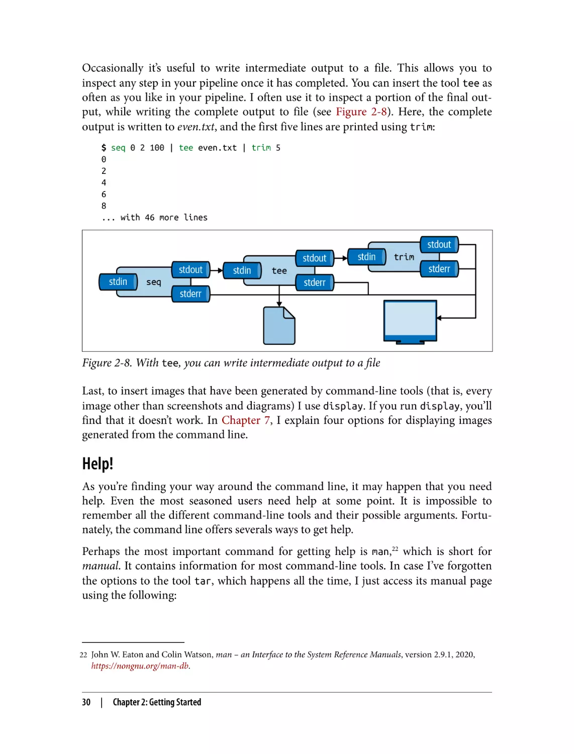
/


Автор: Jeroen Janssens
Теги: programming software computer science
ISBN: 978-1-492-08791-5
Год: 2021


Текст
nd
co ion
Se dit
E
Data Science at
the Command Line
Obtain, Scrub, Explore, and Model Data
with Unix Power Tools
Jeroen Janssens
Foreword by Tim O'Reilly
Praise for Data Science at the Command Line
Traditional computer and data science curricula all too often mistake the command line
as an obsolete relic instead of teaching it as the modern and vital toolset that it is. Only
well into my career did I come to grasp the elegance and power of the command line
for easily exploring messy datasets and even creating reproducible data pipelines
for work. The first edition of Data Science at the Command Line was one of the
most comprehensive and clear references when I was a novice in the art, and now
with the second edition, I’m again learning new tools and applications from it.
—Dan Nguyen, data scientist, former news application developer
at ProPublica, and former Lorry I. Lokey Visiting Professor in
Professional Journalism at Stanford University
The Unix philosophy of simple tools, each doing one job well, then cleverly piped
together, is embodied by the command line. Jeroen expertly discusses how to
bring that philosophy into your work in data science, illustrating how the
command line is not only the world of file input/output, but also the
world of data manipulation, exploration, and even modeling.
—Chris H. Wiggins, associate professor in the department of
applied physics and applied mathematics at Columbia University,
and chief data scientist at The New York Times
This book explains how to integrate common data science tasks into a
coherent workflow. It’s not just about tactics for breaking down problems,
it’s also about strategies for assembling the pieces of the solution.
—John D. Cook, consultant in applied mathematics,
statistics, and technical computing
Despite what you may hear, most practical data science is still focused on interesting
visualizations and insights derived from flat files. Jeroen’s book leans into this
reality, and helps reduce complexity for data practitioners by showing how
time-tested command-line tools can be repurposed for data science.
—Paige Bailey, principal product manager
code intelligence at Microsoft, GitHub
It’s amazing how fast so much data work can be performed at the command line
before ever pulling the data into R, Python, or a database. Older technologies like
sed and awk are still incredibly powerful and versatile. Until I read Data Science
at the Command Line, I had only heard of these tools but never saw their full power.
Thanks to Jeroen, it’s like I now have a secret weapon for working with large data.
—Jared Lander, chief data scientist at Lander Analytics,
organizer of the New York Open Statistical Programming Meetup,
and author of R for Everyone
The command line is an essential tool in every data scientist’s toolbox,
and knowing it well makes it easy to translate questions you have of your
data to real-time insights. Jeroen not only explains the basic Unix philosophy
of how to chain together single-purpose tools to arrive at simple solutions
for complex problems, but also introduces new command-line tools
for data cleaning, analysis, visualization, and modeling.
—Jake Hofman, senior principal researcher at
Microsoft Research, and adjunct assistant professor in the
department of applied mathematics at Columbia University
SECOND EDITION
Data Science at the
Command Line
Obtain, Scrub, Explore, and
Model Data with Unix Power Tools
Jeroen Janssens
Beijing
Boston Farnham Sebastopol
Tokyo
Data Science at the Command Line
by Jeroen Janssens
Copyright © 2021 Jeroen Janssens. All rights reserved.
Printed in the United States of America.
Published by O’Reilly Media, Inc., 1005 Gravenstein Highway North, Sebastopol, CA 95472.
O’Reilly books may be purchased for educational, business, or sales promotional use. Online editions are
also available for most titles (http://oreilly.com). For more information, contact our corporate/institutional
sales department: 800-998-9938 or corporate@oreilly.com.
Acquisitions Editor: Jessica Haberman
Development Editor: Sarah Grey
Production Editor: Kate Galloway
Copyeditor: Arthur Johnson
Proofreader: Shannon Turlington
October 2014:
August 2021:
Indexer: nSight, Inc.
Interior Designer: David Futato
Cover Designer: Karen Montgomery
Illustrator: Kate Dullea
First Edition
Second Edition
Revision History for the Second Edition
2021-08-17:
First Release
See http://oreilly.com/catalog/errata.csp?isbn=9781492087915 for release details.
The O’Reilly logo is a registered trademark of O’Reilly Media, Inc. Data Science at the Command Line, the
cover image, and related trade dress are trademarks of O’Reilly Media, Inc.
The views expressed in this work are those of the author, and do not represent the publisher’s views.
While the publisher and the author have used good faith efforts to ensure that the information and
instructions contained in this work are accurate, the publisher and the author disclaim all responsibility
for errors or omissions, including without limitation responsibility for damages resulting from the use of
or reliance on this work. Use of the information and instructions contained in this work is at your own
risk. If any code samples or other technology this work contains or describes is subject to open source
licenses or the intellectual property rights of others, it is your responsibility to ensure that your use
thereof complies with such licenses and/or rights.
Data Science at the Command Line is available under the Creative Commons Attribution
NonCommercial-No Derivatives 4.0 International License. The author maintains an online version at
https://github.com/jeroenjanssens/data-science-at-the-command-line.
978-1-492-08791-5
[LSI]
Once again to my wife, Esther. Without her continued encouragement, support,
and patience, this second edition would surely have ended up in /dev/null.
Table of Contents
Foreword. . . . . . . . . . . . . . . . . . . . . . . . . . . . . . . . . . . . . . . . . . . . . . . . . . . . . . . . . . . . . . . . . . . . xiii
Preface. . . . . . . . . . . . . . . . . . . . . . . . . . . . . . . . . . . . . . . . . . . . . . . . . . . . . . . . . . . . . . . . . . . . . . . xv
1. Introduction. . . . . . . . . . . . . . . . . . . . . . . . . . . . . . . . . . . . . . . . . . . . . . . . . . . . . . . . . . . . . . . . 1
Data Science Is OSEMN
Obtaining Data
Scrubbing Data
Exploring Data
Modeling Data
Interpreting Data
Intermezzo Chapters
What Is the Command Line?
Why Data Science at the Command Line?
The Command Line Is Agile
The Command Line Is Augmenting
The Command Line Is Scalable
The Command Line Is Extensible
The Command Line Is Ubiquitous
Summary
For Further Exploration
2
3
3
3
4
4
4
5
7
7
8
8
9
9
10
10
2. Getting Started. . . . . . . . . . . . . . . . . . . . . . . . . . . . . . . . . . . . . . . . . . . . . . . . . . . . . . . . . . . . 11
Getting the Data
Installing the Docker Image
Essential Unix Concepts
The Environment
Executing a Command-Line Tool
11
12
13
14
15
vii
Five Types of Command-Line Tools
Combining Command-Line Tools
Redirecting Input and Output
Working with Files and Directories
Managing Output
Help!
Summary
For Further Exploration
16
20
22
26
28
30
33
33
3. Obtaining Data. . . . . . . . . . . . . . . . . . . . . . . . . . . . . . . . . . . . . . . . . . . . . . . . . . . . . . . . . . . . . 35
Overview
Copying Local Files to the Docker Container
Downloading from the Internet
Introducing curl
Saving
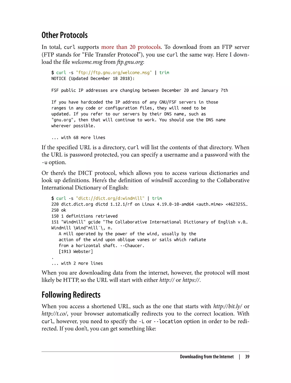
Other Protocols
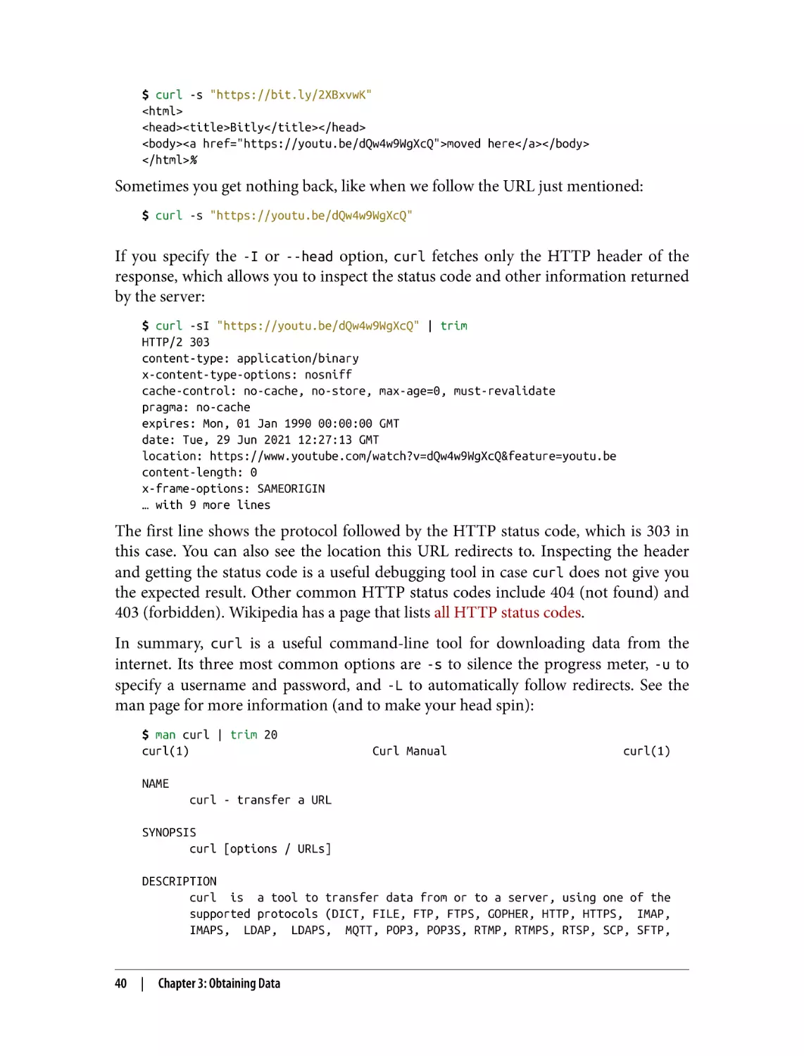
Following Redirects
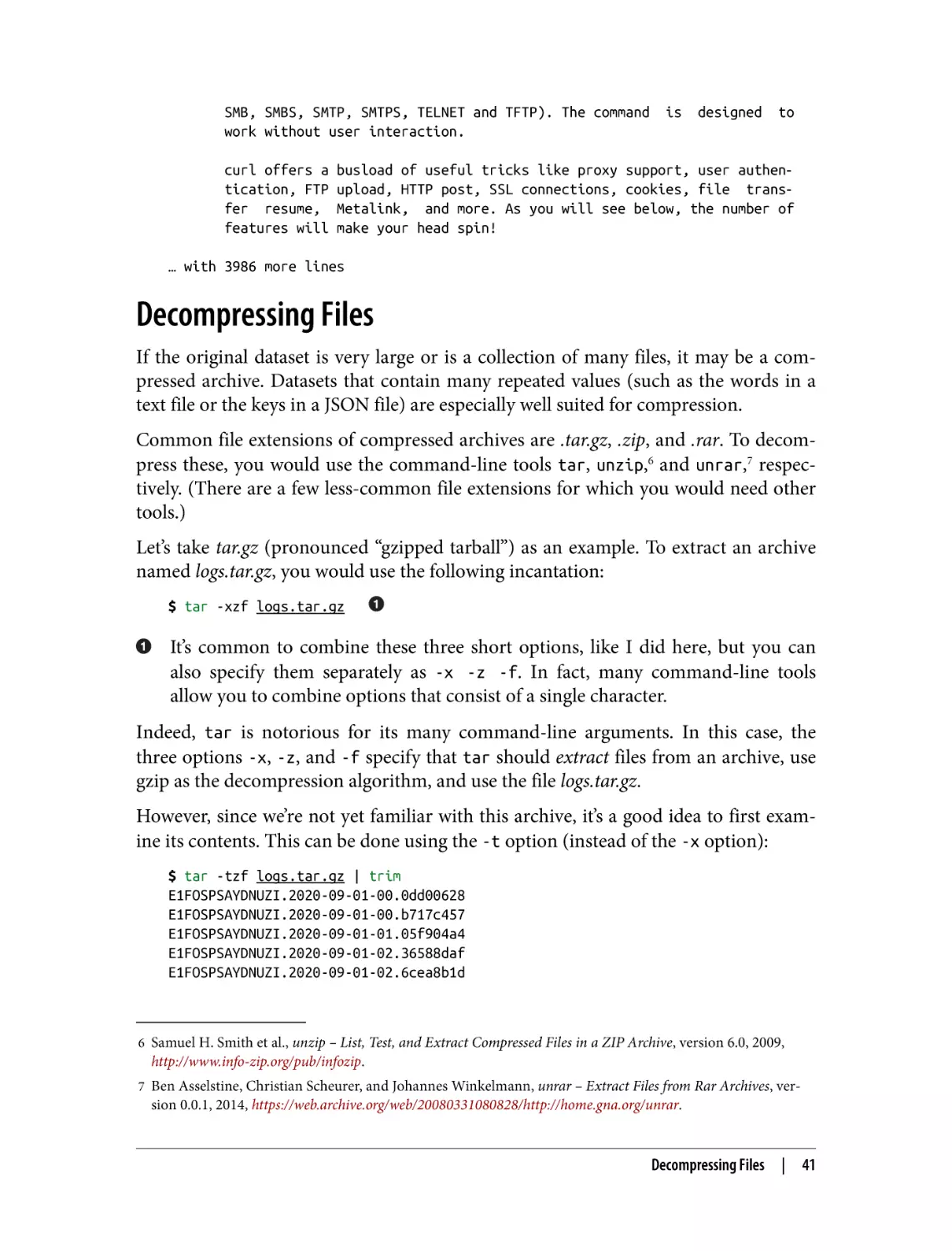
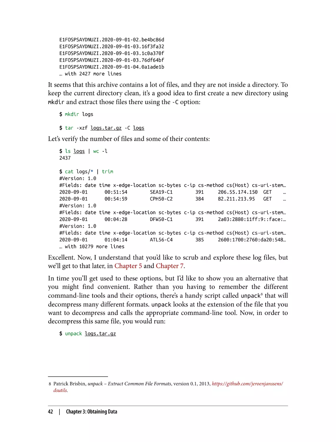
Decompressing Files
Converting Microsoft Excel Spreadsheets to CSV
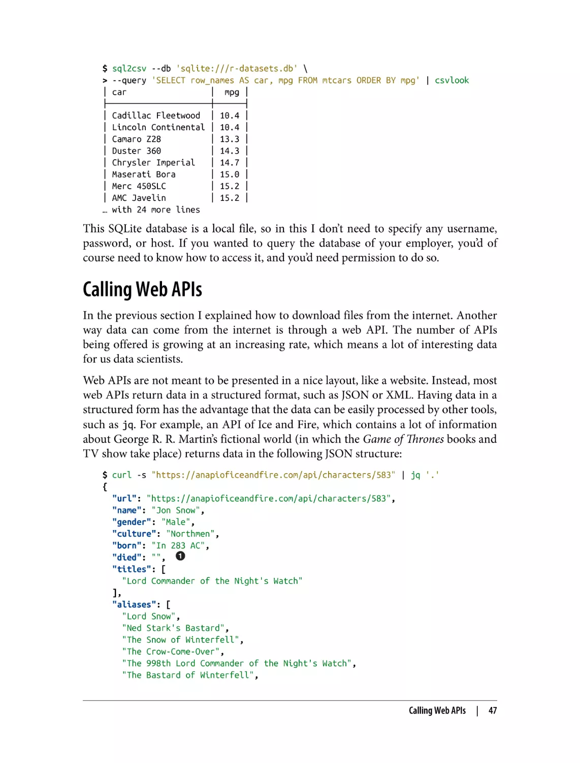
Querying Relational Databases
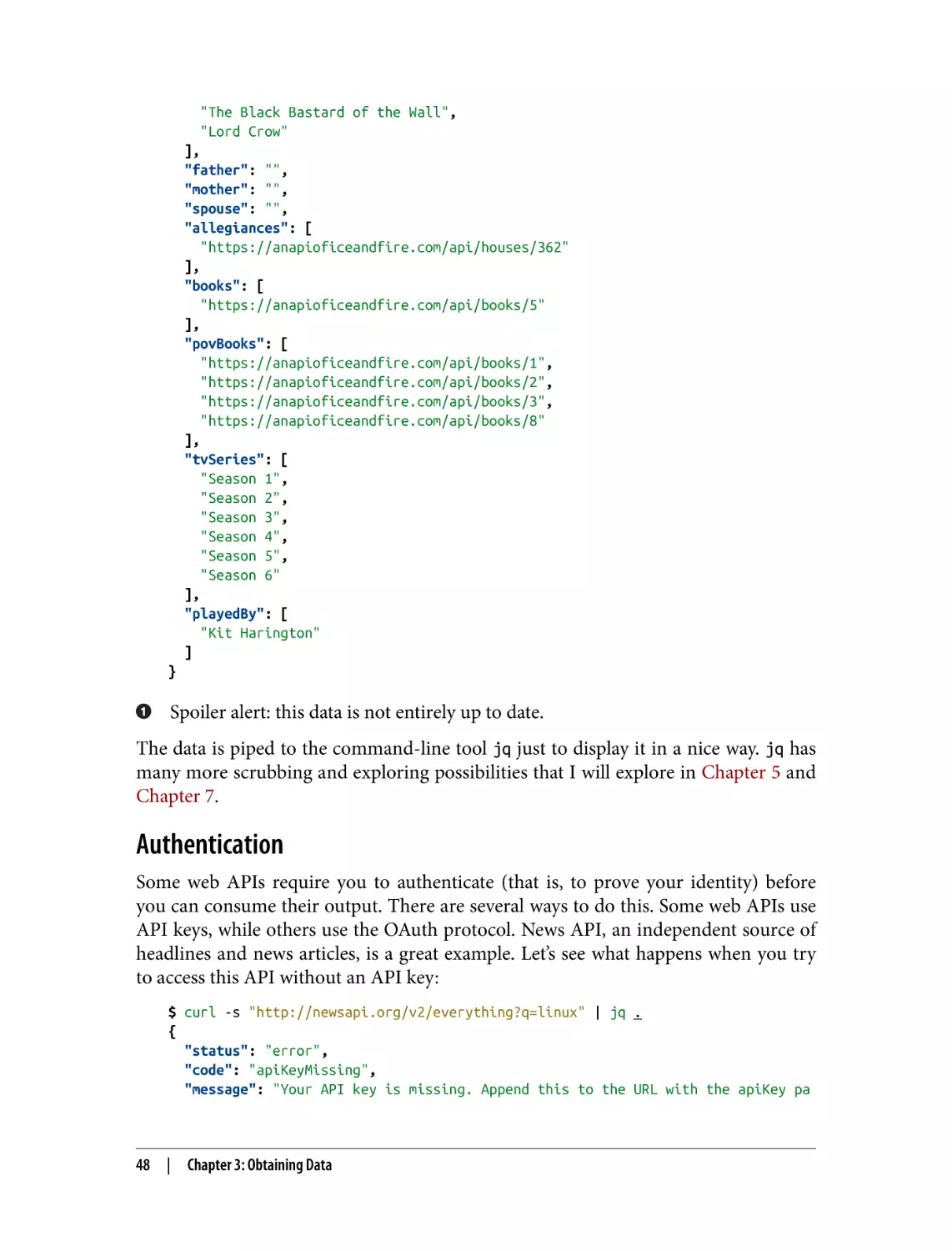
Calling Web APIs
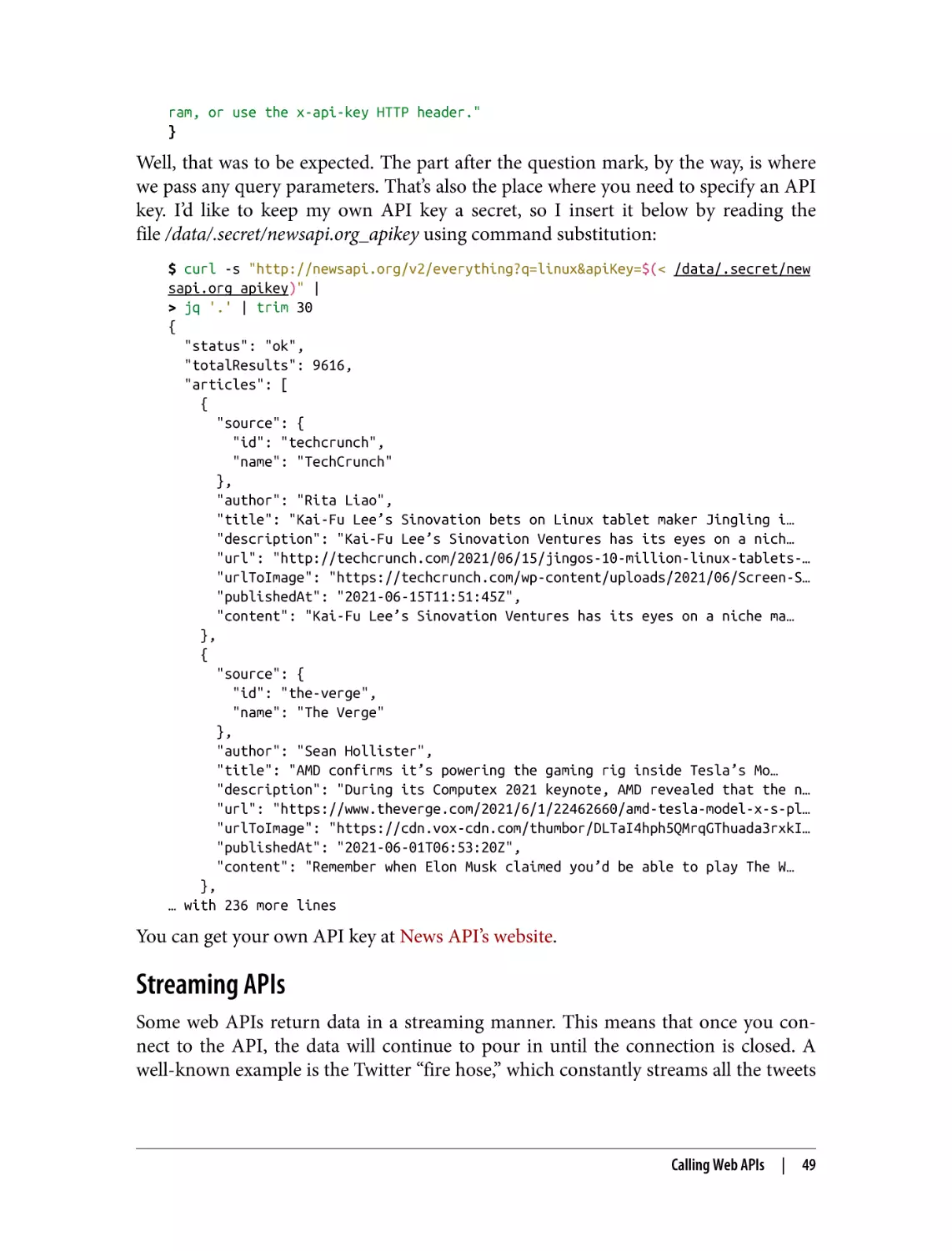
Authentication
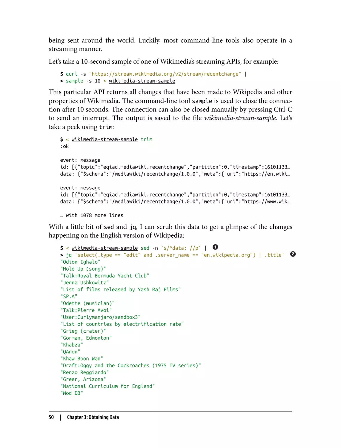
Streaming APIs
Summary
For Further Exploration
36
36
37
37
38
39
39
41
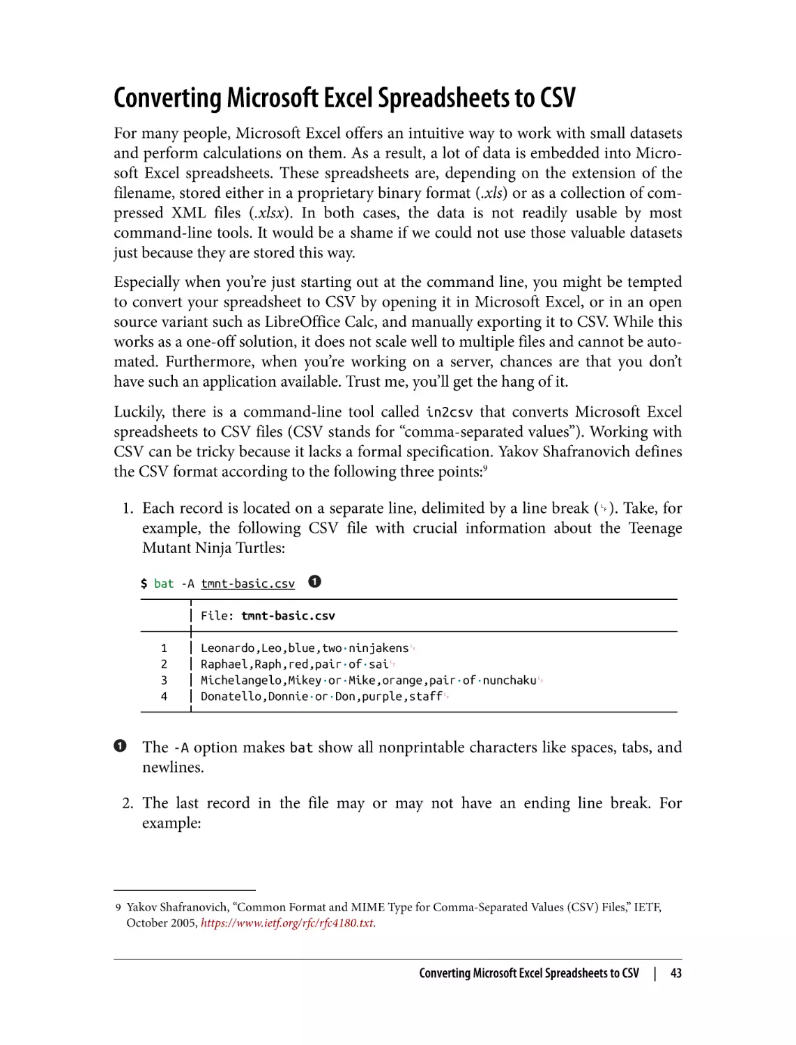
43
46
47
48
49
51
52
4. Creating Command-Line Tools. . . . . . . . . . . . . . . . . . . . . . . . . . . . . . . . . . . . . . . . . . . . . . . . 53
Overview
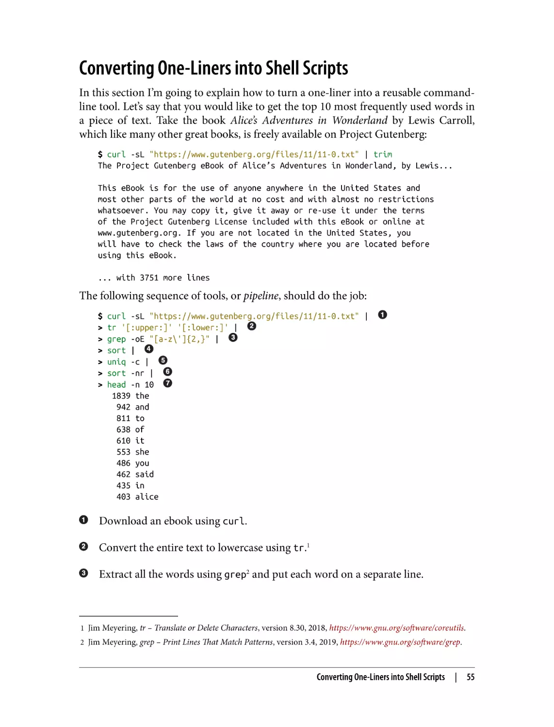
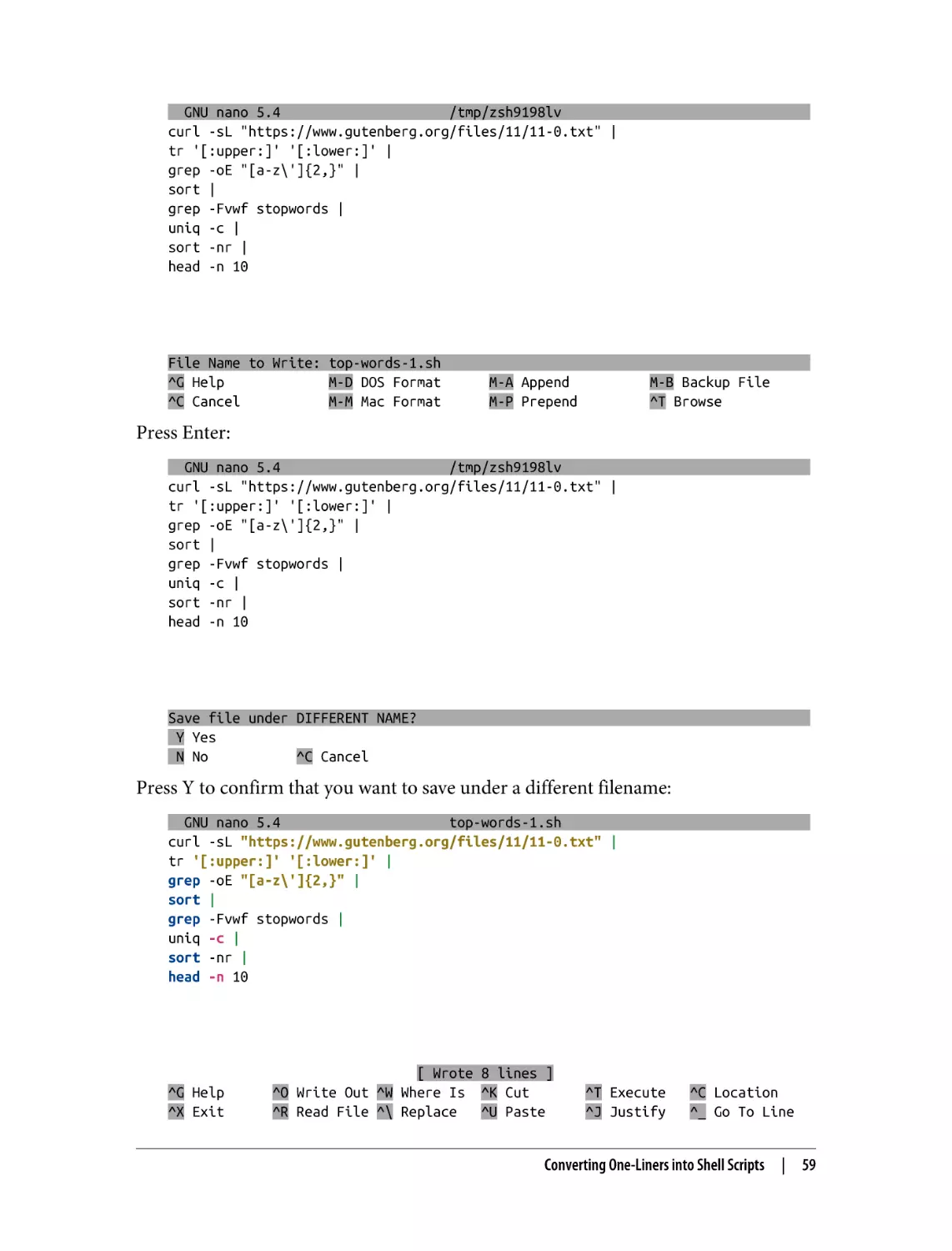
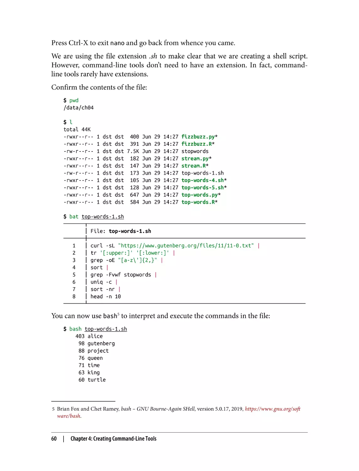
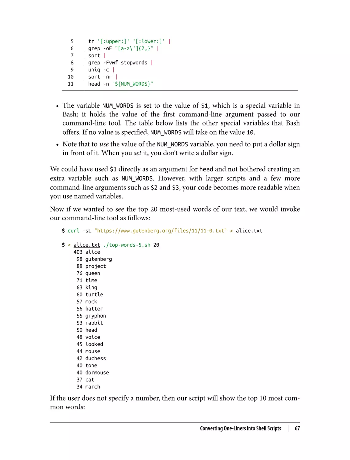
Converting One-Liners into Shell Scripts
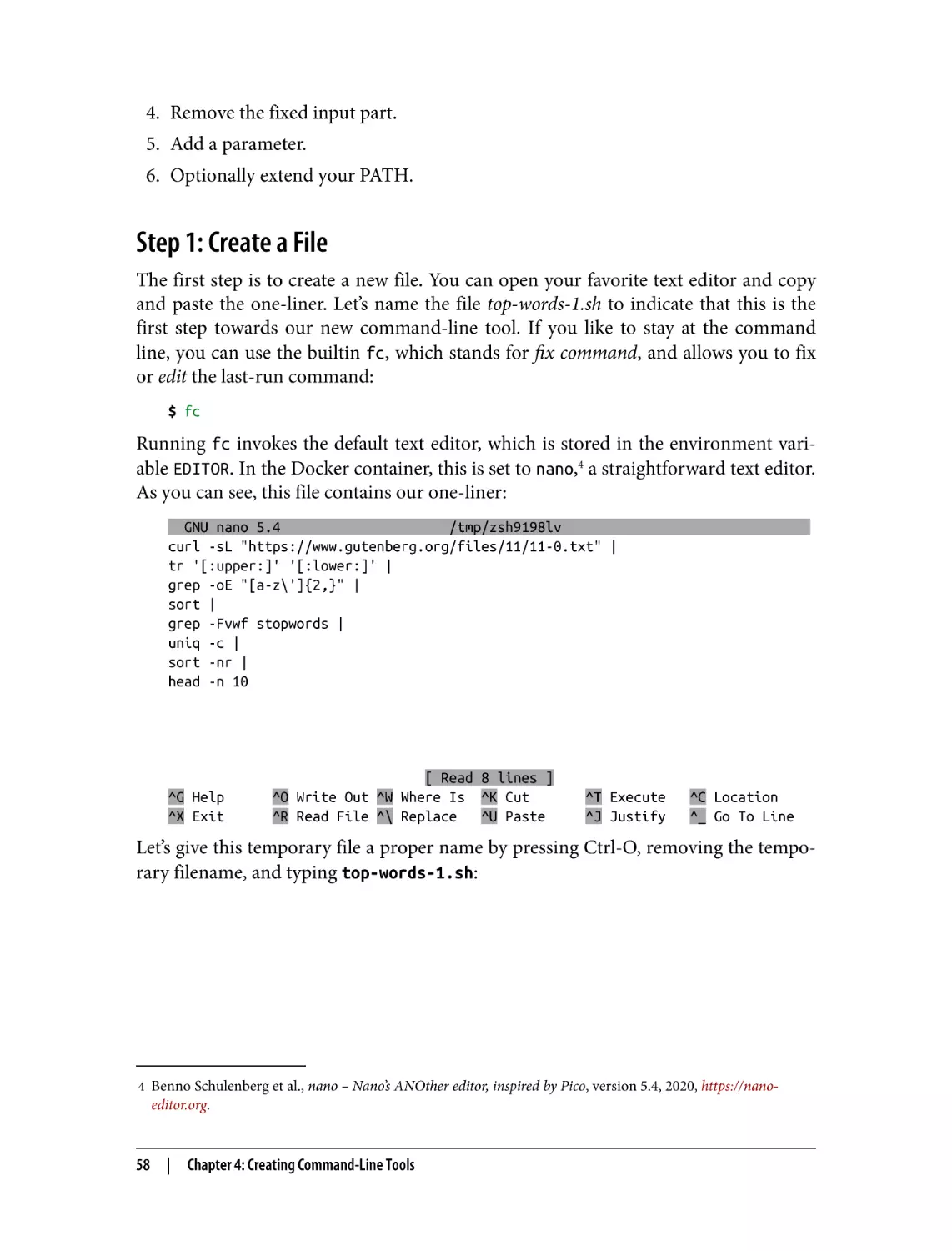
Step 1: Create a File
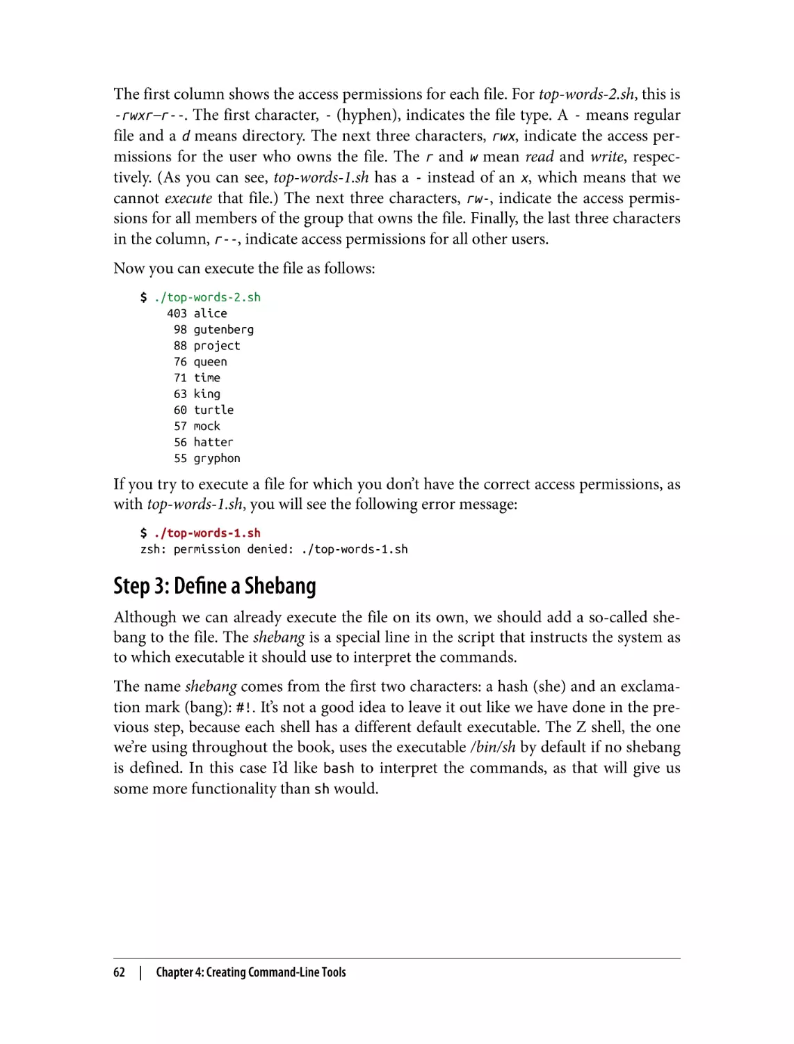
Step 2: Give Permission to Execute
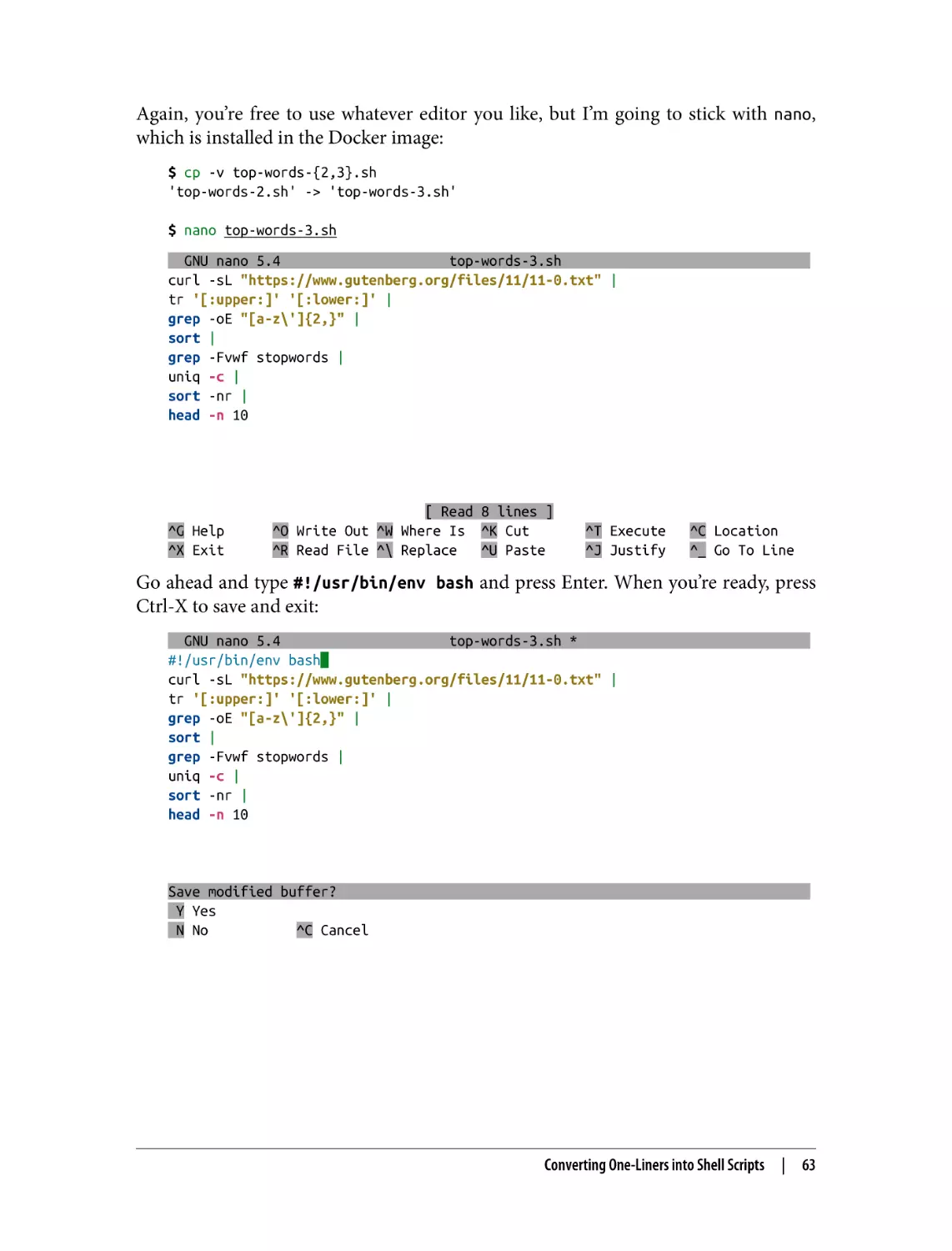
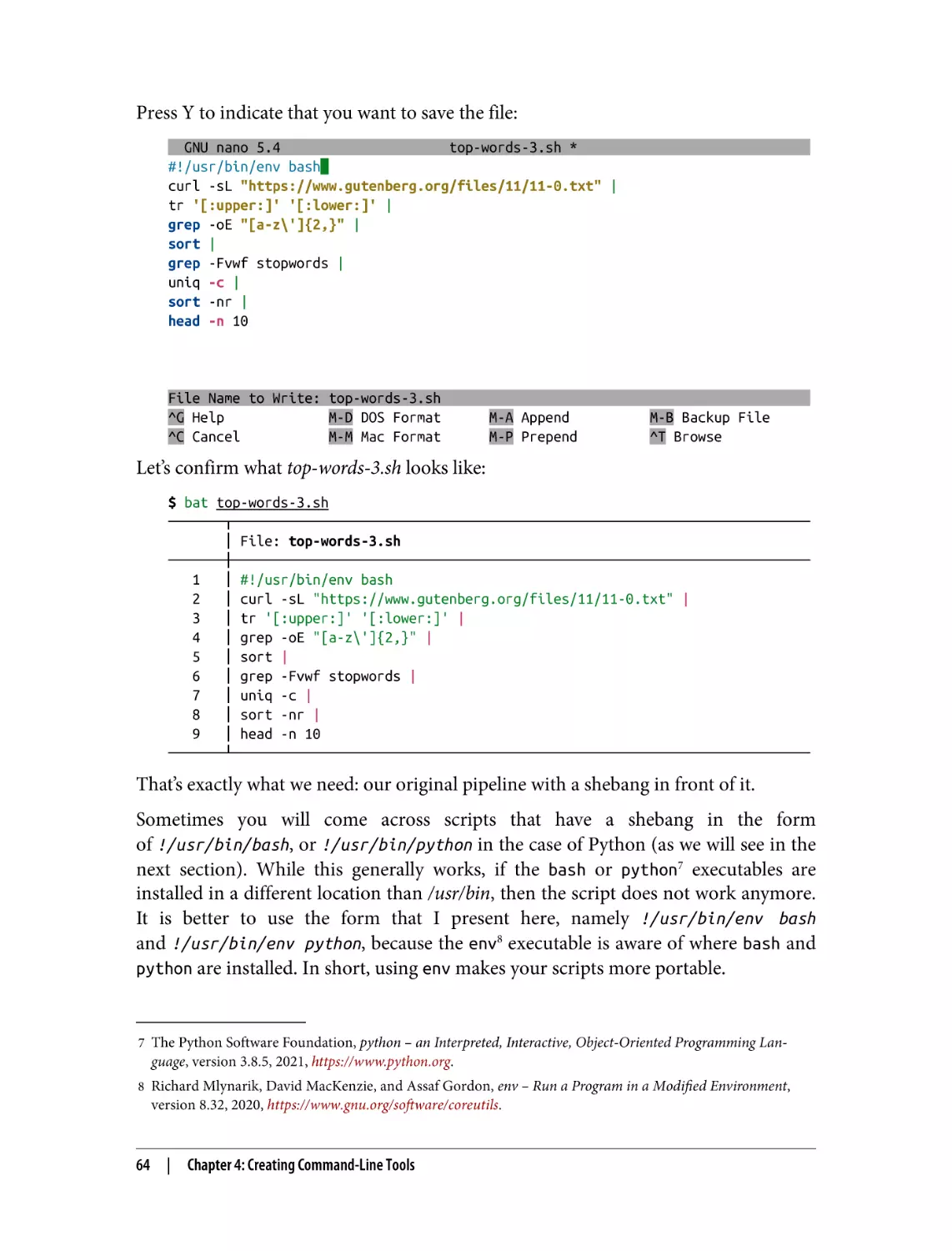
Step 3: Define a Shebang
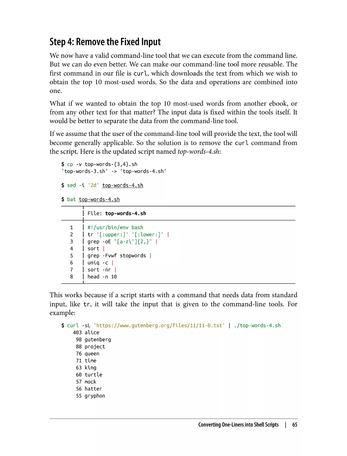
Step 4: Remove the Fixed Input
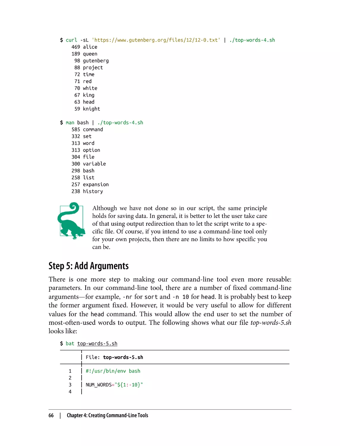
Step 5: Add Arguments
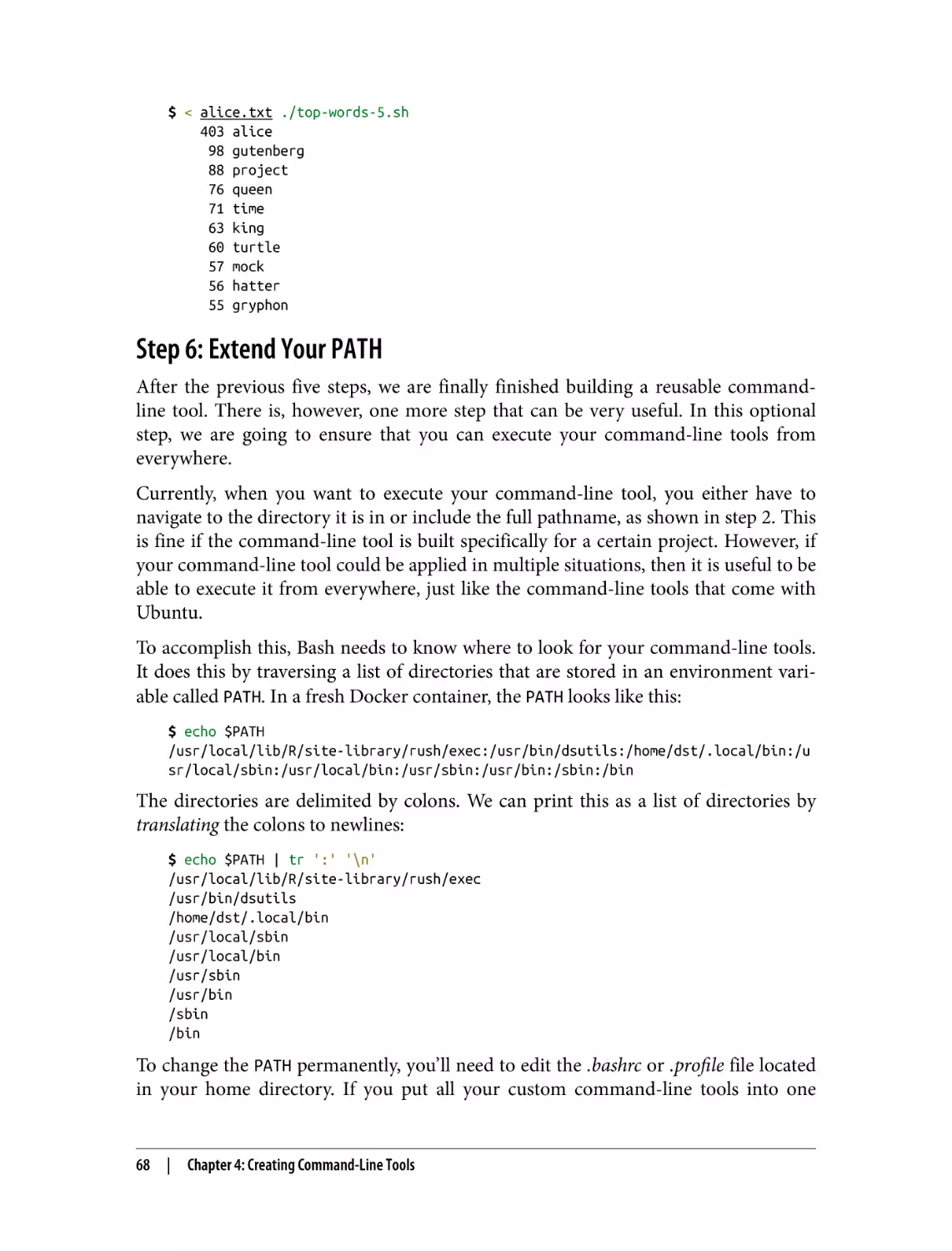
Step 6: Extend Your PATH
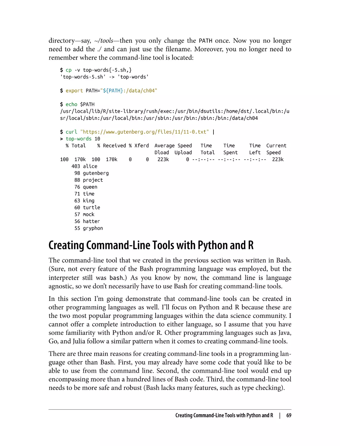
Creating Command-Line Tools with Python and R
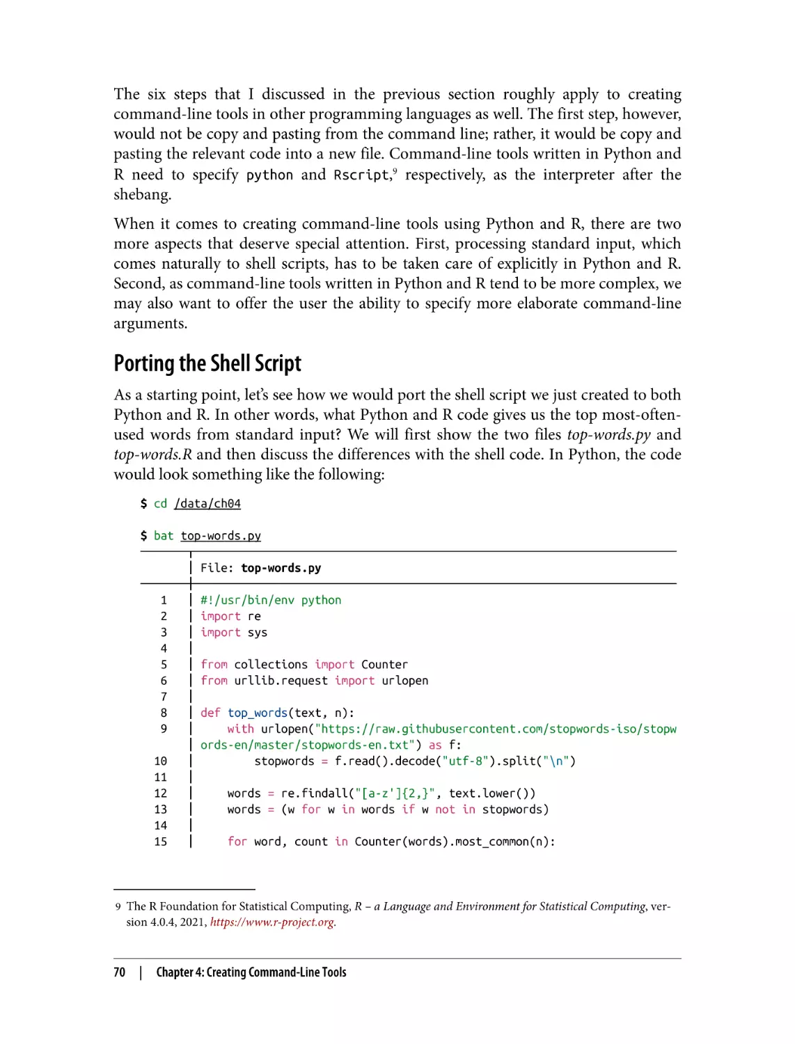
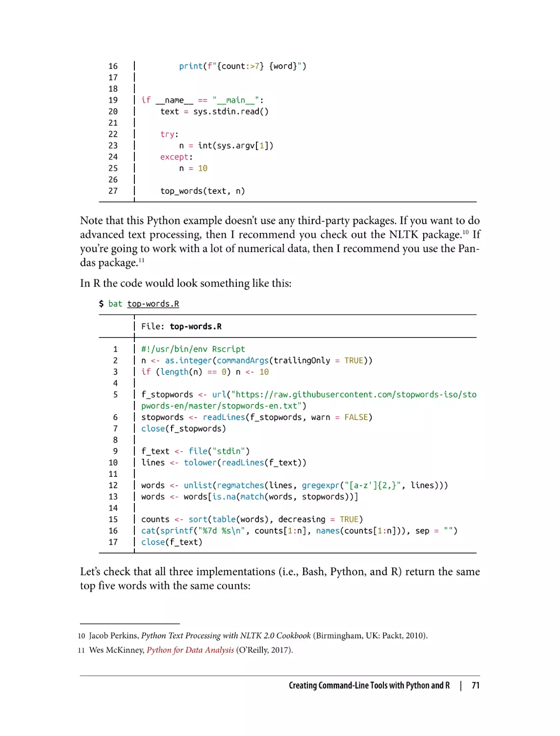
Porting the Shell Script
Processing Streaming Data from Standard Input
Summary
For Further Exploration
viii
|
Table of Contents
54
55
58
61
62
65
66
68
69
70
72
74
74
5. Scrubbing Data. . . . . . . . . . . . . . . . . . . . . . . . . . . . . . . . . . . . . . . . . . . . . . . . . . . . . . . . . . . . 77
Overview
Transformations, Transformations Everywhere
Plain Text
Filtering Lines
Extracting Values
Replacing and Deleting Values
CSV
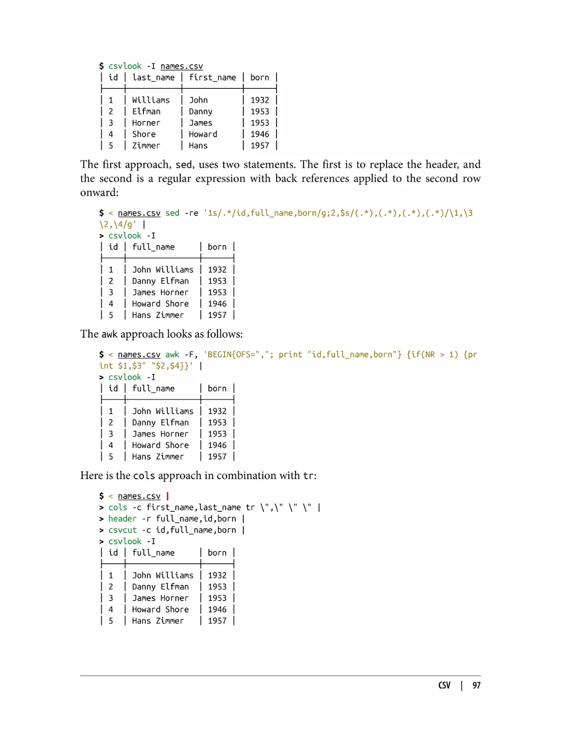
Bodies and Headers and Columns, Oh My!
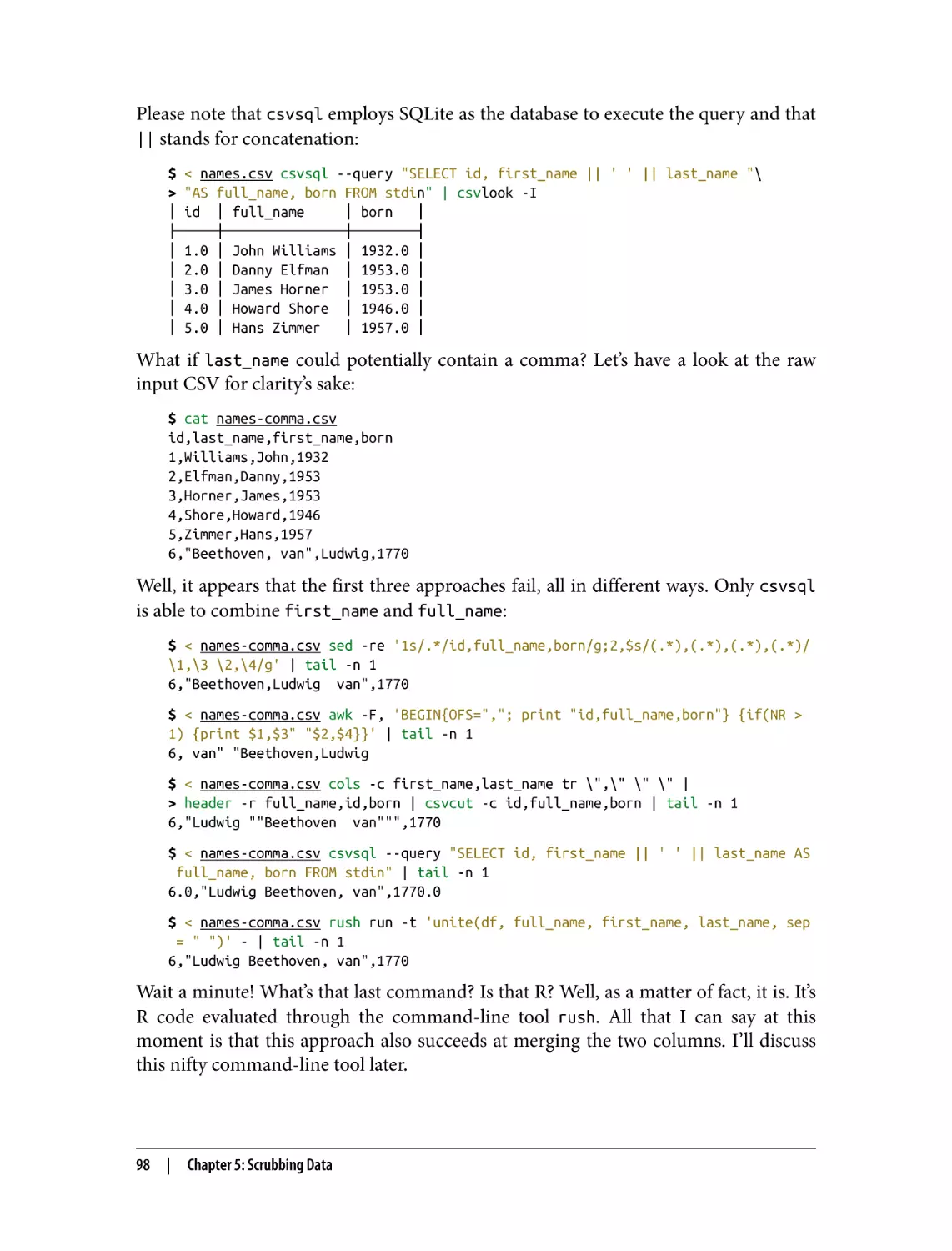
Performing SQL Queries on CSV
Extracting and Reordering Columns
Filtering Rows
Merging Columns
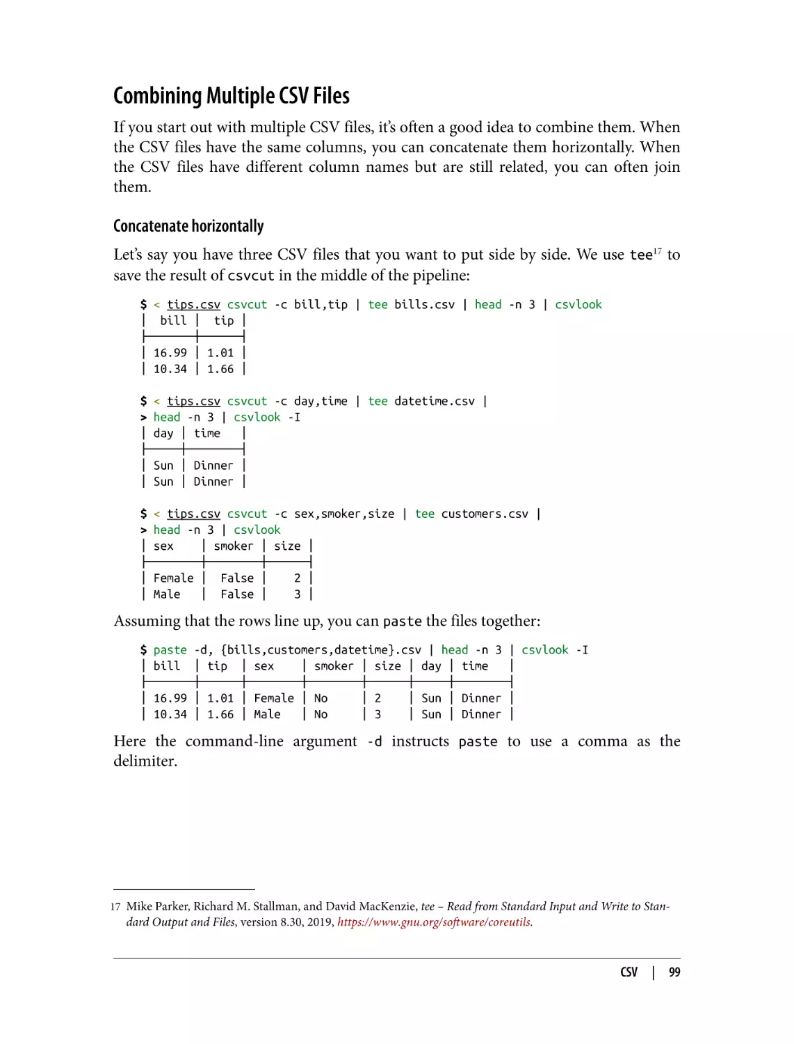
Combining Multiple CSV Files
Working with XML/HTML and JSON
Summary
For Further Exploration
78
78
81
81
86
88
90
90
93
94
95
96
99
101
104
105
6. Project Management with Make. . . . . . . . . . . . . . . . . . . . . . . . . . . . . . . . . . . . . . . . . . . . . 107
Overview
Introducing Make
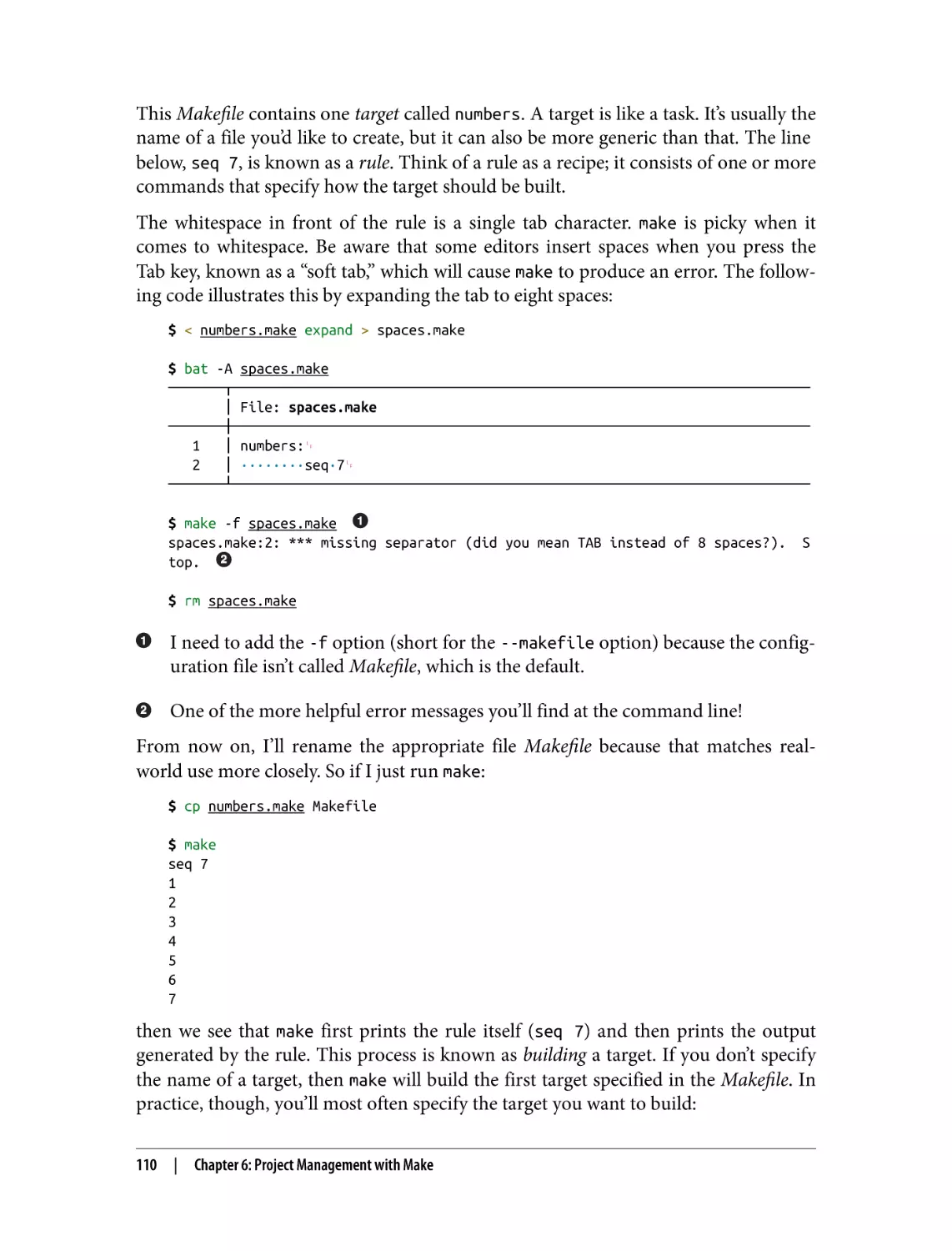
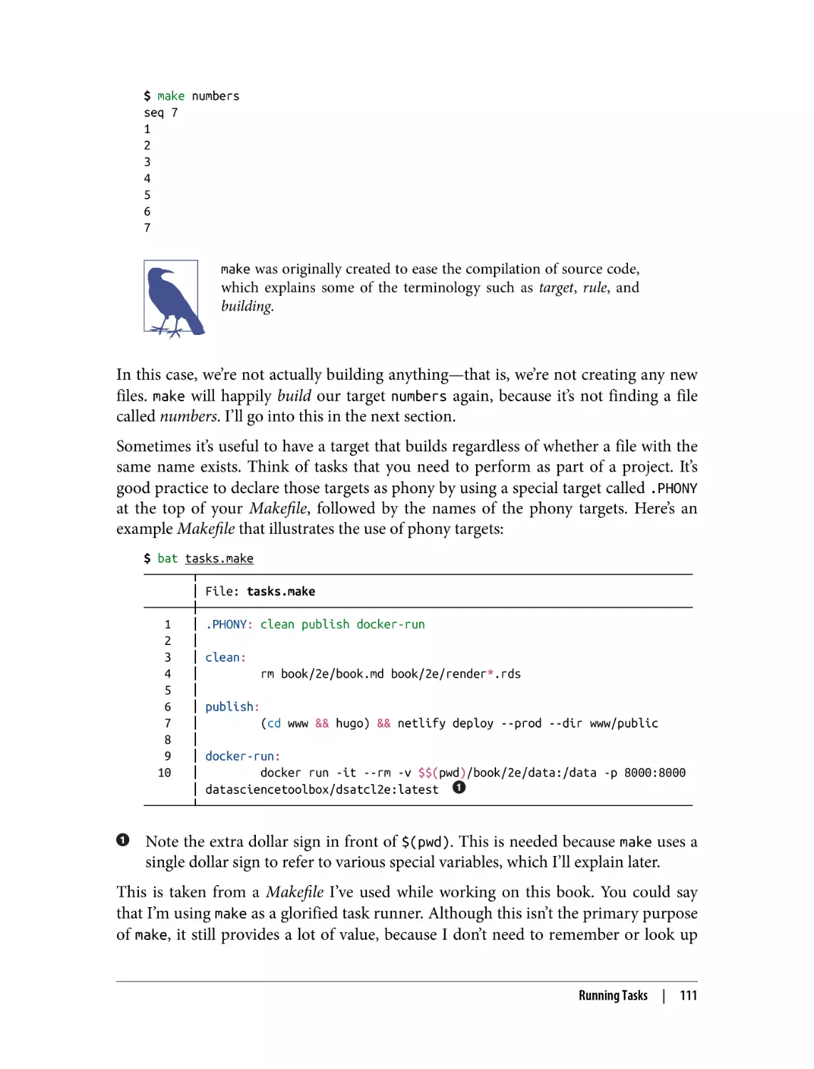
Running Tasks
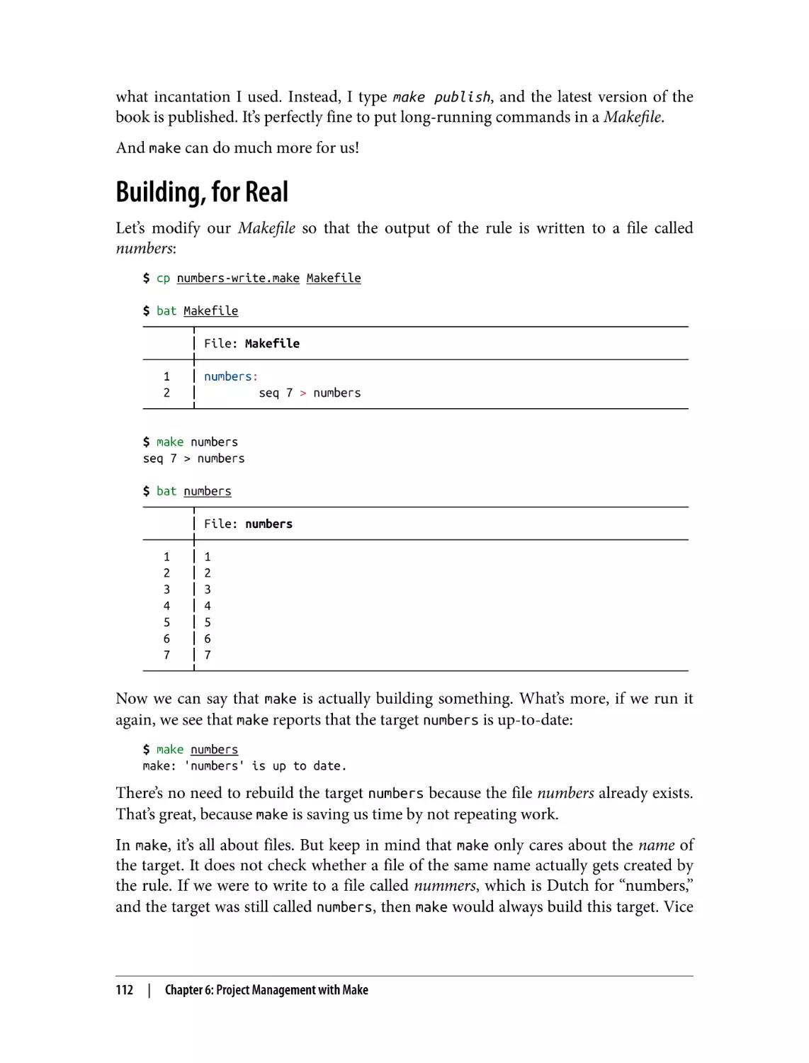
Building, for Real
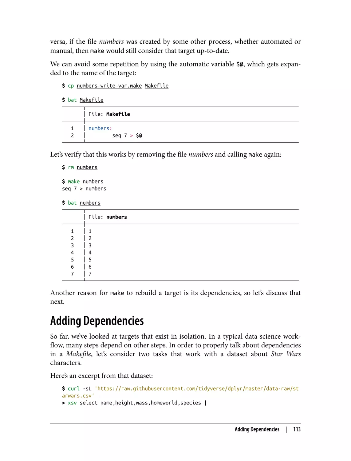
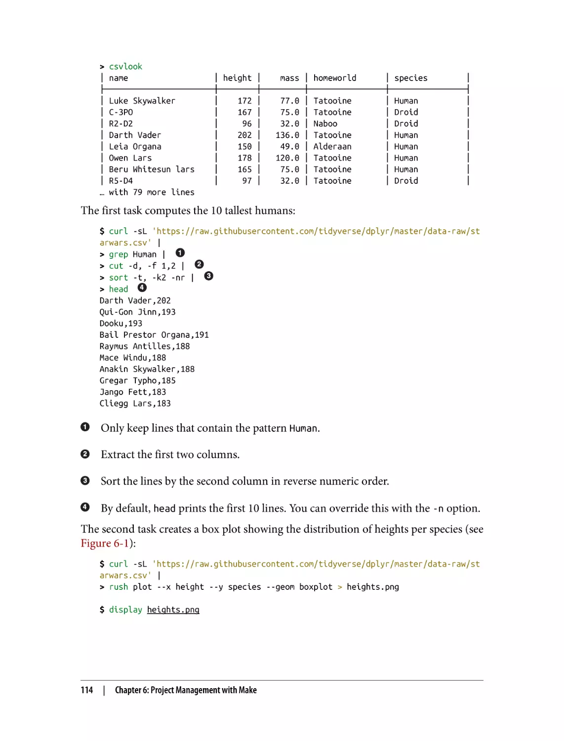
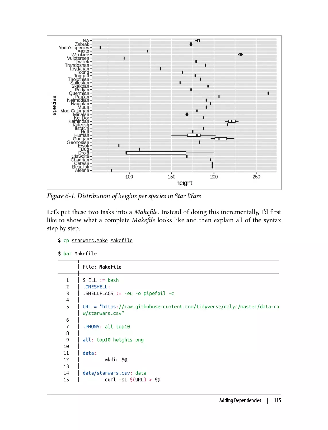
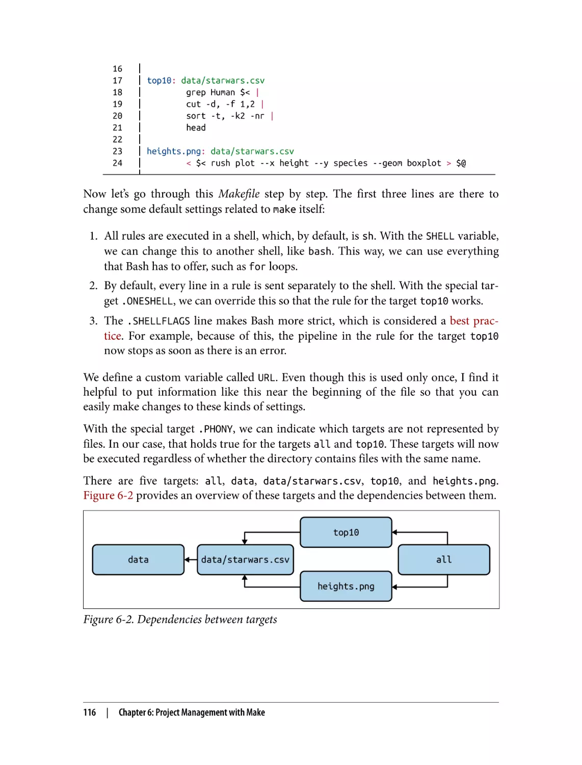
Adding Dependencies
Summary
For Further Exploration
108
109
109
112
113
118
118
7. Exploring Data. . . . . . . . . . . . . . . . . . . . . . . . . . . . . . . . . . . . . . . . . . . . . . . . . . . . . . . . . . . . 119
Overview
Inspecting Data and Its Properties
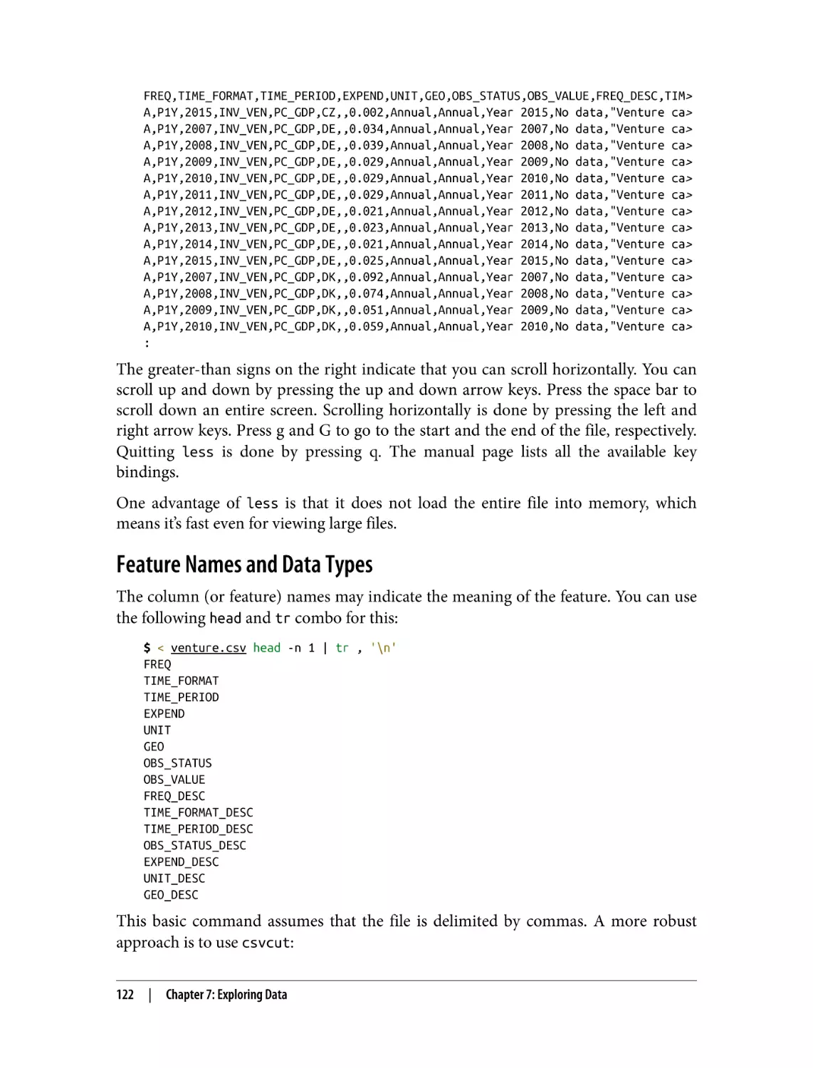
Header or Not, Here I Come
Inspect All the Data
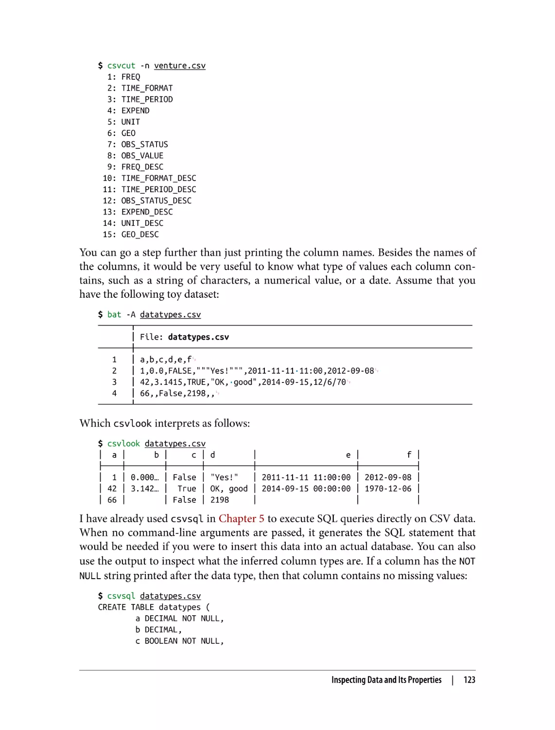
Feature Names and Data Types
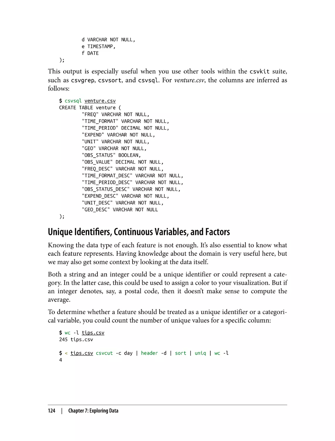
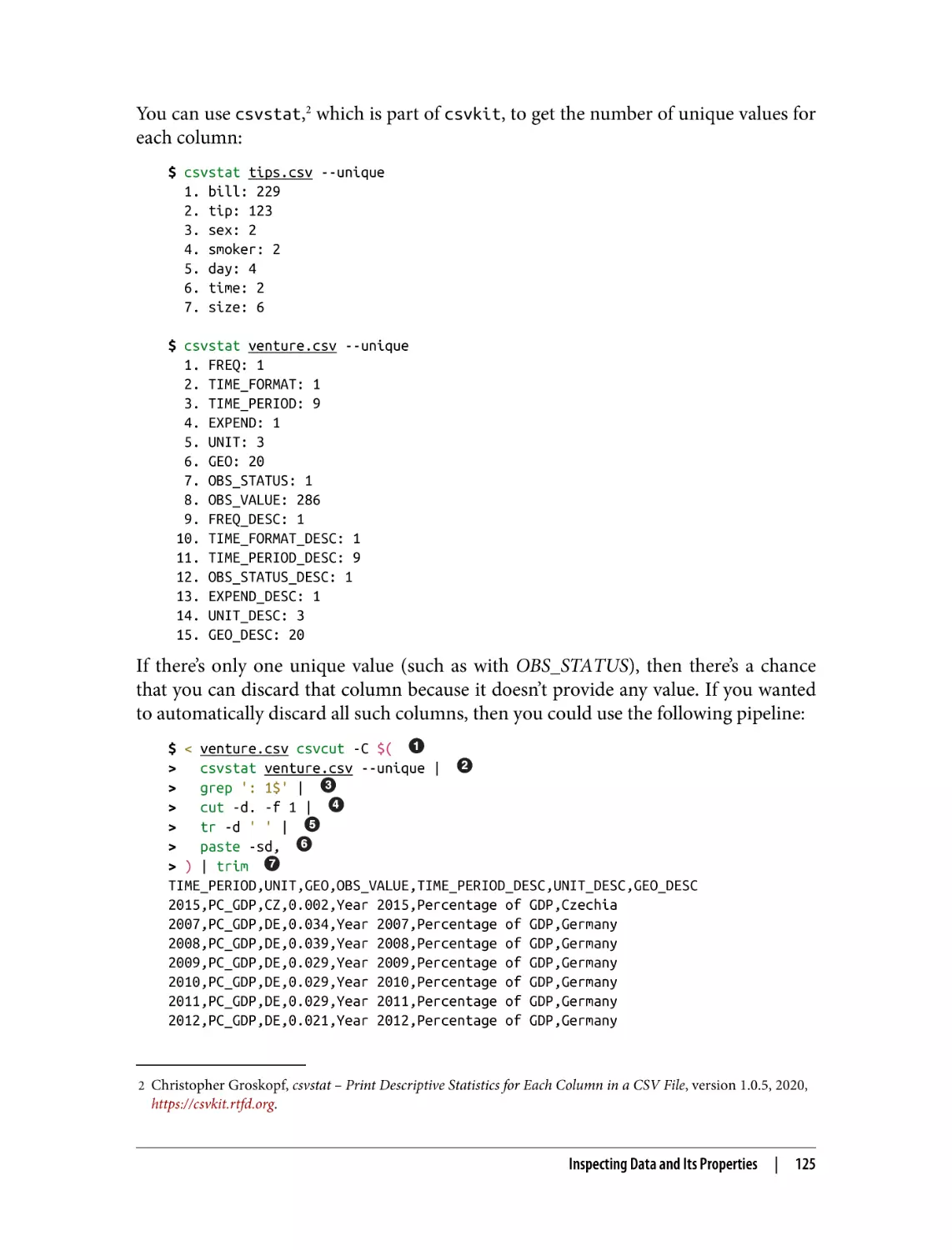
Unique Identifiers, Continuous Variables, and Factors
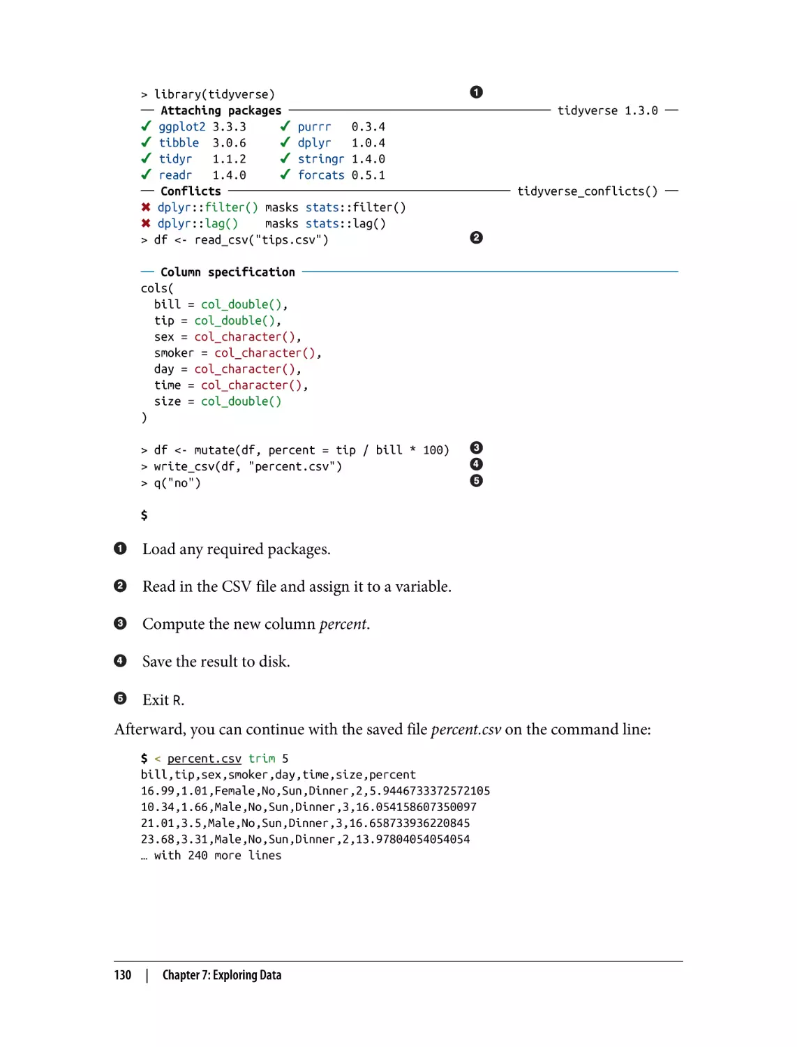
Computing Descriptive Statistics
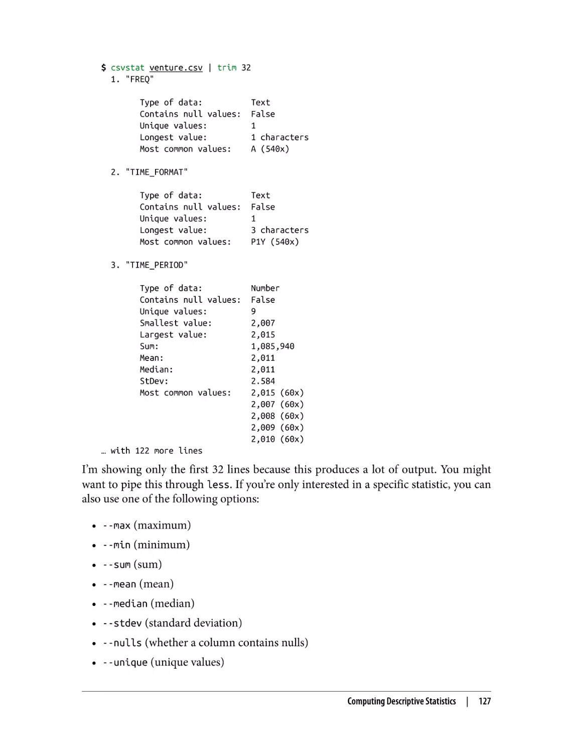
Column Statistics
R One-Liners on the Shell
Creating Visualizations
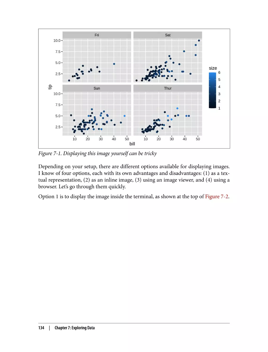
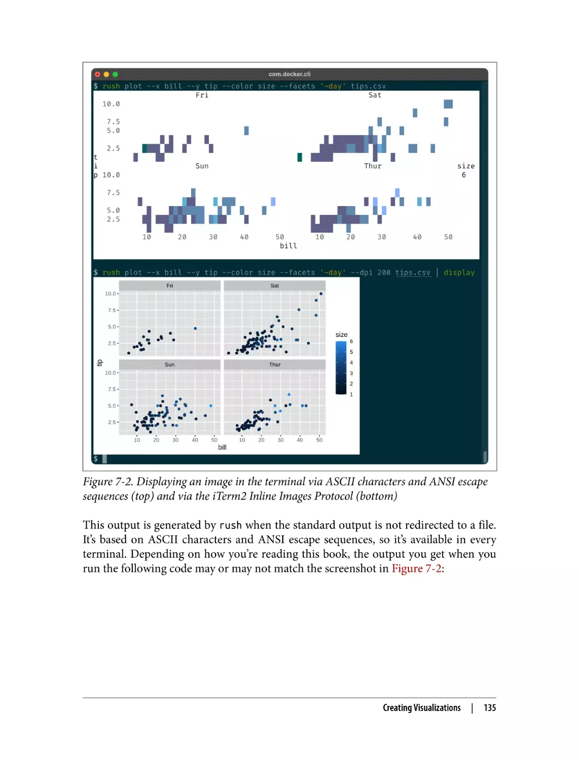
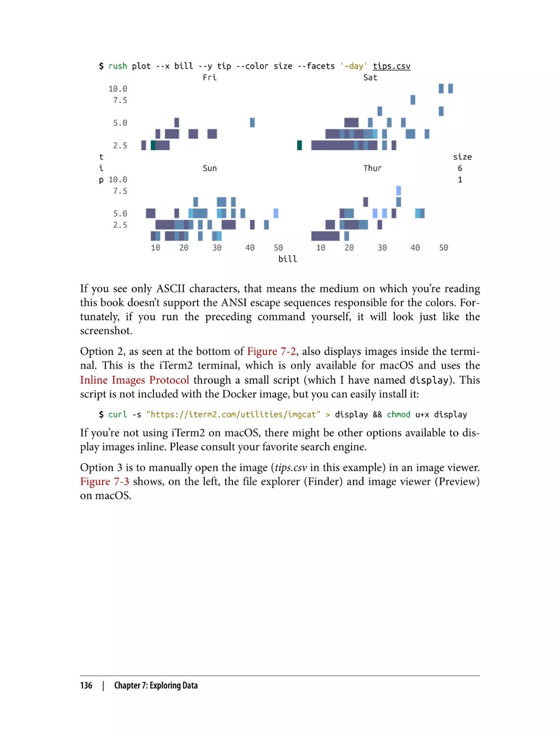
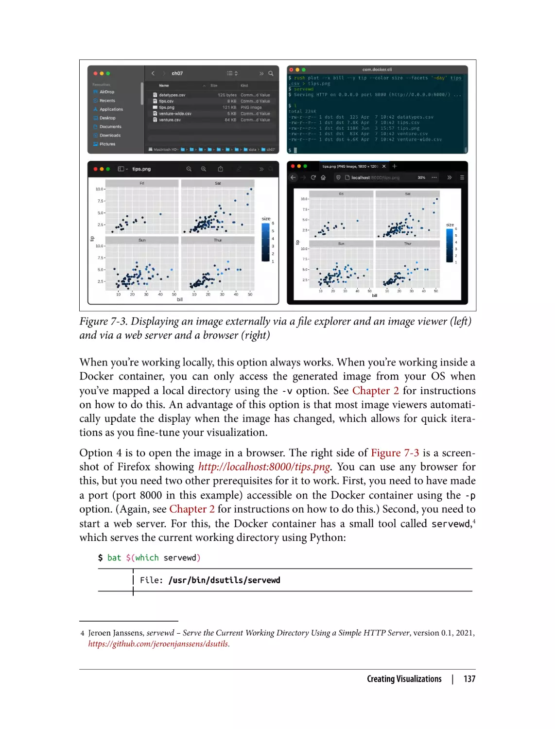
Displaying Images from the Command Line
Plotting in a Rush
Creating Bar Charts
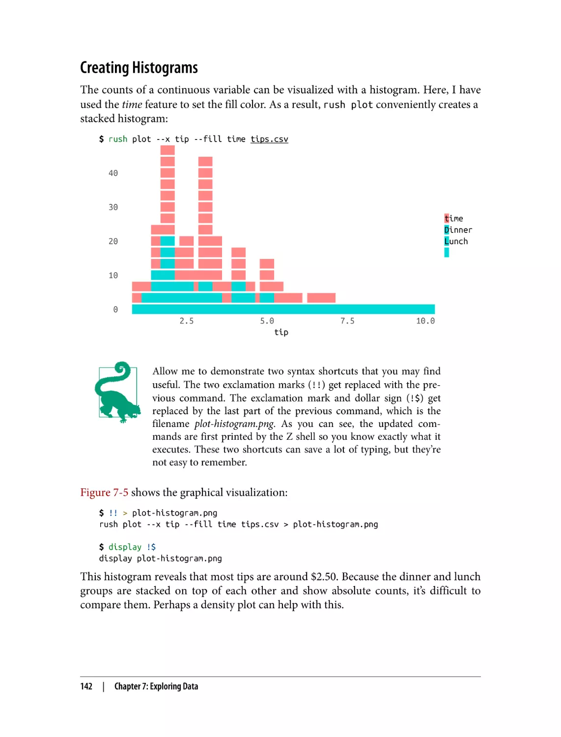
Creating Histograms
120
120
120
121
122
124
126
126
129
133
133
138
140
142
Table of Contents
|
ix
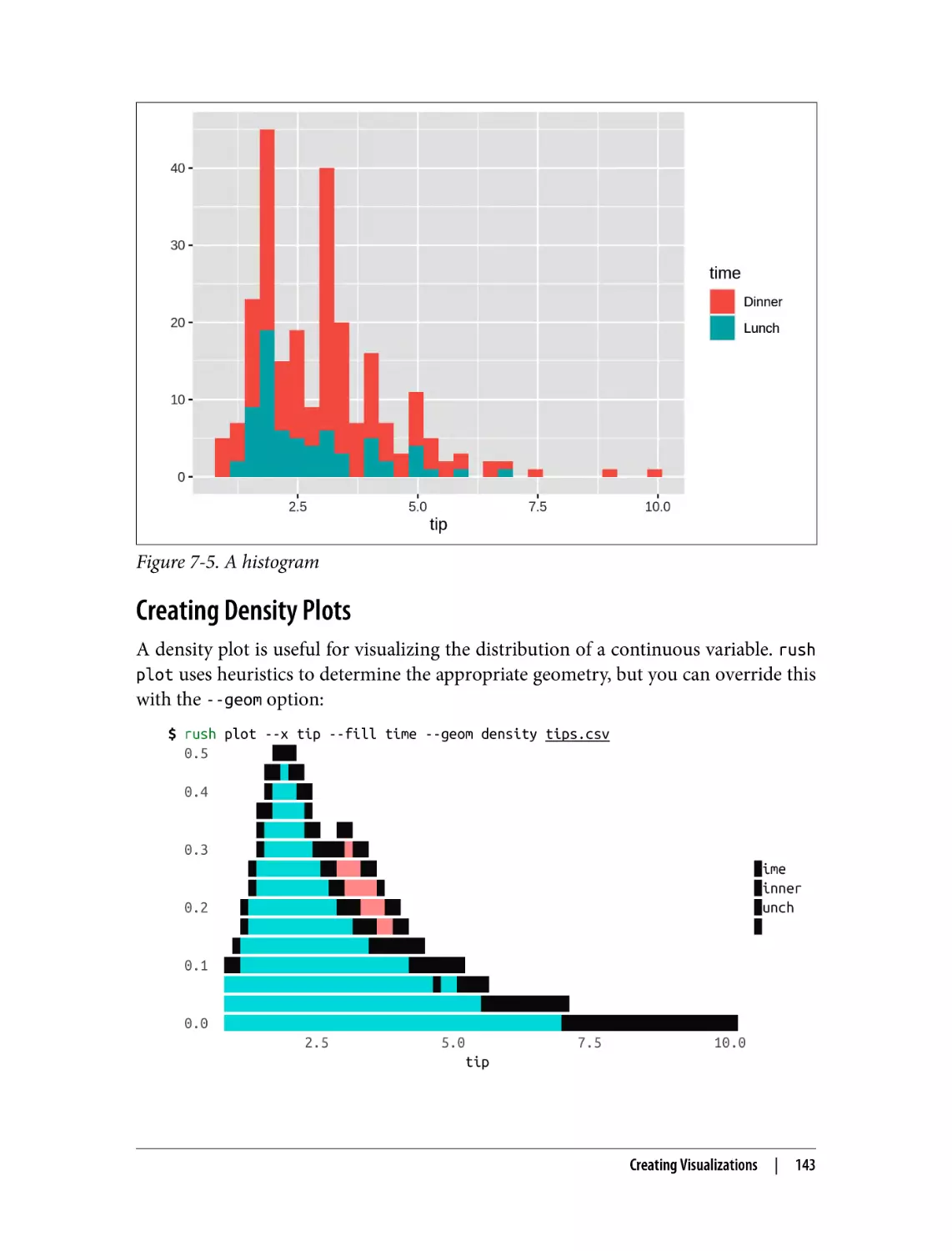
Creating Density Plots
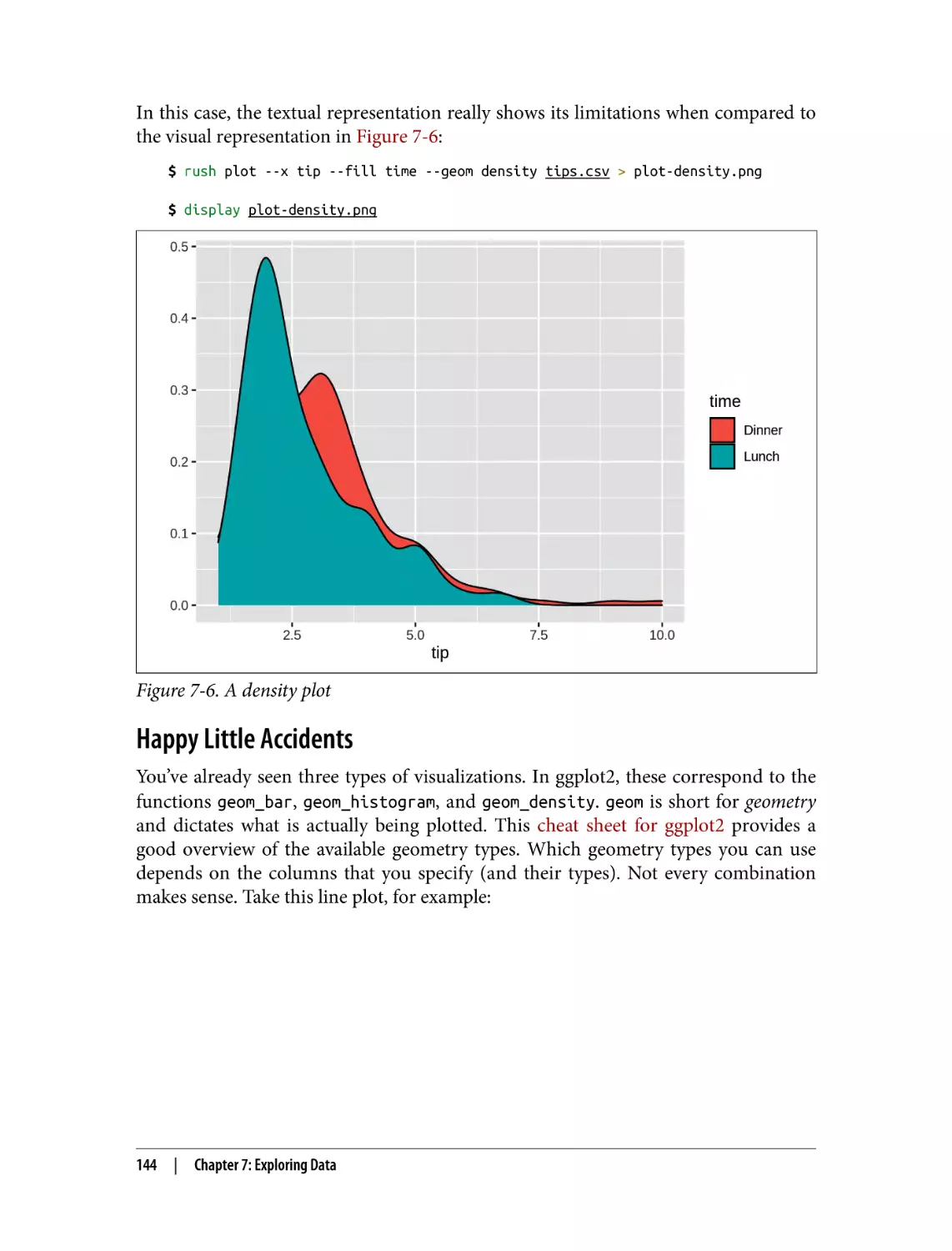
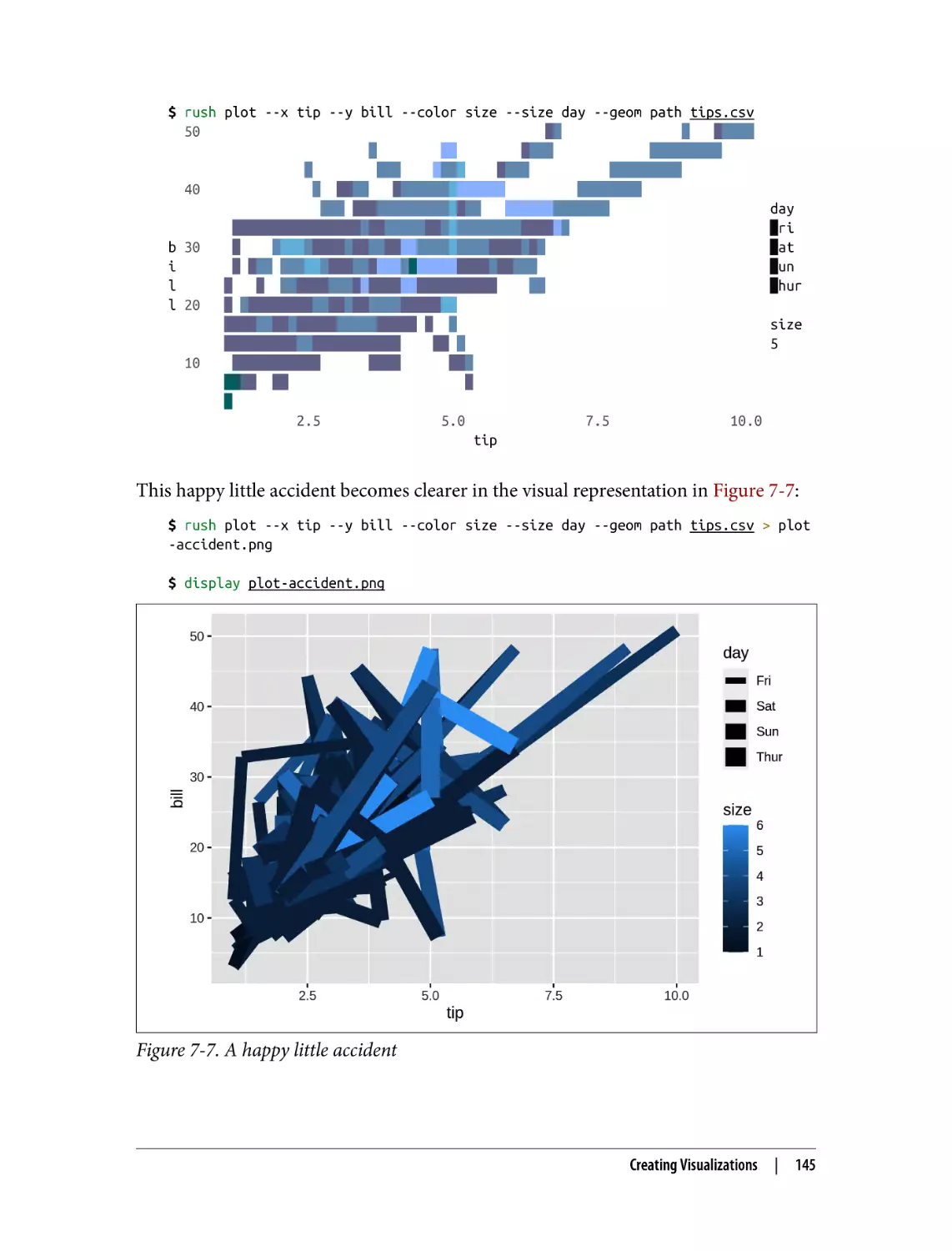
Happy Little Accidents
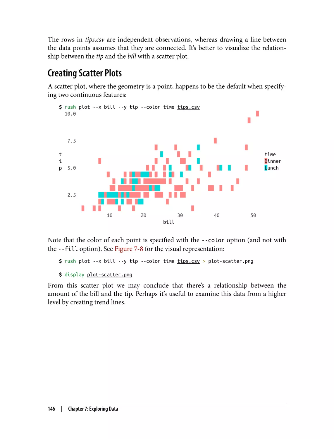
Creating Scatter Plots
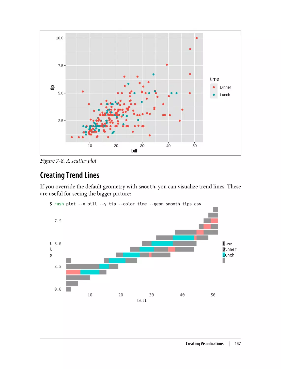
Creating Trend Lines
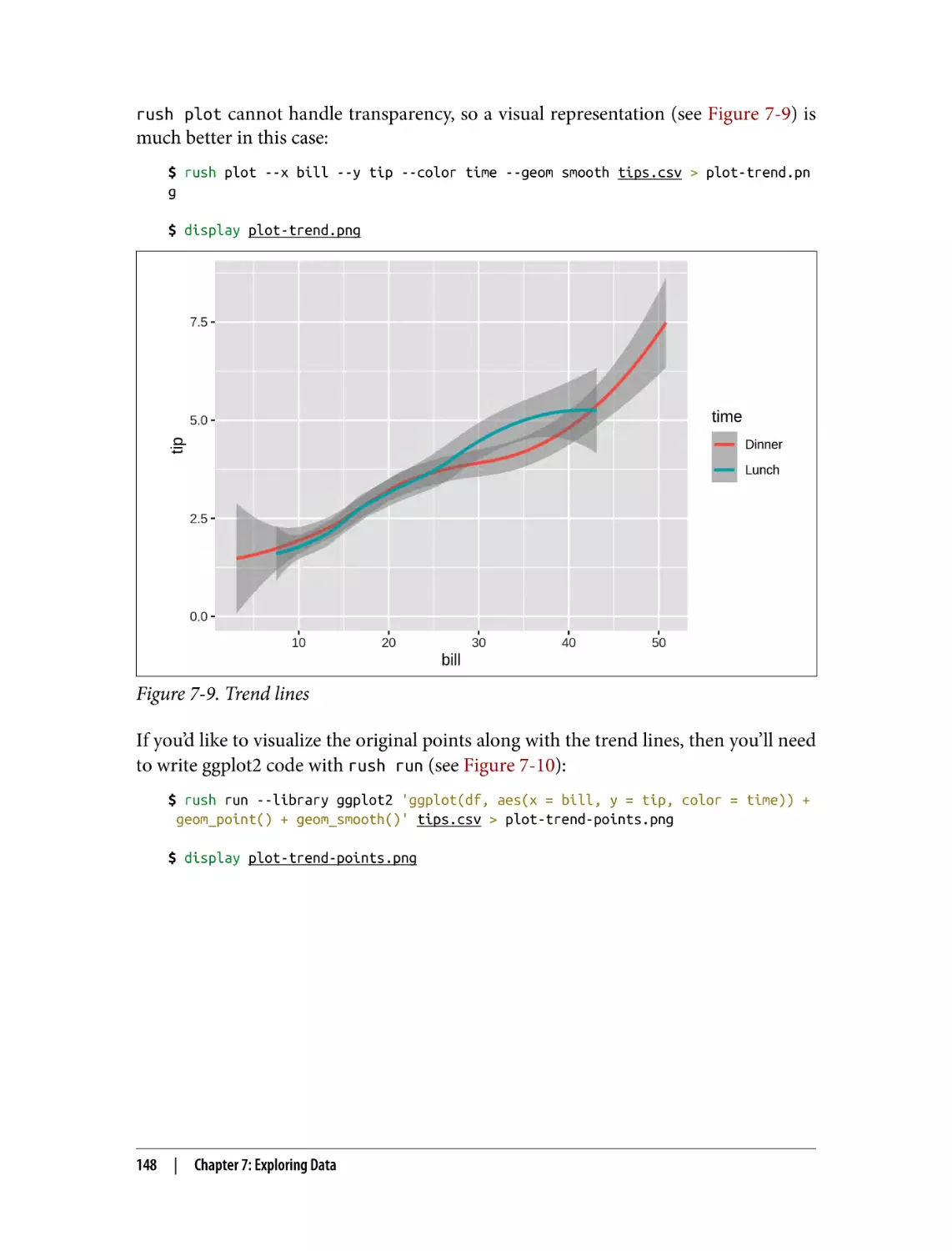
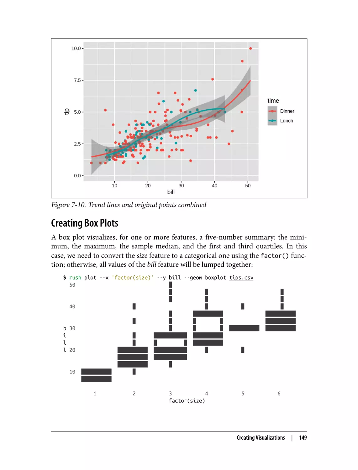
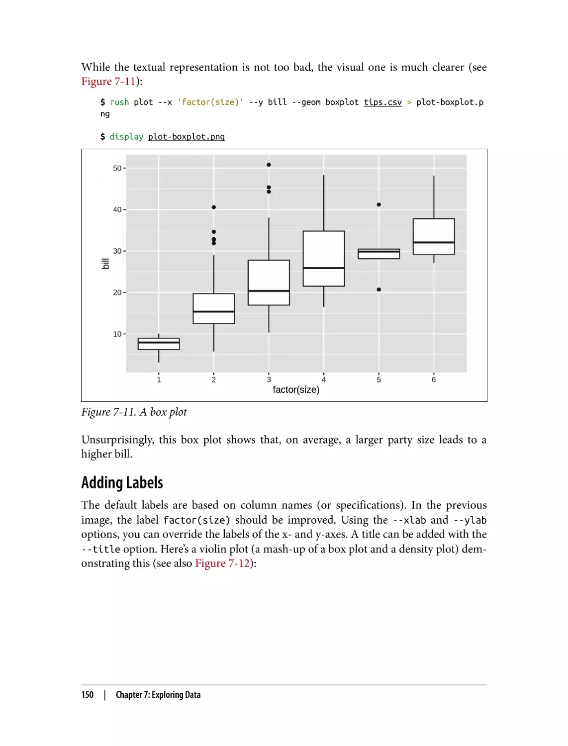
Creating Box Plots
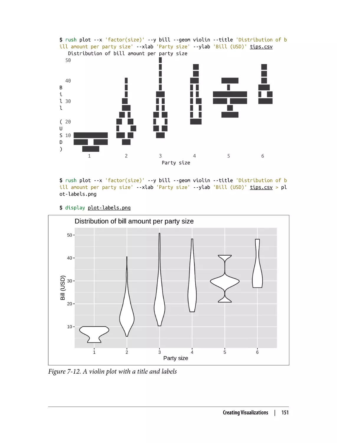
Adding Labels
Going Beyond Basic Plots
Summary
For Further Exploration
143
144
146
147
149
150
152
152
152
8. Parallel Pipelines. . . . . . . . . . . . . . . . . . . . . . . . . . . . . . . . . . . . . . . . . . . . . . . . . . . . . . . . . . 153
Overview
Serial Processing
Looping Over Numbers
Looping Over Lines
Looping Over Files
Parallel Processing
Introducing GNU Parallel
Specifying Input
Controlling the Number of Concurrent Jobs
Logging and Output
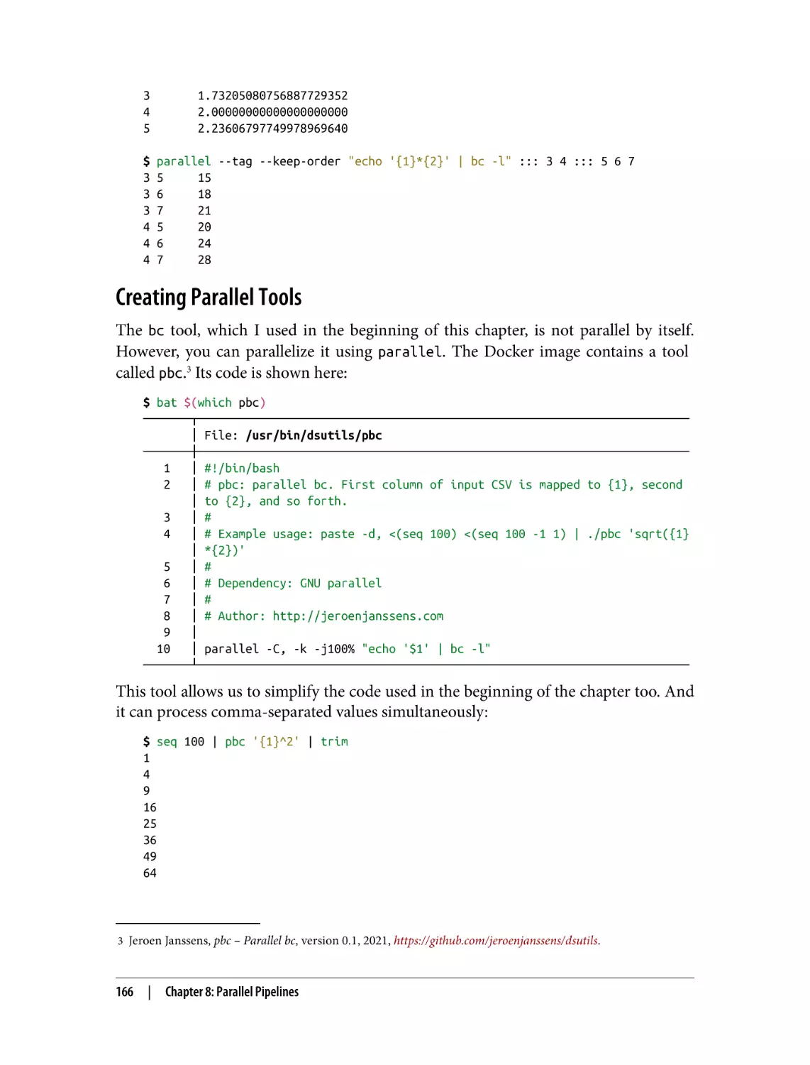
Creating Parallel Tools
Distributed Processing
Get List of Running AWS EC2 Instances
Running Commands on Remote Machines
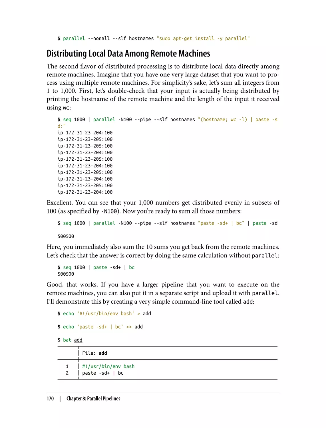
Distributing Local Data Among Remote Machines
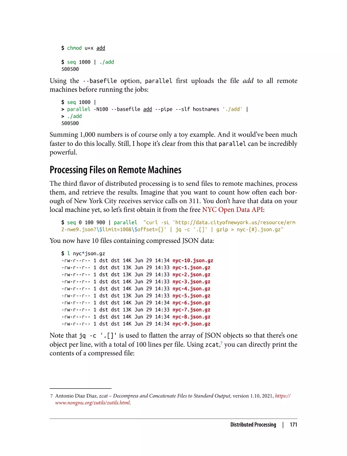
Processing Files on Remote Machines
Summary
For Further Exploration
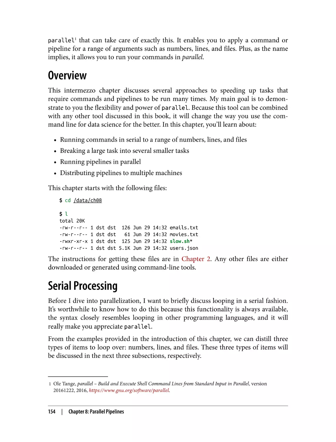
154
154
155
156
157
158
160
162
164
164
166
167
167
169
170
171
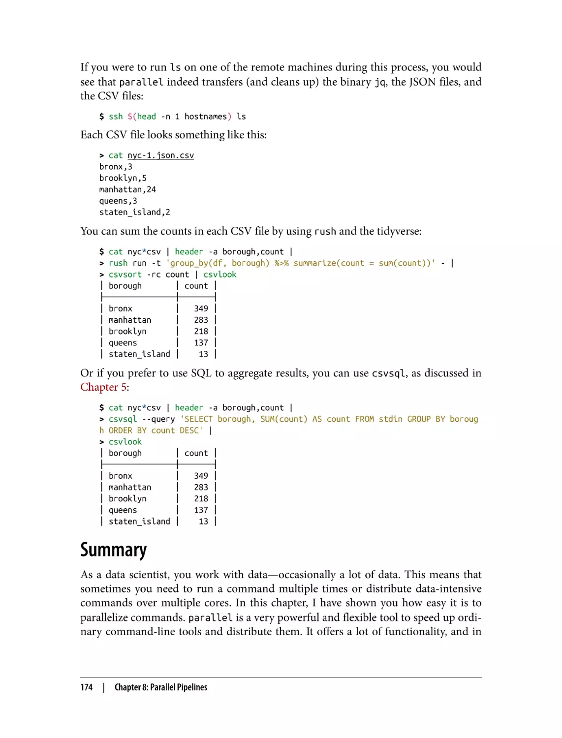
174
175
9. Modeling Data. . . . . . . . . . . . . . . . . . . . . . . . . . . . . . . . . . . . . . . . . . . . . . . . . . . . . . . . . . . . 177
Overview
More Wine, Please!
Dimensionality Reduction with Tapkee
Introducing Tapkee
Linear and Nonlinear Mappings
Regression with Vowpal Wabbit
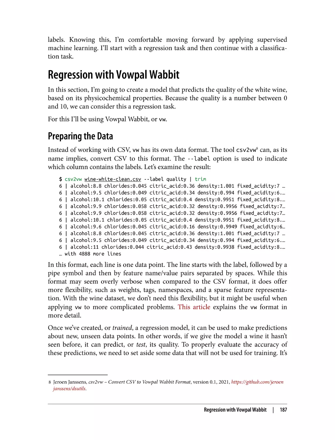
Preparing the Data
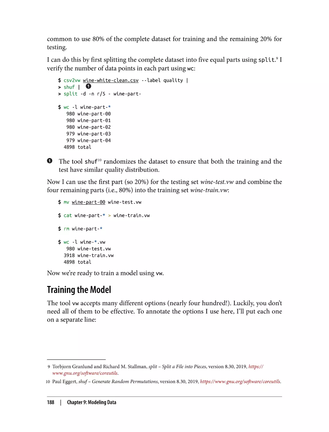
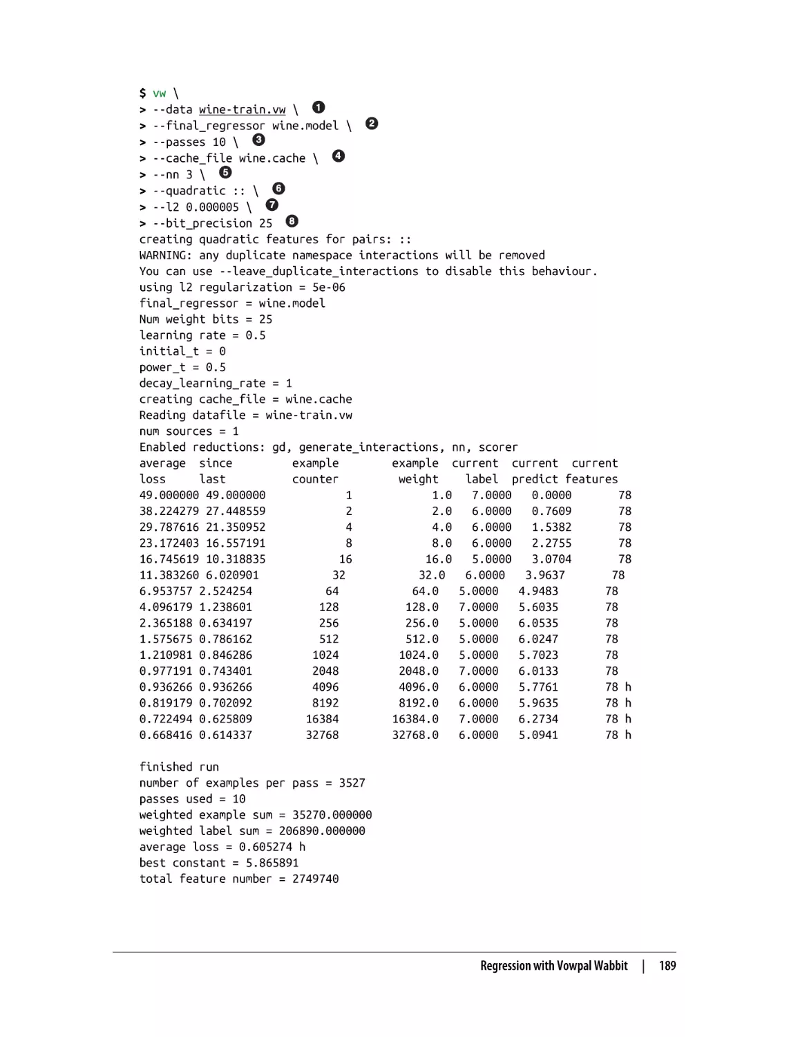
Training the Model
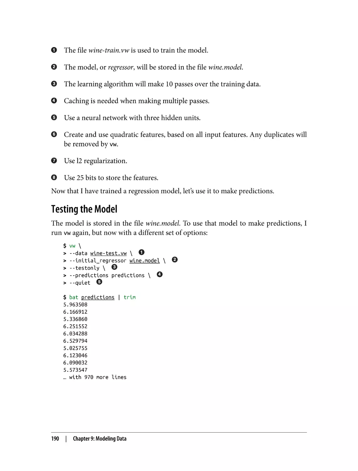
Testing the Model
Classification with SciKit-Learn Laboratory
Preparing the Data
x
|
Table of Contents
178
178
182
183
183
187
187
188
190
193
193
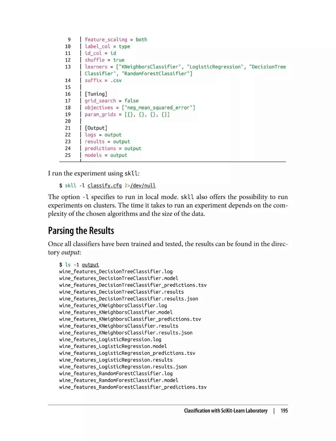
Running the Experiment
Parsing the Results
Summary
For Further Exploration
194
195
197
198
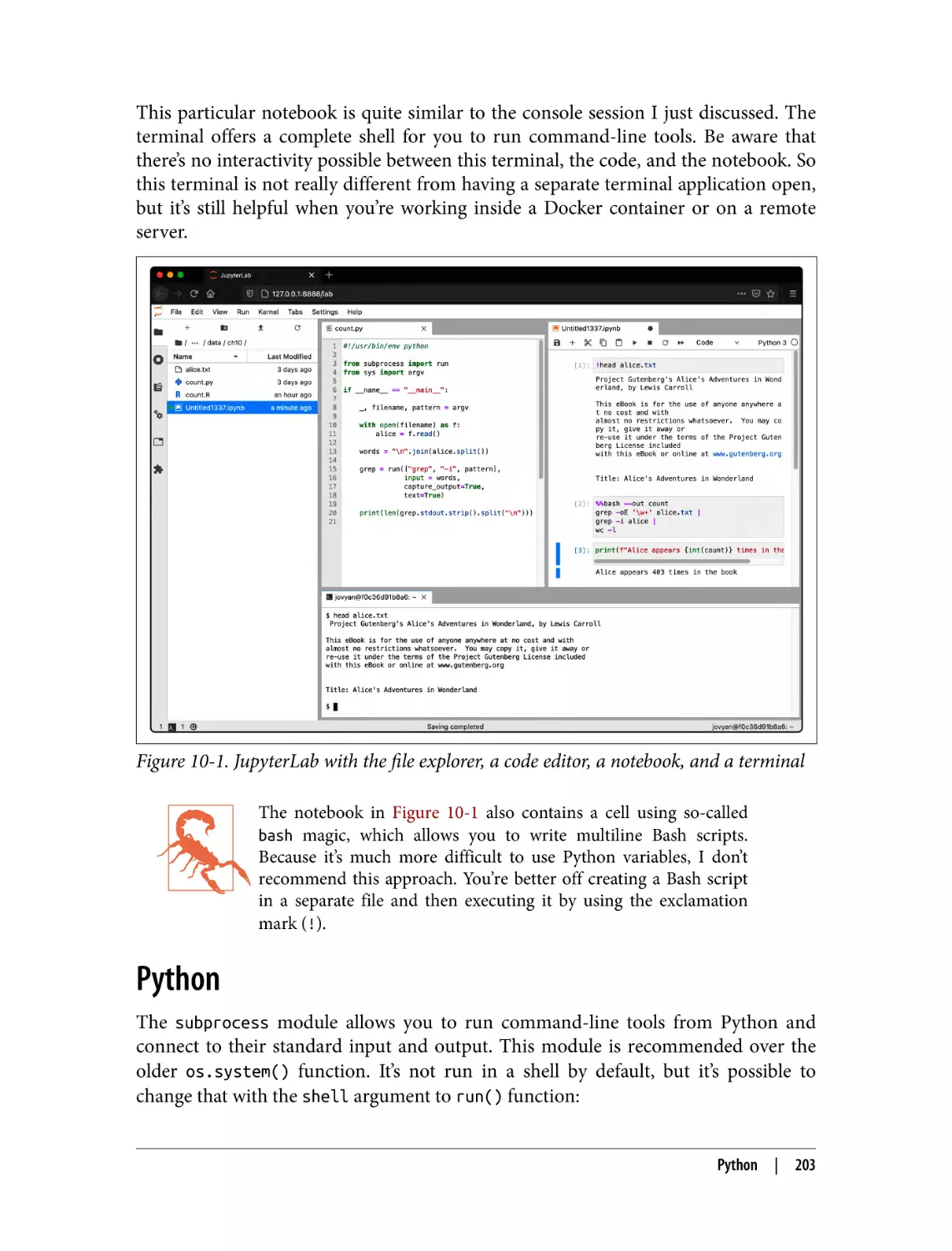
10. Polyglot Data Science. . . . . . . . . . . . . . . . . . . . . . . . . . . . . . . . . . . . . . . . . . . . . . . . . . . . . . 199
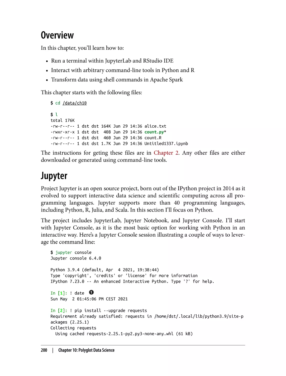
Overview
Jupyter
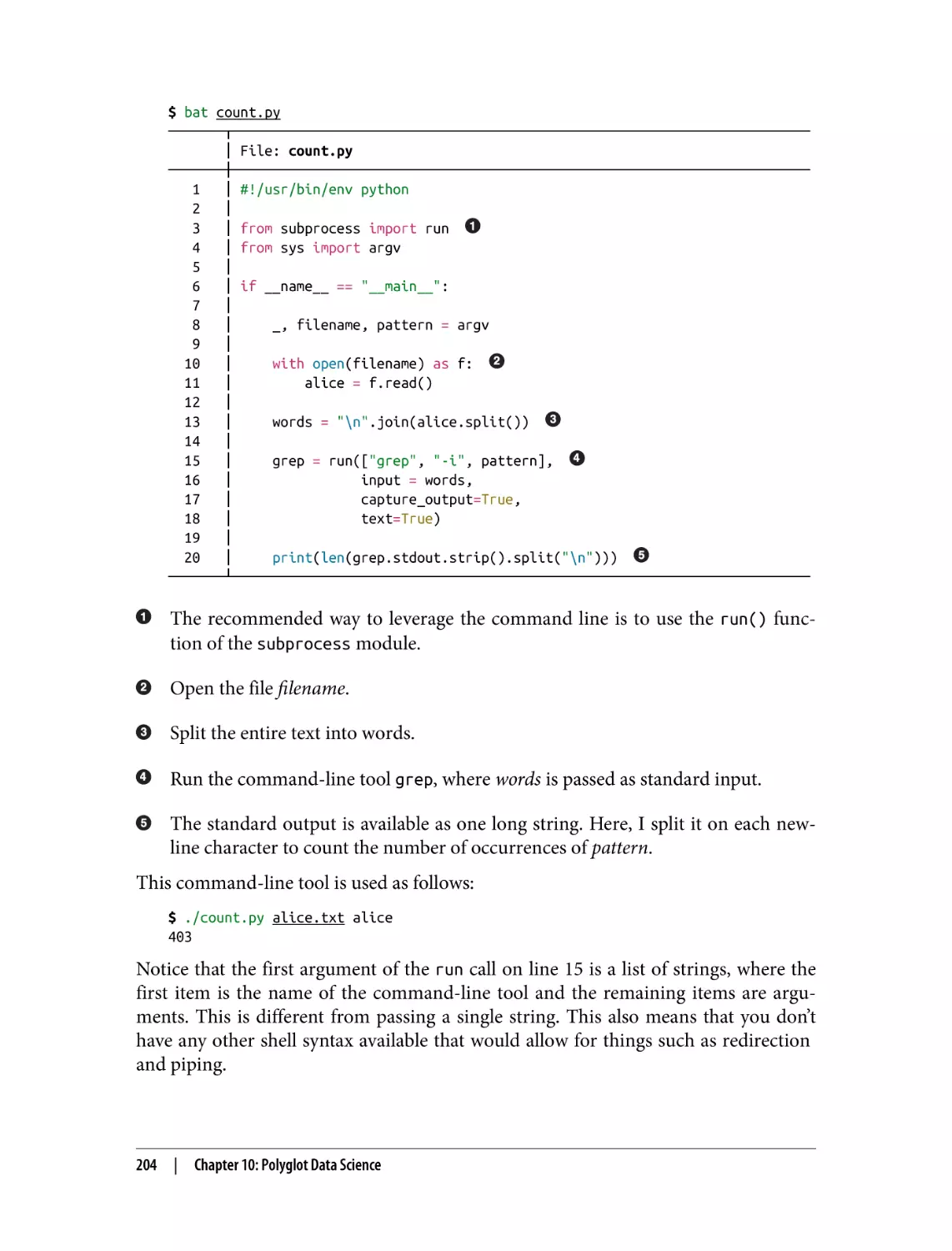
Python
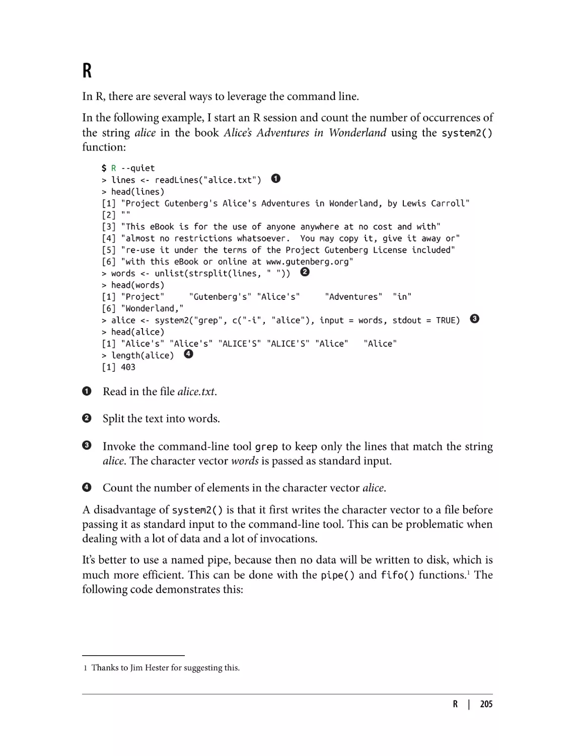
R
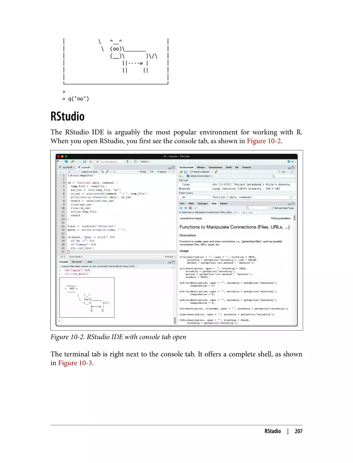
RStudio
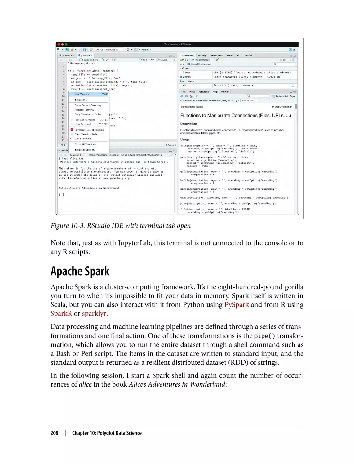
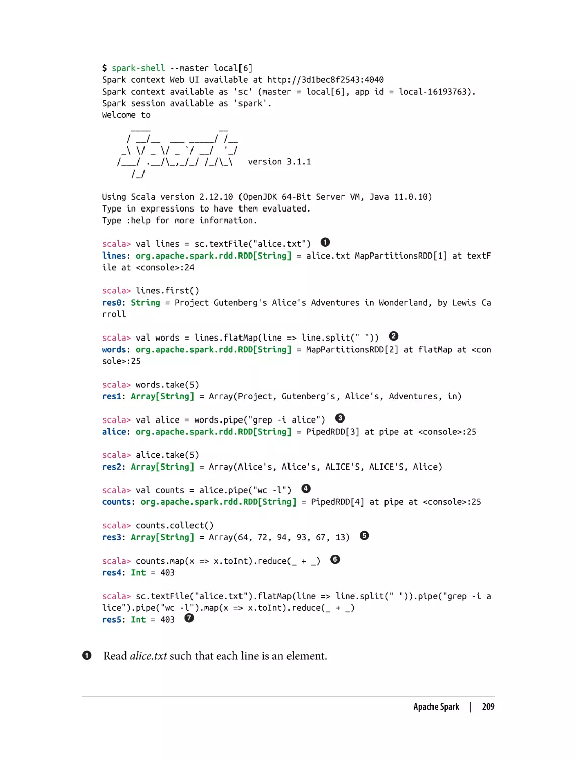
Apache Spark
Summary
For Further Exploration
200
200
203
205
207
208
210
211
11. Conclusion. . . . . . . . . . . . . . . . . . . . . . . . . . . . . . . . . . . . . . . . . . . . . . . . . . . . . . . . . . . . . . . 213
Let’s Recap
Three Pieces of Advice
Be Patient
Be Creative
Be Practical
Where to Go from Here
The Command Line
Shell Programming
Python, R, and SQL
APIs
Machine Learning
Getting in Touch
213
214
214
215
215
215
216
216
216
216
217
217
List of Command-Line Tools. . . . . . . . . . . . . . . . . . . . . . . . . . . . . . . . . . . . . . . . . . . . . . . . . . . . 219
Index. . . . . . . . . . . . . . . . . . . . . . . . . . . . . . . . . . . . . . . . . . . . . . . . . . . . . . . . . . . . . . . . . . . . . . . 249
Table of Contents
|
xi
Foreword
It was love at first sight.
It must have been around 1981 or 1982 that I got my first taste of Unix. Its commandline shell, which uses the same language for single commands and complex programs,
changed my world, and I never looked back.
I was a writer who had discovered the joys of computing, and regular expressions
were my gateway drug. I’d first tried them in the text editor in HP’s RTE operating
system, but it was only when I came to Unix and its philosophy of small cooperating
tools with the command-line shell as the glue that tied them together that I fully
understood their power. Regular expressions in ed, ex, vi (now vim), and emacs were
powerful, sure, but it wasn’t until I saw how ex scripts unbound became sed, the Unix
stream editor, and then AWK, which allowed you to bind programmed actions to
regular expressions, and how shell scripts let you build pipelines not only out of the
existing tools but out of new ones you’d written yourself, that I really got it. Program‐
ming is how you speak with computers, how you tell them what you want them to do,
not just once, but in ways that persist, in ways that can be varied like human lan‐
guage, with repeatable structure but different verbs and objects.
As a beginner, other forms of programming seemed more like recipes to be followed
exactly—careful incantations where you had to get everything right—or like waiting
for a teacher to grade an essay you’d written. With shell programming, there was no
compilation and waiting. It was more like a conversation with a friend. When the
friend didn’t understand, you could easily try again. What’s more, if you had some‐
thing simple to say, you could just say it with one word. And there were already
words for a whole lot of the things you might want to say. But if there weren’t, you
could easily make up new words. And you could string together the words you
learned and the words you made up into gradually more complex sentences, para‐
graphs, and eventually get to persuasive essays.
xiii
Almost every other programming language is more powerful than the shell and its
associated tools, but for me at least, none provides an easier pathway into the pro‐
gramming mindset, and none provides a better environment for a kind of everyday
conversation with the machines that we ask to help us with our work. As Brian Ker‐
nighan, one of the creators of AWK as well as the coauthor of the marvelous book The
Unix Programming Environment, said in an interview with Lex Fridman, “[Unix] was
meant to be an environment where it was really easy to write programs.” [00:23:10]
Kernighan went on to explain why he often still uses AWK rather than writing a
Python program when he’s exploring data: “It doesn’t scale to big programs, but it
does pretty darn well on these little things where you just want to see all the some‐
things in something.” [00:37:01]
In Data Science at the Command Line, Jeroen Janssens demonstrates just how power‐
ful the Unix/Linux approach to the command line is even today. If Jeroen hadn’t
already done so, I’d write an essay here about just why the command line is such a
sweet and powerful match with the kinds of tasks so often encountered in data sci‐
ence. But he already starts out this book by explaining that. So I’ll just say this: the
more you use the command line, the more often you will find yourself coming back
to it as the easiest way to do much of your work. And whether you’re a shell newbie,
or just someone who hasn’t thought much about what a great fit shell programming is
for data science, this is a book you will come to treasure. Jeroen is a great teacher, and
the material he covers is priceless.
— Tim O’Reilly
May 2021
xiv
|
Foreword
Preface
Data science is an exciting field to work in. It’s also still relatively young. Unfortu‐
nately, many people, and many companies as well, believe that you need new technol‐
ogy to tackle the problems posed by data science. However, as this book
demonstrates, many things can be accomplished by using the command line instead,
and sometimes in a much more efficient way.
During my PhD program, I gradually switched from using Microsoft Windows to
using Linux. Because this transition was a bit scary at first, I started with having both
operating systems installed next to each other (known as a dual-boot). The urge to
switch back and forth between Microsoft Windows and Linux eventually faded, and
at some point I was even tinkering around with Arch Linux, which allows you to
build up your own custom Linux machine from scratch. All you’re given is the com‐
mand line, and it’s up to you what to make of it. Out of necessity, I quickly became
very comfortable using the command line. Eventually, as spare time got more pre‐
cious, I settled down with a Linux distribution known as Ubuntu because of its ease
of use and large community. However, the command line is still where I’m spending
most of my time.
It actually wasn’t too long ago that I realized that the command line is not just for
installing software, configuring systems, and searching files. I started learning about
tools such as cut, sort, and sed. These are examples of command-line tools that take
data as input, do something to it, and print the result. Ubuntu comes with quite a few
of them. Once I understood the potential of combining these small tools, I was
hooked.
After earning my PhD, when I became a data scientist, I wanted to use this approach
to do data science as much as possible. Thanks to a couple of new, open source
command-line tools including xml2json, jq, and json2csv, I was even able to use the
command line for tasks such as scraping websites and processing lots of JSON data.
xv
In September 2013, I decided to write a blog post titled “7 Command-Line Tools for
Data Science”. To my surprise, the blog post got quite some attention, and I received a
lot of suggestions of other command-line tools. I started wondering whether the blog
post could be turned into a book. I was pleased that, some 10 months later, and with
the help of many talented people (see the acknowledgments), the answer was yes.
I am sharing this personal story not so much because I think you should know how
this book came about, but because I want to you know that I had to learn about the
command line as well. Because the command line is so different from using a graphi‐
cal user interface, it can seem scary at first. But if I could learn it, then you can as well.
No matter what your current operating system is and no matter how you currently
work with data, after reading this book you will be able to do data science at the com‐
mand line. If you’re already familiar with the command line, or even if you’re already
dreaming in shell scripts, chances are that you’ll still discover a few interesting tricks
or command-line tools to use for your next data science project.
What to Expect from This Book
In this book, we’re going to obtain, scrub, explore, and model data—a lot of it. This
book is not so much about how to become better at those data science tasks. There are
already great resources available that discuss, for example, when to apply which stat‐
istical test or how data can best be visualized. Instead, this practical book aims to
make you more efficient and productive by teaching you how to perform those data
science tasks at the command line.
While this book discusses more than 90 command-line tools, it’s not the tools them‐
selves that matter most. Some command-line tools have been around for a very long
time, while others will be replaced by better ones. New command-line tools are being
created even as you’re reading this. Over the years, I have discovered many amazing
command-line tools. Unfortunately, some of them were discovered too late to be
included in the book. In short, command-line tools come and go. But that’s OK.
What matters most is the underlying idea of working with tools, pipes, and data.
Most command-line tools do one thing and do it well. This is part of the Unix philos‐
ophy, which makes several appearances throughout the book. Once you have become
familiar with the command line, know how to combine command-line tools, and can
even create new ones, you have developed an invaluable skill.
xvi
|
Preface
Changes for the Second Edition
While the command line as a technology and as a way of working is timeless, some of
the tools discussed in the first edition have either been superseded by newer tools
(e.g., csvkit has largely been replaced by xsv) or abandoned by their developers (e.g.,
drake), or they’ve been suboptimal choices (e.g., weka). I have learned a lot since the
first edition was published in October 2014, either through my own experience or as
a result of the useful feedback from my readers. Even though the book is quite niche
because it lies at the intersection of two subjects, there remains a steady interest from
the data science community, as evidenced by the many positive messages I receive
almost every day. By updating the first edition, I hope to keep the book relevant for at
least another five years. Here’s a nonexhaustive list of changes I have made:
• I replaced csvkit with xsv as much as possible. xsv is a faster alternative to
working with CSV files.
• In Chapters 2 and 3, I replaced the VirtualBox image with a Docker image.
Docker is a faster and more lightweight way of running an isolated environment.
• I now use pup instead of scrape to work with HTML. scrape is a Python tool I
created myself. pup is much faster, has more features, and is easier to install.
• Chapter 6 has been rewritten from scratch. Instead of drake, I now use make to
do project management. drake is no longer maintained, and make is much more
mature and very popular with developers.
• I replaced Rio with rush. Rio is a clunky Bash script I created myself. rush is an R
package that is a much more stable and flexible way of using R from the com‐
mand line.
• In Chapter 9 I replaced Weka and BigML with Vowpal Wabbit (vw). Weka is old,
and the way it is used from the command line is clunky. BigML is a commercial
API that I no longer want to rely on. Vowpal Wabbit is a very mature machine
learning tool that was developed at Yahoo! and is now at Microsoft.
• Chapter 10 is an entirely new chapter about integrating the command line into
existing workflows, including Python, R, and Apache Spark. In the first edition I
mentioned that the command line can easily be integrated with existing work‐
flows but never delved into the topic. This chapter fixes that.
How to Read This Book
In general, I advise you to read this book in a linear fashion. Once a concept or
command-line tool has been introduced, chances are that I employ it in a later chap‐
ter. For example, in Chapter 9, I make heavy use of parallel, which is discussed
extensively in Chapter 8.
Preface
|
xvii
Data science is a broad field that intersects many other fields such as programming,
data visualization, and machine learning. As a result, this book touches on many
interesting topics that unfortunately cannot be discussed at great length. At the end of
each chapter, I provide suggestions for further exploration. It’s not required that you
read this material in order to follow along with the book, but if you are interested,
just know that there’s much more to learn.
Who This Book Is For
This book makes just one assumption about you: that you work with data. It doesn’t
matter which programming language or statistical computing environment you’re
currently using. The book explains all the necessary concepts from the beginning.
It also doesn’t matter whether your operating system is Microsoft Windows, macOS,
or some flavor of Linux. The book comes with a Docker image, which is an easy-toinstall virtual environment. It allows you to run the command-line tools and follow
along with the code examples in the same environment as this book was written. You
don’t have to waste time figuring out how to install all the command-line tools and
their dependencies.
The book contains some code in Bash, Python, and R, so it’s helpful if you have some
programming experience, but it’s by no means required to follow along with the
examples.
Conventions Used in This Book
The following typographical conventions are used in this book:
Italic
Indicates new terms, URLs, directory names, and filenames.
Constant width
Used for code and commands, as well as within paragraphs to refer to commandline tools and their options.
Constant width bold
Shows commands or other text that should be typed literally by the user.
Constant width italic
Shows text that should be replaced with user-supplied values or by values deter‐
mined by context.
xviii
| Preface
This element signifies a tip or suggestion.
This element signifies a general note.
This element indicates a warning or caution.
O’Reilly Online Learning
For more than 40 years, O’Reilly Media has provided technol‐
ogy and business training, knowledge, and insight to help
companies succeed.
Our unique network of experts and innovators share their knowledge and expertise
through books, articles, and our online learning platform. O’Reilly’s online learning
platform gives you on-demand access to live training courses, in-depth learning
paths, interactive coding environments, and a vast collection of text and video from
O’Reilly and 200+ other publishers. For more information, visit http://oreilly.com.
How to Contact Us
Please address comments and questions concerning this book to the publisher:
O’Reilly Media, Inc.
1005 Gravenstein Highway North
Sebastopol, CA 95472
800-998-9938 (in the United States or Canada)
707-829-0515 (international or local)
707-829-0104 (fax)
We have a web page for this book, where we list errata, examples, and any additional
information. You can access this at https://oreil.ly/data-science-at-cl.
Preface
|
xix
Email bookquestions@oreilly.com to comment or ask technical questions about this
book. The author also maintains a version of the book online.
For news and information about our books and courses, visit http://oreilly.com.
Find us on Facebook: http://facebook.com/oreilly
Follow us on Twitter: http://twitter.com/oreillymedia
Watch us on YouTube: http://youtube.com/oreillymedia
Acknowledgments for the Second Edition (2021)
Seven years have passed since the first edition came out. During this time, and espe‐
cially during the last 13 months, many people have helped me. Without them, I
would have never been able to write a second edition.
I was once again blessed with three wonderful editors at O’Reilly. I would like to
thank Sarah “Embrace the deadline” Grey, Jess “Pedal to the metal” Haberman, and
Kate “Let it go” Galloway. Their middle names say it all. With their incredible help, I
was able to embrace the deadlines, put the pedal to metal when it mattered, and even‐
tually let it go. I’d also like to thank their colleagues Angela Rufino, Arthur Johnson,
Cassandra Furtado, David Futato, Helen Monroe, Karen Montgomery, Kate Dullea,
Kristen Brown, Marie Beaugureau, Marsee Henon, Nick Adams, Regina Wilkinson,
Shannon Cutt, Shannon Turlington, and Yasmina Greco, for making the collabora‐
tion with O’Reilly such a pleasure.
Despite having an automated process to execute the code and paste back the results
(thanks to R Markdown and Docker), the number of mistakes I was able to make is
impressive. Thank you Aaditya Maruthi, Brian Eoff, Caitlin Hudon, Julia Silge Mike
Dewar, and Shane Reustle for reducing this number immensely. Of course, any mis‐
takes left are my responsibility.
Marc Canaleta deserves a special thank you. In October 2014, shortly after the first
edition came out, Marc invited me to give a one-day workshop about Data Science at
the Command Line to his team at Social Point in Barcelona. Little did we both know
that many workshops would follow. It eventually led me to start my own company:
Data Science Workshops. Every time I teach, I learn something new. They probably
don’t know it, but each student has had an impact, in one way or another, on this
book. To them I say: thank you. I hope I can teach for a very long time.
Captivating conversations, splendid suggestions, and passionate pull requests. I
greatly appreciate each and every contribution by following generous people: Adam
Johnson, Andre Manook, Andrea Borruso, Andres Lowrie, Andrew Berisha, Andrew
Gallant, Andrew Sanchez, Anicet Ebou, Anthony Egerton, Ben Isenhart,
Chris Wiggins, Chrys Wu, Dan Nguyen, Darryl Amatsetam, Dmitriy Rozhkov, Doug
xx
|
Preface
Needham, Edgar Manukyan, Erik Swan, Felienne Hermans, George Kampolis, Giel
van Lankveld, Greg Wilson, Hay Kranen, Ioannis Cherouvim, Jake Hofman, Jannes
Muenchow, Jared Lander, Jay Roaf, Jeffrey Perkel, Jim Hester, Joachim Hagege, Joel
Grus, John Cook, John Sandall, Joost Helberg, Joost van Dijk, Joyce Robbins, Julian
Hatwell, Karlo Guidoni, Karthik Ram, Lissa Hyacinth, Longhow Lam, Lui Pillmann,
Lukas Schmid, Luke Reding, Maarten van Gompel, Martin Braun, Max Schelker, Max
Shron, Nathan Furnal, Noah Chase, Oscar Chic, Paige Bailey, Peter Saalbrink, Rich
Pauloo, Richard Groot, Rico Huijbers, Rob Doherty, Robbert van Vlijmen, Russell
Scudder, Sylvain Lapoix, TJ Lavelle, Tan Long, Thomas Stone, Tim O’Reilly, Vincent
Warmerdam, and Yihui Xie.
Throughout this book, and especially in the footnotes and appendix, you’ll find hun‐
dreds of names. These names belong to the authors of the many tools, books, and
other resources on which this book stands. I’m incredibly grateful for their hard
work, regardless of whether that work was done 50 years or 50 days ago.
Above all, I would like to thank my wife Esther, my daughter Florien, and my son
Olivier for reminding me daily what truly matters. I promise it’ll be a few years before
I start writing the third edition.
Acknowledgments for the First Edition (2014)
First of all, I’d like to thank Mike Dewar and Mike Loukides for believing that my
blog post, “7 Command-Line Tools for Data Science”, which I wrote in September
2013, could be expanded into a book.
Special thanks to my technical reviewers Mike Dewar, Brian Eoff, and Shane Reustle
for reading various drafts, meticulously testing all the commands, and providing
invaluable feedback. Your efforts have improved the book greatly. Any remaining
errors are entirely my own responsibility.
I had the privilege of working with three amazing editors: Ann Spencer, Julie Steele,
and Marie Beaugureau. Thank you for your guidance and for being such great liai‐
sons with the many talented people at O’Reilly. Those people include Laura Baldwin,
Huguette Barriere, Sophia DeMartini, Yasmina Greco, Rachel James, Ben Lorica,
Mike Loukides, and Christopher Pappas. There are many others whom I haven’t met
because they are operating behind the scenes. Together they ensured that working
with O’Reilly has truly been a pleasure.
This book discusses more than 80 command-line tools. Needless to say, without these
tools, this book wouldn’t have existed in the first place. I’m therefore extremely grate‐
ful to all the authors who created and contributed to these tools. The complete list of
authors is unfortunately too long to include here; they are mentioned in the
Appendix. Thanks especially to Aaron Crow, Jehiah Czebotar, Christoph Groskopf,
Preface
|
xxi
Dima Kogan, Sergey Lisitsyn, Francisco J. Martin, and Ole Tange for providing help
with their amazing command-line tools.
Eric Postma and Jaap van den Herik, who supervised me during my PhD program,
deserve special thanks. Over the course of five years they taught me many lessons.
Although writing a technical book is quite different from writing a PhD thesis, many
of those lessons proved to be very helpful in the past nine months as well.
Finally, I’d like to thank my colleagues at YPlan, my friends, my family, and especially
my wife, Esther, for supporting me and for pulling me away from the command line
at just the right times.
xxii
| Preface
CHAPTER 1
Introduction
This book is about doing data science at the command line. My aim is to make you a
more efficient and productive data scientist by teaching you how to leverage the
power of the command line.
Having both data science and command line in the book’s title requires an explana‐
tion. How can a technology that is more than 50 years old1 be of any use to a field that
is only a few years young?
Today, data scientists can choose from an overwhelming collection of exciting tech‐
nologies and programming languages. Python, R, Julia, and Apache Spark are but a
few examples. You may already have experience in one or more of these. And if so,
why should you still care about the command line for doing data science? What does
the command line have to offer that these other technologies and programming lan‐
guages do not?
These are valid questions. In this opening chapter I will answer these questions as fol‐
lows. First, I provide a practical definition of data science that will act as the backbone
of this book. Second, I’ll list five important advantages of the command line. By the
end of this chapter, I hope to have convinced you that the command line is indeed
worth learning for doing data science.
1 The development of the UNIX operating system started back in 1969. It featured a command line since the
beginning. The important concept of pipes, which I will discuss in “Essential Unix Concepts” on page 13, was
added in 1973.
1
Data Science Is OSEMN
The field of data science is still in its infancy, and as such, there exist various defini‐
tions of what it encompasses. Throughout this book I employ a very practical defini‐
tion devised by Hilary Mason and Chris H. Wiggins.2 They define data science
according to the following five steps: (1) obtaining data, (2) scrubbing data, (3)
exploring data, (4) modeling data, and (5) interpreting data. Together, these steps
form the OSEMN (pronounced awesome) model. This definition serves as the back‐
bone of this book because each step (except for step 5, interpreting data, which I’ll
explain shortly) has its own chapter.
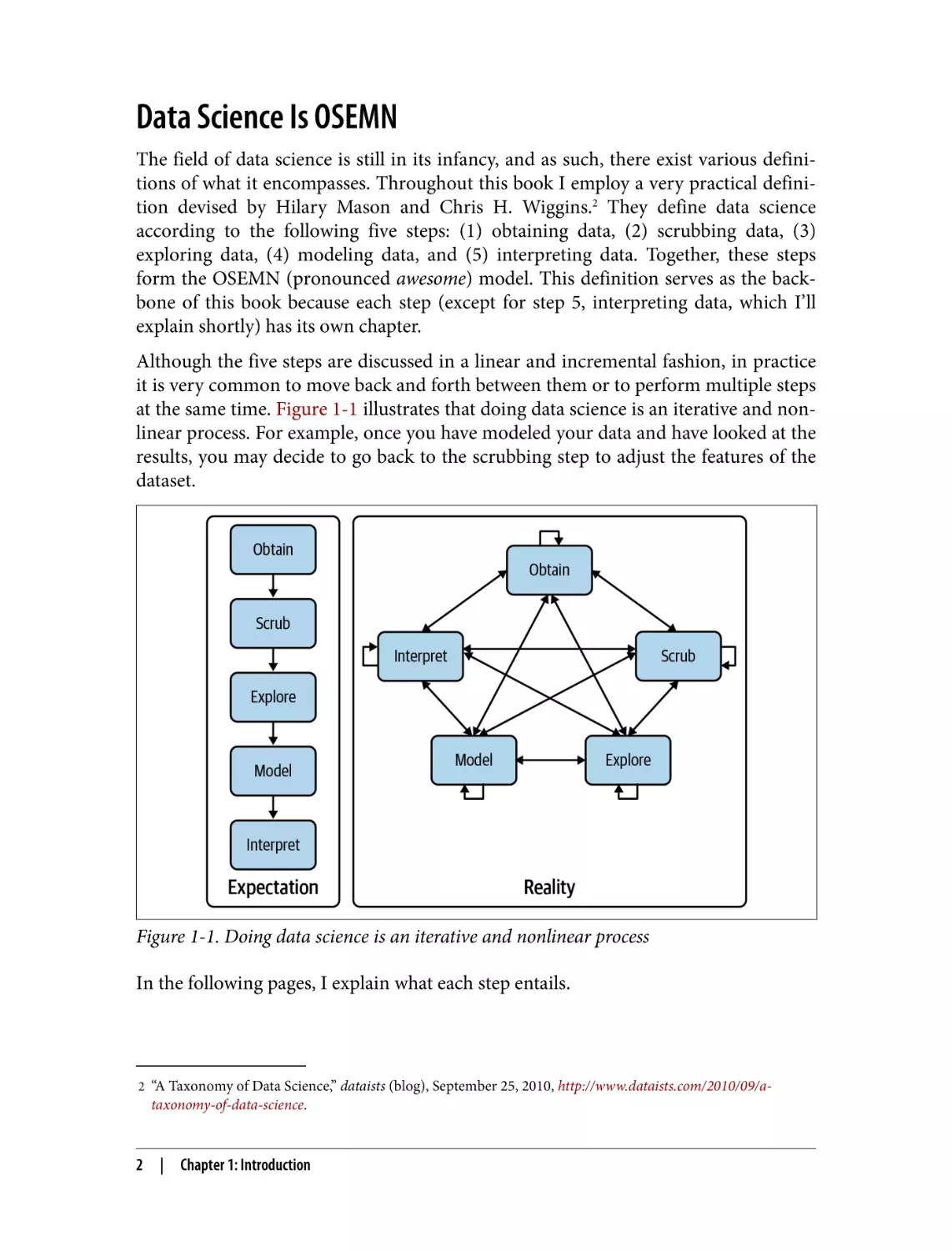
Although the five steps are discussed in a linear and incremental fashion, in practice
it is very common to move back and forth between them or to perform multiple steps
at the same time. Figure 1-1 illustrates that doing data science is an iterative and nonlinear process. For example, once you have modeled your data and have looked at the
results, you may decide to go back to the scrubbing step to adjust the features of the
dataset.
Figure 1-1. Doing data science is an iterative and nonlinear process
In the following pages, I explain what each step entails.
2 “A Taxonomy of Data Science,” dataists (blog), September 25, 2010, http://www.dataists.com/2010/09/a-
taxonomy-of-data-science.
2
|
Chapter 1: Introduction
Obtaining Data
Without any data, there is little data science you can do. So the first step is obtaining
data. Unless you are fortunate enough to already possess data, you may need to do
one or more of the following:
• Download data from another location (e.g., a web page or server)
• Query data from a database or API (e.g., MySQL or Twitter)
• Extract data from another file (e.g., an HTML file or spreadsheet)
• Generate data yourself (e.g., reading sensors or taking surveys)
In Chapter 3, I discuss several methods for obtaining data using the command line.
The obtained data will most likely be in plain text, CSV, JSON, HTML, or XML for‐
mat. The next step is to scrub this data.
Scrubbing Data
It is not uncommon for the obtained data to have missing values, inconsistencies,
errors, weird characters, or uninteresting columns. In such cases, you have to scrub,
or clean, the data before you can do anything interesting with it. Common scrubbing
operations include:
• Filtering lines
• Extracting certain columns
• Replacing values
• Extracting words
• Handling missing values and duplicates
• Converting data from one format to another
While we data scientists love to create exciting data visualizations and insightful mod‐
els (steps 3 and 4 of the OSEMN model), usually much effort goes into obtaining and
scrubbing the required data first (steps 1 and 2). In Data Jujitsu(O’Reilly), DJ Patil
states that “80% of the work in any data project is in cleaning the data.” In Chapter 5, I
demonstrate how the command line can help accomplish such data scrubbing
operations.
Exploring Data
Once you have scrubbed your data, you are ready to explore it. This is where it gets
interesting, because it’s when you’re exploring that you truly get to know your data. In
Chapter 7 I show you how the command line can be used to:
Data Science Is OSEMN
|
3
• Look at your data
• Derive statistics from your data
• Create insightful visualizations
Command-line tools used in Chapter 7 include csvstat and rush.
Modeling Data
If you want to explain your data or predict what will happen, you probably want to
create a statistical model of the data. Techniques to create a model include clustering,
classification, regression, and dimensionality reduction. The command line is not
suitable for programming a new type of model from scratch. It is, however, very use‐
ful to be able to build a model from the command line. In Chapter 9 I will introduce
several command-line tools that either build a model locally or employ an API to per‐
form the computation in the cloud.
Interpreting Data
The final and perhaps most important step in the OSEMN model is interpreting data.
This step involves:
• Drawing conclusions from your data
• Evaluating what your results mean
• Communicating your results
To be honest, the computer is of little use here, and the command line does not really
come into play at this stage. Once you have reached this step, it’s up to you. This is the
only step in the OSEMN model that does not have its own chapter. Instead, I refer
you to the book Thinking with Data by Max Shron (O’Reilly).
Intermezzo Chapters
Besides the chapters that cover the OSEMN steps, there are four intermezzo chapters.
Each discusses a more general topic concerning data science and how the command
line is employed for that. These topics are applicable to any step in the data science
process.
In Chapter 4, I discuss how to create reusable tools for the command line. These per‐
sonal tools can come from long commands that you have typed on the command line
or from existing code that you have written in, say, Python or R. Being able to create
your own tools allows you to become more efficient and productive.
4
|
Chapter 1: Introduction
Because the command line is an interactive environment for doing data science, it
can become challenging to keep track of your workflow. In Chapter 6, I demonstrate
a command-line tool called make, which allows you to define your data science work‐
flow in terms of tasks and the dependencies between them. This tool increases the
reproducibility of your workflow, not only for you but also for your colleagues and
peers.
In Chapter 8, I explain how your commands and tools can be sped up by running
them in parallel. Using a command-line tool called GNU Parallel, you can apply
command-line tools to very large datasets and run them on multiple cores or even on
remote machines.
In Chapter 10, I discuss how to employ the power of the command line in other envi‐
ronments and programming languages, such as R, RStudio, Python, Jupyter Note‐
books, and even Apache Spark.
What Is the Command Line?
Before I discuss why you should use the command line for data science, let’s take a
peek at what the command line actually looks like (it may be already familiar to you).
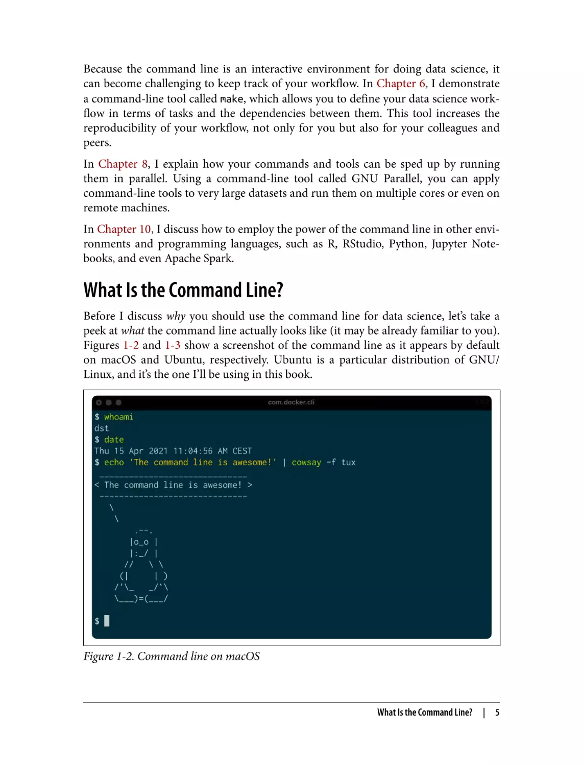
Figures 1-2 and 1-3 show a screenshot of the command line as it appears by default
on macOS and Ubuntu, respectively. Ubuntu is a particular distribution of GNU/
Linux, and it’s the one I’ll be using in this book.
Figure 1-2. Command line on macOS
What Is the Command Line?
|
5
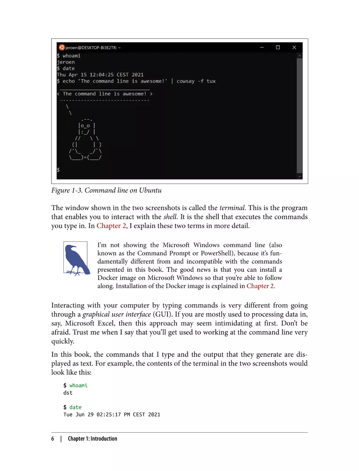
Figure 1-3. Command line on Ubuntu
The window shown in the two screenshots is called the terminal. This is the program
that enables you to interact with the shell. It is the shell that executes the commands
you type in. In Chapter 2, I explain these two terms in more detail.
I’m not showing the Microsoft Windows command line (also
known as the Command Prompt or PowerShell), because it’s fun‐
damentally different from and incompatible with the commands
presented in this book. The good news is that you can install a
Docker image on Microsoft Windows so that you’re able to follow
along. Installation of the Docker image is explained in Chapter 2.
Interacting with your computer by typing commands is very different from going
through a graphical user interface (GUI). If you are mostly used to processing data in,
say, Microsoft Excel, then this approach may seem intimidating at first. Don’t be
afraid. Trust me when I say that you’ll get used to working at the command line very
quickly.
In this book, the commands that I type and the output that they generate are dis‐
played as text. For example, the contents of the terminal in the two screenshots would
look like this:
$ whoami
dst
$ date
Tue Jun 29 02:25:17 PM CEST 2021
6
|
Chapter 1: Introduction
$ echo 'The command line is awesome!' | cowsay -f tux
______________________________
< The command line is awesome! >
-----------------------------\
\
.--.
|o_o |
|:_/ |
//
\ \
(|
| )
/'\_
_/`\
\___)=(___/
$
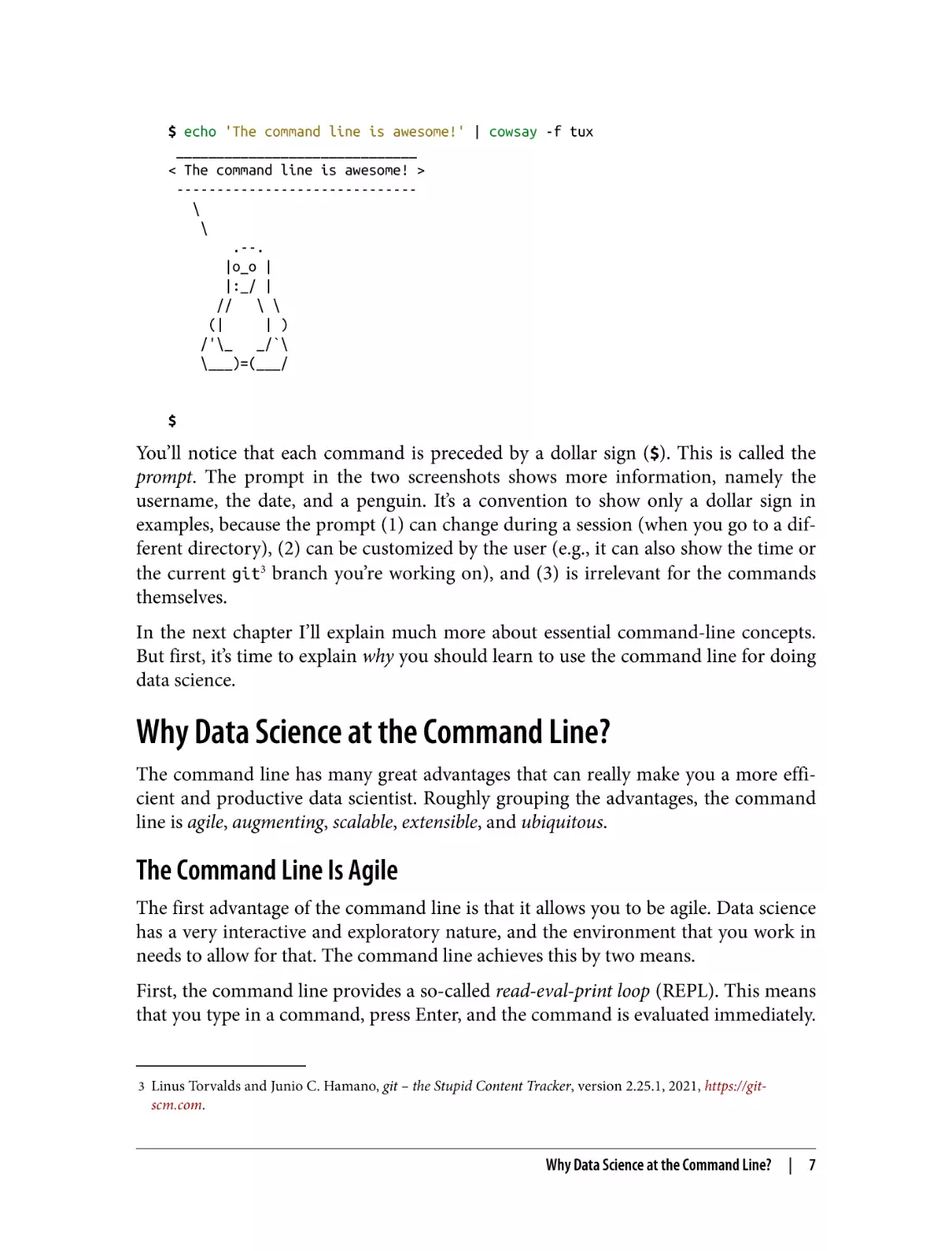
You’ll notice that each command is preceded by a dollar sign ($). This is called the
prompt. The prompt in the two screenshots shows more information, namely the
username, the date, and a penguin. It’s a convention to show only a dollar sign in
examples, because the prompt (1) can change during a session (when you go to a dif‐
ferent directory), (2) can be customized by the user (e.g., it can also show the time or
the current git3 branch you’re working on), and (3) is irrelevant for the commands
themselves.
In the next chapter I’ll explain much more about essential command-line concepts.
But first, it’s time to explain why you should learn to use the command line for doing
data science.
Why Data Science at the Command Line?
The command line has many great advantages that can really make you a more effi‐
cient and productive data scientist. Roughly grouping the advantages, the command
line is agile, augmenting, scalable, extensible, and ubiquitous.
The Command Line Is Agile
The first advantage of the command line is that it allows you to be agile. Data science
has a very interactive and exploratory nature, and the environment that you work in
needs to allow for that. The command line achieves this by two means.
First, the command line provides a so-called read-eval-print loop (REPL). This means
that you type in a command, press Enter, and the command is evaluated immediately.
3 Linus Torvalds and Junio C. Hamano, git – the Stupid Content Tracker, version 2.25.1, 2021, https://git-
scm.com.
Why Data Science at the Command Line?
|
7
A REPL is often much more convenient for doing data science than the edit-compilerun-debug cycle associated with scripts, large programs, and, say, Hadoop jobs. Your
commands are executed immediately, may be stopped at will, and can be changed
quickly. This short iteration cycle really allows you to play with your data.
Second, the command line is very close to the filesystem. Because data is the main
ingredient for doing data science, it is important to be able to work easily with the
files that contain your dataset. The command line offers many convenient tools for
this.
The Command Line Is Augmenting
The command line integrates well with other technologies. Whatever technology
your data science workflow currently includes (whether it’s R, Python, or Excel),
please know that I’m not suggesting you abandon that workflow. Instead, consider
the command line as an augmenting technology that amplifies the technologies
you’re currently employing. It can do so in three ways.
First, the command line can act as a glue between many different data science tools.
One way to glue tools is by connecting the output from the first tool to the input of
the second tool. In Chapter 2 I explain how this works.
Second, you can often delegate tasks to the command line from your own environ‐
ment. For example, Python, R, and Apache Spark allow you to run command-line
tools and capture their output. I demonstrate this with examples in Chapter 10.
Third, you can convert your code (e.g., a Python or R script) into a reusable
command-line tool. That way, the language that it’s written in doesn’t matter any‐
more; it can be used from the command line directly or from any environment that
integrates with the command line, as mentioned in the previous paragraph. I explain
how to do this in Chapter 4.
In the end, every technology has its strengths and weaknesses, so it’s good to know
several technologies and use the one that is most appropriate for the task at hand.
Sometimes that means using R, sometimes the command line, and sometimes even
pen and paper. By the end of this book you’ll have a solid understanding of when you
should use the command line, and when you’re better off continuing with your favor‐
ite programming language or statistical computing environment.
The Command Line Is Scalable
As I’ve said before, working on the command line is very different from using a GUI.
On the command line you do things by typing, whereas with a GUI you do things by
pointing and clicking with a mouse.
8
|
Chapter 1: Introduction
Everything that you type manually on the command line can also be automated
through scripts and tools. This makes it very easy to rerun your commands if you
made a mistake, when the input data has changed, or because your colleague wants to
perform the same analysis. Moreover, your commands can be run at specific inter‐
vals, on a remote server, and in parallel on many chunks of data (more on that in
Chapter 8).
Because the command line is automatable, it becomes scalable and repeatable. It’s not
straightforward to automate pointing and clicking, which makes a GUI a less suitable
environment for doing scalable and repeatable data science.
The Command Line Is Extensible
The command line itself was invented over 50 years ago. Its core functionality has
largely remained unchanged, but its tools, which are the workhorses of the command
line, are being developed on a daily basis.
The command line itself is language agnostic. This allows the command-line tools to
be written in many different programming languages. The open source community is
producing many free and high-quality command-line tools that we can use for data
science.
These command-line tools can work together, which makes the command line very
flexible. You can also create your own tools, allowing you to extend the effective func‐
tionality of the command line.
The Command Line Is Ubiquitous
Because the command line comes with any Unix-like operating system, including
Ubuntu Linux and macOS, it can be found in many places. Plus, 100% of the top five
hundred supercomputers are running Linux.4 So if you ever get your hands on one of
those supercomputers (or if you ever find yourself in Jurassic Park with the door
locks not working), you’d better know your way around the command line!
But Linux doesn’t run only on supercomputers. It also runs on servers, laptops, and
embedded systems. These days, many companies offer cloud computing, where you
can easily launch new machines on the fly. If you ever log in to such a machine (or a
server in general), it’s almost certain that you’ll arrive at the command line.
It’s also important to note that the command line isn’t just hype. This technology has
been around for more than five decades, and I’m convinced that it’s here to stay for
another five. Learning how to use the command line (for data science and in general)
is therefore a worthwhile investment.
4 See TOP500, which keeps track of how many supercomputers run Linux.
Why Data Science at the Command Line?
|
9
Summary
In this chapter I have introduced you to the OSEMN model for doing data science,
which I use as a guide throughout the book. I have provided some background about
the Unix command line and hopefully convinced you that it’s a suitable environment
for doing data science. In the next chapter I’ll show you how to get started by instal‐
ling the datasets and tools and explain the fundamental concepts.
For Further Exploration
• The book UNIX: A History and a Memoir by Brian W. Kernighan (self-published)
tells the story of Unix, explaining what it is, how it was developed, and why it
matters.
• In 2018, I gave a presentation titled “50 Reasons to Learn the Shell for Doing
Data Science” at Strata London. You can read the slides if you need even more
convincing.
• The short but sweet book Thinking with Data by Max Shron (O’Reilly) focuses on
the why instead of the how and provides a framework for defining your data sci‐
ence project that will help you ask the right questions and solve the right
problems.
10
|
Chapter 1: Introduction
CHAPTER 2
Getting Started
In this chapter, I’m going to make sure that you have all the prerequisites for doing
data science at the command line. The prerequisites are threefold: (1) having the
same datasets that I use in this book, (2) having a proper environment with all the
command-line tools that I use throughout this book, and (3) understanding the
essential concepts that come into play when using the command line.
First, I describe how to download the datasets. Second, I explain how to install the
Docker image, which is a virtual environment based on Ubuntu Linux that contains
all the necessary command-line tools. Finally, I go over the essential Unix concepts
through examples.
By the end of this chapter, you’ll have everything you need to continue with the first
step of doing data science, namely obtaining data.
Getting the Data
The datasets I use in this book can be obtained as follows:
1. Download the ZIP file from the book’s website.
2. Create a new directory. You can give this directory any name you like, but I rec‐
ommend you stick to lowercase letters, numbers, and maybe a hyphen or an
underscore so that the name is easier to work with at the command line—for
example, dsatcl2. Remember where this directory is.
3. Move the ZIP file to that new directory and unpack it.
4. This directory now contains one subdirectory per chapter.
11
In the next section I explain how to install the environment containing all the
command-line tools to work with this data.
Installing the Docker Image
In this book we use many different command-line tools. Unix often comes with a lot
of command-line tools preinstalled and offers many packages that contain more rele‐
vant tools. Installing these packages yourself is often not too difficult. However, we’ll
also use tools that are not available as packages and require a more manual and more
involved installation. So that you can acquire the necessary command-line tools
without having to go through the installation process for each tool, I encourage you,
whether you’re on Windows, macOS, or Linux, to install the Docker image that was
created specifically for this book.
A Docker image is a bundle of one or more applications together with all their depen‐
dencies. A Docker container is an isolated environment that runs an image. You can
manage Docker images and containers using the docker command-line tool (which
is what you’ll do below) or the Docker GUI. In a way, a Docker container is like a
virtual machine, only a Docker container uses far fewer resources. At the end of this
chapter I suggest some resources for learning more about Docker.
If you still prefer to run the command-line tools natively rather
than inside a Docker container, then you can, of course, install the
command-line tools individually yourself. The code to build the
Docker image can be found on GitHub and may serve as a guide to
help you with that. Please be aware that this can be time consuming
for some tools, as they require many nontrivial steps, such as
compiling from source.
To install the Docker image, you first need to download Docker itself from the
Docker website. Once it is installed, you invoke the following command on your ter‐
minal or command prompt to download the Docker image (don’t type the dollar
sign):
$ docker pull datasciencetoolbox/dsatcl2e
You can run the Docker image as follows:
$ docker run --rm -it datasciencetoolbox/dsatcl2e
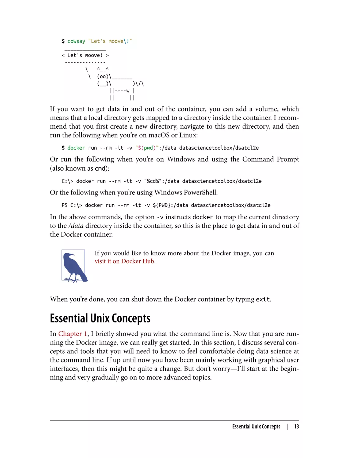
You’re now inside an isolated environment known as a Docker container that has all
the necessary command-line tools installed. If the following command produces an
enthusiastic cow, then you know everything is working correctly:
12
|
Chapter 2: Getting Started
$ cowsay "Let's moove\!"
______________
< Let's moove! >
-------------\ ^__^
\ (oo)\_______
(__)\
)\/\
||----w |
||
||
If you want to get data in and out of the container, you can add a volume, which
means that a local directory gets mapped to a directory inside the container. I recom‐
mend that you first create a new directory, navigate to this new directory, and then
run the following when you’re on macOS or Linux:
$ docker run --rm -it -v "$(pwd)":/data datasciencetoolbox/dsatcl2e
Or run the following when you’re on Windows and using the Command Prompt
(also known as cmd):
C:\> docker run --rm -it -v "%cd%":/data datasciencetoolbox/dsatcl2e
Or the following when you’re using Windows PowerShell:
PS C:\> docker run --rm -it -v ${PWD}:/data datasciencetoolbox/dsatcl2e
In the above commands, the option -v instructs docker to map the current directory
to the /data directory inside the container, so this is the place to get data in and out of
the Docker container.
If you would like to know more about the Docker image, you can
visit it on Docker Hub.
When you’re done, you can shut down the Docker container by typing exit.
Essential Unix Concepts
In Chapter 1, I briefly showed you what the command line is. Now that you are run‐
ning the Docker image, we can really get started. In this section, I discuss several con‐
cepts and tools that you will need to know to feel comfortable doing data science at
the command line. If up until now you have been mainly working with graphical user
interfaces, then this might be quite a change. But don’t worry—I’ll start at the begin‐
ning and very gradually go on to more advanced topics.
Essential Unix Concepts
|
13
This section is not a complete course in Unix. I will explain only
the concepts and tools that are relevant to doing data science. One
of the advantages of the Docker image is that a lot is already set up.
If you wish to know more, consult “For Further Exploration” on
page 33.
The Environment
So you’ve just logged in to a brand-new environment. Before you do anything, it’s
worthwhile to get a high-level understanding of this environment, which is roughly
defined by four layers, listed here from the top down:
Command-line tools
First and foremost, there are the command-line tools that you work with. We use
them by typing their corresponding commands. There are different types of
command-line tools, which I will discuss in the next section. Examples of tools
are ls,1 cat,2 and jq.3
Terminal
The terminal, which is the second layer, is the application that we type our com‐
mands in. If you see the following text mentioned in the book:
$ seq 3
1
2
3
then you would type seq 3 into your terminal and press Enter. (The commandline tool seq,4 as you can see, generates a sequence of numbers.) You do not type
the dollar sign ($). It’s just there to tell you that this is a command you can type in
the terminal. This dollar sign is known as the prompt. The text below seq 3 is the
output of the command.
Shell
The third layer is the shell. Once we have typed in our command and pressed
Enter, the terminal sends that command to the shell. The shell is a program that
interprets the command. I use the Z shell, but many other shells are available,
such as Bash and Fish.
1 Richard M. Stallman and David MacKenzie, ls – List Directory Contents, version 8.30, 2019, https://
www.gnu.org/software/coreutils.
2 Torbjorn Granlund and Richard M. Stallman, cat – Concatenate Files and Print on the Standard Output, ver‐
sion 8.30, 2018, https://www.gnu.org/software/coreutils.
3 Stephen Dolan, jq – Command-Line JSON Processor, version 1.6, 2021, https://stedolan.github.io/jq/
4 Ulrich Drepper, seq – Print a Sequence of Numbers, version 8.30, 2019, https://www.gnu.org/software/coreutils.
14
|
Chapter 2: Getting Started
Operating system
The fourth layer is the operating system, which is GNU/Linux in our case. Linux
is the name of the kernel, which is the heart of the operating system. The kernel
is in direct contact with the CPU, disks, and other hardware. The kernel also exe‐
cutes our command-line tools. GNU, which stands for “GNU’s not UNIX,” refers
to the set of basic tools. The Docker image is based on a particular GNU/Linux
distribution called Ubuntu.
Executing a Command-Line Tool
Now that you have a basic understanding of the environment, it is high time that you
try out some commands. Type the following in your terminal (without the dollar
sign) and press Enter:
$ pwd
/home/dst
You just executed a command that contained a single command-line tool. The tool
pwd5 outputs the name of the directory where you currently are. By default, when you
log in, this is your home directory.
The command-line tool cd, which is a Z shell builtin, allows you to navigate to a dif‐
ferent directory:
$ cd /data/ch02
$ pwd
/data/ch02
$ cd ..
$ pwd
/data
$ cd ch02
Navigate to the directory /data/ch02.
Print the current directory.
Navigate to the parent directory.
Print the current directory again.
5 Jim Meyering, pwd – Print Name of Current/Working Directory, version 8.30, 2019, https://www.gnu.org/soft
ware/coreutils.
Essential Unix Concepts
|
15
Navigate to the subdirectory ch02.
The part after cd specifies the directory you want to navigate to. Values that come
after the command are called command-line arguments or options. The two dots refer
to the parent directory. One dot, by the way, refers to the current directory. While
cd . wouldn’t have any effect, you’ll still see one dot being used in other places.
Let’s try a different command:
$ head -n 3 movies.txt
Matrix
Star Wars
Home Alone
Here we pass three command-line arguments to head.6 The first one is an option.
Here I used the short option -n. Sometimes a short option has a long variant, which
would be --lines in this case. The second one is a value that belongs to the option.
The third one is a filename. This particular command outputs the first three lines of
the file /data/ch02/movies.txt.
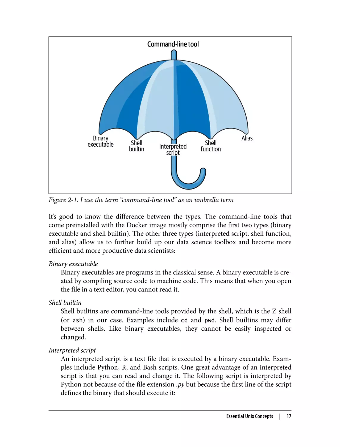
Five Types of Command-Line Tools
I use the term command-line tool a lot, but I haven’t yet explained what I actually
mean by it. I use command-line tool as an umbrella term for anything that can be
executed from the command line (see Figure 2-1). Under the hood, each commandline tool is one of the following five types:
• A binary executable
• A shell builtin
• An interpreted script
• A shell function
• An alias
6 David MacKenzie and Jim Meyering, head – Output the First Part of Files, version 8.30, 2019, https://
www.gnu.org/software/coreutils.
16
|
Chapter 2: Getting Started
Figure 2-1. I use the term “command-line tool” as an umbrella term
It’s good to know the difference between the types. The command-line tools that
come preinstalled with the Docker image mostly comprise the first two types (binary
executable and shell builtin). The other three types (interpreted script, shell function,
and alias) allow us to further build up our data science toolbox and become more
efficient and more productive data scientists:
Binary executable
Binary executables are programs in the classical sense. A binary executable is cre‐
ated by compiling source code to machine code. This means that when you open
the file in a text editor, you cannot read it.
Shell builtin
Shell builtins are command-line tools provided by the shell, which is the Z shell
(or zsh) in our case. Examples include cd and pwd. Shell builtins may differ
between shells. Like binary executables, they cannot be easily inspected or
changed.
Interpreted script
An interpreted script is a text file that is executed by a binary executable. Exam‐
ples include Python, R, and Bash scripts. One great advantage of an interpreted
script is that you can read and change it. The following script is interpreted by
Python not because of the file extension .py but because the first line of the script
defines the binary that should execute it:
Essential Unix Concepts
|
17
$ bat fac.py
───────┬──────────────────────────────────────────────────────────────
│ File: fac.py
───────┼──────────────────────────────────────────────────────────────
1 │ #!/usr/bin/env python
2
│
3
│ def factorial(x):
4
│
result = 1
5
│
for i in range(2, x + 1):
6 │
result *= i
7 │
return result
8 │
9 │ if __name__ == "__main__":
10 │
import sys
11 │
x = int(sys.argv[1])
12 │
sys.stdout.write(f"{factorial(x)}\n")
───────┴──────────────────────────────────────────────────────────────
This script computes the factorial of the integer that we pass as a parameter. It
can be invoked from the command line as follows:
$ ./fac.py 5
120
In Chapter 4, I’ll discuss in great detail how to create reusable command-line
tools using interpreted scripts.
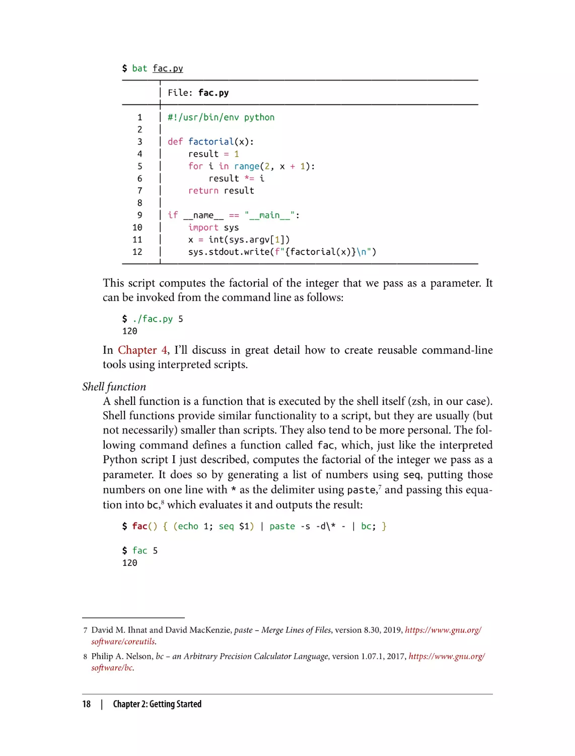
Shell function
A shell function is a function that is executed by the shell itself (zsh, in our case).
Shell functions provide similar functionality to a script, but they are usually (but
not necessarily) smaller than scripts. They also tend to be more personal. The fol‐
lowing command defines a function called fac, which, just like the interpreted
Python script I just described, computes the factorial of the integer we pass as a
parameter. It does so by generating a list of numbers using seq, putting those
numbers on one line with * as the delimiter using paste,7 and passing this equa‐
tion into bc,8 which evaluates it and outputs the result:
$ fac() { (echo 1; seq $1) | paste -s -d\* - | bc; }
$ fac 5
120
7 David M. Ihnat and David MacKenzie, paste – Merge Lines of Files, version 8.30, 2019, https://www.gnu.org/
software/coreutils.
8 Philip A. Nelson, bc – an Arbitrary Precision Calculator Language, version 1.07.1, 2017, https://www.gnu.org/
software/bc.
18
|
Chapter 2: Getting Started
The file ~/.zshrc, which is a configuration file for the Z shell, is a good place to
define your shell functions so that they are always available.
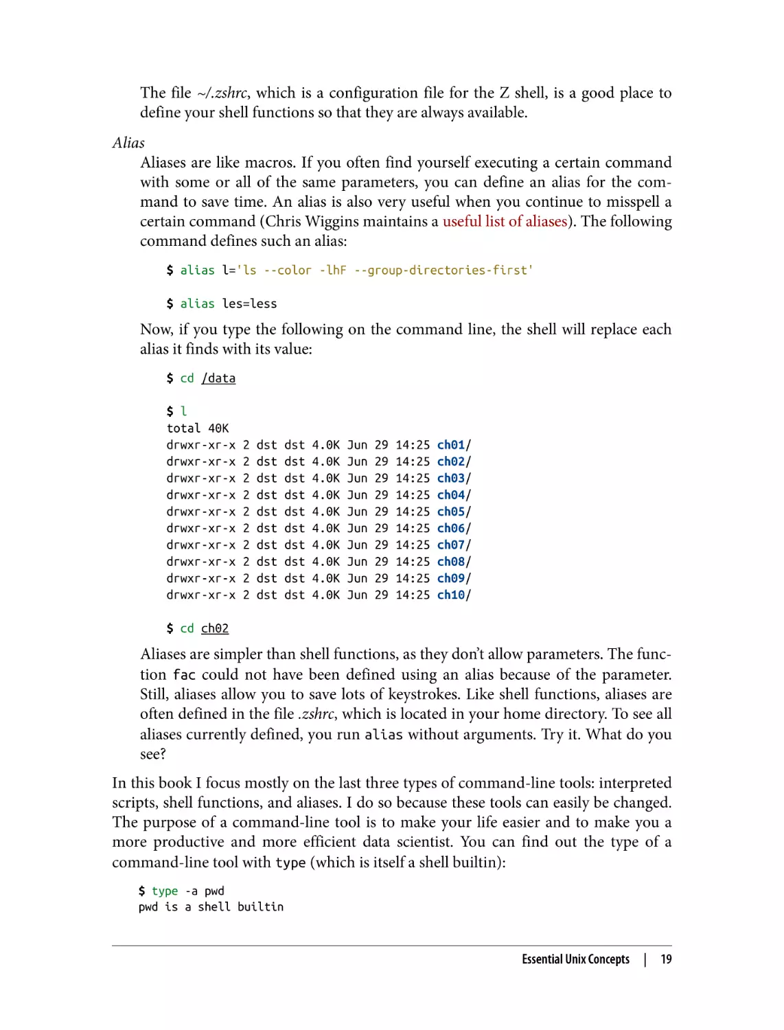
Alias
Aliases are like macros. If you often find yourself executing a certain command
with some or all of the same parameters, you can define an alias for the com‐
mand to save time. An alias is also very useful when you continue to misspell a
certain command (Chris Wiggins maintains a useful list of aliases). The following
command defines such an alias:
$ alias l='ls --color -lhF --group-directories-first'
$ alias les=less
Now, if you type the following on the command line, the shell will replace each
alias it finds with its value:
$ cd /data
$ l
total 40K
drwxr-xr-x
drwxr-xr-x
drwxr-xr-x
drwxr-xr-x
drwxr-xr-x
drwxr-xr-x
drwxr-xr-x
drwxr-xr-x
drwxr-xr-x
drwxr-xr-x
2
2
2
2
2
2
2
2
2
2
dst
dst
dst
dst
dst
dst
dst
dst
dst
dst
dst
dst
dst
dst
dst
dst
dst
dst
dst
dst
4.0K
4.0K
4.0K
4.0K
4.0K
4.0K
4.0K
4.0K
4.0K
4.0K
Jun
Jun
Jun
Jun
Jun
Jun
Jun
Jun
Jun
Jun
29
29
29
29
29
29
29
29
29
29
14:25
14:25
14:25
14:25
14:25
14:25
14:25
14:25
14:25
14:25
ch01/
ch02/
ch03/
ch04/
ch05/
ch06/
ch07/
ch08/
ch09/
ch10/
$ cd ch02
Aliases are simpler than shell functions, as they don’t allow parameters. The func‐
tion fac could not have been defined using an alias because of the parameter.
Still, aliases allow you to save lots of keystrokes. Like shell functions, aliases are
often defined in the file .zshrc, which is located in your home directory. To see all
aliases currently defined, you run alias without arguments. Try it. What do you
see?
In this book I focus mostly on the last three types of command-line tools: interpreted
scripts, shell functions, and aliases. I do so because these tools can easily be changed.
The purpose of a command-line tool is to make your life easier and to make you a
more productive and more efficient data scientist. You can find out the type of a
command-line tool with type (which is itself a shell builtin):
$ type -a pwd
pwd is a shell builtin
Essential Unix Concepts
|
19
pwd is /usr/bin/pwd
pwd is /bin/pwd
$ type -a cd
cd is a shell builtin
$ type -a fac
fac is a shell function
$ type -a l
l is an alias for ls --color -lhF --group-directories-first
type returns three command-line tools for pwd. In that case, the first reported
command-line tool is used when you type pwd. In the next section we’ll look at how to
combine command-line tools.
Combining Command-Line Tools
Because most command-line tools adhere to the Unix philosophy,9 they are designed
to do only one thing, and to do it really well. For example, the command-line tool
grep10 can filter lines, wc11 can count lines, and sort12 can sort lines. The power of the
command line comes from its ability to combine these small yet powerful commandline tools.
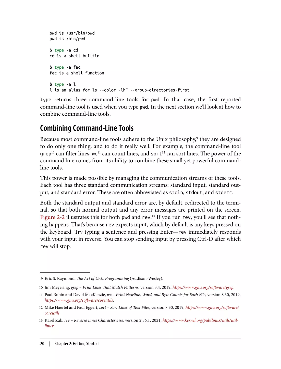
This power is made possible by managing the communication streams of these tools.
Each tool has three standard communication streams: standard input, standard out‐
put, and standard error. These are often abbreviated as stdin, stdout, and stderr.
Both the standard output and standard error are, by default, redirected to the termi‐
nal, so that both normal output and any error messages are printed on the screen.
Figure 2-2 illustrates this for both pwd and rev.13 If you run rev, you’ll see that noth‐
ing happens. That’s because rev expects input, which by default is any keys pressed on
the keyboard. Try typing a sentence and pressing Enter—rev immediately responds
with your input in reverse. You can stop sending input by pressing Ctrl-D after which
rev will stop.
9 Eric S. Raymond, The Art of Unix Programming (Addison-Wesley).
10 Jim Meyering, grep – Print Lines That Match Patterns, version 3.4, 2019, https://www.gnu.org/software/grep.
11 Paul Rubin and David MacKenzie, wc – Print Newline, Word, and Byte Counts for Each File, version 8.30, 2019,
https://www.gnu.org/software/coreutils.
12 Mike Haertel and Paul Eggert, sort – Sort Lines of Text Files, version 8.30, 2019, https://www.gnu.org/software/
coreutils.
13 Karel Zak, rev – Reverse Lines Characterwise, version 2.36.1, 2021, https://www.kernel.org/pub/linux/utils/util-
linux.
20
|
Chapter 2: Getting Started
Figure 2-2. Every tool has three standard streams: standard input (stdin), standard
output (stdout), and standard error (stderr)
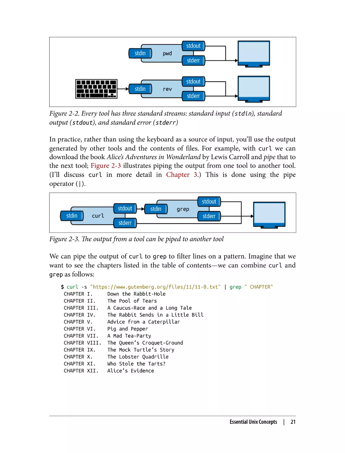
In practice, rather than using the keyboard as a source of input, you’ll use the output
generated by other tools and the contents of files. For example, with curl we can
download the book Alice’s Adventures in Wonderland by Lewis Carroll and pipe that to
the next tool; Figure 2-3 illustrates piping the output from one tool to another tool.
(I’ll discuss curl in more detail in Chapter 3.) This is done using the pipe
operator (|).
Figure 2-3. The output from a tool can be piped to another tool
We can pipe the output of curl to grep to filter lines on a pattern. Imagine that we
want to see the chapters listed in the table of contents—we can combine curl and
grep as follows:
$ curl -s "https://www.gutenberg.org/files/11/11-0.txt" | grep " CHAPTER"
CHAPTER I.
Down the Rabbit-Hole
CHAPTER II.
The Pool of Tears
CHAPTER III.
A Caucus-Race and a Long Tale
CHAPTER IV.
The Rabbit Sends in a Little Bill
CHAPTER V.
Advice from a Caterpillar
CHAPTER VI.
Pig and Pepper
CHAPTER VII.
A Mad Tea-Party
CHAPTER VIII. The Queen’s Croquet-Ground
CHAPTER IX.
The Mock Turtle’s Story
CHAPTER X.
The Lobster Quadrille
CHAPTER XI.
Who Stole the Tarts?
CHAPTER XII.
Alice’s Evidence
Essential Unix Concepts
|
21
And if we want to know how many chapters the book has, we can use wc, which is
very good at counting things:
$ curl -s "https://www.gutenberg.org/files/11/11-0.txt" |
> grep " CHAPTER" |
> wc -l
12
The option -l specifies that wc should output only the number of lines that are
passed into it. By default, it also returns the number of characters and words.
You can think of piping as an automated copy and paste. Once you get the hang of
combining tools using the pipe operator, you’ll find that there are virtually no limits
to the combinations you can make.
Redirecting Input and Output
Besides piping the output from one tool to another tool, you can also save it to a file.
The file will be saved in the current directory, unless a full path is given. This is called
output redirection, and it works as follows:
$ curl "https://www.gutenberg.org/files/11/11-0.txt" | grep " CHAPTER" > chapter
s.txt
% Total
% Received % Xferd Average Speed
Time
Time
Time Current
Dload Upload
Total
Spent
Left Speed
100 170k 100 170k
0
0
231k
0 --:--:-- --:--:-- --:--:-- 231k
$ cat chapters.txt
CHAPTER I.
Down the Rabbit-Hole
CHAPTER II.
The Pool of Tears
CHAPTER III.
A Caucus-Race and a Long Tale
CHAPTER IV.
The Rabbit Sends in a Little Bill
CHAPTER V.
Advice from a Caterpillar
CHAPTER VI.
Pig and Pepper
CHAPTER VII.
A Mad Tea-Party
CHAPTER VIII. The Queen’s Croquet-Ground
CHAPTER IX.
The Mock Turtle’s Story
CHAPTER X.
The Lobster Quadrille
CHAPTER XI.
Who Stole the Tarts?
CHAPTER XII.
Alice’s Evidence
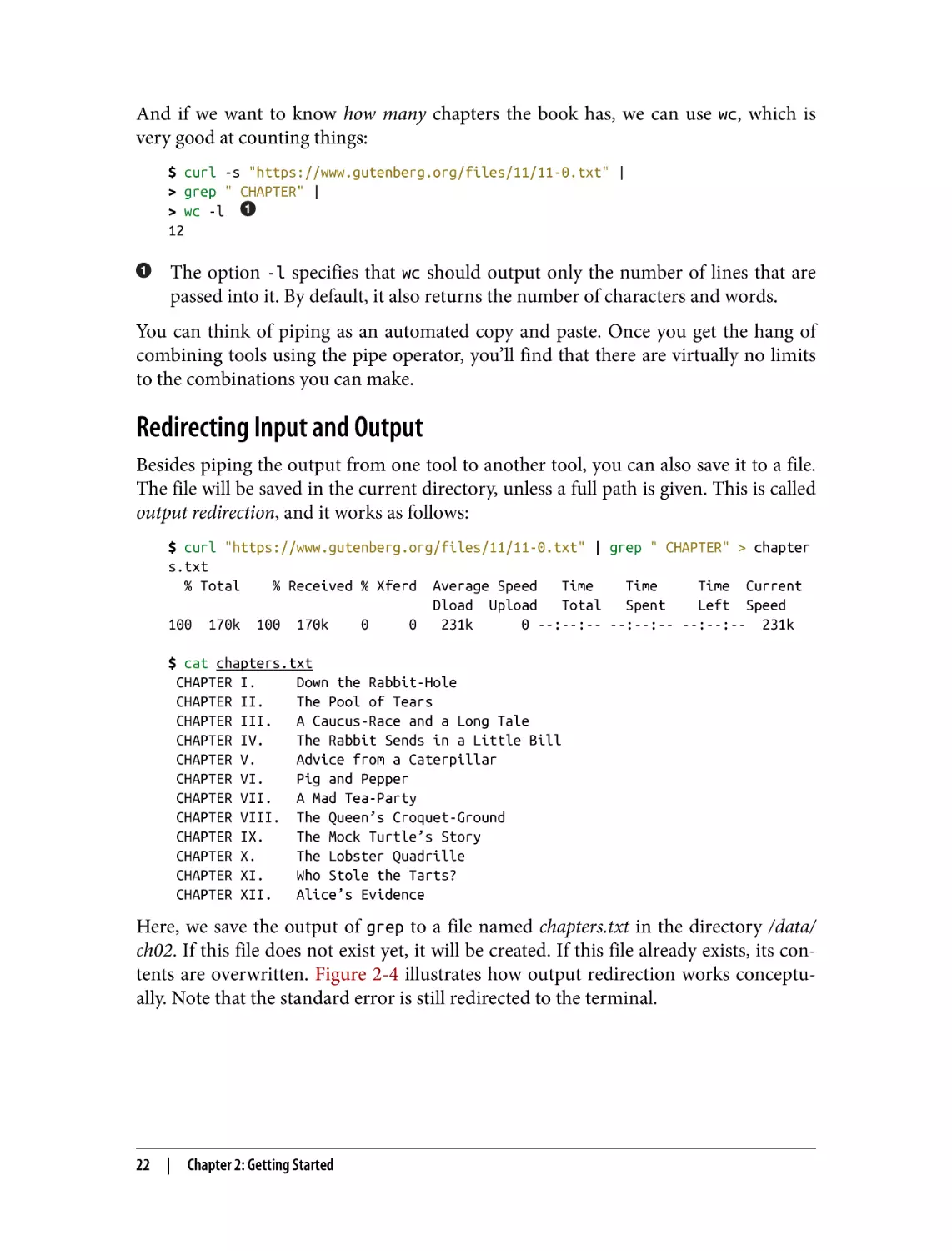
Here, we save the output of grep to a file named chapters.txt in the directory /data/
ch02. If this file does not exist yet, it will be created. If this file already exists, its con‐
tents are overwritten. Figure 2-4 illustrates how output redirection works conceptu‐
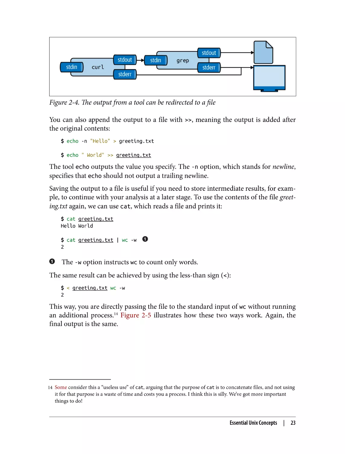
ally. Note that the standard error is still redirected to the terminal.
22
|
Chapter 2: Getting Started
Figure 2-4. The output from a tool can be redirected to a file
You can also append the output to a file with >>, meaning the output is added after
the original contents:
$ echo -n "Hello" > greeting.txt
$ echo " World" >> greeting.txt
The tool echo outputs the value you specify. The -n option, which stands for newline,
specifies that echo should not output a trailing newline.
Saving the output to a file is useful if you need to store intermediate results, for exam‐
ple, to continue with your analysis at a later stage. To use the contents of the file greet‐
ing.txt again, we can use cat, which reads a file and prints it:
$ cat greeting.txt
Hello World
$ cat greeting.txt | wc -w
2
The -w option instructs wc to count only words.
The same result can be achieved by using the less-than sign (<):
$ < greeting.txt wc -w
2
This way, you are directly passing the file to the standard input of wc without running
an additional process.14 Figure 2-5 illustrates how these two ways work. Again, the
final output is the same.
14 Some consider this a “useless use” of cat, arguing that the purpose of cat is to concatenate files, and not using
it for that purpose is a waste of time and costs you a process. I think this is silly. We’ve got more important
things to do!
Essential Unix Concepts
|
23
Figure 2-5. Two ways to use the contents of a file as input
Like many command-line tools, wc allows one or more filenames to be specified as
arguments—for example:
$ wc -w greeting.txt movies.txt
2 greeting.txt
11 movies.txt
13 total
Note that in this case, wc also outputs the names of the files.
You can suppress the output of any tool by redirecting it to a special file called /dev/
null. I often do this to suppress error messages (see Figure 2-6 for an illustration).
The following causes cat to produce an error message because it cannot find the file
404.txt:
$ cat movies.txt 404.txt
Matrix
Star Wars
Home Alone
Indiana Jones
Back to the Future
cat: 404.txt: No such file or directory
You can redirect standard error to /dev/null as follows:
$ cat movies.txt 404.txt 2> /dev/null
Matrix
Star Wars
Home Alone
Indiana Jones
Back to the Future
24
| Chapter 2: Getting Started
The 2 refers to standard error.
Figure 2-6. Redirecting stderr to /dev/null
Be careful not to read from and write to the same file. If you do, you’ll end up with an
empty file. That’s because the tool whose output is redirected immediately opens that
file for writing, thereby emptying it. There are two work-arounds for this: (1) write to
a different file and rename it afterward with mv, or (2) use sponge,15 which soaks up
all its input before writing to a file. Figure 2-7 illustrates how this works.
Figure 2-7. Unless you use sponge, you cannot read from and write to the same file in
one pipeline
For example, imagine that you have used dseq16 to generate a file dates.txt, and now
you’d like to add line numbers using nl.17 If you run the following, the file dates.txt
will end up empty:
$ dseq 5 > dates.txt
$ < dates.txt nl > dates.txt
15 Colin Watson and Tollef Fog Heen, sponge – Soak Up Standard Input and Write to a File, version 0.65, 2021,
https://joeyh.name/code/moreutils.
16 Jeroen Janssens, dseq – Generate Sequence of Dates, version 0.1, 2021, https://github.com/jeroenjanssens/dsutils.
17 Scott Bartram and David MacKenzie, nl – Number Lines of Files, version 8.30, 2020, https://www.gnu.org/soft
ware/coreutils.
Essential Unix Concepts
|
25
$ bat dates.txt
───────┬────────────────────────────────────────────────────────────────────────
│ File: dates.txt
<EMPTY>
───────┴────────────────────────────────────────────────────────────────────────
Instead, you can use one of the work-arounds I just described:
$ dseq 5 > dates.txt
$ < dates.txt nl > dates-nl.txt
$ bat dates-nl.txt
───────┬────────────────────────────────────────────────────────────────────────
│ File: dates-nl.txt
───────┼────────────────────────────────────────────────────────────────────────
1
│
1 2021-06-30
2
│
2 2021-07-01
3
│
3 2021-07-02
4
│
4 2021-07-03
5
│
5 2021-07-04
───────┴────────────────────────────────────────────────────────────────────────
$ dseq 5 > dates.txt
$ < dates.txt nl | sponge dates.txt
$ bat dates.txt
───────┬────────────────────────────────────────────────────────────────────────
│ File: dates.txt
───────┼────────────────────────────────────────────────────────────────────────
1
│
1 2021-06-30
2
│
2 2021-07-01
3
│
3 2021-07-02
4
│
4 2021-07-03
5
│
5 2021-07-04
───────┴────────────────────────────────────────────────────────────────────────
Working with Files and Directories
As data scientists, we work with a lot of data. This data is often stored in files. It is
important to know how to work with files (and the directories they live in) on the
command line. Every action that you can do using a GUI can be done with
command-line tools (and you can do much more than that). In this section I intro‐
duce the most important tools to list, create, move, copy, rename, and delete files and
directories.
Listing the contents of a directory can be done with ls. If you don’t specify a direc‐
tory, it lists the contents of the current directory. I prefer ls to have a long listing for‐
mat and to have the directories grouped before files. Instead of typing the
corresponding options each time, I use the alias l:
26
|
Chapter 2: Getting Started
$ ls /data/ch10
alice.txt count.py
count.R
Untitled1337.ipynb
$ alias l
l='ls --color -lhF --group-directories-first'
$ l /data/ch10
total 176K
-rw-r--r-- 1 dst
-rwxr-xr-x 1 dst
-rw-r--r-- 1 dst
-rw-r--r-- 1 dst
dst
dst
dst
dst
164K
408
460
1.7K
Jun
Jun
Jun
Jun
29
29
29
29
14:25
14:25
14:25
14:25
alice.txt
count.py*
count.R
Untitled1337.ipynb
You have already seen how we can create new files by redirecting the output with
either > or >>. If you need to move a file to a different directory, you can use mv:18
$ mv hello.txt /data/ch02
You can also rename files with mv:
$ cd data
$ mv hello.txt bye.txt
You can also rename or move entire directories. If you no longer need a file, you can
delete (or remove) it with rm:19
$ rm bye.txt
If you want to remove an entire directory with all its contents, specify the -r option,
which stands for “recursive”:
$ rm -r /data/ch02/old
If you want to copy a file, use cp.20 This is useful for creating backups:
$ cp server.log server.log.bak
You can create directories using mkdir:21
$ cd /data
$ mkdir logs
$ l
total 44K
18 Mike Parker, David MacKenzie, and Jim Meyering, mv – Move (Rename) Files, version 8.30, 2020, https://
www.gnu.org/software/coreutils.
19 Paul Rubin et al., rm – Remove Files or Directories, version 8.30, 2019, https://www.gnu.org/software/coreutils.
20 Torbjorn Granlund, David MacKenzie, and Jim Meyering, cp – Copy Files and Directories, version 8.30, 2018,
https://www.gnu.org/software/coreutils.
21 David MacKenzie, mkdir – Make Directories, version 8.30, 2019, https://www.gnu.org/software/coreutils.
Essential Unix Concepts
|
27
drwxr-xr-x
drwxr-xr-x
drwxr-xr-x
drwxr-xr-x
drwxr-xr-x
drwxr-xr-x
drwxr-xr-x
drwxr-xr-x
drwxr-xr-x
drwxr-xr-x
drwxr-xr-x
2
2
2
2
2
2
2
2
2
2
2
dst
dst
dst
dst
dst
dst
dst
dst
dst
dst
dst
dst
dst
dst
dst
dst
dst
dst
dst
dst
dst
dst
4.0K
4.0K
4.0K
4.0K
4.0K
4.0K
4.0K
4.0K
4.0K
4.0K
4.0K
Jun
Jun
Jun
Jun
Jun
Jun
Jun
Jun
Jun
Jun
Jun
29
29
29
29
29
29
29
29
29
29
29
14:25
14:25
14:25
14:25
14:25
14:25
14:25
14:25
14:25
14:25
14:25
ch01/
ch02/
ch03/
ch04/
ch05/
ch06/
ch07/
ch08/
ch09/
ch10/
logs/
Using the command-line tools to manage your files can be scary at
first, because you have no graphical overview of the filesystem to
provide immediate feedback. There are a few visual file managers
that can help with this, such as GNU Midnight Commander,
Ranger, and Vifm. These are not installed in the Docker image, but
you can install one of them yourself by running sudo apt install
followed by either mc, ranger, or vifm.
All of these command-line tools accept the -v option, which stands for verbose, so
that they output what’s going on. For example:
$ mkdir -v backup
mkdir: created directory 'backup'
All tools other than mkdir also accept the -i option, which stands for interactive, and
which causes the tools to ask you for confirmation. For example:
$ rm -i *
zsh: sure you want to delete all 12 files in /data [yn]? n
Managing Output
Sometimes a tool or sequence of tools produces too much output to include in the
book. Instead of manually altering such output, I prefer to be transparent by piping it
through a helper tool. You don’t necessarily have to do this, especially if you’re inter‐
ested in the complete output.
Here are the tools I use to make output manageable.
I often use trim to limit the output to a given height and width. By default, output is
trimmed to 10 lines and the width of the terminal. Pass a negative number to disable
trimming the height and/or the width. For example:
$ cat /data/ch07/tips.csv | trim 5 25
bill,tip,sex,smoker,day,...
16.99,1.01,Female,No,Sun...
10.34,1.66,Male,No,Sun,D...
21.01,3.5,Male,No,Sun,Di...
28
|
Chapter 2: Getting Started
23.68,3.31,Male,No,Sun,D...
... with 240 more lines
Other tools that I use to massage the output are head, tail, fold, paste, and column.
The Appendix contains an example for each of these.
If a file or an output contains a comma-separated value, I often pipe it through
csvlook to turn it into a nice-looking table. If you run csvlook, you’ll see the com‐
plete table. I have redefined csvlook such that the table is shortened by trim:
$ which csvlook
csvlook () {
/usr/bin/csvlook "$@" | trim | sed 's/- | -/──┼──/g;s/| -/├──/g;s/- |/──
┤/;s/|/│/g;2s/-/─/g'
}
$ csvlook /data/ch07/tips.csv
│ bill │
tip │ sex
│ smoker │ day │ time
│ size │
├───────┼───────┼────────┼────────┼──────┼────────┼──────┤
│ 16.99 │ 1.01 │ Female │ False │ Sun │ Dinner │
2 │
│ 10.34 │ 1.66 │ Male
│ False │ Sun │ Dinner │
3 │
│ 21.01 │ 3.50 │ Male
│ False │ Sun │ Dinner │
3 │
│ 23.68 │ 3.31 │ Male
│ False │ Sun │ Dinner │
2 │
│ 24.59 │ 3.61 │ Female │ False │ Sun │ Dinner │
4 │
│ 25.29 │ 4.71 │ Male
│ False │ Sun │ Dinner │
4 │
│ 8.77 │ 2.00 │ Male
│ False │ Sun │ Dinner │
2 │
│ 26.88 │ 3.12 │ Male
│ False │ Sun │ Dinner │
4 │
... with 236 more lines
I use bat to show the contents of a file where line numbers and syntax highlighting
matter—for example:
$ bat /data/ch04/stream.py
───────┬────────────────────────────────────────────────────────────────────────
│ File: /data/ch04/stream.py
───────┼────────────────────────────────────────────────────────────────────────
1
│ #!/usr/bin/env python
2
│ from sys import stdin, stdout
3
│ while True:
4
│
line = stdin.readline()
5
│
if not line:
6
│
break
7
│
stdout.write("%d\n" % int(line)**2)
8
│
stdout.flush()
───────┴────────────────────────────────────────────────────────────────────────
Sometimes I add the -A option when I want to explicitly point out the spaces, tabs,
and newlines in a file.
Essential Unix Concepts
|
29
Occasionally it’s useful to write intermediate output to a file. This allows you to
inspect any step in your pipeline once it has completed. You can insert the tool tee as
often as you like in your pipeline. I often use it to inspect a portion of the final out‐
put, while writing the complete output to file (see Figure 2-8). Here, the complete
output is written to even.txt, and the first five lines are printed using trim:
$ seq 0 2 100 | tee even.txt | trim 5
0
2
4
6
8
... with 46 more lines
Figure 2-8. With tee, you can write intermediate output to a file
Last, to insert images that have been generated by command-line tools (that is, every
image other than screenshots and diagrams) I use display. If you run display, you’ll
find that it doesn’t work. In Chapter 7, I explain four options for displaying images
generated from the command line.
Help!
As you’re finding your way around the command line, it may happen that you need
help. Even the most seasoned users need help at some point. It is impossible to
remember all the different command-line tools and their possible arguments. Fortu‐
nately, the command line offers severals ways to get help.
Perhaps the most important command for getting help is man,22 which is short for
manual. It contains information for most command-line tools. In case I’ve forgotten
the options to the tool tar, which happens all the time, I just access its manual page
using the following:
22 John W. Eaton and Colin Watson, man – an Interface to the System Reference Manuals, version 2.9.1, 2020,
https://nongnu.org/man-db.
30
|
Chapter 2: Getting Started
$ man tar | trim 20
TAR(1)
GNU TAR Manual
TAR(1)
NAME
tar - an archiving utility
SYNOPSIS
Traditional usage
tar {A|c|d|r|t|u|x}[GnSkUWOmpsMBiajJzZhPlRvwo] [ARG...]
UNIX-style usage
tar -A [OPTIONS] ARCHIVE ARCHIVE
tar -c [-f ARCHIVE] [OPTIONS] [FILE...]
tar -d [-f ARCHIVE] [OPTIONS] [FILE...]
tar -t [-f ARCHIVE] [OPTIONS] [MEMBER...]
tar -r [-f ARCHIVE] [OPTIONS] [FILE...]
... with 1147 more lines
Not every command-line tool has a manual page. Take cd, for example:
$ man cd
No manual entry for cd
For shell builtins like cd, you can consult the zshbuiltins manual page:
$ man zshbuiltins | trim
ZSHBUILTINS(1)
General Commands Manual
ZSHBUILTINS(1)
NAME
zshbuiltins - zsh built-in commands
SHELL BUILTIN COMMANDS
Some shell builtin commands take options as described in individual en‐
tries; these are often referred to in the list below as `flags' to
avoid confusion with shell options, which may also have an effect on
the behavior of builtin commands. In this introductory section, `op‐
... with 2735 more lines
You can search by pressing / and exit by pressing q. Try to find the appropriate sec‐
tion for cd.
Newer command-line tools often lack a manual page as well. In such cases, your best
bet is to invoke the tool with the --help (or -h) option. For example:
$ jq --help | trim
jq - commandline JSON processor [version 1.6]
Usage:
jq [options] <jq filter> [file...]
jq [options] --args <jq filter> [strings...]
Essential Unix Concepts
|
31
jq [options] --jsonargs <jq filter> [JSON_TEXTS...]
jq is a tool for processing JSON inputs, applying the given filter to
its JSON text inputs and producing the filter's results as JSON on
standard output.
... with 37 more lines
Specifying the --help option also works for command-line tools such as cat. How‐
ever, the corresponding manual page often provides more information. If, after trying
these three approaches, you are still stuck, then consulting the internet is perfectly
acceptable. In the Appendix, there’s a list of all the command-line tools used in this
book. Besides showing how each command-line tool can be installed, the Appendix
also shows how you can get help for each tool.
Manual pages can be quite verbose and difficult to read. The tool tldr23 (which is
short for “too long; didn’t read”) is a collection of community-maintained help pages
for command-line tools that aims to be a simpler, more approachable complement to
traditional manual pages. Here’s an example of the tldr page for tar:
$ tldr tar | trim 20
tar
Archiving utility.
Often combined with a compression method, such as gzip or bzip2.
More information: https://www.gnu.org/software/tar.
- [c]reate an archive and write it to a [f]ile:
tar cf target.tar file1 file2 file3
- [c]reate a g[z]ipped archive and write it to a [f]ile:
tar czf target.tar.gz file1 file2 file3
- [c]reate a g[z]ipped archive from a directory using relative paths:
tar czf target.tar.gz --directory=path/to/directory .
- E[x]tract a (compressed) archive [f]ile into the current directory [v]erbos…
tar xvf source.tar[.gz|.bz2|.xz]
- E[x]tract a (compressed) archive [f]ile into the target directory:
... with 12 more lines
As you can see, rather than listing the many options alphabetically like man often
does, tldr cuts to the chase by giving you a list of practical examples.
23 Owen Voke, tldr – Collaborative Cheatsheets for Console Commands, version 3.3.7, 2021, https://tldr.sh.
32
|
Chapter 2: Getting Started
Summary
In this chapter you learned how to get all the required command-line tools by instal‐
ling a Docker image. I also went over some essential command-line concepts and
how to get help. Now that you have all the necessary ingredients, you’re ready for the
first step of the OSEMN model for data science: obtaining data.
For Further Exploration
• The subtitle of this book pays homage to the epic Unix Power Tools, 3rd ed. by
Shelley Powers, Jerry Peek, Tim O’Reilly, and Mike Loukides (O’Reilly), and
rightly so. With over 51 chapters and more than a thousand pages, Unix Power
Tools covers just about everything there is to know about Unix. It weighs more
than four pounds, so you might want to consider getting the ebook.
• The website explainshell parses a command or a sequence of commands and pro‐
vides a short explanation of each part. This site is useful for quickly understand‐
ing a new command or option without having to skim through the relevant
manual pages.
• Docker is truly a brilliant piece of software. In this chapter I’ve briefly explained
how to download a Docker image and run a Docker container, but it might be
worthwhile to learn how to create your own Docker images. The book Docker:
Up & Running, 2nd ed. by Sean P. Kane and Karl Matthias (O’Reilly) is a good
resource as well.
Summary
|
33
CHAPTER 3
Obtaining Data
This chapter deals with the first step of the OSEMN model: obtaining data. After all,
without any data, there is not much data science that we can do. I assume that the
data you need to solve your data science problem already exists. Your first task is to
get this data onto your computer (and possibly also inside the Docker container) in a
form that you can work with.
According to the Unix philosophy, text is a universal interface. Almost every
command-line tool takes text as input, produces text as output, or both. This is the
main reason why command-line tools can work so well together. However, as we’ll
see, even just text can come in multiple forms.
Data can be obtained in several ways—for example, by downloading it from a server,
querying a database, or connecting to a Web API. Sometimes the data comes in a
compressed form or in a binary format such as a Microsoft Excel Spreadsheet. In this
chapter, I discuss several tools that help tackle this from the command line, including
curl,1 in2csv,2 sql2csv,3 and tar.4
1 Daniel Stenberg, curl – Transfer a URL, version 7.68.0, 2016, https://curl.haxx.se.
2 Christopher Groskopf, in2csv – Convert Common, but Less Awesome, Tabular Data Formats to CSV, version
1.0.5, 2020, https://csvkit.rtfd.org.
3 Christopher Groskopf, sql2csv – Execute an SQL Query on a Database and Output the Result to a CSV File,
version 1.0.5, 2020, https://csvkit.rtfd.org.
4 John Gilmore and Jay Fenlason, tar – an Archiving Utility, version 1.30, 2014, https://www.gnu.org/software/
tar.
35
Overview
In this chapter, you’ll learn how to:
• Copy local files to the Docker image
• Download data from the internet
• Decompress files
• Extract data from spreadsheets
• Query relational databases
• Call web APIs
This chapter starts with the following files:
$ cd /data/ch03
$ l
total 924K
-rw-r--r--rw-r--r--rw-r--r--rw-r--r--rw-r--r--rw-r--r--
1
1
1
1
1
1
dst
dst
dst
dst
dst
dst
dst 627K Jun 29 14:26 logs.tar.gz
dst 189K Jun 29 14:26 r-datasets.db
dst 149 Jun 29 14:26 tmnt-basic.csv
dst 148 Jun 29 14:26 tmnt-missing-newline.csv
dst 181 Jun 29 14:26 tmnt-with-header.csv
dst 91K Jun 29 14:26 top2000.xlsx
The instructions for getting these files are in Chapter 2. Any other files are either
downloaded or generated using command-line tools.
Copying Local Files to the Docker Container
A common situation is that you already have the necessary files on your own com‐
puter. This section explains how you can get those files into the Docker container.
I mentioned in Chapter 2 that the Docker container is an isolated virtual environ‐
ment. Luckily, there is one exception to that: files can be transferred in and out of the
Docker container. The local directory from which you ran docker run is mapped to a
directory in the Docker container. This directory is called /data. Note that this is not
the home directory, which is /home/dst.
If you have one or more files on your local computer, and you want to apply some
command-line tools to them, all you have to do is copy or move the files to that map‐
ped directory. Let’s assume that you have a file called logs.csv in your Downloads
directory.
If you’re running Windows, open the Command Prompt or PowerShell and run the
following two commands:
36
|
Chapter 3: Obtaining Data
> cd %UserProfile%\Downloads
> copy logs.csv MyDataScienceToolbox\
If you are running Linux or macOS, open a terminal and execute the following com‐
mand on your operating system (not inside the Docker container):
$ cp ~/Downloads/logs.csv ~/my-data-science-toolbox
You can also drag and drop the file into the right directory using a graphical file man‐
ager such as Windows Explorer or macOS Finder.
Downloading from the Internet
The internet provides, without a doubt, the largest resource for interesting data. The
command-line tool curl can be considered the command line’s Swiss Army knife
when it comes to downloading data from the internet.
Introducing curl
When you browse a URL, which stands for uniform resource locator, your browser
interprets the data it downloads. For example, the browser renders HTML files, plays
video files automatically, and shows PDF files. However, when you use curl to access
a URL, it downloads the data and, by default, prints it to standard output. curl
doesn’t do any interpretation, but luckily other command-line tools can be used to
process the data further.
The easiest invocation of curl is to specify a URL as a command-line argument. Let’s
try downloading an article from Wikipedia:
$ curl "https://en.wikipedia.org/wiki/List_of_windmills_in_the_Netherlands" |
> trim
% Total
% Received % Xferd Average Speed
Time
Time
Time Current
Dload Upload
Total
Spent
Left Speed
0
0
0
0
0
0
0
0 --:--:-- --:--:-- --:--:-0<!
DOCTYPE html>
<html class="client-nojs" lang="en" dir="ltr">
<head>
<meta charset="UTF-8"/>
<title>List of windmills in the Netherlands - Wikipedia</title>
<script>document.documentElement.className="client-js";RLCONF={"wgBreakFrames":…
"wikitext","wgRelevantPageName":"List_of_windmills_in_the_Netherlands","wgRelev…
"site.styles":"ready","noscript":"ready","user.styles":"ready","ext.globalCssJs…
"ext.growthExperiments.SuggestedEditSession"];</script>
<script>(RLQ=window.RLQ||[]).push(function(){mw.loader.implement("user.options@…
100 244k 100 244k
0
0 1291k
0 --:--:-- --:--:-- --:--:-- 1291k
… with 1723 more lines
Remember, trim is used only to make the output fit nicely in the book.
Downloading from the Internet
|
37
As you can see, curl downloads the raw HTML returned by Wikipedia’s server; no
interpretation is being done, and the contents are immediately printed on standard
output. Because of the URL, you’d think that this article would list all the windmills in
the Netherlands. However, there are apparently so many windmills that each province
has its own page. Fascinating.
By default, curl outputs a progress meter that shows the download rate and the
expected time of completion. This output isn’t written to standard output but instead
is written to a separate channel known as standard error, so that it doesn’t interfere
when you add another tool to the pipeline. While this information can be useful
when downloading very large files, I usually find it distracting, so I specify the -s
option to silence this output:
$ curl -s "https://en.wikipedia.org/wiki/List_of_windmills_in_Friesland" |
> pup -n 'table.wikitable tr'
234
I’ll discuss pup,5 a handy tool for scraping websites, in more detail in Chapter 5.
And what do you know, there are apparently 234 windmills in the province of Fries‐
land alone!
Saving
You can let curl save the output to a file by adding the -O option. The filename will
be based on the last part of the URL:
$ curl -s "https://en.wikipedia.org/wiki/List_of_windmills_in_Friesland" -O
$ l
total 1.4M
-rw-r--r--rw-r--r--rw-r--r--rw-r--r--rw-r--r--rw-r--r--rw-r--r--
1
1
1
1
1
1
1
dst
dst
dst
dst
dst
dst
dst
dst
dst
dst
dst
dst
dst
dst
427K
627K
189K
149
148
181
91K
Jun
Jun
Jun
Jun
Jun
Jun
Jun
29
29
29
29
29
29
29
14:27
14:26
14:26
14:26
14:26
14:26
14:26
List_of_windmills_in_Friesland
logs.tar.gz
r-datasets.db
tmnt-basic.csv
tmnt-missing-newline.csv
tmnt-with-header.csv
top2000.xlsx
If you don’t like that filename, then you can use the -o option together with a file‐
name or redirect the output to a file yourself:
$ curl -s "https://en.wikipedia.org/wiki/List_of_windmills_in_Friesland" > fries
land.html
5 Eric Chiang, pup – Parsing HTML at the Command Line, version 0.4.0, 2016, https://github.com/EricChiang/
pup.
38
|
Chapter 3: Obtaining Data
Other Protocols
In total, curl supports more than 20 protocols. To download from an FTP server
(FTP stands for “File Transfer Protocol”), you use curl the same way. Here I down‐
load the file welcome.msg from ftp.gnu.org:
$ curl -s "ftp://ftp.gnu.org/welcome.msg" | trim
NOTICE (Updated December 18 2018):
FSF public IP addresses are changing between December 20 and January 7th
If you have hardcoded the IP address of any GNU/FSF servers in those
ranges in any code or configuration files, they will need to be
updated. If you refer to our servers by their DNS name, such as
"gnu.org", then that will continue to work. You should use the DNS name
wherever possible.
... with 68 more lines
If the specified URL is a directory, curl will list the contents of that directory. When
the URL is password protected, you can specify a username and a password with the
-u option.
Or there’s the DICT protocol, which allows you to access various dictionaries and
look up definitions. Here’s the definition of windmill according to the Collaborative
International Dictionary of English:
$ curl -s "dict://dict.org/d:windmill" | trim
220 dict.dict.org dictd 1.12.1/rf on Linux 4.19.0-10-amd64 <auth.mime> <4623255…
250 ok
150 1 definitions retrieved
151 "Windmill" gcide "The Collaborative International Dictionary of English v.0…
Windmill \Wind"mill`\, n.
A mill operated by the power of the wind, usually by the
action of the wind upon oblique vanes or sails which radiate
from a horizontal shaft. --Chaucer.
[1913 Webster]
.
... with 2 more lines
When you are downloading data from the internet, however, the protocol will most
likely be HTTP, so the URL will start with either http:// or https://.
Following Redirects
When you access a shortened URL, such as the one that starts with http://bit.ly/ or
http://t.co/, your browser automatically redirects you to the correct location. With
curl, however, you need to specify the -L or --location option in order to be redi‐
rected. If you don’t, you can get something like:
Downloading from the Internet
|
39
$ curl -s "https://bit.ly/2XBxvwK"
<html>
<head><title>Bitly</title></head>
<body><a href="https://youtu.be/dQw4w9WgXcQ">moved here</a></body>
</html>%
Sometimes you get nothing back, like when we follow the URL just mentioned:
$ curl -s "https://youtu.be/dQw4w9WgXcQ"
If you specify the -I or --head option, curl fetches only the HTTP header of the
response, which allows you to inspect the status code and other information returned
by the server:
$ curl -sI "https://youtu.be/dQw4w9WgXcQ" | trim
HTTP/2 303
content-type: application/binary
x-content-type-options: nosniff
cache-control: no-cache, no-store, max-age=0, must-revalidate
pragma: no-cache
expires: Mon, 01 Jan 1990 00:00:00 GMT
date: Tue, 29 Jun 2021 12:27:13 GMT
location: https://www.youtube.com/watch?v=dQw4w9WgXcQ&feature=youtu.be
content-length: 0
x-frame-options: SAMEORIGIN
… with 9 more lines
The first line shows the protocol followed by the HTTP status code, which is 303 in
this case. You can also see the location this URL redirects to. Inspecting the header
and getting the status code is a useful debugging tool in case curl does not give you
the expected result. Other common HTTP status codes include 404 (not found) and
403 (forbidden). Wikipedia has a page that lists all HTTP status codes.
In summary, curl is a useful command-line tool for downloading data from the
internet. Its three most common options are -s to silence the progress meter, -u to
specify a username and password, and -L to automatically follow redirects. See the
man page for more information (and to make your head spin):
$ man curl | trim 20
curl(1)
Curl Manual
curl(1)
NAME
curl - transfer a URL
SYNOPSIS
curl [options / URLs]
DESCRIPTION
curl is a tool to transfer data from or to a server, using one of the
supported protocols (DICT, FILE, FTP, FTPS, GOPHER, HTTP, HTTPS, IMAP,
IMAPS, LDAP, LDAPS, MQTT, POP3, POP3S, RTMP, RTMPS, RTSP, SCP, SFTP,
40
|
Chapter 3: Obtaining Data
SMB, SMBS, SMTP, SMTPS, TELNET and TFTP). The command
work without user interaction.
curl offers a
tication, FTP
fer resume,
features will
is
designed
to
busload of useful tricks like proxy support, user authen‐
upload, HTTP post, SSL connections, cookies, file trans‐
Metalink, and more. As you will see below, the number of
make your head spin!
… with 3986 more lines
Decompressing Files
If the original dataset is very large or is a collection of many files, it may be a com‐
pressed archive. Datasets that contain many repeated values (such as the words in a
text file or the keys in a JSON file) are especially well suited for compression.
Common file extensions of compressed archives are .tar.gz, .zip, and .rar. To decom‐
press these, you would use the command-line tools tar, unzip,6 and unrar,7 respec‐
tively. (There are a few less-common file extensions for which you would need other
tools.)
Let’s take tar.gz (pronounced “gzipped tarball”) as an example. To extract an archive
named logs.tar.gz, you would use the following incantation:
$ tar -xzf logs.tar.gz
It’s common to combine these three short options, like I did here, but you can
also specify them separately as -x -z -f. In fact, many command-line tools
allow you to combine options that consist of a single character.
Indeed, tar is notorious for its many command-line arguments. In this case, the
three options -x, -z, and -f specify that tar should extract files from an archive, use
gzip as the decompression algorithm, and use the file logs.tar.gz.
However, since we’re not yet familiar with this archive, it’s a good idea to first exam‐
ine its contents. This can be done using the -t option (instead of the -x option):
$ tar -tzf logs.tar.gz | trim
E1FOSPSAYDNUZI.2020-09-01-00.0dd00628
E1FOSPSAYDNUZI.2020-09-01-00.b717c457
E1FOSPSAYDNUZI.2020-09-01-01.05f904a4
E1FOSPSAYDNUZI.2020-09-01-02.36588daf
E1FOSPSAYDNUZI.2020-09-01-02.6cea8b1d
6 Samuel H. Smith et al., unzip – List, Test, and Extract Compressed Files in a ZIP Archive, version 6.0, 2009,
http://www.info-zip.org/pub/infozip.
7 Ben Asselstine, Christian Scheurer, and Johannes Winkelmann, unrar – Extract Files from Rar Archives, ver‐
sion 0.0.1, 2014, https://web.archive.org/web/20080331080828/http://home.gna.org/unrar.
Decompressing Files
|
41
E1FOSPSAYDNUZI.2020-09-01-02.be4bc86d
E1FOSPSAYDNUZI.2020-09-01-03.16f3fa32
E1FOSPSAYDNUZI.2020-09-01-03.1c0a370f
E1FOSPSAYDNUZI.2020-09-01-03.76df64bf
E1FOSPSAYDNUZI.2020-09-01-04.0a1ade1b
… with 2427 more lines
It seems that this archive contains a lot of files, and they are not inside a directory. To
keep the current directory clean, it’s a good idea to first create a new directory using
mkdir and extract those files there using the -C option:
$ mkdir logs
$ tar -xzf logs.tar.gz -C logs
Let’s verify the number of files and some of their contents:
$ ls logs | wc -l
2437
$ cat logs/* | trim
#Version: 1.0
#Fields: date time x-edge-location sc-bytes c-ip cs-method cs(Host) cs-uri-stem…
2020-09-01
00:51:54
SEA19-C1
391
206.55.174.150 GET
…
2020-09-01
00:54:59
CPH50-C2
384
82.211.213.95
GET
…
#Version: 1.0
#Fields: date time x-edge-location sc-bytes c-ip cs-method cs(Host) cs-uri-stem…
2020-09-01
00:04:28
DFW50-C1
391
2a03:2880:11ff:9::face:…
#Version: 1.0
#Fields: date time x-edge-location sc-bytes c-ip cs-method cs(Host) cs-uri-stem…
2020-09-01
01:04:14
ATL56-C4
385
2600:1700:2760:da20:548…
… with 10279 more lines
Excellent. Now, I understand that you’d like to scrub and explore these log files, but
we’ll get to that later, in Chapter 5 and Chapter 7.
In time you’ll get used to these options, but I’d like to show you an alternative that
you might find convenient. Rather than you having to remember the different
command-line tools and their options, there’s a handy script called unpack8 that will
decompress many different formats. unpack looks at the extension of the file that you
want to decompress and calls the appropriate command-line tool. Now, in order to
decompress this same file, you would run:
$ unpack logs.tar.gz
8 Patrick Brisbin, unpack – Extract Common File Formats, version 0.1, 2013, https://github.com/jeroenjanssens/
dsutils.
42
|
Chapter 3: Obtaining Data
Converting Microsoft Excel Spreadsheets to CSV
For many people, Microsoft Excel offers an intuitive way to work with small datasets
and perform calculations on them. As a result, a lot of data is embedded into Micro‐
soft Excel spreadsheets. These spreadsheets are, depending on the extension of the
filename, stored either in a proprietary binary format (.xls) or as a collection of com‐
pressed XML files (.xlsx). In both cases, the data is not readily usable by most
command-line tools. It would be a shame if we could not use those valuable datasets
just because they are stored this way.
Especially when you’re just starting out at the command line, you might be tempted
to convert your spreadsheet to CSV by opening it in Microsoft Excel, or in an open
source variant such as LibreOffice Calc, and manually exporting it to CSV. While this
works as a one-off solution, it does not scale well to multiple files and cannot be auto‐
mated. Furthermore, when you’re working on a server, chances are that you don’t
have such an application available. Trust me, you’ll get the hang of it.
Luckily, there is a command-line tool called in2csv that converts Microsoft Excel
spreadsheets to CSV files (CSV stands for “comma-separated values”). Working with
CSV can be tricky because it lacks a formal specification. Yakov Shafranovich defines
the CSV format according to the following three points:9
1. Each record is located on a separate line, delimited by a line break (␊). Take, for
example, the following CSV file with crucial information about the Teenage
Mutant Ninja Turtles:
$ bat -A tmnt-basic.csv
───────┬────────────────────────────────────────────────────────────────────────
│ File: tmnt-basic.csv
───────┼────────────────────────────────────────────────────────────────────────
1
│ Leonardo,Leo,blue,two·ninjakens␊
2
│ Raphael,Raph,red,pair·of·sai␊
3
│ Michelangelo,Mikey·or·Mike,orange,pair·of·nunchaku␊
4
│ Donatello,Donnie·or·Don,purple,staff␊
───────┴────────────────────────────────────────────────────────────────────────
The -A option makes bat show all nonprintable characters like spaces, tabs, and
newlines.
2. The last record in the file may or may not have an ending line break. For
example:
9 Yakov Shafranovich, “Common Format and MIME Type for Comma-Separated Values (CSV) Files,” IETF,
October 2005, https://www.ietf.org/rfc/rfc4180.txt.
Converting Microsoft Excel Spreadsheets to CSV
|
43
$ bat -A tmnt-missing-newline.csv
───────┬────────────────────────────────────────────────────────────────────────
│ File: tmnt-missing-newline.csv
───────┼────────────────────────────────────────────────────────────────────────
1
│ Leonardo,Leo,blue,two·ninjakens␊
2
│ Raphael,Raph,red,pair·of·sai␊
3
│ Michelangelo,Mikey·or·Mike,orange,pair·of·nunchaku␊
4
│ Donatello,Donnie·or·Don,purple,staff
───────┴────────────────────────────────────────────────────────────────────────
3. There may be a header appearing as the first line of the file with the same format
as normal record lines. This header will contain names corresponding to the
fields in the file and should contain the same number of fields as the records in
the rest of the file. For example:
$ bat -A tmnt-with-header.csv
───────┬────────────────────────────────────────────────────────────────────────
│ File: tmnt-with-header.csv
───────┼────────────────────────────────────────────────────────────────────────
1
│ name,nickname,mask_color,weapon␊
2
│ Leonardo,Leo,blue,two·ninjakens␊
3
│ Raphael,Raph,red,pair·of·sai␊
4
│ Michelangelo,Mikey·or·Mike,orange,pair·of·nunchaku␊
5
│ Donatello,Donnie·or·Don,purple,staff␊
───────┴────────────────────────────────────────────────────────────────────────
As you can see, CSV by default is not too readable. You can pipe the data to a tool
called csvlook,10 which will nicely format it into a table. If the CSV data has no
header, as in the file tmnt-missing-newline.csv, then you need to add the -H option;
otherwise the first line will be interpreted as the header:
$ csvlook tmnt-with-header.csv
│ name
│ nickname
│ mask_color │ weapon
│
├──────────────┼───────────────┼────────────┼──────────────────┤
│ Leonardo
│ Leo
│ blue
│ two ninjakens
│
│ Raphael
│ Raph
│ red
│ pair of sai
│
│ Michelangelo │ Mikey or Mike │ orange
│ pair of nunchaku │
│ Donatello
│ Donnie or Don │ purple
│ staff
│
$ csvlook tmnt-basic.csv
│ Leonardo
│ Leo
│ blue
│ two ninjakens
│
├──────────────┼───────────────┼────────┼──────────────────┤
│ Raphael
│ Raph
│ red
│ pair of sai
│
│ Michelangelo │ Mikey or Mike │ orange │ pair of nunchaku │
│ Donatello
│ Donnie or Don │ purple │ staff
│
$ csvlook -H tmnt-missing-newline.csv
10 Christopher Groskopf, csvlook – Render a CSV File in the Console as a Markdown-Compatible, Fixed-Width
Table, version 1.0.5, 2020, https://csvkit.rtfd.org.
44
|
Chapter 3: Obtaining Data
│ a
│ b
│ c
│ d
│
├──────────────┼───────────────┼────────┼──────────────────┤
│ Leonardo
│ Leo
│ blue
│ two ninjakens
│
│ Raphael
│ Raph
│ red
│ pair of sai
│
│ Michelangelo │ Mikey or Mike │ orange │ pair of nunchaku │
│ Donatello
│ Donnie or Don │ purple │ staff
│
The -H option specifies that the CSV file has no header.
Let’s demonstrate in2csv using a spreadsheet that contains the two thousand most
popular songs according to an annual Dutch marathon radio program, the Top 2000.
To extract the Excel file’s data, you invoke in2csv as follows:
$ curl "https://www.nporadio2.nl/data/download/TOP-2000-2020.xlsx" > top2000.xls
x
% Total
% Received % Xferd Average Speed
Time
Time
Time Current
Dload Upload
Total
Spent
Left Speed
100 92838 100 92838
0
0
625k
0 --:--:-- --:--:-- --:--:-- 625k
$ in2csv top2000.xlsx | tee top2000.csv | trim
NR.,ARTIEST,TITEL,JAAR
1,Danny Vera,Roller Coaster,2019
2,Queen,Bohemian Rhapsody,1975
3,Eagles,Hotel California,1977
4,Billy Joel,Piano Man,1974
5,Led Zeppelin,Stairway To Heaven,1971
6,Pearl Jam,Black,1992
7,Boudewijn de Groot,Avond,1997
8,Coldplay,Fix You,2005
9,Pink Floyd,Wish You Were Here,1975
… with 1991 more lines
Who is Danny Vera? The most popular song is supposed to be “Bohemian Rhapsody,”
of course. Well, at least Queen appears plenty of times in the Top 2000, so I can’t
really complain:
$ csvgrep top2000.csv --columns ARTIEST --regex '^Queen$' | csvlook -I
│ NR. │ ARTIEST │ TITEL
│ JAAR │
├──────┼─────────┼─────────────────────────────────┼──────┤
│ 2
│ Queen
│ Bohemian Rhapsody
│ 1975 │
│ 11
│ Queen
│ Love Of My Life
│ 1975 │
│ 46
│ Queen
│ Innuendo
│ 1991 │
│ 55
│ Queen
│ Don't Stop Me Now
│ 1979 │
│ 70
│ Queen
│ Somebody To Love
│ 1976 │
│ 85
│ Queen
│ Who Wants To Live Forever
│ 1986 │
│ 89
│ Queen
│ The Show Must Go On
│ 1991 │
│ 131 │ Queen
│ Killer Queen
│ 1974 │
… with 24 more lines
The value after the --regex option is a regular expression (or regex). It’s a special
syntax for defining patterns. Here, I only want to match artists that exactly match
Converting Microsoft Excel Spreadsheets to CSV
|
45
“Queen,” so I use the caret (^) and dollar sign ($) to match the start and end of
the values in the column ARTIEST.
By the way, the tools in2csv, csvgrep, and csvlook are part of csvkit, which is a col‐
lection of command-line tools for working with CSV data.
The format of the file is automatically determined by the extension (.xlsx, in this
case). If you were to pipe the data into in2csv, you would have to specify the format
explicitly.
A spreadsheet can contain multiple worksheets. in2csv extracts the first worksheet
by default. To extract a different worksheet, you need to pass the name of the work‐
sheet to the --sheet option. If you’re not sure what the worksheet is called, you can
use the --names option, which prints the names of all the worksheets. Here we see
that top2000.xlsx has only one sheet, named Blad1 (which is Dutch for Sheet1):
$ in2csv --names top2000.xlsx
Blad1
Querying Relational Databases
Many companies store their data in a relational database. Just as with spreadsheets, it
would be great if we could obtain that data from the command line.
Examples of relational databases are MySQL, PostgreSQL, and SQLite. These data‐
bases all have a slightly different way of interfacing with them. Some provide a
command-line tool or a command-line interface, while others do not. Moreover, they
are not very consistent when it comes to their usage and output.
Fortunately, there is a command-line tool called sql2csv that is part of the csvkit
suite and that works with many different databases through a common interface,
including MySQL, Oracle, PostgreSQL, SQLite, Microsoft SQL Server, and Sybase.
The output of sql2csv is, as its name suggests, in CSV format.
We can obtain data from relational databases by executing a SELECT query on them.
(sql2csv also support INSERT, UPDATE, and DELETE queries, but that’s not the focus of
this chapter.)
sql2csv needs two arguments: --db, which specifies the database URL, of which the
typical form is dialect+driver://username:password@host:port/database; and
--query, which contains the SELECT query. For example, given an SQLite database
that contains the standard datasets from R,11 I can select all the rows from the table
mtcars and sort them by the mpg column as follows:
11 Available on GitHub.
46
| Chapter 3: Obtaining Data
$ sql2csv --db 'sqlite:///r-datasets.db' \
> --query 'SELECT row_names AS car, mpg FROM mtcars ORDER BY mpg' | csvlook
│ car
│ mpg │
├─────────────────────┼──────┤
│ Cadillac Fleetwood │ 10.4 │
│ Lincoln Continental │ 10.4 │
│ Camaro Z28
│ 13.3 │
│ Duster 360
│ 14.3 │
│ Chrysler Imperial
│ 14.7 │
│ Maserati Bora
│ 15.0 │
│ Merc 450SLC
│ 15.2 │
│ AMC Javelin
│ 15.2 │
… with 24 more lines
This SQLite database is a local file, so in this I don’t need to specify any username,
password, or host. If you wanted to query the database of your employer, you’d of
course need to know how to access it, and you’d need permission to do so.
Calling Web APIs
In the previous section I explained how to download files from the internet. Another
way data can come from the internet is through a web API. The number of APIs
being offered is growing at an increasing rate, which means a lot of interesting data
for us data scientists.
Web APIs are not meant to be presented in a nice layout, like a website. Instead, most
web APIs return data in a structured format, such as JSON or XML. Having data in a
structured form has the advantage that the data can be easily processed by other tools,
such as jq. For example, an API of Ice and Fire, which contains a lot of information
about George R. R. Martin’s fictional world (in which the Game of Thrones books and
TV show take place) returns data in the following JSON structure:
$ curl -s "https://anapioficeandfire.com/api/characters/583" | jq '.'
{
"url": "https://anapioficeandfire.com/api/characters/583",
"name": "Jon Snow",
"gender": "Male",
"culture": "Northmen",
"born": "In 283 AC",
"died": "",
"titles": [
"Lord Commander of the Night's Watch"
],
"aliases": [
"Lord Snow",
"Ned Stark's Bastard",
"The Snow of Winterfell",
"The Crow-Come-Over",
"The 998th Lord Commander of the Night's Watch",
"The Bastard of Winterfell",
Calling Web APIs
|
47
"The Black Bastard of the Wall",
"Lord Crow"
],
"father": "",
"mother": "",
"spouse": "",
"allegiances": [
"https://anapioficeandfire.com/api/houses/362"
],
"books": [
"https://anapioficeandfire.com/api/books/5"
],
"povBooks": [
"https://anapioficeandfire.com/api/books/1",
"https://anapioficeandfire.com/api/books/2",
"https://anapioficeandfire.com/api/books/3",
"https://anapioficeandfire.com/api/books/8"
],
"tvSeries": [
"Season 1",
"Season 2",
"Season 3",
"Season 4",
"Season 5",
"Season 6"
],
"playedBy": [
"Kit Harington"
]
}
Spoiler alert: this data is not entirely up to date.
The data is piped to the command-line tool jq just to display it in a nice way. jq has
many more scrubbing and exploring possibilities that I will explore in Chapter 5 and
Chapter 7.
Authentication
Some web APIs require you to authenticate (that is, to prove your identity) before
you can consume their output. There are several ways to do this. Some web APIs use
API keys, while others use the OAuth protocol. News API, an independent source of
headlines and news articles, is a great example. Let’s see what happens when you try
to access this API without an API key:
$ curl -s "http://newsapi.org/v2/everything?q=linux" | jq .
{
"status": "error",
"code": "apiKeyMissing",
"message": "Your API key is missing. Append this to the URL with the apiKey pa
48
|
Chapter 3: Obtaining Data
ram, or use the x-api-key HTTP header."
}
Well, that was to be expected. The part after the question mark, by the way, is where
we pass any query parameters. That’s also the place where you need to specify an API
key. I’d like to keep my own API key a secret, so I insert it below by reading the
file /data/.secret/newsapi.org_apikey using command substitution:
$ curl -s "http://newsapi.org/v2/everything?q=linux&apiKey=$(< /data/.secret/new
sapi.org_apikey)" |
> jq '.' | trim 30
{
"status": "ok",
"totalResults": 9616,
"articles": [
{
"source": {
"id": "techcrunch",
"name": "TechCrunch"
},
"author": "Rita Liao",
"title": "Kai-Fu Lee’s Sinovation bets on Linux tablet maker Jingling i…
"description": "Kai-Fu Lee’s Sinovation Ventures has its eyes on a nich…
"url": "http://techcrunch.com/2021/06/15/jingos-10-million-linux-tablets-…
"urlToImage": "https://techcrunch.com/wp-content/uploads/2021/06/Screen-S…
"publishedAt": "2021-06-15T11:51:45Z",
"content": "Kai-Fu Lee’s Sinovation Ventures has its eyes on a niche ma…
},
{
"source": {
"id": "the-verge",
"name": "The Verge"
},
"author": "Sean Hollister",
"title": "AMD confirms it’s powering the gaming rig inside Tesla’s Mo…
"description": "During its Computex 2021 keynote, AMD revealed that the n…
"url": "https://www.theverge.com/2021/6/1/22462660/amd-tesla-model-x-s-pl…
"urlToImage": "https://cdn.vox-cdn.com/thumbor/DLTaI4hph5QMrqGThuada3rxkI…
"publishedAt": "2021-06-01T06:53:20Z",
"content": "Remember when Elon Musk claimed you’d be able to play The W…
},
… with 236 more lines
You can get your own API key at News API’s website.
Streaming APIs
Some web APIs return data in a streaming manner. This means that once you con‐
nect to the API, the data will continue to pour in until the connection is closed. A
well-known example is the Twitter “fire hose,” which constantly streams all the tweets
Calling Web APIs
|
49
being sent around the world. Luckily, most command-line tools also operate in a
streaming manner.
Let’s take a 10-second sample of one of Wikimedia’s streaming APIs, for example:
$ curl -s "https://stream.wikimedia.org/v2/stream/recentchange" |
> sample -s 10 > wikimedia-stream-sample
This particular API returns all changes that have been made to Wikipedia and other
properties of Wikimedia. The command-line tool sample is used to close the connec‐
tion after 10 seconds. The connection can also be closed manually by pressing Ctrl-C
to send an interrupt. The output is saved to the file wikimedia-stream-sample. Let’s
take a peek using trim:
$ < wikimedia-stream-sample trim
:ok
event: message
id: [{"topic":"eqiad.mediawiki.recentchange","partition":0,"timestamp":16101133…
data: {"$schema":"/mediawiki/recentchange/1.0.0","meta":{"uri":"https://en.wiki…
event: message
id: [{"topic":"eqiad.mediawiki.recentchange","partition":0,"timestamp":16101133…
data: {"$schema":"/mediawiki/recentchange/1.0.0","meta":{"uri":"https://www.wik…
… with 1078 more lines
With a little bit of sed and jq, I can scrub this data to get a glimpse of the changes
happening on the English version of Wikipedia:
$ < wikimedia-stream-sample sed -n 's/^data: //p' |
> jq 'select(.type == "edit" and .server_name == "en.wikipedia.org") | .title'
"Odion Ighalo"
"Hold Up (song)"
"Talk:Royal Bermuda Yacht Club"
"Jenna Ushkowitz"
"List of films released by Yash Raj Films"
"SP.A"
"Odette (musician)"
"Talk:Pierre Avoi"
"User:Curlymanjaro/sandbox3"
"List of countries by electrification rate"
"Grieg (crater)"
"Gorman, Edmonton"
"Khabza"
"QAnon"
"Khaw Boon Wan"
"Draft:Oggy and the Cockroaches (1975 TV series)"
"Renzo Reggiardo"
"Greer, Arizona"
"National Curriculum for England"
"Mod DB"
50
|
Chapter 3: Obtaining Data
"Jordanian Pro League"
"List of foreign Serie A players"
This sed expression only prints lines that start with data: and prints the part
after the semicolon, which happens to be JSON.
This jq expression prints the title key of JSON objects that have a certain type
and server_name.
Speaking of streaming, did you know that you could stream Star Wars: Episode IV—A
New Hope for free using telnet?12
$ telnet towel.blinkenlights.nl
And after some time, we see that Han Solo did shoot first!
-===
`"',
""o o
O O|)
_\ -/_
_\o/ _
|| || |*
/|\ / |\
\\ || ***
//| | |\\
\\o=***********
// | | | ||
|\(#'***\\
-==# | | | ||
|====|* ')
'\ |====| /#
|/|| |
| || | "
( )( )
| || |
|-||-|
| || |
| || |
| || |
________________[_][__\________________/__)(_)_____________________
I'll bet you
have!
Sure, it’s probably not a good source of data, but there’s nothing wrong with enjoying
an old classic while training your machine learning models.13
Summary
Congratulations, you have finished the first step of the OSEMN model. You’ve
learned a variety of ways to obtain data, ranging from downloading to querying a
relational database. In the next chapter, which is an intermezzo chapter, I’ll teach you
how to create your own command-line tools. But feel free to skip that discussion and
12 Mats Erik Andersson, Andreas Henriksson, and Christoph Biedl, telnet – User Interface to the TELNET Proto‐
col, version 0.17, 1999, http://www.hcs.harvard.edu/~dholland/computers/netkit.html.
13 If you cannot connect to the server because someone erased it from the archive memory, then you can always
enjoy a recording of the telnet session on YouTube.
Summary
|
51
go on to Chapter 5 (the second step of the OSEMN model) if you cannot wait to learn
about scrubbing data.
For Further Exploration
• Looking for a dataset to practice on? The GitHub repository Awesome Public
Datasets lists hundreds of high-quality datasets that are publicly available.
• Or perhaps you’d rather practice with an API: the GitHub repository Public APIs
lists many free APIs. City Bikes and The One API are among my favorites.
• Writing SQL queries to obtain data from a relational database is an important
skill. The first 15 lessons of the book Sams Teach Yourself SQL in 10 Minutes a
Day by Ben Forta (Sams) teach the SELECT statement and its filtering, grouping,
and sorting capabilities.
52
|
Chapter 3: Obtaining Data
CHAPTER 4
Creating Command-Line Tools
Throughout the book, I’ll introduce you to many commands and combinations of
commands that basically fit on one line. These are known as one-liners or pipelines.
Being able to perform complex tasks with just a one-liner is what makes the com‐
mand line powerful. It’s a very different experience from writing and using traditional
programs.
Some tasks you perform only once, and some you perform more often. Some tasks
are very specific, while others can be generalized. If you need to repeat a certain oneliner on a regular basis, it’s worthwhile to turn this into a command-line tool of its
own. So both one-liners and command-line tools have their uses. Recognizing the
opportunity to turn a one-liner or existing code into a command-line tool requires
practice and skill. The advantages of a command-line tool are that you don’t have to
remember the entire one-liner and that it improves readability if you include it into
some other pipeline. In that sense, you can think of a command-line tool as similar to
a function in a programming language.
The benefit of working with a programming language, however, is that the code is in
one or more files. This means that you can easily edit and reuse that code. If the code
has parameters, it can even be generalized and reapplied to problems that follow a
similar pattern.
Command-line tools have the best of both worlds: they can be used from the com‐
mand line, they accept parameters, and they have to be created only once. In this
chapter, you’re going to get familiar with creating command-line tools in two ways.
First, I explain how to turn those one-liners into reusable command-line tools. By
adding parameters to your commands, you can add the same flexibility that a pro‐
gramming language offers. Subsequently, I demonstrate how to create reusable
command-line tools from code that’s written in a programming language. By follow‐
ing the Unix philosophy, your code can be combined with other command-line tools,
53
which may be written in an entirely different language. In this chapter, I will focus on
three programming languages: Bash, Python, and R.
I believe that creating reusable command-line tools makes you a more efficient and
productive data scientist in the long run. You will gradually build up your own data
science toolbox, from which you can draw existing tools and apply them to problems
you have encountered previously.
To turn a one-liner into a shell script, I’m going to use a tiny bit of
shell scripting. This book demonstrates only a small subset of con‐
cepts from shell scripting, including variables, conditionals, and
loops. A complete course in shell scripting could fill a book all on
its own and is therefore beyond the scope of this one. If you want
to dive more deeply into shell scripting, I recommend the book
Classic Shell Scripting by Arnold Robbins and Nelson H. F. Beebe
(O’Reilly).
Overview
In this chapter, you’ll learn how to:
• Convert one-liners into parameterized shell scripts
• Turn existing Python and R code into reusable command-line tools
This chapter starts with the following files:
$ cd /data/ch04
$ l
total 32K
-rwxr--r--rwxr--r--rwxr--r--rwxr--r--rwxr--r--rwxr--r--rwxr--r--rwxr--r--
1
1
1
1
1
1
1
1
dst
dst
dst
dst
dst
dst
dst
dst
dst
dst
dst
dst
dst
dst
dst
dst
400
391
182
147
105
128
647
584
Jun
Jun
Jun
Jun
Jun
Jun
Jun
Jun
29
29
29
29
29
29
29
29
14:27
14:27
14:27
14:27
14:27
14:27
14:27
14:27
fizzbuzz.py*
fizzbuzz.R*
stream.py*
stream.R*
top-words-4.sh*
top-words-5.sh*
top-words.py*
top-words.R*
The instructions for getting these files are in Chapter 2. Any other files are either
downloaded or generated using command-line tools.
54
| Chapter 4: Creating Command-Line Tools
Converting One-Liners into Shell Scripts
In this section I’m going to explain how to turn a one-liner into a reusable commandline tool. Let’s say that you would like to get the top 10 most frequently used words in
a piece of text. Take the book Alice’s Adventures in Wonderland by Lewis Carroll,
which like many other great books, is freely available on Project Gutenberg:
$ curl -sL "https://www.gutenberg.org/files/11/11-0.txt" | trim
The Project Gutenberg eBook of Alice’s Adventures in Wonderland, by Lewis...
This eBook is for the use of anyone anywhere in the United States and
most other parts of the world at no cost and with almost no restrictions
whatsoever. You may copy it, give it away or re-use it under the terms
of the Project Gutenberg License included with this eBook or online at
www.gutenberg.org. If you are not located in the United States, you
will have to check the laws of the country where you are located before
using this eBook.
... with 3751 more lines
The following sequence of tools, or pipeline, should do the job:
$
>
>
>
>
>
>
curl -sL "https://www.gutenberg.org/files/11/11-0.txt" |
tr '[:upper:]' '[:lower:]' |
grep -oE "[a-z\']{2,}" |
sort |
uniq -c |
sort -nr |
head -n 10
1839 the
942 and
811 to
638 of
610 it
553 she
486 you
462 said
435 in
403 alice
Download an ebook using curl.
Convert the entire text to lowercase using tr.1
Extract all the words using grep2 and put each word on a separate line.
1 Jim Meyering, tr – Translate or Delete Characters, version 8.30, 2018, https://www.gnu.org/software/coreutils.
2 Jim Meyering, grep – Print Lines That Match Patterns, version 3.4, 2019, https://www.gnu.org/software/grep.
Converting One-Liners into Shell Scripts
|
55
Sort these words in alphabetical order using sort.
Remove all the duplicates and count how often each word appears in the list
using uniq.3
Sort this list of unique words by their count in descending order using sort.
Keep only the top 10 lines (i.e., words) using head.
Those words indeed appear the most often in the text. Because those words (apart
from alice) appear very frequently in many English texts, they carry very little mean‐
ing. In fact, they are known as stopwords. If we get rid of those, we keep the most fre‐
quent words that are related to this text.
Here’s a list of stopwords I’ve found:
$ curl -sL "https://raw.githubusercontent.com/stopwords-iso/stopwords-en/master/
stopwords-en.txt" |
> sort | tee stopwords | trim 20
10
39
a
able
ableabout
about
above
abroad
abst
accordance
according
accordingly
across
act
actually
ad
added
adj
adopted
ae
… with 1278 more lines
3 Richard M. Stallman and David MacKenzie, uniq – Report or Omit Repeated Lines, version 8.30, 2019, https://
www.gnu.org/software/coreutils.
56
|
Chapter 4: Creating Command-Line Tools
With grep we can filter out the stopwords right before we start counting:
$
>
>
>
>
>
>
>
curl -sL "https://www.gutenberg.org/files/11/11-0.txt" |
tr '[:upper:]' '[:lower:]' |
grep -oE "[a-z\']{2,}" |
sort |
grep -Fvwf stopwords |
uniq -c |
sort -nr |
head -n 10
403 alice
98 gutenberg
88 project
76 queen
71 time
63 king
60 turtle
57 mock
56 hatter
55 gryphon
Obtain the patterns from a file (stopwords in our case), one pattern per line, with
-f. Interpret those patterns as fixed strings with -F. Select only those lines con‐
taining matches that form whole words with -w. Select nonmatching lines with
-v.
Each command-line tool used in this one-liner offers a man page.
So in case you would like to know more about, say, grep, you can
run man grep from the command line. The command-line tools tr,
grep, uniq, and sort will be discussed in more detail in the next
chapter.
There is nothing wrong with running this one-liner just once. However, imagine if
you wanted to have the top 10 words of every ebook on Project Gutenberg. Or imag‐
ine that you wanted the top 10 words appearing on a news website on an hourly basis.
In those cases, it would be best to have this one-liner as a separate building block that
can be part of something bigger. To add some flexibility to this one-liner in terms of
parameters, let’s turn it into a shell script.
This allows us to take the one-liner as the starting point and gradually improve on it.
To turn this one-liner into a reusable command-line tool, I’ll walk you through the
following six steps:
1. Copy and paste the one-liner into a file.
2. Add execute permissions.
3. Define a so-called shebang.
Converting One-Liners into Shell Scripts
|
57
4. Remove the fixed input part.
5. Add a parameter.
6. Optionally extend your PATH.
Step 1: Create a File
The first step is to create a new file. You can open your favorite text editor and copy
and paste the one-liner. Let’s name the file top-words-1.sh to indicate that this is the
first step towards our new command-line tool. If you like to stay at the command
line, you can use the builtin fc, which stands for fix command, and allows you to fix
or edit the last-run command:
$ fc
Running fc invokes the default text editor, which is stored in the environment vari‐
able EDITOR. In the Docker container, this is set to nano,4 a straightforward text editor.
As you can see, this file contains our one-liner:
GNU nano 5.4
/tmp/zsh9198lv
curl -sL "https://www.gutenberg.org/files/11/11-0.txt" |
tr '[:upper:]' '[:lower:]' |
grep -oE "[a-z\']{2,}" |
sort |
grep -Fvwf stopwords |
uniq -c |
sort -nr |
head -n 10
^G Help
^X Exit
[ Read 8 lines ]
^O Write Out ^W Where Is ^K Cut
^R Read File ^\ Replace ^U Paste
^T Execute
^J Justify
^C Location
^_ Go To Line
Let’s give this temporary file a proper name by pressing Ctrl-O, removing the tempo‐
rary filename, and typing top-words-1.sh:
4 Benno Schulenberg et al., nano – Nano’s ANOther editor, inspired by Pico, version 5.4, 2020, https://nano-
editor.org.
58
|
Chapter 4: Creating Command-Line Tools
GNU nano 5.4
/tmp/zsh9198lv
curl -sL "https://www.gutenberg.org/files/11/11-0.txt" |
tr '[:upper:]' '[:lower:]' |
grep -oE "[a-z\']{2,}" |
sort |
grep -Fvwf stopwords |
uniq -c |
sort -nr |
head -n 10
File Name to Write: top-words-1.sh
^G Help
M-D DOS Format
^C Cancel
M-M Mac Format
M-A Append
M-P Prepend
M-B Backup File
^T Browse
Press Enter:
GNU nano 5.4
/tmp/zsh9198lv
curl -sL "https://www.gutenberg.org/files/11/11-0.txt" |
tr '[:upper:]' '[:lower:]' |
grep -oE "[a-z\']{2,}" |
sort |
grep -Fvwf stopwords |
uniq -c |
sort -nr |
head -n 10
Save file under DIFFERENT NAME?
Y Yes
N No
^C Cancel
Press Y to confirm that you want to save under a different filename:
GNU nano 5.4
top-words-1.sh
curl -sL "https://www.gutenberg.org/files/11/11-0.txt" |
tr '[:upper:]' '[:lower:]' |
grep -oE "[a-z\']{2,}" |
sort |
grep -Fvwf stopwords |
uniq -c |
sort -nr |
head -n 10
^G Help
^X Exit
[ Wrote 8 lines ]
^O Write Out ^W Where Is ^K Cut
^R Read File ^\ Replace ^U Paste
^T Execute
^J Justify
^C Location
^_ Go To Line
Converting One-Liners into Shell Scripts
|
59
Press Ctrl-X to exit nano and go back from whence you came.
We are using the file extension .sh to make clear that we are creating a shell script.
However, command-line tools don’t need to have an extension. In fact, commandline tools rarely have extensions.
Confirm the contents of the file:
$ pwd
/data/ch04
$ l
total 44K
-rwxr--r--rwxr--r--rw-r--r--rwxr--r--rwxr--r--rw-r--r--rwxr--r--rwxr--r--rwxr--r--rwxr--r--
1
1
1
1
1
1
1
1
1
1
dst
dst
dst
dst
dst
dst
dst
dst
dst
dst
dst
dst
dst
dst
dst
dst
dst
dst
dst
dst
400
391
7.5K
182
147
173
105
128
647
584
Jun
Jun
Jun
Jun
Jun
Jun
Jun
Jun
Jun
Jun
29
29
29
29
29
29
29
29
29
29
14:27
14:27
14:27
14:27
14:27
14:27
14:27
14:27
14:27
14:27
fizzbuzz.py*
fizzbuzz.R*
stopwords
stream.py*
stream.R*
top-words-1.sh
top-words-4.sh*
top-words-5.sh*
top-words.py*
top-words.R*
$ bat top-words-1.sh
───────┬────────────────────────────────────────────────────────────────────────
│ File: top-words-1.sh
───────┼────────────────────────────────────────────────────────────────────────
1
│ curl -sL "https://www.gutenberg.org/files/11/11-0.txt" |
2
│ tr '[:upper:]' '[:lower:]' |
3
│ grep -oE "[a-z\']{2,}" |
4
│ sort |
5
│ grep -Fvwf stopwords |
6
│ uniq -c |
7
│ sort -nr |
8
│ head -n 10
───────┴────────────────────────────────────────────────────────────────────────
You can now use bash5 to interpret and execute the commands in the file:
$ bash top-words-1.sh
403 alice
98 gutenberg
88 project
76 queen
71 time
63 king
60 turtle
5 Brian Fox and Chet Ramey, bash – GNU Bourne-Again SHell, version 5.0.17, 2019, https://www.gnu.org/soft
ware/bash.
60
|
Chapter 4: Creating Command-Line Tools
57 mock
56 hatter
55 gryphon
This saves you from typing the one-liner again next time.
However, because the file cannot be executed on its own, it’s not yet a real commandline tool. Let’s change that in the next step.
Step 2: Give Permission to Execute
The reason we cannot execute our file directly is that we don’t have the correct access
permissions. In particular, you, as a user, need to have permission to execute the file.
In this section we change the access permissions of our file.
In order to compare differences between steps, copy the file to top-words-2.sh using
cp -v top-words-{1,2}.sh.
If you ever want to verify what the brace expansion or any other
form of file expansion leads to, replace the command with echo to
just print the result—for example, echo book_{draft,final}.md
or echo agent-{001..007}.
To change the access permissions of a file, we need to use a command-line tool called
chmod,6 which stands for change mode. It changes the file mode bits of a specific file.
The following command gives the user (you), permission to execute top-words-2.sh:
$ cp -v top-words-{1,2}.sh
'top-words-1.sh' -> 'top-words-2.sh'
$ chmod u+x top-words-2.sh
The argument u+x consists of three characters: (1) u indicates that we want to change
the permissions for the user who owns the file, which is you, because you created the
file; (2) + indicates that we want to add a permission; and (3) x indicates the permis‐
sions to execute.
Now let’s have a look at the access permissions of both files:
$ l top-words-{1,2}.sh
-rw-r--r-- 1 dst dst 173 Jun 29 14:27 top-words-1.sh
-rwxr--r-- 1 dst dst 173 Jun 29 14:28 top-words-2.sh*
6 David MacKenzie and Jim Meyering, chmod – Change File Mode Bits, version 8.30, 2018, https://www.gnu.org/
software/coreutils.
Converting One-Liners into Shell Scripts
|
61
The first column shows the access permissions for each file. For top-words-2.sh, this is
-rwxr—r--. The first character, - (hyphen), indicates the file type. A - means regular
file and a d means directory. The next three characters, rwx, indicate the access per‐
missions for the user who owns the file. The r and w mean read and write, respec‐
tively. (As you can see, top-words-1.sh has a - instead of an x, which means that we
cannot execute that file.) The next three characters, rw-, indicate the access permis‐
sions for all members of the group that owns the file. Finally, the last three characters
in the column, r--, indicate access permissions for all other users.
Now you can execute the file as follows:
$ ./top-words-2.sh
403 alice
98 gutenberg
88 project
76 queen
71 time
63 king
60 turtle
57 mock
56 hatter
55 gryphon
If you try to execute a file for which you don’t have the correct access permissions, as
with top-words-1.sh, you will see the following error message:
$ ./top-words-1.sh
zsh: permission denied: ./top-words-1.sh
Step 3: Define a Shebang
Although we can already execute the file on its own, we should add a so-called she‐
bang to the file. The shebang is a special line in the script that instructs the system as
to which executable it should use to interpret the commands.
The name shebang comes from the first two characters: a hash (she) and an exclama‐
tion mark (bang): #!. It’s not a good idea to leave it out like we have done in the pre‐
vious step, because each shell has a different default executable. The Z shell, the one
we’re using throughout the book, uses the executable /bin/sh by default if no shebang
is defined. In this case I’d like bash to interpret the commands, as that will give us
some more functionality than sh would.
62
|
Chapter 4: Creating Command-Line Tools
Again, you’re free to use whatever editor you like, but I’m going to stick with nano,
which is installed in the Docker image:
$ cp -v top-words-{2,3}.sh
'top-words-2.sh' -> 'top-words-3.sh'
$ nano top-words-3.sh
GNU nano 5.4
top-words-3.sh
curl -sL "https://www.gutenberg.org/files/11/11-0.txt" |
tr '[:upper:]' '[:lower:]' |
grep -oE "[a-z\']{2,}" |
sort |
grep -Fvwf stopwords |
uniq -c |
sort -nr |
head -n 10
^G Help
^X Exit
[ Read 8 lines ]
^O Write Out ^W Where Is ^K Cut
^R Read File ^\ Replace ^U Paste
^T Execute
^J Justify
^C Location
^_ Go To Line
Go ahead and type #!/usr/bin/env bash and press Enter. When you’re ready, press
Ctrl-X to save and exit:
GNU nano 5.4
top-words-3.sh *
#!/usr/bin/env bash
curl -sL "https://www.gutenberg.org/files/11/11-0.txt" |
tr '[:upper:]' '[:lower:]' |
grep -oE "[a-z\']{2,}" |
sort |
grep -Fvwf stopwords |
uniq -c |
sort -nr |
head -n 10
Save modified buffer?
Y Yes
N No
^C Cancel
Converting One-Liners into Shell Scripts
|
63
Press Y to indicate that you want to save the file:
GNU nano 5.4
top-words-3.sh *
#!/usr/bin/env bash
curl -sL "https://www.gutenberg.org/files/11/11-0.txt" |
tr '[:upper:]' '[:lower:]' |
grep -oE "[a-z\']{2,}" |
sort |
grep -Fvwf stopwords |
uniq -c |
sort -nr |
head -n 10
File Name to Write: top-words-3.sh
^G Help
M-D DOS Format
^C Cancel
M-M Mac Format
M-A Append
M-P Prepend
M-B Backup File
^T Browse
Let’s confirm what top-words-3.sh looks like:
$ bat top-words-3.sh
───────┬────────────────────────────────────────────────────────────────────────
│ File: top-words-3.sh
───────┼────────────────────────────────────────────────────────────────────────
1
│ #!/usr/bin/env bash
2
│ curl -sL "https://www.gutenberg.org/files/11/11-0.txt" |
3
│ tr '[:upper:]' '[:lower:]' |
4
│ grep -oE "[a-z\']{2,}" |
5
│ sort |
6
│ grep -Fvwf stopwords |
7
│ uniq -c |
8
│ sort -nr |
9
│ head -n 10
───────┴────────────────────────────────────────────────────────────────────────
That’s exactly what we need: our original pipeline with a shebang in front of it.
Sometimes you will come across scripts that have a shebang in the form
of !/usr/bin/bash, or !/usr/bin/python in the case of Python (as we will see in the
next section). While this generally works, if the bash or python7 executables are
installed in a different location than /usr/bin, then the script does not work anymore.
It is better to use the form that I present here, namely !/usr/bin/env bash
and !/usr/bin/env python, because the env8 executable is aware of where bash and
python are installed. In short, using env makes your scripts more portable.
7 The Python Software Foundation, python – an Interpreted, Interactive, Object-Oriented Programming Lan‐
guage, version 3.8.5, 2021, https://www.python.org.
8 Richard Mlynarik, David MacKenzie, and Assaf Gordon, env – Run a Program in a Modified Environment,
version 8.32, 2020, https://www.gnu.org/software/coreutils.
64
|
Chapter 4: Creating Command-Line Tools
Step 4: Remove the Fixed Input
We now have a valid command-line tool that we can execute from the command line.
But we can do even better. We can make our command-line tool more reusable. The
first command in our file is curl, which downloads the text from which we wish to
obtain the top 10 most-used words. So the data and operations are combined into
one.
What if we wanted to obtain the top 10 most-used words from another ebook, or
from any other text for that matter? The input data is fixed within the tools itself. It
would be better to separate the data from the command-line tool.
If we assume that the user of the command-line tool will provide the text, the tool will
become generally applicable. So the solution is to remove the curl command from
the script. Here is the updated script named top-words-4.sh:
$ cp -v top-words-{3,4}.sh
'top-words-3.sh' -> 'top-words-4.sh'
$ sed -i '2d' top-words-4.sh
$ bat top-words-4.sh
───────┬────────────────────────────────────────────────────────────────────────
│ File: top-words-4.sh
───────┼────────────────────────────────────────────────────────────────────────
1
│ #!/usr/bin/env bash
2
│ tr '[:upper:]' '[:lower:]' |
3
│ grep -oE "[a-z\']{2,}" |
4
│ sort |
5
│ grep -Fvwf stopwords |
6
│ uniq -c |
7
│ sort -nr |
8
│ head -n 10
───────┴────────────────────────────────────────────────────────────────────────
This works because if a script starts with a command that needs data from standard
input, like tr, it will take the input that is given to the command-line tools. For
example:
$ curl -sL 'https://www.gutenberg.org/files/11/11-0.txt' | ./top-words-4.sh
403 alice
98 gutenberg
88 project
76 queen
71 time
63 king
60 turtle
57 mock
56 hatter
55 gryphon
Converting One-Liners into Shell Scripts
|
65
$ curl -sL 'https://www.gutenberg.org/files/12/12-0.txt' | ./top-words-4.sh
469 alice
189 queen
98 gutenberg
88 project
72 time
71 red
70 white
67 king
63 head
59 knight
$ man bash | ./top-words-4.sh
585 command
332 set
313 word
313 option
304 file
300 variable
298 bash
258 list
257 expansion
238 history
Although we have not done so in our script, the same principle
holds for saving data. In general, it is better to let the user take care
of that using output redirection than to let the script write to a spe‐
cific file. Of course, if you intend to use a command-line tool only
for your own projects, then there are no limits to how specific you
can be.
Step 5: Add Arguments
There is one more step to making our command-line tool even more reusable:
parameters. In our command-line tool, there are a number of fixed command-line
arguments—for example, -nr for sort and -n 10 for head. It is probably best to keep
the former argument fixed. However, it would be very useful to allow for different
values for the head command. This would allow the end user to set the number of
most-often-used words to output. The following shows what our file top-words-5.sh
looks like:
$ bat top-words-5.sh
───────┬────────────────────────────────────────────────────────────────────────
│ File: top-words-5.sh
───────┼────────────────────────────────────────────────────────────────────────
1
│ #!/usr/bin/env bash
2
│
3
│ NUM_WORDS="${1:-10}"
4
│
66
| Chapter 4: Creating Command-Line Tools
5
│ tr '[:upper:]' '[:lower:]' |
6
│ grep -oE "[a-z\']{2,}" |
7
│ sort |
8
│ grep -Fvwf stopwords |
9
│ uniq -c |
10
│ sort -nr |
11
│ head -n "${NUM_WORDS}"
───────┴────────────────────────────────────────────────────────────────────────
• The variable NUM_WORDS is set to the value of $1, which is a special variable in
Bash; it holds the value of the first command-line argument passed to our
command-line tool. The table below lists the other special variables that Bash
offers. If no value is specified, NUM_WORDS will take on the value 10.
• Note that to use the value of the NUM_WORDS variable, you need to put a dollar sign
in front of it. When you set it, you don’t write a dollar sign.
We could have used $1 directly as an argument for head and not bothered creating an
extra variable such as NUM_WORDS. However, with larger scripts and a few more
command-line arguments such as $2 and $3, your code becomes more readable when
you use named variables.
Now if we wanted to see the top 20 most-used words of our text, we would invoke
our command-line tool as follows:
$ curl -sL "https://www.gutenberg.org/files/11/11-0.txt" > alice.txt
$ < alice.txt ./top-words-5.sh 20
403 alice
98 gutenberg
88 project
76 queen
71 time
63 king
60 turtle
57 mock
56 hatter
55 gryphon
53 rabbit
50 head
48 voice
45 looked
44 mouse
42 duchess
40 tone
40 dormouse
37 cat
34 march
If the user does not specify a number, then our script will show the top 10 most com‐
mon words:
Converting One-Liners into Shell Scripts
|
67
$ < alice.txt ./top-words-5.sh
403 alice
98 gutenberg
88 project
76 queen
71 time
63 king
60 turtle
57 mock
56 hatter
55 gryphon
Step 6: Extend Your PATH
After the previous five steps, we are finally finished building a reusable commandline tool. There is, however, one more step that can be very useful. In this optional
step, we are going to ensure that you can execute your command-line tools from
everywhere.
Currently, when you want to execute your command-line tool, you either have to
navigate to the directory it is in or include the full pathname, as shown in step 2. This
is fine if the command-line tool is built specifically for a certain project. However, if
your command-line tool could be applied in multiple situations, then it is useful to be
able to execute it from everywhere, just like the command-line tools that come with
Ubuntu.
To accomplish this, Bash needs to know where to look for your command-line tools.
It does this by traversing a list of directories that are stored in an environment vari‐
able called PATH. In a fresh Docker container, the PATH looks like this:
$ echo $PATH
/usr/local/lib/R/site-library/rush/exec:/usr/bin/dsutils:/home/dst/.local/bin:/u
sr/local/sbin:/usr/local/bin:/usr/sbin:/usr/bin:/sbin:/bin
The directories are delimited by colons. We can print this as a list of directories by
translating the colons to newlines:
$ echo $PATH | tr ':' '\n'
/usr/local/lib/R/site-library/rush/exec
/usr/bin/dsutils
/home/dst/.local/bin
/usr/local/sbin
/usr/local/bin
/usr/sbin
/usr/bin
/sbin
/bin
To change the PATH permanently, you’ll need to edit the .bashrc or .profile file located
in your home directory. If you put all your custom command-line tools into one
68
|
Chapter 4: Creating Command-Line Tools
directory—say, ~/tools—then you only change the PATH once. Now you no longer
need to add the ./ and can just use the filename. Moreover, you no longer need to
remember where the command-line tool is located:
$ cp -v top-words{-5.sh,}
'top-words-5.sh' -> 'top-words'
$ export PATH="${PATH}:/data/ch04"
$ echo $PATH
/usr/local/lib/R/site-library/rush/exec:/usr/bin/dsutils:/home/dst/.local/bin:/u
sr/local/sbin:/usr/local/bin:/usr/sbin:/usr/bin:/sbin:/bin:/data/ch04
$ curl "https://www.gutenberg.org/files/11/11-0.txt" |
> top-words 10
% Total
% Received % Xferd Average Speed
Time
Time
Time Current
Dload Upload
Total
Spent
Left Speed
100 170k 100 170k
0
0
223k
0 --:--:-- --:--:-- --:--:-- 223k
403 alice
98 gutenberg
88 project
76 queen
71 time
63 king
60 turtle
57 mock
56 hatter
55 gryphon
Creating Command-Line Tools with Python and R
The command-line tool that we created in the previous section was written in Bash.
(Sure, not every feature of the Bash programming language was employed, but the
interpreter still was bash.) As you know by now, the command line is language
agnostic, so we don’t necessarily have to use Bash for creating command-line tools.
In this section I’m going demonstrate that command-line tools can be created in
other programming languages as well. I’ll focus on Python and R because these are
the two most popular programming languages within the data science community. I
cannot offer a complete introduction to either language, so I assume that you have
some familiarity with Python and/or R. Other programming languages such as Java,
Go, and Julia follow a similar pattern when it comes to creating command-line tools.
There are three main reasons for creating command-line tools in a programming lan‐
guage other than Bash. First, you may already have some code that you’d like to be
able to use from the command line. Second, the command-line tool would end up
encompassing more than a hundred lines of Bash code. Third, the command-line tool
needs to be more safe and robust (Bash lacks many features, such as type checking).
Creating Command-Line Tools with Python and R
|
69
The six steps that I discussed in the previous section roughly apply to creating
command-line tools in other programming languages as well. The first step, however,
would not be copy and pasting from the command line; rather, it would be copy and
pasting the relevant code into a new file. Command-line tools written in Python and
R need to specify python and Rscript,9 respectively, as the interpreter after the
shebang.
When it comes to creating command-line tools using Python and R, there are two
more aspects that deserve special attention. First, processing standard input, which
comes naturally to shell scripts, has to be taken care of explicitly in Python and R.
Second, as command-line tools written in Python and R tend to be more complex, we
may also want to offer the user the ability to specify more elaborate command-line
arguments.
Porting the Shell Script
As a starting point, let’s see how we would port the shell script we just created to both
Python and R. In other words, what Python and R code gives us the top most-oftenused words from standard input? We will first show the two files top-words.py and
top-words.R and then discuss the differences with the shell code. In Python, the code
would look something like the following:
$ cd /data/ch04
$ bat top-words.py
───────┬────────────────────────────────────────────────────────────────────────
│ File: top-words.py
───────┼────────────────────────────────────────────────────────────────────────
1
│ #!/usr/bin/env python
2
│ import re
3
│ import sys
4
│
5
│ from collections import Counter
6
│ from urllib.request import urlopen
7
│
8
│ def top_words(text, n):
9
│
with urlopen("https://raw.githubusercontent.com/stopwords-iso/stopw
│ ords-en/master/stopwords-en.txt") as f:
10
│
stopwords = f.read().decode("utf-8").split("\n")
11
│
12
│
words = re.findall("[a-z']{2,}", text.lower())
13
│
words = (w for w in words if w not in stopwords)
14
│
15
│
for word, count in Counter(words).most_common(n):
9 The R Foundation for Statistical Computing, R – a Language and Environment for Statistical Computing, ver‐
sion 4.0.4, 2021, https://www.r-project.org.
70
|
Chapter 4: Creating Command-Line Tools
16
│
print(f"{count:>7} {word}")
17
│
18
│
19
│ if __name__ == "__main__":
20
│
text = sys.stdin.read()
21
│
22
│
try:
23
│
n = int(sys.argv[1])
24
│
except:
25
│
n = 10
26
│
27
│
top_words(text, n)
───────┴────────────────────────────────────────────────────────────────────────
Note that this Python example doesn’t use any third-party packages. If you want to do
advanced text processing, then I recommend you check out the NLTK package.10 If
you’re going to work with a lot of numerical data, then I recommend you use the Pan‐
das package.11
In R the code would look something like this:
$ bat top-words.R
───────┬────────────────────────────────────────────────────────────────────────
│ File: top-words.R
───────┼────────────────────────────────────────────────────────────────────────
1
│ #!/usr/bin/env Rscript
2
│ n <- as.integer(commandArgs(trailingOnly = TRUE))
3
│ if (length(n) == 0) n <- 10
4
│
5
│ f_stopwords <- url("https://raw.githubusercontent.com/stopwords-iso/sto
│ pwords-en/master/stopwords-en.txt")
6
│ stopwords <- readLines(f_stopwords, warn = FALSE)
7
│ close(f_stopwords)
8
│
9
│ f_text <- file("stdin")
10
│ lines <- tolower(readLines(f_text))
11
│
12
│ words <- unlist(regmatches(lines, gregexpr("[a-z']{2,}", lines)))
13
│ words <- words[is.na(match(words, stopwords))]
14
│
15
│ counts <- sort(table(words), decreasing = TRUE)
16
│ cat(sprintf("%7d %s\n", counts[1:n], names(counts[1:n])), sep = "")
17
│ close(f_text)
───────┴────────────────────────────────────────────────────────────────────────
Let’s check that all three implementations (i.e., Bash, Python, and R) return the same
top five words with the same counts:
10 Jacob Perkins, Python Text Processing with NLTK 2.0 Cookbook (Birmingham, UK: Packt, 2010).
11 Wes McKinney, Python for Data Analysis (O’Reilly, 2017).
Creating Command-Line Tools with Python and R
|
71
$ time < alice.txt top-words 5
403 alice
98 gutenberg
88 project
76 queen
71 time
top-words 5 < alice.txt 0.08s user 0.01s system 107% cpu 0.084 total
$ time < alice.txt top-words.py 5
403 alice
98 gutenberg
88 project
76 queen
71 time
top-words.py 5 < alice.txt 0.38s user 0.02s system 82% cpu 0.478 total
$ time < alice.txt top-words.R 5
403 alice
98 gutenberg
88 project
76 queen
71 time
top-words.R 5 < alice.txt 0.29s user 0.07s system 56% cpu 0.652 total
Wonderful! Sure, the output itself is not very exciting. What’s exciting is that we can
accomplish the same task with multiple languages. Let’s look at the differences
between the approaches.
First, what’s immediately obvious are the differences in the amount of code. For this
specific task, both Python and R require much more code than Bash. This illustrates
that, for some tasks, it is better to use the command line. For other tasks, you may be
better off using a programming language. As you gain more experience on the com‐
mand line, you will start to recognize when to use which approach. When everything
is a command-line tool, you can even split up the task into subtasks and combine a
Bash command-line tool with, say, a Python command-line tool—whichever
approach works best for the task at hand.
Processing Streaming Data from Standard Input
In the previous two code snippets, both Python and R read the complete standard
input at once. On the command line, most tools pipe data to the next command-line
tool in a streaming fashion. A few command-line tools such as sort require the com‐
plete data before they write any data to standard output. This means the pipeline is
blocked by these tools. This doesn’t have to be a problem when the input data is finite,
like a file. However, when the input data is a nonstop stream, such blocking
command-line tools are useless.
72
|
Chapter 4: Creating Command-Line Tools
Luckily, Python and R support processing streaming data. You can apply a function
on a line-per-line basis, for example. Here are two minimal examples that demon‐
strate how this works in Python and R, respectively.
Both the Python and R tools solve the by-now-infamous Fizz Buzz problem, which is
defined as follows: print every number from 1 to 100, but if the number is divisible by
3, print “fizz” instead; if the number is divisible by 5, print “buzz”; and if the number
is divisible by 15, print “fizzbuzz.” Here’s the Python code:12
$ bat fizzbuzz.py
───────┬────────────────────────────────────────────────────────────────────────
│ File: fizzbuzz.py
───────┼────────────────────────────────────────────────────────────────────────
1
│ #!/usr/bin/env python
2
│ import sys
3
│
4
│ CYCLE_OF_15 = ["fizzbuzz", None, None, "fizz", None,
5
│
"buzz", "fizz", None, None, "fizz",
6
│
"buzz", None, "fizz", None, None]
7
│
8
│ def fizz_buzz(n: int) -> str:
9
│
return CYCLE_OF_15[n % 15] or str(n)
10
│
11
│ if __name__ == "__main__":
12
│
try:
13
│
while (n:= sys.stdin.readline()):
14
│
print(fizz_buzz(int(n)))
15
│
except:
16
│
pass
───────┴────────────────────────────────────────────────────────────────────────
And here’s the R code:
$ bat fizzbuzz.R
───────┬────────────────────────────────────────────────────────────────────────
│ File: fizzbuzz.R
───────┼────────────────────────────────────────────────────────────────────────
1
│ #!/usr/bin/env Rscript
2
│ cycle_of_15 <- c("fizzbuzz", NA, NA, "fizz", NA,
3
│
"buzz", "fizz", NA, NA, "fizz",
4
│
"buzz", NA, "fizz", NA, NA)
5
│
6
│ fizz_buzz <- function(n) {
7
│
word <- cycle_of_15[as.integer(n) %% 15 + 1]
8
│
ifelse(is.na(word), n, word)
9
│ }
10
│
11
│ f <- file("stdin")
12 This code is adapted from a Python script by Joel Grus.
Creating Command-Line Tools with Python and R
|
73
12
│ open(f)
13
│ while(length(n <- readLines(f, n = 1)) > 0) {
14
│
write(fizz_buzz(n), stdout())
15
│ }
16
│ close(f)
───────┴────────────────────────────────────────────────────────────────────────
Let’s test both tools (to save space, I’ve piped the output to column):
$ seq 30 | fizzbuzz.py | column -x
1
2
fizz
fizz
7
8
11
fizz
13
16
17
fizz
fizz
22
23
26
fizz
28
4
fizz
14
19
fizz
29
buzz
buzz
fizzbuzz
buzz
buzz
fizzbuzz
$ seq 30 | fizzbuzz.R | column -x
1
2
fizz
fizz
7
8
11
fizz
13
16
17
fizz
fizz
22
23
26
fizz
28
4
fizz
14
19
fizz
29
buzz
buzz
fizzbuzz
buzz
buzz
fizzbuzz
This output looks correct to me! It’s difficult to demonstrate that these two tools
actually work in a streaming manner. You can verify this yourself by piping the input
data to sample -d 100 before it’s piped to the Python or R tool. That way, you’ll add a
small delay in between each line so that it’s easier to confirm that the tools don’t wait
for all the input data but instead operate on a line-by-line basis.
Summary
In this intermezzo chapter, I have shown you how to build your own command-line
tool. Only six steps are needed to turn your code into a reusable building block,
which you’ll find makes you much more productive. I advise you to keep an eye out
for opportunities to create your own tools. The next chapter covers the second step of
the OSEMN model for data science, namely scrubbing data.
For Further Exploration
• Adding help documentation to your tool becomes important when the tool has
many options to remember, and even more so when you want to share your tool
with others. docopt is a language-agnostic framework for providing help and
defining the options that your tool accepts. Implementations are available in just
about any programming language, including Bash, Python, and R.
74
|
Chapter 4: Creating Command-Line Tools
• If you want to learn more about programming in Bash, I recommend Classic
Shell Programming by Arnold Robbins and Nelson H. F. Beebe (O’Reilly) and
Bash Cookbook, 2nd Edition by Carl Albing and JP Vossen (O’Reilly).
• Writing a robust and safe Bash script is quite tricky. ShellCheck is an online tool
that will check your Bash code for mistakes and vulnerabilities. A command-line
tool is also available.
• The book Ten Essays on Fizz Buzz by Joel Grus (Brightwalton) is an insightful
and fun collection of 10 different ways to solve Fizz Buzz with Python.
For Further Exploration
|
75
CHAPTER 5
Scrubbing Data
Two chapters ago, in the first step of the OSEMN model for data science, we looked at
obtaining data from a variety of sources. This chapter is all about the second step:
scrubbing data. You see, it’s quite rare that you can move directly from obtaining data
to exploring or even modeling the data. There’s a plethora of reasons why your data
first needs some cleaning, or scrubbing.
For starters, the data might not be in the desired format. For example, you may have
obtained some JSON data from an API, but you need it to be in CSV format to create
a visualization. Other common formats include plain text, HTML, and XML. Most
command-line tools work with only one or two formats, so it’s important that you’re
able to convert data from one format to another.
Once the data is in the desired format, there could still be issues like missing values,
inconsistencies, weird characters, or unnecessary parts. You can fix these by applying
filters, replacing values, and combining multiple files. The command line is especially
well suited for these kind of transformations, because there are many specialized tools
available, most of which can handle large amounts of data. In this chapter I’ll discuss
classic tools such as grep and awk,1 and newer tools such as jq and pup.
Sometimes you can use the same command-line tool to perform several operations or
multiple tools to perform the same operation. This chapter is structured more like a
cookbook in that it focuses on the problems or recipes rather than diving deeply into
the command-line tools themselves.
1 Mike D. Brennan and Thomas E. Dickey, awk – Pattern Scanning and Text Processing Language, version 1.3.4,
2019, https://invisible-island.net/mawk.
77
Overview
In this chapter, you’ll learn how to:
• Convert data from one format to another
• Apply SQL queries directly to CSV
• Filter lines
• Extract and replace values
• Split, merge, and extract columns
• Combine multiple files
This chapter starts with the following files:
$ cd /data/ch05
$ l
total 200K
-rw-r--r--rw-r--r--rw-r--r--rw-r--r--rw-r--r--rw-r--r--rw-r--r--
1
1
1
1
1
1
1
dst
dst
dst
dst
dst
dst
dst
dst
dst
dst
dst
dst
dst
dst
164K
4.5K
179
160
129
7.8K
5.1K
Jun
Jun
Jun
Jun
Jun
Jun
Jun
29
29
29
29
29
29
29
14:28
14:28
14:28
14:28
14:28
14:28
14:28
alice.txt
iris.csv
irismeta.csv
names-comma.csv
names.csv
tips.csv
users.json
The instructions for getting these files are in Chapter 2. Any other files are either
downloaded or generated using command-line tools.
Before I dive into the actual transformations, I’d like to demonstrate their ubiquity
when working at the command line.
Transformations, Transformations Everywhere
In Chapter 1 I mentioned that, in practice, the steps of the OSEMN model will rarely
be followed linearly. In this vein, although scrubbing is the second step of the
OSEMN model, I want you to know that it’s not just the obtained data that needs
scrubbing. The transformations that you’ll learn in this chapter can be useful at any
part of your pipeline and at any step of the OSEMN model. Generally, if one
command-line tool generates output that can be used immediately by the next tool,
you can chain the two tools together by using the pipe operator (|). Otherwise, a
transformation first needs to be applied to the data by inserting an intermediate tool
into the pipeline.
78
|
Chapter 5: Scrubbing Data
Let me walk you through an example to make this more concrete. Imagine that you
have obtained the first one hundred items of a Fizz Buzz sequence (“Processing
Streaming Data from Standard Input” on page 72) and that you’d like to visualize how
often the words fizz, buzz, and fizzbuzz appear using a bar chart. Don’t worry if this
example uses tools that you might not be familiar with yet; they’ll all be covered in
more detail later.
First you obtain the data by generating the sequence and write it to fb.seq:
$ seq 100 |
> /data/ch04/fizzbuzz.py |
> tee fb.seq | trim
1
2
fizz
4
buzz
fizz
7
8
fizz
buzz
… with 90 more lines
The custom tool fizzbuzz.py comes from Chapter 4.
Then you use grep to keep the lines that match the pattern fizz or buzz and count
how often each word appears using sort and uniq:
$ grep -E "fizz|buzz" fb.seq |
> sort | uniq -c | sort -nr > fb.cnt
$ bat -A fb.cnt
───────┬────────────────────────────────────────────────────────────────────────
│ File: fb.cnt
───────┼────────────────────────────────────────────────────────────────────────
1
│ ·····27·fizz␊
2
│ ·····14·buzz␊
3
│ ······6·fizzbuzz␊
───────┴────────────────────────────────────────────────────────────────────────
This regular expression also matches fizzbuzz.
Using sort and uniq like this is a common way to count lines and sort them in
descending order. It’s the -c option that adds the counts.
Note that sort is used twice: first because uniq assumes its input data to be sorted,
and second to sort the counts numerically. In a way, this is an intermediate transfor‐
mation, albeit a subtle one.
Transformations, Transformations Everywhere
|
79
The next step would be to visualize the counts using rush.2 However, since rush
expects the input data to be in CSV format, this requires an initial, less subtle trans‐
formation. awk can add a header, flip the two fields, and insert commas in a single
incantation:
$ < fb.cnt awk 'BEGIN { print "value,count" } { print $2","$1 }' > fb.csv
$ bat fb.csv
───────┬────────────────────────────────────────────────────────────────────────
│ File: fb.csv
───────┼────────────────────────────────────────────────────────────────────────
1
│ value,count
2
│ fizz,27
3
│ buzz,14
4
│ fizzbuzz,6
───────┴────────────────────────────────────────────────────────────────────────
$ csvlook fb.csv
│ value
│ count │
├──────────┼───────┤
│ fizz
│
27 │
│ buzz
│
14 │
│ fizzbuzz │
6 │
Now you’re ready to use rush to create a bar chart; see Figure 5-1 for the result (I’ll
cover this syntax of rush in detail in Chapter 7):
$ rush plot -x value -y count --geom col --height 2 fb.csv > fb.png
$ display fb.png
Figure 5-1. Counting fizz, buzz, and fizzbuzz
Although this example is a bit contrived, it reveals a pattern that is common when
working at the command line. The key tools, such as the ones that obtain data, create
a visualization, or train a model, often require intermediate transformations in order
2 Jeroen Janssens, rush – R One-Liners from the Shell, version 0.1, 2021, https://github.com/jeroenjanssens/rush.
80
|
Chapter 5: Scrubbing Data
to be chained into a pipeline. In that sense, writing a pipeline is like solving a puzzle,
where the key pieces often require helper pieces to fit.
Now that you’ve seen the importance of scrubbing data, you’re ready to learn about
some actual transformations.
Plain Text
Formally speaking, plain text refers to a sequence of human-readable characters and,
optionally, some specific types of control characters such as tabs and newlines.3
Examples are logs, ebooks, emails, and source code. Plain text has many advantages
over binary data, including the following:4
• It can be opened, edited, and saved using any text editor.
• It’s self-describing and independent of the application that created it.
• It will outlive other forms of data, because no additional knowledge or applica‐
tions are required to process it.
Most importantly, the Unix philosophy considers plain text to be the universal inter‐
face between command-line tools.5 This means that most tools accept plain text as
input and produce plain text as output.
That’s reason enough for me to start with plain text. The other formats that I discuss
in this chapter—CSV, JSON, XML, and HTML—are indeed also plain text. For now, I
assume that the plain text has no clear tabular structure (like CSV does) or nested
structure (like JSON, XML, and HTML do). Later in this chapter, I’ll introduce some
tools that are specifically designed for working with these formats.
Filtering Lines
The first scrubbing operation is filtering lines. This means that each line from the
input data will be evaluated on whether it will be kept or discarded.
Based on location
The most straightforward way to filter lines is based on their location. This may be
useful when you want to inspect, say, the top 10 lines of a file, or when you extract a
3 The Linux Information Project, “Plain Text Definition,” last updated February 9, 2007, http://www.linfo.org/
plain_text.html.
4 Andrew Hunt and David Thomas, The Pragmatic Programmer (Reading, MA: Addison-Wesley, 1999).
5 Raymond, The Art of Unix Programming.
Plain Text
|
81
specific row from the output of another command-line tool. To illustrate how to filter
based on location, let’s create a file that contains 10 lines:
$ seq -f "Line %g" 10 | tee lines
Line 1
Line 2
Line 3
Line 4
Line 5
Line 6
Line 7
Line 8
Line 9
Line 10
You can print the first three lines using either head, sed,6 or awk:
$ < lines head -n 3
Line 1
Line 2
Line 3
$ < lines sed -n '1,3p'
Line 1
Line 2
Line 3
$ < lines awk 'NR <= 3'
Line 1
Line 2
Line 3
In awk, NR refers to the total number of input records seen so far.
Similarly, you can print the last three lines using tail:7
$ < lines tail -n 3
Line 8
Line 9
Line 10
You can also you use sed and awk for this, but tail is much faster. Removing the first
three lines goes as follows:
$ < lines tail -n +4
Line 4
Line 5
6 Jay Fenlason et al., sed – Stream Editor for Filtering and Transforming Text, version 4.7, 2018, https://
www.gnu.org/software/sed.
7 Paul Rubin et al., tail – Output the Last Part of Files, version 8.30, 2019, https://www.gnu.org/software/coreutils.
82
|
Chapter 5: Scrubbing Data
Line
Line
Line
Line
Line
6
7
8
9
10
$ < lines sed '1,3d'
Line 4
Line 5
Line 6
Line 7
Line 8
Line 9
Line 10
$ < lines sed -n '1,3!p'
Line 4
Line 5
Line 6
Line 7
Line 8
Line 9
Line 10
Notice that with tail you have to specify the number of lines you want to remove
plus one. Think of it as the line from which you want to start printing. Removing the
last three lines can be done with head:
$ < lines head -n -3
Line 1
Line 2
Line 3
Line 4
Line 5
Line 6
Line 7
You can print specific lines using either sed, awk, or a combination of head and tail.
Here I print lines 4, 5, and 6:
$ < lines sed -n '4,6p'
Line 4
Line 5
Line 6
$ < lines awk '(NR>=4) && (NR<=6)'
Line 4
Line 5
Line 6
$ < lines head -n 6 | tail -n 3
Line 4
Plain Text
|
83
Line 5
Line 6
You can print odd lines with sed by specifying a start and a step, or with awk by using
the modulo operator:
$ < lines sed -n '1~2p'
Line 1
Line 3
Line 5
Line 7
Line 9
$ < lines awk 'NR%2'
Line 1
Line 3
Line 5
Line 7
Line 9
Printing even lines works in a similar manner:
$ < lines sed -n '0~2p'
Line 2
Line 4
Line 6
Line 8
Line 10
$ < lines awk '(NR+1)%2'
Line 2
Line 4
Line 6
Line 8
Line 10
Many of these examples start with the less-than sign (<) followed
by the filename. I do this because it allows me to read the pipeline
from left to right. Please know that this is my own preference. You
can also use cat to pipe the contents of a file. Additionally, many
command-line tools accept the filename as an argument.
Based on a pattern
Sometimes you want to keep or discard lines based on their contents. With grep, the
canonical command-line tool for filtering lines, you can print every line that matches
a certain pattern or regular expression. For example, to extract all the chapter head‐
ings from Alice’s Adventures in Wonderland:
$ < alice.txt grep -i chapter
CHAPTER I. Down the Rabbit-Hole
84
|
Chapter 5: Scrubbing Data
CHAPTER
CHAPTER
CHAPTER
CHAPTER
CHAPTER
CHAPTER
CHAPTER
CHAPTER
CHAPTER
CHAPTER
CHAPTER
II. The Pool of Tears
III. A Caucus-Race and a Long Tale
IV. The Rabbit Sends in a Little Bill
V. Advice from a Caterpillar
VI. Pig and Pepper
VII. A Mad Tea-Party
VIII. The Queen's Croquet-Ground
IX. The Mock Turtle's Story
X. The Lobster Quadrille
XI. Who Stole the Tarts?
XII. Alice's Evidence
The -i option specifies that the matching should be case insensitive.
You can also specify a regular expression. For example, if you wanted to print only
the headings that start with The:
$ < alice.txt grep -E '^CHAPTER (.*)\. The'
CHAPTER II. The Pool of Tears
CHAPTER IV. The Rabbit Sends in a Little Bill
CHAPTER VIII. The Queen's Croquet-Ground
CHAPTER IX. The Mock Turtle's Story
CHAPTER X. The Lobster Quadrille
Note that you have to specify the -E option to enable regular expressions. Otherwise,
grep interprets the pattern as a literal string, which most likely results in no matches
at all:
$ < alice.txt grep '^CHAPTER (.*)\. The'
With the -v option, you invert the matches, so that grep prints the lines that don’t
match the pattern. The regular expression below matches lines that contain white
space only. So with the inverse, and using wc -l, you can count the number of nonempty lines:
$ < alice.txt grep -Ev '^\s$' | wc -l
2790
Based on randomness
When you’re in the process of formulating your data pipeline and you have a lot of
data, debugging your pipeline can be cumbersome. In that case, generating a smaller
sample from the data might be useful. This is where sample8 comes in handy. The
main purpose of sample is to get a subset of the data by outputting only a certain per‐
centage of the input on a line-by-line basis:
8 Jeroen Janssens, sample – Filter Lines from Standard Input According to Some Probability, with a Given Delay,
and for a Certain Duration, version 0.2.4, 2021, https://github.com/jeroenjanssens/sample.
Plain Text
|
85
$ seq -f "Line %g" 1000 | sample -r 1%
Line 50
Line 159
Line 173
Line 682
Line 882
Line 921
Line 986
Here, every input line has a 1% chance of being printed. This percentage can also be
specified as a fraction (namely 1/100) or as a probability (namely 0.01).
sample has two other purposes that can be useful when you’re debugging your pipe‐
line. First, it’s possible to add some delay to the output. This comes in handy when
the input is a constant stream (for example, the Wikipedia stream we saw in Chap‐
ter 3), and the data comes in too fast for you to see what’s going on. Second, you can
put a timer on sample so that you don’t have to kill the ongoing process manually. For
example, to add a one-second delay between each line being printed and to run for
only five seconds, you would type:
$ seq -f "Line %g" 1000 | sample -r 1% -d 1000 -s 5 | ts
Jun 29 14:28:50 Line 28
Jun 29 14:28:51 Line 262
Jun 29 14:28:52 Line 324
Jun 29 14:28:53 Line 546
Jun 29 14:28:54 Line 589
Jun 29 14:28:55 Line 613
Jun 29 14:28:56 Line 629
The tool ts9 adds a timestamp in front of each line.
To prevent unnecessary computation, try to put sample as early as possible in your
pipeline. In fact, this argument holds for any command-line tool that reduces data,
like head and tail. Once you’re confident your pipeline works, you take the tool out
of the pipeline.
Extracting Values
To extract the actual chapter headings from our earlier example, you can take a sim‐
ple approach by piping the output of grep to cut:10
$ grep -i chapter alice.txt | cut -d ' ' -f 3Down the Rabbit-Hole
The Pool of Tears
9 Joey Hess, ts – Timestamp Input, version 0.65, 2021, https://joeyh.name/code/moreutils.
10 David M. Ihnat, David MacKenzie, and Jim Meyering, cut – Remove Sections from Each Line of Files, version
8.30, 2019, https://www.gnu.org/software/coreutils.
86
|
Chapter 5: Scrubbing Data
A Caucus-Race and a Long Tale
The Rabbit Sends in a Little Bill
Advice from a Caterpillar
Pig and Pepper
A Mad Tea-Party
The Queen's Croquet-Ground
The Mock Turtle's Story
The Lobster Quadrille
Who Stole the Tarts?
Alice's Evidence
Here, each line that’s passed to cut is being split on spaces into fields, and then the
third field to the last field is being printed. The total number of fields can be different
per input line. With sed you can accomplish the same task in a much more complex
manner:
$ sed -rn 's/^CHAPTER ([IVXLCDM]{1,})\. (.*)$/\2/p' alice.txt | trim 3
Down the Rabbit-Hole
The Pool of Tears
A Caucus-Race and a Long Tale
… with 9 more lines
This approach uses a regular expression and a back reference. Here, sed also takes
over the work done by grep. I recommend using such a complicated approach only
when a simpler one would not work—for example, if chapter was ever part of the text
itself and not just used to indicate the start of a new chapter. Of course, there are
many levels of complexity that would have worked around this, but this is intended to
illustrate an extremely strict approach. In practice, the challenge is to come up with a
pipeline that strikes a good balance between complexity and flexibility.
It’s worth noting that cut can also split on characters’ positions. This is useful for
when you want to extract (or remove) the same set of characters per input line:
$ grep -i chapter alice.txt | cut -c 9I. Down the Rabbit-Hole
II. The Pool of Tears
III. A Caucus-Race and a Long Tale
IV. The Rabbit Sends in a Little Bill
V. Advice from a Caterpillar
VI. Pig and Pepper
VII. A Mad Tea-Party
VIII. The Queen's Croquet-Ground
IX. The Mock Turtle's Story
X. The Lobster Quadrille
XI. Who Stole the Tarts?
XII. Alice's Evidence
grep has a great feature that outputs every match onto a separate line using the -o
option:
Plain Text
|
87
$ < alice.txt grep -oE '\w{2,}' | trim
Project
Gutenberg
Alice
Adventures
in
Wonderland
by
Lewis
Carroll
This
… with 28615 more lines
But what if you wanted to create a dataset of all the words that start with an a and end
with an e? Well, of course there’s a pipeline for that too:
$ < alice.txt tr '[:upper:]' '[:lower:]' |
> grep -oE '\w{2,}' |
> grep -E '^a.*e$' |
> sort | uniq | sort -nr | trim
available
ate
assistance
askance
arise
argue
are
archive
applicable
apple
… with 25 more lines
I use tr here to make the text lowercase. We’ll have a closer look at tr in the next
section.
The two grep commands might have been combined into one, but in this case I
decided it would be easier to reuse and adapt the previous pipeline. There’s no shame
in being pragmatic to get the job done!
Replacing and Deleting Values
You can use the command-line tool tr, which stands for translate, to replace or delete
individual characters. For example, spaces can be replaced by underscores as follows:
$ echo 'hello world!' | tr ' ' '_'
hello_world!
If more than one character needs to be replaced, then you can combine those
requests:
$ echo 'hello world!' | tr ' !' '_?'
hello_world?
88
|
Chapter 5: Scrubbing Data
tr can also be used to delete individual characters by specifying the argument -d:
$ echo 'hello world!' | tr -d ' !'
helloworld
$ echo 'hello world!' | tr -d -c '[a-z]'
helloworld%
In this case, these two commands accomplish the same thing. The second command,
however, uses two additional features: it specifies a range of characters (all lowercase
letters) using the square brackets and the dash ([-]), and the -c option indicates that
the complement of that should be used. In other words, this command keeps only
lowercase letters. You can even use tr to convert text to uppercase:
$ echo 'hello world!' | tr '[a-z]' '[A-Z]'
HELLO WORLD!
$ echo 'hello world!' | tr '[:lower:]' '[:upper:]'
HELLO WORLD!
However, if you need to translate non-ASCII characters, then tr may not work
because it operates on single-byte characters only. In those cases, you should use sed
instead:
$ echo 'hello world!' | tr '[a-z]' '[A-Z]'
HELLO WORLD!
$ echo 'hallo wêreld!' | tr '[a-z]' '[A-Z]'
HALLO WêRELD!
$ echo 'hallo wêreld!' | tr '[:lower:]' '[:upper:]'
HALLO WêRELD!
$ echo 'hallo wêreld!' | sed 's/[[:lower:]]*/\U&/g'
HALLO WÊRELD!
$ echo 'helló világ' | tr '[:lower:]' '[:upper:]'
HELLó VILáG
$ echo 'helló világ' | sed 's/[[:lower:]]*/\U&/g'
HELLÓ VILÁG
If you need to operate on more than individual characters, then you may find sed
useful. You’ve already seen an example of sed being used to extract the chapter head‐
ings from alice.txt. Extracting, deleting, and replacing are actually all the same opera‐
tion in sed. You just specify different regular expressions. For example, to change a
word, remove repeated spaces, and remove leading spaces:
$ echo ' hello
world!' |
> sed -re 's/hello/bye/' |
> sed -re 's/\s+/ /g' |
Plain Text
|
89
> sed -re 's/\s+//'
bye world!
Replace hello with bye.
Replace any whitespace with one space. The flag g stands for global, meaning that
the same substitution can be applied more than once on the same line.
This removes leading spaces only because I didn’t specify the flag g here.
Again, just as with the grep example earlier, these three sed commands can be com‐
bined into one:
$ echo ' hello
world!' |
> sed -re 's/hello/bye/;s/\s+/ /g;s/\s+//'
bye world!
But tell me—what do you find easier to read?
CSV
The command-line tools such as tr and grep that I’ve used to scrub plain text cannot
always be applied to CSV. The reason is that these command-line tools have no
notion of headers, bodies, and columns.
Bodies and Headers and Columns, Oh My!
What if you want to filter lines using grep but always include the header in the out‐
put? Or what if you want to uppercase the values of only a specific column using tr
and leave the other columns untouched?
There are multistep workarounds for this, but they are very cumbersome. I have
something better. I’d like to introduce you to three command-line tools, aptly named
body,11 header,12 and cols,13 that will enable you to leverage ordinary command-line
tools for CSV.
Let’s start with the first tool, body. With body you can apply any command-line tool
to the body of a CSV file—that is, to everything excluding the header. For example:
11 Jeroen Janssens, body – Apply Command to All but the First Line, version 0.1, 2021, https://github.com/jeroen
janssens/dsutils.
12 Jeroen Janssens, header – Add, Replace, and Delete Header Lines, version 0.1, 2021, https://github.com/jeroen
janssens/dsutils.
13 Jeroen Janssens, cols – Apply Command to Subset of Columns, version 0.1, 2021, https://github.com/jeroenjans
sens/dsutils.
90
|
Chapter 5: Scrubbing Data
$ echo -e "value\n7\n2\n5\n3" | body sort -n
value
2
3
5
7
body assumes that the header of the CSV file spans only one row. It works like this:
• Take one line from standard input and store it as a variable named $header.
• Print out the header.
• Execute all the command-line arguments passed to body on the remaining data
in standard input.
Here’s another example. Imagine that you want to count the lines of the following
CSV file:
$ seq 5 | header -a count
count
1
2
3
4
5
With wc -l, you can count the number of all lines:
$ seq 5 | header -a count | wc -l
6
If you want to consider only the lines in the body (i.e., everything except the header),
you add body:
$ seq 5 | header -a count | body wc -l
count
5
Note that the header is not used and is also printed again in the output.
The second command-line tool, header, allows you to manipulate the header of a
CSV file. If no arguments are provided, the header of the CSV file is printed:
$ < tips.csv header
bill,tip,sex,smoker,day,time,size
This is the same as head -n 1. If the header spans more than one row, which is not
recommended, you can specify -n 2. You can also add a header to a CSV file:
$ seq 5 | header -a count
count
1
2
CSV
|
91
3
4
5
This is equivalent to echo "count" | cat - <(seq 5). Deleting a header is done
with the -d option:
$ < iris.csv header -d | trim
5.1,3.5,1.4,0.2,Iris-setosa
4.9,3.0,1.4,0.2,Iris-setosa
4.7,3.2,1.3,0.2,Iris-setosa
4.6,3.1,1.5,0.2,Iris-setosa
5.0,3.6,1.4,0.2,Iris-setosa
5.4,3.9,1.7,0.4,Iris-setosa
4.6,3.4,1.4,0.3,Iris-setosa
5.0,3.4,1.5,0.2,Iris-setosa
4.4,2.9,1.4,0.2,Iris-setosa
4.9,3.1,1.5,0.1,Iris-setosa
… with 140 more lines
This is similar to tail -n +2, but it’s a bit easier to remember. Replacing a header—
which basically is deleting a header and then adding a new one if you look at the pre‐
ceding source code—is accomplished by specifying the -r option. Here, we combine
it with body:
$ seq 5 | header -a line | body wc -l | header -r count
count
5
And last but not least, you can apply a command to just the header, similar to what
the body command-line tool does to the body. For example:
$ seq 5 | header -a line | header -e "tr '[a-z]' '[A-Z]'"
LINE
1
2
3
4
5
The third command-line tool is called cols, and it allows you to apply a certain com‐
mand to only a subset of the columns. For example, if you wanted to uppercase the
values in the day column in the Tips dataset without affecting the other columns and
the header, you would use cols in combination with body, as follows:
$ < tips.csv cols -c day body "tr '[a-z]' '[A-Z]'" | head -n 5 | csvlook
│
day │ bill │ tip │ sex
│ smoker │ time
│ size │
├────────────┼───────┼──────┼────────┼────────┼────────┼──────┤
│ 0001-01-07 │ 16.99 │ 1.01 │ Female │ False │ Dinner │
2 │
│ 0001-01-07 │ 10.34 │ 1.66 │ Male
│ False │ Dinner │
3 │
│ 0001-01-07 │ 21.01 │ 3.50 │ Male
│ False │ Dinner │
3 │
│ 0001-01-07 │ 23.68 │ 3.31 │ Male
│ False │ Dinner │
2 │
92
|
Chapter 5: Scrubbing Data
Please note that passing multiple command-line tools and arguments as commands
to header -e, body, and cols can lead to tricky quoting citations. If you ever run into
such problems, it’s best to create a separate command-line tool for this and pass it as
command.
In conclusion, while it is generally preferable to use command-line tools that are
made specifically for CSV data, body, header, and cols also allow you to apply the
classic command-line tools to CSV files if needed.
Performing SQL Queries on CSV
In case the command-line tools mentioned in this chapter do not provide enough
flexibility, there is another approach to scrubbing your data from the command line.
The tool csvsql14 allows you to execute SQL queries directly on CSV files. SQL is a
powerful language for defining operations for scrubbing data; it’s a very different
approach from using individual command-line tools.
If your data originally comes from a relational database, then, if
possible, try to execute SQL queries on that database and subse‐
quently extract the data as CSV. As I discussed in Chapter 3, you
can use the command-line tool sql2csv for this. When you first
export data from the database to a CSV file and then apply SQL,
not only is it slower, but there is also a possibility that the column
types will not be correctly inferred from the CSV data.
In the following scrubbing tasks, I’ll include several solutions that involve csvsql. A
basic command is this:
$ seq 5 | header -a val | csvsql --query "SELECT SUM(val) AS sum FROM stdin"
sum
15.0
If you pass standard input to csvsql, then the table is named stdin. The types of the
column are automatically inferred from the data. As you’ll see later in “Combining
Multiple CSV Files” on page 99, you can also specify multiple CSV files. Please keep
in mind that csvsql employs the SQLite dialect of SQL, which has some subtle differ‐
ences with respect to the SQL standard. While SQL is generally more verbose than
the other solutions, it is also much more flexible. If you already know how to tackle a
scrubbing problem with SQL, then why not use it when you’re at the command line?
14 Christopher Groskopf, csvsql – Execute SQL Statements on CSV Files, version 1.0.5, 2020, https://csvkit.rtfd.org.
CSV
|
93
Extracting and Reordering Columns
Columns can be extracted and reordered using the command-line tool csvcut.15 For
example, to keep only the columns in the Iris dataset that contain numerical values
and reorder the middle two columns:
$ < iris.csv csvcut -c sepal_length,petal_length,sepal_width,petal_width | csvlo
ok
│ sepal_length │ petal_length │ sepal_width │ petal_width │
├──────────────┼──────────────┼─────────────┼─────────────┤
│
5.1 │
1.4 │
3.5 │
0.2 │
│
4.9 │
1.4 │
3.0 │
0.2 │
│
4.7 │
1.3 │
3.2 │
0.2 │
│
4.6 │
1.5 │
3.1 │
0.2 │
│
5.0 │
1.4 │
3.6 │
0.2 │
│
5.4 │
1.7 │
3.9 │
0.4 │
│
4.6 │
1.4 │
3.4 │
0.3 │
│
5.0 │
1.5 │
3.4 │
0.2 │
… with 142 more lines
Alternatively, you can specify the columns you want to leave out with the -C option,
which stands for complement:
$ < iris.csv csvcut -C species | csvlook
│ sepal_length │ sepal_width │ petal_length │ petal_width │
├──────────────┼─────────────┼──────────────┼─────────────┤
│
5.1 │
3.5 │
1.4 │
0.2 │
│
4.9 │
3.0 │
1.4 │
0.2 │
│
4.7 │
3.2 │
1.3 │
0.2 │
│
4.6 │
3.1 │
1.5 │
0.2 │
│
5.0 │
3.6 │
1.4 │
0.2 │
│
5.4 │
3.9 │
1.7 │
0.4 │
│
4.6 │
3.4 │
1.4 │
0.3 │
│
5.0 │
3.4 │
1.5 │
0.2 │
… with 142 more lines
Here, the included columns are kept in the same order. Instead of the column names,
you can specify the indices of the columns, which start at 1. This allows you to, for
example, select only the odd columns (should you ever need to do that!):
$ echo 'a,b,c,d,e,f,g,h,i\n1,2,3,4,5,6,7,8,9' |
> csvcut -c $(seq 1 2 9 | paste -sd,)
a,c,e,g,i
1,3,5,7,9
If you’re certain that there are no commas in any of the values, then you can also use
cut to extract columns. Be aware that cut does not reorder columns, as the following
command demonstrates:
15 Christopher Groskopf, csvcut – Filter and Truncate CSV Files, version 1.0.5, 2020, https://csvkit.rtfd.org.
94
|
Chapter 5: Scrubbing Data
$ echo 'a,b,c,d,e,f,g,h,i\n1,2,3,4,5,6,7,8,9' | cut -d, -f 5,1,3
a,c,e
1,3,5
As you can see, the order in which you specify the columns does not matter with the
-f option; with cut, the columns will always appear in their original order. For com‐
pleteness, let’s also take a look at the SQL approach for extracting and reordering the
numerical columns of the Iris dataset:
$ < iris.csv csvsql --query "SELECT sepal_length, petal_length, "\
> "sepal_width, petal_width FROM stdin" | head -n 5 | csvlook
│ sepal_length │ petal_length │ sepal_width │ petal_width │
├──────────────┼──────────────┼─────────────┼─────────────┤
│
5.1 │
1.4 │
3.5 │
0.2 │
│
4.9 │
1.4 │
3.0 │
0.2 │
│
4.7 │
1.3 │
3.2 │
0.2 │
│
4.6 │
1.5 │
3.1 │
0.2 │
Filtering Rows
Filtering rows in a CSV file differs from filtering lines in a plain-text file in that you
may want to base this filtering only on values in a certain column. Filtering on loca‐
tion is essentially the same, but you have to take into account that the first line of a
CSV file is usually the header. Remember that you can always use the body
command-line tool if you want to keep the header:
$ seq 5 | sed -n '3,5p'
3
4
5
$ seq 5 | header -a count | body sed -n '3,5p'
count
3
4
5
When it comes down to filtering on a certain pattern within a certain column, you
can use either csvgrep,16 awk, or, of course, csvsql. For example, to exclude all the
lunch and dinner bills for which the party size was smaller than five people:
$ csvgrep -c size -i -r "[1-4]" tips.csv
bill,tip,sex,smoker,day,time,size
29.8,4.2,Female,No,Thur,Lunch,6
34.3,6.7,Male,No,Thur,Lunch,6
41.19,5.0,Male,No,Thur,Lunch,5
27.05,5.0,Female,No,Thur,Lunch,6
16 Christopher Groskopf, csvgrep – Search CSV Files, version 1.0.5, 2020, https://csvkit.rtfd.org.
CSV
|
95
29.85,5.14,Female,No,Sun,Dinner,5
48.17,5.0,Male,No,Sun,Dinner,6
20.69,5.0,Male,No,Sun,Dinner,5
30.46,2.0,Male,Yes,Sun,Dinner,5
28.15,3.0,Male,Yes,Sat,Dinner,5
Both awk and csvsql can also do numerical comparisons. For example, to get all the
restaurant bills above $40 on a Saturday or a Sunday:
$ < tips.csv awk -F, 'NR==1 || ($1 > 40.0) && ($5 ~ /^S/)'
bill,tip,sex,smoker,day,time,size
48.27,6.73,Male,No,Sat,Dinner,4
44.3,2.5,Female,Yes,Sat,Dinner,3
48.17,5.0,Male,No,Sun,Dinner,6
50.81,10.0,Male,Yes,Sat,Dinner,3
45.35,3.5,Male,Yes,Sun,Dinner,3
40.55,3.0,Male,Yes,Sun,Dinner,2
48.33,9.0,Male,No,Sat,Dinner,4
The csvsql solution is more verbose, but it’s also more robust, as it uses the names of
the columns instead of their indexes:
$ csvsql --query "SELECT * FROM tips WHERE bill > 40 AND day LIKE 'S%'" tips.csv
bill,tip,sex,smoker,day,time,size
48.27,6.73,Male,0,Sat,Dinner,4.0
44.3,2.5,Female,1,Sat,Dinner,3.0
48.17,5.0,Male,0,Sun,Dinner,6.0
50.81,10.0,Male,1,Sat,Dinner,3.0
45.35,3.5,Male,1,Sun,Dinner,3.0
40.55,3.0,Male,1,Sun,Dinner,2.0
48.33,9.0,Male,0,Sat,Dinner,4.0
Note that the flexibility of the WHERE clause in an SQL query cannot be easily
matched with other command-line tools, because SQL can operate on dates and sets
and form complex combinations of clauses.
Merging Columns
Merging columns is useful when the values of interest are spread over multiple col‐
umns. This may happen with dates (where year, month, and day could be separate
columns) or names (where the first name and last name are separate columns). Let’s
consider the second situation.
The input CSV is a list of composers. Imagine that your task is to combine the first
name and the last name into a full name. I’ll present four different approaches for this
task: sed, awk, cols + tr, and csvsql. Let’s have a look at the input CSV:
96
|
Chapter 5: Scrubbing Data
$ csvlook -I names.csv
│ id │ last_name │ first_name │ born │
├────┼───────────┼────────────┼──────┤
│ 1 │ Williams │ John
│ 1932 │
│ 2 │ Elfman
│ Danny
│ 1953 │
│ 3 │ Horner
│ James
│ 1953 │
│ 4 │ Shore
│ Howard
│ 1946 │
│ 5 │ Zimmer
│ Hans
│ 1957 │
The first approach, sed, uses two statements. The first is to replace the header, and
the second is a regular expression with back references applied to the second row
onward:
$ < names.csv sed -re '1s/.*/id,full_name,born/g;2,$s/(.*),(.*),(.*),(.*)/\1,\3
\2,\4/g' |
> csvlook -I
│ id │ full_name
│ born │
├────┼───────────────┼──────┤
│ 1 │ John Williams │ 1932 │
│ 2 │ Danny Elfman │ 1953 │
│ 3 │ James Horner │ 1953 │
│ 4 │ Howard Shore │ 1946 │
│ 5 │ Hans Zimmer
│ 1957 │
The awk approach looks as follows:
$ < names.csv awk -F, 'BEGIN{OFS=","; print "id,full_name,born"} {if(NR > 1) {pr
int $1,$3" "$2,$4}}' |
> csvlook -I
│ id │ full_name
│ born │
├────┼───────────────┼──────┤
│ 1 │ John Williams │ 1932 │
│ 2 │ Danny Elfman │ 1953 │
│ 3 │ James Horner │ 1953 │
│ 4 │ Howard Shore │ 1946 │
│ 5 │ Hans Zimmer
│ 1957 │
Here is the cols approach in combination with tr:
$ < names.csv |
> cols -c first_name,last_name tr \",\" \" \" |
> header -r full_name,id,born |
> csvcut -c id,full_name,born |
> csvlook -I
│ id │ full_name
│ born │
├────┼───────────────┼──────┤
│ 1 │ John Williams │ 1932 │
│ 2 │ Danny Elfman │ 1953 │
│ 3 │ James Horner │ 1953 │
│ 4 │ Howard Shore │ 1946 │
│ 5 │ Hans Zimmer
│ 1957 │
CSV
|
97
Please note that csvsql employs SQLite as the database to execute the query and that
|| stands for concatenation:
$ < names.csv csvsql --query "SELECT id, first_name || ' ' || last_name "\
> "AS full_name, born FROM stdin" | csvlook -I
│ id │ full_name
│ born
│
├─────┼───────────────┼────────┤
│ 1.0 │ John Williams │ 1932.0 │
│ 2.0 │ Danny Elfman │ 1953.0 │
│ 3.0 │ James Horner │ 1953.0 │
│ 4.0 │ Howard Shore │ 1946.0 │
│ 5.0 │ Hans Zimmer
│ 1957.0 │
What if last_name could potentially contain a comma? Let’s have a look at the raw
input CSV for clarity’s sake:
$ cat names-comma.csv
id,last_name,first_name,born
1,Williams,John,1932
2,Elfman,Danny,1953
3,Horner,James,1953
4,Shore,Howard,1946
5,Zimmer,Hans,1957
6,"Beethoven, van",Ludwig,1770
Well, it appears that the first three approaches fail, all in different ways. Only csvsql
is able to combine first_name and full_name:
$ < names-comma.csv sed -re '1s/.*/id,full_name,born/g;2,$s/(.*),(.*),(.*),(.*)/
\1,\3 \2,\4/g' | tail -n 1
6,"Beethoven,Ludwig van",1770
$ < names-comma.csv awk -F, 'BEGIN{OFS=","; print "id,full_name,born"} {if(NR >
1) {print $1,$3" "$2,$4}}' | tail -n 1
6, van" "Beethoven,Ludwig
$ < names-comma.csv cols -c first_name,last_name tr \",\" \" \" |
> header -r full_name,id,born | csvcut -c id,full_name,born | tail -n 1
6,"Ludwig ""Beethoven van""",1770
$ < names-comma.csv csvsql --query "SELECT id, first_name || ' ' || last_name AS
full_name, born FROM stdin" | tail -n 1
6.0,"Ludwig Beethoven, van",1770.0
$ < names-comma.csv rush run -t 'unite(df, full_name, first_name, last_name, sep
= " ")' - | tail -n 1
6,"Ludwig Beethoven, van",1770
Wait a minute! What’s that last command? Is that R? Well, as a matter of fact, it is. It’s
R code evaluated through the command-line tool rush. All that I can say at this
moment is that this approach also succeeds at merging the two columns. I’ll discuss
this nifty command-line tool later.
98
|
Chapter 5: Scrubbing Data
Combining Multiple CSV Files
If you start out with multiple CSV files, it’s often a good idea to combine them. When
the CSV files have the same columns, you can concatenate them horizontally. When
the CSV files have different column names but are still related, you can often join
them.
Concatenate horizontally
Let’s say you have three CSV files that you want to put side by side. We use tee17 to
save the result of csvcut in the middle of the pipeline:
$ < tips.csv csvcut -c bill,tip | tee bills.csv | head -n 3 | csvlook
│ bill │ tip │
├───────┼──────┤
│ 16.99 │ 1.01 │
│ 10.34 │ 1.66 │
$ < tips.csv csvcut -c day,time | tee datetime.csv |
> head -n 3 | csvlook -I
│ day │ time
│
├─────┼────────┤
│ Sun │ Dinner │
│ Sun │ Dinner │
$ < tips.csv csvcut -c sex,smoker,size | tee customers.csv |
> head -n 3 | csvlook
│ sex
│ smoker │ size │
├────────┼────────┼──────┤
│ Female │ False │
2 │
│ Male
│ False │
3 │
Assuming that the rows line up, you can paste the files together:
$ paste -d, {bills,customers,datetime}.csv | head -n 3 | csvlook -I
│ bill │ tip │ sex
│ smoker │ size │ day │ time
│
├───────┼──────┼────────┼────────┼──────┼─────┼────────┤
│ 16.99 │ 1.01 │ Female │ No
│ 2
│ Sun │ Dinner │
│ 10.34 │ 1.66 │ Male
│ No
│ 3
│ Sun │ Dinner │
Here the command-line argument -d instructs paste to use a comma as the
delimiter.
17 Mike Parker, Richard M. Stallman, and David MacKenzie, tee – Read from Standard Input and Write to Stan‐
dard Output and Files, version 8.30, 2019, https://www.gnu.org/software/coreutils.
CSV
|
99
Joining
Sometimes data cannot be combined by vertical or horizontal concatenation. In some
cases, especially in relational databases, the data is spread over multiple tables (or
files) to minimize redundancy. Imagine you wanted to extend the Iris dataset with
more information about the three types of iris flowers, namely the USDA identifiers.
It so happens that I have a separate CSV file with these identifiers:
$ csvlook irismeta.csv
│ species
│ wikipedia_url
│ usda_id │
├─────────────────┼──────────────────────────────────────────────┼─────────┤
│ Iris-versicolor │ http://en.wikipedia.org/wiki/Iris_versicolor │ IRVE2
│
│ Iris-virginica │ http://en.wikipedia.org/wiki/Iris_virginica │ IRVI
│
│ Iris-setosa
│
│ IRSE
│
What this dataset and the Iris dataset have in common is the species column. You can
use csvjoin18 to join the two datasets:
$ csvjoin -c species iris.csv irismeta.csv | csvcut -c sepal_length,sepal_width,
species,usda_id | sed -n '1p;49,54p' | csvlook
│ sepal_length │ sepal_width │ species
│ usda_id │
├──────────────┼─────────────┼─────────────────┼─────────┤
│
4.6 │
3.2 │ Iris-setosa
│ IRSE
│
│
5.3 │
3.7 │ Iris-setosa
│ IRSE
│
│
5.0 │
3.3 │ Iris-setosa
│ IRSE
│
│
7.0 │
3.2 │ Iris-versicolor │ IRVE2
│
│
6.4 │
3.2 │ Iris-versicolor │ IRVE2
│
│
6.9 │
3.1 │ Iris-versicolor │ IRVE2
│
Of course, you can also opt for the SQL approach using csvsql, which is, as per
usual, a bit longer (but potentially much more flexible):
$ csvsql --query 'SELECT i.sepal_length, i.sepal_width, i.species, m.usda_id FRO
M iris i JOIN irismeta m ON (i.species = m.species)' iris.csv irismeta.csv | sed
-n '1p;49,54p' | csvlook
│ sepal_length │ sepal_width │ species
│ usda_id │
├──────────────┼─────────────┼─────────────────┼─────────┤
│
4.6 │
3.2 │ Iris-setosa
│ IRSE
│
│
5.3 │
3.7 │ Iris-setosa
│ IRSE
│
│
5.0 │
3.3 │ Iris-setosa
│ IRSE
│
│
7.0 │
3.2 │ Iris-versicolor │ IRVE2
│
│
6.4 │
3.2 │ Iris-versicolor │ IRVE2
│
│
6.9 │
3.1 │ Iris-versicolor │ IRVE2
│
18 Christopher Groskopf, csvjoin – Execute a SQL-Like Join to Merge CSV Files on a Specified Column or Col‐
umns, version 1.0.5, 2020, https://csvkit.rtfd.org.
100
|
Chapter 5: Scrubbing Data
Working with XML/HTML and JSON
In this section, I’m going to demonstrate a couple of command-line tools that can
convert data from one format to another. There are two reasons to convert data.
First, oftentimes the data needs to be in tabular form, just like a database table or a
spreadsheet, because many visualization and machine learning algorithms depend on
it. CSV is inherently in tabular form, but JSON and HTML/XML data can have a
deeply nested structure.
Second, many command-line tools, especially the classic ones such as cut and grep,
operate on plain text. This is because text is regarded as a universal interface between
command-line tools. Moreover, the other formats are younger. Each of these formats
can be treated as plain text, allowing us to apply such command-line tools to the
other formats as well.
Sometimes you can get away with applying the classic tools to structured data. For
example, by treating the following JSON data as plain text, you can change the
attribute gender to sex using sed:
$ sed -e 's/"gender":/"sex":/g' users.json | jq | trim
{
"results": [
{
"sex": "male",
"name": {
"title": "mr",
"first": "leevi",
"last": "kivisto"
},
"location": {
… with 260 more lines
Like many other command-line tools, sed does not make use of the structure of the
data. Better to either use a tool that makes use of the structure of the data (such as jq,
which I’ll discuss in a moment) or to first convert the data to a tabular format such as
CSV and then apply the appropriate command-line tool.
I’m going to demonstrate converting XML/HTML and JSON to CSV through a realworld use case. The command-line tools that I’ll be using here are curl, pup,
xml2json,19 jq, and json2csv.20
19 François Parmentier, xml2json – Convert an XML Input to a JSON Output, Using xml-mapping, version 0.0.3,
2016, https://github.com/parmentf/xml2json.
20 Jehiah Czebotar, json2csv – Convert JSON to CSV, version 1.2.1, 2019, https://github.com/jehiah/json2csv.
Working with XML/HTML and JSON
|
101
Wikpedia holds a wealth of information. Much of this information is ordered in
tables, which can be regarded as datasets. For example, this page contains a list of
countries and territories together with their border lengths and surface areas and the
ratio between the two.
Let’s imagine that you’re interested in analyzing this data. In this section, I’ll walk you
through all the necessary steps and their corresponding commands. I won’t go into
every little detail, so it could be that you won’t understand everything right away.
Don’t worry—I’m confident that you’ll get the gist of it. Remember that the purpose
of this section is to demonstrate the command line. All tools and concepts used in
this section (and more) will be explained in the subsequent chapters.
The dataset that you’re interested in is embedded in HTML. Your goal is to end up
with a representation of this dataset that you can work with. The very first step is to
download the HTML using curl:
$ curl -sL 'http://en.wikipedia.org/wiki/List_of_countries_and_territories_by_bo
rder/area_ratio' > wiki.html
The HTML is saved to a file named wiki.html. Let’s see what the first 10 lines look
like:
$ < wiki.html trim
<!DOCTYPE html>
<html class="client-nojs" lang="en" dir="ltr">
<head>
<meta charset="UTF-8"/>
<title>List of countries and territories by border/area ratio - Wikipedia</titl…
<script>document.documentElement.className="client-js";RLCONF={"wgBreakFrames":…
"Lists of countries by geography","Lists by area","Border-related lists"],"wgPa…
!1,"wgGELinkRecommendationsFrontendEnabled":!1,"wgWikibaseItemId":"Q6613807"};R…
"ext.navigationTiming","ext.uls.compactlinks","ext.uls.interface","ext.cx.event…
<script>(RLQ=window.RLQ||[]).push(function(){mw.loader.implement("user.options@…
… with 3038 more lines
That seems to be in order. Now image that you’ve been able to determine that the root
HTML element that you’re interested in is a <table> with the class wikitable. This
allows you to look at the part you’re interested in using grep (the -A option specifies
the number of lines you want to print after the matching line):
$ grep wikitable -A 21 wiki.html
<table class="wikitable sortable">
<tbody><tr>
<th>Rank</th>
<th>Country or territory</th>
<th>Total length of land borders (km)</th>
<th>Total surface area (km<sup>2</sup>)</th>
<th>Border/area ratio (km/km<sup>2</sup>)
</th></tr>
<tr>
<td>1
102
|
Chapter 5: Scrubbing Data
</td>
<td>Vatican City
</td>
<td>3.2
</td>
<td>0.44
</td>
<td>7.2727273
</td></tr>
<tr>
<td>2
</td>
You now actually see the countries and their values. The next step is to extract the
necessary elements from the HTML file. For this you can use pup:
$ < wiki.html pup 'table.wikitable tbody' | tee table.html | trim
<tbody>
<tr>
<th>
Rank
</th>
<th>
Country or territory
</th>
<th>
Total length of land borders (km)
… with 4199 more lines
The expression passed to pup is a CSS selector. The syntax is usually used to style web
pages, but you can also use it to select certain elements from HTML. In this case, you
want to select the tbody of the table that has the wikitable class. Up next is
xml2json, which converts XML (and HTML) to JSON:
$ < table.html xml2json > table.json
$ jq . table.json
{
"tbody": {
"tr": [
{
"th": [
{
"$t":
},
{
"$t":
},
{
"$t":
},
{
| trim 20
"Rank"
"Country or territory"
"Total length of land borders (km)"
Working with XML/HTML and JSON
|
103
"$t": [
"Total surface area (km",
")"
],
"sup": {
… with 4691 more lines
The reason you convert the HTML to JSON is because there is a very powerful tool
called jq that operates on JSON data. The following command extracts certain parts
of the JSON data and reshapes it into a form that you can work with:
$ < table.json jq -r '.tbody.tr[1:][] | [.td[]["$t"]] | @csv' | header -a rank,c
ountry,border,surface,ratio > countries.csv
The data is now in a form that you can work with. Those were quite a few steps to get
from a Wikipedia page to a CSV dataset. However, when you combine all of the pre‐
ceding commands into one, you see that it’s actually really concise and expressive:
$ csvlook --max-column-width 28 countries.csv
│ rank │ country
│
border │
surface │ ratio │
├──────┼──────────────────────────────┼───────────┼───────────────┼────────┤
│
1 │ Vatican City
│
3.20 │
0.44 │ 7.273… │
│
2 │ Monaco
│
4.40 │
2.00 │ 2.200… │
│
3 │ San Marino
│
39.00 │
61.00 │ 0.639… │
│
4 │ Liechtenstein
│
76.00 │
160.00 │ 0.465… │
│
5 │ Sint Maarten (Netherlands) │
10.20 │
34.00 │ 0.300… │
│
6 │ Andorra
│
120.30 │
468.00 │ 0.257… │
│
7 │ Gibraltar (United Kingdom) │
1.20 │
6.00 │ 0.200… │
│
8 │ Saint Martin (France)
│
10.20 │
54.00 │ 0.189… │
… with 238 more lines
That concludes the demonstration of converting XML/HTML to JSON to CSV. While
jq can perform many more operations, and while there exist specialized tools to work
with XML data, in my experience, converting the data to CSV format as quickly as
possible tends to work well. This way, you can spend more time becoming proficient
at using generic command-line tools rather than very specific tools.
Summary
In this chapter we’ve looked at cleaning or scrubbing data. As you’ve seen, there is no
single tool that can magically get rid of all the messiness of data; you’ll often need to
combine different tools to get the desired result. Keep in mind that classic commandline tools such as cut and sort can’t interpret structured data. Luckily, there are tools
that convert one data format, such as JSON and XML, into another data format, such
as CSV. In the next chapter, which is again an intermezzo chapter, I’m going to show
you how you can manage your project using make. You’re free to skip Chapter 6 if you
can’t wait to start exploring and visualizing your data in Chapter 7.
104
|
Chapter 5: Scrubbing Data
For Further Exploration
• I wish I could’ve explained more about awk. It’s such a powerful tool and pro‐
gramming language. I highly recommend that you take the time to learn it. Two
good resources for that are the book sed & awk by Dale Doherty and Arnold
Robbins (O’Reilly) and the online GNU Awk User’s Guide.
• In this chapter I have used regular expressions in a couple of places. A tutorial
about them is unfortunately beyond the scope of this book. Because regular
expressions can be used in many different tools, I recommend that you learn
about them. A good book for this is Regular Expressions Cookbook by Jan Goy‐
vaerts and Steven Levithan (O’Reilly).
For Further Exploration
|
105
CHAPTER 6
Project Management with Make
I hope that by now you have come to appreciate that the command line is a very con‐
venient environment for working with data. You may have noticed that, as a conse‐
quence of working with the command line, we:
• Invoke many different commands
• Work from various directories
• Develop our own command-line tools
• Obtain and generate many (intermediate) files
Since this is an exploratory process, our workflow tends to be rather chaotic, which
makes it difficult to keep track of what we’ve done. It’s important that our steps can be
reproduced, both by us and by others. When you continue with a project from some
time ago, chances are that you have forgotten which commands you ran, from which
directory, on which files, with which parameters, and in which order. Imagine the
challenges of sharing your project with a collaborator.
You can recover some commands by digging through the output of the history com‐
mand, but this is, of course, not a reliable approach. A somewhat better approach
would be to save your commands to a shell script. At least this allows you and your
collaborators to reproduce the project. A shell script is, however, also suboptimal, for
several reasons:
• It is difficult to read and to maintain.
• Dependencies between steps are unclear.
• Every step gets executed every time, which is inefficient and is also sometimes
undesirable.
107
This is where make really shines. make1 is a command-line tool that allows you to:
• Formalize your data workflow steps in terms of input and output dependencies
• Run specific steps of your workflow
• Use inline code
• Store and retrieve data from external sources
In the first edition, this chapter used drake2 instead of make. drake
was supposed to be a successor to make with additional features for
working with data. Unfortunately, drake was abandoned by its cre‐
ators in 2016 with too many unresolved bugs. That’s why I’ve deci‐
ded to use make instead.
An important and related topic is version control, which allows you to track changes
to your project, back up your project to a server, collaborate with others, and retrieve
earlier versions of your project when things go wrong. A popular command-line tool
for doing version control is git. It’s often used in combination with GitHub, an
online service for distributed version control. Many open source projects, including
this book, are hosted on GitHub. The topic of version control is beyond the scope of
this book, but I highly recommend that you look into this, especially once you start
collaborating with others. At the end of this chapter I recommend a few resources for
learning more.
Overview
Managing your data workflow with make is the main topic of this chapter. As such,
you’ll learn about:
• Defining your workflow with a Makefile
• Thinking about your workflow in terms of input and output dependencies
• Running tasks and building targets
This chapter starts with the following files:
$ cd /data/ch06
1 Stuart I. Feldman, make – A Program for Maintaining Computer Programs, version 4.3, 2020, https://
www.gnu.org/software/make.
2 Factual, drake – Data Workflow Tool, like a “Make for Data,” version 1.0.3, 2016, https://github.com/Factual/
drake.
108
|
Chapter 6: Project Management with Make
$ l
total 28K
-rw-r--r--rw-r--r--rw-r--r--rw-r--r--rw-r--r--rw-r--r--rw-r--r--
1
1
1
1
1
1
1
dst
dst
dst
dst
dst
dst
dst
dst
dst
dst
dst
dst
dst
dst
37
16
26
21
432
263
27
Jun
Jun
Jun
Jun
Jun
Jun
Jun
29
29
29
29
29
29
29
14:29
14:29
14:29
14:29
14:29
14:29
14:29
Makefile.test
numbers.make
numbers-write.make
numbers-write-var.make
starwars.make
tasks.make
template.make
The instructions for getting these files are in Chapter 2. Any other files are either
downloaded or generated using command-line tools.
Introducing Make
make organizes command execution around data and its dependencies. Your data
processing steps are formalized in a separate text file (a workflow). Each step may
have inputs and outputs. make automatically resolves their dependencies and deter‐
mines which commands need to be run and in which order.
This means that when you have, say, an SQL query that takes 10 minutes, it only has
to be executed when the result is missing or when the query has changed afterward.
Also, if you want to (re)run a specific step, make reruns only the steps on which that
step depends. This can save you a lot of time.
Having a formalized workflow allows you to easily pick up your project after a few
weeks and to collaborate with others. I strongly advise you to have one, even when
you think something will be a one-off project, because you never know when you
might need to run certain steps again or reuse them in another project.
Running Tasks
By default, make searches for a configuration file called Makefile in the current direc‐
tory. It can also be named makefile (lowercase), but I recommend calling your file
Makefile because it’s more common and because it appears at the top of a directory
listing that way. Normally, you would have only one configuration file per project.
Because this chapter discusses many different ones, I have given each of them a dif‐
ferent filename with the .make extension. Let’s start with the following Makefile:
$ bat -A numbers.make
───────┬────────────────────────────────────────────────────────────────────────
│ File: numbers.make
───────┼────────────────────────────────────────────────────────────────────────
1
│ numbers:␊
2
│ ├──────┤seq·7␊
───────┴────────────────────────────────────────────────────────────────────────
Introducing Make
|
109
This Makefile contains one target called numbers. A target is like a task. It’s usually the
name of a file you’d like to create, but it can also be more generic than that. The line
below, seq 7, is known as a rule. Think of a rule as a recipe; it consists of one or more
commands that specify how the target should be built.
The whitespace in front of the rule is a single tab character. make is picky when it
comes to whitespace. Be aware that some editors insert spaces when you press the
Tab key, known as a “soft tab,” which will cause make to produce an error. The follow‐
ing code illustrates this by expanding the tab to eight spaces:
$ < numbers.make expand > spaces.make
$ bat -A spaces.make
───────┬────────────────────────────────────────────────────────────────────────
│ File: spaces.make
───────┼────────────────────────────────────────────────────────────────────────
1
│ numbers:␊
2
│ ········seq·7␊
───────┴────────────────────────────────────────────────────────────────────────
$ make -f spaces.make
spaces.make:2: *** missing separator (did you mean TAB instead of 8 spaces?).
top.
S
$ rm spaces.make
I need to add the -f option (short for the --makefile option) because the config‐
uration file isn’t called Makefile, which is the default.
One of the more helpful error messages you’ll find at the command line!
From now on, I’ll rename the appropriate file Makefile because that matches realworld use more closely. So if I just run make:
$ cp numbers.make Makefile
$ make
seq 7
1
2
3
4
5
6
7
then we see that make first prints the rule itself (seq 7) and then prints the output
generated by the rule. This process is known as building a target. If you don’t specify
the name of a target, then make will build the first target specified in the Makefile. In
practice, though, you’ll most often specify the target you want to build:
110
|
Chapter 6: Project Management with Make
$ make numbers
seq 7
1
2
3
4
5
6
7
make was originally created to ease the compilation of source code,
which explains some of the terminology such as target, rule, and
building.
In this case, we’re not actually building anything—that is, we’re not creating any new
files. make will happily build our target numbers again, because it’s not finding a file
called numbers. I’ll go into this in the next section.
Sometimes it’s useful to have a target that builds regardless of whether a file with the
same name exists. Think of tasks that you need to perform as part of a project. It’s
good practice to declare those targets as phony by using a special target called .PHONY
at the top of your Makefile, followed by the names of the phony targets. Here’s an
example Makefile that illustrates the use of phony targets:
$ bat tasks.make
───────┬────────────────────────────────────────────────────────────────────────
│ File: tasks.make
───────┼────────────────────────────────────────────────────────────────────────
1
│ .PHONY: clean publish docker-run
2
│
3
│ clean:
4
│
rm book/2e/book.md book/2e/render*.rds
5
│
6
│ publish:
7
│
(cd www && hugo) && netlify deploy --prod --dir www/public
8
│
9
│ docker-run:
10
│
docker run -it --rm -v $$(pwd)/book/2e/data:/data -p 8000:8000
│ datasciencetoolbox/dsatcl2e:latest
───────┴────────────────────────────────────────────────────────────────────────
Note the extra dollar sign in front of $(pwd). This is needed because make uses a
single dollar sign to refer to various special variables, which I’ll explain later.
This is taken from a Makefile I’ve used while working on this book. You could say
that I’m using make as a glorified task runner. Although this isn’t the primary purpose
of make, it still provides a lot of value, because I don’t need to remember or look up
Running Tasks
|
111
what incantation I used. Instead, I type make publish, and the latest version of the
book is published. It’s perfectly fine to put long-running commands in a Makefile.
And make can do much more for us!
Building, for Real
Let’s modify our Makefile so that the output of the rule is written to a file called
numbers:
$ cp numbers-write.make Makefile
$ bat Makefile
───────┬────────────────────────────────────────────────────────────────────────
│ File: Makefile
───────┼────────────────────────────────────────────────────────────────────────
1
│ numbers:
2
│
seq 7 > numbers
───────┴────────────────────────────────────────────────────────────────────────
$ make numbers
seq 7 > numbers
$ bat numbers
───────┬────────────────────────────────────────────────────────────────────────
│ File: numbers
───────┼────────────────────────────────────────────────────────────────────────
1
│ 1
2
│ 2
3
│ 3
4
│ 4
5
│ 5
6
│ 6
7
│ 7
───────┴────────────────────────────────────────────────────────────────────────
Now we can say that make is actually building something. What’s more, if we run it
again, we see that make reports that the target numbers is up-to-date:
$ make numbers
make: 'numbers' is up to date.
There’s no need to rebuild the target numbers because the file numbers already exists.
That’s great, because make is saving us time by not repeating work.
In make, it’s all about files. But keep in mind that make only cares about the name of
the target. It does not check whether a file of the same name actually gets created by
the rule. If we were to write to a file called nummers, which is Dutch for “numbers,”
and the target was still called numbers, then make would always build this target. Vice
112
| Chapter 6: Project Management with Make
versa, if the file numbers was created by some other process, whether automated or
manual, then make would still consider that target up-to-date.
We can avoid some repetition by using the automatic variable $@, which gets expan‐
ded to the name of the target:
$ cp numbers-write-var.make Makefile
$ bat Makefile
───────┬────────────────────────────────────────────────────────────────────────
│ File: Makefile
───────┼────────────────────────────────────────────────────────────────────────
1
│ numbers:
2
│
seq 7 > $@
───────┴────────────────────────────────────────────────────────────────────────
Let’s verify that this works by removing the file numbers and calling make again:
$ rm numbers
$ make numbers
seq 7 > numbers
$ bat numbers
───────┬────────────────────────────────────────────────────────────────────────
│ File: numbers
───────┼────────────────────────────────────────────────────────────────────────
1
│ 1
2
│ 2
3
│ 3
4
│ 4
5
│ 5
6
│ 6
7
│ 7
───────┴────────────────────────────────────────────────────────────────────────
Another reason for make to rebuild a target is its dependencies, so let’s discuss that
next.
Adding Dependencies
So far, we’ve looked at targets that exist in isolation. In a typical data science work‐
flow, many steps depend on other steps. In order to properly talk about dependencies
in a Makefile, let’s consider two tasks that work with a dataset about Star Wars
characters.
Here’s an excerpt from that dataset:
$ curl -sL 'https://raw.githubusercontent.com/tidyverse/dplyr/master/data-raw/st
arwars.csv' |
> xsv select name,height,mass,homeworld,species |
Adding Dependencies
|
113
> csvlook
│ name
│ height │
mass │ homeworld
│ species
│
├───────────────────────┼────────┼─────────┼────────────────┼────────────────┤
│ Luke Skywalker
│
172 │
77.0 │ Tatooine
│ Human
│
│ C-3PO
│
167 │
75.0 │ Tatooine
│ Droid
│
│ R2-D2
│
96 │
32.0 │ Naboo
│ Droid
│
│ Darth Vader
│
202 │
136.0 │ Tatooine
│ Human
│
│ Leia Organa
│
150 │
49.0 │ Alderaan
│ Human
│
│ Owen Lars
│
178 │
120.0 │ Tatooine
│ Human
│
│ Beru Whitesun lars
│
165 │
75.0 │ Tatooine
│ Human
│
│ R5-D4
│
97 │
32.0 │ Tatooine
│ Droid
│
… with 79 more lines
The first task computes the 10 tallest humans:
$ curl -sL 'https://raw.githubusercontent.com/tidyverse/dplyr/master/data-raw/st
arwars.csv' |
> grep Human |
> cut -d, -f 1,2 |
> sort -t, -k2 -nr |
> head
Darth Vader,202
Qui-Gon Jinn,193
Dooku,193
Bail Prestor Organa,191
Raymus Antilles,188
Mace Windu,188
Anakin Skywalker,188
Gregar Typho,185
Jango Fett,183
Cliegg Lars,183
Only keep lines that contain the pattern Human.
Extract the first two columns.
Sort the lines by the second column in reverse numeric order.
By default, head prints the first 10 lines. You can override this with the -n option.
The second task creates a box plot showing the distribution of heights per species (see
Figure 6-1):
$ curl -sL 'https://raw.githubusercontent.com/tidyverse/dplyr/master/data-raw/st
arwars.csv' |
> rush plot --x height --y species --geom boxplot > heights.png
$ display heights.png
114
|
Chapter 6: Project Management with Make
Figure 6-1. Distribution of heights per species in Star Wars
Let’s put these two tasks into a Makefile. Instead of doing this incrementally, I’d first
like to show what a complete Makefile looks like and then explain all of the syntax
step by step:
$ cp starwars.make Makefile
$ bat Makefile
───────┬────────────────────────────────────────────────────────────────────────
│ File: Makefile
───────┼────────────────────────────────────────────────────────────────────────
1
│ SHELL := bash
2
│ .ONESHELL:
3
│ .SHELLFLAGS := -eu -o pipefail -c
4
│
5
│ URL = "https://raw.githubusercontent.com/tidyverse/dplyr/master/data-ra
│ w/starwars.csv"
6
│
7
│ .PHONY: all top10
8
│
9
│ all: top10 heights.png
10
│
11
│ data:
12
│
mkdir $@
13
│
14
│ data/starwars.csv: data
15
│
curl -sL $(URL) > $@
Adding Dependencies
|
115
16
│
17
│ top10: data/starwars.csv
18
│
grep Human $< |
19
│
cut -d, -f 1,2 |
20
│
sort -t, -k2 -nr |
21
│
head
22
│
23
│ heights.png: data/starwars.csv
24
│
< $< rush plot --x height --y species --geom boxplot > $@
───────┴────────────────────────────────────────────────────────────────────────
Now let’s go through this Makefile step by step. The first three lines are there to
change some default settings related to make itself:
1. All rules are executed in a shell, which, by default, is sh. With the SHELL variable,
we can change this to another shell, like bash. This way, we can use everything
that Bash has to offer, such as for loops.
2. By default, every line in a rule is sent separately to the shell. With the special tar‐
get .ONESHELL, we can override this so that the rule for the target top10 works.
3. The .SHELLFLAGS line makes Bash more strict, which is considered a best prac‐
tice. For example, because of this, the pipeline in the rule for the target top10
now stops as soon as there is an error.
We define a custom variable called URL. Even though this is used only once, I find it
helpful to put information like this near the beginning of the file so that you can
easily make changes to these kinds of settings.
With the special target .PHONY, we can indicate which targets are not represented by
files. In our case, that holds true for the targets all and top10. These targets will now
be executed regardless of whether the directory contains files with the same name.
There are five targets: all, data, data/starwars.csv, top10, and heights.png.
Figure 6-2 provides an overview of these targets and the dependencies between them.
Figure 6-2. Dependencies between targets
116
|
Chapter 6: Project Management with Make
Let’s discuss each target in turn:
1. The target all has two dependencies but no rule. This is like a shortcut to exe‐
cute one or more targets in the order in which they are specified—in this case,
top10 and heights.png. The target all appears as the first target in the Makefile,
which means that if we run make, this target will be built.
2. The target data creates the directory data. Earlier I said that make is all about
files. Well, it’s also about directories. This target will be executed only if the direc‐
tory data doesn’t yet exist.
3. The target data/starwars.csv depends on the target data. If there’s no data
directory, it will first be created. Once all dependencies are satisfied, the rule will
be executed, which involves downloading a file and saving it to a file with the
same name as the target.
4. The target top10 is marked as phony, so it will always be built if specified. It
depends on the data/starwars.csv target. It makes use of a special variable, $<,
which expands to the name of the first prerequisite, namely data/starwars.csv.
5. The target heights.png, like the target top10, depends on data/starwars.csv
and makes use of both automatic variables we’ve seen in this chapter. See the
online documentation if you’d like to learn about other automatic variables.
Last but not least, let’s verify that this Makefile works:
$ make
mkdir data
curl -sL "https://raw.githubusercontent.com/tidyverse/dplyr/master/data-raw/star
wars.csv" > data/starwars.csv
grep Human data/starwars.csv |
cut -d, -f 1,2 |
sort -t, -k2 -nr |
head
Darth Vader,202
Qui-Gon Jinn,193
Dooku,193
Bail Prestor Organa,191
Raymus Antilles,188
Mace Windu,188
Anakin Skywalker,188
Gregar Typho,185
Jango Fett,183
Cliegg Lars,183
< data/starwars.csv rush plot --x height --y species --geom boxplot > heights.pn
g
No surprises here. Because we didn’t specify any target, the all target will be built,
which in turn causes both the top10 and heights.png targets to be built. The output
of the former is printed to standard output, and the latter creates the file heights.png.
Adding Dependencies
|
117
The data directory is created only once, just like the CSV file is downloaded only
once.
There’s nothing more fun than just playing with your data and forgetting everything
else. But you have to trust me when I say that it’s worthwhile to keep a record of what
you have done using a Makefile. Not only will it make your life easier (pun intended),
but you will also start thinking about your data workflow in terms of steps. Just as
with your own command-line toolbox, which you expand over time, the same holds
for make workflows. The more steps you have defined, the easier it gets to keep doing
it, because very often you can reuse certain steps. I hope that you will get used to
make, and that it will make your life easier.
Summary
One of the beauties of the command line is that it allows you to play with your data.
You can easily execute different commands and process different datafiles. It is a very
interactive and iterative process. After a while, it is easy to forget which steps you
have taken to get the desired result. It’s therefore very important to document your
steps every once in a while. This way, if you or one of your colleagues picks up your
project after some time, the same result can be produced again by executing the same
steps.
In this chapter I’ve shown you that just putting every command in one Bash script is
suboptimal. Instead, I propose that you use make as a command-line tool to manage
your data workflow. The next chapter covers the third step of the OSEMN model for
data science: exploring data.
For Further Exploration
• The book Managing Projects with GNU Make by Robert Mecklenburg (O’Reilly)
and the online GNU Make Manual provide a comprehensive and advanced over‐
view of make.
• There are plenty of other workflow managers besides make. Although they differ
in syntax and features, they all use concepts such as targets, rules, and dependen‐
cies. Examples include Luigi, Apache Airflow, and Nextflow.
• To learn more about version control, and about git and GitHub in particular, I
recommend the book Pro Git by Scott Chacon and Ben Straub (Apress); it’s avail‐
able for free. The online GitHub documentation is also a great starting point.
118
| Chapter 6: Project Management with Make
CHAPTER 7
Exploring Data
After all that hard work (unless you already had clean data lying around), it’s time for
some fun. Now that you have obtained and scrubbed your data, you can continue
with the third step of the OSEMN model, which is to explore your data.
Exploring is the step where you familiarize yourself with the data. Being familiar with
the data is essential when you want to extract any value from it. For example, know‐
ing what kind of features the data has means you know which features are worth fur‐
ther exploration and which ones you can use to answer any questions that you have.
Exploring your data can be done from three perspectives. The first perspective is to
inspect the data and its properties. Here, you want to find out things like what the raw
data looks like, how many data points the dataset has, and which features the dataset
has.
The second is to compute descriptive statistics. This perspective is useful for learning
more about the individual features. The output is often brief and textual and can
therefore be printed on the command line.
The third perspective is to create visualizations of the data. From this perspective you
can gain insight into how multiple features interact. I’ll discuss a way of creating visu‐
alizations that can be printed on the command line. However, visualizations are best
suited for display on a GUI. An advantage of data visualizations over descriptive sta‐
tistics is that the former are more flexible and can convey much more information.
119
Overview
In this chapter, you’ll learn how to:
• Inspect the data and its properties
• Compute descriptive statistics
• Create data visualizations inside and outside the command line
This chapter starts with the following files:
$ cd /data/ch07
$ l
total 104K
-rw-r--r--rw-r--r--rw-r--r--rw-r--r--
1
1
1
1
dst
dst
dst
dst
dst
dst
dst
dst
125
7.8K
83K
4.6K
Jun
Jun
Jun
Jun
29
29
29
29
14:30
14:30
14:30
14:30
datatypes.csv
tips.csv
venture.csv
venture-wide.csv
The instructions for getting these files are in Chapter 2. Any other files are either
downloaded or generated using command-line tools.
Inspecting Data and Its Properties
In this section I’ll demonstrate how to inspect your dataset and its properties.
Because the upcoming visualization and modeling techniques expect the data to be in
a rectangular shape, I’ll assume that the data is in CSV format. You can use the tech‐
niques described in Chapter 5 to convert your data to CSV if necessary.
For simplicity’s sake, I’ll also assume that your data has a header. In the first subsec‐
tion, I’ll show you a way to determine whether that’s the case. Once you know you
have a header, you can continue answering the following questions:
• How many data points and features does the dataset have?
• What does the raw data look like?
• What kind of features does the dataset have?
• Can some of these features be treated as categorical?
Header or Not, Here I Come
You can check whether your file has a header by printing the first few lines using
head:
$ head -n 5 venture.csv
FREQ,TIME_FORMAT,TIME_PERIOD,EXPEND,UNIT,GEO,OBS_STATUS,OBS_VALUE,FREQ_DESC,TIME
120
|
Chapter 7: Exploring Data
_FORMAT_DESC,TIME_PERIOD_DESC,OBS_STATUS_DESC,EXPEND_DESC,UNIT_DESC,GEO_DESC
A,P1Y,2015,INV_VEN,PC_GDP,CZ,,0.002,Annual,Annual,Year 2015,No data,"Venture
ital investment (seed, start-up and later stage) ",Percentage of GDP,Czechia
A,P1Y,2007,INV_VEN,PC_GDP,DE,,0.034,Annual,Annual,Year 2007,No data,"Venture
ital investment (seed, start-up and later stage) ",Percentage of GDP,Germany
A,P1Y,2008,INV_VEN,PC_GDP,DE,,0.039,Annual,Annual,Year 2008,No data,"Venture
ital investment (seed, start-up and later stage) ",Percentage of GDP,Germany
A,P1Y,2009,INV_VEN,PC_GDP,DE,,0.029,Annual,Annual,Year 2009,No data,"Venture
ital investment (seed, start-up and later stage) ",Percentage of GDP,Germany
cap
cap
cap
cap
If the lines wrap around, add line numbers using nl:
$ head -n 3 venture.csv | nl
1 FREQ,TIME_FORMAT,TIME_PERIOD,EXPEND,UNIT,GEO,OBS_STATUS,OBS_VALUE,FREQ_D
ESC,TIME_FORMAT_DESC,TIME_PERIOD_DESC,OBS_STATUS_DESC,EXPEND_DESC,UNIT_DESC,GEO_
DESC
2 A,P1Y,2015,INV_VEN,PC_GDP,CZ,,0.002,Annual,Annual,Year 2015,No data,"Ven
ture capital investment (seed, start-up and later stage) ",Percentage of GDP,Cze
chia
3 A,P1Y,2007,INV_VEN,PC_GDP,DE,,0.034,Annual,Annual,Year 2007,No data,"Ven
ture capital investment (seed, start-up and later stage) ",Percentage of GDP,Ger
many
Alternatively, you can use trim:
$ < venture.csv trim 5
FREQ,TIME_FORMAT,TIME_PERIOD,EXPEND,UNIT,GEO,OBS_STATUS,OBS_VALUE,FREQ_DESC,TIM…
A,P1Y,2015,INV_VEN,PC_GDP,CZ,,0.002,Annual,Annual,Year 2015,No data,"Venture ca…
A,P1Y,2007,INV_VEN,PC_GDP,DE,,0.034,Annual,Annual,Year 2007,No data,"Venture ca…
A,P1Y,2008,INV_VEN,PC_GDP,DE,,0.039,Annual,Annual,Year 2008,No data,"Venture ca…
A,P1Y,2009,INV_VEN,PC_GDP,DE,,0.029,Annual,Annual,Year 2009,No data,"Venture ca…
… with 536 more lines
In this case, it’s clear that the first line is a header because it contains only uppercase
names, and subsequent lines contain numbers. This is quite a subjective process, and
it’s up to you to decide whether the first line is a header or is already the first data
point. When the dataset contains no header, you’re best off using the header tool
(discussed in Chapter 5) to correct that.
Inspect All the Data
If you want to inspect the raw data at your own pace, then it’s probably not a good
idea to use cat, because then all the data will be printed in one go. I recommend
using less,1 which allows you to interactively inspect your data in the command line.
You can prevent long lines (as with venture.csv) from wrapping by specifying the -S
option:
$ less -S venture.csv
1 Mark Nudelman, less – Opposite of more, version 551, 2019, https://www.greenwoodsoftware.com/less.
Inspecting Data and Its Properties
|
121
FREQ,TIME_FORMAT,TIME_PERIOD,EXPEND,UNIT,GEO,OBS_STATUS,OBS_VALUE,FREQ_DESC,TIM>
A,P1Y,2015,INV_VEN,PC_GDP,CZ,,0.002,Annual,Annual,Year 2015,No data,"Venture ca>
A,P1Y,2007,INV_VEN,PC_GDP,DE,,0.034,Annual,Annual,Year 2007,No data,"Venture ca>
A,P1Y,2008,INV_VEN,PC_GDP,DE,,0.039,Annual,Annual,Year 2008,No data,"Venture ca>
A,P1Y,2009,INV_VEN,PC_GDP,DE,,0.029,Annual,Annual,Year 2009,No data,"Venture ca>
A,P1Y,2010,INV_VEN,PC_GDP,DE,,0.029,Annual,Annual,Year 2010,No data,"Venture ca>
A,P1Y,2011,INV_VEN,PC_GDP,DE,,0.029,Annual,Annual,Year 2011,No data,"Venture ca>
A,P1Y,2012,INV_VEN,PC_GDP,DE,,0.021,Annual,Annual,Year 2012,No data,"Venture ca>
A,P1Y,2013,INV_VEN,PC_GDP,DE,,0.023,Annual,Annual,Year 2013,No data,"Venture ca>
A,P1Y,2014,INV_VEN,PC_GDP,DE,,0.021,Annual,Annual,Year 2014,No data,"Venture ca>
A,P1Y,2015,INV_VEN,PC_GDP,DE,,0.025,Annual,Annual,Year 2015,No data,"Venture ca>
A,P1Y,2007,INV_VEN,PC_GDP,DK,,0.092,Annual,Annual,Year 2007,No data,"Venture ca>
A,P1Y,2008,INV_VEN,PC_GDP,DK,,0.074,Annual,Annual,Year 2008,No data,"Venture ca>
A,P1Y,2009,INV_VEN,PC_GDP,DK,,0.051,Annual,Annual,Year 2009,No data,"Venture ca>
A,P1Y,2010,INV_VEN,PC_GDP,DK,,0.059,Annual,Annual,Year 2010,No data,"Venture ca>
:
The greater-than signs on the right indicate that you can scroll horizontally. You can
scroll up and down by pressing the up and down arrow keys. Press the space bar to
scroll down an entire screen. Scrolling horizontally is done by pressing the left and
right arrow keys. Press g and G to go to the start and the end of the file, respectively.
Quitting less is done by pressing q. The manual page lists all the available key
bindings.
One advantage of less is that it does not load the entire file into memory, which
means it’s fast even for viewing large files.
Feature Names and Data Types
The column (or feature) names may indicate the meaning of the feature. You can use
the following head and tr combo for this:
$ < venture.csv head -n 1 | tr , '\n'
FREQ
TIME_FORMAT
TIME_PERIOD
EXPEND
UNIT
GEO
OBS_STATUS
OBS_VALUE
FREQ_DESC
TIME_FORMAT_DESC
TIME_PERIOD_DESC
OBS_STATUS_DESC
EXPEND_DESC
UNIT_DESC
GEO_DESC
This basic command assumes that the file is delimited by commas. A more robust
approach is to use csvcut:
122
|
Chapter 7: Exploring Data
$ csvcut -n venture.csv
1: FREQ
2: TIME_FORMAT
3: TIME_PERIOD
4: EXPEND
5: UNIT
6: GEO
7: OBS_STATUS
8: OBS_VALUE
9: FREQ_DESC
10: TIME_FORMAT_DESC
11: TIME_PERIOD_DESC
12: OBS_STATUS_DESC
13: EXPEND_DESC
14: UNIT_DESC
15: GEO_DESC
You can go a step further than just printing the column names. Besides the names of
the columns, it would be very useful to know what type of values each column con‐
tains, such as a string of characters, a numerical value, or a date. Assume that you
have the following toy dataset:
$ bat -A datatypes.csv
───────┬────────────────────────────────────────────────────────────────────────
│ File: datatypes.csv
───────┼────────────────────────────────────────────────────────────────────────
1
│ a,b,c,d,e,f␊
2
│ 1,0.0,FALSE,"""Yes!""",2011-11-11·11:00,2012-09-08␊
3
│ 42,3.1415,TRUE,"OK,·good",2014-09-15,12/6/70␊
4
│ 66,,False,2198,,␊
───────┴────────────────────────────────────────────────────────────────────────
Which csvlook interprets as follows:
$ csvlook datatypes.csv
│ a │
b │
c │ d
│
e │
f │
├────┼────────┼───────┼──────────┼─────────────────────┼────────────┤
│ 1 │ 0.000… │ False │ "Yes!"
│ 2011-11-11 11:00:00 │ 2012-09-08 │
│ 42 │ 3.142… │ True │ OK, good │ 2014-09-15 00:00:00 │ 1970-12-06 │
│ 66 │
│ False │ 2198
│
│
│
I have already used csvsql in Chapter 5 to execute SQL queries directly on CSV data.
When no command-line arguments are passed, it generates the SQL statement that
would be needed if you were to insert this data into an actual database. You can also
use the output to inspect what the inferred column types are. If a column has the NOT
NULL string printed after the data type, then that column contains no missing values:
$ csvsql datatypes.csv
CREATE TABLE datatypes (
a DECIMAL NOT NULL,
b DECIMAL,
c BOOLEAN NOT NULL,
Inspecting Data and Its Properties
|
123
d VARCHAR NOT NULL,
e TIMESTAMP,
f DATE
);
This output is especially useful when you use other tools within the csvkit suite,
such as csvgrep, csvsort, and csvsql. For venture.csv, the columns are inferred as
follows:
$ csvsql venture.csv
CREATE TABLE venture (
"FREQ" VARCHAR NOT NULL,
"TIME_FORMAT" VARCHAR NOT NULL,
"TIME_PERIOD" DECIMAL NOT NULL,
"EXPEND" VARCHAR NOT NULL,
"UNIT" VARCHAR NOT NULL,
"GEO" VARCHAR NOT NULL,
"OBS_STATUS" BOOLEAN,
"OBS_VALUE" DECIMAL NOT NULL,
"FREQ_DESC" VARCHAR NOT NULL,
"TIME_FORMAT_DESC" VARCHAR NOT NULL,
"TIME_PERIOD_DESC" VARCHAR NOT NULL,
"OBS_STATUS_DESC" VARCHAR NOT NULL,
"EXPEND_DESC" VARCHAR NOT NULL,
"UNIT_DESC" VARCHAR NOT NULL,
"GEO_DESC" VARCHAR NOT NULL
);
Unique Identifiers, Continuous Variables, and Factors
Knowing the data type of each feature is not enough. It’s also essential to know what
each feature represents. Having knowledge about the domain is very useful here, but
we may also get some context by looking at the data itself.
Both a string and an integer could be a unique identifier or could represent a cate‐
gory. In the latter case, this could be used to assign a color to your visualization. But if
an integer denotes, say, a postal code, then it doesn’t make sense to compute the
average.
To determine whether a feature should be treated as a unique identifier or a categori‐
cal variable, you could count the number of unique values for a specific column:
$ wc -l tips.csv
245 tips.csv
$ < tips.csv csvcut -c day | header -d | sort | uniq | wc -l
4
124
|
Chapter 7: Exploring Data
You can use csvstat,2 which is part of csvkit, to get the number of unique values for
each column:
$ csvstat tips.csv --unique
1. bill: 229
2. tip: 123
3. sex: 2
4. smoker: 2
5. day: 4
6. time: 2
7. size: 6
$ csvstat venture.csv --unique
1. FREQ: 1
2. TIME_FORMAT: 1
3. TIME_PERIOD: 9
4. EXPEND: 1
5. UNIT: 3
6. GEO: 20
7. OBS_STATUS: 1
8. OBS_VALUE: 286
9. FREQ_DESC: 1
10. TIME_FORMAT_DESC: 1
11. TIME_PERIOD_DESC: 9
12. OBS_STATUS_DESC: 1
13. EXPEND_DESC: 1
14. UNIT_DESC: 3
15. GEO_DESC: 20
If there’s only one unique value (such as with OBS_STATUS), then there’s a chance
that you can discard that column because it doesn’t provide any value. If you wanted
to automatically discard all such columns, then you could use the following pipeline:
$ < venture.csv csvcut -C $(
>
csvstat venture.csv --unique |
>
grep ': 1$' |
>
cut -d. -f 1 |
>
tr -d ' ' |
>
paste -sd,
> ) | trim
TIME_PERIOD,UNIT,GEO,OBS_VALUE,TIME_PERIOD_DESC,UNIT_DESC,GEO_DESC
2015,PC_GDP,CZ,0.002,Year 2015,Percentage of GDP,Czechia
2007,PC_GDP,DE,0.034,Year 2007,Percentage of GDP,Germany
2008,PC_GDP,DE,0.039,Year 2008,Percentage of GDP,Germany
2009,PC_GDP,DE,0.029,Year 2009,Percentage of GDP,Germany
2010,PC_GDP,DE,0.029,Year 2010,Percentage of GDP,Germany
2011,PC_GDP,DE,0.029,Year 2011,Percentage of GDP,Germany
2012,PC_GDP,DE,0.021,Year 2012,Percentage of GDP,Germany
2 Christopher Groskopf, csvstat – Print Descriptive Statistics for Each Column in a CSV File, version 1.0.5, 2020,
https://csvkit.rtfd.org.
Inspecting Data and Its Properties
|
125
2013,PC_GDP,DE,0.023,Year 2013,Percentage of GDP,Germany
2014,PC_GDP,DE,0.021,Year 2014,Percentage of GDP,Germany
… with 531 more lines
The -C option deselects columns given their locations (or names), which is pro‐
vided with command substitution.
Obtain the number of unique values for each column in venture.csv.
Keep only the columns that contain one unique value.
Extract the column location.
Trim any white space.
Put all column locations on one comma-separated line.
Show only the first 10 lines.
Having said that, I’m going to keep those columns for now.
Generally speaking, if the number of unique values is low compared to the total num‐
ber of rows, then that feature might be treated as a categorical one (such as GEO in
the case of venture.csv). If the number is equal to the number of rows, it might be a
unique identifier, but it might also be a numerical value. There’s only one way to find
out: we need to go deeper.
Computing Descriptive Statistics
In this section, we’re going to use csvstat and rush to compute various descriptive
statistics.
Column Statistics
The command-line tool csvstat gives a lot of information. For each feature (col‐
umn), it shows:
• The data type
• Whether it has any missing values (nulls)
• The number of unique values
• Various descriptive statistics (minimum, maximum, sum, mean, standard devia‐
tion, and median) for those features for which it is appropriate
Invoke csvstat as follows:
126
|
Chapter 7: Exploring Data
$ csvstat venture.csv | trim 32
1. "FREQ"
Type of data:
Contains null values:
Unique values:
Longest value:
Most common values:
Text
False
1
1 characters
A (540x)
2. "TIME_FORMAT"
Type of data:
Contains null values:
Unique values:
Longest value:
Most common values:
Text
False
1
3 characters
P1Y (540x)
3. "TIME_PERIOD"
Type of data:
Contains null values:
Unique values:
Smallest value:
Largest value:
Sum:
Mean:
Median:
StDev:
Most common values:
Number
False
9
2,007
2,015
1,085,940
2,011
2,011
2.584
2,015 (60x)
2,007 (60x)
2,008 (60x)
2,009 (60x)
2,010 (60x)
… with 122 more lines
I’m showing only the first 32 lines because this produces a lot of output. You might
want to pipe this through less. If you’re only interested in a specific statistic, you can
also use one of the following options:
• --max (maximum)
• --min (minimum)
• --sum (sum)
• --mean (mean)
• --median (median)
• --stdev (standard deviation)
• --nulls (whether a column contains nulls)
• --unique (unique values)
Computing Descriptive Statistics
|
127
• --freq (frequent values)
• --len (maximum value length)
For example:
$ csvstat venture.csv --freq | trim
1. FREQ: { "A": 540 }
2. TIME_FORMAT: { "P1Y": 540 }
3. TIME_PERIOD: { "2015": 60, "2007": 60, "2008": 60, "2009": 60, "2010": 60 }
4. EXPEND: { "INV_VEN": 540 }
5. UNIT: { "PC_GDP": 180, "NR_COMP": 180, "MIO_EUR": 180 }
6. GEO: { "CZ": 27, "DE": 27, "DK": 27, "EL": 27, "ES": 27 }
7. OBS_STATUS: { "None": 540 }
8. OBS_VALUE: { "0": 28, "1": 19, "2": 14, "0.002": 10, "0.034": 7 }
9. FREQ_DESC: { "Annual": 540 }
10. TIME_FORMAT_DESC: { "Annual": 540 }
… with 5 more lines
You can select a subset of features with the -c option, which accepts both integers and
column names:
$ csvstat venture.csv -c 3,GEO
3. "TIME_PERIOD"
Type of data:
Contains null values:
Unique values:
Smallest value:
Largest value:
Sum:
Mean:
Median:
StDev:
Most common values:
Number
False
9
2,007
2,015
1,085,940
2,011
2,011
2.584
2,015 (60x)
2,007 (60x)
2,008 (60x)
2,009 (60x)
2,010 (60x)
6. "GEO"
Type of data:
Text
Contains null values: False
Unique values:
20
Longest value:
2 characters
Most common values:
CZ (27x)
DE (27x)
DK (27x)
EL (27x)
ES (27x)
Row count: 540
128
|
Chapter 7: Exploring Data
Keep in mind that csvstat, just like csvsql, employs heuristics to
determine the data type and therefore may not always get it right. I
encourage you to always do a manual inspection, as discussed in
the previous subsection. Moreover, even though the type may be a
string or an integer, that doesn’t say anything about how it should
be used.
As a nice extra, csvstat outputs, at the very end, the number of data points (rows).
Newlines and commas inside values are handled correctly. To see only that last line,
you can use tail. Alternatively, you can use xsv, which returns only the actual num‐
ber of rows:
$ csvstat venture.csv | tail -n 1
Row count: 540
$ xsv count venture.csv
540
Note that using either of these two options is different from using wc -l, which
counts the number of newlines (and therefore also counts the header).
R One-Liners on the Shell
In this section I’d like to discuss the command-line tool rush, which enables you to
leverage the statistical programming environment R3 directly from the command line.
Before I explain what rush does and why it exists, let’s talk a bit about R itself.
R is a very powerful statistical software package for doing data science. It’s an inter‐
preted programming language, has an extensive collection of packages, and offers its
own REPL, which, similar to the command line, allows you to play with your data.
Note that once you start R, you’re in an interactive session that is separated from the
Unix command line.
Imagine that you have a CSV file called tips.csv, and you would like compute the tip
percentage and save the result. To accomplish this in R, you would first run R:
$ R --quiet
>
I use the --quiet option here to suppress the rather long startup message.
And then run the following code:
3 The R Foundation for Statistical Computing, R – a Language and Environment for Statistical Computing, ver‐
sion 4.0.4, 2021, https://www.r-project.org.
Computing Descriptive Statistics
|
129
> library(tidyverse)
── Attaching packages ─────────────────────────────────────── tidyverse 1.3.0 ──
✔ ggplot2 3.3.3
✔ purrr
0.3.4
✔ tibble 3.0.6
✔ dplyr
1.0.4
✔ tidyr
1.1.2
✔ stringr 1.4.0
✔ readr
1.4.0
✔ forcats 0.5.1
── Conflicts ────────────────────────────────────────── tidyverse_conflicts() ──
✖ dplyr::filter() masks stats::filter()
✖ dplyr::lag()
masks stats::lag()
> df <- read_csv("tips.csv")
── Column specification ────────────────────────────────────────────────────────
cols(
bill = col_double(),
tip = col_double(),
sex = col_character(),
smoker = col_character(),
day = col_character(),
time = col_character(),
size = col_double()
)
> df <- mutate(df, percent = tip / bill * 100)
> write_csv(df, "percent.csv")
> q("no")
$
Load any required packages.
Read in the CSV file and assign it to a variable.
Compute the new column percent.
Save the result to disk.
Exit R.
Afterward, you can continue with the saved file percent.csv on the command line:
$ < percent.csv trim 5
bill,tip,sex,smoker,day,time,size,percent
16.99,1.01,Female,No,Sun,Dinner,2,5.9446733372572105
10.34,1.66,Male,No,Sun,Dinner,3,16.054158607350097
21.01,3.5,Male,No,Sun,Dinner,3,16.658733936220845
23.68,3.31,Male,No,Sun,Dinner,2,13.97804054054054
… with 240 more lines
130
| Chapter 7: Exploring Data
Note that only the third line is associated with what you specifically want to accom‐
plish. The other lines are necessary boilerplate. Typing in this boilerplate in order to
accomplish something simple is cumbersome and breaks your workflow. Sometimes,
you want to do only one or two things at a time to your data. Wouldn’t it be great if
you could harness the power of R and use it from the command line?
This is where rush comes in. Let’s perform the same task as before, but now using
rush:
$ rm percent.csv
$ rush run -t 'mutate(df, percent = tip / bill * 100)' tips.csv > percent.csv
$ < percent.csv trim 5
bill,tip,sex,smoker,day,time,size,percent
16.99,1.01,Female,No,Sun,Dinner,2,5.9446733372572105
10.34,1.66,Male,No,Sun,Dinner,3,16.054158607350097
21.01,3.5,Male,No,Sun,Dinner,3,16.658733936220845
23.68,3.31,Male,No,Sun,Dinner,2,13.97804054054054
… with 240 more lines
These small one-liners are possible because rush takes care of all the boilerplate. In
this case, I’m using the run subcommand. There’s also the plot subcommand, which
I’ll use in the next section to produce data visualizations quickly. If you’re passing in
any input data, then by default, rush assumes that it’s in CSV format with a header
and a comma as the delimiter. Moreover, the column names are sanitized so that they
are easier to work with. You can override these defaults using the --no-header (or
-H), --delimiter (or -d), and --no-clean-names (or -C) options, respectively. The
help gives a good overview of the available options for the run subcommand:
$ rush run --help
rush: Run an R expression
Usage:
rush run [options] <expression> [--] [<file>...]
Reading options:
-d, --delimiter <str>
-C, --no-clean-names
-H, --no-header
Delimiter [default: ,].
No clean names.
No header.
Setup options:
-l, --library <name>
-t, --tidyverse
Libraries to load.
Enter the Tidyverse.
Saving options:
--dpi <str|int>
--height <int>
-o, --output <str>
--units <str>
Plot resolution [default: 300].
Plot height.
Output file.
Plot size units [default: in].
Computing Descriptive Statistics
|
131
-w, --width <int>
General options:
-n, --dry-run
-h, --help
-q, --quiet
--seed <int>
-v, --verbose
--version
Plot width.
Only print generated script.
Show this help.
Be quiet.
Seed random number generator.
Be verbose.
Show version.
Under the hood, rush generates an R script and subsequently executes it. You can
view this generated script by specifying the --dry-run (or -n) option:
$ rush run -n --tidyverse 'mutate(df, percent = tip / bill * 100)' tips.csv
#!/usr/bin/env Rscript
library(tidyverse)
library(glue)
df <- janitor::clean_names(readr::read_delim("tips.csv", delim = ",", col_names
= TRUE))
mutate(df, percent = tip/bill * 100)
This generated script:
• Writes out the shebang (#!; see Chapter 4) needed for running an R script from
the command line
• Imports the tidyverse and glue packages
• Loads tips.csv as a data frame, cleans the column names, and assigns it to a vari‐
able df
• Runs the specified expression
• Prints the result to standard output
You could redirect this generated script to a file and easily turn it into a new
command-line tool because of the shebang.
The output of rush doesn’t have to be in CSV format per se. Here, I compute the
mean tip percent, the maximum party size, the unique values of the time column, and
the correlation between the bill and the tip. Finally, I extract an entire column (but
show only the first 10 values):
$ < percent.csv rush run 'mean(df$percent)' 16.0802581722505
$ < percent.csv rush run 'max(df$size)' 6
$ < percent.csv rush run 'unique(df$time)' Dinner
Lunch
132
| Chapter 7: Exploring Data
$ < percent.csv rush run 'cor(df$bill, df$tip)' 0.675734109211365
$ < percent.csv rush run 'df$tip' - | trim
1.01
1.66
3.5
3.31
3.61
4.71
2
3.12
1.96
3.23
… with 234 more lines
That last dash means that rush should read from standard input.
So now if you want to do one or two things to your dataset with R, you can specify it
as a one-liner and keep on working on the command line. All the knowledge that you
already have about R can now be used from the command line. With rush, you can
even create sophisticated visualizations, as I’ll show you in the next section.
Creating Visualizations
In this section, I’m going to show you how to create data visualizations at the com‐
mand line. Using rush plot, I’ll be creating bar charts, scatter plots, and box plots.
Before we dive in, though, I’d first like to explain how you can display your
visualizations.
Displaying Images from the Command Line
Let’s take the image tips.png as an example. Figure 7-1 is a data visualization that was
created using rush and the tips.csv dataset. (I’ll explain the rush syntax in a moment.)
I used the display tool to insert the image in the book, but if you run display you’ll
find that it doesn’t work. That’s because displaying images from the command line is
actually quite tricky.
Creating Visualizations
|
133
Figure 7-1. Displaying this image yourself can be tricky
Depending on your setup, there are different options available for displaying images.
I know of four options, each with its own advantages and disadvantages: (1) as a tex‐
tual representation, (2) as an inline image, (3) using an image viewer, and (4) using a
browser. Let’s go through them quickly.
Option 1 is to display the image inside the terminal, as shown at the top of Figure 7-2.
134
|
Chapter 7: Exploring Data
Figure 7-2. Displaying an image in the terminal via ASCII characters and ANSI escape
sequences (top) and via the iTerm2 Inline Images Protocol (bottom)
This output is generated by rush when the standard output is not redirected to a file.
It’s based on ASCII characters and ANSI escape sequences, so it’s available in every
terminal. Depending on how you’re reading this book, the output you get when you
run the following code may or may not match the screenshot in Figure 7-2:
Creating Visualizations
|
135
$ rush plot --x bill --y tip --color size --facets '~day' tips.csv
Fri
Sat
10.0
7.5
*
#
5.0
#
*
### *
# #
# ### ## ##
#####*####+ *
** #
2.5
# %###
% #########*#*## # #
t
i
Sun
Thur
p 10.0
7.5
=
*
** *
#
*
5.0
##
# +#*# +* * #
=
##*
= = #
+*
2.5
######## # * ###
# #
## #####* #
## ####* * #+
###### #
10
20
30
40
50
10
20
30
40
bill
* #
*
size
6
1
50
If you see only ASCII characters, that means the medium on which you’re reading
this book doesn’t support the ANSI escape sequences responsible for the colors. For‐
tunately, if you run the preceding command yourself, it will look just like the
screenshot.
Option 2, as seen at the bottom of Figure 7-2, also displays images inside the termi‐
nal. This is the iTerm2 terminal, which is only available for macOS and uses the
Inline Images Protocol through a small script (which I have named display). This
script is not included with the Docker image, but you can easily install it:
$ curl -s "https://iterm2.com/utilities/imgcat" > display && chmod u+x display
If you’re not using iTerm2 on macOS, there might be other options available to dis‐
play images inline. Please consult your favorite search engine.
Option 3 is to manually open the image (tips.csv in this example) in an image viewer.
Figure 7-3 shows, on the left, the file explorer (Finder) and image viewer (Preview)
on macOS.
136
| Chapter 7: Exploring Data
Figure 7-3. Displaying an image externally via a file explorer and an image viewer (left)
and via a web server and a browser (right)
When you’re working locally, this option always works. When you’re working inside a
Docker container, you can only access the generated image from your OS when
you’ve mapped a local directory using the -v option. See Chapter 2 for instructions
on how to do this. An advantage of this option is that most image viewers automati‐
cally update the display when the image has changed, which allows for quick itera‐
tions as you fine-tune your visualization.
Option 4 is to open the image in a browser. The right side of Figure 7-3 is a screen‐
shot of Firefox showing http://localhost:8000/tips.png. You can use any browser for
this, but you need two other prerequisites for it to work. First, you need to have made
a port (port 8000 in this example) accessible on the Docker container using the -p
option. (Again, see Chapter 2 for instructions on how to do this.) Second, you need to
start a web server. For this, the Docker container has a small tool called servewd,4
which serves the current working directory using Python:
$ bat $(which servewd)
───────┬────────────────────────────────────────────────────────────────────────
│ File: /usr/bin/dsutils/servewd
───────┼────────────────────────────────────────────────────────────────────────
4 Jeroen Janssens, servewd – Serve the Current Working Directory Using a Simple HTTP Server, version 0.1, 2021,
https://github.com/jeroenjanssens/dsutils.
Creating Visualizations
|
137
1
│ #!/usr/bin/env bash
2
│ ARGS="$@"
3
│ python3 -m http.server ${ARGS} 2>/dev/null &
───────┴────────────────────────────────────────────────────────────────────────
You only need to run servewd once from a directory (/data/, for example), and it will
happily run in the background. Once you’ve plotted something, you can visit local‐
host:8000 in your browser and access the contents of that directory and all of its sub‐
directories. The default port is 8000, but you can change this by specifying it as an
argument to servewd:
$ servewd 9999 > display
Just make sure that this port is accessible. Because servewd runs in the background,
you need to stop it as follows:
$ pkill -f http.server
Option 4 can also work on a remote machine.
Now that we’ve covered four options for displaying images, let’s move on to actually
creating some.
Plotting in a Rush
When it comes to creating data visualizations, there’s a plethora of options. Person‐
ally, I’m a staunch proponent of ggplot2, which is a visualization package for R. The
underlying grammar of graphics is accompanied by a consistent API that allows you
to quickly and iteratively create different types of beautiful data visualizations while
rarely having to consult the documentation—a welcoming set of properties when
exploring data.
We’re not really in a rush, but we also don’t want to fiddle too much with any single
visualization. Moreover, we’d like to stay at the command line as much as possible.
Luckily, we still have rush, which allows us to use ggplot2 from the command line.
The data visualization in Figure 7-1 could have been created as follows:
$ rush run --library ggplot2 'ggplot(df, aes(x = bill, y = tip, color = size)) +
geom_point() + facet_wrap(~day)' tips.csv > tips.png
However, as you may have noticed, I have used a very different command to create
tips.png:
$ rush plot --x bill --y tip --color size --facets '~day' tips.csv > tips.png
While the syntax of ggplot2 is relatively concise, especially considering the flexibility
it offers, there’s a shortcut to create basic plots quickly. This shortcut is available
through the plot subcommand of rush, and it allows you to create beautiful basic
plots without needing to learn R and the grammar of graphics.
138
|
Chapter 7: Exploring Data
Under the hood, rush plot uses the function qplot from the ggplot2 package. Here’s
the first part of qplot’s documentation:
$ R -q -e '?ggplot2::qplot' | trim 14
> ?ggplot2::qplot
qplot
package:ggplot2
R Documentation
Quick plot
Description:
‘qplot()’ is a shortcut designed to be familiar if you're used to
base ‘plot()’. It's a convenient wrapper for creating a number of
different types of plots using a consistent calling scheme. It's
great for allowing you to produce plots quickly, but I highly
recommend learning ‘ggplot()’ as it makes it easier to create
complex graphics.
… with 108 more lines
I agree with this advice; once you’re done reading this book, you’ll find it worthwhile
to learn ggplot2, especially if you want to upgrade any exploratory data visualizations
into ones that are suitable for communication. For now, while we’re at the command
line, let’s take that shortcut.
As Figure 7-2 already showed, rush plot can create both graphical visualizations
(consisting of pixels) and textual visualizations (consisting of ASCII characters and
ANSI escape sequences) with the same syntax. When rush detects that its output has
been piped to another command such as display, or redirected to a file such as
tips.png, it will produce a graphical visualization; otherwise, it will produce a textual
visualization.
Let’s take a moment to read through the plotting and saving options of rush plot:
$ rush plot --help
rush: Quick plot
Usage:
rush plot [options] [--] [<file>|-]
Reading options:
-d, --delimiter <str>
-C, --no-clean-names
-H, --no-header
Delimiter [default: ,].
No clean names.
No header.
Setup options:
-l, --library <name>
-t, --tidyverse
Libraries to load.
Enter the Tidyverse.
Plotting options:
--aes <key=value>
Additional aesthetics.
Creating Visualizations
|
139
-a, --alpha <name>
-c, --color <name>
--facets <formula>
-f, --fill <name>
-g, --geom <geom>
--group <name>
--log <x|y|xy>
--margins
--post <code>
--pre <code>
--shape <name>
--size <name>
--title <str>
-x, --x <name>
--xlab <str>
-y, --y <name>
--ylab <str>
-z, --z <name>
Alpha column.
Color column.
Facet specification.
Fill column.
Geometry [default: auto].
Group column.
Variables to log transform.
Display marginal facets.
Code to run after plotting.
Code to run before plotting.
Shape column.
Size column.
Plot title.
X column.
X axis label.
Y column.
Y axis label.
Z column.
Saving options:
--dpi <str|int>
--height <int>
-o, --output <str>
--units <str>
-w, --width <int>
Plot resolution [default: 300].
Plot height.
Output file.
Plot size units [default: in].
Plot width.
General options:
-n, --dry-run
-h, --help
-q, --quiet
--seed <int>
-v, --verbose
--version
Only print generated script.
Show this help.
Be quiet.
Seed random number generator.
Be verbose.
Show version.
The most important options are the plotting options that take a <name> as an argu‐
ment. For example, the --x option allows you to specify which column should be
used to determine where things should be placed along the x-axis. The same holds for
the --y option. The --color and --fill options are used to specify which column
you want to use for coloring. You can probably guess what the --size and --alpha
options are about. Other common options are explained throughout the sections as I
create various visualizations. Note that for each visualization, I first show its textual
representation (ASCII and ANSI characters) and then its visual representation
(pixels).
Creating Bar Charts
Bar charts are especially useful for displaying the value counts of a categorical feature.
Here’s a textual visualization of the time feature in the tips.csv dataset:
140
|
Chapter 7: Exploring Data
$ rush plot --x time tips.csv
********************************
********************************
150
********************************
********************************
********************************
********************************
100
********************************
********************************
******************************** ********************************
******************************** ********************************
50
******************************** ********************************
******************************** ********************************
******************************** ********************************
******************************** ********************************
0
******************************** ********************************
Dinner
Lunch
time
Figure 7-4 shows the graphical visualization, which is created by rush plot when the
output is redirected to a file:
$ rush plot --x time tips.csv > plot-bar.png
$ display plot-bar.png
Figure 7-4. A bar chart
The conclusion we can draw from this bar chart is straightforward: there are more
than twice as many data points for dinner than lunch.
Creating Visualizations
|
141
Creating Histograms
The counts of a continuous variable can be visualized with a histogram. Here, I have
used the time feature to set the fill color. As a result, rush plot conveniently creates a
stacked histogram:
$ rush plot --x tip --fill time tips.csv
===
===
===
40
===
===
===
===
===
===
30
===
===
===
===
=====
===
20
==+++ === =====
==+++==== ===== ===
==+++==== ===== ===
===
10
+++++========== ===
===
====+++++++++=+++====+++== =====
==+++++++++++++++++==+++++=+++====== ======
0
++++++++++++++++++++++++++++++++++++++++++++++++++++++++++++++++
2.5
5.0
7.5
10.0
tip
time
Dinner
Lunch
+
Allow me to demonstrate two syntax shortcuts that you may find
useful. The two exclamation marks (!!) get replaced with the pre‐
vious command. The exclamation mark and dollar sign (!$) get
replaced by the last part of the previous command, which is the
filename plot-histogram.png. As you can see, the updated com‐
mands are first printed by the Z shell so you know exactly what it
executes. These two shortcuts can save a lot of typing, but they’re
not easy to remember.
Figure 7-5 shows the graphical visualization:
$ !! > plot-histogram.png
rush plot --x tip --fill time tips.csv > plot-histogram.png
$ display !$
display plot-histogram.png
This histogram reveals that most tips are around $2.50. Because the dinner and lunch
groups are stacked on top of each other and show absolute counts, it’s difficult to
compare them. Perhaps a density plot can help with this.
142
|
Chapter 7: Exploring Data
Figure 7-5. A histogram
Creating Density Plots
A density plot is useful for visualizing the distribution of a continuous variable. rush
plot uses heuristics to determine the appropriate geometry, but you can override this
with the --geom option:
$ rush plot --x tip --fill time --geom density tips.csv
0.5
@@@
@@+@@
0.4
@+++@@
@@++++@
@+++++@@ @@
0.3
@++++++@@@@=@@
@++++++++@@===@@
@+++++++++@@====@
0.2
@+++++++++++@@@===@@
@+++++++++++++@@@==@@
@++++++++++++++++@@@@@@@
0.1 @@+++++++++++++++++++++@@@@@@@
++++++++++++++++++++++++++@++@@@@
++++++++++++++++++++++++++++++++@@@@@@@@@@@
0.0 ++++++++++++++++++++++++++++++++++++++++++@@@@@@@@@@@@@@@@@@@@@@
2.5
5.0
7.5
10.0
tip
time
Dinner
Lunch
@
Creating Visualizations
|
143
In this case, the textual representation really shows its limitations when compared to
the visual representation in Figure 7-6:
$ rush plot --x tip --fill time --geom density tips.csv > plot-density.png
$ display plot-density.png
Figure 7-6. A density plot
Happy Little Accidents
You’ve already seen three types of visualizations. In ggplot2, these correspond to the
functions geom_bar, geom_histogram, and geom_density. geom is short for geometry
and dictates what is actually being plotted. This cheat sheet for ggplot2 provides a
good overview of the available geometry types. Which geometry types you can use
depends on the columns that you specify (and their types). Not every combination
makes sense. Take this line plot, for example:
144
|
Chapter 7: Exploring Data
$ rush plot --x tip --y bill --color size --size day --geom path tips.csv
50
#*
*
#####
#
==
#***
****#####
#
###
=**+
#***
*****####
40
# ##**
####***+======
*****###
#*# ###******###+#**
======****###
###################*****##*+*##*****####=#
b 30
#
*+++########**##==****+****#######
i
# #** *##++####**#===*%=====####*##**#
l
#
# ######***#=####==##########
**
l 20
# #########**#####****#####++
########*########*###### # *
######################
## *
10
###########
####
##*
%%## ##
#
%
2.5
5.0
7.5
10.0
tip
day
Fri
Sat
Sun
Thur
size
5
This happy little accident becomes clearer in the visual representation in Figure 7-7:
$ rush plot --x tip --y bill --color size --size day --geom path tips.csv > plot
-accident.png
$ display plot-accident.png
Figure 7-7. A happy little accident
Creating Visualizations
|
145
The rows in tips.csv are independent observations, whereas drawing a line between
the data points assumes that they are connected. It’s better to visualize the relation‐
ship between the tip and the bill with a scatter plot.
Creating Scatter Plots
A scatter plot, where the geometry is a point, happens to be the default when specify‐
ing two continuous features:
$ rush plot --x bill --y tip --color time tips.csv
10.0
=
=
7.5
=
=
t
i
p
=
+
=
5.0
=
=
=
=
=
=
==
time
Dinner
Lunch
+
= =
= +
=+
=
= =+==+++= = = += +
= += =++= ======== =
=
=
== =====+=====+=++
===
=
++=++++=+=+==== == === = = ==
=+ ===+ + == =++
=
= =
=
=
=
10
20
30
bill
=
2.5
+
=+
+
=
=
=
==
=
40
=
50
Note that the color of each point is specified with the --color option (and not with
the --fill option). See Figure 7-8 for the visual representation:
$ rush plot --x bill --y tip --color time tips.csv > plot-scatter.png
$ display plot-scatter.png
From this scatter plot we may conclude that there’s a relationship between the
amount of the bill and the tip. Perhaps it’s useful to examine this data from a higher
level by creating trend lines.
146
|
Chapter 7: Exploring Data
Figure 7-8. A scatter plot
Creating Trend Lines
If you override the default geometry with smooth, you can visualize trend lines. These
are useful for seeing the bigger picture:
$ rush plot --x bill --y tip --color time --geom smooth tips.csv
7.5
t 5.0
i
p
2.5
0.0
==
====
======
========
==================
=======+++++++++======
====+++++++++==========
====++++++=================
===+++++++=============
==
==+++++++=====
==============++++====
======++++++++===
==========
=====
==
10
20
30
40
50
bill
time
Dinner
Lunch
=
Creating Visualizations
|
147
rush plot cannot handle transparency, so a visual representation (see Figure 7-9) is
much better in this case:
$ rush plot --x bill --y tip --color time --geom smooth tips.csv > plot-trend.pn
g
$ display plot-trend.png
Figure 7-9. Trend lines
If you’d like to visualize the original points along with the trend lines, then you’ll need
to write ggplot2 code with rush run (see Figure 7-10):
$ rush run --library ggplot2 'ggplot(df, aes(x = bill, y = tip, color = time)) +
geom_point() + geom_smooth()' tips.csv > plot-trend-points.png
$ display plot-trend-points.png
148
| Chapter 7: Exploring Data
Figure 7-10. Trend lines and original points combined
Creating Box Plots
A box plot visualizes, for one or more features, a five-number summary: the mini‐
mum, the maximum, the sample median, and the first and third quartiles. In this
case, we need to convert the size feature to a categorical one using the factor() func‐
tion; otherwise, all values of the bill feature will be lumped together:
$ rush plot --x 'factor(size)' --y bill --geom boxplot tips.csv
50
%
%
%
%
%
40
%
%
%
%
%%%%%%%%%%
%
%
%
%
b 30
%
%
% %%%%%%%%%%
i
%
%%%%%%%%%%% %%%%%%%%%%
l
%
%
% %%%%%%%%%%
l 20
%%%%%%%%%% %%%%%%%%%%%
%
%
%%%%%%%%%% %%%%%%%%%%%
%%%%%%%%%%
%
10 %%%%%%%%%%
%
%%%%%%%%%%
1
2
3
4
factor(size)
5
%
%
%
%%%%%%%%%%
%%%%%%%%%%
%%%%%%%%%%
6
Creating Visualizations
|
149
While the textual representation is not too bad, the visual one is much clearer (see
Figure 7-11):
$ rush plot --x 'factor(size)' --y bill --geom boxplot tips.csv > plot-boxplot.p
ng
$ display plot-boxplot.png
Figure 7-11. A box plot
Unsurprisingly, this box plot shows that, on average, a larger party size leads to a
higher bill.
Adding Labels
The default labels are based on column names (or specifications). In the previous
image, the label factor(size) should be improved. Using the --xlab and --ylab
options, you can override the labels of the x- and y-axes. A title can be added with the
--title option. Here’s a violin plot (a mash-up of a box plot and a density plot) dem‐
onstrating this (see also Figure 7-12):
150
| Chapter 7: Exploring Data
$ rush plot --x 'factor(size)' --y bill --geom violin
ill amount per party size' --xlab 'Party size' --ylab
Distribution of bill amount per party size
50
%
%
%%
%
%%
40
%
%
%%%
B
%
%
% %
i
%
%%%
% %
l 30
%%
% %
% %%
l
%%%
% %
% %
%% %
%% %%
% %
( 20
%% %%
%
%
%%%%
U
%
%%
%% %%
S 10 %%%%%%%%%%%%
%%% %%
%%%
D
%%%%% %%%%%
%%%
)
%%%%%%
1
2
3
4
Party size
--title 'Distribution of b
'Bill (USD)' tips.csv
%%%%%%
%
%%%%%%%%%%%%
%%%%% %%%%%%
%%
%%%%%%
5
%%
%%
%%
%%%%
% %%
%%%%%
6
$ rush plot --x 'factor(size)' --y bill --geom violin --title 'Distribution of b
ill amount per party size' --xlab 'Party size' --ylab 'Bill (USD)' tips.csv > pl
ot-labels.png
$ display plot-labels.png
Figure 7-12. A violin plot with a title and labels
Creating Visualizations
|
151
Annotating your visualization with proper labels and a title is especially useful if you
want to share it with others (or your future self), as they will make it easier to under‐
stand what’s being shown.
Going Beyond Basic Plots
Although rush plot is suitable for creating basic plots when you’re exploring data, it
certainly has its limitations. Sometimes you need more flexibility and sophisticated
options such as multiple geometries, coordinate transformations, and theming. In
that case, it might be worthwhile to learn more about the underlying package from
which rush plot draws its capabilities, namely the ggplot2 package for R. If you’re
more into Python than R, there’s the plotnine package, which is a reimplementation
of ggplot2 for Python.
Summary
In this chapter we’ve looked at various ways to explore your data. Both textual and
graphical data visualizations have their pros and cons. The graphical ones are obvi‐
ously of much higher quality but can be tricky to view at the command line. This is
where textual visualizations come in handy. At least rush, thanks to R and ggplot2,
has a consistent syntax for creating both types.
The next chapter is yet another intermezzo chapter in which I discuss how you can
speed up your commands and pipelines. Feel free to read that chapter later if you
can’t wait to start modeling your data in Chapter 9.
For Further Exploration
• A proper ggplot2 tutorial is unfortunately beyond the scope of this book. If you
want to get better at visualizing your data, I strongly recommend that you invest
some time in understanding the power and beauty of the grammar of graphics.
Chapters 3 and 28 of the book R for Data Science by Hadley Wickham and Gar‐
rett Grolemund (O’Reilly) are an excellent resource.
• Speaking of Chapters 3 and 28, I translated those to Python using plotnine and
Pandas, in case you’re more into Python than R.
152
|
Chapter 7: Exploring Data
CHAPTER 8
Parallel Pipelines
In the previous chapters, we’ve been dealing with commands and pipelines that take
care of an entire task at once. In practice, however, you may find yourself facing a task
that requires the same command or pipeline to run multiple times. For example, you
may need to:
• Scrape hundreds of web pages
• Make dozens of API calls and transform their output
• Train a classifier for a range of parameter values
• Generate scatter plots for every pair of features in your dataset
In any of these examples, there’s a certain form of repetition involved. With your
favorite scripting or programming language, you could take care of this with a for
loop or a while loop. On the command line, the first thing you might be inclined to
do is to press the up arrow key to bring back the previous command, modify it if nec‐
essary, and press Enter to run the command again. This is fine to do two or three
times, but imagine doing it dozens of times. Such an approach quickly becomes cum‐
bersome, inefficient, and prone to errors. The good news is that you can write such
loops on the command line as well. That’s what this chapter is all about.
Sometimes, repeating a fast command again and again in succession (in a serial man‐
ner) is sufficient. When you have multiple cores (and perhaps even multiple
machines), it would be nice to make use of those, especially when you’re faced with a
data-intensive task. Using multiple cores or machines may reduce the total running
time significantly. In this chapter I will introduce a very powerful tool called
153
parallel1 that can take care of exactly this. It enables you to apply a command or
pipeline for a range of arguments such as numbers, lines, and files. Plus, as the name
implies, it allows you to run your commands in parallel.
Overview
This intermezzo chapter discusses several approaches to speeding up tasks that
require commands and pipelines to be run many times. My main goal is to demon‐
strate to you the flexibility and power of parallel. Because this tool can be combined
with any other tool discussed in this book, it will change the way you use the com‐
mand line for data science for the better. In this chapter, you’ll learn about:
• Running commands in serial to a range of numbers, lines, and files
• Breaking a large task into several smaller tasks
• Running pipelines in parallel
• Distributing pipelines to multiple machines
This chapter starts with the following files:
$ cd /data/ch08
$ l
total 20K
-rw-r--r--rw-r--r--rwxr-xr-x
-rw-r--r--
1
1
1
1
dst
dst
dst
dst
dst 126 Jun 29 14:32
dst
61 Jun 29 14:32
dst 125 Jun 29 14:32
dst 5.1K Jun 29 14:32
emails.txt
movies.txt
slow.sh*
users.json
The instructions for getting these files are in Chapter 2. Any other files are either
downloaded or generated using command-line tools.
Serial Processing
Before I dive into parallelization, I want to briefly discuss looping in a serial fashion.
It’s worthwhile to know how to do this because this functionality is always available,
the syntax closely resembles looping in other programming languages, and it will
really make you appreciate parallel.
From the examples provided in the introduction of this chapter, we can distill three
types of items to loop over: numbers, lines, and files. These three types of items will
be discussed in the next three subsections, respectively.
1 Ole Tange, parallel – Build and Execute Shell Command Lines from Standard Input in Parallel, version
20161222, 2016, https://www.gnu.org/software/parallel.
154
|
Chapter 8: Parallel Pipelines
Looping Over Numbers
Imagine that you need to compute the square of every even integer between 0 and
100. There’s a tool called bc that is a basic calculator you can pipe an equation to. The
command to compute the square of 4 looks as follows:
$ echo "4^2" | bc
16
For a one-off calculation, this will do. However, as mentioned in the introduction,
you would have to be crazy to press the up arrow key, change the number, and press
Enter 50 times! It would be better to let the shell do the hard work for you by using a
for loop:
$ for i in {0..100..2}
> do
> echo "$i^2" | bc
> done | trim
0
4
16
36
64
100
144
196
256
324
… with 41 more lines
The Z shell has a feature called brace expansion, which transforms {0..100..2}
into a list separated by spaces: 0 2 4 … 98 100. The variable i is assigned the
value 0 in the first iteration, 1 in the second iteration, and so forth.
The value of this variable can be used by prefixing it with a dollar sign ($). The
shell will replace $i with its value before echo is executed. Note that there can be
more than one command between do and done.
Although the syntax may appear a bit odd compared to your favorite programming
language, it’s worth remembering this because it’s always available in the shell. I’ll
introduce a better and more flexible way of repeating commands in a moment.
Serial Processing
|
155
Looping Over Lines
The second type of item you can loop over is lines. These lines can come from either
a file or standard input. This is a very generic approach because the lines can contain
anything, including numbers, dates, and email addresses.
Imagine that you want to send an email to all your contacts. Let’s first generate some
fake users using the free Random User Generator API:
$ curl -s "https://randomuser.me/api/1.2/?results=5&seed=dsatcl2e" > users.json
$ < users.json jq -r '.results[].email' > emails
$ bat emails
───────┬────────────────────────────────────────────────────────────────────────
│ File: emails
───────┼────────────────────────────────────────────────────────────────────────
1
│ selma.andersen@example.com
2
│ kent.clark@example.com
3
│ ditmar.niehaus@example.com
4
│ benjamin.robinson@example.com
5
│ paulo.muller@example.com
───────┴────────────────────────────────────────────────────────────────────────
You can loop over the lines from emails with a while loop:
$ while read line
> do
> echo "Sending invitation to ${line}."
> done < emails
Sending invitation to selma.andersen@example.com.
Sending invitation to kent.clark@example.com.
Sending invitation to ditmar.niehaus@example.com.
Sending invitation to benjamin.robinson@example.com.
Sending invitation to paulo.muller@example.com.
In this case you need to use a while loop, because the Z shell does not know
beforehand how many lines the input consists of.
Although the curly braces around the line variable are not necessary in this case
(since variable names cannot contain periods), including them is still good
practice.
This redirection can also be placed before while.
You can also provide input to a while loop interactively by specifying the special file
standard input /dev/stdin. Press Ctrl-D when you are done:
$ while read line; do echo "You typed: ${line}."; done < /dev/stdin
one
You typed: one.
156
|
Chapter 8: Parallel Pipelines
two
You typed: two.
three
You typed: three.
This method, however, has the disadvantage that, once you press Enter, the com‐
mands between do and done are run immediately for that line of input. There’s no
turning back.
Looping Over Files
In this section I discuss the third type of item that we often need to loop over: files.
To handle special characters, use globbing (i.e., pathname expansion) instead of ls:
$ for chapter in /data/*
> do
> echo "Processing Chapter ${chapter}."
> done
Processing Chapter /data/ch01.
Processing Chapter /data/ch02.
Processing Chapter /data/ch03.
Processing Chapter /data/ch04.
Processing Chapter /data/ch05.
Processing Chapter /data/ch06.
Processing Chapter /data/ch07.
Processing Chapter /data/ch08.
Processing Chapter /data/ch09.
Processing Chapter /data/ch10.
Just as with brace expansion, the expression /data/* is first expanded into a list by
the Z shell before it’s processed by the for loop. A more elaborate alternative to listing
files is find,2 which:
• Can traverse down directories
• Allows for elaborate searching on properties such as size, access time, and
permissions
• Handles special characters such as spaces and newlines
For example, the following find invocation lists all files located under the direc‐
tory /data that have csv as their extension and are smaller than 2 KB:
$ find /data -type f -name '*.csv' -size -2k
/data/ch03/tmnt-basic.csv
/data/ch03/tmnt-missing-newline.csv
2 Eric B. Decker, James Youngman, and Kevin Dalley, find – Search for Files in a Directory Hierarchy, version
4.7.0, 2019, https://www.gnu.org/software/findutils.
Serial Processing
|
157
/data/ch03/tmnt-with-header.csv
/data/ch05/names-comma.csv
/data/ch05/irismeta.csv
/data/ch05/names.csv
/data/ch07/datatypes.csv
Parallel Processing
Let’s say that you have a very long running tool, such as the one shown here:
$ bat slow.sh
───────┬────────────────────────────────────────────────────────────────────────
│ File: slow.sh
───────┼────────────────────────────────────────────────────────────────────────
1
│ #!/bin/bash
2
│ echo "Starting job $1" | ts
3
│ duration=$((1+RANDOM%5))
4
│ sleep $duration
5
│ echo "Job $1 took ${duration} seconds" | ts
───────┴────────────────────────────────────────────────────────────────────────
ts adds a timestamp.
The magic variable RANDOM calls an internal Bash function that returns a pseudo‐
random integer between 0 and 32767. Taking the remainder of the division of
that integer by 5 and adding 1 ensures that the duration is between 1 and 5.
sleep pauses execution for a given number of seconds.
This process probably doesn’t take up all the available resources. And it so happens
that you need to run this command a lot of times. For example, you need to down‐
load a whole sequence of files.
A naive way to parallelize is to run the commands in the background. Let’s run
slow.sh three times:
$ for i in {A..C}; do
> ./slow.sh $i &
> done
[2] 162
[3] 163
[4] 164
$ Jun 29 14:32:36 Starting job A
Jun 29 14:32:36 Starting job B
Jun 29 14:32:36 Starting job C
Jun 29 14:32:37 Job B took 1 seconds
[3] - done
./slow.sh $i
$ Jun 29 14:32:40 Job A took 4 seconds
158
|
Chapter 8: Parallel Pipelines
[2] - done
./slow.sh $i
$ Jun 29 14:32:41 Job C took 5 seconds
[4]
$
+ done
./slow.sh $i
The ampersand (&) sends the command to the background, allowing the for loop
to continue immediately with the next iteration.
This line shows the job number given by the Z shell and the process ID, which
can be used for more fine-grained job control. This topic, while powerful, is
beyond the scope of this book.
Keep in mind that not everything can be parallelized. API calls may
be limited to a certain number, and some commands can have only
one instance.
Figure 8-1 illustrates, on a conceptual level, the difference between serial processing,
naive parallel processing, and parallel processing with GNU Parallel in terms of the
number of concurrent processes and the total amount of time it takes to run
everything.
There are two problems with the naive approach. First, there’s no way to control how
many processes you are running concurrently. If you start too many jobs at once, they
could be competing for the same resources, such as CPU, memory, disk access, and
network bandwidth. This could lead to taking longer to run everything. Second, it’s
difficult to tell which output belongs to which input. Let’s look at a better approach.
Parallel Processing
|
159
Figure 8-1. Serial processing, naive parallel processing, and parallel processing with GNU
Parallel
Introducing GNU Parallel
Allow me to introduce parallel, a command-line tool that allows you to parallelize
and distribute commands and pipelines. The beauty of this tool is that existing tools
can be used as they are; they do not need to be modified.
Be aware that there are two command-line tools with the name
parallel. If you’re using the Docker image, then you already have
the correct one installed. Otherwise, you can check that you have
the correct one by running parallel --version. It should say
“GNU parallel.”
Before I delve into the details of parallel, here’s a little teaser to show you how easy
it is to replace the for loop from earlier:
160
|
Chapter 8: Parallel Pipelines
$ seq 0 2 100 | parallel "echo {}^2 | bc" | trim
0
4
16
64
36
100
144
196
324
256
… with 41 more lines
This is parallel in its simplest form: the items to loop over are passed via standard
input, and there aren’t any arguments other than the command that parallel needs
to run. See Figure 8-2 for an illustration of how parallel concurrently distributes
input among processes and collects their outputs.
Figure 8-2. GNU Parallel concurrently distributes input among processes and collects
their outputs
As you can see, it basically acts as a for loop. Here’s another teaser, which replaces the
for loop from the previous section:
$ parallel --jobs 2 ./slow.sh ::: {A..C}
Jun 29 14:32:44 Starting job B
Jun 29 14:32:47 Job B took 3 seconds
Jun 29 14:32:44 Starting job A
Jun 29 14:32:49 Job A took 5 seconds
Jun 29 14:32:47 Starting job C
Jun 29 14:32:51 Job C took 4 seconds
Here, using the --jobs option, I specify that parallel can run no more than two jobs
concurrently. The arguments to slow.sh are specified as an argument instead of via
standard input.
Parallel Processing
|
161
With a whopping 159 different options, parallel offers a lot of functionality. (Per‐
haps too much.) Luckily, you only need to know a handful to be effective. The manual
page is quite informative, in case you need to use a less common option.
Specifying Input
The most important argument to parallel is the command or pipeline that you’d like
to run for every input. The question is: where should the input item be inserted in the
command line? If you don’t specify anything, then the input item will be appended to
the end of the pipeline:
$ seq 3 | parallel cowsay
___
< 1 >
--\
\
^__^
(oo)\_______
(__)\
)\/\
||----w |
||
||
___
< 2 >
--\
\
^__^
(oo)\_______
(__)\
)\/\
||----w |
||
||
___
< 3 >
--\
\
^__^
(oo)\_______
(__)\
)\/\
||----w |
||
||
The above is the same as running:
$ cowsay 1 > /dev/null
$ cowsay 2 > /dev/null
$ cowsay 3 > /dev/null
Because the output is the same as before, I redirect it to /dev/null to suppress it.
Although this often works, I advise you to be explicit about where the input item
should be inserted in the command by using placeholders. In this case, because you
want to use the entire input line (a number) at once, you need only one placeholder.
162
|
Chapter 8: Parallel Pipelines
You specify the placeholder—that is, where to put the input item—with a pair of curly
braces ({}):
$ seq 3 | parallel cowsay {} > /dev/null
There are other ways to provide input to parallel. I prefer piping
the input (as I do throughout this chapter) because that’s how most
command-line tools are chained together into a pipeline. The other
ways involve syntax that’s not seen anywhere else. Having said that,
they do enable additional functionality, such as iterating over all
possible combinations of multiple lists, so be sure to read paral
lel’s manual page if you’d like to know more.
When the input items are filenames, some modifiers allow you to use only a portion
of the filename. For example, with {/}, only the basename of the filename will be
used:
$ find /data/ch03 -type f | parallel echo '{#}\) \"{}\" has basename \"{/}\"'
1) "/data/ch03/tmnt-basic.csv" has basename "tmnt-basic.csv"
2) "/data/ch03/top2000.xlsx" has basename "top2000.xlsx"
3) "/data/ch03/r-datasets.db" has basename "r-datasets.db"
4) "/data/ch03/tmnt-missing-newline.csv" has basename "tmnt-missing-newline.csv"
5) "/data/ch03/tmnt-with-header.csv" has basename "tmnt-with-header.csv"
6) "/data/ch03/logs.tar.gz" has basename "logs.tar.gz"
Characters such as parentheses ()) and quotes (") have a special meaning in the
shell. To use them literally, you put a backslash (\) in front of them. This is called
escaping.
If the input line has multiple parts separated by a delimiter, you can add numbers to
the placeholders. For example:
$ < input.csv parallel --colsep , "mv {2} {1}" > /dev/null
Here, you can apply the same placeholder modifiers. It is also possible to reuse the
same input item. If the input to parallel is a CSV file with a header, then you can
use the column names as placeholders:
$ < input.csv parallel -C, --header : "invite {name} {email}"
If you ever start to wonder whether your placeholders are set up
correctly, you can add the --dryrun option. Instead of actually exe‐
cuting the commands, parallel will print out all the commands
exactly as if they have been executed.
Parallel Processing
|
163
Controlling the Number of Concurrent Jobs
By default, parallel runs one job per CPU core. You can control the number of jobs
that will be run concurrently with the --jobs or -j option. Specifying a number (N)
means that many jobs will be run concurrently. If you put a plus sign in front of the
number, then parallel will run N jobs plus the number of CPU cores. If you put a
minus sign in front of the number, then parallel will run N – M jobs, where M is the
number of CPU cores. You can also specify a percentage, where the default is 100% of
the number of CPU cores. The optimal number of jobs to run concurrently depends
on the actual commands you are running:
$ seq 5 | parallel -j0 "echo Hi {}"
Hi 1
Hi 2
Hi 3
Hi 4
Hi 5
$ seq 5 | parallel -j200% "echo Hi {}"
Hi 1
Hi 2
Hi 3
Hi 4
Hi 5
If you specify -j1, then the commands will be run in serial. Even though this
approach doesn’t do the name of the tool justice, it still has its uses—for example,
when you need to access an API that allows only one connection at a time. If you
specify -j0, then parallel will run as many jobs in parallel as possible. This can be
compared to your for loop with the ampersand. Doing this is not advised.
Logging and Output
To save the output of each command, you might be tempted to do the following:
$ seq 5 | parallel "echo \"Hi {}\" > hi-{}.txt"
This will save the output into individual files. Or if you want to save everything into
one big file, you could do the following:
$ seq 5 | parallel "echo Hi {}" >> one-big-file.txt
However, parallel offers the --results option, which stores the output in separate
files. For each job, parallel creates three files: seq, which holds the job number;
stdout, which contains the output produced by the job; and stderr, which contains any
errors produced by the job. These three files are placed in subdirectories based on the
input values.
164
|
Chapter 8: Parallel Pipelines
parallel still prints all the output, which is redundant in this case. You can redirect
both the standard input and standard output to /dev/null as follows:
$ seq 10 | parallel --results outdir "curl 'https://anapioficeandfire.com/api/ch
aracters/{}' | jq -r '.aliases[0]'" 2>/dev/null 1>&2
$ tree outdir | trim
outdir
└── 1
├── 1
│
├── seq
│
├── stderr
│
└── stdout
├── 10
│
├── seq
│
├── stderr
│
└── stdout
… with 34 more lines
See Figure 8-3 for a pictorial overview of how the --results option works.
Figure 8-3. GNU Parallel stores output in separate files with the --results option
When you’re running multiple jobs in parallel, the order in which the jobs are run
may not correspond to the order of the input. The output of jobs is therefore also
mixed up. To keep the same order, specify the --keep-order or -k option.
Sometimes it’s useful to record which input generated which output. parallel allows
you to tag the output with the --tag option, which prepends each line with the input
item:
$ seq 5 | parallel --tag "echo 'sqrt({})' | bc -l"
1
1
2
1.41421356237309504880
Parallel Processing
|
165
3
4
5
$
3
3
3
4
4
4
1.73205080756887729352
2.00000000000000000000
2.23606797749978969640
parallel --tag --keep-order "echo '{1}*{2}' | bc -l" ::: 3 4 ::: 5 6 7
5
15
6
18
7
21
5
20
6
24
7
28
Creating Parallel Tools
The bc tool, which I used in the beginning of this chapter, is not parallel by itself.
However, you can parallelize it using parallel. The Docker image contains a tool
called pbc.3 Its code is shown here:
$ bat $(which pbc)
───────┬────────────────────────────────────────────────────────────────────────
│ File: /usr/bin/dsutils/pbc
───────┼────────────────────────────────────────────────────────────────────────
1
│ #!/bin/bash
2
│ # pbc: parallel bc. First column of input CSV is mapped to {1}, second
│ to {2}, and so forth.
3
│ #
4
│ # Example usage: paste -d, <(seq 100) <(seq 100 -1 1) | ./pbc 'sqrt({1}
│ *{2})'
5
│ #
6
│ # Dependency: GNU parallel
7
│ #
8
│ # Author: http://jeroenjanssens.com
9
│
10
│ parallel -C, -k -j100% "echo '$1' | bc -l"
───────┴────────────────────────────────────────────────────────────────────────
This tool allows us to simplify the code used in the beginning of the chapter too. And
it can process comma-separated values simultaneously:
$ seq 100 | pbc '{1}^2' | trim
1
4
9
16
25
36
49
64
3 Jeroen Janssens, pbc – Parallel bc, version 0.1, 2021, https://github.com/jeroenjanssens/dsutils.
166
|
Chapter 8: Parallel Pipelines
81
100
… with 90 more lines
$ paste -d, <(seq 4) <(seq 4) <(seq 4) | pbc 'sqrt({1}+{2})^{3}'
1.41421356237309504880
4.00000000000000000000
14.69693845669906858905
63.99999999999999999969
Distributed Processing
Sometimes you need more power than your local machine, even with all its cores, can
offer. Luckily, parallel can also leverage the power of remote machines, which really
allows you to speed up your pipeline.
What’s great is that parallel doesn’t have to be installed on the remote machine. All
that’s required is that you’re able to connect to the remote machine with the Secure
Shell protocol (or SSH), which is also what parallel uses to distribute your pipeline.
(Having parallel installed is helpful because it can then determine how many cores
to employ on each remote machine; I’ll talk more about this later.)
First, we’re going to obtain a list of running Amazon Web Services’ Elastic Compute
Cloud (AWS EC2) instances. Don’t worry if you don’t have any remote machines; you
can replace any occurrence of --slf hostnames, which tells parallel which remote
machines to use, with --sshlogin :. This way, you can still follow along with the
examples in this section.
Once you know which remote machines to take over, there are three flavors of dis‐
tributed processing to consider:
• Running ordinary commands on remote machines
• Distributing local data directly among remote machines
• Sending files to remote machines, processing them, and retrieving the results
Get List of Running AWS EC2 Instances
In this section, we’re creating a file named hostnames that will contain one hostname
of a remote machine per line. I’m using Amazon Web Services (AWS) as an example.
I assume that you have an AWS account and that you know how to launch instances.
If you’re using a different cloud computing service (such as Google Cloud Platform or
Microsoft Azure), or if you have your own servers, please make sure that you create a
hostnames file yourself before continuing to the next section.
Distributed Processing
|
167
You can obtain a list of running AWS EC2 instances using aws,4 the command-line
interface to the AWS API. With aws, you can do almost everything you can do with
the online AWS Management Console.
The command aws ec2 describe-instances returns a lot of information about all
your EC2 instances in JSON format (see the online documentation for more informa‐
tion). You can extract the relevant fields using jq:
$ aws ec2 describe-instances | jq '.Reservations[].Instances[] | {public_dns: .P
ublicDnsName, state: .State.Name}'
The possible states of an EC2 instance are pending, running, shutting-down,
terminated, stopping, and stopped. Because you can only distribute your pipeline to
running instances, you filter out the nonrunning instances as follows:
> aws ec2 describe-instances | jq -r '.Reservations[].Instances[] | select(.Stat
e.Name=="running") | .PublicDnsName' | tee hostnames
ec2-54-88-122-140.compute-1.amazonaws.com
ec2-54-88-89-208.compute-1.amazonaws.com
(Without the -r or --raw-output option, the hostnames would have been surroun‐
ded by double quotes.) The output is saved to hostnames, so that I can pass this to
parallel later.
As mentioned, parallel employs ssh5 to connect to the remote machines. If you
want to connect to your EC2 instances without typing the credentials every time, you
can add something like the following text to the file ~/.ssh/config:
$ bat ~/.ssh/config
───────┬────────────────────────────────────────────────────────────────────────
│ File: /home/dst/.ssh/config
───────┼────────────────────────────────────────────────────────────────────────
1
│ Host *.amazonaws.com
2
│
IdentityFile ~/.ssh/MyKeyFile.pem
3
│
User ubuntu
───────┴────────────────────────────────────────────────────────────────────────
Depending on which distribution you’re running, your username may be different
than ubuntu.
4 Amazon Web Services, aws – Unified Tool to Manage AWS Services, version 2.1.32, 2021, https://
aws.amazon.com/cli.
5 Tatu Ylonen et al., ssh – OpenSSH Remote Login Client, version 1:8.2p1-4ubuntu0.2, 2020, https://
www.openssh.com.
168
|
Chapter 8: Parallel Pipelines
Running Commands on Remote Machines
The first flavor of distributed processing is to run ordinary commands on remote
machines. Let’s first double-check that parallel is working by running the tool host
name6 on each EC2 instance:
$ parallel --nonall --sshloginfile hostnames hostname
ip-172-31-23-204
ip-172-31-23-205
Here, the --sshloginfile or --slf option is used to refer to the file hostnames. The
--nonall option instructs parallel to execute the same command on every remote
machine in the hostnames file without using any parameters. Remember, if you don’t
have any remote machines to utilize, you can replace --slf hostnames with
--sshlogin : so that the command is run on your local machine:
$ parallel --nonall --sshlogin : hostname
data-science-toolbox
Running the same command on every remote machine once requires only one core
per machine. If you wanted to distribute the list of arguments passed in to parallel,
then it could potentially use more than one core. If it’s not specified explicitly,
parallel will try to determine the number of cores:
$ seq 2 | parallel --slf hostnames echo 2>&1
bash: parallel: command not found
parallel: Warning: Could not figure out number of cpus on ec2-54-88-122-140.comp
ute-1.amazonaws.com (). Using 1.
1
2
In this case, I have parallel installed on one of the two remote machines. I’m getting
a warning message indicating that parallel is not found on one of them. As a result,
parallel cannot determine the number of cores and will default to using one core.
When you receive this warning message, you can do one of the following four things:
• Don’t worry and be happy with using one core per machine.
• Specify the number of jobs for each machine via the --jobs or -j option.
• Specify the number of cores to use per machine by putting, for example, 2/ (if
you want two cores), in front of each hostname in the hostnames file.
• Install parallel using a package manager—for example, if the remote machines
all run Ubuntu:
6 Peter Tobias, Bernd Eckenfels, and Michael Meskes, hostname – Show or Set the System’s Host Name, version
3.23, 2021, https://sourceforge.net/projects/net-tools/.
Distributed Processing
|
169
$ parallel --nonall --slf hostnames "sudo apt-get install -y parallel"
Distributing Local Data Among Remote Machines
The second flavor of distributed processing is to distribute local data directly among
remote machines. Imagine that you have one very large dataset that you want to pro‐
cess using multiple remote machines. For simplicity’s sake, let’s sum all integers from
1 to 1,000. First, let’s double-check that your input is actually being distributed by
printing the hostname of the remote machine and the length of the input it received
using wc:
$ seq 1000 | parallel -N100 --pipe --slf hostnames "(hostname; wc -l) | paste -s
d:"
ip-172-31-23-204:100
ip-172-31-23-205:100
ip-172-31-23-205:100
ip-172-31-23-204:100
ip-172-31-23-205:100
ip-172-31-23-204:100
ip-172-31-23-205:100
ip-172-31-23-204:100
ip-172-31-23-205:100
ip-172-31-23-204:100
Excellent. You can see that your 1,000 numbers get distributed evenly in subsets of
100 (as specified by -N100). Now you’re ready to sum all those numbers:
$ seq 1000 | parallel -N100 --pipe --slf hostnames "paste -sd+ | bc" | paste -sd
500500
Here, you immediately also sum the 10 sums you get back from the remote machines.
Let’s check that the answer is correct by doing the same calculation without parallel:
$ seq 1000 | paste -sd+ | bc
500500
Good, that works. If you have a larger pipeline that you want to execute on the
remote machines, you can also put it in a separate script and upload it with parallel.
I’ll demonstrate this by creating a very simple command-line tool called add:
$ echo '#!/usr/bin/env bash' > add
$ echo 'paste -sd+ | bc' >> add
$ bat add
───────┬────────────────────────────────────────────────────────────────────────
│ File: add
───────┼────────────────────────────────────────────────────────────────────────
1
│ #!/usr/bin/env bash
2
│ paste -sd+ | bc
───────┴────────────────────────────────────────────────────────────────────────
170
|
Chapter 8: Parallel Pipelines
$ chmod u+x add
$ seq 1000 | ./add
500500
Using the --basefile option, parallel first uploads the file add to all remote
machines before running the jobs:
$ seq 1000 |
> parallel -N100 --basefile add --pipe --slf hostnames './add' |
> ./add
500500
Summing 1,000 numbers is of course only a toy example. And it would’ve been much
faster to do this locally. Still, I hope it’s clear from this that parallel can be incredibly
powerful.
Processing Files on Remote Machines
The third flavor of distributed processing is to send files to remote machines, process
them, and retrieve the results. Imagine that you want to count how often each bor‐
ough of New York City receives service calls on 311. You don’t have that data on your
local machine yet, so let’s first obtain it from the free NYC Open Data API:
$ seq 0 100 900 | parallel "curl -sL 'http://data.cityofnewyork.us/resource/erm
2-nwe9.json?\$limit=100&\$offset={}' | jq -c '.[]' | gzip > nyc-{#}.json.gz"
You now have 10 files containing compressed JSON data:
$ l nyc*json.gz
-rw-r--r-- 1 dst
-rw-r--r-- 1 dst
-rw-r--r-- 1 dst
-rw-r--r-- 1 dst
-rw-r--r-- 1 dst
-rw-r--r-- 1 dst
-rw-r--r-- 1 dst
-rw-r--r-- 1 dst
-rw-r--r-- 1 dst
-rw-r--r-- 1 dst
dst
dst
dst
dst
dst
dst
dst
dst
dst
dst
14K
13K
13K
14K
14K
13K
14K
13K
14K
14K
Jun
Jun
Jun
Jun
Jun
Jun
Jun
Jun
Jun
Jun
29
29
29
29
29
29
29
29
29
29
14:34
14:33
14:33
14:33
14:33
14:33
14:34
14:33
14:34
14:34
nyc-10.json.gz
nyc-1.json.gz
nyc-2.json.gz
nyc-3.json.gz
nyc-4.json.gz
nyc-5.json.gz
nyc-6.json.gz
nyc-7.json.gz
nyc-8.json.gz
nyc-9.json.gz
Note that jq -c '.[]' is used to flatten the array of JSON objects so that there’s one
object per line, with a total of 100 lines per file. Using zcat,7 you can directly print the
contents of a compressed file:
7 Antonio Diaz Diaz, zcat – Decompress and Concatenate Files to Standard Output, version 1.10, 2021, https://
www.nongnu.org/zutils/zutils.html.
Distributed Processing
|
171
$ zcat nyc-1.json.gz | trim
{"unique_key":"51022229","created_date":"2021-06-28T02:00:31.000","agency":"NYP…
{"unique_key":"51026918","created_date":"2021-06-28T02:00:10.000","agency":"NYP…
{"unique_key":"51024237","created_date":"2021-06-28T02:00:04.000","agency":"NYP…
{"unique_key":"51025570","created_date":"2021-06-28T01:59:56.000","agency":"NYP…
{"unique_key":"51021715","created_date":"2021-06-28T01:59:54.000","agency":"NYP…
{"unique_key":"51029212","created_date":"2021-06-28T01:59:46.000","agency":"NYP…
{"unique_key":"51026777","created_date":"2021-06-28T01:59:42.000","agency":"NYP…
{"unique_key":"51028611","created_date":"2021-06-28T01:59:32.000","agency":"NYP…
{"unique_key":"51019729","created_date":"2021-06-28T01:59:28.000","agency":"NYP…
{"unique_key":"51028159","created_date":"2021-06-28T01:59:17.000","agency":"NYP…
… with 90 more lines
Let’s see what one line of JSON looks like using head:
$ zcat nyc-1.json.gz | head -n 1
{"unique_key":"51022229","created_date":"2021-06-28T02:00:31.000","agency":"NYPD
","agency_name":"New York City Police Department","complaint_type":"Blocked Driv
eway","descriptor":"No Access","location_type":"Street/Sidewalk","incident_zip":
"10031","incident_address":"791 ST NICHOLAS AVENUE","street_name":"ST NICHOLAS A
VENUE","cross_street_1":"WEST 149 STREET","cross_street_2":"WEST 150 STREET","
intersection_street_1":"WEST 149 STREET","intersection_street_2":"WEST 150 STR
EET","city":"NEW YORK","landmark":"ST NICHOLAS AVENUE","status":"In Progress","c
ommunity_board":"09 MANHATTAN","bbl":"1020640033","borough":"MANHATTAN","x_coord
inate_state_plane":"1000047","y_coordinate_state_plane":"240589","open_data_chan
nel_type":"MOBILE","park_facility_name":"Unspecified","park_borough":"MANHATTAN"
,"latitude":"40.827022608423036","longitude":"-73.94292011775158","location":{"l
atitude":"40.827022608423036","longitude":"-73.94292011775158","human_address":"
{\"address\": \"\", \"city\": \"\", \"state\": \"\", \"zip\": \"\"}"},":@compute
d_region_efsh_h5xi":"12428",":@computed_region_f5dn_yrer":"37",":@computed_regio
n_yeji_bk3q":"4",":@computed_region_92fq_4b7q":"36",":@computed_region_sbqj_enih
":"19"}
If you wanted to get the total number of service calls per borough on your local
machine, you would run the following command:
$ zcat nyc*json.gz |
> jq -r '.borough' |
> tr '[A-Z] ' '[a-z]_' |
> sort | uniq -c | sort -nr |
> awk '{print $2","$1}' |
> header -a borough,count |
> csvlook
│ borough
│ count │
├───────────────┼───────┤
│ bronx
│
349 │
│ manhattan
│
283 │
│ brooklyn
│
218 │
│ queens
│
137 │
│ staten_island │
13 │
Expand all compressed files using zcat.
172
| Chapter 8: Parallel Pipelines
For each call, extract the name of the borough using jq.
Convert borough names to lowercase and replace spaces with underscores
(because awk splits on whitespace by default).
Count the occurrences of each borough using sort and uniq.
Reverse the two columns and delimit them by comma using awk.
Add a header using header.
Imagine for a moment that your own machine is so slow that you simply cannot per‐
form this pipeline locally. You can use parallel to distribute the local files among the
remote machines, let them do the processing, and retrieve the results:
$ ls *.json.gz |
> parallel -v --basefile jq \
> --trc {.}.csv \
> --slf hostnames \
> "zcat {} | ./jq -r '.borough' | tr '[A-Z] ' '[a-z]_' | sort | uniq -c | awk '{
print \$2\",\"\$1}' > {.}.csv"
Print the list of files and pipe it into parallel.
Transmit the jq binary to each remote machine. Luckily, jq has no dependencies.
This file will be removed from the remote machines afterward because I specified
the --trc option (which implies the --cleanup option). Note that the pipeline
uses ./jq instead of just jq. That’s because the pipeline needs to use the version
that was uploaded and not the version that may or may not be on the search path.
The command-line argument --trc {.}.csv is short for --transfer --return
{.}.csv --cleanup. (The replacement string {.} gets replaced with the input
filename without the last extension.) Here, this means that the JSON file gets
transferred to the remote machine, the CSV file gets returned to the local
machine, and both files will be removed from the remote machine after each job.
Specify a list of hostnames. Remember, if you want to try this out locally, you can
specify --sshlogin : instead of --slf hostnames.
Note the escaping in the awk expression. Quoting can sometimes be tricky. Here,
the dollar signs and the double quotes are escaped. If quoting ever gets too con‐
fusing, remember that you put the pipeline into a separate command-line tool,
just as I did with add.
Distributed Processing
|
173
If you were to run ls on one of the remote machines during this process, you would
see that parallel indeed transfers (and cleans up) the binary jq, the JSON files, and
the CSV files:
$ ssh $(head -n 1 hostnames) ls
Each CSV file looks something like this:
> cat nyc-1.json.csv
bronx,3
brooklyn,5
manhattan,24
queens,3
staten_island,2
You can sum the counts in each CSV file by using rush and the tidyverse:
$ cat nyc*csv | header -a borough,count |
> rush run -t 'group_by(df, borough) %>% summarize(count = sum(count))' - |
> csvsort -rc count | csvlook
│ borough
│ count │
├───────────────┼───────┤
│ bronx
│
349 │
│ manhattan
│
283 │
│ brooklyn
│
218 │
│ queens
│
137 │
│ staten_island │
13 │
Or if you prefer to use SQL to aggregate results, you can use csvsql, as discussed in
Chapter 5:
$ cat nyc*csv | header -a borough,count |
> csvsql --query 'SELECT borough, SUM(count) AS count FROM stdin GROUP BY boroug
h ORDER BY count DESC' |
> csvlook
│ borough
│ count │
├───────────────┼───────┤
│ bronx
│
349 │
│ manhattan
│
283 │
│ brooklyn
│
218 │
│ queens
│
137 │
│ staten_island │
13 │
Summary
As a data scientist, you work with data—occasionally a lot of data. This means that
sometimes you need to run a command multiple times or distribute data-intensive
commands over multiple cores. In this chapter, I have shown you how easy it is to
parallelize commands. parallel is a very powerful and flexible tool to speed up ordi‐
nary command-line tools and distribute them. It offers a lot of functionality, and in
174
|
Chapter 8: Parallel Pipelines
this chapter I’ve only been able to scratch the surface. In the next chapter I’m going to
cover the fourth step of the OSEMN model: modeling data.
For Further Exploration
Once you have a basic understanding of parallel and its most important options, I
recommend that you take a look at its online tutorial. Among other things, you’ll
learn different ways of specifying input, how to keep a log of all the jobs, and how to
timeout, resume, and retry jobs. As Ole Tange, creator of parallel, says in this tuto‐
rial, “Your command line will love you for it.”
For Further Exploration
|
175
CHAPTER 9
Modeling Data
In this chapter we’re going to perform the fourth step of the OSEMN model: model‐
ing data. Generally speaking, a model is an abstract or higher-level description of
your data. Modeling is a bit like creating visualizations in the sense that we’re taking a
step back from the individual data points to see the bigger picture.
Visualizations are characterized by shapes, positions, and colors: we can interpret
them by looking at them. Models, on the other hand, are internally characterized by
numbers, which means that computers can use them to do things like make predic‐
tions about new data points. (We can still visualize models so that we can try to
understand them and see how they are performing.)
In this chapter I’ll consider three types of algorithms commonly used to model data:
• Dimensionality reduction
• Regression
• Classification
These algorithms come from the field of statistics and machine learning, so I’m going
to change the vocabulary a bit. Let’s assume that I have a CSV file, also known as a
dataset. Each row, except for the header, is considered a data point. Each data point
has one or more features, or properties that have been measured. Sometimes a data
point also has a label, which is, generally speaking, a judgment or outcome. This
becomes more concrete when I introduce the wine dataset later in this chapter.
The first type of algorithm (dimensionality reduction) is most often unsupervised,
which means that it creates a model based on the features of the dataset only. The
other two types of algorithms (regression and classification) are by definition super‐
vised algorithms, which means that they also incorporate the labels into the model.
177
This chapter is by no means an introduction to machine learning.
That implies that I must skim over many details. My general advice
is that you become familiar with an algorithm before applying it to
your data. At the end of this chapter I recommend a few books
about machine learning.
Overview
In this chapter, you’ll learn how to:
• Reduce the dimensionality of your dataset using tapkee1
• Predict the quality of white wine using vw2
• Classify wine as red or white using skll3
This chapter starts with the following file:
$ cd /data/ch09
$ l
total 4.0K
-rw-r--r-- 1 dst dst 503 Jun 29 14:34 classify.cfg
The instructions for getting this file are in Chapter 2. Any other files are either down‐
loaded or generated using command-line tools.
More Wine, Please!
Throughout this chapter, I’ll be using a dataset of wine tasters’ notes on red and white
varieties of a Portuguese wine called vinho verde. Each data point represents a wine.
Each wine is rated on 11 physicochemical properties: (1) fixed acidity, (2) volatile
acidity, (3) citric acid, (4) residual sugar, (5) chlorides, (6) free sulfur dioxide, (7) total
sulfur dioxide, (8) density, (9) pH, (10) sulfates, and (11) alcohol. There is also an
overall quality score between 0 (very bad) and 10 (excellent), which is the median of
at least three evaluations by wine experts. More information about this dataset is
available at the UCI Machine Learning Repository.
1 Sergey Lisitsyn, Christian Widmer, and Fernando J. Iglesias Garcia, tapkee – an Efficient Dimension Reduction
Library, version 1.2, 2013, http://tapkee.lisitsyn.me.
2 John Langford, vw – Fast Machine Learning Library for Online Learning, version 8.10.1, 2021, https://vowpal
wabbit.org.
3 Educational Testing Service, skll – SciKit-Learn Laboratory, version 2.5.0, 2021, https://skll.readthedocs.org.
178
|
Chapter 9: Modeling Data
The dataset is split into two files: one for white wine and one for red wine. The first
step is to obtain the two files using curl (and of course parallel, because I haven’t
got all day):
$ parallel "curl -sL http://archive.ics.uci.edu/ml/machine-learning-databases/wi
ne-quality/winequality-{}.csv > wine-{}.csv" ::: red white
The triple colon is just another way to pass data to parallel:
$ cp /data/.cache/wine-*.csv .
Let’s inspect both files and count the number of lines:
$ < wine-red.csv nl |
> fold |
> trim
1 "fixed acidity";"volatile acidity";"citric acid";"residual sugar";"chlor
ides";"free sulfur dioxide";"total sulfur dioxide";"density";"pH";"sulphates";"a
lcohol";"quality"
2 7.4;0.7;0;1.9;0.076;11;34;0.9978;3.51;0.56;9.4;5
3 7.8;0.88;0;2.6;0.098;25;67;0.9968;3.2;0.68;9.8;5
4 7.8;0.76;0.04;2.3;0.092;15;54;0.997;3.26;0.65;9.8;5
5 11.2;0.28;0.56;1.9;0.075;17;60;0.998;3.16;0.58;9.8;6
6 7.4;0.7;0;1.9;0.076;11;34;0.9978;3.51;0.56;9.4;5
7 7.4;0.66;0;1.8;0.075;13;40;0.9978;3.51;0.56;9.4;5
8 7.9;0.6;0.06;1.6;0.069;15;59;0.9964;3.3;0.46;9.4;5
… with 1592 more lines
$ < wine-white.csv nl | fold | trim
1 "fixed acidity";"volatile acidity";"citric acid";"residual sugar";"chlor
ides";"free sulfur dioxide";"total sulfur dioxide";"density";"pH";"sulphates";"a
lcohol";"quality"
2 7;0.27;0.36;20.7;0.045;45;170;1.001;3;0.45;8.8;6
3 6.3;0.3;0.34;1.6;0.049;14;132;0.994;3.3;0.49;9.5;6
4 8.1;0.28;0.4;6.9;0.05;30;97;0.9951;3.26;0.44;10.1;6
5 7.2;0.23;0.32;8.5;0.058;47;186;0.9956;3.19;0.4;9.9;6
6 7.2;0.23;0.32;8.5;0.058;47;186;0.9956;3.19;0.4;9.9;6
7 8.1;0.28;0.4;6.9;0.05;30;97;0.9951;3.26;0.44;10.1;6
8 6.2;0.32;0.16;7;0.045;30;136;0.9949;3.18;0.47;9.6;6
… with 4891 more lines
$ wc -l wine-{red,white}.csv
1600 wine-red.csv
4899 wine-white.csv
6499 total
For clarity, I use nl to add line numbers.
To see the entire header, I use fold.
At first glance, this data appears to be quite clean. Still, let’s scrub it so that it con‐
forms more to what most command-line tools expect. Specifically, I will:
More Wine, Please!
|
179
• Convert the header to lowercase
• Replace the semicolons with commas
• Replace spaces with underscores
• Remove unnecessary quotes
The tool tr can take care of all these things. Let’s use a for loop—for old times’ sake—
to process both files:
$ for COLOR in red white; do
> < wine-$COLOR.csv tr '[A-Z]; ' '[a-z],_' | tr -d \" > wine-${COLOR}-clean.csv
> done
Let’s also create a single dataset by combining the two files. I’ll use csvstack4 to add a
column named type, which will be “red” for rows of the first file and “white” for rows
of the second file:
$ csvstack -g red,white -n type wine-{red,white}-clean.csv |
> xsv select 2-,1 > wine.csv
The new column type is placed at the beginning by csvstack.
Some algorithms assume that the label is the last column, so I use xsv to move
the column type to the end.
It’s good practice to check whether there are any missing values in this dataset,
because most machine learning algorithms can’t handle them:
$ csvstat wine.csv --nulls
1. fixed_acidity: False
2. volatile_acidity: False
3. citric_acid: False
4. residual_sugar: False
5. chlorides: False
6. free_sulfur_dioxide: False
7. total_sulfur_dioxide: False
8. density: False
9. ph: False
10. sulphates: False
11. alcohol: False
12. quality: False
13. type: False
4 Christopher Groskopf, csvstack – Stack Up the Rows from Multiple CSV Files, version 1.0.5, 2020, https://
csvkit.rtfd.org.
180
|
Chapter 9: Modeling Data
Excellent! If there were any missing values, we could fill them with, say, the average or
most common value of that feature. An alternative, less subtle approach is to remove
any data points that have at least one missing value. Just out of curiosity, let’s see what
the distribution of quality looks like for both red and white wines (Figure 9-1):
$ rush run -t 'ggplot(df, aes(x = quality, fill = type)) + geom_density(adjust =
3, alpha = 0.5)' wine.csv > wine-quality.png
$ display wine-quality.png
Figure 9-1. Comparing the quality of red and white wines using a density plot
From the density plot, you can see that the quality of white wine is distributed more
toward higher values. Does this mean that white wines are better overall than red
wines, or that the white wine experts more easily give higher scores than the red wine
experts? That’s something that the data doesn’t tell us. Or is there perhaps a relation‐
ship between alcohol content and quality? Let’s use rush to find out (Figure 9-2):
$ rush plot --x alcohol --y quality --color type --geom smooth wine.csv > wine-a
lcohol-vs-quality.png
$ display wine-alcohol-vs-quality.png
More Wine, Please!
|
181
Figure 9-2. Relationship between the alcohol contents of wine and its quality
Eureka! Ahem, let’s carry on with some modeling, shall we?
Dimensionality Reduction with Tapkee
The goal of dimensionality reduction is to map high-dimensional data points onto a
lower-dimensional mapping. The challenge is to keep similar data points close
together on the lower-dimensional mapping. As we’ve seen in the previous section,
our wine dataset contains 13 features. I’ll stick with two dimensions because that’s
straightforward to visualize.
Dimensionality reduction is often regarded as being part of exploration. It’s useful for
when there are too many features for plotting. You could do a scatter-plot matrix, but
that shows you only two features at a time. It’s also useful as a preprocessing step for
other machine learning algorithms.
Most dimensionality reduction algorithms are unsupervised. This means they don’t
employ the labels of the data points to construct the lower-dimensional mapping.
182
|
Chapter 9: Modeling Data
In this section I’ll look at two techniques used for dimensionality reduction: PCA,
which stands for Principal Component Analysis,5 and t-SNE, which stands for
t-Distributed Stochastic Neighbor Embedding.6
Introducing Tapkee
Tapkee is a C++ template library for dimensionality reduction.7 The library contains
implementations of many dimensionality-reduction algorithms, including:
• Locally Linear Embedding
• Isomap
• Multidimensional Scaling
• PCA
• t-SNE
More information about these algorithms can be found on Tapkee’s website.
Although Tapkee is mainly a library that can be included in other applications, it also
offers the command-line tool tapkee. I’ll use this tool to perform dimensionality
reduction on our wine dataset.
Linear and Nonlinear Mappings
First, I’ll scale the features using standardization so that each feature is equally impor‐
tant. This generally leads to better results when applying machine learning
algorithms.
To scale, I use rush and the tidyverse package:
5 Karl Pearson, “On Lines and Planes of Closest Fit to Systems of Points in Space,” Philosophical Magazine 2, no.
11 (1901): 559–72, http://pca.narod.ru/pearson1901.pdf.
6 Laurens van der Maaten and Geoffrey Everest Hinton, “Visualizing Data Using t-SNE,” Journal of Machine
Learning Research 9 (2008): 2579–605, https://www.jmlr.org/papers/volume9/vandermaaten08a/vander
maaten08a.pdf.
7 Sergey Lisitsyn, Christian Widmer, and Fernando J. Iglesias Garcia, “Tapkee: An Efficient Dimension Reduc‐
tion Library,” Journal of Machine Learning Research 14 (2013): 2355–59, https://jmlr.org/papers/volume14/lisit
syn13a/lisitsyn13a.pdf.
Dimensionality Reduction with Tapkee
|
183
$
>
>
>
>
rush run --tidyverse --output wine-scaled.csv \
'select(df, -type) %>%
scale() %>%
as_tibble() %>%
mutate(type = df$type)' wine.csv
$ csvlook wine-scaled.csv
│ fixed_acidity │ volatile_acidity │ citric_acid │ residual_sugar │ chlorides │…
├───────────────┼──────────────────┼─────────────┼────────────────┼───────────┤…
│
0.142… │
2.189… │
-2.193… │
-0.745… │
…
│
0.451… │
3.282… │
-2.193… │
-0.598… │
…
│
0.451… │
2.553… │
-1.917… │
-0.661… │
…
│
3.074… │
-0.362… │
1.661… │
-0.745… │
…
│
0.142… │
2.189… │
-2.193… │
-0.745… │
…
│
0.142… │
1.946… │
-2.193… │
-0.766… │
…
│
0.528… │
1.581… │
-1.780… │
-0.808… │
…
│
0.065… │
1.885… │
-2.193… │
-0.892… │
…
… with 6489 more lines
I need to temporarily remove the column type because scale() only works on
numerical columns.
The scale() function accepts a data frame but returns a matrix.
The function as_tibble() converts the matrix back to a data frame.
Finally, I add back the type column.
Now we apply both dimensionality-reduction techniques and visualize the mapping
using Rio-scatter:
$ xsv select '!type' wine-scaled.csv |
> header -d |
> tapkee --method pca |
> tee wine-pca.txt | trim
-0.568882,3.34818
-1.19724,3.22835
-0.952507,3.23722
-1.60046,1.67243
-0.568882,3.34818
-0.556231,3.15199
-0.53894,2.28288
1.104,2.56479
0.231315,2.86763
-1.18363,1.81641
… with 6487 more lines
Deselect the column type.
Remove the header.
184
| Chapter 9: Modeling Data
Apply PCA:
$ < wine-pca.txt header -a pc1,pc2 |
> paste -d, - <(xsv select type wine-scaled.csv) |
> tee wine-pca.csv | csvlook
│
pc1 │
pc2 │ type │
├──────────┼─────────┼───────┤
│ -0.569… │ 3.348… │ red
│
│ -1.197… │ 3.228… │ red
│
│ -0.953… │ 3.237… │ red
│
│ -1.600… │ 1.672… │ red
│
│ -0.569… │ 3.348… │ red
│
│ -0.556… │ 3.152… │ red
│
│ -0.539… │ 2.283… │ red
│
│
1.104… │ 2.565… │ red
│
… with 6489 more lines
Add back the header with columns pc1 and pc2.
Add back the column type.
Now we can create a scatter plot (Figure 9-3):
$ rush plot --x pc1 --y pc2 --color type --shape type wine-pca.csv > wine-pca.pn
g
$ display wine-pca.png
Figure 9-3. Linear dimensionality reduction with PCA
Dimensionality Reduction with Tapkee
|
185
Let’s perform t-SNE with the same approach:
$
>
>
>
>
>
xsv select '!type' wine-scaled.csv |
header -d |
tapkee --method t-sne |
header -a x,y |
paste -d, - <(xsv select type wine-scaled.csv) |
rush plot --x x --y y --color type --shape type > wine-tsne.png
Deselect the column type.
Remove the header.
Apply t-SNE.
Add back the header with columns x and y.
Add back the column type.
Create a scatter plot with the same approach (Figure 9-4):
$ display wine-tsne.png
Figure 9-4. Nonlinear dimensionality reduction with t-SNE
We can see that t-SNE does a better job than PCA at separating the red and white
wines based on their physicochemical properties. These scatter plots verify that the
dataset has a certain structure; there’s a relationship between the features and the
186
|
Chapter 9: Modeling Data
labels. Knowing this, I’m comfortable moving forward by applying supervised
machine learning. I’ll start with a regression task and then continue with a classifica‐
tion task.
Regression with Vowpal Wabbit
In this section, I’m going to create a model that predicts the quality of the white wine,
based on its physicochemical properties. Because the quality is a number between 0
and 10, we can consider this a regression task.
For this I’ll be using Vowpal Wabbit, or vw.
Preparing the Data
Instead of working with CSV, vw has its own data format. The tool csv2vw8 can, as its
name implies, convert CSV to this format. The --label option is used to indicate
which column contains the labels. Let’s examine the result:
$
6
6
6
6
6
6
6
6
6
6
…
csv2vw wine-white-clean.csv --label quality | trim
| alcohol:8.8 chlorides:0.045 citric_acid:0.36 density:1.001 fixed_acidity:7 …
| alcohol:9.5 chlorides:0.049 citric_acid:0.34 density:0.994 fixed_acidity:6.…
| alcohol:10.1 chlorides:0.05 citric_acid:0.4 density:0.9951 fixed_acidity:8.…
| alcohol:9.9 chlorides:0.058 citric_acid:0.32 density:0.9956 fixed_acidity:7…
| alcohol:9.9 chlorides:0.058 citric_acid:0.32 density:0.9956 fixed_acidity:7…
| alcohol:10.1 chlorides:0.05 citric_acid:0.4 density:0.9951 fixed_acidity:8.…
| alcohol:9.6 chlorides:0.045 citric_acid:0.16 density:0.9949 fixed_acidity:6…
| alcohol:8.8 chlorides:0.045 citric_acid:0.36 density:1.001 fixed_acidity:7 …
| alcohol:9.5 chlorides:0.049 citric_acid:0.34 density:0.994 fixed_acidity:6.…
| alcohol:11 chlorides:0.044 citric_acid:0.43 density:0.9938 fixed_acidity:8.…
with 4888 more lines
In this format, each line is one data point. The line starts with the label, followed by a
pipe symbol and then by feature name/value pairs separated by spaces. While this
format may seem overly verbose when compared to the CSV format, it does offer
more flexibility, such as weights, tags, namespaces, and a sparse feature representa‐
tion. With the wine dataset, we don’t need this flexibility, but it might be useful when
applying vw to more complicated problems. This article explains the vw format in
more detail.
Once we’ve created, or trained, a regression model, it can be used to make predictions
about new, unseen data points. In other words, if we give the model a wine it hasn’t
seen before, it can predict, or test, its quality. To properly evaluate the accuracy of
these predictions, we need to set aside some data that will not be used for training. It’s
8 Jeroen Janssens, csv2vw – Convert CSV to Vowpal Wabbit Format, version 0.1, 2021, https://github.com/jeroen
janssens/dsutils.
Regression with Vowpal Wabbit
|
187
common to use 80% of the complete dataset for training and the remaining 20% for
testing.
I can do this by first splitting the complete dataset into five equal parts using split.9 I
verify the number of data points in each part using wc:
$ csv2vw wine-white-clean.csv --label quality |
> shuf |
> split -d -n r/5 - wine-part$ wc -l wine-part-*
980 wine-part-00
980 wine-part-01
980 wine-part-02
979 wine-part-03
979 wine-part-04
4898 total
The tool shuf10 randomizes the dataset to ensure that both the training and the
test have similar quality distribution.
Now I can use the first part (so 20%) for the testing set wine-test.vw and combine the
four remaining parts (i.e., 80%) into the training set wine-train.vw:
$ mv wine-part-00 wine-test.vw
$ cat wine-part-* > wine-train.vw
$ rm wine-part-*
$ wc -l wine-*.vw
980 wine-test.vw
3918 wine-train.vw
4898 total
Now we’re ready to train a model using vw.
Training the Model
The tool vw accepts many different options (nearly four hundred!). Luckily, you don’t
need all of them to be effective. To annotate the options I use here, I’ll put each one
on a separate line:
9 Torbjorn Granlund and Richard M. Stallman, split – Split a File into Pieces, version 8.30, 2019, https://
www.gnu.org/software/coreutils.
10 Paul Eggert, shuf – Generate Random Permutations, version 8.30, 2019, https://www.gnu.org/software/coreutils.
188
|
Chapter 9: Modeling Data
$ vw \
> --data wine-train.vw \
> --final_regressor wine.model \
> --passes 10 \
> --cache_file wine.cache \
> --nn 3 \
> --quadratic :: \
> --l2 0.000005 \
> --bit_precision 25
creating quadratic features for pairs: ::
WARNING: any duplicate namespace interactions will be removed
You can use --leave_duplicate_interactions to disable this behaviour.
using l2 regularization = 5e-06
final_regressor = wine.model
Num weight bits = 25
learning rate = 0.5
initial_t = 0
power_t = 0.5
decay_learning_rate = 1
creating cache_file = wine.cache
Reading datafile = wine-train.vw
num sources = 1
Enabled reductions: gd, generate_interactions, nn, scorer
average since
example
example current current current
loss
last
counter
weight
label predict features
49.000000 49.000000
1
1.0
7.0000
0.0000
78
38.224279 27.448559
2
2.0
6.0000
0.7609
78
29.787616 21.350952
4
4.0
6.0000
1.5382
78
23.172403 16.557191
8
8.0
6.0000
2.2755
78
16.745619 10.318835
16
16.0
5.0000
3.0704
78
11.383260 6.020901
32
32.0
6.0000
3.9637
78
6.953757 2.524254
64
64.0
5.0000
4.9483
78
4.096179 1.238601
128
128.0
7.0000
5.6035
78
2.365188 0.634197
256
256.0
5.0000
6.0535
78
1.575675 0.786162
512
512.0
5.0000
6.0247
78
1.210981 0.846286
1024
1024.0
5.0000
5.7023
78
0.977191 0.743401
2048
2048.0
7.0000
6.0133
78
0.936266 0.936266
4096
4096.0
6.0000
5.7761
78 h
0.819179 0.702092
8192
8192.0
6.0000
5.9635
78 h
0.722494 0.625809
16384
16384.0
7.0000
6.2734
78 h
0.668416 0.614337
32768
32768.0
6.0000
5.0941
78 h
finished run
number of examples per pass = 3527
passes used = 10
weighted example sum = 35270.000000
weighted label sum = 206890.000000
average loss = 0.605274 h
best constant = 5.865891
total feature number = 2749740
Regression with Vowpal Wabbit
|
189
The file wine-train.vw is used to train the model.
The model, or regressor, will be stored in the file wine.model.
The learning algorithm will make 10 passes over the training data.
Caching is needed when making multiple passes.
Use a neural network with three hidden units.
Create and use quadratic features, based on all input features. Any duplicates will
be removed by vw.
Use l2 regularization.
Use 25 bits to store the features.
Now that I have trained a regression model, let’s use it to make predictions.
Testing the Model
The model is stored in the file wine.model. To use that model to make predictions, I
run vw again, but now with a different set of options:
$
>
>
>
>
>
vw \
--data wine-test.vw \
--initial_regressor wine.model \
--testonly \
--predictions predictions \
--quiet
$ bat predictions | trim
5.963508
6.166912
5.336860
6.251552
6.034288
6.529794
5.025755
6.123046
6.090032
5.573547
… with 970 more lines
190
| Chapter 9: Modeling Data
The file wine-test.vw is used to test the model.
Use the model stored in the file wine.model.
Ignore label information and just test.
The predictions are stored in a file called predictions.
Don’t output diagnostics or progress updates.
Let’s use paste to combine the predictions in the file predictions with the true, or
observed, values that are in the file wine-test.vw. Using awk, I can compare the predic‐
ted values with the observed values and compute the mean absolute error (MAE).
The MAE tells us how far off vw is on average when it comes to predicting the quality
of a white wine:
$ paste -d, predictions <(cut -d '|' -f 1 wine-test.vw) |
> tee results.csv |
> awk -F, '{E+=sqrt(($1-$2)^2)} END {print "MAE: " E/NR}' |
> cowsay
_______________
< MAE: 0.569113 >
--------------\
^__^
\ (oo)\_______
(__)\
)\/\
||----w |
||
||
So the predictions are, on average, about 0.6 points off. Let’s visualize the relationship
between the observed values and the predicted values using rush plot (Figure 9-5):
$ < results.csv header -a "predicted,observed" |
> rush plot --x observed --y predicted --geom jitter > wine-regression.png
$ display wine-regression.png
Regression with Vowpal Wabbit
|
191
Figure 9-5. Regression with Vowpal Wabbit
I can imagine that the options used to train the model might be a bit overwhelming.
Let’s see how vw performs when I use all the default values:
$ vw -d wine-train.vw -f wine2.model --quiet
$ vw -data wine-test.vw -i wine2.model -t -p predictions --quiet
$ paste -d, predictions <(cut -d '|' -f 1 wine-test.vw) |
> awk -F, '{E+=sqrt(($1-$2)^2)} END {print "MAE: " E/NR}'
MAE: 0.626015
Train a regression model.
Test the regression model.
Compute the MAE.
Apparently, with the default values the MAE is 0.046 higher, meaning that the predic‐
tions are slightly worse.
In this section, I’ve only been able to scratch the surface of what vw can do. There’s a
reason why it accepts so many options. Besides regression, it also supports binary
classification, multiclass classification, reinforcement learning, and Latent Dirichlet
Allocation, among other things. You can learn more from the many tutorials and arti‐
cles on the Vowpal Wabbit website.
192
| Chapter 9: Modeling Data
Classification with SciKit-Learn Laboratory
In this section I’m going to train a classification model, or classifier, that predicts
whether a wine is red or white. While we could use vw for this, I’d like to demonstrate
another tool: SciKit-Learn Laboratory (SKLL). As the name implies, it’s built on top
of SciKit-Learn, a popular machine learning package for Python. SKLL, itself a
Python package, provides the run_experiment tool, which makes it possible to use
SciKit-Learn from the command line. Instead of run_experiment, I use the alias skll
because I find it easier to remember, as it corresponds to the package name:
$ alias skll=run_experiment
$ skll
usage: run_experiment [-h] [-a NUM_FEATURES] [-A] [-k] [-l] [-m MACHINES]
[-q QUEUE] [-r] [-v] [--version]
config_file [config_file ...]
run_experiment: error: the following arguments are required: config_file
Preparing the Data
skll expects the training and test datasets to have the same filenames, located in sep‐
arate directories. Because its predictions are not necessarily in the same order as the
original dataset, I add a column, id, that contains a unique identifier so that I can
match the predictions with the correct data points. Let’s create a balanced dataset:
$ NUM_RED="$(< wine-red-clean.csv wc -l)"
$ csvstack -n type -g red,white \
> wine-red-clean.csv \
> <(< wine-white-clean.csv body shuf | head -n $NUM_RED) |
> body shuf |
> nl -s, -w1 -v0 |
> sed '1s/0,/id,/' |
> tee wine-balanced.csv | csvlook
│
id │ type │ fixed_acidity │ volatile_acidity │ citric_acid │ residual_sug…
├───────┼───────┼───────────────┼──────────────────┼─────────────┼─────────────…
│
1 │ red
│
7.50 │
0.400 │
0.18 │
1.…
│
2 │ red
│
6.70 │
0.760 │
0.02 │
1.…
│
3 │ white │
5.70 │
0.260 │
0.27 │
4.…
│
4 │ white │
5.80 │
0.230 │
0.27 │
1.…
│
5 │ red
│
7.90 │
0.765 │
0.00 │
2.…
│
6 │ white │
5.30 │
0.260 │
0.23 │
5.…
│
7 │ red
│
6.70 │
0.580 │
0.08 │
1.…
│
8 │ white │
8.00 │
0.170 │
0.29 │
2.…
… with 3190 more lines
Store the number of red wines in the variable NUM_RED.
Combine all red wines with a random sample of white wines.
Classification with SciKit-Learn Laboratory
|
193
Add line numbers using nl in front of each line.
Replace the 0 on the first line with id so that it’s a proper column name.
Let’s split this balanced dataset into a training set and a test set:
$ mkdir -p {train,test}
$ HEADER="$(< wine-balanced.csv header)"
$ < wine-balanced.csv header -d | shuf | split -d -n r/5 - wine-part$ wc -l wine-part-*
640 wine-part-00
640 wine-part-01
640 wine-part-02
639 wine-part-03
639 wine-part-04
3198 total
$ cat wine-part-00 | header -a $HEADER > test/features.csv && rm wine-part-00
$ cat wine-part-* | header -a $HEADER > train/features.csv && rm wine-part-*
$ wc -l t*/features.csv
641 test/features.csv
2559 train/features.csv
3200 total
Now that I have a balanced training dataset and a balanced test dataset, I can continue
with building a classifier.
Running the Experiment
Training a classifier in skll is done by defining an experiment in a configuration file.
It consists of several sections that specify, for example, where to look for the datasets,
which classifiers to train, and what kind of output to generate. Here’s the configura‐
tion file classify.cfg that I’ll use:
$ bat classify.cfg
───────┬────────────────────────────────────────────────────────────────────────
│ File: classify.cfg
───────┼────────────────────────────────────────────────────────────────────────
1
│ [General]
2
│ experiment_name = wine
3
│ task = evaluate
4
│
5
│ [Input]
6
│ train_directory = train
7
│ test_directory = test
8
│ featuresets = [["features"]]
194
|
Chapter 9: Modeling Data
9
10
11
12
13
│ feature_scaling = both
│ label_col = type
│ id_col = id
│ shuffle = true
│ learners = ["KNeighborsClassifier", "LogisticRegression", "DecisionTree
│ Classifier", "RandomForestClassifier"]
14
│ suffix = .csv
15
│
16
│ [Tuning]
17
│ grid_search = false
18
│ objectives = ["neg_mean_squared_error"]
19
│ param_grids = [{}, {}, {}, {}]
20
│
21
│ [Output]
22
│ logs = output
23
│ results = output
24
│ predictions = output
25
│ models = output
───────┴────────────────────────────────────────────────────────────────────────
I run the experiment using skll:
$ skll -l classify.cfg 2>/dev/null
The option -l specifies to run in local mode. skll also offers the possibility to run
experiments on clusters. The time it takes to run an experiment depends on the com‐
plexity of the chosen algorithms and the size of the data.
Parsing the Results
Once all classifiers have been trained and tested, the results can be found in the direc‐
tory output:
$ ls -1 output
wine_features_DecisionTreeClassifier.log
wine_features_DecisionTreeClassifier.model
wine_features_DecisionTreeClassifier_predictions.tsv
wine_features_DecisionTreeClassifier.results
wine_features_DecisionTreeClassifier.results.json
wine_features_KNeighborsClassifier.log
wine_features_KNeighborsClassifier.model
wine_features_KNeighborsClassifier_predictions.tsv
wine_features_KNeighborsClassifier.results
wine_features_KNeighborsClassifier.results.json
wine_features_LogisticRegression.log
wine_features_LogisticRegression.model
wine_features_LogisticRegression_predictions.tsv
wine_features_LogisticRegression.results
wine_features_LogisticRegression.results.json
wine_features_RandomForestClassifier.log
wine_features_RandomForestClassifier.model
wine_features_RandomForestClassifier_predictions.tsv
Classification with SciKit-Learn Laboratory
|
195
wine_features_RandomForestClassifier.results
wine_features_RandomForestClassifier.results.json
wine.log
wine_summary.tsv
skll generates four files for each classifier: one log, two files with results, and one file
with predictions. I extract the algorithm names and sort them by their accuracies
using the following SQL query:
$ < output/wine_summary.tsv csvsql --query "SELECT learner_name, accuracy FROM s
tdin ORDER BY accuracy DESC" | csvlook -I
│ learner_name
│ accuracy │
├────────────────────────┼───────────┤
│ RandomForestClassifier │ 0.9890625 │
│ KNeighborsClassifier
│ 0.9875
│
│ LogisticRegression
│ 0.9859375 │
│ DecisionTreeClassifier │ 0.9640625 │
The relevant column here is accuracy, which indicates the percentage of data points
that are classified correctly. From this we see that actually all algorithms are
performing really well. RandomForestClassifier comes out as the best-performing
algorithm, closely followed by KNeighborsClassifier.
Each JSON file contains a confusion matrix, giving you additional insight into the
performance of each classifier. A confusion matrix is a table in which the columns
refer to the true labels (red and white) and the rows refer to the predicted labels.
Higher numbers on the diagonal mean more correct predictions. With jq I can print
the name of each classifier and extract the associated confusion matrix:
$ jq -r '.[] | "\(.learner_name):\n\(.result_table)\n"' output/*.json
DecisionTreeClassifier:
+-------+-------+---------+-------------+----------+-------------+
|
|
red |
white |
Precision |
Recall |
F-measure |
+=======+=======+=========+=============+==========+=============+
|
red | [309] |
8 |
0.954 |
0.975 |
0.964 |
+-------+-------+---------+-------------+----------+-------------+
| white |
15 |
[308] |
0.975 |
0.954 |
0.964 |
+-------+-------+---------+-------------+----------+-------------+
(row = reference; column = predicted)
KNeighborsClassifier:
+-------+-------+---------+-------------+----------+-------------+
|
| red |
white |
Precision |
Recall |
F-measure |
+=======+=======+=========+=============+==========+=============+
|
red | [311] |
6 |
0.994 |
0.981 |
0.987 |
+-------+-------+---------+-------------+----------+-------------+
| white |
2 |
[321] |
0.982 |
0.994 |
0.988 |
+-------+-------+---------+-------------+----------+-------------+
(row = reference; column = predicted)
LogisticRegression:
196
|
Chapter 9: Modeling Data
+-------+-------+---------+-------------+----------+-------------+
|
|
red |
white |
Precision |
Recall |
F-measure |
+=======+=======+=========+=============+==========+=============+
|
red | [311] |
6 |
0.990 |
0.981 |
0.986 |
+-------+-------+---------+-------------+----------+-------------+
| white |
3 |
[320] |
0.982 |
0.991 |
0.986 |
+-------+-------+---------+-------------+----------+-------------+
(row = reference; column = predicted)
RandomForestClassifier:
+-------+-------+---------+-------------+----------+-------------+
|
|
red |
white |
Precision |
Recall |
F-measure |
+=======+=======+=========+=============+==========+=============+
|
red | [313] |
4 |
0.991 |
0.987 |
0.989 |
+-------+-------+---------+-------------+----------+-------------+
| white |
3 |
[320] |
0.988 |
0.991 |
0.989 |
+-------+-------+---------+-------------+----------+-------------+
(row = reference; column = predicted)
A confusion matrix is especially helpful when you have more than two classes, so that
you can see which kinds of misclassifications happen, and when the cost of an incor‐
rect classification is not the same for each class.
From a usage perspective, it’s interesting to consider that vw and skll take two differ‐
ent approaches: vw uses command-line options, whereas skll requires a separate file.
Both approaches have their advantages and disadvantages. While command-line
options enable more ad hoc usage, a configuration file is perhaps easier to reproduce.
Then again, as we’ve seen, invoking vw with any number of options can easily be
placed in script or in a Makefile. The opposite approach—making skll accept
options such that it doesn’t need a configuration file—is less straightforward.
Summary
In this chapter we’ve looked at modeling data. Through examples, I dived into three
different machine learning tasks—namely dimensionality reduction, which is unsu‐
pervised, and regression and classification, which are both supervised. A proper
machine learning tutorial is unfortunately beyond the scope of this book. In the next
section I have a couple of recommendations in case you want to learn more about
machine learning. This was the fourth and last step of the OSEMN model for data
science that I’m covering in this book. The next chapter is the last intermezzo chapter
and will be about leveraging the command line elsewhere.
Summary
|
197
For Further Exploration
• The book Python Machine Learning by Sebastian Raschka and Vahid Mirjalili
(Packt) offers a comprehensive overview of machine learning and how to apply it
using Python.
• The later chapters of R for Everyone by Jared Lander (Addison-Wesley) explain
how to accomplish various machine learning tasks using R.
• If you want to get a deeper understanding of machine learning, I highly recom‐
mend you pick up Pattern Recognition and Machine Learning by Christopher
Bishop (Springer) and Information Theory, Inference, and Learning Algorithms by
David MacKay (Cambridge University Press).
• If you’re interested in learning more about the t-SNE algorithm, I recommend
the original article about it: “Visualizing Data Using t-SNE” by Laurens van der
Maaten and Geoffrey Hinton.
198
|
Chapter 9: Modeling Data
CHAPTER 10
Polyglot Data Science
A polyglot is someone who speaks multiple languages. A polyglot data scientist, as I
see it, is someone who uses multiple programming languages, tools, and techniques
to obtain, scrub, explore, and model data.
The command line stimulates a polyglot approach. The command line doesn’t care
which programming language a tool is written in, as long as it adheres to the Unix
philosophy. We saw that very clearly in Chapter 4, where we created command-line
tools in Bash, Python, and R. Moreover, we executed SQL queries directly on CSV
files and executed R expressions from the command line. In short, we have already
been doing polyglot data science without fully realizing it!
In this chapter I’m going take this further by flipping it around. I’m going to show
you how to leverage the command line from various programming languages and
environments. Because let’s be honest: we’re not going to spend our entire data sci‐
ence careers at the command line. As for me, when I’m analyzing some data, I often
use the RStudio integrated development environment (IDE); and when I’m imple‐
menting something, I often use Python. I use whatever helps me get the job done.
I find it comforting to know that the command line is often within arm’s reach,
without my having to switch to a different application. It allows me to quickly run a
command without switching to a separate application and breaking my workflow.
Examples are downloading files with curl, inspecting a piece of data with head, creat‐
ing a backup with git, and compiling a website with make. Generally speaking, these
are tasks that normally require a lot of code or simply cannot be done at all without
the command line.
199
Overview
In this chapter, you’ll learn how to:
• Run a terminal within JupyterLab and RStudio IDE
• Interact with arbitrary command-line tools in Python and R
• Transform data using shell commands in Apache Spark
This chapter starts with the following files:
$ cd /data/ch10
$ l
total 176K
-rw-r--r--rwxr-xr-x
-rw-r--r--rw-r--r--
1
1
1
1
dst
dst
dst
dst
dst
dst
dst
dst
164K
408
460
1.7K
Jun
Jun
Jun
Jun
29
29
29
29
14:36
14:36
14:36
14:36
alice.txt
count.py*
count.R
Untitled1337.ipynb
The instructions for geting these files are in Chapter 2. Any other files are either
downloaded or generated using command-line tools.
Jupyter
Project Jupyter is an open source project, born out of the IPython project in 2014 as it
evolved to support interactive data science and scientific computing across all pro‐
gramming languages. Jupyter supports more than 40 programming languages,
including Python, R, Julia, and Scala. In this section I’ll focus on Python.
The project includes JupyterLab, Jupyter Notebook, and Jupyter Console. I’ll start
with Jupyter Console, as it is the most basic option for working with Python in an
interactive way. Here’s a Jupyter Console session illustrating a couple of ways to lever‐
age the command line:
$ jupyter console
Jupyter console 6.4.0
Python 3.9.4 (default, Apr 4 2021, 19:38:44)
Type 'copyright', 'credits' or 'license' for more information
IPython 7.23.0 -- An enhanced Interactive Python. Type '?' for help.
In [1]: ! date
Sun May 2 01:45:06 PM CEST 2021
In [2]: ! pip install --upgrade requests
Requirement already satisfied: requests in /home/dst/.local/lib/python3.9/site-p
ackages (2.25.1)
Collecting requests
Using cached requests-2.25.1-py2.py3-none-any.whl (61 kB)
200
| Chapter 10: Polyglot Data Science
Downloading requests-2.25.0-py2.py3-none-any.whl (61 kB)
|████████████████████████████████| 61 kB 2.1 MB/s
Requirement already satisfied: urllib3<1.27,>=1.21.1 in /home/dst/.local/lib/pyt
hon3.9/site-packages (from requests) (1.26.4)
Requirement already satisfied: certifi>=2017.4.17 in /home/dst/.local/lib/python
3.9/site-packages (from requests) (2020.12.5)
Requirement already satisfied: chardet<5,>=3.0.2 in /usr/lib/python3/dist-packag
es (from requests) (4.0.0)
Requirement already satisfied: idna<3,>=2.5 in /home/dst/.local/lib/python3.9/si
te-packages (from requests) (2.10)
In [3]: ! head alice.txt
Project Gutenberg's Alice's Adventures in Wonderland, by Lewis Carroll
This eBook is for the use of anyone anywhere at no cost and with
almost no restrictions whatsoever. You may copy it, give it away or
re-use it under the terms of the Project Gutenberg License included
with this eBook or online at www.gutenberg.org
Title: Alice's Adventures in Wonderland
In [4]: len(open("alice.txt").read().strip().split("\n"))
Out[4]: 3735
In [5]: total_lines = ! < alice.txt wc -l
In [6]: total_lines
Out[6]: ['3735']
In [7]: int(total_lines[0])
Out[7]: 3735
In [8]: url = "https://www.gutenberg.org/files/11/old/11.txt"
In [9]: import requests
In [10]: with open("alice2.txt", "wb") as f:
...:
response = requests.get(url)
...:
f.write(response.content)
...:
In [11]: ! curl '{url}' > alice3.txt
% Total
% Received % Xferd Average Speed
Time
Time
Time Current
Dload Upload
Total
Spent
Left Speed
100 163k 100 163k
0
0
211k
0 --:--:-- --:--:-- --:--:-- 211k
In [12]: ! ls alice*txt
alice2.txt alice3.txt alice.txt
In [13]: ! rm -v alice{2,3}.txt
Jupyter
|
201
zsh:1: no matches found: alice(2, 3).txt
In [14]: ! rm -v alice{{2,3}}.txt
removed 'alice2.txt'
removed 'alice3.txt'
In [15]: lower = ["foo", "bar", "baz"]
In [16]: upper = ! echo '{"\n".join(lower)}' | tr '[a-z]' '[A-Z]'
In [17]: upper
Out[17]: ['FOO', 'BAR', 'BAZ']
In [18]: exit
Shutting down kernel
You can run arbitrary shell commands and pipelines such as date or pip to
install a Python package.
Compare this line of Python code to count the number of lines in alice.txt with
the invocation of wc below it.
Note that standard output is returned as a list of strings, so to use the value of
total_lines, you need to get the first item and cast it to an integer.
Compare this cell and the next to download a file with the invocation of curl
below it.
You can use Python variables as part of the shell command by using curly braces.
If you want to use literal curly braces, type them twice.
Using a Python variable as standard input can be done, but it gets quite tricky, as
you can see.
Jupyter Notebook is, in essence, a browser-based version of Jupyter Console. It sup‐
ports the same ways to leverage the command line, including the exclamation mark
and bash magic. The biggest difference is that a notebook can contain not only code
but also marked-up text, equations, and data visualizations. It’s very popular among
data scientists for this reason. Jupyter Notebook is a separate project and environ‐
ment, but I like to use JupyterLab to work with notebooks, because it offers a more
complete IDE.
Figure 10-1 is a screenshot of JupyterLab showing the file explorer (left), a code editor
(middle), a notebook (right), and a terminal (bottom). The latter three all show ways
to leverage the command line. The code is something I get back to in the next section.
202
|
Chapter 10: Polyglot Data Science
This particular notebook is quite similar to the console session I just discussed. The
terminal offers a complete shell for you to run command-line tools. Be aware that
there’s no interactivity possible between this terminal, the code, and the notebook. So
this terminal is not really different from having a separate terminal application open,
but it’s still helpful when you’re working inside a Docker container or on a remote
server.
Figure 10-1. JupyterLab with the file explorer, a code editor, a notebook, and a terminal
The notebook in Figure 10-1 also contains a cell using so-called
bash magic, which allows you to write multiline Bash scripts.
Because it’s much more difficult to use Python variables, I don’t
recommend this approach. You’re better off creating a Bash script
in a separate file and then executing it by using the exclamation
mark (!).
Python
The subprocess module allows you to run command-line tools from Python and
connect to their standard input and output. This module is recommended over the
older os.system() function. It’s not run in a shell by default, but it’s possible to
change that with the shell argument to run() function:
Python
|
203
$ bat count.py
───────┬────────────────────────────────────────────────────────────────────────
│ File: count.py
───────┼────────────────────────────────────────────────────────────────────────
1
│ #!/usr/bin/env python
2
│
3
│ from subprocess import run
4
│ from sys import argv
5
│
6
│ if __name__ == "__main__":
7
│
8
│
_, filename, pattern = argv
9
│
10
│
with open(filename) as f:
11
│
alice = f.read()
12
│
13
│
words = "\n".join(alice.split())
14
│
15
│
grep = run(["grep", "-i", pattern],
16
│
input = words,
17
│
capture_output=True,
18
│
text=True)
19
│
20
│
print(len(grep.stdout.strip().split("\n")))
───────┴────────────────────────────────────────────────────────────────────────
The recommended way to leverage the command line is to use the run() func‐
tion of the subprocess module.
Open the file filename.
Split the entire text into words.
Run the command-line tool grep, where words is passed as standard input.
The standard output is available as one long string. Here, I split it on each new‐
line character to count the number of occurrences of pattern.
This command-line tool is used as follows:
$ ./count.py alice.txt alice
403
Notice that the first argument of the run call on line 15 is a list of strings, where the
first item is the name of the command-line tool and the remaining items are argu‐
ments. This is different from passing a single string. This also means that you don’t
have any other shell syntax available that would allow for things such as redirection
and piping.
204
|
Chapter 10: Polyglot Data Science
R
In R, there are several ways to leverage the command line.
In the following example, I start an R session and count the number of occurrences of
the string alice in the book Alice’s Adventures in Wonderland using the system2()
function:
$ R --quiet
> lines <- readLines("alice.txt")
> head(lines)
[1] "Project Gutenberg's Alice's Adventures in Wonderland, by Lewis Carroll"
[2] ""
[3] "This eBook is for the use of anyone anywhere at no cost and with"
[4] "almost no restrictions whatsoever. You may copy it, give it away or"
[5] "re-use it under the terms of the Project Gutenberg License included"
[6] "with this eBook or online at www.gutenberg.org"
> words <- unlist(strsplit(lines, " "))
> head(words)
[1] "Project"
"Gutenberg's" "Alice's"
"Adventures" "in"
[6] "Wonderland,"
> alice <- system2("grep", c("-i", "alice"), input = words, stdout = TRUE)
> head(alice)
[1] "Alice's" "Alice's" "ALICE'S" "ALICE'S" "Alice"
"Alice"
> length(alice)
[1] 403
Read in the file alice.txt.
Split the text into words.
Invoke the command-line tool grep to keep only the lines that match the string
alice. The character vector words is passed as standard input.
Count the number of elements in the character vector alice.
A disadvantage of system2() is that it first writes the character vector to a file before
passing it as standard input to the command-line tool. This can be problematic when
dealing with a lot of data and a lot of invocations.
It’s better to use a named pipe, because then no data will be written to disk, which is
much more efficient. This can be done with the pipe() and fifo() functions.1 The
following code demonstrates this:
1 Thanks to Jim Hester for suggesting this.
R
|
205
> out_con <- fifo("out", "w+")
> in_con <- pipe("grep b > out")
> writeLines(c("foo", "bar"), in_con)
> readLines(out_con)
[1] "bar"
> close(out_con); close(in_con); unlink("out")
The function fifo() creates a special first-in-first-out file called out. This is just a
reference to a pipe connection (like standard input and standard output are). No
data is actually written to disk.
The tool grep will keep only lines that contain a b and write them to the named
pipe out.
Write two values to standard input of the shell command.
Read the standard output produced by grep as a character vector.
Clean up the connections and delete the special file.
Because this requires quite a bit of boilerplate code (creating connections, writing,
reading, cleaning up), I have written a helper function sh(). Using the pipe operator
(%>%) from the magrittr package, I chain together multiple shell commands:
> library(magrittr)
>
> sh <- function(.data, command) {
+
temp_file <- tempfile()
+
out_con <- fifo(temp_file, "w+")
+
in_con <- pipe(paste0(command, " > ", temp_file))
+
writeLines(as.character(.data), in_con)
+
result <- readLines(out_con)
+
close(out_con)
+
close(in_con)
+
unlink(temp_file)
+
result
+ }
>
> lines <- readLines("alice.txt")
> words <- unlist(strsplit(lines, " "))
>
> sh(words, "grep -i alice") %>%
+
sh("wc -l") %>%
+
sh("cowsay") %>%
+
cli::cat_boxx()
┌──────────────────────────────────┐
│
│
│
_____
│
│
< 403 >
│
│
----│
206
|
Chapter 10: Polyglot Data Science
│
\
^__^
│
│
\ (oo)\_______
│
│
(__)\
)\/\
│
│
||----w |
│
│
||
||
│
│
│
└──────────────────────────────────┘
>
> q("no")
RStudio
The RStudio IDE is arguably the most popular environment for working with R.
When you open RStudio, you first see the console tab, as shown in Figure 10-2.
Figure 10-2. RStudio IDE with console tab open
The terminal tab is right next to the console tab. It offers a complete shell, as shown
in Figure 10-3.
RStudio
|
207
Figure 10-3. RStudio IDE with terminal tab open
Note that, just as with JupyterLab, this terminal is not connected to the console or to
any R scripts.
Apache Spark
Apache Spark is a cluster-computing framework. It’s the eight-hundred-pound gorilla
you turn to when it’s impossible to fit your data in memory. Spark itself is written in
Scala, but you can also interact with it from Python using PySpark and from R using
SparkR or sparklyr.
Data processing and machine learning pipelines are defined through a series of trans‐
formations and one final action. One of these transformations is the pipe() transfor‐
mation, which allows you to run the entire dataset through a shell command such as
a Bash or Perl script. The items in the dataset are written to standard input, and the
standard output is returned as a resilient distributed dataset (RDD) of strings.
In the following session, I start a Spark shell and again count the number of occur‐
rences of alice in the book Alice’s Adventures in Wonderland:
208
| Chapter 10: Polyglot Data Science
$ spark-shell --master local[6]
Spark context Web UI available at http://3d1bec8f2543:4040
Spark context available as 'sc' (master = local[6], app id = local-16193763).
Spark session available as 'spark'.
Welcome to
____
__
/ __/__ ___ _____/ /__
_\ \/ _ \/ _ `/ __/ '_/
/___/ .__/\_,_/_/ /_/\_\
version 3.1.1
/_/
Using Scala version 2.12.10 (OpenJDK 64-Bit Server VM, Java 11.0.10)
Type in expressions to have them evaluated.
Type :help for more information.
scala> val lines = sc.textFile("alice.txt")
lines: org.apache.spark.rdd.RDD[String] = alice.txt MapPartitionsRDD[1] at textF
ile at <console>:24
scala> lines.first()
res0: String = Project Gutenberg's Alice's Adventures in Wonderland, by Lewis Ca
rroll
scala> val words = lines.flatMap(line => line.split(" "))
words: org.apache.spark.rdd.RDD[String] = MapPartitionsRDD[2] at flatMap at <con
sole>:25
scala> words.take(5)
res1: Array[String] = Array(Project, Gutenberg's, Alice's, Adventures, in)
scala> val alice = words.pipe("grep -i alice")
alice: org.apache.spark.rdd.RDD[String] = PipedRDD[3] at pipe at <console>:25
scala> alice.take(5)
res2: Array[String] = Array(Alice's, Alice's, ALICE'S, ALICE'S, Alice)
scala> val counts = alice.pipe("wc -l")
counts: org.apache.spark.rdd.RDD[String] = PipedRDD[4] at pipe at <console>:25
scala> counts.collect()
res3: Array[String] = Array(64, 72, 94, 93, 67, 13)
scala> counts.map(x => x.toInt).reduce(_ + _)
res4: Int = 403
scala> sc.textFile("alice.txt").flatMap(line => line.split(" ")).pipe("grep -i a
lice").pipe("wc -l").map(x => x.toInt).reduce(_ + _)
res5: Int = 403
Read alice.txt such that each line is an element.
Apache Spark
|
209
Split each element on spaces. In other words, each line is split into words.
Pipe each partition through grep to keep only the elements that match the string
alice.
Pipe each partition through wc to count the number of elements.
There’s one count for each partition.
Sum all counts to get a final count. Note that elements first need to be converted
from strings to integers.
This shows the preceding steps combined into a single command.
The pipe() transformation is also available in PySpark, SparkR,
and sparklyr.
If you want to use a custom command-line tool in your pipeline, then you need to
make sure that it’s present on all nodes in the cluster (known as the executors). One
way to do this is to specify the filename(s) with the --files option when you’re sub‐
mitting Spark applications using spark-submit.
Bill Chambers and Matei Zaharia (the original authors of Apache Spark) mention in
their book Spark: The Definitive Guide (O’Reilly) that “[t]he pipe method is probably
one of Spark’s more interesting methods.” That’s quite the compliment! I think it’s
fantastic that the developers of Apache Spark added the ability to leverage a 50-yearold technology.
Summary
In this chapter you learned several ways to leverage the command line in other situa‐
tions, including programming languages and other environments. It’s important to
realize that the command line doesn’t exist in a vacuum. What matters most is that
you use tools, sometimes in combination with one another, that reliably get the job
done.
Now that we’ve had the four OSEMN chapters and the four intermezzo chapters, it’s
time to wrap this up in the final chapter.
210
| Chapter 10: Polyglot Data Science
For Further Exploration
There are also ways to integrate two programming languages directly without the use
of the command line. For example, the reticulate package in R allows you to interface
with Python directly.
For Further Exploration
|
211
CHAPTER 11
Conclusion
In this final chapter, the book comes to a close. I’ll first recap what I’ve discussed in
the previous 10 chapters, and then I’ll offer you three pieces of advice and provide
some resources to further explore the related topics we touched on. Finally, in case
you have any questions, comments, or new command-line tools to share, I provide a
few ways to get in touch with me.
Let’s Recap
This book explored the power of using the command line to do data science. I find it
an interesting observation that the challenges posed by this relatively young field can
be tackled using such a time-tested technology. I hope that you now see what the
command line is capable of. The many command-line tools offer all sorts of possibili‐
ties that are well suited to the variety of tasks encompassing data science.
There are many definitions of data science available. In Chapter 1, I introduced the
five-step OSEMN model as defined by Hilary Mason and Chris Wiggins, because it is
a very practical one that translates to very specific tasks. The acronym OSEMN stands
for obtaining, scrubbing, exploring, modeling, and interpreting data. Chapter 1 also
explained why the command line is very suitable for doing these data science tasks.
In Chapter 2, I explained how you can get all the tools used in this book. Chapter 2
also provided an introduction to the essential tools and concepts of the command
line.
The four OSEMN model chapters focused on performing those practical tasks using
the command line. I did not devote a chapter to the fifth step, interpreting data,
because quite frankly, the computer—let alone the command line—is of very little use
here. I have, however, provided some pointers for further reading on this topic.
213
In the four intermezzo chapters, we looked at some broader topics of doing data sci‐
ence at the command line, topics that are not really specific to a particular step. In
Chapter 4, I explained how you can turn one-liners and existing code into reusable
command-line tools. In Chapter 6, I described how you can manage your data work‐
flow using a tool called make. In Chapter 8, I demonstrated how ordinary commandline tools and pipelines can be run in parallel using GNU Parallel. In Chapter 10, I
showed that the command line doesn’t exist in a vacuum but can be leveraged from
other programming languages and environments. The topics discussed in these inter‐
mezzo chapters can be applied at any point in your data workflow.
It’s impossible to demonstrate all the command-line tools that are available and rele‐
vant for doing data science. New tools are created on a daily basis. As you may have
come to understand by now, this book is more about the idea of using the command
line rather than giving you an exhaustive list of tools.
Three Pieces of Advice
You probably spent a good bit of time reading these chapters and perhaps also follow‐
ing along with the code examples. In the hope that it maximizes the return on this
investment and increases the probability that you’ll continue to incorporate the com‐
mand line into your data science workflow, I would like to offer you three pieces of
advice: (1) be patient, (2) be creative, and (3) be practical. In the next three subsec‐
tions I elaborate on each piece of advice.
Be Patient
The first piece of advice that I can give is to be patient. Working with data on the
command line is different from using a programming language, and therefore it
requires a different mindset.
Moreover, the command-line tools themselves are not without their quirks and
inconsistencies. This is partly because they have been developed by many different
people over the course of multiple decades. If you ever find yourself at a loss regard‐
ing their mind-dazzling options, don’t forget to use --help, man, tldr, or your favor‐
ite search engine to learn more.
Still, especially in the beginning, working on the command line can be a frustrating
experience. Trust me, you’ll become more proficient as you practice using the com‐
mand line and its tools. The command line has been around for many decades and
will be around for many more to come. It’s a worthwhile investment.
214
|
Chapter 11: Conclusion
Be Creative
The second, related piece of advice is to be creative. The command line is very flexi‐
ble. By combining the command-line tools, you can accomplish more than you might
think.
I encourage you to not immediately fall back onto your programming language. And
when you do have to use a programming language, think about whether the code can
be generalized or reused in some way; if so, consider creating your own commandline tool with that code using the steps I discussed in Chapter 4. If you believe your
tool may be beneficial for others, you could even go one step further by making it
open source. Maybe there’s a step you know how to perform at the command line, but
you would rather not leave the comfort of the main programming language or envi‐
ronment you’re working in. Perhaps you can use one of the approaches listed in
Chapter 10.
Be Practical
The third piece of advice is to be practical. Being practical is related to being creative
but deserves a separate explanation. In the previous subsection, I mentioned that you
should not immediately fall back to a programming language. Of course, the com‐
mand line has its limits. Throughout the book, I have emphasized that the command
line should be regarded as a companion approach to doing data science.
I’ve discussed four steps for doing data science at the command line. In practice, the
applicability of the command line is higher for step 1 than it is for step 4. You should
use whichever approach works best for the task at hand. And it’s perfectly fine to mix
and match approaches at any point in your workflow. As I’ve shown in Chapter 10,
the command line is wonderful at being integrated with other approaches, program‐
ming languages, and statistical environments. There’s a certain trade-off with each
approach, and part of becoming proficient at the command line is to learn when to
use which approach.
In conclusion, when you’re patient, creative, and practical, the command line will
make you a more efficient and productive data scientist.
Where to Go from Here
As this book is on the intersection of the command line and data science, many
related topics have only been touched on. Now it’s up to you to further explore these
topics. The following subsections provide a list of topics and suggested resources to
consult.
Where to Go from Here
|
215
The Command Line
• The Linux Command Line: A Complete Introduction, 2nd ed., by William Shotts
(San Franciscio: No Starch, 2019)
• Unix Power Tools, 3rd ed., by Shelley Powers, Jerry Peek, Tim O’Reilly, and Mike
Loukides (Sebastopol, CA: O’Reilly, 2002)
• Learning the vi and Vim Editors, 7th ed., by Arnold Robbins, Elbert Hannah, and
Linda Lamb (Sebastopol, CA: O’Reilly, 2008)
Shell Programming
• Classic Shell Scripting by Arnold Robbins and Nelson H. F. Beebe (Sebastopol,
CA: O’Reilly, 2005)
• Wicked Cool Shell Scripts, 2nd ed., by Dave Taylor and Brandon Perry (San Fran‐
ciscio: No Starch, 2017)
• bash Cookbook, 2nd ed., by Carl Albing and JP Vossen (Sebastopol, CA: O’Reilly,
2017)
Python, R, and SQL
• Learn Python 3 the Hard Way by Zed A. Shaw (Boston: Addison-Wesley, 2017)
• Python for Data Analysis, 2nd ed., by Wes McKinney (Sebastopol, CA: O’Reilly,
2017)
• Data Science from Scratch, 2nd ed., by Joel Grus (Sebastopol, CA: O’Reilly, 2019)
• R for Data Science by Hadley Wickham and Garrett Grolemund (Sebastopol, CA:
O’Reilly, 2016)
• R for Everyone, 2nd ed., by Jared P. Lander (Boston: Addison-Wesley, 2017)
• Sams Teach Yourself SQL in 10 Minutes a Day, 5th ed., by Ben Forta (Hoboken:
Sams, 2020)
APIs
• Mining the Social Web, 3rd ed., by Matthew A. Russell and Mikhail Klassen
(Sebastopol, CA: O’Reilly, 2019)
• Data Source Handbook by Pete Warden (Sebastopol, CA: O’Reilly, 2011)
216
| Chapter 11: Conclusion
Machine Learning
• Python Machine Learning, 3rd ed., by Sebastian Raschka and Vahid Mirjalili (Bir‐
mingham, UK: Packt, 2019)
• Pattern Recognition and Machine Learning by Christopher M. Bishop (New York:
Springer, 2006)
• Information Theory, Inference, and Learning Algorithms by David J. C. MacKay
(Cambridge, UK: Cambridge University Press, 2003)
Getting in Touch
This book would not have been possible without the many people who created the
command line and the numerous tools. It’s safe to say that the current ecosystem of
command-line tools for data science is a community effort. I have only been able to
give you a glimpse of the many command-line tools available. New ones are created
every day, and perhaps some day you will create one yourself, in which case, I would
love to hear from you. I’d also appreciate it if you would drop me a line whenever you
have a question, comment, or suggestion. There are a few ways to get in touch:
• Email: jeroen@jeroenjanssens.com
• Twitter: @jeroenhjanssens
• Book website: https://datascienceatthecommandline.com
• Book GitHub repository: https://github.com/jeroenjanssens/data-science-at-thecommand-line
Thank you.
Getting in Touch
|
217
APPENDIX
List of Command-Line Tools
This is an overview of all the command-line tools discussed in this book. This
includes binary executables, interpreted scripts, and Z Shell builtins and keywords.
For each command-line tool, the following information, when available and appro‐
priate, is provided:
• The actual command to type at the command line
• A description
• The version used in the book
• The year that version was released
• The primary author(s)
• A website to find more information
• How to obtain help
• An example usage
All command-line tools listed here are included in the Docker image. See Chapter 2
for instructions on how to set it up. Please note that citing open source software is not
trivial, and that some information may be missing or incorrect.
alias
Define or display aliases. alias is a Z shell builtin.
$ type alias
alias is a shell builtin
$ man zshbuiltins | grep -A 10 alias
219
$ alias l
l='ls --color -lhF --group-directories-first'
$ alias python=python3
awk
Pattern scanning and text processing language. awk (version 1.3.4) by Mike D.
Brennan and Thomas E. Dickey (2019). More information: https://invisible-island.net/
mawk.
$ type awk
awk is /usr/bin/awk
$ man awk
$ seq 5 | awk '{sum+=$1} END {print sum}'
15
aws
Unified tool to manage AWS services. aws (version 2.1.32) by Amazon Web Services
(2021). More information: https://aws.amazon.com/cli.
$ type aws
aws is /usr/local/bin/aws
$ aws --help
bash
GNU Bourne-Again Shell. bash (version 5.0.17) by Brian Fox and Chet Ramey
(2019). More information: https://www.gnu.org/software/bash.
$ type bash
bash is /usr/bin/bash
$ man bash
bat
A cat clone with syntax highlighting and Git integration. bat (version 0.18.0) by
David Peter (2021). More information: https://github.com/sharkdp/bat.
$ type bat
bat is an alias for bat --tabs 8 --paging never
$ man bat
220
|
List of Command-Line Tools
bc
An arbitrary precision calculator language. bc (version 1.07.1) by Philip A. Nelson
(2017). More information: https://www.gnu.org/software/bc.
$ type bc
bc is /usr/bin/bc
$ man bc
$ bc -l <<< 'e(1)'
2.71828182845904523536
body
Apply expression to all but the first line. body (version 0.1) by Jeroen Janssens (2021).
More information: https://github.com/jeroenjanssens/dsutils.
$ type body
body is /usr/bin/dsutils/body
$ seq 10 | header -a 'values' | body shuf
values
7
5
2
6
10
3
9
8
1
4
cat
Concatenate files and print on the standard output. cat (version 8.30) by Torbjorn
Granlund and Richard M. Stallman (2018). More information: https://www.gnu.org/
software/coreutils.
$ type cat
cat is /usr/bin/cat
$ man cat
$ cat *.log > all.log
List of Command-Line Tools
|
221
cd
Change the shell working directory. cd is a Z shell builtin.
$ type cd
cd is a shell builtin
$ man zshbuiltins | grep -A 10 cd
$ cd ~
$ pwd
/home/dst
$ cd ..
$ pwd
/home
$ cd /data/ch01
chmod
Change file mode bits. chmod (version 8.30) by David MacKenzie and Jim Meyering
(2018). I use chmod in Chapter 4 to make a tool executable. More information: https://
www.gnu.org/software/coreutils.
$ type chmod
chmod is /usr/bin/chmod
$ man chmod
$ chmod u+x script.sh
cols
Apply command to a subset of columns. cols (version 0.1) by Jeroen Janssens (2021).
More information: https://github.com/jeroenjanssens/dsutils.
$ type cols
cols is /usr/bin/dsutils/cols
column
Columnate lists. column (version 2.36.1) by Karel Zak (2021). More information:
https://www.kernel.org/pub/linux/utils/util-linux.
$ type column
column is /usr/bin/column
222
|
List of Command-Line Tools
cowsay
Configurable speaking cow. cowsay (version 3.0.3) by Tony Monroe (1999). More
information: https://github.com/tnalpgge/rank-amateur-cowsay.
$ type cowsay
cowsay is /usr/bin/cowsay
$ man cowsay
$ echo 'The command line is awesome!' | cowsay
______________________________
< The command line is awesome! >
-----------------------------\
^__^
\ (oo)\_______
(__)\
)\/\
||----w |
||
||
cp
Copy files and directories. cp (version 8.30) by Torbjorn Granlund, David MacKen‐
zie, and Jim Meyering (2018). More information: https://www.gnu.org/software/coreu
tils.
$ type cp
cp is /usr/bin/cp
$ man cp
$ cp -r ~/Downloads/*.xlsx /data
csv2vw
Convert CSV to Vowpal Wabbit format. csv2vw (version 0.1) by Jeroen Janssens
(2021). More information: https://github.com/jeroenjanssens/dsutils.
$ type csv2vw
csv2vw is /usr/bin/dsutils/csv2vw
csvcut
Filter and truncate CSV files. csvcut (version 1.0.5) by Christopher Groskopf (2020).
More information: https://csvkit.rtfd.org.
List of Command-Line Tools
|
223
$ type csvcut
csvcut is /usr/bin/csvcut
$ csvcut --help
$ csvcut -c bill,tip /data/ch05/tips.csv | trim
bill,tip
16.99,1.01
10.34,1.66
21.01,3.5
23.68,3.31
24.59,3.61
25.29,4.71
8.77,2.0
26.88,3.12
15.04,1.96
… with 235 more lines
csvgrep
Search CSV files. csvgrep (version 1.0.5) by Christopher Groskopf (2020). More
information: https://csvkit.rtfd.org.
$ type csvgrep
csvgrep is /usr/bin/csvgrep
$ csvgrep --help
csvjoin
Execute a SQL-like join to merge CSV files on a specified column or columns.
csvjoin (version 1.0.5) by Christopher Groskopf (2020). More information: https://
csvkit.rtfd.org.
$ type csvjoin
csvjoin is /usr/bin/csvjoin
$ csvjoin --help
csvlook
Render a CSV file in the console as a Markdown-compatible, fixed-width table.
csvlook (version 1.0.5) by Christopher Groskopf (2020). More information: https://
csvkit.rtfd.org.
$ type csvlook
csvlook is a shell function
$ csvlook --help
224
|
List of Command-Line Tools
$ csvlook /data/ch05/tips.csv
│ bill │
tip │ sex
│ smoker │ day │ time
│ size │
├───────┼───────┼────────┼────────┼──────┼────────┼──────┤
│ 16.99 │ 1.01 │ Female │ False │ Sun │ Dinner │
2 │
│ 10.34 │ 1.66 │ Male
│ False │ Sun │ Dinner │
3 │
│ 21.01 │ 3.50 │ Male
│ False │ Sun │ Dinner │
3 │
│ 23.68 │ 3.31 │ Male
│ False │ Sun │ Dinner │
2 │
│ 24.59 │ 3.61 │ Female │ False │ Sun │ Dinner │
4 │
│ 25.29 │ 4.71 │ Male
│ False │ Sun │ Dinner │
4 │
│ 8.77 │ 2.00 │ Male
│ False │ Sun │ Dinner │
2 │
│ 26.88 │ 3.12 │ Male
│ False │ Sun │ Dinner │
4 │
… with 236 more lines
csvquote
Enable common Unix utlities to work correctly with CSV data. csvquote (version
0.1) by Dan Brown (2018). More information: https://github.com/dbro/csvquote.
$ type csvquote
csvquote is /usr/local/bin/csvquote
csvsort
Sort CSV files. csvsort (version 1.0.5) by Christopher Groskopf (2020). More infor‐
mation: https://csvkit.rtfd.org.
$ type csvsort
csvsort is /usr/bin/csvsort
$ csvsort --help
csvsql
Execute SQL statements on CSV files. csvsql (version 1.0.5) by Christopher Gros‐
kopf (2020). More information: https://csvkit.rtfd.org.
$ type csvsql
csvsql is /usr/bin/csvsql
$ csvsql --help
csvstack
Stack up the rows from multiple CSV files. csvstack (version 1.0.5) by Christopher
Groskopf (2020). More information: https://csvkit.rtfd.org.
$ type csvstack
csvstack is /usr/bin/csvstack
List of Command-Line Tools
|
225
$ csvstack --help
csvstat
Print descriptive statistics for each column in a CSV file. csvstat (version 1.0.5) by
Christopher Groskopf (2020). More information: https://csvkit.rtfd.org.
$ type csvstat
csvstat is /usr/bin/csvstat
$ csvstat --help
curl
Transfer a URL. curl (version 7.68.0) by Daniel Stenberg (2016). More information:
https://curl.haxx.se.
$ type curl
curl is /usr/bin/curl
$ man curl
cut
Remove sections from each line of files. cut (version 8.30) by David M. Ihnat, David
MacKenzie, and Jim Meyering (2019). More information: https://www.gnu.org/soft
ware/coreutils.
$ type cut
cut is /usr/bin/cut
$ man cut
display
Display an image or image sequence on any X server. display (version 6.9.10-23) by
ImageMagick Studio LLC (2019). More information: https://imagemagick.org.
$ type display
display is a shell function
226
|
List of Command-Line Tools
dseq
Generate a sequence of dates. dseq (version 0.1) by Jeroen Janssens (2021). More
information: https://github.com/jeroenjanssens/dsutils.
$ type dseq
dseq is /usr/bin/dsutils/dseq
$ dseq 3
2021-06-30
2021-07-01
2021-07-02
echo
Display a line of text. echo (version 8.30) by Brian Fox and Chet Ramey (2019). Use‐
ful for using literal text as standard input to the next tool. More information: https://
www.gnu.org/software/coreutils.
$ type echo
echo is a shell builtin
$ man echo
$ echo Hippopotomonstrosesquippedaliophobia | cowsay
______________________________________
< Hippopotomonstrosesquippedaliophobia >
-------------------------------------\
^__^
\ (oo)\_______
(__)\
)\/\
||----w |
||
||
$ echo -n Hippopotomonstrosesquippedaliophobia | wc -c
36
env
Run a program in a modified environment. env (version 8.32) by Richard Mlynarik,
David MacKenzie, and Assaf Gordon (2020). More information: https://www.gnu.org/
software/coreutils.
$ type env
env is /usr/bin/env
$ man env
List of Command-Line Tools
|
227
export
Set export attribute for shell variables. Useful for making shell variables available to
other command-line tools. export is a Z shell builtin.
$ type export
export is a reserved word
$ man zshbuiltins | grep -A 10 export
$ export PATH="$PATH:$HOME/bin"
fc
Control the interactive history mechanism. fc is a Z shell builtin. I use fc in Chap‐
ter 4 to edit the command in nano.
$ type fc
fc is a shell builtin
$ man zshbuiltins | grep -A 10 '^ *fc '
find
Search for files in a directory hierarchy. find (version 4.7.0) by Eric B. Decker, James
Youngman, and Kevin Dalley (2019). More information: https://www.gnu.org/soft
ware/findutils.
$ type find
find is /usr/bin/find
$ man find
$ find /data -type f -name '*.csv' -size -3
/data/ch03/tmnt-basic.csv
/data/ch03/tmnt-missing-newline.csv
/data/ch03/tmnt-with-header.csv
/data/ch05/names-comma.csv
/data/ch05/irismeta.csv
/data/ch05/names.csv
/data/ch07/datatypes.csv
fold
Wrap each input line to fit in specified width. fold (version 8.30) by David MacKen‐
zie (2020). More information: https://www.gnu.org/software/coreutils.
$ type fold
fold is /usr/bin/fold
228
|
List of Command-Line Tools
$ man fold
for
Execute commands for each member in a list. for is a Z shell builtin. In Chapter 8, I
discuss the advantages of using parallel instead of for.
$ type for
for is a reserved word
$ man zshmisc | grep -EA 10 '^ *for '
$ for i in {A..C} "It's easy as" {1..3}; do echo $i; done
A
B
C
It's easy as
1
2
3
fx
Interactive JSON viewer. fx (version 20.0.2) by Anton Medvedev (2020). More infor‐
mation: https://github.com/antonmedv/fx.
$ type fx
fx is /usr/local/bin/fx
$ fx --help
$ echo '[1,2,3]' | fx 'this.map(x => x * 2)'
[
2,
4,
6
]
git
The stupid content tracker. git (version 2.25.1) by Linus Torvalds and Junio C.
Hamano (2021). More information: https://git-scm.com.
$ type git
git is /usr/bin/git
$ man git
List of Command-Line Tools
|
229
grep
Print lines that match patterns. grep (version 3.4) by Jim Meyering (2019). More
information: https://www.gnu.org/software/grep.
$ type grep
grep is /usr/bin/grep
$ man grep
$ seq 100 | grep 3 | wc -l
19
gron
Make JSON greppable. gron (version 0.6.1) by Tom Hudson (2021). More informa‐
tion: https://github.com/TomNomNom/gron.
$ type gron
gron is /usr/bin/gron
$ man gron
head
Output the first part of files. head (version 8.30) by David MacKenzie and Jim Meyer‐
ing (2019). More information: https://www.gnu.org/software/coreutils.
$ type head
head is /usr/bin/head
$ man head
$ seq 100 | head -n 5
1
2
3
4
5
header
Add, replace, and delete header lines. header (version 0.1) by Jeroen Janssens (2021).
More information: https://github.com/jeroenjanssens/dsutils.
$ type header
header is /usr/bin/dsutils/header
230
|
List of Command-Line Tools
history
GNU History Library. history (version 8.1) by Brian Fox and Chet Ramey (2020).
More information: https://www.gnu.org/software/bash.
$ type history
history is a shell builtin
hostname
Show or set the system’s host name. hostname (version 3.23) by Peter Tobias, Bernd
Eckenfels, and Michael Meskes (2021). More information: https://sourceforge.net/
projects/net-tools/.
$ type hostname
hostname is /usr/bin/hostname
$ man hostname
$ hostname
faa90036a8ee
$ hostname -i
172.17.0.2
in2csv
Convert common, but less awesome, tabular data formats to CSV. in2csv (version
1.0.5) by Christopher Groskopf (2020). More information: https://csvkit.rtfd.org.
$ type in2csv
in2csv is /usr/bin/in2csv
$ in2csv --help
jq
Command-line JSON processor. jq (version 1.6) by Stephen Dolan (2021). More
information: https://stedolan.github.io/jq.
$ type jq
jq is /usr/bin/jq
$ man jq
List of Command-Line Tools
|
231
json2csv
Convert JSON to CSV. json2csv (version 1.2.1) by Jehiah Czebotar (2019). More
information: https://github.com/jehiah/json2csv.
$ type json2csv
json2csv is /usr/bin/json2csv
$ json2csv --help
l
List directory contents in long format with directories grouped before files, humanreadable file sizes, and access permissions. l by Unknown (1999).
$ type l
l is an alias for ls --color -lhF --group-directories-first
$ cd /data/ch03
$ ls
logs.tar.gz
tmnt-basic.csv
tmnt-with-header.csv
r-datasets.db tmnt-missing-newline.csv top2000.xlsx
$ l
total 924K
-rw-r--r--rw-r--r--rw-r--r--rw-r--r--rw-r--r--rw-r--r--
1
1
1
1
1
1
dst
dst
dst
dst
dst
dst
dst
dst
dst
dst
dst
dst
627K
189K
149
148
181
91K
Jun
Jun
Jun
Jun
Jun
Jun
29
29
29
29
29
29
14:36
14:36
14:36
14:36
14:36
14:36
logs.tar.gz
r-datasets.db
tmnt-basic.csv
tmnt-missing-newline.csv
tmnt-with-header.csv
top2000.xlsx
less
Opposite of more. less (version 551) by Mark Nudelman (2019). More information:
https://www.greenwoodsoftware.com/less.
$ type less
less is an alias for less -R
$ man less
$ less README
232
|
List of Command-Line Tools
ls
List directory contents. ls (version 8.30) by Richard M. Stallman and David MacKen‐
zie (2019). More information: https://www.gnu.org/software/coreutils.
$ type ls
ls is /usr/bin/ls
$ man ls
$ ls /data
ch01 ch02
ch03
ch04
ch05
ch06
ch07
ch08
ch09
ch10
make
A program for maintaining computer programs. make (version 4.3) by Stuart I. Feld‐
man (2020). More information: https://www.gnu.org/software/make.
$ type make
make is /usr/bin/make
$ man make
$ make sandwich
man
An interface to the system reference manuals. man (version 2.9.1) by John W. Eaton
and Colin Watson (2020). More information: https://nongnu.org/man-db.
$ type man
man is /usr/bin/man
$ man man
$ man excel
No manual entry for excel
mkdir
Make directories. mkdir (version 8.30) by David MacKenzie (2019). More informa‐
tion: https://www.gnu.org/software/coreutils.
$ type mkdir
mkdir is /usr/bin/mkdir
$ man mkdir
$ mkdir -p /data/ch{01..10}
List of Command-Line Tools
|
233
mv
Move (rename) files. mv (version 8.30) by Mike Parker, David MacKenzie, and Jim
Meyering (2020). More information: https://www.gnu.org/software/coreutils.
$ type mv
mv is /usr/bin/mv
$ man mv
$ mv results{,.bak}
nano
Nano’s ANOther editor, inspired by Pico. nano (version 5.4) by Benno Schulenberg,
David Lawrence Ramsey, Jordi Mallach, Chris Allegretta, Robert Siemborski, and
Adam Rogoyski (2020). More information: https://nano-editor.org.
$ type nano
nano is /usr/bin/nano
nl
Number lines of files. nl (version 8.30) by Scott Bartram and David MacKenzie
(2020). More information: https://www.gnu.org/software/coreutils.
$ type nl
nl is /usr/bin/nl
$ man nl
$ nl /data/ch05/alice.txt | head
1 Project Gutenberg's Alice's Adventures in Wonderland, by Lewis Carroll
2
3 This eBook is for the use of anyone anywhere at no cost and with
4 almost no restrictions whatsoever. You may copy it, give it away or
5 re-use it under the terms of the Project Gutenberg License included
6 with this eBook or online at www.gutenberg.org
7
8
9 Title: Alice's Adventures in Wonderland
10
parallel
Build and execute shell command lines from standard input in parallel. parallel
(version 20161222) by Ole Tange (2016). More information: https://www.gnu.org/soft
ware/parallel.
234
|
List of Command-Line Tools
$ type parallel
parallel is /usr/bin/parallel
$ man parallel
$ seq 3 | parallel "echo Processing file {}.csv"
Processing file 1.csv
Processing file 2.csv
Processing file 3.csv
paste
Merge lines of files. paste (version 8.30) by David M. Ihnat and David MacKenzie
(2019). More information: https://www.gnu.org/software/coreutils.
$ type paste
paste is /usr/bin/paste
$ man paste
$ paste -d, <(seq 5) <(dseq 5)
1,2021-06-30
2,2021-07-01
3,2021-07-02
4,2021-07-03
5,2021-07-04
$ seq 5 | paste -sd+
1+2+3+4+5
pbc
Parallel bc. pbc (version 0.1) by Jeroen Janssens (2021). More information: https://
github.com/jeroenjanssens/dsutils.
$ type pbc
pbc is /usr/bin/dsutils/pbc
$ seq 3 | pbc '{1}^2'
1
4
9
pip
A tool for installing and managing Python packages. pip (version 20.0.2) by PyPA
(2020). More information: https://pip.pypa.io.
$ type pip
pip is /usr/bin/pip
List of Command-Line Tools
|
235
$ man pip
$ pip install pandas
$ pip freeze | grep sci
scikit-learn==0.24.2
scipy==1.7.0
pup
Parsing HTML at the command line. pup (version 0.4.0) by Eric Chiang (2016). More
information: https://github.com/EricChiang/pup.
$ type pup
pup is /usr/bin/pup
$ pup --help
pwd
Print name of current/working directory. pwd (version 8.30) by Jim Meyering (2019).
More information: https://www.gnu.org/software/coreutils.
$ type pwd
pwd is a shell builtin
$ man pwd
$ cd ~
$ pwd
/home/dst
python
An interpreted, interactive, object-oriented programming language. python (version
3.8.5) by the Python Software Foundation (2021). More information: https://
www.python.org.
$ type python
python is an alias for python3
$ man python
236
|
List of Command-Line Tools
R
A language and environment for statistical computing. R (version 4.0.4) by the R
Foundation for Statistical Computing (2021). More information: https://www.rproject.org.
$ type R
R is /usr/bin/R
$ man R
rev
Reverse lines characterwise. rev (version 2.36.1) by Karel Zak (2021). More informa‐
tion: https://www.kernel.org/pub/linux/utils/util-linux.
$ type rev
rev is /usr/bin/rev
$ echo 'Satire: Veritas' | rev
satireV :eritaS
$ echo 'Ça va?' | rev | cut -c 2- | rev
Ça va
rm
Remove files or directories. rm (version 8.30) by Paul Rubin, David MacKenzie,
Richard M. Stallman, and Jim Meyering (2019). More information: https://
www.gnu.org/software/coreutils.
$ type rm
rm is /usr/bin/rm
$ man rm
$ rm *.old
rush
R One-Liners from the Shell. rush (version 0.1) by Jeroen Janssens (2021). More
information: https://github.com/jeroenjanssens/rush.
$ type rush
rush is /usr/local/lib/R/site-library/rush/exec/rush
$ rush --help
$ rush run '6*7'
List of Command-Line Tools
|
237
42
$ rush run --tidyverse 'filter(starwars, species == "Human") %>% select(name)'
# A tibble: 35 x 1
name
<chr>
1 Luke Skywalker
2 Darth Vader
3 Leia Organa
4 Owen Lars
5 Beru Whitesun lars
6 Biggs Darklighter
7 Obi-Wan Kenobi
8 Anakin Skywalker
9 Wilhuff Tarkin
10 Han Solo
# … with 25 more rows
sample
Filter lines from standard input according to some probability, with a given delay, and
for a certain duration. sample (version 0.2.4) by Jeroen Janssens (2021). More infor‐
mation: https://github.com/jeroenjanssens/sample.
$ type sample
sample is /usr/local/bin/sample
$ sample --help
$ seq 1000 | sample -r 0.01 | trim 5
481
503
695
940
scp
OpenSSH secure file copy. scp (version 1:8.2p1-4ubuntu0.2) by Timo Rinne and Tatu
Ylonen (2019). More information: https://www.openssh.com.
$ type scp
scp is /usr/bin/scp
$ man scp
238
|
List of Command-Line Tools
sed
Stream editor for filtering and transforming text. sed (version 4.7) by Jay Fenlason,
Tom Lord, Ken Pizzini, and Paolo Bonzini (2018). More information: https://
www.gnu.org/software/sed.
$ type sed
sed is /usr/bin/sed
$ man sed
seq
Print a sequence of numbers. seq (version 8.30) by Ulrich Drepper (2019). More
information: https://www.gnu.org/software/coreutils.
$ type seq
seq is /usr/bin/seq
$ man seq
$ seq 3
1
2
3
$ seq 10 5 20
10
15
20
servewd
Serve the current working directory using a simple HTTP server. servewd (version
0.1) by Jeroen Janssens (2021). More information: https://github.com/jeroenjanssens/
dsutils.
$ type servewd
servewd is /usr/bin/dsutils/servewd
$ servewd --help
$ cd /data && servewd 8000
List of Command-Line Tools
|
239
shuf
Generate random permutations. shuf (version 8.30) by Paul Eggert (2019). More
information: https://www.gnu.org/software/coreutils.
$ type shuf
shuf is /usr/bin/shuf
$ man shuf
$ echo {a..z} | tr ' ' '\n' | shuf | trim 5
v
g
m
z
k
… with 21 more lines
$ shuf -i 1-100 | trim 5
13
96
68
50
46
… with 95 more lines
skll
SciKit-Learn Laboratory. skll (version 2.5.0) by Educational Testing Service (2021).
The actual tool is run_experiment. I use the alias skll because I find that easier to
remember. More information: https://skll.readthedocs.org.
$ type skll
skll is an alias for run_experiment
$ skll --help
sort
Sort lines of text files. sort (version 8.30) by Mike Haertel and Paul Eggert (2019).
More information: https://www.gnu.org/software/coreutils.
$ type sort
sort is /usr/bin/sort
$ man sort
$ echo '3\n7\n1\n3' | sort
1
240
|
List of Command-Line Tools
3
3
7
split
Split a file into pieces. split (version 8.30) by Torbjorn Granlund and Richard M.
Stallman (2019). More information: https://www.gnu.org/software/coreutils.
$ type split
split is /usr/bin/split
$ man split
sponge
Soak up standard input and write to a file. sponge (version 0.65) by Colin Watson and
Tollef Fog Heen (2021). Useful if you want to read from and write to the same file in a
single pipeline. More information: https://joeyh.name/code/moreutils.
$ type sponge
sponge is /usr/bin/sponge
sql2csv
Execute an SQL query on a database and output the result to a CSV file. sql2csv
(version 1.0.5) by Christopher Groskopf (2020). More information: https://
csvkit.rtfd.org.
$ type sql2csv
sql2csv is /usr/bin/sql2csv
$ sql2csv --help
ssh
OpenSSH remote login client. ssh (version 1:8.2p1-4ubuntu0.2) by Tatu Ylonen,
Aaron Campbell, Bob Beck, Markus Friedl, Niels Provos, Theo de Raadt, and Dug
Song (2020). More information: https://www.openssh.com.
$ type ssh
ssh is /usr/bin/ssh
$ man ssh
List of Command-Line Tools
|
241
sudo
Execute a command as another user. sudo (version 1.8.31) by Todd C. Miller (2019).
More information: https://www.sudo.ws.
$ type sudo
sudo is /usr/bin/sudo
$ man sudo
tail
Output the last part of files. tail (version 8.30) by Paul Rubin, David MacKenzie, Ian
Lance Taylor, and Jim Meyering (2019). More information: https://www.gnu.org/soft
ware/coreutils.
$ type tail
tail is /usr/bin/tail
$ man tail
tapkee
An efficient dimension reduction library. tapkee (version 1.2) by Sergey Lisitsyn,
Christian Widmer, and Fernando J. Iglesias Garcia (2013). More information: http://
tapkee.lisitsyn.me.
$ type tapkee
tapkee is /usr/bin/tapkee
$ tapkee --help
tar
An archiving utility. tar (version 1.30) by John Gilmore and Jay Fenlason (2014).
More information: https://www.gnu.org/software/tar.
$ type tar
tar is /usr/bin/tar
$ man tar
tee
Read from standard input and write to standard output and files. tee (version 8.30)
by Mike Parker, Richard M. Stallman, and David MacKenzie (2019). More informa‐
tion: https://www.gnu.org/software/coreutils.
242
|
List of Command-Line Tools
$ type tee
tee is /usr/bin/tee
$ man tee
telnet
User interface to the TELNET protocol. telnet (version 0.17) by Mats Erik Ander‐
sson, Andreas Henriksson, and Christoph Biedl (1999). More information: http://
www.hcs.harvard.edu/~dholland/computers/netkit.html.
$ type telnet
telnet is /usr/bin/telnet
tldr
Collaborative cheat sheets for console commands. tldr (version 3.3.7) by Owen Voke
(2021). More information: https://tldr.sh.
$ type tldr
tldr is /usr/local/bin/tldr
$ tldr --help
$ tldr tar | trim
✔ Page not found. Updating cache...
✔ Creating index...
tar
Archiving utility.
Often combined with a compression method, such as gzip or bzip2.
More information: https://www.gnu.org/software/tar.
- [c]reate an archive and write it to a [f]ile:
tar cf target.tar file1 file2 file3
… with 22 more lines
tr
Translate or delete characters. tr (version 8.30) by Jim Meyering (2018). More infor‐
mation: https://www.gnu.org/software/coreutils.
$ type tr
tr is /usr/bin/tr
$ man tr
List of Command-Line Tools
|
243
tree
List contents of directories in a tree-like format. tree (version 1.8.0) by Steve Baker
(2018). More information: https://launchpad.net/ubuntu/+source/tree.
$ type tree
tree is /usr/bin/tree
$ man tree
$ tree / | trim
/
├── bin -> usr/bin
├── boot
├── data
│
├── ch01
│
├── ch02
│
│
├── fac.py
│
│
└── movies.txt
│
├── ch03
│
│
├── logs.tar.gz
… with 122908 more lines
trim
Trim output to a given height and width. trim by Jeroen Janssens (2021). More infor‐
mation: https://github.com/jeroenjanssens/dsutils.
$ type trim
trim is /usr/bin/dsutils/trim
$ echo {a..z}-{0..9} | fold
a-0 a-1 a-2 a-3 a-4 a-5 a-6
c-0 c-1 c-2 c-3 c-4 c-5 c-6
e-0 e-1 e-2 e-3 e-4 e-5 e-6
g-0 g-1 g-2 g-3 g-4 g-5 g-6
i-0 i-1 i-2 i-3 i-4 i-5 i-6
… with 8 more lines
| trim 5 60
a-7 a-8 a-9
c-7 c-8 c-9
e-7 e-8 e-9
g-7 g-8 g-9
i-7 i-8 i-9
b-0
d-0
f-0
h-0
j-0
b-1
d-1
f-1
h-1
j-1
b-2
d-2
f-2
h-2
j-2
b-3
d-3
f-3
h-3
j-3
b-4…
d-4…
f-4…
h-4…
j-4…
ts
Timestamp input. ts (version 0.65) by Joey Hess (2021). More information: https://
joeyh.name/code/moreutils.
$ type ts
ts is /usr/bin/ts
$ echo seq 5 | sample -d 500 | ts
Jun 29 14:39:19 seq 5
244
|
List of Command-Line Tools
type
Show the type and location of a command-line tool. type is a Z shell builtin.
$ type type
type is a shell builtin
$ man zshbuiltins | grep -A 10 '^ *type '
uniq
Report or omit repeated lines. uniq (version 8.30) by Richard M. Stallman and David
MacKenzie (2019). More information: https://www.gnu.org/software/coreutils.
$ type uniq
uniq is /usr/bin/uniq
$ man uniq
unpack
Extract common file formats. unpack (version 0.1) by Patrick Brisbin (2013). More
information: https://github.com/jeroenjanssens/dsutils.
$ type unpack
unpack is /usr/bin/dsutils/unpack
unrar
Extract files from RAR archives. unrar (version 0.0.1) by Ben Asselstine, Christian
Scheurer, and Johannes Winkelmann (2014). More information: https://
web.archive.org/web/20080331080828/http://home.gna.org/unrar/.
$ type unrar
unrar is /usr/bin/unrar
$ man unrar
unzip
List, test, and extract compressed files in a ZIP archive. unzip (version 6.0) by Samuel
H. Smith, Ed Gordon, Christian Spieler, Onno van der Linden, Mike White, Kai Uwe
Rommel, Steven M. Schweda, Paul Kienitz, Chris Herborth, Jonathan Hudson, Sergio
Monesi, Harald Denker, John Bush, Hunter Goatley, Steve Salisbury, Steve Miller, and
Dave Smith (2009). More information: http://www.info-zip.org/pub/infozip.
$ type unzip
unzip is /usr/bin/unzip
List of Command-Line Tools
|
245
$ man unzip
vw
Fast machine learning library for online learning. vw (version 8.10.1) by John Lang‐
ford (2021). More information: https://vowpalwabbit.org.
$ type vw
vw is /usr/local/bin/vw
$ vw --help --quiet
wc
Print newline, word, and byte counts for each file. wc (version 8.30) by Paul Rubin
and David MacKenzie (2019). More information: https://www.gnu.org/software/coreu
tils.
$ type wc
wc is /usr/bin/wc
$ man wc
which
Locate a command. which (version 0.1) by unknown (2016).
$ type which
which is a shell builtin
$ man which
xml2json
Convert an XML input to a JSON output, using xml-mapping. xml2json (version
0.0.3) by François Parmentier (2016). More information: https://github.com/parmentf/
xml2json.
$ type xml2json
xml2json is /usr/local/bin/xml2json
xmlstarlet
Command-line XML/XSLT toolkit. xmlstarlet (version 1.6.1) by Dagobert Michel‐
sen, Noam Postavsky, and Mikhail Grushinskiy (2019). More information: https://
sourceforge.net/projects/xmlstar.
246
|
List of Command-Line Tools
$ type xmlstarlet
xmlstarlet is /usr/bin/xmlstarlet
$ man xmlstarlet
xsv
A fast CSV command-line toolkit written in Rust. xsv (version 0.13.0) by Andrew
Gallant (2018). More information: https://github.com/BurntSushi/xsv.
$ type xsv
xsv is /usr/bin/xsv
$ xsv --help
zcat
Decompress and concatenate files to standard output. zcat (version 1.10) by Paul
Eggert (2021). More information: https://www.nongnu.org/zutils/zutils.html.
$ type zcat
zcat is /usr/bin/zcat
$ man zcat
zsh
The Z shell. zsh (version 5.8) by Paul Falstad and Peter Stephenson (2020). More
information: https://www.zsh.org.
$ type zsh
zsh is /usr/bin/zsh
$ man zsh
List of Command-Line Tools
|
247
Index
Symbols
$ (dollar sign) prompt, 14, 111
$@ variable, 113
A
advice, 214-215
algorithms
modeling data, 177
classification, 177, 193-197
dimensionality reduction, 177, 182-187
regression, 177, 187-192
alias tool, 219
aliases, 19
Apache Spark, 208-210
arguments, one-liner conversion to shell script,
66-67
as_tibble( ) function, 184
authentication, web APIs, 48-49
automatic variables, 113
awk tool, 80, 96, 220
AWS EC2, running instances, 167-168
aws tool, 168, 220
B
bar charts, 140-141
bash command-line tool, 60
bash magic, 203
Bash shell, 116
bash tool, 62-67, 220
bat tool, 29, 220
bc tool, 155, 166, 221
binary executables, 17
body tool, 90-92, 221
box plots, 114, 149-150
brace expansion, 155
C
cat tool, 121, 221
categorical variables, 124-126
cd tool, 15, 17, 222
characters, deleting, 89
chmod tool, 61, 222
classification, 177
classification models, 193-197
classifiers
results, 195-197
skll tool, 193, 194
code, converting to command-line tool, 8
cols tool, 90, 92, 97, 222
column tool, 29, 222
columns
CSV files
extracting and reordering, 94-95
merging, 96-98
data types, 123
headers, 122
comma-separated values (CSV) (see CSV
(comma-separated values))
command
unpack, 42
command line
agility, 7
as augmenting technology, 8
extensibility, 9
filesystem and, 8
languages, 9
prompt, 7, 14
REPL (read-eval-print loop), 7
249
scalability, 8
shell, 6
terminal, 6
ubiquity, 9
command-line tools
alias, 19, 219
arguments, 66
awk, 80, 96, 220
aws, 168, 220
bash, 62-67, 220
bat, 29, 220
bc, 155, 166, 221
binary executables, 17
body, 90-92, 221
cat, 121, 221
cd, 15, 17, 222
chmod, 61, 222
cols, 90, 92, 97, 222
column, 29, 222
combining, 20-22
communication streams, 20
converting from code, 8
cowsay, 12, 162, 223
cp, 27, 223
creating, 4
csv2vw, 187, 223
csvcut, 122, 223
csvgrep, 46, 95, 124, 224
csvjoin, 100, 224
csvlook, 29, 44, 123, 224
csvquote, 225
csvsort, 124, 225
csvsql, 96, 98, 225
csvstack, 180, 225
csvstat, 126-129, 226
curl, 37-38, 65, 226
cut, 87, 94, 226
display, 133, 226
docker, 12
dseq, 25, 227
echo, 23, 61, 227
env, 64, 227
export, 228
fc, 58, 228
find, 157, 228
fold, 29, 228
for, 229
fx, 229
git, 108, 229
250
|
Index
gluing, 8
GNU Parallel, 5
grep, 20, 79, 84, 87, 230
gron, 230
head, 82, 122-124, 230
header, 90, 91, 230
history, 231
hostname, 231
in2csv, 43, 231
interpreted scripts, 17
jq, 101, 104, 231
json2csv, 101, 232
l, 19, 232
less, 121, 232
ls, 26, 233
make, 5, 108, 233
man, 30, 233
mkdir, 27, 233
mv, 27, 234
nano, 234
nl, 121, 234
parallel, 154, 155, 160-162, 234
paste, 99, 235
PATH variable, 68-69
pbc, 166, 235
pip, 202, 235
pup, 103, 236
pwd, 15, 17, 20, 236
python, 70, 236
R, 237
rev, 20, 237
rm, 27, 237
Rscript, 70
run_experiment, 193
rush, 80, 129-133, 183, 237
rush plot, 138, 191
sample, 85, 238
scp, 238
sed, 82, 84, 89, 96, 239
seq, 14, 18, 110, 239
servewd, 137, 239
shell builtins, 17
shell functions, 18
shuf, 188, 240
skll, 178, 193, 194-195, 240
sort, 79, 240
split, 188, 241
sponge, 25, 241
sql2csv, 46, 241
ssh, 241
sudo, 28, 242
syntax shortcuts, 142
tail, 82, 242
tapkee, 183, 242
tar, 41, 242
tee, 99, 242
telnet, 51, 243
tldr, 32, 243
tr, 88, 122-124, 180
tree, 244
trim, 28, 121, 244
ts, 86, 244
type, 19, 245
uniq, 79, 245
Unix, 14, 15-16
unpack, 245
unrar, 41, 245
unzip, 41, 245
vw, 246
wc, 22-24, 246
which, 246
xml2json, 101, 103, 246
xmlstarlet, 246
xsv, 129, 247
zcat, 171, 247
zsh, 17, 247
communication streams, 20
compressed files, decompressing, 41-42
concurrent jobs, parallel processing, 164
confusion matrix, 196
cowsay tool, 12, 162, 223
cp tool, 27, 223
creativity, 215
CSV (comma-separated values)
bodies, 90-93
columns, 90-93
extracting and reordering, 94-95
merging, 96-98
concatenating files, 99
csvcut tool, 122
files, 174
combining, 99-100
converting Excel to, 43-46
headers, 44, 45
joining, 100
headers, 90-93
line breaks, 43
rows, filtering, 95-96
SQL queries, 93-93
csv2vw tool, 187, 223
csvcut tool, 122, 223
csvgrep tool, 46, 95, 124, 224
csvjoin tool, 100, 224
csvlook tool, 29, 44, 123, 224
csvquote tool, 225
csvsort tool, 124, 225
csvsql tool, 96, 98, 225
csvstack tool, 180, 225
csvstat tool, 126-129, 226
curl tool, 37-38, 65, 226
file saving, 38
output, 21
redirects, 39
curly braces, 156
cut tool, 87, 94, 226
D
data points, 177
features, 177
Labels, 177
data properties, 120-126
data types, 122-124
data visualization
bar charts, 140-141
box plots, 149-150
density plots, 143-144, 181
ggplot2, 138-140
graphical, 139
histograms, 142-142
images, 133-138
labels, 150-152
rush tool and, 138-140
scatter plots, 146-146
textual, 139
trend lines, 147-148
databases, relational, 46-47
datasets, 177
creating, 88
downloading, 11
files, combining, 180
values, missing, 180
wine dataset, 178
decompressing files, 41-42
density plots, 143-144, 181
dependencies (Makefiles), 113-118
descriptive statistics, 126-133
DICT protocol, 39
Index
|
251
dictionaries, 39
dimensionality reduction, 177
Tapkee, 182-187
directories
creating, 27
listing, 68
listing contents, 26
moving, 27
removing, 27
renaming, 27
volumes, 13
display tool, 133, 226
distributed processing, 167
AWS EC2 instances, 167-168
local data on remote machines, 170-171
remote machines, 169
remote machines, file processing, 171-174
Docker
containers, 12
volumes, 13
downloading, 12
images
installation, 6, 12-13
running, 12
docker tool, 12
dollar sign ($), 7
downloads
datasets, 11
files, 37-40
curl tool, 37
FTP server, 39
dseq tool, 25, 227
E
echo tool, 23, 61, 227
env tool, 64, 227
Excel spreadsheets, converting to CSV files,
43-46
exploring data, 3
data visualizations, 133-152
descripting statistics, 126-133
inspecting, 120-126
properties, 120-126
export tool, 228
extensibility, 9
F
fac function, 18
factor( ) function, 149
252
|
Index
fc builtin, 58, 228
feature names, 122-124
fifo( ) function, 205
file extensions
.sh (shell scripts), 60
compressed files, 41
.make, 109
File Transfer Protocol (FTP), 39-40
files
copying, 27
to Docker container, 36
creating, 27
CSV files, combining, 99-100
decompressing, 41-42
downloading, 37-40
curl tool, 37
FTP server, 39
moving, 27
naming, 58
renaming, 27
saving, 38
text editor, 58
visual file managers, 28
filesystem, 8
filtering rows, CSV files, 95-96
find tool, 157, 228
fixed input, one-liner conversion to shell script,
65-66
fold tool, 29, 228
for loops, 155
for tool, 229
FTP (File Transfer Protocol), 39-40
functions
as_tibble( ), 184
fac, 18
factor( ), 149
fifo( ), 205
geom_bar, 144
geom_density, 144
geom_histogram, 144
pipe( ), 205, 210
Python, 73
qplot, 139
R, 73
scale( ), 184
sh( ), 206
shell functions, 18
system2( ), 205
fx tool, 229
G
geom_bar function, 144
geom_density function, 144
geom_histogram function, 144
ggplot2, 138-140
git tool, 108, 229
GitHub, 108
globbing, 157
GNU Midnight Commander, 28
GNU Parallel, 5, 160-162
graphical user interface (GUI) (see GUI (graph‐
ical user interface))
graphical visualization, 139
grep tool, 20, 79, 84, 87, 206, 230
output, 21
stopwords, filtering, 57
gron tool, 230
GUI (graphical user interface), 6
Docker GUI, 12
versus command line, 8
H
head tool, 82, 122-124, 230
header tool, 90, 91, 230
headers
checking for, 120-121
column names, 122
help, man tool, 30
histograms, 142-142
history tool, 231
hostname tool, 231
HTML files, downloading, 102
I
images
data visualization and, 133-138
displaying
as text, 134-136
manually open, 136-137
open in browser, 137-138
terminal, 134-136
inserting, 30
in2csv tool, 43, 231
input
fixed, removing, 65-66
parallel processing, 162-163
redirecting, 22-26
streaming data processing, 72-74
tool output, 21
inspecting data, 120-126
intermediate output, 30
interpreted scripts, 17
interpreting data, 4
iTerm2 terminal, 136
J
joining CSV files, 100
jq tool, 101, 104, 231
JSON
confusion matrix, 196
EC2 instances, 168
file transfer to remote machine, 173
head tool, 172
objects, flattening, 171
scrubbing data and, 101-104
json2csv tool, 101, 232
Jupyter, 200-203
Jupyter Console, 200-202
Jupyter Notebook, 202
JupyterLab, 202
L
l tool, 19, 232
Labels, data points, 177
less tool, 121, 232
line filtering
by location, 81-84
by pattern, 84-85
by randomness, 85-86
line numbers, 121
looping
for loops, 155
over files, 157
over lines, 156-157
over numbers, 155
while loops, 156
ls tool, 26, 233
remote machines, 174
M
.make file extension, 109
make tool, 5, 108-109, 233
$ (dollar) sign, 111
command execution and, 109
soft tabs, 110
source code compile, 111
Index
|
253
targets, building, 110
Makefile, 109
box plots, 114
dependencies, 113-118
ONESHELL variable, 116
PHONY variable, 116
rules, 110
writing output to file, 112-113
sh (shell), 116
SHELL variable, 116
SHELLFLAGS variable, 116
syntax, 115
targets, 110
all, 117
building, 110, 112-113
data, 117
data/starwars.csv, 117
heights.png, 117
phony, 111, 116
top10, 117
tasks, running, 109-112
URL variable, 116
whitespace, 110
man pages, 57
man tool, 30, 233
merging columns, CSV files, 96-98
mkdir tool, 27, 233
modeling data, 4
algorithms, 177
classification, 177, 193-197
dimensionality reduction, 177, 182-187
regression, 177, 187-192
mv tool, 27, 234
MySQL, 46
N
nano tool, 234
nl tool, 121, 234
O
obtaining data, 3
copying files, Docker container, 36
downloading files, 37-40
relational databases, 46-47
web APIs, 47-51
one-liners, 53
converting to shell scripts, 55-69
arguments, 66-67
execute permission, 61-62
254
|
Index
file creation, 58-61
fixed input removal, 65-66
PATH variable, 68-69
shebang, 62-64
R and, 129-133
rush tool and, 131
OSEMN model, 2, 213
(see also specific steps)
exploring data, 3
interpreting data, 4
modeling data, 4
obtaining data, 3
scrubbing data, 3
output
intermediate, 30
limiting, 28
management, 28-30
parallel processing and, 164-165
redirecting, 22-26
saving to file, 23
suppressing, 24
P
parallel processing, 158-159
concurrent jobs, 164
input specification, 162-163
logging, 164-165
output, 164-165
parallel tool, 160-162
parallel tools, creating, 166
parallel tool, 154, 160-162, 234
concurrent jobs, 164
looping
over files, 157
over lines, 156-157
over numbers, 155
triple colon, 179
paste tool, 99, 235
PATH variable, one-liner conversion to shell
script, 68-69
patience, 214
pbc tool, 166, 235
permissions, one-liner conversion to shell
script, 61-62
phony targets, 111
pip tool, 202, 235
pipe( ) function, 205, 210
pipelines, 53
plain text, scrubbing data and, 81-90
polygot definition, 199
porting shell scripts, 70-72
PostgreSQL, 46
practicality, 215
prompt, 7, 14
pup tool, 103, 236
pwd tool, 15, 17, 20, 236
Python, 203-204
command-line tools
creating, 69-74
subprocess module, 203
python tool, 70, 236
Q
queries, CSV files, 93-93
R
R, 205-206
command-line tools, creating, 69-74
one-liners, 129-133
REPL (read-eval-print loop), 129
R tool, 237
Ranger file manager, 28
redirects, curl tool, 39
regression, 177
model testing, 190-192
model training, 188-190
predictions, 190
vw (Vowpal Wabbit), 187-192
regular expressions
sed tool, 89
syntax, 45
relational databases, queries, 46-47
remote machines
file processing, 171-174
local data distribution, 170-171
ls tool, 174
running commands, 169
renaming files, mv tool, 27
REPL (read-eval-print loop), 7, 129
resources, 215
rev tool, 20, 237
rm tool, 27, 237
rows, CSV files, filtering, 95-96
Rscript tool, 70
RStudio, 207
rules (Makefiles), 110
output, writing to file, 112-113
shell and, 116
run subcommand, 131
run_experiment tool, 193
skll tool, 193
rush plot tool, 138, 191
geometry, 143
plotting options, 139-140
qplot function, 139
saving options, 139-140
stacked histogram, 142
rush tool, 80, 129-133, 183, 237
S
sample tool, 85, 238
saving files, curl tool, 38
scalability, 8
scale( ) function, 184
scatter plots, 146-146
scp tool, 238
scripts
interpreted, 17
shell
converting from one-liners, 55-69
one-liners as, 54
porting, 70-72
shells and, 18
scrubbing data, 3
CSV
bodies, 90-93
columns, 90-93, 94-95, 96-98
combining files, 99-100
headers, 90-93
rows, 95-96
SQL queries, 93-93
filtering lines
by location, 81-84
by pattern, 84-85
by randomness, 85-86
JSON files and, 101-104
plain text and, 81-90
values
deleting, 88-90
extracting, 86-88
replacing, 88-90
XML/HTML files and, 101-104
sed tool, 82, 84, 89, 96, 239
combining commands, 90
seq tool, 14, 18, 110, 239
serial processing, looping
over files, 157
Index
|
255
over lines, 156-157
over numbers, 155
servewd tool, 137, 239
.sh file extension, 60
sh( ) function, 206
shebang, one-liner conversion to shell script,
62-64
shell, 6
Bash, 116
parentheses, 163
quotes in, 163
rule execution, 116
Unix, 14
Z shell, 14
shell builtins, 17
shell functions, 18
shell scripts, 18
converting from one-liners, 55-69
arguments, 66-67
execute permission, 61-62
file creation, 58-61
fixed input, 65-66
PATH variable, 68-69
shebang, 62-64
one-liners as, 54
porting, 70-72
.sh file extension, 60
shuf tool, 188, 240
SKLL (SciKit-Learn Laboratory), 193-197
skll tool, 178, 193, 240
classifiers, files, 196
running experiment, 194
soft tabs, 110
sort tool, 79, 240
special characters, 157
split tool, 188, 241
sponge tool, 25, 241
SQL queries, CSV files, 93-93
sql2csv tool, 46, 241
SQLite, 46
SSH (Secure Shell), 167
ssh tool, 241
stacked histogram, 142
statistics, descriptive, 126-133
stderr, 20
stdin, 20
stdout, 20
stopwords, 56
streaming
256
|
Index
APIs, 49-51
data processing, 72-74
subprocess module (Python), 203
sudo tool, 28, 242
syntax
Makefile, 115
regular expressions, 45
rush, 138
shortcuts, 142
system2( ) function, 205
T
t-SNE, 186
tail tool, 82, 242
Tapkee, 182
mappings, 183-187
tapkee tool, 242
tar tool, 41, 242
tar.gz files, 41
targets (Makefiles), 110
all, 117
building, 110
writing output to file, 112-113
data, 117
data/starwars.csv, 117
heights.png, 117
phony, 111, 116
top10, 117
tasks, Makefile, 109-112
tee tool, 99, 242
telnet tool, 51, 243
terminal, 6
Unix, 14
text editor, fc builtin, 58
textual visualization, 139
tidyverse, 183
timestamps, 86
tldr tool, 32, 243
tools, 4
(see also command-line tools)
tr tool, 88, 122-124, 180
transformations, 78
tree tool, 244
trend lines, data visualization and, 147-148
trim tool, 28, 121, 244
ts tool, 86, 244
type tool, 19, 245
U
Ubuntu, 5
uniq tool, 79, 245
unique identifiers, 124
unique values and, 124-126
Unix, 15
command-line tools, 14
executing, 15
directories, 16
prompt, 14
shell, 14
terminal, 14
unpack tool, 42, 245
unrar tool, 41, 245
unzip tool, 41, 245
V
values
datasets, missing, 180
deleting, 88-90
extracting, 86-88
replacing, 88-90
unique identifiers and, 124-126
variables
automatic, 113
categorical, 124-126
version control, 108
GitHub, 108
Vifm file manager, 28
vw (Vowpal Wabbit), 187-192
csv2vw tool, 187
options, 188
vw tool, 187-192, 246
W
wc tool, 22-24, 246
web APIs, 47-51
authentication, 48-49
which tool, 246
while loops, 156
whitespace, 110
wine dataset, 178
workflow, 109
(see also make tool)
X
XML/HTML files, scrubbing data and, 101-104
xml2json tool, 101, 103, 246
xmlstarlet tool, 246
xsv tool, 129, 247
Z
Z shell, 14
(see also shell)
zcat tool, 171, 247
zsh tool, 17, 247
Index
|
257
About the Author
Jeroen Janssens is an independent data science consultant and instructor. He enjoys
visualizing data, implementing machine learning models, and building solutions
using Python, R, JavaScript, and Bash. Jeroen manages Data Science Workshops, a
training and coaching firm that organizes open enrollment workshops, in-company
courses, inspiration sessions, hackathons, and meetups. Previously, he was an assis‐
tant professor at Jheronimus Academy of Data Science and a data scientist at Elsevier
in Amsterdam and various startups in New York City. Jeroen holds a PhD in machine
learning from Tilburg University and an MSc in artificial intelligence from Maastricht
University. He lives with his wife and two kids in Rotterdam, the Netherlands.
Colophon
The animal on the cover of Data Science at the Command Line is a wreathed hornbill
(Rhytidoceros undulatus). Also known as the bar-pouched wreathed hornbill, the spe‐
cies is found in forests in mainland Southeast Asia and in northeastern India and
Bhutan. Hornbills are named for the casques that form on the upper part of the birds’
bills. No single obvious purpose exists for these hollow, keratizined structures, but
they may serve as a means of recognition between members of the species, as an
amplifier for the birds’ calls, or—because males often exhibit larger casques than
females of the species—for gender recognition. Wreathed hornbills can be distin‐
guished from plain-pouched hornbills, to whom they are closely related and other‐
wise similar in appearance, by a dark bar on the lower part of the wreathed hornbills’
throats.
Wreathed hornbills roost in flocks of up to four hundred but mate in monogamous,
lifelong partnerships. With help from the males, females seal themselves up in tree
cavities behind dung and mud to lay eggs and brood. Through a slit large enough for
his beak alone, the male feeds his mate and their young for up to four months. A diet
of animal prey becomes predominantly fruit when females and their young leave the
nest. Hornbill couples have been known to return to the same nest for as many as
nine years.
Many of the animals on O’Reilly covers are endangered; all of them are important to
the world.
The color illustration is by Karen Montgomery, based on a black and white engraving
from Braukhaus’s Lexicon. The cover fonts are Gilroy Semibold and Guardian Sans.
The text font is Adobe Minion Pro; the heading font is Adobe Myriad Condensed;
and the code font is Dalton Maag’s Ubuntu Mono.
There’s much more
where this came from.
Experience books, videos, live online
training courses, and more from O’Reilly
and our 200+ partners—all in one place.
©2019 O’Reilly Media, Inc. O’Reilly is a registered trademark of O’Reilly Media, Inc. | 175
Learn more at oreilly.com/online-learning