/


Текст
'· »
tR
i
Ε
Ν
OXFORD MATHEMATICAL MONOGRAPHS
Series Editors
J. M. BALL E. M. FRIEDLANDER I. G. MACDONALD
L. NIRENBERG R.PENROSE J.T.STUART
OXFORD MATHEMATICAL MONOGRAPHS
A. Belleni-Morante: Applied semigroups and evolution equations
A.M. Arthurs: Complementary variational principles 2nd edition
M. Rosenblum and J. Rovnyak: Hardy classes and operator theory
J.W.R Hirschfeld: Finite projective spaces of three dimensions
A. Pressley and G. Segal: Loop groups
D.E. Edmunds and W.D. Evans: Spectral theory and differential operators
Wang Jianhua: The theory of games
S. Omatu and J.H. Seinfeld: Distributed parameter systems: theory and applications
J. Hilgert, K.H. Hofmann, and J.D. Lawson: Lie groups, convex cones, and semigroups
S. Dineen: The Schwarz lemma
S.K. Donaldson and RB. Kronheimer: The geometry of four-manifolds
D. W. Robinson: Elliptic operators and Lie groups
A.G. Werschulz: The computational complexity of differential and integral equations
L. Evens: Cohomology of groups
G. Effinger and D.R. Hayes: Additive number theory of polynomials
J.W.P. Hirschfeld and J.A. Thas: General Galois geometries
RN. Hoffman and J.F. Humpherys: Projective representations of the symmetric groups
I. Gyori and G. Ladas: The oscillation theory of delay differential equations
J. Heinonen, T. Kilpelainen, and O. Martio: Non-linear potential theory
B. Amberg, S. Franciosi, and F. de Giovanni: Products of groups
M.E. Gurtin: Thermomechanics of evolving phase boundaries in the plane
\. Ionescu and M. Sofonea: Functional and numerical methods in viscoplasticity
N. Woodhouse: Geometric quantization 2nd edition
U. Grenander: General pattern theory
J. Faraut and A. Koranyi: Analysis on symmetric cones
I.G. Macdonald: Symmetric functions and Hall polynomials 2nd edition
B.L.R. Shawyer and B.B. Watson: Borers methods of summability
M. Holschneider: Wavelets: an analysis tool
Jacques Thevenaz: G-algebras and modular representation theory
Hans-Joachim Baues: Homotopy type and homology
RD.D'Eath: Black holes: gravitational interactions
R. Lowen: Approach spaces: the missing link in the topology-uniformity-metric traid
Nguyen Dinh Cong: Topological dynamics of random dynamical systems
J.W.R Hirschfeld: Projective geometries over finite fields 2nd edition
K. Matsuzaki and M. Taniguchi: Hyperbolic manifolds and Kleinian groups
David E. Evans and Yasuyuki Kawahigashi: Quantum symmetries on operator algebras
Norbert Klingen: Arithmetical similarities: prime decomposition and finite group theory
Isabelle Catto, Claude Le Bris, and Pierre-Louis Lions: The mathematical theory of
thermodynamic limits: Thomas-Fermi type models
D. McDuff and D, Salamon: Introduction to symplectic topology 2nd edition
William M. Goldman: Complex hyberbotic geometry
Charles J. Colboum and Alexander Rosa: Triple systems
V.A. Kozlov, V.G. Maz'ya and A.B. Movchan: Asymptotic analysis of fields in multi-structures
Gerard A. Maugin: Nonlinear waves in elastic crystals
George Dassios and Ralph KJeinman: Low frequency scattering
Gerald W. Johnson and Michel L. Lapidus: The Feynman integral and
Feynman *s operational calculus
Luigi Ambrosio, Nicola Fusco and Diego Pallara: Functions of bounded variation
and free discontinuity problems
Functions of Bounded Variation
and Free Discontinuity Problems
Luigi Ambrosio
Scuola Normale Superiore, Pisa
Nicola Fusco
University of Florence
Diego Pallara
University ofLecce
CLARENDON PRESS · OXFORD
2000
OXTORD
UNIVBRSITY PRBSS
Great Clarendon Street. Oxford OX2 6DP
Oxford University Press is a department of the University of Oxford.
Π furthers the University's objective of excellence in research, scholarship.
and education by publishing worldwide in
Oxford New York
Athens Auckland Bangkok Bogota Buenos Aires Calcutta
Cape Town Chcnnai Dares Salaam Delhi Florence Hong Kong Istanbul
Karachi Kuala Lumpur Madrid Melbourne Mexico City Mumbai
Nairobi Paris Sao Paulo Singapore Taipei Tokyo Toronto Warsaw
with associated companies in Berlin Ibadan
Oxford is a registered trade mark of Oxford University Press
in the UK and in certain other countries
Published in the United States
by Oxford University Press. Inc.. New York
© L. AmbroMO. N. Fusco and D. Pallara. 2000
The moral rights of the authors have been asserted
Database right Oxford University Press (maker)
First published 2000
All rights reserved. No part of this publication may be reproduced.
stored in a retrieval system, or transmitted, in any form or by any means.
without the prior permission in writing of Oxford University Press,
or as expressly permitted by law. or under terms agreed with the appropriate
reprographics rights organisation. Enquiries concerning reproduction
outside the scope of the above should be sent to the Rights Department.
Oxford University Press, at the address above
You must not circulate this book in any other binding or cover
and you must impose this same condition on any acquirer
A catalogue record for this book is available from the British Library
Library of Congress Cataloging in Publication Data
ISBN 0 19 850245 I
Typeset by
Newgen Imaging Systems (P) Ltd.. Chcnnai. India
Printed in Great Britain
on acid-free paper by
Biddies Ltd.
Guildford & King's Lynn
We dedicate this book to Ennio De Giorgi, who generously
shared with us his deep insight on this subject
and much more
PREFACE
Functions of bounded variation (B V functions in the sequel) have had an important role
in several classical problems of the calculus of variations, for instance in the theory of
graphs with minimal area. More recently, this class of functions has been the natural tool
to study several problems characterised by the appearance of discontinuity hypersurfaces;
examples come from image segmentation theory and fracture mechanics. The analysis
of these problems requires a knowledge of some basic concepts of geometric measure
theory, such as Hausdorff measures and rectifiable sets.
One of the motivations which led us to write this book is the desire to provide a
systematic and self-contained presentation of the theory of functions of bounded variation
and, at the same time, an elementary introduction to geometric measure theory. In fact,
after the classical treatises of V. G. Maz'ja (213J, A. I. УоГреП and S. I. Hudjaev [272]
and H. Federer [1521 (in the latter BV functions are presented in the more general
framework of currents), some aspects of the theory of В V functions have been treated in
the monographs of E. Giusti [175], U. Massari and M. Miranda (208], W. Ziemer [278],
L. C. Evans and R. F. Gariepy [145], M. Giaquinta, G. Modica and J. SouCek [173], but
the analysis of fine properties of В V functions and the development of general variational
problems in В V is not the central goal of any of these monographs. The first half of our
book is, instead, explicitly devoted to the theory of BV functions, from the classical
results up to the developments of the last ten years.
Our starting point is, in Chapter 1, abstract measure theory. We assume the reader
has an elementary knowledge of the subject, and we emphasise some aspects perhaps
less widely known, but fundamental for the development of the book, such as weak
convergence in spaces of measures, outer measures and Caratheodory construction.
In the second chapter we introduce all the basic ingredients of geometric measure
theory, such as Hausdorff measures W*t covering theorems, rectifiable sets, area and
coarea formulae, Minkowski content. Moreover, the chapter contains a brief treatment
of Young measures and of the continuity and semicontinuity properties of functional
defined on measures. The aim is to give a quite general presentation, without restricting
e.g. to the case of hypersurfaces, which is the only one relevant for the development of
BV theory. In our treatment of geometric measure theory a fundamental role is played
by Lipschitz functions: indeed, these functions are more flexible than C1 functions with
respect, for instance, to truncation and extension and, by the classical Rademacher
theorem, they are almost everywhere differentiable. Hence, as shown by H. Federer in
[152], the canonical linearisation techniques can be adapted to this context. In particular,
we develop the whole theory without using the link between Lipschitz and C1
functions provided by the Whitney extension theorem. Another feature of this chapter and
of the subsequent one is the emphasis on the so-called blow-up technique, which is
used both for the study of the local properties of rectifiable sets and for the fine
theory of В V functions. In this respect, a unifying concept is that of tangent measure,
VIII
PREFACE
introduced (adopting with minor variants the original definition of D. Preiss in [242]) in
Section 2.7.
The core of the book is Chapter 3, entirely devoted to В V functions and to the closely
related theory of sets of finite perimeter. В V functions in R^ are first defined as those Ll
functions whose distributional derivative is representable by a finite R^-valued Radon
measure, denoted by Du. After a discussion of the functional properties of the space
BV analogous to those of the Sobolev space W]l (compactness, smoothing, extension,
embedding, Lipschitz transformations in the independent variable), we analyse the fine
properties of В V functions. The first step in this direction is the study of sets of finite
perimeter, first introduced by R. Caccioppoli in [82]: we prove the (N - I )-rectifiability
of the De Giorgi reduced boundary and the existence of an N-dimensional density at
W^^-a.e. point of the domain. A strong link between sets of finite perimeter and BV
functions is provided by the Fleming-Rishel coarea formula, which allows us to prove
several properties (rectifiability of the jump set, approximate continuity W^^-a.e. out
of the jump set Ju) from the corresponding properties of sets. This chapter also contains
more recent developments of the theory, collected for the first time in book form, such
as the decomposition of the distributional derivative Du into absolutely continuous part
Dau = VuCN (with Vw equal to the approximate differential of w), jump part D}u
and Cantor part Dcu4 the rank one property of the Cantor part and its consequences
for the blow-up behaviour of В V functions. Moreover, we present a general structure
theorem for В V functions, first proved in [ 19], which allows to recover the approximate
differential Vw, the jump set JU4 the approximate limits w+, u~ on both sides of Ju and
all components Dau, Dy w, Dcu of Du from the restrictions of и to one-dimensional
sections of the domain. In this respect, we have made an effort to treat in a unified way
the one-dimensional theory and the N-dimensional theory: these theories historically
developed along different lines, the first being based on the use of monotone functions
and the second being based on the existence of a distributional derivative. The chapter
also contains a new proof, based on tangent measures, of the Vol·pert chain rule for
Lipschitz transformations in the dependent variable.
In Chapter 4, devoted to special functions of bounded variation, the second part of our
book begins, more oriented towards the study of specific variational problems. In [ 121]
E. De Giorgi coined the term "free discontinuity problems" to indicate a class of minimum
problems characterised by a competition between volume energies, concentrated on
N-dimensional sets, and surface energies, concentrated on (N — I ^dimensional sets.
Another feature of these problems is the fact that the supports of the surface energy are
not fixed a priori, and are in many cases the relevant unknown of the problem. At the
end of this chapter we present some typical problems with free discontinuity, suggested
by image analysis, liquid crystal theory, continuum mechanics.
The best-known example of a free discontinuity problem, proposed by D. Mumford
and J. Shah in a fundamental paper [233] and to which the last three chapters of the book
are entirely devoted, is the minimisation of the functional
У(Г,и):= f \νΐ4\2+α\ΐΑ-8\2άχ + βΗΝ-ι(ΙΐηΓ) (I)
JR\r
PREFACE
IX
among all pairs (Г, и) with Г с R closed and и e C](R\ Г). In the Mumford-
Shah image reconstruction model the domain R is typically an open rectangle in the
plane, g : R -* [0, 1 ] represents the grey level of an image seen by a camera and
α, β > 0 are scale parameters. The advantage of the minimisation of the Mumford-
Shah functional, compared with other schemes (for instance the minimisation in С'(/?) of
/я I Vm I2 +ot\u —g\2 dx) is that smoothing across sharp discontinuities of g is prevented,
thus retaining the edges of the objects seen by the camera.
With the aim of providing a unitary framework for the study of free discontinuity
problems, E. De Giorgi and L. Ambrosio defined in [123] the space SB V of special
functions with bounded variation, defined as those В V functions with null Cantor part
of derivative; equivalently, the distributional derivative of SBV functions is the sum of
a "gradient" measure absolutely continuous with respect to Lebesgue measure and a
"jump" measure concentrated on a set or-finite with respect to HN~l. The resemblance
of the structure of the distributional derivative with the structure of the energy explains
why SBV functions are a natural tool in free discontinuity problems. For instance, the
weak formulation in SB V of the Mumford-Shah minimisation problem is
inf I f |Vw|2 + a\u - g\2dx + βΗΝ'ι№ Π Su): и € SBV(/?)| (2)
where Su is the set of approximate discontinuity points of w. The compactness and lower
semicontinuity theorems presented in Chapter 4 lead, by applying the direct method
in the calculus of variations, to an existence theorem for the weak formulation of this
and many other problems. More technical tools introduced in this chapter are Poincare
inequality in SBV, Caccioppoli partitions (partitions of a domain in sets with finite
perimeter with summable series of perimeters) and generalised functions of bounded
variation GBV, i.e. functions whose truncations are all flVW
Chapter 5 is a survey on the semicontinuity properties of volume and surface energies.
In treating a subject which is still the object of investigation and under continuous
evolution, we decided to present only the more meaningful models and techniques,
without pretending to be exhaustive. More precisely, in the case of one independent
variable we present an optimal lower semicontinuity theorem for functionals of the form
X€SU
where \Dcu\ is the total variation of the Cantor part of Du and м+(дг), м~(дг) are
respectively the right and left approximate limits of м at дг. We also deal with the sequential
lower semicontinuity of the functionals
F(«, v) = f f (jc, м(л), v(x)) dx (m, v) e [Ll(Q))m χ [Ll(Q)]k,
Jn
with respect to strong Ll convergence in и and weak Ll convergence in υ, under convexity
assumptions on /. As a byproduct, we obtain a lower semicontinuity theorem for the
functional /Ω /(jc, и, Vw) dx in Sobolev spaces.
χ
PREFACE
After a detailed analysis of necessary and sufficient conditions for the lower semicon-
tinuity of surface energies relative to Caccioppoli partitions, we consider more complex
functional, containing both volume and surface energies, of the form
I(W)= [ f(x.u,Vu)dx+ f <t>(u+,u-.vu)dHN-\
where Ju is the jump set of w, w"*\ w~ are the approximate limits on both sides of Ju and
vti is the approximate normal to Ju. We prove general lower semicontinuity theorems for
I which extend the previous results for partitions and for functions in Sobolev spaces;
we also consider the case of a quasi-convex dependence of / on Vm.
The last three chapters of the book are mainly devoted to minimisers of the Mumford-
Shah functional. In Chapter 6 we present in a rather informal way several results
concerning the minimisers of this functional, collecting all the available results on the structure
of the optimal segmentation set and presenting some open problems.
In the first part of Chapter 7 we prove that the classical formulation of the Mumford-
Shah problem and the weak one in SBV are indeed equivalent in any space dimension.
More precisely, we show that if и e SB V is a solution of (2) then the Lebesgue
representative ii is continuously differentiable in R \ Su and the pair (Sw, w) minimises the
functional J in (1). The proof of the equivalence is based on the density lower bound
HN-l(SinBQix))>uoQN-1 (3)
for any χ € Su and ρ > 0 sufficiently small (depending on α, β. \\g\\oo) for some
absolute constant #o > 0 depending only on N. An equivalent formulation of this
estimate is the so-called elimination property: if HN~l (Su П BiQ{x)) is sufficiently
small, compared with ρΝ~ι4 then Su Π Βρ(χ) = 0. Estimate (3) is also important as a
starting point of the regularisation process culminating in Chapter 8. In the second part
of Chapter 7 we study the first variation of the functional; these computations are used
to show higher regularity of the solutions, depending on the regularity of the datum g.
Chapter 8 is entirely devoted to the proof of the following partial regularity theorem
for the optimal jump set: if (K. u) is a minimising pair for У, then, up to a closed
HN~l-negligible set, К is locally a C,,,/4 regular manifold. In comparison with the
original papers [30), [36], we have lost something in generality, trying at the same time
to illuminate the main ideas underlying the proofs, which come from the regularity theory
of elliptic equations and minimal hypersurfaces.
Several paths can be followed in reading this book. The first two chapters can be read
as an introduction to geometric measure theory and contain all the prerequisites to the
other parts. Readers who wish to get an overall knowledge of ВV and SBV functions
should read also Chapter 3 and the first three sections in Chapter 4. However, those who
are already acquainted with the basic properties of В V functions can start reading the
book from Chapter 4, using the first three chapters as a reference for those results quoted
in the sequel.
Those readers who are mostly interested to the Mumford-Shah problem should
read mainly the second part of the book, possibly skipping Chapter 5. Finally, readers
interested in semicontinuity and relaxation should read Section 4.4 and Chapter 5.
PREFACE
xi
The bibliography, though far from being complete, contains the main references to
the material treated in the book and is updated to 1998. Section 4.6 and Chapter 6, written
in a more colloquial way, can be used as a guide to the literature on free discontinuity
problems.
Most chapters contain a section of exercises. Some of them deal with auxiliary results
used in the book, others (not always easy) are intended to suggest further developments
of the theory.
Pisa L. A.
Florence N. F.
Lecce D. P.
June 1999
CONTENTS
Basic terminology and notation xvi
Measure theory 1
1.1 Abstract measure theory 1
1.2 Weak convergence in Lp spaces 15
1.3 Measures in metric spaces 18
1A Outer measures and weak* convergence 21
1.5 Operations on measures 29
1.6 Exercises 35
Basic geometric measure theory 40
2.1 Convolution 40
2.2 Sobolev spaces 42
2.3 Lipschitz functions 45
2.4 Covering and derivation of measures 48
2.5 Disintegration 56
2.6 Functional defined on measures 62
2.7 Tangent measures 69
2.8 Hausdorff measures 72
2.9 Rectifiable sets 79
2.10 Area formula 85
2.11 Approximate tangent space 92
2.12 Coarea formula 100
2.13 Minkowski content 108
2.14 Exercises 113
Functions of bounded variation 116
3.1 The space BV 117
3.2 В V functions of one variable 134
3.3 Sets of finite perimeter 143
3.4 Embedding theorems and isoperimetric inequalities 148
3.5 Structure of sets of finite perimeter 153
3.6 Approximate continuity and differentiability 160
3.7 Fine properties of В V functions 167
3.8 Decomposability of В V and boundary trace theorems 177
3.9 Decomposition of derivative and rank one properties 184
3.10 The chain rule in В V 188
3.11 One-dimensional restrictions of В V functions 193
XIV
CONTENTS
3.12 A brief historical note on В V functions 204
3.13 Exercises 208
4 Special functions of bounded variation 211
4.1 The space SB V 212
4.2 Proof of the closure and compactness theorems 217
4.3 Poincare inequality in SB V 225
4.4 Caccioppoli partitions 227
4.5 Generalised functions of bounded variation 235
4.6 Introduction to free discontinuity problems 243
4.6.1 Sets with prescribed mean curvature 244
4.6.2 Optimal partitions 244
4.6.3 The Mumford-Shah image segmentation problem 245
4.6.4 A problem related to the theory of liquid crystals 246
4.6.5 Vector valued and higher order problems 247
4.6.6 Connexions with plasticity theory 249
4.6.7 Brittle fracture 250
4.6.8 Structured deformations 251
4.7 Exercises 251
5 Semicontinuity in В V 254
5.1 Isotropic functional in В V 255
5.2 Convex volume energies 264
5.3 Surface energies for partitions 269
5.4 Lower semicontinuous functionals in 55 V 281
5.5 Functionals with linear growth in В V 298
5.6 Exercises 316
6 The Mumford-Shah functional 319
6.1 Weak and strong solutions 320
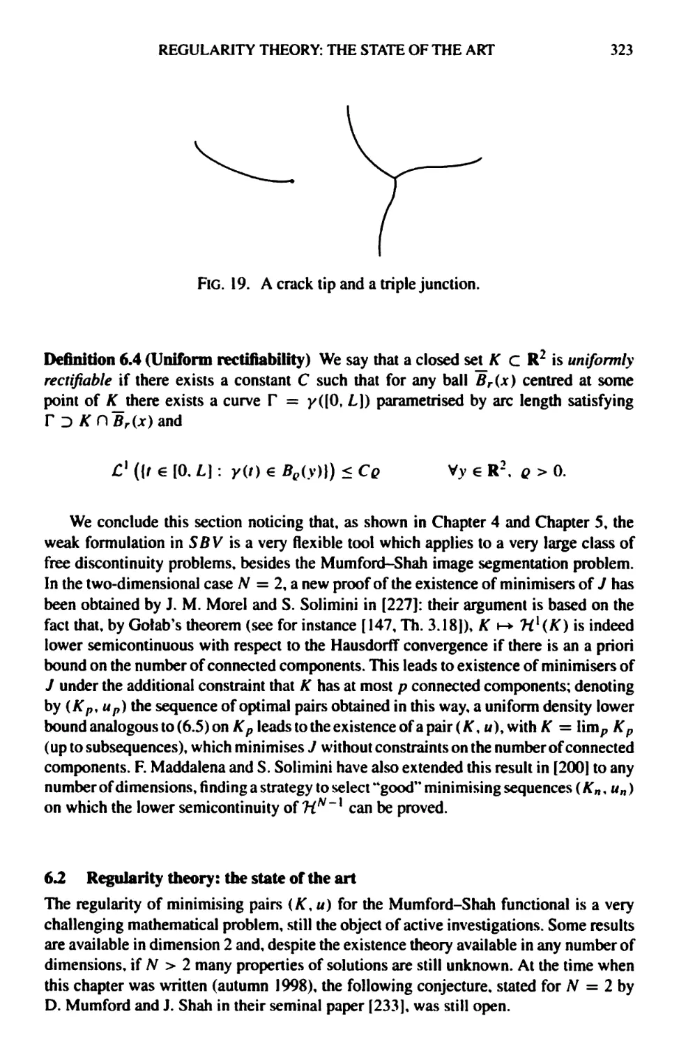
6.2 Regularity theory: the state of the art 323
6.3 Local and global minimisers 325
6.4 Variational approximation and discrete models 331
7 Minimisers of free discontinuity problems 337
7.1 Limit behaviour of sequences in SB V 339
7.2 The density lower bound 347
7.3 First variation of the area and mean curvature 354
7.4 The Euler-Lagrange equation 360
7.5 Harmonic functions 366
7.6 Regularity of solutions of the Neumann problem 370
7.7 Equations of mean curvature type 376
7.8 Exercises 379
CONTENTS
xv
8 Regularity of the free discontinuity set 381
8.1 Limit behaviour of sequences of quasi-minimisers 383
8.2 Lipschitz approximation 391
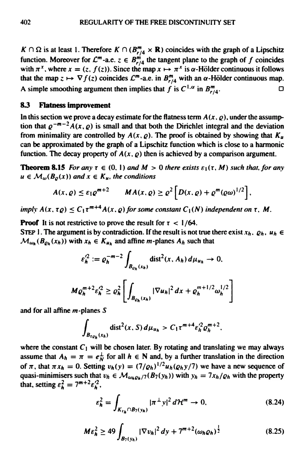
8.3 Flatness improvement 402
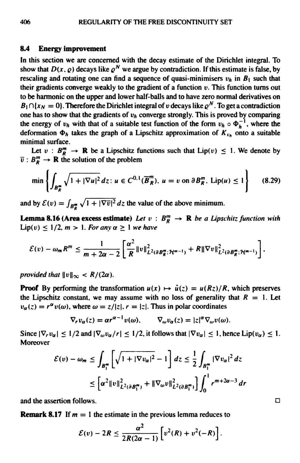
8.4 Energy improvement 406
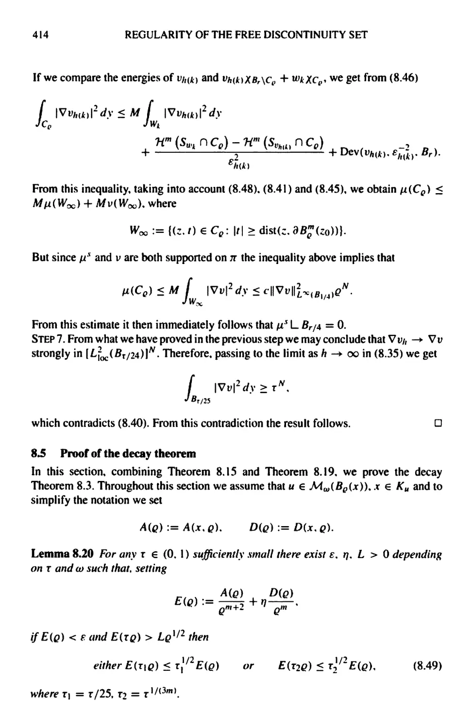
8.5 Proof of the decay theorem 414
References 419
Index 431
BASIC TERMINOLOGY AND NOTATION
Warning: terms like positive, negative, increasing, decreasing are always understood in
their wide sense, for instance'V positive** means r > 0; we use "strictly" for the restricted
sense, for instance "r strictly positive" means r > 0.
Set-theoretic operations:
€ membership U union
Π intersection \ set-theoretic difference
Δ symmetric difference с inclusion, not necessarily proper
Topological and metric space notation: let (X, d) be a metric space.
£ topological closure of £
д Ε topological boundary of Ε
Ε с С F Ε С F, £ compact
BQ(x) open ball with centre χ and radius ρ (χ — 0 can be omitted)
distU, E) infimum of d(x. y) as у varies in Ε
Ιρ(Ε) open ρ neighbourhood [χ € Χ : dist(x, Ε) < q] of Ε
dist(£, F) infimum of d(x. y)asx varies in £ and у varies in F
а = o(b) Landau symbol: lim (α/b) = 0
Number sets and vector spaces:
Ν, Ζ, Q, R natural, integer, rational and real numbers
R extended real line R U {-oot +00}
(a, b), [a, b] open and closed intervals with endpoints a, b € R
α л fet 4 ν b minimum and the maximum of a and b
RN, Ss~l euclidean /V-dimensional space and its unit sphere
a ® b m χ Ν matrix with (i>)-th entry atbj (for α € Rm, b € R^)
G* set of unoriented *-dimensional subspaces of RN
Functions and function spaces: let / : X -► Y.
/\e restriction of / to £ С X
im/ range of/
Г/ graph of /
/* * /~ positive part / ν 0 and negative part -(/ л 0) of /
fx f dp, mean value [μ(Χ)]~ι fx fdpoffonX
f(a+), /(a-) right and left limits at a of a function / of one real variable
supp/ closure of {jc e X : f(x) Φ 0}
C(X) space of real continuous functions on the topological space X
CC(X) space of real continuous functions with compact support on X
Co(X) closure, in the sup norm, of CC(X)
Cka(Sl) space of real functions continuously derivable in Ω up to the
order к € Ν, with locally α-Holder continuous derivatives in Ω
BASIC TERMINOLOGY AND NOTATION
XVII
Measure theory:
B(X) a -algebra of Borel subsets of a topological space X
Sβ μ -completion of the a -algebra S
[-Mioc(*)lm the space of Rm-valued Radon measures on X
[M(X)]m the space of Rm-valued finite Radon measures on X
CN Lebesgue outer measure in RN
Cs Lebesgue measurable sets in R^
о>лг Lebesgue measure of the unit ball of R^
D* ν upper and lower spherical density of ν relative to μ
ν/μ Radon-Nikodym density of ν with respect to μ
Hk A:-dimensional Hausdorff measure
Щ (Μ» *)♦ 0**(Мэ х) upper and lower spherical it-dimensional densities of μ
θ£(£\ x)% ©*♦(£* χ) upper and lower spherical it-dimensional densities of £
JkL Jt-dimensional Jacobian of a linear map L : R* -► R^
Tan* (μ, jc ) approximate tangent space to μ at χ
Tan*(Ε, χ) approximate tangent space to Ε at χ
CkL A:-dimensional coarea factor of a linear map L : RN -> R*
Μ*к, Λ1* upper and lower Jt-dimensional Minkowski content
Functions of bounded variation:
Du distributional derivative
ТУ1 и absolutely continuous part of derivative
0s и singular part of derivative
DJ и jump part of derivative
Dcu Cantor part of derivative
Du diffuse part of derivative
V(m, Ω) variation of a in Ω
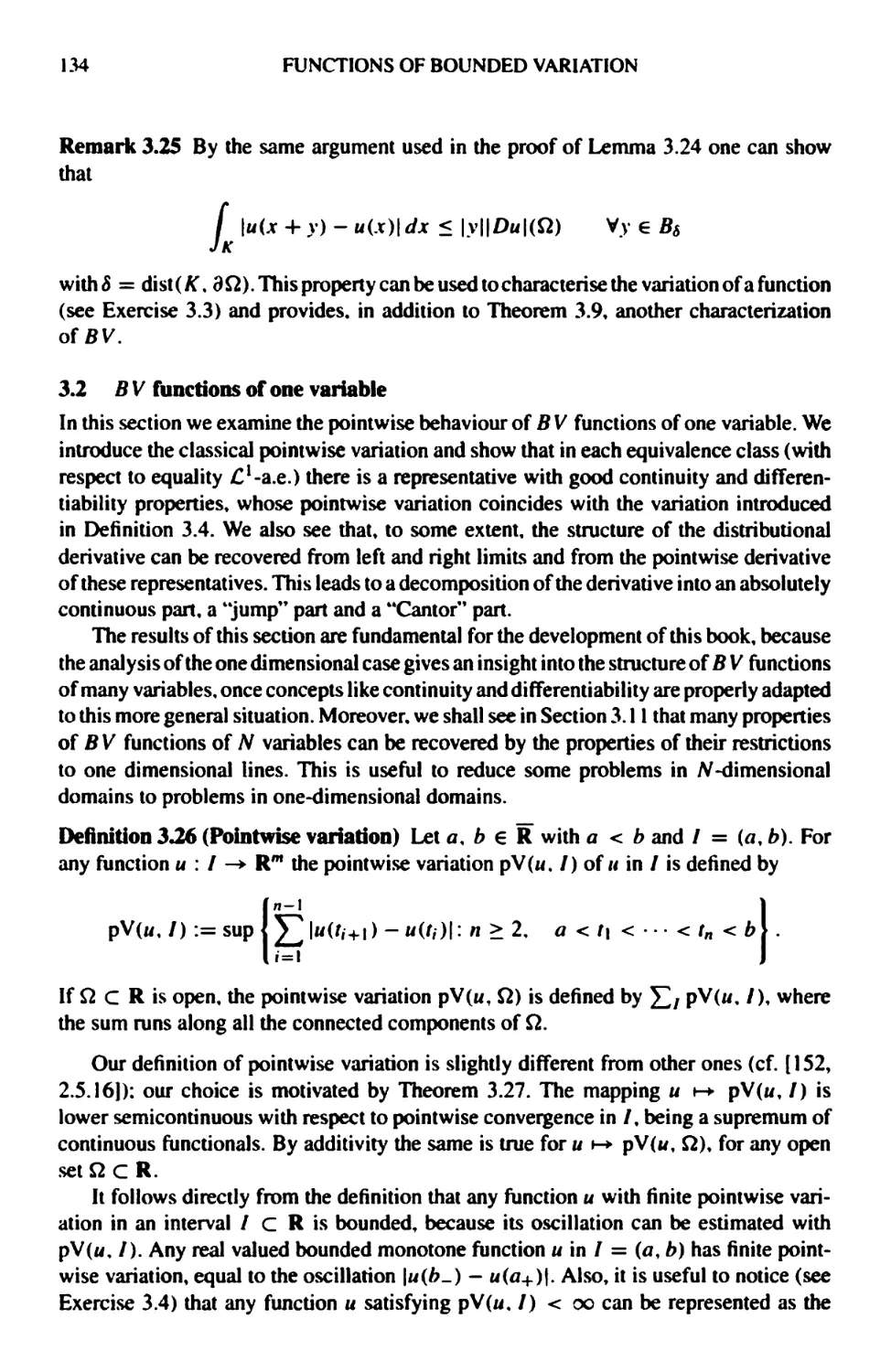
pV(wf /) pointwise variation of и in / с R
eV(w, /) essential variation of и in / с R
/Л ur left and right representatives of и
и * precise representative of и
Ρ (Ε, Ω) perimeter of £ in Ω
ve generalised inner normal to Ε
ТЕ reduced boundary of £
3*£ essential boundary of £
Et set of points of density / of £
Su approximate discontinuity set of и
и approximate limit of и
Ju approximate jump set of и
vu approximate unit normal to the jump set
и*, u~ approximate limits at jump points
Vu approximate differential of и
ui traces of и on both sides of Г
w** trace of и on the boundary of Ω
XV1I1
BASIC TERMINOLOGY AND NOTATION
Conventions: Euclidean spaces are endowed, unless otherwise stated, with the euclidean
inner product (·, ·) and the induced norm | ♦ |.
The set G* is viewed as a subset of RN , identifying any it-dimensional subspace
π with the matrix of the orthogonal projection onto π, computed with respect to the
canonical basis of RN.
By Ω, unless otherwise stated, we denote a generic open set in R^.
The space of linear maps between R^ and Rm will usually be identified with Rm/Vt
identifying any linear map ρ with the m χ Ν matrix p" = (p(ej)t εα), where e\ es
and ει em are the canonical bases in R^ and Rmv respectively.
MEASURE THEORY
We present the basic notions of measure theory which are useful in the book, with the
aim of fixing the notation and making the exposition self-contained, at least as far as
the results are concerned; as regards the proofs, we present mainly those that cannot be
found in the standard books. In particular, we devote the first section to recalling the
basic notions of measure theory that can be given in the abstract setting, i.e. the notions
of positive, real and vector measures in sets equipped with a a -algebra of subsets and the
related notions of integral and Lp space, as well as the Radon-Nikodym theorem. We
collect some useful facts about the weak topology in Lp spaces in Section 1.2, whereas
in the Section 1.3 we pass on to consider measures in (locally compact and separable)
metric spaces and introduce Borel and Radon measures. In the Section 1.4 we discuss the
notion of outer measure, the Caratheodory criterion, the Riesz theorem and the weak*
convergence of measures, and in Section 1.5 some operations on measures, such as
product, push-forward, and some related notions such as the support of a measure.
1Л Abstract measure theory
Definition 1.1 (σ-algebras and measure spaces) Let X be a nonempty set and let £ be
a collection of subsets of X.
(a) We say that £ is an algebra if 0 € Ε, E\ U £2 € £ and X \ E\ € £ whenever
£1. E2€E.
(b) We say that an algebra £ is a σ-algebra if for any sequence (£/») С Е its union
Ua Eh belongs to Ε.
(c) For any collection Q of subsets of X% the σ -algebra generated by Q is the smallest
σ-algebra containing Q. If (X, r) is a topological space, we denote by B(X) the
σ-algebra of Borel subsets of X, i.e., the σ-algebra generated by the open subsets
ofX.
(d) If £ is a σ-algebra in X, we call the pair (X, E) a measure space.
It is obvious by the De Morgan laws that algebras are closed under finite intersections,
and σ -algebras under countable intersections. Moreover, since the intersection of any
family of σ-algebras is a σ-algebra, the definition of generated σ-algebra is well posed.
Sets endowed with a σ-algebra are the right frame to introduce measures; let us start
from positive measures.
Definition \2 (Positive measures) Let (X, E) be a measure space and μ : Ε -* [0, ос].
2
MEASURE THEORY
(a) We say that μ is additive if, for E\, £2 e £,
£|П£2 = 0 =*· μ(£ιυ£2) = μ(£ι) + μ(£2).
(b) We say that μ is σ-subadditive if, for £ € £, (£*) С €,
CO 00
£C[J^ => μ(£)<£μ(£/,).
(c) We say that μ is a positive measure if μ(0) = 0 and μ is α-additive on £, i.e. for
any sequence (£я) of pairwise disjoint elements of £
(ОС \ 00
υ*)-Σ
μ(£*).
We say that μ is finite if μ(Χ) < ос.
(d) We say that a set £ С X is σ-finite with respect to a positive measure μ if it is the
union of an increasing sequence of sets with finite measure. If X itself is σ-finite,
we also say that μ is σ-finite.
A positive measure μ such that μ(Χ) = 1 is also called a probability measure.
Remark U Any positive measure μ is monotone with respect to set inclusion and
continuous along monotone sequences, i.e., if (£л) is an increasing sequence of sets
(resp. a decreasing sequence of sets with μ(£ο) finite), then
WU^l = Jim μ(£Λ), resp. μ ( Π Eh ) = Jim μ(£Λ).
We note also that the σ-additivity is implied by σ-subadditivity and additivity:
(00 \ 00 Я
(J £л ) < £μ(£Α) = ton £μ(£/,)
h=0 / A=0 П->ОСА=0
\h=0 / \л=0 /
Beside positive measures, it is also possible to define vector-valued measures; this
notion is essential in this book, because the gradient of a function of bounded variation
in the sense of distributions is a measure of this kind. We give here the abstract
definition. Notice that positive measures are not a particular case of real measures, since real
measures, according to the following definition, must be finite.
Definition 1*4 (Real and vector measures) Let (Χ. ί) be a measure space and let
m € N,m > 1.
ABSTRACT MEASURE THEORY
3
(a) We say that μ : 8 -► Rm is a measure if μ(0) = 0 and for any sequence (Eh) of
pairwise disjoint elements of £
ΙΙ*)-Σ
If m = 1 we say that μ is a real measure, if m > 1 we say that μ is a vector
measure.
(b) If μ is a measure, we define its total variation |μ| for every £ € S as follows:
Ioo oo 1
Y^ \μ(ΕΗ)\: Eh € £ pairwise disjoint, £ = (J Eh \ .
л=о л=о j
(c) If μ is a real measure, we define its positive and negative parts respectively as
follows:
+ ΙμΙ + μ . - ΙμΙ-μ
μ :=—2— and μ :=—2—'
Notice that the absolute convergence of the series in (a) is a requirement on the set
function μ: in fact, the sum of the series cannot depend on the order of its terms, as the
union does not. Let us give some easy example of measures in the abstract setting.
Example 1*5 If X is a nonempty set and € is the σ -algebra of all its subsets, we define
the following measures on (X, €):
(a) (Counting measure) We define #(0) = 0, #(£) as the cardinality of Ε if it is finite,
#(£) = +oo otherwise.
(b) (Dirac measures) With each χ e X we associate the measure Sx defined by 8X (£) =
1 if jr € £,$*(£) = 0 otherwise. If (jc/,) is a sequence in X and if (c/,) is a sequence
in Rm such that the series Ση Iе* Ils convergent, we can set
V»=0 / \h:xh€E)
and obtain an Rm-valued measure. Measures of this kind are called purely atomic.
More generally, the set 5μ of atoms of a measure μ in a measure space (X, E) is
defined by
5μ:={χεΧ:μ({χ))φΟ),
provided the singletons {x) are elements of £. If μ is finite or σ-finite the set of
atoms is at most countable,
(c) (Integrals of Dirac measures) Let (X, S) be a measure space. If / : R -* X is such
that f~] (£) € B(R) for any £ € £, we define a positive measure in (X, S) by
(f */d)*) (E) := f ifuy(E)dt = Cx (/"'(Ε)) .
4
MEASURE THEORY
where Cx is the Lebesgue measure on R (see Definition 1.52 below); this example
will be interpreted as a push-forward of Cx in Section 1.5.
Let us show that the total variation of a measure is a positive finite measure.
Theorem 1,6 Let μ be a measure on (X% E); then \μ\ is a positive finite measure.
Proof Let us show that |μ| is σ-subadditive and additive.
To prove the σ-subadditivity, let (£/,) с S be a sequence such that £ с Ua!o ^л
and set E'0 = £o, E'h = £* \ U;io &j ^ог ^У * - 1. Let (F/) be a countable partition
of £; using the σ-additivity of μ and observing that for every j e N the sequence
(Fj Π E'h)л is a countable partition of £,, we get
00
У=0 ;=0
£^(£*nf>)
л=о
A=Oy=0 Λ=0
and the σ-subadditivity of |μ| follows from the arbitrariness of the partition (Fj).
In order to prove the additivity, let E\4 Ει € £ be disjoint, and let ε > 0 be given;
then two countable partitions of E\, £2» resp. (£^), (£j*), exist in ί such that
|μ|(£ι)<£|μ(£;)
л=о
+ ε. ί = 1.2
and E\ Π Ε\ = 0 for any А, к e N, so that (Elh, £j) is a countable partition of £1 U £2.
Then
2 00
|μ|(£ι U £2) > £ ]Γ μ(£ΐ) > |μ|(£ι) + |μ|(£2) - 2г,
and the thesis follows from the arbitrariness of ε.
To prove the finiteness, it is sufficient to assume that μ is real, the Rm-valued case
being an easy consequence of the following estimate:
m
И(£)<]Г|мл1(£)
for every £ e ί% μ = (μι μΛ).
Assume by contradiction that |μ|(Χ) = oo; then there exist a countable partition
(Xh) of X and η e N such that
£|μ(ΧΛ)|>2(|μ(Χ)| + 1).
л=о
Summing the positive and negative terms separately, we find a set £ € ί (union of
some of the X/,) such that |μ(£)| > |μ(Χ)| + 1; setting F = X \ £, we compute
ABSTRACT MEASURE THEORY
5
|μ(£)| = |μ(Χ) - μ(£)| > |μ(£)| - |μ(Χ)| > 1. By the additivity of |μ|, either
|μ|(£) = oo or |μ|(£) = oo: assuming the latter, we set E\ = £ and repeat the
above argument in £, splitting F as the disjoint union of £2 and F\. with |μ(£2>| > 1
and |μ|(£|) = oo; otherwise, we set E\ = £. The iteration leads to a sequence of
disjoint sets (£/,) such that |μ(£/,)| > 1 for any Λ, hence the series Σ μ(£*) cannot be
convergent. This contradiction proves that |μ| is finite. D
The above theorem shows that for any real measure μ, its positive and negative part
are positive finite measures, hence the decomposition μ = μ+ - μ~ holds; it is known
as the Jordan decomposition of μ.
Remark 1.7 It is immediate to check that Rm-valued measures can be added and
multiplied by real numbers, hence they form a real vector space; moreover, an easy
consequence of Theorem 1.6 is that the total variation is a norm on the space of measures,
which turns out to be a Banach space (see Exercise 1.2). If X is a locally compact
separable metric space, it will be identified with the dual of a space of continuous functions,
and this will give the completeness in another way (see Remark 1.S7).
We continue this discussion on general measure theory by showing a useful criterion
that ensures that two measures coincide in a σ-algebra, provided that they coincide in a
smaller family of subsets closed under finite intersections. We state this result for <r-finite
positive measures, but it obviously holds for vector measures as well.
Proposition 1.8 (Coincidence criterion) Let μ, ν be positive measures on the measure
space (Χ, £), and let Q С S be a family closed under finite intersection; assume that
μ(£) = v(E)for every Ε € Q, and that there exists a sequence (Xh) in Q such that
X = ил Xh and μ(Χ/,) = v(Xh) < 00 for any Λ. Then μ and ν coincide on the
a -algebra generated by Q.
Proof It is not restrictive to assume that μ and ν are finite measures with μ(Χ) = v(X),
because the general case easily follows. Let Μ be the smallest family of subsets of X
containing Q and verifying the following conditions:
(i) (£л) С Μ, £Λ t £ => £ € .Μ;
(ii) £, £, £U£€.M => £ Π F € Μ:
(iii) Ε eM => X\E €λί.
Let also Τ — [Ε € £:μ(£) = ν(£)}; since, by the finiteness hypothesis and the
properties of measures, Τ satisfies (i), (ii), (iii), we have Μ С Т. Therefore, it is
sufficient to prove that Μ is a a -algebra, and this follows if we prove that Μ is closed
under finite intersection. To this end, for any £ let us set
ME = {F eM: EOF eM].
We first show that if £ € Μ then (i)t (ii), (iii) hold for Με\ in fact. Me clearly satisfies
(i); to check (ii), let F\, Fi € Me (i.e. Ε Γ) F\ e Μ and £ Π £2 € Μ) and assume
that £ Π (F\ U £2) = (£ Π £1) U (£ Π £2) € M\ this last condition implies that
(£n£!)n(£n£2) = £Π(£, Π £2) belongs to Λί, hence £ι Π £2 € Me, as required.
6
MEASURE THEORY
To see (iii), let F e A*£;then, £П(Х\£) = £ Π (Χ \(£ OF)) belongs to ΛΊ, because
£, Χ \ (£ Π F) and £ U (Χ \ (Ε Π £)) = X belong to Λί and (ii) holds.
Let £ € Q\ since Alf Э i? we conclude that Me = Λ4, i.e. ΕΠ F € Μ whenever
F e M. Since £ e £ is arbitrary, this proves that Mf Э Q for any F e ΛΊ, and again
the minimality of Μ shows that Mf = ΛΊ. Since £ is arbitrary, this shows that Μ is
closed under finite intersection, so that the thesis is achieved. □
Remark 1.9 In the proof of the preceding result, we have proved the following
statement, which will be used elsewhere: let Q be a family of generators for the σ -algebra Ε
in X, stable under binary intersection and such that X = |JA Хд, with Xh 6 Q\ if Μ
is any family of subsets of X containing Q and verifying conditions (i), (ii), (iii) in the
above proof, then Μ contains £. In fact, we have proved that the smallest family with
these properties is the σ -algebra generated by &.
As an application of Proposition 1.8 in metric spaces, we observe that if two measures
coincide on the family of open or closed sets then they coincide on the Bore! sets; in RN
another interesting case (see Example 1.77 below) is the coincidence on the cartesian
products of intervals. The following example shows that the hypothesis that μ and ν are
σ-finite cannot be removed.
Example 1Л0 Let X = Ν, μ the positive measure whose value is +oo for every
nonempty subset of X% and ν the counting measure; then, μ and ν agree on all the
subsets of X whose complement in X is finite (a class which is closed under finite
intersection), but they do not agree everywhere.
Definition Ml ^-negligible sets) Let μ be a positive measure on the measure space
(X.S).
(a) We say that N С X is μ-negligible if there exists £ e £ such that N С Е and
μ(£) = 0.
(b) We say that a property P{x) depending on the point χ € X holds μ-a.e. in X if
the set where Ρ fails is a μ-negligible set.
(c) Let Εμ be the collection of all the subsets of X of the form F = EON, with £ 6 Ε
and N μ-negligible; then Εμ is a σ-algebra which is called the μ-completion of
Εy and we say that £ С X is μ-measurable if £ e Εμ. The measure μ extends to
Εμ by setting, for F as above, μ(£) = μ(£).
If μ is a real (or vector) measure we call the completion of Ε with respect to the total
variation |μ| of μ the μ-completion Εμ of E. Then, the measure μ can be extended to
Εμ as above.
Definition 1Л2 (Measurable functions) Let (X, E) be a measure space and (K, d) a
metric space.
(a) A function / : X -► Υ is said to be E-measurable if /~! (A) e Ε for every open
set А С К.
(b) If μ is a positive measure on (X, E) the function / is said to be μ-measurable if
it is Eu -measurable.
ABSTRACT MEASURE THEORY
7
In particular, if / is <f-measurable then /"] (B) € ε for every В € B( Y). Moreover,
if Υ is separable, it can be proved that / is μ-measurable if and only if it coincides with
an ^-measurable function outside of a μ-negligible set (see Exercise 1.3).
Proposition 1.13 Let (X, £) be a measure space; then for (extended) real-valued
ε-measurable functions ff g the following results hold:
(a) if f, g : X -► R then af + fig (with α, β € R), / · g, are ε-measurable, and
also fjg, provided g(x) φ Ofor any jc € X.
(b) If f% g : X -* R then min{/, g\ and max{/, g) are ε-measurable; in particular
/+ = max{/, 0}, /"" = max{—/, 0} and \f\ are ε-measurable.
(c)Iffh:X-+Risa sequence of ε-measurable functions then
inf fh, sup fh, lim inf fh, lim sup fh
are all ε-measurable.
In the following definition we present several standard notions, which are listed
for completeness. After giving the definitions of characteristic function of a set and of
simple function, we define the integral with respect to a positive measure for these
functions, extend the notion of integral to every measurable positive function and introduce
summable and integrable functions. Finally, all these notions are extended to real and
vector functions, and to real and vector measures.
Definition 1.14 (Integrals) Let (X, £) be a measure space.
(a) For Ε С X we define the characteristic function of E, denoted by xe, by
Χ£(Λ)={θ if,* Ε.
We say that / : X -► R is a simple function if the image of / is finite, i.e., if
/ belongs to the vector space generated by the characteristic functions.
(b) Let μ be a positive measure on (X, 5); the integral of a simple μ-measurable
function и : X -» [0, oo) is defined by
/,
udpi := Σ z^u '(*))·
zeim(u)
where we adopt the convention that whenever ζ = 0 and μ(^](ζ)) = oo
the product ζμ(ΐ4~](ζ)) is set equal to zero. The definition is extended to any
μ-measurable function и : X -» [0, oo] by setting:
I иάμ := sup { ι υάμ: ν μ-measurable, simple, ν < и \.
We say that a μ-measurable map и : X -► R is μ-summable if
|Μ|*/μ < oo.
/.
8
MEASURE THEORY
We say that a μ measurable map и : X -* R is μ-integrable if either
I u* άμ < oo or / u" άμ < oo.
Jx Jx
If и is μ-integrable, we set
Ι αάμ:= I u*άμ — / и"άμ.
Jx Jx Jx
(c) Let μ be a measure on (X. S) and w:X->Ra |μ|-measurable function; we say
that и is μ-summable if к is ΙμΙ-summable and, if μ is real, we set
Ι uάμ:= Ι uάμ* — Ι Η*/μ~~.
/χ Jx Ух
If μ is an Rm-valued vector measure then we set
Ι αάμ := ί Ι κ</μι / uάμmJ.
If μ is real and и = (и j,... , w*) : X -► R* is |μ|-measurable, we say that w is
№\-summable if all its components are ΙμΙ-summable, and we set
/ uάμ := i Ι ιιχάμ / ^άμ).
When £ is a μ-measurable set the integral of a function и on £ is defined by
«ΧεΊβ*
/-*.:-/.
provided that the right-hand side makes sense.
Notice that an immediate consequence of the above definition is the inequality
\( αάμ\< f \ϋ\ά\μ\. (1.1)
which holds for every extended real or vector valued summable function и and for every
positive, real or vector measure μ. More generally, let us recall the classical Jensen
inequality.
Lemma 1.15 (Jensen inequality) Let Φ :Rk -+ Ru {+00} be a convex lower semi-
continuous Junction, μ a probability measure on (X, £) and и : X -> R* a μ-summable
function; then
Φ I I uάμ\ < Ι Φ(Μ)</μ.
ABSTRACT MEASURE THEORY
9
Proof Let Фл be affine functions such that Φ = supA Φ/, (cf. Proposition 2.31). Then
by
Фл ί / иацЛ = Ι ΦΛ(ιι)Λμ < I Ф(и)άμ
the statement follows letting h | oo. □
Notice also that, if и is μ-summable, for any ε > 0 there is a measurable set A with
finite measure such that fx.A \u\ ά\μ\ < ε. In fact, there is a simple function ν < \u\
such that, setting A = {jc e X: v(x) > 0}, \μ\(Α) < oo and
[ \α\ά\μ\< ί (Μ-ν)ά\μ\<ε.
JX\A JX
Definition 1.16 (Lp spaces) Let (X, 8) be a measure space, μ a positive measure on it
and и : X -» R a μ-measurable function. We set
\Μ\Ρ:=Π\4\Ράμ^
\/p
if 1 < ρ < oo, and
HhII^ :=inf{C €[0,oo]: |m(jc)| < С for д-а.е. jc € X).
We say that и e LP(X, μ) if ||w||p < oo. The set LP{X% μ) is a real vector space and
|| · Up is a semi-norm.
Remark 1.17 (Identification of functions equal a.e.) When dealing with measure-
theoretic or functional-analytic properties of functions and Lp spaces, it is often
convenient to consider functions that agree a.e. as identical, thinking of the elements of Lp
spaces as equivalence classes; in particular, this makes || · \\p a norm. We shall follow
this path whenever our statements will depend only on the equivalence class without
further mention, provided that this is clear from the context. But we shall not consider
functions agreeing a.e. to be identical if we are concerned with fine properties of the
single function.
Remark 1.18 (Chebyshev inequality) Notice that if / € Ο (Χ, μ) is positive, then for
any/ > 0
μ({* €*:/(*) >!})<- ί ίάμ\ (1.2)
hence letting / -► oo we obtain that μ ([χ € X: f(x) = oo}) = 0; moreover, if the
integral of / vanishes, then letting /-►Owe obtain that / = 0 μ-a.e. in X.
We assume that the reader is familiar with the properties of integrals, measurable
functions and Lp spaces, and refer to [245] for the notions relative to abstract
measure theory not stated here. For completeness sake, we state here the main convergence
theorems of Levi, Fatou, Lebesgue.
10
MEASURE THEORY
Theorem 1.19 (Monotone convergence theorem) Let uh : X -► R be an increasing
sequence of μ-measurable functions, and assume that uh > g, with g e LX(X> μ), for
any Λ € N. Then,
lim / ΐί^άμ= I lim u/,ί/μ.
Theorem 1.20 (Fatou's lemma) Let uh : X -* R be μ-measurable functions and
geL](X^).Then
I lim inf ии άμ < lim inf / w/, ί/μ
Jx Λ—οο Л—ос Jx
ifuh > g for any A € N am/
I limsupii/,ί/μ > lim sup ι ιΐπάμ
JX Л->оо Л—ос JX
if**h < g for any h € N.
Theorem 1Л (Dominated convergence theorem) Let uy uh : X -► R be μ·
measurable functions, and assume that ин(х) -► u(x) for μ-a-e. χ e X as h -+ oo. If
then
I sup|ii/fc|^ < oo
JX h
lim / ^άμ= Ι ιιάμ.
-+<x>Jx Jx
lim
h-+oojx
We consider now the classical notions of absolute continuity and the Radon-Nikodym
theorem. To begin with, let us introduce the measure induced by a summable distribution
of mass.
Definition 122 Let μ be a positive measure on the measure space (X, £) and let
/ € [L! (Χ· μ)Γ· we define the Rm-valued measure
fniB)
:= [ ίάμ Vfie£.
Jb
Using the elementary properties of the integrals, it is easily checked that the above
formula defines a Rm-valued measure; its total variation is computed in the following
proposition.
Proposition 1.23 Let /μ be the measure introduced in the previous definition: then
\ίμ\(Β)=[\/\άμ Vfie5.
JB
ABSTRACT MEASURE THEORY
II
Proof It is easily checked that |/μ| < |/|μ. Let us fix a countable dense set
D = (zh: A € N} in Sm_l and В e £. For any ε > 0 let us define
σ(χ) :=min{A 6 N: (f(x).Zk) > (I - *)I/U)II,
and let Ял = σ~! ({Λ}) Π β e ί be the level sets of σ. We have then
(\-s) [ l/|rfM = f\l-*)/ 1/1</μ
ос эо
< £</μ(βΛ).*Α> < £|/м(А)1 < Ι/μΙ(«)
and the thesis follows. □
From Remark 1.18 it immediately follows that if the measures /μ and %μ coincide
then g = f μ-a.e.; moreover, if Ε is μ-negligible it is /μ-negligible as well; this
important relation between measures is presented in the following definition.
Definition 1*24 (Absolute continuity and singularity) (a) Let μ be a positive
measure and ν a real or vector measure on the measure space (X, £). We say
that ν is absolutely continuous with respect to μ, and write ν <$c μ, if for every
В € € the following implication holds:
μ(β)=0 => М(Я)=0.
(b) If μ, у are positive measures, we say that they are mutually singular, and write
ν J_ μ, if there exists Ε € ε such that μ(£) = 0 and v(X \ E) = 0; if μ or ν are
real or vector valued, we say that they are mutually singular if |μ | and | v\ are so.
Observe that if / is μ-su mm able then the measure /μ is absolutely continuous with
respect to μ. In the following remark we point out a useful characterisation of the absolute
continuity and then we present the notion of an equiintegrable family of functions; these
concepts will be useful in connexion with the Vitali-Hahn-Saks and Dunford-Pettis
theorems.
Remark 1*25 The notion of absolute continuity can be rephrased as follows: i> is
absolutely continuous with respect to μ if and only if for every ε > 0 there exists δ > 0 such
that, for every Ε € ε, μ(£) < 6 implies M(£) < ε. In fact, assume that ν <«c μ and, by
contradiction, that for some ε > 0 there exists a sequence (Eh) such that μ(£/,) < 2"h
and \v\(Eh) > ε. Setting
ОС 00
Л=0>=Л
we have μ(£) = 0 and M(£) > f, which is impossible. The converse implication is
obvious.
12
MEASURE THEORY
Definition 1.26 (EquUntegrability) If Τ С Ll(X. μ) we say that Τ is an equiinte-
grable family if the following two conditions hold:
(i) for any ε > 0 there exists a μ-measurable set A with μ (A) < oo such that
fx\A I/'1''* < * for any / € Я
(ii) for any ε > 0 there exists 5 > 0 such that, for every μ-measurable set E4
if μ(Ε) < 8 then fE \f\ άμ < ε for every / 6 /\
Notice that the first condition is trivially satisfied for finite measures: it suffices to
take A = X. In the following proposition we give three equivalent formulations of the
equiintegrability property.
Proposition 1.27 Let Τ С Ll (Χ, μ). Лкст, .E /5 equiintegrable if and only if
(£л)С£, Ел |0 => lim sup [ |/|</μ=0. (1.3)
If μ is a finite measure and F is bounded in Lx (Χ, μ), then Τ is equiintegrable if and
only if
ГС If € Ζ,'(Χ,μ): ί φ{\ί\)άμ < l) (1.4)
for some increasing continuous function φ : [О. oo) —► [0, oo) satisfying <p(t)/t —► 00
ast -* ooor equivalently if and only if
lim sup / |/|</μ =0. (1.5)
'-*°° /eW(l/l>r)
Proof The necessity of (1.3) for equiintegrability easily follows splitting the sets £/,
into Eh Π A and Eh \ A, with A given by property (i) for an arbitrary ε > 0. Since
μ(£Λ Π A) -► 0, using property (ii) the integrals on Ел П A can be uniformly estimated
with ε for A large enough, as well as the integrals on Eh \ A.
Now we prove that (1.3) implies both (i) and (ii). For the first, assume by contradiction
that there exists ε > 0 such that for every measurable F С X with μ(Ε) < oo the
inequality fXyF \f\dμ > ε holds for some / € T. Take F\ with μ(Ε|) < oo and f\
such that fXxFl \Α\όμ > £,andfixE2 D F\ witl^(E2) < ooand/x^2 \ί\\άμ < ε/2;
proceeding inductively we get an increasing sequence (Ел) of finite measure sets and
a sequence (/л) С Τ such that ffM\pk ΙΛΙ^μ > */2 holds for any integer h > 1.
Denoting by Ε the union of the sets Ел the contradiction is achieved with Eh = F \ Fh.
For the second, if for some ε > 0 measurable sets Ел and functions /л € ,Ε can be
found such that μ (Ел) < 2"л and /^ |/л1 <*μ > ε9 the contradiction with (1.3) is found
with
00 oc
Eh := (J (Ε* \ Eoc) where Ε<* := p| (J Fk
k>h Л=0А=Л
because E^ is μ-negligible.
ABSTRACT MEASURE THEORY
13
Now, we prove that the family Q in the right-hand side of (1.4) is equiintegrable.
Since μ(Χ) < oo we need only to check condition (ii). Let ε > 0, let τ > 0 such that
(p(t) > It Ι ε in (rf oo) and δ > 0 such that τ 8 < ε /2. Then, if f e <?, Ε is μ-measurable
and μ(£) < S we get
ί Ι/|4μ< ί 1/1<*μ+ ί Ι/Ι<*μ<τί + £ / φ(\/\)άμ<ε.
J Ε ^£Π(1/|<τ| JEC\\\f\>T) * JX
Conversely, if T is equiintegrable and bounded, condition (ii) implies (1.5), because
М({|/1 > '}) < ΙΙ/ΙΙιΛ· Hence, we can find a sequence of integers (a,) f oo such that
ίι/ι>«ι^'^ < 2"1"'forany ' € ^ Since
]Г Х(л,оо)(0 < * Χ(β|· W> Vi € Ν, ί € (0, 00)
n>di
we obtain that Ση>α Μ ((I/I > nD can ^ estimated with 2"1"'. Let
bn :=#{/: a, < n)
and notice that />„ | oo as л —► oo. Denoting by /?(/) the piecewise constant function
equal to bn in [л, π + 1) and setting <p(t) = yjj b(s)ds4 let us check that fx φ(\/\)όμ
can be uniformly estimated for / e T. In fact,
ί <ρ(|/|)</μ = У] / φ(\ί\)άμ < ΤΤ^μ «ί < |/| < / + 1})
'Χ fto-/|i<l/l<i+l| ?=0л3)
ос
= Σ^μ<{ΐ/ι>πΐ)
/ι=0
and the last sum can be estimated by using the definition of bt and writing
Σ Σ μ(ιι/ι>π}) = ςΣμ(π/ι>π})<Σ2-,-' = ι.
л=0 [i: a, <n} / =0 л >α, ι =0
We now show that condition (1.5) implies that Τ is equiintegrable (the necessity of
this condition has been already observed). Indeed, given ε > 0, let г > 0 such that
^(l/l>r) '^' ^ < €^ f°ra" /; *en ^ & *s μ-roeasurable and μ(£) < ε/(2τ) we have
ί Ι/Μμ< ί \ί\άμ+ ί \/\άμ<^ + τμ(Ε)<ε.
JE J{\f\>r) JEn{\f\<r) 2
α
The following classical result shows that if a measure is absolutely continuous with
respect to another one, then an integral representation as in Definition 1.22 holds. In
the following statements, uniqueness is meant in the sense of equivalence classes of
functions agreeing μ-a.e.
14
MEASURE THEORY
Theorem 1-28 (Radon-Nikodym) Let μ, ν be as in Definition 1.24(a), and assume that
μ is σ-finite. Then there is a unique pairofRm-valuedmeasures va, v5 such that va <3C μ,
ν5 L μ and ν = va + vs. Moreover, there is a unique function f e [L1 (X, μ)]"1 such
that va = /μ. The function f is called the density of ν with respect to μ and is denoted
by ν/μ.
Since trivially each real or vector measure μ is absolutely continuous with respect to
|μ|, the following useful decomposition immediately follows from the Radon-Nikodym
theorem and Proposition 1.23.
Corollary 1*29 (Polar decomposition) Let μ be a Rm-valued measure on the measure
space (X% £); then there exists a unique Sm~l-valued function f € [£!(X\ ΙμΙ)]"1 such
that μ = /|μ|.
The following result is similar to the Banach-Steinhaus uniform boundedness
theorem and gives a useful condition for the equiintegrability of a sequence of summable
functions. It will be useful when dealing with various notions of convergence in /Λ
Theorem 1.30 (VitaW-Hahn-Saks) Let μ be a positive measure on (X4 £)t let (fa) be
a sequence in L^(X, μ), and set ν/, = /Άμ.
(a) Assume that for every Ε € Ε with finite measure the limit limj, Vh(E) exists and
is finite; then for every ε > 0 there is δ > 0 such that supA \vh |(£) < ε wlienever
μ(£) < δ.
(b) Assume that for every Ε e Ε the limit lim/, v^(E) exists and is finite; then (fa) is
equiintegrable.
Proof (a) Let Γ = {Ε € Ε: μ(Ε) < οο}, and for £, F e E\ let </(£, F) = μ(£Δ£);
since £ »-► xe is an isometry carrying (£', d) into a closed subset of the Banach space
L](X4 μ), it follows that (£', d) is a complete metric space, provided that sets £, F with
μ(£Δ£) = 0 are identified. The measures v* = fal*> are well defined on (£', d) under
the above identification, and are clearly real valued continuous functions. Fix ε > 0 and
for any Jt € N consider the closed sets
& =
£€£': sup |ι/Λ(£) - ι>/(£)| < ε
hj>k
since lima v/,(£) exists finitely for any £ € E\ we have \Jk Ek = E'. From the Bairc
category theorem it follows that at least one among the Ek has nonempty interior, i.e.
there exist £ € £' and it € N such that for some δ' > 0 the condition d(E% F) < δ'
implies F e Ek. or \vh(F) - vi(F)\ < ε for any A, / > *. Let 0 < δ < δ' be such that
\»н(П\ < ε for Λ < Jt whenever μ(£) < 5, and let £ € Γ be such that μ(£) < 5;
setting £| = £ U F and F2 = £ \ £, we see that F = F\ \ F2, with d(E. F\) < 5,
d(£, £2) < Я- Thus, μ(£) < δ and Λ > it imply
l^iniilvH^I + kHn-^iF)!
< \vk(F)\ + |p*(£i) - v*(£i)l + \vk(F2) - ил(£2)1
<|v*(F)l + 2*<3e.
WEAK CONVERGENCE IN Lp SPACES
15
To conclude, it suffices to consider the following estimate:
Wh\(F) = j ί^άμ + Ι f~ άμ<6ε
which can be deduced, for any F with μί/7) < 5, by the previous one applied to
Fn[fh>0}andFn[fh<0}.
(b) By statement (a), we need only to show that for every ε > 0 there is A e S such
that μ(Α) < oo and sup;, \ν^\(Χ \ A) < ε. Notice first that, possibly replacing X by
the σ-finite μ-measurable set [jh{fh φ 0}, we can assume that X is σ-finite. Hence, by
Exercise 1.5 we can find a μ-summable function θ : X -► (0, oo). Let us check that
A, = {Θ > t) has the required properties for/ > 0 small enough. In fact, by Chebyshev
inequality, μ{Α() < ос for any /> 0. On the other hand, since vh << θ μ for any /i,
by statement (a) we can find for any ε > 0 a number 5 > 0 such that supj, \vb\(E) < ε
whenever θμ(Ε) < 6. Since
lim / θάμ=0
ПО Jx\At
because (X\At) I 0as/ l 0, choosing E = (X\A() with /small enough the conclusion
follows. □
\2 Weak convergence in Lp spaces
In this section we discuss some properties of the Lp spaces which are well known but not
always covered in the standard textbooks: we are mainly concerned with weak
convergence of sequences of Lp functions and comparison with other notions of convergence,
such as strong convergence, convergence a.e., etc. Some of the examples we are going
to present rely on the notion of Lebesgue measure: this measure will be introduced in
Section 1.4, but we assume only elementary properties which are likely known to the
reader.
We fix a measure space (X, £) and a positive measure μ on it; then, for I < ρ < ос
the Banach spaces Lp = LP(X% μ) are defined (see Remark 1.17) and we recall that for
1 < ρ < oo the space LP is uniformly convex (hence reflexive) and its dual is Lp , with
p' = p/(p - 1); if μ is σ-finite, the dual of Lx is L^ and, whenever we shall refer to
the duality between О and Lxtwe always assume σ-finiteness. Accordingly, the weak
convergence of sequences is defined: given /, (/a) 6 Lp% we say that fh-*f weakly
if /χ ίπ&άμ -* fx ί%άμ for any g 6 Lp if I < ρ < oo, and that /л -► / weakly* in
L°° if ρ = oo and fx ^άμ -* fx ίζάμ for any g e Ll.
Definition 131 (Convergence in measure) Let //, and / be μ-measurable functions.
We say that (fy) converges to / in measure if
lim μ([χ£Χ: \fh(x) - f(x)\ > ε)) = 0 W > 0.
The a.e. convergence can be easily compared with the convergence in measure; in
fact, if (fh) is a sequence of μ-measurable real valued functions in X, the following
16
MEASURE THEORY
statements hold:
(i) if μ(Χ) < oo and fh~+f μ-a.e. then fh -► / in measure,
(ii) if fh -* / in measure, then a subsequence (/*<*>) converges to / /x-a.e.
For, fixe > 0 and let Ζ7* = Па>*{1Л~Л < ε}; since (F^)isan increasing sequence
and μ(Χ \ \Jk Ft) = 0, we have that μ(Χ \ Fk) -* 0 as к -► oo and (i) follows.
Conversely, if fh -+ f in measure, let A(I) be the smallest integer A such that
M(II/a - /I > U) < 1 /2, and, inductively, let A(* + 1) be the smallest integer h > h(k)
such that μ({|/Λ - /I > l/(* + 1))) < l/2<+l. If Ek = Ц,>*{1Ло) " /I > 1//K
since μ(£|) < oo and £* i F = Πα ft· we have m(F) = lim* μ(Ε*) = 0, and it is
easily seen that /*<*)(*) -* f(x) for any χ € X \ F.
In statement (i) the hypothesis μ(Χ) < oo cannot be removed (to get a
counterexample, simply take //, = X[M+i| in R), and in (ii) the whole sequence in general does
not converge a.e. (see Exercise 1.6).
As a consequence of the previous discussion, we remark that if fh -* / strongly in
Lp then a subsequence converges to / a.e. This is trivial for ρ = oo; for 1 < ρ < oo, by
Chebyshev inequality (1.2) we immediately get that fh -+ fin measure and (ii) applies.
Let us show that no immediate relation exists between weak convergence and the
notions of a.e. convergence and convergence in measure.
Example 132 Let X = [0,1] and let μ = Cx be the Lebesgue measure (see
Section 1.4).
(i) For every ρ > 1, consider the sequence fh = Αχ[ο.ι/Α): it converges to 0 a.e.,
but it does not converge to 0 weakly in Lp. Notice that the sequence (||/a \\p) is
bounded only if ρ = I.
(ii) The sequence fh(x) = 1 + sin(2tfA;t) it is easily seen to be weakly convergent
to f{x) = 1 in Lx; nevertheless, even though the norm \\fh II ι converges to ||/|| ι,
(fh) does not converge either in Z,1, either a.e. or in measure to /.
In the following proposition the convergence of the Lp norm is exploited to get strong
convergence from the convergence a.e. (see also Exercise 1.19).
Proposition U3 Let I < ρ < oo, let (fh) be a sequence in Lp and assume that
Λ — / a.e. and \\fh\\P -+ ||/||,. Then fh -+ f strongly in Lp.
Proof Note that die functions 2p~l(\f\p + I/a lp)-1/- fh \p are positive and converge
to 2p\f\p a.e.; by the Fatou lemma
2p\\f\\pp < liminf \\2p~](\f\p + \fh\p) - I/ - fh\p\\\
= 2'||/||£-limsup||/-/A||£
and the strong convergence follows. □
If μ is a finite measure then the convergence μ-a.e. is equivalent to uniform
convergence up to arbitrarily small sets, as shown in the following theorem.
WEAK CONVERGENCE IN Lp SPACES
17
Theorem 134 (Egorov) Assume that μ is a finite measure and that a sequence of
μ-measurable functions (/л) converges to f μ-ле. in X; then, for any ε > 0 there exists
a measurable set Xe such that μ(Χ\Χ€) < ε and fh converges to f uniformly in Χε.
Proof Let £ be a negligible set such that fh-+f everywhere in X \ £. Define
ЕЫ = (jc € Χ \ Ε: \Mx) - f(x)\ < \/n УЛ > *}
and note that for every η > 1 the sequence к »-* £*,,, is increasing and \Jk £*„ = X\E\
then, for any ε > 0 and η > 1 there is k(n) € N such that μ(Χ \ ЕцП),п) < 2~ηε.
Setting Χε = (\ Ek(n).n, we have μ(Χ \Χε) < ε and //,-►/ uniformly in X£, because
\fh(x) - /U)l < l/я for Л > к(п) and for every χ € X€. □
We come now to a deeper analysis, showing that under additional assumptions the
convergence of a sequence in Lp can be improved. The first result says that convergence
a.e. or in measure implies weak convergence, provided the norms are equibounded.
Theorem 1Л5 Let 1 < ρ < oo and (//,) be a sequence in Lp converging μ-a-e. or
in measure to f with (\\fh \\p) bounded; then f e Lp and (fh) converges to f weakly
in Lp.
Proof Assume first that fh-*f a.e. and notice that Fatou's lemma immediately gives
/ € Lp. Let С = supa{||/a||,,} and let ε > 0, g e Lp' be given; we can determine
S > 0 and А С X such that μ(£) < δ implies fE \g\p'άμ < ερ' and μ(Α) < oo,
Ix\a \8\p df1 < £P · Moreover, by Egorov*s theorem there exists As С A such that
μ(Α\ As) < δ and /л -* / uniformly in As* Then, splitting the region of integration
in X \ A, A \ As, As and using Holders inequality we get
lim<
пырМ (fh~ f)gdμ\<2cUJ \8\ρ'άμ\ ? + [J \g\p άμ^
<4Cf.
Since ε > 0 is arbitrary the weak convergence follows.
Now let fh -* / in measure, and assume that there is g € Lp such that fx(fh(k) -
f)gdμ converges to a nonzero limit for some subsequence h(k)\ choosing a further
subsequence converging μ-a.e. we get a contradiction. Π
Observe that the phenomenon presented in Example l.32(i) is tied to the non-
reflexivity of L1: in fact, in the reflexive case bounded sets are sequentially weakly
relatively compact.
Theorem 1-36 (Weak compactness) Let 1 < ρ < oo and (fh) be a sequence in Lp:
then, |/(||/л||р) is a bounded sequence, there is a weakly converging subsequence.
Using directly the uniform convexity of the spaces Lp (1 < ρ < oo) it is easy to
deduce the following result (see Exercise 1.8).
Theorem 1.37 (Radon-Riesz) Let I < ρ < oo and (fa) be a sequence in Lp weakly
converging to f € Lp with \\fh\\p -* ||/||p; then fh~+f strongly.
18
MEASURE THEORY
In the ZJ case, it is possible to characterise the weak compactness of bounded families
through equiintegrability as follows. Moreover Exercise 1.7 shows that boundedness is
implied by equiintegrability for a suitable class of measures μ.
Theorem 1J8 (Dtmford-Fettis) Let Τ С Ll be bounded; then, Τ is relatively weakly
sequentially compact if and only if Τ is equiintegrable.
Proof We shall prove that relative weak sequential compactness is equivalent to (1.3),
which in turn is equivalent to equiintegrability. Let Τ be relatively weakly sequentially
compact. If we assume that there exist ε > 0, a sequence of measurable sets (£/,) j 0 and
a sequence (fh) С Τ such that fE \^\άμ >ε for any Λ, we can assume also that (fh)
weakly converges to / 6 Ll: then Ипц fE fh άμ exists for every measurable set Ε and
the Vitali-Hahn-Saks theorem shows that (fh) is equiintegrable, giving a contradiction.
Conversely, let Τ be equiintegrable and (//,) с Т\ without loss of generality we
can assume that the σ -algebra Ε is generated by a countable set (£*) stable under finite
intersection and containing X (otherwise, replace € by the σ-algebra Q generated by
[fh > t} for / > 0 and [fh < t] for t < 0, with A € N and t e Q, and X by Υ =
Uhifh Φ 0} in order to obtain a subsequence converging in the duality with L°°(Y. Q)
functions; then, use Exercise 1.21). By a diagonal argument on the generators £*, we get
a subsequence, which we call again (//,) for simplicity, such that lim/, fE fh άμ exists
for any generator £*. Let us show that the above limit exists for any measurable set E.
In fact, let
S\ := I F € £: lim I fh άμ exists |
and notice that E\ contains the family of generators and trivially fulfils conditions (ii),
(iii) of Proposition 1.8. Concerning condition (i) of stability under countable union, this
property is easily implied by (1.3). According to Remark 1.9 we infer that S\ = €.
Finally, by the Vitali-Hahn-Saks theorem the limit of fE fh άμ is absolutely
continuous, hence fE fh άμ -* fE f άμ for a suitable f e L]. Moreover, fx Λ£</μ -►
fx ί^άμ if £ is a simple function: since simple functions are dense in L°° (which by
the ст-finiteness of μ is the dual of L') the weak convergence of (fh) follows. Π
By the same density argument used in the proof of Theorem 1.38 one can easily
prove the following criterion for weak convergence in Lx:
Corollary U9 Let /. fh be functions in Ll; then, (fh) converges weakly to f in L{ if
ana only if( || fh II ι) is bounded ana fE fh άμ —► fE f άμίοτ every μ -measurable set E.
13 Measures in metric spaces
In the present section all the metric spaces are understood to be locally compact and
separable, l.c.s. metric spaces for short. Notice (sec Exercise 1.9) that every such space
is σ-compact (i.e. countable union of compact subsets) together with all its open subsets.
MEASURES IN METRIC SPACES
19
Definition 1.40 (Borel and Radon measures) Let X be an l.c.s. metric space, β(Χ) its
Borel σ-algebra, and consider the measure space (X. B(X)).
(a) A positive measure on (X, B(X)) is called a Borel measure. If a Borel measure is
finite on the compact sets, it is called a positive Radon measure.
(b) A (real or vector) set function defined on the relatively compact Borel subsets of
X that is a measure on (X\ B{K)) for every compact set К С X is called a (real
or vector) Radon measure on X. If μ : B(X) —► Rm is a measure, according to
Defintion 1.4, then we say that is & finite Radon measure. We denote by [M ioc (X) lm
(resp. [M (X)Jm) the space of the Rm-valued Radon (resp. finite Rm-valued Radon)
measures on X.
(c) All the Borel measures are tacitly understood to be extended to the completion of
the B(X), denoted by Βμ(Χ), according to Definition 1.11(c).
Remark 1.41 Notice that if μ is a Radon measure and sup{M(X): К С X compact) <
oo then it can be extended to the whole of B(X) and the resulting set function, which
we still denote μ, is a finite Radon measure. For, assume that μ is positive, and set
μ(£) = $νρ[μ(Ε Π К): К С X, К compact) for any Ε 6 β(Χ); the general case may
be treated componentwise.
Definition 1.42 (Borel functions) Let Χ, Υ be metric spaces, and let / : X -+ Y.
We say that / is a Borel function if /~x (A) 6 B(X) for every open set А С Υ.
As already observed in the general case of abstract measure spaces, if Υ is separable
it can be proved that / is μ-measurable if and only if it coincides with a Borel function
out of a μ-negligible set (see Exercise 1.3). Notice also that, in the special case Υ = R
(or Υ = R) only the μ-measurability of the sets {/ > v} needs to be checked, because
the half-lines (y, oo) generate the Borel σ-algebra.
As far as stability under composition is concerned, the composition of Borel functions
is still Borel, but the composition of μ-measurable functions is not μ-measurable in
general (see Exercise 1.4); however, g о f is a μ-measurable function if g is Borel and
/ is μ-measurable; these stability properties suffice in the majority of cases.
If / : X —► R is a μ-measurable function and μ is a Borel measure it can be easily
checked that there exists a maximal open set Л с X such that u(x) = 0 μ-a.e. in A. The
closed set X \ A is called the support of / and denoted by supp/; clearly it coincides
with the usual notion of support when / is continuous.
In the following proposition we state an approximation result for measurable sets
through open or compact sets; its proof is sketched in Exercise 1.10. Notice that the
hypothesis in (ii) is slightly stronger than σ-finiteness, since it requires that the invading
sets Xh in the definition of σ-finiteness are open.
Proposition 1.43 (Inner and outer regularity of measures) Let X be a l.c.s. metric
space and μ a Borel measure on X; let Ε be a μ-measurable set.
(/) If μ is a -finite then
μ(Ε) =sup^(X): К С £, К compact).
20
MEASURE THEORY
(it) Assume that a sequence (Xh) of open sets in X exists such that μ(Χπ) < oofor
any h and X = [Jh Xh: then
M(£) = inf {μ(Λ): Ε С Л, A open).
Let us introduce the spaces of continuous functions on X that provide the functional
setting for the duality theory with Radon measures. Two spaces of continuous functions
are interesting, in connexion with the notions of Radon and finite Radon measures.
Remark 1.44 We denote by CC(X) the vector space of real continuous functions with
compact support defined in X; if X is not compact and Ah t X is a sequence of relatively
compact open subsets, then CC(X) can be thought of as the union of the Banach spaces
Co(Ah) endowed with the strongest locally convex topology such that all the inclusions
are continuous and turns out to be a complete topological vector space; notice that
иj —► w if and only if there is h such that all the supports of the Uj are contained
in Ah and Uj -► и uniformly. The space CC(X) can also be endowed with the norm
||и|| = sup{|w(*)l: χ e X}> and in this case we denote by Co(X) its completion; it is
easily seen that и € Cq(X) if and only if и is continuous on X and for any ε > 0 there
exists a compact set К С X such that \u(x)\ < ε for any χ e X \ K. Of course, if X is
compact we give the same meaning to Co(X) and CC(X).
The following result is often useful in order to approximate bounded measurable
functions through continuous functions without increasing the sup norm (see Exercise 1.11).
Theorem 1.45 (Lusin) Let X be an l.c.s. metric space and μ a hotel measure on X.
Let и : X —► R be α μ-measurable function vanishing outside of a set with finite
measure. Then, for any ε > 0 there exists a continuous function υ : X —► R such that
IMI*>< Moo and
M({jc€X: v(x) φ u(x)}) < ε.
Remark 1.46 If μ is a finite Borel measure on X, an easy consequence of Lusin's
theorem is that for any μ-measurable function и : X -► R there exists a sequence (Kh)
of compact sets in X such that
„(x\Q*)-o
and u\kh is continuous for every h. In an equivalent way. we can say that there exists a
sequence of functions Uh € CC(X) such that иь = и in Kf, for every h, with ||ыл||сх> <
||wHoc . This fact in turn implies that if X is σ-finite then CC(X) is dense in LP(X, μ)
for every 1 < ρ < ос.
The above remark and the polar decomposition given by Corollary 1.29 lead to the
following formula for the computation of the total variation measure.
OUTER MEASURES AND WEAK* CONVERGENCE
21
Proposition 1*47 Let X be an l.c.s. metric space and μ a finite Rm-valued Radon
measure on it. Then for every open set А С X the following equality holds:
m
лт
|μ|(Λ) = sup О / Ujdn-.ue [Cc(A)]m, IMU < I |
Proof Let / : X -*■ Sm_l be given by Corollary 1.29 and fix А с X open; since
Τ / Uid^=T UifidM < 1ИосЫ(А)
the inequality > is trivial. In order to show the opposite inequality, since [Сг(Л)]т is
dense in [L^A, \μ\)Υ", we can choose a sequence (иь) С ICC(A)1W converging to /
in [LX(A% |д|)]т. Moreover, by a truncation argument we can assume that \\uhHoc < 1 ·
Since (иь) converges to /хд in [Ll(X. |μ|)Γ we obtain
ton Υ ί u^d^ = Jim ί (*"» />rflMl = iMl(A).
and the inequality < follows. Ω
1.4 Outer measures and weak* convergence
In this section we present a definition of outer measure in metric spaces, which embodies
an additivity condition on separated sets. Outer measures are useful in connexion with
geometric measure theory and will be systematically used in Chapter 2. As we shall see,
Borel measures and outer measures are strictly connected notions.
Definition 1.48 (Outer measures) Let X be a metric space and μ a function defined on
all the subsets of X with values in [0, oo]; we say that μ is an outer measure if μ(0) = 0,
μ is σ-subadditive and moreover the following additivity condition holds:
dist(£, F)>0 => μ(£υΓ) = μ(£) + μ(Ρ) (1.6)
for any E.F <Z X.
The main result on outer measures is the following Caratheodory criterion, which
states a first link with Borel measures.
Theorem 1.49 (Caratheodory criterion) Let μ be an outer measure on the metric
space X; then μ is σ-additive on B(X), hence the restriction of μ to the Borel sets
of X is a positive measure.
Proof By Remark 1.3, it is sufficient to prove that μ is additive on the Borel sets. To
this aim, we set
Τ := [Ε € B(X): μ(Β Π £) + μ(Β \ Ε) = μ(Β) VB € Β(Χ))
and we prove that T is a σ-algebra containing the Borel sets. Beside, given E% F 6 Τ
disjoint, by choosing В = Ε U F it is readily seen that μ is additive on Τ.
22
MEASURE THEORY
Step 1. The collection Τ is a σ -algebra. It is clear that if £ € Τ then Χ \ Ε e T. Let
£, F € .F; for any В € 23(X) we have
μ<β) = μ(«Π£)+μ(β\£)
= μ(β Π Ε) + μ((Β \E)ClF) + μ((Β \E)\F)
= μ(Β Π Ε) + μ(Β Π Ε \ Ε) + μ(Β \ (£ U £))
= μ(β Π (£ U £)) + μ(Β \ (£ U £)),
the last equality being justified by
βΠ(£ϋ£)\£ = βΠ£\£, β П (£ U Ε) П £ = β П Ε.
This shows that (£ U F) e T* hence Τ is an algebra. Now, let (Ен) С ,F be a sequence
and let us show that the union £ of all the £/, belongs to T. Possibly replacing (for
A > 1) Eh by E'h = £a \ Ц/<* £7' we can assume that the Eh arc pairwise disjoint
We have then
ОС
μ(Β) < μ(Β \ Ε) + μ(Β Π Ε) < μ(Β \ Ε) + £μ(Β Π Eh)
< lim inf μίβ\υ£Μ+μ(βπυ£Α|< μ(*).
Hence, Ε e Τ and the claim follows.
Step 2. We prove that Τ = 5(X), showing that Τ contains all the closed sets. Given
С с X closed and В Bore!, we have to show that
μ(ί)>μ(δΠθ + μ(β\α
hence we may assume that μ(Β) < oo. Lei Bq = [χ e В: distU, C) > 1}, and
Bh := |jc € В : - < distf.t, C) < - 1 for Л > 1.
[ h + 1 Л J
By the additivity hypothesis (1.6) we get
η η
£μ(*2Λ)<μ(Β). Σμ(*2Λ+ΐ)<μ(β)
Л=0 А=0
OUTER MEASURES AND WEAK* CONVERGENCE
23
for any integer л > 0, hence £A д(Вл) < oo. Since В \ С = \Jh B/,, by the
σ-subadditivity of μ we get
μ(ΒΓ\0 + μ(Β\0<μ(ΒΓ\0 + μ[\ Ι β* 1 + !><**)
(n-1 \ oo
(n-1 \ oo
oo
<μ(β) + 5^μ(βΛ)
for any integer л > 1. By letting η -► oo the inequality follows. D
Remark 1-50 The Caratheodory criterion shows that an outer measure always defines
a Borel measure; conversely, if μ is a Borel measure on X, then it can be extended to
every £ с X by setting:
μ(£) = inf [μ(Β): В 6 5(X), В Э Ε),
and it is easily checked that this extension is an outer measure. Notice also that the
Caratheodory criterion applies as well to set functions defined only on Borel sets.
Let us now introduce a construction which leads to the Lebesgue measure.
Example 1.51 Let Qr(x) = {>' 6 R^: max, |jc, - y41 < r} be the open cube with side
2r centred at χ and set
Ioo oo I
£(2rA)" :Ec(jQrh(xh)\
for any Ε с R^. It is not hard to see that μ is an outer measure. For, notice that
dividing a big cube into smaller cubes does not change its contribution to the sum
defining μ(£), hence the cubes Qrh(*h) can be taken as small as one wants. This leads
at once to the verification of (1.6). In addition, since the cubes Q\h (xf,) covering £, can
be collected to give a doubly indexed cover of (J, £, by cubes, this easily leads to the
σ-subadditivity of μ.
Definition 1.52 (Lebesgue measure) Let μ be the outer measure in Example 1.51; we
call it the Lebesgue outer measure, and we denote it by CN. Since it is finite on compact
sets, according to Caratheodory criterion its restriction to B(RN) is a Radon measure;
we say that £ € R^ is Lebesgue measurable if £ belongs to the completion Bqn (R*).
The σ-algebra of Lebesgue measurable sets is denoted by £/y/. For brevity's sake, we
write |£| for CN(E) for any £ С R".
The procedure outlined in Example 1.51, known as Caratheodory construction, can
be repeated with other families than cubes, yielding the same result. A variant of this
24
MEASURE THEORY
construction (with arbitrary covers, weighted by the Jfc-th power of the diameter) leading
to the Hausdorff measure HK in R*\ will be studied in Section 2.8.
The following theorem, due to E. De Giorgi and G. Lena, provides a sufficient
condition to obtain a Borel measure starting with an increasing function defined only on
the open sets of a metric space.
Theorem 1-53 (De Giorgi-Letta) Let X be a metric space, let us denote by A its open
sets, and let μ : A-+ [0, oo] be an increasing set function such that μ (in) = 0; assume
that μ is subadditive, superadditive and inner regular, i.e.
(i)A],A2eA ==> μ(ΑιυΑ2)<μ(Α|) + μ(Α2)
(ιϊ) Αι, Α2€Α AiOA2 = 0 => μ(ΑιϋΑ2)>μ(Α!) + μ(Α2)
(Hi) μ(Α) = ϊ\}ρ{μ(Β): β € Α В С С А}.
Then, the extension of μ to every В С X given by
μ(Β) = inf |μ(Α): A e Л A D В)
is an outer measure. In particular the restriction ο[μίοΒ(Χ) is a positive measure.
Proof It is sufficient to prove that the above extension of μ is σ-subadditive; in fact the
additivity condition (1.6) immediately follows from (ii), and then Caratheodory criterion
applies. Let us first prove the о -additivity in -4; to this aim, let (Ah) be a sequence of
open sets and let A € A be contained in their union. Let В с С A be an open set. Since
В is compact» we can find finitely many indices /i(l) h(n) such that
η
Bc\jAh(j).
By (i) we deduce
(n \ η oo
and the σ-subadditivity in A follows from the arbitrariness of β, using (in).
Let now be (β/,) a sequence of subsets of X, and let В be contained in their union.
It is not restrictive to suppose that μ(Βπ) < oo for every A; therefore, fix ε > 0 and, for
every Λ, choose A/, e A such that β/, с A/, and
μ(ΑΛ)<μ(βΑ) + ε2-/,-,;
by the σ-subadditivity of μ on A we get
(ОС \ OO OO ОС
U Ah ι ξ ]£mMa) - Σ WBh) + ε2'Η~Ί = Σμ(*Λ) + ε
Λ=0 / Λ=0 Α=0 Λ=0
and the thesis follows from the arbitrariness of ε.
α
OUTER MEASURES AND WEAK* CONVERGENCE
25
We now state the classical Riesz representation theorem, which can be deduced from
Caratheodory criterion (see Exercise 1.13). Recall that we denote by CC(X) the space of
continuous functions with compact support and by Co(X) its completion with respect to
the sup-norm.
Theorem 1.54 (Riesz) Let X be a l.c.s. metric space; suppose that the functional
L : [Co(X)]m —► R is additive and hounded, i.e. satisfies the following conditions:
L(u + v) = Liu) + L(v) Vm. ν € [C0(X)]m
and
\\L\\ :=supJL(M): и e [C0{X)]m, |w| < 1} < oo.
Then, there is a unique Rm-valued finite Radon measure μ on X such that
m t
uhdnh VM€[Co(X)Jw.
From Proposition 1.47 we infer
\\L\\ = |μ|(Χ). (1.7)
In the following corollary we state a local version of the Riesz theorem, whose proof is
a direct consequence of the global version.
Corollary 1.55 Let X he a l.c.s. metric space; suppose that the functional L :
[Cc(X)]m -► R is linear and continuous with respect to the convergence described
in Remark 1.44; then, there is a unique Rm -valued Radon measure μ on X such that
L(u) = £ / uhdvh Vw € [Cc(X))m.
Example L56 (Riemann integral) Let be X = R and L : C<(R) -^ R the linear
functional which assigns to / € С (R) its Riemann integral; according to Riesz
theorem. L defines a measure on R. This is a way to construct the Lebesgue measure, see
Proposition 1.76 and Exercise 1.14.
Remark 1.57 The Riesz theorem can be restated by saying that the dual of the Banach
space [Co(X)]m is the space {M(X)]m of finite Rm-valued Radon measures on X, under
the pairing
(w,/i) := Σ I uhdμh\
Λ=1 Jx
moreover, by Proposition 1.47 \μ \(X) is the dual norm. Analogously, {М\ж(Х)]т can be
identified with the dual of the locally convex space [Cc(X)]m. Accordingly, two different
notions of weak* convergence of Radon measures are defined, and both are interesting
from our point of view. After defining the notions of weakly* convergent sequence, we
prove some weak* compactness criteria for sequences of measures.
26
MEASURE THEORY
Definition 1-58 (Weak* convergence) Let μ e [MocWF and let (μΛ) С
[«A4loc(*)lw; we say that (μ^) locally weakly* converges to μ if
lim / и άμπ = Ι ι*άμ
Л-ocJx J χ
for every и e CC(X); if μ and the μ/, are finite, we say that (μ^) weakly* converges to
μ if
lim / ιιάμ^ = / и άμ
Λ-+00.
I иάμΗ = Ι и
J X J X
for every a e Co(X).
It is easily seen that the weak* convergence of a sequence (μ*) of finite Radon
measures is equivalent to the local weak* convergence together with the condition
sup/,Ιμ/,ΚΧ) <oo.
We prove now the classical De La Vallee Poussin compactness criterion for finite
Radon measures.
Theorem 1-59 (Weak* compactness) //(μ/,) is a sequence of finite Radon measures
on the l.c.s. metric space X with sup{^*|(X) : h e N} < oo, then it has a weakly*
converging subsequence. Moreover, the map μκ \μ\(X)is lower semicontinuous with
respect to the weak* convergence.
Proof Assume that |μ*|(Χ) 5 1 for any Λ, and let (и*) С iCo(X)lw be a sequence such
that ||w^ Hoc < I and whose linear span G is dense in [Cb(X)]m. Then, by a diagonal
argument, a subsequence (μ/κ») can be found such that for every λ € N the sequence
("ь МЛ(») has a limit as у —► oc whose absolute value does not exceed 1. The above
limit exists in the whole of C; hence by density it yields a linear continuous functional
of norm less than or equal to 1 on {Co(X)]w, i.e. a measure μ with |μ|(Χ) < I. To
prove that μ is the weak* limit of (μ*ο')) 'et w e KoWP1 and ε > 0 be given; then, a
function ν € G exists such that \\w - υ||οο < ε, hence
|(ш, μΛ0)) - (w, μ)| < |(ш - ν. μπ(]))\ + \(w - ν, μ)\ + \(ν, μΗ{])) - (υ, μ)|
< 2\\w - ν\\χ + |(ι>, μ/,0)) - (υ, μ)| < 3ε
for j large enough, so that μ^]) weakly* converge to μ.
Finally, by Proposition 1.47, the total variation is the supremum of a family of weakly*
continuous functional, hence it is lower semicontinuous. D
By Remark 1.57 the above theorem can be obtained as a consequence of the fact
that bounded sets of the dual of a separable Banach space are sequentially relatively
compact with respect to the weak* topology. By the same remark it follows that the
weak* convergence is metrisable on bounded sets of [M(X)]m.
The previous theorem can be used to get immediately a corresponding result in the
frame of local weak* convergence. To prove it, consider a sequence Aj of relatively
compact open sets such that Aj | X and apply Theorem 1.59 to the restrictions of the
measures μ/, to the Aj together with a diagonal argument.
OUTER MEASURES AND WEAK' CONVERGENCE
27
Corollary 1.60 Let (μ*) be a sequence of Radon measures on the l.c.s. metric space X
such that 8υρ{|μ/,|(ΑΓ): Λ e Ν} < ос for every compact К С X; then it has a locally
weakly* converging subsequence. Moreover, for every open set A the map μ *-► |μ|(Α)
is lower semicontinuous with respect to the local weak* convergence.
In the following lemma, we give a useful approximation theorem for semicontinuous
functions through Lipschitz continuous ones.
Lemma 1.61 Let с € R, и : X —► [с, ос] not identically equal to oo and define for
t >0
ut(x) := inf [u(y) + td(x, у): у e X].
where d is the distance in X. Then, Lip(w,) < t, ut < и and ut(x) t u(x) as t \ oo
whenever χ is a lower semicontinuity point ofu.
Proof Since the Lipschitz constant of χ н+ и(у) + td{x, y) is equal to t for any у е X,
it follows that Lip(w,) < /.
Let jc € X be a lower semicontinuity point of и and let xt e X be such that
u(xt) + td(x,xt) < u,(x) + 2~'.
If ut(x) t oo as / t oo, we are done. If ut(x) converge to a finite limit, then td(x, xt)
is bounded, hence xt converge to χ as / | oo. Passing to the limit in the inequality
u(x,) < ut(x) + 2-/ we get
u(x) < liminf u(xt) < lim ut(x),
г|эс /|oc
as claimed. □
In the following proposition we discuss the behaviour of the maps μ и μ(£) and
μ н» / /</μ under weak* convergence.
Proposition 1.62 Let (μ/,) be a sequence of Radon measures on the l.c.s. metric space
X locally weakly* converging to μ. Then
(a) If the measures μ/, are positive, then for every lower semicontinuous function
if : X -> [0. oo]
liminf / ud^h > / **άμ
л-ос Jx Jx
and for every upper semicontinuous function ν : X -* [0, oo) with compact
support
lim sup I vdiih 5 / νάμ.
h->oo JX JX
28
MEASURE THEORY
(b) Ι/\μπ I locally weakly* converges to λ, then λ > |μ|. Moreover, if Ε is a relatively
compact μ-measurable set such that λ(3 Ε) =0, thenph(E) -+ μ(Ε) as h -+ oo.
More generally
I и άμ = lim l и άμ^
У X А-«>Ух
for any bounded Borel function и : X —► R with compact support such that the
set of its discontinuity points is k-negligible.
Proof (a) Let и : X -► [0, oo] be a lower semicontinuous function, and (excluding the
trivial case и = oo) let ut be as in Lemma 1.61. Taking ψ e CC(X) such that 0 < ψ < I
we get
ι ^Μ;έ/μ= lim / фигάμ>> < \im\nf Ι ^άμπ.
Ух h^ooJx A—oo Jx
Taking the supremum among all the ψ as above and letting / —► +oo we obtain the
thesis. If ν : X -* [0, oo) is upper semicontinuous with compact support, we follow a
similar argument using vt(x) = sup [v(y) — td(x4 у): у € X). Since the support of ν is
compact and ν is bounded, there exists a relatively compact neighbourhood U of supp ν
which contains the support of vt for any / sufficiently large.
(b) Let А С X be a relatively compact open set, At = [x € A: dist(x, ЗА) > /}, and let
и е CC(A) such that хд, < и < хд. Then, we have by Corollary 1.60
\μ\(Α,) < liminf \μπ\(Α() < liminf / ud^h\ = I udk< X(A).
л—oo л-юо Jx Jx
By letting f -* 0 we get |μ|(Α) < λ(Λ), and since A is arbitrary, the inequality |μ| < λ
follows from Proposition 1.43.
In order to prove the last equality, we first assume that μ/, are positive, finite
measures. Let и be a bounded Borel function with compact support, let 5 be the set of its
discontinuity points, and let w,, vt as before; observe that S e B(X), t н+ (vt — ut) is
decreasing and (vt — ut) -* 0 on X \ S as t -* +oo; since λ = μ we get
lim ι{νι—ηι)άμ= lim / (vt — uI)dμ = 0.
'-+<*> Ух ,-^+0СУх\5
Thus, for r large enough, we infer
/ utdμ=. lim / W/ έ/μ/, < lim inf / и </μ/,
Ух л-юсУх л-оо Jx
< lim sup I ΐ4(1μΗ < lim / υ, άμπ = / υ, έ/μ,
a—oo Ух *-*ooJx Ух
hence, letting f | oo, the conclusion follows.
OPERATIONS ON MEASURES
29
Now we turn to the general case of vector valued μ/,. Let
MA =(МЛ,1 MA,m) and μ = (μι μ«).
Possibly extracting a subsequence, we can assume that μ^, weakly* converges as Λ -►
oo to positive finite measures v, for / = 1 m. Since |μ* | > μ£, , λ is greater than
or equal to i>, and in particular v, (5) = 0 for any ι. We have then
lim ι Μ</μί, = / и dv,
A-Wx ht J χ
for i = 1 m. A similar argument gives
lim Ι ικίμ", = lim / иά(μ^ -μ/,.,) = Ι ϋέ/(ν,-μ,)
h^ocJx "· Λ-ooJx Ух
for ι = 1 m. By adding the two equalities above, the thesis follows. О
Example 1.63 Interesting particular cases of of Proposition 1.62(a) are obtained for
characteristic functions of compact and open sets: if К is compact we have
and if A is open we have
μ(Κ)>Υιτη$\ιρμΗ(Κ). (1.8)
h
μ(Α) <ΐΗηΗΐίμΑ(Α) (1.9)
л
whenever (μ/,) is locally weakly* convergent to μ.
A typical application of statement (b) of the above proposition is the following: let
us consider an increasingjamily (A/) of relatively compact open sets labelled on an
interval J С R such that A$ с A, for s < r; then, except for countably many / € J we
have X(3Af) = 0, hence μ*(Α#) -+ μ(Α/). In fact, since 3Af are pairwise disjoint, by
the additivity of λ the set
{/ € 7:λ(9Α,) >ε. J, С Y\
is finite for any open set Υ CC X and any ε > 0.
Let us define the sequence of measures μ/, on the interval (0,1) by setting μ/, =
sin(/uc)£I (where £* is the Lebesgue measure in R); then, it is easily seen that μ/, -► 0
weakly*, but |μ/,| -► (2/π)£ι, hence in statement (b) the equality λ = |μ| does not
occur, in general.
1-5 Operations on measures
In this section we discuss some useful operations on measures and related notions: among
them, we describe the product measures, and state the related Fubini theorem, together
with some consequences.
30
MEASURE THEORY
Definition 1.64 (Support) Let μ be a positive measure on the l.c.s. metric space X; we
call the closed set of all points χ e X such that μ(1ί) > 0 for every neighbourhood U of
χ the support of μ, denoted supp μ. If μ is a real or vector measure, we call the support
of μ the support of |μ|.
In the general case of a measure on a measure space (X, £), we say that μ is
concentrated on 5 С X if S e £ and \μ\(Χ \ S) = 0. Notice that it is impossible in general to
define a "minimal" set where a measure is concentrated, hence the set 5 is not uniquely
determined. However, for any pair μι. μι of mutually singular measures there exist
pairwise disjoint ^-measurable sets S\, 52 such that μ/ is concentrated on S,, / = 1,2, a
property which is not shared by the support (consider, for instance, the measures C] and
£л 2~n8Xn, with (x„) dense in R). Notice also that if X is a metric space, then supp μ
is the smallest closed set where μ is concentrated.
Definition 1.65 (Restriction) Let μ be a positive, real or vector measure on the measure
space (X, £). If Ε e S we set μ L £(£) = μ(£ Π F) for every F e€.
Notice that the restriction of μ to £ can be also defined аsμL·E = χζμ; moreover,
if μ is a Borel (resp. Radon) measure and £ is a Borel set, then the measure μ L £ is a
Borel (resp. Radon) measure, too.
Example 1.66 Let μ and ν be two measures as in the Radorv-Nikodym theorem; then
there exists a set £ such that μ(£) = 0 and vs = vL £. This set (where vs is
concentrated) can be constructed as the union of a maximising sequence for the function
В н* \v\(B) among all the μ-negligible sets.
In the following example we show that a sequence of linear functionaJs defining
measures absolutely continuous with respect to the Lebesgue measure C] may converge
to a functional whose induced measure is not absolutely continuous with respect to the
Lebesgue measure and nonatomic (i.e. all the finite sets are negligible).
Example 1.67 (Cantor-Vitali function) Let С be the Cantor middle third set П/, ch>
where Co = [0,1J and Ch+\ is obtained from Ca as follows: one splits each interval of
Си in three closed intervals of equal length, and removes the interior of the middle one.
It turns out that Сл consists of 2h pairwise disjoint closed intervals of size (1 /3)h. hence
\Ch\ = (2/3)л tends to 0 as A -► oo and \C\ = 0.
Now, define piecewise linear functions /* : [0,1] -► R and linear functionals £л
опСДО. 1) by
/*<*>:= / (3/2)лхсА(')</л Lhu:= [ f'h{t)u{i)dt.
Jo Jo
A simple computation shows that (fh) is a Cauchy sequence in C([0,1]), hence it
converges to a continuous and monotone function ψ, the so-called Cantor-Vitali function.
Moreover, by integrating by parts, the sequence (L^u) converges to /0 фи' for any
и € Cl (0,1) and by the density of this space and the uniform bound on the norms of
the Lh* the limit defines a linear functional L in C([0,1 J), representable by /0! udμ for
OPERATIONS ON MEASURES
31
some Radon measure μ in [0, 1 ]. By construction the measure μ is the weak* limit of
f'hCx (the distributional derivative of ψ, as we shall see in Chapter 3).
The measure μ is singular with respect to the Lebesgue measure because it is
concentrated on C: in fact, if / is a connected component of [0,1] \ C, for h large enough
fh is constant on / and so is ψ. hence μ(/) = 0. Finally, μ is non-atomic because for
any ε > 0 the equicontinuity of (fh) gives S > 0 such that
0 < ν - jc < δ
f ti(t)dt = fh(y)-fh(x)<e;
hence (1.9) gives μ ((*, у)) < * whenever 0 < у — jc < δ.
In Example 3.34 we shall give another construction and we shall see that the measure
μ coincides with a multiple of the (log3 2)-dimensional Hausdorff measure restricted to
the Cantor middle third set.
Useful operations which generate new measures are introduced in the following
definitions; in the first one, in connexion with the natural order between positive measures,
we define the greatest (resp. smallest) measure less (resp. greater) than or equal to all
the measures of a given family of positive measures.
Definition 1.68 (L.u.b. and gJ.b. of measures) Let (X, 8) be a measure space, and let
(Μα)α<Μ be positive measures defined on it. We define for every Ε € Ε
\j μα(£) := sup
α€Α
5^ μ* (£«)·' Ea € ε pairwise disjoint, Ε = Μ Εα
[a<=A' aeA'
and
/У μα(Ε) := inf | 2_J Pa(Ea)- Ea e ε pairwise disjoint, Ε = |^J Ea ι ,
аеЛ 1аеЛ' аеЛ' J
where A' runs along all finite or countable subsets of A.
It is easily checked that \/a μα and /\a μα are positive measures, respectively the
smallest greater than supa μα and the largest smaller than infa μα, so that the class of
positive measures is a complete lattice.
Remark 1.69 Assume that all the measures μα in the preceding definition are absolutely
continuous with respect to a fixed measure μν so that, for any a e A4 μα = /αμ for
suitable positive functions /a. Then, if Л is a countable set the equality Va Ma =
(supa fa)μ holds.
Given a measure space (X, 8) and a measure on it, we see now how it can be carried
on another set Υ through a function f : X -+ Y.
32
MEASURE THEORY
Definition 1.70 (Push-forward) Let (X, S) and (У, T) be a measure spaces, and let
/ : X -► К be such that f~x(F) eS whenever £ € /\ For any positive, real, or vector
measure μ on (X, £) we define a measure /#μ in (Κ, Τ) by
/#μ(£):= μ (/-*(£)) VFeJF.
From the previous definition the corresponding change of variable formula for
integrals follows immediately: if и is a (real- or vector-valued) function on Υ summable with
respect to /#μ, then и о / is summable with respect to μ and we have the equality:
/ ι*</(/#μ)= / Μο/</μ.
Notice also that in Example 1.5 the integral of Dirac measures / δ/{ί) dt is nothing but
the push-forward of the Lebesgue measure Cl through the function /.
The very general definition given above can be easily seen to have good properties
in l.c.s. spaces when / is assumed to be continuous and proper, i.e. such that f~{(K)\s
compact for any compact К С Υ, as the following remark shows.
Remark 1.71 Let Χ, Κ be l.c.s. metric spaces, f : X -* Υ continuous and proper, the
continuity of /ensures that f~l(B) e B(X) whenever В е B(Y), and since /is proper
the spaces C((Y) and Cq(Y) are continuously mapped in Cf (X) and Co(X) respectively
by и i-+ и о f. As a consequence, if μ is a Radon measure on X then /#μ is a Radon
measure on K. Moreover, if the sequence (μ*) of Radon measures on X locally weakly*
converges to the measure μ, then the sequence (/«μ*) locally weakly* converges to
/#μ, and the same statement holds for finite Radon measures and weak* convergence.
We consider now two measure spaces and see the resulting structure on their cartesian
product.
Definition 1.72 (Product α-algebra) Let (Xi, S\) and (X2. Si) be measure spaces. The
product σ-algebra of £j and S2, denoted by S\xSi> is the a -algebra generated in X1 χ Χ2
by
5 = |£ιχ Ε2: £| €S\,E2eS2).
Remark 1.73 Let £ e S\ χ S2\ then for every дг € Xi the section Ex = [у е
X2' (**y) € E) belongs to S2 .and for every у e X2 the section £v = U € X|: (jc.>0 e
£} belongs to S\. In fact, it is easily checked that the collections
Tx =|£б£| xS2: Fx e £2b Fy = \F eS\ x£2: Fy zS{\
are σ-algebras in Χι χ Χι and contain Q.
Theorem 1.74 (Fubini) Let (X\, S\), (X2, S2) be measure spaces and μ ι, μ2 be posl·
tive σ-finite measures in X\% X2 respectively. Then, there is a unique positive σ-finite
measure μ on (X\ χ Χ2, S\ χ S2) such that
μ(£| χ £2) = μι(£ι) · μ2(£2> V£t € £|, V£2 € E2.
OPERATIONS ON MEASURES
33
Furthermore, for any μ-measurable function и : X\ χ Хг —► [0, oo] we have that
χ »-► / u(x,y)dμι(y) and у н* / w(x, y)^i(x)
Jx2 JX\
are respectively μ\-measurable and ^-measurable and
I udii= I ( I и(х.у)ацг(у) J άμ\(χ)
JxyxX2 JX\ \Jx2 /
= / (/ uix'y)dv]{x))diJL2iyh
As usual, once the product measure μ has been introduced on X| χ Χι, μ-
measurability refers to (E\ χ Εг )μ , the completion of E\ χ £2 with respect to μ. Particular
cases of the function и in Fubini's theorem are of course characteristic functions, and
their properties can be rephrased as follows: if £ € (E\ χ Ег)ц then for μι-a.e. χ € X|
we have Ex e (Ег)ц2 and for Д2-а.е. у € Χ2 we have Ey € (£\ )μί.
Moreover» notice that if Х\щ Хг and Υ are metric spaces and f : X\ χ Хг -► К is a
Borel function, then all its sections are Borel.
A nice application of Fubini's theorem, which can also be often useful, is the
computation of the derivative of the distribution function of a Radon measure on the real line.
Example 1.75 Let μ be a Radon measure in (a, b)% and let u(t) = μ ((α, /)); then, using
Fubini's theorem we see that the distributional derivative of и is μ. In fact, for every
function φ € С£°(я, b) the equality
/ u(t)<t>\t)dt = - Ι φ«Μμ(ί)
Ja Ja
can be deduced by Fubini's theorem as follows:
pb [b pi tb rb pb
/ u(t)<f>'(t)dt = / φ'{ΐ)<1μ{*)άΐ= I / 0\t)dtdn{s) = - I φ(5)άμ(5).
Ja Ja Ja Ja J s J a
Let us see that the Lebesgue outer measure introduced in Definition 1.52 can be
also obtained starting from the one-dimensional case and using Fubini's theorem: in the
following proposition we state the existence and uniqueness of a measure that will be
readily seen to coincide with the Lebesgue measure Cl in R.
Proposition 1.76 There exists a unique a-finite Borel measure μ\ on R such that
μ ι ((a, b)) = b — a for any interval (a. b) С R; moreover, for every с € R and
for every В e S(R) the μ\ measure of с + В coincides with the μ \ -measure of B.
Proposition 1.76 can be easily proved by a suitable application of Riesz's theorem;
a sketch of the proof is given in Exercise 1.14.
34
MEASURE THEORY
Example 1.77 (Lebesgue measure revisited) Let μι be the Borel measure given by
Proposition 1.76, and μ^ the Borel measure on R" inductively defined as the product
measure of μ ι by itself. According to Remark 1.50. we can extend μs to all the subsets
of Rv as an outer measure; let us prove that μ ν coincides with the Lebesgue outer
measure CN.
Using the σ-subadditivity of μ# we infer (remember that Qr(x) = [y €
R" : max, |jc, - у, | < r}) that
00 00 00
Ε C\J Qrh(*h) => Y^(2rh)N = ^2μΝ(ΰΓΗ(ΧΗ))>μΝ(Ε):
hence CN > μ s. On the other hand, since the positive Radon measure CN — μ ν vanishes
on cubes (because, by definition. CN(Qr(x)) < (2r)N = μ^ν(βΓ(^)))* this proves that
CN - μ/ν is identically 0, i.e. μ/ν and CN agree on B(RN). Using Remark 1.50 the
equality extends to all subsets of R*.
We denote by ω ν the volume of the unit bail in R^, expressed by (see Exercise 1.15)
r»<* л ίΠ1/2)ΐ" ΙΓ(\/2)]Ν 2π^2
сом г= £ (οι) = = = . (1.10)
" ' Γ(Ν/2+1) (Ν/2)Γ(Ν/2) ΝΓ(Ν/2)
We end this section by showing an interesting result that easily follows from Fubinfs
theorem.
Proposition 1.78 Let (X, £) be a measure space, μ a positive measure on it and и :
X -* [0, ос] а μ-measurable function. Then
(•00
μ({χ € X :u(x) > t))dt.
ί *άμ= Γ
Jx Jo
Proof If {u > 0} is not σ-finite with respect to μ then both sides are oo; otherwise,
possibly replacing μ by μL·{u > 0}, we can assume that μ is a σ-finite measure. We
apply Fubini's theorem in Χ χ (0, oo) with μι = μ and μι = C], the Lebesgue measure
on the real line. Let
E, = |jc € X :u(x) > t).
We have
j udμ = j (J xEt(x)dt\ άμ(χ)
= Γ(ί Χε,(χ)Ίμ(χλάί= ί μ(Ε,)άί.
Remark 1.79 Notice that the above formula allows us to define the integral of a function
и : X -► (0, oo] with respect to any increasing set function μ defined on all the subsets of
X; in fact the function / η* μ{ΕΙ) is decreasing, hence Cx -measurable, and the integral
does make sense.
EXERCISES
35
The preceding result can also be used to prove a useful convergence criterion for
positive, finite Radon measures.
Proposition 1Λ0 Let (μπ) be a sequence of positive Radon measures on X, and assume
the existence of a positive, finite Radon measure μ in X such that
lim μ/,(Χ) = μ(Χ) and liminf μπ(Α) > μ(Α)
for every А С X open. Then
lim / ιιάμπ = Ι ϋάμ
h-+ocJx J χ
for any bounded continuous function и : X -► R. In particular (μΗ) weakly* converges
to μ in X.
Proof Let и : X -* R be continuous and bounded. Possibly replacing и by cu + λ for
suitable c, λ we can assume without loss of generality that 0 < и < 1. We first show
that
liminf Ι υάμ^ > Ι νάμ (1.11)
л-эо Jx Jx
for any continuous function ν : X -> [0, ex). Indeed, by Proposition 1.78 and the Fatou
lemma we infer
liminf / νάμπ = liminf ι μπ(\ν > t))dt > I liminf μ>,({ν > t))dt
h-+oo Jx h-+oc Jo J0 Λ—oo
> / μ({ν > t\)dt = / νάμ.
Jo Jx
Now we use the following fact, whose proof is elementary: if (ah), (bh) are sequences
such that
lim inf ah >a, lim inf bh > fe, lim sup(^ + bh) < (a + 6)
Л-»0О Л-*ОС Л-»9С
for some я, 6 € R, then (я/,) converges to a and (ft/,) converges to b. Setting
αΛ=ΐΜί/μΛ, a=|udμ. bh = / (1 - κ)</μ*· b=|(\-u)dμ.
from (1.11) and the assumption μ*(Χ) -* μ(Χ) the statement follows. D
1.6 Exercises
Exercise 1.1 (Hahn decomposition) Let μ be a real measure on (X. £); define
λ(£) = sup^(A): А С £), v(£) = supl-μίΑ): А С Е)
for every Ε e Ε; prove that there exist disjoint sets X+. X~ ef such that k(E) =
μ(ΕΠΧ+) and i>(£) = -μ(£Π X") for every £ € £ and that λ = μ+, ν = μ~.Τ!ιί8
36
MEASURE THEORY
property is known as Hahn decomposition. Hint: X+ (resp. X") are maximal positive
(resp. negative) sets, i.e. such that μ(Ε) > 0 (resp. μ(Ε) < 0) for any μ-measurable set
£CX+ (resp. Ε с X") and μ(Χ' \ X±) = 0 for any set X' with the same property.
Notice that since |μ|(Χ) = μ(Χ+) — μ(Χ~), this argument leads to an alternative
proof of the finiteness of |μ|.
Exercise 1.2 Prove the completeness of the space of Rm-valued measures (see
Remark 1.7). Hint: look at series of measures, rather than sequences.
Exercise 13 Let μ be a positive measure in (X, £) and let У be a separable metric space.
Show that / : X -► Υ is μ-measurable if and only if it coincides with an ^-measurable
function outside of a μ-negligible set. Hint: one implication is trivial, the other one can be
proved first for functions with countably many values and eventually in the general case.
Exercise 1.4 Find two measurable functions /, g such that / о g is not measurable.
Hint: consider the Lebesgue measure on the real line, let ψ : [0. 1 ] -► R be the classical
Cantor-Vitali function, and let g be the inverse of дг 4- ψ(χ)\ look for / = χ£, for
suitable E.
Exercise 1.5 Let (Χ, Ε) be a measure space and μ a positive measure on it; prove that
L1 (Χ, μ) contains a strictly positive function if and only if X is σ-finite with respect
to μ.
Exercise 1.6 Find a sequence converging in measure which does not converge a.e. Hint:
look for the characteristic functions of a sequence of smaller and smaller intervals.
Exercise 1.7 Let (X, £) be a measure space, and μ a positive finite measure on it such
that for any Ε € £ with μ(£) > 0 there exists F e £ contained in Ε such that
0 < M(F) < μ(£).
(a) Prove that for every ε > 0 there is a finite partition of X in measurable subsets
Χι Xn witl^iX,) <ε.
(b) Prove that for every a e [0, μ(Χ)] there is Ε e £ such that μ(Ε) = a.
(c) Show that, if μ is as above, any equiintegrable family Τ С О (X, μ) is bounded,
hence this hypothesis can be dropped from the statement of Theorem 1.38.
Exercise 1.8 Recall that a Banach space X is uniformly convex if for any ε > 0 there
exists δ > 0 such that ||jc|| = ||>·|| = I and ||jc - v|| > ε imply ||(jc + y)/2\\ < 1 - 5.
Use this property in Lp (1 < ρ < oo) to prove the Radon-Riesz theorem.
Exercise 1.9 Prove that if X is an l.c.s. metric space, then all its open subsets are
σ -compact. Hint: prove that there exists a countable base whose members are open
balls with compact closure.
Exercise 1.10 (Sketch of the proof of Proposition 1.43) Let X be an l.c.s. metric
space, μ an σ-finite Borel measure on X.
(a) Assume μ(Χ) < oo and let £ be the collection of all the subsets F С X such
that for any ε > 0 there exists a closed set С С F such that μ(Γ \ С) < ε.
EXERCISES
37
Prove that Ε is closed under countable union and intersection and hence that
/=(FcX:F€i, X \ F e £} is aσ-algebracontainingB(X).
(b) Deduce statement (i) of Proposition 1.43.
(c) Use the σ-finiteness condition (with an increasing sequence of open sets) and
statement (i) to obtain statement (ii).
Exercise 1.11 Prove Lusin's theorem. Hint:
(a) Use Urysohn's lemma and Proposition 1.43 to show the result for characterestic
and simple functions;
(b) Use Egorov's theorem to obtain the general result.
Exercise 1Л2 Let μ be a positive Radon measure on the l.c.s. metric space X; prove
that
A open ==> μ(Α) = sup I / \ιάμ\ и е Co(X). \u\ < хд 1,
К compact => μ(Κ) = inf | I ϋάμ: и € Со(Х). и > χκ \ ·
Exercise 1.13 (Sketch of the proof of the Riesz theorem) Notice first that the case
m > 1 easily follows from the case m = I.
Put λ(Α) = sup{L(n): и e СГ(Х). 0 < и < I, suppu С A) for every open set
А С X, and λ(Β) = inf{X(A): A open, В С A] for every В С X. Then prove that λ
is an outer measure by arguing as follows.
(a) Prove that if the σ-subadditivity and the additivity condition (1.6) hold for the
open sets then the general case readily follows.
(b) To prove the σ-subadditivity on the open sets, fix A, (Ah) open, with А с (J Ал,
take и e CC(X) with 0 < и < 1, suppu С A and use a partition of unity
argument on the compact support of и together with the additivity assumption on
L to conclude. Proceed in an analogous way for condition (1.6).
(c) Prove that L(u) < 2 fx \u\dk\ to this aim, reduce to 0 < и < 1 and, for every
integer/! > landA = 1 n-l.selKh = {x e X: h/n < u(x) < (h+l)/n).
Choose open sets ί/Λ э Кл such that λ(ί/Λ\Κh) < 1/л2,и(лг) < (Л+1)/л+1/л2
for дг е С/л· and argue as in point (b) to get
\L(u)\ < \L(\/n - (u - \/n)~)\ + \L((u - l//i)+)|
< +2 1 udk
Jx
and pass to the limit as η -» -foe.
(d) Use the Riesz representation theorem in Hubert spaces and the Holder inequality
to extend L to L2(X, λ) and to construct μ. Then, use Proposition 1.23 to get
||L|| = |μ|(Χ). Finally, uniqueness follows from Remark 1.18.
38
MEASURE THEORY
Exercise 1.14 (Sketch of the proof of Proposition 1.76) Fix R > 0, consider the
linear functional given by the Riemann integral on (- /?, R) and let μ/? be the Borel measure
given by the Riesz theorem.
(a) For —R<a<b<R approximate X(a,b) by continuous functions and pass to
the limit to get μ*((α, b)) = b - a.
(b) Define
£!(S) = Urn μ*(Β) VB € #(R),
observe that the uniqueness follows from Proposition 1.8, and use the uniqueness
to deduce that £! (B) = £! (B + c) for any с € R.
Exercise 1.15 (Computation of aw) For χ eRN (with W > 3), set г = (jcf + jc|),/2
and Ar = {(jc3 xn) : (jc| Η h jc^) < 1 - r2}. Then, using polar coordinates,
ωΝ = / £*~2ΜΓ) Jx|Ja;2 = Ιπω^-ι / <?(1 - (?2)""^ <*<? = -77^-2·
J{r<l) JO ^
Since ω\ = 2 and <t>2 = л\ deduce a>2* = 7r*/Jt! and o>2*+i = 2*+1тг*/(2А: + 1)!!,
where (2* + 1)!! = 1 · 3 · · · (2* - l)(2Jfc + 1). The above results can be synthetically
written as in (1.10) through the Euler Gamma function Γ(ζ) = /0°° tz~]e~* dt, defined
for ζ > 0; in fact, the formulae Γ(ζ + 1) = ζΓ(ζ) and Γ(1/2) = π,/2 hold.
Exercise 1.16 Let / : R* -► [0, +00) be a Borel function; show that the greatest
convex function smaller than f(p) can be computed by minimising /R.v f(q)d^(q)
among all probability measures μ in R^ such that
/ |<7|</μ(<7) < oc, / qdp(q) = p.
If / is lower semicontinuous and f(p)/\p\ -► 00 as \p\ —► oc show that the infimum
is attained.
Exercise 1.17 Let fh : (-1, 1) -► R be a sequence of continuous odd functions with
supp/й С [-1/А, l/hlffh = 0and/|/*| = 1. Prove that μ* = fhCx -*0strictly
(i.e. / %άμπ -► 0 for any continuous and bounded g), but the fh are not equiintegrable,
even though both the μ/, and the limit are absolutely continuous with respect to £'.
Exercise 1.18 (Vitali theorem) Prove the following form of the dominated convergence
theorem, due to G. Vitali. Let μ be a positive measure on (X, S) and let fh. / : X -► R,
with fh μ-measurable. Assume that fh -► / in measure and that a sequence of positive
equiintegrable functions (#/,) exists such that for any A the inequality \fh(x)\ < gh(*)
holds μ-a.e. Then, / is summable and fx fhdp, -► fx fd^.
EXERCISES
39
Exercise 1.19 Let μ be a positive measure on (X. S) and let /л, / : X -* [0, ос) be
μ-summable. Show that the conditions
liminf fa > f μ-a.e., limsup / /πάμ < I f άμ
л-°° Л-эо JX JX
imply that /л -► / in L](X, μ). #m/: first prove that inf*>/, /* converge in
L!(X-M)to/.
Exercise 1.20 Let Ω с R* be an open set, and w*, и е Ζ-!(Ω); prove that if uhCn
converges weakly* to uCN and /Q JI + wjji/д: -► /Q \/l +u2dx then w^ -► w in
L] (Ω). Яш/: use the lower semicontinuity of the integral fQ J\ + g2dx with respect
to the weak* convergence (see Theorem 2.38) to show that J1 + u\ + Vl +u2 -
2У1+((« + м/1)/2)2 -♦ 0 strongly in Ι^Ω).
Exercise 1.21 Let (K, <f) be a measure space and let μ be a σ -finite positive measure
on it. Show that for any φ € Ζ,°°(Κ,£. μ) and any α-algebra в С S there exists
^eL^K^^suchthat
J ίψάμ = / /φάμ V/ € /Λ^μ).
Hint: apply Radon-Nikodym theorem to the measure Ε н* /£ ^>*/μ in (?.
2
BASIC GEOMETRIC MEASURE THEORY
In the first chapter we developed a rather abstract theory based only on the structures
of measure space and metric space: in fact no gain would be obtained by restricting to
particular cases like euclidean spaces. In the present chapter, instead, we leave the general
setting and deal with measures in euclidean spaces, heavily exploiting the interplay
between the above-mentioned structures and the vector space structure of R^.
The aim of this chapter is twofold: we first collect some classical notions and briefly
recall the main results needed in the sequel about convolutions, Sobolev spaces, Lipschitz
functions, covering and densities; then, we study in detail more specific ideas from
geometric measure theory, like tangent measures, rectifiability, Hausdorff measures,
area and coarea formulae. A quite general technique that will often be used relies on the
idea of getting blow-up limits in order to understand the local behaviour of functions,
measures and mildly regular sets.
2.1 Convolution
We collect here the main properties of the convolution between functions, together with
the main norm estimates in Lp spaces, and then the definition of convolution of functions
with Radon measures. In the following, integrals with respect to the Lebesgue measure
are denoted by dx, dy and so on.
Let us recall that the convolution of two functions /, g defined in RN is given by
the expression
/*gU) = / f(y)8(x~y)dy
whenever this makes sense, and is a commutative and associative operation; / * g can
be defined for instance if / e LX(RN) and g e LP(RN) for some ρ e 11, ooj, and in
this case it belongs to LP(RN) and satisfies the estimate:
II/**ll,<ll/lh 11*11,. (2.1)
Analogously, / * g can be defined if / € L^iR^) and g e CC(RN), and it is a
continuous function; moreover, the following relation between the supports holds:
supp(/ * g) С supp / + suppg,
whence we infer in particular that f*g has compact support if both / and g have compact
support. Beside the continuity, the convolution f * g shares all regularity properties
CONVOLUTION
41
ofg: in particular, if g e C?(RN)andf e Lloc(RN)(org e C°°(RN)andf e L](RN)
with compact support) then / * g e C°°(RN) and the equalities
Va(/*g)(jt)= / f{y)Wg(x-y)dy (2.2)
hold for any multiindex or e NN. A very useful application of the previous statement
is the construction of a family of regular approximations of / through convolution
with mollifiers; we say that a family of functions (ρε)ε>0 is a family of modifiers if
ρε(χ) = £~Νρ(χ/ε), where ρ e C™(RN) satisfies p(x) > 0 and р(-дг) = p(x) for
anyjr,supppc B\ and fRN p(x)dx = 1. If / € Lf^R") then/*ρε eC°°(RN)and
Urn ||/ * ρε - /WW =0 VA CC R*
for any 1 < ρ < oo, so / * ρε is a regular approximation of /; moreover, if / is
continuous then / * ρε -► / uniformly on the compact sets of R^. Observe that, in
view of the previous properties, mollifiers are also called approximate identities.
Analogous results can be obtained more generally for the convolution between
functions and Radon measures, a topic that is discussed in more detail because it is not
presented in all the standard textbooks.
Definition 2.1 Let μ be an Rm-valued Radon measure in an open set Ω с RA; if / is
a continuous function, we call the function
μ */(*):= f f(x-y)dn(y),
the convolution between / and μ whenever this makes sense.
Notice that there is no function / e /.^(R^) such that / * и = и for every
continuous function w, whereas such a measure exists and is the Dirac delta Sq defined
in Example 1.5(b).
For the convolution of continuous functions with measures the following convergence
result holds: if (μ/,) is a sequence of Radon measures in R;V locally weakly* converging
in R^ to μ and / € CC(RN), then μ/, * / -► μ * / uniformly on the compact sets of
RN. In fact, μ^ * / are locally equicontinuous, hence pointwise convergence implies
local uniform convergence.
The main applications of the above definition are with / = p£, a family of mollifiers;
the convolutions μ * ρε are still regular functions, and are well behaved with respect to
the limit of the measures of sets. We gather the related statements in the next theorem.
Notice that
μ * Ρε(x) = / Ps(x - y)dμ(y) = ε~Ν Ι ρ Ι' - \ </μ(ν)
is defined for any x e Ωε, the set of all points χ e Ω such that disttx, 9Ω) > ε.
42
BASIC GEOMETRIC MEASURE THEORY
Theorem 22 Let Ω С R^ be an open set, μ = (μι,... , μ„) be a Radon measure in
Ω and let {ρε)ε>ο be a family ofmollifiers. Then
(a) The functions μ*ρ£ belong to [C°°(S2$)]m and να(μ * ρε) = μ * V«pEforany
aeNN.
(b) The measures μ€ = μ* peCN locally weakly* converge in Ω to μ as ε -► 0 and
the estimate
Ι \μ*ρε\(χ)άχ<\μ\ (ΙΛΕ))
holds whenever Ε С Ωε is a Borel set.
(c) The measures \με\ locally weakly* converge in Ω to \μ\ as ε I 0.
Proof (a) The first statement can be easily proved by induction on the length of a by
using a difference quotient argument and passing to the limit under the integral.
(b) By (2.3) below we deduce the convergence of με to μ. Let Ε be a Borel set such that
Ε С Ωε and let us estimate \με\(Ε); for, by Fubini's theorem
f \μ*ρε\(χ)άχ = Ι\Ιρε(χ-γ)άμ^)\άχ< ί Ι ρε(χ - γ)ά\μ\{γ)άχ
J ε Je\Jq I JeJq
= f [ pe(x-y)dxdM(y)= [ [ M*-y)dxd№y)
JqJE Jlf{E)JE
<|μ| </«(£)>.
(c) By the same argument of Example 1.63 we can find an increasing sequence of open
sets Ak CC Ω such that |μ|(3Λ*) = 0. As a consequence of (b), limsupf |με|(Λ*) <
|μ|(Λ*); on the other hand. Corollary 1.60 implies that liming \με\(Α) > \μ\(Α) for
any open set A CC Ω. By Proposition 1.80 we infer that \με\ weakly* converges to |μ|
in Ak, and since к is arbitrary the statement follows. Q
Using Fubinfs theorem and the symmetry of the kernel ρ it is easily seen that
Ι (μ*ps)vdx = Ι υ*ρεάμ (2.3)
Jn Jq
if ι; € Ll (Ω) and either μ is concentrated in Ω£ or и = 0 £^-a.e. outside of Ω^.
2.2 Sobolev spaces
The aim of this section is to give the definition and the minimal information, needed
in the sequel, on weak derivatives and Sobolev spaces; we confine ourselves to very
few results, mostly stated without proofs, which are meant only to pave the way for the
deeper study of functions of bounded variation. We refer to the treatises [6], [213], [278]
for a detailed analysis of these subjects.
SOBOLEV SPACES
43
Definition 23 (Weak derivatives) Let Ω с R;V be an open set, and let ι € {1 W},
w e L^iSi); if there is я е ^(Ω) such that
f u??-dx = - [ <t>gdx V0eC,
(Ω)
then we say that и has weak i-th derivative given by g. The ι'-th weak derivative if exists
is unique and is denoted by V,m or Эй/Эх,.
The weak derivatives coincide with the classical ones if и е С1 (Ω). For this reason
we have not introduced a special notation for the weak derivatives.
Definition 2.4 (Sobolev spaces) Let Ω с R^ be an open set» and 1 < ρ < ос; we
say that и e Wl<p(il) if и e LP(Q) and has weak derivatives in LP(Q) for every
i = l N. For any и € Wl-p(il) we set
Vw:=(VlM Vmi).
We recall that Wlp(Q) becomes a Banach space (Hubert for ρ = 2) when endowed
with the norm || · H^-i.Γ(Ω) defined by
4p
I N \
if 1 < ρ < oo; for ρ = oo the norm is given by
N
Mw^m = ««lie» + Σ iiv'wii~·
r = l
The space Ψ{ρ(Ω) is separable for 1 < ρ < oo and reflexive for 1 < ρ < ос. The
following sufficient conditions for membership in WLp(Q) will often be useful.
Proposition 2.5 Let Ω С Rs be open, and (мл) a sequence in Wl-p(il) converging in
Lp(ii) to some function u; then the following statements hold:
(a) if \ < ρ < oo. and for every i e {1 N] there is gi e Lp(&) such that
V/мл -► gi in Lp(Q). then и € Wlp(Q)andgj = V,w;
(b) if I < ρ < oo and the sequences (Vjut,) are bounded for any i = Ϊ Nt then
и e WUp(Q)andViUh -* V,-m weakly (weakly* if ρ = oo)foranyi = 1 N.
As regards convolutions, it is useful to remark that if и e L{(RN)andv e Wip(RN)
then, using mollifiers it can be easily proved that property (2.2) still holds for weak first
order derivatives and then и * υ e W]p(RN) as well; in particular, choosing и = p€ it
turns out that \\ρε * ν - v|lw!.p(R") —► 0 as ε | 0. Still using mollifiers, the following
result can be proved.
Theorem 2.6 Let м, g belong to L]loc(Q). and i e {I N). Then g = V,m if and
only if there is a sequence (ин) С C^iQ) such that Uf, —► и and V,Uf, —► g in ЦЖ(П).
A much deeper result is also true, i.e. the density of the space (Γ^ίΩ) Π Wlp(ii)
in WUp(Q) (for any 1 < ρ < oo) with respect to the norm of νν'^ίΩ) (see [214] and
44
BASIC GEOMETRIC MEASURE THEORY
also the proof of Theorem 3.9). Hence, W* Ρ(Ω) could be defined as the completion of
C^iQ) with respect to the norm || · II ^^(Ω) (but in general this does not agree with
the completion of C°°(0), see Exercise 2.2). This point of view leads to the following
definition of the subspace of Ψϊρ(Ω) of the functions vanishing on the boundary, in a
weak sense.
Definition 2.7 We denote by W*'P(Q) the closure of CC°°(Q) in WlΡ(Ω).
Theorem 2.6 indicates an approximation procedure that gives rise to the so called
strong derivatives of an L^ function and, at the same time, shows at least locally the
equivalence between strong and weak derivatives. An immediate consequence is that
the Leibniz formula V,(wi;) = «V, υ + vVr-n holds for weak derivatives, too, whenever
w, ν have weak derivatives in Ω and u,ve L°°\ more generally, it is possible to assume
uv e ^^(Ω) and iiV/v -I- vVju e L^ii) instead of the boundedness of и and υ, but
this result is not trivial (see Exercise 3.17).
Now we prove the following form of the fundamental theorem of calculus in the
spaces Wl p(I), where / is an interval of the real line; we denote by и' the weak derivative
of к.
Theorem 2Л Let I С R be a bounded interval 1 < ρ < oo, and let и e Wlp(I);
then there is a unique function и € C(/) such that u(x) = u(x)for Cl-a.e. χ € I and
u(b) - u(a) = J u(x)dx Va, b € /. (2.4)
Ja
Proof Let of = inf Λ and put v(x) = /J u\y)dy\ by the absolute continuity of the
integral ν is continuous, and by the computation in Example 1.75, with μ((α, χ)) = υ(χ),
the weak derivative of i; is u'. Hence, the weak derivative of и - υ is zero, and a simple
smoothing argument based on (2.2) for weak derivatives shows that и-vis constant, i.e.
и - ν = с С1 -a.e. in / for some с e R. Then, the required function is и = с + v. D
The above theorem shows in particular that a function и € WLp(I) agrees £*-
a.e. with a continuous function, or, equivalently, that the equivalence class of и as a
Lp function (cf. Remark 1.17) has a continuous representative. Notice that, by Holder
inequality, и e C°A'l/^U) if ρ > 1 (w € C°l(I) if ρ = oo).
By the general theory of Banach spaces, weak topologies are defined in Sobolev
spaces, but a detailed discussion of this topic in a functional-theoretic frame would
require representations of the dual spaces and much more; since this is far from the goals
of our book, we simply state as a definition the weak convergence in Sobolev spaces
(which is all that we need in the sequel). It is easy to show that the convergence defined
below coincides with the abstract weak (or weak*) convergence if the boundary of Ω is
sufficiently regular.
Definition 2.9 (Weak convergence in W1^) Let Ω с R*, 1 < ρ < oo and и, и/, е
νν'-^Ω); then, we say that Uh -► и weakly in WUp(Q) (weakly* if ρ = oo) if Vw*
weakly converge in Lp(il) (weakly* if ρ = ос) to Wu and uh -► и strongly in Ζ,Ρ(Ω).
LIPSCHITZ FUNCTIONS
45
Remark 2.10 (Higher order Sobolev spaces) Higher order weak derivatives Vau
(with a multiindex) can be introduced, giving rise to the spaces Wkp. If и е /^(Ω)
we say that g e Цж(&) is the α-th weak derivative of и if
[ uVa<t>dx = (-l)|a| f g<t>dx V0 e Ct°°(Q).
Given an integer к > 1 and 1 < ρ < oo the Sobolev space Wkp(Q) is thus defined as
the set of functions и € LP(Q) such that all weak derivatives Van belong to Lp(ii) for
any |cr| < k. It can be endowed with a norm, setting for 1 < ρ < oo
\ /=| |α|=ι /
and for /? = oo
к
ыνν*.~(Ω) = Nioo+Σ Σ ιινο<|ΐΐοο·
ί=Ι |α|=ί
23 Lipschitz functions
We devote this section to a discussion of some properties of Lipschitz functions, a class
of functions very useful in the geometric measure theoretic setting: in fact, Lipschitz
functions combine a sufficient degree of regularity with a good amount of flexibility.
Definition 2.11 Let Ε С R* and / : Ε -► Rm; we say that / is a Lipschitz function
in Ε and we write / e [Lip(£)]m if
ι·,* it* fl/(*)-/(.v)l , ^Л
Lip(/, E) := sup { ■ ■ : jc φ у, jc, ν 6 Ε \ < oo.
I 1-х- - ν| )
We simply write Lip(/) for Lip(/, E) when there is no ambiguity on the domain of /.
By definition Lip(/, E) is the least Μ e [0, oc] such that
l/U) - /001 < M\x - y\ Vjc, уьЕ.хф у.
If a real-valued function / has the Lipschitz property, then it is possible to extend it to
the whole space preserving the Lipschitz constant.
Proposition 2.12 Let Ε С RN and let f : Ε -+ Rbea Lipschitz function; then there
is / : R" -► R such that /(jc) = f(x)foranyx e Ε andLipif, RN) = Lip(/ £).
Proof Let L = Lip(/ E) and put / = /+, where
/+(jc) := inf {/(v) + L\x - y\: у € £} (2.5)
to get the required extension. О
46
BASIC GEOMETRIC MEASURE THEORY
The previous result holds with the same proof if £ is an arbitrary metric space, and
also (but it should be proved by a much less simple argument) if £ с R* and / takes
its values in Rm, a result due to M. D. Kirszbraun, see [152, 2.10.43]. Notice also that
the extension given by (2.5) is the largest extension; analogously, the smallest extension
is given by
Г(х) := sup{/00 - L\x - y\: ν € £}. (2.6)
We think it right to add some comments on the comparison between Wlo° functions
and Lipschitz ones: since the Lipschitz property is preserved under mollification, using
Proposition 2.5 it is easily checked that any bounded Lipschitz function u : Ω —► R
belongs to Wl00{Q) and satisfies IIVwH/^Q) < Lip(w, Ω).
In general, however, и e WXoc(il) does not imply и e ίίρ(Ω), and even if и is a
Lipschitz function it may happen that \\Vu\\l*>(Q) < Lip(n. Ω). In fact, it suffices to
consider
Ω,
.= j(jc,y)€R2.jr2 + j2 < 1, χ < |.v|l/2)
and u(x4y) = (81^у)дгах|Л>о)(*..у) with 1 < or < 2; then Vw has a continuous
extension up to 3Ω| (hence и e Wloo(Q\)), but Lip(w, Ω\) = oo. То prove the second
claim, fix polar coordinates (#, &) in R2, fix 0 < r < R and π/2 < #o < я and
let Ω2 = [(Q.#) : r < ρ < R, -π < & < ϋοΐ ΐ4(ρ,ϋ) = £,/2sin(i?/2); then
и € W^^and
Lip(ii, Ω2) > —= = ||Vii|||.»(n2).
2ψ
A simple but useful sufficient condition ensuring the equality between the Lipschitz
constant and the sup norm of the gradient is given in the following proposition.
Proposition 2.13 Let Ω С R* be a bounded, convex, open set. and и: Ω —► R. Then,
и € νν1οο(Ω) if and only i/Lip(w, Ω) < oo, and ||Vw||L«(Q) = Lip(w, Ω).
Proof The statement is obvious if и е C] (Ω), because
=1/'
Jo
\u(x + h) - u(x)\ = \ {Vu(x + th)<h)dt
< l|Vw||z~(n>|A|
whenever jc, χ + h € Ω. For general ν € νν,00(Ω), consider ue = ι; * pe and apply the
preceding estimate to u£ to get that L\p(uf f Ω() < || νυ||,χ, where Ωε is the set of all
points χ e Ω such that dist(jc, 3Ω) > ε. □
A noteworthy property of Lipschitz functions in R^ is the £^-а.е. differentiability.
We prove this classical result» due to H. Rademacher, through a blow-up argument,
showing that any Lebesgue point for the weak gradient is actually a differentiability
point; the notion of Lebesgue point is introduced in Section 2.4.
LIPSCHITZ FUNCTIONS
47
Theorem 2.14 (Rademacher) Any function f e WUoo(Q) is differentiable CN-a.e. in
Ω and the differential coincides CN~a.e. with the weak derivative V/ in Definition 2.3.
Proof We prove that / is differentiable, with gradient equal to V/(jc), for any Lebesgue
point χ of V/. To this aim, setting q = dist(jr, 9Ω), we introduce the reseated maps
/g(v):=/(X + eV)-/(r) >·€*,. β6(0.β)
Q
and notice that the stated differentiability property is equivalent to the uniform
convergence of (fQ) to /o(y) = (V/U), y) as ρ I 0.
Since / is a Lipschitz function in Bq(x). it follows that the functions (fQ) are
equibounded and equicontinuous in B\. By Ascoli compactness theorem we need only
to show that any uniform limit / of fQh for some infinitesimal sequence (<?/,) coincides
with /o. A simple change of variables argument shows that V/^( v) = V/(jc + ρν)·
hence
lim f \VfQh(y)-Vf(x)\dy= lim f |V/(jr + <?*>·) - V/U)|<v
= lim 4г ί |V/(c)-V/(x)|rfz=0.
Since, by Proposition 2.5, (/ρΑ) -► / weakly* in W1 ^(Ω) as well, we obtain V/ =
V/(jc), so that /(>·) = (V/U), у) + с is an affine function. Since /p(0) = 0 it follows
that /(0) = 0, hence с = 0 and / = /0. О
We end this section with a result concerning R^-valued functions of class W1·00 in
RA\ the weak* continuity of determinants; it is a typical result on gradients of vector-
valued functions, because in the scalar case there is no nonlinear weakly continuous
function. Let us first state an analytical property of cofactors of the jacobian matrix of
a regular function. Notice that it is easier to deduce it in the framework of differential
forms, even though an independent proof could be given.
Lemma 2Л5 Let Ω С R^ open, и е [C2(Q)]N and let CyM be the matrix of cofactors
ofVu, whose (ji)-th element is (— 1)'^det ((Vm)'-'), (Vm)17 being the matrix obtained
from Vu removing the i-th row and the j-th column. Then
Σ Т~ (С^Ьг = ° ν/ = I Ν. (2.7)
7 = 1 OXJ
Proof Let dxj = dx\ л · · · л dxj-\ л dxj+\ л · · · л dxs and
ω, := (-ijW0 λ ... л du{i~l> л du{i+[) л ·. · л du{N).
48
BASIC GEOMETRIC MEASURE THEORY
It is easily checked that a>, = £,·(— 1V (C\/U)jj dx}. Since the exterior differential of
ω, is zero and dxj л dxj = -(- IV dx\ л · · · л </дг/у we obtain
N a
0 = -</ω, = ^ — (Cvm)7, rfjri λ · · · λ dxN.
D
Theorem 2.16 (Weak* continuity of determinants) LetQcRN bean open bounded
set and let (и/,) be weakly* converging in [W^°°(Sl)]N to u. Then det(Vw^) weakly*
converge in £°°(Ω) to det(Vw).
Proof Since det( Vw/,) are bounded in L°°(Q)f by a density argument we need only to
show that
lim / <f>det(Vuh)dx = f 4>det(Vu)dx V0 € C]C(Q). (2.8)
We prove the statement by induction on N. The case N = 1 is trivial. So, let us assume
the statement true for N - 1 f with N > 2, and let us prove its validity for N.
A simple application of the induction assumption and Fubini theorem gives
lim / ψ (СУмл) dx = [ ψ (Cvu)ji dx V^r e ί,*(Ω) (2.9)
because, for i\ у given, in (CVh*) , only differentiations with respect to the variables jc*
with к ф j are involved. By (2.7) we infer
det(Vii) = £ — (CVu)„ = J] — [v<{) (Cvv)ji\
for any smooth function υ : Ω -► R^, hence
ί 0det(Vw)rfjr = -У" ί t^w(,,(cVu)/i έ/χ V0 € (^(Ω). (2.10)
•/Ω yTf -/Ω oxj
A smoothing argument shows that the same identity holds as well for every и €
[\ν]0°(Ω))Ν. Then, (2.8) follows from (2.9) with ι = 1 and (2.10). D
2.4 Covering and derivation of measures
The main goal of the present section is to prove Theorem 2.22, where the density of a
vector valued Radon measure ν with respect to a positive Radon measure μ is computed
by means of a passage to the limit in the quotient between the measures of smaller and
smaller balls. It will be obtained after proving some covering results that are geometric
in nature and hold in a more general form than we need and state here. The results of this
COVERING AND DERIVATION OF MEASURES
49
section are strictly related to the Radon-Nikodym theorem: in particular. Theorem 2.22
gives a concrete representation of the density ν/μ. Moreover they are important tools
when one tries to deduce global properties of a measure from local ones. We first prove
the Besicovitch covering theorem, which gives a control on the possible overlapping
of countable subfamilies of an arbitrary cover of closed balls, then a μ-a.e. covering
theorem of Vitali type for general Radon measures, and finally the announced derivation
theorem.
To begin with, let us agree that by disjoint family of subsets of R^ we mean a family
Τ such that £ Π F = 0 whenever £, F € Τ and Ε φ F; we set also
Notice that any disjoint family of sets with nonempty interior is at most countable. We
shall often be concerned with families of closed balls which cover some set Л С R^;
we say that such a cover F is bfine cover of A if for every χ e A there are balls in Τ
centred at χ and with arbitrarily small radii.
Before stating the Besicovitch covering theorem, let us briefly describe a simpler
elementary result, where some of the ideas used in the proof of the general result are
present.
Let А С R^ be a bounded set and and let ρ > 0 be given. Then, there are finitely
many points jcj xn e A such that А С (J/ BQ(xi), χί & U^i Bq(*j) and *e
number of overlapping of the balls Bq(xj) is controlled by a universal constant ζ(Ν).
To prove this claim, proceed by iteration: fix .tj 6 A, set Α ι = A \ B0(x\), choose
JC2 6 A], set Αι = A] \ B0(x2), and go on in this way. By construction, since A is
bounded and |jc, - Xj\ > q for i Φ y\ this procedure stops after finitely many steps.
Then we can estimate С by a simple geometric argument: in fact, if дг € RA belongs to
the balls Βρ(χ,) for any i e J. then the reduced balls BQ/2(xt) are pairwise disjoint and
contained in B$0/i(x)% hence the cardinality of J is at most 3iV.
The following theorem, due to A. S. Besicovitch, deals with a much more general
situation, because the centres of the balls are now assigned and cannot be chosen, and
their radii vary from a ball to another; moreover, even the thesis is stronger it ensures
that the balls extracted by the given family can be arranged in a finite number of disjoint
countable families.
Theorem 2.17 There exists a natural number ξ(Ν) (depending only on the space
dimension) with the following property: if Τ is a family of closed balls in RN such
that the set A of their centres is bounded, there are ξ disjoint countable subfamilies Th
such that
acUU^·
Proof We may always assume that the supremum of the radii of the balls in Τ is finite,
since otherwise the result is trivial.
50
BASIC GEOMETRIC MEASURE THEORY
Step 1. Let us first construct a countable subfamily Q С Τ which still covers A. For, let
Ao = A,
5(1) e 1вс(х) €Τ:ρ> -sup{r: fir(jc) e 7 for some x\ 1
and A\ = Aq\ B(l). Inductively, let A„ С A be such that
л
An = A0\(jB(hh
where B(h) = В0ь{хн), choose B(n + 1) in the set
- 2 -
B0(x) e T\ χ e A„, ρ > - sup{r: дг € A„, firU) € ^}
and set An+\ = A„ \в(л +1). Now, if An = 0 for some (minimal) η we set и*» =л + 1,
otherwise л ос = oo. In both cases, Q = [B(h) : 1 < A < Woe) covers A. This is trivial
if η ос < oo. Otherwise, note that |jc* — хи I > Qh for it > Л > 1, sojhat ρ/, -* 0 because
A is bounded; hence if there were jc e p|„ A„, we would have Bq(x) € Τ for some
ρ > 0, whence qh > (2/3)ρ for every A, and this is impossible because the sequence
(Qh) is infinitesimal. Notice that by our choice of ρ,
Qk<\oh V1<A<*. (2.11)
Step 2. Let us now prove that for a suitable constant ξ depending only on the space
dimension N the cardinality of
In = {Λ € [l.n - 1]: β(Α) Π Β(η) φ 0}
does not exceed ξ for any /? < /ioc·
Set
l'„ = {heIn'Qh< 7ρ„}, С = /π \ С
and look first at /^. Since \xh — Xk\ > Qh for Jt > A > 1 and (2Л1) holds, the balls
β2<?Λ/5(*Λ) are pairwise disjoint, and for A € //, are contained in B^Cn/s(xn). In fact,
for* € B2Ch/5(xh) and A € Vn
\x - *„| < |jt - *λΙ + \xh - Xn\ < 2ρΛ/5 + ρΛ + Q„ < 14ρ„/5 + 7ρ„ + ρΛ = 54ρ„/5.
In particular, since B2Qh/$(xh) Э B^/isOt*)» by a comparison of the Lebesgue
measures we infer that Vn does not contain more than (81 /2)N elements. Passing to 1Ц, choose
A, к € ///with A < *, put
хи - xn Xk - xn
\Xh-Xn\ 1**-*л|
COVERING AND DERIVATION OF MEASURES
51
Fig. 1. α is the angle between у and η.
and let us prove that \y — η\ > δ > 0 for a suitable universal constant δ: thus the
cardinality of /„' is less of the maximum number of points in the sphere S^"1 that are
pairwise at a distance greater than 6. From the identity
\xh - *n\2 + \*k - *„|2 - \xh - Xk\2
<y.ii> =
2\xh -xn\\xk -xn\
we deduce
(Qh + Qn)2 + \*k - *n\2 - Q2h
{У* tf) < ^—; ; "
20h\xn -xn\
\xk-xn\ 2Qh\xk-xn\ 2Qh
Qn qI Qk + Qn 1 1 3 1
< 11 + *n + 1Ϊ ll <_ + _ + _ + _ =
" Qk IQhQk 2Qh - 7 98 4 14
J2<i.
196
Then, fori = λ/ΪΟ/14 we have \γ - η\ > δ.
Step 3. For n e [ 1, n^) we inductively arrange the balls B(n) in rows T-% keeping each
row disjoint, putting the ball B(n + 1) in the first row whose elements are disjoint from
it. From Step 2 it follows that the number of rows does not exceed ξ and the families Ti%
by Step 1, cover A. Π
Notice that the result above is still true if A is unbounded provided that d =
supfo: BQ(x) € Τ for some jc) is finite. In fact, set for any i e N A, = А П {дг: 3di <
\x\ < 3J(/ + 1)}. Then by Theorem 2.17 there exist ξ disjoint, countable subfamilies
T\,... , ^, whose balls are centred in A/, such that А/ С UJLi U ^л· Setting for any
/i=i ξ
ι=0 ι=0
T\ Тг$ are disjoint, countable subfamilies of Τ whose union covers A.
52
BASIC GEOMETRIC MEASURE THEORY
By inspection of the proof it is easily seen that the above result holds for open balls
as well; for families of more general sets we refer e.g. to [231]. An easy consequence
of the preceding result is the following one, which is useful when dealing with density
estimates. With the notation introduced in the statement, it can be proved by applying
Theorem 2.17 to the cover Τ = \Βρ(Χ)(χ)) to get ξ countable subfamilies T\ T$
of T\ S is the set of the centres of all the balls belonging to the T\.
Theorem 2Л8 (Besicovitch covering) Let А С RN be a bounded set, and ρ : A -►
(0, so). Then, there is a set S С A, at most countable, such that
ЛС \jBoix)(x)
JT65
and every point of Rn belongs at most to ξ balls BC{X) (x) centred at points of S.
The following theorem is similar to the classical Vitali theorem concerning Lebesgue
measure. In this case the hypothesis of closed balls is essential (as Example 2.20 shows).
Theorem 2.19 (Vitali-Besicovitch covering) Let А с RN be a bounded Borel set,
and let Τ be a fine cover of A. Then, for every positive Radon measure in RN there is a
disjoint family Τ С Т such that
Proof Let ξ be given by Theorem 2.17, and set δ = I - (2ξ)~] < 1. Let us first check
that a finite family Q\ С Т exists such that
м(лпи^,)>1д(Д).
In fact, since Τ is a fine cover of A, according to Theorem 2.17 there are ξ countable
and disjoint subfamilies T\,... , T$ that cover A. In particular, for some i € {I,... , ξ]
we have
д(дпи^)> -μ(Λ).
hence there is a suitable finite subfamily Q\ as claimed.
Set Α ι = A \ (J Q\% we can apply the same argument to the fine cover of A \ given
by
G := \B0{x) e JF: ^(jc) Π [JG\ = Й|
and get a finite disjoint subfamily Qz such that Q\ U Gi is still disjoint and
μ(Λιηυζτ2)> ^μ(Λ,).
COVERING AND DERIVATION OF MEASURES
53
Af^uinginthisway,wedefineadecreasingsequence(A/i)suchthatM(A/,4.i) < δμ(Α/,)
(whence μ (A/,) -► 0) and the countable and disjoint family F = [Jh Gh\ since
A\\jFcf]Ah
the thesis follows. D
The above theorem still holds true for families of open balls if μ is the Lebesgue
measure (in this case it reduces to the classical Vitali covering theorem); if μ is a general
Radon measure, further conditions have to be imposed: for instance, we may require that
for every jc e A and ε > 0 the cardinality of the balls of Τ centred at jc with radius less
than ε is more than countable, or that this property fails for a μ-negligible set of points.
In this case, in fact, it is possible to select only those balls В such that μΟΒ) = 0 (thus
getting again a fine cover) and apply Theorem 2.19 to the cover given by the closure of
the selected balls. However, it is interesting to note that Theorem 2.19 does not hold in
its full generality for families of open balls, as the next example shows.
Example 2.20 Let μ be a positive Radon measure on the real line concentrated on the
countable set S = {\/n: η > I} U {0} with μ({χ)) > 0 for any χ e 5. Consider the fine
cover .T7 of S whose members are the intervals with centre 0 and radii 1 /n (n > 1). and the
intervals with centres 1 /n and radii 1 /m, with m > n. If these intervals are taken closed,
then a subcover F of Τ is obtained simply by taking the interval [— 1, I J. On the other
hand, if the intervals are taken open, there is no way to get a disjoint subcover F with
negligible complement: in fact, if no neighbourhood of 0 is chosen in Τ\ then 0 £ UF.
but keeping some interval (-1 / к, l/к) forces the deletion of the intervals centred at 1 / к
to obtain a disjoint family, thus losing the mass concentrated in the point \/k.
We now come to study the derivation of a measure with respect to another one.
To begin, for positive Radon measures μ, ν and χ e supp/x we define the following
quantities:
\>(Bc(x)) c v(Bg(x))
D„ v(x) := limsup—^ . DiA v(x) := hminf—~ .
μ oiO μ(Β0(χ)) μ βίο μ(Β0(χ))
Using the left continuity properties of ρ н-» k(BQ)(x) for Radon measures λ it can be
easily seen that DfLv are Bore) functions in their domain. Moreover, since open balls
can be approximated from inside by closed balls and closed balls can be approximated
from outside by open balls, the densities DfLv do not change if we replace open balls by
closed balls.
The first step is to deduce a global comparison between μ(£) and v(E) if some
pointwise estimate of DfL ν is available in £. Beside its own interest, this result is useful
in the proof of Theorem 2.22.
54
BASIC GEOMETRIC MEASURE THEORY
Proposition 2.21 Let μ and ν be positive Radon measures in RN and let t € [0. oo).
For any Borel set Ε С supp μ the following two implications hold:
D~v(x) <t VxeE=> v(E) < fμ(£). (2.12)
D+ v(x) >t V* e Ε => v(E) > /μ(£). (2.13)
In particular if ν is finite then μ([χ : D+v(x) = oo}) = 0.
Proof It is not restrictive to assume that Ε is bounded. Let A D Ε be a bounded open
set, ε > 0, and define
Τ = [Βρ(χ): χ e £, βρ(χ) с Д. v(BQ(x)) < (/ + ε)μ(β<,(ΑΓ))}.
By our assumption, JF is a fine cover of £, hence by Theorem 2.19 a disjoint family
Τ dT exists which covers v-almost all of E. We have then
v(E) < ^ »<*> ^ Σ (/ + ε)μ(*> - (' + ε)μ{Α)-
Letting ε Ι 0 and using the outer regularity of μ, we obtain v(E) < /μ(£). The proof
of (2.13) is analogous. D
We are now ready to prove the derivation theorem.
Theorem 2.22 (Besicovitch derivation theorem) Let μ be a positive Radon measure
in an open set Ω С R^, and ν an Rm-valued Radon measure. Then, for μ-д.*. χ in the
support of μ the limit
/W-H-*^ (2.14)
οίο μ(Β0(χ))
exists in Rm and moreover the Radon-Nikodym decomposition of ν is given by ν =
fμ + v\ where v5 = yL£ and Ε is the μ-negligibleset
Ε = (Ω\$υρρμ)υ Ι* €5υρρμ : hm ————- = oo\.
I QiO μ(Β0(χ)) j
Proof We can assume without loss of generality that ν is positive and both μ and ν are
finite. By Proposition 2.21 we know that D+υ is finite μ-a.e., hence Ε is μ-negligible.
The statement would be proved if we show that / = Ομν exists μ-a.e. and /μ = ν L F,
with F = Ω \ E. To this aim, we define
λ+(£) := J 0+ν{χ)άμ(χ). λ"(Β) := / 0~ν{χ)άμ(χ)
for any Borel set β с Ω and claim that λ+ < vLF <λ". This implies that D+v is
μ-summable and D+v<D~v μ-a.e., hence / exists μ-a-e. and /μ = vL· F.
COVERING AND DERIVATION OF MEASURES
55
We now prove the inequality λ+ < υ; let/ > 1 and В € 5(Ω) be fixed and, assuming
with no loss of generality that В С $ιιρρμ and that D+ ν € (0, ос) on B% we define
Bn := |лг €fl: D+v(x)e(tn.tn+*)\ С F η € Ζ.
By Proposition 2.21 we get
λ+(βΛ)</π+,μ(βπ)</ΚβΛ)
and adding with respect to η we obtain λ+(β) < tvL· F(B)% because В С F. Letting
t I 1 the inequality follows.
The proof of the inequality vL F < λ" is analogous, taking into account that by
Proposition 2.21 it suffices to consider Borel sets В С F where D~v is strictly positive;
moreover D~ ν is finite on F. D
The following result is an immediate consequence of the previous theorem.
Corollary 2*23 (Lebesgue points) Let μ be a positive Radon measure in an open set
Ω С R^, and f € Ll (Ω. μ). Then, for μ-a.e. χ e Ω the following equality holds:
H!5 iJi n ί |/ίν) " /<*)l^ = °· <2Л5)
*Ю μ(β<>(*)) JBc(x)
Any point χ € Ω н>Л*ге (2.15) /ю/ifr /5 called a Lebesgue point of /.
Proof Applying Theorem 2.22 to |/ - ^|μ with q e Q% we have the equality
»т ' f \f(y)-q№ = \f(x)-q\
οίθμ(ΒΩ(χ)) JBq{x)
outside of a μ-negligible set; since Q is countable, the union of the exceptional sets is
still μ-negligible, and outside of this set the estimate
\_
"οΐοΓ β(Βΰ(χ))
holds for any q e Q. From the density of Q the conclusion follows. G
As an application of the above results, let us consider the classical pointwise derivative
of Sobolev functions of one real variable. In Section 3.2 we shall return to the existence
of the pointwise derivative for functions of one variable in a more general setting.
Example 2.24 Let / be a real interval and и € Wlp(l)\ then, the continuous
representative и of Theorem 2.8 is differentiable at any Lebesgue point of w\ the weak derivative
of w. In fact, by (2.4) we infer
limsup ' / \f(y) - f(x)\dμ(y)
< limsup /D\ v4 [ \/Ъ')-я\ац(у) + \q- f(x)\ = 2\f(x) -q\
Jb0{\)
й(/+Л)-й(г)
и (t)
h
whenever r, / + h € / and Λ Φ 0.
< — / \u{s)-u'U)\ds
\h\ Λ-ΙΛΙ
56
BASIC GEOMETRIC MEASURE THEORY
2.5 Disintegration
In this section we describe a generalised notion of product of measures (where one of the
factors is allowed to vary from a point to another) which is useful in various contexts, and
prove a disintegration theorem, which allows us to decompose a measure on a product
space as a generalised product of this kind. This notion is of some interest (among others)
in connexion with the so-called Young measures introduced by L. C. Young, a topic that
we also briefly discuss.
Definition 2.25 (Measurable measure-valued maps) Let £ с RN\ F с RA' be open
sets, μ a positive Radon measure on £, and дг н* vx a function which assigns to each
л 6 £ a Rm -valued finite Radon measure vx on F. We say that this map is μ-measurable
if χ >-* vx(B) is μ-measurable for any В е B(F).
A fairly simple sufficient condition for measurability of measure-valued maps is the
following, analogous to Proposition 1.8.
Proposition 2-26 Let £, F, μ and vx be as in the preceding definition. If χ Η» vx(A)
is μ-measurable for any open set А С F, then χ н* vx is μ-measurable. Moreover,
χ ι-* fF g(x. y)dvx(y) is μ-measurable for any bounded Βμ(Ε) χ B(F)-measurable
function g : £ χ F —► R.
Proof According to Remark 1.9, it suffices to show that the family Μ of Borel subsets
В of F such that χ н* \>X(B) is μ-measurable verifies properties (i), (ii), (iii) in the proof
of Proposition 1.8. Properties (ii) and (iii) immediately follow from Proposition 1.13.
To check (i), take an increasing sequence (Bh) С Μ, define B^ as the union of the
Bh and observe that |i>rl(F) < эс implies that |νΛ|(#<χ \ Bh) -* 0 as h -► oo,
whence vx(Bh) -* М#эс) and the μ-measurability of χ »-► VxiBoo) follows again by
Proposition 1.13.
In order to prove the second part of the statement it suffices to check that χ »-►
ff Xb(x- y)dvx(y) is μ-measurable in Ε for any В e Βμ{Ε) χ #(F), because simple
functions can be used to approximate uniformly any bounded measurable function. It is
easily checked that the class
Μ := I В € ВЦ(Е) xB(F):.vk Ι χΒ(χ, y)dvx(y) is μ-measurable I
contains all rectangles Β = Β\ χ Βι with B\ € Βμ(Ε) and Вг € B(F)\ in this case
the map reduces to χ#, (χ)νχ (φ)· Since this family of rectangles is stable under finite
intersection and generates Βμ(Ε) χ £(F), we can conclude using Remark 1.9 (the
verification of properties (i), (ii), (iii) can be done as in the first part of the proof). О
As a consequence of Proposition 2.26 we have the implication
vx μ-measurable => \vx \ μ-measurable. (2.16)
In fact, if vx is μ-measurable and А с F is an open set we notice that (1.7) gives
K|(A) = suply ^2ui(y)d(vx)i(y):u e d\
DISINTEGRATION
57
where D is any countable dense set in the unit ball of [Cc(A)]m. Hence, χ η* \vx\ is
μ-measurable.
Measurable measure-valued functions give rise to the following notion of integral of
measures, which generalises the product of two measures.
Definition 2.27 (Generalised product) Let £, F. μ and vx be as in Definition 2.25 and
assume that
/.
vx\(F)dv(x) < oo V£' CC £ open.
We denote by μ ® vx the Rm-valued Radon measure on£xf defined by
μ®νχ(Β):= j if XB(x.\)dvx(yA άμ{χ) VBeB(K xf),
where К С Е is any compact set.
The measure μ ® vx is well defined, thanks to Proposition 2.26. Notice that the
integration formula
J /(jr.y)i/(M®^)(Jr-y)= I ( J flx,y)dvx{y)\ άμ{χ).
holds for every bounded Borel function / : Ε χ F —► R with supp / С Er χ f\ with
£'CC£· due to the fact that any bounded Borel function can be uniformly approximated
by a sequence of simple functions. By approximation the above formula is still true if
/ is μ ® Vj-summable on in the case m = 1 and \\ > 0, if / is a positive or negative
function.
The following theorem shows that under suitable conditions a measure ν on the
product £ χ F can be written as μ ® vX9 where μ is the push-forward of |v| under
the projection on £. This decomposition is known as disintegration of i\ or layerwise
decomposition.
Theorem 2.28 (Disintegration) Let m > 1, £ с Rs and F с RM open setst ν an
Rm -valued Radon measure on ExFtn:ExF-+E the projection on the first factor
and μ = 7Г#|И. Let us assume that μ is a Radon measure, Le. that \v\{K χ F) < oofor
any compact set К С £.
Then there exist Rm-valued finite Radon measures vx in F such that χ ι-* i»c is
μ-measurable,
and
\vx\(F)= 1 μ-a.e.inE (2.17)
fix. ·) € Ll(F. \vx\) /огм-а.е>. jc € £ (2.18)
x^ I f(x.y)dvx{y) eLl(E^) (2.19)
[ f(x.y)dv(x.y) = ( ( f f(x.y)dvAy)) άμ(χ) (2.20)
Jexf Je \Jf /
58
BASIC GEOMETRIC MEASURE THEORY
for any f e Lx (£ χ F% \v\). Moreover, ifvx is any other μ-measurable map satisfying
(2.19), (2.20) for every bounded Borel function with compact support and such that
v'x(F) € 1*1Ж(Е. μ), then vx = v'xfor μ-ал. χ e E.
Proof Assume for simplicity that ν is finite. We shall construct the measures vx applying
the Riesz theorem to a family of linear functional defined on [Co(F)]m and show that
(2.20) holds; then, we prove (2.17) and the uniqueness.
Step 1. Let us first see that for any g e Co(F) it is possible to construct an Rm-valued
Radon measure μ^ « μ on £; simply, put μ8 = 7T#(gv), i.e.
Jb
g(y)dv(x4y) VfleS(£).
BxF
Since
|μ*Ι < **\gv\ < llslloo*#M = Hgll^cM.
by Theorem 2.22 we can find a function Λ^ e [L°°(E4 μ)Γ such that \\hg\\oc < llglloc
and μ# = Ад μ. The above construction is additive, i.e.
μ8+ζ> = μΗ + μ? = Λ,,μ + hgrμ = (hg + Λ^)μ
for any g. g' 6 Co(F), hence if we fix a countable set V dense in Co(F)4 we find a
μ-negligible set N e B(E) such that
hg+g>(x) = hg(x) + hg(x) VxeE\N4g4g € V.
The map Tx : V -+ Rm defined by Tx(g) = hg(x) (for χ e Ε \ Ν) is additive on
V and by the inequality \Tx(g)\ < Hgllcc, we can extend Гг to an additive, bounded
Rm-valued operator defined on the whole of Co(F), hence the Riesz theorem gives a
unique Rm-valued Radon measure vx on F such that \vx\(F) < 1 and
-\ш*ь
Tx(g)= I gdvx V^€C0(F).
We can extend the map vx to all Ε by choosing an arbitrary у € F and defining
vx(g) = g(y) for any g € Co(F) and any jc € N. By construction the map дг н* Vjr(g)
is μ-measurable for any g € P; by approximation the same property is still true if
g € Cq(F) or if g = хд, with A open. Hence, Proposition 2.26 implies that χ н* vt is
μ-measurable.
Step 2. For every β e £(£) and g 6 V we have
/ Χ*(Λ)*(ν)Λι>(*.ν) = μ*(β) = f hg(x)dμ{x)
JExF Jb
= / (/ *(y)rfi;jr(-v)) άβ{χ) = / (/ ^eU)«(y)rfvx(y)) <*M<*>.
By approximation again, the same identity is true for g € Cq(F) and g = χΑ% with
A open, so that (2.20) holds for characteristic functions /(дг, ν) = хв(х)Хл(у)1 by
DISINTEGRATION
59
Remark 1.9 it still holds for characteristic functions of any Borel set В с £ χ F. In
particular if β € B(E χ F) is such that \v\(B) = 0 then χΒ(χ. ·) e Ll(F. \vx\) and
SF X*(*· y)dvx(>) = ° for Д-ае· * ^ £. Thus (2.18), (2.19), (2.20) hold for / = χβ,
where β is any set in Bv(Ε χ F); the general case then follows by Exercise 2.12, splitting
/ in positive and negative part.
Step 3. In order to prove (2.17), we recall that by (2.16) the map χ »-► \vx\ is μ-
measurable. Hence, setting Bx = {у 6 F: (jr, y) 6 β}, we have
N5)1 < j \νχ\(Βχ)άμ(χ)
for any В € B(E χ F) and. since В is arbitrary, the definition of variation gives \v\(B) <
fE \νχ\(Βχ)άμ{χ); finally, for Β = Ε χ F
M(£ χ F) = f \ άμ(χ) > f \νχ\(Ε)άμ(χ) > \v\(E x F)
implies (2.17).
Step 4. Finally, let vx be as in the statement. For any g eV and any В е B{E) relatively
compact we have
^g(y)dvx(y)) άμ(χ) = / g(y)dv(x.y) = [ ( [ g(y)dvx(y)) άμ(χ)
J Jb*f Jb \Jf /
and therefore there is a μ-negligible set N' such that vx(g) = v'x(g) for any g e V and
any χ e E\ N'. Since V is dense in Co(F), vx = υ^ for any χ € E\Nf and the proof
is complete. О
The same argument used in Step 3 of the above proof allows us to draw the following
general conclusion.
Corollary 2·29 With the same notation as Theorem 2.28. the equality \v\ = μ ® \νΛ \
holds.
Notice that if ν is a positive measure on £ χ F, then the νλ in the above theorem
are actually probability measures for μ-a.e. дг € £. Indeed, the construction of vx shows
that vx is a positive measure for μ-a.e. χ e £, so that (2.17) gives vx(F) = I for μ-
a.e. χ € £. In probability theory, this result is known as the existence of conditional
probabilities of an £ χ F-valued random variable with law v, see for instance [255].
Observe also that the definition of measure-valued measurability, the measurability
criterion and Theorem 2.28 can be stated and proved in the same way in l.c.s. metric
spaces, with essentially the same proofs.
As an application of Theorem 2.28. let us discuss the following problem: we are given
a bounded sequence (ин) in [L^iE)]4 and we are looking for a way to compute the
weak* limit of (/(w^))· where/ : RM —► R is any continuous function. The knowledge
60
BASIC GEOMETRIC MEASURE THEORY
of the weak* limit of (и/,) is not sufficient for this purpose, due to the fact that / may be
nonlinear. The heuristic idea is to associate with any function и : £ -► RM the measure
(which can also be represented as the push-forward of the Lebesgue measure onto the
graph of и under the map χ н+ (дг, u(x))) and to look to the limit in the space of
measures in £ χ RM. We shall see that something different can appear in the limit,
namely measures of the form CN ® vx where vx are not necessarily Dirac measures. This
typically happens when the functions w/, oscillate, because vx represents the asymptotical
statistical distribution of the values of w/, around дг.
Proposition 230 (Young measures) Let £ с RN be a bounded open set, and (w/,) С
[L](E)]M. Then, there exist a subsequence (u^)) and a Cs-measurable map vx defined
in Ε such that
(/) for any f € CC(RM) the sequence (/ о и^(к)) weakly* converges in /,°°(£) to the
function
g(x):= [ f(y)dvx(>):
(ii) if (\\uh II ι) is bounded then vx is a probability measure in RM for CN-a.e. χ e Ε
and
и
, \y\dvx(y)dx < liminf ||Μλ|||. (2.21)
Proof Let Vh = CN ®iii/,u) be the measures canonically associated with u^ in Ε χ RM.
Since (vh) is a bounded sequence of positive Radon measures in £ χ RM, it has a locally
weakly41 convergent subsequence, which we still denote by (iv,). Let ν be the limit of vh
and let us prove that its projection on £, π#ι\ is less than CN L £. In fact, for Л С £
open, (1.9) implies
π»ν(Α) = ν(Α xRM) <liminfv/,(A χ RM) = CN(A).
h-+OG
whence π#ι> < CN L £. Let a : Ε -* [0, 1] be a Borel function such that щν = aCN
in £. We can now apply Theorem 2.28 to get probability measures v[ in RM such that
ν = aCN ® vx in £ χ RM. Setting vx = a(x)v'x, we obtain ν = С" ® vx. hence, for
φ € Ct(RM) and ^ € Cr(£h(2.20)yields
lim / ir(x)<t>(uh{x))dCs(x)= lim / irixWy)dvk(x4v)
= ί ψ(χ)φ(\)άν(χ. ν) = ί tf U) f / <Д(у) Jv,(v)) </£*(*).
j£xR* J Ε \Jr" /
(2.22)
By a density argument, ф(ин) converges to дг η-* fR4 φ(\)άνχ(γ) weakly* in Loc(£),
and this proves (i).
DISINTEGRATION
61
Fig. 2. The Young measure generated by the functions s\n{2xhx) is the diffuse measure
(ttv/I -у2Г1С1Ц-1. I).
Concerning (ii), we notice that (1.8) and Chebyshev inequality give
π*ν(Κ) > v(K χ S*) > limsupiy,(tf χ S*)
h-*oc
= Km sup |{.t € К : \uh(x)\ < ft)| > £*<*) - ^^i^
for any compact set К С £ and any к > 0. Letting к t oo and using Proposition 1.43
we obtain that /r#i> = CN L £, hence я(дг) = I for £*-а.е. jc € £. Choosing sequences
of positive functions ^ t X£ and Фн t Ul in (2.22) we obtain (2.21) by the monotone
convergence theorem. о
The family of measures vx in Proposition 2.30 is usually called the Young measure (or
also the parametrised measure) generated by (ί//,(^)). As an example, consider £ = (0, I),
Μ = I and uhix) = sin{2nhx): then (see Exercise 2.5) this sequence generates a Young
measure vt independent of л and given by (Пу/l — y2)~lCl L(— 1, 1).
Young measures were introduced by L. C. Young (see [277]) to deal with noncon-
vex variational problems in control theory in which classical mini misers do not exist
62
BASIC GEOMETRIC MEASURE THEORY
and a closer study of the behaviour of minimising sequences appeared to be necessary;
applications have also been given to nonlinear partial differential equations and
conservation laws (see for instance [141], (142], [260], [261], [262]). Young measures have
also proved to be useful in the analysis of microstructure of composed materials (see
for instance [47], [143]) and are in the background of varifold theory in geometrical
variational problems (see [15], [14], [76]).
L. C. Young proved that Proposition 2.30 is optimal, namely that any CN-measurable
map jc *-► vx satisfying vx(RM \ K) = 0 for some compact set К С R^ independent
of χ can be generated by a bounded sequence in [Lx(£))w.
2.6 Functionate defined on measures
In the present section we are concerned with the lower semicontinuity and the continuity
of functional depending on Radon measures.
Recall that if X is a vector space a function / : X -► R U {-hoc} is called convex if
/ (r.r, + (1 - t)x2) < tf(x\) + (1 - t)f(x2) Vjc,, jc2 € X, / € [0, 1].
In the following proposition we list, for the reader's convenience, some well-known facts
about convex and lower semicontinuous functions in dual spaces.
Proposition 231 Let X be a separable Banach space and f : X* -► RU {+00) convex.
Then
(/) / is weakly* lower semicontinuous if and only iff is sequentially weakly* lower
semicontinuous;
{ii) f is weakly* lower semicontinuous if and only if there exist sequences (xh) С X,
(аи) С R such that
f(y) = sup \y(xh) + ah) Vv 6 X*. (2.23)
heS
Moreover, f is positively I -homogeneous if and only if we can take ан = О in
(2.23).
Proof (i) One implication is trivial. By the Krein-Smulian theorem (see e.g. Exercise
21 in Chapter 4 of [246]), any convex set С in a dual space is weakly* closed if and
only if all intersections of С with closed balls are weakly* closed. If / is convex and
sequentially weakly* lower semicontinuous, by applying the Krein-Smulian theorem to
the sequentially weakly* closed and convex sets Ct = {/ < /} we obtain that all Ct are
weakly* closed, hence / is weakly* lower semicontinuous.
(ii) We can assume with no loss of generality that / is not identically 00. Setting К :=
|(χ. a) 6 Χ χ R: f(y) > y(x) + a V> € X*}, we need only to prove that
/(y) = sup[y(x) + a:(x,a)e П) Vv € X*. (2.24)
In fact, we notice that (2.24) can be restated by saying that the complement of
Epi(/):={(>%i)€X*xR:/>/(y)}
FUNCTIONALS DERNED ON MEASURES
63
is covered by the family of open sets
{(>·,/)€ X* xR: / <>'(x)+i} (x.a)eK.
Since Χ* χ R is σ-compact with respect to the weak* topology we obtain that countably
many open sets are enough to cover the complement of Epi(/), whence (2.23) follows.
We first prove (2.24) under the assumption / > 0. Let yo € X* and s < /(yo).
We apply the Hahn-Banach separation theorem to the convex and weakly* closed sets
{(ycb-s)) and Epi(/) to obtain г e Xanda, b e R such that у (ζ) +bt > a > yo(z)+bs
for any (y, t) € Epi(/). In particular
y(z) + bf(y) >a> y0(z) + bs Vy e {/ < oo}. (2.25)
Choosing у e {/ < oo} and / > /(y), we can let / | oo to obtain that b > 0; we
consider separately the cases b = 0 and b > 0. If b = 0 then /(yo) = oo, since
otherwise у = yo could be chosen in (2.25): moreover the pairs (-ζ/ε, α/ε) belong to
ft for any ε > 0 because
у (^\ + ^ < 0 < f{y) Vy e[f < oo).
Since }'ο(-ζ/ε)+α/ε tends to oo as ε | 0, this proves (2.24) in the case b = 0. If b > 0,
from (2.25) we obtain that (-z/b% (bs + yo(z))/b) belongs to Л and since
f-z\ t bs + yo(z)
we obtain that the supremum in (2.24) is greater than s. Since s < /(yo) is arbitrary,
this proves (2.24) if / > 0.
In the general case we choose yo e [f < oo), s < /(yo) and apply the Hahn-
Banach theorem as above to obtain ζ € X and b € R such that y(z) + bt > yo(z) + bs
for any (y, /) 6 Epi(/). This inequality with у = yo and / = /(yo) implies that b > 0,
hence by applying the first part of the proof to the positive function
Λν» :=/(>·) +!>(;>-ί^ί>
we easily obtain that also / can be represented as the supremum of a family of linear
functions.
Finally, if (хн, ан) satisfy (2.23) and / is positively 1 -homogeneous, the numbers я/,
are negative because /(0) = 0, hence /(y) < sup,, у(хь) for any у e X*. On the other
hand, we can use the homogeneity of / to obtain /(у) > у(хн) + tan for any A e N
and f > 0. Letting / | 0 we obtain that /(y) > sup,, yU/,). □
The behaviour at infinity of a convex function can be understood with the aid of its
recession function, whose definition is given below.
64
BASIC GEOMETRIC MEASURE THEORY
Definition 2J2 (Recession function) Let / : Rm — R U {+00} be convex and lower
semicontinuous, not identically equal to +00. The recession function f^ : Rw -►
R U {+oo) of / is defined by
/ββ(ρ) := fim f<* + 'P>-fW vp 6 R-
ftoo t
where po € Rm is any vector such that f(po) < 00. If / = do we set /»(/>) = oo if
/?^Oand/<x(0) = 0.
The recession function is obviously positively homogeneous of degree I, i.e.
/«,(()) = 0 and
fooUp) = tf*(p) VpeRw, />0.
hence it is identified by its values on the unit sphere: foe is finite along the directions of
(at most) linear growth of / and is infinite along the directions of superlinear growth. The
existence of the limit in the definition of foe follows by the convexity assumption: in fact,
the function/ н* [/(po-f fp)-/(/*))]/Ms increasing in (0,00) for any p$ € {/ < 00).
The same argument also proves that foe is convex and lower semicontinuous.
The following lemma provides a different characterisation of foe and shows in par-
ticular that the definition is well posed, i.e. independent of the choice of po.
Lemma 2J3 Let f : Rm -* R U {+00} be convex and lower semicontinuous, not
identically equal to 00 and let (лт,) С Rm. (ан) CR be given by Proposition 2.31(ii).
Then
foelp) = supta, p) V/>eRw.
/i€N
Proof We choose po € {/ < 00} and notice that
, , ν f(Po + kp)- f{po) (xh<Po)+<*h- fipo) , . x
foc(p) = SUp 7 = SUp SUp 7 + (Xh, p)
keS * keSheN *
= SUp SUp ; + {Xh. P) = SUp(jTft. p)
h€Sk€S * Λ€Ν
because (дг/,, ро)+ан- f(po) < 0. □
Using the recession function, we can define functional depending on pairs of Radon
measures: let / : Rm -► [0, ool be convex, ν be Rm-valued, μ a positive measure in
Ω с RN, and set
G(i>, μ) := I f (-U)) ^μ(χ) + /" /*> (j^<*>) «VlC*)· (226)
where v5 is the singular part of ν with respect to μ. The following lower semicontinuity
result has been proved in [81].
FUNCTIONALS DEFINED ON MEASURES
65
Theorem 234 Let Ω be an open subset ofRN and v, vn be Rm-valued Radon
measures, μ, μ/, positive Radon measures in Ω; let f : Rm -* [0. сю] be a convex lower
semicontinuous function, and G the functional defined by (2.26). If vt, -* ν and μ н -* μ
locally weakly* in Ω, then
G(^M) < liminf G(vh%vLh).
h-*oc
Proof If / = oc the result is trivial, hence assume f(z) < oc for some ζ € Rm; by
Proposition 2.31(ii) and Lemma 2.33 there are sequences (л,) in Rm and (bj) in R such
that
f(p) = sup Lj(p). foc(p) = supfa;, p) Vp € R"
(2.27)
with Lj{p) = (а7. /?) + bj. Let us introduce some notation for the densities given by
the Radon-Nikodym theorem: g/t = ν/ι/μ*, g = υ/μ, ψπ = ^/l^l. ^ = v*/\v*V
Let further Λ € N and let Ao A* be pairwise disjoint open subsets of Ω. For any
У € {0 k\ and any ф} € C\ (Ay) such that 0 < 4>j < 1 we have
/ b,tf>7 </μΛ + \aj. I 0y dvhJ= Ι φ}1}(gh)dμh+ Ι ф} (aj*Yh)d\\fh\
< ί f(gh)dμh + ί f*Wk)d\v%h\.
JAj JAj
so that adding with respect to j and passing to the limit as Λ -► oc we find
V* / bjφj άμ + (α.-, / φ) dv) < liminf G(vh, μΛ).
J^oJAj > JAj ' *-*>
Let N be a μ-negligible set where \v* | is concentrated, and define the functions:
(2.28)
<Pj(x) =
Lj(glx)) ifieQ\iV
I (aj.\{/(x)) if.t € /V
«><*) = {
f(g(x)) ifxeQ\N
/xW<*>) if* € /V.
Set further λ = μ + |ι>Λ | and observe that with this notation we can rewrite (2.28) as
V" / φjφjdλ < liminf G(vh^h)
whence, taking the supremum with respect to the φ} above,
У/ ψ] d\ < liminf G(
ινι.μΛ)·
66
BASIC GEOMETRIC MEASURE THEORY
By (2.27) we infer sup; φ} = φ, hence sup; φ* = φ (because φ > 0). Since к and Aj
are arbitrary by Lemma 2.35 below we conclude that
C(v, μ) = / <pdk < liminf G(i>/,,m/,).
Lemma 235 Let к be a positive σ-finite Borel measure in Ω and let φί■ : Ω -* [0, oo],
/ € Nt be Borel functions. Then
I sup^dk = sup] Y] / <Pid\
where the supremum ranges over all finite sets l С fi and all families {Д/},е/ ofpairwise
disjoint open sets with compact closure in Ω.
Proof By the monotone convergence theorem, it suffices to show that
/ max φι dk = sup | У/ ψίdk \
jQ0<i<k 1^0-4 J
for any it e N, where the supremum ranges over all (it 4-1 )-ples До Am ofpairwise
disjoint open subsets with compact closure in Ω. Let
Bi := \x € Ω: <pi(x) = max ^>>(jc)|
I o<j<k J
i=0.
and C, = Bi \ \Jj<j Bj for ι > 0, Co = Bo. By construction the sets С, е β(Ω) are
pairwise disjoint and satisfy
/ max ψι dk = > / α>, </λ.
By using the inner regularity of λ we can approximate the C, from inside by compact
sets K\, and separate them by a family of pairwise disjoint open sets A, D Kt. Hence the
supremum on pairwise disjoint Borel families equals the supremum on pairwise disjoint
compact families, and this equals the supremum on pairwise disjoint open families with
compact closure in Ω. О
In the following example we see how the above lower semicontinuity theorem can be
used to show that, under suitable conditions, the absolute continuity property is preserved
in the limit (see also [182] for a different proof). To this aim, notice that if / has
superlinear growth (i.e. /ooU) < oo only if ζ = 0) then G(i\ μ) < ос only if ν «; μ
and in this case
ЧАН
G(v.M)= / fi-(x) )άμ(χ)
FUNCTIONALS DEFINED ON MEASURES
67
Example 236 (Stability of absolute continuity) Let / : Rm -► [0, oo] be a convex
lower semicontinuous function with superlinear growth, and let vh, ν, μΛ, μ as in
Theorem 2.34. If Vk «: дл and fQ f (ιν,/μΛ) dt*h is bounded then ν «[ μ and
[ f (-(*)) άμ(χ) < liminf f /( — (*>) </μΑ(*).
The assumption on / is optimal: it suffices to take m = 1, /(г) = |г|. μ£ = μ = С1
and ιν = pf Cx, locally weakly* converging in R to ίο as ε I 0.
Now we study the lower semicontinuity and the continuity under weak* convergence
of the functional
Η (μ) := J f (x. р-(дгЛ ^\μ\(χ) (2.29)
depending on vector valued Radon measures μ in an open subset Ω of RAr, first studied
by Y. G. Reshetnyak in [243]. Let us first state without proof some elementary properties
of the functional Η in (2.29).
Proposition 237 Let f : Ω χ Rm -* [0,oc] be a Borel function positively 1-
homogeneous and convex in the second variable and let Η be as in (2.29). Then Η
is convex, positively 1 -homogeneous,
«<μ) = f f(x.j(x))dk(x)
for any positive, finite Radon measure λ in Ω such that |μ | <Κ λ and
Η(μ + у) = Η(μ) + H(v) whenever |μ| and \v\ are mutually singular.
Theorem 238 (Reshetnyak lower semicontinuity) Let Ω be an open subset of RN
and μ. μ/, be Rm-valuedfinite Radon measures in Ω; if μ^ -* μ weakly* in Ω then
[ f (x. JLix)) ά\μ\(χ) < liminf f f (x. j^-Ax)) ά\μΗ\{χ)
for every lower semicontinuous function f: Ω χ Rm —» [0, oo], positively 1-
homogeneous and convex in the second variable.
Proof By Corollary 1.29. there exist Borel functions g, gh : Ω -* S"1""1 such that
μΛ = ^Λ|μΛ| and μ = #|μ|. For any Λ € Ν, define measures Vf, on Ω χ Sm~! by
ι>Λ = lM/il®^A(jr)»i.e.
f 4>(x4y)dvh{x.y) = [ Φ(χ.8Η(χ))ά\μΗ\(χ)
for every continuous and bounded φ : Ω χ Sm~l —► R. Since the sequence (v^) is
bounded, up to a subsequence which we can still denote in the same way, it weakly*
68
BASIC GEOMETRIC MEASURE THEORY
converges to a finite Radon measure ν on Ω χ Sm_l. If π : Ω χ Sw"! -► Ω denotes
the projection, we have obviously |μ/,| = π#ι>Α, and from Remark 1.71 we infer that
\μπ\ -► л#1> weakly* in Ω as Л -^ ос; setting λ = π#υ, by Proposition 1.62(b) we
obtain λ > |μ|.
Theorem 2.28 yields a λ-measurable map χ н-> vx such that Rt(Sm~l) = 1 and
ν = λ ® vx. We now prove that
/ ydvx = g(x) — (jr) forX-a.e.jr € Ω. (2.30)
J$m-l ' λ
Indeed, using as test functions ф(х, у) = ψ(χ)\\ with φ e (Γο(Ω) arbitrary, we get
f Ψ(χ)( f ydvx(y))dk(x) = ί ψ(χ)\άν(χ,\)
= lim / Y(x)ydvh(x4y) = lim / \f/(x)gh(x)d^h\(x)
= lim ί ψ(χ)άμΗ(χ) = ί ψ(χ)άμ(χ) = [ iff(x)g(x)^(x)dk(x).
h->ocJQ Jq Jq λ
whence (2.30) follows. Using Proposition 1.62. (2.30) and Jensen's inequality we obtain
liminf / f(x.gh(x))d№h\(x) = liminf / f(x.y)dvh(x.y)
> [ f(x,y)dv(x,y)= [ [ f(x.y)dvx(y)dk(x)
> J ί(χ.8(χ)γ{χλ dk(x) = j f(x.g(x))dMix).
D
Now we show that the convergence of the total variations to the total variation of the
limit measure entails the convergence of the functional Η in (2.29).
Theorem 239 (Reshetnyak continuity) Let Ω. μ*, μ as in Theorem 2.38; if
|μΛ|(Ω)-* |μ|(Ω)ί/κ?/ι
for every continuous and bounded function f : Ω χ Sm_1 —► R.
Proof Let gh,g and ν/,, ν as in the proof of Theorem 2.38; by Proposition 1.80 we infer
that λ = lim/, |μ/,| coincides with |μ|. Let us now prove that vx = 8^(x) for ΙμΙ-a.e.
χ e Ω. In fact, since |μ| = λ, from (2.30) we infer
\ [ \>'-g(x)\2dvx = 1 -lg(x). [ ydvx) = 0
for Ι μ |-a.e. χ € Ω, hence for any χ e Ω where the equalities above hold the measure vx
is concentrated at {#(*)}, i.e. vx = 5^).
TANGENT MEASURES
69
Since MQxS"1"1) = |μΛ|(Ω) converge as Λ -► οοΚ>|μ|(Ω) = v(QxSw"l),by
Proposition 1.80 we conclude that
lim I f(x.gh(x))d^h\(x) = lim f f(x,y)dvk(x4y)
= f f(x.y)dv(x.y) = f f(x,g(x))dM(x)
for every continuous and bounded function /, as claimed. □
2.7 Tangent measures
In this section we continue the study, begun in Section 2.4, of measures from the local
viewpoint, looking at the asymptotic behaviour of a measure μ near a point χ of its
support. This leads to the introduction of the rescaled measures
μχ^(Β):=μ(χ + ρΒ)
around χ and to the analysis of the behaviour of suitable normalisations of μχ%0 as ρ I 0.
In this section, unless otherwise stated, μ denotes an Rm-valued Radon measure
in an open set Ω С R^. Notice that μχ,0 coincides with /#,ρ(μ), where Iх'0(y) =
(У — *)/Q is the homothety with scaling factor ρ"1 mapping χ to 0. Notice also that for
ρ < dist(jc, 3Ω) the measures μχ%0 are defined for any Borel set С С В\ч where B\ is
the unit ball of R*.
Definition 2.40 (Tangent measures) We denote by Tan (μ, χ) the set of all Rm-valued
finite Radon measures ν in B\ which are weak* limits of
μΧΛθι with cx.e := \μ\(Β0(χ)) (2.31)
ιχ-ο,
for some infinitesimal sequence (ρ,·) С (0. ос). The elements of Тап(д. .r) are called
tangent measures to μ at jr.
The normalisation in (2.31) is convenient because
|μ*.*Κ*ΐ) = —\μ\(Βρ(χ)) =1 Υρ € (0, dist(jc. 3Ω)).
Cx.Q CX.Q
By Theorem 1.59, this implies that Tan^. л) is not empty; in addition, by the weak*
metrisability of bounded subsets of Λ1(Ω) (see the comments after Theorem 1.59),
a diagonal argument shows that Tan (μ,.ν) is closed under weak* convergence in B\.
Finally, the lower semicontinuity of μ »-► |μ|(βι) with respect to weak* convergence in
B\ implies
\v\(B\) < 1 Vi>€Tan^.*).
70
BASIC GEOMETRIC MEASURE THEORY
Example 2.41 Let μ = / CN\ with / e Lx (¥LN). Then, it is easily checked that
I sign/U) -ν
hm μχ Q = С
for any Lebesgue point χ of / such that f(x) φ 0. This follows from the fact that cx%Q =
(I + o(\))\f(x)\<ONQN and the measures μχ%ρ have densities fx,0(y) = QN f(x + Qy)
with respect to £^.
Another interesting example of tangent measure comes considering tangent planes
to regular embedded manifolds: here we use Hausdorff measures, which will be defined
in the next section. Let Г С RN be а к -dimensional C1 surface and let μ = tfLr.
Then (cf. Remark 2.84) Tan (μ, дг) contains only the measure
—HkLn(x)
(Ok
for any χ € Г, where тг(дг) = ТХГ is the tangent space to Г at jr.
Existence of tangent nonzero measures follows from density assumptions on μ, as
the following proposition shows:
Proposition 2.42 Let a e (0, oo), and assume that μ is a positive Radon measure in Ω
satisfying
μ(ΒΩ(χ))
hm sup = oo.
Then, for any t e (0, 1) there exists ν e Тап(д. jc) such that v(B,) > ία.
Proof It is not restrictive to assume χ = 0. We claim that
hm sup ——— > t (2.32)
for any t e (0, 1). Indeed, if the claimed property were not true for some / € (0,1), we
would be able to find ρ € (0, 1] such that μ (Я,ρ) < rαμ(ββ)forany^ < ρ. In particular
μ(5^)<ίΑαμ(βέ) V*eN
and, since any ρ e (0, ρ] belongs to (ί*+1ρ, ί*ρ] for some integer k% we would get
L(B'Q)
taQ<*
μ(Βρ) < μ(Β^) < ί'°μ(Β-0) < ^|V,
contradicting our density assumption on μ.
From (2.32) we obtain an infinitesimal sequence (ρ,) such that
lim M(gfg,) >ta with сл:=д(вл).
t-+oo c0l
Possibly extracting a subsequence, we can assume that μο,ρ, /cQi weakly* converge in
B\ to some measure i>. Then, the inequality above and the upper semicontinuity (cf.
Example 1.63) of μ \-+ μ(β,) under weak* convergence yield v(Bt) > ta. D
TANGENT MEASURES
71
We shall see in Theorem 2.56 that any positive measure μ in Ω с R^ satisfies
lim sup = oc for u-a.e. χ 6 Ω
оЮ Qa
for any or > N. In particular, since Тап(д. х) is weakly* closed, applying this property to
a sequence (or7) I N, from Proposition 2.42 we obtain the following corollary, showing
that Tan (μ, χ) contains nonzero measures for μ-a.e. χ e Q.
Corollary 2.43 If μ is a positive measure in Ω the following property holds for μ-a.e.
x: for any / e (0, 1) there exists ν e Тап(д. дг) such that v(Bt) > tN.
Now, we extend the previous analysis to Rm-valued measures μ, and show that for
ΙμΙ-a.e. χ any tangent measure to μ at χ is a constant multiple of a positive measure.
More precisely, if / is the Sm~] -valued function in the polar decomposition μ = /|μ | of
μ (cf. Corollary 1.29), Tan^, jc) consists of all the measures of the form f(x)a4 where
σ бТап(|р|.дг).
Theorem 2.44 Let μ be a Rm-valued Radon measure in Ω and let μ = /|μ| be its
polar decomposition. For any Lebesgue point χ of f relative to μ the following property
holds:
v = iim ^±£l e Tan(M, jr) <=> |i>| = lim ^^
and ν = f(x)\v\. In particular
Тап(Д, χ) = /(jr)Tan(lMl. x). (2.33)
Proof Let {μ'}ι</<ιη be the components of μ, μρ = μΧ6 and cQ = \μ\(ΒΩ(χ)). For
any φ € Cf (Si), using the identity μ' = f |μ|· we find
[ φ(ζ)4\μ0\-ΣΜχ) [ φωάμ?0= ί 4HzHl-(f(x+Qi).f(x)))dte0\
JB\ " JB\ JB\
= f * (^—^) <' - </<>'>· /<*»> dM-
JBgiX) \ Q /
Since 11 - {/(y), f(x))\ < \f(y) - f(x)\ and φ is bounded, we infer
/ 000^1 - £/i(*) / ф(у)а^=о(с0) (2.34)
JBi jr{ Jbx
because χ is a Lebesgue point of /.
If the measures μ0ί fcQl weakly* converge in B\ to some measure i\ then (2.34)
shows that \μχ,ρ, \/cQl weakly* converge in B\ to σ = £4 fi(x)vi- Representing ν =
g\v\ by polar decomposition, we know from Proposition 1.62(b) that σ > |ν|, hence
72
BASIC GEOMETRIC MEASURE THEORY
(/(*). β)Μ > M· This proves that g coincides with f(x) |v|-a.e. in β], hence \v\ = σ
and
v = g\v\ = f(x)\v\ = f(xfc.
This proves the inclusion с in (2.33). Conversely, if the measures \v\x.Qt/c0i weakly*
converge in B\ to some measure σ, we can assume (possibly extracting a subsequence)
that ^x.0l/cQl weakly* convene in B\ to a measure u. We know from the previous
argument that ν = f(x)\v\ and \v\ = σ, hence f(x)a = /(jt)|i>| = v. This proves the
inclusion D in (2.33). D
Notice that, for real measures, the above theorem says that for ΙμΙ-a.e. point χ all
tangent measures at χ have the same sign.
Remark 2*45 (Preiss tangent measures) The original definition of tangent measure,
introduced by D. Preiss in (242], is slightly different from ours. In fact, according to
Preiss, a nonzero positive Radon measure ν in the whole of R;V is a tangent measure
to μ at л if there exist suitable infinitesimal radii ρ, and strictly positive normalisation
constants di such that the sequence (μΛ.^Μ) locally weakly* converges in R^ to v.
The Preiss set of tangent measures is a cone, possibly empty. It turns out that this cone
is not empty for |д|-а.е. х. Using the identity
βχ^ = μ(Β0,(χ)) μχ.Ωι = μχ,0ι μχ.0,
di di μ(Β6ι(χ)) di 1Г μ(Β0ι(χ))
and Proposition 1.62 it can be easily proved that any tangent measure ν according to
Preiss induces a tangent measure ν = ν /a in our sense (when restricted to B(B\)) for
some or € [v(B\). v(B\)], provided that v(B\) > 0.
T. O'Neil found in [234] a surprising example of a measure μ in RN having for
μ-a.e. χ any nonzero measure in R v as tangent measure, in the Preiss sense. The previous
discussion shows that for μ-a.e. χ any nonzero measure ν in B\ belongs to Tan (μ, χ).
2.8 HausdorfT measures
This section is concerned with the HausdorfT it-dimensional measures in R^. This class
of outer measures proves to be very useful in geometric measure theory, because it allows
a definition of A:-dimensional area in a purely intrinsic way, i.e. without any reference to
parametrisations. Moreover, the definition makes sense in any metric space and even for
a noninteger/:.
If к € 10, ос), in the following the constant пк/2/Г(\ + k/2) (where Г(/) =
/0°° я'~{е~5 ds is the Euler Г function) is denoted by ωι. By (1.10) and Exercise 1.15,
this constant coincides with the Lebesgue measure of the unit ball of R* if к > 1 is an
integer.
Definition 2.46 (HausdorfTmeasures) Let к e [0, oc) and Ε С R". The
k-dimensional Hausdorff measure of Ε is given by
«*(£):= \\тП\(Е)
HAUSDORFF MEASURES
73
Fig. 3. Covering with smaller sets is needed to compute the length where the curvature
is higher.
where, for 0 < δ < oo. Hki E) is defined by
£ (diam(£, ))* : diam(£,) < <$, £ С |J E{1 (2.35)
i€/ l€/ ]
for finite or countable covers {£, h€/. with the convention diam(0) = 0.
We notice that Hk{E) < ос whenever Й > 0 and Ε is bounded, no matter what к is:
we recover a 4t-dimensional measure" only taking the limit as S | 0, i.e. making finer
and finer covers of the set. Since 4и H\ (Ε) is decreasing in (0, oo) the limit defining
Tik(E) exists, finite or infinite. Strictly speaking, the Hausdorff pre-measures Hk are
not outer measures, because (1.6) does not hold for dist(£. F) > 0, and in general
Borel sets are not measurable. Nevertheless, we shall sometimes use expressions like
7i\-negligible, or similar, with the obvious meaning. It is also worth noticing that the
measure Ή? corresponds to the counting measure of Example 1.5(a).
Remark 2.47 Since diam(H) = 0. the index set / in the definition of Hk can be assumed
to be countable without changing the infimum. Moreover, we can constrain the £< to
be closed and convex (or open, enlarging them a little bit) and we can assume that they
intersect £. We shall often tacitly use these facts in the following. On the other hand,
further restrictions on the E, still produce outer measures, but can affect the value of Hk:
for instance, if only covering of £ by balls is allowed, we get the so-called spherical
HausdorfT measure, which in general is strictly larger than Hk (see (152. Chap. 31 for a
more detailed discussion).
The reason of the normalisation factor o>*/2* will be clarified later. Indeed, in
Theorem 2.53 we prove that HN coincides with the outer Lebesgue measure CN and. for
\ <k < N integer, in Theorem 2.71 we prove that Hk(B) coincides with the classical
7iJ(£):=^inf
74
BASIC GEOMETRIC MEASURE THEORY
A:-dimensional area of В if В € B(RN) is contained in а С1 к -dimensional manifold
embedded in R^.
Remark 2.48 The definition of Hausdorff measure can be extended with no change to
subsets £ of any metric space (X, d). Moreover, Hk does depend on the metric but not
on the ambient space, i.e.
HkX)(E)=HkX2(E) (2.36)
whenever £ С X\ and (Χι,έ/ι) is isometrically contained in (X2. ^2)· As a consequence,
since we always work with the euclidean metric, our notation does not emphasise the
ambient space.
Proposition 2.49 (Properties of Hausdorff measures) The measure Hk in RN enjoys
the following properties:
(1) The measures Hk are outer measures in RN and, in particular, σ-additive on
B(RN);
(ii) Hk has the following behaviour with respect to translations and homotheties:
Hk(E + z) = Hk(E) VzeRA\ Hk(\E) = \kHk(E) νλ > 0
for any Ε С R^, and is identically zero if к > Ν;
(Hi) if к > *' > 0 then
Hk(E)>0 => Hk(E) = oo:
(/v) *// : R" -► Rm is a Lipschitz function then
Hk (/(£)) < [Lip(/)]* Hk(E) V£ с RN
Proof (i) It can be easily checked that 7i\ is σ-subadditive for every S > 0, i.e.
Ε с (j£, => П\(Е) < f)Wf (£,·).
Since the supremum of σ-subadditive set functions is σ-subadditive, the same is true
for Tik. In order to prove that Hk is an outer measure we need only to show that Hk is
additive on distant sets. If d = dist(£, F) > 0 and δ < d, any set intersecting £ U F
with diameter strictly less than δ intersects only one of the sets £, F. This shows that
Hk(E U F) > Hks(E) + Hks(F). and since Hk is subadditive we get
Hk6(EUF) = Hk6(E) + Hk6(F).
Letting δ I 0 we obtain the additivity property.
(ii) The translation invariance of Hk and its behaviour under homotheties follow from
the analogous properties of £ »-► [diam(£)]*. Let now be к > N. Since any unit cube
HAUSDORFF MEASURES
75
Q can be covered by nN closed cubes with sides equal to l/n we obtain Hk(Q) <
a)k(yiN/2)kn"-k with 5 > >/Ή/η. Letting η -* oo we obtain Hk(Q) = 0. The
σ-subadditivity and the translation invariance imply that Hk is identically 0.
(iii) follows from the inequality
2* 2*'
—HkAE) < &k~k'—НкЛЕ) 0<S <oq
<Ok 0)k'
whose verification is straightforward.
(iv) follows from the inequality diam(/(£)) < Lip(/)diam(£). □
Remark 2.50 (Integration with respect to Hk) Notice that for к < N the Borel
measure Hk is not even σ-finite in R*. The theory of integration outlined in Definition 1.14,
in which deliberately no σ-finiteness assumption was made, can be used to integrate with
respect to Hk. However, readers which are more familiar with integration with respect
to σ-finite measures can skip that definition and identify the integrals
f f{x)dHk{x) . / f(x)dHkL·E{x)
where Ε = {/ φ 0). In fact, if / is W*-summable according to Definition 1.14, then
(by Chebyshev inequality) Ε is σ-finite with respect to W*, hence the measure HkL·E
in the integral on the left-hand side is σ-finite.
We also notice that, with a few exceptions (see the statements of Theorem 2.71 and
Theorem 2.93), we always integrate Borel functions, although the integrals above make
sense for Hk-measurable functions (coinciding by Exercise 1.3 with Borel functions out
of a H*-negligible set).
Definition 2.51 (HausdorfF dimension) The Hausdorffdimension of £ С Rv is given
by
7i-dim(£) := inf \k > 0 : Hk(E) = θ!
By Proposition 2.49(iii), Hk(E) = oc if it < W-dim(E) and Hk(E) = 0 if к >
H-dim(B). If к = W-dim(B) nothing can be said, in general. For instance finite sets
have Hausdorff dimension 0, but using a suitable modification of the construction of
the Cantor middle third set examples of compact sets with Hausdorff dimension 0 and
the cardinality of the continuum (hence not even σ-finite with respect to W°) can be
constructed.
Now we prove the isodiametric inequality, saying that the greatest volume among
all sets with given diameter 2r is co^rN, the volume of the ball.
Proposition 2.52 (Isodiametric inequality) The inequality
Cs(B)<<oN[ J
holds for any £;V-measurable set В С R'v.
76
BASIC GEOMETRIC MEASURE THEORY
Чу4-^,
Fig. 4. Steiner symmetrisation.
Proof We use Steiner's symmetrisation argument. For any a € S^"1 we denote by na
the hyperplane orthogonal to a and, given any bounded CN-measurable set β С RN,
we set for b € πα
Ва.ь:=[* eR: b + ta€ В).
The symmetrised set Sa{B) is defined by
Sa(B):= \b + ta:bena. 2\t\ <Cl(Bab)\.
Since b н> Cl(Baj,) is CN~X-measurable in πα% it can be easily checked that Sa(B) is
still CN-measurable. By construction the one-dimensional sections Ba ь and (Sa(B))a%b
have the same £,-measuref therefore Fubini's theorem implies that \Sa(B)\ = \B\. In
addition, if В is symmetric with respect to a direction orthogonal to a then Sa(B) still
has the same symmetry. Finally, using the elementary inequality
£'(/)+ £*(/') < 2 sup |/-r'| /, /'gS(R)
it can be readily checked that diam(Sa(B)) < diam(fi).
Setting r = diam(fi)/2. Bo = ~B. B\ = 5„ (Bo) BN = 5ev (fl/v-ι) we obtain
an CN -measurable set Β χ with the same measure of Bo. diameter not greater than 2r
and invariant under the mapping χ \-> -jc. In particular Bs С Br. hence
N
CN(B) < CN(B0) = £N(BN) < <oNrN = ωΝ {^ψΣ}
as claimed. Π
We use the isodiametric inequality to prove a part of the following result, which
shows that the measures CN % HN and H^ (for any δ) coincide in R^.
Theorem 2.53 For any Borel set В cRN and any δ e (0, oo] there holds
CN(B) = H%(B) = HN(B).
HAUSDORFF MEASURES
77
Proof In the proof of inequality HN(B) < CN(B) we can assume with no loss of
generality that В is bounded. Moreover, the same decomposition argument of
Proposition 2.49(H) shows that 7iN is finite on bounded sets, and therefore is a positive Radon
measure in R^. Given S > 0 and an open set A D B% by the Besjcovitch-Vitali theorem
we can find a sequence of pairwise disjoint closed balls B„ = BQn(xn) contained in A
with diameter strictly less than 6, whose union covers Η v-almost all of В (in particular
H"-almost all of B). The σ-subadditivity of H* gives
n$m < f>№) < ωΝ Σρ» = Σε*(Βη) < cNw
л=0 л=0 л=0
and the conclusion follows letting δ Ι 0 and applying Proposition 1.43(H).
We prove that CN(B) < H^(B) using the isodiametric inequality. Let (Bn) be any
cover of В with closed sets having diameter strictly less than <S; the σ-subadditivity of
CN gives
CN(B) < <£С»Ш < ^Σ[ά\™(Β„))Ν .
Since the cover is arbitrary the inequality follows. Π
By Exercise 2.8 we obtain that HN and CN actually agree on any subset of R^. By
Theorem 2.53 and (2.36) we obtain also
W*(£) = W*(£) = 4(£) (2.37)
for any subset £ of a λ-plane π С R*. The following remark is frequently used in the
sequel to prove that some sets are W*-negligible.
Remark 2*54 Ingenei^W*(£)isstrictlygraterthanW^(£),unIessit > N. However,
Hk(E) = 0 if and only if Hkx(E) = 0. In fact, if H^iE) = 0 we can find for any
σ 6 (0,1) a finite or countable family of sets {£,} with diameter 2r, whose union
contains £, such that £f. ω*Γ* < σ. Since the supremum of r, can be estimated with
(σ/ω*)!/* (in the special case к = 0 this proves that £ is empty), we get
Η\{σ){Ε)<σ with ί(σ):=2(σ/ω*)Ι/*.
By letting σ | 0 we obtain that Hk(E) = 0.
We have seen that HkL·E induces a positive finite measure in R^ whenever £ is
Hk-measurable and Hk(E) < oo. Conversely, in many applications one needs to know
whether a given measure μ is representable in terms of the Hausdorff measure, or at least
needs to estimate the Hausdorff dimension of the set where μ is concentrated. In order
to compare μ with Hk the natural idea is to look at the ratio μ(Βρ(χ))/(ωιί(>Ιί) as ρ I 0,
and this motivates the following definition.
78
BASIC GEOMETRIC MEASURE THEORY
Definition 2.55 (it-dimensional densities) Let μ be a positive Radon measure in an
open set Ω С R^ and it > 0. The upper and lower k-dimensional densities of μ at χ are
respectively defined by
Θ* (μ,*) :=hmsup *-г—·, θ**(μ,*) :=hminf τ—.
If Θ£(μ, jc) = Θ**(μ, jc) their common value is denoted by ©д (μ, jc), and this notation
is also used for Rm-valued Radon measures μ whenever the densities of their components
μ, are defined, i.e. the ι'-th component of Θ* (μ, jc) is θ* (μ/, jc) for any ί = 1 /л.
For any Borel set £ С Ω we define also
QUE.χ) :=hmsup -^ . θ**(£<*) := liminf r=
c;o *>kQ* QlO (OkQk
and. if they agree, we denote the common value of these densities by θ&(£, χ).
Clearly Θ£(£, jc) = &*k(Hk L £, x) and θ^(£. jc) = Θ^(ΗΚ L £, jc). Using the
left continuity of ρ »-► μ(Β0(χ)) it can be easily checked that all the densities are Borel
functions of jc. Now we see how the upper density θ£(μ, jc) can be used to estimate
from below and from above μ with Hk.
Theorem 2·56 (HausdorfTand Radon measures) Let Ω С R^ be an open set and μ
a positive Radon measure in Ω. Then, for any t € (0, oo) and any Borel set В С Ω the
following implications hold:
θ*(μ.x) > t V* € В => M>m*LB (2.38)
в*(μ- x) < t Vjc e Β => μ < 2ktHk L fl. (2.39)
Proof We can assume without loss of generality t = \4k > 0 and В с С Ω. To prove
(2.38) we fix 5 € (0, 1), an open set А С С Ω containing В and consider all the open
balls С contained in A, centred at points of В and with diameter dc strictly less than Й,
such that μ(0 > (1 — ί )ω**/£/2*. By applying Besicovitch covering theorem we obtain
a sequence (C,) of these balls with intersection controlled by ξ whose union covers B.
In particular
*$<*> ί Σ %4, * Σ rh"<c·) * rb"(A)·
By letting J j Owe obtain that Hk(B) < oo. In particular, we can now apply the
Besicovitch-Vitali theorem to the above-mentioned fine cover of В (just replacing open
balls by closed balls) to obtain a pairwise disjoint family (C,} which covers Ή*-almost
all (hence Hk-almost all) of B. As a consequence
**<*> * Σ %4, - Σ гг7"(С'>5 rhM(A)
ι *" ι
and the arbitrariness of S and A gives Hk(B) < μ{Β). This argument can be repeated
for any Borel subset of fl, giving (2.38).
RECTIF1ABLE SETS
79
Now we prove (2.39); given any г > I. we define
Β„^\χ€Β:^ψ1<τ νβ€(0.1/Α)1
for any integer h > l/dist(fi, 3Ω). The sequence (£/,) is increasing and its union is
B. Let {C,·} be sets with diameter strictly less that 1/Λ, having at least one point art-
belonging to Вн, whose union contains Bh and satisfying
Σωκ>ΐ < n\/h(Bh) + - with Qi := -diam(Cj).
The sets C\ = B^, (Xi) still cover Вн. hence
μ(ΒΗ) < £m(C,') < τ Y^wk(2Qi)k < т2к (пк(В) + *Л .
it ^ '
By letting A -► oo and r | 1 we obtain that μ(Β) < 2kHk(B). As for (238), the same
argument can be repeated for any Bore I subset of Β. □
Two useful consequences of Theorem 2.56 are
Θ£(μ, χ) < ос for W*-a.e. χ € Ω (2.40)
and
β€Β(Ω), μ(Β) = 0 =* Θ*(μ.*) = 0 for«*-a.e.jr € S. (2.41)
In fact, for any Borel set В С С {jc € Ω : θ£(μ, χ) = oo} the inequality μ(Β) >
tHk(B) holds for any t > 0, hence W*(S) = 0. The σ-subadditivity of Hk gives (2.40).
The proof of the implication (2.41) is similar.
19 Rectifiable sets
Throughout this section we assume that it € [0, N ] is an integer. If £ is an Tik -measurable
set with Hk(E) < oo, in the extreme cases к = 0, it = N we know that the density
θ*(£, дг) exists and coincides with xe(jc) for HA-a.e. χ e R*. On the other hand, if
0 < it < N the only information coming from Theorem 2.S6 can be summarised by
Θ*(Ε. χ) = 0 for W*-a.e. χ € RN \ Ε (2.42)
2~k < ©*(£. x) < 1 for W*-a.e. χ e £. (2.43)
In fact, (2.42) follows from (2.41) with μ = W*L£, the lower bound on ©£(£,*)
follows from
μ(5,) <2*ίμ(Β,) with β, := {χ e Ε: ©£(£,*) <f}, t < 2"k
and the upper bound can be proved similarly. Quite surprisingly. Theorem 2.56 gives no
lower bound on θ**(£, jc), hence no information on the existence of θ*(£* x) on £.
We shall see that these and other properties are related to a mild regularity property of
£, known as (local) W*-rectifiability.
80
BASIC GEOMETRIC MEASURE THEORY
Definition 2.57 (Rectifiable sets) Let £ с RN be an ft'-measurable set. We say that
£ is countably k-rectifiable if there exist countably many Lipschitz functions fi : R* ->
RN such that
Ε c\Jfi(Rk).
i=0
We say that £ is countably Hk -rectifiable if there exist countably many Lipschitz
functions /; : R* -* R" such that
nk(E\{jMRk)\=0.
Finally, we say that £ is Hk -rectifiable if £ is countably Hk -rectifiable and Hk (£) < oo.
For it = 0 countably ^-rectifiable and countably Hk-rectifiable sets correspond to
finite or countable sets, while Hk-rectifiable sets correspond to finite sets. An immediate
consequence of Proposition 2.49(iv) is the fact that rectifiable sets are stable under
Lipschitz transformations. An important example of countably ύ-rectifiable set is the
graph of a Lipschitz function of к variables (briefly, a Lipschitz k-graph).
Example 2*58 (Lipschitz A:-graphs) Let π с R" be a £-plane and φ : π —► πχ be a
Lipschitz function. Let
Γ:= \χ€ΚΝ:φ(πχ) = π1χ\
be the graph of 0. Then, choosing an orthonormal basis [e\ ek) of π and setting
fly) - J>« +φ (Σ v'*') / : R* - Γ
we obtain that Г is countably ^-rectifiable. By Proposition 2.49(iv) we conclude that any
compact subset of Г is Hk -rectifiable.
We shall see in Proposition 2.76 that countable %*-rectifiability is equivalent to
the seemingly stronger requirement that ft*-almost all of the set can be covered by a
sequence of Lipschitz it-graphs. Using Whitney extension theorem (see e.g. [ 152,3.1.14])
to approximate (in the sense of Lusin theorem) Lipschitz functions by C1 functions,
it could be possible to show that Hk-almost all of countably Hk-rectifiable sets can
be covered by a sequence of C1 it-graphs ([152, 3.1.16J). However, since we feel that
Lipschitz functions are more manageable than С' functions in many typical constructions
of geometric measure theory (see, for instance, Proposition 2.12), we work only with
Lipschitz functions, never exploiting this stronger property of countably ft*-rectifiable
sets.
It is also useful to introduce the class of A-rectifiable measures.
RECTIFIABLE SETS
81
Fig. 5. The graph of a Lipschitz function and the cones χ + Км(п), with Μ = lip(/).
Definition 2-59 (Rectifiable measures) Let μ be a Rm-valued Radon measure in RN.
We say that μ is k-rectifiable if there exist a countably W*-rectifiable set S and a Borel
function θ : S -* Rw such that μ = вНк L S.
In the extreme cases к = 0 and it = W we obtain the class of purely atomic measures
and the class of all measures absolutely continuous with respect to CN. Notice that,
according to the Radon-Nikodym theorem, μ is representable by 9Hk L S, for suitable
S e B(RN) and θ : S -► Rm, if and only if it is absolutely continuous with respect to
Hk and concentrated on a set σ-finite with respect to Hk. However, the Radon-Nikodym
theorem does not provide an explicit formula for 0; we shall see in Theorem 2.83 that
if μ is concentrated on a countably Hk -rectifiable set the function θ(χ) coincides μ-a.e.
with Θ^(μ, jc).
Definition 2.60 Let π с R* be а к -plane and Μ > 0; the cone Км (π) with axis π
and opening Μ is defined by
ΚΜ(π):= |jc€R": \π±χ\ <Λί|πχ|).
Noticetoattf^i^reducestOTrifA/ = 0,and#Af(*)\{0} t (R^^asA/ Τ οο.
Subsets of Lipschitz it-graphs can be easily characterised as those sets 5 such that there
exist a it-plane π and a constant Μ satisfying 5 с χ 4- Км (π) for any jr e S. In fact, if
jcl X2 € 5 then
l*4xi -Jr2)l <Л#|я(*1-дг2)|;
hence πχ\ = пхг implies jci = jq. This proves that for any у е n(S) there exists a
unique ζ 6 π1- such that ν 4- : € S; setting ζ = φ (у) we obtain that the Lipschitz
constant of φ does not exceed Μ. The converse implication is trivial.
Now we see that a weaker property (with a local inclusion and π, Μ possibly
depending on x) provides a sufficient condition for countable it-rectifiability.
82
BASIC GEOMETRIC MEASURE THEORY
Let G* be the compact metric space of unoriented it-planes on R , with the metric
*/(тг, тг') = |π - τγ'Ι coming from the identification plane-projection matrix.
Theorem 2.61 (Reetifiability criterion for sets) Let S cRN and assume that for any
χ € S there exist q(x) > 0, Μ (χ) > 0 andak-plane π(χ) С R* such that
SnB0(x)(x)Cx + KMix)(n(x))-
Then. S is contained in the union ofcountably many Lipschitz k-graphs whose Lipschitz
constants do not exceed 2 supt Μ (χ).
Proof This proof is taken from [252], where more general reetifiability criteria of this
type are investigated. Possibly splitting 5 in a countable union of subsets we can assume
with no loss of generality that α = supt Μ (χ) e (0, oo). Let
Si? := I jc € S : q(x) > T J r € Ν. ι > 1
and let us prove that the statement holds for all sets S,. Let 5 > 0 be satisfying
< 2a, &{a + I) < 1
l-S(a+l) -
and let (tti nn) be a finite set of к -planes such that min, |тгу - π \ < S for any
it-plane я. Setting
5,7 := [x € Si : |лг(дг) - nj\ < 8) 1 < j < η
we need only to show that any subset Τ of S,y· with diameter less than I// is contained
in a Lipschitz Α-graph with Lipschitz constant less than 2a. For, \etx, x' e Τ and notice
that the identity π(χ)1 —nf = Ttj — л-(х) gives
\*j-(x - *')l < \π(χ)λ(χ - x')\ + 8\x - jr'| < α|ττ(*)(* - χ )| + δ\χ - x'\
<a\nj(x-x')\+8(<* + l)\x-x'\
< [а + 5(а + 1)]|^U - x')| + 5(a + 1)|тг/(дг - x')\.
Our choice of δ implies that |тг^(дг - jc')| < 2a\nj(x - *')|, i.e. Τ Cx + K^irrj). By
the remarks following Definition 2.60 the conclusion follows. D
Example 2.62 (Lipschitz parametrisations) Let К с R* be a compact set and let
/ : К -* R* be a one-to-one Lipschitz map, differentiable at any point of К
with rank(rf/v) = к for any у e K. Then, S = f(K) satisfies the assumptions of
Theorem 2.61 with π(χ) = dff-\ix)(Rk) for every χ e 5, A/(jc) = ε > 0 and ρ(χ) > 0
sufficiently small. In fact, if by contradiction jc/, = f(>'h) converge to χ and satisfy
\π(χ)λ{χΗ-χ)\>ε\π(χ)(χΗ-χ)\
RECTIFIABLE SETS
83
we can use the compactness of К and the continuity of / to show that (v/,) converges
to у = f~l(x)- Assuming with no loss of generality that (ул — у)/|ул — у I converge to
some θ € S*"1 as A -* oo, dividing both sides in the inequality above by |ул — у I and
using the differentiability of / at у we get
0 = \n{x)Ldfy№\ > s\n(x)dfy(e)\ = e\dfym\ > 0.
Hence, for any ε > OS can be covered by a sequence of Lipschitz*-graphs with Lipschitz
constants less than ε.
Although only Theorem 2.61 (and its consequence. Theorem 2.83) are used in this
book to prove recti ft ability, for the sake of completeness we conclude this section by
recalling two classical rectifiability criteria. The first one relies on density properties of
the set and the second one on projection properties on it-planes.
Theorem 2.63 (Besicovitcb-Marstrand-MattUa) Let Ε e B(RN) with Hk(E) < oc.
Then, Ε is Hk-rectifiable if and only ifBk(E. x) = 1 for Чк-сие. χ 6 £.
In Section 2.11 we shall prove one implication, namely that Hk -rectifiable sets Ε
have density 1 H*-a.e. on £; the opposite implication is much harder, see [54] for it = 1
and [212] for the general case. Preiss improved these results in [242] proving that, for
any Radon measure μ > 0, the existence of Θ*(μ, x) € (0, oo) for μ-a.e. jc implies the
Jt-rectifiability of the measure.
Definition 2.64 (Purely unrectifiable sets) Let Ε С R" be a Borel set. We say that Ε
is purely Hk-unrectifiable ifHk (Ε Π /(R*)) = 0 for any Lipschitz function / : R* -►
R"
Equivalent^, we might say that Ε is purely Hk-unrectifiable if Hk(E Π F) = 0 for
any Lipschitz it-graph, or countably Hk -rectifiable set, F (see Proposition 2.76). There
exist examples of purely Hk -unrectifiable sets with HausdorfT dimension strictly greater
than к (for к = 1 one example is the Koch snowflake in the plane, whose HausdorfT
dimension is In 4/ In 3). In Example 2.67 we show how a purely Η '-unrectifiable set in
R2 with HausdorfT dimension 1 can be constructed.
Given any Borel set Ε with Hk(E) < oo we can always find Er С Е such that Er
is countably Hk -rectifiable and Eu = Ε \ Er is purely Hk-unrectifiable. For instance,
Er can be obtained by taking the union of a maximising sequence for the problem
sup |w*(S): S с £. S countably Uk-rectifiableI.
Also, it can be easily checked that the decomposition (£r, Eu) is unique, up to Hk-
negligible sets.
Any orthogonal map U € O(N) acts on G* by associating with the it-plane π the
λ-plane U'nU. Since this action is transitive, there exists a unique probability measure
μ* in G* (called Haar measure, see [152, Sec. 2.7J), characterised by the invariance
property
μΗί//βί/) = μλ(β) VUeO(N). В € B(Gk).
84
BASIC GEOMETRIC MEASURE THEORY
The following theorem, proved by A. S. Besicovitch in the case к = 1 and by H. Federer in
the general case (see [149], [152, 3.3.13] and also the simpler proof found by B. White
in [274]), characterises the rectifiable part Er and the unrectifiable part Eu using the
projection on it-planes.
Theorem 2-65 (Structure theorem) Let Ε e B(HLN) with 0 < Hk(E) < oo.
(ι) If Ε is countably Hk-rectifiable then Ck (π(Ε)) > Ofor μ*-α.*. π e G*.
(it) Ε is purely Hk-unrectifiable if and only ifCk (π(Ε)) = Ofor μ^-a.e. π € G*.
The structure theorem essentially says that Hk -rectifiable sets are "visible" from
almost any direction, while purely %*-unrectifiable sets are "invisible" from almost any
direction. In Exercise 2.19 we only sketch a proof of statement (i). based on the coarea
formula, in the codimension 1 case к = N — 1. Here, using the area formula and an
equivalent characterisation of rectifiablity (cf. Theorem 2.71 and Proposition 2.76) we
show that the measure of countably Hk -rectifiable sets can be recovered from the measure
of their projections.
Proposition 2.66 For any countably Hk-rectifiable set E, Hk(E) is equal to
sup
/,Ck (ni(Ki)) : л, € G*, К, С Ε compact pairwise disjoint). (2.44)
i=l
Proof Let L be the supremum in (2.44). Since Ck (π(Κ)) < 7ik(K) for any orthogonal
projection π and any К С Ε compact, it follows that L < Hk(E). In order to show the
opposite inequality we can find by Proposition 2.76 a countable collection of Lipschitz
it-graphs Γ, with Lipschitz constants less than ε > 0 covering Hk-almost all of £.
Assuming with no loss of generality that Hk(E) < oo, we can find a finite number of
pairwise disjoint compact sets Ki С £ПГ, suchthatW*(E) < ε+ΣιHk{Ki). Denoting
by 7Γ, and fi : 7r, -> π± the it-planes and the Lipschitz functions corresponding to the
graphs Γ,, the area formula (see Section 2.10) and the Lipschitz estimate on /, give
7ik(Ki) = [ Μφί dCk < (1 + Cs)Ck (n(Ki))
Jn(Kt)
with <pi(x) = χ + f(x) and С depending only on N. k. Hence
Пк(Е) <ε + (Γε«*(£) + ]Γ £* (π(Κί)) < ε (l + CHk(E)) + L
i
and the conclusion follows letting ε I 0. □
We conclude this section with an example of a purely Η '-unrectifiable set in the
plane having negligible projections on both axes and projections with strictly positive
measure in a diagonal direction.
AREA FORMULA
Fig. 6. The projection of С х С on the line у = 2jc is a segment.
Example 2.67 Let С с [0,1] be the Cantor type set obtained as follows. Let Co = [0,1]
and, given Cn, let us construct Cn+\ by removing from any interval of Cn the central
open interval with length 2~2n~]. In this way
«-№[!■']· Ч**№*М№[М4·-·
and С is the intersection of all the Cn. Let us check that £ = С х С satisfies 0 <
W1 (£) < оо and is purely W^unrectifiable.
Since Сn χ Сn contains £ and is made of 4n squares with side 4"л, using these
squares to estimate H\ (E) we find that Ηl (E) < л/2. On the other hand it can be easily
checked that the projection of Cn x Cn on the line у = Ix is a segment with length
З/л/5, hence £ has the same property and Proposition 2.49(iv) gives HX(E) > 3/>/5.
By the coarea formula (see Theorem 2.93 below), any countably 7i!-rectifiable set
with strictly positive 7il -measure has projections with strictly positive Lebesgue measure
on at least one of the coordinate axes. Since the projection of Ε on both axes is the
C]-negligible set С this proves that £ is purely W'-unrectifiable. Alternatively, the
unrectifiability of £ could be proved using Exercise 2.9 and Theorem 2.63.
2.10 Area formula
In this section we see how the A'-dimensional Hausdorff measure of sets В = /(£)
parametrised by a Lipschitz map / : R* -* R^ can be computed. In this case the
Hausdorff measures show all their flexibility, because in this context the usual regularity
86
BASIC GEOMETRIC MEASURE THEORY
assumptions on the parametrisation (injectivity, at least C1 regularity, differential with
rank k) can be weakened or dropped.
Definition 2.68 (it-dimensional Jacobian) Let V, W be Hubert spaces with dim( V) =
к < N = dim(W) and let L : V -► W be a linear map. The k-dimensional Jacobian is
defined by
lkL := >/deta* о L)
where L* : W* -► V* is the transpose of L.
Notice that J*L = 0 if and only if the rank of L is strictly less than k. Given a matrix
representation L\j of L with respect to orthonormal bases of V and W\ it follows directly
from the definition that
N
JkL = y/det(C) with Cji:=J2LUL"· <2·45)
Another useful formula for the computation of J*L is based on the determinants of all
it χ it minors of Lij.
Proposition 2.69 (Cauchy-Binet) Let V. W be as above and L : V -► W be linear.
Then
J*L = /£det2(fl)
where В runs along all к х к minors of a matrix representation of L in orthonormal
bases of V, W.
Proof Let Lij be a matrix representation of L with respect to orthonormal bases of V
and W; let also Ρ be the set of permutations of {1,... , it}, Λ the set of strictly increasing
functions
λ:{1 Jt}-*{1 N1
Φ the family of all functions between the same sets and Ф* С Ф the class of those which
are one-to-one. Then we get
к N к
(J* Ζ,)2 = £ Slgn(tf) Y[ ]T LuLl.a(i) = Σ δί8η(σ) Σ Π L^(').i^(i).a(i).
σςΡ ί=1/=1 aeV 0€Φι=1
Notice that if φ is not one to one then Σσ€ρ sign(a) f]?=i ί*φ(ΐ>.ι £φ(0.σ<ι) = 0» hence
in evaluating (JkL)2 we may restrict to those φ in Φ*. Since any such φ can be uniquely
AREA FORMULA
87
represented by λ ο θ for suitable θ € V and λ e Λ we have
к
(hL)2 = ς δ«8η<σ> Σ Σ Π Lw
= Σ δίεη(σ) Σ Σ Π Luj).o'l<j)Lkij).oi0-*w)
к
= Σ Σ Σ si8n(cT) Π Luji0(j)LbU).<>«H)))
= Σ Σ Σ sign(e)sign(p) ]~[ Lk{j)Mj)LHjhp{j) (ρ = σ ο θ)
λ€Λ0€Ρρ€Ρ ; = 1
2
= Σ(Σδί8η^)Π^(ΐ)^))
λ€Λ \θ^ν 1 = 1 /
The terms in parentheses in the last equality are exactly the determinants of it χ λ minors
of Ls with rows indexed by the image of λ. О
Remark 2.70 Using a polar decomposition of L we shall see (cf. Step 1 in the proof of
Theorem 2.71) that }kL is the ?ΐ*-measure of the it-simplex S = L(Q) С И\ where
Q С V is any unit cube. On the other hand, if {*i €n\ is the basis of W used to
represent L and В is а к χ it minor of L, the classical change of variables formula shows
that |det(£)| is the it-dimensional Hausdorff measure of the projection nB(S) on the
it-plane π в С W spanned by {€,, €,έ J, where {i\ i*} are the row labels of B.
In fact, B(Q) = πβ о L(Q) = ttb(S). Hence, the Cauchy-Binet formula is a kind of
higher dimensional version of Pitagora's theorem:
*i,s,=/¥
[Hk(*B(S))f.
Theorem 2.71 (Area formula) Let f : R* -► R* be a Lipschitz function with N > it.
Then, for any Ck-measurable set Ε С R* the multiplicity function Ή? (Ε Π /"{(y)) is
Hk-measurable in RN and
JN-H°(Enf-](y))dHk{y) = f Jkdfxdx.
Before proving the area formula, we point out in the following remark some useful
consequence of it.
Remark 2.72 The set /(E) is Ή*-measurable, being the support of the multiplicity
function. If / is one-to-one on Ε we obtain
Hk{f(E)) = f ikdfxdx. (2.46)
88
BASIC GEOMETRIC MEASURE THEORY
This formula allows the computation of the area of parametrised Lipschitz it-manifolds.
In the particular case of a cartesian parametrisation f(x) = (дг, ф(х)) we get
«*(/(£))= ί Nl(V<p(x))dA
where
M(A):= /l + £det2(fi)
and the sum runs this time along all square minors of A. Finally, representing any Borel
function g : Ε -* (0, ooj as a series of characteristic functions (see Exercise 2.12) one
immediately obtains the general change of variables formula
/ Τ g(x)dHk(y)= ( g(x)hdfxdx. (2.47)
*«fnr«(,i Je
In order to show the area formula we first check that ^-negligible sets or sets where
Jkdf vanishes are mapped into W*-negligible sets.
Lemma 2.73 Let f : R* -► R" be a Lipschitz function and let Ε С R* be a Ck-
measurable set such that }kdfx = Ofor Ck-a.e. χ e £. Then Hk(f(E)) = 0.
Proof We can assume with no loss of generality that Ε is bounded. By
Proposition 2.49(iv) we can also assume that / is differentiable and Jkdf = 0 at any
point of £. Let jc 6 £ and ε e (0, 1); by the differentiability assumption we get
/ {Βρ(χ)) С fix) + hQ [dfABQ)) (2.48)
for q < 1 sufficiently small, where lr (F) denotes the open r-neighbourhood of a generic
set F. Since dfx{BQ) is contained in a (it — 1 )-plane тг, we can use covers by cubes with
side sq and faces either parallel or orthogonal to π to see that
>4 {leQ(dfABQ))) < MsQk Vjc e £, ρ 6 (0,1), ε e (0,1)
for some constant Μ depending only on /V, it and the Lipschitz constant of /. By Vitali's
covering theorem (see the comments after Theorem 2.19) we can cover Ck-almost all of
£ by a sequence of pairwise disjoint balls BQi (jc, ) С l\ (£) satisfying (2.48). Since the
union of the images f{BQt(xt)) covers W*-almost all of /(£) we obtain
nUf(E)) < £?& (/<*«>(*») < E^w*.^»)
ι /
<MeTCk <—£*(/,(£)).
*J* (Ok
Since ε e (0, 1) is arbitrary the conclusion follows from Remark 2.54. D
AREA FORMULA
89
Now, following [152, Lemma 3.2.2], we prove that in the region where J*<// is
strictly positive the function / can be approximated very closely by linear functions.
Lemma 2.74 (Lipschitz linearisation) Let f : Rk -+ RN be a Upschitz function and
Ε С R* a Ck-measurable set such that Jkdfx > Ofor Ck-a.e. χ e £. Then, for any
t > 1, Ck-almost all of Ε can be covered by a sequence ofpairwise disjoint compact
sets (£,) satisfying
(/) the function /|jr is one-to-one with Lipschitz inverse, f is differentiable at any
point of Ei and Jkdfx > Ofor any χ € £,;
(ιί) there exists a linear map Li : R* —► R^ such that J* L, > 0 and
Up((f\El)oL;l)<t. ир(^о(/|£,)~')<'.
Proof We can assume with no loss of generality that £ is a Borel set and that / is
differentiable with ikdfx > 0 for any χ e £. Under this assumption we prove that £ is
contained in a countable union of Borel sets £, satisfying conditions (i), (ii) with F, in
place of £,. Recovering from £, pairwise disjoint Borel sets F\ whose union still covers
£ and representing (thanks to Proposition 1.43(i)) £*-almost all of Fj as the countable
union of pairwise disjoint compact sets EtJ the conclusion follows.
Let us fix ε > 0 such that \/t + ε < 1 < / - ε, a countable dense set С С £ and a
countable dense set S in the class
JL:RA — R" linear: JkL > θ)
For χ € С L € S and j > 1 an integer, we denote by £(.*, L, j) the collection of all
>· € B\/j(x) satisfying
(e + -J \Lv\ < |V/(y)u| < tt - e)\Lv\ Vv e Rk (2.49)
\f(z) - f(y) - V/(v)(: - y)| < e\L(z - y)\ *z 6 B2/J(y). (2.50)
From (2.49) with ν = ζ - у and (2.50) it readily follows that
-\L(z - y)\ < \f(z) - f(y)\ < t\Uz - y)\ Vy € F(x. L, j) (2.51)
for any ζ € Bi/j(y) Π £.
Let us first check that the countable collection of sets F(x, L, j) covers £. In fact,
for any у € £ we can find L € S such that
Lip(L о V/(y)"!) < (ε + - j . Lip(V/(y) oL~l)<t -ε
and choose у and jc 6 С in such a way that * € B\/j(y) and
Ι/ω - /<>·) - V/(y)U - >·>| < .. * ,Jz - vl < *|1Лг - y)l V^ 6 fi2/y(y).
With these choices of L4 j\ χ we obtain that у e F(x, L, j).
90
BASIC GEOMETRIC MEASURE THEORY
Finally, since F(x4L,j) С B\fj(x) С B2/j(y) for any у € F(x,LJ). (2.51)
implies that / is one to one and with Lipschitz inverse on F(x,L4j). Condition (ii)
follows from (2.51). О
Remark 2.75 If we drop the requirement that the sets £, are compact and assume / to
be differentiable with J*rf/ > 0 on E% then in the above lemma we can choose (£,) to
be a Ck-measurable partition of £.
A useful consequence of Lemma 2.74 is the following equivalent formulation of
countable ft*-rectifiability, based on covers by countable Lipschitz it-graphs.
Proposition 2.76 Any Hk-measurable set Ε is countably Hk-rectifiable if and only if
there exist countably many Lipschitz k-graphs Г, С R^ such that
W4£\pr,)=0.
Moreover, given any ε > 0, the graphs Γ, can be chosen in such a way that their Lipschitz
constants are less than ε.
Proof Since any Lipschitz it-graph in RN is representable as /(R*) for some Lipschitz
function / : R* -► R*, one implication is trivial. Conversely, assuming that Ε is
covered by L U |Jy />(R*) for suitable Lipschitz functions fj : Rk -* R^ and an
Hk-negligible set L, we need only to prove that, for any j4 Hk-almost all of fj(Rk) can
be covered by Lipschitz it-graphs.
To this aim, let
Ej := |jt e R*: 3d(fj)x and hd(fj)x > θ)
and let (Ej) be a sequence of compact subsets of Ej, given by Lemma 2.74 with / = fj
and t = 2. By Lemma 2.73 the set /, (R* \ Uf £/") is Hk-negligible, while Example 2.62
shows that all sets //(£/) can be covered by a sequence of Lipschitz it-graphs with
Lipschitz constant less than ε. Hence, £ can be covered with the exception of the Hk-
negligible set
Lu\Jfj(^\\jEl).
α
Now we recall a standard decomposition property of linear maps.
Proposition 2.77 (Polar decompositions) Let 1 < к < N be integers.
(ι) For any linear map L : R* -► RN there exist a positive semi-definite symmetric
map S : Rk -► R* and an orthogonal map 0 : R* -► R* such that L = О о S.
(ii) For any linear map L : Rs —► R* there exist a positive semi-definite symmetric
map S : R* -► R* and an orthogonal map О : Rk -► R* such that L = 5oO*.
AREA FORMULA
91
The simple proof of statement (i) is proposed in Exercise 2.13: the second statement
follows from the first one applied to L*.
Remark 2.78 Let L = О о S as in Proposition 2.77(i). Since L* о L = S2 we obtain
that
J*L = det(S). (2.52)
Identity (2.S2) can be used to see that J*rf/ and Li in Lemma 2.74 are related by
rkJkLi < ikdfx < tkJkLi V* € £,. (2.53)
In fact, representing V/(jt) = 0oS and L = LX? = Οχ ο S\ by polar decomposition,
from (2.49) we infer
-|0| oS\v\ < \OoSv\ <t\0\ oS\v\ νυ € R*
and therefore \w\/t < \S о S^lw\ < t\w\ for any w = S\v e Rk. Since S| is onto and
B\/t С SoS^(B\) с Btv/t obtain \/tk < det ^5 о S^x\ < tk which gives, together
with (2.52), inequality (2.53).
Proof of Theorem 2Л1. We split the proof into three steps: linear functions /, meas-
urability of the multiplicity function and eventually the general case.
Step 1. In this step we prove the theorem under the additional assumption that f(x) = Lx
is a linear map. Let L = OoSbea polar decomposition of L and let π be any
it-plane containing the image of L; since the Hausdorff measure is clearly invariant
under isometries, using the classical change of variables formula for linear maps, (2.37)
and (2.52) we get
Hk(L(E)) = Hi (L(£)) = Hk(S(E))
= Ck(S(E)) =det(5)£*(£) = f Jkdfdx.
IE
Step 2. Let £' = {* e £: 3dfx. Jkdfx = 0} and notice that Lemma 2.73 gives
Ή0 (£' Π f-l(y)) = 0 for W*-a.e. у € R^.
Hence, possibly replacing £ by £ \ £' we can assume in the following that Skdfx > 0 for
anyx e £. As a consequence, for any/ > 1 we can apply Lemma 2.74 to obtain pairwise
disjoint compact sets (£f) covering Ck-almost all of £ and linear maps Lt : Rk -*
R^, such that /\e, is one-to-one and (2.53) holds. In particular, since /(£ \ U,£,) is
Hk -negligible we obtain
00
W^fn/^O·)) = 52w°(E|· П/-!(у)) forH*-a.e.y € RN'. (2.54)
Since the function у »-► H° (£j Π /-l(y)) = X/(£,)(>') is upper semicontinuous for
any /\ it follows that the multiplicity function is Hk-measurable in Rv.
92
BASIC GEOMETRIC MEASURE THEORY
Step 3. By conditions (ii) of Lemma 2.74 we infer
nk(f{Ei)) = Hk ((/|£,) о LJX о £,(£,)) < tknk(Li(Ei))
Hk(Lt(Ei)) = Hk (Li о (f\Eirx о (/к,)(£,)) < /<«'(/(£,)).
Using Step 1 and (2.53) to compare the Jt-jacobians we obtain
г"йИ*(/(й)) < r*W*(ti(£,)) = r-4£*№)J*L/ < [ hdfxdx
< tkCk(Ei)JkLi = f*«*(L,(£,)) < /^H*(/(£/)).
Adding with respect to / and taking into account (2.54) we get
'* f * W°(£n/"l(>r>) dHkW * / WA^
< tu [ H° (f П Гх(y)) dHk(yh
and the conclusion follows letting t I 1. О
2.11 Approximate tangent space
In this section we study the density properties oU-rectifiable measures, proving that these
measures are, for almost every point jc, asymptotically concentrated near to χ on an affine
it-plane. This important property allows us to define an approximate tangent space to
Jt-rectifiable measures (and to countably W*-rectifiable sets as well) which plays, in this
context, the same role played by the classical tangent space in differential geometry (see
e.g. the area formula stated in Theorem 2.91). Furthermore, this concentration property
can be used to establish a rectifiability criterion for measures.
In order to analyse the local behaviour of a Radon measure μ in Ω around jc we use,
as in Section 2.7, the rescaled measures
μχ.ρ(Β) = μ(χ +ρΒ) Be B(RN), В С —-
Q
and study the behaviour of д"кцх,е as ρ I 0. Unlike Section 2.7, the normalisation
constants g~k are now fixed because we are interested to compare μ with Hk.
Definition 2.79 (Approximate tangent space to a measure) Let μ be an Rm -valued
Radon measure in an open set Ω С RN and дг € Ω. We say that μ has approximate
tangent space π € G* with multiplicity θ e Rm at jc, and we write
Τ3η*(μ,χ) = 0Η*Ι_7Τ
if ρ kVx.Q locally weakly* converge to 0Hk Ltt in R;V as ρ | 0.
APPROXIMATE TANGENT SPACE
93
According to the definition of μΛ.ρ, the existence of the approximate tangent space
with multiplicity θ can be rephrased as follows:
limC-* [ φ (^^) dn(y) = θ [ 4>(y)dHk(y) V0 € CC(RN). (2.55)
The formula does make sense, because for ρ > 0 small enough the support of
У ■-► Φ ((у - x)/Q) is contained in Ω. We shall often use in the sequel the
elementary implication
Тап*(д, jc) = <r, |μ - v\(BQ(x)) = ο(ρ*) => Tan*(v,x) = σ (2.56)
which simply follows from (2.55). It could be proved that the set of points where
Tan*(μ, χ) is defined is a Borel set, and that both the multiplicity and the approximate
tangent space are Borel functions in this domain.
Remark 2*80 Let £ be an W*-measurable subset of R^ with locally finite W*-measure
and let μ = Hk L £. By the behaviour of Hausdorff measures under translations and
homotheties, £~*μ*.<? corresponds to Hk L EXmQ9 with EX%Q = (Ε—χ)/ρ4 hence π € G*
is the approximate tangent space to W* L £ at jc with multiplicity 1 if and only if
lim [ ф(у)аНк(у) = / ф(у)аНк(у) V0 € CC(RN). (2.57)
In the following theorem we state some elementary properties of Tan* (μ, χ).
Theorem 3L81 Let μ be a Rm-valued Radon measure in RN, and assume that
\β\(Βρ(χ))/ρίί is bounded as ρ J, 0. Then
(a) v = Tan* (μ, jc) if and only if any local weak* limit in RN of'βχ^/Ο* far some
infinitesimal sequence (#,·) С (0, ос) coincides with v.
(b) If β = /|μ| and χ is a Lebesgue point off relative to |μ|, then ν = Tan* (μ, jc)
if and only if \v\ = Τυι*(|μ|. jr).
Proof (a) If ρ^βχ,ο does not converge to v, we can find φ € CC(RN) and an
infinitesimal sequence of radii (#,) such that
converges to a nonzero limit as / -► oc. Since
hmsup-j№XQ\(Bx) = limsup т^ < oo V/? > 0,
<?|0 Q* Qio QK
applying Corollary 1.60 we obtain a contradiction.
(b) The proof is analogous to that one of Theorem 2.44. One has only to notice
that any infinitesimal faster than \β\(Βρ(χ)) is an infinitesimal faster than ρ\ because
\β\(Β0(χ))/ρίζ is bounded as ρ I 0. □
94
BASIC GEOMETRIC MEASURE THEORY
It is interesting to point out that the multiplicity can be recovered as a spherical
density, while the approximate tangent space is identified by a conical density.
Remark 2.82 (Spherical and conical densities) With the same notation as
Theorem 2.81, i{θ7ίkL·π = Tan*(μ, χ), and л: is a Lebesgue point of /, then statement
(b) implies that (Q~k№\x,0) locally weakly* converges to \6\Hk\-n in R* as ρ | 0,
hence
ljm **W*» = lim \μχ Q(B\) = 9Hk L^) = а>кв
QiO Qk QlOQk '"
by the continuity properties of Ε н* μ(£) under local weak* convergence, stated in
Proposition 1.62. This proves that
Tan*(M,Jc)=0W*L7r => θ*(μ.χ)=0. (2.58)
For similar reasons, the approximate tangent space is the unique it-plane π on which the
measures μ^/ρ* are asymptotically concentrated, i.e.
Ы (B0(x) \ [x + ΚΜ(π))) = о(бк) VAf > 0 (2.59)
where Км (π) is the cone with axis π and opening Μ introduced in Definition 2.60.
We mentioned in Section 2.9 that rectifiability of sets and measures can be
characterised by the existence of the density, but with very difficult proofs. In the following
theorem we present a simpler characterisation, based on the existence of the approximate
tangent spaces; taking into account Theorem 2.81(b), the statement is given for positive
Radon measures only.
Theorem 2Λ3 (Rectifiability criterion for measures) Let μ be a positive Radon
measure in an open set Ω С R^.
(ι) If μ = вНк L S and S is countably Hk-rectifiable, then μ admits an approximate
tangent space with multiplicity θ(χ) for Hk-a.e. χ e S. In particular θ(χ) =
®k{li*x)forHk-a.e. χ € 5.
(tf) If μ is concentrated on a Borel set S and admits an approximate tangent space
with multiplicity θ(χ) > Ofor μ-cLe. χ € St then S is countably k-rectifiable and
μ = вНк L 5. In particular
3Ώη*(μ« χ) for μ-α.*, χ € Ω => μ is k-rectifiable. (2.60)
Proof (i) We first assume that S = f(K) for some Lipschitz one-to-one function / :
R* -► R*, with К cRk compact. Under this assumption we prove that eHk\-f(K)
has approximate tangent space with multiplicity 9(x) for any χ € /(£), where Ε с К
is the collection of all differentiability points у of f where lkdfy > 0, &k(K, у) = 1
and
lim<T* / \0(f(z))Jkdfz - e(f(y))Jkdfy\ dz = 0. (2.61)
^W JB6(y)
APPROXIMATE TANGENT SPACE
95
In fact, given yo e Ε and φ € CC(RN), setting xq = f(yo) the area formula gives
<T* f v <Hx) άμΧ0.0(χ) = Q'k ί νΦ (?—^\ άμ(χ)
-JT ^(/(УО-Н^))0(/(>'О4-^-/(>'О))^^^
with K^ = (ЛГ — yo)/i?· Since 0 has compact support and rf/>t) has rank k% it can be
easily seen that the supports of the functions ζ н* φ (Ifiyo + Qz) — f(yo)]/Q) are equi-
bounded for ρ sufficiently small. Hence, by (2.61), the convergence of χχ0 in L'^XR*)
to 1 and the Vitali dominated convergence theorem (cf. Exercise 1.18) we infer
Ηπιρ-* Ι φ(χ)άμχο%(,(χ)=θ(χο)ϊί<1/η [ φ(ά/χχ>(ζ)) dz
eiO Jrn Juk
= θ{χ0) [ ф(х)аНк(х)
with 7Г0 = rf/^(R*). This proves that θ(xo)HkL·πo = Tan*(S, дг0).
Since Ck(K \ E) = 0, it follows that Hk (f(K) \ /(£)) = 0, and this proves that
Tan* (0«*L/(*),*) exists with multiplicity θ(χ) forW*-a.e. χ e f(K).
In the general case, by Proposition 2.76, we can write Hk-almost all of 5 as a disjoint
union of a countable family of compact sets 5, parametrised by Lipschitz one-to-one maps
of к variables. Setting μ, = μΙ_ 5,, we know that Tan*(μ,, дг) exists with multiplicity
θ(χ) for W*-a.e. χ e S,. On the other hand, (2.41) gives
Θ* faUS \ Si).x) = 0 for W*-a.e. jc 6 S,.
Hence, since μ = μ, + μ L(S \ S,), from (2.56) we infer that Tan*(μ, jc) exists with
multiplicity θ(χ) for H*-a.e. χ e 5,. Since / is arbitrary the conclusion follows,
(ii) For any integer η > 1 we define
S„:= \χ€5:μ{Β0(χ))>^ V<? € (0, l/n) J .
Since, by (2.S8), the union of the S„ is μ-almost all of 5, we need only to prove that
all the sets Sn are Jt-rectifiable. We prove this fact showing by contradiction that all sets
Sn satisfy the assumptions of Theorem 2.61 with Μ (χ) = 2 and ρ(χ) > 0 sufficiently
small. In fact, if (дг*) с Sn \ [χ + Κ2(π(χ))] converges to χ e S„, from the inequality
|тг(лг)х(дгл — дг)| > 2Ιτγ(*)(λ:λ — jc>| it follows that \n(x)L(xh — Jr)| > 2\xh-x\/>/5\a
%
BASIC GEOMETRIC MEASURE THEORY
simple computation shows that BQh (x/,) does not intersect χ + K\ (тг(дг)) provided that
Qh = \xh - дг|/(2>/5), because for у e веА(хл) we have
\Mx)x(y - x)| > |π<χ)χ(χ* - x)| - ^-=^ > ^\η(χ)λ(χΗ - x)l + ^p
> |π(χ)(χ* - x)\ + '** ~-A > |я(х)(у - x)|.
2V5
Therefore, foror = I + 2-Jb and qh < \/n the definition of 5„ gives
μ {Baek(x) \ [x + ЛГ|(лг(х))]) > μ (Be„(xh)) > ^.
η
This contradiction with (2.S9) proves that all sets Sn are countably Jt-rectifiable.
Finally, we can prove (2.60) choosing as 5 the set of points χ e Ω where Tan*(μ, дг)
is defined; by Theorem 2.56 and (2.58) we infer that μ vanishes on Borel H*-negligible
subsets of 5, hence on any Borel W*-negligible set (being concentrated on 5). Since
HkLS is σ-finite and μ << HkLS, Radon-Nikodym theorem shows that μ is
Jt-rectifiable. О
Remark 2*84 (Approximate tangent space to C1 and Lipschitz λ-graphs) Let Γ =
{jc: f(nx) = πλχ\ be a it-dimensional graph of class C1, and consider P(x) =
{ν + df7TX{v): υ e π}.Then
Tan*(W*Lr,jr) = HkL·P(x) Vjc € Γ. (2.62)
In fact, since Γ is parametrised by the C1 function φ(χ) = jc + fix) on π, the proof
follows from the area formula as in the first part of the proof of Theorem 2.83(i). If /
is a Lipschitz function then P(x)\s defined at any χ € Γ such that / is differentiable at
πχ and, for the same reasons explained above, (2.62) holds for W*-a.e. χ € Г.
In the following proposition we point out a very useful locality property of
approximate tangent spaces.
Proposition 2Л5 (Locality оГТап*(д,дг)) Let μ, = 0fW*LS„ i = 1,2 be positive
k-rectifiable measures and let тг,- be the approximate tangent space to μ,, defined for
Hk-a.e.x e Si. Then
*iU) = *2(x) forHk-cLe. χ e S\ Π S2 (2.63)
Proof Let£ = 5| П52, extend^ toOoutofSf and define ν = (θχ/^μι = μιΙ_£.
Notice that
0|Uo)
ν μ2
02Uo)
(B6(x0)) = / —— - ——-
Ίμ2(χ) = ο(μ2(Β0(χο)))
APPROXIMATE TANGENT SPACE
97
1
2Л-И
η 1
#t+t "2^
JL
2"
Fig. 7. The Hl rectifiable set in the picture has density 1 at the origin, and its tangent
line in the χ-axis.
for M2-a.e. jco € £, hence W*-a.e. xo e E. By (2.40) we conclude that
- ^т—T^2 {B0(x0)) = o(q*)
02 (*o) I
for W*-a.e. jco € E. By (2.56) the approximate tangent spaces (with multiplicities) to ν
and μ 2 are related by
TanVxo) = ^^η*(μ2,χ0) for W*-a.e. jt0 € £.
&i (.to)
(2.64)
On the other hand, (2.41) gives
|μΐ - v|(Be(jr0)) = μι USi \ E)(B0(x0)) = o(Qk)
fortt*-a.e.jc0€ Ε
and therefore (2.64) holds with μ ι in place of ν for W*-a.e. jco 6 E. Since nt (jc) are the
supports of Tan* (μ,, л) the conclusion follows. G
If we assume 5i = 52 in Proposition 2.85, we realise that generically the approximate
tangent space to 9Hk L 5 does not depend on θ but only on 5; the locality property stated
in (2.63) suggests the possibility to define an approximate tangent space Tan*(5, jc) to
countably Hk -rectifiable sets 5 as follows.
Definition 2Л6 (Approximate tangent space to a set) Let S с R* be a countably
Hk-rectifiable set and let (S,) be a partition of Hk-almost all of S into Hk-rectifiable
sets; we define Tan*(S, jc) to be the approximate tangent space to Hk L S, at χ for any
χ € Si where the latter is defined.
Remark 2.87 (Locality of approximate tangent spaces) Notice that the measure
Tan*(μ, jc) is univocally defined at any point χ where it exists, and from this measure
both the approximate tangent space and the multiplicity at jc can be recovered. In
contrast. Definition 2.86 is well posed (i.e. independent of the partition (£,) chosen) only
98
BASIC GEOMETRIC MEASURE THEORY
if we understand Tan (5, дг) as an equivalence class of Η -measurable maps from S to
G*. In fact, by a simple application of (2.63), two different partitions produce tangent
space maps coinciding W*-a.e. on S and satisfying the locality property
Tan*(S, jc) = Tan*(S\ jc) for W*-a.e. jc 6 S Π S' (2.65)
for any pair of countably W*-rectifiable sets 5, S' and the consistency property
supphan*(0H*LS, jc)] = Tan*(S, jc) for«*-a.e. jc e S (2.66)
for any Borel function θ : S -* (0, oo) locally summable with respect to Hk L S.
By Proposition 2.76 one can use as sets (S,) in the definition of Tan*(S, jc) subsets of
Lipschitz it-graphs (or even С' it-surfaces, see Section 2.9), for which the tangent space
can be defined in an elementary way, thanks to (2.62).
In the following proposition we compare our definition of approximate tangent space
with a parametric one which is often useful in applications.
Proposition 2-88 Let φ : R* -► RN be a one-to-one Lipschitz function and let D С R*
be a Ck-measurable set. Then, Ε = φ(ϋ) satisfies
Tan*(£, jc) = афф-х{х){Кк) forHk-a.e. χ € £.
Proof Let D' С D be any bounded Ck -measurable set and £' = ф(О'). By
Definition 2.86, we need only to prove that
supp [Тап*(д, jc)1 = афф-1{х)(Як) for W*-a.e. χ e E' (2.67)
with μ = Hk L £'. We prove that the above equality is satisfied at any point of L Π 5,
where L С £' is the set of points jc where Tan* (μ, jc) is defined and S = 0(D"), where
D" := [zeD': 3άφζ< Μφζ > 0}.
Let дг = φ(ζ) 6 L Π S, π = афг(Кк) and Af > 0. A simple computation shows that the
differentiability of φ at ζ implies that φ(Βρ(ζ)) is contained in jc + Км (тг) for ρ small
enough. As a consequence, (2.59) is satisfied and π = Tan*(μ, jc). Since E' \L and
£' \ 5 are both W*-negligible (by Theorem 2.83(i) and Lemma 2.73), the statement is
proved. □
When dealing with the differentiability properties of a Lipschitz function /, defined
in а к -dimensional subset £ of RN, with к < N, Rademacher's theorem provides no
ir.forrr.aticn because Ε is £"-negligible, and indeed i! might happen that / is nowhere
differentiable on £. However, we can prove that a "tangential** differential does exist
Hk -almost everywhere, provided £ is countably W*-rectifiable.
Definition 2.89 (tangential differential of Lip§chitz functions) Let £ be a countably
W*-rectifiable set in R* and / : KN -> Rm a Lipschitz function. We say that
APPROXIMATE TANGENT SPACE
99
/ is tangentially different table at χ € £ if the restriction of / to the affine space
χ + Tan*(£, x) is differentiable at x.
The tangential differential, denoted by dE fx in the sequel, is a linear map between
the spaces Tan*(£, jc) and Rm.
Clearly, if / is differentiable at jc € £, then dE fx is the restriction of the differential
dfx to Tan*(£,.*), provided that the approximate tangent space exists. Since χ »-►
Tan*(£, x) is understood as an equivalence class of maps from £ to G*, the same is
true for the tangential differential dE fx. Hence, even for smooth functions / in the
ambient space, the tangential differential dE fx is not well defined at a specific point
jc, but quantities such as fFJkdEfx rfjt, whose relevance will soon be clear, are well
defined for any £ € £(£). The tangential differential inherits from approximate tangent
spaces a very useful locality property:
3dEfx W*-a.e. on £ =» 3dF fx = dE fx W*-a.e. on £ Π £ (2.68)
(for £, £ countably W*-rectifiable); the proof directly follows from (2.65).
Definition 2.89 is motivated by the following natural extension of Rademacher's
differentiability theorem.
Theorem 2.90 (Tangential differentiability) With the notation of Definition 2.89,
dEfx exists for Hk-a.e. χ e £.
Proof We first assume that £ = 4>(D) for some Lipschitz one-to-one function φ :
R* -» R^ and some £*-measurable set D С R*. Let
D' :={z€ D: 3άφζ. 3d(f о 0)-, Ι^φζ > 0}. (2.69)
By Theorem 2.14, Proposition 2.49(iv) and Lemma 2.73, Hk (£ \ #(£>')) = 0. Let
jc = φ(ζ) e 0(D')» η = аф2(Кк) and let us check that the restriction of / to jc + π
is differentiable at jr. In fact, let t; = άφζ(χν) e π, xt = дг + tv e χ + π and у, =
φ(ζ + tw) € £. Since |» - jc, | = o(t) as t -* 0, we have
.. fixt) - f(x) v f(y<)-f(x) .. /o0(z + ru;)-/o0(z)
lim = hm = lim ;
f->0 / /-0 t r->0 t
hence / has a partial derivative along ν at дг. given by
¥-(x) = d(fo<t>)z(d4>z)-l(v).
As υ *-+ df/dv(x) is linear in ν € 7r, Exercise 2.14 shows that /|д+я is differentiable
at x. Since, by Proposition 2.88, Tan*(£, jc) = dφφ-^^x)(Rk) for W*-a.e. л: е £, this
proves the statement for £.
In the general case, using (2.68) we need only to represent Hk -almost all of £ by
a disjoint union of sets £,, each contained in 0, (RA) for some Lipschitz one-to-one
function φι : R* -► R^. This representation is provided by Proposition 2.76. D
100
BASIC GEOMETRIC MEASURE THEORY
The example proposed in Exercise 2.15 suggests that the statement of Theorem 2.90
is nearly optimal, because in general we cannot expect the restriction of / to Ε to be
differentiable %*-a.e. on Ε (unless Ε is a Lipschitz it-graph). Using tangential
differentials we can prove a generalised area formula; given a countably W*-rectifiable set
Ε С RM and an R^ -valued Lipschitz function / on RM, with N > Jt, it shows how
HkL·E changes under the action of /.
Theorem 2.91 (Generalised area formula) Let f : RM -► RN be a Lipschitz
function and Ε С RM a countably Hk -rectifiable set. Then, the multiplicity function
Ή?(ΕΟ /"'(ν)) is Hk-measurable in RN and
J ΝΉ°(εη Г](У)) dHk(y) = J hdEfx dHk(x).
Proof By Proposition 2.76 and (2.68) we can assume with no loss of generality that Ε =
0(D) for some Lipschitz one-to-one function φ : R* -► R^ and some Ck-measurable
set D С R*. Under this assumption, we have seen in the proof of Theorem 2.90 that
d(f о Ф)ф-\{х) = dEfx ο άφφ-\{χ) for H*-a.e. jc € ф(О'). where D' is given by (2.69);
as a consequence Exercise 2.16 gives
Миоф)ф-1(х)=МЕЛ }кафф-х{х) forW*-a.e.jr € ф(О'). (2.70)
Applying Theorem 2.71 to g = / ο φ, we obtain
/ Ή0 (D'ng-{(y)) dHk(y) = ( hdgzdz.
Since φ (D' Π g~l(y)) = φ(Ο') Π f'Hy) and Hk(E \ φ(Ω')) = 0, the first integral
corresponds to the left-hand side of the generalised area formula. By applying the area
formula again and (2.70), let us show that the second integral is the right-hand side of
the generalised area formula. In fact
/ hdgz dz= Ι τ^ττ J*<ty; dz
JO* JD' Лк<*фг
= / \ktT{x) dHk^ = / *kdEf*dnk^
2.12 Coarea formula
Given a Lipschitz function / : RM -* Rk and an /V-dimensional domain Ε с RM with
N > k, in many applications it is useful to reduce an integral on £ to a double integral,
where the first integral is computed on the level set Ε Π {/ = /} with respect to HN~k,
and the result is integrated in / with respect to Ck. If Μ = N and / is an orthogonal
projection the level sets of / are (N - &)-planes and this procedure corresponds to
Fubini's theorem. In this section we study the natural extension of Fubini's theorem to
the above mentioned more general setting, first proved by H. Federer in [ 151 ].
COAREA FORMULA
101
Fig. 8. The shaded region is the inverse image of the vertical line.
Definition 2.92 (A:-dimensional coarea factor) Let V, W be Hubert spaces with
dim(V) = N >k = dim( W) and let L : V -► W be a linear map. The k-dimensional
coarea factor C*L is given by
CkL := y/dei(L о L*)
where L* : W* -► V* is the transpose of L.
By Definition 2.68, C*L simply corresponds to J*L*. As a consequence, CkL > 0
if and only rank(L) = Jtc and Proposition 2.69 gives
QL= /]Tdet2(e), (2.71)
where β runs along all λ χ it minors of a matrix representation of L in orthonormal
bases of V and IV. Using (2.71) it can be readily checked that Qi = I for orthogonal
projections on it-planes π.
Theorem 2.93 (Coarea formula) Let f :RM -* R* be a Lipschitz function and let Ε
be a cowitablyHs-rectifiabie subset ofRM. Then, the function t ■-► HN~k (Ε Π f~]it))
is Ck-measurable in R*. Enf'l(t) is countably HN ~k-rectifiabie for Ck-a.e. t e R*
and
f CkdEfx dHN(x) = / HN~k (Ε Π f'lit)) dt.
Remark 2.94 A more general coarea formula for Lipschitz mappings between a count-
ably HN-rectifiabie subset of RM and a countably Hk -rectifiabie subset of R"1 is given
in [152, Theorem 3.2.22].
Using Exercise 2.12 we can obtain the more general formula
f g(x)CkdEfxdHN(x) = ( ([ g(y)dHN-k(y)) dt (2.72)
JE JR* \JEn[f=t\ /
102
BASIC GEOMETRIC MEASURE THEORY
for any Borel function g : RM -► [0, oo]. In the particular case к = 1 and Μ = N we
notice that (2.71) gives
CkdEfx = |V/(x)| (2.73)
hence (2.72) becomes
[ *(jc)|V/(x)| Ar = Γ ( f g(y)dnN'l(y)) dt. (2.74)
J Ε J-oo \JEn\f=t) /
Sets with zero HN-measure or sets where CtdE f vanishes can be removed from Ε
without affecting the left-hand side of the coarea formula. In the following two lemmas
we check that the same is true for the right-hand side.
Lemma 2-95 Let Ε С RM be an HN-negligible set and f : RM -► R* a Lipschitz
function. Then
HN~k (Ε Π /-1(/)) = 0 for Ck-cue. t € R*.
Proof Let π > 1 be an integer, there exist compact sets Kt with diameter
2c, < \/n whose union covers Ε and satisfying ^}c? < \/n. Setting gn(t) =
Σ/ <f~*X/<A:,>(0, t € R* the definition of H^k gives
η\Γη (E n /"'<'>) * »N-kg*«) * e R* (2.75)
and the isodiametric inequality gives
/ 8n(t)d, = £#-*/*</<*,» < [iMfjf £>с? < i^nhi _> o.
J* 1=0 i=0
Hence, we can find a subsequence (gn(h)) converging £*-a.e. to 0 as h -► oo. If gn{h)(t)
converge to 0, inequality (2.75) implies that Ε Π f~x (t) is HN~k-negligible. D
Lemma 2.96 Let f :RN -+ Rk be a Lipschitz function, Ε С RN a CN-measurable
set and assume that f is differentiable and Ckdfx = 0 for any χ 6 £. Then
HN~k (Ε Π Ζ"1 (Ο) = 0forCk-a.e. teRk.
Proof We first remark the following useful upper semicontinuity property of Щ with
S > 0: if (Kh) is a sequence of equibounded compact sets and if К contains all the limit
points of sequences хцк) € AT/,(*bthen
limsuptt?(tfa) <«£(*). (2.76)
In fact, any open cover of К whose elements have diameter strictly less than S also covers
Kh for h sufficiently large. As a consequence of (2.76) we obtain that
is upper semicontinuous whenever К С RN is a compact set.
COAREA FORMULA
103
For С С R compact, let us define
ii(C) := Jk «£Г*(сп/-'(/)) dt
and notice that ν is a a -subadditive set function in its domain. We claim that v(BQ Uo)) =
o(qn) for any дго € £. In fact
Q-Nv(B0(x0)) = ρ~Ν f k Н$7к (В0Ш П /~1(θ) dt
= Q~k [ «£~* ({>< € S, : /(xo + 0У) = t}) dt
= ^<-*(β,η/-,(/'))^'
with the changes of variables χ = ργ + xq4 t = ρΐ + /(*ο) and the rescaled function
fQ(y) = [/(jco + ργ) - /(*ο)]/£· Since (/ρ) uniformly converges on compact subsets
of R^ to dfXQ4 whose image is contained in a (A —J_)-plane π с R*, for any t' $ π the set
B\ Π f~x(t') is empty for ρ small enough. Since B\ Π f~l(t') is empty if |f'| > Lip(/),
the dominated convergence theorem proves the claim._
For any compact set К с Ε, the collection of balls/^(x) such that χ € Кч ρ e (0,1)
and ^(^^(д:)) < εω^ρΝ covers A\ hence the Besicovitch covering theorem provides a
finite or countable family [BQi (л,·)) of these balls which still covers K4 with overlapping
controlled by ξ. The σ-subadditivity of ν gives
v(#) < ]£ ν(ϊΑ(*)) < *££"(**,(*,)) < *££" (Λ(*))
where I\(K) = {jc : dist(jr, K) < 1}. Passing to the limit as ε 4 0 we get и(К) = 0,
i.e.
H%Tk (Κ Π Γι(ίή = 0 for £*-a.e. t € R*. (2.77)
Choosing a sequence (Kh) of compact sets whose union covers £^-almost all of E%
(2.77) with К = Kh and Remark 2.54 imply
HN~k ({jKhD rl(t)\ = 0 for £*-a.e. / € R*.
Since CN(E \UhKh) = 0, the conclusion follows from Lemma 2.95. D
Remark 2.97 (Comparison with Sard's theorem) Let Ζ с RN be the set of points
where dfx exists and has rank strictly less than it; from Lemma 2.96 we infer
HN~k (ζ Π /"!(r)) = 0 for £*-a.e. t € R*. (2.78)
Having only a Lipschitz condition on /, this fact could be considered as a weak version of
Federer-Morse-Sard theorem, which says that f(Z) is ^-negligible (hence Zf)f~l(t)
104
BASIC GEOMETRIC MEASURE THEORY
is empty for £*-a.e. r), provided / is at least of class Ca for some a > N + 1 — it (see
[152, 3.4.3]). In particular, under these stronger assumptions on /, £*-a.e. the level set
of / is an (N - it)-manifold of class Ca.
The proof of the coarea formula for the case Μ = N follows a path similar to
that one of the area formula, given in Section 2.10. Hence, we first prove that, under a
nondegeneracy assumption on C*<//, W^-almost all of Ε can be written as the union of
sets where / is very close to an orthogonal projection.
Lemma 2.98 Let f : R* -► R* be a Lipschitz function and Ε с RN an CN-
measurable set such that Ckdfx > QforCN-a.e.x € E. Then, for any t > 1, CN-almost
all of Ε can be covered by a sequence ofpairwise disjoint compact sets (E,·) satisfying
(0 there is a linear map Pi : R* -► RN'k such that F,(jc) = (/(*), />,(*)) is
one-to-one on E,, differentiable at any point ofEi, with J^έ/F, > 0 on E4;
(ii) there is a linear one-to-one map Li = (π,·, π·') : R^ -* R* χ RN~k such that
Lip (l~x о еЛ < /, Lip (f~1 о L,) < /;
(iii) rkCkni < Ckdfx < tkCkniforanyx e E,.
Proof It is not restrictive to assume that / is differentiable and Ckdfx > 0 at any point
χ € E. By the same argument explained in the proof of Lemma 2.74 we need only to
cover £N-almost all of Ε by a sequence of CN-measurable sets satisfying conditions (i),
(»), (iii).
Step 1. Let (P,) be a dense sequence of linear maps from R^ toR*~*. For any χ € Ε
there exists / e N such that χ н* (V/(x), Р,(дг)) has rank N. Hence, splitting Ε if
necessary into a countable union of sets we can assume in the following the existence of
a linear map Ρ : R* -► R*~* such that
F(x) := (f(x). P(x))
satisfies iNdFx > 0 for any χ e E.
Step 2. By applying Remark 2.75 to F we obtain an CN -measurable countable partition
(D,) of Ε such that F\o( is one-to-one, (F\o,)~l is a Lipschitz function and JatJE > 0
on Д. By Proposition 2.12 we can extend (F\o,)~] to Lipschitz functions φξ defined
on the whole of R*.
We claim that Jff</(ft)>- > 0 for £"-а.е. у 6 Е(Д). In fact, the set C, of points
ν 6 F(Di) where φ, is differentiable and Jw</(0,)> = 0 is mapped by tf>,\ because
of Lemma 2.73, onto an CN-negligible subset D\ of Д. Hence, C, = F(D\) is CN-
negligible. Therefore, we can apply Lemma 2.74 to φ, to obtain CN -negligible sets
/?,,o С F(Di), compact sets {/?/,*}*>!♦ and linear опе-юч>пе maps 7/д : RN -► R^
such that {/?/.* }*>o is a partition of F(Dt) and
Lip((*l*.i) о ТГк1) < /, Lip (τίΛ о (ΛΙ^)-1) < / (2.79)
for any integer к > 1.
COAREA FORMULA
105
Step 3. The sets S,·,* = φι(/ϊ,.*) cover £ and the sets S,.o are CN-negligible, because
φ, is a Lipschitz function. Hence, to conclude the proof we need only to show that
for ι € N and it > 1 integer, properties (i), (ii) arc satisfied with P,(jc) = P(x) and
Lit = (тг,д, n[k) = Т(~к{ (and S,·,* in place of £,). Indeed, (i) simply follows from the
inclusion D, э S/д. Concerning (ii), we notice that
-I _ π _ τ ~ /л ι \-\ itr\ \~\
on 5,д, hence we need only to apply (2.79).
Let q : R* -► R* be the projection on the first к variables and set С = LJ~£ о V £(jc );
we have
V/ = q о VF = 9 о Li,* ο (ζ.^1 ο Vf\ = *,·.* о С
because f = q о F.By Exercise 2.17 and the Lipschitz estimates on С and C"1 the
estimates (iii) follow. Q
Proof of Theorem 2.93. We split the proof into three steps: in the first two we assume
Μ = N and consider first linear functions /, then the general case; the third step
deals with the case Μ > N. The measurability of HN'k (£ Π /_ι (/)) and the HN~k-
rectifiability of £ Π /_1 (/) are proved in Lemma 2.99 below.
Step 1. Let f(x) = Lx be a linear function and let L = S о О* be a polar decomposition
of L, given by Proposition 2.77(H); since 0*0 = / we obtain C* L = det(S). Since the
statement is trivial if det(S) = 0 (in this case the image of L is £*-negligible) we can
assume that det(S) > 0. Hence, using the change of variables / = S(y) we compute
f HN-k(EnL-l(t))dt=f HN-k(EniOTl(S-l(t)))dt
= det(S) / HN~k (Ε Π (0*Γι(y)) dy.
On the other hand, since 0* is an orthogonal projection on a it-plane, Fubini's theorem
and Theorem 2.53 give
CN(E)= f HN-k(En(0*)-l(y))dy
and this proves the coarea formula for linear functions /.
Step 2. Let £' = [x e Ε : 3dfx, Ckdfx = 0} and notice that Lemma 2.% gives
HN'k (£' Π /-'(/)) = 0 for £'-a.e. / € R*.
Hence, possibly replacing £ by £ \ £' we can assume in the following that Ckdfx > 0
for £*-a.e. χ € £. As a consequence, for any / > 1 we can apply Lemma 2.98 to obtain
a sequence of pairwise disjoint compact sets £, С £ whose union covers CN-almost all
106
BASIC GEOMETRIC MEASURE THEORY
= r2"
= r2N
of £, satisfying conditions (i), (ii), (iii) of the lemma. Let us denote by q : R^ -► R*
the projection on the first к variables; using properties (ii), (iii) and Step 1 we get
' j HN~k (f~x (fH£,)n<r'({/}))) dt
' Jt-HN-k [(F~l oLi)(L7l(Ft(Ei)nq-l({t))))) dt
< rN~k jt HN-k ((Ζ."' о Fi)(Ei)nn-\{t\)) dt
= rN-kCkmCN ((if ο FMEi))
<rkCknjCN(Ei)< [ Ckdfxdx <tkCkniCN(E,)
JEi
<tk+NCkn,CN ((LJ* oFMEi))
= tk+N f 4N-k ((t"1 о FfHEf) Π jrf'd/})) dt
<t2N f t nN~k ((F.-' о Li) (LT\Fi(E,) П q~l({/})))) dt
= f2N Г HN-k[F-i (Fi(Ei)nq-l({t)))) dt
= t2N f HN~k (E,;П /-·(»))*.
Adding with respect to ι and recalling that £* (£ \ Uj £,) = 0, from Lemma 2.95 we get
Γ1Ν f HN-k(EC\f-x(t)) dt<j Ckdfxdx
<t1N f «"^(еп/Ло) dt
and the statement for Μ = N follows as / | 1.
Step 3. In this step с denotes a (computable) constant depending only on N and jfc, whose
value can change from line to line. Let us fix ε e (0, 1). By Proposition 2.76 there exists
a partition (£,) of £ such that HN (£o) = 0 and for all / > 1 £, is contained in the graph
of a Lipschitz function φι : л-, -► лу1 with Lip(<£,) < ε. Let us set ft (г) = ζ + Φί(ζ) for
аПгетгьх, = /oft and Ή = ft" *(£,). Since for £*-a.e. г € R* £,,, = ηηχΓι(ξ)
is countably W^~*-rectifiable, by the generalised area formula we have
«""*(£, П/-V))= / lN-kdF«mzdHN-kiz).
COAREA FORMULA
107
It can be easily checked that 1 < is-kdFit(ψί)ζ 5(1+ се): hence the above formula
implies that for £*-a.e. / e R*
nN~k(Fu) < HN~k (ft n/^d)) < (l+ce)HN-k(Fu) (2.80)
for all ι > 1. On the other hand from Step 2 it follows that
/ HN-k(FL,)dt= f Ckd(Xi)zdC^(z), (2.81)
JRk JFi
while the general change of variables formula (2.47) gives
f CkdEfxdHN(x)= f CkdEUt{z)JNd(^)zdC^(z)^ (2.82)
JE> JFi
Moreover for ££|-a.e. ζ € F, there exist ά{ψί)ζ% dE/^(Z>, d(xj)z and the equality
d(Xi)z = dE/ψ((Ζ) ο ά(ψί)ζ holds; thus, taking into account that the Lipschitz constant
of dxffj and its inverse can be estimated by (1 + ce), from Exercise 2.17 we get
(1 +се)-1СкаЕи,и) < Ckd(Xi)z < (1 + ce)CkdEUiiz).
Adding with respect to ι and taking into account (2.80), (2.81) and (2.82). from
Lemma 2.95 we obtain that
(Ι+сеГ1 f HN~k(Er\f-4t))dt < I CkdEfxdHN{x)
< (1 +ce) f nN~k (£П/-!(о) du
whence the result follows letting ε 4 0. D
The proof of the coarea formula is completed by the following lemma.
Lemma 2.99 The function t н+ HN~k {Ε Π /_l (/)) is Ck-measurable in R* and for
Ск-а.е. t € R* the set Ε Π /"l(0 is countably HN~k-rectijiable.
Proof Since HNL·E is a σ-finite Borel measure, there exists an increasing sequence
(Ki) of compact subsets of Ε such that HN(E \ U, £,) = 0. From Lemma 2.95 we then
have
HN'k (fn/-*(/)) = Jim HN~k (*/ П/-*(/))
for £*-a.e. / € R*; hence the £*-measurability of the function on the left-hand
side follows from the fact that, as we have seen in the proof of Lemma 2.%, t н>
HN~k (Κ Π f~x(t)) is a Borel function for any compact set К С R^.
To prove the rectifiability of Ε Π f~l(t) by Lemma 2.95 it is not restrictive to
assume that Ε = φ(Ω) for some Lipschitz one-to-one function φ : R^ -► R^ and
some measurable set D. Set
D':= (z€ D: 3d(f οφ)ζ and Ckd(f οφ)ζ > 0},
108
BASIC GEOMETRIC MEASURE THEORY
g = / ο φ and cover CN -almost all D' with a sequence of pairwise disjoint compact sets
Di satisfying (i) and (ii) of Lemma 2.98. Denoting by G, = (g. Pi): D/ -► R* χ R*~*
the one-to-one functions provided by the lemma, the sets Gi(Dj) Π ({/} χ R^~*) are
W*"*-rectifiable for all / € R* hence, by the stability of rectifiable sets under Lipschitz
maps, the W^^-rectifiability of
ОТ1 (Gi(Di) Π ({/} χ R"-*)) = Di ng-l(t)
for all t e R* and ι 6 N follows. This in turn implies that φ (D, Π g~l (/)) = φφι) Π
f~l(t) is HN~k-rectifiable and thus the result immediately follows from Lemma 2.95.
D
2·13 Minkowski content
In this section we study another intrinsic definition of A:-dimensional area for
compact sets, due to H. Minkowski. Given a compact set 5 С R^· the idea is to look
at the rate of convergence to 0 of ρ н* CN (Iq(S)) as ρ I 0, where lQ(S) denotes
the open ^-neighbourhood of 5. It is intuitively clear that CN (lQ(K)) behaves like
a)N-№N~kHk(S) if 5 is a smooth it-manifold without boundary; we investigate to what
extent this regularity condition on 5 can be relaxed.
We use in the sequel the following elementary property of lQ:
Ф(/^(5))С/^(Ф(5)) with L = Lip(4>). (2.83)
Definition 2.100 (Upper and lower Minkowski contents) Let S с R* be a closed
set. The upper and lower it-dimensional Minkowski contents M*k(S), A4*(S) are
respectively defined by
M*iS) := Hmsup^^^], M*<S) := liminf £" ^j.
If M*k(S) = Mk(S) their common value is denoted by Mk(S).
It is not hard to see that Mk exists and agrees with Hk on compact subsets 5 of a
£-plane л\ because
Ijc: distil, S) < q, \πλχ\ < ρ\ D IQ(S) D \x: πχ e S, \πλχ\ < ρ\
and therefore Fubini's theorem gives
0)N-kQN-k
Proposition 2.101 (Lower bound on Λ4*) For any countablyHk -rectifiable closed set
S the inequality X*(S) > H*(S) holds.
MINKOWSKI CONTENT
109
Proof Given any finite family of pairwise disjoint compact sets S\ Sn contained
in S, since the sets Ιρ(5ί) are pairwise disjoint for ρ small enough we obtain that Mk(S)
is greater than У^ Л4*(5,·). On the other hand, we can use Fubini's theorem as above
to show that M*(Sj) > Нк (*,($)) for any choice of it -planes {πι π„}, because
Iq(Si) Π 7ΓΓ1 (ζ) contains an (N - *)-dimensional ball with radius q for any ζ e 7r, (S,).
Therefore
η η
and the conclusion follows from Proposition 2.66. О
In order to find upper bounds on M*k(S) we prove, following Lemma 2.74, that,
given a countably W*-rectifiabIe set S, Hk -almost all of 5 can be covered by a sequence
of compact sets whose upper Minkowski content is close to the HausdorfT measure.
Lemma 2Л02 Let S С RN be a countably Hk rectifiable set and τ > 1. Then. Hk-
almost all of S can be covered by a sequence (S,) of pairwise disjoint compact sets
satisfying M*k(Si) < rHk(Si) < oc.
Proof By Proposition 2.76 we can cover Hk -almost all of S by a countable disjoint
family of subsets of Lipschitz A:-graphs. Since the property stated in the lemma is easily
seen to be invariant under countable disjoint unions, we can assume without loss of
generality that 5 = /(£) for some Lipschitz one-to-one function / : R* -► R^,
Ε e B(Rk).
Let t = τχ,{2Ν) and let (£,), (Li) be given by Lemma 2.74; the compact set S, =
/(£,) are pairwise disjoint, cover W* -almost all of Sand (2.83) with Φ = Lio(f\El)~l :
Si -► RN gives
CN (lQ(Si)) = CN (l0 (φ"1 ο Φ ο /(£,))) < CN (Ф"! (/„(Φ о /(£,))))
< tNCN (/„(Φ о /(£,))) = tNCN (lt0(Li(Ei)))
because Lip(O) < t, ίίρίΦ"1) < t. Dividing both sides by (ON-kQs~k and letting
q I 0, we obtain
M*k(Sj) < tw-kHk (Li(Ei)) = t2N~k [ hLidx
because Ll(El) is contained in a A-plane. Finally, using (2.53) and the area formula again
we obtain M*(Si) <t2NHk(Si) = rW*(S,). D
In general Lemma 2.102 provides no upper bound of ,VP*(S), as the following
simple example shows.
Example 2.103 For η > 1 integer, let Sn с В\/п be a finite set in R* such that
I2^H.i(Sn) d B\/n and let 5 be the union of the S„, with So = {0}. Then, S is a
110
BASIC GEOMETRIC MEASURE THEORY
compact countable set whose unique accumulation point is the origin, and since l0(S) D
l2-»-\(S„) D B\/n Ли-г-"-' < ρ < 2-", we obtain
This proves that Mk(S) = oo for any it € [0, N).
Under additional assumptions on 5, besides rectifiability, we can prove that Mk(S) =
Hk(S). Our first result in this direction requires the density lower bound
ν {BQ(x)) > YQk Vjr € S, ρ € (0, 1) (2.84)
for a suitable measure ν <<Hk. Using covering arguments, (2.84) permits us essentially
to control the number of balls necessary to cover S \ (J, $* where the S, are given by
Lemma 2.102, and this shows that M*k(S) can be estimated with £, A4**(S,).
Theorem 2.104 LetS С R^ be a countablyHk-rectifiable compact setandassume that
(2.84) holds for some γ > 0 and some Radon measure ν in RN absolutely continuous
with respect to Hk. Then Mk(S) = Hk(S).
Proof By Proposition 2.101 only the estimate A4**(S) < Hk(S) needs to be proved, and
we can assume that Hk(S) < oo. For any ε > 0 we can find, by Lemma 2.102, a finite
number η of pairwise disjoint compact subsets S, of S such that v(S) < ε + £f. i>(S,·)
andM**(S,) < (1 +e)Hk(Si) for any i. Let £ = S\|Ji$ and, for ρ, λ€ (0,1) fixed,
define
SQ := |jc €S: dist(jr,Qsi) >λρ|.
By Besicovitch's theorem we can find a cover of SQ by balls [Bxq(xj)]j£j centred at
points of SQ and with overlapping controlled by ^; by the definition of SQ we obtain
У€У j*J \ i /
provided ρ is sufficiently small. This proves that У is a finite set, with cardinality less
than (f £)/(yX*g*). As a consequence,
r" (ι <* \\ < V r" in (* \\ < ω*(| +2k)Nts_N_k
£ y(\+k)Q(Se>) - L,c \B(i+2k)QlXj)) ^ "^i Q
MINKOWSKI CONTENT
111
Therefore, by the inclusions
η η
l0(S) С I0(E) U (J l0(Si) С /<ι+Α>ρ<ν U (J le(St)
1 = 1 r=rl
and our choice of S, we obtain
M^^s^^ + a + s^i^s^^ + o+e)^^
o>N-kYbk f^ ω/ν-*/λ*
Choosing λ = £,/jV and letting ε | 0 the statement follows. α
In many applications, condition (2.84) is satisfied with ν = Hk L S' for some closed
set S' Э S, so that
W* (5' Π вв(л)) > ye* Vx € 5. e € (0, 1). (2.85)
Assuming that S = /(AT) for some one-to-one Lipschitz function / : R* -* R^, with
К cRk closed, condition (2.85) is satisfied with S' = f(Rk) if /~! : S' -+ R* is a
Lipschitz function. In fact, since
l/U) - /0)1 > — U - vl Vjc, у б R*
Μ
with A/ = Lip(/"'), it follows that ikdfx > l/Mk4 hence
Hk (S' Π Bg(f(y))) = f ikdh dz> [ hdfz dz > τίχζτβ*
with L = Lip(/).
Lemma 2.105 Let f : Rk -♦ RA be a Lipschitz function. К С R* compact and assume
thatjkdfx = 0/or £*-*.*. r € tf. 7Λ« ΛίΑ (/(/Γ)) = 0.
Proof For ε > O.let/,(лг) = (f(x).ex) and notice that Lipi/^1) < 1/s, so that
Λ1Α </,(*)) = Пк (МЮ) = /* ikd(fF)x dx.
Since, by the Cauchy-Binet formula, Jkdfe is infinitesimal as ε I 0, we obtain that
Mk (/*(#)) tends to 0 as ε I 0. On the other hand, by the implication
x€K. |y -/(jt)| < <?. \ζ-εχ\<ο => (y\z)el^(fe(K))
and Fubini's theorem we get £v+* (/^(/ИЮ)) > ω*ρ*£" (^(/(tf))). Dividing both
sides by u>x-kQN~k and letting ρ I 0 we find
M* (/(*)) < 2 ** Λ4* (MK)).
Since £ > 0 is arbitrary the statement is proved. Π
112
BASIC GEOMETRIC MEASURE THEORY
Using these remarks and a perturbation argument due to H. Federer we can now prove
that Hk and Mk also agree on compact images of Lipschitz functions / : R* -► R*, a
result first obtained by M. Kneser in [187].
Theorem 2.106 Let f :Rk -> RN bea Lipschitzfunction and icR* compact. Then
Mk(f(K)) = Hk(f(K)).
Proof Let ε > 0, S = f(K) and let F be the subset of К where / is differentiable and
ikdf is strictly positive. Lettf' С AT \F be a compact set such that £* (K \ (F U K')) <
e4 So = f(K') and recall that Lemma 2.105 yields Mk(So) = 0.
The measure ν = /#(£* L F) is absolutely continuous with respect to Hk: in fact, if
S'cS is W*-negligible, the condition
f hdfx dx= [ H°(Fn Г](у)) dHk(y) = 0
Jmf-Hs') Js' v '
together with the nondegeneracy of Jkdf on F implies that FC\f~] (5') is Ck -negligible.
As a consequence, by Lemma 2.102 we can find pairwise disjoint compact subsets
5| 5Я of S such that v(S) < ε + E, *№) and ЛГ*(5,·) < (1 + е)Нк(Ь) for any
/ 6 {I л}. Let
η
Ε := 5 \ (J S,·, А:=КП f~x{E)
i=0
and notice that Ck{A) < 2ε because Α Π F С f~](E) Π F. whose Lebesgue measure
is less than ε (because v(E) < ε\ while A \ F is contained in К \ (F U K') (because
£ Π Sb = 0).
Set L = Lip(/) and choose ρ > 0 such that Ck (Iq/l(^) \K) < ε. For every ρ €
(0, ρ) and λ € (0t 1). the proof proceeds as in Theorem 2.104, defining S0 and finding
a cover of this set by balls [B^ixj))^ centred at points of SQ and with overlapping
controlled by ξ; by the definition of SQ, all the intersections of these balls with 5 are
contained in £, hence their number can be estimated with a constant multiple of ε(λρ)~*
using the inequalities
£ω*Ζ,-'(λρ)' < Σ& (/c/L(K)nf-l(BkQ(Xj)))
jeJ j€J
< SCk (lQ/L(K) Π /-' (VjBxetxj)))
< ξ [ck(K Π Γ1 (Ε)) + Ck(ld/L(K) \ Κ)] < 3ξε.
The conclusion of the proof follows the same lines as Theorem 2.104. estimating
/<>(/(*)) with
lc(f(Si)) /=0 η and /<ι+2λΗ?(1^}) JeJ
and letting first q and then ε tend to 0% with λ = ε]/Ν. □
EXERCISES
113
2.14 Exercises
Exercise 2.1 Prove that if / € LP(RN), with 1 < ρ < oo% and g e LP'(RN). with
\/p+\/pr = l.then /*g is uniformly continuous; if 1 < ρ < oo,then/*g € Со(К^).
Hint: show that Thf(x) = fix + A) converge in LP(RN) to / as h -► 0.
Exercise 2J Let u(x, y) as in Example 4.1 and let
Ω:= Βι \|и,у)бК2л<0, у = θ|.
Show that w 6 W' ' (Ω), but cant be approximated in the norm of W' ·] (Ω) by functions
in C!(i2). Hint: show that и t W{A(B\), and that functions in the closure of С1(й)
belong to W1 ](B\).
Exercise 23 Prove that WI/X(R/V) is the dual space of
W"1 A(RN) :=\fe V(RN): f = fy + £ Д/,, /0 fs € £4R") I .
Яш/: use the same argument as in Remark 3.12.
Exercise 2.4 Prove that if к д -► и weakly* in /.^(Ω), then м/, —► и strongly in LP(Q)
for any ρ < oo if and only if the Young measure generated by (uj,) is vx = Suix) for
£"-а.е. χ e Ω.
Exercise 2·5 LetweL^iRJbea I-periodic function. Set wa(jc) = u(hx) and consider
the sequence of the associated measures iv, = C{ χ 6лл(.о in R2: prove that (i>A) locally
weakly* converges in R2 to С1 ® w#(£l L[0. 1])% i.e.
lim / f(x% v)dvh(x, v)= / / f(x.uiy))dydx V/€ CC(R2).
h^OcJR2 JRJ0
Hint: consider first functions ф(дг)\И ν), with φ. ψ € Cr(R).
Exercise 2.6 Use the Reshetnyak continuity Theorem 2.39 to prove the property stated
in Exercise 1.20. Hint: consider the sequence of Revalued measures (UhdCN, CN) and,
for any φ e Cr(Q), the function f(x. ξ) = \ξ\ - &Φ(*)Ι·
Exercise 2.7 Assume that v([Q)) > c(x) > 0 for every ν € Tan (μ, χ) and every
χ € supp^, with μ > 0. Show that the Hausdorff dimension of the support of μ is zero.
Hint: consider the quotients μ(Β,0(χ))/μ{Β0(χ)) and argue as in Proposition 2.42 to
infer that μ has strictly positive lower α-dimensional density for any a > 0.
Exercise 2.8 Let В с R'v and * > 0. Show that
Пк(В) = min |tt*(C) : С e B(RS). С D β).
Hint: find a minimising С as the intersection of open sets C„ given by the union of
suitable open covers used to estimate Ή*_„(β).
114
BASIC GEOMETRIC MEASURE THEORY
Exercise 2.9 Let Ε be the set in Example 2.67. Show that θ,ι(£\ jc) < 1/2 < 1 for
any .v € £. Hint: consider the radii ρ, = >/2/4'.
Exercise 2.10 Show that £ С R* is countably W*-rectifiable if and only if there exists
a 1-Lipschitz function / : R* -► RN such that Hk (£ \ /(R*)) = 0. Hint: first cover
W*-almost all of £ by Uhfh(Qh) for suitable unit cubes Qh С R* and 1-Lipschitz
functions fh '· Qh -* RN -
Exercise 2.11 Let / : RA —► R be a lower semicontinuous convex function and define
the subdifferential of / at χ as the convex set
df(x) := jρ € RN: f(y) > f(x) + (p. ν - л) Vy € Rv).
Given it € (0. N] integer, let Σ* = {.v e RN: dim (df(x)) = *}, where, for С convex,
dim(C) is the dimension of the linear span of С Prove that Σ* is countably (N - k)-
rectifiable. Hint: write Σ* as the countable union of the sets
Σ* := \x € Σ* : df(x) contains a closed Α-ball of radius a > θ!
and apply Theorem 2.61 with π(χ) = [dfix)]1- and A/ = 2.
Exercise2.12 Let £ be a <r-algebra in X and let (а,) с (0, ex) be an infinitesimal
sequence such that ]Г, я, = oc. Show that for any ^-measurable function / : X -►
10, oo] there exists a sequence of £-me&surable sets (£,) such that
f(x) = J^alXE,(x)= £ а( V*eX.
i=0 [i: ve£,|
Exercise 2.13 Show Proposition 2.77(i). Hint: reduce to the case ker L = {0} and set
S= y/L* о L, О = ioS"1.
Exercise 2.14 Let/ : R* -* R be a Lipschitz function and assume that df/dp(0) exists
for any ρ € R* and is a linear function of p. Show that / is differentiable at the origin.
Hint: show that the functions
//(l)):=/^)-/(0) /€RX{0| vesA_,
are equicontinuous. hence pointwise convergence as / -* 0 implies uniform
convergence.
Exercise 2.15 Find an Hx -rectifiable set £ С R2 and a Lipschitz function / : R2 -* R
such that the restriction of / to £ is nowhere differentiable on £. Яш/; for all integers
η > I and 0 < j < 2я"1 - I set qJM = (2j + l)/2"; then for all χ € R2 set
/<*> = Σι. 4~" Σ, distU, lj.a). where /y.„ = {<?,,„} χ [0, 1]. Clearly / is Lipschitz:
then £ can be constructed as union of suitable subsets of the sets ljm„.
EXERCISES
115
Exercise 2.16 Using a polar decomposition argument, show that for N > к the following
implication holds:
A:Rk-+Rk. B:Rk^RN => Jk(B о A) = JkB · JkA.
Exercise 2.17 Let N > Jkjet i/, V, W be Hubert spaces with N = dim(U) = dim(W),
Jfc = dim(V).Lete :U -+V4C:W-> U be linear maps, with det(C) φ 0. Show that
[LipiC"1)]" CkB < Ck(BoC) < [Lip(C)]*Qe.
Hint: Notice that Ck(B о С) = h(C* ο β*), CkB = JkB* and
Lip(C*) = Lip(C). Lip ((C*)"1) = Lip^C"1)*) = LipCC^1).
Exercise 2.18 Using the coarea formula and FubinPs theorem, show that
/Лг-1
H"-l(E) =
for any countably HN~l -rectifiable set £ С R'v, where π$ is the hyperplane orthogonal
tof. Hint: show that См-\аЕЦ = |($, v)\ (see also (3.110), where Ц(х) = χ-(χ4ξ)ξ
is the orthogonal projection on π$ and ν e SN~l is the approximate normal direction to
£, i.e. πι, is the approximate tangent space to E.
Using the measures μ* of Theorem 2.65, this result can be extended to codimension
higher than 1, see [ 152, 3.2.26].
Exercise 2.19 With the same notation and assumptions of Exercise 2.17, define
S := (* € S"-1: HN~X ([x € Ε: Сы^аЕЦ = 0}) > θ).
Using Fubini's theorem in ExS4"1, prove that Hs~l (S) = 0. From the coarea formula,
deduce that
HN~l(E)>0 => Сы~1(щ(Е))>0 V$€S*-'\S.
Exercise 2.20 Let μ be a finite Radon measure in R. Show that there exists a Lipschitz
function φ : R -* R and a e L^iR) such that Lip(^>) < 1, ||α||χ < I and μ =
<p#(aCl). Hint: let <p(t) be the inverse function of s \-+ s + |μ|((-οο. s)), let μ =
μΙ_Χ++μΙ_Χ~ be the Hahn decomposition of μ and define
a(t) :=
I -<p\t) if/ €<p~}(X+)
-1 +φ'(ί) iff €φ'ι(Χ~).
Show that φ*(€{) = С1 + |μ| using the fact that the two measures agree on all intervals,
and use the area formula to show that φ*(φ£χ) = C].
3
FUNCTIONS OF BOUNDED VARIATION
This chapter is entirely devoted to functions of bounded variation and sets of finite
perimeter. We have collected several results scattered in the literature, from classical
ones up to recent developments, trying to give a self-contained and unified treatment
of this topic. In particular, no prior knowledge of Sobolev spaces and weak derivatives
is assumed, besides the basic terminology introduced in Section 2.2. Many proofs are
obtained by blow-up arguments, and for this reason we use as much as possible the
measure theoretic tools introduced in Chapter 2. We also deal from the beginning with
real- and vector-valued В V functions at the same time, because in some cases the vector
case (see for instance Theorem 3.9) cannot be obtained from the scalar case arguing
component by component; as a consequence we develop the whole theory without using
the classical identification between real-valued BV functions and subgraphs of finite
perimeter. Although this identification leads to a geometric understanding of the fine
properties of В V functions and is of great importance in some applications (see for
instance [11 ], [ 106), [237]), we omit it because this aspect of the theory is already well
developed in other treatises, such as [1S2], [208] and [173].
Now we give a more detailed description of the content of this chapter. The first
section is devoted to the introduction of В V spaces and to their main two
characterisations: functions with a measure distributional derivative or functions which arc L1 limit
of bounded sequences in W! · l. We study the stability properties of В V under Lipschitz
transformations of the independent variable, the main properties of В V as a Banach
space, the compactness of the embedding in О and introduce two weak convergences
in В V, namely the weak* convergence and the strict convergence.
Section 3.2 is devoted to В V functions of one independent variable. AH the properties
of this class of functions can be studied with more elementary measure theoretic tools
(essentially, we use only Besicovitch derivation Theorem 2.22) and all the discussion
focuses on the existence of a "good" representative in the equivalence class of а В V
function having optimal continuity and differentiability properties. This section is also
intended to giving an insight into the kind of constructions and properties that could
be used in more than one independent variable: one example is the decomposition of
distributional derivative in absolutely continuous part, jump part and Cantor part. In
Section 3.3 we discuss the basic properties of sets of finite perimeter, pointing out the
compactness and stability properties of this class of sets, the lower semicontinuity of the
perimeter and the strong connexions between В V functions and sets of finite perimeter,
in particular we prove the Fleming-Rishel coarea formula. Section 3.4 is devoted to
isoperimetric inequalities, embedding theorems and Poincare inequalities in BV.
In Section 3.5 we begin the analysis of approximate continuity properties of BV
functions, starting from characteristic functions of sets of finite perimeter. We prove
THE SPACE В V
117
that for these functions the distributional derivative is representable by integration with
respect to HN~K and that for HN~] -almost every point the N-dimensional density of
the set belongs to (0, 1/2. 1}. In order to find the proper extension to higher dimensions
of the continuity and differentiability properties presented in Section 3.2, we introduce
in Section 3.6 suitable notions of approximate limit, approximate jump, approximate
differentiability. In Section 3.7 we study several fine properties of В V functions, proving
in particular the existence of one-sided approximate limits on countably HN "! -rectifiable
sets inside the domain, that HN~X-almost every approximate discontinuity point is an
approximate jump point, the approximate differentiability and the characterisation of the
approximate differential as the density of the absolutely continuous part of distributional
derivative with respect to CN. In Section 3.8 we show some decomposability properties
of 5 V spaces and prove the existence of traces on the boundary of the domain.
The next three sections contain more precise results on the structure of the
distributional derivative. In Section 3.9 we split the distributional derivative into three parts, an
absolutely continuous part, a jump part and a Cantor part. We prove several properties of
these parts of the derivative, showing in particular that the absolutely continuous part and
the jump part can be recovered, unlike the Cantor part, from a suitable blow-up analysis
of the behaviour of the function. Section 3.10 is devoted to the chain rule in В V, i.e. the
behaviour of the distributional derivative under Lipschitz transformations in the
dependent variable. In Section 3.11 we systematically study restrictions of В V functions of N
variables to one-dimensional sections, showing that the global distributional derivative
can be recovered, by a disintegration method, from the distributional derivatives of the
one-dimensional restrictions. The same holds for the three components of distributional
derivative, the approximate jump set and the approximate one-sided limits.
Finally, in the last section wc sketch the history of В V functions, from their definition
up to discovery of the main fine properties and trace theorems.
3.1 The space BV
Throughout this chapter we denote by Ω a generic open set in R^. We begin this
section with the most common definition of В V(Q)% based on the existence of a measure
distributional derivative.
Definition 3.1 Let и € L * (Ω): we say that и is a function of bounded variation in Ω if
the distributional derivative of и is representable by a finite Radon measure in Ω, i.e. if
[ u^dx = - ί <t>dDm ЧфеС?(П). /= I N (3.1)
Jn oxi Jq
for some R^-valued measure Du = (D\u D^u) in Ω. The vector space of all
functions of bounded variation in Ω is denoted by BV(Q).
Some remarks on this definition are in order. First, a smoothing argument shows
that the integration by parts formulae (3.1) are still true for any φ € C<! (Ω), or even for
118
FUNCTIONS OF BOUNDED VARIATION
Lipschitz functions φ with compact support in Ω. These formulae can be summarised in
a single one by writing
N
J и divφdx = - Σ I W dD*u *<P € [C! <Ω>] · <3·2)
We use the same notation also for functions и € [BV{Q)]m; in this case Du is an
m χ Ν matrix of measures D,wa in Ω satisfying
I ua^-dx = - I <t>dDma ЧфеСхс№, ι = 1 Ν4 a = l m
(3.3)
or, equivalent^
m ρ m N a
Υ / i#edi Vd* = -YY V?dDiu° V*> € [C(!(Ω)Γ;ν. (3.4)
TheSobolevspacelV1·,(Ω)iscontainedinβV(Ω);indeedJoranyw € IVм (Ω) the
distributional derivative is given by VuCN. This inclusion is strict: there exist functions
и € βν(Ω) such that Du is singular with respect to CN (for instance the Heaviside
function X(o.oc)< whose distributional derivative is the Dirac measure So). Our notation
Du for the distributional derivative is motivated by the necessity to keep it distinct from
the (approximate) pointwise differential Vm, introduced in Section 3.6 and representing,
by Theorem 3.83, only the density of Du with respect to CN.
Simple but useful properties of the distributional derivative are stated in the following
proposition.
Proposition 32 (Properties of Du) Let и € [0Vjoc(£2)]m.
(a) If Du = 0. и is (equivalent to a) constant in any connected component ο/Ω.
(b) For any locally Lipschitz function \f/ : Ω —► R the function и ψ belongs to
[BVioc(Q)]m and
D(u\lf) = jffDu + (и ® Vjf/)CN.
(c) If ρ is any convolution kernel and Q€ = {jc € Ω: distU. 3Ω) > ε), then
V(u * ρε) = Du * pi in Ω,.
Proof (a) follows from (c) and a smoothing argument, while the verification of (b) is
straightforward. To prove (c) it suffices to notice that (2.2) and the convolution identity
(2.3) (applied first with μ = V\f/Cs\ then with μ = Du) give
/ (u*pt)V\lrdx = I uip£*V\j/)dx = / uV(\lr*pe)dx
Jq Jq Jq
= - I (\l/*P?)dDu = - I (Du*p£)\ftdx V^ € C™(SiB).
α
THE SPACE В V
119
One of the main advantages of the В V space is that it includes, unlike Sobolev spaces,
characteristic functions of sufficiently regular sets and, more generally, piecewise smooth
functions. The following important example motivates the definition in Section 4.1 of
the space SBV of special functions of bounded variation.
Example 33 Let Ω С R2 be a bounded open set and let us assume the existence of
pairwise disjoint open sets with piecewise C1 boundary {Ω, }i<,<p such that
Ρ Ρ __
(Jfi/ С Ω С UΩ,.
ι = 1 ι = Ι
If Ui € С1 (Ω,), we can define и : Ω -► R to be equal to и, on any subdomain Ω,,
and define it arbitrarily on the remaining negligible set Σ. By applying the Gauss-Green
theorem to any domain Ω;, for / = 1 p, we find
/ ud\\(pdx = - I (Vu.(p)dx- I т{<р^{)аНх 4φ € [Cl(Hi)]2
where v, is the inner unit normal to Ω,. Adding with respect to / these identities we find
that и е В ν(Ω), with Du given by
ρ
Vm£2 + Y^UiViH} Ufi Π 9Ω,).
/=i
Now we introduce the so-called variation V(h, Ω) of a function и € [Цос(П)\т.
The variation can be infinite, and we will see that a function и 6 [Lx(Q)]m belongs to
[BV(Q)]m if and only if V(w, Ω) < oo.Sincei/ h-* V(u% Ω) is lower semicontinuous in
the [/^(Ω)]"1 topology (cf. Remark 3.5 below), this provides a useful method of
showing that some function и € [Ζ,1 (Ω))"1 belongs to [BV(Q)]m: one needs only to
approximate и in [LlK(Q)]m by functions (uh) whose variations V(uh. Ω) are equibounded.
Definition 3.4 (Variation) Let и e [^(Ω)]™. The variation V(u, Ω) of и in Ω is
defined by
V(ii, Ω):= sup I £ J иаЛч<р"ахире[С1с(П)Гы. Ml* < I
A simple integration by parts proves that V(w, Ω) = fQ \ Vu\ dx if и is continuously
differentiable in Ω. Other useful properties of the variation are listed in the following
remark.
Remark 3.5 (Properties of the variation)
(Lower semicontinuity) The mapping и н-» V(u, Ω) e [0, oo] is lower semicontinuous
in the [Ζ.|ιος(Ω)|,π topology. To check this, we need only to notice that
m *
и η* 2_, I wadiv^u dx
is continuous in the [L,1 (Ω)]1" topology for any choice of φ e [C^(Q)]mN.
120
FUNCTIONS OF BOUNDED VARIATION
(Additivity) Notice also that V(w, A) is defined for any open set Л С Ω (in this case the
test vector fields φ must be supported in A); it can be proved (see Exercise 3.1) that
V(w, B) = inf {V(u. A): AD B< A open) Β e β(Ω)
extends V(w, ·) to a Borel measure in Ω.
(Locality) The mapping и н* V(w, A) is also local, i.e. V(u. A) = V(v. A) if (/coincides
with ι; £*-а.е. in А С Ω.
Proposition 3.6 (Variation of В V functions) Let и £ [L](Q))m. Then, и belongs to
[BV(Q)]m if and only ifV(u. Ω) < oo. In addition, V(u. Ω) coincides with \Du\(Q)
for any и € [BV(Q)]m and и н> \Du\(Q) is lower semicontinuous in [BV(Q)]m with
respect to the [/-^(Ω)]"1 topology
Proof If и € [ВV(&)]m we can estimate the supremum defining V(w, Ω) observing
that
m * N m i·
£ / n«di V Ac = - £ £ / < ^'^
forany^ € [C^ (Ω)]™*. Since in the computation of V(m, Ω) we require that |№Hoc < К
from Proposition 1.47 we infer that V(w, Ω) < |Ομ|(Ω) < ос.
Conversely, if V(u. Ω) < ooa homogeneity argument shows that
divv?a */лг
< V(nfn)Mloc ν^βΙ^ίΩ)]
mN
Since [Cc! (Ω)]"1*' is dense in [Co{£2)]mN, we can find a continuous linear functional L
on [Co(Sl)]mN coinciding with
φ »-► У^ I ^αά\\φα dx
on [C*(Sl)]mN and satisfying ||L|| < V(w, Ω). By the Riesz theorem, there exists a
Rmyv-valued finite Radon measure μ = (μ?) such that ||L|| = |μ|(Ω) and
ЛГ m ^
*·<*> = ΣΣ / tfdtf ^€ ^ο(Ω)Γ^.
From (3.4) and the identity
m ρ Ν m *
Τ / ftofdx = ΣΣ / tf </μ? νφ € [Cj(Q)rW
we obtain that u € [Д ν(Ω)Γ, Dm = -μ and
|Ζ>ιι|(Ω) = |μ|(Ω) = ||ί.|| < ν(ιι.Ω) .
Finally, the lower semicontinuity of и н* )Du\(Q) follows directly from Remark 3.5.
О
THE SPACE Я V
121
Motivated by Proposition 3.6, also \Du\(&) will be sometimes called the variation of
и in Ω; however, unlike V(u. Ω), the expression \Du\(Q) will be used for В V functions
only. We notice that [Β ν(Ω)]"\ endowed with the norm
Ыву:= [ \u\dx + \Du\(il)
is a Banach space, but the norm-topology is too strong for many applications. Indeed,
one can notice that, even for m = 1, continuously differentiable functions are not dense
in В V(Q); one can consider any и е BV(il) such that Du is not гею and singular with
respect to CN and notice that
\D(u - ΐ')|(Ω) = \Du\(Q) + \Dv\{Q) > \Du\iQ) > 0
for any t; € C1 (Ω) Π BV(Q). This is true because, as it can be easily checked. |λ-μ| =
|λ| + \μ\ for mutually singular measures λ, μ.
However, [BV{Q)]m functions can be approximated, in the [Ll(Q)]m topology, by
smooth functions whose gradients are bounded in (/J (Ω)]™. To see this, assume first that
Ω = Нл'. Let ρ be a convolution kernel and let u£ = и * ρε be the mollified functions.
Recalling Proposition 3.2(c), Theorem 2.2(b) gives
\Due\(RN)= [ \VuF\dx=[ \Du*p>\dx < \Du\(RN).
In particular, by the lower semicontinuity of the variation, \Duf \(RS) converges to
|Dw|(R;V) as ε I 0. A local version of this result is the following.
Proposition 3.7 Let и € [Β ν(Ω)Γ and let ί/CCfi such that \Du\(dU) = 0. Then,
\\m\Due\(U) = \Du\(U).
Proof By the lower semicontinuity of the variation, we have liming \Du€\(U) >
\Du\(U). On the other hand, denoting by Ue the open ^-neighbourhood of I/, from
Theorem 2.2(b) we infer
limsup|Dff,|((/) < limsup|Dw|(i/f) = \Du\(U) = \Du\(U).
D
Remark 3.8 In particular
lim \DuF\(BQ(x)) = \Du\(B0(x)) (3.5)
ε 40
for any ball Βρ(χ) С С Ω such that \Du \(дВс(х)) = 0. This continuity property
is quite useful because, given x. the set of all ρ > 0 such that Bc(x) С С Ω and
\Du\(3Bc(x)) > 0 is at most countable (cf. Example 1.63).
122
FUNCTIONS OF BOUNDED VARIATION
Now we show that, for general domains Ω, the approximability by smooth functions
with gradients bounded in L] actually characterises BV functions. This theorem could
be considered as the В V version of the classical Meyers-Serrin theorem for Sobolev
spaces, stating the coincidence of weak and strong derivatives (see [214]).
Theorem 3.9 (Approximation by smooth functions) Let и e [L1(Q)]m. Then, и €
[В V(Q)]m if and only if there exists a sequence (ин) С [С00 (Ω)]"1 converging to и in
[Ll(Q))m and satisfying
:= lim f
\Vuh\dx<oo. (3.6)
Moreover, the least constant L in (3.6) is |Οι/|(Ω).
Proof Assume that и can be approximated in [Lx(Si)]m by smooth functions satisfying
(3.6). Possibly extracting a subsequence, by Theorem 1.59 we can assume that the
measures VuhCN weakly* converge in Ω to some Rm/v-valued measure μ in Ω such that
|μ|(Ω) < L. Passing to the limit as Λ —► oo in the classical integration by parts formula
I uah — dx = - f φ^-dx ty€Cj(Q). ι = 1 Ν, α = \ m
Jn Элг, Jn dxi
we obtain that (3.3) is fulfilled with Du = μ, i.e. и е lBV(Q)]m. In particular
|/)ιι|(Ω) = |μ|(Ω) < L.
Assuming now w € [BV(Q)]m we construct for any 8 > 0 a function^ e [СК(Й)Г
such that
[ \u-vt\dx <&, f \Vv8\dx < |Οιι|(Ω) + «. (3.7)
Jq Jn
To this aim. we notice that Ω can be written as the union of a countable family of sets
{Ω/, }h> ι with compact closure in Ω and such that any point of Ω belongs to at most four
sets Ω/,. For instance, this family can be obtained setting
Ω*.ι = {лг eQC\Bk+\ \β*-ι: distOr^) > 1/2}
and
:= \x € ΩΠβ*+{ \β*_|. > distt*^) > -|
Ι Ρ-1 Ρ+1 J
Ω*.
for integers к > 1, ρ > I. where Bo = 0. Choosing a partition of unity relative to the
covering Ωα, i.e. positive functions ψπ € C™(Qh) such that ]ΓΛ φ^ = 1 in Ω, for any
integer Λ > 1 we can find £/, > 0 such that supp ((кф>д) * ArJ С Ω/, and
L
\\(ич>Н) * Peh " «Ы + l(« ® V<Ph) * Ρε„ - « ® V<Ph\] dx < 2~hS. (3.8)
Ω
THE SPACE В V
123
The function щ = £л(м^л) * pfh is smooth in Ω because the sum is locally finite;
moreover, our choice of ε/, gives
/ \νδ -u\dx < Y] / |(ιι^Λ)*ρ,Λ -u<ph\ dx < 8.
J Ω /~f JQ
Now we evaluate \Dvs\(Q): by Proposition 3.2(b). we obtain
ОС CC
Vvi = Σ V ((м<рл) * />,„) = ^ (D(m^)) * /v„
ОС ЭС
/t=l A=l
00 Χι
h=\ h=\
Using (3.8) and Theorem 2.2(b), by integration we obtain
\Dv6№) = / \Vv6\dx < δ + Υ f <ph\Du\ = S + |Dn|(0).
This proves the existence of vs. Choosing Й/, = 2~h and setting Uf, = илл , from (3.7) we
infer
lim / \uh -u\dx = 0. limsup / \S7uh\dx < |Οιι|(Ω).
The lower semicontinuity of variation implies that | Dw/, |(Ω) (i.e. fu \Vuf, \ dx) converge
to \Du\(Q). hence |Ζ)μ|(Ω) is the least constant in (3.6). D
Remark ЗЛО If и is only locally summable in Ω, a similar argument provides a sequence
(uf,) С ^(Ω) converging to и in (Ζ,,^ΛΩ)]"1 and such that V(wa, Ω) converge to
V(u, Ω). By Exercise 1.19 and the coarea formula (3.40) we obtain also that a
subsequence Ok = иык) satisfies Р({г* > t), Ω) —► P(\u > /), Ω) as к -* ос for £J-a.e.
/ € R, where Ρ denotes the perimeter of a set (see Definition 3.35).
We also notice that Theorem 3.9 cannot be proved first in the scalar case (m = I)
and then arguing component by component. Indeed, this strategy provides an estimate of
the Ll norm of the gradient with £α |Οιισ|(Ω), which is in general strictly larger than
|Οιι|(Ω), even for smooth functions. To avoid this difficulty, one could be tempted to
replace | Du | (Ω) by Σα |Οιια|(Ω) in the definition of the В V norm and, correspondingly,
to adopt the norm |A \\ = ]Γα [Λσ| for m χ Ν matrices with rows A1 Am. By the
inequalities (whose verification is straightforward)
m
max |Οι/Ί(Ω) < \Du\(Q) < Y\Dua\(Q) (3.9)
\<a<m *—f
this choice leads to an equivalent norm in [В V (Ω)!"1. However, since Η ι is not a strictly
convex norm (for which the analogue of Theorem 2.39 is not true), problems arise in
124
FUNCTIONS OF BOUNDED VARIATION
many proofs where a smoothing argument involving the Reshetnyak continuity theorem
is used.
For these reasons, in this section we have stated our results for vector В V functions,
since not all of them can be directly deduced from the corresponding scalar ones.
A useful consequence of Theorem 3.9 is that В V(Q) Π ί.°°(Ω) is an algebra. Indeed,
if ι/' (/ = I, 2) belong to this space, a simple truncation argument in conjunction
with Theorem 3.9 shows that we can find sequences (u*h) of smooth functions such
that (\Du'h\(Q)) converges to \Du'\(Q) and (Hiijjloc) converges to ||κ'||<χ>,fori = 1· 2·
Since the functions vh = u{hul converge to ν = и1 w2t passing to the limit as h —► oo in
the inequality
[ \Vvh\dx < Ни"!!* [ IVnJlAr + Hn^l* / |ViiJ|<to
Jq Jq Jq
we obtain that ν belongs to В V(S2) Π Ζ,00 (Ω) and
|Ον|(Ω)<||ιι,||3οΙΟιι2ΙίΩ) + Ι|ιι2ΙΙβο|ί)ιιΙΙ(Ω). (3.10)
An explicit formula for Dv will be given in Section 3.10.
Now we introduce so-called weak* convergence and strict convergence in В V(Q).
The former is useful for its compactness properties, while the latter is useful to prove
several identities in В V by a smoothing argument. Both convergences are much weaker
than the norm convergence.
Definition 3.11 (Weak* convergence) Let «, uh e [BV(Q)]m. We say that (/</,)
weakly* converges in [BV(Q))m to и if (uh) converges to и in [Ll(Q)]m and (Dun)
weakly* converges to Du in Ω, i.e.
lim / фаОин = / <t>dDu Vtf> e Γ0(Ω).
Remark 3.12 (B V as a dual space) We do not use weak convergence in [BV(Sl)]m as
a Banach space because this convergence is hard to characterise: in fact, very little can
be said on the dual space of BV (see however [2151, [2781 and (133)). On the other
hand, it can be proved that BV is the dual of a separable space, and that, at least for
sufficiently regular domains, the convergence of Definition 3.11 corresponds to weak*
convergence in the usual sense. However, we do not use this abstract representation of
В V in the sequel. Just for completeness we give a brief sketch of how this representation
can be obtained: let X be the space of all (Af + I )-ples φ = (φο Φν)οϊ functions
in Со(Й) and let Υ С X be the closure of the subspace
£ := \φ € Χ: φ = (ft φΝ) € [(^(Ω)]", div^ = 0o).
THE SPACE β V
125
Notice that X*, the dual of X, consists of all finite R^"1"1-valued Radon vector
measures μ = (μο μ/ν) in Ω. We can associate with any и е BV(Q) a measure
μ = Tu € X* by setting
Tu = (uCN,D\u DNuV
By the definition of the BV norm, ||w||av < 2||Ги|| < 2\\u\\Bv for any и е flV(Q).
Moreover, (7* и,ф) =Oforany# € £, hence Кег(Гм) contains E. On the other hand, by
Exercise 3.2, any μ € X* whose kernel contains Ε is equal to Τ и for some и € В V(Q).
By general results of the theory of Banach spaces, this implies that the image of Τ
is isomorphic to the dual of the quotient space X/Y. In particular Τ establishes an
isomorphism between BV(Q) and (X/Y)*.
A simple criterion for weak* convergence is stated in the following proposition.
Proposition3.13 Let (uh) С [BV(Sl))m. Then (uh) weakly* converges to и in
[BV(Sl)]m if and only if (uh) is bounded in [BV(Q)]m and converges to и in [Lx(Q)]m.
Proof Assuming that (/</,) is bounded in BV and converges in L1 to м, we need only
to show that (Duh) weakly* converges in Ω to Du. Since, by Theorem 1.59, (Dm/,) is
weakly* relatively compact, we need only to prove that any limit point μ = lim* Duhtt)
coincides with Du. Indeed, passing to the limit as к -► oo in
£«"(*)|^* = -£^A«AU) V0eCj(^. / = l N, a=\ m
we obtain
[ u°^dx = - [ φόμ? ЧфеС*с(П). i = I /V, cr=I,...,m
as claimed. The opposite implication follows from the Banach-Steinhaus theorem,
because weak* convergence of finite Radon measures in Ω corresponds to weak*
convergence in the dual of [Co(Q)]mN (cf. Remark 1.57). D
Actually, the proof of Proposition 3.13 establishes the implication
s\ip\\uh\\BV < oo, uh ^ и => u€[BV(Q)]m andDuh^ Du (3.11)
/i€N
in which membership of и to В V follows from the boundedness of (uh).
Definition 3.14 (Strict convergence) Let к, ин € [BV(Q))m. We say \hat(uh) strictly
converges in [BV(Q))m to и if (uh) converges to и in [Ll(il)]m and the variations
IDw/,ΚΩ) converge to \Du\(Sl) as h -* oo.
It can be easily checked that
</(w, v) = [ \u- v\dx + ||Du|(Q) - \Dv\(Q)\
126
FUNCTIONS OF BOUNDED VARIATION
is a distance in [Z?V(Q)]m, inducing strict convergence. By Proposition 3.13, strict
convergence implies weak* convergence, and easy examples show that the opposite
implication is not true in general. For instance, the functions sin(hx)/ h weakly* converge
in В V(0,2π) to 0, but the convergence is not strict because | Dun |((0, 2π)) = 4 for any
Λ > I. We now see that strict convergence in Ω of (w/,) to и induces weak* convergence
in Ω (actually, a slightly stronger convergence property holds) of \DutA to \Du\ and
also of \Du%\ to \Dua\ for any α € {1,... . m). The proof is based on the Reshetnyak
continuity theorem.
Proposition 3.15 lf(uh) С [В V(Q)]m strictly converges to w, and f : RmN -» R is a
continuous and positively \-homogeneous function, we have
&Ып&)"*»'-Ы£Н' ,3I2)
for any hounded continuous function φ : Ω —► R. As a consequence, the
measures f(Duh/\Duh\)\Duh\ weakly* converge in Ω to f(Du/\Du\)\Du\; in particular,
\Duh\ -► \Du\ and \Duah\ -* | Dua \ for anу a 6 {I m) weakly* in Ω.
Proof From Proposition 1.80 it readily follows that \Duh\ -► \Du\ weakly* in Ω.
Possibly splitting / in positive and negative part we can assume with no loss of generality
that / > 0. By the Reshetnyak continuity Theorem 2.39, we have
Moreover, by Proposition 1.62(b), the same convergence property holds if Ω is replaced
by any open domain A CC Ω such that \Du\(dA) = 0. Taking into account that any
open set Л С Ω can be approximated from inside by a sequence of sets with this property
we get
w//(i£iH*//(i=ib
Hence, (3.12) directly follows from Proposition 1.80.
Finally, given a € {1 m} we can choose f(A) = \Aa\ and notice that
\\Dv\J
f 77ΓΤ )\Dv\ =
Dva
\Dv\ = \Dva\ Vv e (BV(Q)f
\\Dv\\
in order to obtain the weak* convergence of | Duah \ to | Dua \. О
Now we prove that the В V property is stable under proper Lipschitz transformations
of the domain. We recall that a map φ : Ω —► Ω' between open sets is said to be proper
if φ~' (К) is a compact subset of Ω for any compact set К С Ω'.
For any и e L' (Ω) and φ € ГДлрФ)]'' we define
щи(у):= ^ u(x)a{x) with σ(χ) := sign |det(V?>(.r))]
■r€(p-l(v)
THE SPACE β V
127
if у € 0>(Ω), <р#и(у) = Ο if у € R^ \ ^(Ω). Notice that ν = φ*ιι is not defined
only in φ(Ε). where £ С Ω is the set of points where either φ is not differentiable or
det(V^) = 0, and φ(Ε) is negligible by Lemma 2.73. Using the area formula it can be
easily seen that i' e Ll(RN) and
/ v(\)\(f(v)dy= I u(x)Y(<p(x))det(V(p(x))dx (3.13)
for any bounded Borel function ψ, because σ^χάφ = det( V^>). In particular, this identity
uniquely determines v.
Theorem 3.16 LetQ, Ω' be open subsets ofRN, let φ : Ω -* Ω' be a proper Lipschitz
function and и € В V(Q). Then <p*u belongs to В V(Q!) and
\D(<p*u)\ < [Lip^)]""1 <p*\Du\. (3.14)
Proof Let us introduce some notation: given any Ν χ Ν matrix Μ, we denote by См
the matrix of cofactors of Μ (see Lemma 2.15); the matrix См equals M"ldet(M) if
A/ is nonsingular and, in the special case N = I, we set См = I. We use the identity
(2.7) and the inequality
\CMz\<\M\%Tl\z\ VzeR" (3.15)
(here |Af loo = sup.^o |A/z|/U| is the sup norm). Let us prove (3.15) for nonsingular
matrices A/, since the general case follows by a density argument. Noticing that
Q//det(Af) = Af ~l, the inequality reduces to
|u>||det(Af)| < \M\%7l\Mw\ Vu; € R*
withw = Af"1 z- This new inequality is easy to prove: by polar decomposition Μ = OoS
it is equivalent to
Γ "Γ"'
Μλ| λ# < max λ,
Ν
2
ΣλΝ
where λ,- > 0 are the eigenvalues of S and w, the coordinates of w in an orthonormal
basis in which 5 is diagonal.
Lety € [C2^)]N,letA' С S'andA С Ωbeopen sets such that y~l(A') С А С Ω
and let ф' € [C*(A'))N with ||ф'||ос < 1; we define φ e [С1С(А)]Ы as the vector field
whose j'th component is
Л'
Σ
«=ι
Σ{€νγ)μΦ'ί°Υ·
128
FUNCTIONS OF BOUNDED VARIATION
By (3.15), ll^Hoo can be estimated with sup^ | Vy (дг)|£гl , which in turn can be estimated
with [Lip(y)]^~l. Setting w = y#w, by a change of variables and (2.7) we infer
Г JUdo' Г А Эф'
/ И>оУ] т-2· (>')</? = / u(x)J]^(Y(x))dct(Vy(x))dx
J A' £ϊ Э>' J * Ы\ дУ*
= fA u(x) Σ ^iyix))jTjix) far™)*dx
= /"<*> Σ 5?(yW)|r(x)<Cv^b/rfx
= f «<*> Σ Щг^ЬНЪуы)» dx = f «(χ)Σ|^(χ)Λ. (3.16)
By the definition of variation this proves that
V(w. A') < \\φ\\χV(u4 A) < [Lipiy)]""' V(u, A) < oo. (3.17)
In order to prove an analogous property for ν = щи we extend φ to a Lipschitz
function on the whole of RA, with Lipschitz constant L, and approximate ν by w, = yf#w,
where y, = ^ * pf. are mollified functions. Let A' с С Ω7; since φ is proper, for any
open set А С Ω containing φ~](Α') we have A DD γ~](Α') for i large enough: in
fact, the inequality \\φ - у,Цоо < ££/ implies the inclusion γ~](Α') с ^"'(/г^М'))
and ^^(ЫА')) is contained in A for δ sufficiently small. In addition, since (by the
area formula) (w,) is bounded in L](Af) and by (3.17) also (\Dw,\(Af)) is bounded,
Theorem 3.23 implies that up to a subsequence (10,·) converges in L^A') to some
function w. Passing to the limit as i -* oc in the identities (analogous to (3J3))
/ Wi(y)t(y)dy = / ii(jc)^(K(jr))det(VKf(jr))i/jr Щ € C,!(A')
J A' Jy~l(A')
and taking into account the £N-a.e. and dominated convergence of Vy, = V^> * p*. to
Vty we obtain
/ w(y)^(y)dy = [ u(x)rlf(<p(x))dei(V(p(x))dx = f ι;(ν)ιΜ>·)</>·
for any ψ € С^(Л'), hence w = ν in A'. We also notice that if и е ΐνΜ(Ω) and
0' € [Cj (Ω')]* we can choose А' э supp0\ pass to the limit in the identities (coming
from (3.16))
f Wi(y)dix<t>'(y)dy = - / (Чи(х)СчуАх),ф'(п(х)))ах (3.18)
THE SPACE Д V
129
and use the dominated convergence theorem to obtain
[ v{y)div<p'(y)dy = - / (νϋ{χΚνφ{χί.φ\φ(χ)))άχ. (3.19)
Jo* Ja
By the lower semicontinuity of variation, (3.17) with w = ш, gives that ν e BV(A')
and V(v. A') < cV(u, A), with с - [Lip^)]^""1. Letting A' t Ω' we conclude that
V(v% Ω') <_ oc, i.e. ν € BV(Q'). Moreover, letting A j φ'ι(Α") we get \Dv\(A') <
cw\Du\{A'). Since any open set В с Ω' can be approximated by open sets A' С С В
we conclude that |Ζ>υ| < сщ\Du| on the open subsets of Ω\ hence (3.14) holds. D
Let us point out that φ* operates in a different way on functions and on measures. In
particular. <p§(uCN) is. by definition, the measure σ satisfying
<7(β)= / u(x)dx νβ€β(Ω')
and does not coincide, in general, with (<p#u)CN. In the following two remarks we deal
with the case when φ is a linear map and with the case when φ is an homothety.
Remark 3.17 (Intrinsic definition of В V) Let V be a ;V-dimensional Banach space
and let e\ es be a basis of it. We say that и е В V( V) if the function
=„(!>,)
w(*i xn) :=
belongs to В V(RN). By Theorem 3.16 this property is well defined, i.e. is independent
of the choice of the basis. According to this viewpoint, if V is a Hubert space and the
basis is orthonormah it is also convenient to view Duos a V-valued measure, defined by
Du(B) := ]T DMB)€i Vfi € B(V).
i=l
Remark 3.18 (Scaling of derivatives) In the proof of many statements by a blow-up
argument we will use the map φ(χ) = /χ°-β(χ) = {χ — χο)/ρ. with Ω = B0(xq) and
Ω' = fl|. In this case a simple computation based on the definition of distributional
derivative shows that
D(<P*u) = -тг-г«»<0«О Vm € BV(B0(xo)) (3.20)
with <p#u{ v) = и ο φ~l (у) = u(xo + £.v). In particular equality holds in (3.14).
More generally, if the function φ in Theorem 3.16 belongs to C2(Q. Ω'), identity
(3.16) shows that
N
Djbpnu) = ]Г {С^)и V#(A«) Vy = I N.
i = \
130
FUNCTIONS OF BOUNDED VARIATION
By the same smoothing argument used in the proof of Theorem 3.16 the formula is still
true if φ e (Γι(Ω, Ω'). In the special case TV = 1 we simply have D(<p*u) = ^>#(£>w),
with φ only proper and Lipschitz.
Under stronger assumptions on φ (the so-called Lusin N-property οίφ~{. satisfied if
φ'' exists and is a Lipschitz function too) we can see that щ coincides, up to a constant
sign, with right composition with φ~χ and maps Sobolev spaces in Sobolev spaces.
Corollary 3.19 Let Ω be a connected, bounded open set, let φ : Ω -» Ω' be a Lipschitz*
proper and invertible map and assume that ψ = φ~χ maps CN-negligible sets into
CN-negligible sets. Then ми и ο ψ maps WlA(&) in WlA(Q') and
V(w ο ψ)(χ) = Vw(\ir(y)) [V^(v))]-1 for CN-a.e. у € Ω'.
Proof By applying Theorem 3.16 with u = I we obtain that а с ψ is equivalent to a
constant in Ω'. Hence, by the assumption on ψ, either σ = I £^-а.е. in Ω or σ = — 1
£ v-a.e. in Ω. Thus щи reduces in this case to ±u ο ψ\ in the following we assume, to
fix the ideas, that φ*ιι = и ο ψ. We also notice that Jyv(V^) > 0 £л'-а.е. in Ω; in fact,
if Ε is the set of points where 4φ exists and is singular, the set φ(Ε) is CN-negligible,
hence Ε = \Ι/(φ{Ε)) is CN-negligible, too.
By (3.14) we infer that \D(u ο φ'ι)\ «; Cs if \Du\ «; £N, hence и о ψ belongs to
ννιΙ(Ω') for any и e Wl Α(Ω). In addition, rewriting the second integral in (3.19) with
the area formula and taking into account that Cy^/J^(V^) = [V^p! we get
f (V(iio^)(y).0'(v))i/v = ί <Vw(^(v))[V^(\Hv))r^4v))rfv
Jq' Jq·
for any ф' e [Cj (Ω')]". From the density of [Clc (Ω'))Ν the thesis follows. D
The assumption that φ~] maps jC^-negligible sets in CN-negligible sets is essential.
Using Exercise 2.20 and the identity D{<p#u) = (p*(Du) it can be easily seen that any
BV function in R can be represented as щи for suitable Lipschitz functions и, ψ.
In many situations one needs to extend a function и е [BV(Q)]m to a function
и € (В V (RN )]m. This extension will be used several times to deduce global statements in
Ω from local ones in RN. For instance, it is used in Section 3.8 to obtain the trace theorem
in BV on boundaries of Lipschitz domains. This motivates the following definition.
Definition Э.20 (Extension domains) We say that an open set Ω с R/V is an extension
domain if 9Ω is bounded and for any open set A Э Ω and any m > 1 there exists a
linear and continuous extension operator Γ : [BV(Q)]m -► [BV(RN)\m satisfying
(a) Tu = 0 a.e. in R* \ A for any и e [B V(Q))m:
(b) \DTu\('oQ) = Oforanyue[BV(Q)]m:
(c) for any ρ e [I, ooj the restriction of Τ lo[Wl-p(Si)]m induces a linear continuous
map between this space and [WXp(RN)]m.
The additional restrictions (a), (b), (c), on the extension operators are technically
very useful. For instance it is often convenient to use the same extension operator for
THE SPACE β V
131
both Sobolev and В V spaces. For domains Ω satisfying HN~l{dQ) < oo we shall see
in Section 3.7 that (b) means that the discontinuities (in a suitable approximate sense)
across 3Ω of the extended function Τ и are HN~X -negligible.
Proposition 3.21 Any open set Ω with compact Lipschitz boundary is an extension
domain.
Proof Since 9Ω is bounded we can assume without loss of generality that Ω is bounded,
too: moreover, arguing component by component and using (3.9) we can assume m = 1.
Since Ω is compact, we can find a finite collection {/?,},<=/ of open rectangles whose
union В contains Ω, is contained in A and satisfies the following property: for any / € /
either /?, с Ω or 3Ω Π /?, is the graph of a Lipschitz function defined on one face L,
of /?,. Possibly reducing a little the rectangles, we can also assume that the closure of
3Ω Π /?, intersects neither Ll nor the closure of the face opposite to L,.
Let {*1i)i€i be a partition of unity relative to {/f/}l€/, i.e. supp(r//) С /?,, 0 < ηι < I
for any # € / and £, ηι == 1 in a neighbourhood of Ω. We define Ω, = Ω Π /?, and
Τ и := J^7i(w4i)
where 7} : Β ν(Ω,) —► В V(/?,) are suitable linear and continuous extension operators
satisfying
(a') \DTtu\iRi Π3Ω) = 0 for any и e [ЯУ(0,-)Г;
(b') for any ρ € (I. ooj the restriction of Τ to W*-p(&i) induces a linear continuous
map between this space and W]p{Ri).
Using Proposition 3.2(b) it can be easily checked that Τ satisfies all conditions of
Definition 3.20. Hence, we need only to show the existence of 7). Let i e /be fixed:
excluding the trivial case Ω, = R,. up to a rotation, a translation and a homothety, in the
construction of Tt we can assume with no loss of generality that
Ri = Lx (-1, Ι), Ω, = {jt = (v\c)e L χ (-1, I): с > ф(у))
for some rectangle L с Rs~~\ with inf φ > -1 and sup φ < I. We can transform Ω,
in R* = L χ (0, 1) using the "vertical deformation" φ : /?, -* /?, defined by
V l+tf(v)/
V(y.c):=
if с <Ф(у).
Since both φ and its inverse are Lipschitz orientation preserving maps, we can build a
linear and continuous extension operator T- : BV(Rf) ->· BV(Rj) satisfying (a'), (b')
with R* in place of Ω, and then recover 7) as 7/(u) = Г('(ио^"')о φ. Using
Theorem 3.16 it is easily seen that 7) inherits property (a') from T[, and also the verification
of (b') is straightforward, using Corollary 3.19.
132
FUNCTIONS OF BOUNDED VARIATION
In conclusion, let us define 7*' : BV(R^) -► BV(Rj) by reflection, setting
Tju( v. z) = w(>\ Ul). We can prove that
\DT{u\(L x(-r.r)) <2\Du\(L χ (O.r)) Vr € (0, I]
in three steps: first if и е СЧ7?, ) (by the Gauss-Green theorem), then if и е C](R*)(by
approximation with the functions м/,(>·, ζ) = м(у, ζ +/a), with f/, I 0) and eventually in
the general case, using Theorem 3.9 in L χ (0. r). Letting r I 0 in the previous inequality
we obtain that T- fulfils (a"). The verification of (b') is similar. О
Not all bounded open sets are extension domains: as an example in R we may
consider any bounded open set Ω with countably many connected components In such
*at Ση \'n\V2 < эс: the function и = £„ \1ηΓχι1Χΐη belongs to BV(Q) \ Δ~(Ω),
hence (cf. Theorem 3.47) cannot be extended to а В V function in R. Similar examples
can be repeated in higher dimensions.
Remark 322 Theorem 3.9 says that for every open set Ω the space ICoc(Q)lm Π
lBV{il)\m is dense in \BV(Sl)]m. endowed with the topology induced by strict
convergence. If Ω is an extension domain we can say something more: let и € [BV(Q)]m%
let Τ и be an extension operator and let uF be the mollified functions (Tu)*p£. We know
by Proposition 3.7 and the remarks preceding it that us converge to Τ и in (Lx (R*) Jm and
| Duf\(il) converge to |ΟΓμ|(Ω) as ε I 0. because \DTu\(dQ) = 0. Since Tu coincides
with и in Ω. this proves the possibility of approximating и in the strict convergence by
functions in ICX(U) Г.
The following compactness theorem for BV functions is very useful in connexion
with variational problems with linear growth in the gradient (e.g. least area problems
for cartesian hypersurfaces· see (I75J). Since the Sobolev space VV1 ! has no similar
compactness property this provides also a justification for the introduction of В V spaces
in calculus of variations.
Theorem 3.23 (Compactness in BV) Every sequence (ин) С [ВЦос(^))т satisfying
sup I / \uh\dx + \Duh\(A): Л eNj < oo VA CC Ω open
admits a subsequence (uf,a)) converging in [ίΊΙ(κ.(Ω)]'η to и € [ВУ\ж(&)]т. //Ω is a
bounded extension domain and the sequence is bounded in [B V(&)]m we can say that
и e [β ν(Ω)]'" and that the subsequence weakly* converges to u.
Proof Let Ω' С С Ω be an open set. By the same diagonal argument described before
Corollary 1.60 we need only to show the existence of a subsequence (иди>) converging
in [Δ4Ω')Γ to some function и (notice that и € [BV(Sl')]m by (3.11)).
Let 8 = dist^\ 9Ω) > 0, U С Ω the open δ/2 neighbourhood of Ω' and let
uh,€ = ith * Ρε- If ε e (0. 5/2) the functions Uh.e are smooth in Ω' and satisfy
llMA.fllc^ < I|«aIIi.i,i/,II/vI|3c. ΙΐνιιΛ.,||Γ(ϊ?) < \\uh\\Li{Ui\\Vpt\\x.
THE SPACE В V
133
By our assumption on (w/,). the sequence (w/,.£) is equibounded and equicontinuous for
ε fixed. This means that, with ε fixed, we can find converging subsequences of (uh.f)
in (Γ(Ω'). By a diagonal argument we can find a subsequence (h(k)) such that (илаи)
converges in (Γ(Ω') for any ε = 1/p, with ρ > 2/5 integer. Applying Lemma 3.24
below we find
limsup / \uh{k) -uh{k)\dx < limsup / \uh<k).\/p - uh{k')A/p\dx
+ limsup / [\иь(к)-ин{к)Л/р\ + \ина'М/р-имк')\]<1х
k.k'—ocJ&
2
< -sup\Duh\(U).
P/i€N
Since arbitrarily large ρ can be chosen and Ζ^ίΩ') is a Banach space, this proves that
(uh(k)) converges in ί.!(Ω').
Finally, we prove the last part of the statement. If we assume that Ω is a bounded
extension domain, we can apply the first part of the statement to the extensions Гм/, €
[BV(Rs)]m to obtain (L|,0C(R^v)]m convergence of a subsequence (Ти^к)) to some
function и € [BV(RN)]m. In particular (w/,<*>) converges in [Ll(Q)]m to и and и €
[Β 14Ω)Γ ЬУ <3·'· )· Τ*16 weak* convergence follows at once from (3.II). D
Lemma 3.24 Lei и e [B V(Q)]m and К С Ω a compact set Then
*pt -u\dx <ε\ϋΐί\(Ω) Ve € (0, distitf, 3Ω)).
l·
Proof By Theorem 3.9 we can assume without loss of generality that и е \Clito)]m.
Starting from the identity
u(x -εχ) - u(x) = -f / (VwU-f/v). v)rfr xeK% v€
Jo
Bi
we can take norms in both sides, integrate with respect to χ and use Fubini's theorem to
obtain
/ \υ{χ-ε\)-υ{χ)\άχ <ε Ι I \Vu(x - e/v)| dxdt < ε|Οκ|(Ω).
J к Jo J к
Multiplying both sides by p(y) and integrating we obtain
I (j \u(x - εν) - u(x)\p(y)dy\ dx < ε|Οιι|(Ω). (3.21)
Since и *pe(x) -u(x) is equal to /R* \u(x — εχ) - u(x)]p(у) dy\ which can be estimated
with the integral among parentheses in (3.21), the statement follows. Π
134
FUNCTIONS OF BOUNDED VARIATION
Remark 3.25 By the same argument used in the proof of Lemma 3.24 one can show
that
/ \u(x + y)-u(x)\dx < |v||Du|(Q) Vy € Bs
Jk
with δ = dist(£\ 9Ω). This property can be used to characterise the variation of a function
(see Exercise 3.3) and provides, in addition to Theorem 3.9, another characterization
ofBV.
3.2 В V functions of one variable
In this section we examine the pointwise behaviour of В V functions of one variable. We
introduce the classical pointwise variation and show that in each equivalence class (with
respect to equality £!-a.e.) there is a representative with good continuity and
differentiability properties, whose pointwise variation coincides with the variation introduced
in Definition 3.4. We also see that, to some extent, the structure of the distributional
derivative can be recovered from left and right limits and from the pointwise derivative
of these representatives. This leads to a decomposition of the derivative into an absolutely
continuous part, a "jump" part and a "Cantor" part.
The results of this section are fundamental for the development of this book, because
the analysis of the one dimensional case gives an insight into the structure of В V functions
of many variables, once concepts like continuity and differentiability are properly adapted
to this more general situation. Moreover, we shall see in Section 3.11 that many properties
of В V functions of N variables can be recovered by the properties of their restrictions
to one dimensional lines. This is useful to reduce some problems in /V-dimensional
domains to problems in one-dimensional domains.
Definition 3.26 (Pointwise variation) Let a, b e R with a < b and / = (я, b). For
any function и : / -► Rm the pointwise variation pV(n. /) of и in / is defined by
in-l
Y^\u(ti+\) - u(ts)\: η > 2, a < t\ < ··· < tn <b
If Ω С R is open, the pointwise variation pV(w, Ω) is defined by £7 pV(w, /), where
the sum runs along all the connected components of Ω.
Our definition of pointwise variation is slightly different from other ones (cf. [152,
2.5.16]): our choice is motivated by Theorem 3.27. The mapping и н+ pV(w, /) is
lower semicontinuous with respect to pointwise convergence in /, being a supremum of
continuous functional By additivity the same is true for и >-► pV(w, Ω), for any open
set Ω С R.
It follows directly from the definition that any function и with finite pointwise
variation in an interval / С R is bounded, because its oscillation can be estimated with
pV(w, /). Any real valued bounded monotone function и in / = (a, b) has finite point-
wise variation, equal to the oscillation \u(b-) - u(a+)\. Also, it is useful to notice (see
Exercise 3.4) that any function и satisfying pV(w, /) < oo can be represented as the
В V FUNCTIONS OF ONE VARIABLE
135
difference of two bounded monotone functions. Denoting for any integer h > 1 by
[xj*)-nh<i<nh a possibly infinite collection of points such that
xt„k = *, < =b. 0 < *?+, - jrf < X- Vi € ΖΠΗΛ + 1,ял - 2],
with jc^nA+j I a and дг * _ x t Ь the representation of the components of и as a difference
of bounded monotone function implies that the step functions
i<hV)'= Σ "(>|Λ)ν ^i)(0 (3,22)
i=-nh
for any choice of ev* e (**, .г*^) converge in [L,,oc(/)]m to м as A -> oo.
Clearly, pV(w, Ω) is very sensitive to modifications of the values of и even at a single
point. This suggests the following definition of essential variation eV(w. Ω), in which
the pointwise variation is minimised in the equivalence class:
eV(w.Q) :=inf (ρν(υ.Ω): v = u £l-a.e. in&|. (3.23)
Theorem 3.27 For anx и e [Ζ.'χ.(Ω)Γ the infimwn in (3.23) is achieved and the
variation V(u% Ω) coincides with the essential variation eV(w, Ω).
Proof We first assume that Ω = / = (a. b) is an interval. Let us first prove the inequality
V(u, I) < eV(M, /). By the definition of essential variation, we have to prove that
V(u* I) < pV(u. /) for any ν in the equivalence class of u. For h > 1, let t/д be step
functions as in (3.22), so that
"h~l
V(vh.I)= Σ |Hv-l+|)-t4yf)|<pV(i;,/).
i = -nt,
Assuming without loss of generality that pVu. /) is finite, we can pass to the limit as
Λ —► oo and use the lower semicontinuity of the variation in the [Ll (I)]m topology
to get
V(u, I) = V(i\ /) < lim inf V(vh, D < pV(u. /).
Н-+ЭС
Now, let us prove the opposite inequality eV(/i. /) < V(u. I). With this aim. it is not
restrictive to assume that V(w, /) < oc, hence (by Proposition 3.6) и e [вЦос(/)]т
and \Du\(J) = V(u. J) for any J CC /. Since Du is a Radon measure in / and
sup \Du\(J) = sup V(u. J) = V(w, /) < oc
vcc/ ice/
by Remark 1.41 it can be extended to a finite Radon measure in / satisfying \Du\(l) =
V(w, /). Let μ = Dm, w(t) = μ ((я, r)); using Fubini's theorem as in Example 1.75
we obtain that Dw = μ: as a consequence Proposition 3.2(a) gives с е Rm such that
136
FUNCTIONS OF BOUNDED VARIATION
u(t) — w(t) = с for £-a.e. / € /. and this proves that w + с is in the equivalence class
of u.
Now we notice that
n-l я-l n-\
Σ ktt+l) - *>Vi)\ = Χ] Ιμ (fc. *i + l» I < Σ И <fc. /ί+l)) < |Д|(/)
for any collection of points t\ < · · · < tn in /. In particular
eV(n, /) < pV(w + c, /) = pV(tu, /) < |μ|(/) = V(i#, /).
As a byproduct of the proof, we also obtain that w + с is a minimiser in (3.23).
Finally, if Ω is any open set, we notice that eV(w, Ω) = Σι е^(м, /) because Ω
has at most countably many connected components. Hence, by additivity, V(u,Q) and
eV(ii, Ω) still coincide. D
Ifw € [βν(Ω)Γ, we know by Proposition 3.6 that V(u.&) = \Du\(Q) < oc: since
V(u. Ω) = eV(w, Ω), there exists й in the equivalence class of и such that
pV(fi, Ω) = eV(M, Ω) = V(m, Ω). (3.24)
We call any representative of и with this property a good representative. The following
theorem provides the characterization and the main properties of good representatives.
Since all the statements are of local nature we restrict ourselves to intervals.
Theorem 3*28 (Good representatives) Let / = (a4 b) С R be an interval and и е
[B V(/)]m. Let A be the set of atoms ofDu, i.e. t € A if and only if Du([t)) φ 0. Then*
the following statements hold.
(a) There exists a unique с е Rm such that
ul(t) := с + Du ((a, t)), ur(t) := с + Du ((a. t]) t el
are good representatives of и, the left continuous one and the right continuous
one. Any other function й : I —► Rm is a good representative of и if and only if
u(t) e (0и;(/) + (1 -в)иг(П: θ € [0, 1]| V/ 6 /. (3.25)
(b) Any good representative й is continuous in I \A and has a jump discontinuity at
any point of A:
w(f.) = u\t) = wr(/_). w(f+) = *Λί+) = ur(t) Vf € A.
(c) Any good representative и is differentiable at Сx -a.e. point of I. The derivative и
is the density of Du with respect to Cl.
Proof (a) We have seen in the proof of Theorem 3.27 that the function ul is a good
representative of и, for a suitable с € Rm. A similar argument shows that also ur is a
good representative.
В V FUNCTIONS OF ONE VARIABLE
137
Checking that any function и satisfying (3.25) is a good representative is not very
difficult: by the elementary estimate
n—\ n—\ n—\
/ = 1
л-1
+ ^|ιι,(ίι·+ι)-ιιΓ(//+ι)|,
ί=Ι / = 1 ί=Ι
л-1
noticing that ul = иг in / \ A one obtains that pV(w, /) < |Du|(/) 4- 2\Du\(A) < oc,
hence й has left and right limits in /. Noticing that
limw(s) = Mm u*(s) = ul(t). Wmu(s) = l\mur{s) = ur(t)
for any t € / the conclusion follows from Exercise 3.6. Now we prove that any good
representative й fulfils (3.25). To this aim, it is convenient to consider pV(u, ·) as a
function of the intervals J С /; this function is inner regular (i.e. pV(w, J) is the
supremum of pV(w, J') in the class of all the intervals /' CC J) and superadditive, i.e.
ρ
и
ι = 1 i = l
r r
JD[jJi, JiC)Jk=id \fi*k => рУ(й,Л >£ρν(ΰ,Λ).
Using these properties of V we can show that w is a good representative on any interval
J = (t\ rf)c/. Indeed, since A is at most countable and V is inner regular, to prove the
inequality pV(w, J) < \Du\(J) we can assume that neither с nor d belongs to A. Under
this assumption we find
pV(u, J) < -pV(w, (a. c)) - pV(f*. (d. b)) + pV(M, /)
< -\Du\ ((a, c)) - |Dii| <(</. ft)) + \Du\ ((a, b)) = |Dw| ((c, rf)).
Since, by Exercise 3.4, the components of w are differences of monotone functions, the
right and left limits of й exist at any point in /. Since й is a representative of и the
following holds:
u(t-) = lim - / u(x)dT = lim - I ul{x)dx = ul(t) Vr € /,
cio q J,-c e+o Q Jt-Q
*<(/+) = lim - / w(r)rfr = lim - / ur(r)dr = ur(t) Vr € /.
oio q J, 0ψο ρ Jt
Hence, passing to the limit as ρ I 0 in the inequality
\u(t - ρ) - й(0| + |ώ(ί) - ΰ(/ + ρ)| < pV(w, β2ί>(0) = |Ом|(в^(О)
we find |ιι'(/) - fi(i)| + |Γ#(ί) - wr(r)| < \u!(t) - urU)l which implies (3.25).
138
FUNCTIONS OF BOUNDED VARIATION
(b) By definition, ul and ur are continuous and coincide at any point of / \ A. By (3.25),
any other good representative has the same properties. For the same reason, the left and
right limits of good representatives are the same as those of и7, ur.
(c) Let i' be a density of Du with respect to Cx and let D5u = Du - vCx be the singular
part of Du. Let us prove that any good representative и is differentiable at any Lebesgue
point f of ν such that \Dsu\(B0(t)) = ο(ρ). By Corollary 2.23, ^-a.e. point t € / has
these properties. By the definition of ul we infer
< w t ч ι· "/(r + ^)- "/(ί) r Du ([/'; + Q))
(u )At) = lim = hm
QiO ρ qO) ρ
-■mi Γ
QlO Q Jt
i;(r)i/r + lim = υ(ι).
ί>|0 ρ
A similar argument shows that the left derivative of u1 is v(t). The differentiability of
any other good representative й easily follows from the differentiability of ul and by the
inequality |м(/) - ιι;(/)| < \Du\({t)) = |D5M|({f}). Π
It can be easily checked that any monotone function is a good representative in its
own equivalence class. Therefore, by applying Theorem 3.28 to monotone functions we
obtain the following result.
Corollary 3.29 (Monotone functions) Let и : (a. b) -* R be a monotone function.
Then и is differentiable at Cx-a.e. t € {a. b) and
MM - «(Ml > / \u(t)\dt + ]П М/+) - W(r_)|
where Ги is the discontinuity set ofu.
We shall see in Example 3.34 that the inequality in Corollary 3.29 can be strict. The
previous theorems also show that [B V(a< b)]m can be put in one-to-one correspondence
with the set of pairs (c, μ), where с € Rm and μ € [М(ач b)]m.
Theorem ЗЛО Let (a, b) С R be a bounded interval. Then, the linear tnap (c, μ) н»·
u(t) = с + μ ((α, /)) establishes an isomorphism between the Banach spaces Rm χ
\M(a,b)]m and[BV(a.b))m.
Proof Let Г(с, μ)(/) = с + μ ((я, /)). Γ is a linear map and we know from the proof
of Theorem 3.27 that Г(с, μ) € [BV(a. b))m and that
\\TU: μ)\\Βν = \\T(c. μ)||ι + |μ| ((a. b)) < \c\(b - a) + (h - a + 1)|μ| ((α, Ь))
therefore Τ is continuous. If T(c\ μ) zero, so is its distributional derivative, hence μ =
DT{c4 μ) = 0 and the definition of Τ implies that с = 0. Therefore Τ is one to one,
and by Theorem 3.28 is surjective, hence the closed graph theorem implies that Τ is an
isomorphism. D
В V FUNCTIONS OF ONE VARIABLE
139
The equations defining и and ur can be rephrased without mention of c:
u'(s) - m'(0 = Du ([f. s)). ur(s) - //(/) = Du ((/. s]) a < t < s < b
and could be considered as the fundamental theorem of calculus in β V. We have seen,
however that even good representatives are not uniquely determined by the distributional
derivative, because this measure could have an atomic part. This difficulty is not present
when dealing with absolutely continuous functions, whose definition is given below.
Definition 331 (Absolutely continuous functions) Let Ω С R be open and let и €
[Ll(il)]m. We say that и is absolutely continuous in Ω if и е (δν(Ω)Γ and Du is
absolutely continuous with respect to Cl.
The vector space of absolutely continuous functions in Ω coincides with the Sobolev
space [IV1·1 (Ω)]"1 introduced in Section 2.2. From Theorem 3.28 we obtain that for
any absolutely continuous function и there exists a unique continuous representative и
differentiable £'-a.e. in Ω and satisfying the fundamental theorem of calculus κ(') —
u(s) = J1 u'(x)dx in any interval {5, /] contained in Ω. For these reasons it is often
convenient to consider [W]A (il)\m as a subspace of [C(Q)]m, identifying и with й.
Remark 3J2 Since и is the density of Du with respect to C], it is integrable. By the
absolute continuity of u'C] we infer that any absolutely continuous function has the
following property (cf. Remark 1.25): for any ε > 0 there exists δ > 0 such that
P P
for any collection of pairwise disjoint intervals У, = (a^bi) С / (indeed^ by the
fundamental theorem of calculus, the second sum can be estimated with the integral
of \u'\ on the union of the intervals 7,·. whose measure is less than S). Actually, if Ω
is a bounded interval, this property characterises absolutely continuous functions (see
Exercise 3.7) and is frequently used as the definition of this class of functions. By
Theorem 3.30. absolutely continuous functions in intervals (a. b) are precisely those
representable by с + /J g(r)dr for suitable с e Rm and # e [L*{a. b)]m.
In general, any measure μ on an open set Ω С R can be split into three parts,
an absolutely continuous one μα (with respect to £!), a purely atomic one μΛ and a
diffuse (i.e. without atoms) singular one μΓ. To obtain this decomposition we denote by
A = [t € Ω: μ({*}) φ 0} the set of atoms of μ (recall that A is at most countable), we
split μ into the absolutely continuous part μ" and singular part μ5 given by the Radon-
Nikodym theorem, and we define μ' = μΛ L A and μλ = μ51_(Ω \ A). In this way we
obtain
μ =μ° +μΛ = μ" +μ; + μΓ.
(3.26)
140
FUNCTIONS OF BOUNDED VARIATION
This decomposition of μ is unique and since the measures μ", μ Λ μ' are mutually
singular we have also |μ| = Ιμ"! + |μ^ | + |μΓ|. By Theorem 2.22 we know that μ5 can
also be represented by the restriction of μ to the Cx -negligible set
Η
t € Ω: hm = oo
containing A, hence we can describe these three measures in a more constructive way:
μα = μΙ_(Ω \ S), μ> = μ LA, μΓ = μΙ_(5 \ Α). (3.27)
According to this decomposition, we will say that и е В V(Q) is a jump function if
Du = D*u% i.e. if Du is a purely atomic measure, and we will say that и is a Cantor
function if Du = Dcw, i.e. if Du is a singular measure without atoms. By Theorem 3.30
and (3.26) we infer a useful representation of В V functions in intervals.
Corollary 3-33 (Decomposition of В V functions) Let Ω = (a. b) с R be a bounded
interval. Then, any и € [BV(Q)]m can be represented by ua + wy + uc, where ua 6
\WXA (Ω))"1, wy is a jump function and uc is a Cantor junction. The three functions are
uniquely determined up to additive constants and
\Du\(Sl) = \Dua\(Q) + \Duj\{Q) + \Duc\(Q)
rb
= / |й'||/г + 5^|й(г+)-й(г.)| + |0||г|(П)
where и is any good representative ofu.
This decomposition of В V function is typical of the dimension one: we shall see in
Example 4.1 that no similar result is true for В V functions of two or more variables.
Examples of jump functions are quite easy to construct: given any sequence (dn) С
(0. 1), one can define
u(t):= Σ Г"·
\n:dn<t\
The distributional derivative of и is the positive finite measure μ = Ση 2 ~nSjn. because
u(t) — μ ((0, t)) for any t € (0. 1). In general, the distributional derivative of a jump
function can be reconstructed by left and right limits of a good representative, as
Theorem 3.28 shows.
The construction of (nonconstant) Cantor functions is more involved: these functions
(here we are talking of good representatives, of course!) are continuous in their domain
and difierentiable, with 0 derivative, almost everywhere. This shows that, unlike
absolutely continuous functions and jump functions, the derivative of Cantor functions can
be seen only as a measure, in the distributional sense, and cannot be recovered from the
classical analysis of the pointwise behaviour of the function, based on concepts like left
limit, right limit and derivative.
В V FUNCTIONS OF ONE VARIABLE
141
A classical example of a compact perfect set is Cantor's middle third set. introduced in
Example 1.67. Since С С Сп , made by 2" pairwise disjoint intervals with diameter 1 /3",
using these intervals to cover С one can prove that W(C) < oo with γ = In 2/ In 3.
Actually, С is a particular case of self-similar fractal. The theory of these fractals has
been developed by J. E. Hutchinson in [183] and a good treatise on this topic is К. Н.
Falconer's book [148]. The basic idea of the theory is that several classical fractals (the
Cantor set, the Von Koch snowflake, the Sierpinski gasket, and so on) can be characterised
by a self-similarity property. For instance, the Cantor set is characterised by the property
C = ^i(C)Ute(C)
where ψ\{ί) = //3 and fo(0 = (f + 2)/3 are the homotheties with scaling factor 1/3
mapping [0, 1] onto [0, 1/3] and [0. I] onto (2/3, 1] respectively. Using this
representation of C, it can be proved that с = HY{C) is strictly positive, and in particular that
the Hausdorff dimension of С is γ. Moreover, by Exercise 3.8, c~l Hy L С is the unique
probability measure ν in R satisfying
ι> = \{ψχ*(ν) + to#(v)] (3.28)
where ^,#(v) is the push forward of ν through \2r,, according to Definition 1.70.
The example that justifies our terminology of "Cantor** function is a classical one,
the Cantor-Vitali function, already seen in Example 1.67. Revisiting that example, we
see now that the distributional derivative is exactly a constant multiple of Hy LC. More
precise information on the pointwise derivative of this function can be found in [109].
Fig. 9. Two self-similar fractals; F2 is known as Sierpinski sponge. F| is obtained
by homotheties with scaling factor 1/2. Starting with an equilateral triangle with
side I, at the nth step one retains 3" triangles with side 2~n. Hence, the
Hausdorff dimension of ¥\ is log3/log2. Similarly, the reader can easily guess that
H-dim(F2) = Iog20/log3. (From Studies in Geometry by Blumenthal and Manger
©1970 by W.H. Freeman and Company, used with permission.)
142
FUNCTIONS OF BOUNDED VARIATION
3 3
Fig. 10. The graph of the function /3 on [0,1].
Example 3*54 Let us define by induction a sequence of increasing, onto functions
fh : R -► 10, 1) setting /0(/) = 0 ν / л 1 and
fh+\(0 = -
I
-1
(/)
-1,
I+/ao^1(0
if/ e (-oc, 1/3]
iff €[1/3,2/3]
iff €[2/3, 00)
VA >0.
It can be easily checked by induction that fh(t) = 0 for t < 0, fh(t) = 1 for / > I and
(a) ||//1+|-Л11эо<2-л-|/3:
(b) fn = /* is constant in any interval of R \ Qif η > к > 0.
By (a) (/a) is a Cauchy sequence in C([0, 1]), hence uniformly converging in [0,1]
(and then in R) to some continuous function /. This construction of / and of the fh is
equivalent to the one of Example 1.67, but we do not need that in the following.
The function / is still increasing and maps [0, 1] onto [0. I]; in particular / €
В V(0. I) and Df is a probability measure in (0, 1). On the other hand, from (b) we infer
that / is constant in any connected component of (0, 1) \ С These properties allow us
to conclude that / is a Cantor function, because Df has no atoms (/ is continuous) and
0й f = 0 (/' = 0 in the complement of С a set with full measure in (0, 1)).
The distributional derivative of //,+ 1 is given by ^i#(D//i)/2 on (-00, 1/3) and by
^2#Ф/л)/2 on (2/3, 00), hence
D/fc+i = J lti*(Dfh) + ШО/ь)).
Since, by Proposition 3.13, (Dfy) weakly* converges to (Df) in R, from Remark 1.71
we infer that the measures ^i#( А/л) weakly* convene in R to \ir,#(D/). Passing to the
limit as h -+ 00 we obtain that ν = Df satisfies (3.28), hence Df = c-{HyL·C and,
by integration, /(/) = c"1 «>4[0, /] П С) for any / > 0.
SETS OF FINITE PERIMETER
143
We conclude this example noticing that the one dimensional Hausdorff measure of
the graph of / is 2 (see Exercise 3.9). Since /J v^l + (f')2dt = 1, this proves that the
classical area formula does not hold in В V.
3J Sets of finite perimeter
In this section we study a particular class of В V functions, the characteristic functions
of the so-called sets of finite perimeter introduced by R. Caccioppoli in (82]; a detailed
analysis of these sets was carried on by E. De Giorgi in [ 120], [ 116], [ 117b [ 119] and by
H. Federer in (150], [152]. We reformulate many definitions and results of Section 3.1
for this class of functions and we see that sets of finite perimeter can also be viewed
as the closure, in a suitable sense, of regular domains. A more detailed analysis of the
distributional derivative Dxe of sets £ of finite perimeter is given in Section 3.S.
Definition 3J5 (Sets of finite perimeter) Let £ be an CN-measurable subset of RN
For any open set Ω С RN the perimeter of Ε in Ω, denoted by P(E. Ω), is the variation
of xe in Ω, i.e.
/>(£, Ω) := sup j J div^rf*: φ e [(^(Ω))", Мое < 1} (3.29)
We say that £ is a set of finite perimeter in Ω if P(£, Ω) < oo.
The class of sets of finite perimeter in Ω includes all the sets £ with Cl boundary
inside Ω such that HN~l (Ω Π Э£) < ос. Indeed, by the Gauss-Green theorem, for these
sets £ we have
f divipdx = - / (vE. φ)dHN^ 4φ 6 1С,!(Ω)]" (3.30)
Je JcindE
where vE is the inner unit normal to £. Using this formula the supremum in (3.29)
can be easily computed and it turns out that P(£, Ω) = ΗΝ~ι(Ω Π 3£). It can also
be proved that (3.30) holds even if 9£ has singular points, provided the singular set is
HN~l -negligible (see Exercise 3.10).
The theory of sets of finite perimeter is closely connected to the theory of BV
functions, and we present many links between the two theories. To begin with, we notice
that if |£ Π Ω| is finite, then xe € £'(Ω) and we tan conclude from Proposition 3.6
that £ has finite perimeter in Ω if and only if xe € BV(Q) and that P(£. Ω) coincides
with |Οχ£|(Ω), the total variation in Ω of the distributional derivative of xe In general,
we can always say that characteristic functions of sets of finite perimeter in Ω belong to
Β νΐος(Ω). On the other hand if xe € Β ^(Ω), then £ has finite perimeter in any open
set Ω' С С Ω; in this case we say that £ is a set of locally finite perimeter in Ω.
Theorem 336 For any set Ε of finite perimeter in Ω the distributional derivative Dxe
is an RN-valuedfinite Radon measure in Ω. Moreover, P(£, Ω) = \Οχε|(Ω) and a
generalised Gauss-Green formula holds:
[ div<pdx = - / (νΕ,φ)d\DXE\ *φ € [(^(Ω)]" (3.31)
JE JQ
where Dxe = ve\Dxe\ is the polar decomposition of Dxe·
144
FUNCTIONS OF BOUNDED VARIATION
Proof Since χε € ^^(Ω) and the perimeter is an increasing function of Ω, by
Proposition 3.6 we obtain that χε € BV\oc(Q). Since
\Dxe\W = P(£. A) < P(£, Ω) VA CC Ω open
by Remark 1.41 we conclude that Οχε is a finite Radon measure in Ω. □
Remark 337 (Convergence in measure) When dealing with sets with finite measure,
we will typically use convergence in measure: we recall that (£/,) converges to £ in
measure ίηΩίί|ΩΠ (£^A£)|convergestoOas/i -> oo. In many applications it will also
be useful the so-called local convergence in measure, i.e. convergence in measure in any
open set A с С Ω. These convergences correspond to L] (Ω) and ^^.(Ω) convergences
of the characteristic functions. Notice that local convergence in measure in Ω is equivalent
to convergence in measure in domains Ω with finite measure.
Since P(£, Ω) = V(xe, Ω), from Remark 3.5 we infer some useful properties
of perimeter: locality and lower semicontinuity with respect to £, additivity in Ω. In
addition, we can say that the class of sets of finite perimeter in Ω is an algebra.
Proposition 3J8 (Properties of perimeter)
(a) The function Ω κ* P(£, Ω) is the restriction to open sets of a Borel measure
in R".
(b) £ η* P(£, Ω) is lower semicontinuos with respect to local convergence in
measure in Ω.
(c) Ε h+ P(£, Ω) is local Le. P(£, Ω) = P(F, Ω) whenever |Ω Π (£Δ£)| = 0.
(d) Ρ(£,Ω) = P(RN \E4Q)and
P(£ U F, Ω) + P(£ П F, Ω) < Ρ(£, Ω) + Ρ(£, Ω).
Proof Only statement (d) needs a proof. By Remark 3.10 and a simple truncation
argument we can find sequences (и*), (ν*) in (7°°(Ω) respectively converging to χε and xf
in ^(Ω), such that 0 < ι#Λ < 1.0 < v* < land
lim / \Vuh\dx = Ρ(£,Ω), lim / \Vvh\dx = Ρ(£,Ω).
By the convergence of (i*a v*) to χεηε and the convergence of (uh + Vh-uhVh) to χευε
we obtain the estimate passing to the limit as h -* oo in the inequality
/ \V(uhvh)\dx+ I \V(uh + vh-uhvh)\dx< [ \Vuh\dx+ I \Vvh\dx.
Jq Ja Jit Jq
D
The compactness Theorem 3.23, applied to characteristic functions, shows that the
families of sets with locally equibounded perimeter are relatively compact with respect
to local convergence in measure.
SETS OF FINITE PERIMETER
145
Theorem 339 Any sequence of CN-measurable sets (Eh) such that
sup{P(Eh. A): A € N} < oo VA CC SI open
admits a subsequence (£&(*>) locally converging in measure in Ω. If |Ω| < oo the
subsequence converges in measure in Ω.
The coarea formula for Lipschilz function has a weak version in BV4 proved by
W. H. Fleming and R. Rishel in [156]. in which fu \Vu\dx is replaced by V(w, Ω) and
the Hausdorff measures of level sets are replaced by the perimeters of superlevels of u.
Theorem 3.40 (Coarea formula in BV) For any open set Ω с R* and и € Llloc(Q)
one has
V(w, Ω) = / P([x eSl: u(x) > /}, Ω) dt. (3.32)
J-oo
In particular, if и e BV(Q)theset[u > t) has finite perimeter into for Cx-a.e.t € Rand
\Du\(B)= f \DX{u>t]\(B)dt, Du(B)= f DX{u>t](B)dt (3.33)
for any Borel set flcQ.
Proof Being the statement invariant under modifications of и in CN -negligible sets, we
can assume with no loss of generality that и is a Borel function; denoting by Et(v) the
superlevel sets [v > t] of a generic function t\ we use the fact (whose simple proof is
left to the reader) that (jc, /) *-> χ£,(ν>(χ) is a Borel function in Ω χ R whenever υ is a
Borel function. By the coarea formula for Lipschitz functions, we know that (3.32) is
true for any и e C1 (Ω). Indeed, denoting by £ the zero set of Vw, by Lemma 2.% we
infer that HN~l(E Π [и = /}) = 0 for £*-a.e. / € R (notice that, according to Sard
theorem, it could be proved that £ Π [и = t} = 0 for Cx -a.e. / e R if и б (7°°(Ω), but
we prefer to give a self-contained proof). From Exercise 3.10 we infer
P(£,(w), Ω) = HN~4\x e Ω: u(x) = r}) for £!-a.e. / € R
and, since C| V/ = |V/|, (3.32) follows.
We first prove inequality < in (3.32). For, we note that v(x) = f£° XEt{v)(x)dt for
any positive Borel function ν : Ω -► R and this leads to the identity
"U)=/ ХЕ,м(х)<Н- f (l-XEt(u))(*)dt ν*€Ω. (3.34)
Given any φ € [^(Ω)]* with Hv^lloo < 1, we use the fact that the integral of div^ is
zero to get
/ u(x)a\\<p(x)dx = / / XEt(U)(x)di\<p(x)dtdx
Jq Jn J-sc
= / / XE,<u)(x)di\<p(x)dxdt < / P(Et(u)M)dt.
J-oc Jq j-эс
Since φ is arbitrary, the inequality < follows from Definition 3.4.
146
FUNCTIONS OF BOUNDED VARIATION
In order to prove the opposite inequality, it is not restrictive to assume that V (w, Ω) <
oo. Moreover, by the inner regularity of perimeter and variation, we can also assume that
и € Ll (Ω). Under these assumptions we know from Proposition 3.6 that и e BV(il)and
\Du\(Q) = V(u%Q), hence we can find a sequence (а*) с С°° (Ω) strictly converging to
и in Β ν(Ω). If (Uh(k)) is any subsequence converging £*-a«e. to а, χ£,<ΜΛα)) converges
Cn-slc to X£,<„> for any / such that {u = t) is £^-negligible. Therefore, the lower
semicontinuity of perimeter gives
J P(E,(u)M)dt < I liminfPiEtiuhik^MWt
J—oo J—oo *~~*эс
/oo
P(Et(uh{k>)M)dt
■oo
= lim \Duhik)\(Q) = |Dif|(Q).
k-+oo
Now we prove (3.33), taking into account Remark 3.41. If и е В V(Q)% from (3.32)
we infer that the measures \Du\(B) and μ(Β) = /^ P({jc € Ω: w(jc) > /}, fl)rfr
agree on the open subsets of Ω, hence coincide. The second identity in (3.33) can be
proved noticing that (3.34) in conjunction with Fubini's theorem gives
/ 4>dDu = - / и(х)Чф{х)ах
β~/ (ΓXE'<")(x)dt)**(x)dx + f (/ 0-XEtM(*))dt^V<l>(x)dx
= " L (/ X£'<*)ix)V*ix)dx)dt - / (/ XEiMteWWd*)*
= /- (J *dD*E«"4dt
for any φ 6 (Γ^°(Ω). Since both sides are real measures in Ω, they coincide not only as
distributions, but also as measures. D
Remark 3.41 The real functions in (3.33) are understood to be arbitrarily defined at
points / such that [u > /} has not finite perimeter in Ω, and can be proved to be
£'-measurable (cf. Exercise 3.11). We shall see in Section 3.7 that (3.33) has several
consequences on the structure of the distributional derivative of a function и € BV(Q).
The following approximation theorem plays the role of Theorem 3.9, showing that
sets of finite perimeter in R* can be approximated in measure by open sets with smooth
boundaries in an optimal way, i.e. also getting convergence of perimeters to perimeters.
The local version of this approximation is given in Remark 3.43.
SETS OF FINITE PERIMETER
147
Theorem 3.42 (Density of smooth sets) Let Ε be a set of finite perimeter in RN.
N > 2. Then, there exists a sequence (Eh) of open sets with smooth boundaries
converging in measure to Ε and such that
lim P(Eh,RN) = P(E.RN).
Л-юс
Proof By the isoperimetric inequality of Theorem 3.46 below we can assert that either
Ε orRN \ Ε have finite Lebesgue measure. By Proposition 338(d), possibly replacing
EbyRN\ E. we can assume that |£| < oo. Let (ε*) С (0, oo) be any infinitesimal
sequence; since /£ € BV(RN) from the remarks preceding Proposition 3.7 we know
that the mollified functions uk = χε * Pek converge to xe in LX(RN) and satisfy
lim \Duk\(RN) = \DXE\(RN) = P(E<RNh
k-+oc
Denoting by F* the sets [uk > /}, the coarea formula gives
P(E.RN) = lim |Dk*I(R")= Hm / P(F^RN)dt
> [ Um\nfP(Fi.RN)dt.
Jo *-*°°
By Sard's theorem we know that for ^-a.e. / € (0, 1) all the sets F* have a smooth
boundary in R^t hence we can choose / e (0, 1) with this property such that
L := lim inf P(F,', R") < />(£, R").
k-*oo
Let (Eh) = (£*(Л)) be a subsequence such that the perimeters P(Eh*RN) converge to
L. By Chebyshev inequality we infer
\Eh\E\<l-f \ukih)-xE\dx, |£\£л| < -i— /* \uk(h) - XE\dx
therefore (Eh) converges to Ε in measure. The lower semicontinuity of perimeter implies
that L > P(E. R"), hence L = />(£, R*) and the statement is proved. D
Remark 3.43 (Local approximation) A local version of Theorem 3.42 is the
following: if Ω is a bounded extension domain and if £ С Ω satisfies P(£, Ω) < oo. then
a sequence (£/,) of open sets with smooth boundary in RN can be found such that
(Eh Π Ω) converges in measure to £ and (Р(£л, Ω)) converges to P(E% Ω). The proof
of this statement can be obtained taking a function ν e BV(RN) with compact support
extending xe and such that \Dv\{dQ) = 0 and 0 < ν < 1. By applying the construction
of Theorem 3.42 to Ft = [v > /} for some / € (0, I) with P(Ft% 3Ω) = 0 one obtains
148
FUNCTIONS OF BOUNDED VARIATION
a sequence (£*) of open sets with smooth boundary converging in measure to F, such
that P(Eh, RN) -+ P(Ft, RN). Noticing that
limMP(Eh,Q) > P(F,M). liminf P(Eh.RN \ Ω) > P(F,,RN \Ω)
Л-+эс й-юс
and that P(FtM) + P(F,.RN \ Ω) = P(FtJRN)y one concludes that (P(EhM))
converges to P(F,4 Ω) = Ρ(Ε4 Ω) by the same argument of Proposition 1.80.
3.4 Embedding theorems and isoperimetric inequalities
In this section we see that the oscillation in an Lp sense of В V functions can be controlled
by the distributional derivative. In particular, we prove that any В V function и is close
to a constant in balls such that \Du\(BQ(x)) is small compared with ρ'ν_ι (Poincare
type inequality). For characteristic functions of sets Ε of finite perimeter this means
that Ε Π BQ(x) is close either to 0 or to the whole of BQ{x) in balls BQ(x) such that
P(E4 BQ(x)) «/"l. These local properties lead, via a covering argument, to global
properties, i.e. higher integrability of BV functions, up to the power N/(N - 1). and
isoperimetric inequalities for sets of finite perimeter.
All the inequalities of this section involve constants depending only on N, the
dimension of the ambient space. These dimensional constants are numbered progressively, in
order of appearance. We are not interested in the computation of their optimal values
although, in some cases, this computation could be done (see for instance [119], [258],
[1961).
The results of this section are stated and proved for real valued functions (indeed,
sometimes the coarea formula is used). However, using (3.9) the extensions to vector
valued В V functions are straightforward, arguing component by component. Also, it
is convenient to introduce a compact notation for the mean value uq of a function
we ΖΛΩ):
uq := / u(x)dx = T^r ί u(x) dx. (3.35)
Theorem 3.44 Let Ω С R^ be a bounded connected extension domain. Tlien
№ -uQ\dx < C\Du\{Q) Vk € BV(ii)
L
for some real constant С depending only on Ω.
Proof We argue by contradiction, assuming the existence of a sequence (ин) С BV(Q)
such that
[ In a - (uh)n\dx > h\Duh\(Q) VA e N.
Jn
Since both sides in the previous inequality are homogeneous of degree 1, we can renor-
malise and translate w/, to get functions vi, e BV(Q) such that h\Dvh\(&) < I and
[\vh\dx=l. [vhdx=0 V/i€N.
EMBEDDING THEOREMS AND ISOPERIMETRIC INEQUALITIES 149
By Theorem 3.23 we can also assume that (i^) converges in Ll (Ω) to some function ν
satisfying
/ \v\dx = I, / vdx=0.
However, since \Dvh\(&) < 1/Λ, the lower semicontinuity of the variation implies
\Dv\(Q) = 0. Since Ω is connected ν must be constant in Ω (cf. Proposition 3.2(a)),
contradicting the equalities above. D
Remark 3.45 In particular. Theorem 3.44 is applicable to balls B0(x). Clearly, in this
case the best constant С does not depend on x, and a simple scaling argument (using the
transformation u(y) = u(x + Qy), which maps BV(B0(x)) onto BV(B\)) shows that
C(BQ(x)) = y\Q9 where γ\ is the constant relative to the unit ball. This proves that
[ \u-uBeix)\dy < Y\Q\Du\(BQ(x)) VM e BV(B0[x)) (3.36)
JB^ix)
for any χ e RN and any q > 0. If we apply (3.36) to characteristic functions χε of sets
of finite perimeter we obtain
/>(£♦ B0(x))
2(xe)bv(x)0 ~(Xe)bc(x)) < Y\ jtzt— .
Since (ХЕ)ве[х) € [0, l]andmin{/, 1 -/} < 2/(1 - t) for any/ 6 10, I), we obtain
P(E В (r\\
min{(x£)*,u). 1 -(X£)^(.t)} <Y\ ' ^ - (3.37)
Similar inequalities can be obtained for balls in any norm of RN4 e.g. for cubes. In
dimension 1, Proposition 3.52 implies a much stronger statement: if / С R is an interval
and/>(£, /) < I, then either |/ Π £| = 0or|/\£| =0.
Theorem 3.46 (Isoperimetric inequality) Let N > 1 bean integer For any set Ε of
finite perimeter in RN either Ε or RN \ Ε has finite Lebesgue measure and
min (|£|, |R'V \ £|| < w [/>(£. R*)]""""11
for some dimensional constant γι.
Proof By Remark 3.45, there exists a dimensional constant с such that
mm {ар(л), 1 - aQ(x)\ < с ^ (3.38)
for any open cube QQ(x) С R" with centre χ and side length 1ρ and any set £
of finite perimeter in QQ{x)% where aQ(x) is the mean value of χ£ in QQ{x), i.e.
\Q0(x) Π Ε\/(2ρ)Ν. Choosing ρ = [3cP(£, RN)]lfiN~l) we obtain
ao(x)€[0. 1/2) U (1/2, I].
150
FUNCTIONS OF BOUNDED VARIATION
By a continuity argument, either or^x) e [0,1/2) for any jc € RN ога0(дг) € (1/2,1)
for any χ € RN. If the first possibility is true, from (3.38) we infer
(2q)n -effW^-^ V*€R ·
Covering £^-almost all of R^ by a disjoin! family of cubes [Q0(xh))heZN* eventually
we get
|£| = Σ \QqW Π £| < 2V £ P(£, (fcix*)) < 2ncqP{E. Rn)
htZ» heZN
and the statement follows from our choice of q with γι = 2N3i/iN'l)cN/iN~lK If
flfcU) € (1/2,1] for any jr € RN a symmetric argument shows that \RN \ £| can be
estimated as above. □
Theorem 3.46 is false in dimension one: the half-line £ = (0, ос) has finite perimeter
in R but both Ε and R \ £ have infinite measure. Using the isoperimetric inequality
in conjunction with the coarea formula we can now prove the embedding theorem of
ВV(RN) in LNHN~lHRN)· The statement is true even in dimension one, adopting the
convention (which will also be useful when dealing with Sobolev spaces)
-^- ifp<N
N - ρ r 1 <p<N (3.39)
oo if ρ = N
p*:=i
under which 1* = oo if N = 1, N/(N — I) otherwise.
Theorem 3·47 For any function и e Lloc(RN) satisfying V(w, R*) < oc there exists
m € R such that
If и 6 Ll{RN) then m = 0. и € BV(RN) and hence \\u\\Lr < yy\Du\(RN). In
particular, the embedding BV(R*) <-* Lr(RN) is continuous.
Proof If N = К as we have seen in the proof of Theorem 3.27, и € ВIWtR), Du
is a real Radon measure in R such that |Dw|(R) = V(u, R) and there exists a unique
real constant с such that с + Du ((—oo, 0) is in the equivalence class of u. Therefore,
choosing m = с we obtain
||n -mlleo = sup|Dn((-oof 0)1 < |Dn|(R).
Hence, in the sequel, we can assume N > 1.
Let £, = U € RjV: u(x) > t) and let Τ be the set of all t e R such that
P(Et, RN) < oo. By the coarea formula in В V, this set is dense in R. By Theorem 3.46
we know that for any t e Τ either £, or its complement has finite measure; we define
m :=inf [t € T: |£,| < oo}.
If t > m we can find τ € Τ Π (m, /) such that |£T| < oo, hence |£f| < oo; a similar
argument shows that |R* \ £, | < oo for any t < m. Now, we claim that m € R. Assume,
EMBEDDING THEOREMS AND ISOPERIMETRIC INEQUALITIES 151
I
<-(i:
by contradiction, that m = -oo; then Et has finite measure for any / e R and we can
apply the coarea formula to get
.-л
/>(£„ R") dt < V(u4 RN) VA 6 N.
Hence, we can find f* € (-A, —A— l)such that P(E,h4 RN)are uniformly bounded in A.
By Theorem 3.46 this means that the Lebesgue measures of Eth are uniformly bounded,
which contradicts the fact that the union of this increasing sequence of sets is R^. A
similar argument shows that m < oo.
Since m e R and the estimate we have to prove is translation invariant in u, we can
assume with no loss of generality in the following that m = 0. Let ν = и ν 0; using
Proposition 1.78 and Lemma 3.48 below with ρ = Ν/{Ν - 1) we find
f ΌΝ/ΙΝ-Ι)άχ= r{{vN/(N-\)>i]]dt = ^L· Γ\Ε5\3^Ν-»<ΐ5
Jrn h N - 1 Jo
\N/{N-\)
\Es\(N-l)/Nds\ (3.40)
Since Es has finite Lebesgue measure for any s € (0, oo), from Theorem 3.46 we infer
\ES\{N-U/N < cP({u > si RN) V5 > 0
for some dimensional constant t\ hence we can apply the coarea formula to get
a,(N-\)/N foo
vN/(N-\) d\ <c p{{u > 5} RN) ds < c|Dl||(RN)e
In a similar way we can estimate the negative part of к, taking into account that
|R* \ Et\ < oo for any / e (-oo,0). If и € Ll(RN) a simple application of
Chebyshev's inequality shows that m = 0. D
The preceding proof is completed by the following technical lemma.
Lemma 3.48 For any ρ e [ 1, oo) and any decreasing function g : (0, oo) -► [0, oo)
the following inequality holds:
ρ J g(s)sp~{ ds < ( I gl/p(s)dsj УГ>0.
Proof We first prove the inequality under the extra assumption that g is bounded. Let
ψ(Τ)9 φ (Τ) be respectively the functions on the left-hand side and on the right-hand
side. Notice that ψ and φ are both absolutely continuous in any bounded interval of
[0, oo),^(0) = φ(0) = 0 and
ΨΌ) = Pg(t)tP~\ φ'«) = pgl/p(t) (f gl/p(s)dx\
for every continuity point t e (0, oo) of g. Since ψ'(ί) = pgl/p(t) (tgl/p(t))p~ . the
monotonicity of g shows that ψ\ί) < ф'Ц) for £!-a.e. / € (0, oo), hence the inequality
152
FUNCTIONS OF BOUNDED VARIATION
follows from integration in (О, Г). If g is not bounded we approximate g from below by
gk = g а к and use the monotone convergence theorem to conclude. D
Corollary 3.49 (Embedding theorem) Let Ω с RN be a bounded extension domain.
Then, the embedding В V (Ω) <-* L! * (Ω) is continuous and the embeddings βν(Ω) ^
LP(Q) are compact for 1 < ρ < 1*.
Proof The embedding BV(Q) «-> Lr(Q) is a straightforward consequence of the
extension theorem and of Theorem 3.47. Bounded sets in В V (Ω) are bounded in Ll * (Ω)
and, by the compactness of the embedding βν(Ω) «-* Ζ,!(Ω) stated in Theorem 3.23,
relatively compact in £'(Ω). Hence, a simple application of Holder's inequality shows
that the embedding of ВV(Q) in LP(Q) is compact for any ρ e [1,1*). □
Remark 3.50 (Poincare inequalities) If Ω is a bounded connected extension domain,
the continuity of the embedding of BV(Q) into Ζ-!*(Ω) and Theorem 3.44 imply
Им - uq\\lp(Q) < C|Dii|(0) Vk € Β V(Q), 1 < ρ < 1* (3.41)
for some constant С depending only on Ω. For balls, using the scaling argument of
Remark 3.45 we find
II" - uBv(X)\\lp<bcM) < Y4QN/p{Duli^X)) Vk € BV(B0(x)h \<p<l*.
(3.42)
As a simple consequence of (3.42) with ρ = 1 *, following the same argument leading
to (3.37) from (3.36) we obtain the relative isoperimetric inequality in balls:
min \\BQ(x) Π E\iN~n/N, \BQ(x) \ £|(yv"l)//v) < γ5Ρ(Ε. Β0(χ)). (3.43)
This inequality can be used in place of the global isoperimetric inequality to obtain a
local version in balls BQ(x) of Theorem 3.47; in this case, m is any median of и in BQ(x).
i.e. a real constant such that
Existence of medians can be proved by a simple continuity argument; in some
applications (see for instance Section 4.3) medians are more useful than means, because they
commute also with nonlinear transformations: if m is a median of и then ф(т) is a
median of φ о и for any monotone function φ : R -► R.
Theorem 3·51 For any и б В V(B0(x)) and any median m of и in B0(x) we have
\\u -т\\тВеШ < У50»^°и^х)) Vp e [1, 1·]. (3.44)
STRUCTURE OF SETS OF FINITE PERIMETER
153
Proof By scaling and translation invariance it is not restrictive to assume χ = 0, ρ = I
and m = 0. By Holder's inequality we need only to prove (3.44) for p = 1*. By
applying (3.40) to ν = m+XBfixh taking into account the relative isoperimetric inequality
(3.43) we get
It (u+)rdx) < [°0\[u>t)nBQix)\l'imdt
\JBg(x) ) J0
<Ys( P{{u>tlBe(x))dt.
Jo
By a similar argument also the integral of u~~ can be estimated, and adding the two
estimates we obtain (3.44) from the coarea formula. О
We conclude this section recalling that if и e W*p(Bq(x)) with 1 < p < /V,
Poincare inequalities similar to (3.42) can be established (see e.g. [278]):
£-£ + !
Hu-UBff(xi\\L*lB0ix)) <YbQ« P \\4u\\LPiB0M) ' < Я < Ρ*· (3.45)
3.5 Structure of sets of finite perimeter
In this section we perform a deeper analysis of the properties of sets Ε of finite perimeter
in Ω, showing the existence of an HN~] -rectifiable set ТЕ С Ω, the reduced boundary
introduced by E. De Gioqji in (117], such that \ΟχΕ\ coincides with HN~lLTE. This
leads to a new version (3.47) of the Gauss-Green formula for sets of finite perimeter
in which ТЕ (and not the topological boundary) is involved. In addition, following
H. Federer's note [ISO], we examine the density properties of these sets, showing that
\E Π BQ{x)\/\BQ(x)\ converges, as ρ ! 0, to 0, to 1 or to 1/2 for HN~X-almost every
point χ € Ω. AH the results of this section are of fundamental importance in Section 3.7
in which the fine properties of В V functions are studied.
The structure of sets of finite perimeter is very simple in dimension 1, as the following
proposition shows.
Proposition 3.52 If Ε has finite perimeter in (a. b) and \E Π (я, b)\ > 0. there exist
an integer p > 1 and p pairwise disjoint intervals Jt = [a2/-i^2il С R such that
Ε Π (α, b) is equivalent to the union of the Jj and
P(£, (a, b)) = # ({/ € {1 2p]: a> € (a, b)\). (3.46)
Proof Being the statement of local nature, there is no loss of generality if we assume that
(a, b) is a bounded interval. Let и = χ£ e В V(a, ft), let ul : (a, b) -► R, А С (a. b)
be the set of atoms of Du and recall that ul has a jump discontinuity equal to Du({t}) at
any point of A. Since ul(x) e (0, I} for £1-a.e. χ e (a, ft), any jump of u! is either 1 or
— I. In particular,
#(A) = \Du\(A) < \Du\ {(a, b)) = P(£, {a. b)) < oo.
The function u1 is continuous in (a, b)\ A and equal to χ£ £1-a.e. in (a, b)4 hence is
constant in any connected component of(a,b)\A. Therefore the sets J, can be taken as
154
FUNCTIONS OF BOUNDED VARIATION
the closure of the intervals in which u1 is equal to 1. By construction #( A) = Ρ (Ε, (a, b))
equals the number of endpoints a, inside (a.b). Q
One can also remark that the intervals Jt and their number ρ in Proposition 3.S2 are
unique. The structure of sets of finite perimeter in R* is much more complex for N > 1.
Indeed, the following example shows that in this case there exist open sets A of finite
perimeter in R* whose boundary has strictly positive Lebesgue measure.
Example 3.53 Let N > 2 and let (qn) be an enumeration of Q^. For any ε > 0 we can
find a sequence (<?/,) с (0.£)suchthat]TA Νω^Ο^"1 < land define A/, = |j£ BQi(qi).
By Proposition 3.38(d) we infer
h h
P(Ah,RN) < £>(вА (<?,), R") = ΣΝωΝΰ?-* < 1.
i=0 ί=0
By the lower semicontinuity of perimeter with respect to local convergence in measure,
we find that the union A of all sets Ah satisfies P(A, R*) < 1 < oo. Moreover,
\A\<Y,h<»NQNh <*·
To prove that |ЭА| is strictly positive (actually, infinite) we notice that A is dense
in RN % hence ЭА Э R* \ A and |ЭА| = oo. This is still true for any Borcl set A'
equivalent to A, because A' is still dense and the interior of A' is contained in A, up to
CN -negligible sets.
The above example also shows that, unlike dimension one, one cannot hope to have
good representatives because any set A' equivalent to A satisfies |dA'| = oo. This
motivates the necessity of a new concept of boundary playing the same role as the
topological boundary for smooth sets.
Definition 3*54 (Reduced boundary) Let £ be an CN-measurable subset of R^ and
Ω the largest open set such that Ε is locally of finite perimeter in Ω. We call reduced
boundary ТЕ the collection of all points χ € supp|Dx£| Π Ω such that the limit
ve(x) := hm
(?|0 \DXE\(B6(x))
exists in R* and satisfies |i>£(jc)| = 1. The function ve : ТЕ -* Ss 4s called the
generalised inner normal to E.
It is easily checked that ТЕ is a Borel set and that ν ε : ТЕ -► Sn~! is a Borel
map. By the Besicovitch derivation theorem we know that | Οχε I is concentrated on ТЕ
and Dxe = ve\Dxe\. We shall see that ТЕ is a countably (N - 1 )-rectifiable set (see
Definition 2.57) and that I Dxe I coincides with HN"X L·TE. These results imply that the
Gauss-Green formula (3.31) for sets of finite perimeter in Ω can be rewritten in the form
f div<pdx = - [ (vE.<p)dHN-] V<p e [(^(Ω)]" (3.47)
Je Jte
much closer to the classical formula. Indeed, the only difference is that the inner normal
and the boundary are understood in a measure theoretic sense and not in the topological
STRUCTURE OF SETS OF FINITE PERIMETER
155
one; in particular, for a generic set of finite perimeter, ТЕ needs not to be closed and
V£ needs not to be continuous.
Following basically De Giorgi's original argument, the proof of these results is
achieved by a careful analysis of the behaviour of Ε in small balls Bq(xq) centred
at points xo 6 ТЕ. In particular we shall see that the rescaled sets EQ = (£ — xq)/q
converge as ρ | 0 to the characteristic function of the halfspace orthogonal to vE(xo)
and containing Vf (дго), with local convergence of perimeters too. The proof is essentially
based on the identity (cf. Remark 3.18)
DXE,k=l?*k(DxE)/Q!-1 (3.48)
where IXoQh(x) = (x - xo)/qh is the homothety with scaling factor ρ^] mapping *o
to 0. Since xo is a Lebesgue point of ν ε we can use Theorem 2.81 to show that any limit
measure of Οχεβ as ρ | 0 has a special structure, see (3.58) below.
Remark 3.55 Noticing that
„n ' , u f ШУ) - vE(x)\2d\DXE\(y) = 1 - <i/£(jr), P^W*»)
2\DxE\(B0(x)) JBeix) \ΟχΕ\(Β0(χ))
one proves that any .t e ТЕ is a Lebesgue point of i>£, relative to |£>X£|.
Proposition 3.56 (Localisation) Let Ε be a set of finite perimeter in Ω. jcq 6 Ω and
S = dist(jto, 3Ω). Then
P(E Π B6(x0), RN) < />(£, fi^Uo)) + m'+(Q) νρ e (0, δ) (3.49)
where m(Q) = \E Π BQ(xo)\ andm'+ is the lower right derivative ofm.
Proof It is not restrictive to assume xo = 0. Indeed, we prove the following more general
inequality
\Duc\(RN)<\Du\(BQ) + lf \u(x)\dx\ νρ€(0,5) (3.50)
for any и 6 BV(Q)4 where uQ = ихвс. Given any σ € (0, ί — ρ) we construct
ιισ e BV(RS) supported in Β0+σ, coinciding with и on Βρ and satisfying
\Du°\(Rs) < \Du\(BQ+a)+a-x f \u(x)\dx. (3.51)
To this aim, we set u°(x) = u(x)ya(\x\), where
M'):=
I iff < ρ
1 + - if β < t <ρ + σ .
σ
0 ίΠ>ρ+σ
By Proposition 3.2(b) we obtain Dua = Ya(\x\)Du-\-u(x)Y^{x)x/\x\CN, which
immediately yields (3.51). Since (u°) converges to wc in Ll(RN) as σ | 0, (3.50) follows at
once from (3.51) and the lower semicontinuity of variation. Π
156
FUNCTIONS OF BOUNDED VARIATION
Remark 3.57 If P(E, dBQ(x0)) = 0, subtracting P(£, Βρ(χ0)) in both sides of (3.49)
and taking into account the locality of perimeter we obtain
Ρ (£ Π BQ(x0). дВд(х0)) < m'+(Q) Υρ e (0, 5). (3.52)
In the sequel we need some preliminary a priori estimates on \E Π Bq(xq)\ and
/>(£, BQ(xo)) for points *o € ТЕ and ρ > 0 sufficiently small.
Lemma 3-58 (Bounds on perimeter and volume) Let Ε be a set of finite perimeter in
Ω and let xo € ТЕ Π Ω. Then, there exist ρο € (0, distUo, 3Ω)) and dimensional
constants α, β > 0 such that
/>(£. BQ(x0)) < αρΝ~] νρ e (0, ρο) (3.53)
min {\E Π B0(xq)\. \Bq(xq) \E\}> βρΝ Υρ € (0, ρ0). (3.54)
Proof By Proposition 3.52 it is not restrictive to assume N > 1. We can choose ρο €
(0, dist(jr0. 3Ω)/2) such that
/>(£. Bc(xQ)) = \DXE\(BQ(x0)) < 2\DxE(BQ(xo))\ νρ e (0, 2ρο).
Set EQ = £ Π B^Uo) for any ρ 6 (0,2ρο) such that />(£. ЪВ0(хъ)) = 0; by the locality
of the perimeter, the equality Οχερ(11Ν) = 0 and (3.52) we infer
\Dxe(B0(x0))\ = \DXEq(Bc(x0))\ = \DXEc(dBQ(x0))\
< P(EQ4dBQ(xo))<m'+te).
Taking into account our choice of ρο we obtain
/>(£. BQ(x0)) < 2/η'(ρ) for £l-a.e. ρ e (0.2ρ0). (3.55)
Given any ρ e (0, ρο), by integration between ρ and 2ρ we get
/>(£, В0Ш) < ρ"1 [ P(E. B,(xo))dt < ^^ < 2Ν+]ωΝρΝ-{
J0 Q
and this proves (3.53). In order to show (3.54) we notice that, by (3.49) and (3.55)f
P{EQ. Rn) can be estimated from above by 3/Η'(ρ) for £!-a.e. ρ e (Ο,ρο). By the
global isoperimetric inequality of Theorem 3.46 we get
(m'^'O?) = -!тт<'-">/%)*,'(£>) > ±m<l-N>tN(a)P(E0. RN) > У (3.56)
N ЗЛг
for £'-a.e. ρ e (0.ρ0), with γ = y^~N)/N/(ЗЛГ). In particular, by Corollary 3.29,
integration in ρ gives m{Q) > γΝρΝ for any ρ e (0. ρο)· The same argument with
R" \ Ε in place of £ gives (3.54). D
STRUCTURE OF SETS OF FINITE PERIMETER 157
Fig. 11. The blow-up construction of Theorem 3.59.
Theorem 3.59 (De Giorgi) Let Ε be a CN-measurable subset ofRN. Then f Ε is count-
ably (N - \)-rectifiable and \ΟχΕ\ = HN~l L·JrE. In addition, for any jc0 € ТЕ the
following properties hold:
(a) the sets (E — xq)/q locally converge in measure in RN as ρ | 0 to the half space
Η orthogonal to ve(xo) and containing ve(jco);
(b) Tan""1 (ΗΝ~{ LTE. jc0) = HN~{ L u£(jr0) and, in particular,
hm 77—; = I. (3.57)
0i(> ωΝ-\ρ"-1
Proof Again, we assume N > I because the proof of all statements is simple for N = 1,
due to Proposition 3.52. Let дго € TE% ν = ve(xo). Qo as in Lemma 3.58 and E0 =
(E-jro)/0-
Step 1. (convergence to Η) Since P(E0, Br) = P(E, BeR(xo))/oN~K from (3.53)and
Theorem 3.39 we infer that (E0) is relatively compact with respect to the topology of
local convergence in measure in R". Hence, to prove the convergence of (EQ) to Η we
need only to show that any F, limit of a sequence (EQk) with qh I 0, coincides with //.
Since Dx£eh locally weakly* converges in R* to Dxf as Λ -► oc and since, by
Remark 3.55, jco is a Lebesgue point of ν ε relative to |Dxf|, the same argument of the
proof of Theorem 2.44 shows that \Dxe0h I weakly* converge to \Dxf | and that
Dxf = v\DXFl (3.58)
with ν = v(jco). In particular, Dxf has no component in directions orthogonal to ν and
moreover (Οχ/τ. v) > 0. Since
V(X^ * Ρε) = (Dxf) * Pe = (\Dxf\ * Ρε)ν
we obtain that χ^ * ρε(χ) can be represented as γε((χ. ν)) for suitable increasing
functions y€ : R -► [0, 1). Passing to the limit as ε j 0 we get
XF(x) = у ((Хщ ν)) for £"-а.е. х е RN
for some function у : R -► [0, 1] such that Dy > 0. Since xf € {0,1} £*-a.e.
it follows that у is (equivalent to) a characteristic function χ^., and Proposition 3.52
158
FUNCTIONS OF BOUNDED VARIATION
implies that L is a half-line (cf oc). If с were strictly positive, setting d = с л 1 we
would get
Hm 1£ПУХ0)'= ,im \EekC\Bd\ = \Ff\Bd\=Q
contradicting the fact that £ has strictly positive lower density at xo· Hence, с < 0; by
a symmetric argument с cannot be strictly negative, hence с = 0 and F = //.
Step 2. Since (£<>) converges to tf, Oxje^ weakly* convene to Οχ// as ρ I 0, so that
Tan""1 (Dxe, jco) = DW""1 LdH. By applying Theorem 2.81(b) we obtain
TanN-x(\DXElx0) = Н*-^дН. (3.59)
The rectifiability of ,F£ and the coincidence of \Dxe\ and ΗΝ~Χ\~ΤΕ follow at
once from the rectifiability criterion stated in Theorem 2.83(H). Replacing \Dxe\ by
ΗΝ~Χ\^ΤΕ in (3.59) statement (b) follows. Finally, equality (3.57) follows from
Remark 2.82. D
Statement (b) and (2.66) also imply
Tan""1 ДО. jc) = u£(jc) for W^-a.e. jc e ТЕ. (3.60)
However, statement (b) contains a more precise information, see the discussion in
Remark 2.87. Now we examine the density properties of sets of finite perimeter.
Definition 3.60 (Points of density / and essential boundary) For every / € (0, 1 ] and
every ^-measurable set Ε с R^ we denote by E' the set
f N \ΕΠΒρ(χ)\ }
\ χ € R" : lim ———=Ц— = t \
\ eW \BQ(x)\ J
of all points where Ε has density t. We denote by 3*£ the essential boundary of £, i.e.
the set R^ \ (£° U El) of points where the density is neither 0 nor 1.
The sets Ει and E° could be considered as the measure theoretic interior and exterior
of £\ and this motivates the definition of essential boundary. All the sets Et are Borel
sets, as one can easily check.
Theorem 3.61 (Federer) Let Ε be a set of finite perimeter in Ω. Then
ЯПЙС£1/2СЭ$£ and ΗΝ-](Ω \ (£° VTE U E1)) = 0.
In particular, Ε has density either 0 or 1 /2 or 1 at HN~~x-a.e. jc € Ω and HN~~x-a*e.
χ € d*E Π Ω belongs to ТЕ.
Proof The inclusion ТЕ С £,/2 easily follows from the convenience of (£ - χ)/ρ to
an halfspace, stated in Theorem 3.59. Now we notice that
Ρ(Ε,Βΰ(χ)) = ο(ρΝ~ι) => xeE°UE]. (3.61)
Indeed, denoting by α(ρ) the function |£ Π BQ(x)\/\BQ(x)\, the relative isoperimetric
inequality (3.37) implies that min {α (ρ), 1 - α (ρ)} is infinitesimal as ρ I 0, therefore
STRUCTURE OF SETS OF FINITE PERIMETER
159
(being a a continuous function) either α(ρ) -* 0 or α(ρ) -► I. Since P(E, B0(x)) =
HN~X(?E Π BQ(x))y by (3.61) we infer that Э*£ Π Ω is contained in the set of strictly
positive (N — 1 )-dimensional upper density of HN"X \-TE. On the other hand, from
(2.42) we know that HN~x -a.e. point in this set belongs to ТЕ. П
We conclude this section noticing that, because of Theorem 3.61, for sets of finite
perimeter both 9*£ and £,/2 can be used in place of ТЕ in the Gauss-Green formula
(3.47) and to compute the perimeter
/>(£, Ω) = HN~X(Ω Π д*Е) = ΗΝ~ι(Ω Π £ι/2). (3.62)
As a consequence, we can also rewrite the coarea formula using the essential boundaries
of level sets:
|Dif|(0) = [ HN~X (В П д*[и > t}) dt VB € β(Ω). (3.63)
A remarkable result of Federer (see [ 152,4.5.11 ]) shows that any Borel set £ satisfying
HN~l(iind*E) < oo has finite perimeter in Ω; in particularthe first equality in (3.62) is
true for any Borel set £. We use only a particular case of Federer's statement, concerning
the topological boundary.
Proposition 3.62 AnyopensetQ С RN satisfying HN~x(dQ) < oo has finite perimeter
in RN and \Οχη\ < HN~X L·дΩ. Equality holds ι/Ω has Lipschitz boundary.
Proof By a truncation argument we can assume without loss of generality that Ω is
bounded. For any 8 > 0 we can find a finite collection of closed sets {C, }f€/ with
diameter 2r, < 3, whose union contains 9Ω, such that
J^ow-ir/*-1 <Илг"|(ЭП) + «. (3.64)
Denoting by {ft }l€/ closed balls of radius 2r, centred at arbitrary points jc, e C,, we
find that the union of all balls ft still contains 9Ω. Let Ω$ be the union of Ω and all
balls ft; since 3Ω$ С (J, 3ft\ from Exercise 3.10 and (3.64) we infer that Ω$ has finite
perimeter in R* and
PiQa.R") < Ун"-х(дВ<) < ^^ [ΗΝ-ιΟΟ) + δ].
Since 2r, < £, using (3.64) again, it can be easily seen that |Ω* \ Ω| tends to 0 as S I 0,
hence
Ν(λ>κιΊ^~'χ
Ρ(Ω, R") < lim inf P(QS, RN) < ΗΝ"χΟΩ) < oo.
«HO o>/v-i
Since |£>χα| = W"_1L^f the shaiper inequality |£>xq| < ft""11_3Ω follows from
the obvious inclusion ΤΩ с 3Ω.
160
FUNCTIONS OF BOUNDED VARIATION
Finally, if Ω has Lipschitz boundary we can notice that for any point χ € 9Ω there
exist ρ > 0 and a solid cone С with vertex χ such that one side of С Π BQ (χ) is contained
in Ω and the other side is contained in R" \ Ω. Hence, 3Ω С 3*Ω and the conclusion
follows from (3.62). D
3.6 Approximate continuity and differentiability
We have seen in Section 3.5 an example of а В V function и of N > 1 variables (the
characteristic function of an open set) discontinuous in a set with strictly positive Lebesgue
measure, together with any function in its equivalence class. By a similar strategy
examples can also be produced with functions in Sobolev spaces W] *\ with p < N. So,
apparently, there is no hope to get "good representatives" as in dimension 1 (cf. Theorem 3.28).
These remarks show the necessity of weak continuity and differentiability notions
suitable to be satisfied by functions in Sobolev spaces or in BV. These notions can be
introduced following the basic idea that not only sets with zero measure, as in dimension
1, but also sets with zero density can be disregarded. We start with approximate limits.
Definition 3.63 (Approximate limit) Let w e [/^(Ω)]"; we say that и has an
approximate limit at χ e Ω if there exists ζ € Rm such that
lim / \u(y)-z\dy=0. (3.65)
^^0 Jb0(x)
The set Su of points where this property does not hold is called the approximate
discontinuity set. For any χ e Ω \ Su the vector z, uniquely determined by (3.65), is called
approximate limit of и at л: and denoted by w(jc).
In the following we say that и is approximately continuous at χ if л: & Su and
u(x) = u(jt), i.e. jc is a Lebesgue point of u. Notice that the set of points where the
approximate limit exists does not depend on the representative in the equivalence class
ofu,i.e. if ι/ = м£^-а.е. in Ω then .t # Su if and only if* £ Svandu(x) = D(jc).Onthe
other hand, the property of being approximately continuous at jc depends on the value
of и at the point, and this value could be different for functions in the same equivalence
class.
Proposition 3.64 (Properties of approximate limits) Let и be α function in [L1,oc(Q)]m.
(a) Su is a CN-negligible Borelset and и : Ω\5Ι/ -► Rw is a Borel function, coinciding
.e. in Ω \ Su with u;
(b) ifxeQ\ Su the functions и * ρε (χ) converge to й(х) as ε Ι 0;
(c) j/ / : Rw -» Rp is a Lipschitz map and v = /om, then Sv С Su and v(x) =
f(u(x))forany χ e Ω \ S„.
Proof Since the complement of the set of Lebesgue points of и is CN-negligible, we
infer that Su is CN -negligible and и coincides £^-a.e. with м. One can prove that Su is
a Borel set noticing that
ОС
o\s. = n U
χ € Ω: lim sup i \u(y) -q\dy < -
f>|0 JB6(x) Λ
APPROXIMATE CONTINUITY AND DIFFERENTIABILITY
161
Indeed» the inclusion с is trivial, by the density of Q"1. If χ belongs to the set on the
right side, then for any integer л > I we can find qn € Q"1 such that
limsup
CIO JBQix)
f \u(y)-qn
JBAx)
\dy<-
n
It is easily seen that (qn) is a Cauchy sequence and that its limit ζ satisfies (3.65), hence
χ £ Su. As a consequence of (3.65), for any χ € Ω \ Su the mean values ubq{X) of и
on Βρ(χ) converge to ζ = й(х) as ρ i 0. Hence, the Borel property of и in Ω \ Su
simply follows from its representation as the pointwise limit as ρ | 0 of the continuous
functions JC h+ UB0(x).
Finally, (b) can be proved noticing that
\u * ps(x) - u(x)\ < [ \u(x-ez)-u(x)\p(z)dz< ^^ [ \u(y)-u{x)\dy
Jr» *N Jb,(x)
(with the change of variables χ — εζ = y) and (c) follows at once from the estimate
Nv) - f(u(x))\ < Lip(/)|«(v) - fi(x)|. D
Slightly weaker definitions of approximate limits are available in the literature; for
instance, according to H. Federer [152], one might say that the approximate limit of
и € [Ζ,,^ίΩίΓ at дг € Ω is ζ if all the sets
Εε :={>€ Ω: |w(v)-z| > ε)
(3.66)
have density 0 at jr. For locally bounded functions our definition of approximate limit is
equivalent to Federer's one. as the following proposition shows.
U
Fig. 12. The graph of the function и, which has value 2h in the interval
(24,24(/i2 + 2)/(A2 -I-1)), is even and is 0 elsewhere. The function is summable,
0 € 5M9 but the approximate limit in the sense of Federer of и at the origin is 0.
162
FUNCTIONS OF BOUNDED VARIATION
Proposition 3.65 (Approximate limit and density of level sets) If и е [Цж(П)]т,
χ 6 Ω \ Su and ζ = u(x), then all the sets E€ in (3.66) have density 0 at x. Conversely,
assuming и € (L^(Q)]W. if all the sets Εε have density Oat x, и has approximate limit
at χ andu(x) = z.
Proof If дг € Ω \ Su and ζ = м(х), Chebyshev inequality gives
ε\ΕεΠΒρ(χ)\< [ \u(y)-z\dy = o(QN)
JBc(x)
for any € > 0. Conversely, if all the sets E€ have density 0 at дг and there exists a constant
Μ such that \u\ < Μ in a neighbourhood of x, splitting for ρ small enough the region
of integration we can estimate
/.
■ / ι u wux. ίΧ\Β0(χ)ΠΕε\ ш \BQ(x)\E,\
\u(y)-z\dy<(M + \z\) ,p , 4I—+ ε-
в0(х) ' \BQ(x)\ \BQ(x)\
Passing to the limit as ρ | 0 we get limsup^/^ (jr) \u(y) - z\dy < ε and since ε is
arbitrary this proves that ζ = й(х). D
Remark 3.66 As shown by Figure 12, in general, the L^ assumption in Proposition 3.65
cannot be dropped. Another example is given by the function
10 if either ν <0огу > x2 .o
\y\ a otherwise
which has no approximate limit at the origin provided 1 /2 < a < I. due to the fact that
fB \u\ dx dy tends to oo as ρ I 0; on the other hand, choosing ζ = 0 we find that all
sets Ef have density 0 at the origin.
The difference between Definition 3.63 and Federer's one is due to the fact that the
second one takes into account only the geometry of level sets, no matter how large the
function can be on small sets. Federer's definition has advantages and drawbacks: for
instance it makes sense even for functions which are not locally summable and, using
Federer's definition, statement (c) of Proposition 3.64 can be proved to be true for any
continuous function /. On the other hand, statement (b) requires the stronger convergence
(3.6S). Our choice to work with a stronger concept of approximate limit is motivated and
justified by the fact that, as we shall see, in BV spaces approximate limits do exist in
this sense. The only exception is in Section 4.5 when dealing with generalised functions
of bounded variation. In addition, to avoid an unnecessary generality, we confine our
discussion to approximate limits (and differentials) with respect to Lebesgue measure
only, although all the concepts introduced in this section could be easily extended to a
more general setting.
In the same spirit of Definition 3.63 we now single out among approximate
discontinuity points those corresponding to an approximate jump discontinuity between two
APPROXIMATE CONTINUITY AND DIFFERENTIABILITY
163
values a and b along a direction v. To this aim we introduce the convenient notation
B+ix. v) := {>> € BQ(x): (y -x.v)> 0}
Λ~(χ'v) := \y€ B°(x): <y -*· v)<0\
\a \{{y.v)>0
"влЛу):={, ... . л (3.68)
lb if (у, ν) < 0
for the two half balls contained in BQ(x) determined by ν and for the function jumping
between a and b along the hyperplane orthogonal to i>.
Definition 3.67 (Approximate jump points) Let и € [LxXoc(il)\m and jc € Ω. We say
that χ is an approximate jump point of и if there exist a, b e Rm and ν € SN~l such
that α Φ b and
lim / \u(y)-a\dy = 0, Hm f \u(y) - b\dy = 0. (3.69)
2i° JBf(x.v) Ol° JBe(x.v)
The triplet (a, b% i>), uniquely determined by (3.69) up to a permutation of (a, b) and a
change of sign of i\ is denoted by (h+(jc), m~(jc). i>„(.r)).
The set of approximate jump points is denoted by Ju
To simplify several statements it is also convenient to say that two triples (a, b, v)4
(a\ b\ v') are equivalent if
either (a, b. v) = (a\ b\ v) or (a. fc, v) = (fc\ a', -u'). (3.70)
Example 3.68 (Characteristic functions) If и is a characteristic function, say и = χ ε.
then S„ is the essential boundary d*E of £ introduced in Definition 3.60. In fact, if и
has approximate limit ζ at χ, then either ζ = 0 or ζ = 1 because the range of w is {0, 1}.
For similar reasons Ju is a subset of £l/2 and {м+(дг), w~(jc)} = {0, 1} for any x e Ju.
The inclusion is strict, as shown by the set [xy > 0} С R2 at the origin.
For sets of finite perimeter. De Giorgi theorem implies that the reduced boundary
ТЕ is contained in Ju. Also this inclusion is strict: setting
£:= Ux.y) €R2: у < ф(х)\ with ф(х) :=jc2sin-
we find that 0 e Jxe (because ф'(0) = 0) but condition (3.S7) fails to be satisfied at
jco = 0. Hence, the origin does not belong to ТЕ. However, by Theorem 3.61 the sets
ΗΠΩ, ;ΧέΠΩ, £1/2ΠΩ. Э*£ПЙ
have the same HN~l measure if £ has finite perimeter in Ω.
Now we state the main properties of the approximate jump set Ju and of the triplets
(u+lx).u-{xhvu{x)).
164
FUNCTIONS OF BOUNDED VARIATION
Proposition 3.69 Letue [^(Ω)]"1.
(a) The set Ju is a Borel subset ofSu and there exist Borel functions
(k+(jc),h-(jO, VuW): Λ -> Rw χ Rm χ S""1
such that (3.69) is fulfilled at any χ e Ju:
(/?) ifx € Ju the functions и * ρε(χ) converge to [u+(x) + u"(x)\/2 as ε I 0:
(c) iff : Rm -► Rp isa Lipschitz map, υ = / о и and χ € JU9 then χ e Jv if and
only iff(u+(x)) Φ /(и~(дг)). and in this case
(i;+(jr), t;"(jc), vv(x)) = (f(u+(x)h f(u-(x)). vu(x)).
Otherwise, χ i Sv and v{x) = f(u+(x)) = /(м~(дг)).
Proof (a) Let D = |(a„, fe„, v„)} be a countable dense set in Rm χ Rm χ S*"1 and let
wn(y) = ua^bm,v„< according to (3.68). Then, the same argument used in the proof of
Proposition 3.64(a) shows that
(Ω\5Μ)υΛ, = ηυ
p=\n=0
χ 6 Ω: limsup i \u(x + v) - wn(y)\dy < —
q№ Jb0 Ρ
Since the right side is a Borel set and Ju С Su we infer that Ju is a Borel set. Let
us select for any χ e Ju a triplet (w+(jc), й"(х)щ vu(x)) satisfying the conditions of
Definition 3.67 (notice that vu need not to be a Borel function, because the sign of vu is
not uniquely determined) and let us prove that jc h* ф(х) = (w+U) — й~(дг)) ® i>w(*)
is a Borel map in Ju\ to this aim we define
. ч \й+(х) if (>\ *„(*))> О
wx{\) := {
\й(х) if(y.vuix))<0
and notice (cf. Remark 3.72) that the reseated functions ux°(y) = u(x + q\) converge
in [Ι,^Φ^Γ to wx as ρ j 0. In particular
л н-> / wx(y)®VY(y)dy = \ιπιρ-Ν I w(v)®VVr| ^-^ )d\
JBX <?i° JBe(x) ' \ Q )
is a Borel map in Ju for any ψ 6 C™(B\). Taking a sequence (фн) С С^(В\) mono-
tonically converging to χβχ we get
ωΝ-{φ(χ) = Dwx(B\)= lim / ^h(y)dDwAy)
*-><*> J B\
= - lim [
Wx(y)®VYh(y)dy
and this proves that φ is a Borel map. For any or e {1 m) Jet Ea be the set of all
χ € Ju such that a is the least index such that the α-th row οϊφ(χ) is nonzero. Since φ is
APPROXIMATE CONTINUITY AND DIFFERENTIABILITY
165
a Borel map it can be easily seen that {£a} is a Borel partition of Ju. On any set Ea we
can define vu as φα/\φα\\ this defines a Borel map on Ju. Accordingly, since vu and vu
are either equal or opposite, we can define (и+(х). u~(x)) to be equal to (m+(jc), u~{x))
if vu(x) = vu(x) and to be equal to (й"(дг), й+(*)) if vu(x) = —vm(jc). An argument
similar to the one used in the proof of Proposition 3.64(a) with S*U. vu(x)) instead of
Βρ(χ> vu(x)) shows that u± are Borel maps in У„.
(bMc) The proof is analogous to the one of Proposition 3.64, splitting the region of
integration in B+(x, v) and B~(x. v). D
Looking at the mean value of |w(>) - u(x) - L(y — x)\/q in small balls BQ(x) we
can now introduce a notion of approximate differentiability.
ОевпШоп 3.70 (Approximate differentiability) Let и e [^(Ω)]"1 and let л е Ω \
Su\ we say that и is approximately differentiable at χ if there exists a m χ Ν matrix L
such that
£ M,v)
lim f -^-^-Цу-х)^ 0| 371)
If w is approximately differentiable at jc the matrix Lt uniquely determined by (3.71), is
called the approximate differential of и at χ and denoted by Vw(jc).
The set of approximate differentiability points is denoted by Vu.
Even for the approximate differential weaker definitions are available in the literature:
Federer's one can be formulated by saying that the sets
ly €Ω\{χ}: ■ ■ >*
I |v-x|
have density 0 at χ for any ε > 0. Since in this book we are mainly concerned with В V
functions which are approximately differentiable in the stronger sense (cf. Theorem 3.83)
we adopt the stronger definition based on (3.71).
Proposition 3.71 Lei и е [Δ,ιος(Ω)Γ.
(a) The set Vu С Ω \ Su of points where и is approximately differentiable belongs to
β(Ω) and Vw : Vu -+ RmN is a Borel map;
(h) ifxeT>u and f : Rm —► R^ is a function with linear growth at infinity and
differentiable at й(дг), then ν = f ou is approximately differentiable at χ and
Vu(.t) = V/(i(jc))Vn(jr).
Proof (a) Denoting by D = {Ln) a countable dense set in the space ofmxN matrices,
an argument analogous to the one seen in the proof of Proposition 3.69(a) shows that Vu
is representable by
Π Μ J дг € Ω\5„: limsupiT"-1 f \u(y) - m(jc) - Ln(y - *)\dv < - I
166
FUNCTIONS OF BOUNDED VARIATION
and therefore is a Borel set. For any bounded rectangle R cRN with nonempty interior
x *+ 7^7 / Vu(x)ydy = -i- lim*-"-1 [ (u(y) - u(x))dy
1*1 Jr \R\ eW Jx+0R
is a Borel function in 2V Given ν e S^"1 and choosing
Лр:=Ь€К^:0<(у,у)< I. \y - <y, i>)v| < - Ι ρ € Ν, ρ > Ι
(whose intersection is the segment joining 0 to v) a limiting argument proves that χ t->»
\7u(x)v is a Borel map.
(b) Let G = V/(i (.*)), L = Vw(at). By our assumptions on / we can find a bounded
continuous function ω : (О, ос) -* [0, oo) such that ω(0) = 0 and
\f(z) - /(fiijr)) - С(г - й(д:))| < α>(|ζ - й(лг)|)|г - й(дг)| V* € Rw.
Let Ug(z) = w(x + qz) — w(jc), and recall that uQ converges to 0 in Ll(B\). The
approximate differentiability of и at χ and the Vitali dominated convergence theorem in
Exercise 1.18 give
lim super"""1 f \f(u(y)) - f(u(x)) - G[u(y) - u(x)]\ dy
Slimsupe-"-1 / <o(\u(y)-u(x)\)\u(y)-u(x)\dy
QiO JBQ(X)
<Wms\xVQ-N-x I a>(\u(y)-u(x)\)\L(y-x)\dy
eio JB0(x)
< ILIoolimsup / ω(\ΐΑρ{ζ)\)άζ = 0.
do JB\
On the other hand
Ιπηρ-"-1 / |G(w(j)-w(jr))-CL(v-Jr)|</y = 0.
Q& JBq(x)
Adding the two identities the statement follows. □
Remark 3.72 AH the concepts introduced so far (i.e. approximate limits, approximate
jump points, approximate differentiability) can be rephrased in a different way by a
rescaling in the independent variable. Namely, и has approximate limit ζ at χ if and
only if the reseated functions ux°(y) = u(x + oy) converge in [L,10C(RAr)]w to ζ as
£ | 0; the Ll{oc convergence makes sense because any bounded set of RN is contained
in [Ω - x]/q (i.e. the domain of uXQ) for ρ small enough. Analogously, χ e Ju and
(n+(jr).n~<jr). vu(x)) = (a,fc, v) if and only if ux*Q converges in [£^(Κ*)Γ to the
function ua,b.v in (3.68). Finally, rescaling also in the dependent variable we can say
FINE PROPERTIES OF В V FUNCTIONS
167
that и is approximately differentiable at jc and Vm(jc) = L if and only if the functions
v0(y) = [u(x + ργ) - ϋ{χ)]/ρ converge in [/^(R^)]"1 to the linear function Ly.
Working with Federer's approximate limits and differentials all these convergences occur
in a weaker topology: the local convergence in measure in RN.
We conclude this section pointing out useful locality properties of approximate limits,
jumps and differentials.
Proposition 3.73 (Locality properties) Letu. ve [L1loc(R;v)]m.
(a) й(дг) = v(x) for every point χ e Q\(Sul)Sv) of density 1 of{u = υ}, in particular
for Сы-а*е. χ € [u = υ};
(b) if χ e 7M Π Jv and [u = v] has density 1 at jc, then (ii+(jc), ii~(jc), vu(x)) is
equivalent to (v+ (jc), v~(x), vv(x)), according to (3.70);
(c) Vii(jc) = Vv(x) for every χ eVuDVv of density lof{u = v), in particular for
CN-a.e. χ € {u = ν) Π Vu Π Vv.
Proof (a) Assuming that jc i (Su USt), the rescaled functions uXQ% v*6 of Remark 3.72
convene in [L^iR^)]"1 to u(x)4 v(x) respectively as ρ | 0. In particular (see
Section 1.2) we have convergence in measure in B\. If jc is a point of density 1 for
[u = v) we find that
lim \[y e Βλ: uXQ(y) φ vx*(y)}\ = lim<r" \[y e BQ{x): u(y) φ v(y))\ = 0
and this implies that u*,Q and vXQ converge in measure to the same limit, i.e. u(x) = v(x).
(bHc) Analogous to the proof of statement (a). □
3.7 Fine properties of В V functions
This section is devoted to the investigation of the approximate continuity and
differentiability properties of BV functions. In particular, extending and using the results of
Section 3.5 for characteristic functions, we shall see that any BV function и has traces
on ^"'-rectifiable sets contained in its domain, the approximate discontinuity set Su
is countably W^^-rectifiable and HN~] -almost every point jc € Su is an approximate
jump point, with the direction of jump vu(x) orthogonal to the approximate tangent
space Тап^'ЧЛ.*)· Concerning the approximate differentiability, we shall see that
any BV function и is approximately differentiable £N-a.e. in its domain, and that Vu is
the density of the absolutely continuous part of Du with respect to CN.
Throughout this section we tacitly assume that the dimension of the ambient space
RN is strictly greater than 1. In dimension one all the statements are true with much
simpler proofs (and stronger statements), and the reader is referred to Section 3.2.
We begin with a few preliminary results that we prefer to state separately, being of
independent interest. The first one is the following: we sometimes need to estimate the
size of the intersection of suitable sequences of sets of finite perimeter. Under some
assumptions this intersection can be proved to be ΉΛ_1-negligible, at least if one takes
into account only points where the density of the sets is sufficiently large.
168
FUNCTIONS OF BOUNDED VARIATION
Lemma 3.74 Let (Eh) С Β(Ω) be a sequence of sets such that both (Я(£л, Ω)) and
(| Ε/, |) are infinitesimal as h -* oo. Then
HN~X if) \x € Ω: Q*N(Eh<x) > a\ \ = 0
Va >0.
Proof Let Ω' CC Ω be an open set, σ = dist(Q'. 3Ω), a € (0. I). Given ρ > 2/α and
setting δ = (p\E\/o>nY,nу we prove the estimate
«""'(Ω'Π Ε°) < 2γιξ(°Ν-] Ρ(Ε. Ω), (3.72)
provided δ < σ. In (3.72) £ с Ω is a Borel set, £α = {jc € RN: &*N(x, £) > a},
ξ is the constant of Besicovitch covering theorem and y\ is the constant in the relative
isoperimetric inequality (3.37). To prove (3.72) we notice that for any χ € Ω' Π Εα
the ratio |£ Π BQ(x)\/\BQ(x)\ exceeds a/2 for arbitrarily small radii q\ since, by our
choice of 6,
\ECiBs(x)\ |£| Ι α
< —гаг = - < χ*
Шх)\ - ωΝδΝ ρ 21
a continuity argument gives ρ € (0, δ) such that |£ Π В^(дг)| = α|βρ(*)|/2 and (3.37)
gives 2γ\ P(£, в^(дг)) > ω^αρΝ~]. Using the Besicovitch covering theorem we can
cover Ω' Π Εα by a family {S^, (jc,)} of balls of this type with overlapping controlled
by ξ. Using this cover to estimate W^~! (Ω' Π £α) we get
2γ\ωΝ-\
2}>i£^_i
«S~'(°' Π £«) < сод,., У>Г' * ^^^ Σ *<*· *"<*<»
Ρ(£,Ω).
For A large enough we can apply (3.72) to £/, to obtain
*%' (я'пП(£/)а) ^
with 6h = (p\Eh\/a>N)XIN. Letting Λ -* oo and Ω' t Ω the thesis follows. D
By applying the previous lemma to a suitable sequence of level sets of а В V function
u, we are now able to prove that the mean value of \u\r on balls BQ(x) is uniformly
bounded as ρ I 0 for HN~X -almost every point .r.
Lemma 3.75 For any и е [BV(Q)]m the set
L := I jc e Ω: limsup i \u(y)\r dy = oo J
[ tfiO JBe{x) J
FINE PROPERTIES OF В V FUNCTIONS
169
Proof It is not restrictive to assume m = 1 and (possibly replacing w by |w|, see
Exercise 3.12) и > 0. Let
| \Du\(BQ(x)) I
D := {χ € Ω: lim sup — = oo \
I oiO QN J
and notice that DisHN~l -negligible because of (2.40). Let th € (Λ, h + 1) be such that
лЛ + 1
P({u > th), Ω) < / P([u > /}, Ω)dt УЛ e N.
Setting Eh = {u > fa), the sequence (|£*,|) is infinitesimal because of the summability
of и and the series £Λ Ρ (Eh, Ω) is convergent by the coarea formula:
Σ P(Eh. Ω) < / P([u > /}, Ω)dt = \Du\(Q) < oo.
ηΞο Jo
Hence, denoting by E'h the set of all points χ e Ω where Eh has upper density 1,
Lemma 3.74 gives HN~X(Пл £л) = °·
We now prove that L С D U Пл E£. Let ,tji(DU Пл E h) and ,el co ·* Ле mcan
value of и on S^(jc). By the Poincare inequality (3.42)
• L·™-*1*** L—5*=»—J
I·
we need only to prove that (cQ) is bounded as ρ I 0. Assume by contradiction that (cQt)
goes to oo as/ -► oo for some infinitesimal sequence (#,). Let t/,-(y) = u(x+Qiy)—cQi\
since (|DM|(Bft (jc))/ef"') is bounded, from
/.
we infer that (u,) is relatively compact in Ll (B\). It is not restrictive to assume, possibly
extracting a subsequence, that (u,·) converges CN-almost everywhere to some function
w € Ll(B\). In particular, u(x + £,y) = cQt + i7,(y) tend to oo for £*-almost every
у е B\. From the identities
wN = lim Ну € B\: u{x + Q,y) > th)\ = lim -^ \[u > th) П fift(x)|
we infer that the upper density at л of all sets [u > th} is 1 f contradicting our assumption
that**n*^. α
The necessity to work with level sets in the proof of Lemma 3.75 (even for a
function in a Sobolev space) could be explained noticing that the standard estimates on
170
FUNCTIONS OF BOUNDED VARIATION
the oscillation of ρ н* ив0(х) imply boundedness (or convergence) of the mean
values only under assumptions stronger than the boundedness of \Du\(Bq(x))/qn~\ like
\Du\(BQ(x)) = o(oN'Ue) for some ε > 0 (cf. Remark 3.82 and Exercise 7.1). By
(2.40) with μ = |Dw|, this argument only proves that the Hausdorff dimension of Su
does not exceed (N — 1). For a comprehensive treatment of this problem in В V and
in Sobolev spaces, using capacities rather than Hausdorff measures to estimate SM, the
reader may consult [278].
In the following lemma we compare | Du | with HN 'x, proving in particular that | Du |
vanishes on any HN~X-negligible set.
Lemma3.76 Letu € [BV(Q)]m. Then\Du\ > |и+ -u^\nN~]LJuandforanyBorel
set В С Ω the following two implications hold:
HN~X(B)=0 => |Dm|(B) = 0 (3.73)
HN-\B) <oo, BnSu=V => |Dw|(fi) = 0. (3.74)
Proof Let χ € Ju\ by the definition of u±(x) the family of rescaled functions uQ(y) =
w(jc + Qy) converges in LJ^iR*) to
/ \u+(x) if(y,vu(x)) >0
ji|-(jr) if(>«,yMU))<0.
In particular, the lower semicontinuity of the variation gives
. c \Du\(Be(x)) . €\Du0№) \Dwx\(Bi) . .
Iim inf v . = lim inf > = \u^(x) - и (х)\
QiO (un-\Q* x θ№ ω/ν-| <*>Ν-\
and Theorem 2.56 implies that |Du\ > |и+ - u'\HN'x L·^.
Now we prove (3.73). If m = landu = χε is a characteristic function the implication
follows from the representation \Du\ = HN~] L·J:E given in Theorem 3.59. If и €
BV(Q) the implication follows from the coarea formula (3.63). Finally, if и € [ В V (Ω)Γ
we can use inequality (3.9).
To prove (3.74) we notice that if и e L{ (Ω) for any point χ where the approximate
limit of и exists there is at most one f, namely m(jc)· such that χ e 3*{m > /}. Indeed, if
t > ii(x) we have
\[u > /} Π BQ(x)\ < \— [ \u(y) - u(x)\dy = ο(ρΝ)
hence [u > /} has density Oat x. Similarly, if/ < u(x) we find that [u > r} has density 1
at x. Let В e Β(Ω) with finite HN~]-measure and disjoint from Su and let и e В V(Q).
By (3.63) and Fubini's theorem we infer
/ОС
«"^LfiO^w >t})dt
-ОС
= / £' ({t 6 R: χ e Э*{« > r}}) άΗΝ~\χ) = 0.
FINE PROPERTIES OF BV FUNCTIONS
171
Finally, if w € [BV(Q)]m we notice that В and Su<> are still disjoint for any component ua
of и, hence \Dua\(B) = 0 for any a = I m. By applying (3.9) again we complete
the proof. D
The first theorem of this section is concerned with existence of traces of В V functions
и on countably ^"'-rectifiable sets Г inside the domain. We shall also see that the
traces provide a representation of Du L Г. In the statement of this and other theorems it
is convenient to introduce the following terminology: we say that Г is oriented by a Borel
mapv: Г-► S"~! ifTan"-!(r\ jc) = νλ(χ) for W^-a.e. χ e Γ. By Theorem 2.83
and (2.66), this is equivalent to say that any (N — 1 )-rectifiable measure μ concentrated
on Γ has approximate tangent space νλ(χ) with multiplicity ©лг_](д, χ) for μ-a.e.
χ € Г. Moreover it can be easily checked that any countably W^^-rectifiable set can
be oriented.
Theorem 3.77 (Traces on interior rectifiable sets) Let и be a function in [BV(Q)]m
and let Г С Ω be a countably HN~X -rectifiable set oriented by v. Then, for HN ~x -almost
every χ € Γ there exist wjt (дг), m^(jc) in Rm such that
[lim f |w(v)-wr(jt)|</y = 0
|<?i° JB+(xMx))
lim f \u(y)-ur(x)\dy = 0.
0i° JBa(xMx))
(3.75)
Moreover, DwLT = (wjt - wp) ® vHN~x LT.
Proof Arguing on each component of w, it is not restrictive to assume m = 1. For
the reasons already explained after the proof of Lemma 3.75, it is convenient to work
with level sets. Hence, the proof of the existence of traces will be first obtained for
characteristic and simple functions* then for bounded BV functions and eventually in
the general case.
Step 1. (existence of traces) If и = χε is the characteristic function of a set of finite
perimeter in Ω we know from Theorem 3.61 that TiN ~l -a.e. χ € Ω (in particular HN "! -
a.e. χ € Γ) belongs to (£° U ТЕ U E1). If jc € E° we can simply take uf(x) = 0,
and similarly if jc e E1 we can take Wp(jc) = 1. Now we consider points χ e TE\
we recall that the reseated sets EQ = (E — x)/q converge in L]]oc(RN) as ρ I 0 to the
characteristic function of the halfspace orthogonal to ve(x) and containing ve(x). By
(3.60) and the locality properties of approximate tangent spaces (cf. (2.65)) we infer
vE(x) = ±v(jr) for W*-!-a.e. jc € ТЕ П Г.
If vE(x) = v(x) then (3.75) is fulfilled with wjt(jc) = 1 and uf(x) = 0; if vE(x) =
-y(jc) then (3.75) is fulfilled with wjt(.v) = 0 and u^(x) = 1.
By linearity w^ still exist W^_l-a.e. on Г if и is a simple BV function, i.e. if there
exist finitely many numbers z\ zn and sets E\ En of finite perimeter in Ω
such that и = Σι £< X£,· On the other hand, using the coarea formula it can be easily
seen that any bounded В V function и can be approximated in the uniform convergence
172
FUNCTIONS OF BOUNDED VARI ΑΠΟΝ
by a sequence (и*) of simple В V functions (see Exercise 4.2). It turns out that uf (x)
are defined at any point χ e Γ where all the traces (uh)f(x) are defined.
Let и € BV(Q) and let u* = h л (и ν —A) be the truncated functions. By
Exercise 3.12 all these functions belong to Β ν(Ω). Let L С Ω be the HN~X-negligible set
of Lemma 3.75 and let Мн С Г be the HN~X -negligible sets where the traces (ил)р are
not defined. We shall see that uf (x) exist at any point χ € Γ \ (L U (Jfc Afa). Indeed,
the sequences ((ил)р (*)) are both bounded because χ £ L and |ид| < И; denoting by
((**h(k))r (*)) subsequences converging to real numbers z* we can estimate
I \a(y)-z±\dy
JB*(xMx))
< / x My) - ил<*)(у)|dy + / |ил<*)(у) - ("Λ(*))ρMl ^
JBf(xMx)) JBi(xMx))
+ (^!j-\(Uh(k))t(x)-Z±\
Dividing both sides by QN and passing to the limit as ρ I 0 we obtain
limsup^* / \u(y)-z±\dy
eio Jb£{xmx))
<2Нт5ир^-^ f \u(y)\dy+(^\(uh{k))f(x)-z±\
OiO J Вс(х)П[\и\>Н(к)) *
■fc/Mi/(^i)limsuPg"N / !"O0r^+^l(^))rW-^l·
Λ(*)1/(" υ сю J^u) 2
Since Jt is arbitrary, passing to the limit as к -> oo we obtain that uf (x) = z± satisfy
(3.75).
Step 2. (representation of Dw L Г) The representation of Dm L Г by means of the measure
(wjt —ΐέγ)νΗΝ~x L Γ will be obtained by a blow-up argument, based on the rectifiability
of Γ. In the following we can assume without loss of generality that HN~X (Γ) < oo and
that both traces Ир (jc), u^(x) are defined at any point χ € Г.
Let Din = DttLT and #2" = Du - D\u. By (3.73) we know that D\u «;
W^"' L Г, hence by the Besicovitch derivation theorem we have only to prove that
1ΙΓο^-ΐ(ΓΠΒ,(,))= ("rW —rW) v(x)
for Ή^-' -a.e. χ e Γ where the limit exists. Taking into account that
|Ζ)2ι/|(β<,(χ)) = ο(ρ/ν-1). lim - дгг—^ = 1
FINE PROPERTIES OF В V FUNCTIONS
173
for HN-]-a.e. χ e Г (by (2.41), Theorem 2.83(i) and Remark 2.82) we need only to
show the existence of an infinitesimal sequence (#,) С (0, ос) such that
lim Du{B°'{x)) = („+(*) - и^(х)) v(x) (3.76)
for W^'-a.e. χ 6 Г. We shall prove that this happens for any χ e Γ where
\Du\(Bq(x))/qn~1 is bounded as ρ I 0 (by (2.40) this condition fails in an HN~l-
negligible subset of Ω). Let л € Γ with this property; by the definition of uf the family
of rescaled functions αρ(ν) = u(x + ργ) converges in /^(R*) to
Wx(y) = {
wjt(jc) if(v\v(jt)> >0
wp(jc) if (>\ v(x)) < 0.
Since, by our assumption on jc, \Du°\(B\) = \Du\(Bq(x))/qn~1 is bounded as ρ | 0,
from Proposition 3.13 we infer that (Du°) weakly* converges in B\ to Dwx as ρ | 0.
Let (/?,) с (0, oo) be an infinitesimal sequence such that \DuVt\ weakly* converges
to some measure a in B\% let t € (0, 1) such that σ(3Β,) — 0 and ρ, = ί/;,. By
Proposition 1.62(b) we infer
.. Ωα(Βρί(χ)) Du*{Bt) Dwx(Bt)
lim 77—г = «πι —
Since Dwx = (ujt - u^) ν(χ)ΗΝ-^νλ(χ)4 (3.76) follows. α
We have seen in Theorem 3.59 and Theorem 3.61 that the essential boundary 3*£
of a set £ of finite perimeter in Ω is HN~{-rectifiable and HN~x-almost every point in
Э*£ belongs to ТЕ. In particular, setting и = χ£, this means that the discontinuity set
Su (i.e. Э*£) is ft""1-rectifiable and W^-almost every point in Su is an approximate
jump point. This statement is also true in [B V(Q)]m, as the following theorem shows.
Theorem 3.78 (Federer-Vol'pert) For any и € lBV(&))m the discontinuity set Su is
countablyHN~x-rectifiable andHN~\Su\Ju) = Q. Moreover, DwL7M = (н + -*0®
v^-lLyMfl/tti
TmN-liJ4.x) = M*)"1.
TanN~](\Du\LJu.x) = |w^(jc)-ii-(jc)|Wyv-|LyliU)-L
forHN~x-a.e.x e Ju.
Proof We first prove that Su is countably HN~X -rectifiable. Since Su is contained in
|Ja 5^, in the proof of this fact it is not restrictive to assume m = 1. By the В V coarea
formula we can find a countable dense set D с R of real numbers / such that [u > t)
has finite perimeter in Ω for any / € D. We prove that
Su\Lc\j3*lu>tl
teD
where L is the Hs~x-negligible set of Lemma 3.75. Since essential boundaries of sets
of finite perimeter are HN~X -rectifiable, this inclusion proves the rectifiability of S„.
174
FUNCTIONS OF BOUNDED VARIATION
Lei χ g L and assume that χ is not in the above union, i.e. χ is either a point of
density 0 or a point of density 1 of {u > /} for any / e D. Since
\[u > t} П Be(x)\ ^ 1
\Be(x)\ ~ ωΝρΝ JB(){X)
t- ,, , ν < ν / \"(y)\dy
N L
for any t e D Π (0, oo). for r € D large enough jc is a point of density 0 of \u > /}.
Analogously, if t e D П (—oo* 0) and —/ is lai^e enough, дг is a point of density 1 for
[u > /}. This proves that
ζ := sup {/ € D: [u > t) has density 1 at *}
is a real number. By the definition of z. [u > /} has density 0 at jr for any / e D, t > z;
since D is dense in R a comparison argument shows that the same property is true for
any set [u > /} with t > z. A similar argument, based on the fact that χ £ д*[и > /} for
any t € D% proves that [u < /} has density 0 at jc for any / < z.
Now we prove that ζ = u(x); to this aim, we define Εε = {\u — z\ > ε) and estimate
/ \u - z\dy < ea>NQN + / \u - z\dy
JB0ix) JEPnBc(x)
([ И-^уУ
\JB0(x) /
Bc(x) JEPnBe(x)
< εωΝοΝ + \Er Π BQ(x)\x'"
Dividing both sides by ω^ρΝ and taking into account that \Εε Π Β0(χ)\ = o(QN) and
χ £ L we obtain
limsup f \u(y) -z\dy <ε.
QlQ JBgiX)
Since ε is arbitrary this proves that χ <£ Su.
Coming back to the general case m > 1, we prove that Hs~l(Su \ Ju) = 0. Since
Γ = Su is countably W^^-rectifiable we can fix an orientation ν of Su to obtain
from Theorem 3.77 one-sided approximate limits ujt and #p defined at W/V_,-almost
every .v € Γ. By the definition of Ju> any point where both wjt and Mp exist is an
approximate jump point with
(u+(xh ы~С*), vu(xj) := (ttp(jr), «р(дг), Р(д:)).
Notice that wjt(jc) ^ ар(лг) because дг € SM. This proves that HN~X (Su \ Ju) = 0 and
the first identity in (3.77), because vu(x) = v(x) is an orientation of Ju.
Now we prove the second identity. By Theorem 3.77 we infer
\Du\LJu = |njt -npiW^LA, = |u+ - u-\HN~lLJu.
By Theorem 2.83(i) and (2.66) we obtain that \Du\LJu has approximate tangent space
Vyix)1 with multiplicity \u+(x) - u~(x)\ for W^-a-e. χ e Ju. □
FINE PROPERTIES OF В V FUNCTIONS
175
Remark 3.79 This theorem can be considered as a stronger version of Theorem 3.77,
because we can use it to specify the values of а В V function at HN~X -almost every point
of the domain, without any reference to a set Г. In fact, if Г с Ω is any countably HN~X-
rectifiable set with an orientation ν we find that the traces (wjt, u^) of и on Г \ (Su \ Ju)
are given by
(a) (wU),w(A))forany.r € T\SW;
(b) cither (u+(x).u~(x)) or {и~(х).и+{х)) for any χ e Γ Π Ju.
Since HN~l(Su \ Ju) =0, (a) and (b) uniquely determine (up to the orientation) the
traces for W^^-a.e. χ e Γ.
Federer-Vol'pert theorem can also be used in conjunction with Proposition 3.64(b)
and Proposition 3.69(b) to show convergence of the mollified functions и * ρε out of
SU\JU* hence for HN~l -a.e. point in the domain of u.
Corollary 3-80 (Convergence to the precise representative) Let и be α function in
[BV(Q)]m and define the precise representative u* : Ω \ (Su \ Ju) -+ Rm of и to
be equal to и on&\Su and equal to [н+ + u~]/2 on Ju. Then, the mollified functions
и * pF pointwise converge to u* in its domain.
Notice that in dimension I the precise representative is a good representative,
according to Theorem 3.28. Now we examine the approximate differentiability properties of
BV functions. We first prove in the following lemma an estimate on the difference
quotients; then, approximate differentiability will be obtained by a linear perturbation
argument.
Lemma 3.81 Let и e [B V(Br(x))]m and assume that и has approximate limit at x.
Then
ί |м(у)-Д(лг)| Jv< fl \Du\(Btr(x)) A
Jb,(x) |v-*I } ~ Jo ts
Proof It is not restrictive to assume χ = 0. Temporarily assuming и to be smooth, for
any ρ e (0. 1) we can integrate the inequality
Wy)-«(ey)| rl
lyl
and use Fubini's theorem to get
»i
<-i
|Vw|(/v)<//
J Br \y\ Jq J Br J ρ
By a smoothing argument based on Remark 3.8. the same inequality holds true for any
и e BV(Br). Since 0 g S„, it holds
lim / \u(q\) - ii(0)\d\ = HmQ-N [ \u(z) - u(0)\dz = 0.
QlOJBr ' сЮ JBor
176
FUNCTIONS OF BOUNDED VARIATION
In particular, we can find an infinitesimal sequence (#,) С (0, 1) such that u(ay)
converge to w(0) for jC^-almost every у € /?r. Therefore, setting ρ = ρ, in the
previous inequality and passing to the limit as i -* oo, the result follows from Fatou's
lemma. О
Remark 3.82 Assume that m = I. By using the inequality
N-\ [° \Du\(Bt(x)) \Du\(Bn{x))
N\uBp{x) - uBltix)\ < '—— Г |1>И|У dt + —-J, (3.78)
<ON JO t 4
for balls Βη(χ) с Вс(х) с Ω (see Exercise 3.14) it can be easily proved that the
conditions
rjft«*u))A<eei ,ο,,,^,,, .„,.-.,
Jo tn
imply that и has approximate limit at jr. Indeed, the summability assumption implies that
the averages ивд{х) of и on BQ(x) converge to some limit ζ as β I 0. From the Poincare
inequality and the assumption \Du\(BQ(x)) = ο(ρΝ~ι) we infer that ζ = u(x).
Theorem 3Λ3 (Calderon-Zygmund) Any function и е [BV{&)]m is approximately
differentiable at CN-almost every point ofQ. Moreover, the approximate differential Vu
is the density of the absolutely continuous part of Du with respect to CN.
Proof Let Dm = D° u+Dsu be the Radon-Nikodym decomposition of Du in absolutely
continuous and singular part with respect to CN % and let ν e [L] (Ω)]"1 be the density
of D°u with respect to CN. We shall prove that и is approximately differentiable at any
,t0 € Ω \ (Su U Sv) such that \Dsu\(BQ(x0)) = ο(ρ") as ρ I 0. By the Besicovitch
derivation theorem, CN -almost every point of Ω has these properties. To prove the
approximate differentiability property at any such point xq we apply Lemma 3.81 to the
function
w(x) = u(x) - w(xo) - (i(*o). x - xq)
to get
N f \JL
Jbaxo)
(jr)-nUo)-(t>Uo),*-*o>l . \Dw\(Bir(x0))
; ; dx < SUp —;τ: .
U-*ol f€(o.n (tr)N
Since Dw = [v — v(xq)]Cn + /Ум, our choice of jco yields
\Dw\(B0(x0)) = [ \v(x) - v(x0)\dx + \B>u\(BQ(x0)) = ο(ρ").
JBq{xq)
By letting r I 0 in the previous inequality we obtain the approximate differentiability
of и at jco and the equality Vw(.*o) = u(*o)· D
DECOMPOS ABILITY OF В V AND BOUNDARY TRACE THEOREMS 177
We conclude this section noticing that, by Exercise 3.15, a stronger continuity
property
lim / \u(\)-u{x)\rdy = 0 (3.79)
^№ JB0(x)
holds for HN~]-a.e. χ € Ω \ Su (analogous improvements can be obtained for HN~X-
a.e. χ e Ju). Similarly, Exercise 3.16 shows that also the convergence to zero of the
difference quotients can be improved for £^-a.e. jc € Ω:
Цт С /MJr)-to)-<Vrt»).Jr-»>iy)ty_ft
3*8 Decomposability of В V and boundary trace theorems
In many situations one needs to study functions arising from "cutting and pasting"
two functions w, ι» e [BV(Q)]m; denoting the cut region by £, one needs to know
whether w = uxE + νχη\Ε is still in [Β V(Q)]m4 and if this is the case a formula for
Dw is needed. This construction is used, for instance, to construct suitable comparison
functions in variational problems (see for instance Lemma 7.3). Let us prove that w is a
В V function if £ is a set of finite perimeter and the difference и££ — v~^E between the
"interior" trace of и and the "exterior" trace of ν is summable on ТЕ. This summability
condition is of course satisfied if и and ν are globally bounded and if £ is sufficiently
regular no global В V or boundedness condition on и and υ is necessary, as Corollary 3.89
shows.
Theorem 3.84 Let u. ν e [В V(Q)]m and let Ε be a set of finite perimeter in Ω. with
ТЕ Π Ω oriented by vE. Let w^.£. v^E be given for 7iN~*-a.e. χ e ТЕ Π Ω by
Theorem 3.77. Then,
w:=uxE + vxQ,EelBV{Q))m » f |i££ - v}E\ dHN~l
< ОС.
Ifw € [BV(Q)]m the measure Dw is representahle by
Dw = DuL·E] + (ii££. - v~TE) ® vEHs-{ L(TE Π Ω) + Di;L£°. (3.81)
Proof To simplify the notation we assume that ТЕ С Ω.
Assume that w e \B ν(Ω)Γ; then, by Theorem 3.77
DwLTE = (wpE - wjrE) ® vEHN~] LTE
where w^E are the one sided traces of w on ТЕ. It is not hard to see that UjrE(x) =
tVjrE(x) for any χ e ТЕ where both traces u^E are defined, due to the fact that и ξξ w
178
FUNCTIONS OF BOUNDED VARIATION
in £. In fact
[ \u(y)-w£E(x)\dy
< I \w(y) - w+ U)| dy + / \u(y) - w±E(x)\ dy
JEnB+ix) Jb^(x)\E
= o(qn) +qn f \ux«(y) - w+E(x)\ dy
withfi+U) = B£(x. vE(x))4u*-*ly) = u{x+gy)mdF0 = β+(0, ve(x))\[E-x)/q.
The convergence of [£ — χ]/ρ to the halfspace orthogonal to vE and containing vE(x)
implies that FQ is infinitesimal as ρ | 0. Since the functions ge = \ux%Q - WjrE(x)\
are strongly converging in Lx (B\), hence equiintegrable, by Exercise 1.18 we infer that
(gQXFg) converges to 0 in Lx (B\), and this proves that w££(jc) = u/££(jc). By a similar
argument one can prove that v^E = uy£ W^^-a.e. in ^£. As a consequence
f \u^E(x) - vj:E{x)\dHN-l(x) = / N>£U> ~ w>£U)|rfWAf^lU)
= |Dw|(.FE) < oo
andDu>L.F£ = (ν^Ε-ΜΓΕ)®νΕΗΝ-^ΡΕ = ^Ε-νΓΕ)®νΕΗΝ-^ΓΕ.
Since (£° U Ex U ^£) covers W*"1-almost all of Ω and since Dw vanishes on
HN~X-negligible sets, in order to obtain (3.81) we need only to prove that DwL· Ex =
Du L Ε] and DwL £° = DvL £°. To this aim, we show that D/ L f1 =0 whenever
/ € β Κ(Ω) is equal to 0 £"-а.е. in E. This fact can be proved noticing that at any point
χ € Ex the reseated functions f**Q(y) = f(x + ρν) converge in measure in B\ to 0,
hence there is at most one real number л namely t = 0, such that χ e Э*{/ > /}; using
the coarea formula (3.63) with и = / and В = £* we obtain |D/|(£§) = 0.
Now, we prove that $TE |n££ - i££| JW*"1 < oo implies w e \BV(il)]m. In the
proof of this statement we can assume without loss of generality m = I. Given any integer
A Jet и a = Aa(mv-A), iv, = А л (ι; ν -A) be the truncated functions. By Exercise 3.12
all these functions belong to BV(tl) and \Duh\(&) < |Οκ|(Ω), \Dvh\(Q) < \Dv\(il).
By (3.10) we know that Wh = UhXE + ^λΧω\£ belongs to Ζ?ν(Ω); in addition, as
(w/,)^.£ = А л (u1jrE ν -A) and (iv,)J.£ = А л (t;^.£ ν —A), we can estimate
ΙΟκάΙ(Ω) < \Duh\(Ex) + j \(uh)^E-{vhyTE\dHN-x^\Dvh\(EQ)
< \Du\(Q) + [ \u^E - v~TE\dHN-x + |Οι/|(Ω).
Passing to the limit as A —► oc the lower semicontinuity of variation gives w e BV(Q).
α
DECOMPOSABILITY OF В V AND BOUNDARY TRACE THEOREMS 179
Remark 3.85 Since ТЕ is a boundary, the traces u^E can also be characterised
in a slightly different way by replacing the half balls B£(x,vE(x)) (respectively,
Bg(x. vE(x))) with Ε (resp. Ω \ Ε). In fact
MmQ-N f |n(v) - u+(x)\ dv = lime"" / |ιι(ν) - и?Е(jr)| d.v = 0
for any point .r € /"£ where both traces are defined, due to the fact that
Bt(x, vE(x))AE\=o(qn).
B;(x.vE(x))A(Q\E)
= o(q").
The proof, based on Exercise 1.18, is analogous to the one given in Theorem 3.84 to
show the coincidence of upE and ш£.£.
Simple examples show that neither и~^Е nor v^E or their difference are summable
on ТЕ in general. In the following theorem we see that, for a generic В V function и, й
and |a+| + |w"| are locally summable on (N — 1 )-dimensional sets Г (not necessarily
boundaries, or rectifiable) satisfying a suitable density assumption (3.83). In particular,
if Г = ТЕ fulfils this assumption, recalling (cf. Remark 3.79) that u^E coincide with
и on ТЕ \ Su and (up to a permutation) with w* on ТЕ П Ум, we obtain
L
Л I . I..- I j-uN-\
/Af_1 < C\\u\
BV
\ujrE\ + \u?E\dn <0° VAccn. (3.82)
Theorem 3*86 (Summability of traces) Let и ζ [BV(Q)]m and let Г СС Ω be a
Borel set satisfying
ΗΝ~*(Γ Π Β0(χ)) < Λρ""1 V* e Γ. ρ € (0, ρ) (3.83)
for some constants ρ e (0, dist(T. 9Ω)), Λ > 0. Then,
I \u\dHN-{ + f |n+| + |i|-|rfH'
Jr\Su J\r)Ju
for some constant С depending only on H'V_I (Γ), ρ, Λ.
Proof It is not restrictive to assume m = 1 and и > 0 (possibly replacing и by \u\). Let
£ С Ω be a set of finite perimeter in Ω, satisfying 3| E\ < ω\>ρΝ; we prove the estimate
wA'-l(£l/2 n Γ) < ΪΖ]ΪΑρ(Ε Ω) (3Μ)
where £l/2 is defined as in Lemma 3.74, ξ is the constant of Besicovitch covering
theorem and y\ is the constant in the relative isoperimetric inequality (3.37). To prove
(3.84) we notice that for any χ e El/1 Π Γ the ratio \E Π Βρ{χ)\/\Β0(χ)\ exceeds 1/3
for arbitrarily small ρ > 0; since, by our assumption on |£|
\ЕПВд(х)\ < J£|_ <
a continuity argument gives ρ e (0, ρ) such that \ΕΓιΒ0(χ)\ = \B0(x)\/3 and therefore
(3.37) gives 3yi P(E. Βΰ(χ)) > ω^ρΝ~Κ Using the Besicovitch covering theorem we
180
FUNCTIONS OF BOUNDED VARIATION
can cover £,/2 Π Γ by a family [B0i (дг,)} of balls of this type with intersection controlled
by £. Using this cover we get
Η*-ι(£ι/2ΠΓ)<Λ£ *-i<2n^
For any jc € Ju we define
u)x(y) :=
w+U) if(y,vu(x)) >0
u~{x) if(y,vu(x)) <0.
<ΐθΗΝ^(Γ) + ^^ ί />(£,. Ω) Jr.
We know that the rescaled functions ux^(y) = u(x + ρχ) converge to wx in /-^(R^)
as q i 0 for any χ e Ju, and this easily implies the inclusion
[x e У„: w+(x) + u'(x) > ή С {и > //2}l/2
for any / > 0. By Chebyshev inequality Et = [u > //2} satisfies 3\Et\ < ω^ρлr as
soon as / > /o = 6||m|| ι ((<unQN). Using Proposition 1.78 in conjunction with (3.84) for
/ > /o we get
f u+ +u~dHN~l = / HN~l([x emju: u+(x) + ιΓ(χ) > /}) dt
Jrnju Jo
<Гн*-'((Е,)"!Пг)л
f
By the coarea formula, this proves that frnJ (w+ + u~)dHN~x can be estimated with
INI#y. A similar argument» based on the convergence of the rescaled functions to и on
Г \ S„, provides the estimate of fr^ \u\dHN~]. □
By applying the previous general theorems about existence and summability of traces
we are now able to prove a classical result, namely the existence of a trace uQ of a
function и € [В V(Q)]m on 9Ω for bounded Lipschitz domains Ω. This trace leads to a
new integration by parts formula analogous to (3.3) in which Cl(Q) test functions are
involved: for any / € {1 N], a e [ 1 m) and φ e Cj (Ω) there holds
[ ua^dx = - [ 4>dDtua - f (uQ)a(v^)^dHN-1. (3.85)
Jq oxi Jq Jbq
Theorem 3.87 (Boundary trace theorem) Let Ω с R^ be an open set with bounded
Lipschitz boundary and и е [BV(Q)]m. Then, for HN~X-almost every χ € 3Ω there
exists иΩ(jc) 6 Rm such that
Птд~" f \u(v)-uQ(x)\dv = 0. (3.86)
<?10 JQnBg(x)
DECOMPOSABILITY OF В V AND BOUNDARY TRACE THEOREMS 181
Moreover, Ни^Н^оя) < C\\u\\bv for some constant С depending only on Ω, the
extension й of и to 0 out of Ω belongs to [B V(RN)]m and, viewing Du as a measure on the
whole ofRN and concentrated on Ω, Du is given by
Dii = Du + (uQ <g> vq)Hn~1 LdQ. (3.87)
Proof By Proposition 3.21 and Proposition 3.62, Ω is an extension domain, a set of
finite perimeter in R* and HN~](3Ω \ ^Ώ) = 0. It is not hard to see that 3Ω fulfils
(3.83): for instance ρ could be chosen in such a way that, for every χ € 3Ω, 3Ω Π Вд(х)
is the graph of some Lipschitz function фх whenever χ € 3Ω and Λ could be taken as
о>лг-|\/1 + L2, where L is an upper bound on the Lipschitz constants of φχ (since 3Ω
is bounded, a covering argument proves that both ρ and Λ may be chosen independent
ofjr).
Let w € [BV(RN)]m be an extension of и satisfying \\ιν\\Βν < C\\\u\\Bv. with C\
depending only on Ω. By Remark 3.8S, the trace α>^-Ω satisfies
Ηιηρ-* / Ιιι(ν) - w±Q(.x)\ d\ = UmQ~N I \w(y) - a»tQ(jr)| dy = 0
for any jc € /Ώ where both traces WjrQ are defined. Therefore we set wQ = u£Q and,
by Theorem 3.86 and the remarks preceding it, we infer
ί \uQ\dHN'1 = f |m£q| dHN~x < C2\\w\\Bv < CxCiMbv
for some constant Ci depending only on Ω. By applying Theorem 3.84 in R* (with
υ ξ 0, Ε = Ω) we obtain that the function й = ινχςι belongs to [BV(RN)]m and its
distributional derivative is given by Οιτί-Ω1 -I- w+Q ® vqHs~1 L/Ώ. Taking into
account that Ω = Ω1 and our definition of uQ we obtain (3.87). D
E. Gagliardo proved in [167] that any function и € [£!(3Ω. HN~y 1_3Ω)Γ is the
trace of a suitable function in | IV1,1 (Ω)]"1, and this proves that the trace operator in
Theorem 3.87 is onto.
The trace operator is not continuous if [B V(Q)]m is endowed with the topology of
weak* convergence: for instance the sequence (1 л ht) weakly* converges in BV(0, I)
to 1 as h -► oo but the traces at 0 do not converge to 1. We have continuity, however,
under strict convergence; since, by Remark 3.22, [Cl(Cl))m is dense in [BV(Q)\m with
respect to the topology induced by strict convergence, in this way we recover a classical
approach (see e.g. [197]) to the theory of trace operators, viewing the trace of a BV
function as the limit of the classical traces of a smooth strictly approximating sequence.
Theorem ЗЛ8 (Continuity of the trace operator) Let Ω be an open subset of RN
with bounded Lipschitz boundary. Then, the trace operator и н» ηω is continuous
between [BV(Q)]m, endowed with the topology induced by strict convergence, and
\Li(dil.HN-]LdQ)]m.
182
FUNCTIONS OF BOUNDED VARIATION
Proof Let (иь) С [BV(Q))m be strictly converging to w, and recall that, by
Proposition 3.15
lim / 4>dDiUh = / фаО\и
for any φ € С (Ω) and any i € {1 N]. Hence (3.85) implies that the (n£)a(i>a),
converge in the sense of distributions to (Μβ)α(ι>Ω), for any / = 1 TV. In particular,
this proves the statement in dimension 1, hence in the following we can assume N > 1.
Let R С R^ be an open rectangle such that Г = <)Ω Π R is the graph of a Lipschitz
function φ defined on one face L of R. By a standard covering argument, it suffices to
prove 0Хос convergence of the traces on Г. Up to a rotation we can also assume that
L С R*"1, / С R, R = L χ / and that Ω is the hypograph of φ. We denote by
x = (y\ z) the generic point in R and fix an open rectangle L* CC L; we prove L1
convergence of the traces on Γ\ the graph of φ on L\ Since ф(Ь') CC /, we can find
с > 0 such that ф(у) -re/ whenever у e L' and / € (0. c).
Denoting for any f e (0, c) by At с V χ / the open region between the graphs of
φ — t and φ, we claim that
/ \vr(x) - l'v(y)\dHN^(x) < C\Dv\(At) Vv € [BV{At)]m (3.88)
Jr
for any / € (0, c). where /'ν(>·) = /J *>(>'. 0(v) - r) Jr and С = у/1 + Lip2(0). If
ν € [C' (A/ )]m inequality (3.88) is easy to prove, starting from the elementary inequality
w(z)
- f w(z-r)dz < Г \w\x)\dr welCl(z-t,z)]n
Jo Jz-t
with ζ = 0(y) and integrating with respect to y. In the general case one can use
Remark 3.22 to approximate ν in the strict topology by a sequence (17,) of smooth
functions; taking into account the above mentioned convergence of traces (and of I'vh
as well) in the sense of distributions we recover (3.88) in the limit using Lemma 3.90.
By (3.88), the inequality
J \1*ик{у)-1*и{у)\*Ны-х{х)
' Jo Ju
< - I \uh(x)-u(x)\dx
and the Lx convergence of «/, to и we get
limsup [ \u%-iP\dHN-y <C\Du\(At)+ C\imsup\Duh\{At) Vi€(0,c).
h-+oo Jr' Л-+ос
DECOMPOSABILITY OF В V AND BOUNDARY TRACE THEOREMS 183
By the inequality \Duh\(At) < |Dn^|(Q)--|DiiA|(^\A/)andthelowersemicontinuity
of the total variation on the open set Ω \ At we infer
msup / |w£-
.Я1 ^^-1
limsup / и? -и11 dHN'1 < 2C\Du\(SlCi At) Vr € (O.c).
л—so Jr
Hence, letting t I 0 the conclusion follows. D
Corollary 3.89 Let Ω С R* be an open set with bounded Lipschitz boundary, и е
[Β ν(Ω)Γ and ν e [BV(RN \ Q)]m. Then, the function
. v |ii(jc) ifxeQ
\v(x) ifx €RN\Q
belongs to [BV(RN)]m and, viewing Du (resp. Dv) as a measure on the whole ofRN
and concentrated on Ω (resp. R^ \ Ω), there holds
Dw = Du + (uQ - vRS^) ® vqHs"1 LЭΩ + Dv.
Proof By Theorem 3.87 both traces are integrable on 3Ω and u% v4 extended with the 0
value, can both be viewed as В V functions on the whole of R*. In this way w = и + ν
and the statement follows from (3.87). D
Lemma 3.90 Let Ω С RN be an open set with Lipschitz boundary and let (u)h) С
[Ll{HN-lLdQ)r be such that, for some w e [Ζ-1(«Ν-1Ι_3Ω)Γ *
lim [ фи>к{\ъ)1<ГН"-1 = f 4>w(vn)idHs-{ V<p€C?(RN)
*— ooJan Jan
for any i = 1 N. Tlien
I \w\dHs~x <liminf [ \wh\dHN-{.
JdQ h-"* JdQ.
Proof For any φ € \C?(RN)]mN we have
[ (w®vQ.<p)dH"-] = lim / (wh®VQ,<p)dHN-{
hence if IMIoo < I we obtain
/ {w®vq4φ)dHN~l <\iminf I \wh ® vQ\dHN~x = liminf / \wh\dHN~}.
Taking the supremum with respect to φ the assertion follows. Ω
184
FUNCTIONS OF BOUNDED VARIATION
3.9 Decomposition of derivative and rank one properties
This section is devoted to a closer analysis of the distributional derivative of а В V
function u. In analogy with the results obtained in Section 3.2 for BV functions of one
variable we write Du = Dau + Dsu, where Dau is the absolutely continuous part of
Du with respect to CN and Dsu is the singular part of Du with respect to CN. We also
split D*u in two parts: the jump part DJ и and the Cantor part Dl u. Our terminology is
justified by the Cantor-Vitali function (described in Example 3.34) whose distributional
derivative has no jump part and no absolutely continuous part. We also call the sum
D°u + Dlu the diffuse part of the derivative and denote it by Dm.
This decomposition of Du has several motivations; a purely mathematical one is
for instance the different behaviour, proved in Theorem 3.96, of the diffuse part and the
jump part under left composition with Lipschitz mappings. Another motivation comes
from the applications of the β V theory we have in mind, in which one is interested in
integral functional on BV and consequently in identifying the absolutely continuous
and the singular part of the energy, in some cases a Cantor part. The formal definitions
of D'u and Dcu are given below:
Definition 3.91 (Jump and Cantor parts) For any и е [BV(Q))m the measures
Dju := D5uLJu. Dvu := DsuL(Q\Su)
are called respectively the jump parr of the derivative and the Cantor part of the derivative.
Recalling that Du vanishes on the HN "x -negligible set (Su \ Ju)% from Definition 3.91
we obtain the following decompositions of Du:
Du = Dau + Dsu = D"w + Dju + Dcu = Du + DJu. (3.89)
Furthermore, we know from Theorem 3.83 that Dau = VuCN, where Vm is the
approximate differential of w. Since Ju is a countably W^-^rectifiable set oriented by
the direction of jump i>„. Theorem 3.77 implies that D*u = DuL·Ju can be computed
with vu and the one-sided approximate limits u±:
Dju(B) = [ (n+(jr) - м"(д)) ® vu(x)dHN~l(x) Vfl e 5(Ω). (3.90)
JBf\Ju
In the following proposition we list the main properties of the three components of
Du% noticing also that, in analogy with (3.27), they can also be obtained by restriction
of Du to the sets of points jc € Ω where ρ »-► \Du\(BQ(x)) is comparable with ρΝ, with
ρΝ~χ or has an intermediate behaviour.
Proposition 3-92 (Properties of DV D>w, Dcu) Letue [BV(Q)]W.
{a) Dau = ΟκΙ_(Ω \ 5) and Dsu = DuLS, where
S := [x € Ω: limρ"N\Du\(B0(x)) = oo}.
If Ε С Rm is an Hx -negligible Borel set, then Vu vanishes CN-a.e. in u~l (£).
DECOMPOSITION OF DERIVATIVE AND RANK ONE PROPERTIES 185
(b) LetGu С S be defined by
С-)и := Ijc € Ω: liminf ox~N\Du\(B0{x)) > 0}.
ThenQu D Ju.HN-](&u\Ju) =Oandhence DJu = DuL&u. More generally,
D'u = DuL· Σ /or απν воле/ set Σ containing Ju and σ-finite with respect to
HN-\
(c) Dcu = Du L(S \ 0W). /л addition, D' и vanishes on sets which are σ-finite with
respect to HN~X and on sets of the form u~x (£) with Ε С Rm. Hx (£) = 0.
Proof The first part of statement (a) simply follows from the Besicovitch derivation
theorem. Concerning statement (b), we have already seen in the proof of Lemma 3.76
that Ju С Θ„. Denoting by L : (~)M -* (0, oo] the lim inf in the definition of θΜ, by
Theorem 2.56 we know that
|Dm|L{L > l/p) > -ωΝ-\ΗΝ~χ L{L > \/p) (3.91)
Ρ
for any integer ρ > 1. In particular HN~X({L > \/p\) < oo and (3.74) implies that
\Du\([L > l/p} \ Su) = 0. By applying (3.91) again we obtain that [L > l/p) \ S„
is HN"X-negligible. Taking into account that (Su \ Ju) is 7iN~{«negligible we obtain
that HN~X(®U \ Ju) = 0 letting ρ -► oo. If Σ С Ω is any CN-negligible Borel set
containing Ju we have
DuL·Σ = DuLJu + DmL(L \ Ju) = PuL·^ + DwL(Z \ S„)
+ΟμΙ_(Σ DSU\ Ju) = DyM + DuUZ \ 5U)
because HS'~X(SU \ Ju) = 0. If Σ is σ-finite with respect to HN~X we can conclude
from (3.74) that DuL·Σ = D'h.
Finally, we prove statement (c). The representation of Dcu simply follows from
(3.89) and the representations of Dau4 D'u. Let В с Ω be a Borel set σ-finite with
respect to HN~X\ from (3.73) and (3.74) we obtain that \Du\ vanishes on В \ Ju and
since DwLJu = 0 we obtain that Du(B) = 0. If m = 1 and В = й"!(£) СЙ\5„,
then Proposition 3.65 shows that d*{u > t] and В are disjoint if / £ £. If £](E) = 0
the coarea formula (3.63) gives
|Dw|(B) = f Η*'1 (d*{u >/)ηβ)Λ=0.
In the general case m > 1, setting
£<* := {/ € R: / = Ca for some с е £} or = 1 m
and noticing that Cx(Ea) < Tix(E) = 0, we can use (3.9) in order to estimate
|Dw|(ii"l(£))with
m m
Σ \Dua\(u-\E)) < £ \Dua\(ua~\Ea)) = 0.
a=l a=l
186
FUNCTIONS OF BOUNDED VARIATION
In particular, Vm vanishes £^-а.е. in и ' (£) and this proves the second part of statement
(a) because и and и coincide £N-a.e. in Ω. D
Remark 3.93 (Locality of Du) By applying Proposition 3.92(a) to the difference of
two functions U), иг € [ WXp(Q)]m we obtain
Vmj(jc) = Vm2(jc) £*-a.e. in {jc e Ω: u\(x) = u2(x)).
More generally, let щ, иг е [BV(Q)]m and
L := {jc € Ω \ (SUi U SU2): й\(х) = й2{х)}.
By applying Proposition 3.92 with Ε = {0} to и = и ι - W2 we obtain |Dn|LZ, = 0f
hence Du \ L L = Dii2 L- L.
Let Du = g\Du\ be a polar decomposition of и е [BV(Q)]m. Since all parts of
derivative of к are mutually singular, we have
Dau = g|D*u|, D'w = g\D'u\. Dcu = g|D' u\
as well. In particular g(x) = VwU)/|Vw(jr)| for £*-a.e. χ e Ω such that Vm(jc) 9ε 0
and (3.90) shows that
g(x) = ijU) ® Mr) for H^_1-a.e. χ e Ju
with^U) = (ич*(.г)-м"(д:))/|м+и)-м"(дг)|. So, nothing can be said in general about
the rank of g |D"u|-a.e., but g has rank one at |D^w|-a.e. point. Can we say anything
about the rank of g at |Dru|-a.e. every point? In [8], positively answering to a question
raised in [123], Alberti proved the following result:
Theorem 3.94 (Rank one theorem) If и € [BV(Q)\m and Du = g\Du\ then g has
rank one for \DJu\ + \Dcu\-a.e. point ο/Ω.
The proof of this theorem is very long and complicated, and cannot be obtained (see
the discussion after Theorem 3.95) by the usual blow-up arguments. A simpler proof,
based on the area formula and Reshetnyak continuity theorem, has been given in [9];
unfortunately this proof works for particular В V functions only, the monotone ones
(gradients of locally bounded convex functions, for instance). Since Theorem 3.94 is
used only in Theorem 3.9S, which in turn will be used only in Section S.S, we omit its
proof.
We conclude this section with the description of the asymptotic behaviour of а В V
function и near | Du |-a.e. point of its domain Ω. By the Calderon-Zygmund theorem, the
rescaled functions [u(x + <?y) - u(x)\/q converge in |L|loc(R/v)|m to the linear function
Vu(x)y for £*-a.e. дг 6 Ω. On the other hand, by the definition of JU4 for any χ e Ju the
rescaled function u{x + Qy) converge in (L^iR*)]"1 to the function in (3.68), jumping
between u+(x) and u~{x) along the hyperplane orthogonal to vu{x). These two facts
DECOMPOSITION OF DERIVATIVE AND RANK ONE PROPERTIES 187
describe the asymptotic behaviour of и near \D°u\ + |D;a|-a.e. .t € Ω. To analyse the
influence of Dcu we can adopt a more general scaling:
n(.v+gy)-Kggu)
U*'°W := — \ ΛΓ-Ι wilh c*·* := \Du\(Be(x)Y (3.92)
This scaling ensures, by Remark 3.18, that \DuXQ\{B\) = 1; since the functions ux -°
have 0 mean in β ι, Theorem 3.23 and the Poincare inequality show that the family ux,Q
is relatively compact in the [L] (B\)Jm topology as ρ I 0. Using Theorem 3.94 we can
state some properties of limit points of ux° as ρ I 0.
Theorem 3.95 Let и € [ВV(Q)]m and let η : Ω -* S"-1, ξ : Ω -+ SN~l be Borel
maps such that Dcu = η ® $\1Уи\. Then, for \Dcu\-a.e, χ 6 Ω there exist nonconstant
limit functions of u*° in the {L{(B\)]m topology and any limit function ν is repre-
sentahle by
ν(}) = η(χ)γ((}\ξ(χ))) (3.93)
for some increasing function γ : ( — 1, 1) -* R such that
ωΝ-\ Л О -r){N-{)l2dDY(t) < 1. (3.94)
Proof Let Du = g\Du\ be a polar decomposition of и and let ν = lim, uXQ' for some
infinitesimal sequence (ρ,); we prove that г is representable as in the statement of the
theorem if χ fulfils the following two properties:
(a) jc is a Lebesgue point of g. relative to \Du\\
(b) 8(χ) = η(χ)®ξ(χ).
Condition (a) is fulfilled |Dw|-a.e., hence |Dcw|-a.e., in Ω; by the rank one
theorem also condition (b) holds ID1 w|-a.e. in Ω. Denoting the scaling map by lXQ(xf) =
(χ' -χ)/ρ. we know from Remark 3.18 that Dm* *' = /#r Qi(Du) /cQi. and since DuXQ'
weakly* converge to Dv in B\ we obtain that Dv e Tan(Dii, x). Conditions (a) and (b)
together with Theorem 2.44 imply \Dv\ € Tan(|Dw|, jr) and
Dv = n(x)®l;(x)\Dv\.
We first prove that υ(.ν) = q(x)w(y) for some function w e BV(B\)\ in fact, if η is
any vector orthogonal to η(χ) we have D(v. η) = 0, hence <ι>, η) = 0 in B\ because
и has zero mean in B\. As a consequence, we can rewrite the identity above as Dw =
%(x)\Dw\. Now we see that that w(y) depends only on {ξ(χ)> у), i.e. there exists a
function у : (—1, 1) -* R such that w(y) = γ({ξ(χ). у)). This easily follows from the
factthat(Du\£) = 0 for any vector ξ orthogonal to £(jc), by a smoothing argument based
on Proposition 3.2(c). The same smoothing argument also proves that γ is increasing,
188
FUNCTIONS OF BOUNDED VARIATION
because (Du\$(jc)) = \Dw\ > 0. This proves that (3.93) holds. Inequality (3.94)
follows from the fact that \Dv\(B\) < 1 and by the representation of Dv as
*#(£«Ji x Dy) with Λ(>'· ° := y + *ξ(χ)
which, in turn, follows from (3.93). If. in addition to conditions (a) and (b). we require
also that Tan(|Ou|. x) contains nonzero measures (this condition is satisfied |Du|-a.e.
by Corollary 2.43), choosing a suitable sequence (ρ,) in the previous argument we find
a nonconstant function v. D
Essentially. Theorem 3.9S shows that any BV function asymptotically behaves as
a function of a single variable and a single component near to points where ID^I
is supported. The statement is optimal: even in dimension 1 we can expect neither
convergence of ux%Q to a unique limit as ρ | 0 nor a special form of the limit, besides
(3.93): using the O'Neil measure μ already recalled in Section 2.7 (see [234]) and
recalling that Dux ρ = l^,Q(Du)lcXmQ one can find by integration of μ a pathological
increasing function u in R such that, for |Dw|-a.e. χ e R, any nonconstant increasing
function γ in (-1, 1) with zero mean and such that y(l_) - y(-l+) < 1 can be found
by a suitable choice of an infinitesimal sequence (β,) | 0.
ЗЛО The chain rule in BV
Given a bounded open set Ω С R". и е [В V(il))m and a Lipschitz function / : Rm -►
R*\ it is not hard to see (cf. the first part of the proof of Theorem 3.% below) that
ν = f о и belongs to [BV(Q)]p and that \Dv\ << |Dw|. Hence, a natural problem
is to look for a "chain rule" in BV, relating Dv, Du and the derivative of /. We shall
see that the diffuse part and the jump part of the derivative behave in a quite different
way: assuming for simplicity m = p = 1. we shall prove that Dv = f'(u)Du (here D
stands, as in the previous section, for the diffuse part of the derivative), in analogy with
the classical chain rule formula, while
DJv = DJu
M+ — U
due to (3.90) and to the fact that on Ju Π Jv the function ν jumps between f(u*) and
f(u~). A compact formula, due to Vbrpert, for the density of Dv with respect to Du is
also given in Remark 3.98.
In the following theorem, whose proof is achieved by a blow-up argument (see [23]
for a simpler proof in the scalar case based on the coarea formula), we first assume that
/ is continuously differentiable: this assumption will be dropped later, in Theorem 3.99
for real valued BV functions and eventually in Theorem 3.101 for the general case.
THE CHAIN RULE IN В V
189
Theorem 3.96 (Chain rule in βV) Let и е [BV(Q))m and f € [Cl(Rm))p be a
Lipschitz function satisfying /(0) = 0 // |Ω| = ос. Then, υ = / о и belongs to
[BV(Q)]Pand
IDv = Vf(u)\7uCN + Vf(u)Dcu = Vf(u)Du
Dh = (/(w+) - f(u-)) ® vuHN-]LJu.
Proof We first prove that υ e [BV(S1)]P and |Di;| < M\Dul where Μ =
sup. |V/(z)|c» is the Lipschitz constant of/(in the proof of these facts the С! regularity
is not used). To this aim, given any open set А С Ω we can apply Theorem 3.9 to и to
get a sequence (и/,) С [С°°(А)]т converging in [L](A)]m to и such that (\Duh\№)
converges to \Du\(A). Then, since / is a Lipschitz function, и* = /(мл) converge in
[Ll(A))P to υ and
\Dvh\(A) = f \Vvh\dx = f \Vf(uh)Vuh\dx
< Μ J \Vuh\dx = M\Duh\(A).
Passing to the limit as h -► oo, the lower semicontinuity of variation gives \Dv\{A) <
M\Du\{A)4 hence \Dv\ < M\Du\ by Proposition 1.43(H). Notice that, if we drop the
requirement that / is continuously differentiable, a simple smoothing argument based
on (3.11) proves that ν is still a BV function and \Dv\ < M\Du\.
Step 1. We prove the representation of Dυ by a blow-up argument. The proof is
essentially based on a Taylor expansion of /: using the approximate continuity of и this
enables to compare blow-up limits v°. u° of ν and u. and to find the linear relation
(3.96) below; this relation can be used to show that
<?;o \Du\(Bc(x0))
for |Dw|-a.e. *o € Ω \ Su. where Du = g\Du\ is a polar decomposition of Du. Since
the diffuse part of the derivative has no natural scaling or dimension, in the blow-up
argument we work with the tangent set to a measure introduced in Section 2.7. The
blow-up points .to 6 Ω \ Su will be chosen according to these conditions:
(a) jco is a Lebesgue point of g, relative to \Du\, Tan(|Du|, xo) contains a nonzero
measure and \Du\{BQ(xo)) = o(qn~{);
(b) Dv(BQ(xo))/\Du\(B0(xo)) converge to some limit λ(χο) as ρ | 0.
We prove that λ(χ0) = V/ (й(х0)) g(x0). In fact, let c6 = \Du\(BQ(x0)h mQ the
mean value of и in Bq(xq) and
u(XQ + Qy)-m0 v(xq + Qy) - f{m6)
The normalisation is chosen in such a way that, by Remark 3.18· \DuQ\(B\) =
\Du\(Bq(xq))/cq = 1. Denoting by lQ{x) the scaling map (x — xq)/q, by condition (a)
190
FUNCTIONS OF BOUNDED VARIATION
we can find an infinitesimal sequence (ρ,) С (0, oo) such that \DuQi | = I$'(\Du\)/c0i
weakly* converge in B\ to a nonzero measure ν as / -* oo; since xo is a Lebesgue point
of g. Theorem 2.44 implies that (/#'(Du)/c0i) weakly* converges in B\ to g(x$)v as
i -* oo. By the Poincare inequality (3.36) we infer
[ \u°(y)\dy = — [ \u(x) - m6\dx<Yx.
JBX QCq JBq(xo)
As a consequence, by the compactness Theorem3.23, we can assume that {u0t )converges
in [Ll(B\))m and £*-a.e. in B\ to some function w°. Recalling that by Remark 3.18
DuQt = I^(Du)/Cgt,tht continuity of distributional derivative gives Du° = g(xo)v.
Now we examine the behaviour of u*': since \DvCi\ < M\DuQt\, extracting one
more subsequence we can assume that \Dv6i\ weakly* converge in B\ to a measure
σ < Mv as ι —► oo. By applying the mean value theorem to each component fa of /
we find
f(z) - f(mQ) z-mQ
\z — m6\
< m ω(\ζ - mQ\)——тт-г
Cq/Qn~x
cQ/QN'x ' " c6fQ
where ω is a continuity modulus of all functions V/a. Hence
И.У) - Vf(mQ)uQ{y)\ < m(o(\uQ{y)\c6lQN-x) \u*{y)\
and the £^-а.е. convergence of u0t to u° and the convergence of mQ to w(jco) as ρ I 0
imply that vc> converge £*-а.е. in B\ to
v° = Vf(u(x0))u0. (3.%)
On the other hand, since |i^'| < M\u0,\ the functions are also equiintegrable, and
Exercise 1.18 shows that (v°*) converges to v° also in [L](B\ )]m. In particular (Dv6i)
weakly* converges to Dv° in B\.
Choosing t € (0,1) such that v(Bt) > 0 and v(dBt) = 0 (hence σ(ΘΒ,) = 0),
by the continuity properties of the measure of Bt under weak* convergence (cf.
Proposition 1.62(b)) and (3.96) we obtain
r Dv(Bt0l(xQ)) Dv(Bt0l(x0)) \Οΐ4\(Βρ,(χ0)) .. Dv*(Bt)
lim = lim ■ = lim
i-c» \Du\(BtQl(xo)) ί-oc \Du\{BQi(xo)) \Du\(BIQi(xQ)) /-oo v(Bt)
Dv°(Bt) Du°(Bt)
v(Br) v(Bt)
By condition (b) we can conclude that X(xq) = V/ (й(дго)) g(xo)·
Using Corollary 2.43, Proposition 3.92 and the Besicovitch derivation theorem it can
be easily checked that, given g, | Du |-a.e. *o 6 Ω \ Su has the properties (a), (b). Hence,
DvL(Q \ Su) = Vf(u)g\Du\L(Q \ Su) = V/(w)D«L(fi \ Su) = V/(i)Dw.
Taking into account that Ο-* υ Ι_(Ω \ S„) = 0 (because, by Proposition 3.64, Sv is a subset
of Su) we obtain that DvL·^ \ Su) = V/(w)Dw. Finally, noticing that Dv vanishes on
THE CHAIN RULE IN В V
191
Borel subsets of Su (which is σ-finite with respect to HN l) we obtain the first identity
in (3.95).
Step 2. The second identity in (3.95), true even though / is not continuously dififeren-
tiable, can be proved noticing that Jv, being contained in Sr, is a subset of Su and, by
Proposition 3.69,
(t>+(jr), iT(jt), vv(x)) - (/(w+0O). f(u-(x)h vu(*)) Vjc 6 Ju Π Jv
while /(м+) = /(м-)опУм\ Jv. Using also the fact that (Su \ У„) is W*"1-negligible
we find
Djv = DvLJv = DoL(Jv nju) + DvUJvCi(Su\Ju))
= (/("+) - /UO) ® ^W^"1 UJ,, η Ju)
= (/(M+)-/(n)®a^LyM.
D
Example 3.97 Applying Theorem 3.% with f(y\, У2) = >Ί V2 we obtain
D(u\u2) = ίιDm2 + uiDu\. Dj(u\u2) = (/(w+) - /GOHbtt*"1 L7*
for any pair of bounded functions w ι, u2 € β ν(Ω), with w = (u ι, wi)· More explicitly,
noticing that Ju is contained, modulo the 7iN~~{-negligible set (SU} \ Уи|) U (SW2 \ УМ2),
in the disjoint union of JUl \ SM2, JU2 \ SM| and JUx Π У„2, we have
/<h+(jO)-/(«-(*)) =
W2(v)(wf U) - aj~(*)) if д: € УМ| \ S„2
й\(х)(и$(х)-и;(х)) if* € JU2\SUi
u^(x)u^ix) - ttj~(x)aj(.t) if дг € У„, П У„2
if v„ is chosen equal to vUl on JUx \ SW2, equal to vU2 on У„2 \ SM|, and i>tt = vux = v„2
on УМ1 HJU2.
Remark 3.98 Let us define Vol'pert averaged superposition
7nU):= ί Vf(tu(x) + {\-t)u"(x))dt
Jo
where (w\m") = (м+, w~)on Ум, (w\ w") = (w, w) on Ω \SU and are arbitrarily defined
on (Su \ Ju)- Both formulae (for the jump and the diffuse part_of the derivative) in
Theorem 3.96 can be summarised in a single one, writing Dv = fuDu.
We have seen in the proof of Theorem 3.% that v = /om belongs to [BV(Q)]p
assuming only that /is a Lipschitz function and, if |Ω| = oc,/(0) =0; we have also seen
that these assumptions are sufficient to obtain the representation of DJ υ given in (3.95).
However, if we drop the assumption that / is differentiable on the whole of Rm a difficulty
arises even in the interpretation of the first identity in (3.95), due to the fact that the range
192
FUNCTIONS OF BOUNDED VARIATION
of и might be contained in regions where / is not differenliable. The only information
we have at hand comes from Rademacher theorem: / is differentiable at £m-a.e. point of
Rm. As a consequence, if m = I we can use Proposition 3.92(a) to obtain that Vw = 0
£*-a.e. in the set where /'(«) is not defined, hence w = f'(u)Vu is a well-defined
map provided we agree that w(x) = 0 if / is not differentiable at u(x) (equivalently, we
define f'(u(x)) to be an arbitrary real number if/ is not differentiable at u(x)). Similarly,
Proposition 3.92(c) shows that f'(u)Dcu is a well-defined measure, because f'(u) is
undefined in a \Dcu\-negligible set. Using these remarks and a smoothing argument we
can easily prove the following chain rule for real-valued В V functions:
Theorem 3.99 Let и е В V(Q) and let f : R -► R be a Lipschitz function satisfying
/(0) = 0 ι/|Ω| = oo. Then, ν = / о и belongs to BV(Q) and
Dv = f'(u)VuCN + (/(«+) - /(и")) vuHN~X LJU + f'(u)Dcu.
Proof Being the statement of local nature we can assume |Ω| < oc without loss of
generality, hence constant functions belong to BV(Q). Let f€ = / * pF be the mollified
functions and let υε = fB о и. By Theorem 3.96 we infer
Dvf = X(u)VuC* + (Л(и+) - Л0О) VuHN~* t-Λ + f'€{u)Dcu (3.97)
for any ε > 0. Since \Dve\{Si) are equibounded and since (vt) uniformly converges
to ν in Ω as ε I 0 we obtain from (3.11) that ν e [BV(Q)]P and that the measures
(Dv*) weakly* converge to Dv. On the other hand, //(f) = /' * pf (t) converges to /'
as £ | 0 at any Lebesgue point of /'. Denoting by F the set of Lebesgue points of /', we
know that Vm vanishes £^-a.e. in w-l(R \ F). Hence, //(w)Vm converge to f\u)Vu
£^-a.e. in Ω. By a similar argument, /е'(м) converge to /'(w) |Dcn|-a.e. in Ω because
|/Ум| (й""!(К \ A7)) = 0. We conclude by passing to the limit as ε I 0 in (3.97) and
taking into account the dominated convergence theorem. О
Using Remark 3.93 we can sometimes compute Dv if / is piecewise C1. A simple
example in the case m = 2 illustrates this situation.
Example3.100 Let m = 2, ρ = 1 and fiyi.yz) = iraxfyi, va). Then, if и =
<m. «2) € [BV(Q)]2 and ι; = f(u\.u2h if
£:=U 6Ω\5Μ : Si(jr) = £2U)}
satisfies |Du|(£) > 0 we cannot write (3.95) because / is not differentiable on the
diagonal of R2. On the other hand, taking into account Remark 3.93 we find DvL· Ε =
Du ι L Ε = £>M2 L Ε because ν = м, on £, while
Di;L{ui > йг] = DmiL{mj > ibb DrL{u| < Й2) = Dui^ux < W2}·
Assuming / to be only a Lipschitz function we can still write a density of Dv with
respect to \Du\\ however, this formula does not involve the global differential of / at
wU), which might not exist, but a sort of tangential differential of / to the image of и,
ONE-DIMENSIONAL RESTRICTIONS OF В V FUNCTIONS
193
in analogy with Theorem 2.90. Let и € [BV(Q)]m and let Du = g\Du\ be the polar
decomposition of Du\ viewing g as an m χ Af-matrix valued map, for any χ & Su we
define the affine space
A(x) := u(x) + G(x) with G(x) := [g(x)v: υ e RN) С Rm (3.98)
and look for the derivative of /U<o at m(jc). Notice that the dimension of A(x) is equal
to the rank of g(x) and need not be constant.
Theorem 3.101 (General chain rule formula) Let и e [BV(Q)]m, let / Rm — Rp
be a Lipschitz function satisfying /(0) = 0 ι/|Ω| = oo and let ν = / о и € [В ViQ)]^.
Then, for \Du\-a.e. χ € Ω \ SM the restriction of f to the affine space A(x) in (3.98) is
differentiate at u(x). Denoting the differential by VT/ (u(x)) : G{x) -* Rp. н^ have
Dv = Vxf{u(x))g(x)\Du\USl\Su)
and Dh = (/(w+) - /(м-)) ® i'm^-'L^.
The general chain rule formula has been proved by L. Ambrosio and G. Dal Maso in
[27]. The proof can be achieved using the results of Section 3.11 to obtain a reduction
to the case N = I and then using the fact that for N — 1 the density of Du with respect
to \Du\ is given by the limit of the ratio Dv([/. / -I- Q))/\Du\([t. t -Ι- ρ)) as ρ | 0. We
do not give a detailed proof of Theorem 3.101 because it is not really needed in the
development of this book: the chain rule with C1 (or piecewise C1) functions / suffices
for most applications.
3.11 One-dimensional restrictions of В V functions
We have seen in Section 3.1 that the derivative of В V functions can be introduced in two
ways, either using an integration by parts formula or by a suitable completion process.
These two approaches correspond, for Sobolev spaces, to Wkp (weak derivatives) and
Hkp (strong derivatives), which developed almost independently until it was understood
that they lead to the same result. Here we introduce one more way to look at derivatives
of 5 V or Sobolev functions, based on one-dimensional sections which goes back to B.
Levi, see Section 3.12.
In R^, the basic idea is to look for summable functions u(x\ χ κ) such that the
one dimensional restrictions
/ h-* U(X\ JC/-|.f, X/+1 X<\) / = 1 N
have finite pointwise variation (or are absolutely continuous) in R for £л_1-а.е.
Ui jr,_i,.r,+i jcjv) € R^-1. The derivatives of these restrictions can be
used to define globally the ι-th partial derivative of u. Conversely, we shall see that
if и € BV(R*) (or и € Wll(RiV)) it is always possible to find a representative of и
whose one-dimensional restrictions have generic all у finite pointwise variation (or are
absolutely continuous).
194
FUNCTIONS OF BOUNDED VARIATION
Fig. 13.
In order to describe these results in a modern language it is convenient to fix some
notation. Given ν € S^~! we denote by πν the hyperplane orthogonal to ν and by Ων the
orthogonal projection of Ω on πν; for any у e Ών the section of Ω corresponding to у
{t €R: y + fv €Ω)
is not empty and is denoted by Ω£. Accordingly, for any function и : В С Ω -► Rw
and any ν € Bv the function uvy : Bvy -► Rw is defined by u^Xt) = u(y + tv).
We need in the sequel a definition of directional distributional derivative, along the
lines of Definition 3.1.
Definition 3.102 Let и e [/^(Ω)]"1 and ρ € R*; we say that the distributional
derivative of и along ρ is a measure if there exists an Rm -valued Radon measure μ in Ω such that
f u^dx = - f φάμ Чф € C?(tl).
Jq op Jq
The measure μ is uniquely determined by this condition and will be denoted by Dpu.
More generally. Dpu makes sense as a distribution in Ω and ρ »-► Dpu is linear, by
the linearity of the map ρ »-► дф/Ър. Hence, и е [BV(Q)]m ifandonlyifn € [ΖΛΩ)]"1
and there exist linearly independent vectors p\ ps such that all derivatives DPiu
are Rm -valued finite Radon measures in Ω. A similar characterisation is true for first
order Sobolev spaces [Wl<i(Q)]m, requiring DPlu to be absolutely continuous with
respect to £л and to have densities in [/^(Ω)]™.
Now we define, in analogy with the variation introduced in Definition 3.4. the
variation Vv(u. Ω) of и € [^(Ω)]"1 along a direction ν e SN~{ as follows:
Vv(u. Ω) := sup | J uj^dx : φ € Cj!<Q). ||φ||κ < 11.
ONE-DIMENSIONAL RESTRICTIONS OF В V FUNCTIONS
195
The directional variation has many properties in common with the variation: и »-*
Vv(u, Ω) is lower semicontinuous with respect to [/^(Ω)]"1 convergence,
Vv(u< Ω) = [ Й </* Vw € [С1№)Г (3.99)
Ju I dvI
and using the Riesz theorem it can be proved that Vv(u. Ω) < oo if and only if Dv,u is a
finite Rw-valued Radon measure in Ω. and in this case Vv(u, Ω) = \Dvu\{Q). All these
statements can be proved by the same arguments used in Remark 3.5 and in the proof of
Proposition 3.6, hence a detailed proof is omitted.
The following result describes a first link between directional derivative and one-
dimensional sections.
Theorem 3.103 Let и e [£,,ος(Ω)Γ and ν € S""1. Then
Vv(uM)=[ V(uvyMvY)dy. (3.100)
Proof Since ν is fixed throughout the proof we drop the dependence on ν in w^ Ω^..
Inequality < in (3.100) is a simple consequence of Fubini's theorem: in fact, for any
φ € CC'(Q) such that \\ф\\х < 1 we can estimate
1Л"- - L (L -Ή *£ L ι,<"··Ω',"·ν
A similar argument proves that (3.100) is true if и € [С1 (Ω))"\ because of (3.99). For
this reason, in order to prove the opposite inequality we use a smoothing argument: we
can assume with no loss of generality that Vv(u, Ω) < oo. hence Dvu is a finite Radon
measure in Ω. Let
Ω' := \x € Ω: |jr| < -. distOc. 3Ω) > t\.
and let us fix ί > 0 such that \Dvu\(dQ?) = 0. Then, arguing as in the proof of
Proposition 3.7 we find that | Dv (κ*ρ,)|(Ω') = |(0Γκ)*ρΓ|(Ω') converge to \DK u\(&)
as ε | 0. Since
lim / lldi *pf)v -uY\\Li{(QtKydy = lim / \u * pt -u\dx =0.
we can find an infinitesimal sequence (ε,) such that t>, = и * ρε, satisfy
lim / \(vi)y-ux\ds = 0 forCN~l-M. v € (Ω'Κ·.
196
FUNCTIONS OF BOUNDED VARIATION
By the lower semicontinuity of variation we get
/ V{uv.i&)v)d\ < I liminfV((i/,)v,<tf)v)</v
< liminf / Vtivi)vA&h)dv
= lim \DvVi\(&) = \Dvu\(&) < Vv(u.Q).
Since, by Example 1.63, \Dvu\(SQl) > 0 for at most countably many numbers t > 0,
letting χ i 0 we obtain the inequality > in (3.100). D
Theorem 3.103 says that Dvu is representable by a finite Radon measure in Ω if and
only if /Ω V(uVY, QVY) dy < oo; in particular, by Proposition 3.6, the functions uvY belong
to BVIoc(hp forr^-a.e. у € Ων. If и e [L}(Sl))m we know that Сы~1-а.е. function
uvY belongs to [Ll (Ωνγ)]"\ For this reason (3.100) provides the following characterisation
oif BV functions.
Remark 3.104 (Characterisation of β V by sections) Let и e [Ll (Ω)Γ. Then,
taking into account the linearity of the distributional derivative, we obtain that и €
[BV{&)]m if and only if there exist N linearly independent unit vectors v, such that
iij? € [βν(Ων')Γ for/^-a.e. у € QVi and
/ \Du*\{n*)dv <oo V/ = I N.
We now see that a similar characterisation holds for functions и whose directional
distributional derivative Dvu is representable by a Lp function.
Proposition3.105 Let ρ € [I, oo), и € [^(Ω)Γ and ν € S"4 If Dvu = fCN for
some f b lLP(ii)]m.thenu^ e [W1 p(QvY)]m and Du^ = f»CxforCN-*-a.e.y € Qv.
Conversely) ifuvy € \Wxr(SlvY)r for CN~]-a.e. У € Ων and
/ (А |уиу(г)|рл)*
V < ОС
гЛде Drw = fCN for some f e (/^(Ω))"1.
Proof The first implication can be proved by a smoothing argument as in Theorem 3.103,
taking into account that Dv(u * ρε) = / * p€ converge in [L^K(Q)]m to /. The second
one can be proved as follows: assuming with no loss of generality и to be a Borel function
and m = 1, we define
ft+Q
w(v + fv) := lim sup f u(v + sv)ds
0i0 Jt
f(\ + tv) := lim sup .
ONE-DIMENSIONAL RESTRICTIONS OF BV FUNCTIONS
197
It is not hard to sec that и and / are still Borel functions in Ω. Moreover, uvy is the
continuous representative in the equivalence class of u\. for any ν e Ων such that
<<. € [Wl'l{Qy)Y*. By Example 2.24 we have also that Ц = Vuvy £,-a.e. in Щ for
any such y. By Fubini's theorem
α
Proposition 3.105 provides, in analogy with Remark 3.104, a characterisation of
the Sobolev spaces Wl-p by restrictions to one-dimensional sections of the domain: for
ρ e [1, oo), a function и e [Lp(Q)]m belongs to [WLP{Q))m if and only if there exist
N linearly independent unit vectors v, such that uvx' e [WUp(Qvy!))m for £лг"1-а.е.
у € Ων, and
L. (L ιν"?<"|,,<")
d\ < oo Vi = 1 N.
The case ρ = oo is similar: и e [VV1 ος(Ω)Γ if and only if ||Vi«5? Hoc < С < oo, with
С independent of i, ν (see also Proposition 2.13).
Now we want to extend this analysis of the weak derivative up to BV functions,
showing that (Du,v). denoting with a slight abuse of notation the component of Du
along ν (which coincides with Dvu), can be recovered from the distributional derivatives
of uvv through the generalised product of measures described in Section 2.S. In fact, we
shall prove that (Dw. v) = CN~]LSlv ® Du\. i.e.
J<pd(Du.v) = J UyydDuA
d\
for any bounded Borel function φ : Ω -> R. Strictly speaking, the construction seen in
Definition 2.27 applies only to cartesian products. However, we can always think of Du as
a measure in RN = R* χ R concentrated in Ω and of Du\ as measures in R concentrated
in Ω* to give a precise meaning to the formula (Dw, v) = CN~l L Ων ® Du\..
We also characterise both the density of /Уи^. (the absolutely continuous part of
Du\, with respect to Cl) and (Vw, v) through the classical directional derivative along
ν of the precise representative
u*(x) =
ii(x) ifxeQ\Su
u+(x) + ir(x)
— if JT € Ju
2
introduced in Corollary 3.80. Notice that u* is not defined on (Su \ Ju)% the set of
approximate discontinuity points which are not approximate jump points, hence (***)'.
198
FUNCTIONS OF BOUNDED VARIATION
is not defined on the whole of Ωιν; only if у € (Su \Ju)v- Since, by the Federer-Vbrpert
theorem, (5U \ JM)v isHN~] -negligible, {u*)vy is defined on the whole of Ω* for CN~]-
almost every ν € Ων. Also, by Fubinfs theorem, (u*)\. and uy are equivalent in Lx (Ω*)
for^^-a.e. у € Ω»..
We begin with a technical lemma concerning the ^"^measurability of the maps
у v-+ DuvY, у ι-> Dauly у н-> D'n*. у ι-> Dc< (3.101)
on Qlf. By (2.16) the measurability of у »-► |/>и*.| follows from the measurability of
у »-► Dm*.
Lemma 3.106 Letu e [BV(Q)]m and ν e SN~[. Then, the maps in (3.101) are CN~X-
measurable in Qv.
Proof Since the statement has a local nature, in the following we assume Ω = R^. The
general case can be easily recovered using the functions Mifo, where (ψπ) С C^(Q) is
a sequence such that, for any compact set К с Ω, ψπ = 1 in Κ for h large enough. Up
to a rotation we can also assume that ν = ем, identifying RN with R*-1 χ R, so that
Ων = R*"*1, Ω?. = R, and set for simplicity uy = uvy.
Using Proposition 2.26 it is not hard to prove that у ι-* Duy (arbitrarily defined
if uy i [5V(R)Jm) is £^-1-measurable. In fact, let А С R be an open set and let
(4>h) С С(!(Л) be satisfying фь \ хд. By Fubini's theorem the functions
m Фл(у):= / uy<t>'hdt
are £iV"1-measurable in R'v~! for any Л е N, and since Оиу(фн) = -Фл(>) for
£^-1-a.e. у € R^""1, passing to the limit as A -> <x> we obtain that у »-► DuY(A) is
Cs~] -measurable.
Now we prove that (y, /) н-* \Duy\(B0(t)) is £\-ι χ i?(R)-measurable in R* for
any ρ > 0. In fact, denoting by (фи) С Cj(—ρ, ρ) a countable dense set in the unit ball
of Co(-e, ρ), by Proposition 3.6 we need only to show that
(v./)h-> / iiv(T)^(l + r)i/r
•/r
is £\-i x S(R)-measurable for any h e N. Let h € N be fixed: the above map is
continuous if и е C](RN)\in the general case, choosing as in the proofofTheorem 3.103
a sequence u, = u*pFi of mollified functions such that (м, )v converge to uy in [L1 (R)]m
as ι -> oo outside of a CN~X -negligible set £ С R^"1, the measurability follows from
lim / (n,-)r(T)0i(/ + r)rfr= / ny(T)0i(r + x)dx Vy € R*'1 \ E. / € R.
i-ocJr JR
ONE-DIMENSIONAL RESTRICTIONS OF BV FUNCTIONS
199
4
In particular, the sets
<v.„:lim|P"'"g°('),<ool ,3.,02,
L :=](>,/): lim|Dwv|(^(/))>0| (3.103)
belong to Cn-\ x S(R).
According to Proposition 2.26, у »-> xbsDuy is CN~]-measurable for any В е
£/ν-ι χ B(R). Hence, choosing В = К from (3.27) we infer that у »-► D°ux is
CN~~] -measurable. Analogously, choosing B = Lwe obtain that у н+ D^uy is £^~!-
measurable. The measurability of у н-> Dc w v follows from (3.89). D
Theorem 3.107 (Differentiability of the precise representative) // и belongs to
[BV(Q)\m andve S"-1, then
{Du% v) = CN~l LQV <g> D<. <DV v) = CN~X LQV ® Οχ. (3.104)
In addition, the precise representative u* has classical directional derivative along ν
CN-a.e. in Ω,/or CN~]-a.e. у € Qv the function (u*)\ is a good representative in the
equivalence class ofu\. and
du* Dau\
-—iy + tv) = __^(/) = (Vii(v + /v).v) forC-a.e.t € Ω"!. (3.105)
dv Cl
Proof AsintheproofofLemma3.106weassumeQ = R^andv = e#. The first identity
in (3.104) can be proved using Fubini's theorem, as in the proof of Proposition 3.10S.
By Lemma 3.106 we infer
(DV v) - CN~] ® DP и у = -(D'u. ν) + CN~X ® Dsu>. (3.106)
The measure on the left-hand side of (3.106) is absolutely continuous with respect to CN
because any £*-negligible set В satisfies Cl(By) = 0 for ^"■-a.e. у € R*"1. On the
other hand, the measure on the right-hand side is concentrated on S = Ε U (R^ \ K)y
where Ε is an CN -negligible set on which D* и is concentrated and К is defined in (3.102).
Since Cl(Sy) = 0 for £*_|-а.е. у 6 R^"1 also 5 is CN-negligible and therefore the
measure on the right-hand side of (3.106) is singular. Hence, both measures are zero and
this proves the second identity in (3.104).
Now we prove (3.105). Arguing as in the proof of Theorem 3.103 we have the
inequalities
sup / liminf V Uu*peh.Av) dx < Vv(u.RN)= [ V(iiv,R)rfy.
лес*»'** n° J*"1
By Corollary 3.80 we infer
limw *pf(v + /v) = u*(y + tv) V/ e R. у i (Su \JU)V
200
FUNCTIONS OF BOUNDED VARIATION
hence, using the lower semicontinuity of ν »-► pV(i\ /) under pointwise convergence in
/ (for / С R open) we get
sup f pw(u*.Ay)dy< f V(uy.R)dy
and the inner regularity of / »-► pV(i\ /) gives
/ pV(u*.R)d\< [ V(uV9R)dv. (3.107)
JRS-\ V / jR/V-l
Since, by Theorem 3.27, V coincides with the essential variation defined in (3.23),
pV(n*,R) > V(iiy.Ry) for any у e RN~l such that uy and w* are in the same
equivalence class. Hence, (3.107) gives
pV(w;,R)= V(uy.R) forCN-]-b.e.y€RN-1
showing that u* is a good representative for ^""'-a.e. у € RN~l. By the Calderon-
Zygmund theorem (D°u, v) has density (Vw, v); the second identity in (3.104) implies
that for £yv~,-a.e. у e RN~* the absolutely continuous part of Du\. has density / !-►
(Vii(y + r v). v). Then, the differentiability of w* and (3.105) follow from Theorem 3.28.
D
Now we continue our analysis of one-dimensional restrictions of В V functions,
showing that both the jump part and the Cantor part of derivative can, in analogy with
(3.104), be recovered from the corresponding parts of the derivatives of the restrictions.
In addition, by looking at the classical discontinuities and left and right limits along the
direction ν of the precise representative, one can recover the sections (Ju)y of the jump
set and the one-sided approximate limits u±(у + tv). The first result in this direction is
due to Vol*pert (see [271]) and concerns characteristic functions.
Theorem ЗЛ08 (Continuity of the precise representative) If и belongs to [BV(to))m
and veSN-{, then
(Djut v) = CN~X LOv ® DX, (Dcuy v) = £*-' L·QV ® Dcu\. (3.108)
In addition, for CN~*-a.e. у 6 Ων the following properties hold:
(a) (u*)* is a good representative ofu\. and its discontinuity set is (Ju )\;
(b) σ(/)"= (ν, vu(y + tv)) φ 0 for any t 6 (Ju)vy and
ilimn*(v + sv) = u*(v + ftO, limii*(v + sv) = u~{y + tv) ifo(t) > 0
|limn*(v + 5i') = u~(v + tv), limn*(y + sv) = w+(v + /i>) ifo(t) < 0.
I sir ' sff
Proof For the same reasons explained in the proof of Lemma 3.106 we can assume with
no loss of generality Ω = R* and ν = ей · We denote by Ε с R*~! an CN~! -negligible
set such that uy e [B V(R))m for any >' e R*"1 \ E.
ONE-DIMENSIONAL RESTRICTIONS OF В V FUNCTIONS
201
Fig. 14. A function и and its section uv.
Step 1. We first prove (3.108). By (3.104) and (3.89) we infer
(DJu, v) - CN~X ® D'uy = -(Dcu. v) + CN~] ® Dluy. (3.109)
Let L be defined as in (3.103); in order to prove that both sides in (3.109) are zero we
prove that the measure in the left-hand side is concentrated in
Μ :=JUUL\(E xR),
while the restriction of that in the right-hand side to Μ is zero. The measure in left-hand
side is clearly concentrated on Μ because, by definition, D^u is concentrated in Ju and
DJuy is supported in Ly for any у € R^"1 \ E. By the coarea formula
/ Ή°(Τχ)άγ = / CN-\dTnvdHN~% < Н"~1(Т) < oc
Λι*-1 J τ
for any WN-,-rectifiable set Г С R*. Since Ju is σ-finite with respect to HN~{ we
obtain that (7i/)v is at most countable for jC^-'-a.e.y e R^"1. Hence, A#y = Uu)yVLy
is at most countable for £лг~,-а.е. у eRN~l \ Ε and this proves that
CN~X ® \Dcuy\(M) = f \Dcuy\(My)dy = 0
because (by definition) for any у € R^"1 \ Ε the measure \Dcuy\ has no atomic part.
In order to conclude this step we need only to show that \(Dcu, v)\ vanishes on Λ/. By
the definition of Dcu it suffices to show that |(Du, v)\ vanishes on Τ = Μ \ SU4 and this
fact follows from Lemma 3.110 below, because Τ is contained in the union of the sets
7* :=|<y,/): у €R"-'\£. k\Duy\{[i})> l| к =1,2....
and/R*_, 7{°((Tk)y) rfy <*/rA-i \Duv\(R)dy < oo.
202
FUNCTIONS OF BOUNDED VARIATION
Step 2. Let J'u с Ju be the set where vu is not orthogonal to ν and since our statement
is invariant under changes of sign of vu, assume that (vu(x), v) > 0 on J'u.
If nf с R^ is any hyperplane and vq € S*-1 is normal to π\ it is easy to prove with
the aid of (2.71) that 0\άπ πν = |(v, ц>)|. As a consequence
C\dsnv = |<v, vs)\ W^-'-a-e. on S (3.110)
for any countably W^^-rectifiable set S С RN and any orientation vs of 5. Hence,
using the coarea formula and the identity above with S = Ju we can represent (D'u% v)
as follows:
(Dju. v) = (W+ - и"Ж. у^-'ЬЛ = (ιι+ - и")^-,^^"^;,;
= £^-,LRf-1® £ [<-+b-(0,]*i·
Recalling that, by the coarea formula and (3.110) again, {Ju \ J'u)v is CN~X-negligible,
by the first identity in (3.108) we can find an CN~l-negligible set £ С R^"1 containing
£ such that (/4ί)ν = (Λι).ν and
^ [(«+)Γ(ΜΊν]ίι = θ4· VveR^-^f. (3.111)
We have also seen in the proof of Theorem 3.107 the existence of an CN~X -negligible
set F С R^"1 such that uy € [i?V(R)]m and (u*)y is a good representative in the
equivalence class of uy for any у € R^*! \ £. We shall prove that statement (a) holds
for any у € R^-1 \ (£ U £). In fact, since D*uy is an atomic measure whose support
is the jump set of nVt (3.111) shows that (Ju)y and Ju, coincide. Moreover, since (w*)v
is a good representative we know from Theorem 3.28 that D^uy is given by
У limn*(v + sv) - limii*(y + sv) \δξ
where 5V is the classical discontinuity set of (a*) v Taking into account (3.111) again
we conclude that
w+(v + tv) - w~(v -f tv) = limw*(ν + sv) - limw*(ν + $t>) (3.112)
«U * «f
for any у € R^1 \ (£ U £) and any / € (Ju)y = 7M>.
In order to pass from (3.112) to the identities in the statement, we use a perturbation
argument.
Let G be the class of smooth bi-Lipschitz maps φ : Rm -► Rw such that 0(0) = 0
and let Ρ be a countable dense subset, in the sup norm. Theorem 3.% ensures that
ф(и) € [BV(RN))m for any φ € Z>; in addition, by Proposition 3.69(c), Уф(||) = Ju
can be oriented by i\ getting [^(и)]* = 0(1/*) on Уфы", similar properties are true for
ONE-DIMENSIONAL RESTRICTIONS OF В V FUNCTIONS
203
the one-dimensional restrictions of <p(u). By applying (3.112) to all functions ф(и) with
φ € V we obtain a CN~*-negligible set G С R*"1 such that
0(w+(v + tv)) - 0(w~(v + iv)) = ф(Птw*(v + sv)) - #(limw*( ν + sv))
sit Jtl
for any >· 6 R^""1 \ G, any / € (Ум)£ and any φ e Z>. By a density argument the same
identity is true for any φ € £, with the same restrictions on y, t. Using the implication
ф(а) - ф(Ь) = ф(с) - φ(ά) Чфев => a = c,b = d (3.113)
for я, b. t\ J 6 Rm with а ф Ьъе conclude.
Step 3. In this step we prove (3.113). To this aim, we notice that for any ψ e [C^°(RW) Jm
such that ^(0) = 0 the function φ(χ) = χ + εψ(χ) belongs to Q for |ε| small enough.
Hence, we need only to prove that
ψ (a) - ψφ) = if{c) - ψ id) У/ψ e [Cr0C(Rm)]m
implies a = c\ b = d provided α Φ b (the initial condition ^(0) =0 can be dropped
adding to ψ a constant). From the assumption α φ bv/e infer с ф dy because it is always
possible to find ψ e [C^°(Rm)]m such that ψ(α) Φ ф(Ь). A similar argument proves
that a = с if and only if b = d. Now, if a = с and b = d are both false we could
find ψ € [C?(Rm)]m such that ψφ) = \J/(c) = с ^(a) = \И</) = α to obtain that
ψ(α) - ψφ) = я - с is not equal to ψ(ε) - ψ(ά) = с - a. О
Remark 3.109 Recalling the properties of good representatives, stated in Theorem 3.28,
statements (a) and (b) of Theorem 3.108 imply that Ju* = (Ju)" and
u{\ + tv) = u\\t) = \\m f u\(x)dx Vr € Ω>. \ V
for jC^^-a.e. у € Ω4,. In addition, assuming for simplicity (υ, v„) > 0, the following
holds:
[t+Q
ii+(v + rv) = (<)+(') = lim t tt!:(r)rfr
ιι-(ν + /v) = (wl')-(/) = lim / <(r)rfr
V/ € У„>
for£A'-|-a.e.y € Ω,,.
We have seen in Lemma 3.76 that the diffuse part of derivative vanishes on sets
with finite (or σ-finite) Hs~] measure. More generally, we now prove that the diffuse
directional derivative vanishes on sets Τ whose sections in that direction have genetically
finitely many points.
Lemma 3.110 Let и e [Β ν(Ω)Γ. ν e S*"1 and lei Τ cQ\Subea Borel set such
thalfQx ft°(7prfy < oc. Then. \(Du. v)\(T) =0.
204
FUNCTIONS OF BOUNDED VARIATION
Proof Using (3.9) we can assume with no loss of generality m = I. Let N С R be a
Cx-negligible set such that E, = \u > /} has finite perimeter in Ω for any / € R \ N.
By Proposition 3.65, the reduced boundaries [ΡΕχ}χζκ\ν intersect only in Slt. As a
consequence, by applying the coarea formula as in Step 2 of Theorem 3.108 we get
< ί Η{)(Τΐ)άχ
for any finite set / С R \ N. This proves that
L€R\W: f \{vEs.v)\dHN-1 > θ)
is at most countable, hence the statement follows from the В V coarea formula (3.33).
D
We conclude by noticing that many results presented so far could be extended to the
case when restrictions of // to higher-dimensional sets are considered, with no essential
change in the proofs. For instance, if и € В V(R3), it can be proved that ιιΛ( ν. z) =
м(дг. v. z) e ВV(R2) for £!-a.e. χ € R and
Dyu = Cx ® Dyux. D:ii = Cx ® Drw.t.
In a slightly different context, this possibility is used in [35] to prove, by induction on
N. some fine properties of functions with bounded deformation (see Section 4.6).
3.12 A brief historical note on В V functions
The idea of function of bounded variation developed along different streams, both in an
analytical and in a geometrical vein. From the point of view of the classical analysis, В V
functions were singled out as those for which a control on the oscillations is possible,
suitable to ensure the convergence of the Fourier series. The geometric counterpart is
that rectifiable curves (i.e. images of continuous parametrisations with finite length)
are precisely those parametrised by В V functions. For functions of several variables
the situation is not so easy to describe, and many attempts have been needed in order
to clarify the links between the possible extensions of the concept of variation of a
function and the finiteness of the area of its graph. Moreover, another point of view came
to the fore in connexion with Schwartz' distribution theory, leading to a definition of
В V functions in terms of distributional derivatives. In this section we briefly recall, in a
historical perspective, the main ideas that originated in this context, until the more recent
achievements.
Functions of bounded variation in R have been introduced by С Jordan in 1881 (see
[185]) in connexion with Dirichlet's test for the convergence of Fourier series; Jordan
also pointed out the canonical decomposition of a BV function as the difference of
A BRIEF HISTORICAL NOTE ON В V FUNCTIONS
205
two increasing functions. In the same vein, in 1905, G. Vitali (see [269]) introduced
the absolutely continuous functions of one variable as those functions verifying the
condition in Remark 3.32. In the same paper, Vitali pointed out that the function defined
in Example 1.67 is of bounded variation and continuous, but not absolutely continuous,
and gave also the first definition of a BV function of two real variables. Given и :
Ω С R2 -* R, for every rectangle R С Ω with vertices P,y = U,, yy) with *i < χι.
У\ < У2> set
dV(n, R) := u(Pn) - u(Pn) - u(P2\) + u(P22)
and define the double variation of и in Ω as
In
y^dV(w, /?,): Rj С Ω pairwise disjoint rectangles
i = l
then, и is said to have bounded variation in Ω if dV(w, Ω) is finite. Accordingly, Vitali
called и absolutely continuous if for every ε > 0 there is S > 0 such that
π
]TdV(w, Ri) <€
i = l
whenever the /?, are pairwise disjoint rectangles with £, C2(Ri) < S. The same
definition of BV functions has been considered by H. Lebesgue in [192] and Ch. J. De
La Vallee-Poussin in [128]. In particular, Lebesgue related the absolute continuity to
the existence of the derivative of the set function Ε η* dV(w, Ε) with respect to the
Lebesgue measure of E.
L. Tonelli, who had already used BV functions of one variable in connexion with
rectifiable curves, noticed that the double variation was not the right generalisation of
the one-dimensional variation, because it contains second order elements, related to the
curvature of the graph of и rather than its area. Hence, in a closer analogy with the
one-dimensional variation, which measures the length of the projection of the graph
of и onto the vertical axis (counting multiplicities) at least for continuous functions,
Tonelli proposed to call functions of bounded variation in Ω С R2 those continuous
functions for which the surface area of the projections of the graph of и onto the vertical
coordinate planes (counting multiplicities) are finite. Taking for simplicity Ω = (0, I)2,
this amounts to require
/ pV(wr,(0. l))dx <oo, / pV(Mv,(0, \))dy < oo, (3.114)
Jo Jo
wherewjfi) = m(jc, ·),«/>() = и(-.у). As pointed out by C.R.Adams and J. A. Clarkson
in [5], while suitable for continuous functions, the above definition depends on the
choice of the coordinate axes if и is not continuous. To recover this case, which had
proved to be interesting in one dimension, L. Cesari (see [92] and [266]) modified
Tonelli's definition by requiring that the integrals in (3.114) are finite for some function
206
FUNCTIONS OF BOUNDED VARIATION
г equal to и a.e. in Ω: this definition does not depend on the coordinates even for
discontinuous functions, and functions of bounded variation in this sense have been called
in the subsequent literature В V functions in the sense ofTonelli-Cesari. This approach
led also to the following definition of absolutely continuous function of two variables
due to G. C. Evans (see [ 144]) and, again, Tonelli: и is said to be absolutely continuous if
almost all the sections ux and uy are so. This idea was not completely new, since it goes
back to B. Levi, who, already in 1906, attempting to give a rigourous proof of Dirichlet's
principle, introduced in [19S] the class of functions whose one-dimensional sections are
absolutely continuous and square summable; again, the original Levi definition depended
on the choice of the coordinate axes, but it was the starting point of the modern theory
of weak derivatives and Sobolev spaces.
It was with G. Fichera and E. De Giorgi that the theory of BV functions was tied
with distributions. Given и : Ω С R* continuous, Fichera considered in [153] the set
functions TtUs defined, for Q cube in Ω with sides parallel to the coordinate axes, by the
following equality:
TMQ):= [ uvjdC"-1. / = I N. (3.115)
Jbq
where i>, is the /-th component of the outward pointing unit normal to dQ. Then, и is В V
if the set functions Ttu have finite total variation: analogously, и is absolutely continuous
if the Ti и are so. Fichera also proved that his definition is equivalent to that of Evans and
Tonelli. Notice that, by (3.115), the fact that и is in В V means that its partial derivatives,
in the sense of distributions, are measures with finite total variation.
In [116] De Giorgi introduced in another way the class of functions whose
distributional derivatives are measures: given и € L*4R*), set, for λ > 0, <рь(х) =
(πλ)~ΝΙ1 ехр{-|лг|2А). Then, De Giorgi proved that the following limit exists:
/(w):=lim/ |V(n *φλ)\άχ9
HOJrn
and that / (w) is finite if and only if the distributional gradient of и is an RA -valued
measure Du with finite total variation. Moreover, if this is the case, then I(u) = |Dw|(R,v).
If a is the characteristic function of a measurable set £, then De Giorgi proved that I(u)
is the perimeter of Ε in the sense of Caccioppoli ([82]), i.e.
liminf/>(£*): dEh polyhedral, lim CN(EhAE) = θ! ,
h-+oo h-*oo J
where the perimeter of the approximating polyhedra Eh is defined in an elementary way.
In 1955, С Υ. Раис ([239]) proved that the definitions of Fichera and De Giorgi are
equivalent for continuous functions.
Meanwhile, L. С Young and W. H. Fleming were developing their theory of
generalised curves and surfaces, briefly recalled in Section 2.5, see [277], which also leads
to consideration of a vector valued measure called the track of the generalised surface.
P(E) := inf
A BRIEF HISTORICAL NOTE ON В V FUNCTIONS
207
The papers in (157] are devoted to some comparison between all the notions described
thus far. In particular. Krickeberg and Fleming prove, independently, that the track of a
closed generalised surface is equivalent to the gradient of a function when the latter is
a vector measure. In the same paper, Krickeberg also shows that а В V function in the
sense of Tonelli-Cesari has a vector measure as its distributional gradient, thus obtaining
the equivalence with De Giorgi's definition. Moreover, he also proves that a continuous
function и : Ω -► R, assuming CN(Q) < oo. has graph with finite measure if and only
if и is В V in Ω; in this case, the area of the graph, in the sense of Lebesgue. is given by
the total variation of the R,v+1-valued measure (CN. D\u D/vw). Still in his
contribution to [157], Fleming points out the compactness theorem in BV% Theorem 3.23,
showing how it can be deduced from the compactness theorem for sets of finite perimeter
first proved by De Giorgi in [117]. As regards Pauc's contribution in [157]. he considers
again the definitions of В V proposed by Fichera and De Giorgi and shows that the former
can be adapted, for noncontinuous functions, in such a way as to become independent of
the coordinates and equivalent to De Giorgi's definition: the idea is to restrict the given
function to hyperplanes where it is approximately continuous.
In the papers [217]. [218]. M. Miranda introduces the quantity V(u4 Ω) in order to
characterise the functions и е L]]oc{RN) whose distributional gradient is a measure, and
to define the perimeter of a set: he proves that for Ω С R v bounded the hypograph of
и has finite perimeter in Ω χ R if and only if и е BV(Q). Moreover, in [220] Miranda
proves the trace Theorem 3.87 for В V functions, in view of applications to the Dirichlet
problem for the mean curvature equation.
We end this overview dealing with the discovery of fine properties. In this direction,
the first milestone is Theorem 3.83 of Calderon-Zygmund (see [83]), which shows that
if и € В IW(R*) then и is approximately differentiable a.e. in RiV.
Around 1966-67, H. Federer and A. I. VoPpert. independently, discovered the main
fine properties of BV functions. Their methods are quite different, since VoPpert's
arguments rely on one-dimensional sections and properties of sets of finite perimeter,
while Federer embodies his treatment in the theory of De Rham's currents, viewing
и € BV(RN) as an N-dimensional normal current. Nevertheless, their results overlap
greatly. Both use the same notion of approximate limit and prove that the approximate
limit of а В V function и is finite Hs~x -a.e. outside of SM. and that u± exist HN~! -a.e.
in SM, thus identifying Ju. They also prove that Su is countably H'^'-rectifiable. and
find the representation of Du on S„, a remarkable result quoted as the Federer-VoPpert
theorem. Theorem 3.78. Again, both prove the existence of traces on rectifiable sets and
on the boundary of a set of finite perimeter, deducing a Gauss-Green formula. Also
the notion of precise representative has been singled out by these authors, who proved
the convergence of any symmetric integral average of и to the precise representative
W^^-a.e. Finally, Federer deduces another proof of the Calderon-Zygmund theorem,
and VoPpert shows a chain rule formula for /ow, with / of class C1, and uses it in his
treatment of quasilinear equations. Federer's results, after being announced on various
occasions, are collected, with complete proofs, in his treatise [152]. VoPpert's results
are presented in [271 ] and in [272].
208
FUNCTIONS OF BOUNDED VARIATION
3.13 Exercises
Exercise 3.1 Let и е [Цос(П))т. Show that the set function А ь-> V{u, A) (with the
convention V(m, 0) = 0) satisfies all the assumptions of Theorem 1.S3 and hence is the
trace on open sets of a Borel measure in Ω.
Exercise 3.2 Let μ be a finite Radon measure in Ω с R^ whose first order distributional
derivative ν is a finite Radon measure, i.e.
( ^-άμ = - [ φάν, V^eC^Q), i = l N.
Show that there exists a unique и € BV(Q) such that μ = uCN.
Exercise 3J Let и € [L]loc(Q)]m. Show that V(u4 Ω) is the least Borel measure μ such
that
Jk \y\
for any compact set К с Ω and any у € R^ \ {0} such that | v| < dist(ΑΓ. 3Ω).
Exercise 3.4 Show that any function и with finite pointwise variation in {a, b) can be
represented as the difference of two increasing functions u\, иг with pV(w, (a, b)) =
pV(w ι. (a, b)) + pV(w2» {a. b)). Hint: consider the function
g(i) := sup |£|w(/,+i) - u(u)\ : a < t\ < < tn <t\.
Exercise3*5 Show that if / = (a. b) is an interval and и e [Ll(/)]"\ then eV(**t /)
coincides with the supremum of ΣΊΖ\ M*i+1 )-w (ft )| among all collections of Lebesgue
points a < t\ < · · < tn < b of w. Hint: to prove that the supremum exceeds eV(w, /)
construct a sequence (ид) of piecewise linear functions such that the discontinuity set of
u'h is contained in the Lebesgue set of и.
Exercise 3.6 Given that / = (a, b) is an interval and и : 1 -► Rm has finite pointwise
variation in Л show that the supremum of ΣΊΖ\ \uUi+\) - **(/,·)! among all collections
of continuity points a < t\ < · · < tn < b of и is the pointwise variation of и if and
only if
m(;) € [ви«-) + (1 -0)w(/+): θ € [0.1]} Vr € /.
Hint: one implication has already been shown in Theorem 3.28. For the other one, use a
convexity argument to show that the sum increases if u(tt) is replaced either by «(/<+)
or u(tj-) (depending on /), which can be approximated by the value of и at continuity
points.
EXERCISES
209
Exercise 3.7 Let / = (a, b) с R be a bounded interval and let и : / -* R be a function
satisfying the following: for any ε > 0 there exists & > 0 such that
π я
£<*.·-<!,·)<« => ]£|и<Ь,-)-и(«1,-)1<*
/=l Ϊ = Ι
for any collection of pairwise disjoint intervals У, = (a, , 6,) С /. Prove that и is
absolutely continuous in /. Hint: first prove that pV(n, /) < oo. then apply Theorem 3.28.
Exercise 3.8 Let С с [0,1 ] be the Cantor middle third set and γ = In 2/ In 3. Assuming
that 0 < с = HY(C) < oc, show that c"1^ LC is the unique probability measure ν
satisfying (3.28). Hint: show that v(l) = 2~" on any interval arising in the /ι-th step of
the construction of the Cantor set and use Proposition 1.8.
Exercise 33 Let / : [0,1) -► (0, 1] be the Cantor-Vitali function and let Г С [0, ll2
be its graph. Show that W1 (Г) = 2. Hint: to estimate Hx (Г) from above, compute the
length of the graphs of /*. To estimate it from below, project Г on the two axes.
Exercise 3.10 Let £ с Ω be an open set, assume that HN~X(Ω Π Э£) < oo and that
there exists a closed set Σ such that Ω Π Э£ \ Σ is а С1 surface and HN~ ■ (Ω Π Σ) = 0.
Show that the Gauss-Green formula (3.30) holds for £ and in particular P(£, Ω) =
HN~l (Ω Π 9£). Hint: truncate the test function near to Σ.
Exercise 3.11 Let и e BV(Q) and let £f = [u > t] for / e R. Show that the set L of
all f € R such that Et has not finite perimeter in Ω is a Bore! set and that
t*-+ \DXE,\(B) , /»-+ Dxe,(B)
are Borel functions in R \ L for any В e β(Ω). Яш/: the Borel property of L can be
checked using the right continuity of f н-» £f. Then, the Borel property of the functions
can be verified first if В is an open set and then, by the argument in Remark 1.9, in the
general case.
Exercise 3.12 Let и € BV(Q) and let / : R -► R be a Lipschitz function such that
/(0) = 0. Show that ν = / с и belongs to βν(Ω) and \Dv\(Q) < Lip(/)|Οιι|(Ω).
Hint: use Theorem 3.9 and a smoothing argument on /.
Exercise 3.13 Show that for any extension domain Ω there exist constants с. С > 0
such that
|£|<c => |£| <C[P(E.n)]N/iN~l>
for any Borel set £ С Ω. Hint: apply the extension property and Theorem 3.47.
Exercise 3.14 Show the inequality
N\ Τ Μ(.ν)<ν- f u(v)rfy < / jj dt + rr-ij
^(.r) JBnix) (ON JO tN η»~]
210
FUNCTIONS OF BOUNDED VARIATION
for balls Βη(χ) С Βρ(χ) С Ω and и € BV(Q). Hint: assume first that и е C^iQ),
χ = 0 and use φ( ν) = \[η~Ν л \y\~N - Q~N]* as test function in
/ ιιά\\φάχ = - / (Vw(v),0(v))*/v
to get
AtoJ / Μ(>·)έ/ν- / u(y)dy\< [ \y\(\y\~s A,r")\Vu\(y)dy.
| JBgix) JBnix) I JHt,
Then, use a smoothing argument to obtain a similar inequality for и e BV{Q). Finally
estimate fB {x) \y\]~s d\Du\ using Proposition 1.78 with μ = \Ои\{-В0.
Exercise 3.15 Let и е В V(ti). Show that (3.79) holds for any point a* e Ω \ Su such
that \Du\(BQ(x)) = ο(ρΝ~*). Show that a similar property occurs at jump points. Hint:
use the Poincare inequality.
Exercise 3.16 Let и е В V(Q). Show that (3.80) holds for any approximate
differentiability pointjc € Qsuchuiat \Du-S7u(x)Cs\(B0(x)) = o(QN)bSQ i 0.Hint:estimate
the averaged integral with the series
2,T2"A/,'(i)/2,rAf-r / |m(v) - fi(jr) - (Vw(jc). ν - .t)|r dv
and use the Poincare inequality to prove that
/ My) - u(x) - (Vm(jc), ν - .r)|r dy = o(QN+r).
JBfix)
Exercise 3.17 [Leibniz formula for weak derivatives] Let w, ν be two locally
summable functions such that the weak derivatives V,m. V,t» exist for some i =
I N. Show that if uv € L^iQ) and wV, t» + vVju e ^(Ω) then the weak
derivative V,(ar) exists and V,(wt;) = mV, t> + uV,w £л'-а.е. in Ω.
4
SPECIAL FUNCTIONS OF BOUNDED VARIATION
The knowledge of the tine properties of functions of bounded variation and sets of
finite perimeter presented in the previous chapter allows us to introduce and study the
subspace SB V of special В V functions. These functions (defined as those В V functions
whose Cantor part of derivative vanishes) have been singled out by E. De Giorgi and L.
Ambrosio in [123] as good candidates for setting a wide class of variational problems
where both volume and surface energies are involved (we refer to Section 4.6 for an
introduction to these problems): in fact, the derivative of an SB V function и is the sum
of a measure absolutely continuous with respect to CN and a measure concentrated on
the jump set (hence, absolutely continuous with respect to HN~l L Ju).
Of course, in view of applications to variational problems, it is important to have
closure and compactness properties suitable to be applied to minimising sequences: we
shall perform this task giving sufficient conditions on a weakly* convergent sequence
of SBV functions to converge to an SBV function: suitable uniform bounds on the
approximate gradients and on the jumps are needed to prevent the appearance of a Cantor
part in the limit; adding a uniform bound on the Lx norms a compactness criterion
follows. The proof of the compactness theorem relies on a criterion for membership in
5flV/introduced in [23): the idea is to look to the behaviour of the map \ir н* D(\irow)-
ty'(u)VuCN to discriminate between the Cantor part and the jump part of the derivative.
The criterion is geometric in spirit and can be explained in terms of differential forms
and currents (see Remark 4.13).
A further analytical tool particularly useful in the applications is a refinement of the
Poincare inequality: it states that, even though the mean oscillation of a SB V function
α in a ball В cannot be controlled by the Lp norm of the approximate gradient Vw
alone, nevertheless, it is possible to use || Vu\\lp<B) to control the oscillation of a suitable
truncation of u% provided that HS~{(SU Π β) is small enough (the size of Su Π Β
determining the truncation levels).
If a function in SB V(Q) has countably many values, then its derivative reduces to the
jump part alone, and a partition of the set Ω is induced: if the series of the perimeters of
the sets in the partition is convergent, following a terminology introduced by G. Congedo
and I. Tamanini in [100], we call it a Caccioppoli partition and say that the function is
piecewise constant: piecewise constant functions are the natural candidates to give locally
constant approximations of a given function, when one wants to keep a control on the
size of the discontinuities. Both Caccioppoli partitions and piecewise constant functions
have interesting structure and compactness properties that are discussed in Section 4.4.
Notice that both in the compactness theorem for general SBV functions and in the
corresponding one for piecewise constant functions a uniform bound on the L°° norm is
needed: this amounts, in the applications, to an a priori estimate on the L~*° norm of the
212
SPECIAL FUNCTIONS OF BOUNDED VARIATION
minimising sequences. If a similar estimate is not available, but the other assumptions
of the compactness theorems are fulfilled, then one obtains limit functions that are not
summable in general (even locally), but nevertheless inherit good structure properties:
these functions, generalised В V and SB V functions, are briefly discussed in Section 4.S.
Finally, we end this chapter presenting, in a rather informal way, some examples of the
most typical variational problems with free discontinuities.
4.1 The space SBV
We say that и € BV(il) is a special function with bounded variation, and we write
и e SB V(a). if the Cantor part of its derivative Dcu is zero. By (3.89) and (3.90) we
obtain
Du = Dau + D'u = VuCs + (И+ - αΊα^^Λ Vu € SBV(Q). (4.1)
This shows that the distributional derivative of SBV functions has a special structure,
i.e. it is the sum of an absolutely continuous measure with respect to CN and an (N - I )-
rectifiable measure. Moreover, Du can be recovered from the approximate differential
V/i, the approximate one-sided limits (n+, tO and the normal vu to the jump set Ju
We have seen in Section 3.2 that SBV(Q) is a proper subspace of BV(&) if Ω С
R: in fact. Example 3.34 shows that the Cantor-Vitali function belongs to Z?V(0, 1) \
SBV(0, I). Considering Cantor-Vitali like functions which depend only on one variable
it iseasy to realise thatSeV(ft)isapropersubspaceof 2?V(&)for any open set Ω с R*.
As the discussion in Section 3.2 shows, Vm and (м+. м~, vu) are not sufficient to build
the distributional derivative of a general В V function.
Clearly W{A(&) is contained in SBV(Q) and (4.1), together with the Federer-
Vol'pert theorem, gives
u£Wll(Q) <=> HN~](Su) = 0 VueSBV(Q). (4.2)
The inclusion of Wll(il) in SBV(Q) is strict: for instance, if и = χ^ and |£| < oo,
0 < P(E% Ω) < oc then и € SBV(Q) but и is not a Sobolev function (because
Du = vEHN"x L^"£, see Section 3.5). In Section 4.4 we study the space Χ(Ω) of
functions и € SBV (Ω) whose derivative reduces to the jump part, i.e. satisfying Vu = 0
£*-а.е. in Ω. The space Χ(Ω) includes all BV functions with finite range, but it may
contain functions having a continuum of values (for any representative in the equivalence
class), see Example 4.24. On the other hand, not all functions whose essential range is
countable belong to SBV: in fact, the Cantor-Vitali function has a countable range on
the complement of the Cantor set.
According to Corollary 3.33, any SB V function и : Ω с R -► R can be represented
as ua + uK where ua e W11 (Ω) and μ·' β Χ (Ω) (i.e. Du* is a purely atomic measure).
However, as the following example shows» in dimension higher than 1 the decomposition
(4.1) does not induce, in general, an analogous decomposition of u. Hence, SBV(il)
strictly contains ννΜ(Ω) φ Χ(Ω).
Example 4.1 (Square root example) Let S = (-oo. 0] χ {0} с R2 be the left χ axis
and let и : R2 \ S -► R be defined in polar coordinates (ρ, Θ) € (0. oo) χ (-π, π), by
THE SPACE SB V
213
Jpuntf/l). Then, it is easy to check that и € SAV^R2), with Su = Ju = S \ {0}.
If it were possible to decompose и in the form w = ua + w; with ua € W^1 (R2) and
Dauj = 0, we would obtain that V(u-ua) = Vuj = 0. Since (м-w,,) € h£.'(R2\S)
and R2 \ S is connected we conclude that и — ua is (equivalent to a) constant. Hence,
и = ua + с € W^1 (R2), a contradiction.
Since, by definition, D'w = D5wL(Q \ SM), we can say that и belongs to SBV(Q)
if and only if Dsu is concentrated on S„. More generally, the following result holds.
Proposition 4.2 Any и e BV (Ω) belongs to SBV{Sl) if and only if D* и is concentrated
on a Borel set σ-finite with respect to HN~{.
Proof If и € SB V(Q) then Dsu = DJu is concentrated, by definition, on Ju. By the
Federer-Vol'pert theorem, Ju С Su is countably W^^-rectifiable, hence σ-finite with
respect to H*"1.
To prove the opposite implication we recall, according to Proposition 3.92(c), that
the Cantor part of the derivative vanishes on any Borel set σ -finite with respect to Hs~x.
Hence, if 0s и is concentrated on a set of this type the Cantor part of the derivative must
be zero. D
Corollary 43 SB V{Q) is a closedsubspace ofBV(Q).
Proof If / is finite or countable, w, € SBV(il) for any i e I and £i€/ w, converges
to и € BV(to) in the В V norm, then Du = £, Dw,. Since £, DaUi is absolutely
continuous with respect to CN and £, D*uj is singular, we have
Dau = £ D%, D*u = J] D5wf,
i€/ l€/
and since D*w is concentrated on IJ- 5„t, we conclude that и € SBV(Q). This proves
that Si? V(Q) is a closed subspace of Β ν(Ω). Ο
We have seen that WLi(Q) с SflV(Q) с BV(Q) and that both inclusions are
strict. In fact, SBV(Q) contains bounded "piecewise Sobolev" functions in a very weak
sense, as the following proposition and example show.
Proposition 4.4 LetQ cRs be open and bounded К CRN closed and assume tliat
HN~X (ΚΟΩ) < oo. Then, any function и : Ω -* R that belongs to L™(Q \К)П
ννΜ(Ω \ Κ) belongs also to SBV{Q) and satisfies HN~l (Su \ K) = 0.
Proof For all Л € Ν, Λ > 1, there exists a finite or countable number of balls β,./,,
ι = 1 , л*,, with radii r,./, < 1/A, such that
Qh-ijBij.DKnQ. ΣωΝ-ΧΓ%;] <2Ν-ι\ηΝ-ι{κηςΐ)+ι].
214
SPECIAL FUNCTIONS OF BOUNDED VARIATION
By the subadditivity of perimeter (see Proposition 3.38 (d)) we infer that Ρ(Ωλ, Ω) <
(ΝωΝ2Ν^/ωΝ-\)ΙΗΝ'1 (Κ Π Ω) + I]. Hence, setting
ии(х) :=
u(x) ifjt € Ω\ΩΑ
0 ίί*€ΩΠΩΑ,
\Duh№< f \Vu\dx + — ^^ΙΙϋΙΙοοΓ^^"1 (Λ: ΠΩ)+ l].
Jq\k <*>n-\ l j
by Theorem 3.84 with Ε = ΩΑ we obtain that uh € BV(&) and
\Vu\dx + —
fQ\K
The uniform estimate on ]T, r/^~! easily implies that |Ω/,| —► 0 as h —► oc, hence
(uh) converges to и in £!(Ω), the lower semicontinuity of total variation implies that
и е 6V^)and
i/v-i,
|Vn|rfjr + —
\Du№)< [ \Vu\dx + — ^^HmIIoo ΓΚ^'1 (/Γ Π Ω) 4- ll
Jn\K &N-\ L J
Finally, the singular part of Du is supported in К because и e IV1·1 (Ω \ К)щ hence
Proposition 4.2 implies that и e SB ν(Ω). By (4.2) we obtain that the intersection of Su
with Ω \ Κ is HN~! -negligible. α
The L°° assumption on и in Proposition 4.4 cannot be dropped, unless we strengthen
the assumptions on K: for instance, using Theorem 3.87, we can assume that К СС Ω
is locally contained in a Lipschitz (N - 1 )-graph.
Example4*5 Let иь "2 € WUI(Q) Π £°°(Ω) and let £ be a set of finite perimeter
in Ω. Then, Theorem 3.84 implies that the function и = u\xe + ι*2ΧΩ\ε belongs to
SBV(Sl) and satisfies
Du = [VM|X£ + Vu2Xq\e] Cn + (iii - u2)vEHN-1 ЦЙ ΓΙ ^£).
In fact, since SUI and SU2 are both W^"1-negligible, the approximate limits й\ and Й2
respectively coincide TiN~x -a.e. on ТЕ with the interior trace (и \ )££ and the exterior
trace (u2)pE given by Theorem 3.77. Assuming that u\ — иг is W^"11_(Ω Π ,F£)
summable the L°° assumption on u\, «2 can be dropped.
More generally, using the chain rule as in Example 3.97, it can be proved that, for
Ω bounded, SB ν(Ω) Π L°°(Q) is an algebra of functions, i.e. stable under sums and
products.
We conclude this survey on the space SBV with a remarkable result, due to G. Alberti
[7]: we cannot expect that gradients of SBV functions have special properties, because
any L] vector field is the gradient of a SB V function. A corresponding statement holds
for the jump part of the derivative.
THE SPACE SB V
215
Theorem 4.6 (i) For any w e (L^R*)]" there exists и € SBV^R") such that
Vm = w CN-a.e. in RN and \Du\(RN) < c||w||Li for some dimensional cotxstant с.
(it) Let S С RN be a countably HN~x-rectifiable set, let ν be an orientation of
S and let θ € LX(HN~X L·S) be a strictly positive function. Then, there exists
и € SSViociR*) such that D'u = θυΗΝ~χ LS. i.e.
HN~X(SAJU) = 0, (w+ - u~)vu = θν HN~x-a.e. onSDJu
and | Du | (R*) <cfs9 dHN~] for some dimensional constant с
In this book we shall deal with several variational problems whose natural
formulation takes place in SBV spaces. In order to have compactness in SBV of
minimising sequences (which, together with lower semicontinuity, ensures existence of
minimisers), it is therefore important to know for which topologies the limit и of
a sequence (w/,) с SBV(Q) still belongs to SBV(&). possibly under additional
assumptions on the sequence, e.g. suitable a priori bounds coming from the variational
problem itself. We know that this closure property is true for the norm topology of
В V(Q)% but in general strong convergence fails to hold for minimising sequences. Since
Theorem 3.23 provides a compactness theorem with respect to the weak* topology (at
least if Ω is a bounded Lipschitz domain), we can restate our problem as follows: given
(иь) С SBV(Q) weakly* converging in BV(Q) to u. find conditions on (w/,) which
ensure that и е SBV(Q).
It is easy to realise that additional conditions are needed, because SBV(Ω) contains
ννιι(Ω), whose weak* closure is, according to Theorem 3.9, the whole of BV(Q).
Actually, any и е BV(il) can also be weakly* approximated by simple (i.e. with finitely
many values) В V functions, see Exercise 4.2. These facts suggest that additional bounds
both on D°uh and on DJun are needed. The natural assumption on |Vu/J is the equi-
integrability; this forces, according to Dunford-Pettis theorem, any limit measure of
D°Uh, and of \D°Uh I as well, to be absolutely continuous with respect to Cs. By
Proposition 1.27 this assumption can be stated by saying that fQ(p(\Vuh\)dx is uniformly
bounded with respect to h for some function <p(t) having a more than linear growth as
/ -> oo. The assumption on Djuh is analogous: fj в(\и^ - u^\)dHs~l has to be
uniformly bounded with respect to A for some function 9(t) satisfying 9(t)/t -* oc
as t I 0. A typical choice for 0, useful in connexion with the Mumford-Shah problem
(which is discussed in Chapter 6), is θ = 1. In this case HN~{(JUh) is assumed to be
uniformly bounded with respect to h.
We can now state the two main results of this chapter. The first theorem is concerned
with the closure property of SB ν(Ω) for the weak* topology, the convergence of both
parts of derivative and the lower semicontinuity of the simplest volume and surface
energies, which comes as a natural byproduct of the proof. More general volume and
surface energies are considered in Chapter S. The second theorem, based on the first one
and on Theorem 3.23, under an extra equiboundedness assumption (see also Remark 4.9)
ensures the existence of weakly* convergent subsequences.
216
SPECIAL FUNCTIONS OF BOUNDED VARIATION
Theorem 4.7 (Closure of SBV) Let φ : [0. oo) -> [0,oo|, θ : (0, oo) -+ (0,ooJ be
lower semicontinuous increasing functions and assume thai
hm = oo, lim = oo. (4.3)
/—*. t /—о /
LetQ CRN be open and bounded, and let (и/,) С SBV (Ω) such that
sup j f ip(\Vuh\)dx + f 0(|i#+ - uJt\)dH
"/l
} < oo. (4.4)
If (uit) weakly* converges in В V(Q) to и, then и € SBV(Q), the approximate gradients
Vm/, weakly converge to Vw in [Ll(Q)\N, D^ui, weakly* converge to Dju in Ω and
I (p(\Vu\)dx < liminf / <p(\Vuit\)dx if φ is convex. (4.5)
f θ(\ι<+ -ιΓ\)άΗΝ~] < liminf / 0(|i#+ - uZ\)dHN'1 (4.6)
//# /л concave.
Theorem 4.8 (Compactness of SBV) Let φ. β Μ as in Theorem 4.7. Let (///,) С
SBV(Q) be satisfying (4.4) and assume, in addition, that ||w/,||x; w uniformly bounded
in h. Then, there exists a subsequence (м/,Ц)) weakly* converging in BV{Q) to
и € SBViQl
The one-dimensional model is quite illuminating for the comprehension of the
compactness and closure theorems in SBV. in particular when θ = I and Ω = (a, b) is
an interval. Under these assumptions the cardinality of Jttft is uniformly bounded and
the functions w/, are absolutely continuous in the connected components of Ω \ Jttir For
these reasons, in this case the proof is simple, and is sketched in Exercise 4.3. Also (4.6)
has an obvious meaning in this case: since
H{)(A Π J„) < lim inf H{)(A Π Jtt.)
for any open set А С Ω as well, it means that any jump point of the limit function и can
be approximated by jump points of и и. We have only lower semicontinuity, because it
may happen that a single jump point of// is approximated by more than one jump point
of /</,, or that the jump of w/, vanishes in the limit.
In order to explain the main difficulty in the proof of Theorem 4.7, we can assume that
\Dau/t\ and \D'uh\ weakly* converge in Ω to suitable measures λ, σ respectively. Since
\DuiA = \Dauh\ + \Djiib\. from Proposition 1.62(b) we conclude that \Du\ < λ + <r,
hence the membership of и to SB V would be proved if we knew that λ is absolutely
continuous and a is concentrated on an {N - 1 bdimensional set. However, under the
growth condition (4.4) the measure λ must be absolutely continuous (because of the
equiintegrability), but it may happen that a is any positive finite measure (unless N = I
PROOF OF THE CLOSURE AND COMPACTNESS THEOREMS 217
and θ = 1, but in this case the proof is elementary); examples of this phenomenon can be
constructed even with sequences of characteristic functions. For this reason, following
this strategy we can conclude neither that м e SB V (Ω) nor that the separate convergence
occurs.
The discussion of the one-dimensional case opens the possibility of proving the
compactness and closure theorems in SB V by an integralgeometric approach relying on
the slicing theory of Section 3.11. In fact, we know from the results of that section that
a function и e BV(il) belongs to SBV(Q) if and only if, for any direction ν e S^"1,
generically the one-dimensional section u\. belongs to SBV(Q^) (see Theorem 3.108
and, in particular, (3.108)). The drawback of this strategy, pursued in [19J, is that the
weak convergence of gradients is very hard to recover and, in addition, that the whole
proof relies on the quite sophisticated results of Section 3.11.
For these reasons, we have chosen to present in the following section a more recent
proof of the compactness and closure theorems in SBV (see [23), [10]) which has the
advantage of requiring more elementary tools (essentially only the chain rule in BV).
This proof relies on a global criterion for membership to SB V stated in Proposition 4.12.
However, we take into account the integralgeometric approach in Chapter 5 to study the
lower semicontinuity of isotropic integral functionals in В V.
We conclude this section with a discussion of some possible generalisations of the
compactness and closure theorems in SB V.
Remark 4.9 (a) Vector-valued functions. Arguing on the single components of w/, one
can easily show that the closure property and the separate convergence property stated
in Theorem 4.7 hold, together with (4.5). Only (4.6) is not a direct consequence of this
argument: it will be proved, in a much more general setting, in Chapter 5. Theorem 4.8
is still true for vector-valued functions.
(b) Unbounded functions. The L** uniform bound in Theorem 4.8 is necessary to
estimate D7«/,, and this is necessary to have compactness in the BV weak* topology of
the sequence, according to Theorem 3.23. For instance, if θ = 1, then |£>7«/,|(Ω) can
be estimated with 2||w/, \\χ>ΗΝ~' (JUh)· In general, the assumption
sup I / \t*h\pdx: h e N1 < oc
for some ρ e (I, oc) is sufficient to provide compactness in L4 (Ω) for q < />, but limit
functions need not be of bounded variation in Ω (unless N = I and в = I). Examples
are presented in Section 4.5, where generalised (special) functions of bounded variation
are introduced exactly to overcome this difficulty (see in particular Example 4.38).
4.2 Proof of the closure and compactness theorems
In this section we prove the theorems stated in the previous section, following essentially
the proof given by G. Alberti and C. Mantegazza in [ 10), which is a further simplification
of the one given in [23] (see also [237 b [203] for additional extensions of the SB V theory
in the framework of functions defined on currents and Hutchinson's curvature varifolds
introduced in [182]).
218
SPECIAL FUNCTIONS OF BOUNDED VARIATION
Given any increasing function 0 : (0, oo) -* (0, oo) we define
II* He := sup | '^" У : 5, / € R. 5 φ t J V* € Lip(R).
If//0(0 is bounded in (0,1] and φ e W!oc(R), the supremum can be estimated using
the boundedness of ψ if \s — t\ > 1 or the boundedness of ψ' if \s — t\ < 1 to get
\m\e<Sr\\*\\sc+ sup —IW'll·* V^ <e Wloo(R). (4.7)
0(1) /€(0.1)0(0
Hence, || · ||# can be estimated with c(0)|| · II w» ^(R>* Notice that \\ψ\\« is the oscillation
of φ (i.e. sup ^ — inf \ir) if 0 = 1, and is the Ltpschitz constant of ψ if 0(0 = /.
In the following lemma we examine the behaviour of || · \\e under a reseating in the
independent variable; this is useful in the proof of Proposition 4.12, based on a blow-up
argument.
Lemma 4.10 Let 0 : (0, oo) -* (0, oo) be ал increasing function satisfying 0(0// -*
oo as t I 0 and let γ e Wloc(R). For ρ > 0. let ψΩ(ί) = γ(ί/ρ). Then, ρ\\ψ0\\β is
infinitesimal as ρ | 0.
Proof By the change of variables t' = t/ρ and s' = s/ρ we get
l»g(5) - »g(OI Q\y(s') - Yit')\
Л*.и-ву „,„_,„ -m e(g|s,_,,„ ■
The last expression can be estimated using the boundedness of γ if \s' — t'\ > I or the
boundedness of χ' if \s' - /'| < 1 to get
qU0U<^t:\\y\\oo+ sup ^1-ъу'\\ж.
Since //0(0 -► 0 as t I 0 the lemma is proved. α
Next, for 0 concave, we show how || · ||# can be used to obtain by duality a useful
representation formula.
Lemma 4.11 Any concave increasing function θ : (0, oo) —► (0, oo) is subadditive and
satisfies
\\lf(s)-u(t)\
*ΖΧ \\Ψ\\θ
where X = [ψ € C!(R): *' € Cr(R), * w/cww/wi/}.
Proof We first assume that 0(0+) = 0. If / > s > 0, using the concavity inequality
0(0 > r0(5+ /) + (! - r)0(5) with г = I -s/r, we obtain
/0(/)-50(j) л,
0(5 + О < —— — < 0(0 + 0(5).
/ -5
In fact, the second inequality can obtained noticing that 0(0// < 0(s)/s, by the concavity
of 0 and the assumption 0(0+) = 0. This proves that 0 is subadditive.
PROOF OF THE CLOSURE AND COMPACTNESS THEOREMS
219
It can be easily checked that || ψ * pF We < II φ \\β for any ψ e Lip(R); since the map
/ *-* WfWu is lower semicontinuous with respect to pointwise convergence (being the
supremumofa family of continuous maps) we conclude that \\ψ*ρε\\β converge to \\ψ\\β
as ε I 0. As a consequence, the supremum does not increase if we take into account
all nonconstant functions ψ € Lip(R) such that V^ = 0 £'-a.e. out of a bounded set.
Moreover, a simple truncation argument proves that the supremum is the same if we
consider all nonconstant Lipschitz functions, whose collection in the sequel is denoted
byLip*(R).
By translation invariance, we need only to show that
**'> = SUP I Т77Г : * € Lip*(R), ψ(0) = θ! V/ > 0.
\ \\Ψ\\β I
Inequality > directly follows from the definition of || · ||#. For t > 0 and ε > 0, let
ψε (t) = θ(ΐ + ε) - θ(ε); the concavity of θ gives
M) - ΨΛ*) 0(t + ε) - 0(s + ε) θ(ε) - θ(ε/2)
= < 0 < s < t < oo
t - s t - s ε/2
hence \j/F is a Lipschitz function in [0. oo). The even extension of \J/y to R, still denoted
by ψ?, is a Lipschitz function satisfying (by the subadditivity of Θ)
№0) - ψΛ*)\ = №(|/|) - lMM)l = \θ(\ί\ + ε) - 0(|s| + ε)\
<β(||ί|-Μ|)<β(|/-5|)
and this proves that \\ψε\\ο < I. Since #(0+) = 0 and 0(/) > 0 for any / > 0,
ψΡ € Lip*(R) for ε small enough. In particular
SUP Ι Τ7ΤΓ: * e LiP*(R). *№> = °) > lim 1^(01 = ВЦ).
I W\* J no
In the general case we approximate θ from below by the concave increasing functions
0k{t) = 0(t) л kt to obtain that all of them are subadditive and
sup —гл sup —πι = ^(|л"'|}
*eX W\t> ψζχ WW
because || · We < II · \\ek- The conclusion follows letting Λ f oo. D
The main technical difficulty in Theorem 4.7 lies in showing that, under conditions
(4.3) and (4.4), no Cantor part of the derivative is created in the limit and that the stated
separate convergence occurs. To this aim, the idea is to look not only to Du but also to
D\l/(u), where ψ : R -► R is any Lipschitz function. According to Theorem 3.99, the
measure au = D\//{u) - \l/'(u)VuCN is representable by
<7„ = Dj\l/(u) + О'Хи) = (^(w+) - V("~)) VuHN-x LJ„ + ф'(й)Оси. (4.8)
By the definition of \\ψ\\β. if и € SBV(&) the total variation of σ„ can be estimated
by \\Ψ\\βμ with μ = 6К|м+ - ιΟ^""1 L7M. On the other hand, if м i SBV{Sl)
220
SPECIAL FUNCTIONS OF BOUNDED VARIATION
(i.e. \Dcu\(Q) > 0) and 9(t)/t —► oo as / 1 0, we do not expect any estimate of
this type to be true. For instance, if θ = 1, this would amount to a pointwise estimate
of ψ'(ύ) with the oscillation of ψ in R. and this is impossible. By Exercise 4.4. for
any В V function и there exists an increasing function θ : (0, oo) -► (0. oo) such that
θ(ΐ)/ΐ -> oo as/ lOandfJite(\u+-u-\)dHN-{ < oo.
These remarks lead to the following characterisation of SB V functions. As stated,
the characterisation involves a more general class of measures, of the form D\fi(u) —
\lt'(u)aCN. This refinement is useful to prove the weak convergence of the approximate
gradients in Theorem 4.7.
Proposition 4.12 (Characterisation of SB V) Let Ω с R* be open and bounded and
let θ : (0, oo) —► (0. oo) be an increasing function satisfying 9(t)/t -> oc as t I 0. Let
и € В V (Ω) and assume that a function a in [L' (Ω))^ and a finite positive measure μ
in Ω exist such that
\θφΐϋ)-ψ'{ϋ)α£Ν\ < \\Ψ\\βμ Vtfr e WL3C(R)nC,(R). (4.9)
Then и e SBV(il). a = Vu CN-a.e. in Ω and. if θ is concave, μ > в(\и+ -
tt-,)Wtf-lLyM
Conversely, if и e SBV(Q)andfJu в(\и^-u-\)dHN~x < oo. (4.9) holds with a = Vu
and μ = 0(|ιι + - u'\)HN'1 L-л"
Proof The remarks preceding the proposition show that (4.9) is satisfied with a = Vw
and μ =0(|ы+ -iOW*""1 1_УМ ifw € SB ν(Ω). The opposite implication is achieved
in three steps: assuming the validity of (4.9) for some я, μ, we first prove that a = Vw,
then the vanishing of the Cantor part and eventually the lower bound on μ.
Step I. We claim that a(xo) = Vn(.to) for any Lebesgue point jco of a and и where и
is approximately differentiable and μ(ΒΩ(χο))/ρΝ is bounded as ρ | 0. By (2.40) and
the Calderon-Zygmund theorem. Theorem 3.83, £^-a.e. *o € Ω has these properties,
hence a = Vw. To prove the claimed equality we set uq{\) = (Vu(xq). y) and we
fix у € C(!(R) coinciding with the identity on uq(B\) and a nonzero positive function
φ € C(! (B\). Let us rescale γ and φ setting
We first notice that
hm —S——f = hm e hM * ν = ° (4Л0)
because of Lemma 4.10. Now, changing variables we find
= <?""' f Y{ue(y))V<p{y)dy
PROOF OF THE CLOSURE AND COMPACTNESS THEOREMS
221
where uQ(y) = [u(xo + oy) — u(xo))/q. On the other hand,
/ Ψ0(ϋ)νφ0άχ = - / 4>Q(x)dD\l;Q(u)
Jq Jq
= - [ φβά[Οψβ{ιι)-αψ'β(υ)€Ν] - / <f>Qat'0(u)dx
= o(qn-{)-qs-{ [ i>(y)a(xo + Qy)Y'(uQ(y))dx
Jb{
because (4.9) and (4.10) imply
Ι ί Φ0ά[Οψ0(α)-αψ'ν(ΐ4)εΝ\\ < \\φ\\χ\\ψ0\\θμ{Β0{χο)) = ο{ΩΝ~χ).
\Jq I
Comparing the two expressions of fQ фд{и)Уф0 dx, we find
/ Y(u0(y))V<p(y)dy = - I v>(y)a{xo + Cy)Y'(uQ{y))dy + o{\)
JBi Jbx
= - / <P(y)a(xo)Y*{uQ(y)) dy + o(\)
JBx
because φ and γ' are bounded and xo is a Lebesgue point of я. Now we can pass to the
limit as ρ I 0 and use the L1 convergence of uQ to mo to get
/ Υ (uo(y)) V<p(>·) dy = - Ι φ(χ)α(χ0)γ' (u0{y)) dy.
Jbx Jbx
Finally, an integration by parts proves that
(Vm(xo) - aUo)l / Y'(i*oKy))<p{y)dy = 0.
JB\
Since γ' = 1 on the range of но we conclude that Vw(jco) = a(xo).
STEP 2. By (3.95), the absolutely continuous part D°\l/(u) of Ωψ(υ) with respect to CN
is ф'(и)ЧиС". Hence, by (4.9) and Step 1 we infer
\0'ψ(ΐ4)\ < \\ψ\\θμ V^ € W,ao(R)nCl(R). (4.11)
By restricting both measures to Ε = Ω \ Su and again using (3.95), we get
№'(u)\\Dcu\ < ||*||*μΙ_Ε V^ e WLoc(R)nC,(R).
Choosing Ψΐ(ί) = sin(//e) and ψ;(ί) = cos(//£) we obtain
-\s\n{u/s)\\Dcu\ < ||*£2||*μΙ_£. -\cos(u/e)\\Dcu\ < ^\\θμL·E
ε ε
and since | sin /| + I cos/1 > 1 for any t € R it follows that
\&Η\<ε^\ψΙ\\θ + \\ψ%)μ{-Ε.
Passing to the limit as ε | 0 and using Lemma 4.10 again we obtain that |/>^| = 0,
i.e. ueSBV(Sl).
222
SPECIAL FUNCTIONS OF BOUNDED VARIATION
Step 3. Restricting both measures in (4.11) to Ju and taking into account that by
Theorem 3.99 Dc}li(u) — 0, we obtain
\ψ(ϋ+) - t(u-)\HN-] LJU = |D'>(ii)| < Ι№μΙ_Λ V^ € W1^ Π C!(R).
Let X be as in Lemma 4.11 and notice that X is a separable subspace of lVloc(R),
because, by definition, the derivative of any function in X belongs to CC(R). Let D с X
be a countable dense set; taking into account Remark 1.69 and Lemma 4.11 we obtain
* * ν '^'fv-u=[sup '^г-/'101 V-'Ly.
_ Г '^'-/'"'"l^-'Ly. -«!.♦ -.-iW-'l*.
[^€X II iM* J
α
In the following remark we give a geometric interpretation, based on the theory of
currents, of Proposition 4.12 in the case θ = 1. In this case we can reformulate (4.9) by
saying that all functional
i-i<«*> := / Γ£^<w> + <W(w)0,1 dx φ € (^(Ω), ψ € C]c(R) (4.12)
are representable by integration with respect to a real measure al in Ω χ R with finite
total variation. In fact, it is easy to see that this condition implies (4.9), and conversely
if (4.9) holds then we know that и e SBV(Q)y a = Vw and HN~]{JU) < эо, hence σ,
is given by
f <pdai=- [ [<р(х,и+(х))-(р(х.и-(х))]Мх).еЛаН"-Чх)
Jqx* Jju
for any bounded Borel function φ : Ω χ R —► R. This implies that |σ,|(Ω χ R) <
2HN-\J„) <oo.
Remark 4.13 (Geometric interpretation) The functional in (4.12) are related to the
boundary (in the sense of Stokes theorem) of the nonvertical part of the graph of u. We
briefly explain this by using the notation and the terminology of the theory of currents
(see for instance [251] or [228]).
For any и € BV(Q) we denote by Г„ the graph of и on the set of approximate
differentiability points, i.e.
Гц := {(jc, y) € Ω χ R: jc € Vu, у = й(х)\ .
PROOF OF THE CLOSURE AND COMPACTNESS THEOREMS
223
It can be shown (see for instance [172]) that Ги is a countably Ti^-rectifiable set, that
HN(TU) < oc and that its approximate tangent space is spanned by the N-vector
/ Эй \ f du \
4«U. v) := lei, — (x)J л.-л1ед,-—(дг) I,
where^i es is the canonical basis of R*. Given a 6 [Ll(Q)]Jv.forany(jr. v) € Гм
we can define an N-vector ηα(χ* y) in R^ χ R by
Ч«(*.У) := t = (*i. fli U)) A-Afa fljvU)).
^1 + |V«(.v)|2
Then, 7^ = ЧдНл' L Г„ is an W-current with rectifiable support finite mass and
multiplicity one in Ω χ R; since we have not included any "vertical" part in Гм, the boundary
of 7^, defined by ΒΤ£(ω) = ТЦ(аш)% is not zero in general (unless и € WXA{Q) and
a = Vw). Then, a simple computation based on the area formula shows the identity
Щфф) = (-О'-'ЭГ" (φ(χ)ψ(\)άχ{ л ... л rfjry-ι л rfjri+| л .. л rfjr*).
Hence, saying that the functional Li are representable by measures is equivalent to
saying that some components of the vector distribution dT£ (the nonvertical ones
corresponding to (N - l)-forms with no "rfy") are representable by measures. Also, the
equality a = Vw, which implies that ηα = ηα. can be interpreted as a "flatness" property
of 7*
Pursuing this point of view, in [33] the class SBVq(Q) of functions и е SBV{Q)
such that all components of dT*u are measures is studied; it turns out that the traces
w+, u~ of a function in SBVq(Q) are weakly differentiable on Su.
Now we have at our disposal all the ingredients for the proof of Theorem 4.7 and
Theorem 4.8.
Proof of Theorem 4.7 Possibly replacing θ by θ л ρ and letting ρ —► oo we can assume
that θ(() < oo for any t e (0, oo). Since φ has a more than linear growth at infinity.
Proposition 1.27 shows that the functions |Vw/,| are equiintegrable in Ω. By Dunford-
Pettis theorem and Theorem 1.59 we can assume, possibly extracting a subsequence,
that (Vm/,) weakly converges to some function a in [Ο (Ώ)]Ν and that the measures
μ* :=в(|и2"-и^ 1)^-^7,
weakly* converge in Ω to some finite positive measure μ. Let us prove that и satisfies
condition (4.9) of Proposition 4.12: to this aim, we first show that ^\иц)^иц weakly
converges to $'(и)а in [L1 (Q)]N for any Lipschitz function ψ e C1 (R). To check this
property, it is enough to write
*'<ha)Vi#a = [(\lr'(uh) - i0r'<n))VnA] + *'(h)Viia
224
SPECIAL FUNCTIONS OF BOUNDED VARIATION
and use the Vitali dominated convergence theorem (cf. Exercise 1.18) to conclude that
the terms between square brackets tend to 0 in the Ll norm, hence
lim / (p\lf'(uh)Vuhdx = Iim / <pil/'(u)\7uhdx = / (p\fr\u)adx
for any φ € Ζ,°°(Ω). Also, by Theorem 3.96 the total variations |£>^(ιιλ)|(Ω) are
equibounded, hence (according to Proposition 3.13) the Lx convergence of ф(ин) to
yff{u) implies the weak* convergence of D^(uh) to Оф(и). In particular
lim D\lr(uh) - Y\uh)VuhCN = D$(u) - ф'(и)аС*. (4.13)
Л-* ос
We are now ready to prove (4.9). Let (Λ(λ)) be a subsequence (possibly depending on
ψ) such that the measures
\оф(иш) - t'{uh{k))Vuh{k)CN\
weakly* converge to some positive measure a in Ω. Taking into account (4.13) and
Proposition 1.62(b), passing to the limit as к -► oo in
\Dxlr(uh{k)) - ^'(ι#Λ(Α))νιιΛα)£^| < ||iH*MAU)
we obtain
\Dt(u) - Y(u)aCN\ <σ< \\ψ\\θμ.
By Proposition 4.12 we obtain that и e SB ν(Ω); in addition, since a = Vw, the weak
convenience of gradients follows. In particular D°uh weakly* converges in Ω to /Уа,
hence Dyii/, = Duh — DaUh weakly* converges to Du — D°u = D7w. If φ is convex
and increasing, then w η* /β <p(\w\)dx is convex in [Ll (Ω)]^. Since this functional is
strongly lower semicontinuous (by Fatou's lemma) it is also weakly lower semicontinu-
ous, and this proves (4.5).
Finally, (4.6) is a direct consequence of the convergence of μ/, to μ and of the
inequality μ > <9(|w+ - u-\)HN-xLJu. D
Proof of Theorem 4Λ Let Μ be the least upper bound of II и/, Hoc- By (4.3) we can find
or € R and β € (0, ex) such that
<p(t)>t + a Vre[0,oc), Θ(ι)>βι V/e(0,2Af].
These inequalities imply
|Ομλ|(Ω)= f \Vuh\dx+ f \u+-u-h\dHN-x
Jn JjUh
< [ <p(\Vuh\)dx-a\Q\ + !- / в(|и+ - и,|)dHN~x.
J«h
This proves that the total variations |Ομ/,|(Ω) are equibounded, hence Theorem 3.23
provides a subsequence (и^к)) converging in Цж(&) to и € вЦос(Й). Since Ω is
POINCARE INEQUALITY IN SBV
225
bounded and \\ии II» +1 Dun Ι (Ω) are equibounded, it follows that и € ^^(ΩΚμ/^) —► w
in Ζ,!(Ω) and |Οιι|(Ω) < с». Therefore, (ицк)) weakly* converges to и in Ω and from
Theorem 4.7 we conclude that и e SBV(to). D
43 Poincare inequality in SB V
In this section we analyse the behaviour of SB V functions и in balls В where HN "l (Su Π
В) is small, compared with the size of the ball. In particular, we want to estimate the
oscillation of и, in an Lq sense, only with the Lp norm of Vw, neglecting the jump part of
the derivative. Simple examples show that this is impossible, in general: one may consider
functions identically equal to 0 in Bi \ Bf and with very large constant values on Βε, with
ε << 1, to realise that even a very small jump set prevents any possibility of having a
Poincare inequality involving only Va. However, we shall see that a modified Poincare
inequality is true, provided we truncate и between two levels r* (w. В), г ""(и. В). The
truncation levels τ±(и. β) depend on the size ofHN~] (Su Π Β) in such a way that, in the
limit case HN~l(Su Π Β) = 0, the formula reduces to Poincare*s inequality in Sobolev
spaces.
Let В С RA be a ball, let и : В -+ R be a measurable function and define
u*(s.B) :=inf {/ € [-oc. ooj: \[u < t)\ >s)
for any s € [0, \B\]. It is easy to see that m — и*(|В|/2, В) is a median of и, i.e.
\№<t\\<^Y Vr</w. |{w>/||<^ V/>m
and is the smallest number with this property. Denoting by ys the dimensional constant
in the relative isoperimetric inequality (3.43), and assuming
(2y5HN-*{SunB)) <^ (4.14)
we define
τ~(ΐ4. B) := u, {\2nbN-l(Su Π Β)]Ν'{Ν-ιΚ Β)
(4.15)
r+(w. B) := i#„ (\B\ - [2y5Hs'-l(Su Π β)]"'**-1*. B).
By (4.14) we know that r"(w, B) < m < r + (w. B) for any median m of и in B. Now
we can state the Poincare inequality in SBV, proved by E. De Giorgi, M. Carriero and
A. Lead in [1241.
Theorem 4.14 Let В be a ball in R*. и € SBV(B) and I < ρ < N. //(4.14) holds,
the function и = г"(м. Β) ν и л г+(н. В) satisfies \Du\(B) <2fB \Vu\dx and
/or a/iv median m of и in B.
226
SPECIAL FUNCTIONS OF BOUNDED VARIATION
Proof Adding a constant to и if necessary, we can assume m = 0; we briefly denote the
numbers т+(и. В), т"~(м, В) by г+, г".
By Theorem 3.99 we know that и е SBV(B); moreover Proposition 3.64(c) implies
that Su С Su. Recalling also that, by the locality properties of approximate differentials,
Vw(jc) = Vw(.r) for £*-a.e. χ e [и = w} while Vi(x) = 0 for £"-a.e. χ € [и φ м},
we get
\DU\(B)= [ \VU\dx+ f \fi+-u~\dHN-x
Jb JSj,
< / \Vu\dx + (r+-x-)HN-](SunB) (4.17)
Jb
(with the usual convention oo · 0 = 0 to cover the case HN~x (Su Пй)= 0). From the
coarea formula for В V functions and the relative isoperimetric inequality (3.43) we get
\Dii\iB) = [ Р([й > /}, B)dt = f P([u > /}, B)dt
J-oo Jx~
> 1 Г/° |{и < ξ)ϊ»-»/Νά,+ Γ ци > ,)|<"-«>/"Л1 .
By the definitions of r*, we have
[u <t)\iN~*)/N >2y5nN"l(SuDB) Vr е(т",0)
[|{w >t)\{N-W >2y5HN-l(SunB) V/€(0.r+):
hence 2(r+ - t")Hn~](Su Пй)< \DH\(B). and therefore (4.17) gives
(τ+ -T-)1iN-](SunB) < I \Vu\dx.
Jb
Using (4.17) again we can estimate |Dw|(fl) with 2fB \Vu\dx. From the Poincare
inequality (3.44) we can conclude that
(j \u\]*dx\ <Y5\Du\(B)<2Y5j \Vu\dx. (4.18)
This proves the theorem for ρ = 1. If I < /> < W, assume that и is bounded and set
ι» = \u\4~xu with q = p(N - l)/(N — /?); observing that 0 is a median of i\
τ+(ν, B) = (r + (w, B))q . r~(v. B) = - (-T~(w, B)Y .
applying (4.18) to ν and using Holder's inequality we obtain (4.16). The general case
can be obtained by a truncation argument. О
CACC10PP0LI PARTITIONS
227
Remark4.15 Since [и ф й) = {и > r^(w. В)} U |w < r~(w, B)}, the definition of
τ* gives
/ ν ι \N/iN-\)
\[u фй)\<2 (2ysHN-l(Su Π Β)) (4.Ι9)
Moreover, we have seen in the proof of the theorem that
\DU\(B) < 2 / \Vu\dx < 2\B\1-x'p\\VuUhb).
Jb
Finally, if ρ > N from the previous theorem it follows that
\\й - m\\L<(B) < c(q. N. Y5)\B\^^-T\\Vu\\Lp{B)
for any q e [l,oc): in fact, for any q > N/(N - 1), choose г = Nq/{N + </), so that
r < N and r* = q, and apply (4.16) with r in place of ρ and Holder's inequality and
the above inequality follows at once.
More generally, the Poincare inequality holds for generalised special functions with
bounded variation и e GSBV(Q) and for balls В СС Ω, due to the fact that, by
definition, any truncated function uM = Μ ли ν —Μ belongs to SBV(B) (see Section 4.5);
the only difference is that Su and Vu must be understood in a weaker sense, according
to Definition 4.28 and Definition 4.31.
4.4 Caccioppoli partitions
In this section we study the properties of partitions of a domain Ω in sets of finite
perimeter, called Caccioppoli partitions: they have proved to be useful mainly in connexion with
piecewise constant functions, i.e. functions that are constant in each set of a Caccioppoli
partition. The results of this section were first obtained, with different proofs, in [100].
Definition 4.16 (Caccioppoli partitions) Let Ω с R^ be an open set and / С N; we
say that a partition {£,},€/ of Ω is a Caccioppoli partition if Σι€/ P(Ei% Ω) < oc.
We say that a Caccioppoli partition {£, )lG/ is ordered if |£,·| > |£71 whenever i < j.
By Proposition 3.52 any Caccioppoli partition essentially consists of a finite union
of intervals and half-lines if N = 1; in the following we will implicitly assume in many
proofs that N > 2, although all statements are true, with simpler proofs, if N = 1.
A Caccioppoli partition always induces an ordered one just by a permutation of the
indexes in / if |Ω| < ос or if Ω = R^ (see Exercise 4.6). In particular, if {£, },€n is an
ordered Caccioppoli partition of R* only Eq has infinite measure. Ordered Caccioppoli
partitions are important in connexion with the compactness theorem for partitions, stated
below.
The structure of Caccioppoli partitions can be described using basically
Theorem 3.61, which says that if £ is a set of finite perimeter in Ω, then Ti^^-a.e.
point of Ω is either a point of density 0 or a point of density 1 or a point of the reduced
boundary ТЕ (in particular, of density 1/2). This easily implies that, for finite
Caccioppoli partitions {£,}i€/, W^~l-a.e. point of Ω either belongs to one (and only one) set
228
SPECIAL FUNCTIONS OF BOUNDED VARIATION
Fig. 15. The partition [Eh) of the square (0, x\) χ (0, y\) is a Caccioppoli partition if
and only if Σ(χ/, + ν/,) < эо.
(Ε,·)1 or belongs to the intersection of two sets TEi (and only two). In fact, if fy are
the exceptional HN~X-negligible sets corresponding to E,, for any χ e Ω \ (J4 Nj the
densities (**)* (Ε,. χ) exist, and can take only the values 0. 1/2, 1. Since
i€/
the conclusion follows. Using Lemma 3.74 we can extend this analysis to countable
Caccioppoli partitions.
Theorem 4.17 (Local structure of Caccioppoli partitions) Let {£,}i€/ be a
Caccioppoli partition ofΏ. Then
\J(E,)XV (J TE%C\TE}
i€/ ».>€/. I*j
contains HN~x -almost all ofSl.
Proof To fix the ideas, assume/ = N and Ω bounded. Let У С Ω be the union of the TEX
(viewed as subsets of Ω). and notice that HS~X(J) < эс. because £#- P(E,\ Ω) < oc.
We study separately the density of the sets E, at points in J and outside.
By (2.41) with μ = HN'X L7 and fl = Ω \ J we infer that the set
IW^-'iinjLU)) |
jc € Ω \ J: lim sup tj± > 0}
is Η v~! -negligible. Let Ел = υ,ΐ/ι+1 ει; ЬУ Lemma 3.74 we obtain that the set
ОС
/ι=0
CACCIOPPOLI PARTITIONS
229
is HN~l -negligible. We claim that any χ e Ω \ 7 is a point of density 1 for one of the
sets £, provided jc £ (Li U £2): in fact, assume that л <£ (L\ UL2) and choose an integer
h such that χ g (/τ,)1: since
h
Ω = Fh U (J £,
1=0
it follows that дг £ (£,)° for some integer 1 e [0, A]. On the other hand, by the inclusion
7 Э TE{ we conclude that P(£,, BQ(x)) = я(£Л~1), and the relative isoperimetric
inequality implies, by the same argument as Theorem 3.61, that £, has either density 0
or density 1 at jc. This shows that χ e (Ei)1.
In order to conclude the proof we show that Нл'"!-а.е. χ e 7 belongs to two sets
ΤΕ%. Let дг € 7, / € / be such that jt € TEX and assume that χ $ TE} for any j φ ι.
If, in addition, .t does not belong to the HN~x -negligible set
[Jnnd*Ej\fEj
we conclude that дг £ Э*£у (i.e. χ e (£y)° U (Ej)1) for j φ ι. On the other hand, since
Ei has density 1/2 at дг, we conclude that jc e (£;)° for any j φ i. Hence, all the sets
Fh have upper density at least 1 /2 at jc and, by Lemma 3.74 again, this can be true only
in an HN " * -negligible set. D
Example 4.18 (Indecomposable components) A nice example of Caccioppoli
partition is given by the indecomposable components of a set with finite measure and
perimeter. We say that a CN-measurable set £ such that |£| € (0, oc) and P(E. RN) < 00 is
indecomposable if £ cannot be written as E\ U £2, with
£, Π £2 = 0, |£i ||£2| > 0, P(£, RN) = Я(£ь R*) + P(£2. R").
It can be proved that any set £ with finite measure and perimeter can be represented as
a disjoint union of indecomposable components £,, unique modulo permutations and
£/v-negligible sets and satisfying £, />(£,, Rs) = P(E% RN). In the exercises a proof
of these facts, based on the compactness theorem for Caccioppoli partitions, is sketched
(see also [ 186] for a different proof based on Liapunov's theorem on the convexity of the
range of a vector measure). In particular, adding Rv \ £ to the family of components,
one obtains a Caccioppoli partition of R*.
Now we can state a compactness theorem for ordered Caccioppoli partitions.
Theorem 4.19 (Compactness of Caccioppoli partitions) Let {£,./, )/€y. h € N. be
Caccioppoli partitions ofRs satisfying
:=sup\J^P(ELh.RN):heN
< 00.
Then, if either I is finite or the partitions are ordered, there exist a Caccioppoli partition
{£,)l€/ and a subsequence (h(k)) such that (£,./,<*,) locally com>erges in measure in
RN to Eiforanyi € /.
230
SPECIAL FUNCTIONS OF BOUNDED VARIATION
Proof Assume that {£Ί.λ }/e/ are ordered and that / = N, the proof for finite / being
much simpler. To begin with, we notice that Proposition 3.38(d) implies
(u*.«")sE
\i€J I /еУ
P(Ej.R")
(4.20)
for any finite set 7 С /· and the lower semicontinuity of the perimeter shows that the
same is true for any subset of /. We recall that, according to the isoperimetric inequality
(see Theorem 3.46), P(E%RN) < oo implies that either £ or its complement have finite
measure, which can be estimated with γ>Ρ(Ε. rW)W/<n-1)
By Theorem 3.39 and a diagonal argument we can find a subsequence (A (k)) and sets
£, of finite perimeter such that (£,./,(*)) locally converges in measure in R^ to £,· for any
/ € /. From the lower semicontinuity of the perimeter we infer that Σί P(Ej<RN) < L
and since
\BR Π Ei Π Ej\ = lim \BR Π ЕШк) П EjMk)\ = 0
K-+OQ
V/f > 0. \ φ j
we obtain that {£,},·€/ are pairwise disjoint, up to /^-negligible sets. Therefore, {£, },€/
is (equivalent to) an ordered Caccioppoli partition if the union of the £, covers CN -almost
all of R".
To show this fact it suffices to prove that for any given ε > 0 an integer я = η (ε) > I
exists such that
/i-l
и
f=0
R'VO'
< ε.
(4.21)
First, we notice that (4.20) implies
\E„.h\ < -
η
IK<
/ = l
nLN/iN-\)
because / н* | £/,/,! is decreasing. Therefore
ЭС ОС
^|£,,//| = ^|£/./1|,^|£,<л
(N-\)/N
I/*/ \/{N-\) эс
\/N
i\h
\iN-\)/N
i=W
i=n
< r-^-^.— Σ P(£'·'" R ' - --— < ε
Ι=/ί
П
\/N
η
\/N
< ε% and passing to
α
for η large enough, independent of/?. Hence, R^ \ (J?=o E*Mk\
the limit as к -*> oo we obtain (4.21).
No similar result holds for countable unordered Caccioppoli partitions: in fact, simple
examples show that it may happen that the limit as h -* oo of £,·./, is the empty set for
any / € /. In the following remark we show a local version of Theorem 4.19.
CACC10PPOLI PARTITIONS
23!
Remark 4.20 (Compactness in LipscMtz domains) The same compactness theorem
holds for ordered Caccioppoli partitions of bounded open sets Ω with Lipschitz boundary,
under the assumption that Σ/ P(Ei,h· Ω) is uniformly bounded. In fact, by adding RN\ Ω
to the original partitions one obtains ordered Caccioppoli partitions of R* to which
Theorem 4.19 can be applied, because Corollary 3.89 gives
£ P(Eimh. RN) = £ />(£,.*♦ Ω) + ΗΝ'ι№).
ί€/ Ι€/
Since Ω is bounded, in this case the convergence of the subsequence occurs in measure.
Now we introduce the class of piecewise constant functions, i.e. SBV functions
whose family of level sets is a Caccioppoli partition.
Definition 4*21 (Piecewise constant functions) We say that и : Ω —► Rm is piecewise
constant in Ω if there exist a Caccioppoli partition {£, }j€/ of Ω and a map / : / —► Rm
such that
" = X/,X£,. (4.22)
16/
Notice that we do not assume that /, φ /y for ι φ j% hence the level sets {u = z) are
in genera] the union of some elements £, of the partition, those for which r, = z. This
additional freedom in the choice of the sets (E,) is useful in the compactness theorem for
piecewise constant functions given below. However, any piecewise constant function и
can be represented by Σ;€</ ZjXFj where {zj )7€y is the range of и and Fj = [u = Zj},
and using Proposition 3.38(d) it can be easily checked that {Fj)jej is a Caccioppoli
partition of Ω.
In the following remark, extending Example 3.68, we describe the approximate jump
set J и and the approximate discontinuity set 5„ of a bounded piecewise constant function
и using the sets (E,)1 and TE\ Π TEj.
Remark 4.22 Let и = £· r, χ£, be a bounded piecewise constant function in Ω. Then,
by the same argument as Proposition 3.65. it can be easily checked that
χ € (Ε,·)1 Π Ω => χ i S„, й{х) = /,. (4.23)
This implies
mN~x(Su) <£/>(£,. Ω). (4.24)
l€/
In fact, Theorem 4.17 and (4.23) give
2HN-X{SU) <ΣΣηΝ~1{*Εί n^£>) Ξ ΣηΝ-χ(?Ει) = ]Γ />(£,, Ω)
i€/ j-φι iel /€/
232
SPECIAL FUNCTIONS OF BOUNDED VARIATION
because, for / fixed, the sets {/*£, Π ΤΕ}\}& are pairwise disjoint. More precisely,
Ω \ S„ coincides, up to HN~{-negligible sets, with
(JnrUE,)1 U (J ΩΠΗ/ΠΗ;.
Analogously
.ν € ТЕ-, Π ,F£,, .ν € Ju.
/ί #0 Κ(.ν)./Γ(Λ·),υΜ(.θ) = (ti.tj.vE,(x)) ' Л'
for any л' € Ω. Using these two implications in conjunction with Theorem 4.17 we
conclude that Ju contains
(J Ω П ТЕ, П Τ Ε j
and is contained in this set, up to HN~l -negligible sets.
By using Poincare inequality in SBV we can give an intrinsic characterisation of
bounded piecewise constant functions based on the distributional derivative; moreover,
equality holds in (4.24) if the £, are the level sets of w.
Theorem 4.23 Let и e |£ίΧ(Ω)|Μ. Then, и is (equivalent to) a piecewise constant
function if and only if и € [BV^Q)]"', Du is concentrated on Slt and 7iN~* (Su) < oo.
Moreover, denoting by {£, }l6/ the level sets ofu. equality holds in (4.24).
Proof Without loss of generality, let us assume that |Ω| < oo.
If и is piecewise constant we notice that the series (4.22) absolutely converges in the
[BV(Q)]m norm because
Σ \UiXl·:, Uv = Σ "Ί (|£'Ί + P(£" Ω)) - """^ f ΙΩ| + Σ P{Ei< Ω)) ·
16/ /€/ \ #€/ /
Since tiXt:, e \SBV(Q)\,n for any / € / and [SBV(Q)\m is a closed subspace of
[βν(Ω)Γ, и € \SBV(Q)\m. Moreover, since all the measures D(tiXEi) are singular
with respect to CN, the same is true for Du. This proves that both Dau and Dl и are
zero, hence Du = D*u is concentrated on S„.
Conversely, let us take и € Β ν(Ω) with distributional derivative concentrated on Stl
and HN~l(Su) < oo, and prove that и is piecewise constant in three steps: we first show
that и is representable as in (4.22), then that all the level sets £, have finite perimeter
and eventually that £f. P(£,, Ω) < oo.
In order to show that a function equivalent to и has countably many values, we find
for any ε > 0 a finite or countable set TF С Rw such that |Ω \ u~] (TF)| < ε|Ω|. For, fix
ε > 0 and let Te be the collection of all the open balls BQ(x) с Ω satisfying
2m \2y5HN-](Slt Π Bp(.v))J < ε\Β0(χ)\
where уз is the constant of the isoperimetric inequality (3.43). Choosing vectors
m{x. ρ) € R"1 in such a way that ma(x.Q) is a median in BL,(x) of the component
CACCIOPPOLI PARTITIONS
233
ua of m, by applying Theorem 4.14 to all the functions ua and taking into account that
Vw = 0 we obtain
/ |fi-iff(jr,<?)|dy = 0
Jbl,(x)
for some function и (obtained by truncation of the components of u) such that \B0(x) Π
{и φ й)\ < Ъп [2y5HN-{(Su Π BQ(x))]N/iN~U (see (4.19)). In particular
ι ι Γ α/ ι ·λΝ/(Ν-\)
\Bl,(x) \ [u = iii(jr,Q))\ < 2m \2y$HN-{(Su Π Βρ(χ))\ < ε\Β0(χ)\
foranyballfl^U)e^.SinceH^"^5lin^U)) = ^(e/v",)forW/v-,-a.e..v € Ω\5Μ,
the family FF is a fine cover of HN~X-almost all of Ω \ S„. By the Vitali-Besicovitch
theorem we can find a finite or countable disjoint family [B0j{xj))jej с Ть whose
union covers ^-almost all of Ω. Using this cover we find, for TF = [m(Xj,Qj))jej9
|12\if-4rr)|==^|e^(jry)\if-4rl,)| <^^|eff#(xy)| = c|Q|.
JeJ J*J
The finite or countable set Τ = U;i>i T\/n satisfies |Ω\ι/_ι(Γ)| =0; assuming with
no loss of generality Τ = (r, }/€n with tt Φ tj for / φ j, we will prove that the family of
sets £, = [u = ti} is a Caccioppoli partition of Ω. According to Theorem 3.96
\D\l/(u)\(Q) = \Dj\l/(u)№= f \ylf{u+)-$(iC)\dHN-x <2\\n~HN-x(Slt)
for any ψ e Lip(Rw). Let/ e N and let (^/,) С Lip(R"\ [0, l])beasequencepointwise
converging to xjf.j. By applying the previous inequality with φ = \f//t4 from the lower
semicontinuity of the total variation we obtain
P(£,, Ω) < liminf \D\l/h(u)\(Q) < 2HN~x(Sit) < oo.
Now, taking into account that any χ e Ω belongs to at most two reduced boundaries TE\,
inordertoshowthat£,W"-^JF£,nn) is finite (actually, smaller than 2H/V"l(5ii)),we
need only to check that ^Ε,ΠΩ С Su% up to HN~l -negligible sets. This inclusion follows
from the same argument used to show that и has countably many values: we have seen that
forft^-'-a.e.* e n\S„andfore > 0 sufficiently small, \B0(x)\{u = z)\ < ε\Βρ(χ)\
for some с = z(x.Q) e T.lf ε < 1/2 this implies that χ £ (£,)l/2, hence л cannot
belong to TEt.
Finally, since {£,}/€/ is a Caccioppoli partition. Theorem 4.17 gives
nN~{ inn^E/XU^EyJ =0 V/€/
234
SPECIAL FUNCTIONS OF BOUNDED VARIATION
because TE\ does not intersect (£y )* for any j € /. By (4.25) we infer that any point
of J„ belongs to at most two intersections TEt Π TEj with / φ j. Hence
Y^P(EiM) = ^HN'l(Qn^Ei)<^^HN'\QnjrEinrEj)
<2HN-](Jlt)<2HN-{(Stt).
D
Example4.24 The assumption HN~](Slt) < oo in Theorem 4.23 cannot be dropped,
or weakened to fj 0(|i#+ — м~ \)άΗΝ~χ <oofor some function Θ : (0, oo) —> (0. oo)
infinitesimal as / \ 0. In fact, let
«</) = ]T an t € R.
where {</„ }„€n is an enumeration of Q and (or,,) с (0, oo) is any sequence satisfying the
condition Ση α" +^ (α") < °°· Then, и is bounded and has a purely atomic distributional
derivative but, being strictly increasing, has an uncountable range. The same is true for
any function ν in the equivalence class of u. On the other hand,
ОС
*€./„ feQ w=0
Now we can state a compactness theorem for piecewise constant functions,
assuming, as in Theorem 4.8, a uniform L^ bound. This assumption will be weakened in
Section 4.5.
Theorem 4.25 (Compactness of piecewise constant functions) Let Ω be a bounded
open set with Lipschitz boundary. Let (u„) С \SBV(Q)]m be a sequence of piecewise
constant functions such that (||ι</,||χ + tiN~*(Snh)) is bounded. Then, there exists a
subsequence (инк)) converging in measure to a piecewise constant function u.
Proof Let us represent each it/, as £, /,./, xt;lh for suitable ordered Caccioppoli partitions
{£/./i}i<=N of Ω and tjjt e Rm. By Theorem 4.23, £, P{E,\„. Ω) is uniformly bounded
with respect to Λ, hence by Remark 4.20 we can assume the existence of an ordered
Caccioppoli partition {£/),€ν of Ω such that (£/./,) converges in measure to £,· as
h -► oo for any / € N. By a diagonal argument we can also assume that /,-.д converge to
suitable vectors /, e R"1 as A -* oo for any / € N. Setting и = £, /,-χ^, we now prove
that (и/,) converges in measure to и exploiting the following property of {£,./,}, already
used in the proof of Theorem 4.19: for any ε > 0 there exists an integer η depending
only on ε such that
I " I
Ω \ (J £,·./, \<f V/ieN.
GENERALISED FUNCTIONS OF BOUNDED VARIATION
235
Hence, for every δ > 0, there is an integer Λο such that for every Л > Ло
π
£ |Ε,·,λΔΕ,·| < ε, sup |/,·,Λ - ц\ < δ;
then \{\tih — u\ > &}\ <2ε< and since ε is arbitrary the convergence is proved. □
4*5 Generalised functions of bounded variation
In this section we define and briefly describe some generalisations of BV and SBV
spaces: essentially, the functions in these spaces lose (even locally) all summability
properties, but have generalised derivatives that still retain the same structure as those
of ВV or SBV functions.
GBV and GSBV functions have been introduced in [1231 together with SBV
through a relaxation technique: both the equivalence between the original definition and
the one we adopt here, and some other properties of these classes are shown in [238].
GBV functions can appear as limits of sequences of functions of bounded variation when
no bound on the L00 norm is imposed (see Remark 4.9), hence in particular as weak
solutions of variational problems where no such estimate is available (see Section 4.6).
Further generalisations and variants have been introduced in the last ten years, but we
defer their mention to the next section, in connexion with the variational problems that
were their motivation, and refer to the original papers for further information.
Definition 4.26 (GBV and GSBV functions) Let Ω be an open set of Rv; we say
that a function и : Ω -* Rm is a generalized function of bounded variation, and write
и e GBV(Q4 Rw), if for every φ e C!(RW) with the support of V0 compact, the
composition φ о и belongs to BV\oc(Q).
We say that и e GSBV(Q, Rm) if for every φ as above the composition φ о и
belongs to SflVfcc^).
As usual we set GBV(Q) = GBV(Q, R) and GSBV(Q) = GSBV(Q, R). The
above defined generalisations of functions of bounded variation are clearly based on
a double localisation, with respect to both the independent and dependent variables.
Pursuing this point of view, it is natural to define in a similar way generalized Sobolev
spaces CIV1,1 (Ω); this class of functions has indeed been used in [53) to study a particular
class of nonlinear elliptic equations.
Remark 4.27 In the sequel of this section we shall always deal with real-valued
functions, and we point out that in this case the definition of GBV(Ω) can be rephrased by
requiring that the truncated functions u4 = (—Μ) ν и л М belong to Βν^Ω) for
any Μ > 0: accordingly, и e GSBV(Q) if uM € StflW^) for any A/ > 0. Notice,
however, that the product space [GBV(Q)]m is strictly contained in GB ν(Ω, Rw) even
for Ω С R: as an example, consider Ω = (—I. 1) and the function
fix) :=
l/x if -1 <лг <0
sin(l/jc) if 0 < χ < 1.
236
SPECIAL FUNCTIONS OF BOUNDED VARIATION
Then u(x) = (/(.r), /(-jc)) belongs to GBν(Ω, R2), but none of its components is
in GBV(Q)4 as / does not. Arguing in the same way, it is easily seen that GBV(Q) is
not a vector space: in fact, both u(x) = l/x and v(x) = (l/jr) — sinO/дг) belong to
GBV((— 1, I)), but и — υ does not. However, see Exercise 4.13.
Since GBV functions are not locally summable in general, we cannot work with
the notions of approximate continuity, jump points and differentiability introduced in
Definitions 3.63, 3.67, 3.70. According to the discussion in Section 3.6 we can use,
instead, weaker definitions of approximate limit in order to introduce the analogues of
SUn JUnVu. Let us begin with the upper and lower approximate limits.
Definition 4.28 (Upper and lower approximate limits) Let w : Ω -> R be a Borel
function and jc e Ω a point where the lower density of Ω is strictly positive; we define
the upper and lower approximate limits of и at χ respectively by
av(jr) :=inf I/ €R: \in\Q-N\{u > t) Π B0(x)\ = OL
wa(jc) :=sup|/ €R: \im q~n\[u < t) Π Bc(x)\ = θ!.
If wv(.r) = uA(x) we call their common value, denoted w*U), the weak approximate
limit of и at x. We also set S* = [x € Ω : ил(х) < wvU)}.
As for Su and u, it can be proved (using for instance Remark 4.32 and a truncation
argument) that S£ is CN -negligible and that u* is real valued £N-a.e. in Ω. If и е L^iQ)
by Proposition 3.65 we infer that 5* С Su and that u(x) = um(x) for any jc € Ω \ Su.
Remark 4.29 In the preceding definition the cases й*(л) = ±ос are not excluded,
and in this case χ ^5*. The choice of working in R is useful when dealing with real-
valued functions, because one is interested in keeping distinct the values ±oo; instead,
when dealing with vector-valued functions, it turns out to be preferable to think of the
approximate limits as taking values in the one-point compact i fie at ion of the target space;
in this case, for и : Ω -► Rm, set Rw = Rm U {oo} (endowed with the natural topology),
the weak approximate limit of и at χ would be given by ζ 6 Rm if
Hm / g(u(y))dy = g(z) VS6C(RW).
For ζ e Rm this definition is equivalent to (£)*(*) = ^ for / = 1 m or to the
following condition:
r \{yennBQ(x):\u(y)-z\>€\\
hm z, =0 Vf > 0.
as immediately follows from the definition. This allows a comparison with
approximate limits defined in Section 3.6: if и € [Ζ,^ίΩ)!"1 then all the above conditions are
equivalent, according to Proposition 3.65.
GENERALISED FUNCTIONS OF BOUNDED VARIATION
237
In the same vein, we can define the weak approximate one-sided limits of a function,
and the weak approximate jump points.
Definition 4.30 (Weak approximate jump points) Let w : Ω —► R be a Borel
function. We say that χ e Ω is a weak approximate jump point, and we write jc € J*% if there
exist a, b € R with a > b and a unit vector ν € R^ such that, setting
//+ :={ν€Ω: (у-л\ ν) > 0}, //" := [у € Ω: (у-χ. ν) < 0}
the weak approximate limit of the restriction of и to Η + is a and the weak approximate
limit of the restriction of и to //" is b.
Κ χ £ J* then a = mv(jc) and b = ил(х). The vector i\ uniquely determined by
this condition, will be denoted by v*(x).
Notice that weak approximate one-sided limits have been introduced in a rather
different fashion with respect to Section 3.6. In fact, here we have taken the values of
the limits in some sense as the starting point, whereas in Section 3.6 we started by fixing
the unit vector v. As a consequence, the direction of v*(x) is now uniquely determined,
and the values a and by if they are finite, are characterised by the following conditions:
\{уеППВ+(х):\и(у)-а\>е\\
lim б =0 Ve > 0,
t. \\уеаг)В;(х):\и(у)-Ь\>е)\ a w л
lim Tt =0 \fc > 0,
q№ qn
where as usual B+(x) = BQ(x) П #+ and B~(x) = flp(.r) Π Η~.
It can be easily proved that Ju С /M* for any и € ^^(Ω); moreover mv(.c) =
тах{и+(.г),и~~и)}, мл(дг) = min{w+(jc), m~(jc)| and и*(дг) = ±vm(jc) for any χ e Ju.
Using again the density of level sets, we now introduce the weak approximate
differential of a Borel function.
Definition 431 (Weak approximate differentiability) Let и : Ω -► R be a Borel
function and χ e Ω \ S*. We say that и is weakly approximately differentiable at χ if
m*(jt) € R and there exists a linear map L : R^ -> R such that for any ε > 0 the set
has density 0 at jc; in this case we set V*w (jr) = L.
Notice that if и is approximately differentiable at jc e Ω \ Su according to
Definition 3.70 then it is weakly approximately differentiable as well, and V*w(jc) =
Vm(jc). In fact, assume that
/ |u(v) - u(x) - Vff (jc)( ν - jt)| dy = ο(ρΝ), (4.26)
238
SPECIAL FUNCTIONS OF BOUNDED VARIATION
and assume, by contradiction, that ε > 0. a > 0 and a sequence of radii ρ, j 0 exist
such that for any / e N
ΤΓ |{v€ BQi(x): |i#(v)-fi*U)- Vn(jc)(y-jr)| >е|у-дг|}| > α;
ω ν ρ}
then, for some β > 0 (e.g. β = (a/2)x/N) we would have
jr \\y e BQi{x) \ Ββ0ι{χ): \u(y) - u*ix) - VwUXy - jt)| > *|y -.v|}| > £
ω/ν ρ,· 2
whence for any / € N
w |{y 6 B0t(x): |w(y) - «*U) - Vn(.r)(y - .r)| > εββί\\ > £.
CON Qj l
As w(.v) = /7*(.v) (see Proposition 3.65). this cannot be true if (4.26) holds.
Remark 432 As easily follows from the previous definitions, given two Borel functions
r/and u, if л is a point of density I for{// = y}. then и is weakly approximately continuous
at χ if and only if ν is so: if this is the case, the weak approximate limits coincide and
either both и and ν or none of them is weakly differentiable (with V*mU) = V*i>(.v) in
the affirmative case). Analogously, л* € J* if and only if χ e J* and
(wv(jr),nAU). v*(x)) = (vv(x). vA(x), v*(x))
if л is a weak approximate jump point of/л i\
We collect in the next statements the structure properties of real-valued
generalized functions of bounded variation; the corresponding properties in the product spaces
[GBV(&)]m are obvious consequences (see also [20] and [238] for more information
on the general vector valued case).
The following theorem shows that the structure of the generalised derivative of a
GBV function is similar to that of a BV function, even though in general the weak
approximate gradient is not locally jC^-summable and the difference (wv — wA) is not
(HN~] L У,*)-1оса11у summable; as regards the Cantor part of the derivative, it can be
defined using the least upper bound of measures, as follows.
Definition 4J3 Let и e GB V(Q) and set uM = (-M) ν и л М. We define the Cantor
part of the derivative of w by |Drn| = \/M>{) \D{ uM\.
Since (uK)M = ым whenever К > Л/, we have \DuM\ < \DuK\. and the same
inequality is true for the Cantor part of derivatives; as a consequence \Dcu\(B) is the
limit of \Dl uM\(B) as Μ -► ос for any Β € β(Ω).
GENERALISED FUNCTIONS OF BOUNDED VARIATION
239
Theorem 4J4 (Fine properties of GBV functions) Let и ς. GBV(Q), let Μ > Oand
set uM = {-Μ) ν μ AM. Then
(«) $ϊ = LU>(A" arti/
uv(x) = lim (mw)v(jc), uA(x) = lim (мА,)л(д);
(b) S* is countably HN ~x-rectifiable, nN~\S* \ J*) = 0and
Tanw-'(5*.jc) = (itfU))1 forHN~l-a.e. χ e S*:
(c) μ /.ν weakly approximately differentiable CN-a.e. in Ω απ</
У*м(лг) = VMW(.r) forCN-a.e. χ e {|м| < Л/};
(</) [и > t] has finite perimeter in Ω for Cx-a.e. t 6 R «и</
J-00
= f |V*w|</jr + [ [uv(x) - maU)]JW/v~iU) + \Dvu
•ЭО
> t).B) dt
-00
|(β)
for any Borel set В С Ω.
Proof (a) Since obviously (-Λ/) ν wv л Μ = (</^)v, (-M) ν wA л Л/ = (мм)л for
every Л/, the limit relations in (a) hold and the family Μ !-► S*M is increasing, hence
К = Ua* 5*л/ = Um s«w ЬУ Proposition 3.65.
(b) The rectifiability of 5* follows from (a) and the monotonicity of the set family (Sum )
with respect to Л/, which allows us to write S* as the countable union \JM€N Sum . Since
moreover v*M = v*K HN~x-*a.t. in S„jw Π 5ma , a unit normal field ν to 5* is defined
ΗΝ~χ-&&. by putting v(jc) = Нтм v*M(x) whenever the latter exists. For these.* € 5*
let //+(*) = (ν € Ω : (ν - χ. ν(χ)) > 0}. Then, for every Μ e Ν, (ым)VU) is the
weak approximate limit of the restriction of uM to Я+(л), hence, arguing as in (a), the
weak approximate limit of the restriction of и to W+(jc) exists for 7iN~*-a.e. χ e S*.
and coincides with \\n\\f (uM)v(.x). Arguing in the same way in the complementary half-
spaces, we obtain that HN~l-a.e. χ e S* belongs to J*: the final part of the statement
follows by applying (3.77) to the truncated functions uM and using the locality properties
of approximate tangent spaces.
(c) Note first that Ω = [JM[x : \u(x)\ < A/}, hence it suffices to prove that и is weakly
approximately differentiable £^-а.е. in {\u\ < M] for arbitrary M. If x^e {\u\ <
Μ} = {и = uM) is a point of density I, by Remark 4.32 we get й*(х) = uM*(x) and
V*m(jt) = V*uM(x) whenever V*uM(x) exists. The latter is known to exist (in fact,
VuM(x) is known to exist) £^-a.e in Ω.
(d) For any Μ > 0 and any t e (-M, Μ) the identity [u > t) = {uM > t) shows that
for /^-a.e. / € (-Λ/, Af) the set {w < f} has finite perimeter in Ω; as Μ is arbitrary we
240
SPECIAL FUNCTIONS OF BOUNDED VARIATION
conclude that [u > t) has finite perimeter in Ω for £' -a.e. / € R. Fix a Borel set В с Ω;
by the coarea formula (3.32) applied to the truncated function uM we get
/A/ [M
P([u >t),B)dt = I P([uM >t],Bj dt = \DuM\(B)
= / \VuM\dx+ f [(uMf -(u»)*]dHN~l + \1Ги»\(В).
Taking into account that VuM = 0 £*-а.е. in [\u\ > Μ}, the conclusion follows by the
monotone convergence theorem as A/ f oo. □
Notice that, more generally, the proof of the existence of one-sided limits in the
preceding proposition holds for a generic W^'-rectifiable set Г С Ω, and gives the
existence of the traces along I\ as is proved for BV functions in Theorem 3.77.
Taking into account the slicing theory for В V functions developed in Section 3.11 and
Theorem 4.34. we can state the following slicing theorem in GBV. where we retain the
notation introduced in the BV setting; the proof follows by the equality (uy)M = (uM)vy
between the truncations of the slices of и and the slices of the truncated functions и м.
Proposition 4J5 Let и : Ω -* R be a Borel function. Then, и € GBV(il) if and only
if for every ν e SN~l and for CN ~χ-a.e. у € Qv the I-dimensional section uy belongs
toGBV(Slvy)andf^ \D(uM)vy\(Qvy)dy < ocforanyM > 0;moreover,forCN~l-a.e.
у б Ων the following equalities hold:
(V*u(y + /v), v) = νχ</) for C*-a.e. t € Qvy
S*u* =MQ;:UiveS;i
(<)Λ(/) = κΑ(ν + 'ι>) and (wpv(/) = wv(y + /v) for any t e Qvy.
Let us now come to the discussion of the variational properties oiGSBV functions:
the main result is the following compactness theorem, analogous to the compactness
SBV Theorem 4.8f from which it can be deduced: if the L°° bound is removed,
compactness holds in GSBV instead of SB V.
Theorem 4J6 (Compactness of GSBV) Let φ : [0, oo) -» [0, ocj and Θ : (0, oo) ->
(0, oo] be lower semicontinuous increasing functions verifying (4.3), and let g :
[0. oo) -► (0, oo] be increasing, with g(t) -► oo as t -+ oo. Let (w/,) С GSBV(Q) be
such that
sup
h
\J [<Pi\V*Uh\) + g(\uh\)]dx + j9 6(u];-ui)dHN-l\ <oo. (4.27)
Then, there exist a subsequence (ил<*)) and a function и € GSBV (Ω) such that
Uhik) —► и CN-a.e. in Ω; moreover, V*Ub(k) -► V* и weakly in[Lx(A)\N for any open set
GENERALISED FUNCTIONS OF BOUNDED VARIATION
241
А С С Ω. Finally, if φ is convex and θ is concave, we have also:
I 0>(|V*n|)</jr < liminf / ^(|V*wA|)rfjr,
I 0(uv -u*)dH*~] <l\minf [ e(uyh-u$)dH
Proof For any Μ € Ν, we can apply the compactness Theorem 4.8 in SBV(Q) and
a diagonal argument to get a subsequence, still denoted by (ы/,Κ and functions vM e
SBV\oc(Q) such that, for any Μ e Ν, (-A/) vmaaA/-> vm CN-a.e. as A -► oo and,
for tf > A/, i;M = Af л νκ ν -Af in Ω. Defining
u(x) := lim им(дг)
it is not hard to see that (uh) converges to и £^-a.e. in Ω, and that uM = vM for any
Af € N. To prove that и is real-valued, we set g(oo) = oo and by (4.27) and Fatou's
lemma we get fQg(\u\)dx < oo; by Chebyshev inequality (see Remark 1.18) g(\u\)
is finite £^-a.e. in Ω and so is \u\. Since by Theorem 4.7 the truncated functions uM
belong to SBЦосФ), и е GSBV(fl).
The convenience of V*w^ follows by their equiintegrability, by the convergence of
gradients of the truncated functions and by Theorem 4.34(c). Finally, the last inequalities
immediately follow from the corresponding ones for the truncated functions. О
Remark 4 J7 If N = 1 and θ = 1 then the above compactness theorem ensures that
the functions ut, and the limit function и are in SBV)(K(Q); in fact, in this case
hypothesis (4.27) gives a uniform bound on the number of jump points and implies that the
gradients I V*u/, | are summable, hence in particular all the ин are bounded (although not
equibounded). In this connexion, see also Exercise 4.7.
The following example shows that in general, limits of SB V functions without L00
bounds are not SB V, even though some Lp bound is imposed (see Remark 4.9).
Example438 For ρ > 2, let a > 0 be such that a(p - 2) < 1, and, for Λ > I.
define qh = Л"1"**, с/, = ha. Fix a sequence of points */, in R2 such that the balls
Bh = B0h(xh) verify dist(fi/,. \Jk^h Bk) > 0, and set
h=\ Λ=1
then, it is easy to check that (к„) С SBV(R2). supn{\\u„\\p+H](JUh)) <oo,h„ -► и
in ΖΛ but и $ SBV{R2) because /..(mv - u*)dHx = oo.
Combining the arguments used in Theorem 4.2S and Theorem 4.36, the following
compactness theorem for piecewise constant functions in GSB V can be easily obtained.
242
SPECIAL FUNCTIONS OF BOUNDED VARIATION
Theorem 4J9 Let Ω be a bounded open set with Upschitz boundary. Let (ин) С
GSB V(il) be a sequence ofpiecewise constant functions such that
sup [ g(\uh\)dx +nN-l(S*Uh) < oo
h JQ
for some increasing function g : [0. oo) —* [0, oo] such that g(t) —* oo as t —► oo.
Then, there exists a subsequence (ицк)) converging in measure to a piecewise constant
function и € GSBV(ii).
We end this brief section with a result that holds for GBV functions satisfying a
suitable a priori bound, often natural when dealing with minimisation problems: it leads
very close to classical BV functions.
Theorem 4.40 Let и € GBV(Q) be such that
\V*u\dx + HN~](S*) + \Dcu\(Q) < oo.
L
/Ω
Then, HN'x([x € Ω : |wa(jc)| = oo or \uv(x)\ = oo}) = 0.
Proof Without loss of generality, we can assume и > 0. Set Ω^ = {л* € Ω : uv(x) =
ос); if iV = 1 the result is trivial because 5* is a finite set and и is then bounded, so
Ωος is empty. For N > 2, we can use a slicing argument and Proposition 4.35: since for
every ν e SN~l and 7iN~l-a.t. у е Qv the set (Ωοο)ί is empty, the projection of Ωοο
on πν is CN~{ -negligible. From the rectifiability of 5* and Proposition 2.66 we deduce
that S* Π Ω^ is HN~{-negligible.
Let us now prove that HN~X(Ω^ \ S*) = 0. Set Β = Ω \ S* and notice that
/ У^'ЧЛ" >h + r)C)B)dT = / HN-\T[u >t)C\B)dt
Jo ^o Jo
= I \V*u\dx + \Dcu\(B)
because Β Π S* = 0. Hence we can find τ € (0.1) such that, for //, = h + r, [u > //,}
have finite perimeter in Ω for any Λ € N and ]£Λ ΗΝ~λ (T[u > //,} Π Β) is convergent.
In particular, splitting any Borel set С С Ω into the union of С \ В С 5* and С Π β we
get
limsupW*-1^!" >^nC)<H^l(S;nC).
Now, we claim that
ΗΝ~ι(Ωκ DA)< cnN~x(Sl Π A) (4.28)
for any open set А С С Ω, where с depends only on the space dimension. For, fix
А с С Ω, К С A compact, ίο = dist( Кч ЗА) and observe that all the points in Ω^ \ S*
INTRODUCTION TO FREE DISCONTINUITY PROBLEMS
243
are of density 1 for {w > //,} hence, given δ e (0, δο), for h large enough and for every
χ e Ωοο \ S* Π Κ there is дНчХ e (0, δ) such that
|{u > th)nB0kJx)\ = ]>\BQhJx)l (4.29)
In fact, by a continuity argument, we need only to know that |{м > //,}| < |fl^|/2, and
this is true for h large enough, because и is real-valued. By the Besicovitch covering
theorem there is a finite or countable subcollection (BQhi (xhj)) that covers Ωοο Π Κ and
with overlapping less than ξ; using Remark 3.45 and (4.29) we get
\{u > th)r\B0hl(xhJ)\ = iwNoi!j < Y\HN-x(F{u > th)r\B0ht(xhJ)),
whence £,. q%Jx < (2ξγ{/ωΝ)ΗΝΉ^^ > th) Π A). In particular
«2"'(Ωοο \ ^ П /Г) < ^^^-^^'(Ям > fe) Π Α).
(ON
Letting first /ι -> οο and then 5 | 0 we obtain
ω/ν
and (4.28) follows by letting К f A.
By (4.28) we infer the inequality H^LQ^ < с^_|Ь5*. Evaluating both
measures at В we obtain that Ωοο \ 5* is HN~X-negligible. □
4.6 Introduction to free discontinuity problems
This section is meant as a rather informal introduction to variational problems that can
be formulated and studied in spaces of (special) functions of bounded variation, and
also as a trait bunion between the two main themes of the book, the general theory of
functions of bounded variation and the applications.
В V functions enjoy good properties from both a functional and a geometric point of
view. To be more precise, as regards the "functional*' side, we recall that BV functions
appear as О limits of Sobolev (and even more regular) functions when dealing with
integral functionals with a linear growth in the gradient, hence it is natural to look for
solutions of these variational problems in а В V setting. In fact, the compactness and
approximation theorems presented in Chapter 3 provide efficient tools in this direction.
What is still missing is of course a discussion of lower semicontinuity results, but this is
the object of the next chapter. In this section we present only some variational models
that give a motivation for the functionals studied in the next chapter.
A first link between В V functions and geometric problems is provided by the notion
of perimeter: in fact the level sets of a BV function are all (generically) sets of finite
perimeter. But, more generally, the discontinuity set of а В V function is mildly regular
and has good geometric properties, in the measure-theoretic sense explained in Chapter
2: it has. in this sense, the structure of a hypersurface. The notion of rectifiability. in this
244
SPECIAL FUNCTIONS OF BOUNDED VARIATION
context, appears then as a geometric counterpart of the weak differentiability, and the
use of measure-theoretic concepts serves to compare and unify the various properties
involved.
The interplay between the functional and geometric sides of the theory is even
stronger in the SBV setting: here the distributional derivative splits exactly into those
two components that appear as blow-up limits of rescaled functions; the possible blow-up
limits correspond then, if thought of as tangent measures, either to volume or to surface
densities. As a result, the space SBV appears as the natural setting to study variational
models where both volume and surface energy densities have to be taken into account.
The terminology "free discontinuity problems" has been introduced by E. De Giorgi in
[1211 to indicate the class of variational problems that consist in the minimisation of a
functional, involving both a volume and a surface energy, depending on a closed set К
and a function и usually smooth outside of K. Notice that К is not fixed a priori and is
not a boundary, in general. Therefore, these problems do not fall into the class of free
boundary problems, and require a new approach to be successfully handled; the use of
SB V functions has proved to be particularly fruitful, through suitable weak formulations
of the original problems and regularisation of the solutions of the relaxed problems.
4.6.1 Sets with prescribed mean curvature
The simplest problem where volume and surface energies compete is probably the so-
called prescribed curvature problem:
mini f g(x)dx + HN-l(dE): EcR*\
where g € Ll(RN) is given. In this problem, if g < 0 in some region F, the two terms
can have opposite sign, and» if F is not too irregular, it may be convenient to include F
in Ε to decrease the value of the functional. The terminology for this problem can be
explained through the first variation: if £ is continuous at a regular point jc of ЭЕ, and Ε
minimises the functional, then the equation
H(x) = g(x)vE(x)
holds, where Η is the mean curvature vector of dE and ν ε is the outer normal to Ε (see
Section 7.3). This problem has been dealt with in the classical framework of sets of finite
perimeter, see [2081.
4.6.2 Optimal partitions
A generalisation of the prescribed mean curvature problem, is the optimal partition
problem: given Ω С R^ and g e Ζ-°°(Ω), one looks for the following:
min\HN-l(K ΠΩ)+α / |ii-g|2</jcl
Ku \ Jq\k J
among all the closed sets К С R v and all the functions и that are constant in the
connected components of Ω \ tf. This minimum problem corresponds to the best piecewise
INTRODUCTION TO FREE DISCONTINUITY PROBLEMS 245
constant approximation of #, with a control (whose strength depends on a) on the total
area of the discontinuity set K% and is also interesting in image segmentation. Notice that
if К is given then obviously the value of и in each connected component is the mean
value of g therein, and giving и in turn determines К as its discontinuity set, so that the
unknown variables K% и can reduce to only one, and the above problem can be easily
rephrased in SBV(Q) looking for the
min |WJV"l(Sll) + a f \u-g\2dx\
among all the piecewise constant functions и € SBV(Q). We refer to [233К (99],
[100], [101], [226], [209], [227] for the study of the relaxed problem, existence of
minimising pairs (A', u) and regularity properties of the optimal segmentation A\ and
some applications.
4.6.3 The Mumford-Shah image segmentation problem
The optimal partition problem appears also as a limit case of the most famous example
of free discontinuity problem, the minimisation of the Mumford-Shah functional
inf (у(К\м) : К С Ω closed, и eC]{Sl\K)\.
where J is defined by
J(K,u):= f \\Vu\2+a(u-g)2] άχ + βΗΝ-{(Κηςΐ).
Jq\k l J
As above, Ω is a bounded open set in R'v, or, β > 0 are fixed parameters and £ € Ζ-°°(Ω).
This free discontinuity problem is in some sense canonical, since it involves two classical
objects in mathematics, the Dirichlet integral and the area functional. By letting β \ oo
the problems converge (in the variational sense of Γ-convergence, see Chapter 6) to an
optimal partition problem.
A detailed discussion of the Mumford-Shah problem, which plays a central role in
this book, is the main theme of Chapter 6. Here, we only remark that one can reduce the
variables К and // to only one, in the following sense: if К is given then и is determined
as the solution of the variational problem in the Sobolev space WL2(Q \ K):
mini ί \\Vu\2+a(u-g)2] dx : ueWl2(Q\K)\
or the weak solution of the following boundary value problem coming from the first
variation:
Δμ = a(u — g) in Ω \ Κ
ди
— = 0 on 9Ω U К.
dv
But minimising J by the direct method of the calculus of variations is not easy because
there is no topology on the closed sets which ensures compactness of minimising
246
SPECIAL FUNCTIONS OF BOUNDED VARIATION
sequences and lower semicontinuity of the Hausdorff measure. On the other hand, one
can think of и as defined in the whole of Ω and allow и to be discontinuous along
(N - l)-dimensional sets, e.g. и e BV(Q) Π W{2(Q \ K)% with К = Stt. But, ВV(&)
turns out to be too large: in fact, by Exercise 4.12, the set of Cantor-like BV functions
(i.e^suchthat Vw = 0CN^.c.andHN~{(Slt) = 0) is dense in L2(Q): as a consequence,
У(5„, и) reduces to a fQ \u — g\2dx for these functions, and can be arbitrarily small,
no matter what g is. Instead, it is possible to give a meaningful weak formulation of the
functional J in SBV(Q), setting for и е SBV(tt)
T(u):= f \\Vu\2 +a(u - g)2] dx + fiHN-*(Su).
Even though the existence of minimisers of Τ in SB V can be proved using the
compactness and lower semicontinuity theorems developed in the present chapter, this does
not lead immediately to a minimising pair for 7, because Su is not closed for a generic
SB V function, and its closure may be even the whole of Ω: in brief, some more work
is needed to show that the closure of Su for minimisers is not much larger than S„, and
this will be done, among other things, in Chapter 7.
We conclude this section noticing that another problem of interest in image analysis
and related to the В V spaces is the total variation minimisation, proposed by S. Osher
and L. Rudin in [236] (see also [139]).
4.6.4 A pmblem related to the theory of liquid crystals
Besides the Mumford-Shah problem, some examples of free discontinuity problems
related to the mathematical theory of nematic liquid crystals are worth mentioning.
A first formulation similar to the Mumford-Shah functional is the problem
min I / [\Vu\p + a(u - g)*] dx + ΗΝ~\Κ Π Ω) Ι
*·" [Jq\k )
where К and // are as above, but и : Ω \ Κ —► R* (the optic axis of the liquid crystal if
N = it = 3) is vector-valued and constrained to satisfy \u\ = 1 (see [87] for a proof of
the existence of minimisers). Another model related to the theory of liquid crystals can
be described as follows. For any bounded domain D с R·* with Lipschitz boundary and
any function и e [WL2(D)]2 with И = I, define
S(D,u):= I W(u,Vu)dx+ I f(u.vD)dH2 (4.30)
Jd Jsd
where ν ρ is the outer normal to D. Here D is a drop of liquid crystal and w, as above,
is the optic axis of the crystal; the above functional represents the sum of the volume
energy and the surface contact energy associated with the crystal; typical choices of W
and / are
Wf(u, Vm) := K\ (divw)~ + κι ({и, сиг!и)) + *з I" А сиг!м|
+(«■2 +*4) (tr(Vi<)2 - (divw)2)
f{u.v):= 1+г|(м.у)|2.
INTRODUCTION TO FREE DISCONTINUITY PROBLEMS
247
№>, the so-called Oseen-Frank energy, reduces to *|V«|2 for a particular choice of
the constants *,·. Even though initially the surface energy is supported on a boundary, the
minimisation of £(D, u) with suitable boundary conditions and constraints falls in the
class of free discontinuity problems because D might develop an interior boundary with
surface energy supported on it. Usually, the minimisation of Ε is afforded either fixing
D a priori, or putting constraints on D (e.g. convexity) which prevent the formation of
interior boundaries.
The variational problem to be solved to describe the equilibrium configurations of a
drop of liquid crystal is the minimisation of the functional (4.30) in the class of the pairs
(D, w), where D is assumed to be contained in a fixed compact К С R3. with a volume
constraint, say £3(D) = γ > 0, and и as above. This problem can be discussed in the
SB V setting, defining the class
Л := |w € [SflV(R3)]3 : u(x) € S2 U {0} for £3-a.e. χ € R3),
and the weak form of the energy (4.30)
€*(u) := /^ W*(u4 Vu)dx + J [/*(n+, vu) + f*(iT, -vu)] d7i\
with
[ W(u4z) if|n| = 1
\z\2 ifw=0.
/"(и, ν) := {
/(и, ν) if|ii| = l
W*(u,z):=
0 ifw = 0
Notice that the surface energy term contains an additional energy contribution due to
"interior boundary points", i.e. points χ e Su such that w+(jc), w"(jc) both belong to
S2. Then, the minimum is to be found among all the и € Л such that Du = {x €
R3 : \u(x)\ = 1} С K% C*(DU) = y. Existence of minimisers for E* can be proved
using some lower semicontinuity results of Chapter 5, see in particular Theorem 5.22,
Example 5.23(b) and Theorem 5.24.
4.6.5 Vector valued and higher order problems
As regards free discontinuity problems for vector-valued SBV functions without
constraints, we point out that also functionals like
[ \Vu\pdx+HN-{(Su)+ additional terms
have been considered (see [161], [3]), where the additional terms are e.g. /i(Vw), with a
r-growth at infinity, 1 < r < p, or, for и : Ω -► R^ and ρ > N4 A(det Vm), where h is
a convex function with a linear growth at infinity.
Another wide class of free discontinuity problems comes from higher order problems,
where volume integrals with derivatives of order greater than 1 are present, and possibly
both the unknown function and its gradient are allowed to be discontinuous. Models that
248
SPECIAL FUNCTIONS OF BOUNDED VARIATION
lead to such problems come from different areas of applications, and sometimes can be
treated using SBV functions or some related spaces. For instance, the equilibrium of an
elastic-perfectly plastic thin plate can be described by minimising the functional
S(K.u):= I Q(V2u)dx + H](K)+ f \[Vu]\dH} + lower order terms
where Ω С R2 is the undeformed state of the plate, К is the plasticity set, [Vm J denotes
the difference between the traces of Vw on Af, and
Q(V2u) := d(I - i>)|V2«|2 + ν|Δκ|2
(d is the stillness, ν the Poisson coefficient). This model corresponds to a linear elastic
energy density for deformations in Ω \ K% and to a weak elastic hinge energy density
|[Vh|| for bending the plate along K4 while the plate yielding contribution to energy is
the length of K. The existence of minimisers, with К closed and и € (7(Ω)Γ)(Γ2(Ω\ К)ч
has been proved in [88], under suitable hypotheses on the dead load appearing as a lower
order term and boundary or obstacle conditions. In this case, the weak formulation of
the above problem has been found in the space of special hounded Hessian functions
SBH(Q) := in € ννι,(Ω) : Vw € [S£V^)]2J ,
in analogy with the space BH(il) introduced by F. Demengel, see [I35|. Higher
order free discontinuity problems arise also in image segmentation: in fact, beside the
Mumford-Shah model, other variational models have been proposed (see (2271 for more
information). We limit ourselves to quote the Blake-Zisserman functional (see 155J)
£(tf,.tf2.«):= f i\V2u\2+a\u-g\2]dx
Jq\(K\uk2)
+βΗΝ-*(Κ\ Π Ω) + γΗΝ-\(Κ2 \ Κχ) Π Ω)
(with g € L°°(il))% to be minimised among all the triplets (K\. Κι* w). with K\ (the
jump set) and Кг (the crease set) closed, and ι/ e C(Q \ K\) Π (72(Ω \ (Κ\ U AS)).
A weak formulation of this problem has been given in the space
GSBV2(Q) := \u e GSBV{Q) : Vi/ e [GSflV^)]4
writing
S*(u) := f [|V2ii|2 +a\u - g\2\dx + fiHN^(Stt) + yHN'\Svn \ Stl)
Jn\iK\UK2)
and the existence of minimisers has been proved assuming that β e [γ.2γ]: indeed,
as shown in [5I|, this is a necessary condition for lower semicontinuity even in the
one-dimensional case. Further properties of the minimisers of E* and some result on the
functional S are also available: we refer to [89], [90] for more information on this topic.
INTRODUCTION TO FREE DISCONTINUITY PROBLEMS
249
4.6.6 Connexions with plasticity theory
Let φ : R -»· [0. oo) be a convex function and let θ : (0, oo) -* (0, oo) be a strictly
subadditive function. The functional
F{u) := / (p(u')dt + Υθ (\u+(t) - и_(/)|) и € SBV(0. i)
(here a+ and w_ are the right and left approximate limits) has recently been studied (see
[73]. [132]) in connexion with the elastic properties of a bar. In this case, for β > 1
given, typically one minimises F under the constraints
и+(0) = 0, u-{t) = βΙ% u+(t) > w-(/) V/ € Su.
This energetic model provides a quite satisfactory description of the phenomenological
properties of several materials (e.g. concrete) under traction: in fact, existence of a critical
stress, localisation of damage at a single point for β sufficiently large and failure can
be rigorously proved through the analysis of this one-dimensional variational problem.
Moreover, in [73] (see also [132]) this model has also found a theoretical justification,
as the limit of discrete models consisting of a finite number of interacting springs with
the same elastic response. It is worth noticing that the assumption that 0(t)/t is bounded
as / | 0 is necessary to model a plastic behaviour, hence, F fails to be coercive in
SBV(0% l); however, passing through a weak formulation of the minimum problem in
В V(0,1) it can be proved that the derivative of any В V minimiser has no Cantor part,
and hence is a minimiser of the original problem in SBV.
New free discontinuity problems also appear when dealing with plastic behaviour
in more than one independent variable. In this setting, the bulk energy density W is
a quadratic form, degenerate because it depends only on the linearised strain tensor
Su = j (V|-ii' + V,V).. (the symmetric part of the gradient: of course, from now on
we assume m = N): due to this lack of coercivity, the В V setting is no longer suitable,
and new spaces have been introduced, starting from the space of functions of bounded
deformation (see [210], [256], [264], [263]). If и € [/-'(Ω)]*, then и € BD(Q) if
the symmetric part of its gradient is a (matrix-valued) measure, i.e. real finite Radon
measures E4u exist such that
\L[и'£,+·'£]dx - -кфаЕ"и Y*ec?m-
1 < in j < N.
The analogy with BV spaces is apparent, but BD(Q) is strictly larger than [#ν(Ω)]Λ\
In particular, the study of fine properties of BD functions, started in [52], needs some
nontrivial modifications; it can be proved that for BD functions the set Ju is HN~X-
rectifiable, but it is unknown presently whether HN~X(SU \ Ju) = 0 or not, and whether
Stt is α-finite with respect to HN~l. All that is known is that Su \ JH has Hausdorff
dimension N - 1, is purely W^^-unrectifiable and has vanishing (N — 1 )~dimensional
capacity (these results are due to R. V. Kohn), and that Su \ Ju is |£f|-negligible for
250
SPECIAL FUNCTIONS OF BOUNDED VARIATION
every ν 6 BD(Q)4 see [35]. Nonetheless, a decomposition of Ε и analogous to that of
Du for и е В V holds, namely
Eu = (Su)CN + (k+ - u~) Θ vuHN~x LJU + £си,
where a Q b = [a ® b + b ® a]/2 is the symmetric tensor product. It is worth noticing
that, as in the В V case, the density Ε и of Ей with respect to CN can be interpreted
as an approximate symmetric differential; moreover BD functions are approximately
differentiable £^-a.e. in their domain (see [35], [181]), and the approximate differential
satisfies suitable weak Lx estimates. According to the above decomposition of Ей. а
space SBD(il) of special functions with bounded deformation can be defined, with
и € SBD(Q) if и € BD(Q) and Ecu = 0. In SBD some variational problems tied to
the linear elasticity can be formulated, e.g. for functionals like
/ \£u\2dx + Ι φ(να)άΗΝ~χ + lower order terms.
Jq Jju
Further structure and variational properties of BD and SBD functions, such as slicing
and compactness theorems, can be found in [35], [52].
4.6.7 Brittle fracture
Finally, let us present some further models from elasticity theory that can be formulated
in SB V or related spaces. Think of Ω с R^ (Ν = 3 in the applications) as the
reference configuration of an elastic body, possibly subject to fracture, and of и : Ω —► Rm
(again, m = iV = 3 in the applications) as the deformation. When studying the fracture
mechanics, one has to take into account both the bulk energy density relative to the elastic
deformation outside the fracture, and the energy necessary to produce the crack. If the
material is hyperelastic and brittle, i.e. the elastic deformation outside the fracture can
be modelled by an elastic energy density independent of the crack, it is possible to study
the existence of equilibria by minimising a suitable functional subject to boundary
conditions. In the framework of Griffith's materials, the energy necessary to the production
of the crack is proportional to the crack surface, and in the general non-isotropic case
may depend on the orientation of the crack, leading to functionals of the following form:
?\(K.u):= [ W(\7u)dx+ f φ(ν)άΗΝ~\
Jq\k Jk
where К (assumed smooth enough) is the crack surface, ν is the unit normal field to Κ,
and the bulk energy is typically a quasi-convex function satisfying, for some ρ > 1, a
growth condition like c\\z\p < W(z) < сз(1 + \z\p) for any m χ Ν matrix z; in this
model, the function φ fulfils the condition a < φ(ν) < β, with a > 0, for any v. Such
a model requires a singular stress at the crack tip, hence different models have been
proposed to allow an interaction between the two sides of the crack opening; this can be
done by considering, in the isotropic case, functionals like
Fl(K,u):= f W(Vii)Jjc+ [ Θ(\ΐ4+ -u-\)dHN-1
Jq\k Jk
EXERCISES
251
with 9(t) -► 0 as t -► 0. Both T\ and ^ can be extended to SBV functions, giving
rise to expressions of the form (see Section 5.4)
[ f(x.u,Vu)dx + f 4>{u+4u-9v)dHN-l9 ue[SBV(Q)]m.
Jn JJu
Notice, however, that if φ(α, A, v) behaves like a multiple of \a — A|, for a close to A,
the jump set of a minimising sequence can develop a "plasticity zone1', i.e., can have as
limit a set of Hausdorff dimension greater than N — I. In this case coerciveness in SB V
fails and the functionals must be extended, by relaxation, to В V (see for instance [49],
[61И70]).
4.6.8 Structured deformations
Structured deformations, introduced and studied by G. Del Piero and D. R. Owen in
[130] and [131], provide a natural way to describe not only the smooth deformations
of classical solid and fluid mechanics and the piecewise smooth deformations of
fracture mechanics, but also more complex combinations of macroscopic and microscopic
changes. In the SB V setting, a structured deformation can be identified by a pair (g, G),
where g € [SBV(il)]N (Ω being the N -dimensional body used as a reference
configuration) and G e [L*(Q)]N~. Pairs (#, Vg) correspond to simple deformations with no
microstructure, while in general the difference Vg - G represents the deformation due
to microscopic rearrangements. Using the Alberti theorem, R. Choksi and I. Fonseca
proved in [97] that any structured deformation (#. G) can be approximated by simple
deformations (w/,, Vw/,) so that ui, -► g in [/J (Ω)]^ and the measures VuixCN weakly*
converge in Ω to GCN. An energetic criterion for assigning an effective energy to (#, G)
and for selecting the approximating sequences is given by the minimisation of
liminf / W(Vuh)dx+ f G(ui(x)-uj;(x),vUk(x))dHN-l(x).
Λ-oc ,/Ω Jjuh
In [97] a detailed discussion of this relaxation problem is given, while in [98] several
applications of this model are described.
4.7 Exercises
Exercise4.1 Show that any и е [Ll(Q)\m with finitely many values belongs to
[BV(il)\m if and only if all the level sets of и have finite perimeter in Ω. If this is
the case, и e [SBV(Q)]m and Vw = 0 £"-a.e. in Ω. Hint: apply the ВV coarea
formula to the components of w.
Exercise 4.2 Show that any и е BV(Q) can be strictly approximated by a sequence of
simple В V functions. Hint: for h > I integer and j e Z, choose /,./, e 07 A. (j + I)/ A)
as in Lemma 3.75 and define a simple function ///, in such a way that
i{uh > t) =0 for/ > A
l[uh > t) = [u >tj,h\ forr €0/A,0+ I)/A)
[ {uft > t) = Ω for/ < -A.
Using the BV coarea formula, show that |Ομ/,|<Ω) < \Du\(Q).
252
SPECIAL FUNCTIONS OF BOUNDED VARIATION
Exercise 43 Show the SB V closure theorem in the special case Q = (а,Ь) с R,
0=1. Hint: show that
Jumk) = ixk xk Ь ,im xk = *i V/ = ' n
for some integer η and some subsequence of (u/,). Then, show that и is locally absolutely
continuous in Ω\ {x\ jc„).
Exercise 4.4 Let μ be a positive measure in Ω с RN and ν : Ω -► (0, ос) μ-summable.
Show the existence of θ : (0, oo) -» (0, oo) such that 0(0+) = 0,0(/)// -► oo as / \ 0
and /Ω 0(ι;) */μ < oo. Яш/: let (/„) be a strictly decreasing sequence with to = oo and
/*" μ({υ>τ})ί/τ=2-',~ι [ μ({υ> τ)) άτ Vn € Ν.
Then, define θ so that θ' = (3/2)" in (f„+i, /„) and use Proposition 1.78.
Exercise 4.5 Let Ω. Ω' be open subsets of R* and let φ : Ω -► Ω' be an invertible
Lipschitz map, with Lipschitz inverse. Prove that ν = и о φ belongs to SBV(Q) for any
и € SBV(&) and that
Vv(jc) = Vm(^U))Vv?U) £"-а.е. in Ω, Sv = ^(SJ.
///m: in order to prove that у e Sfi ν(Ω), use (3.14) and Proposition 3.92(c). The formula
for the approximate differential can be proved at any differentiability point jc of φ such
that и is approximately differentiable at φ(χ).
Exercise 4.6 Let {£,},<=/ be a Caccioppoli partition ofRN,N > 1. Show that there
exists a unique i e I such that |£,| = oo, and that Σ;*ί \&j\ < °°- *η particular, there
is a permutation a : I -* / such that {£σ(ί))/€/ is an ordered Caccioppoli partition.
Hint: apply Theorem 3.46.
Exercise 4.7 Let Ω be a bounded open set with Lipschitz boundary and ρ € [К oo].
Show that и € GSBV(il) belongs to IV'^(Q) if and only if nN'l(S^) = 0 and
|V*m| e £Ρ(Ω). Wmf: using the Poincare inequality (3.42) show that the family of
truncated functions is bounded in WltP(il).
Exercise 4Λ Let £ С R" be a Borel set satisfying |£| + P(£, R*) < oo and let V be
the collection of all finite or countable partitions (£,)r€/ of £ such that ]T, /*(£/. R^) £
P(£, R*) and |£, | > 0 for any / € /; show that the problem
max £ |£,|α:(£,),<=/€ Ρ
l'€/
has a solution for any a e (I / Г. 1). Hint: order £, and argue as in Theorem 4.19.
Exercise 4.9 Let (£/),e/ be an optimal partition in Exercise 4.8, with a < 1. Show
that any set £, is indecomposable and that J^i p(Ei* R/V) = **(£· R*)· Hint: any
decomposition contradicts the maximality of the partition.
EXERCISES
253
Exercise 4.10 Let F be an indecomposable set and assume that F с £ = Ц £,,
with (£,) pairwise disjoint and £,. />(£,, R*) = />(£, R*). Show that there exists /
such that \Ek-\ F\ = 0, and use this fact to prove that the family of indecomposable
components is unique, modulo CN-negligible sets and permutations. Hint: use the fact
that HN~{ -almost every point of R^ belongs either to £°U,· (£,)! or to only one reduced
boundary ТЕ-, to prove that £. P(F Π £,, R") = P(F% RN).
Exercise 4.11 Let F\, Fi be indecomposable sets with | F\ Π Fi \ > 0. Show that F\ U Fi
is indecomposable. Hint: apply Exercise 4.10 with £ = F\ U £2·
Exercise 4.12 Show that the space
μ € ΒΚ(Ω) Π Ζ.2(Ω) : Dw = Dcu\
is dense in Ζ,2(Ω). Hint: let С be the class of ВV functions in R with compact
support, whose derivative is supported on a finite number of rescaled and translated copies
of the Cantor set. Show that any characteristic function of a rectangle in RN can be
approximated in L2 by functions of the form v\ (x\) · · · ό^(χν) with υ, € С.
Exercise 4.13 Prove that
Χ(Ω):= \u eGSBV(Q): f \V*u\dx + HN'X {S*) < 00}
is a vector space. Hint: use a slicing argument based on Proposition 4.3S.
5
SEMICONTINUITY IN В V
This chapter is entirely devoted to the lower semicontinuity of integral functional in
[BV(Q)]m, with Ω с R^. This problem, presenting many nontrivial aspects even when
the domain is restricted to Sobolev spaces, is more difficult in В V because of the possible
interaction between the different parts of the derivative. For instance, if к/, converges to
и, then the jump part of the derivative of и can be approximated, totally or in part, by
the absolutely continuous part of the derivative of wj,, and any of the other eight possible
combinations can occur. Since a complete treatment of this topic (and of the related
problem of relaxation) would certainly go beyond the scope of this book, we have chosen
to treat only some model problems, focusing mainly on lower semicontinuity in SB V.
The interested reader can find more information in the monographs by G. Buttazzo [80],
G. Dal Maso [107], I. Fonseca [159] and in the several papers listed in the bibliography,
but our list is far from being exhaustive.
In the one-dimensional case N = 1 we find in Section 5.1 a simple list of necessary
and sufficient conditions for lower semicontinuity in [BV(Q)]m with respect to the L1
topology. By means of a typical reduction to a one-dimensional problem, we apply this
result to the lower semicontinuity of isotropic integral functionals in [B V(Q)]m, getting
also a new proof of the SBV closure theorem under the weaker assumption that θ is
subadditive (rather than concave).
In Section S.2 we study the lower semicontinuity of integral functionals
(u4v)l·^ I f(x,u(x).v(x))dx (u.v)e[Ll{Q)]m x[Ll(Q)]k
Jn
under strong convergence in и and weak convergence in v\ under suitable lower
semicontinuity and convexity assumptions on /, the lower semicontinuity (following essentially
[45]) can be proved using Young measures. Section 5.3 is devoted, on the other hand,
to the lower semicontinuity of surface energies on partitions. The results of these two
sections are combined in Section 5.4 to obtain lower semicontinuity of integral
functionals in SBV. under coercivity assumptions which imply that sequences with uniformly
bounded energy must satisfy the assumptions of the SВ V closure theorem. According
to this theorem, the absolutely continuous parts converge to the absolutely continuous
part and the jump parts converge to the jump part, hence the interaction described before
does not occur. The section also contains an extension to SB V of the Acerbi-Fusco
lower semicontinuity theorem for quasi-convex integral functionals and some related
facts, such as the Lusin type approximation of β V functions by Lipschitz functions, the
Chacon biting lemma and the weak continuity properties of minors.
ISOTROPIC FUNCTIONALS IN В V
255
The final section of the chapter deals with functionals with linear growth in the
gradient; we treat in detail the model problem of finding the lower semicontinuous
extension of
F(u) = [ f(Vu)dx и € [WlA(il)]m
Jq
to [B V(ii)]m under quasi convexity assumptions on /, extending a representation
formula first proved in (178] by C. Goffman and J. Serrin for the convex case. Moreover,
we discuss without proof the general case when / depends also on (jc, u).
5.1 Isotropic functionals in В V
In this section we study a class of isotropic and translation invariant (in both variables)
integral functionals on BV(Q), of the form
F(w):= [ <p(\Vu\)dx + / в(\и+ - u~\)dHN-{ + fi\Dcu\(Q). (5.1)
Jq Jju
In the one-dimensional case, using the identification between derivatives of β V functions
and measures, we can represent F(u) as .F(Dw), where Τ is a functional defined on real
or vector measures. In a more general setting, we also study functionals Τ of the form
Γ(μ) := f φ(/μ) dt +Σγ (μ({/))) + J ψ (^) ^Ч (52>
with А С R open and μ € [М(А)]т. Неге /μ is the density of the absolutely continuous
part μα with respect to Cl and the singular part μ3 = μ - /μ£! has been split in two
parts, namely the atomic part
μ> =μΙ_5;ι =μ^5μ with SM := [ΐ € A : μ({/))^0}
and the Cantor part μ€ = μ5 - μ}'. If μ = Du for some и е [BV(A)]m then /ц is
£,-a.e. the derivative of a good representative of w, 5μ is its jump set and μ€ = Dcu
is the Cantor part of the derivative. All the results of this section have been obtained
by G. Bouchitte and G. Buttazzo in [59] (see also [61] for the applications to isotropic
functionals).
Let φ : Rm -► [0, oo] be a Borel function, let γ : Rm \ {0} -► [0, oo] and let
ψ : Rm -► [0, oo] be a Borel and positively 1-homogeneous function. Under these
minimal assumptions the functional Τ above is well defined in [M(A)]m. If φ, γ and φ
are lower semicontinuous, then Τ is strongly lower semicontinuous in the norm topology
of [M(A)]m (see Exercise 5.1). On the other hand, when we are concerned with weak*
lower semicontinuity, we must take into account that any part (absolutely continuous,
atomic, or Cantor) of a measure μ, weak* limit of a sequence (μ*,), can be approximated
by any other part of the measures μ/,; this leads to several additional necessary conditions
for lower semicontinuity, listed in Proposition 5.1 below. For instance, the inequality γ <
Φοο (where φ^ is the recession function of φ) arises from the possibility of approximating
any Dirac measure by a sequence of measures absolutely continuous with respect to Cx.
256
SEMICONTINUITY IN В V
Proposition 5.1 (Necessary conditions) Assume that the functional Τ in (5.2) is
sequentially weakly* lower semicontinuous in [M(A)]m and that φ is not identically
equal to oo. Then φ. γ, ψ are lower semicontinuous and the following properties hold:
(ι) φ and ψ are convex and γ is subadditive;
(U) Y(P) < Фос(р)Мапу p€Rm\ {0} and
ψ(ρ) = φ^ρ) < Hm inf ^> Vp 6 Rw \ {0}.
/-o+ t
я-+р
Proof For the sake of simplicity we assume that A = (0, 1); possibly replacing J7(μ)
with Τ(μ + poC1) and φ(ρ) with φ(ρ + po) for some po e [φ < oo)v/e can assume
with no loss of generality that φ(0) < oo.
(i) The lower semicontinuity of φ simply follows from the identity φ(ρ) = T{pCx).
Let рь p2 € Rm,f € (0, l)andp = f/>i + (1 -/)Ρ2ί we define
w(s) :=
p\ - ρ if s € [0, /)
P2 - ρ ifseff, 1)
and extend ш by 1 -periodicity to R. Let u(x) = f£ w(s)ds and notice that «is 1-periodic,
continuous and piecewise linear. Since the functions Vh(x) = u(hx)/h uniformly
converge to 0, their derivatives v'h weakly* converge in Z,°°(0, 1) to 0 as A -► oo, because
v'h are equi-bounded in L°°(0,1). In particular, Dvh = v'hCl weakly* converge as
measures to 0, and since \[v'h = p\ — p}\ = / and |(υ^ = p2 - p]\ = (I - 0, the lower
semicontinuity of Τ gives
ίφ(ρ\) + (1 - Пф(р2) = liminf ?{pCx + υ^1) > T{pCx) = <£(/>)
Λ~*οο
hence φ is convex.
The lower semicontinuity of у follows from the identity y(p) = T(pST ) — φ(0) for
any r 6 (0, 1). The subadditivity of у can be easily proved taking into account that the
measures
Мл := Pi5T_2~A + P2*r+2-*
weakly* converge in (0,1) to (/?ι + ρι)8τ as A -► oo. Finally, the lower semicontinuity
and the convexity of ψ follow from the identity ψ = ф1Х>у proved below.
(ii) The inequality y(p) < фоо(р) can be obtained passing to the limit as t t oo in
the identity
Яд/) = ^p- + (' - 7) *<0> ™* ^ := %PLX L<T' T + VD,
taking into account that the measures μ, weakly* convene to ρδτ as / f °°-
ISOTROPIC FUNCTIONALS IN BV
257
Now we prove that ψ < ^.Letp € R'Met/ : 10, 1] -► [0,1] be the Cantor-Vitali
function, a = 2/3 and let fh : [0,1] -*- [0, 11 as in Example 3.34. As Dfh = f'kCx
weakly* converge as A -»· oo to the probability measure Df we obtain
tf(0) + ψ(ρ) = T(pDf) < liminfT(pDfh)
h-+oc
= lim inf0(O)(l - or*) + αίιφ{α~Ηρ) = 0(0) + φοο(ρ)
Λ-»οο
whence the inequality ψ(ρ) < φοο(ρ) follows.
Now we show that φ<χ> < ψ* Let / be the Cantor-Vitali function, let A > 1 be any
integer and define
= m+/№,-[*.!) ¥,e(0,„,
A
where [A/) is the integer part of A/. The sequence (//,) uniformly converges to focU) = ' *
and since /л(0) = 0 and /),(1) = 1 we obtain that D//, are probability measures weakly*
converging in (0, 1) to £!. Since the functions //, are continuous and with zero derivative
£!-a.e. the measures Dfh are nonatomic and singular with respect to £!, hence
f(pDfb) = 0(0) + ψ(ρ) \fp 6 Rw.
The lower semicontinuity of ogives 0(0) + ψ{ρ) > T(pCx) = 0(/>). Replacing ρ by
rp in the previous inequality we obtain
Φ(ΐρ)-φφ) ^ ,, .
and the inequality φοο(ρ) < ^(/>) follows by letting / f oo.
Finally, we prove that lim inf„ Y(tnqn)ltn > Фос(р) for any sequence (/„) С (0. ос)
converging to 0 and any sequence (qn) С Rw \ {0} converging to ρ φ 0. Possibly
replacing qn by qn/\qn\ and #„ by /л|</л| we can assume that \qn\ = 1, hence \p\ = 1;
for any integer * > I we define
βη := /JnqnSit„/k
where y„ is the integer part of 1 //„. As (μ„) weakly* converges to pkC1 L(0, 1 /k)% the
lower semicontinuity of Τ gives
liminf—2-^L- = liminf y(tnqn)L = liminf·?7^,,) -0(0)
w-*oc /;i л-*ос н-*ос
.F (/>*£'L(0, I /it)) -0(0) =
ф(рк)-ф(0)
Letting к t oo the inequality is achieved. □
258
SEMICONTINUITY IN В V
In this one-dimensional problem we are also able to show a complete agreement
between necessary and sufficient conditions, i.e. we can prove that Τ is lower semicon-
tinuous if φ% γ, ψ arc lower semicontinuous and conditions (i), (ii) above are fulfilled.
Notice that if 0oc* У and ψ coincide on Rm \ {0} we can use Proposition 2.37 to obtain
«И>-/^(£)* + /д*.(£;)«Л.
In particular. Theorem 2.34 provides the lower semicontinuity of Τ if φ is convex and
lower semicontinuous. However, while the equality of 0oo and ψ is a necessary condition
for lower semicontinuity. simple examples show that γ = ψ is by no means a necessary
condition, because only the behaviour of γ(ρ)/\ρ\ for \p\ small is important. Hence,
in general, the lower semicontinuity of Τ cannot be directly deduced by the results of
Section 2.6 and a separate analysis (essentially of the behaviour of the atomic parts) is
required.
Theorem 5*2 (Sufficient conditions) The conditions on φ. yt ψ listed in
Proposition 5.1 are also sufficient for the lower semicontinuity ofJF.
Proof Let (да) С [Л4(А)]т, and assume with no loss of generality that 7(μπ) has
a limit as h -* oc. Setting y(0) = 0, we first prove the lower semicontinuity of Τ
assuming also the existence of ε > 0 such that γ(ρ) > ε\ρ\ for any ρ e Rm. Let
С = sup/, |μ*,|(Α) and let us represent the atomic parts of μ* by
oc
for suitable t (i\ A) € A and a-i%k € Rw such that £, |я,,л| < С. Defining
I/: K*l>2-*|
we can assume, possibly extracting a subsequence obtained by a diagonal argument, that
for any к € N the measures λ/,.* and |λ/,,* | weakly* converge to suitable measures λ*, <*k
respectively as h -* oo. Since the measures λ/, * have at most C2k atoms, all measures
λ* are purely atomic and have at most C2k atoms. We denote by T* the atomic part
of 7, i.e.
&(μ) := £ Υ ίμ(ΙΠ)) *μ € [M(A))m.
its»
Let us prove that
liminf ГНкнл) > fj(h) V* € N. (5.3)
Л-*ос
Let к € Ν, let t\ f/ be the atoms of λ* and let g > 0 be such that all the intervals
Jj = [/, - ρ, /, + ρ) are contained in A, are pairwise disjoint and a^dJi) = 0 for any
ISOTROPIC FUNCTIONALS IN В V
259
i = l /. By the subadditivity. the lower semicontinuity of γ and Proposition 1.62(b)
we get
/ /
HminWX*.*) > Vliminf Υ γ (Хкщк({/})) > Vliminf γ (Xk.kUi))
/ /
= Y^Y^kUi)) = J]у (λ*({',})) = ^;<λ*).
/=1 ι = 1
By Lemma 2.33 we can find convex functions φη : Rm -► [0, oo) such that φη <
φη+\* Hm„ φη = φ and lim„ φηοο = </>oc (the functions φη are given by the supremum
of a finite number of affine functions). We also define γ„ as the inf-convolution of фпос
and γ% i.e.
Yn(p) := ΦηοοΔγ(ρ) = inf (^noo(pi) + K(/>2) : P\ + P2 = />} Vpe Rm.
According to Lemma 5.3 below and our assumption that γ(ρ) > ε\ρ\% the functions γη
are subadditive and
sup γ„ = ^Ay = γ
because #<χ > Κ· The subadditivity of γη also gives
ΣλΜ + ΣλΜϊ Σ Μλ<ΐ'))+λ'({'ΐ>) (54>
for purely atomic measures λ, λ'.
Replacing φ by φη and both γ and ^ by φηοο in (5.2) we define
(μ) := J Α.(/μ)Λ + Σ *»<* M'l)) + / *"*> (τΤ[) J|/xC|
and notice that Proposition 2.37 gives
In particular, by Theorem 2.34, TZn is sequentially weakly* lower semicontinuous in
[M(A)]m. Now we claim that for any π € N and any S > 0 there exists k(n, S) € N
such that
Yip) > Фпю(р) - S\p\ Vp € fl2-i \ {0}. (5.5)
In fact, if (5.5) fails for all k, using the compactness of the unit sphere we can find a
sequence (/*) С (0, oo) converging to 0 and a sequence (t>*) С S^"1 converging to
260
SEMICONTINU1TY IN ВV
some ν such that yttkVk) < Фпоо^кЧ) - 8tk- Dividing both sides by tk and letting
к -► ex we find
lim sup < φηοο(ν) - ί < 0эс(ν).
k-+oo h
which contradicts our assumption on у.
Let л € Ν, 5 > 0 and let it € N satisfy (5.5); we estimate
Лдл) = Лм* - λΑ.*) + Я(Ау) > π„(μΛ - λΑ.έ) + ^<λΜ) - С8.
Passing to the limit as h -* oo and using (5.3), the lower semicontinuity oiTln and (5.4)
we obtain
CS + lim Лмл) > Κη(μ - λ*) + ^(λΑ)
Л-*ос
= π„<μ"+μΓ) + J] Α.σο((μ-λ*)({ί}))+^(λ4)
> ππ(μΰ + μ1') + Σ Υη ((μ - λ*)<{/))) + ]£ γ„ (λέ({/}))
ί€5„_λΑ ί€5λΑ
>π„(μΛ+μΓ)+Σ^(μ(ίι,))·
Letting л t oc and 6 4 0 the lower semicontinuity inequality follows.
Finally, our initial assumption y(p) > ε\ρ\ can be easily removed by using the lower
semicontinuity of all functional /V(μ) = Ρ(μ) + ε\μ\(Α) with ε > 0, and using the
fact that |μ* |( A) < C\ with С independent of ε. □
Lemma 53 (Inf-convolution) For any pair of subadditive functions ψ, у : Rw -►
[0. oo ] 5wr/i /Λα/ ^(0) = y(O) = 0 the inf-convolution
ψΔγ(ρ) := inf {ψ(ρι) + y(p2) : p\ + ft = pi Vp € Rm
15 /Λ? greatest subadditive function less that ψ Λ у.
Moreover, if γ is lower semicontinuous and γ(ρ) -* oo 05 |p| -► oo, шк/ (f
^„ : Rm -* [0, oo] are lower semicontinuous and subadditive with ψη < ^#ι+ι. 'Лея
sup (^ΜΔ)/) = ( sup ^я ) Δ>/.
Proof The first part of the statement is a simple exercise. To prove the second part
we fix ρ e Rm with sup„ ψ„Αγ(ρ) < oo (otherwise the thesis is trivial) and choose
P\.n· P2,n £ Rm such that p\%n + pi,n = Ρ and
2"" + ψηΑγ(ρ) > ψη(ρ\Μ) + у(р2м).
ISOTROPIC FUNCTIONALS IN В V
261
By the coercivity assumption on γ, we can find a subsequence (p2.n{k)) converging to
some vector pi € Rw; as a consequence, (p\M(k)) converges to p\ = ρ - p2 and
lim φηΑγ(ρ) > \iminf фь(Р\мк)) + У(Р2мк)) > Шр\) + У(рг)
>»—ос к-юс
for any integer A. Passing to the limit as h -► oo we obtain
(*\λρψη)Αγ(ρ) > lim ψηΑγ(ρ) > sup^/,(/?i) + Y(pi) > (sup^w )Αγ(ρ).
\i€N ' w^°° /,€N V#i6N '
D
Using the one dimensional lower semicontinuity theorem and the results of
Section 3.11 we can recover a lower semicontinuity theorem for the functional in (5.1),
defined on В V functions of any number of variables.
Theorem 5.4 Let ψ : |0, oo) —► [0, oo] be an increasing, lower semicontinuous and
convex function, let θ : (0, oo) —► [0, oo] be an increasing, lower semicontinuous and
subadditive function and β e [0, oo). //
lim = β = lim
/foe / Ц0 /
the functional F in (5.1) is sequentially weakly* lower semicontinuous in В V(Q).
Proof By the same argument as Theorem 5.2, we can prove the theorem under the
additional assumption
<p(t) >et , Θ0) >et (5.6)
for some ε > 0. Setting φ(ρ) = <p(\p\) and γ(ρ) = θ(\ρ\)% ψ(ρ) = β\ρ\ if ρ φ 0 and
ψ(0) = 0, by Theorem 5.2 we infer that the functional
ЯМ):= /ν(Ι//,!)^+Υ]^(|μΙ({/}))+^ΙμΊ(β) (5.7)
J* ilsH
is sequentially weakly* lower semicontinuous in M( B) for any open set В С R. By (5.6)
the functional ^satisfies Τ(μ) > ε\μ\(Β) for any μ € M(B). Hence, Proposition 3.13
implies
liminfJT(DW/i) > F(Du)
for any sequence (и/,) с BV(B) converging in 0(B) to и е BV(B). In particular the
functional
GB(u):=f(Du)= f V(\u'\)dt+ Σ β(\"+-»~\) + β\Ρ'"\(Β)
'B teJ„r)B
is L] (В blower semicontinuous in BV(B).
262
SEMICONTINUITY IN BV
If N = 1, since Gn(u) = F(w), the semicontinuity of F is proved. In the case
N > 1, adopting the notation of Section 3.11, we notice that (3.105) and Remark 3.109
of that section imply that
<м*<<) = f V>(\(Vu(y + tv).v)\)di+ £0(Ι«+-"ΊΟ>+ '*>))
^ϊ Г€(УИПЛ)'·
+/»|Ос<|(Ар for £"-!-a.e. у € πν (5.8)
for any и € β ν(Ω), ν € S^"1 and А С Ω open. Moreover, identity (3.110) and the
coarea formula give
f \(vu,v)\vdHN-] = f ]T v(y + tv)dy (5.9)
for any Borel function υ : Ju Π A -► [0, ooj, and (3.108) gives
|<D4v>l(A) = / \Dfuvy\{Avy)dy. (5.10)
Hence, setting for every open set А С Ω
FA(u):= [ 9>Wu\)dx+ f в{\и+ - u-\)dHN~] + fi\Dcu\(A)
J A JjuHA
and
Fa.vM := ί <P(l<Vn, v)|) Ac + / |(ιν ι>>|0(|ι<+ - iT|) i/H*"1
.M JJunA
+M{Dcu.v)\{A) ,
we obtain from (5.8), (5.9) with ν = в(\и+ - м" |), and (5.10) the identity
FA,v(u) = [ GA»{uvy)dy. (5.11)
Notice also that, by the monotonicity of ψ. Fa > Fa.v. The plan of the proof is the
following: first we prove the lower semicontinuity of Fa,v, using essentially (5.11) and
the one-dimensional case; then, by an approximation argument based on Lemma 2.35,
we recover the lower semicontinuity of F = Fq.
Let (ma) С BV(Q) converge in Ll (Ω) tow € £V(a),andlet ν e SN~* and А С Ω
open be given. Since
lim
h-+oc
[If l("A)v " <l A ) dy = lim / \uh -u\dx=Q
Λ„ \Ja» f b-"*jA
ISOTROPIC FUNCTIONALS IN В V
263
we can find a subsequence (h(k)) such that
Uminf FA,v(uh) = Hm Гд.у(илц))
h-+OQ K-+OQ
and (м/,ц))у converge to uvy in L1 My) for £^"!-а.е. ν € πν. The lower semicontinuity
of Ga\ implies
\iminfGAX{(uhik))»)>GA*(uvv)
k—+oc
for £^_l-a.e. у e πν. Integrating both sides on лу, using Fatou's lemma and (5.11)
we get
liminf FA.v(Uh) = Hm FA%v(i*h(k)) > FA%v(u)-
Л-юо к->оо
Let λ = CN + HN~]LJU + \Dcu\ and let (v,) С SN~l be a countable dense
sequence. Choosing an CN-negligible set Ε С Ω \ Ju on which \Dcu\ is concentrated,
we can define
and obtain from (5.11) that
<p(|(Vw(jr),u,)|) ifx€Q\(EUJu)
KM*). iv)|0(|n+(jr) - u~(x)\) if χ € Ju
β — (χ) ifxeE
P \1Уы\
liminf FA(uh) > liminf FAA(uh) > FA,v(u) = / <pjdk
for any У € N and any open set А С Ω. By the superadditivity of the lim inf operator, we
obtain that lim inf л F(uh) is greater than £. fA φ^ dk for any finite family of pairwise
disjoint open sets AjС Ω. By Lemma 2.35 we conclude
liminf F(uh) > I sup φjdk
= [ <P(\Vu\)dx+ [ θ(\ιι+-ir\)dHN-]+MDcu\(Q) = F(u).
Jq Jju
If β = oo the functional F is infinite on ВV(Q) \ SBV(Q). This means that for
any sequence (и/,) С SBV(Q) weakly* converging in BV(Q) to w, the inequality
F(u) < lim inf/, F(uh) can be used to show that и e SBV(Sl), if the lim inf is finite.
In particular Theorem 5.4 provides a new proof of the closure property of SBV(Q)
264
SEMICONTINUITY IN BV
stated in Theorem 4.8, under a weaker assumption on 0, namely subadditivity in place
of concavity. Using the lower semicontinuity inequalities
,N-\
f <p(\Vu\)dx + t [ 0(|w+ - u~\)dH*
Jq Jja
<liminf / ip{\Vuh\)dx + t [ θ(\ιιϊ - u7\)dHN~* V/> 0
*^*> Jq Jju
also (4.5) and (4.6) can be easily recovered. However, this strategy does not provide
a direct proof of the weak L] convergence of the approximate gradients. This can be
obtained using Exercise 5.2 and checking (see [ 19) for a detailed proof) that
I τ uH Ac < Inn inf /
Jq I d.r, I h-*oc Jq I dxj
w
dx Vu;€ Ll(Q), i = l N.
5.2 Convex volume energies
In this section we study the sequential lower semicontinuity of integral functional of
the form
F(m.i;):= [ f{x.u(x).v(x))dx u€[Ll(a)f. ve[Ll(H))k
Ju
with Ω с R>v open and bounded. These functionals are of common use in control
theory and optimization: in this context и is the state variable and ν is the control
variable, usually coupled by some differential equation, which in the classical problems
of calculus of variations is simply Vw = v. In this section we give sufficient conditions
for the sequential lower semicontinuity of F under strong convergence in и and weak
convergence in i\ stating a theorem which has the advantage of being rather general and
independent of the particular coupling between и and v\ this coupling will be important
in Section 5.4. where the convexity assumption on /(дг. s. ) will be relaxed to quasi-
con vex ity.
Definition 5*5 (Normal and Caratheodory functions) Let / : Ω χ Rp -► R be a
function. We say that / is a normal function if / is С ν * SiRO-measurable and
s ·-► /(jc, s) is lower semicontinuous in Rp for £^-а.е. χ € Ω. We say that / is a
Caralheodory function if / is real-valued, Cs x S(Rp)-measurable and s н* /(л, s)
is continuous in Rp for ^-a.e. χ e Ω.
The £/vxS(Rp)-measurability of/implies that .t i-> f(xy u(x)) is CN -measurable
in Ω whenever и : Ω —► Rp is CN-measurable. In fact, by Exercise 5.4 and Exercise 1.3
we know that / (дг, u(x)) isequal for £*-a.e. jc € Ω to / (дг, u(x)) for suitable Borel
functions / : Ω χ Rp -* R and и : Ω -* R*\ and since χ и-* /(дг. й(х)) is a Borel
function the £^-measurability of χ к* / (дг, m(jc)) follows. In the following, when no
ambiguity arises, the function / (jc, u(x)) will be simply denoted by /(дг. w).
We now give a simple characterisation of Caralheodory functions as those functions
which are CN-measurable in the first variable and continuous in the second one.
CONVEX VOLUME ENERGIES
265
Proposition 5.6 Let f : Ω χ Rp -► R be a function. Then, f is a Caratheodoryfunction
if and only if
(ι) χ h* /(jc, л) /.ν CN -measurable in Ω for any s e R7*;
(it) s ι-* /(дг, .v) is continuous in Rp for CN-a.e. χ e Ω.
Proof One implication is trivial. Assuming that / fulfils (i) and (ii), possibly modifying
/ in a product Ε xRp with CN(E) = 0, we can assume with no loss of generality that
/(jc, ·) is continuous for any χ € Ω. In order to prove that / is Cn χ #(Rp)-measurabIe
we can also assume that /(.r, ·) € CC(RP) for any χ € Ω: if not, we approximate / by
/l0r,\ where (ψι) С CC(RP) satisfies 0,· f 1 · Under these assumptions we fix ε > 0 and
show the existence of a Caratheodory function fF such that sup |/ — fF \ < ε. Letting
ε I 0 the conclusion follows.
Since the space CC(RP) is separable (when endowed with the sup norm) we can find
a countable dense sequence (0,) С CC(RP) and define
£, := \x 6Ω: sup \f(x,s) - 0,(.v)| < ε\
I A€R/' J
By the continuity of /(jc, ·), the sets £, coincide with
p| (jcgQ: l/U, а)-0,Ы| <*},
which are CN-measurable by condition (i). Hence, the £, are CN-measurable. Setting
B{) = £o and Bj = £; \ (Jy<i ^' *°г'' - ' we ob*ain that the Caratheodory function
Μχ.5):=ΣχΒί(χ)Φϊ(5) (5.12)
satisfies, by construction, sup |/ — fF\ < ε. D
Now we prove a very general lower semicontinuity property involving Young
measures and normal functions.
Lemma 5.7 Let(zh) С [£1(Ω)|/,( where Ω is a boundedopen sett and assume that (zh)
generates a Young measure vXl according to Proposition 2.30. Then
liminf / f(x%zh)dx > / / /(jc, w)dvx(w)dx (5.13)
for any normal function f : Ω χ Rp —> [0, oo].
Proof We first prove the result under the additional assumption that / is a Caratheodory
function. By the same argument as Proposition 5.6 (choosing ψι > 0) we can assume
with no loss of generality that /(л\ ·) e CC{RP) for all jc € Ω. Under these assumptions,
we have seen in the proof of Proposition 5.6 that for any ε > 0 there exists a function fF
satisfying sup |/ - /F| < ε and representable as in (5.12) for suitable positive functions
266
SEMICONTINUITY IN В V
φι € CC{RP) and CN-measurable pairwise disjoint sets B,. By Proposition 2.30 we
obtain
lim / 4>i(zh)dx=\ I <pi(w)dvx(u?)dx
for any ι e N, and adding with respect to ι we get
liminf / fF(x,Zh)dx > liminf V* / 4>i(zh)dx
-Σ// ti(w)dvx(u>)dx= I I YxBi(^i(w)dvAw)dx
T^o JBt Jrp Jn Jrp ^o
for any A: € N. The monotone convergence theorem gives
liminf/ f£(x.Zh)dx> I I fE(x,w)dvx(w)dx
h~**> Jq JqJrp
and eventually (5.13) follows by letting ε I 0.
Now we prove (5.13) under the only additional assumption that / is real valued.
We prove that / can be approximated from below by a sequence (/„) of Caratheodory
functions. In fact, it suffices to define
/„(jc, s) := inf [f(x, t) + n\s - t\ : t e Rp\.
By Lemma 1.61 we obtain that Lip(/„(.r, ·)) < η for any jc e Ω. Hence, in order
to prove that the fn are Caratheodory functions it suffices to show condition (i) in
Proposition 5.6. In fact, as a consequence of the measurable projection theorem (see [91,
III.23]),if Ε € CN xB(Rp), then π(Ε) is £"-measurable, where π : RN xRp -► R*
is the projection on the first factor. This immediately implies (i) because, for s e Rp and
α € R fixed,
{jc € Ω : fn(x4 s) <α) = π ({(.r, /) € Ω χ R^ : /(jc, /) + n\t - s\ < a}).
The proof can be concluded by applying (5.13) with / = /„ to obtain
liminf/ f(x,Zh)dx > liminf / fn(x4 Zh)dx > / / fn(x. w)dvx(w)dx
h^*> Jq л-*°° Jq Jqjrp
and then using the monotone convergence theorem: in fact, by Lemma 1.61, /n(jc, ·) f
/(jc, ·) for any χ e Ω such that /(jc. ·) is lower semicontinuous in R^.
Finally, if / is not real-valued we approximate / from below by the functions /* =
/ л Jfc, repeating the above argument. О
Now we can state the main lower semicontinuity theorem of this section; its proof
involves Lemma 5.7 and the analysis of the Young measures generated by sequences
(ma, iv,), with (ma) strongly convergent and (Vf,) weakly convergent.
CONVEX VOLUME ENERGIES
267
Theorem 5.8 (Ioffe) Let f : Ω χ R'"+* -> [0, ool be a normal function, and assume
that z*-+ f(x%s<z) is convex in Rk for any χ e Ω and any s e Rm. Then
liminf / f(x,iif,4Vh)dx > I f(x,u,v)dx
h-+oc Jq J ω
whenever (и/,) С \L{(&)]m strongly converges to и and (vh) С Ι^'ίΩ)!* weakly
converges to v.
Proof Let ρ = m + k% w/, = (ι//,, Vhh and assume with no loss of generality that the
lim inf is a limit, that w/, converge to и £^-a.e. and that the measures Vft = CN L Ω ®
ίΜ.Αυτ) associated to ш/ι locally weakly* converge in Ωχ R;'to some measure ν = CN ®vx
(cf. Proposition 2.30) satisfying
f [ (\s\ + \z\)dvA(s.z)dx <oo.
J« Jw>
From Lemma 5 J we infer
lim / f(x.u/,.Vh)dx > I I f(x.s,z)dvx(s<z)dx.
Let us show that for £^-а.е. jr e Ω there exists a probability measure σχ in R* such that
vx = 8„{X) χ σχ and
/ zdax(z) = v(x). (5.14)
JR'
As a consequence, the convexity of f(x4 s\ ·) and Jensen's inequality give
/ / f(x.s9z)dvx(s.z)dx= I J f(x.u.z)dax(z)dx> I f(x.u.u)dx
Jn Jr/» Jq Jr* J Ω
and the conclusion of the theorem follows.
Let φ : Rm -> [0, oo), \f/ : Rk -> |0, 1 ] be continuous and with compact support;
by Proposition 2.30 we know that φ(ι*ΐι)Ψ(νΐι) weakly* converge in L^iQ) to
1*φ.ψ(χ):= I 4>(s)\l/(z)dvx(s.z).
Jr/'
On the other hand, 0(w/,) strongly converges in L^Jto^M^hence^iiiU)) > L^.^U)
for £^-а.е. χ e Ω, because \f/ < I. Choosing a sequence (^/,) t I we obtain
/ <t>(s)dvA(s\z)<<f>(u(x))
Jrp
for £^-a.e. χ € Ω. By a continuity argument, taking into account that C, (R'w) is
separable and that CN-negligible sets are closed under countable unions, we obtain an
CN-negligible set £ С Ω such that the inequality above holds for any дг € Ω \ Ε and any
268
SEMICONTINUITY IN BV
φ € Cr(Rm), φ > 0. For any χ e Ω \ Ε we can choose a sequence (фн) t 1 ~ X|i*U)|
to obtain that
i>x((Rw\ («<*>)) χ R*)=0.
This means that vx is concentrated on [u(x)\ χ R*, and hence representable by Su{x) χ σχ
for a suitable probability measure σχ in R*.
It remains to prove (5.14). Let g e Cc(il χ Rm) and \j/j e Cc(Rk) be positive
functions such that 1 > tyj > хв}ф)\ by the dominated convergence theorem the
functions g(x, Uh) strongly converge in L' (Ω) to g(*, w). Moreover, adding and subtracting
g(x.u)Vh it is easily checked that g{x,Uh)Vh weakly converge in [Ll(ii)]k to g(x,u)v.
We now notice that
I g(x.u) I zdax(z)dx = lim / g(x,s)ztj(z)dv{x,s,z) (5.15)
Jit JRk J-*°cjQxRP
= lim lim / g(x,s)zYj(z)dvh(x.s, z)
= lim lim / g(x.uh)vhYj(vh)dx.
On the other hand, the equiintegrability of Vh gives
lim limsup / g(x,uh)\vhrl/j(vh) - vh\dx < \\g\\oo lim limsup / \vh\dx =0:
hence from (5.15) we can conclude that
/ g(x.u) I zdox(z)dx= lim / g(x.uh)vhdx = / g(x.u)vdx.
J Q JRk Λ-ogJq J Ω
Let φ e C< (Ω) be a positive function and (^a) С Cc(Rm) be such that ^o = 0 and
\f/h | 1- By applying the identity above with gh(x. s) = Φ(χ)Ψη^) and letting Λ | oo
we obtain
[ φ(χ) f zdax(z)dx = f φ(χ)ν(χ)άχ.
As φ is arbitrary we conclude that (5.14) holds Cs -a.e. in Ω. D
Ioffe also proved in [184] that semicontinuity of (s, z) н* f(x9 *, z) and convexity
of ζ н^ /U, .v. z) are necessary for lower semicontinuity. More generally, if / : Ω χ
цт+* _+ jq ^j js аПу £N 0 f?(Rm+*)-measurable function, it can be shown (see e.g.
[80, Sec. 2.6J) that the greatest sequentially lower semicontinuous (under strong-weak
convergence) functional smaller than fQ f(x. и, v)dx is /Ω /(*, и, v)dx% where / is
the greatest function smaller than / that is lower semicontinuous in (5, z) and convex in z.
SURFACE ENERGIES FOR PARTITIONS
269
5.3 Surface energies for partitions
In this section we study the lower semicontinuity of a class of functional defined on
Caccioppoli partitions {£, },€/ of a bounded open set Ω с R^. The functional that we
consider are given by
ί?(|£ί},·€/):= У]У; / rJOJ,vEi)dHN-] (5.16)
for some function
ψ: (Ι χ I\A)xSN~{ -►[Ο,οο],
where Δ is the diagonal of / χ / and TE\ are the reduced boundaries of £,. The function
φ(i, y\ v) represents in many physical applications the possibly anisotropic interfacial
energy density due to the contact between two immiscible fluids, or two phases of the
same fluid, indexed by i\ j. It is also technically convenient to extend ψ to the whole of
/ χ / χ R* by setting
YVJ,p) =
IPl*(/,J,]pi) ifP#°
tfr(i\i\p)=0. (5.17)
0 if ρ = 0,
The index set /, finite or countable, is fixed throughout all the section; for convenience
we assume that / is a bounded subset of some euclidean space Rm. Under this assumption,
£N-measurable partitions {£, }/€/ can be put in one-to-one correspondence with bounded
Rw-valued functions и of the form
" = L'X*<· (5J8)
16/
Following Theorem 4.23, using the space В V we now give an intrinsic characterisation of
functionsrepresentableasin(5.!8) with ^, Ρ(Ε/, Ω) < oo. This provides a convenient
representation of Q as an integral functional in В V, which will be used until the end of
this section.
Proposition 5.9 Let и : Ω -► /. Then, и is representable as in (5.1 S)fora Caccioppoli
partition {£/},-€/ of Ω if and only if и е [BV№)]m, Du is concentrated on the
approximate jump set Ju and HN~x{Ju) < oo; moreover, Ju is related to FEi by
[j ТЕ, Π FEj Π Ω С Л С N U (J TEk; П ТЕ} Π Ω (5.19)
i.j€t. Ίφ] ij€t. i^j
for some HN~X -negligible set N С Ω and
(n + U),i|-(jr), v„(x)) = (/\y\ vEi(x)) (5.20)
270
SEMICONTINUITY IN В V
for any χ 6 TE% Π 7Ej Π Ω. Finally, setting
0O"< j, P) := Ψ0. j. p) + 1r(j. ι. -p)
the functional Q ({£, },€/) coincides with
?{u):= I <Hu+.u-.vtt)dHN-1. (5.21)
Proof Let и be representable as in (5.18). By Remark 4.22 and Theorem 4.17 we infer
that both (5.19) and (5.20) hold. Using these identities we get
TTij^iJTEir^FEj^
= ΣΣί 1r(u+.u-.vu)dHN-* = T{u)
iZij^jJfEirxFEjnn
because HN~]-almost every point χ € Ju belongs to TEt Π FEj with [i4j] =
|w+(.v), м"(дг)}. Theorem 4.23 also gives that Du = D*u is concentrated on Ju and
2«"-|(Λ) = Σ.·'4£··.Ω><»·
Conversely, if и : Ω -► / belongs to [BV(Q)]m, Du is concentrated on Ju and
HN~]{JU) < oo, we obtain from Theorem 4.23 (taking also into account that HN~l(Su\
Ju) = 0, by the Federer-VoFpert theorem. Theorem 3.78) that и is representable as
Σ; hXFj fora suitable Caccioppoli partition [Fj}y€y of Ω. Setting £, = 0 if/; ^ / for
any j € J and
£,· := (J F, with iV(i) := [j € У : /, = /}
>€ΑΤ(ί)
and taking into account that />(£,·, Ω) < £^#(0 ^Cy· Ω) we recover a representation
of и as in (5.18). D
Notice that the function φ in Proposition 5.9 satisfies by construction the symmetry
condition
0(i. J. A>) = ΦΟ\ ι. -P) Vi, у € /. /> € R* (5.22)
This condition is necessary to make the functional in (5.21) well posed, due to the fact
that the triplet (и4*, u~ % vu) is uniquely determined only up to a permutation of (w+, w~~)
and a change of sign of vu (cf. (3.70)).
We denote in the following by Β ν*(Ω, /) the class of all /-valued functions и €
[βν(Ω)Γ such that Du is concentrated on Ju and HN'l(Ju) < oo; βν*(Ω, /) is a
subset of [SB V(Q)]m and if / is a finite set Exercise 4.1 shows that
Β ν*(Ω. 1) = {ие [В ν(Ω)Γ : "OO € / for £*-a.e. jc 6 Ω}.
However, if / is countable only the inclusion С holds (one may consider, for instance,
the Cantor- Vitali function and the set / of dyadic numbers in (0, I]). As convergence in
Β ν*(Ω, /) we consider without further mention [L] (Q)]m convergence. Another kind
of convergence is introduced in the following remark.
SURFACE ENERGIES FOR PARTITIONS
271
Remark 5.10 If / is finite it is easily checked that (L1 (Ω)]'" convergence and
convergence in measure of all level sets are equivalent, namely
lim / |iiд —u\dx = 0
lim \{uh = /)Δ{ϋ= i)|=0 V/ € /.
/l-*OC
We begin our study of the semicontinuity of Τ pointing out two necessary conditions
which are easily checked in many examples. We shall see in Proposition 5.21 that these
conditions are sufficient if / contains at most three points.
In the next theorem and until the end of this section we denote by QQ(v) any open
N-cube with centre 0, side length ρ and faces either parallel or orthogonal to ν £ SN~'.
By Mf.y.i» we denote the function jumping between i and j across the hyperplane πν
orthogonal to ν (see (3.68)).
Theorem 5.11 (Necessary conditions) Let φ : Ι χ Ι χ RN -* [0, oc) be a lower
semicontinuous function positively \-homogeneous in the third variable and vanishing
on A x RN. If the functional Τ in (5.21) is lower semicontinuous in Β ν*(Ω, /) then
(ι) (subadditivity) for any p eRN we have
0O\ j. P) < Φ0. k. p) + ф(к< ;, p) Vi\ j. к е /;
(//) (convexity) for any /, j e I the function p н> φ(ι, j4 p) is convex in RN.
Proof It is not restrictive to assume that 0 € Ω. By homogeneity it suffices to check the
subadditivity when p = ν is a unit vector. Let ρ > 0 such that QQ(v) is contained in Ω,
let (sh) i 0 and define и = м,.7> and
<</rU) := {
i if (л\ ν) > €fj
к if 0 < (χ. ν) < Sh
j if (jr. v) < 0
* € QQ(v).
Fig. 16. The values of the function w/,.
272
SEMICONTINUITY IN BV
Ъ
P\
Fig. 17. The sets £2 (dotted) and £5.
We extend w/, to the whole of Ω setting uh = и in Ω \ QQ(v). It is easily checked that
(иь) converges to и and that (T{uh)) converges to
HN-X (ttv Π Ω \ QQ(v)) 0(ι, j. ν) + ρΝ~ι [φ(ί4 *, ν) + ф(к, j4 v)]
where πν is the hyperplane orthogonal to u. Since this quantity must exceed
F(u) = HN~X (πνηη\ Q0(v))ф(и j4 ν) + οΝ'ιφϋ. j. v)
the subadditivity inequality follows.
In the proof of the convexity property we assume for simplicity N = 2. Let us prove
that
4>tiJ,po) <Ф(**]*р\) + Ф(**]*рг) vJ>o* pu pi eR2· po = p\ + рг-
(5.23)
Since φ(ι4 j\ ·) is positively 1-homogeneous this inequality is equivalent to convexity.
Assuming with no loss of generality that all vectors p{ are not zero, we can find a triangle
Γ with sides orthogonal to v, = P\l\p%\ having length
i-0 = C.
L\ =
glpil
\po\ '
L2 =
Q\Pl\
Ipol "
(5.24)
Let £ be the half-space orthogonal to vo with inner normal mo and, for Λ > 1 integer,
let Eh be obtained by adding h copies of Τ to £, scaled by a factor 1 /// and contained
in (?c(vu). Setting и (respectively w/,) equal to / on Ε (resp. on Eh) and equal to ; on
the complement of £ (resp. of £/,) the sequence (ид) converges in [Ll (Ω)]"1 to и and a
simple computation based on (5.24) shows that
0 < lim ?{uh) - T(u) = -£- [φ(ι\ >. ρχ) + фЦч j. p2) - φ(ί. j. Po)].
We give now an example, taken from [26], showing that in general convexity and
subadditivity do not imply lower semicontinuity of T, at least if the cardinality of / is
greater than 6. The cases card(7) = 4 and card(/) = 5 are open.
SURFACE ENERGIES FOR PARTITIONS
273
В i p
1 / \ h / \ l
/ m \ / it \
J
Fig. 18. The function ν in Example 5.12.
Example 5.12 Let / = {Λ, k% ι, y, /, /я), υ = (0.1) e Sl and let us consider the piece-
wise constant function υ : Q\{v) -+ ! in figure 18. By Remark 5.16 below, taking into
account that the triangles are equilateral, we infer that a new necessary condition for
lower semicontinuity of the functional Τ in (5.21) is
20(*\ j. v) < ф(т. j. v) + ф(к, j% ν) + 0(ι, Α, ν) + 0(ι\ /, ν)
+0(/, m.v0 + 0(/i, m, V2) + 0(Λ, *, νι) + 0(/. it, ι*) (5.25)
where v\4 vj are the unit vectors normal to A B and D£ respectively, with positive
second component. Let
and let h(p) be the convex envelope of \p\ + min {|<p, /η)|, |(p, P2)ll- By Exercise 5.5,
h(v) is strictly greater than 1. If we define φ : / χ / χ R2 -* [0, 00) requiring (5.22),
\ф{т.1.р)=ф01.к<р) = \(р,р\)\
Шт. h. ρ) = ф(к.1. ρ) = \(p. p2)\
\ ф(т. j. ρ) = ф(кч j. ρ) = 0(/\ Л ρ) = 0(ι. Λ. ρ)
10(/, у, ρ) = 0(Α. ;\ ρ) = 0(m, ι. ρ) = ф(к. /, ρ)
[0(/π, Ач ρ) = 0(Λ, /. ρ) = |(ρ. Ρϊ)\ + |(ρ, Л2>1
and 0(/, у, ρ) = \ρ\ + Λ(ρ)· with long but easy computations it can be checked that
0(i, y. p) is subadditive in (1. y). On the other hand, (5.25) reduces to h(v) < 1. This
proves that φ does not satisfy (5.25).
Motivated by Example 5.12 we now look for new conditions on 0. strong enough
to provide lower semicontinuity of T. We can now identify a necessary and sufficient
condition (introduced in [26] by L. Ambrosio and A. Braides) for lower semicontinuity
which is the analogue in this context of Morrcy quasi-convexity (see Definition 5.25).
An analogous condition has been introduced by H. Federer in [ 152,5.1.2] for functionals
defined on currents.
= IpI
= h(p)
274
SEMICONTINUITY IN BV
Definition 5.13 (B V-ellipticity) Let Τ С Rm and φ : Τ χ Τ χ S""! -> [0, οο]. We say
that^isfiV-W/Zpf/cif
/ ^ΟΛιΓ,!;,)*/^"1 >*(/.>. ν) (5.26)
for any bounded piecewise constant function υ : βι(ι>) -* Τ such that {ι» ^ ujj%v) С С
(?i (*>) and any triplet (i\ j% v) in the domain of φ.
Now we prove that β V-ellipticity is necessary and sufficient for lower
semicontinuity.
Theorem 5.14 Let φ : Ι χ / χ S^""1 —► [0, oo) be a bounded continuous function.
Then, the functional Τ in (5.21) is lower semicontinuous in BV*(il.l) if and only if
φ is В V-elliptic.
Proof Let us assume that Τ is lower semicontinuous; by a simple scaling argument
we can assume that Ω contains Q\(v). Given i\ j e I and ν e SN~l. и = и,.;> and
a bounded piecewise constant function υ as in Definition 5.13 we can define ии to be
equal to и in Ω \ Q\(v)y and equal to
ί if (jr. v) > \/h
v(h{x -x„)) if 0 < (x.v) < l/Aand.r € Qn
у if (jt, v) < 0
in Q\(v), where xn are the centres of the standard subdivision of the strip Q\(v) Π
{0 < (дг, ν) < Ι/Λ} into Λ^"1 equal N -cubes Qn with side length 1/Λ. Since the
functions ин are equibounded and \[uh Φ u}\ < \/h% the sequence (///,) converges to
и in [Ζ,ι(Ω)]'η. Taking into account that ин may jump across dQ\(v). but do not jump
across dQn Π Q\ (υ), by a scaling argument we have
hs~x
= Wj!»wAf-2(8e (v)n )+ /* φ^,,-.^^ν-'.
Letting Л -*· oo. from the lower semicontinuity of Τ we infer
/ φ{ν+.υ~,νν)άΗΝ~χ > Hminf Л«а) > Яи)=*(«./*. ν) .
Conversely, we prove that в V-ellipticity implies lower semicontinuity in three steps:
first we prove the lower semicontinuity inequality in the special case Ω = Q\(v) and
SURFACE ENERGIES FOR PARTITIONS
275
the limit function и is ujj.v for some ι, j € / and ν eSN~{. These special assumptions
on Ω and ι/ are removed by a blow-up argument in the second and third step.
Step 1. Let (w/,) с BV*(Q. I) be a sequence convergent to u. Since
lim / f \uh-u\dHN-ldQ= lim [ |ил-и|Аг=0
we can assume, possibly extracting a subsequence, that
lim [ \uh-u\dHN-x = 0 (5.27)
for £*-a.e. ρ e (0, I). By Lemma 5.15 below we can find ρ € (0, I) such that (5.27)
holds and the functions м>/, = UhXQLAv) + uXQ\(v)\q0{v) satisfy
f 0(w+, шл", vWh)<lHN-] < f <t>(«t<uh> »uk)dHN-x
Jju-hnQ\(v) Jj„hr\Q0(v)
+ f ф{ик.и. v0)dHN-] + ||0||oc(l -ρΝ~1)
JuQv(v)
for any A € N, where up is the inner normal to QQ(v). The definition of В V-ellipticity
with у = Wft and the Vitali dominated convergence theorem (see Exercise 1.18) give
liminf f 4>(ut.u];.vUk)dHN-1 > liminf / 4>(uj;.uj;. \>Uh)dH
>φ(ιJ. v)-limsup / <t>{uh<u<vQ)dHN-x — ll^llood -ρ""1)
> 4HLj.v)- ИФЫ1 -ρ""1)·
Letting ρ | 1 the proof of this step is achieved.
Step 2. In this step we prove the lower semicontinuity inequality when the limit function
и is UjjA, and Ω = B\ is the unit ball. With this aim, we notice that by a scaling
argument Step 1 provides the lower semicontinuity inequality when Ω is any rescaled
and translated copy of Q\ (u). For any ε > 0 we can find a finite number of pairwise
disjoint cubes Qn с B\ of this type such that HN~X(B\ Ππν \VnQn) < whence
liminf f 4>iiii.u;.vUk)dHN-1 > V* liminf /* Φ^^;.νΗΗ)άΗΝ^1
>φα.Ιν)^ΗΝ'ι(0„ηπν)
>φ(ι.7.ν)[«/ν-|(βιηπ1,)-ε].
Since ε is arbitrary this step is proved.
276
SEMICONTINUITY IN BV
Step 3. Now we study the general case. With no loss of generality we can assume that
Т(ин) is bounded and that the measures
weakly* converge in Ω to some positive, finite Radon measure μ as h -► oc. By (1.9),
we need only to show that μ > 0(w+, w~, vu)HN~x L Ум, and by Theorem 2.56 this
inequality is proved if we show that Θ^ _, (μ, jc ) is greater than φ (и+(jr), и ~ (x), vu (jc))
for W^~'-a.e. jc € Ju. Representing и as in (5.18), by (5.19) it suffices to show that
lim sup Д( g(*)}. > φ (u+(x). iT(jr), vu(x)) = φ (ί, j\ vEl ix)) (5.28)
for any /, j e I and any χ € TEi Π FEj Π Ω. Let (ρ*) Ι 0 be a sequence such that
ц(ЭВ0к (χ)) = 0 and let us choose integers h(k) > к such that (see (1.8))
/ Ык) -u\dx < ρ^+ι, μΗ«)(Β0ί(χ)) < μ(Β0ί(χ)) + ρ^.
We denote by t>*(y) = ил<*>(* + ρ* ν)· ик(у) = m(jc + ρ*>·) the reseated functions in
B\ and set ν = i>£,(jc); by (5.20), jc € Λ and (м+U), n~(.t), vm(jc)) coincides with
(/, j. i>), hence the uk converge to ι#,·.7·.ν as * —► oo. Concerning υ*, our choice of h(k)
gives
/ |t* - ULj.vldy ^ I \vk~ uk\d>% + I Wk - "i.j.v\dy
JR\ J B\ J B\
<Qk+ I \uk -Ujj%v\dy
Jbi
hence (vk) converges to w,.7>, too. By Step 2 we infer
liminf μ»<*>(**|(χ)) =Hminf ί φ{ν^υΓ,νν.)άηΝ'{ >a>N-i4>UJ.v)
and taking into account our choice of ρ* and h(k) we get
r μΧΒ^χϊ) . ,μ(Β^(χ)) ^ ,. . μ/кЫ/^и)) .
lim sup v > hm inf v , > lim mf ^—г- > φ(ι. j, ν).
α
Lemma 5Л5 Let и, ν £ [BV(Q\(v))]m. For C{-a.e. ρ € (0, 1) the function w =
(ш+, ш", ν«.) = (v, w, v^) HN~x-a.e. in Jw CidQQ(v).
where vQ is the inner normal to Q0(v).
SURFACE ENERGIES FOR PARTITIONS
277
Proof Let 5 = Su U Sv: since both Su and Sv are u-finite with respect to HN x, the set
R\ :=(ρ€(0. I): Hs~x (SO 3Q0(v)) > θ)
is at most countable (see also Example 1.63). By Fubini's theorem, the set
/?2:=
ρ €(0,1): f \u-u\ + \O-v\dHN-1 > 0
is £l-negligible. If we choose q € (0. I) \ (R\ U /?2) and set
£ := (5 Π dQQ(v)) U {.t € 3Qe(v) \ S : u(x) φ u(x) or υ<*) φ ν(χ)\
it is easily checked that for any point χ € Jw Π dQ0(v) \ Ε where the normal v^ exists
the triplet (u;+(jr), w~(x). vu(x)) is given by
(u(.t). v(x). vv(x)) = (м(дг), t'U). v0(x)).
Since £ is HN~*-negligible and v^ exists HN !-a.e. in 3βρ(ν) the conclusion follows.
D
Remark 5.16 The argument used in the proof of the necessity of В V-ellipticity shows,
more generally, that the lower semicontinuity of Τ implies inequality (S.26) for any
piecewise constant function ν : Q\ (v) —► / having equal traces on any pair of opposite
faces of Q \ (v) parallel to i\ trace equal to i on the face {{x, v) = 1} orthogonal to ν and
trace equal to j on the opposite face \{x. v) = -1}. In fact, repeating the construction
of the function мл. Corollary 3.89 can be used to show that the intersections of JUh
with dQn Π Q\(v) are HN~X-negligible, hence the whole argument works with no
modification.
As for quasi convexity, the drawback of the В V-ellipticity is that this condition is
not easily checked in practice. Also, since it is often convenient to work with unbounded
and possibly infinite energy densities φ (to handle, for instance, constrained problems),
it turns out that real valued and continuous functions φ, as in Theorem 5.14, are not
general enough. These difficulties can be overcome by using the joint convexity property,
a sufficient condition for β V-ellipticity introduced in [26] which can be tested in many
concrete examples (see Example S.23 below). The joint convexity plays in this context
the same role as the polyconvexity introduced by J. M. Ball in [46], in connexion with
nonlinear elasticity and the calculus of variations for vector valued Sobolev functions;
jointly convex functions are those functions φ(ΐ, j, p) which can be approximated from
below by functions that are additive both in (i\ j) and /*. The joint convexity property
will also be used in Section S.4 to establish lower semicontinuity theorems for integral
functionals in S#V.
278
SEM1CONTINUITY IN В V
Definition 5.17 (Joint convexity) Let К с Rm be compact and φ : Κ χ Κ χ R* -►
[0. oo]. We say that φ is jointly convex if
φϋ. j. p) = sup (gh(i) - gh(j), p) V(i\ j,p)eK xK xRN
/J€N
for some sequence (g*) с [С(К)\N.
Necessary conditions for the joint convexity of φ(ί9 у, р) are the lower semicontinuity
and
00*. y\ ·) positively 1-homogeneous Vi\ j € K.
The joint convexity property arises in a natural way if we identify a triplet (i\ j4 />) with
the finite R^-valued finite Radon measure (6, -&j)p in Rw. In fact, the following result
can be established:
Proposition 5.18 Let К and φ as in Definition 5.17. Then φ is jointly convex if and only
if there exists a convex, weakly* lower semicontinuous and positively 1 -homogeneous
functional Φ in [M(Rm)]N such that
Φ ((Si - &j)p) = Φ«, j. Ρ) V(i\ j.p)€K χ Κ χ R". (5.30)
Proof If φ is jointly convex and gh are as in Definition 5.17 we extend them as continuous
functions with compact support on Rm and define
N
Φ(μ) := supV / ^Η)ί(ζ)άμί(ζ).
f
:=sup£ /
Λ€Ν " JIT
where (μ ь ... , μ\) are the components of μ. For μ = (δ, - Sj)p we recover (5.30).
The opposite implication follows from Proposition 2.3 l(ii). □
If К is a finite set and φ is real valued we can also restate the joint convexity property
as a generalised subadditivity condition which includes (5.25):
r r
Σ(^„-^)Ρπ = №-5>)ρ =» J]0(in.>„.pn)>0(i.y\p). (5.31)
л=0 л=0
Proposition 5.19 Let К с Rm be a finite set and φ : Κ χ Κ χ R* -► 10, oo). Then,
φ is jointly convex if and only if both (5.22) and (5.31) hold.
Proof The necessity of (5.31) follows by the fact that any function ^(i, y\ p) = (g(0 -
g(y)· P) satisfies
г г
£<М»'л. Jn.Pn) = Фх0. У- Р) whenever £(й„ " 5>»)p" = (ί' ~ ^)ρ·
Since any jointly convex function φ is representable by supA фНк for some sequence (gh),
(5.31) follows.
SURFACE ENERGIES TOR PARTITIONS
279
To prove the sufficiency, let M! be the finite dimensional vector space generated by
(8( - 8j)p as ρ varies in R^ and i\ j vary in if. We set Φο(μ) = φ(ι\ j, ρ) if μ =
(Si - Sj)p for some i\ j e Κ, ρ 6 R^, Φο(μ) = oo otherwise. Let Φ : Μ' -* (0. oo)
be the convex envelope of Φο, given by
Φ (μ) = inf
Σ>θ(μΐ): "6 Ν. £μ,=μ νμ € Μ'.
11 = 1 /=1 J
Using the above representation of Φ and (5.31) we obtain that Φ(μ) = Φο(μ) for any
generator μ of M\ hence Φ satisfies (5.30). Extending Φ to the whole of [M(Rm)]N
with the value oo, the joint convexity of φ follows by Proposition 5.18. D
Now we can prove that joint convexity implies flV-ellipticity. Moreover, we show
that subadditivity and convexity imply joint convexity if card(/) < 3.
Theorem 5.20 IfKcRm is compact any jointly convex function φ : Κ χ Κ χ R^ -*
[0, oo] is В V elliptic.
Proof Let и = UijtV and let г : Q\ (v) -+ К be a piecewise constant function such that
{ν Φ и] С С Q\(v); we claim that
[ <g(v+)-giO-hvv)dHN-}=(g(i)-g(Jhv) (5.32)
for any g € [Co(Rm)]N. In fact since HN~X(JV) < oo, by a smoothing argument it is
not restrictive to assume that g e [Cf°(Rm)]N; under this assumption the chain rule in
BV gives
Dg(v) = (g(v+) - g(v~)) ® vvHN-] LA
because ι; has only jump part of derivative. Since Dg(i;)(gi(v)) = Dg(u)(Q\(v))
because g(v) — g(u) has compact support in Q\(v), we get
N
[ <g{v+)-giv-hvv)dHN-1 =YDigi(v)(Qx(v))
N
= Σ Digi(u)(Qx(v)) = (g(i) - g(j). v).
i = l
Let (gh) as in Definition 5.17; taking the supremum in both sides of (5.32) with g = gh
we find
[ φ(ν+4ν-,νν)άΗΝ-χ > sup I {gh(v+)-gh{v-)<Vv)dHN-x
Jjt /l€N Jjr
= sup (gh(i) - gh(j)> v) = 0(/, y\ v).
ΛβΝ
280
SEMICONTINUITY IN В V
Proposition 5.21 //card( /) < 3. then the subadditivity and convexity conditions (i), (ii)
in Theorem 5.11 imply the joint convexity.
Proof Ifcard(/) = 2 the joint convexity trivially reduces to convexity with respect to the
last variable p. If / = {i\ j% ik), by Proposition 5.19 it suffices to check the implication
(5.31). To fix the ideas we assume i = i and j = j; the proof in the other cases is similar.
We order / in such a way that i < к < j. Possibly changing the sign of pn and reducing
r we can assume with no loss of generality that /„ < jn% hence either (/„, j„) = (#, j)
or (i„. jn) = (k. j) or 0„, /„) = (i\ it). Denoting by N\9 M> N$ the induced partition
of {0 , r}, the convexity of φ gives
Σ Φ(*η>ίη>Ρη) = £ <t>{*J*Pn) >0O.7.9l)
with 91 = Ση€Ν Ρη· Defining 92 and 93 in an analogous way. we find that (5.31) is
implied by
0O\ /. 9i) + 0(*. 7* 42) + 00. *. </3) > 00. 7. Ρ)· (5.33)
Since £„(<5/я - <5/„)ρΛ = (й - fy)p, evaluating both sides at {/}, (7} and [k] we obtain
the equations 91 + 93 = p· 91 + 92 = ρ and 93 — ς^ = 0, hence (5.33) reduces to
00'. 7-9i) + 0(*.7·93> + 0О\*.9з) > 00". у. 91 +«).
This last inequality is a direct consequence of subadditivity and convexity:
0ОД.9з)+0(*.7-9з) - 00,7-93). 00.7.91) + 00.7.93) > 00.7· 91 + 93>·
D
We conclude this section noticing that other conditions on 0, besides β V-ellipticity
and joint convexity, have been considered in the literature. F. J. Almgren considered in
[16] the following condition on φ (we assume that / С R is finite and Ω is bounded):
for any Caccioppoli partition {E, }/€/ of Ω and any /'0 € / the energy
$<{£.·},■€/>:= Σ f Φ«*]*νε,)<1Η»-{
(|.У€Л|<У1^^П^УП«
decreases if the f'o-th set £,0 is replaced by another one, i.e. if {£, },€/ is replaced by
£. = !
-l
Ei if i e / \ {10.70}
£/o U £>n if ί = 70
0 if / = 10
for some 70 € / \ {i'ob Thinking in terms of interfacial energy between immiscible fluids,
we can imagine that if a fluid is taken away, the other ones will "flow" into the region left
empty, reshaping to a configuration with less energy. By a simple reduction argument to
LOWER SEM1CONT1NUOUS FUNCTIONALS IN SB V
281
only two regions it is easy to show that for functions φ which are lower semicontinuous
and convex with respect to ρ Almgren's condition implies BV-ellipticity. A weaker
condition has been studied in 126], allowing all the other regions to fill £,0 to reduce the
energy, not just one of them. An even weaker property has been studied by F. Morgan
in [229J, requiring that for any ι, j e I there exists a map a : / -► {/, j) such that
a(i) = i.a(j) = j and the partition in the two sets
£,':= (J Ek, E'j.= (J Ek
\k:a(k)=i) [k:a{k)=j]
has less energy than the original one. All these conditions, like BV-ellipticity, are not
easily checked, unless one makes special assumptions. For instance, if <p{i. j. ·) are
all multiples of a single norm, using graph theory F. Morgan proved in [229] that his
condition. BV-ellipticity, joint convexity and subadditivity are all equivalent (see also
[273]). No result in this direction is known for general anisotropic energy densities.
5.4 Lower semicontinuous functional in S В V
In this section we study the lower semicontinuity of integral functional
I(u):= [ f(x.u.Vu)dx + f 4>U4+,u-.vu)dHN-1 (5.34)
defined on SBV functions и : Ω С R^ -► Rm. As a byproduct, we obtain a general
existence theorem for minimum problems in SBV.
We proved in Theorem 4.7 that, under suitable assumptions, a separate convergence
property holds for the absolutely continuous part and the jump part of the derivative. This
suggests that, on sequences satisfying the assumptions of that theorem, the volume
integrals and the surface integrals whose sum gives I are separately lower semicontinuous. In
fact, the lower semicontinuity of the volume integrals follows from Theorem 5.8, under
convexity assumptions on /(.v. 5. ♦), or from Theorem 5.29 below, under a more general
quasi convexity assumption on f(x. s. ·), coupled with a more restrictive growth
condition. The following theorem deals with the lower semicontinuity of the surface integral
under the joint convexity assumption introduced in Definition 5.17.
Theorem 5.22 Let К С Rm compact and φ : Κ χ Κ χ R* -► [0. oo\ be a jointly
convex function satisfying
ФИ. j. P) > c\p\ V/. j еКУгф j. ρ e R v (5.35)
for some с > 0. Let (и/,) С [SBV(Q)]m be a sequence converging in |Ll(Q)|m to w.
such that (IVttftl) is equiintegrable and. for any Л € N. м/Ддг) б К for CN-a.e. χ 6 Ω.
Then и € lSBV(Q))mt u{x) € К for CN-a.e. χ € Ω and
j ^(M^w-.t^rfW*-1 <liminf / ф(и + , и^ .vUh)dHN~].
Jju h~** Jju„
282
SEMICONTINUITY IN В V
Proof It is not restrictive to assume that Ω is bounded and that (и/,) converges £ -a.e. to
m; since К is closed it follows that u(x) e К for £*-a.e. χ € Ω. By the equiintegrability
assumption and Proposition 1.27 we infer the existence of an increasing continuous
function φ such that fQ(p(\4uh\)dx is uniformly bounded in h and φ(()/( -> oo as
t t oc. From (5.35) we infer
Л/ := sup||nAHoo+ f <p(\Vuh\)dx + HN-x(JUh) < oo,
so that, by applying Theorem 4.8 to the components ofu/,, we obtain that и € [5BV(Q)]m
and Vuh weakly converge in [Ll(il))mN to Vu.
Let g* € [C(K))N be as in Definition 5.17, extend them to functions in [Co(Rm)]N
and notice that
0(i\ >. P) = sup (gA(i) - gk(j)4 p) = sup (#,(/) - gk{j). p)*
because ф is positive. Setting
Tiv) := f 0(ν+. ν". vv)dHN~l υ e [SBV№)m.
by Lemma 2.35 we infer
Я*) = я|р|у] [ {gi(v+)-gilv~).*v)+dHN-l\ Vve[SBV{a)r
I ,-€/ «"■ ™· J
where the supremum runs along all finite sets / С N and all families {Л, }/€/ of pairwise
disjoint open sets with compact closure in Ω. Being the lower semicontinuity property
stable under sums and supremum, it suffices to check, for A С С Ω and g € [Co(Rm)]N
fixed, that the functional
?Λ.χ(ν):= ί (g(v+)-g(v-),vv)+dHN-] ve[SBV(tl)]m
JjtDA
satisfies \im\nfьГл.кЫн) > Fa.^u). We first assume that g € [C^iR1")]"; under
this assumption, the chain rule in В V gives
FA.g(v) = sup If (g(v+) - β(ιΓ), υν)ψάΗΝ'1 : Ψ e Clc(A)9 0 < ψ < 1 J
= sup|- I {Vg(v)Vv,V}lr) + (8(ν).4ψ)dx : ψ e C{C(A). 0< ψ < ll
because D(# с υ) = Vg(i;)Vv£jV + (s(t'+) - g(i>~)) ® vvHN~lLJv for any υ €
[5β V(Q)Jm. The strong Lx convergence of Vg(w/,) to Vg(w) and the weak Lx
convergence of Vuh to Vh entail the weak О convergence of V#(itft)Vff д to V^(m)Vw. In fact,
LOWER SEMICONTINUOUS FUNCTIONALS IN SBV
283
it suffices to write
Vg(uh)Vuh = l(Vg(uh) - Vg(u))Vuh] + Vg(u)Vuh
and use the generalised dominated convergence theorem (cf. Exercise 1.18) and the
boundedness of V# to conclude that the terms between square brackets tend to 0 in the
L] norm. This proves that the functional
v*-+ I (Vg(v)Vv. νψ) + (κ(ν).νψ)άχ феС*(А)
are continuous along the sequence (мл), whence the semicontinuity property of /д.$
follows. In the general case we can find for any ε > 0 a function ge e [C™(Rm))'v such
that \\g - g£ \\oc < ε to obtain
liminf FA Auh) > liminf FA - (uh) - 2snN"](JUh ПД)> Fa*№) ~ 2***.
Letting ε | 0 the conclusion follows. D
On piecewise constant functions и the functional I reduces to
f /<jMi,0)Ar+ [ 4>(u+.u-.vu)dHN-*
Jo. Jju
and we have seen in Theorem 5.14 that В V-ellipticity (see Definition 5.13) is a necessary
condition for lower semicontinuity. Actually, it could be proved that a result similar to
Theorem 5.22 holds for В V-elliptic functions ф% but under more restrictive growth and
continuity assumptions (see [20. Th. 3.3]). However, since the proof of this result is
rather technical (an approximation by piecewise constant functions and Theorem S.14
are involved), and since no example of В V-elliptic function which is not jointly convex
is presently known, we have chosen to state the lower semicontinuity result for jointly
convex functions only, giving a proof independent of the results of Section 5.3. We now
give some simple examples of jointly convex functions.
Example 5.23 (a) Let К С Rm compact, let θ : Κ χ Κ -► [0. оо) be continuous and
ψ : RN —► [0, ос] lower semicontinuous functions. Then
0UJ.p):=O(iJ)xl;(p)
is jointly convex if θ is a pseudo-distance in К (i.e. a positive, symmetric function
satisfying the triangle inequality) and ψ is even, positively 1-homogeneous and convex.
In fact, choosing a countable dense sequence (с/,) с К and a sequence (ft) С R^ such
that ψ(ρ) = sup*(ад· P) for any Ρ € RA, we obtain
φ(ί. j. p) = sup [θϋ. ch) - 0(7. ch)]{qk. p) V(i\ j.p)eK χ Κ χ R'v.
It is not clear whether the continuity assumption on θ can be replaced by lower semi-
continuity. This is certainly true if 0(i, j) = γ(|/ - j\) for some lower semicontinuous,
increasing and subadditive function γ (see Exercise 5.6).
284 SEMICONTINUITY IN В V
(b) Let К с Rm be compact and ψ : Κ χ R" -► [0, ос] a lower semicontinuous
function, positively 1 -homogeneous and convex in the second variable. Then, the function
0 if i = j
is jointly convex. In fact, by Proposition 2.37 and Theorem 2.38, the functional
Φ(μ):= f ^(ζ,^(ζ)\ά\μ\(ζ)
is convex, positively 1 -homogeneous and sequentially weakly* lower semicontinuous.
By Proposition 2.31 (i) Φ is also weakly* lower semicontinuous and by construction Φ
fulfils (5.30).
If AT is a finite set, the joint convexity of φ can also be proved noticing that (5.31)
holds: in fact, assuming with no loss of generality that in φ j and jn φ i for any
η € [0, r], from
we infer £,л=| ψ(ίη% pn) > ψ0. ρ) and Ey„=y Ψϋη* -ρη) > Y(j, -/>). whence
(5.31) follows.
The direct method of calculus of variations provides the following general existence
theorem for minimum problems in SBV.
Theorem 5.24 (Existence of minimisers in SB V) LetQcRN be open and bounded,
/ : Ω χ Rm χ RmN -► [0, oc] as in Theorem 5.8 (with k = mN) and satisfying
fix. 5, z) > <p(z) V* € Ω, s € Rm, ζ e RmN (5.36)
for some lower semicontinuous increasing function φ : [0, oo) —► [0, oc] such that
<p(t)/t -* со as t | oo. Let К С Rm, Φ as in Theorem 5.22 and I as in (5.34). Then,
the problem
min jl(w): и e [SBV(tl)]m, u(x) e К for CN-a.e. χ e Ω}
has at least one solution.
Proof Given a minimising sequence (и/,) for the problem, by (5.35) and (5.36) we infer
sup \\uh\\cK + f <p(\Vuh\)dx + HN-x(JUh) < oc,
/t€N JSl
hence by Theorem 4.8 we can assume, possibly passing to a subsequence, that (w/,)
converges in [L](ii)]m and £*-a.e. in Ω to a function и e [SBV(Sl)]m. Since К is
0('\ J. P) :=
LOWER SEMICONTINUOUS FUNCTIONALS IN SBV
285
closed we conclude that u{x) € К for £^-a.e. jc € Ω, hence и is an admissible function
for the minimisation problem. Theorem 5.8 and Theorem 5.22 give
/ /(jc,m, Sfu)dx < liminf / /(χ,μ/,, Vn/,)d.r
ί <f>(u+.u-.vlt)dHN-] < liminf ί <fi(u+<u-.vUk)dHN-1
Jju h^<* JjUh
whence we conclude that l(u) < liminf/,I(w/,). This shows that л is a minimises
D
When dealing with variational problems involving vector valued maps u> the
convexity assumption is often too restrictive. Typical examples are the integral functional
depending on the determinants of some minors of the jacobian matrix of u. Money's quasi
convexity is a much weaker convexity condition, essentially based on Jensen inequality
for gradients of C%° functions.
Definition 5.25 (Quasi-convexity) Let g : RmN -> R be a continuous function. We
say that g is quasi-convex if
'•эс/ои'л
/ g (Z + V<p(x)) dx > g(z) V<p € [<:Γ~(Ω)]η
Jq
for any bounded open set Ω С R^ and any ζ € Rm/V.
As the following classical result shows (see e.g. [ 105, Th. 4.2.11), the quasi-convexity
is a necessary and sufficient condition for sequential lower semicontinuity in the weak*
topology of Wloc.
Theorem 5*26 (Morrey) Let g : RmS -► R be a continuous function, Ω С R*
bounded and let
:= ί g(Vu
Jq
l.oc/o\i»n
G(u) := / g(Vu(x)) dx ue [^ιος(Ω)]'
Then* G is sequentially weakly* semicontinuous in [ Wloo(Q)]m if and only ifg is quasi
convex.
Remark 5*27 In the previous theorem, general sets Ε e Β(Ω) can be considered as
domains of integration: in fact, let (Ω*) be a decreasing family of open subsets of Ω
containing Ε and such that |Ω* \ £| -* 0 as к -* oo. By applying Theorem 5.26 to all
sets Ω* and passing to the limit as к -* oo we obtain
liminf [ g(Vuh(x)) dx > I g(Vu(x)) dx
Л-ос JE JE
for any quasi-convex function g and any sequence (w/,) С [Wl-°°(Sl)]m weakly*
converging to и € [Wl-°°(il)]m.
286
SEMICONTINUITY IN BV
As the following example shows, additional growth conditions on g are necessary,
besides quasi-convexity, to ensure lower semicontinuity in the weak topology of W]jr
for some r < oo.
Example 5.28 (Ball-Murat) Let Q = (-1. 1 )N and let
V(X) = 77"—^ —"Τ X € Q \ {()}.
max {|*i | l-ryvll
It is easily checked that t; € W{r(Q) for any г < N and that det(Vt;) = 0 CN-a.e.
in Q (as ν maps Q onto the CN-negligible set <)Q% this can also be seen with the aid
of the area formula). For any integer A > I, denoting by Q\ Qhs the canonical
subdivision of Q into hN cubes with side length 2/A and centres л*,, we can define
uiAx) := Xi + Tv(h{x -Xi)) χ € Qi \ [xt), i = \ /Л
A
A simple rescaling argument shows that (мд) is bounded in Wlr(Q) for any r < /V,
and that det(Vw/r) = 0 £^-а.е. in (λ On the other hand, as
|ил(дг)-дг| < — V.r e Q\[x{ Λ/Γν)
the weak W]-r limit of (w/,) is the identity function, whose jacobian determinant
is not zero. In particular, choosing the quasi-convex function g(p) = |det(/?)| (see
Exercise 5.7), we obtain that for any г < N the functional и н» jQ |det(Vw)| dx is not
sequentially lower semicontinuous in the weak topology of \WLr(Q)\N. However, this
lower semicontinuity property still holds for г > N — 1 if one restricts to C1 functions
(see (2041, [Ц, [166], [201]).
No similar example could be constructed with sequences bounded in W]-N. In fact,
assuming that g satisfies a r-growth condition for some г > 1, Ε. Acerbi and N. Fusco
improved in [2] Morrey's lower semicontinuity theorem, showing the sequential lower
semicontinuity of
Mh>iS (Vw(jc)) dx и € [Wu(a)\m
Jq
in the weak topology of Wlr. Choosing N = m = 2 and g(p) = |det(/*)| (which has
a quadratic growth) we obtain that any limit //, in the weak W1,2 topology, of functions
Uh satisfying det(Vw^) = 0 £2-a.e. in Ω still satisfies det(Vw) = 0 £2-a.e. in Ω.
The Acerbi-Fusco theorem includes also functions g(x.u% Vw), provided that a
Caratheodory condition holds. The following result, obtained in [22], is the natural
extension of their result to integral functionals defined in SBV (see also Remark 5.30
below).
LOWER SEMICONTINUOUS FUNCTIONALS IN SB V 287
Theorem 5.29 Let f : Ω χ Rm+m7v -* [0, oo) be a Caratheodory function satisfying
c\z\r <f(x,s.z) <а(дг) + 1ИИ)(1+|гГ) *(*.*.*>€ B{ χ Rw xR^ (5.37)
for some r > I. с > 0. α € /J (Ω) and some increasing function ψ : [0. oo) —► |0, oo).
/f ζ н* /(jc, s. г) /a* quasi convex in KmN for any χ € Ω am/ s € Rm /A«i
liminf / f(x<Uh,Vuh)dx > I f(x.u%Vu)dx
h-*oc Jq Jq
for any sequence (uh) С [5βν(Ω)Γ converging in [L](Q)]m to и € [SBV (Ω)}™ and
satisfying sup,, HN~sUUh) < oo.
Theorem 5.29, whose proof will be given at the end of this section, may seem to
be in contradiction with Theorem 4.6(i), which says that any L1 vector field is the
gradient of a SBV function, thus showing that these gradients have nothing to do with
gradients of Sobolev functions. The seeming contradiction can be resolved by noticing
that no analogue of Theorem 4.6(i) is known to be true for V vector fields with r > 1.
The heuristic idea that plays an important role in the proof of Theorem S.29 (see also
Theorem 4.14) is that Vw is, for и е SBV, close to a zero curl vector field in the regions
where the jump set is small.
Remark 5 JO The lower bound in (5.37) can be easily replaced by an a priori bound on
II Vm/, ||r, as it happens in Sobolev spaces when the weak W1,r convergence occurs. It is
enough to apply Theorem 5.29 to
Mx.s.z):=e\z\r + f(x.s.z)
and then let f | 0. Notice also that the growth condition (5.37) is slightly more
general than that of [2]. Recently J. Kristensen. in [190], proved an extension of
Theorem 5.29 under a weaker assumption consistent with the SBV closure theorem, namely
that fj 9(\и£ — Ub\)dHN~l is uniformly bounded for some function θ such that
9(t)/t -► oo as t I 0.
Extending Theorem 2.16 and other well-known results of the same type in Sobolev
spaces, we can now prove a weak continuity property of determinants of minors of Vu
in the SB V setting.
Corollary 531 (Weak continuity of minors) Let (uh) С [SBV(ii)]m converge in
[ΖΛΩ)Γ to и € [SBV(Q))m, and assume that (\Vuh\) is bounded in U(Ω) for some
r > I and that supA HN~] (JUh) < oo. Then, for any integer η e [ I. r) and any choice
ofot\ € {I m)t kj € { 1 N), for i\ j = 1 л. we have
lim det I —£ —*— I = del [ — )
a-oc у дхкх. ·. дхкп f у dxks.. · дхкп f
in the weak Lq(Q) topology for any q < r/n.
288
SEMICONTINUITY IN BV
Proof Let g(z) = det(z?'), vh — g(VM^), ν = *(Vm). Notice that (vh) is bounded in
L*(£2) for any q < г/π, hence we need only to prove that (vh) weakly converges to ν
in Ll (Ω). As(vh) is equiintegrable, by Exercise 5.2 it suffices to show that
liminf / \vh - w\dx > I \v - w\ dx VweLl(Q).
This inequality is a simple consequence of Theorem 5.29. In fact, since ζ н* \g(z) — /|
is quasi convex for any / € R (see e.g. £105) or Exercise 5.8), we can apply the theorem
with f£(x<s,z) = s\z\r + \g(z)- w(x)\ to obtain
/ s\Vu\r + \g(Vu)-w\dx < liminf / s\Vuh\r -f \g(Vuh) - w\dx.
J я *->«> J я
Letting ε Ι 0 the proof is achieved. D
The proof of Theorem 5.29 relies on several preliminary results, many of which
have an independent interest. The first ingredient in the proof is the Chacon biting
lemma (see [78]), which is often used to recover an equiintegrable (sub)sequence from a
sequence which is only bounded in ΖΛ The proof we present here follows an argument
of J. Kristensen ([ 190]) and makes use of Young measures. A more elementary proof is
suggested in Exercise 5.9.
Lemma 5*32 (Chacon biting lemma) Let Ω С RN be open and bounded and let
(ин) С [Ll(Q)]m be bounded. Then, there exist a subsequence (uf,(k)) ond a
decreasing sequence of sets Ep e Β(Ω) such that \EP\ -» 0 as ρ —► с» and the sequence
(XQ\Ep\uh(k)\) is equiintegrable for any ρ € N.
Proof Possibly replacing ин by \ин I we can assume m = 1 and иь > 0. Moreover,
extracting if necessary a subsequence we can assume that (ин) generates a family of
probability Young measures vx in R, according to Proposition 2.30. We denote by vh the
measures £/vLQ®iMfc(jr), weakly* converging in R^ χ R to£NLQ® vx.Letn € N;
since zxb» (ζ) is dominated by some function / € Cr(R), with 0 < f(z) < |z|, we have
limsup I uhdx < limsup I f(z)dvh(x,z) =11 f(z)dvx(z)dx
Л--оо J\uh<n) Л-юо JtlxR J&Jr
\z\dvx(z)dx < oo.
JqJr
/R
Hence, we can find integers π (it) > 2k and h(k) > к such that
limsup/ Vkdx< I I \z\dvx(z)dx (5.38)
with щ = инк)· We set Ep = \Jk>p{vk > n{k)) and notice that Chebyshev inequality
gives
\EP\ < Σ l{"* - л(*)}| - sopllwAlli Σ -?77 < 2'^ sup ||ил||i.
k>P h к>рП{1С) h
LOWER SEMICONTINUOUS FUNCTIONALS IN SB V
289
In particular \EP\ —► 0 as ρ —► oo. Now we fix ρ € Ν, define Fp = Ω \ Ep and check
that (XFpVk) is equiintegrable. We first notice that Proposition 2.30(i) gives
lim / ф{пк(х))ах=( I <f>(z)dvx(z)dx V0 € CC(R), φ > 0
*—» У£П|1-4 <*(*)} J£ JR
(5.39)
for any £ € β(Ω). Choosing a sequence (φ)) | kl in (5.39) we obtain
liminf / vk(x)dx > I I \z\dvx(z)dx V£ € β(Ω).
This inequality with Ε = £,,, in conjunction with (5.38). gives
limsup/ vk(x)dx < I I \z\dvx(z)dx (5.40)
writing for Jt large enough {vk < n(k)) = FpU({vk < η(Ι<))Γ\Ερ).Νον/Μ{φι e C<(R)·
\z\ > φ^ζ) > cxio.y): using (5.39) and (5.40) we estimate
lim sup lim sup / vk dx
< lim sup lim sup ( I vk dx - I vk dx I
y^oc A_^c \JF/, JFpn\vk<j\ )
< lim sup lim sup [ I I \z\dvx(z)dx - I φ/(14 Mr)
>-><* *-эс \JfpJk Jfp f
= lim sup/ / \z\-φj(z)dvx(z)dx=0
у— ас ^„JR
by the dominated convergence theorem. The thesis follows from (1.5). D
Passing if necessary to a further subsequence obtained by a diagonal argument, the
biting lemma can also be strengthened by saying that there exists a function и € L * (Ω)
such that Uh(k)Xu\Ep weakly converges in L1 to uxq\ep^ as * -► oo, for any ρ € N.
Remark 533 (Equiintegrability and Young measures) If (uh) С Lx(Ω) is bounded
and generates a Young measure vx. the same argument used in the final part of the proof
of Lemma 5.32 shows that (u/,) is equiintegrable if and only if
lim / \uh(x)\dx = f f \z\dvxdx.
Now we prove that В V functions can be approximated in the sense of Lusin (i.e. on
larger and larger sets whose union is CN-almost all the domain) by Lipschitz functions.
Actually, this property is satisfied by any approximately differentiable map (see [152,
290
SEMICONTINUITY IN BV
3.1.81), but in В V we can say more, estimating the area of the exceptional sets with
the inverse of the Lipschitz constant of the approximating function (see also [198]).
This quantitative estimate can be used to recover bounded sequences in Wl ,iX from
sequences in SBV, thus leading to an estimate from below of the volume integrals for
integral functional in SBV.
The proof of this Lusin type result is mainly based on the use of the maximal function
W(M)(.t):=sup^^ ,€R"
of a positive, finite Radon measure μ in R^. A simple argument, based on the Besicovitch
covering theorem, shows that
[x eRN : Μ(μ)(χ) > λ}| < -μ(ΚΝ) νλ > 0. (5.41)
In particular, Μ(μ)(χ) < οο for CN-a.e. χ e RN. A reference book for the properties
of the maximal function is |254|; see also in this connexion the work of P. Hajtasz [ 1811
on Sobolev functions in a metric space.
Theorem 5.34 (Lusin approximation in BV) For every и e [BV(RN)]m and λ > 0
there exists a Lipschitz function ν : R^ -► R'" such that Lip(u, RN) < κλ and
\[x e RN : u(x)^v(x))
with к depending only on N, m.
< j\Du\(RN) (5.42)
Proof By using (3.9) it can be easily checked that we need only to prove the theorem
for real-valued BV functions. Let μ = \Du\\ by Lemma 3.81 and Remark 3.82, и has
an approximate limit at any point χ such that Μ(μ)(χ) < οο and
1 [ \u(y)-u(x)\ , ^ fl \Du\(BtQ(x)) ^
й / j ;— dy < / N dt < Μ(μ)(χ) Υρ > 0.
o>NQN Jbla.\) l.v-.t| Jo ωΝ(ίρ)Ν
This inequality shows that for any λ > 0 the restriction of и to M\ = [Μ(μ) < λ} is a
Lipschitz function. In fact, if*, χ' € Λ/χ and ρ = |дг — х'\ > 0, setting
_ |gg(.v)ngg(.v;)|
Y '" QN
(independent of ρ, χ. χ') we find
\й(х) - м(л')| = —тт [ |Й(.г) - м(.г')|dy
YQ JB,,(x)r\Bvix')
ζ—я f [i"(v)-,7(А)1+ i"(v)-й(дг,)1]d?
<9^.[Μ(μ)(χ)^Μ(μ)(χ·)]<^^\χ-χ'\.
Υ Υ
LOWER SEMICONTINUOUS FUNCTIONALS IN SB V
291
Let i' be any extension of и\м> to R with the same Lipschitz constant (cf.
Proposition 2.12); using (5.41) we find
\[u*O)\<\RN\Mk\<l\Du\(RN)
where ξ is the constant of the Besicovitch covering theorem. Π
Remark 535 A similar result holds for BV functions и in extension domains Ω. In
fact, by applying (5.42) to an extension Τ и е [В V(Rs)]m we obtain
\{x € Ω : u(x) φ v(x))\ < j\DTu\{RN) < *^\\и\\Ву (5.43)
for some Lipschitz function ν : R* -► Rm with Lip(u, RA') < κλ.
If и e SBV(RN) and |Vn| € Lr(RN) for some r > I we can improve (5.42),
showing the separate contributions in the right-hand side due to the absolutely continuous
and to the jump part of the derivative.
Theorem 5.36 (Lusin approximation in SBV) Let r € (I, oc) and η > 0. For any
и € [SBV(RN))m such that |Vn| 6 Lr (RN) there exists a Lipschitz function υ : RN ->
Rm satisfying Lip(i;, RN) < τη and
\[x € £ : uix) φ v(x)}\ < - f |n+ - n"|dHN~x + \ [ g(x)dx (5.44)
л Jju n JEn\g>nr)
for any Ε e B(RN), with g = A/r(|Vw|) and τ depending only on N, m.
Proof Again, we can assume with no loss of generality that m = 1. Let λ = 2n and ν e
[Lip(RN)]m as in the proof of Theorem 5.34; as ν coincides with и in [M(\Du\) < λ),
we need only to estimate the Lebesgue measure of Ε Π [Μ(|Du\) > λ}. The identity
\Du\ = \Vu\CN + \DJu\ implies that this set is contained in
χ e E: M(\Dju\)(x) >«|u|jc e E: Af(|Vii|)(jr) > л}.
Setting g = A/r(|Vi/|), by (5.41) and Chebyshev inequality we conclude
|{jte£: M(\Du\)(x)>2n)\<-\DJu\iRN) + l- f g(xhdx.
α
Using the biting lemma and the Lusin approximation theorem in SB V we can now
prove Theorem 5.29 in the special case when Ω is the unit ball B\. the limit function
и is linear, and HN"x(JUh) is not only bounded, but also infinitesimal. Once the lower
semicontinuity inequality has been established in this special case, a simple blow-up
argument leads to the general case, at least if f(x% 5, z) does not depend on (дг, s).
If / depends on these variables there are additional technical difficulties, because the
rescaling argument used in the blow-up procedure forces to vary both the integrand and
the function. This explains why we do not consider a single integrand g(z) in the analysis
of the special case.
292
SEMICONTINU1TY IN В V
Proposition 5.37 Let (gh) be a sequence of Caratheodory functions satisfying
c\z\r < gh(y. sy z) < ah(y) + ф(ШI + \z\r) V(v, 5, z)eB{xRm χ RmN
(5.45)
forsomer > \.c > 0,д* € L](B\) and some increasing function ψ : [0, ос) -+ 10, oo).
Assume that {ah) is equiintegrable and that there exist an CN -negligible set Ε С В\ and
a quasi-convex function g such that
lim gh(y\ .*. z) = g(z) locally uniformly in Rm+mN
for any у € B\\ E. Then
liminf / gh(y.wh, Vwh)dy > / g{Vw)dy
*-*<* Jb} Jb{
for any sequence (tty,) С [SBV(B\)]m converging in [L](B\)]m to a linear function w
and satisfying 7iN ~x (J wh) -* Oash -► oo.
Proof Let L = Vu;; possibly replacing it;/, by Wh — w; and £*(y, s* z) by g/,( v, s +
L\\ ζ + L) we can assume with no loss of generality that ш = 0, i.e. that (wh) converges
in L' to 0. Assuming that the lim inf is a finite limit, from the inequality
lim sup I c\Vwb\r dy < lim sup I g/,(v. ut,, Vu>h)dy
h-+oc JB\ Л—>ос JB\
< OO
we infer that the sequence (|Vw/,|) is bounded in Lr(B\).
Step 1. In this step we show that the additional assumption ||ш/,||эс, < 3 can be made
without any loss of generality. Let u/, = (y/l + \wh\2 — 2)+ and notice that, by
Theorem 3.96, vh € SBV(B{) and |Viv,| < \Vwh\ £*-a.e. in B\. Moreover,
Proposition 3.64(c) ensures that SVh is contained in SWh. By the coarea formula in BV we
have
f HN-l(f[vh>t)n(B{\SVh))dt<\Dvh\(B]\SVh)= [ \VOk\dx
J0 JB\
< I \Vi»h\dx
J\\wh\>y/i)
because Vi;*, = 0 £^-a.e. in [\wh\ < \/3}. Since (|Vit^|) is equiintegrable (being
bounded in Lr(B\)) and \{\wh\ > \/3}| -* 0 as A -* oo, the right-hand side in the
previous inequality is infinitesimal as h -* oo. In particular we can find //, e (0, I) such
that the sets Eh = [vh > //,) have finite perimeter in B\ and
limsupH*-1 (FEh \ Slfl) < limsup / \Vwh\dx = 0. (5.46)
We define Wh = u>aX*i\£*· As Ι^λΙ Ξ to < ' in βι \ £л·we have 1^*1 - 2>/2 < 3,
and since [wh Φ u>h) = Eh is contained in {|ш/,| > >/3), whose measure tends to 0,
LOWER SEMICONTINUOUS FUNCTIONALS IN SB V
293
the sequence tbh still converges in [Lx(B\)\m to 0. By Remark 3.85, the exterior trace
(wi,)jrE of wh on Τ Eh Π B\ (oriented by the inner normal to Eh) belongs to B$% hence
/,
WV-I ^ vi^V-L
\(whVTE \dH"-1 < 3H"-l(fEh Π β,) < oo.
Тем * h
According to Theorem 3.84 this condition ensures that vbh € [SB V{B\ ))m. In order to
check that HN~l(Jwk)ls st'" infinitesimal, we notice that at any point χ e B\ where
wh has an approximate limit and £/, has density 0 (respectively 1) the function wh has
approximate limit equal to ιί'/,(.ν) (respectively 0); in other words, S^h is contained in
SWh U 3*£/,. By (5.47) and the inclusion SVh с SWh we get
limsupW*-1^.,) < limsupH"-*(SUh) + limsupH*-1 (Э*Eh \ SVh) = 0
Л-»эс h-*-?c Л-*эс
because HN~x(d*Eh \ FEh) = 0 and HN'xiSu.k \ Juh) = 0. Finally, the locality of
approximate differentials (see Proposition 3.73) gives
Vwh = Vwh £л-а.е. in ^i \ £л, Vii7,=0 £*-a.e. in Eh
hence from (5.45) we infer
liminf / £*(v. ω*. Vii'a)</y < liminf / #a(y. шд. Vu;a)</v.
Step 2. By Step 1, taking into account (4.1), we obtain that the sequence (117,) is bounded
in \BV(B\)\m and in \L™(B\)]m. Let ρ € (0. 1): the statement will be proved if we
show that
liminf / gh(\\ wh% Vwh)dy > toNQNg(0). (5.47)
eventually letting ρ f I. In order to prove (5.47), possibly multiplying шд by χ with
χ € C^(B\) identically equal to I in BQ% we can assume with no loss of generality that
Wh have compact support in B\, hence Theorem 5.36 is applicable to ш/, (notice that, by
the L°° bound on шд, the sequence V(u^x) is still bounded in Lr(RN)).
We choose a subsequence (h(k)) such that
lim / ghik)(>\ Wh(k)* Vwhik))dy = lim inf / gh(v. wh. Vwh)dy
and prove in the next step that
*л<Ыу. пш. Vu'AaO^.v > VNQNg(0)- (5.48)
lim /
Let m* = Mr(\4whik)\) + ялаь by the Hardy-Littlewood maximal theorem (see e.g.
[254] and Exercise 5.10) the sequence (w*) is bounded in Lx(R*). Hence, taking into
294
SEMICONTINUITY IN В V
account Lemma 532, in the proof of (5.48) we can assume (extracting, if necessary,
a further subsequence) the existence of a decreasing sequence of CN -measurable sets
Ε ρ such that \EP\ -* 0 as ρ -* oo and (ткхвх\Ер) is equiintegrable for any ρ € N.
Accordingly, we define
»(/):= sup I lim sup I mk(y)dy : F e CN. FcB\\Ep, \F\<t\
and notice that yp(t) I 0 as t I 0.
By Theorem 5.36 we obtain functions uk%n : RN -*· Rm (with π strictly positive
integer) and CN-measurable sets Екм С R* such that
Lip(a4.n) < тл, икм = шЛ(А) in R* \ Екм
and
\EkM \E\<- [ \wt{k) - w^lrfW""1 +1 f m4(y)rfy (5.49)
for any £ € SfR*) and for some constant τ > 1 depending only on the dimensions N,
m. By Step 1 and a truncation argument (on the single components of ukM) we can find
functions wkM : RN -* Rm such that
Lipiu;*,,,) < mm, wkM = wh{k) in R* \ Екм (5.50)
and \wk%n | < 3m in β ι. As HN~x(JWh) tends to 0 as A -* oo and
\{mk >nr)\ < — I mk(y)dy.
passing to the limit as к -» oo in (5.49) with Ε = Epwt obtain
l\msupnr\Ek.n \ Ep\ < γΡ ( ^ J (5.51)
with Μ = sup* \\mk \\ \. As mk > ал<*ь a similar argument gives
lim sup / ahik)(y) dy < γρ I — ). (5.52)
*—<x JEk^\EP \n /
For π > 0 fixed the sequence (w*.„) is equibounded and equicontinuous in 5j, hence
relatively compact in \C(B\)]m. Therefore, using a diagonal argument and extracting if
necessary a further subsequence we can assume that for any integer η > 1 the functions
LOWER SEMICONTINUOUS FUNCTIONALS IN SB V
295
Wk,n uniformly converge as к -* oo to suitable functions ψ„ in B\. By (5.52), taking
into account the lower semicontinuity of
w ^ \{y eBx\Ep: \u\(y) φ 0}| = [ χ(0.οο (N(v)) dy
Jb}\ep
under L1 convergence, we obtain, taking и = юьм) — ш*,л,
/Г |{y eBx\Ep: ψη(ν) φ 0}| < γρ (£\ Vn > 1. (5.53)
Step 3. In this final step we show (5.48). Since \EP\ -* 0 as ρ -► oo we need only to
prove that
liminf / gh(k)(y* u>h(k)* Vwh(k))dy > \BQ \ Ep\g{Q) (5.54)
*-+<* Jbq
for ρ € N fixed. For η > 1, using (5.50) and (5.45) we get
/ 8Ык)(}\ Wh(k)* Vu>h(k))dy > I gh(k)(y. wh{k). Vwh(k))dy
JBC JBc\(Ek.„UEp)
= / gh(k)(}\Wk.n<VWk,n)dy > I gh(k)(>\Wk.n>VWk.n)dy
JBQ\(Ek,„UEp) JBC\EP
- / ah(k)(y) + ^(3w)(l -I- (rmn)r)dy.
JEk.n\EP
Passing to the limit as к -» oo we can use the dominated convergence theorem.
Remark 5.27 and (5.51), (5.52) to obtain
lim inf / gh(k)(}\ ma), Vu>h(k))dy
*-*> Jbc
> liminf / g(Vwk.n)dy- I ahik)(y) + 2\{/(Зт)(ттп)г dy
k~**> JBc\Ep JEk.n\£P
> / gW*)dy - [2^(3w)(mr)r + l]yp (^)
JBQ\Ep \"r/
> f g(0)dy - [2^(3m)(mr)r + l]yp ί^Λ
JB0\(EpULn) \П /
with Ln = [y € B\ : фп(у) Φ 0}. Since, by (5.53), \Ln\ -* 0 as η -+ oo, we can pass
to the limit as η -* oo in the previous inequality to obtain (5.55). This concludes the
proof of the proposition. D
In the following technical lemma we establish a mild continuity property in all
variables of Caratheodory functions.
296
SEMICONTCNUITY IN BV
Lemma 5J8 Let f : Ω χ Rm+mN -* [0, ос] be a Caratheodory function and let
и : Ω —► Rm. Then, for CN-a.e. xq e Ω the following property holds: for any sequence
(Qi) i 0 there exist a subsequence (Qnk)) and an CN-negligible set Ε С B\ such that
lim / (x0 + Qnk)>'< "(*o) + Qnk)S. z) = f (xo. u(x0), z)
k-+oo
locally uniformly in Rm+mN forany у e B\ \ E.
Proof It is not restrictive to assume that Ω is bounded. Let К С Ω such that the restriction
of / to Κ χ Цш+тЛГ is continuous. We prove that the stated property holds for any point
xq € К such that &n(K.xq) = 1. In fact, as the rescaled sets #, = (K — xo)/Qi
converge in measure to B\% we can find a subsequence (£,ц>) such that хкцк) converge
£^-а.е. in B\ to I. Denoting by Ε the set where the pointwise convergence fails, for any
у € B\ \ Ε the points xo + £/<*)>' belong to К for к large enough, and hence
lim / (xo + Qnk)\\ u(x0) + Qnk)S% z) = / (xo. wU0). z).
k-*>oc
By the Scorza-Dragoni theorem (see Exercise 5.3) we can find for any ε > 0 a
compact set KV С Ω such that the restriction of f to Κε χ Rm+mAr is continuous and
(Ω \ K€\ < ε. Since &н(КЕч xo) = 1 for £*-a.e. xo € #ε, this proves that the set of all
points xo where the convergence property does not hold has Lebesgue measure less that
ε, and the conclusion follows by letting ε I 0. □
Proof of Theorem 5.29. Possibly extracting a subsequence we can assume that (u/,)
converges to и £^-а.е. in Ω, and that HN~X 1_УИЛ and /(x. и/,, Vuh)CN weakly*
converge in Ω to suitable Radon measures μ and λ, respectively. By (1.9) we need only to
show that λ > /(χ, и. Ум)£^, and by the Besicovitch derivation theorem this inequality
will be proved if we show that
lim sup λ( q{X°)] > f (xo, u(x0). Vw(x0)) (5.55)
for ^-a.e. xo € Ω. We prove that (5.55) holds at any xo € Ω satisfying
(a) xo is Lebesgue point of a and u\
(b) иь(хо) converge to u(xo) and и is approximately differentiable at xo:
(c) θ#_ι(μ,χο) =0;
(d) for any sequence (Qt) I 0 there exist a subsequence (оцк)) and an CN-negligible
set Ε С В\ such that
lim /(xo + ρ,·(Α).ν, u(x0) + Qi(k)S. z) = / (xo. w(xo). z)
k-^no
locally uniformly in Rm+mN for any у € B\ \ £.
Notice that Theorem 2.56 can be used to show that the set
{x0 6 Ω : &Ν-\(μ,χ0) > 0}
is σ-finite with respect to HN~{* hence £v-negligible. By Lemma 5.38 also condition
(d) is fulfilled £"-a.e. in Ω.
LOWER SEMICONTINUOUS FUNCTIONALS IN SB V
297
Let*o € Ω with the properties listed above and let (#,) I 0 such that X(dBQl(xo)) =0
for any ι 6 N; extracting if necessary a subsequence from (#,) we can assume, by
condition (d), the existence of an CN-negligible set £ С В\ such that
lim /(.to + ft>\ wUo) + Qis. z) = f Uc и(*о). z) (5.56)
for any (>\ s, г) € (fl| \ £) χ Rm χ RmN. Let u,(y) = [u(x0 + ft.v) - </Uo)l/ft be
the rescaled maps of w. As u is approximately differentiable at xq, these maps converge
in [L](B\)]m to the linear function v^iy) = Vw(jto)y. Accordingly, we define инл =
[нн(*о + ft v) - wUo))/ft and notice that w/,,, converge in \L{(B\ ))m to v, as Л -* oc
and
n («V,) = /v^l
β.·
/ giiy.Uh.i.Vuh.i)dy = Q~N I f(x.uh%Vuh)dx
JB\ JB0i(xo)
with gi(y\ s, z) = f(xo + fty, wUo) + ft*, c). Taking into account (1.8) and the two
identities above, for any ι € N we choose an integer h(i) > i such that ш, = ii^co.i
satisfy
„»-.(7,,»<ft + ii%!!i> (5.57,
/ fr(v4u>,,Vu;,Kv< Vg;°4ft= lg' 0,+ft (5.58)
JBi Q'i ρ"
and ||mv - ViHi < \\щ - vx\\\ +Qt.
The sequence (w,) converges in [Ll (B\ )\m to t^. and (5.57) and condition (c) imply
that HN~x (JWi) is infinitesimal as ί -► ос. Taking into account (5.56). Proposition 5.37
yields
liminf / £,-(v, u>i\Vu>i)i/v > / g(^v^)d\ = ow/Uo- wUo), Vw(.ro))
Л-оо Уд, Уд,
with gU) = / Uo, kUo), r). This inequality, in conjunction with (5.58), gives
lim sup jr— > ltm mf τ-— > / (дто, «(.to). Vw(*o)) .
as claimed. D
298
SEMICONTINUITY IN BV
5.5 Functionate with linear growth in BV
In calculus of variations one is often faced with the problem of minimising an integral
functional of the form
F(u)= I f(x.u(x).Vu(x))dx
Jn
among all C1 (or WiA) functions и : Ω —► Rm with a given boundary value wo on 3Ω.
However, if / satisfies a linear growth condition of the type
|c|</(Jc,«^)<Af(l + |z|), (5.59)
a substantial difficulty arises when proving the existence of a minimiser by the standard
direct methods. In fact if («/,) с [С1 (Ω)]"* with ид = мо on 9Ω is a minimising
sequence for F. from (5.59) it follows that (uh) is bounded in BV and thus that, up to
a subsequence, it converges in L1 to а В V function и. It is then natural to try to extend
the functional F to the space [BV(Q)]m in such a way that the resulting functional F
is lower semicontinuous with respect to the L1 convergence and has the property that
the minimum of F in the class of β V functions // such that u = i/0 on 3Ω is equal to
the infimum of F among all C1 functions with jhe same boundary datum. The natural
choice for F is the so-called relaxed functional F(u% Ω). defined by
inf lliminf Лм/,.Ω) : uh € [Clitl)]m9 uh — и in [/.^(Ω)]"11 (5.60)
for any и € [L{(Ω)!"1. Our notation emphasises the dependence of the relaxed functional
on the domain of integration because the analysis of this dependence is crucial in order
to obtain an integral representation of F. We assume that / is a quasi-convex function
of Vw; this assumption is not really restrictive, since quasi-convexity is known to be a
necessary condition for F to be lower semicontinuous with respect to the L{ convergence
in [C1 (Ω)!1" and a preliminary relaxation with respect to the weak convergence in W1·1
would produce a new integrand / quasi-convex with respect to Vw (cf. [105]). Moreover,
the model case F(u) = /Ω γ/ΐ + \Vu\2dx, for which the above formula gives
T(u) = I J\ + \Vu\2dx + \Dsu\(Q) Vk € [Β14Ω)Γ.
suggests that F will be in general given as the sum of the original functional (evaluated
on the absolutely continuous part of Du) and an integral depending on the singular part
of Dm. _
In this section we prove the representation formula for F in the case when / depends
only on Vm and we discuss (without proving it) the general case when / depends
explicitly also on л and w.
We start by taking a closer look to the notion of quasi-convexity.
FUNCTIONALS WITH LINEAR GROWTH IN В V
299
Definition 539 (Rank one convexity) Let / : RmN —► R be a continuous function.
We say that / is rank one convex if for all ζ eRmN the function
ГИ /(ζ + !η®ξ)
is convex in R whenever η € Rm and ξ € RN.
Since a function g : Rp -► R is convex if and only if its restriction to any line
of Rp is convex, it is not hard to see that the rank one convexity condition can also
be reformulated in a seemingly stronger form, as the separate convexity of the map
(η, ξ) н* f(z + η Θ £). In particular, if either N = I or m = 1 rank one convexity is
equivalent to convexity. For a more detailed discussion of these (and other) convexity
conditions and of their mutual relationships we refer to the results and the examples
contained in [105].
Remark 5.40 (Legendre-Hadamard condition) If / € C2(Rm'v) we can
differentiate twice the function above and set t = 0 to obtain
Σ Σ τΝί—{ζ)™ύ& - ° v*€ Rm"- * € Rm- * € rV (5·6,)
u£\p£\dz*idZhk
This inequality is called the Legendre-Hadamard condition, and is clearly equivalent to
the rank one convexity when / € C2.
Proposition 5.41 Any quasi-convex continuous function f : RmN -► R is rank one
convex.
Proof Let us first assume that / € C2(Rm,v). By the quasi convexity assumption it
follows that for all φ € [C<! (Ω)]"\ where Ω is any bounded open set, the function
"- I /U + /V0(v))rfv
Jq
has a minimum for t = 0, hence its second derivative in 0 is positive, i.e.
Σ Σ / τ~τ-(^j<t>i(y)vk<i>h(y)dy>o.
u£\ p^\ J* dzu^hK
By choosing in this formula ф(у) = ηφ(\)οο${ξ. ту) and ф(у) = w»(v)sin(€, τ ν).
with φ € Ct! (Ω), and then adding up, we get
™ * r a2/ [3φ 3φ , . 1 л
ij^ljJ^lJn^ZijdZkk 1*У]йук J
Dividing by r2 and letting r —► oo, by the arbitrariness of φ we obtain the Legendre-
Hadamard condition.
If / is not C2, it is enough to notice that the regularised functions ff = f *QF are
smooth quasi-convex functions. Therefore / is rank one convex, since it is the pointwise
limit of rank one convex functions. D
300
SEMICONTINUITY IN В V
From Proposition 5.41 it follows in particular that a quasi-convex function f(z) is
separately convex in each of the variables Zij* i = 1 m, j = 1 W. This fact
implies that quasi-convex functions enjoy the same Lipschitz continuity properties as
convex functions.
Lemma 5.42 Let f : R* -* R be locally bounded and separately convex with respect
tox\ x^. Then f is locally Lipschitz in R*. Moreover, if for some ρ > 1, L > 0
|/<*)|<£.<1 + |*ΙΓ) Vjc€R\ (5.62)
then there exists a constant С = C(Jt, p) such that
l/U) - /<y)| < CL(\ + \x\p~] + \y\p-l)\x - y\ Vjc. ν € R*. (5.63)
Proof Notice that if g : R —► R is convex, then for all jr. у € [-г, г) we have
\g{x) ~ g(y)\ < |Jf - v|. (5.64)
Г
where Μ = sup{#(/) : \t\ < 2r|, m = inf [g(t) : \t\ < 2r). Assuming у > jc, the
inequality follows noticing that the monotonicity of difference quotients of convex
functions gives
g(v) - gU - r) < g(y) - g(x) ^ g(y + r) - g(x)
у - χ +r ~ v-jc ~ у + r - χ
Thus if / : R* —► R is continuous and separately convex, applying (5.64) to each of the
variables on which / depends we immediately get
l/U) - f(y)\ < k(M~m)\x _ v| V*, у € [-r. r]k. (5.65)
r
where Μ = sup (/(:): ζ e l-2r. 2r]*}, m = inf \f(z) : ζ € l-2r, 2r)k). Finally, if
/ satisfies (5.62), inequality (5.63) follows from (5.65) applied with г = |*| + |y| + 1.
D
By Exercise 5.11 the local boundedness assumption on / can be dropped in
Lemma 5.42; we included it just for simplicity. Using the Lipschitz property of a quasi-
convex function we can now restate Definition 5.25 in the following way (here Q denotes
the unit cube (0, 1)*).
Corollary 5.43 Let f : RmN -► R be a continuous function. Then f is quasi-convex if
and only if
[ f(z + V*(v))dv > f(z) Vc € Rm\ (5.66)
Jq
for all functions φ € [C](RN)]m which are l-periodic in all variables y\ y#.
FUNCTIONALS WITH LINEAR GROWTH IN BV
301
Proof Let / be quasi-convex. Given φ, for all integers h > I we set фн(у) = 0(Л.у)/Л.
Then || νφΗ И», = К for all Л, with К = HV^Hoc.Letusfixr € (0. l/2)and< бС'.(б)
such that 0 < ζ < 1 and <(v) = 1 for all у e (/, 1 — t)N. If Л is large enough we
have |V(f#/,)| < К + 1; therefore, denoting by L the Lipschitz constant of / in the ball
centred at the origin and of radius К + 1 + |г|, we have
(z)< [ f(z
Jo
f(z)< / /(z + V({fc)(y))<ty
Jq
< [ f(z + ν^(Λν)) dy + L [ (I^Vil + (1 - ?)|Vfc|) dy
Jq Jq
< · / fiz+^iy))dy+L(mss^^+K{i.{l.2if))
hN J{Q,h)N V Λ )
= //U + V0(y))<v-bZ.(Ma°|[VC"9C+A:(l-(l-2OJV))
for Λ sufficiently large. From this inequality (S.66) follows by first letting h go to oo and
then t | 0. On the other hand, if / satisfies (5.656) we get
f f(z + V*(>·)) dy > f(z) Чф € [Clc(Q))]m
Jq
because any φ e [Cl(Q)\m can be extended by periodicity. By a scaling argument the
same inequality holds for any cube Q С RN and this immediately implies the quasi-
con vex ity of/. D
We shall need the following technical joining lemma, based on an averaging principle.
Lemma 5.44 Let f : RmN -» R be a Borel function satisfying
0 < /(г) < M(l + |2|) Vz € RmN (5.67)
for some Μ > 0 and let U\, U2, Ц. V2 be open subsets ofRN such that V\ С С U\
and V2<Z U2. LetO <& < dist( Vi. MJ\) and set
:= V2 Π j
6 25
*€f/i : - <dist(x. V|) < y
Then.foranys > 0 and any pair offunctions w\ € [Cl(U\)]m, w2 € [Cl(U2)]mt 'Леле
em/s a function φ e C*(U\) with 0 < ^> < 1 and φ = 1 in a neighbourhood of V\ such
that thefimction w = <pw\ + (1 — ψ)χν2 satisfies the estimate
I f(Vw)dx< I f(Vw\)dx+ f f(Vw2)dx + — I \w\ - w2\dx+ε.
Jvxuv2 Ju\ Ju2 ° Js
302
SEMICONTINUITY IN BV
Proof Let us fix ε. u>\ and u>2 and choose A: € N such that
Μ Ml + |V«mI + \Vw2\)tlx < ek. (5.68)
For all / = I к let us denote by S,· the strip
_ | ^ _w (k + i-\)8 (k + i)S
and by w a C1 function from R* into [0· 1| such that ^,U) = 1 if dist(.v, V\) <
(k + i - 1)5/3*, suppw CC [x : dist(.v. V\) < (k + i)S/3k) and ||V^|loc < 4k/S.
Setting Vj = ^|M>| + (1 - <pi )w2 we get
/ f{Vvi)dx < I f(Vw\)dx + J f(Vw2)dx
С 4Мк f
+M I (1 + \Vw\\ + \Vw2\) dx + —— / \w\ -w2\dx.
Jsnst <> JsnSj
Averaging this inequality, from (5.68) we have
τΣ I f(^Vi)dx < I f(S7wi)dx+f f(Vw2)dx+e
ш Л
* Js
and thus we can find an index / such that the function w = Vj satisfies the required
estimate. □
As an immediate consequence of the above lemma we have the following
corollary, which states that quasi-convex functionals are lower semicontinuous at the linear
functions.
Corollary 5.45 Let f : Rw/V -> R be a quasi-convex function satisfying (5.67), let
Ω С R^ be a bounded open set and let и : R^ -► R be a linear function. Then, for any
sequence (///,) С [С1 (Ω))"' converging to и in [L,I(K;(Q)]W we have
[ f(Vu)dx < liminf / f(Vuh)dx.
Proof Let Ωι, Ω2, Ω3 be open sets suchjhat Ωι CC Ω2 CC Ω3 CC Ω. Setting
U\ = Ω3, Vx = Ω2, U2 = V2 = Ω \ Ωι, for all /1 € N we apply Lemma 5.44
with ε = l/A, w\ = и/,. w2 = w· thus getting a sequence (ι;/,) of C1 functions with
suppii;/, - и) С С Ω such that
/ f(Vvh)dx < [ f(Vuh)dx+ I _ f(Vu)dx + — [ \uh-u\d.\
Jq JQ) Jq\Q) д Jn>\n2
I
FUNCTIONALS WITH LINEAR GROWTH IN В V
303
where δ < dist^2, ЗЙз) is fixed. Letting h -> so, by the quasi-convexity of / we
then get
/ f(4u)dx < liminf / f(Vuh)dx + I f(Vu)dx.
Jq h^°° Jn Jq\Q{
Hence the result follows letting Ωι | Ω· D
Let / : RmN -* R be a quasi-convex function satisfying (5.67). Notice that explicit
nonconvex examples of functions with this property are hard to exhibit; in fact, the
typical example of quasi-convex function is a convex function of the minors of the matrix
(the class of so-called polyconvex functions introduced by J. Ball), and any nonconvex
function of this type grows more than linearly at infinity. Nevertheless, the class of
quasi-convex functions with linear growth, first studied by V. Sverdk in [257], is far
from being empty and plays the same role as affine functions in convex analysis: in fact,
it has recently been proved in [190] that quasi-convex functions with ^-growth can be
approximated from below by an increasing family of quasi-convex functions with linear
growth. For any open set Ω С R^ and any function и € [С1 (Ω)]"1 we set
F(u.£l)= I f(Vu)dx
Jq
and we denote by F(w, Ω) the relaxed functional of F defined in (5.61).
Remark 5.46 By this definition one can easily check that F(>, Ω) is lower semicon-
tinuous with respect to the L]{oc convergence, in fact that it is the greatest lower semi-
continuous functional in [Δ1(Ω)]Π> less than or equal to F(·, Ω), where F is extended
to [0(ίΙ)Γ by setting F(w, Ω) = oo if и £ \Cx{$l)\m. We also notice that the infi-
mum defining F is always attained, i.e. for all и e [L](Q)]m there exists a sequence
(uh) С [С{(П)Г converging to и in [L{{oc(ii)]m and such that
T(uM) = lim Γ(μλ.Ω).
Л-»эс
Finally we remark that F inherits from F many properties: it is translation invariant, i.e.
F(w + η. Ω) = F(w, Ω) Vi; € Rm, F(w(· - .t0)..t0 + Ω) = T(u(), Ω) Vjc0 € R*
and rescales nicely. In fact, setting u0(y) = [u(xo +gy) — u(xo))/g for ν e (Ω -xo)/Q,
we have
For all ζ 6 RmN we set
foc(z) = hmsup .
/Too t
Notice that since / is rank one convex the above lim sup is actually a limit and coincides
with sup/>0[/(/z) - f(0)]/t whenever rank(z) < 1. The recession function /χ is
304
SEMICONTINUITY IN BV
positively 1-homogeneous and quasi-convex. In fact, if с € RmN and φ € [C< (Ω)]"1, let
th t oo be such that /<χ>(ζ) = linv, f(thz)/th- Then by the quasi-convexity of / and the
Fatou lemma we have
/«,(г)= lim ^^<limsup f -f(thz + thV<p)dx
Л—ос th /,—oc J Я th
< f Umsup-f(thz + thV<p)dx < f foc(z + Vq>)dx.
We can now state the main result of this section, proved in [28] by L. Ambrosio and
G. Dal Maso.
Theorem 5.47 Let f : RmN -* R be a quasi-convex function satisfying (5.67). For any-
open set Ω С R" and any и е \B V(Q)]m we have
?<.. Ω) = £ /.v.,., + j[ Л. (j^i) I*-!· (5.69)
Notice that from Theorem 5.47 we have in particular that under the above assumptions on
/ the functional on the right-hand side of (5.69) is lower semicontinuous on [BV(to)]m
with respect to the [L|OC(Q)]m convergence. This result is comparable with Theorem 5.4.
However, unlike the one-dimensional case, no characterisation is known for the lower
semicontinuity of a general functional of the form
f f{4u)dx + / γ(ιι+ - и-, vH)dHN~x + f Ψ (^:) ΙΟΉ
Jq Jsu Jq\su \|Dcm|/
To obtain the representation formula (5.69) we first prove (see Proposition 5.48 below)
that given и € [BV{Q)]m the function А н> F(m, A) is the restriction to the open
subsets Л of Ω of a Radon measure on Ω, still denoted by F(m, ·). Then we decompose
this measure as
Т(и..)=Тц(и.-)+Т*(и.·).
where F and F^ respectively denote the absolutely continuous and the singular part
of the measure F(u% ·) with respect to the Lebesgue measure. The result will be then
obtained by proving that for any Borel subset β С Ω
Г и, ·> = jf /<v„,</,. Г <„.» = l л. (iii) iD-,ι.
If и € [Ll(Q)]m no such representation formula as (5.69) is known. But it can still be
proved (see for instance [38]) that F(w, ·) is the trace of a measure in Ω, which in general
is not σ-finite. However, F(u% Ω) can be finite even if the function и is not in [B V(Q)]m
(see [238]).
FUNCTIONALS WITH LINEAR GROWTH IN В V
305
Proposition 5.48 Let f : RmN -► R be a Bore! function satisfying (5.67). For all
и € [Β ν(Ω)Γ and for all open set А С Ω иг Ααν*
F(w. A) < Λί(|Α| + |Dn|(A)). (5.70)
Moreover the set function А н-> F(w, A) is the restriction to the open subsets of Ω of a
finite Radon measure in Ω.
Proof Given w, by Theorem 3.9 we can find a sequence (ин) С [C°°(A)]m such that
uh -> и inJL1 and |Омл|(А) -► |Dii|(A). Then (5.70) follows from (5.67) and from the
inequality F(u, A) < liminf/, F(uh, A).
The result will be proved by showing that the set function F(m, ·) satisfies the
assumptions (i), (ii) and (iii) of Theorem 1.53. Let us first prove that (iii) holds, i.e. that for all
А с Ω open
F(n, A) = sup{F(w. B) : В С С A. «open}. (5.71)
Let us fix^open sets B\ CC B2 CC Вз CC A and let u\m € [Cx{B$)\m4 игм €
[CX{A \ B\)\m be two sequences converging to и in №\ж(Ву)]т and [L^M \ δι )Γ
respectively, such that
lim / f(Vu\h)dx = F(w, fi3), lim / _ f(Vu2h)dx = 7(w, A\fij).
By applying Lemma 5.44 with £/| = Вз, Vi = i?2» I/2 = V2 = ^\Bj, * = 1/Λ« wi =
mi./, and Ш2 = М2.Л, we get a sequence (ш/,) С [С1 (A)lm converging tow in [L^)C(A))m
and such that
F(w,A) <Iiminf / f(Vwh)dx <T(u, B$)+T(u, A\H\).
A-oc Уд
Then (5.71) follows from (5.70) by letting B\ | A. Since the superadditivity condition (ii)
is an immediate consequence of the definition of F, it only remains to show that if A1
and A 2 are open subsets of Ω then
F(w, A| UA2) < F(n, A|) + F(m. A2).
Given two open sets β| CC A\. B2 CC A2 and two sequences (и^л). (И2.л) of С1
functions such that for щль —► м in [Z4Ioc(A,)]m and
lim / f(VuLh)dx=T(u.Ai)
for 1 = 1, 2, by Lemma 5.44 we can find a sequence (u>h) of C1 functions converging
to 11 in ΙΖ.!(β| U В2)Г and such that
F(u. S] Ufl2) < liminf / f(Vwh)dx < F(u, АО+7(м. А2).
Λ-<* Уя,ив2
Then the result follows by letting B\ t A \ and B2 t ^2· D
Using mollifiers we can now estimate from above the relaxed functional.
306
SEMICONT1NUITY IN BV
Proposition 5.49 (Estimate from above) Let f he as in Theorem 5.47. If и €
[BV(Sl)]m. then
Ти.. О, < j[ /<V„> A + £ Λ. (j^j) ||>·.|. (5.72,
Proof Given и, let ин = и * ρεΛ, where ρ*Α are the usual mollifiers and Eh I 0; then
S7uh = Vw * ρ^ -f D*w * Qfh. Let Д CC Ω be an open set. Since, by Lemma 5.42, / is
Lipschitz continuous, denoting by L the Lipschitz constant of /, from Theorem 2.2(b)
we obtain
j f(Vuh)dx< f f(Vu*QFh)dx + L\Dsu\(IFh(A)) V/i e N.
Thus, if \Dsu\(dA) = 0, letting h -* oc, we get
T(u.A)< f f(Vu)dx + L\D5u\(A).
By (5.71) this inequality actually holds for all open subsets A of Ω, hence by
approximation for all Borel subsets of Ω. In particular we have
^V B) < [ f(Vu)dx Vfl 6 β(Ω), (5.73)
Jb
where ^(w, ·) is the absolutely continuous part of F(u, ·) with respect to CN. If F*(u, ·)
denotes the singular part of F(u% ·), we claim that
T{u. B)< f fn (t^|) \D5h\ *B € Β(Ω). (5.74)
To prove this inequality we recall that Theorem 3.94 implies that for |D5w|-a.e. дг € Ω
the density Dsu/\Dsu\ is a rank one matrix. Setting for all ζ € R",yv
fin) - /(0)
g(z) = sup ,
i>0 /
g is Lipschitz continuous and positively 1-homogeneous. Let А С С Ω be an open set
such that | Du\(d A) = 0 and let ин be the functions defined above. Since by Theorem 2.2
\Duh\ -* I Du | weakly* in A and | Duf, К А) -► |Dw|(A),from theReshetnyak continuity
theorem and the inequality f < g + /(0) we obtain
F(w, A) < liminf f f(Vuh)dx < f(0)\A\ + f g (^-) \Du\.
By approximation again, this inequality holds for all Borel subsets of Ω. Hence (5.74)
holds, since g = f^, on rank one matrices. D
FUNCTIONALS WITH LINEAR GROWTH IN В V
307
To prove the inequality opposite to (5.72) we need the description of the asymptotic
behaviour of а В V function at li^wl-a.e. point provided by Theorem 3.95. Thus we are
naturally led to consider the lower semicontinuity of quasi convex integrals at functions
of the form
v(y) = **«>·. v» (5.75)
for suitable η € Sm"~!, ν € S'v~!, with ψ bounded and increasing.
Lemma 5.50 Let Q be an open N-cube with side length 1 and faces either parallel
or orthogonal to v, let ν € [BV(Q)]m be representable in Q as in (5.75) and let
и € \BV(Q)\m be such that supp(n - v) С С {λ Then
T(u4Q)>f(Du(Q)).
Proof It is not restrictive to assume that ν = e\ and, by Remark 5.46, that Q = (0, 1 )N.
Hence v(y) = ηψ(χ\) and ψ : (0, 1) —► R is a bounded increasing function. Setting
q = \Dv\(Q), we have
q = |D^|<0, 1) = lim\M/)-lim\ir(/).
Let us denote by [/] the integer part of a real number t: if χ e RN the same symbol (jc)
denotes the vector ([x\] Ujv])· If w € [BV(Q)\m% the function
w(x) = u(x - [x])+qn[x\l χ € R"
belongs to [B ViociR*)]"1 and it iseasily checked that the functions м/,(у) = ш(Ау)/Ааге
bounded in [BV{Q))m and converge in [L{ (Q)\m to the linear function «o( v) = ЯПУ\ ·
In fact
J \"h(y) - no(v)|«/y = j} J \u(hy - [Ay]) - </n(hy} - [Лу,])| dy
= Тл^Т / |w(v -\χ\)-41<χ\ -UlDI dx
Ал + | J(0.h)s
= τΙ l"(y)-qny\\dy.
h Jq
Let us denote by Q\ Qh\ the canonical decomposition of £л -almost all of Q in
open cubes with sides parallel to those of Q. By Remark 5.46 we get
T(uh. Qi) = Fin*. (0. \/h)N) = h-N7(u. Q) V/ = 1 Λ'ν.
Moreover if supp(n - v) CC (?, then \Dw\ vanishes on every hyperplane of the form
Xj = *, with к € Ζ, j = 1 /V. Thus we have that \Duh\(Q П Э£<) = 0 for all
i = l hN\ hence by (5.70) also 7{u, Q Π dQt) = 0. Therefore for any Λ € N we
308
SEMICONTINUrrY CM BV
have that F{uh< (?) = F(uy Q) and the lower semicontinuity of F and Corollary 5.45
imply that
T(u, Q) = lim T(uh, Q) > fW Q) = f(qn ® e,).
H-+OQ
This proves the lemma since Du(Q) = Dv((?) = qr\ ® ei. D
We now prove a strong version of the Besicovitch derivation Theorem 2.22, which is
based upon an extension of the Besicovitch-Vitali covering theorem due to A. P. Morse
(see [231, Th. 5.11 J, where this result is proved in a more general form).
In the following theorem we consider the family K\ of all nonempty convex compact
sets К С R* such that i?xdiam(tf) С К.
Theorem 5.51 (Morse) Let А С R^ be a bounded Borel set, let μ be a positive Radon
measure in RN and let
fc{x + K : xe Α. Κ €£λ}
with the property that for any χ € A and any ε > 0 there exists Κ e Κ,χ such that
χ + К € Τ and diam( АО < ε. Then there exists a disjoint family T* С Т such that
n(A\\Jf)=0.
Theorem 5*52 (Besicovitch derivation: strong form) Let μ. ν be Radon measures in
Ω, with μ positive. Then, there exists a μ-negligible Borel set Ε С 5иррд such that
.. ν(χ + ρΟ ν
hm , , ^ = -CO (5.76)
<?10μ(χ+ ρΟ μ
for any χ € $ιιρρμ \ Ε and any open convex set С containing the origin.
Proof We can assume with no loss of generality that also у is a positive Radon measure.
Let us denote for all R > 1 by Cr the family of all convex bounded open sets С such
that
B\/r(0) С С С Br(0).
It is then enough to show that there exists a μ-negligible Borel set £ С suppM such
that (5.76) holds for all χ e $υρρμ \ £ and for all С e Cr. Let us set / = ν/μ and let
f\ /" : suppM -► [0, oo] be defined by
f (χ) := limmf mf —. / (д:) := hmsup sup —.
QiO σ^κμ{χ+ρΟ qW CeCRl*(x + Qc)
A simple separability argument proves that /' and f" are both Borel functions. We
claim that /'(*) = f(x) = /"(*) Л>гд-а.е. χ € $\ιρρμ. We shall only prove the second
equality, since the proof of the first is similar. If / > 0, let us define
At = [x 6 suppM : f{x) < t < f"(x)\,
and let К be any compact subset of At. The proof will be achieved if we show that
μ(Κ) = 0. With this aim notice that for all χ e К and all r > 0 there exist ρ' < r
FUNCTIONALS WITH LINEAR GROWTH IN В V
309
and С € Cr such that ίμ(χ + q'C) < v(x -f q'C). Hence for some ρ < r close to ρ we
have also
ίμ(χ + <?C) < v(x -f ρΟ. (5.77)
Given ε > 0, the family Ть of all closed sets F = дг + gC\ with ρ < ε, С € С/? and
such that (5.77) holds is a fine cover of К. Then by Theorem 5.51 there exists a disjoint
family (Fj)iej С Tt covering μ-almost all of AT. Therefore
ΐμ(Κ) < l £μ<ί>) < Σ V{FJ] - ν<ΜΚ».
Letting ε I 0 we then get that ίμ(Κ) < \>{K) and, since / < / in Κ, this inequality in
turn implies that μ (Κ) = 0. D
We can now complete the proof of Theorem 5.47 by showing that the inequality
opposite to (5.72) holds.
Proposition 5.53 (Estimate from below) Let f be as in Theorem 5.47. If и е
[BV(ii)]mtthen
*й>/п№,*+/й/,(^)№
Proof The proof is obtained by a blow-up argument. Let xo € Ω be a point where и is
approximately differentiable and for all ρ < distUo. 3Ω) let us set
u(xo + qx) - Щхо) . . _ , . w D
u0(y) = . uo(y) = Vu(xo)v Vv6fi|.
Q
Since from the approximate differentiability of и at xo it follows that u0 converge to uq
in [L] (B\ )]m, by Remark 5.46 and Corollary 5.45 we get
liminf U% * =liminf T{uQ.B\)> F(ii0. B{) > /(Vii(jro))aw.
Therefore from Theorem 2.56 we obtain
Т°(и% B)> I f{Vu)dx VB € β(Ω).
Let Du = ζ I Ok I be a polar decomposition of Dw and recall that for | D* и | -a.e. дго we can
represent z(xq) by η(χο) ® vUo), with r/Uo) € Б"1'1 and v(*o) € S*"1. To simplify
the notation let us set Q = Q\(v(xo)) as in Section 5.3 and QQ(xo) = *o + QQ- To
prove that
Г (и. B)> Jf /ж (jj^) IDfw| VB e β(Ω)
310
SEMICONTINUITY IN BV
it is enough to show that
Ci0 \Du\(Q0(Xq))
at any Lebesgue point лго of ζ (relative to \Du\) such that the limit on the left-hand side
exists and
z(xo) = п(дго) <8> v(.r0h hm ^ = oo. (5.78)
οίο ρ"
We recall that, by Theorem 5.52 and the rank one theorem, this happens at |£Hw|-a.e.
дго € Ω. We set ν = ι>(*οΚ »j = η(χο) and, for ρ < yv-l/2dist(jto. 3Ω). we define
, . и(х0 + ду)-йе ρΝ
v°w ; id.i«?.w) vee'
where ίϊ<> is the average of и in (2^Uo)· Let us fix / € (0, 1). By (2.32), which still holds
with balls replaced by cubes, there exists a sequence (qh) converging to 0 such that
lim '»"«'»<»» > ,». (5.79)
й-ос \Du\(Qeh(x0)) ~
Setting vi, = veh, we have \Dvh\(Q) = 1; hence passing if necessary to a subsequence
we may assume that {Vf,) converges in [Lx(Q)]m to a BV function v. Then, by the
definition of vc and (5.79) we have
\Dv\(Q)<\ and \Dv\(Qt) > tN. (5.80)
with Q, = tQ. The same argument used in the proof of Theorem 3.95 gives now that
v(y) = ηψ((}\ ν)), for some bounded increasing function ψ in (—1/2,1/2). Let us fix
φ € Cj!(0), such that φ = lon0,andO<^< 1. and let us define u/, = φνι,+(1—φ)ν.
The functions и* also converge to ν in [Ll{Q))m and moreover we have
\D(uh-vh)\(Q)<\D(vh-v)\(Q\Qt)+ [ \V9\\vk - v\dy
Jq
<\Dvh\(Q\Q,) + \Dv\(Q\Q,)+ ( \V<p\\vh - v\dy.
Jq
Therefore by (5.79) and (5.80) we have
limsup|D(KA - vh)\(Q) < 2(1 - tN). (5.81)
h-*oo
Similarly,
\Duh\(Q\Qt)<\Dvh\(Q\Q,) + \Dv\(Q\Q()+ f \4<p\\vh-v\dy
Jq
FUNCTIONALS WITH LINEAR GROWTH IN BV
311
and thus we obtain also that
lim sup \Duh\(Q\Q,)< 2(1-tN). (5.82)
A-»oo
Setting c/, = \Du\(Qeh (xo))/^. by the scaling properties of F and by (5.70) we get
T(u>Q6h(xo)) =7(chVh.Q) ^ T(chuh,Q,)
\Du\(Q„h(xo)) ch ~ ch
>T{CkU^Q)-M(c^\Q\Qt\ + \Duhm\Q,)).
Therefore, since by (5.78) q -* oo, using (5.82) we have that
r T(u, Qq(xq)) T(chuh< Q) N
lim — -=■ > hm sup 2A/( I - t ).
<?№ \Du\(QQ(x0)) - л-ос сл
On the other hand by Lemma 5.50 we have that for all A € N
T(chuh4 Q) > f(chDuh(Q)) > f(chDvh(Q))-chL\D(uh - vh)\(Qh
where L is the Lipschitz constant of /. Then we have also by (5.81)
r "F(u4 Qc(xq)) ^ r f(chDvh(Q)) ./JL,^/W1 v.
lim — > lim sup 2(Af + L)( 1 - r ).
<?i0 |Dii|(eff(jco)) ~ л-сс ch
Notice that, by the definition of Vh. Dvh(Q) = Du(QQh(xo))/\Du(QQh(xo))\, hence
Dvh(Q) —► z(jco) because jco is a Lebesgue point of z. Therefore, by the Lipschitz
continuity of / and the fact that rank (ζ (.to)) < 1 it follows that
.. f(chDvh(Q)) f(chz(xo)) ^
hm sup = lim = /oo(zUo))·
л—oo ch л—oc th
In conclusion we have proved that
lim *М:%(!*1 * /«<*(*» - 2(Λ# + ί.)(Ι - Л).
eW \Du\(Q0(xo))
and from this inequality the result follows by letting t f I. α
We now discuss the general case when the functional F takes the form
F(uM)= I f(x,u(x).Vu(x)) dx ue[Cl(Q)]m
Jq
and / : Ω χ Rm χ RmN -► [0, oo) is a continuous integrand satisfying the following
312
SEMICX)NTINUITY IN BV
assumptions:
(i) ζ -► /(jr. w, z) is quasi convex for all (л\ и) e Ω χ Rm;
(π) U| < /(*, u.z)<M(\+ \z\) V(.t, м, z) € Ω χ Rm χ RmN;
(iii) for every compact subset К of Ω χ Rm there exists a continuous function ωκ%
with ω* (0) = 0, such that
|/U. и. z) - /(>\ i\ z)\ < ωκ(\χ - v| + \u - t/|)(l + |z|)
for all (jr. и, z). (y, f,z) 6 if χ RmA^ and moreover for every *o € Ω and any ε > 0
there exists S > 0 such that if |jt — jcoI < δ, then
/U, u. z) - /Uo,". z) > -ε(I + \z\) V(tt. z) € Rm χ Rw":
(iv) there exist or € (0. 1) and С Ζ. > 0 such that if/|z| > L then
focix.u.z)-
< C— V(jc, w, z) € Ω χ Rm χ Rm".
Under the above assumptions on /, the following representation formula holds for the
relaxed functional F, proved by I. Fonseca and S. Muller in [163] (see also [381, [29b
[42], [431, [I64J for the convex case).
Theorem 5.54 /// satisfies the assumptions (i)-(iv) and и е [В V(Sl)]m, then
T(u,Q)= I f(x.u(x),Vu(x))dx+ I Yf(x.u+(x).u-(x).vu(x))dHN-{
Ju Jjm
+/n/~('iw^)iDf"1·
where γ/ : Ω χ Rw χ Rm χ S*"1 -► [0, oo) is given by (5.83) below.
To give the representation formula for }>/, let us fix a4 b e Rm and ν e S^"1.
If [v\ vjv-h v] is an orthonormal basis of RN and Q(v) is the unit cube centred at
the origin with faces parallel to 14 v#-1, i\ we define
A(a. b. ν) := {φ 6 \WUx(Q(v))r : Ф(У) = a if <y, v) = 1/2, Ф(у) = b if
(v, v) = -1/2, 0 is I-periodic in the v\ t>yv-i directions}.
Then, for all (jc, я, ft, v) we have
у/(л, a. b, v) = inf I / /oc (Jr. ф(у). V0(y)) rfy : φ € Λ(α, 6, ν) I. (5.83)
[jQlv) J
We do not give the proof of Theorem 5.54, which follows the lines of that of Theorem 5.47
but presents several additional technical complications. We rather discuss in more detail
the above formula giving the representation of the surface energy density y/.
FUNCTIONALS WITH LINEAR GROWTH IN BV
313
Let us show that if / depends only on (x. z) then
Y/(x,a.b, v) = f00(xAa-b)®v). (5.84)
Thus, as in Theorem 5.47, we have that
T<..0)-/o/U.V.)*+j[A.(,.^j)|B-.|.
In fact, the inequality < can be easily obtained choosing affine functions in A(a* b4 v)
depending only on (jc, v); to prove the opposite one, notice that any φ € Л(аУ b, ν) can
be represented as φ = φ\ + fa where φο is the affine function фо(у) = (a - b){\\ v) +
(a + b)/2 and ф\ is 1-periodic in all directions v\ ι>λτ~ι, v. Hence, since /Oc is
quasi-convex, from Corollary 5.43 we get
/ /ocU, V0)<v > / Лс(дг, V0o(v))<v = fy; (.t. (a - b) ® v)
jQiv) JQiv)
and (5.84) follows.
Another case in which y/ can be explicitly exhibited is the scalar case, i.e. when
m = I. In this case we can canonically choose an orientation of Ju such that u+(x) >
u~(x) for any jc € J и and, since / is convex with respect to c, it can be easily shown
using Jensen inequality that
>7(дг,м+(х),и~(дг), vu(x)) = Ι f3o(x.s.vu(x))ds.
JWiX)
This formula (first obtained in [106] by a different method) suggests that in the scalar
case the optimal way to approximate и by smooth functions near a point χ e Ju is to
stay as close as possible to the segment connecting и+(дг) and w~(jc), thus filling the
vertical hole in the graph of u. However, in the vectorial case there could be several ways
of filling up the hole (see also, in this connexion, the papers [42], [43] by P. Aviles and
Y. Giga). For instance, any Lipschitz path γ : [0, I ] -► Rm connecting a and b induces
a function φ e А(ач ft, ι>), defined by γ( (у. ν) + 1 /2); this leads at once to the estimate
Yf 5 */♦ where
r,a,M):=inf \f
Sf(x.a.b^) := inf { / /* (дг. ψ(ί). ^'(/) ® ξ) dt : ψ e Ca.b\
and Ca.b is the collection of all Lipschitz maps ψ : [0, I ] -* Rm such that ψ(0) = b and
ψ (I) = a. Since convexity is a necessary condition for lower semicontinuity, it can be
easily proved (see for instance [381) that also y/ < sy, where &*,*(α. b% ) is the convex
envelope of &/(я, b% ·). It is known that the equality y/ = Sy holds if / satisfies the
following isotropy condition (see [42]):
/U. u>z)>f (x, w, (ζ · ν) ® v) Vv e S*"1 and V(x, w, :).
where (z · v), = £7 Ci>vy, ι = 1 m. A typical example for which the result holds
is for instance /(jc, m, z) = g(x, w)|cl- However, in general γ/ can be strictly smaller
than &y. The example we are now going to describe is taken from [29].
314
SEMICONTINUITY IN В V
Set Л = (-l/2,>/3/2), ι = (-1.0), j = (1.0), к = (1/2.л/3/2), / =
(1/2, -\/3/2).m = (-1/2, ->/5/2), let/ = {A,i,y,*,/,m) be the set of the vertices
of the regular hexagon 7\ and let 0 : / χ / χ R2 -► [0, oo) defined in Example 5.12. It
can be checked by simple calculations that if εο > 0 is small enough the function
8(a, ft, ξ) = ф(а, ft, ξ) + ε0\ξ\, (β. Μ) € / χ / χ R2,
is convex in £ and subadditive with respect to (л, ft), but does not satisfy (5.2S), hence
(cf. Remark S.16) the functional
I 8(u+,u-.vu)dHN-{
fails to be lower semicontinuous in В V* (Ω, /) (with respect to the [L!(Ω)}2 topology)
at the function υ = и,\;>2* where Ω is an open set containing (— 1 /2, 1/2)2, ul%j4&1 (see
(3.68)) denotes the function jumping between ι and j across the χ axis. The existence
of an integrand / for which γ/ φ h*T is provided by the following result.
Theorem 5.55 There exists a continuous function / : R2 χ R4 -► R. convex and
positively I-homogeneous with respect to ζ € R4. such that εο\ζ\ < /(w, z) < Mo\z\
for some 0 < Bq < Mq and for which y/(/, j4 ei) < &y*{i, j. ei).
Proof Let Я be the union of the boundary of the hexagon Τ and of the two diagonals
joining the vertices (1/2, -%/3/2) and (1/2, \/3/2) with the vertices respectively
opposite to them and let εο be chosen as above. For every я, b € /, α Φ b let каь : R4 -► R
be a convex function, 1-homogeneous, with kahiz) > εο\ζ\ for all ζ € R4, and such that
kab((a - b) ® ξ) = 8(я, ft, $) for all £ € R2, where 8 is the function defined above. Let
Μ > εο; the function
/a#(«*.2) =
A#|z| ifz#H
εοΙζΙ ifzE/U{0}
*аб(г) if z 6 // \ {0} lies inside the segment joining a and ft
is lower semicontinuous and it is easily checked that for Μ = Λ/ο large enough and,
for all a, ft € / and ξ e R2, 8(a, ft, £) = Sfa (i, y. £). From the definition of fM
it is easy to construct an increasing sequence of continuous functions (#/,), convex and
positively 1 -homogeneous in z, such that gh(u, z) —► /a/(m, ζ) for all (w, z) and moreover
εο\ζ\/2 < g/,(w, z) < Mo\z\. Since from Lemma 5.56 below it follows that 5**(я, ft, £)
converges to £(a, ft, £) for all a% ft € /, ξ € R2, we obtain that for h sufficiently large
8**(i, j. ei) does not satisfy condition (5.25), hence the functional
&*♦/..+ ..- .. \ a<ijH-\
[ s;*h(u+,u-.vu)dnr
is not lower semicontinuous at the function ν defined above. Hence, taking / = gh
it follows that y/(/, j\ ei) < &*f(i* j, ei), as claimed. D
FUNCTIONALS WITH LINEAR GROWTH IN В V
315
Lemma 5.56 Let gh : R2 χ R4 —► R be an increasing sequence of continuous functions,
convex and positively I-homogeneous with respect to ζ £ R4, converging to a function
g : R2 χ R4 -> R. If there exists со > 0 such that
gh(u. z) > co\z\ VA e N, V(w, z) e R2 χ R4 (5.85)
then for all A € N and all (a. Α, ξ) € R2 χ R2 χ R2 we have
t*hia.b.l;)>ca\b-a№. (5.86)
Moreover, (8Hh) | &K and (8**) | 5** as A -► oo.
Proof Notice that inequality (5.86) is a straightforward consequence of the definition
and of assumption (5.85). Let us show that &Xh(a4 Α, ξ) converges to 8H(a4b%$) for all
(я, Α, ξ). With this aim it is not restrictive to assume that the supremum of 8Hh (a. h% ξ) is
finite, otherwise the result is trivial. For any A > 1 let ψιχ e (Lip([0, 1 ])]W be a function
such that
I Г1
h Jo
Denoting by L/, the length of the parametrised curve ^/,, from (5.85) we have that the
sequence (L/,) is bounded. Hence, up to a subsequence, we may assume that L/, -► L.
Moreover, if χ/, is an arclength reparametrisation of ^л» we have also
j+8Mk(a,b^)> f " gh(Xh(0.x'h(t)®t;)dt.
h Jo
Therefore, passing if necessary to a further subsequence, we may assume, by the Ascoli-
Arzela theorem, that there exists a Lipschitz curve χ : [0, L] -► Rw, with χ(0) =
a% x(L) = A, such that χ/, converges uniformly to χ in all intervals [0, λ| with λ < L.
Since for all к < A we have
J * gk(Xh.x'h(t)®l;)dt <8Kk(a.b.l;) + -.
by the convexity of #*(w, ·) and the Ioffe lower semicontinuity Theorem 5.8 we get
ί Λ<Χ.χ'<0®*)Λ <liminf f * gk(Xh*x'h(i)®ll)dt < Jim ί^Οι.Μ)
Jo *-♦<» Jo Л—ос
for all к € N and λ < L. Therefore, letting it -^ oo and λ | L4 we deduce that
«*<*·Μ>< / jf(X-X;(0®f)^< lim 5*„(«,Α,£)
Jo л-*00
and from this inequality we deduce the pointwise convergence of 8Hh to 8M.
316
SEMICONTINUITY IN BV
Let us now prove that also (δ**) pointwise converges to δ**. With this aim we recall
that if/ : R^ -► R is a lower semicominuous function Jts lower semicontinuous convex
envelope /** is obtained by taking the supremum among all affine functions φ < f (this
is a simple consequence of Proposition 2.31). Hence, let us fix α Φ b (the case a = b
being trivial), and let ψ : R2 -► R2 be an affine function such that φ(ξ) < δκ(α, b% ξ)
for all ξ. From the homogeneity of δΗ(α< b4 ·) it follows that without loss of generality
we may assume that φ(ξ) = (£, £o) for some £o € R2· Given τ e (0, 1), let us show that
there exists A' € N such that
«**<*· M> > r(f.fo> VA > k. ί € R2. (5.87)
In fact, if this is not true then for infinitely many integers A there exists v/t e S1 such
that 8gh(a%b. v/,) < r{v/,,£o)· Hence passing to a subsequence we would have that
Vh —► ν € S1. Passing to the limit as h -» oo we then get δΗ(α% A, v) < r{v< &>) and
since φ(ν) < δΗ(α, ft, ι;) we would conclude that δΜ(α. b% v) = 0, which by (5.86) is
impossible. Therefore (5.87) holds and from this inequality we get that
*;>. b. ξ) > τ (£. ξ0) VA > к. ξ € R2.
Since φ is arbitrary, the thesis follows by first letting A -* oo and then r | 1 . D
5.6 Exercises
Exercise5Л Show that the functional Ρ(μ) in (5.2) is lower semicontinuous in
\M(A))m if 0, γ and ψ are lower semicontinuous. Hint: first show that
\μ\(Α) = \μ"\(Α) + \μ'\(Α) + \μζ \(A)
for any measure μ, and then show that each term of Τ is lower semicontinuous.
Exercise 5*2 Let (v/t) С /J (Ω) be an equiintegrable sequence, t; € L1 (Ω) and assume
that |Ω| < oc and
/ \v - w\dx < liminf / |i»/, - u>|*/.v Vu'eL1^).
Show that (у/,) weakly converges to и in L! (Ω). Hint: assuming with no loss of generality
ν = 0, assume that (a subsequence of) (υ/,) weakly converges to t/ in Lx (Ω) and consider
all functions w = fl(X(,.'>o) — X{i>'<o|)< WM a > 0 sufficiently large.
Exercise 5.3 [Scorza-Dragoni theorem] Show that for any normal function / : Ω χ
Rn —> [О, ос J and any ε > 0 there exists a compact set К С Ω such that | Ω \ K\ < ε and
the restriction of / to Κ χ Rf} is lower semicontinuous. Show an analogous statement for
Caratheodory functions. Hint: use the approximations of Proposition 5.6 and Lemma 5.7
to reduce the problem to the case / = £,· χε,Φΐ with £, € £/v and 0, € C, (R;>).
Exercise 5.4 Show that for any Cn χ B{Rrhmeasurable function / : Ω χ R;' -► R
there exist an CN -negligible set N С Ω and a Borel function / : Ω χ Rp -► R such
that / = / in (Ω \ Ν) χ R'\ Hint: first show that the property is true for characteristic
functions of Cn x SiRO-measurable sets using Remark 1.9.
EXERCISES
317
Exercise 5-5 Let h : R2 -* R be the function in Example 5.12 and ν = (0, 1). Show
that h(v) > 1. Hint: arguing by contradiction, take a sequence of probability measures
ой in R2 satisfying (see Exercise 1.16)
/ \p\ + nun {\(py p\)\t\(p. p2)\] dah(p) ^> 1, / pdah(p) = v
and take two pairwise disjoint open cones C\, Ci whose axes are the lines through the
origin orthogonal to p\, рг· Show that the vectors
rh := / pdoh e Ci, sh := / pdah e Ci
JC\ JC2
satisfy гн + Sh -► ν and |гд| + \sh\ -* 1. and from this derive a contradiction if
vtC\ UC2.
Exercise 5.6 Let γ : [0, ос) -» [0, ос] be a lower semicontinuous, increasing and sub·
additive function such that γ (0) = 0 and let ψ : RN -* [0, oo] be lower semicontinuous,
positively I-homogeneous, even and convex. Show that for any compact set К С Rw
the function
4>(i, h P) := y(K - ]\)Ψ(Ρ) О". j.p)€KxKxRN
is jointly convex. Hint: Arguing as in Lemma 1.61, approximate γ from below by a
sequence of continuous subadditive functions. Then use Example 5.23(a).
Exercise 5.7 Let Ω С R^ be open and bounded. Using (2.7) show that
/ det(VwU)) dx = / det(Vv(jc)) dx
for any pair of functions n, ν e [W1 °°(Ω)]Ν such that [u Φ ν] С С Ω. Use this identity
to show that the function g(p) = γ (del(ρ)) is quasi-convex for any convex function
γ :R -► R.
Exercise 5Λ Using the previous exercise and Fubini's theorem, show that ρ »->
γ idet(p£')) is quasi-convex in Rm* for any convex function γ : R -> R and any
choice of αϊ a„ in {I m}, i\ /„ in {1 N},n < m л N.
Exercise 5.9 Prove Chacon's biting lemma by the following argument. As a first step
show, arguing by contradiction, that for all ε > 0 there exist a Borel set Fe С Ω, with
\Fe\ < ε, an infinite set 5 С N and δ > 0 such that
I \uk\dx <ε VJt 6 S, Vfl € β(Ω \ FE) with \B\ < 5.
From this deduce Lemma 5.32.
318
SEMICONTINUITY IN BV
Exercise 5.10 Given / € ЦЖ(К"), denote by M(f)(x) the maxima) function
M(\f\CN)(x). Using (5.41) show that
CN ({x € RN : M(f)(x) > λ») < J [ l/l dx νλ > 0.
v ' λ J||/|>a/2>
for some dimensional constant c. From this inequality, using Proposition 1.78, deduce
that if ρ > 1
f \M(f)\pdx < c2'-'p Γ λ""2 ( [ \f\dx) dk
JU" JO \^{|/|>λ) /
and thus, using Fubini's theorem, that
7-1
f \M(f)\"dx<c^—^ [ l/l"
Jr» p-i J*»
dx Vp > 1.
Show also that Af(/) € Ll(RN) only if / is identically zero.
Exercise 5.11 Let / : RN -*· R be a separately convex function. Show that / is locally
bounded on RN. Hint: use the monotonicity of difference quotients to prove by induction
on N that
sup |/(x)| < (2N+t - l)sup||/U)| : дг € \-h - l.h + if Γ)ΖΝ\
xe[-h.h)" \ / 1 I
for any integer h.
6
THE MUMFORD-SHAH FUNCTIONAL
This chapter is entirely devoted to the Mumford-Shah image segmentation problem. We
have tried to gather all the present knowledge on this problem and, to keep the length
of the chapter within reasonable limits, the statements are usually given without proof,
referring either to the original papers or to other, more formal, parts of this book.
Assume that a bounded open set Ω С R*, a function g e L°°(Q) and strictly
positive parameters α, β are given; the Mumford-Shah functional is defined by
J(K,u):= [ \Vu\2+a(u-g)2dx + fiHN~x(KnQ). (6.1)
Jq\k
The problem is to minimise J in the set of admissible pairs
A:=\(K,u): tf enclosed, w€ ^(Ω \ *)).
By minimising J one looks for a "piecewise smooth" approximation of g, thus
generalising the classical problem of finding a global smooth approximation of g in the whole
of Ω. In the two-dimensional case the study of the functional J has been proposed by
D. Mumford and J. Shah in [233], following earlier models proposed in a discrete setting
by D. Geman and S. Geman (see [168]) and by A. Blake and A. Zisserman (see [55]) as
a variational formulation for the image segmentation problem in computer vision. In this
context, Ω is a rectangle in the plane and the datum g : Ω -* [0, 1 ] represents the grey
level of a picture; or and β are positive scale and contrast parameters, and one wants to
solve a joint smoothing and edge-detection problem, i.e. to obtain a piecewise smoothed
image и outside a set of contours К (which is expected to be a system of smooth curves)
coming from the sharp discontinuities of g.
We describe in Section 6.1 how the existence of minimisers (К, и) of J can be
achieved in general space dimension; a byproduct of the proof is also the fact that Κ Π Ω
is countably W^'-rectifiable, i.e. HN~X-almost all of Α" Π Ω can be covered by a
sequence of С] hypersurfaces (if 3Ω is sufficiently regular the same is true for the whole
set K4 see [87]); moreover ||м||оо < ||g||oo and hence и € Wh2(Q \ K).
If (K, u) e A minimises J we say that (К, и) is an optimal pair; clearly we can
add to К any closed HN~X-negligible piece and obtain a new optimal pair (K\ w). For
this reason it is also useful to introduce the concept of essential optimal pain it has the
property that HN~X (Κ Π Βρ(χ)) > 0 for any χ e К and any ball BQ(x) С Ω. It is
not hard to prove that any optimal pair (К, и) induces an essential optimal pair (K\ и'),
with К' С К and и = и on Ω \ Κ, and that the procedure described in Section 6.1
produces automatically a pair which is not only optimal but also essential.
320
THE MUMFORD-SHAH FUNCTIONAL
As we shall see in Section 6.2 and Section 6.3, the regularity properties of optimal
pairs (AT, w) are far from being fully understood, even in the two dimensional case; the
only simple fact is that the regularity of u in Ω \ AT depends on the regularity of g via
the equation (in the sense of distributions)
bu=a(u-g)eL°°(n\K),
which can be easily obtained by means of the additive perturbations и н* и + εφ with
φ € (7^(Ω \ Κ); this implies, by standard elliptic regularity theory (see Theorem 7.47),
that и 6 ΐν|ο^(Ω \ К) for any ρ < oo and hence, by the Sobolev embedding theorems,
ioCla(Q \ K) for any α € (0, 1).
The last section of the chapter is devoted to the connexion between the Mumford-
Shah model and discrete models; we also see how the Mumford-Shah functional can
be approximated, in the variational sense of Γ-convergence, by families of functional
which are easier to handle from the numerical viewpoint. This topic is also the main
theme of A. Braides' recent monograph [67].
6.1 Weak and strong solutions
Let us consider a minimising sequence (Kn,un) for the functional J in (6.1). Assuming,
by a simple truncation argument, that ||ип||ос < WgWoc, we would like to show that, up
to a subsequence, (Kn%un) converges in a suitable sense to an admissible pair (K% u)
and that
J(K. u) < lim inf J(Kn< и„). (6.2)
These facts would imply of course that (K,u) minimises 7. Concerning the convergence
of Кпч a natural choice is the convergence in the Hausdorff metric
δ(Κ, Kf) := inf [r > 0: К С 1ЛК') and К' С Ш)).
Theorem 6.1 (Blaschke) The collection of all nonempty closed subsets of Ω is a
compact metric space, when endowed with the Hausdorff metric δ.
Proof Since Ω is bounded, it is easy to check that Kh С Ω converge to К in the
Hausdorff metric if and only if the following two properties hold (this is also known as
convergence in the sense of Kuratowski):
(a) any χ € К is the limit of a sequence (*/,) with хн € AT/,;
(b) if хн € Kh. any limit point of (хн) belongs to K.
Let Kh С Ω and dh(x) = distU, Kh)y the distance function from AT/,; since these
functions are equibounded and equicontinuous (because Lip(dh) < 1) we can find a
subsequence (</*(*>) uniformly converging to some function d in Ω. If К = [d = 0),
condition (b) is trivially satisfied and condition (a) can be obtained noticing that there
exist xh(k) € Kh(k) such that \xh(k) - x\ = dh(k)(x). hence \xhik) - x\ convene to
d(x) =0. D
WEAK AND STRONG SOLUTIONS
321
Assuming, thanks to the previous theorem, that Kn converge to some compact set К
as η -* oo, a convergence for un can be easily recovered noticing that any closed ball
В c&\K fails to intersect Kn if я is large enough. Hence, for any open set Л С С Ω \ Κ,
u„ belongs to WK2(A) for η large enough and (u„) is a bounded sequence. Therefore,
through to a diagonal argument, we can also assume that (un) weakly converges to some
function и in W^(Q \ K). The problem is that in general the lower semicontinuity
property (6.2) fails, because
К ^ HN~X(K)
is not lower semi continuous with respect to the Hausdorff metric: for instance, any К
can be approximated in this metric by discrete sets, whose HN~X measure is 0. It is
interesting to notice, however, that in the case N = 2 the lower semicontinuity property
holds along sequences satisfying a suitable uniform concentration property (see (108]
and Definition 6.2 below), but it is not easy to show the existence of minimising sequences
with this property.
One way to remove this difficulty is to pass through a weak formulation of the
problem: the idea is to drop the requirement that К is a closed set, and to allow it to be
the jump set of an SB V function u. In this way we define
F(u):= [ \Vu\2+a(u-g)2dx+fiHN~x{Su) и € SBV(Q). (6.3)
The restriction of the domain of /"to SBV(Q) is natural, because the infimum of /"on
the whole of BV(Q) is zero, no matter what g is (see the discussion at the beginning
of Chapter 4 and Section 4.6). It is not hard to prove (see Proposition 4.4) that any
admissible pair (K. u) induces an SBV function ν such that F(v) < J(K% u)% hence
inf T{v) < inf J(K.u). (6.4)
vsSBV(Q) (K.u)eA
By applying the 5 В V compactness and closure theorems of Chapter 4 we obtain at once
that Τ has a minimiser ν in SBV(Q). In order to recover a minimiser of J, the crucial
step is to prove the density lower bound
HN~X (Sv Π B0(x)) > θοΝ~ι Ve € (0, distU, 3Ω)). aWgWlcQ < β (6.5)
for any χ € 5M, with θ = θ (Ν) > 0. This was proved by E. De Giorgi, M. Carriero and
A. Leaci in [ 124J (see also [108] for the two-dimensional case and also [3], [87], [161],
[ 191]) by means of a blow-up argument; the idea is that in the balls Bc{x) such that
HN~X (Sv Π BQ(x)) is very small, compared with qn~{, the rate of decay of the energy
q^ ί \Vv\2dy + HN-x{Svr\B0{x))
JB0{x)
is close to that of harmonic functions, i.e. ρΝ. This implies that if the energy in a ball
is sufficiently small, then in a smaller concentric ball there is actually no jump set, and
322
THE MUMFORD-SHAH FUNCTIONAL
hence that χ £ Sv. We shall prove these facts in a more general setting, but following
basically the original proof, in Chapter 7.
By (6.5) and the property
HN~X {Sv Π B0(x)) = ο(ρΝ~]) for W^-a-e. χ e RN \ Sv
(see (2.42)) one immediately obtains that Sv Π Ω and Sv have the same HN~l measure,
i.e.
HN-l(svna\sv) = o.
Therefore, setting К = St, and и = υ € Η^2(Ω \ К)ч it follows that J(K, u) < f(v).
By (6.4) we conclude that (К, u) minimises У; by construction (К, u) is also essential.
This proves the existence of optimal pairs (К, u); simple one-dimensional examples
show that optimal (essential) pairs are not unique in general, but at least in the case
N = 1 uniqueness is a generic property (see [171). We also mention the work of T. J.
Richardson [244], where the behaviour of optimal pairs as a —► ex is investigated.
The density lower bound (6.5) implies mild regularity properties of К = Sv; we
mention for instance that, for any compact set С С К ΠΩ, the Hausdorff measure
HN~\C) is equal to the Minkowski content MN~](C), where (see Section 2.13 and
Theorem 2.104)
v , CN(UO)
MN~X (C) := lim V ;.
<?;o 2ρ
Even though the equality of Hausdorff measure and Minkowski content is a very weak
regularity property, well short of C!of regularity, it is very useful from the analytic
viewpoint. For instance, it plays an important role in the approximation theorems of
Section 6.4.
In the two-dimensional case the density lower bound can also be improved, getting
(locally in Ω) uniform concentration properties (see [ 108]), uniform projection properties
(see [137], [138]) and uniform rectifiability properties (see [113] and also the higher
dimensional result in [114]). We now state these properties in a formal way, referring
the reader to [ 112] and to the survey [225] for a more detailed presentation.
Definition 6JS (Uniform concentration) We say that a closed set К С R2 satisfies the
uniform concentration property if for every ε > 0 there exists cts > 0 such that, if В is
any open ball centred at jc € К with radius q e (0, 1), there exists an open ball В' С В
with radius at least αερ such that
Н1(КПВ')> (1 -e)diam(fl').
Definition 63 (Uniform projection) We say that a closed set К С R2 satisfies the
uniform projection property if there exists с > 0 such that
П1 (πι(Κ Π Qc(x))) + H{ (π2(Κ Π QQ(x))) > eg
for any ρ € (0, 1) and any square Q0(x) with side 2ρ centred at χ e K4 where тг, are
the orthogonal projections on the coordinate axes.
REGULARITY THEORY: THE STATE OF THE ART
323
Fig. 19. A crack tip and a triple junction.
Definition 6.4 (Uniform rectifiability) We say that a closed set_tf с R2 is uniformly
rectifiable if there exists a constant С such that for any ball Br(x) centred at some
point of К there exists a curve Г = γ([0, Ц) parametrised by arc length satisfying
Г D KnHr(x)and
Cl {{t € [0. L] : y(t) € BQ(y)}) < Cq My € R2, q > 0.
We conclude this section noticing that, as shown in Chapter 4 and Chapter 5, the
weak formulation in SBV is a very flexible tool which applies to a very large class of
free discontinuity problems, besides the Mumford-Shah image segmentation problem.
In the two-dimensional case N = 2, a new proof of the existence of minimisers of J has
been obtained by J. M. Morel and S. Solimini in [227]: their argument is based on the
fact that, by Golab's theorem (see for instance [147, Th. 3.18J), К н* Н{(К) is indeed
lower semicontinuous with respect to the Hausdorff convergence if there is an a priori
bound on the number of connected components. This leads to existence of minimisers of
J under the additional constraint that К has at most ρ connected components; denoting
by (Kp, Up) the sequence of optimal pairs obtained in this way, a uniform density lower
bound analogous to (6.S) on Kp leads to the existence of a pair {K.u), with К — limp Kp
(up to subsequences), which minimises J without constraints on the number of connected
components. F. Maddalena and S. Solimini have also extended this result in [200] to any
number of dimensions, finding a strategy to select "good" minimising sequences (K„,u„)
on which the lower semicontinuity ofHN~l can be proved.
62 Regularity theory: the state of the art
The regularity of minimising pairs (К, и) for the Mumford-Shah functional is a very
challenging mathematical problem, still the object of active investigations. Some results
are available in dimension 2 and, despite the existence theory available in any number of
dimensions, if N > 2 many properties of solutions are still unknown. At the time when
this chapter was written (autumn 1998), the following conjecture, stated for N = 2 by
D. Mumford and J. Shah in their seminal paper [233], was still open.
324
THE MUMFORD-SHAH FUNCTIONAL
Conjecture (Mumford-Shah) Let (K,u) bean optimal essential pair for J; then, К is
locally in Ω the union of finitely many С1*1 embedded arcs.
A more precise form of the conjecture states that only two kinds of singularities can
occur inside Ω: either a line terminates at some point, the so-called "crack tip", or three
lines meet forming equal angles of 2л-/3, the so called "triple junction", see figure 19.
In [233] it has been proved that if the conjecture is true then only these two singularities
can occur.
The distance between the Mumford-Shah conjecture and the mild regularity
properties of the previous section (rectifiability, density lower bounds, etc.) is striking. However,
some promising regularity results have been obtained in the very last years,
simultaneously and independently, by the authors of this book ([301, [36]), by A. Bonnet ([56],
[57], [58]) and by G. David ([110]).
Our regularity theorem, valid in any number of dimensions, states that there exists a
closed singular set Σ с К such that Κ \ Σ is locally а С, ·l/4 embedded hypersurface; the
exponent 1 /4 can actually be improved to any a < 1 and to 1 in the special case N = 2
(see Proposition 7.41), but our result is still far from the Mumford-Shah conjecture
because we are only able to say that Σ is W*"1-negligible (and not that Σ has locally
finite HN~2 measure, as the higher dimensional version of the Mumford-Shah conjecture
says, see [121]). The last chapter of this book is mainly devoted to the proof of this
difficult partial regularity theorem: our proof takes advantage of the regularity theory for
varifolds developed by W. K. AI lard in [14] and by K. A. Brakke in [76], which is in
turn reminiscent of the regularity techniques introduced by De Giorgi in [120] (see also
[ 125]) for minimal boundaries. In particular, a key quantity in the regularisation process
is the mean flatness of K% defined by
Mx,Q) :=Q-N~}min [ dist2(v, A)dHN'l(y).
A JB0(x)nK
where Λ runs along all affine hyperplanes in R^. This quantity can be used in conjunction
with the scaled Dirichlet energy, defined by
DU.O) :=*■""" f |Vn|2(.v)rfv
JBqKx)
to prove the following ε-regularity theorem: any point χ e К where A(.t, ρ) + DU, ρ)
falls below a critical threshold eq(N) > 0 for a sufficiently small ρ (depending on of,
/*· llffllso)is a regular point of K, i.e. Κ Π BQfj{x) is a Cu/4 hypersurface. Hence, this
leads to a constructive characterisation of the singular set Σ:
л: e Σ <=> lim sup[A(.r, (?) + D(*, ρ)] > £q.
010
LOCAL AND GLOBAL MINIMISERS
325
It is interesting to notice that D(jr, ρ) is infinitesimal if л is a triple junction, while
А(л\ ρ) is not; on the other hand, if л is a crack tip, then А(л\ ρ) is infinitesimal while
D(jr, ρ) is not. The strategy of our proof is based on two decay properties: the first one,
concerning D, is true if A << D and is related to classical elliptic regularity theory; the
second one, concerning A, is true if D is comparable with A and is related to the classical
flatness improvement theorem of the theory of minimal surfaces. If D(jc, ρ) + A(jc, ρ)
is small enough a joint decay property can be proved, leading to regularity near to x.
Bonnet's regularity theorem [58] yields a positive answer to the Mumford-Shah
conjecture and to the classification of singularities in triple junctions and crack tips for
all optimal essential pairs (K% u) such that К has locally a finite number of connected
components in Ω. We shall say something more about Bonnet's proof in Section 6.3;
notice that for an optimal essential pair (Кч и) it is not even known whether the connected
components of A' are countably many or not.
David's regularity result [110], obtained in the two-dimensional case, is analogous to
ours. It is quite interesting to remark that David's proof and our one seem to have little in
common: his ideas come mostly from harmonic analysis, and led him to an ε-regularity
theorem for the quantities (analogous to D and A)
ω(Λ',ρ):=ρ-3[ / |Vif|</y). /3(.r, ρ) := inf sup ISt('V' *.
\1вклх) f A уекпв0м 0
A byproduct of his ε-regularity theorem and of the so-called Carleson type estimates is
the fact that any ball В centred at a point of К contains a ball B' with comparable size
such that К П B' is a C,0f curve; this implies (see [115, Sec. 5.61) that the Hausdorff
dimension of the singular set Σ is strictly less than 1.
We conclude this section noticing that, besides the hard problem of regularity, it
is interesting to know whether the Mumford-Shah problem is well posed, in the sense
that not only do optimal pairs (К, u) exist, but they can be approximated in energy by
extremely regular pairs (A*/,, w/,). To state a positive result in this direction, let us say
that a compact set К С R^ is piecewise smooth if there exist finitely many smooth
hypersurfaces Г, with smooth boundaries 9Г, such that К = (J, Г, and the sets Г, \ ЭГ,
are pairwise disjoint. The following result has been proved in (37J; related results are
also [651, [1031 and [140).
Theorem 6.5 Assume that Ω is a bounded open set with Lipschitz boundary. Then, the
minimum of the functional J in (6.1) coincides with the infimum of J in the class
A* := {(Κ Π Ω, и): К С R" piecewise smooth, и € С°°(П \К)}.
63 Local and global minimisers
The analysis of the local behaviour of minimisers of the Mumford-Shah functional
is related, through the typical blow-up arguments of regularity theory, to the study of
minimisers of the localised energy
F(n,A):= / \Vu\2dx+fiHN'l(SunA)
326
THE MUMFORD-SHAH FUNCTIONAL
(for A cRN open and и € S£ ViacM))· obtained from the Mumford-Shah functional
by removing the a f(u - g)2dx term. In fact, by the density lower bound, this term can
be considered a higher order perturbation on small scales. By a scaling argument we also
assume β = 1.
Definition 6.6 (Local minimisers) Let Ω с R^ be an open set; we say that и e
SSVioc(&) is a local minimiser in Ω if F(u. A) < oo for any open set A CC Ω
and
F(u. A) < F(v. A) whenever {u Φ ν) С С A CC Ω.
If Ω = R^ we say that и is a global minimiser.
In other words, compact perturbations of м inside Ω do not decrease F: we use any
intermediate set A to evaluate the energy difference because in principle the total energy
could be infinite (for instance when Ω = R^). but we can take A = Ω if F(w, Ω) < oo.
The following conjecture was stated by E. De Giorgi in [122].
Conjecture (De Giorgi) The only nonconstant global minimiser in R2 is (in the canon-
ical polar coordinate system)
tiir%e) = yJ — si
sin(0/2) r > 0. -π < θ < π. (6.6)
Of course, in De Giorgi's conjecture uniqueness is meant up to the natural invariance
properties of F, namely rotations and translations in the plane and translations in u.
Recently G. David announced a proof of the global minimality of the function и in (6.6),
but uniqueness is still open. It is known, however, among global minimisers и such that
Su is connected, as a byproduct of Theorem 6.11 below. Another interesting result is the
following representation formula for the derivative of a global minimiser in R2. if we
identify R2 and С and use complex coordinates (see [194]):
Theorem 6.7 (Leger) Let и be a global minimiser in С andU = ux - iuY. Then
W2(U;) = --L f ' <mxiz) VweC\S„.
2π JK (z - и>У
This nice identity is obtained, with some nontrivial computations, from the the first
variation formula (see Section 7.3)
[ [|Vn|2div η - 2(Vn. Vw · Vq)l dx + j d\\SundHl = 0,
which holds for any η e [C(! (Ω)]2 (here div5" η is the tangential divergence of η). Nothing
similar seems to be known, nor even conjectured, in dimensions higher than 2.
LOCAL AND GLOBAL MINIMISERS
327
Let us explain how some natural candidates for being global minimisers can be ruled
out. We might consider first local minimisers of the volume part and the surface part of
f\ namely harmonic functions and piecewise constant functions jumping either along a
hyperplane, or (in dimension 2) along a propeller, that is three half-lines meeting with
equal angles. Nonconstant harmonic functions can be excluded, noticing that since | Vm |2
is subharmonic the following growth estimate holds (see Exercise 7.4):
[ \Vu(x)\2dx > <uNRN\Vu(x0)\2 Vjt0 € R", R > 0.
Hence, choosing .ro such that VwCto) Φ 0 and R > N/\Vu(xo)\2, we find that the
function ι; equal to и outside fl/?Uo) and equal to 0 inside fl/?(*o) decreases the energy.
If и jumps along a hyperplane we can assume with no loss of generality that the jump
set is {xh = 0} and that и = a in [xs > 0} and и = -я in [xs < 0}t for some a > 0.
Let ρ > 2a2 and L > 4(N - \)q2/(q - 2a2) and define the comparison function
v(x\ xs) =
-*;V for (jri xv)e[0.L]N-] χ[-ρ,ρ]
Q
u(x) otherwise.
Then it is easy to check that for every bounded open set A containing [0. L\N~x χ [—ρ, ρ]
the inequality F(v, A) < F(u. A) holds.
A similar argument (for N = 2) rules out also the functions jumping along propellers.
However, all the functions considered before are local minimisers in sufficiently small
domains, as the following proposition shows.
Proposition 6Л Let Ω С R" open and и : Ω -► R.
(0 If и is harmonic, then и is a local minimiser in any open set А С Ω such that
(sup и - inf и I
a ^ )
|Vn||i~M) < 1;
(ii) ι/Ω = R^, и = a in the half-space [xs > 0} and и = b in the half-space
{jc/v < 0), then и is a local minimiser in any rectangle Rxl with C](l) < (b—a)2;
(Hi) if Ω = R2, и jumps along a propeller and a, b, с are the values ofut then и is a
minimiser in any ball Br with
R < \ min | |a - b\2. \b - c|2, \c - a\2).
Proof (i) (this proof is due to A. Chambolle, see also [ 188]). We can assume with no loss
of generality that inf* и = 0, and set Μ = s\i$A u. Let A' CC A and let ι; € SBV(A)
be minimising ш н* F(w. A) with the Dirichlet condition и = и on A \ A ; the existence
of t; follows by the compactness and closure theorems in SBV presented in Chapter 4.
328
THE MUMFORD-SHAH FUNCTIONAL
A simple truncation argument proves that 0 < ν < M\ moreover, using vF = v+f(u-v)
as comparison functions, noticing that 5,v С 5,. and differentiating at ε = 0 we obtain
i(Vi!.V(M- v))dx = 0.
As A' is arbitrary, the local minimality of и in A will be proved if we show that F(v. A) >
F(u. A)\ using the previous equation, this inequality is equivalent to
nN~l(Sv)> f (Vu.V(u-v))dx
Ja
But taking into account that
У / — dDj(it- v) = - I Au(u-v)dx=0
JT{ J a 9xi J л
and that D{u - v) = V(w - ιΟΖ^ + (i^+ - v~)vvHN~l LS,., the latter inequality is
equivalent to
HN~](SV) > - [ (v+ - v-)(S?u.vv)dHN-1.
Jsv
This inequality is trivially true, by estimating \v+ — v~\ with M.
(ii) Let us first assume N = 1 and / = (/|, /2) and let и be a comparison function. Then,
either t> has at least one jump and hence F(v. I) > 1, or it has no jump, and hence
its energy can be estimated from below with (b - я)2/(/2 - /ι), corresponding to the
Dirichlet integral of the linear (harmonic) function with the same boundary values. In
both cases we have
F(v.l) > 1 > F{u, /).
If N > I the proof can be achieved using the slicing theory of Section 3.11 (see also
Theorem 5.4), which provides the inequality
F(o. Rxl)> J (j \i\\2dt + W°(S«4 )) dy
for any ν 6 SBV\iyi:{R χ /), where vy{t) = r(vi v^-i·/) belongs to SBV\iyc(!)
for£/v~l-a.e. ν € Λ; in particular, if {и ф и) CC R x / then {νγ φ wv} CC / for any
у € R and from the one-dimensional case we obtain
F(v,Rx /)> HN-](R)>HN~] (Sltn(Rx /)) = F(u. R χ /).
(iii) This is proved in [II] using a very promising theory of calibrations for the
Mumford-Shah functional, which is inspired by the classical calibration method for
minimising currents (see for instance [228|). This approach provides also a new proof of
(i) and (ii). □
LOCAL AND GLOBAL MINIMISERS
329
Using the results of Section 6.1 (see also Chapter 7) it is also easily seen that the
local minimality property can be equivalently formulated in terms of pairs (К. и), with
К closed in Ω and и € Ν^2(Ω \ K)% writing
[ \Vtt\2dx + HN-l(KnA)< [ \VO\2dx + HN'liCnA)
Ja\k Ja\c
whenever [u φ υ\ CC A CC Ω and К АС СС A. A. Bonnet realised that in the
two-dimensional case a weaker minimality condition can actually be useful in the usual
blow-up arguments of regularity theory.
Definition 6.9 (Bonnet minimisers) Let К С R2 be closed, и e W^(R2 \ K). We
say that a pair (C, v) is an admissible competitor with respect to (A\ u) if the following
two conditions hold:
(a) CcR2 is closed and υ € W,j;2(R2 \ C);
(b) there exists an open ball В such that K\B = C\B, и = υ outside В and any pair
of points in R2 \ (K U B) which are in distinct connected components of R2 \ К
remain in distinct connected components of R2 \ C.
We say that (K% u) is a global B-minimiser if
[ \Vu\2dx + H}(KnB')< f \Vv\2dx + H\CnB')
Jb'\k Jb'\c
whenever (C, v) is an admissible competitor with respect to (K, w), В is as in (b) and
B' is the concentric ball with doubled radius.
Basically condition (b) says that we cannot increase the number of connected
components of R2 \ К at infinity; for instance, if К is a line, we cannot delete a segment from
it, as we did when we proved that functions jumping along К are not global minimisers.
As a consequence, it turns out that (K\ 0) is a global β-minimiser if К is a line or a
propeller (see the remarks after Theorem 6.11).
The importance of global fl-minimality is due to the following theorem, which shows
that any optimal essential pair (К, и) for the functional J in (6.1) is close, when seen on
small scales, to a global β-minimiser. To make the statement precise, let us assume that
the blow-up point is the origin and let Kft = Κ /ρ/,, with ρ/, Ι 0. Possibly extracting a
subsequence we can assume, by Theorem 6.1. that Kh locally converge in the Hausdorff
metric to a closed set K\ denoting by {V/}/6/ the family of connected components of
R2 \ K4 we choose points .r, € V, and define a piecewise constant function c/t equal to
u(QhXi) in Vj. We rescale and translate и setting
Uhix) := -t= \uiQhX) - Ch(x)] ·
yf0hv J
330
THE MUMFORD-SHAH FUNCTIONAL
The translation by c/, is necessary in order to keep the values of w/, locally bounded in
R2 \ K4 as the following theorem shows.
Theorem 6.10 (Bonnet blow-up theorem) The sequence (u/t) constructed above has
a subsequence converging in W^ (R~ \ K). If и is any limit of a subsequence (н/,Ц)).
the pair (K,u) is a global В-minimise r and
lim [ IVmauiI2 = [ \Vi<\2dx
k^^JBr\Khiki JBr\Kh
lim Н](К,,{к)ПВг) = Н](КПВг)
А->эс
for C]-a.e. r > 0.
Actually it could be remarked that since we now know that и is uniquely
determined by K% by Leger's theorem, we can also say that the whole sequence (u/t) strongly
converges to и in W^(R2 \ К), with convergence in energy on almost every ball.
Theorem 6.10 is the main step in the proof of Bonnet's regularity theorem. Another
crucial point is the classification of global β-minimisers, and here the connectedness
assumption plays a role. In fact, an important role in the proof is played by the mono-
tonicity formula (see [58, Theorem 3.11)
- / |Vn|2.</v < - f |Vi#|2,tfv Vq e (Ο,ρ).
П JBqixWK Q JHv(.x)\K
obtained under the assumption that Κ Π Βν[χ) is connected. An extension of
Theorem 6.11 to possibly disconnected sets satisfying a suitable "flatness" assumption
has been proved by J. C. Leger in [ 1941.
Theorem 6.11 (Classification of global B-minimisers) Let (K.u) be a global
В-minimiser and assume that К is connected. Then. К can be the empty set, a line, a
propeller and a half line. In the first three cases и is constant in the connected components
ofR2 \ К and in the last case
= c±^su
u(r.0) = c± J — sin(fl/2)
in a suitable polar coordinate system (r, Θ) centred at the tip of the half-line, for some
constant c.
All the sets listed in Theorem 6.11 are actually global β-minimisers: if К is a line or
a propeller we can use Bonnet's blow-up theorem (which applies to local mini misers as
well) and Proposition 6.8 to obtain a global β-minimiser (K. 0). If К is a half-line the
global β-minimality of (K.u) % equivalent to global minimality, since R2 \ К has only
one connected component, was recently proved by G. David in [ 111).
VARIATIONAL APPROXIMATION AND DISCRETE MODELS 331
6.4 Variational approximation and discrete models
Even though a general existence theory is by now available, exact computation of
solutions of free discontinuity problems can be very rarely performed, with the exception of
situations in which some symmetries allow a reduction to a one-dimensional problem,
as we have seen in the previous section (see also [134]). Hence, the computation of
approximate solutions of free discontinuity problems is a crucial issue in the
applications: moreover, computations can also be useful as a heuristic guide in the mathematical
analysis of still open problems (e.g., the nature of singularities in dimensions higher than
2). The numeric computation of solutions of the Mumford-Shah problem depends, of
course, on the connexion between discrete and continuous models.
Assuming for the sake of simplicity N = 1 and Ω equal to a bounded interval,
the weak membrane model of Blake-Zisserman is based on the minimisation of the
functional
BZh(u) :=hJ2\Vh (Ui+l~Ui) + «* Σ(Μ' - *')2· <6·7>
where A > 0 is the mesh size, w, = ti(/ii) and Wh(t) = t2 л β/h is a truncated
quadratic potential. Heuristically, while near a discontinuity with jump J the cost is
β/h for h < J2/β sufficiently small, near regular points the cost is the square of the
difference quotient. Hence, the first sum in (6.7) is related, in the continuous model, to
[ \u'U)\2dt + fi?P(K)
Jq\k
and obviously the second one is an approximation of сг||л - g||;.
A rigorous proof of the convergence of the Blake-Zisserman model to the Mumford-
Shah model in the one-dimensional case has been established by A. Chambolle in [93].
The convergence must be understood in the sense of Г-convergence (introduced
by E. De Giorgi and T. Franzoni in [ 126]), which ensures convergence of extremal values
to extremal values and of minimisers to minimisers. Let us briefly recall its definition
(see [107] for an exhaustive treatment of this subject).
Definition 6.12 (Г-convergence) Let (X,d) be a metric space and let /, /Л : X -►
[0, oc] be functions. We say that (/„) Г-converges to / if the following two conditions
are satisfied:
(i) for any sequence (x„) С X converging to χ the following holds:
liminf/„(*„)> f{x):
n—*эс
(ii) for any χ € X there exists a sequence (xn) С X converging to χ such that
lim sup/„(*„) < f(x).
и-»сс
The function / is uniquely determined by (i), (ii) and is denoted by Γ- lim /„.
332
THE MUMFORD-SHAH FUNCTIONAL
We notice that the Γ-convergence is not in general comparable with point wise
convergence, because we allow the argument of /„ to depend on /i. Therefore, this kind of
convergence is well suited to the approximation of a given problem by others defined
on different function spaces (as in Theorem 6.14 below). The variational character of
Γ-convergence is well explained by the following result.
Proposition 6.13 Assume that /„ : X —► [0, ooj Γ-converge to f and that there exists
a compact set К С X such that
inf f„(x) = inf f„(x) Vw e N. (6.8)
хеК лгеХ
Then, inf* //, converge to minx f as η —► oo and any limit point of any sequence
(xlt) С X such that
lim i/w(jc„)- inf fn(x)\ = 0
is a minimise r off.
Proof Let (x,t) as in the statement of the proposition and let χ be the limit of any
subsequence **,<*>· Then, properly (i) in Definition 6.12 yields
fix) < lim inf fh(k)U'hik)) = liminf inf/Λ(Α). (6.9)
к-*эс k-*oo X
On the other hand, for any x' e X we can find a sequence (x'h) converging to x' such
that the upper limit of fi№'h) is less than /(.*'), so that
f(xf) > lim sup //,(.ν/,) > lim sup inf/дц·). (6.10)
//-►oc *-юо *
Since by (6.8) there exist sequences (xn) with at least one limit point, from (6.9) and
(6.10) we infer that χ minimises /; moreover, (6.9) and (6.10) with χ' = χ imply
minf = \\^\nffhik).
Since the subsequence is arbitrary the thesis follows. □
Now, setting X = L2(Q). we can extend BZft(u)4 initially defined on the class of
piecewise affine maps
V\x := [u e C(Q) : и affine on [ι/ι, (/ + I )h] for any / }
to the whole of X. setting BZ/,(w) = oc if и e X \ TV Analogously, we can define
?(u) := / [|i#'|2 +«(!# - g)2]dt + /W°(S„)
VARIATIONAL APPROXIMΑΠΟΝ AND DISCRETE MODELS 333
if μ € SBV(Sl)9F(u) = ooifw € X\SBV(Sl). With this notation, the following result
holds.
Theorem 6.14 (Chambolle) Thefimctionals BZh Γ-converge to Τ ash j 0. Moreover,
assumption (6.8) is fulfilled for any infinitesimal sequence (hn), hence
lim min BZh(u) = ттР(и)
and any limit point ofminimisers of BZh is я minimiser off.
As explained in [93], the functional BZh(u) can be extended to the two (or higher)
dimensional case (setting м,,; = u(hiy hj)) by
BZh(u) := h £ Wh (Ui+ii~"ij) + Wk (UiJ+\~UiJ) + «* Σ>> " ^)2
but their Γ-limit, necessarily anisotropic, does not coincide with the Mumford-Shah
functional and is indeed an anisotropic version of it. To overcome this intrinsic difficulty,
a different approach has been suggested by A. Braides and G. Dal Maso in [71 ] (see also
[102] for a much more general framework). Their approach is based on approximation,
as ε i 0, by the nonlocal functional
5D,(w):=- [ f(e i \Vu\4y)dy\ dx+a f (u(x) - g(x))2dx,
ε J Q \ JBf(x)nC2 / J CI
with и € ννι,2(Ω). Неге / is any continuous increasing function satisfying
/(0) = 0, /40) =1, /(oo) = β/2
(for instance f(t) = tA β/2)\ this function plays the same role as the truncated quadratic
potential W^ in (6.7).
One more possibility, proposed by E. De Giorgi and developed by M. Gobbino, is to
average the difference quotients among all possible directions; this leads to
approximating functional defined in /^(R*) of the form
CM.if / /("U + «)-*')|,U»l.^+./(.-,>'*:
e /r" Ун* V ε ) yR/v
here / : [0, so) —► [0, oc) is continuous, increasing, subadditive and verifies /(0) = 0,
and J : [0, oo) -► [0, oo) is a Borel function such that j(k) = /0°° tkJ(t)dt < oo for
any integer к (typical examples are /(/) = arctanr, J(t) = e~l ). Gobbino proved in
334
THE MUMFORD-SHAH FUNCTIONAL
(176) the Γ-convergence of Ge in the /^(R*) topology to the functional
[λ/ \Vu\2dx + iiHN-x(Su) ifueGSBV(RN)
MS^(u) :=
oo otherwise
with λ = a>Nf'(0)j(N + I) and μ = 2u>N-\f(oc)j(N).
A different strategy, closer to the initial formulation of the Mumford-Shah problem
in terms of pairs (AT, w), is based on the approximation of functionate depending on two
variables (ι\ α), with the first one related to the set A'. The Modica-Mortola theorem
(see [224], [223]) enables the variational approximation of the functional Ε н+ P(£, Ω)
by the quadratic, elliptic functionate
ΜΜε(ν):= f (e\Vv\2 + ^^ j dx ν e W]·2(Ω), (6.11)
where W(t) is a "double well" potential. For instance, choosing W(t) = /2(1 - f)2,
assuming that Ω is bounded with Lipschitz boundary and setting MM£(v) = oo if
ι; € Ζ-2(Ω) \ ννΚ2(Ω), the functionals MM€(v) Γ-converge in Δ2(Ω) to
F(i>) =
\ P(E, Ω) if υ = xe for some Ε e Β(Ω)
oo otherwise.
In the Mumford-Shah problem the set К is not necessarily a boundary, but we can still
use a construction similar to (6.11), with the potential W(t) = (I - /)2 instead. Indeed,
let X = [£2(Ω)12 and let us define
ATF(v. u) := / v2 [|Vw|2 + a{u - s)2] dx + ^ J (e\Vv\2 + ^j^) dx
(6.12)
if ν € Ψ]2(Ω), uv 6 ννΚ2(Ω), 0 < ι; < 1 and ΑΤε(ν, и) = oo otherwise (here vVu
is, by definition, V(m;) — wVt>). Let
F(u, u) := / [|VM|2 + a(u - g)2] dx + fiH"-l(Su)
VARIATIONAL APPROXIMATION AND DISCRETE MODELS
335
if w € SBV(Q) and ν = I. F(v, u) = oo otherwise. Then, following a suggestion of
De Giorgi's, L. Ambrosio and V. M. Tortorelli proved in [321 (see also [311, where a
different approximation was used) the following result:
Theorem 6.15 The functional s ATF(v,u) V-converge in X to F(v% u) and (6.8) is
satisfied for any infinitesimal sequence {εη).
The heuristic explanation of Γ-convergence is the following: on one hand iv is forced
to stay very close to I as ε I 0, because the potential W(t) is positive and vanishes only
for / = I; on the other hand, the factor v; in front of \VuF\2 must go to zero near to
discontinuities of и to keep the Dirichlet integral bounded. Hence, vF is forced to make
transitions (which are sharper and sharper as ε tends to 0) between 0 and I near to
discontinuities of w. The balance between the W term and the Dirichlet integral in the
second integral of (6.12) shows that the energy of cheapest transitions is proportional to
HN'liSu).
Theorem 6.15 implies that any limit point of minimisers (vF, uF) of ATF is a pair
(I, м), with и e SB V(Q) a minimiser of the Mumford-Shah problem. G. Bellettini and
A. Coscia proved in |S0] that Γ-convergence still holds for some discretised functionals
ATFjl{F). provided the mesh size Л(е) is an infinitesimal faster than ε.
FlG. 20. Two images g and the corresponding functions uF. vF obtained by the
minimisation of A TF.
336
THE MUMFORD-SHAH FUNCTIONAL
Further results on this topic and numerical simulations are given in [12], [13], [62],
[79], [94], [95], [104]. [154], [206], [207], [221 J, [222], [235], [249], [250]. Two
numerical examples of the Ambrosio-Tortorelli functionals are shown in Figure 20. We thank
R. March for kindly providing us with these figures.
7
MINIMISERS OF FREE DISCONTINUITY PROBLEMS
In this chapter and in the next one we study existence and regularity of solutions of
a class of free discontinuity problems whose model is the Mumford-Shah functional
introduced in Chapter 4:
J(K. u) := [ \\Vu\2 + a(u - g)2] dx + βΗΝ~ι (Κ Л Ω).
Jn\xL J
Here Ω С R^ is an open set, g e L2(&) Π /^(Ω) and α, β are strictly positive
parameters. The problem consists in minimising К among all pairs (K,u). with К а
closed set in R* and и е Сl (Ω \ AT). Though a direct proof of existence of minimisers
has been given in the two-dimensional case in [227], the usual direct methods of calculus
of variations do not apply easily to the functional we consider here. The reason is that
there is no topology on closed sets which guarantees the compactness of the minimising
sequences and the lower semicontinuity of the HN~X measure. To avoid this difficulty
E. De Giorgi. M. Camera and A. Lead introduced in [124] the relaxed functional
F(u) := f [|Vw|2 + a(u - *)2] dx + βΗΝ~ι (Su) и € SBV(Q)
for which, using the SB V compactness Theorem 4.8 and the SB V closure Theorem 4.7,
which we saw in Section 4.1, one can easily get the existence of an absolute minimiser.
The key point of the theory developed by De Giorgi, Carriero and Leaci in [124] is then
to prove that if и is a minimiser, for any χ € Su and any ball BQ(x) с Ω, with q small
enough (depending on the data), the following density lower bound holds:
HN~X (Su Π B0(x)) > flo*?'4-1, (7.1)
where do = ϋο(Ν) is a strictly positive dimensional constant. This estimate has a number
of interesting consequences, but information which can be deduced immediately is that
ifw € SBV{Q) and (7.1) holds then
Κ/ν",(ΩΠ5„\5ί1)=0.
At this point it is not hard to show that и has a representative и € С1 (Ω \ 5„) and that
the pair (Su,u) is indeed a minimising pair for the functional 7.
Once one gets hold of a minimiser и it is then natural to investigate which regularity
can be expected for и and for the discontinuity set Su. Assuming g € C](^), a good
338
MIN1MISERS OF FREE DISCONTINUITY PROBLEMS
start is to derive the Euler-Lagrange equation for T\
J j [|Vm|2 + a{u - g)2] div η - 2a(u - g)(Vg< η)
-2(Vi#.Vw .Vi|)]i/jr+ β Ι di\s"ndHs-] = 0
for any η € [C^(Q)]iV. Roughly speaking, this equation says that for a minimiser и
the Dirichlet integral controls the mean curvature of the discontinuity set Su. The next
chapter is entirely devoted to the study of the regularity of SM, but here, assuming that
Su Π A is a graph, i.e. that up to a rotation
SUC)A = \x = (z,0(:))::e D. with D с R*"1 open and φ e C{y{D)\.
we prove that w and the discontinuity set are related by
Δη = a(u — g) in A \ Su
^=0 ОП5.ПА. {12)
and
-iSdiv ( V<^ ) = f|VW|2 + a(u - g)2l± in D. (7.3)
where [w^ denotes the jump across Su of a generic function w having traces on both
sides of Su. Using these equations, further regularity of и and Su can be proved, provided
g is sufficiently smooth.
In brief, the content of the chapter is the following. In the first section we analyse
the limit behaviour of a sequence (ид) of SB V functions which "almost" minimise Τ
and such that the area terms ΗΝ~] (SUh) vanish in the limit. The result we obtain is
used in the next section to prove the density lower bound (7.1) by means of a typical
reseating and blowing-up argument. In Section 7.3 we prove the formula of the first
variation of the area and recall some basic facts on curvatures. Then in Section 7.4 we
establish the Euler-Lagrange equation and prove the regularity properties of и and Su
which can be derived from equations (7.2) and (7.3). The final three sections contain
various results from the theory of elliptic P.D.E. and could be skipped at a first reading.
Section 7.S contains some material that is probably well known to the reader, while
the results contained in the two other sections are specifically developed in view of the
applications we make in this chapter.
Finally it should be said that, in treating a subject which is already fairly technical,
we have decided not to present all results in their full generality. Furthermore we have
also chosen to restrict the matter to scalar problems. leaving out various extensions and
related applications of the several problems described in Section 4.6. which would lead
us beyond the scope of this book.
Since in this chapter and in the next one we often deal with {N - 1 )~dimensional
sets, we warn the reader that we have replaced N - I throughout by the symbol m.
LIMIT BEHAVIOUR OF SEQUENCES IN SBV
339
7.1 Limit behaviour of sequences in SBV
Let / : RN -► R be a convex function such that
L~]\z\p <f(z)<L\z\p VzeR"
for some L > 0 and ρ > 1. If и е 5ВУ\Ж(&) and с > 0 we set for every Borel set
F(m, c, £) := I /(Vw) dx + cTT (Sa Π £).
We will also use the simplified notation F(m. E) = F(n. 1, £).
Definition 7.1 (Local minimisers) We say that и е SBV^iQ) is a local minimiser of
F(u%c% E) in Ω if
F(u, c, A) < oo VA CC Ω (7.4)
and F(n.c, A) < F(u.c\ A) whenever t; e ίβΙ^Ω) and {υ ^ и) CC A CC Ω.
Analogously, we say that и e ^ΙοεΡ(Ω) is a local minimiser in Ω of the functional
F0{u,E):= j f(Vu)dx
if F0(u4 A) < Fo(v. A) for any υ e W^(0) such that {ι; φ и] CC A CC Ω.
The next definition provides a way to estimate how far is и from being a minimiser.
Definition 7.2 (Deviation from minimality) Let с > 0. The deviation fmm minimality
Dev(w, c. Ω) of a function и е SB Vjoc(Q) satisfying (7.4) is defined as the smallest
λ € [0. oo] such that
I f(Vu)dx + cHm(SunA) < I /(Vi;)rf.t + cWm(S,.nA) + X
for all ι; € SBVW^) satisfying (t· φ и) CC A CC Ω.
As above we shorten Dev(w, Ω) = Dev(n. Ι. Ω). Clearly Dev(w, c\ Ω) = 0 if and
only if и is a local minimiser of F(u. c\ Ω) in Ω.
The following energy comparison arguments are typical in minimal surface theory
and elliptic variational problems. In the first one, for 0 < ρ < q\ the energy of и in a
ball BQ is compared with the energy of
ζ:=νχβν +uxbq,\bq.
In the estimate of the energy jump the area of {S φ й]Г\дВ0 appears, due to the fact
that ζ is not approximately continuous in this set. In the second one и is compared with
ψυ + (1 - </?)u, where φ is a cut-off function in BQ . In this case the control of the
energy difference can be obtained using the Lp norm of и - ν instead of the Hm measure
of [u φν)Γ\ dBg. Both arguments will be useful, because F contains a volume and a
surface energy.
340
MINIMISERS OF FREE DISCONTINUITY PROBLEMS
Lemma 7J Let u.v € SBVloc(Br), q < q' < r. If Hm (Sv П 3B0) = 0 а/и/
F(u, c. BQ>) < oo, F(v, c. Be>) < oo then
F(u, c, Ββ) < F(i>. c, ββ) + cHm ({Й # С) П ЭВр) + Dev(n. c, fy), (7.5)
Dev(v. c. βρ) < F(v. c, £<,) - F(m. c, Be)
+cHm ({Й # £5}П ЭЯР) + Dev(K. c, flp). (7.6)
Proof Setting ζ as above, from Corollary 3.89 it follows that г € SBV(Be'); moreover it
is easily checked that Sz ПдВе с (Su US„ U (м ^ v})ПдВе, hence from the assumption
and the definition of deviation we obtain
F(u, c, Be>) < F(z, с BQ>) + Dev(n, c, Be)
< F(v. c, BQ) + F(u, c. Bc· \ B~e)
+ cHm (S, П ЭВе) + Dev(M, с, BQ)
< F{v, c, Be) + F{u, c. 5ff< \ B0)
+cHm ({й # v) П ЭДР) + Dev(M. с, Др.)
and thus (7.5) follows. Take now any w € SBV{BQ) such that {w Φ ν) CC B<, and set
w' :=wxBe+uxBg,\Be.
As before we easily get
F(v,c, B0) < F(v.c, B0) + F(w'.c. Be>) + Dev(i<,c. Be>) - F(u.c, Be)
< F(w, c. Be) + {F(v.c. Be) - F{u. c. B6)
+ Dev(M, c. Be·) + cHm ({μ Φ v\ П ЗВР)}
and (7.6) follows by the definition of deviation from minimality. □
Lemma 7.4 Then exists a constant у (p, L) such that if и, υ € SBV\oc(Br), Q < Q' <
r and F(u, c, Be>) < oc then
F(u, c. Bp·) < F(v. c, fitf) + у [F(u. c. βρ- \ BQ) + F(v, c. Β0· \ Be)]
+ , , Y XB f iM-ul^^ + DeviM.c.^).
te' - qV JBe.\Be
Proof Let η 6 Cxc{Be·) be a function such that ι; = 1 on Be, 0 < η < 1, |Vq| <
2/(tf' — β). If u> = ην + (1 - п)м, from the growth assumption of / we obtain
F{u,c. Be>) < F(w,c, B0>) + Dev(M.c, B„)
< F(v, c. Be) + y(p. L) ί [|V«|P + |Vi>|' + '""^'H dx
+c [Wm (5„ Π βρ- \ B0) + Hm (S„ Π Β0· \ BQ)\ + Dev(M, c. B^)
and from this inequality the assertion immediately follows. α
LIMIT BEHAVIOUR OF SEQUENCES IN SB V
341
The next result is a consequence of the Poincare inequality and of the
compactness theorem in SBV. We recall that, if β is a ball and и e SBV(B), и stands for
(и л т+(м, В)) ν т~0л β), where т~(м, β), г+(м, β) are defined in (4.15).
Proposition 7.5 Let В С R" be a ball let (w/,) С SBV (В) be a sequence such that
sup / f(Vuh)dx < oof lim Hm {SUfl) = 0
and let w/, be medians ofuh in B. Then there exist a subsequence (uf,(j)) and a function
и € Wlp(B) such that the functions Tih(j) - юл(./) converge in LP(B) to и and
I f(Vu)dx < liminf / f{Vuh{j))dx. (7.7)
Jb У-*°° Jb
Proof For simplicity let us assume I < ρ < N. The case ρ > N can be dealt with in a
similar way taking into account Remark 4.15. From the Poincare inequality Theorem 4.14
and from the assumption we have for h large
(f \uh-mhfdx\ <c(N,p)(f IViiAl'rfx)
<c(j f(Vuh)dx\
2Li\d\DHh\(B) < 2fB | Vuh\d jr. Thus the compactness theorem for В V functions implies
that there exists a subsequence Vj = «/,(;> — /и/,<7) converging strongly in Lf)(B) to a
function u € β V(B). If for any Μ > 0 and any measurable function ν we set vM =
(-M) vmaA/, from the SBV compactness Theorem 4.8 we get that uM e SBV(B).
Moreover, Theorem 4.7 implies that
/ f(VuM)dx < liminf / f(Vv**)dx < liminf / f(Vuhij))dx, (7.8)
Jb J->°° Jb J-*00 Jb
Um (Stin) < liminf ?T (svm) < lim Hm (SlthiJ)) = 0.
By (4.2) we infer that uM e W{{(B) forall Μ > 0 and by (7.8) (VuM) is equibounded
in U\ Therefore, passing to the limit as Μ \ oo, we obtain that и е W]p(B) and (7.7)
holds. D
Remark 7.6 It is clear that in the proposition above we may choose the subsequence
(АО')) so that the functions Tih(j) - t^hij) converge also £^-a.e. to и in β. Therefore,
since by (4.19)
\Whij) φ «/,(,)} Π β| < 2 (2у5Пт {SUh{j) Π β))1*. (7.9)
where y$ is the dimensional constant in the relative isoperimetric inequality (3.43), the
functions Uhij) — tnh(j) converge to и as well, £^-а.е. in β.
342
MDMIMISERS OF FREE DISCONTINUITY PROBLEMS
The following result describes the limit behaviour of a sequence (u*,) of SBV
functions, when the deviations from minimality go to zero and also the area terms Hm (SUh)
vanish in the limit.
Theorem 7.7 Let (ut,) С SBV(Br), nth medians ofuh in Br% (о,) С (0, ос). Assume
that
(a) lim Hm(SUh)=0.
Л-*оо
(b) sup F(uh% chy Br) < oc,
(с) Urn Οβν(ι/Λ,ο„βΓ)=0,
h-+oc
(d) lim (uh - mh) = и б Wlp(Br) CN-a.e. in Br.
Then и is a local minimiser of the functional ν κ* fB /(Vv) dx in W**p(Br) and
lim
Л-*эо
FiwA.c*. B<,) = f f(Vu)dx νρ € (0,r).
Jb0
Proof Since the functions ρ »-► F(n*t с/,, βρ) are increasing and equibounded we can
assume, possibly extracting a subsequence, that
a(Q) = lim F(uh,ch, B0) exists for £l-a.e. ρ e (0, r)
Л-*ое
for some real valued increasing function a, and that Coc = Hm/, ел exists in [0, oc].
From assumptions (a) and (b) and Proposition 7.S we deduce that Tih - mh converge
to и in Lp(Br) and that
/ f(Vu)dx <UminfF<Mhych,Bg) Vee(0,r). (7.10)
Integrating with respect to ρ and using (4.19) we obtain
ch J Hm ([uh Φ Ы Π дВс} dQ = ch\[uh фин)ПВг\
<2ch(2y5Hm{SUhnBr)f.
We claim that
lim 2ch(2y5Hm(SUhnBr))r = 0.
LIMIT BEHAVIOUR OF SEQUENCES IN SB V
343
In fact, this immediately follows from (a) if Cqo < oo, while if Coo = oo, from (b) we
have
2c/, {2y5Hm (SUh П ВГ))Г < 2c;l,m(2y5M){\
where Μ is the supremum in (b), and again the claim follows. Therefore, up to another
subsequence, we may also assume that
lim chHm ([uh φ uh] Π 3Βρ) = О
h-юо V /
Λ-»οο
for £*-а.е. ρ e (О, г). Since for any A € N and for £,-a.e. ρ € (0, г) we have that
Hm (Suh Π dBQ) = 0, from Lemma 7.3 we deduce that
F(uh, ch, BQ) < F(uh, c/,, BQ)
< F(uh, ch% BQ) + chHm ({йл φ bh} П дВ^ + Dev(nA, сл, Вг).
Thus, recalling (с), we may conclude that for ^-a.e. ρ e (0, r)
lim F(uh,ch,BQ) = a(6); (7.11)
Л->оо
from this and from (7.6) we also have that
lim Oev(uh, ch, BQ) = 0 νρ € (0, r).
Л-*оо
Now we can prove that и is a local minimises Let ν € Wl p{Br) be a function such that
|у ^ и) СС flr and let ρ' € (0, г) such that (7.11) holds, a is continuous at ρ' and
{и ф и] ее Д^'. Choosing ρ < ρ' so that (7.11) holds, from Lemma 7.4 we have
)
F(uh, сл, BQ) < f f(Vv)dx + Dev(^, сл, Bj) + y[F(uh, сл, Д^ \ Bc
+F0(v, BQ> \ BQ) \+ γ / —— — dx.
Therefore, letting A -^ oo, we get
<*(ρ) < ί /(Vu) rfjc + у α(ρ') - α(ρ) + ί /(Vv) dx
Jb0 I JBe,\Be J
+ , / л„ f \u-v\'dx .
From this inequality» letting ρ t <?' and observing that и = и on β^ \ BQ if ρ is close
enough to ρ\ we have
ct(Q')< [ f(Vv)dx.
Choosing υ = w in the previous inequality and taking into account (7.10) we obtain that
α(ρ') coincides with fB f(Vu)dx. In particular, the inequality above says that u is a
local minimisen
344
MIN1MISERS OF FREE DISCONTINUITY PROBLEMS
Finally, if ρ € (0, г) is not a continuity point of a, by monotonicity we can estimate
lim sup/, F(uh> c/,, BQ) by fB t f{Vu)dx for any continuity point ρ € (ρ, г) of α.
Letting p' I p we obtain
limsupFO^tvfic) < / f(Vu)dx
h-юо JBQ
which, in conjunction with (7.10), concludes the proof. О
An application of the Poincare inequality for SB V functions leads to a sufficient
condition for the existence of the approximate limit at a given point.
Theorem 7.8 Letq > 1, и e SBV\oc(Q) and χ e Ω. //
lim£-w f \Vu\pdy + Hm(SunB0(x)) =0
Qi0 [JBgiX) J
and
limsup / \u(y)\qdy < oo (7Л2)
QiO JBe(x)
then χ & Su
Proof It is not restrictive to assume p < Ν, χ = 0. By the assumption there exists
ρο > 0 such that for any ρ < ρο
f 1 /1 \,/r
j \Vu\''dy + HM{SunB6)<— (rlfitfl) · (7.13)
With the notation introduced in Section 43 we denote by mQ a median of и in BQ and
set
uQ := (и л t+(w, Bc)) ν τ" (m, BQ).
We claim that mQ has a real limit ζ as ρ | 0. To prove this claim, let us fix α € R such
that 1/2 < aN < I and two radii $, г such that err < s < r < ρο· Then we have
r~(w, Bs) < mr < r+(w, Bs), r"(tt, βΓ) < w5 < r+(w, flr). (7Л4)
We only prove the last two inequalities because the first ones can be proved similarly. If
there exists / such that ms < t < r~(w, Br), then from (7.13) and the definition of τ~
we get
\[u < /} Π 0,| < \{u < /} П Br\ < (2y5Hm {Su Π ВГ))Г
LIMIT BEHAVIOUR OF SEQUENCES IN SBV
345
which contradicts the definition of median of и in Bs. Similarly, if t is such that
т+(и, Br) <t < ms, we obtain
Ци</}ПВ5|>Ци</)ПВг|-|вг\Я4|
> \Br\ - {2y5Hm (Su П Br))r - \Br \ Bs\
> o>nsN - %а>нгЫ > \u>nsN,
which is again a contradiction. Let us now define for any ν e Bs
Шу) = («О") л г+(м, Br) л г+(«. Β,)) ν (r-(w, Br) ν r"(«, Bs))
and notice that (7.14) gives
№ -ms\< \us - ms\, \й - mr\ < \ur - mr\.
Therefore, from the Poincare inequality for SB V functions Theorem 4.14 and (7.13) we
get
\mr - m, | < \Bt\-l,p' \(j |ff - m,|''* dy\ +(j \u- mrf dy\
< \Bx\~4p' (j Ws-n,s\p*dy\ IP + (f \ur-mrfdy\ IP 1
<c(N,p)r-N^'\(j \Vu\pdy\ +(( \Vu\Pdy\
<crx-{'P.
Ifρ < r < Q{) and к € N is such that cr*+lr < ρ < akr, the estimate above gives
k-\ к
J2\mai+\r-mair\<cY^
i=0 /=0
\mQ
-»^<l'"e-^rl + X>a/+ir-^
with с depending on a, N4 p. This inequality clearly implies that mQ converge to some
real number ζ as ρ | 0.
Let us now prove that ζ is the approximate limit of к at дг. We first notice that the
Poincare inequality in SBV gives
/ \a0-mQ\Pndx<clj IViiCi/jrj
ρΊρ
346
MINIMISERS OF FREE DISCONTINUITY PROBLEMS
for ρ > 0 small enough, hence
f \uQ-mQfdx=o(QN) (7.15)
because mp*/p > N. Since Hm (Su Π BQ) is infinitesimal, (4.19) gives
\\uQ*u\riBQ\=o{QN)
and (7.12) gives
/ \u-uQ\dx=o{QN). (7.16)
Jbv
Now, using (7.15), (7.16) and Holder's inequality we obtain
/ \u-z\dx<\ \u-m0\dx+ \m0-z\(uhQN
Jbv Jb0
<[ \ug-mQ\dx+ I \u-ue\dx + o(QN)=o(QN)
Jbl, Jb0
as claimed. □
Simple examples show that the assumption (7.12) in the previous theorem cannot be
dropped. Without this assumption we can only say that и has an approximate limit in the
sense of Federer, i.e.
|{ν e BQ(x) : \u(y) -z\> ε)\ = o(qn) Vs > 0
for some ζ e R. As the proof of Theorem 7.8 shows, this more general statement holds
in GSB V as well (see also Section 4.5).
Proposition 7.9 Let p > 1 and и е SBV^ii) such that Vw e LJ^iQ). Then
JB0{.x)
Υιτηρ-"1 / \Vu\pdy = 0 forHm-a.e. χ e Ω.
<?i0 '
Proof Let μ = | Vu\pCN. A CC Ω open and ε > 0. By Theorem 2.56 the Hm measure
of the set Eb of all points χ e A such that <τ)^(μ, .ν) > ε satisfies
r.Hm(EF)< I IVnl'i/jr.
(EF)< f Wi
In particular Hm (EF) < oo and hence CN (EF) = 0. By using the inequality above
again we obtain that EF is Hm-negligible. Since A and ε are arbitrary the conclusion
follows. D
THE DENSITY LOWER BOUND
347
Remark 7.10 Recalling Lemma 3.75 and the property that Hm (S„ Π BQ(x)) = o(Qm)
for Ww-a.e. jc e Ω \ Su whenever Su has locally finite Hm-measure in Ω (see (2.42)),
the result that we have just proved can be rephrased by saying that if и е ΞΒν^Ω) and
F(u% A) < oo for any open set A С С Ω, then Su coincides Wm-a.e. with the set of points
in Ω such that the Radon measure μ(£) = F(u. E) has strictly positive m-dimensional
lower density.
72 The density lower bound
In this section we prove existence of minimisers for the functional
J(K,u):= [ f(Vu)dx+af \u - g\* dx + βΉ™ (Κ Π Ω),
Jn\K Jq\k
where α, β > 0, q > I. g € Ζ/*(Ω) Π Ζ-°°(Ω) and / : R* -► R is a convex function
such that for all ζ € RN and φ € C(! (Ω)
(#,) L~{\z\p <f{z)<L\z\p p> 1, L> 1.
(«2) fOz) = tpf(z) V/ > 0.
(#3) ί /(Ζ + VV) Jjc > ί [/(Ζ) + 1>(И2 + |V^|2)(^2)/2|V^|2] rfjr, ι; > 0.
Remark 7.11 Assumption (//3) is certainly satisfied if/ belongs to C2 (RN) and verifies
the usual ellipticity condition
Σ ТПГЫ* * ИгГ2К12 Р > 2. (7.17)
t.j = \ *" *v
for all г. f € R*. Similarly (//3) holds if 1 < ρ < Ζ f e C2(RN \ {0}) and (7.17)
is satisfied for all ξ and all ζ Φ 0. On the other hand assumption (#3), which implies
that / is strictly convex, does not even require / to be everywhere differentiable. A
characterisation of functions satisfying (//3) can be found in Exercise 7.9.
Theorem 7.12 Iff satisfies the assumptions (H\) and (#3) and и e W*J* (Ω) is a local
minimise r of the functional
w\-+ I f(Vw)dx.
Jq
then и is locally Upschitz in Ω and
sup \Vu\pdx<C0f \Vu\pdx. (7.18)
ЛГ€*г/2(ЛГ0> 'ВгШ
for all balls Br(xo) С Ω, where Co depends only on N, p, L and v.
348
MINIMISERS OF FREE DISCONTINUITY PROBLEMS
This result is proved in [161]. For a proof in the case when / is C2 and satisfies
the ellipticity assumption (7.17) instead of (//3) see [202] and, for ρ > 2, [136] and
[ 171 ]. If f{z) = |z|2 the above sup estimate can be easily deduced using the fact that и
is harmonic (see Exercise 7.6).
Remark 7.13 (Scaling) It is easily checked that if к € SBV(Q). BQ(x0) с Ω and
uc{y):=Q°-p)/pu(xQ + Qy)>
then Ug € SBV(Q0). where QQ = ρ~ι(Ω - *o)» and
Пт {SUe Πβσ) = Q-mHm (Su Π BOQ(x0))
for all 0 < σ < 1. Moreover, if / satisfies assumption (#2) we have also
/ f(Vu0)dy = Q-m [ f(Vu)dx,
JBa JB„e(xo)
and therefore
F(uQ,c. Βσ) = Q~mF(u,c, BoQ(x0)),
Device, Bo) = e~mDev(ii,c, BOQ(xo)).
In proving the existence of minimisers for Q we shall assume / to be positively
homogeneous, i.e. that (Hi) holds. Thus, possibly replacing и with fix/pu, we may always
assume that the parameter β appearing in J is equal to 1. For this reason henceforth we
take
J(K.u):= f f(Vu)dx+a I \u - gf dx + Hm (Κ ΠΩ)
Jq\k Jn\K
for any closed set К С R" and any и е W^ito \K).
The scaling properties of the functional F and of the deviation from the minimality
allow us to perform a typical blow-up argument aimed to estimate the decay of F in
small balls.
Lemma 7.14 (Decay) Let f :RN -+Rbea convex function satisfying (Н\)ЛНг) and
(#3). Tliere exists a constant С \(N4 p% L, v) with the property that for every0 < τ < 1,
there exist ε(τ), ϋ(τ) such that if и € SBV(Q), \7u e LP(Q), B0(x) С Ω and
Пт {Su Π Ββ(χ)) < едт. Dev(n, BQ) < uF(u, B0(x)).
then
F(u,BT0(x))<CxtnF(u,Bq(x)).
THE DENSITY LOWER BOUND
349
Proof We fix 0 < r < 1/2 and show by contradiction that the statement is true provided
C\ > L2Co, where Co is the constant appearing in (7.18). If the decay property were not
true there would exist two sequences (ε*)» (#д). with lim* eh = lim* ι?/, = 0. functions
ин € SBV(il) with \Vuh\ € Lp(Q) and balls BQhixh) С Ω, such that
Hm {SUh Π B6h(xh)) = енд%, Dev(w/„ B0h(xh)) = uhF(uh, B0h(xh))
and
F(ufc. βτΛ(«)) > C\xNF(uh, BQk(xh)Y
Setting
My) := в?"р)/рс1/рил(зд +eAy) Л € Ν, у 6 β,,
with о, = ρ* [F(fiA. β(?Λ(*Λ»]~ ♦ from Remark 7.13 we obtain easily that
F(vh<ch, fl,) = I, Device*, Bx) = *A. Hw (Sv, Π β|) = εΛ
and
F(vh.ch.Bx)>C]rN. (7.19)
Since Urn/, W"1 (SVh Π β ι) = 0, by Proposition 7.5 and Remark 7.6 it follows that there
exist a subsequence (still denoted by (υ*)) and a function ν e Wlp(B\) such that
(vh — ть)% where nth is a median of vh. converges to ν £*-a.e. in B\ and
/ f(Vv)d\> < liminf / f(4vh)d\ < 1.
Since lim/, Dev(u/,, c*, βι) = 0, we may apply Theorem 7.7 and conclude that υ is a
local minimiser of the functional w н* fB /(Vu;) Jy in WXp(B[) and that
lim F(vh.ch.Bc)= f f(Vv)dy V<? e (OJ).
Hence, by Theorem 7.12, и is locally Lipschitz in B\ and
sup |Vv(v)|p < Co f |Vu|^d\ < LC0 t f(Vv)dy <—-.
Therefore
lim F(vh,ch.Bx)= f f(Vv)dy<L[ \Vv\p dy < L2C0rN
*-<*> Jbt Jbt
which contradicts (7.19)v since С ι > L2Cq. This proves the assertion when 0 < τ < 1/2.
The case 1/2 < τ < I is immediately recovered taking C\ greater than 2N. D
350
MINIMISERS OF FREE DISCONTINUITY PROBLEMS
In order to prove the existence of minimisers of the functional J we introduce the
following relaxed functional setting for all и € SBV\<K(Q)
T{u, Ω) := / /<Vw) dx + a f \u - g\4 + П"1 (S„ П Ω). (7.20)
Jq Jq
Notice that if we truncate м, defining
uM :=-A# ν (w л Af) (7.21)
with Μ = HeHoo. then T(uM. Ω) < .F(w. Ω). In fact wM e 50ЦСК.(П). V С 5tt
and by Theorem 3.99 VuM = Vi*X[\u\<M) £^-a.e. in Ω. From the inequality above
it is then clear that in order to minimise Τ we may restrict to those functions и such
that ||fi Hoc < \\g\\oo- Therefore a straightforward application of the SBV compactness
Theorem 4.8 together with Theorem 4.7 immediately leads to the existence result.
Theorem 7.15 (Existence of SBV minimisers) Let a > 0, q > I. let g e L4(Q) Π
Ζ.°°(Ω) and let f be a convex integrand satisfying (H\). Then there exists a minimiser
и € S ВV\iM:(Sl) of the functional F. Moreover, any minimiser is such that ||w||oo S ll# Hoc-
Remark 7.16 If μ is a minimiser of T, Вд(х) С Ω and ν e SBV(BQ(x)) is such that
[v фи) СС BQ(xh then
F{u,B0lx))<FivM.B0(x)).
where Μ and vM are defined as in (7.21), because still [vM фи) С С Ω. As a
consequence we have
f f(Vu)dy + H"t{SlinB0(x))< f f(Vv)dy + HM(SvnB0(x))
Jbv(.x\ Jbvi\)
+ 2«αωΝ\Μ\%ρΝ.
In other words· if и is a minimiser of J7, then Dev(w, BQ(x)) < 2ifaa)N\\g\\(cKiQN for all
balls B0(x) С Ω.
An important feature of the theory we are presenting in this chapter and in the next one
is that the regularity results hold not only for the minimisers of T% but also for all those
SB V functions if whose deviation from the minimality Dev(w% BL>(x)) decays as ρ\ for
some s > m. when ρ goes to zero. However, to avoid some technical complications and
to make the ideas clearer, we restrict ourselves to the case when the deviation decays as
qn. For the general case we refer to [30] and [361.
Definition 7.17 (Quasi-minimisers) We say that a function и е SBV\lK(Q) is a quasi-
minimiser of the functional F in Ω if there exists a constant ω > 0 such that for all balls
BQ{x) С Ω
Dev(w, BQ(x)) < ωρΝ. (7.22)
The class of all quasi-minimisers satisfying (7.22) is denoted by ΛΟΩ).
THE DENSITY LOWER BOUND
351
We have proved in Remark 7.16 that any minimiser of 7 belongs to Μω(Ω), with
ω = 2(*αωΝ\^\\10.
Remark 7.18 (Scaling of quasi-ntinimisers) Assume that / satisfies (H2)Af BQ(x) С
Ω is a given ball and uQ(y) = Q{X~p)lpu(x + Qy). Then the following implication holds:
и e Μω(Ω) => uQ e Μρω(Ώ0),
ν/\ύ\Ω0 = ρ~,(Ω-*).
A starting point in the study of the regularity of the discontinuity set Su of a quasi-
minimiser consists in proving that if BQ(x) is a ball centred at a point χ e Su the amount
of the discontinuity set contained in the ball, i.e. Hm (Su Π BQ(x)), is controlled from
above and from below (this property is known in the literature as Ahlfors regularity, see
e.g. [ 115]). The upper bound immediately follows from a simple comparison argument.
Lemma 7.19 (Energy upper bound) // / fulfils assumption (H\) and и е ΛΊ,,ΛΩ).
then for all balls B0(x) С Ω
f f(Vu)dy + H"1 (Su Π BQ(x)) < ΝωΝριη + ωρΝ. (7.23)
Proof Fix q' < ρ and compare и with the function w(y) = ихв0{х)\в »<*)· Then, by the
quasi-minimality of w, we get
[ /(Vn)rfv + Hm (StinlB0>(x)) < H'" (Swn~BQ>{x)) + Dev(M, B0(x))
JBv'ix)
< ΝωΝρ"' +ωρΝ.
The assertion then follows letting ρ' t Q- D
Notice that to get the upper bound (7.23) it is not important whether the centre of the
ball is in Su or not. On the contrary, to be sure that BQ(x) contains a good deal of the
discontinuity set, we have to take the centre χ in Su.
Remark 7.20 Let и <E Μω(Ω) Π W,^ (Ω). If BQ(x) с Ω, from the energy upper bound
and the Poincare inequality for Sobolev functions we have
f My) - Μ,,/rfy < cgP f IVmIVv < cQm+p,
JByix) Jbl,(x)
where ux%0 is the average of и in BQ(x). Thus from Theorem 7.51 below it follows that
и e C°^(Ω), with γ = (p - I)/p.
Theorem 7.21 (Density lower bound) Let f be a convex integrand satisfying (H\h
(#2) ond (//3). There exist #0 and ρο, depending only on N. p. L and ν with the
property that if и € ΛΊω(Ω), then
Пт (Su Π BQ(x)) > i?oCw (7.24)
for all balls BQ{x) С Ω with centre χ e Sit and radius ρ < ρω = ρο/ω.
352
MINIMISERS OF FREE DISCONTINUITY PROBLEMS
Proof Let us fix 0 < r < I such that C\xN < τΝ~χ/1 and set ε0 = ε(τ), where C\
and ε {τ) are as in the decay Lemma 7.14. Still using the notation of that lemma, let
0 < σ < 1 be chosen such that
C\a(Na>N + 1) <εο
and define
ρο = min Ιΐ,εοΛ(τ), £0amt?(a)J.
Finally, with no loss of generality, let us assume that the point χ in Su is the origin.
Step 1. We claim that if ρ < Qo/ω and Be С Ω the inequality
Hm (Su Π Βρ) < e(a)gm (7.25)
implies
F{u% Boxhq) < ε0τΛ/2(στΛρΓ VA € N. (7.26)
Let us prove (7.26) for A = 0. If (7.25) holds and
Dev(ii, BQ) < tf (a)F(w, BQ), (7.27)
from the decay lemma and the energy upper bound (7.23) we infer that
F(u. Βσο) < C\aNF(u, BQ) < C\aN{N<oNQm +ωβΝ)
< (σρ)ηε\σ(ΝωΝ + 1) < e0(ag)m.
On the other hand, if (7.27) is not true, then from the quasi-minimality of и and the
definition of eo we get
F(u. BOQ) < F(u. BQ) < —— Dev(n, BQ) < -f- < ε0(σρ)η.
This establishes (7.26) when A = 0. If (7.26) holds for a given A > 0 and
Dev(", BaTHQ) < d(x)F(u, Boxhq\ (7.28)
the decay lemma again implies that
F(n, BaTH+xQ) < CxxsF(u, Вахне) < CxTSe0Th/2(arhQ)m.
Thus, recalling the choice of т\ we get (7.26) for A + 1. Finally if (7.26) holds for A, but
(7.28) is not tnie, as before we get that
F(uy Boxh+xq) < F(m. BaxkQ) < Jj-j1*v(u, ΒσΤΗ0)
< _^(σΤΛρ)Α^ < εοτ<Λ+ι>/2(στΛ+ιρΓ.
#(г)
THE DENSITY LOWER BOUND
353
Step 2. Assume now that
Hm(SunB0) <ε(σ)ρΜ
for some ball BQ С Ω with ρ < ρω. From (7.26) we immediately deduce that F(n. Br)
oir"*) as г 4 0 and in turn Theorem 7.8, with q = 1*, implies that 0 £ /, where
/ := (jc €Q:limsup f \u(y)\l
[ c№ JBe(x)
This proves (7.24) for all jc e Su\ /. By a density argument the inequality is still true
for balls centred at points in Su \ /. Hence, the proof will be complete if we show that
57\7 = 5tt.
Let χ $ Su \ /; since, by Lemma 3.75, / is Hm-negligible, we can find a
neighbourhood U of χ such that Hm(U Π Su) = 0. By (4.2) we infer that и е Wl-**(U)9
hence Remark 7.20 shows that (a representative of) и is Holder continuous in i/. As a
consequence, jc £ SM. О
As a first consequence of the density lower bound and (2.42) we obtain
Hm(SlD'Su\Sti) = 0. (7.29)
From (7.29) we immediately obtain the existence of an absolute minimiser for J among
all pairs (K, u) with К с Ω closed and и e W^iSl \ K).
Theorem 7.22 (Existence of minimising pairs (K.u)) Let f be a convex integrand
satisfying (#j), (H2)and(H^a > 0, q_> 1, g e £°°(Ω)ηΖ-«(Ω). If и е SBV]oc(Q)
is a minimiser ofT{u% Ω) then the pair (Su. u) is a minimiser of J, i.e.
J(Su.u) < J(K%v).
for any dosed set К с Ω and any ν € «^(Ω \ Κ).
Proof First notice that if и is a minimiser of Τ in Ω then Т(ц* Ω) < Т(0Ч Ω) =
HgllJ < oo. Therefore Vu e LP{Q) and thus и e W^{ii \ SJ. Let now и be a
function belonging to W|ocp(ft \ K) and such that J(K% v) < oo. It is not restrictive to
assume ν bounded. By Proposition 4.4, ν € SB^(Ω) and Hm (Sv \ K) = 0, therefore
from the minimality of и and (7.29) it follows that
J(SU. и) = Ям, Ω) < Πυ. Ω) < J(K. v),
thus proving the assertion. Q
Another consequence of the density lower bound is a sup estimate of the height of the
discontinuity set with respect to a given m-plane. This estimate is the analogue, in our
setting, of the usual sup estimates which are proved for solutions of partial differential
equations of elliptic type.
354
MINIMISERS OF FREE DISCONTINUITY PROBLEMS
Let us denote by Gm the Grassmann manifold of m-planes in R*. We recall that we
identify each π € Gw with the matrix (π,7) representing the orthogonal projection onto
π with respect to the canonical basis e\% ei es and that |π| denotes the euclidean
norm of the matrix n.
Remark 7.23 If π € Gm and ν is a unit vector normal to the plane π, then for all χ € RN
the orthogonal projection πχ of дг onto π is given by χ — nLxy where πλχ = (дг, v)v.
Notice that, if v, = (v, г,·), for any i, j = 1 TV we have
π4 = {nej%ei) = &ij - ViVj = {ne^ej) = π,,,
thus the matrix representing π is symmetric. Moreover, since Μ = I we get easily that
Ν Ν
and that £,· 7Г,, = m.
Proposition 7.24 (Height bound) Let f be a convex integrand satisfying conditions
(H\), (#2), (#3), and let и e Μω(Β2^(χο)) be a quasi-minimiser of F. If ρω and t>o
are the constants appearing in Theorem 7.21, we have
sup |тгЧ* - jto)!"4*1 < -r— / |ttxU - xo)\2dHm, (7.30)
provided q < 2qw and Su Π Bq(xq) φ 0.
Proof Take for simplicity ло = О and assume
|1/(ЛГ+1)
Г = Ι —— I \Л~Х\-С1П"' < Q
L #0 Λ,η*^ J
(otherwise the assertion is trivial). If there exists a point J € SUOB0 such that \πλx\ > r
then \πλχ\ > r/2 for all χ e Br/2(x) С #2c and from the density lower bound (7.24)
we deduce
[ \n1x\2dHm>[ \n1x\2dHm
>»0(r-)"^ = [ \n±x\2dHm.
X^' JSur)B2<,
which gives a contradiction. □
73 First variation of the area and mean curvature
We assume that basic notions like the gradient on a manifold or the mean curvature
are already familiar to the reader. However, in this section we recall these concepts and
FIRST VARIATION OF THE AREA AND MEAN CURVATURE
355
establish the notation we are going to use in the rest of the book. To avoid unnecessary
complications we only refer to /w-dimensional manifolds, since we do not deal with
manifolds of codimension higher than one.
Definition 7.25 (Tangential gradient) Let Μ be a C1 m-manifold and φ e C1 (Ω). If
χ € Μ Π Ω and h is any vector belonging to the tangent space TXM to Μ at jc, the
directional derivative V/,</?(jt) is defined as
VAy(jr):=(Vp(jr)fA)
and the tangential gradient VM<p(x) of ψ at χ is defined as
m
i = l
where г ι тт is an orthonormal basis of TXM.
Thus the gradient of φ at χ is just the orthogonal projection of V^(jc) on the tangent
plane TXM. Similarly, if φ e [Cl(Q)]p4 the directional derivative V^(jc) is defined as
ν
where ψ\ φρ are the components of ψ and e\ ep is the standard basis in Rp.
The induced linear map dMφχ :TXM -+ Rp given by
dM<px(h) = Vh<p(x) heTxM,
is called the tangential differential of φ at jr.
Remark 7.26 Notice that if Λ € TxM and γ : (-\A) ^ Μ isaC1 curve such that
y(0) = x, /(0) = h then
d I
νΛ^(Λ) = — φ(γ(ί))\
dt l/=o
Thus the definition of directional derivative depends only on the values of φ on M.
Therefore if φ is another C1 map coinciding with φ on Μ Π U for some open set i/, the
directional derivatives of φ and φ agree on Α/ Π U. For this reason, if ψ : Μ -► К*1 is
defined on the manifold, it makes sense to say that ψ is а С1 function on Μ if, for any
xq € Λ/, ψ admits a C1 extension in a neighbourhood of xq and to talk of directional
derivatives of ψ along Μ without referring to any particular С' (local) extension of ψ.
It is easy to show (see Exercise 7.3) that ψ is C1 on Μ in the sense defined above if and
only if ψ ο Φ € [C{(D)]P for any local parametrisation Φ : D с Rw -► M.
Definition 7.27 (Tangential divergence) If φ e [C{(M)] the tangential divergence
of φ on Μ is defined by
N
Σ
div*Vu) = £{VW^U). **} V* e M. (7.31)
356
MINIMISERS OF FREE DISCONTINUITY PROBLEMS
Remark 7.28 If we set г,* = (г,, *ч) for ι = I m and к = 1 N4 from the
above definitions we get
N m m
div%U) = ££<VW(jr). г,)т,ч = ]T(Vr^U), Ti).
k=\/ = 1 / = l
Another useful way of expressing the divergence on A/ can be obtained by using the
matrix (nij) that represents the orthogonal projection on the tangent plane to Μ at x. In
fact, since
from (7.31) it follows that
Ν *
div^.v) = Σ πυ^-(χ)· <7·32)
/.7 = 1 '
Since the notions just recalled are all local, we can always think of the manifold Μ as
the graph of a C1 function; let us fix some related notation.
Let φ : D с Rw -+ R be a C1 function on an open set D and let
Μ:=[χ = (ζ.φ(ζ)): zeD).
The upper normal ν at a point (ζ. φ(ζ)) of A/ is given by the vector
v(z) = , :(-У0(;). 1).
У1 + |V0(c)|2
Since the matrix representing the orthogonal projection on the tangent space has
coefficients (see Remark 7.23)
πυ = δυ - V'VJ* /« У = 1 Ν.
from (7.32) it follows that the divergence of a C1 vector field φ on Μ is given by
N дш
ύ\νΜφ(ζ. φ(ζ)) = div^(c, φ(ζ)) - У] ν;U)vy(c)r^(c· 0(c)). (7.33)
•ι 3*7
/.7 = 1 У
Example 7.29 If A/ is the graph of a C2(D) function, then the upper normal ν defines
a C1 vector field v(z. t) = v(z) for all (z* t) e D χ R, whose divergence on Μ is then
given by
div^p =divi> - У ViVizr^·
A·*. Jdxj
/.7 = 1 J
As M2 = 1, £, Vidvj/dxj = 0 for any у = I N. Hence
FIRST VARIATION OF THE AREA AND MEAN CURVATURE
357
Fig. 21. A manifold Μ and its deformation under the difFeomorphism Фе.
Remark 7.30 The above definitions can be extended when Μ is a countably Hm-
rectifiable set: in fact, when Μ is a countably 7YW-rectifiable set it is understood that
all the tangential operations defined above are done on the approximate tangent space
Tanm(Af, jc), defined for Wm-a.e. χ e Μ. Notice also that in this case the definition of
tangential differential coincides with that given in Definition 2.89.
Let then Ω с R* open and Μ с Ω be a Hm-recti fiable set. Let Φ : Ω -► R* be
a C1 map with the property that the restriction of Φ to Μ is one-to-one. We recall that
from the generalised area formula it follows that for any Borel set Ε с М
Hm (Ф(£)) = J }т(амФх)аНт.
where for Hw-a.e. χ € Ε 5т(^мФх) denotes the tangential m -dimensional jacobian of
dM Фх on Tanm (Μ, χ) (see Definition 2.68). We also recall that, if A is an Ν χ Ν matrix,
the matrix / + ε A is invertible for \ε\ sufficiently small and
det(/ + ε A) = 1 + είτ(Α) + ο(ε),
where tr(A) denotes the trace of A. Moreover, (/ + εΛ)"1 = / — εΑ + ο(ε). We are
now in a position to prove the formula of the first variation of the area functional.
Theorem 7*31 (First variation of the area) Let Ω с R" be open and let Μ с Ω be
Hm-rectifiable. If η e [C*(tt)]N and ΦΛ*) =x+ εη(χ) then
d
^-Нт(Ф€(МПЯ))
άε
= [ а\\мцаНт.
:=0 JMHQ
Proof Since νΦΓ(χ) = / + ε4η(χ)4 for |ε| small Φε is a diffeomorphism of Ω into
itself (Figure 21). Let us now calculate the tangential m-dimensional jacobian of Φε; the
matrix С representing the differential map dM (Φε)χ with respect to an orthonormal basis
τ ι xm of Tanm(Af, дг) and to the standard basis e\ es of R^ has coefficients
where it = 1 /V, ι = 1 m. Hence, denoting by A = (я,;) the matrix
representing (όΜΦχ)* οέ/ΜΦν we have
N
au = Σ€*ί€**
k=\
= fa, Tj)+e[{VTfrtxh Tj) + (Vr.r?U), τ,)] +ε2(ντίη(χ), VZjn(x))
358
MINIMISERS OF FREE DISCONTINUITY PROBLEMS
for all ι, j = 1 iw. Since (г,·, ту) = 5/у we easily obtain
m
det(tf,,) = Ι +2ε J](Vr(^(x),T/> +ί)(ε) = 1 +2£divAVjr) + *(*).
i = l
Therefore, since VT+7 = 1+1/2+o(t) we getЗт(с1м(Фе)х) = l+sdiv^ijOO+tfte)
and thus, taking into account that the above expansion is uniform in дг, the area formula
gives
Пт (ФЛМ Π Ω)) - Hm (Μ Π Ω) = ε ί ά\νΜηάΗΜ + ο(ε). (7.35)
From this equation the result immediately follows. D
If Μ is of class C2 it is clear that one can always define (locally) on Μ a C] normal
unit vector Held v. The divergence of ν on Μ plays an important role in describing the
geometry of the manifold as well as in providing with the right version of the integration
by parts formula.
Definition 732 (Mean curvature vector) Let Μ be a C2 m-dimensional manifold, χ e
M, A an open set and ν : Μ Π Α -> Sm a C1 normal vector field, i.e. v(x) is orthogonal
to the tangent space TXM at every point χ e Μ Π A. Then the mean curvature vector Η
is defined by
H(jc) = - (div^u(jt)) v(x) Vjc еМПА (7.36)
and the scalar mean curvature with respect to ν is defined in Μ Π A as Η = -divM ν,
so that Η = Я v.
Remark 7.33 It is clear that the mean curvature vector defined in (7.36) does not depend
on the orientation of v. If Μ is a C2 graph and
Μ :=[x = (z.4>(z)):z€Dl (7.37)
where φ : D С Rm -► R is a C2 function on an open set D, from (7.34) it follows that
the scalar mean curvature Η with respect to the upper normal is given by
divf—Л==) = Н. (7.38)
\v/l + |V0|2/
Given Я, the above equation is known as the mean curvature equation, though the
name is a little misleading since the arithmetic mean of the principal curvatures is actually
equal to H/m. We shall come back to the mean curvature equation in Section 7.7. For the
moment we recall that the notion of curvature provides a useful version of the integration
by parts formula.
FIRST VARIAT10N OF THE AREA AND MEAN CURVATURE
359
Theorem 734 (Divergence theorem on manifolds) Let Μ с Ω be а С2 manifold with
no boundary in Ω, i.e. dM Π Ω = 0. Then
[ di\Mη dHM = - / (η. H)dHm Vi/ € [Clc(Q)]N.
Jm Jm
Proof It is enough to assume that Μ is a C2 graph as in (7.37) and that Ω = D χ R. The
general case follows in a standard way by a partition of unity argument Let η belong to
[Cl (D χ R)]* and set ή(ζ. t) = η(ζ, φ(ζ)) for all (z, t) € D χ R. Since η and ή agree
on Μ by Remark 7.26 it is clear that divM η = ώχΜή. Therefore from (7.33) and from
the area formula it follows that
where g(z) = yj\ + |V^(z)|2. Recalling that νχ(ζ< t) = \/g(z) and
1 дф
v,(z,/) =—ГТ^1^ v/ = 1 m
g(z) dZi
it is easily checked that
Jt-£4 £<„„>_«. 2.,„M)_o
for any y = l m. From these relations, integrating by parts we have
-J2^2njVi—{vjg)-J^iiNVi—(vNg)\dz
= /ΣΣ>ίτν** = / ΣΣ^λτ
and the assertion immediately follows recalling that by (7.34) and (7.36)
m /V
ΣΣ
360
MINIMISERS OF FREE DISCONTINUITY PROBLEMS
7.4 The Euler-Lagrange equation
Henceforth we concentrate on the regularity of minimisers of the functional T% or more
generally of the quasi minimisers of F. But» to make our exposition clearer, we make a
drastic simplification of the volume term appearing in Τ in (7.20), setting
Ли,П):= / |Vw|2Jjr+a / \u - g\2 dx + Hm (Su Π Ω) Va € SBVklc(Q).
The reader will realise that most of what we say can be carried on (with some effort* but
with substantially no new ideas) also in the general case, at least when / is a C2 convex
integrand satisfying the assumptions (#i), (//2) and (//3) of Section 7.2.
In the sequel we assume that и € 5β\/|(Χ(Ω) is a local minimiser of T, i.e. that
Ли, Ω') < oo forevery open subset Ω' CC Ω and that for any function ν e SBViodQ),
with {ν Φ и) CC A CC Ω
Ли. А) < f(v. A).
Notice that if и is a local minimiser of Τ then Remark 7.16 and (7.29) apply and thus
nm(nnsu\su) = o.
Theorem 735 (Euler-Lagrange equation) Let и e SB Vjoc(£0 be a local minimiser
ofΤ and g € ϋ](Ω). Then for any vector field η € [^(Ω)] the following equation
holds:
f (i|Vw|2 + a(u - £)2]divi/ - 2ot(u - g){Vg. η)
-2(Vu,VuVtf\dx + f d\\s*ndHm = 0.
Proof Let η be a [Cj (Ω)] vector field and ε φ 0 such that the map Φε(χ) = jc + €η(χ)
is a diffeomorphism of Ω into itself. If we set uE(y) = и(Ф~1 (у)) from the minimality
of и we obtain
[ |Vne|2rfv- f \Vu\2dx+<x [ \u€-g\2dy-a [ \u-g\2dx
Ju Jq Jq Jn
+Hm (SUt)-HM(Su)> 0. (7.39)
By changing variable we have
/ |VMy)l2<ty= [ \Vu V<t>;](<PB(x))\2\detV<t>e(x))\dx
and since
νΦ~! (Ф£(х)) = [/ + ενη(χ)Γι = / - ε4η(χ) + ο(ε).
det 4Φε(χ) = det(/ + ε4η(χ)) = 1 + εώ\η(χ) + ο(ε).
THE EULER-LAGRANGE EQUATION
36!
with a simple calculation we get
f \Vue\2dv- f \Vu\2dx
= J [|VwU)-eVw(x). νη(χ)\2(\+€άι\η)~ |Vw(jc)|21 άχ + ο(ε)
= ε J [|Vw|2divrj - 2<Vw, Vw · V//>1 dx + ο(ε). (7.40)
Similarly, since g(<PE(x)) - g(x) = e(Vg(x), η(χ)) + υ(ε), we get that
/ \u£-g\2dy- [ \u-g\2dx
= [ \u(x) -g(<t>e(x))\2\detV<t>Ax)\<lx - [ \u(x) - g(x)\2 dx
= I \\u-g~e(Vg<4)\20 4-^div?;) — |w — ^|2j άχ + ο(ε)
= ε I [\u- g\2tivn - 2(w - g)(Vg. //)] dx + ο(ε).
Finally, observing that S„f = 4>F(SM) and applying (7.35), we have
Hw(S,,,)-Wm(S„) = £ f divs»ηdHm +ο(ε). (7.41)
The result then easily follows dividing (7.39) by ε and letting ε -► 0. D
In the next chapter we prove that if и is a minimiser of Τ there exists a closed set
S С Sw such that Hm (S) = 0 and S„ \ 5 is a Cu/4 manifold. We have postponed the
proof of this partial regularity result, which holds for quasi-minimisers of F as well,
because it is quite long and complicated. Here, instead, taking for granted the partial
regularity of the discontinuity set, we see which further information can be drawn from
the Euler-Lagrange equation near a regular portion of Su.
Thus if и € SBV\iK(Q) is a local minimiser of Τ we shall denote by A С С Ω an
open set such that Su Π Λ is a graph. Hence up to a rotation we may assume that
~SltnA = {x = (z.<t>(z)):zeD)
for some open set D С Rm and φ : D -* R, and that
A = A+U/Г U(SMH/4),
where
A+ := {(c, /) € A : t > φ(ζ)}, A~ := |(z, t) e A : t < φ(ζ)).
362
MINIMISERS OF FREE DISCONTINUITY PROBLEMS
If ψ € С1 (A) is a function vanishing in a neighbourhood of ЭА+ \ SM, comparing и with
the function ν such that ι; = и + εφ in A+ and ν = и in Д~, from the minimality of и
we easily get
/ f (Vw, νφ) + ct(u - g)(p) dx = 0.
This means that и is a weak solution of the problem
Διι = α(ιι - ^) in ^ +
^=0 опЭЛ+Щ.. (742)
dv
A similar problem is solved by и in Л ~.
Remark 7.36 Notice that if g is bounded in Ω and и minimises Τ then и is bounded too,
and thus from Theorem 7.47 below it follows that и e Wlt£(A \ Su) for all ρ € [ 1. oo)
and therefore that и € ClfT(A \ Su) for all σ e (0. 1).
The following result concerns the regularity of w up to SltD A.
Theorem 7*37 If и € 5вУ|ос(£2) is a local minimiser of?\ g € L^.(Q) and~Su Π A is
the graph of a CXy function, γ < I, then и has аСХм extension on each side ofS„ Π A
for some σ < γ (σ = γ if N = 2).
Proof Since и is a weak solution of equation (7.42) this result is an immediate
consequence of Theorems 7.49 and 7.52 of Section 7.6. D
Still assuming that Su Π A is the graph of aC1^ function, we may put the Euler-
Lagrange equation in a different form. With this aim, if w : A \ Stt -> R is a function
having continuous extensions on each side of S„ Π Λ, let us denote by u»+ (respectively
by w~) the upper (lower) trace of w on Slt Π A and by
[m»]* = м>+ - w~
the jump of w across S„.
Theorem 738 (Second form of the Eiiler-Lagrange equation) Let и a local
minimiser of T, let g € Cl(&) and assume that Sti Π A is the graph ofaC{y function.
Then, for any vector field η e [CJ. (A)] the following equation holds:
f [|V«|2 +ct(u - g)2]* (η, v)dHm = [ divS<W"< (7.43)
JsuHA L J JSunA
where ν is the upper normal to Su Π A.
THE EULER-LAGRANGE EQUATION
363
Proof Let us assume that и e IV22(A+) Π IV22(A ). Given //, we start integrating by
parts the left-hand side of the Euler-Lagrange equation:
/ [\Vu\2 +a(u - g)2]dixndx
where V2m denotes the matrix of second derivatives of u. Notice that, by Theorem 7.37,
и and Vw have Holder continuous extensions up to Su Π A. Using equation (7.42) and
the fact that the normal derivative of и on ЭА+ Π SM is zero, we easily get
2/ (ViifVii-Vi/)Ac = -2 / [Δι/to. VM) + (>bVVVM>]</jr
= -2 / [а(м - g){n. Vu) + (f/. V2w · Vu)]dx.
Ja+
Therefore
([|Vw|2 + or(u - £)2] divq - 2a(w - g)(Vg. η) - 2(Vu. Vw · Vi/)) rfjr
[|VM|2+a(W-^)2]+(/;.WrfWw
JL
-I
and similarly
I j [lVw|2 + αίι/ - я)2] div// - 2a(u - g)(Vg. η) - 2(Vm, Vm · Vi/)) Ar
JSunA L J
Thus from the two equations above and from the Euler-Lagrange equation the assertion
follows when и e W2*2(A+) Π IV2*2(A~). However, in our case we may only say that
и e IV,"(A \ S„) (see Remark 7.36). Nevertheless (7.43) still holds. In fact, by lifting
up (or pulling down) a little Su Π A we can obtain integration by parts formulae similar
to those above with extra terms which disappear in the limit, because both и and Vw are
bounded and du/dv = 0 on Su Π A in a classical sense. О
Remark 739 From the proof of Theorem 7.38 it is clear that (7.43) holds also when
Su Π A is a Lipschitz graph and и e IV2*2(A+) Π IV22(A~), provided that the traces
of |Viip + a(u — g)2 are taken in the sense of Sobolev spaces (see [6]). Notice also
that if Su Π A is the graph of a C2 function, from Theorem 7.34 and (7.43) it follows
364
MIN1MISERS OF FREE DISCONTINUITY PROBLEMS
that the scalar curvature Η of Su Π A with respect to the upper normal ν is given by
—[|Vm|2 + a(u - g)2)*. Therefore, from (7.38) we get that
-div( _XJL=) = f|Vn|2 + a{u - g)2]* . (7.44)
Vi + iv*i2/ L J
where φ is the function whose graph is Su Π A.
Let us see that indeed equation (7.44) still holds, but in a weak sense, if φ is known
to be only of class Cxy(D). Before proving this result we make a further simplification
of the problem assuming, with no loss of generality, that A = D χ (-1, I) and that
11ФНос = т <1.
Proposition 7.40 Under the same assumptions of Theorem 7.38 the function φ is a weak
solution of 0.44).
Proof Let us take η € [С}. (A)]N such that ifc· = 0 if 1 < ί < m. Then by (7.33) we get
div5*!!
" Эх* 1 + |V0p [£* Эдг, dxi dxN\4
where all the derivatives are evaluated at (г,ф(г)). If we choose iftv(jr) of the form
<(гЖО. where С € C*(D) and ^ e Ct!(-1, 1) is such that ^(O = 1 when |/| < τ,
(7.43) implies
f\\Vii\2+a(u-g)2]±U^{imz)dz = [ (*<ч*Ф)аг
Jd Jd у/\ + \Чф\2
and (7.44) follows. D
The proofs of Theorem 7.35 and of Theorem 7.38 heavily depend on the assumption
g € сЧй). However, even when g is bounded the function φ still satisfies the mean
curvature equation with a suitable right-hand side.
Proposition 7.41 If и is a local minimiser ofT, g € L0C(Q) and SUH A is the graph
of a Cly(D) function φ, there exists a function Η € L°°(D) such that the equation
-div ( , Ψ ) = Η (7.45)
V1 + IV0I2/
Ы(/5 ишД/у m D. Moreover, φ 6 CM(D) ifN = 2апафе W^(D) Π Clc7(D)/or
βπνσ € (0. l)i//V > 2.
Proof By Theorem 7.37 we may assume that u and Vu are bounded in D.
THE EULER-LAGRANGE EQUATION
365
Step 1. We claim that there exists Λ > 0, depending only on φ, such that if φ e C}.(D)
and HVIIc'i/» < '/л then
/ y/l + \V4>\2dz < j y/\ + W + Vt\2dz + λ j \ψ(ζ)\dz. (7.46)
where λ is a positive constant depending only on φ and on the bounds on и, Vm. In other
words, φ minimises the functional
X» f y/\ + Wx\2dz + kj \χ-φ\άζ (7.47)
with respect to the functions χ € φ + CXC(D) which are close enough to φ in the C1
norm. Let us choose Λ such that whenever ψ belongs to Cl(D) and ||^Hc«(0) < 'M
then ИФИоо + 2||^||oo < 1 and IIV^U*, < 1. Let us denote by Φ : A -► A the map
Φ(ζ,0 = (ζ, MO), where, for any ζ e D. Lz(t) : (-1, 1) -► (-1, I) is the Lipschitz
map defined by
Lz(t) := {
t ιίφ(ζ) + 2\ψ(ζ)\<ΐ
linear if φ(ζ) < t < φ(ζ) + 2\ψ(ζ)\
φ(ζ) + ψ{ζ) if ί=φ(ζ)
linear if φ(ζ) - 2\ψ(ζ)\ < t < φ(ζ)
t iff <φ(ζ)-2\φ(ζ)\.
It is easily checked that Φ reduces to the identity in a neighbourhood of ЭД, that Φ is
invertible and that Φ(5Μ Π A) is equal to the graph Γ of the function φ + ψ. Moreover,
since the derivatives dLz/dzt are bounded by the Lipschitz constants of φ and ψ, and
1/2 < L'z(t) < 3/2, both the Lipschitz constants of Φ and Φ""1 are bounded. Finally
\[xeA: Φ(χ)ϊχ]\<\[(ζ.ί): ζ e D, \t - φ(ζ)\ < 2\ψ(ζ)\)\ = 4 [ \ψ\άζ.
If we now compare f(u, A) and T(v% /4), where υ = и оФ \ taking into account the
inequality above we get
Hm(SunA)<Hm{r) + X f №z)\dz
Jd
for a suitably large λ depending only on the bounds on g, w, Vw. Thus (7.46) is proved.
Step 2. Let us show that (7.4S) is indeed the Euler-Lagrange equation of the functional
(7.47). In fact, if in (7.46) we take ψ = -εη, where η e C(!(D)andi > 0, differentiating
with respect to ε we obtain
D y/1 + |V0|2
Therefore, the left-hand side of the previous inequality defines a continuous linear
functional on L' (£>) and this means that φ satisfies equation (7.4S) for some bounded function
Η whose L°° norm does not exceed λ.
/.
366
MINIMISERS OF FREE DISCONTINUITY PROBLEMS
The regularity properties of φ follow from Proposition 7.56 and Theorem 7.57 of
Section 7.7. D
We conclude this section showing that, as soon as we know that Su Π A is a Cl,Y
graph, we may obtain as much regularity as we want by assuming enough regularity
ОП£.
Theorem 7.42 (Higher regularity) Let и be a local minimiser of 7 and let ~SUD Abe
the graph of a CXy(D) function φ. Ifg € Ck β (A) for some к > 1, β < 1, there exists σ
depending only on Ν. β and φ such that φ € Ck+2a (D) and и has a C*+2or extension
on each side ofSu Π A.
Proof Let us assume к = 1. From Proposition 7.41 it follows that φ e Cl8(D) for any
δ < I and that φ has second derivatives in L^iD). Therefore φ satisfies equation (7.44)
pointwise £m-a.e. in D. If we expand the divergence on the left-hand side of (7.44) we
obtain that φ solves the elliptic equation
Σ Aij^- = -\\Vu\2 + a(u ^ g)2T (ζ.φ(ζ)), (7.48)
да dZidzJ L J
where the coefficients are locally ^-Holder continuous for any 8 < 1 and the right-hand
side is locally a -Holder continuous for some σ > 0. Therefore, by the classical Schauder
estimates for elliptic equations (see [ 174, Theorem 9.191), ^ has locally Holder
continuous second derivatives. This implies, using equation (7.42) and the classical Schauder
estimates for Neumann*s problem (see [174, Theorem 6.31]), that и has locally Holder
continuous second derivatives up to Su Π A. So we may conclude that the coefficients
and the right-hand side of equation (7.48) belong to CXfT(D) for some σ > 0 and this
in turn gives that φ € C^°(D) and that и has a C3<7 extension on each side of Su Π A.
This proves the result when it = 1. If к > I the higher regularity of и and φ follows by
a standard bootstrap argument, based again on equations (7.48) and (7.42). G
As a consequence of Theorem 7.42, if φ e C^Y(D) and g € C°°(A). then φ €
C°°(D) and и has a C°° extension on each side of Su Π A. In connexion with this result,
we mention the following open problem.
Conjecture. (De Giorgi) If (AT,«) is a local minimiser of the functional F and К DA
is a C{,y manifold for some open set A, then Κ Π A is analytic.
7·5 Harmonic functions
In this section we recall a few basic facts from the theory of elliptic partial differential
equations which are quite classical and probably well known to the reader, limiting
ourselves to those properties that are explicitly used in the book.
We recall that a function и € С2(Ω) is harmonic if it is a solution of the Laplace
equation, i.e. Au = 0 in Ω.
HARMONIC FUNCTIONS
367
Remark 7.43 If Laplace equation is satisfied only in a weak sense, i.e. и € W^(Q)
and
/ (Vh, νφ) dx=0 V<p e C(!(Ω),
Jn
then и belongs to С2(й) and it is harmonic in classical sense (see Exercise 7.5). Any
harmonic function is infinitely differentiable and analytic.
If и is harmonic in a ball В the values of и and of all higher order derivatives of и at
the centre of the ball can be controlled by the L' norm of u.
Lemma 7.44 (Interior estimates) If и € О (Вг(дго)) is harmonic in Br(xo) then
W(jc0)= / u(x)dx (7.49)
JBriXQ)
and for any к e N there exists a constant c(k, N) such that
\Vku(xQ)\<c{k.N)r-k I \u(x)\dx, (7.50)
JBrixu)
where V*m denotes the vector of all the k-order derivatives of u. Moreover, for all
V € Br/2(X0)
\u{y) - ii(jco) - (Vn(y), ν - jco)| < c\y - х{)\2г~2 f \u(x)\dx (7.51)
■2 f μ
withe = 2"+{c(2,N).
Proof Equality (7.49) is just the mean value formula for harmonic functions (see
Exercise 7.4). To prove (7.50) notice that since also Vw is harmonic from the mean value
formula we have
2N f 2N С
VwUo) = 77 / Vudx = 77 / u(x)v(x)dHm(x).
where ν is the outer normal to 3Br/2Uo)· Therefore, if J is a point where \u\ attains its
maximum on dBr/2(x())< using the mean value equality at Ί we get
2N 2N f 2N+{N f
|Vn(.ro)|<—\u(x)\<— f \u(x)\dx< f \u(x)\dx.
r r JBr/2(x) r JBr(xi))
This proves (7.50) when it = I. The case к > I follows inductively by a similar argument.
Finally if ν e Br/2(xo), since
w( v) - u(xo) - (Vii(.v). .v - лго) = j (v - *o- V2w(z) · (v - jro»
for some ζ 6 flr/2Uo). (7.51) follows immediately if we apply (7.50) to the
ball Br/2(z). D
368
MINIMISERS OF FREE DISCONTINUITY PROBLEMS
Harmonic functions having zero normal derivative on an m-plane π can be reflected
across л\ still remaining harmonic. To see this, let us fix some notation: denoting χ e RN
by (>\/) with у € Rmand/ € R,letfi+ = B\Ci[t > 0) (respectively β" = BxCi{t < 0})
be the upper (lower) unit half ball in RN. For any a e (0,1) we set
# := {(г, /) e B+ : t > a}, 5" := {(г, t) e B~ : t < -a}.
Lemma 7.45 (Harmonic reflection) Let и : B+ -► R be a function such that и е
Wl2(S^)foralla>0;then
(a) и belongs to Wl2(B+) if and only if Vu e L2(B+);
(b) ifue Wl2(B+)and
I (Vw,Vv>>rfjc = 0 (7.52)
for all φ € C^fii), then the function й(г, t) = и(г, -t\for (г, t) € B~, и = и
in S"1", is the harmonic extension of и to B\.
Proof (a) Let Vw € L2(S+). We want to show that и e L2(S+). In fact for any it € N
the function uk = -it ν (и л it) belongs to νν,2(β+), ||Vw*||2 < IIV1/H2 and from a
simple variant of Poincare's inequality (see Exercise 7.7) we get
f \uk-uk\2dx<c f \Vuk\2dx<cl \Vu\2dx.
jb+ Jb+ Jb+
where uk denotes the average of uk on 5^/2. Since uk converge to the average и of и in
Sj^2 as it -► oo, from the previous inequality we obtain
f \u-u\2dx <c f |Vw|2rfjc,
Jb+ Jb+
hence и € L2(S+). The other implication is trivial.
(b) Notice that и belongs to WX*2(B\), by the same argument used in the proof of
Proposition 3.21. For all φ € Cj! (B\), using the assumption and performing a change of
variable we get
/ <w,V^)</jc = / {uyV<p)dx + I (u,V<p)dx
Jb\ Jb+ Jb-
= / (и. V^) dx + I (w, V^) dx = 0.
Jb+ Jb+
where φ{ζ,t) = φ(ζ* -t) for (г,/) € B\. Hence, see Remark 7.43, и is harmonic
inS|. □
Actually, by the unique continuation property of analytic functions, и is the unique
harmonic extension of w.
HARMONIC FUNCTIONS
369
Remark 7.46 Equation (7.52) expresses the fact that и is harmonic in 0+ and ди/dv =
0 on the flat part Η of ЭЯ+. If instead и € WX2(B+) and
I (Vw, V<p)dx = / gipdx
Jb+ Jb+
for all φ € Cj (i?i), where g € L2(B+), и is a weak solution of the Neumann problem
-Δμ = g in B+
Эй (7.53)
— =0 on W.
If и is defined as above and g similarly, the same argument used in the previous lemma
shows that —Δμ = g in B\ weakly, i.e.
/ (w, V<p)dx = Ι g<pdx
JB\ JB\
fora!l^€Cj(Bi).
The following theorems are classical results of the Lp theory for elliptic operators
(see [174, Corollary 9.10 and Theorem 9.15]).
Theorem 7.47 If и € Η^2(Ω) is α weak solution of the equation
—Δμ = g in Ω.
where g is locally bounded, then и e W^(£l)for any ρ € 11, oo).
More generally, for solutions of elliptic equations not in divergence form, we can state
the following result, provided that the coefficients are continuous (see [174, Theorem
9.11]).
Theorem 7.48 Let и be a function in νν,^Γ(Ω) satisfying for CN-a.e. χ e Ω the linear
equation
t.) — \ J
where g € ί,^(Ω) and the matrix of coefficients (a,y) is continuous in Ω and elliptic,
i.e.
N
£ au(x)Mj > λ(χ) > 0 V$ € RA\ |f | = 1
for any χ € Ω. 77i*ti w € W£f(Q)forany ρ € [1, oo).
370
MIN1MISERS OF FREE DISCONTINUITY PROBLEMS
7.6 Regularity of solutions of the Neumann problem
Let и € IV1·2 (Ω) be a weak solution of the following Neumann problem
—Au = g in Ω
3" л с (7.54)
— =0 on 5.
dv
where 5 С 9Ω is a relatively open C,a manifold and g € L°°(Q). In this section we
study the regularity of Vw near to 5. Though our arguments clearly apply to more general
elliptic operators, the case of the Laplace operator is the only one we need in the sequel.
Yet it requires the use of all the main ideas needed in further generalisations. Only in the
two-dimensional case does working with the Laplacian give a real advantage: in fact the
use of conformal mapping greatly simplifies the proofs and leads to an optimal regularity
result.
Theorem 7.49 Let Ω be an open set inR2, g e £°°(Ω) and и e W{·2(Ω) a solution of
the Neumann problem (7.54). IfS С 3Ω is a Cla curve relatively open in 3Ω, a < 1,
then Vw has a C0,a extension up to S.
Proof If xo €_S there exist ρ > 0 and aC,,a conformal mapping (see [241, Theorem
3.6J) Φ from BQ(xo) Π Ω onto the closure of the upper unit half ball B+ such that
Bo(xq) Π 3Ω = Βρ(χο) Π 5 is mapped onto the flat part Η of the boundary of S+. Since
Φ is conformal. setting for all у е S+
и(у) = и(ф-1(у)). A(y) = g(0"l(.v))|detVO-|(.v)|.
t; solves the homogeneous Neumann problem
-Δι; = Λ infi+
— = 0 on W.
dv
Denoting by ν and h the even reflections across Η of ν and h respectively, ν € IVX,2(B\)
by Remark 7.46 and satisfies the equation — Δν = Λ. Therefore by Theorem 7.47 ν
belongs to C] β(Β\) for all β < I. Since u = t/ о Ф, the assertion follows immediately
from the СlM regularity of Ф. D
In contrast to the two-dimensional case, the situation when N > 3 is more
complicated and requires the use of deeper techniques. In particular, we use the following
well-known regularity result, due to E. De Giorgi (see [118]), concerning the Holder
continuity of solutions of elliptic equations with measurable coefficients. As usual, fXtQ
denotes the average of a function / in the ball BQ(x).
Theorem 7.50 (De Giorgi) Let и е W^(Q) be a weak solution of the equation
Elj v; (<*ij(x)Viu) = о in a t.e.
REGULARITY OF SOLUTIONS OF THE NEUMANN PROBLEM 371
where the coefficients a§j are CN -measurable functions satisfying
N
λ|£|2 < £ au(x)Mj < Λ\ξ\2 V* € R*
and λ, Λ are strictly positive constants. Then there exist or > 0, с > 0, depending only
on λ, Λ and N. such that и € C° α(Ω) and for any ball Br(x0) С Ω, ρ € (0, г),
max |w|2J.t<r f \u\2dx
Br.2<xo) JBAxq)
[ \u-uX0,Q\2dx<c(^)N+2a f \u-uXQ.r\2dx. (7.56)
JBe(xo) Vr/ JBr(xv)
Notice that inequality (7.S6) expresses the fact that и is locally a-Holder continuous
in Ω. This is indeed a consequence of an integral characterisation of Holder continuity
due to S. Campanato (see [84]). This characterisation turns out to be very useful in
dealing with the integral estimates typical of the theory of elliptic equations.
Theorem 7.51 Let и е Lp(B2R(xo))for some p € 11, oc) and let us assume t/tatfor
some a € (0. Ι], γ > 0
f \uiy)-*x.0\pdy<Yp(%)P°-
Jblax) Xi</
for any ball BQ(x) with ρ < /?. χ € Βχ(χο). Then (a representative of) и is a-Holder
continuous in fi/?Uo) and
\u(x) - u(y)\ < cy (^^) V*. ν e BR(x0).
max \u{x)\ < cy + K0.*|, (7.57)
xzBr(xo)
where с is a constant depending only on N and a.
The proof of this result is sketched in Exercise 7.8. Let us now come back to the
Neumann problem (7.54) in dimension N > 3.
Theorem 7.52 Let S с dQbea C}a m-manifoldf relatively open in 3Ω, g e L^iQ)
and let и € W Ι,2(Ω) be a solution of the Neumann problem (7.54). For all xo € S there
exists a neighbourhood U ofxo such that Vh has α σ-Holder continuous extension up
to S Hit, for some σ which depends only on xq and S.
Proof If и is a solution of (7.54) then
I (Vu%V<p)dx = I g<pdx
Jq Jq
for all φ e С! (R^) vanishing in a neighbourhood of 9Ω \ S. Let xq be a point of S. Then
there exist a neighbourhood U of λό and aC1,a diffeomorphism Φ from U onto the closed
372
M1NIMISERS OF FREE DISCONTINUITY PROBLEMS
unit ball B\, such that Φ(ί/ΠΩ) = B+andUDdQ = UDS is mapped onto the flat part Η
of the boundary of B+. Setting v(y) = ы(Ф~!0')), h(y) = *(Φ~'θΟ)Ι*ΐ νφ-"θΟΙ·
from the above equation it follows that for any φ € CX(RN) with φ = ОопдВ+ \ Η
iji\h+ Эу, Эуу Ув+
where, for every ί, у = 1, Ν4 Ajj(y) is given by
Moreover we may always assume that | det V4>| is bounded away from zero in U. If this
is the case it can be easily checked that there exists a strictly positive constant ν such
that
N
Σ Aijiymj > ν\ξ\2 V£ € R", ν € *,, (7.58)
that the functions A,; (v) are α-Holder continuous in B\ and that h is bounded. The proof
of the assertion can now be achieved by a reflection argument. For any у = (y\ ум) €
β~\ we redefine v. h and Ay setting v(y) = v(y\ -y/v), h(y) = Л(у\ — ys) and
A/y(y) :=
Л/>(У» ->W) if 1 < i, > < N. or i = j = N
—Ajj (y'. — улг) otherwise.
In this way it turns out that ι; € W]2(B), h € L°°(B) and
(i) Aij e C0a(B+) Π C0a(B"") for all /,;;
(it) the matrix A = (A;7) satisfies the ellipticity condition (7.58).
Moreover (see Remark 7.46) ν solves the equation
ί AU7Tirdy = ί hWiy)*y* (7.59)
for all ψ € С* (В). The assertion now becomes an immediate consequence of the
following interior regularity result. Π
Theorem 7.53 Let ν € W]2(B\) be a solution of (7.59) with h e L°°{B\). and assume
that (i) and (ii) /ю/ά Set
N
DTv := (Vn/ Vmu). Dci; := £ AiNViV.
i = l
77ι*/ι DTu я/и/ Dqv are locally σ-Holder continuous for some σ depending only on
Ν. α. ν and ||Α||οο·
REGULARITY OF SOLUTIONS OF THE NEUMANN PROBLEM 373
Proof In the following с denotes a generic constant whose value may change from line
to line. The reader however will realise that its value actually depends only on jV, a. the
ellipticity constant v, the C0or norms of A in fl+ and in B~ and on the L°° norm of Л.
Let us fix a point xq in B\ and a ball Br(xq) contained in B\. We denote by A4* and A~
the averages of A on Br(xq) Π Β+ and 0/?Uo) Π β" respectively and if ν € BR(xo) we
set
A(y):=
A+ ifyN>0
A" if v\ < 0.
From assumption (/) it follows that
|A(v)-A(v)l <cR° (7.60)
for all у € Β μ (дго). Let w be the solution of the problem
div(A(y)Vu;)=0 \nBR(x0)
w = v опдВв(хо).
and set
Dcu;(v) = J] A,n(.v)V,m;(v).
i = l
The plan of the proof is the following. We first estimate the tangential gradient DT w and
subsequently Dcw. These estimates, by a comparison argument, imply a decay estimate
on Vu and eventually the Holder continuity of DTv and Dcv.
Step 1. Since A(y) is constant along tangential directions, a standard application of the
difference quotient method (see e.g. [174, Theorem 8.8]) easily implies that DTw e
wfJ(BR(x0)) and that for all balls B^(x) С BR(x0)
f \V(DTw)\2dy < Л f \DTw - (Dtw)x.24>\2dy. (7.62)
Moreover, DTw satisfies div (A(y)V(DTw)) = 0 in Br(xo). Therefore, De Giorgi's
regularity Theorem 7.50 applies and for any ball Br(x) с BR(xq) we get
max|Drii/|2<c/ \Dxw\2d\\ (7.63)
Br;lix)
ί \Dxx
JBAx)
[ \Dxw-(DTw)x.ff\2dy<c(-Y*~Y f \DTw-(DTw)x.r\2dy (7.64)
JBffix) Vr/ JBAx)
for all q € (0, r), with γ > 0 depending only on N% ν and the L00 norm of A.
374
M1NIMISERS OF FREE DISCONTINUITY PROBLEMS
Step 2. Since DT(Dcw) = Dc(Drw). it follows that Dcw has tangential derivatives
in Lflv(B/e(jro)). The normal derivative of Dqw can be obtained from equation (7.61),
which gives
N m
i=\ 7 = 1
Therefore V(Dcw) is locally in L2 and moreover
|V(Dcw)| < c\V{DTw)\ in Br{xq).
From this estimate and (7.62), using the Poincare inequality, we infer that for all balls
B2o(x) С BR(x{))
I \Dcw - (Dcw)x,e\2dy < eg1 J \V(Drw)\2dy
JB0(x) Jb0(x)
<c Ι \DTw-(DTw)x.2i,\2dy.
Je^Ax)
Hence from (7.64) we have in particular that for all д* e Br/4(xq) and ρ < R/4
I \Dcw - {Dcw)x.c\2dy <c(^) *~Y I \DTw - (Drw)x,R/2\2dy
JB0(x) УК/ JBR,2ix)
<c(|) / \DTw\2dy. (7.65)
Therefore Dqw is y-Holder continuous and from (7.57) we infer that
max \Dcw\2<cf \Vw\2dy. (7.66)
Вк/л(ха) JBfiixo)
Step 3. From equations (7.59) and (7.61) we have that
f _ / dv dw\ dw . f г— л Ί dv 'όφ .
/ Аи(у) — - — )-^-dy = / p0(y) - Aij(y)] j-j^dy
+ / A(»(.v)i/.v
for all φ € W{)~(Bn(xo)). Choosing φ = ν - w and using (7.58) and (7.60) we easily
obtain
/ |Vv - V«>|2 dy < cR2a [ \Vv\2 + cRN+2. (7.67)
REGULARITY OF SOLUTIONS OF THE NEUMANN PROBLEM 375
To estimate the decay of the Dirichlet integral of υ we use the previous inequality and
the sup estimates (7.63), (7.66), getting for all ρ < R/A
f \4v\2dy<lt \Vw\2dy + lf \Vv-Vw\2dy
Jb0(x{)) JBpixu) Jbc{x{))
<2ωΝρΝ sup |Vu;|2+rJf2flf / \Vv\2dy + cRN+2
B/t/4(4)) JBr(xo)
-€(τ)Ν [ Wwfdy + cR2" f \Vv\2dy + cRN+2
V#7 JBR(x()) JBR(x{))
-€(τ)Ν ί IVvfdy + cR2" f \Vv\2dy + cRN+2.
Since this inequality is trivial when R/A < ρ < R (provided с > AN)4 it actually holds
for any ρ e (0, R]. Hence, by applying Lemma 7.54 below with p = N, q = N — a
and .v = 2cr, we infer that there exists /?o such that for all *o € B\ and ρ < R <
min{/?o, 1 - |*ol)
/ \Vv\2dy <c(^)N~" f \Vv\2dy + ceN~a.
JBQW V*7 JBftixu)
In particular, if |jco| < 1 - 5, for some S € (0, 1) and r < /?o л S from the previous
inequality we obtain that
[ \Vv\2dy<c&rN-a, (7.68)
JBr(x„)
where q depends on S and on the L2 norm of Vt; in B\ (jco).
Step 4. Fix S > 0 and take *o such that |*o| < 1 - δ. If ρ < R < /?o л δ, d is any real
number and w is defined as above, from (7.60), (7.67) and (7.68) we have
f \Dcv-d\2dy <2 f \Dcv-d\2dy + cR2a [ \Vv\2dy
JBq(x{)) JBq(x{)) JBg(xo)
<A [ \Dcw-d\2dy+cRN+a.
JB0{x{))
If we insert d = (Dcw)XiimQ in the previous inequality, use (7.65) with χ = дго and (7.67)
and (7.68) again, we obtain for ρ < R/A
[ IDcv-iDcvh^fdyici^Y^f \DTv-(Dxv)X0%R\2dy + cRN+a.
JB0(x0) x*/ JBRix{))
376
MINIMISERS OF FREE DISCONTINUITY PROBLEMS
By a similar argument, based now on (7.64) instead of (7.65), we have also
/ \DTv-(DTv)XthQ\2dy
yK' JBiti.xn)
Thus from the two previous estimates, applying Lemma 7.54 with ρ = Ν + 2γ% Ν <
q < min{N + 2j/, N +a), we deduce from Theorem 7.51 that DqV and DTv belong to
C{)o(B) for all 0 < a < min{a/2. γ) and all balls В С В\. Ώ
Lemma 7.54 Let f : (0, a] -► [0, oo) be an increasing function such that
f(Q) < A [(jzY + Rs] f(R) + BRq whenever 0 <q < R <a
for some constants Α. Β > 0. 0 < q < /?, .v > 0. Then there exist /?o(/?.</, .v. A) and
c(p.q. A) such that
f(Q) < с (j-) /(/?) + cBq4 whenever 0 <q< R<RqAo.
Proof Let us fix r € (</, p) and τ € (0. I) such that 2Ατρ < τΓ. Let /?0 be such that
R() < r'\ If /? < /?<> л л, from the assumption we get
/(T/+Ii?) < Trf(rlR) + Bx'iR11 Vi € N.
Iterating this estimate we obtain
A-l
f(rkR) <Tkrf(R) + BTa-l)t'R«YfTi{r-i')
< Tk(if(R)+c(T)B(TkR)if
for any integer к > I. If ρ < rR the assertion follows from the previous inequality,
choosing к such that rA+! R < ρ < тк /?. Choosing с so large that ex4 > I the inequality
holds for q € (rtf. R]. Π
7.7 Equations of mean curvature type
In this section we prove the interior regularity result for C1 solutions of the mean
curvature equation
-div I , ) = Η in Ω
\v/I+|Vm|V
that we have already used in Section 7.4 in order to prove higher regularity for the
discontinuity set of minimisers of the Mumford-Shah functional. We shall see that,
EQUATIONS OF MEAN CURVATURE TYPE
377
assuming that Η is bounded, every С{ solution of the mean curvature equation is indeed
Clof for all a < I and has second derivatives in L^. Indeed, this regularity property is
shared by solutions of a larger class of nonlinear elliptic equations.
Let then и € С1 (Ω), with Ω с R^ open, be a weak solution of the equation
-div4(Vi/) = Η in Ω, (7.69)
where Η is bounded in Ω and A e [C1 (R^)] is a locally strictly monotone operator,
i.e. for any compact set К с R^ there is a constant с к > 0 such that
(A(z) - A(z). z-z)> cK\z - z\2 V;, z' e K. (7.70)
We recall that и is a weak solution of equation (7.69) if for all φ e C(! (Ω)
/<A(Vw),V<p)djc= / Htpdx. (7.71)
Remark 7.55 Clearly the mean curvature equation is a particular case of (7.69),
corresponding to A(z) = z/y/\ + |z|2. Notice also that, since we are assuming Л to be
C1, condition (7.70) is equivalent to saying that for any compact К С RN there exists
vk > 0 such that
Σ ^Г-Ьт * "KM2 *Z€K,l;€RN.
Proposition 7.56 Let и € С1 (Ω) be a weak solution of equation (7.69), where A €
[C'iR")]" satisfies (7.70). Then и € й£?(П).
Proof Since we are proving a local property of и it is not restrictive to assume that
Ω is a ball of measure less than I and that Vu is bounded in Ω, say ||VuH^ < M.
So we may denote simply by c* the constant ск appearing in (7.70), where К = Вмч
and by L the Lipschitz constant of A in К. Let s be a given integer between I and
N. We denote the difference quotient of a generic function ν in the direction es by
Δ/, ν(x) = [ v(x + hes) - v(x)]/h. Notice that if η is a continuous function with compact
support and ν is C1 in a neighbourhood of the support of ?j, for h small we have by the
Fubini theorem
f rix)\&-hv(x)\dx < [ η2(χ)ί f \VsO(x-ihes)\dt] dx
Jr» -/rv \Jo J
= j n |VAi>U)| If i]2(x + thes)dt\ dx. (7.72)
378
M1NIMISERS OF FREE DISCONTINUITY PROBLEMS
Let us take ψ € (^(Ω), h sufficiently small and choose as a test function in (7.71) first
φ(χ - hes) and then <p(x). Subtracting the resulting identities we thus obtain
^ [ (A(Vu(x + hes))-A(Vu(x)),V<p(x))dx = - f ΗΑ.Ηψάχ. (7.73)
л Jq Jq
If we insert φ = *72Δ/,μ in (7.73), where η € С* (Ω) and О < η < 1, the integral on the
right-hand side becomes
f HA-hn2A-hudx+ f Hn2A-h(Ahu)dx.
Jq Jq
Using (7.72) with υ = Ани, this sum is controlled by
lltflloo [гЛ/НУ^ + J Xh\Ah(Vsu)\dxY (7.74)
where χΗ{χ) = jjj η2(χ + thes)dt. But since \\χΗ - >r ||<χ < 2/iHVf/Hoo, the quantity
(7.74) can be estimated by
lltflloo [όΛίHV^Hoe + J ι72|ΔΛ(ν,Μ)|^χ1 .
Since V^> = ΙηνηΑπί* + ψ-Ah^u, we may estimate the left-hand side of (7.73) from
below by
• / f\Ah(Vu)\2 dx -ILMWV^^ f
Jq Jq
с I ^|AA(VW)|^jc-2LAf||Vi;||0O / riAh{Vu)\dx.
Taking into account these estimates and equation (7.73) we thus obtain a uniform bound
for the integral
[ r\Ah(Vu)\2dx
Jq
as h -* 0. Since A/,(Vw) converges in the sense of distributions to Ds(Vu)% we obtain
that D, (Vm) is representable by a Ljj^ function in Ω. D
Once we know that и has second derivatives, equation (7.69) can be viewed as an
equation in nondivergence form. In fact, for CN-almost all jc e Ω we have
N дА д2и
Τ _L(Vn(jr))——(jt) = -//U). (7.75)
да <*Z, dXidXj
This leads at once to the following interior regularity result.
Theorem 7.57 Let и e C{(Q) be a weak solution of equation (7.69), where A €
[C^R")!" satisfies (7.70). IfN = I then и € С1 Λ (Ω) and if Ν > 2 then и € С1 β(Ω)
for all а е Φ, 1).
EXERCISES
379
Proof If N = 1 equation (7.69) simply means that A(w') is locally Lipschitz continuous
in Ω and this implies that u' is locally Lipschitz too, since A! > 0. In case N > 1, since
и is in Η^2(Ω) and satisfies equation (7.75), recalling Remark 7.55· the result follows
from Theorem 7.48 and the Sobolev embedding theorems. Π
7.8 Exercises
Exercise 7.1 Let 1 < ρ < Ν. ε > 0, и € νν,^(Ω). Using the Poincare inequality
prove that if χ € Ω and
Нтор-"~€ / \Vu\pd\ = 0.
i>±0 Jb€(.x)
then χ £ Su. From this deduce that W-dim(SM) < N — p. Hint: use Exercise 3.14.
Exercise 7.2 Let (μ/,) be a sequence of Radon measures in Ω locally weakly* converging
in Ω to μ. Show that for any χ € supp μ there exists a sequence (хи) converging to χ
such that xh € supp μ/, for any h. Assume also that for any g > 0 there exists c(q) > 0
such that μπ(Β0(χ)) > c(q) for any χ € supp μ/, and any Λ € N. Prove that in this case
xh € supp μ/, and Urn/, xh = χ 6 Ω implies χ e supp μ.
Exercise 73 Let Μ be a C1 w-manifold and ψ : A/ -► R*7. Show that V admits a C1
extension in a neighbourhood of any point jc e Μ if and only ψ ο Φ € С1 (U) for any
local parametrisation Φ : t/ с Rm -* Af.
Exercise 7.4 Let u e (Γ2(Ω) be subharmonic, i.e. such that Au > 0. Show that
/ u(x)dx<(^)N f u(x)dx
JB0(x0) V*' JBr(xo)
for any ball Яд (vo) С Ω and any q e (0. R). From this deduce the mean value equality
for harmonic functions:
w(*o) = i u(x)dx.
JBR(xo)
Hint: using the Gauss-Green formula, prove that q »-► /ai? udHN ! is increasing.
Exercise 7.5 (Weyl lemma) Show that if it e Ι|1(χ:(Ω) and satisfies the Laplace equation
in the sense of distributions, i.e.
L
ιιΔφάχ = 0
Ω
for all ψ € ^(Ω), then u is harmonic. Hint: use a smoothing argument and (7.49),
(7.50).
380
MINIMISERS OF FREE DISCONTINUITY PROBLEMS
Exercise 7.6 Use Exercise 7.4 to show that if и is harmonic in Ω then
f \Vu\2dx < (£)" f \Vu\2dx
JBe(xo) v^7 JBR(xo)
for all balls Bc(xq) с Br(xq) с Ω. From this inequality deduce that there exists a
constant Co(N) such that (7.18) holds.
Exercise 7.7 Let Ω be a bounded connected extension domain. Prove that if £ с Ω is
measurable with |£| > 0 and ρ 6 [I, oo) there exists a constant c(py E) such that
/ \u-uE\pdx <c [ \Vu\pdx Vn€ νν!^(Ω).
where Wf is the mean value of и on £. Hint: use the compact embedding of Wlp{Q)
in ί^(Ω).
Exercise 7.8 (Proof of Campanato theorem) Let и е LP(B2r(xo)) satisfy the
assumptions of Theorem 7.51. Show that
l«*.«-*-» - «t.*2-*l < c(N)y2-ha Vjr € BR(x0h Л € N,
and hence that й(х) = lim* ux.R2~h exists. From the above inequality deduce
Theorem 7.51.
Exercise 7.9 Let / : RN -► [0, oo) be a function such that 0 < f(z) < L\z\p\ with
L > 0,p > l.Showthat/satisfies(W3)inSection7.2ifandonlyif/(z)isrepresentable
as c\z\p + g(z) for some г > 0 ang g convex. Hint: one implication follows easily from
Jensen's inequality. For the other one, show that (//3) implies that for some a > 0
Then, deduce that f(z) - c(z)p is convex for с > 0 small enough.
8
REGULARITY OF THE FREE DISCONTINUITY SET
In this chapter we study the partial regularity of the discontinuity set of the quasi
minimisers of the functional
F{u. Ω) = / |Vm|2 dx + Hm (Su Π Ω)
(with m = {N — 1)) and prove the following result.
Theorem8.1 If и e SB V^ (Q)isa quasi-minimiser off* there exists an Hm -negligible
set Σ С Su Π Ω relatively closed in Ω such that Ω Π Su \ Σ is a hvpersurface of class
Cl.l/4
This result can be applied in particular to minimisers of the Mumford-Shah functional
/ \Vu\2dx+a / \u-g\2dx+Hm(SunSl)
which are quasi-minimisers of Fy provided that g is bounded in Ω (see Remark 7.16).
The main difficulty in proving the result above is due to the interaction between
the Dirichlet integral and the area term. This can be easily seen by looking at the first
variation formula for a local minimiser of F (see Theorem 7.35)
/ f|Vw|2divi; - 2(Vn, Va . 4η)] dx + f d\\SundHm = 0
for any η € (С<! (Ω)]^. The surface integral appearing in this equation is the first variation
of the area and thus the formula implies that the mean curvature of Su is controlled by
the Dirichlet integral of u. Therefore, though the regularity theory that we discuss in
this chapter presents many analogies with De Gioigi's regularity theory of minimal
surfaces and Allard's regularity results on area-minimising varifolds (see [125], [14]),
the situation we deal with here is quite different Indeed, our setting is closer to the one
considered in Brakke's book [76], where varifolds whose mean curvature is only in О
are studied.
Here the starting point is an integral characterisation of the regularity of the
discontinuity set. To this aim the relevant quantities are the Dirichlet integral
D(x.q):= f \Vu\2dy (8.1)
JB0(x)
382
REGULARITY OF THE FREE DISCONTINUITY SET
and the flatness of S„ in the ball Βρ(χ)> which we define as
Л(л\ ρ) := min I dist2(>\ A)dHm{y). (8.2)
A*AJsunB0ix)
where A denotes the set of all the affine m-planes in RN. In fact, the C,0f regularity of
the discontinuity set of a quasi-minimiser и € Μω(Ω) can be described in terms of the
decay of the sum of these two quantities.
Theorem 8.2 Let и e Λ4ω(Ω), c0 > 0, s e (0, 1/2]. //
0(χ.ρ) + ρ-2Α(χ.ρ)<4ρ,η+5
for any ball BQ(x) С Ω and any χ e 5W Π Ω. /Лет! 5M Π Ω и α CL5/2 embedded
hypersurface.
The next step is to show that the rate of decay of D(x, ρ) + ρ~2Α(χ% ρ) (which, by
the energy upper bound (7.23). is controlled just by Qm) can be actually improved. As
it happens for instance in the context of minimal surfaces, it turns out that as soon as
this sum is sufficiently small (compared to ρ") in a certain ball, it starts decaying fast
enough in smaller balls.
Theorem S3 (Decay) There exist two strictly positive numbers /?o. £o depending only
on N and ω such that if и € Μω(Ω), χ e SM Π Ω, BQ(x) С Ω, ρ < /?ο and
S(x. ρ) := D(jc, ρ) + ρ~2Α(χ, ρ) < ε0ρΜ,
then
(vm-fl/2
-J [ρ^Ι/2 + 5(χ,ρ)] νΓ€(0,ρ),
where the constant С also depends only on N and ω.
At this point the partial regularity Theorem 8.1 follows quite easily.
Proof of Theorem 8.1. Let
R := {jc € Su Π Ω: 5(дг, ρ) < εορ™ for some ρ € (0, /?0 л distU, 3Ω))}.
Clearly R is relatively open in Su Π Ω and, by Theorem 8.2 and Theorem 8.3, Sun R
is a C1,,/4 embedded hypersurface. It remains to check that the set Σ = Ω П Su \ R is
Hm -negligible. Observe that if χ e Σ then either
ϋπιίηίρ-"1 ί \Vu\2dv>E0 (8.3)
040 JBc(x)
or
limsupρ"',,-2 min [ dist2(y, A)dHm(y) > 0. (8.4)
24,0 AsAJsunBv(x)
LIMIT BEHAVIOUR OF SEQUENCES OF QUASI-MINIMISERS 383
By Proposition 7.9 the set of points in Ω where (8.3) holds has zero Hm-measure.
Moreover, if χ € Su is a point where πχ = Tanm(H/w L Sit, x) exists, then by definition
and Proposition 1.62(b) it easily follows that
lime""'-2 f dist2(y,jr + πχ)dHm(y) = / dist2 (y,nx)dHM(y) = 0.
0*° JsunB0(.x) JB\C\n%
Thus also the set of points of Su Π Ω where (8.4) holds has Hm -measure equal to zero.
Therefore Wm(Z)=0. D
We now briefly describe the content of the chapter. The next section contains a few
preliminary lemmas concerning the limit behaviour of sequences of quasi minimisers.
These results will be used later in various blow-up arguments. The section contains also
the main density properties of quasi-minimisers. These properties are used in Section 8.2,
where we prove (Theorem 8.13) that Slt can be approximated in a ball BQ(x) by the graph
Γ/ of a suitable Lipschitz function / : π -► 7Γ1, provided that the integral
f \n1x\2dHm(x) (8.5)
is sufficiently small. This Lipschitz approximation result and the estimate of the
oscillation of the tangent planes to Su with respect to a given plane π stated in Lemma 8.11 are
the ingredients needed to prove Theorem 8.2. The proof of Theorem 8.3 is more involved
and requires the separate study of the decay of both Dirichlet integral and flatness. In
Section 8.3 we prove that if the flatness A(x< ρ) is sufficiently small, compared with
ρ"1"1"2, but is larger than ρ20(χ, ρ), then in smaller balls A(jc,r) decays like rm+4. A
similar property is proved in the subsequent section for the Dirichlet integral. If D(jc, ρ)
is small enough, compared with ρ"1, and if Q2D{x% ρ) is larger than A(jc, ρ), then the
Dirichlet integral decays like rN in smaller balls. In the last section a "two speed" iteration
argument is used in order to combine the two decay estimates into Theorem 8.3.
8.1 Limit behaviour of sequences of quasi-minimisers
In the sequel if и € SB У\Ж(Л) we denote by Kit the closure of the discontinuity set Su.
Notice that if м e Μω(Ω) by (7.29) it follows that Hm (Ω П K„ \ SM) = 0. Hence if
ι; € SB Vioc(ft) and [υ Φ и) СС В0(х) с Ω we obtain
[ \Vu\2dy + Hm(KunBQ(x))< [ \Vv\2dy + Hm{KvnBQ(x))+a>eN.
Jbv(x) JBv(x)
We also write μΜ to denote the measure Hm L Klt. Moreover, it is useful to introduce
a different notation for m-dimensional balls: henceforth, we denote by B™(z) the ball
with centre ζ and radius ρ in R'".
384
REGULARITY OF THE FREE DISCONTINUITY SET
Lemma 8.4 Let (и/,) С M^B^Xh)) be a sequence of quasi-minimisers such that
Xh € KUk and
lim / |тгх.г|2£/дм, =0 (8.6)
for some m-plane я. Then
lim sup \πλχ\ =0 V^ € (0, /?).
h-^00xeKUhr\Bc(xh)
Proof If \лххн\ > σ > 0 for infinitely many Λ, with σ < 2(R л Qtv)% from the density
lower bound (7.24) we get
/ Ιπ^χΐάμ^Ζ^Υ^ϋο.
Ja„/7{xk) y2/
thus contradicting (8.6). Therefore я1** -► 0. Then the assertion follows immediately
since the height bound (7.30) implies by a standard covering argument that for any r < I
sup |7τ4ν-χΛ)Γ+2 <c(r) / |*4r-*A)l2<W
xeKuhnBtR(Xh) JBK(xh)
D
Lemma SJ> Let (ин) С ΜωΗ (Br) be a sequence of quasi-minimisers such that
lim / \Vuh\2dx+ wh = 0
and μ„Λ —► μ locally weakly0 in Br. If
lim sup 1*^*1=0 V^ e (0, R) (8.7)
then μ <7imLn.
Proof The inclusion supp μ С я follows immediately from (8.7) and from Exercise 7.2.
By rotating we may always assume я = e^. Let us fix zo £ я and Bg(zo) С С В%.
Then, possibly extracting a subsequence, for £l-a.e. a > 0 such that the cylinder С =
B%(zo) χ (-я, a) is contained in Br, we have
lim f \Vuh\2dHM =0
h'J'!XJix:xs^±a)nBR
LIMIT BEHAVIOUR OF SEQUENCES OF QUASI-MINIMISERS 385
and uh(-, ±a) belongs to SB V(B^(zo)) for any Λ € N. Choosing a with the properties
above and setting χ = (z.t) with ζ € я, we define the functions
vh(x) :=
M/.CO if x€BR\C
uh{z.a) if jc eC, t € (O.a)
ыл(г. -α) if jc € C. / € (-α,Ο).
Noticing that for h large ы/,ύ. ±a) belongs to W,2(B^ (го)) and comparing the energies
of iia and f/, we obtain
μ(Β?(ζο)) = м(С) < HminfWm (*„* ПС)
" Л-»зс
< liminf Hm (KVh ПС) < ω„ρ'η +2/ηωιηρη,'",α.
Л—►ос
The assertion then follows letting α |0. D
As a consequence of the previous lemma we may show that, given any λ > 1, if
Кu Π Br is sufficiently flat with respect to some m -plane it and both the Dirichiet integral
and the deviation from the minimality are sufficiently small, then the m-dimensional
density of Ku in a smaller ball is less than λ.
Corollary 8.6 For any λ > 1 and r € (0, 1) there exists a constant κ\ (τ, λ) such that
for any m-plane π and any и € Mw(Br), the conditions
[ |Vw|2Jjc + /T2 / \π^χ\1άμ«<κ\11'η4 <oR<tc{4
Jb* Jbr
imply
Hm(KunBxR) <ka>m(rR)m.
Proof We argue by contradiction. Given λ > I and r e (0. 1), assume that there exist
"h €MWh(BRh) such that
JbRh JBRh h
u>hRh < 1 / h and
Пт (KUh Π BrRh) > X<um(rRh)m. (8.8)
Reseating, by Remarks 7.13 and 7.18 we may assume that Rи = 1 for any integer Л > I.
By the energy upper bound (7.23) it is also not restrictive to assume that, up to some
subsequence, μαΗ converge locally weakly* in B\ to a measure μ. By Proposition 1.62(a)
f \π±χ\2όμ=0.
JB\
386
REGULARITY OF THE FREE DISCONTINUITY SET
hence μ is supported in 7г; moreover, using Exercise 7.2 it can be easily checked that
lim sup Itt^jcI = 0 V^ e (0, I).
Therefore Lemma 8.5 implies that μ < 7^mL·π and this gives a contradiction, because
by (8.8) we have μ(Βτ) > kwmrm >a>mTm. D
If Br is any ball centred at the origin and a > 0, in the sequel we denote by S* R (or
simply S^ if the radius R is fixed) the sets
Sa,R := K-DeBR:t>al S~R := {(z,t)eBR:t < -a) (8.9)
with* = (z.f) € Rm χ R.
Lemma 8.7 Let (ин) С ΜωΗ(Br) be a sequence of quasi-minimisers such that
lim / \Чин\гах+а>н =0,
h-*ocJBR
Ммл ~* β locally weakly* in Br. supp/i С л\ тг = e·^. ГА^л μ = Wm 1_π am/
lim
h
η sup I Uhdx - I Uhdx
> 0 νρ € (0, R). a e (0, ρ). (8.10)
Proof The inequality μ < Wm L·π follows from Lemma 8.5, since $υρρμ is contained
in π and
lim sup \πλχ\=0 (8.11)
by Exercise 7.2. Let us fix ρ € (0, /?), л б (0, ρ) and set
c*±:== Luhdx-
By translating ид, changing sign and passing to a subsequence (if necessary) we may
assume c^ = 0 and c£ -* с € [0, oo]. To prove (8.10) we argue by contradiction. If
с = 0 by the generalised Poincare inequality (see Exercise 7.7) it follows that ии -* 0
in Wu2(S+0 U S"^) for any <r e (0, a). Therefore, for /^-a.e. σ < a we have that
lim / Г|«л124-|Уал|21^т=0.
h^°°J{izJ): \t\=a\nBg, L J
Setting vh(z. t) = мл(г, f) on (Br \ BQ) U {S^Q U S^) and equal to
t - σ
"h(z. σ) — [ии(1. -σ) - uh(z, σ)]
2σ
LIMIT BEHAVIOUR OF SEQUENCES OF QUASI-MINIMISERS 387
on the complement, by the quasi-minimality of и/, we get that
lim sup [Hm (KVh П ~BQ) - Hm (KUh Π ~BC)] > 0.
Н-юо
Since (see Exercise 7.2) there exist Xh € KUh such that лг/, -► 0, the density lower bound
(7.24) implies that the left-hand side of the previous inequality is less than or equal to
c(N)Qm~{o — i?o£w; since this is impossible if σ is small enough, (8.10) holds.
To conclude the proof let и и = -1 v (hi, л 1). By the SB V compactness theorem we
may assume that (м/,) converges in L^Bq) to a function w, and Theorem 4.7 implies
that Vw = 0 in BQ and Su С π. Hence we have и = 0 in B~ and и = -1 ν (с л 1) in
В+. Since с > 0 it follows that Su Π BQ = π Π Вс and thus from Theorem 4.7 we get
<omQm = ft" (Su Π Я,) < lim inf Hm (SUh Π Д<>) < μ(Β0).
This shows that the m-dimensional density of μ at the origin is 1. Since the above
argument can be repeated, by translating along л\ at any point ζ € π Π Br% the result
follows. D
The next theorem shows that if the Dirichlet integral, the deviation from the
minimality and the oscillation of the tangent planes to Ku with respect to a given m-plane π
are small, then μ is close to a locally finite sum of measures of the form Hm L7r,, where
7Г, are affine m-planes parallel to π\
Theorem 8.8 Let (w/,) С MWh (Ω) be a sequence of quasi-minimisers such that
lim / \Vuh\2dx+ \πχ - π|2</μΜ/( +a>h = 0.
Then a subsequence of (μ„Λ) locally weakly* converges in Ω to a measure μ which
is locally a finite sum of Hausdorff measures on affine m-planes parallel to π with
multiplicity 1.
Proof Let us set Gm(Q) = Ω χ Gm. For any Λ € N we consider the measure V/, =
μΜ„ ®ur, onG„,^),i.e.
/ 0U,S)</V,,(;r,S) = / φ(χ.πχ)άμ14,(χ)
for any function ф(хч S) with compact support in β,,,ΙΩ) (recall that πχ stands for the
approximate tangent space to μ whenever integrations with respect to μ are involved).
Since the measures V/, are locally equibounded, possibly passing to a subsequence, we
may assume that they converge locally weakly* to a measure V. Moreover, from the
assumption and Proposition 1.62(a) it follows that
f \S-n\2dV(x.S) = 0.
Jg,„(Q)
i.e. V is concentrated in Ω χ {π}. If we denote by μ the projection of V on Ω, defined
by μ(£) = V(E χ G,„) for any Borel set Ε С Ω, then from Remark 1.71 it follows
388
REGULARITY OF THE FREE DISCONTINUITY SET
that μΜ/ι locally weakly* converge to μ in Ω. Moreover, from Exercise 7.2 it follows
that μ(Βρ(χ)) > i?oew for all balls B0{x) с Ω centred at points in the support of μ.
Therefore, by Theorem 2.56, supp/л is a set of locally finite Hm -measure.
We now claim that
Σ / *υττ-<1μ=0 ν,/ΕΚ,'ίΩ))", <8.Ι2)
or equivalently that
[ divsn<iV(x.S)= Τ f Sijp-dV(x.S) = Q VnelCJAWf.
Let us fix η and let Л С С Ω be an open set containing the support of η such that
V('dA χ G,„) = 0. For \ε\ small the map Φ, U) = x + en(x) is a diffeomorphism of Ω
into itself. Comparing w/, with w/, ο Φ"1, we easily get from (7.40) and (7.41) that
* / [|Vw/,|2divf? - 2(Vw/,. Vuh . V>/)1 dx +e / d\wsndVh(x% S)
J л L J JaxG„,
+Dev(w/,.A) + oh{e) > 0,
where <>ι,(ε)/ε -> 0 as ε -> 0 uniformly with respect to Λ. First letting h -► oc and
then dividing by ε and letting ε -► 0 we get (8.12).
Let us show that μ is invariant by translations along π. Indeed, given b e л\ set
Ф,(.г) = .ν - tb and μ, = (Φ,)# μ. For any φ € С,!(Ω) we then have by (8.12)
— / φ(χ)άμ, = — I ipix-th)dp = - I (V<p(x-tb).b)dμ
dt Jq dt Jq Jq
Thus the support of μ is contained in a locally finite sum of affine m-planes parallel to
π. To prove that μ has /я-dimensional density I, let us take л е supp/i. By translating
we may suppose χ = 0. Then there exists a ball Br such that supp/i Π Br = π Π Br.
The result then follows from Lemma 8.7. D
As a consequence of the theorem above we can show that, given any λ 6 (0, 1). if the
Dirichlet integral, the deviation from minimality and the oscillation of tangent planes
with respect to a given /w-plane π are small in a given ball, then the w-dimensional
density of Ku is bigger than λ at the centre of the ball and along the direction of π.
Corollary 8.9 For any λ € (0, 1) there existsк2Ш such that if и € Μω{Βι&)4 0 6 AT,,,
b € π Π ~Br and
f \Vti\2dx + ί \πχ - π|2ί/μ„ < k2R"\ ω/? < κ2.
Jh2k JBir
LIMIT BEHAVIOUR OF SEQUENCES OF QUASI-MINIMISERS 389
then
Hm(KunBR(b))>X<omRm.
Proof As in the proof of Corollary 8.6 we argue by contradiction. If the result were not
true there would exist мд € ΜωΗίBiRh) and ft/, e π Π Brh% with 0 € KUh% such that
С С Rm
/ |Vn*|2Jjr + / |7ΓΓ-π|2^μΜΛ < -£-.
ωΑ/?Α < 1/Λ and
Hm (KUh Π ЛЛ(ЬА)) < ka>mRZ. (8.13)
By reseating we may assume /?/, = 1 for all A. Furthermore it is also not restrictive to
assume that bh -* b e η Π Β \ and that μΜΑ -* μ locally weakly* in #2- By Theorem 8.8
μ is a locally finite sum of restrictions of Hm to m-planes parallel to π. Since 0 € supp μ
and b € π we have μ(Β\φ)) > o>m, while (8.13) implies that ц(В\(Ь)) < Xa>m. From
this contradiction the result follows. D
The next result shows that if jr. xf € Br are two points of Ku, given their vertical
separation and a parameter λ e (I /2, I h if the Dirichlet integral and the oscillation of
the tangent planes with respect to π are small at arbitrary scales, then for any b skHBr
Hm (Ku Π [BR(b + x) U BR(b + x')]) > 2kwmRm.
We shall see later that using this result the vertical separation of large portions of Ku can
be controlled, thus leading to a Lipschitz approximation theorem.
Proposition 8.10 Given λ 6 (1/2, 1) and L €_(0, 1] there exists к$(к. L) such that if
и € McjiB^R), дг, xr € Ku Π Br and b e π Π Br for some m-plane π. the conditions
(a) I \Vu\2dy + f \7ty - π\2άμ„ < K^Qm Vq € (0, 2Λ),
J Bgix\\JB0Kx') Jbq{x\KjB0{x')
(b) \n±(x - .v')| > L\n{x - jc')|. wR < #сз·
ύηρ/ν
ttm (Ku Π [fl*U + A) U £*(*' + b)]) > 2Xa>mRm.
Proof If the result is not true there exist functions м/, 6 MWfl(B}Rh). jc/,, x'h e KUh Π
Brh, m-planes π/, and ft/, e л·/, П Brh such that (a) and (6) hold with **з = 1/Л and
Hm (tf„A Π [«*,<** + fcA) U BRk{x'k + *А)]) < 2λω*/ϊ™.
By a rotation we may assume лт, = π = e# for all A € N. From Corollary 8.9 it follows
that for h large enough (namely such that 2W/A < *2(λ)), the number rA defined by
sup [r < Rh: μαΗ (в< (xh + ^|ϋβ, (x'h + ψ\\ > 2Xa>msm V* € (0, г) J
390
REGULARITY OF THE FREE DISCONTINUITY SET
is strictly positive; moreover we have also that r/, < /?/, for all A € N. If we rescale by
n, and translate x'h to the origin, setting
ин(х) := rh u(x'h + n,x). xh := rh l(xh - x'h) = (гл. th)<
then, by Remark 7.13 and Remark 7.18, setting Ω/, = r^ * (Аздл - x'h ), the functions w/,
belong to Mi0hrh(Slh), both 0 and Xh belong to А^л and
\lh\ > L\zhI тгь < τ-
Α
f |VM,,|2</.r + f |π, - тг|2 άμα, <γ ¥{6 (0, 2/?л/гл).
JBv(Th)VBit JB0(Jh)VBv h
Hm (кйк Π Γβ, (jf* + |-) U β, (^)Ι) = 2λωΜι (8.Ι4)
И1" (*й„ Π Γβ„ [xh + η^)νΒ0 (^)j) > 2λω,ρ- νρ € (0, I).
Notice that |л/, | < 2 for A large enough. Indeed if |Jc/, | were strictly greater that 2 the balls
B\(bh/Rh) and В\(хи + bh/Rh) would be disjoint and by Corollary 8.9 we would get
Uminf «- (*„ Π [., (д, + i) и », (I)]) > 2*.
which gives a contradiction with (8.14). So we may assume that (J/,) (up to a
subsequence) converges to Jc = (z, /), with |/| > L\z\. and bh/Rh converge to b e B\ Π 7r.
From Theorem 8.8 we may also assume that (μ^,,) locally weakly* converges in
B\ (x + b) U B\ (A) to a measure μ that is locally the sum of Hm restricted to a finite
number of affine planes parallel to π. Moreover we have
μ(β,(ί+Α)ϋβ,(Α))<2λω^.
Notice also that, since 0, */, belong to Kfth, from Exercise 7.2 it follows that 0 and Jc
belong to the support of μ. Therefore to get a contradiction it is enough to show that
χ & π, i.e. that / φ 0. To prove this, notice that if χ e π then χ = 0, thus for A large and
ρ < ρ' < 1 we would get
and then μ(Β^φρ)) > 2λωηιρη\ hence μ{ΒΡφρ)) > 2λωΜρ'η. Since for ρ small
enough 8υρρμ Π ΒΩφρ) = β™ (Αρ) we would have cow£>w > 2λρηχω,η. Since λ > 1/2
from this contradiction the result follows. Π
LIPSCHITZ APPROXIMATION
391
8.2 Lipschitz approximation
In this section we prove that the discontinuity set Ku of a quasi-minimiser и can be
approximated by the graph Г/ of a Lipschitz function / : π —► π1, provided that the
rescaled integral
-Jjj [ \nLy\2dHm(y)
™ Jf<unB0(x)
<Г™ JKunBQ(x)
is small enough. The proof of this result is based on the density results of the previous
section and on the height bound. The section contains also an estimate of the oscillation
(also called the "tilt") of the tangent planes to Ktt with respect to a given plane π. This
result, stated in Lemma 8.11, is the analogue in our setting of the energy estimate that
in the elliptic regularity theory is called Caccioppoli or energy inequality. The Lipschitz
approximation and the tilt lemma are the main tools for proving Theorem 8.2.
Lemma 8Л1 (Tilt estimate) For any τ € (0, I) there exist ε(τ) e (0, 1), с(т) such
that if и е M(0(Br) andcoR < ε2(τ) then
ί |7ΓΛ-7Γ|2</μ„< c(r)\f \Vu\2dx
+/Г2 I \nHx -S)\2dvu(x) + a)l/2Rm+l/2] (8.15)
for any m-plane π and any ξ e RN.
Proof Let us first assume R = I and |л-х£| < 2. If η e [(^.(Ω)]*, using the quasi-
minimality of w and arguing as in the proof of the Euler-Lagrange equation and of the
first variation of the area, we have that there exist ε(η) e (0, 1), ο(η) > 0, depending
only on the C1 norm of/;, such that if 0 < \ε\ < ε(η) and ω < 1 then
ε I MVi/|2div/7 - 2(Vw, Vw · V/;) 1 dx + ε I div5">?^w + ω
>-€(η)ε2\ί |Уи|2Лдг + Н'"(*мПв|)|
> -α(η)ε2(ΝωΝ +ω)> -ν(η)ε2(ΝωΝ + 1) = -ηΟ?)*2.
where σ\(η) too depends only on the C1 norm of η (see (7.40), (7.41)). Let us now
choose η(χ) = φ2{χ)(π±(χ - ξ)), where φ e C(!(fii), 0 < φ < 1, φ = 1 on Βτ% and
V?<p\ < 2/(1 — r). With this choice of /; the constants ε(η) and σ\(η) will ultimately
depend only on τ. Since for any π' e Gm
άι\π'η = 2φ(νπ'φ. πλ{χ - ξ)) + φ2Λ\π'πλ.
392
REGULARITY OF THE FREE DISCONTINUITY SET
and by Remark 7.23
div*'*1 = Σ*ί№ - *'>> = Σπ/< - Σπί>π'>=m - ΣΧπ<>
i.j i i.j i.j
= \ \\n'\2 + N2 - 2 ]>;,.» J «}!*'- n\\
we get that
Φ1
div* > =r γ|π' - 7Γ|2 + 2?{jr'(V?(jr)). 7rx(jr - $))
(Λ2
= у Ιπ' - я|2 + 2<р<(тг' - n)(V<p(x)h nL{x - $))
О)2
> ζ-Ι*' - π|2 " 4|УИл)12|яхи - *)t2.
4
Therefore if —ε(τ) < ε < 0, setting π' = πχ we get
-fc(r) / \Vu\2dx - - -Γιε.
/β, ε
The result then follows assuming ω < ε2(τ) < 1 and choosing ε = —ω]/2. The
case /? > 0, |;гх£| < 2R can then be obtained by reseating and taking into account
Remark 7.13 and Remark 7.18. Finally the case |7ГХ£| > 2R can be recovered using
(8.15) with ξ replaced ЬyξR/\π1ξ\ and then observing that since jc € В к
И-&)И^-*„.
The following result is a useful consequence of the tilt lemma.
Proposition 8.12 Let (ин) С Мшм(Вц) and let (я/,) be a sequence ofaffine m-planes
such that
lim / \Vuh\2dx + / dist2(jr, щ) άμ^ + a>h = 0.
lf(nh) converges to π and dist(0, КUft) tend to 0, then π contains the origin and
lim sup |л-хдг| =0 V^ e (0, R). (8.16)
Moreover the measures Hm L KUh locally weakly* converge to HmLn in Br.
LIPSCHITZ APPROXIMATION
393
Fig. 22. Su (continuous line) and a Lipschitz approximation (dotted).
Proof By assumption there exist д/, € KUh such that л/, -* 0. If there exists a
subsequence (π/,**)) such that lim* dist(0. я/,ц)) = t > 0, taking ρ < min{l/2, /?}, we
have that
liminf inf ЛьНх.щц)) > q
*-*oo itBv(xhiki)
and thus from the density lower bound we get that for к large enough
/ а\м2(х,щ«))<1циН{к}> I d\srix%nha))d^iUhiki > #оет+2.
J Br JBeixka*)
which is impossible. Hence dist(0. я/,) —* 0 and я contains the origin. Since
/ \π^χ\2άμΗΙΙ = 0 V^ € (0, Я).
•4
lim
(8.16) follows from Lemma 8.4. To prove that μΜΛ converges to Hm L-я, let (μ«Λα>) be
a subsequence locally weakly * converging to a measure μ. From the above relation it
follows that supp/i с я. Then, since the tilt lemma implies
lim / \πχ - x\2dvUk = 0 Vp € (0.
Rl
from Theorem 8.8 we have that μ = 7^mL·π. Hence the result follows. D
Theorem 8ЛЗ (Lipschitz approximation) Let и € Мш{Вьн), L e (0, 1]. There exist
ka(L. N) and Po(L. N) such that ifKu Π BRf\b φ И. a>R < κ* and
J Bar
\π^χ\~άμ„ <K4Rn
394
REGULARITY OF THE FREE DISCONTINUITY SET
for some m -plane π, then there exists a Lipschitz function f : π —► π1 withLip(f) < L
such that
sup|/U)r+2<^- / |πχ.ν|2£/μ„. (8.17)
Hm {BR П K„ \ Γ/) + Η'" (β^4 П π(Γ/ \ Κ,,))
<Ρθ\[ Ι ν« Ι2 </л + ί |π.ν - 7Γ |2 άμ „ 1.
Lyes/? •'0s* J
Proof Let us assume π = e„. Since н is fixed throughout the proof we simply write К
instead of K„ and μ in place of μ„. Let us fix λ. г € (1/2. I) such that 2'"τ'" < 2λ and
5 > 0 so that
5v^2 , Π ~ 5
+ —<2r' V76+*2<8-
I
Finally we assume that
a>R < к := min j^i(r, X/(2m",rw)).jr2(l/2), U3U, L), 2^,. Wow).
where κι . κι, κ$ are the constants appearing respectively in Corollary 8.6, Corollary 8.9
and Proposition 8.10, and £0 is given by the density lower bound. Theorem 7.21. We set
. [ , Q /&L\'"+2\
K4 := mm j к , д0 I — J | .
Since /? < 2ρω = 2ρο/α>, from the height bound it follows that for any .v € К П Вц
\nLx\<l(^J^ \π1χ\2ίΙμ^ <SR.
Moreover we may always assume that
f \Vu\2dx < κι{τΛ/(2'"-]τ,η))/ϊ'".
In fact, if this inequality were not true, as a consequence of the energy upper bound and
of the condition u)R < Νω^, the result would be true for / = 0 with a suitable constant
P(){N). Therefore, assuming the inequality above and recalling the choice of K4, from
Corollary 8.6 we have
Hm (Κ Π B4rR) < ^r^cottMrR)m = 2"'+,λω„,/?"\ (8.18)
LIPSCHITZ APPROXIMATION
395
Let us now define
F:= \xe KHBR: f \Vu\2dy+[ \πγ - π\2άμ < σρ,η Vg e (0,4Λ) Ι.
\ JB0(X) JBgix) J
where σ is a strictly positive number less than min {*з(л. L)/2y к2(1/2)/2т). For any
ζ € n(F) we set
wU) :=#{/: (z,f)€F}.
Step 1. Let us show that m(z) = 1 for any ζ € π(F). In fact, if for some с € n(F) there
exist t Φ t' such that (z. f). (г, /') € F, from Proposition 8.10 it follows that
Hm(K Π (β2*(0, r) U β2*(0, г'))) > 2m^ku>mRm.
But since f, /' € (—5/?. 5/?) by the choice of δ we get
B2R(0.t)UB2R(0.t')cB4TR.
which contradicts (8.18). We now define/ : n(F) -* R so that (z, f(z)) € Fandshow
that
\f(z) - /(c')l < L\z - z\ Vz. z' € π(F). (8.19)
In fact, if \f(z) - f(z)\ > L\z-z'\ and \z - z'\ > SR. noticing that R < 2ρω = 2ρ0/ω
we get
(/ср\'Я-г2 ът+2 г
^) < sup Ur^r+2 £ 2 ί ^V^,
which by the assumption and the choice of/q gives a contradiction. If. instead, (8.19) does
notholdand|z-z'| < 3/f,applying Proposition 8.10 withдг = (ζ. /(с)),*' = (z\ f(z'))
and Ь = -: we get
Пт {К П (β2*(0, /(c)) U B2r(z - с, /(z'))j) > 2m^\a>mRm.
Since by the choice of δ
B2r(0. f(z)) U B2R(z - c, /(ζ')) С B4rR,
we get again a contradiction with (8.18). Therefore by Proposition 2.12 we may extend
/ to a Lipschitz function defined on all π with Lip(/) < L and satisfying the desired
sup estimate.
3%
REGULARITY OF THE FREE DISCONTINUITY SET
Step 2. Let us fix χ e Br Π Κ \ F; then there exists q(x) e (0.4/?) such that
/ \Vu\2dy+ f \π)-π\1άμ>σο'η(χ).
JBeU)(x) JBe„^x)
By the energy upper bound
Пт (К П Beil)(x)) < ΝωΝρη(χ) + ωβΝ (x) < SN<oNem(xh
hence
Hm (Κ Π B6{x)(x)) < 5-^- Γ f \Vu\2dy + ( |πν - π\2άμΙ.
<* lJBe{tt(x) JBeWix) J
Therefore, by a standard covering argument, we easily get that
Η"(Β«ηΚ\η<5ΝωΝξ(Ν)\[ \Vu\*dx+[ \πχ-π\*άμ]. (8.20)
σ Ub5/1 Jbm J
where ξ(Ν) is the constant in the Besicovitch covering Theorem 2.17. Then from this
inequality the estimate of the measure of ΒχΠ Κ \Γ/ immediately follows.
Step 3. To estimate Hm (Β%/ΑΓ\π(Γ/ \ K)) it is not restrictive to assume that FCiBr/z φ
0. In fact if this intersection were empty, from the assumption Κ Π Br/хь φ И and the
density lower bound we would get
*>(-^) <nm(KnBm) = Hm(BR/*nK\F)
and the thesis would immediately follow from (8.20) choosing Pq large enough. Let us
then assume that F Π Β^β Φ 0 and set
Ε := B%/4\n(F) D ί^ΠπίΓ/ \ Κ).
For any ζ € Ε let r be the supremum of the radii ρ such that CQ(z) = B0(z) x R does
not intersect F. Since F is closed in Br there exists x' = (z\ f(z')) € dCr(z) Л F.
Notice thatr < 3Λ/8. If we apply Corollary 8.9 with b = ζ - ζ' to the ball B2r(z\ f(z'))
we get
ΚΛ(ί:ηβΓ(ζ,/(:')))>γΛ
Since
Ife ЯЛ» S/£ + ·»*<£.
it follows that Яг(г, /(г')) С СГ(г) Π ΒΛ and thus
«т(ЛГПСГ(с)ПАл)> -2—.
LIPSCHITZ APPROXIMATION
397
By the Besicovitch covering Theorem 2.17 we can cover Ε with the union of £(m)
families T\ J^(m) of disjoint balls B™(z) of this kind, thus getting that
(Sim) \
U U B?{z)
1=1 в?ь)€я /
Sim) *(m)
-Σ Σ ^rm<2j2 Σ nm(KnCr(z)nBR).
i=l B™<z)efj i=l ^«Oe^i
Since the cylinders corresponding to the balls of each T\ are disjoint we get
Hm (E) < 2!;{m)Hm (BRHK\F).
The conclusion of the proof then follows from (8.20). D
Using the tilt lemma the Lipschitz approximation theorem can be restated in a more
convenient way.
Theorem 8.14 Under the same assumptions as Theorem 8.13 and ifbcoR < ε2(5/6),
where ε is as in Lemma 8.1 /, the Lipschitz function f satisfies the following conditions:
(a)
Hm {BR Π Ku \ Vf) + Hm (Bm/4 П π(Γ/ \ Кн)) < Ρ \θ + A + ^1/2^+1/2!
(b) [ \f(z)\2dz<A + (PA)^p\D + A+0,1/2^+1/21
(c) / |ν/(ζ)|2^<ρΓθ + Α+ω»/2^+ι/2"1
Jb%/a L к J
where Ρ is a constant depending only on L and N and
A:= [ \nLx\2diiu, D := / \Vu\2dx.
JBbR JBbR
Proof As before we assume π = ejj. Since <oR < ε2(5/6) condition (a) follows
immediately from Theorem 8.13 and the tilt lemma with r = 5/6. Let us set
Ε := *JJ/4 Π πΙΓ/ \ K„). X := B%.A \ Ε = B%/4 Π π(Γ/ Π *и).
Then
ί |/(z)|2rfc= / \f(z)\2dz+ f \f(z)\2dz.
Jb™/a Je Jx
398
REGULARITY OF THE FREE DISCONTINUITY SET
/.
From the sup estimate (8.17) and (a) we get
\f(z)\2dz<(PA)^Hm(E)
<(PA)£tp\D+-jp+ ω,/2/Τ+,/21
and by the area formula
/ \f(z)\2dz < [ \f(z)\2Jl + \Vf\2dz = ί \nxx\2dHm
JX JX J(B$/4xR)nKur\rf
< f \n±x\2dHm.
Thus (b) follows at once. To prove (c), notice that
/ IV/|2rfz < L2P \d + A + ^1/2^^1/21
because ||У/Ц» < L, while (see Remark 2.84) for Wm-a.e. χ = (г. /(c)) € Г/ П Ки П
(β£/4 χ R) the approximate tangent plane πχ to ЛГИ at jc is given by
I df . . 1
span je, + ^77^: ι = 1 m J .
Therefore, if v(jr) is a unit normal to Г/ at jc, by Remark 7.23 we have
\πχ - π|2 = |7Γ,|2 + |π|2 - 2 £(*,),, π,7 = 2/w - 2^(i<7 - vjVjHSjj - SiNSjN)
i.j i.j
on 2 x 2|V/(z)|2
= 2(1 - vi) =
'"'"ι + ιν/ωι*'
Hence by the area formula we get
f \Vf(z)\2dz<^ f \лх-л\2аНт
Jx * JB5RnKu
and the conclusion follows from the tilt lemma. D
We are now in a position to give the proof of Theorem 8.2.
Proof of Theorem 8*2. Since our result is local it is not restrictive to assume that Ω is
bounded. As in the proof of Theorem 8.13 we set К = Кич μ = μΜ. As usual c denotes
a constant whose value may change from line to line. Notice that from the tilt lemma
and the assumption it follows that \ix e К then
ρ-""5 min I |ttv - π\2άμ < C\ (8.21)
*€Gm JBc(x)
for all balls B20(x) С Ω, where С depends on Co, ω and сйатШ). Let us now fix an
open set If С С Ω and prove that Κ Π U is a C,i/2 manifold.
LIPSCHITZ APPROXIMATION
399
STEP 1. For all χ € Κ Π t/, ρ € (0, dist(l/, 3Ω)) /2, let us denote by πχ%0 an w-plane
such that
min / \πν-π\2άμ=Ι |πν - πχ%β\2άμ.
By the energy upper bound and (8.21) we have that for a suitable constant Μ > 0
f \πγ-πχ.9\άμ<ΜρΓ+°.
JBQix)
where a = .v/2. We claim that πχ%0 converge to some m-plane πχ as ρ I 0 and
that the map jt η* πχ is cr-Holder continuous on Κ Π U. In fact, if г < /? =
min^, dist(i/, 9Ω)/2}, дг б tf П U and г/2 < ρ < г then
l*r.<? -πϊ>Γ| < —-— μίβ^ί*))!*^ -πΛ.Γ|
ί?0ρ'Λ
2m [f Г Ί 2^ Λ/
UQrm\jBe(x) ' JBr(x) ' J *0
Thus if ρ < r < R and к e N is such that r2~A_l < ρ < r2~k
к
ι = Ι
/=0
hence πΛ.0 converge as ρ I 0 to some m-plane jr* and
\*x.r -ях\< cra Vr € (0. R). (8.22)
To show that the map χ ι-»- πΛ is Holder continuous we take χ. χ € К Г) U and set
r = |-v — Jr|. If г < Л/2
|π·» _ л-*| < \„* _ Яж r| + \Пхг _ π- ,r| + \π. 2r _ я*|
- ίτβ + Т~^Г / In*r ~^ν\άμ + / l*v - Щ.2г Ι ί/μ
< £τβ = с|дг — i|a.
Finally we remark that π" coincides with the approximate tangent space πχ to К at χ
for H"'-a.e. .t € Λ" Π t/. In fact, if xo is a Lebesgue point for the approximate tangent
400
REGULARITY OF THE FREE DISCONTINUITY SET
space map χ *-* Tanm(Af, x) we get
1
Ιπ*ο·ί> - π*οΙ -
Оое"*
/ l^o.e - Jr¥| </μ + / \πγ - πΧ{)\άμ.
]_JBe{xo) JBe(x0) J
Mq° 1 f
? JBMo)
&0 &0Q"
ae
^ Hm {К П В^лго)) Ллвса0) μ'ν /,Jr°'
< Чг- + „,~, ^ , ^ / l*v - **0I </«m (у)
L
for any £ € (0, R). Then letting ρ 4 0 we get πΛ° = πΛ0.
Step 2. To prove that Κ Π ί/ is locally the graph of a Lipschitz function we first show thai
given xo e К C\U there exist an m-plane π and a ball вг(дго) such that the assumptions
of the Lipschitz approximation Theorem 8.13 (with L = 1) are satisfied. As a plane we
choose π = π x° and we assume, up to a rigid motion, that π = *£ and jco = 0. To
choose r we first impose the condition that r < R/Ь and that ωτ < κ*% where к* is the
constant in Theorem 8.13 corresponding to L = 1. Then let π e Gw, $ e RN be such
that
Λ(0
Then
,4r)= ί Ιπ^ΛΤ-π1*!2^.
JBAr
I \πΣχ\2άμ<ΐΙ \{π -π)^χ\2άμ + 2 Ι |*χ*|2</μ. (8.23)
JBa, JBat JBat
The first integral can be controlled by the energy upper bound, (8.22), (8.21) and the tilt
lemma by
crm+2|7T - π\2 < сгт+2|тг - тго.г!2 + ΓΓ2μ(βΓ/2)|πο.Γ - π
„a
<crm+2+5+CT2
< crm+2+s
ί |παΓ-7Γν|2</μ + / |πν-π|2</μ
\jBr JBr/2 J
+ cr2\( \Vu\2dx + r~2 f \π^χ-π±ξ\2άμ+ωί,2ΓΜ+ι/2'\
< crm+2+5.
To control the second integral on the right-hand side of (8.23) we set d = |7rx$|. If
J > 2r by the density lower bound and the assumption we have
C0(4r)m+2+* > Л(0,4г) > / \π±χ -π^Ϋάμ > г2д(Вг) > 1>0гт+2.
•/Br
L1PSCHITZ APPROXIMATION
401
which is impossible if г is chosen such that Co4m+2+V5 < #o· Hence, with such a
choice of г it turns out that d <2r and
[ \π1χ\2άμ<2[ \πΣχ-π^ξ\2άμ + 2ά2μ(Β*)
JBat JBat
< 2C0(4r)w+2+A; + c(N,co)d2rm.
But since
j \nLx-nLH\2dn> J \π±χ-π±ξ\*άμ>№\ μ(Βά/2) > #0 (γ\ .
we get
\π±χ\ζόμ < 2C0(4r)w+-+5 + c(N, ω. &0)гт+~-^^ < cr
L
^xri2W// < *>rn(ar\m+2+5 -и^гл/ /.» i^^rm","ri^i+r£i < i~rm+2+;fe
if г < 1. Hence for г sufficiently small
A4r
\πλχ\2άμ <tTm+2+J&.
In conclusion there exists tq depending on Co, /?, Ν, ω, ϋο* but not on jco, such that if
r < ro the assumptions of Theorem 8.13 are satisfied with L = 1.
Step 3. Let us assume again *o = 0 and let / : π —► πλ be the l-Lipschitz function
provided by Theorem 8.13. From the proof of that theorem it follows that the graph of
/ contains the set
F:=
еКГ)Вг: f \Vu\2dy+ f \π,.-π\2άμ <aQm Ve€(0,4r)l.
JBn(x) JBnlx) I
where о is a suitable strictly positive constant. But if г is chosen small enough and
дг e Κ Π Br we have for all ρ e (0,4r)
[ \Vu\2dy+ f \π,-π\2άμ <C0gm+s+2 f \πγ-πχ\2άμ
+2μ(Β0(χ))\πχ - π\2 < cr*Qm < σρ"1.
Hence, with such a choice of г the graph of / contains the whole of Κ Π Br. Let us now
prove that К П Вг/г contains the graph of / on B™,4. In fact, if there is a point ζ € B™4
such that (z. f(z)) $ Κ Π Br/i we can take the largest cylinder CQ = B™(z) x R not
intersecting К П Вгц. Then ЭС0 Π Κ Π Br/i is not empty. Let x\ = (zi. f(z\)) be a
point in this intersection, with z\ € B™/4. Notice that since |z| < r/4, then ρ < г/4
and jci € βΓ/2· But since C0 does not intersect Κ Π βΓ/2, the m-dimensional density of
К at jci is at most \/2/2 (recall that Lip(/) < 1). This is a contradiction, since by the
assumption and (8.21). using Corollary 8.9. it follows that the density at every point of
402
REGULARITY OF THE FREE DISCONTINUITY SET
Χ" Π Ω is at least 1. Therefore Κ Π (Β™,4 χ R) coincides with the graph of a Lipschitz
function. Moreover for £m-a.e. ζ € B™/4 the tangent plane to the graph of / coincides
with л-*, where jc = (г, /(ζ)). Since the map л н* πχ is α-Holder continuous it follows
that the map ζ н* V/(z) coincides £m-a.e. in Z?^4 with an cr-Holder continuous map.
A simple smoothing argument then implies that / is C,0f in B^4. D
83 Flatness improvement
In this section we prove a decay estimate for the flatness term A(x, ρ), under the
assumption that ρ~η~2Α(χ, ρ) is small and that both the Dirichlet integral and the deviation
from minimality are controlled by Л (л, ρ). The proof is obtained by showing that Ku
can be approximated by the graph of a Lipschitz function which is close to a harmonic
function. The decay property of A(jc, ρ) then is achieved by a comparison argument.
Theorem 8Л5 For any τ € (0, 1) and Μ > 0 there exists ε\ (τ, Μ) such that, for any
и € Μω(Ββ(χ)) and χ € Κμ, the conditions
A(x. ρ) < εχρ"1*1 ΜΑ(χ, ρ) > ρ2 [d(jc. ρ) + ρ"4ρω),/2] ,
imply Α(χ% τ ρ) < C\rm'¥4A(x. ρ) for some constant C\(N) independent on r, Af.
Proof It is not restrictive to prove the result for τ < 1 /64.
STEP 1. The argument is by contradiction. If the result is not true there exist хи, £л, ил €
ΜωΜ(ΒρΗ(χΗ)) with jc/, € K„h and affine m-planes A/, such that
eh := Qhm~2 [ disl2(-^ Ah)diiUh -* 0.
JB6h{xh)
r24>u[fBt
fBehixh)
and for all affine m-planes S
/.
dist20t,S)</M„A > С|ТЖчН1^+2.
where the constant C] will be chosen later. By rotating and translating we may always
assume that Ah = π = ejj for all h € N and, by a further translation in the direction
of л\ that пхн = 0. Setting v^iy) = (7/ел),/2ил(£лу/7) we have a new sequence of
quasi-minimisers such that Vh € ΜωΗ0Η/η(Βη(γιί)) with », = Ίχπ/ρπ with the property
that, setting ε\ = 7m+2£^,
-/*
|;гху|2</Нт->0. (8.24)
ΛΠβ7(ν·Α)
Ate2, > 49 / \Vvh\2dy + 7"·+2<ω*β*)ί (8.25)
FLATNESS IMPROVEMENT
403
and for every affine m-plane 5 and any Λ 6 N
/ disr(>\ S)dHm > Схтт^в\. (8.26)
Notice that from (8.24). the density lower bound and the fact that ун е KVh it follows
that п±ун -► 0, thus уь -► 0. Moreover (8.25) implies that a>hQh -* 0. Thus for h
sufficiently large we may apply Theorem 8.14 in B^ с Bi(yh). Hence, there exists a
sequence of 1-Lipschitz functions fh : π -► R such that
2»>+2
ырШт+2<—-el
Hm (fli Π KVh \ rfh) + Hm («Γ/4 n *VfH \ *vh))
<p\J Wvh\2dx + f \π1χ\^μνΗ+(ρΗωΗ)]/2]<€(Μ)εΙ
f \Mz)\2dz < ei+o{el), f |Vfh(z)\2dz < c(M)e2.
Setting git = fa/en* from the estimates above it follows that the sequence (gh) is
bounded in W]'2(B™/4)\ hence, possibly passing to a subsequence, we may assume that
it converges weakly in W1·2 to a function g. Moreover,
/ \g(z)\2dz<\. (8.27)
J*T,4
Step 2. We claim that g is harmonic. To prove this it is enough to show (see Remark 7.43)
that
h-*oc Eh JbT/4 '
Given φ. let us set η = (0 0, φ(ζ)χ(ΐ)) with χ e Ct!(-i,S), χ в 1 on (-Й/2,8/2)
and δ > 0 is chosen such that supp η С supp^> χ (—5, S) С Β\μ. Since by (8.24) and
the height bound it follows that the supremum of \πχχ\ on KVh Π Β\ is infinitesimal,
for h sufficiently large η coincides with φβχ on KVh Π Β\μ. By comparing Vh with
Wh = vh о Ф^1, where Фн(х) = * - sjfrt*)· we obtain, by the quasi minimality of м^
f |Ушл|2^ - f \Vvh\2dx + Wm(tfu,„ Π β1/4) - Ww(tfrA Π β|,4) + ^ ^ °·
404
REGULARITY OF THE FREE DISCONTINUITY SET
Therefore by (7.40) and (7.41) we get
/* ών5'*ΐϊ</μ,Λ <^ + \ [ \\Vwh\2 - \Vvh\2] dx + cel
< с I | Viv,\2 dx + νε\ ί «·ί»ί· Μ)€%
JbW4
and since the same inequality also holds for -η we may deduce that
lim — / div5,,Aijtf/i,,A =0.
To prove the claim it is then enough to show that
lim — / div5'M/</Ml7f - / (Vfh.V<p)dz
= 0.
Therefore, setting £Λ = β™4 Π π(Γ/Λ Π КГУ|), f), = ЛГ,,Л Π ΓΛ Π β|/4. to prove the
relation above is equivalent to showing that
±- \f div*M<fc«* - f (V//m 4φ)άλ
(8.28)
converges to zero. If ν denotes the upward unit normal to Г/л, from (7.33) we have that
for A large enough and Ww-a.e. χ = (ζ. fh(z)) € f/,
cty
cty
(Vy. V/,,)
Thus by the area formula the quantity in (8.28) can be controlled by
- [ (4φ. V/a) 1 - ' J- < -\\V<p\\x / |ν/Λ|2^ < се,,
Iе* Л» [ v^+|V//,|2J | ** JEk
and this proves the claim.
Step 3. From Lemma 7.44 and (8.27) it follows that there exists a constant γ depending
only on N such that
max{|*(0)|. |V*<0)|) < у If \x(w)\2dw J < γ.
\giz) - giO) -
WO). z)\ < γ (j \g(w)\2clw j |c|2 < K|c|2
V; e Β"'β.
FLATNESS IMPROVEMENT
405
Define also
Zh := {.x e figr: Ιπ-Ч > ^/(m+2)). Lh(z) := ζ + eh(Vg(0). z)eN.
Kh{x) := Lh(nx) + £/,5(0)^. Sh := Kh(RN).
Since va -*■ 0, by the height bound (see Proposition 7.24) we obtain that Zh and KVh
are disjoint for h large enough. We now estimate
JBgr
dist2(.v,Sn)i/M,.A
For every χ € β ι we have
distCc. 5A) < |* - Kh(x)\ = \χ-πχ- eh[g(0)eN + (Vg(0), nx)eN]\
< \πλχ\ + Bh[\g(0)\ + \Vg(0)\) < \πλχ\ + 2γεΗ.
If in particular χ = (ζ, /л(с)) e Γ/Α η β8τ and |ζ| < 1/8 we get
distU. Sh) < \x - Kh(x)\ = \fh(z)eN - ehlg(0)eN + (Vg(0). z)eN]\
< \Mz) - ekg(z)\ + eh\g(z) - g(0) - (Vg(0). z)\
<eh\gh(z)-g{z)\ + ehy\z\2.
Therefore for h large enough
/ dist2U,5^)i/Mv, = / dist2(*.$*)<///,.„+ / dist2(jr, ΞΗ)άμ
< 2 / |яхлг|2 άμν„ + Sy2e2kHm (*,/8 Π Κη \ ΓΛ)
+ 2ε\ ί J\ + |V/*|2 Γ|ίΑ(ζ) - *(г)|2 + y2|z|4l rfz
< 2 ^Г3 + 4y2*2] Пт (*,/8 П^\ГЛ)
+ 2<Ле| /" Isa(z) - s(z)|2 rfz + 2>/2у2ф'
i«+4T«+4u>m
From the previous inequalities we then get
limsupT~m_4f^2 I dist^x.S/,)^^
< limsup r_m-4^2 / dist2U, Sh)άμν„ < 2<ЛуЧт^а>„
А-*эо JBet
which contradicts (8.26) if C| > 2v/2y28m+4<wm.
406
REGULARITY OF THE FREE DISCONTINUITY SET
8.4 Energy improvement
In this section we are concerned with the decay estimate of the Dirichlet integral. To
show that D(jt. ρ) decays like qn we argue by contradiction. If this estimate is false, by
rescaling and rotating one can find a sequence of quasi-minimisers vh in B\ such that
their gradients converge weakly to the gradient of a function v. This function turns out
to be harmonic on the upper and lower half-balls and to have zero normal derivatives on
B\ Π [xs = 0}. Therefore the Dirichlet integral of υ decays like qn . To get a contradiction
one has to show that the gradients of Vf, converge strongly. This is proved by comparing
the energy of vh with that of a suitable test function of the form Vh οΦΛ_1, where the
deformation Φ/, takes the graph of a Lipschitz approximation of KVh onto a suitable
minimal surface.
Let ν : B^ —► R be a Lipschitz functions such that Lip(t>) < 1. We denote by
ν : Ββ -* R the solution of the problem
mm
14^
|2 dz: и е С0А(В%). u = von ЭЯ£, Lip(w) < I | (8.29)
and by ε (ν) = fBm >J\ + |VUp dz the value of the above minimum.
Lemma 8.16 (Area excess estimate) Let ν : B^ -► R be a Lipschitz function with
Lip(t>) < 1/2. m > 1. For any a > 1 we have
provided that \\ν\\^ < /?/(2α).
Proof By performing the transformation u(x) н> u(z) = u(Rz)/R< which preserves
the Lipschitz constant, we may assume with no loss of generality that R = 1. Let
va(z) = rav(u>), where ω = z/\z\, r = \z\. Thus in polar coordinates
Vrva(z) =αΓα-|υ(ω), V„va(z) = \ζ\α4ωυΙω).
Since |Vrua| < 1/2 and \Va>va/r\ < 1/2, it follows that |Vva| < 1, hence Lip(ua) < 1.
Moreover
S(v) - ωΜ < / Iji+lVOaP - l] dz < l- j m \Vva\2dz
and the assertion follows. О
Remark 8.17 If m = 1 the estimate in the previous lemma reduces to
ENERGY IMPROVEMENT
407
Fig. 23. The onto but not one-to-one deformation Φ used in the proof of Lemma 8.18.
Lemma 8.18 (Deformation) Let g+. g . g : flj" -+ R be Lipschitz functions such
that g+ = g~ = g on ЭЯ™ and
-2 < g-(z) < g(z) < g+(z) < 2 Vz € B?.
Let С be the cylinder Β™ χ (-3. 3), Yg the graph ofg and
W :=[(z.t)eC:t > g+(z)ort <g~(z)\.
Then for any υ € SBV(C) there exist w e SBV{C) such that the traces of υ and w on
ЭС are equal and
I \Vw\2dx < Μ f |Vi'|2rf.r. Hm {Sw \ Γ*) < MHm (Sv Π
Jc Jw
with Μ depending only on the Lipschitz constants ofg*. g~. g.
Proof Let Φ : С -► С be the Lipschitz map
W),
<t>(z.t):=
(c,3 + (3-/)(s(c)- 1 -g+(z)))
(z.t + g(z)-g+(z))
(z.g(z))
(c.f-hg(c)-g-(c))
(z,-3 + (t + 3)(l+g(z)-g-(z)))
f2 </ <3.
fg+(z) <t <2,
fg~(z)<t<g+(z),
f -2</<g-(c).
f - 3 < / < -2.
It is easily checked that Φ coincides with the identity map on ЭС\ that Φ : W -* С \ Гн
is invertible and that the L°° norm of the derivatives of Φ and Φ"! can be estimated with
the Lipschitz constants of g+, g". g. Moreover Φ is proper, i.e. Φ"] (K) is compact for
any К С С compact. Hence, by Theorem 3.16 the function w = ν ο Φ~! (arbitrarily
defined on rg) belongs to BV(C) and also, by Exercise 4.5. to SBV(C \ Гя); since.
408
REGULARITY OF THE FREE DISCONTINUITY SET
according to Proposition 3.92(c), the Cantor part of the derivative is zero on Tg, we
conclude that w e SBV(C). From the definition it is clear that Sw \ Гя = 4>(Sr П W),
hence
Hm {Sw \ rg) < MHm (Sv Π W),
while Exercise 4.5 again gives
j \Vw(y)\2dy = J \VO&-l(y))4*-l(y)\2dy
= [ \Vv(x)V<t>~l(<b(x))\2\detV<t>(x)\dx < Μ [ \Vv\2dx.
Jw Jw
α
Theorem 8.19 (Energy improvement) For any τ e (0, 1) there exist €2 > 0 and η €
(0, 1) depending only on N and τ such that, for any и € Μω(Βρ(χ))9 the conditions
D(x. ρ) < s2Qm. A(x, Q) < €2Qm+2, Qm+2(a>Q)]/2 + A(x, tq) < ηρ2Ω(χ4 ρ)
and χ € К и imply
D(jr,g)<r"DU,<>).
Proof As in the proof of the flatness improvement theorem the argument is by
contradiction.
Step 1. Assume that there exists a sequence (ид) С ΜωΗ (BQh (хн)),хн £ Kuh and two
sequences of affine m-planes (Ah), (Ah) such that
f \Vuh\2dx < (е'И)2в%, f dist2(jc, Ah)άμ„„ < е*0%+2.
JB0h(xh) JB0h{xh)
ρ^2(ωΗρΗ)Χ/1 + [ dist2(jc, Ah)dnUh < ε£ρ2 [ \Vuh\2dx
JBrQh(xh) JBQk(xh)
for a suitable infinitesimal sequence s'h, and
I \4uh\2dx>xN I \Vuh\2dx.
JBrCh/2s(xh) JB0hixk)
By a rotation and a translation we may assume that A/, = π = ej$ and пхн = О for all
Λ € N. Then, setting
И(у)=вА1/2«*(<ЙУ).
ENERGY IMPROVEMENT
409
by Remark 7.13 and Remark 7.18 we have that w/, € MWhQh {B\ (>л)), with ун = *л/(?л»
and that there exists a sequence (Sh) of affine m-planes such that
/ №h\2dy < ε*, f dist2(*. Sh)dn-Uh < ε£, (8.30)
(ωΛρΛ)ι/2 + [ dist2(jt, ττ)</μύΑ < ε;2 ί \4uh\2dy (8.31)
and
/ \Vuh\2dy >τΝ I \4uh\2dy. (8.32)
Notice that from the density lower bound it follows that пхуь -* 0, hence ун -► 0.
Therefore from Proposition 8.12 we may conclude that (Sh) converges to some m-
plane 5 and that (7imL·Kйk) locally weakly* converges in B\ to 7imLS. Since by
Proposition 1.62(a)
/ dist2(jr,;r)<mm < lim / dis^C*,*)*^ = 0,
Jsr\Br h-+°°JBr<yh)
we have that S = л\ Setting
€h = (f |ν"Λ|2έ/>)
1/2
and defining vh = ил/£л, (8.30), (8.31), (8.32) can be rewritten as follows:
lim \eh + I dist2U. π)άμνΗ = 0, (8.33)
h-
[ dist2U, π)άμν, + (ωΗΰΗ){/2 = ο(ε2Η) (8.34)
and
/ |Vi>„|2</>> > r", f \Vvh\2dy = 1. (8.35)
Moreover the functions Vh are quasi-minimisers in B\ (y/,) of the functional
Fit;, ε?. E) = [ \Vv\2 dy + -^«m (Kv П £)
У£ ε£
and the deviation from minimality of 17, is
Οβν(ι;Λ,ε,;2, Β|(>Λ)) < ^ = ο(ε^). (8.36)
£h
410
REGULARITY OF THE FREE DISCONTINUITY SET
Step 2. In the rest of the proof we denote the generic point у of R^ also by (с, /). From
(8.33), arguing as in the proof of Lemma 8.4, we have
Urn sup |/| = 0 νρ € (0, 1). (8.37)
If S* = 5* ,/2 are the sets defined in (8.9), we denote by cf the average of iv, on Sf/4. Up
to a change of sign we may assume that cjj" < c%. Moreover, from Lemma 8.7 (applied
to Ль) it is not restrictive to assume, possibly extracting a subsequence, that
lim *■/,(<·+-<·,-) >0. (8.38)
From (8.37) it is clear that, if a < l/4.vi,-cf € Wlm2(S*) for/? large enough. Moreover,
from the generalised Poincare inequality (see Exercise 7.7) it follows that (щ - cf) is
bounded in WL2(S*). Therefore, possibly extracting a further subsequence obtained by
a diagonal argument, we may conclude that there exists a function ν e Wl2(B\/2\n)
such that tv, — c* -* ν weakly in W1-2 (S,f) for all a € (0, 1/4). Moreover, (8.35) gives
[ |Vu|2rfv<I.
Step 3. We claim that υ is harmonic in Β\/2\π and that и has zero normal derivative on
both sides of π. To show that ν is harmonic, we compare the values of F(u/,, ε;~·\ Β\/ι)
and F(vi} + >/<4V<S/72. Я|/2). where φ € C}.(B\/2 \π) and dh = Dev(iv,, е^ш. Si/:).
Hence by the quasi-minimality of ι;/,, dividing by y/dh. we get
2 f <Vi;,„ V<p) dy + JIh f |VV|2 dy + ^ > 0.
Letting // —► oo, from (8.36) and the arbitrariness of ψ we immediately get that ν is
harmonic. To prove that ν has zero normal derivative on both sides of π we have to show
that
L
JB\/2
(Vv.V<p)dy = 0 (8.39)
for all φ e C(!(fl|/2h where B^/2 is the upper half-ball (and B]/2 the lower one).
Given ε > 0, let ψ € C!(R) be an increasing function such that ψ'(ί) < ε for any
/ € R, ^r(-oo) = 0, ^(+oo) = I. Setting c/t = (r,+ + c,~)/2 and comparing the
energies corresponding to щ and vi, + >/άϊ}ψψ(νιι - r/,), where φ e C(! (Z?i/2), arguing
as above we obtain
lim
/ι
fninf / $(vh -cil)(\7vfi.V<p)dy+ I <p\l/'(vfi -c7i)|Vi//,|2i/y
>0.
ENERGY IMPROVEMENT
411
Since, by (8.38). ψ{νι, — си) converge strongly in L2(B\/2) to χΒ+. from (8.35) we get
<Vi>.V>Kv> -ε\\φ\\χ·
L··
JB\/2
As ε and φ are arbitrary this proves (8.39) for B*,1% and the argument for B,"/2 is similar.
By Lemma 7.45, if we extend by reflection along π the restriction of υ on Bf/2 (°r B^/2)
we get a harmonic function on B\/2- Therefore (see Exercise 7.6)
/ |Vv|2 dy < 2nqn [ \\7v\2dy < 2* ρ" Ve € (0. 1/2). (8.40)
Jb0 Jb12
Step 4. Now we prove an estimate from below on the size of KVk. We want to show that
if zo € π and the cylinder C6 = B™(zo) x (-3ρ. 3(?) is contained in B\/2 then
Hm (KVh Π CQ) > <omQM + ο{ε2Η). (8.41)
To prove this estimate it is enough to show that Cm(Zh) — (omQm + ο(ε\)% where
Zh is the projection of CQ Π KVh on π. or equivalently that £m(C/,) = ο{ε\), where
Gh = B^(zo) \ Zh. By Proposition 3.105 for £m-a.e. ζ e Gh the function t -► ιτ,ίζ, /)
is absolutely continuous in (-30.3ρ), hence if α € (0, 3ρ)
[ \vh(z,a)-vh(z.-a)\2dz <2a f f ^ dtdz
JGh JGh J-a\ <" |
<2a I \Vvh\2d\ <2a. (8.42)
Jb]/2
Since (υ^ — с*) converges to ι; in ίΛ up to a subsequence we have that for £r-a.e.
a e (—3q% 3ρ) also the integrals
Jch
Hvbiz.a) - c+) - (Mc, -α) - c,~)|2</c
are bounded, hence Cm(Gh)(c£-ch )2 is bounded. Thus, by (8.38). Cm(Gh) is
infinitesimal, hence
lim f \(vh(z.a)-c+)-(vh(z.-a)-c-)\2dz = Q
n^ooJGh
and from (8.42) we infer in particular that
limsup£m(G*)(c£ -ф2 < 2a.
By the arbitrariness of α we may conclude that Cm(Gh )(c£ - cjj" )2 -► 0 as Λ -* oo and
by (8.38) again we get that Cm(Gh) = ο(ε\).
412
REGULARITY OF THE FREE DISCONTINUITY SET
Step 5. Passing if necessary to a subsequence we may assume that the measures
\Vvh\2CN locally weakly* converge in B\/2 to some measure μ. Since (Viv,)
converges weakly in[L2(B\/2))N to Vv4 by Proposition 1.62(b) μ is greater than \Vv\2CN.
We shall prove later that in a suitably smaller ball μ = \Vv\2CN and thus from the
Radon-Riesz Theorem 1.37 it follows that the sequence (Vu/,) converges strongly to
Viin L^. For the moment» let us remark that the absolutely continuous part of μ with
respect to CN is 14v\2CN and the singular part of μ is concentrated on тт. In fact, if
φ e Cl(B\/i \ π), comparing the energies of Vh and <p(v + c*) + (1 - <p)Vh we get
ί \Vvh\2dy < (1 + ε) [ \<p\Vv\2 + (1 - y)|Viv,|2l dy
Jb[/2 JB\/2 l j
+ (1 + ~) ί l^l2(%-i-w)2^ + Dev(i;*,^2fBi/2)
V e'Jbv2
for any ε > 0. Thus, since v* - c£ -* ι; in £^(£1/2 \ тг), letting first Л -► 00 and then
ε 4 0 we get
Ι φάμ < I tp\Vv\2dy.
JB\{2 JB\/2
Since φ is arbitrary from the above inequality we get immediately that μ L(/?i/2 \ π) =
|Vv|2£" and thus that the singular part of μ is concentrated on тт. Since (ω/,ρ*,) is
infinitesimal, given a radius r < τ/6, by (8.31) for h large enough we may apply
Theorem 8.14 to йн in the ball Br. Thus, using also (8.17), it follows that there exists a
sequence of 1 /2-Lipschitz functions //, : π -+ R such that
sup|/*(jr)| =ο(ε2Η), ί \fk\2dz = oiej)4 (8.43)
/* |V/A|2<fc < Le2, Wm (Br П ДГВЛ \ ГЛ) < Ιε\ (8.44)
-4m/4
for a suitable constant L > 0. Moreover, up to a subsequence, we may also assume that
the measures
vh:=\HmUKVh\rfh)
4
locally weakly* converge in Br to some measure ν which clearly is concentrated on π,
since the maximal height of KVh in Br is infinitesimal.
Step 6. We claim that μ5 L ΒΓμ = 0, where μ5 is the singular part of μ with respect to
CN. As we have already remarked, once we prove this it will follow that Уил converge to
ENERGY IMPROVEMENT
413
Vi; strongly in [LJ^iBr^)]^. Let us fix a cylinder CQ = B£(zq) χ (-3ρ, 3ρ) contained
in Br/4 and with zo € л*. For £!-a.e. ρ the following additional condition holds
MOQ) = y(3Q) = 0t (8.45)
and, if m > 2,
lim inf-^ f \Vfh\2dHm~{ = L' < oo.
Л-*оо ^ Ji)B£(Zi>)
Let (fhik)) be a subsequence such that the above lim inf is attained, i.e.
'hik) '"*o*
For all Ac € N let gk : β"(ζο) -► R be the 1-Lipschitz solution of the least area problem
(8.29) with gk = fh{k) on ЭЯ^Сго). Let
g£(z) := inf {/*<*>(«>) + \z - w\]
^~(z) := sup \fh(k)(w) -\z- w\],
we'oBgizu)
be respectively the largest and the smallest 1 -Lipschitz extensions to R'" of the restrictions
of hik) to dB%(zo). By definition,
gtb) < f,,ik)(z) < ft+(z), «έ-(ζ) < «ω < tfU) Vz € fl™(z0).
Since (//,) converges uniformly toOon dB™ (zo), the functions gjf(z) converge uniformly
to ±dist(A\ dB£(zo)). Hence for к large enough ||gf Hoc < 2ρ and thus we may apply
the deformation Lemma 8.18. If Wk denotes the open portion of CQ below the graph
of g^ and above the graph of g^, we know that for every к large enough there exists a
function wk € SBV(Cq), with the same trace of i^(*) on dCQ, such that
I \Vwk\2dy<M f \VOkiki\2dy. (8.46)
«w {Swk \ Гл) < WWW (*„„«, Π W*) (8.47)
for some constant A/. Then by (8.43), using Lemma 8.16, we get that if m > 2
пш w(r.)-^-< ,r γο>1
л-оо ^a) /w+2a-2
Hence from the arbitrariness of α it follows that Hm (Γ^) < ωη1ρ,η + olejj{k)). A
similar estimate also holds for m = 1, by Remark 8.17. Therefore, as KVh{k) Π VV* =
Wk Π KVfl(k) \ Γ/Ααι, from (8.47) and the definition of vk we get
414
REGULARITY OF THE FREE DISCONTINUITY SET
If we compare the energies of ιν,(*> and Vh(k)XBr\ce + ЩХсе* we get from (8.46)
[ \Vvh{k)\2dy<M I \Vvh(k)\2dy
Jc0 Jwt
, w^ncJ-K-^nc,) 2
+ 2 + °βν(υ'«(*>·ε/ι(Α)' Β^·
eh{k)
From this inequality, taking into account (8.48). (8.41) and (8.4S), we obtain μ(ϋβ) <
Μμ(\νχ) + Λ/ιΚΝΌο). where
Woo := Uz.t) € C„: \t\ > dhl{z.dB%(zo))}.
But since μ* and ν are both supported on π the inequality above implies that
μ(Ο,) < Μ f \Vv\2dy < c\\^v\\2L^Bi/4)QN.
*^ Woe
From this estimate it then immediately follows that μ5 L ΒΓμ = 0.
Step 7. From what we have proved in the previous step we may conclude that Vu/, —► Vv
strongly in ILjioc(BT/24)|/v. Therefore, passing to the limit as Λ —► oo in (8.35) we get
/ |Vv|2rf.y > τ*,
JBt/25
r/25
which contradicts (8.40). From this contradiction the result follows. α
8-5 Proof of the decay theorem
In this section, combining Theorem 8.15 and Theorem 8.19, we prove the decay
Theorem 8.3. Throughout this section we assume that и е Μω(Β0(χ))% χ € Ku and to
simplify the notation we set
Λ(ρ):=Λ(*,ρ). D(q) := D(x. ρ).
Lemma 8.20 For any τ e (0. 1) sufficiently small there exist ε. η. L > 0 depending
on τ and ω such that, setting
A(Q) D{Q)
gm-!-,: gm
ifE(Q) < ε and Ε(τρ) > Ζ,ρ1/2 then
either Ε(τ\ρ) < τ\,2Ε(ρ) or Ε(τ2ρ) < τ21/2£(ρ), (8.49)
where τ\ = г/25, τι = r1/(3w).
PROOF OF THE DECAY THEOREM
415
Proof Let us fix r 6 (0, I) so that
r < ' and 2С!Г2/(3т) < г1"6"1*,
4 · 252m+5
where C\ (N) is the constant appearing in Theorem 8.15. Having fixed τ, let η = η(τ)
be as in Theorem 8.19 and
where ε\. $2 are given by Theorems 8.15 and 8.19, respectively. Finally, let us choose
L such that L > 2o>1/2T"m. Let us assume that
Ε(ρ) < ε and Ε(τρ) > Lq]/2. (8.50)
Case 1. We claim that if
A(rQ)<rM+*4Q2D{Q) (8.51)
then the first inequality in (8.49) holds. In fact, in this case by the choice of ε we have
D(Q) < ^^- < V < ε2(τ)<Λ
Α(ρ) < E(Q)Qm+2 < едт+2 < e2(T)Qm+2
and by the second inequality in (8.50) and (8.S1)
ρΜ+2(ρω)^2 + Α(τρ) < ρ"-+2ω'/2^Μ + Α(τρ)
Li
J/2 η ^#>ι/2 θ(τρ)
,, Γ, ω"2 1 2a>*'2D(x
< OQ2D(Q) \rm+3 + ^— + ^1 < ηρ2Ω(ρ).
The last inequality follows from the choice of r and L, that makes the quantity in the
square brackets smaller than I. Therefore, by Theorem 8.19 and (8.51) we get
v, пъ Μτρ/25) , P(rg/25)
Ε(τθβ5)=(τρΙ25)^+η-^ρΊΪ^
< 25^r6) 25^Р(в) < τηΟ^ 2
— rm+2g/n+2 ' TmQm "" Qm
Hence, recalling the choice of τ, we obtain
E(tq/25) < (τ/25),/2>7^ < (τ/25),/2Ε(ρ),
as claimed.
Qm
416
REGULARITY OF THE FREE DISCONTINUITY SET
Case 2. We now assume that (8.S1) does not hold and in this case we claim that the
second inequality in (8.49) holds. In fact, by the first inequality in (8.50) and the choice
of ε we get
4^<min{i,(T,2„-,r-"-3).i,(T,/;,'".2^-,r-m-3)}
and by the second inequality in (8.50) and the assumption that (8.51) does not hold we
have also that
*ш+•■* W2 < SmQ) + ^ [%g + Щ*Щ
Γ Ι ω"2 ω"2 1
-Μτρ) l^hj+ τ^ + τ^\
Γ£)Γ τωχ'2 ωχ'2Λ 2Α(ρ)
'+4 L +Lr'"J< ητ"'+^
Α(τρ)
<
ητ"Η
Hence we may apply Theorem 8.15 with Μ = 2η 'г '" 3 and with rl/l3m) (in place
of г) as well as with r itself. Therefore, recalling that now (8.51) does not hold, we get
1Л*пл1 _ Л<г'/(3м,С) . 0(r'/«3»>g)
m+4
< C|^£> (т2/(Ят) + ,2/3) < T'/<^)^£1 < τ'^'Είβ).
Hence the result follows. □
By a standard iteration argument we can prove the following decay property of £,
which leads immediately to the proof of Theorem 8.3.
Corollary 8.21 Let r, ε, L and Ε be as in Lemma 8.20. There exists Rq such that if
ρ < /?o and Ε (ρ) < ε then
/25чш+2+1/2 f/r\l/2 / )
E(r) < ( — J max i-J E{q). ^щг1/2 Vr € (0. ρ].
Proof Let uschoose/?o such that Lr~l/2/?(/~ < ε and let us assume ρ < /?ο, Ε(ρ) < ε.
Let us define an infinitesimal sequence of radii (ρ/,) such that ρο = ρ. Qk+\/Qk €
{r. ri. г:) and such that
E(Qk) < max I ( — \ Ε(ρ). ^ρ^2 |. (8.52)
PROOF OF THE DECAY THEOREM
417
Clearly (8.S2) holds for к = 0. Assume that this inequality holds for some ρ*; if
EUQk) < ^75 (W/2.
we choose ρ*+ι = τ ρ*, otherwise £(τρ*) > Lq^ and since (8.52) holds for ρ*, from
the assumption Ε (ρ) < e and the choice of Rq it follows that also £(ρ*) < ε. Hence
we may apply Lemma 8.20 and set ρ*+ι = τι ρ* or ρ*+ι = Τ2ρ*. This proves (8.52) for
any к. Then, given r e (0, ρ], there exists a unique к such that ρ*+ι < г < ρ*. Since
Qk+\lQk > */25 we then have
£(r)<(y) £(ρ*)<(—J E(Qk)
*(?Г-|(5Г«*;И
D
This page intentionally left blank
REFERENCES
11 ] Ε. Acerbi & G. Dal Maso: New lower semicontinuity results for polyconvex functionals.
Calc. Var., 2 (1994), 329-372.
[2| E. Acerbi & N. Fusco: Semicontinuity problems in the calculus of variations. Arch.
Rational Mech. Anal., 86 (1984), 125-145.
[3] E. Acerbi. I. Fonseca & N. Fusco: Regularity results for equilibria in a variational model
for fracture. Pmc. Roy. Sot: Edinburgh Sect. A, 127 (1993), 889-902.
(4| E. Acerbi, I. Fonseca & N. Fusco: Regularity of minimizers in fracture mechanics. Ann.
Scuola Norm. Sup. di Pisa CI. Sci. (4), 25 (1997), 11-25.
[5] С R. Adams & J. A. Clarkson: Properties of functions f(x, v) of bounded variation.
Trans. Amer. Math. Soc., 36 (1934), 711 -730.
[6| R. Adams: Sobolev spaces. Academic Press, 1975.
[7] G. Alberti: A Lusin type property of gradients. J. Funct. Anal., 100(1991), 110-118.
[8J G. Alberti: Rank-one properties for derivatives of functions with bounded variation. Proc.
Roy, Sot: Edinburgh Sect. A, 123 (1993), 239-274.
(9] G. Alberti & L. Ambrosio: A geometric approach to monotone functions in R". Math.
Z., 230 (1999), 259-316.
110J G. Alberti & C. Mantegazza: A note on the theory of SB V functions. Boll. Un. Mat.
//«/. B<7), 11 (1997), 375-382.
1111 G. Alberti, G. Bouchitte & G. Dal Maso: The calibration method for the Mumford-Shah
functional. Forthcoming.
[12| R. Alicandro, A. Braides & M. S. Gelli: Free discontinuity problems generated by
singular perturbation. Proc. Roy. Soc. Edinburgh Sect. A, 128 (1998), 1115-1129.
113] R. Alicandro, A. Braides & J. Shah: Free discontinuity problems via functionals
involving the /.'-norm of the gradient and their approximation, interfaces and free boundaries, 1
(1999), 17-38.
114) W. K. Allard: On the first variation of a varifold. Л/ш. of Math., 95 (1972), 417-491.
115) F. J. Almgren: The theory of varifolds - A variational calculus in the large, Princeton
University Press, 1972.
[16] F. J. Almgren: Existence and regularity almost everywhere of solutions to elliptic
variational problems with constraints. Mem. Amer. Math. Soc, 165 (1976).
[ 17J M. Amar & V. De Cicco: The uniqueness as a generic property for some one dimensional
segmentation problems. Rend. Sem. Mat. Univ. Padova, 88 (1992), 151-173.
[18] L. Ambrosio: Variational problems in Si? V and image segmentation. Acta Appl. Math., 17
(1989), 1^0.
[19] L. Ambrosio: A compactness theorem for a special class of function of bounded variation.
Boll Un. Mat. ItaL B(7), 3 (1989), 857-881.
[20] L. AMBROSIO: Existence theory for a new class of variational problems. Arch. Rational
Mech. Anal., Ill (1990), 291-322.
[211 L. Ambrosio: Metric space valued functions with bounded variation. Ann. Scuola Norm.
Sup. Pisa CI. Sci. (A), 17 (1990), 439-478.
[22] L. Ambrosio: On the lower semicontinuity of quasi-convex integrals in SBV. Nonlinear
Anal., 23 (1994), 405-425.
420
REFERENCES
[23] L. AMBROSIO: A new proof of the SBV compactness theorem. Cede. Var., 3 (1995),
127-137.
[24] L. AMBROSIO: Free discontinuity problems and special functions with bounded
variation. Prtweedings ECM2 Budapest 1996, Progress in Mathematics 168, Birkhauser, 1998,
15-35.
[25] L. Ambrosio & A. Braides: Functionals defined on partitions in sets of finite perimeter I:
integral representation and Γ-convergence. J. Math. Pures Appl., 69 (1990), 285-306.
[26] L. Ambrosio & A. Braides: Functionals defined on partitions in sets of finite perimeter
II: semicontinuity, relaxation, homogenization. / Math. Pures Appl., 69 (1990), 307-333.
[27] L. Ambrosio & G. Dal Maso: A general chain rule for distributional derivatives. Proc.
Amer. Math. Soc., 108 (1990), 691-702.
[28] L. Ambrosio & G. Dal Maso: On the representation in BV(Q: Rm) of quasi-convex
integrals. J. Funct. Anal., 109 (1992), 76-97.
[29] L. Ambrosio & D. Pallara: Integral representation of relaxed functionals on BV{Q: R')
and polyhedral approximation. Indiana Univ. Math. J., 42 (1993), 295-321.
[30] L. Ambrosio & D. Pallara: Partial regularity of free discontinuity sets I. Ann. Scuola
Norm. Sup. Pisa CI. Sci. (4), 24 (1997), 1-38.
[31 ] L. AMBROSIO & V. M. Tortorelli: Approximation of functionals depending on jumps by
elliptic functionals via Γ-convergence. Comm. Pure Appl. Math., 43 (1990), 999-1036.
[32] L. Ambrosio & V. M. Tortorelli: On the approximation of free discontinuity problems.
Boll. Un. Mat. Ital. B(7). 6 (1992), 105-123.
[33] L. Ambrosio, A. Braides & A. Garroni: Special functions with bounded variation and
with weakly differentiable traces on the jump set. Nonlinear Differential Equations Appl.,
5 (1998), 219-243.
[34] L. Ambrosio, G. Buttazzo & I. Fonseca: Lower semicontinuity problems in Sobolev
spaces with respect to a measure. J. Math. Pures Appl., 75 (1996). 211-224.
[35] L. Ambrosio, A. Coscia & G. Dal Maso: Fine properties of functions in BD. Arch.
Rational Mech. Anal., 139 (1997), 201-238.
[36] L. Ambrosio. N. Fusco & D. Pallara: Partial regularity of free discontinuity sets 11. Ann.
Scuola Nonn. Sup. Pisa CI. Sci. (4). 24 (1997). 39-62.
[37] L. Ambrosio. N. Fusco & D. Pallara: Higher regularity of solutions of free discontinuity
problems. Diff. Int. Eqs., 12 (1999), 499-520.
[38] L. Ambrosio, S. Mortola & V. M. Tortorelli: Functionals with linear growth defined
on vector valued В V functions. / Math. Pures Appl., 70 (1991). 269-323.
[39] G. Anzellotti & M. Giaquinta: Funzioni flVe tracce. Rend. Sem. Mat. Univ. Padova,
60(1978). 1-21.
[40] G. Anzellotti, S. Delladio & G. Scianna: В V functions over rectifiable currents. Ann.
Mat. Рига Appl. (4). 170 (19%), 257-296.
[41] P. Aviles & Y. GIGA: Singularities and rank one properties of hessian measures. Duke Math.
J., 58 (1989), 441^167.
[42] P. Aviles & Y. Giga: Minimal currents and relaxation of variational integrals on mappings
of bounded variation. Proc. Japan Acad. Sen A Math. Sci., 66 (1990), 68-71.
[43] P. Aviles & Υ Giga: Variational integrals on mappings of bounded variation and their
lower semicontinuity. Arch. Rational Mech. Anal., 115 (1991). 201-255.
[44] P. Aviles & Υ Giga: On lower semicontinuity of a defect energy obtained by a singular
perturbation of a Ginzburg-Landau type energy for gradient fields. Proc. Roy. Soc. Edinburgh
Sect. A, 126 (1996), 923-938.
REFERENCES
421
[45] Ε. G. Balder: A general approach to lower semicontinuity and lower closure in optimal
control theory. SI AM J. Control Optim., 22 (1984), 570-598.
[46] J. M. Ball: Convexity conditions and existence theorems in nonlinear elasticity. Arch.
Rational Mech. Anal., 63 (1977), 337-403.
[47] J. M. Ball & R. D. James: Fine phase mixtures as minimizers of energy. Arch. Rational
Mech. AnaL 100 (1987), 13-52.
[48] J. M. Ball & F. Murat: Wlp quasi convexity and variational problems for multiple
integrals. J. Fund. Anal.% 58 (1984), 225-253.
[49] A. C. Barroso, G. Bouchitte, G. Buttazzo & I. Fonseca: Relaxation of bulk and
interfacial energies. Arch. Rational Mech. Anal·,135 (1996), 107-173.
[50] G. Bellettini & A. Coscia: Discrete approximation of a free discontinuity problem.
Numer. Funct. Anal Optim. % 15 (1994), 201-224.
[51] G. Bellettini & A. Coscia: Approximation of a functional depending on jumps and
corners. Boll Vn. Mat Itai B(7), 7 (1994), 151-181.
[52] G. Bellettini, A. Coscia & G. Dal Maso: Compactness and lower semicontinuity in
SBD(Q). Math. Z, 228 (1998), 337-351.
[53] P. Benilan, L. Boccardo, T. Gallouet, R. Gariepy, M. Pierrel, J. L. Vazquez. An О
theory of existence and uniquenes of solutions of nonlinear elliptic equations. Ann. Scuola
Norm. Sup. Pisa CI. Sci. (4), 22 (1995), 241-273.
[54] A. S. Besicovitch: On the fundamental properties of linearly measurable plane sets
of points I, II, HI. Math. Ann. 98 (1928), 422-464: 115 (1938), 296-329; 116 (1939),
349-357.
[55] A. Blake & A. Zisserman: Visual reconstruction, MIT Press, 1987.
[56] A. Bonnet: Caracterisation des minima globaux de la fonctionelle de Mumford-Shah en
segmentation damages. С R. Acad Sci. Paris Ser. I Math., 321 (1995), 1121-1126.
[57] A. Bonnet: Sur la regularite des bords des minima de la fonctionelle de Mumford-Shah.
С R. Acad. Sci Paris Ser. I Math., 321 (1995), 1275-1279.
[58] A. Bonnet: On the regularity of edges in image segmentation. Ann. Inst. H. PoincareAnai
Non Lineaire, 13 (1996), 485-528.
[59] G. Bouchitte & G. Buttazzo: New lower semicontinuity results for nonconvex function-
als defined on measures. Nonlinear Anal., 15 (1990), 679-692.
[60] G. BOUCHITTE & G. Dal Maso: Integral representation and relaxation of convex local
functionals on В V(Q). Ann. Scuola Norm. Sup. Pisa CI. Sci. (4), 20 (1993), 483-533.
[61] G. Bouchitte, A. Braides & G. Buttazzo: Relaxation of free discontinuity problems.
J. ReineAngew. Math., 458 (1995), 1-18.
[62] В. Bourdin: Image segmentation with a finite element method. RAIRO Model. Math. Anal.
Numer., forthcoming.
[63] A. BRAIDES: Lower semicontinuity conditions for functionals depending on jumps and
creases. SI AM J. Math Anal., 26 (1995), 1184-1198.
[64] A. Braides: Homogenization of bulk and surface energies. Boll. Un. Mat. Ital. B(7), 9
(1995), 375-398.
[65] A. Braides: The Lavrentiev phenomenon for free discontinuity problems. J. Funct. Anal.,
127(1995), 1-20.
[66] A. Braides: New lower semicontinuity and relaxation results for functionals defined on
ВV(Q). Adv. Math. Sci Appl., 6 (1996), 1-30.
[67] A. Braides: Approximation of free-discontinuity problems, Lecture Notes in Mathematics
1694, Springer, 1998.
422
REFERENCES
(68] A. Braides & V. Chiado Piat: Integral representation results for functionals defined on
SBV(S2.Rm).J. Math. Pares Appl., 75 (1996), 595-626.
(69J A. Braides & A. Coscia: A singular perturbation approach to variational problems in
fracture mechanics. Math. Mod. Meth. Appl. Sri., 3 (1993), 302-340.
(70J A. Braides & A. Coscia: The interaction between bulk energy and surface energy in
multiple integrals. Ptvc. Roy. Soc. Edinburgh Sect. A. 124 (1994). 737-756.
[71J A. Braides & G. Dal Maso: Nonlocal approximation of the Mumford-Shah functional.
Of ft·. Var.% 5 (1997), 293-322.
(72J A. Braides & A. Garroni: On the nonlocal approximation of free discontinuity problems.
Comm. Partial Differential Equations. 23 (1998). 817-829.
(731 A. Braides. G. Dal Maso & A. Garroni: Variational formulation of softening phenomena
in fracture mechanics: the one-dimensional case. Arch. Rational Mech. Anal.. 146 (1999),
23-58.
(74J A. Braides. A. Defranceschi & E. Vitali: Homogenization of free discontinuity
problems. Arch. Rational Mech. Anal.. 135 (1996). 297-356.
(75) A. Braides. A. Defranceschi & E. Vitali: A relaxation approach to Hencky's plasticity.
Appl. Math. Optim^ 35 (1997). 45-68.
(76) K» A. Brakke: The motion of a surface by its mean curvature* Princeton University Press.
1978.
(77) P. Brandi & A. Salvadori: A mean value property for lower semicontinuity on В V. Atti
Sem. Mat. Fis. Uniw Modern*. 43 (1995). 473^82.
(78J J· K. Brooks & R. V. Chacon: Continuity and compactness of measures. Adv. Math.. 37
(1980), 16-26.
(79J M· Buliga: Energy minimizing brittle crack propagation. Journal of Elasticity. 52 (1998),
201-238.
(80J G. BUTTAZZO: Semicontinuity, relaxation and integral representation in the calculus of
variations. Pitman Res. Notes Math. Ser., 207. Longman. 1989.
(81] G. Buttazzo & L. Freddi: Functionals defined on measures and applications to non
equi-uniformly elliptic variational problems. Ann. Mat. Рига Appl. (4), 159 (1991),
133-149.
(821 R· Caccioppolc Misurae integrazionesugli insiemi dimensionalmenteorientati I. II. Rend.
Ace. Naz. Lincei. (8) 12(1952), 3-11, and 137-146: also in Opere.Cremonese. 1963· vol.
I. 358-380.
(831 Α. Ρ Calderon 8l A. Zygmund: On the differentiability of functions which are of bounded
variation in Tonelli's sense. Rev. Un. Mat. Argentina. 20 (1960). 102-121.
[841 S. Campanato: Proprieta di holderianita di alcune classi di funzioni. Ann. Scuola Norm.
Sup. Pisa CL Sci. (3), 17 (1963), 175-188.
(851 Ρ Cannarsa, A. Mennucci & С Sinestrari: Regularity results for solutions of a class
of Hamilton-Jacobi equations. Arch. Rational Mech. Anal.. 140 (1997), 197-223.
(86J M. Carriero & A. Leaci: Existence theorem for a Dirichlet problem with free discontinuity
set. Nonlinear Anal., 15 (1990). 661-677.
(871 M. Carriero & A. Leaci: Sk-valued maps minimizing the //-norm of the gradient with
free discontinuities. Ann. Scuola Norm. Sup. Pisa CI. Sci. (4), 18 (1991). 321-352.
(88) M. Carriero, A. Leaci & F. Tomarelli: Strong solution for an elastic-plastic plate. Calc.
Var.. 2 (1994), 219-240.
(89J M. Carriero. A. Leaci & F. Tomarelli: A second order model in image
segmentation: Blake & Zisserman functional. Variational methods for discontinuous structures
(R. Serapioni and F. Tomarelli eds.) Birkhauser. 1996, 57-72.
REFERENCES 423
Μ. Carriero, A. Leaci & F. Tomarelli: Strong minimizers of Blake 8c Zisserman
functional. Ann. Scuola Norm. Sup. Pisa CL Sci. (4), 25 (1997), 257-285.
С Castaing & M. Valadier: Convex analysis and measurable multifunctions. Lecture
Notes in Mathematics 580, Springer, 1977.
L. Cesari: Sulle funzioni a variazione limitata. Ann. Scuola Norm. Sup. Pisa CI. Sci. (2),
5(1936X299-313.
A. Chambolle: Image segmentation by variational methods: Mumford and Shah functional
and the discrete approximations. SI AM J. Appl. Math., 55 (1995), 827-863.
A. Chambolij·: Finite-differences discretizations of the Mumford-Shah functional. RAIRO
Model. Math. Anal. Numer.. forthcoming.
A. Chambolle & G. Dal Maso: Discrete approximation of the Mumford-Shah functional
in dimension two. RAIRO Model. Math. Anal. Numer.% forthcoming.
A. Chambolle & F. Doveri: Minimizing movements of the Mumford and Shah energy.
Discrete Contin. Dinam. Systems. 3 (1997), 153-174.
R. Choksi & I. Fonseca: Bulk and interfacial energy densities for structured deformations.
Arch. Rational Mech. AnaL 138 (1997), 37-103.
R. Choksi, G. Del Piero, I. Fonseca & D. Owen: Structured deformations as energy
minimizers in models of fracture and hysteresis. Math, and Mech. of solids, forthcoming.
G. Congedo& I. Tamanini: On the existence of solutions to a problem in multidimensional
segmentation. Ann. hist. H. Poincare Anal. Non Lineaire, 8 (1991), 175-195.
G. Congedo & I. Tamanini: Problemi di partizioni ottimali con dati illimitati. AttiAccad.
Naz. Lincei CI. Sci. Fis. Mat. Natun Rend. Uncei (9) Mat. AppL, 4 (1993), 103-108.
G. Congedo & I. Tamanini: Optimal segmentation of unbounded functions. Rend. Sem.
Mat. Univ. Padova, 95 (19%), 153-172.
G. Cortesani: Sequences of non local functionals which approximate free discontinuity
problems. Arch. Rational Mech. Anal., 144 (1998), 357-402.
G. Cortesani: Strong approximation of GSBV functions by piecewise smooth functions.
Ann. Univ. Ferrara, 43 (1998), 27-49.
G. Cortesani & R. Toader: Finite element approximation of non isotropic free
discontinuity problems. Numer. Funct. Anal. Optim., 18 (1997), 921-940.
B. Dacorogna: Direct methods in the calculus of variations, Springer, 1989.
G. Dal Maso: Integral representation on BV(Q) of Γ-limits of variational integrals.
Manuscripta Math.. 30 (1980). 387-416.
G. Dal Maso: An Introduction to Г-Convergence, Birkhauser, 1993.
G. Dal Maso, J. M. Morel & S. Solimini: A variational method in image segmentation:
existence and approximation results. Acta Math., 168 (1992), 89-151.
R. Darst: The Hausdorff dimension of the nondifferentiability set of the Cantor function
is [ln(2)/ ln(3)]2. Proc. Amen Math. Soc, 119 (1993), 105-108.
G. David: C1 arcs for the minimizers of the Mumford-Shah functional. SI AM J. AppL
Math., 56 (1996), 783-888.
G. David: Crack tips are global minimizers of the Mumford-Shah functional. Forthcoming.
G. David & S. Semmes: Analysis of and on uniformly rectifiable sets, American
Mathematical Society, 1993.
G. David & S. Semmes: On the singular set of minimizers of the Mumford-Shah functional.
/ Math. Pures Appl., 75 (1996), 299-342.
G. David & S. Semmes: Uniform rectifiability and singular sets. Ann. Inst. H. Poincare
Anal. Non Line aire. 13 (1996), 383-443.
424
REFERENCES
[115J G· David & S. Semmes: Fractured fractals and broken dreams - Self-similar geometry
through metric and measure, Oxford University Press, 1997.
(116] E. De Giorgi: Su una teoria generate del la misura (r - 1 )-dimensionale in uno spazio a r
dimension!. Ann. Mat. PuraAppl. (4), 36 (1954). 191-213.
[117] E. DE GlORGl: Nuovi teoremi relativi alie misure (r — I )-dimensionali in uno spazio a
r dimension!. Ricerche Mat.. 4 (1955), 95-113.
[118] E. DE GlORGl: Sulla differenziabilita e Panaliticita delie estremali degli integral! multipli
regolari. Mem Accad. Sci. Torino CL Sci. Fis. Mat. Nat.. 3 (1957). 25-43.
[119] E. De GlORGl: Sulla proprieta isoperimetrica dell'ipersfera, nelta classe degli insiemi aventi
frontiera orientata di misura finita. Atti Accad. Naz. Lincei Mem. CI. Sci. Fis. Mat. Nat. Sez.
I, (8) 5 (1958), 33-44.
[ 120] E. De Giorgi: Frontiere orientate di misura minima. Seminario di Matematica Scuola Nonn.
Sup. Pisa., Editrice Tecnico Scientifica, 1961, Pisa.
[121] E. De GlORGl: Free discontinuity problems in calculus of variations. Frontiers in pure and
applied Mathematics, a collection of papers dedicated to J. L Lions on the occasion of his
60-th birthday. R. Dautray ed.. North Holland, 1991, 55-62.
[ 122] E. De GlORGl: Problemi con discontinuity libera. Int. Symp. "Renato Caccioppoir (Napoli,
1989), Ricerche Mat.. suppL 40 (1991), 203-214.
1123] E. De GlORGl & L. AMBROSIO: Un nuovo funzionale del calcolo delle variazioni. Atti Accad.
Naz. Uncei CL Sci. Fis. Mat. Natur. Rend. Lincei (8) Mat. Appl.. 82 (1988), 199-210.
[ 124] E. DE GlORGl, M. Carriero & A. LEACi: Existence theorem for a minimum problem with
free discontinuity set. Arch. Rational Mech. Anal.. 108 (1989), 195-218.
[125] E. De Giorgi, F. Colombini & L. С Piccinini: Frontiere orientate di misura minima e
question! collegate, Quad. Scuola Norm. Sup. Pisa. Numero 1. Editrice Tecnico Scientifica
Pisa, 1972.
[126] E. De Giorgi & T. Franzoni: Su un tipo di convergenza variazionale. Atti Accad. Naz.
Uncei Rend. CL Sci. Fis. Mat. Natur.. 58 (1975), 842-850.
[127] E. De GlORGl & T. Franzoni: Su un tipo di convergenza variazionale. Rend. Sem. Mat.
Brescia. 3.63-101.
[128] Си. J. DE La VALLEE-POUSSIN: Integrale de Lebesgue. fonctions d'ensemble. classes de
Baire. Paris, 1916.
[ 129] G. Del Piero: A new function space for the mathematical theory of plasticity. Proceedings
of "Plasticity 7*9", A. S. Kahn & M. Tokuda eds., Pergamon Press, 1989.
[130] G. Del Piero & D. R. Owen: Structured deformations of continua. Arch. Rational Mech.
Anal.. 124 (1993), 99-155.
[131] G. Del Piero & D. R. Owen: Integral-gradient formulae for structured deformations. Arch.
Rational Mech. Anal.. 131 (1995), 121-138.
[ 132] G. Del Piero & L. TRUSKINOWSKY: A one-dimensional model for localized and distributed
failure. Forthcoming.
[ 133] T. De Pauw: On SB V dual. Indiana Univ. Math. J.. 47 (1998), 99-121.
[134] T. De Pauw & D. Smets: On explicit solutions for the problem of Mumford and Shah.
Comm. Contemp. Math.. 1 (1999). 201-212.
[ 135] F. Demengel: Fonctions a hessian borne. Ann. Inst. Fourier. 34 (1985), 155-190.
[136] E. Di Benedetto: C1 * regularity of weak solutions of degenerate elliptic equations.
Nonlinear Anal.. 7 (1983). 827-850.
[137] F. Dibos: Uniform rectifiability of image segmentations obtained by a variational method.
J. Math. Pures Appl. (9), 73 (1994), 389-^12.
REFERENCES
425
[138] F. DibOS & G. Koepfler: Propriete de regulante des contours d'une image segmentee.
С R. Acad. Sci. Paris Sen I Math.. 313(1991), 573-578.
[139] F. DiBOS & G. KOEPFLER: Global total variation minimization. Forthcoming.
[140] F. Dibos & E. Sere: An approximation result for the minimizers of the Mumford-Shah
functional. Boll. Un. Mat. Ital. A(7), 11 (1997), 149-162.
[141] R.J. DiPern a: Convergence of approximate solutions to conservation laws. Arch. Rational
Meek Anal., 82 (1983), 27-70.
[ 142] R. J. DiPERNA: Compensated compactness and general systems of conservation laws. Trans.
Amer. Math. Soc, 292 (1985), 383-420.
[143] G. Dolzmann & S. Muller: Microstructures with finite surface energy: the two-well
problem. Arch. Rational Mech. Anal., 132 (1995), 101-141.
[ 144] G. С Evans: Fundamental points of potential theory. The Rice Institute Pamphlets, 7 (1920),
252-329.
[145] L. С Evans & R. F. Gariepy: Lecture notes on measure theory and fine properties of
functions, CRC Press, 1992.
[146] S. Faetti & E. G. Virga: On a curvature surface energy for liquid crystals. Arch. Rational
Mech. Anal., 140 (1997), 31-52.
[ 147] K. J. Falconer: The geometry of fractal sets, Cambridge University Press, 1985.
[148] K. J. Falconer: Fractal geometry. Mathematical foundations and applications, Wiley,
1989.
1149] H. Federer: Dimension and measure. Trans. Amer. Math. Soc., 62 (1947), 536-547.
[ 150] H. Federer: A note on the Gauss Green theorem. Proc. Amen Math. Soc, 9 (1958), 447-
451.
[151] H. Federer: Curvature measures. Trans. Amer. Math. Soc., 93 (1959), 418-491.
[ 152] H. Federer: Geometric measure theory. Springer, 1969.
[153] G. Fichera: Lezioni sulle trasformazioni lineari. Istituto matematico dell'Universita di
Trieste, vol. I, 1954.
[154] S. Finzi-Vita & P. Perugia: Some numerical experiments on the variational approach to
image segmentation. Proc. II European workshop on image processing and mean cun'ature
motion, 1995,233-240.
[155] W. H. Fleming: Functions whose partial derivatives are measures. Illinois J. Math. A (1960),
452-478.
[156] W. H. FLEMING & R. RlSHEL: An integral formula for total gradient variation. Arch. Math.
11 (I960), 218-222.
1157] W. H. Fleming, K. Krickeberg & С Υ. Pauc: Three papers on summable functions whose
first derivatives are measures. Ann. Mat. Рига Appl. (4), 44 (1957), 91 -152. (Functions with
generalized gradient and generalized surfaces, by W. H. FLEMING, 93-103; Distributionen.
Funktionen beschrankter Variation und Lebesguescher Inhalt nichtparametrischer Flaschen,
by K, Krickeberg, 105-133; Functions with generalized gradients in the theory of cell
functions, by C. Y. Pauc, 135-152.)
[ 158] I. Fonseca: Lower semicontinuity of surface energies. Proc. Roy. Soc. Edinburgh Sect. A,
120 (1992), 99-115.
[159] I. FONSECA: Topics in the calculus of variations: lower semicontinuity and relaxation.
Forthcoming.
[160] I. Fonseca & G. Francfort: Relaxation in BV versus quasiconvexification in W1·'' -
a model for the interaction between fracture and damage. Calc. Var., 3 (1995),
407-446.
426 REFERENCES
[161 ] I. Fonshca & N. Fusco: Regularity results tor anisotropic image segmentation models.
Ann. Scuola Norm. Sup. Pisa CI. Sci. (4), 24 (1997). 463-499.
[ 1621 I· FONSECA & S. MULLER: Quasiconvex integrands and lower semicontinuity in O. SIAM
J. Math. Anal.. 23 (1992), 1081-1098.
[163] I· FONSECA & S. MulXER: Relaxation of quasiconvex functionals in BV(Q. R'*) for
integrands /(л\ w. Vu). Arch. Rational Mech. Anal.. 123 (1993). 1-49.
[ 164) 1. FONSECA & P. Rybka: Relaxation of multiple integrals in the space Β У(Й, If). Рте.
Roy. Soc. Edinburgh Sect. A, 121 (1992). 321-348.
[ 165] G. A. Francfort & J. J. Marigo: Revisiting brittle fracture as an energy minimization
problem. J. Mech. Phys. Solids. 46 (1998), 1319-1342.
[1661 N. Fusco & J. E. Hutchinson: A direct proof for lower semicontinuity of polyconvex
functionals. Manuscripta Math.. 87 (1995), 35-50.
[167] E. Gagliardo: Caratterizzazione delle tracce sulla frontiera relative ad alcune classi di
funzioni in piu variabili. Rend. Sem. Mat. Univ. Padova. 27 (1957), 284-305.
[ 168| D. Geman & S. Geman: Stochastic relaxation. Gibbs distributions and the Bayesian
restoration of images. IEEE Trans. Pattern Anal. Much. Intell.. 6 (1984), 721-741.
[1691 M. GlAQUlNTA: Introduction to regularity theory for nonlinear elliptic systems. Lecture
Notes in Math. ΕΤΗ Zurich, Birkhauser, 1993.
[ 1701 M. Giaquinta, G. Modica: Functionals with linear growth in the calculus of variations.
Comment. Math. Univ. Carolinae. 20 (1974), 143-172.
[ 1711 M. Giaquinta & G. Modica: Remarks on the regularity of certain degenerate functionals.
Manuscripta Math., 57 (1986). 55-99.
[ 1721 M. Giaquinta, G. Modica & J. Soucek: Area and the area formula. Rend. Sem. Mat. Fis.
Milano. 62 (1982), 53-87.
[ 1731 M. Giaquinta, G. Modica & J. Soucek: Cartesian currents in the calculus of variations.
Part I: Cartesian currents. Part II: Variational integrals. Springer. 1998.
[174] D. GlLBARG 8c N. S. TRUDINGER: Elliptic partial differential equations of second order.
second edition. Springer, 1983.
[175) E. Giusti: Minimal surfaces and functions of bounded variation. Birkhauser. 1994.
[176) M. Gobbino: Finite difference approximation of the Mumford-Shah functional. Comm.
PureAppl. Math.. 51 (1998). 197-228.
[ 177) M. Gobbino: Gradient flow for the one dimensional Mumford-Shah functional. Ann. Scuola
Norm. Sup. Pisa CI. Sci. (4), 27 (1998), 145-193.
1178) C. GoMMAN & J. SERRIN: Sublinear functions on measures and variational integrals. Duke
Math. J.. 3t (1964), 159-178.
[179] A. A. Griffith: The phenomenon of rupture and flow in solids. Philos. Trans. Roy. Sw.
Umdon Ser. A, 221 (1920), 163-198.
1180) Μ. Ε. Gurtin: On the energy release rate in quasi-static elastic crack propagation. Journal
of Elasticity. 9 (1979), 187-195.
[1811 P. Hajlasz: Sobolev spaces on an arbitrary metric space. Potential Analysis. 5 (19%).
403-415.
[1821 J. E. Hutchinson: Second fundamental form for varifolds and the existence of surfaces
minimizing curvature. Indiana Univ. Math. J.. 35 (1986), 45-71.
[I83| J. E. HUTCHINSON: Fractals and self similarity. Indiana Univ. Math. J.. 30 (1981),
713-747.
[ 1841 A. D. Ioffe: On lower semicontinuity of integral functionals I, II. SIAM J. Control Optim..
15 (1977), 521-538 and 991-1000.
REFERENCES 427
[ 185] С. Jordan: Sur la serie de Fourier. С R. Acad. Set. Paris Tome XCII (1881), 228-230, and
Oeuvres, Tome IV, Gauthier-Villars (1964), 393-395.
[186] B. Kirchheim: Lipschitz minimizers of the 3-well problem having gradients of bounded
variation. Forthcoming.
1187) M. Kneser: Einige Bemerkungen iiberdas Minkowskische Flachenma^. ArchivderMath.,
6 (1955). 382-390.
[188] J. K. Knowles: A note on the energy release rate in quasi-static elastic crack propagation.
SIAMJ. AppL Math.. 41 (1981), 401-412.
[ 189] J. Kristensen: Lower semicontinuity of quasi-convex integrals in В V. Сак. Var.,7 (1998),
249-261.
[190] J. Kristensen: Lower semicontinuity in spaces of weakly differentiable functions. Math.
Ann., 313 (1999). 653-710.
[ 191 ] A. Leaci: Free discontinuity problems with unbounded data. Math, Models Methods Appl.
Set.. 4 (1994), 843-855.
[192] H. Lebesgue: Sur Г integration des fonctions discontinues. Ann. Ec. Norm. Sup.. 27
(1910), 361 -450, and Oeuvres Scientifiques,Tome II, L'Enseignement mathematique, 1972,
185-274.
[193] J. С LEGER: Une remarque sur la regularite d'une image segmentee. J. Math. Pures AppL,
73 (1994), 567-577.
[194] J. С Leger: Flatness and finiteness in the Mumford-Shah problem. J. Math. Pures Appl,
78 (1999), 431-^59.
[ 195] B. Levi: SuI principio di Dirichlet. Rend, Circ. Mat. Palermo, 22 (1906), 293-359.
[196] E. H. Lieb & Μ Loss: Analysis, American Mathematical Society, 1997.
[ 197| J. L. Lions & E. Magenes: Non homogeneous boundary value problems I. //, ///. Springer,
1972-73.
[ 1981 F. С Liu: A Lusin type property of Sobolev functions. Indiana Univ. Math. J.. 26 (1977),
645-651.
[ 1991 S. Luckhaus & L. Modica: The Gibbs-Thompson relation within the gradient theory of
phase transitions. Arch. Rational Mech. Anal·, 107 (1989), 71-83.
|2001 F. Maddalena & S. SoLIMINl: Lower semicontinuity properties of functionals with free
discontinuities. Forthcoming.
[2011 J. Maly: Weak lower semicontinuity of polyconvex integrals. Proc. Roy. Soc. Edinburgh
Sect. A, 123(1993).681-691.
[202] J. MANFREDl: Regularity for minima of functionals with p-growth. J. Diff. Eq.. 76 (1988),
203-212.
[203] С Mantegazza: Curvature varifolds with boundary. J. Diff. Geom., 43 (1996), 807-843.
|204] P. Marcellini: On the definition and lower semicontinuity of certain quasi-convex integrals.
Ann. Inst. H.Poincare Anal. Non Lineaire. 3 (1986), 391^09.
[205] R. March: Computation of stereo disparity using regularization. Pattern Recognition Let-
/™, 8 (1998), 181-187.
[206] R. March: Visual reconstruction with discontinuities using variational methods. Image and
Vision Computing. 10 (1992), 30-38.
[207] R. March & M. Dozio: A variational method for the recovery of smooth boundaries. Image
and Vision Computing. 15 (1997), 705-712.
[208] U· Massari & М. Miranda: Minimal surfaces of codimension one, North Holland, 1984.
[209J U. Massari & I. Tamanini: Regularity properties of optimal segmentations. J. ReineAngew.
Math., 420 (1991), 61-84.
428
REFERENCES
Η. Matthies, G. Strang & E. Christiansen: The saddle point of a differential program.
Energy methods infinite elements analysis. R. Glowinsky, Ε. Υ. Rodin and О. С Zienkiewicz
ed. Wiley, 1979.309-318.
P. Mattila: Geometry of sets and measures in euclidean spaces, Cambridge University
Press, 1995.
P. Mattila: Hausdorff m regular and rectifiable sets in л-spaces. Trans. Amer. Math. Soc.
205 (1975), 263-274.
V. G. Maz'ja: Sobolev spaces. Springer, 1985.
N. G. Meyers & J. Serrin: Η = W. Proc. Nat. Acad. Sci. USA, 51 <1964). 1055-1056.
N. G. Meyers & W. P. Ziemer: Integral inequalities of Poincare and Wirtinger type for В V
functions. Am. J. Math.. 99 (1977), 1345-1360.
W. J. Milnor: Topology from the differentiahle viewpoint. University Press of Virginia.
1965.
M. Miranda: Distribuzioni aventi derivate misure. Insiemi di peri metro localmente finito.
Ann. Scuola Norm. Sup. Pisa CI. Sci. (3). 18 (1964), 27-56.
M. Miranda: Supertici cartesiane generalizzate ed insiemi di peri metro finito sui prodotti
cartesiani. Ann. Scuola Norm. Sup. Pisa CI. Sci. (3). 18 (1964), 515-542.
M. Miranda: Sul minimo delFintegrate del gradiente di una funzione. Ann. Scuola Norm.
Sup. Pisa CI. Sci. (3), 19 (1965). 627-665.
M. Miranda: Comportamento delle succession! convergent! di frontiere minimali. Rend.
Sem. Mat. Univ. Padova. 38 (1967), 238-257.
S. Mitter & T. Richardson: Approximation, computation and distortion in the variational
formulation. Proceedings "Geometry driven diffusion in Computer Vision4 Stockholm
1994, 169-190. Kluwer Academic Publishers, 1994.
S. Mitter & T. Richardson: A variational formulation based edge focussing algorithm.
Sadhana Acad. P. Eng.. 22 (1997). 553-574.
L. Modica: The gradient theory of phase transitions and the minimal interface criterion.
Arch. Rational Mech. Anal.. 98 (1987), 123-142.
L. Modica & S. Mortola: Un esempio di Γ-convergenza. Boll. Un. Mat. Ital. B(5). 14
(1977), 285-299.
J. M. Morel: The Mumford-Shah conjecture in image processing. Societe Mathematique
de France, Asterisque.. 241 (1997), 221-242. Expose 813.
J. M. Morel & S. Solimini: Density estimates for the boundaries of optimal segmentations.
C.R. Acad. Sci. Paris. Ser. I Math.. 312 (1991). 429-432.
J. M. Morel & S. Solimini: Variational models in image segmentation, Birkhauser. 1994.
F. Morgan: Geometric measure theory - A beginner л guide, second edition. Academic
Press, 1995.
F. Morgan: Lower semicontinuity of energy clusters. Ρ юс. Roy. Soc. Edinburgh Sect. A.
127 (1997). 819-822.
C. В. Morrey: Multiple integrals in the calculus of variations. Springer. 1966,
A. P. Morse: Perfect blankets. Trans. Amer. Math. Soc. 61 (1947). 418-442.
D. Mumford& J. Shah: Boundary detection by minimizing functionals. IEEE Conference
on Computer Vision and Pattern Recognition, San Francisco 1985.
D. Mumford & J. Shah: Optimal approximation by piecewise smooth functions and
associated variational problems. Comm. Pure Appl. Math.. 17 (1989), 577-685.
T. O'Neil: A measure with a large set of tangent measures. Proc. Amer. Math. Soc. 123
(1995). 2217-2220.
REFERENCES 429
[235] P. Nbsi: Variational approach to optical flow estimation managing discontinuities. Image
and Vision Computing. 11 (1993), 419-439.
(236| S. Osher & L. Rudin: Feature-oriented image enhancement using shock filters. SI AM J.
Numer. AnaL 27 (1990), 919-940.
[237] E. Ossanna: SBV functions defined on currents and a compactness theorem. J. Math.
PuresAppl.. 76(1997), 1-13.
[238] D. Pallara: Some new results on functions of bounded variation. Rend. Accad. Naz. Sci.
XL Mem. Mat. (5), 14 (1990), 295-321.
[239] C. Y. Pauc: Considerations sur les gradients generalises de G. Fichera et E. De Giorgu Ann.
Mat. PuraAppl. (4).40(1955), 183-192.
[240] P. Pedregal: Parametrized measures and variational principles, Birkhauser, 1997.
[241] С Η. POMMERENKE: Boundary behaviour of conformal mappings. Springer, 1992.
[242] D. PREISS: Geometry of measures in R": distributions, rectifiability, and densities. Ann. of
Math.. 125 (1987), 537-643.
[243] Y. G. Reshetnyak: Weak convergence of completely additive vector functions on a set.
Siberian Math. J., 9 (1968), 1039-1045.
[244] T. J. Richardson: Limit theorems for a variational problem arising in computer vision.
Ann. Scuola Norm. Sup. Pisa CI. Sci. (4). 19 (1992), 1^9.
[245] W. Rudin: Real and complex analysis, McGraw-Hill, 1987.
[246] W. Rudin: Functional analysis, McGraw-Hill. 1991.
[247] J. Serrin: A new definition of the integral for non-parametric probles in the calculus of
variations. Acta Math.. 102 (1959). 23-32.
[248] J. Serrin: On the definition and properties of certain variational integrals. Trans. Amen
Math. Soc, 161 (1961), 139-167.
[249] J. Shah: Uses of elliptic approximations in computer vision. Variational methods for
discontinuous structures (R. Serapioni, F. Tomarelli eds.) Birkhauser, 19%. 19-34.
[250] J. Shah & Η. Η. PlEN: Recovery of surfaces with discontinuities by fusing shading and
range data within a variational framework. IEEE Transactions on image processing, 5
(1996), 1243-1251.
[251 ] L. Simon: Lectures on geometric measure theory, Proc. Centre for Math. Anal., Australian
Nat. Univ., 3, 1983.
[252] L. Simon: Theorems on regularity and singularity of energy minimizing maps. Lecture
Notes in Mathematics ΕΤΗ Zurich, Birkhauser, 1996.
[253] S. Solimini: Simplified excision techniques for free discontinuity problems in several
variables./ Funct. AnaL 151 (1997), 1-34.
[254| Ε. Μ. Stein: Singular integrals and differentiability properties of functions, Princeton
University Press. 1970.
[255] D. W. STROOK & S. R. S. Varadhan: Multidimensional diffusion processes. Springer,
1979.
[256] P. Suquet: Un espace fonctionnel pour les equations de la plasticite. Ann. Fac. Sci. Toulouse
Math., 1 (1979), 77-87.
[257] V. SverAK: Quasiconvex functions with subquadratic growth. Proc. Roy. Soc. Umd. A, 433
(1990,723-725.
[258] G. Talenti: Best constant in Sobolev inequality. Ann. Mat. Рига Appl. (4). 110 (1976),
353-372.
[259] I. Tamanini & G. Congedo: Density theorems for local minimizers of area-type functional.
Rend. Sem. Mat. Univ. Padova, 85(1991), 217-248.
430
REFERENCES
[260] L. Tartar: The compensated compactness method applied to systems of conservation laws.
Systems of nonlinear partial differential equations. J. M. Ball ed., Reidel, 1983.
[261) L. Tartar: Etude des oscillations dans les equations aux derivees partielles nonlineaires.
Springer Lecture Notes in Physics 195 (1984), 384-412.
[262) L. Tartar: //-measures, a new approach for studying homogenisation, oscillations and
concentration effects in partial differential equations. Proc. Roy. Soc. Edinburgh Sect. A,
115(1990), 193-230.
[263] R. ТЪмам: Problemes mathematiques en plasticite. Gauthier-Viliars, 1983.
[264] R. TfeMAM & G. Strang: Functions of bounded deformation. Arch. Rational Meek Anal..
75 (1980), 7-21.
[265] L. TONBLLl: Sulla quadratura delle superfkie I, IK UK Rend. Ace. Naz. UnceL 3 (1926),
357-362,445-450 and 633-638; also in Opere scelte, Cremonese, I960, vol 1,432-452.
[266] L. Tonklli: Sulle funzioni di due variabili generalmente a variazione limitata. Ann. Scuola
Norm. Sup. Pisa CI. Sci. (2), 5 (1936), 315-320, and Opere scelte. Cremonese, 1960, vol К
531-538.
[267] Ε. G. Virga: Drops of nematic liquid crystals. Arch. Rational Mech. Anal.. 107 (1989),
371-390.
[268] E. G. Virga: Variational theories for liquid crystals. Chapman & Hall, 1994.
[269] G. VlTALl: Sulle funzioni integrali. Atti Accad. Sci. Torino CI. Sci. Fis. Mat. Natur. 40
(1904-5), 1021-1034, and Opere sulVanalisi reale, Cremonese, 1984,205-220.
[270] G. Vitali: Sui gruppi di punti e sulle funzioni di variabili reali. Atti Accad. Sci. Torino
CI. Sci. Fis. Mat. Natur., 43 (1907-8), 229-246, and Opere sulVanalisi reale. Cremonese,
1984,257-276.
[271] A. I. Vol'pert: Spaces BV and quasi-linear equations. Math. USSR Sh.4 17 (1967),
225-267.
[272] A. I. VOL'PERT & S. I. Hudjaev: Analysis in classes of discontinuous functions and
equations of mathematical physics. Martinus NijhofT Publishers. 1985.
[2731 B. White: Existence of least energy configurations of immiscible fluids. J. Geom. Analysis,
6(1996), 151-161.
[274] B. White: A new proof of Federefs structure theorem for A:-dimensional subsets of R*.
/ Amen Math. Soc.. 11 (1998), 693-701.
[275] H. Whitney: Analytic extension of differentiable functions defined in closed sets. Trans.
Amer. Math. Soc.% 36 (1934), 63-89.
[276] G. Wulff: Ziir Frage der Geschwindigkeit des Wachstums und der Auflosung der
Kristallflachen. Z. Krist., 34 (1901), 449-530.
[277] L. С YOUNG: Lectures on the calculus of variations and optimal control theory, Saunders,
1969.
[278] W. P.ZlEMER: Weakly differentiable functions. Springer, 1989.
INDEX
Acerbi-Fusco theorem, 286
Alberti theorem. 214
algebra of sets. 1
Ambrosio-Tortorelli theorem, 335
approximate
continuity. 160
differentiability set, 165
differential, 165
discontinuity set. 160
jump set. 163
limit. 160
tangent space to a measure. 92
tangent space to a set, 97
area
excess estimate. 406
first variation, 357
formula. 87. 100
atom of a measure, 3
Ball-Murat example. 286
Bellettini-Coscia theorem. 336
Besicovitch
covering theorem. 52
derivation theorem. 54.308
Besicovitch-Marstrand-MaUila theorem, 83
Blake-Zisserman functional. 248, 331
Blaschke compactness theorem. 320
Bonnet
blow-up theorem. 330
classification theorem. 330
monotonicity formula, 330
regularity theorem, 325
Borel measure, 18
boundary
essential. 158
reduced. 154
Braides-Dal Maso theorem, 333
Caccioppoli partition, 227
compactness. 229
local structure. 228
Calderon-Zygmund theorem. 176
calibration theory, 329
Campanato theorem. 371. 380
Cantor set, 30, 141.209
Cantor-Vitali function, 30, 141. 209. 212, 270
Caratheodory construction. 23
Cauchy-Binet formula. 86
Chacon biting lemma, 288, 317
chain rule in BV. 189. 192,193
Chambolle theorem, 333
coarea factor. 101
coarea formula
for Lipschitz functions, 101
in BV. 145
convergence in measure, 15. 144. 271
convolution
of functions. 40
of measures, 41
criterion
differentiability. 114
Caratheodory, 21
coincidence. 5
rectifiability for measures, 94
rectifiability for sets, 82
weak convergence, 316
David regularity theorem. 325
DeGiorgi
conjecture, 366
rectifiability theorem. 157
regularity theorem. 370
De Giorgi-Letta theorem, 24
De La Vallee Poussin theorem. 26
decay lemma. 321, 348
decomposition of BV functions. 140
deformation lemma, 407
density
A-dimensional. 78
lower bound, 321,351
of smooth sets, 147
upper and lower, 53
upper bound. 351
deviation from minimality. 339
Dirac measure. 3
disjoint family, 49
distributional derivative, 117
absolutely continuous part 139. 184
Cantor part. 139. 184
diffuse part, 184
jump part, 139. 184
divergence theorem on manifolds. 358
Dunford-Pettis theorem, 18
Egorov theorem. 17
equiintegrability, 12.289
Euler-Lagrange equation. 360.362
extension domain. 130
432
INDEX
family of mollifiers, 41
Fatou's lemma. 10
Federer theorem, 158
Federer-Vol'pert theorem. 173
fine cover, 49
flatness of a set. 324
Fubini theorem. 32
function
absolutely continuous. 139.209
Borel. 19
0V-clliptie,274
Cantor, 140. 253
Caratheodory. 264. 2%
characteristic, 7, 163
convex, 62
£-measurablc, 6
jointly convex, 277. 283.317
jump. 140
Lipschit/. 45
maximal. 290.318
μ-integrable. 8
μ -measurable. 6
μ-summable. 8
normal. 264.265
piecewise constant. 231. 234
proper, 126
quasi-convex, 285
rank one convex. 298
recession. 64
simple. 7. 251
subadditive. 271
Γ-convergence. 332
Gauss-Green formula, 143.209
generalized inner normal. 154
Gobbino theorem, 334
Gofab theorem, 323
Haar measure. 83
Hahn decomposition. 36
Hahn-Banach theorem, 63
harmonic function. 321.366. 368.379, 380
Hausdorff
dimension. 75. 113. 325
measure. 72
metric. 320
height bound. 354
inequality
Chebyshev. 9
isodiamctric. 75
isoperimetric, 149.209
Jensen. 8
relative isoperimetric. 152
inf-convolution. 260
integral. 7
lofTe semicontinuity theorem. 266
Jacob i an. 86
Jordan decomposition. 5
Kirs/braun theorem, 46
Krcin-Smulian theorem. 62
Kuratowski convergence, 320.379
Leger representation formula. 327
Lebesgue measure. 23
Legcndre-Hadamard condition. 299
Leibniz formula. 44. 210
Lipschit/ к-graph. 80
local minimi/.er. 339
locality
of approximate differentials, 167
of approximate limits, 167
of approximate tangent space. 96.97
of distributional derivative. 186
Lusin
approximation in #V, 290
approximation in SBV. 291
W-property. 130
theorem. 20
mean curvature. 358
equation. 358
of a set. 244
measure
absolutely continuous. 11
concentrated on a set. 30
counting. 3
generalized product. 57
greatest lower bound. 31
inner regular. 19
least upper bound. 31
Lebesgue. 34
outer, 21
outer regular. 19
positive. 2
positive and negative part. 3
probability. 2
purely atomic. 3
push forward. 32
real. 3
rectifiable. 81
restriction. 30
α-finite. 2
singular. 11
space. I
tangent. 69
total variation. 3
vector. 3
Young. 60. 265. 289
INDEX
median of a function. 152.225
Minkowski content, 108. 322
Modica-Mortola theorem. 334
Morrey lower semicontinuity theorem. 285
Morse covering theorem, 308
/i-a.e., 6
μ-completion of a σ -algebra. 6
Mumford-Shah conjecture. 323
Mumford-Shah problem. 245.319
Bonnet minimizer. 329
global minimizer, 326
local minimi/er. 326
minimizing pairs. 353
optimal pair. 319. 321
weak solution. 321
optimal partitions. 244
perimeter of a set, 143
Poincare inequality
inflV. 152
in5fiV.225.34l.344
in W,'\ 153.380
point
approximate continuity. 160
approximate differentiability. 165
approximate jump. 163
Lebesgue. 55, 160
polar decomposition
of a linear map. 90. 114
of a measure, 14
propeller. 327
quasi-minimi/cr. 350
Rademaeher theorem. 47
Radon measure. 19
Radon-Nikodym theorem. 14
Radon-Ries/ theorem. 17
representative
good. 136. 199. 200
precise. 175. 199.200
Reshetnyak
continuity theorem. 68. 113
lower semicontinuity theorem. 67
Riemann integral. 25
Riesz theorem. 25. 37
Sard theorem, 103
scalar mean curvature. 358
Scorza-Dragoni theorem. 2%. 316
set
indecomposable. 229. 252
μ -measurable. 6
μ-negligible. 6
of finite perimeter. 143
purely unrectifiable. 83. 113
recti fiable. 80
a -finite, 2
singular, 324
set function
additive. 2
a -additive, 2
a -subadditive. 2
σ -algebra
completion. 6
generated. 1
of Bore! sets. I
of sets. 1
product. 32
Sobolev spaces. 43.44
space
BDiQ). 249
BH(Q)tSBH(Qh24S
£V(Q). 117
C£V(tt).235
GSflV(ft).235
CSflV2(Q).248
U.S., 18
ΙΡ(Χ.μΐ9
SBD(Q), 249
SBV{Qh2\2
ν^,',(Ω).43
ΐνΑ·''(Ω).44
square root
conjecture. 326
example. 113.213
strict convergence in В V. 125
subdifferential. 114
subharmonic function. 379
support
of a function, 19
of a measure. 30
tangential
differentiability theorem. 99
differential, 98
divergence. 355
gradient. 355
theorem
boundary regularity. 370.371
closure of SBV. 215
compactness for sets. 145
compactness in BV, 132
compactness in GSBV% 240
compactness in SВ V. 216. 252
decay. 382
disintegration. 57
dominated convergence, 10
embedding. 152
434
INDEX
energy improvement. 408
existence of SBV minimizers. 284.350
flatness improvement. 402
higher regularity. 366
interior regularity. 372.378
Lipschit/ approximation. 393. 397
monotone convergence. 10
partial regularity. 381
rank one. 186
structure. 84
weak* compactness. 26
tilt estimate. 391
trace
continuity. 181
integrability. 179
on a rectihable set. 171. 175
on the boundary. 180
operator in BV% 181
upper and lower approximate limits. 236
variation. 119. 120.208
essential. 135.208
pointwise. 134,208
Vitali theorem. 38
Vital i-Besicov itch covering theorem. 52
Vitali-Hahn-Saks theorem. 14
Vol'pert chain rule. 191
weak approximate differentiability, 237
weak compactness in Ln, 17
weak continuity of minors. 287
weak convergence
in ΙΛ 15
in Sobolev spaces. 44
weak derivative. 43
weak* continuity of determinants. 48
weak* convergence
inflV. 124
ίη/Λ. 15
of measures. 26
Weyl lemma. 379
Whitney extension theorem. 80
Young measure. 113